
ExogenousVariablesinDynamic ConditionalCorrelationModelsfor...
161
Fachbereich Wirtschaftswissenschaft Exogenous Variables in Dynamic Conditional Correlation Models for Financial Markets Dissertation zur Erlangung der Doktorw¨ urde durch den Promotionsausschuss Dr. rer. pol. der Universit¨ at Bremen vorgelegt von Jan-Hendrik Schopen Mainz, 2012 Erstgutachter: Prof. Dr. Martin Missong Zweitgutachter: Prof. Dr. Thorsten Poddig
Transcript of ExogenousVariablesinDynamic ConditionalCorrelationModelsfor...

Fachbereich Wirtschaftswissenschaft
Exogenous Variables in Dynamic
Conditional Correlation Models for
Financial Markets
Dissertation
zur Erlangung der Doktorwurde
durch den
Promotionsausschuss Dr. rer. pol.
der Universitat Bremen
vorgelegt von
Jan-Hendrik Schopen
Mainz, 2012
Erstgutachter: Prof. Dr. Martin Missong
Zweitgutachter: Prof. Dr. Thorsten Poddig

Contents i
Contents
List of Tables iii
List of Figures vii
List of Abbreviations ix
1 Introduction 1
2 Correlation Models 7
2.1 Introduction . . . . . . . . . . . . . . . . . . . . . . . . . . . . . . . . . 7
2.2 The DCC Model . . . . . . . . . . . . . . . . . . . . . . . . . . . . . . 8
2.3 Tests for Constant Conditional Correlation . . . . . . . . . . . . . . . . 11
2.4 Conditional Correlation Models with Exogenous Variables . . . . . . . 12
2.4.1 The DCCX Model . . . . . . . . . . . . . . . . . . . . . . . . . 12
2.4.2 The Generalized DCCX Model . . . . . . . . . . . . . . . . . . 13
2.4.3 The STCC Model . . . . . . . . . . . . . . . . . . . . . . . . . . 14
2.4.4 The Sheppard Model . . . . . . . . . . . . . . . . . . . . . . . . 16
2.5 Model Estimation . . . . . . . . . . . . . . . . . . . . . . . . . . . . . . 18
2.6 A Simulation Study . . . . . . . . . . . . . . . . . . . . . . . . . . . . . 20
2.7 Summary . . . . . . . . . . . . . . . . . . . . . . . . . . . . . . . . . . 25
3 Comparison of the Models 27
3.1 Introduction . . . . . . . . . . . . . . . . . . . . . . . . . . . . . . . . . 27
3.2 Comparing Models by Simulation . . . . . . . . . . . . . . . . . . . . . 29
3.3 Comparing Models by Employing Bond Market Data . . . . . . . . . . 32
3.3.1 Testing Criteria . . . . . . . . . . . . . . . . . . . . . . . . . . . 32
3.3.2 Data . . . . . . . . . . . . . . . . . . . . . . . . . . . . . . . . . 34
3.3.3 Empirical Results . . . . . . . . . . . . . . . . . . . . . . . . . . 39
3.4 Summary . . . . . . . . . . . . . . . . . . . . . . . . . . . . . . . . . . 55
4 Exogenous Variables in Correlation and Volatility 57
4.1 Introduction . . . . . . . . . . . . . . . . . . . . . . . . . . . . . . . . . 57
4.2 The Interrelation Between Variance and Correlation . . . . . . . . . . . 58

Contents ii
4.3 Conditional Variance and Exogenous Variables: The GARCHX Model . 63
4.4 GDCCX Simulation when an Exogenous Variable Drives Conditional
Variances . . . . . . . . . . . . . . . . . . . . . . . . . . . . . . . . . . 63
4.5 Summary . . . . . . . . . . . . . . . . . . . . . . . . . . . . . . . . . . 71
5 Market Turbulence and Conditional Correlations 73
5.1 Introduction . . . . . . . . . . . . . . . . . . . . . . . . . . . . . . . . . 73
5.2 Data . . . . . . . . . . . . . . . . . . . . . . . . . . . . . . . . . . . . . 75
5.3 Empirical Results . . . . . . . . . . . . . . . . . . . . . . . . . . . . . . 80
5.3.1 European Bonds . . . . . . . . . . . . . . . . . . . . . . . . . . 80
5.3.2 European Stocks . . . . . . . . . . . . . . . . . . . . . . . . . . 89
5.3.3 US and Europe: Bonds and Stocks . . . . . . . . . . . . . . . . 95
5.4 Summary . . . . . . . . . . . . . . . . . . . . . . . . . . . . . . . . . . 102
6 Stock-Bond Correlations and Real Time Macroeconomic Announcements 103
6.1 Introduction . . . . . . . . . . . . . . . . . . . . . . . . . . . . . . . . . 103
6.2 Data . . . . . . . . . . . . . . . . . . . . . . . . . . . . . . . . . . . . . 105
6.2.1 Bond and Stock Returns . . . . . . . . . . . . . . . . . . . . . . 105
6.2.2 Exogenous Variables . . . . . . . . . . . . . . . . . . . . . . . . 107
6.2.3 Real Time Macroeconomic Announcements . . . . . . . . . . . . 108
6.2.4 The Dataset . . . . . . . . . . . . . . . . . . . . . . . . . . . . . 110
6.3 Empirical Results . . . . . . . . . . . . . . . . . . . . . . . . . . . . . . 112
6.3.1 The DCC Model . . . . . . . . . . . . . . . . . . . . . . . . . . 112
6.3.2 The GARCHX Model . . . . . . . . . . . . . . . . . . . . . . . 113
6.3.3 The GDCCX model . . . . . . . . . . . . . . . . . . . . . . . . 120
6.4 Summary . . . . . . . . . . . . . . . . . . . . . . . . . . . . . . . . . . 126
6.A Appendix . . . . . . . . . . . . . . . . . . . . . . . . . . . . . . . . . . 127
6.A1 GARCHX Modell: Bayesian Information Criterion . . . . . . . . 127
6.A2 GDCCX Modell: Bayesian Information Criterion . . . . . . . . 129
7 Summary and Conclusion 133

List of Tables iii
List of Tables
2.1 Model Parameter Differences: Mean . . . . . . . . . . . . . . . . . . . . 23
2.2 Model Parameter Differences: Standard Deviations . . . . . . . . . . . 24
2.3 Mean Absolute Error of Conditional Correlation Estimates . . . . . . . 24
3.1 Mean Absolute Error of Conditional Correlation Estimates . . . . . . . 31
3.2 Dataset: European and US Bond Sectors . . . . . . . . . . . . . . . . . 35
3.3 European Bonds: Unconditionals Correlations . . . . . . . . . . . . . . 37
3.4 US Bonds: Unconditional Correlations . . . . . . . . . . . . . . . . . . 37
3.5 European Bonds: Engle Sheppard (2001) Test for Constant Conditional
Correlations . . . . . . . . . . . . . . . . . . . . . . . . . . . . . . . . . 37
3.6 US Bonds: Engle Sheppard (2001) Test for Constant Conditional Cor-
relations . . . . . . . . . . . . . . . . . . . . . . . . . . . . . . . . . . . 38
3.7 Descriptive Statistics . . . . . . . . . . . . . . . . . . . . . . . . . . . . 38
3.8 European Bonds: Influence of Risk Aversion Changes on Conditional
Correlations (Trivariate Model) . . . . . . . . . . . . . . . . . . . . . . 40
3.9 European Government and High Yield Corporate Bonds: Influence of
Risk Aversion Changes on Conditional Correlations (Bivariate Model) . 44
3.10 US Bonds: Influence of Risk Aversion Changes on Conditional Correla-
tions (Trivariate Model) . . . . . . . . . . . . . . . . . . . . . . . . . . 46
3.11 US Government and Investment Grade Corporate Bonds: Influence of
Risk Aversion Changes on Conditional Correlations (Bivariate Model) . 48
3.12 Statistical Criteria . . . . . . . . . . . . . . . . . . . . . . . . . . . . . 50
3.13 Economic Criteria: Comparison of Volatilities . . . . . . . . . . . . . . 51
3.14 Economic Criteria: Unweighted Diebold-Mariano-Test Statistics for a
Global Minimum Variance Portfolio . . . . . . . . . . . . . . . . . . . . 52
3.15 Economic Criteria: Weighted Diebold-Mariano-Test Statistics Using Ex-
pected Returns . . . . . . . . . . . . . . . . . . . . . . . . . . . . . . . 53
5.1 Dataset . . . . . . . . . . . . . . . . . . . . . . . . . . . . . . . . . . . 75
5.2 Descriptive Statistics . . . . . . . . . . . . . . . . . . . . . . . . . . . . 77
5.3 European Bonds: Unconditional Correlations . . . . . . . . . . . . . . . 78
5.4 European Stocks: Unconditional Correlations . . . . . . . . . . . . . . 79
List of Tables iv
5.5 European Bonds: Univariate GARCH Models . . . . . . . . . . . . . . 80
5.6 European Bonds: Univariate GARCHX Models . . . . . . . . . . . . . 81
5.7 European Bonds: DCC Models . . . . . . . . . . . . . . . . . . . . . . 82
5.8 European Bonds: GDCCX Models with One Exogenous Variable . . . . 85
5.9 European Bonds: GDCCX Models with Two Exogenous Variables . . . 87
5.10 European Bonds: GDCCX Models with Three Exogenous Variables . . 88
5.11 European Stocks: Univariate GARCH Models . . . . . . . . . . . . . . 89
5.12 European Stocks: Univariate GARCHX Models . . . . . . . . . . . . . 90
5.13 European Stocks: DCC Models . . . . . . . . . . . . . . . . . . . . . . 90
5.14 European Stocks: GDCCX Models with One Exogenous Variable . . . 92
5.15 European Stocks: GDCCX Models with Two Exogenous Variables . . . 93
5.16 European Stocks: GDCCX Models with Three Exogenous Variables . . 95
5.17 US and Europe: DCC Models . . . . . . . . . . . . . . . . . . . . . . . 96
5.18 US and Europe: GDCCX Models with One Exogenous Variable . . . . 99
5.19 US and Europe: GDCCX Models with Two Exogenous Variables . . . . 100
5.20 US and Europe: GDCCX Models with Three Exogenous Variables . . . 101
6.1 Macroeconomic Announcements . . . . . . . . . . . . . . . . . . . . . . 109
6.2 Descriptive Statistics . . . . . . . . . . . . . . . . . . . . . . . . . . . . 111
6.3 European Bonds and Stocks: Univariate GARCH and DCC Models . . 113
6.4 European Bonds: GARCHX Model Separate Estimations . . . . . . . . 115
6.5 European Stocks: GARCHX Model Separate Estimations . . . . . . . . 116
6.6 European Bonds: GARCHX Model Combined Effects . . . . . . . . . . 118
6.7 European Stock: GARCHX Model Combined Effects . . . . . . . . . . 119
6.8 European Bond and Stock Correlations in a GDCCX Model: Effect of
High Frequency Variables . . . . . . . . . . . . . . . . . . . . . . . . . 121
6.9 European Bond and Stock Correlations in a GDCCX Model: Macroeco-
nomic Announcements and High-Frequency Variables . . . . . . . . . . 122
6.10 European Bonds and Stock Correlations in a GDCCX Model: Macroe-
conomic Announcements during Recession and Expansion . . . . . . . . 124
6.11 European Bonds: GARCHX Model - Bayesian Information Criterion . 127
6.12 European Stocks: GARCHX Model - Bayesian Information Criterion . 128
6.13 European Bond and Stock Correlations in a GDCCX Model with only
one exogenous variable: Bayesian Information Criterion . . . . . . . . . 129
6.14 European Bond and Stock Correlations in a GDCCX Model: Bayesian
Information Criterion . . . . . . . . . . . . . . . . . . . . . . . . . . . . 130

List of Tables v
6.15 European Bonds and Stock Correlations in a GDCCX Model with
Macroeconomic Announcements during Recession and Expansion:
Bayesian Information Criterion . . . . . . . . . . . . . . . . . . . . . . 131


List of Figures vii
List of Figures
1.1 Dissertation Outline . . . . . . . . . . . . . . . . . . . . . . . . . . . . 3
2.1 Empirical Rejection Frequencies for Different Parameters and Sample Sizes 22
3.1 Simulated Correlation Structures . . . . . . . . . . . . . . . . . . . . . 30
3.2 Sum of Mean Absolute Errors . . . . . . . . . . . . . . . . . . . . . . . 32
3.3 European Government and Investment Grade Corporate Bond Condi-
tional Correlations . . . . . . . . . . . . . . . . . . . . . . . . . . . . . 42
3.4 European Government and High Yield Corporate Bond Conditional Cor-
relations . . . . . . . . . . . . . . . . . . . . . . . . . . . . . . . . . . . 45
3.5 US Government and High Yield Corporate Bond Conditional Correlations 47
3.6 US Government and Investment Grade Corporate Bond Conditional Cor-
relations . . . . . . . . . . . . . . . . . . . . . . . . . . . . . . . . . . . 49
4.1 Empirical Rejection Frequencies for GDCCX/GARCH Estimations . . 67
4.2 Empirical Rejection Frequencies for GDCCX/GARCH Estimations . . 68
4.3 Empirical Rejection Frequencies for GDCCX/GARCHX Estimations . 69
4.4 Empirical Rejection Frequencies for GDCCX/GARCHX Estimations . 70
5.1 European Government Bond Conditional Correlations (DCC(1,1) Model) 83
5.2 Greece Government Bond Conditional Correlations . . . . . . . . . . . 84
5.3 European Stocks Conditional Correlations (DCC(1,1) Model) . . . . . . 91
5.4 US Government Bond Conditional Correlations (DCC(1,1) Model)) . . 97
5.5 US Stocks Conditional Correlations (DCC(1,1) Model) . . . . . . . . . 98
6.1 European Bonds and Stocks Conditional Correlations (DCC(1,1) Model) 114


List of Figures ix
List of Abbreviations
ADCC Asymmetric Dynamic Conditional Correlation
AIC Akaike Information Criterion
ARCH Autoregressive Conditional Heteroskedasticity
BBG Bloomberg
BC Bureau of the Census
BEA Bureau of Economic Analysis
BIC Bayesian Information Criterion
BLS Bureau of Labor Statistics
CAPM Capital Asset Pricing Model
CCC Constant Conditional Correlation
CET Central European Time
DCC Dynamic Conditional Correlation
DCCX Dynamic Conditional Correlation with Exogenous Variables
DOL Department of Labor
DSTCC Double Smooth Transition Conditional Correlation
DSTCC-CARR Double Smooth Transition Conditional Correlation with Conditional
Auto Regressive Range
ECB European Central Bank
EMU European Monetary Union
ES Eurostat
FED Federal Reserve System
FLO Federal Labour Office
FRB Federal Reserve Board
GARCH Generalized Autoregressive Conditional Heteroskedasticity

List of Figures x
GDCCX Generalized Dynamic Conditional Correlation with Exogenous Vari-
ables
GDP Gross Domestic Product
GMVP Global Minimum Variance Portfolio
HCPI Harmonized Consumer Price Index
IFO Ifo Institute
JPM J.P. Morgan
LL Log-Likelihood
LM Lagrange Multiplier
MAE Mean Absolute Error
ML Bank of America Merrill Lynch
MVP Minimum Variance Portfolio
PMI Purchase Manager Index
STCC Smooth Transition Conditional Correlation
US United States
VIX Chicago Board Options Exchange Volatility Index
VSTOXX Euro Stoxx 50 Volatility Index

1 Introduction 1
1 Introduction
Correlations between time series are important in various areas. For example, modern
portfolio theory is based on the concept of diversification which in turn depends on the
correlation of asset returns. Specifically, as a minimum requirement, an investor needs
forecasts of the covariance matrix and expected returns to calculate optimal portfolio
weights. In addition, the correlation of a security to the market is a crucial input
for pricing models such as the capital asset pricing model (CAPM). Similarly, basket
derivatives as well as structured products are sensitive to correlation changes. Risk
management is another area in which correlations are essential. Risk figures such as
the value at risk cannot be computed without an estimate of the covariance matrix.
Moreover, if any security is hedged with a number of other securities, the calculation
of the optimal hedge ratio depends on the correlation estimate.
Since correlations are not observable, they have to be estimated. The estimate for
the unconditional sample correlation is easy to compute. If there are two assets with
returns r1 and r2, then the unconditional correlation coefficient ρ is:
ρ =E (r1, r2)
√
E (r21)E (r22)(1.1)
Accordingly, using this formula, it is implicitly assumed that conditional variances and
conditional correlations are constant over time. However, numerous studies have shown
that these linkages are in fact time-varying (Longin and Solnik, 1995; Cappiello et al.,
2006b; Aslanidis et al., 2010; Berben and Jansen, 2009; Cai et al., 2009; Goetzmann
et al., 2008). Even testing for a change in correlations imposes several econometric
challenges. Testing for a change in correlations by splitting a sample into sub-samples
might suffer from a heteroscedasticity bias caused by rising volatility during crises
(Forbes and Rigobon, 2002) and is subject to a selection bias (Boyer et al., 1999).
Furthermore, Billio and Pelizzon (2003) show that the choice of the window length is
crucial for the analysis.1 Addressing this issue, Boyer et al. (1999) suggest to model
the data generating process taking into account conditional correlations.
1Corsetti et al. (2005) provide an overview of these econometric issues.

2
This task can be fulfilled by correlation models. Starting with the Constant Conditional
Correlation model (Bollerslev, 1990) and the Dynamic Conditional Correlation model
(Engle, 2002), several correlation models and extensions have been proposed in the lit-
erature. Since conditional correlation models explain the evolution of correlations over
time, they can be compared to Generalized Autoregressive Conditional Heteroskedas-
ticity (GARCH) models that describe the dynamics of conditional variances. As such,
most models are based exclusively on time series properties.
Correlation models are also different from the copula approach, another popular method
to model dependencies. The copula is an intrinsically static concept that allows for a
rather flexible merging of univariate marginals to a joint probability distribution and
therefore allows to model rather general dependency structures. Hence, it also calls for
more complex dependency measures as compared to the (linear) correlation coefficient
1.1. Moreover, empirical applications of the copula approach to more than two assets
typically require severe restrictions on the functional form of the copula, limiting the
potential flexibility of the approach.2
Yet, the influence of exogenous variables such as economic indicators on correlations
has largely been ignored in the literature. Nevertheless, economic variables have the
potential to simultaneously influence several time series, thereby driving conditional
correlations. Moreover, using regression analysis, some studies already demonstrate
that economic conditions can alter conditional correlations (Quinn and Voth, 2008;
Andersson et al., 2008; Li, 2002). In addition, it is established that economic variables
help explaining the conditional mean (Guidolin and Timmermann, 2008; Aıt-Sahalia
and Brandt, 2001) and the conditional volatility (Engle and Rangel, 2008; Engle et al.,
2009; Whitelaw, 1994) of asset returns.
Several areas of empirical research might benefit from employing correlation models
which allow for the influence of exogenous variables. For example, there is an ongo-
ing debate on the existence of contagion among stock market returns and its potential
triggers. Since many studies define contagion as a change in conditional correlations
(King and Wadhwani, 1990; Forbes and Rigobon, 2002; Corsetti et al., 2005), correla-
tion models with exogenous variables could be employed to identify contagion and its
causes. Another line of research focuses on the benefits of international diversification
2For a survey on copulas see for instance Joe (1997) or Embrechts et al. (2002). Recently, dependencymeasurement and theoretical as well as empirical issues of the copula approach have been coherentlydiscussed by Yener (2012).

1 Introduction 3
(e.g. Solnik et al., 1996; Longin and Solnik, 1995, 2001; Goetzmann et al., 2008) and
asset-allocation (e.g. Ang and Bekaert, 2002; d’Addona and Kind, 2006; Guidolin and
Timmermann, 2008). In this line of research, it is interesting to see why correlations
between markets change. Similarly, quite a few studies focus on the convergence in the
Eurozone (Cappiello et al., 2006b; Berben and Jansen, 2005) and search for drivers that
explain increasing correlations among Eurozone markets.
Against this background, this dissertation presents a thorough, in-depth analysis of
conditional correlations models which incorporate exogenous variables. The strength
and weaknesses of the models are discussed in order to suggest which model to use for
a certain research purpose. Furthermore, the models are employed in several empirical
applications.
Figure 1.1: Dissertation Outline
4
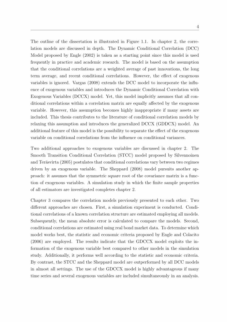
The outline of the dissertation is illustrated in Figure 1.1. In chapter 2, the corre-
lation models are discussed in depth. The Dynamic Conditional Correlation (DCC)
Model proposed by Engle (2002) is taken as a starting point since this model is used
frequently in practice and academic research. The model is based on the assumption
that the conditional correlations are a weighted average of past innovations, the long
term average, and recent conditional correlations. However, the effect of exogenous
variables is ignored. Vargas (2008) extends the DCC model to incorporate the influ-
ence of exogenous variables and introduces the Dynamic Conditional Correlation with
Exogenous Variables (DCCX) model. Yet, this model implicitly assumes that all con-
ditional correlations within a correlation matrix are equally affected by the exogenous
variable. However, this assumption becomes highly inappropriate if many assets are
included. This thesis contributes to the literature of conditional correlation models by
relaxing this assumption and introduces the generalized DCCX (GDDCX) model. An
additional feature of this model is the possibility to separate the effect of the exogenous
variable on conditional correlations from the influence on conditional variances.
Two additional approaches to exogenous variables are discussed in chapter 2. The
Smooth Transition Conditional Correlation (STCC) model proposed by Silvennoinen
and Terasvirta (2005) postulates that conditional correlations vary between two regimes
driven by an exogenous variable. The Sheppard (2008) model pursuits another ap-
proach: it assumes that the symmetric square root of the covariance matrix is a func-
tion of exogenous variables. A simulation study in which the finite sample properties
of all estimators are investigated completes chapter 2.
Chapter 3 compares the correlation models previously presented to each other. Two
different approaches are chosen. First, a simulation experiment is conducted. Condi-
tional correlations of a known correlation structure are estimated employing all models.
Subsequently, the mean absolute error is calculated to compare the models. Second,
conditional correlations are estimated using real bond market data. To determine which
model works best, the statistic and economic criteria proposed by Engle and Colacito
(2006) are employed. The results indicate that the GDCCX model exploits the in-
formation of the exogenous variable best compared to other models in the simulation
study. Additionally, it performs well according to the statistic and economic criteria.
By contrast, the STCC and the Sheppard model are outperformed by all DCC models
in almost all settings. The use of the GDCCX model is highly advantageous if many
time series and several exogenous variables are included simultaneously in an analysis.

1 Introduction 5
The more heterogeneous the respective conditional correlations respond to the exoge-
nous variable, the more rewarding it is to use the GDCCX model. As a result, the
GDCCX model is the focus of the analysis in chapters 4 to 6.
In line with previous studies (Engle and Sheppard, 2008; Berben and Jansen, 2009;
Bauer, 2011), the models investigated in chapter 2 and 3 assume that conditional vari-
ance can be best explained using a GARCH model. Thus, the effect of exogenous
variables on volatility is ignored. However, recent studies find that this assumption
might not be appropriate (Engle et al., 2009; Cakmakli and van Dijk, 2010; Chris-
tiansen et al., 2011). In the first part of chapter 4, a theoretical model of Forbes and
Rigobon (2002) is presented which shows that, given certain conditions, a change in
conditional variances results in changing conditional correlations despite the depen-
dence structure being left unchanged. This issue is further investigated in a Monte
Carlo simulation. Specifically, it is simulated that conditional variances are driven by
an exogenous variable but this variable has no effect on conditional correlations. Then,
ignoring the effect of the exogenous variable on conditional variances, it is examined
whether the models incorrectly identify that exogenous variable drives conditional cor-
relations. A GARCH model for the variance equation and a GDDCX model to estimate
conditional correlations is employed. The results indicate that in certain cases, it is in-
correctly postulated that there is an effect of the exogenous variable on conditional
correlations. However, in a subsequent simulation, all parameter estimates are accu-
rate if the effect of the exogenous variable on conditional variances is modeled. For this
purpose, a GARCHX model (Hwang and Satchell, 2005; Brenner et al., 1996; Engle and
Patton, 2001) is employed instead of the GARCH model used previously. As a result,
in chapters 5 and 6, the GARCHX model is employed in order to estimate conditional
variances and model conditional correlations with the GDCCX model.
Chapter 5 and 6 focus on empirical applications. As correlations between different asset-
classes are central in both portfolio management and risk management, this dissertation
examines the correlations between the most important asset classes in chapter 6: stocks
and bonds. However, correlations within different bond or stock sectors are equally im-
portant. Therefore, chapter 5 investigates the determinants of conditional correlations
between European bond markets as well as conditional correlations between European
stock markets. The sample period covers both calm and turmoil market times. It is
especially interesting whether correlations are influenced by either risk aversion, market
turbulences, or the business cycle. Employing a GDCCX model and estimating con-

6
ditional variances with a GARCHX model, the results indicate that both the business
cycle and market turbulences drive conditional correlations. However, risk aversion
has almost no effect on correlations. Moreover, it is shown that investigating several
exogenous variables simultaneously is advantageous.
In chapter 6, high-frequency stock-bond correlations in the Eurozone are examined.
Employing intra-day data allows to investigate the effect of macroeconomic announce-
ments in addition to exogenous variables previously used. The results show that both
risk aversion and macroeconomic announcements separately drive conditional corre-
lations and variances of bonds and stocks in the Eurozone. Conditional correlations
fall as risk aversion rises even when controlling for the influence of macroeconomic an-
nouncements and the influence of these variables on volatility. Comparing the effects
of Eurozone and US announcements, the most important announcements in the US are
news on nonfarm payroll employments while, in Europe, the announcement of the ECB
rates receives most attention.

2 Correlation Models 7
2 Correlation Models
2.1 Introduction
As argued in the general introduction getting correct correlation estimates is important
but difficult since correlations are not observable. In addition, they are time-varying.
Therefore, several correlation models have been proposed in the literature, that allow
to estimate the conditional covariance matrix. Examples are the Constant Conditional
Correlation (CCC) model of Bollerslev (1990) or the Dynamic Conditional Correlation
(DCC) model of Engle (2002).1 Several extensions to the DCC model have been devel-
oped either to account for asymmetries in the correlation dynamics (Cappiello et al.,
2006a; Audrino and Trojani, 2007) or to better capture dynamics for a large number of
assets (Franses and Hafner, 2003).2
However, these models are based exclusively on the time series properties. The influence
of economic variables such as macroeconomic indicators on correlations has largely been
ignored in the literature although these variables have the potential to simultaneously
influence several time series. Yet, including exogenous variables imposes additional
difficulties in the estimation procedure: Additional parameters must be estimated and
it must be guaranteed that the conditional covariance matrix is positive definite at any
time.
Only recently some models, which were developed, include exogenous variables. Vargas
(2008) extends the DCC model to allow for exogenous variables and introduces the
DCCX model. However, the model restricts the exogenous variables to influence each of
the conditional correlations by the same amount. This assumption becomes increasingly
more conflicting with reality the greater the number of included time series. Therefore,
we relax this assumption and propose a generalized DCCX (GDCCX) model which
allows for a series specific impact of the economic variable on conditional correlations.
1Engle (2009), Bauwens et al. (2006), and Silvennoinen and Terasvirta (2008) provide a comprehensiveoverview on various other correlation models.
2For an introduction to correlation models see Engle (2009). Model comparisons can be found inBauer (2011), Engle and Sheppard (2008), and Engle and Colacito (2006).

2.2 The DCC Model 8
Furthermore, we allow this exogenous variables to affect conditional covariances directly
and not via the change in the conditional variances.
There are also some correlation models that include the effect of exogenous variables
and which are not based on the DCC model. Silvennoinen and Terasvirta (2005)
introduce the Smooth Transition Conditional Correlation (STCC) model which features
a transition variable that drives the correlation between two regimes. This model is
already employed in recent empirical studies. Finally, Sheppard (2008) models the
square root of the conditional covariance matrix as a function of one or more exogenous
variables. In this model, parameters are not directly interpretable as each element of
conditional covariance matrix is a function of several parameters and crossproducts of
the explanatory variables. As a result, marginal effects of the exogenous variables must
be calculated for a given sample point.
The STCC model as well as the DCC type models allow for any univariate GARCH
model to be used to estimate the conditional variance. In addition, Engle and Sheppard
(2008), Berben and Jansen (2009), and Bauer (2011) argue that the choice of the
univariate GARCH model is of minor relevance. Following this argument, we assume
throughout this chapter and in chapter 3, that all conditional variances follow a GARCH
(1,1) process and that the exogenous variables do not influence conditional variances.
We relax this assumption from chapter 4 onwards and discuss the consequences.
This chapter proceeds as follows. As the DCCX and the GDCCX models build heavily
on the DCC model, we first introduce the DCC model. Thereafter, section 2.4 presents
the various models with exogenous variables and develops the generalized DCCX model.
We discuss the estimation of the models in section 2.5 and study the finite sample
properties of all estimators in a small Monte Carlo simulation in section 2.6. Section
2.7 summarizes and concludes the chapter.
2.2 The DCC Model
In this section, we discuss the DCC model as introduced by Engle (2002) and some
recent extensions.3 The DCC model postulates the idea that conditional correlations
follow a GARCH-type structure: Conditional correlations are influenced by past con-
3For surveys of multivariate GARCH models, see e.g. Bauwens et al. (2006), and Silvennoinen andTerasvirta (2008).

2 Correlation Models 9
ditional correlations, current standardized returns, and the long-term average of the
conditional correlation. Hence, the model allows for correlation clustering, but correla-
tions can also be mean reverting.
Specifically, let rt denote an n× 1 vector of N asset returns at time t which is assumed
to be conditionally normal. Without loss of generality, it is furthermore assumed that
E (rt|Ft−1) = 0, (2.1)
E (rtr′t|Ft−1) = Ht, (2.2)
whereHt is an n×nmatrix with time varying conditional covariances, and Ft−1 denotes
the information set at time t−1. Any covariance matrix is positive definite by definition
so that Ht can further be decomposed as follows
Ht = DtRtDt. (2.3)
Rt is the n × n time varying correlation matrix and Dt is an n × n diagonal ma-
trix with the square root of the conditional variances on the diagonal i.e. Dt =
diag(√
h1t, · · · ,√hnt
)
. To increase the flexibility, the conditional variances can be
estimated by any univariate GARCH model.
The various conditional correlations models differ in the way they explain the evolution
of Rt. For example, the constant conditional correlation (CCC) model of Bollerslev
(1990) assumes that Rt ∀ t is the constant sample correlation matrix. Thus, variations
in the covariance between two assets can only result from changes in the assets’ con-
ditional standard deviations. This reduces the number of parameters to be estimated
and alleviates the estimation process. However, the assumption of constant conditional
correlations is often too restrictive in empirical applications.
Relaxing the assumption of constant conditional correlations, Engle (2002) introduces
the dynamic conditional correlation (DCC) model in which the correlations evolve ac-
cording to:4
Rt = Q∗−1t Qt Q
∗−1t . (2.4)
4A similar model was proposed by Tse and Tsui (2002). For differences between the models pleasesee Bauwens et al. (2006) and Engle (2009).
2.2 The DCC Model 10
Q∗t is a diagonal matrix that contains the square roots of the diagonal elements of
Qt. Hence, the conditional correlation between time series i and j at time t is ρij,t =qij,t√
qii,t√qjj,t
, where qij,t is the i,jth entry of Qt. Qt is a n × n matrix and is defined as
follows:
Qt = Q (1− a− b) + a ǫt−1ǫ′t−1 + bQt−1, (2.5)
where a and b are non-negative scalar parameters and ǫt is a n × 1 vector with stan-
dardized residuals(
ǫt = rit/√
hijt
)
. Q is the unconditional covariance matrix of the
standardized residuals. Equation 2.5 depicts Qt as a weighted average of the uncondi-
tional covariance matrix, current standardized returns, and its own past realizations.
The DCC model has several attractive features. First, similar to the CCC model it
allows for a two-step estimation of the volatility and the correlation equation. For this
procedure, Engle and Sheppard (2001) establish the asymptotic consistency and nor-
mality of the estimated parameters. Second, by replacing Q with the sample covariance
matrix of the standardized residuals, the long run correlation matrix will be equal to
the sample correlation matrix. Hence, only a and b have to be estimated in the second
step. Third, the resulting correlation matrices are guaranteed to be positive definite as
long as Qt is positive definite, a suitable starting point is chosen, and a + b < 1.
As suggested by Cappiello et al. (2006a) the half-life of the innovations can be approx-
imated by: ln (0.5) / ln (a2 + b2). The half-life is the expected period of time it takes
until the influence of any correlation innovation has decreased by half.
The DCC model is widely used in empirical research. For example, Engle and Colacito
(2006) show that DCC models can be applied for asset allocation decisions between
stocks and bonds, Cappiello et al. (2006b) assess the integration of European bond and
stock markets, Bali and Engle (2010) augment a capital asset pricing model with esti-
mated correlations, and Chiang et al. (2007) document contagion among stock markets
in Asia. Moreover, the DCC model is applied to currencies (van Dijk et al., 2005) and
non-financial time series such as macroeconomic data (Lee, 2006).5
The parsimonious parameterization of the DCC model comes with some limitations.
For example, it is assumed that all correlations are driven by the same dynamic pat-
tern, which is hard to justify as the number of time series grows. Thus, Franses and
5See Engle (2009) for further references.
2 Correlation Models 11
Hafner (2003) generalize the DCC model by replacing the common a with series spe-
cific ai parameters. Another restriction imposed by the DCC model is that positive
and negative shocks have symmetric effects on conditional correlations. Cappiello et al.
(2006a) introduce the scalar asymmetric DCC (ADCC) model that allows conditional
correlations to increase more when both returns are falling then when both are rising:6
Qt =(
Q− a2Q− b2Q− g2N)
+ a2ǫt−1ǫ′t−1 + b2Qt−1 + g2nt−1n
′t−1, (2.6)
where nt = I [ǫt < 0]◦ ǫt and I [·] is a n×1 dummy variable that takes on the value one
if ǫt < 0. In addition, N = T−1∑T
t=1 nt−1n′t−1, and a, b, and g are scalar parameters.
A necessary condition for Qt to be positive definite is that g2nt−1n′t−1 > 0 which is
guaranteed if g2 > 0 and nt−1n′t−1 > 0.7 However, this restricts the model in a way that
it only allows correlations to increase more when there is a negative shock on returns
but not to increase less.
2.3 Tests for Constant Conditional Correlation
Before estimating conditional correlations, it is important to test the
constant-correlation hypothesis. For this purpose, Bera and Kim (2002) test the
constancy of the correlation parameter in the CCC model over time. Tse (2000) tests
the null of constant correlations against an extended version of the constant
correlation model. Similarly, Silvennoinen and Terasvirta (2005) propose an Lagrange
multiplier (LM) test of constant correlations against a STCC model alternative.
However, in this dissertation, we focus on the Engle and Sheppard (2001) correlation
test as it is easy to implement and can be applied in settings where conditional cor-
6Cappiello et al. (2006a) also propose a generalized version of the ADCC model in which the param-eters are allowed to vary for each correlation pair. However, this comes with the cost of additionalparameters that have to be estimated.
7Cappiello et al. (2006a) show that a sufficient condition for Qt to be positive definite is that thematrix in parentheses in equation 2.6 is positive semi-definite. This is guaranteed as long as
a2 + b2 + δg2 < 1 where δ is the maximum eigenvalue of(
Q−1/2
N Q−1/2
)
.

2.4 Conditional Correlation Models with Exogenous Variables 12
relations of several time series are examined simultaneously.8 In this test, the null
hypothesis of constant conditional correlations
H0 : Rt = R ∀ t (2.7)
is tested against the alternative
H1 : vech(Rt) = vech(R) + β1 vech(Rt−1) + · · ·+ βp vech(Rt−p). (2.8)
R is the sample correlation matrix, Rt is the time-varying correlation matrix, and vech
is the half-vectorization operator. Engle and Sheppard (2001) show that H0 implies
that all coefficients of the vector autoregression
Yt = β0 + β1Yt−1 + · · ·+ βpYt−p + ut (2.9)
are equal to zero. Yt is defined as follows: Yt = vechu (ztz′t − IN) where vechu is a
modified half-vectorization operator that only includes the elements above the diagonal
and zt = R− 1
2 D−1
t rt. The latter term is a vector of returns standardized with the
estimated variances and with the symmetric square root decomposition of R. The test
statistic βV′Vβ′
σ2 has a limiting chi-squared distribution with p + 1 degrees of freedom
where V is the T × (p+ 1) matrix of regressors.9
2.4 Conditional Correlation Models with Exogenous Variables
2.4.1 The DCCX Model
Vargas (2008) extends the scalar ADCC model of Cappiello et al. (2006a) by allowing
exogenous variables to drive correlations. The ADCCX model as described in equation
2.10 results.
Qt =(
Q− a2Q− b2Q− g2N−Kc′x)
+ a2ǫt−1ǫ′t−1 + b2Qt−1+
g2nt−1n′t−1 +Kc′xt−1.
(2.10)
8An implementation of this test can be found, for example, in the UCSD GARCH toolbox.9I.e. V = [1, Yt−1, Yt−2, · · · , Yt−p].
2 Correlation Models 13
xt is a p × 1 vector with p exogenous variables while x = T−1∑T
t=1 xt. c is a p × 1
vector with p parameters that measure the impact of the exogenous variables on Qt.
The model implies that all correlations are equally influenced by any exogenous variable.
K is a n × n matrix which can either be an identity matrix or a matrix of ones. In
the former case the exogenous variables are restricted to drive conditional variances
(qii,t) only, in the latter case conditional correlations are influenced as well. Note that
if g is zero, the model will reduce to the DCCX model and will not account for any
asymmetries in the conditional correlations.
Engle and Sheppard (2001) show that a necessary and sufficient condition for the cor-
relation matrix to be positive definite is that Qt is positive definite. Since both the
DCCX and the ADCCX do not ensure that Qt is positive definite, Vargas proposes to
bound c between 0 and 1. However, that fails to ensure positive definiteness of Qt if
the exogenous variables are negative. In addition, bounding c between 0 and 1 restricts
the model to only allowing conditional correlations to increase (decrease) when the ex-
ogenous variables rise (fall). As there is no general condition which guarantees that Qt
is positive definite, we estimate the model using constrained maximum likelihood. The
parameter space is restricted so that the smallest eigenvalue for any estimated Qt is
positive (see section 2.5 for more details).
2.4.2 The Generalized DCCX Model
The DCCX model restricts the exogenous variables to influence all correlations in an
equal way. This assumption is unrealistic if the number of time series and the number
of correlations to be estimated grows. Therefore, we propose to generalize the DCCX
model (GDCCX model) in which the exogenous variables can influence all correlations
separately:
Qt =
(
Q− a Q− b Q−p∑
i=1
ci xi
)
+ a ǫt−1ǫ′t−1 + b Qt−1 +
p∑
i=1
ci xi,t−1, (2.11)

2.4 Conditional Correlation Models with Exogenous Variables 14
where x1, x2, . . . , xp represent the exogenous variables and xi = T−1∑T
t=1 xi,t. ci is
a n × n parameter matrix with zeros on the diagonal.10 The zeros on the diagonal
ensure that the exogenous variables influence conditional covariances directly and not
via the change in the conditional variances.11 By definition, the conditional correlation
is ρij,t =qij,t√
qii,t√qjj,t
so that the exogenous variables drive conditional covariances, qij,t,
in the numerator but not the conditional variances, qii,t.
Similar to the DCCX model, the generalized version does not ensure that the resulting
correlation matrix is positive definite. To make parameter estimation feasible, again,
a constrained maximum likelihood estimation is employed (see section 2.5 for more
details) and we use the estimated DCCX values as starting values for the generalized
version. While the number of parameters to be estimated rises from 3n+ 2+ p for the
DCCX model to 3n + 2 + pn(n−1)2
, it is still more parsimonious then, e.g., the STCC
model or the model proposed by Sheppard.
2.4.3 The STCC Model
A number of recent papers discuss conditional correlation models that allow the
conditional correlations to switch between distinct values. For example, Pelletier
(2006) assumes that an unobserved first-order Markov process drives the transition
between different correlation regimes. A similar approach is proposed by Silvennoinen
and Terasvirta (2005). They introduce the smooth transition conditional correlation
(STCC) model in which conditional correlations change between two correlation
matrices R1 and R2 according to an observed exogenous variable:
Rt = (1−Gt)R1 +GtR2, (2.12)
10For example, for three time series and two exogenous variables that would be:
p∑
i=1
ci xi,t−1 =
0 c121 c131c121 0 c231c131 c231 0
x1,t−1 +
0 c122 c132c122 0 c232c132 c232 0
x2,t−1
11In the empirical analysis we found that restricting the parameters on the diagonal to be zero doesnot alter other results. Furthermore, the model is more parsimonious.
2 Correlation Models 15
where Gt is the transition function which is bounded between zero and one. The
elements of R1 and R2 are parameters of the model. Although Gt can be any transition
function, most authors use the logistic function:
Gt =(
1 + e−γ(st−c))−1
, γ > 0, (2.13)
where st is the transition variable, γ determines the speed of the transition, and c is
the midpoint of the transition, i.e. the value of the transition variable for which Gt
takes the value 0.5. It is furthermore assumed that the conditional variances follow an
univariate GARCH process. In the special case Rt = R1 ∀ t, the model reduces to the
CCC model. Furthermore, as long as both R1 and R2 are positive semi-definite, the
resulting conditional correlation matrices are guaranteed to be positive semi-definite.
However, letting γ and c vary among correlations would possibly suspend this feature
so that both parameters are restricted to be constant for all conditional correlations.
Although estimation using a two-step approach is possible, asymptotic consistency and
normality of this estimator has not been established. Therefore, the parameters of the
STCC model are either jointly estimated (Aslanidis et al., 2010; Berben and Jansen,
2005) or estimated iteratively by concentrating the likelihood.12 However, the number
of parameters to be estimated grows quickly with the number of time series. For
example, using a univariate GARCH(1,1) process to model the variance, the model has
n2 + 2n+ 2 parameters. Thus, estimation can be difficult due to numerical problems.
Silvennoinen and Terasvirta (2005) point out that there is no change in the resulting
estimated conditional correlations for γ values greater than 100. Therefore, they restrict
γ to be smaller than 100. Furthermore, as shown in equation 2.13, they restrict γ to
be greater than zero. We relax the latter restriction for two reasons. First, we find
that it is not necessary for the model interpretation. If γ is less than zero, a value of st
greater than c results in a transition of the conditional correlation matrix from R2 to
R1. Second, the estimation performance improves substantially. Therefore, we restrict
γ to values between -100 and 100. Furthermore, we replace st in equation 2.13 with
st−1 so that all estimations are based on the same information set in order to facilitate
the comparison of the models.
12Silvennoinen and Terasvirta (2005) propose to divide the parameters into three sets and iterativelymaximize the log likelihood over one set of parameters while leaving the other sets of parametersconstant. This procedure is repeated until the estimator converges.
2.4 Conditional Correlation Models with Exogenous Variables 16
As the STCCmodel only allows one exogenous variable to drive conditional correlations,
Silvennoinen and Terasvirta (2009) recently proposed an extension of the STCC model
in which they introduce a second transition variable: the Double Smooth Transition
Conditional Correlation (DSTCC) GARCH model. However, the additional flexibil-
ity due to the second exogenous variable has to be weighted against the number of
parameters to be estimated which is 2n2 + n+ 4.
The STCC model is employed in some recent empirical papers to model conditional
correlations. For example, Silvennoinen and Terasvirta (2005) explain correlations
of up to five single US stocks with lagged realized volatility. Other studies (Berben
and Jansen, 2005; Aslanidis et al., 2010; Savva and Aslanidis, 2010) investigate co-
movements among equity markets in order to assess the degree of integration. These
papers use time as transition variable which implies a gradual change of one correlation
regime to another but restricts the correlation to move in only one direction. Aslanidis
et al. (2010) employ a DSTCC model and take US stock market volatility as the second
transition variable. Yang et al. (2009) document that macroeconomic variables drive
the correlations between stocks and bonds.
2.4.4 The Sheppard Model
Another model which allows for the inclusion of exogenous variables is presented by
Sheppard (2008). He factorizes Ht using the spectral decomposition. That is the
factorization of a symmetric positive definite matrix A into A = VΛV′ where Λ is the
diagonal matrix of eigenvalues. The corresponding eigenvectors form the columns of a
matrix V. The matrix A can further be decomposed to:
A = VΛ1/2 Λ1/2V′, (2.14)
where Λ1/2 is the symmetric square-root of the matrix A. Sheppard assumes that the
symmetric square-root of the conditional covariance matrix is a linear function of one
or more exogenous variables:
Ht+1 = B (In ⊗ xt) (In ⊗ x′t)B
′, (2.15)

2 Correlation Models 17
and
√
Ht+1 = B (In ⊗ xt) , (2.16)
where xt is a p× 1 vector with p exogenous variables and In is a n× n identity matrix
where n is the number of time series. B is a block symmetric n× np parameter matrix
and consists of n2 blocks so that there are in total n (n+ 1) /2 different blocks. Each
block is a 1 × p vector. For example, for 3 time series and 2 exogenous variables, the
square-root of the conditional covariance matrix is:
√
Ht+1 =
b111x1t + b112x2t b121x1t + b122x2t b131x1t + b132x2t
b121x1t + b122x2t b221x1t + b222x2t b231x1t + b232x2t
b131x1t + b132x2t b231x1t + b232x2t b331x1t + b332x2t
where bijq are the sensitivity parameters that measure the influence of each exogenous
variable q = 1, · · · , p on each distinct element of√Ht+1. In contrast, each element of
Ht+1 is a function of several parameters and cross-products of the explanatory variables,
which can be seen by rearranging equation 2.15:
Ht+1 = B (In ⊗ xtx′t)B
′. (2.17)
As a result, the parameters bijq are not directly interpretable. However, the average
partial effect of each exogenous variable on each element of the conditional covariance
matrix can be calculated. This is simply the first derivative of Rt with respect to
each exogenous variable. It is also possible to test for the influence of each exogenous
variable on each element of the covariance matrix by applying a Wald test.
The model described by equation 2.17 restricts the correlations to be constant in case
of only one exogenous variable. The reason is that the exogenous variable influences
both conditional variances and covariances in a similar way so that the effect of the
exogenous variables simply cancels out.13 Therefore, Sheppard proposes to augment
13From equation 2.16 it can be derived that hij,t = (∑n
k=1bik ⊗ bjk) (xt ⊗ xt) where bik and bkj are
p× 1 parameter blocks from B. In case that there is only one exogenous variable xt is a scalar and
(xt ⊗ xt) = x2
t . Using ρij =hij√
hii
√hjj
gives ρij,t =(∑n
k=1bik⊗bjk) x2
t√
(∑
nk=1
bik⊗bik) x2
t
√
(∑
nk=1
bjk⊗bjk) x2
t
where x2
t
cancel out so that ρijt =(∑n
k=1bik⊗bjk)
√
(∑
nk=1
bik⊗bik)√
(∑
nk=1
bjk⊗bjk).
2.5 Model Estimation 18
the model in equation 2.17 into a simple multivariate ARCH framework where lagged
return cross-products are also included:
Ht+1 = B (In ⊗ xtx′t)B
′ +A ◦RCt, (2.18)
where A is a symmetric positive semi-definite n× n matrix with parameters and RCt
is a n × n matrix with lagged return cross-products: RCt =∑t
d=1 rdr′d. Due to the
influence of the lagged return cross-products the correlation is now varying even when
there is only one exogenous variable. Another possibility is to include a constant so
that the number of exogenous variables is always greater one. In addition, as long as
a constant is included, the model guarantees that Ht+1 is positive definite even though
there are no constraints on the parameter space which greatly alleviates the estimation
process. Therefore, we also include a constant in all estimations. However, estimation
can be time consuming as the number of parameters in equation 2.18 is (n2+n)(p+1)2
where p is the number of exogenous variables including a constant.
2.5 Model Estimation
In line with the number of time series and exogenous variables the number of parameters
to be estimated grows for the models. The model estimation is therefore very important.
All models are estimated by maximum likelihood.14 The sample log likelihood, LL, that
is maximized with respect to all parameters is:15
LL = −1
2
T∑
t=1
(
n log(2π) + log|Ht|+ r′tH−1t rt
)
;
= −1
2
T∑
t=1
(
n log(2π) + 2 log |Dt|+ log |Rt|+ ǫ′tR−1t ǫt
)
;
= −1
2
T∑
t=1
(
n log(2π) + 2 logn∑
i=1
hiit + log |Rt|+ ǫ′tR−1t ǫt
)
. (2.19)
|Ht| denotes the determinant of the matrix Ht. It is generally not necessary to assume
that residuals are normally distributed since Bollerslev and Wooldridge (1992) show
14All computations are performed with Matlab. The code for the estimation of the GARCH and theDCC models was taken from the UCSD GARCH toolbox.
15Details can be found in Engle (2002), Engle and Sheppard (2001), or Sheppard (2008).

2 Correlation Models 19
that maximizing 2.19 results in a consistent estimator in these cases. Thus, 2.19 has a
quasi-maximum likelihood interpretation.
As proposed by Engle and Sheppard (2001) and Engle (2002), we estimate the DCC,
the DCCX, and the GDCCX model in two steps in order to improve the numerical
performance of the estimation routine. In the first step the variance part of 2.19 is
maximized which is equivalent to estimating univariate GARCH models. In the second
step the log likelihood function
LLC = −1
2
T∑
t=1
(
log |Rt|+ ǫ′tR−1t ǫt
)
(2.20)
is maximized conditioning on the parameters estimated in the first step, i.e. given the
estimated standardized residuals. Engle and Sheppard (2001) show that this limited
information estimator is consistent but not fully efficient. Therefore, we correct the
standard errors to account for this loss in efficiency as suggested by Engle and Sheppard
(2001) and Engle (2009).
Silvennoinen and Terasvirta (2005) estimate the STCC model iteratively by concen-
trating the likelihood since the number of parameters is quite large. However, in order
to increase efficiency and speed, we jointly estimate the conditional variances and cor-
relations (Aslanidis et al., 2010).
In section 2.4 we argued that the DCCX models as well as the GDCCX model impose
several linear and non-linear constraints on the parameter space. As suggested by
de Goeij and Marquering (2004) and Chou and Liao (2008), we restrict the parameter
space for these models so that the smallest eigenvalue of any estimated Rt is positive.
As a result, we have an optimization problem with inequality constraints. We tested
two optimization methods. First, as suggested by Greene (2008) and Hamilton (1994)
it is possible to translate the constrained problem to an unconstrained one by imposing
some sort of penalty function for constraints that are near or beyond the boundary.
Yet, different penalty functions might lead to different solutions. Second, sequential
quadratic programming methods can be applied which focus on the solution of the
Karush-Kuhn-Tucker equations.16 After running extensive simulations and tests with
real data, we find that both methods yield equal estimates. However, using the penalty
functions is preferable in terms of estimation speed.
16See Fletcher (2000) or Levy (2009) for introductions to constrained optimization.

2.6 A Simulation Study 20
A general drawback of estimating the models by constrained maximum likelihood is
that it has to be assumed that both the true as well as the estimated parameters fall
within the interior of the allowable parameter space. Otherwise asymptotic standard
errors are not valid.17 This is especially relevant for the STCC γ parameter. The
parameter is restricted to values between -100 and +100. Therefore, if the γ estimate
is on the boundary, similar to Silvennoinen and Terasvirta (2005), we do not report
standard errors for this parameter.
All models are estimated by quasi-maximum likelihood with robust standard errors
(Bollerslev and Wooldridge, 1992). Hafner and Herwartz (2008) as well as Lucchetti
(2002) argue that employing analytical derivatives instead of numerical scores is prefer-
able for quasi-maximum likelihood estimation and inference if the number of model
parameters is high. Therefore, we employ analytical derivatives for the estimation of
both Sheppard’s model and the STCC model.18 We find that although the resulting
parameter estimates remain unchanged, the speed of estimation improves remarkably.
2.6 A Simulation Study
In this section, we study the estimators discussed in section 2.4 in a simulation. Similar
to Silvennoinen and Terasvirta (2005) and Hafner and Herwartz (2008), we estimate
parameters from samples with simulated correlated data and compare them to the true
parameters for different sample sizes. For each model we create samples in which the
true correlation evolves according to the pattern implied by the respective model.19
That allows us to investigate the finite sample properties as well as the empirical per-
formance of the estimators.
We generate 1000 samples with two normally distributed random time series for each
estimator and for each sample size. We assume that the series exhibit time-varying
volatility clustering and evolve according to a GARCH(1,1) model. The exogenous
variable is a normally distributed random variable with unit variance. The generated
conditional correlations between the two series evolve according to the correlation struc-
17See Hamilton (1994) for details. In addition, Schoenberg (1997) points out that in finite samplesstandard errors have to be corrected if the estimated parameters are in the region of the boundaries.
18All DCC models are estimated applying numerical derivatives since the optimization is less demand-ing for the optimizer due to the two-step estimation.
19We employ all models on the same sample in order to compare the model performance in chapter 3.
2 Correlation Models 21
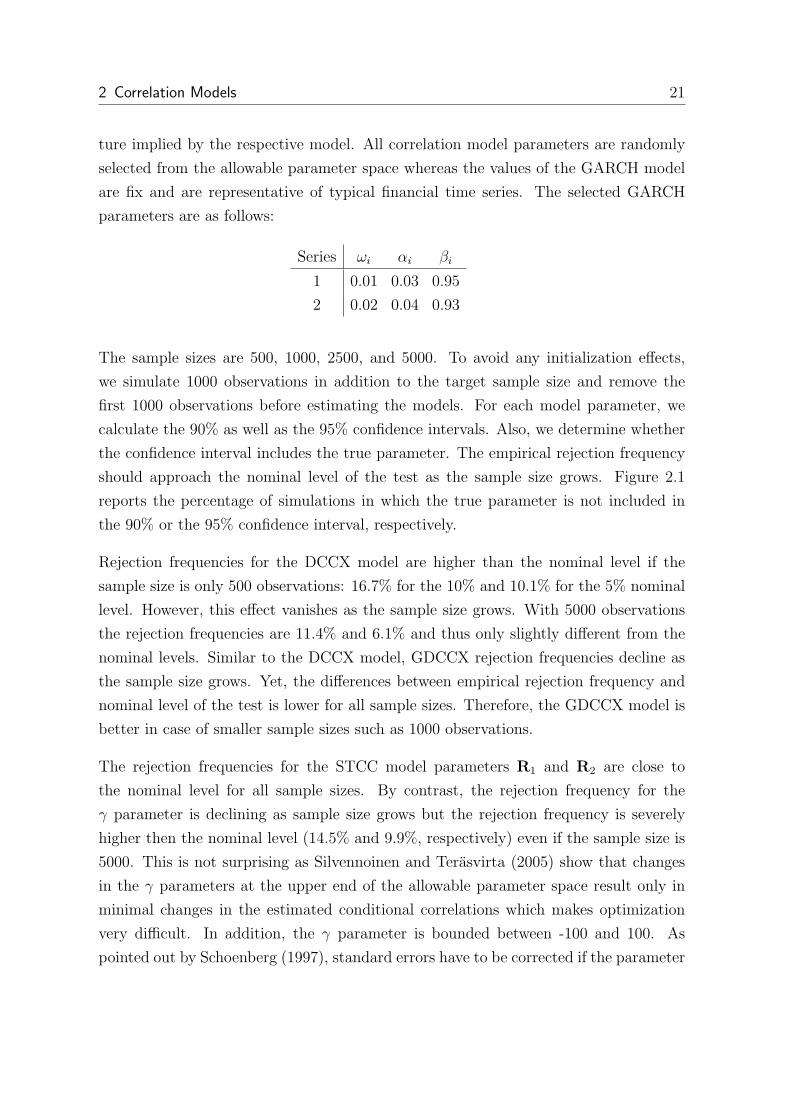
ture implied by the respective model. All correlation model parameters are randomly
selected from the allowable parameter space whereas the values of the GARCH model
are fix and are representative of typical financial time series. The selected GARCH
parameters are as follows:
Series ωi αi βi
1 0.01 0.03 0.95
2 0.02 0.04 0.93
The sample sizes are 500, 1000, 2500, and 5000. To avoid any initialization effects,
we simulate 1000 observations in addition to the target sample size and remove the
first 1000 observations before estimating the models. For each model parameter, we
calculate the 90% as well as the 95% confidence intervals. Also, we determine whether
the confidence interval includes the true parameter. The empirical rejection frequency
should approach the nominal level of the test as the sample size grows. Figure 2.1
reports the percentage of simulations in which the true parameter is not included in
the 90% or the 95% confidence interval, respectively.
Rejection frequencies for the DCCX model are higher than the nominal level if the
sample size is only 500 observations: 16.7% for the 10% and 10.1% for the 5% nominal
level. However, this effect vanishes as the sample size grows. With 5000 observations
the rejection frequencies are 11.4% and 6.1% and thus only slightly different from the
nominal levels. Similar to the DCCX model, GDCCX rejection frequencies decline as
the sample size grows. Yet, the differences between empirical rejection frequency and
nominal level of the test is lower for all sample sizes. Therefore, the GDCCX model is
better in case of smaller sample sizes such as 1000 observations.
The rejection frequencies for the STCC model parameters R1 and R2 are close to
the nominal level for all sample sizes. By contrast, the rejection frequency for the
γ parameter is declining as sample size grows but the rejection frequency is severely
higher then the nominal level (14.5% and 9.9%, respectively) even if the sample size is
5000. This is not surprising as Silvennoinen and Terasvirta (2005) show that changes
in the γ parameters at the upper end of the allowable parameter space result only in
minimal changes in the estimated conditional correlations which makes optimization
very difficult. In addition, the γ parameter is bounded between -100 and 100. As
pointed out by Schoenberg (1997), standard errors have to be corrected if the parameter

2.6 A Simulation Study 22
5%
10%15%20%
DCCX Model: c parameter
Re
jectio
n R
ate
5%
10%15%20%
GDCCX Model: c parameter
5%
10%15%20%
STCC Model: R1 parameter
Re
jectio
n R
ate
5%
10%15%20%
STCC Model: R2 parameter
5%
10%15%20%
STCC Model: c parameter
Re
jectio
n R
ate
5%
10%15%20%
STCC Model: γ parameter
5%
10%15%20%
Sheppard Model: parameter 1
Re
jectio
n R
ate
5%
10%15%20%
Sheppard Model: parameter 2
5%
10%15%20%
Sheppard Model: parameter 3
Re
jectio
n R
ate
5%
10%15%20%
Sheppard Model: parameter 4
500 1000 2500 5000
5%10%15%20%
Sheppard Model: parameter 5
Sample Size
Re
jectio
n R
ate
500 1000 2500 5000
5%10%15%20%
Sheppard Model: parameter 6
Sample Size
90% Confidence Interval
95% Confidence Interval
Figure 2.1: Empirical Rejection Frequencies for Different Parameters and Sample Sizes
2 Correlation Models 23
estimate is on the boundary.20 Rejection frequencies for the c parameter are lower but
they rise as the sample size grows from 500 to 2500 observations. In addition, the
rejections frequencies for the 90% confidence intervals are lower then expected. As the
total number of parameters estimated is the highest for the STCC model, both the
number of replications and the sample size might still be too low.
Finally, the sample size does not matter for the Sheppard model estimates. However,
we find that some rejection frequencies are slightly lower or higher than the nominal
level. Like the STCC model, different parameter settings for the Sheppard model might
result in the same or very similar estimated conditional correlations.
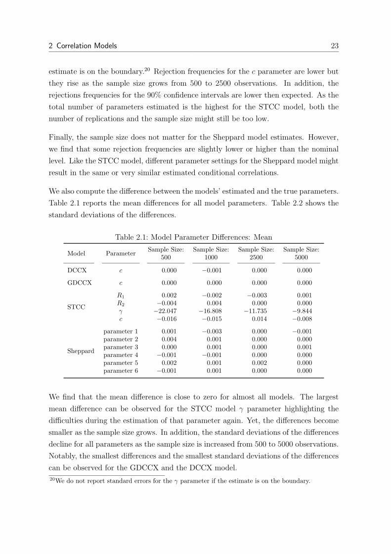
We also compute the difference between the models’ estimated and the true parameters.
Table 2.1 reports the mean differences for all model parameters. Table 2.2 shows the
standard deviations of the differences.
Table 2.1: Model Parameter Differences: Mean
Model ParameterSample Size:
500Sample Size:
1000Sample Size:
2500Sample Size:
5000
DCCX c 0.000 −0.001 0.000 0.000
GDCCX c 0.000 0.000 0.000 0.000
STCC
R1 0.002 −0.002 −0.003 0.001R2 −0.004 0.004 0.000 0.000γ −22.047 −16.808 −11.735 −9.844c −0.016 −0.015 0.014 −0.008
Sheppard
parameter 1 0.001 −0.003 0.000 −0.001parameter 2 0.004 0.001 0.000 0.000parameter 3 0.000 0.001 0.000 0.001parameter 4 −0.001 −0.001 0.000 0.000parameter 5 0.002 0.001 0.002 0.000parameter 6 −0.001 0.001 0.000 0.000
We find that the mean difference is close to zero for almost all models. The largest
mean difference can be observed for the STCC model γ parameter highlighting the
difficulties during the estimation of that parameter again. Yet, the differences become
smaller as the sample size grows. In addition, the standard deviations of the differences
decline for all parameters as the sample size is increased from 500 to 5000 observations.
Notably, the smallest differences and the smallest standard deviations of the differences
can be observed for the GDCCX and the DCCX model.
20We do not report standard errors for the γ parameter if the estimate is on the boundary.

2.6 A Simulation Study 24
Table 2.2: Model Parameter Differences: Standard Deviations
Model ParameterSample Size:
500Sample Size:
1000Sample Size:
2500Sample Size:
5000
DCCX c 0.031 0.020 0.011 0.006
GDCCX c 0.023 0.016 0.009 0.006
STCC
R1 0.113 0.101 0.083 0.035R2 0.120 0.098 0.078 0.055γ 33.869 33.454 30.381 27.485c 0.372 0.315 0.297 0.266
Sheppard
parameter 1 0.065 0.047 0.027 0.026parameter 2 0.035 0.021 0.014 0.011parameter 3 0.067 0.045 0.028 0.026parameter 4 0.062 0.038 0.036 0.015parameter 5 0.035 0.019 0.026 0.008parameter 6 0.064 0.041 0.036 0.015
These results are confirmed by our next test. We compute the mean absolute error of
the conditional correlation estimates for all models and the same sample sizes as before.
Table 2.3 displays the results. It turns out that mean absolute errors for all models
decline as the sample size grows. In addition, the results indicate that the STCC
model conditional correlation estimates are very close to the true estimates despite
higher rejection frequencies as the mean absolute errors are the second lowest among
the correlation models with exogenous variables. Interestingly, conditional correlations
estimated by the Sheppard model are even closer to the true conditional correlations
than the DCC model.
Table 2.3: Mean Absolute Error of Conditional Correlation Estimates
Sample Size
Model 500 1000 2500 5000
DCC 0.038 0.027 0.017 0.012DCCX 0.049 0.033 0.021 0.015GDCCX 0.048 0.036 0.022 0.016STCC 0.045 0.026 0.017 0.012Sheppard 0.023 0.016 0.010 0.007
2 Correlation Models 25
2.7 Summary
In this chapter, we argue that it is useful to model conditional correlations. Fur-
thermore, as conditional correlations between two time series might be influenced by
exogenous variables, the effect of these variables should not be neglected by the cor-
relation models. Therefore, we present several correlation models that incorporate the
effect of one or several exogenous variables and propose the GDCCX model.
First, we explain the DCC model (Engle, 2002) that neglects the influence of exogenous
variable but is the basis for two of the models. Conditional correlations are modeled
similar as conditional volatilities are explained in a GARCH model: they are a weighted
average of past innovations, the previous estimate and the long-term average correlation.
As such, conditional correlations are a function of past time series properties, but the
DCC model does not include the effect of exogenous variables. Thus, Vargas (2008)
introduces the DCCX model in which conditional correlations evolve similar to the DCC
model but are also driven by exogenous variables. As the model allows the exogenous
variables to influence all conditional correlation in an equal way only, we propose the
GDCCX model that relaxes that restriction. In addition, we modify the model to
ensure that the exogenous variables influence conditional covariances directly and not
via the change in the conditional variances. That also alleviates the interpretation of
the coefficients and reduces the number of parameters to be estimated.
Thereafter, we explain the STCC model (Silvennoinen and Terasvirta, 2005). It allows
conditional correlations to switch between distinct values driven by only one exogenous
variable. Finally, we present the Sheppard (2008) model. The symmetric square-root
of the conditional covariance matrix is modeled as a function of one or more exogenous
variables. Each element of the conditional covariance matrix is a function of several
parameters and crossproducts of the explanatory variables. As a result, parameters are
not directly interpretable but average marginal effects can be calculated.
Going forward, we discuss the model estimation. The DCC type models can be es-
timated using a two step estimation. As the DCCX and the GDCCX model do not
guarantee that estimated conditional correlations are positive definite, we restrict the
parameter space for these models so that the smallest eigenvalue of any estimated
correlation matrix is positive.

2.7 Summary 26
In the last section, we compare the performance and the finite sample properties of
all estimators in a Monte Carlo experiment. We find that the empirical rejection fre-
quencies are close the nominal level of the the tests for all models. Moreover, the
difference between the empirical rejection frequency and the nominal level diminishes
as the sample size grows. Calculating the mean absolute error of the conditional corre-
lation estimates further confirms the accuracy of the estimators.

3 Comparison of the Models 27
3 Comparison of the Models
3.1 Introduction
In the previous chapter, we introduced conditional correlations models that allow ex-
ogenous variables to affect correlations and discussed the model properties. It remains
yet to be established which model works best in different contexts. This is the focus of
this chapter. We pursue two different approaches to comparing the models.
First, we test the models in a simulation study in which the true correlation structure
is known but, as opposed to the experiment in the previous chapter, not implied by the
models. In addition, the calculation of the mean absolute error allows us to generally
assess the value of including exogenous variables in correlation models. Furthermore,
we will establish how the models react to different correlation settings.
Our second approach is to apply the models to real data. Obviously, real correlations
are not measurable and hence unknown. Comparing the models is, thus, not as straight
forward as it was in the simulation study. Yet, both statistical and economic criteria
can be employed. While statistical criteria such as information criteria are easy to
calculate, they lack an economic basis. Therefore, several studies evaluate covariance
estimates within an asset allocation framework (e.g. Fleming et al., 2001, 2003). An
investor calculates optimal portfolio weights given a vector of expected returns and the
estimated covariance matrix. However, using the realized portfolio return or the Sharpe
ratio in order to compare models is critical as they depend on the correct specification
of both expected returns and the covariance matrix.1 Therefore, Engle and Colacito
(2006) argue that correlation models can be ranked according to the variance of the
mean variance optimal portfolio and develop a test statistic. We employ these criteria
with datasets of daily returns as we have to assume that the conditional expected value
of return is constant. We take bond returns from the Eurozone as well as from the US
covering up to 20 years.
1Chopra and Ziemba (1993) point out that ”errors in means are about ten times as important aserrors in variances and covariances”.

3.1 Introduction 28
In addition to comparing the models, these datasets allows us to investigate on an
interesting empirical question: Does risk aversion influence conditional correlations
in different settings? Several studies demonstrate that growing risk aversion results
in rising conditional correlations among international equity markets which in turn
diminishes diversification benefits (Cappiello et al., 2006a; Solnik et al., 1996; Kasch-
Haroutounian, 2005). Other authors analyze the conditional correlations between stock
and bond returns and observe a flight-to-quality effect (Cappiello et al., 2006a; Anders-
son et al., 2008; Connolly et al., 2005; Kim et al., 2006; Baele et al., 2010; Aslanidis and
Christiansen, 2010). Conditional correlations between bond returns have received less
attention. Hunter and Simon (2005) use a bivariate conditional correlation GARCH
model to show that rising risk aversion, as measured by the conditional volatility of
US bond markets, results in lower conditional correlations among US, German and
Japanese government bonds. Also, focusing on the volatility of European bond mar-
kets, Skintzi and Refenes (2006) as well as Christiansen (2007) find evidence of volatility
spillovers from the US to European government bond markets.
Yet, the conditional correlation between different bond sectors, such as corporate bonds
and government bonds, has been largely neglected in existing studies. This is remark-
able as investors are currently trying to diversify supposedly risk free government bond
portfolios into other sectors. An exception is the study of Briere et al. (2008). They
find that during periods of financial turmoil conditional correlations between Euro-
pean bond sectors decrease. However, their analysis depends crucially on the correct
identification of crisis periods (Boyer et al., 1999).
We examine the conditional correlation of bond sectors using two datasets: one for
Europe and one for the US. We include government and corporate bonds. Corporate
bonds are furthermore segmented into investment grade and high yield since returns of
the higher quality bonds are mostly driven by interest rate risk whereas for high yield
bonds default risk is most important. In line with prior research (Andersson et al.,
2008; Connolly et al., 2005, 2007; Bali and Engle, 2010; Silvennoinen and Thorp, 2010;
Kim et al., 2006), we employ the implied volatility of equity market options in order to
capture the perceived risk aversion in the market.
In the next section, we compare the correlation models in a simulation study. There-
after, we focus on testing the various correlation models with real data. Different testing
3 Comparison of the Models 29
criteria are explained in section 3.3.1. Section 3.3.2 describes the data and results are
reported and discussed in section 3.3.3. Section 3.4 summarizes and concludes.
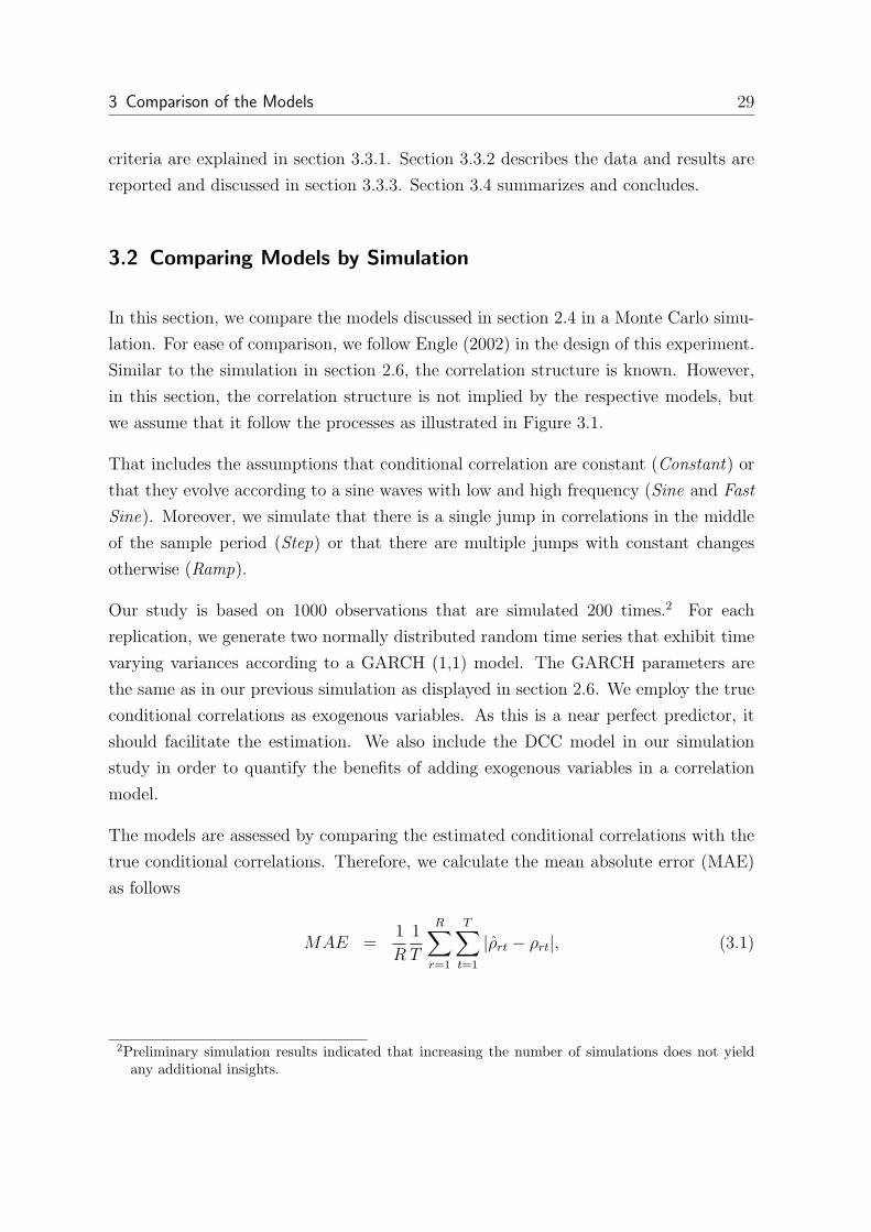
3.2 Comparing Models by Simulation
In this section, we compare the models discussed in section 2.4 in a Monte Carlo simu-
lation. For ease of comparison, we follow Engle (2002) in the design of this experiment.
Similar to the simulation in section 2.6, the correlation structure is known. However,
in this section, the correlation structure is not implied by the respective models, but
we assume that it follow the processes as illustrated in Figure 3.1.
That includes the assumptions that conditional correlation are constant (Constant) or
that they evolve according to a sine waves with low and high frequency (Sine and Fast
Sine). Moreover, we simulate that there is a single jump in correlations in the middle
of the sample period (Step) or that there are multiple jumps with constant changes
otherwise (Ramp).
Our study is based on 1000 observations that are simulated 200 times.2 For each
replication, we generate two normally distributed random time series that exhibit time
varying variances according to a GARCH (1,1) model. The GARCH parameters are
the same as in our previous simulation as displayed in section 2.6. We employ the true
conditional correlations as exogenous variables. As this is a near perfect predictor, it
should facilitate the estimation. We also include the DCC model in our simulation
study in order to quantify the benefits of adding exogenous variables in a correlation
model.
The models are assessed by comparing the estimated conditional correlations with the
true conditional correlations. Therefore, we calculate the mean absolute error (MAE)
as follows
MAE =1
R
1
T
R∑
r=1
T∑
t=1
|ρrt − ρrt|, (3.1)
2Preliminary simulation results indicated that increasing the number of simulations does not yieldany additional insights.
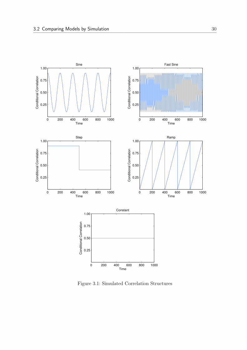
3.2 Comparing Models by Simulation 30
0 200 400 600 800 1000
0.25
0.50
0.75
1.00
Conditio
nal C
orr
ela
tion
Time
Sine
0 200 400 600 800 1000
0.25
0.50
0.75
1.00
Conditio
nal C
orr
ela
tion
Time
Fast Sine
0 200 400 600 800 1000
0.25
0.50
0.75
1.00
Conditio
nal C
orr
ela
tion
Time
Step
0 200 400 600 800 1000
0.25
0.50
0.75
1.00
Conditio
nal C
orr
ela
tion
Time
Ramp
0 200 400 600 800 1000
0.25
0.50
0.75
1.00
Conditio
nal C
orr
ela
tion
Time
Constant
Figure 3.1: Simulated Correlation Structures
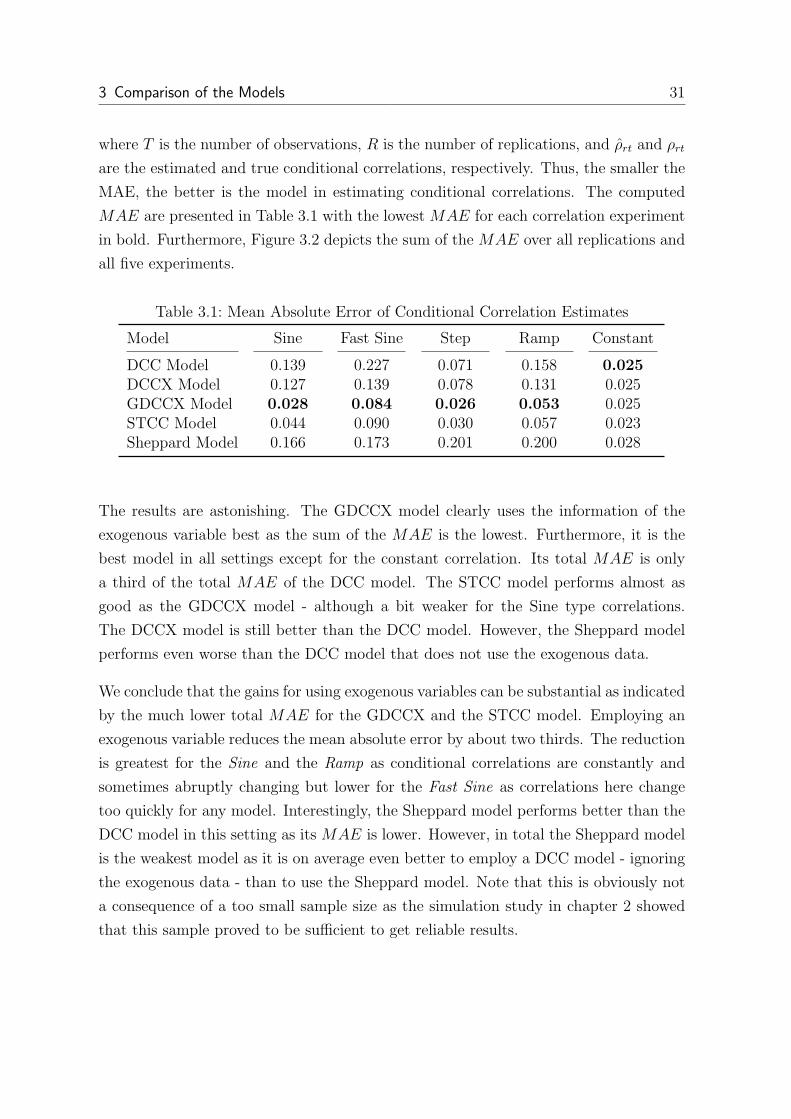
3 Comparison of the Models 31
where T is the number of observations, R is the number of replications, and ρrt and ρrt
are the estimated and true conditional correlations, respectively. Thus, the smaller the
MAE, the better is the model in estimating conditional correlations. The computed
MAE are presented in Table 3.1 with the lowest MAE for each correlation experiment
in bold. Furthermore, Figure 3.2 depicts the sum of the MAE over all replications and
all five experiments.
Table 3.1: Mean Absolute Error of Conditional Correlation Estimates
Model Sine Fast Sine Step Ramp Constant
DCC Model 0.139 0.227 0.071 0.158 0.025
DCCX Model 0.127 0.139 0.078 0.131 0.025GDCCX Model 0.028 0.084 0.026 0.053 0.025STCC Model 0.044 0.090 0.030 0.057 0.023Sheppard Model 0.166 0.173 0.201 0.200 0.028
The results are astonishing. The GDCCX model clearly uses the information of the
exogenous variable best as the sum of the MAE is the lowest. Furthermore, it is the
best model in all settings except for the constant correlation. Its total MAE is only
a third of the total MAE of the DCC model. The STCC model performs almost as
good as the GDCCX model - although a bit weaker for the Sine type correlations.
The DCCX model is still better than the DCC model. However, the Sheppard model
performs even worse than the DCC model that does not use the exogenous data.
We conclude that the gains for using exogenous variables can be substantial as indicated
by the much lower total MAE for the GDCCX and the STCC model. Employing an
exogenous variable reduces the mean absolute error by about two thirds. The reduction
is greatest for the Sine and the Ramp as conditional correlations are constantly and
sometimes abruptly changing but lower for the Fast Sine as correlations here change
too quickly for any model. Interestingly, the Sheppard model performs better than the
DCC model in this setting as its MAE is lower. However, in total the Sheppard model
is the weakest model as it is on average even better to employ a DCC model - ignoring
the exogenous data - than to use the Sheppard model. Note that this is obviously not
a consequence of a too small sample size as the simulation study in chapter 2 showed
that this sample proved to be sufficient to get reliable results.
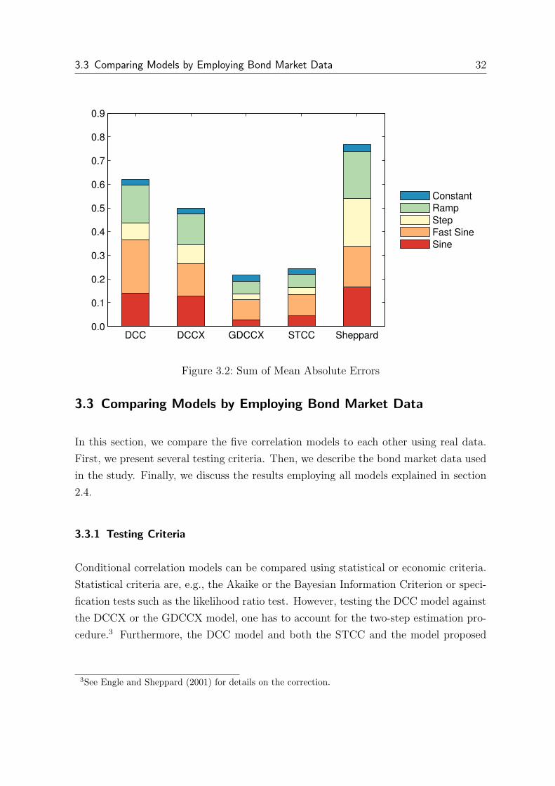
3.3 Comparing Models by Employing Bond Market Data 32
DCC DCCX GDCCX STCC Sheppard0.0
0.1
0.2
0.3
0.4
0.5
0.6
0.7
0.8
0.9
Constant
Ramp
Step
Fast Sine
Sine
Figure 3.2: Sum of Mean Absolute Errors
3.3 Comparing Models by Employing Bond Market Data
In this section, we compare the five correlation models to each other using real data.
First, we present several testing criteria. Then, we describe the bond market data used
in the study. Finally, we discuss the results employing all models explained in section
2.4.
3.3.1 Testing Criteria
Conditional correlation models can be compared using statistical or economic criteria.
Statistical criteria are, e.g., the Akaike or the Bayesian Information Criterion or speci-
fication tests such as the likelihood ratio test. However, testing the DCC model against
the DCCX or the GDCCX model, one has to account for the two-step estimation pro-
cedure.3 Furthermore, the DCC model and both the STCC and the model proposed
3See Engle and Sheppard (2001) for details on the correction.

3 Comparison of the Models 33
by Sheppard are non-nested. A popular test for non-nested models is the Vuong (1989)
test which can also be employed to compare the models.
Some recent papers assess the model performance in an economic application (Bauer
and Missong, 2008; Engle and Colacito, 2006; Milunovich and Thorp, 2006; Thorp
and Milunovich, 2007) as conditional correlation forecasts are a key input into many
financial decisions. An important and widely evaluated application is the mean-variance
portfolio optimization.4 One approach is to form the global minimum variance portfolio
(GMVP). Its vector of portfolio weights wt is calculated using:
wt =H−1
t ι
ι′H−1t ι
, (3.2)
where Ht is the forecasted conditional covariance matrix at time t, and ι is a vector
of ones. By assuming that the returns on all assets are equal this approach avoids the
specification of expected returns for all assets. Yet, this assumption is quite unrealis-
tic especially in an asset allocation framework and seldom used in practice. Another
approach is to construct a portfolio using the general mean-variance optimization so
that:
wt =H−1
t µt
µ′tH
−1t µt
, (3.3)
where µt is the vector of expected returns in excess of the risk free rate. As expected
returns are unknown, many studies use ex-post means instead and evaluate the risk
and return of the optimal portfolios. However, Engle and Colacito (2006) point out
that performing a mean-variance optimization is a combined test of the correct speci-
fication of expected returns and the forecasted covariance matrix. In addition, Chopra
and Ziemba (1993) argue that correctly estimated covariances are not as important as
correctly estimated expected returns for the construction of the optimal portfolio.
Yet, Engle and Colacito (2006) show that if expected returns are constant, i.e. µi,t =
µi ∀ t, it will still be possible to rank covariance forecasts according to the variance of
the optimal portfolio. The reason is that for every vector of expected returns a portfolio
which is optimized on the true covariance will have a lower or equal variance than a
4The use of further economic applications and testing criteria is discussed in Patton and Sheppard(2009), Engle et al. (2008) as well as in Engle and Sheppard (2001).

3.3 Comparing Models by Employing Bond Market Data 34
portfolio which is optimized on any other covariance matrix. It is generally assumed
that the true expected value of return is constant for daily or higher frequency data.
Moreover, the significance of the difference between two conditional correlation models
can be tested by employing the Diebold and Mariano (1995) test statistic. First, the
estimated difference between the realized covariance of the two models is computed as
follows:
dt =(
w′t,Art
)2 −(
w′t,Brt
)2, (3.4)
where wt,A and wt,B are the weights for the respective optimal portfolio calculated from
the forecasted covariance matrices HA
tand HB
tof the two models while rt is a vector
with returns. Second, dt is regressed on a constant using a Newey-West covariance
matrix to account for heteroscedasticity, autocorrelation, and nonnormality. The null
hypothesis is that the mean of dt is 0. Engle and Colacito (2006) propose a weighted
version of this test and modify equation 3.4 in order to further adjust for heteroscedas-
ticity:
vt = dt
[
2(
µ′ (HA
t
)−1µ)(
µ′ (HB
t
)−1µ)]1/2
. (3.5)
In a second step, vt is regressed on a constant using a Newey-West covariance matrix,
and the null hypothesis is that the mean of vt is 0.
3.3.2 Data
3.3.2.1 Bond Return Data
We employ several bond indices in order to both conduct a comprehensive test on the
correlation models and to investigate conditional correlations between these indices.
An overview is presented in Table 3.2.
We construct a dataset consisting of aggregate data on government, investment grade
corporate, and high yield corporate bond indices provided by Bank of America Merrill
Lynch which are widely used in practice. The indices are obtained for the Euro area as
well as for the United States. All six indices are based on bond prices observed in the
secondary market. Index constituents are capitalization weighted except for the two
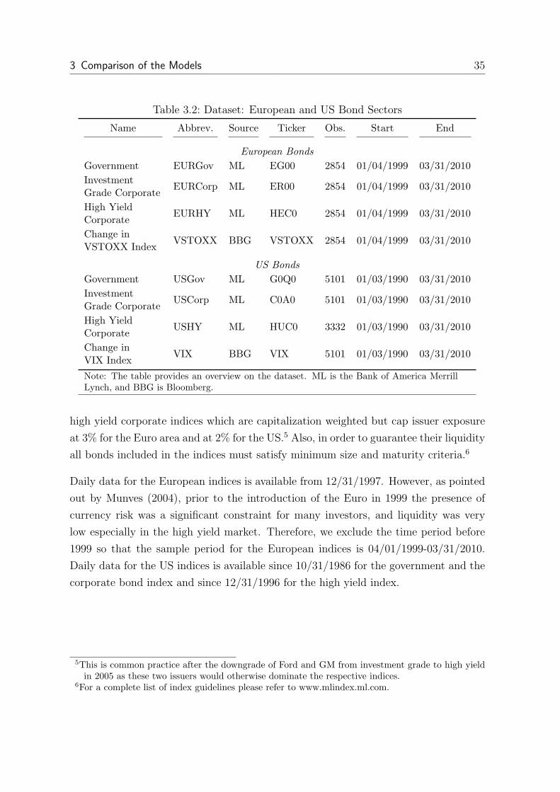
3 Comparison of the Models 35
Table 3.2: Dataset: European and US Bond Sectors
Name Abbrev. Source Ticker Obs. Start End
European Bonds
Government EURGov ML EG00 2854 01/04/1999 03/31/2010
InvestmentGrade Corporate
EURCorp ML ER00 2854 01/04/1999 03/31/2010
High YieldCorporate
EURHY ML HEC0 2854 01/04/1999 03/31/2010
Change inVSTOXX Index
VSTOXX BBG VSTOXX 2854 01/04/1999 03/31/2010
US Bonds
Government USGov ML G0Q0 5101 01/03/1990 03/31/2010
InvestmentGrade Corporate
USCorp ML C0A0 5101 01/03/1990 03/31/2010
High YieldCorporate
USHY ML HUC0 3332 01/03/1990 03/31/2010
Change inVIX Index
VIX BBG VIX 5101 01/03/1990 03/31/2010
Note: The table provides an overview on the dataset. ML is the Bank of America MerrillLynch, and BBG is Bloomberg.
high yield corporate indices which are capitalization weighted but cap issuer exposure
at 3% for the Euro area and at 2% for the US.5 Also, in order to guarantee their liquidity
all bonds included in the indices must satisfy minimum size and maturity criteria.6
Daily data for the European indices is available from 12/31/1997. However, as pointed
out by Munves (2004), prior to the introduction of the Euro in 1999 the presence of
currency risk was a significant constraint for many investors, and liquidity was very
low especially in the high yield market. Therefore, we exclude the time period before
1999 so that the sample period for the European indices is 04/01/1999-03/31/2010.
Daily data for the US indices is available since 10/31/1986 for the government and the
corporate bond index and since 12/31/1996 for the high yield index.
5This is common practice after the downgrade of Ford and GM from investment grade to high yieldin 2005 as these two issuers would otherwise dominate the respective indices.
6For a complete list of index guidelines please refer to www.mlindex.ml.com.

3.3 Comparing Models by Employing Bond Market Data 36
3.3.2.2 The Exogenous Variable: Risk Aversion
Several authors document the effects of risk aversion on conditional correlations in dif-
ferent markets and employing different methods and sampling frequencies. For example,
the effect of risk aversion on conditional correlations between stock markets is inves-
tigated by Solnik et al. (1996), Kasch-Haroutounian (2005), Cappiello et al. (2006a),
and Cai et al. (2009). These studies find that increasing risk aversion results in rising
conditional correlations among international equity markets. Also, stock bond correla-
tions are affected by risk aversion as growing risk aversion triggers a flight-to-quality
(Connolly et al., 2005; Cappiello et al., 2006a; Kim et al., 2006; Connolly et al., 2007;
Andersson et al., 2008; Aslanidis and Christiansen, 2010, 2011; Baele et al., 2010).
As risk aversion is not measurable, these studies proxy risk aversion with the implied
volatility of equity options as it incorporates all information available to market par-
ticipants on future volatility. Specifically, we use the change in volatility indices as
exogenous variables for the correlation models. We employ the change in the Euro
Stoxx 50 Volatility Index (VSTOXX) for the Eurozone. For the US we use the change
in the Chicago Board Options Exchange Volatility Index (VIX). Both are popular mea-
sures of the implied volatility of index options over the next 30 days on the Euro Stoxx
50 Index and the S&P 500 Index respectively. Data is available since 1/4/1999 for the
VSTOXX and since 1/2/1990 for the VIX.
3.3.2.3 The Datasets
Combining the volatility and the bond data, we get three datasets: first, the European
aggregate bond data and the VSTOXX index starting at 1/4/1999; second, the US
aggregate bond indices and the VIX index which are available since 1/2/1997. We
construct a third dataset which includes the US government and the investment grade
corporate index only. That allows us to expand the length of the time series considerably
as all series are at least available since 1/31/1990.
For all indices, we compute the continuously compounded daily returns. Furthermore,
all returns are expressed in local currency. For the volatility indices, we calculate the
daily differences. It is worth looking at the unconditional correlations in Tables 3.3 and
3.4. In all samples the government and investment grade corporate bond indices are on
average strongly correlated while the high yield indices are unsurprisingly uncorrelated
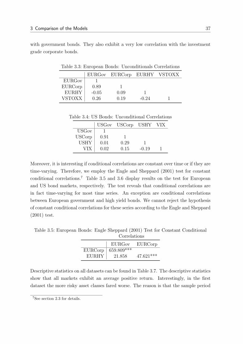
3 Comparison of the Models 37
with government bonds. They also exhibit a very low correlation with the investment
grade corporate bonds.
Table 3.3: European Bonds: Unconditionals Correlations
EURGov EURCorp EURHY VSTOXXEURGov 1EURCorp 0.89 1EURHY -0.05 0.09 1
VSTOXX 0.26 0.19 -0.24 1
Table 3.4: US Bonds: Unconditional Correlations
USGov USCorp USHY VIXUSGov 1USCorp 0.91 1USHY 0.01 0.29 1VIX 0.02 0.15 -0.19 1
Moreover, it is interesting if conditional correlations are constant over time or if they are
time-varying. Therefore, we employ the Engle and Sheppard (2001) test for constant
conditional correlations.7 Table 3.5 and 3.6 display results on the test for European
and US bond markets, respectively. The test reveals that conditional correlations are
in fact time-varying for most time series. An exception are conditional correlations
between European government and high yield bonds. We cannot reject the hypothesis
of constant conditional correlations for these series according to the Engle and Sheppard
(2001) test.
Table 3.5: European Bonds: Engle Sheppard (2001) Test for Constant ConditionalCorrelations
EURGov EURCorpEURCorp 659.809***EURHY 21.858 47.621***
Descriptive statistics on all datasets can be found in Table 3.7. The descriptive statistics
show that all markets exhibit an average positive return. Interestingly, in the first
dataset the more risky asset classes fared worse. The reason is that the sample period
7See section 2.3 for details.

3.3 Comparing Models by Employing Bond Market Data 38
Table 3.6: US Bonds: Engle Sheppard (2001) Test for Constant ConditionalCorrelations
USGov USCorpUSGov 1287.800***USHY 120.427*** 69.688***
covers both the burst of the dotcom bubble in 2000/2001 and the financial crisis in 2008.
The other US samples cover a larger time period so that the effect of these events is
less pronounced. It can also be noted that all returns series are heavily left skewed and
exhibit fat-tails. Moreover, they are non-normal as indicated by a Jarque–Bera test.
In addition, the minima and maxima of the returns indicate the presence of outliers as
the minimum of the US high yield index is a 16 standard deviation event.
Both the non-normality and the presence of outliers might severely affect the estima-
tion since all models assume that asset returns are conditionally normal. Therefore,
some authors truncate outliers (Silvennoinen and Terasvirta, 2005) or standardize the
data (Cappiello et al., 2006a). However, Engle (2002) argues that results have a quasi-
maximum likelihood estimation interpretation when returns are non-normal. Further-
more, a standardization of the data would make the interpretation of the coefficients
more difficult so that we do not transform the data.
Table 3.7: Descriptive Statistics
Abbreviation Mean Mean p.a. Min. Max. Std. Dev. Skewn. Kurtosis
European Bonds
EURGov 0.02% 4.42% −1.17% 1.10% 0.22% −0.23 1.38***EURCorp 0.02% 4.26% −0.82% 0.60% 0.17% −0.53 1.62***EURHY 0.02% 3.62% −5.01% 2.62% 0.45% −1.85 17.54***VSTOXX 0.00 −13.98 22.64 1.76 1.63 25.62***
US Bonds
USGov 0.03% 6.35% −1.96% 2.07% 0.29% −0.24 2.45***USCorp 0.03% 7.05% −2.31% 1.97% 0.31% −0.37 2.69***USHY 0.02% 6.30% −4.60% 2.81% 0.29% −2.22 37.00***VIX 0.00 −17.36 16.54 1.48 0.44 19.13***
Note: The table reports descriptive statistics for the variables employed in the analysis.*** denotes series that differ from a normal distribution at 1% level as indicated by aJarque–Bera test.

3 Comparison of the Models 39
In line with Silvennoinen and Terasvirta (2005) and Engle and Colacito (2006) we mul-
tiply the return series with a fixed factor in order to enhance the numerical performance
of the estimator and to avoid rounding errors. Rounding errors can easily be encoun-
tered given that daily returns for bond indices are small in magnitude and the effects
of exogenous variables on the correlations might even be smaller. We generally found
that optimization is less numerically demanding when the dimensions of the return and
the exogenous data are similar. Therefore, we multiply the return series with 1000. As
the mean of the return series is non-zero we demean the return series.
3.3.3 Empirical Results
3.3.3.1 European Bond Sectors
Table 3.8 reports the results of running the models on the first sample with different
European aggregate bond sectors indices: government, investment grade corporate,
and high yield corporate bonds. The change in the VSTOXX Index is our exogenous
variable.
The top panel contains the estimated parameters of the DCC and the DCCX model.
For both the DCCX and the GDCCX model, the c parameter is the influence of the
exogenous variable as shown in equation 2.10. It turns out that, for the DCCX model,
the influence of the exogenous variable on the conditional correlations between govern-
ment, investment grade corporate and high yield corporate bonds is negative but not
significant.
The second panel reports the estimated parameters for the GDCCX model. The in-
fluence of the exogenous variable is indicated by the c1 − c3 parameters (see equation
2.11) and is broken down by correlation pair.
For example, the exogenous variable drives conditional correlations between European
government and investment grade corporate bonds significantly downwards as the co-
efficient c1 is negative (-0.0021) and significant. The exogenous variable’s influence on
the conditional correlation between government and high yield corporate bonds is also
negative (-0.0024) but not significant as indicated by coefficient c2. Finally, the condi-
tional correlation between investment grade corporate and high yield corporate bonds
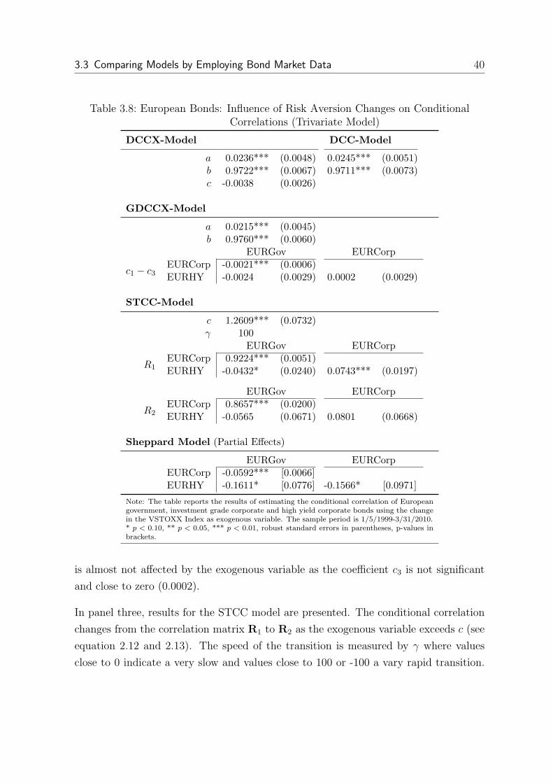
3.3 Comparing Models by Employing Bond Market Data 40
Table 3.8: European Bonds: Influence of Risk Aversion Changes on ConditionalCorrelations (Trivariate Model)
DCCX-Model DCC-Model
a 0.0236*** (0.0048) 0.0245*** (0.0051)b 0.9722*** (0.0067) 0.9711*** (0.0073)c -0.0038 (0.0026)
GDCCX-Model
a 0.0215*** (0.0045)b 0.9760*** (0.0060)
EURGov EURCorp
c1 − c3EURCorp -0.0021*** (0.0006)EURHY -0.0024 (0.0029) 0.0002 (0.0029)
STCC-Model
c 1.2609*** (0.0732)γ 100
EURGov EURCorp
R1EURCorp 0.9224*** (0.0051)EURHY -0.0432* (0.0240) 0.0743*** (0.0197)
EURGov EURCorp
R2EURCorp 0.8657*** (0.0200)EURHY -0.0565 (0.0671) 0.0801 (0.0668)
Sheppard Model (Partial Effects)
EURGov EURCorpEURCorp -0.0592*** [0.0066]EURHY -0.1611* [0.0776] -0.1566* [0.0971]
Note: The table reports the results of estimating the conditional correlation of Europeangovernment, investment grade corporate and high yield corporate bonds using the changein the VSTOXX Index as exogenous variable. The sample period is 1/5/1999-3/31/2010.* p < 0.10, ** p < 0.05, *** p < 0.01, robust standard errors in parentheses, p-values inbrackets.
is almost not affected by the exogenous variable as the coefficient c3 is not significant
and close to zero (0.0002).
In panel three, results for the STCC model are presented. The conditional correlation
changes from the correlation matrix R1 to R2 as the exogenous variable exceeds c (see
equation 2.12 and 2.13). The speed of the transition is measured by γ where values
close to 0 indicate a very slow and values close to 100 or -100 a vary rapid transition.

3 Comparison of the Models 41
For example, the conditional correlation between European government and investment
grade corporate bonds is 0.9224 if the exogenous variable is less than 1.26. Once the
exogenous variable exceeds this value, conditional correlations quickly (as γ is 100) fall
to 0.8657.
The bottom panel reports the partial effects of an increase of the exogenous variable
on the conditional correlations as estimated by the Sheppard model. Estimated pa-
rameters are omitted as they are not directly interpretable. Instead, the partial effects
evaluated at the sample mean are displayed. For example, the effect of an increase in the
exogenous variable is that conditional correlations between government and investment
grade corporate bonds decrease as the partial effect is negative.
Considering the conditional correlation between the government and the investment
grade corporate bonds, the picture is quite clear: The GDCCX, the STCC, and the
Sheppard model all reveal that there is a significant flight-to-quality effect. The con-
ditional correlation between government and corporate bonds drops significantly when
risk aversion, as measured by the change in the VSTOXX index, rises. Figure 3.3 de-
picts the conditional correlation between government and investment grade corporate
bonds as estimated by the different models.
While correlations estimated by the DCCX and the GDCCX model are close to those es-
timated by the DCC model, the correlations estimated by the STCC and the Sheppard
model exhibit a different pattern. Notably, the greatest differences between conditional
correlations estimated by the DCC and the GDCCX model are after 9/11 and in the
wake of the Lehman collapse in September and October 2008. In addition, all esti-
mated conditional correlations share a common feature: they drop considerably during
the financial crisis. However, the estimates of the actual level of conditional correla-
tions during the crisis vary widely among the models: the DCC type models find that
conditional correlations fall to about 0.6. Correlations estimated by the STCC model
are not lower than 0.86 and the minimum of the conditional correlations estimated by
the Sheppard model is as low as 0.2.
We now turn to the correlation between government and high yield corporate as well
as between high yield corporate and investment garde corporate bonds as shown in
Table 3.8. We find that the picture is more ambiguous. The coefficients of the GDCCX
model indicate that there is no significant influence of the exogenous variable on the
correlations while the Sheppard model suggests a drop in correlations - but only at the

3.3 Comparing Models by Employing Bond Market Data 42
0.00.20.40.60.81.0
DCC: Conditional Correlation
0.00.20.40.60.81.0
DCCX: Conditional Correlation
0.00.20.40.60.81.0
Generalized DCCX: Conditional Correlation
0.00.20.40.60.81.0
STCC: Conditional Correlation
1999 2000 2001 2002 2003 2004 2005 2006 2007 2008 2009 20100.00.20.40.60.81.0
Sheppard Model: Conditional Correlation
Figure 3.3: European Government and Investment Grade Corporate BondConditional Correlations
10% level of significance. The STCC model shows that there is only one correlation
regime close to the respective unconditional correlations. Finally, the c parameter for
the DCCX model is insignificant.
This result is not surprising given that the model depends on the assumption of a
common effect of the exogenous variable on all conditional correlations, which clearly
seems not to be true in this sample. That illustrates an important result: By assuming
that there is a common effect of the exogenous variable on all conditional correlations,
the DCCXmodel misses the influence of the risk aversion on the government/investment
grade corporate bond correlation. This is an clear argument in favor of the generalized
version of the DCCX model.

3 Comparison of the Models 43
In order to further analyze the impact of the common parameters on the model results,
we repeat the analysis but only with two indices, i.e. we drop the investment grade
corporate index. The parameter estimations are reported in Table 3.9. In addition,
Figure 3.4 plots the estimated conditional correlations.
A comparison between Figures 3.3 and 3.4 shows that conditional correlations between
government and high yield corporate bonds are much lower than between government
and investment grade corporate bonds. Specifically, the correlation between government
and investment grade corporate bond is around 0.8 to 1 during non-crisis periods while it
is around 0 between high yield corporate and government bonds. This is not surprising
as credit risk is more important for high yield corporate bonds than for investment
grade corporate bonds. More astonishing is that the conditional correlations between
government and high yield corporate bonds barely change during the financial crisis.
Comparing parameter estimates for the conditional correlations between the trivariate
estimation in Table 3.8 and the bivariate estimation in 3.9, the largest changes can be
observed for the DCCX and the STCC model. This is not surprising since both restrict
some parameters to be equal for all conditional correlations in the trivariate case. The
STCC model assumes that there is a common place and speed of the transition (i.e. a
common c and γ) and the DCCX model restricts the c parameter to be equal for all
correlations.
The parameter for the DCCX and the GDCCX model are both negative but still in-
significant at the 5% level. By contrast, the Sheppard model finds that risk aversion
significantly drives conditional correlations between government and high yield corpo-
rate bonds. However, the STCC model indicates that a change in the VSTOXX index
greater than 6.69 results in rising correlations which seems to be counterintuitive at a
first view.
To understand the difference in the sign of the effect, it is important to notice the
differences in the models. The DCCX models and the Sheppard model are built on
the assumption that the exogenous variable has a constant effect on the conditional
correlations while the STCC model distinguishes two correlation regimes. However,
the second correlation regime might be observed only once, e.g. there is a correlation
“outlier”. This happens if the location of transition between the two regimes is close to
the maximum or minimum of the exogenous variable and the speed of the transition is
very high. Values of 6.69 for c and 95.53 for γ might reflect correlation outliers after
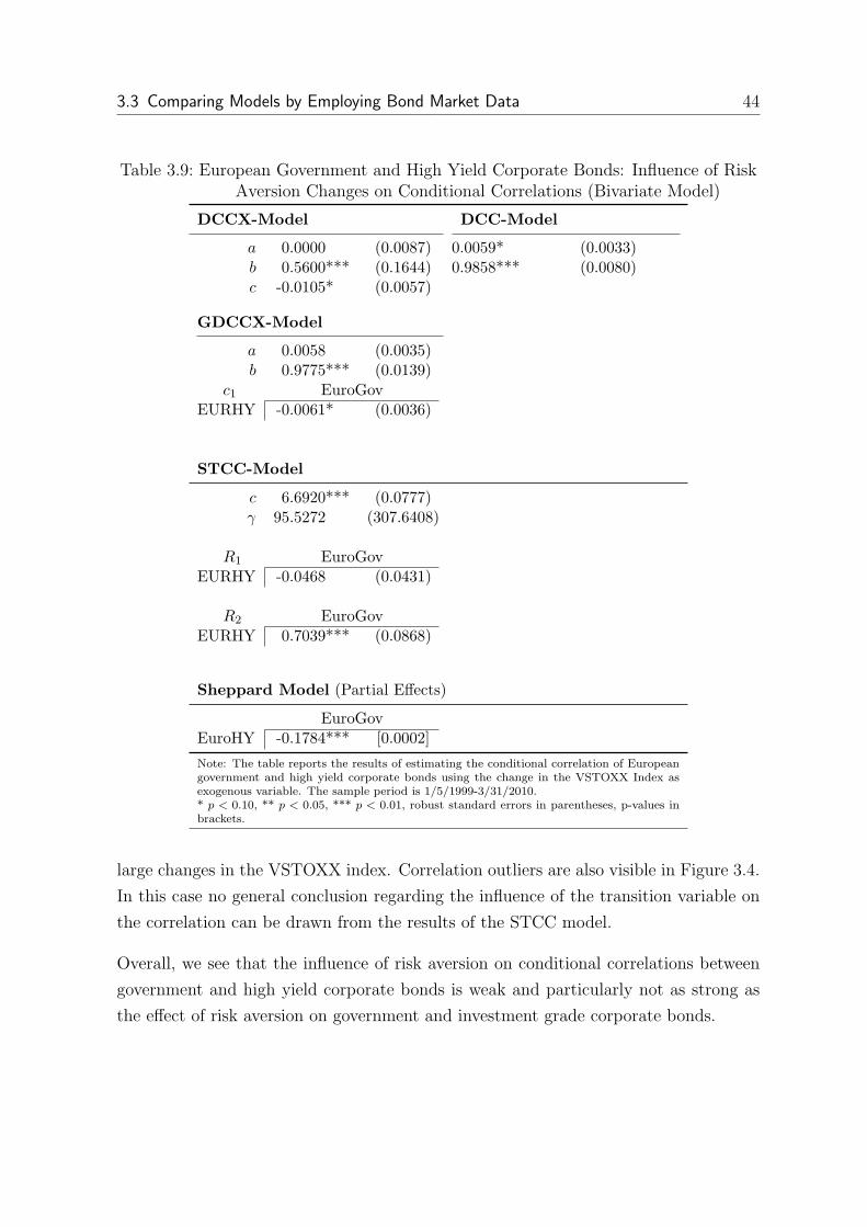
3.3 Comparing Models by Employing Bond Market Data 44
Table 3.9: European Government and High Yield Corporate Bonds: Influence of RiskAversion Changes on Conditional Correlations (Bivariate Model)
DCCX-Model DCC-Model
a 0.0000 (0.0087) 0.0059* (0.0033)b 0.5600*** (0.1644) 0.9858*** (0.0080)c -0.0105* (0.0057)
GDCCX-Model
a 0.0058 (0.0035)b 0.9775*** (0.0139)
c1 EuroGovEURHY -0.0061* (0.0036)
STCC-Model
c 6.6920*** (0.0777)γ 95.5272 (307.6408)
R1 EuroGovEURHY -0.0468 (0.0431)
R2 EuroGovEURHY 0.7039*** (0.0868)
Sheppard Model (Partial Effects)
EuroGovEuroHY -0.1784*** [0.0002]
Note: The table reports the results of estimating the conditional correlation of Europeangovernment and high yield corporate bonds using the change in the VSTOXX Index asexogenous variable. The sample period is 1/5/1999-3/31/2010.* p < 0.10, ** p < 0.05, *** p < 0.01, robust standard errors in parentheses, p-values inbrackets.
large changes in the VSTOXX index. Correlation outliers are also visible in Figure 3.4.
In this case no general conclusion regarding the influence of the transition variable on
the correlation can be drawn from the results of the STCC model.
Overall, we see that the influence of risk aversion on conditional correlations between
government and high yield corporate bonds is weak and particularly not as strong as
the effect of risk aversion on government and investment grade corporate bonds.

3 Comparison of the Models 45
−1.0
−0.5
0.0
0.5
1.0DCC: Conditional Correlation
−1.0
−0.5
0.0
0.5
1.0DCCX: Conditional Correlation
−1.0
−0.5
0.0
0.5
1.0Generalized DCCX: Conditional Correlation
−1.0
−0.5
0.0
0.5
1.0STCC: Conditional Correlation
1999 2000 2001 2002 2003 2004 2005 2006 2007 2008 2009 2010−1.0
−0.5
0.0
0.5
1.0Sheppard Model: Conditional Correlation
Figure 3.4: European Government and High Yield Corporate Bond ConditionalCorrelations
3.3.3.2 US Bond Sectors
We repeat the analysis on a sample with US bond sectors. Results are reported in
Table 3.10. Similar to our previous analysis, we include government bonds, investment
grade corporate, and high yield corporate bonds. We take the change in the VIX index
as exogenous variable and find that the flight-to-quality effect is even stronger than in
the Eurozone.
All models show that conditional correlations decrease if risk aversion, as measured by
the VIX index, rises. Specifically, the estimated c parameter of the DCCX model is
negative and significant indicating a negative effect of the exogenous variable on the
conditional correlations.
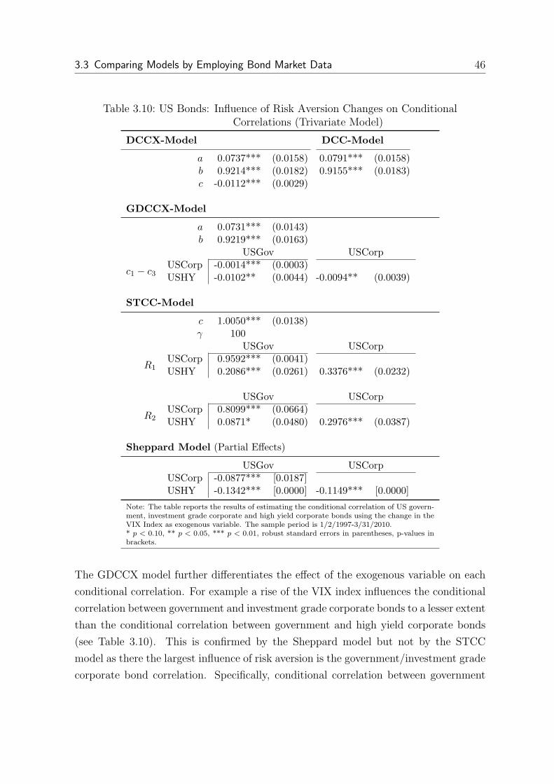
3.3 Comparing Models by Employing Bond Market Data 46
Table 3.10: US Bonds: Influence of Risk Aversion Changes on ConditionalCorrelations (Trivariate Model)
DCCX-Model DCC-Model
a 0.0737*** (0.0158) 0.0791*** (0.0158)b 0.9214*** (0.0182) 0.9155*** (0.0183)c -0.0112*** (0.0029)
GDCCX-Model
a 0.0731*** (0.0143)b 0.9219*** (0.0163)
USGov USCorp
c1 − c3USCorp -0.0014*** (0.0003)USHY -0.0102** (0.0044) -0.0094** (0.0039)
STCC-Model
c 1.0050*** (0.0138)γ 100
USGov USCorp
R1USCorp 0.9592*** (0.0041)USHY 0.2086*** (0.0261) 0.3376*** (0.0232)
USGov USCorp
R2USCorp 0.8099*** (0.0664)USHY 0.0871* (0.0480) 0.2976*** (0.0387)
Sheppard Model (Partial Effects)
USGov USCorpUSCorp -0.0877*** [0.0187]USHY -0.1342*** [0.0000] -0.1149*** [0.0000]
Note: The table reports the results of estimating the conditional correlation of US govern-ment, investment grade corporate and high yield corporate bonds using the change in theVIX Index as exogenous variable. The sample period is 1/2/1997-3/31/2010.* p < 0.10, ** p < 0.05, *** p < 0.01, robust standard errors in parentheses, p-values inbrackets.
The GDCCX model further differentiates the effect of the exogenous variable on each
conditional correlation. For example a rise of the VIX index influences the conditional
correlation between government and investment grade corporate bonds to a lesser extent
than the conditional correlation between government and high yield corporate bonds
(see Table 3.10). This is confirmed by the Sheppard model but not by the STCC
model as there the largest influence of risk aversion is the government/investment grade
corporate bond correlation. Specifically, conditional correlation between government

3 Comparison of the Models 47
−1.0
−0.5
0.0
0.5
1.0DCC: Conditional Correlation
−1.0
−0.5
0.0
0.5
1.0DCCX: Conditional Correlation
−1.0
−0.5
0.0
0.5
1.0Generalized DCCX: Conditional Correlation
−1.0
−0.5
0.0
0.5
1.0STCC: Conditional Correlation
1997 1998 1999 2000 2001 2002 2003 2004 2005 2006 2007 2008 2009 2010−1.0
−0.5
0.0
0.5
1.0Sheppard Model: Conditional Correlation
Figure 3.5: US Government and High Yield Corporate Bond Conditional Correlations
and investment grade corporate bonds decrease quickly (γ = 100) from 0.96 to 0.81
if the VIX increases more than 1.005 points while the correlation between government
and high yield corporate bonds falls from 0.2086 to 0.0871.
Figure 3.5 stresses the differences between the models. While the estimated conditional
correlations of the DCC type models are somewhat similar, conditional correlations as
estimated by the STCC model jump frequently between two regimes, and the Shepard
model conditional correlations largely fluctuate. Notably, the DCC correlations are not
as smooth as in the Eurozone as the estimated half life of the innovations is about
4.4 days in the US while it is 12.4 days in the Eurozone. As suggested by Cappiello
et al. (2006a) the half-life is approximated by: ln (0.5) / ln (a2 + b2). The half-life is the
expected period of time it takes until the influence of any correlation innovation has
decreased by half.

3.3 Comparing Models by Employing Bond Market Data 48
Table 3.11: US Government and Investment Grade Corporate Bonds: Influence ofRisk Aversion Changes on Conditional Correlations (Bivariate Model)
DCCX-Model DCC-Model
a 0.0622*** (0.0111) 0.0748*** (0.0158)b 0.9356*** (0.0118) 0.9220*** (0.0169)c -0.0358*** (0.0019)
GDCCX-Model
a 0.0670*** (0.0152)b 0.9297*** (0.0161)
c1 USGovUSCorp -0.0017*** (0.0004)
STCC-Model
c 1.0095*** (0.1140)γ 100
R1 USGovUSCorp 0.9467*** (0.0033)
R2 USGovUSCorp 0.8281*** (0.0501)
Sheppard Model (Partial Effects)
USGovUSCorp -0.0280*** [0.0057]
Note: The table reports the results of estimating the conditional correlation of US gov-ernment and investment grade corporate bonds using the change in the VIX Index asexogenous variable. The sample period is 1/3/1990-3/31/2010.* p < 0.10, ** p < 0.05, *** p < 0.01, robust standard errors in parentheses, p-values inbrackets.
In order to test the robustness of the results we ran the analysis with a longer sample
covering more than 20 years of daily observations from 1/1990 to 3/2010. However, this
is a bivariate model as this sample only includes the government and the investment
grade corporate bonds. Results are presented in Table 3.11.
They largely confirm the results of the previous analysis. Other than in the European
sample, the estimated c parameter for the STCC model is almost identical to the one
previously estimated. Thus, the common c parameter for all correlations imposes no

3 Comparison of the Models 49
−1.0
−0.5
0.0
0.5
1.0DCC: Conditional Correlation
−1.0
−0.5
0.0
0.5
1.0DCCX: Conditional Correlation
−1.0
−0.5
0.0
0.5
1.0Generalized DCCX: Conditional Correlation
−1.0
−0.5
0.0
0.5
1.0STCC: Conditional Correlation
1990 1991 1992 1993 1994 1995 1996 1997 1998 1999 2000 2001 2002 2003 2004 2005 2006 2007 2008 2009 2010−1.0
−0.5
0.0
0.5
1.0Sheppard Model: Conditional Correlation
Figure 3.6: US Government and Investment Grade Corporate Bond ConditionalCorrelations
additional restriction. Figure 3.6 also shows that both during the subprime crisis as
well as during the burst of the dot-com bubble conditional correlations were lower.
3.3.3.3 Comparison by Statistical and Econometric Criteria
After estimating the coefficients of the models, we compare the models using the selec-
tion criteria proposed in section 3.3.1. Table 3.12 reports several statistical criteria.
Looking at the AIC and the BIC, the GDCCX model performs best in the US samples.
For the European samples, the DCC model is best according to the BIC while the
AIC favors the GDCCX and the STCC. Generally, according to the statistical crite-
ria, the performance of the DCC-type models is somewhat similar. By contrast, the

3.3 Comparing Models by Employing Bond Market Data 50
Table 3.12: Statistical Criteria
DCCModel
DCCXModel
GDCCXModel
STCCModel
SheppardModel
European Government, Investment Grade, and High Yield Corporate Bonds
LL −15649.778 −15648.053 -15629.604 −15883.451 −16671.083AIC 10.975 10.974 10.963 11.143 11.695BIC 10.988 10.999 10.992 11.178 11.733Param. 11 12 14 17 18
European Government and High Yield Corporate Bonds
LL −13289.321 −13294.328 −13287.360 -13282.907 −13976.980AIC 9.318 9.323 9.318 9.315 9.801BIC 9.335 9.341 9.337 9.336 9.820Param. 8 9 9 10 9
US Government, Investment Grade, and High Yield Corporate Bonds
LL −17890.388 −17871.776 -17782.521 −19059.471 −19346.052AIC 10.745 10.735 10.682 11.451 11.623BIC 10.765 10.757 10.708 11.482 11.656Param. 11 12 14 17 18
US Government and Investment Grade Corporate Bonds
LL −18501.106 −18411.540 -18406.544 −19835.020 −19942.682AIC 7.257 7.222 7.220 7.781 7.823BIC 7.267 7.234 7.232 7.794 7.834Param. 8 9 9 9 10
Note: The table reports the log-likelihood values (LL), the values of the Akaike (AIC)and Bayesian information criteria (BIC), and the number of parameters (Param.) wehave to estimate.
STCC model performs worse in all samples except in the sample which only includes
European government and high yield corporate bonds. Moreover, the Sheppard model
always ranks last. Although the DCC model does not consider the influence of exoge-
nous variables, it outperforms the STCC and the Sheppard model if BIC is chosen as
criterion.
The economic criteria reveal the differences between the DCC type models on the one
hand and the STCC and the Sheppard model on the other hand. Table 3.13 presents
the volatility of portfolios formed with the estimated covariance matrix of the respective
models. The lowest standard deviation is normalized to 100. As described in section
3.3.1, results are reported for both the global minimum variance portfolio (GMVP) and
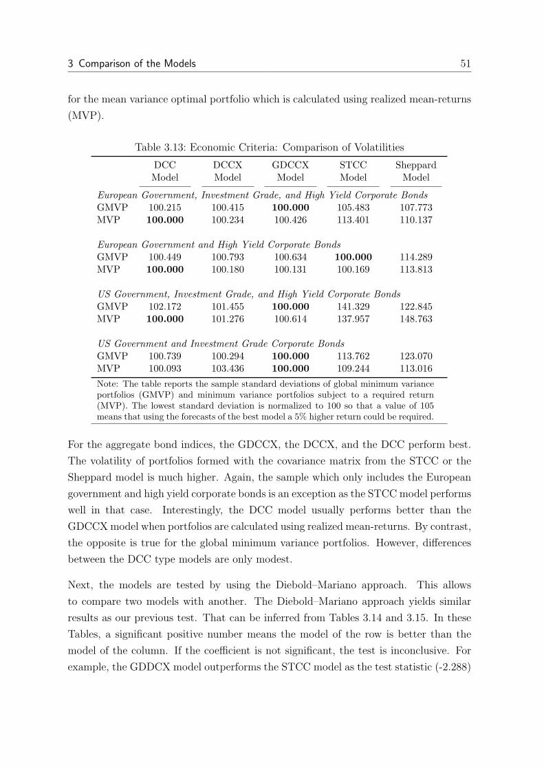
3 Comparison of the Models 51
for the mean variance optimal portfolio which is calculated using realized mean-returns
(MVP).
Table 3.13: Economic Criteria: Comparison of Volatilities
DCCModel
DCCXModel
GDCCXModel
STCCModel
SheppardModel
European Government, Investment Grade, and High Yield Corporate Bonds
GMVP 100.215 100.415 100.000 105.483 107.773MVP 100.000 100.234 100.426 113.401 110.137
European Government and High Yield Corporate Bonds
GMVP 100.449 100.793 100.634 100.000 114.289MVP 100.000 100.180 100.131 100.169 113.813
US Government, Investment Grade, and High Yield Corporate Bonds
GMVP 102.172 101.455 100.000 141.329 122.845MVP 100.000 101.276 100.614 137.957 148.763
US Government and Investment Grade Corporate Bonds
GMVP 100.739 100.294 100.000 113.762 123.070MVP 100.093 103.436 100.000 109.244 113.016
Note: The table reports the sample standard deviations of global minimum varianceportfolios (GMVP) and minimum variance portfolios subject to a required return(MVP). The lowest standard deviation is normalized to 100 so that a value of 105means that using the forecasts of the best model a 5% higher return could be required.
For the aggregate bond indices, the GDCCX, the DCCX, and the DCC perform best.
The volatility of portfolios formed with the covariance matrix from the STCC or the
Sheppard model is much higher. Again, the sample which only includes the European
government and high yield corporate bonds is an exception as the STCC model performs
well in that case. Interestingly, the DCC model usually performs better than the
GDCCXmodel when portfolios are calculated using realized mean-returns. By contrast,
the opposite is true for the global minimum variance portfolios. However, differences
between the DCC type models are only modest.
Next, the models are tested by using the Diebold–Mariano approach. This allows
to compare two models with another. The Diebold–Mariano approach yields similar
results as our previous test. That can be inferred from Tables 3.14 and 3.15. In these
Tables, a significant positive number means the model of the row is better than the
model of the column. If the coefficient is not significant, the test is inconclusive. For
example, the GDDCX model outperforms the STCC model as the test statistic (-2.288)

3.3 Comparing Models by Employing Bond Market Data 52
Table 3.14: Economic Criteria: Unweighted Diebold-Mariano-Test Statistics for aGlobal Minimum Variance Portfolio
DCCModel
DCCXModel
GDCCXModel
STCCModel
European Government, Investment Grade, and High Yield Corporate Bonds
DCCX Model -0.520GDCCX 0.520 1.076STCC Model -2.309** -2.130** -2.288**Sheppard Model -2.518** -2.483** -2.563** -0.719
European Government and High Yield Corporate Bonds
DCCX Model -1.773*GDCCX -0.637 0.598STCC Model 0.716 1.331 0.785Sheppard Model -5.033*** -4.842*** -4.896*** -5.107***
US Government, Investment Grade, and High Yield Corporate Bonds
DCCX Model 1.473GDCCX 1.631 1.254STCC Model -2.117** -2.143** -2.256**Sheppard Model -2.761*** -2.809*** -3.177*** 1.315
US Government and Investment Grade Corporate Bonds
DCCX Model 2.175**GDCCX 1.662* 0.919STCC Model -3.003*** -3.105*** -3.206***Sheppard Model -4.510*** -4.600*** -4.693*** -3.229***
Note: The table reports the unweighted Diebold-Mariano test statistics of equal pre-dictive accuracy of the models for all datasets used. A significant positive numbermeans the model of the row is better than the model of the column. The panel showsresults for the global minimum variance portfolio.* p < 0.10, ** p < 0.05, *** p < 0.01
is significantly less than zero. Both the weighted and the unweighted versions of the
test find that the STCC model and the Sheppard model are significantly outperformed
by the DCC type models. The only exception is the conditional correlation between
European government and high yield corporate bonds since the STCC model is not
outperformed by the other models in this sample. The differences between the DCC,
the DCCX and the GDCCX model are mostly not significant. Comparing the STCC
and the Sheppard model only results in significant results in the sample with European
government and high yield corporate bonds and in the sample with US government
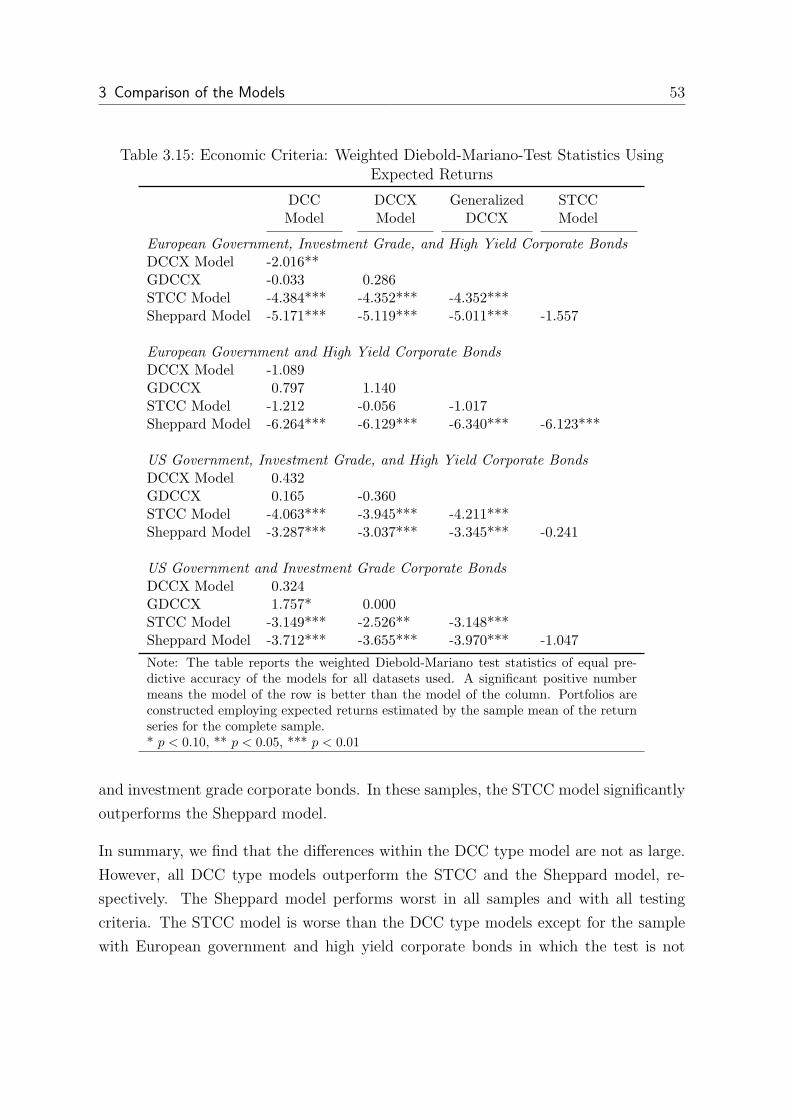
3 Comparison of the Models 53
Table 3.15: Economic Criteria: Weighted Diebold-Mariano-Test Statistics UsingExpected Returns
DCCModel
DCCXModel
GeneralizedDCCX
STCCModel
European Government, Investment Grade, and High Yield Corporate Bonds
DCCX Model -2.016**GDCCX -0.033 0.286STCC Model -4.384*** -4.352*** -4.352***Sheppard Model -5.171*** -5.119*** -5.011*** -1.557
European Government and High Yield Corporate Bonds
DCCX Model -1.089GDCCX 0.797 1.140STCC Model -1.212 -0.056 -1.017Sheppard Model -6.264*** -6.129*** -6.340*** -6.123***
US Government, Investment Grade, and High Yield Corporate Bonds
DCCX Model 0.432GDCCX 0.165 -0.360STCC Model -4.063*** -3.945*** -4.211***Sheppard Model -3.287*** -3.037*** -3.345*** -0.241
US Government and Investment Grade Corporate Bonds
DCCX Model 0.324GDCCX 1.757* 0.000STCC Model -3.149*** -2.526** -3.148***Sheppard Model -3.712*** -3.655*** -3.970*** -1.047
Note: The table reports the weighted Diebold-Mariano test statistics of equal pre-dictive accuracy of the models for all datasets used. A significant positive numbermeans the model of the row is better than the model of the column. Portfolios areconstructed employing expected returns estimated by the sample mean of the returnseries for the complete sample.* p < 0.10, ** p < 0.05, *** p < 0.01
and investment grade corporate bonds. In these samples, the STCC model significantly
outperforms the Sheppard model.
In summary, we find that the differences within the DCC type model are not as large.
However, all DCC type models outperform the STCC and the Sheppard model, re-
spectively. The Sheppard model performs worst in all samples and with all testing
criteria. The STCC model is worse than the DCC type models except for the sample
with European government and high yield corporate bonds in which the test is not

3.3 Comparing Models by Employing Bond Market Data 54
significant. However, as we have seen by plotting conditional correlations (see Figure
3.4), conditional correlations estimated by the STCC model are almost constant.
3 Comparison of the Models 55
3.4 Summary
In this chapter, we compare the performance of conditional correlation models in dif-
ferent settings. First, we conduct a simulation study employing the true conditional
correlation as exogenous variable. We find that GDCCX model uses the information of
the exogenous variable best in all settings. The STCC model performs almost as good
as the GDCCX model and the DCCX model is still better than the DCC model that
does not account for the effect of exogenous variables. By contrast, the Sheppard model
performs even worse than the DCC model. Interestingly, the Sheppard model performs
well in a setting where correlation change very quickly. Furthermore, we demonstrate
that employing models which account for a potential effect of an exogenous variable
reduces the mean absolute estimation error by about two thirds. We conclude that the
gains for using exogenous variables can be substantial.
We then turn to an application of the correlation models employing real data. We
include bond sector data for the Eurozone and the US in our analysis. Our empiri-
cal results can be summarized as follows. First, the greater the number of time series
analyzed and the more heterogeneous the respective conditional correlations respond
to the exogenous variable the more rewarding it is to use the GDCCX model instead
of the DCCX model. For example, in a sample with European government, corporate
investment grade and corporate high yield bonds, conditional correlations between in-
vestment grade and government bonds react differently to risk aversion than conditional
correlations between high yield and investment grade bond. That effect is captured by
the GDCCX model since there are coefficients that measure the influence of the ex-
ogenous variable on each correlation separately. Yet, there is only one coefficient that
measures the effect of the exogenous variable on all correlations in the DCCX model.
As a result, this coefficient is not significant and cannot be interpreted as well. Also,
the GDCCX model performs well in terms of both statistic and economic criteria. Sec-
ond, the most striking result when comparing the different models is that the DCC,
the DCCX and the GDCCX model outperform the Sheppard and the STCC model in
most settings with respect to both statistical and economic criteria.
By the choice of our exogenous variable, we also address an empirical research question
in this chapter. We investigate the influence of risk aversion on conditional correlations.
We find statistical evidence for a flight-to-quality effect. When risk aversion rises, the
conditional correlation between government and corporate bonds falls. That holds

3.4 Summary 56
true both for the US and the Eurozone and can be observed for either investment
grade or high yield bonds though the results are not as strong for high yield bonds
in the Eurozone. The results are robust among all models we consider. As opposed
to equity investments, the benefits of diversification between different bond sectors are
not diminished in times of market turbulences. Our findings further indicate that the
conditional correlation between investment grade and high yield corporate bonds fall
in the US but not in the Eurozone.

4 Exogenous Variables in Correlation and Volatility 57
4 Exogenous Variables in Correlation and Volatility
4.1 Introduction
In the models presented in the previous chapters, we assumed that all conditional vari-
ances are sufficiently described by a univariate GARCH (1,1) model. This approach is
supported by Engle and Sheppard (2008), Berben and Jansen (2009), and Bauer (2011)
who argue that the choice of the GARCH model is of minor relevance given that pat-
terns of conditional variances produced by many univariate GARCH models are similar.
Moreover, we assumed that the exogenous variables affect conditional correlations but
do not affect conditional variances. This is justified since Schwert (1989) examines the
stock volatility from 1857 to 1987 and does not find any macroeconomic variable that
explains return volatility. Likewise, a study of Paye (2010) provides little support for
volatility predictability by exogenous variables.
However, Officer (1973) demonstrates that market volatility can be related to industrial
production. Recently, the modeling of volatility as a function of exogenous variables
has gained additional attention. For example, Engle et al. (2009) provide evidence
that economic fundamentals such as inflation and industrial production growth drive
stock market volatility. Cakmakli and van Dijk (2010) demonstrate that a number
of macroeconomic variables can help predicting US stock volatility between 1980 and
2005. Christiansen et al. (2011) get similar results for the foreign exchange, the com-
modity, and the bond market. Last, Engle and Rangel (2008) find that volatility in
macroeconomic and financial factors are important determinants of increased volatility.
The influence of exogenous variables on conditional variance is important for correlation
models and is the focus of this chapter. As already noted by King and Wadhwani (1990)
and later by Forbes and Rigobon (2002), a change in the conditional variance of one
time series can result in increasing conditional correlations. Corsetti et al. (2005) argue
that this is true only under certain restrictive assumptions regarding the dependence
structure and the time-series specific variance. However, provided these assumptions
hold, a change in the exogenous variable can drive conditional correlations without
changing the dependence structure of the time series.

4.2 The Interrelation Between Variance and Correlation 58
We further investigate the consequences of a misspecification of the variance equation
in the GDCCX model. We present the GARCHX model that is an extension of a
GARCH model but allows exogenous variables to drive conditional variances. This
model is employed in a simulation experiment. We simulate time series in which con-
ditional variances are influenced by an exogenous variable according to a GARCHX
model but conditional correlations are not. Then, we estimate a GDCCX model as-
suming that conditional variances are driven by a GARCH (1,1) process and that only
conditional correlations are affected by the exogenous variable. We repeat the sim-
ulation for various different sample sizes, exogenous variables, correlation structures,
and parameter constellations. We find that in some settings, the parameter estimates
are biased as the model incorrectly finds an influence of the exogenous variable on the
conditional correlations.
We therefore propose to replace the GARCH model in the variance equation of the
GDCCX model by a GARCHX model to capture the effect of exogenous variables on
conditional variances. We repeat the previous simulation experiment with this estima-
tor and demonstrate that parameter estimates are unbiased in all settings now.
This chapter proceeds as follows. In the next section, we discuss a theoretical model
that describes the interrelation between variances and correlations. In section 4.3, we
introduce the GARCHX model. We investigate how the GDCCX model estimation is
affected if exogenous variables drive conditional variances instead of correlations and
examine how result change once the variance equation is correctly specified with a
GARCHX model. Section 4.5 summarizes and concludes.
4.2 The Interrelation Between Variance and Correlation
In this section, we discuss the interaction between variance and correlation. Forbes
and Rigobon (2002) argue that conditional correlations rise as conditional variances
increase during periods of crisis. As a result, testing for a change in correlations suffers
from heteroscedasticity bias.1
1Ronn et al. (2009), Loretan and English (2000), and Boyer et al. (1999) also document this biasemploying a different statistical framework and more restrictive assumptions.
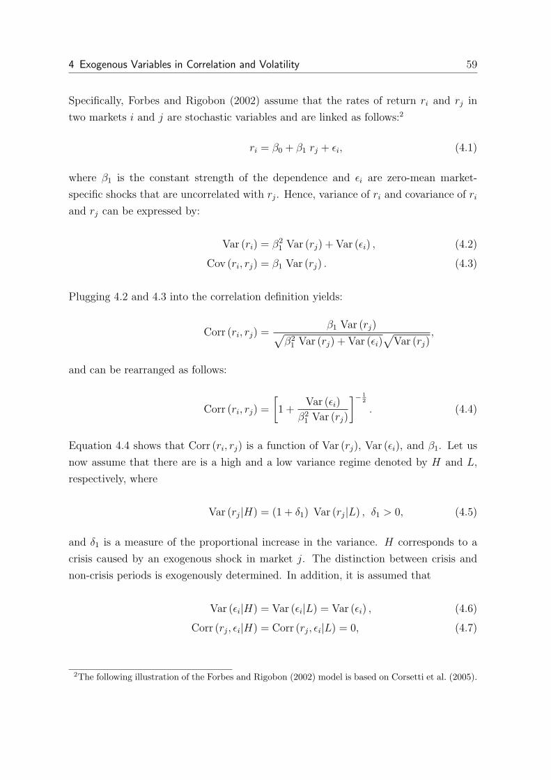
4 Exogenous Variables in Correlation and Volatility 59
Specifically, Forbes and Rigobon (2002) assume that the rates of return ri and rj in
two markets i and j are stochastic variables and are linked as follows:2
ri = β0 + β1 rj + ǫi, (4.1)
where β1 is the constant strength of the dependence and ǫi are zero-mean market-
specific shocks that are uncorrelated with rj. Hence, variance of ri and covariance of ri
and rj can be expressed by:
Var (ri) = β21 Var (rj) + Var (ǫi) , (4.2)
Cov (ri, rj) = β1 Var (rj) . (4.3)
Plugging 4.2 and 4.3 into the correlation definition yields:
Corr (ri, rj) =β1 Var (rj)
√
β21 Var (rj) + Var (ǫi)
√
Var (rj),
and can be rearranged as follows:
Corr (ri, rj) =
[
1 +Var (ǫi)
β21 Var (rj)
]− 1
2
. (4.4)
Equation 4.4 shows that Corr (ri, rj) is a function of Var (rj), Var (ǫi), and β1. Let us
now assume that there are is a high and a low variance regime denoted by H and L,
respectively, where
Var (rj|H) = (1 + δ1) Var (rj|L) , δ1 > 0, (4.5)
and δ1 is a measure of the proportional increase in the variance. H corresponds to a
crisis caused by an exogenous shock in market j. The distinction between crisis and
non-crisis periods is exogenously determined. In addition, it is assumed that
Var (ǫi|H) = Var (ǫi|L) = Var (ǫi) , (4.6)
Corr (rj, ǫi|H) = Corr (rj, ǫi|L) = 0, (4.7)
2The following illustration of the Forbes and Rigobon (2002) model is based on Corsetti et al. (2005).

4.2 The Interrelation Between Variance and Correlation 60
i.e. the variance of the market-specific shocks in market i is constant across variance
regimes and is not correlated with rj. Thus, the exogenous shock in market j does not
affect the specific shocks in market i in any way. Applying 4.5 and 4.6 to 4.4, we get:
[
1 +Var (ǫi)
β21 (1 + δ1)Var (rj|L)
]− 1
2
>
[
1 +Var (ǫi)
β21 Var (rj|L)
]− 1
2
(4.8)
Corr (ri, rj|H) > Corr (ri, rj|L)
Hence, the correlation between ri and rj increases in the high variance regime,
although the strength of the dependence β1 remains constant during the crisis.
However, as pointed out by Corsetti et al. (2001) and Corsetti et al. (2005), the
results critically depend on assumptions 4.6 and 4.7. It is easy to imagine a situation
in which a shock in market j gives rise to a higher risk aversion in all markets
resulting in higher variance of the market-specific shocks in market i:
Var (ǫi|H) = (1 + δ2) Var (ǫi|L) (4.9)
and therefore the relation between the correlation in high and low variance regimes as
expressed by 4.8 becomes:
[
1 +(1 + δ2)Var (ǫi)
β21 (1 + δ1)Var (rj|L)
]− 1
2
R[
1 +Var (ǫi)
β21 Var (rj|L)
]− 1
2
(4.10)
Corr (ri, rj|H) R Corr (ri, rj|L)
depending on
(1 + δ1) R (1 + δ2) .
Therefore, a change in the correlation between market i and market j can be caused in
different ways.
In one scenario, a shock in market j results in rising correlations. The increase in vari-
ance in market j is higher than the rise in market-specific variance (δ1 > δ2) although
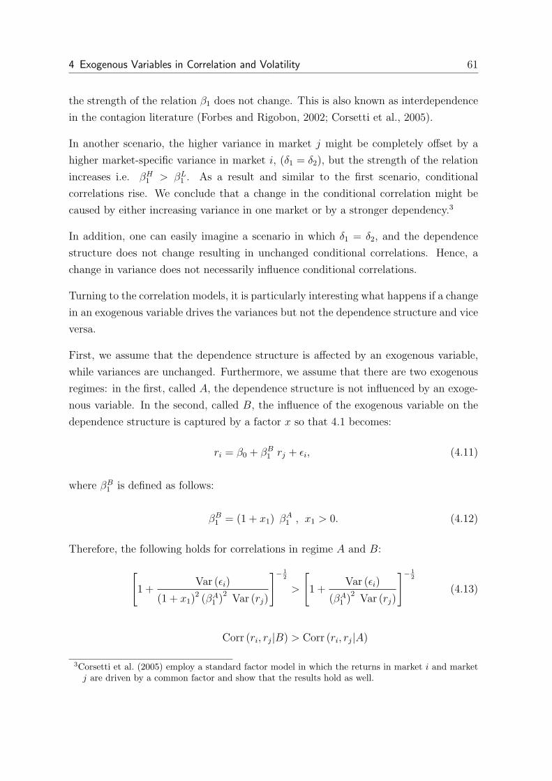
4 Exogenous Variables in Correlation and Volatility 61
the strength of the relation β1 does not change. This is also known as interdependence
in the contagion literature (Forbes and Rigobon, 2002; Corsetti et al., 2005).
In another scenario, the higher variance in market j might be completely offset by a
higher market-specific variance in market i, (δ1 = δ2), but the strength of the relation
increases i.e. βH1 > βL
1 . As a result and similar to the first scenario, conditional
correlations rise. We conclude that a change in the conditional correlation might be
caused by either increasing variance in one market or by a stronger dependency.3
In addition, one can easily imagine a scenario in which δ1 = δ2, and the dependence
structure does not change resulting in unchanged conditional correlations. Hence, a
change in variance does not necessarily influence conditional correlations.
Turning to the correlation models, it is particularly interesting what happens if a change
in an exogenous variable drives the variances but not the dependence structure and vice
versa.
First, we assume that the dependence structure is affected by an exogenous variable,
while variances are unchanged. Furthermore, we assume that there are two exogenous
regimes: in the first, called A, the dependence structure is not influenced by an exoge-
nous variable. In the second, called B, the influence of the exogenous variable on the
dependence structure is captured by a factor x so that 4.1 becomes:
ri = β0 + βB1 rj + ǫi, (4.11)
where βB1 is defined as follows:
βB1 = (1 + x1) βA
1 , x1 > 0. (4.12)
Therefore, the following holds for correlations in regime A and B:
[
1 +Var (ǫi)
(1 + x1)2 (βA
1 )2Var (rj)
]− 1
2
>
[
1 +Var (ǫi)
(βA1 )
2Var (rj)
]− 1
2
(4.13)
Corr (ri, rj|B) > Corr (ri, rj|A)
3Corsetti et al. (2005) employ a standard factor model in which the returns in market i and marketj are driven by a common factor and show that the results hold as well.

4.2 The Interrelation Between Variance and Correlation 62
As expected, if an exogenous variable strengthens the relation between the markets i
and j, the correlation rises.
Let us now assume that the variance in market j is affected by an exogenous variable
but not the dependence structure. Again, there are two regimes: there is no influence
of the exogenous variable on the variance in regime C. By contrast, in regime D,
exogenous variables cause the variance in market j to increase as follows:
Var (rj|D) = (1 + x1) Var (rj|C) , x1 > 0. (4.14)
Furthermore, the market-specific variance is assumed to remain constant, i.e.
Var (ǫi|C) = Var (ǫi|D) = Var (ǫi) (4.15)
Corr (rj, ǫi|C) = Corr (rj, ǫi|D) = 0. (4.16)
Then, for x1 > 0, the respective correlations in regimes C and D are:
[
1 +Var (ǫi)
β21 (1 + x1)Var (rj|C)
]− 1
2
>
[
1 +Var (ǫi)
β21 Var (rj|C)
]− 1
2
(4.17)
Corr (ri, rj|D) > Corr (ri, rj|C)
As expected, if an exogenous variable affects the variance in market j but not the
market-specific variance ǫi, the correlation between market i and j rises. Thus, a
change in the exogenous variable drives the conditional correlations without changing
the dependence structure of the time series. However, as shown previously, if assump-
tions 4.15 and 4.16 are dropped, i.e. we assume that the market-specific variance in
market i is also affected by the exogenous variables, the outcome changes: conditional
correlation might increase, decrease, or not change at all.
Although we do not have a general result indicating what happens if the variance is
affected by an exogenous variable, there are cases in which an influence of the exogenous
variable on the variance also drives correlations.
4 Exogenous Variables in Correlation and Volatility 63
4.3 Conditional Variance and Exogenous Variables: The GARCHX
Model
In this section, we present a model that captures the influence of any exogenous variable
on conditional variances. Several studies argue that macroeconomic or financial vari-
ables might help in forecasting volatility while others are more sceptical.4 As already
noted by Engle (1982), any variance function can be augmented with exogenous vari-
ables. Previous studies employ both multivariate GARCH(1,1) and GARCHX models.
The former studies model conditional variance as a function of its own and exogenous
variables’ past squared innovations (Bollerslev, 1990; Fratzscher, 2002; Kaltenhauser,
2003; Hunter and Simon, 2005). GARCHX models as proposed by Hwang and Satchell
(2005), Brenner et al. (1996) or Engle and Patton (2001) directly include the exogenous
variable in the GARCH conditional variance equation such as
ht = ω + αrt−1 + βht−1 + γXt−1, (4.18)
where rt−1 is a lagged demeaned time series, ht is the conditional variance and Xt−1 a
vector with lagged exogenous variables.5 For γ = 0 the model reduces to the traditional
GARCH(1,1) model. Han (2010) establishes the asymptotic properties. Furthermore,
the GARCHX model is widely used in empirical research.6. Depending on the formu-
lation of Equation 4.18, different parameter restrictions are imposed to ensure that the
non-negativity condition of variance is always satisfied (Hwang and Satchell, 2005) Al-
ternatively, the model can be estimated by constrained maximum likelihood, restricting
the parameter space so that the conditional volatility process is always positive (de Goeij
and Marquering, 2004).
4.4 GDCCX Simulation when an Exogenous Variable Drives
Conditional Variances
In this section, we study the consequences of estimating a GDCCX model when the
variance equation is misspecified. Therefore, we conduct a simulation experiment.
4See Christiansen et al. (2011) for an overview on these papers.5An alternative formulation is replacing γXt−1 with γX2
t−1which ensures that the term with the
exogenous variable is positive.6See Fleming et al. (2008) or Han (2010) for an overview.

4.4 GDCCX Simulation when an Exogenous Variable Drives Conditional Variances 64
Specifically, we simulate time series where the conditional variances but not condi-
tional correlations are driven by an exogenous variable. We model the influence of
the exogenous variables with a GARCHX model. We include four different types of
exogenous variables:
1. The exogenous variable is an independent identically-distributed random time
series sampled from a normal distribution.
2. The exogenous variable is similar to defined above but exhibits conditional het-
eroscedasticity according to a GARCH(1,1) model. Typically, financial time series
behave like series from this data generating process.
3. The exogenous variable takes on a standard normal distributed value every 100th
observation only. All other observations are zero. This type of series simulates
macroeconomic announcements which are usually published periodically.7 Al-
though the simulated announcement values are standard normally distributed,
the complete time series of the exogenous variable is not normally distributed
due to the large number of zeros.
4. The exogenous variable is similar to the exogenous variable as described before
but the value during the announcement is one. That simulates a dummy variable
which indicates the release of an macroeconomic announcement.
Furthermore, we test two different parameter sets for the GARCHX model (see Equa-
tion 4.18) that describes the influence of the exogenous variable on conditional variances:
Parameter Set Series ωi αi βi γi
I1 0.01 0.03 0.90 0.000102 0.01 0.03 0.90 -0.00005
II1 0.01 0.03 0.90 0.0102 0.01 0.03 0.90 -0.005
7These types of time series are included in the empirical analysis in chapter 6.

4 Exogenous Variables in Correlation and Volatility 65
The parameter sets differ in the dimension of the γ parameter as they vary by a factor of
100. Thus, GARCHX effects are more pronounced when parameter set II is employed.8
In all simulated time series, the conditional variances but not conditional correlations
are driven by an exogenous variable. Two different correlation structures are tested.
First, we assume that the true correlation structure of the simulated time series is gen-
erated by a DCC (1,1) model. Second, we assume that the time series are uncorrelated.
In addition, we examine the effect of different sample sizes. We investigate samples
with 500, 1000, 2500, and 5000 observations. All simulations are repeated 200 times.
After simulating the data, we estimate a GDCCX model and estimate conditional
variances using a GARCH (1,1) model. We calculate the 90% as well as the 95%
confidence intervals for the c parameter that measures the influence of the exogenous
variable (see section 2.4.2 and equation 2.11). Next, we check if the confidence interval
includes the true parameter. That should be the case in 95% of all simulations for
the 95% confidence interval, i.e. the empirical rejection frequency should be 5%. The
empirical rejection frequency should approach the nominal level as the sample size
grows. The true c parameter is zero since the conditional variances are not affected by
the exogenous variable. Results for the different settings are presented in Figures 4.1
and 4.2.
Employing parameter set II and assuming that the true correlation structure is gener-
ated by a DCC (1,1) model results in the most exceptional results as shown in Figure
4.1(b). If we simulate that the exogenous variables are homoscedastic or heteroscedas-
tic normally distributed random time series the rejection frequency approaches 100%
as the sample size grows . That means that the estimated c parameter of the GDCCX
model is significantly different from zero in all simulations. However, the true param-
eter is zero as conditional correlations are not influenced by the exogenous variable.
In this setting, the GDCCX estimator is biased. Most probably this is caused by the
univariate GARCH model not being well specified. Obviously, the large influence of
exogenous variable on the conditional variances is incorrectly assigned to a change in
conditional correlations.
8We also employed parameter sets where the γ parameter is constant among series or takes on differentvalues. However, we found that changing the parameter dimension among parameter sets is moreimportant than changing the sign or the actual value of the parameter.
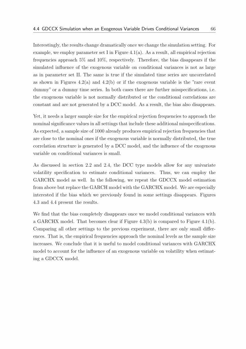
4.4 GDCCX Simulation when an Exogenous Variable Drives Conditional Variances 66
Interestingly, the results change dramatically once we change the simulation setting. For
example, we employ parameter set I in Figure 4.1(a). As a result, all empirical rejection
frequencies approach 5% and 10%, respectively. Therefore, the bias disappears if the
simulated influence of the exogenous variable on conditional variances is not as large
as in parameter set II. The same is true if the simulated time series are uncorrelated
as shown in Figures 4.2(a) and 4.2(b) or if the exogenous variable is the ”rare event
dummy” or a dummy time series. In both cases there are further misspecifications, i.e.
the exogenous variable is not normally distributed or the conditional correlations are
constant and are not generated by a DCC model. As a result, the bias also disappears.
Yet, it needs a larger sample size for the empirical rejection frequencies to approach the
nominal significance values in all settings that include these additional misspecifications.
As expected, a sample size of 1000 already produces empirical rejection frequencies that
are close to the nominal ones if the exogenous variable is normally distributed, the true
correlation structure is generated by a DCC model, and the influence of the exogenous
variable on conditional variances is small.
As discussed in section 2.2 and 2.4, the DCC type models allow for any univariate
volatility specification to estimate conditional variances. Thus, we can employ the
GARCHX model as well. In the following, we repeat the GDCCX model estimation
from above but replace the GARCH model with the GARCHX model. We are especially
interested if the bias which we previously found in some settings disappears. Figures
4.3 and 4.4 present the results.
We find that the bias completely disappears once we model conditional variances with
a GARCHX model. That becomes clear if Figure 4.3(b) is compared to Figure 4.1(b).
Comparing all other settings to the previous experiment, there are only small differ-
ences. That is, the empirical frequencies approach the nominal levels as the sample size
increases. We conclude that it is useful to model conditional variances with GARCHX
model to account for the influence of an exogenous variable on volatility when estimat-
ing a GDCCX model.

4 Exogenous Variables in Correlation and Volatility 67
500 1000 2500 5000
10%
20%
30%
40%
50%
Exogenous variable:normally distributed
Re
jectio
n R
ate
500 1000 2500 5000
10%
20%
30%
40%
50%
Exogenous variable:normally distributed and heteroskedastic
500 1000 2500 5000
10%
20%
30%
40%
50%
Exogenous variable:infrequent
Re
jectio
n R
ate
Sample Size 500 1000 2500 5000
10%
20%
30%
40%
50%
Exogenous variable:infrequent and dummy
Sample Size
(a) True Correlation Structure: DCC; Parameter Set I
500 1000 2500 5000
25%
50%
75%
100%
Exogenous variable:normally distributed
Reje
ction R
ate
500 1000 2500 5000
25%
50%
75%
100%
Exogenous variable:normally distributed and heteroskedastic
500 1000 2500 5000
10%
20%
30%
40%
50%
Exogenous variable:infrequent
Reje
ction R
ate
Sample Size 500 1000 2500 5000
10%
20%
30%
40%
50%
Exogenous variable:infrequent and dummy
Sample Size
95% Confidence Interval
90% Confidence Interval
(b) True Correlation Structure: DCC; Parameter Set II
Figure 4.1: Empirical Rejection Frequencies for GDCCX/GARCH Estimations

4.4 GDCCX Simulation when an Exogenous Variable Drives Conditional Variances 68
500 1000 2500 5000
10%
20%
30%
40%
50%
Exogenous variable:normally distributed
Re
jectio
n R
ate
500 1000 2500 5000
10%
20%
30%
40%
50%
Exogenous variable:normally distributed and heteroskedastic
500 1000 2500 5000
10%
20%
30%
40%
50%
Exogenous variable:infrequent
Re
jectio
n R
ate
Sample Size 500 1000 2500 5000
10%
20%
30%
40%
50%
Exogenous variable:infrequent and dummy
Sample Size
(a) True Correlation Structure: Uncorrelated; Parameter Set I
500 1000 2500 5000
10%
20%
30%
40%
50%
Exogenous variable:normally distributed
Re
jectio
n R
ate
500 1000 2500 5000
10%
20%
30%
40%
50%
Exogenous variable:normally distributed and heteroskedastic
500 1000 2500 5000
10%
20%
30%
40%
50%
Exogenous variable:infrequent
Re
jectio
n R
ate
Sample Size 500 1000 2500 5000
10%
20%
30%
40%
50%
Exogenous variable:infrequent and dummy
Sample Size
95% Confidence Interval
90% Confidence Interval
(b) True Correlation Structure: Uncorrelated; Parameter Set II
Figure 4.2: Empirical Rejection Frequencies for GDCCX/GARCH Estimations

4 Exogenous Variables in Correlation and Volatility 69
500 1000 2500 5000
10%
20%
30%
40%
50%
Exogenous variable:normally distributed
Re
jectio
n R
ate
500 1000 2500 5000
10%
20%
30%
40%
50%
Exogenous variable:normally distributed and heteroskedastic
500 1000 2500 5000
10%
20%
30%
40%
50%
Exogenous variable:infrequent
Re
jectio
n R
ate
Sample Size 500 1000 2500 5000
10%
20%
30%
40%
50%
Exogenous variable:infrequent and dummy
Sample Size
(a) True Correlation Structure: DCC; Parameter Set I
500 1000 2500 5000
10%
20%
30%
40%
50%
Exogenous variable:normally distributed
Re
jectio
n R
ate
500 1000 2500 5000
10%
20%
30%
40%
50%
Exogenous variable:normally distributed and heteroskedastic
500 1000 2500 5000
10%
20%
30%
40%
50%
Exogenous variable:infrequent
Re
jectio
n R
ate
Sample Size 500 1000 2500 5000
10%
20%
30%
40%
50%
Exogenous variable:infrequent and dummy
Sample Size
95% Confidence Interval
90% Confidence Interval
(b) True Correlation Structure: DCC; Parameter Set II
Figure 4.3: Empirical Rejection Frequencies for GDCCX/GARCHX Estimations

4.4 GDCCX Simulation when an Exogenous Variable Drives Conditional Variances 70
500 1000 2500 5000
10%
20%
30%
40%
50%
Exogenous variable:normally distributed
Re
jectio
n R
ate
500 1000 2500 5000
10%
20%
30%
40%
50%
Exogenous variable:normally distributed and heteroskedastic
500 1000 2500 5000
10%
20%
30%
40%
50%
Exogenous variable:infrequent
Re
jectio
n R
ate
Sample Size 500 1000 2500 5000
10%
20%
30%
40%
50%
Exogenous variable:infrequent and dummy
Sample Size
(a) True Correlation Structure: Uncorrelated; Parameter Set I
500 1000 2500 5000
10%
20%
30%
40%
50%
Exogenous variable:normally distributed
Re
jectio
n R
ate
500 1000 2500 5000
10%
20%
30%
40%
50%
Exogenous variable:normally distributed and heteroskedastic
500 1000 2500 5000
10%
20%
30%
40%
50%
Exogenous variable:infrequent
Re
jectio
n R
ate
Sample Size 500 1000 2500 5000
10%
20%
30%
40%
50%
Exogenous variable:infrequent and dummy
Sample Size
95% Confidence Interval
90% Confidence Interval
(b) True Correlation Structure: Uncorrelated; Parameter Set II
Figure 4.4: Empirical Rejection Frequencies for GDCCX/GARCHX Estimations

4 Exogenous Variables in Correlation and Volatility 71
4.5 Summary
In this chapter, we investigate the consequences of a misspecification of the GDCCX
model estimation. Specifically, we examine what happens if an exogenous variable in-
fluences conditional variances and the variance equation is misspecified. We argue that
this question is relevant since previous research has shown that various macroeconomic
as well as financial variables have an effect on conditional variances.
Therefore, we present the theoretical model of Forbes and Rigobon (2002). It is assumed
that one time series is dependent on another time series as well as on time series
specific shocks. It can be shown that an exogenous shock and a resulting change in
conditional variance in one time series result in higher conditional correlations although
the dependence structure does not change. Corsetti et al. (2005) point out that this
result critically depends on the assumption that the variance of the time series specific
shocks is not affected by the exogenous shocks. We demonstrate that this outcome is
also true when variances are driven by an exogenous variable.
Depending on assumptions regarding the time series specific variance, the theoretical
results are inconclusive. Thus, the effects of exogenous variables on conditional vari-
ances are studied in a simulation experiment. In different settings, we simulate that
conditional variances but not conditional correlations are affected by an exogenous vari-
able. We find that under certain conditions, the GDCCX estimator, which assumes that
conditional variances follow a GARCH(1,1) model, is biased. These conditions include
that the effect of the exogenous variable on conditional variances is very strong, the
true correlation structure is generated by a DCC model, and the exogenous variable is
normally distributed. Furthermore, we show that this bias is caused by the misspecifi-
cation of the variance equation. If the same simulation experiment is repeated but the
variance is model with a GARCHX model instead of the GARCH model, the estimator
is unbiased and consistent. We conclude that it is generally reasonable to model con-
ditional variances with a GARCHX model if conditional variances are affected by the
exogenous variable.
Moreover, the GDCCX and the GARCHX model individually account for exogenous
influences on the stochastic structure of financial returns. From a theoretical point of
view, combining both models allows to separate the influence of exogenous variables
on volatility from the impact of exogenous variables on the dependence structure of

4.5 Summary 72
financial returns in a clear cut manner. We will consider both models in the empirical
analysis in chapter 5 and chapter 6.
5 Market Turbulence and Conditional Correlations 73
5 Market Turbulence and Conditional Correlations
5.1 Introduction
In the previous chapters, we lay out and discussed an econometric framework that al-
lows us to investigate the drivers of conditional correlations. We find that the GDCCX
model is particularly well suited for an empirical analysis of the determinants of condi-
tional correlations. Moreover, we show that it is advantageous to estimate conditional
variances with a GARCHX model in order to separate the effects of exogenous variables
on volatility from the effects on the dependence structure.
In this chapter, we put this empirical framework into action. Specifically, we want to
extend the analysis to the effects of risk aversion in general, market turbulences, as
well as the business cycle on conditional correlations. Since the GDCCX model allows
for the simultaneous inclusion of several exogenous variables, we are able to examine if
the effect of a specific variable on correlations is dominating. By contrast, most studies
employ a limited set of only one (Berben and Jansen, 2009; Yang et al., 2009) or two
(Cai et al., 2009; Aslanidis et al., 2010) exogenous variables at a time.
We are especially interested in the effects of risk aversion since several authors sug-
gest that risk aversion influences correlations. For example, Cai et al. (2009) employ
a Smooth Transition Conditional Correlation (STCC) type model1 and analyze corre-
lations between daily international equity market returns. They find that conditional
correlations are higher when risk aversion, as measured by the implied volatility of
index options, is larger. Using regression analysis, Kim et al. (2006) as well as An-
dersson et al. (2008) demonstrate that the linkages between stocks and bonds weaken
when risk aversion rises. Furthermore, Connolly et al. (2007) show that stock bond
return correlations are lower and equity market correlations are higher when the VIX
volatility index is above its 99% percentile. This raises the question whether there is a
nonlinear impact of risk aversion on conditional correlations. For example, conditional
correlations might rather be affected by extreme values of risk aversion than by risk
aversion in general.
1Cai et al. (2009) use the Double Smooth Transition Conditional Correlation with Conditional AutoRegressive Range (DSTCC-CARR) model.

5.1 Introduction 74
A number of studies investigate if macroeconomic fundamentals affect conditional cor-
relations. For example, some authors find that an increase in the inflation rate results
in an increase in conditional correlations between major international stock markets
(Cai et al., 2009) and between bonds and stocks (Yang et al., 2009; Ilmanen, 2003; Li,
2002; Andersson et al., 2008). By contrast, the evidence on the effects of the business
cycle on conditional correlations is mixed. Employing a rolling regressions approach,
Erb et al. (1994) suggest that the linkage between G7 equity markets is stronger during
recessions. However, King et al. (1994), Karolyi and Stulz (1996), Kizys and Pierdzioch
(2006), and Andersson et al. (2008) do not find any significant effect for business-cycle
fluctuations.
Turning to the linkages between international bond markets, Hunter and Simon (2005)
use a bivariate conditional correlation GARCH model and find that conditional corre-
lations between international bond returns do not increase in times of market stress. In
addition, in chapter 3, we have shown that the correlation between different bond mar-
ket sectors fall as risk aversion rises. However, the literature on the linkages between
bond markets is scarce.
We aim to investigate the effects of risk aversion, market turbulences, and economic
fundamentals in this chapter employing the empirical framework we developed in the
previous chapters. Therefore, we construct a dataset that covers both bond and equity
markets in the US and in the Eurozone. Thus, we can assess if there are differences in
the way exogenous variables affect conditional correlations between stocks and linkages
between bonds. Moreover, we can examine if the effect of exogenous variables within
the Eurozone is similar to the effects on linkages between the Eurozone and the US.
In addition to the large government and stock markets in Germany, France, Italy, and
Spain, we also include Greece, Ireland, and Portugal in our dataset in order to document
the effects of the recent European sovereign debt crisis.
To preview our results, we find that both GDP growth and market turbulences drive
conditional correlations whereas risk aversion has almost no effect. The impact of
market turbulences is especially pronounced in the peripheral countries. There is an
important difference between bonds and stocks: While market turbulences result in a
drop of conditional correlations between international bond markets, conditional cor-
relations between stock markets rise strongly. This is a clear sign of contagion. We
conclude that benefits from international diversification diminish for stock but not for
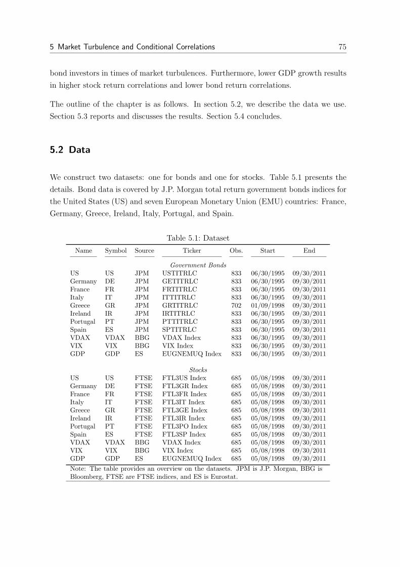
5 Market Turbulence and Conditional Correlations 75
bond investors in times of market turbulences. Furthermore, lower GDP growth results
in higher stock return correlations and lower bond return correlations.
The outline of the chapter is as follows. In section 5.2, we describe the data we use.
Section 5.3 reports and discusses the results. Section 5.4 concludes.
5.2 Data
We construct two datasets: one for bonds and one for stocks. Table 5.1 presents the
details. Bond data is covered by J.P. Morgan total return government bonds indices for
the United States (US) and seven European Monetary Union (EMU) countries: France,
Germany, Greece, Ireland, Italy, Portugal, and Spain.
Table 5.1: Dataset
Name Symbol Source Ticker Obs. Start End
Government Bonds
US US JPM USTITRLC 833 06/30/1995 09/30/2011Germany DE JPM GETITRLC 833 06/30/1995 09/30/2011France FR JPM FRTITRLC 833 06/30/1995 09/30/2011Italy IT JPM ITTITRLC 833 06/30/1995 09/30/2011Greece GR JPM GRTITRLC 702 01/09/1998 09/30/2011Ireland IR JPM IRTITRLC 833 06/30/1995 09/30/2011Portugal PT JPM PTTITRLC 833 06/30/1995 09/30/2011Spain ES JPM SPTITRLC 833 06/30/1995 09/30/2011VDAX VDAX BBG VDAX Index 833 06/30/1995 09/30/2011VIX VIX BBG VIX Index 833 06/30/1995 09/30/2011GDP GDP ES EUGNEMUQ Index 833 06/30/1995 09/30/2011
Stocks
US US FTSE FTL3US Index 685 05/08/1998 09/30/2011Germany DE FTSE FTL3GR Index 685 05/08/1998 09/30/2011France FR FTSE FTL3FR Index 685 05/08/1998 09/30/2011Italy IT FTSE FTL3IT Index 685 05/08/1998 09/30/2011Greece GR FTSE FTL3GE Index 685 05/08/1998 09/30/2011Ireland IR FTSE FTL3IR Index 685 05/08/1998 09/30/2011Portugal PT FTSE FTL3PO Index 685 05/08/1998 09/30/2011Spain ES FTSE FTL3SP Index 685 05/08/1998 09/30/2011VDAX VDAX BBG VDAX Index 685 05/08/1998 09/30/2011VIX VIX BBG VIX Index 685 05/08/1998 09/30/2011GDP GDP ES EUGNEMUQ Index 685 05/08/1998 09/30/2011
Note: The table provides an overview on the datasets. JPM is J.P. Morgan, BBG isBloomberg, FTSE are FTSE indices, and ES is Eurostat.

5.2 Data 76
Our sample includes countries which are in the center of the current European sovereign
debt crisis and countries that are considered to be safe investments. All indices are cap-
italization weighted, assume a reinvestment of received coupon payments or redemp-
tions, and are based on prices observed in the secondary market. Furthermore, all
bonds must satisfy certain liquidity criteria.2
We use FTSE All-World country indices for our stock dataset. We choose the same
countries as in the bond sample. The indices are value weighted total return indices that
include dividend payments. They provide a broad measure of stock market returns.3
For all indices, we compute the continuously compounded weekly returns from Friday to
Friday. We choose to study returns at a weekly frequency in order to avoid the problems
caused by non-synchronous trading (Burns et al., 1998). All returns are expressed in
local currency.
We use different exogenous variables in our analysis. As described in section 3.3.2.2,
the implied volatility of equity options is a popular proxy of risk aversion. We employ
the VDAX volatility index as a measure of risk aversion. The index tracks the expected
volatility over the next 45 days implied in index options on the German DAX stock
index.4 For analysis which include the US indices, we employ the Chicago Board
Options Exchange Volatility Index (VIX) as proxy for risk aversion. The VIX is a
popular measure of the implied volatility of index options on the S&P 500 Index over
the next 30 days. Several authors (Connolly et al., 2005, 2007; Hunter and Simon,
2005; Cappiello et al., 2006a) point out that conditional correlations change quickly in
high-stress periods. Therefore, we take the 1% percentile of the VDAX and VIX indices
as a proxy for high market stress by using an appropriately defined dummy variable
Since large values of the exogenous variable result in very small values of the respective
coefficient, we avoid rounding errors during optimization and calculation of standard
errors by dividing the level of risk aversion by 1000. We employ quarterly Eurozone
GDP growth as a proxy for the business cycle. We take quarterly growth figures from
Eurostat for the Eurozone. Quarterly data is converted into weekly data by allowing the
2For further details on the index construction and guidelines please refer to www.morganmarkets.com.3For further details on the index construction and guidelines please refer to www.ftse.com.4An alternative to the VDAX volatility index is the Euro Stoxx 50 Volatility Index (VSTOXX) thattracks implied volatility of index options on the Euro Stoxx 50 Index. However, the VSTOXXindex is only available since 1/4/1999. Besides, the correlation between the VSTOXX and theVDAX is very high: 0.98. Therefore, we consider both as equally representative for the Eurozone.

5 Market Turbulence and Conditional Correlations 77
variable to remain constant during a quarter. This transformation of macroeconomic
data has already been applied to convert monthly to daily (Cai et al., 2009) or to weekly
data (Aslanidis and Christiansen, 2010).
Table 5.2: Descriptive Statistics
Symbol Mean Min. Max. Std. Dev. Skewness Kurtosis
Government Bonds
US 0.12% −3.28% 2.57% 0.68% −0.49 4.16∗∗∗DE 0.11% −2.05% 1.91% 0.53% −0.20 3.66∗∗∗FR 0.12% −1.99% 1.89% 0.54% −0.24 3.71∗∗∗IT 0.13% −2.74% 4.81% 0.65% 0.06 8.11∗∗∗GR 0.02% −15.18% 22.36% 1.75% 1.90 60.59∗∗∗IR 0.11% −7.97% 13.16% 1.13% 1.54 35.78∗∗∗PT 0.09% −10.95% 10.15% 1.02% 0.00 42.88∗∗∗ES 0.13% −2.82% 4.91% 0.64% 0.02 8.27∗∗∗VDAX 22.98 10.10 64.28 9.37 1.35 4.91∗∗∗VIX 21.68 10.02 79.13 8.83 2.01 10.11∗∗∗GDP 0.43% −2.50% 1.30% 0.58% −2.57 12.99∗∗∗
Stocks
US 0.02% −20.12% 11.51% 2.75% −0.75 8.86∗∗∗DE −0.01% −23.90% 15.43% 3.53% −0.69 7.78∗∗∗FR 0.02% −24.93% 12.58% 3.20% −0.93 9.37∗∗∗IT −0.07% −24.50% 19.66% 3.38% −0.89 10.95∗∗∗GR −0.22% −20.08% 18.80% 4.46% −0.33 5.88∗∗∗IR −0.18% −37.10% 16.61% 4.09% −1.50 15.25∗∗∗PT −0.08% −20.61% 13.09% 2.91% −0.93 9.31∗∗∗ES 0.02% −23.80% 13.07% 3.36% −0.83 8.26∗∗∗VDAX 24.04 10.98 64.28 9.53 1.36 4.71∗∗∗VIX 22.43 10.02 79.13 9.31 1.89 9.23∗∗∗GDP 0.40% −2.50% 1.20% 0.62% −2.51 11.69∗∗∗Note: The table reports descriptive statistics for all variables.*** denotes series that differ from a normal distribution at 1% level as indi-cated by a Jarque–Bera test.
All government bond indices are available at least since 12/30/1994 except for the
Greece government bond index that starts at 12/31/1997.5 The volatility index starts
1/2/1990. As Eurozone GDP growth is available since 06/30/1995 only, it deter-
mines the starting point for our bond sample. Altogether, we cover the period from
06/30/1995 to 09/30/2011. Fridays on which markets were closed are removed from
the sample which gives us 833 observations. However, all analysis that include gov-
5Data from the US, France, and Germany are available since 12/31/1985, time series from Ireland,Italy, Spain start at 12/31/1987, while data from Portugal and Greece are only available since12/30/1994 and 12/31/1997, respectively.

5.2 Data 78
Table 5.3: European Bonds: Unconditional Correlations
US DE FR IT GR IR PT ES VDAX VIX GDPUS 1DE 0.73 1FR 0.71 0.95 1IT 0.48 0.55 0.67 1GR 0.08 0.03 0.13 0.53 1IR 0.31 0.32 0.40 0.60 0.61 1PT 0.24 0.23 0.33 0.64 0.74 0.80 1ES 0.52 0.62 0.70 0.87 0.50 0.64 0.68 1VDAX 0.10 0.10 0.09 0.01 -0.02 0.05 0.03 0.04 1VIX 0.11 0.13 0.12 0.02 -0.03 0.05 0.04 0.05 0.86 1GDP 0.04 -0.03 -0.04 -0.03 -0.01 -0.02 -0.04 -0.03 -0.33 -0.44 1
Note: The table reports the unconditional correlations of our bond sample.
ernment bonds of Greece start at 12/31/1997 leaving us with a reduced sample of 702
observations.
Table 5.2 provides descriptive statistics for the bond sample. All bond markets exhibit
an average positive return. With the exception of Greece, the average weekly return
is about the same level in all countries. The peripheral countries in the Eurozone are
riskier as measured by the range between minimum and maximum return. In addition,
most time series are heavily left skewed and exhibit fat-tails. Moreover, they are non-
normal as indicated by the Jarque-Bera test. We find large outliers during the last two
years in the sample that can be attributed to the sovereign debt and the financial crisis.
All FTSE stock indices are available at least since 5/1/1998. That results in 685 ob-
servations from 5/8/1998 to 9/30/2011. Remarkably, average stock returns are slightly
positive only for Germany, France, and Spain and even negative for all other countries.
The reason for this is that our sample covers both the burst of the dot-com bubble and
the recent sovereign debt crisis. As expected, the standard deviation is higher for stock
than for bond index returns. Similar to the bond sample, stock returns are left skewed,
exhibit fat-tails, and are non-normal.
Both the non-normality and the presence of extreme values might severely affect the
estimation since the models are constructed by assuming conditionally normal asset
returns. Therefore, some authors truncate extreme values (Silvennoinen and Terasvirta,
2005) or standardize the data (Cappiello et al., 2006a; Aslanidis and Christiansen, 2010).
On the other hand, we are especially interested in periods of high market stress in which
the presence of extreme values is most likely. Since Engle (2002) argues that results

5 Market Turbulence and Conditional Correlations 79
Table 5.4: European Stocks: Unconditional Correlations
US DE FR IT GR IR PT ES VDAX VIX GDPUS 1DE 0.79 1FR 0.80 0.91 1IT 0.74 0.84 0.88 1GR 0.47 0.54 0.55 0.54 1IR 0.59 0.64 0.67 0.63 0.47 1PT 0.55 0.65 0.69 0.67 0.49 0.49 1ES 0.71 0.82 0.84 0.83 0.56 0.60 0.71 1VDAX -0.10 -0.23 -0.20 -0.18 -0.18 -0.16 -0.16 -0.16 1VIX -0.26 -0.27 -0.25 -0.25 -0.25 -0.23 -0.22 -0.23 0.86 1GDP 0.02 0.04 0.04 0.03 0.00 0.02 0.02 0.02 -0.39 -0.48 1
Note: The table reports the unconditional correlations of our stock sample.
have a quasi-maximum likelihood estimation interpretation if returns are non-normal,
we do not truncate or standardize the data. Moreover, outliers may be accounted for
by an exogenous variables, particularly by the market turbulences dummy. Similar to
section 3.3.2, we multiply the return series with 1000 to avoid rounding error during
estimation. Since the mean of the return series is non-zero, we demean the return series.
Table 5.3 presents the unconditional correlations of the bond sample and suggests the
presence of three distinct groups: US, France, and Germany as they are considered to
be the safest investments; Greece as it is the main country affected by the sovereign debt
crisis during our sample period; and all other countries - namely, Ireland, Italy, Portugal,
and Spain. The unconditional correlation between France and Germany is close to 1.
That compares to correlations in the range of 0.24 to 0.70 between countries of the first
and the third group and exceptionally low correlations between US/France/Germany
and Greece (between 0.03 and 0.13). Unconditional correlations within the third group
are in the range between 0.53 and 0.87 while correlations between the third group and
Greece are mostly lower.
Table 5.4 provides the unconditional correlations for our stock sample. They are some-
what similar to the bond correlations with the exception of Italy and Spain which are
stronger correlated with France and Germany than in our bond sample. Notably, the
correlation between the volatility indices and the bond indices is negative while it is
positive for stocks.

5.3 Empirical Results 80
5.3 Empirical Results
5.3.1 European Bonds
At first, we estimate the conditional correlations between the bond index returns of
our sample employing the DCC(1,1) model. Thus, we need conditional variances as
estimated by a univariate GARCH model. In chapter 4, we have argued that it is
reasonable to estimate conditional variances with a GARCHX model in order to better
separate the effects of exogenous variables on volatility from the effects on the de-
pendence structure. Parameter estimates for the univariate GARCH model and the
GARCHX model are presented in Table 5.5 and 5.6, respectively.
Table 5.5: European Bonds: Univariate GARCH Models
Countries α0 α1 α2
US 1.178* (0.694) 0.058*** (0.019) 0.918*** (0.029)DE 1.005* (0.562) 0.079*** (0.026) 0.886*** (0.039)FR 1.260* (0.700) 0.072*** (0.026) 0.885*** (0.043)IT 2.678** (1.308) 0.149*** (0.040) 0.788*** (0.059)GR 0.848 (0.620) 0.155*** (0.052) 0.842*** (0.057)IR 1.995*** (0.769) 0.207*** (0.051) 0.783*** (0.039)PT 0.801** (0.373) 0.183*** (0.046) 0.817*** (0.036)ES 1.677** (0.783) 0.143*** (0.044) 0.820*** (0.050)
Note: The table reports the GARCH (1,1) model estimates for government bond indices in our sample.* p < 0.10, ** p < 0.05, *** p < 0.01, robust standard errors in parentheses.
As almost all coefficients in Table 5.5 are significant, there are clear signs of volatility
clustering in the bond return time series. By contrast, the exogenous variables we em-
ploy in our study do not influence conditional variances as the GARCHX γ coefficients
depicted in Table 5.6 are not significantly different from zero with the exception of the
US data.6 Hence, conditional variances are not driven by the exogenous variables we
considered. Nevertheless, we still employ the GARCHX model when estimating con-
ditional variances in the GDCCX model in order to clearly separate the effects of the
exogenous variables on the dependence structure from the effects on the volatility.
Table 5.7 presents the DCC model estimates. The sums of the DCC a and b parameters
are close to one implying a high degree of persistence in the conditional correlations.
Therefore, we employ the Engle and Sheppard (2001) correlation test as described in
6Results are unchanged if the insignificant parameters are dropped.

5 Market Turbulence and Conditional Correlations 81
Table 5.6: European Bonds: Univariate GARCHX Models
Countries Risk Aversion Market Turbulence GDP
US 260.337*** (85.408) 174.351 (169.044) −2881.405** (1134.129)DE 28.188 (28.375) 273.536 (201.039) −1100.420 (693.951)FR 30.904 (37.250) 348.669 (277.919) −779.713 (654.704)IT −66.290 (62.116) 601.639 (374.589) −1649.987 (1383.919)GR −4.050 (7.782) 382.021 (388.269) −969.616 (810.326)IR 35.903 (51.002) 923.729* (515.484) −1004.079 (1240.029)PT 8.308 (67.144) 150.417 (282.964) −545.560 (598.178)ES −11.833 (38.202) 463.990 (349.892) −1246.786 (944.105)
Note: The table reports the GARCHX model estimates for government bond indices in oursample. We use three exogenous variables simultaneously. We estimate conditional correlationsfor each country pair separately.* p < 0.10, ** p < 0.05, *** p < 0.01, robust standard errors in parentheses.
chapter 2.3. The right panel of Table 5.7 indicates that there is strong statistical
evidence for time-varying correlations between almost all countries. In addition, most
DCC parameter estimates are significantly different from zero.
Figure 5.1 plots the conditional correlations as calculated by the DCC model for the
EMU bonds. Looking at the graphs, different periods can be identified. Conditional
correlations are in the range between zero and one and rise steadily in the first period
prior to the introduction of the Euro in 1999. Correlations are close to one in the second
period which lasts nine years after the introduction of the Euro.
Figure 5.2 zooms into the conditional correlations of Greece. It becomes clear that
Greece is an exception as the second phase starts about two years later. This may reflect
the fact that Greece joined the Eurozone in 2001 two years after the introduction of the
Euro due to the non compliance with the Euro deficit criteria. With the start of the
financial crisis in 2008 conditional correlations decline. Particularly, there is a sudden
drop at the end of 2009 which marks the beginning of the European sovereign debt crisis.
Conditional correlations fall to values as low as -0.5. This is particularly interesting as
the relation changed from positive to negative indicating a complete reassessment of
Greek government bonds. However, since the announcement of the European Financial
Stability Facility in May 2010 conditional correlations are rising once again but remain
volatile.
Next, we use a GDCCX model to shed light on the economic causes of the changes in
conditional correlations and model variances with a GARCHX model. That allows us to
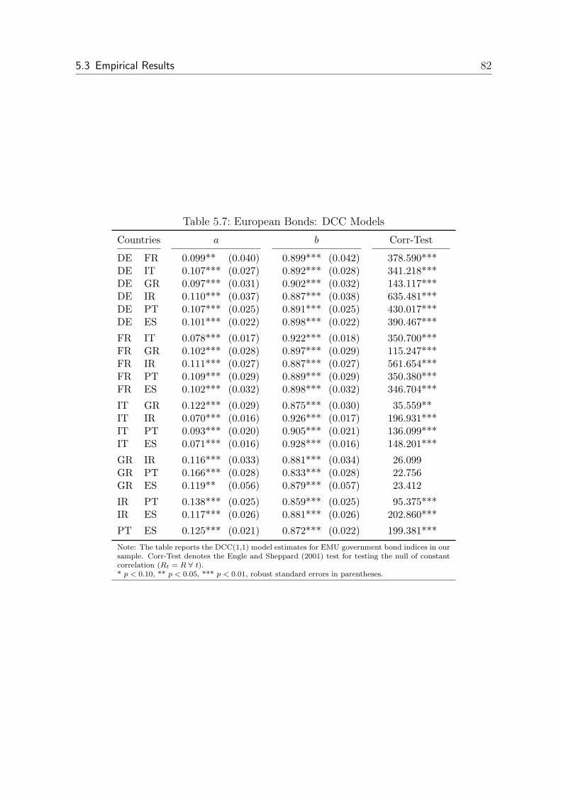
5.3 Empirical Results 82
Table 5.7: European Bonds: DCC Models
Countries a b Corr-Test
DE FR 0.099** (0.040) 0.899*** (0.042) 378.590***DE IT 0.107*** (0.027) 0.892*** (0.028) 341.218***DE GR 0.097*** (0.031) 0.902*** (0.032) 143.117***DE IR 0.110*** (0.037) 0.887*** (0.038) 635.481***DE PT 0.107*** (0.025) 0.891*** (0.025) 430.017***DE ES 0.101*** (0.022) 0.898*** (0.022) 390.467***
FR IT 0.078*** (0.017) 0.922*** (0.018) 350.700***FR GR 0.102*** (0.028) 0.897*** (0.029) 115.247***FR IR 0.111*** (0.027) 0.887*** (0.027) 561.654***FR PT 0.109*** (0.029) 0.889*** (0.029) 350.380***FR ES 0.102*** (0.032) 0.898*** (0.032) 346.704***
IT GR 0.122*** (0.029) 0.875*** (0.030) 35.559**IT IR 0.070*** (0.016) 0.926*** (0.017) 196.931***IT PT 0.093*** (0.020) 0.905*** (0.021) 136.099***IT ES 0.071*** (0.016) 0.928*** (0.016) 148.201***
GR IR 0.116*** (0.033) 0.881*** (0.034) 26.099GR PT 0.166*** (0.028) 0.833*** (0.028) 22.756GR ES 0.119** (0.056) 0.879*** (0.057) 23.412
IR PT 0.138*** (0.025) 0.859*** (0.025) 95.375***IR ES 0.117*** (0.026) 0.881*** (0.026) 202.860***
PT ES 0.125*** (0.021) 0.872*** (0.022) 199.381***
Note: The table reports the DCC(1,1) model estimates for EMU government bond indices in oursample. Corr-Test denotes the Engle and Sheppard (2001) test for testing the null of constantcorrelation (Rt = R ∀ t).* p < 0.10, ** p < 0.05, *** p < 0.01, robust standard errors in parentheses.
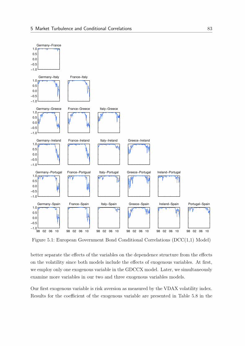
5 Market Turbulence and Conditional Correlations 83
−1.0
−0.5
0.0
0.5
1.0Germany−France
−1.0
−0.5
0.0
0.5
1.0Germany−Italy
−1.0
−0.5
0.0
0.5
1.0Germany−Greece
−1.0
−0.5
0.0
0.5
1.0Germany−Ireland
−1.0
−0.5
0.0
0.5
1.0Germany−Portugal
98 02 06 10 −1.0
−0.5
0.0
0.5
1.0Germany−Spain
France−Italy
France−Greece
France−Ireland
France−Portgual
98 02 06 10
France−Spain
Italy−Greece
Italy−Ireland
Italy−Portugal
98 02 06 10
Italy−Spain
Greece−Ireland
Greece−Portugal
98 02 06 10
Greece−Spain
Ireland−Portugal
98 02 06 10
Ireland−Spain
98 02 06 10
Portugal−Spain
Figure 5.1: European Government Bond Conditional Correlations (DCC(1,1) Model)
better separate the effects of the variables on the dependence structure from the effects
on the volatility since both models include the effects of exogenous variables. At first,
we employ only one exogenous variable in the GDCCX model. Later, we simultaneously
examine more variables in our two and three exogenous variables models.
Our first exogenous variable is risk aversion as measured by the VDAX volatility index.
Results for the coefficient of the exogenous variable are presented in Table 5.8 in the

5.3 Empirical Results 84
−1.0
−0.5
0.0
0.5
1.0Greece and Germany
−1.0
−0.5
0.0
0.5
1.0Greece and France
−1.0
−0.5
0.0
0.5
1.0Greece and Italy
−1.0
−0.5
0.0
0.5
1.0Greece and Ireland
−1.0
−0.5
0.0
0.5
1.0Greece and Portugal
1998 1999 2000 2001 2002 2003 2004 2005 2006 2007 2008 2009 2010 2011−1.0
−0.5
0.0
0.5
1.0Greece and Spain
Figure 5.2: Greece Government Bond Conditional Correlations
first column. Remarkably, almost all estimated parameters are negative indicating that
conditional correlations fall if risk aversion rises. However, only some coefficients for
country pairs including Germany are significant. This might reflect the special status
of German bonds as a “save haven”.

5 Market Turbulence and Conditional Correlations 85
Table 5.8: European Bonds: GDCCX Models with One Exogenous Variable
Countries Risk Aversion Market Turbulence GDP
DE FR −0.037*** (0.000) −0.224** (0.103) 0.212* (0.112)DE IT −0.043* (0.026) −0.373 (0.299) 0.512 (0.397)DE GR −0.068 (0.064) −1.746** (0.803) 2.100* (1.178)DE IR −0.132 (0.081) −0.434 (0.609) 2.279*** (0.846)DE PT −0.139* (0.084) −0.552 (0.429) 2.515*** (0.742)DE ES −0.030** (0.014) −0.558 (0.438) 0.293* (0.163)
FR IT −0.002 (0.008) −0.073 (0.192) 0.204 (0.221)FR GR −0.046 (0.034) −1.391** (0.696) 2.213*** (0.857)FR IR −0.088 (0.057) −0.495 (0.474) 1.924*** (0.678)FR PT −0.083 (0.057) −0.278 (0.294) 1.775*** (0.539)FR ES −0.023 (0.023) −0.428 (0.351) 0.456** (0.209)
IT GR −0.045 (0.041) −0.532*** (0.204) 1.994*** (0.589)IT IR 0.035 (0.034) −0.221 (0.267) 1.884** (0.869)IT PT −0.006 (0.016) −0.249** (0.105) 0.805* (0.472)IT ES −0.003 (0.008) −0.437 (0.287) 0.156 (0.212)
GR IR −0.013 (0.053) −0.554 (0.462) 2.105* (1.116)GR PT −0.036 (0.027) −0.914*** (0.327) 0.807 (0.581)GR ES −0.032 (0.042) −1.163* (0.614) 1.563 (0.985)
IR PT −0.044 (0.036) −0.216 (0.276) 0.762* (0.453)IR ES −0.047 (0.049) −1.060 (0.978) 1.533** (0.633)
PT ES −0.034 (0.025) −0.334 (0.227) 0.932** (0.371)
Note: The table reports the c coefficients of the exogenous variable employing a GDCCX modelfor EMU government bonds. We estimate volatility with a GARCHX model. The c parametermeasures the influence of the exogenous variable on the respective conditional correlations. Weestimate conditional correlations for each country pair separately. Risk aversion is proxied bythe VDAX volatility index, market turbulence is the upper first percentile of the VDAX index,and GDP growth is quarterly Eurozone GDP.* p < 0.10, ** p < 0.05, *** p < 0.01, robust standard errors in parentheses.
We are also interested in the evolution of correlations in times of extreme market stress.
The VDAX reached its peaks in several phases of market turbulence: in the aftermath
of the LTCM crisis in October 1998, in the wake of the dot-com bubble in October
2002, and in October 2008 after the collapse of Lehman Brothers. Therefore, similar to
Connolly et al. (2005) we focus on the percentiles of the distribution of the volatility in-
dex. We construct a proxy for market turbulence using the first percentile of the VDAX
index and employ this measure as exogenous variable. We define market turbulence m
as follows: mt = I [V DAXt > VDAX99] · V DAXt where I [·] is an indicator function

5.3 Empirical Results 86
that takes on the value 1 if the argument is true and 0 otherwise.7 The second column
in Table 5.8 shows the effects of market turbulence. Conditional correlations for Greece
government bond return indices significantly fall in case of market turbulence.
These results raise the question if market turbulence rather than risk aversion explains
conditional correlations. Therefore, we repeat our analysis including the risk aversion
measure and the proxy for market turbulence simultaneously in a two exogenous vari-
ables model.8 As shown in Table 5.9, the results for our market turbulence proxy remain
largely unchanged while the effect of risk aversion on conditional correlations dimin-
ishes. When accounting for both risk aversion and market turbulence simultaneously,
risk aversion significantly explains the conditional correlations only for the linkage be-
tween France and Germany and the signs of the coefficients even changes to positive
for some country pairs.
Next, as reported in third column in Table 5.10, we consider the effects of macroeco-
nomic fundamentals on conditional correlations within the Eurozone. Using Eurozone
GDP growth as a proxy for the business cycle, we find that higher GDP growth results
in higher conditional correlations. The effect can be found for both correlations between
the safest and the riskier countries and for correlations within riskier countries.
Employing GDP growth as the only explaining variable might be misleading as market
turbulence usually coincides with lower GDP growth. Therefore, in our final analysis
we employ all three exogenous variables simultaneously. Results presented in Table
5.10 confirm our previous findings. Both GDP growth and market turbulences drive
conditional correlations downwards whereas risk aversion has almost no effect. There-
fore, when GDP growth turns negative during a crisis, correlations decline. In addition,
if there are market turbulences, conditional correlations fall even more. As expected,
the impact of market turbulences is most pronounced for the peripheral countries. Fur-
thermore, there is no general effect of risk aversion on conditional correlations since the
signs of the coefficients are positive for some country pairs and are negative for other
country pairs. Yet most coefficients are significantly different from zero.
7Repeating all analysis with a market turbulence dummy i.e. mt,alt = I [V DAXt > VDAX99] leavesresults qualitatively unchanged.
8When using both the proxy for risk aversion and for market turbulence in the two and three ex-ogenous variables models, we remove the first percentile from the risk aversion indicator in orderto better separate the effects of risk aversion and market turbulence. Employing the unchangedVDAX index does not change our results qualitatively.

5 Market Turbulence and Conditional Correlations 87
Table 5.9: European Bonds: GDCCX Models with Two Exogenous Variables
Countries Risk Aversion Market Turbulence
DE FR −0.033* (0.019) −0.172 (0.128)DE IT −0.037 (0.029) −0.263 (0.346)DE GR −0.007 (0.045) −1.742** (0.809)DE IR −0.130 (0.083) −0.305 (0.502)DE PT −0.122 (0.087) −0.424 (0.512)DE ES −0.020 (0.014) −0.549 (0.506)
FR IT 0.001 (0.010) −0.078 (0.226)FR GR −0.003 (0.023) −1.383** (0.705)FR IR −0.080 (0.061) −0.354 (0.435)FR PT −0.071 (0.055) −0.222 (0.301)FR ES −0.001 (0.012) −0.425 (0.358)
IT GR 0.017 (0.019) −0.546*** (0.202)IT IR 0.056 (0.038) −0.364 (0.302)IT PT 0.012 (0.015) −0.264** (0.107)IT ES 0.011 (0.007) −0.444* (0.261)
GR IR 0.021 (0.049) −0.621 (0.483)GR PT 0.004 (0.015) −0.916*** (0.323)GR ES 0.020 (0.025) −1.191** (0.589)
IR PT −0.037 (0.040) −0.147 (0.262)IR ES −0.016 (0.047) −1.076 (1.046)
PT ES −0.008 (0.018) −0.325 (0.230)
Note: The table reports the c coefficients of the exogenous variable employing a GDCCX model for EMUgovernment bonds. We estimate volatility with a GARCHX model. The c parameter measures the influenceof the exogenous variable on the respective conditional correlations. We estimate conditional correlationswith two exogenous variables simultaneously and for each country pair separately. Risk aversion is proxiedby the VDAX volatility index, market turbulence is the upper first percentile of the VDAX index, and GDPgrowth is quarterly Eurozone GDP.* p < 0.10, ** p < 0.05, *** p < 0.01, robust standard errors in parentheses.
In summary, we find that conditional correlations between bond indices fall as GDP
growth declines and if there is market turbulence. From a portfolio perspective this is
a very favorable result since it implies that the benefits of international diversification
increase in times of market turmoils.
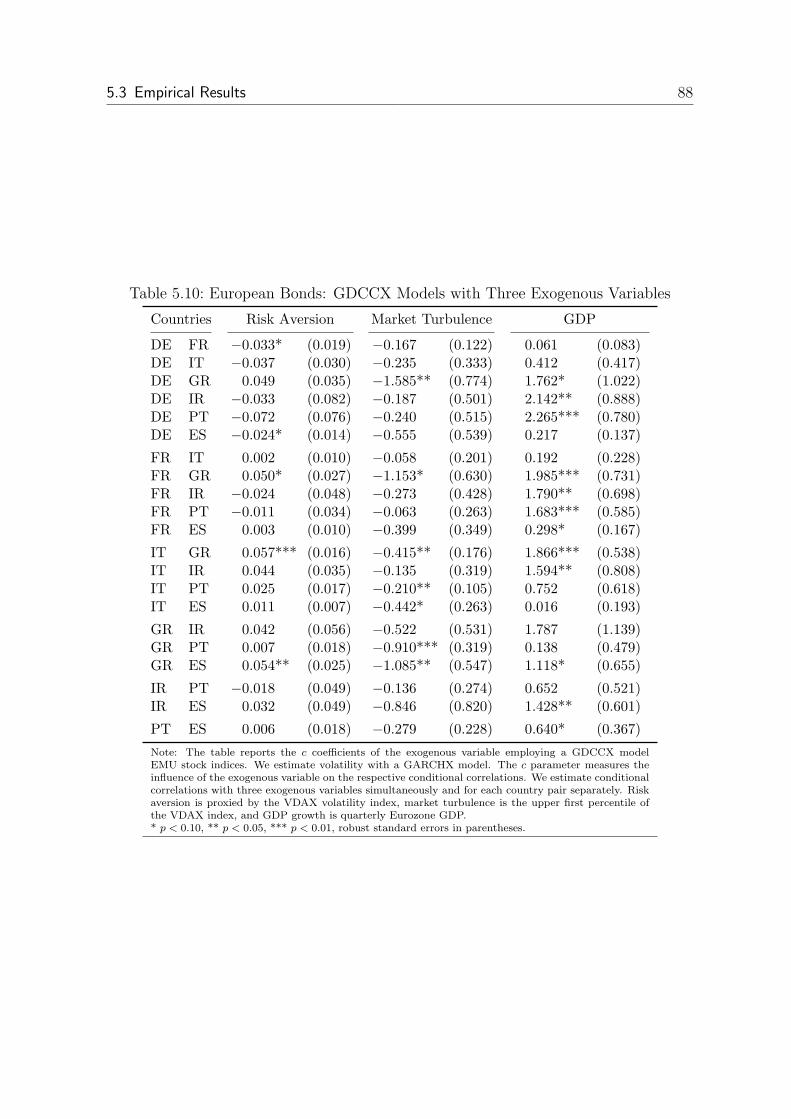
5.3 Empirical Results 88
Table 5.10: European Bonds: GDCCX Models with Three Exogenous Variables
Countries Risk Aversion Market Turbulence GDP
DE FR −0.033* (0.019) −0.167 (0.122) 0.061 (0.083)DE IT −0.037 (0.030) −0.235 (0.333) 0.412 (0.417)DE GR 0.049 (0.035) −1.585** (0.774) 1.762* (1.022)DE IR −0.033 (0.082) −0.187 (0.501) 2.142** (0.888)DE PT −0.072 (0.076) −0.240 (0.515) 2.265*** (0.780)DE ES −0.024* (0.014) −0.555 (0.539) 0.217 (0.137)
FR IT 0.002 (0.010) −0.058 (0.201) 0.192 (0.228)FR GR 0.050* (0.027) −1.153* (0.630) 1.985*** (0.731)FR IR −0.024 (0.048) −0.273 (0.428) 1.790** (0.698)FR PT −0.011 (0.034) −0.063 (0.263) 1.683*** (0.585)FR ES 0.003 (0.010) −0.399 (0.349) 0.298* (0.167)
IT GR 0.057*** (0.016) −0.415** (0.176) 1.866*** (0.538)IT IR 0.044 (0.035) −0.135 (0.319) 1.594** (0.808)IT PT 0.025 (0.017) −0.210** (0.105) 0.752 (0.618)IT ES 0.011 (0.007) −0.442* (0.263) 0.016 (0.193)
GR IR 0.042 (0.056) −0.522 (0.531) 1.787 (1.139)GR PT 0.007 (0.018) −0.910*** (0.319) 0.138 (0.479)GR ES 0.054** (0.025) −1.085** (0.547) 1.118* (0.655)
IR PT −0.018 (0.049) −0.136 (0.274) 0.652 (0.521)IR ES 0.032 (0.049) −0.846 (0.820) 1.428** (0.601)
PT ES 0.006 (0.018) −0.279 (0.228) 0.640* (0.367)
Note: The table reports the c coefficients of the exogenous variable employing a GDCCX modelEMU stock indices. We estimate volatility with a GARCHX model. The c parameter measures theinfluence of the exogenous variable on the respective conditional correlations. We estimate conditionalcorrelations with three exogenous variables simultaneously and for each country pair separately. Riskaversion is proxied by the VDAX volatility index, market turbulence is the upper first percentile ofthe VDAX index, and GDP growth is quarterly Eurozone GDP.* p < 0.10, ** p < 0.05, *** p < 0.01, robust standard errors in parentheses.

5 Market Turbulence and Conditional Correlations 89
Table 5.11: European Stocks: Univariate GARCH Models
Countries α0 α1 α2
US 36.068** (14.971) 0.192*** (0.065) 0.773*** (0.060)DE 109.276** (50.962) 0.266** (0.123) 0.671*** (0.113)FR 24.859** (11.738) 0.163*** (0.055) 0.831*** (0.037)IT 44.727** (17.642) 0.285*** (0.103) 0.715*** (0.064)GR 17.147 (13.316) 0.064*** (0.023) 0.930*** (0.026)IR 35.084* (19.370) 0.129*** (0.042) 0.855*** (0.038)PT 50.419** (20.537) 0.233*** (0.079) 0.730*** (0.066)ES 10.714 (6.857) 0.098*** (0.022) 0.902*** (0.026)
Note: The table reports the GARCH (1,1) model estimates for stock indices in our sample.* p < 0.10, ** p < 0.05, *** p < 0.01, robust standard errors in parentheses.
5.3.2 European Stocks
We repeat the analysis with the same set of countries but now for stock indices. Sim-
ilar to the bond sample, GARCH estimates as shown in Table 5.11 indicate volatility
clustering. This confirms results reported by Cappiello et al. (2006a).
Turning to the results of the GARCHX model for stocks as reported in Table 5.12, we
find that stock volatilities in the US, in Germany, in France, and in Italy are influenced
by the exogenous variables. By contrast, we have previously shown these variables
do not affect conditional bond variances. Specifically, stock volatility increase if risk
aversion grows or if there are market turbulences. It is important to stress the difference
between market turbulences and volatility. We define market turbulences as extremes
in the VDAX index. This index is a gauge of future volatility as expected by the market
whereas the estimated variance is the current volatility. In addition to risk aversion and
market turbulences, also negative GDP growth results in rising volatility. Interestingly,
for Greece, Ireland, Portugal, and Spain, we cannot reject the hypothesis that our set
of exogenous variables does not influence conditional variances.
Table 5.13 reports the results of DCC(1,1) models on stock indices. Most parameters
are significantly different from zero. Employing the Engle and Sheppard (2001) correla-
tion test we cannot reject the hypothesis that conditional correlations are time-varying
for pair-wise correlations between almost all countries included. Remarkably, the DCC
model innovation parameter a is lower for stocks than for bonds. Accordingly, con-
ditional stock correlations plotted in Figure 5.3 are smoother than conditional bond
correlations (see Figure 5.1).
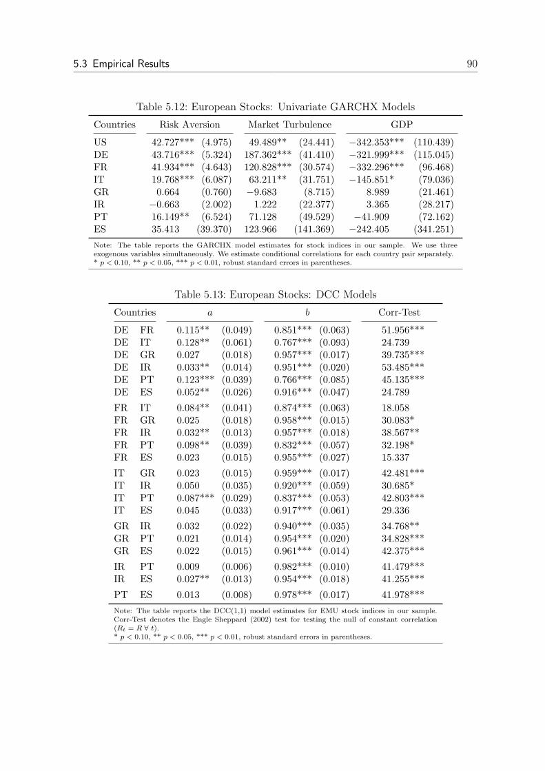
5.3 Empirical Results 90
Table 5.12: European Stocks: Univariate GARCHX Models
Countries Risk Aversion Market Turbulence GDP
US 42.727*** (4.975) 49.489** (24.441) −342.353*** (110.439)DE 43.716*** (5.324) 187.362*** (41.410) −321.999*** (115.045)FR 41.934*** (4.643) 120.828*** (30.574) −332.296*** (96.468)IT 19.768*** (6.087) 63.211** (31.751) −145.851* (79.036)GR 0.664 (0.760) −9.683 (8.715) 8.989 (21.461)IR −0.663 (2.002) 1.222 (22.377) 3.365 (28.217)PT 16.149** (6.524) 71.128 (49.529) −41.909 (72.162)ES 35.413 (39.370) 123.966 (141.369) −242.405 (341.251)
Note: The table reports the GARCHX model estimates for stock indices in our sample. We use threeexogenous variables simultaneously. We estimate conditional correlations for each country pair separately.* p < 0.10, ** p < 0.05, *** p < 0.01, robust standard errors in parentheses.
Table 5.13: European Stocks: DCC Models
Countries a b Corr-Test
DE FR 0.115** (0.049) 0.851*** (0.063) 51.956***DE IT 0.128** (0.061) 0.767*** (0.093) 24.739DE GR 0.027 (0.018) 0.957*** (0.017) 39.735***DE IR 0.033** (0.014) 0.951*** (0.020) 53.485***DE PT 0.123*** (0.039) 0.766*** (0.085) 45.135***DE ES 0.052** (0.026) 0.916*** (0.047) 24.789
FR IT 0.084** (0.041) 0.874*** (0.063) 18.058FR GR 0.025 (0.018) 0.958*** (0.015) 30.083*FR IR 0.032** (0.013) 0.957*** (0.018) 38.567**FR PT 0.098** (0.039) 0.832*** (0.057) 32.198*FR ES 0.023 (0.015) 0.955*** (0.027) 15.337
IT GR 0.023 (0.015) 0.959*** (0.017) 42.481***IT IR 0.050 (0.035) 0.920*** (0.059) 30.685*IT PT 0.087*** (0.029) 0.837*** (0.053) 42.803***IT ES 0.045 (0.033) 0.917*** (0.061) 29.336
GR IR 0.032 (0.022) 0.940*** (0.035) 34.768**GR PT 0.021 (0.014) 0.954*** (0.020) 34.828***GR ES 0.022 (0.015) 0.961*** (0.014) 42.375***
IR PT 0.009 (0.006) 0.982*** (0.010) 41.479***IR ES 0.027** (0.013) 0.954*** (0.018) 41.255***
PT ES 0.013 (0.008) 0.978*** (0.017) 41.978***
Note: The table reports the DCC(1,1) model estimates for EMU stock indices in our sample.Corr-Test denotes the Engle Sheppard (2002) test for testing the null of constant correlation(Rt = R ∀ t).* p < 0.10, ** p < 0.05, *** p < 0.01, robust standard errors in parentheses.

5 Market Turbulence and Conditional Correlations 91
−0.5
0.0
0.5
1.0Germany−France
−0.5
0.0
0.5
1.0Germany−Italy
−0.5
0.0
0.5
1.0Germany−Greece
−0.5
0.0
0.5
1.0Germany−Ireland
−0.5
0.0
0.5
1.0Germany−Portugal
98 02 06 10 −0.5
0.0
0.5
1.0Germany−Spain
France−Italy
France−Greece
France−Ireland
France−Portgual
98 02 06 10
France−Spain
Italy−Greece
Italy−Ireland
Italy−Portugal
98 02 06 10
Italy−Spain
Greece−Ireland
Greece−Portugal
98 02 06 10
Greece−Spain
Ireland−Portugal
98 02 06 10
Ireland−Spain
98 02 06 10
Portugal−Spain
Figure 5.3: European Stocks Conditional Correlations (DCC(1,1) Model)
Figure 5.3 allows us to discuss the trends in conditional stock correlations during the last
years. Berben and Jansen (2009) find that correlations rise between 1995 and 1997, and
Cappiello et al. (2006b) note that correlations for large EMU countries increase in the
second half of the 1990s. By contrast, we cannot observe a major trend in conditional
correlations during the sample period. However, our stock sample starts 5/8/1998.
At this time, the transition to a regime with higher correlations might already have
been completed. In addition, the level of the conditional correlations is fluctuating
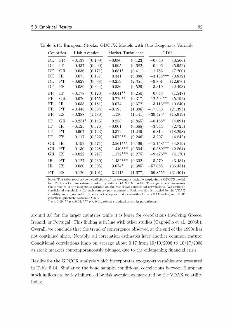
5.3 Empirical Results 92
Table 5.14: European Stocks: GDCCX Models with One Exogenous Variable
Countries Risk Aversion Market Turbulence GDP
DE FR −0.137 (0.139) −0.080 (0.123) −0.640 (0.566)DE IT −0.437 (0.290) −0.995 (0.682) 0.296 (5.952)DE GR −0.036 (0.171) 0.681* (0.411) −11.786 (7.200)DE IR 0.075 (0.157) 0.341 (0.388) −3.188*** (0.812)DE PT −0.627 (0.638) −0.259 (2.351) −9.801 (12.676)DE ES 0.089 (0.344) 0.536 (0.529) −3.319 (2.493)
FR IT −0.178 (0.120) −0.641** (0.250) 0.043 (1.548)FR GR −0.076 (0.155) 0.729** (0.317) −12.504** (5.192)FR IR 0.058 (0.181) 0.074 (0.372) −3.116*** (0.840)FR PT −0.448 (0.684) −0.195 (1.006) −17.848 (21.393)FR ES −0.388 (1.480) 1.130 (1.141) −39.475** (15.919)
IT GR −0.251* (0.145) 0.258 (0.865) −8.168* (4.891)IT IR −0.125 (0.376) −0.001 (0.668) −3.944 (2.725)IT PT −0.907 (0.723) 0.322 (1.249) −6.814 (18.298)IT ES 0.117 (0.522) 0.572** (0.246) −3.207 (4.842)
GR IR 0.192 (0.471) 2.561*** (0.196) −15.758*** (4.819)GR PT −0.130 (0.228) 1.440*** (0.504) −10.589*** (2.864)GR ES −0.022 (0.217) 1.172*** (0.275) −9.476** (4.170)
IR PT 0.127 (0.230) 1.432*** (0.302) −5.579 (3.484)IR ES 0.080 (0.305) 0.674* (0.385) −57.065 (36.351)
PT ES 0.120 (0.101) 3.141* (1.677) −59.855* (31.401)
Note: The table reports the c coefficients of the exogenous variable employing a GDCCX modelfor EMU stocks. We estimate volatility with a GARCHX model. The c parameter measuresthe influence of the exogenous variable on the respective conditional correlations. We estimateconditional correlations for each country pair separately. Risk aversion is proxied by the VDAXvolatility index, market turbulence is the upper first percentile of the VDAX index, and GDPgrowth is quarterly Eurozone GDP.* p < 0.10, ** p < 0.05, *** p < 0.01, robust standard errors in parentheses.
around 0.8 for the larger countries while it is lower for correlations involving Greece,
Ireland, or Portugal. This finding is in line with other studies (Cappiello et al., 2006b).
Overall, we conclude that the trend of convergence observed at the end of the 1990s has
not continued since. Notably, all correlation estimates have another common feature:
Conditional correlations jump on average about 0.17 from 10/10/2008 to 10/17/2008
as stock markets contemporaneously plunged due to the enlargening financial crisis.
Results for the GDCCX analysis which incorporates exogenous variables are presented
in Table 5.14. Similar to the bond sample, conditional correlations between European
stock indices are barley influenced by risk aversion as measured by the VDAX volatility
index.

5 Market Turbulence and Conditional Correlations 93
Employing our proxy for market turbulence as an exogenous variable reveals an impor-
tant difference between bonds and stocks. Although conditional correlations between
bonds indices decline in times of market turbulences, they rise for stock indices. This is
a clear indication of contagion in stock markets in times of market stress. These effects
can be observed for most markets and especially for the peripheral countries.
Table 5.15: European Stocks: GDCCX Models with Two Exogenous Variables
Countries Risk Aversion Market Turbulence
DE FR −0.151 (0.137) −0.047 (0.161)DE IT −0.569 (0.370) −0.032 (0.457)DE GR −0.161 (0.183) 0.696* (0.364)DE IR 0.028 (0.175) 0.325 (0.392)DE PT −0.708 (0.932) −0.409 (1.184)DE ES 0.000 (0.387) 0.536 (0.650)
FR IT 0.057** (0.026) −0.617*** (0.132)FR GR −0.202 (0.168) 0.758*** (0.246)FR IR 0.066 (0.217) 0.023 (0.365)FR PT −0.554 (0.872) −0.148 (0.782)FR ES −1.143 (1.380) 0.710 (1.088)
IT GR −0.442** (0.189) 0.681 (0.480)IT IR −0.191 (0.462) 0.161 (0.624)IT PT −1.202 (0.909) 0.102 (1.070)IT ES −0.083 (0.384) 0.553** (0.264)
GR IR −0.305 (0.332) 2.442*** (0.187)GR PT −0.379 (0.236) 1.461*** (0.378)GR ES −0.261 (0.193) 1.144*** (0.242)
IR PT −0.123 (0.210) 1.419*** (0.272)IR ES −0.120 (0.316) 0.694** (0.351)
PT ES −0.319 (2.334) 3.028* (1.635)
Note: The table reports the c coefficients of the exogenous variable employing a GDCCX model. We estimatevolatility with a GARCHX model. The c parameter measures the influence of the exogenous variable onthe respective conditional correlations. We estimate conditional correlations with two exogenous variablessimultaneously and for each country pair separately. Risk aversion is proxied by the VDAX volatility index,market turbulence is the upper first percentile of the VDAX index, and GDP growth is quarterly EurozoneGDP.* p < 0.10, ** p < 0.05, *** p < 0.01, robust standard errors in parentheses.
Turning to GDP growth as exogenous variable, we note another interesting difference
between stock and bond markets as presented in the third column in Table 5.14. We
find that higher GDP growth results in lower conditional correlations between stock
markets. Yet, if GDP growth turns negative, conditional correlations between stock
markets actually increase. These are additional indications of contagion effects be-
5.3 Empirical Results 94
tween stock markets in adverse market conditions. However, in the previous section
we did not find any signs of contagion for bond markets. Specifically, conditional bond
return correlations fall in times of falling GDP growth while conditional stock return
correlations rise.
Next, we repeat our analysis with two exogenous variables simultaneously. We use our
general measure of risk aversion9 and our proxy for market turbulence as exogenous vari-
ables. Table 5.15 presents the results. Yet, it turns out that coefficients and standard
errors change only marginally. Our proxy for risk aversion does not explain conditional
correlations in this specification whereas market turbulences increase correlations.
Finally, we examine all three exogenous variables together (see Table 5.16). Controlling
for risk aversion as well as market turbulences, the effect of GDP growth on conditional
correlations is even more pronounced than in the specification in which GDP growth
is the only explaining variable (see Table 5.16). For example, all conditional stock
correlations that include Greece rise when GDP growth turns negative.
By contrast, the effect of market turbulences on conditional correlations diminishes.
The influence of GDP growth seems to dominate in the peripheral countries. Exceptions
are the Greece-Ireland, Greece-Portugal, and Greece-Spain conditional correlations.
Interestingly, all coefficients for the exogenous variable risk aversion are negative while
only some are significantly different from zero.
In summary, we find that conditional stock correlations increase when there is negative
GDP growth,. If there are market turbulences, conditional correlations increase even
further, however, only for a limited set of countries. This diminishes any diversifica-
tion benefits in portfolios of European stock indices. We also note that the effects
of market turbulences on conditional correlations that we found in the one exogenous
variable model mostly disappear once we take GDP growth into account. In order to
avoid incorrect conclusions, we strongly suggest to examine several exogenous variables
simultaneously. That is also a strong argument for choosing correlation models that
allow for several exogenous variables (e.g. GDCCX, DCCX) instead of those that can
only allow for one or two variables (e.g. STCC, DSTCC).
9Similar to our analysis with bonds, we remove the first percentile from the VDAX index whenemploying both the risk aversion and the market stress proxy to better separate both effects.Employing the unchanged VDAX index does not change our results qualitatively.

5 Market Turbulence and Conditional Correlations 95
Table 5.16: European Stocks: GDCCX Models with Three Exogenous Variables
Countries Risk Aversion Market Turbulence GDP
DE FR −0.356 (0.532) −0.217 (0.356) −3.054 (3.559)DE IT −0.873* (0.450) −0.218 (0.450) −5.371 (3.501)DE GR −0.326 (0.345) 0.540 (0.492) −11.682* (6.951)DE IR −0.084 (0.287) −0.465 (2.005) −4.633 (5.729)DE PT −1.059 (1.520) −0.906 (1.012) −12.711 (18.234)DE ES −0.243 (0.335) 0.327 (0.482) −4.481 (3.090)
FR IT −0.100 (0.100) −1.103*** (0.426) −3.222*** (0.640)FR GR −0.531* (0.296) 0.319 (0.238) −13.032*** (3.983)FR IR −0.522 (0.386) −0.141 (0.328) −6.452*** (2.398)FR PT −0.017 (0.133) −0.197 (0.404) −4.742*** (1.283)FR ES −1.916 (1.840) −0.337 (1.220) −43.106*** (11.211)
IT GR −0.709** (0.283) 0.079 (0.628) −10.386** (4.648)IT IR −0.401 (0.277) −0.350 (0.626) −6.607*** (1.939)IT PT −1.807* (1.005) −0.395 (0.817) −18.037 (11.019)IT ES −0.342 (0.415) 0.403 (0.268) −3.851 (3.091)
GR IR −0.585 (0.516) 1.899*** (0.341) −15.387*** (5.948)GR PT −0.721** (0.316) 0.994** (0.402) −12.413*** (3.342)GR ES −0.530** (0.260) 0.798*** (0.255) −9.325** (3.673)
IR PT −0.217 (0.684) 0.771 (4.358) −4.811** (1.971)IR ES −0.363 (0.411) 0.467 (0.391) −4.167 (2.838)
PT ES −0.042 (0.324) 0.250 (0.477) −4.435 (3.406)
Note: The table reports the c coefficients of the exogenous variable employing a GDCCX model EMUgovernment bonds. We estimate volatility with a GARCHX model. The c parameter measures theinfluence of the exogenous variable on the respective conditional correlations. We estimate conditionalcorrelations with three exogenous variables simultaneously and for each country pair separately. Riskaversion is proxied by the VDAX volatility index, market turbulence is the upper first percentile ofthe VDAX index, and GDP growth is quarterly Eurozone GDP.* p < 0.10, ** p < 0.05, *** p < 0.01, robust standard errors in parentheses.
5.3.3 US and Europe: Bonds and Stocks
Last, we extend our sample and include the US. First, we estimate time-varying cor-
relations with a DCC(1,1) model. Results are presented in Table 5.17 for both bonds
and stocks. Most parameters are significantly different from zero and shocks to corre-
lation are typically highly persistent since the b parameter is close to one while the a
parameter is close to zero. As expected, the average half-life of the innovations is much
higher for bonds than for stocks. Furthermore, we employ the Engle and Sheppard
(2001) correlation test for testing the null hypothesis that Rt = R ∀ t. We find strong
evidence against the assumption of a constant conditional coefficient for most US and
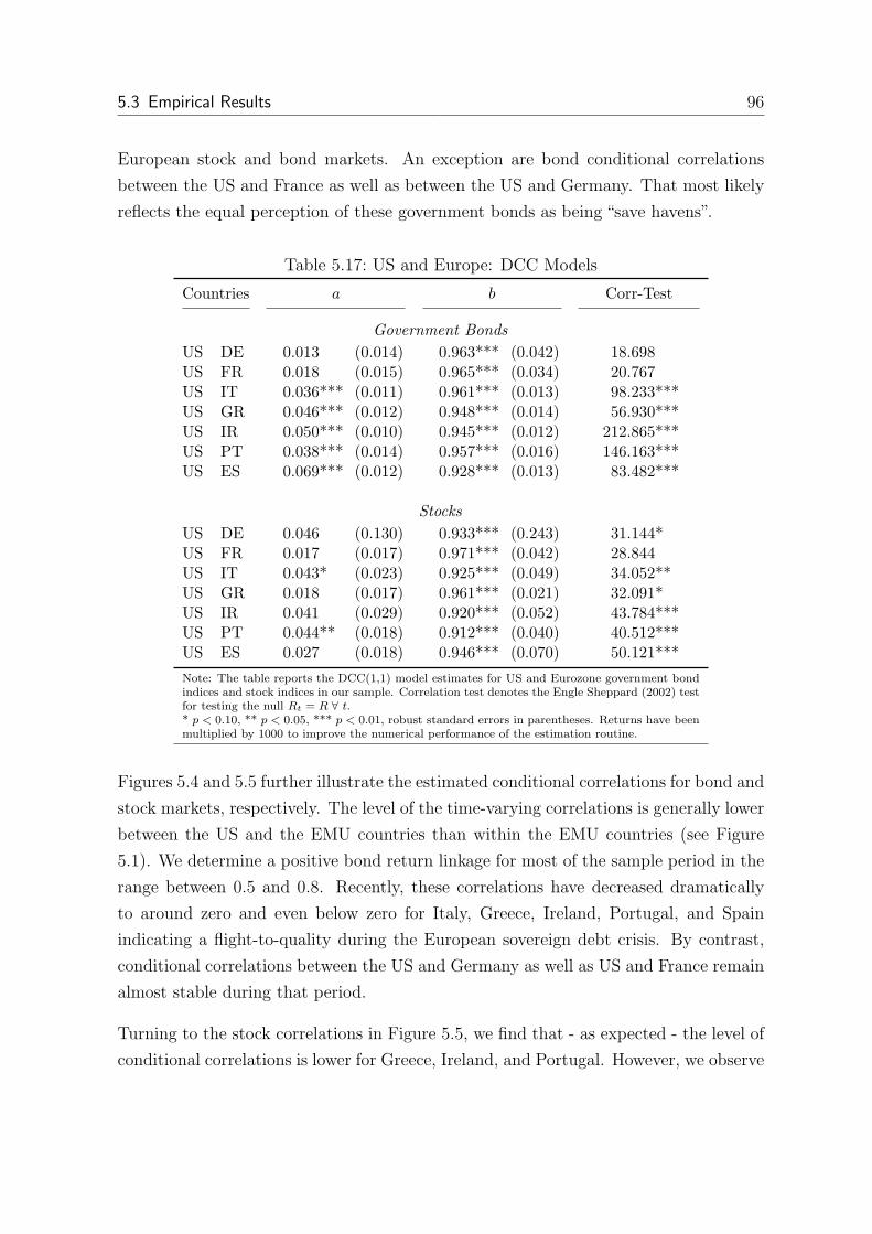
5.3 Empirical Results 96
European stock and bond markets. An exception are bond conditional correlations
between the US and France as well as between the US and Germany. That most likely
reflects the equal perception of these government bonds as being “save havens”.
Table 5.17: US and Europe: DCC Models
Countries a b Corr-Test
Government Bonds
US DE 0.013 (0.014) 0.963*** (0.042) 18.698US FR 0.018 (0.015) 0.965*** (0.034) 20.767US IT 0.036*** (0.011) 0.961*** (0.013) 98.233***US GR 0.046*** (0.012) 0.948*** (0.014) 56.930***US IR 0.050*** (0.010) 0.945*** (0.012) 212.865***US PT 0.038*** (0.014) 0.957*** (0.016) 146.163***US ES 0.069*** (0.012) 0.928*** (0.013) 83.482***
Stocks
US DE 0.046 (0.130) 0.933*** (0.243) 31.144*US FR 0.017 (0.017) 0.971*** (0.042) 28.844US IT 0.043* (0.023) 0.925*** (0.049) 34.052**US GR 0.018 (0.017) 0.961*** (0.021) 32.091*US IR 0.041 (0.029) 0.920*** (0.052) 43.784***US PT 0.044** (0.018) 0.912*** (0.040) 40.512***US ES 0.027 (0.018) 0.946*** (0.070) 50.121***
Note: The table reports the DCC(1,1) model estimates for US and Eurozone government bondindices and stock indices in our sample. Correlation test denotes the Engle Sheppard (2002) testfor testing the null Rt = R ∀ t.* p < 0.10, ** p < 0.05, *** p < 0.01, robust standard errors in parentheses. Returns have beenmultiplied by 1000 to improve the numerical performance of the estimation routine.
Figures 5.4 and 5.5 further illustrate the estimated conditional correlations for bond and
stock markets, respectively. The level of the time-varying correlations is generally lower
between the US and the EMU countries than within the EMU countries (see Figure
5.1). We determine a positive bond return linkage for most of the sample period in the
range between 0.5 and 0.8. Recently, these correlations have decreased dramatically
to around zero and even below zero for Italy, Greece, Ireland, Portugal, and Spain
indicating a flight-to-quality during the European sovereign debt crisis. By contrast,
conditional correlations between the US and Germany as well as US and France remain
almost stable during that period.
Turning to the stock correlations in Figure 5.5, we find that - as expected - the level of
conditional correlations is lower for Greece, Ireland, and Portugal. However, we observe
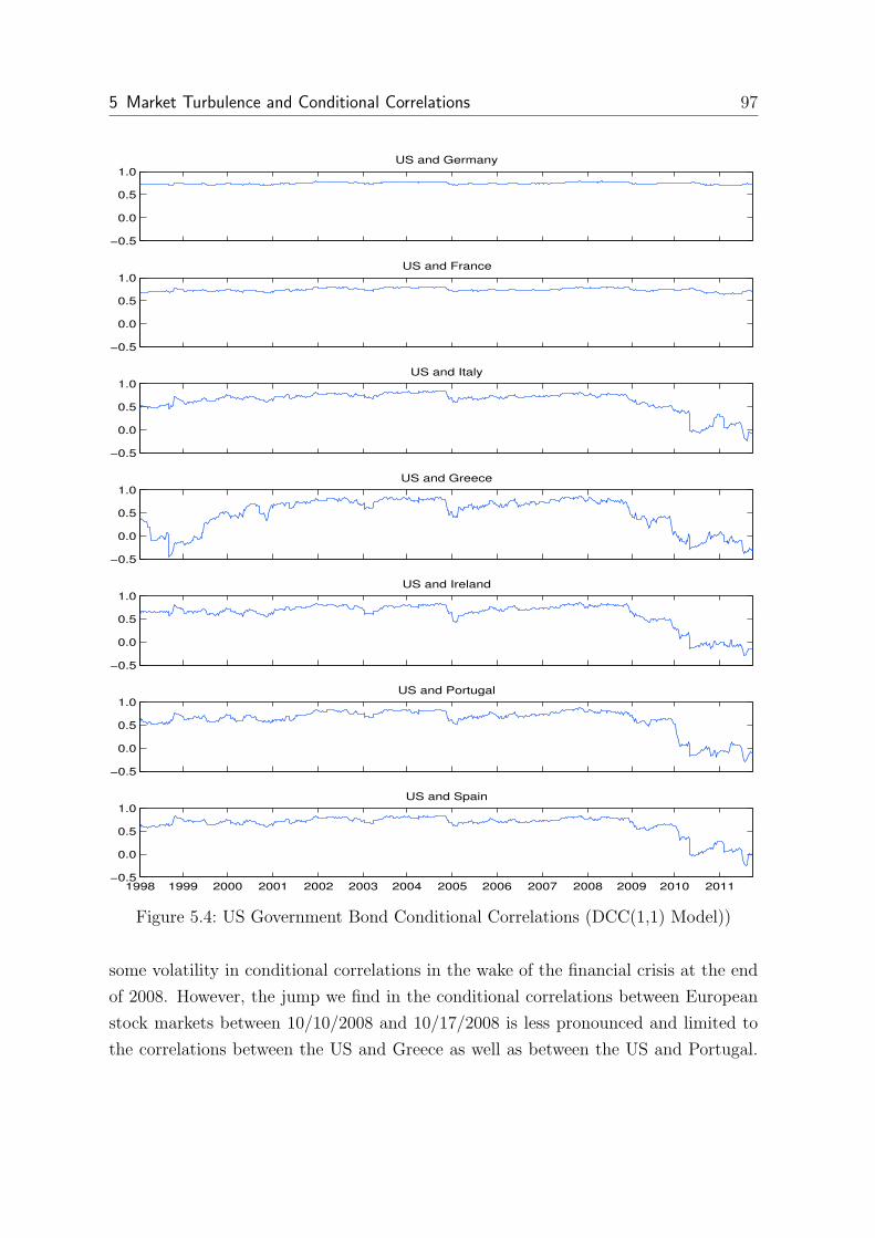
5 Market Turbulence and Conditional Correlations 97
−0.5
0.0
0.5
1.0US and Germany
−0.5
0.0
0.5
1.0US and France
−0.5
0.0
0.5
1.0US and Italy
−0.5
0.0
0.5
1.0US and Greece
−0.5
0.0
0.5
1.0US and Ireland
−0.5
0.0
0.5
1.0US and Portugal
1998 1999 2000 2001 2002 2003 2004 2005 2006 2007 2008 2009 2010 2011−0.5
0.0
0.5
1.0US and Spain
Figure 5.4: US Government Bond Conditional Correlations (DCC(1,1) Model))
some volatility in conditional correlations in the wake of the financial crisis at the end
of 2008. However, the jump we find in the conditional correlations between European
stock markets between 10/10/2008 and 10/17/2008 is less pronounced and limited to
the correlations between the US and Greece as well as between the US and Portugal.
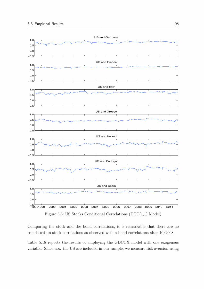
5.3 Empirical Results 98
−0.5
0.0
0.5
1.0US and Germany
−0.5
0.0
0.5
1.0US and France
−0.5
0.0
0.5
1.0US and Italy
−0.5
0.0
0.5
1.0US and Greece
−0.5
0.0
0.5
1.0US and Ireland
−0.5
0.0
0.5
1.0US and Portugal
19981999 2000 2001 2002 2003 2004 2005 2006 2007 2008 2009 2010 2011−0.5
0.0
0.5
1.0US and Spain
Figure 5.5: US Stocks Conditional Correlations (DCC(1,1) Model)
Comparing the stock and the bond correlations, it is remarkable that there are no
trends within stock correlations as observed within bond correlations after 10/2008.
Table 5.18 reports the results of employing the GDCCX model with one exogenous
variable. Since now the US are included in our sample, we measure risk aversion using
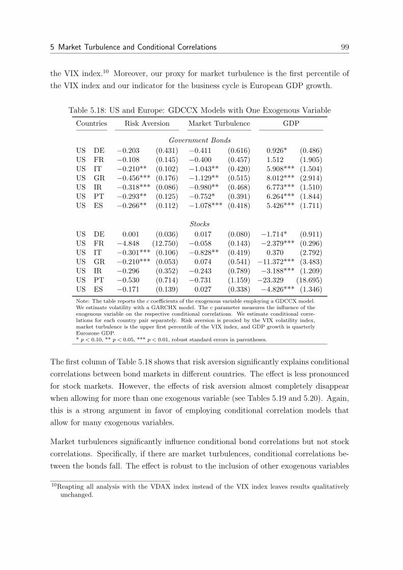
5 Market Turbulence and Conditional Correlations 99
the VIX index.10 Moreover, our proxy for market turbulence is the first percentile of
the VIX index and our indicator for the business cycle is European GDP growth.
Table 5.18: US and Europe: GDCCX Models with One Exogenous Variable
Countries Risk Aversion Market Turbulence GDP
Government Bonds
US DE −0.203 (0.431) −0.411 (0.616) 0.926* (0.486)US FR −0.108 (0.145) −0.400 (0.457) 1.512 (1.905)US IT −0.210** (0.102) −1.043** (0.420) 5.908*** (1.504)US GR −0.456*** (0.176) −1.129** (0.515) 8.012*** (2.914)US IR −0.318*** (0.086) −0.980** (0.468) 6.773*** (1.510)US PT −0.293** (0.125) −0.752* (0.391) 6.264*** (1.844)US ES −0.266** (0.112) −1.078*** (0.418) 5.426*** (1.711)
Stocks
US DE 0.001 (0.036) 0.017 (0.080) −1.714* (0.911)US FR −4.848 (12.750) −0.058 (0.143) −2.379*** (0.296)US IT −0.301*** (0.106) −0.828** (0.419) 0.370 (2.792)US GR −0.210*** (0.053) 0.074 (0.541) −11.372*** (3.483)US IR −0.296 (0.352) −0.243 (0.789) −3.188*** (1.209)US PT −0.530 (0.714) −0.731 (1.159) −23.329 (18.695)US ES −0.171 (0.139) 0.027 (0.338) −4.826*** (1.346)
Note: The table reports the c coefficients of the exogenous variable employing a GDCCX model.We estimate volatility with a GARCHX model. The c parameter measures the influence of theexogenous variable on the respective conditional correlations. We estimate conditional corre-lations for each country pair separately. Risk aversion is proxied by the VIX volatility index,market turbulence is the upper first percentile of the VIX index, and GDP growth is quarterlyEurozone GDP.* p < 0.10, ** p < 0.05, *** p < 0.01, robust standard errors in parentheses.
The first column of Table 5.18 shows that risk aversion significantly explains conditional
correlations between bond markets in different countries. The effect is less pronounced
for stock markets. However, the effects of risk aversion almost completely disappear
when allowing for more than one exogenous variable (see Tables 5.19 and 5.20). Again,
this is a strong argument in favor of employing conditional correlation models that
allow for many exogenous variables.
Market turbulences significantly influence conditional bond correlations but not stock
correlations. Specifically, if there are market turbulences, conditional correlations be-
tween the bonds fall. The effect is robust to the inclusion of other exogenous variables
10Reapting all analysis with the VDAX index instead of the VIX index leaves results qualitativelyunchanged.

5.3 Empirical Results 100
Table 5.19: US and Europe: GDCCX Models with Two Exogenous Variables
Countries Risk Aversion Market Turbulence
Government Bonds
US DE 0.162 (0.221) −0.575 (0.718)US FR 0.094 (0.152) −0.473 (0.508)US IT 0.000 (0.060) −1.043** (0.446)US GR −0.209 (0.164) −0.972* (0.514)US IR −0.078*** (0.021) −1.305*** (0.212)US PT −0.107 (0.102) −0.676* (0.389)US ES 0.000 (0.122) −1.078* (0.615)
Stocks
US DE 0.013 (0.039) 0.005 (0.082)US FR −4.306 (5.856) 0.763 (2.634)US IT −0.050 (0.115) −0.778* (0.402)US GR −0.332*** (0.109) 0.331 (0.359)US IR 0.061 (0.409) −0.295 (0.957)US PT 0.072 (0.478) −0.751 (1.371)US ES 0.349 (0.226) −0.057 (0.208)
Note: The table reports the c coefficients of the exogenous variable employing a generalized DCCX model.We estimate volatility with a GARCHX model. The c parameter measures the influence of the exogenousvariable on the respective conditional correlations. We estimate conditional correlations with two exogenousvariables simultaneously and for each country pair separately. Risk aversion is proxied by the VIX volatilityindex, market turbulence is the upper first percentile of the VIX index, and GDP growth is quarterlyEurozone GDP.* p < 0.10, ** p < 0.05, *** p < 0.01, robust standard errors in parentheses.
such as risk aversion. Interestingly, most coefficients for bonds and for stocks are nega-
tive. By contrast, remember that market turbulences resulted in increasing conditional
correlations between stocks in Europe. This is an indication that the European stock
market are subject to contagion whereas the US is not affected.
Third, we find that the most important driver of correlations between the US and
Europe are effects of the business cycle. Positive GDP growth results in increasing
correlations between bonds but decreasing correlations between stocks. That is true
both for bonds and for stocks and is robust to including risk aversion and market
turbulence as exogenous variables.
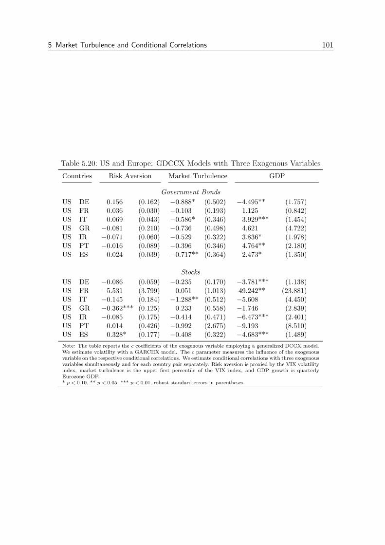
5 Market Turbulence and Conditional Correlations 101
Table 5.20: US and Europe: GDCCX Models with Three Exogenous Variables
Countries Risk Aversion Market Turbulence GDP
Government Bonds
US DE 0.156 (0.162) −0.888* (0.502) −4.495** (1.757)US FR 0.036 (0.030) −0.103 (0.193) 1.125 (0.842)US IT 0.069 (0.043) −0.586* (0.346) 3.929*** (1.454)US GR −0.081 (0.210) −0.736 (0.498) 4.621 (4.722)US IR −0.071 (0.060) −0.529 (0.322) 3.836* (1.978)US PT −0.016 (0.089) −0.396 (0.346) 4.764** (2.180)US ES 0.024 (0.039) −0.717** (0.364) 2.473* (1.350)
Stocks
US DE −0.086 (0.059) −0.235 (0.170) −3.781*** (1.138)US FR −5.531 (3.799) 0.051 (1.013) −49.242** (23.881)US IT −0.145 (0.184) −1.288** (0.512) −5.608 (4.450)US GR −0.362*** (0.125) 0.233 (0.558) −1.746 (2.839)US IR −0.085 (0.175) −0.414 (0.471) −6.473*** (2.401)US PT 0.014 (0.426) −0.992 (2.675) −9.193 (8.510)US ES 0.328* (0.177) −0.408 (0.322) −4.683*** (1.489)
Note: The table reports the c coefficients of the exogenous variable employing a generalized DCCX model.We estimate volatility with a GARCHX model. The c parameter measures the influence of the exogenousvariable on the respective conditional correlations. We estimate conditional correlations with three exogenousvariables simultaneously and for each country pair separately. Risk aversion is proxied by the VIX volatilityindex, market turbulence is the upper first percentile of the VIX index, and GDP growth is quarterlyEurozone GDP.* p < 0.10, ** p < 0.05, *** p < 0.01, robust standard errors in parentheses.

5.4 Summary 102
5.4 Summary
In this chapter, we employ both DCC and GDCCX models and investigate the effects
of exogenous variables on bond and stock market correlations in the US and in the
Eurozone between 1998 and 2011. We model volatility with a GARCHX model in
order to separate the effects of the exogenous variables on volatility from the effects on
the dependence structure. At first, we examine conditional correlations using the DCC
model. We find no trend of further convergence among linkages between Eurozone bond
and stock indices. By contrast, Eurozone bond correlations have dramatically fallen
since the begin of the financial crisis.
Moreover, we show that both GDP growth and market turbulences drive conditional
correlations whereas risk aversion has almost no effect. The impact of market turbu-
lences is most pronounced for the peripheral countries. There is an important difference
between bonds and stocks: When there is negative GDP growth, conditional bond cor-
relations fall, but European stock correlations increase strongly which is a clear sign
of contagion. If, in addition, there are market turbulences, this effect becomes even
more pronounced, but not for all countries. In line with Hunter and Simon (2005), we
conclude that international diversification benefits for stock investors but not for bond
investors are diminished in times of crisis.
In addition, it is useful to examine the impact of several exogenous variables on con-
ditional correlations simultaneously. For example, the effects of market turbulences on
conditional correlations nearly disappear once we account for GDP growth. In order to
avoid incorrect conclusions, we strongly suggest to examine several exogenous variables
simultaneously. That is also a strong argument for choosing correlation models that
allow for several exogenous variables such as the DCCX or the GDCCX model instead
of those that can only allow one or two variables such as the STCC model.

6 Stock-Bond Correlations and Real Time Macroeconomic Announcements 103
6 Stock-Bond Correlations and Real Time
Macroeconomic Announcements
6.1 Introduction
In this chapter, we present another application of the econometric framework, we em-
ploy in the previous chapters. Correlation dynamics between major asset clases are of
special interest for asset allocation and risk management. For example, time-varying
correlations might either impede or enhance the diversification benefits of a portfolio.
As we examined the conditional correlations between different sectors of the same asset
class in the previous chapter, in this chapter, we study correlations between different as-
set classes. More precisely, we investigate how risk aversion and macro announcements
influence high-frequency correlations between bonds and stocks in the Eurozone.
Against this background, central questions remain unanswered. Is risk aversion deter-
mining conditional correlations or do macroeconomic announcements drive prices? Did
the recent financial crisis have any (lasting) effects on stock-bond correlations? Is the
direction or the size of macroeconomic announcements surprise of higher importance?
Generally, do these variables change the stock-bond dependence structure or just the
volatility, or both? Although there are numerous studies that investigate stock-bond
correlations,1 the literature is not yet conclusive.
Specifically, employing a high-frequency dataset, Andersen et al. (2007) and Boyd et al.
(2005) find that macroeconomic announcements affect correlations. Furthermore, they
show that the impact of news varies considerably during the business cycle. Christiansen
and Ranaldo (2007) analyze realized correlations and highlight that the occurrence of a
macroeconomic announcement but not the actual announced figure plays an important
role for stock-bond correlations.
1An incomplete sample of relevant papers includes: Li (2002); Ilmanen (2003); Pastor and Stambaugh(2003); Boyd et al. (2005); Connolly et al. (2005); Kim et al. (2006); Andersen et al. (2007);Christiansen and Ranaldo (2007); Connolly et al. (2007); Corsi and Audrino (2007); Anderssonet al. (2008); Baur and Lucey (2009); Panchenko and Wu (2009); Yang et al. (2009); Aslanidisand Christiansen (2010); Baele et al. (2010); Bansal et al. (2010) and Aslanidis and Christiansen(2011).
6.1 Introduction 104
Using daily or lower frequency but not high-frequency data, several studies present
evidence for stock and bond prices moving in the same direction during periods of higher
uncertainty about long-term expected inflation (Li, 2002), high inflation expectations
(Andersson et al., 2008), or high inflation rates (Yang et al., 2009). Moreover, Ilmanen
(2003) suggests that the inflation level as well as the business cycle explain stock-bond
correlations. By contrast, Baele et al. (2010) argue that macroeconomic factors do not
drive conditional correlations. Employing quarterly data and a dynamic conditional
correlation framework model, they provide evidence that rather illiquidity and flight-
to-quality are important for correlations. Additionally, Bansal et al. (2010) find that
correlations vary across two regimes. A high-stress regime coincides with higher risk
aversion, higher trading volumes and lower stock-bond correlation. Several other studies
focus on the influence of risk aversion on correlations and confirm the flight-to-quality
effect (Connolly et al., 2005, 2007; Aslanidis and Christiansen, 2010, 2011; Kim et al.,
2006).
We contribute to the literature across several dimensions. Using a high-frequency
dataset for Eurozone stocks and bonds, we simultaneously estimate the influence of
risk aversion, macroeconomic announcements, and other exogenous variables on both
conditional correlations and conditional variances. We analyze conditional correlations
using a GDCCX model and estimate variances with a GARCHX model as described
in the previous chapters. That approach allows us to separate the effects of the exoge-
nous variables on the dependence structure from those on the volatility. The correct
specification of the variance equation is of particular importance as our sample covers
the recent financial crisis, a period of extreme volatility.
We include 15 macroeconomic announcements from the US and 5 from the Eurozone
and compare their influence on volatility and stock-bonds correlations. We employ
real-time data, i.e. news that are available to market participants at the time of the
release. Accordingly, we can analyze the information content of specific announcements
and compare the importance of US to European news. For example, news that convey
information regarding future cash-flows should primarily move stocks thus reducing
conditional stock-bond correlations. Falling conditional correlation might also be caused
by a flight-to-quality. If the announcement can be interpreted as news about the future
discount rates, bond and stock prices should move in the same direction (Andersen
et al., 2007).

6 Stock-Bond Correlations and Real Time Macroeconomic Announcements 105
Furthermore, most papers which analyze stock-bond correlations focus on the stock and
bond correlations in the US.2 Yet, we use a high-frequency dataset for European stocks
and bonds as we want to know if the driving forces of high-frequency correlations in
the Eurozone are similar to those already documented for the US.
To preview our results, we find that both risk aversion and macroeconomic announce-
ments separately drive conditional correlations. Conditional correlations fall as risk
aversion rises even when simultaneously accounting for the influence of macroeco-
nomic announcements on conditional correlations and the influence of these variables
on volatility. Interestingly, the additional effects of the financial crisis on correlations
are only small. Generally, the most important news are nonfarm payrolls in the US and
the European Central Bank (ECB) rate decision in Europe. For most macroeconomic
announcements, the absolute value of the surprise is of higher importance for correla-
tions than the mere occurrence of the announcement. Moreover, most macroeconomic
news result in falling conditional correlations. Yet, the publication of news concerning
future interest rates or inflation figures moves bond and stock prices in the same direc-
tion. We do not find any evidence that the influence of economic announcements on
conditional correlations changes during the cycle. This conclusion is driven from the
observation that splitting the effects of the macroeconomic variables between expansion
and recession does not alter the results. Turning to the results on volatility, we present
evidence that the occurrence of any macroeconomic announcement results in a higher
volatility as do surprises for both stocks and bonds.
The outline of the chapter is as follows. We start by describing the data in section
6.2. We report and discuss the empirical results in section 6.3. Section 6.4 provides
concluding remarks.
6.2 Data
6.2.1 Bond and Stock Returns
The data employed for this study consist of stock and bond returns as well as economic
variables. As we focus on the Eurozone, we choose the Euro Stoxx 50 Future to represent
the stock market. It is based on the Dow Jones Euro Stoxx 50 index which is composed
2Exceptions are Li (2002); Andersen et al. (2007); Connolly et al. (2007) and Andersson et al. (2008).
6.2 Data 106
of 50 large blue chip companies in the Eurozone that is widely applied as benchmark
index for Eurozone equities.
We use the Bund Future to calculate bond market returns. The underlying security of
this future is the German 10 year treasury bond. We analyze the German bond market
as it is considered to be the safest investment in the Eurozone and it is regarded as a
representative of a liquid, risk-free government bond in the Eurozone. Similar to Faust
et al. (2007), we prefer the Bund future over other bond market futures (such as the
Bobl or the Schatz) as it is by far the most actively traded bond future in the Eurozone.
Both the bond and the stock future are traded at the Eurex from 8 am to 10 pm and
are highly liquid with a daily trading volume of more than 0.7 million and more than
0.9 million, respectively.
There are several advantages in using futures instead of cash indices. First, futures
markets lead cash markets in terms of price discovery (Hasbrouck, 2003). Second, the
contracts are actively traded, transaction costs are minimal, and no legal constraints
on short selling are imposed. Third, high frequency data for futures are available from
several vendors. Therefore, previous studies on correlations and volatility also focus on
futures markets.3
Following several other studies (Andersen et al., 2007; Aslanidis and Christiansen, 2010,
2011; Andersson, 2010; Hussain, 2011), we obtain raw tick-by-tick transaction prices
from Tick Data Inc.4 The symbols are BN for the Bund future and XX for the Euro
Stoxx 50 future. Both futures have four delivery months (March, June, September and
December), and several contracts are traded at a time. Thus, we construct a continuous
return series employing the most liquid contract. As almost all trading takes place in
the contract closest to expiry, we use this contract. In practice, futures are rolled to
next contract a few days prior to expiry. Similarly, we switch to the next-maturity
contract as soon as the trading volume is higher in the second nearby contract, which
is usually two days before maturity (McMillan and Speight, 2003).5
3For example Christiansen and Ranaldo (2007); Corsi and Audrino (2007); Andersson (2010); Bansalet al. (2010); Aslanidis and Christiansen (2010, 2011); Christiansen et al. (2011) study futuresinstead of cash markets.
4In order to verify the accuracy of the data we reconcile the data with intraday-data available onBloomberg.
5Switching to the next-maturity contract earlier as done in Andersen et al. (2007) and Christiansenand Ranaldo (2007) or at a fixed date prior to expiry as in Bansal et al. (2010) or in Fleming et al.(2003) would result in more missing observations.
6 Stock-Bond Correlations and Real Time Macroeconomic Announcements 107
6.2.2 Exogenous Variables
We test several exogenous variables. Since the futures data we obtained includes details
on each trade, we can calculate the trading volume in any time interval. However,
Bansal et al. (2010) point out that the futures volume is heavily affected by rolling
activity in the week before the expiry of the contract. In addition, there might be a
time trend. Therefore, we adjust the trading volume by regressing the volume on a
constant, a time trend and a dummy indicating the five trading days prior to expiry.
We employ the regression residuals as our volume variable.
Bansal et al. (2010) argue that higher trading volume is associated with high-stress
regimes that also feature higher volatility. Accordingly, we primarily see trading volume
as a proxy for high volatility. In addition, futures trading volume is generally much
lower before holidays but much higher during and after macroeconomic announcements
(Balduzzi et al., 2001). Hence, we can also think of it as a proxy for liquidity.
As pointed out in section 3.3.2.2, option-implied volatility is widely regarded as a good
proxy for risk aversion as it incorporates all information available to market participants
on future volatility. Numerous studies on volatility and conditional correlations6 use
this measure as an estimate of market uncertainty. We obtain data on the Euro Stoxx
50 Volatility Index (VSTOXX). The index is derived from prices of the underlying
Euro Stoxx 50 options and is computed daily from 9.15am to 5.30pm. We obtain
intraday-data on this index from CQG Inc., which is an official Eurex data vendor.7
The sampling interval for our VSTOXX data is two minutes. For all our analysis, we
compute the log differences of the VSTOXX index.
Christiansen et al. (2011) argue that the term spread is an important variable for mod-
eling bond and stock volatility. Therefore, we also include the daily difference between
10 year and 3 months interest rates provided by J.P. Morgan. We have neither intra-
day data nor a specific announcement time for this variable. Thus, we increase the
frequency by allowing the variable to remain constant throughout the day.8 Further-
6For example Andersson et al. (2008), Aslanidis and Christiansen (2010, 2011), Cai et al. (2009),Connolly et al. (2005, 2007), and Kim et al. (2006) analyze the VIX or the VDAX index. Bansalet al. (2010) use the VXO index.
7Other studies such as Le and Zurbruegg (2010), Hashimoto (2005) or Martens and Zein (2002) alsoemploy CQG data.
8This transformation of data has already been applied to convert monthly to daily (Cai et al., 2009)or to weekly data (Aslanidis and Christiansen, 2010).

6.2 Data 108
more, interest rates differences are lagged by one day to make sure that we keep the
dataset in chronological order.
In order to measure the influence of the financial crisis in 2008 and 2009, we construct
a dummy variable that is one from October 2008 to April 2009 coinciding with the
financial crisis.9
6.2.3 Real Time Macroeconomic Announcements
We also want to investigate the effect of various macroeconomic variables on stock-
bond correlations. During European trading hours macroeconomic announcements oc-
cur both in the Eurozone and in the US. Accordingly, announcements made in both
regions are included.10 Moreover, previous studies suggest that the US macroeconomic
announcements are not only important for US but also for European markets (Ander-
sen et al., 2003, 2007; Faust et al., 2007; Albuquerque and Vega, 2009; Hussain, 2011;
Mittnik et al., 2011).
All announcements occur at a predefined time and are released instantaneously at a
precise time. European announcements take place in the morning starting with the
German unemployment rate at 9.55 am CET and ending with the ECB interest rate
announcement at 1.45 pm CET (see Table 6.1). US announcements are in the afternoon
starting at 2.30 pm CET.11 All announcement data are available during our whole
sample period.
Similar to Bollerslev et al. (2000) and Mittnik et al. (2011), our source for announce-
ments and market expectations is Bloomberg. We obtain the date and time as well as
the actual release and the market consensus.12 The Bloomberg market expectation is
the median forecast of a large number of economists and is widely considered as consen-
9As with any recession or crisis it is difficult to determine a definite starting point or. Although thecollapse of Lehman Brothers was at mid September 2008, stock and bond market reacted strongestin mid October 2008 and did not rebound until April 2009.
10The Federal Reserve System (FED) rate decision is an exception as the release time is not includedin our sample and thus not included in our analysis.
11Since 2007 the daylight savings time in the US starts on the second Sunday in March and ends onthe first Sunday in November while in Europe it is three weeks shorter starting on the last Sundayin March and ending on the last Sunday in October. Therefore, the time difference is only 5 hoursin the non-overlapping period so that announcements are one hour earlier in CET.
12Furthermore, in order to verify the accuracy of the release data, we reconcile Bloomberg data withdata available on the website of the respective institution.

6 Stock-Bond Correlations and Real Time Macroeconomic Announcements 109
Table 6.1: Macroeconomic Announcements
Data Release SourceaNumberof Obser-vations
UnitsRelease time
(CET)
U.S. Announcements
Capacity utilizatione FRB 48 % of capacity 15:15Construction spending BC 47 % change mom 16:00Consumer confidence CB 48 Diffusion index 16:00Consumer prices BLS 48 % change mom 14:30Durable good orders BC 46 % change mom 14:30Factory orders BC 47 % change mom 16:00U.S. GDPb BEA 48 % change qoq 14:30Industrial productione FRB 48 % change mom 15:15Initial claims DOL 204 Thousands 14:30ISM index ISM 45 Diffusion index 16:00New home sales BC 47 % change mom 16:00Nonfarm payroll employmente BLS 47 Change in thousands 14:30Producer price index BLS 48 % change mom 14:30Retail sales BC 48 % change mom 14:30Unemployment ratee BLS 47 % rate 14:30
German Announcements
IFO index IFO 48 Diffusion index 10:00Unemployment FLO 49 % rate 9:55
Eurozone Announcements
ECB rate decision ECB 49 Change in pct pts 13:45Eurozone HCPIc ES 49 % change yoy 11:00Eurozone GDPb ES 48 % change qoq 11:00
Note: All frequencies are monthly except for the Initial claims which are announced weekly.a Acronyms for the sources are as follows:Bureau of Economic Analysis (BEA), Bureau of Labor Statistics (BLS), Bureau of the Census (BC), Departmentof Labor (DOL), European Central Bank (ECB), Eurostat (ES), Federal Labour Office (FLO), Federal ReserveBoard (FRB), Ifo Institute (IFO).b Quarterly GDP figures are reported three times: advance, preliminary, and final.c HCPI is the Harmonized Consumer Price Index Flash estimatate.d Manufacturing PMI is the Manufacturing Purchasing Managers’ Index.e The following economic figures are announced at the same time: capacity utilization and industrial production;nonfarm payroll employment and the unemployment rate.
sus estimate of the market. Furthermore, we test whether the survey data is unbiased
over our sample period (Flannery and Protopapadakis, 2002). For all economic mar-
ket expectations except of the German unemployment rate, we cannot reject the null
hypothesis that the mean of the consensus data is zero at the 5% level. Accordingly,
market expectations are unbiased.
In line with Balduzzi et al. (2001), Bollerslev et al. (2000), and Andersen et al. (2003),
we are especially interested in the surprise component of the announcement since, given
6.2 Data 110
rational markets, expectations should already be reflected in prices. The surprise is sim-
ply calculated as the median forecast minus the released value. Moreover, we standard-
ize the surprise by its respective standard deviation in order to correct for the different
units of measurement of the economic variables. It may be that the magnitude of the
surprise is more important than the actual direction of the surprise when it comes
to modeling correlations or volatilities. As in Christiansen et al. (2011), we also test
the absolute value of the surprise. As suggested by Christiansen and Ranaldo (2007)
and Andersen et al. (2003), dummy variables for each macroeconomic announcement
are included to separate the influence of a mere presence of a specific announcement
from any corresponding surprise. A dummy variable which becomes one if there is any
macroeconomic announcement is constructed to capture the general announcement ef-
fect.13
Once it is established that a macroeconomic announcement influences correlations, it
is still unclear how long the effect will last. Different time windows have been chosen
in the previous literature. While Andersen et al. (2003) focus on the 15 minutes after
the economic news, Andersen et al. (2007) consider 20 minutes for the influence of
announcements on asset returns and 70 minutes on asset volatility. Our approach is
different, as the persistence of any news is modeled within the DCC framework and
assumed to follow a geometric lag with parameters being estimated from the data.
Therefore, announcement variables take on the value of the surprise only at the time
of the announcement.
6.2.4 The Dataset
The dataset covers the period from 4/30/2007 to 4/30/2011. This period includes both
the tranquil period before the start of the financial crisis, the financial crisis itself and
the initial recovery thereafter. Corresponding to the trading time of the VSTOXX
index, the daily time interval in the sample starts at 9.15 am and ends at 5.30 pm.
Similar to most studies that employ high frequency data,14 we split trading days into
5-minute intervals. This is a compromise between microstructure biases which arise
due to nonsynchronous trading and the desire to sample at a high frequency (Bollerslev
13Henceforth, we will label that dummy all announcements dummy.14A sample of papers that use 5 minute data includes Andersen and Bollerslev (1998); Bollerslev et al.
(2000); Andersen et al. (2001, 2003, 2007); Christiansen and Ranaldo (2007); Andersson (2010)and Aslanidis and Christiansen (2010, 2011).

6 Stock-Bond Correlations and Real Time Macroeconomic Announcements 111
et al., 2000; Andersen et al., 2001; Hansen and Lunde, 2006). As the VSTOXX sampling
frequency is two minutes (i.e. we have 248 observations per day), we synchronize the
data by using the last recorded VSTOXX price in any five minute interval.
Table 6.2: Descriptive Statistics
Name Obs. Mean Std. Dev. Min. Max. Skewn. Kurt.
Bund Futurea 100,625 0.00% 0.03% -0.50% 0.35% −0.35 11.13***Euro Stoxx 50 Futurea 100,624 0.00% 0.14% -2.10% 4.84% 0.23 28.85***Vstoxx Indexa 100,108 0.00% 0.42% -8.48% 10.27% 0.57 28.10***Trading Volume Bonds 100,625 7,122 6,432 30 120,393 3.46 26.09***Trading Volume Stocks 100,624 9,041 8,987 14 374,769 3.80 50.07***
Note: The table reports descriptive statistics for the high-frequency variables employed in the analysis.*** denotes series that differ from a normal distribution at 1% level as indicated by a Jarque–Beratest; aLog change of the variable.
Compared with daily or lower frequency data, high-frequency data is subject to more
extreme outliers. Table 6.2 shows that, even after ignoring the overnight return, the
Bund future minimum is a 16 standard deviation event whereas the maximum of the
Euro Stoxx 50 future is a 34 standard deviations away from the mean. The same is true
for our risk aversion measure15 as well as for most of the other high-frequency variables.
However, the estimation procedure is sensitive to extreme outliers. In addition, extreme
observations of the exogenous variable might set implicit boundaries to the parameter
space of the GDCCX model.16 Therefore, we follow Silvennoinen and Terasvirta (2005)
as well as Boudt and Zhang (2010) and truncate all observations that deviate more than
10 standard deviations from the mean allowing us to keep the information contained in
the outliers.17
Following Andersen and Bollerslev (1997), we ignore the overnight return, i.e. from the
close in t-1 to the first observation in t. This period is special because it incorporates
15The minimum is 20 standard deviations away from the mean while the maximum 24 standarddeviations outlier.
16An intuitive explanation is as follows: The exogenous variable influences the estimated conditionalcorrelation with the strength of the effect measured by the parameter c. For example, the effect ofan exogenous variable on conditional correlations is positive for a positive c and any observationof the exogenous variable greater than zero. Furthermore, the greater the c parameter and theobservation, the greater is the effect on conditional correlations. Yet, conditional correlations arebounded between plus and minus one. Therefore, given a large outlier, the c parameter must besmaller just to make sure that the conditional correlation remain between plus and minus one forthat single observation. That establishes an implicit boundary on the c parameter.
17I.e., all outliers are set to 10 standard deviations.

6.3 Empirical Results 112
all information accumulated overnight and over-weekend and consequently has a much
higher volatility.
Sometimes, there is no trading within a 5 minute interval.18 Following Bollerslev et al.
(2000) and Andersen and Bollerslev (1997), we linearly interpolate all intraday data in
these cases. Calculating continuously compounded five minute returns for 1017 trading
days with 99 observations per day (excluding the overnight return) gives us 100,682
observations.19 As in section 3.3.2, we multiply the return series with 1000 and divide
the exogenous variables by 100 to avoid the accumulation of rounding errors. As the
mean of the time series is non-zero, we furthermore demean all time series except the
dummy variables.
6.3 Empirical Results
6.3.1 The DCC Model
At first, we are interested in the conditional correlations between high-frequency returns
of bonds and stocks in the Eurozone and ignore any economic explanations. We estimate
a DCC(1,1)-GARCH(1,1) model (see section 2.2) as a benchmark model. Table 6.3
shows the results.
In line with previous literature, the results of the GARCH(1,1) model indicate volatil-
ity clustering. As the sums of the αi and βi parameters are close to one, we conclude
that conditional variances are highly persistent. Turning to the correlation equation,
we find clear evidence for time-varying conditional correlations. The estimated param-
eters of the DCC(1,1) model are highly significant and the Engle and Sheppard (2001)
test20 clearly rejects the null hypothesis of constant conditional correlations. Moreover,
the innovations to the conditional correlations are highly persistent: the half-life is
approximately 2 hours and 15 minutes.21
18The number of missing observations for the Bund future (0.06%) and the Eurostoxx 50 future (0.06%)is very low. Specifically, trading at the EUREX stopped shortly at 11/18/2009 and 2/4/2009 dueto technical difficulties. However, on both days there were no significant market moves. Othermissing occur especially if there is trading on a public holiday or just before a public holiday. Thenumber of missing observations for the VSTOXX index is higher but still acceptable (0.24%).
19Furthermore, we remove the observation 3/28/2008 at 12:20 pm as there has been a mistradeaffecting the Bundfuture only and reversing itself within less than two minutes.
20See section 2.3 for details.21Please see section 2.2 for details on the calculation of the half-life of the innovations.

6 Stock-Bond Correlations and Real Time Macroeconomic Announcements 113
Table 6.3: European Bonds and Stocks: Univariate GARCH and DCC Models
Univariate GARCH (1,1) Models Multivariate DCC (1,1) Models
Bonds Stocks DCC Model Corr-Test
ωi 0.004*** (0.000) 0.024*** (0.002) a 0.009*** (0.003) 95.722***αi 0.089*** (0.004) 0.108*** (0.004) b 0.987*** (0.005)βi 0.877*** (0.006) 0.886*** (0.004)
Note: The table reports the univariate GARCH(1,1) and DCC(1,1) estimates for Europeanbonds and stocks. Robust standard errors in parentheses. Corr-Test denotes the Engle andSheppard (2001) test for testing the null of constant correlation (Rt = R ∀ t).*p < 0.10, **p < 0.05, ***p < 0.01.
The time-varying nature of the conditional correlations is highlighted by Figure 6.1.
Conditional correlations fluctuate in the range between 0.31 and -0.79. Although corre-
lations are persistent, there is no clear time trend. The highest conditional correlations
are at the beginning of the sample (mid-2007) while they are lower for the rest of our
sample. Interestingly, there is no distinctive change in the correlations during the recent
financial crisis on the first view.
6.3.2 The GARCHX Model
We now turn to the estimation of conditional variances which allows for effects of ex-
ogenous variables. Employing a GARCHX(1,1) model and a single exogenous variable
gives us a first idea which variables can help explaining volatility.22 Results for the γ
parameter are presented in Table 6.4 and 6.5 for the bond and stock market, respec-
tively.
As expected, a rise in the VSTOXX results in higher volatility for both bonds and
stocks. Notably, the effect is much stronger for stocks - possibly reflecting the overall
higher stock volatility. The parameter for the financial crisis dummy is also positive
and highly significant. As expected, stock and bond volatility rose during the financial
crisis. Similarly, the effect is more pronounced for stocks than for bonds. In line with
Christiansen et al. (2011), we find that the term spread matters for bond but not for
stock volatility. The negative sign of the parameter is plausible as the term spread often
becomes negative during recessions. Finally, our variable indicating the stock trading
volume is significant whereas the bond volume seems to have less explanation power
22Please see section 4.3 for details on the GARCHX model.

6.3 Empirical Results 114
10/2007 04/2008 10/2008 04/2009 10/2009 04/2010 10/2010 04/2011−1.0
−0.5
0.0
0.5Conditional Correlations: European Bonds and Stocks
Figure 6.1: European Bonds and Stocks Conditional Correlations (DCC(1,1) Model)
when considered as the only exogenous variable.23 Thus, lower trading volume in stocks
coincides with lower volatility. This situation well describes periods before holidays or
at specific times during day when volatility is low.
A glance through Tables 6.4 and 6.5 immediately indicates that volatility rises signifi-
cantly during almost all economic announcements as most coefficients are positive. In
addition, the coefficient for the all announcements dummy is positive and significant
for both bonds and stocks. The effect is larger for stocks indicating that the macro
news are of higher importance for stocks than for bonds. Furthermore, all models are
23One might argue that bond and stock trading volume should influence volatility similarly as theunconditional correlation between the level of the bond and stock trading volume is 0.44. However,the unconditional correlation between the log change of the two variables is negative (-0.37) makingdifferent effects on the respective change rates more plausible.

6 Stock-Bond Correlations and Real Time Macroeconomic Announcements 115
Table 6.4: European Bonds: GARCHX Model Separate Estimations
High-FrequencyVariables
VSTOXXa 22.634** (9.795)Trading Vol. Bondsa 0.001 (0.014)Trading Vol. Stocksa 0.366*** (0.090)Financial crisis 0.426*** (0.062)Term spread −0.053*** (0.014)
AnnouncementDummyb
Absolute Surprisec Surprise
All announcements 12.306*** (1.120)
U.S. Announcements
Capacity utilizationd 3.917** (1.633) 20.453** (8.585) 1.596 f (4.615)Construction spending 17.680*** (4.311) 71.261*** (18.413) 5.698 (5.090)Consumer confidence 5.554*** (1.686) 28.175*** (8.383) −3.426 f (3.140)Consumer prices 15.425*** (2.272) 81.203*** (14.701) 0.506 f (1.817)Durable good orders 11.080*** (1.844) 55.555*** (9.833) 0.463 f (0.391)Factory orders 6.913*** (2.480) 33.795*** (12.288) −8.873**f (4.282)U.S. GDP 9.613*** (2.482) 49.462*** (13.694) 6.779* (3.629)Industrial productiond 3.917** (1.633) 19.373** (8.254) 5.355 f (4.752)Initial claims 14.385*** (1.479) 41.013*** (4.510) −0.737 f (0.674)ISM index 17.886*** (4.500) 90.560*** (22.876) 3.258 f (5.212)New home sales 6.065*** (1.545) 32.086*** (8.155) −1.890 f (2.017)Nonfarm payroll empl.e 59.040*** (7.959) 302.555*** (41.241) 0.943 f (2.979)Producer price index 17.828*** (3.796) 88.127*** (19.396) 2.613 f (4.725)Retail sales 22.965*** (4.367) 121.425*** (22.782) 1.828 f (3.346)Unemployment ratee 59.040*** (7.959) 592.980*** (200.487) −3.896 (4.019)
German and Eurozone Announcements
IFO index 14.527*** (4.394) 72.371*** (21.890) 7.404 (5.307)German unemployment −1.555*f (0.808) −7.110*f (4.048) −11.267**f (5.078)ECB rate decision 24.538*** (7.428) 198.904*** (58.413) 140.062*** (36.109)Eurozone HCPI 2.178 (2.373) 17.697 (13.343) 9.135 (7.533)Eurozone GDP −1.954***f (0.639) −7.223**f (3.630) −10.140**f (4.960)
Note: The table reports the γ estimates of a GARCHX(1,1) model (see Equation 4.18) for the Bund future. Werun separate estimations for each γ presented. Robust standard errors in parentheses.*p < 0.10, **p < 0.05, ***p < 0.01, aLog change of the variable; bAnnouncement Dummy is an indicator functionthat takes on the value 1 if there is an announcement and 0 otherwise; cAbsolute value of the surprise is employed.d, e Economic figures are announced at the same time; fA GARCH (1,1) model is preferred to this estimationaccording to the BIC criterion.
compared to each other using the bayesian information criterion (BIC).24 It turns out
that the GARCHX model which employs the all announcements dummy fits the data
best.
24Details on the bayesian information criterion are provided in in Table 6.12 in the appendix 6.A1.
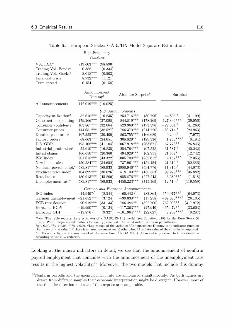
6.3 Empirical Results 116
Table 6.5: European Stocks: GARCHX Model Separate Estimations
High-FrequencyVariables
VSTOXXa 719.603*** (98.890)Trading Vol. Bondsa 0.388 (0.334)Trading Vol. Stocksa 3.018*** (0.503)Financial crisis 8.732*** (1.121)Term spread 0.154 (0.158)
AnnouncementDummyb
Absolute Surprisec Surprise
All announcements 112.019*** (10.025)
U.S. Announcements
Capacity utilizationd 52.610*** (16.835) 254.716*** (80.796) 44.895 f (41.199)Construction spending 179.266*** (37.098) 844.819*** (178.269) 127.834*** (39.056)Consumer confidence 103.867*** (32.064) 523.969*** (173.396) −22.364 f (41.268)Consumer prices 144.651*** (38.527) 786.370*** (214.720) −23.714 f (24.963)Durable good orders 167.355*** (30.400) 863.755*** (166.680) 9.290 f (7.977)Factory orders 68.663*** (24.651) 308.829** (129.336) 1.733***f (0.184)U.S. GDP 195.108*** (41.104) 1067.918*** (263.671) 57.778** (26.845)Industrial productiond 52.610*** (16.835) 254.764*** (97.528) 61.587 f (40.242)Initial claims 166.650*** (20.360) 494.929*** (62.955) 21.562* (12.742)ISM index 201.615*** (43.322) 1005.700*** (232.612) 4.157**f (2.055)New home sales 150.584*** (34.652) 737.961*** (151.454) −21.616 f (52.886)Nonfarm payroll empl.e 583.817*** (89.933) 2980.946*** (534.776) 11.814 f (44.073)Producer price index 104.699*** (30.026) 518.100*** (155.553) 99.279*** (35.882)Retail sales 180.913*** (45.800) 955.876*** (227.243) −3.289**f (1.518)Unemployment ratee 583.817*** (89.933) 4450.223*** (745.169) 12.510 f (119.559)
German and Eurozone Announcements
IFO index −14.949*f (8.544) −60.442 f (83.864) 159.977**f (64.073)German unemployment −21.652*** (3.724) −99.030*** (17.258) −87.680***f (26.105)ECB rate decision 90.919*** (33.133) 786.484** (322.700) 752.003** (317.972)Eurozone HCPI −29.990*** (0.124) −117.363*** (27.940) −65.472*f (33.603)Eurozone GDP −13.876 f (9.327) −101.964***f (22.627) 2.708***f (0.287)
Note: The table reports the γ estimates of a GARCHX(1,1) model (see Equation 4.18) for the Euro Stoxx 50future. We run separate estimations for each γ presented. Robust standard errors in parentheses.*p < 0.10, **p < 0.05, ***p < 0.01, aLog change of the variable; bAnnouncement Dummy is an indicator functionthat takes on the value 1 if there is an announcement and 0 otherwise; cAbsolute value of the surprise is employed.d, e Economic figures are announced at the same time; fA GARCH (1,1) model is preferred to this estimationaccording to the BIC criterion.
Looking at the macro indicators in detail, we see that the announcement of nonfarm
payroll employment that coincides with the announcement of the unemployment rate
results in the highest volatility.25 Moreover, the two models that include this dummy
25Nonfarm payrolls and the unemployment rate are announced simultaneously. As both figures aredrawn from different samples their economic interpretation might be divergent. However, most ofthe time the direction and size of the surprise are comparable.

6 Stock-Bond Correlations and Real Time Macroeconomic Announcements 117
as exogenous variable are - according to the BIC - the best among all models which use
any of the single announcements. This is not surprising as Andersen et al. (2007) and
Andersen and Bollerslev (1998) argue those are most important announcement for all
markets.
There is a remarkable difference between the announcements in the US and the Euro-
zone. While the occurrence of an US announcement always results in rising conditional
variances, this does not hold for all European announcements. For example, the disclo-
sure of the IFO index results in higher volatility for bonds but lower volatility for stocks.
Also, the publication of Eurozone GDP and German unemployment rate coincide with
lower volatility. Calculating the BIC indicates that the GARCHX model is simply not
suitable for these variables as a GARCH (1,1) model fits the data better. Thus, a
specification without these exogenous variables is preferable. There might also be an
economic reason why the GARCHX model does not fit the data for these European
announcements. As the financial crisis started in the US and covers a large part of our
sample, market participants might pay specific attention to the US announcements.
Also, it might be that large parts of the volatility in this period is caused by market
participants in the US who do not react to early European announcements instantly
due to the time differences.26 This would also explain why the effect of the ECB deci-
sions, which is the latest European announcement at 1.45 pm, results in significantly
higher volatility for both stocks and bonds.
As discussed in section 6.2.3, we compute the absolute value of the standardized surprise
of each announcement in order to employ it as exogenous variable. Results are presented
in the second column in Tables 6.4 and 6.5 and are highly significant. The second
column shows that the greater the absolute surprise of each announcement, the larger
the volatility. The effect is stronger for stocks than for bonds, and again an absolute
surprise in nonfarm payroll employment as well as in the unemployment rate drive
conditional variances the most. Similar to the estimations with the announcement
dummy, we are puzzled by the negative signs of some estimations involving news from
the Eurozone. Again, besides ECB rate decisions, most of the models that include the
absolute surprise of news from Germany or the Eurozone do not fit the data better
than a GARCH (1,1) model.
26This does not imply that the information is generally not taken into account by these marketparticipants but that the exact time when the news is incorporated cannot be identified.

6.3 Empirical Results 118
In column three in Tables 6.4 and 6.5, we display estimation results for GARCHX mod-
els that include the actual surprise values of the respective macroeconomic announce-
ment. Yet, most coefficients are not significantly different from zero. Calculating the
BIC indicates that both a GARCH (1,1) and models that use absolute values of the
surprise fit the data better.
Again, we are interested whether the combination of several exogenous variables im-
proves the fit to the data. We estimate several combinations of exogenous variables that
include the high-frequency variables and macroeconomic announcements27 and select
the best model according to the BIC criterion. Tables 6.6 and 6.7 present the two best
models for bonds and stocks, respectively. It turns out that the inclusion of the fol-
lowing macroeconomic announcements improves the fit of the model: nonfarm payroll
employment, US GDP (stocks only), consumer prices, and initial jobless claims.
Table 6.6: European Bonds: GARCHX Model Combined Effects
2nd Best Model Bonds Best Model Bonds
VSTOXXa 19.005*** (9.518) 19.045*** (10.271)Trading Vol. Bondsa 0.145*** (0.055) 0.145*** (0.059)Trading Vol. Stocksa 0.468*** (0.073) 0.468*** (0.073)Financial crisis 1.016*** (0.163) 1.017*** (0.169)All Announcements 11.116*** (1.608) 11.219*** (1.588)Term spread −0.061*** (0.017) −0.061*** (0.017)Nonfarm payroll empl.b 93.848*** (15.190) 93.804*** (15.042)U.S. GDPb 2.315 (7.411)Consumer pricesb 10.207*** (3.454) 10.106*** (3.398)Initial claimsb 9.707*** (2.430) 9.792*** (2.426)
BIC 41876.685 41866.258
Note: The table reports the γ estimates of a GARCHX(1,1) model (see Equation 4.18) for the Bund future.All parameters in each column are estimated simultaneously. Robust standard errors in parentheses.*p < 0.10, **p < 0.05, ***p < 0.01, aLog change of the variable. b Dummy variable indicating themacroeconomic announcement.
The interpretation of the single news dummies changes as now both the individual
macroeconomic news dummies and the all announcements dummy are included. They
now explain the effects of the individual announcement on volatility in excess of the
general effect of a macroeconomic announcement. The estimated coefficients are mostly
similar to those already reported. An exception is the coefficient of all announcements
27That means that we use a specific to general approach in variable selection. Including all possibleexogenous variables in a single estimation might result in a better fit. However, it might makenumerical optimization infeasible due to the very large number of parameters that have to beestimated.
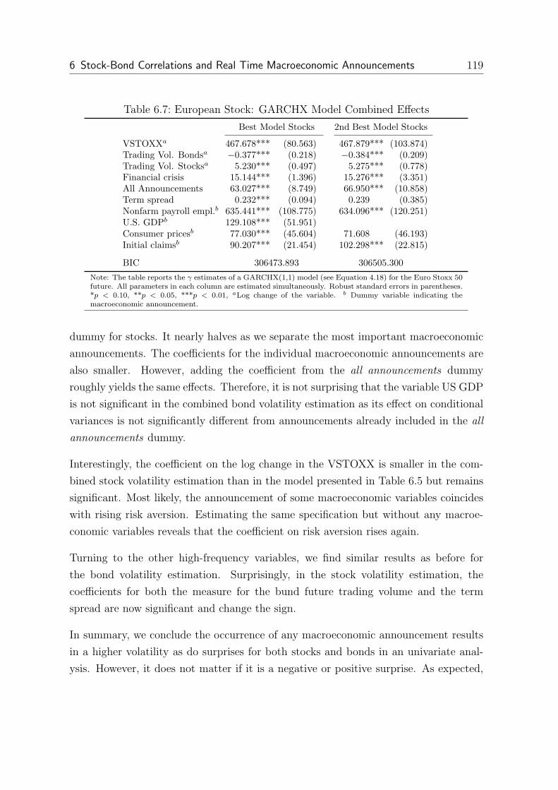
6 Stock-Bond Correlations and Real Time Macroeconomic Announcements 119
Table 6.7: European Stock: GARCHX Model Combined Effects
Best Model Stocks 2nd Best Model Stocks
VSTOXXa 467.678*** (80.563) 467.879*** (103.874)Trading Vol. Bondsa −0.377*** (0.218) −0.384*** (0.209)Trading Vol. Stocksa 5.230*** (0.497) 5.275*** (0.778)Financial crisis 15.144*** (1.396) 15.276*** (3.351)All Announcements 63.027*** (8.749) 66.950*** (10.858)Term spread 0.232*** (0.094) 0.239 (0.385)Nonfarm payroll empl.b 635.441*** (108.775) 634.096*** (120.251)U.S. GDPb 129.108*** (51.951)Consumer pricesb 77.030*** (45.604) 71.608 (46.193)Initial claimsb 90.207*** (21.454) 102.298*** (22.815)
BIC 306473.893 306505.300
Note: The table reports the γ estimates of a GARCHX(1,1) model (see Equation 4.18) for the Euro Stoxx 50future. All parameters in each column are estimated simultaneously. Robust standard errors in parentheses.*p < 0.10, **p < 0.05, ***p < 0.01, aLog change of the variable. b Dummy variable indicating themacroeconomic announcement.
dummy for stocks. It nearly halves as we separate the most important macroeconomic
announcements. The coefficients for the individual macroeconomic announcements are
also smaller. However, adding the coefficient from the all announcements dummy
roughly yields the same effects. Therefore, it is not surprising that the variable US GDP
is not significant in the combined bond volatility estimation as its effect on conditional
variances is not significantly different from announcements already included in the all
announcements dummy.
Interestingly, the coefficient on the log change in the VSTOXX is smaller in the com-
bined stock volatility estimation than in the model presented in Table 6.5 but remains
significant. Most likely, the announcement of some macroeconomic variables coincides
with rising risk aversion. Estimating the same specification but without any macroe-
conomic variables reveals that the coefficient on risk aversion rises again.
Turning to the other high-frequency variables, we find similar results as before for
the bond volatility estimation. Surprisingly, in the stock volatility estimation, the
coefficients for both the measure for the bund future trading volume and the term
spread are now significant and change the sign.
In summary, we conclude the occurrence of any macroeconomic announcement results
in a higher volatility as do surprises for both stocks and bonds in an univariate anal-
ysis. However, it does not matter if it is a negative or positive surprise. As expected,

6.3 Empirical Results 120
higher risk aversion results in higher volatility even when taking into account various
macroeconomic announcements. Corroborating the results of the previous chapters,
we also find that a multivariate analysis that includes multiple exogenous variables is
preferable as the effects partly overlap.
6.3.3 The GDCCX model
We now turn to the estimation of conditional stock-bond correlations employing a
GDCCX model (see section 2.4.2) with exogenous variables. Volatility is modeled with
a GARCHX model as shown in Tables 6.6 and 6.7 for bonds and stocks, respectively.
At first, we are interested in the separate effects of variables on correlations. Results
can be found in the left panel in Table 6.8. Similar to previous studies (Connolly et al.,
2005, 2007), we see that risk aversion - as measured by the change in the VSTOXX index
- is an important driver of conditional correlations. As risk aversion rises, conditional
correlations between stocks and bonds fall. However, both the term spread and the
dummy for the financial crisis do not significantly influence conditional correlations
which contrasts with our findings on volatility. Yet, another very important driver of
conditional correlations are macroeconomic announcements. The effect of the dummy
that covers all announcements is negative and significant. The model that uses this
dummy fits the data best according to the BIC. Lastly, we find that both higher trading
volume in stocks and in bonds result in lower conditional correlations. This confirms
findings of Bansal et al. (2010). They argue that higher bond and stock trading volume
is associated with a high-stress regime that exhibits lower correlations between stocks
and bonds. However, it might also be a result of higher trading volume coinciding with
higher risk aversion or macroeconomic announcements.
Therefore, next, we estimate conditional correlations employing all previous variables
simultaneously. Results are shown in right panel in Table 6.8. The effect of trading
volume is now smaller but still significant. Moreover, the coefficient for the dummy
on the financial crisis is now significant and positive, i.e. conditional correlations rose
during the financial crisis. This is remarkable as other studies (Andersen et al., 2007;
Ilmanen, 2003) demonstrate that stock bond correlations tend to rise in expansions but
decrease in recessions. Yet, these studies cover different time periods. Again, there
is no effect of the term spread on correlations and the coefficients of the change in

6 Stock-Bond Correlations and Real Time Macroeconomic Announcements 121
Table 6.8: European Bond and Stock Correlations in a GDCCX Model: Effect of HighFrequency Variables
SeparateEstimations
CombinedEstimation
VSTOXXa −64.116* (36.201) −65.760*** (14.184)Trading Vol. Bondsa −0.374*** (0.090) −0.216*** (0.059)Trading Vol. Stocksa −0.374*** (0.108) −0.273*** (0.087)All announcements −10.253*** (1.325) −12.298*** (1.285)Financial crisis 0.082 (0.104) 0.353*** (0.118)Term spread −0.009 (0.007) −0.008 (0.023)
Note: The table reports the c estimates of a GDCCX model (see Equation 2.11) for European bonds andstocks. We model volatility with a GARCHX (1,1) model (see Equation 4.18 and Table 6.6 and 6.7). In theleft panel, we run separate estimations for each c presented whereas in the right panel, all parameters areestimated simultaneously. Robust standard errors in parentheses.*p < 0.10, **p < 0.05, ***p < 0.01, aLog change of the variable
the VSTOXX index and on the dummy for the macroeconomic announcements remain
negative and significant confirming our previous results.
We want to explore the effect of the specific macroeconomic announcements in more
detail. Therefore, we repeat our previous estimation and consecutively add each an-
nouncement (one at a time). We employ all variables from above except the term
spread as the coefficient has never been significant. Thus, a single estimation includes
the respective macroeconomic announcement, VSTOXX, Trading Vol. Bonds, Trading
Vol. Stocks, the all announcements dummy, and the Financial Crisis Dummy as exoge-
nous variables. Table 6.9 contains the estimated c coefficients and standard errors. We
analyze two different variables for each announcement: a dummy variable that takes
the value 1 at the time of the announcement and 0 else as well as the absolute value of
the announcement surprise.28
Table 6.9 highlights the importance of each single macroeconomic announcement: al-
most all coefficients are significant. Furthermore, we find that in almost all estimations
the coefficient on risk aversion is negative and significant. We conclude that even after
taking account for all kinds of macroeconomic news, risk aversion still drives conditional
stock-bond correlations on a high-frequency level.
28Thus, we take another approach than Christiansen and Ranaldo (2007) as we do not use the actualvalue of the surprise as variable. A preliminary analysis including the actual value, the absolutevalue, and the dummy variable shows that, according to the BIC, models that employ the actualvalue of the macroeconomic announcements do not fit the data in almost all cases. The BIC valuesof this preliminary analysis are presented in Table 6.13 in appendix 6.A2.
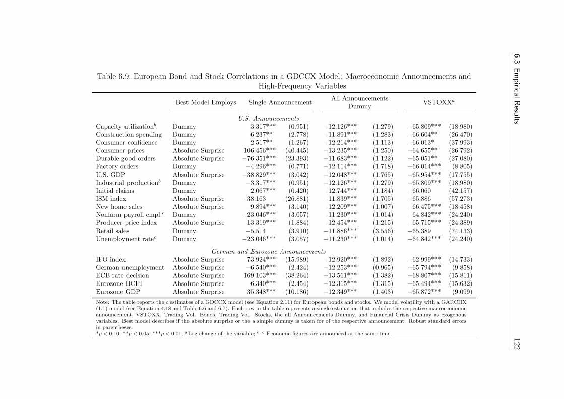
6.3
Empirica
lResu
lts122
Table 6.9: European Bond and Stock Correlations in a GDCCX Model: Macroeconomic Announcements andHigh-Frequency Variables
Best Model Employs Single AnnouncementAll Announcements
DummyVSTOXXa
U.S. Announcements
Capacity utilizationb Dummy −3.317*** (0.951) −12.126*** (1.279) −65.809*** (18.980)Construction spending Dummy −6.237** (2.778) −11.891*** (1.283) −66.604** (26.470)Consumer confidence Dummy −2.517** (1.267) −12.214*** (1.113) −66.013* (37.993)Consumer prices Absolute Surprise 106.456*** (40.445) −13.235*** (1.250) −64.655** (26.792)Durable good orders Absolute Surprise −76.351*** (23.393) −11.683*** (1.122) −65.051** (27.080)Factory orders Dummy −4.296*** (0.771) −12.114*** (1.718) −66.014*** (8.805)U.S. GDP Absolute Surprise −38.829*** (3.042) −12.048*** (1.765) −65.954*** (17.755)Industrial productionb Dummy −3.317*** (0.951) −12.126*** (1.279) −65.809*** (18.980)Initial claims Dummy 2.067*** (0.420) −12.744*** (1.184) −66.060 (42.157)ISM index Absolute Surprise −38.163 (26.881) −11.839*** (1.705) −65.886 (57.273)New home sales Absolute Surprise −9.894*** (3.140) −12.209*** (1.007) −66.475*** (18.458)Nonfarm payroll empl.c Dummy −23.046*** (3.057) −11.230*** (1.014) −64.842*** (24.240)Producer price index Absolute Surprise 13.319*** (1.884) −12.454*** (1.215) −65.715*** (24.389)Retail sales Dummy −5.514 (3.910) −11.886*** (3.556) −65.389 (74.133)Unemployment ratec Dummy −23.046*** (3.057) −11.230*** (1.014) −64.842*** (24.240)
German and Eurozone Announcements
IFO index Absolute Surprise 73.924*** (15.989) −12.920*** (1.892) −62.999*** (14.733)German unemployment Absolute Surprise −6.540*** (2.424) −12.253*** (0.965) −65.794*** (9.858)ECB rate decision Absolute Surprise 169.103*** (38.264) −13.561*** (1.382) −68.807*** (15.811)Eurozone HCPI Absolute Surprise 6.340*** (2.454) −12.315*** (1.315) −65.494*** (15.632)Eurozone GDP Absolute Surprise 35.348*** (10.186) −12.349*** (1.403) −65.872*** (9.099)
Note: The table reports the c estimates of a GDCCX model (see Equation 2.11) for European bonds and stocks. We model volatility with a GARCHX(1,1) model (see Equation 4.18 and Table 6.6 and 6.7). Each row in the table represents a single estimation that includes the respective macroeconomicannouncement, VSTOXX, Trading Vol. Bonds, Trading Vol. Stocks, the all Announcements Dummy, and Financial Crisis Dummy as exogenousvariables. Best model describes if the absolute surprise or the a simple dummy is taken for of the respective announcement. Robust standard errorsin parentheses.*p < 0.10, **p < 0.05, ***p < 0.01, aLog change of the variable; b, c Economic figures are announced at the same time.

6 Stock-Bond Correlations and Real Time Macroeconomic Announcements 123
According to the BIC,29 the most important announcement for conditional correlations
are the nonfarm payroll and the US unemployment rate announcement that are always
released at the same time. That matches our results from the volatility equation.
Moreover, the ECB interest rate decision as well as the US consumer prices are almost
as important as nonfarm payrolls.
The second column in Table 6.9 reports whether the best model according to the BIC
either includes the dummy variable of the announcement or the absolute value of the
announcement-surprise. Although Christiansen and Ranaldo (2007) show that the oc-
currence of an announcement by itself influences conditional correlations, we notice
that the absolute surprise of an announcement sometimes drives correlations even more.
That is true for all announcements in the Eurozone as well as the inflation (consumer
and producer prices) and the GDP release in the US. Furthermore, for all announce-
ments that are released at the same time,30 we favor the model with an announcement
dummy. That points towards our measure for the surprise being imprecise in case of si-
multaneously released announcements since the actual surprise might be a combination
of the surprises of both announcements.
Interestingly, the signs of the coefficients vary among announcements. In order to
calculate the total effect of a specific announcement the coefficient of the respective
announcement and of the all announcements dummy must be added. Most releases
indicating real economic shocks (i.e. GDP, unemployment, surveys of activity etc.)
have a negative effect on conditional correlations in the US. However, for consumer
prices in the US and in the Eurozone as well as for the ECB rate decision, we find
that conditional correlations rise the more the larger the surprise. Yet, in case of
no surprise, the general effect of all macroeconomic announcements dominates and
conditional correlations fall as well.
This fits well theoretical models in which equity prices are determined by the present
value of future cash flows.31 Furthermore, if monetary policy is strictly anti-inflationary,
market participants will assume that higher inflation makes future interest rate rises
more likely and vice versa. Hence, interest rate and inflation announcements should
influence the prices of bonds and stocks via the discount rate in the same way resulting
29Table 6.14 in appendix 6.A2 displays the BIC values for Table 6.9.30The announcement of nonfarm payrolls and unemployment rate as well as the release of the industrial
production and capacity utilization are the same time.31An example might be the Gordon (1959) growth model.

6.3 Empirical Results 124
in rising conditional correlations. By contrast, if an announcement such as GDP or
the unemployment rate conveys information about future cash flows, conditional cor-
relations between bonds and stocks should fall. Another interpretation is that these
announcements trigger a flight-to-quality. Interestingly, in Eurozone the announcement
of the IFO index and the GDP result in rising conditional correlations. Probably, in
the Eurozone these announcements are more informative for future interest rates than
for future cash flows.
Table 6.10: European Bonds and Stock Correlations in a GDCCX Model:Macroeconomic Announcements during Recession and Expansion
Best ModelAnnouncement in
RecessionAnnouncement in
Expansion
U.S. Announcements
Capacity utilizationa Dummy −7.125 (9.396) −21.857* (11.719)Construction spending Dummy −13.446*** (2.574) −17.318*** (2.094)Consumer confidence Dummy −6.434*** (0.653) −15.747*** (1.811)Consumer prices Abs. Surpr. 68.510*** (13.766) 48.527*** (10.324)Durable good orders Abs. Surpr. −68.884*** (10.145) −211.228*** (22.215)Factory orders Abs. Surpr. −58.861** (25.070) −121.827** (48.871)U.S. GDP Dummy 2.684*** (0.736) −26.586*** (3.546)Industrial productiona Dummy −7.125 (9.396) −21.857* (11.719)Initial claims Dummy −1.761*** (0.573) −16.108*** (2.731)ISM index Abs. Surpr. −116.103*** (7.511) −124.382*** (34.656)New home sales Abs. Surpr. −33.415*** (9.339) −59.784*** (11.411)Nonfarm payroll empl.b Dummy −31.129** (12.864) −33.463*** (3.286)Producer price index Dummy −12.599*** (1.958) −6.855 (6.859)Retail sales Dummy −24.503*** (3.846) −12.674*** (1.745)Unemployment rateb Dummy −31.129** (12.864) −33.463*** (3.286)
German and Eurozone Announcements
IFO index Abs. Surpr. 73.721*** (22.421) 19.617*** (5.990)German unemployment Abs. Surpr. 65.188* (37.665) −129.100** (50.584)ECB rate decision Abs. Surpr. 79.795*** (22.929) −0.133 (0.254)Eurozone HCPI Dummy −5.209 (3.664) −14.170*** (4.700)Eurozone GDP Dummy 13.917*** (3.072) −12.972* (7.883)
Note: The table reports the c estimates of a DCCX(1,1) model (see Equation 2.11) for European bonds andstocks. We model volatility with a GARCHX(1,1) model (see Equation 4.18 and Table 6.6 and 6.7). Eachrow in the table represents a single estimation that includes the respective macroeconomic announcement,VSTOXX, Trading Vol. Bonds, and Trading Vol. Stocks as exogenous variables. Best model describes ifthe absolute surprise or the a simple dummy is taken for of the respective announcement. Robust standarderrors in parentheses.*p < 0.10, **p < 0.05, ***p < 0.01, a, b Economic figures are announced at the same time.
Previous studies have shown that announcement effects can vary with the business
cycle (Andersen et al., 2007; Boyd et al., 2005; Christiansen and Ranaldo, 2007). On
average, macroeconomic announcements should not drive conditional correlations as the
effects should cancel out over the full cycle. In order to further investigate the influence

6 Stock-Bond Correlations and Real Time Macroeconomic Announcements 125
of the business cycle, we repeat the analysis but split the announcement variables in
two parts: a recession and an expansion variable.32 We define the beginning of the
recession as the time when market participants learn that the European GDP growth
turned from positive to negative and the end when GDP growth turns positive again.33
Furthermore, we drop the all announcements dummy and the dummy for the financial
crisis to clearly separate the effects of recession and expansion. Table 6.10 reports
the results. The analysis confirms that the sign of most coefficients does not differ
between periods of recession and periods of expansion. Moreover, the models that do
not distinguish between contraction and expansion periods fit the data better according
to the BIC.34
There are several possible explanations for these results. First, since our sample covers
only four years, we at most cover one full cycle. This period might be too short for a
valid analysis of the business cycle. Second, the shock of the financial crisis might last
longer than the effects on the real economy. Therefore, we re-estimate our previous
analysis but assume that the recession lasted at least until the end of our sample.
However, results are qualitatively unchanged. Third, numerous definitions for the exact
start and end of a recession can be applied which might also change our results. Fourth,
the sample period of Andersen et al. (2007) runs from 1994 to 2002, Christiansen and
Ranaldo (2007) cover the years 1988 to 2003 so that the years after the burst of the
dot-com bubble are not covered. Possibly, there has been a structural break with
market participants becoming more risk averse. Accordingly, announcements cause
conditional stock-bond correlations to become more negative, and a flight-to-quality
can be observed more often. However, a longer sample will be necessary to ultimately
answer these questions.
32The variables that measure announcements in a recession take the value of the announcement duringa recession and 0 else. The variables that measure announcements in an expansion take the valueof the announcement during an expansion and 0 else.
33According to our definition the economy is contracting from 8/14/2008 to 11/13/2009.34Table 6.15 in appendix 6.A2 displays the BIC values for Table 6.10.

6.4 Summary 126
6.4 Summary
In this chapter, we analyze the influence of risk aversion, macroeconomic announce-
ments, and other variables on high-frequency correlations between bonds and stocks
in the Eurozone. We find that both risk aversion and macroeconomic announcements
separately drive conditional correlations and variances of bonds and stocks in the Eu-
rozone. Conditional correlations fall as risk aversion rises even when controlling for
the influence of macroeconomic announcements and the influence of these variables
on volatility. Interestingly, the additional effects of the financial crisis on conditional
correlations are only small. For most macroeconomic announcements, the absolute
value of the surprise is of higher importance for correlations than the mere occurrence
of the announcement. We get similar results when analyzing stock and bond volatil-
ity. Moreover, macroeconomic news result in falling conditional correlations. Yet, the
publication of news concerning future interest rates or the release of inflation figures
moves bond and stock prices in the same direction. These news convey information
concerning future cash-flows or trigger a flight-to-quality. We do not find that the ef-
fect of economic announcements on conditional correlations changes during the cycle
as splitting the effects of the macroeconomic variables between expansion and recession
does not alter the results and offer several explanations. However, we cannot assess if
this represents a structural break in the data or is caused by the particular period we
cover in our dataset. Comparing the effects of Eurozone and US announcements, we
find evidence that the most important announcements in the US are news on nonfarm
payroll employments while in Europe the announcement of the ECB rates receives most
attention.
Hence, the analysis of high-frequency data corroborates the findings of the previous
chapter: A sensible approach to incorporate exogenous information in correlation mod-
els should explicitly allow for exogenous effects in both volatilities and correlations.
Moreover, the advantage of multivariate exogenous variables models as compared to
models allowing for just one exogenous driver has again been underlined.
Our results have also important implications for both investors as well as risk managers.
We demonstrate that the stock-bond correlation falls and, hence, the diversification of
a stock-bond portfolio benefits in times of rising risk aversion i.e. at the time when
diversification benefits are needed most. This is an important result as it is well known
that stock-stock correlations rise in times of market turbulence.

6 Stock-Bond Correlations and Real Time Macroeconomic Announcements 127
6.A Appendix
6.A1 GARCHX Modell: Bayesian Information Criterion
Table 6.11: European Bonds: GARCHX Model - Bayesian Information Criterion
High-FrequencyVariables
VSTOXXa 47556.676Trading Vol. Bondsa 47600.873Trading Vol. Stocksa 47170.859Financial crisis 47224.536Term spread 47474.874
AnnouncementDummyb
Absolute Surprisec Surprise
All announcements 43815.434
U.S. Announcements
Capacity utilizationd 47586.567 47585.911 47600.680Construction spending 47298.972 47379.348 47588.441Consumer confidence 47563.415 47560.135 47598.967Consumer prices 47380.324 47428.147 47600.793Durable good orders 47452.321 47467.049 47600.804Factory orders 47562.629 47563.818 47592.100U.S. GDP 47486.977 47494.600 47587.426Industrial productiond 47586.567 47586.027 47598.557Initial claims 46781.375 46843.125 47598.075ISM index 47305.032 47301.092 47596.084New home sales 47564.550 47561.475 47600.412Nonfarm payroll empl.e 45494.565 45501.870 47598.039Producer price index 47277.226 47282.450 47596.340Retail sales 47095.341 47080.820 47598.023Unemployment ratee 45494.565 45876.565 47567.510
German and Eurozone Announcements
IFO index 47345.566 47342.778 47572.583German unemployment 47596.058 47596.058 47592.831ECB rate decision 47355.989 47342.322 47374.050Eurozone HCPI 47585.783 47570.453 47582.578Eurozone GDP 47592.017 47597.998 47597.102
Note: The table reports the Bayesian Information Criterion of a GARCHX(1,1) model (see Equation 4.18) for theBund future. Coefficients are reported in table 6.4. We run separate estimations for each model presented. Thebest model for each macroeconomic variable is indicated in bold.aLog change of the variable; bAnnouncement Dummy is an indicator function that takes on the value 1 if there is anannouncement and 0 otherwise; cAbsolute value of the surprise is employed. d, e Economic figures are announcedat the same time.
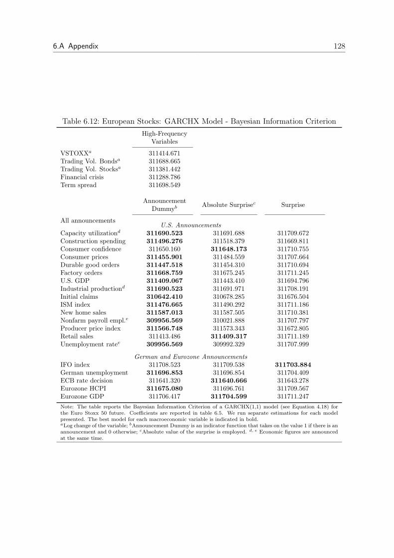
6.A Appendix 128
Table 6.12: European Stocks: GARCHX Model - Bayesian Information Criterion
High-FrequencyVariables
VSTOXXa 311414.671Trading Vol. Bondsa 311688.665Trading Vol. Stocksa 311381.442Financial crisis 311288.786Term spread 311698.549
AnnouncementDummyb
Absolute Surprisec Surprise
All announcementsU.S. Announcements
Capacity utilizationd 311690.523 311691.688 311709.672Construction spending 311496.276 311518.379 311669.811Consumer confidence 311650.160 311648.173 311710.755Consumer prices 311455.901 311484.559 311707.664Durable good orders 311447.518 311454.310 311710.694Factory orders 311668.759 311675.245 311711.245U.S. GDP 311409.067 311443.410 311694.796Industrial productiond 311690.523 311691.971 311708.191Initial claims 310642.410 310678.285 311676.504ISM index 311476.665 311490.292 311711.186New home sales 311587.013 311587.505 311710.381Nonfarm payroll empl.e 309956.569 310021.888 311707.797Producer price index 311566.748 311573.343 311672.805Retail sales 311413.486 311409.317 311711.189Unemployment ratee 309956.569 309992.329 311707.999
German and Eurozone Announcements
IFO index 311708.523 311709.538 311703.884
German unemployment 311696.853 311696.854 311704.409ECB rate decision 311641.320 311640.666 311643.278Eurozone HCPI 311675.080 311696.761 311709.567Eurozone GDP 311706.417 311704.599 311711.247
Note: The table reports the Bayesian Information Criterion of a GARCHX(1,1) model (see Equation 4.18) forthe Euro Stoxx 50 future. Coefficients are reported in table 6.5. We run separate estimations for each modelpresented. The best model for each macroeconomic variable is indicated in bold.aLog change of the variable; bAnnouncement Dummy is an indicator function that takes on the value 1 if there is anannouncement and 0 otherwise; cAbsolute value of the surprise is employed. d, e Economic figures are announcedat the same time.
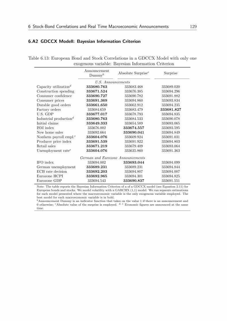
6 Stock-Bond Correlations and Real Time Macroeconomic Announcements 129
6.A2 GDCCX Modell: Bayesian Information Criterion
Table 6.13: European Bond and Stock Correlations in a GDCCX Model with only oneexogenous variable: Bayesian Information Criterion
AnnouncementDummyb
Absolute Surprisec Surprise
U.S. Announcements
Capacity utilizationd 333680.763 333683.468 333689.020Construction spending 333671.524 333676.385 333694.296Consumer confidence 333690.727 333690.782 333691.882Consumer prices 333691.369 333694.860 333693.834Durable good orders 333661.650 333662.912 333694.235Factory orders 333684.659 333683.479 333681.827
U.S. GDP 333677.017 333678.793 333694.835Industrial productiond 333680.763 333684.533 333690.078Initial claims 333649.333 333654.589 333693.065ISM index 333676.002 333674.557 333693.595New home sales 333692.664 333690.041 333694.849Nonfarm payroll empl.e 333604.076 333609.924 333691.031Producer price index 333691.539 333691.922 333694.803Retail sales 333671.219 333679.409 333693.064Unemployment ratee 333604.076 333635.860 333691.363
German and Eurozone Announcements
IFO index 333694.002 333693.044 333694.099German unemployment 333689.231 333689.231 333694.844ECB rate decision 333692.203 333694.807 333694.007Eurozone HCPI 333692.965 333694.301 333694.825Eurozone GDP 333694.543 333690.837 333691.551
Note: The table reports the Bayesian Information Criterion of a of a GDCCX model (see Equation 2.11) forEuropean bonds and stocks. We model volatility with a GARCHX (1,1) model. We run separate estimationsfor each model presented where the macroeconomic variable is the only exogenous variable employed. Thebest model for each macroeconomic variable is in bold.bAnnouncement Dummy is an indicator function that takes on the value 1 if there is an announcement and0 otherwise; cAbsolute value of the surprise is employed. d, e Economic figures are announced at the sametime.

6.A Appendix 130
Table 6.14: European Bond and Stock Correlations in a GDCCX Model: BayesianInformation Criterion
AnnouncementDummyb
Absolute Surprisec
U.S. Announcements
Capacity utilizationd 333332.064 333332.354Construction spending 333328.547 333330.654Consumer confidence 333332.366 333332.456Consumer prices 333323.348 333310.478
Durable good orders 333317.544 333314.779
Factory orders 333331.316 333331.406U.S. GDP 333330.208 333328.748
Industrial productiond 333332.064 333332.431Initial claims 333331.841 333332.547ISM index 333328.541 333326.721
New home sales 333332.815 333332.566
Nonfarm payroll empl.e 333285.720 333289.240Producer price index 333332.477 333332.192
Retail sales 333329.591 333331.390Unemployment ratee 333285.720 333302.033
German and Eurozone Announcements
IFO index 333317.464 333314.608
German unemployment 333332.714 333332.713
ECB rate decision 333307.032 333305.570
Eurozone HCPI 333332.900 333332.576
Eurozone GDP 333332.698 333331.691
Note: The table reports the Bayesian Information Criterion of a of a GDCCXmodel (see Equation 2.11) for European bonds and stocks. We model volatilitywith a GARCHX (1,1) model. Coefficients are reported in table 6.9. We runseparate estimations for each model presented. Each model includes the respec-tive macroeconomic announcement, VSTOXX, Trading Vol. Bonds, Trading Vol.Stocks, the all Announcements Dummy, and Financial Crisis Dummy as exoge-nous variables. The best model for each macroeconomic variable is indicated inbold.bAnnouncement Dummy is an indicator function that takes on the value 1 if thereis an announcement and 0 otherwise; cAbsolute value of the surprise is employed.d, e Economic figures are announced at the same time.
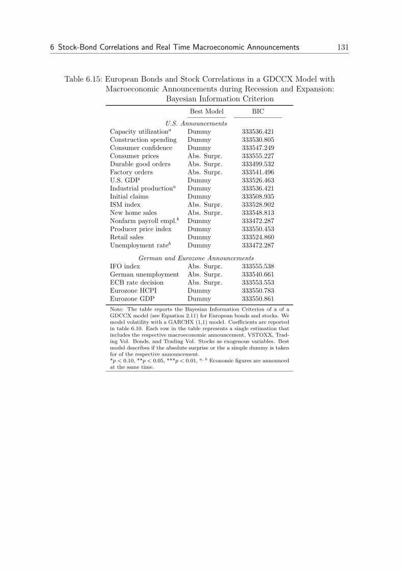
6 Stock-Bond Correlations and Real Time Macroeconomic Announcements 131
Table 6.15: European Bonds and Stock Correlations in a GDCCX Model withMacroeconomic Announcements during Recession and Expansion:
Bayesian Information Criterion
Best Model BIC
U.S. Announcements
Capacity utilizationa Dummy 333536.421Construction spending Dummy 333530.805Consumer confidence Dummy 333547.249Consumer prices Abs. Surpr. 333555.227Durable good orders Abs. Surpr. 333499.532Factory orders Abs. Surpr. 333541.496U.S. GDP Dummy 333526.463Industrial productiona Dummy 333536.421Initial claims Dummy 333508.935ISM index Abs. Surpr. 333528.902New home sales Abs. Surpr. 333548.813Nonfarm payroll empl.b Dummy 333472.287Producer price index Dummy 333550.453Retail sales Dummy 333524.860Unemployment rateb Dummy 333472.287
German and Eurozone Announcements
IFO index Abs. Surpr. 333555.538German unemployment Abs. Surpr. 333540.661ECB rate decision Abs. Surpr. 333553.553Eurozone HCPI Dummy 333550.783Eurozone GDP Dummy 333550.861
Note: The table reports the Bayesian Information Criterion of a of aGDCCX model (see Equation 2.11) for European bonds and stocks. Wemodel volatility with a GARCHX (1,1) model. Coefficients are reportedin table 6.10. Each row in the table represents a single estimation thatincludes the respective macroeconomic announcement, VSTOXX, Trad-ing Vol. Bonds, and Trading Vol. Stocks as exogenous variables. Bestmodel describes if the absolute surprise or the a simple dummy is takenfor of the respective announcement.*p < 0.10, **p < 0.05, ***p < 0.01, a, b Economic figures are announcedat the same time.


7 Summary and Conclusion 133
7 Summary and Conclusion
In this dissertation, the influence of exogenous variables on conditional correlations is
investigated. First, it is examined how to model the possible effects of exogenous vari-
ables. Various correlation models proposed by the previous literature are introduced:
the DCC, the DCCX, the STCC, and the Sheppard model. In a next step, the DCCX
model is generalized and the GDCCX model is proposed. In that model exogenous
variables can drive conditional correlations in different ways. In addition, it is guar-
anteed that the exogenous variables affect conditional covariances but not conditional
variances.
Following the investigation of the finite sample properties of all estimators, the models
are compared. A simulation experiment is conducted, and estimated correlations are
compared with the true conditional correlations. In order to ensure that the exogenous
variable has some forecast ability, the lagged conditional correlations are employed
as exogenous variable. The results show that the GDCCX model uses the information
contained in the exogenous variable best as the mean absolute error is lowest for several
different settings. By contrast, the Sheppard model performs even worse than a simple
DCC model that does not use any exogenous data. Moreover, by accounting for the
influence of exogenous variables it is possible to reduce the mean absolute error by about
two thirds. This further strengthens the argument for employing exogenous variables
when conditional correlations are sought to be explained.
Going forward, the models are compared to each other employing real data. As the
true conditional correlations are unknown, the testing criteria developed by Engle and
Colacito (2006) are used to compare the models. The DCC, the DCCX, and the GD-
CCX model significantly outperform the STCC and the Sheppard model. In addition,
the benefits of using the GDCCX model rise as the number of time series included
increases. Since real bond market data is analyzed, the interpretation of the results is
meaningful. The results indicate that conditional correlation between government and
corporate bonds fall as risk aversion increases, a clear sign of a flight-to-quality. This is
good news from a portfolio management perspective as diversification benefits remain
intact in times of crisis.

134
Up to this point, it is assumed that conditional variances are not influenced by the ex-
ogenous variables and can be explained with a GARCH model. However, several recent
studies suggest that this assumption may not hold. Possible consequences of this mis-
specification of the variance equation on the estimation of conditional correlations are
examined. First, a theoretical model of Forbes and Rigobon (2002) is consulted. It is
demonstrated that a change in the conditional variance of one of the time series caused
by an exogenous variable can result in higher conditional correlations between that
time series and a second one although the dependence structure does not change. Yet,
this result is based on assumptions concerning the transmission and the specific vari-
ance of the second time series. Second, a simulation study is carried out to investigate
the estimation of conditional correlations if conditional variances but not correlations
are driven by the exogenous variable. It is shown that the influence of the exogenous
variable on the conditional correlation cannot be distinguished from the the exogenous
variable driving the dependency structure in certain settings. However, once the influ-
ence of the exogenous variable on conditional variances is modeled with a GARCHX
model, the effect of the exogenous variable on conditional correlations and variances is
correctly specified in all settings. Going forward, conditional variances are estimated
with the GARCHX model and conditional correlations with the GDCCX model.
Employing the econometric framework developed in the previous parts, several em-
pirical research questions are addressed. First, the effects of risk aversion, market
turbulence, and the business cycle on conditional correlations between weekly Euro-
pean bonds and between weekly European stock returns are examined. In a first step,
the influence of each variable is analyzed separately. In a second step, all variables
are included simultaneously. That allows investigating whether the effect of one vari-
able is dominating and whether the effects are persistent after taking account for other
exogenous variables. The results indicate that, while both GDP growth and market
turbulences influence conditional correlations, the effect of risk aversion vanishes once
the other variables are included in the analysis. As expected, the impact of market
turbulences is most pronounced in the peripheral countries. The empirical results also
show that there is an important difference between bonds and stocks. While market
turbulences result in decreasing conditional correlations between international bond
markets, conditional correlations between stock markets rise strongly. These are clear
signs of contagion in the stock market diminishing the diversification within a stock
market portfolio. Diversification is further impeded by negative GDP growth which
results in higher stock return correlations. By contrast, diversification benefits remain

7 Summary and Conclusion 135
intact in a bond portfolio since lower GDP growth coincides with decreasing bond
return correlations.
In the final empirical analysis, the sample frequency is substantially increased. The
dataset adopted to examine intra-day stock-bond correlations consists of 5 minute
stock and bond returns. Specifically, the effects of risk aversion and macroeconomic an-
nouncements both in Europe and in the US on stock-bond correlations are investigated.
Since volatility can also be influenced by exogenous variables, conditional correlations
are estimated using a GDCCX model and conditional variances are modeled using a
GARCHX model. Estimating the effects of the announcements on both conditional
correlations and variances is particularly important since previous studies found that
volatility increases considerably at the time of announcements. The results indicate
that both risk aversion and macroeconomic announcements are important drivers of
conditional stock-bond correlations. Conditional correlations fall as risk aversion rises.
While previous studies found that the mere occurrence of an announcement matters
most for correlations, the results demonstrate that the absolute value of the announce-
ment surprise is even more important. This is also true for stock volatility. Generally,
news on nonfarm payroll employments in the US and the announcement of the ECB
rates drive conditional correlations most. The publication of almost all announcements
results in falling conditional correlations. An exception are interest rates and infla-
tion announcements. These news drive conditional correlations upwards. It can be
concluded that these figures convey information concerning future cash-flows or that
they trigger a flight-to-quality. Furthermore, the results show that the effect of the
macroeconomic variables is not sensitive to the business cycle.
The results of this thesis have important implications for both academics and practition-
ers. It is highlighted that diversification benefits remain intact in a portfolio consisting
of stocks and bonds or of different bond sectors. Moreover, a powerful econometric
framework that is particularly suited for the empirical analysis of influencing factors
of conditional correlations has been developed. The combination of the GDCCX and
the GARCHX model allows for the simultaneous analysis of the effects of one or more
exogenous variables on conditional variances and correlations. Moreover, the effects of
exogenous variables on variances can be distinguished from those on the dependency
structure. Therefore, this econometric framework is especially useful if a researcher is
unsure whether the exogenous variables drive conditional variances, conditional corre-
lations or both.

136
In the empirical analysis, the focus lies on the effects of risk aversion and macroeco-
nomic figures on correlations between different asset classes. Assessing the correlations
between different asset classes is important both for portfolio and risk management.
The econometric framework can easily be applied to various research areas. For exam-
ple, the CAPM postulates that the expected return of a security is a function of its
correlation with the market. Remaining questions are whether price changes are caused
by changes of the correlation of the security with the market and what the determinants
of this correlation change are. Moreover, changes in correlations between markets in
different countries are often associated with the notion of contagion. The econometric
framework presented in this thesis can be employed to reveal triggers of correlation
changes. Prospective studies might also investigate the ability of exogenous variables
to forecast changes in correlations. This is especially interesting for applied portfolio
and risk management, as exogenous variables might improve the forecasting perfor-
mance of DCC models in this context. In practice, a forecasted increase in conditional
correlations might induce hedging of some parts of a portfolio.
Yet, there are some interesting model extensions that remain for future research. While
the GDCCX model is based on the assumption that the effect of the exogenous variable
on Qt is linear, that is not necessarily true. Another reasonable assumption is that the
effect varies with the sign of the estimated conditional correlation. For example, it
might be that the absolute value of the conditional correlations is a function of the
exogenous variables. For example, the conditional correlation between two time series
increases to 1 or decreases to -1, i.e. the economic connection strengthens, with larger
values of an exogenous variable but decreases to 0 as a result of smaller values of the
exogenous variable. If that is true, the estimated c coefficient of the GDCCX model
will turn the sign depending on the conditional correlation estimated previously. Thus,
the assumption that the effect of the exogenous variable is independent of the sign of
previous estimated conditional correlations could be relaxed in further generalizations
of the model.

Bibliography 137
Bibliography
Aıt-Sahalia, Y. and M. W. Brandt (2001): “Variable Selection for Portfolio
Choice,”The Journal of Finance, 56, 1297–1351.
Albuquerque, R. and C. Vega (2009): “Economic News and International Stock
Market Co-movement,”Review of Finance, 13, 401–465.
Andersen, T. G. and T. Bollerslev (1997): “Intraday Periodicity and Volatility
Persistence in Financial Markets,” Journal of Empirical Finance, 4, 115–158.
——— (1998): “Deutsche Mark-Dollar Volatility: Intraday Activity Patterns, Macroe-
conomic Announcements, and Longer Run Dependencies,” The Journal of Finance,
53, 219–265.
Andersen, T. G., T. Bollerslev, F. X. Diebold, and P. Labys (2001): “The
Distribution of Realized Exchange Rate Volatility,” Journal of the American Statis-
tical Association, 96, 42–55.
Andersen, T. G., T. Bollerslev, F. X. Diebold, and C. Vega (2003): “Micro
Effects of Macro Announcements: Real-Time Price Discovery in Foreign Exchange,”
The American Economic Review, 93, 38–62.
——— (2007): “Real-time Price Discovery in Global Stock, Bond and Foreign Exchange
Markets,” Journal of International Economics, 73, 251–277.
Andersson, M. (2010): “Using Intraday Data to Gauge Financial Market Responses
to Federal Reserve and ECB Monetary Policy Decisions,” International Journal of
Central Banking, 6, 117–146.
Andersson, M., E. Krylova, and S. Vahamaa (2008): “Why Does the Cor-
relation Between Stock and Bond Returns Vary Over Time?” Applied Financial
Economics, 18, 139–151.
Ang, A. and G. Bekaert (2002): “International Asset Allocation With Regime
Shifts,”The Review of Financial Studies, 15, 1137–1187.

Bibliography 138
Aslanidis, N. and C. Christiansen (2010): “Smooth Transition Patterns in the
Realized Stock Bond Correlation,” CREATES Research Paper No. 2010-15.
——— (2011): “Quantiles of the Realized Stock-Bond Correlation,” SSRN Working
Paper.
Aslanidis, N., D. R. Osborn, and M. Sensier (2010): “Co-movements Between
US and UK Stock Prices: The Role of Time-varying Conditional Correlations,” In-
ternational Journal of Finance and Economics, 15, 366–380.
Audrino, F. and F. Trojani (2007): “A General Multivariate Threshold GARCH
Model with Dynamic Conditional Correlations,” University of St. Gallen Discussion
Paper 2007-25.
Baele, L., G. Bekaert, and K. Inghelbrecht (2010): “The Determinants of
Stock and Bond Return Comovements,”The Review of Financial Studies, 23, 2374–
2428.
Balduzzi, P., E. J. Elton, and T. C. Green (2001): “News and Bond Prices:
Evidence from the U.S. Treasury Market,” Journal of Financial and Quantitative
Analysis, 36, 523–543.
Bali, T. G. and R. F. Engle (2010): “The Intertemporal Capital Asset Pricing
Model with Dynamic Conditional Correlations,” Journal of Monetary Economics,
57, 377–390.
Bansal, N., R. A. Connolly, and C. Stivers (2010): “Regime-Switching in Stock
and T-bond Futures Returns and Measures of Stock Market Stress,”The Journal of
Futures Markets, 30, 753–779.
Bauer, F. (2011): Dynamic Conditional Correlation Models and Portfolio Risk Man-
agement, Aachen: Shaker Verlag.
Bauer, F. and M. Missong (2008): “Dynamic Conditional Correlation Modelling -
Complexity vs. Feasibility,”Working Paper, University of Bremen.
Baur, D. G. and B. M. Lucey (2009): “Flights and Contagion - An Empirical
Analysis of Stock-Bond Correlation,” Journal of Financial Stability, 5, 339–352.
Bauwens, L., S. Laurent, and J. V. K. Rombouts (2006): “Multivariate GARCH
Models: A Survey,” Journal of Applied Econometrics, 21, 79–109.

Bibliography 139
Bera, A. K. and S. Kim (2002): “Testing Constancy of Correlation and Other
Specifications of the BGARCH Model with an Application to International Equity
Returns,” Journal of Empirical Finance, 9, 171–195.
Berben, R.-P. and W. J. Jansen (2005): “Comovement in International Equity
Markets: A Sectoral View,” Journal of International Money and Finance, 24, 832–
857.
——— (2009): “Bond Market and Stock Market Integration in Europe: A Smooth
Transition Approach,”Applied Economics, 41, 3067–3080.
Billio, M. and L. Pelizzon (2003): “Contagion and Interdependence in Stock Mar-
kets: Have They Been Misdiagnosed?” Journal of Economics and Business, 55,
405–426.
Bollerslev, T. (1990): “Modelling the Coherence in Short-Run Nominal Exchange
Rates: A Multivariate Generalized Arch Model,” The Review of Economics and
Statistics, 72, 498–505.
Bollerslev, T., J. Cai, and F. M. Song (2000): “Intraday Periodicity, Long
Memory Volatility, and Macroeconomic Announcement Effects in the US Treasury
Bond Market,” Journal of Empirical Finance, 7, 37–55.
Bollerslev, T. and J. M. Wooldridge (1992): “Quasi-maximum Likelihood Es-
timation and Inference in Dynamic Models with Time-varying Covariances,”Econo-
metric Reviews, 24, 143–172.
Boudt, K. and J. Zhang (2010): “Jump Robust Two Time Scale Covariance Esti-
mation and Realized Volatility Budgets,” SSRN Working Paper.
Boyd, J. H., J. Hu, and R. Jagannathan (2005): “The Stock Market’s Reaction
to Unemployment News: Why Bad News Is Usually Good for Stocks,” The Journal
of Finance, 60, 649–672.
Boyer, B. H., M. S. Gibson, and M. Loretan (1999): “Pitfalls in Tests For
Changes in Correlations,” International Finance Discussion Papers No. 597.
Brenner, R. J., R. H. Harjes, and K. F. Kroner (1996): “Another Look at
Models of the Short-Term Interest Rate,” Journal of Financial and Quantitative
Analysis, 31, 85–107.

Bibliography 140
Briere, M., A. Chapelle, and A. Szafarz (2008): “No Contagion, Only Global-
ization and Flight to Quality,” Centre Emile Bernheim Working Paper No. 08/018.
Burns, P., R. Engle, and J. Mezrich (1998): “Correlation And Volatilities of
Asynchronous Data,”The Journal of Derivatives, 5, 7–18.
Cai, Y., R. Y. Chou, and D. Li (2009): “Explaining International Stock Correla-
tions with CPI Fluctuations and Market Volatility,” Journal of Banking & Finance,
33, 2026–2035.
Cappiello, L., R. F. Engle, and K. Sheppard (2006a): “Asymmetric Dynam-
ics in the Correlations of Global Equity and Bond Returns,” Journal of Financial
Econometrics, 4, 537–572.
Cappiello, L., P. Hordahl, A. Kadareja, and S. Manganelli (2006b): “The
Impact of the Euro on Financial Markets,” ECB Working Paper Series No. 598.
Cakmakli, C. and D. van Dijk (2010): “Getting the Most Out of Macroeconomic
Information for Predicting Stock Returns and Volatility,” Tinbergen Institute Dis-
cussion Paper 2010-115/4.
Chiang, T. C., B. N. Jeon, and H. Li (2007): “Dynamic Correlation Analysis of
Financial Contagion: Evidence from Asian Markets,”Journal of International Money
and Finance, 26, 1206–1228.
Chopra, V. K. and W. T. Ziemba (1993): “The Effect of Error in Means, Variances
and Covariances on Optimal Portfolio Choice,”Journal of Portfolio Management, 19,
6–11.
Chou, R. Y. and W.-Y. Liao (2008): “Explaining the Great Decoupling of the
Equity-Bond Linkage with a Modified Dynamic Conditional Correlation Model,”
Working Paper, National Chiao Tung University.
Christiansen, C. (2007): “Volatility-Spillover Effects in European Bond Markets,”
European Financial Management, 13, 923–948.
Christiansen, C. and A. Ranaldo (2007): “Realized Bond-Stock Correlation:
Macroeconomic Announcement Effects,” The Journal of Futures Markets, 27, 439–
469.

Bibliography 141
Christiansen, C., M. Schmeling, and A. Schrimpf (2011): “A Comprehensive
Look at Financial Volatility Prediction by Economic Variables,” SSRN Working Pa-
per.
Connolly, R., C. Stivers, and L. Sun (2005): “Stock Market Uncertainty and
the Stock-Bond Return Relation,” Journal of Financial and Quantitative Analysis,
40, 161–194.
Connolly, R. A., C. Stivers, and L. Sun (2007): “Commonality in the Time-
Variation of Stock-Stock and Stock-Bond Return Comovements,” Journal of Finan-
cial Markets, 10, 192–218.
Corsetti, G., M. Pericoli, and M. Sbracia (2001): “Correlation Analysis of
Financial Contagion: What One Should Know before Running a Test,”Banca d’Italia
Working Paper 408.
——— (2005): “Some Contagion, Some Interdependence: More Pitfalls in Tests of
Financial Contagion,” Journal of International Money and Finance, 24, 1177–1199.
Corsi, F. and F. Audrino (2007): “Realized Correlation Tick-by-Tick,” University
of St. Gallen Discussion Paper 2007-02.
d’Addona, S. and A. H. Kind (2006): “International Stock–Bond Correlations in a
Simple Affine Asset Pricing Model,” Journal of Banking & Finance, 30, 2747–2765.
de Goeij, P. and W. Marquering (2004): “Modeling the Conditional Covariance
Between Stock and Bond Returns: A Multivariate GARCH Approach,” Journal of
Financial Econometrics, 2, 531–564.
Diebold, F. X. and R. S. Mariano (1995): “Comparing Predictive Accuracy,”
Journal of Business & Economic Statistics, 13, 253–263.
Embrechts, P., A. J. McNeil, and D. Straumann (2002): “Correlation and
Dependence in Risk Management: Properties and Pitfalls,” in Risk Management:
Value at Risk and Beyond, ed. by M. A. H. Dempster, Cambridge University Press.
Engle, R. F. (1982): “Autoregressive Conditional Heteroscedasticity with Estimates
of the Variance of United Kingdom Inflation,” Econometrica, 50, 987–1007.

Bibliography 142
——— (2002): “Dynamic Conditional Correlation: A Simple Class of Multivariate Gen-
eralized Autoregressive Conditional Heteroskedasticity Models,” Journal of Business
& Economic Statistics, 20, 339–350.
——— (2009): Anticipating Correlations: A New Paradigm for Risk Management,
Princeton, New Jersey: Princeton University Press.
Engle, R. F. and R. Colacito (2006): “Testing and Valuing Dynamic Correlations
for Asset Allocation,” Journal of Business & Economic Statistics, 24, 238–253.
Engle, R. F., E. Ghysels, and B. Sohn (2009): “Stock Market Volatility and
Macroeconomic Fundamentals,”Working Paper, New York University.
Engle, R. F. and A. J. Patton (2001): “What Good Is a Volatility Model?” Quan-
titative Finance, 1, 237–245.
Engle, R. F. and J. G. Rangel (2008): “The Spline-GARCH Model for Low-
Frequency Volatility and Its Global Macroeconomic Causes,”The Review of Financial
Studies, 21, 1187–1222.
Engle, R. F., N. Shephard, and K. Sheppard (2008): “Fitting and Testing Vast
Dimensional Time-varying Covariance Models,” Working Paper, New York Univer-
sity.
Engle, R. F. and K. Sheppard (2001): “Theoretical and Emprical Properties of
Dynamic Condtional Correlation Multivariate GARCH,” NBER Working Paper No.
8554.
——— (2008): “Evaluating the Specification of Covariance Models for Large Portfolios,”
Working Paper, New York University.
Erb, C. B., C. R. Harvey, and T. E. Viskanta (1994): “Forecasting International
Equity Correlations,” Financial Analysts Journal, 50, 32–45.
Faust, J., J. H. Rogers, and S.-Y. B. W. J. H. Wright (2007): “The High
Frequency Response of Exchange Rates and Interest Rates to Macroeconomic An-
nouncements,” Journal of Monetary Economics, 54, 1051–1068.
Flannery, M. J. and A. A. Protopapadakis (2002): “Macroeconomic Factors Do
Influence Aggregate Stock Returns,”The Review of Financial Studies, 15, 751–782.

Bibliography 143
Fleming, J., C. Kirby, and B. Ostdiek (2001): “The Economic Value of Volatility
Timing,”The Journal of Finance, 56, 329–356.
——— (2003): “The Economic Value of Volatility Timing Using ‘Realized’ Volatility,”
Journal of Financial Economics, 67, 473–509.
——— (2008): “The Specification of GARCH Models with Stochastic Covariates,”The
Journal of Futures Markets, 28, 911–934.
Fletcher, R. (2000): Practical Methods of Optimization, John Wiley and Sons.
Forbes, K. J. and R. Rigobon (2002): “No Contagion, Only Interdependence:
Measuring Stock Market Comovements,”The Journal of Finance, 58, 2223–2261.
Franses, P. H. and C. M. Hafner (2003): “A Generalized Dynamic Condi-
tional Correlation Model for Many Asset Returns,” Econometric Institute Report
No. 2003–18.
Fratzscher, M. (2002): “Financial Market Integration in Europe: On the Effects
of EMU on Stock Markets,” International Journal of Finance and Economics, 7,
165–193.
Goetzmann, W. N., L. Li, and K. G. Rouwenhorst (2008): “Long-Term Global
Market Correlations,” Journal of Business, 78, 1–38.
Gordon, M. J. (1959): “Dividends, Earnings, and Stock Prices,” The Review of
Economics and Statistics, 41, 99–105.
Greene, W. H. (2008): Econometric Analysis, Upper Saddle River, New Jersey:
Pearson Prentice Hall.
Guidolin, M. and A. Timmermann (2008): “International Asset Allocation under
Regime Switching, Skew, and Kurtosis Preferences,”The Review of Financial Studies,
21, 889–935.
Hafner, C. M. and H. Herwartz (2008): “Analytical Quasi Maximum Likelihood
Inference in Multivariate Volatility Models,”Metrika, 67, 219–239.
Hamilton, J. D. (1994): Time Series Analysis, Princeton, New Jersey: Princeton
University Press.

Bibliography 144
Han, H. (2010): “Asymptotic Properties of GARCH-X Processes,” Working Paper,
National University of Singapore.
Hansen, P. R. and A. Lunde (2006): “Realized Variance and Market Microstructure
Noise,” Journal of Business & Economic Statistics, 24, 127–161.
Hasbrouck, J. (2003): “Intraday Price Formation in U.S. Equity Index Markets,”
The Journal of Finance, 58, 2375–2400.
Hashimoto, Y. (2005): “The Impact of the Japanese Banking Crisis on the Intraday
FX Market in Late 1997,” Journal of Asian Economics, 16, 205–222.
Hunter, D. M. and D. P. Simon (2005): “A Conditional Assessment of the Relation-
ships between the Major World Bond Markets,” European Financial Management,
11, 463–482.
Hussain, S. M. (2011): “Simultaneous Monetary Policy Announcements and Inter-
national Stock Markets Response: An Intraday Analysis,” Journal of Banking &
Finance, 35, 752–764.
Hwang, S. and S. E. Satchell (2005): “GARCH Model With Cross-Sectional
Volatility: GARCHX Models,”Applied Financial Economics, 15, 203–216.
Ilmanen, A. (2003): “Stock-Bond Correlations,” The Journal of Fixed Income, 12,
55–66.
Joe, H. (1997): Multivariate Models and Dependence Concepts, New York: Chapman
and Hall.
Kaltenhauser, B. (2003): “Country and Sector-specific Spillover Effects in the Euro
Area, the United States and Japan,” ECB Working Paper Series No. 286.
Karolyi, G. A. and R. M. Stulz (1996): “Why Do Markets Move Together? An
Investigation of U.S.-Japan Stock Return Comovements,” The Journal of Finance,
51, 951–986.
Kasch-Haroutounian, M. (2005): “Volatility Threshold Dynamic Conditional Cor-
relations: Implications for International Portfolio Diversification,” Working Paper,
University of Bonn.

Bibliography 145
Kim, S.-J., F. Moshirian, and E. Wu (2006): “Evolution of International Stock
and Bond Market Integration: Influence of the European Monetary Union,” Journal
of Banking & Finance, 30, 1507–1534.
King, M., E. Sentana, and S. Wadhwani (1994): “Volatility and Links between
National Stock Markets,” Econometrica, 62, 901–933.
King, M. A. and S. Wadhwani (1990): “Transmission of Volatility between Stock
Markets,”The Review of Financial Studies, 3, 5–33.
Kizys, R. and C. Pierdzioch (2006): “Business-cycle Fluctuations and International
Equity Correlations,”Global Finance Journal, 17, 252–270.
Le, V. and R. Zurbruegg (2010): “The Role of Trading Volume in Volatility Fore-
casting,” Journal of International Financial Markets, Institutions & Money, 20, 533–
555.
Lee, J. (2006): “The Comovement Between Output and Prices: Evidence from a
Dynamic Conditional Correlation GARCH Model,” Economics Letters, 91, 110–116.
Levy, A. B. (2009): The Basics of Practical Optimization, Society for Industrial and
Applied Mathematics.
Li, L. (2002): “Macroeconomic Factors and the Correlation of Stock and Bond Re-
turns,” Yale ICF Working Paper No. 02-46.
Longin, F. and B. Solnik (1995): “Is The Correlation in International Equity Re-
turns Constant: 1960-1990?” Journal of International Money and Finance, 14, 3–26.
——— (2001): “Extreme Correlation of International Equity Markets,”The Journal of
Finance, 56, 649–676.
Loretan, M. and W. B. English (2000): “Evaluating “Correlation Breakdowns”
During Periods of Market Volatility,” in International Financial Markets and the Im-
plications for Monetary and Financial Stability, Bank for International Settlements.
Lucchetti, R. (2002): “Analytical Score for Multivariate GARCH Models,”Compu-
tational Economics, 19, 133–143.
Martens, M. and J. Zein (2002): “Predicting Financial Volatility: High-Frequency
Time-Series Forecasts Vis-a-Vis Implied Volatility,” SSRN Working Paper.
Bibliography 146
McMillan, D. G. and A. E. H. Speight (2003): “Asymmetric Volatility Dynamics
in High Frequency FTSE-100 Stock Index Futures,” Applied Financial Economics,
13, 599–607.
Milunovich, G. and S. Thorp (2006): “Valuing Volatility Spillovers,” Global Fi-
nance Journal, 17, 1–22.
Mittnik, S., N. Robinzonov, and K. Wohlrabe (2011): “Market Uncertainty
and Macroeconomic Announcements: High-Frequency Evidence from the German
DAX,”Working Paper.
Munves, D. (2004): “The Eurobond Market,” in The Handbook of European Fixed
Income Securities, ed. by F. J. Fabozzi and M. Choudhry, John Wiley and Sons.
Officer, R. R. (1973): “The Variability of the Market Factor of the New York Stock
Exchange,” Journal of Business, 46, 434–453.
Panchenko, V. and E. Wu (2009): “Time-varying Market Integration and Stock and
Bond Return Concordance in Emerging Markets,”Journal of Banking & Finance, 33,
1014–1021.
Pastor, L. and R. F. Stambaugh (2003): “Liquidity Risk and Expected Stock
Returns,” Journal of Political Economy, 111, 642–685.
Patton, A. J. and K. Sheppard (2009): “Evaluating Volatility and Correlation
Forecasts,” in Handbook of Financial Time Series, ed. by T. G. Andersen, R. A.
Davis, J.-P. Kreiß, and T. Mikosh, Berlin/Heidelberg: Springer.
Paye, B. S. (2010): “Do Macroeconomic Variables Forecast Aggregate Stock Market
Volatility?” Working Paper, Rice University.
Pelletier, D. (2006): “Regime Switching for Dynamic Correlations,” Journal of
Econometrics, 131, 445–473.
Quinn, D. P. and H.-J. Voth (2008): “A Century of Global Equity Market Corre-
lations,”The American Economic Review: Papers & Proceedings, 98, 535–540.
Ronn, E. I., A. Sayrak, and S. Tompaidis (2009): “The Impact of Large Changes
in Asset Prices on Intra-Market Correlations in the Domestic and International Mar-
kets,”The Financial Review, 44, 405–436.

Bibliography 147
Savva, C. S. and N. Aslanidis (2010): “Stock Market Integration Between New EU
Member States and the Euro-zone,” Empirical Economics, 39, 337–351.
Schoenberg, R. (1997): “Constrained Maximum Likelihood,” Computational Eco-
nomics, 10, 251–266.
Schwert, G. W. (1989): “Why Does Stock Market Volatility Change Over Time?”
The Journal of Finance, 44, 1115–1153.
Sheppard, K. (2008): “Economic Factors and the Covariance of Equity Returns,”
Working Paper, University of Oxford.
Silvennoinen, A. and T. Terasvirta (2005): “Multivariate Autoregressive Con-
ditional Heteroskedasticity with Smooth Transitions in Conditional Correlations,”
Quantitative Finance Research Centre Research Paper No. 168.
——— (2008): “Multivariate GARCH models,”CREATES Research Paper No. 2008-6.
——— (2009): “Modeling Multivariate Autoregressive Conditional Heteroskedasticity
with the Double Smooth Transition Conditional Correlation GARCH Model,” Jour-
nal of Financial Econometrics, 7, 373–411.
Silvennoinen, A. and S. Thorp (2010): “Financialization, Crisis and Commodity
Correlation Dynamics,” Quantitative Finance Research Centre Research Paper No.
267.
Skintzi, V. D. and A. N. Refenes (2006): “Volatility Spillovers and Dynamic Cor-
relation in European Bond Markets,” International Financial Markets, Institutions
and Money, 16, 23–40.
Solnik, B., C. Boucrelle, and Y. L. Fur (1996): “International Market Corre-
lation and Volatility,” Financial Analysts Journal, 52, 17–34.
Thorp, S. and G. Milunovich (2007): “Symmetric Versus Asymmetric Conditional
Covariance Forecasts: Does It Pay To Switch?” The Journal of Financial Research,
30, 355–377.
Tse, Y. K. (2000): “A Test for Constant Correlations in a Multivariate GARCH
Model,” Journal of Econometrics, 98, 107–127.
Bibliography 148
Tse, Y. K. and A. K. C. Tsui (2002): “A Multivariate Generalized Autoregressive
Conditional Heteroscedasticity Model With Time-Varying Correlations,” Journal of
Business & Economic Statistics, 20, 351–362.
van Dijk, D., H. Munandar, and C. M. Hafner (2005): “The Euro Introduction
and Non-Euro Currencies,” Tinbergen Institute Discussion Paper No. 2005-044/4.
Vargas, G. A. (2008): “What Drives the Dynamic Conditional Correlation of Foreign
Exchange and Equity Returns?” MPRA Paper No. 8027.
Vuong, Q. H. (1989): “Likelihood Ratio Tests for Model Selection and Non-Nested
Hypotheses,” Econometrica, 57, 307–333.
Whitelaw, R. F. (1994): “Time Variations and Covariations in the Expectation and
Volatility of Stock Market Returns,”The Journal of Finance, 49, 515–541.
Yang, J., Y. Zhou, and Z. Wang (2009): “The Stock–bond Correlation and Macroe-
conomic Conditions: One and a Half Centuries of Evidence,” Journal of Banking &
Finance, 33, 670–680.
Yener, T. (2012): “Risk Management Beyond Correlation,” Ph.D. thesis, Lud-
wig–Maximilians–Universitat Munchen.

Bibliography 149
Erklarung
Diese Arbeit wurde ohne unerlaubte Hilfe angerfertigt. Keine anderen als die angegebe-
nen Quellen und Hilfsmittel wurden genutzt. Die in den benutzten Werken wortlich
oder inhaltlich entnommenen Stellen wurden als solche kenntlich gemacht.