Faculty of Engineering INW -...
68
W e l c o m e ! 热烈欢迎 Herzlich willkommen! Добро пожаловать! B i e n v e n u e ! Faculty of Engineering and Natural Sciences 22.03.14 | Page 1 Merseburg University of Applied Sciences Faculty of Engineering and Natural Sciences INW
Transcript of Faculty of Engineering INW -...

W e l c o m e
热烈欢迎Herzlich willkommen
Добро пожаловать
B i e n v e n u e
Faculty of Engineering and Natural Sciences
220314 | Page 1
Merseburg Universityof Applied Sciences
Faculty of Engineeringand Natural Sciences
INW
Lecture
Prof Dr-Ing Manfred Lohoumlfener Dean of the Faculty for Engineering and Natural Sciences
Professor of Mechatronic Systemshttpwwwhs-merseburgdeinw
Model Based Design of Mechatronic Systems
Hochschule MerseburgUniversity of Applied Sciences
Faculty of Engineering and Natural Scienceshttpwwwhs-merseburgde
httpwebhs-merseburgde~lohoefenBrno05Lecture-2014pdf
220314 Prof Dr M Lohoumlfener 3
Content
1Introduction
2Mechatronic Systems and Design
3Software Tools
4Modelling
5Simulations
220314 Prof Dr M Lohoumlfener 4
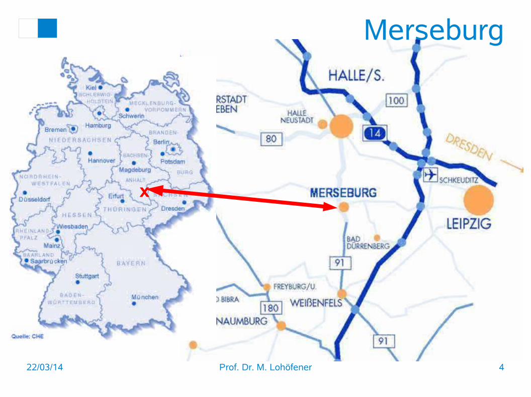
Merseburg
x
220314 Prof Dr M Lohoumlfener 5
MerseburgOver 1000 years old
Residence of German kings
About 35000 inhabitants
Industrial centre
220314 Prof Dr M Lohoumlfener 6
UniversityUniversity site since 60 years
About 2800 students
About 300 staff members with 111 professors and lecturers
4 faculties
220314 Prof Dr M Lohoumlfener 7
International Partners
220314 Prof Dr M Lohoumlfener 8
~700 Students~700 Students
30 Professors and 30 Professors and LecturersLecturers
70 Employees70 Employees
Faculty of Engineering and Natural Sciences
220314 Prof Dr M Lohoumlfener 9
Profiles Associated Institutes Networks
Fluid and Pump Technology reg ass
Research- and Consulting Centre of Machines and Energy Systems reg ass
Institute of Polymer Materials reg ass
Mechatronics Physics Tech-nology
Mechanical Engineering Production and Energy Technology
Industrial Engineering and Business Studies
Chemical and Polymer En-gineering
Process and Environ-mental Engineering Competence Network of Applied
and Transfer Oriented Research
PlasticsCompetenceCentre
220314 Prof Dr M Lohoumlfener 10
International Partners (Examples)
TU Brno (CZ)Faculty of
Mechanical Engineering
TU Łoacutedź (PL)Faculty of Civil Engineering Archi-tecture and Environmental Engin-eering
Uni Riga (LV)Faculty of Physicsand Mathematics
Teachers ExchangeStudents ExchangeResearch Projects
JTUT Changzhou (CN)
220314 Prof Dr M Lohoumlfener 11
Study Courses
Mechanical Engineering
Mechatronics Physics
Technologies
Chemical and Environmental Engineering
Mechanical Engineering
Mechatronics Physics
Technologies
Chemical and Environmental Engineering
MasterMasterBachelorBachelor
Chemistry Chemical
Engineering Pharmacy TechnologyCooperation
6161
126126
Industrial Engineering
and Business Studies
(Dual Course)
2121
Polymer Engineer-
ing1919
3333
3535
The numbers are the beginners last year
~300 new students per year
220314 Prof Dr M Lohoumlfener 12
Akaflieg self-constructed ULA Pilot School
Urban Concept Car NIOS
Shell Eco-Marathon
Special Students Projects
Ultra Light A
irplane
220314 Prof Dr M Lohoumlfener 13
Content
1Introduction
2Mechatronic Systems and Design
3Software Tools
4Modelling
5Simulations
220314 Prof Dr M Lohoumlfener 14
Mechatronic Systems
ABSABSESPESPASRASR
EDSEDS
ACCACC
MSRMSR
CANCAN
EHBEHBEGASEGAS
EMSEMS
GDIGDI
FSIFSIGMAGMA
MotronicMotronic
MOSTMOST
OBDOBD
220314 Prof Dr M Lohoumlfener 15
In VDI guide line 2206 are some defini-tions
In our German working group ldquoMechatronicsrdquo we often use the definition by Harashima Tomizuka and Fukuda
Mechatronics
copy VDI guideline 2206 Design methodology for mechatronic systems Berlin Beuth 2004copy Harashima F Tomizuka M Fukuda T Mechatronics ndash ldquoWhat Is It Why and Howrdquo An Editorial IEEEASME Transactions on Mechatronics 1 (1996) 1 pp14
220314 Prof Dr M Lohoumlfener 16
Mechatronics
ldquoMechatronics is an interdis-ciplinary design methodsolving mainly mechanicaldirected product tasks by thesynergetic spatial and func-
tional integration of mechanicelectric and information pro-
cessing subsystemsrdquo
VDIVDE GMA Technical Committee Mechatronics 2003
Mecha-nics
Electrics Electronics
Infor-matics
Mecha-tronics
Aktua-torics Sensorics
Model-ling
Microcon-trollers
220314 Prof Dr M Lohoumlfener 17
Design Process
Mechanical engineeringElectrical engineeringInformation technologyPrototype
Time axis rarr
Parallel development in different departments ndash requires use of models
Classical product development
What we need
220314 Prof Dr M Lohoumlfener 18
Design Process
Mechanical engineeringElectrical engineeringInformation technologyPrototype
Time axis rarr
Parallel development in different departments ndash requires use of models
Classical product development
What we need
copy httpuploadwikimediaorgwikipediacommonsddeAirbus_A380jpg
220314 Prof Dr M Lohoumlfener 19
Better ldquoA model is the representation of substan-tial aspects of an ab-stract a planned or an ex-isting systems A model can exist as a theoretical imagination as an ab-stract system of signs or in reality of a determined material-energetic basis rdquo (Brockhaus abc Automa-tisierung Leipzig 1975)
Model
Short in DIN ldquoA model renders substantial char-acteristics of an original in a suitable mannerrdquo
220314 Prof Dr M Lohoumlfener 20
VDI 2206
1 Introduction
2 Introduction to the de-velopment of mechat-ronic systems
3 Development methodo-logy of mechatronics
4 Application examples
220314 Prof Dr M Lohoumlfener 21
The V model in product development (according to VDI 2206 Design methodology for mechatronic systems Beuth Berlin 2004)
httpwwwbeuthdedetechnische-regelvdi-220673296956
V Model
220314 Prof Dr M Lohoumlfener 22
Design Process
Cyclic design process again and again hellip
220314 Prof Dr M Lohoumlfener 23
Steps to Get a Model
1 Design an overall structure pay at-tention to inter-faces signals in-put and output of subsystems
2 Design of subsys-tems eg from analytic modelling differential equa-tions or transfer functions in block diagrams pay at-tention to state variables
3 Setting of para-meters eg get-ting technical dates from design drawings or from experimental modelling
4 Verification of the model with the real object if available
copy httpenwikipediaorgwikiSegway_PT
220314 Prof Dr M Lohoumlfener 24
Steps to Get a Model Example
a) Is a Functional Specification re-quired
b) Which domains are to be con-sidered
c) How can we get a block diagram with all necessary sig-nals
copy httpmediabestofmicrocom32156926originalsegway_i2_technik2jpg
220314 Prof Dr M Lohoumlfener 25
Content
1Introduction
2Mechatronic Systems and Design
3Software Tools
4Modelling
5Simulations
220314 Prof Dr M Lohoumlfener 26
Simulations Methods
Solving differential equation systems
Block diagram simulation
MultiMultidomaindomain
modellingmodelling
Description with VHDL-AMS
State flow
graphs
Real-timesimulation
VHDL-AMS Very High Speed Integrated Circuit Hardware Description Languageanalogue and mixed-signal extensions standard IEEE 10761-1999
220314 Prof Dr M Lohoumlfener 27
Software Tools Requirements Solve differential equations Transform equations Solve difference equations Script language Graphical user interface
GUI Compiler for PC and mi-
crocontrollers Plotting graphs
Block diagrams State flow graphs Physical modelling Standardized Interfaces
ndash Other tools
ndash Digital and analogue IO simulators
Import and export of mod-els C- and VHDL-AMS-code
Block libraries hellip
220314 Prof Dr M Lohoumlfener 28
MathWorks MATLABSimulinkCompany The MathWorks Inc
Web httpwwwmathworkscom
Price on request student version 89 USD
MATrix LABoratory ndash MATLAB
Scripts to execute as m file
Also symbolic calculation (CAS) possible
SIMULINK
Graphical input of block diagrams stored as mdl file
mdl-file can be called in M-script
RTW Real Time Workshop
Compilation to real-time models for different processors microcontrollers and for different operating systems or run-time systems
ldquoThe MathWorks delivers a complete set of tools for model-based design of con-trol systems ndash from the development of concepts to the application of software in embedded systemsrdquo
Market Leader
220314 Prof Dr M Lohoumlfener 29
MathWorks MATLABSimulink
Overview from August 2009copy ftpftpmathworkscompubsseminarsSimEventsStateflowWebinarFilesStateflowTechnicalKitProductOverviewpdf
220314 Prof Dr M Lohoumlfener 30
Real-Time Workshop
Rapid Prototyping
220314 Prof Dr M Lohoumlfener 31
Commercial and Open Source All called software tool are
commercial programs with the benefits
ndash (Very) Good professional support
ndash Broad use in industry
ndash Further development will be done
ndash Libraries available
ndash Warranty is understood
Open source software can give us some advantages
ndash No runtime license costs
ndash inexpensive development tools
ndash Open source code allows to be verified of anyone
ndash Open source code can readily be used in future projects
ndash Further development with other suppliers easily possible no dependence on a certain supplier
220314 Prof Dr M Lohoumlfener 32
Author John W Eaton
Web httpwwwgnuorgsoftwareoctave
httpoctavesourceforgenetpackagesphp
Price free
GNU-Octave
Scripts can be executed as oct or m file (compatible to MATLAB m file)
Characteristics
ldquoGNU Octave is a high-level language primarily intended for numerical computations It provides a con-venient command line interface for solving linear and nonlinear problems numerically and for performing other numerical exper-iments using a language that is mostly compatible with Matlab It may also be used as a batch-oriented languagerdquo
Documentation httpwwwgnuorgsoftwareoctaveoctavepdf
hellip And a GUI Its under development and to be tested
220314 Prof Dr M Lohoumlfener 33
ScilabXcosOrganization Scilab Enterprises SAS Orsay
Cedex France
Web httpwwwscilaborg
Price Free
Scilab
Scripts can be executed as sci file (not compatible to MATLAB)
Xcos Graphical input of block diagrams stored as xcos
file (not compatible to Simulink mdl file) XCOS file can be called in SCI Script Multi domain simulation is available for electrical
and mechanical systems and for thermo-hydraulic elements
Documentation
httpwwwscilaborgsupportdocumentation
220314 Prof Dr M Lohoumlfener 34
ScilabXcosExample
Inverted pendu-lum from
Scilab Demos rarr Xcos rarr Control Systems rarr In-verted pendulum
220314 Prof Dr M Lohoumlfener 35
Content
1Introduction
2Mechatronic Systems and Design
3Software Tools
4Modelling
5Simulations
Complex Example
Model of a car with lift nod and roll oscillations (too complex to solve it in this lecture)
220314 Prof Dr M Lohoumlfener 37
Example UnicycleModelling in several
ways
Block diagram in
ndash time domain with a classical integrator chain and in
ndash Laplace domain with transfer func-tions
Scripts with transfer functions
System of differential equation with solution in state space domain
Physical modelling
mA
kA
dA
kR
xR
mR
xS
FR
FA
FA
FR
xA
shock absorber
tire
wheel
carbody
street
220314 Prof Dr M Lohoumlfener 38
Dynamics
From basic physics eg Newtons 2nd law we know the links between forces acceleration velocity and position eg
In mechanical engineering we need dynamic models to describe the dynamic behaviour of constructions based on the above mentioned laws So we have time derivations like
The Laplace operator s simplifies it to
msdota t =F t
a t =d v t dt
=v t =d 2 x t
dt 2= x t
a s=ssdotv s =s2sdotx s
220314 Prof Dr M Lohoumlfener 39
Equations
mAsdotx A(t)+d Asdotx A(t)+k Asdotx A(t )=d Asdotx R(t)+k Asdotx R(t )
mRsdotx R(t )+d Asdotx R(t)+(k A+k R)sdotx R(t )=d Asdotx A(t )+k Asdotx A(t)+k Rsdotx S (t)
Differential equations
Transfer functions
GRA s=X As
X Rs =
k Ad Asdots
k Ad AsdotsmAsdots2
GSRs=X Rs
X S s =
k Rk Ak Rd AsdotsmRsdots
2
G AR s=X Rs
X As =
k Ad Asdots
k Ak Rd AsdotsmRsdots2
Differential equation system
Msdotx (t )+ Dsdotx (t)+ Ksdotx (t )= F e(t)
GSA s=X As
X S s =
GSRssdotG RA s
1minusG RAssdotG AR s
220314 Prof Dr M Lohoumlfener 40
Algorithm
1st step
Transpose the differential equation of nth order to the highest derivation
will become
2nd step
Set up of a chain of n integrators
3rd step
Connect the input of the chain in or-der of the equation
Derivations of the output signal are put from the integrator chain
All other signals and its derivations are input signals
4th step
For differential equation systems steps 1 to 3 are to be done for each differential equation and the result-ing block diagrams are to be con-nected with its signals to an overall block diagram
x= f y d n x
d t n= f x y
d n x
d t n= f x y
Algorithm to get a block diagram from a differential equation
220314 Prof Dr M Lohoumlfener 41
Block Diagram Time Domain
Solved with Xcos
httpwwwhs-merseburgde~lohoefenBrno05Unicyclexcos
x A(t)=d AmA
( x R(t)minus x A(t))+k AmA
( x R(t)minusx A(t))
x R(t)=d AmR
( x A(t)minus x R(t ))+k AmR
( x A(t )minusx R(t))+k RmR
( x S (t )minusx R(t))
220314 Prof Dr M Lohoumlfener 42
Block Diagram Time Domainx A(t)=
d AmA
( x R(t)minus x A(t))+k AmA
( x R(t)minusx A(t))
x R(t)=d AmR
( x A(t)minus x R(t ))+k AmR
( x A(t )minusx R(t))+k RmR
( x S (t )minusx R(t))
Solved with Simulink
httpwwwhs-merseburgde~lohoefenBrno05unicyclemdl
220314 Prof Dr M Lohoumlfener 43
Block Diagram Laplace Domain
httpwwwhs-merseburgde~lohoefenBrno05Einrad_G(s)xcos
Transfer function simulated with Xcos
220314 Prof Dr M Lohoumlfener 44
Single Transfer Function
httpwwwhs-merseburgde~lohoefenBrno05Einradsce
Solution with Scilab script
220314 Prof Dr M Lohoumlfener 45
Single Transfer FunctionSolution with M-script in MATLAB or Octave
httpwwwhs-merseburgde~lohoefenBrno05unicycle_tfm
220314 Prof Dr M Lohoumlfener 46
Time and Laplace Domain
Features Solution in time domain Solution in Laplace domain
Signals variables Includes also steady state variables
Includes only necessary variables
Functions connections blocks
Many functions blocks and connections shown in detail
Clearly only a few functions or blocks required
Initial values Simulation can start with initial values
All initial values must be zero
Nonlinearity Nonlinear functions are allowed in equation system
No nonlinear functions allowed
Time range Whole time range allowed -infin lt t lt infin
Only positive time range allowed 0 le t lt infin
220314 Prof Dr M Lohoumlfener 47
Differential Equation Systems1st Sketch of mechanical sys-
tem
Marking of masses and inertia
Marking of mechanical ele-ments
Drawing of deflections and its directions
Drawing of forces and its dir-ections
2nd Fixing of time variant de-flection vector
3rd Force balance for any de-flection x
i(t)
Inertia force = sum of acting forces
4th Force basic equations
for spring damper friction hellip
5th Using force basic equa-tions with force balance
Natural dynamics = acting forces
xT (t)=( x1(t) ⋯ xi (t ) ⋯ xn(t ))
msdotx i t =sum F t
F i (t )= f ( x(t) ⋯)
220314 Prof Dr M Lohoumlfener 48
Differential Equation Systems
Msdotx (t)+ Dsdotx(t)+ Ksdotx (t )= F e(t)
6th Representation as differ-ential equation system in matrix form
with the constant matrices
massmatrix
dampermatrix
M= (m1 ⋯ 0 ⋯ 0⋮ ⋮ ⋮0 ⋯ mi ⋯ 0⋮ ⋮ ⋮0 ⋯ 0 ⋯ mn
)D=(
d 11 ⋯ d 1j ⋯ d 1n⋮ ⋮ ⋮d i1 ⋯ d ij ⋯ d in⋮ ⋮ ⋮d n1 ⋯ d ni ⋯ d nn
)
K=(k 11 ⋯ k 1j ⋯ k 1n⋮ ⋮ ⋮k i1 ⋯ k ij ⋯ k in⋮ ⋮ ⋮k n1 ⋯ k nj ⋯ k nn
)stiffnessmatrix
and the time variant force vec-tor
F eT(t)=(F 1(t) ⋯ F i(t) ⋯ F n (t ))
220314 Prof Dr M Lohoumlfener 49
Differential Equation Systems7th Transformation in state
space representation
State space equation
Output equation
xSS (t)= AsdotxSS (t)+ Bsdotu (t)
y (t )=CsdotxSS (t)+Dsdotu(t)
Input vector u(t) State variables vector x
SS(t)
Output vector y(t) System matrix A Input matrix B Output matrix C Transfer matrix D
From
we get with the substitution and
or simplified
M ODEsdotxODE (t)+ DODEsdotxODE (t )+ KODEsdotxODE (t)= F e(t)xODE (t)= v (t) F e(t)=K esdotu(t)
[ xODE (t)vODE (t) ]=[ 0 1minusM ODE
minus1 sdotKODE minusM ODEminus1 sdotDODE ]sdot[ xODE (t)vODE (t) ]+[ 0
M ODEminus1 sdotK e
]sdot[ u (t )]
[ y (t )]=[ 1 0 ]sdot[ xODE (t )vODE (t )]+ [ 0 ]sdot[ u (t )] [ y(t )]=[ 1 0 ]sdot[ xODE (t )vODE (t )]
and
220314 Prof Dr M Lohoumlfener 50
Differential Equation Systems
After all we only need thetransformation rules
x SS (t)=[ xODE (t)vODE (t ) ]A=[ 0 1
minusM ODEminus1
sdotKODE minusM ODEminus1
sdotDODE ]B= [ 0
M ODEminus1
sdotK e]
C= [ 1 0 ]
D=[ 0 ]
Scilab program (wwwscilaborg) Steady state transformation Using matrices M D K Ke
[nrnc]=size(M)
A=[zeros(nrnc) eye(nrnc) -inv(M)K -inv(M)D]
B=[zeros(nr1) inv(M)Ke]
C=[eye(nrnc) zeros(nrnc)]
Model=syslin(cABC)instants=00054 time axisy=csim(stepinstantsModel)xtitle(SimulationsResponse)plot2d(instantsy)
220314 Prof Dr M Lohoumlfener 51
State Space Solution Scilab program 1Radsci Prof Dr M Lohoumlfener 26503 Data inputkA=32500dA=10000mA=1300kR=50000mR=20xS=1 differential equation system M=[mA 0 0 mR]D=[dA -dA -dA dA]K=[kA -kA -kA kR+kA]Ke=[0 kR] Transformation in state space[nrnc]=size(M)A=[zeros(nrnc) eye(nrnc) -inv(M)K -inv(M)D]B=[zeros(nr1) inv(M)Ke]C=[eye(nrnc) zeros(nrnc)]Einrad=syslin(cABC)instants=00014y=csim(stepinstantsEinrad)xtitle(Simulation EinradZeit t in sSprungantwort)xgrid(32)plot2d(instantsy)
Msdotx (t)+ Dsdotx(t)+ Ksdotx (t )= F e(t)
Step response of the unicycledue to a pavementblue ndash wheel position black ndash body position
httpwwwhs-merseburgde~lohoefenBrno051radsce
Solution with Scilab script
220314 Prof Dr M Lohoumlfener 52
State Space Solution
httpwwwhs-merseburgde~lohoefenBrno051_SSxcos
Solution with Xcos
220314 Prof Dr M Lohoumlfener 53
Physical Modelling
Unicycle with SimMechanics
220314 Prof Dr M Lohoumlfener 54
Content
1Introduction
2Mechatronic Systems and Design
3Software Tools
4Modelling
5Simulations
220314 Prof Dr M Lohoumlfener 55
Use of SimulationsExpectations Save time in develop-
ment Rapid software proto-
typing Avoid failures during
implementation of res-ults
Make experiments bet-ter to be avoided in reality
Make automated exper-iments
Get reproducible res-ults
Make a lot more exper-iments in the same time
Reduce costs for exper-iments
220314 Prof Dr M Lohoumlfener 56
Model and Reality
Environment
Model Real
Object to be developed
Model MiL SiL
Real HiL Final Test
1 MiL Model in the Loopno real-time requirements
2 SiL Software in the Loopwith hardware interface
3 HiL Hardware in the Loopwith hardware test-bench
4 Final Test
220314 Prof Dr M Lohoumlfener 57
Software in the Loop ndash SiLExplanation
A mechanical or electron-ic component as a part of a system is first imple-mented (realized) as a computer model simula-tion in software The computer is connected to the real world ie to the other parts of the system with a special interface to be tested and optimized
220314 Prof Dr M Lohoumlfener 58
Example dSpaceDrive control with a real-time control-ler board DS1104 (dSpace)
Students project in the mechatron-ics lab in Merseburg
httpwwwdspacecom
220314 Prof Dr M Lohoumlfener 59
Example dSpaceDesign of the PID-controller with Sim-ulink and dSpace library to connect the simulated con-troller with the ap-plication
220314 Prof Dr M Lohoumlfener 60
Example dSpaceChange parameters and plot results during real-time test using ControlDesk (dSpace)
220314 Prof Dr M Lohoumlfener 61
Hardware in the Loop ndash HiLExplanation
A mechanical or electron-ic component as a part of a system is manufactured as a real prototype To in-vestigate this prototype a computer simulates a real world as a model with a special interface to test and optimize the proto-type
Use
HiL simulation makes it possible to test a real sys-tem instead of a model
A complete environment is simulated to the object in real-time and the ob-ject has to react to virtual environmental influences
Important is the simula-tion of failure situations to electronic devices like cable corruption etc
220314 Prof Dr M Lohoumlfener 62
Simulation and HardwareTest-bench with configura-tions of real vehicles
httpwwwipgde
220314 Prof Dr M Lohoumlfener 63
Example LABCAR LABCAR software
modules Hardware components
Product of ETAS devel-opment and application tools for electronic sys-tems in automotive in-dustry
httpwwwetascomenproductsapplications_ecu_development-testing-labcar_component_overviewphp
220314 Prof Dr M Lohoumlfener 64
Code GenerationWe tried several toolchains
Classical waydiams MATLAB Simulink
RTW
Additional compilerdiams dSpace
Alternative OSdiams Linux
Other tooldiams LabVIEW
Open source tools diams Scilab Xcos
Environment diams RTAI-Lab RTAI-Linuxdiams Linux with RT patches
Last trial diams SCALE-RT
220314 Prof Dr M Lohoumlfener 65
MATLAB rarr RTAI-Linux
copy Dr C Schroumlder Ilmenau httpwwwimmsdeen
220314 Prof Dr M Lohoumlfener 66
Scilab rarr RTAI-Laba) Add a Comedi AD block and con-nect it Close the window
b) RTAI CodeGen on the Super Block
c) Execute the real-time task dcmot -v
d) xrtailab -v
e) xrtailab adjust unitsdiv and secdiv
f) Visualize the signal on an oscillo-scope (ensure all grounds are well connected)
The laptop is a Fujitsu P-2040
Data acquisition hardware National Instruments PCMCIA DAQCard-6024E
copy RTAI-Lab tutorial Scilab Comedi and real-time control
Signal generation and visualization
httpwwwrtaiorg
220314 Prof Dr M Lohoumlfener 67
SCALE-RTCombination of host sys-tem on Win-dows with MATLAB Simulink ScilabScicos and Com-pilers and target system on RTAI-Linux
Free for uni-versities
In short It works
httpwwwscale-rtcom
220314 Prof Dr M Lohoumlfener 68
Future Tasksradic More useful tool chains also
for open source software is necessary
radic Useful tools for different mi-crocontrollers and RT OS
radic More support for open source tools is needed
radic RTAI Linux is well suited and has a support also for drivers with the COMEDI project but is difficult to maintain with the kernel development
radic The introduction of RT pree-mpt patches to the standard Linux kernel substitutes RTAI but a new driver framework must be developed
- Folie 1
- Folie 2
- Folie 3
- Folie 4
- Folie 5
- Folie 6
- Folie 7
- Folie 8
- Folie 9
- Folie 10
- Folie 11
- Folie 12
- Folie 13
- Folie 14
- Folie 15
- Folie 16
- Folie 17
- Folie 18
- Folie 19
- Folie 20
- Folie 21
- Folie 22
- Folie 23
- Folie 24
- Folie 25
- Folie 26
- Folie 27
- Folie 28
- Folie 29
- Folie 30
- Folie 31
- Folie 32
- Folie 33
- Folie 34
- Folie 35
- Folie 36
- Folie 37
- Folie 38
- Folie 39
- Folie 40
- Folie 41
- Folie 42
- Folie 43
- Folie 44
- Folie 45
- Folie 46
- Folie 47
- Folie 48
- Folie 49
- Folie 50
- Folie 51
- Folie 52
- Folie 53
- Folie 54
- Folie 55
- Folie 56
- Folie 57
- Folie 58
- Folie 59
- Folie 60
- Folie 61
- Folie 62
- Folie 63
- Folie 64
- Folie 65
- Folie 66
- Folie 67
- Folie 68
-
Lecture
Prof Dr-Ing Manfred Lohoumlfener Dean of the Faculty for Engineering and Natural Sciences
Professor of Mechatronic Systemshttpwwwhs-merseburgdeinw
Model Based Design of Mechatronic Systems
Hochschule MerseburgUniversity of Applied Sciences
Faculty of Engineering and Natural Scienceshttpwwwhs-merseburgde
httpwebhs-merseburgde~lohoefenBrno05Lecture-2014pdf
220314 Prof Dr M Lohoumlfener 3
Content
1Introduction
2Mechatronic Systems and Design
3Software Tools
4Modelling
5Simulations
220314 Prof Dr M Lohoumlfener 4
Merseburg
x
220314 Prof Dr M Lohoumlfener 5
MerseburgOver 1000 years old
Residence of German kings
About 35000 inhabitants
Industrial centre
220314 Prof Dr M Lohoumlfener 6
UniversityUniversity site since 60 years
About 2800 students
About 300 staff members with 111 professors and lecturers
4 faculties
220314 Prof Dr M Lohoumlfener 7
International Partners
220314 Prof Dr M Lohoumlfener 8
~700 Students~700 Students
30 Professors and 30 Professors and LecturersLecturers
70 Employees70 Employees
Faculty of Engineering and Natural Sciences
220314 Prof Dr M Lohoumlfener 9
Profiles Associated Institutes Networks
Fluid and Pump Technology reg ass
Research- and Consulting Centre of Machines and Energy Systems reg ass
Institute of Polymer Materials reg ass
Mechatronics Physics Tech-nology
Mechanical Engineering Production and Energy Technology
Industrial Engineering and Business Studies
Chemical and Polymer En-gineering
Process and Environ-mental Engineering Competence Network of Applied
and Transfer Oriented Research
PlasticsCompetenceCentre
220314 Prof Dr M Lohoumlfener 10
International Partners (Examples)
TU Brno (CZ)Faculty of
Mechanical Engineering
TU Łoacutedź (PL)Faculty of Civil Engineering Archi-tecture and Environmental Engin-eering
Uni Riga (LV)Faculty of Physicsand Mathematics
Teachers ExchangeStudents ExchangeResearch Projects
JTUT Changzhou (CN)
220314 Prof Dr M Lohoumlfener 11
Study Courses
Mechanical Engineering
Mechatronics Physics
Technologies
Chemical and Environmental Engineering
Mechanical Engineering
Mechatronics Physics
Technologies
Chemical and Environmental Engineering
MasterMasterBachelorBachelor
Chemistry Chemical
Engineering Pharmacy TechnologyCooperation
6161
126126
Industrial Engineering
and Business Studies
(Dual Course)
2121
Polymer Engineer-
ing1919
3333
3535
The numbers are the beginners last year
~300 new students per year
220314 Prof Dr M Lohoumlfener 12
Akaflieg self-constructed ULA Pilot School
Urban Concept Car NIOS
Shell Eco-Marathon
Special Students Projects
Ultra Light A
irplane
220314 Prof Dr M Lohoumlfener 13
Content
1Introduction
2Mechatronic Systems and Design
3Software Tools
4Modelling
5Simulations
220314 Prof Dr M Lohoumlfener 14
Mechatronic Systems
ABSABSESPESPASRASR
EDSEDS
ACCACC
MSRMSR
CANCAN
EHBEHBEGASEGAS
EMSEMS
GDIGDI
FSIFSIGMAGMA
MotronicMotronic
MOSTMOST
OBDOBD
220314 Prof Dr M Lohoumlfener 15
In VDI guide line 2206 are some defini-tions
In our German working group ldquoMechatronicsrdquo we often use the definition by Harashima Tomizuka and Fukuda
Mechatronics
copy VDI guideline 2206 Design methodology for mechatronic systems Berlin Beuth 2004copy Harashima F Tomizuka M Fukuda T Mechatronics ndash ldquoWhat Is It Why and Howrdquo An Editorial IEEEASME Transactions on Mechatronics 1 (1996) 1 pp14
220314 Prof Dr M Lohoumlfener 16
Mechatronics
ldquoMechatronics is an interdis-ciplinary design methodsolving mainly mechanicaldirected product tasks by thesynergetic spatial and func-
tional integration of mechanicelectric and information pro-
cessing subsystemsrdquo
VDIVDE GMA Technical Committee Mechatronics 2003
Mecha-nics
Electrics Electronics
Infor-matics
Mecha-tronics
Aktua-torics Sensorics
Model-ling
Microcon-trollers
220314 Prof Dr M Lohoumlfener 17
Design Process
Mechanical engineeringElectrical engineeringInformation technologyPrototype
Time axis rarr
Parallel development in different departments ndash requires use of models
Classical product development
What we need
220314 Prof Dr M Lohoumlfener 18
Design Process
Mechanical engineeringElectrical engineeringInformation technologyPrototype
Time axis rarr
Parallel development in different departments ndash requires use of models
Classical product development
What we need
copy httpuploadwikimediaorgwikipediacommonsddeAirbus_A380jpg
220314 Prof Dr M Lohoumlfener 19
Better ldquoA model is the representation of substan-tial aspects of an ab-stract a planned or an ex-isting systems A model can exist as a theoretical imagination as an ab-stract system of signs or in reality of a determined material-energetic basis rdquo (Brockhaus abc Automa-tisierung Leipzig 1975)
Model
Short in DIN ldquoA model renders substantial char-acteristics of an original in a suitable mannerrdquo
220314 Prof Dr M Lohoumlfener 20
VDI 2206
1 Introduction
2 Introduction to the de-velopment of mechat-ronic systems
3 Development methodo-logy of mechatronics
4 Application examples
220314 Prof Dr M Lohoumlfener 21
The V model in product development (according to VDI 2206 Design methodology for mechatronic systems Beuth Berlin 2004)
httpwwwbeuthdedetechnische-regelvdi-220673296956
V Model
220314 Prof Dr M Lohoumlfener 22
Design Process
Cyclic design process again and again hellip
220314 Prof Dr M Lohoumlfener 23
Steps to Get a Model
1 Design an overall structure pay at-tention to inter-faces signals in-put and output of subsystems
2 Design of subsys-tems eg from analytic modelling differential equa-tions or transfer functions in block diagrams pay at-tention to state variables
3 Setting of para-meters eg get-ting technical dates from design drawings or from experimental modelling
4 Verification of the model with the real object if available
copy httpenwikipediaorgwikiSegway_PT
220314 Prof Dr M Lohoumlfener 24
Steps to Get a Model Example
a) Is a Functional Specification re-quired
b) Which domains are to be con-sidered
c) How can we get a block diagram with all necessary sig-nals
copy httpmediabestofmicrocom32156926originalsegway_i2_technik2jpg
220314 Prof Dr M Lohoumlfener 25
Content
1Introduction
2Mechatronic Systems and Design
3Software Tools
4Modelling
5Simulations
220314 Prof Dr M Lohoumlfener 26
Simulations Methods
Solving differential equation systems
Block diagram simulation
MultiMultidomaindomain
modellingmodelling
Description with VHDL-AMS
State flow
graphs
Real-timesimulation
VHDL-AMS Very High Speed Integrated Circuit Hardware Description Languageanalogue and mixed-signal extensions standard IEEE 10761-1999
220314 Prof Dr M Lohoumlfener 27
Software Tools Requirements Solve differential equations Transform equations Solve difference equations Script language Graphical user interface
GUI Compiler for PC and mi-
crocontrollers Plotting graphs
Block diagrams State flow graphs Physical modelling Standardized Interfaces
ndash Other tools
ndash Digital and analogue IO simulators
Import and export of mod-els C- and VHDL-AMS-code
Block libraries hellip
220314 Prof Dr M Lohoumlfener 28
MathWorks MATLABSimulinkCompany The MathWorks Inc
Web httpwwwmathworkscom
Price on request student version 89 USD
MATrix LABoratory ndash MATLAB
Scripts to execute as m file
Also symbolic calculation (CAS) possible
SIMULINK
Graphical input of block diagrams stored as mdl file
mdl-file can be called in M-script
RTW Real Time Workshop
Compilation to real-time models for different processors microcontrollers and for different operating systems or run-time systems
ldquoThe MathWorks delivers a complete set of tools for model-based design of con-trol systems ndash from the development of concepts to the application of software in embedded systemsrdquo
Market Leader
220314 Prof Dr M Lohoumlfener 29
MathWorks MATLABSimulink
Overview from August 2009copy ftpftpmathworkscompubsseminarsSimEventsStateflowWebinarFilesStateflowTechnicalKitProductOverviewpdf
220314 Prof Dr M Lohoumlfener 30
Real-Time Workshop
Rapid Prototyping
220314 Prof Dr M Lohoumlfener 31
Commercial and Open Source All called software tool are
commercial programs with the benefits
ndash (Very) Good professional support
ndash Broad use in industry
ndash Further development will be done
ndash Libraries available
ndash Warranty is understood
Open source software can give us some advantages
ndash No runtime license costs
ndash inexpensive development tools
ndash Open source code allows to be verified of anyone
ndash Open source code can readily be used in future projects
ndash Further development with other suppliers easily possible no dependence on a certain supplier
220314 Prof Dr M Lohoumlfener 32
Author John W Eaton
Web httpwwwgnuorgsoftwareoctave
httpoctavesourceforgenetpackagesphp
Price free
GNU-Octave
Scripts can be executed as oct or m file (compatible to MATLAB m file)
Characteristics
ldquoGNU Octave is a high-level language primarily intended for numerical computations It provides a con-venient command line interface for solving linear and nonlinear problems numerically and for performing other numerical exper-iments using a language that is mostly compatible with Matlab It may also be used as a batch-oriented languagerdquo
Documentation httpwwwgnuorgsoftwareoctaveoctavepdf
hellip And a GUI Its under development and to be tested
220314 Prof Dr M Lohoumlfener 33
ScilabXcosOrganization Scilab Enterprises SAS Orsay
Cedex France
Web httpwwwscilaborg
Price Free
Scilab
Scripts can be executed as sci file (not compatible to MATLAB)
Xcos Graphical input of block diagrams stored as xcos
file (not compatible to Simulink mdl file) XCOS file can be called in SCI Script Multi domain simulation is available for electrical
and mechanical systems and for thermo-hydraulic elements
Documentation
httpwwwscilaborgsupportdocumentation
220314 Prof Dr M Lohoumlfener 34
ScilabXcosExample
Inverted pendu-lum from
Scilab Demos rarr Xcos rarr Control Systems rarr In-verted pendulum
220314 Prof Dr M Lohoumlfener 35
Content
1Introduction
2Mechatronic Systems and Design
3Software Tools
4Modelling
5Simulations
Complex Example
Model of a car with lift nod and roll oscillations (too complex to solve it in this lecture)
220314 Prof Dr M Lohoumlfener 37
Example UnicycleModelling in several
ways
Block diagram in
ndash time domain with a classical integrator chain and in
ndash Laplace domain with transfer func-tions
Scripts with transfer functions
System of differential equation with solution in state space domain
Physical modelling
mA
kA
dA
kR
xR
mR
xS
FR
FA
FA
FR
xA
shock absorber
tire
wheel
carbody
street
220314 Prof Dr M Lohoumlfener 38
Dynamics
From basic physics eg Newtons 2nd law we know the links between forces acceleration velocity and position eg
In mechanical engineering we need dynamic models to describe the dynamic behaviour of constructions based on the above mentioned laws So we have time derivations like
The Laplace operator s simplifies it to
msdota t =F t
a t =d v t dt
=v t =d 2 x t
dt 2= x t
a s=ssdotv s =s2sdotx s
220314 Prof Dr M Lohoumlfener 39
Equations
mAsdotx A(t)+d Asdotx A(t)+k Asdotx A(t )=d Asdotx R(t)+k Asdotx R(t )
mRsdotx R(t )+d Asdotx R(t)+(k A+k R)sdotx R(t )=d Asdotx A(t )+k Asdotx A(t)+k Rsdotx S (t)
Differential equations
Transfer functions
GRA s=X As
X Rs =
k Ad Asdots
k Ad AsdotsmAsdots2
GSRs=X Rs
X S s =
k Rk Ak Rd AsdotsmRsdots
2
G AR s=X Rs
X As =
k Ad Asdots
k Ak Rd AsdotsmRsdots2
Differential equation system
Msdotx (t )+ Dsdotx (t)+ Ksdotx (t )= F e(t)
GSA s=X As
X S s =
GSRssdotG RA s
1minusG RAssdotG AR s
220314 Prof Dr M Lohoumlfener 40
Algorithm
1st step
Transpose the differential equation of nth order to the highest derivation
will become
2nd step
Set up of a chain of n integrators
3rd step
Connect the input of the chain in or-der of the equation
Derivations of the output signal are put from the integrator chain
All other signals and its derivations are input signals
4th step
For differential equation systems steps 1 to 3 are to be done for each differential equation and the result-ing block diagrams are to be con-nected with its signals to an overall block diagram
x= f y d n x
d t n= f x y
d n x
d t n= f x y
Algorithm to get a block diagram from a differential equation
220314 Prof Dr M Lohoumlfener 41
Block Diagram Time Domain
Solved with Xcos
httpwwwhs-merseburgde~lohoefenBrno05Unicyclexcos
x A(t)=d AmA
( x R(t)minus x A(t))+k AmA
( x R(t)minusx A(t))
x R(t)=d AmR
( x A(t)minus x R(t ))+k AmR
( x A(t )minusx R(t))+k RmR
( x S (t )minusx R(t))
220314 Prof Dr M Lohoumlfener 42
Block Diagram Time Domainx A(t)=
d AmA
( x R(t)minus x A(t))+k AmA
( x R(t)minusx A(t))
x R(t)=d AmR
( x A(t)minus x R(t ))+k AmR
( x A(t )minusx R(t))+k RmR
( x S (t )minusx R(t))
Solved with Simulink
httpwwwhs-merseburgde~lohoefenBrno05unicyclemdl
220314 Prof Dr M Lohoumlfener 43
Block Diagram Laplace Domain
httpwwwhs-merseburgde~lohoefenBrno05Einrad_G(s)xcos
Transfer function simulated with Xcos
220314 Prof Dr M Lohoumlfener 44
Single Transfer Function
httpwwwhs-merseburgde~lohoefenBrno05Einradsce
Solution with Scilab script
220314 Prof Dr M Lohoumlfener 45
Single Transfer FunctionSolution with M-script in MATLAB or Octave
httpwwwhs-merseburgde~lohoefenBrno05unicycle_tfm
220314 Prof Dr M Lohoumlfener 46
Time and Laplace Domain
Features Solution in time domain Solution in Laplace domain
Signals variables Includes also steady state variables
Includes only necessary variables
Functions connections blocks
Many functions blocks and connections shown in detail
Clearly only a few functions or blocks required
Initial values Simulation can start with initial values
All initial values must be zero
Nonlinearity Nonlinear functions are allowed in equation system
No nonlinear functions allowed
Time range Whole time range allowed -infin lt t lt infin
Only positive time range allowed 0 le t lt infin
220314 Prof Dr M Lohoumlfener 47
Differential Equation Systems1st Sketch of mechanical sys-
tem
Marking of masses and inertia
Marking of mechanical ele-ments
Drawing of deflections and its directions
Drawing of forces and its dir-ections
2nd Fixing of time variant de-flection vector
3rd Force balance for any de-flection x
i(t)
Inertia force = sum of acting forces
4th Force basic equations
for spring damper friction hellip
5th Using force basic equa-tions with force balance
Natural dynamics = acting forces
xT (t)=( x1(t) ⋯ xi (t ) ⋯ xn(t ))
msdotx i t =sum F t
F i (t )= f ( x(t) ⋯)
220314 Prof Dr M Lohoumlfener 48
Differential Equation Systems
Msdotx (t)+ Dsdotx(t)+ Ksdotx (t )= F e(t)
6th Representation as differ-ential equation system in matrix form
with the constant matrices
massmatrix
dampermatrix
M= (m1 ⋯ 0 ⋯ 0⋮ ⋮ ⋮0 ⋯ mi ⋯ 0⋮ ⋮ ⋮0 ⋯ 0 ⋯ mn
)D=(
d 11 ⋯ d 1j ⋯ d 1n⋮ ⋮ ⋮d i1 ⋯ d ij ⋯ d in⋮ ⋮ ⋮d n1 ⋯ d ni ⋯ d nn
)
K=(k 11 ⋯ k 1j ⋯ k 1n⋮ ⋮ ⋮k i1 ⋯ k ij ⋯ k in⋮ ⋮ ⋮k n1 ⋯ k nj ⋯ k nn
)stiffnessmatrix
and the time variant force vec-tor
F eT(t)=(F 1(t) ⋯ F i(t) ⋯ F n (t ))
220314 Prof Dr M Lohoumlfener 49
Differential Equation Systems7th Transformation in state
space representation
State space equation
Output equation
xSS (t)= AsdotxSS (t)+ Bsdotu (t)
y (t )=CsdotxSS (t)+Dsdotu(t)
Input vector u(t) State variables vector x
SS(t)
Output vector y(t) System matrix A Input matrix B Output matrix C Transfer matrix D
From
we get with the substitution and
or simplified
M ODEsdotxODE (t)+ DODEsdotxODE (t )+ KODEsdotxODE (t)= F e(t)xODE (t)= v (t) F e(t)=K esdotu(t)
[ xODE (t)vODE (t) ]=[ 0 1minusM ODE
minus1 sdotKODE minusM ODEminus1 sdotDODE ]sdot[ xODE (t)vODE (t) ]+[ 0
M ODEminus1 sdotK e
]sdot[ u (t )]
[ y (t )]=[ 1 0 ]sdot[ xODE (t )vODE (t )]+ [ 0 ]sdot[ u (t )] [ y(t )]=[ 1 0 ]sdot[ xODE (t )vODE (t )]
and
220314 Prof Dr M Lohoumlfener 50
Differential Equation Systems
After all we only need thetransformation rules
x SS (t)=[ xODE (t)vODE (t ) ]A=[ 0 1
minusM ODEminus1
sdotKODE minusM ODEminus1
sdotDODE ]B= [ 0
M ODEminus1
sdotK e]
C= [ 1 0 ]
D=[ 0 ]
Scilab program (wwwscilaborg) Steady state transformation Using matrices M D K Ke
[nrnc]=size(M)
A=[zeros(nrnc) eye(nrnc) -inv(M)K -inv(M)D]
B=[zeros(nr1) inv(M)Ke]
C=[eye(nrnc) zeros(nrnc)]
Model=syslin(cABC)instants=00054 time axisy=csim(stepinstantsModel)xtitle(SimulationsResponse)plot2d(instantsy)
220314 Prof Dr M Lohoumlfener 51
State Space Solution Scilab program 1Radsci Prof Dr M Lohoumlfener 26503 Data inputkA=32500dA=10000mA=1300kR=50000mR=20xS=1 differential equation system M=[mA 0 0 mR]D=[dA -dA -dA dA]K=[kA -kA -kA kR+kA]Ke=[0 kR] Transformation in state space[nrnc]=size(M)A=[zeros(nrnc) eye(nrnc) -inv(M)K -inv(M)D]B=[zeros(nr1) inv(M)Ke]C=[eye(nrnc) zeros(nrnc)]Einrad=syslin(cABC)instants=00014y=csim(stepinstantsEinrad)xtitle(Simulation EinradZeit t in sSprungantwort)xgrid(32)plot2d(instantsy)
Msdotx (t)+ Dsdotx(t)+ Ksdotx (t )= F e(t)
Step response of the unicycledue to a pavementblue ndash wheel position black ndash body position
httpwwwhs-merseburgde~lohoefenBrno051radsce
Solution with Scilab script
220314 Prof Dr M Lohoumlfener 52
State Space Solution
httpwwwhs-merseburgde~lohoefenBrno051_SSxcos
Solution with Xcos
220314 Prof Dr M Lohoumlfener 53
Physical Modelling
Unicycle with SimMechanics
220314 Prof Dr M Lohoumlfener 54
Content
1Introduction
2Mechatronic Systems and Design
3Software Tools
4Modelling
5Simulations
220314 Prof Dr M Lohoumlfener 55
Use of SimulationsExpectations Save time in develop-
ment Rapid software proto-
typing Avoid failures during
implementation of res-ults
Make experiments bet-ter to be avoided in reality
Make automated exper-iments
Get reproducible res-ults
Make a lot more exper-iments in the same time
Reduce costs for exper-iments
220314 Prof Dr M Lohoumlfener 56
Model and Reality
Environment
Model Real
Object to be developed
Model MiL SiL
Real HiL Final Test
1 MiL Model in the Loopno real-time requirements
2 SiL Software in the Loopwith hardware interface
3 HiL Hardware in the Loopwith hardware test-bench
4 Final Test
220314 Prof Dr M Lohoumlfener 57
Software in the Loop ndash SiLExplanation
A mechanical or electron-ic component as a part of a system is first imple-mented (realized) as a computer model simula-tion in software The computer is connected to the real world ie to the other parts of the system with a special interface to be tested and optimized
220314 Prof Dr M Lohoumlfener 58
Example dSpaceDrive control with a real-time control-ler board DS1104 (dSpace)
Students project in the mechatron-ics lab in Merseburg
httpwwwdspacecom
220314 Prof Dr M Lohoumlfener 59
Example dSpaceDesign of the PID-controller with Sim-ulink and dSpace library to connect the simulated con-troller with the ap-plication
220314 Prof Dr M Lohoumlfener 60
Example dSpaceChange parameters and plot results during real-time test using ControlDesk (dSpace)
220314 Prof Dr M Lohoumlfener 61
Hardware in the Loop ndash HiLExplanation
A mechanical or electron-ic component as a part of a system is manufactured as a real prototype To in-vestigate this prototype a computer simulates a real world as a model with a special interface to test and optimize the proto-type
Use
HiL simulation makes it possible to test a real sys-tem instead of a model
A complete environment is simulated to the object in real-time and the ob-ject has to react to virtual environmental influences
Important is the simula-tion of failure situations to electronic devices like cable corruption etc
220314 Prof Dr M Lohoumlfener 62
Simulation and HardwareTest-bench with configura-tions of real vehicles
httpwwwipgde
220314 Prof Dr M Lohoumlfener 63
Example LABCAR LABCAR software
modules Hardware components
Product of ETAS devel-opment and application tools for electronic sys-tems in automotive in-dustry
httpwwwetascomenproductsapplications_ecu_development-testing-labcar_component_overviewphp
220314 Prof Dr M Lohoumlfener 64
Code GenerationWe tried several toolchains
Classical waydiams MATLAB Simulink
RTW
Additional compilerdiams dSpace
Alternative OSdiams Linux
Other tooldiams LabVIEW
Open source tools diams Scilab Xcos
Environment diams RTAI-Lab RTAI-Linuxdiams Linux with RT patches
Last trial diams SCALE-RT
220314 Prof Dr M Lohoumlfener 65
MATLAB rarr RTAI-Linux
copy Dr C Schroumlder Ilmenau httpwwwimmsdeen
220314 Prof Dr M Lohoumlfener 66
Scilab rarr RTAI-Laba) Add a Comedi AD block and con-nect it Close the window
b) RTAI CodeGen on the Super Block
c) Execute the real-time task dcmot -v
d) xrtailab -v
e) xrtailab adjust unitsdiv and secdiv
f) Visualize the signal on an oscillo-scope (ensure all grounds are well connected)
The laptop is a Fujitsu P-2040
Data acquisition hardware National Instruments PCMCIA DAQCard-6024E
copy RTAI-Lab tutorial Scilab Comedi and real-time control
Signal generation and visualization
httpwwwrtaiorg
220314 Prof Dr M Lohoumlfener 67
SCALE-RTCombination of host sys-tem on Win-dows with MATLAB Simulink ScilabScicos and Com-pilers and target system on RTAI-Linux
Free for uni-versities
In short It works
httpwwwscale-rtcom
220314 Prof Dr M Lohoumlfener 68
Future Tasksradic More useful tool chains also
for open source software is necessary
radic Useful tools for different mi-crocontrollers and RT OS
radic More support for open source tools is needed
radic RTAI Linux is well suited and has a support also for drivers with the COMEDI project but is difficult to maintain with the kernel development
radic The introduction of RT pree-mpt patches to the standard Linux kernel substitutes RTAI but a new driver framework must be developed
- Folie 1
- Folie 2
- Folie 3
- Folie 4
- Folie 5
- Folie 6
- Folie 7
- Folie 8
- Folie 9
- Folie 10
- Folie 11
- Folie 12
- Folie 13
- Folie 14
- Folie 15
- Folie 16
- Folie 17
- Folie 18
- Folie 19
- Folie 20
- Folie 21
- Folie 22
- Folie 23
- Folie 24
- Folie 25
- Folie 26
- Folie 27
- Folie 28
- Folie 29
- Folie 30
- Folie 31
- Folie 32
- Folie 33
- Folie 34
- Folie 35
- Folie 36
- Folie 37
- Folie 38
- Folie 39
- Folie 40
- Folie 41
- Folie 42
- Folie 43
- Folie 44
- Folie 45
- Folie 46
- Folie 47
- Folie 48
- Folie 49
- Folie 50
- Folie 51
- Folie 52
- Folie 53
- Folie 54
- Folie 55
- Folie 56
- Folie 57
- Folie 58
- Folie 59
- Folie 60
- Folie 61
- Folie 62
- Folie 63
- Folie 64
- Folie 65
- Folie 66
- Folie 67
- Folie 68
-
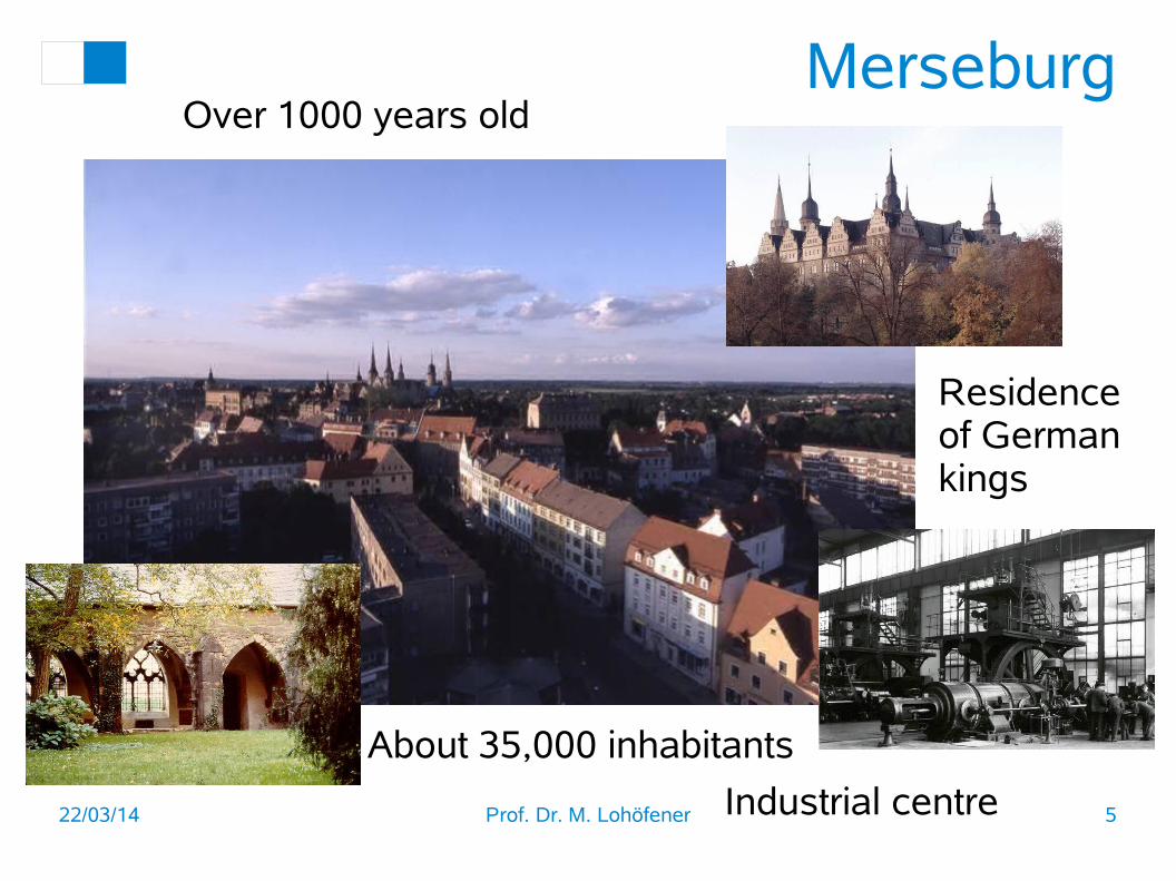
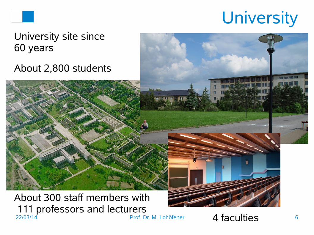
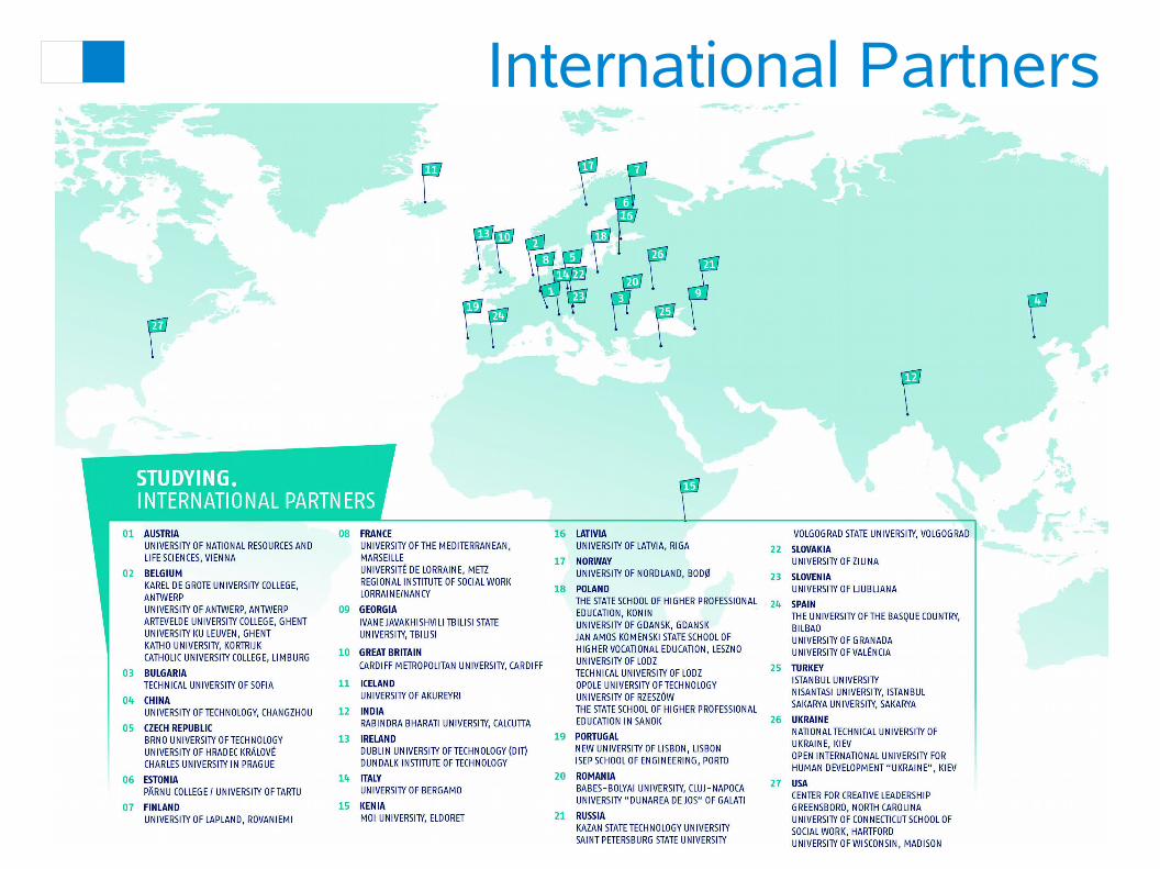
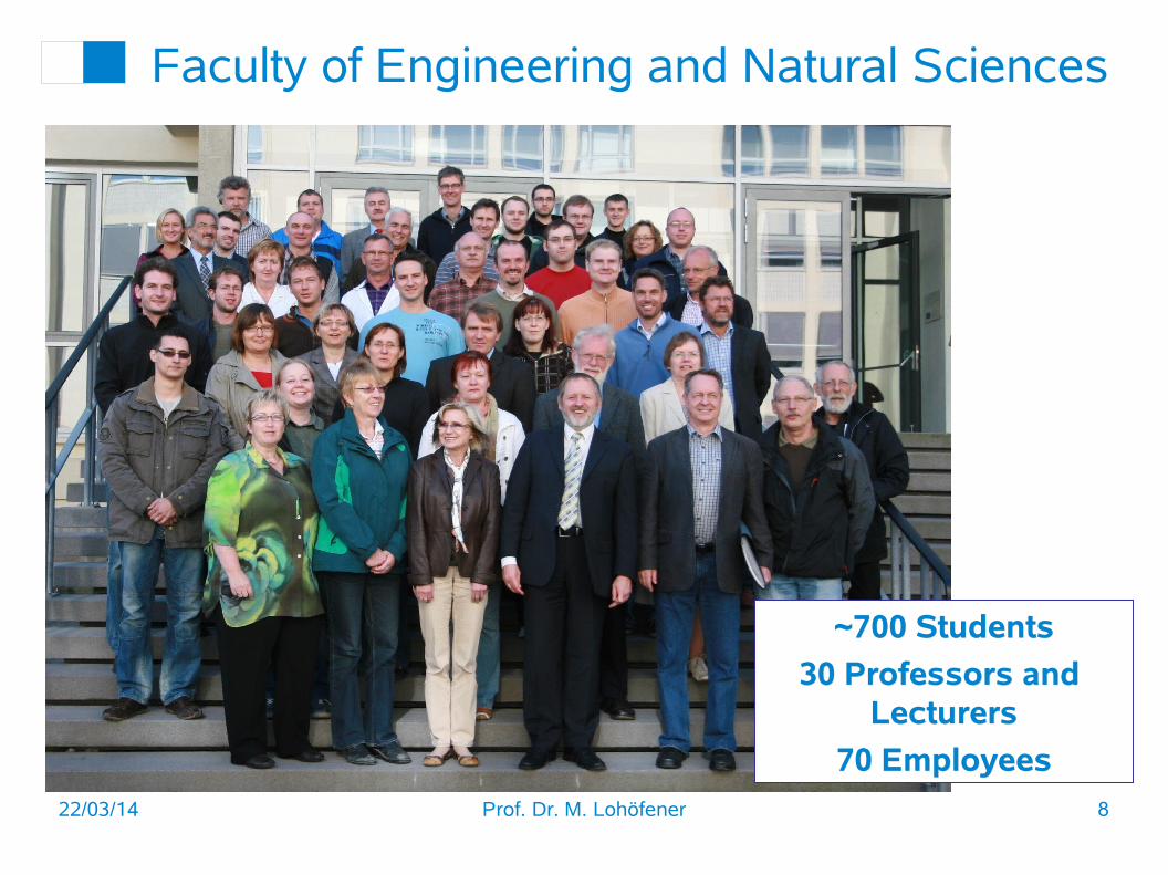
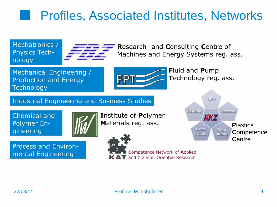
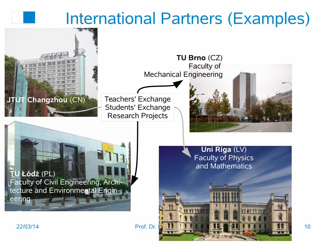
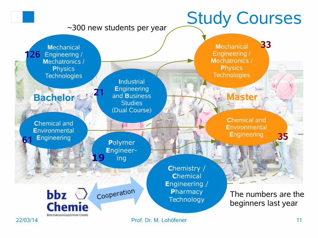
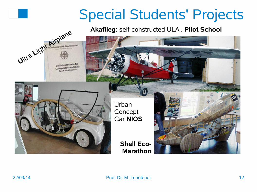
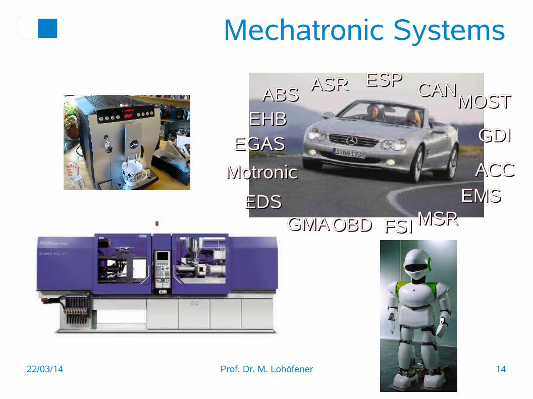
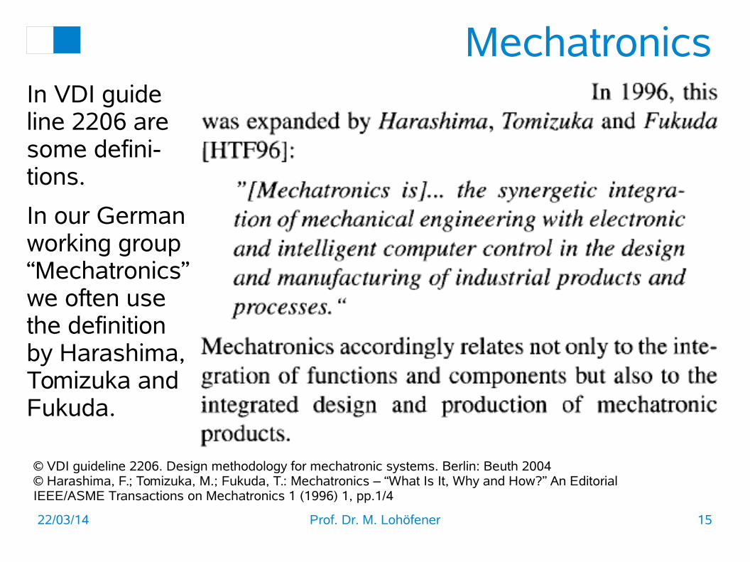
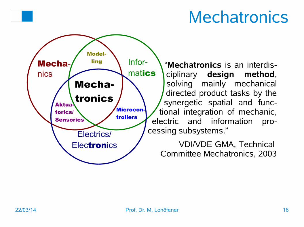
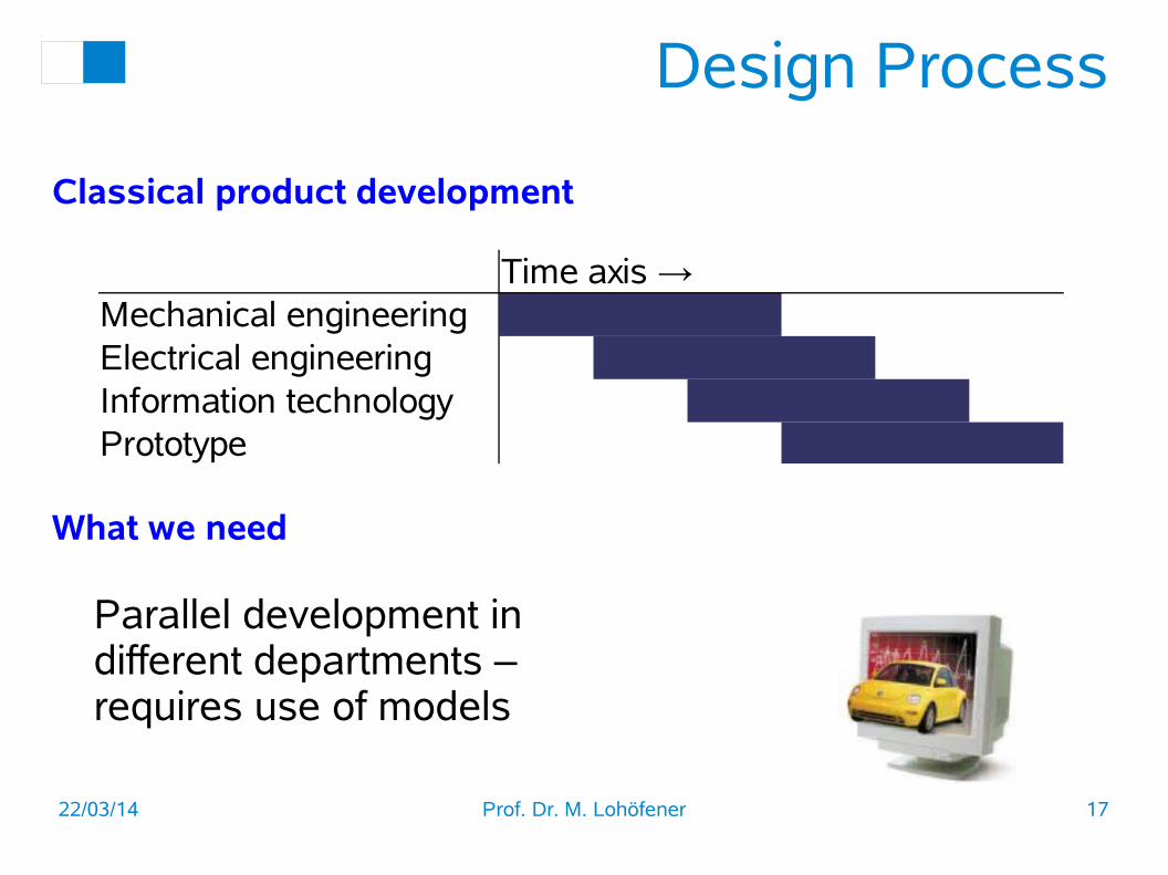
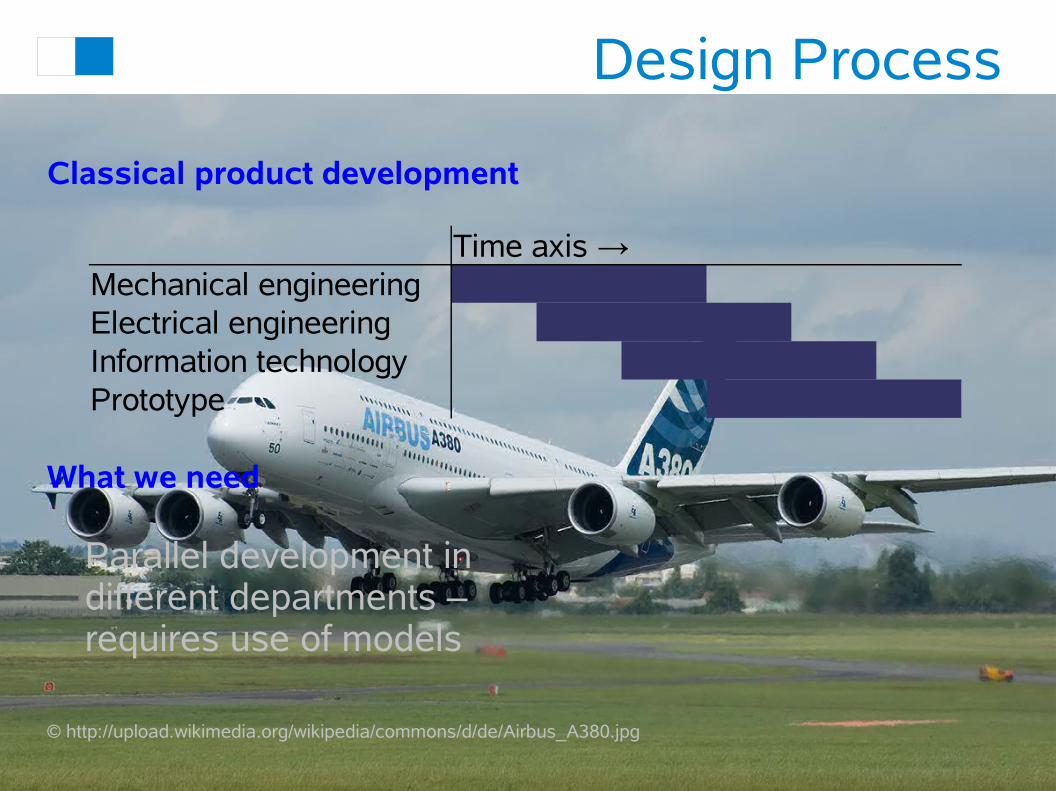
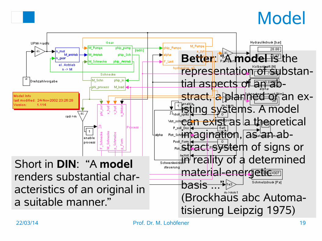
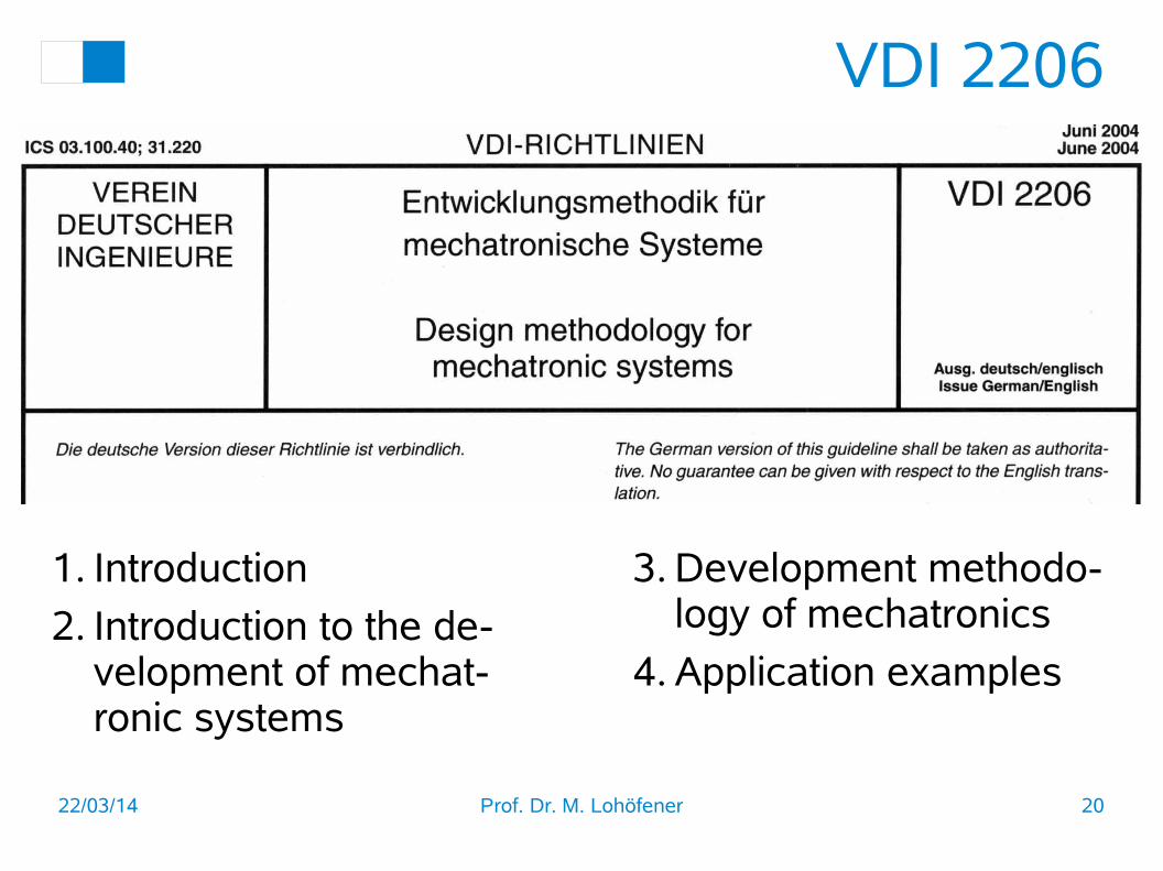
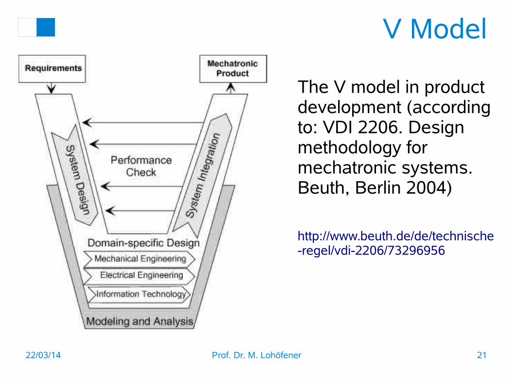
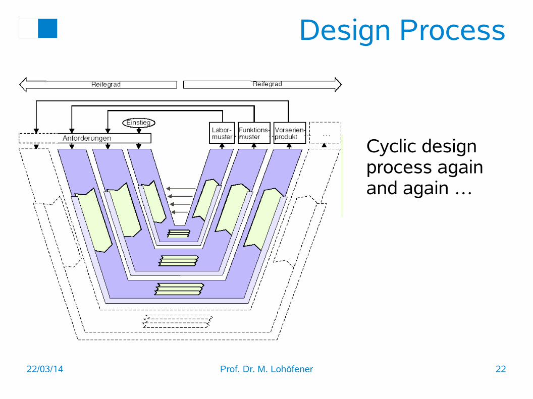
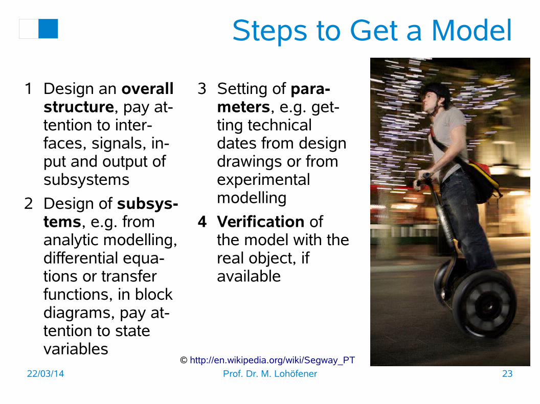
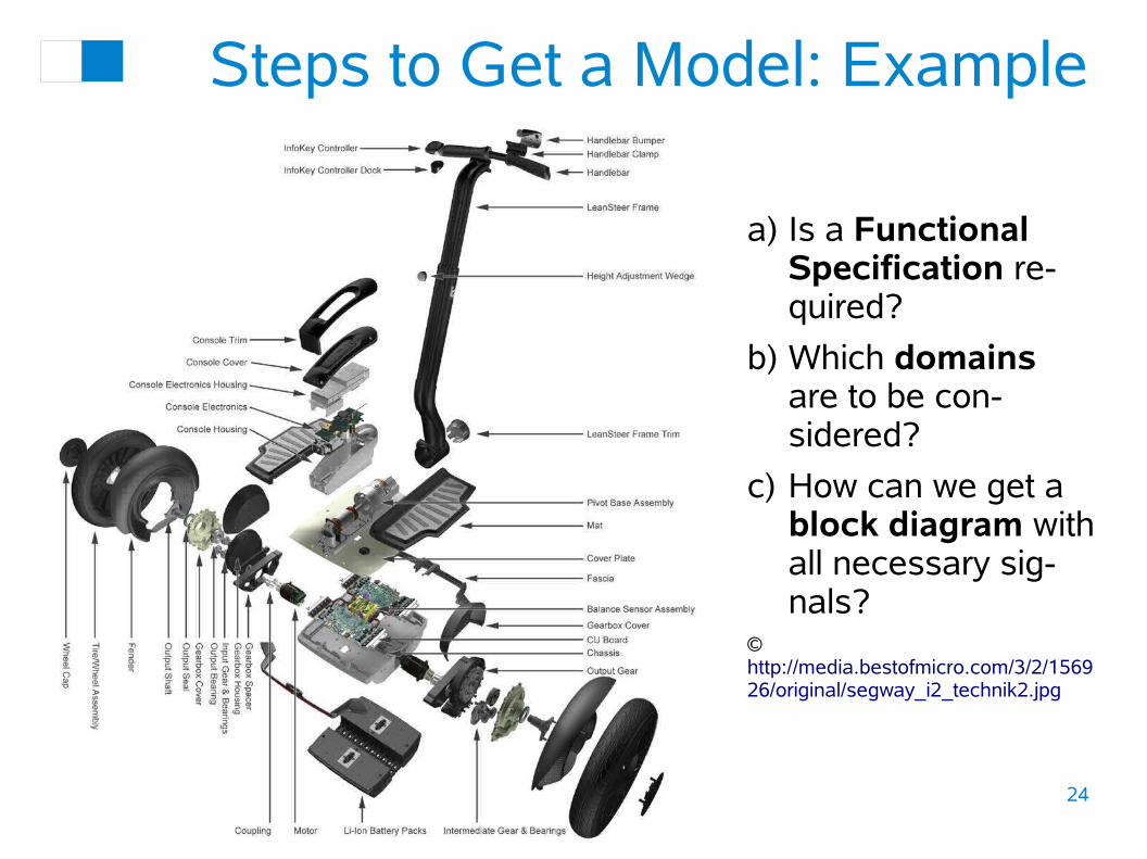
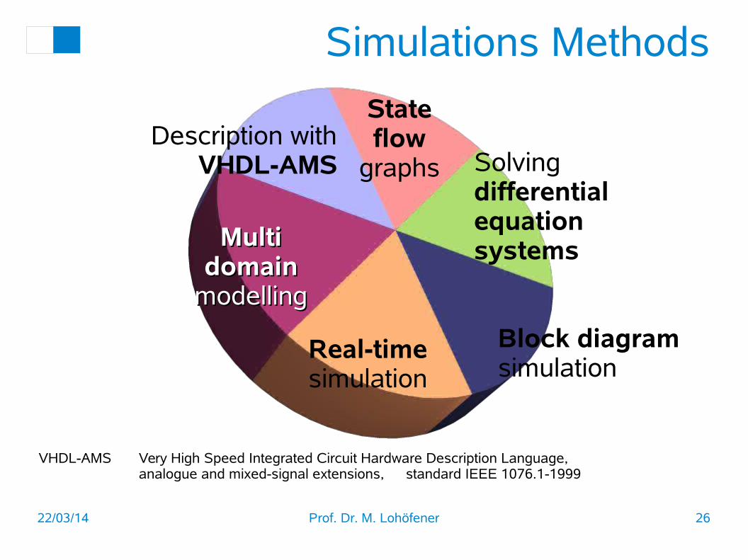
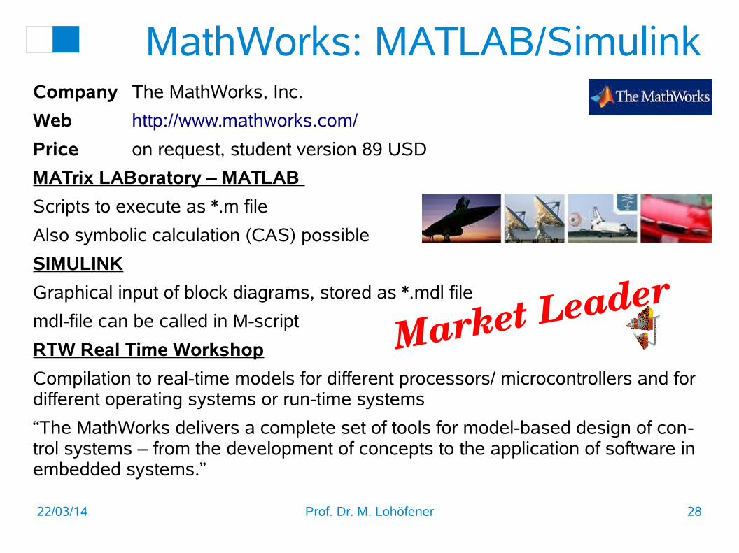
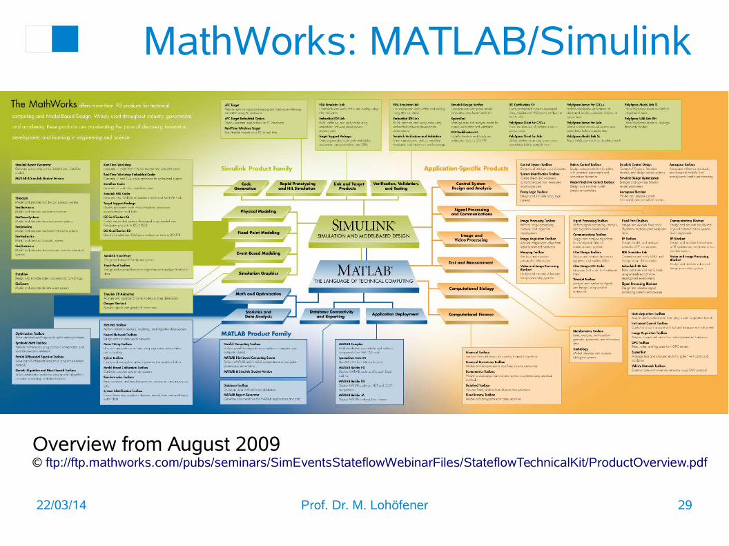
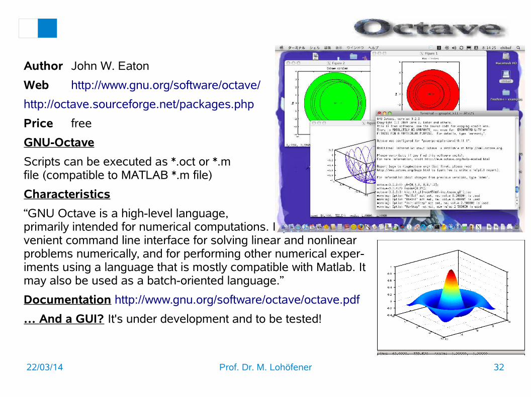
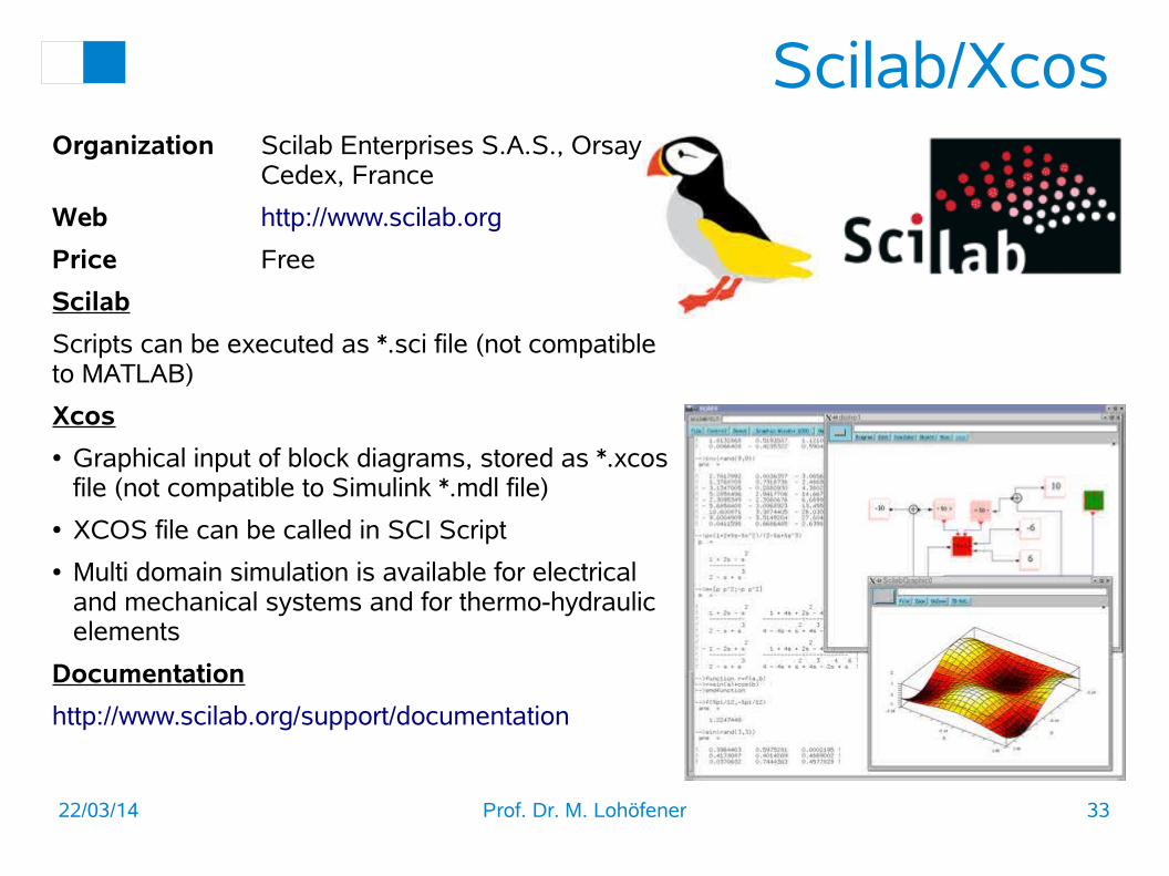
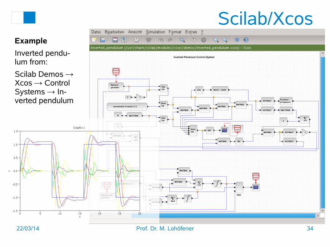
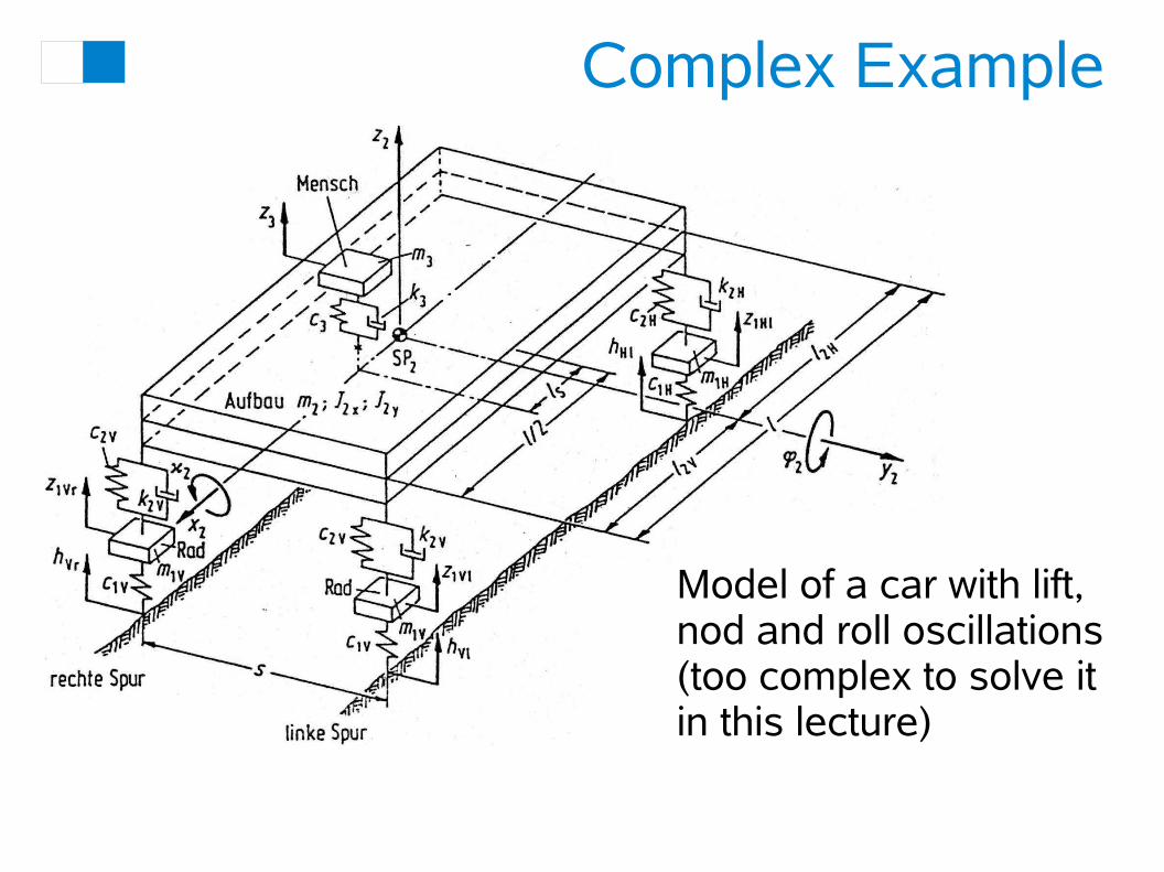
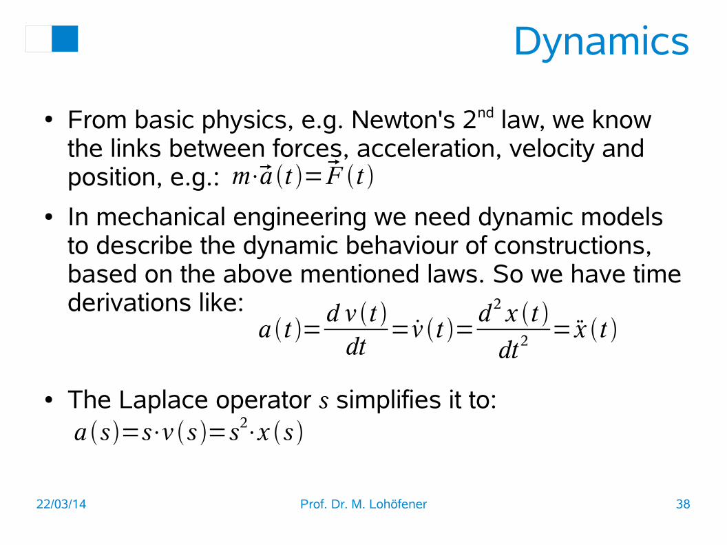
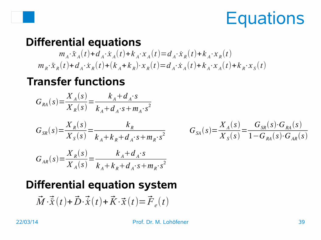
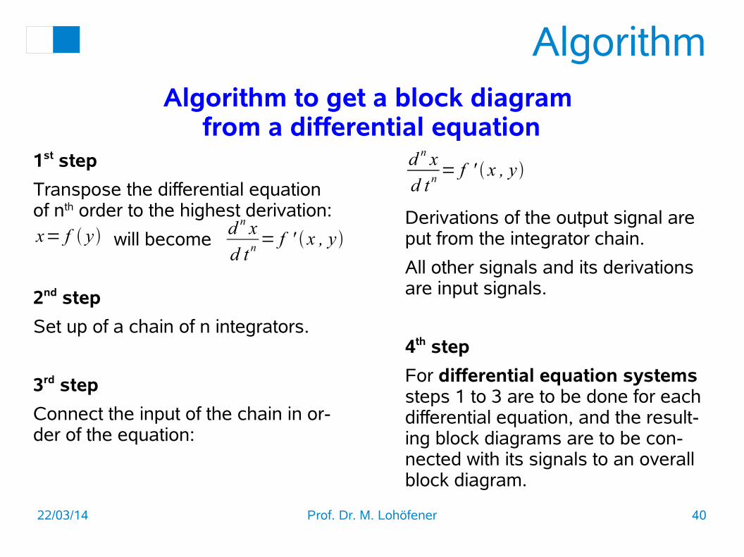
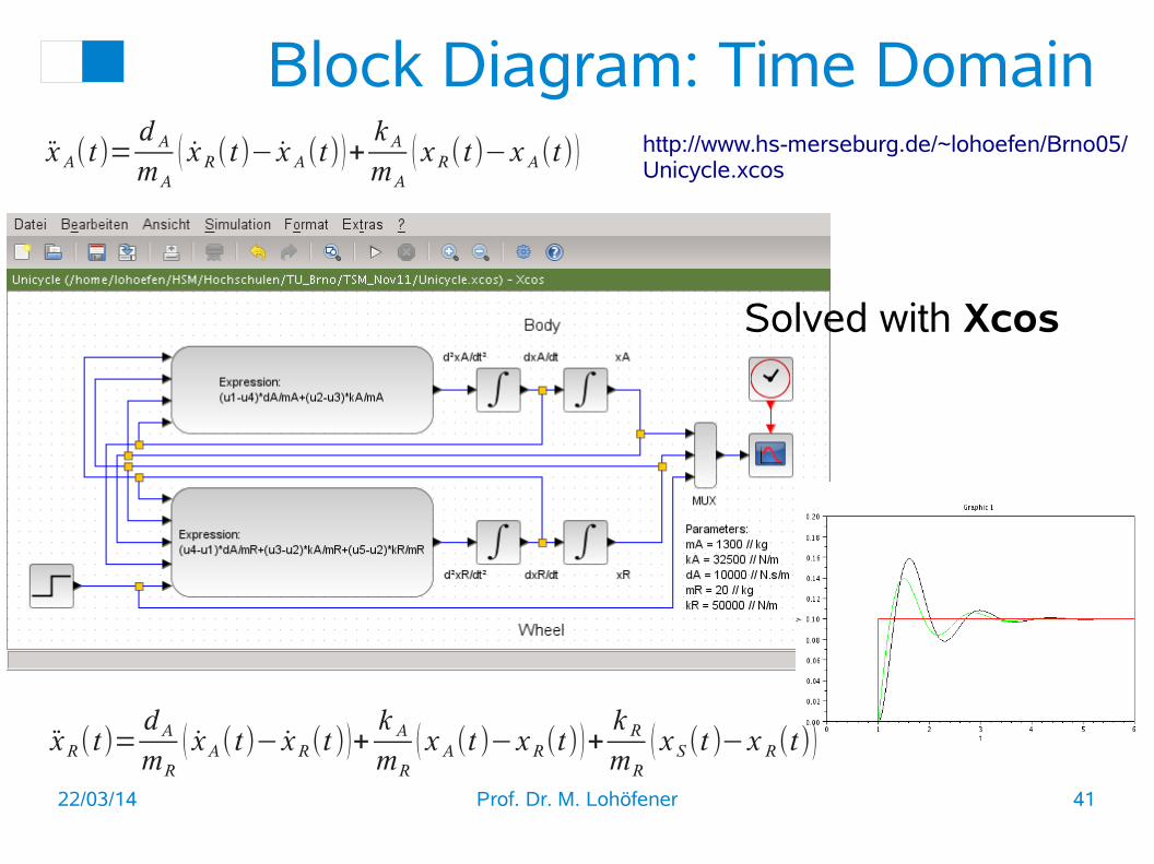
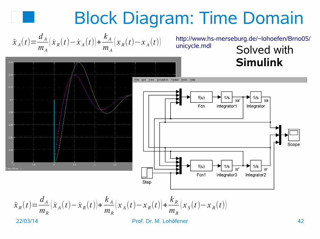
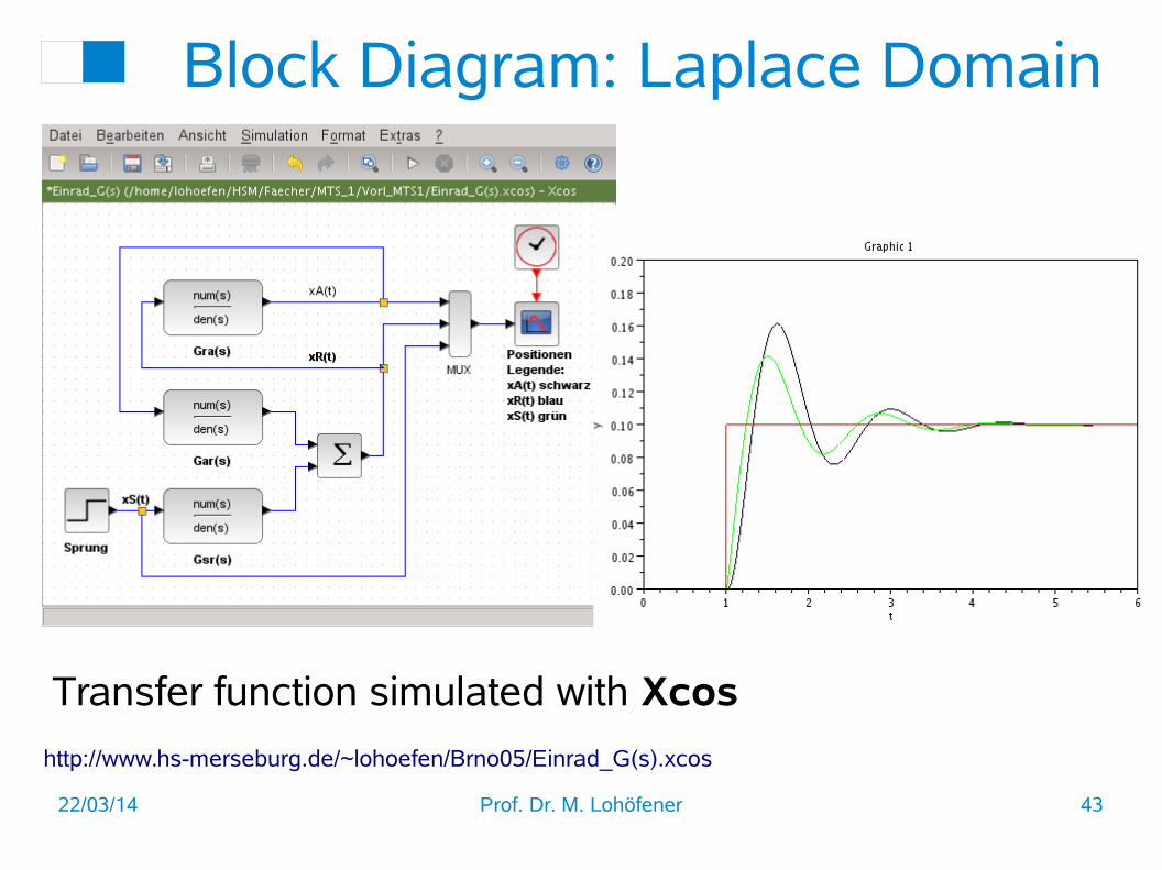
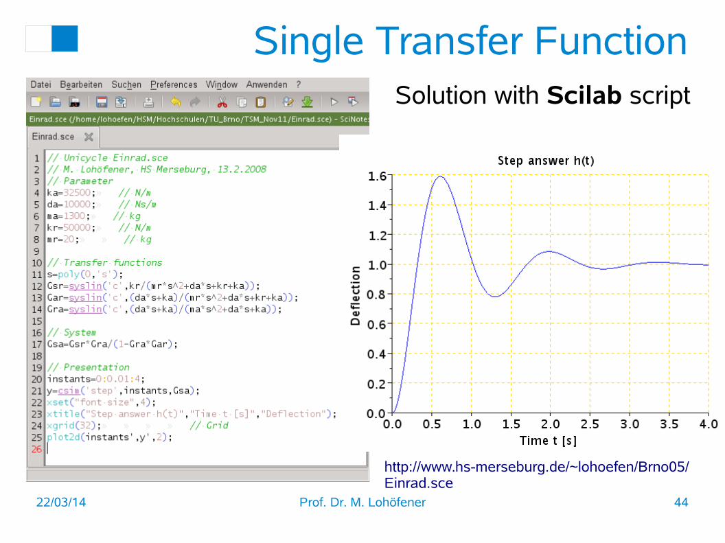
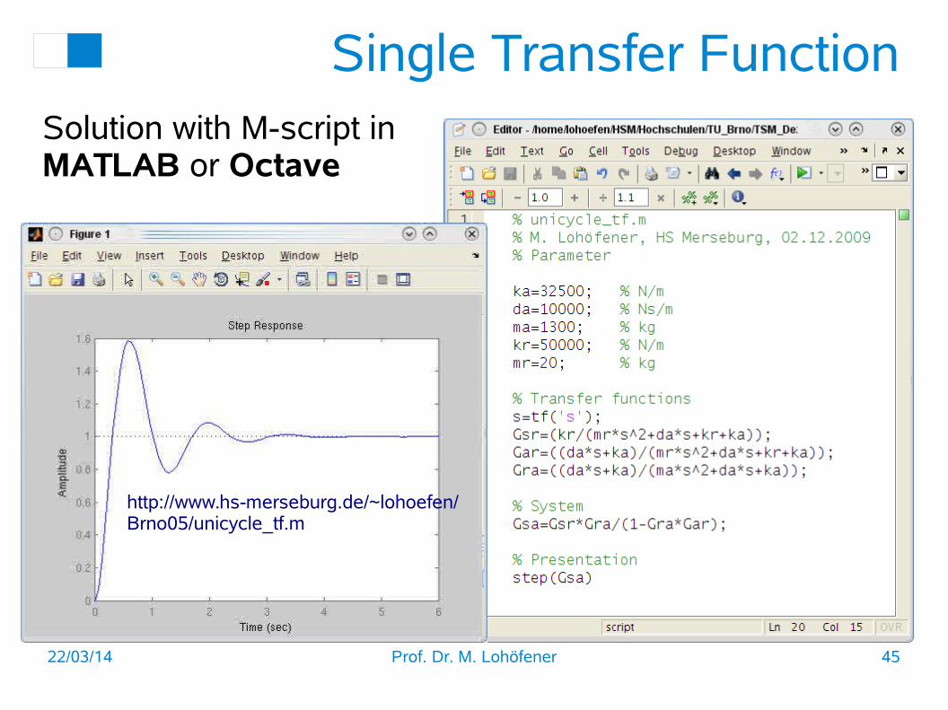
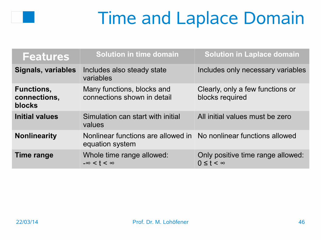
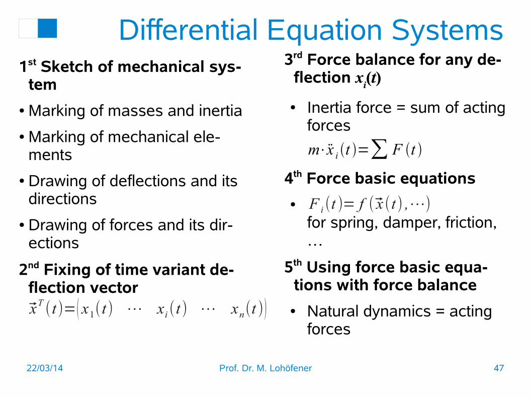
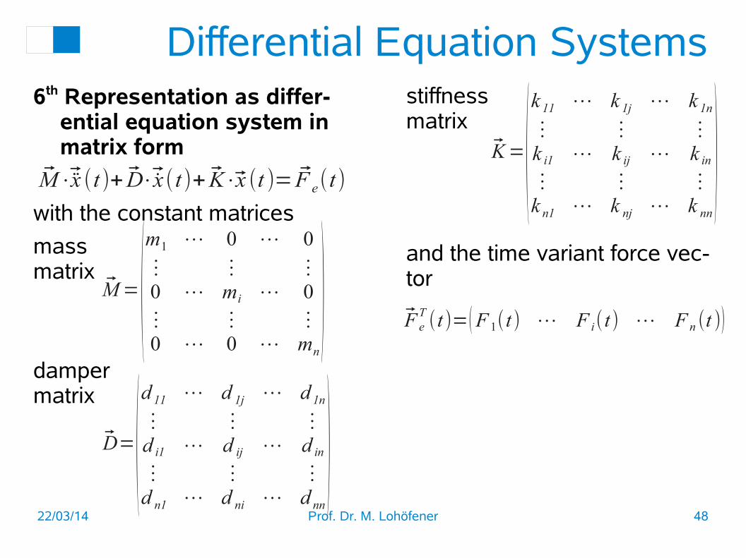
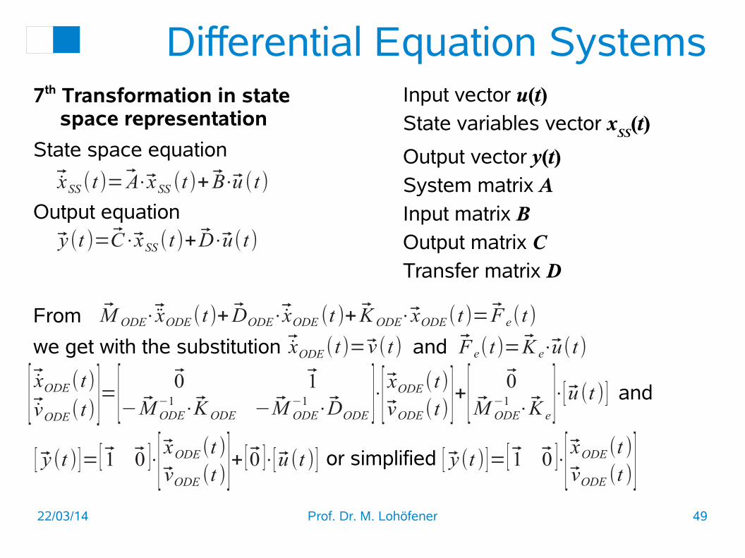
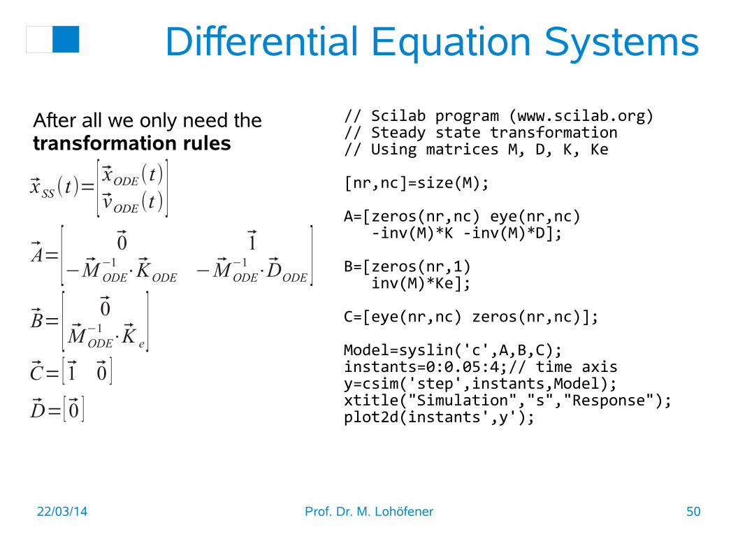
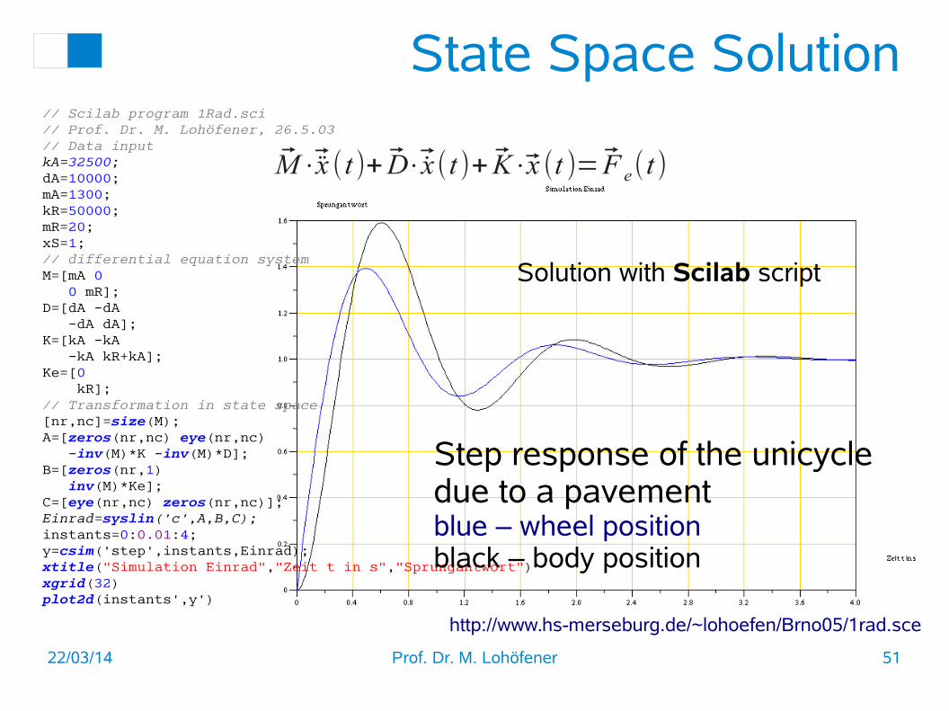
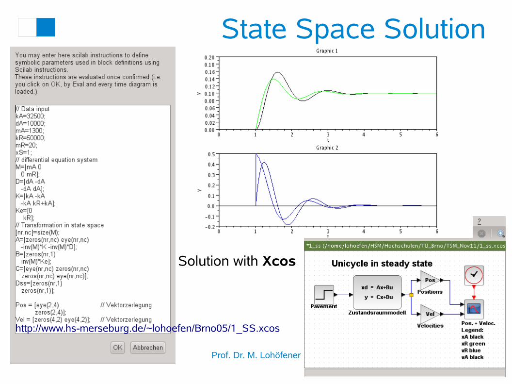
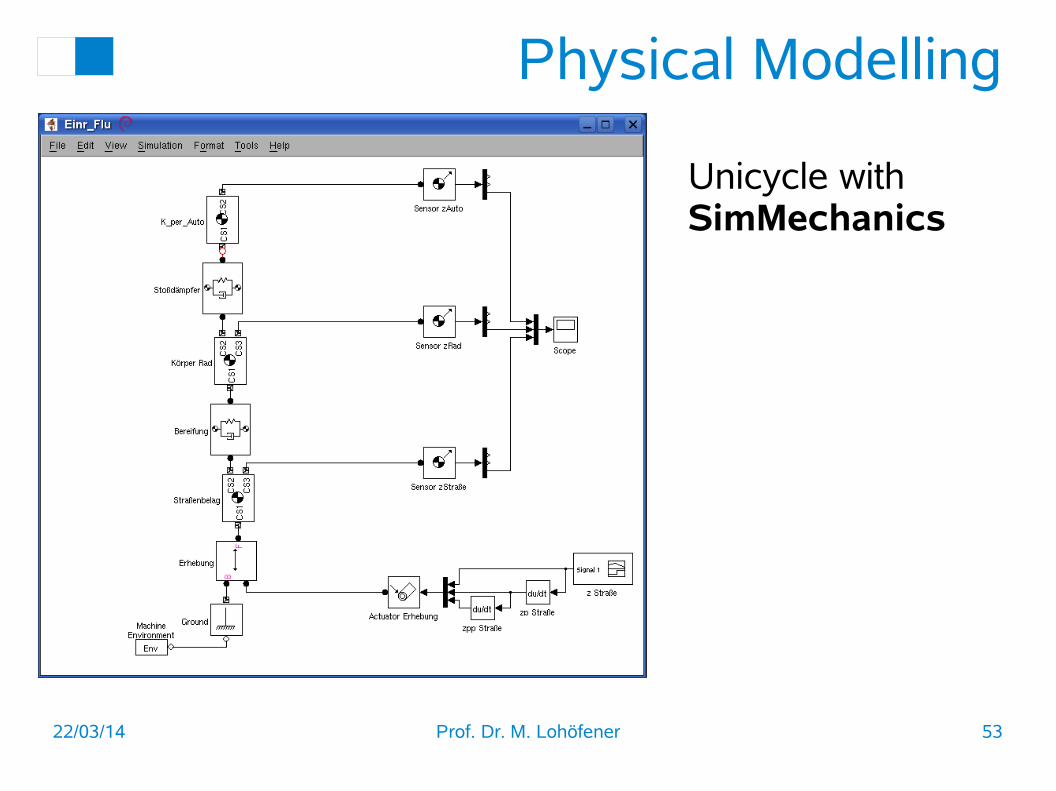
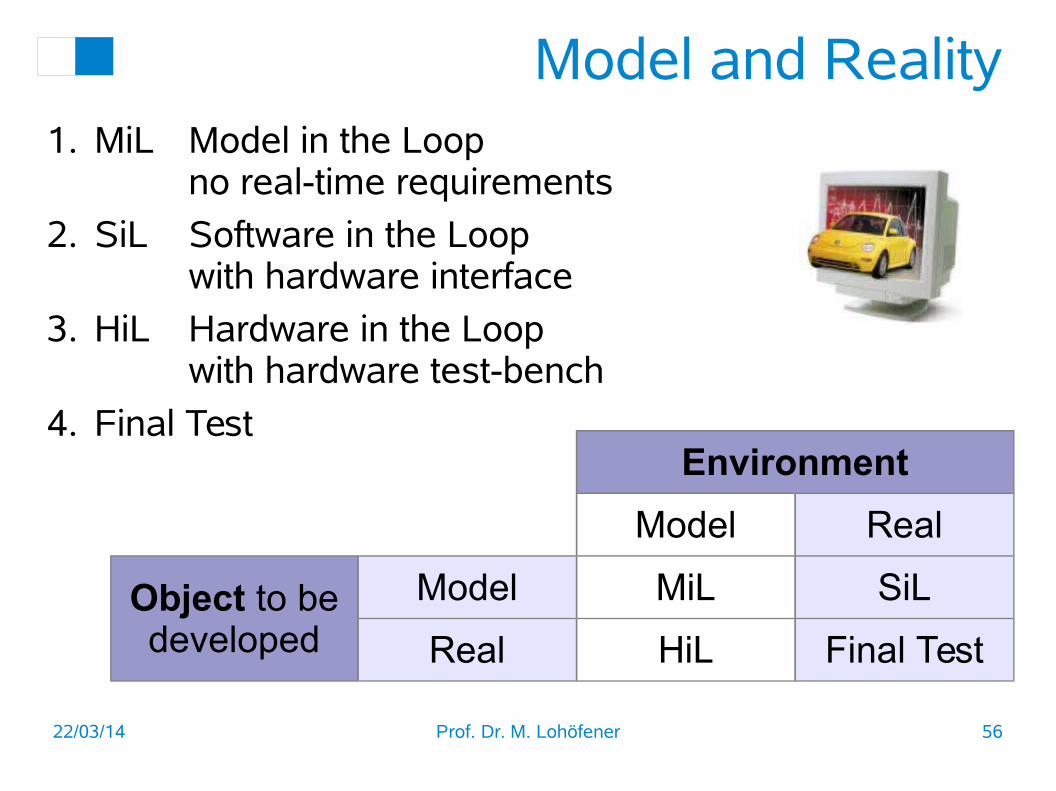
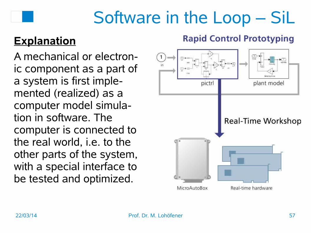
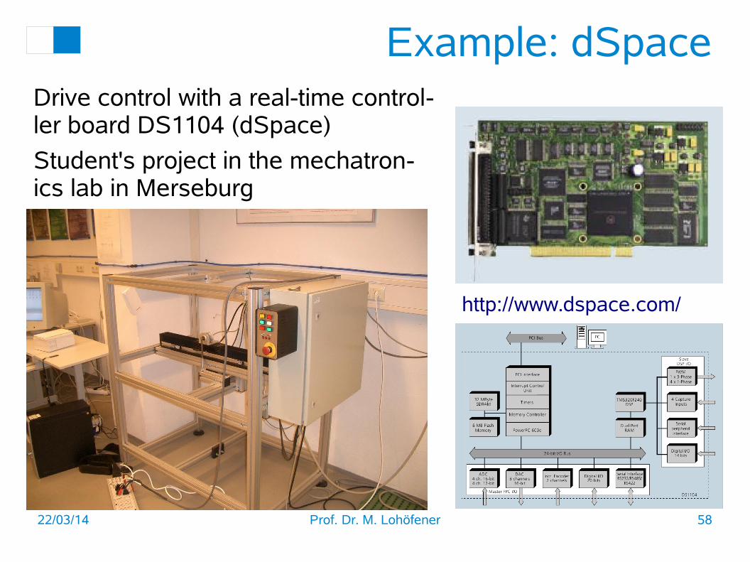
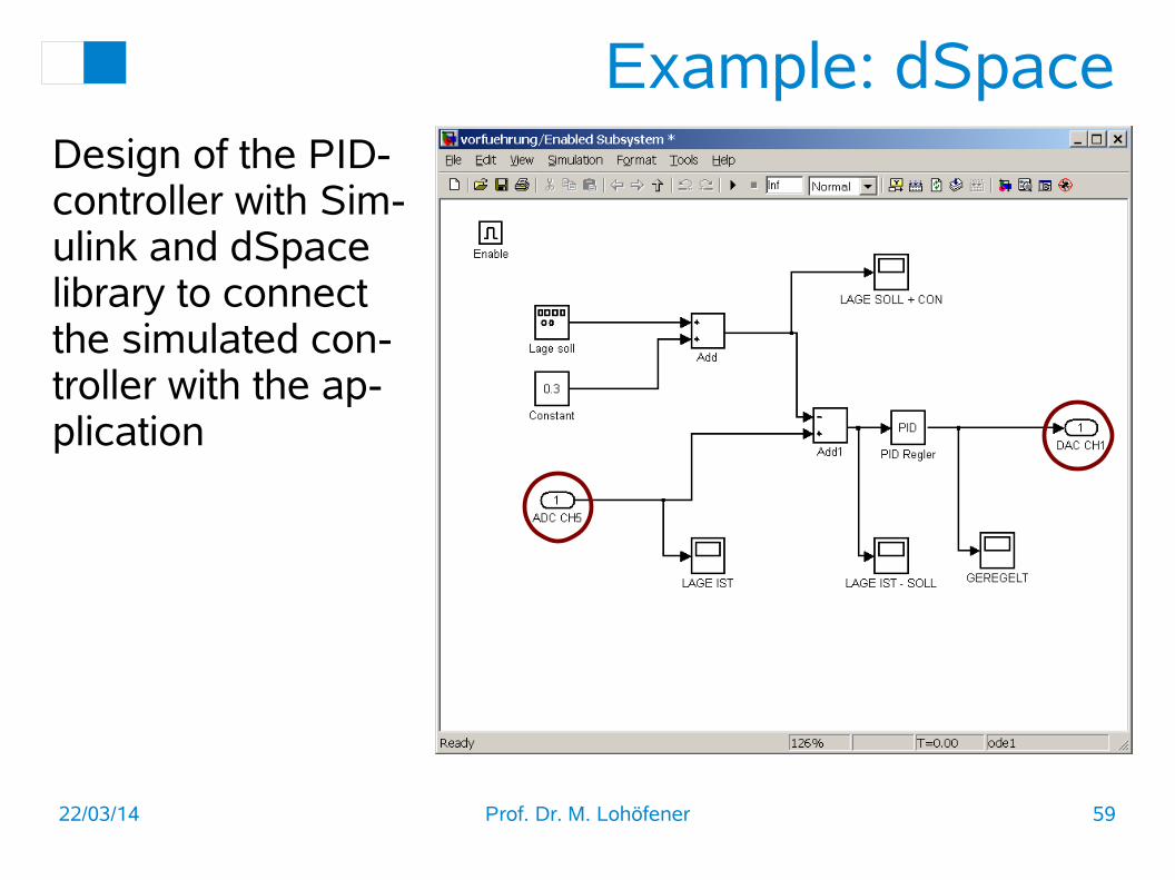
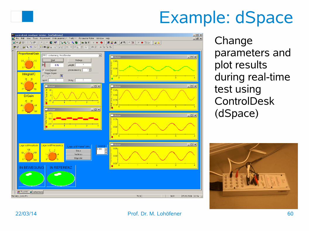
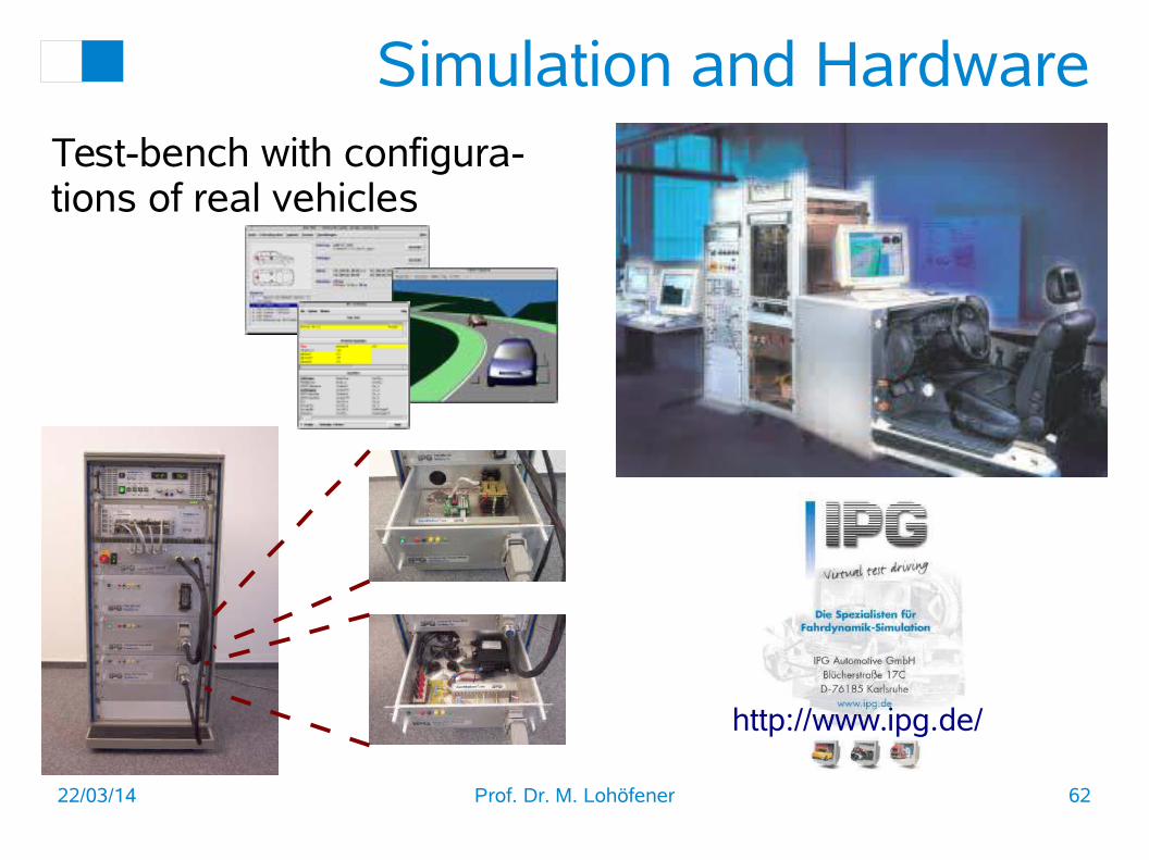
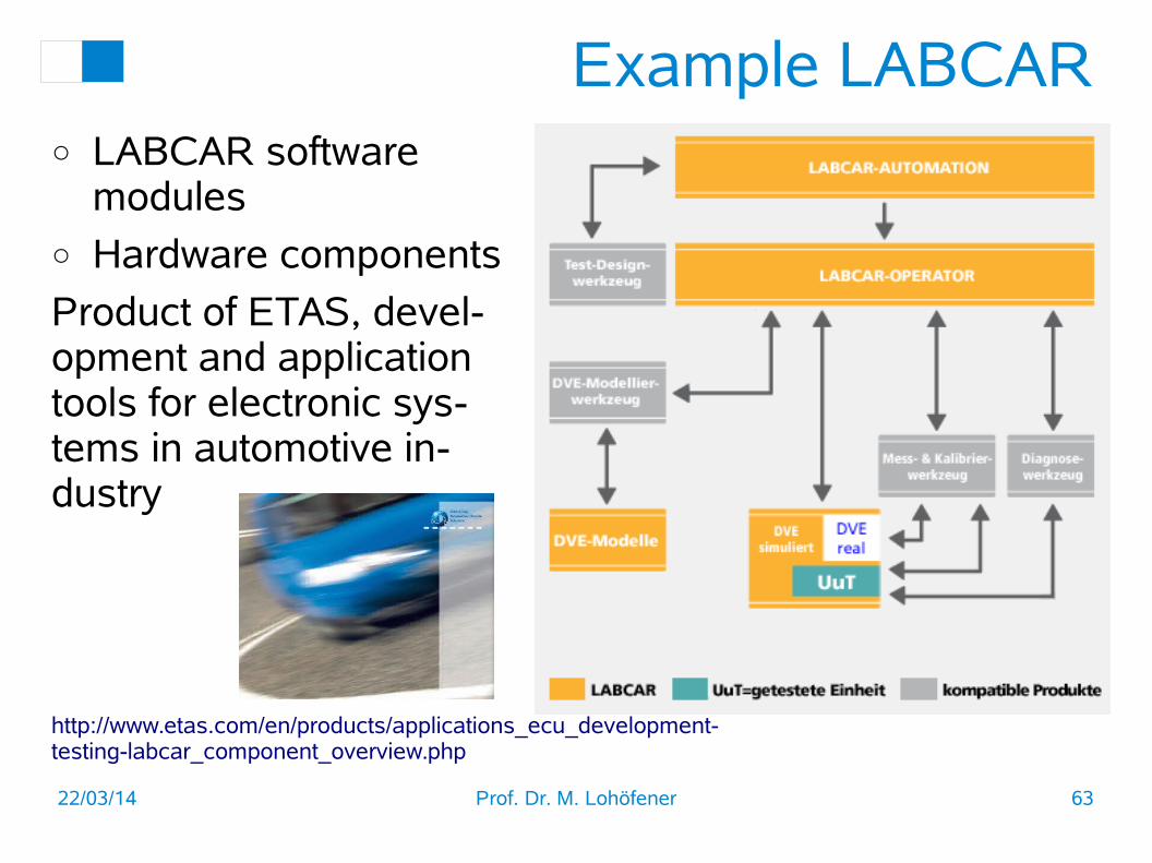
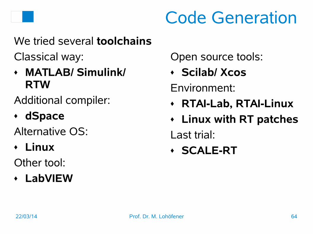
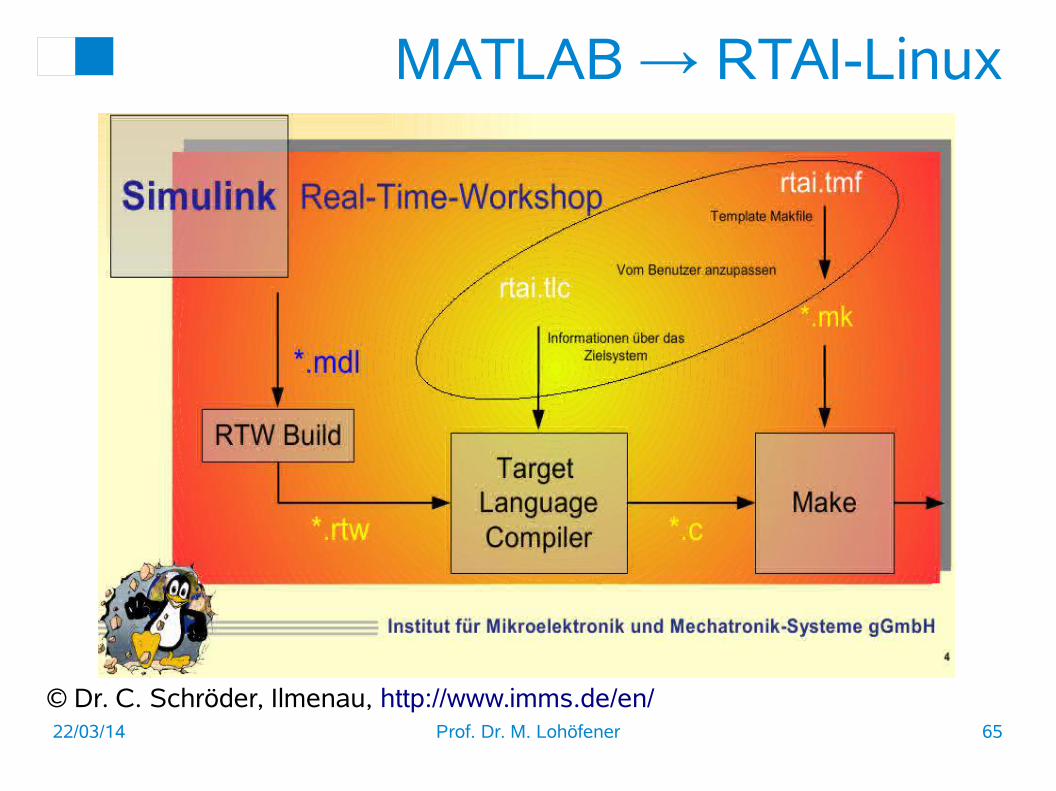
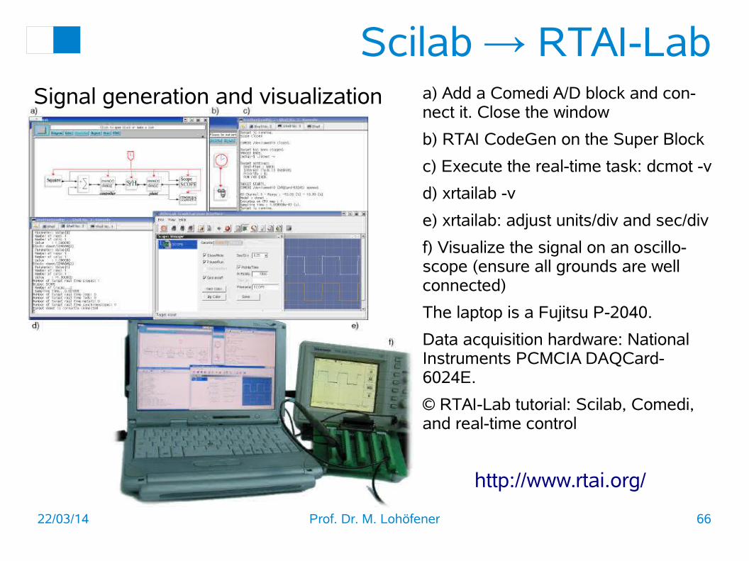
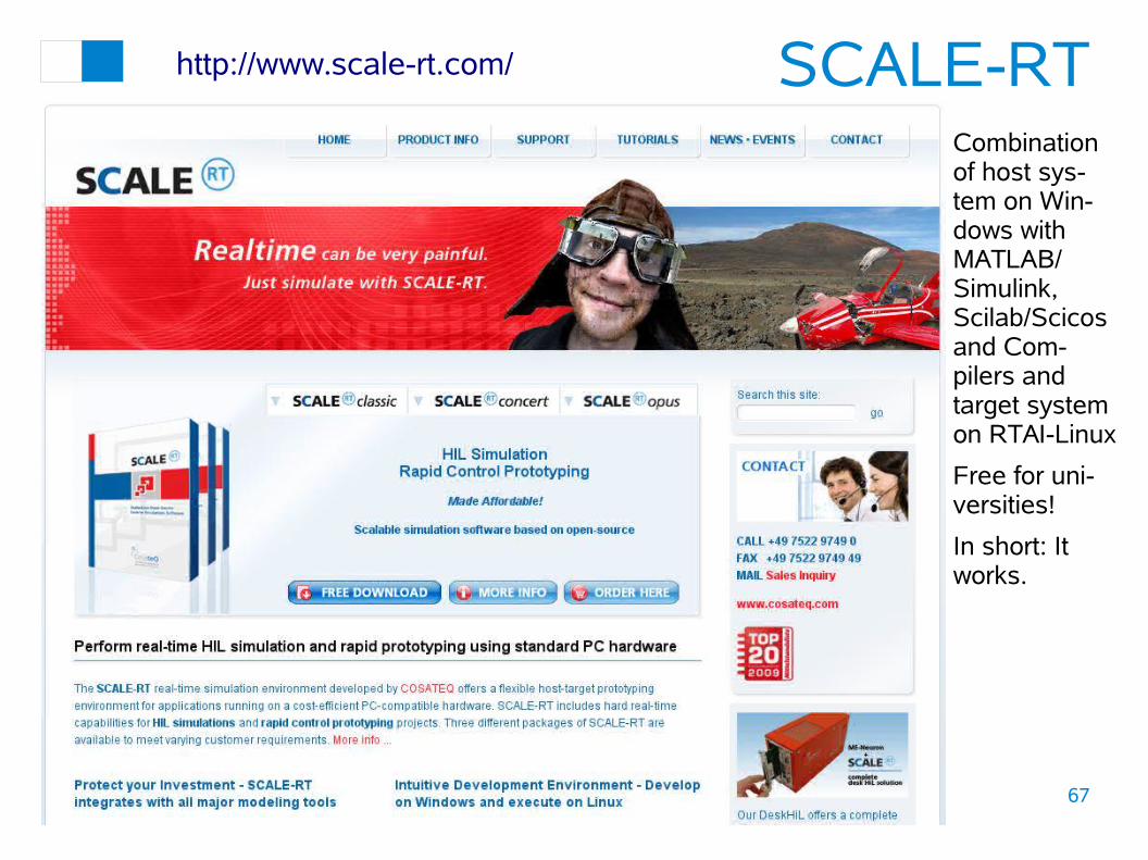
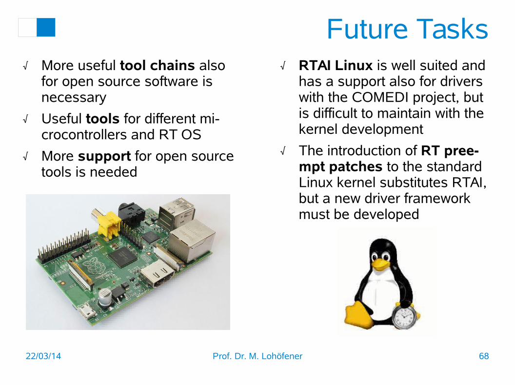