Financial Risks, BankruptcyProbabilities, and theInvestment Behaviour ofEnterprises

Kai Kirchesch

HWWA DISCUSSION PAPER

299Hamburgisches Welt-Wirtschafts-Archiv (HWWA)

Hamburg Institute of International Economics2004

ISSN 1616-4814

Hamburgisches Welt-Wirtschafts-Archiv (HWWA)Hamburg Institute of International EconomicsNeuer Jungfernstieg 21 - 20347 Hamburg, GermanyTelefon: 040/428 34 355Telefax: 040/428 34 451e-mail: hwwa@hwwa.deInternet: http://www.hwwa.de

The HWWA is a member of:

• Wissenschaftsgemeinschaft Gottfried Wilhelm Leibniz (WGL)• Arbeitsgemeinschaft deutscher wirtschaftswissenschaftlicher Forschungsinstitute

(ARGE)• Association d’Instituts Européens de Conjoncture Economique (AIECE)

HWWA Discussion Paper

Financial Risks, BankruptcyProbabilities, and the

Investment Behaviour ofEnterprises

Kai Kirchesch*

HWWA Discussion Paper 299http://www.hwwa.de

Hamburg Institute of International Economics (HWWA)Neuer Jungfernstieg 21 - 20347 Hamburg, Germany

e-mail: hwwa@hwwa.de

* AcknowledgementsI would like to thank the Deutsche Bundesbank for granting access to the firm-leveldata of the balance sheet statistics and for the technical support. The analysis of thedata took place at the premises of the Deutsche Bundesbank. Only anonymized datawere used in order to maintain the confidentiality of the data.

This discussion paper is assigned to the HWWA’s research programme “Business CycleResearch”

Edited by the Department International MacroeconomicsHead: Dr. Eckhardt Wohlers

HWWA DISCUSSION PAPER 299October 2004

Financial Risks, BankruptcyProbabilities, and the

Investment Behaviour ofEnterprises

ABSTRACTThe link between investment and finance usually enters the empirical literature in theform of financial constraints which are defined as the wedge between the costs of inter-nal and external finance or as the risk of being rationed on the credit market. In thiscontext, the sensitivity of investment with respect to single internal or external financeindicators is assumed to be appropriate to proxy for these constraints. However, enter-prises that rely on external funds do not only face this external finance premium andpotential borrowing limits, but also the risk of not being able to meet their repaymentobligations and thus the risk of bankruptcy.

If the risk of bankruptcy enters the profit maximization of the firm, the resulting empiri-cal investment function includes the probability of survival as an additional explanatoryvariable. This modified neoclassical investment equation is tested with West Germanpanel data which include more than 6000 enterprises and cover a period of 12 years.The empirical results confirm the assumption that the risk of bankruptcy is an importantdeterminant of the enterprises' investment behaviour. Additionally, the results raise thequestion whether financial constraints respective cash flow sensitivies are the appro-priate way to test for the influence of the financial sphere on the investment decisions ofenterprises, or whether bankruptcy probabilities better account for these potential finan-cial risks.

JEL-Classification: E22, D92, G33, C23

Keywords: Investment, Bankruptcy, Financial Constaints, GMM

Kai KircheschDepartment of International MacroeconomicsHWWA-Hamburg Institute of International EconomicsNeuer Jungfernstieg 21D-20347 HamburgGermanyTel.: +49-40-42834368e-mail: kirchesch@hwwa.de

1 Introduction

Real economies unfortunately seldom satisfy the rather strict assumptions of the most fa-mous investment theories like the neoclassical model of investment or Tobin’s q theory. Eventhough early empirical investgations found evidence for the financial decisions of enterprisesbeing an important determinant of their investment behaviour, these theories eclipse the fi-nancial sphere with the postulation of a perfect world as it was put forward by the famousModigliani-Miller (1958) irrelevance theorem. In their world without any frictions, the finan-cial structure of an enterprise does not influence its investment decisions. Hence, the determi-nation of the firm’s demand for new capital is merely driven by factor prices and technology.Cash flow, the level of debt, and other financial variables are to be ignored while decidingabout the level of investment, since firms will always obtain enough funds at the economy-wide riskless interest rate to finance all of their desired investment projects if capital marketsare perfect and no frictions arise.

Starting with the seminal lemon paper of Akerlof (1970), the proceedings in the literature onasymmetric information in capital markets shed light on the shortcomings of the neoclassi-cal approach and emphasized potential capital market imperfections between borrowers andlenders and their consequences on the functioning of these markets. As borrowers usuallypossess more information about their investment projects than lenders do, the latter will haveto find ways to mitigate their risk by means of credit contracts that account for the existinginformational asymmetries and implement mechanisms which entail self-selection and costlystate verification. These mechanisms lead the banks to either demand a risk premium on themarket interest rate for borrowed funds or to refrain from meeting the complete demand forcredits in case borrowers appear to be too risky. However, as soon as it becomes more ex-pensive to raise borrowed funds than to rely on own funds in order to finance an investmentproject, the irrelevance of the financial structure on business fixed investment does no longerhold. Due to these capital market imperfections, firms will prefer to use internal rather thanexternal funds to finance their investment spending, as predicted by the pecking order theory.As a consequence, the internal net worth of the firms as well as the level of its indebtnessmay play a crucial role in the determination of the enterprise’s optimal level of investment.

The past 15 years have witnessed a number of publications pursuing this track and extendingthe above mentioned conventional models of business investment with elements of asymmet-ric information to incorporate the role of financial factors in determining the demand for newcapital. As regards the implementation of these financial factors, the performed studies fo-cus on the existence of financial constraints and their impact on business fixed investment.

1

In this context, financial constraints denote either the risk premium that enterprises have tobear in order to receive borrowed funds, or the risk of being credit rationed by the bank, bothof which owe to the incidence of adverse selection or moral hazard for these providers ofexternal funds.

In order to analyze the impact of financial constraints on the investment behavior of enter-prises, most studies followed the influential paper of Fazzari-Hubbard-Petersen (1988) andperformed tests referring to the excess sensitivity of internal funds such as cash flow with re-spect to the firm’s investment spending. Since firms that are subject to more severe financialconstraints are assumed to rely more heavily on retained earnings and even bank debt thanon direct credit, the investment spending of this type of firm is supposed to be more sensitiveto fluctuations in internal net worth. The same holds true for enterprises that face some sortof borrowing limits. Furthermore, a number of studies account explicitly for financial con-straints by including some sort of external finance premium into the profit maximization ofthe firm. With this risk premium depending on the enterprise’s level of debt and its capitalstock, the empirical investment equation usually contains the firm’s leverage rather than itscash flow. The same holds true for the inclusion of a debt ceiling and the firm’s leverageas a proxy for the risk of reaching this boundary. The appropriateness of cash flow or otherfinancial variables to proxy for financial constraints, as well as the methods of classifyingenterprises according to these variables, meet with severe criticism in the course of a stillongoing debate.

Yet, these studies do not account for the complete effect of the enterprise raising externalfunds in order to finance its investment. Without doubt, the higher costs of external funds andthe likelihood that the availability of these funds may be restricted constitute one importantpart of the financial risks that firms are facing. Yet, borrowing external funds also entails therisk of not being able to repay these funds and consequently default on the debt repayments.Hence, if an enterprise aims at maximizing its future profits by defining the optimal capitalaccumulation path, it has to take into account the danger of facing bankruptcy in some futureperiod.

The present study therefore tries to expand the conventional literature on financial constraintsby establishing the connection between the firm’s investment decision and financial risksas a whole. Hence, the intention of this study is the empirical estimation of an investmentfunction which explicitly accounts for the risk of bankruptcy as a complete measure for theenterprises’ financial risks. Therefore, these bankruptcy risks are introduced into the neoclas-sical theory of investment by altering the calculations of the profit maximizing firm insofar

2

that its expected future revenues will be weighted with its probability of survival. The result-ing modified investment function which contains the firm’s survival probability will then betested with data stemming from the balance sheet statistic of the Deutsche Bundesbank.

The remainder of the paper is organized as follows. Section 2 shortly reviews the exist-ing literature on financial constraints before introducing the concept of financial risks andexplaining its advantages compared to the narrower definition of financial constraints. Themodified neoclassical model of investment which explicitly includes the risk of bankruptcywill be described in section 3. After the description of the dataset in section 4, the empiricalresults will be presented in section 5. Section 6 concludes.

2 Financial Risks and Financial Constraints

Fazzari-Hubbard-Petersen (1988) were the first to investigate whether capital market im-perfections lead to corporate underinvestment as a result of insufficiently available internalfunds.1 In order to estimate these financial constraints, they assume the existence of asym-metric information and a resulting hierarchy of finance, while credit rationing does not occur.The presumption that at least some enterprises are constrained as regards the costs of creditsis tested by quantifying the investment sensitivity of these enterprises with respect to theircash flow. Firms with lower dividend payout ratios are assumed to be more constrainedon the credit market, and therefore are expected to exhibit stronger cash flow sensitivities.The empirical results confirm these assumptions in the way that all groups of enterprisesexhibit significant coefficients for these sensitivities, and those firms with higher retentionratios prove to be more sensitive with respect to changes in their cash flow than firms that aredeemed to be less financially constrained.

While there is considerable support of the results obtained by Fazzari-Hubbard-Petersen,Kaplan-Zingales (1997) among others address criticism concerning the usefulness of cash-flow sensitivities to represent financial constraints by challenging the monotonicity assump-tion of these sensitivities with regard to the financial constraints. Additionally, they dis-approve the method of classification that Fazzari-Hubbard-Petersen apply. Cleary (1999)confirms the results obtained by Kaplan-Zingales using a large sample of U.S. enterprisesand employing a more objective classification criterion which is obtained by using multiplediscriminant analysis analogous to the proceeding of Altman (1968).

1At least, their study can be regarded as the most influential paper. For an overview of this strand of literatureas well as the earlier liquidity theory literature, see Kirchesch (2004).

3

However, Fazzari-Hubbard-Petersen paved the way for a large body of empirical studies thatadopted their indirect approach of testing the role of financial constraints for the enterprises’investment decision in the framework of the q theory. Furthermore, Whited (1992) and Bond-Meghir (1994) were the first to discard the q model in favor of an Euler equation approach,with financial constraints being tested by including variables that account for the externalrather than internal finance of the enterprise. Meanwhile, a vast quantity of studies for nu-merous countries is available which test the influence of financial decisions on the enterprises’investment behaviour in either theoretical framework.2 Yet, all of these studies mostly applyinternal or external finance sensitivity tests by adding single financial variables to the empiri-cal investment equation in order to find out whether departures from the standard model holdunder conditions of imperfect capital markets.

Hence, theories of investment in consideration of the firms’ financial sphere are hithertolimited to theories of financial constraints in the presence of asymmetric information, withthe prevalent definition of these financial constraints being unanimously accepted. Withoutdoubt, all firms that rely on external finance are financially constrained in the way that ex-ternal funds are more expensive than internal funds. Additionally, but not necessarily, thefirm can face some sort of credit rationing.3 Yet, the question remains whether the effect ofexternal finance is fully captured by these financial constraints and thus the wedge betweeninternal and external funds. In a world of asymmetric information, lenders charge an interestpremium due to the uncertainty about the enterprise being able to repay its obligations in thefuture. If this is not the case, the firm will file for bankruptcy, and the bank has to write offits loan. Analogous to the bank, the enterprise has to allow for this risk while calculating itsoptimal capital accumulation path. However, while many studies are aware of the danger ofbankruptcy in case of external financing, this kind of risk does not enter neither the theoreticalmodels nor most of the empirical investment equations in a comprehensive way.

In some studies, the risk of bankruptcy enters the theoretical model of investment in a simi-lar way to the external finance premium in the form of an agency cost function.4 Under thecommon assumption that the default risk will rise with the level of the firm’s debt and declinewith its capital stock, the specification of the investment function does not differ significantlyfrom the models that include an external finance premium. Yet, those studies do not accountfor the risk of not being able to earn future revenues as the result of a possible bankruptcy.

2See Schiantarelli (1996), Hubbard (1998), or Chatelain (2002) for overviews of these studies.3In this study, credit rationing is not taken into consideration since it would not impose any significant changesas regards the functional form of the model.

4See, for example, Leith (1999) or Pratap-Rendon (2003). Other studies include financial distress costs functionsin order to capture the effect of the external finance premium on business investment, see, among others,Hansen-Lindberg (1997), Hansen (1999) or Siegfrid (2000).

4

If this risk enters the maximization calculus of an enterprise, future profits must be weightedwith the probability of survival and therewith the likelihood of gaining future revenues at all.In case the survival probability enters the firm’s profit maximization, the resulting investmentequation will contain an additional variable which accounts for this probability. Since theresearcher is given plenty of rope to vitalize this bankruptcy probability in the course of theestimation, it must not necessarily be interpreted as the pure risk of bankruptcy, but ratheras a comprehensive measure for the financial distress a firm may face. Actually, there existmany possibilities to empirically model this financial risk. In the simplest case, some lever-age variable could be employd in order to account for this risk with the consequence of theinvestment function being equal to many empirical functions that account for financial con-straints. Yet, as there exist explicit measures to estimate the firms’ bankruptcy probabilities,these measures can definitely be regarded as being more appropriate to account for the firms’financial distress.

Bond-Meghir (1994) are one of the few to include both the risk premium on the interest rateas well as the risk of bankruptcy into their model of investment behavior both of which aredependent on the company’s debt in relation to its capital stock. In addition to the risk ofdefault, bankruptcy costs enter the model which depend only on the level of debt, but noton the capital stock. However, the empirical equation does not entail explicitly the risk ofbankruptcy, but rather the squared debt-to-capital ratio as the indicator for this risk, sincethe danger of bankruptcy does not enter the profit maximization as a discounting weight forfuture revenues. Leith (1999) includes the costs of bankruptcy into a model of aggregateinvestment by substracting these costs from the revenues in the firm’s profit maximization.Since the model describes aggregate investment spending, the probability of bankruptcy is in-cluded in form of the liquidation rate amongst all firms.5 According to Leith, this liquidationrate can be seen as a reflection of general macroeconomic conditions, while the bankruptcyprobability also depends on firm-specific factors represented by the firm’s cash flow. Inte-grating this bankruptcy probability into a q model of investment yields a wedge between therate of investment and marginal q. As a consequence, the adjustment process is slower thanwithout accounting for the firm’s likelihood of insolvency.

Besides the classification of the sample according to the firm’s creditworthiness ratio, Kalkreuth(2001) introduces this ratio as explanatory variable into his estimation of an autoregressivedistributed lag model. Drawing his conclusions from the debate about cash flow sensitivities,he argues for the use of rating data to classify the enterprises according to their differential

5The liquidation rate calculates the number of firms being insolvent in one period in relation to the total numberof firms in the economy, see Leith (1999), 6.

5

access to external finance. In this context, the creditworthiness ratio does not account for therisk of bankruptcy, but rather for the financial risks of firms in terms of a potential increaseof the external finance premium in case of financial distress. Frisse-Funke-Lankes (1993)introduce a borrowing limit into the profit maximization of the firm which is assumed to de-pend on the firm’s Z-score of Altman (1968) as an indicator for the firm’s risk of bankruptcy.The Z-score is used both as explanatory variable and as classification criterion, yielding theresult that the group of firms that is considered to be less solvent exhibit significantly highersensitivities with respect to the Z-score than the more solvent enterprises.

Wald (2003) is the first to include the probability of bankruptcy as a weight into the firm’sprofit maximization in order to account for the relationship between risk and investment.This approach yields an empirical investment equation which contains the survival probabil-ity as well as a term that is almost identical to q, yet multiplied with the survival probability.Wald draws the conclusion that those studies that supply evidence on the existence of fi-nancial constraints may mistake these constraints with bankruptcy risks. Hence, the risk ofbankruptcy is not interpreted as an extension of the existing literature on financial constraints,as in the present case, but rather as their counterpart. Yet, both measures indicate some sortof financial distortion due to a deterioration of the borrower’s creditworthiness, with the dis-tinction that financial constraints are the result of informational asymmetries, while the riskof bankruptcy may even occur in an environment with symmetric information, but uncertainrevenues.6 According to Wald, a high bankruptcy risk will decrease the expected value ofthe firm’s investment and thus renders some projects unprofitable. In contrast, financial con-straints will not lower the value of investment, but rather cause the firm to miss profitableinvestment opportunities. However, while this may be the case if enterprises face some sortof credit rationing, it does not apply if firms are confronted with a risk premium on their bor-rowed funds, as is the case in the present model. Both a rise in the bankruptcy probability andan increase of the risk premium will lower the costs of postponing the investment decisionuntil tomorrow and consequently renders some investment projects unprofitable.

In order to conclude, it is noteworthy that most of the described studies include a measure ofthe firm’s default probability into their investment models in a rather ad hoc manner. Only afew studies, which include Bond-Meghir (1994) and Wald (2003), explicitly account for thisdeterminant by introducing some sort of bankruptcy probability into the profit calculation ofthe firm and the derivation of the optimal investment level. Yet, only the Wald study capturesthe complete effect of bankruptcy risks on the investment decision of the firm. This approachwill be prosecuted subsequently by deriving a model of investment that contains the firm’s

6See Wald (2003), 3-5.

6

likelihood to survive as a part of its objective function, and consequently as a part of theempirical investment equation.

3 The Model

In this chapter, the model of corporate investment behavior under asymmetric informationand financial risks will be derived. The special feature of this model is, as addressed above,the explicit inclusion of financial risks as a whole into the investment decision of enterprises.These financial risks occur in form of the firm’s uncertainty about its future existence whichdepends on whether the firm is able to pay back its borrowed funds or not. This risk ofbankruptcy has two implications for the investment behaviour of the enterprise, one of whichis that the interest rate the firm has to pay for its borrowed funds will depend on the degreeof the firm’s financial risks. Hence, the cost of capital will rise with the degree of the firm’sindebtness. Secondly, the company has to account for its default risk by weighting its futureprofits with its probability of survival. As a consequence, investment projects may becomeless profitable if the firm accumulates borrowed funds.

The subsequently derived model of investment behavior follows the standard neoclassicalpartial equilibrium approach that can be found in numerous contributions that deal with To-bin’s q theory or with Euler equations. In order to reproduce the lender’s behavior, the modelwill integrate the approach that is used among others in Bernanke-Gertler-Gilchrist (1999)by deriving the optimal contractual arrangement between the lender and the borrower and itsimpact on the investment decision of the firm. As a result, the external finance premium aswell as the bankruptcy probability depend on the level of debt as well as the capital stock ofthe enterprise. Both types of financial risks will be introduced into the profit maximizationof the firm. Additionally, the firm’s future revenues will be weighted by the firm’s survivalprobability. As a consequence, financial variables as well as the probability of survival willenter the resulting investment equation.

3.1 The Basic Setting

Time is discrete, indexed by t ∈ {0, 1, ...}. All variables in the current period are known,whereas all future variables are stochastic. The time horizon is finite.7 There exists an infinite

7Most of the theoretical models argue in infinite-time optimization models. However, they do not addressproblems concerning the existence of the optimal solution which is not trivial in case of these models. In orderto simplify the analysis, the finite-time horizon is chosen, see Janz (1997), 22.

7

number of enterprises in the economy that is involved in the production process. Each firm i

produces the output Y it with period t’s real input factors capital, Ki

t , and labor, Lit, according to

the usual neoclassical technology, Y it = F(Ki

t , Lit). The concave production function is twice

continuously differentiable in capital and labor, with the technology being characterized asusual by positive, but diminishing returns with respect to any input factor.8 Changing thecapital stock of a company entails adjustment costs, G(Ii

t ,Kit), which depend on the level

of investment, Iit , and the capital stock, Ki

t . These adjustment costs are introduced into themodel in the form of lost output which means that a part of the production is lost due to aresource consuming process of installing new capital. The adjustment cost function is convexin both its arguments and, as usual, it is assumed to be twice continuously differentiablewith increasing marginal costs.9 The capital good that is acquired in period t will becomeproductive in the same period, as will be defined later in the capital accumulation constraint.The existing capital of the previous period is subject to depreciation at the beginning of thefollowing period at the constant economic rate of depreciation δ, where 0 ≤ δ ≤ 1.

Earnings of firm i before interest and taxes, EBIT it , are defined as the revenue from producing

the output good less the labor outlays and capital adjustment costs:

EBIT it = pi

tF(Kit , L

it) − wtLi

t − ptG(Iit ,K

it). (1)

where wt denotes the wage rate identical for all firms, and pt is the price of the output good.There exist two alternatives to finance the firm’s investment projects one of which is the useof internal funds, while the other is debt financing. The firm will, in accordance with thepecking order theory, primarily use its retained earnings, REi

t. This is the part of the firm’safter tax profits, πi

t, that is not distributed among the owners of the enterprise. If these internalfunds do not suffice to finance all investment projects the firm wants to undertake, it has toborrow the required amount of debt, Bi

t, at the specified interest rate, rit, from the bank, since

the issuance of new shares is not possible. Thus, at the beginning of period t, the firm receivesthe demanded amount of debt, and repays it along with the associated interest at the end ofthe same period.10

8That means FK(Kt, Lt) > 0, FKK(Kt, Lt) < 0, FL(Kt, Lt) > 0, and FLL(Kt, Lt) < 0. Additionally, the productionfunction satisfies the Inada conditions that bound Ki

t and Lit away from zero, i.e. FL(Ki

t , 0) = FK(0, Lit) = ∞

for positive Kit and Li

t, as well as the conditions FL(Kit ,∞) = FK(∞, Li

t) = 0. Note that the term Fx willsubsequently denote the first partial derivative of a function F(x, ·), i.e. ∂F(x,·)

∂x , while Fxx will denote the second

partial derivative, i.e. ∂F2(x,·)∂x2 .

9That means GI(It,Kt) > 0, GK(It,Kt) > 0, GII(It,Kt) > 0, and GK(It,Kt) > 0.10This assumption simplifies the notation while leaving the results unchanged. Note that under this assumption,

nominal debt equals real debt.

8

With τ being the corporate profit tax rate that is equal to all firms, and 0 ≤ τ < 1, the earningsafter taxes and interest payments, and thus the profit of the firm, can be written as

πit = (1 − τ)

[ptF(Ki

t , Lit) − wtLi

t − ptG(Iit ,K

it) − ri

tBit

]. (2)

Interest payments serve as a tax shield in terms of the static tradeoff hypotheses, which meansthat the firm is balancing the rising distress costs caused by a higher debt level with the taxbenefits of deducting the associated interest payments from corporate taxation.11

Since firms are not necessarily incorporated, profits that are not retained in the company areassumed to be paid out to the owners in the form of entrepreneurial profits. Yet, the usualnotation for dividends, Di

t, applies for the latter as the implications for the model remainthe same. These entrepreneurial profits will be positive if the retained earnings exceed theamount of new capital goods that the enterprise intends to purchase. Since investment isfinanced with retained earnings or net borrowing, the possibility of negative entrepreneurialprofits is exluded from the model. The owner of the firm is not obliged to pay the firm’s debtif it is not able to cover its debt payments with its earnings, since there is no credit rationingand firms may borrow as much as they want.12

With the firm’s investment being financed with retained earnings and net borrowed funds,pI

t Iit = REi

t+Bit, and after-tax profits being composed of retained earnings and entrepreneurial

profits less debt repayments, πit = REi

t + Dit − Bi

t, entrepreneurial profits can be written as

Dit = (1 − τ)

[ptF(Ki

t , Lit) − wtLi

t − ptG(Iit ,K

it) − ri

tBit

]− pI

t Iit + Bi

t − Bit. (3)

The objective function of the firm’s management will be the maximization of entrepreneurialprofits over the given time horizon, with these profits being the excess of the firm’s cashinflows over its cash outflows. Each firm has to deal with a firm-specific shock, ωi

t, whichwill be the determinant of bankruptcy in this model.13 This idiosyncratic disturbance to thereturn of firm i is a random variable that is independent and identically distributed acrosstime and firms with the continuously differentiable probability density function f (ωi

t) and the

11See Miller (1977), 262 or Myers (1984), 577.12See Groessl-Hauenschild-Stahlecker (2000), 4. Yet, the firm-specific interest rate rises with the amount of debt

which may lead firms to refrain from borrowing and rather cut back their investment spending if the level ofdebt rises too high.

13For reasons of simplicity, the economy does not face any aggregate uncertainty which means no aggregateproductivity shock occurs.

9

probability distribution function F(ωit).

14 Note that this shock can be both a positive and anegative shock. Yet, the random variable has a non-negative support and an expected value ofE{ωi

t} = 1 for all t. In case a negative shock is large enough, the firm will not be able to meetits repayment obligations and thus will default. Besides the firm’s earnings before interestand taxes, the firm-specific shock will also affect its capital stock after depreciation, as willbe defined later.

3.2 Debt Contracts and the Risk of Bankruptcy

Recalling the link between finance and investment, the amount of debt needed in period t

can be written as that part of the enterprises’ investment that exceeds the firm’s retainedearnings, and thus Bi

t = pIt I

it − REi

t. In order to obtain external funds, the enterprise has tonegotiate debt contracts with the bank. Under the assumption of informational asymmetriesbetween borrowers and lenders, the determination of the contract conditions will be difficult.Whilst firms can observe the state of nature without any costs, banks cannot. Since the lattercannot act on the assumption that the firm has necessarily an incentive to always report thecorrect outcome, it would have to specify a comprehensive debt contract. Since this is notpossible, a costly state verification (CSV) problem is assumed as put forward by Townsend(1979)15 In this context, lenders can undertake audits to gather missing information whichinvolve monitoring costs. The auditing fee that the bank has to pay in case of monitoringcan be interpreted as bankruptcy costs, with these costs being proportional to the value of themonitored firm. The situation in which the lender monitors the borrower can be interpretedas bankruptcy of the latter.16

Without any aggregate uncertainty, the optimal contract is a standard debt contract includingrisky debt, as described in Gale-Hellwig (1985). The optimality stems from the fact that thiscontract maximizes the borrower’s expected profits from being truthful under the constraint ofminimizing the informational costs of the lender. The basic feature of a standard debt contractrelies on the borrower’s promise to offer a constant repayment over states, with the bank being

14See, for example, Williamson (1987a), 136 and Bernanke-Gertler-Gilchrist (1999), 1349, or in the case of priceuncertainty Groessl-Hauenschild-Stahlecker (2000), 3.

15See also Gale-Hellwig (1985) or Williamson (1987a). Bernanke-Gertler-Gilchrist (1999) apply such a CSVproblem in the general equilibrium approach.

16See Williamson (1987a), 135. Note that there only exist short-term relationships between borrowers andlenders due to the presumably high anonymity on financial markets. Otherwise informational asymmetriescould be reduced, and the contracting problem would take the form of a repeated game with moral hazard. Fora theoretical analysis of that case see Gertler (1992). Note also that the assumption of no economies of scalein monitoring may meet with criticism, but it is set up for reasons of simplicity while not being too unrealistic.

10

allowed to seize the remains of the firm in case the repayment cannot be guaranteed.17

With the knowledge about the optimal contract between the enterprise and its bank, the con-dition for bankruptcy and its probability can be derived. The optimal contract is characterizedby the gross non-default loan rate (1+ri

t) on the amount of debt Bit, and by the threshold value

ωit of the firm-specific shock ωi

t. In case the shock exceeds its threshold value, the bank willreceive the contracted interest payments and the granted loan. In case of a negative shock, thebank will receive the remains of the firm and thus less than the contracted amount. FollowingAlessandrini (2003), the firm-specific shock will affect the earnings before interest and taxesand the capital stock after depreciation. If the earning before interest and taxes as well asthe remaining capital stock are not large enough to satisfy the repayment obligation of thecompany, it will declare bankrupt. The condition for default thus can be written as18

ωit

[EBIT i

t + Kit(1 − δ)

]< (1 + ri

t)Bit. (4)

Hence, the bankruptcy threshold for the specific firm is that value of ωit below which the

firm’s profits and its residual capital are too small to pay back wages and debt. Rearrangingequation (4) with regard to the threshold value then yields

ωit =

(1 + rit)B

it

ptF(Kit , Li

t) − wtLit − ptG(Ii

t ,Kit) + Ki

t(1 − δ). (5)

It is obvious that the bankruptcy threshold is increasing in the amount of debt and, if theadjustment of the capital stock is assumed to be costless, decreasing in the amount of capital.The same holds true for the latter in case of a costly adjustment process if ptFK(Ki

t , Lit) +

(1 − δ) > ptGK(Iit ,K

it). To summarize, a rising level of debt as well as a declining capital

stock will augment the firm’s bankruptcy threshold. As the insolvency threshold rises, theprobability of being solvent in the next period decreases, since the range of negative shocksthat may render the firm insolvent grows. Therefore, the enterprise’s survival probability canbe written as follows:19

17See Gale-Hellwig (1985), 654.18Bernanke-Gertler-Gilchrist (1999) assume that the firm-specific shock only takes effect on the gross return

on capital. However, the modification of Alessandrini (2003) adds a more realistic dimension to the model.First, by striking the firm at the EBIT level, the firm is allowed to pay wages even in the case of bankruptcy.Furthermore, by affecting the firm’s level of capital, the firm cannot easily pay its debt by selling parts of itscapital stock. In the model of Bernanke-Gertler-Gilchrist (1999), the firm would be able to sell a fraction of itscapital in order to meet its repayment obligations in case of a negative shock, and, as a consequence, the riskof bankruptcy would nearly disappear.

19For reasons of simplicity, the influence of labor outlays on the bankruptcy threshold is ignored, even though itis obviously positive.

11

Pr(no de f ault) = Pi(Bit,K

it). (6)

Naturally, the probability of bankruptcy is Pr(de f ault) = 1 − Pi(Bit,K

it). As derived above,

the probability of survival increases with the level of capital, and decreases with the level ofdebt, i.e. PK(Bi

t,Kit) > 0, and PB(Bi

t,Kit) < 0.

3.3 The Lending Behavior of the Bank

By lending funds to the enterprise, the bank faces opportunity costs equal to the economy’sriskless gross rate of return, (1+ r), since this is the rate the bank can serve to agends holdingbonds due to its perfect diversification.20 Without doubt, the lending activity of the bank mustyield at least its opportunity costs. The only uncertainty about the return is still idiosyncraticto the firm. If the firm cannot repay its contractuary repayment and thus defaults, the bankwill monitor the firm and seize everything it finds. However, the bank has to pay the auditingfee, µ, and only receives (1 − µ) of the remaining firm value. Accounting for the bankruptcythreshold, ωi

t, the return of the bank is as follows:

(1 + rit)B

it

(1 − µ)ωit

[EBIT i

t + Kit(1 − δ)

] ifωi

t ≥ ωit,

ωit < ω

it.

(7)

In equilibrium, lending to firms with their firm-speficic interest rate has to be at least asprofitable for the bank as lending to others imposing the risk-free market interest rate. Thus,the risk-free return (1 + r)Bi

t must equal the return from lending Bit to firm i, with both the

case of default and the case of non-default necessarily entering this calculation:21

(1 + r)Bit =ωi

t∫0

[(1 − µ)ωi

t

(EBIT i

t + Kit(1 − δ)

)]dF(ωi

t) +

∞∫ωi

t

[(1 + ri

t)Bit

]dF(ωi

t). (8)

With limωi

t→∞F(ωi

t) = 1, and Pi(Bit,K

it) = 1−F(ωi

t), the firm-specific interest rate can be written,

20Since the bank is assumed to hold sufficiently large and diversified portfolios to achieve perfect risk-pooling, itbehaves as if it was risk-neutral, see Gale-Hellwig (1985), 650. Note that for reasons of simplicity this risk-freeinterest rate is equal across firms and constant over time.

21See Groessl-Hauenschild-Stahlecker (2000) or Bernanke-Gertler-Gilchrist (1999), 1351.

12

after rearrangement, as

1 + rit =

(1 + r)Bit

Pi(Bit,Ki

t)Bit−

ωit∫

0

[(1 − µ)ωi

t

(EBIT i

t + Kit(1 − δ)

)]dF(ωi

t)

Pi(Bit,Ki

t)Bit

. (9)

This interest rate will be higher than the market interest rate, since the bank needs to be com-pensated for the firm’s risk of bankruptcy and the resulting uncertain repayment of the bor-rowerd funds. Equation (9) shows this mark-up that reflects the firm’s probability of default.This risk premium is a decreasing function of the survival probability and thus an increasingfunction of the default probability.22 A decreasing level of debt as well as a rising capitalstock reduce the default probability and thus the risk premium, since a lower compensationof the bank for a potential default is needed. Thus, for reasons of simplicity, it is assumedthat the idiosyncratic interest rate only depends on the firm’s level of debt and its capital stock,

rit = ri(Bi

t,Kit), (10)

with riB(Bi

t,Kit) > 0 and ri

K(Bit,K

it) < 0.

3.4 The Profit Maximization of the Firm

As derived in the previous sections, the investment decision of the firm has to take placesimultaneously with the decison about its financing. In doing so, the firm is aware of its risk ofdefault and thus the risk of the firm value falling to zero in any future period. Therefore, futurevalues of the firm have to be weighted with the probability to survive. Both the amount ofcapital and debt will have an impact on this probability, and thus real and financial decisionswill interact.

The time schedule of the investment decision is as follows: After the firm decides on its de-sired level of new capital and the required amount of debt, the bank fixes the interest ratefor the demanded borrowed funds with the latter being transferred to the firm. Now, thebankruptcy threshold can be calculated, before the firm-specific shock is realized, and theoutput good is produced and sold. Hereafter, bankruptcies are determined. Surviving com-

22If the latter is zero and survival thus is guaranteed, the firm’s interest rate equals the economy wide risklessrate of return.

13

panies calculate their profits, pay back their borrowed funds and their interest obligations,before paying out the entrepreneurial profits to their owners. Bankrupt companies will beliquidated, with the banks seizing the remains and paying the monitoring costs.

Recapitulating the explications about the decisions of the firm, its maximization problem cannow be determined within the above described neoclassical model of capital accumulation inthe presence of adjustment costs and bankruptcy risks. Assuming a finite time horizon andno agency problems between managers and owners of a firm, the management’s aim is tomaximize the value of the enterprise over the given time horizon, with the firm value being

V it0 = Ei

t0

T∑t=t0

βt

t∏u=t0

Pi(Biu,K

iu)

Dit

, (11)

where β = 11+r is the discount factor equal to all firms.23 Hence, the maximization of the

expected firm value equals the maximization of all expected future entrepreneurial profitsdiscounted with β and Pi(Bi

t,Kit). While maximizing the value of the firm, the entrepreneur

has to take into account several constraints.

The first constraint is the flow of funds constraint that defines the composition of the en-trepreneurial profits which add up to the firm value. As already derived in equation (3), theseprofits are defined as the difference between total revenue and total costs,

Dit = (1 − τ)

[ptF(Ki

t , Lit) − wtLi

t − ptG(Iit ,K

it) − ri(Bi

t,Kit)B

it

]− pI

t Iit . (12)

The second constraint is the usual capital stock accounting identity. The capital stock of firmi at period t is formed by the existing capital stock from the last time period, Ki

t−1, which issubject to depreciation with rate δ, and the sum of the capital acquired in the present period,Iit . Note again that newly invested capital becomes productive immediatly:

Kit = Ii

t + Kit−1(1 − δ). (13)

23The value V it of firm i can be derived from the arbitrage condition which must hold when investors are risk-

neutral and capital markets are in equilibrium, rV it = Di

t+Eit

{Pi(Bi

t+1,Kit+1)V i

t+1

}−V i

t , see, for example, Whited(1992), 1430. Remember that no dividends are paid to shareholders, as commonly assumed in the context ofthis arbitrage condition, but rather the revenue to the entrepreneur from operating his business. This revenueis composed of current entrepreneurial profits, Di

t, and the value added of the enterprise in future periods,Ei

t

{Pi

t+1V it+1

}− V i

t . Hereby, Eit is the expectation operator conditional on all relevant information which is

available at time t. Solving this stochastic difference equation forward to find the time path for the value of thefirm, and taking into account the transversality condition which prevents this value from becoming infinite infinite time yields the above expression for the value of the firm at time t0, see, for example, Poterba-Summers(1983), 142.

14

The next two constraints recall that the interest rate which firm i has to pay for its borrowedfunds, as well as its survival probability depend on the levels of capital and debt, as was de-rived before:

ri = ri(Bit,K

it), (14)

Pi = Pi(Bit,K

it). (15)

The last constraints specify the starting values for both the capital stock and the debt level:

Kt−1 = K ≥ 0, (16)

Bt−1 = B ≥ 0. (17)

In every period, the enterprise has to decide about the level of investment, Iit , and labor, Li

t,knowing about its level of capital, Ki

t−1.24 After substituting the entrepreneurial profits in theobjective function (11) with equation (12), and taking into account equations (14) - (17), thediscrete Hamiltonian at time t for the optimization problem of the profit maximizing enter-prise can be written as

H it (L

it, I

it ,K

it , B

it, λ

it) =

= Eit{β

tPi(Bit,K

it)[(1 − τ)(ptF(Ki

t , Lit) − wtLi

t − ptG(Iit ,K

it) −

− ri(Bit,K

it)Bt) − pI

t Iit] + λ

it

[Iit − δK

it−1

]} for t = t0, ...,T .

(18)

In the following, the expected value of the shadow price for capital, λit, will be inserted for

the periods t and t+1 into the first order condition for capital in order to derive the investmentequation.25 Note that, when setting up its expectations about its firm value in period t, thefirm faces a zero probability of default in this period, and thus P(Bt,Kt) = 1. Likewise, thereis no discounting in the current period, and thus βt = 1 for period t. Assuming the existenceand optimality of the derived solution, the rearranged first-order condition for capital thus canbe written as

24Since debt is completely repaid at the end of each period, Bit−1 is known to be zero in the present case.

25For a description of the stochastic maximum principle in discrete time, see for example Bertsekas-Shreve(1978), Whittle (1982), Arkin-Evstigneev (1987). For a more detailed derivation of the investment equation,see Appendix A.

15

Eit

{ptGI(Ii

t ,Kit) +

pIt

(1 − τ)

}= Ei

t

{βPi(Bi

t+1,Kit+1)(1 − δ)

[pt+1GI(Ii

t+1,Kit+1) +

pIt+1

(1 − τ)

]}+

+ Eit

{ptFK(Ki

t , Lit) − ptGK(Ii

t ,Kit) − ri

K(Bit,K

it)B

it

}+ Ei

t

{1

(1 − τ)Pi

K(Bit,K

it)D

it

},

(19)

while the rearranged debt function takes the following form:

Eit

{τ[ri

B(Bit,K

it)B

it + ri

t(Bit,K

it)]}=

= Eit

{Pi(Bi

t,Kit)

[ri

B(Bit,K

it)B

it + ri

t(Bit,K

it)]− Pi

B(Bit,K

it)D

it

}.

(20)

3.5 The Investment and Financing Decision of the Firm

The rearranged first order condition for capital, equation (19), relates the costs of investingtoday to the costs of postponing the investment until tomorrow, and thus shows the optimalcapital allocation path. As can easily be seen, the standard Euler equation for capital issubject to some important extensions due to the introduction of taxes, adjustment costs, andthe possibility of default.

The left hand side of equation (19) shows the marginal installation and purchasing costs of in-vesting today, with the latter being tax-adjusted. The right hand side presents the opportunitycosts of delaying the investment until tomorrow. These costs include the expected discountedvalue of the costs for purchasing and installing the new capital, with the former again beingtax-adjusted, as well as the foregone change in production less the marginal change of theinstallation costs due to the change in the capital stock.

Additionally, the firm has to take into account the changes of its bankruptcy risk due tochanges in the level of capital and debt. Thus, the opportunity costs of postponing the invest-ment decision are weighted by the probability of survival. Since capital becomes productiveimmediately, only the costs for the delayed investment project have to be weighted. While thefirm has to bear the opportunity costs of not earning the revenue from today’s investment inany case, it needs to pay the postponed investment project only in case of survival. Togetherwith the corporate tax rate, this weighting reduces the present value of an additional unit oftomorrow’s capital.

16

Two additional consequences of a potential default have to be taken into account both ofwhich offer an incentive to invest rather today than tomorrow. Firstly, such a change in thecapital stock increases the chance of future profits by lowering the default probability. Asa consequence, the probability of receiving entrepreneurial profits in the future and thus thepresent discounted value of an additional unit of today’s capital increases. Secondly, thisinvestment lowers interest rates and thus interest payments for the necessary borrowed funds.With the newly invested capital becoming productive immediately, and interest rates beingfixed after its installation, the costs of capital decrease in the present period.

The rearranged first order condition for debt, equation (20), presents the optimal decisionof the firm concerning its level of borrowed funds, saying that the firm should take on debtsuntil it is indifferent between the tax advantages of an additional unit of debt and its associatedcosts. Regarding the right hand side, the first term of equation (20) captures the aggravatedcredit conditions in the present period as a consequence of the higher debt level. Since thebank includes the new debt into its calculation, it will charge the risk premium accordingto the present financial indicators of the firm. Hence, the higher level of debt will increasethe probability of not being able to repay the borrowed funds at the end of the period whichresults in higher interest rates and thus dearer credits on the part of the bank. The secondterm takes into account that a rising debt level will decrease the survival probability and thusthe chance to receive entrepreneurial profits at the end of the period. The left hand side ofthe debt equation shows the discounted present value of the tax advantages of the additionalunit of debt weighted with the survival probability. This is the amount of tax relief that stemsfrom the higher costs of borrowing as described on the right hand side.

3.6 Econometric Specification of the Investment Function

The econometric estimation of the rearranged first order condition for capital, equation (19) isnot possible. In order to derive the investment equation explicitly, it is necessary to specify theproduction function and the adjustment cost function. In the present case, the default prob-ability and the external finance premium also have to be specified. Following Bond-Meghir(1994), an explicit specification of the production function can be avoided by assuming thatit is linear homogenous in capital and labor. Under this assumption, the following equality,achieved by total differentiation, holds:

F(Kit , L

it) = FK(Ki

t , Lit)K

it + FL(Ki

t , Lit)L

it. (21)

Substituting the marginal productivity of labor by the real wage, and rearranging the produc-

17

tion function produces the following expression for the marginal productivity of capital:26

FK(Kit , L

it) =

F(Kit , L

it) −

wtpt

Lit

Kit

=Yt −

wtpt

Lit

Kit

. (22)

Since it is not possible to replace the adjustment costs of investment in a way similar to themarginal costs of labor, an adjustment cost function has to be explicitly specified. In thepresent case, a standard quadratic adjustment cost function of the Summers (1981) type thatis linear homogenous in its arguments is introduced into the model as follows:27

G(Iit ,K

it) =

b2

(Iit

Kit− a

)2

Kit , (23)

where a and b are finite constants with b > 0. The constant term a denotes some rate of in-vestment that can be undertaken without facing adjustment costs, and thus can be interpretedas a ’normal’ rate or a target rate of investment. Otherwise, adjustment costs rise quadrati-cally in the investment ratio.28 The premium on external finance, ri(Bi

t,Kit), will be specified

by the following financial distress function:

ri(Bit,K

it) = c

Bit

Kit, (24)

where c > 0. Thus, the interest rate on debt that a firm has to pay, consists of the risklessmarket rate plus an external finance premium that is linear in the degree of the debt-to-capitalratio. The parameter c displays the extent to which a deterioration of the firm’s creditwor-thiness is transferred into a higher firm-specific interest rate. For reasons of simplicity, thefinancial distress function is assumed to be linear in the debt-to-capital ratio. 29 This specifi-cation meets the requirements for the external finance premium, as derived before. A higherlevel of debt will increase the external finance premium, and a larger capital stock will de-crease this premium. The default probability will be set up in a comparable way by

26See Bond-Meghir (1994), 207. The real wage equation is derived in equation A.2 in appendix A.27See Summers (1981), 95.28See equation (A.10) in appendix A for the first derivatives of this adjustment cost function.29See equation (A.11) in appendix A for the first derivatives. Note that the existing literature mostly introduces

some sort of financial distress function that is assumed to be quadratic and homogenous of degree one in debtand capital, see Hansen-Lindberg (1997), 17, for example. However, in the present case, default probabilitiesrather than external finance premia are the crucial element of the investment function. Hence, the agency costfunction will be held as simple as possible which also holds true for the bankruptcy cost function. In any case,different specifications do not alter the results significantly.

18

Pit(B

it,K

it) = 1 − d

Bit

Kit, (25)

where d > 0.30 Analogous to the financial distress function, the parameter d specifies thetransformation of a higher debt-to-assets ratio into a higher bankruptcy probability.

Additionally, the expectations of the managers who decide about the investment projects areassumed to be rational which means that mistakes will not be made systematically as con-cerns the managers’ formation of expectations. Formally, the forecast error is white noiseand thus serially uncorrelated, Hence, the unobserved terms in the first order condition forcapital, equation (19), can be substituted by their realizations plus an error term, εi

t+1, withzero mean, Ei

t

{εi

t+1

}= 0, and no correlation with the information set available to the firm at

time t, i.e. Eit

{εi

t+1εit

}= 0 for t , t + 1. Including the specifications for the adjustment costs,

the external finance premium, and the default probabilites as well as the manager’s rationalexpectations, equation (19) can be written as

Pit+1

Iit+1

Kit+1

= α0 + α1Iit

Kit+ α2

(Iit

Kit

)2

+ α3Y i

t

Kit+ α4

wtLit

Kit+

+ α5

(Bi

t

Kit

)+ α6

(Bi

t

Kit

Dit

Kit

)+ α7Pi

t+1 + fi + ηt+1 + εit+1,

(26)

where the coefficients are the following:

α0 =

(a2

2 − a + 1b(1−τ)

pIt

pt

)φt+1, α1 = φt+1, α2 = −

12φt+1,

α3 = −1bφt+1, α4 =

1bptφt+1, α5 = −

cbptφt+1,

α6 = −d

bpt(1−τ)φt+1, α7 = a − 1

b(1−τ)pI

t+1pt+1

, φt+1 =1

(1−δ)βpt

pt+1.

Analogous to Bond-Meghir (1994), φt+1 is defined as the real discount rate. As is commonpractice in studies that deal with neoclassical investment functions, the rate of inflation is as-sumed to be constant over time and across firms for the output prices and the price of the cap-ital good.31 Consequently, the real discount rate φt+1 and the coefficients α0, ..., α7 do not vary

30The default probability is 1 − Pit(B

it,K

it ) = d Bi

t

Kit, and the survival probability hence is 1 − Pi

t(Bit,K

it ). The first

derivative can be seen in equation (A.12) in appendix A.31See Bond-Meghir (1994), 208, Janz (1997a), 31, or Whited-Wu (2003), 9.

19

over time which permits an estimation of equation (26). In any case, the neoclassical modelassumes that firms face identical prices due to perfect competition, with the consequence ofno variation of prices accross firms within one year. Hence, even if there are changes in theprice level, these changes may be captured by the inclusion of the time-specific term ηt+1,which may additionally account for changes in macroeconomic conditions. The term fi cap-tures firm-specific effects, while the disturbance term εi

t+1 reflects forecast errors, as discussedearlier.

The coefficient on the lagged investment ratio, α1, is positive and greater than one, while α2

as the coefficient on the lagged squared investment ratio is negative. With b > 0, the outputcoefficient, α3, is negative, while the coefficient on the labor outlays, α4, is positive. Notethat both coefficients depend on the magnitude of the adjustment costs. The coefficients onboth debt-to-assets ratios, α5 and α6, control for ”the non-separability between investmentand borrowing decisions.”32 Like the output and labor costs coefficients, they depend onthe adjustment costs parameter, and additionally on the magnitude of the financial distressrespective bankruptcy probability parameters c and d. Both coefficients have a negative sign.Interestingly, the coefficient of the survival probability, α7, merely depends on the adjustmentcost parameters a and b, but not on the parameter of the survival probability function. Yet,the coefficient in the theoretical model does not point in one specific direction.

4 The Data

The empirical analysis was performed with firm-level data stemming from the corporate bal-ance sheet database of the Deutsche Bundesbank. It constitutes the largest source of account-ing data for non-financial enterprises in Germany. An extensive description is provided byDeutsche Bundesbank (1998) or Stoess (2001). The dataset is based on the financial state-ments that enterprises submitted to the German central bank in connection with bill-basedrediscount and lending operations. With the beginning of the Euopean Monetary Union inthe year 1999, the Bundesbank discontinued its rediscount lending operations which is thereason for the year 1998 being the last year of the covered period. Due to accounting regula-tory changes in German corporate law in line with the harmonization of national requirementsto financial statements in the mid 1980’s, the use of data prior to the year 1987 is not possiblefor reasons of comparability. Thus, a period of 12 years ranging from 1987 to 1998 is avail-able for the present investigation. Since the coverage of the Eastern part of Germany beingrather unsatisfactory, and no data being available for the years prior to the German unifica-

32Bond-Meghir (1994), 208.

20

tion, the analysis will be restricted to enterprises having their principle office in the Westernpart of Germany.

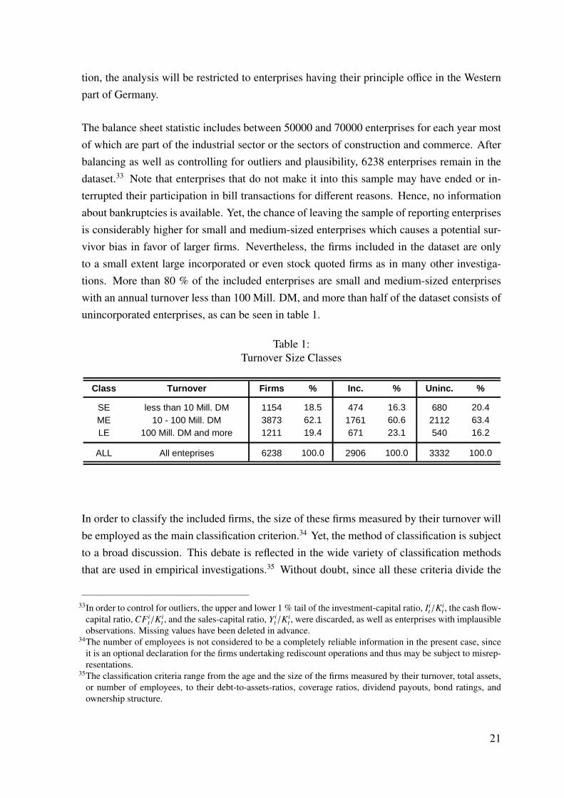
The balance sheet statistic includes between 50000 and 70000 enterprises for each year mostof which are part of the industrial sector or the sectors of construction and commerce. Afterbalancing as well as controlling for outliers and plausibility, 6238 enterprises remain in thedataset.33 Note that enterprises that do not make it into this sample may have ended or in-terrupted their participation in bill transactions for different reasons. Hence, no informationabout bankruptcies is available. Yet, the chance of leaving the sample of reporting enterprisesis considerably higher for small and medium-sized enterprises which causes a potential sur-vivor bias in favor of larger firms. Nevertheless, the firms included in the dataset are onlyto a small extent large incorporated or even stock quoted firms as in many other investiga-tions. More than 80 % of the included enterprises are small and medium-sized enterpriseswith an annual turnover less than 100 Mill. DM, and more than half of the dataset consists ofunincorporated enterprises, as can be seen in table 1.

Table 1:Turnover Size Classes

Class Turnover Firms % Inc. % Uninc. %

SE less than 10 Mill. DM 1154 18.5 474 16.3 680 20.4ME 10 - 100 Mill. DM 3873 62.1 1761 60.6 2112 63.4LE 100 Mill. DM and more 1211 19.4 671 23.1 540 16.2

ALL All enteprises 6238 100.0 2906 100.0 3332 100.0

In order to classify the included firms, the size of these firms measured by their turnover willbe employed as the main classification criterion.34 Yet, the method of classification is subjectto a broad discussion. This debate is reflected in the wide variety of classification methodsthat are used in empirical investigations.35 Without doubt, since all these criteria divide the

33In order to control for outliers, the upper and lower 1 % tail of the investment-capital ratio, Iit/K

it , the cash flow-

capital ratio, CF it/K

it , and the sales-capital ratio, Y i

t/Kit , were discarded, as well as enterprises with implausible

observations. Missing values have been deleted in advance.34The number of employees is not considered to be a completely reliable information in the present case, since

it is an optional declaration for the firms undertaking rediscount operations and thus may be subject to misrep-resentations.

35The classification criteria range from the age and the size of the firms measured by their turnover, total assets,or number of employees, to their debt-to-assets-ratios, coverage ratios, dividend payouts, bond ratings, andownership structure.

21

sample a priori into different subgroups of enterprises, they all may be subject to the criticismput forward by Kaplan-Zingales (1997).

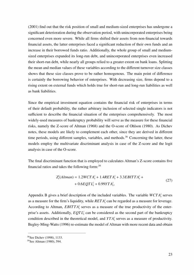
In the present case, the size of the firm is regarded to be a qualified approximation for thedegree of financial risks the firms are exposed to, apart from the fact that this is the mostcommonly used classification if economic problems are adressed in the context of differentgroups of enterprises. The descriptive analysis will reveal that the risk position of the includedenterprises decreases with the size of the firm. Additionally, as derived before, bankruptciesrise with decreasing firm size, as can be seen in table 2 which presents the number of Germanenterprises that declared bankrupt in the year 2002. It is obvious that smaller enterprises,measured either by the number of employees or the level of outstanding debt, account for adisproportionate share of insolvencies in Germany.36

Table 2:Insolvencies in Germany (2002)

Level of debt Firms % Employees Firms %

< 50000 Euro 7562 20.1 no employees 12935 34.450000 - 250000 Euro 14307 38.1 1 employee 4182 11.1

250000 - 500000 Euro 5838 15.5 2 - 5 employees 6481 17.2500000 - 1 Mill. Euro 3958 10.5 6 - 10 employees 2806 7.5

1 Mill. - 5 Mill. Euro 3935 10.5 11 - 100 employees 4237 11.3> 5 Mill. Euro 1057 2.8 > 100 employees 373 1.0

unknown 922 2.5 unknown 6565 17.5

Source: Federal Statistical Office of Germany.

Table 3 presents the summary statistics of the ratios that will be employed in the estimationof the investment function as well as selected indicators for the risk position of the incliudedenterprises.37 Note that the median values of the variables are all well below their meanswhich indicates that the distributions of the variables are skewed, with the longer tail forlarger values. Groessl-Stahlecker-Wohlers (2001) as well as Kirchesch-Sommer-Stahlecker

36In the course of the empirical analysis, other classification criteria were applied to confirm the obtained results.These criteria included the level of total assets as another measure for firm size, as well as the debt-to-assetsratio and the bankruptcy probabilities as measures for the firms’ financial strength. Since the different measuresof firm size did not yield significantly different results, which also holds true for the classification accordingto the firms’ financial risk position, the presentation of the empirical results from estimating the investmentfunction will be restricted to the turnover size classes.

37The variables that will be employed in the course of the present analysis will be described in detail in appendixB.

22

(2001) find out that the risk position of small and medium-sized enterprises has undergone asignificant deterioration during the observation period, with unincorporated enterprises beingconcerned even more severe. While all firms shifted their assets from non-financial towardsfinancial assets, the latter enterprises faced a significant reduction of their own funds and anincrease in their borrowed funds ratio. Additionally, the whole group of small and medium-sized enterprises expanded its long-run debt, and unincorporated enterprises even increasedtheir short-run debt, while nearly all groups relied to a greater extent on bank loans. Splittingthe mean and median values of these variables according to the different turnover size classesshows that these size classes prove to be rather homogenous. The main point of differenceis certainly the borrowing behavior of enterprises. With decreasing size, firms depend to arising extent on external funds which holds true for short-run and long-run liabilities as wellas bank liabilities.

Since the empirical investment equation contains the financial risk of enterprises in termsof their default probability, the rather arbitrary inclusion of selected single indicators is notsufficient to describe the financial situation of the enterprises comprehensively. The mostwidely-used measures of bankruptcy probability will serve as the measure for these financialrisks, namely the Z-score of Altman (1968) and the O-score of Ohlson (1980). As Dichevnotes, these models are likely to complement each other, since they are derived in differenttime periods, using different samples, variables, and methods.38 Concerning the latter, thesemodels employ the multivariate discriminant analysis in case of the Z-score and the logitanalysis in case of the O-score.

The final discriminant function that is employed to calculates Altman’s Z-score contains fivefinancial ratios and takes the following form:39

Zit(Altman) = 1.2WCT Ai

t + 1.4RET Ait + 3.3EBITT Ai

t +

+ 0.6EQT Lit + 0.99YT Ai

t,(27)

Appendix B gives a brief description of the included variables. The variable WCT Ait serves

as a measure for the firm’s liquidity, while RET Ait can be regarded as a measure for leverage.

According to Altman, EBITT Ait serves as a measure of the true productivity of the enter-

prise’s assets. Additionally, EQT Lit can be considered as the second part of the bankruptcy

condition described in the theoretical model, and YT Ait serves as a measure of productivity.

Begley-Ming-Watts (1996) re-estimate the model of Altman with more recent data and obtain

38See Dichev (1998), 1133.39See Altman (1980), 594.

23

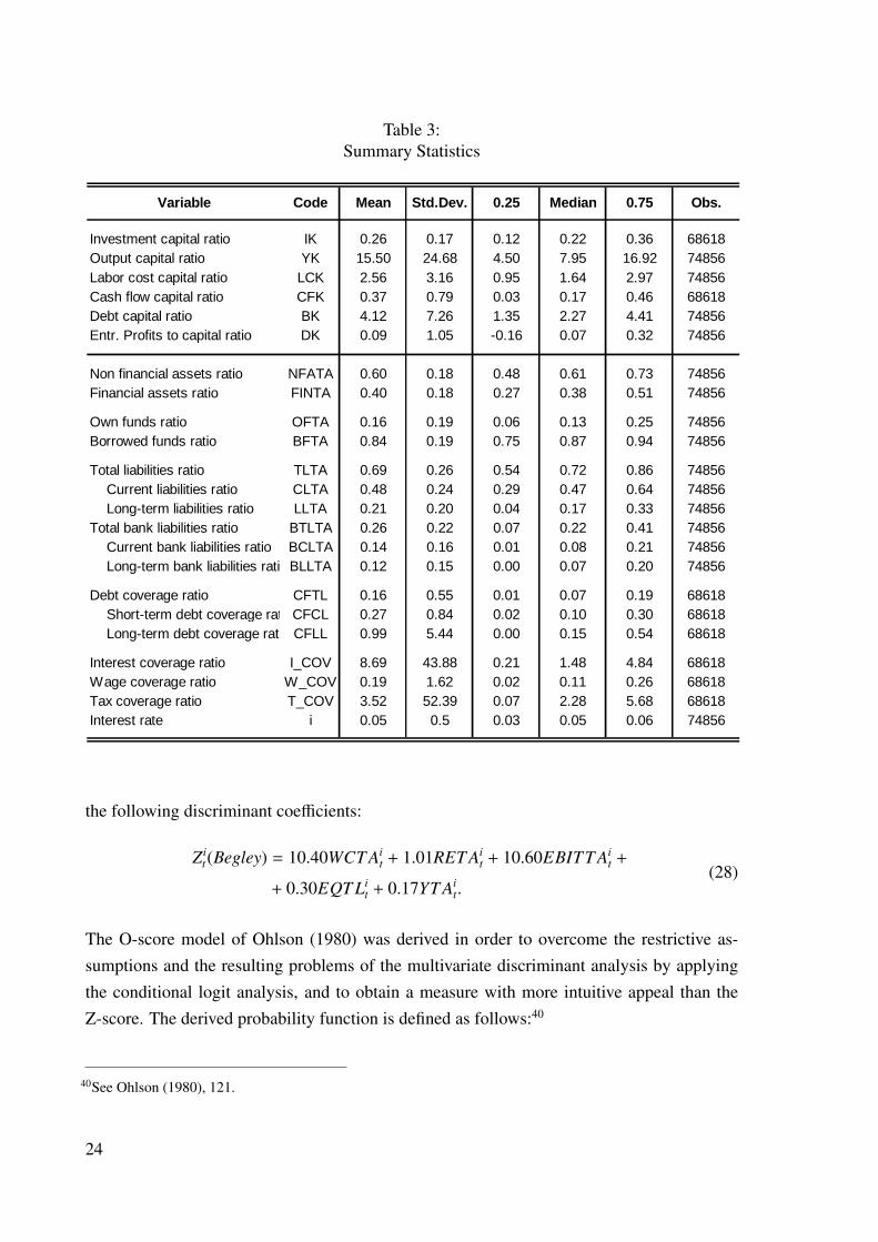
Table 3:Summary Statistics

Variable Code Mean Std.Dev. 0.25 Median 0.75 Obs.

Investment capital ratio IK 0.26 0.17 0.12 0.22 0.36 68618Output capital ratio YK 15.50 24.68 4.50 7.95 16.92 74856Labor cost capital ratio LCK 2.56 3.16 0.95 1.64 2.97 74856Cash flow capital ratio CFK 0.37 0.79 0.03 0.17 0.46 68618Debt capital ratio BK 4.12 7.26 1.35 2.27 4.41 74856Entr. Profits to capital ratio DK 0.09 1.05 -0.16 0.07 0.32 74856

Non financial assets ratio NFATA 0.60 0.18 0.48 0.61 0.73 74856Financial assets ratio FINTA 0.40 0.18 0.27 0.38 0.51 74856

Own funds ratio OFTA 0.16 0.19 0.06 0.13 0.25 74856Borrowed funds ratio BFTA 0.84 0.19 0.75 0.87 0.94 74856

Total liabilities ratio TLTA 0.69 0.26 0.54 0.72 0.86 74856Current liabilities ratio CLTA 0.48 0.24 0.29 0.47 0.64 74856Long-term liabilities ratio LLTA 0.21 0.20 0.04 0.17 0.33 74856

Total bank liabilities ratio BTLTA 0.26 0.22 0.07 0.22 0.41 74856Current bank liabilities ratio BCLTA 0.14 0.16 0.01 0.08 0.21 74856Long-term bank liabilities ratioBLLTA 0.12 0.15 0.00 0.07 0.20 74856

Debt coverage ratio CFTL 0.16 0.55 0.01 0.07 0.19 68618Short-term debt coverage rat CFCL 0.27 0.84 0.02 0.10 0.30 68618Long-term debt coverage rati CFLL 0.99 5.44 0.00 0.15 0.54 68618

Interest coverage ratio I_COV 8.69 43.88 0.21 1.48 4.84 68618Wage coverage ratio W_COV 0.19 1.62 0.02 0.11 0.26 68618Tax coverage ratio T_COV 3.52 52.39 0.07 2.28 5.68 68618Interest rate i 0.05 0.5 0.03 0.05 0.06 74856

the following discriminant coefficients:

Zit(Begley) = 10.40WCT Ai

t + 1.01RET Ait + 10.60EBITT Ai

t +

+ 0.30EQT Lit + 0.17YT Ai

t.(28)

The O-score model of Ohlson (1980) was derived in order to overcome the restrictive as-sumptions and the resulting problems of the multivariate discriminant analysis by applyingthe conditional logit analysis, and to obtain a measure with more intuitive appeal than theZ-score. The derived probability function is defined as follows:40

40See Ohlson (1980), 121.

24

O = P(de f ault) =1

1 + e−yit, (29)

where yit is given by:

yit = −1.32 − 0.407S IZEit + 6.03T LT Ai

t − 1.43WCT Ait +

+ 0.0757CLCAit − 2.37NIT Ai

t − 1.83CFT Lit +

+ 0.285INTWOit − 1.72OENEGi

t − 0.521CHIN it .

(30)

Again, the O-score model is re-estimated by Begley-Ming-Watts (1996) which yields the fol-lowing coefficients:

yit = −1.249 − 0.211S IZEit + 2.262T LT Ai

t − 3.451WCT Ait −

− 0.293CLCAit + 1.080NIT Ai

t − 0.838CFT Lit +

+ 1.266INTWOit − 0.907OENEGi

t − 0.960CHIN it .

(31)

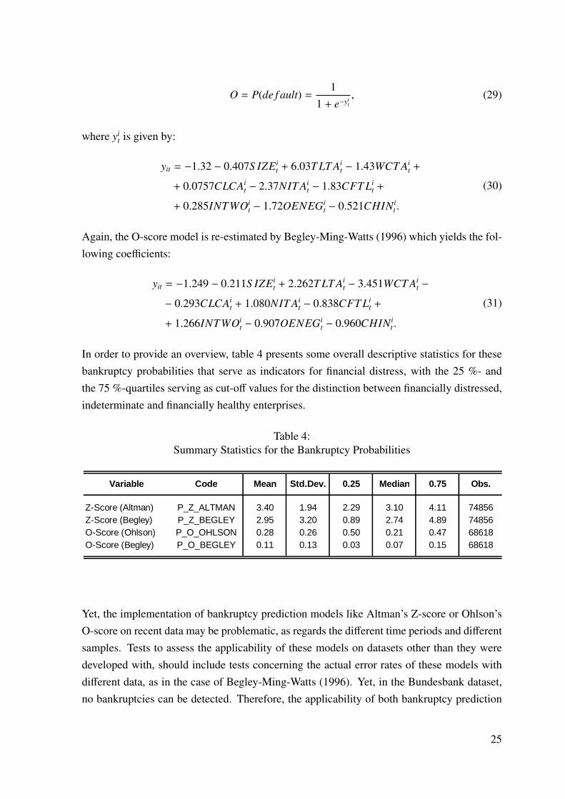
In order to provide an overview, table 4 presents some overall descriptive statistics for thesebankruptcy probabilities that serve as indicators for financial distress, with the 25 %- andthe 75 %-quartiles serving as cut-off values for the distinction between financially distressed,indeterminate and financially healthy enterprises.

Table 4:Summary Statistics for the Bankruptcy Probabilities

Variable Code Mean Std.Dev. 0.25 Median 0.75 Obs.

Z-Score (Altman) P_Z_ALTMAN 3.40 1.94 2.29 3.10 4.11 74856Z-Score (Begley) P_Z_BEGLEY 2.95 3.20 0.89 2.74 4.89 74856O-Score (Ohlson) P_O_OHLSON 0.28 0.26 0.50 0.21 0.47 68618O-Score (Begley) P_O_BEGLEY 0.11 0.13 0.03 0.07 0.15 68618

Yet, the implementation of bankruptcy prediction models like Altman’s Z-score or Ohlson’sO-score on recent data may be problematic, as regards the different time periods and differentsamples. Tests to assess the applicability of these models on datasets other than they weredeveloped with, should include tests concerning the actual error rates of these models withdifferent data, as in the case of Begley-Ming-Watts (1996). Yet, in the Bundesbank dataset,no bankruptcies can be detected. Therefore, the applicability of both bankruptcy prediction

25

models can only be tested by comparing the mean values of the different samples, as putforward by Bhagat-Moyen-Suh (2003), in order to assess whether significant structural breaksoccured in the meantime, or whether fundamental differences can be detected between thediffernt countries of the datasets. Note that, in the present case, bankruptcy probabilitiesare employed to describe the enterprises’ degree of financial distress rather than their defaultprobability. Hence, the predictive ability with regard to the firm’s bankruptcy is not the crucialrequirement.

Table 5:Applicability of the Bankruptcy Probabilities

Reference Studies Deutsche Bundesbank Balance Sheet Statistic

Ratio

bankr.non-

bankr.bankr.

non-bankr.

bankr.non-

bankr.fin.

distr.not

distr.small

me-dium

largefin.

distr.inde-term.

not distr,

WCTA -0.061 0.414 0.178 0.321 0.170 0.223 0.276 0.059 0.231 0.400RETA -0.626 0.355 -1.110 0.030 0.012 0.041 0.076 -0.012 0.034 0.123

EBITTA -0.318 0.153 -0.137 0.070 0.094 0.085 0.087 0.051 0.084 0.136EQTL 0.401 2.477 7.845 5.029 0.228 0.287 0.432 0.070 0.211 0.769YTA 1.500 1.900 0.619 1.558 2.517 2.617 2.540 2.738 2.634 2.299

SIZE 12.134 13.260 12.210 12.740 11.168 13.201 7.487 9.126 11.380 8.247 9.282 10.390TLTA 0.905 0.488 0.810 0.500 0.764 0.430 0.808 0.697 0.544 0.914 0.703 0.393WCTA 0.041 0.310 0.030 0.310 0.156 0.375 0.170 0.223 0.276 0.059 0.231 0.400CLCA 1.320 0.525 0.781 0.350 1.057 0.418 0.808 0.711 0.645 0.967 0.697 0.466NITA -0.208 0.053 -0.170 0.030 -0.222 0.068 0.072 0.060 0.062 0.039 0.061 0.093CFTL -0.117 0.281 -0.070 0.250 -0.254 0.342 0.137 0.142 0.225 0.050 0.105 0.391

INTWO 0.390 0.043 0.500 0.110 0.427 0.030 0.051 0.051 0.047 0.075 0.043 0.038OENEG 0.180 0.004 0.180 0.010 0.092 0.0005 0.132 0.024 0.004 0.131 0.009 0.000

CHIN -0.322 0.038 -0.340 0.010 -0.256 0.081 -0.007 0.007 0.021 -0.005 0.009 0.016

Firms 33 33 105 2058 165 3300 1154 3873 1211 1712 3051 1475Period

1 Bhagat-Moyen-Suh (2003) only state the sample size of their unbalanced sample. For the estimation of Altman's model, 9123 (27273) obser- vations for (not) financially distressed firms were incuded, for Ohlson's model 4320 (12961).

Bhagat et al.

(2003)1

1946-1965 1970-1976 1980-1989 1979-1996

Turnover Classes O-Score ClassesAltman (1968)

Ohlson (1980)

Begley et al. (1996)

1987-19981987-1998

In order to assess the applicability of the bankruptcy prediction models to the balance sheetdata of the Deutsche Bundesbank, table 5 presents the descriptive statistics of the originalstudies of Altman and Ohlson first. Since the empirical implementation of the investmentfunction will additionally be tested with the re-estimated bankruptcy prediction models ofBegley-Ming-Watts, they will also be considered in the table. Unfortunately, they only dis-play the means of the variables that are part of Ohlson’s O-score model. The descriptivestatistics of Bhagat-Moyen-Suh (2003) complete the reference studies in the table.41

41Grice-Ingram (2001) and Grice-Dugan (2001) test both the Z-score and the O-score model to assess theirgeneralizability. To keep the table as simple as possible, their results will not be included. Both studies drawthe conclusion that these models are more appropriate to predict financial distress than bankruptcies.

26

On the right hand side of table 5, the mean values of the current sample are presented for thedifferent turnover size classes. Even though the variation between the groups is considerablysmaller for the Bundesbank sample, the differnces between the size classes point in the samedirection. Consistent with the conclusions of Begley-Ming-Watts and Bhagat-Moyen-Suh,Ohlson’s O-score model will be regarded subsequently as an appropriate model to assess therisk of financial distress, since possible structural changes that could distort the prediction offinancial distress for the dataset of the Bundesbank cannot be detected. The generalizabilityof Altman’s Z-score turns out to be more problematic, since the variable means of the currentdataset partly differ fundamentally from the original data of the Altman study. In addition,the variation between the size classes is very low. Therefore, in line with the Bhagat-Moyen-Suh findings, caution is indicated for the prediction even of financial distress if the Z-score isused.42

5 Empirical Results

In this chapter, the above derived model of investment behaviour will be estimated usingthe balance sheet statistic of the Deutsche Bundesbank. The included enterprises will beclassified according to their size measured by their turnover. Additionally, the sample is splitaccording to the legal form of the enterprises. The investment function takes the form ofa linear fixed effects model, with the transformed investment-to-capital ratio as dependentvariable and the above described ratios as regressors, as captured by equation (26). Pricesare, as discussed earlier, not explicitly included in the investment equation, since they do notdisplay any cross-sectional variation. This also holds true for macroeconomic variables suchas the sectoral capacity utilization. In order to capture the influence of these determinants,time dummies are included in the regression equation.

The investment equation will be estimated using Ordinary Least Square (OLS), Fixed Effects(FE) respective Within Group (WITHIN), and Generalized Method of Moments (GMM) asdeveloped by Arellano-Bond (1991). The OLS level estimator is known to be upward biased,since it does not control for the possibility of unobserved firm-specific effects, while theWITHIN estimator may produce rather downward biased paramter values in finite samples.Consequently, the GMM estimator will serve as some sort of compromise between these twoapproaches. Yet, in case of weak instruments it may likewise be biased. Hence, the strategywill be to account for all three estimators. Referring to the severe finite sample biases in thepresence of weak instruments, Bond (2002) concludes that the comparison of these estimators

42It is noteworthy that these results also apply for the tests performed by Grice-Ingram and Grice-Dugan.

27

may help detecting and avoiding the above mentioned biases.43

The reported GMM estimates are two-step estimates. Although the standard errors of two-step GMM estimations are more efficient than the one-step estimators, they tend to be biaseddownwards in small samples. For reasons of inference, the one-step standard errors that areasymptotically robust to heteroscedasticity of arbitrary form will be reported. Additionally,Wald tests regarding the joint significance of all regressors and the dummy variables are in-cluded in terms of their p-values. In case of the OLS and WITHIN estimations, the adjustedR-squared statistic is reported. Instruments that are used for estimation include the undiffer-enced values of all regressors, lagged two periods and earlier.44 In order to verify that theerror term is not serially correlated beyond first-order correlation, m1 and m2 are included astests for first- and second-order serial correlation. Additionally, the validity of the includedinstruments will be tested using the Sargan test of overidentifying restrictions. For all of thevalidity tests, p-values will be reported in the included tables.

Table C.1 in appendix C shows the estimation results of equation (26) for the different sizeclasses and legal forms with the financial risk position of the included enterprises being mea-sured by Ohlson’s O-score. Note that the performance of the GMM regressions in terms ofthe second-order serial correlation and the Sargan test statistic is rather unsatisfactory formedium-sized and large enterprises, whereas the performance of the OLS and WITHIN esti-mations can be regarded as satisfactory. Hence, caution is advisable for the valuation of theGMM results in all of the cases, and OLS respective WITHIN estimates will always be takeninto account for inference.45

Turning to the estimated parameters, the coefficients of the investment ratio, β1, and thesquared investment ratio, β2, have their expected signs. The values of these coefficients arefurthermore reasonable and in line with earlier studies. The higher parameter values of thelagged investment ratio of larger enterprises may be an indicator for the fact that enterprisesinvest more continuously with rising size, while small firms tend to invest more intermittently.The test statistics concerning the second-order serial correlation may point in the same direc-

43See Bond (2002), 26-27.44Additionally, four lags were added to the investment function in order to capture the dynamics of the investment

decision. Including these lags does not change the results significantly, but improves the performance ofthe regressions. Only the magnitude of the lagged investment ratio and the lagged squared investment ratioincreases slightly.

45The estimations of medium and large enterprises may suffer from the finite sample bias as a consequence ofweak instruments in terms of Blundell-Bond (1998). However, the standard errors of the GMM estimatesappear to be not too large, even though they exceed the OLS and WITHIN standard errors. Consequently.if the estimated GMM coefficients turn out to be significant, have the expected signs, and do not divergefundamentally from both the OLS and the WITHIN estimates, then the results may nevertheless suggest somevalidity of the derived investment function despite of the rather low performance of the GMM regressions.

28

tion, as they are lower for larger and incorporated enterprises. In contrast to the theoreticalmodel, but consistent with other studies, β3 as the coefficient of the output ratio displayspositive values for all groups of enterprises, yet insignificant for large unincorporated enter-prises. The influence of labor outlays on investment, captured by the coefficient, β4, matchwith theory, as all enterprises display positive values which prove to be significant and higherfor larger enterprises. This confirms the assumption about large enterprises producing morecapital intensive than their smaller counterparts. The difference between smaller and largerfirms is even higher for unincorporated enterprises. The GMM estimates appear to overesti-mate the influence of labor costs, regardless of the size and legal form. Yet, the increase oftheir influence with the size of the firm can be found in these estimates, too.

As could be expected, and in line with the predictions from the model, the coefficients of thedebt-to-capital ratio, β5, display a negative relation between external finance and investment.Usually, higher parameter values or a higher significance of the debt-to-assets ratio of smallerenterprises are interpreted as indication for informational problems on capital markets beingmore severe for these firms. Yet, no unambiguous conclusion can be drawn for the debt-to-assets ratio concerning the different size classes. Medium-sized unincorporated enterprisesdisplay the closest negative relation between debt and investment, while their incorporatedcounterparts show the opposite behavior. Large unincorporated enterprises even display pos-itive values of their debt coefficient if estimated with OLS or WITHIN regressions. Thesecond debt term which is composed of the debt-to-capital ratio times the entrepreneurialprofits ratio, is a rather technical term stemming from the profit maximization of the firm as-sociated with the bankruptcy probability, and is not easy to interpret. Anyhow, its coefficient,β6, proves to be very small and furthermore insignificant. The reason for the low perfor-mance of this debt indicator is presumably the debt-to-assets ratio which already captures theinfluence of external funds on the investment decision of the firm.

The remaining coefficient, β7, belongs to the variable that accounts for the influence of fi-nancial risks in terms of the bankruptcy probability. While the model does not provide anunambiguous relation between the bankruptcy probability of an enterprise and its level ofinvestment, one would rather assume this relation to be negative which corresponds to a pos-itive influence of the survival probability on the company’s investment. The few existingstudies dealing with the link between investment and bankruptcy risk confirm this view.46

The same holds true for the results obtained with the Bundesbank’s balance sheet statistics.Without exception, all size classes display rather high positive correlations between their in-vestment and their financial healthiness in terms of survival probabilities. These correlations

46See Frisse-Funke-Lankes (1993) and Wald (2003).

29

are throughout significant at the 1 % level. According to the theory of asymmetric informa-tion and in line with the financial constraints literature, smaller enterprises should exhibit arather high sensitivity of their investment with regards to their financial risks. This can beobserved for incorporated enterprises, while the opposite holds true for unincorporated enter-prises. Additionally, the latter surprisingly display lower sensitivities than corporations, eventhough incorporated enterprises are assumed to have easier access to the capital market thanunincorporated firms.

In order to verify whether the obtained results are due to the specific calculation of Ohlson’sO-score with the original parameters, Tables C.2-C.4 in appendix C provide estimation resultsfor the same investment function, yet with bankruptcy probabilities calculated with, in orderof their appearence, the O-score as calculated by Begley-Ming-Watts, the Z-score of Altman,and the Z-score of Begley-Ming-Watts. The modified calculation of the O-score in table C.2yields almost the same results as the original O-score, with the parameter values being slightlysmaller. Yet, the relation between firm size and the influence of financial risks on the firm’sinvestment decision is more ambiguous in case of the modified O-score. The GMM estimatesprovide evidence for a decline of this influence with firm size for both incorporated andunincorporated enterprises, while OLS and WITHIN estimates do not point in this direction.

Even though Altman’s Z-score is calculated completely different from the O-score, it is evi-dent that its inclusion instead of the O-score does not change the obtained results in a funda-mental way, as can be seen in tables C.3 and C.4.47 Yet, it is not clear whether the influenceof financial risks rises with the size of the firm or not. If the Z-score is calculated by themethod of Begley-Ming-Watts, this correlation is again decreasing with the size of the firmin case of incorporated enterprises, and rising with firm size in case of their unincorporatedcounterparts. Note that the estimations were additionaly performed with other classificationcriteria such as Ohlson’s O-score. Yet, the results remain almost unchanged.

6 Conclusion

Financial risks traditionally enter the theoretical models of investment such as the q modelor the Euler equation model in the form of financial constraints that enterprises are facing asa consequence of informational asymmetries while deciding on the level of their investment.In this context, financial constraints are unanimously defined as the risk premium that enter-prises have to bear in order to raise external funds, or as a limited access to borrowed funds.

47Note that, with a rising value being equal to declining financial risks, it is not necessary to transform the Z-scoreinto a survival probability as in the case of the O-score.

30

Tests for financial constraints are performed by estimating excess sensitivities of investmentwith regard to financial indicators concerning the enterprises’ internal or external funds thatare assumed to best approximate these constraints.

However, the impact of financial risks as a whole rather than merely financial constraintshas rarely been implemented explicitly in theoretical or empirical investigations dealing withthe interaction of the firms’ financial sphere with their investment decisions. While financialrisks contain the wedge in the costs between internal and external funds and therewith finan-cial constraints, they furthermore account for the possibility of the firm loosing its ability torepay its borrowed funds and thus being subject to potential bankruptcy. Beyond doubt, bothkinds of risks point in the same direction. The external finance premium will cause the invest-ment costs to rise directly which lowers the firm’s demand for new capital. The probabilityof bankruptcy lowers expected future profits and thus dampens the enterprises’ demand forinvestment, too.

The inclusion of the bankruptcy probabilities has to take place by weighting the future rev-enues of the company with the probability of actually earning these revenues, and thus theprobability of survival. As a consequence, the resulting specification of the investment func-tion explicitly includes this survival probability as an additional explanatory variable. Theadvantage of this variable is a rather high degree of freedom for the researcher to understandand to model this survival probability. Whether one may understand this probability in theoriginal sense or in the sense of financial distress, one may employ bankruptcy predictionmodels to calculate the degree of financial distres the enterprises may face. It is even possibleto understand these probabilities as a proxy for financial constraints, since these constraintsrepresent one case of financial risks, namely the case of firms facing higher costs for externalfinance without being endangered by the risk of bankruptcy.

The empirical analysis performed with the balance sheet data of the Deutsche Bundesbankconfirms the position that the survival probabilities as measured by the different bankruptcyprediction models are appropriate to account for the link between the investment and the fi-nancial risks of enterprises. As the reuslts show, some groups of enterprises turned out todisplay a higher sensitivity of their investment with regard to their survival probabilities thanothers. Thus, apart from the debate about the usefulness of the analysis of single internalor external financial indicators to proxy for financial constraints, the results of both meth-ods undisputedly point in the same direction, independent of whether one tests for financialconstraints or financial risks as a whole.

31

A Mathematical Appendix

The Hamiltonian for the profit maximizing firm which faces an external finance premium andthe risk of bankruptcy can be written as

H it (L

it, I

it ,K

i1, B

it, λ

it) = Ei

t{βtPi(Bi

t,Kit)[(1 − τ)(ptF(Ki

t , Lit) −

− wtLit − ptG(Ii

t ,Kit) − ri(Bi

t,Kit)Bt) − pI

t Iit] + λ

it

[Iit − δK

it−1

]}.

(A.1)

Since the enterprise has to survive up to time t to calculate the Hamiltonian at time t, theprobabilities of survival are equal to 1 for s = t0, ..., t − 1. The necessary conditions of themaximum principle for the present problem involve three first order difference equations inthe state variables, Ki

t and Bit, and the costate variable, λi

t, with the latter denoting the shadowprice of capital. Besides these necessary conditions, the maximum principle requires themaximization of the Hamiltonian with respect to the control variable, Ii

t , at every point oftime. The first order condition of the Hamiltonian with respect to labor, Li

t, leads to the usualmarginal productivity rule for labor:

∂H it

∂Lit= Ei

t

{βtPi(Bi

t,Kit)(1 − τ)

[ptFL(Ki

t , Lit) − wt

]}= 0

⇐⇒ FL(Kit , L

it) =

wt

pt.

(A.2)

The first order condition for investment, Iit , gives:

∂H it

∂Iit= Ei

t

{−βtPi(Bi

t,Kit)

((1 − τ)ptGI(Ii

t ,Kit) + pI

t

)}− Ei

t

{λi

t

}⇐⇒ Ei

t

{βtPi(Bi

t,Kit)

[(1 − τ)ptGI(Ii

t ,Kit) + pI

t

]}= Ei

t

{λi

t

}.

(A.3)

For capital, Kit , the necessary condition reads:

∂H it

∂Kit= −Ei

t

{λi

t+1 − λit

}(A.4)

⇐⇒ −Eit

{λi

t+1 − λit

}= Ei

t

βtPi

K(Bit,K

it)D

it+

+βtPi(Bit,K

it)(1 − τ)[ptFK(Ki

t , Lit)−

−ptGK(Iit ,K

it) − ri

k(Bit,K

it)B

it] − δλ

it+1

⇐⇒ Ei

t

{λi

t

}= Ei

t

βtPi

K(Bit,K

it)D

it+

+βtPi(Bit,K

it)(1 − τ)[ptFK(Ki

t , Lit)−

−ptGK(Iit ,K

it) − ri

K(Bit,K

it)B

it] + (1 − δ)λi

t+1

.

32

The necessary condition with respect to debt, Bit, is as follows:

∂H it

∂Bit=Ei

t

βtPiB(Bi

t,Kit)D

it − β

tPi(Bit,K

it)(1 − τ) ×

×[ri

B(Bit,K

it)B

it + ri(Bi

t,Kit)] = 0 (A.5)

⇐⇒ Eit

{τ[ri

B(Bit,K

it)B

it + ri(Bi

t,Kit)]}=

Eit

{Pi(Bi

t,Kit)

[ri

B(Bit,K

it)B

it + ri(Bi

t,Kit)]− Pi

B(Bit,K

it)D

it

}.

To be complete, the first partial derivative with respect λit, as well as the necessary transver-

sality condition are

Eit

{Ki

t − Kit−1

}= Ei

t

{Iit + −δ)K

it−1

}, (A.6)

Eit

{λi

T

}= 0. (A.7)

In order to derive the empirical investment equation, the expected shadow price of capital,Ei

t

{λi

t

}, from the first order condition with respect to investment, equation (A.3), is substituted

into the first order condition for capital, equation (A.4). Rearranging yields the followingequation:

Eit

{Pi(Bi

t,Kit)

[ptGI(Ii

t ,Kit) +

pIt

(1 − τ)

]}= (A.8)

= Eit

{βPi(Bi

t+1,Kit+1)(1 − δ)

[pt+1GI(Ii

t+1,Kit+1) +

pIt+1

(1 − τ)

]}+

+ Et

{βPi(Bi

t,Kit)

[ptFK(Ki

t , Lit) − ptGK(Ii

t ,Kit) − ri

K(Bit,K

it)B

it

]}+

+ Et

{β

(1 − τ)Pi

K(Bit,K

it)D

it

}.

Since βt = P(Bt,Kt) = 1 for period t, and the expected values of period t are the realizedvalues, equation (A.8) can be written as follows:

ptGI(Iit ,K

it) +

pIt

(1 − τ)= (A.9)

= Et

{βPi(Bi

t+1,Kit+1)(1 − δ)

[pt+1GI(Ii

t+1,Kit+1) +

pIt+1

(1 − τ)

]}+

+ ptFK(Kit , L

it) − ptGK(Ii

t ,Kit) − ri

K(Bit,K

it)B

it +

1(1 − τ)

PiK(Bi

t,Kit)D

it.

33

The first derivatives of the adjustment cost function with respect to new and old capital are

GI(Iit ,K

it) = b

(Iit

Kit− a

), GK(Ii

t ,Kit) = −

b2

(Iit

Kit

)2

+b2

a2. (A.10)

Additionally, the first derivatives of the interest premium function as well as the survivalprobablity function read

riB(Bi

t,Kit) = c

1Ki

t, ri

K(Bit,K

it) = −c

Bit(

Kit)2 , (A.11)

and

PiB(Bi

t,Kit) = −d

1Ki

t, Pi

K(Bit,K

it) = d

Bit(

Kit)2 . (A.12)

Substituting these derivatives into equation (A.9), assuming rational expextations, and denot-ing the survival probability in period t + 1 with Pi

t+1 yields:

ptb(

Iit

Kit− a

)+

pIt

(1 − τ)=

= βPit+1(1 − δ)

[pt+1b

(Iit+i1

Kit+1

− a)+

pIt+1

(1 − τ)

]+ pt

Y it −

wtpt

Lit

Kit−

− pt

−b2

(Iit

Kit

)2

+b2

a2

− cBi

t(Ki

t)2 Bi

t +d

(1 − τ)Bi

t(Ki

t)2 Di

t + εit+1.

(A.13)

This equation can be written after rearranging and dividing by β(1 − δ)bpt+1:

Pit+1

Iit+1

Kit+1

=1

β(1 − δ)pt

pt+1

Iit

Kit−

12β(1 − δ)

pt

pt+1

(Iit

Kit

)2

− (A.14)

−1

β(1 − δ)bpt

pt+1

Y it

Kit+

1β(1 − δ)b

pt

pt+1

wtLit

Kit+

+c

β(1 − δ)bpt

pt+1

1pt

(Bi

t

Ki2t

)2

− −d

(1 − τ)1

β(1 − δ)bpt

pt+1

1pt

Bit(

Kit)2 Di

t +

+

(a −

b(1 − τ)

pIt+1

pt+1

)Pi

t+1 + +a2

2β(1 − δ)pt

pt+1−

aβ(1 − δ)

pt

pt+1+

+pI

t

b(1 − τ)β(1 − δ)pt+1.

34

Substituting φt+1 =1

(1−δ)βpt

pt+1yields the investment equation

Pit+1

Iit+1

Kit+1

= φt+1Iit

Kit−

12φt+1

(Iit

Kit

)2

−1bφt+1

Y it

Kit+

1bφt+1

wtLit

Kit+

+c

bptφt+1

(Bi

t

Ki2t

)2

−d

bpt(1 − τ)φt+1

Bit

Kit

Dit

Kit+

+

(a −

b(1 − τ)

pIt+1

pt+1

)Pi

t+1 +

(a2 − 2

2+

1b(1 − τ)

pIt

pt

)φt+1,

(A.15)

with the following coefficients:

α0 =

(a2

2 − a + 1b(1−τ)

pIt

pt

)φt+1, α1 = φt+1, α2 = −

12φt+1,

α3 = −1bφt+1, α4 =

1bptφt+1, α5 = −

cbptφt+1,

α6 = −d

bpt(1−τ)φt+1, α7 = a − 1

b(1−τ)pI

t+1pt+1

, φt+1 =1

(1−δ)βpt

pt+1.

35

B Definition of the Variables

The variables that are included in the empirical analysis are derived from the balance sheetsand the profit and loss accounts included in the balance sheet statistic of the Deutsche Bun-desbank. Albeit all variables are measured in thousands of Deutsche Mark, the dimension isnot of importance, since the empirical analysis will rely on financial ratios composed of thesevariables.48

• The level of the capital stock, K, of the included enterprises is defined as the level ofgross tangible fixed assets of firm i in period t. These tangible fixed assets includeassets that are used in production longer than one year, comprising land, buildings,machinery, technical plant, as well as furniture and equipment. They include assetsunder construction and payments made on account of such assets.

• The level of investment, I, of an enterprise thus is calculated as additions to the grosstangible fixed assets in one year. Note that both the capital stock and the level ofinvestment are not derived from the detailed schedule of fixed asset movements.

• Output, Y , is the level of turnover achieved by the particular enterprise.

• Cash flow, CF, as a measure of the internally generated funds is calculated from theprofit for the year plus write-downs and changes in provisions, special reserves anddeferred income, less write-ups of tangible fixed assets and changes in prepayments.

• Total assets, T A, as the sum of all property owned by the business is calculated as cur-

rent assets, CA, plus long-term assets, LA. The former include all property the businessownes for short-term use, and include particularly cash, securities, bank accounts, andbusiness equipment. Besides the tangible fixed assets, long-term assets particularlyinclude intangible assets and financial assets.

• Non-financial assets, NFA, encompass tangible fixed assets and inventories, while fi-

nancial assets, FIN, are composed of cash holdings, short- and long-term outstandingaccounts, securities, and shareholdings.

• Own funds, OF, consist of the firm’s equity and reserves, while borrowed funds, BF,are composed of short- and long-term liabilities, trade credits, and provisions. Ownfunds and borrowed funds sum up to total assets, T A if deferrals are ignored.

48For a detailed description of all variables contained in the Bundesbank’s balance sheet statistics, see DeutscheBundesbank (1999b), 10-14.

36

• Total liabilities, T L, are composed of current liabilities, CL, and long-term liabili-

ties, LL, The Bundesbank classifies the former by short-run liabilities not exceedinga maturity of one year, including among others trade creditors, liabilities on bills, andpayments received on account. Long-term liabilities include debt with a residual ma-turity of at least one year. The same classification with respect to the maturity holdstrue for total bank liabilities, BT L, which are part of total liabilities and thus consist ofcurrent bank liabilities, BCL, and long-term bank liabilities, BLL.

• Working capital, WC, is defined as current assets minus current liabilities and thusincludes the accessible resources needed to support the day-to-day operations of anorganization.

• Besides wages and salaries, labor cost, LC, consit of social security contributions, vol-untary social security expenses and transfers to provisions for pensions. Interest paid,IC, are made of interest payments as well as discount expenditures, loan and overdraftcommissions and write-downs of discounts shown on the asset side. Taxes, TC, includeamong others taxes on income and earnings, corporation taxes and operating taxes.

• Net income, NI, is the amount of profit a company realizes after all costs, expenses andtaxes have been paid. It is calculated by subtracting business, depreciation, interest andtax costs from revenues. In order to asses the financial performance of companies withhigh levels of debt and interest expenses, net income before interest and taxes, EBIT ,is often used rather than the net income after interst and taxes.

• Entrepreneurial profits, D, are defined as that part of net income that is not used asretained earnings, RE, and thus can be distributed to the owners of the enterprise.

The definitions of the variables that are included in the Z-score model of Altman (1968) areas follows:

Zit = Overall index,

WCT Ait = Working Capital / Total assets,

RET Ait = Retained earnings / Total assets,

EBITT Ait = Earnings before interest and taxes / Total assets,

EQT Lit = Market value equity / Book value of total debt,

YT Ait = Sales / Total assets.

37

The variables that are included in the O-score model of Ohlson (1980) are defined in thefollowing way:

S IZEit = Log (Total assets / GNP price level)49,

T LT Ait = Total liabilities / Total assets,

WCT Ait = Working capital / Total assets,

CLCAit = Current liabilities / Current assets,

NIT Ait = Net income / Total assets,

CFT Lit = Funds provided by operations / Total liabilities,

INTWOit = 1 if net income was negative for the last two years,= 0 otherwise,

OENEGit = 1 if total liabilities exceed total assets,= 0 otherwise,

CHIN it = (NIi

t − NIit−1)/(|NIi

t | + |NIit−1|),

where NIit is net income in the most recent period.

38

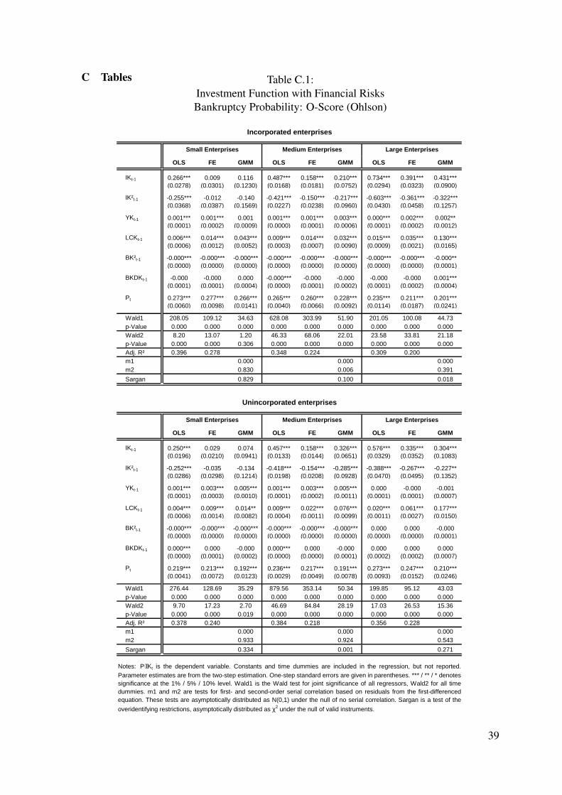
C Tables Table C.1:Investment Function with Financial RisksBankruptcy Probability: O-Score (Ohlson)

Incorporated enterprises

Small Enterprises Medium Enterprises Large Enterprises

OLS FE GMM OLS FE GMM OLS FE GMM

IKt-1 0.266*** 0.009 0.116 0.487*** 0.158*** 0.210*** 0.734*** 0.391*** 0.431***(0.0278) (0.0301) (0.1230) (0.0168) (0.0181) (0.0752) (0.0294) (0.0323) (0.0900)

IK²t-1 -0.255*** -0.012 -0.140 -0.421*** -0.150*** -0.217*** -0.603*** -0.361*** -0.322***(0.0368) (0.0387) (0.1569) (0.0227) (0.0238) (0.0960) (0.0430) (0.0458) (0.1257)

YKt-1 0.001*** 0.001*** 0.001 0.001*** 0.001*** 0.003*** 0.000*** 0.002*** 0.002**(0.0001) (0.0002) (0.0009) (0.0000) (0.0001) (0.0006) (0.0001) (0.0002) (0.0012)

LCKt-1 0.006*** 0.014*** 0.043*** 0.009*** 0.014*** 0.032*** 0.015*** 0.035*** 0.130***(0.0006) (0.0012) (0.0052) (0.0003) (0.0007) (0.0090) (0.0009) (0.0021) (0.0165)

BK²t-1 -0.000*** -0.000*** -0.000*** -0.000*** -0.000*** -0.000*** -0.000*** -0.000*** -0.000**(0.0000) (0.0000) (0.0000) (0.0000) (0.0000) (0.0000) (0.0000) (0.0000) (0.0001)

BKDKt-1 -0.000 -0.000 0.000 -0.000*** -0.000 -0.000 -0.000 -0.000 0.001***(0.0001) (0.0001) (0.0004) (0.0000) (0.0001) (0.0002) (0.0001) (0.0002) (0.0004)

Pt 0.273*** 0.277*** 0.266*** 0.265*** 0.260*** 0.228*** 0.235*** 0.211*** 0.201***(0.0060) (0.0098) (0.0141) (0.0040) (0.0066) (0.0092) (0.0114) (0.0187) (0.0241)

Wald1 208.05 109.12 34.63 628.08 303.99 51.90 201.05 100.08 44.73p-Value 0.000 0.000 0.000 0.000 0.000 0.000 0.000 0.000 0.000Wald2 8.20 13.07 1.20 46.33 68.06 22.01 23.58 33.81 21.18p-Value 0.000 0.000 0.306 0.000 0.000 0.000 0.000 0.000 0.000Adj. R² 0.396 0.278 0.348 0.224 0.309 0.200m1 0.000 0.000 0.000m2 0.830 0.006 0.391

Sargan 0.829 0.100 0.018

Unincorporated enterprises

Small Enterprises Medium Enterprises Large Enterprises

OLS FE GMM OLS FE GMM OLS FE GMM

IKt-1 0.250*** 0.029 0.074 0.457*** 0.158*** 0.326*** 0.576*** 0.335*** 0.304***(0.0196) (0.0210) (0.0941) (0.0133) (0.0144) (0.0651) (0.0329) (0.0352) (0.1083)

IK²t-1 -0.252*** -0.035 -0.134 -0.418*** -0.154*** -0.285*** -0.388*** -0.267*** -0.227**(0.0286) (0.0298) (0.1214) (0.0198) (0.0208) (0.0928) (0.0470) (0.0495) (0.1352)

YKt-1 0.001*** 0.003*** 0.005*** 0.001*** 0.003*** 0.005*** 0.000 -0.000 -0.001(0.0001) (0.0003) (0.0010) (0.0001) (0.0002) (0.0011) (0.0001) (0.0001) (0.0007)

LCKt-1 0.004*** 0.009*** 0.014** 0.009*** 0.022*** 0.076*** 0.020*** 0.061*** 0.177***(0.0006) (0.0014) (0.0082) (0.0004) (0.0011) (0.0099) (0.0011) (0.0027) (0.0150)

BK²t-1 -0.000*** -0.000*** -0.000*** -0.000*** -0.000*** -0.000*** 0.000 0.000 -0.000(0.0000) (0.0000) (0.0000) (0.0000) (0.0000) (0.0000) (0.0000) (0.0000) (0.0001)

BKDKt-1 0.000*** 0.000 -0.000 0.000*** 0.000 -0.000 0.000 0.000 0.000(0.0000) (0.0001) (0.0002) (0.0000) (0.0000) (0.0001) (0.0002) (0.0002) (0.0007)

Pt 0.219*** 0.213*** 0.192*** 0.236*** 0.217*** 0.191*** 0.273*** 0.247*** 0.210***(0.0041) (0.0072) (0.0123) (0.0029) (0.0049) (0.0078) (0.0093) (0.0152) (0.0246)

Wald1 276.44 128.69 35.29 879.56 353.14 50.34 199.85 95.12 43.03p-Value 0.000 0.000 0.000 0.000 0.000 0.000 0.000 0.000 0.000Wald2 9.70 17.23 2.70 46.69 84.84 28.19 17.03 26.53 15.36p-Value 0.000 0.000 0.019 0.000 0.000 0.000 0.000 0.000 0.000Adj. R² 0.378 0.240 0.384 0.218 0.356 0.228m1 0.000 0.000 0.000m2 0.933 0.924 0.543

Sargan 0.334 0.001 0.271

Notes: P⋅IKt is the dependent variable. Constants and time dummies are included in the regression, but not reported.Parameter estimates are from the two-step estimation. One-step standard errors are given in parentheses. *** / ** / * denotessignificance at the 1% / 5% / 10% level. Wald1 is the Wald test for joint significance of all regressors, Wald2 for all timedummies. m1 and m2 are tests for first- and second-order serial correlation based on residuals from the first-differencedequation. These tests are asymptotically distributed as N(0,1) under the null of no serial correlation. Sargan is a test of the

overidentifying restrictions, asymptotically distributed as χ2 under the null of valid instruments.

39

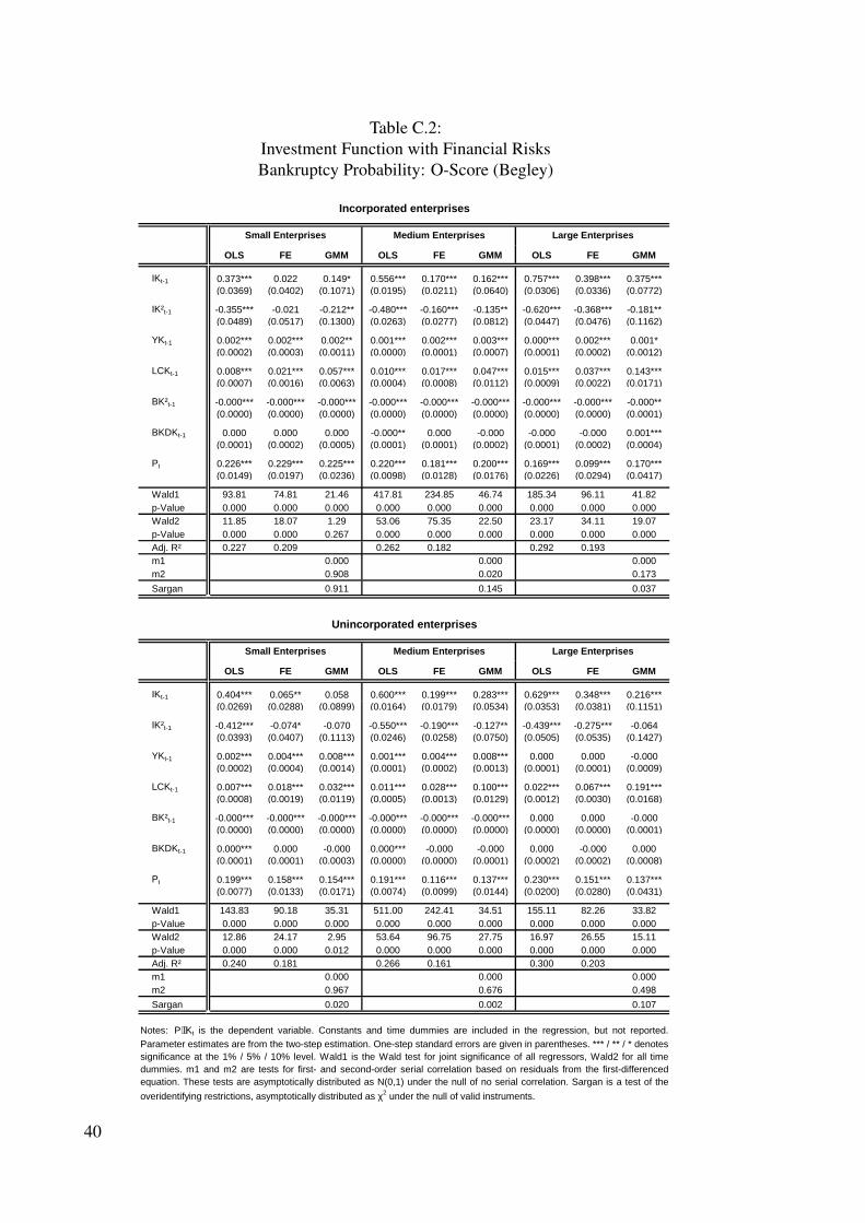
Table C.2:Investment Function with Financial RisksBankruptcy Probability: O-Score (Begley)

Incorporated enterprises

Small Enterprises Medium Enterprises Large Enterprises

OLS FE GMM OLS FE GMM OLS FE GMM

IKt-1 0.373*** 0.022 0.149* 0.556*** 0.170*** 0.162*** 0.757*** 0.398*** 0.375***(0.0369) (0.0402) (0.1071) (0.0195) (0.0211) (0.0640) (0.0306) (0.0336) (0.0772)

IK²t-1 -0.355*** -0.021 -0.212** -0.480*** -0.160*** -0.135** -0.620*** -0.368*** -0.181**(0.0489) (0.0517) (0.1300) (0.0263) (0.0277) (0.0812) (0.0447) (0.0476) (0.1162)

YKt-1 0.002*** 0.002*** 0.002** 0.001*** 0.002*** 0.003*** 0.000*** 0.002*** 0.001*(0.0002) (0.0003) (0.0011) (0.0000) (0.0001) (0.0007) (0.0001) (0.0002) (0.0012)

LCKt-1 0.008*** 0.021*** 0.057*** 0.010*** 0.017*** 0.047*** 0.015*** 0.037*** 0.143***(0.0007) (0.0016) (0.0063) (0.0004) (0.0008) (0.0112) (0.0009) (0.0022) (0.0171)

BK²t-1 -0.000*** -0.000*** -0.000*** -0.000*** -0.000*** -0.000*** -0.000*** -0.000*** -0.000**(0.0000) (0.0000) (0.0000) (0.0000) (0.0000) (0.0000) (0.0000) (0.0000) (0.0001)

BKDKt-1 0.000 0.000 0.000 -0.000** 0.000 -0.000 -0.000 -0.000 0.001***(0.0001) (0.0002) (0.0005) (0.0001) (0.0001) (0.0002) (0.0001) (0.0002) (0.0004)

Pt 0.226*** 0.229*** 0.225*** 0.220*** 0.181*** 0.200*** 0.169*** 0.099*** 0.170***(0.0149) (0.0197) (0.0236) (0.0098) (0.0128) (0.0176) (0.0226) (0.0294) (0.0417)

Wald1 93.81 74.81 21.46 417.81 234.85 46.74 185.34 96.11 41.82p-Value 0.000 0.000 0.000 0.000 0.000 0.000 0.000 0.000 0.000Wald2 11.85 18.07 1.29 53.06 75.35 22.50 23.17 34.11 19.07p-Value 0.000 0.000 0.267 0.000 0.000 0.000 0.000 0.000 0.000Adj. R² 0.227 0.209 0.262 0.182 0.292 0.193m1 0.000 0.000 0.000m2 0.908 0.020 0.173

Sargan 0.911 0.145 0.037

Unincorporated enterprises

Small Enterprises Medium Enterprises Large Enterprises

OLS FE GMM OLS FE GMM OLS FE GMM

IKt-1 0.404*** 0.065** 0.058 0.600*** 0.199*** 0.283*** 0.629*** 0.348*** 0.216***(0.0269) (0.0288) (0.0899) (0.0164) (0.0179) (0.0534) (0.0353) (0.0381) (0.1151)

IK²t-1 -0.412*** -0.074* -0.070 -0.550*** -0.190*** -0.127** -0.439*** -0.275*** -0.064(0.0393) (0.0407) (0.1113) (0.0246) (0.0258) (0.0750) (0.0505) (0.0535) (0.1427)

YKt-1 0.002*** 0.004*** 0.008*** 0.001*** 0.004*** 0.008*** 0.000 0.000 -0.000(0.0002) (0.0004) (0.0014) (0.0001) (0.0002) (0.0013) (0.0001) (0.0001) (0.0009)

LCKt-1 0.007*** 0.018*** 0.032*** 0.011*** 0.028*** 0.100*** 0.022*** 0.067*** 0.191***(0.0008) (0.0019) (0.0119) (0.0005) (0.0013) (0.0129) (0.0012) (0.0030) (0.0168)

BK²t-1 -0.000*** -0.000*** -0.000*** -0.000*** -0.000*** -0.000*** 0.000 0.000 -0.000(0.0000) (0.0000) (0.0000) (0.0000) (0.0000) (0.0000) (0.0000) (0.0000) (0.0001)

BKDKt-1 0.000*** 0.000 -0.000 0.000*** -0.000 -0.000 0.000 -0.000 0.000(0.0001) (0.0001) (0.0003) (0.0000) (0.0000) (0.0001) (0.0002) (0.0002) (0.0008)

Pt 0.199*** 0.158*** 0.154*** 0.191*** 0.116*** 0.137*** 0.230*** 0.151*** 0.137***(0.0077) (0.0133) (0.0171) (0.0074) (0.0099) (0.0144) (0.0200) (0.0280) (0.0431)

Wald1 143.83 90.18 35.31 511.00 242.41 34.51 155.11 82.26 33.82p-Value 0.000 0.000 0.000 0.000 0.000 0.000 0.000 0.000 0.000Wald2 12.86 24.17 2.95 53.64 96.75 27.75 16.97 26.55 15.11p-Value 0.000 0.000 0.012 0.000 0.000 0.000 0.000 0.000 0.000Adj. R² 0.240 0.181 0.266 0.161 0.300 0.203m1 0.000 0.000 0.000m2 0.967 0.676 0.498

Sargan 0.020 0.002 0.107

Notes: P⋅IKt is the dependent variable. Constants and time dummies are included in the regression, but not reported.Parameter estimates are from the two-step estimation. One-step standard errors are given in parentheses. *** / ** / * denotessignificance at the 1% / 5% / 10% level. Wald1 is the Wald test for joint significance of all regressors, Wald2 for all timedummies. m1 and m2 are tests for first- and second-order serial correlation based on residuals from the first-differencedequation. These tests are asymptotically distributed as N(0,1) under the null of no serial correlation. Sargan is a test of the

overidentifying restrictions, asymptotically distributed as χ2 under the null of valid instruments.

40

Table C.3:Investment Function with Financial RisksBankruptcy Probability: Z-Score (Altman)

Incorporated enterprises

Small Enterprises Medium Enterprises Large Enterprises

OLS FE GMM OLS FE GMM OLS FE GMM

IKt-1 1.204*** -0.035 2.871*** 2.083*** 0.476*** 3.344 2.865*** 1.084*** -1.460**(0.1501) (0.1625) (1.1249) (0.0938) (0.0972) (5.6649) (0.1387) (0.1437) (0.9927)

IK²t-1 -1.106*** 0.059 -3.389*** -1.795*** -0.482*** -4.335* -2.299*** -0.900*** 2.732***(0.1989) (0.2089) (1.3846) (0.1266) (0.1274) (7.3429) (0.2021) (0.2034) (1.2844)

YKt-1 0.008*** 0.012*** 0.013*** 0.008*** 0.014*** 0.024*** 0.006*** 0.016*** 0.024***(0.0007) (0.0013) (0.0062) (0.0002) (0.0005) (0.0100) (0.0004) (0.0008) (0.0074)

LCKt-1 0.023*** 0.061*** 0.207*** 0.026*** 0.050*** 0.115*** 0.063*** 0.117*** 0.500***(0.0030) (0.0064) (0.0294) (0.0018) (0.0037) (0.0629) (0.0040) (0.0096) (0.0688)

BK²t-1 -0.000*** -0.000*** -0.000*** -0.000*** -0.000*** -0.000*** -0.001*** -0.001*** -0.001*(0.0000) (0.0000) (0.0001) (0.0000) (0.0000) (0.0000) (0.0001) (0.0001) (0.0004)

BKDKt-1 -0.000 -0.001 0.001 0.001** 0.001*** 0.001 -0.001 -0.000 0.007***(0.0006) (0.0007) (0.0019) (0.0002) (0.0003) (0.0021) (0.0005) (0.0007) (0.0018)

Pt 0.254*** 0.214*** 0.200*** 0.168*** 0.150*** 0.119*** 0.234*** 0.187*** 0.112***(0.0067) (0.0117) (0.0334) (0.0022) (0.0039) (0.1340) (0.0042) (0.0086) (0.0258)

Wald1 221.06 98.23 28.45 927.69 348.89 146.99 573.76 155.44 43.25p-Value 0.000 0.000 0.000 0.000 0.000 0.000 0.000 0.000 0.000Wald2 9.32 14.00 4.03 34.78 56.50 27.28 12.74 24.23 25.53p-Value 0.000 0.000 0.001 0.000 0.000 0.000 0.000 0.000 0.000Adj. R² 0.411 0.257 0.441 0.248 0.562 0.279m1 0.000 0.000 0.000m2 0.520 0.576 0.642

Sargan 0.629 0.000 0.179

Unincorporated enterprises

Small Enterprises Medium Enterprises Large Enterprises

OLS FE GMM OLS FE GMM OLS FE GMM

IKt-1 1.374*** 0.118 0.309 2.066*** 0.583*** 0.579 2.031*** 0.854*** 4.791***(0.1242) (0.1328) (0.7269) (0.0671) (0.0714) (0.4894) (0.1694) (0.1744) (3.9797)

IK²t-1 -1.303*** -0.066 -0.411 -1.829*** -0.557*** 0.048 -1.028*** -0.412* -5.285***(0.1811) (0.1880) (0.8690) (0.1003) (0.1031) (0.6423) (0.2424) (0.2449) (4.9510)

YKt-1 0.012*** 0.028*** 0.049*** 0.009*** 0.023*** 0.040*** 0.003*** 0.008*** -0.001(0.0008) (0.0017) (0.0081) (0.0004) (0.0008) (0.0053) (0.0003) (0.0007) (0.0249)

LCKt-1 0.017*** 0.037*** 0.071** 0.037*** 0.073*** 0.285*** 0.091*** 0.224*** 0.688***(0.0037) (0.0090) (0.0550) (0.0020) (0.0053) (0.0392) (0.0055) (0.0136) (0.2070)

BK²t-1 -0.000** -0.000*** -0.000*** -0.000*** -0.001*** -0.001*** -0.000 -0.000 -0.001**(0.0000) (0.0000) (0.0000) (0.0000) (0.0000) (0.0001) (0.0001) (0.0001) (0.0015)

BKDKt-1 0.000 -0.000 0.001 0.001*** 0.000 -0.000 0.001 -0.002 0.009(0.0003) (0.0003) (0.0014) (0.0002) (0.0002) (0.0006) (0.0009) (0.0011) (0.0194)

Pt 0.221*** 0.189*** 0.142*** 0.228*** 0.156*** 0.103*** 0.259*** 0.225*** 0.115***(0.0048) (0.0084) (0.0330) (0.0027) (0.0049) (0.0167) (0.0050) (0.0093) (0.1176)

Wald1 312.86 130.20 220.04 1'341.45 386.62 46.24 579.25 129.43 140.93p-Value 0.000 0.000 0.000 0.000 0.000 0.000 0.000 0.000 0.000Wald2 7.06 12.66 3.23 41.15 84.46 33.66 8.26 15.32 14.81p-Value 0.000 0.000 0.006 0.000 0.000 0.000 0.000 0.000 0.000Adj. R² 0.408 0.242 0.488 0.234 0.616 0.286m1 0.000 0.000 0.000m2 0.969 0.682 0.968

Sargan 0.673 0.092 0.166

Notes: P⋅IKt is the dependent variable. Constants and time dummies are included in the regression, but not reported.Parameter estimates are from the two-step estimation. One-step standard errors are given in parentheses. *** / ** / * denotessignificance at the 1% / 5% / 10% level. Wald1 is the Wald test for joint significance of all regressors, Wald2 for all timedummies. m1 and m2 are tests for first- and second-order serial correlation based on residuals from the first-differencedequation. These tests are asymptotically distributed as N(0,1) under the null of no serial correlation. Sargan is a test of the

overidentifying restrictions, asymptotically distributed as χ2 under the null of valid instruments.

41

Table C.4:Investment Function with Financial RisksBankruptcy Probability: Z-Score (Begley)

Incorporated enterprises

Small Enterprises Medium Enterprises Large Enterprises

OLS FE GMM OLS FE GMM OLS FE GMM

IKt-1 0.992*** -0.064 1.356 2.037*** 0.788*** 3.264 2.821*** 1.409*** 3.889*(0.1816) (0.2018) (3.1671) (0.1012) (0.1052) (6.8789) (0.1526) (0.1605) (3.7811)

IK²t-1 -0.954*** 0.039 -1.753 -1.753*** -0.810*** -4.221 -2.282*** -1.226*** -4.485*(0.2407) (0.2594) (3.8936) (0.1366) (0.1378) (8.3718) (0.2225) (0.2269) (4.8786)

YKt-1 0.006*** 0.009*** 0.020*** 0.002*** 0.007*** 0.009 0.002*** 0.006*** -0.001(0.0008) (0.0016) (0.0116) (0.0003) (0.0005) (0.0069) (0.0004) (0.0009) (0.0072)

LCKt-1 0.030*** 0.062*** 0.153*** 0.048*** 0.078*** 0.181*** 0.082*** 0.200*** 0.542***(0.0037) (0.0079) (0.0581) (0.0019) (0.0040) (0.0677) (0.0046) (0.0107) (0.1812)

BK²t-1 -0.000*** -0.000*** -0.000*** -0.000*** -0.000*** -0.000* -0.000*** -0.001*** -0.000(0.0000) (0.0000) (0.0002) (0.0000) (0.0000) (0.0000) (0.0001) (0.0001) (0.0006)

BKDKt-1 -0.001 -0.002** 0.000 -0.001** 0.000 0.000 -0.000 0.001 0.002(0.0007) (0.0008) (0.0032) (0.0003) (0.0003) (0.0026) (0.0005) (0.0008) (0.0053)

Pt 0.273*** 0.272*** 0.241*** 0.255*** 0.250*** 0.221*** 0.245*** 0.228*** 0.183***(0.0035) (0.0058) (0.0265) (0.0018) (0.0030) (0.0330) (0.0025) (0.0045) (0.0288)

Wald1 498.81 182.63 39.53 1'815.03 670.84 67.44 877.48 277.00 55.13p-Value 0.000 0.000 0.000 0.000 0.000 0.000 0.000 0.000 0.000Wald2 3.78 5.18 2.40 21.16 33.46 8.56 16.58 24.52 13.97p-Value 0.000 0.000 0.035 0.000 0.000 0.000 0.000 0.000 0.000Adj. R² 0.612 0.392 0.607 0.389 0.662 0.408m1 0.000 0.000 0.000m2 0.606 0.328 0.239

Sargan 0.541 0.001 0.086

Unincorporated enterprises

Small Enterprises Medium Enterprises Large Enterprises

OLS FE GMM OLS FE GMM OLS FE GMM

IKt-1 0.868*** -0.179 -4.955*** 1.624*** 0.460*** 0.908 1.467*** 0.999*** 2.824(0.1684) (0.1795) (3.3644) (0.0810) (0.0866) (2.0577) (0.1812) (0.1827) (4.2055)

IK²t-1 -0.835*** 0.356 6.187*** -1.358*** -0.411*** -0.305 -0.272 -0.644** -3.269(0.2459) (0.2542) (4.7064) (0.1210) (0.1249) (2.7359) (0.2592) (0.2564) (5.7154)

YKt-1 0.006*** 0.020*** 0.028*** 0.005*** 0.013*** 0.026*** 0.000 -0.001 -0.003(0.0010) (0.0023) (0.0074) (0.0004) (0.0009) (0.0087) (0.0003) (0.0007) (0.0067)

LCKt-1 0.025*** 0.038*** 0.086* 0.049*** 0.089*** 0.303*** 0.120*** 0.269*** 0.618***(0.0050) (0.0122) (0.0590) (0.0025) (0.0064) (0.0633) (0.0060) (0.0143) (0.2014)

BK²t-1 -0.000*** -0.000* -0.000*** -0.000*** -0.001*** -0.001*** -0.000*** -0.000** -0.001(0.0000) (0.0000) (0.0000) (0.0000) (0.0000) (0.0002) (0.0001) (0.0001) (0.0011)

BKDKt-1 0.000 -0.001** -0.001 0.001*** 0.000 0.002 0.001 0.002 0.009(0.0004) (0.0005) (0.0017) (0.0002) (0.0002) (0.0015) (0.0010) (0.0012) (0.0123)

Pt 0.222*** 0.205*** 0.213*** 0.243*** 0.230*** 0.209*** 0.276*** 0.242*** 0.230***(0.0026) (0.0046) (0.0132) (0.0014) (0.0024) (0.0126) (0.0027) (0.0046) (0.0311)

Wald1 563.26 173.21 1'001.45 2'547.71 801.52 68.14 899.51 250.09 65.08p-Value 0.000 0.000 0.000 0.000 0.000 0.000 0.000 0.000 0.000Wald2 4.27 7.05 2.07 19.47 36.74 13.31 9.20 16.05 7.59p-Value 0.000 0.000 0.066 0.000 0.000 0.000 0.000 0.000 0.000Adj. R² 0.554 0.299 0.644 0.388 0.714 0.436m1 0.000 0.000 0.000m2 0.202 0.991 0.463

Sargan 0.223 0.016 0.047

Notes: P⋅IKt is the dependent variable. Constants and time dummies are included in the regression, but not reported.Parameter estimates are from the two-step estimation. One-step standard errors are given in parentheses. *** / ** / * denotessignificance at the 1% / 5% / 10% level. Wald1 is the Wald test for joint significance of all regressors, Wald2 for all timedummies. m1 and m2 are tests for first- and second-order serial correlation based on residuals from the first-differencedequation. These tests are asymptotically distributed as N(0,1) under the null of no serial correlation. Sargan is a test of the

overidentifying restrictions, asymptotically distributed as χ2 under the null of valid instruments.

42

References

[1] Akerlof, George A. (1970): The Market for Lemons: Quality Uncertainty and theMarket Mechanism. In: Quarterly Journal of Economics 84, 488-500.

[2] Alessandrini, Fabio (2003): Introducing Capital Structure in a Production Economy:Implications for Investment, Debt and Dividends. Mimeo.

[3] Altman, Edward I. (1968): Financial Ratios, Discriminant Analysis and the Predictionof Corporate Bankruptcy. In: Journal of Finance 23, 589-609.

[4] Arellano, Manuel / Bond, Stephen (1991): Some Tests of Specification for Panel Data:Monte Carlo Evidence and an Application to Employment Equations. In: The Reviewof Economic Studies 58, 277-297.

[5] Arkin, Vadim / Evstigneev, Igor V. (1987): Stochastic Models of Control and EconomicDynamics. London.

[6] Begley, Joy / Ming, Jin / Watts, Susan G. (1996): Bankruptcy Classification Errorsin the 1980s: An Empirical Analysis of Altman and Ohlson’s Models. In: Review ofAccounting Studies 1, 267-284.

[7] Behr, Andreas / Bellgardt, Egon (2000): Investitionsverhalten unter Liq-uiditatsrestringiertheit. Eine Sensitivitatsanalyse. In: Jahrbucher fur Nationalokonomieund Statistik 220, 257-283.

[8] Bernanke, Ben S. / Gertler, Mark / Gilchrist, Simon (1999): The Financial Acceleratorin a Quantitative Business Cycle Framework. In: Taylor, John B. /Woodford, Michael(eds.): Handbook of Macroeconomics, Amsterdam, 1341-1396.

[9] Bertsekas, Dimitri P. / Shreve, Stephen E. (1978): Stochastic Optimal Control: TheDiscrete Case. New York.

[10] Blundell, Richard / Bond, Stephen (1998): Initial Conditions and Moment Restrictionsin Dynamic Panel Data Models. In: Journal of Econometrics 87, 115-143.

[11] Bond, Steven / Meghir, Costas (1994): Dynamic Investment Models and the Firm’sFinancial Policy. In: Review of Economic Studies 61, 197-222.

[12] Chatelain, Jean-Bernard (1998): Investment Facing Credit Rationing. In: The Manch-ester School 66 (Supplement), 102-115.

[13] Cleary, Sean (1999): The Relationship between Firm Investment and Financial Status.In: Journal of Finance 54, 673-692.

43

[14] Deutsche Bundesbank (1998): The Methodological Basis of the Deutsche Bundes-bank’s Corporate Balance Sheet Statistics. Monthly Report October 1998, 51-67.

[15] Deutsche Bundesbank (1999a): The Bundesbank’s Method of Assesing the Creditwor-thiness of Business Enterprises. Monthly Report January 1999.

[16] Deutsche Bundesbank (1999b): Annual Accounts of West German Enterprises 1971to 1996. Special Statistical Publication 5.

[17] Dichev, Ilia D. (1998): Is the Risk of Bankruptcy a Systematic Risk? In: Journal ofFinance 53, 1131-1147.

[18] Fazzari, Steven M. / Hubbard, R. Glenn / Petersen, Bruce C. (1988): Finance Con-straints and Corporate Investment. In: Brookings Papers on Economic Activity 1, 141-206.

[19] Frisse, Kenneth / Funke, Michael / Lankes, Fidelis (1993): An empirical analysisof West German corporate investment decisions using company-level panel data. In:Zeitschrift fur Wirtschafts- und Sozialwissenschaften 113, 579-595.

[20] Gertler, Mark (1992): Financial Capacity and Output Fluctuations in an Economy withMultiperiod Financial Relationships. In: Review of Economic Studies 59, 455-472.

[21] Greenwald, Bruce C. / Stiglitz, Joseph E. (1988a): Imperfect Information, FinanceConstraints, and Business Fluctuations. In: Kohn, Meir / Tsiang, Sho-chieh (eds.):Financial Constraints, Expectations and Macroeconomics, Oxford, 103-140.

[22] Greenwald, Bruce C. / Stiglitz, Joseph E. (1988b): Money, Imperfect Information, andEconomic Fluctuations. In: Kohn, Meir / Tsiang, Sho-chieh (eds.): Financial Con-straints, Expectations and Macroeconomics, Oxford, 141-165.

[23] Großl, Ingrid / Hauenschild, Nils / Stahlecker, Peter (2000): Individual and AggregateSupply Behaviour with Bankruptcy Risks. Beitrage aus dem Institut fur Statistik undOkonometrie der Universitat Hamburg Diskussionspapier Nr. 49.

[24] Groessl, Ingrid / Stahlecker, Peter / Wohlers, Eckhard (2001): An Empirical Investi-gation of German Firms’ Financial Structure and Ensuing Risks. In: Jahrbucher furNationalokonomie und Statistik 221, 491-521.

[25] Hansen, Sten (1999): Agency Costs, Credit Constraints and Corporate Investment.Central Bank of Sweden Working Paper No. 79.

[26] Hansen, Sten / Lindberg, Sara (1997): Agency Costs, Financial Deregulation, andCorporate Investment. An Euler Equation Approach to Panel Data for Swedish Firms.Uppsala University Department of Economics Working Paper Series 1997-20.

44

[27] Hsiao, Cheng / Tahmiscioglu, A. Kamil (1997): A Panel Analysis of Liquidity Con-straints and Firm Investment. In: Journal of the American Statistical Assiciation 92,455-465.

[28] Hubbard, R. Glenn (1998): Capital-Market Imperfections and Investment. Journal ofEconomic Literature 36, 193-225.

[29] Janz, Norbert (1997): Okonometrische Panelanalysen des Investitionsverhaltensdeutscher Aktiengesellschaften. Baden-Baden.

[30] Kalkreuth, Ulf von (2001): Monetary Transmission in Germany: New Perspectives onFinancial Constraints and Investment Spending. ECB Working Paper No. 109.

[31] Kaplan, Steven N. / Zingales, Luigi: Do Investment-Cash Flow Sensitivities ProvideUseful Measures of Financing Constraints? In: Quarterly Journal of Economics 112,169-215.

[32] Kirchesch, Kai / Sommer, Marc / Stahlecker, Peter (2001): A Further Empirical Inves-tigation of German Firms’ Financial Structure and Ensuing Risks. In: Jahrbucher furNationalokonomie und Statistik 221, 530-555.

[33] Kirchesch, Kai: The Influence of Financial Risks on the Investment Decision of En-terprises. Baden Baden, forthcoming.

[34] Leith, Campbell (1999): Aggregate Investment, Tobin’s Q and Insolvency Risk. Uni-versity of Exeter Discussion Paper No. 99/11.

[35] Miller, Merton H. (1977): Debt and Taxes. In: Journal of Finance 32, 261-275.

[36] Modigliani, Franco / Miller, Merton H. (1958): The Cost of Capital, Corporate Fi-nance, and the Theory of Investment. In: American Economic Review 48, 261-297.

[37] Myers, Steward C.: The Capital Structure Puzzle. In: Journal of Finance 39, 575-592.

[38] Ohlson, James A. (1980): Financial Ratios and the Probabilistic Prediction ofBankruptcy. In: Journal of Accounting Research 18, 109-131.

[39] Poterba, James M / Summers, Lawrence H.: Dividend Taxes, Corporate Investmentand Q. In: Journal of Public Economics 22, 135-167.

[40] Pratap, Sangeeta / Rendon, Silvio (2003): Firm Investment in Imperfect Capital Mar-kets: A Structural Estimation. In: Review of Economic Dynamics 6, 513-545.

[41] Siegfried, Nikolaus A. (2000): Microeconomic Evidence for a German Credit Chan-nel. University of Hamburg Quantitative Macroeconomics Working Paper Series No.1/2000.

45

[42] Stoess, Elmar (2001): Deutsche Bundesbank’s Corporate Balance Sheet Statistics andAreas of Application. In: Schmollers Jahrbuch: Zeitschrift fur Wirtschafts- und Sozial-wissenschaften (Journal of Applied Social Science Studies) 121, 131-137.

[43] Summers, Lawrence H. (1981): Taxation and Corporate Investment: A Q-Theory Ap-proach. In: Brookings Papers on Economic Activity 1, 67-127.

[44] Wald, John K. (2003): Adding Bankruptcy to Models of Investment. Mimeo.

[45] Whited, Toni (1992): Debt, Liquidity Constraints and Corporate Investment. In: Jour-nal of Finance 47, 1425-1460.

[46] Whited, Toni /Wu, Guojun (2003): Financial Constraints Risk. Mimeo.

[47] Whittle, Peter (1982): Optimization over Time, Dynamic Programming and StochasticControl Vol. 1. Chichester.

[48] Williamson, Stephen D. (1987): Costly Monitoring, Loan Contracts, and EquilibriumCredit Rationing. In: Quarterly Journal of Economics 102, 135-145.

46