
Fingerprints of Geometry and Topology in Low Dimensional ... · microscopic building blocks of an...
155
Fingerprints of Geometry and Topology on Low Dimensional Mesoscopic Systems Dissertation zur Erlangung des naturwissenschaftlichen Doktorgrades der Bayerischen Julius-Maximilians-Universität Würzburg Jan Carl Budich Würzburg 2012
Transcript of Fingerprints of Geometry and Topology in Low Dimensional ... · microscopic building blocks of an...
Fingerprints of Geometry and Topologyon Low Dimensional Mesoscopic Systems
Dissertation zur Erlangung desnaturwissenschaftlichen Doktorgrades der
Bayerischen Julius-Maximilians-Universität Würzburg
Jan Carl Budich
Würzburg 2012

Eingereicht am: . . . . . . . . . . . . . . . . . . . . . . . . . . . . . . . . . . . . . . . . . . . . . . . . . . . . . . . . . . . . .
bei der Fakultät für Physik und Astronomie
1. Gutachter: . . . . . . . . . . . . . . . . . . . . . . . . . . . . . . . . . . . . . . . . . . . . . . . . . . . . . . . . . . . . . . .
2. Gutachter: . . . . . . . . . . . . . . . . . . . . . . . . . . . . . . . . . . . . . . . . . . . . . . . . . . . . . . . . . . . . . . .
3. Gutachter: . . . . . . . . . . . . . . . . . . . . . . . . . . . . . . . . . . . . . . . . . . . . . . . . . . . . . . . . . . . . . . .
der Dissertation
1. Prüfer: . . . . . . . . . . . . . . . . . . . . . . . . . . . . . . . . . . . . . . . . . . . . . . . . . . . . . . . . . . . . . . . . . . .
2. Prüfer: . . . . . . . . . . . . . . . . . . . . . . . . . . . . . . . . . . . . . . . . . . . . . . . . . . . . . . . . . . . . . . . . . . .
3. Prüfer: . . . . . . . . . . . . . . . . . . . . . . . . . . . . . . . . . . . . . . . . . . . . . . . . . . . . . . . . . . . . . . . . . . .
4. Prüfer: . . . . . . . . . . . . . . . . . . . . . . . . . . . . . . . . . . . . . . . . . . . . . . . . . . . . . . . . . . . . . . . . . . .
im Promotionskolloquium
Tag des Promotionskolloquiums: . . . . . . . . . . . . . . . . . . . . . . . . . . . . . . . . . . . . . . . . . . . .
Doktorurkunde ausgehändigt am: . . . . . . . . . . . . . . . . . . . . . . . . . . . . . . . . . . . . . . . . . . .
Zusammenfassung
In dieser Doktorarbeit wird der Zusammenhang zwischen den mathematischen Bereichen dermodernen Differentialgeometrie sowie der Topologie und den physikalischen Eigenschaftenniedrigdimensionaler mesoskopischer Systeme erläutert. Insbesondere werden Phänomene desholographischen Quantentransportes in Quanten Spin Hall Systemen fernab des thermodyna-mischen Gleichgewichtes untersucht. Die Quanten Spin Hall Phase ist ein zweidimensionaler,zeitumkehrsymmetrischer elektrisch isolierender Zustand, dessen charakteristische Eigen-schaft eindimensionale metallische Randzustände sind. Diese im Englischen als “helical edgestates” bezeichneten Randkanäle zeichnen sich dadurch aus, dass Spin und Bewegungsrichtungder Ladungsträger fest miteinander verknüpft sind und zwei Zustände mit gleicher Energieaber unterschiedlicher Bewegungsrichtung stets durch die Symmetrieoperation der Zeitumkehrzusammenhängen. Diese Phänomenologie bedingt einen sogenannten topologischen Schutzdurch Zeitumkehrsymmetrie gegen elastische Einteilchenrückstreuung. Wir beschäftigenuns mit den Grenzen dieses Schutzes, indem wir inelastische Rückstreuprozesse in Betrachtziehen, wie sie etwa durch das Wechselspiel von extrinsischer Spin-Bahn Kopplung und Git-terschwingungen induziert werden können, oder aber indem wir Mehrteilchen-Streuprozesseuntersuchen, welche die Coulomb-Wechselwirkung ermöglicht. Desweiteren werden Anwen-dungen aus dem Gebiet der Spintronik vorgeschlagen, welche auf einer dem Quanten SpinHall Effekt eigenen Dualität zwischen dem Spin und dem Ladungsfreiheitsgrad beruhen.Diese Dualität existiert in einem aus zwei Randzuständen mit entgegengesetzter Helizitätzusammengesetzten System, wie etwa durch zwei gegenüberliegende Ränder einer streifenför-migen Probe im Quanten Spin Hall Zustand realisiert.
Konzeptionell gesehen ist der Quanten Spin Hall Zustand das erste experimentell nachge-wiesene Beispiel eines symmetriegeschützten topologischen Zustandes nichtwechselwirkenderMaterie, also eines Bandisolators, welcher eine antiunitäre Symmetrie besitzt und sich voneinem trivialen Isolator mit gleicher Symmetrie aber ausschliesslich lokalisierten und dahervoneinander unabhängigen atomaren Orbitalen topologisch unterscheidet. Im ersten Teildieser Dissertation geben wir eine Einführung in die theoretischen Konzepte, welche demForschungsgebiet der nichtwechselwirkenden topologischen Zustände zugrunde liegen. In die-sem Zusammenhang werden die topologischen Invarianten, welche diese neuartigen Zuständecharakterisieren, als globales Analogon zur lokalen geometrischen Phase dargestellt, welchemit einer zyklischen adiabatischen Entwicklung eines physikalischen Systems verknüpft ist.Während die ausführliche Diskussion der globalen Invarianten einem tieferen Verständnis desQuanten Spin Hall Effektes und damit verwandten physikalischen Phänomenen dienen soll,wird die nicht-Abelsche Variante der lokalen geometrischen Phase für einen Vorschlag zurRealisierung von holonomiebasierter Quanteninformationsverarbeitung genutzt. Das Quan-tenbit der von uns vorgeschlagenen Architektur ist ein in einem Quantenpunkt eingesperrterSpinfreiheitsgrad.
iii


Summary
In this PhD thesis, the fingerprints of geometry and topology on low dimensional mesoscopicsystems are investigated. In particular, holographic non-equilibrium transport properties ofthe quantum spin Hall phase, a two dimensional time reversal symmetric bulk insulatingphase featuring one dimensional gapless helical edge modes are studied. In these metallichelical edge states, the spin and the direction of motion of the charge carriers are locked toeach other and counter-propagating states at the same energy are conjugated by time reversalsymmetry. This phenomenology entails a so called topological protection against elasticsingle particle backscattering by time reversal symmetry. We investigate the limitations ofthis topological protection by studying the influence of inelastic processes as induced by theinterplay of phonons and extrinsic spin orbit interaction and by taking into account multielectron processes due to electron-electron interaction, respectively. Furthermore, we proposepossible spintronics applications that rely on a spin charge duality that is uniquely associatedwith the quantum spin Hall phase. This duality is present in the composite system of twohelical edge states with opposite helicity as realized on the two opposite edges of a quantumspin Hall sample with ribbon geometry.
More conceptually speaking, the quantum spin Hall phase is the first experimentallyrealized example of a symmetry protected topological state of matter, a non-interactinginsulating band structure which preserves an anti-unitary symmetry and is topologicallydistinct from a trivial insulator in the same symmetry class with totally localized and henceindependent atomic orbitals. In the first part of this thesis, the reader is provided with afairly self-contained introduction into the theoretical concepts underlying the timely researchfield of topological states of matter. In this context, the topological invariants characterizingthese novel states are viewed as global analogues of the geometric phase associated with acyclic adiabatic evolution. Whereas the detailed discussion of the topological invariants isnecessary to gain deeper insight into the nature of the quantum spin Hall effect and relatedphysical phenomena, the non-Abelian version of the local geometric phase is employed in aproposal for holonomic quantum computing with spin qubits in quantum dots.
v


Contents
Introduction 1
I Theory of topological states of matter and their nonequilibrium transportproperties 3
1 Adiabatic time evolution and geometric phases 71.1 Adiabatic time evolution in quantum mechanics . . . . . . . . . . . . . . . . . 7
1.1.1 General outline . . . . . . . . . . . . . . . . . . . . . . . . . . . . . . . 71.1.2 The adiabatic theorem . . . . . . . . . . . . . . . . . . . . . . . . . . . 8
1.2 Geometric interpretation of adiabatic phases . . . . . . . . . . . . . . . . . . . 121.2.1 Adiabatic time evolution and parallel transport . . . . . . . . . . . . . 121.2.2 Gauge dependence and physical observability . . . . . . . . . . . . . . 16
2 Topological states of matter 172.1 From geometry to topology . . . . . . . . . . . . . . . . . . . . . . . . . . . . 17
2.1.1 Gauss-Bonnet theorem . . . . . . . . . . . . . . . . . . . . . . . . . . . 182.1.2 From adiabatic pumping to Chern numbers . . . . . . . . . . . . . . . 182.1.3 Bulk boundary correspondence . . . . . . . . . . . . . . . . . . . . . . 222.1.4 Symmetry protected topological states of matter . . . . . . . . . . . . 232.1.5 Local topological quantum phase transitions . . . . . . . . . . . . . . . 24
2.2 Bulk classification of all possible non-interacting TSM . . . . . . . . . . . . . 242.2.1 Cartan-Altland-Zirnbauer symmetry classes . . . . . . . . . . . . . . . 252.2.2 Definition of the classification problem for continuum models and
periodic systems . . . . . . . . . . . . . . . . . . . . . . . . . . . . . . 272.2.3 Topological classification of unitary vector bundles . . . . . . . . . . . 292.2.4 K-Theory approach to a complete classification . . . . . . . . . . . . . 30
2.3 Calculation of topological invariants of individual systems . . . . . . . . . . . 352.3.1 Systems without anti-unitary symmetries . . . . . . . . . . . . . . . . 362.3.2 Dimensional reduction and real symmetry classes . . . . . . . . . . . . 382.3.3 Bulk invariants of disordered systems and twisted boundary conditions 402.3.4 Taking into account interactions . . . . . . . . . . . . . . . . . . . . . 42
2.4 Examples of TSM . . . . . . . . . . . . . . . . . . . . . . . . . . . . . . . . . 492.4.1 The QSH state . . . . . . . . . . . . . . . . . . . . . . . . . . . . . . . 492.4.2 The Majorana wire . . . . . . . . . . . . . . . . . . . . . . . . . . . . . 53
2.5 Limitations of the framework of TSM . . . . . . . . . . . . . . . . . . . . . . 59
vii
Contents
3 Non-equilibrium quantum transport in interacting 1D systems 613.1 Electron-electron interaction in one spatial dimension . . . . . . . . . . . . . 61
3.1.1 Spatial dimension and transmutation statistics . . . . . . . . . . . . . 623.1.2 Bosonization and the Tomonaga Luttinger Liquid . . . . . . . . . . . . 62
3.2 Non-equilibrium perturbation theory . . . . . . . . . . . . . . . . . . . . . . . 653.2.1 From equilibrium to non-equilibrium . . . . . . . . . . . . . . . . . . . 663.2.2 Keldysh perturbation theory of the Tomonaga Luttinger Liquid . . . . 68
3.3 Peculiarities of the helical Tomonaga Luttinger Liquid . . . . . . . . . . . . . 723.3.1 A composite spinful TLL consisting of two hTLLs . . . . . . . . . . . 723.3.2 Peculiarities of a single hTLL . . . . . . . . . . . . . . . . . . . . . . . 74
II Application to low dimensional mesoscopic systems 77
4 All-electric qubit control via non-Abelian geometric phases 794.1 Motivation . . . . . . . . . . . . . . . . . . . . . . . . . . . . . . . . . . . . . 794.2 Qubit control via quadrupole fields . . . . . . . . . . . . . . . . . . . . . . . . 824.3 Estimation of experimental parameters . . . . . . . . . . . . . . . . . . . . . . 85
4.3.1 Quadrupole induced HH/LH splitting in strained GaAs quantum dots 874.3.2 Stability of the quantum dot setup against perturbating potentials . . 90
4.4 Summary and outlook . . . . . . . . . . . . . . . . . . . . . . . . . . . . . . . 92
5 Transport properties of helical edge states 955.1 Charge-spin duality in non-equilibrium transport of helical liquids . . . . . . 95
5.1.1 Motivation and outline . . . . . . . . . . . . . . . . . . . . . . . . . . . 955.1.2 Model and spin-charge duality . . . . . . . . . . . . . . . . . . . . . . 965.1.3 Short junction case . . . . . . . . . . . . . . . . . . . . . . . . . . . . . 995.1.4 Long junction case . . . . . . . . . . . . . . . . . . . . . . . . . . . . . 1025.1.5 Summary and outlook . . . . . . . . . . . . . . . . . . . . . . . . . . . 104
5.2 Phonon-Induced Backscattering in Helical Edge States . . . . . . . . . . . . . 1055.2.1 Motivation . . . . . . . . . . . . . . . . . . . . . . . . . . . . . . . . . 1055.2.2 Topological protection against backscattering and its limitations . . . 1055.2.3 Model without Coulomb interaction . . . . . . . . . . . . . . . . . . . 1065.2.4 Inelastic backscattering . . . . . . . . . . . . . . . . . . . . . . . . . . 1075.2.5 hTLL with Coulomb interaction . . . . . . . . . . . . . . . . . . . . . 1105.2.6 Summary and outlook . . . . . . . . . . . . . . . . . . . . . . . . . . . 112
5.3 RG approach for the scattering off a single Rashba impurity in a helical liquid 1135.3.1 Motivation . . . . . . . . . . . . . . . . . . . . . . . . . . . . . . . . . 1135.3.2 Model . . . . . . . . . . . . . . . . . . . . . . . . . . . . . . . . . . . . 1155.3.3 RG for interacting fermions . . . . . . . . . . . . . . . . . . . . . . . . 1155.3.4 Bosonization . . . . . . . . . . . . . . . . . . . . . . . . . . . . . . . . 1175.3.5 Transport . . . . . . . . . . . . . . . . . . . . . . . . . . . . . . . . . . 1185.3.6 Summary and outlook . . . . . . . . . . . . . . . . . . . . . . . . . . . 120
6 Conclusion 121
viii

Contents
Bibliography 125
Acknowledgments 139
List of publications 141
Curriculum Vitae 143
Erklärung 145
ix


Introduction
Throughout the history of science, a main pursuit has been the understanding of naturevia identifying its elementary building blocks and studying their interplay to explain thephenomenology of composite objects. Nowadays, this line of reasoning is at the heart ofelementary particle physics. For a long time, this approach has been considered the onlyfundamental route towards a better understanding of the laws of the universe, renderingevery less microscopic ansatz derivative.
A key incentive to change this way of thinking was provided by P.W. Anderson’s seminalarticle "More Is Different" in 1972 [Anderson72]: At every level of complexity, there isemergent phenomenology due to the interplay of a large number of constituents which isnot readily derived from the microscopic theory of these building blocks. In some sense,the more microscopic theory can hence be disconnected from the complex phenomenologyof a composite system. In practice, this means that the crucial ingredients guiding thederivation of an effective theory for a complex system are often times symmetry argumentsand physical input rather than an approximate solution of the microscopic laws governingthe interaction of a few elementary constituents. The standard model of elementary particlephysics for example predicts accurately the experimentally observed interaction of quarksand leptons through different types of gauge bosons at very high energies. Since all matter acondensed matter physicist will ever work with is made of these building blocks, one couldnaively expect any solid state system to be at least in principle readily derived from these"fundamental laws". However, in reality, even the mechanism which stably binds three quarksto a proton is not conclusively understood at the level of these microscopic interactions. Froma more critical point of view, one could hence consider Quantum Electrodynamics (QED),the microscopic parent theory of condensed matter physics, already as an effective theorywhich has not been proven fully consistent with the standard model from first principles.Even then, the emergence of say a phonon, one of the key ingredients of many phenomena insolid state physics, could not be readily derived from the two particle Coulomb interaction.As a matter of fact, a phonon is the fingerprint of the spontaneous breaking of translationsymmetry, a symmetry which is present in QED but is broken when a gas condenses intoa crystalline structure at low temperatures. The acoustic phonons then play the role ofGoldstone bosons, where each branch is associated with a generator of the broken continu-ous translation symmetry of the crystal that has only a discrete residual translation symmetry.
Another example of emergent behavior is the existence of quasi-particles which are themicroscopic building blocks of an effective low energy theory, but behave fundamentallydifferent from all elementary particles. In particular, all elementary particles are eitherfermions or bosons. In two dimensional condensed matter systems, quasi-particles which areneither fermions nor bosons, namely so called anyons [Leinaas77] can occur. Thus, there is
1
Introduction
fundamentally more to condensed matter physics than solving the many body problem fromfirst principles, because a complex system can be more than a collection of building blocksthe interaction of which is governed by microscopic laws.
From the above motivation, it is evident that identifying possible states of matter whichshow interesting novel phenomenology is among the fundamental problems in condensedmatter physics. Until the discovery of the quantum Hall effect of a two dimensional electrongas subjected to a strong perpendicular magnetic field in 1980 [Klitzing80], it had beenbelieved that all states of matter can be classified in terms of their broken symmetries whichgive rise to characteristic local order parameters. However, this classification fails for thequantum Hall state which is classified by a global topological invariant [Thouless82, Niu85].States with different values of this topological invariant concur in all conventional symme-tries. Topologically distinct systems cannot be adiabatically, i.e., without closing the bulkenergy gap, deformed into each other as long as their fundamental symmetries are preserved.This phenomenology is manifestly macroscopic which is also reflected in the fact that thetopological classification becomes mathematically rigorous in the thermodynamic limit.
The main focus of this thesis is precisely on such topological phenomena which go beyondthe mechanism of local order parameters associated with spontaneous symmetry breaking.Interestingly, these global topological features are not always immediately visible in themicroscopic equations of motion. However, the bulk topology leads to unique finite size effectsat the boundary of a finite sample which has been coined bulk boundary correspondence.This general mechanism gives rise to peculiar holographic transport properties of topologicallynon-trivial systems. Predicting and probing the rich phenomenology of these topologicalboundary effects in mesoscopic samples has become one of the most rapidly growing fields incondensed matter physics in recent years.
More specifically, we concentrate on topological effects which can be constructed at thelevel of non-interacting insulating band structures and mean field superconducting models.In Part I, we discuss the classification and phenomenology of such systems in great detailworking out the close geometrical relation between adiabatic quantum dynamics and bandstructure topology. In this context, gapped single particle Hamiltonians are divided into tensymmetry classes reflecting their behavior under time reversal, particle hole conjugation,and the combiniation of these two operations. While the mentioned quantum Hall state hasnone of these symmetries, the first symmetry protected topologically nontrivial insulator isthe quantum spin Hall state [Kane05a, Kane05b, Bernevig06a, König07] which relies on thepresence of time reversal symmetry. The holographic transport properties of the quantumspin Hall state are the main subject of the more applied Part II of this thesis.
2

Part I
Theory of topological states of matterand their nonequilibrium transport
properties


In this first part, we introuduce the general concepts which are at the heart of the moreapplied discussion presented in Part II of this thesis. Owing to the enormous interest therapidly growing field of topological states of matter (TSM) has attracted in recent years,the main focus of our discussion is to shed some light on the theoretical foundations ofTSM. Starting from the adiabatic theorem of quantum mechanics [Born28, Kato50] whichwe present from a geometrical perspective in Chapter 1, the concept of TSM is introduced inChapter 2 to distinguish gapped many body ground states of non-interacting systems andmean field superconductors, respectively, regarding their global geometrical features. Theseclassifying features are topological invariants defined in terms of the adiabatic curvature ofthese bulk insulating systems. Having introduced the general notion of TSM we will focuson the quantum anomalous Hall (QAH) effect [Haldane88], the quantum spin Hall (QSH)effect [Kane05a, Kane05b, Bernevig06a, König07], and the one dimensional (1D) topologicalsuperconductor (TSC) [Kitaev01] as concrete examples of TSM which will be of particularrelevance for the remainder of this thesis. Furthermore, we outline how interactions anddisorder, which will be to some extend present in any realistic system, can be included intothe theoretical framework of TSM by reformulating the relevant topological invariants interms of the single particle Green’s function and by introducing twisted boundary conditions,respectively. We integrate the field of TSM into a broader context by distinguishing TSMfrom the concept of topological order [Wen90] which has been introduced to study fractionalquantum Hall (FQH) [Stormer83, Laughlin83, Zee95] systems. Most of our discussion reviewsrecent developments in the field of TSM. However, even this first part contains a substantialamount of original work which has been done in the context of this PhD project and will becited during the discussion.Finally, in Chapter 3, we introduce the essential elements of non-equilibrium quantum
transport in interacting one dimensional systems which are excessively used in Part II. Manyof those concepts are rather standard tools of condensed matter theory by now and arehence only briefly reviewed to establish our notation and to systematically refer the readernot acquainted with quantum transport theory of low dimensional systems to the relevantreferences. However, the application of these methods to holographic transport in TSMentails some intriguing peculiarities which are less known and are hence discussed in greaterdetail for the QSH state which will be the main focus of the more applied Part II.
5


Chapter 1
Adiabatic time evolution and geometricphases
We review the adiabatic theorem of quantum mechanics and discuss the geometric characterof cyclic adiabatic evolutions. We demonstrate how the structure of a classical gauge theoryemerges in this framework. Interestingly, the non-Abelian version of this gauge theoryaffords a global gauge invariant formulation [Kato50] which has interesting consequencesas to the experimental observability of its predictions (see Section 1.2.2). Throughout thischapter, we refer the reader to to the mathematical literature for a rigorous definition oftechnical terms from the mathematical fields of differential geometry and topology (see, e.g.,Refs. [Choquet-Bruhat82, Kobayashi96, Nakahara03, Nash11] for excellent introductions)which will not be repeated explicitly here for the sake of readability.
1.1 Adiabatic time evolution in quantum mechanics
1.1.1 General outline
The HamiltonianH(R) of a physical system often times depends on a set of control parameters,here denoted by R ∈ R. For concreteness, the reader might think of external electric ormagnetic fields which enter the Hamiltonian of a charged particle. In the following, we willimplicitly assume R to have the mathematical structure of a smooth manifold. If we considera Hamiltonian H (R(t)) which depends on time via the time dependence of its parametersR(t), the time dependent Schrödinger equation reads
id
dt|Ψ(t)〉 = H (R(t)) |Ψ(t)〉, (1.1)
where we have set ~ = 1. Eq. (1.1) is formally solved by |Ψ(t)〉 = U(t, t0)|Ψ(t0)〉 where theDyson time evolution operator U(t, t0) is defined as
U(t, t0) = T e−i∫ tt0H(R(τ))dτ (1.2)
with the time ordering operator T . Eq. (1.1) is in general very hard to solve for an arbitrarytime dependence R(t). In contrast, for a time independent Hamiltonian H(R), Eq. (1.2)boils down to U(t, t0) = e−i(t−t0)H(R) which is readily calculated once the spectral problemof H(R) is solved.
7

Chapter 1 Adiabatic time evolution and geometric phases
The notion of adiabatic time evolution is an intermediate case where the time dependenceof H is sufficiently slow so that the system state |Ψ(t)〉 stays in the eigenspace of the sameinstantaneous eigenvalue of the Hamiltonian and its dynamics is determined solely by thegeometrical relation between neighboring instantaneous eigenspaces. In the remainder ofthis section, we will explain what sufficiently slow means and what the adiabatic dynamicsin terms of this purely geometric connection looks like. We will use the shorthand notationH(t) = H(R(t)) unless in cases where suppressing the parameter coordinates R might causeconfusion.
1.1.2 The adiabatic theoremThe gist of the adiabatic assumption can be understood at a very intuitive level: Onceprepared in an instantaneous eigenstate with an eigenvalue which is separated from theneighboring states by a finite energy gap ∆, the system can only leave this state via atransition which costs a finite excitation energy ∆. A simple way to estimate whether sucha transition is possible is to look at the Fourier transform H(ω) of the time dependentHamiltonian H(t). If the time dependence of H is made sufficiently slow, H(ω) will onlyhave finite matrix elements for ω ∆. In this regime the system will stick to the sameinstantaneous eigenstate. This behavior is known as the adiabatic assumption.
Proof due to Born and Fock
The latter rather intuitive argument is at the heart of the adiabatic theorem of quantummechanics which has been first proven by Born and Fock in 1928 [Born28] for non-degeneratesystems. Let |n(t)〉n be an orthonormal set of instantaneous eigenstates of H(t) witheigenvalues En(t)n. The exact solution of Eq. (1.1) can be generally expressed as
|Ψ(t)〉 =∑n
cn(t)|n(t)〉e−iφnD(t), (1.3)
where the dynamical phase φnD(t) =∫ tt0En(τ)dτ has been separated from the coefficients
cn(t) for later convenience. Plugging Eq. (1.3) into Eq. (1.1) yields
cn = −cn〈n|d
dt|n〉 −
∑m6=n
cm〈n|(ddtH
)|m〉
Em − Enei(φnD(t)−φmD (t)). (1.4)
The salient consequence of the adiabatic theorem is that the last term in Eq. (1.4) can beneglected in the adiabatic limit since its denominator |En − Em| ≥ ∆ is finite whereas thematrix elements of d
dtH become arbitrarily small. More precisely, if we represent the physicaltime as t = Ts, where s is of order 1 for a change in the Hamiltonian of order ∆ and T isthe large adiabatic timescale, then d
dt = 1Tdds . Now,
ddsH (t(s)) is by construction of order ∆.
The entire last term in Eq. (1.4) is thus of order 1T . Under these conditions1, Born and Fock
[Born28] showed that the contribution of this second term vanishes in the adiabatic limit1As a minor technical point, we note that the proof by Born and Fock [Born28] also takes into account levelcrossings at isolated points. These slightly more general conditions are not of relevance for our purposes aswe will only discuss fully gapped systems. More recent work by Avron and coworkers [Avron99] reported
8

1.1 Adiabatic time evolution in quantum mechanics
T →∞. Note that this is not a trivial result since the differential equation (1.4) is supposedto be integrated from t = 0 to t ∼ T , so that one could naively expect a contribution of order1 from a coefficient that scales like 1/T . The coefficient of cn in the first term on the righthand side of Eq. (1.4) is purely imaginary since 0 = d
dt〈n|n〉 = ( ddt〈n|)|n〉 + 〈n| ddt |n〉 andhence doesn’t change the modulus of cn when the differential equation cn = −cn〈n| ddt |n〉 issolved as
cn(t) = cn(t0) e−∫ tt0〈n| d
dτ|n〉dτ (1.5)
Born and Fock [Born28] argue that 〈n| ddt |n〉 = 0 ∀t amounts to a choice of phase for theeigenstates and therefore neglect also the first term on the right hand side of Eq. (1.4).
This thesis is mainly concerned with physical phenomena associated with corrections tothis in general unjustified assumption.
Notion of the geometric phase
By the latter assumption, Ref. [Born28] overlooks the potentially nontrivial adiabaticevolution, known as Berry’s phase [Berry84], associated with a cyclic time dependence of H.After a period [0, T ] of such a cyclic evolution, Eq. (1.5) yields
cn(T ) = cn(0)e−∮ T
0 〈n|ddτ|n〉dτ (1.6)
To understand why the phase factor e−∮ T
0 〈n|ddτ|n〉dτ can in general not be gauged away, we
remember that the Hamiltonian depends on time via the time dependence R(t) of someexternal control parameters. Hence, 〈n| ddt |n〉 = 〈n|∂µ|n〉Rµ, where ∂µ = ∂
∂Rµ . To reveal themathematical structure of the latter expression, we define
AB(d
dt
)= ABµ Rµ = −i〈n|∂µ|n〉Rµ, (1.7)
where AB = ABµ dRµ is called Berry’s connection. AB clearly has the structure of a gauge
field: Under the local gauge transformation |n〉 → eiξ|n〉 with a smooth function R 7→ ξ(R),Berry’s connection transforms like
AB → AB + dξ.
Furthermore, the cyclic evolution defines a loop γ : t 7→ R(t), t ∈ [0, T ] , R(0) = R(T ) in theparameter manifold R. γ can be expressed as the boundary of some piece of surface S ⊂ R.Using the theorem of Stokes, we can now calculate
−i∮ T
0〈n| d
dτ|n〉dτ =
∫γAB =
∫SdAB =
∫SFB, (1.8)
a proof of the adiabatic theorem which, under certain conditions on the level spectrum, works withoutany gap condition.
9

Chapter 1 Adiabatic time evolution and geometric phases
where in the last step Berry’s curvature FB = FBµνdRµ ∧ dRν is defined as
FBµν = −i (〈∂µn|∂νn〉 − 〈∂νn|∂µn〉) = 2Im 〈∂µn|∂νn〉
with the shorthand notation |∂µn〉 = ∂µ|n〉. Note that FB is a gauge invariant quantitythat is analogous to the field strength tensor in electrodynamics. Defining the Berry phaseassociated with the loop γ as ϕBγ =
∫γ AB =
∫S FB we can rewrite Eq. (1.6) as
cn(T ) = cn(0)e−iϕBγ . (1.9)
The manifestly gauge invariant Berry phase ϕBγ can have observable consequences dueto interference effects between coherent superpositions that undergo different adiabaticevolutions. The analogue of this phenomenology due to an ordinary electromagnetic vectorpotential is known as the Aharonov-Bohm effect [Aharonov61]. The geometrical reasonwhy Berry’s connection AB cannot be gauged away all the way along a cyclic adiabaticevolution is the same as why a vector potential cannot be gauged away along a closed paththat encloses magnetic flux, namely the notion of holonomy on a curved manifold. We willcome back to the concept of holonomy shortly from a more mathematical point of view. Fornow we only comment that the Berry phase ϕBγ is a purely geometrical quantity which onlydepends on the inner-geometrical relation of the family of states |n (R)〉 along the loop γ andreflects an abstract notion of curvature in Hilbert space which has been defined as Berry’scurvature FB.
Proof due to Kato
For a degenerate eigenvalue, Berry’s phase is promoted to a unitary matrix acting on thecorresponding degenerate eigenspace [Wilczek84]. The first proof of the adiabatic theorem ofquantum mechanics that overcomes both the limitation to non-degenerate Hamiltonians andthe assumption of an explicit phase gauge for the instantaneous eigenstates was reported inthe seminal work by Tosio Kato [Kato50] in 1950. We will review Kato’s results briefly forthe reader’s convenience and use his ideas to illustrate the geometrical origin of the adiabaticphase. The explicit proofs are presented at a very elementary and self contained level in Ref.[Kato50]. Our notation follows Ref. [Avron89] which is convenient to relate the physicalquantities to elementary concepts of differential geometry.
Let us assume without loss of generality that the system is at time t0 = 0 in its instantaneousground state |Ψ0(0)〉 or, more generally, since the ground state might be degenerate, in astate |Ψ〉 satisfying
P (0)|Ψ〉 = |Ψ〉, (1.10)
where P (t) is the projector onto the eigenspace associated with the instantaneous groundstate energy E0(t) which is defined as
P (t) = 12πi
∮c
dzz −H(t) ,
10
1.1 Adiabatic time evolution in quantum mechanics
where the complex contour c encloses E0(t) which is again assumed to be separated fromthe spectrum of excitations by a finite energy gap ∆ > 0. To understand the adiabaticevolution, we are not interested in the dynamical phase φD(t) =
∫ t0 E0(τ)dτ . We thus define
a new time evolution operator U(t, 0) = eiφD(t)U(t, 0). Clearly, U represents the exact timeevolution operator of a system which has the same eigenstates as the original system buthas been subjected to a time dependent energy shift that transforms E0(t)→ E0(t) = 0 ∀t.Kato proved the adiabatic theorem in a very constructive way by writing down explicitly thegenerator A of the adiabatic evolution:
A(d
dt
)= −
[P , P
]. (1.11)
In the adiabatic limit, U(t, 0)P (0) was shown [Kato50] to converge against the adiabaticKato propagator K, i.e.,
U(t, 0)P (0) adiabatic limit−→ K(t, 0) = T e−∫ t
0 A( ddτ )dτ . (1.12)
The adiabatic assumption is now a direct corollary from Eq. (1.12) and can be elegantlyexpressed as [Avron89]
P (t)K(t, 0) = K(t, 0)P (0), (1.13)
implying that a system, which is prepared in an instantaneous ground state at t0 = 0, will bepropagated to a state in the subspace of instantaneous ground states at t by virtue of Kato’spropagator K. Note that K is a completely gauge invariant quantity, i.e., independent of thechoice of basis in the possibly degenerate subspace of ground states. The Kato propagatorK(T, 0) associated with a cyclic evolution in parameter space thus yields the Berry phase[Berry84] and its non-Abelian generalization [Wilczek84], respectively. We will call thisgeneral adiabatic phase the geometric phase (GP) in the following. The GP Kγ representingthe adiabatic evolution along a loop γ in parameter space can be expressed in a manifestlygauge invariant way as
Kγ = T e−∫γA. (1.14)
Kato’s propagator is the solution of an adiabatic analogue of the Schrödinger equation (1.1),an adiabatic equation of motion that can be written as(
d
dt+A
(d
dt
))|Ψ(t)〉 = 0, (1.15)
for states satisfying P (t)|Ψ(t)〉 = |Ψ(t)〉, i.e., states in the subspace of instantaneousgroundstates. Before closing the section, we give a general and at least numerically alwaysviable recipe to calculate the Kato propagator K(t, 0). We first discretize the time interval[0, t] into n steps by defining ti = i tn . The discrete version of Eq. (1.15) for the Kato
11

Chapter 1 Adiabatic time evolution and geometric phases
propagator reads (see Eq. (1.11))
K(ti, 0)−K(ti−1, 0) = (P (ti)− P (ti−1))P (ti−1)− P (ti) (P (ti)− P (ti−1))K(ti−1, 0).(1.16)
Using P (ti−1)K(ti−1, 0) = K(ti−1, 0) and P 2 = P , Eq. (1.16) can be simplified to
K(ti, 0) = P (ti)K(ti−1, 0),
which is readily solved by K(ti, 0) =∏ij=0 P (tj). Taking the continuum limit yields [Simon83,
Wilczek84, Avron89]
K(t, 0) = limn→∞
n∏i=0
P (ti), (1.17)
which is a valuable formula for the practical calculation of the Kato propagator.
1.2 Geometric interpretation of adiabatic phases
In this section, we analyze the GP from a viewpoint of differential geometry. In particular,we view the adiabatic time evolution as an abstract notion of parallel transport in Hilbertspace and reveal the GP associated with a cyclic evolution as the phenomenon of holonomydue to the presence of curvature in the vector bundle of ground state subspaces over themanifold R of control parameters. Interestingly, Kato’s approach to the problem provides agauge invariant, i.e., a global definition of the geometrical entities connection and curvature,whereas standard gauge theories are defined in terms of a complete set of local gauge fieldsalong with their transition functions defined in the overlap of their domains. This differencehas an interesting physical ramification: Quantities that are gauge dependent in an ordinarygauge theory like quantum chromodynamics (QCD) are physical observables in the theory ofadiabatic time evolution. To name a concrete example, only gauge invariant quantities likethe trace of the holonomy, also known as the Wilson loop, are observable in QCD whereasthe holonomy itself, in other words the GP defined in Eq.(1.14), is a physical observablein Kato’s theory. This subtle difference has been overlooked in standard literature on thissubject [Zee88, Bohm03] which we interpreted as an incentive to clarify this point below ingreater detail.
1.2.1 Adiabatic time evolution and parallel transport
To get accustomed to parallel transport, we first explain the general concept with the helpof a very elementary example, namely a smooth piece of two dimensional surface embeddedin R3 (see Ref. [Kuehnel05] for rigorous definitions). If the surface is flat, there is a trivialnotion of parallel transport of tangent vectors, namely shifting the same vector in theembedding space from one point to another. However, on a curved surface, this programis ill-defined, since a tangent vector at one point might be the normal vector at anotherpoint of the surface. Put shortly, a tangent vector can only be transported as parallel
12

1.2 Geometric interpretation of adiabatic phases
as the curvature of the surface admits. On a curved surface, parallel transport along acurve is thus defined as a vanishing in-plane component of the directional derivative, i.e.,a vanishing covariant derivative of a vector field along a curve. The normal componentof the directional derivative reflects the rotation of the entire tangent plane in the embed-ding space and is not an inner-geometric quantity of the surface as a two dimensional manifold.
The analogue of the curved surface in the context of adiabatic time evolution is themanifold of control parameters R, parameterizing for example external magnetic and electricfields. The analogue of the tangent plane at each point of the surface is the subspace ofdegenerate ground states of the Hamiltonian H(R) at each point R in parameter space. Anadiabatic time dependence of H amounts to traversing a curve t 7→ R(t) in R at adiabaticallyslow velocity. A cyclic evolution is uniquely associated with a loop γ in R. We will nowexplicitly show that the adiabatic equation of motion (1.15) defines a notion of paralleltransport in the fiber bundle of ground state subspaces over R in a completely analogousway as the ordinary covariant derivative ∇ on a smooth surface defines parallel transport inthe tangent bundle of the smooth surface. We first note that d
dt = Rµ∂µ is referring to aparticular direction Rµ in parameter space, which depends on the choice of the adiabatictime dependence of H. We can get rid of this dependence by rephrasing Eq. (1.15) as
(d+A) |Ψ〉 = 0, (1.18)
where A = − [(dP ), P ] and here as in the following P |Ψ〉 = |Ψ〉 and the R-dependencehas been dropped for notational convenience. The adiabatic derivative D = d+A takes atangent vector, e.g., d
dt , as an argument to boil down to the directional adiabatic derivativeddt +A
(ddt
)appearing in Eq. (1.15). For the following analysis the identities P 2 = P and
P |Ψ〉 = |Ψ〉 are of key importance. It is now elementary algebra to show
P (dP )P = 0. (1.19)
Eq. (1.19) has a simple analogue in elementary geometry: Consider the family of normalvectors n(t)t where t parameterizes a curve on a smooth surface. Then, since 1 = 〈n|n〉,we get 0 = d
dt〈n|n〉 = 2〈n|n〉, i.e., the change of a unit vector is perpendicular to the unitvector itself. Using Eq. (1.19), we immediately derive PA|Ψ〉 = 0 and with that
D|Ψ〉 = 0⇔ Pd|Ψ〉 = 0. (1.20)
This makes the analogy of our adiabatic derivative D = d + A to the ordinary notion ofparallel transport manifest: |Ψ〉 is parallel-transported if the in-plane component of itsderivative vanishes.
Curvature and holonomy
Let us again start with a very simple example of a curved manifold, a two dimensional sphereS2, which has constant Gaussian curvature. Parallel-transporting a tangent vector around ageodesic triangle, say the boundary of an octant of the sphere gives a defect angle whichis proportional to the area of the triangle or, more precisely, the integral of the Gaussian
13

Chapter 1 Adiabatic time evolution and geometric phases
curvature over the enclosed area. This defect angle is called the holonomy of the traversedclosed path. This elementary example suggests that the presence of curvature is in somesense probed by the concept of holonomy. This intuition is absolutely right. As a matter offact, the generalized curvature at a given point x of the base manifold of a fiber bundle isdefined as the holonomy associated with an infinitesimal loop at x. More concretely, thecurvature Ω is usually defined as Ωµν = [∇µ,∇ν ] which represents an infinitesimal paralleltransport around a parallelogram in the µν-plane.
In total analogy, we define
Fµν |Ψ〉 = [Dµ, Dν ] |Ψ〉 = P [Pµ, Pν ]P |Ψ〉, (1.21)
with the shorthand notation Pµ = ∂µP . Restricting the domain of F to states which are inthe projection P , we can rewrite Eq. (1.21) as the operator identity
F = FµνdRµ ∧ dRν = P [(dP ), (dP )]P, (1.22)
where the product of the two differential forms dP in the commutator is to be understood asthe usual exterior ∧-product.
In the general case of of a non-Abelian adiabatic connection, i.e., if the dimension of P islarger than 1, we cannot simply use Stokes theorem to reduce the evaluation of Eq. (1.14)to a surface integral of F over the surface bounded by γ, as has been done in the case ofthe Abelian Berry curvature in Eq. (1.8). However, the global one to one correspondencebetween curvature and holonomy still exists and is the subject of the Ambrose-Singer theorem[Nakahara03].
Relation between Kato’s and Berry’s language
In order to make contact to the more standard language of gauge theory, we will now expressKato’s manifestly gauge invariant formulation [Kato50] in local coordinates thereby recoveringBerry’s connection AB [Berry84, Simon83] and its non-Abelian generalization [Wilczek84],respectively. For this purpose, let us fix a concrete basis |α(R)〉α, R ∈ O ⊂ R inan open subset O of the parameter manifold. We assume the loop γ to lie inside of O.Otherwise we would have to switch the gauge while traversing the loop. We will drop theR-dependence of |α〉 right away for notational convenience. The projector P can then berepresented as P =
∑α|α〉〈α|. Let us start the cyclic evolution without loss of generality
with |Ψ(0)〉 = |α(0)〉. From Eq. (1.13) we know that the solution |Ψ(t)〉 = K(t, 0)|α(0)〉 ofEq. (1.15) satisfies P (t)|Ψ(t)〉 = |Ψ(t)〉 at every point in time during the cyclic evolution.Hence, we can represent |Ψ(t)〉 in our gauge as
|Ψ〉 =∑β
〈β|Ψ〉|β〉 = UBβα|β〉, (1.23)
14

1.2 Geometric interpretation of adiabatic phases
where the t-dependence has been dropped for brevity. From Eq. (1.20), we know thatP ddt |Ψ〉 = 0 which implies 〈γ| ddt |Ψ〉 = 0. Plugging this into Eq. (1.23) yields
d
dtUBγα = −
∑β
〈γ| ddt|β〉UBβα. (1.24)
Redefining AB for the non-Abelian case as a matrix valued gauge field through ABαβ =−i〈α|∂µ|β〉dRµ, Eq. (1.24) is readily solved as
UB(t) = T e−i∫ t
0 AB( d
dτ)dτ .
The representation matrix of the GP associated with the loop γ then reads
UBγ = T e−i∫γAB. (1.25)
By construction, UBγ is the representation matrix of the GP Kγ , i.e.,(UBγ
)α,β
= 〈α(0)|Kγ |β(0)〉,
or, more general, for any point in time along the path(UB(t)
)α,β
= 〈α(t)|K(t, 0)|β(0)〉. (1.26)
Eq. (1.26) makes the relation between Kato’s formulation of adiabatic time evolution andthe non-Abelian Berry phase manifest. In contrast to the gauge independence of Kato’sglobal connection A, AB behaves like a local connection (see Ref. [Choquet-Bruhat82] forrigorous mathematical definitions) and depends on the gauge, i.e., on our choice of the family|α(R)〉α of basis states. Under a smooth family of basis transformations U(R)R actingon the local coordinates AB transforms like [Choquet-Bruhat82, Nakahara03]
AB → AB = U−1ABU + U−1dU (1.27)
resulting in the following gauge dependence of Eq. (1.25),
UBγ → UBγ = U−1UBγ U, (1.28)
which only depends on the basis choice U = U (R(0)) at the starting point of the loop γ.
Inserting our representation P =∑α|α〉〈α| into the gauge independent form of the
curvature, Eq.(1.22), we readily derive
FBµν,αβ = 〈α| [Pµ, Pν ] |β〉 = (dAB)µν,αβ + (AB ∧AB)µν,αβ ,
15
Chapter 1 Adiabatic time evolution and geometric phases
which defines FB as the usual curvature of a non-Abelian gauge field [Nakahara03], i.e.,
FB = dAB +AB ∧ AB, (1.29)
which transforms under a local gauge transformation U like
FB → U−1FBU.
1.2.2 Gauge dependence and physical observabilityThe gauge dependence of the non-Abelian Berry phase UBγ (see Eq. (1.28)) has led severalprominent authors [Zee88, Bohm03] to the conclusion that only gauge independent featureslike the trace and the determinant of UBγ can have physical meaning. However, working withKato’s manifestly gauge invariant formulation, it is understood that the entire GP Kγ isexperimentally observable. In the remainder of this section we will try to shed some light onthis ostensible controversy.
In gauge theory, it goes without saying that explicitly gauge dependent phenomena are notimmediately physically observable and that only the gauge invariant information resultingfrom a calculation performed in a special gauge can be of physical significance. At a formallevel this is a direct consequence of the fact that the Lagrangian of a gauge theory isconstructed in a manifestly gauge invariant way by tracing over the gauge space indices. Thephysical reason for this is quite simple: A concrete gauge amounts to a local choice of thecoordinate system in the gauge space. Under a local change of basis, a non-abelian gaugefield A transforms like (see also Eq. (1.27))
A→ A = U−1AU + U−1dU
where U(x) is a smooth family of basis transformations, with x labeling points in the basespace of the theory, e.g., in Minkowski space. Now, since the gauge space is an internaldegree of freedom, the basis vectors in this space are not associated with physical observables.This situation is fundamentally changed in Kato’s adiabatic analogue of a gauge theory.Here, the non-Abelian structure is associated with a degeneracy of the Hamiltonian, e.g.,Kramers degeneracy in the presence of time reversal symmetry (TRS). For a system inwhich spin is a good quantum number, Kramers degeneracy is just spin degeneracy, whichmakes the spin the analogue of the gauge degree of freedom in an ordinary gauge theory.However, the magnetic moment associated with a spin is a physical observable which can bemeasured. The basis vectors, e.g., |↑〉, |↓〉 have an objective meaning for the experimentalist(a magnetic moment that points from the lab-floor to the sky which we call z- direction).For concreteness, let us assume that we have calculated a GP Kγ = |↑〉〈↓| + |↓〉〈↑|. Therepresentation matrix of Kγ in this basis of Sz eigenstates is clearly the Pauli matrix σx.Choosing a different gauge, i.e., a different basis for the gauge degree of freedom at thestarting point of the cyclic adiabatic evolution, we of course would have obtained a differentrepresentation matrix UBγ for Kγ , e.g., σz, had we chosen the basis as eigenstates of Sx (seeEq. (1.28)). However, the fact that Kγ rotates a spin which is initially pointing to thelab-ceiling upside down is gauge independent physical reality.
16
Chapter 2
Topological states of matter
In this chapter, we discuss how insulating ground states can be distinguished by theirtopological features that are formulated in terms of their adiabatic curvature F . Thesetopological features are bulk quantities of the gapped ground state of an infinite system.Interestingly, the so called bulk boundary correspondence [Halperin82, Volovik03] genericallyleads to experimentally observable boundary effects which are uniquely associated with therespective bulk topological properties. Very generally speaking, the understanding of TSMcan be divided into two subproblems. First, finding the group that represents the topologicalinvariant for a class of systems characterized by their fundamental symmetries and spatialdimension. Second, assigning the value of the topological invariant to a representative ofsuch a symmetry class, i.e., measuring to which topological equivalence class a given systembelongs. We will address the first problem in Section 2.2 and the second problem in Section2.3. Furthermore, we discuss generalizations for the practical calculation of the topologicalinvariants for interacting and disordered systems. In Section 2.1, we give an accessibleintroduction to the phenomenology of TSM establishing the relation between TSM andadiabatic pumping processes. The purpose of our analysis is not to give a broad overviewover all possible TSM which has been presented from different perspectives in several researchpapers [Qi08a, Schnyder08, Kitaev09, Ryu10] and review articles [Hasan10, Qi11]. We rathermotivate the general concept of topologically classifying band insulators and elaborate on afew examples in greater detail. Finally, we point out the limitations of our construction bydistinguishing the field of TSM from the phenomenon of topological order [Wen90].
2.1 From geometry to topology
In Section 1.2, we worked out the relation between the GP and the notion of curvature as alocal geometric quantity. The topological invariants introduced in this section are in somesense global GPs. They measure global properties which cannot be altered by virtue oflocal continuous changes of the physical system. Continuous is at this stage of the analysissynonymous with adiabatic, i.e., happening at energies below the bulk gap. Later on, wewill additionally require local continuous changes to respect the fundamental symmetries ofthe physical system, e.g., particle hole symmetry (PHS) or time reversal symmetry (TRS).We will illustrate some fundamental working principles in the field of TSM with the help ofa minimal toy model for the QAH state.
17

Chapter 2 Topological states of matter
2.1.1 Gauss-Bonnet theorem
Let us illustrate the correspondence between local curvature and global topology of a manifoldwith the help of the simplest possible example. We consider a two dimensional sphere S2 withradius r. This manifold has a constant Gaussian curvature of κ = 1
r2 . The integral of κ overthe entire sphere obviously gives 4π, independent of r. The Gauss-Bonnet theorem in itsclassical form (see, e.g., Ref. [Kuehnel05]) relates precisely this integral of the Gaussiancurvature of a closed smooth two dimensional manifoldM to its Euler characteristic χ inthe following way:
12π
∫Mκ = χ(M) (2.1)
Note that χ is a purely algebraic quantity which is defined as the number of vertices minusthe number of edges plus the number of faces of a triangulation [Nash11] of M. χ is byconstruction of simplicial homology [Nash11] a topological invariant which can only bechanged by poking holes intoM and gluing the resulting boundaries together so as to createclosed manifolds with different genus. Hence, Eq. (2.1) nicely demonstrates how the integralof the local inner-geometric quantity κ over the entire manifold yields a topological invariant,i.e., a global feature ofM. Concretely, for our example S2, a triangulation is provided bycontinuously deforming the sphere into a tetrahedron. Simple counting of vertices, edges,and faces yields χ(S2) = 4−6 + 4 = 2, in agreement with Eq. (2.1). More generally speaking,e = κ
2π is our first encounter with a characteristic class [Milnor74], the so called Euler class ofM, which upon integration overM yields the topological invariant χ. Similar mathematicalstructures will be ubiquitous when it comes to the classification of TSM.
2.1.2 From adiabatic pumping to Chern numbers
We now establish explicitly the relation between adiabatic evolution and TSM by viewingthe integer quantum Hall state [Klitzing80, Laughlin81, Thouless82], the archetype of aTSM as an adiabatic charge pumping process. For pedagogical reasons we discuss thetranslation-invariant realization of this phase [Haldane88], the QAH state. Our analysismainly follows Refs. [Zak89, Fu06]. For concreteness, we choose the two band square latticerealization of the QAH effect proposed in Ref. [Qi08a]. The Bloch Hamiltonian of thissystem with lattice constant a = 1 reads
h(k) = vi(k)σi,v1 = sin kx, v2 = sin ky, v3 = m+ 4− 2 cos kx − 2 cos ky, (2.2)
where σi are Pauli matrices in some band pseudo spin space. We will come back to thisinnocent looking but phenomenologically extremely rich model from various viewpoints inother parts of this thesis. Let us for now consider a tube of unit circumference and infinitelength (say in x-direction) of this insulator as a 1D system with one filled and one emptyband. For m = −1, this insulator is gapped in its entire Brillouin Zone (BZ). ky now plays therole of a free parameter of our 1D system which we will intermediately call t for reasons thatwill become obvious shortly. The charge polarization of the Wannier-function |0〉 localized at
18

2.1 From geometry to topology
x = 0 can be expressed as
P (t) = 〈0(t)|x|0(t)〉 = i
2π
∫ 2π
0dkx〈ukx(t)|∂x|ukx(t)〉,
where |ukx(t)〉 are the instantaneous Bloch states of the 1D insulator and ∂x = ∂∂kx
. Byformal analogy to Eq. (1.7), we define ABt (∂x) = −i〈ukx(t)|∂x|ukx(t)〉, which yields
P (t) = −12π
∫ 2π
0dkxABt (∂x), (2.3)
Next, we thread a flux through our cylindric 1D system in axial direction. Such a flux φ canbe generated by applying a vector potential of strength φ in the circumferential, i.e., inthe y-direction. Physically, this vector potential just shifts ky by φ. Hence, adiabaticallythreading one quantum of flux 2π through the cylinder amounts to varying t from 0 to 2π inEq. (2.3). This defines a cyclic adiabatic evolution of the 1D system. We would like to askby what amount the polarization P changes upon varying t from t0 to t1. The instantaneousBZ of the 1D system has the topology of a circle S1. The 1D BZ at t0 minus the kx-circle att1 can be viewed as the boundary of the cylinder T01 = S1 × [t0, t1]. Using the theorem ofStokes we can thus write∫ 2π
0dkxABt1(∂x)−
∫ 2π
0dkxABt0(∂x) =
∫T01FBtkx ,
where the Berry curvature FBtkx = 2Im 〈∂tukx(t)|∂xukx(t)〉 has been defined. Choosingt0 = 0, t1 = 2π, T01 becomes the torus T 2 and the change ∆P of the charge polarizationduring this adiabatic cycle can be expressed as
∆P = − 12π
∫T 2FB. (2.4)
The formal similarity between Eq. (2.1) and Eq. (2.4) is striking. As a matter of fact, −FB2π isagain a characteristic class, the so called first Chern character ch1 [Nakahara03] of the U(1)-bundle of occupied Bloch functions over the 2D (kx, ky)-BZ. From a viewpoint of algebraictopology, the integral of ch1 over the BZ T 2 gives an integer valued topological invariant ofthe bundle, the so called first Chern number C1. The physical interpretation of the quantizedadiabatic observable ∆P as Hall conductivity σxy in units of the quantum of conductanceG0 = e2
h = 12π has been first given by Laughlin [Laughlin81] using a similar adiabatic pumping
argument as the one just presented. Shortly after Laughlin’s explanation, σxyG0as resulting
from a linear response calculation for a non-interacting insulator was analytically shown toconcur with the mentioned Chern number C1 [Thouless82, Avron83, Kohmoto85].
Several comments are in order. We have demonstrated that the Hall conductivity ofan insulator can be viewed as a quantized global GP of its Bloch Hamiltonian, where theparameter manifold R introduced in Section 1.1 is represented by the BZ of the 2D system.In Section 1.1.2, we argued that the the local GP associated with a loop γ is analogous to amagnetic flux threading the parameter region that is bounded by γ where the role of the
19

Chapter 2 Topological states of matter
Figure 2.1: Configuration vc(k) for m = −1 (red) and m = 0.2 (blue).
electromagnetic field-strength tensor is played by Berry’s curvature. Along similar lines,the first Chern number C1 measures the monopole charge of the k-space Berry curvatureappearing in Eq. (2.4) in the entire BZ. The interchangeability of the time variable of anadiabatic evolution and the wave vector has been shown by applying an electric field throughadiabatic flux-threading in a cylinder-geometry. Distinguishing periodic 2D insulators withoutany symmetry except charge conservation by their first Chern number C1 is the first exampleof a topological classification, the QAH state characterized by non-vanishing C1 is ourfirst example of a TSM. The topological invariance of C1 entails that its value cannot bechanged upon variation of the model parameters without closing the bulk gap of the bandinsulator. However, so far, the advertised robustness of this quantized conductivity againstsmall physical perturbations such as impurities has not been established since we explicitlyassumed translation invariance and a quadratic Hamiltonian. The classification scheme justpresented thus fails to account for interactions and disorder. Hence, C1 globally distinguishesinsulating band structures of periodic systems but does not at all explain the robustnessof topological features of a given band structure against the tiniest of physically relevantperturbations. Interestingly, this additional robustness generically does exist: Physicalproperties which stem from topological band structure features of the clean system areadiabatically protected by the bulk gap and the fundamental symmetries of the disorderedinteracting system (see Section 2.2). However, there are certain exceptions to this statement,so called weak TSM, which only exist in the presence of translation-invariance.
Geometric illustration of the topological defect
Following Ref. [Bernevig06a], we illustrate the topologically nontrivial structure of the QAHtoy model (2.2). For simplicity, we only consider the corresponding continuum Hamiltoniancharacterized by vi → vic, with v1
c = kx, v2c = ky, v3
c = m+ k2. The configurations of theunit vector vc(k) are shown in Fig. 2.1 for a trivial configuration at m = 0.2 and a nontrivialconfiguration at m = −1, respectively. For large values of k, vc always points up. Hence, aone point compactification of the k-space to a sphere S2 can be performed by identifyingk → ∞ with the north pole of the sphere. It is now clear that the trivial configurationcan be combed smooth into a constant configuration vc(k) = ez, whereas the nontrivialconfiguration looks like a hedgehog on alert which cannot be continuously unwound.
20
2.1 From geometry to topology
Explicit calculation of the topological invariant
Let us explicitly calculate C1 starting from the definition of the adiabatic curvature F inEq. (1.22). Our toy model (2.2) is non-degenerate and we have P (k) = |u−(k)〉〈u−(k)|,with the Bloch state |u−(k)〉 of the occupied band associated with the lower eigenvalueε−(k) = −|v(k)|. The matrix structure of the Abelian F is trivial and can be neglected byidentifying F with its matrix element 〈u−|F|u−〉. Hence,
Fµν = 〈u−| [(∂µP ) , (∂νP )] |u−〉 = 2iIm 〈∂µu−|∂νu−〉 .
Using [∂µ, h(k)] = (∂µh(k)) implying 〈uα| [∂µ, h] |uβ〉 = (εβ − εα)〈uα|∂µuβ〉 = 〈uα| (∂µh) |uβ〉,we explicitly represent F as
Fµν = 〈u−| (∂µh) |u+〉〈u+| (∂νh) |u−〉 − 〈u−| (∂νh) |u+〉〈u+| (∂µh) |u−〉(ε+ − ε−)2 . (2.5)
Due to its usefulness for practical calculations we would like to note that the Abelianadiabatic curvature of an insulating model with an arbitrary number of occupied states|uα〉 end empty states |uβ〉 reads
Fµν =∑
α occ,β em
〈uα| (∂µh) |uβ〉〈uβ| (∂νh) |uα〉 − 〈uα| (∂νh) |uβ〉〈uβ| (∂µh) |uα〉(εβ − εα)2 . (2.6)
Plugging the general form h = viσi = |v|viσi into Eq. (2.5), a straight forward calculationyields
Fµν = −i2 v (vµ × vν) = −i2 εijkvivjµvkν ,
where vµ = ∂µv. The first Chern number C1 can now be expressed as
C1 =∫T 2
iF2π = εijk
4π
∫BZ
d2k vivjxvky . (2.7)
The integer quantization of Eq. (2.7) can be understood at a very intuitive geometric level.k 7→ v(k) defines a map from the torus T 2 representing the BZ to the unit sphere S2 [Qi06].v (vµ × vν) is the oriented Jacobian of this map. Hence, C1 measures the surface swept out byv on the sphere in units of 4π, i.e., in units of the entire surface of the sphere. To understandthe integer quantization, we need to understand why non-integer fractions of surface cannotcontribute. To this end, let us vary the map v by an infinitesimal k-dependent rotation,
v →(1 + δi(k)Ri
)v, (2.8)
where (Ri)jk = εijk are the generators of SO(3) rotations. It is straight forward to show[Altland10] that C1 is invariant under such an infinitesimal deformation. From the elementarytheory of Lie groups it is clear that this manifests the topological invariance of C1 as any finitecontinuous deformation is generated by a transformation of the form (2.8). Geometrically,the integer quantization can be illustrated as follows: An incomplete cover of the unit
21

Chapter 2 Topological states of matter
sphere looks like a unit sphere with a hole, which is a topologically trivial surface. Uponcontinuous variation, such an incomplete configuration can be rolled up to the constant mapto the north pole which sweeps out zero surface without changing the value of C1. FromFig. 2.1 it is clear that for m = −1 the unit sphere is covered once by v, whereas them = 0.2 configuration never reaching the south pole only incompletely covers S2. Pluggingthe corresponding functions v into Eq. (2.7) indeed yields C1 = 1 for m = −1 and C1 = 0 form = 0.2, respectively.
2.1.3 Bulk boundary correspondence
The generic experimental fingerprint of a topologically nontrivial band structure in quantumtransport is not the bulk invariant itself but a boundary effect appearing in a finite sizesample which is uniquely associated with the bulk topology. This so called bulk boundarycorrespondence has first been explained by Halperin [Halperin82] for the integer quantumHall effect. A simple phenomenological argument for the existence of gapless boundarymodes is the following: The bulk topological invariant cannot change without closing the bulkgap. Hence, at the boundary between a trivial system, e.g., the vacuum, and a nontrivialQAH insulator, there must be a metallic domain wall. This argument has been formalizedby Volovik [Volovik03] relating the change in the bulk topological invariant between twodomains to the number of zero modes of the Dirac operator in the domain wall. This in turnis a special case of the Atiyah-Singer index theorem [Atiyah63, Nakahara03] which can beconsidered the mathematical foundation of the bulk boundary correspondence.
We will now explicitly construct the gapless edge modes for our QAH toy model (2.2)in the half space geometry x > 0 following a similar analysis as Refs. [Zhou08, Qi11]. Forsimplicity, we again consider the continuum model hc = vicσi. On partial Fourier transformin y-direction where the system is still translation-invariant, the full Hamiltonian reads
hc(kx, ky) = kyσy + kxσx +(m+ (kx)2 + (ky)2
)σz,
with kx = −i∂x. The time independent Schrödinger equation hcψ = Eψ now defines anordinary differential equation (ODE). We consider ky = 0 for simplicity and search forzeromodes, i.e., we set E = 0. Then, using the ansatz ψ = eλxφ, the ODE simplifies to
λφ = (m− λ2)σyφ.
Expanding the solution in terms of the eigenstates φ± = i√2 (1,±i)T of σy, we find that a
φ+ solution with parameter λ is automatically a φ− solution with parameter −λ. Solvingthe quadratic equation for φ+ we get λ1/2 = 1
2(−1 ±√
1 + 4m). Imposing the closedboundary condition ψ(0) = 0 along with the normalizability for x > 0, yields the constraintReλ1/2 < 0 which is satisfied for the φ+ solution precisely for m < 0, i.e., for an inverted bandstructure with C1 = 1 and cannot be satisfied for the φ− solutions. Hence, for m < 0, ky = 0,the zero energy solution reads
ψ0 = N(e−|λ1|x − e−|λ2|x)φ+, (2.9)
22
2.1 From geometry to topology
-3 -2 -1 1 2 3k y
-6
-4
-2
2
4
6
E
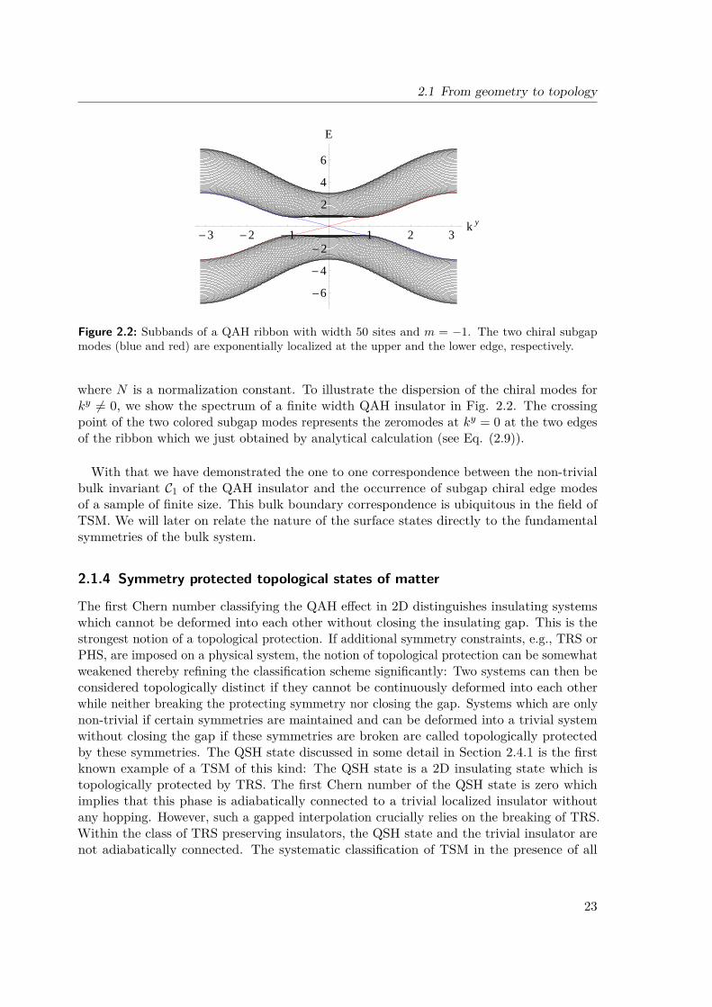
Figure 2.2: Subbands of a QAH ribbon with width 50 sites and m = −1. The two chiral subgapmodes (blue and red) are exponentially localized at the upper and the lower edge, respectively.
where N is a normalization constant. To illustrate the dispersion of the chiral modes forky 6= 0, we show the spectrum of a finite width QAH insulator in Fig. 2.2. The crossingpoint of the two colored subgap modes represents the zeromodes at ky = 0 at the two edgesof the ribbon which we just obtained by analytical calculation (see Eq. (2.9)).
With that we have demonstrated the one to one correspondence between the non-trivialbulk invariant C1 of the QAH insulator and the occurrence of subgap chiral edge modesof a sample of finite size. This bulk boundary correspondence is ubiquitous in the field ofTSM. We will later on relate the nature of the surface states directly to the fundamentalsymmetries of the bulk system.
2.1.4 Symmetry protected topological states of matter
The first Chern number classifying the QAH effect in 2D distinguishes insulating systemswhich cannot be deformed into each other without closing the insulating gap. This is thestrongest notion of a topological protection. If additional symmetry constraints, e.g., TRS orPHS, are imposed on a physical system, the notion of topological protection can be somewhatweakened thereby refining the classification scheme significantly: Two systems can then beconsidered topologically distinct if they cannot be continuously deformed into each otherwhile neither breaking the protecting symmetry nor closing the gap. Systems which are onlynon-trivial if certain symmetries are maintained and can be deformed into a trivial systemwithout closing the gap if these symmetries are broken are called topologically protectedby these symmetries. The QSH state discussed in some detail in Section 2.4.1 is the firstknown example of a TSM of this kind: The QSH state is a 2D insulating state which istopologically protected by TRS. The first Chern number of the QSH state is zero whichimplies that this phase is adiabatically connected to a trivial localized insulator withoutany hopping. However, such a gapped interpolation crucially relies on the breaking of TRS.Within the class of TRS preserving insulators, the QSH state and the trivial insulator arenot adiabatically connected. The systematic classification of TSM in the presence of all
23

Chapter 2 Topological states of matter
generic additional symmetries is the subject of Section 2.2. Interestingly, also the nature ofthe bulk boundary correspondence reflects the protecting symmetry. A rough but useful ruleof thumb in this context is: If the system preserves TRS with T 2 = −1, the edge modes arehelical, i.e., opposite spins have opposite chirality and are degenerate due to the Kramerstheorem. If the system has an emergent PHS as for example a mean field superconductor,the protected edge modes are Majorana modes. Combination of both symmetries yieldshelical Majorana modes.
2.1.5 Local topological quantum phase transitionsFrom our discussion so far and the explicit calculation of the topological invariant for ourtoy model (2.2) of the QAH state, it is clear that the topology of a band structure is a globalfeature which encompasses information about the function k 7→ h(k) everywhere in theBrillouin zone. However, in reality such a complete information about the physical systemis often times lacking. For example, the theoretical prediction of the QSH state in HgTe[Bernevig06a] is based on a perturbative k.p calculation which approximates h(k) as a loworder polynomial around the Γ-point k = 0. Without further discussion such an approximationseems to be inadequate for the investigation of topological features. However, as the authorsof Ref. [Bernevig06a] point out, the gap closing which separates the experimentally observed[König07] QSH phase from the trivial insulating phase happens at the Γ-point and could thusbe correctly described by a local theory. Such a singularity changing the topological invariantof the system has been coined topological quantum phase transition (TQPT) [Bernevig06a].For our toy model (2.2), the TQPT also happens via a gap closing at the Γ-point for m→ 0.This singular point where the Chern number C1 is not well defined separates the trivial(C1 = 0) from a non-trivial (C1 = 1) QAH phase as is illustrated in Fig. 2.1. An only locallyvalid theory can thus be suitable for the study of topological features under the followingcircumstances [Budich12d]: The state to be investigated must be known to concur with atopologically well understood reference state away from the validity regime of the effectivetheory. A possible transition between the reference state and the state of interest musthappen locally at a point within the validity regime of the effective theory. An examplewhere these conditions are not met is the integer quantum Hall effect with degenerate Landaulevels. In this case, there is no local gap closing point and the wave functions of all occupiedstates have to be known to determine the topological invariant [Budich12d]. In Section 2.3.4,we will see that the topology of an interacting system can even change due to dynamicalfluctuations which affect the frequency dependence of the single particle Green’s function.
2.2 Bulk classification of all possible non-interacting TSMIn this section, we review the general framework for the topological classification of non-interacting systems. This framework does not provide a recipe how to classify an individualsystem, as we characterized the QAH insulator by calculating its first Chern number inSection 2.1. It rather determines the group of possible topological equivalence classes fora non-interacting system with given spatial dimension and given fundamental symmetries.Regarding the QAH state, the result of this procedure would be: A non-interacting 2Dinsulator with no fundamental symmetries is characterized by a Z topological invariant. The
24
2.2 Bulk classification of all possible non-interacting TSM
calculation of the value of the respective topological invariants for a given representative of asymmetry class is the subject of Section 2.3.
The general idea that yields the entire table of TSM is quite simple: In addition torequiring a bulk insulating gap, physical systems of a given spatial dimension are divided into10 symmetry classes distinguished by their fundamental symmetries, i.e., TRS, PHS, andchiral symmetry (CS) [Altland97]. The topological properties of the corresponding Cartansymmetric spaces of quadratic candidate Hamiltonians determine the group of possibletopologically inequivalent systems. We outline the mathematical structure behind thisgeneral classification scheme in some detail. First, we briefly review the construction of theten universality classes [Altland97]. Then, we present the associated topological invariantsfor non-interacting systems of arbitrary spatial dimension giving a complete list of all TSM[Ryu10] that can be distinguished by virtue of this framework. Finally, we discuss in somedetail the origin of characteristic patterns appearing in this table using the framework ofK-Theory along the lines of the pioneering work by Kitaev [Kitaev09].
2.2.1 Cartan-Altland-Zirnbauer symmetry classes
A physical system can have different types of symmetries. An ordinary symmetry [Ryu10]is characterized by a set of unitary operators representing the symmetry operations thatcommute with the Hamiltonian. The influence of such a symmetry on the topologicalclassification can be eliminated by transforming the Hamiltonian into a block-diagonal formwith symmetry-less blocks. The total system then consists of several uncoupled copiesof symmetry-irreducible subsystems which can be classified individually. In contrast, the“extremely generic symmetries” [Ryu10] follow from the anti-unitary operations of TRS andPHS. Involving complex conjugation according to Wigner, they impose certain reality condi-tions on the system Hamiltonian. In total, the behavior of the system under these operations,and their combination, the CS operation, defines ten universality classes which we call theCartan-Altland-Zirnbauer (CAZ) classes. For disordered systems, these classes correspondto ten distinct renormalization group (RG) low energy fixed points in random matrix theory[Altland97]. The spaces of candidate Hamiltonians within these symmetry classes correspondto the ten symmetric spaces introduced by Cartan in 1926 [Cartan26] defined in terms ofquotients of Lie groups represented in the Hilbert space of the system. For translation-invariant systems, the imposed reality conditions are inherited by the Bloch Hamiltonian h(k).
In the following, the anti-unitary TRS operation will be denoted by T and the anti-unitaryPHS will be denoted by C. The Hamiltonian H of a physical system satisfies these symmetriesif
T HT −1 = H, (2.10)
and
CHC−1 = −H, (2.11)
respectively. According to Wigner’s theorem, these anti-unitary symmetries can be repre-
25

Chapter 2 Topological states of matter
sented as a unitary operation times the complex conjugationK. We define T = TK, C = CK.Using the unitarity of T,C along with H = H† we can rephrase Eqs. (2.10-2.11) as
THTT † = HCHTC† = −H (2.12)
There are two inequivalent realizations of these anti-unitary operations distinguished by theirsquare which can be plus identity or minus identity. For example, T 2 = ±1 for the unfoldingof a particle with integer/half-integer spin, respectively. Clearly, T 2 = ±1⇔ TT ∗ = ±1 andC2 = ±1⇔ CC∗ = ±1. In total, there are thus nine possible ways for a system to behaveunder the two anti-unitary symmetries: each symmetry can be absent, or present withsquare plus or minus identity. For eight of these nine combinations, the behavior under thecombination T C is fixed. The only exception is the so called unitary class which breaks bothPHS and TRS and can either obey or break their combination, the CS. This class hencesplits into two universality classes which add up to a grand total of ten classes shown in Tab.2.1. For a periodic system, symmetry constraints similar to Eq. (2.12) hold for the Bloch
Class TRS PHS CSA (Unitary) 0 0 0AI (Orthogonal) +1 0 0AII (Symplectic) -1 0 0AIII (Chiral Unitary) 0 0 1BDI (Chiral Orthogonal) +1 +1 1CII (Chiral Symplectic) -1 -1 1D 0 +1 0C 0 -1 0DIII -1 +1 1CI +1 -1 1
Table 2.1: Table of the CAZ universality classes. 0 denotes the absence of a symmetry. For PHS andTRS, ±1 denotes the square of a present symmetry, the presence of CS is denoted by 1. The last fourclasses are Bogoliubov deGennes classes of mean field superconductors where the superconductinggap plays the role of the insulating gap.
Hamiltonian h(k), namely
ThT (−k)T † = h(k)ChT (−k)C† = −h(k), (2.13)
where T,C now denote the representation of the unitary part of the anti-unitary operationsin band space.
For a continuum model, the real space Hamiltonian H(x) is defined through
H =∫
ddxΨ†(x)H(x)Ψ(x),
26
2.2 Bulk classification of all possible non-interacting TSM
where Ψ is a vector/spinor comprising all internal degrees like spin, particle species, etc. Thek-space on which the Fourier transform H(k) of H(x) is defined does not have the topologyof a torus like the BZ of a periodic system. However, the continuum models one is concernedwith in condensed matter physics are effective low energy/large distance theories. For largek, H(k) will thus generically have a trivial structure (c.f. Fig. 2.1), so that the k-spacecan be endowed with the topology of the sphere Sd by a one point compactification whichmaps k → ∞ to a single point (see Section 2.1 for an explicit example of this procedure).The symmetry constraints on H(k) have the same form as those on the Bloch Hamiltonianh(k) shown in Eq. (2.13). By abuse of notation, we will denote both H(k) and h(k) by h(k).Nevertheless, we will point out several differences between periodic systems and continuummodels along the way.
2.2.2 Definition of the classification problem for continuum models andperiodic systems
For translation-invariant insulating systems with n occupied and m empty bands and con-tinuum models with n occupied and m empty fermion species, respectively, the projectionP (k) =
∑nα=1|uα(k)〉〈uα(k)| onto the occupied states is the relevant quantity for the topo-
logical classification. The spectrum of the system is not of interest for adiabatic quantitiesas long as a bulk gap between the empty and the occupied states is maintained. We thusdeform the system adiabatically into a flat band insulator, i.e., a system with eigenenergyε− = −1 for all occupied states and eigenenergy ε+ = +1 for all empty states. The eigenstatesare not changed during this deformation. The Hamiltonian of this flat band system thenreads [Qi08a, Schnyder08]
Q(k) = (+1) (1− P (k)) + (−1)P (k) = 1− 2P (k)
Obviously, Q2 = 1,Tr [Q] = m− n. Without further symmetry constraints, Q is an arbitraryU(n+m) matrix which is defined up to a U(n)×U(m) gauge degree of freedom correspondingto basis transformations within the subspaces of empty and occupied states, respectively.Thus, Q is in the symmetric space
Gn+m,m(C) = Gn+m,n(C) = U(n+m)/(U(n)× U(m)).
Geometrically, the complex Grassmannian Gk,l(C) is a generalization of the complex projec-tive plane and is defined as the set of l-dimensional planes through the origin of Ck. Theset of topologically different translation-invariant insulators is then given by the group g ofhomotopically inequivalent maps k 7→ Q(k) from the BZ T d of a system of spatial dimensiond to the space Gn+m,m(C) of possible Bloch Hamiltonians. For continuum models T d isreplaced by Sd and g is by definition given by
g = πd (Gn+m,m(C)) , (2.14)
where the n-th homotopy group πn of a space is by definition the group of homotopicallyinequivalent maps from Sd to this space. For translation-invariant systems defined on a BZ,the classification can be more complicated than Eq. (2.14) if the lower homotopy groups
27
Chapter 2 Topological states of matter
πs, s = 1, . . . , d − 1 are nontrivial. For our previous example of the QAH insulator, a2D translation-invariant state which does not obey any fundamental symmetries, we caninfer from π2 (Gn+m,m(C)) = Z, π1 (Gn+m,m(C)) = 0 that an integer topological invari-ant must distinguish possible states of matter in this symmetry class, i.e., possible mapsT 2 → Gn+m,m(C). The condition π1 (Gn+m,m(C)) = 0 is necessary because the π2 classifiesmaps from S2, which is only equivalent to the classification of physical maps from T 2 if thefundamental group π1 of the target space is trivial. The difference between the base space ofa periodic systems which is a torus and of continuum models which has the topology of asphere has interesting physical ramifications: The so called weak topological insulators areonly topologically distinct over a torus but not over a sphere. Physically, this is visible in thelacking robustness of these TSM which break down with the breaking of translation symmetry.
Requiring further symmetries as appropriate for the other nine CAZ universality classes istantamount to imposing symmetry constraints on the allowed maps T d → Gn+m,m(C), k 7→Q(k) for translation-invariant systems and Sd → Gn+m,m(C), k 7→ Q(k) for continuummodels, respectively. The set of topologically distinct physical systems is then still givenby the set of homotopically inequivalent maps within this restricted space, i.e., the space ofmaps which cannot be continuously deformed into each other without breaking a symmetryconstraint. For example, for the chiral classes characterized by CS = 1, Q can be broughtinto the off diagonal form [Schnyder08]
Q =(
0 qq† 0
),
with qq† = 1, which reduces the corresponding target space to U(n). For the chiral uni-tary class AIII without further symmetry constraints, the calculation of g amounts tocalculating g = πd (U(n)) = Z for odd d and g = πd (U(n)) = 0 for even d, respectively. Addi-tional symmetries will again impose additional constraints on the map T d → U(n), k 7→ q(k).
This procedure rigorously defines the group g of topological equivalence classes for non-interacting translation-invariant insulators in arbitrary spatial dimension and CAZ univer-sality class. However, the practical calculation of g can be highly non-trivial and has beenachieved for continuum models via various subtle detours, for example the investigationof surface nonlinear σ-models, in Refs. [Schnyder09, Ryu10]. In the following, we outlinea mathematical brute force solution to the classification problem in terms of K-Theorywhich has been originally introduced in the seminal work by Kitaev in 2009 [Kitaev09].This method will naturally explain the emergence of weak topological insulators. We willnot assume any prior knowledge on K-Theory. In Tab. 2.2, we summarize the resultinggroups of topological sectors g for all possible systems [Schnyder09]. We notice an interestingdiagonal pattern relating subsequent symmetry classes to neighboring spatial dimensions.Furthermore, the pattern of the two unitary classes shows a periodicity of two in the spatialdimension. If we had shown the classification for higher spatial dimensions, we would haveobserved a periodicity of eight in the spatial dimension for the eight real classes. Thefollowing discussion is dedicated to provide a deeper understanding of these fundamentalpatterns as pioneered in Ref. [Kitaev09]. The mentioned periodicities have first been pointed
28

2.2 Bulk classification of all possible non-interacting TSM
out in Refs. [Qi08a, Schnyder09].
Class constraint d = 1 d = 2 d = 3 d = 4A none 0 Z 0 ZAIII none on q Z 0 Z 0AI QT (k) = Q(−k) 0 0 0 ZBDI q∗(k) = q(−k) Z 0 0 0D τxQ
T (k)τx = −Q(−k), m = n Z2 Z 0 0DIII q(k)T = −q(−k),m = n even Z2 Z2 Z 0AII iσyQ
T (k)(−iσy) = Q(−k), m, n even 0 Z2 Z2 ZCII iσyq
∗(k)(−iσy) = q(−k), m = n even Z 0 Z2 Z2C τyQ
T (k)τy = −Q(−k), m = n 0 Z 0 Z2CI q(k)T = q(−k),m = n 0 0 Z 0
Table 2.2: Table of all groups g of topological equivalence classes. The first column denotes the CAZsymmetry class, divided into two unitary classes without anti-unitary symmetry (top) and eight “real”classes with at least one anti-unitary symmetry (bottom). The second column shows the symmetryconstraints on the flat band maps, where we have chosen the representation T = K for T 2 = 1,T = iσyK for T 2 = −1, as well as C = τxK for C2 = 1, C = τyK for C2 = −1. Here, σy denotesthe Pauli matrix in spin space, τx, τy denote Pauli matrices in the particle hole pseudo spin space ofBogoliubov deGennes Hilbert spaces. In the last four columns, g is listed for d = 1, . . . , 4.
2.2.3 Topological classification of unitary vector bundles
In order to prepare the reader for the application of K-Theory and motivate its usefulness, wefirst formulate the classification problem in the language of fiber bundles. The mathematicalstructure of a non-interacting insulator of spatial dimension d is that of a vector bundleE
π→M. The base manifoldM of E is the d dimensional k-space of the system, and thefiber over a point k given by the (projective) space of occupied states P (k). The gauge groupof the bundle is U(n), where n is the dimension of P . If no further symmetry conditionsare imposed (see class A in Tab. 2.1), the question of how many topologically distinctinsulators in a given dimension exist is tantamount to asking how many homotopicallydifferent U(n) vector bundles can be constructed overM. This question can be formallyanswered for arbitrary smooth manifoldsM as we will outline now. The general idea is thefollowing. There is a universal Bundle ξ Π→ X into which every bundle E can be embeddedthrough a bundle map [Nakahara03] f : E → ξ such that
f∗ξ = E, (2.15)
where f :M→ X is the map between the base manifolds associated with the bundle mapf . That is to say every bundle can be represented as a pullback bundle [Nakahara03] ofthe universal bundle ξ by virtue of a suitable bundle map f . The key point is now thathomotopically different bundles E are distinguished by homotopically distinct maps f . Thus,the set of different TSM is the set π [M,X ] of homotopy classes of maps from the k-spaceM to the base manifold X of the universal bundle. X is also called the classifying space of
29

Chapter 2 Topological states of matter
U(n) and is given by the Grassmanian GN,n(C) = U(N)/(U(n)× U(N − n)) for sufficientlylarge N , i.e., N > dd2 + ne. To be generic in the dimension of the system d, we take theinductive limit X = Gn(C∞) = limN→∞GN,n(C) = limN→∞ U(N)/(U(n)× U(N − n)). Wethus found for the set Vectn(M,C) of inequivalent U(n) bundles overM the expression
Vectn(M,C) = π [M, Gn(C∞)] ,
which is known for some rather simple base manifolds. In particular for spheres Sd, thereis a trick to calculate Vectn(Sd,C): Sd can always be decomposed into two hemisphereswhich are individually trivial. The homotopy of a bundle over Sd is thus determined bythe clutching function fc defined in the overlap Sd−1 of the two hemispheres, i.e., along theequator of Sd. Physically, fc translates a local gauge choice on the upper hemisphere into alocal gauge choice on the lower hemisphere and is thus a function fc : Sd−1 → U(n). Thegroup of homotopy classes of such functions is by definition given πd−1(U(n)). Interestingly,for n > d−1
2 , these groups are given by
Vectn(Sd,C) = πd−1(U(n)) =Z, d− 1 odd0 , d− 1 even (2.16)
This periodicity of two in (d− 1) is known as the complex Bott periodicity. The physicalmeaning of Eq. (2.16) is the following: In the unitary universality class A, there is an integertopological invariant in even spatial dimension (QAH in d = 2) and no TSM in odd spatialdimension.
This classification has two shortcomings. First, it cannot be readily generalized to otherCAZ classes at this simple level. Second, only systems with the same number of occupiedbands n can be compared. However, adding some trivial bands to the system should yield asystem in the same equivalence class. Both shortcomings can be overcome in the frameworkof K-Theory [Karoubi78, Nash91].
2.2.4 K-Theory approach to a complete classification
K-Theory [Karoubi78, Nash91] is concerned with vector bundles which have a “sufficientlylarge” fiber dimension. This means, that topological defects which can be unwound by justincreasing the fiber dimension are not visible in the resulting classification scheme. Thisis physically reasonable, as trivial occupied bands from inner localized shells for exampleincrease the number of bands as compared to the effective low energy models under investi-gation. Models of different number of such trivial bands should be comparable in a robustclassification scheme. The use of K-Theory for the classification of TSM has been pioneeredin Refs. [Kane05a, Kane05b] and more systematically been discussed in Ref. [Kitaev09].
Crash-course in K-Theory
The direct sum of two vector bundles E ⊕ F is the direct sum of their fibers over each point.This addition has only a semi-group structure, since E ⊕G = F ⊕G; E ' F . A minimal
30

2.2 Bulk classification of all possible non-interacting TSM
counterexample is given by E = TS2, F = S2 × R2. F is clearly trivial, whereas E, thetangent bundle of S2 is well known to be non-trivial. However, adding NS2, the bundle ofnormal vectors to S2, to both bundles E,F we obtain the same trivial bundle S2 ×R3. Thismotivates the concept of stable equivalence
Es' F ⇔ E ⊕ Zm ' F ⊕ Zn, (2.17)
where Zn =M×Kn, K = R,C is the trivial bundle over the fixed base manifoldM, whichplays the role of an additive zero as far as stable equivalence is concerned. We denote theset of K-vector bundles overM by VK(M) in the following. Note that stably equivalentbundles can have different fiber dimension, as m 6= n in general in Eq. (2.17). The benefit ofthis construction is:
E ⊕G = F ⊕G⇒ Es' F (2.18)
This is because for vector bundles on a smooth manifold every bundle can be augmented toa trivial bundle, i.e.,
∀G∃H,l G⊕H = Z l. (2.19)
Eq. (2.18) naturally leads to the notion of a subtraction on VK(M) by virtue of theGrothendieck construction: Consider the pairs (E1, E2) ∈ VK(M)× VK(M) and define theequivalence relation
(E1, E2) ∼ (F1, F2)⇔ ∃HF1 ⊕ E2 ⊕H ' E1 ⊕ F2 ⊕H. (2.20)
Looking at Eq. (2.20), we can intuitively think of the equivalence class (E1, E2)∼ as theformal difference E1 − E2. We now define the K-group as the quotient
K(M) = (VK(M)× VK(M)) / ∼, (2.21)
which identifies all formal differences that are equivalent in the sense of Eq. (2.20). Dueto Eq. (2.19), every group element in K(M) can be represented in the form (E,Zn).However, (E,Zn) (E,Zm) for n 6= m. We define the virtual dimension of (E,F ) asdv = rk(E) − rk(F ), where rk denotes the rank, i.e., the fiber dimension of a vector bun-dle. By restricting K(M) to elements with dv = 0, we obtain the restricted K-groupK(M) = g ∈ K(M)|dv(g) = 0. K(M) is isomorphic to the set of stable equivalenceclasses of VK(M). Up to now, the construction has been independent of the field over whichthe vector spaces are defined. In the following, we will distinguish the real and complexK-groups KR(M),KC(M).
A crucial notion in K-Theory which is also our main physical motivation to study it is thatof the stable range. The idea is that at sufficiently large fiber dimension n no “new” bundlescan be discovered by looking at even larger fiber dimension. Sufficiently large in terms ofthe dimension d ofM means n ≥ nC = d/2 + 1 for the complex case and n ≥ nR = d+ 1 forthe real case, respectively. More formally, every bundle E with n > nK can be expressed as
31

Chapter 2 Topological states of matter
a sum
E ' F ⊕ Zn−nK (2.22)
of a bundle F with fiber dimension nK and a trivial bundle for K = R,C. Since clearlyE
s' F (see Eq. (2.18)), this means that all stable equivalence classes have representativesin fiber dimension n ≤ nK . Furthermore, a situation like our counterexample above wherewe augmented two non-isomorphic bundles by the same trivial bundle NS2 to obtain thesame trivial bundle cannot occur in the stable range. That is to say F as appearing in Eq.(2.22) is uniquely defined up to isomorphism. The stable range hence justifies the approachof K-theory of ignoring fiber dimension when defining the stable equivalence. The key resultin the stable range which connects K-Theory to our goal of classifying all inequivalent vectorbundles with sufficiently large but arbitrary fiber dimension on equal footing reads [Nash91]
KK(M) = Vectn(M,K) = π [M, Gn(K∞)] ∀n≥nK . (2.23)
The complex Bott periodicity Eq. (2.16) with period pC = 2 has a real analogue concerningthe homotopy groups of O(n) with period pR = 8. This immediately implies in the languageof K-Theory
KK(Sd+pK ) = KK(Sd), K = R,C. (2.24)
We define
K−dK (M) = KK(SdM), (2.25)
where S is the reduced suspension [Nash91] which for a sphere Sk indeed satisfies SSk = Sk+1.The stronger version of the Bott periodicity in K-Theory now reads [Nash91]
K−d−pKK (M) = K−dK (M), K = R,C (2.26)
which only forM = Sl trivially follows from Eq. (2.24). Using this periodicity, the definitionof K−dK in Eq. (2.25) can be formally extended to d ∈ Z.
The Bott clock
From the very basic construction of homotopy groups the following identities for the homotopyof a topological space X are evident:
πd(X) = π[Sd, X
]= π
[SSd−1, X
]= π
[Sd−1,ΩX
],
where ΩX denotes the loop space [Nash91] of X, i.e., the space of maps from S1 toX. Iterating this identity gives πd(X) = π0(ΩnX) using the complex Bott periodicity(2.16), we immediately see that counting the connected components π0 (U(n)) , π1 (U(n)) =π0 (ΩU(n)) of the unitary group and its first loop space, we can classify all U(n) vectorbundles over Sd in the stable range, i.e., with n > d
2 . The real analogue of the Bott periodicitywith period pR = 8 leads to analogous statements for O(n) bundles over Sd which depend
32
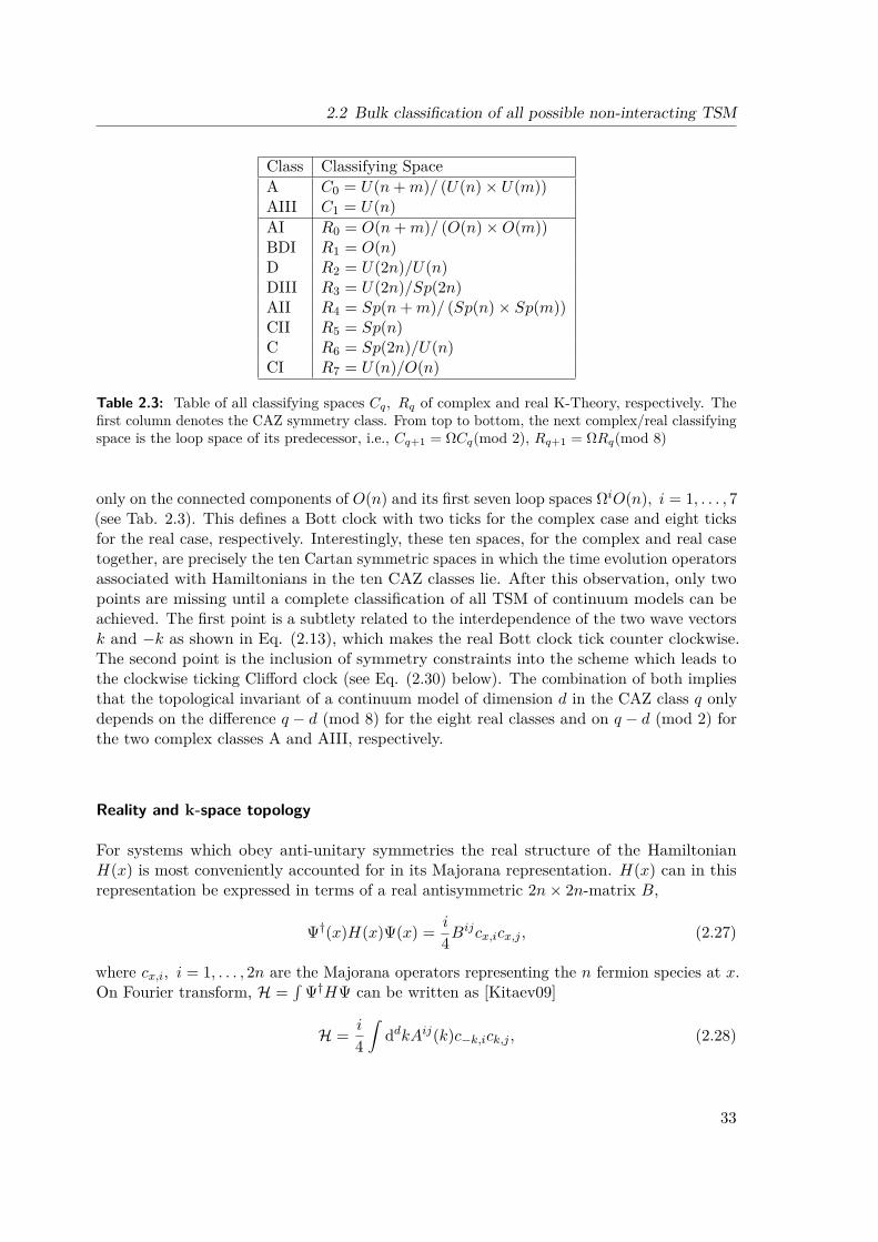
2.2 Bulk classification of all possible non-interacting TSM
Class Classifying SpaceA C0 = U(n+m)/ (U(n)× U(m))AIII C1 = U(n)AI R0 = O(n+m)/ (O(n)×O(m))BDI R1 = O(n)D R2 = U(2n)/U(n)DIII R3 = U(2n)/Sp(2n)AII R4 = Sp(n+m)/ (Sp(n)× Sp(m))CII R5 = Sp(n)C R6 = Sp(2n)/U(n)CI R7 = U(n)/O(n)
Table 2.3: Table of all classifying spaces Cq, Rq of complex and real K-Theory, respectively. Thefirst column denotes the CAZ symmetry class. From top to bottom, the next complex/real classifyingspace is the loop space of its predecessor, i.e., Cq+1 = ΩCq(mod 2), Rq+1 = ΩRq(mod 8)
only on the connected components of O(n) and its first seven loop spaces ΩiO(n), i = 1, . . . , 7(see Tab. 2.3). This defines a Bott clock with two ticks for the complex case and eight ticksfor the real case, respectively. Interestingly, these ten spaces, for the complex and real casetogether, are precisely the ten Cartan symmetric spaces in which the time evolution operatorsassociated with Hamiltonians in the ten CAZ classes lie. After this observation, only twopoints are missing until a complete classification of all TSM of continuum models can beachieved. The first point is a subtlety related to the interdependence of the two wave vectorsk and −k as shown in Eq. (2.13), which makes the real Bott clock tick counter clockwise.The second point is the inclusion of symmetry constraints into the scheme which leads tothe clockwise ticking Clifford clock (see Eq. (2.30) below). The combination of both impliesthat the topological invariant of a continuum model of dimension d in the CAZ class q onlydepends on the difference q − d (mod 8) for the eight real classes and on q − d (mod 2) forthe two complex classes A and AIII, respectively.
Reality and k-space topology
For systems which obey anti-unitary symmetries the real structure of the HamiltonianH(x) is most conveniently accounted for in its Majorana representation. H(x) can in thisrepresentation be expressed in terms of a real antisymmetric 2n× 2n-matrix B,
Ψ†(x)H(x)Ψ(x) = i
4Bijcx,icx,j , (2.27)
where cx,i, i = 1, . . . , 2n are the Majorana operators representing the n fermion species at x.On Fourier transform, H =
∫Ψ†HΨ can be written as [Kitaev09]
H = i
4
∫ddkAij(k)c−k,ick,j , (2.28)
33

Chapter 2 Topological states of matter
where A is skew hermitian and satisfies
A∗(k) = A(−k). (2.29)
Eq. (2.29) naturally leads to a real vector bundle structure as defined in Ref. [Atiyah66]for the bundle of eligible A-matrices over the k-space (Rd, τ), where the involution τ (seeRef. [Atiyah66]) is given by k 7→ −k. On one-point compactification, this real k-spacebecomes a sphere Sd = (Sd, τ) with the same involution [Kitaev09]. Whereas the ordinarysphere Sd can be viewed as a reduced suspension S of Sd−1 over the real axis, Sd can beunderstood as the reduced suspension S of Sd−1 over the imaginary axis. This picture isalgebraically motivated by comparing the involution τ to the ordinary complex conjugationwhich, restricted to the imaginary axis of the complex plane is of the same form. Interestingly,in the language of definition (2.25), S plays the role of an inverse to S [Atiyah66, Kitaev09],i.e.,
KR(M) = K−1R (SM) = KR(SSM).
This means that the Bott clock over Sd is reversed as compared to its analogue over Sd.
Real K-theory and the Clifford clock
The main reason for the real construction of Eq. (2.28) is that the anti-unitary symmetryconstraints yielding the eight real CAZ classes (all except A and AIII) can be distinguished interms of anti-commutation relations of the A-matrix with real Clifford generators [Karoubi78,Kitaev09]. At a purely algebraic level, these constraints can be transformed so as to beexpressed only in terms of positive Clifford generators [Kitaev09], i.e., generators that squareto plus identity. We call the restricted K-group of a vector bundle of A-matrices overM that anti-commute with q positive Clifford generators Kq
R(M). Interestingly [Karoubi78,Kitaev09],
KqR(M) ' K−qR (M). (2.30)
Eq. (2.30) defines a Clifford clock that runs in the opposite direction as the Sd Bott clock.This algebraic phenomenon explains the full periodic structure of the table of TSM ofcontinuum models (see Tab. 2.2). The classifying spaces of A-matrices for systems thatanti-commute with q Clifford generators are shown in Tab. 2.3.
Periodic systems
The classification of periodic systems is much more complicated from a mathematical pointof view. Their base space is the real Brillouin zone T d = (T d, τ), where the involutionτ giving rise to the real structure is again given by k 7→ −k. For T d the reduced suspensiondoes not provide a trivial relation between the K-Theory of different spatial dimension likeSSd = Sd+1 for the base space of continuum models. The general calculation of all relevantK-groups over T d has been reported in Ref. [Kitaev09]. Interestingly, the resulting groupsalways contain the respective classification of continuum models in the same symmetry class
34
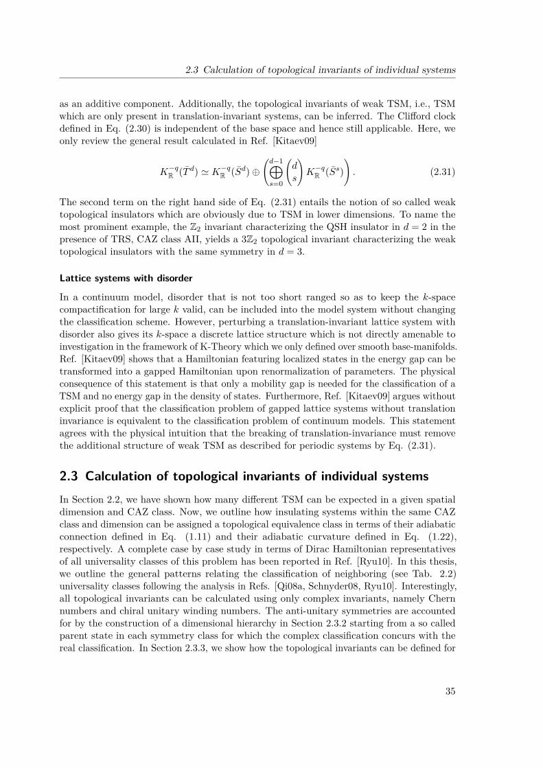
2.3 Calculation of topological invariants of individual systems
as an additive component. Additionally, the topological invariants of weak TSM, i.e., TSMwhich are only present in translation-invariant systems, can be inferred. The Clifford clockdefined in Eq. (2.30) is independent of the base space and hence still applicable. Here, weonly review the general result calculated in Ref. [Kitaev09]
K−qR (T d) ' K−qR (Sd)⊕(d−1⊕s=0
(ds
)K−qR (Ss)
). (2.31)
The second term on the right hand side of Eq. (2.31) entails the notion of so called weaktopological insulators which are obviously due to TSM in lower dimensions. To name themost prominent example, the Z2 invariant characterizing the QSH insulator in d = 2 in thepresence of TRS, CAZ class AII, yields a 3Z2 topological invariant characterizing the weaktopological insulators with the same symmetry in d = 3.
Lattice systems with disorder
In a continuum model, disorder that is not too short ranged so as to keep the k-spacecompactification for large k valid, can be included into the model system without changingthe classification scheme. However, perturbing a translation-invariant lattice system withdisorder also gives its k-space a discrete lattice structure which is not directly amenable toinvestigation in the framework of K-Theory which we only defined over smooth base-manifolds.Ref. [Kitaev09] shows that a Hamiltonian featuring localized states in the energy gap can betransformed into a gapped Hamiltonian upon renormalization of parameters. The physicalconsequence of this statement is that only a mobility gap is needed for the classification of aTSM and no energy gap in the density of states. Furthermore, Ref. [Kitaev09] argues withoutexplicit proof that the classification problem of gapped lattice systems without translationinvariance is equivalent to the classification problem of continuum models. This statementagrees with the physical intuition that the breaking of translation-invariance must removethe additional structure of weak TSM as described for periodic systems by Eq. (2.31).
2.3 Calculation of topological invariants of individual systemsIn Section 2.2, we have shown how many different TSM can be expected in a given spatialdimension and CAZ class. Now, we outline how insulating systems within the same CAZclass and dimension can be assigned a topological equivalence class in terms of their adiabaticconnection defined in Eq. (1.11) and their adiabatic curvature defined in Eq. (1.22),respectively. A complete case by case study in terms of Dirac Hamiltonian representativesof all universality classes of this problem has been reported in Ref. [Ryu10]. In this thesis,we outline the general patterns relating the classification of neighboring (see Tab. 2.2)universality classes following the analysis in Refs. [Qi08a, Schnyder08, Ryu10]. Interestingly,all topological invariants can be calculated using only complex invariants, namely Chernnumbers and chiral unitary winding numbers. The anti-unitary symmetries are accountedfor by the construction of a dimensional hierarchy in Section 2.3.2 starting from a so calledparent state in each symmetry class for which the complex classification concurs with thereal classification. In Section 2.3.3, we show how the topological invariants can be defined for
35
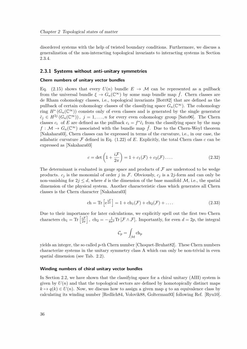
Chapter 2 Topological states of matter
disordered systems with the help of twisted boundary conditions. Furthermore, we discuss ageneralization of the non-interacting topological invariants to interacting systems in Section2.3.4.
2.3.1 Systems without anti-unitary symmetries
Chern numbers of unitary vector bundles
Eq. (2.15) shows that every U(n) bundle E → M can be represented as a pullbackfrom the universal bundle ξ → Gn(C∞) by some map bundle map f . Chern classes arede Rham cohomology classes, i.e., topological invariants [Bott82] that are defined as thepullback of certain cohomology classes of the classifying space Gn(C∞). The cohomologyring H∗ (Gn(C∞)) consists only of even classes and is generated by the single generatorcj ∈ H2j (Gn(C∞)) , j = 1, . . . , n for every even cohomology group [Sato96]. The Chernclasses ci of E are defined as the pullback ci = f∗ci from the classifying space by the mapf : M → Gn(C∞) associated with the bundle map f . Due to the Chern-Weyl theorem[Nakahara03], Chern classes can be expressed in terms of the curvature, i.e., in our case, theadiabatic curvature F defined in Eq. (1.22) of E. Explicitly, the total Chern class c can beexpressed as [Nakahara03]
c = det(
1 + iF2π
)= 1 + c1(F) + c2(F) . . . . (2.32)
The determinant is evaluated in gauge space and products of F are understood to be wedgeproducts. cj is the monomial of order j in F . Obviously, cj is a 2j-form and can only benon-vanishing for 2j ≤ d, where d is the dimension of the base manifoldM, i.e., the spatialdimension of the physical system. Another characteristic class which generates all Chernclasses is the Chern character [Nakahara03]
ch = Tr[eiF2π]
= 1 + ch1(F) + ch2(F) + . . . . (2.33)
Due to their importance for later calculations, we explicitly spell out the first two Cherncharacters ch1 = Tr
[iF2π
], ch2 = − 1
8π2Tr [F ∧ F ]. Importantly, for even d = 2p, the integral
Cp =∫M
chp
yields an integer, the so called p-th Chern number [Choquet-Bruhat82]. These Chern numberscharacterize systems in the unitary symmetry class A which can only be non-trivial in evenspatial dimension (see Tab. 2.2).
Winding numbers of chiral unitary vector bundles
In Section 2.2, we have shown that the classifying space for a chiral unitary (AIII) system isgiven by U(n) and that the topological sectors are defined by homotopically distinct mapsk 7→ q(k) ∈ U(n). Now, we discuss how to assign a given map q to an equivalence class bycalculating its winding number [Redlich84, Volovik88, Golterman93] following Ref. [Ryu10].
36

2.3 Calculation of topological invariants of individual systems
From Tab. 2.2 it is clear that only in odd spatial dimension d = 2j − 1 there can be anon-trivial winding number. We define
wq2j−1 = (−(j − 1)!)(2j − 1)!(2πi)jTr
[(q−1dq)2j−1
], (2.34)
which has been dubbed winding number density [Ryu10]. Integrating this density over theodd-dimensional base manifoldM representing the k-space of the physical system, we getthe integral winding number ν2j−1
ν2j−1 =∫Mwq2j−1, (2.35)
which is well known to measure the homotopy of the map k 7→ q(k).
Relation between chiral winding number and Chern Simons form
So far, the relation between the adiabatic connection of a chiral system and its topologicalinvariant has not been made explicit. Since characteristic classes like Chern characters areclosed 2j-forms, they can locally be expressed as exterior derivatives of a (2j − 1)-forms.These odd forms are called the Chern Simons forms associated with the even characteristicclass [Chern74, Nakahara03]. For the j-th Chern character chj , which is a 2j form, theassociated Chern Simons form Q2j−1 reads [Nakahara03]
Q2j−1(A,Ft) = 1(j − 1)!
(i
2π
)j ∫ 1
0dt STr
[A,F j−1
t
], (2.36)
where Ft = tF + (t2 − t)A ∧ A is the curvature of the interpolation tA between thezero connection and A and STr denotes the symmetrized trace. Explicitly, we haveQ1 = i
2πTr [A] , Q3 = − 18π2Tr
[AdA+ 2
3A3].
It is straightforward to show [Ryu10], that in a suitable gauge, the Berry connection ofa chiral bundle yields AB = 1
2qdq†, where q ∈ U(n) is again the chiral map characterizing
the system. This is not a pure gauge due to the factor 12 which entails that the associated
curvature FB does not vanish. Plugging AB and FB into Eq. (2.36) immediately yields[Ryu10]
Q2j−1(AB,FBt ) = 12w
q2j−1. (2.37)
Eq. (2.37) directly relates the winding number density to the Chern Simons form. We definethe Chern Simons invariant of an odd dimensional system as
CS2j−1 =∫MQ2j−1 (mod 1),
where (mod 1) accounts for the fact that∫MQ2j−1 has an integer gauge dependence due to
37

Chapter 2 Topological states of matter
Figure 2.3: Illustration of the WZW dimensional extension. The circle at v = 0 represents thephysical system. The poles at v = ±π represent the trivial reference system without k-dependence.The two interpolations are conjugated by an anti-unitary symmetry, here exemplary denoted by TRS.
π2j−1 (U(n)) = Z for n > j. Looking back at Eq. (2.35), we immediately get
ν2j−1(mod 2) = 2CS2j−1(mod 2).
We note that the (mod 2) can be dropped if we fix the gauge as described above toAB = 1
2qdq−1. This establishes the desired relation between the winding number of a chiral
unitary system and its adiabatic curvature.
2.3.2 Dimensional reduction and real symmetry classes
Until now, we have only discussed how to calculate topological invariants of systems in thecomplex symmetry classes A and AIII. Interestingly, for some real universality classes, theclassification in the presence of anti-unitary symmetries concurs with the unitary classification(see Tab. 2.4). The first known example of this type is in the symplectic class AII ind = 4 which is characterized by the second Chern number of the corresponding complexbundle [Avron88, Zhang01]. Another example of this kind is the p+ ip superconductor ind = 2 and symmetry class D which is characterized by its first Chern number, i.e., in thesame way as the QAH effect in class A. In odd dimensions similar examples exist for realchiral classes, e.g., for DIII in d = 3, where the winding number is calculated using Eq.(2.34) in the same way as for the chiral unitary class AIII in the same dimension. All thetopological invariants just mentioned are integer invariants. In some universality classes,these integers can only assume even values (see Tab. 2.4). For physically relevant dimensions,i.e., d = 1, 2, 3, these exceptions are CII in d = 1, C in d = 2, and CI in d = 3. All other stateswhere the complex and the real classification concur, can be viewed as parent states of adimensional hierarchy within the same symmetry class from which all Z2 invariants appearingin Tab. 2.4 can be obtained by dimensional reduction. This approach was pioneered in theseminal work by Qi, Hughes, and Zhang [Qi08a].
The general idea is more intuitive if we consider the parent state as a Wess-Zumino-Witten(WZW) dimensional extension [Witten83, Wang10] of the lower dimensional descendants
38
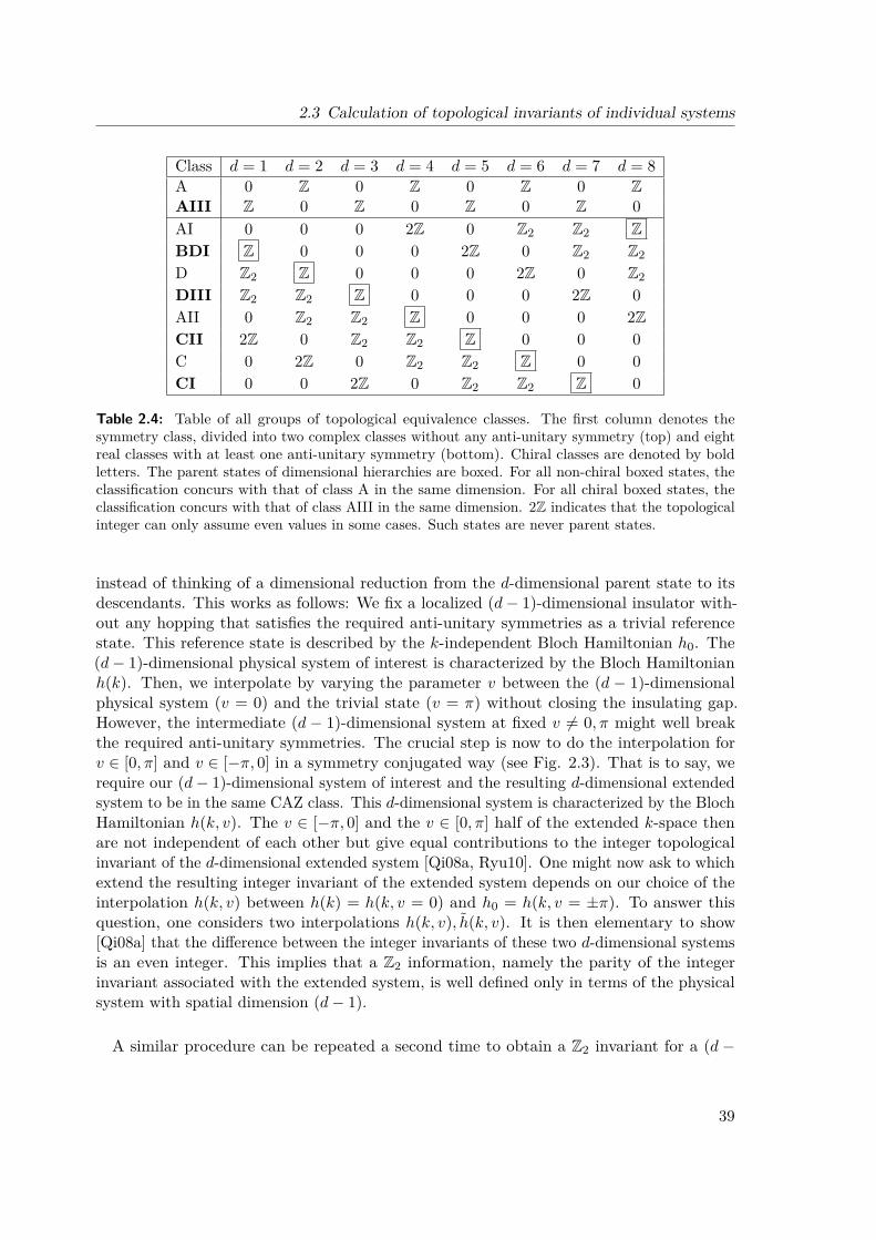
2.3 Calculation of topological invariants of individual systems
Class d = 1 d = 2 d = 3 d = 4 d = 5 d = 6 d = 7 d = 8A 0 Z 0 Z 0 Z 0 ZAIII Z 0 Z 0 Z 0 Z 0AI 0 0 0 2Z 0 Z2 Z2 ZBDI Z 0 0 0 2Z 0 Z2 Z2D Z2 Z 0 0 0 2Z 0 Z2DIII Z2 Z2 Z 0 0 0 2Z 0AII 0 Z2 Z2 Z 0 0 0 2ZCII 2Z 0 Z2 Z2 Z 0 0 0C 0 2Z 0 Z2 Z2 Z 0 0CI 0 0 2Z 0 Z2 Z2 Z 0
Table 2.4: Table of all groups of topological equivalence classes. The first column denotes thesymmetry class, divided into two complex classes without any anti-unitary symmetry (top) and eightreal classes with at least one anti-unitary symmetry (bottom). Chiral classes are denoted by boldletters. The parent states of dimensional hierarchies are boxed. For all non-chiral boxed states, theclassification concurs with that of class A in the same dimension. For all chiral boxed states, theclassification concurs with that of class AIII in the same dimension. 2Z indicates that the topologicalinteger can only assume even values in some cases. Such states are never parent states.
instead of thinking of a dimensional reduction from the d-dimensional parent state to itsdescendants. This works as follows: We fix a localized (d− 1)-dimensional insulator with-out any hopping that satisfies the required anti-unitary symmetries as a trivial referencestate. This reference state is described by the k-independent Bloch Hamiltonian h0. The(d− 1)-dimensional physical system of interest is characterized by the Bloch Hamiltonianh(k). Then, we interpolate by varying the parameter v between the (d − 1)-dimensionalphysical system (v = 0) and the trivial state (v = π) without closing the insulating gap.However, the intermediate (d − 1)-dimensional system at fixed v 6= 0, π might well breakthe required anti-unitary symmetries. The crucial step is now to do the interpolation forv ∈ [0, π] and v ∈ [−π, 0] in a symmetry conjugated way (see Fig. 2.3). That is to say, werequire our (d− 1)-dimensional system of interest and the resulting d-dimensional extendedsystem to be in the same CAZ class. This d-dimensional system is characterized by the BlochHamiltonian h(k, v). The v ∈ [−π, 0] and the v ∈ [0, π] half of the extended k-space thenare not independent of each other but give equal contributions to the integer topologicalinvariant of the d-dimensional extended system [Qi08a, Ryu10]. One might now ask to whichextend the resulting integer invariant of the extended system depends on our choice of theinterpolation h(k, v) between h(k) = h(k, v = 0) and h0 = h(k, v = ±π). To answer thisquestion, one considers two interpolations h(k, v), h(k, v). It is then elementary to show[Qi08a] that the difference between the integer invariants of these two d-dimensional systemsis an even integer. This implies that a Z2 information, namely the parity of the integerinvariant associated with the extended system, is well defined only in terms of the physicalsystem with spatial dimension (d− 1).
A similar procedure can be repeated a second time to obtain a Z2 invariant for a (d −
39

Chapter 2 Topological states of matter
2) dimensional second descendant [Qi08a]. From the procedure just sketched, it is obviouswhy the exceptional phases which are characterized by an even integer are not parent statesof such a dimensional hierarchy. The generic constructions for all possible classes can befound in Refs. [Qi08a, Ryu10]. With that, we are provided with a general and fairly explicitrecipe for the practical calculation of the topological invariants for all possible CAZ classesin all spatial dimensions. We will work out the dimensional extension explicitly in Section2.4 for a model of the 1D TSC state which has recently received enormous attention due toits experimental relevance.
2.3.3 Bulk invariants of disordered systems and twisted boundary conditions
Our practical calculation of topological invariants so far has been focused on periodic systemswith a BZ, i.e., M = T d and continuum models where the k-space can be compactifiedto a sphere, i.e., M = Sd. As already pointed out in Section 2.2, the situation is morecomplicated for disordered lattice models. Seminal progress along these lines was reportedfor the quantum Hall state by Niu et al. in 1985 [Niu85]. These authors use twistedboundary conditions (TBC) to define the quantized Hall conductivity σxy for a 2D system asa topological invariant only requiring a bulk mobility gap. We briefly review their analysisand propose the framework of TBC as a general recipe to calculate topological invariants fordisordered systems.
The Hall conductivity σxy resulting from a linear response calculation at zero temperatureyields
σxy = −2A
Im∑n6=0
〈0|Hx|n〉〈n|Hy|0〉(En − E0)2 ,
where |0〉 is the many body ground state, A is the area of the system, and Hi = ∂H∂ki
. Inthe presence of a magnetic field, translation-invariance is defined in terms of the magnetictranslation operator TB [Kohmoto85] which concurs with the ordinary translation operatorT (a) = eiak in the absence of a magnetic field. TBC now simply mean that a (magnetic)translation by the system length Lj in j-direction gives an additional phase factor eiφj . φj iscalled the twisting angle in j-direction. Gauging away this additional phase to obtain a wavefunction with periodic boundaries amounts to a gauge transformation of the Hamiltonianwhich shifts the momentum operator like
−i∂j → −i∂j + φj (2.38)
This demonstrates the close relation between the flux threading arguments employed inSection 2.1 and TBC. Using Hi = Hφi = [∂φi ,H] the Hall conductivity can be expressed asthe sensitivity of the ground state wave function to TBC.
σxy = 2AIm〈∂φx0|∂φy0〉,
40

2.3 Calculation of topological invariants of individual systems
or, defining θ = Lxφx, ϕ = Lyφy
σxy = 2Im〈∂θ0|∂ϕ0〉 = iFθϕ. (2.39)
The main merit of Ref. [Niu85] is to show that this expression actually does not depend onthe value of (θ, ϕ) as long as the single particle Green’s function of the system is exponentiallydecaying in real space. This condition is met if the Fermi energy lies in a mobility gap.Hence, a trivial integration can be introduced as follows:
σxy = i
4π2
∫ 2π
0dθ∫ 2π
0dϕFθϕ = G0
∫T 2
iF2π = G0C1, (2.40)
where G0 = e2
h = 12π and the integer C1 is by definition the first Chern number of the ground
state line bundle over the torus of twisting angles. This construction makes the topologicalquantization of the Hall conductivity manifest.
Eq. (2.38) shows the close relation between momentum and twisting angles. One is thustempted to just replace the BZ of each periodic system by the torus of twisting angles forthe corresponding disordered system which is topologically equivalent to a fictitious periodicsystem with the physical system as single lattice site [Fu07, Leung12]. We will proceedalong these lines below but would like to comment briefly on the special role played by thequantum Hall phase first. Eq. (2.39) represents the physical observable σxy in terms of thetwisting angles. Niu et al. argued rigorously [Niu85] that σxy of a bulk insulating systemcan actually not depend on the value of these twisting angles which allows them to expressσxy as a manifestly quantized topological invariant in Eq. (2.40). For a generic TSM, thetopological invariant of the clean system does in general not represent a physical observable.Furthermore, the integration over the twisting angles will not be trivial, i.e., the functionto be integrated will actually depend on the twisting angles. Employing the picture of aperiodic system with the physical system as a single site is problematic inasmuch as the bulkboundary correspondence at the “boundary” of a single site is hard to define mathematicallyrigorously. In the quantum Hall regime for example, it is well known that in disorderedsystems a complicated landscape of localized states and current carrying regions produces theunchanged topologically quantized Hall conductivity [Halperin82]. However, as opposed tothe clean QAH insulator discussed in Section 2.1, the edge states of the disordered quantumHall state are in general not strictly localized at the boundary.
Replacing the BZ of a translation-invariant system by the torus of twisting angles in thedisordered case yields a well defined topological invariant which adiabatically connects tothe topological invariant of the clean system where the relation
∂kj = ∂φj (2.41)
follows from Eq. (2.38). This is because from a purely mathematical perspective it cannotmatter which torus we consider as the base space of our system. In this sense, the frameworkof TBC is as good as it gets concerning the definition of topological invariants for disorderedsystems. The fact that in some symmetry protected topological phases the topological
41
Chapter 2 Topological states of matter
invariants are not directly representing physical observables is a not a problem of theapproach of TBC but is a remarkable difference between these TSM and the quantum Hallstate at a more fundamental level.
2.3.4 Taking into account interactions
Up to now, this entire thesis has only been concerned with non-interacting systems. As amatter of fact, the entire classification scheme discussed in Sec. 2.2 massively relies on theprerequisite that the Hamiltonian is a quadratic form in the field operators. The violationof this classification scheme for systems with two particle interactions has been explicitlydemonstrated in Ref. [Fidkowski10].
As we are not able to give a general classification of TSM for interacting systems, we searchfor an adiabatic continuation of the non-interacting topological invariants to interactingsystems. This procedure does from its outset impose certain adiabaticity constraints on theinteractions that can be taken into account. The topological invariants for non-interactingsystems are defined in terms of the projection P on the occupied single particle states definingthe ground state of the system. The main assumption is thus that the gapped ground stateof the non-interacting system is adiabatically connected to the gapped ground state of theinteracting system. A counter-example of this phenomenology is the fractional quantum Hallstate, where a gap due to non-adiabatic interactions emerges in a system which is gaplesswithout interactions. However, it is clear that the phase space for low energy interactions willbe much larger in a gapless than in a gapped non-interacting system. We thus genericallyexpect the classification scheme at hand to be robust against moderate interactions. However,beyond mean field interactions, the Hamiltonian cannot be expressed as an effective singleparticle operator. Hence, we need to find a formulation of the topological invariants thatadiabatically connects to the non-interacting language and is well defined for general gappedinteracting systems. The key to achieving this goal is to look at the single particle Green’sfunction G instead of the system Hamiltonian. This approach has been pioneered in thefield of TSM by Qi, Hughes, and Zhang [Qi08a] who formulated a topological field theoryfor TSM in the CAZ class AII.
Chern numbers and Green’s function winding numbers
The role model for this construction is again the Hall conductivity σxy of a gapped 2Dsystem. In Ref. [Redlich84], σxy has been expressed in terms of G by perturbative expansionof the effective action of a gauge field A that is coupled to the gapped fermionic system. Theleading contribution stemming from a vacuum polarization diagram yields the Chern Simonsaction
SCS = σxy2
∫d2xdt εµνσAµ∂νAσ = σxy
2
∫A ∧ dA.
42

2.3 Calculation of topological invariants of individual systems
The prefactor σxy in units of the quantum of conductance assumes the form
σxy = 124π2
∫d2kdωTr
[(GdG−1)3
], (2.42)
where d now denotes the exterior derivative in combined frequency-momentum space andG is the time ordered Green’s function, or, equivalently as far as the calculation of topologicalinvariants is concerned, the continuous imaginary frequency Green’s function as used in zerotemperature perturbation theory. An analogous expression has been derived by Volovik usinga semi-classical gradient expansion [Volovik88]. The similarity between Eq. (2.34) and theintegrand of Eq. (2.42) is striking. Obviously, Eq. (2.42) represents σxy as a winding numberin 3D frequency-momentum space. If this construction makes sense, we should by integrationof Eq. (2.42) over ω recover the representation of σxy as the first Chern number in the 2DBZ for the special case of the non-interacting Green’s function G0(ω, k) = (iω − h(k))−1 .Due to its importance and generic relevance, we explicitly perform the calculation. For agapped band structure the spectrum can be deformed into a gapped flat band spectrumwithout changing the Bloch-eigenstates [Qi08a]. The resulting Hamiltonian
h(k) = εcPc(k) + εvPv(k), εv < 0 < εc,
where Pv =∑αocc|uαk 〉〈uαk |, Pc =
∑βempty|u
βk〉〈u
βk | are the projectors on the occupied and
the empty states, respectively, then has the same topology as the original model. For thistopologically equivalent model, the time ordered Green function can be readily expressed as
G(ω, k) = (ω + isgn(ω)δ −H(k))−1 = Pv(k)ω + iδ − εv
+ Pc(k)ω + iδ − εc
.
In the last expression the sign dependence of the regularization δ is suppressed for notationalconvenience. In the derivative of G(ω, k) with respect to ω, this dependence is also neglectedsince we do by construction not have zero modes here. Using ∂ωG
−1 = 1; ∂kiG−1 =
(εc − εv)∂iPv we get
σxy = 18π2 lim
δ→0
∫d2kdωενρ
∑n,m
Tr [Pn(∂νPv)Pm(∂ρPv)] (εc − εv)2
(ω + iδ − εn)2(ω + iδ − εm) , n,m = v, c. (2.43)
Using Pv + Pc = 1 as well as PvPc = 0, the following identities [Qi08a] are readily derived
Pc∂iPv = −(∂iPc)Pv = (∂iPv)Pv,Pv∂iPv = −Pv∂iPc = (∂iPv)Pc. (2.44)
With the help of these two equations it is obvious that non-vanishing contributions to Eq.(2.43) require n 6= m. For the two relevant terms, the integration over ω can be readily
43

Chapter 2 Topological states of matter
performed using the residue theorem. We get
σxy = i
4π
∫T 2d2kενρTr [Pv(∂νPv)Pc(∂ρPv)]− Tr [Pc(∂νPv)Pv(∂ρPv)] =
i
2π
∫T 2d2kενρTr [(∂νPv)Pc(∂ρPv)] ,
where in the last equality Eq. (2.44) has again been used. Inserting Pv =∑αocc|uαk 〉〈uαk |, Pc =∑
βempty|uβk〉〈u
βk | into the latter equation it is straight forward to show that
σxy = i
2π
∫T 2d2kενρTr [(∂νPv)Pc(∂ρPv)] =
−i2π
∑α occ
∫T 2d2k ((∂1〈uαk |)(∂2|uαk 〉)− (∂2〈uαk |)(∂1|uαk 〉)) =
i
2π
∫T 2F12dk
1dk2 = i
2π
∫T 2F = C1. (2.45)
With that we have shown explicitly that the representation of σxy in terms of the singleparticle Green’s function, Eq. (2.42), is in the non-interacting case equal to the first Chernnumber C1 associated with the Bloch Hamiltonian k 7→ h(k). This result can be readilygeneralized to higher even spatial dimensions and higher Chern numbers, respectively. InRef. [Golterman93], a perturbative expansion similar to Ref. [Redlich84] has been presentedfor fermions coupled to a gauge field in arbitrary even spatial dimension 2n. The resultinganalogue of the Hall conductivity,i.e., the prefactor of the Chern Simons form in (2n+ 1)D(see Eq. (2.36)) can be expressed as [Golterman93, Volovik03, Qi08a]
N2r+1 [G] = −r!(2r + 1)!(2πi)r+1
∫BZ×Rω
Tr[(GdG−1
)2r+1]. (2.46)
A similar calculation [Qi08a] to the one just presented shows that N5 [G0] = C2 for the secondChern number C2 characterizing the TRS preserving (4 + 1)D analogue of the quantum Halleffect [Zhang01]. Along similar lines it is now straightforward to generally show
N2r+1 [G0] = Cr. (2.47)
Eq. (2.47) makes manifest that we have exactly found what we were looking for, namely a topo-logical invariant N2r+1 [G] that can be formulated for an interacting system and which repro-duces the non-interacting classification for the free Green’s function G0 of the non-interactingsystem. The topological invariance of N2r+1 [G] is clear by analogy with Eq. (2.35): Whereasthe winding number ν2j−1 measures the homotopy of the chiral map k 7→ q(k) ∈ U(n) which,properly normalized, yields an integer due to π2j−1 (U(n)) = Z, n > j, Eq. (2.46) measuresthe homotopy of G ∈ GL(n+m,C) in the (2r + 1)D frequency-momentum space which isalso integer due to π2r+1 (GL(n+m,C)) = Z, n+m > r.
The dimensional hierarchy for symmetry protected descendants of a parent state whichis characterized by a Chern number (see Section 2.3.2) can be constructed in a completely
44
2.3 Calculation of topological invariants of individual systems
analogous way for the interacting generalization N2r+1 of the Chern number Cr [Wang10].The resulting topological invariants for the descendant states have been coined topologicalorder parameters in Ref. [Wang10]. Disorder can again be accounted for by imposing TBCand replacing the k-space of the system by the torus of twisting angles (see Section 2.3.3).
Interacting chiral systems
The integer invariant of chiral unitary systems (class AIII) in odd spatial dimension 2r− 1 isnot a Chern number but a winding number (see Section 2.3.1). For all these systems anddimensional hierarchies with a chiral parent state, i.e., all chiral TSM (see Tab. 2.4), asimilar interacting extension of the definition of the invariants in terms of G(iω, k) has beenreported in Ref. [Gurarie11]:
I2r [G] = n(r)∫
BZ×RωTr[Q (dQ)2r
], (2.48)
where n(r) is a normalization constant, and Q(iω, k) = G−1(iω)UCHG(iω, k), with theunitary representation matrix UCH of the chiral symmetry operation. In the non-interactinglimit, I2r reduces to ν2r−1 as defined in Eq. (2.35) [Gurarie11].
Fluctuation driven topological transitions
Thus far, we have shown that for a non-interacting system the integration over ω reproducesthe band structure classification scheme formulated in terms of the adiabatic curvature.However, the additional frequency dependence of the single particle Green’s function cancause phenomena without non-interacting counterpart. To see this, we represent the singleparticle Green’s function of an interacting system as
G(ω, k) = (iω − h(k)− Σ(ω, k))−1 ,
where Σ is the self-energy of the interacting system. In Ref. [Gurarie11], it has beenpointed out, that the value of N2r+1 [G] cannot only change due to gap closings in theenergy spectrum as in the case of the Chern number Cr. This is due to the possibilityof poles in the ω-dependence of the self-energy which give rise to zeros of the Green’sfunction, whereas gap closings correspond to poles of G. From the analytical form of N1 itis immediately clear that both poles and zeros of G can change the value of N1. Moregenerally, the G↔ G−1 symmetry of N2r+1 makes clear that poles of G can be seen as zerosof G−1 and vice versa on an equal footing. In Ref. [Wang11a], it has been demonstratedthat the ω-dependence of Σ can change a non-trivial winding number into a trivial one. Theemergence of a topologically nontrivial phase due to dynamical fluctuations which has nonon-interacting counterpart has been presented in Ref. [Budich12c]. We would like to reviewthis new phenomenology in some detail.
To this end, let us consider a local self energy Σ = Σ1(k) + Σ2(ω) consisting of the HartreeFock part Σ1(k) and the local dynamical self energy Σ2(ω). The latter can be represented as
45

Chapter 2 Topological states of matter
a pole expansion [Wang11b]
Σ2(ω) = V †(iω − P )−1V
with a frequency independent Hermitian N ×N matrix P , where N is the number of polesof Σ2(ω) on the imaginary axis. V is an N × n matrix, where n denotes the number ofbands. It has been shown [Wang11b] that N2r+1 of the single particle Green’s functionG(k, ω) = (iω+µ−h(k)−Σ(k, ω))−1 with the single particle Bloch Hamiltonian h(k) can becalculated by introducing an effective extended (n+N)× (n+N) single particle Hamiltonian
H(k) =(h(k) + Σ1(k)− µ V †
V P
), (2.49)
and then calculating N3 of the single particle Green’s function G(k, ω) = (iω−H(k))−1. Wenow show that a transition from trivial to nontrivial can in principle be driven by meansof local fluctuations as described by a non-scalar local self energy. While our idea is verygeneral, let us for concreteness explicitly construct a minimal toy model for such a type oftransition. Consider the two band model of the QAH insulator [Qi08a]
h(k) = vi(k)σi, (2.50)
where v1 = sin(kx), v2 = sin(ky), v3 = (m+ cos(kx) + cos(ky)) and m is a real parameterwhich tunes the sign of the band gap. Assuming an interaction which brings about twopoles in the self energy, we make the following ansatz for the parameters V, P of the poleexpansion
V = µσx, P = λσz
which, for the effective extended Hamiltonian, yields
H(k) =(h(k) µσxµσx λσz
). (2.51)
For m = −2.5, the two band model is located in its trivial regime. A two dimensional phasediagram of the single particle Hamiltonian defined in Eq. (2.51) is shown in Fig. 2.4. Wefind that local fluctuations can drive a system into a topologically nontrivial phase in thismodel. Note that Σ1(k) = 0 in our case. Hence, exclusively Σ2(ω) causes a transition whichhas no band structure analogue due to a gap closing in the two band Hamiltonian (2.50),and is a purely fluctuation-induced phase transition that does not connect to a static meanfield ansatz.
Chern numbers of effective single particle Hamiltonians
Due to its additional ω-integration, the practical calculation of N2r+1 can be numericallyvery challenging once the single particle Green’s function of the interacting system has beencalculated. A major breakthrough along these lines has been reported in Ref. [Wang12d].These authors show using the spectral representation of the Green’s function that one can
46

2.3 Calculation of topological invariants of individual systems
Figure 2.4: Phase diagram of the QAH insulator with local fluctuations. m = −2.5 is fixed. The polestructure of the local self energy encoded in λ, µ is varied. The Chern numbers C1 of the differentphase domains are indicated.
always get rid of the ω-dependence of G. We only review the physical results of this analysis.The both accessible and explicit proof can be found in Ref. [Wang12d]. The physicalconclusion is as elegant as simple: Instead of calculating N2r+1 we can just calculate theChern number Cr associated with the fictitious Hamiltonian
h(k) = −G−1(0, k), (2.52)
the occupied states of which are just its eigenstates with negative eigenvalues which havebeen dubbed R-zeros [Wang12d] since they are positive energy eigenstates of G−1(0, k).Obviously, −G−1
0 (0, k) = h(k) for the non-interacting Green’s function. Hence, h(k), whichhas recently been coined topological Hamiltonian [Wang12b], adiabatically connects toh(k) in the non-interacting limit. Note that the possibility of eliminating the ω-dependence isnot in contradiction to the relevance of this ω-dependence for the topology of the interactingsystem. All it shows is that the relevant changes due to a different pole structure of G as afunction of ω can be inferred from its value at ω = 0. We will use the method of the fictitiousHamiltonian h(k) in Section 2.4.2 to formulate the topological invariant of an interacting 1DTSC.
Topological Hamiltonian for chiral interacting systems
Obviously, this classification scheme just presented only pertains to non-chiral systems, theclassification of which can be reduced to the Chern number classifying a unitary bundlein the same dimension (see Section 2.3). In principle, the construction of the topologicalHamiltonian h(k) can be readily generalized to chiral interacting systems. To see this, wenote that the crucial argument for the construction of the topological Hamiltonian brought
47
Chapter 2 Topological states of matter
forward in Ref. [Wang12d] is the following: The continuous interpolation
G(iω, k, λ) = (1− λ)G(iω, k) + λ[iω +G−1(0, k)
]−1
does not contain any singularities or gap closings. Thus, as long as the calculation of atopological invariant in terms of G(iω, k) is concerned, we can also use G(iω, k) = G(iω, k, λ =1) =
[iω +G−1(0, k)
]−1. Obviously, G(iω, k) =[iω − h(k)
]−1is the Green’s function of a
fictitious non-interacting system which is governed by the topological Hamiltonian h(k).The mere existence of the topological invariant for chiral systems in terms of G(iω, k) aspresented in Ref. [Gurarie11] (see also Eq. (2.48)) hence suffices to argue that one canequally well investigate the topology of h(k) and its symmetry protected descendants (seeSection 2.3.2) instead of directly evaluating Eq. (2.48). Since the single particle Green’sfunction inherits the fundamental symmetries from the Hamiltonian [Gurarie11], h(k) willalso obey these symmetries. In particular, for an interacting system with chiral symmetry,the topological Hamiltonian can be brought into the flat band off-diagonal form
h(k) '(
0 q(k)q†(k) 0
), (2.53)
where q(k) ∈ U(n) for the topologically equivalent flat-band system. This constructiongenerically defines a topological invariant for the chiral interacting system which adiabaticallyconcurs with the non-interacting system: The winding number ν associated with the fictitiousHamiltonian h(k). A similar construction for a chiral 1D system has been presented in Ref.[Manmana12].
Discussion of the topological Hamiltonian and practical consequences
As already mentioned above, our construction cannot be valid for arbitrary interactingsystems. In particular in 1D, the breakdown of the Z classification in the presence of generalinteractions has been investigated in Ref. [Fidkowski10]. However, this problem does notpertain to the concept of the topological Hamiltonian itself but rather reflects the limitedvalidity of the adiabatic continuation of the non-interacting invariants in terms of the singleparticle Green’s function, i.e., the limited validity of Eq. (2.46) and Eq. (2.48). In the validityregime of these equations, we have just shown that we can equivalently use the topologicalHamiltonian h(k) = −G−1(0, k) to classify an interacting system in any symmetry class.This is of enormous practical usefulness for at least two reasons. First, we get rid of the ω-integration appearing in Eq. (2.46) and Eq. (2.48) which is cumbersome to evaluate. Second,the method of dimensional extension, though generally valid, is not always the most conve-nient way to calculate the topological invariant of a symmetry protected descendant state.Provided with the formal equivalence between the non-interacting classification problem ofthe topological Hamiltonian and the Green’s function topology, we can directly apply allsimplified schemes that have been introduced to directly calculate non-interacting invariantsof symmetry protected states (see, e.g., Refs. [Kitaev01, Fu06, Fu07, Prodan11, Wang12a])to the topological Hamiltonian. The framework of dimensional extension and Eq. (2.46) or
48

2.4 Examples of TSM
Eq. (2.48) for the parent state are, with the benefit of hindsight, only needed to justify thevalidity of the topological Hamiltonian.
Before closing the section, we would like to discuss the role of the bulk boundary corre-spondence, as introduced for non-interacting systems in Section 2.1.3, in the presence ofinteractions. In general, interactions can spontaneously break the protecting symmetry of asymmetry protected TSM (see Section 2.1.4) locally at the boundary thus gapping out thecharacteristic metallic surface states. Importantly, this spontaneous symmetry breaking atthe gapless surface will typically happen at a lower critical interaction strength than in thegapped bulk. This is because the gapless surface modes offer more phase space for interac-tions. A generally valid bulk boundary correspondence is hence absent in the interactingcase. Within the validity regime of Eq. (2.46) and Eq. (2.48) for chiral TSM, respectively,an interacting analogue of the bulk boundary correspondence has been reported in Refs.[Gurarie11, Essin11]. The main difference to the non-interacting case is that boundaryzero-modes, which represent poles of the Green’s function can be canceled by zeros of theGreen’s function as far as the calculation of topological invariants is concerned. Note thatthe Green’s function of a non-interacting system does not have zeros.
2.4 Examples of TSMHaving analyzed the general framework for the classification and identification of TSM inthe last two sections, we now turn to a more phenomenological physical discussion of twoexamples of TSM: The QSH state (CAZ class AII in 2D) and in particular its holographicsubgap states, will be of great relevance for the more applied Part II of this thesis. The 1DTSC state (CAZ class D or BDI) is presented in more detail to practically illustrate at anaccessible level virtually all concepts for the calculation of topological invariants that havebeen introduced in Section 2.3.
2.4.1 The QSH stateThe QSH state [Kane05a, Kane05b, Bernevig06a] is, historically speaking, the first symmetryprotected TSM. By symmetry protected, we here mean that upon breaking of TRS, the QSHstate can be adiabatically deformed to a trivial localized insulator without any hopping (seeSection 2.1.4). The QSH state is a 2D phase which preserves TRS with T 2 = −1 and isthus located in the CAZ class AII (see Tab. 2.1). According to Tab. 2.2, the QSH phaseis characterized by a Z2 invariant which has been originally identified in the framework ofK-Theory and explicitly been calculated by Kane and Mele in 2005 [Kane05a, Kane05b].These authors proposed a realization of the QSH phase in graphene with intrinsic spin orbitinteraction (SOI). However, the bulk gap defining the adiabatic energy scale in this materialsystem is only of the order 20µeV [Gmitra09] which considerably limits its experimentalrelevance. Shortly after this discovery, an experimentally much more promising realizationof the QSH state in HgTe/CdTe quantum wells (QW) was proposed in 2006 by Bernevig,Hughes, and Zhang [Bernevig06a] and experimentally discovered in 2007 by König et al.[König07] in the Molenkamp lab at the University of Würzburg. In this system, the bulk bandgap is tunable via the thickness t of the QW and can assume values of tens of meV [König07].
49

Chapter 2 Topological states of matter
Figure 2.5: Comparison of the inverted band structure of HgTe (left) and the non-inverted bandstructure of CdTe (right) in the bulk (top) and in a QW geometry (bottom) [Bernevig06a].
Basic phenomenology of the QSH state in HgTe/CdTe quantum wells
The guiding idea behind the search for the QSH phase in material systems based on heavyelements such as Hg is the following: The QSH phase in graphene relies on intrinsic SOI. SOIin atoms goes with the fourth power of the proton number Z. In the II-VI semiconductorHgTe, SOI in the valence bands with orbital p-symmetry and the relativistic Darwin termshifting the conduction band electrons are so strong that the bandgap is inverted. This meansthat the hole-like J = 3
2 bands with Γ8 symmetry are energetically above the electron-likeJ = 1
2 bands with Γ6 symmetry. In contrast, the band structure in CdTe is non-inverted(see Fig. 2.5). The heterostructure proposed in Ref. [Bernevig06a] consists of a HgTe QWsandwiched between two layers of CdTe. For sufficiently large thickness of the HgTe QW,its effective 2D band structure will be inverted, i.e., the first Γ8 2D sub-band H1 will beenergetically above the first Γ6 sub-band E1. For a very thin QW, however, the effective2D band structure will be inherited from the surrounding CdTe, i.e., it will be non-inverted.At a critical thickness tc ≈ 6.4nm of the QW, the 2D bulk gap closes. This critical Diracpoint has been identified as a TQPT (see Section 2.1.5) from a trivially insulating quantumwell for t < tc to the QSH state for t > tc [Bernevig06a]. The topology of this transitioncan be understood in a geometrically simple way: Without Rashba SOI and neglecting therather weak bulk inversion asymmetry (BIA) term, there is a fixed spin quantization axisand the QSH effect can be decomposed into two TRS conjugated copies of the QAH state.
50

2.4 Examples of TSM
In the E1/ H1 basis of one spin projection the two band model for this QAH insulator reads[Bernevig06a]
h(k) = ε0σ0 + diσi
d1 = Akx, d2 = −Aky, d3 = M −Bk2, ε0 = C −Dk2, (2.54)
where B < 0. Eq. (2.54) is referred to as the Bernevig-Hughes-Zhang (BHZ) model.As long as the spectrum remains fully gapped, the gapless part ε0 is irrelevant for thetopological classification of the model. The total Hamiltonian H(k) is given by H(k) =diag (h(k), h∗(−k)) where the diagonal structure is in spin space. The band gap at theΓ-point (k = 0) is 2M . At t = tc the gap closing entails M = 0. For negative M , the unitvector d points in the negative z-direction, for positive M , d points in the positive z-directionat the Γ-point. Hence, the band inversion can be visualized as a pseudo spin flip of the E1/H1pseudo spin at the Γ-point. This spin flip is exactly what distinguishes a non-trivial from atrivial QAH state since for large k, the −Bk2 term dominates and tilts the spin upwards nomatter what sign M has (see Fig. 2.1). By comparison with Eq. (2.7), we immediately seethat the Chern number C+
1 of this QAH block can be expressed as
C+1 = i
2π
∫S2F+ = εijk
4π
∫S2didjxd
ky = δ1,sgn(M
B),
where S2 denotes the compactified spherical k-space. It is straightforward to show that theadiabatic curvature F− of the TRS conjugated block satisfies F−(−k) = −F+(k). Thus theChern number C−1 of the conjugated block satisfies C−1 = −C+
1 . This relation holds generallyfor a TRS preserving 2D insulator which has an additional U(1) spin rotation symmetry, i.e.,a fixed spin quantization axis. Under these conditions the Z2 invariant ν characterizing theQSH effect can be expressed as
ν = C+1 (mod 2) = C−1 (mod 2). (2.55)
General calculation of the Z2 invariant characterizing the QSH state
As already mentioned, Eq. (2.55) is only valid in the presence of a fixed spin quantizationaxis. However, the notion of the QSH state is much more general as it only requires thepresence of TRS with T 2 = −1. It is hence of great practical interest to have a general recipehow to calculate ν without the assumption of additional symmetries. Such a calculation hasfirst been presented in Ref. [Kane05b] and in a more pedagogical way in Ref. [Fu06]. Ofcourse, we could also use the general framework outlined in Section 2.3 viewing the QSHstate as a second descendant of its 4D parent state, as has been done in Ref. [Qi08a]. Forpedagogical reasons, we would like to review a more recent method due to Prodan [Prodan11]which has the practical advantage of being manifestly gauge invariant and which makes therelation to our discussion of adiabatic time evolution in Section 1.2 manifest.Let θαβ(k) = 〈uα(k)|T |uβ(k)〉 be the (gauge dependent) representation matrix of the TRSoperation T in the subspace of occupied states at wave vector k. We assume a square latticewith unit lattice constant. The straight line (kx, π)→ (kx,−π) is then a closed loop whichwe call γkx . We denote by Kγkx the non-Abelian GP associated with γkx (see Eq. (1.14)).
51
Chapter 2 Topological states of matter
Since T P (k)T −1 = P (−k) it is clear that any adiabatic evolution along a not necessarilyclosed path in k-space maps to a TRS conjugated evolution by simply mapping k → −k.With that, we decompose Kγkx into two Kato propagators (see Eq. (1.12)) as
Kγkx = Kkx(π, 0)Kkx(0,−π) = Kkx(π, 0)T(Kkx(π, 0)
)†T −1. (2.56)
It is elementary to show [Prodan11] that for the representation matrix (T O(k))αβ =〈uα(k)|T O|uβ(k)〉, where O(k) is an arbitrary linear operator, the identity
(T O(k))αβ =(θ(k)O∗(k)
)αβ
(2.57)
holds. Plugging Eq. (2.57) into Eq. (2.56) yields
Kγkx = Kkx(π, 0)θ(kx, 0)(Kkx(π, 0)
)Tθ−1(kx, π),
where the hat on the Kato propagators indicates representation matrices in an arbitrarygauge at (kx, 0) and (ky,±π) in which the θ-matrices of the TRS operation are represented.In the following, we are only interested in the gauge independent determinant of the aboveexpression, i.e.,
detKγkx
= det
Kkx(π, 0)
2det
θ(kx, 0)
det
θ−1(kx, π)
. (2.58)
The two loops connecting the four time reversal invariant momenta (TRIM) also used for theclassification in Ref. [Fu06] are given by γ0 and γπ. At the TRIM, θ is antisymmetric so thatits Pfaffian is well defined. Hence, we can take the square-root of Eq. (2.58) which yields
Ξkx =det
Kkx(π, 0)
Pfθ(kx, 0)
Pfθ−1(kx, π)
√det
Kγkx
= ±1, kx = 0, π. (2.59)
For each individual loop, the sign on the right hand side of Eq. (2.59) is arbitrary since itdepends on the branch of the square root which is not fixed. However, the sign of the productΞ0Ξπ is well defined since the branch of
√det
Kγkx
can be chosen identically for both
loops by interpolating continuously between them [Prodan11]. If this common choice of thebranch is assured, the sign of Ξ0Ξπ represents the desired generalization of the Z2 invariantdefined in Eq. (2.55) to systems without additional unitary symmetries:
(−1)ν = Ξ0Ξπ. (2.60)
The practical calculation of the Kato propagators entering the definition of Ξkx , kx = 0, π isreadily achieved at least numerically using Eq. (1.17).
52

2.4 Examples of TSM
Bulk boundary correspondence and helical edge states
In Section 2.1.3, we explicitly demonstrated the correspondence between the edge statesof the QAH state and its bulk Chern number. The phenomenology of the bulk boundarycorrespondence of the QSH state is most conveniently understood if we begin with a rep-resentative with fixed spin quantization axis. As already mentioned, with this additionalU(1)-symmetry, the QSH phase can be understood as two uncoupled TRS conjugated copiesof the QAH effect. Hence, the bulk boundary correspondence holds for each of the uncoupledQAH blocks separately. Performing an analysis which is completely analogous to the onepresented in Section 2.1.3 for the BHZ model of the QSH effect, we find two chiral edge modeswith opposite chirality and spin polarization which are TRS conjugated to each other. Thischaracteristic pair of subgap modes has been coined helical edge states [Wu06]. Like the bulkChern number of a QAH sample counts the number of chiral edge modes, the Z2 invariantν can also be intuitively understood at the level of the bulk boundary correspondence: Aneven number of Kramers pairs can be gapped out by virtue of local scatterers, whereasan odd number of Kramers pairs is protected by TRS [Wu06, Fu06, Qi11]. Looking at Eq.(2.55) immediately establishes the one to one correspondence between the bulk topologicalinvariant ν and and the parity of the number of Kramers pairs at the edge. In the absence ofthe additional U(1) symmetry, the QSH state cannot simply be represented as two copies ofthe QAH state but is still adiabatically connected to such a representation without breakingTRS. Since a single Kramers pair of subgap modes at the edge cannot be adiabaticallyremoved from the spectrum of the sample without breaking TRS [Kane05a, Fu06], the helicaledge modes are still present in this more general situation. However, the Kramers partnersrepresenting the helical pair in general have a spin quantization axis that depends on bothposition and energy. This limits the physical observability of the QSH effect: Whereas thespin Hall conductivity is topologically quantized in the presence of a fixed spin quantizationaxis, only a generalized twisted spin [Sugimoto12] is conserved and can be assigned a quan-tized conductivity in the presence of SOI.
The QSH phase is in principle a promising candidate as to spintronics applications due toits quantized dissipationless edge conductance. However, thus far not many concrete deviceshave been proposed. For example, it is not immediately clear how to build a transistor,since the QSH phase in a single HgTe well cannot be readily switched on and off by electricmeans. Recently, several composite realizations of the QSH phase have been predicted[Liu08, Michetti12] which resolve this problem: In these setups, the QSH phase and withthat the existence of edge channels can be locally tuned by virtue of a gate voltage.
2.4.2 The Majorana wire
The key feature of a 1D TSC [Kitaev01, Lutchyn10, Oreg10, Beenakker11], also known as theMajorana wire, is a holographic single Majorana bound state (MBS) associated with each ofits ends which is topologically protected by PHS. The recently proposed realization of the 1DTSC in an InSb nanowire with strong SOI and proximity induced s-wave superconductivity[Lutchyn10, Oreg10] is so far the most promising candidate as to its experimental feasibility.Very recently, first experimental signatures of MBS have been reported by several experi-
53
Chapter 2 Topological states of matter
mental groups [Mourik12, Deng12, Das12], however, it should be mentioned that alternativeexplanations for robust zero bias resonances not owing to Majorana zeromodes have beenbrought forward [Bagrets12, Liu12].
Note that PHS in this class of systems does not imply a true limitation on the bandstructure of the normal-conducting spin orbit coupled quantum wire but is emergent fromthe Bogoliubov-deGennes (BdG) mean field description of superconductivity. Without addi-tional symmetries, the 1D TSC generically belongs to the CAZ class D and is characterizedby a Z2 topological invariant (see Tab. 2.2). An additional chiral symmetry present inthe ideal model systems proposed in Refs. [Lutchyn10, Oreg10] promotes the Z2 invariantcharacterizing the presence of an unpaired MBS to a Z invariant [Ryu02, Tewari11] countingthe number of zeromodes at each edge. However, perturbations modifying the SOI as well asmagnetic impurities can break the chiral symmetry and gap out paired MBS.
In this section, we demonstrate the concepts introduced in Sections 2.3.3 and 2.3.4 toinclude disorder and adiabatic interactions into the classification scheme. We present theZ2-classification of the 1D TSC phase in terms of its single particle Green’s function alongthe lines of Section 2.3.4 and Ref. [Budich12e], respectively. In a first step, we work outexplicitly a dimensional extension procedure (see Section 2.3.2) for a realization of the1D TSC in a nanowire with strong SOI and proximity induced s-wave superconductivity[Lutchyn10, Oreg10]. This allows us to reduce the topological classification of the 1D TSCto the calculation of the first Chern number of its parent state, the p+ ip superconductor in2D, CAZ class D. As explained in Section 2.3.2, this classification of the parent state concurswith that of the unitary (CAZ class A) state in 2D, i.e., the QAH state.
This procedure fits into the general classification framework of topological field theory(TFT) proposed for time reversal invariant topological insulators in Refs. [Qi08a, Wang10]and allows for a reformulation of the invariant in terms of the single particle Green’s function(see Section 2.3.4). Upon switching on interactions adiabatically, our classification remainsvalid for Luttinger liquid like interactions as was argued in Ref. [Volovik03]. Thereafter,we employ the recently proposed topological Hamiltonian [Wang12d, Wang12b] (see Section2.3.4) showing that the interacting invariant can be expressed in terms of the zero frequencysingle particle Green’s function of the physical 1D system, which is independent of thepreviously introduced extra dimension (see Section 2.3.4 for the general framework). Finally,we demonstrate how a hybrid approach of TBC [Niu85] (see also Section 2.3.3) in thephysical dimension and periodic boundary conditions in the extra dimension can be usedto additionally include disorder at the level of the bulk topological invariant, i.e., withoutprobing the presence of unpaired MBS, quantized zero bias resonances, or other finite size ef-fects. The topological invariants of TSC in 2D and 3D have been discussed in Ref. [Wang12c].
54

2.4 Examples of TSM
Model of the 1D TSC
A lattice model of the 1D TSC [Lutchyn10, Tewari11] can be cast into the form H =∫Ψ†HBdGΨ, where the basis is chosen such that Ψ = (ψ↑, ψ↓, ψ†↑, ψ
†↓). In this basis,
HBdG =(H0 δδ† −H∗0
).
For the 1D TSC,H0(k) = ξk+Bσx+u sin(k)σy is the Hamiltonian of a single channel quantumwire in the presence of a B-field induced Zeeman splitting and Rashba SOI. The proximity
induced s-wave superconducting gap is of the form δ =(
0 −∆∆ 0
)and ξk = 1− cos k − µ.
Introducing the set of Pauli-matrices τi for the particle hole pseudo spin, the BdG BlochHamiltonian reads
HBdG(k) = (ξk +Bσx + u sin(k)σy) τz + ∆σyτy. (2.61)
In this representation, the PHS operation has the intuitive form
C = τxK, (2.62)
where K denotes complex conjugation. Let us very briefly review the salient physics startingfrom the continuum model obtained from Eq. (2.61) by substituting sin(k)→ k, cos(k) 7→1− k2
2 . For B = ∆ = 0 6= u, the band structure consists of two particle hole symmetric copies(emergent from the BdG picture) of the shifted Rashba parabolae. The lattice regularizationin Eq. (2.61) is introduced to make the topological invariants well defined. ∆ 6= 0 gaps outthe system in its entire Brillouin zone (BZ). For small k this gap competes with a Zeemangap due to B 6= 0 leading to a band inversion at B2 = µ2 + ∆2. For B2 > µ2 + ∆2 we havea TSC with a single MBS associated with each end of a finite wire.
Dimensional extension
Following the general outline in Section 2.3.2, we explicitly perform a dimensional extensionintroducing an extra coordinate v, thus reducing the topological classification of the non-interacting model to the analysis of the QAH effect of the extended 2D system. The ideais quite simple: Our system cannot be deformed into a trivial 1D superconductor withoutbreaking PHS which provides the topological protection of the TSC phase. However, breakingthis symmetry we can deform the TSC, say upon varying v from 0 to π, into a trivial 1Dsuperconductor without ever closing the bulk gap of the instantaneous system. As pointedout in Section 2.3.2, it is crucial to perform the particle hole conjugated interpolation to thesame trivial state for v ∈ [−π, 0] in such a way that the resulting 2D system is 2π-periodicin v. Then, the extended 2D system is again in the CAZ class D and its first Chern numberC1, is well defined up to even integers. This means that a Z2 information ν = C1(mod 2) iswell defined and only depends on the physical 1D system. It is worth noting that findinga suitable interpolation is nontrivial and requires some insight into the physical mecha-
55
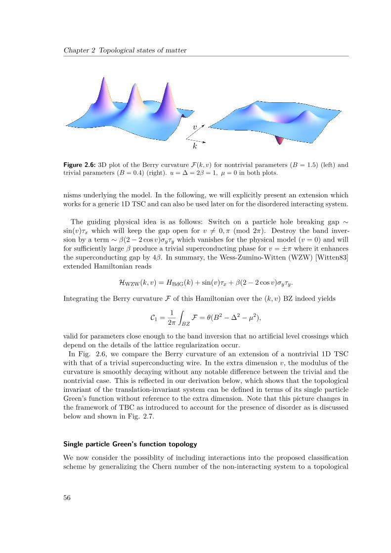
Chapter 2 Topological states of matter
Figure 2.6: 3D plot of the Berry curvature F(k, v) for nontrivial parameters (B = 1.5) (left) andtrivial parameters (B = 0.4) (right). u = ∆ = 2β = 1, µ = 0 in both plots.
nisms underlying the model. In the following, we will explicitly present an extension whichworks for a generic 1D TSC and can also be used later on for the disordered interacting system.
The guiding physical idea is as follows: Switch on a particle hole breaking gap ∼sin(v)τx which will keep the gap open for v 6= 0, π (mod 2π). Destroy the band inver-sion by a term ∼ β(2− 2 cos v)σyτy which vanishes for the physical model (v = 0) and willfor sufficiently large β produce a trivial superconducting phase for v = ±π where it enhancesthe superconducting gap by 4β. In summary, the Wess-Zumino-Witten (WZW) [Witten83]extended Hamiltonian reads
HWZW(k, v) = HBdG(k) + sin(v)τx + β(2− 2 cos v)σyτy.
Integrating the Berry curvature F of this Hamiltonian over the (k, v) BZ indeed yields
C1 = 12π
∫BZF = θ(B2 −∆2 − µ2),
valid for parameters close enough to the band inversion that no artificial level crossings whichdepend on the details of the lattice regularization occur.In Fig. 2.6, we compare the Berry curvature of an extension of a nontrivial 1D TSC
with that of a trivial superconducting wire. In the extra dimension v, the modulus of thecurvature is smoothly decaying without any notable difference between the trivial and thenontrivial case. This is reflected in our derivation below, which shows that the topologicalinvariant of the translation-invariant system can be defined in terms of its single particleGreen’s function without reference to the extra dimension. Note that this picture changes inthe framework of TBC as introduced to account for the presence of disorder as is discussedbelow and shown in Fig. 2.7.
Single particle Green’s function topology
We now consider the possiblity of including interactions into the proposed classificationscheme by generalizing the Chern number of the non-interacting system to a topological
56
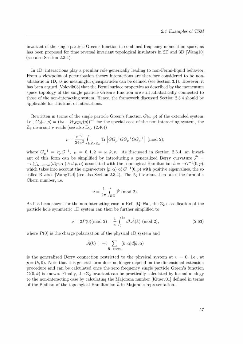
2.4 Examples of TSM
invariant of the single particle Green’s function in combined frequency-momentum space, ashas been proposed for time reversal invariant topological insulators in 2D and 3D [Wang10](see also Section 2.3.4).
In 1D, interactions play a peculiar role generically leading to non-Fermi-liquid behavior.From a viewpoint of perturbation theory interactions are therefore considered to be non-adiabatic in 1D, as no meaningful quasiparticles can be defined (see Section 3.1). However, ithas been argued [Volovik03] that the Fermi surface properties as described by the momentumspace topology of the single particle Green’s function are still adiabatically connected tothose of the non-interacting system. Hence, the framework discussed Section 2.3.4 should beapplicable for this kind of interactions.
Rewritten in terms of the single particle Green’s function G(ω, p) of the extended system,i.e., G0(ω, p) = (iω −HWZW(p))−1 for the special case of the non-interacting system, theZ2 invariant ν reads (see also Eq. (2.46))
ν = εµνρ
24π2
∫BZ×Rω
Tr[GG−1
µ GG−1ν GG−1
ρ
](mod 2),
where G−1µ = ∂µG
−1, µ = 0, 1, 2 = ω, k, v. As discussed in Section 2.3.4, an invari-ant of this form can be simplified by introducing a generalized Berry curvature F =−i∑R−zeros(d〈p, α|) ∧ d|p, α〉 associated with the topological Hamiltonian h = −G−1(0, p),
which takes into account the eigenvectors |p, α〉 of G−1(0, p) with positive eigenvalues, the socalled R-zeros [Wang12d] (see also Section 2.3.4). The Z2 invariant then takes the form of aChern number, i.e.
ν = 12π
∫BZF (mod 2).
As has been shown for the non-interacting case in Ref. [Qi08a], the Z2 classification of theparticle hole symmetric 1D system can then be further simplified to
ν = 2P (0)(mod 2) = 1π
∫ 2π
0dkA(k) (mod 2), (2.63)
where P (0) is the charge polarization of the physical 1D system and
A(k) = −i∑
R−zeros〈k, α|d|k, α〉
is the generalized Berry connection restricted to the physical system at v = 0, i.e., atp = (k, 0). Note that this general form does no longer depend on the dimensional extensionprocedure and can be calculated once the zero frequency single particle Green’s functionG(0, k) is known. Finally, the Z2-invariant can be practically calculated by formal analogyto the non-interacting case by calculating the Majorana number [Kitaev01] defined in termsof the Pfaffian of the topological Hamiltonian h in Majorana representation.
57
Chapter 2 Topological states of matter
Disorder and Twisted Boundary Conditions
Our formulation so far has been relying on translation-invariance which implies the existenceof a BZ. This description will thus no longer be applicable in the presence of disorder. Tothis end, the concept of TBC has been introduced to topologically classify quantum Hallsystems in the absence of translation-invariance [Niu85]. As long as a bulk mobility gapis present, the Green’s function is exponentially bounded in real space for energies in thisgap. Under these conditions, Niu et al. [Niu85] showed that the Hall conductivity can berepresented as a constant ground state Berry curvature with the wave vector replaced bythe twisting angles θ, φ of the TBC (see also Section 2.3.3). In this formalism, the Hallconductivity σxy reads
σxy = 2πiG0
(〈∂ψ0∂θ|∂ψ0∂φ〉 − 〈∂ψ0
∂φ|∂ψ0∂θ〉)
= 2πiG0Fθφ = G0
∫T 2
iFθφ2π , (2.64)
where ψ0 denotes the ground state wave function and G0 = e2
h = 12π is the quantum of
conductance. In the last equality of Eq. (2.64), the independence of Fθφ on the twisting angles[Niu85] has been used to make the topological quantization of σxy manifest by representingit as G0 times the Chern number of the U(1)-bundle over the torus T 2 of the twistingangles (θ, φ). Since in this example, we consider a disordered 1D system, we can withoutloss of generality assume translation-invariance in the extra dimension. Integrating overthe momentum v associated with the direction of translational invariance is equivalent toevaluating Eq. (2.64) for θ = 0 for the special case of a system with translational invariancein x-direction. Within this hybrid approach of twisted boundary conditions in the physicaldimension and v-momentum integration in the extra dimension, the Chern number of theextended 2D system in the presence of this stripe-like disorder can be expressed as
C1 =∫ π
−πdv
∫ π
−πdφFvφ2π =
∫ π
−πdv Fvφ (2.65)
where F is the Berry curvature on the “mixed” torus defined by the wave vector in v-directionand the twisting angle φ of the TBC imposed in the physical direction. The first equalitysign in Eq. (2.65) makes the integer quantization of our topological invariant manifest,whereas the second equality sign follows from the independence of
∫ π−π dvFvφ = Fθφ|θ=0 of
the twisting angle φ. The main advantage of Eq. (2.65) as compared to the general 2Dcase (see Eq. (2.64)) is that only the eigenstates of a 1D system have to be calculated toevaluate the topological invariant which is numerically less costly. This program allowsfor a topological classification of disordered systems with periodic boundaries, i.e., withoutexplicitly probing the presence of unpaired MBS. For non-interacting systems with closedboundary conditions, the influence of disorder on the 1D TSC phase has been studied usinga scattering matrix approach [Akhmerov11, Brouwer11a, Brouwer11b].
In Fig. 2.7, we show the mixed Berry curvature Fv,φ∣∣∣φ=0
for a weakly disordered system(γ = 1) in the topologically nontrivial phase and a strongly disordered trivial system (γ = 5).Here, γ is the strength of a scalar Gaussian onsite potential. Note that in contrast to the
58
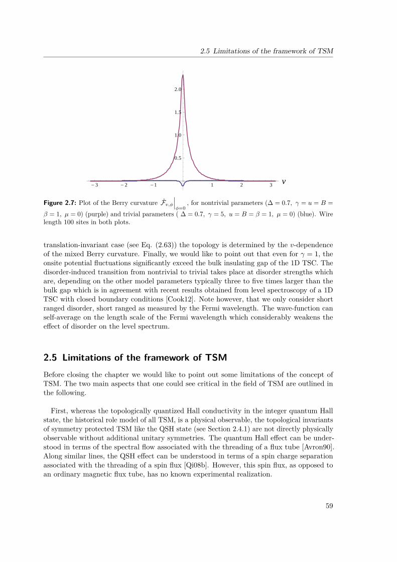
2.5 Limitations of the framework of TSM
- 3 - 2 -1 1 2 3 v
0.5
1.0
1.5
2.0
Figure 2.7: Plot of the Berry curvature Fv,φ∣∣∣φ=0
, for nontrivial parameters (∆ = 0.7, γ = u = B =β = 1, µ = 0) (purple) and trivial parameters ( ∆ = 0.7, γ = 5, u = B = β = 1, µ = 0) (blue). Wirelength 100 sites in both plots.
translation-invariant case (see Eq. (2.63)) the topology is determined by the v-dependenceof the mixed Berry curvature. Finally, we would like to point out that even for γ = 1, theonsite potential fluctuations significantly exceed the bulk insulating gap of the 1D TSC. Thedisorder-induced transition from nontrivial to trivial takes place at disorder strengths whichare, depending on the other model parameters typically three to five times larger than thebulk gap which is in agreement with recent results obtained from level spectroscopy of a 1DTSC with closed boundary conditions [Cook12]. Note however, that we only consider shortranged disorder, short ranged as measured by the Fermi wavelength. The wave-function canself-average on the length scale of the Fermi wavelength which considerably weakens theeffect of disorder on the level spectrum.
2.5 Limitations of the framework of TSMBefore closing the chapter we would like to point out some limitations of the concept ofTSM. The two main aspects that one could see critical in the field of TSM are outlined inthe following.
First, whereas the topologically quantized Hall conductivity in the integer quantum Hallstate, the historical role model of all TSM, is a physical observable, the topological invariantsof symmetry protected TSM like the QSH state (see Section 2.4.1) are not directly physicallyobservable without additional unitary symmetries. The quantum Hall effect can be under-stood in terms of the spectral flow associated with the threading of a flux tube [Avron90].Along similar lines, the QSH effect can be understood in terms of a spin charge separationassociated with the threading of a spin flux [Qi08b]. However, this spin flux, as opposed toan ordinary magnetic flux tube, has no known experimental realization.
59
Chapter 2 Topological states of matter
Second, the entire construction and classification of TSM is based on single particleHamiltonians. In Section 2.3.4, we discussed how adiabatic interactions can be taken intoaccount and argued that interactions of moderate strength are not likely to destroy thephenomenology of TSM. In order to position the field of TSM in a broader context, wewould like to point out that there are also phenomena of topological origin which emergeonly due to the presence of interactions. The historically first phenomenon is the 1
ν FQHeffect [Stormer83, Laughlin83] which cannot be adiabatically connected to an insulatingnon-interacting state. The non-interacting state is in this case a partially filled Landau levelwhich provides an enormous density of states at the Fermi energy. In a system with periodicboundaries, the 1
ν FQH has a characteristic ν-fold ground state degeneracy. Interestingly,this simplest FQH state can still be analyzed in the framework of TBC [Niu85]. For moregeneral FQH systems the concept of topological order has been introduced by Wen [Wen90].A crucial notion in this framework is the quantum dimension of the topologically orderedsystem which can be viewed as the ground state degeneracy of the system on a torus, i.e.,with periodic boundary conditions. All TSM have quantum dimension one, like a trivialinsulator. From the vantage point of topological order, all states discussed in this chapter arethus trivial. Recently, the concepts of TSM and topological order have been combined to thedefinition of the fractional Chern insulator [Tang11, Sun11, Neupert11] and the fractionaltopological insulator [Bernevig06b, Levin09, Maciejko10, Swingle11], a translation-invariantrealization of the FQH and its symmetry protected analogues, respectively.
60

Chapter 3
Non-equilibrium quantum transport ininteracting 1D systems
This chapter is dedicated to the discussion of some elementary elements of non-equilibriumquantum transport in interacting 1D systems. We first very briefly review the method ofAbelian bosonization and its application to Tomonaga Luttinger liquids, mainly to establishour notation. Thereafter, we introduce the Keldysh formalism as the non-equilibrium analogueof zero-temperature perturbation theory. This formalism is ready made for perturbativequantum transport calculations at finite bias voltage. Interestingly, this non-equilibriumtheory can be used for finite temperature calculations under fairly general conditions withouta construction that corresponds to the Matsubara formalism in equilibrium perturbationtheory. Since our main application of this transport theory in Part II will be dealing withthe helical edge states realized at the boundary of a QSH sample (see Section 2.4.1), wefinally point out some peculiarities of the so called helical Tomonaga Luttinger liquid (hTLL)[Wu06] representing a single pair of helical edge states in the presence of Coulomb interaction.
3.1 Electron-electron interaction in one spatial dimensionIn a system with spatial dimension larger than one, repulsive Coulomb interaction can beswitched on adiabatically in a broad class of systems which leads to the notion of the Fermiliquid [Landau57]. The quasiparticles of this Fermi liquid have well defined momentum andare characterized by their effective mass and charge just like electrons in a free Fermi gasbut with renormalized effective parameters. Close to the Fermi surface, the lifetime of thesequasi-particles diverges, which renders them well defined excitations as far as the physicsat sufficiently low energy scales is concerned. In 1D, the phenomenology is fundamentallychanged since no fermionic quasi-particles that adiabatically connect the non-interactingelectrons can be defined [Voit95]. Instead, bosonic electron-hole excitations are the elementaryexcitations of the electron gas in 1D. In this section, we outline how this observation canbe used to construct an effective bosonic low energy theory of the interacting fermionic 1Dsystem, the so called Tomonaga Luttinger liquid (TLL) [Tomonaga50, Luttinger63, Mattis65,Haldane81], see Refs. [Schönhammer97, Voit95, von Delft98, Grabert01, Giamarchi04] forexcellent review articles and textbooks. The low energy fixed point theory of the TLL remainsquadratic in the bosonic fields and thus exactly solvable in the presence of interactions[Haldane81]. We first motivate phenomenologically why a bosonic description of a fermionicsystem in 1D is possible and thereafter review very briefly the procedure of Abelian algebraicbosonization.
61

Chapter 3 Non-equilibrium quantum transport in interacting 1D systems
3.1.1 Spatial dimension and transmutation statistics
Let us think of indistinguishable particles as hard balls which cannot penetrate each other.Since the particles are indistinguishable, the proper configuration space XN of N indis-tinguishable particles is a quotient space of the N -fold direct product of the single par-ticle spaces X modulo the symmetric group SN of permutations, i.e., XN = XN/SN[Laidlaw71, Dowker72, Leinaas77]. In this space, points which can be obtained by exchang-ing particle labels are identified. In spatial dimension d = 3 this space for N = 2 has onlytwo connected components. This can be intuitively understood if one considers that inthe unrestricted configuration space every closed loop of a particle can be contracted toa point without penetrating the second particle. However, there are loops in X2 whichinterchange the particle coordinates and are not contractible. This Z2 topology of X2 withX = R3 leads to the conclusion that there can only be two types of particles, namely fermionsand bosons in 3D [Laidlaw71, Leinaas77]. In 2D, the situation is more complicated. Thedifference can again be understood at a very intuitive level: Loops of one particle which havea different winding number around the position of the other particle cannot be deformedinto each other as long as the two particles cannot penetrate each other. This gives riseto a configuration space of two indistinguishable particles which has an infinite number ofconnected components. As a consequence, there are infinitely many types of particles, socalled anyons, in 2D [Laidlaw71, Leinaas77]. In a 1D world, particles cannot be exchangedat all without penetrating each other. This illustrates why particles in 1D will behavecollectively and why it should be in principle possible to switch between a fermionic and abosonic description of a 1D system of indistinguishable particles.
3.1.2 Bosonization and the Tomonaga Luttinger Liquid
We consider a 1D lattice of spinless free fermions with unit lattice constant and L sites.Close to the Fermi energy EF , the spectrum can be linearized. This gives rise to twobranches, with opposite constant slope vF , called the left-moving and the right-movingbranch which are denoted by p = ± (see Fig. 3.1). As long as only the physical propertiesof the model at energies close to the Fermi energy are concerned, this linearization is areasonable approximation. When extending the linearized model to states with negativeenergy, only inert states that do not affect the low energy physics are added. As alreadymentioned, the elementary excitations of the 1D electron gas can be represented as particlehole excitations which are closely related to the Fourier components of the density operator
ρp(q) =∑k
c†p(k)cp(k + q), p = ±
where cp(k) is the electronic annihilation operator for a p-mover with wave vector k of theextended linearized model. These Fourier components satisfy the commutation relations[Giamarchi04]
[ρp(q), ρp′(q′)
]= pqL
2π δp,p′δq,−q′ (3.1)
62
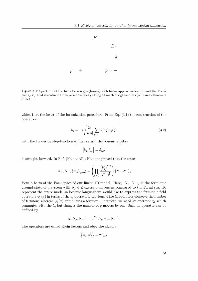
3.1 Electron-electron interaction in one spatial dimension
Figure 3.1: Spectrum of the free electron gas (brown) with linear approximation around the Fermienergy EF that is continued to negative energies yielding a branch of right-movers (red) and left-movers(blue).
which is at the heart of the bosonization procedure. From Eq. (3.1) the construction of theoperators
bq = −i√
2πL|q|
∑p=±
θ(pq)ρp(q) (3.2)
with the Heaviside step-function θ, that satisfy the bosonic algebra[bq, b
†q′
]= δq,q′
is straight-forward. In Ref. [Haldane81], Haldane proved that the states
|N+, N−, mqq 6=0〉 =
∏q 6=0
(b†q
)mq√mq!
|N+, N−〉0
form a basis of the Fock space of our linear 1D model. Here, |N+, N−〉0 is the fermionicground state of a system with Np ∈ Z excess p-movers as compared to the Fermi sea. Torepresent the entire model in bosonic language we would like to express the fermionic fieldoperators ψp(x) in terms of the bq operators. Obviously, the bq operators conserve the numberof fermions whereas ψp(x) annihilates a fermion. Therefore, we need an operator ηp whichcommutes with the bq but changes the number of p-movers by one. Such an operator can bedefined by
ηp|Np, N−p〉 = pNp |Np − 1, N−p〉.
The operators are called Klein factors and obey the algebra,ηp, η
†p′
= 2δp,p′
63

Chapter 3 Non-equilibrium quantum transport in interacting 1D systems
with all other anti-commutators vanishing. We define the so called bosonic phase fields as
φp(x) = p√2L
∑q 6=0
θ(pq)eiqxe−a|q|/2√|q|
bq,
where a is a short distance cutoff regularizing the divergence in the commutators of thebosonic phase fields for equal points in space. The chiral hermitian fields are the linearcombinations
Φp(x) = φp(x) + φ†p(x). (3.3)
With these definitions, the fermionic field operator can be represented as (see [Grabert01]for a step by step derivation)
ψp(x) = ηp√2πa
eip(kF+2πNp/L)x+√
4πipΦp(x), (3.4)
where Np is the number operator of the p-moving electrons. The NpL term in the exponent
on the right hand side of Eq. (3.4) is a q = 0 contribution which can be neglected in thelimit L→∞. Throughout this thesis, the influence of these so called zero-modes will alwaysbe neglected which we will make manifest by dropping the mentioned 1/L-term from nowon. For |x− x′| a, the commutator of the chiral hermitian fields reads
[Φp(x),Φp′(x′)
]= ipδp,p′
4 sgn(x− x′). (3.5)
The chiral hermitian field Φp is directly related to the density ρp(x) of p-moving electronicexcitations via the relation [Grabert01]
∂xΦp(x) =√πρp(x).
For practical calculations, we will often times use the non-chiral fields
ϕ = Φ+ + Φ−,θ = Φ+ − Φ−. (3.6)
The total density ρ and the current density j can be readily expressed in terms of these fieldsas
ρ(x) = ρ+(x) + ρ−(x) = 1√π∂xϕ(x),
j(x) = evF (ρ+(x)− ρ−(x)) = evF√π∂xθ. (3.7)
From Eq. (3.5) and Eq. (3.6) it is immediately clear that Πϕ(x) = −∂xθ(x) is the conjugatemomentum of ϕ, i.e.,
[ϕ(x),Πϕ(y)] = iδ(x− y). (3.8)
64

3.2 Non-equilibrium perturbation theory
The free Hamiltonian H0 of the non-interacting 1D model with linear dispersion can then beexpressed as
H0 = vF2
∫ +L2
−L2dx[Π2ϕ(x) + (∂xϕ(x))2
].
The main advantage of this bosonic representation is that the Hamiltonian remains quadraticif one includes Coulomb interaction into the picture: Forward-scattering terms due to localCoulomb interaction only renormalize the model parameters and the backscattering termcan in the spinless case be viewed as a Pauli exchange term of the forward scattering (see[Grabert01] for a more detailed discussion). At this level of rigor, short ranged Coulombinteraction enters the low energy fixed point theory only through a single parameter g, whereg = 1 is the non-interacting case, g < 1 indicates repulsive interaction, and g > 1 in thecase of attractive interaction. The Hamiltonian HTLL of the interacting Tomonaga LuttingerLiquid then reads [Grabert01]
HTLL = vF2
∫ +L2
−L2dx[Π2ϕ(x) + 1
g2 (∂xϕ(x))2]. (3.9)
Note that vF here is an effective Fermi velocity which can be renormalized from its bare non-interacting value when high energy modes that are also affected by the Coulomb interactionare integrated out to obtain the effective low energy theory [Grabert01]. Using the Heisenbergequation of motion
∂tϕ = i [HTLL, ϕ] = vFΠϕ, (3.10)
the current operator j defined in Eq. (3.7) can be expressed as
j(x, t) = − e√π∂tϕ(x, t). (3.11)
3.2 Non-equilibrium perturbation theory
Applying a finite bias voltage can drive a physical system out of thermal equilibrium. Hence,a non-equilibrium theory is needed in order to describe quantum transport phenomenabeyond the level of linear response theory. In this section, we review the construction ofa non-equilibrium theory which is ready made for transport calculations in helical edgestates. In Section 3.2.1, we follow the construction by Schwinger [Schwinger61] and Keldysh[Keldysh65] to generally formulate a non-equilibrium perturbation theory. In Section 3.2.2,we apply this formalism to the TLL and show how non-equilibrium expectation values ofcrucial physical observables like the current operator can be calculated in this framework.
65

Chapter 3 Non-equilibrium quantum transport in interacting 1D systems
3.2.1 From equilibrium to non-equilibrium
Validity of equilibrium zero temperature perturbation theory and its limitations
Assuming that the reader is familiar with equilibrium perturbation theory in many bodyphysics, we now outline how the absence of thermal equilibrium changes the perturbativeapproach. In thermal equilibrium at zero temperature, the time ordered Green’s functionGT (x, t;x′, t′) = −i〈T (ψ(x, t)ψ†(x′, t′))〉 of an interacting many body system with physicalHamiltonian H = H0 + V can in a broad class of cases be represented as
GT (x, t;x′, t′) = −i〈0|T
(S(∞,−∞)ψI(x, t)ψ†I(x′, t′)
)|0〉
〈0|S(−∞,∞)|0〉 , (3.12)
where |0〉 denotes the unique ground state of the non-interacting system, S(t, t′) denotes thetime evolution operator in the interaction picture, and ψI denotes the field operator in theinteraction picture. The key assumptions under which Eq. (3.12) is valid are the followingones: If the interaction term is switched on and off adiabatically as V (t) = limη→0+ V e−|t|η,S(0,−∞) evolves the ground state |0〉 of the non-interacting system adiabatically into theground state of the interacting system. The formal conditions entering this assumptionare the Gell-Mann and Low theorem [Gell-Mann51, Nozieres97] and the Luttinger theorem[Luttinger60a]: The Gell-Mann and Low theorem states that if the adiabatic limit of|ψ0〉 = S(0,−∞)|0〉
〈0|S(0,−∞)|0〉 exists, it corresponds to an eigenstate of the interacting system with theground state energy of the non-interacting system [Nozieres97]. However, this state doesnot have to be the ground state of the interacting system. For interactions that can berepresented as a power series, the Luttinger theorem shows that the volume enclosed bythe Fermi surface and for isotropic interaction also the spherical shape of the Fermi surface[Luttinger60b] are preserved. Under these conditions, |ψ0〉 is indeed the interacting groundstate and the adiabatic switching procedure makes sense as the interacting system then hasevolved to its physical ground state by the time the field operators ψ(x, t), ψ†(x′, t′) are acting.There is one additional assumption entering Eq. (3.12), namely that S(∞,−∞)|0〉 differsfrom |0〉 only by a phase factor. This amounts to assuming thermal equilibrium at zerotemperature for each point in time since the system is assumed to relax to its non-interactingground-state during the adiabatic switching-off of interactions.The mentioned assumptions of equilibrium zero temperature perturbation theory fail underthe following physical circumstances. First, the interactions might not be representable as apower series, i.e., the iterative expansion of the full time evolution operator as a von Neumannseries fails to converge or does not represent the time evolution operator. An example forthis scenario is a superconducting ground state consisting of a condensate of Cooper pairs.This class of problems can only be treated by non-perturbative methods. Second, the vonNeumann series represents the time evolution operator but the physical ground state doesnot evolve adiabatically from the non-interacting one. In this case, the Matsubara method[Matsubara55] which works in thermal equilibrium at arbitrary temperature and does notrely on an adiabatic switching procedure can be used. The difference between the zerotemperature limit of the Matsubara approach and the above ground state formalism has beendemonstrated by Kohn and Luttinger [Kohn60]. Third, if a system which is coupled to an
66

3.2 Non-equilibrium perturbation theory
Figure 3.2: Time contour c′ and extended time contour c. The arrows indicate the time orderingenacted by the operators Tc′ and Tc, respectively.
external time dependent field is out of thermal equilibrium, it might be dynamically pumpedto a different state than its equilibrium ground state even if the time dependent perturbationis switched off adiabatically for t→∞. Then, S(∞,−∞)|0〉 differs from |0〉 by more than asimple phase factor. This scenario is only problematic in that it precludes the picture ofan instantaneous thermal equilibrium but does not pertain to the perturbative ansatz itself.Hence, this issue can be overcome by a non-equilibrium construction of perturbation theorywhich we review now.
The non-equilibrium construction
We consider a physical system with the Hamiltonian H(t) = H0 + V + F (t), where H0 isa quadratic non-interacting Hamiltonian, V represents the time independent many bodyinteractions and F (t) is a coupling induced by a time dependent external field which vanishesas t→ −∞. For t→ −∞, the system is assumed to be in a non-interacting thermal statewith density matrix ρ0 = 1
Z0e−β(H0−µN), where Z0 = Tr
[e−β(H0−µN)
]. This assumption
amounts to neglecting initial correlations [Rammer86]. The time ordered Green’s functioncan then be represented in a straightforward way as [Rammer07]
GT (x, t;x′, t′) = −iTr[ρ0S(−∞, tm)T
(ψI(x, t)ψ†I(x
′, t′)S(tm,−∞))], tm = max(t, t′).
(3.13)
Obviously, we can represent the order of operators in Eq. (3.13) by a generalized timeordering Tc′ along the time contour c′ shown in Fig. 3.2. Noting that S(tm,∞)S(∞, tm) = 1,we can extend the time contour c′ to c (see Fig. 3.2) which stretches from −∞ to∞ (forwardbranch) and back (backward branch). The external times t, t′ then always lie on the forwardbranch of the contour where the ordering operator Tc concurs with the ordinary time-orderingT . The time-ordered Green’s function can then be represented as
GT (x, t;x′, t′) = −iTr[ρ0Tc
(e−i∫cdτHI(τ)ψI(x, t)ψ†I(x
′, t′))]
.
67

Chapter 3 Non-equilibrium quantum transport in interacting 1D systems
Later on, we would like to do perturbation theory which amounts to an expansion of thetime evolution operator on the contour c as a von Neumann series. This expansion will ofcourse produce operators HI(τ), the time argument of which is integrated over the entirecontour c. A straight-forward non-equilibrium generalization of Wick’s theorem [Rammer07]will then produce contour-ordered pairwise contractions of the field operators appearing inthese HI(τ). In order to represent the perturbation series in a closed form, we thus introducethe contour ordered Green’s function
Gc(x1, τ1;x2, τ2) = −iTr[ρ0Tc
(e−i∫cdτHI(τ)ψI(x1, τ1)ψ†I(x2, τ2)
)],
the time arguments τ1, τ2 of which can lie anywhere on the contour c. Obviously, Gc concurswith GT if both arguments are located on the forward branch of c. Denoting the branches ofc by + (forward) and − (backward), Gc affords a representation as a 2× 2 matrix in the socalled Keldysh space of branches:
Gc =(G++ G+−G−+ G−−.
)(3.14)
As already mentioned, G++ = GT . Furthermore G−− = GT is the anti-time-ordered Green’sfunction, G−+(x1, τ1;x2, τ2) = −iTr
[ρ0ψ(x1, τ1)ψ†(x2, τ2)
], and
G+−(x1, τ1;x2, τ2) = iTr[ρ0ψ
†(x2, τ2)ψ(x1, τ1)]. Note that the extra minus sign in the defi-
nition of G+− is due to the Grassman algebra that the fermionic field operators satisfy underthe time/contour ordering operator.
By now, we have formulated the non-equilibrium problem in a strikingly similar way toits equilibrium counterpart. The salient new element in the non-equilibrium theory is thebackward branch of the contour c which allows us to drop any assumptions as to the relationbetween the system state at t→ −∞ and t→∞. This construction comes at a price: TheGreen’s function naturally appearing in the perturbation series is the contour ordered Green’sfunction Gc which can be represented as a 2×2 matrix of Green’s functions with an ordinaryreal time argument (see Eq. (3.14)). Once this complication has been digested, practicalperturbative calculations work fairly analogous to the ordinary equilibrium case (see Ref.[Rammer07] for a detailed elementary discussion). Hence, instead of reviewing more detailsof the general construction, we would here like to focus on the bosonic non-equilibriumperturbation theory in the TLL which will be of crucial relevance for Chapter 5.
3.2.2 Keldysh perturbation theory of the Tomonaga Luttinger Liquid
In Section 3.1 we constructed the translation-invariant TLL which is even in the presence ofCoulomb interaction quadratic in the bosonic field operators. A bias voltage can be modeled[Dolcini05] by adding the following perturbation to the Hamiltonian:
HϕV (t) = − e√
π
∫dxE(x, t)ϕ(x). (3.15)
68

3.2 Non-equilibrium perturbation theory
For our purposes, we can think of the bias term as induced by the gradient of a chemicalpotential, i.e., −eE = ∂xµ
ϕ. The simplest perturbation which makes the TLL non-quadraticin the bosonic fields is a single impurity with strength λ at x = 0 which is described by themodel Hamiltonian [Kane92a, Dolcini05]
HS = λ cos(√
4πϕ(x = 0)). (3.16)
Obviously, this perturbation is of infinite order in the bosonic field operator ϕ which precludesthe efficient application of Wick’s theorem in the non-equilibrium perturbative expansion.Our general strategy will thus be as follows: We first perform a unitary operation thusrepresenting the bias term Eq. (3.15) as a shift in the field ϕ appearing in the impurityHamiltonian (3.16). Using 2 cos(x) = eix+e−ix, we note that the impurity can be representedas a sum of so called vertex operators, i.e., operators of the form eiαϕ, α ∈ R. For the freeexpectation value of such an operator, we can use the crucial identity
〈eαϕ〉0 = eα2 〈ϕ2〉02 , α ∈ C. (3.17)
However, the current operator (see Eq. (3.7)) is not a vertex operator but is linear in ϕ.We thus need a vertex operator which generates expectation values of ϕ, a source term likeeiJϕϕ which satisfies −i∂Jϕ〈eiJ
ϕϕ〉∣∣∣Jϕ=0
= 〈ϕ〉. This naturally leads us to the constructionof a generating functional.
Let us now follow the program just outlined in more detail. Since our impurity HamiltonianHS will later on in general depend on both ϕ and θ, we generalize the analysis in Ref.[Dolcini05] meaning that Πϕ = −∂xθ is not integrated out. We follow Ref. [Liu11] but forthe spinless TLL for simplicity. First, we combine the two bosonic fields to the vector Φη =(ϕη, θη)T , where η is the index in Keldysh space, i.e., η = ± on the forward/backward branchof the contour c. For later convenience, we would like to generalize the bias Hamiltonian(3.15) so as to include a generalized chemical potential µθ which couples to the dual field θ.This gives rise to the additional term
HθV = 1√
π
∫dx(∂xµ
θ(x, t))θ(x).
Furthermore, we also introduce a source-term Jθ which generates expectation values of thedual field θ. Let us compactify our notation by the following definitions
Φ(r) =
ϕ+(r)ϕ−(r)θ+(r)θ−(r)
,
69
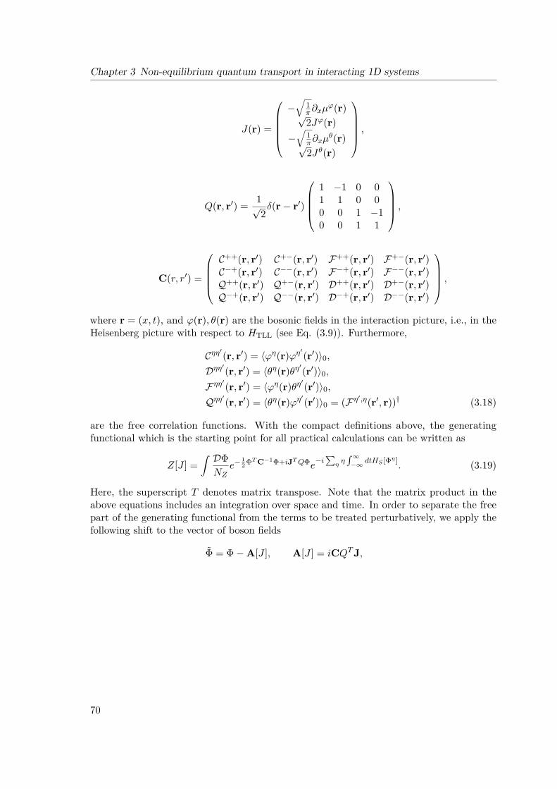
Chapter 3 Non-equilibrium quantum transport in interacting 1D systems
J(r) =
−√
1π∂xµ
ϕ(r)√2Jϕ(r)
−√
1π∂xµ
θ(r)√2Jθ(r)
,
Q(r, r′) = 1√2δ(r− r′)
1 −1 0 01 1 0 00 0 1 −10 0 1 1
,
C(r, r′) =
C++(r, r′) C+−(r, r′) F++(r, r′) F+−(r, r′)C−+(r, r′) C−−(r, r′) F−+(r, r′) F−−(r, r′)Q++(r, r′) Q+−(r, r′) D++(r, r′) D+−(r, r′)Q−+(r, r′) Q−−(r, r′) D−+(r, r′) D−−(r, r′)
,where r = (x, t), and ϕ(r), θ(r) are the bosonic fields in the interaction picture, i.e., in theHeisenberg picture with respect to HTLL (see Eq. (3.9)). Furthermore,
Cηη′(r, r′) = 〈ϕη(r)ϕη′(r′)〉0,Dηη′(r, r′) = 〈θη(r)θη′(r′)〉0,Fηη′(r, r′) = 〈ϕη(r)θη′(r′)〉0,Qηη′(r, r′) = 〈θη(r)ϕη′(r′)〉0 = (Fη′,η(r′, r))† (3.18)
are the free correlation functions. With the compact definitions above, the generatingfunctional which is the starting point for all practical calculations can be written as
Z[J ] =∫ DΦNZ
e−12 ΦTC−1Φ+iJTQΦe
−i∑
ηη∫∞−∞ dtHS [Φη ]
. (3.19)
Here, the superscript T denotes matrix transpose. Note that the matrix product in theabove equations includes an integration over space and time. In order to separate the freepart of the generating functional from the terms to be treated perturbatively, we apply thefollowing shift to the vector of boson fields
Φ = Φ−A[J ], A[J ] = iCQTJ,
70
3.2 Non-equilibrium perturbation theory
and explicitly A[J ] =(A+,ϕ, A−,ϕ, A+,θ, A−,θ
)Twith
Aη,ϕ[J ] = − i√2π
∫dr′(CR(r, r′)∂xµϕ(r′)
+FR(r, r′)∂xµθ(r′))
+ i
∫dr′(CK(r, r′) + ηCA(r, r′))Jϕ(r′)
+i∫dr′(FK(r, r′) + ηFA(r, r′))Jθ(r′),
Aη,θ[J ] = − i√2π
∫dr′(QR(r, r′)∂xµϕ(r′)
+DR(r, r′)∂xµθ(r′))
+ i
∫dr′(QK(r, r′) + ηQA(r, r′))Jϕ(r′)
+i∫dr′(DK(r, r′) + ηDA(r, r′))Jθ(r′).
The generating functional then factorizes as follows
Z[J ] = Z0[Jc]ZS [J ] (3.20)
where
Z0[J] = e−12 JT CJ,
and
C = QCQT =0 CA(r, r′) 0 FA(r, r′)
CR(r, r′) CK(r, r′) FR(r, r′) FK(r, r′)0 QA(r, r′) 0 DA(r, r′)
QR(r, r′) QK(r, r′) DR(r, r′) DK(r, r′)
with
CR(r, r′) = θ(t− t′)〈[ϕ(r), ϕ(r′)]〉0,CA(r, r′) = −θ(t′ − t)〈[ϕ(r), ϕ(r′)]〉0,CK(r, r′) = 〈ϕ(r), ϕ(r′)〉0
and similar definitions for the other correlation functions D, F and Q. ZS [J ] is given by
ZS [J ] =∫ DΦNZ
e−12 ΦTC−1Φe
−i∑
ηη∫∞−∞ dtHS[Φη+Aη] = 〈e−i
∫c
dτHS[Φ+A]〉0. (3.21)
Next, we need to relate the physical quantities to the generating functional. From Eq.(3.7), it is clear that we need to calculate expectation values like 〈ϕ〉 and 〈θ〉 which can be
71

Chapter 3 Non-equilibrium quantum transport in interacting 1D systems
conveniently evaluated from the functional derivatives of the generating functional Z[J ] withrespect to Jϕ and Jθ. A direct calculation shows that
〈ϕ(r)〉 = 12∑η
〈ϕη(r)〉 = − i21
Z[0]δZ[J ]δJϕ(r)
∣∣∣∣J=0
= − i2
[δZ0[J ]δJϕ(r) + 1
ZS [0]δZS [J ]δJϕ(r)
]∣∣∣∣J=0(3.22)
with a similar expression holding for 〈θ〉. From Eq. (3.22), we find that 〈ϕ〉 can be decomposedinto two parts: one is the zero order term coming from Z0[J ], and the other one is thescattering term coming from ZS [J ]. Consequently, any physical quantity O can also bedivided into two parts 〈O〉 = 〈O0〉 + 〈O2〉. All transport calculations in this thesis willbe based on a perturbative evaluation of Eq. (3.22) and its analogue for the dual field θ,respectively.
3.3 Peculiarities of the helical Tomonaga Luttinger Liquid
In this section, we briefly would like to point out some peculiarities of the helical TLL (hTLL)as realized on the edge of a QSH sample. Our at this stage rather general discussion ismeant to give a short overview over the unique features of the hTLL which motivate themore detailed transport studies presented in Chapter 5. The hTLL consists of one left andon right moving channel which have opposite spin polarization. Hence, ignoring the spinpolarization, a single hTLL has the same number of degrees of freedom as the spinless TLL.However, the counter-propagating states at a given energy are conjugated by TRS, .i.e., theyare so called Kramers partners. This imposes serious constrictions on possible scatterers inthe hTLL as long as TRS is conserved as we will detail in Section 3.3.2. If we consider twohTLLs with opposite helicity, e.g., the two parallel edges of a QSH ribbon, we recover thedegrees of freedom of a spinful TLL (sTLL). In Section 3.3.1, we will discuss the phase spaceconstraints on the Coulomb interaction imposed by the nonlocal nature of this compositerealization of the sTLL.
3.3.1 A composite spinful TLL consisting of two hTLLs
The spinful TLL
We consider a model with linear dispersion as in the construction of the spinless TLL withthe sole difference that there are two species s =↑, ↓ for each direction of motion p = ±.The fermionic operators ψp,s(x) can then be represented in terms of bosonic fields in totalanalogy to the spinless case, Eq. (3.4):
ψp,s(x) = ηp,s√2πa
eip(kF+2πNp,s/L)x+√
4πipΦp,s(x), (3.23)
where Φp,s are the spinful chiral hermitian fields which are defined by Eq. (3.3) for eachspin species separately and the 1/L terms will be neglected from now on following the sameargumentation as for the spinless case above. Let us define a non-chiral bosonic field and its
72
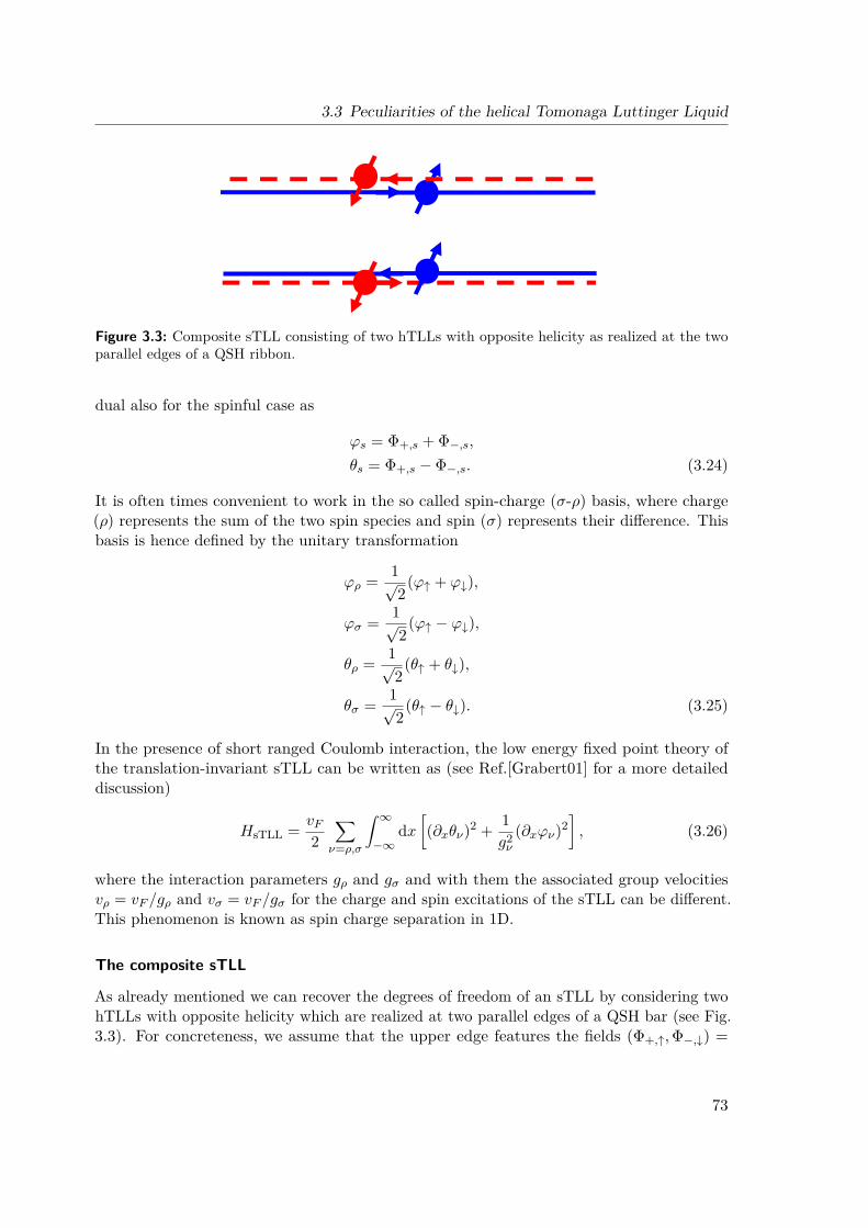
3.3 Peculiarities of the helical Tomonaga Luttinger Liquid
Figure 3.3: Composite sTLL consisting of two hTLLs with opposite helicity as realized at the twoparallel edges of a QSH ribbon.
dual also for the spinful case as
ϕs = Φ+,s + Φ−,s,θs = Φ+,s − Φ−,s. (3.24)
It is often times convenient to work in the so called spin-charge (σ-ρ) basis, where charge(ρ) represents the sum of the two spin species and spin (σ) represents their difference. Thisbasis is hence defined by the unitary transformation
ϕρ = 1√2
(ϕ↑ + ϕ↓),
ϕσ = 1√2
(ϕ↑ − ϕ↓),
θρ = 1√2
(θ↑ + θ↓),
θσ = 1√2
(θ↑ − θ↓). (3.25)
In the presence of short ranged Coulomb interaction, the low energy fixed point theory ofthe translation-invariant sTLL can be written as (see Ref.[Grabert01] for a more detaileddiscussion)
HsTLL = vF2
∑ν=ρ,σ
∫ ∞−∞
dx[(∂xθν)2 + 1
g2ν
(∂xϕν)2], (3.26)
where the interaction parameters gρ and gσ and with them the associated group velocitiesvρ = vF /gρ and vσ = vF /gσ for the charge and spin excitations of the sTLL can be different.This phenomenon is known as spin charge separation in 1D.
The composite sTLL
As already mentioned we can recover the degrees of freedom of an sTLL by considering twohTLLs with opposite helicity which are realized at two parallel edges of a QSH bar (see Fig.3.3). For concreteness, we assume that the upper edge features the fields (Φ+,↑,Φ−,↓) =
73

Chapter 3 Non-equilibrium quantum transport in interacting 1D systems
Figure 3.4: Coulomb-backscattering process that gives a non-quadratic contribution to the sTLL.Red denotes spin up, blue denotes spin down. Solid lines represent right movers and dashed linesrepresent left movers.
(Φu+,Φu
−), whereas the lower edge features the fields (Φ+,↓,Φ−,↑) = (Φl+,Φl
−). The two edgesu, l are assumed to have identical interaction strength g and can be represented as twospinless TLL with the Hamiltonian
HµhTLL = vF
2
∫ ∞−∞
dx[(∂xθµ)2 + 1
g2 (∂xϕµ)2], µ = u, l. (3.27)
If we ignore the u, l-labels on the bosonic fields, we can rewrite the total HamiltonianH2Edge = Hu
hTLL +H lhTLL of the two independent edges in the language of an sTLL as defined
in Eq. (3.26) and find by simple comparison of coefficients [Hou09, Teo09]
gc = g, gs = 1gc
= 1g. (3.28)
As we will work out in Section 5.1, this constraint is at the heart of a duality between thecharge and spin degree of freedom which even survives in a non-equilibrium setup.
3.3.2 Peculiarities of a single hTLLLet us now focus on a single hTLL. Instead of ignoring the spin degree of freedom, one mightask what kind of interesting consequences the locking between spin and direction of motionmight bring about.
Vanishing Coulomb backscattering
The first point worth mentioning is that the hTLL is in some sense a better TLL than theordinary sTLL. Let us explain what we mean by this argument. To derive Eq. (3.26) forthe interacting sTLL, a non-quadratic term stemming from a spin conserving backscattering
74
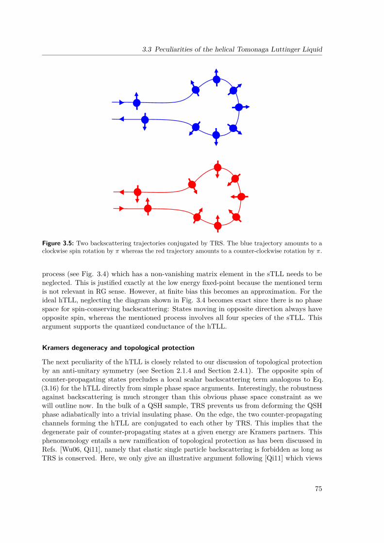
3.3 Peculiarities of the helical Tomonaga Luttinger Liquid
Figure 3.5: Two backscattering trajectories conjugated by TRS. The blue trajectory amounts to aclockwise spin rotation by π whereas the red trajectory amounts to a counter-clockwise rotation by π.
process (see Fig. 3.4) which has a non-vanishing matrix element in the sTLL needs to beneglected. This is justified exactly at the low energy fixed-point because the mentioned termis not relevant in RG sense. However, at finite bias this becomes an approximation. For theideal hTLL, neglecting the diagram shown in Fig. 3.4 becomes exact since there is no phasespace for spin-conserving backscattering: States moving in opposite direction always haveopposite spin, whereas the mentioned process involves all four species of the sTLL. Thisargument supports the quantized conductance of the hTLL.
Kramers degeneracy and topological protection
The next peculiarity of the hTLL is closely related to our discussion of topological protectionby an anti-unitary symmetry (see Section 2.1.4 and Section 2.4.1). The opposite spin ofcounter-propagating states precludes a local scalar backscattering term analogous to Eq.(3.16) for the hTLL directly from simple phase space arguments. Interestingly, the robustnessagainst backscattering is much stronger than this obvious phase space constraint as wewill outline now. In the bulk of a QSH sample, TRS prevents us from deforming the QSHphase adiabatically into a trivial insulating phase. On the edge, the two counter-propagatingchannels forming the hTLL are conjugated to each other by TRS. This implies that thedegenerate pair of counter-propagating states at a given energy are Kramers partners. Thisphenomenology entails a new ramification of topological protection as has been discussed inRefs. [Wu06, Qi11], namely that elastic single particle backscattering is forbidden as long asTRS is conserved. Here, we only give an illustrative argument following [Qi11] which views
75

Chapter 3 Non-equilibrium quantum transport in interacting 1D systems
the protection as a weak anti-localization with perfect efficiency. Let us assume that we put animpurity that can rotate spin but does preserve TRS in a clean hTLL. Such an imperfectioncould be realized by locally induced extrinsic SOI. Fig. 3.5 shows two backscattering pathswhich are conjugated by TRS. Obviously, the two paths differ by a spin rotation of 2π which,for half-integer fermions, entails a relative phase factor of −1, i.e., destructive interference.Since all possible trajectories have a conjugated counterpart canceling their contribution,there is no backscattering provided that the range of the scattering potential is smaller thanthe phase coherence length. In Section 5.2, we will discuss this protection more formally andinvestigate its limitations in great detail in Sections 5.2-5.3.
76

Part II
Application to low dimensionalmesoscopic systems

Chapter 4
All-electric qubit control in heavy holequantum dots via non-Abelian geometricphases
In this chapter, we demonstrate how non-Abelian geometric phases (see Section 1.1.2) can beused to universally process spin qubits [Loss98] in heavy hole quantum dots in the absence ofmagnetic fields. An adiabatically time dependent electric quadrupole field is used to performany desired single qubit operation by virtue of non-Abelian holonomy. During the proposedoperations, the degeneracy of the time dependent two level system representing the qubitis not split. Since time reversal symmetry is preserved and hyperfine coupling is known tobe weak in spin qubits based on heavy holes, we expect very long coherence times in theproposed setup. Our analysis follows closely Ref. [Budich12b]. The theoretical foundationsunderlying this application are presented in Chapter 1. We will repeat some of the keyequations to increase the readability of this chapter.
4.1 Motivation
Coherent spin control by all-electric means (without breaking TRS) is among the majorgoals of spintronics. One of the reasons why is that the presence of TRS is known to forbidseveral dephasing mechanisms, for example, in spin qubits [Loss98], due to the interplay ofelectron phonon coupling and Rashba spin orbit coupling [Bulaev05]. In the original workby Loss and DiVincenzo [Loss98], the proposed scheme for universal quantum computingbased on spin qubits in quantum dots (QDs) relied on the one hand on all-electric twoqubit operations, but, on the other hand, on single qubit operations based on magneticfields or ferromagnetic auxiliary devices that both break TRS. A few years later, electric-dipole-induced spin resonance (EDSR) has been proposed [Golovach06] and experimentallyrealized [Nowack07] as a way to process spins electrically in the presence of a static magneticfield which is still breaking TRS. Rather recently, it has been theoretically shown that inspin qubits based on carbon nanotube QDs it is indeed possible to accomplish all-electricsingle qubit operations using EDSR [Bulaev08, Klinovaja11]. This is possible because thespecific spin orbit interaction in carbon nanotubes provides a way to split spin up and spindown states in the absence of magnetic fields (zero field splitting). However, spin qubitsbased on carbon nanotubes face other problems related to readout and integrability andit is hence fair to say that all host materials for spin qubits have advantages and disadvantages.
79

Chapter 4 All-electric qubit control via non-Abelian geometric phases
Figure 4.1: Schematic of a single particle (red ball) with a HH (pseudo)spin (yellow arrow) in aJ = 3
2 valence band QD. The three-dimensional QD is surrounded by 18 gates that allow to generatean electrostatic potential with quadrupole symmetry in any direction in real space. The red andgreen colors on the gates should visualize applied electrostatic potentials with opposite sign that giverise to the quadrupole field shown in light blue.
In this chapter, we are interested in spin qubits based on heavy hole (HH) QDs. Weshow how universal single qubit operations can be performed by all-electric means in theframework of holonomic quantum computing [Zanardi99] in these systems. The gist ofholonomic quantum computing is to employ non-Abelian GPs (see Eq. (1.14)) to performunitary operations on qubits. In our subsequent proposal, the adiabatic evolution in thepresence of a time dependent electric quadrupole field is used as a means to control theHH qubit (see Fig. 4.1 for a schematic). For our purposes, HH spin qubits (composed ofJ = 3
2 states) are the simplest two level system that can be manipulated in the desiredway. However, HH spin qubits are, of course, a very active research area by itself beyondholonomic quantum computing. Two reasons why HH QDs are promising and interestingcandidates for spin qubits are, for instance, the advanced level of optical control [Gerardot08,Eble09, Brunner09, de Greve11] and the predicted long coherence times [Fischer10].
The topological properties of TRS preserving half integer spin systems have been ana-lyzed in a series of seminal papers by Avron and coworkers [Avron88, Avron89]. The caseJ = 3
2 is of particular interest both from a theoretical and from a more applied point of view.From the theoretical side, all TRS preserving gapped Hamiltonians are unitarily relateddue to an SO(5) symmetry [Avron88, Avron89] giving rise to an SO(5) Clifford algebra[Avron89, Demler99] which allows for a simple analytical calculation of the adiabatic timeevolution and with that the GP. From the experimental side, the J = 3
2 system is naturallyrealized in the p-like valence band of many semiconductors where spin orbit coupling iso-
80
4.1 Motivation
lates the J = 32 states from the so called split-off band. Interestingly, the fingerprints of
SU(2) non-Abelian GPs [Kato50, Wilczek84] (see Eq. (1.14)) could also be identified onseveral transport properties of this class of semiconducting materials [Arovas98, Murakami04].
The pioneering idea of using non-Abelian holonomy to perform quantum computing tasksin the J = 3
2 system is due to Bernevig and Zhang [Bernevig05] who proposed the electricStark effect to process valence band impurities in III-V semiconductors. Their idea works forthe light hole (LH) subspace of the J = 3
2 Hilbert space. However, the resulting holonomyis Abelian on the HH subspace [Zee88] so that the electric Stark-effect cannot be used toprocess HH qubits. In contrast, the electric quadrupole fields employed in our proposal allowfor full adiabatic control over the entire J = 3
2 Hilbert space. This is a consequence of thetopologically nontrivial structure of the accessible parameter space which becomes manifestin the nontrivial second Chern number (see Section 2.3.1) of the associated SU(2) gaugetheory over the four dimensional parameter space of quadrupole tensors with unit strength[Avron88].
Holonomic quantum computing with dark exciton states [Solinas03] and due to tunablespin orbit coupling with electron spins in spatially transported quantum dots [San-Jose08,Golovach10], respectively, has been suggested previously. Our idea is conceptually muchsimpler. We derive below the time dependent electric quadrupole field that realizes anydesired single qubit operation
U(n, ϕ) = exp(iϕn~σ
2
)(4.1)
on the HH spin qubit. Here, n is a unit vector representing the rotation axis, ϕ is the angle ofthe rotation, and ~σ denotes the vector of Pauli matrices acting on the qubit space. Two-qubitgates can be performed by all-electric means along the lines of Ref. [Loss98]. To performuniversal quantum computing with a device which employs our proposal, initialization andreadout tasks have to be implemented without magnetic fields. All-electric spin pumping andspin filtering techniques, respectively [Brosco10], can be used to perform these crucial taskson the quantum dots without breaking TRS. Alternatively, it is of course also possible torealize initialization and readout of our qubit in a standard way using static magnetic fields[Hanson07]. Then, our proposal would still have the advantage that during the computationalsteps, the degeneracy of the two-level system is not lifted.
This chapter is organized as follows: In Section 4.2, we derive the time dependentquadrupole field associated with an arbitrary single qubit gate and illustrate our results bydiscussing an exemplary operation in great detail. In Section 4.3, we discuss the influenceof several imperfections, which might be present in an experimental setup, on the workingprecision of our proposal. By virtue of a detailed numerical calculation, we provide anestimate of the adiabatic time scale which determines the maximum operating frequency ofsingle qubit gates showing that the physics we describe is experimentally feasible. Finally, inSection 4.4, we sum up our findings.
81

Chapter 4 All-electric qubit control via non-Abelian geometric phases
4.2 Qubit control via quadrupole fields
The non-Abelian GP, occurring in a degenerate subspace after an adiabatic cyclic evolution,is readily expressed once the time-dependent projection P (t) onto this degenerate subspace isknown. In Section 1.1.2, it has been discussed that the generator of the adiabatic evolutionreads [Kato50] (see also Eq. (1.11))
A(d
dt
)= −
[dP (t)dt
, P (t)].
On the basis of this generator, the non-Abelian GP [Wilczek84] (see Section 1.2) associatedwith a loop γ in parameter space is given by the holonomy (see also Eq. (1.14))
Kγ = T e−∫γA, (4.2)
where T denotes time-ordering. For the Hilbert space of a J = 32 particle in the presence of
TRS, this holonomy is readily calculated analytically as we explicitly demonstrate below.The Hamiltonian of a spin 3
2 particle coupled to an electric quadrupole field can be writtenas [Avron88]
H(Q) = JiQijJj , (4.3)
where J is the angular momentum operator and Q is the quadrupole tensor of the appliedfield. Q is a real, symmetric, traceless matrix. The space of such matrices is five dimensional.An orthonormal basis of this space is given by the matrices Qµµ , µ = 0, . . . , 4 with
Q0 = 13
−1 0 00 −1 00 0 2
, Q1 = 1√3
0 0 10 0 01 0 0
,Q2 = 1√
3
0 0 00 0 10 1 0
, Q3 = 1√3
1 0 00 −1 00 0 0
,Q4 = 1√
3
0 1 01 0 00 0 0
,which satisfy the normalization condition
32Tr QµQν = δµν .
A general quadrupole field is then of the form xµQµ and the associated Hamiltonian reads
H(Q) = H(xµQµ) = xµJiQijµ Jj = xµΓµ,
where the basis Hamiltonians Γµ = JiQijµ Jj obey the SO(5) Clifford algebra [Avron89,
82

4.2 Qubit control via quadrupole fields
Demler99]
Γµ,Γν = 2δµν .
As far as the geometric phase associated with a cycle in this parameter space is concerned,we can confine our interest to quadrupole fields of constant strength, say |x| = 1. (This isjustified because the quadrupole energy is so far the only energy scale of the problem.) Notethat the experimentally relevant scale of |x| defines the splitting between the two Kramerspairs and therefore the adiabatic operating frequencies of the proposed setup. Due to thementioned SO(5) symmetry in the system [Avron88], all possible quadrupole HamiltoniansH(Q) are unitarily related by a Spin(5) representation of this SO(5) symmetry. The tengenerators of this symmetry group of our family of Hamiltonians are given by [Avron89]
Vii =1
2 [Γα,Γβ] = ΓαΓβα<β
, i ∈ 0, . . . , 9,
where α, β ∈ 0, . . . , 4. A cyclic time evolution t 7→ H(t) starting from H(t = 0) = Γ0 is thengiven by a 2π SO(5) rotation in the space of quadrupole fields which is uniquely associatedwith a 2π Spin(5) rotation
t 7→ H(t) = eta~V2 Γ0e−t
a~V2 , t ∈ [0, 2π] ,
in Hilbert space, where a is a ten-component unit vector specifying the direction of therotation in the Lie algebra of SO(5). We call
P±0 = 12(1± Γ0)
the projector on the Kramers pair with eigenvalue ±|x|. In fact, due to our choice of theinitial Hamiltonian, P±0 concurs with the projection on the HH/LH subspaces. Startingwith a HH state |ψ(0)〉 satisfying P+
0 |ψ(0)〉 = |ψ(0)〉, the Kato propagator K(t, 0) can beconveniently expressed as [Simon83, Wilczek84, Avron89] (see also Eq. (1.17))
K(t, 0) = limn→∞
Kn(t, 0) with
Kn(t, 0) = P+(t)P+((n− 1)t
n
)· · ·P+
(2tn
)P+
(t
n
)P+
0 , (4.4)
where the time dependent projector on the Kramers pair with positive eigenvalue is given byP+(t) = et
a~V2 P+
0 e−ta~V2 .
Along any such loop γ in parameter space the adiabatic evolution is readily computedanalytically to yield [Avron89]
K(t, 0) = eta~V2 e−tP
+0a~V2 P+
0 . (4.5)
The first factor gives e2π a~V2 = −1 once the loop is completed. The second factor at t = 2π de-
83
Chapter 4 All-electric qubit control via non-Abelian geometric phases
fines an SU(2) transformation on the HH subspace which is the desired holonomy Kγ (seeEq. (4.2)) up to a sign. As has been shown in Section 1.2, the holonomy associated with aloop γ is a purely geometrical object. It does not depend on the parameterization, i.e., onthe time-dependent velocity with which the electric field is ramped, as long as the adiabaticapproximation is justified.
We now explicitly construct the direction a needed to obtain any holonomy as parameterizedin Eq. (4.1). The angle and axis of the rotation can be tuned using the relations
P+0 Γ0ΓµP+
0 = 0, µ 6= 0, (4.6)
as well as
P+0 Γ4Γ1P
+0 = iσx, P
+0 Γ1Γ3P
+0 = iσy,
P+0 Γ1Γ2P
+0 = iσz, (4.7)
where σi are the Pauli matrices on the HH subspace with eigenvalue +|x|. To see this, let usrestrict ourselves to the four generators Γ1Γµ, µ 6= 1 and label them V0 = Γ0Γ1, V1 = Γ4Γ1,V2 = Γ1Γ3, V3 = Γ1Γ2. With this restriction, a only has the nonvanishing componentsa0, a1, a2, a3 satisfying
∑3i=0 a
2i = 1. Using Eqs. (4.5-4.7) we get by comparison to Eq. (4.1)
ϕ = 2π
1−√∑i 6=0
a2i
= 2π(
1−√
1− a20
)∈ [0, 2π] ,
n = (a1, a2, a3)|(a1, a2, a3)| . (4.8)
Next, we translate the loop associated with the direction a into a time dependent quadrupolefield. To this end, we write the time dependent Hamiltonian H(t) = xµ(t)Γµ in two differentways:
H(t) = eta~V2 xµ(0)Γµe−t
a~V2 =
(eta ~Wx(0)
)µΓµ, (4.9)
Spelling Eq. (4.9) out for infinitesimal transformations and using the independence ofthe different Γµ, i.e., 1
4Tr ΓµΓν = δµν , we obtain the desired real SO(5) generatorsW0, . . . ,W3 associated with the Spin(5) generators V0, . . . , V3. Explicitly, the SO(5) definingrepresentation W0 . . .W3 of the Spin(5) generators V0 . . . V3 reads
W0 =
0 1 0 0 0−1 0 0 0 00 0 0 0 00 0 0 0 00 0 0 0 0
, W1 =
0 0 0 0 00 0 0 0 −10 0 0 0 00 0 0 0 00 1 0 0 0
,
84

4.3 Estimation of experimental parameters
W2 =
0 0 0 0 00 0 0 1 00 0 0 0 00 −1 0 0 00 0 0 0 0
, W3 =
0 0 0 0 00 0 1 0 00 −1 0 0 00 0 0 0 00 0 0 0 0
.
Now, we can define the time dependent quadrupole field associated with the loop in directiona:
Q(t) = xµ(t)Qµ =(eta ~Wx(0)
)µQµ, t ∈ [0, 2π] ,
which needs to be experimentally applied to perform the desired single qubit operation.
Let us give a concrete example. If we were to rotate the HH spin from pointing in z-direction
to the x-direction, this would correspond to the operation U(−ey, π2 ) = 1√2
(1 −11 1
)which
is associated with the quadrupole field
Q(t) =(et
(√7
4 W0− 34W2
)e0
)µQµ, t ∈ [0, 2π] ,
i.e., a = (a0, a1, a2, a3) = (√
74 , 0,−
34 , 0) and x(t = 0) = e0 = (1, 0, 0, 0, 0) in the language of
our general analysis. Indeed, plugging this choice of a into Eq. (4.8) yields n = −ey, ϕ = π2 .
A stroboscopic illustration of a possible electrostatic gating scheme realizing this time-dependent quadrupole field is shown in Fig. 4.2. For this particular example, we only need10 of the 18 gates illustrated in Fig. 4.1. To perform an arbitrary SU(2) transformation 14of these 18 gates are needed. We could drop, for instance, the four gates that are colored inred and green in Fig. 4.1 and still would be able to perform any desired single qubit rotationon the HH subspace. This is because only two non-commuting generators need to be realizedto represent an arbitrary SU(2) operation as a composite operation.
4.3 Estimation of experimental parametersUp to now, the energy scale ∆E = |Q| = |x| (see Eq. (4.3)) has been treated as a free param-eter. To show that this scale is amenable to state of the art experiments on GaAs quantumdots, we give a numerical estimate for ∆E. To this end, we calculate the HH-LH splitting∆E associated with an electrostatic potential eΦ4(~r) = λ~rTQ~r with quadrupole symmetry onthe basis of a Luttinger four-band model for the valence bands of a GaAs/AlGaAs quantumwell [Andreani87, Chuang91]. Here, ~r denotes the real space position vector and the QDs aremodeled by a parabolic lateral confinement potential defining the dots on a typical lengthscale of 50nm. The strength of the potential is determined by the constant λ. For a realisticquadrupole potential eΦ4 ∼ 50meV at a distance r ∼ 50nm away from the center of the dot,we obtain a splitting of ∆E = 0.57meV, which corresponds to a temperature of 6.6 K and anadiabatic frequency of ω = 0.87THz, respectively (see Section 4.3.1). Therefore, it is easilypossible to stay below this frequency such that the adiabatic evolution is justified and at the
85

Chapter 4 All-electric qubit control via non-Abelian geometric phases
Figure 4.2: (a) A 10-gate setup realizing the operation U(−ey, π2 ) on the HH spin (yellow arrow).The colors of the schematic gates visualize their time-dependent charge during the loop operation, attimes from left to right and top to bottom, t = 0, π2 , π,
3π2 , and 2π. All charges are normalized to the
charge qm of the topmost gate at t = 0. (b) Time-dependence of non-zero components of x duringthe operation U(−ey, π2 ).
86

4.3 Estimation of experimental parameters
same time complete the loop much faster than typical dephasing times in HH spin qubits.(T2 of the order of µs has been measured in Ref. [de Greve11].)
In real experiments, there will not only be the (wanted) HH-LH splitting ∆E induced bythe quadrupole field but also an (unwanted) HH-LH splitting ∆E0 induced by confinement.For our purposes, the former should be much larger than the latter. We estimate in Section4.3.1 that often times it is the other way round, i.e. ∆E0 is much larger than ∆E whichis a true problem for our proposal. However, by applying mechanical strain, the splittingof the individual quadruplet subbands on the quantum dot can be engineered significantly[Andreani87, Chuang95]. For the parameters used in our model, the confinement inducedsplitting ∆E0 can then be realistically tuned below our estimated value of ∆E = 0.57meV(see Section 4.3.1). Hence, strain engineering of the QD is needed to guarantee a reliableperformance of our setup. Additionally, we note that our proposal is robust against unwantedresidual dipole fields, deviations from a quadrupole potential with only l = 2 contributions,and deviations from a quadratic confinement potential. The influence of these perturbationson ∆E are carefully analyzed in the Section 4.3.2 and shown to be harmless.
4.3.1 Quadrupole induced HH/LH splitting in strained GaAs quantum dots
In this section, we give a quantitative estimate of the HH-LH splitting induced by an electricquadrupole field on strained GaAs quantum dots. We model a quantum dot using theeffective 2D Hamiltonian of a [001] quantum well [Andreani87] (QW) and add some parabolicconfinement Φ1(x, y). This reduces the symmetry to D2d and therefore, even without aquadrupole potential, we expect a HH/LH splitting ∆E0. We account for this by extendingthe Hamiltonian H(Q) = JTQJ to
H ′ = H(Q) + ∆E02 τz
with τz = diag(1,−1,−1, 1) and the Hamiltonian is written in the basis∣∣∣∣32 , 32
⟩,
∣∣∣∣32 , 12
⟩,
∣∣∣∣32 ,−12
⟩,
∣∣∣∣32 ,−32
⟩.
Without loss of generality, we use a quadrupole potential eΦ4 = 1R2~r
TQ~r associated withthe quadrupole tensor of four Coulomb charges ±q at equal radius R in the (x, y) plane(corresponding to λ = 1
R2 above),
Q = 14πε
6eqR
1 0 00 −1 00 0 0
.Whereas the spectrum of H is E = ±|x|, where x is the 5-component vector defined by
the expansion Q = xµQµ, the spectrum of H ′ simplifies for our choice of the quadrupolepotential to
E = ±12
√∆E2
0 + 4|x|2. (4.10)
87
Chapter 4 All-electric qubit control via non-Abelian geometric phases
We will use this relation to fit |x| as a function of the strength of the quadrupole potential. Toobtain an effective Hamiltonian for the QW, we first solve the envelope function ~f(z) wherez is the direction of growth. In general, the 4-component envelope function ~f(z) depends onk‖ = (kx, ky). We simplify the problem by performing a k · p calculation with expansion ofk‖ around the Γ point. The Luttinger Hamiltonian HL(k‖ = 0) is diagonal and for the ithcomponent fi of ~f we find(
kz1
2mi(z)kz + V (z)
)fi(z) = Eifi(z).
Here, mi(z) is the material dependent bulk effective mass, which is mB,i for the barrier andmW,i for the material of the well and band dependent (index i). Furthermore, V (z) = VB inthe barrier and zero otherwise. We use the symmetric ansatz
fi(z) =
Aie
ξi(z+W/2) z < −W/2,Bi cos(kiz) −W/2 ≤ z ≤W/2,Aie−ξi(z−W/2) z > W/2,
where W = 60nm is the QW width, ki =√
2mW,iEi, and ξi =√
2mB,i(VB − Ei). Continuityof fi(z) and mi(z)f ′i(z) give the secular equation
√1− 1
ki2 =
(mB,i
mW,i
)3/2
tan
kiW√mW,iVB
2
with ki
√2mW,iVB = ki.
The Luttinger Hamiltonian for Γ8 bands including corrections due to strain reads
HL = −
P +Q −S R 0−S† P −Q 0 RR† 0 P −Q S0 R† S† P +Q
written in the basis
∣∣∣32 , 32
⟩,∣∣∣32 , 1
2
⟩,∣∣∣32 ,−1
2
⟩,∣∣∣32 ,−3
2
⟩. The strain tensor εij gives the dis-
placement of an atom at unit vector i along unit vector j. We consider only uniaxial strainwith εxx = εyy 6= εzz and εxy = εxz = εyz = 0. Then, only P and Q include corrections dueto strain:
P = t0γ1(k2x + k2
y) + t0kzγ1kz + Pε,
Q = t0γ2(k2x + k2
y)− 2t0kzγ2kz +Qε,
R = t0√
3(−γ2(k2x − k2
y) + 2iγ3kxky),S = t0
√3(kx − iky)γ3, kz
88

4.3 Estimation of experimental parameters
with t0 = 12m0
and
Pε = −av(εxx + εyy + εzz),
Qε = − b2(εxx + εyy − 2εzz).
The GaAs/AlAs lattice constants are almost the same (5.65Å vs. 5.66Å). This is desirablebecause one needs rather wide quantum wells and intends to avoid uncontrolled relaxation ofstrain. Here, we assume additional strain due to external pressure τzz which can be expressedin terms of the stiffness tensor C relating strain and stress. The condition of no transversalstress τxx = τyy = 0 gives
εxx = εyy = −C12C2
11 + C11C12 − 2C212τzz
εzz = C11 + C12C2
11 + C11C12 − 2C212τzz,
where C11 = 11.88 105bar, C12 = 5.38 105bar. [Chuang95] We take the same values forbarrier and QW for the deformation potentials, av = 1.16eV and b = −1.7eV. [Chuang95]The parameter ζ := Qε will be used as strain control. A pressure of 1kbar gives ζ = 2.61meV.Note that Pε is an unimportant overall energy shift.
The effective QW Hamiltonian is obtained by integration over envelope functions fα(z) ofthe lowest LH and HH QW subbands,
HQWαβ =
∫dz f †α(z)HLfβ(z).
Contributions of higher subbands give quantitative, but not qualitative changes of ourestimates, since strain gives a diagonal correction to HQW and can be used to tune ∆E0.Together with the in-plane potentials Φi, HQW gives our QD model which is numericallydiagonalized.
For a quantitative estimate of |x|, we use the same parameters as Ref. [Andreani87]: ForGaAs, γ1 = 6.85, γ2 = 2.1, γ3 = 2.9. For AlAs, γ1 = 3.45, γ2 = 0.68, γ3 = 1.29. The barriermaterial is Al1−νGaνAs with ν = 0.21 and the Luttinger parameters are obtained by linearinterpolation. The bulk gap difference is ∆Eg = (1.04ν + 0.47ν2)eV = 0.239eV. We assumethat the valence band shift from well to barrier is −0.4∆Eg.
For the in-plane confinement, we use eΦ1 = −0.15eV(r/Rmax)2 where r2 = x2 + y2.eΦ1(Rmax) should not exceed ∆Eg. Φ1 is discretized on a lattice corresponding to L=100nm side length, so Rmax = 50nm. By choosing Rmax and W comparable, we intend to haveabout the same level spacing due to in-plane and QW confinement. Then, the confinementcomes closer to the ideal, fully rotationally symmetric confinement.
With this geometry, a value of eΦi(Rmax) = −1 eV gives a field strength of 40 meV/nm
89

Chapter 4 All-electric qubit control via non-Abelian geometric phases
0.5 1.0 1.5 2.0 2.5 3.0Ζ meV
0.5
1.0
1.5
2.0
2.5
3.0
ÈDE 0È meV
Figure 4.3: HH/LH splitting ∆E0 (in the absence of a quadrupole field) as a function of the strain-induced subband shift ζ for a QW thickness W = 60 nm. Evidently, the (unwanted) HH/LH splitting∆E0 can be tuned down to zero by a uniform strain in z direction. The dashed line marks the valueof the typical (wanted) HH/LH splitting ∆E = 0.57meV due to a quadrupole field as discussed inSection 4.2.
at Rmax. Fig. 4.3 shows the zero-field splitting ∆E0 as a function of strain, demonstratingthat the confinement induced splitting can be tuned down to zero by means of uniaxial strain.
Fig. 4.4 shows fits to the dispersion (4.10) in order to obtain the quadrupole inducedsplitting |x|. A realistic quadrupole with a maximum potential eΦ4|r=50nm of 50meV gives aquadrupole induced splitting of 2|x| ≈ 0.57 meV.
4.3.2 Stability of the quantum dot setup against perturbating potentials
The aim of this section is to analyze the stability of the effective quadrupole Hamiltonian H ′against deviations from a perfect quadrupole potential with l = 2. These deviations includeexternal dipole fields and deviations from the quadratic confinement and will be describedas V (r, φ) in the following. The stability of H ′ implies the stability of the quadrupoleHamiltonian H(Q) since a change in the unwanted ∆E0 can be suppressed by adjusting thestrain.
We consider the axial multipole expansion of the in-plane potential V (r, φ) given by adistribution of Coulomb charges ρ(R,φ′). The QD extension is small against the distance tothe gates, i.e., r R. We expand the potential in the Legendre Polynomials Pl,
V (r, φ) = e
4πε
∞∑l=0
rl∫ 2π
0dφ′Pl(cos(φ− φ′))
∫ ∞0
dR1Rlρ(R,φ′). (4.11)
90

4.3 Estimation of experimental parameters
10 20 30 40 50Qm meV
0.1
0.2
0.3
0.4
0.5
0.6
DE meV
Figure 4.4: HH/LH splitting ∆E as function of the quadrupole potential Qm = max(eΦ4) atr = 50nm. The dots are numerical results and the continuous lines fits to the expected dispersion(4.10) with the quadrupole parameter |x| = 0.00575Qm (red dashed) and |x| = 0.00565Qm (bluesolid). The dashed red line corresponds to a strain energy ζ = 2meV and the solid blue line toζ = 1.9meV.
We continue by expanding the Pl as
rlPl(cos(φ− φ′)) = rl∑
j=l,l−2,..αl,j cos(j(φ− φ′)). (4.12)
For the quadrupole symmetry V (r, φ+ π2 ) = −V (r, φ) and upon inserting (4.12) into (4.11),
the nonzero coefficients αl,j have j = 2, 6, 10, . . . and j ≤ l. Similiarly, for the dipolesymmetry V (r, φ+π) = −V (r, φ), the nonzero coefficients αl,j fullfill j = 1, 3, 5, . . . and j ≤ l.Table 4.1 shows how some characteristic terms in the expansion (4.11) enter our model.
Let us now summarize the results included in Table I. The l = 0 term induces an unin-teresting energy shift. The l = 1 term could give rise to a linear or quadratic Stark effect.However, in very good approximation, we may assume that GaAs and AlAs have inversionsymmetry and can be described by a Luttinger Hamiltonian. Since the Luttinger HamiltonianHL is even under inversion, the lowest bound states have even parity. This excludes thelinear Stark effect by symmetry. Further, as long as we model both the confinement and thequadrupole potential as quadratic in r, a linear potential will simply shift the center of thewave function. Thus, the quadratic Stark effect cannot change ∆E either.
For a numerical estimate of higher-l terms, we model the gates by four Coulomb chargesat r = 50nm. We find that the l = 3 and l = 4 terms barely change ∆E even if the corre-sponding charge imbalance at the gates is highly overestimated as compared to a realisticexperimental setup, meaning we have chosen them of the order of the quadrupole chargesitself. If quadrupole symmetry of the potential holds, the lowest perturbation term is l = 6.This term will change depending on the shape of the gates, but, since it contains a smallparameter (r6/R6), it is negligible.
91

Chapter 4 All-electric qubit control via non-Abelian geometric phases
l = 0 Overall shift in energy that does not change ∆E.l = 1 r cosφ Shift of the center of the bound state assuming
that quadrupole and confining potentials ( Φ1 +Φ4 ) are quadratic in r. ∆E unchanged.
l = 2 r2, r2 cos 2φ Included in the model as Φ1 + Φ4.l = 3 r3P3 = r3(3
8 cosφ+ 58 cos 3φ) Lowest order that appears in dipole expansion
and can induce quadratic Stark effect.l = 4 r4 cos 4φ Deviation from quadrupole symmetry by four
equally charged gates.r4 cos 2φ Allowed by quadrupole symmetry leading to the
same effective HamiltonianH(Q) with J = 32 but
with the induced value ∆E only a few percent incomparison with l = 2 term. Does not influenceholonomy operations.
r4 Correction to the confinement potential, whichremoves stability against the l = 1 perturbation.
l = 6 r6 cos 6φ Lowest order perturbation that appears inquadrupole expansion.
Table 4.1: Characteristic terms of the axial multipole expansion.
Finally, we note that the system is no longer robust against the quadratic Stark effect if theconfinement potential behaves other than r2. We analyze this case in Fig. 4.5 by changingthe in-plane confinement to eΦ′1 = −0.15eV(r/Rmax)2(1 + 1
3r2
R2max
). A residual constantdipole field is modeled by an additional potential eΦ2 = −0.025eV r
Rmaxcos(φ− π/3) so that
it is not aligned with the other potentials, and corresponds to a dipole charging being 13 of
the quadrupole charging. This certainly overestimates the error expected in an experiment.Nevertheless, as can be seen in Fig. 4.5, ∆E is barely affected by this perturbation.
Summarizing, we find that the effective Hamiltonian H(Q) remains valid in good approxi-mation. In all cases, the quadrupole splitting dominates the other (disturbing) contributionsfor realistic parameters.
4.4 Summary and outlookWe have demonstrated that an electric quadrupole field can be used to fully control a HHqubit without breaking TRS. The adiabatic time scale of our proposal is determined bythe field induced splitting ∆E between the two Kramers pairs, which we have estimatedfor GaAs QDs to be on the order of 0.57meV. The maximum operating frequency of thedevice should be significantly below this energy scale to justify the adiabatic assumptionwhich is understood throughout our analysis. Confinement induced splitting between thetwo Kramers pairs in the J = 3
2 quadruplet of levels at the relevant energy in the HHQD impinges on the efficiency of the geometric control over the qubit. The scale of thissplitting for a given quadruplet can be tuned/reduced by applying strain. We note that
92
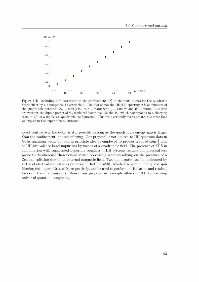
4.4 Summary and outlook
æ
æ
æ
æ
æ
æ
æ
æ
æ
æ
æ
à
à
à
à
à
à
à
à
à
à
à
10 20 30 40 50Qm meV
0.1
0.2
0.3
0.4
0.5
DE meV
Figure 4.5: Including a r4 correction to the confinement (Φ′1 in the text) allows for the quadraticStark effect by a homogeneous electric field. The plot shows the HH/LH splitting ∆E as function ofthe quadrupole potential Qm = max (eΦ4) at r = 50nm with ζ = 1.9meV and W = 60nm. Blue dotsare without the dipole potential Φ2 while red boxes include the Φ2, which corresponds to a chargingratio of 1/3 of a dipole vs. quadruple configuration. This ratio certainly overestimates the error thatwe expect in the experimental situation.
exact control over the qubit is still possible as long as the quadrupole energy gap is largerthan the confinement induced splitting. Our proposal is not limited to HH quantum dots inGaAs quantum wells, but can in principle also be employed to process trapped spin 3
2 ionsor HH-like valence band impurities by means of a quadrupole field. The presence of TRS incombination with suppressed hyperfine coupling in HH systems renders our proposal lessprone to decoherence than non-adiabatic processing schemes relying on the presence of aZeeman splitting due to an external magnetic field. Two-qubit gates can be performed byvirtue of electrostatic gates as proposed in Ref. [Loss98]. All-electric spin pumping and spinfiltering techniques [Brosco10], respectively, can be used to perform initialization and readouttasks on the quantum dots. Hence, our proposal in principle allows for TRS preservinguniversal quantum computing.
93


Chapter 5
Transport properties of helical edge states
This chapter is dedicated to the study of non-equilibrium transport properties of the hTLL.We employ the theory developed in Chapter 3 to investigate several holographic quantumtransport peculiarities of the QSH state (see Section 2.4.1). In Section 5.1, we study an sTLLcomposed of two hTLLs (see Section 3.3.1) under non-equilibrium conditions and investigatethe fingerprints of several coupling terms between the two hTLLs on the transport propertiesin a four terminal setup. In Section 5.2, we discuss the topological protection against elasticsingle electron backscattering (see also Section 3.3.2) in the hTLL in more detail and showhow phonons can induce inelastic backscattering. In contrast, two electron backscatteringdue to Coulomb interaction has been known in the literature since the discovery of the hTLL[Wu06]. However, more recent literature [Ström10] on the microscopic realization of suchinteraction induced backscattering terms failed to predict the vanishing of backscattering inthe non-interacting limit. We interpreted this as an incentive to resolve this controversy byrevisiting the problem of Coulomb induced backscattering from an RG perspective which isthe subject of Section 5.3.
5.1 Charge-spin duality in non-equilibrium transport of helicalliquids
In this section, we study non-equilibrium transport properties of the charge and spin sectorsof two edges of a QSH insulator in a four-terminal configuration following Ref. [Liu11]. Asimple duality relation between charge and spin sector is found for two hTLLs (see alsoSection 3.3.1) connected to non-interacting electron reservoirs. If the hTLLs on oppositeedges are coupled locally or non-locally, the mixing between them yields interesting physicswhere spin information can be easily detected by a charge measurement and vice versa.Particularly, we show how a pure spin density in the absence of charge current can begenerated in a setup that contains two hTLLs and one sTLL in between.
5.1.1 Motivation and outlineAn important feature of the hTLL is that spin and momentum are locked to each other (seeSection 3.3 for a more detailed discussion). Consequently, we can easily manipulate the spindegree of freedom by electric means in an hTLL and vice versa. One hTLL has only halfthe degrees of freedom of an sTLL. Thus, two hTLLs, which naturally exist at two oppositeedges of a QSH insulator, can recover the degrees of freedom of a single sTLL (see Section3.3.1). It is well known and has even been experimentally confirmed [Auslaender05] that
95
Chapter 5 Transport properties of helical edge states
there is spin-charge separation for a 1D sTLL. Therefore, it is natural and interesting toask how the spin and the charge sector behave for two uncoupled as well as coupled hTLLs.In this section, we investigate the non-equilibrium transport properties of two hTLLs in afour-terminal configuration. The practical calculation follows closely our general outline inSection 3.2.2 with the minor complication that an additional index ν labeling the two hTLLsat the two edges of the QSH sample appears.
Most interestingly, we find a duality relation between the charge and the spin sector of twohTLLs taking into account the coupling to non-interacting electron reservoirs. As a physicalconsequence, there is a simple relation between the charge current and spin polarizationin the dual voltage configurations of two hTLLs. Importantly, the coupling between thetwo edges will destroy the simple duality relation. However, we can still manipulate thecharge and the spin sector separately only by electric means. To demonstrate this, we studydifferent scattering mechanisms between the two hTLLs within the non-equilibrium Keldyshformalism (see Section 3.2) and bosonization (see Section 3.1). Different bias dependencesare found for different scattering mechanisms which can be used to distinguish and identifythem in experiments.
5.1.2 Model and spin-charge duality
We consider a QSH insulator in a four-terminal configuration as shown in Fig. 5.1 (a). Thetwo edges are denoted by ν = u(l) for the upper (lower) edge. On each edge ν, there aretwo terminals with chemical potentials µi,ν (i = 1, 2 means left and right lead, respectively).Two terminals on the same edge are connected by an hTLL of finite length L. As far as the1/L terms appearing in Eq. (3.4) are concerned, we still consider L as infinite. The hTLLstates are described by the field operators ψp,s where (p, s) = (R, ↑) or (L, ↓) for the upperedge and (p, s) = (R, ↓) or (L, ↑) for the lower edge. In the middle region of the sample,the hTLLs at the two edges can mix and different types of coupling mechanisms will bediscussed below.
As discussed in Section 3.3.1, there are two possibilities for choosing the basis states of thecomposite sTLL: (i) the helical edge basis and (ii) the spin-charge basis. For the helical edgebasis, the nonchiral boson field is defined separately for each edge with ϕu(l) = φR,↑(↓) +φL,↓(↑)at the upper (lower) edge and the corresponding dual field θu(l) = φR,↑(↓) − φL,↓(↑). Here,φp,s (p = R,L and s =↑, ↓) is the spinful chiral hermitian field appearing in the bosonizationidentity, Eq. (3.23). This basis is suitable to study the current at different terminals.However, when we are interested in spin properties, it is more convenient to introduce thespin-charge basis, which ignores the u, l labels and is related to the basis of the spinfulbosonic fields defined in Eq. (3.24) by Eq. (3.25) which we repeat here for the reader’s
96
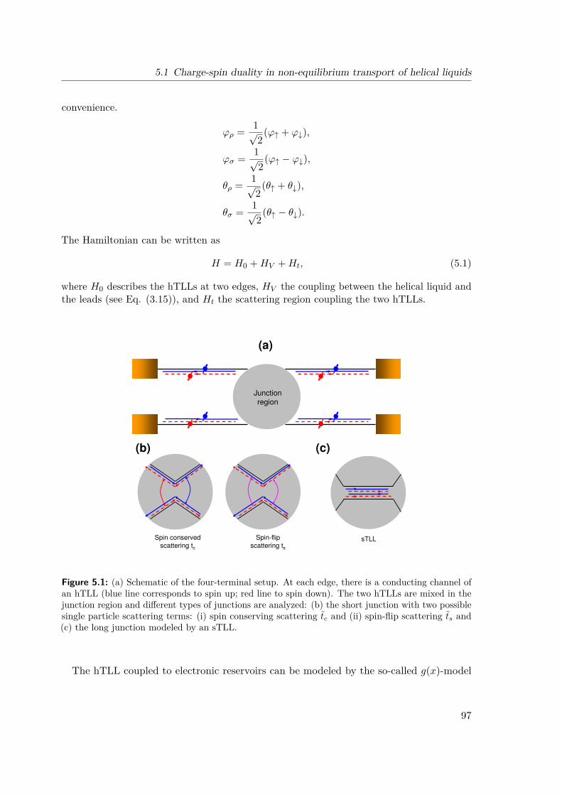
5.1 Charge-spin duality in non-equilibrium transport of helical liquids
convenience.
ϕρ = 1√2
(ϕ↑ + ϕ↓),
ϕσ = 1√2
(ϕ↑ − ϕ↓),
θρ = 1√2
(θ↑ + θ↓),
θσ = 1√2
(θ↑ − θ↓).
The Hamiltonian can be written as
H = H0 +HV +Ht, (5.1)
where H0 describes the hTLLs at two edges, HV the coupling between the helical liquid andthe leads (see Eq. (3.15)), and Ht the scattering region coupling the two hTLLs.
Junctionregion
(a)
(b) (c)
Spin conservedscattering tc
Spin-flipscattering ts
sTLL
Figure 5.1: (a) Schematic of the four-terminal setup. At each edge, there is a conducting channel ofan hTLL (blue line corresponds to spin up; red line to spin down). The two hTLLs are mixed in thejunction region and different types of junctions are analyzed: (b) the short junction with two possiblesingle particle scattering terms: (i) spin conserving scattering tc and (ii) spin-flip scattering ts and(c) the long junction modeled by an sTLL.
The hTLL coupled to electronic reservoirs can be modeled by the so-called g(x)-model
97
Chapter 5 Transport properties of helical edge states
[Maslov95, Ponomarenko95, Safi95] given by
Hρ0 = vF
2
∫dx
[(∂xθρ)2 + 1
g2(x)(∂xϕρ)2],
Hσ0 = vF
2
∫dx
[ 1g2(x)(∂xθσ)2 + (∂xϕσ)2
](5.2)
in the spin-charge basis. Here, vF is the Fermi velocity and g(x) is the hTLL interactionparameter, with g(x) = g0 < 1 for repulsive interactions within the helical edge located at|x| < L/2, and g(x) = 1 for the non-interacting fermions in the leads with |x| > L/2. Weassume the same parameters vF and g0 at the two edges (ν = u, l). This is reasonable fortwo edges of the same system. The chemical potentials in the leads are naturally taken intoaccount with the bias Hamiltonian
HV =∫
dx√2π
[∂xµρ(x)ϕρ + ∂xµσ(x)θσ] ,
where
∂xµρ(σ) = −µ1,ρ(σ)δ(x+ L/2) + µ2,ρ(σ)δ(x− L/2)
with µi,ρ = µi,u + µi,l and µi,σ = µi,u − µi,l (i = 1, 2). Remarkably, µρ couples to ϕρ whileµσ couples to θσ. Therefore, the electric voltage can couple to both the charge and the spinsector of the composite sTLL. This provides us with a means to control the charge sectorand the spin sector separately, in contrast to the usual sTLL where the electric chemicalpotential only couples to the charge sector. Moreover, we discover that there is a dualityrelation between the charge sector and the spin sector
ϕρ ↔ θσ, θρ ↔ ϕσ. (5.3)
For Hλ0 (λ = ρ, σ), the above duality relation is directly related to the constraint gc = 1/gs
discovered in Ref. [Hou09] before (see also Section 3.3.1). Here, we show that this relationremains valid even if the system is coupled to non-equilibrium electron reservoirs. Thus, it isobservable in transport properties of the system.
What is the physical consequence of this duality relation? To answer this question, weinvestigate the total charge current and the total spin density of the system. The chargecurrent is given by jρ = −e
√2π∂tϕρ, which is the sum of the currents along the two edges
jρ = ju + jl, with jν(x) = − e√π∂tϕν (see Eq. (3.11)). The spin density can be defined as
ρσ =√
2π∂xϕσ. Combining Eq. (3.25) and ∂tϕν = −vF∂xθν (see Eq. (3.10)), it is evident
that the spin density can be directly related to the charge current along the two edges by
ρs = 1evF
(ju − jl).
In the absence of mixing between the two edges, our setup describes the transport throughtwo independent 1D channels. Then, it follows directly from previous work [Maslov95,
98

5.1 Charge-spin duality in non-equilibrium transport of helical liquids
Ponomarenko95, Safi95] that
〈j0,ν〉 = e2
hVν ,
where −eVν = µ1,ν − µ2,ν . Thus, the total charge current is 〈j0,ρ〉 = 2e2h Vρ with Vρ =
Vu + Vl = − 12e(µ1,ρ − µ2,ρ), while the total spin density is given by 〈ρ0,σ〉 = 2e
hvFVσ with
Vσ = Vu − Vl = − 12e(µ1,s − µ2,s). Importantly, it is spin density and not spin current that is
dual to the charge current, which is a direct consequence of the duality relation (5.3). Physi-cally, Vρ and Vσ can be easily generated by two different voltage configurations of the fourterminal setup, as shown in Fig. 5.2. In Fig. 5.2(a), µ1,+ = µ1,− = −µ2,+ = −µ2,− = −eV0/2,which yields Vρ = V0 and Vσ = 0; and in Fig. 5.2(b), µ1,+ = µ2,− = −µ1,− = −µ2,+ = −eV0/2,resulting in Vρ = 0 and Vσ = V0. In these two symmetrical bias configurations, we findeither charge current or spin density but no spin current. This is different for unsymmetricalbias configurations where charge current and spin density are usually accompanied by spincurrent as well.
Thus, in Fig. 5.2(a), there is charge current but no spin density while in Fig. 5.2(b) thereis spin density but no charge current. There is a simple physical picture to understand thisresult. For the upper edge, the right mover has spin up and the left mover has spin down,while for the lower edge the situation is just the other way round. In Fig. 5.2(a), on bothedges the left movers have a larger chemical potential than the right movers resulting intotal charge current from left to right. However, since now the left movers for the upperedge and lower edge have opposite spin, the spin density at the two different edges willcancel each other. A similar analysis can also be applied to the configuration of Fig. 5.2(b),in which the left movers have higher (lower) Fermi energy than the right movers for theupper (lower) edge. Since both the left movers at the upper edge and the right moversat the lower edge have spin up, the spin density will be finite and maximal in this configuration.
Up to now, we have discussed the transport properties of two hTLLs and shown a simplerelation between the charge current and the spin density in two (dual) voltage configurations.In the following, we would like to take into account a junction structure introducing scatteringbetween the two hTLLs within a region of finite length d. We consider two different scenarios:(i) the short junction (SJ) with d λF and (ii) the long junction (LJ) with d λF , whereλF is the electron Fermi wave length. For SJ, we can neglect the length of the scatteringregion and model it as a quantum point contact, while for LJ, we can regard the scatteringregion as a finite length sTLL.
5.1.3 Short junction case
In the following, we concentrate on the experimentally relevant regime 1/2 < g0 < 1 [Teo09].Then, all the possible one-particle and two-particle scattering terms will be irrelevant [Teo09].Hence, we can safely treat the scattering Hamiltonian Ht as a perturbation. For the SJ case,two types of one particle scattering terms, which preserve time reversal symmetry, are taken
99

Chapter 5 Transport properties of helical edge states
Figure 5.2: (a). (I) and (III) show band dispersions and chemical potentials of the upper edgeand the lower edge, respectively. (II) illustrates the voltage configuration µ1,u = µ1,l = eV0/2 andµ2,u = µ2,l = −eV0/2. (b). Similar to (a) with a different voltage configuration µ1,u = µ2,l = eV0/2and µ2,u = µ1,l = −eV0/2.
into account (see Fig. 5.1(b)): the first one is the spin conserving term
Ht1 = tc(ψ†R,↑(x0)ψL,↑(x0) + ψ†L,↓(x0)ψR,↓(x0) + h.c.),
and the second one is the spin flip term
Ht2 = ts(ψ†R,↑(x0)ψR,↓(x0)− ψ†L,↓(x0)ψL,↑(x0) + h.c.)
with the junction position x0. In bosonization,
Ht = itc∑s
ηR,sηL,s sin(√πΞs) + its
∑ν
ην,↑ην,↓ sin(√πΨν)
100

5.1 Charge-spin duality in non-equilibrium transport of helical liquids
with Ξs =√
2(ϕρ + sϕσ) and Ψν =√
2(ϕσ + νθσ). Here, ην,s is the Klein factor andtc(s) = tc(s)
π . We now perform the perturbative calculation of our four terminal system withinthe non-equilibrium Keldysh formalism (see Section 3.2.2). All physical quantities can berelated to the expectation value of boson fields, which can be obtained from the functionalderivatives of the generating function Z[J ] which includes the Hamiltonian (5.1) and theadditional source term J coupling to the boson field ϕν or θν . Treating Ht as a perturbation,we can expand any physical quantity O in powers of tc(s), e.g., 〈O〉 = 〈O0〉 + 〈O2〉 up tosecond order (see Eq. (3.22) and discussion thereafter).
The first corrections to 〈j0,ρ〉 and 〈ρ0,σ〉 come from one particle scattering and can beexpressed as 〈j2,ρ〉 =
∑s=± JΞ,s and 〈ρ2,σ〉 = 1
evF
∑ν=± νJΨ,ν with
JΞ,s = et2c4
∫ ∞−∞
dt∑m
meimeVρteπCΞs (x0,x0;t),
JΨ,ν = et2s4
∫ ∞−∞
dt∑m
meimaeVσteπCΨν (x0,x0;t)
for the edge ν = ±. All the information about the detailed sample configuration is nowincluded in the correlators CΞ
s and CΨν , which are given by CΞ
s = 2(Cρ + Cσ) and CΨν =
2(Cσ +Dσ) + 2ν(Fσ +Qσ) with the correlation functions
Cλ = 〈ϕλϕλ〉0,Dλ = 〈θλθλ〉0,Fλ = 〈ϕλθλ〉0,Qλ = 〈θλϕλ〉0, λ = ρ, σ,
defined in total analogy to Eq. (3.18) but with an additional spin-charge index λ. We notethat the spin conserving scattering tc can only be induced by a charge voltage Vρ and, hence,will reduce the total charge current in the voltage configuration of Fig. 5.2(a), while thespin-flip scattering ts is only driven by the spin voltage Vσ and decreases the spin densityin the configuration of Fig. 5.2(b). For clarity, we further divide the operator O2 into twoparts 〈O2〉 = 〈O(0)
2 〉+ 〈O(1)2 〉, where 〈O
(0)2 〉 is calculated on the basis of L→∞ correlation
functions, while 〈O(1)2 〉 contains all finite length corrections. Then, analytical expressions for
the charge current and the spin density are readily obtained and given by
〈j(0)2,ρ〉 = − eπt
2cτg0+ 1
g0c
Γ(g0 + 1
g0
)sgn (Vρ) |eVρ|g0+ 1
g0−1,
〈ρ(0)2,σ〉 = − πt2sτ
g0+ 1g0
c
vFΓ(g0 + 1
g0
)sgn (Vσ) |eVσ|g0+ 1
g0−1.
Here, τc is the short time cutoff. Both the charge current and the spin density depend in apower law fashion on the voltage. This coincides with earlier work based on a renormalizationgroup analysis [Hou09, Teo09, Ström09, Tanaka09]. Then, for Vρ = Vσ, we find that theratio between the charge current and spin density in the two different voltage configurations
101

Chapter 5 Transport properties of helical edge states
is
〈j(0)2,ρ〉/〈ρ
(0)2,σ〉 = evF
t2ct2s,
which contains the information about the scattering strength for the different types ofscattering. In the finite length case, we use the numerical method of Ref. [Dolcini05] toevaluate JΞ,s and JΨ,ν . As shown in Fig. 5.3(a) and (b), the finite length will introduceoscillations in both the backscattering current and the spin density, which originates fromFabry-Perot-type interferences of plasmonic excitations [Safi95]. However, since the powerlaw g0 + 1
g0− 1 is always larger than 1 for positive g0, 〈j(0)
2,ρ〉 (〈ρ(0)2,σ〉) will increase rapidly
with Vρ (Vσ) and dominate the oscillatory corrections for large Vρ (Vσ). Hence, finite lengthcorrections are not very important in this setup.
5.1.4 Long junction case
Now, we consider the opposite limit d λF as shown in Fig. 5.1(c). This case could beachieved by gradually narrowing the QSH sample into a 1D wire experimentally. In thefollowing, we analyze finite size effects related to d and assume that L d, hence L→∞is a reasonable approximation. For simplicity, we model the LJ as an sTLL described byHt = Ht0 +Ht2 with Ht0 = Hρ
t0 +Hσt0 where
Hρt0 = vF
2
∫dx
[(∂xθρ)2 + 1
g20
(∂xϕρ)2],
Hσt0 = vF
2
∫dx[(∂xθσ)2 + (∂xϕσ)2
],
for |x| < d/2. Compared to Eq. (5.2), we find that the charge sector remains unchangedwhile the interaction parameter of the spin sector varies from 1/g0 to 1. This originatesfrom the SU(2) symmetry of the spin sector of an sTLL. For the charge sector, since theHamiltonian remains the same, we see that the interaction between two hTLL will not affectthe charge current 〈jρ〉 at all. For the spin sector of a 1D sTLL, besides Hσ
t0, we considertwo additional interaction terms [Gritsev05, Tanaka09]
Ht2 =∫ d
2
− d2dx[g1⊥ cos
(√8πϕσ
)+ gsf cos
(√8πθσ
)],
where the g1⊥-term is related to spin conserving backscattering ψ†L,↑ψ†R,↓ψL,↓ψR,↑+h.c. while
the gsf -term is related to the spin-flip backscattering process ψ†L,↓ψ†R,↓ψL,↑ψR,↑ + h.c., see
Fig. 5.3(c). These are the most important perturbations in the absence of impurity scatteringwhich we assume here. Since the g1⊥-term conserves spin, it will not influence the spindensity. Thus, we focus on the gsf -term below. Up to second order perturbation theory, we
102

5.1 Charge-spin duality in non-equilibrium transport of helical liquids
eVc/ ωωωωL eVs/ ωωωωL
BSchargecurrent|jb|
BSSpin
density| ρρ ρρ
s|(a) (b)
g0=0.7g0+1/g0-1=1.13
0 1 2 3 4 5
eVs/ ωωωωsd
BSSpin
density| ρρ ρρ
s| (d)(c)
Figure 5.3: (a) The backscattering current as a function of charge bias Vρ generated by the spinconserving tc-term for the voltage configuration of Fig. 5.2(a). The blue dashed line corresponds tothe charge current 〈j(0)
2,ρ〉, while the red solid line additionally includes the finite length corrections.
The current unit is 2et2c(τcωL)g0+ 1
g0
ωL. (b) is similar to (a), except that now we show the spin density
〈ρ(0)2,σ〉 and 〈ρ2,σ〉 as a function of the spin bias Vσ generated by the spin-flip ts-term for the voltage
configuration of Fig. 5.2(b). The spin density unit is 2t2s(τcωL)g0+ 1
g0
vFωL. (c) Possible two particle
backscattering terms: spin conserving backscattering g1⊥ and spin-flip backscattering gsf . (d) Thevoltage dependence of the correction to the spin density 〈ρ2,σ〉 due to the two particle spin-flip termgsf . The spin density unit is (gsfd)2(τcωd)4/g0
2vFωd. In all expressions above, we use ωL = vF
g0L, ωd = vF
d ,and g0 = 0.7.
103

Chapter 5 Transport properties of helical edge states
obtain the following correction to the spin density
〈ρ2,σ〉 = −g2sfd
2
vF
∫ 1
0dR
∫ 1−|R|
0drf(r,R),
f(r,R) =∫ ∞−∞
dt′∑m
mei2meVσt′e8πDσ(x,y,t′),
where r = (x− y)/d and R = (x+ y)/d. The above triple integration can be easily evaluatednumerically and the obtained correction to the spin density is shown in Fig. 5.3(d). Tomake analytical progress, we can again divide the obtained spin density into two parts〈ρ2,σ〉 = 〈ρ(0)
2,σ〉+ 〈ρ(1)2,σ〉 with 〈ρ
(0)2,σ〉 for the infinite d contribution and 〈ρ(1)
2,σ〉 accounting forfinite length corrections. We find that 〈ρ(0)
2,σ〉 always dominates over 〈ρ(1)2,σ〉. In the limit
eVσωd 1, we obtain
〈ρ(0)2,σ〉 ≈ −sgn (eVσ) ωdg
2sfd
2π2τ4/g0c
vFΓ2(2/g0) |eVσ|4g0−2
with ωd = vF /d.It is important to analyze the validity regime of our perturbation theory. Note that for
g0 < 1, the power law exponent 4g0− 2 will always be larger than 2. Thus, the second
order correction to the spin density 〈ρ2,σ〉 will increase faster than the zero order term 〈ρ0,σ〉as a function of bias voltage. Evidently, our perturbation theory is only justified when(ωdτc) (gsfdτc)2 |eVστc|
4g0−3 1.
5.1.5 Summary and outlook
We have analyzed the charge current and the spin density in a four-terminal setup basedon two hTLL coupled to non-interacting electron reservoirs. Different types of scatteringmechanisms between the edges have been taken into account, particularly short junctionsand long junctions. It has been shown that different power law dependencies as a functionof bias voltages applied to the four terminals can be used to distinguish the scatteringmechanisms. A simple duality relation between charge current and spin density has beendiscovered. Remarkably, all spin-related observables can be measured by straightforwardcharge measurements in the four-terminal configuration. It is interesting to ask the questionwhether the spin density in such a setup can also be measured by other means (e.g., as a testof the model). Taking typical values for vF = 3eV ·Å and eVσ = 5meV , we find that the zeroorder spin density is about 〈ρ0,σ〉 ≈ 5.3µm−1. This may be detected by state-of-the-art localFaraday/Kerr rotation [Kato04]. Furthermore, the possibility of applying a spin dependentbias voltage in the composite sTLL is also interesting in the context of non-equilibrium twochannel Kondo physics. Exact results on the non-equilibrium Kondo cloud in a related setuphave recently been reported in Ref. [Posske12] demonstrating how such a spin bias can beused to manipulate spin correlations in a way which is not viable by virtue of a conventionalbias.
In the next two sections, we focus on a single hTLL. We will take a closer look at the
104
5.2 Phonon-Induced Backscattering in Helical Edge States
quantized conductance of a single helical edge state mentioned in Section 3.3.2 and investigateits robustness against phonon-induced and Coulomb interaction induced backscattering,respectively.
5.2 Phonon-Induced Backscattering in Helical Edge States
A single pair of helical edge states as realized at the boundary of a quantum spin Hallinsulator is known to be robust against elastic single particle backscattering as long as timereversal symmetry is preserved [Wu06] (see also Section 3.3.2). However, there is no symmetrypreventing inelastic backscattering as brought about by phonons in the presence of Rashbaspin orbit coupling. In this section, we first review the phenomenon of topological protectionby TRS and point out its limitations. We then show that the quantized conductivity of asingle channel of helical Dirac electrons is protected even against the mentioned inelasticmechanism to leading order. We further demonstrate that this result remains valid whenCoulomb interaction is included in the framework of a helical Tomonaga Luttinger liquid.Our analysis follows closely the original material published in Ref. [Budich12a].
5.2.1 Motivation
During recent years, great interest has been attracted by the theoretical prediction [Kane05a,Bernevig06a] and experimental discovery [König07] of the QSH state (see Section 2.4.1). TheQSH phase is a two dimensional TRS preserving TSM that differs essentially from trivialatomic insulators by a Z2 topological invariant [Kane05b, Qi11, Hasan10] (see Section 2.4.1for a detailed discussion). Besides the enormous conceptual depth of TSM, the QSH phaseis also considered a promising candidate as to future applications in nanoelectronics. This isdue to its topologically protected transport properties which might be exploited for highprecision spintronics devices operating at low power consumption. Therefore, modeling theQSH effect under experimentally relevant conditions is crucial to test the practical limitationsof these protected features.
5.2.2 Topological protection against backscattering and its limitations
As far as the robustness of the topological protection is concerned, the QSH effect isfundamentally different from the integer quantum Hall (IQH) effect. For the TRS breakingIQH insulator [Klitzing80, Laughlin81, Thouless82], the bulk topology leads to a quantizationof conductivity to impressive accuracy. In the IQH regime, edge state transport is chiral,meaning that the density of states for subgap backscattering vanishes. This excludes suchprocesses by simple phase space arguments. In contrast, in the TRS preserving QSH phase asingle pair of helical edge states induced by bulk boundary correspondence is supported atthe edge of the QSH bar. This means that both right- and leftmovers exist at a single edge.However, states of opposite direction of motion are Kramers partners due to TRS. The wellknown topological protection of a single pair of helical edge states against backscatteringin this scenario can be mathematically illustrated by the following simple argument [Xu06].
105

Chapter 5 Transport properties of helical edge states
Let |φ〉 and |ψ〉 = T |φ〉 be Kramers partners. Then, as long as H is a TRS preservingHamiltonian
〈ψ|H|φ〉 =〈φ|H|ψ〉∗ = 〈Tφ|TH|ψ〉 =〈ψ|HT |ψ〉 = 〈ψ|HT 2|φ〉 = −〈ψ|H|φ〉, (5.4)
i.e., the matrix element for scattering between the Kramers partners vanishes. Note thatthe argument (5.4) of protection relies on two fundamental constraints: First, only singleelectron processes are considered. Second, since Kramers partners are degenerate states,it only precludes elastic backscattering. Within the validity of these restrictions extensivestudies of the hTLL [Xu06, Wu06] representing a single pair of helical edge states have shownthat Anderson localization is avoided [Kane05a, Ryu10] in the presence of TRS preservingdisorder and that TRS breaking magnetic impurities can open a gap in these systems[Maciejko09]. Furthermore, interedge backscattering can occur if the QSH sample is locallynarrowed down to a quantum point contact [Ström09, Teo09, Hou09, Liu11, Schmidt11] (seealso Section 5.1) or if two QSH bars are brought close to each other [Tanaka09]. In general,backscattering at a single helical edge requires spin flip processes. In realistic setups, these areinduced by Rashba SOI originating from unavoidable potential fluctuations. Preserving TRS,Rashba SOI cannot cause single electron elastic backscattering, though. However, relaxingthe single electron processes constraint by additionally including Coulomb interaction, twoelectron backscattering processes have been shown to arise in these systems [Ström10]. Suchbackscattering terms are well known to be allowed by TRS [Wu06].
Under realistic experimental conditions, finite temperature and bias voltage also imply thepresence of phonons, i.e., inelastic processes that undermine the second constraint for thevalidity of the argument (5.4). It is thus of crucial importance to investigate the influenceof this dissipative mechanism on the topological protection. Here, we show two importantresults of the helical edge states in the presence of two TRS preserving perturbations: RashbaSOI and electron phonon coupling. First, we demonstrate that in this scenario there is nostrict protection against inelastic single electron backscattering. Second, we find that forhelical Dirac fermions the leading order contribution of this mechanism vanishes, supportingthe protection for practical purposes. We further demonstrate how this additional robustnessfully survives in the presence of Coulomb interaction, i.e., in an hTLL with electron phononcoupling and Rashba SOI. In a nonequilibrium transport calculation for the hTLL, we takethe electron phonon coupling into account exactly by integrating out the phonons using aKeldysh contour path integral representation of the generating functional (see Section 3.2.2).Our analysis is relevant for any realization of the hTLL as a one dimensional system.
5.2.3 Model without Coulomb interaction
We investigate a single pair of helical Dirac fermions coupled linearly to longitudinal acousticphonons. The two species of electrons are coupled via Rashba SOI (see Fig. 5.4). In mostparts of this work, we will have a sharp impurity-like scattering potential in mind whichbrings about momentum transfer on the order of 2kF , where kF is the Fermi wave vector.We represent the helical fermionic fields as a spinor Ψ = (ΨR↑,ΨL↓)T = (Ψ+,Ψ−)T . The
106
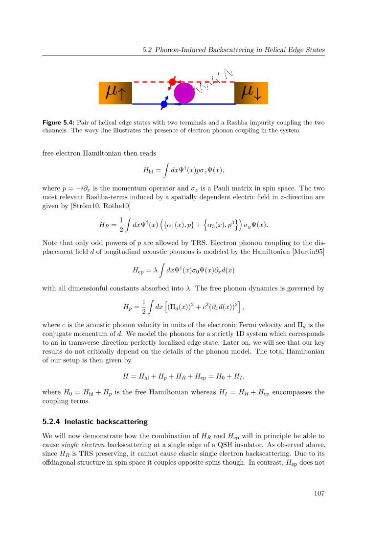
5.2 Phonon-Induced Backscattering in Helical Edge States
Figure 5.4: Pair of helical edge states with two terminals and a Rashba impurity coupling the twochannels. The wavy line illustrates the presence of electron phonon coupling in the system.
free electron Hamiltonian then reads
Hhl =∫dxΨ†(x)pσzΨ(x),
where p = −i∂x is the momentum operator and σz is a Pauli matrix in spin space. The twomost relevant Rashba-terms induced by a spatially dependent electric field in z-direction aregiven by [Ström10, Rothe10]
HR = 12
∫dxΨ†(x)
(α1(x), p+
α3(x), p3
)σyΨ(x).
Note that only odd powers of p are allowed by TRS. Electron phonon coupling to the dis-placement field d of longitudinal acoustic phonons is modeled by the Hamiltonian [Martin95]
Hep = λ
∫dxΨ†(x)σ0Ψ(x)∂xd(x)
with all dimensionful constants absorbed into λ. The free phonon dynamics is governed by
Hp = 12
∫dx[(Πd(x))2 + c2(∂xd(x))2
],
where c is the acoustic phonon velocity in units of the electronic Fermi velocity and Πd is theconjugate momentum of d. We model the phonons for a strictly 1D system which correspondsto an in transverse direction perfectly localized edge state. Later on, we will see that our keyresults do not critically depend on the details of the phonon model. The total Hamiltonianof our setup is then given by
H = Hhl +Hp +HR +Hep = H0 +HI ,
where H0 = Hhl + Hp is the free Hamiltonian whereas HI = HR + Hep encompasses thecoupling terms.
5.2.4 Inelastic backscattering
We will now demonstrate how the combination of HR and Hep will in principle be able tocause single electron backscattering at a single edge of a QSH insulator. As observed above,since HR is TRS preserving, it cannot cause elastic single electron backscattering. Due to itsoffdiagonal structure in spin space it couples opposite spins though. In contrast, Hep does not
107

Chapter 5 Transport properties of helical edge states
mix different spin species but can bring about energy dissipation by virtue of energy transferfrom the electronic degrees of freedom to phonons. Thus, the second order in HI diagramsshown in Figure 5.5 which are first order in Hep and in HR cause backscattering at finite bias(see Fig. 5.6) if their contribution does not vanish for momentum transfer pi−pf ≈ 2kF . We
Figure 5.5: Tree diagrams for lowest order backscattering. Dashed line with square represents theexternal Rashba potential. Wavy line denotes the phonon propagator.
consider scattering between a right mover |p+i 〉 and a left mover |p−f , qph〉 with an additional
phonon. Up to second order, the corresponding scattering matrix element Mif can be writtenas
Mif = 〈p−f , qph|HIG0HI |p+i 〉,
where G0 is the free propagator corresponding to H0. Interestingly, the lowest ordercontribution of the Rashba term linear in momentum associated with α1 vanishes due to anontrivial destructive quantum interference of the two contributing diagrams which stemsfrom the linearity of both Hhl and the α1-Rashba term. To show that this is not due to anyfundamental symmetry like TRS, we calculate the same matrix element for the Rashba termassociated with α3 which yields
|Mif |2 = λ2c
16π α23
(qph + p−f − p
+i
)|qph|5
where α3(k) is the Fourier transform of α3(x). At the level of an analytical Fermi’s goldenrule calculation for a δ-shaped Rashba impurity α3(x) = α3δ(x), the backscattering currentIBS at zero temperature can be readily expressed as
IBS = 2πe∫
dp+i
∫dp−f
∫dqph
[f+
FD(ε+i )(1− f−FD(ε−f )
)|Mif |2δ(ε+i − ε
−f − ωph)
], (5.5)
where ε+i = p+i −kF and ε−f = −p−f −kF denote the initial and the final energy of the scattered
electron, ωph = c|qph| is the phonon frequency and f±FD is the Fermi-Dirac distribution functionassociated with the chemical potential µ± of the branch of right movers (+) and left movers(−), respectively. Using f±FD(ε) = θ(µ± − ε) at zero temperature, we can readily perform theintegrals occuring in Eq. (5.5) analytically and obtain
IBS = α23λ
2e
672π2c5V7. (5.6)
108

5.2 Phonon-Induced Backscattering in Helical Edge States
eV
Figure 5.6: Voltage configuration to pass a spin up current from the left to the right. The biasV opens an energy window for inelastic phonon scattering.
This contribution will be negligible at low bias V reflecting the irrelevance of the p3-Rashbaterm. The importance of this non-vanishing result is that it demonstrates how in principleinelastic single electron backscattering can occur at finite bias even though the perturbationsRashba SOI and electron phonon coupling preserve TRS. The lowest order nonvanishingmatrix element for the α1 term could be third order in α1 which has the same relevance asα3 in renormalization group (RG) sense. Also, quadratic corrections to the linear electronicdispersion which might become relevant at higher energies can give rise to α1 backscattering.
At finite temperature, there will be additional scattering contributions to the current,e.g., from processes where a phonon is absorbed or where an electron is scattered from athermally excited state in the branch with the lower chemical potential to an empty statebelow the chemical potential of the other branch. For finite T , we numerically evaluate thecorrection ∆G to the conductance by calculating
∆G = ∂∆I(V, T )∂V
∣∣∣∣V=0
,
where ∆I contains all perturbative corrections to the current up to second order in HI . InFig. 5.7, we show the temperature dependence of the conductance which scales to convincingaccuracy with the sixth power of T .
We would again like to point out that the vanishing matrix element Mif for the α1-Rashbaleads to an exactly quantized conductance in the absence of the α3-Rashba term also atfinite temperature. We hence conclude that for the helical edge state without Coulombinteraction the most relevant inelastic backscattering contributions allowed by TRS andphase space arguments cancel out. This can be interpreted as an enhanced precision of thequantized conductivity of the helical edge states at finite temperature/bias going beyond thetopological protection only pertaining to elastic scattering.
109

Chapter 5 Transport properties of helical edge states
logT
logG
Figure 5.7: Temperature dependence of the conductance G in arbitrary units (red solid). Plot of thepower law ∼ T 6 (blue dashed). Logarithmic scale on both axes.
5.2.5 hTLL with Coulomb interaction
Now, we want to investigate whether the observed robustness of the helical Dirac fermionsagainst inelastic backscattering by virtue of the α1-Rashba SOI term, i.e., the most relevantTRS preserving term coupling opposite spins, persists in the presence of Coulomb interaction.In order to account for Coulomb interaction we represent the fermionic degrees of freedomin terms of an hTLL using the bosonization identity (see also Eq. (3.4))
ψ± = 1√2πa
η±ei√π(ϕ±θ),
where ψ± now denote the slowly varying fields with a factor of e±ikF x separated off, a is thehigh energy cutoff of the model and ϕ, θ are the bosonic phase field and its dual, respectively.In the thermodynamic limit, the Klein factors η± obey the algebra of Majorana fermions.Absorbing a prefactor of 1
π by redefining λ, the electron phonon coupling can be representedas
Hep = λ
∫dx∂xϕ(x) ∂xd(x).
The translation invariant hTLL Hamiltonian reads (see also Eq. (3.9))
HhTLL = 12
∫dx
[Π2ϕ(x) + 1
g2 (∂xϕ(x))2]
with the interaction strength parameter g < 1 modeling repulsive Coulomb interaction. Theα1-Rashba Hamiltonian with α1(x) = αδ(x) in bosonized form yields
HR = iα√πaη+η− : (∂xθ(x)) cos
(√4πϕ(x)
):∣∣∣x=0
(5.7)
110

5.2 Phonon-Induced Backscattering in Helical Edge States
where the dots denote normal ordering.
We want to calculate the average current I(x, t) = − e√π∂t〈ϕ(x, t)〉 due to an applied bias
V. Such expectation values can be most easily represented for practical calculations in termsof a generating functional
Z [J ] =∫D(ϕ, θ, d)eiS0−i
∫cHR+i e√
πET σ3ϕ+ i√
2JTϕ
, (5.8)
where S0 encompasses the electron phonon system without the Rashba impurity,∫c denotes
the integral along the Keldysh contour, σ3 is a Pauli matrix in Keldysh space, and scalarproducts like JTϕ involve an integration over real space and time. The applied bias ismodeled by E(x, t) along the lines of Ref. [Dolcini05] (see also Eq. (3.15)).
To make further analytical progress we now integrate out the phonons on the Keldyshcontour. The part of the Lagrangian involving the phonon field d reads
Ld = 12((∂td)2 − c2(∂xd)2
)− λ(∂xϕ)(∂xd).
The phonon dependent part of the action can be represented on the Keldysh contour as
Sd = 12d
TG−1ph d+ λdTσ3∂2
xϕ
with the phonon propagator Gph. Performing the Gaussian integral∫Dd eiSd(d,ϕ) = eiSdiss(ϕ)
in the rotated Keldysh basis(ϕ+
ϕ−
)→ 1√
2
(1 11 −1
)(ϕ+
ϕ−
)= Uϕ
yields for the dissipative action
Sdiss = −λ2
2 (∂2xϕ)Tσ1Gphσ1∂
2xϕ, (5.9)
where σ1Gphσ1 =(
0 GAphGRph GKph
). By this dissipative action, the inverse free electron Green’s
function in Fourier space is changed to the following dressed version
(G−1e (k, ω)
)ϕϕ→(G−1e (k, ω)
)ϕϕ− λ2k4
ω2 − c2k2 . (5.10)
This result generalizes to the Keldysh formalism a similar imaginary time calculation carriedout in Ref. [Martin95]. The retarded, advanced and Keldysh part of this Green’s functioncan be calculated exactly. From now on the free action S0(ϕ, θ) refers to the effective action
111

Chapter 5 Transport properties of helical edge states
where the phonons have been integrated out. To calculate the current we basically have toevaluate
〈ϕ(x)〉 = −i√2δZ[J ]δJ(r)
∣∣∣∣J=0
, (5.11)
which can be done along the lines of Ref. [Dolcini05] (see also Section 3.2.2). The equation ofmotion ∂tϕ = −∂xθ (see Eq. 3.10) inside the free correlators averaged with S0(ϕ, θ) remainsvalid for the free action which is dressed by the phonon dissipation. That is because Sdiss(see Eq. (5.9)) depends only on ϕ and not on its conjugate momentum Πϕ = −∂xθ (see Eq.(3.8)). Using only this property of the electron phonon coupling the current to second orderin α1 is readily shown to be zero. This proves that our result for the case without Coulombinteraction persists in the nonequilibrium hTLL.
This result might be understood on more general grounds. The fact that S0 remainsquadratic in Πϕ = −∂xθ means that the following argument first brought forward inRef. [Ström10] for an hTLL in equilibrium without electron phonon interaction could be usedfor our setup as well: Integrating out Πϕ in the path integral representation of the generatingfunctional will produce terms proportional to (∂tϕ)2, α(∂tϕ) cos(
√4πϕ), α2 cos(
√4πϕ)2 in
the action. While the first contribution is the term well known from the free hTLL case, thesecond one is a pure gauge which can be dropped. The third term can up to a constant bewritten as cos(
√16πϕ) which is a two electron TRS preserving backscattering term [Wu06].
Note that the presence of the source term JTϕ in Eq. (5.8) does not affect this argument.Thus, we have found that the α1-Rashba term cannot lead to a single electron backscatteringterm in the presence of any external spin independent dissipation which couples linearly tothe electron density.
One cautious remark is in order: In the non-interacting limit, i.e., for g → 1, theterm α2 cos(
√4πϕ)2 does not seem to vanish which suggests the presence of two-particle
backscattering in the absence of Coulomb interaction. This cannot be true. Since, at thispoint, it is not clear to us how the physical thruth can be reconciled with the argumentbased on integrating out Πϕ, the latter should be taken with care. However, this does notaffect at all our previous discussion of phonon-induced backscattering in helical edge states.We again point out that this result goes beyond the topological protection of the hTLL. It isdue to the quadratic form of S0 in Πϕ, the Luttinger liquid analogue of the linear dispersionof helical Dirac fermions on which our result without Coulomb interaction relied. Bosonizingthe α3-Rashba term implies terms up to third power in ∂xθ thus breaking the quadraticform of S0 in Πϕ. Furthermore mixed terms like (∂xϕ)(∂xθ)2 will occur which render themodifications of free Green’s function (see Eq. (5.10)) by the presence of phonons important.These observations are perfectly compatible with our nonvanishing result for single electronbackscattering in the presence of α3 (see Eq.(5.6)).
5.2.6 Summary and outlookIn summary, we have studied helical Dirac fermions in the presence of electron phononcoupling and Rashba SOI, which both preserve TRS. We have shown that, although TRS
112

5.3 RG approach for the scattering off a single Rashba impurity in a helical liquid
does not provide a protection against inelastic scattering, the current carried by the helicalstates in the presence of a finite bias is not changed to leading order. Furthermore, we haveproven that this result still holds for an hTLL including Coulomb interaction. The lineardispersion of the helical edge states of a QSH bar has been nicely verified experimentally[König07] and is an exact feature of the four band model for inverted HgTe/CdTe quantumwells introduced in Ref. [Bernevig06a]. Therefore, our analysis is not only interesting for theabstract model of an hTLL. It supports the robustness of the quantized subgap conductanceof a QSH sample beyond the well known argument (5.4) of topological protection. Ourresults turn out to be not restricted to the coupling to longitudinal acoustic 1D phonons.In fact, we have shown that any external bath coupling linearly to the electron densitycannot give rise to inelastic single electron backscattering in the presence of linear in k spinorbit coupling. In HgTe/CdTe layer structures, external coupling mechanisms, e.g., couplingto charge puddles in the bulk, are likely to cause phase decoherence which gives rise toadditional backscattering. However, such effects are not intrinsic features of the hTLLand can in principle be contained by improving the sample quality. In contrast, electronphonon coupling and Coulomb interaction are intrinsic mechanisms the role of which wehave investigated for a generic realization of the hTLL. The discussed mechanism of phonon-induced backscattering gives rise to conductance corrections that scale like T 6. We alreadypointed out that integrating out Πϕ in the path integral leads to the unphysical result ofnon-vanishing backscattering in the limit of vanishing Coulomb interaction. In the followingsection, we resolve this controversy by studying the interplay of the α1-Rashba term andCoulomb interaction from an RG perspective.
5.3 Renormalization group approach for the scattering off asingle Rashba impurity in a helical liquid
The occurrence of two-particle inelastic backscattering has been conjectured in helical edgestates of topological insulators and is expected to alter transport. In this section, by using arenormalization group approach, we provide a microscopic derivation of this process, in thepresence of a time-reversal invariant Rashba impurity potential. Unlike previous approachesto the problem, we are able to prove that such an effect only occurs in the presence ofelectron-electron interaction. Furthermore, we find that the linear conductance as a functionof temperature exhibits a crossover between two scaling behaviors: T 4K for K > 1/2 andT 8K−2 for K < 1/2, with K the Luttinger parameter modeling Coulomb interaction. Here,we choose a notation which is convenient for our RG analysis and which slightly differs fromour general presentation in Section 3.1. The relation between the two notations will beestablished explicitly below. Our presentation follows closely the analysis of Ref. [Crépin12].
5.3.1 Motivation
Since the prediction of the quantum spin Hall phase [Kane05a, Kane05b] (see Section 2.4.1)in HgTe quantum wells [Bernevig06a], transport measurements on these compounds haveshown evidence of a quantized edge conductance G = 2e2/h, thereby paving the wayfor non-local dissipationless transport in semiconductors at zero external magnetic field
113
Chapter 5 Transport properties of helical edge states
[König07, König08, Roth09]. In the simplest case of quantum wells with inversion symmetry,transport occurs through two counter-propagating edge channels that carry opposite spin-1/2 quantum numbers. Such helical liquids form a new class of 1D quantum liquids inthe sense that they are protected by time-reversal symmetry against single-particle elasticbackscattering [Kane05a, Xu06, Wu06] (see also Section 5.2). However, deviations from thequantized conductance arise in various situations, involving either a breaking of time-reversalsymmetry – by a magnetic impurity for instance – or the interplay between a TRS preservingexternal potential and a source of inelastic scattering. Inelastic single-particle backscattering[Budich12a, Schmidt12] and two-particle backscattering [Kane05a, Xu06, Wu06, Ström10]are two examples of the latter. In this section, we focus on two-particle backscattering offa TRS preserving impurity and report new results regarding the temperature scaling ofconductance corrections. Our purpose is to derive the Hamiltonian for such a process startingwith a minimal model of an interacting helical liquid coupled to a TRS preserving potential.In particular, we focus on a Rashba spin-orbit potential [Ström10, Budich12a], which canoriginate from fluctuations of an electric field perpendicular to the 2D electron gas [Rothe10],and acts as a TRS preserving effective magnetic field that couples right and left movers. Inthe recent literature, inelastic two-particle backscattering off an impurity was mostly studiedphenomenologically, by postulating the generic form of the Hamiltonian due to symmetryconsiderations – namely TRS and Pauli principle [Kane05a, Xu06, Wu06, Lezmy12],
H in2p = γ2p
[(∂xΨ†+)Ψ†+(∂xΨ−)Ψ−
](x0) + H.c., (5.12)
where ± designate right and left movers respectively. A straightforward scaling analysis[Kane92a, Kane92b] would lead to a temperature dependence of T 8K−2 for conductancecorrections, with K the Luttinger parameter, implying a T 6 behavior in the limit of weakCoulomb interaction, K ' 1. These studies, however, do not explain how two-particlebackscattering is generated at the microscopic level. To our knowledge, the only micro-scopic explanation proposed so far is the one by Ström et al. [Ström10], already based onRashba spin-orbit coupling. Their analysis, however, leads to the unphysical conclusionthat these processes are present even in the limit of vanishing Coulomb interaction. Indeed,without interaction, two-particle backscattering can always be factorized to two uncorrelatedsingle-particle elastic backscattering processes and does not affect transport. A satisfactoryexplanation of the effect is therefore still lacking.
Here, we use a renormalization group (RG) approach to show how two-particle inelasticbackscattering is generated from Rashba spin-orbit coupling and Coulomb interaction. Uponintegrating the flow equations, we are able to demonstrate that the effect only occurs inthe presence of electron-electron interaction. Furthermore, we find a K-dependent crossoverbehavior for the temperature scaling of the conductance corrections, namely
δG/G0 ∼
(a0T/v)4K if K > 1/2,(a0T/v)8K−2 if 1/4 < K < 1/2, (5.13)
where a0 is the inverse bandwidth and v the interaction-renormalized Fermi velocity. Ouranalysis demonstrates that, in the limit of weak interactions, two-particle inelastic processes,
114

5.3 RG approach for the scattering off a single Rashba impurity in a helical liquid
with a scaling of T 4, are a more important source of scattering than usually anticipated fromphenomenology.
5.3.2 Model
We study an interacting 1D helical liquid in the presence of Rashba spin-orbit coupling. TheHamiltonian of the system is the sum of three terms, H = H0 +HI +HR, given by
H0 =∫dx
∑η=±
Ψ†η(x)(−iηvF∂x − EF )Ψη(x), (5.14)
HI =∫∫
dxdx′Ψ†+(x)Ψ†−(x′)g2(x− x′)Ψ−(x′)Ψ+(x),
HR =∫dx α(x)
[(∂xΨ†+)Ψ− −Ψ†+(∂xΨ−)
](x) + H.c..
Here, Ψ†+(x) and Ψ†−(x) are creation operators for right and left moving electrons, respectively.Both species carry spin-1/2 opposite quantum numbers and hence transform as T Ψ†±(x)T −1 =±Ψ†∓(x) under time reversal. H0 entails a strictly linear spectrum, with a finite bandwidth,the size of the bulk band gap. vF is the Fermi velocity, EF the Fermi energy. Withoutloss of generality, we consider in HI only interaction between electrons moving in oppositedirections, since chiral interactions – so-called g4 terms – only renormalize the Fermi velocity.Finally, HR describes a linear Rashba spin-orbit potential likely to stem from fluctuationsof a transverse electric field [Ström10, Budich12a]. We emphasize that HR is, in a helicalliquid, the time-reversal invariant Hamiltonian with the lowest scaling dimension, able tocouple right and left-movers. Nevertheless it has no effect on transport as long as elasticscattering is concerned [Xu06]. In the following, we consider a point-like impurity, that is,α(x) = αδ(x). We show with a RG calculation how two-particle inelastic backscatteringis generated. First, we carry it out on the fermion partition function before treating theCoulomb interaction exactly using bosonization.
5.3.3 RG for interacting fermions
Much insight is gained by first treating, at the fermion level, both Coulomb interactionand the Rashba potential as perturbations to the non-interacting fixed point. We use thepath integral representation of the partition function, Z =
∫DΨ∗±DΨ±e−S , with an action
S =∫ β0 dτ
[∑η=±
∫dxΨ∗η(x, τ)∂τΨη(x, τ) +H(τ)
], and Ψ±(x, τ), Ψ∗±(x, τ) Grassmann fields.
We introduce an ultra-violet (UV) cutoff Λ of the order of half the bulk band gap on thedispersion relation of both right and left movers as vF |ηk − kF | < Λ, with kF the Fermimomentum. Following Ref. [Shankar94], we then proceed to integrate out the fields livingon an infinitesimal momentum shell Λ/s < vF |ηk − kF | < Λ, with s = 1 + d`. As usual in a1D quantum liquid, interactions contribute an infinite series of diagrams. However, in theabsence of 2kF scattering processes, and the impurity being point-like, g2 is invariant underRG transformations. The integration of high energy fields also generates new terms. Tothird order perturbation theory, the diagram (b) depicted in Fig. 5.8 generates an inelastic
115

Chapter 5 Transport properties of helical edge states
∂
∂
1
2
3
4
k′′, ω′′
k′, ω′
(a) (b)
1
2
3
4
∂
∂
Figure 5.8: Examples of diagrams to order α2 (a) and g2α2 (b), in the expansion of the partition
function. Partial derivative signs indicate which external lines are differentiated with respect to x.Full (dashed) arrows are for right (left) movers. Wavy lines are for Coulomb interaction, and greyballs denote scattering off the impurity.
two-particle backscattering process whose action is of the form
S2p = γ2p
∫ 4∏i=1
dki2π
dωi2π 2πδ(ω1 + ω2 − ω3 − ω4)×
(−ik3Ψ∗+(3))Ψ∗+(4)(ik2Ψ−(2))Ψ−(1) + +↔ −. (5.15)
This is precisely the action one would derive from the Hamiltonian of Eq. (5.12) in momentumspace. The scaling dimension of γ2p is (−3) by power-counting. We take into account theaforementioned third-order diagram (b) shown in Fig. 5.8, which is of second order inthe Rashba coupling constant α and of first order in the Coulomb forward scattering g2.Performing the momentum shell integration on the contribution of this diagram, we obtainthe flow equation
dγ2pd`
= −3γ2p(`) + α(`)2
vFΛg2
2πvF, (5.16)
where the first term on the right hand side stems from the scaling dimension of γ2p andthe second term accounts for the perturbative third order correction. Note that the initialcondition is γ2p(` = 0) = 0, since two-particle inelastic backscattering is absent from thebare action. Finally, power counting on the Rashba action yields for α(`) the flow equation
dα
d`= −α(`). (5.17)
This calculation confirms that inelastic two-particle backscattering off a Rashba impurity isonly generated in the presence of Coulomb interaction, as it disappears altogether as soon asg2 = 0. We emphasize that to second order in α, diagrams such as (a) in Fig. 5.8 do notgenerate inelastic processes since Matsubara frequencies are conserved independently at eachRashba scattering vertex; in this example, ω1 = ω3 and ω2 = ω4. Finally, we point out thatg4 (chiral) interactions fail to generate inelastic two-particle backscattering as all diagramswill be suppressed by the Pauli principle.
116

5.3 RG approach for the scattering off a single Rashba impurity in a helical liquid
5.3.4 Bosonization
We refine our analysis by treating interactions exactly, through bosonization of the fermionHamiltonian. Excitations around the true ground state of the 1D interacting helical liquidare indeed described by the Tomonaga Luttinger liquid Hamiltonian (see also Eq. (3.9))
H0 = v
2
∫dx
[K(∂xθ)2 + 1
K(∂xϕ)2
], (5.18)
where the notation is related to Eq. (3.9) through the identifications K = g, and v = vF /g.The present symmetric notation is more convenient for our RG analysis. By using thebosonization identity, Eq. (3.4), the bosonized form of the Rashba Hamiltonian is readilyobtained as [Ström10, Budich12a] (see also Eq. (5.7))
HR = iη+η−∫dx
α(x)(π)
32a
(2πaL
)K: ∂xθ(x)
(: e−i2ϕ(x) : ei2kF x+ : ei2ϕ(x) : e−i2kF x
): (5.19)
where : . . . : indicate normal order with respect to boson operators that annihilate the groundstate of the helical liquid (see Eq. (3.2)). Here, η± are again the Klein factors, and a isa short-distance cutoff and the running scale in the RG approach. For all purposes here,its bare value a0 can readily be identified with Λ−1, where Λ is the bandwidth previouslyintroduced in the fermion RG analysis. The total bosonized Hamiltonian of the system isH = H0 +HR. We perform an RG transformation in real space [Cardy96], which consists inrescaling first the short distance cutoff, a→ a′ = (1 + d`)a, and then the couplings in orderto keep the low-energy form of the Hamiltonian invariant. We rescale the cutoff order byorder in an expansion to order O(α2) of the partition function Z = Tre−βH0U(β, 0), whereU(β, 0) = Tτe−
∫ β0 dτ1HR(τ1) is the time-evolution operator in the interaction representation.
At tree level, we derive the following flow equation for the Rashba coupling
dα
d`= −Kα(`), (5.20)
in which we have introduced the dimensionless variable α = α/(πva). Bosonization readilytakes into account vertex corrections due to interactions and we recover Eq. (5.17) in thelimit of weak interactions, K → 1. Two-particle inelastic backscattering is generated asa second-order perturbation process. Indeed, the expansion to order α2 of the partitionfunction leads to a term
α2(2av
)∫ β
0dτ1
[(∂xψ†+)ψ†+(∂xψ−)ψ−
](1)
+ α2
2
∫v|τ1−τ2|>adτ1dτ2 (∂xψ†+)(1)ψ†+(2)(∂xψ−)(1)ψ−(2) + H.c., (5.21)
where the UV cutoff is enforced by splitting the double integral over imaginary time into twoparts for which v|τ1 − τ2| < a and v|τ1 − τ2| > a, respectively. The first line, correspondingto short time differences τ1 ' τ2, contributes an inelastic scattering process. Importantly, inthe limit of vanishing interactions, the first term exactly cancels a similar term generated
117

Chapter 5 Transport properties of helical edge states
by the cutoff rescaling in the second integral, proving that no two-particle backscatteringoccurs without interactions 1. By writing Eq. (5.21) in terms of the bosonic fields and afternormal ordering, we obtain(
: ∂xθ(1) : ei2√Kϕ(1) ::
) (: ∂xθ(2) : ei2
√Kϕ(2) ::
)=
12
(2πL
(y + a))2K 1− 2K
(y + a)2 : ei2√Kϕ(1)ei2
√Kϕ(2) : + . . . (5.22)
Note that we have rescaled the bosonic fields according to√Kπθ → θ and
√πKϕ → ϕ.
Furthermore, y1(2) = vτ1(2) has dimension of a length and we define y = y1 − y2. The dotsrepresent extra terms that have a vanishing expectation value. Keeping the lowest orderterm in an operator product expansion, the rescaling of a generates a new coupling, whichwe identify with a two-particle inelastic backscattering process. At the end of the RG step,the time-evolution operator U(β, 0) is corrected by a Hamiltonian∫ β
0dτ1H2p(τ1) = γ2p
a
∫ vβ
0dy[ei4√Kϕ(x0,y) + H.c.
],
where γ2p is a dimensionless coupling 2 given by
γ2p(`) = γin2p(`)− α(`)2
2K (1− 2K). (5.23)
On the r.h.s of Eq. (5.23), γin2p(`) stands for the true inelastic backscattering processes, which
in the present case, has the bare value γin2p(` = 0) = 0. The second term is the correction
arising from the first integral in Eq. (5.21). Using Eq. (5.20), the flow equation for the trueinelastic two-particle backscattering reads
dγin2pd`
= (1− 4K)γin2p(`) +
(1− 1
K
)(1− 2K)α(`)2. (5.24)
In the absence of interactions, K = 1 and γin2p(`) = 0 at any scale `, consistently with the
fermionic result of Eq. (5.16).
5.3.5 Transport
We now apply a small voltage bias V to the hTLL. The dc conductance G is then obtainedfrom linear response as the zero-frequency limit of the current-current correlation function[Kane92a, Kane92b]. The latter is evaluated in perturbation theory, and because of TRS,corrections to the quantized conductance G0 = e2/h arise only to order O(α4). Equivalentlyhere, by letting the system flow to a certain scale ` we obtain corrections to the conductanceto order O(γin
2p(`)2) in perturbation theory. Integrating equations (5.20) and (5.24) between
1This subtlety of the RG procedure for impurity scattering was first noticed by Giamarchi and Schulz intheir study of Anderson localization in 1D interacting liquids [Giamarchi88], and recently emphasized byGornyi et al. [Gornyi07] in their treatment of weak localization.
2Compared to Eq. (5.12), we have γ2p = γ2p/(π2va3)
118

5.3 RG approach for the scattering off a single Rashba impurity in a helical liquid
*
0 2 4 6 8 10
10-7
10-5
0.001
0.1
=ln@a a0D
ΓΑ
H0L2
0 2 4 6 8 100.00
0.01
0.02
0.03
0.04
= ln@a a0 D
ΓΑ
H0L2
Figure 5.9: Flow of γin2p as a function of ` = ln[a/a0], for K = 0.7. A crossover scale `∗ separates a
region of linear growth for small ` < `∗ from a region of exponential decay at large ` > `∗. The insetis the same plot on a semi-logarithmic scale. The asymptote is for e−2K`.
0 and ` we find α(`) = α(0)e−K` and
γin2p(`) =
(1− 1
K
)α(0)2
[e(1−4K)` − e−2K`
], (5.25)
which we plot in Fig. 5.9 for a particular value of K. We find two different asymptoticbehaviors, separated by a crossover scale `∗ = (2K − 1)−1 ln[(4K − 1)/(2K)], independent ofα(0), the bare value of the Rashba coupling. For small ` `∗, γin
2p(`) ' α(0)2(1−K−1)(1−2K)`e−2K` while for ` `∗, γin
2p crosses over from
γin2p(`) ' −α(0)2(1−K−1)e−2K`
for K > 1/2 to
γin2p(`) ' α(0)2(1−K−1)e(1−4K)`
for K < 1/2. As can be seen from Eq. (5.24), K = 1/2 is an intermediate fixed pointwhere two-particle inelastic backscattering is not generated, at least not in second orderperturbation theory. Integrating out energy scales between the bare cutoff a0 and the thermallength a(`) = vβ, we obtain the temperature scaling of Eq. (5.13) for conductance correctionsto order O(α4), which we repeat here for the reader’s convenience
δG/G0 ∼
(a0T/v)4K if K > 1/2,(a0T/v)8K−2 if 1/4 < K < 1/2.
119

Chapter 5 Transport properties of helical edge states
Note that this power-law behavior holds for temperatures lower than the crossover tem-perature T ∗ = (v/a0)e−`∗ and measures the exponential decay of the flow of γin
2p(`) for` `∗ as exemplary shown for K = 0.7 in Fig. 5.9. In contrast, for T > T ∗, i.e., ` < `∗,these corrections are logarithmically suppressed as T approaches T0 = v/a0, i.e.,
δG/G0 ∼ (a0T/v)4K ln2(a0T/v), (5.26)
for all values of K. This behavior reflects the asymptotic temperature dependence ofγin
2p(`)2 in the regime ` < `∗ where the flow of γin2p(`) shown in Fig. 5.9 increases linearly.
Note that for K < 1/4, two-particle backscattering becomes a relevant perturbation andthe Rashba impurity effectively cuts the helical liquid into two separate regions [Kane92a,Kane92b, Wu06]. We emphasize that at low temperatures, T T ∗, and in the limit ofweak interactions, K ' 1, we predict corrections to the conductance from two-particlebackscattering off a Rashba impurity that scale as T 4 instead of T 6, as one would naivelypredict from the Hamiltonian of Eq. (5.12).
5.3.6 Summary and outlookIn summary, we have studied the simplest model of a 1D helical liquid in the presence ofa TRS preserving impurity and electron-electron interactions, that alters transport. Ourapproach provides a firm microscopic explanation for the generation of two-particle backscat-tering in helical liquids and predicts the occurrence of a conductance crossover, which couldnot be captured by previous approaches. As current estimates for the Luttinger parameterin HgTe quantum wells, ranging between K ' 0.5 and K ' 1, show a strong dependenceon the geometry of the device [Maciejko09, Teo09, Hou09, Ström10], all regimes presentedhere could be of experimental relevance in transport measurements. However, a correct pathintegral formulation of the model studied in this section is still an open question that shoulddefinitely be addressed by future work.
It is worth emphasizing the difference with respect to a recent work by Schmidt etal. [Schmidt12], where a different model for a helical liquid with broken Sz symmetry wasanalysed. There, Rashba spin-orbit coupling, by imposing a momentum-dependent rotation ofthe spin of right and left movers, allows for inelasic single-particle backscattering off a scalarimpurity. These processes contribute a T 4 correction to the quantized conductance, in thelimit of weak Coulomb repulsion. The fact that in our approach, two-particle backscatteringactually leads to the same temperature dependence is a mere coincidence.
120
Chapter 6
Conclusion
The main focus of this thesis was on signatures of geometry and topology in mesoscopiccondensed matter systems which were first investigated from a conceptual perspective andwere then applied to non-equilibrium quantum transport phenomena and quantum infor-mation processing with spin qubits, respectively. This chapter is intended to provide aconcluding presentation of the main points of our analysis and to give a brief outlook as toopen questions that could be subject of future work.
In Chapter 1, we elucidated the role of differential geometry in the time evolution ofa gapped physical system with an adiabatically time dependent Hamiltonian. A cyclicadiabatic evolution amounts to a unitary transformation within the eigenspace of a singleenergy eigenvalue, the geometric phase. Most interestingly, this geometric phase turns outto be a physical observable which can be formulated in a manifestly gauge invariant waywhich is a key difference as compared to analogous geometric effects in conventional gaugetheories. In Chapter 2, we viewed the topological invariants characterizing topological statesof matter as a global version of the geometric phase where the k-space of the physicalsystem plays the role of the parameter manifold. Non-interacting insulators and mean fieldsuperconductors were divided into ten symmetry classes and the classification for all symme-try classes and spatial dimensions was outlined employing the mathematical framework ofK-Theory. Furthermore, the practical calculation of all relevant topological invariants wasdiscussed and possible generalizations to interacting and disordered systems were presented.However, the entire notion of topological states of matter is defined for quadratic modelHamiltonians, which limits the validity of interacting generalizations to systems that canbe adiabatically connected to a non-interacting gapped phase. In order to prepare thereader for our holographic transport studies in the quantum spin Hall phase in Chapter 5,some basic perturbative techniques of non-equilibrium quantum transport were introducedin Chapter 3 along with the bosonized description of the one-dimensional Fermi systemmodeling the metallic holographic states of the two dimensional QSH state. In this context,we emphasized some peculiarities of these so called helical edge states, where the wordhelical stands for the locking of spin and direction of motion. The notion of a non-Abeliangeometric phase introduced in Chapter 1 was employed for a proposal realizing holonomicquantum information processing in Chapter 4. The qubit of the studied architecture is givenby a heavy hole subband of a valence band quantum dot which is twofold degenerate inthe presence of time reversal symmetry. This qubit was demonstrated to be controllable byvirtue of adiabatically time dependent electric fields with quadrupole symmetry. In Chapter5, we took a closer look at the quantum spin Hall phase using a perturbative non-equilibrium
121

Chapter 6 Conclusion
approach to quantum transport. In particular, the mentioned locking of spin and momentumof the helical edge states was shown to entail a spin charge duality which remains valid awayfrom thermal equilibrium. Therefore, both spin and charge properties of a pair of helicaledge states can be inferred from charge transport measurements in a four terminal setup,a very promising scenario as to future spintronics applications of the quantum spin Hallinsulator. A key feature of a single helical edge state is its quantized conductance whichstems from the protection against elastic single electron backscattering. We pointed outthat an interacting system at finite bias or finite temperature offers loop holes for boththe elasticity and the single particle condition. We investigated inelastic phonon-inducedbackscattering in the presence of Rashba spin orbit interaction and found a non-trivialrobustness of the quantized conductance due to a destructive quantum interference. Owingto two electron backscattering in the presence of both Coulomb interaction and Rashba spinorbit coupling, we found corrections to the conductance that scale with the fourth power oftemperature in the weakly interacting limit. All in all, our results of Chapter 5 corroboratethe robustness of the peculiar holographic transport properties of the quantum spin Hall phase.
From a conceptual point of view, the entire zoo of topological states of matter can be seenas conclusively understood in the framework outlined in Chapter 2 of this thesis. However,there are at least two general routes to be considerably further explored by future research.First, the precise experimental implications of many topological states of matter have notbeen fully understood yet. Whereas in the quantum Hall state, the topological invariantdirectly represents a physical observable, namely the Hall conductivity of the sample, theobservability of the topological invariants of several topological states of matter is unknownor still under active debate (see our discussion in Section 2.4.2). This issue is from our pointof view closely related to the rather limited number of promising proposals for concrete tech-nological applications based on these novel states of matter. Obviously, successful researchin this direction will be of decisive importance for the long term future of the entire field oftopological states of matter. Second, the influence of interactions and open quantum systemeffects on topological states of matter is by no means conclusively understood, let alone anexhaustive topological classification of interacting or dissipative systems. As a first step alongthese lines, a purely dissipation driven topological state has been reported in Ref. [Bardyn12].
On a more concrete note, there are several natural questions arising from our studiespresented in Chapter 4 and Chapter 5, respectively. The quantum information processingarchitecture presented in Chapter 4 uses the geometric phase only to perform single qubitoperations. All-holonomic universal quantum computing would require control over degener-ate subspaces of coupled pairs of heavy hole spin qubits which has not been explored in thisthesis. For a full theoretical understanding of the role of Rashba spin orbit coupling in helicaledge states, a consistent path integral formulation of the problem could be very helpful. Aswe pointed out in Section 5.3, the path integral analysis presented in Ref. [Ström10] is notcareful enough as to the normal ordering of the Rashba Hamiltonian which leads to physicalinconsistencies. A resolution of this issue in path integral language would be elucidating buthas not been achieved in this thesis. Furthermore, we treated the helical edge states as apure 1D system throughout this thesis. For a realistic quantum spin Hall insulator, the finitebulk gap entails the influence of the gapped bulk states on the effective theory of spin orbit
122

coupling on the edge. A microscopic modeling of such effects including the crossover to pure1D behavior in the limit of an infinite bulk gap would be another crucial step towards themodeling of quantum spin Hall devices under experimentally realistic conditions.
123


Bibliography
[Aharonov61] Y. Aharonov and D. Bohm. Further Considerations on ElectromagneticPotentials in the Quantum Theory. Phys. Rev. 123, 1511 (1961).
[Akhmerov11] A. R. Akhmerov, J. P. Dahlhaus, F. Hassler, M. Wimmer, and C. W. J.Beenakker. Quantized Conductance at the Majorana Phase Transition ina Disordered Superconducting Wire. Phys. Rev. Lett. 106, 057001 (2011).
[Altland97] A. Altland and M. R. Zirnbauer. Nonstandard symmetry classes inmesoscopic normal-superconducting hybrid structures. Phys. Rev. B 55,1142 (1997).
[Altland10] A. Altland and B. Simons. Condensed matter field theory. CambridgeUniversity Press, 2010.
[Anderson72] P. W. Anderson. More Is Different. Science 177, 393 (1972).
[Andreani87] L. C. Andreani, A. Pasquarello, and F. Bassani. Hole subbands in strainedGaAs-Ga1−xAlxAs quantum wells: Exact solution of the effective-massequation. Phys. Rev. B 36, 5887 (1987).
[Arovas98] D. P. Arovas and Y. Lyanda-Geller. Non-Abelian geometric phases andconductance of spin-3
2 holes. Phys. Rev. B 57, 12302 (1998).
[Atiyah63] M. F. Atiyah and I. M. Singer. The index of elliptic operators on compactmanifolds. Bull. Amer. Math. Soc. 69, 422 (1963).
[Atiyah66] M. F. Atiyah. K-Theory and Reality. The Quarterly Journal of Mathe-matics 17, 367 (1966).
[Auslaender05] O. M. Auslaender, H. Steinberg, A. Yacoby, Y. Tserkovnyak, B. I. Halperin,K. W. Baldwin, L. N. Pfeiffer, and K. W. West. Spin-Charge Separationand Localization in One Dimension. Science 308, 88 (2005).
[Avron83] J. E. Avron, R. Seiler, and B. Simon. Homotopy and Quantization inCondensed Matter Physics. Phys. Rev. Lett. 51, 51 (1983).
[Avron88] J. E. Avron, L. Sadun, J. Segert, and B. Simon. Topological Invariants inFermi Systems with Time-Reversal Invariance. Phys. Rev. Lett. 61, 1329(1988).
[Avron89] J. E. Avron, L. Sadun, J. Segert, and B. Simon. Chern numbers, quater-nions, and Berry’s phases in Fermi systems. Communications in Mathe-matical Physics 124, 595 (1989).
125

Bibliography
[Avron90] J. E. Avron, R. Seiler, and B. Simon. Quantum Hall effect and the relativeindex for projections. Phys. Rev. Lett. 65, 2185 (1990).
[Avron99] J. E. Avron and A. Elgart. Adiabatic Theorem without a Gap Condition.Communications in Mathematical Physics 203, 445 (1999).
[Bagrets12] D. Bagrets and A. Altland. Class D spectral peak in Majorana quantumwires. arXiv:1206.0434 (2012).
[Bardyn12] C.-E. Bardyn, M. A. Baranov, E. Rico, A. Imamoglu, P. Zoller, andS. Diehl. Majorana Modes in Driven-Dissipative Atomic Superfluids WithZero Chern Number. arXiv:1201.2112 (2012).
[Beenakker11] C. W. J. Beenakker. Search for Majorana fermions in superconductors.arXiv:1112.1950 (2011).
[Bernevig05] B. A. Bernevig and S.-C. Zhang. Holonomic quantum computing basedon the Stark effect. Phys. Rev. B 71, 035303 (2005).
[Bernevig06a] B. A. Bernevig, T. L. Hughes, and S.-C. Zhang. Quantum Spin HallEffect and Topological Phase Transition in HgTe Quantum Wells. Science314, 1757 (2006).
[Bernevig06b] B. A. Bernevig and S. C. Zhang. Quantum spin Hall effect. Phys. Rev.Lett. 96, 106802 (2006).
[Berry84] M. V. Berry. Quantal phase factors accompanying adiabatic changes. Proc.R. Soc. Lond. A 392, 45 (1984).
[Bohm03] A. Bohm, A. Mostafazadeh, H. Koizumi, Q. Niu, and J. Zwanziger. Thegeometric phase in quantum systems. Springer, 2003.
[Born28] M. Born and V. Fock. Beweis des Adiabatensatzes. Zeitschrift für PhysikA Hadrons and Nuclei 51, 165 (1928).
[Bott82] R. Bott and L. W. Tu. Differential Forms in Algebraic Topology. Springer,1982.
[Brosco10] V. Brosco, M. Jerger, P. San-José, G. Zarand, A. Shnirman, and G. Schön.Prediction of resonant all-electric spin pumping with spin-orbit coupling.Phys. Rev. B 82, 041309 (2010).
[Brouwer11a] P. W. Brouwer, M. Duckheim, A. Romito, and F. von Oppen. ProbabilityDistribution of Majorana End-State Energies in Disordered Wires. Phys.Rev. Lett. 107, 196804 (2011).
[Brouwer11b] P. W. Brouwer, M. Duckheim, A. Romito, and F. von Oppen. Topologicalsuperconducting phases in disordered quantum wires with strong spin-orbitcoupling. Phys. Rev. B 84, 144526 (2011).
126

Bibliography
[Brunner09] D. Brunner, B. D. Gerardot, P. A. Dalgarno, G. Wüst, K. Karrai, N. G.Stoltz, P. M. Petroff, and R. J. Warburton. A Coherent Single-Hole Spinin a Semiconductor. Science 325, 70 (2009).
[Budich12a] J. C. Budich, F. Dolcini, P. Recher, and B. Trauzettel. Phonon-InducedBackscattering in Helical Edge States. Phys. Rev. Lett. 108, 086602(2012).
[Budich12b] J. C. Budich, D. G. Rothe, E. M. Hankiewicz, and B. Trauzettel. All-electric qubit control in heavy hole quantum dots via non-Abelian geometricphases. Phys. Rev. B 85, 205425 (2012).
[Budich12c] J. C. Budich, R. Thomale, G. Li, M. Laubach, and S.-C. Zhang.Fluctuation-induced Topological Quantum Phase Transitions in Quan-tum Spin Hall and Quantum Anomalous Hall Insulators. arXiv:1203.2928(2012).
[Budich12d] J. C. Budich and B. Trauzettel. Local topological phase transitions inperiodic condensed matter systems. Eur. Phys. J. B 85, 94 (2012).
[Budich12e] J. C. Budich and B. Trauzettel. Z2 Green’s function topology of Majoranawires. arXiv:1207.1104 (2012).
[Bulaev05] D. V. Bulaev and D. Loss. Spin Relaxation and Decoherence of Holes inQuantum Dots. Phys. Rev. Lett. 95, 076805 (2005).
[Bulaev08] D. V. Bulaev, B. Trauzettel, and D. Loss. Spin-orbit interaction andanomalous spin relaxation in carbon nanotube quantum dots. Phys. Rev.B 77, 235301 (2008).
[Cardy96] J. Cardy. Scaling and Renormalization in Statistical Physics. CambridgeLecture Notes in Physics. Cambridge University Press, 1996.
[Cartan26] E. Cartan. Sur une classe remarquable d’espaces de Riemann. Bull. Soc.Math. France 54, 214–264 (1926).
[Chern74] S.-S. Chern and J. Simons. Characteristic Forms and Geometric Invariants.The Annals of Mathematics 99, pp. 48 (1974).
[Choquet-Bruhat82] Y. Choquet-Bruhat and C. deWitt Morette. Analysis Manifolds andPhysics. Elsevier Science, 1982.
[Chuang91] S. L. Chuang. Efficient band-structure calculations of strained quantumwells. Phys. Rev. B 43, 9649 (1991).
[Chuang95] S. L. Chuang. Physics of optoelectronic devices. Wiley-Interscience, 1995.
[Cook12] A. M. Cook, M. M. Vazifeh, and M. Franz. Stability of Majorana Fermionsin Proximity-Coupled Topological Insulator Nanowires. arXiv:1206.3829(2012).
127

Bibliography
[Crépin12] F. Crépin, J. C. Budich, F. Dolcini, P. Recher, and B. Trauzettel. Renor-malization group approach for the scattering off a single Rashba impurityin a helical liquid. arXiv:1205.0374 (2012).
[Das12] A. Das, Y. Ronen, Y. Most, Y. Oreg, M. Heiblum, and H. Shtrikman.Evidence of Majorana fermions in an Al - InAs nanowire topologicalsuperconductor. arXiv:1205.7073 (2012).
[de Greve11] K. de Greve, P. L. McMahon, D. Press, T. D. Ladd, D. Bisping, C. Schnei-der, M. Kamp, L. Worschech, S. Höfling, A. Forchel, and Y. Yamamoto.Ultrafast coherent control and suppressed nuclear feedback of a singlequantum dot hole qubit. Nature Physics 7, 872 (2011).
[Demler99] E. Demler and S.-C. Zhang. Non-Abelian Holonomy of BCS and SDWQuasiparticles. Annals of Physics 271, 83 (1999).
[Deng12] M. T. Deng, C. L. Yu, G. Y. Huang, M. Larsson, P. Caroff, and H. Q. Xu.Observation of Majorana Fermions in a Nb-InSb Nanowire-Nb HybridQuantum Device. arXiv:1204.4130 (2012).
[Dolcini05] F. Dolcini, B. Trauzettel, I. Safi, and H. Grabert. Transport properties ofsingle-channel quantum wires with an impurity: Influence of finite lengthand temperature on average current and noise. Phys. Rev. B 71, 165309(2005).
[Dowker72] J. S. Dowker. Quantum mechanics and field theory on multiply connectedand on homogeneous spaces. Journal of Physics A: General Physics 5, 936(1972).
[Eble09] B. Eble, C. Testelin, P. Desfonds, F. Bernardot, A. Balocchi, T. Amand,A. Miard, A. Lemaitre, X. Marie, and M. Chamarro. Hole–Nuclear SpinInteraction in Quantum Dots. Phys. Rev. Lett. 102, 146601 (2009).
[Essin11] A. M. Essin and V. Gurarie. Bulk-boundary correspondence of topologicalinsulators from their respective Green’s functions. Phys. Rev. B 84, 125132(2011).
[Fidkowski10] L. Fidkowski and A. Kitaev. Effects of interactions on the topologicalclassification of free fermion systems. Phys. Rev. B 81, 134509 (2010).
[Fischer10] J. Fischer and D. Loss. Hybridization and Spin Decoherence in Heavy-HoleQuantum Dots. Phys. Rev. Lett. 105, 266603 (2010).
[Fu06] L. Fu and C. L. Kane. Time reversal polarization and a Z2 adiabatic spinpump. Phys. Rev. B 74, 195312 (2006).
[Fu07] L. Fu and C. L. Kane. Topological insulators with inversion symmetry.Phys. Rev. B 76, 045302 (2007).
128
Bibliography
[Gell-Mann51] M. Gell-Mann and F. Low. Bound States in Quantum Field Theory. Phys.Rev. 84, 350 (1951).
[Gerardot08] B. D. Gerardot, D. Brunner, P. A. Dalgarno, P. Öhberg, S. Seidl, M. Kro-ner, K. Karrai, N. G. Stoltz, P. M. Petroff, and R. J. Warburton. Opticalpumping of a single hole spin in a quantum dot. Nature 451, 441 (2008).
[Giamarchi88] T. Giamarchi and H. J. Schulz. Anderson localization and interactions inone-dimensional metals. Phys. Rev. B 37, 325 (1988).
[Giamarchi04] T. Giamarchi. Quantum physics in one dimension. Oxford UniversityPress, 2004.
[Gmitra09] M. Gmitra, S. Konschuh, C. Ertler, C. Ambrosch-Draxl, and J. Fabian.Band-structure topologies of graphene: Spin-orbit coupling effects fromfirst principles. Phys. Rev. B 80, 235431 (2009).
[Golovach06] V. N. Golovach, M. Borhani, and D. Loss. Electric-dipole-induced spinresonance in quantum dots. Phys. Rev. B 74, 165319 (2006).
[Golovach10] V. N. Golovach, M. Borhani, and D. Loss. Holonomic quantum compu-tation with electron spins in quantum dots. Phys. Rev. A 81, 022315(2010).
[Golterman93] M. F. L. Golterman, K. Jansen, and D. B. Kaplan. Chern-Simons currentsand chiral fermions on the lattice. Physics Letters B 301, 219 (1993).
[Gornyi07] I. V. Gornyi, A. D. Mirlin, and D. G. Polyakov. Electron transport in adisordered Luttinger liquid. Phys. Rev. B 75, 085421 (2007).
[Grabert01] H. Grabert. Transport in Single Channel Quantum Wires. arXiv:cond-mat/0107175 (2001).
[Gritsev05] V. Gritsev, G. Japaridze, M. Pletyukhov, and D. Baeriswyl. CompetingEffects of Interactions and Spin-Orbit Coupling in a Quantum Wire. Phys.Rev. Lett. 94, 137207 (2005).
[Gurarie11] V. Gurarie. Single-particle Green’s functions and interacting topologicalinsulators. Phys. Rev. B 83, 085426 (2011).
[Haldane81] F. D. M. Haldane. Effective Harmonic-Fluid Approach to Low-EnergyProperties of One-Dimensional Quantum Fluids. Phys. Rev. Lett. 47,1840 (1981).
[Haldane88] F. D. M. Haldane. Model for a Quantum Hall Effect without LandauLevels: Condensed-Matter Realization of the "Parity Anomaly". Phys.Rev. Lett. 61, 2015 (1988).
[Halperin82] B. I. Halperin. Quantized Hall conductance, current-carrying edge states,and the existence of extended states in a two-dimensional disorderedpotential. Phys. Rev. B 25, 2185 (1982).
129

Bibliography
[Hanson07] R. Hanson, L. P. Kouwenhoven, J. R. Petta, S. Tarucha, and L. M. K.Vandersypen. Spins in few-electron quantum dots. Rev. Mod. Phys. 79,1217 (2007).
[Hasan10] M. Z. Hasan and C. L. Kane. Colloquium: Topological insulators. Rev.Mod. Phys. 82, 3045 (2010).
[Hou09] C.-Y. Hou, E.-A. Kim, and C. Chamon. Corner Junction as a Probe ofHelical Edge States. Phys. Rev. Lett. 102, 076602 (2009).
[Kane92a] C. L. Kane and M. P. A. Fisher. Transmission through barriers andresonant tunneling in an interacting one-dimensional electron gas. Phys.Rev. B 46, 15233 (1992).
[Kane92b] C. L. Kane and M. P. A. Fisher. Transport in a one-channel luttingerliquid. Phys. Rev. Lett. 68, 1220 (1992).
[Kane05a] C. L. Kane and E. J. Mele. Quantum Spin Hall Effect in Graphene. Phys.Rev. Lett. 95, 226801 (2005).
[Kane05b] C. L. Kane and E. J. Mele. Z2 Topological Order and the Quantum SpinHall Effect. Phys. Rev. Lett. 95, 146802 (2005).
[Karoubi78] M. Karoubi. K-Theory: An Introduction. Springer, 1978.
[Kato50] T. Kato. On the Adiabatic Theorem of Quantum Mechanics. Journal ofthe Physical Society of Japan 5, 435 (1950).
[Kato04] Y. K. Kato, R. C. Myers, A. C. Gossard, and D. D. Awschalom. Current-Induced Spin Polarization in Strained Semiconductors. Phys. Rev. Lett.93, 176601 (2004).
[Keldysh65] L. V. Keldysh. Diagram Technique for Nonequilibrium Processes. Sov.Phys. JETP 20, 1018 (1965).
[Kitaev01] A. Kitaev. Unpaired Majorana fermions in quantum wires. Physics-Uspekhi 44, 131 (2001).
[Kitaev09] A. Kitaev. Periodic table for topological insulators and superconductors.AIP Conference Proceedings 1134, 22 (2009).
[Klinovaja11] J. Klinovaja, M. J. Schmidt, B. Braunecker, and D. Loss. Carbon nanotubesin electric and magnetic fields. Phys. Rev. B 84, 085452 (2011).
[Klitzing80] K. v. Klitzing, G. Dorda, and M. Pepper. New Method for High-AccuracyDetermination of the Fine-Structure Constant Based on Quantized HallResistance. Phys. Rev. Lett. 45, 494 (1980).
[Kobayashi96] S. Kobayashi and K. Nomizu. Foundations of Differential Geometry.Wiley-Interscience, 1996.
130

Bibliography
[Kohmoto85] M. Kohmoto. Topological invariant and the quantization of the Hallconductance. Annals of Physics 160, 343 (1985).
[Kohn60] W. Kohn and J. M. Luttinger. Ground-State Energy of a Many-FermionSystem. Phys. Rev. 118, 41 (1960).
[König07] M. König, S. Wiedmann, C. Brüne, A. Roth, H. Buhmann, L. Molenkamp,X.-L. Qi, and S.-C. Zhang. Quantum Spin Hall Insulator State in HgTeQuantum Wells . Science 318, 766 (2007).
[König08] M. König, H. Buhmann, L. W. Molenkamp, T. Hughes, C.-X. Liu, X.-L. Qi, and S.-C. Zhang. The Quantum Spin Hall Effect: Theory andExperiment. Journal of the Physical Society of Japan 77, 031007 (2008).
[Kuehnel05] W. Kuehnel. Differential Geometry: Curves - Surfaces - Manifolds.American Mathematical Society, 2005.
[Laidlaw71] M. G. G. Laidlaw and C. M. DeWitt. Feynman Functional Integrals forSystems of Indistinguishable Particles. Phys. Rev. D 3, 1375 (1971).
[Landau57] L. D. Landau. The theory of a Fermi liquid. Soviet Physics JETP-USSR3, 920 (1957).
[Laughlin81] R. B. Laughlin. Quantized Hall conductivity in two dimensions. Phys.Rev. B 23, 5632 (1981).
[Laughlin83] R. B. Laughlin. Anomalous Quantum Hall Effect: An IncompressibleQuantum Fluid with Fractionally Charged Excitations. Phys. Rev. Lett.50, 1395 (1983).
[Leinaas77] J. Leinaas and J. Myrheim. On the theory of identical particles. Il NuovoCimento B 37, 1 (1977).
[Leung12] B. Leung and E. Prodan. Effect of strong disorder in a three-dimensionaltopological insulator: Phase diagram and maps of the Z2 invariant. Phys.Rev. B 85, 205136 (2012).
[Levin09] M. Levin and A. Stern. Fractional Topological Insulators. Phys. Rev. Lett.103, 196803 (2009).
[Lezmy12] N. Lezmy, Y. Oreg, and M. Berkooz. Single and multi-particle scatteringin Helical liquid with an impurity. arXiv:1201.6197 (2012).
[Liu08] C. Liu, T. L. Hughes, X.-L. Qi, K. Wang, and S.-C. Zhang. QuantumSpin Hall Effect in Inverted Type-II Semiconductors. Phys. Rev. Lett.100, 236601 (2008).
[Liu11] C.-X. Liu, J. C. Budich, P. Recher, and B. Trauzettel. Charge-spin dualityin nonequilibrium transport of helical liquids. Phys. Rev. B 83, 035407(2011).
131

Bibliography
[Liu12] J. Liu, A. C. Potter, K. T. Law, and P. A. Lee. Zero-bias peaks in spin-orbit coupled superconducting wires with and without Majorana end-states.arXiv:1206.1276 (2012).
[Loss98] D. Loss and D. P. DiVincenzo. Quantum computation with quantum dots.Phys. Rev. A 57, 120 (1998).
[Lutchyn10] R. M. Lutchyn, J. D. Sau, and S. Das Sarma. Majorana Fermionsand a Topological Phase Transition in Semiconductor-SuperconductorHeterostructures. Phys. Rev. Lett. 105, 077001 (2010).
[Luttinger60a] J. M. Luttinger. Fermi Surface and Some Simple Equilibrium Propertiesof a System of Interacting Fermions. Phys. Rev. 119, 1153 (1960).
[Luttinger60b] J. M. Luttinger and J. C. Ward. Ground-State Energy of a Many-FermionSystem. II. Phys. Rev. 118, 1417 (1960).
[Luttinger63] J. M. Luttinger. An Exactly Soluble Model of a Many-Fermion System.Journal of Mathematical Physics 4, 1154 (1963).
[Maciejko09] J. Maciejko, C. Liu, Y. Oreg, X.-L. Qi, C. Wu, and S.-C. Zhang. KondoEffect in the Helical Edge Liquid of the Quantum Spin Hall State. Phys.Rev. Lett. 102, 256803 (2009).
[Maciejko10] J. Maciejko, X.-L. Qi, A. Karch, and S.-C. Zhang. Fractional TopologicalInsulators in Three Dimensions. Phys. Rev. Lett. 105, 246809 (2010).
[Manmana12] S. R. Manmana, A. M. Essin, R. M. Noack, and V. Gurarie. Topo-logical invariants and interacting one-dimensional fermionic systems.arXiv:1205.5095 (2012).
[Martin95] T. Martin and D. Loss. Phase Diagram for a Luttinger Liquid Coupled toPhonons in One Dimension. International Journal of Modern Physics B9, 495 (1995).
[Maslov95] D. L. Maslov and M. Stone. Landauer conductance of Luttinger liquidswith leads. Phys. Rev. B 52, R5539 (1995).
[Matsubara55] T. Matsubara. A New Approach to Quantum-Statistical Mechanics.Progress of Theoretical Physics 14, 351 (1955).
[Mattis65] D. C. Mattis and E. H. Lieb. Exact Solution of a Many-Fermion Systemand Its Associated Boson Field. J. Math. Phys. 6, 304 (1965).
[Michetti12] P. Michetti, J. C. Budich, E. G. Novik, and P. Recher. Tunable quantumspin Hall effect in double quantum wells. Phys. Rev. B 85, 125309 (2012).
[Milnor74] J. W. Milnor and J. Stasheff. Characteristic Classes. Princeton UniversityPress, 1974.
132
Bibliography
[Mourik12] V. Mourik, K. Zuo, S. M. Frolov, S. R. Plissard, E. P. A. M. Bakkers,and L. P. Kouwenhoven. Signatures of Majorana Fermions in HybridSuperconductor-Semiconductor Nanowire Devices. Science 336, 1003(2012).
[Murakami04] S. Murakami, N. Nagosa, and S.-C. Zhang. Spin-Hall Insulator. Phys.Rev. Lett. 93, 156804 (2004).
[Nakahara03] M. Nakahara. Geometry, Topology and Physics. Taylor & Francis, 2003.
[Nash91] C. Nash. Differential Topology and Quantum Field Theory. AcademicPress, 1991.
[Nash11] C. Nash and S. Sen. Topology and Geometry for Physicists. DoverPublications, 2011.
[Neupert11] T. Neupert, L. Santos, C. Chamon, and C. Mudry. Fractional QuantumHall States at Zero Magnetic Field. Phys. Rev. Lett. 106, 236804 (2011).
[Niu85] Q. Niu, D. J. Thouless, and Y.-S. Wu. Quantized Hall conductance as atopological invariant. Phys. Rev. B 31, 3372 (1985).
[Nowack07] K. C. Nowack, F. H. L. Koppens, Y. V. Nazarov, and L. M. K. Vander-sypen. Coherent Control of a Single Electron Spin with Electric Fields.Science 318, 1430 (2007).
[Nozieres97] P. Nozieres. Theory of interacting Fermi systems. Westview Press, 1997.
[Oreg10] Y. Oreg, G. Refael, and F. von Oppen. Helical Liquids and MajoranaBound States in Quantum Wires. Phys. Rev. Lett. 105, 177002 (2010).
[Ponomarenko95] V. V. Ponomarenko. Renormalization of the one-dimensional conductancein the Luttinger-liquid model. Phys. Rev. B 52, R8666 (1995).
[Posske12] T. Posske, C.-X. Liu, J. C. Budich, and B. Trauzettel. Exact results forthe Kondo screening cloud of two helical liquids. arXiv:1207.7081 (2012).
[Prodan11] E. Prodan. Manifestly gauge-independent formulations of the Z2 invari-ants. Phys. Rev. B 83, 235115 (2011).
[Qi06] X.-L. Qi, Y.-S. Wu, and S.-C. Zhang. Topological quantization of the spinHall effect in two-dimensional paramagnetic semiconductors. Phys. Rev.B 74, 085308 (2006).
[Qi08a] X.-L. Qi, T. L. Hughes, and S.-C. Zhang. Topological field theory oftime-reversal invariant insulators. Phys. Rev. B 78, 195424 (2008).
[Qi08b] X.-L. Qi and S.-C. Zhang. Spin-Charge Separation in the Quantum SpinHall State. Phys. Rev. Lett. 101, 086802 (2008).
133
Bibliography
[Qi11] X.-L. Qi and S.-C. Zhang. Topological insulators and superconductors.Rev. Mod. Phys. 83, 1057 (2011).
[Rammer86] J. Rammer and H. Smith. Quantum field-theoretical methods in transporttheory of metals. Rev. Mod. Phys. 58, 323 (1986).
[Rammer07] J. Rammer. Quantum field theory of non-equilibrium states. CambridgeUniv Pr, 2007.
[Redlich84] A. N. Redlich. Parity violation and gauge noninvariance of the effectivegauge field action in three dimensions. Phys. Rev. D 29, 2366 (1984).
[Roth09] A. Roth, C. Brüne, H. Buhmann, L. W. Molenkamp, J. Maciejko, X.-L.Qi, and S.-C. Zhang. Nonlocal Transport in the Quantum Spin Hall State.Science 325, 294 (2009).
[Rothe10] D. G. Rothe, R. W. Reinthaler, C.-X. Liu, L. W. Molenkamp, S.-C. Zhang,and E. M. Hankiewicz. Fingerprint of different spin–orbit terms for spintransport in HgTe quantum wells. New Journal of Physics 12, 065012(2010).
[Ryu02] S. Ryu and Y. Hatsugai. Topological Origin of Zero-Energy Edge Statesin Particle-Hole Symmetric Systems. Phys. Rev. Lett. 89, 077002 (2002).
[Ryu10] S. Ryu, A. P. Schnyder, A. Furusaki, and A. W. W. Ludwig. Topologicalinsulators and superconductors: tenfold way and dimensional hierarchy.New Journal of Physics 12, 065010 (2010).
[Safi95] I. Safi and H. J. Schulz. Transport in an inhomogeneous interactingone-dimensional system. Phys. Rev. B 52, R17040 (1995).
[San-Jose08] P. San-Jose, B. Scharfenberger, G. Schön, A. Shnirman, and G. Zarand.Geometric phases in semiconductor spin qubits: Manipulations and deco-herence. Phys. Rev. B 77, 045305 (2008).
[Sato96] H. Sato. Algebraic Topology: An Intuitive Approach. American Mathe-matical Society, 1996.
[Schmidt11] T. L. Schmidt. Current Correlations in Quantum Spin Hall Insulators.Phys. Rev. Lett. 107, 096602 (2011).
[Schmidt12] T. L. Schmidt, S. Rachel, F. von Oppen, and L. I. Glazman. InelasticElectron Backscattering in a Generic Helical Edge Channel. Phys. Rev.Lett. 108, 156402 (2012).
[Schnyder08] A. P. Schnyder, S. Ryu, A. Furusaki, and A. W. W. Ludwig. Classificationof topological insulators and superconductors in three spatial dimensions.Phys. Rev. B 78, 195125 (2008).
134

Bibliography
[Schnyder09] A. P. Schnyder, S. Ryu, A. Furusaki, and A. W. W. Ludwig. Classifi-cation of Topological Insulators and Superconductors. AIP ConferenceProceedings 1134, 10 (2009).
[Schönhammer97] K. Schönhammer. Interacting fermions in one dimension: The Tomonaga-Luttinger model. eprint arXiv:cond-mat/9710330 (1997).
[Schwinger61] J. Schwinger. Brownian motion of a quantum oscillator. J. Math. Phys.2, 407 (1961).
[Shankar94] R. Shankar. Renormalization-group approach to interacting fermions. Rev.Mod. Phys. 66, 129 (1994).
[Simon83] B. Simon. Holonomy, the Quantum Adiabatic Theorem, and Berry’sPhase. Phys. Rev. Lett. 51, 2167 (1983).
[Solinas03] P. Solinas, P. Zanardi, N. Zanghì, and F. Rossi. Semiconductor-basedgeometrical quantum gates. Phys. Rev. B 67, 121307 (2003).
[Stormer83] H. L. Stormer, A. Chang, D. C. Tsui, J. C. M. Hwang, A. C. Gossard,and W. Wiegmann. Fractional Quantization of the Hall Effect. Phys. Rev.Lett. 50, 1953 (1983).
[Ström09] A. Ström and H. Johannesson. Tunneling between Edge States in aQuantum Spin Hall System. Phys. Rev. Lett. 102, 096806 (2009).
[Ström10] A. Ström, H. Johannesson, and G. I. Japaridze. Edge Dynamics in aQuantum Spin Hall State: Effects from Rashba Spin-Orbit Interaction.Phys. Rev. Lett. 104, 256804 (2010).
[Sugimoto12] N. Sugimoto and N. Nagaosa. Spin-Orbit Echo. Science 336, 1413 (2012).
[Sun11] K. Sun, Z. Gu, H. Katsura, and S. Das Sarma. Nearly Flatbands withNontrivial Topology. Phys. Rev. Lett. 106, 236803 (2011).
[Swingle11] B. Swingle, M. Barkeshli, J. McGreevy, and T. Senthil. Correlatedtopological insulators and the fractional magnetoelectric effect. Phys. Rev.B 83, 195139 (2011).
[Tanaka09] Y. Tanaka and N. Nagaosa. Two Interacting Helical Edge Modes inQuantum Spin Hall Systems. Phys. Rev. Lett. 103, 166403 (2009).
[Tang11] E. Tang, J.-W. Mei, and X.-G. Wen. High-Temperature Fractional Quan-tum Hall States. Phys. Rev. Lett. 106, 236802 (2011).
[Teo09] J. C. Y. Teo and C. L. Kane. Critical behavior of a point contact in aquantum spin Hall insulator. Phys. Rev. B 79, 235321 (2009).
[Tewari11] S. Tewari and J. D. Sau. Topological invariants for spin-orbit coupledsuperconductor nanowires. arXiv:1111.6592 (2011).
135

Bibliography
[Thouless82] D. J. Thouless, M. Kohmoto, M. P. Nightingale, and M. den Nijs. Quan-tized Hall Conductance in a Two-Dimensional Periodic Potential. Phys.Rev. Lett. 49, 405 (1982).
[Tomonaga50] S.-I. Tomonaga. Remarks on Bloch’s Method of Sound Waves applied toMany-Fermion Problems. Progress of Theoretical Physics 5, 544 (1950).
[Voit95] J. Voit. One-dimensional Fermi liquids. Reports on Progress in Physics58, 977 (1995).
[Volovik88] G. Volovik. Analog of quantum Hall effect in superfluid 3He film. JETP67(9), 1804 (1988).
[Volovik03] G. E. Volovik. The Universe in a Helium Droplet. Clarendon Press, 2003.
[von Delft98] J. von Delft and H. Schoeller. Bosonization for beginners - refermionizationfor experts. Annalen der Physik 7, 225 (1998).
[Wang10] Z. Wang, X.-L. Qi, and S.-C. Zhang. Topological Order Parameters forInteracting Topological Insulators. Phys. Rev. Lett. 105, 256803 (2010).
[Wang11a] L. Wang, X. Dai, and X. C. Xie. Frequency domain winding numberand interaction effect on topological insulators. Phys. Rev. B 84, 205116(2011).
[Wang11b] L. Wang, H. Jiang, X. Dai, and X. C. Xie. Pole expansion of self-energyand interaction effect on topological insulators. arXiv:1109.6292 (2011).
[Wang12a] Z. Wang, X.-L. Qi, and S.-C. Zhang. Topological invariants for interactingtopological insulators with inversion symmetry. Phys. Rev. B 85, 165126(2012).
[Wang12b] Z. Wang and B. Yan. Topological Hamiltonian as an Exact Tool forTopological Invariants. arXiv:1207.7341 (2012).
[Wang12c] Z. Wang and S.-C. Zhang. Correlated topological superconductors andtopological phase transitions via Green’s function. arXiv:1204.3149 (2012).
[Wang12d] Z. Wang and S.-C. Zhang. Simplified Topological Invariants for InteractingInsulators. Phys. Rev. X 2, 031008 (2012).
[Wen90] X.-G. Wen. Topological Orders in Rigid States. Int. J. Mod. Phys. B 4,239 (1990).
[Wilczek84] F. Wilczek and A. Zee. Appearance of Gauge Structure in Simple Dynam-ical Systems. Phys. Rev. Lett. 52, 2111 (1984).
[Witten83] E. Witten. Global aspects of current algebra. Nuclear Physics B 223, 422(1983).
136
Bibliography
[Wu06] C. Wu, B. A. Bernevig, and S.-C. Zhang. Helical Liquid and the Edge ofQuantum Spin Hall Systems. Phys. Rev. Lett. 96, 106401 (2006).
[Xu06] C. Xu and J. E. Moore. Stability of the quantum spin Hall effect: Effects ofinteractions, disorder, and Z2 topology. Phys. Rev. B 73, 045322 (2006).
[Zak89] J. Zak. Berry’s phase for energy bands in solids. Phys. Rev. Lett. 62,2747 (1989).
[Zanardi99] P. Zanardi and M. Rasetti. Holonomic quantum computation. PhysicsLetters A 264, 94 (1999).
[Zee88] A. Zee. Non-Abelian gauge structure in nuclear quadrupole resonance.Phys. Rev. A 38, 1 (1988).
[Zee95] A. Zee. Quantum Hall Fluids. Lecture Notes in Physics 456, 99 (1995).
[Zhang01] S.-C. Zhang and J. Hu. A Four-Dimensional Generalization of the Quan-tum Hall Effect. Science 294, 823 (2001).
[Zhou08] B. Zhou, H.-Z. Lu, R.-L. Chu, S.-Q. Shen, and Q. Niu. Finite Size Effectson Helical Edge States in a Quantum Spin-Hall System. Phys. Rev. Lett.101, 246807 (2008).
137


Acknowledgments
Primary acknowledgments are due to my supervisor Björn Trauzettel from whose peerlessprofessional expertise in general and outstanding physical intuition in particular I couldprofit a lot during my PhD studies. He enormously stimulated both my scientific andpersonal development in recent years. With his casual and consultive leadership and inspiringcreativity he enabled me to develop my own scientific research interests on the one handand gave decisive physical input as well as key incentives for fruitful projects on the other hand.
Furthermore, I would like to thank my closest collaborator Patrik Recher for numerousfruitful discussions. From his friendly policy of open doors and tireless willingness to discussand explain interesting physics, I could benefit significantly. I would also like to acknowl-edge helpful and interesting discussions with all members of the TP4 group at WürzburgUniversity and with numerous guests and visitors. In particular, I would like to thankFrançois Crépin, Fabrizio Dolcini, Ciao-Xing Liu, Paolo Michetti, Thore Posske, DietrichRothe, Joerg Schelter, Pauli Virtanen, and Stefan Walter for countless physical discussions.Generally speaking, the friendly and cooperative atmosphere in the TP4 group provided aperfect environment for both enjoyable and fruitful studies. Cordial acknowledgments arealso due to our secretary Nelly Meyer for her absolute helpfulness and for keeping all bu-reaucratic matters running smoothly which is a highly nontrivial task at a German university.
I am also gratefully indebted to Shou-Cheng Zhang for hosting me during my stay atStanford University during the winter term 2012 and for explaining so much interestingphysics to me. During my stay at Stanford, I could also profit a lot from the scientificexpertise of the condensed matter theory group at Stanford, in particular I would like tothank Martin Claassen and Ronny Thomale in this context.
Finally, I would like to thank my girlfriend Mihaela Varnica, my parents Birgit and WulfBudich, my sister Harriet Budich, and my friends as well as other family members for theirunlimited patience and permanent encouragement which, as I am convinced, were crucialcontributions to my motivation during my work on this thesis.
139


List of publications
1. Thore Posske, Chao-Xing Liu, Jan Carl Budich, and Björn Trauzettel.Exact results for the Kondo screening cloud of two helical liquids.arXiv:1207.7081 (2012), under review at PRL.
2. Jan Carl Budich and Björn Trauzettel.Z2 Green’s function topology of Majorana wires.arXiv:1207.1104 (2012), under review at PRL.
3. Tobias Wech, Daniel Stäb, Jan Carl Budich, André Fischer, Johannes Tran-Gia, Diet-bert Hahn, and Herbert Köstler.Resolution evaluation of MR images reconstructed by iterative thresholding algorithmsfor compressed sensing.Med.Phys. 39, 4328 (2012).
4. François Crépin, Jan Carl Budich, Fabrizio Dolcini, Patrik Recher, and Björn Trauzettel.Renormalization group approach for the scattering off a single Rashba impurity in ahelical liquid.arXiv:1205.0374 (2012), accepted for publication in PRB:RC.
5. Jan Carl Budich, Ronny Thomale, Gang Li, Manuel Laubach, Shou-Cheng Zhang.Fluctuation-induced Topological Quantum Phase Transitions in Quantum Spin Halland Quantum Anomalous Hall Insulators.arXiv:1203.2928 (2012), under review at PRL.
6. Jan Carl Budich, Dietrich Gernot Rothe, Ewelina M. Hankiewicz, and Björn Trauzettel.All-electric qubit control in heavy hole quantum dots via non-Abelian geometric phases.Phys.Rev. B 85, 205425 (2012).
7. Jan Carl Budich, Stefan Walter, and Björn Trauzettel.Failure of protection of Majorana based qubits against decoherence.Phys.Rev. B 85, 121405(R) (2012).
141

8. Jan Carl Budich, Fabrizio Dolcini, Patrik Recher, and Björn Trauzettel.Phonon-induced Backscattering in Helical Edge States.Phys.Rev. Lett. 108, 086602 (2012).
9. Paolo Michetti, Jan Carl Budich, Elena G. Novik, and Patrik Recher.Tunable quantum spin Hall effect in double quantum wells.Phys.Rev. B 85, 125309 (2012).
10. Jan Carl Budich and Björn Trauzettel.Local topological phase transitions in periodic condensed matter systems.Eur. Phys. J. B 85(3), 94 (2012).
11. Chao-Xing Liu, Jan Carl Budich, Patrik Recher, and Björn Trauzettel.Charge-spin duality in nonequilibrium transport of helical liquids.Phys.Rev. B 83, 035407 (2011).
12. Jan Carl Budich and Björn Trauzettel.Entanglement transfer from electrons to photons in quantum dots: an open quantumsystem approach.Nanotechnology 21, 274001 (2012).

Curriculum VitaePersönliche Angaben:
Name: Jan Carl Budich
Geburtsdatum: 10. November 1985
Geburtsort: Marktheidenfeld
Staatsangehörigkeit: deutsch
Familienstand: ledig
Schulbildung:
09/1995–06/2004: Balthasar Neumann Gymnasium MarktheidenfeldAbschluss: Abitur
Universitätsbildung:
10/2004–09/2000: Studium der Physik,Julius-Maximilians-Universität WürzburgAbschluss: Diplom („mit Auszeichnung“)
seit 10/2009: Doktorand an der Universität Würzburgunter Leitung von Prof. Dr. Björn Trauzettel
Würzburg, den . . . . . . . . . . . . . . . . . . . . . . . . . . . . . .
. . . . . . . . . . . . . . . . . . . . . . . . . . . . . . . . . . . . . . . . . . . . .
(Jan Budich)


Erklärung
Die vorliegende Dissertation wurde am Lehrstuhl für Theoretische Physik IV am Institutfür Theoretische Physik und Astrophysik der Fakultät für Physik und Astronomie ander Bayerischen Julius-Maximilians-Universität Würzburg angefertigt unter Betreuung vonProf. Dr. Björn Trauzettel. Hiermit versichere ich, Jan Carl Budich, geboren am 10. November1985 in Marktheidenfeld, an Eides statt, dass ich die vorliegende Dissertation eigenständig,d. h. insbesondere selbstständig und ohne Hilfe eines kommerziellen Promotionsberatersangefertigt und keine anderen als die angegebenen Quellen und Hilfsmittel benutzt habe. Icherkläre außerdem, dass die vorliegende Dissertation weder in gleicher noch in anderer Form ineinem anderen Prüfungsfach vorgelegen hat, und dass ich außer den mit dem Zulassungsgesuchurkundlich vorgelegten Graden keine weiteren akademischen Grade erworben oder zu erwerbenversucht habe.
Würzburg, den . . . . . . . . . . . . . . . . . . . . . . . . . . . . . .
. . . . . . . . . . . . . . . . . . . . . . . . . . . . . . . . . . . . . . . . . . . . .
(Jan Budich)