Geophysical Journal InternationalGeophys. J. Int. (2014) 197, 119–134 doi: 10.1093/gji/ggt518Advance Access publication 2014 January 26

GJI

Geo

mag

netism

,ro

ckm

agne

tism

and

pala

eom

agne

tism

Full sphere hydrodynamic and dynamo benchmarks

P. Marti,1,2 N. Schaeffer,3,4 R. Hollerbach,1,5 D. Cebron,1 C. Nore,6,7 F. Luddens,6

J.-L. Guermond,8 J. Aubert,9 S. Takehiro,10 Y. Sasaki,11 Y.-Y. Hayashi,12

R. Simitev,13,14,15 F. Busse,14,16 S. Vantieghem1 and A. Jackson1

1Institute of Geophysics, ETH Zurich, Zurich 8092, Switzerland2Department of Applied Mathematics, Engineering Center, Room ECOT 521, University of Colorado, Boulder, CO 80309-0526, USA.E-mail: philippe.marti@colorado.edu3Univ. Grenoble Alpes, ISTerre, F-38041 Grenoble, France4CNRS, ISTerre, F-38041 Grenoble, France5Department of Applied Mathematics, University of Leeds, Leeds LS2 9JT, UK6Laboratoire d’Informatique pour la Mecanique et les Sciences de l’Ingenieur, CNRS UPR 3251, BP 133, 91403 Orsay Cedex, France,and Universite Paris-Sud 117Institut Universitaire de France, 103, bd Saint-Michel, 75005 Paris, France8Department of Mathematics, Texas A&M University 3368 TAMU, College Station, TX 77843-3368, USA9Dynamique des Fluides Geologiques, Institut de Physique du Globe de Paris, Sorbonne Paris Cite, Universite Paris Diderot, UMR 7154 CNRS,F-75005 Paris, France10Research Institute for Mathematical Sciences, Kyoto University, Japan11Department of Mathematics, Kyoto University, Japan12Center for Planetary Science/Department of Earth and Planetary Sciences, Kobe University, Japan13Solar Physics, Hansen Experimental Physics Laboratory, Stanford University, CA 94305, USA14Department of Earth and Space Sciences, University of California, Los Angeles, CA 90095, USA15School of Mathematics and Statistics, University of Glasgow, Glasgow, G12 8QW, UK16Institute of Physics, University of Bayreuth, 95440 Bayreuth, Germany

Accepted 2013 December 19. Received 2013 December 12; in original form 2013 March 8

S U M M A R YConvection in planetary cores can generate fluid flow and magnetic fields, and a numberof sophisticated codes exist to simulate the dynamic behaviour of such systems. We reporton the first community activity to compare numerical results of computer codes designed tocalculate fluid flow within a whole sphere. The flows are incompressible and rapidly rotatingand the forcing of the flow is either due to thermal convection or due to moving boundaries. Allproblems defined have solutions that allow easy comparison, since they are either steady, slowlydrifting or perfectly periodic. The first two benchmarks are defined based on uniform internalheating within the sphere under the Boussinesq approximation with boundary conditions thatare uniform in temperature and stress-free for the flow. Benchmark 1 is purely hydrodynamic,and has a drifting solution. Benchmark 2 is a magnetohydrodynamic benchmark that cangenerate oscillatory, purely periodic, flows and magnetic fields. In contrast, Benchmark 3is a hydrodynamic rotating bubble benchmark using no slip boundary conditions that hasa stationary solution. Results from a variety of types of code are reported, including codesthat are fully spectral (based on spherical harmonic expansions in angular coordinates andpolynomial expansions in radius), mixed spectral and finite difference, finite volume, finiteelement and also a mixed Fourier–finite element code. There is good agreement betweencodes. It is found that in Benchmarks 1 and 2, the approximation of a whole sphere problemby a domain that is a spherical shell (a sphere possessing an inner core) does not represent anadequate approximation to the system, since the results differ from whole sphere results.

Key words: Numerical solutions; Non-linear differential equations; Dynamo: theories andsimulations; Planetary interiors.

1 I N T RO D U C T I O N

The predominant theory for the generation mechanism of the Earth’smagnetic field is that of magnetic field generation by thermal

and compositional convection, creating the so-called self-exciteddynamo mechanism. Beginning with the first 3-D self-consistentBoussinesq models of thermal convection (Glatzmaier & Roberts1995; Kageyama et al. 1995), there has been burgeoning interest

C© The Authors 2014. Published by Oxford University Press on behalf of The Royal Astronomical Society. 119

at Texas A

&M

College Station on July 22, 2014

http://gji.oxfordjournals.org/D

ownloaded from

120 P. Marti et al.

in numerical solutions to the underlying equations of momentumconservation, magnetic field generation and heat transfer. Giventhe complexity and non-linearity of the physics, it has been of im-portance to verify that the codes used correctly calculate solutionsto the underlying equations, and also to provide simple solutionsthat allow newly developed codes to be checked for accuracy. Itis now over 11 yr since the undoubtedly successful numerical dy-namo benchmark exercise of Christensen et al. (2001); Christensenet al. (2009), hereinafter B1. This benchmark exercise was set inthe geometry of a spherical shell, with convection driven by a tem-perature difference between an inner core and the outer boundaryof the spherical shell. In this respect, the computational domainis similar to that of the Earth, possessing as it does a small in-ner core. Three different benchmarks were devised, the first beingpurely thermal convection, and the second and third being dynamos(supporting magnetic fields). The latter two benchmarks differedin the treatment of the inner core: in one case the inner core wastaken to be electrically insulating and fixed in the rotating frame,and in the other case the core was taken to be electrically conduct-ing and free to rotate in response to torques that are applied to it,arising from the convection in the outer core. Central to these bench-marks was the fact that all of them possessed simple solutions, inthe form of steadily drifting convection. As a result, energies areconstant and, together with other diagnostics, these provide veryclear solutions that could be reproduced by different numericaltechniques. A measure of the success of this exercise is given bythe fact that it has been used by numerous groups to check theircodes.

The present benchmarking exercise is one of two brethren de-signed to broaden the scope of the original B1 and to provide fur-ther accurate solutions for a new generation of computer codes. Theassociated exercise by Jackson et al. (2013) is also set in a spher-ical shell as in B1; it is similar to B1 but has been designed to beparticularly amenable to computer codes based on local (rather thanspectral or global) descriptions of the temperature, magnetic andvelocity fields. Thus, that benchmark allows comprehensive check-ing of finite element, finite volume and similar computer codes, as aresult of the implementation of a local rather than global magneticboundary condition. This paper treats a similar situation to B1 butdiffers in the removal of the inner core, and thus treats only a wholesphere. Flows in the first two benchmarks thus defined are drivenby thermal convection, again under the Boussinesq approximation,and in the third by a boundary forcing. There are two reasons fordefining benchmarks set in the whole sphere rather than the spher-ical shell. First, the whole sphere represents a canonical problem,surely a simpler geometry than the shell. There is one less degreeof freedom, since the aspect ratio of the shell is no longer a de-fined parameter. Secondly, in the context of rapidly rotating fluiddynamics, there is likely to be a simplification in the flow structuresgenerated because of the absence of an inner core. It is well knownthat the dynamics of rapidly rotating systems is dominated by theCoriolis force, thus leading to the Proudman–Taylor constraint, thealignment of flow structures with the rotation (z) axis. In a spheri-cal shell when viscosity is reduced, as one moves from outside theso-called tangent cylinder (the cylinder that just encloses the innercore) to inside the tangent cylinder, a jump is present in the lengthof a column in the z-direction. Hence, there is the possibility of theneed to resolve very fine shear layers in this region; for a recent dis-cussion, see Livermore & Hollerbach (2012). The presence of veryfine structures that need to be resolved can have very deleterious ef-fects on a numerical method, particularly a spectral method based onspherical harmonics (again, for a discussion, see Livermore 2012).

Thus, the choice of a full sphere is likely to be advantageous in thelimit in which the viscosity is dropped to insignificant levels.

We note in passing that the whole sphere geometry is particularlyrelevant to the generation of magnetic fields in the early Earth,prior to the formation of the inner core. In this time period, theconvection in the core was driven by secular cooling (and possiblyinternal heating), and this is precisely the scenario studied here inBenchmarks 1 and 2. Associated with this geometry is a possiblenumerical obstacle that has perhaps been responsible for the dearthof full-sphere calculations in the literature. Working in a sphericalcoordinate system (r, θ , φ), that is presumably convenient from thepoint of view of boundary conditions, the presence of the origin ofthe spherical coordinate system (r = 0) in the integration domainleads to additional numerical challenges. The results presented hereshow that the employed methods are able to correctly handle thissingularity in coordinates.

The Benchmarks 1 and 2 set up here differ from those of B1 intheir use of stress-free boundary conditions, rather than non-slipconditions. This arose purely as a result of our survey of parame-ter space while searching for whole-sphere dynamos that possesssimple solutions with clear diagnostics suitable for a benchmark.In performing this survey, we did not find a dynamo that had asteady character similar to that in B1; this is not to say that onedoes not exist. The dynamo solution in Benchmark 2 shows an ex-act periodic character with energy conversion between kinetic andmagnetic forms. It thus allows very precise comparison. The use ofstress-free boundaries can cause problems with angular momentumconservation (see the discussion in Jones et al. 2011), but these werehandled gracefully in the solutions we report.

We mention in passing the other benchmarks that have recentlybeen provided to the community. A new benchmark for anelasticconvection has recently been described by Jones et al. (2011) andalready used as a comparison for the newly developed code of Zhanet al. (2012). This benchmark again is set in a spherical shell, buthas a background state with a very large change in density acrossthe shell. Three solutions are again compared, the first two (purethermal convection and dynamo action, respectively) possessingsimple drifting solutions with very precise diagnostics. A solarmean field benchmark has also recently been provided by Jouveet al. (2008).

The layout of the paper is as follows: in Section 2, we describethe physical problems to be addressed. Benchmarks 1 and 2 aredriven by internal heating and Benchmark 3 by boundary forcing.In Section 3, we give a brief overview of the different numeri-cal methods that have been employed by the different contributingteams. In Section 4, we present and discuss the results from thedifferent codes.

2 T E S T C A S E S

Three benchmarks for incompressible flows in a rapidly rotatingwhole sphere are considered. The first two test problems, Bench-marks 1 and 2, are subject to the thermal forcing of a homoge-neous distribution of heat sources in the volume. Benchmark 1 isa purely hydrodynamic problem while Benchmark 2 consists of aself-sustained dynamo problem. Benchmark 3 extends the scopeof these test cases by considering the mechanical forcing inducedby moving boundaries. In all cases, the system consists of a wholesphere of radius ro, filled with a fluid of density ρ and a kinematicviscosity ν. The system rotates at a rotation rate �. The fluid motion

at Texas A

&M

College Station on July 22, 2014

http://gji.oxfordjournals.org/D

ownloaded from

Full sphere benchmarks 121

is described by the velocity field u and, for Benchmarks 1 and 2,the temperature field is denoted by T.

2.1 Benchmark 1: thermal convection

Benchmark 1 is a purely hydrodynamic problem with the motion ofthe fluid described in the reference frame of the mantle. The systemis described within the frame of the Boussinesq approximation,neglecting the density fluctuations except for the ones responsiblefor the buoyancy. Under the action of a gravitational field

g = gr

ro(1)

and in the presence of a homogeneous heat source distribution S,the basic state is given by

Tb = β

2

(r 2

o − r 2)

(2)

with β = S/3κ , where κ is the thermal diffusivity. The equationsare non-dimensionalized using the radius ro as length scale, thediffusion time r 2

o /ν as timescale and βr 2o as temperature scale.

The three non-dimensional parameters are chosen to be the Ekmannumber E

E = ν

2�r 2o

, (3)

the Prandtl number Pr

Pr = ν

κ(4)

and the modified Rayleigh number Ra

Ra = gαβr 3o

2�κ, (5)

with α the thermal expansion coefficient. The motion of the fluid isthen described by the non-dimensional Navier–Stokes equation andthe incompressibility condition for the velocity field u

E(∂t − ∇2

)u = Eu ∧ (∇ ∧ u) + RaTr − z ∧ u − ∇π, (6)

∇ · u = 0 (7)

with z being the rotation axis. The evolution of the temperature Tis described by the non-dimensional transport equation(

Pr∂t − ∇2)

T = S − Pr u · ∇T, (8)

and the non-dimensional basic state is given by

Tb = 1

2

(1 − r 2

). (9)

The system is subject to stress-free and impenetrability mechanicalboundary conditions and a fixed temperature at the outer boundary.Thus, while the radial velocity component has to vanish, a non-zerohorizontal velocity component is possible at the boundary.

The benchmark solution is obtained for an Ekman numberE = 3 × 10−4, a Prandtl number Pr = 1, a Rayleigh numberRa = 95 and a source term S = 3. This choice of parameters isclose to the critical values for the onset of convection. More thanone solution exists for this choice of parameters. To select the rightsolution branch, the following initial condition should be used forthe temperature field:

T = 1

2

(1 − r 2

) + 10−5

8

√35

πr 3

(1 − r 2

)(cos 3φ + sin 3φ) sin3 θ.

(10)

For the sake of completeness, the second solution branch mightbe selected by replacing the spherical harmonic perturbation ofdegree and order 3 by a spherical harmonic perturbation of degreeand order 4. The velocity field can safely be initialized to zero

u = 0. (11)

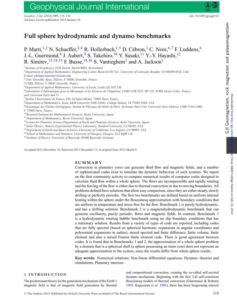
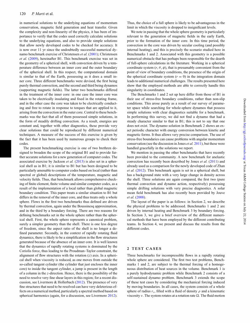
After the initial transient, the solution to Benchmark 1 settles in aquasi-stationary solution with a threefold symmetry. The alternativebranch would lead to a similar solution with fourfold symmetry. Toillustrate the solution, a few equatorial and meridional slices of thevelocity field are provided in Figs 1 and 2.

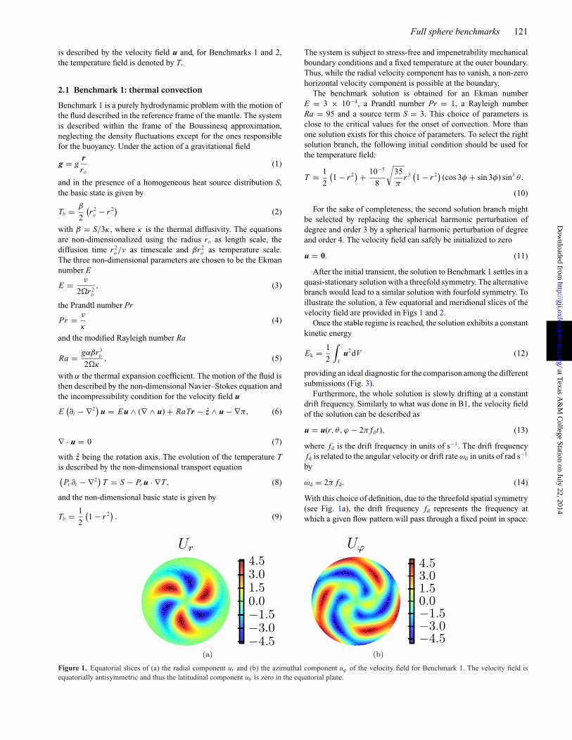
Once the stable regime is reached, the solution exhibits a constantkinetic energy

Ek = 1

2

∫V

u2dV (12)

providing an ideal diagnostic for the comparison among the differentsubmissions (Fig. 3).

Furthermore, the whole solution is slowly drifting at a constantdrift frequency. Similarly to what was done in B1, the velocity fieldof the solution can be described as

u = u(r, θ, ϕ − 2π fdt), (13)

where fd is the drift frequency in units of s−1. The drift frequencyfd is related to the angular velocity or drift rate ωd in units of rad s−1

by

ωd = 2π fd. (14)

With this choice of definition, due to the threefold spatial symmetry(see Fig. 1a), the drift frequency fd represents the frequency atwhich a given flow pattern will pass through a fixed point in space.

Figure 1. Equatorial slices of (a) the radial component ur and (b) the azimuthal component uϕ of the velocity field for Benchmark 1. The velocity field isequatorially antisymmetric and thus the latitudinal component uθ is zero in the equatorial plane.

at Texas A

&M

College Station on July 22, 2014

http://gji.oxfordjournals.org/D

ownloaded from

122 P. Marti et al.

Figure 2. Meridional slices of the velocity field u for Benchmark 1: (a) radial component ur, (b) latitudinal component uθ and (c) azimuthal component uϕ .The slices are chosen such that they contain the maximal amplitude of the velocity field |u|.

Figure 3. Typical time evolution of the kinetic energy Ek for Benchmark 1.After the initial transient, the kinetic energy reaches a constant value.

The whole solution pattern completes a full rotation at a frequencyfd = fd/3.

To compare the results of the six participants in Benchmark 1,the constant kinetic energy Ek and the drift frequency fd of theirsolution were requested.

2.2 Benchmark 2: thermally driven dynamo

Benchmark 2 extends the first benchmark by incorporating the gen-eration and evolution of magnetic fields. While still working withinthe frame of the Boussinesq approximation, the sphere is now filledwith a conducting fluid with magnetic diffusivity η and magneticpermeability μ. It is still thermally forced through the presence ofa homogeneous distribution of heat sources resulting in the basicstate given by eq. (2). The system of equations is extended by theinduction equation to describe the evolution of the magnetic field B.The equations are non-dimensionalized using the radius ro as lengthscale, the magnetic diffusion time r 2

o /η as timescale, βr 2o as the tem-

perature scale and the magnetic field is rescaled by√

2�ρμη. Thefour required parameters are the Ekman number E

E = ν

2�r 2o

, (15)

the magnetic Rossby number (also referred to as the magneticEkman number) Ro

Ro = E

Pm= η

2�r 2o

, (16)

the Roberts number q

q = Pm

Pr= κ

η, (17)

with κ the thermal diffusivity and the Rayleigh number Ra

Ra = gαβr 3o

2�κ, (18)

with α the thermal expansion coefficient. To ease the conversion todifferent choices of non-dimensionalizations, the Prandtl numberPr

Pr = ν

κ= Pm

q= E

q Ro, (19)

and the magnetic Prandtl number Pm

Pm = ν

η= E

Ro, (20)

are also introduced. The motion of the conducting fluid is describedby the non-dimensional Navier–Stokes equation and the incom-pressibility condition for the velocity field u(

Ro∂t − E∇2)

u = Rou ∧ (∇ ∧ u) + (∇ ∧ B) ∧ B

+ q RaTr − z ∧ u − ∇π, (21)

∇ · u = 0. (22)

The magnetic induction equation and the solenoidal condition forthe magnetic field B read as(∂t − ∇2

)B = ∇ ∧ (u ∧ B) , (23)

∇ · B = 0, (24)

and finally the transport equation for the temperature T is given by(∂t − q∇2

)T = S − u · ∇T . (25)

As for Benchmark 1, the outer boundary is maintained at fixedtemperature and a stress-free mechanical boundary condition isimposed. Furthermore, the outer region is considered to be a perfectinsulator.

The thermal dynamo solution for Benchmark 2 is obtained foran Ekman number E = 5 × 10−4, a magnetic Rossby numberRo = 5

7 × 10−4, a Roberts number q = 7, a Rayleigh numberRa = 200 and a source term S = 3q = 21. In terms of the Prandtlnumbers, the Benchmark 2 is obtained for a Prandtl number Pr = 1and a magnetic Prandtl Pm = 7. This parameter regime is approx-imately two times supercritical and a magnetic field is generatedand sustained by the system. Although the solution for Benchmark2 can be obtained by starting from a small initial perturbation, theconvergence to the final state is extremely slow and requires pro-hibitively high computational resources. Furthermore, the presence

at Texas A

&M

College Station on July 22, 2014

http://gji.oxfordjournals.org/D

ownloaded from

Full sphere benchmarks 123

of several solution branches can not be excluded even if it was notseen during the computations. To reduce the computational loadto a reasonable level, a special initial condition exhibiting a muchfaster convergence has been worked out.

The temperature field T should be initialized with the backgroundconducting state with a small perturbation as a spherical harmonicof degree and order 3

T = 1

2

(1 − r 2

) + ε

8

√35

πr 3

(1 − r 2

)(cos 3ϕ + sin 3ϕ) sin3 θ

(26)

with ε = 10−5. The magnetic field should be initialized with a purelytoroidal magnetic field given by

Br = 0, (27)

Bθ = −3

2r(−1 + 4r 2 − 6r 4 + 3r 6

)(cos ϕ + sin ϕ) , (28)

Bϕ = −3

4r(−1 + r 2

)cos θ

[3r

(2 − 5r 2 + 4r 4

)sin θ

+ 2(1 − 3r 2 + 3r 4

)(cos ϕ − sin ϕ)

]. (29)

Finally, the velocity field should be initialized with a purely toroidalvelocity given by

ur = 0, (30)

uθ = −10r 2

7√

3cos θ

[3(−147 + 343r 2 − 217r 4 + 29r 6

)cos ϕ

+ 14(−9 − 125r 2 + 39r 4 + 27r 6

)sin ϕ

], (31)

uϕ = − 5r

5544

{7[(43 700 − 58 113r 2 − 15 345r 4

+ 1881r 6 + 20 790r 8) sin θ

+ 1485r 2(−9 + 115r 2 − 167r 4 + 70r 6

)sin 3θ

]+ 528

√3r cos 2θ

[14

(−9 − 125r 2 + 39r 4 + 27r 6)

cos ϕ

+ 3(147 − 343r 2 + 217r 4 − 29r 6

)sin ϕ

]}. (32)

For simulations using spherical harmonics and a toroidal/poloidaldecomposition, the expression of the initial conditions can be writ-ten in a simpler form. Assuming that the magnetic field is decom-posed as B = ∇ ∧ T r + ∇ ∧ ∇ ∧ P r , the initial field is given bythe two scalars

T = r

[(3

4−3r 2+ 9

2r 4− 9

4r 6

)+

(3

4−3r 2+ 9

2r 4− 9

4r 6

)ı

]Y1

1

+ r 2

(3

2− 21

4r 2 + 27

4r 4 − 3r 6

)Y0

2 + c.c., (33)

P = 0, (34)

where c.c. stands for the complex conjugate without the m = 0modes and Ym

l are Schmidt normalized complex spherical harmon-ics. Similarly assuming that the velocity field is decomposed asu = ∇ ∧ T r + ∇ ∧ ∇ ∧ P r , the initial condition is given by

T = r 2

[ (30 + 1250

3r 2 − 130r 4 − 90r 6

)

+(

105 − 245r 2 + 155r 4 − 145

7r 6

)ı

]Y1

2

+ r

(−54 625

198+ 350r 2 + 625

2r 4 − 325r 6

)Y0

1

+ r 3(45 − 575r 2 + 835r 4 − 350r 6

)Y0

3 + c.c., (35)

P = 0. (36)

Details of the definition and the normalization of the sphericalharmonics Ym

l are given in Appendix A.The structure of the solution to Benchmark 2 is much more

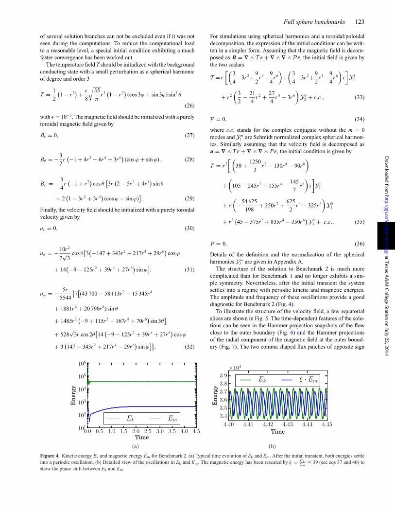
complicated than for Benchmark 1 and no longer exhibits a sim-ple symmetry. Nevertheless, after the initial transient the systemsettles into a regime with periodic kinetic and magnetic energies.The amplitude and frequency of these oscillations provide a gooddiagnostic for Benchmark 2 (Fig. 4).

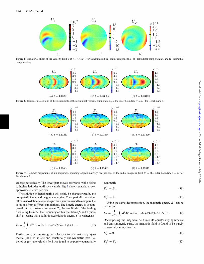
To illustrate the structure of the velocity field, a few equatorialslices are shown in Fig. 5. The time-dependent features of the solu-tions can be seen in the Hammer projection snapshots of the flowclose to the outer boundary (Fig. 6) and the Hammer projectionsof the radial component of the magnetic field at the outer bound-ary (Fig. 7). The two comma shaped flux patches of opposite sign

Figure 4. Kinetic energy Ek and magnetic energy Em for Benchmark 2. (a) Typical time evolution of Ek and Em. After the initial transient, both energies settleinto a periodic oscillation. (b) Detailed view of the oscillations in Ek and Em. The magnetic energy has been rescaled by ξ = Ck

Cm≈ 39 (see eqs 37 and 40) to

show the phase shift between Ek and Em.

at Texas A

&M

College Station on July 22, 2014

http://gji.oxfordjournals.org/D

ownloaded from

124 P. Marti et al.

Figure 5. Equatorial slices of the velocity field u at t = 4.43241 for Benchmark 2: (a) radial component ur, (b) latitudinal component uθ and (c) azimuthalcomponent uϕ .

Figure 6. Hammer projections of three snapshots of the azimuthal velocity component uϕ at the outer boundary (r = ro) for Benchmark 2.

Figure 7. Hammer projections of six snapshots, spanning approximatively two periods, of the radial magnetic field Br at the outer boundary r = ro forBenchmark 2.

emerge periodically. The lower part moves eastwards while risingto higher latitudes until they vanish. Fig 7 shows snapshots overapproximately two periods.

The solution to Benchmark 2 will solely be characterized by thecomputed kinetic and magnetic energies. Their periodic behaviourallows us to define several diagnostic quantities used to compare thesolutions from different simulations. The kinetic energy is decom-posed into a constant component Ck, the amplitude of the leadingoscillating term Ak, the frequency of this oscillation fk and a phaseshift ζ k. Using these definitions,the kinetic energy Ek is written as

Ek = 1

2

∫V

u2dV = Ck + Ak cos(2π fkt + ζk) + · · · (37)

Furthermore, decomposing the velocity into its equatorially sym-metric [labelled as (s)] and equatorially antisymmetric part [la-belled as (a)], the velocity field was found to be purely equatorially

symmetric

E (s)k = Ek, (38)

E (a)k = 0. (39)

Using the same decomposition, the magnetic energy Em can bewritten as

Em = 1

2Ro

∫V

B2dV = Cm + Am cos(2π fmt + ζm) + · · · (40)

Decomposing the magnetic field into its equatorially symmetricand antisymmetric parts, the magnetic field is found to be purelyequatorially antisymmetric

E (s)m = 0, (41)

E (a)m = Em. (42)

at Texas A

&M

College Station on July 22, 2014

http://gji.oxfordjournals.org/D

ownloaded from

Full sphere benchmarks 125

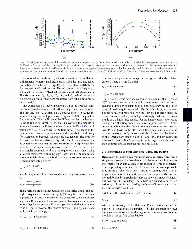
Figure 8. (a) Frequency spectrum of the kinetic energy Ek and magnetic energy Em for Benchmark 2 after a flat top window has been applied on the time-series.(b) Details of the peak of the main amplitude of the kinetic and magnetic energies after a Kaiser window with parameter β = 14 has been applied to thetime-series. Note the use of a logarithmic scale for the ordinate, meaning that the frequency localization is extremely good. Both spectra have been obtained ona time-series over approximatively 0.35 diffusion times at a sampling rate of 1.75 × 105 obtained by (MJ) at N = 31 and L = M = 63 (see Section 3 for details).

It was found and confirmed by all participants that the oscillationsin the magnetic energy and kinetic energy have the same frequency.In addition, as can be seen in Fig. 4(b), there is a phase shift betweenthe magnetic and kinetic energy. This relative phase shift (ζk − ζm)is found to have value 1.91rad but is not included in the benchmark.The six constants Ck, Ak, fk, Cm, Am and fm defined above arethe diagnostic values that were requested from all submissions toBenchmark 2.

The computation of decompositions 37 and 40 requires somefurther explanations as several different approaches are possible.The first one involves computing the Fourier series. To reduce thespectral leakage, a flat top window (Oliphant 2007) is applied onthe time-series. The amplitude of the different modes can then eas-ily be extracted as shown in Fig. 8(a). Conversely, to compute anaccurate frequency, a Kaiser window (Kaiser & Kuo 1966) withparameter β = 14 is applied to the time-series. The peaks in thespectrum are then well approximated with a parabolic fit allowingfor interpolation between the available frequencies. The peak forthe main oscillation is shown in Fig. 8(b). The frequencies can alsobe computed by counting the zero crossings. Both approaches pro-vide the frequency within a relative error of 10−4 per cent. Thereis a simpler approach to obtain the requested data without usinga Fourier transform. Assuming Emin

i , Emaxi are the minimum and

maximum of the time-series for the energy, the constant componentis approximatively given by

Ci ≈ Emini + Emax

i

2, (43)

and the amplitude of the main oscillation is approximatively givenby

Ai ≈ Emaxi − Emin

i

2. (44)

These relations are not exact because the time-series do also includehigher frequencies as shown in Fig. 8(a). Using the Fourier series, itis possible to bound the relative errors generated by the simplifiedapproach. By including the second peak with a frequency of 2fi andaccounting for the phase shift, a comparison with the approxima-tions 43 and 44 provides the relative errors εCk and εAk on Ck andAk for the kinetic energy

εCk = 3 × 10−2 per cent, (45)

εAk = 5 × 10−2 per cent. (46)

The same analysis on the magnetic energy provides the relativeerrors εCm and εAm on Cm and Am

εCm = 0.4 per cent, (47)

εAm = 0.6 per cent. (48)

These relative errors have been obtained by assuming that Emini and

Emaxi are exact. An accurate value for the minimum and maximum

requires a time-series sampled at a high frequency but it does inprinciple only require one cycle. On the other hand, an accurateFourier series will require a long time-series. The errors made byusing this simplified approach depend strongly on the relative mag-nitude of the higher frequencies. For the kinetic energy, the secondoscillation with a frequency of 2fk has an approximatively 63 timessmaller amplitude which leads to the rather small errors given ineqs (45) and (46). On the other hand, the second oscillation in themagnetic energy is only approximatively 10 times smaller leadingto the larger errors given in eqs (47) and (48). In both cases, thethird oscillation with a frequency 3f can be neglected as it is morethan 20 times smaller than the second oscillation.

2.3 Benchmark 3: boundary forced rotating bubble

Benchmark 3 is again a purely hydrodynamic problem. It provides asimple test problem for boundary driven flows in a whole sphere asthey might, for example, arise in precession or libration problems.The proposed system describes the motion of an incompressiblefluid inside a spherical bubble rising in a rotating fluid. It is animportant addition to the first two cases as it replaces the internalthermal forcing by a mechanical forcing due to an imposed tangen-tial flow over the boundary. The bubble is assumed to be of unitradius ro = 1 and is described by the Navier–Stokes equation andincompressibility condition

∂t u + u · ∇u + 2� z ∧ u = −∇ p + ν∇2u, (49)

∇ · u = 0 (50)

with ν the viscosity of the fluid and � the rotation rate of thebubble. The rotation axis is parallel to z. The tangential flow overthe boundary imposes a non-homogeneous boundary condition onthe fluid at the surface of the bubble

uθ = −u0 cos θ cos φ, (51)

uφ = u0 sin φ, (52)

at Texas A

&M

College Station on July 22, 2014

http://gji.oxfordjournals.org/D

ownloaded from

126 P. Marti et al.

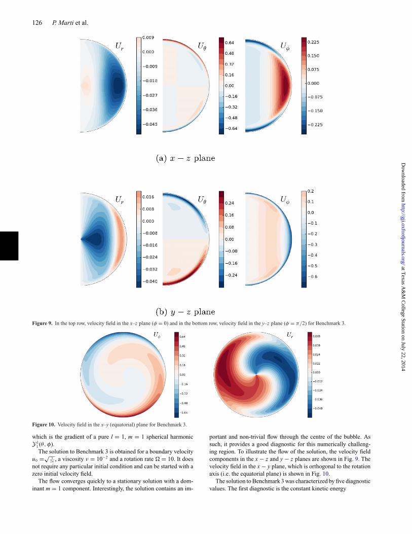
Figure 9. In the top row, velocity field in the x–z plane (φ = 0) and in the bottom row, velocity field in the y–z plane (φ = π/2) for Benchmark 3.

Figure 10. Velocity field in the x–y (equatorial) plane for Benchmark 3.

which is the gradient of a pure l = 1, m = 1 spherical harmonicY1

1 (θ, φ).The solution to Benchmark 3 is obtained for a boundary velocity

u0 =√3

2π, a viscosity ν = 10−2 and a rotation rate � = 10. It does

not require any particular initial condition and can be started with azero initial velocity field.

The flow converges quickly to a stationary solution with a dom-inant m = 1 component. Interestingly, the solution contains an im-

portant and non-trivial flow through the centre of the bubble. Assuch, it provides a good diagnostic for this numerically challeng-ing region. To illustrate the flow of the solution, the velocity fieldcomponents in the x − z and y − z planes are shown in Fig. 9. Thevelocity field in the x − y plane, which is orthogonal to the rotationaxis (i.e. the equatorial plane) is shown in Fig. 10.

The solution to Benchmark 3 was characterized by five diagnosticvalues. The first diagnostic is the constant kinetic energy

at Texas A

&M

College Station on July 22, 2014

http://gji.oxfordjournals.org/D

ownloaded from

Full sphere benchmarks 127

Ek = 1

2

∫V

u2dV (53)

reached after the initial transient. When available, the energy in thespherical harmonic orders m = 0, m = 1 and m = 2 have also beencollected. Secondly, the z component of the angular momentumLz is reported. The three components of the velocity field u at thecentre of the bubble provide that last diagnostic data.

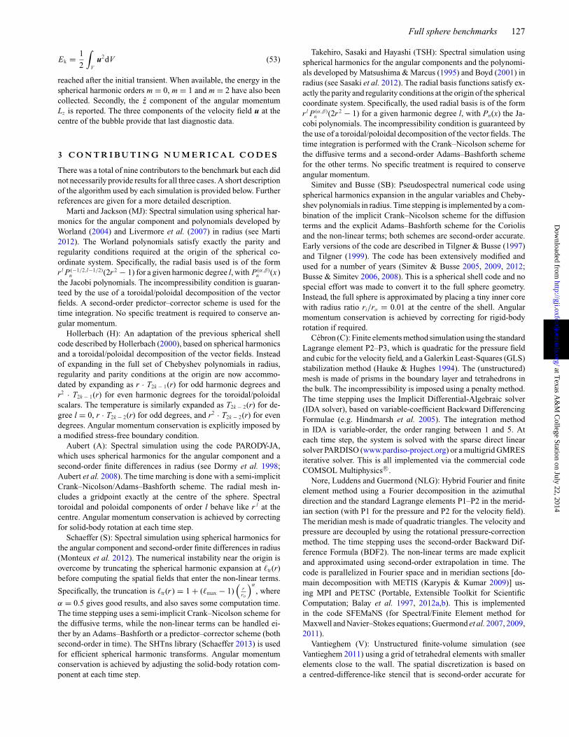
3 C O N T R I B U T I N G N U M E R I C A L C O D E S

There was a total of nine contributors to the benchmark but each didnot necessarily provide results for all three cases. A short descriptionof the algorithm used by each simulation is provided below. Furtherreferences are given for a more detailed description.

Marti and Jackson (MJ): Spectral simulation using spherical har-monics for the angular component and polynomials developed byWorland (2004) and Livermore et al. (2007) in radius (see Marti2012). The Worland polynomials satisfy exactly the parity andregularity conditions required at the origin of the spherical co-ordinate system. Specifically, the radial basis used is of the formr l P (−1/2,l−1/2)

n (2r 2 − 1) for a given harmonic degree l, with P (α,β)n (x)

the Jacobi polynomials. The incompressibility condition is guaran-teed by the use of a toroidal/poloidal decomposition of the vectorfields. A second-order predictor–corrector scheme is used for thetime integration. No specific treatment is required to conserve an-gular momentum.

Hollerbach (H): An adaptation of the previous spherical shellcode described by Hollerbach (2000), based on spherical harmonicsand a toroidal/poloidal decomposition of the vector fields. Insteadof expanding in the full set of Chebyshev polynomials in radius,regularity and parity conditions at the origin are now accommo-dated by expanding as r · T2k − 1(r) for odd harmonic degrees andr2 · T2k − 1(r) for even harmonic degrees for the toroidal/poloidalscalars. The temperature is similarly expanded as T2k − 2(r) for de-gree l = 0, r · T2k − 2(r) for odd degrees, and r2 · T2k − 2(r) for evendegrees. Angular momentum conservation is explicitly imposed bya modified stress-free boundary condition.

Aubert (A): Spectral simulation using the code PARODY-JA,which uses spherical harmonics for the angular component and asecond-order finite differences in radius (see Dormy et al. 1998;Aubert et al. 2008). The time marching is done with a semi-implicitCrank–Nicolson/Adams–Bashforth scheme. The radial mesh in-cludes a gridpoint exactly at the centre of the sphere. Spectraltoroidal and poloidal components of order l behave like r l at thecentre. Angular momentum conservation is achieved by correctingfor solid-body rotation at each time step.

Schaeffer (S): Spectral simulation using spherical harmonics forthe angular component and second-order finite differences in radius(Monteux et al. 2012). The numerical instability near the origin isovercome by truncating the spherical harmonic expansion at �tr(r)before computing the spatial fields that enter the non-linear terms.

Specifically, the truncation is �tr(r ) = 1 + (�max − 1)(

rro

)α

, where

α = 0.5 gives good results, and also saves some computation time.The time stepping uses a semi-implicit Crank–Nicolson scheme forthe diffusive terms, while the non-linear terms can be handled ei-ther by an Adams–Bashforth or a predictor–corrector scheme (bothsecond-order in time). The SHTns library (Schaeffer 2013) is usedfor efficient spherical harmonic transforms. Angular momentumconservation is achieved by adjusting the solid-body rotation com-ponent at each time step.

Takehiro, Sasaki and Hayashi (TSH): Spectral simulation usingspherical harmonics for the angular components and the polynomi-als developed by Matsushima & Marcus (1995) and Boyd (2001) inradius (see Sasaki et al. 2012). The radial basis functions satisfy ex-actly the parity and regularity conditions at the origin of the sphericalcoordinate system. Specifically, the used radial basis is of the formr l P (α,β)

n (2r 2 − 1) for a given harmonic degree l, with Pn(x) the Ja-cobi polynomials. The incompressibility condition is guaranteed bythe use of a toroidal/poloidal decomposition of the vector fields. Thetime integration is performed with the Crank–Nicolson scheme forthe diffusive terms and a second-order Adams–Bashforth schemefor the other terms. No specific treatment is required to conserveangular momentum.

Simitev and Busse (SB): Pseudospectral numerical code usingspherical harmonics expansion in the angular variables and Cheby-shev polynomials in radius. Time stepping is implemented by a com-bination of the implicit Crank–Nicolson scheme for the diffusionterms and the explicit Adams–Bashforth scheme for the Coriolisand the non-linear terms; both schemes are second-order accurate.Early versions of the code are described in Tilgner & Busse (1997)and Tilgner (1999). The code has been extensively modified andused for a number of years (Simitev & Busse 2005, 2009, 2012;Busse & Simitev 2006, 2008). This is a spherical shell code and nospecial effort was made to convert it to the full sphere geometry.Instead, the full sphere is approximated by placing a tiny inner corewith radius ratio ri/ro = 0.01 at the centre of the shell. Angularmomentum conservation is achieved by correcting for rigid-bodyrotation if required.

Cebron (C): Finite elements method simulation using the standardLagrange element P2–P3, which is quadratic for the pressure fieldand cubic for the velocity field, and a Galerkin Least-Squares (GLS)stabilization method (Hauke & Hughes 1994). The (unstructured)mesh is made of prisms in the boundary layer and tetrahedrons inthe bulk. The incompressibility is imposed using a penalty method.The time stepping uses the Implicit Differential-Algebraic solver(IDA solver), based on variable-coefficient Backward DifferencingFormulae (e.g. Hindmarsh et al. 2005). The integration methodin IDA is variable-order, the order ranging between 1 and 5. Ateach time step, the system is solved with the sparse direct linearsolver PARDISO (www.pardiso-project.org) or a multigrid GMRESiterative solver. This is all implemented via the commercial codeCOMSOL Multiphysics R©.

Nore, Luddens and Guermond (NLG): Hybrid Fourier and finiteelement method using a Fourier decomposition in the azimuthaldirection and the standard Lagrange elements P1–P2 in the merid-ian section (with P1 for the pressure and P2 for the velocity field).The meridian mesh is made of quadratic triangles. The velocity andpressure are decoupled by using the rotational pressure-correctionmethod. The time stepping uses the second-order Backward Dif-ference Formula (BDF2). The non-linear terms are made explicitand approximated using second-order extrapolation in time. Thecode is parallelized in Fourier space and in meridian sections [do-main decomposition with METIS (Karypis & Kumar 2009)] us-ing MPI and PETSC (Portable, Extensible Toolkit for ScientificComputation; Balay et al. 1997, 2012a,b). This is implementedin the code SFEMaNS (for Spectral/Finite Element method forMaxwell and Navier–Stokes equations; Guermond et al. 2007, 2009,2011).

Vantieghem (V): Unstructured finite-volume simulation (seeVantieghem 2011) using a grid of tetrahedral elements with smallerelements close to the wall. The spatial discretization is based ona centred-difference-like stencil that is second-order accurate for

at Texas A

&M

College Station on July 22, 2014

http://gji.oxfordjournals.org/D

ownloaded from

128 P. Marti et al.

regular tetrahedra. Time stepping is based on a canonical fractional-step method (Kim & Moin 1985), and the equations are integratedin time with a fourth order Runge–Kutta method. A BiCGstab(2) al-gorithm is used to solve the pressure Poisson equation. The reportedFourier components are obtained by an a posteriori interpolationof the results on a regular grid in terms of spherical coordinates(Nr = 36, Nθ = Nϕ = 18), which is subject to considerable addi-tional numerical (interpolation) errors.

Table 1. Contributions to Benchmark 1. The labelsused for the different codes are defined in Section 3.The values are shown with the number of significantdigits provided by the authors. As all these codes arebased on a spherical harmonics expansion for the an-gular component, the resolution is given as the radialresolution N, the highest harmonic degree L and thehighest harmonic order M.

Code Ek fd N L M

(MJ) 29.08502 12.38841 8 15 15(MJ) 29.07661 12.38860 8 23 23(MJ) 29.12178 12.38604 12 23 23(MJ) 29.12064 12.38619 16 23 23(MJ) 29.12064 12.38619 16 31 31(MJ) 29.12068 12.38619 23 47 47(MJ) 29.12068 12.38619 31 63 63(H) 29.11784 12.3862 12 23 23(H) 29.12054 12.3862 16 31 31(H) 29.12053 12.3862 23 31 31(H) 29.12053 12.3862 23 47 47(H) 29.12053 12.3862 31 63 63(S) 29.219 12.388 120 31 31(S) 29.1446 12.387 250 63 63(S) 29.13501 12.38648 320 85 85(TSH) 29.03074 12.3878 16 21 21(TSH) 29.12878 12.3863 32 42 42(TSH) 29.12878 12.3863 48 85 85(SB) 29.00617 11.89445 33 42 42(A) 29.12062 12.3931 1600 63 63

4 R E S U LT S

There is quite an important diversity in the type of simulationsthat took part in these benchmarks. All the diagnostics that havebeen considered for these benchmarks should be straightforwardto obtain whenever the simulation code is based on some spec-tral expansion or on a local method. On the other hand, a directcomparison of the resolution used is a more subtle problem. Thecomparison will be done by comparing solutions based on the num-ber of degrees of freedom present at the time stepping level. Forlocal methods, the resolution R is computed as R = N 1/3

grid whereNgrid is the number of gridpoints and for spherical harmonic–based

codes R = {Nr · [

Lmax(2Mmax + 1) − M2max + Mmax + 1

]}1/3. The

same approach was used in B1.

4.1 Benchmark 1

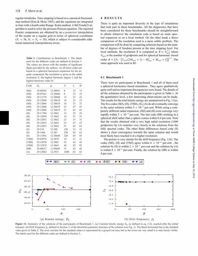
There were six participants in Benchmark 1 and all of them useda spherical harmonics–based simulation . They agree qualitativelyquite well and no important discrepancies were found. The details ofall the solutions obtained by the participants is given in Table 1. Atthe quantitative level, a few interesting observations can be made.The results for the total kinetic energy are summarized in Fig. 11(a).The five codes (MJ), (H), (TSH), (S), (A) do all eventually convergeto the same solution within 5 × 10−2 per cent. While using a com-pletely different radial expansion, (MJ) and (H) even converge veryrapidly within 5 × 10−4 per cent. The last code (SB) working in aspherical shell rather than a sphere comes within 0.4 per cent. Notethat the results obtained with a very high radial resolution (1600gridpoints) by (A) matches very closely to the solutions from thefully spectral codes. The other finite differences–based code (S)shows a clear convergence towards the same solution and wouldmost likely have reached it at a higher resolution.

The picture is very similar for the drift frequency (Fig. 11b). Thecodes (MJ), (H) and (TSH) agree within 6 × 10−4 per cent , thesolution by (S) is within 2 × 10−3 per cent and the solution by (A)is within 6 × 10−2 per cent. Finally, the solution by (SB) is within4 per cent.

Figure 11. Summary of the solutions of the participants of Benchmark 1. (a) Constant kinetic energy Ek, as defined in eq. (12), reached after the initialtransient. (b) Drift frequency fd, defined in Section 2, of the threefold symmetric structure of the solution (see Fig. 1). The black horizontal line is the standardvalue given in Table 2. The error corridor for the standard values is represented by a greyed out area, but as the errors are very small it is only barely visible.The labels used for the different codes are defined in Section 3.

at Texas A

&M

College Station on July 22, 2014

http://gji.oxfordjournals.org/D

ownloaded from

Full sphere benchmarks 129

Table 2. Summary table and standard values obtained forBenchmark 1. The Ekman number E, the Prandtl numberPr and the modified Rayleigh number Ra as well as thegoverning equation for the velocity u and the temperature Tare given in Section 2. The kinetic energy Ek is defined ineq. (12) and the drift frequency by eq. (13).

Benchmark 1: Thermal convection

Parameters

E Pr Ra3 × 10−4 1 95

Boundary conditions

u: stress-freeT: fixed temperature

homogeneous heat sources

Requested values

Ek 29.1206 ±1 × 10−4

fd 12.3862 ±1 × 10−4

A standard value for the kinetic energy and drift frequency forBenchmark 1 is derived from the three simulations showing thebest convergence to a common result. The values as well as a shortsummary of the problem definition are given in Table 2. The veryhigh convergence to a common solution allow to provide these withroughly six significant digits.

4.2 Benchmark 2

All the groups participating in Benchmark 1 also participated inBenchmark 2, except for (A). There are thus again only solutionsfrom spherical harmonics–based simulations. The overall picture isvery similar to Benchmark 1. The fully spectral simulations con-verge very rapidly to their final solution and which are in most casesvery close to each other. The finite differences simulation, whilerequiring higher radial resolution, eventually reaches a similar so-lution. As was already observed in Benchmark 1, the simulationby (SB) which approximates the whole sphere as a shell with a

tiny inner core, shows the largest discrepancy. The details of all thesolutions to Benchmark 2 are given in Table 3.

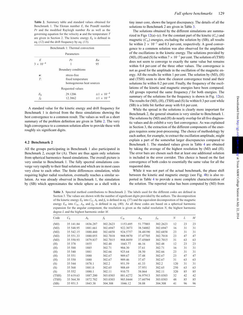
The solutions obtained by the different simulations are summa-rized in Figs 12(a)–(e). For the constant part of the kinetic (Ck) andmagnetic (Cm) energies, excluding the solution by (SB), all resultslie within 2 × 10−2 and 0.3 per cent, respectively. A good conver-gence to a common solution was also observed for the amplitudeof the oscillations in the kinetic energy. The solutions provided by(MJ), (H) and (S) lie within 7 × 10−3 per cent. The solution of (TSH)does not seem to converge to exactly the same value but remainswithin 0.4 per cent of the three other values. The convergence isnot as good for the amplitude in the oscillation of the magnetic en-ergy. All the results lie within 1 per cent. The solution by (MJ), (H)and (TSH) seem to show the clearest convergence trend and theirsolutions lie within 0.2 per cent. Finally, the frequency of the oscil-lations of the kinetic and magnetic energies have been compared.All groups reported the same frequency f for both energies. Thesummary of the solutions for the frequency is shown in Fig. 12(e).The results for (MJ), (H), (TSH) and (S) lie within 0.3 per cent while(SB) is a little bit further away with 0.6 per cent.

While the spread in the solutions is clearly more important forBenchmark 2, the general situation is very similar to Benchmark 1.The solutions by (MJ) and (H) do nearly overlap for all five diagnos-tic values and do exhibit a very fast convergence. As was explainedin Section 3, the extraction of the different components of the ener-gies requires some post-processing. The choice of methodology byeach author, for example, to extract the oscillation amplitude, mightexplain a part of the somewhat larger discrepancies compared toBenchmark 1. The standard values given in Table 4 are obtainedby taking the average of the highest resolution by (MJ) and (H).The error bars are chosen such that at least one additional solutionis included in the error corridor. This choice is based on the fastconvergence of both codes to essentially the same value for all therequested data.

While it was not part of the actual benchmark, the phase shiftbetween the kinetic and magnetic energy (see Fig. 4b) is also re-ported in Table 4 to provide a more complete characterization ofthe solution. The reported value has been computed by (MJ) from

Table 3. Spectral method contributions to Benchmark 2. The labels used for the different codes are defined inSection 3. The values are shown with the number of significant digits provided by the authors. The decompositionof the kinetic energy Ek into Ck, Ak and fk is defined in eq. (37) and the equivalent decomposition of the magneticenergy Em into Cm, Am and fm is defined in eq. (40). As all these codes are based on a spherical harmonicexpansion for the angular component, the resolution is given as the radial resolution N, the highest harmonicdegree L and the highest harmonic order M.

Code Ck Ak fk Cm Am fm N L M

(MJ) 35 141.84 1836.287 302.2623 1153.695 51.77003 302.2623 12 23 23(MJ) 35 548.95 1881.661 302.6947 922.3073 38.54002 302.6947 16 31 31(MJ) 35 542.15 1880.460 302.6858 924.5757 38.48190 302.6858 23 31 31(MJ) 35 551.33 1880.055 302.7018 908.9870 37.47705 302.7018 23 47 47(MJ) 35 550.93 1879.837 302.7015 908.8059 37.45069 302.7015 31 63 63(H) 35 378 1855 302.48 1043.77 46.16 302.48 12 23 23(H) 35 588 1885 302.71 904.30 37.61 302.71 16 31 31(H) 35 540 1881 302.66 925.64 38.50 302.66 23 31 31(H) 35 551 1880 302.67 909.67 37.48 302.67 23 47 47(H) 35 550 1880 302.67 909.46 37.47 302.67 31 63 63(S) 35 544 1878.1 302.2 951.59 41.33 302.2 120 31 31(S) 35 568 1881.0 302.65 908.69 37.951 302.65 250 63 63(S) 35 552 1880.1 302.11 910.75 38.064 302.11 320 85 85(TSH) 35 619.63 1887.200 303.0303 881.6272 36.97913 303.0303 32 42 42(TSH) 35 564.30 1872.702 303.0303 905.8444 37.60794 303.0303 48 85 85(SB) 35 951.5 1843.38 304.308 1046.12 38.08 304.308 41 96 96

at Texas A

&M

College Station on July 22, 2014

http://gji.oxfordjournals.org/D

ownloaded from

130 P. Marti et al.

Figure 12. Summary of the solutions of the participants to Benchmark 2. The decomposition of the kinetic energy Ek into a constant part Ck, the amplitude ofthe main oscillation Ak and its frequency fk is defined in eq. (37). The equivalent decomposition for the magnetic energy Em, defining the three constants Cm,Am and fm is given in eq. (40). The black horizontal line is the standard value given in Table 4. The error corridor for the standard values, defined such that thethree most converged solutions are included, is represented by a greyed out area. The labels used for the different codes are defined in Section 3.

time-series of the kinetic and magnetic energy at the highest re-ported resolution (N = 31, L = M = 63). The phase shift has beenextracted from the Fourier series shown in Fig. 8.

4.3 Benchmark 3

Benchmark 3 had the highest number of participants with eightcodes taking part. It is also the only case where results from localmethods are available. The computation for Benchmark 3 does notrequire a very high horizontal resolution. For example, sphericalharmonics–based codes exhibit a very good convergence at reso-

lutions as low as Lmax = 30 and Mmax = 10. However, it is moredemanding in the radial direction. The centre requires a sufficientlyhigh resolution to describe flow crossing it properly as well as themoving outer boundary which is forcing the system.

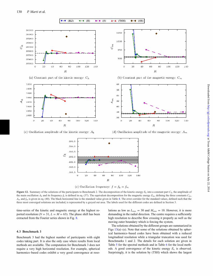
The solutions obtained by the different groups are summarized inFigs 13(a)–(e). Note that some of the solutions obtained by spher-ical harmonics–based codes have been obtained with a reducedlongitudinal resolution while a triangular truncation was used forBenchmarks 1 and 2. The details for each solution are given inTable 5 for the spectral methods and in Table 6 for the local meth-ods. A good convergence of the kinetic energy Ek is observed.Surprisingly, it is the solution by (TSH) which shows the largest

at Texas A

&M

College Station on July 22, 2014

http://gji.oxfordjournals.org/D

ownloaded from

Full sphere benchmarks 131

Table 4. Summary table and standard values obtained for Benchmark 2. TheEkman number E, the magnetic Rossby number Ro, the Roberts number qand the modified Rayleigh number Ra, as well as the governing equationsfor the velocity u, the magnetic field B and the temperature T are given inSection 2. The decomposition of the kinetic energy Ek into constant andoscillating components is defined in eq. (37) and the decomposition of themagnetic energy is defined in eq. (40).

Benchmark 2: Thermally driven dynamo

Parameters

E Ro q Ra5 × 10−4 5/7 × 10−4 7 200

Boundary conditions

u: stress-freeB: insulatingT: fixed temperature

homogeneous heat sources

Requested values

Kinetic energy Ek

Ck 35 550.5 ±1.5Ak 1879.84 ±0.26

Magnetic energy Em

Cm 909.133 ±1.62Am 37.4603 ±0.1476

Frequency f = fk = fm 302.701 ±0.33

Additional characteristic

Phase shift |ζk − ζm| 1.91rad

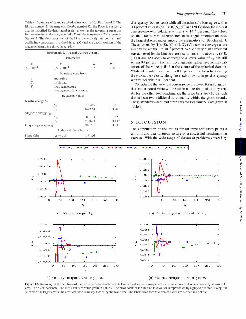
discrepancy (0.4 per cent) while all the other solutions agree within0.1 per cent at least. (MJ), (H), (S), (C) and (NLG) show the clearestconvergence with solutions within 8 × 10−3 per cent. The valuesobtained for the vertical component of the angular momentum showthe largest discrepancies among the diagnostics for Benchmark 3.The solutions by (H), (S), (C), (NLG), (V) seem to converge to thesame value within 7 × 10−2 per cent. While a very high agreementwas achieved for the kinetic energy solutions, simulations by (MJ),(TSH) and (A) seem to converge to a lower value of Lz but stillwithin 0.4 per cent. The last two diagnostic values involve the eval-uation of the velocity field at the centre of the spherical domain.While all simulations lie within 0.15 per cent for the velocity alongthe y-axis, the velocity along the x-axis shows a larger discrepancywith values within 0.3 per cent.

Considering the very fast convergence it showed for all diagnos-tics, the standard value will be taken as the final solution by (H).As for the other two benchmarks, the error bars are chosen suchthat at least two additional solutions lie within the given bounds.These standard values and error bars for Benchmark 3 are given inTable 7.

5 D I S C U S S I O N

The combination of the results for all three test cases paints auniform and unambiguous picture of a successful benchmarkingexercise. With the wide range of classes of problems covered by

Figure 13. Summary of the solutions of the participants to Benchmark 3. The vertical velocity component uz is not shown as it was consistently shown to bezero. The black horizontal line is the standard value given in Table 7. The error corridor for the standard values is represented by a greyed out area. Except for(c) which has larger errors, the error corridor is mostly hidden by the black line. The labels used for the different codes are defined in Section 3.

at Texas A

&M

College Station on July 22, 2014

http://gji.oxfordjournals.org/D

ownloaded from

132 P. Marti et al.

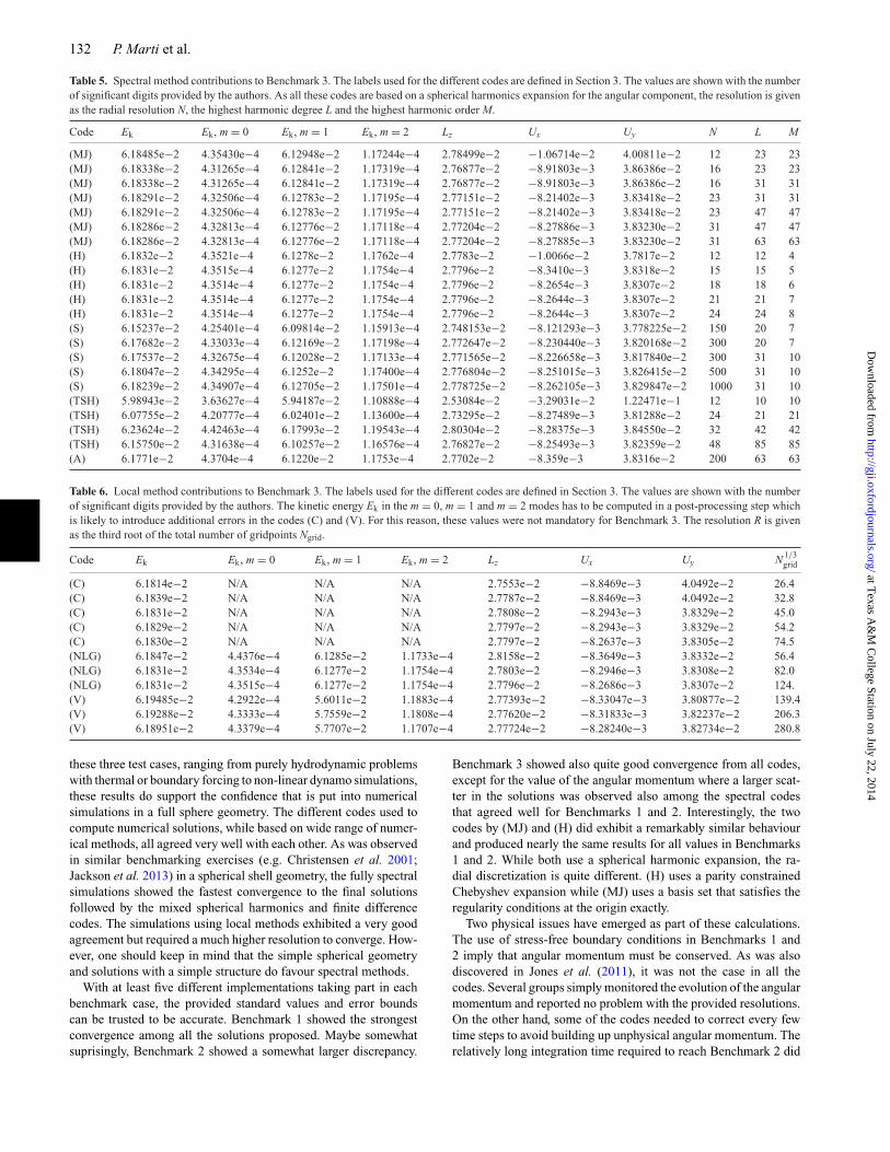
Table 5. Spectral method contributions to Benchmark 3. The labels used for the different codes are defined in Section 3. The values are shown with the numberof significant digits provided by the authors. As all these codes are based on a spherical harmonics expansion for the angular component, the resolution is givenas the radial resolution N, the highest harmonic degree L and the highest harmonic order M.

Code Ek Ek, m = 0 Ek, m = 1 Ek, m = 2 Lz Ux Uy N L M

(MJ) 6.18485e−2 4.35430e−4 6.12948e−2 1.17244e−4 2.78499e−2 −1.06714e−2 4.00811e−2 12 23 23(MJ) 6.18338e−2 4.31265e−4 6.12841e−2 1.17319e−4 2.76877e−2 −8.91803e−3 3.86386e−2 16 23 23(MJ) 6.18338e−2 4.31265e−4 6.12841e−2 1.17319e−4 2.76877e−2 −8.91803e−3 3.86386e−2 16 31 31(MJ) 6.18291e−2 4.32506e−4 6.12783e−2 1.17195e−4 2.77151e−2 −8.21402e−3 3.83418e−2 23 31 31(MJ) 6.18291e−2 4.32506e−4 6.12783e−2 1.17195e−4 2.77151e−2 −8.21402e−3 3.83418e−2 23 47 47(MJ) 6.18286e−2 4.32813e−4 6.12776e−2 1.17118e−4 2.77204e−2 −8.27886e−3 3.83230e−2 31 47 47(MJ) 6.18286e−2 4.32813e−4 6.12776e−2 1.17118e−4 2.77204e−2 −8.27885e−3 3.83230e−2 31 63 63(H) 6.1832e−2 4.3521e−4 6.1278e−2 1.1762e−4 2.7783e−2 −1.0066e−2 3.7817e−2 12 12 4(H) 6.1831e−2 4.3515e−4 6.1277e−2 1.1754e−4 2.7796e−2 −8.3410e−3 3.8318e−2 15 15 5(H) 6.1831e−2 4.3514e−4 6.1277e−2 1.1754e−4 2.7796e−2 −8.2654e−3 3.8307e−2 18 18 6(H) 6.1831e−2 4.3514e−4 6.1277e−2 1.1754e−4 2.7796e−2 −8.2644e−3 3.8307e−2 21 21 7(H) 6.1831e−2 4.3514e−4 6.1277e−2 1.1754e−4 2.7796e−2 −8.2644e−3 3.8307e−2 24 24 8(S) 6.15237e−2 4.25401e−4 6.09814e−2 1.15913e−4 2.748153e−2 −8.121293e−3 3.778225e−2 150 20 7(S) 6.17682e−2 4.33033e−4 6.12169e−2 1.17198e−4 2.772647e−2 −8.230440e−3 3.820168e−2 300 20 7(S) 6.17537e−2 4.32675e−4 6.12028e−2 1.17133e−4 2.771565e−2 −8.226658e−3 3.817840e−2 300 31 10(S) 6.18047e−2 4.34295e−4 6.1252e−2 1.17400e−4 2.776804e−2 −8.251015e−3 3.826415e−2 500 31 10(S) 6.18239e−2 4.34907e−4 6.12705e−2 1.17501e−4 2.778725e−2 −8.262105e−3 3.829847e−2 1000 31 10(TSH) 5.98943e−2 3.63627e−4 5.94187e−2 1.10888e−4 2.53084e−2 −3.29031e−2 1.22471e−1 12 10 10(TSH) 6.07755e−2 4.20777e−4 6.02401e−2 1.13600e−4 2.73295e−2 −8.27489e−3 3.81288e−2 24 21 21(TSH) 6.23624e−2 4.42463e−4 6.17993e−2 1.19543e−4 2.80304e−2 −8.28375e−3 3.84550e−2 32 42 42(TSH) 6.15750e−2 4.31638e−4 6.10257e−2 1.16576e−4 2.76827e−2 −8.25493e−3 3.82359e−2 48 85 85(A) 6.1771e−2 4.3704e−4 6.1220e−2 1.1753e−4 2.7702e−2 −8.359e−3 3.8316e−2 200 63 63

Table 6. Local method contributions to Benchmark 3. The labels used for the different codes are defined in Section 3. The values are shown with the numberof significant digits provided by the authors. The kinetic energy Ek in the m = 0, m = 1 and m = 2 modes has to be computed in a post-processing step whichis likely to introduce additional errors in the codes (C) and (V). For this reason, these values were not mandatory for Benchmark 3. The resolution R is givenas the third root of the total number of gridpoints Ngrid.

Code Ek Ek, m = 0 Ek, m = 1 Ek, m = 2 Lz Ux Uy N 1/3grid

(C) 6.1814e−2 N/A N/A N/A 2.7553e−2 −8.8469e−3 4.0492e−2 26.4(C) 6.1839e−2 N/A N/A N/A 2.7787e−2 −8.8469e−3 4.0492e−2 32.8(C) 6.1831e−2 N/A N/A N/A 2.7808e−2 −8.2943e−3 3.8329e−2 45.0(C) 6.1829e−2 N/A N/A N/A 2.7797e−2 −8.2943e−3 3.8329e−2 54.2(C) 6.1830e−2 N/A N/A N/A 2.7797e−2 −8.2637e−3 3.8305e−2 74.5(NLG) 6.1847e−2 4.4376e−4 6.1285e−2 1.1733e−4 2.8158e−2 −8.3649e−3 3.8332e−2 56.4(NLG) 6.1831e−2 4.3534e−4 6.1277e−2 1.1754e−4 2.7803e−2 −8.2946e−3 3.8308e−2 82.0(NLG) 6.1831e−2 4.3515e−4 6.1277e−2 1.1754e−4 2.7796e−2 −8.2686e−3 3.8307e−2 124.(V) 6.19485e−2 4.2922e−4 5.6011e−2 1.1883e−4 2.77393e−2 −8.33047e−3 3.80877e−2 139.4(V) 6.19288e−2 4.3333e−4 5.7559e−2 1.1808e−4 2.77620e−2 −8.31833e−3 3.82237e−2 206.3(V) 6.18951e−2 4.3379e−4 5.7707e−2 1.1707e−4 2.77724e−2 −8.28240e−3 3.82734e−2 280.8

these three test cases, ranging from purely hydrodynamic problemswith thermal or boundary forcing to non-linear dynamo simulations,these results do support the confidence that is put into numericalsimulations in a full sphere geometry. The different codes used tocompute numerical solutions, while based on wide range of numer-ical methods, all agreed very well with each other. As was observedin similar benchmarking exercises (e.g. Christensen et al. 2001;Jackson et al. 2013) in a spherical shell geometry, the fully spectralsimulations showed the fastest convergence to the final solutionsfollowed by the mixed spherical harmonics and finite differencecodes. The simulations using local methods exhibited a very goodagreement but required a much higher resolution to converge. How-ever, one should keep in mind that the simple spherical geometryand solutions with a simple structure do favour spectral methods.

With at least five different implementations taking part in eachbenchmark case, the provided standard values and error boundscan be trusted to be accurate. Benchmark 1 showed the strongestconvergence among all the solutions proposed. Maybe somewhatsuprisingly, Benchmark 2 showed a somewhat larger discrepancy.

Benchmark 3 showed also quite good convergence from all codes,except for the value of the angular momentum where a larger scat-ter in the solutions was observed also among the spectral codesthat agreed well for Benchmarks 1 and 2. Interestingly, the twocodes by (MJ) and (H) did exhibit a remarkably similar behaviourand produced nearly the same results for all values in Benchmarks1 and 2. While both use a spherical harmonic expansion, the ra-dial discretization is quite different. (H) uses a parity constrainedChebyshev expansion while (MJ) uses a basis set that satisfies theregularity conditions at the origin exactly.

Two physical issues have emerged as part of these calculations.The use of stress-free boundary conditions in Benchmarks 1 and2 imply that angular momentum must be conserved. As was alsodiscovered in Jones et al. (2011), it was not the case in all thecodes. Several groups simply monitored the evolution of the angularmomentum and reported no problem with the provided resolutions.On the other hand, some of the codes needed to correct every fewtime steps to avoid building up unphysical angular momentum. Therelatively long integration time required to reach Benchmark 2 did

at Texas A

&M

College Station on July 22, 2014

http://gji.oxfordjournals.org/D

ownloaded from

Full sphere benchmarks 133

Table 7. Table of the standard values obtained for Benchmark 3. The vis-cosity ν, the rotation rate � and boundary velocity u0 are used to parametrizeBenchmark 3. The governing equation for the velocity u is given in Sec-tion 2. The kinetic energy Ek is defined in eq. (53). Lz is the z componentof the angular momentum. ux and uy are the x and y components of thevelocity through the centre of the bubble.

Benchmark 3: Boundary forced rotating bubble

Parameters

ν � u0

10−2 10√

32π

Boundary conditions

Tangential flow: ubc = u0∇Y11 (θ, φ)

Requested values

Ek 6.1831 × 10−2 ±1 × 10−6

Lz 2.7796 × 10−2 ±1 × 10−6

Velocity through centreux −8.2644 × 10−3 ±2.3 × 10−6

uy 3.8307 × 10−2 ±2 × 10−6

exacerbate the problem as even small errors do accumulate to asizeable value over a large number of time steps. (H) did follow adifferent approach and imposed a modified boundary condition toexplicitly impose conservation.

The full sphere dynamo problem is of great geophysical im-portance, as it accurately represents the Early Earth prior to theformation of the inner core (see Jacobs 1953). The results fromBenchmarks 1 and 2 show that even a small inner core may result insolutions that strongly differ from the full sphere solutions. Indeedthe use of a small inner core systematically produced less accuratesolutions. Problems in a full sphere geometry, like the simulation ofEarly Earth’s dynamo, should be addressed with specialized codes.It is expected that this issue will become even more important inmore complex flows.

A C K N OW L E D G E M E N T S

This work was partly funded by ERC grant 247303 ‘MFECE’ to AJ.AJ and PM acknowledge SNF grant 200021-113466, and are grate-ful for the provision of computational resources by the Swiss Na-tional Supercomputing Centre (CSCS) under project ID s225. PMacknowledges the support of the NSF CSEDI Programme throughaward EAR-1067944. For this work, DC was supported by the ETHZurich Post-doctoral fellowship programme as well as by the MarieCurie Actions for People COFUND Programme. JLG acknowledgessupport from the University Paris-Sud, the National Science Foun-dation (grants NSF DMS-1015984 and DMS-1217262), the AirForce Office of Scientific Research, (grant FA99550-12-0358) andthe King Abdullah University of Science and Technology (AwardNo. KUS-C1-016-04). The computations using SFEMaNS werecarried out on IBM SP6 of GENCI-IDRIS (project 0254).

R E F E R E N C E S

Aubert, J., Aurnou, J. & Wicht, J., 2008. The magnetic structure ofconvection-driven numerical dynamos, Geophys. J. Int., 172(3), 945–956.

Balay, S., Gropp, W.D., McInnes, L.C. & Smith, B.F., 1997. Efficient man-agement of parallelism in object-oriented numerical software libraries,Modern Software Tools in Scientific Computing, pp. 163–202, eds Arge,E., Bruaset, A.M. & Langtangen, H. P., Birkhauser, Boston.

Balay, S. et al., 2012a. PETSc Users Manual Revision 3.3.

Balay, S. et al., 2012b. PETSc Web page, available at: http://www.mcs.anl.gov/petsc, last accessed 12 January 2014.

Boyd, J.P., 2001. Chebyshev and Fourier Spectral Methods, Courier Dover.Busse, F. & Simitev, R., 2008. Toroidal flux oscillation as possible cause of

geomagnetic excursions and reversals, Phys. Earth planet. Inter., 168(3),237–243.

Busse, F.H. & Simitev, R.D., 2006. Parameter dependences of convection-driven dynamos in rotating spherical fluid shells, Geophys. astrophys.Fluid Dyn., 100(4–5), 341–361.

Christensen, U. et al., 2009. Erratum to a numerical dynamo benchmark[Phys. Earth planet. Inter. 128(1–4) (2001) 25–34], Phys. Earth planet.Inter., 172(3–4), 356.

Christensen, U.R. et al., 2001. A numerical dynamo benchmark, Phys. Earthplanet. Inter., 128, 25–34.

Dormy, E., Cardin, P. & Jault, D., 1998. MHD flow in a slightly differentiallyrotating spherical shell, with conducting inner core, in a dipolar magneticfield, Earth planet. Sci. Lett., 160(1–2), 15–30.

Glatzmaier, G.A. & Roberts, P.H., 1995. A three-dimensional convectivedynamo solution with rotating and finitely conducting inner core andmantle, Phys. Earth planet. Inter., 91(1–3), 63–75.

Guermond, J.-L., Laguerre, R., Leorat, J. & Nore, C., 2007. An interiorpenalty Galerkin method for the MHD equations in heterogeneous do-mains, J. Comput. Phys., 221(1), 349–369.

Guermond, J.-L., Laguerre, R., Leorat, J. & Nore, C., 2009. Nonlinearmagnetohydrodynamics in axisymmetric heterogeneous domains using aFourier/finite element technique and an interior penalty method, J. Com-put. Phys., 228(8), 2739–2757.

Guermond, J.-L., Leorat, J., Luddens, F., Nore, C. & Ribeiro, A., 2011. Ef-fects of discontinuous magnetic permeability on magnetodynamic prob-lems, J. Comput. Phys., 230(16), 6299–6319.

Hauke, G. & Hughes, T., 1994. A unified approach to compressible andincompressible flows, Comput. Methods Appl. Mech. Eng., 113(3–4),389–395.

Hindmarsh, A.C., Brown, P.N., Grant, K.E., Lee, S.L., Serban, R., Shu-maker, D.E. & Woodward, C.S., 2005. Sundials: suite of nonlinear anddifferential/algebraic equation solvers, ACM Trans. Math. Softw., 31(3),363–396.

Hollerbach, R., 2000. A spectral solution of the magneto-convection equa-tions in spherical geometry, Int. J. Numer. Methods Fluids, 32(7), 773–797.

Jackson, A. et al., 2013. A spherical shell numerical dynamo benchmark withpseudo-vacuum magnetic boundary conditions, Geophys. J. Int., 196(2),712–723.

Jacobs, J.A., 1953. The Earth’s inner core, Nature, 172(4372), 297–298.Jones, C.A., Boronski, P., Brun, A.S., Glatzmaier, G.A., Gastine, T., Miesch,

M.S. & Wicht, J., 2011. Anelastic convection-driven dynamo benchmarks,Icarus, 216(1), 120–135.

Jouve, L. et al., 2008. A solar mean field dynamo benchmark, A&A, 483(3),949–960.

Kageyama, A. & Sato, T. Complexity Simulation Group, 1995. Computersimulation of a magnetohydrodynamic dynamo. II, Phys. Plasmas, 2(5),1421–1431.

Kaiser, J. & Kuo, F., 1966. Systems Analysis by Digital Computer, Wiley.Karypis, G. & Kumar, V., 2009. METIS: Unstructured Graph Partitioning

and Sparse Matrix Ordering System, Version 4.0, University of Min-nesota.

Kim, J. & Moin, P., 1985. Application of a fractional-step method to incom-pressible navier-stokes equations, J. Comput. Phys., 59(2), 308–323.

Livermore, P.W., 2012. The spherical harmonic spectrum of a function withalgebraic singularities, J. Fourier Anal. Appl., 18, 1146–1166.

Livermore, P.W. & Hollerbach, R., 2012. Successive elimination of shearlayers by a hierarchy of constraints in inviscid spherical-shell flows,J. Math. Phys., 53(7), 073104, doi:10.1063/1.4736990.

Livermore, P.W., Jones, C.A. & Worland, S.J., 2007. Spectral radial basisfunctions for full sphere computations, J. Comput. Phys., 227(2), 1209–1224.

Marti, P., 2012. Convection and boundary driven flows in a sphere, PhDthesis, ETH Zurich.

at Texas A

&M

College Station on July 22, 2014

http://gji.oxfordjournals.org/D

ownloaded from

134 P. Marti et al.

Matsushima, T. & Marcus, P., 1995. A spectral method for polar coordinates,J. Comput. Phys., 120(2), 365–374.

Monteux, J., Schaeffer, N., Amit, H. & Cardin, P., 2012. Can a sinkingmetallic diapir generate a dynamo? J. geophys. Res. Planets, 117, E10005,doi:10.1029/2012JE004075.

Oliphant, T.E., 2007. Python for scientific computing, Compu. Sci. Eng.,9(3), 10–20.

Sasaki, Y., Takehiro, S. & Hayashi, Y.-Y. SPMODEL Development Group,2012. Project of MHD Dynamo in rotating spheres and spherical shells.Available at: http://www.gfd-dennou.org/library/dynamo/, last accessed 9January 2014.

Schaeffer, N., 2013. Efficient spherical harmonic transforms aimed atpseudo-spectral numerical simulations, Geochem. Geophys. Geosyst.,14(3), 751–758.

Simitev, R. & Busse, F., 2005. Prandtl-number dependence of convection-driven dynamos in rotating spherical fluid shells, J. Fluid Mech., 532,365–388.

Simitev, R. & Busse, F., 2012. How far can minimal models explain thesolar cycle? Astrophys. J., 749(1), 9, doi:10.1088/0004-637X/749/1/9.

Simitev, R.D. & Busse, F.H., 2009. Bistability and hysteresis of dipolardynamos generated by turbulent convection in rotating spherical shells,Europhys. Lett., 85(1), 19001, doi:10.1209/0295-5075/85/19001.

Tilgner, A., 1999. Spectral methods for the simulation of incompressibleflows in spherical shells, Int. J. Numer. Methods Fluids, 30(6), 713–724.

Tilgner, A. & Busse, F., 1997. Finite-amplitude convection in rotating spher-ical fluid shells, J. Fluid Mech., 332(1), 359–376.

Vantieghem, S., 2011. Numerical simulations of quasi-static magnetohydro-dynamics using an unstructured finite volume solver: development andapplications, PhD thesis, Universitee Libre de Bruxelles.

Worland, S., 2004. Magnetoconvection in rapidly rotating spheres, PhDthesis, University of Exeter.

Zhan, X., Schubert, G. & Zhang, K., 2012. Anelastic convection-drivendynamo benchmarks: a finite element model, Icarus, 218(1), 345–347.

A P P E N D I X A : S P H E R I C A L H A R M O N I C S

The Schmidt quasi-normalized spherical harmonic basis was used toprovide a simpler expression for the initial conditions. The sphericalharmonic Ym

l of degree l and order m is given by

Yml (θ, ϕ) = Pm

l (cos θ )eimϕ, (A1)

where the Pml (cos θ ) are the Schmidt quasi-normalized associated

Legendre functions. The above definition of the spherical harmoniccan also be written as function of the normalized associated Legen-dre functions Pm

l (cos θ ) leading to the expression

Yml (θ, ϕ) =

√(l − m)!

(l + m)!Pm

l (cos θ )eimϕ. (A2)

The orthogonality relation for the Yml defined above is given by∫ π

0

∫ 2π

0Ym

l Ym′l ′

∗d� = 4π (2 − δm0)

2l + 1δll ′δmm′ , (A3)

where the ∗ denotes the complex conjugate.

at Texas A

&M

College Station on July 22, 2014

http://gji.oxfordjournals.org/D

ownloaded from