Global Properties of Orthogonal Separable Coordinates for ... · domains the parameter along its...

S i tz u n g s b e r . Abt. II (1998) 207:133-171 S i t z u n g s b e r i c h t eMathematisch-naturwissenschaftliche Klasse Abt. II Mathematische, Physikalische und Technische Wissenschaften

© Österreichische Akademie der Wissenschaften 1999 Printed in Austria

Global Properties of Orthogonal Separable Coordinates for the Klein-Gordon Equation

in 2 + 1-Dimensional Flat Space-TimeBy

F. Hinterleitner*(Vorgelegt in der Sitzung der math.-nat. Klasse am 15. Oktober 1998 durch das w. M. Walter Thirring)

Abstract

In 2 + 1 flat space-time there are 82 pseudoorthogonal coordinate systems allowing for separation of the Klein-Gordon equation by a product ansatz; they were characterized by Kalnins and Miller in connection with the symmetry group of the wave equation. In the present work for those 31 systems, which cannot be reduced to a separating coordinate system in 2 dimensions, coordinate domains and their horizons were constructed. The latter turn out to be lightlike ruled surfaces, generated by the totality of tangents to a lightlike curve. Technically this article adds supplementary global considerations to the local aspect of separability of wave equations by means of projective plain coordinates, dual to the usual point coordinates.

PACS 02.40.Ma, 03.65.Pm

1. Introduction

Separation of partial differential equations into ordinary ones plays a great role not only as a solving technique but, as in the case of various wave

* Supported by the “Jubiläumsfonds der Österreichischen Nationalbank”, project no. 5425.

©Akademie d. Wissenschaften Wien; download unter www.biologiezentrum.at

equations, also as a basis for quantization via mode-decomposition. Whenever there is a timelike K illing vector field d / d r , the time-depen- dence of solutions can be separated off by a product ansatz and one can always find a basis of solutions of the form exp(±/a;r) X (a function of spatial coordinates). In these cases there is a natural concept of positive and negative frequencies.

If there are more than one timelike K illing vector field at least in parts of space-time, ambiguities about positive or negative frequencies may arise and additional criteria must be applied to select a vacuum state. There is a famous example in flat space, the Unruh effect: The (boost) K illing vector field t d fd t + x d/dx is timelike in two “wedges” of space-time, given by |x| > |/| and bounded by lightlike horizons. In these domains the parameter along its trajectories is a non-inertial time coordinate. This time coordinate together with space coordinates orthogonal to it were introduced by Rindler as comoving coordinates for uniformly accelerated observers [1].

A nonstandard Quantum Field Theory (QFT) in a Rindler wedge in flat space-time was constructed in 1973 by Fulling [2], applying explicitely a mode decomposition with respect to Rindler time. He found that the quantum (“particle”) states obtained thus, particularly the vacuum state, are not equivalent to the states of the usual Minkowski QFT. In 1976 Unruh [3] found that the Minkowski vacuum appears as a thermal state in the “Fulling-Rindler QFT” with a temperature proportional to the proper acceleration of the observers on Rindler time trajectories. The great importance of this phenomenon lies in its close relationship to the Hawking effect, the thermal radiation of black holes.

Later, by a completely different approach, Bisognano and Wichmann [4] showed that the thermal nature of the Minkowski vacuum for uniformly accelerated observers is connected with the fact that the boundaries of Rindler wedges are “bifurcate K illing horizons”. Such horizons are accompanied by asymptotically stationary regions, so their occurrence always signals a rather natural definition at least of in- and outgoing particle states, even in curved space-times [5]. Whereas in Fulling’s calculations, using explicitly different coordinate systems, local transformations of coordinates appear to be fundamental, in the second approach the global aspect, that is the boundedness of the space-time domains by horizons, is dominant from the beginning.

Among the systems allowing for separation of the Klein-Gordon equation in flat space-time there are a few ones with a K illing time coordinate, generically separating coordinates are characterized by symmetric K illing tensor fields of order two. They were discovered by Stäckel [6] in connection with the separability of the Hamilton-Jacobi equation where


they give rise to constants of motion. Their significance for the separation of wave equations was studied by Eisenhart [7]; and, more recently, Benenti and Francaviglia [8, 9] performed extensive studies on K illing tensors in general relativistic systems.

When time translation is not an isometry some of the different attempts to generalize the concept of particles (for example [10]) predict particle creation in the course of time, others do not. For an eventual study of QFT restricted to the domain of separating coordinate systems the first step is an investigation of the global structure - this is the main content of this paper.

2. Geometric Classification

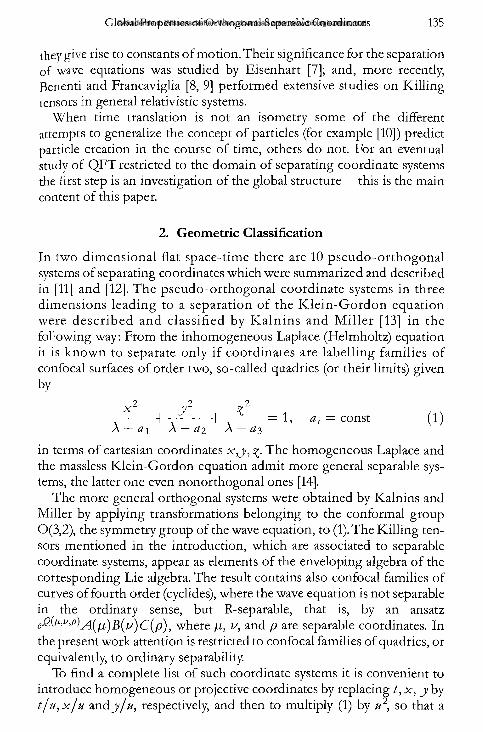
In two dim ensional flat space-time there are 10 pseudo-orthogonal systems of separating coordinates which were summarized and described in [11] and [12]. The pseudo-orthogonal coordinate systems in three dimensions lead ing to a separation of the K lein-G ordon equation were described and c lassified by K aln in s and M ille r [13] in the following way: From the inhomogeneous Laplace (Helmholtz) equation it is known to separate only if coordinates are labelling fam ilies of confocal surfaces of order two, so-called quadrics (or their limits) given by

x 2 y2 z 2---------- h - --------- h - ------- = 1, a-, = const ( l )A — ä\ A — a.2 A — ^3

in terms of cartesian coordinates x , j , The homogeneous Laplace and the massless Klein-Gordon equation admit more general separable systems, the latter one even nonorthogonal ones [14].

The more general orthogonal systems were obtained by Kalnins and Miller by applying transformations belonging to the conformal group 0(3,2), the symmetry group of the wave equation, to (1). The K illing tensors mentioned in the introduction, which are associated to separable coordinate systems, appear as elements of the enveloping algebra of the corresponding Lie algebra. The result contains also confocal families of curves of fourth order (cyclides), where the wave equation is not separable in the ordinary sense, but R-separable, that is, by an ansatz

where fi, v, and p are separable coordinates. In the present work attention is restricted to confocal families of quadrics, or equivalently, to ordinary separability.

To find a complete list of such coordinate systems it is convenient to introduce homogeneous or projective coordinates by replacing /, x , j by t/u,x/u zn&y/u, respectively, and then to multiply (1) by u2, so that a


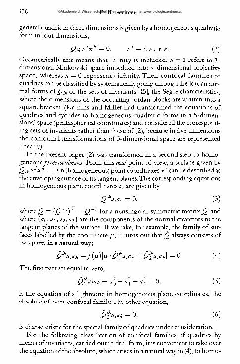
general quadric in three dimensions is given by a homogeneous quadratic form in four dimensions,

Q;k x ' x k = 0, x l = t , x , y , u . (2)

Geometrically this means that infin ity is included; u = 1 refers to 3- dimensional Minkowski space imbedded into 4-dimensional projective space, whereas u = 0 represents infinity. Then confocal fam ilies of quadrics can be classified by systematically going through the Jordan normal forms ofj2 ,* or the sets of invariants [15], the Segre characteristics, where the dimensions of the occurring Jordan blocks are written into a square bracket. (Kalnins and M iller had transformed the equations of quadrics and cyclides to homogeneous quadratic forms in a 5-dimensional space (pentaspherical coordinates) and considered the corresponding sets of invariants rather than those of (2), because in five dimensions the conformal transformations of 3-dimensional space are represented linearly)

In the present paper (2) was transformed in a second step to homogeneous plane coordinates. From this dual point of view, a surface given by Qik x 'x = 0 in (homogeneous) point coordinates x ' can be described as the enveloping surface of its tangent planes. The corresponding equations in homogeneous plane coordinates a-, are given by

Q ‘ka :ak = 0, (3)

where Q = ( j2 _1) T = j 2 _1 for a nonsingular symmetric matrix j2, and where (^0, 01,^ 25^3) are the components of the normal covectors to the tangent planes of the surface. If we take, for example, the family of surfaces labelled by the coordinate fi, it turns out that j2 always consists of two parts in a natural way;

Q ika iak = f ( ß ) [ ß ■ Q f a , a k + Q ^ a }a k] = 0. (4)

The first part set equal to zero,

j 2 ? a ,ak = a\ - a\ - a\ = 0, (5)

is the equation of a lightcone in homogeneous plane coordinates, the absolute of every confocal family. The other equation,

Q £*iak = (6)

is characteristic for the special family of quadrics under consideration.For the following classification of confocal families of quadrics by

means of invariants, carried out in dual form, it is convenient to take over the equation of the absolute, which arises in a natural way in (4), to homo-


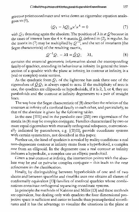
geneous point coordinates and write down an eigenvalue equation analogous to (4),

021 - Aß) = 0 (?)with j2 i denoting again the absolute. The position of A is at Q because in the cases of interest here the 4 X 4-matrix j2, defined in (2), is regular. So the matrix in (7) may be multiplied b y j^ -1, and the set of invariants (the Segre characteristic) of the resulting matrix,

Q - ' Q , - Al = <2£, - Al, (8)

contains the essential geometric information about the corresponding family of quadrics, encoding its behaviour at infinity. In general the intersection of a quadric with the plane at infinity, its contour at infinity, is a (real or complex) conic section.

As the quadratic form Q \ of the lightcone has rank three one of the eigenvalues of QQ\ is always equal to zero. If the multiplicity of zero is one, the quadrics are ellipsoids or hyperboloids, if it is 2, 3, or 4, they are paraboloids and the contour at infinity degenerates to a pair of straight lines.

The way how the Segre characteristic of (8) describes the relation of the contours at infinity of a confocal family to each other, and particularly, to that of the absolute is given by the following tables.

In the case [1111] and in the parabolic case [211] two eigenvalues of the matrix in (8) may be complex conjugate. Families characterized by two or more equal eigenvalues with mutually orthogonal subspaces, conventionally indicated by parentheses, e.g. [(11)11], provide coordinate systems with certain symmetries, not described in this paper.

Further on, the kind of quadrics is revealed by reality conditions: a real non-degenerate contour at infinity stems from a hyperboloid, a complex one from an ellipsoid. In the degenerate case a real contour at infinity indicates a hyperbolic, a complex one an elliptic paraboloid.

Given a real contour at infinity, the intersection points with the absolute may be real or pairwise complex conjugate - this leads to the next refinement in the classification.

Finally, by distinguishing between hyperboloids of one and of two sheets and between spacelike and timelike axes one obtains all classes of conformally equivalent [13] families of confocal quadrics whose combinations constitute orthogonal separating coordinate systems.

In principle the methods of Kalnins and M iller [13] and these methods are equivalent, but dealing only with quadrics the four-dimensional projective space is sufficient and easier to handle than pentaspherical coordinates and it has the advantage to visualize the situations in the plane at


138 F. Hinterleitner

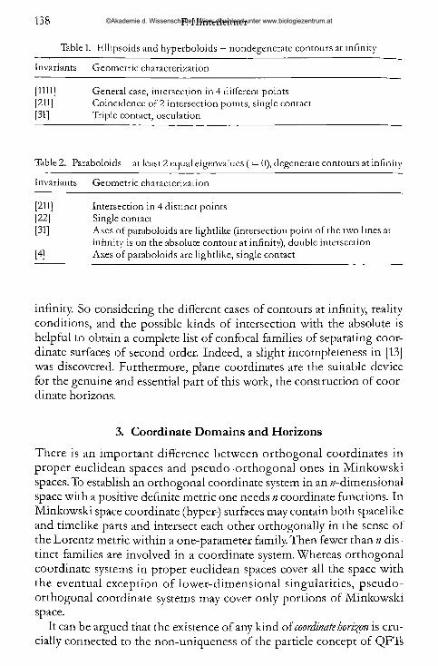
Table 1., Ellipsoids and hyperboloids - nondegenerate contours at infinity

Invariants Geometric characterization

[1111] General case, intersection in 4 different points[211] Coincidence of 2 intersection points, single contact[31] Triple contact, osculation

Table 2. Paraboloids — at least 2 equal eigenvalues ( = 0), degenerate contours at infinity

Invariants Geometric characterization

[211] Intersection in 4 distinct points[22] Single contact[31] Axes of paraboloids are lightlike (intersection point of the two lines at

infinity is on the absolute contour at infinity), double intersection[4] Axes of paraboloids are lightlike, single contact

infinity. So considering the different cases of contours at infinity, reality conditions, and the possible kinds of intersection with the absolute is helpful to obtain a complete list of confocal families of separating coordinate surfaces of second order. Indeed, a slight incompleteness in [13] was discovered. Furthermore, plane coordinates are the suitable device for the genuine and essential part of this work, the construction of coordinate horizons.

3. Coordinate Domains and Horizons

There is an important difference between orthogonal coordinates in proper euclidean spaces and pseudo-orthogonal ones in M inkowski spaces. To establish an orthogonal coordinate system in an «-dimensional space with a positive definite metric one needs n coordinate functions. In Minkowski space coordinate (hyper-) surfaces may contain both spacelike and timelike parts and intersect each other orthogonally in the sense of the Lorentz metric within a one-parameter family. Then fewer than n distinct families are involved in a coordinate system. Whereas orthogonal coordinate systems in proper euclidean spaces cover all the space with the eventual exception of lower-dim ensional singularities, pseudo- orthogonal coordinate systems may cover only portions of Minkowski space.

It can be argued that the existence of any kind of coordinate horizon is crucially connected to the non-uniqueness of the particle concept of QFTs


based on different coordinate systems [16]. The Unruh-effect may be established by considering the information cut offby the horizon. The negative energy densities of the vacuum states, defined with respect to non-inertial coordinates covering only parts of the Minkowski space, can be related also to the Casimir effect [17,18].

In two space-time dimensions the horizons of the separating coordinates are simply lightlike lines - characteristics of the wave equation - so that the coordinate domains are half-planes, wedges or squares. In three dimensions in general horizons are lightlike 2-surfaces generated by lightrays. In the dual description they arise naturally as enveloping surfaces of lightlike planes which are either asymptotic or tangent to the coordinate surfaces.

Usually a family of confocal quadrics can intersect with another one in a certain domain and with a third one in a different domain, so extending to more than one coordinate patch. Disjoint domains parametrized by overlapping coordinate functions are distinguished by lower case roman numbers in Section 5. Therefore coordinate surfaces may either touch the boundary of a given coordinate patch or extend beyond it and touch the horizon somewhere else, away from this domain. In the first case, when surfaces remain entirely inside a coordinate domain, they contain spacelike and timelike parts and only one or two families are sufficient for a coordinate system. In the second case only spacelike or timelike parts of the quadrics lie in a certain domain. If the coordinate surfaces approach the horizon asymptotically, they are spacelike or timelike as a whole.

4. Construction Procedure of the Horizons

The coordinate systems were introduced in [13] by expressing the Minkowski coordinates (/, x , j ) as functions of the three curvilinear separating coordinates (/i, z/, p). They w ill be investigated one by one in the following way:

1. The coordinate surfaces are calculated explicitly in terms of the Minkowski coordinates.

2. The equations of the coordinate surfaces are transformed to homogeneous coordinates x ' = (/, x , jy, u), so that they assume the form (4).

3. (4) denotes the equation for a ll the tangent planes to a surface ß = const. To obtain the tangent planes common to all the surfaces of a family one must assume the validity of the equation for every fi. So (5) and (6) must hold simultaneously. A sj2 i denotes a lightcone, the geometric meaning is that the common tangent planes are tangent to a lightcone, too. From (5) and (6) two of the four^/s can be eliminated,


furthermore it turns out that the equations of the common tangent planes,

a ,* :1 = 0, i = 0 , l , 2 , 3 , (9)

can always be expressed by the ratio of the remaining two a -, ’s; usually k := a\fdQ w ill be taken. So one obtains a one-parameter family of lightlike planes.

4. The equations of an enveloping surface of these common tangent planes have the form

t = Xfo(k) + £ o W usually

x = \ fx (k )+ gx (k ) , f 2{k) = l , g 2(k) = 0 (10)

y = \ f2(k) + g 2{k) is chosen.

From the linearity of these equations in A it can immediately be seen that the enveloping surfaces are ruled surfaces, ruled by light rays. The p aram etervaries from line to line, and A is the parameter along the lines. These enveloping surfaces are the horizons for the coordinate system under consideration.

5. The generating straight lines of the horizons turn out to have always an enveloping curve, so the surfaces are analogous to developable surfaces in euclidean space (they are isometric to a null plane) and the enveloping curves of their generators are their edges of regression, so that, in turn, the horizons are generated by the totality of tangents to a lightlike curve.

6. Having drawn the horizons by computer graphics, it is not immediately obvious which part of them actually bounds a given coordinate patch. So often further considerations are necessary; sometimes it is helpful to find out whether a coordinate system covers parts of some Minkowski coordinate axis or plane.

7. At last the metric coefficients in terms of the separating coordinates are calculated; it depends on the definition interval of /z, v, and p, which of them is the timelike coordinate in a particular case.

5. Horizons - Actual Construction

In the following the horizons of the quadratic coordinate surfaces listed by Kalnins and M iller are investigated. The enumeration of the systems refers to [13]; as only coordinate systems rendering the massive Klein- Gordon equation separable in the ordinary sense are considered here, and the K aln in s-M ille r case (A) deals w ith coordinates lead ing to


R-separation of the massless equation, the present list begins with (B). As noted before, it is also restricted to the geometrically most interesting “genuinely three-dimensional” cases (B.l)—(F.l) and (G), the remainder contains symmetric coordinate systems which have a radial coordinate or may be obtained from two-dim ensional ones. Their horizons are planes and cones.

Coordinate systems distinguished by an asterisk in front of their number do not occur in [13], systems marked by a “o” were recognized as conformally equivalent to another one in the sense of containing the same types and arrangements of quadrics, up to some rescaling of lengths and eventually a rotation by 7r/2 around the /-axis.

(B.1) The structure of invariants in this group is [1111], in (f) two of the eigenvalues are complex conjugate, denoted by [1111]. The coordinate surfaces are arranged in one, two, or three families of hyperboloids of one or two sheets with fixed (a—e) or varying (f) axes and one family of ellipsoids.

(B .l .a) Defining equations'. Coordinate surfaces'.

2 = (ß ~ a ) (v ~ a)(p - a) t 2 _ x 2 _ y =a{a — l ) ’ fi — a fi — 1 fi ’

* = ------------------ :------------ 5 ------------- ^ -------- 1------ = ha — 1 a — v 1 — v —v

0 iw p t 2 x 2 y2J 2 = - — ; ---------- + 1---------- - = i;a a — p 1 — p p

—oo < v < 0 < p < \ < a < p, < oo.

Coordinate domain: There are three mutually pseudoorthogonal families of hyperboloids, covering the whole space-time with the exception of two- dimensional areas bounded by their focal curves. The common tangent planes are complex.Metric for (a)—(d):

? 1 dj- = - (p - v ) (p - p) d^2 d ,;- 1)(m - a) ( - ^ X 1 - v)(a - v)

dpp( 1 - p ) ( a - p )

/i is timelike over its whole range, v and p are spacelike,

o (B .l.b ) Equivalent to (a).


(B .l.c .i) This is the first example with only two families of coordinate surfaces and a real coordinate horizon. Here the calculations outlined in paragraph 4 w ill be demonstrated step by step as a representative for all the other systems. The defining equations are valid for all of (B.l.c).

Defining equations'. Coordinate surfaces'.

f2 = pvp t 2 x 2 y 2 =ä ’ fi fl — a fl — 1 ’

2 _ { p - a ) { a - v ) ( p ~ a ) t 2 x 2 y 2 _ 1x ~ ----------- 1------------------ ’ ----- 1--------------------7 ’a\a — 1) v a —v v — 1

2 (fj, — \)(v — \)(p - 1)y 2 = ---------—--------— -------. \ < v < a < p < p < oo.a — 1

As the equations of the surfaces labelled by fi and by p are identical (they describe hyperboloids of two sheets belonging to the same family), one of them was omitted.

The matrix Q introduced in (2) of the first family of surfaces is given by

j2 = d i a g ( i , -----— , ------- J - r . - l ) , (11)\p ji — a fi — 1 /

the corresponding equation in homogeneous plane coordinates (4) is

P a 0 ~ ( P ~ a ) a \ ~ ( p ~ 1 ) ^ 2 _ a 3— 2 2 2\ | 2 , 2 2 __ rv— f i y a q — a ^ — a 2 ) ~ r a a ^ + a 2 — ^3 — U.

For the tangent planes common to all the surfaces

Oq — a 2 — a 2 = 0 and aa2 + a\ — a 2 = 0 (13)

(corresponding to (5) and (6)) must be valid. From this one can derive

a 2 = ± y « o “ a \. an< a ?> — i y aa\ — a\. (14)

So the equations of the tangent planes common to the considered family of surfaces assume the form


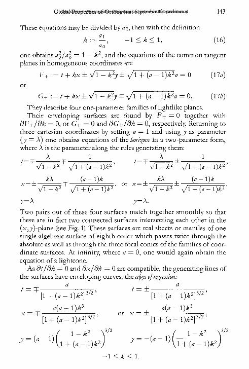
These equations may be divided by ao, then with the definition

k : = — , (16)a o

one obtains a\/a\ = 1 — k 2, and the equations of the common tangent planes in homogeneous coordinates are

F± := t + k x zb VI — k 2y i y/ 1 4- (a — 1 ) k 2u = 0 (17a)or

G± := t 4- kx ± \J 1 — k 2y =F \/l + {a — \)k2u = 0. (17£)

They describe four one-parameter families of lightlike planes.Their enveloping surfaces are found by F± = 0 together with

dF±/dk = 0, or G± = 0 and dG±/dk = 0, respectively. Returning to three cartesian coordinates by setting u = 1 and using y as parameter ( j = A) one obtains equations of the horizons in a two-parameter form, where A is the parameter along the rules generating them:

A 1 A , 1t = T —r^---- =T ; , = = = , t = T ,------- t ±-

y/\ — k 1 yj\ + (a — \)k2 \/l — k 2 yj\ + (a — \)k2

kX ( a — l)k kX ( a — \)k• = ± —____ — _, or x = =fc , =b ■

y/\ — k 2 yj\ + (a — l ) k 2 \/\ — k 2 yj\ + {a — \)k2

J= X J = A.

Two pairs out of these four surfaces match together smoothly so that there are in fact two connected surfaces intersecting each other in the (x,j/)-plane (see Fig. 1). These surfaces are real sheets or mantles of one single algebraic surface of eighth order which passes twice through the absolute as well as through the three focal conics of the families of coordinate surfaces. At infinity, where u = 0, one would again obtain the equation of a lightcone.

As dt/dk = 0 and dx/dk = 0 are compatible, the generating lines of the surfaces have enveloping curves, the edges of regression:

at = T : ------ :------- iTTTi ’ ' = ±[l + (a-l)£2]3/2’ [\ + ( a - \ ) k 2f 12'

aid — \)k? a{a—T ----------------------777 5 or x = ±

[l + ( « - l ) ^ 2] 3/2’ [\ + ( a - \ ) k 2] i l 2 '

1 — k 2 V^2 / 1 — k 2 ^3//21 + (a — 1 ) k 2J \1 + (a — l ) k ‘

- K k < l .


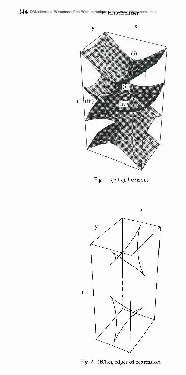
Fig. 2. (B.l.c), edges of regression


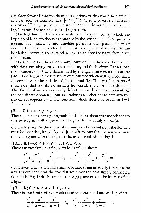
Coordinate domain: From the defining equations of this coordinate system one can see, for example, that |/| > yfa > 1, so it covers two disjoint regions of R 3, lying inside the upper and the lower shells shown in Fig. 1. Figure 2 shows the edges of regression.

The first family of the coordinate surfaces ( p = const), which are hyperboloids of two sheets, is bounded by the horizon. A ll these quadrics contain both spacelike and timelike portions; the spacelike part of one of them is intersected by the timelike parts of others. At the borderline between their spacelike and their timelike parts they touch the horizon.

The members of the other family, however, hyperboloids of one sheet with their axes along thej-ax is, extend beyond the horizon. Rather than the boundary of (B.l.c.i), determined by the space-time extension of the family labelled by p, they touch its continuation which will be recognized as providing the boundaries of (ii), (iii) and (iv). The spacelike parts of these extended coordinate surfaces lie outside the coordinate domain. This family of surfaces not only links the two disjoint components of the coordinate domain (i) but also belongs to other coordinate systems, treated subsequently— a phenomenon which does not occur in 1 +1 dimensions.

(B.l.c.ii) 1 < v < p < p < a .There is only one family of hyperboloids of one sheet with spacelike axes intersecting each other pseudo-orthogonally, the family (v ) of (i).

Coordinate domain: As the values of/, x a n d j are bounded now, the domain must be bounded, from 1 /^Ja < \t\ < a it follows that the system covers the two regions with the shape of distorted tetrahedra in Fig. 1.

*(B.l.c.iii) —oo < v < p < 0,1 < p < a.There are two families of hyperboloids of one sheet:

t 2 x 2 j 2 t 2 x 2 y 2p a — p p — 1 ’ — v a — v 1 — v

Coordinate domain: Now x andj/ cannot be zero simultaneously, therefore the /-axis is excluded and the coordinates cover the non simply connected domain in Fig. 1 which contains the (x-, j/)-plane except the interior of an ellipse.

*(B.l.c.iv) 0 < v < p < \ < p < a.There is one family of hyperboloids of one sheet and one of ellipsoids:


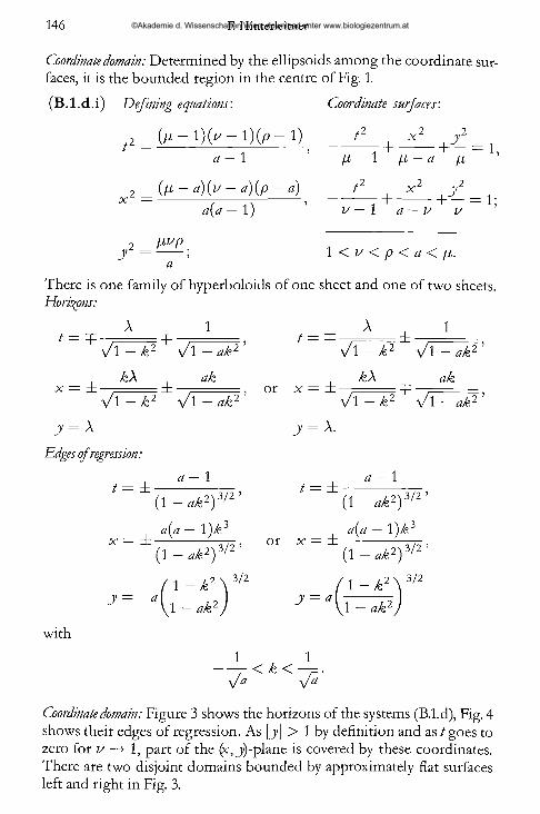
Coordinate domain: Determined by the ellipsoids among the coordinate surfaces, it is the bounded region in the centre of Fig. 1.

(B .l .d .i) Defining equations'. Coordinate surfaces'.

( f i - 1 ) 0 - l ) ( p - 1) t 2 x 2 y 2t . 5 „ ~T \ — 1,a — 1 \1 — 1 fi — a ji

‘2 x 2 j/2------ 1----------- \-J—

i(a — 1) ’ v — 1 a — v v2 (ß — a){v — a)(p - a) t x 2 y

X / \ 5 . "T~ "i — 1 J

? ßvpJ = ------; 1 < v < p < a < / i .a

There is one family of hyperboloids of one sheet and one of two sheets. Horizons:

A 1 A 1,-------= T , ------- = , t = =F ,------- = ±

y/l — k 2 1 — ak 2 "\/l — k 2 \/1 — ak 2

k\ ak k\ nkx = =t —- ■ d= — — — =, or x = ±

\J\ — k 2 \/1 — ak 2 — k 2 \/\ — ak 2

y = A j = A.

Edges of regression:a — 1 , a — 1

/ = =t--------------rrr , / = =L( l - « i 2) 3/2’ (1 — ak 2Y^2 '

ä(ä — l)/£3 <2(0 — l ) k 3i T7T, or x — ±-

(1 - a k 2f /2" (1 - ^ 2) 3/2 ’

/1 - k 2 \ 3/2 /1 - ^ 2 'J = - a [ T ^ e J = a \ T ^ k 2

with

1 1~ ^ < k < ~ r -y j a yfa

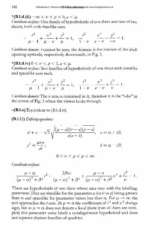
Coordinate domain: Figure 3 shows the horizons of the systems (B.l.d), Fig. 4 shows their edges of regression. As \y\ > 1 by definition and as t goes to zero for v —» 1, part of the (v, j)-p lane is covered by these coordinates. There are two disjoint domains bounded by approximately flat surfaces left and right in Fig. 3.


y

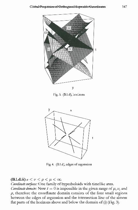
Fig. 3. (B.l.d), horizons

(B.l.d.ii) a < v < p < j i < 00.Coordinate surfaces: One family of hyperboloids with timelike axes. Coordinate domain: Now / = 0 is impossible in the given range of fi, u, and p , therefore the coordinate domain consists of the four small regions between the edges of regression and the intersection line of the almost flat parts of the horizons above and below the domain of (i) (Fig. 3).


*(B.l.d.iii) —oo < v < p < 0 , a < ß .Coordinate surfaces: One family of hyperboloids of one sheet and one of two sheets, both with timelike axes.

/2 x 2 j 2 /2 x 2 j 2+ ------- + ^ - = 1, ---------------------- ^— = \ .

ß — \ fi — a ß 1 — v a — v —v

Coordinate domain: t cannot be zero, the domain is the interior of the shell opening upwards, respectively downwards, in Fig. 3.

*(B.l.d.iv) 0 < v < p < \ , a < ß.Coordinate surfaces: Two families of hyperboloids of one sheet with timelike and spacelike axes each.

t 2 x 2 y2 t 2 x 2 y2+ ------- + — = 1, ------------------- + — = 1.

ß — 1 ß — a ß 1 — v a — v

Coordinate domain: The x-axis is contained in it, therefore it is the “tube” in the centre of Fig. 3 where the viewer looks through.

o(B.l.e) Equivalent to (B.l.d.iv).

(B.l.f.i) Defining equations:

(ß — a) (v — a)(p — a)i{a — b)

0 < y < p < p < o o .

ex -\- i ß ,

a — i ß ;

Coordinate surfaces:

u — a 0 2 ß tx ß — a 9 y2t 2 --------------- -------------------------------- - x + — = 1.

(ß - a ) + ß 2 (ß - a ) + ß 2 (ß - a ) + ß 2 ß

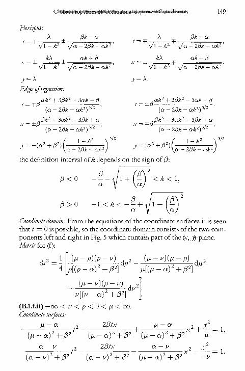
These are hyperboloids of one sheet whose axes vary with the labelling parameter. They are timelike for the parameter ß (or v or p) being greater than a and spacelike for parameter values less than a . For ß —»■ oo the axis approaches the /-axis. At ß — a the coefficients of t 2 and x 2 change sign, but as ß = a does not denote a focal plane (two of them are complex) this parameter value labels a nondegenerate hyperboloid and does not separate distinct families of quadrics.


Horizons:

t = TA

: ± -ßk — a

\/l — k2 y/a — 2ßk — a k 2

kX ak + ß\/l — k 1 \Ja — 2ßk — a k 1

y = AEdges of regression :

Oik 3 + 3ßk2 — 3ak — ß

t = T\/l — k2 y/a — 2ßk — a k 2 ’

ak + ßk\± .-------- T\/l — k2 y/a — 2ßk — ak 2

J = A.

/ = T ß

x = ± ß

(a; — 2ßk — ak 2)

ß k 3 — 3a?/£2 — 3ßk + a (ct — 2ßk — a k 2) ' 2

,2 \ 3/2

t = i/3

* = Tß

j = - { a * + ß*) 1 -

ct — 2/3A — o;^2

ct/£3 + 3ßk2 — i a k — ß {a — 2ßk — a k 2) 3 2

ß k 3 — 3ak2 — 3ßk + ct (a — 2ßk — a k 2)'

, 2 \ 3/2

J,=(a2+/?2)( ^ w b ^ )the definition interval of k depends on the sign of ß:

ß < 0

ß > 0 - 1 < k < - - + 4/1 + ( -a y \ a

Coordinate domain: From the equations of the coordinate surfaces it is seen that / = 0 is possible, so the coordinate domain consists of the two components left and right in Fig. 5 which contain part of the (x, j/)-plane. Metric for (f):

d-r"1 ( p - p ) { p - u ) d p 2 - ( M - W (M - P ) d 2

p [ ( p - a ) + ß 2} p [ ( p - a ) + ß 2

iAdu

u[(u - a ) 2 + ß 2]

(B.l.f.ii) —oo < u < p < 0 < p < o o . Coordinate surfaces:

p — a 2 ß tx+

p — a

(p — a ) + ß 2 ( p L - a ) + ß 2 ( p ~ a ) + ß 2 p a — u 2 2 ßtx

2

a — u

2 , yx -i— = 1.

( a — u) + ß 2 ( a — u) + ß 2 (p — a ) + ß 2


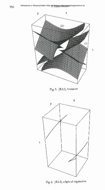
Fig. 5. (B.l.f), horizons

x

Fig. 6. (B.l.f), edges of regression


There is one family of hyperboloids of one and one of two sheets with timelike axes.Coordinate domain: In the first equation the coefficients of t 2 and x 2 can assume both signs but in the second one they are fixed, so t — 0 is impossible and the coordinate system is bounded away from the (v, j/)-plane by the upper, respectively the lower, shell in Fig. 5.

o(B .l.g) Equivalent to (B.l.f.i)

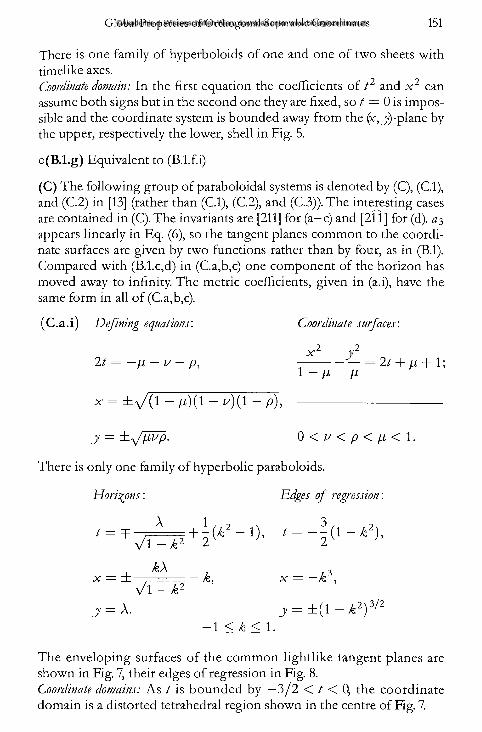
(C) The following group of paraboloidal systems is denoted by (C), (C.l), and (C.2) in [13] (rather than (C.l), (C.2), and (C.3)). The interesting cases are contained in (C). The invariants are [211] for (a— c) and [211] for (d). <23 appears linearly in Eq. (6), so the tangent planes common to the coordinate surfaces are given by two functions rather than by four, as in (B.l). Compared with (B.l.c,d) in (C.a,b,c) one component of the horizon has moved away to infinity. The metric coefficients, given in (a.i), have the same form in all of (C.a,b,c).

(C .a .i) Defining equations'. Coordinate surfaces'.

x 2 y221 = n v yO, - = 2/ + /z + 1;

1 - p p

*• = ±>/(i - r i ( i - ^ ) ( i - p ), -----------------------------------

J = ± y / H V p . 0 < I Z < P < I J L < 1 .

There is only one family of hyperbolic paraboloids.

Horizons: Edges of regression'.

/ t ~ 7 2 + ^ 2 ~ 1) ’ t = - \ ( X~ k2) ’v l - k 2 2 2

kX ax = ± . — k. x = — k ,

y / l ^ k 2j = A. j = ±(1 - k 2) 3/2

- 1 < k < 1.

The enveloping surfaces of the common lightlike tangent planes are shown in Fig. 7, their edges of regression in Fig. 8.Coordinate domains: As t is bounded by —3/2 < / < 0, the coordinate domain is a distorted tetrahedral region shown in the centre of Fig. 7.


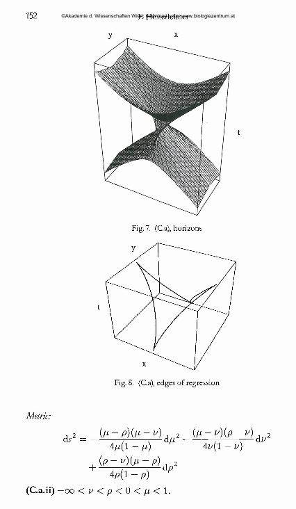
Fig. 7. (C.a), horizons

Fig. 8. (C.a), edges of regression

Metric:

d j2 = _ (A* - P)(M - *) 2 _ (A* - »0(p -J O d|/24/i(l - /z)

, (p — — p)+ M i - p ) d/>

(C.a.ii) —co < ^ < / 9 < 0 </x<l.

4i/(l - v )


G lo b a l P r o p e r t i e s o f O r t h o g o n a l S e p a ra b le C o o r d , n a ,e s

X

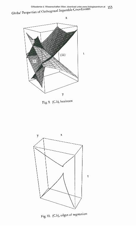
F ig . 9. (Cb), h o r iz o n s


Coordinate surfaces:2 2 2 2 x y x y

------------------ 2/ — u, — 1 — 0, -----------1--------- 2/ is — 1 — 0.1 — fl fi 1 — v — v

These are one family of hyperbolic (fi) and one of elliptic (z/, p) paraboloids.Coordinate domain: As / > —1/2, the coordinate domain is the interior of the upper shell in Fig. 7.

o(C .a.iii) Equivalent to (ii), defined in the lower shell in Fig. 7.

(C.b.i) Defining equations'. Coordinate surfaces'.

t = ±yfiwp, -h— - —2y - / x - 1 = 0;ji [i I

*■ = ±y/(»~ l ) ^ - 1){P~ 1). ----------------------------

2y = —[i — v — p. 1 < v < p < fi < oo.

This is one family of hyperbolic paraboloids.


A 1 1[ ’

( i - m2) 3/2

^ V i - k 2 + k ’ k 3 ’

x = x = ■/&■'

. kX 1 3J , ^ ~ 2 k 2 ’

- 1 < k < 0 , 0 < k < 1.

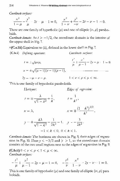
Coordinate domain: The horizons are shown in Fig. 9, their edges of regression in Fig. 10. H ere j < —3/2 and |/| > 1, so the coordinate domain consists of the two small regions next to the edges of regression in Fig. 9.

(C .b.ii) 0 < Z ' < / 3 < l < / i < o o .Coordinate surfaces:

— 2 y - p i - l = 0, — — — 2y — v — \ = 0 ./ i / z — 1 v 1 — V

This is one family of hyperbolic (fi) and one family of elliptic (z/, p) paraboloids.


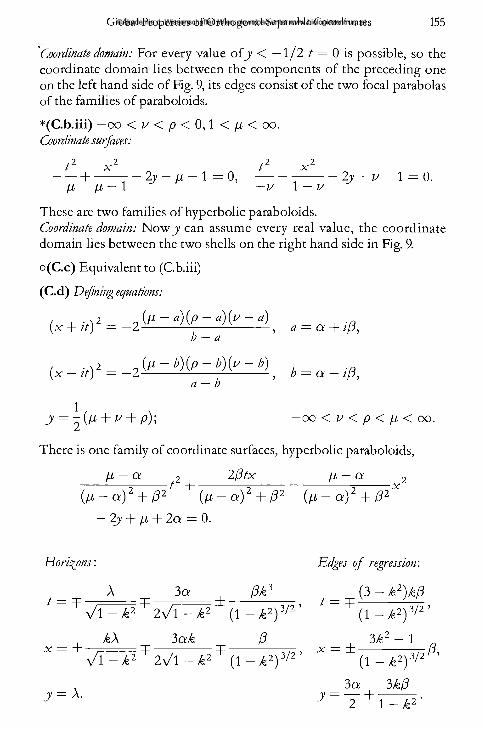
Coordinate domain: For every value o f j < —1/2 / = 0 is possible, so the coordinate domain lies between the components of the preceding one on the left hand side of Fig. 9, its edges consist of the two focal parabolas of the families of paraboloids.

*(C .b .iii) —oo < v < p < 0,1 < ß < oo.Coordinate surfaces:

,2 2 , 2 2 t X t X— 2y — ß — 1 = 0, ------------------- 2y — v — 1 = 0.

ß ß — 1 —v 1 — v

These are two families of hyperbolic paraboloids.Coordinate domain: N o w j can assume every real value, the coordinate domain lies between the two shells on the right hand side in Fig. 9.

o(C.c) Equivalent to (C.b.iii)

(C.d) Defining equations:

( , -a2 _ a )(P ~ a) ( v ~ a) _ „ i -a+ it) — —Z-------------------------------3 Cl — Qt ifj)b — a

( x _ * ) 2 = _ 2 ( ^ ) M M i b = a - , ß ,a — b

y = - [ß + v + p)\ -o o < v < p < ß < oo.

There is one family of coordinate surfaces, hyperbolic paraboloids,

ß — a 2 2 ß tx ß — a

( ß - a ) 2 + ß 2 (ß - a ) 2 + ß 2 ( ß - a ) 2 + ß 2

— 2y ß -\- 2d — 0.


A 3a ß k 3 (3 - k 2)kß

t ~ Zf7 T ^ :¥ 2V :i ^ e ( i - ^ ) 3/2’ / _ = F ( i - ^ ) 3/2 ’

^A 3 ak ß 3k2 — 1

x = V i T P ^ I Ä ^ P ^ i - * 2) 3' 2 ’ x = ( \ - k i f ' 2 '

3 a 3kßy = a. j —


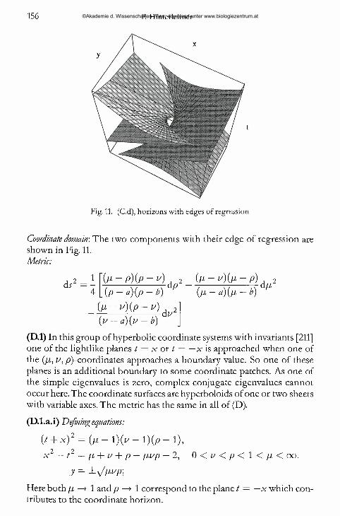
Fig. 11. (C.d), horizons with edges of regression

Coordinate domain-. The two components with their edge of regression are shown in Fig. 11.Metric:

7 1ds■I

~ p ) { p - v ) d 2 d 2( p - a ) ( p - b ) ( f i - a ) ( f i - b )

( f i - v ) ( p ~ v)(v — a) (v — b)

dv*

(D.l) In this group of hyperbolic coordinate systems with invariants [211] one of the lightlike planes t = x or / = —x is approached when one of the (//, z/, /^-coordinates approaches a boundary value. So one of these planes is an additional boundary to some coordinate patches. As one of the simple eigenvalues is zero, complex conjugate eigenvalues cannot occur here. The coordinate surfaces are hyperboloids of one or two sheets with variable axes. The metric has the same in all of (D).

(D .l.a.i) Defining equations:

(t + x ) 2 = { ß - 1) (y ~ 1 )(p ~ 1),x 2 — t 2 ~ f i + p + p — p,vp — 2 , 0 < v < p < 1 < fi < oo.

J =

Here both ß —» 1 and p —> 1 correspond to the plane t = —x which contributes to the coordinate horizon.


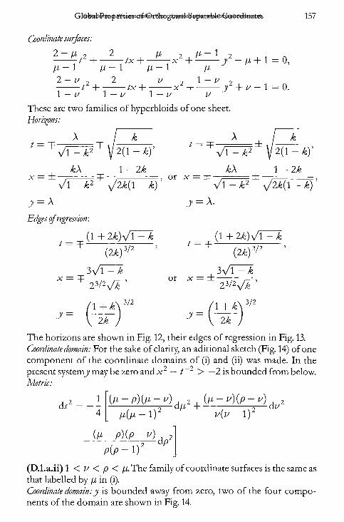
Coordinate surfaces:2 — U 7 2--------1 H---------- txfi — 1 p — 1 ß ~ 1 ß2 — u 1 - i/

r +1 - v

These are two families of hyperbloids of one sheet. Horizons:

Xt = =F

= ±-kX

=F

=F

2(1 - k f

1 - 2k

yj\ - k 2 y/2k(l - k)

j = A

Edges of regression-.

(1 +2k)y/\ ~ k

t = -F

or x = =t

A ±V 2( ! - * ) ’

kX ± 1 — 2k

V l ~ k 2 y/2k(\ ~ k)

J = A.

T

x = =p ■

J =

{2k)l/1

3>/l2 3/2^ ’

/ = T

or x = ±

(1 + 2>fe)>/l

(2/6)3/2

3\/l

2 3/2y ^ ’

1 +/ 2/6

3/2 1 +/ 2/6

3/2

The horizons are shown in Fig. 12, their edges of regression in Fig. 13. Coordinate domain: For the sake of clarity, an aditional sketch (Fig. 14) of one component of the coordinate domains of (i) and (ii) was made. In the present system j may be zero and x 2 — t~2 > —2 is bounded from below. Metric:

dj-'{ p - p ) { p - v)

p ( p - I ) 'dfi +

( f i - v ) { p - v )

v i y - l ) 2

p (p - i ) 2

(D .l.a .ii) 1 < v < p < p. The family of coordinate surfaces is the same as that labelled by p in (i).Coordinate domain:y is bounded away from zero, two of the four components of the domain are shown in Fig. 14.


y

t

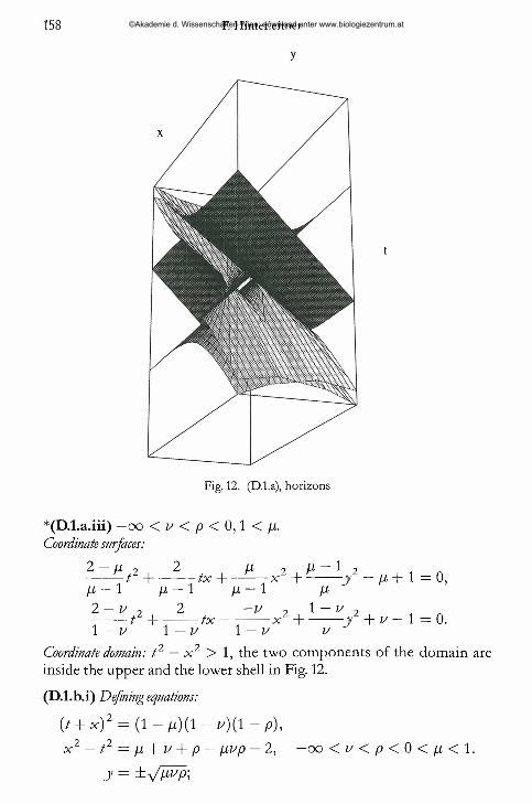
Fig. 12. (D.l.a), horizons

*(D.l.a.iii) — o o < v < p < 0 , 1 < fi .Coordinate surfaces:

2 — ^ 2 , 2 ß 2 i ß 2 .. I 1 _ n------ - t H-------- --------------- r * H--------- -J —/x+1 — 0,H — 1 M ~ l ß — l M2 — v 0 2 —v 9 1 — z/ 9------- 1 H---------- / x ----------- x H---------- r + z' — 1 = 0 .1 — Z/' 1 - z / 1 - z / z/

Coordinate domain: t 1 — x 2 > 1, the two components o f the domain are inside the upper and the lower shell in Fig. 12.

(D.l.b.i) Defining equations:

(t + x ) 2 = (1 - ^)(1 - if) ( l - p),

x 2 — t 2 = f i + t' + p — f i v p — 2, —oo < z / < p < 0 < / i , < l .

y = ±^/Jwp\


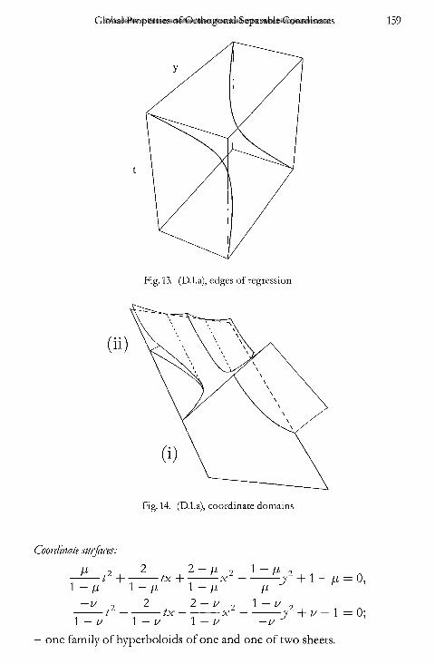
Fig. 13. (D.l.a), edges of regression


ß 2■t 11 — fi 1 — [i 1 — [i

—1/t 2 - tx - J + v ~ 1 = 0 ;l —i/ l — i/ l —i/ —i/

— one family of hyperboloids of one and one of two sheets.


Horizons:A 2 — k A 2 — k

t = T ~-,------- = T , , = , t = T ----- -=±— k 1 \/2( l — /6) \/\ — k 2 \/2 ( l — /6)

£A , 1 £A 1x = ± — =t — =, or x = ± . = =F

V i - £ 2 V 2 ! 1 - ’ V i - / 62 V 20 -j = A j = - A .

Edges of regression:

3 V l - £/ _ ^ ^ 3/2 ’ * — T ^3/2 ’

, (2 + /fe)Vl , (2 + /fe)Vlx = ± ------ ^ ------ - or x = ± ------ ^ ------

1 + A 3/2 / l + 3/2y = - \ ~ ) J =

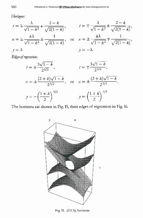
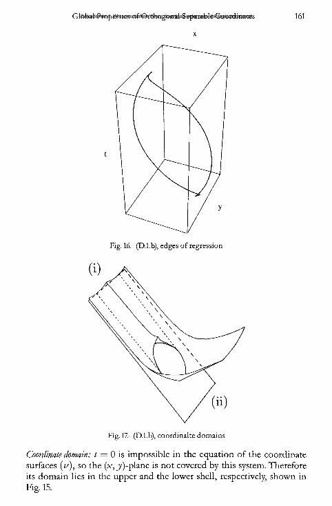
The horizons are shown in Fig. 15, their edges of regression in Fig. 16.

t

Fig. 15. (D.l.b), horizons


X

Fig. 16. (D.l.b), edges of regression

Coordinate domain: t — 0 is impossible in the equation of the coordinate surfaces (v ), so the (x, j/)-plane is not covered by this system. Therefore its domain lies in the upper and the lower shell, respectively, shown in Fig. 15.


(D.l.b.ii) 0< Z /'< 1 oo.Coordinate surfaces:

ß 2 2 ß — 2 2 ß 1 2t H----------t x ------------x ----------- y + ß — 1 = 0,ß ~ \ ß — 1 ß — 1 ß

z/ 9 2 2 — z/ 9 1 —/ H--------- /xH---------- x ----------- y + 1 — v = 0.

1 — z/ 1 — v 1 — v

Two families of hyperboloids of one sheet.Coordinate domain: Shown in Fig. 17, it may be found by taking into account th a tj may assume every real value.

(D.l.b.iii) 0 < v < p < ß < \ . There is one family of hyperboloids of one sheet.Coordinate domain: y is bounded by 0 < \y\ < 1, the domain is shown in Fig. 17.

o(D .l.c) Equivalent to (a.i).

(D .l.d) Defining equations:

(t + x ) 2 = (ß - 1)(1 - v )( 1 - p),

t 2 — x 2 = ß - \ - v + p — ßvp — 2 , —oo < v < 0 < p < 1 < ß < oo.

y = ± ^/-ßvp ;


ß 2 2 2 ß 2 ß 1 2t H----------tx H---------- x ----------- y — ß + 1 = 0

ß — 1 ß — 1 ß — 1—v ? 2 2 — v 9 _ _ . ^

--------- / H---------- tx H---------- x H---------- v + z — 1 = 0 ,1 — v 1 — z/ 1 — z

P ,2, 2 ( 2 — P 2 1 A' 2t H--------- /x H---------- x ----------- j/ + p — 1 = 0

ß - 1

ß1 — z/

—u1 - p

1 - p 1 - p \ - p p

One family of hyperboloids of one sheet, two of two sheets.Coordinate domain: From (6) it follows that a 2 = 2ao(a\ — ao) which is < 0.So a\ must be equal to a$ and the quadrics have only one common asymptotic plane (t = —x). There is no further horizon and two copies of this system are sufficient to cover the whole Minkowski space.

(E.1) This is a group of paraboloidal coordinate systems with the invariants [31], the coordinate surfaces are arranged either in one family of elliptic and one of hyperbolic paraboloids, or in only one family of hyperbolic paraboloids. There is only one type of coordinate horizon, its edge


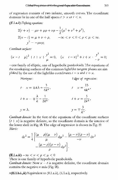
of regression consists of two infinite, smooth curves. The coordinate domains lie in one of the half-spaces t > x or t < x.

(E.l.a.i) Defining equations:\

2(t + x ) = ßl> + pp + l/p — — (/Li2 + V2 + p 2),

2 (x — /) = ß + V + p, —OO < 1 S < 0 < P < P < oo.

J /2 = —

Coordinate surfaces:2 2

(x — t — /i) t -(- x - f - — 0, (x — t — lA -\-1 x ------- --- 0jp —v

-o n e family of elliptic, one of hyperbolic paraboloids. The equations of the enveloping surfaces of the common lightlike tangent planes are simplified by the use of the lightlike coordinates t — x and t + x.


3 15t — x — T/6A -|------7 , t — x = —

4k4 4 k l

A 1 5t + x = T ---------- 7 , / + x = ----7 ,

2k 6 ’ 2£ 6 ’

, 37 7 =

main: In the first of the equations of the coordinate surfaces (/ + x ) is negative definite, so the coordinate domain is the interior of the lower shell in Fig. 18. The edge of regression is shown in Fig. 19. Metric:

\p - p) (p - v) 2 ( p - v ) ( p - v ) ^ 2? 1 ds — —4 I p —v

( p - p ) ( p - v ) 2------------------------ dp

P(E.l.a.ii) —00 < v < p < p < 0There is one family of hyperbolic paraboloids.Coordinate domain: Now x — / is negative definite, the coordinate domain contains the negative x-axis (Fig. 18).

o(E.l.b.i.,ii) Equivalent to (E.l.a.ii), (E.l.a.i), respectively.


x

Fig. 18. (E.l.a), horizons

Fig. 19. (E.l.a), edges of regression

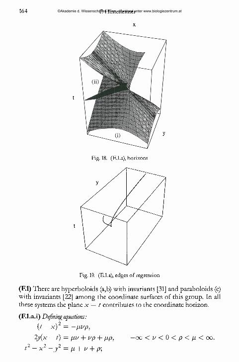
(Fl) There are hyperboloids (a,b) with invariants [31] and paraboloids (c) with invariants [22] among the coordinate surfaces of this group. In all these systems the plane x = t contributes to the coordinate horizon.

(F .l.a .i) Defining equations:(t — x ) 2 = —ßvp,

2y ( x — t) — /iv + up + /zp, — oo < v < 0 < p < p < oo.

t 2 - x 1 - j 2 = /i + v + p\



-------- -----2y it — x ) — fl i t + x ) ( t — x ) + f i j 2 + f i2 = 0 ,ß

-- -------- -----2)i(t — x ) + (—v) (t + x) (/ — x ) — (—v ) y 2 + v 2 = 0;

- one family of hyperboloids of two sheets, one of one sheet.


j 3k 3k= l + * = ^ 2 ’

A 1 , 1

> + X ~ ~ k i T V ^ ' ‘ ~ X ~ i j l k ? '

J = X' 7 =0 < k < oo

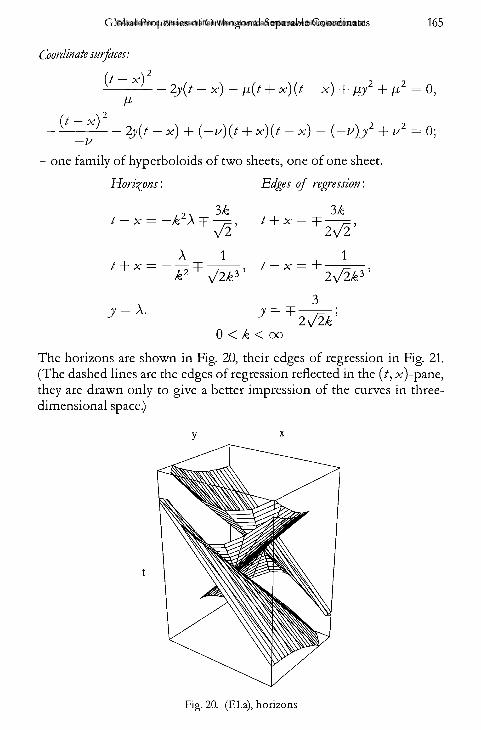
The horizons are shown in Fig. 20, their edges of regression in Fig. 21. (The dashed lines are the edges of regression reflected in the (/, x)-pane, they are drawn only to give a better impression of the curves in three- dimensional space.)

Fig. 20. (F.l.a), horizons


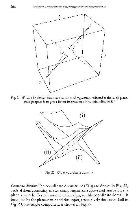
Fig. 21. (F.l.a). The dashed lines are the edges of regression reflected at the (/, x)-plane, their purpose is to give a better impression of the imbedding in R 3

Coordinate domain: The coordinate domains of (F.l.a) are drawn in Fig. 22, each of them consisting of two components, one above and one below the plane x = t. In (i)y can assume either sign, so this coordinate domain is bounded by the plane x = t and the upper, respectively the lower shell in Fig. 20; one single component is shown in Fig. 22.


dr2 = - 4

( p - p ) ( ß - v ) J 2 ( p - p K p - v ) j „ 2 ----------- —— — d / i -------------- ---------- dpp-

d v l

(F .l.a .ii) —O O < V < P < H < 0 .There is one family of hyperboloids of one sheet.Coordinate domain: Now /2 — x 2 — y 2 < 0, so the coordinate system must lie outside the lightcone, furthermore,j/(x — t) is strictly positive, so that the sign of'y is definite in each component; these conditions are fulfilled for the two small regions shown in Fig. 22.

o(F.l.b) Equivalent to (F.l.a.i).

(F .l.c.i) Defining equations:

(/ — x ) 2 = pup,

t 2 — X 2 = p v + up + z'P, 0 < v < p < p < oo.

2y = p + v + p;

Coordinate surfaces (hyperbolic paraboloids):

P— (/ — x ) (/ + x ) + 2 py — p = 0

Horizon: Edge of regression'.

k l\ 3 2 3 4k ) 2k k 3 ’ k k 3 "1

x = -----4 k ) 2k k 3 ’ k k 3 '

x 6J = A - ■ > = * •

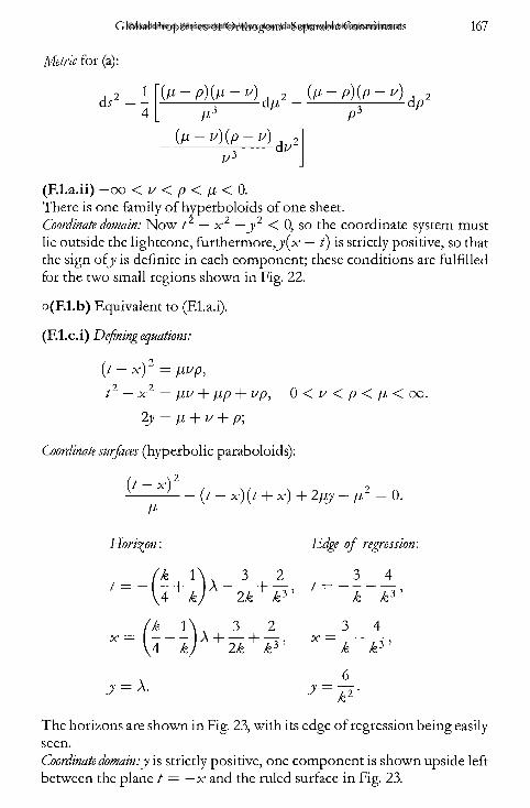
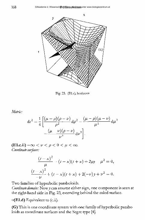
The horizons are shown in Fig. 23, with its edge of regression being easily seen.Coordinate domain:y is strictly positive, one component is shown upside left between the plane t = —x and the ruled surface in Fig. 23.


Metric:

ds2 = - (ß ~ P ) ( P - v) l 2 ( V - p K l t - v ) J . .2d p ---------------------------- —-------- dß

( ß - i s ) ( p ~ i s ) d^ 2

(F .l.c .ii) —oo < v < p < 0 < ß < oo. Coordinate surfaces:

(/ — x)

— (/ — x ) (t + x ) + 2 ßy — ß 2 = 0 ,

(/ — x ) ( t + x ) + 2{—u)y + v 2 — 0 .

Two families of hyperbolic paraboloids.Coordinate domain: Nowj/can assume either sign, one component is seen at the right-hand side in Fig. 23, extending behind the ruled surface.

o(F.l.d) Equivalent to (c.ii).

(G) This is one coordinate system with one family of hyperbolic paraboloids as coordinate surfaces and the Segre type [4].


2{t — x ) = fi + v + p,

2 (t + x ) = —- f iv p + - [v2(p + p) + p 2(fi + v) + f i2{v + p)

- ( f i 3 + ^ + p %\

A-y = fiv + f i p + v p - - {fi2 + v 2 + p2),

— oo < v < p < f i < o o .

Coordinate surfaces:2 1

(t — x ) 2 -----(/ — x)y — 2fi(t — x ) H— (/ + x ) + 2y + f i2 = 0 .fi fi

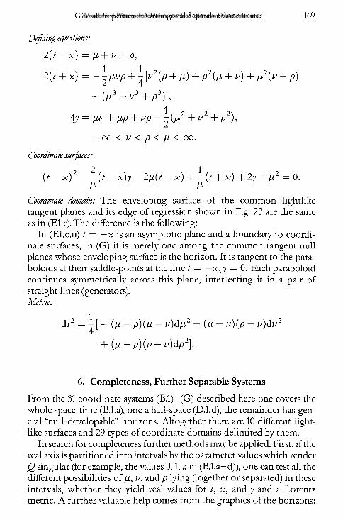
Coordinate domain: The enveloping surface of the common lightlike tangent planes and its edge of regression shown in Fig. 23 are the same as in (F.l.c). The difference is the following:

In (F.l.c.ii) t = —x is an asymptotic plane and a boundary to coordinate surfaces, in (G) it is merely one among the common tangent null planes whose enveloping surface is the horizon. It is tangent to the paraboloids at their saddle-points at the line t = — x , j = 0. Each paraboloid continues symmetrically across this plane, intersecting it in a pair of straight lines (generators).Metric:

\ds2 = - [ - ( f i - p ) ( f i - v )df i2 - ( f i - v ) ( p - v )dv 2

+ (ß ~ P){P ~ v)&P2]-

6. Completeness, Further Separable Systems

From the 31 coordinate systems (B.l)—(G) described here one covers the whole space-time (B.l.a), one a half-space (D.l.d), the remainder has general “null-developable” horizons. Altogether there are 10 different lightlike surfaces and 29 types of coordinate domains delimited by them.

In search for completeness further methods may be applied. First, if the real axis is partitioned into intervals by the parameter values which render Q singular (for example, the values 0,1, a in (B .l.a-d)), one can test all the different possibilities of fi , v, and p lying (together or separated) in these intervals, whether they yield real values for /, x , a n d j and a Lorentz metric. A further valuable help comes from the graphics of the horizons:


Starting from a certain coordinate patch and crossing the horizon one leaves the domain of this group of coordinates, crossing it a second time, one enters into another patch of the same group.

There are 51 further coordinate systems part of which are generated by translation, rotation, or boost from a two-dimensional system of separating coordinates in a timelike or spacelike plane, or arise from two-dimensional coordinate systems in a timelike plane by the less familiar lightlike (isotropic) rotation achieved by the Lorentz matrix

L '

( b2 b2 \ I 1 + — ------ b\

V

+

2b

2

’ 2 -b

b

1 /

b e R,

which leaves the vector (1,1,0) invariant. This transformation rotates every plane through the line x = t rigidly around this axis; this family of planes with the common line x = t is found among the coordinate surfaces. Other systems have a radial coordinate, they contain families of cones as lim iting cases of quadrics. The horizons of all these coordinate systems, if any, consist of parts of planes and lightcones. An overview over the complete number of ordinarily separable coordinates in 2 +1 dimensional Minkowski space may be found in [19].

Acknowledgements

The author thanks Prof. H. K. Urbantke for the idea for this investigation and for helpful advice and support, and Prof. H. Kühnelt for support at producing the computer graphics; furthermore the relativity group of the Masaryk university in Brno, where part of this final version of the paper was accomplished.

References[1] Rindler,W.: Essential Relativity, SpringerTracts and Monographs in Physics, 2nd ed.

Springer-Verlag, Berlin, Heidelberg, New York 1977.[2] Fulling, S. A.: Nonuniqueness of Canonical Field Quantization in Riemannian

Space-Time. Phys. Rev. D 7, 2850 (1973).[3] Unruh,W. G.: Notes on black-hole evaporation. Phys. Rev. D 14, 870 (1976).[4] Bisognano, J. J.,Wichmann, E. H.: On the duality condition for a Hermitian scalar

field. J. Math. Phys. 16,985 (1975).[5] Kay, B. S., Wald, R. M.: Theorems on the Uniqueness and Thermal Properties of

Stationary, Non singular, Quasifree States on Spacetime with a Bifurcate Killing Horizon. Phys. Rep. 207, 49 (1991).


[6] Stäckel, P : Über quadratische Integrale der Differentialgleichungen der Dynamik. Ann. Math. Pura Appl. 26, 55 (1897).

[7] Eisenhart, L. P.: Separable systems of Stäckel. Ann. Math. 36, 57 (1934).[8] Benenti, S., Francaviglia, M.: The theory of separability of the Hamilton-Jacobi

equation and its application to general relativity. In: General Relativity and Gravitation (Held, A. ed.) Plenum Press, New York (1980), p. 393.

[9] Benenti, S.: Stäckel systems and K illing tensors. Note Mat. 9 (Suppl.), 39 (1989).[10] Costa, I., Svaiter, N. F.: Separable Coordinates and Particle Creation III: Accelerat

ing, Rindler and Milne Vacua. Rev. Bras. Fis. 19, 271 (1989).[11] Klement, S.: Pseudo-orthogonale Koordinatensysteme zur Separation der Klein-

Gordon-Gleichung im zweidimensionalen Minkowskiraum. Diploma thesis, University of Vienna, 1990.

[12] Kalnins, E. G., Miller, W.: On the separation of variables for the Laplace equation Aip + K 2,tp = 0 in two and three dimensional Minkowski space, SIAM Math. Anal. 6, 340 (1975).

[13] Kalnins, E.G., Miller, W.: Lie theory and separation of variables. 9. Orthogonal R- separable coordinate systems for the wave equation ip,, — A2"0 = 0, J. Math. Phys. 17, 331 (1976). P. M. Morse and H. Feshbach, Methods of Theoretical Physics, PartI (McGraw-Hill, New York, 1953).

[14] Kalnins, E. G., Miller,W.: Lie theory and separation of variables. 10. Nonorthogonal R-separable solutions of the wave equation d„ ip = A 2 ip. J. Math. Phys. 17,356 (1976).

[15] Bromwich,T. J. FA.: Quadratic Forms and their Classification by Means of Invariant Factors. Cambridge Tracts in Mathematics and Mathematical Physics No. 3. Cambridge University Press, 1906.

[16] Unruh, W. G., Wald, R. M.: What happens when an accelerating observer detects a Rindler particle. Phys. Rev. D29,1047 (1984).

[17] DeWitt, B. S.: Quantum Gravity: the new synthesis. In: General Relativity, an Einstein centenary survey, p. 680 (Hawking, S.W., Israel,W. eds.). Cambridge University Press, 1979.

[18] Fulling, S. A., Davies, P. C.W.: Radiation from a moving mirror in two-dimensional space-time: conformal anomaly. Proc. R. Soc. London Ser. A348, 393 (1976).

[19] Hinterleitner, F.: Global properties of orthogonal separating coordinates for the Klein-Gordon equation in 2 + 1 - dimensional flat space-time. University ofVienna preprint, UWThPh-1994-19.

Author’s address: Dr. F. Hinterleitner, Institut fürTheoretische Physik der UniversitätWien, Boltzmanngasse 5, A-1090 Wien.


Global Properties of Orthogonal Separable Coordinates for ... · domains the parameter along its...

Documents

Transcript of Global Properties of Orthogonal Separable Coordinates for ... · domains the parameter along its...