H ans K onrad K nörr - FernUniversität Hagen · O n the P roblem of R epresentability and the B...
156
O n the P roblem of R epresentability and the B ogoliubov –H artree –F ock T heory H ans K onrad K nörr D issertation
-
Upload
truongkhanh -
Category
Documents
-
view
213 -
download
0
Transcript of H ans K onrad K nörr - FernUniversität Hagen · O n the P roblem of R epresentability and the B...
O n t h e P r o b l e m o f
R e p r e s e n t a b i l i t y
a n d t h e
B o g o l i u b o v – H a r t r e e – F o c k
T h e o r y
H a n s K o n r a d K n ö r r
D i s s e r t a t i o n
On the Problem of Representability and theBogoliubov–Hartree–Fock Theory
Von derCarl–Friedrich–Gauß–Fakultät
der Technischen Universität Carolo–Wilhelmina zu Braunschweig
zur Erlangung des Grades einesDoktors der Naturwissenschaften (Dr. rer. nat.)
genehmigte Dissertation(kumulative Dissertation)
vonHans Konrad Knörr
geboren am 31.08.1982in Ansbach
Eingereicht am 26. Juli 2013Disputation am 22. November 20131. Referent: Prof. Dr. Volker Bach2. Referent: Prof. Dr. Heinz Siedentop
(2013)
Colophon
On the Problem of Representability and the Bogoliubov–Hartree–Fock Theory
A dissertation by Hans Konrad Knörr. Written under the supervision of VolkerBach at the Institut für Analysis und Algebra, Carl–Friedrich–Gauß–Fakultät, Tech-nische Universität Braunschweig.
Contains one figure (created with the vector graphics editor Xfig).
Typeset using LATEX and the memoir document class. The text is set with thePalatino font at 10.0/12.0pt, and the Pazo Math fonts are used for mathematicalformulae.
Among the packages used are the AMS packages amsfonts, amsmath, amssymb,as well as babel, dsfont, fontenc, graphicx, hyperref, inputenc, mathpazo,mathtools, ntheorem, soul, and url. Questions and comments are welcome, andcan be sent to the author by emailing [email protected].
Preface
The present thesis discusses questions which originate from quantum che-mistry. The results also hold for more general physical systems consistingof fermions or bosons. It is a cumulative dissertation and its main bodyare the following three papers: “Generalized One-Particle Density Ma-trices and Quasifree States” [BBKM13], “Fermion Correlation Inequalitiesderived from G- and P-Conditions” [BKM12], and “Representability Con-ditions by Grassmann Integration” [BKM13]. Following this preface weoutline the results of this thesis in an English and in a German summary.
∗ ∗ ∗
Many people have, directly or indirectly, contributed to the success of myPhD thesis and I am grateful to all of them. Mentioning all of them would,however, go beyond the scope of this preface. Therefore I only have thepossibility to thank those individually which had the greatest influence inmy PhD project.
First of all, I wish to express my deep gratitude to my supervisor VolkerBach for the opportunity to work on this interesting project. His greatexpertise in many-body quantum mechanics, but also in other fields ofmathematical physics, was a great benefit for me and this work.
Moreover, I am indebted to Edmund Menge for his friendship andmany fruitful discussions. Despite often appearing disagreements, thesediscussion were one of the driving forces for our joint work.
Furthermore, I am grateful to Luigi Delle Site for his scientific supportand interest in the PhD project.
A great help in writing this dissertation has been the use of a LATEXtemplate which is based on Matthias Westrich’s and Rasmus Villamoes’PhD theses and the proofreading of parts of the manuscript by S. Breteaux,E. Menge, and T. Mühlenbruch. This work was supported in part by theMax Planck Graduate Center in Mainz.
Lastly, I am deeply grateful to my parents and my family for theirsupport and encouragement during my PhD studies.
Hans Konrad KnörrAnsbach, July 2013
i
Summary
The general topic of this thesis is an approximation of the ground stateenergy for many-particle quantum systems. In particular the Bogoliubov–Hartree–Fock theory and the representability of one- and two-particle den-sity matrices are studied. After an introductory chapter we specify somebasic notation of many-body quantum mechanics in Chapter 2. The Chap-ters 3 to 5 comprehend the papers [BBKM13], [BKM12], and [BKM13].
In Chapter 3 we consider boson, as well as fermion systems. We firsttackle the question of representability for bosons, i.e., the question whichconditions a one- and a two-particle operator must satisfy to ensure thatthey are the one- and the two-particle density matrix of a state. For aparticle number-conserving system, the representability conditions up tosecond order for bosons are well-known [GP64, GM04] and called admissi-bility, P-, and G-conditions. Since, however, most physical systems consist-ing of bosons are not particle number-conserving, we give an alternativefor such systems: Generalizing the two-particle density matrix, we ob-serve that the representability conditions up to second order hold if andonly if this generalized two-particle density matrix is positive semi-definiteand the one- and the two-particle density matrices fulfill trace class andsymmetry conditions. Moreover, we study the Bogoliubov–Hartree–Fockenergy of boson and fermion systems. We generalize Lieb’s variationalprinciple [Lie81] which in its original formulation holds for purely re-pulsive particle interactions for fermions only. Our second main resultis the following: for bosons, as well as for fermions the infimum of theenergy for a variation over pure quasifree states coincides with the one fora variation over all quasifree states under the assumption that the Hamil-tonian is bounded below. In the last section of Chapter 3 we specify therelation between centered quasifree states and their corresponding gene-ralized one-particle density matrix, which finds an application in the vari-ational process in the Bogoliubov–Hartree–Fock theory. It is well-knownthat the generalized one-particle density matrix of a pure quasifree fer-mion state is a projection, and uniquely determines this pure quasifreestate [BLS94, Sol07]. We show that for fermions only pure quasifree stateshave a generalized one-particle density matrix which is a projection, anda similar statement for bosons which is the third main result.
Chapter 4 is concerned with fermion representability conditions anda relation to the fermion correlation inequalities. After two introductorysections specifying the problem and notation, we derive the representa-bility conditions up to second order for fermions. We explain that thesebasic conditions on the one- and two-particle density matrices, namely
ii
Summary iii
the admissibility and the G-, P-, and Q-conditions, arise from certain ex-pectation values of polynomials of degree two in fermion creation andannihilation operators. Furthermore we verify that there are no furtherindependent conditions that can be obtained that way. The main resultproven in Chapter 4 is the theorem stating that the admissibility, and theG- and P-conditions imply the fermion correlation inequality which wasused in [Bac92] to derive a lower bound to the ground state energy. Thislower bound is equal to the Hartree–Fock energy minus an error termwhich is small in the limit of large particle numbers. Thus a similar lowerbound can already been obtained if one just requires the representabilityconditions mentioned above.
In the last chapter we study representability conditions for fermions.There are several different versions of representability conditions, but toour knowledge all of them use the Fock representation of the canonical an-ticommutation relations. In Chapter 5 we reformulate the representabilityconditions up to third order using Grassmann integrals. While Grassmannintegration is a very common method in quantum field theory, represen-tability conditions from quantum chemistry have not been studied withinthis framework. This transcription in another mathematical language willhopefully yield new insights into the problem of representability. Ingredi-ents for this transcription are the introduction of a positivity property forGrassmann variables and the definition of an analogue of a density matrix,called Grassmann density. We prove that a certain Grassmann integral ofsuch positive Grassmann variables is non-negative as the fundamental the-orem of this chapter. We show that the representability conditions up tothird order are implied by this fundamental theorem. Finally we adoptthe notion of quasifree density matrices for Grassmann densities, allow-ing for a future study of the Hartree–Fock theory within the Grassmannintegration formalism.
Zusammenfassung
Den Hauptteil dieser Dissertation bilden drei Artikel zu Fragen, die ihrenUrsprung in der Vielteilchen-Quantenmechanik haben. In den ersten bei-den Kapiteln führen wir zu den behandelten Fragestellungen hin und denmathematischen Formalismus ein.
Kapitel 3 besteht aus dem Artikel „Generalized One-Particle DensityMatrices and Quasifree States“ [BBKM13], der zur Veröffentlichung ein-gereicht ist. Wir beschäftigen uns zunächst mit der Frage der Darstell-barkeit für Bosonen, d.h. welche Bedingungen an Ein- und Zweiteilchen-operatoren stellen sicher, daß diese die Ein- und Zweiteilchendichtema-trizen eines Zustandes sind. Für teilchenzahlerhaltende bosonische Sys-teme wurden die Darstellbarkeitsbedingungen bis zur zweiten, aber auchhöherer Ordnung bereits untersucht und werden Zulässigkeit und G- undP-Bedingung genannt [GP64, GM04]. Da aber die meisten aus Bosonenbestehenden physikalischen Systeme nicht teilchenzahlerhaltend sind, ge-ben wir eine Alternative für diese Systeme: Nachdem wir eine Verallge-meinerung der Zweiteilchendichtematrix einführen, stellen wir fest, daßdie Darstellbarkeitsbedingungen bis zur zweiten Ordnung genau danngelten, wenn diese verallgemeinerte Zweiteilchendichtematrix positiv se-midefinit ist und die Ein- und die Zweiteilchendichtematrix eine bestimm-te Symmetriebedingung und Spurklassebedingungen erfüllen. Das zweiteResultat beschäftigt sich mit der Bogoliubov–Hartree–Fock–Energie einesbosonischen oder fermionischen Systems mit nach unten beschränktemHamiltonian. Wir verallgemeinern das Liebsche Variationsprinzip [Lie81],welches in seiner ursprünglichen Formulierung für Fermionen mit reinrepulsivem Wechselwirkungspotential gilt, auf diese Systeme. Genauergesagt zeigen wir, daß für diese Systeme auch eine auf reine quasifreieZustände eingeschränkte Variation die Bogoliubov–Hartree–Fock–Energieliefert. Schließlich untersuchen wir die Beziehung zwischen zentriertenquasifreien Zuständen und deren verallgemeinerten Einteilchendichtema-trizen, was eine Anwendung im Variationsprozeß in der Bogoliubov–Har-tree–Fock–Theorie finden kann. Es ist bekannt, daß die verallgemeinerteEinteilchendichtematrix eines reinen quasifreien Zustandes für Fermioneneine Projektion ist und eindeutig diesen reinen quasifreien Zustand be-stimmt [BLS94, Sol07]. Wir zeigen als drittes Resultat dieses Kapitels, daßfür Fermionen nur reine quasifreie Zustände verallgemeinerte Einteilchen-dichtematrizen haben, die eine Projektion sind, und eine analoge Aussagefür Bosonen.
Das Kapitel 4 befaßt sich mit fermionischen Darstellbarkeitsbeding-ungen und deren Beziehung zu fermionischen Korrelationsungleichung-
iv
Zusammenfassung v
en. Es entspricht der Veröffentlichung „Fermion Correlation Inequali-ties Derived from G- and P-Conditions“ [BKM12]. Nach zwei einleiten-den Abschnitten, in denen wir das Problem dar- und die Notation fest-legen, leiten wir die Darstellbarkeitsbedingungen bis zur zweiten Ord-nung für Fermionen her. Wir begründen, daß die Zulässigkeit und die G-,P- und Q-Bedingung von bestimmten Erwartungswerten von Polynomenzweiter Ordnung in fermionischen Erzeugungs- und Vernichtungsopera-toren abgeleitet werden können, und, daß es keine weiteren, davon unab-hängigen Bedingungen gibt, die man auf diese Weise gewinnen kann. Daswichtigste Ergebnis dieses Kapitels ist allerdings, daß die Zulässigkeit unddie G- und die P-Bedingung bereits die fermionische Korrelationsunglei-chung implizieren, die in [Bac92] benutzt wurde, um eine untere Schrankean die Grundzustandsenergie herzuleiten. Diese untere Schranke stimmtmit der Hartree–Fock–Energie minus eines Fehlertermes, der für großeTeilchenzahlen klein ist, überein. Demzufolge gilt eine analoge untereSchranke an die Grundzustandsenergie bereits, wenn man nur die oben er-wähnten Darstellbarkeitsbedingungen an die Ein- und Zweiteilchendich-tematrix veraussetzt. Insbesondere wird die Q-Bedingung in der Her-leitung der Ungleichung nicht benötigt.
Im letzten Kapitel verbleiben wir bei den Darstellbarkeitsbedingun-gen für Fermionen. Es gibt viele verschiedene Versionen dieser Darstell-barkeitsbedingungen, aber unseres Wissens benutzen diese die Fockdar-stellung der kanonischen Antivertauschungsrelationen. Während Grass-mannvariablen und die Grassmannintegration in der Quantenfeldtheorieeine große Rolle spielen, wurde die Frage der Darstellbarkeit aus derQuantenchemie noch nicht in diesem Rahmen untersucht. In Kapitel 5formulieren wir die Darstellbarkeitsbedingungen bis zur dritten Ordnungunter Verwendung von Grassmannintegralen um. Unsere Hoffnung ist,daß die angegebene Übersetzung in diese mathematische Sprache neueEinsichten liefert. Zu diesem Zweck führen wir als wichtige Grundlageneine Semidefinitheitseigenschaft für Grassmannvariablen und ein Grass-mannanalogon zu den Dichtematrizen ein, welches wir als Grassmann-dichte bezeichnen. Als wichtigste Aussage dieses Kapitels wird gezeigt,daß das Grassmannintegral solcher positiven Grassmannvariablen nicht-negativ ist. Im Anschluß werden die Darstellbarkeitsbedingungen biszur dritten Ordnung daraus hergeleitet. Desweiteren wird zum Abschlußangegeben, wie der Begriff der Quasifreiheit auf Grassmanndichten über-tragen werden kann, was eine zukünftige Untersuchung der Hartree–Fock–Theorie im Rahmen des Grassmannintegral-Formalismus ermögli-chen soll. Eine Version dieses Kapitels ist als Artikel „RepresentabilityConditions by Grassmann Integration“ [BKM13] zur Veröffentlichung ein-gereicht.
Contents
Preface i
Summary ii
Zusammenfassung iv
1 Introduction 11 Physical Models . . . . . . . . . . . . . . . . . . . . . . . . . . 2
1.1 Atoms and Molecules . . . . . . . . . . . . . . . . . . 21.2 Bose Gas and Bosonic Atoms . . . . . . . . . . . . . . 3
2 Outline and Results . . . . . . . . . . . . . . . . . . . . . . . . 42.1 Generalized One-Particle Density Matrices and
Quasifree States . . . . . . . . . . . . . . . . . . . . . . 62.2 Fermion Correlation Inequalities Derived from G-
and P-Conditions . . . . . . . . . . . . . . . . . . . . . 72.3 Representability Conditions by Grassmann
Integration . . . . . . . . . . . . . . . . . . . . . . . . . 9
2 Mathematical Framework 121 Bosons . . . . . . . . . . . . . . . . . . . . . . . . . . . . . . . 15
1.1 The Weyl Operators and the CCR Algebra . . . . . . 161.2 States and Density Matrices . . . . . . . . . . . . . . . 171.3 One- and Two-Particle Density Matrices and Repre-
sentability . . . . . . . . . . . . . . . . . . . . . . . . . 201.4 Generalized One–Particle Density Matrices . . . . . . 21
2 Fermions . . . . . . . . . . . . . . . . . . . . . . . . . . . . . . 222.1 States and Density Matrices . . . . . . . . . . . . . . . 242.2 One- and Two-Particle Density Matrices and Repre-
sentability . . . . . . . . . . . . . . . . . . . . . . . . . 252.3 Generalized One-Particle Density Matrices . . . . . . 27
3 Bogoliubov Transformations . . . . . . . . . . . . . . . . . . . 273.1 Boson Bogoliubov Transformations . . . . . . . . . . 283.2 Fermion Bogoliubov Transformations . . . . . . . . . 29
4 Bogoliubov–Hartree–Fock Theory . . . . . . . . . . . . . . . 304.1 Boson Bogoliubov–Hartree–Fock Theory . . . . . . . 304.2 Fermion Bogoliubov–Hartree–Fock Theory . . . . . . 30
3 Generalized One-Particle Density Matrices andQuasifree States 33
vi
Contents vii
1 Introduction . . . . . . . . . . . . . . . . . . . . . . . . . . . . 332 Second Quantization and the Bogoliubov–Hartree–Fock
Theory . . . . . . . . . . . . . . . . . . . . . . . . . . . . . . . 362.1 Bosons . . . . . . . . . . . . . . . . . . . . . . . . . . . 372.2 Fermions . . . . . . . . . . . . . . . . . . . . . . . . . . 472.3 Bogoliubov–Hartree–Fock Theory . . . . . . . . . . . 52
3 Bosonic Representability Conditions and the GeneralizedTwo-Particle Density Matrix . . . . . . . . . . . . . . . . . . . 543.1 Particle Number-Conserving Systems . . . . . . . . . 543.2 Systems without Particle Number-Conservation and
the Generalized Two-Particle Density Matrix . . . . . 554 Variation over Pure Quasifree States and the Bogoliubov–
Hartree–Fock Energy . . . . . . . . . . . . . . . . . . . . . . . 564.1 Bosons . . . . . . . . . . . . . . . . . . . . . . . . . . . 574.2 Fermions . . . . . . . . . . . . . . . . . . . . . . . . . . 59
5 Pure Quasifree States and their Generalized One-ParticleDensity Matrix . . . . . . . . . . . . . . . . . . . . . . . . . . . 635.1 Bosons . . . . . . . . . . . . . . . . . . . . . . . . . . . 635.2 Fermions . . . . . . . . . . . . . . . . . . . . . . . . . . 70
4 Fermion Correlation Inequalities Derived from G- andP-Conditions 741 Introduction . . . . . . . . . . . . . . . . . . . . . . . . . . . . 742 Density Matrices and Reduced Density Matrices . . . . . . . 76
2.1 Fock Space, Creation and Annihilation Operators . . 762.2 Density Matrices . . . . . . . . . . . . . . . . . . . . . 782.3 Reduced Density Matrices . . . . . . . . . . . . . . . . 782.4 Hamiltonian and the Ground State Energy . . . . . . 79
3 G-, P-, and Q-Conditions . . . . . . . . . . . . . . . . . . . . . 804 Correlation Inequalities from G- and P-Conditions . . . . . 90
4.1 Preparation . . . . . . . . . . . . . . . . . . . . . . . . 914.2 Estimation of the Remainder . . . . . . . . . . . . . . 954.3 Estimation of the Main Error Term . . . . . . . . . . . 974.4 Estimation of the Main Part . . . . . . . . . . . . . . . 99
5 Summary . . . . . . . . . . . . . . . . . . . . . . . . . . . . . . 101
5 Representability Conditions by Grassmann Integration 1031 Introduction . . . . . . . . . . . . . . . . . . . . . . . . . . . . 1032 Reduced Density Matrices and Representability . . . . . . . 1053 Grassmann Algebras . . . . . . . . . . . . . . . . . . . . . . . 1074 Grassmann Integration . . . . . . . . . . . . . . . . . . . . . . 1095 Representability Conditions from Grassmann Integrals . . . 122
5.1 Conditions on the One-Particle Density Matrix . . . 1235.2 G-, P-, and Q-Condition . . . . . . . . . . . . . . . . . 1245.3 T1- and Generalized T2-Condition . . . . . . . . . . . 126
6 Quasifree Grassmann States . . . . . . . . . . . . . . . . . . . 130
A Generalized Two-Particle Density Matrix as 7× 7-Matrix 136

Contents viii
B Diagonalization of Selfadjoint Polynomials of Degree 2 for Bo-sons 138
Bibliography 141
Chapter 1Introduction
As the name implies, many-body quantum mechanics is a physical theoryfor quantum systems consisting of N particles where N is a possibly hugenatural number. Of particular interest for these systems is the ground stateenergy, i.e., the lowest energy expectation value, and the correspondingground state. Unfortunately this ground state and its energy cannot becomputed exactly for most systems. Nevertheless there are methods toapproximate the ground state energy, as well as the ground state, and toestimate the error of the approximation. Two of these methods are thesubject matter of this thesis: the Bogoliubov–Hartree–Fock theory and amethod related to the representability of reduced density matrices.
The first method is a generalization of the Hartree-Fock theory to sys-tems where the number of particles can change in its time evolution. TheHartree–Fock theory yields an upper bound to the exact ground stateenergy and is based on the so-called variational principle. From its deve-lopment in the 1930’s it took growing processing powers of computers,until it was commonly used to study the energetic properties of electronsystems like atoms and molecules. For fermionic matter it is still one of thestandard approximation methods in quantum chemistry to estimate theground state and the ground state energy. The Bogoliubov–Hartree–Focktheory, or also called generalized Hartree–Fock theory, was developed inthe last 20 years. A good account of this theory can be found, e.g., in[BLS94] for fermions and in [Sol06, Sol07] for bosons. The number of par-ticles is not fixed in the Bogoliubov–Hartree–Fock theory, but it is itself aresult obtained in the computation of the lowest energy expectation value,the Bogoliubov–Hartree–Fock energy, and the corresponding state. TheBogoliubov–Hartree–Fock energy is an upper bound to the ground stateenergy of the system.
The other method to tackle the ground state energy is connected to theproblem of representability. Here the reduction of an N-particle wavefunction to a one- and a two-particle density matrix is crucial. Theseone- and two-particle density matrices are operators on the one- and two-particle Hilbert spaces. Given a Hamiltonian of a system with no higherinteractions than pair interactions, they completely determine the energyof the system in the state described by the N-particle wave function. Thus
1
Chapter 1. Introduction 2
the degrees of freedom are reduced in the computation of individualenergy expectation values. It is, however, a complicated and still un-solved task to characterize the set of all pairs of one- and two-particledensity matrices. This is referred to as the “problem of representabi-lity”. Starting in the 1950’s, representability conditions have been de-rived obtaining sets of necessary conditions on the reduced density ma-trices [Löw55, Col63, GP64, Erd78a, Erd78b]. After some quiet time, theresearch in this area has intensified in the last decade and yielded newinsights and results. Recently an algorithm has been published to grad-ually derive representability conditions of higher orders for fermion sys-tems [Maz12a, Maz12b]. Nevertheless a complete set of conditions can-not be computed in practice. Sufficient sets of conditions have, however,been used to produce lower bounds to the ground state energy, see, e.g.,[CLS06].
Before we give an overview of the results of this thesis, we presentsome of the physical models for which the results are valid. We henceforthuse those units in which the reduced Planck’s constant h, Coulomb’s con-stant Ke, and the elementary charge e are +1, and the mass of the mainlyconsidered particle is 1/2. Furthermore we only consider nonrelativisticmodels. Therefore we neglect relativistic effects in our analysis.
1 Physical Models
The physical systems of interest are diverse and we only state a few ofthem explicitly. However, they all have in common that they can be de-scribed by an semi-bounded Hamiltonian H on the respective Fock spaceF± ≡ F±[h] over a separable Hilbert space h. Here F± denotes either theFock space F+ of symmetric wave functions representing boson systemsor the Fock space F− of antisymmetric wave functions describing fermi-ons. This Fock representation corresponds to the grand canonical ensem-ble known from statistical mechanics. Furthermore interaction potentialswhich link more than two particles are not considered.
1.1 Atoms and Molecules
The first model we want to mention is one for atoms and molecules. TheHamiltonian of an atom or a molecule with N electrons and K nuclei withcharges Z := (Z1, . . . , ZK) and positions R := (R1, . . . , RK) (K = 1 foratoms) is given by
H(N)(Z, R) :=N
∑n=1
(−∆xn −
K
∑k=1
Zk|xn − Rk|
)+ ∑
1≤n<m≤N
1|xn − xm|
in first order of the Born–Oppenheimer approximation. In the Born–Oppenheimer approximation the positions of the nuclei are assumed tobe fixed at positions R1, . . . , RK which is justified by the relatively largemass of the nuclei compared to the small mass of the electron. For eachn = 1, . . . , N, xn denotes the position of the n-th electron. The negativeLaplacian −∆xn represents the kinetic energy of the n-th electron. The
Chapter 1. Introduction 3
attraction between the n-th electron and the k-th nucleus is given by theCoulomb potential − Zk
|xn−Rk |and the last sum in the Hamiltonian denotes
the mutual repulsion of the N electrons, again by a Coulomb potential.For more details and the second quantization H of this Hamiltonian seeChapter 4, Sections 1 and 2.4.
1.2 Bose Gas and Bosonic Atoms
We present only three prominent models of a Bose gas in three spatialdimensions. For an overview of results for the Bose gas see, e.g., [RSSS12,Chapter2]. For a more detailed survey of results for the Bose gas we referto [LSSY05, ZB01].
The Bose gas is a sample of bosons which are confined in a box ΛL ⊆R3 of length L or trapped by an external potential. The simplest case isthe ideal Bose gas confined to a box of length L with suitable boundaryconditions. Here the bosons do not interact and there is no external po-tential. The N-particle Hamiltonian of this system is the sum of the kineticenergies of the bosons:
HN := −N
∑n=1
∆xn .
Assume that the density of the Bose gas is fixed to a value ρ. The sys-tem shows Bose–Einstein condensation for a proper thermodynamic limitL → ∞, which keeps the density ρ fixed. Bose–Einstein condensation is aphenomenon first experimentally discovered in 1908 by K. Onnes in liquidhelium. If the temperature of the system is below a critical value Tc(ρ),two different aggregate states appear: part of the bosons are still in thegas phase, but a macroscopic part is in the ground state, forming a con-densate. The one-particle density matrix defined in the next section canbe used to quantify the macroscopic part. One criterion for Bose–Einsteincondensation is for instance that one eigenvalue of the one-particle densitymatrix has to be of order N. This implies that most of the particles are inthe same state.
A step higher in complexity is a Bose gas with a particle interaction vand a low density ρ, again in a box of length L. The particle interactionis assumed to be suitably short range, radially symmetric, and repulsive.We denote the scattering length of the interaction potential by a. The N-particle Hamiltonian of this so-called dilute Bose gas is
HN := −N
∑n=1
∆xn + ∑1≤n<m≤N
v(|xn − xm|).
Let ε(ρ) := limL→∞Egs(N,L)
N where Egs(N, L) is the ground state energyand ρ = N
L3 is kept fixed. Then ε(ρ) ≈ 4πρa for small ρa3 [LY98] and Bose–Einstein condensation is not needed to explain the ground state energy.
Finally we mention a boson system which is related to the atoms dis-cussed in the previous section. It is called bosonic atom and is obtained
Chapter 1. Introduction 4
from the usual atoms by assuming the electrons were bosons. The Hamil-tonian on the symmetric N-particle Fock space is given by
H(N)(Z, R) :=N
∑n=1
(−∆xn −
Z|xn − R|
)+ ∑
1≤n<m≤N
1|xn − xm|
where Z is the charge of the nucleus which is fixed at position R. Thebosonic atom as well as bosonic molecules have been studied in [Bac91]to determine the ionization energy using the Hartree approximation. In[Nam11] the bosonic atom is discussed within the Bogoliubov theory,i.e., the variation is over non-particle number-conserving quasifree stateswhich are not necessarily centered, i.e., expectation values of single crea-tion or annihilation operators can be non-zero. In this context it is note-worthy that atoms, molecules etc., would not be stable if electrons werebosons. The instability of bosonic matter was proven by Dyson in 1967[Dys67]. Later the asymptotics of the ground state energy in the limit oflarge particle numbers were determined more precisely. A lower boundfor the asymptotics of the ground state energy was proven by Lieb andSolovej [LS04] and an upper bound by Solovej [Sol06]. These two bounds,derived for a more general model called two-component charged Bose gas,confirmed Dyson’s conjectured asymptotic behaviour. The proof of stabil-ity of atoms and molecules with fermionic electrons was first given byDyson and Lenard in 1967/68 [DL67, LD68]. A later proof by Lieb andThirring in 1975 [LT75] had a great impact on mathematical physics. Anoutline of results for bosonic as well as fermionic matter with respect tostability is given in [LS10] and, more condensed, in [RSSS12, Chapter 3].
As stated before, this is not a complete list of the physical modelscovered in this thesis. It should only give an impression of the modelsthe following results might be valid for.
2 Outline and Results
The basic notation and mathematical concepts are discussed in Chapter 2in more detail. The subsequent Chapters 3 to 5 consist of the papers[BBKM13], [BKM12], and [BKM13]. Therefore the respective necessarynotation is (re-) introduced at the beginning of each chapter.
The physical quantity, which this thesis is mostly concerned with, isthe ground state energy, i.e., the infimum of the spectrum of a given Ha-miltonian H:
Egs := inf σ(H) .
An early attempt to approach the ground state energy of a Hamiltonian isthe Rayleigh–Ritz variational principle
Egs = inf〈Φ,HΦ〉F
∣∣∣Φ ∈ F±, ‖Φ‖2 = 1
. (1.1)
The Rayleigh–Ritz principle originates from the study of vibrating platesand was first elaborated more than one hundred years ago [Ray78, Rit09a,
Chapter 1. Introduction 5
Rit09b]. In principle, the normalized wave function Φ ∈ F± containsall information about the system that is in the pure state ωΦ given byωΦ( · ) := 〈Φ, ( · )Φ〉. Consequently ωΦ(H) = 〈Φ,HΦ〉 is the energy ofthe system if it is in the state ωΦ. The notion of states can be extendedfrom pure states described by a wave function to a suitable set of function-als ω which assign a real number to the Hamiltonian (and other selfadjointoperators called observables). The states form a convex set with the purestates as extreme elements. We remark that the state, as well as the wavefunction and the Hamiltonian, are, however, abstract objects and cannotbe measured directly in physical experiments. The measurable quanti-ties are expectation values as for example the energy expectation valueω(H). Using the general notion of states, the Rayleigh–Ritz principle canbe rewritten as
Egs = inf
ω(H)∣∣ω is a state
. (1.2)
The number of degrees of freedom in this variation is, however, too largeand for most systems it is an impossible task to determine the groundstate that way. Thus, it seems promising to reduce the degrees of freedom.To this end the one- (1-pdm) and two-particle density matrices (2-pdm)γω ∈ L1(h) and Γω ∈ L1(h× h) of a state ω are defined by their matrixelements
〈 f , γωg〉 := ω(a∗(g)a( f )) and (1.3)〈 f1 f2, Γω(g1 g2)〉 := ω(a∗(g1)a∗(g2)a( f2)a( f2)) (1.4)
for f , g, f1, f2, g1, g2 ∈ h, respectively. Here a∗ and a denote the usual crea-tion and annihilation operators on F+ for bosons and on F− for fermions.Furthermore the energy functional E , given by
E(γω, Γω) := ω(H),
often has a less complicated structure than ω(H) with the full state andHamiltonian. Then the variation (1.2) reads
Egs = infE(γ, Γ)
∣∣ (γ, Γ) is representable
.
Here the notion of “representability” appears for the first time:
Definition 1.1. We say that a pair (γ, Γ) of a one- and a two-particle ope-rator is representable if there is a state ω that has γ as its one- and Γ as itstwo-particle density matrix.
Given this definition, the question (or problem) of representability ari-ses: How can one verify that given one- and two-particle operators arein fact the one- and two-particle density matrices of an unknown state?First of all, we cannot give the answer to this question (at least no feasibleanswer). Nevertheless this question is the starting point for approachingthe ground state energy using representability conditions. Despite the factthat this set of conditions on the one- and two-particle operators is notcomplete, it is quite powerful to estimate the ground state energy.
Chapter 1. Introduction 6
2.1 Generalized One-Particle Density Matrices and QuasifreeStates
In Chapter 3 we consider boson, as well as fermion systems. After intro-ducing the basic notation we tackle the question of representability forbosons in Section 3. For a particle number-conserving system the re-presentability conditions up to second order for bosons are well-known[GP64, GM04] and called admissibility, P-, and G-conditions. Except fortrace conditions of the one- and two-particle density matrices they arisefrom the positivity of expectation values of the form
ω (P∗P) (1.5)
where ω is a state and P a polynomial of degree two in boson creation andannihilation operators. As, however, most physical systems consisting ofbosons are not particle number-conserving, we give an alternative for suchsystems. To this end we define a generalization of the two-particle densitymatrix. For this generalized two-particle density matrix we have:
Theorem 1.2. The representability conditions up to second order hold if and onlyif the generalized two-particle density matrix is positive semi-definite, the pair(γ, Γ) of the one- and two-particle density matrices is in L1(h)×L1(h h) withtrh (γ) < ∞, and the two-particle density matrix is symmetric, i.e., Γ Ex =Ex Γ = Γ with the exchange operator Ex : h h→ h h, f g 7→ g f .
This theorem can be used as a starting point of the future study of bosonicrepresentability conditions.
In Section 4 we turn toward the Bogoliubov–Hartree–Fock energy
EBHF := inf
ω(H)∣∣ω is a quasifree state
with a Hamiltonian H on the boson or fermion Fock space F±[h]. TheBogoliubov–Hartree–Fock energy is an upper bound to the ground stateenergy since the variation is restricted compared to the one in (1.2). Forparticle number-conserving systems the Bogoliubov–Hartree–Fock energymatches the Hartree–Fock energy. In its original formulation, Lieb’s vari-ational principle for the Hartree–Fock energy
Ehf := inf
ω(H)∣∣ω is a particle number-conserving
pure quasifree state
states that in fact
Ehf = inf
ω(H)∣∣ω is a particle number-conserving quasifree state
for purely repulsive particle interactions for fermions [Lie81]. We presenta generalization of Lieb’s variational principle. More precisely we showthe following theorem for bosons, as well as for fermions:
Theorem 1.3. Let H be a Hamiltonian that is bounded below. Then
EBHF = inf
ω(H)∣∣ω is a pure quasifree state
.
Chapter 1. Introduction 7
It is remarkable that we do not need particle number-conservation orrepulsiveness of the interaction potential. Recently a version of this theo-rem for the so-called fiber Hamiltonian in the Pauli–Fierz model has beenshown in [BBT13].
In the last section of Chapter 3 the relation between a centered quasifreestate ω and its corresponding generalized one-particle density matrix γω
is specified. The generalized one-particle density matrix is an operator onh h and can be written as
γω =
(γω αω
αω 1h ± γω
)where γω = γ∗ω is the usual one-particle density matrix, αω = ±αT
ω, andthe plus-sign holds for bosons and the minus-sign for fermions. It is well-known [BLS94] that the generalized one-particle density matrix γ of a purequasifree fermion state is a projection,
γ2 = γ = γ∗, (1.6)
and that two distinct pure quasifree states cannot have the same genera-lized one-particle density matrix. For bosons a similar statement holdstrue for centered pure quasifree states and their generalized one-particledensity matrix γ which satisfies
γS γ = −γ (1.7)
where S :=(1h 00 −1h
)∈ B(h h), [Sol07, Nam11]. As the third result of
this chapter we show the following:
Theorem 1.4. The following statements are equivalent:
(i) The centered state ω is pure and quasifree.
(ii) The generalized one-particle density matrix γω of the state ω satisfies (1.6)for fermions, (1.7) for bosons, and trh(γω) < ∞.
Therefore the relation between centered pure quasifree states and theirgeneralized one-particle density matrix is unique.
Interesting properties of two objects are examined in the appendix: arepresentation of the generalized two-particle density matrix as a 7× 7-matrix and an algorithm to simplify certain polynomials of degree two inboson creation and annihilation operators are given.
2.2 Fermion Correlation Inequalities Derived from G- andP-Conditions
After considering both quantum particle types in the previous chapters,we now restrict our attention to fermion systems. The physical modelsmainly considered in Chapter 4 are atoms and molecules in first order ofthe Born-Oppenheimer approximation, i.e., a system of Z electrons inter-acting via a Coulomb potential and moving in the Coulomb field of the
Chapter 1. Introduction 8
fixed nuclei. We study the ground state energy of this system and an ap-proximation. To this end we observe that the representability conditionsup to second order on the one- and two-particle density matrices arisefrom certain expectation values of the form (1.5):
Theorem 1.5. Let ρ be a (not necessarily positive) trace class operator that isnormalized, trF−(ρ) = 1, particle number-conserving, Nρ = ρN, and satisfiestrF−(ρN2) < ∞. Denote by γρ and Γρ the one- and two-particle operatorsdefined as in (1.3) and (1.4) neglecting that ρ is not necessarily a density matrix.Then the following statements are equivalent:
(i) If Pr ∈ B(F−) is a polynomial in creation and annihilation operators ofdegree r ≤ 2, then trF−(ρP∗r Pr) ≥ 0.
(ii) The pair(γρ, Γρ
)is admissible and fulfills the G-, P- and Q-conditions.
Generally the representability conditions are conditions on the pair(γ, Γ) of a one- and a two-particle operator. These conditions ensurethat γ and Γ are the one- and two-particle density matrices of a densitymatrix (or equivalently a state). The basic conditions, as well as condi-tions of higher order have been studied in quantum chemistry, e.g., in[Col63, GP64, GM04, Maz12a].
In [Bac92] the fermion correlation inequality
trhh
((X X)Γ(T)
)≥ −trh (Xγ)min
1, c√
trh (X(γ− γ2))
(1.8)
has been proven where c is a numerical constant, X an orthogonal pro-jection, Γ(T) := Γ− (1hh − Ex)(γ γ) the truncated two-particle densitymatrix, and γ and Γ the one- and two-particle density matrices. Further-more, this inequality was used to derive a lower bound to the groundstate energy. This lower bound is the Hartree–Fock energy minus an errorthat is small in the limit of large particle numbers. For neutral atoms theobtained asymptotic behaviour reads
Egs ≥ Ehf −O(
Z53−ε)
for some ε > 0 and large atomic number Z. Note that Egs and Ehf alsodepend on Z.
In Section 4 we show that the fermion correlation inequality (with adifferent constant than in [Bac92]) is already implied only assuming that(γ, Γ) fulfills some necessary representability conditions. More precisely,considering only the admissibility condition, the P-condition on Γ, i.e.,
Γ ≥ 0,
and the G-condition,
trhh ((A A)(Γ + Ex(γ 1h))) ≥ |trh(Aγ)|2
for any A ∈ B(h), we show the main result of Chapter 4:
Chapter 1. Introduction 9
Theorem 1.6. Let X be an orthogonal projection, γ and Γ a one- and a two-particle operator and Γ(T) := Γ − (1hh − Ex)(γ γ). If (γ, Γ) obeys theadmissibility, and the G- and P-conditions, the fermion correlation inequality (1.8)with a slightly larger numerical constant than in [Bac92] holds.
Therefore, the last theorem together with the calculations in [Bac92]yields that the lower bound “Hartree–Fock energy minus error” is alreadyimplied if we only assume the one- and two-particle density matrices tosatisfy the representability conditions mentioned in the previous theorem.
There are further questions that arise at this point and are subject tofuture studies. On the one hand, one direction is an improvement of theestimate by considering more representability conditions. On the otherhand, it is not clear that all conditions, used here to prove the fermioncorrelation inequality, are necessary and maybe the assumptions in Theo-rem 1.6 can be relaxed.
2.3 Representability Conditions by Grassmann Integration
Our focus remains on fermion representability conditions. There are se-veral different versions of representability conditions, but to our know-ledge the representability conditions have not been studied in the contextof Grassmann integrals. The formalism using Grassmann variables andintegration has proven its value in quantum field theory [Sal98, FKT02].In Chapter 5 we reformulate representability conditions up to third order.
Let M be a finite index set and H an |M|-dimensional Hilbert space.The Grassmann algebra GM is generated by the set
ψi, ψi
i∈M. These
generators fulfill the anticommutation relations
ψiψj + ψjψi = ψiψj + ψjψi = ψiψj + ψjψi = 0
for any i, j ∈ M. Furthermore, a linear mapping between the boundedoperators on the fermion Fock space ∧H and the Grassmann algebra isdefined. Then ψii∈M can be considered as the orthonormal basis of theunderlying, finite dimensional Hilbert space H.
There are two important ingredients which introduce a notion of pos-itivity and are given in Section 4. We define the (modified) Grassmannintegral
∫D(Ψ, Ψ) as a linear functional GM → C and the star product
“µ ? η” between any two Grassmann variables µ, η ∈ GM. This star prod-uct induces a structure similar to the CAR for fermion creation and annihi-lation operators. After discussing some properties of the star product andthe Grassmann integral, we define a positivity property for Grassmannvariables as the first ingredient:
A Grassmann variable µ ∈ GM is called positive semi-definite, abbrevi-ated by µ ≥ 0, if there is an η ∈ GM such that µ = η∗ ? η.
Finally we can show as the second ingredient:
Theorem 1.7. For any positive semi-definite µ ∈ GM we have
(−1)|M|∫D(Ψ, Ψ) µ ≥ 0.
Chapter 1. Introduction 10
In Section 5 we tackle the problem of representability by Grassmannintegration. To this end we define a Grassmann analogue of a densitymatrix:
A Grassmann density is a positive semi-definite Grassmann variable κwhich is normalized, i.e.,
∫D(Ψ, Ψ)κ = 1.
With this Grassmann density the one- and two-particle density matri-ces γκ and Γκ can be defined by
〈ψk, γκψl〉H :=∫D(Ψ, Ψ)κ ? ψl ? ψk,
〈ψm ψn, Γκ (ψl ψk)〉HH :=∫D(Ψ, Ψ
)κ ? ψk ? ψl ? ψm ? ψn,
where ψkk∈M is an ONB of the underlying Hilbert space H.Then the representability conditions up to second order can be ob-
tained using the previous theorem:
Theorem 1.8. Let κ ∈ GM be a Grassmann density. Then the following state-ments are equivalent:
(i) The pair (γκ , Γκ) fulfills 0 ≤ γκ ≤ 1H and the G-,P-, and Q-conditions.
(ii)∫D(Ψ, Ψ)κ ? µ ≥ 0 for any µ ∈ GM which is at most quartic in the
generators of the Grassmann algebra GM.
Furthermore, we present a derivation of two further conditions thatare representability conditions of third order. These conditions are calledT1-condition and generalized T2-condition and obtained considering∫
D(Ψ, Ψ)κ ? (τ∗ ? τ + τ ? τ∗) ≥ 0
for certain τ ∈ GM which are cubic in the generators of GM.Finally we adopt the notion of quasifree states to this formalism in
Section 6. As for usual density matrices we can assign a Grassmann state〈·〉κ : GM → C to each Grassmann density κ ∈ GM by
〈µ〉κ :=∫D(Ψ, Ψ)κ ? µ
for every µ ∈ GM. We call this Grassmann state, as well as its correspond-ing Grassmann density, quasifree if it fulfills Wick’s Theorem in a versionfor Grassmann variables. Adapting methods from [BLS94], we can showthat quasifree Grassmann densities are of a specific form:
Theorem 1.9. The Grassmann state given by
κ =1Z
(Θ0 ?
[(e−qi1 − 1
)ψi1 ψi1 + 1
]? · · · ?
[(e−qim − 1
)ψim ψim + 1
])is quasifree. i1, . . . , im ⊆ M, qi1 , . . . , qim ∈ R, and Θ0 ∈ GM are determined
by the corresponding generalized one-particle density matrix γκ =(
γκ 00 1H−γκ
)and 1/Z is a normalization factor.
Chapter 1. Introduction 11
This allows for a investigation of the Hartree–Fock theory for fermions bymeans of Grassmann variables and integrals.
Starting from the notions of positivity and Grassmann densities elab-orated in Chapter 5, a more detailed study of the representability of one-and two-particle density matrices within the framework of Grassmann in-tegration will hopefully yield new insights. It may also result in a new,more practical characterization of quasifree Grassmann densities and con-sequently of the Hartree–Fock energy and the corresponding state.
Chapter 2Mathematical Framework
Let H denote a complex Hilbert space with the inner product 〈·, ·〉H :H×H → C. An element f ∈ H of the Hilbert space is called wave function.For the inner product we choose the convention that it is antilinear in thefirst and linear in the second argument:
〈η f1 + f2, g1〉H = η 〈 f1, g1〉H + 〈 f2, g1〉H ,〈 f1, ηg1 + g2〉H = η 〈 f1, g1〉H + 〈 f1, g2〉H
for any f1, f2, g1, g2 ∈ H and any η ∈ C. The norm induced by the innerproduct is given by
‖ f ‖H :=√〈 f , f 〉H
for any wave function f and turns (H, ‖·‖H) into a Banach space. We callthe Hilbert space H separable if there is a countable subset which is densein H. Then we can choose an orthonormal basis (ONB) ϕkk∈M where〈ϕk, ϕl〉 = δij andM⊆ N with |M| = dim(H).In the following we always presume that the Hilbert space H is separa-ble with dim(H) = ∞, and M = N . E.g., for many physical systemsin a d-dimensional space, this Hilbert space is chosen to be L2(Rd;C),the vector space of all square-integrable functions, with the inner product〈 f , g〉L2 :=
∫Rd dx f (x)g(x) where f denotes the complex conjugate of the
wave function f ∈ L2(Rd;C).
A map A : D(A)→ H2 satisfying A (µ f + g) = µA f + Ag for any µ ∈C and any f , g ∈ D(A) is called a linear operator where D(A) ⊆ H1 is thedomain of the operator A and H1 and H2 two (not necessarily different)Hilbert spaces. In the following we only deal with linear operators and, ifwe speak of operators, we always assume them to be linear.An operator A is bounded if it satisfies
‖A‖op := sup‖A f ‖H
∣∣∣ f ∈ D(A), ‖ f ‖H = 1< ∞
where ‖·‖op is called operator norm. The set of all bounded operators onH is denoted by B(H). A selfadjoint operator A is positive semi-definite,
12
Chapter 2. Mathematical Framework 13
abbreviated by A ≥ 0, if
〈 f , A f 〉H ≥ 0
for any f ∈ D(A) ⊂ H. A is called positive definite if the inequality is strict,and negative (semi-) definite if −A is positive (semi-) definite. Furthermore,an operator A is bounded above by another operator B, denoted by A ≤ B,if B− A is positive semi-definite. We call an operator A on H trace class,or shortly A ∈ L1 (H), if
trH (|A|) < ∞
where the absolute value of an operator is given by |A| :=√
A∗A. In par-ticular, all trace class operators are bounded. The subset of all positivesemi-definite trace class operators onH is denoted by L1
+(H). The Hilbert–Schmidt operators are those operators A on H, which satisfy
trH (A∗A) < ∞,
and the set of all Hilbert–Schmidt operators is denoted by L2(H).
For any vector space K we denote the dual space, i.e., the set of alllinear functionals K → C, by K∗. For a Hilbert space H any element of thedual space H∗ can be expressed by f ∗ with f ∈ H where f ∗g := 〈 f , g〉hfor every g ∈ H.
Now let h be a complex separable Hilbert space which we henceforthcall the one-particle Hilbert space. For any N ∈ N the N-particle Hilbertspace which represents a physical system consisting of N indistinguishableparticles is given as the N-fold tensor product of copies of the one-particleHilbert space, i.e.,
hN :=⊗N
h.
The inner product 〈·, ·〉hN : hN × hN → C is defined by
〈 f1 · · · fN , g1 · · · gN〉hN :=N
∏k=1〈 fk, gk〉h
for any f1, . . . , fN , g1, . . . , gN ∈ h. However, not every element of the N-particle Hilbert space can be written as such a tensor product of one-particle wave functions. Nevertheless, every N-particle wave function isat least the limit of a sequence of (finite) linear combinations of such ten-sor products. Thus, by linearity the definition of the inner product extendsto all N-particle wave functions, as well.
If the number of particles is not conserved by the dynamics of thesystem, a common method to tackle such physical systems is the so-calledsecond quantization. There the Fock space F is considered. It is defined asthe direct sum of all N-particle Hilbert spaces,
F ≡ F [h] :=∞⊕
N=0hN .
Chapter 2. Mathematical Framework 14
Here, by convention h0 := Cwith the inner product given by 〈µ, ν〉h0 :=µν for any µ, ν ∈ h0. Every element Ψ ∈ F can be written as a sequenceof N-particle wave functions f (N) ∈ hN :
Ψ = ( fN)∞N=0 .
With the inner product 〈·, ·〉F : F ×F → C defined by
〈Ψ, Φ〉F :=∞
∑N=0〈 fN , gN〉hN
for any Ψ ≡ ( fN)∞N=0 and Φ ≡ (gN)
∞N=0 ∈ F the Fock space is a Hilbert
space. As an important reference vector of the Fock space we introducethe vacuum vector
Ω := (1, 0, 0, . . . ) ∈ F .
Since we only consider physical systems with at most pair interactions,i.e., no three-particle interactions or higher, it suffices to introduce thesecond quantization for one- and two-particle operators. A selfadjointoperator h : D(h)→ h with domain D(h) ⊆ h is extended to an operator
h ≡ dΓ(h) : D(h)→ F
on the Fock space F with domain
D(h) :=( fN)
∞N=0 ∈ F
∣∣∣ fN ∈ D(h(N)) := (D(h))N ⊆ hN
as follows. The operator h is first lifted to an operator h(N) := ∑Nk=1 hk
with hk :=(1k−1h h 1N−k
h
)on hN and then for any Ψ ≡ ( fN)
∞N=0 ∈
F , fN ∈ D(h(N)), we define the N-th component of h for N ∈ N∪ 0 by
(hΨ)N := h(N) fN .
Furthermore, the second quantization of a selfadjoint two-particle operatorV : D(V)→ hh, D(V) ⊆ hh, that can be written as a (finite or infinite)linear combination of tensor products of the form X X, X : B(X) → hwith B(X) ⊆ h, is extended in a similar way. An example of such a two-particle operator is the Coulomb interaction (cf. Lemma 4.8). For everyk, l ∈ 1, . . . , N with k 6= l, N ∈ N, and N ≥ 2 we define the operatorVkl on hN = h1 h2 · · · hN with hi = h, i = 1, . . . , N, as the operatorwhich acts as the identity operator on all spaces except for hk and hl andlinks the spaces hk and hl with V. Then for every N ∈ N with N ≥ 2 thesecond quantized operator V : D(V) ⊆ F → F is given by
(VΨ)N := V(N) fN
where Ψ ≡ ( fN)∞N=0 ∈ D(V), fN ∈ hN , N ∈ N ∪ 0, and V(N) :=
∑1≤k<l≤N Vkl .The second quantization A of a selfadjoint operator A is selfadjoint.
Chapter 2. Mathematical Framework 15
The particle number operator N : D(N)→ F is defined as the second quan-tized identity operator 1h, i.e.,
N := dΓ (1h) ,
with the domain
D(N) :=
Ψ = ( fN)
∞N=0 ∈ F
∣∣∣∣∣ ∞
∑N=0
(N + 1)2 ‖ fN‖2hN < ∞
.
An easy computation shows that actually N ( fN)∞N=0 = (N fN)
∞N=0 for any
( fN)∞N=0 ∈ F .
A more detailed description of the second quantization can be foundin [BR79, BR81, Thi08].
1 Bosons
The boson Fock space, or symmetric Fock space, is the symmetric subspaceof the Fock space F [h], i.e.,
F+ ≡ F+[h] := S∞⊕
N=0hN .
Here for any N ∈ N and any set fkNk=1 ⊂ h the symmetrization operator
S ∈ B(F ) is defined by
S
(N⊗
k=1
fk
)∞
N=0
:=
(1
N! ∑π∈SN
N⊗k=1
fπ(k)
)∞
N=0
,
where SN denotes the symmetric group with permutations π of N ele-ments.
Definition 2.1. For any f ∈ h the boson creation and annihilation operatorsare denoted by a∗( f ) and a( f ) with a∗( f ) = (a( f ))∗. Their domain is thedense subset
D(N12 ) ∩ F+ =
Ψ ≡
(f (N)
)∞
N=0∈ F+
∣∣∣∣∣ ∞
∑N=0
(N + 1)∥∥∥ f (N)
∥∥∥2< ∞
of F+. They are completely characterized by the properties
a( f )Ω = 0, a∗( f )Ω = f ,
and the canonical commutation relations (CCR)
[a∗( f ), a∗(g)] = 0 , [a( f ), a(g)] = 0 , and [a( f ), a∗(g)] = 〈 f , g〉1F
for any pair ( f , g) ∈ h× h where 1F ∈ B(F ) is the identity operator onthe Fock space. [A, B] := AB− BA denotes the commutator.
Chapter 2. Mathematical Framework 16
The creation operator a∗( f ) is linear in f while the annihilation ope-rator a( f ) is antilinear. Since the particle number operator is unboundedand
‖a∗( f )‖op ≤ ‖ f ‖h∥∥∥∥(N + 1F
) 12∥∥∥∥
op,
‖a( f )‖op ≤ ‖ f ‖h∥∥∥∥(N + 1F
) 12∥∥∥∥
op,
the boson creation and annihilation operators are not bounded by 1F .We henceforth use the abbreviations a∗k ≡ a∗(ϕk) and ak ≡ a(ϕk) for anyelement of a given arbitrary orthonormal basis (ONB) ϕk∞
k=1 of h.
Let h be a one-particle operator on D(h) ⊆ h. Given an arbitrary ONBϕk∞
k=1 of D(h), the second quantization of h restricted to the boson Fockspace, h
∣∣F+ := ShS : D(h) ∩ F+ → F+, can be expressed as
h∣∣F+ =
∞
∑k,l=1
hkl a∗k al
as a quadratic form using the creation and annihilation operators. Herehkl := 〈ϕk, hϕl〉h ∈ C for k, l ∈ N. In particular, the particle numberoperator on F+ can be rewritten as
N =∞
∑k=1
a∗k ak
for any ONB ϕk∞k=1 of h. The second quantizationV
∣∣F+ := SVS : F+ →
F+ of a two-particle operator V : h h→ h h reads
V∣∣F+ =
∞
∑k,l,m,n=1
Vkl;mn a∗l a∗k aman
where Vkl,mn := 〈ϕk ϕl , V (ϕm ϕn)〉hh for any k, l, m, n ∈ N and ϕk ϕl ∈ D(V) for any k, l ∈ N.
1.1 The Weyl Operators and the CCR Algebra
Next we introduce the C∗-algebra of operators on the boson Fock space.Unlike the fermionic case the space generated by all boson creation andannihilation operators cannot be used. Therefore, we construct the so-called CCR algebra. For a detailed survey on the Weyl operators and theCCR algebra see, e.g., [BR81].
We define the field operator Φ( f ) : F+ → F+ for every f ∈ h by
Φ( f ) :=1√2(a∗( f ) + a( f )) . (2.1)
The field operator is essentially selfadjoint on the boson Fock space and,therefore, its closure, which we also denote by Φ( f ), is selfadjoint.
Chapter 2. Mathematical Framework 17
Definition 2.2. Let f ∈ h and Φ( f ) be the corresponding field operatordefined in (2.1). We define the Weyl operator W( f ) : F → F for any f ∈ has the unitary map given by
W( f ) := exp (iΦ( f )) .
The Weyl operators satisfy W( f )∗ = W(− f ) and the Weyl commuta-tion relations
W( f )W(g) = e−i2 Im〈 f ,g〉hW( f + g)
for any f , g ∈ h. The Weyl commutation relations completely determinethe commutator of any two Weyl operators. Furthermore, we haveW(0) =1F .
A given field operator Φ( f ) with f ∈ h is transformed by the Weyloperator W(g) with g ∈ h as follows:
W(g)Φ( f )W(g)∗ = Φ( f )− Im 〈g, f 〉h 1F .
Thus, the transform of a creation operator a∗( f ) and an annihilation ope-rator a( f ) can be specified for any f ∈ h. For an arbitrary g ∈ h we obtain
Wga∗( f )W∗g = a∗( f ) + 〈g, f 〉h andWga( f )W∗g = a( f ) + 〈g, f 〉h
where Wg ≡W(i√
2g) is the so-called Weyl transformation.
Definition 2.3. The C∗-algebra W generated byW( f )
∣∣ f ∈ h
is calledWeyl algebra or CCR algebra.
This algebra is unique up to ∗-automorphisms (Cf. Theorem 5.2.8. of[BR81]). We call the selfadjoint elements of the Weyl algebra observables.They represent physically measurable properties of the system like theenergy or the positions of the particles.
1.2 States and Density Matrices
Complementarily to the observables the state comprehends all informationcontained in the physical system and determines all quantities we canmeasure.
Definition 2.4. A continuous linear functional ω ∈ W∗ on the Weyl alge-bra W is called a state if it is normalized and positive, i.e., if ω(1F ) = 1and ω(A) ≥ 0 for all positive semi-definite operators A ∈ W .
For A ∈ W the complex number ω(A) is called expectation value of A.This expectation value of A is real and corresponds to the measured valuefor the quantity, which is represented by A, of the system in the state ω.
Since the creation and annihilation operators are not bounded by 1Ffor bosons, their expectation values are not well-defined for all states. We
Chapter 2. Mathematical Framework 18
restrict ourselves to a subset of states since we will consider also expecta-tion values of creation and annihilation operators. To this end, let W( f )denote a Weyl operator for any f ∈ h. We assume that for the state ω themap
Tf : R→ C, t 7→ ω(W(t f )
)is four times continuously differentiable for all f ∈ h, shortly denoted byTf ∈ C4(R;C). Then we can state a definition of the expectation valueof a single creation or annihilation operator and of the particle numberoperator. For instance, we have
ω(Φ( f )
):=
ddt
ω(W(t f )
)∣∣∣t=0
< ∞
for any f ∈ h and by linearity of ω we get
ω(a( f )) =1√2
[ω(Φ( f )
)+ iω
(Φ(i f )
)].
Analogously we obtain
ω(a∗( f )
), ω
(e( f ) e(g)
), and ω
(e( f1) e( f2) e(g2) e(g1)
)for f , g, f1, f2, g1, g2 ∈ h due to Tf ∈ C4(R;C) where e denotes either thecreation operator a∗ or the annihilation operator a. In the state ω, forwhich Tf ∈ C(R;C), the expectation value for polynomials of degree fourin creation and annihilation operators can be defined. We give a generalpolynomial of degree two as an example of such a polynomial:
Example. For any polynomial P2 of degree two there are an ONB ϕk∞k=1
of h, an N ∈ N, and coefficients αkl , βkl , εkl , ζk, ξk, µ ∈ C, k, l ∈ 1, . . . , N,such that
P2 =N
∑k,l=1
[αkla∗k al + βkla∗k a∗l + εklakal ] +N
∑k=1
[ζka∗k + ξkak] + µ
We denote the extension of the CCR algebra to the polynomials ofdegree four by A.
Definition 2.5. Given this new set A, we define A+ := A as its closure.
Given an ONB ϕk∞k=1 of h, the polynomials NN := ∑N
k=1 a∗k ak withN ∈ N form a monotonously increasing sequence which converges strong-ly to the particle number operator N on the domain
D(N) ∩ F+ =
Ψ ≡
(f (N)
)∞
N=0∈ F+
∣∣∣∣∣ ∞
∑N=0
(N + 1)2∥∥∥ f (N)
∥∥∥2< ∞
.
Definition 2.6. We write ω ∈ Z+ if ω satisfies the following conditions:
(i) ω is a state,
Chapter 2. Mathematical Framework 19
(ii) Tf ∈ C4(R;C), and
(iii) ω(N2) := limN→∞ ω
(N2
N)< ∞.
The subset of all N-particle states is Z+N :=
ω ∈ Z+
∣∣∣ω(N) = N
.
For any ω ∈ Z+ the particle number expectation value is finite sinceby the Cauchy–Schwarz inequality
ω(N)≤√
ω(N2)< ∞.
Definition 2.7. A state ω ∈ Z+ is called pure if there is a Φ ∈ F+ suchthat for any A ∈ A+
ω(A) = 〈Φ, AΦ〉F .
Definition 2.8. We call a state ω ∈ Z+ centered and write ω ∈ Z+cen if
ω(a∗( f )) = 0 (2.2)
for any f ∈ h.
Any centered state satisfies ω(a( f )) = 0 which follows from (2.2).
Definition 2.9. A state ω ∈ Z+ is quasifree, shortly ω ∈ Z+qf , if there are a
wave function fω ∈ h and a positive semi-definite operator hω on h suchthat for every f ∈ h
ω(W f)= exp
(2i 〈 fω, f 〉h − 〈 f , (1h + hω) f 〉h
)where W f denotes the Weyl transformation. The subset of pure quasifreestates is denoted by Z+
pqf.
Remark 2.10. Note that the above definition of quasifreeness differs fromthe common ones, i.e., the property to satisfy Wick’s Theorem in the ver-sion given below. Nevertheless, if we assume the quasifree state ω to becentered, it fulfills Wick’s Theorem in a simplified version:
ω(e1e2 · · · e2N−1) = 0 and
ω(e1e2 · · · e2N) = ∑π
′ ω(eπ(1)eπ(2)) · · ·ω(eπ(2N−1)eπ(2N))
for every N ∈ N. For every i ∈ 1, 2, . . . , 2N ei is either a creation or anannihilation operator. The prime at the summation symbol indicates thatthe sum is taken over all permutations π ∈ S2N satisfying
π(1) < π(3) < · · · < π(2N − 1) and π(2k− 1) < π(2k)
for every k ∈ 1, 2, . . . , N.
Chapter 2. Mathematical Framework 20
Definition 2.11. We say that a state ω ∈ Z+ is coherent, ω ∈ Z+coh, if there
is a wave function f ∈ h such that for all A ∈ A+
ω(A) =⟨
Ω,W∗f AW f Ω⟩F
.
Obviously any centered quasifree or pure quasifree state is quasifree.For bosons there are quasifree states that are not centered and ones thatare not pure. Furthermore, the set of coherent states is a proper subset ofthe set of pure quasifree states.
The notion of states is a generalization of the density matrices used inquantum physics and chemistry.
Definition 2.12. A density matrix ρ is a positive semi-definite trace classoperator with trF (ρ) = 1.
For any density matrix ρ ∈ L1+(F+) the map A+ → C, A 7→ trF (ρA),
defines a state (which is not necessarily in Z+). In particular, for everystate ω ∈ Z+ there is a density matrix ρ with tr (ρA) = ω(A) for allA ∈ A+.
1.3 One- and Two-Particle Density Matrices andRepresentability
Now we are prepared to define the one- and two-particle density matrices.
Definition 2.13. Let ω ∈ Z+. The operator γω : h→ h defined by
〈 f , γωg〉h := ω(a∗(g)a( f ))
for every f , g ∈ h is called (boson) one-particle density matrix (1-pdm).
The one-particle density matrix is a positive semi-definite trace classoperator. Let h : D(h) → h be an operator with domain D(h) ⊆ h andsecond quantization h : D(h) ∩F+ → F+. Then the expectation value ofh in the state ω ∈ Z+ can be rewritten as
ω(h) = trh (hγω)
where γω : h→ h is the 1-pdm of the state ω.
Definition 2.14. The (boson) two-particle density matrix (2-pdm) Γω : h h→ h h of a state ω ∈ Z+ is given by
〈 f1 f2, Γω (g1 g2)〉 := ω (a∗(g2)a∗(g1)a( f1)a( f2))
for any f1, f2, g1, g2 ∈ h.
The two-particle density matrix is a positive definite trace class opera-tor that is symmetric, i.e., Γω ( f g) = Γω (g f ) for any f , g ∈ h. Fora two-particle operator V : D(V) → h h, D(V) ⊆ h h, with secondquantization V : D(V) ∩ F+ → F+ and any state ω ∈ Z+ we obtain
ω(V) = trhh (VΓω)
with the 2-pdm Γω of ω.
Chapter 2. Mathematical Framework 21
Definition 2.15. We call a pair (γ, Γ) of bounded operators on h× (h h)admissible if
(i) Γ ∈ L1 (h h) is symmetric, i.e., ExΓ = ΓEx = Γ, and selfadjoint,and
(ii) γ ∈ L1 (h) with trh (γ) = ω(N)
is selfadjoint and positive semi-definite.
The exchange operator Ex : h h→ h h is defined by
Ex ( f g) := g f
for any f , g ∈ h.
Definition 2.16. We say that the pair (γ, Γ) of operators on h× (h h) isN-representable if there is a state ω ∈ Z+
N with γω = γ and Γω = Γ, andrepresentable if there is a state ω ∈ Z+ having γ as its 1-pdm and Γ asits 2-pdm. Necessary conditions on the pair (γ, Γ) to be representable arecalled representability conditions.
In particular, every representable pair (γ, Γ) is admissible.
1.4 Generalized One–Particle Density Matrices
A generalization of the Hartree–Fock theory for fermions was introduced20 years ago by Bach, Lieb, and Solovej, [BLS94], by using a generalizedone-particle density matrix. Later, Solovej extended this concept to bosonsystems [Sol06, Sol07] (see also [Nam11]). We provide a definition of thegeneralized 1-pdm.
Throughout this subsection we use a fixed, but arbitrary ONB of theone-particle Hilbert space h which we denote by ϕk∞
k=1. We define thecomplex conjugate f of a function f = ∑∞
k=1 µk ϕk ∈ h by f := ∑∞k=1 µk ϕk
and the complex conjugate A of an operator A by⟨
f , Ag⟩h
:=⟨
f , Ag⟩h
.
The transpose of an operator A is AT := A∗. Therefore, the followingdefinitions depend on the choice of the ONB. We refer the reader to [Sol07]for a basis independent formulation.
Definition 2.17. Let ω ∈ Z+. The corresponding generalized one-particledensity matrix γω is the operator on h h given by
〈 f1 f2, γω (g1 g2)〉hh := ω([a∗(g1) + a(g2)]
[a( f1) + a∗( f 2)
] )for f1, f2, g1, g2 ∈ h.
Let ω ∈ Z+. With
α∗ω : h→ h , 〈 f , α∗ω g〉h := ω(a∗(g) a∗( f )
),
Chapter 2. Mathematical Framework 22
the generalized 1-pdm can be written as a matrix with operator-valuedentries:
γω =
(γω αω
α∗ω 1h + γω
).
An easy computation shows that αω is symmetric, i.e., αTω = αω.
In Chapter 3 properties of this generalized 1-pdm are discussed, furthergeneralizations of the one-, as well as the two-particle density matrix areintroduced (Chapt. 3, Subsubsect. 2.1.4) and their relation to the bosonicrepresentability problem is considered (Chapt. 3, Subsect. 3.2).
2 Fermions
The fermion (or antisymmetric) Fock space F− ≡ F−[h] ≡ ∧h is defined as
the orthogonal sum
F−[h] :=∞⊕
N=0h∧N
of the antisymmetrized N-particle Hilbert spaces
h∧N := ANhN
which are antisymmetric tensor products of N copies of h with N ∈ N, andh∧0 := C. The antisymmetrization operator A : F → F−, A :=
⊕∞N=0 AN
with AN : hN → h∧N is uniquely defined by
AN
(N⊗
k=1
fk
):=
(1
N! ∑π∈SN
(−1)πN⊗
k=1
fπ(k)
)∞
N=0
=:1√N!
f1 ∧ · · · ∧ fN ,
for f1, . . . , fN ∈ h, where (−1)π denotes the sign of the permutation π ∈SN .
Definition 2.18. The fermion creation and annihilation operators are boundedoperators on the fermion Fock space F−, which we denote by c∗( f ) andc( f ), respectively, for any f ∈ h, and are completely characterized by theproperties
c( f )Ω = 0 , c∗( f )Ω = f ,
and the canonical anticommutation relations (CAR)
c∗( f ), c∗(g) = 0, c( f ), c(g) = 0, and c( f ), c∗(g) = 〈 f , g〉h 1F(2.3)
for any f , g ∈ h where A, B := AB + BA is the anticommutator.
Chapter 2. Mathematical Framework 23
The map f 7→ c∗( f ) is linear and f 7→ c( f ) is antilinear. Furthermore,they are adjoints of each other: c∗( f ) = (c( f ))∗. For any N ∈ N andf1, . . . , fN ∈ h the creation operators satisfy
c∗( f1) · · · c∗( fN)Ω = f1 ∧ · · · ∧ fN .
The creation and annihilation operators introduced here are a specific rep-resentation of the (abstract) CAR (2.3), namely the Fock representation.
Definition 2.19. The C∗-algebra A− generated by
1, c∗( f ), c( f )∣∣ f ∈ h
is
called CAR algebra.
Note that the CAR algebra defined here is isomorphic to the Grass-mann algebra introduced in Chapter 5, Section 3.
For a given arbitrary ONB ϕk∞k=1 of h we here and henceforth use the
abbreviations c∗k ≡ c∗(ϕk) and ck ≡ c(ϕk). Using this ONB the setc∗k1· · · c∗kN
Ω∣∣∣ 1 ≤ k1 < · · · < kN
is an ONB of the N-particle Hilbert space h∧N and the set
c∗k1· · · c∗kN
Ω∣∣∣N ∈ N0, 1 ≤ k1 < · · · < kN
is an ONB of the fermion Fock space F−.
For fermions a second quantized operator can be expressed in termsof fermion creation and annihilation operators analogously to the bosoncase. For a one-particle operator h on h and any ONB ϕk∞
k=1 of D(h) thesecond quantization h
∣∣F− := AhA : D(h) ∩ F− → F− restricted to the
fermion Fock space can be rewritten as
h∣∣F− =
∞
∑k,l=1
hkl c∗k cl
with hkl := 〈ϕk, hϕl〉h ∈ C for all k, l ∈ N. The second quantizationV∣∣F− := AVA : F− → F− of a two-particle operator V : D(V) →
h h, D(V) ⊆ h h is
V∣∣F− =
∞
∑k,l,m,n=1
Vkl;mn c∗l c∗k cmcn
where Vkl,mn := 〈ϕk ϕl , V (ϕm ϕn)〉hh for any k, l, m, n ∈ N. Here wehave to assume that ϕk ϕl ∈ D(V) for any two elements ϕk, ϕl of theONB. Therefore, the particle number operator reads
N =∞
∑k=1
c∗k ck
as a quadratic form for any ONB ϕk∞k=1 of h.
Chapter 2. Mathematical Framework 24
2.1 States and Density Matrices
As for the bosons the states carry all information about the system whilethe selfadjoint elements of the CAR algebra, the so-called observables, rep-resent physical quantities that can be measured.
Definition 2.20. A continuous linear functionals ω ∈ (A−)∗ is called stateif it is normalized, ω(1F) = 1, and positive, i.e., ω(A) ≥ 0 for all positivesemi-definite operators A ∈ A−.
The fermion systems we are dealing with in this work are particle num-ber conserving. Therefore, we only consider even states, i.e., states forwhich
ω(e( f1) · · · e( fn)) = 0
for every odd integer n. Here and henceforth in this section on fermi-ons e denotes either a creation operator c∗ or an annihilation operator c.Moreover, the particle number expectation value, as well as its varianceare assumed to be finite and we restrict ourselves to the following states:
Definition 2.21. The set of all even states with finite particle number vari-ance is
Z− :=
ω ∈ L(A−)∣∣ ω(1F ) = 1; ω(A) ≥ 0 ∀ A ∈ A−, A ≥ 0;
ω(N2) < ∞; ω(e( f1) · · · e( fn)) = 0 ∀ odd n ∈ N
.
For any N ∈ N Z−N :=
ω ∈ Z−∣∣∣ ω(N) = N
denotes the set of even
N-particle states.
In order to ensure that the particle number expectation value is finite,it suffices to require a finite particle number variance since
ω(N) ≤√
ω(N2) < ∞
by the Cauchy–Schwarz inequality.
Definition 2.22. The state ω ∈ Z− is called pure if there is a Φ ∈ F− suchthat
ω(A) = 〈Φ, AΦ〉F
for any A ∈ A−.
Definition 2.23. We say that the state ω ∈ Z− is quasifree and write ω ∈Z−qf if ω fulfills Wick’s Theorem, i.e.,
ω(e1e2 · · · e2N−1) = 0 and
ω(e1e2 · · · e2N) = ∑π
ω(eπ(1)eπ(2)) · · ·ω(eπ(2N−1)eπ(2N))
Chapter 2. Mathematical Framework 25
for every N ∈ N where the sum is over all permutations π ∈ S2N satisfy-ing
π(1) < π(3) < · · · < π(2N − 1) and π(2k− 1) < π(2k)
for every k ∈ 1, 2, . . . , N. Z−pqf denotes the subset of all pure quasifreestates.
Every Slater determinant, i.e., a wave function of the form f1 ∧ · · · ∧ fN ∈F− with orthonormal f1, . . . , fN ∈ h and N ∈ N, defines a pure quasifreestate.
In particular, even states are centered (in a sense analogous to Defini-tion 2.8 for bosons). For bosons the set of centered quasifree states (Re-mark 2.10) is a proper subset of the set of quasifree states (Definition 2.9),Z+
cqf ( Z+qf . For fermions all quasifree states are centered.
Definition 2.24. Let ρ ∈ L1+(F ) have unit trace, i.e., trF ρ = 1. Such
trace class operators are called density matrices.
For any density matrix ρ ∈ L1+(F ) the map A− → C, A 7→ 〈A〉ρ :=
trF (ρA) defines a state. The assumption of particle number-conservationcan be transferred to density matrices by requiring
ρ =∞⊕
N=0ρ(N) and
⟨N2⟩
ρ< ∞ (2.4)
with ρ(N) : h∧N → h∧N . Note that for any f1, . . . , fm, g1, . . . , gn ∈ h withm, n ∈ N, m 6= n,
trF (ρ c∗( f1) · · · c∗( fm)c(g1) · · · c(gn)) = 0.
For every state ω ∈ Z− there is a density matrix ρ ∈ L1+(F ) fulfilling (2.4)
and tr (ρA) = ω(A) for all A ∈ A−.
2.2 One- and Two-Particle Density Matrices andRepresentability
Definition 2.25. For any state ω ∈ Z− we define the (fermion) one-particledensity matrix (1-pdm) γρ ∈ B(h) and the two-particle density matrix (2-pdm)Γω ∈ B(h h) by
〈 f1, γωg1〉h := ω(c∗(g1)c( f1)) and
〈 f1 f2, Γω (g1 g2)〉hh := ω(c∗(g2)c∗(g1)c( f1)c( f2))
for any f1, f2, g1, g2 ∈ h.
With the exchange operator Ex ∈ B(h h) given by
Ex ( f g) := g f
Chapter 2. Mathematical Framework 26
for any f , g ∈ h the CAR yields the antisymmetry property of Γω:
ExΓω = −Γω = ΓωEx.
For any state ω ∈ Z− the 1-pdm satisfies
γω ∈ L1(h) , 0 ≤ γω ≤ 1h , and trh (γω) = ω(N)
and the 2-pdm
Γω ∈ L1(h h) , 0 ≤ Γω ≤ ω(N)1hh ,
and trhh (Γω) = ω(N(N− 1F
)).
Assuming ω ∈ Z−N we have
〈 f , γγg〉h =1
N − 1
∞
∑k=1〈 f ϕk, Γω (g ϕk)〉hh
for all f , g ∈ h where ϕk∞k=1 denotes an ONB of h.
If and only if ω ∈ Z− is a pure state with ω(·) = 〈Ψ, (·)Ψ〉F whereΨ := c∗( f1) · · · c∗( fN)Ω with f1, . . . , fN ∈ h is a Slater determinant, the1-pdm fulfills
γω =N
∑i=1| fi〉 〈 fi| .
In this case the 2-pdm is completely determined by the 1-pdm:
Γω = (1hh − Ex) (γω γω) .
Definition 2.26. A pair (γ, Γ) of operators on h× (h h) is called repre-sentable if there is a state ω ∈ Z− with γω = γ and Γω = Γ. If we restrictour attention to N-particle states, i.e.,Z−N , with a given N ∈ N, we callthe a representable pair N-representable. Necessary conditions on the pair(γ, Γ)to be representable, are called representability conditions.
The properties given in the following definition are the basic represen-tability conditions.
Definition 2.27. The pair (γ, Γ) of operators on h× (h h) is called admis-sible if
(i) Γ is antisymmetric, i.e., ExΓ = Γ Ex = −Γ, selfadjoint, and Γ ∈L1 (h h), and
(ii) γ is selfadjoint, positive semi-definite and bounded by 1, i.e., 0 ≤γ ≤ 1h, and γ ∈ L1 (h) with trh (γ) = ω
(N)
.
Chapter 2. Mathematical Framework 27
2.3 Generalized One-Particle Density Matrices
In [BLS94] a generalization of the one-particle density matrix was intro-duced. We recall this definition and state some basic properties, but referthe reader to [BLS94] and [Sol07] for a more detailed survey. As for bo-sons we use a notation in which the defined objects depend on the specificchoice of the ONB of h. The complex conjugates of a function and an ope-rator are defined as in Subsection 1.4. A basis-independent formulationcan be found in [Sol07].
Definition 2.28. Let ϕk∞k=1 be an ONB of h. The generalized one-particle
density matrix γω : h h→ h h of a state ω ∈ Z− is defined by
〈( f1 f2) , γω (g1 g2)〉 := ω([
c∗(g1) + c(g2)][
c( f1) + c∗( f 2)])
for f1, f2, g1, g2 ∈ h.
With the operator α∗ω : h→ h given for every f , g ∈ h by
〈 f , α∗ω g〉 := ω(c∗(g) c∗( f )
)the generalized 1-pdm can be expressed as
γω =
(γω αω
α∗ω 1h − γω
).
Note that α is antisymmetric, i.e., αT = −α, as follows from CAR.A further generalization of the 1-pdm and a generalization of the 2-
pdm like the ones for bosons (see Chapter 3, Definitions 3.25 and 3.29)do not yield new information for the system: Since the fermion states areassumed to be even, the matrices obtained by such generalizations havea block-diagonal structure. The independent conditions on the 1- and 2-pdm obtained from these matrices are exactly the admissibility and the G-,P-, and Q-condition specified in Chapter 4, Section 3.
3 Bogoliubov Transformations
The Bogoliubov transformations are the equivalent of a change of co-ordinates known from Linear Algebra. Therefore, we require that thetransformed creation and annihilation operators fulfill the CCR for bosonsand the CAR for fermions.
This section follows the lecture notes of Solovej [Sol07] in defining theBogoliubov transformations. For reasons of consistency, we customizethe notation to the one used throughout this work. We choose an ONBϕk∞
k=1 of h. As before, the complex conjugate of a function f is given asf := ∑∞
k=1 µk ϕk if f = ∑∞k=1 µk ϕk. Moreover, the complex conjugate A of
an operator A is defined by⟨
f , Ag⟩h
:=⟨
f , Ag⟩h
and the transpose of A
is AT := A∗. Therefore, the objects defined subsequently depend on thechoice of the ONB. A basis-independent formulation is given in [Sol07].
Chapter 2. Mathematical Framework 28
3.1 Boson Bogoliubov Transformations
Definition 2.29. A linear map U = ( u vv u ) : h h → h h is called (boson)
Bogoliubov transformation if the two linear operators u : h→ h and v : h→h fulfill
uu∗ − vv∗ = 1h,
u∗u− vTv = 1h,
u∗v− vTu = 0,
uvT − vuT = 0.
The conditions on u and v from the definition are equivalent to the twoconditions
U∗SU = S and USU∗ = S .
A further equivalent statement is
〈UF1,SUF2〉hh = 〈F1,SF2〉hh
for every F1, F2 ∈ h h. Therefore, the inverse of a Bogoliubov transfor-mation is
U−1 = SU∗S ,
where
S :=(1h 00 −1h
),
and itself a boson Bogoliubov transformation.
Lemma 2.30. For a boson Bogoliubov transformation U = ( u vv u ) : h h →
h h there is a unitary transformation UU : F+ → F+ fulfilling
UU [a∗( f ) + a(g)]U∗U = a∗(u f + vg) + a(v f + ug)
for all f , g ∈ h if and only if U fulfills the Shale–Stinespring condition, i.e., if v∗vis trace class. The map UU is called unitary representation or implementation onthe Fock space.
The conditions on u and v from Definition 2.29 ensure that the trans-formed creation and annihilation operators, which are given by b∗( f ) :=UUa∗( f )U∗U and consequently b( f ) = UUa( f )U∗U for every f ∈ h, satisfythe CCR.
3.1.1 Bogoliubov–Weyl transformation
We extend the Bogoliubov transformation slightly. Therefore, we mergethe unitary Weyl transformation (see Subsection 1.1) and the boson Bogo-liubov transformation. This more general map is obtained by a translationof the creation or annihilation operator with a Weyl operator and after-wards mixing the creation and annihilation operators by a Bogoliubovtransformation.
Chapter 2. Mathematical Framework 29
Definition 2.31. Let φ ∈ h and U = ( u vv u ) : h h → h h with v ∈
L2(h) be a Bogoliubov transformation. The Bogoliubov–Weyl transformationis defined by
Uφ,Ua( f )U∗φ,U := a(u f ) + a∗(v f ) + 〈 f , φ〉1F
for any f ∈ h. The map Uφ,U : F+ → F+ is unitary and Uφ,U = UUWφ.
We consequently have Uφ,Ua∗( f )U∗φ,U = a∗(u f ) + a(v f ) + 〈φ, f 〉1F .
3.2 Fermion Bogoliubov Transformations
Analogously we have for fermions:
Definition 2.32. Let u : h → h and v : h → h be two linear maps thatsatisfy
uu∗ + vv∗ = 1,
u∗u + vTv = 1,
u∗v + vTu = 0,
uvT + vuT = 0.
Then the linear map U := ( u vv u ) : h h→ h h is called fermion Bogoliubov
transformation.
The conditions on u and v are necessary and sufficient conditions thatU is unitary, i.e.,
U∗U = 1hh and UU∗ = 1hh,
what is also equivalent to
〈UF1, UF2〉hh = 〈F1, F2〉hh
for every F1, F2 ∈ h h. Thus, the inverse of a fermion Bogoliubov trans-formation U is the fermion Bogoliubov transformation U∗.
Lemma 2.33. Let U = ( u vv u ) : h h → h h be a fermion Bogoliubov trans-
formation. There is a unitary transformation UU : F− → F− with
UU [c∗( f ) + c(g)]U∗U = c∗(u f + vg) + c(v f + ug)
for all f g ∈ h h if and only if v∗v is trace class. This condition on v is calledShale-Stinespring condition.
The transformed creation and annihilation operators, which are givenby b∗( f ) := UUc∗( f )U∗U and, thus, b( f ) = UUc( f )U∗U for any f ∈ h, satisfythe CAR due to the conditions imposed on u and v in Definition 2.32.Since we assume fermion systems to be particle number-conserving, wedo not need a Weyl transformation and consequently Bogoliubov–Weyltransformation for fermions.
Chapter 2. Mathematical Framework 30
4 Bogoliubov–Hartree–Fock Theory
The Bogoliubov–Hartree–Fock theory, for fermions also called generalizedHartree–Fock theory and for bosons Bogoliubov variational theory, is amethod to approximate ground state energies, as well as ground states ofa given HamiltonianH on F±. In this work we focus on an approximationof the ground state energy Egs := inf σ(H).
For a more detailed discussion of the Bogoliubov–Hartree–Fock the-ory for fermions we refer the reader to [BLS94] and for bosons to [Sol06,Nam11].
4.1 Boson Bogoliubov–Hartree–Fock Theory
Since most boson systems do not conserve the particle number, an approx-imation method is required where the particle number is not fixed in thevariational process. The Rayleigh–Ritz principle allows us to determinethe ground state energy by the variation
Egs = inf
ω(H)∣∣∣ω ∈ Z+
.
Since an exact calculation of this energy is only possible for very few sys-tems, we have to restrict the variation obtaining an upper bound for theground state energy. The Bogoliubov–Hartree–Fock (BHF) theory is basedon such a restriction of the variation, namely the restriction to quasifreestates. So the Bogoliubov–Hartree–Fock energy is
EBHF := inf
ω(H)∣∣∣ω ∈ Z+
qf
.
Recall that a quasifree boson state ω ∈ Z+qf is not necessarily centered and
note that any quasifree state is uniquely determined by its first moment bω
and its generalized 1-pdm γω, see [Sol06, Nam11, BBKM13]. Thus, we candefine an energy functional EBHF : D(EBHF)→ C, D(EBHF) ⊆ B(h h)× hby EBHF(γω, bω) := ω(H). Then we have
EBHF = infEBHF(γω, bω)
∣∣∣ω ∈ Z+qf
= inf
EBHF(γ, b)
∣∣∣ b ∈ h; γ ∈ B(h h) with γ ≥ 0, tr(γ) < ∞
.
Here, we used that any quasifree state is uniquely linked to a centeredquasifree state with the Weyl transformation Wb for a b ∈ h, namely its
first moment, and that any positive semi-definite operator γ ≡(
γ αα∗ 1h+γ
):
h h → h h with tr(γ) ≤ ∞ is the generalized 1-pdm of a unique cen-tered quasifree state, cf. [Sol06, Nam11, BBKM13].
4.2 Fermion Bogoliubov–Hartree–Fock Theory
The standard examples for fermion systems which should be covered inthis work are atoms and molecules in the Born–Oppenheimer approxima-tion. The Hamiltonian of such a system with N electrons is the selfadjoint
Chapter 2. Mathematical Framework 31
operator on h∧N given by
H(N) :=N
∑i=1
[−∆i −U(xi)] + ∑1≤i<j≤N
V(xi, xj)
where ∆i is the Laplace operator acting on the space of the i-th electronand xi ∈ R3, 1 ≤ i ≤ N. U is an external potential, usually the attractionbetween electrons and nuclei, which are on fixed positions in the Born–Oppenheimer approximation, and V the repulsive interaction between twoelectrons. The multiplication operators associated to these potentials wealso denote by U and V, respectively. This Hamiltonian can be extendedto the fermion Fock space and then reads
H :=∞
∑i,j=1
hijc∗i cj +12
∞
∑i,j,k,l=1
Vij,klc∗j c∗i ckcl .
The one-particle operator h and the pair-interaction operator V are definedby
hij :=⟨
ϕi, (−∆−U) ϕj⟩h
and
Vij,kl :=⟨
ϕi ϕj, V (ϕk ϕl)⟩hh
,
respectively, for any elements of a given ONB ϕi∞i=1 of h with ‖∇ϕi‖h <
∞. The ground state energy of this Hamiltonian can be determined usingthe Rayleigh–Ritz principle:
Egs = inf
ω(H)∣∣∣ω ∈ Z−
.
Defining
E(γ, Γ) := tr(hγ) +12
tr(VΓ),
we obtain
Egs = infE(γ, Γ)
∣∣∣ (γ, Γ) is representable
where the problem of representability arises: Is there a (simple) classificationof all representable operator pairs (γ, Γ) on h× (h h)?
Up to today this question waits for its answer. Thus, an important topicin quantum chemistry is the approximation of the ground state energy ofan atom or molecule. The Bogoliubov–Hartree–Fock energy
EBHF := inf
ω(H)∣∣∣ω ∈ Z−qf
yields an upper bound to the ground state energy Egs. Since we assumethe fermion system to be particle number-conserving, we know that thequasifree fermion states are, in particular, centered and are uniquely de-termined by their generalized 1-pdm.
Chapter 2. Mathematical Framework 32
In defining the Bogoliubov–Hartree–Fock functional EBHF by
EBHF(γω) := ω(H)
for any quasifree state ω with generalized 1-pdm γω we can write
EBHF = infEBHF(γ)
∣∣∣ γ ≥ 0, trh(γ) < ∞
.
This is the starting point of our further survey in Subsection 4.2 of Chap-ter 3.
Chapter 3Generalized One-Particle
Density Matrices and QuasifreeStates
This chapter is a joint work with Volker Bach, Sébastien Breteaux, andEdmund Menge and a revised version of the article [BBKM13].
1 Introduction
The Rayleigh–Ritz variational principle for the ground state energy is thestarting point of many computations and approximations in quantumchemistry. For a many-particle system, whose dynamics is generated by aHamiltonian H, it can be written as
Egs = inf
trF (ρH)∣∣∣ ρ ≥ 0, trF (ρ) = 1
(3.1)
where ρ varies over the density matrices on the Fock space F± ≡ F±[h]of the system (Egs in (3.1) is actually the total ground state energy in thegrand canonical ensemble). A typical many-particle Hamiltonian is givenas the sum H = h + V of the second quantization h of a one-particleoperator h and the second quantization V of a pair potential V. Since h isquadratic and V is quartic in the field operators, one can rewrite (3.1) interms of the one-particle density matrix γρ ∈ L1
+(h) and the two-particledensity matrix Γρ ∈ L1
+(h h) of a given density matrix ρ ∈ L1+(F ) as
Egs = infE(γρ, Γρ)
∣∣∣ ρ ≥ 0, trF (ρ) = 1
where the energy functional E is defined by
E(γρ, Γρ) := trh(hγρ) +12
trhh(VΓρ).
The computation of the ground state energy and the correspondingground state vector of a quantum mechanical many-particle system is a
33
Chapter 3. Generalized 1-pdm and Quasifree States 34
complex, if not impossible, task and one resorts to approximation meth-ods. The Hartree–Fock approximation is one of the first approximationsthat emerged from ground state computations in quantum chemistry, cf.[Bac92, BLS94, BKM12].
In its original formulation the Rayleigh–Ritz principle for the groundstate energy in terms of wave functions,
Egs = inf〈Ψ,HΨ〉F
∣∣∣Ψ ∈ F , ‖Ψ‖F = 1
,
of a fermion system with Hamiltonian H is replaced by a variation overSlater determinants,
Ehf = inf〈Φ,HΦ〉F
∣∣∣N ∈ N, Φ = ϕ1 ∧ · · · ∧ ϕN ,⟨
ϕi, ϕj⟩h= δi,j
(3.2)
where the Hamiltonian H conserves the particle number, i.e., [H, N] = 0with N being the particle number operator. The density matrix ρ = |Φ〉 〈Φ|associated to a Slater determinant is a pure, particle number-conserving,quasifree state and (3.2) can be rewritten as
Ehf = inf
trF (ρH∣∣∣ ρ is a pure, particle number-conserving,
quasifree density matrix
.
Since the one-particle density matrix γ of a fermion Slater determi-nant, Φ = ϕ1 ∧ · · · ∧ ϕN with N ∈ N, is the rank-N orthogonal projec-tion onto spanϕ1, . . . , ϕN and its two-particle density matrix is given asΓ = (1hh − Ex)(γ γ), the Hartree–Fock energy can be written as
Ehf = infE(γ, (1hh − Ex)(γ γ)
)∣∣∣ γ = γ2 = γ∗, trh(γ) < ∞
.
In case of purely repulsive pair potentials V Lieb’s variational principle[Lie81, Bac92, BLS94] asserts that
Ehf = infE(γ, (1hh − Ex)(γ γ)
)∣∣∣ 0 ≤ γ ≤ 1h, trh(γ) = N
.
Going back to a description on the Fock space, Lieb’s variational prin-ciple reads
Ehf = inf
trF (ρH)∣∣∣ ρ is a particle number-conserving
quasifree density matrix
, (3.3)
i.e., it asserts that the pureness requirement of the quasifree density matrixcan be dropped. As was shown in [BLS94], the property [ρ, N] = 0 ofparticle number conservation is also obsolete for repulsive pair potentialsV and the Hartree–Fock energy Ehf agrees with the Bogoliubov–Hartree–Fock energy EBHF defined by
EBHF := inf
trF (ρH)∣∣∣ ρ is a quasifree density matrix
. (3.4)
Chapter 3. Generalized 1-pdm and Quasifree States 35
Our first main result is a generalization of Lieb’s variational principle(3.3) in several ways. Namely, we show that the infimum in (3.4) is alreadyobtained from a variation over pure quasifree density matrices,
EBHF = EpureBHF := inf
trF (ρH)
∣∣∣ ρ is a pure, quasifree density matrix
,
under the mere assumption that H is bounded below. Neither repulsive-ness of the pair potential V nor the form H = h+V or even the conser-vation of the particle number by H is assumed. Furthermore, we showthat EBHF = Epure
BHF for both fermion and boson systems. The precise for-mulation of this first result and its proof is given in Theorem 3.53. Notethat, especially for boson systems, it is crucial that our result does not re-quire the Hamiltonian to conserve the particle number because for mostphysically interesting models such an assumption would not be fulfilled.
The above result, i.e., Theorem 3.53, brings pure quasifree density ma-trices ρ into focus. These are fully characterized by their generalized one-particle density matrix γρ defined in terms of their two-point correlationfunctions as⟨
f1 f2, γρ(g1 g2)⟩hh
:= trF(
ρ[a∗(g1) + a(g2)
][a( f1) + a∗( f 2)
])where
a∗( f ), a( f )
∣∣ f ∈ h
are the usual boson or fermion creation ope-rators on F± fulfilling the canonical commutation or anticommutationrelations, respectively, on the symmetric or antisymmetric Fock space F±with a( f ) annihilating the vacuum and f 7→ J( f ) =: f being (a fixed anti-linear involution on h which we refer to as) the complex conjugation. Herewe implicitly assume trF (ρ a( f )) = 0 for all f ∈ h, i.e., that ρ is centered.This assumption is irrelevant for fermion systems and made without lossof generality for boson systems, as is explained below. The higher corre-lation of the (centered) quasifree density matrix ρ can be computed fromsums over products of the two-point correlation function, i.e., in termsof γρ, using Wick’s Theorem. It is well-known [BLS94, Sol06] that, as a(2× 2)-matrix with operator-valued entries, γρ can be written as
γρ =
(γρ αρ
αρ 1h ± γρ
), γρ = γ∗ρ , αρ = ±αT
ρ (3.5)
where “+” holds for boson and “−” for fermion systems, and A := JAJdenotes the complex conjugate and AT := A∗ the transpose of a boundedoperator A ∈ B(h). It is easy to check that
γρ ≥ 0 for boson systems, (3.6)
0 ≤ γρ ≤ 1hh for fermion systems. (3.7)
We restrict our attention to density matrices with finite particle numberexpectation for which
trh(γρ) = trF (ρ N) < ∞.
Chapter 3. Generalized 1-pdm and Quasifree States 36
In this case it is well-known that the converse of (3.6) and (3.7) holds truein the sense that, given γ as in (3.5) with γ = γ∗ ∈ L1(h), γ ≥ 0, α = ±αT ,and obeying
γ ≥ 0 for boson systems,0 ≤ γ ≤ 1hh for fermion systems,
there exists a centered quasifree density matrix ρ ∈ L1+(F ) such that
γ = γρ.
It is furthermore well-known [BLS94, Sol06] that, if ρ is a pure, quasifreedensity matrix, then
γρ = γ2ρ for fermion systems and (3.8)
γρ = −γρS γρ for boson systems (3.9)
where
S =
(1h 00 −1h
).
Our second main result is the converse statement: If the generalized one-particle density matrix γρ of a density matrix ρ fulfills (3.8) in the fermioncase or (3.9) in the boson case, then the density matrix is a pure, quasifreestate. Note that the quasifreeness of ρ is asserted and not assumed. Theprecise formulation of this result is given in Theorem 3.60.
As our third result we derive representability conditions on the two-particle density matrix Γρ of a boson density matrix ρ. Similar to G-, P-,and Q-conditions for fermion reduced density matrices these conditionsfollow from the positivity
trF(ρP∗2 (a∗, a)P2(a∗, a)
)≥ 0 (3.10)
of the expectation value of positive semi-definite observables of the formP∗2 (a∗, a)P2(a∗, a), where P2(a∗, a) is a polynomial of degree 2 or smaller inthe creation and annihilation operators with respect to the density matrixρ. A crucial difference, however, is that ρ is not assumed to be parti-cle number-conserving as this would not be a fair assumption for bosonsystems. Hence, the reduction of the general condition (3.10) to simplerconditions like G, P, and Q is not as straightforward as in the fermion caseand is in fact not carried out in this paper, but is subject to future work.
2 Second Quantization and theBogoliubov–Hartree–Fock Theory
Let(h, 〈·, ·〉h
)be a complex separable Hilbert space with the inner prod-
uct 〈·, ·〉h : h × h → C. For any N ∈ N the N-particle Hilbert spacerepresenting a physical system of N indistinguishable particles is given asthe N-fold tensor product of copies of h, i.e.,
hN :=⊗N
h.
Chapter 3. Generalized 1-pdm and Quasifree States 37
The inner product 〈·, ·〉hN : hN × hN → C is given by
⟨f (N), g(N)
⟩hN
:=N
∏k=1〈 fk, gk〉h
for any f (N) ≡ f1 · · · fN , g(N) ≡ g1 · · · gN ∈ hN and extensionby linearity.
The Fock space F is defined as the direct sum of all N-particle Hilbertspaces,
F ≡ F [h] :=∞⊕
N=0hN .
Here by convention h0 := C. For h0 we set⟨
f (0), g(0)⟩h0
:= f(0)
g(0)
for f (0), g(0) ∈ h0. Any vector Ψ ∈ F can be written as a sequence ofN-particle wave functions f (N) ∈ hN :
Ψ =(
f (N))∞
N=0.
The vacuum vector Ω := (1, 0, 0, . . . ) ∈ F is considered as the basis vectorof h0. With the inner product 〈·, ·〉F : F ×F → C defined by
〈Ψ, Φ〉F :=∞
∑N=0
⟨f (N), g(N)
⟩hN
for any Ψ ≡(
f (N))∞
N=0and Φ ≡
(g(N)
)∞
N=0∈ F the Fock space is a
Hilbert space.The particle number operator is defined as
N :=∞⊕
N=0N1hN .
For any bounded operator C ∈ B(h) Γ(C) :=⊕∞
N=0 CN is an operatoron F . In particular, Γ(C) is trace class, Γ(C) ∈ L1(F ), if C ∈ L1(h) andfor bosons additionally ‖C‖B(h) ≤ 1.
A detailed description of the Fock representation can be found for in-stance in [BR86, BR79, BR81, Sol07, Thi08].
2.1 Bosons
The boson Fock space is the symmetric subspace of the Fock space F , i.e.,
F+ ≡ F+[h] := S∞⊕
N=0hN .
Here the symmetrization operator S ∈ B(F ) is defined by
S(
f (N))∞
N=0:=
(1
N! ∑π∈SN
N⊗k=1
f (N)π(k)
)∞
N=0
Chapter 3. Generalized 1-pdm and Quasifree States 38
with f (N) = f (N)1 · · · f (N)
N ∈ hN for any N ∈ N where SN denotesthe symmetric group with permutations π of N elements.
Definition 3.1. For any f ∈ h the boson creation and annihilation opera-tors are denoted by a∗( f ) and a( f ), respectively. Their domain, which liesdense in F+, is
D(N12 ) ∩ F+ =
Ψ ≡
(f (N)
)∞
N=0∈ F+
∣∣∣ ∞
∑N=0
(N + 1)∥∥∥ f (N)
∥∥∥2< ∞
.
A complete characterization of a∗ and a is given by the properties
a( f )Ω = 0, a∗( f )Ω = f ,
and the canonical commutation relations (CCR)
[a∗( f ), a∗(g)] = 0, [a( f ), a(g)] = 0, and[a( f ), a∗(g)] = 〈 f , g〉1F+
for any f , g ∈ h where 1F+ ∈ B(F ) is the identity operator restricted theboson Fock space and [A, B] := AB− BA the commutator.
The creation operator a∗( f ) is linear in f while the annihilation opera-tor a( f ) is antilinear. Furthermore the creation and annihilation operatorsare adjoints of each other: a∗( f ) = (a( f ))∗. Henceforth we use the abbre-viations a∗k ≡ a∗(ϕk) and ak ≡ a(ϕk) for a fixed, but arbitrary orthonormalbasis (ONB) ϕk∞
k=1 of h.For any ONB ϕk∞
k=1 of h the particle number operator reads
N =∞
∑k=1
a∗k ak
as a quadratic form on F+.
Unlike the fermion case the space generated by all boson creation andannihilation operators cannot be used to define a C∗-algebra. To this endwe introduce the Weyl operators and construct the CCR algebra. For adetailed survey see, e.g., [BR81].
For every f ∈ h we define the field operator Φ( f ) : D(Φ( f )) ⊆ F+ →F+ by
Φ( f ) :=1√2(a∗( f ) + a( f )) .
The field operator is essentially selfadjoint on F+. Therefore its closure isselfadjoint and we denote it by Φ( f ) as well.
Definition 3.2. For every f ∈ h the unitary transformation W( f ) : F+ →F+, called Weyl operator, is defined by
W( f ) := exp (iΦ( f )) .
Chapter 3. Generalized 1-pdm and Quasifree States 39
The Weyl operators satisfy W( f )∗ = W(− f ) and the Weyl commuta-tion relations
W( f )W(g) = e−i2 Im〈 f ,g〉hW( f + g)
for any f , g ∈ h. The commutator of two Weyl operators is completelydetermined by the Weyl commutation relations. Furthermore, we haveW(0) = 1F+ .
A given field operator Φ( f ) with f ∈ h is transformed by the Weyloperator W(g) with g ∈ h as
W(g)Φ( f )W(g)∗ = Φ( f )− Im 〈g, f 〉h 1F+ .
Hence, Wg ≡ W(i√
2g) defines a unitary transformation, called Weyltransformation, for any g ∈ h. For any f ∈ h this transformation yields
Wga∗( f )W∗g = a∗( f ) + 〈g, f 〉h 1F+ and
Wga( f )W∗g = a( f ) + 〈 f , g〉h 1F+ .
Definition 3.3. The C∗-algebra W generated byW( f )
∣∣∣ f ∈ h
is calledWeyl algebra or CCR algebra.
This algebra is unique up to ∗-automorphisms (Cf. Theorem 5.2.8. of[BR81]).
2.1.1 Boson Bogoliubov Transformation
Remark 3.4. The following definition of the Bogoliubov transformationdepends on the choice of the ONB ϕk∞
k=1 of h since the complex con-jugate of a function f ∈ h, that is given by f = ∑∞
k=1 µk ϕk with someµk ∈ C, k ∈ N, is defined by
f :=∞
∑k=1
µk ϕk. (3.12)
Furthermore, we define for any operator A the complex conjugate operatorA by ⟨
f , Ag⟩
:=⟨
f , Ag⟩
. (3.13)
We emphasize that there is also a formulation to obtain a basis indepen-dent definition of the Bogoliubov transformation, e.g., in [Sol07, Nam11].There the underlying space is h h∗ instead of h h and an antilinearmap J : h → h∗, defined by Jg( f ) := 〈g, f 〉h for any f , g ∈ h, and itsinverse J∗ : h∗ → h are required. Then the second component of a vectorf g ∈ h h is replaced by Jg ∈ h∗ such that f Jg ∈ h h∗. The newvector is antilinear in the second component. This supersedes the defini-tion of the complex conjugate of a function. Furthermore some operatorsmap from h∗ to h or vice versa, e.g., v : h → h∗. Then, for instance, vand u of the following definition are replaced by the maps v : h→ h∗ andJuJ∗ : h∗ → h∗, respectively.
For any linear operator A the transpose is defined as AT := A∗ = A∗.Now we are prepared to define a boson Bogoliubov transformation.
Chapter 3. Generalized 1-pdm and Quasifree States 40
Definition 3.5. A linear map U = ( u vv u ) : h h → h h is called boson
Bogoliubov transformation if the linear operators u : h→ h and v : h→ hfulfill
uu∗ − vv∗ = 1h, u∗u− vTv = 1h, (3.14a)
u∗v− vTu = 0, uvT − vuT = 0. (3.14b)
Remark 3.6. Eqs. (3.14a,b) on u and v are equivalent to stating
U∗SU = S and USU∗ = S
with
S :=(1h 00 −1h
).
As can be easily deduced from Remark 3.6, any boson Bogoliubovtransformation U is invertible. The inverse is given by the Bogoliubovtransformation
U−1 = SU∗S .
Lemma 3.7. Let U = ( u vv u ) : h h→ h h be a boson Bogoliubov transforma-
tion. There is a unitary transformation UU : F+ → F+ such that
UU [a∗( f ) + a(g)]U∗U = a∗(u f + vg) + a(v f + ug)
for all f , g ∈ h if and only if v is Hilbert–Schmidt. We call UU unitary represen-tation or implementation of U on F+.
The condition that v is Hilbert–Schmidt is named after Shale and Stine-spring [SS65].
2.1.2 States and Density Matrices
After introducing the CCR algebra and the Bogoliubov transformation, weare prepared to define states, certain subclasses of states, and afterwardsdensity matrices.
Definition 3.8. A continuous linear functional ω ∈ W∗ on the CCR alge-bra W is called a state if it is normalized and positive, i.e., ω(1F+) = 1and ω(A) ≥ 0 for all positive semi-definite operators A ∈ W .
Since the boson creation and annihilation operators are not inW , theirexpectation values are not well-defined for all states. In order to find well-defined expressions for these expectation values, we first restrict ourselvesto specific states and then extend the domain for these states appropriately.
Let W( f ) denote a Weyl operator for any f ∈ h and let ω be a state.We assume that the map Tf : R → C, t 7→ ω
(W(t f )
), is four times
continuously differentiable for all f ∈ h, shortly Tf ∈ C4(R;C). Thisassumption provides the definition of the expectation value of a single
Chapter 3. Generalized 1-pdm and Quasifree States 41
creation or annihilation operator and of the particle number operator. Forinstance, we have
ω(Φ( f )
):=
ddt
ω(W(t f )
)∣∣∣t=0
< ∞
for any f ∈ h and hence by linearity of ω
ω(a( f )
)=
1√2
[ω(Φ( f )
)+ iω
(Φ(i f )
)].
Analogously we give a meaning to
ω(a∗( f )
), ω
(e( f ) e(g)
), and ω
(e( f1) e( f2) e(g2) e(g1)
)for f , g, f1, f2, g1, g2 ∈ h due to Tf ∈ C4(R;C). Here e denotes either thecreation operator a∗ or the annihilation operator a. Thus the expectationvalue in this state ω can be defined not only for elements of the CCR-algebra, but also for polynomials of degree 4 in creation and annihilationoperators. In order to exemplify such polynomials, we note that, e.g., ageneral polynomial of degree 2 can be written as
P2 :=N
∑k,l=1
[αkla∗k al + βkla∗k a∗l + εklakal ] +N
∑k=1
[ζka∗k + ξkak] + µ
with an ONB ϕk∞k=1 of h, some N ∈ N, and αkl , βkl , εkl , ζk, ξk, µ ∈ C for
1 ≤ k, l ≤ N. In Appendix B we show how to simplify such polynomialsof degree 2. In particular, we find conditions for a diagonalization ofthe quadratic and (at least partial) cancellation of the linear part using aBogoliubov–Weyl transformation.
Definition 3.9. We denote the closure of the indicated extension to thepolynomials of degree 4 in creation and annihilation operators by A+.
For any ONB ϕk∞k=1 of h the monotonously increasing sequence of
the polynomials NN := ∑Nk=1 a∗k ak with N ∈ N converges strongly to the
particle number operator N on
D(N) ∩ F+ =
Ψ ≡
(f (N)
)∞
N=0∈ F+
∣∣∣∣∣ ∞
∑N=0
(N + 1)2∥∥∥ f (N)
∥∥∥2< ∞
.
Definition 3.10. Let ω be a state. If Tf ∈ C4(R;C) for any f ∈ h andω(N2) := limN→∞ ω
(N2
N)< ∞, we write ω ∈ Z+. For any N ∈ N, we
denote the subset of all N-particle states, i.e., states satisfying ω(N)= N,
by Z+N .
For any ω ∈ Z+ the Cauchy–Schwarz inequality yields
ω(N)≤√
ω(N2)< ∞.
Chapter 3. Generalized 1-pdm and Quasifree States 42
Definition 3.11. A state ω ∈ Z+ is called pure if there is a Ψ ∈ F+ suchthat for any A ∈ A+
ω(A) = 〈Ψ, AΨ〉F .
Definition 3.12. A centered state is a state ω ∈ Z+ with
ω(a∗( f )
)= 0 (3.15)
for any f ∈ h. We denote the set of all centered states by Z+cen.
As follows from (3.15), we also have ω(a( f )
)= 0 for ω ∈ Z+
cen.
Definition 3.13. A state ω ∈ Z+ is called quasifree, shortly ω ∈ Z+qf , if
there is a positive semi-definite operator hω on h and fω ∈ h such that forevery f ∈ h
ω(W f)= exp
(−2i 〈 fω, f 〉h − 〈 f , (1h + hω) f 〉h
).
The subset of pure quasifree states is denoted by Z+pqf.
The sets Z+qf and Z+
pqf are invariant under Bogoliubov and Weyl trans-formations, i.e., the transform of a (pure) quasifree state is (pure) quasifreeas well.
Remark 3.14. Any centered quasifree state ω ∈ Z+cqf := Z+
cen ∩ Z+qf fulfills
Wick’s Theorem (in a simplified form), namely,
ω(e1e2 · · · e2n−1) = 0 and
ω(e1e2 · · · e2n) = ∑π
ω(eπ(1)eπ(2)) · · ·ω(eπ(2n−1)eπ(2n))
for every n ∈ N where ei denotes either the creation operator a∗i or theannihilation operator ai for every i ∈ 1, 2, . . . , 2n. The sum is taken overall permutations π ∈ S2n satisfying
π(1) < π(3) < · · · < π(2n− 1) and π(2k− 1) < π(2k)
for every k ∈ 1, 2, . . . , n. Note that for non-centered quasifree states amore complicated version of Wick’s Theorem holds which we omit hereand refer the reader to, e.g., [BR86].
Definition 3.15. We say that a state ω ∈ Z+ is coherent, ω ∈ Z+coh, if there
is an f ∈ h such that for all A ∈ A+
ω(A) =⟨
Ω,W f AW∗f Ω⟩F
.
In particular we have
Z+cqf ( Z
+qf and Z+
coh ( Z+pqf ( Z
+qf .
Chapter 3. Generalized 1-pdm and Quasifree States 43
Definition 3.16. We call a positive semi-definite operator ρ ∈ L1(F+)with trF+(ρ) = 1 a density matrix.
For a density matrix ρ ∈ L1(F+) the map
A+ → C, A 7→ trF+
(ρ
12 Aρ
12)
defines a state. In particular for every state ω ∈ Z+ there is a densitymatrix ρ with trF+
(ρ
12 Aρ
12)= ω(A) for all A ∈ A+. Therefore the notions
of pureness, quasifreeness etc. can be transferred to the correspondingdensity matrix.
2.1.3 One- and Two-Particle Density Matrices and Representability
For systems with a one-particle part and pair-interactions the formulationof the variational problem can be reduced by the notion of one- and two-particle density matrices.
Definition 3.17. For any state ω ∈ Z+ the corresponding (boson) one-particle density matrix (1-pdm) γω : h → h is defined by its matrix ele-ments
〈 f , γωg〉h := ω(a∗(g) a( f )
)(3.16)
for every f , g ∈ h.
Since any state is positive, we have
〈 f , γω f 〉h = ω(a∗( f ) a( f )
)≥ 0
for any f ∈ h. Hence the 1-pdm is a selfadjoint and positive semi-definiteoperator. Moreover γω ∈ L1(h) due to
trh (γω) =∞
∑k=1〈ϕk, γω ϕk〉h = ω
( ∞
∑k=1
a∗k ak
)= ω
(N)< ∞.
Definition 3.18. The (boson) two-particle density matrix (2-pdm) Γω : hh→ h h of a state ω ∈ Z+ is defined by
〈 f1 f2, Γω (g1 g2)〉 := ω(a∗(g2) a∗(g1) a( f1) a( f2)
)for any f1, f2, g1, g2 ∈ h.
The 2-pdm is a positive semi-definite trace class operator since
trhh (Γω) = ω(N2 − N
)< ∞
and for any ψ ≡ ∑∞k,l=1 µkl(ϕk ϕl) ∈ h h, µkl ∈ C
〈ψ, Γωψ〉hh =∞
∑i,j,k,l=1
µklµijω(a∗k a∗l ajai
)= ω
(PP∗
)≥ 0
Chapter 3. Generalized 1-pdm and Quasifree States 44
where P := ∑∞k,l=1 µkla∗k a∗l . Furthermore the 2-pdm is symmetric, i.e.,
Γω Ex = Ex Γω = Γω. Here the exchange operator Ex : h h → h his the linear map defined by
Ex ( f g) := g f
for any f , g ∈ h. Summarizing the basic properties of the 1- and 2-pdm,we introduce the notions of admissibility and representability.
Definition 3.19. We call a pair (γ, Γ) of operators on h× (h h) admissibleif
(i) Γ ∈ L1 (h h) is symmetric, i.e., Ex Γ = Γ Ex = Γ, and selfadjoint,and
(ii) γ ∈ L1 (h) with trh(γ) = ω(N)
is selfadjoint and positive semi-definite.
Definition 3.20. We say that the pair (γ, Γ) of operators on h and h h,respectively, is representable if there is a state ω ∈ Z+ with γω = γ andΓω = Γ. Necessary conditions on the pair (γ, Γ) to be representable arecalled representability conditions.
Every representable pair (γ, Γ) is in particular admissible. Note that inthe literature also the term “N-representability" appears which is obtainedby replacing Z+ by Z+
N in the previous definition, i.e., if we assume (γ, Γ)to be the 1- and 2-pdm of a N-particle state.
2.1.4 Generalized One- and Two-Particle Density Matrices for Bosons
In [BLS94] a generalized one-particle density matrix is defined for fermi-ons on the space h h. We provide a definition of the generalized 1-pdmfor bosons and then further generalize the one- and the two-particle den-sity matrices. Again the subsequent definitions depend on the choice ofthe ONB of h since we use complex conjugates of functions, as well asoperators as explained in Remark 3.4. We refer the reader to [Sol07] for abasis independent formulation.
Definition 3.21. For any state ω ∈ Z+ the generalized one-particle den-sity matrix γω is an operator on h h defined by
〈( f1 f2) , γω (g1 g2)〉hh := ω([a∗(g1) + a(g2)]
[a( f1) + a∗( f 2)
] )(3.17)
for f1, f2, g1, g2 ∈ h.
Remark 3.22. Defining
α∗ω : h→ h, 〈 f , α∗ωg〉h := ω(a∗(g) a∗( f )
), (3.18)
we are able to write the generalized 1-pdm as
γω =
(γω αω
α∗ω 1h + γω
),
Chapter 3. Generalized 1-pdm and Quasifree States 45
a matrix with operator-valued entries. The 1-pdm γω is selfadjoint and αω
symmetric, i.e., αTω = αω for its transpose αT
ω := α∗ω.
Lemma 3.23. For any ω ∈ Z+ the generalized one-particle density matrix γω
as defined by (3.17) is a positive semi-definite operator on h h. In particular itis selfadjoint.
Proof. By setting g1 = f1 and g2 = f2 the assertion is a direct consequenceof (3.17) and the positivity of the corresponding state.
Therefore the boson 1-pdm γ is positive semi-definite, too. Unlike thefermion case the boson 1-pdm is not bounded above by 1h.
So far the definitions and statements are well established and can befound, for example, in [Nam11], in [Sol07] for both particle types, and, ina version for fermions, in [BLS94].
Lemma 3.24. Let ω ∈ Z+ be a state and γ : h h → h h its generalizedone-particle density matrix. For a boson Bogoliubov transformation U : h h → h h with unitary representation UU : F+ → F+ define a state ωU byωU(A) := ω
(UU AU∗U
)for any A ∈ A+. Then the generalized one-particle
density matrix γU of the state ωU is given by
γU = U∗γU. (3.19)
Furthermore γS γ = −γ implies γUS γU = −γU .
Proof. We consider the matrix elements of γU . For the first assertion weobtain
〈( f1 f2) , γU (g1 g2)〉hh
= ω(UU [a∗(g1) + a(g2)]U
∗UUU
[a( f1) + a∗( f 2)
]U∗U
)= ω ([a∗(ug1 + vg2) + a(ug2 + vg1)]
×[
a(u f1 + v f2) + a∗(u f 2 + v f 1)])
= 〈U ( f1 f2) , γU (g1 g2)〉hh
for any f1, f2, g1, g2 ∈ h. Thus, (3.19) holds.The second assertion follows from (3.19) and USU∗ = S :
γUS γU = U∗γUSU∗γU = U∗γS γU = −U∗γU = −γU
which completes the proof.
In the following we give a further generalization of the 1-pdm on thespace Hgen := h hC.
Definition 3.25. For any state ω ∈ Z+ the further generalized one-particledensity matrix γω : Hgen → Hgen is defined by
〈G, γω F〉Hgen:= ω
([a∗( f1) + a( f 2) + µ
][a(g1) + a∗(g2) + ν
])(3.20)
for F ≡ f1 f2 µ and G ≡ g1 g2 ν ∈ Hgen.
Chapter 3. Generalized 1-pdm and Quasifree States 46
Remark 3.26. We rewrite the further generalized 1-pdm γω as a (3× 3)-matrix:
γω =
γω αω bω
α∗ω 1h + γω bω
b∗ω b∗ω 1
. (3.21)
Here the first moment bω ∈ h and its dual element b∗ω ∈ h∗ are given by
〈g, bω〉h := ω(a(g)
)and b∗ω · g ≡ 〈bω, g〉h = ω
(a∗(g)
)(3.22)
for every g ∈ h. For the complex conjugate bω of the wave function bω ∈ h
we have⟨
g, bω
⟩h= 〈g, bω〉h = ω
(a(g)
)= ω
(a∗(g)
).
Proposition 3.27. The further generalized one-particle density matrix is positivesemi-definite and selfadjoint.
Proof. The selfadjointness is a direct consequence of (3.21). By setting F =G in (3.20) γ ≥ 0 follows from the positivity of the state ω.
Lemma 3.28. Let γ =
(γ α bα∗ 1h+γ bb∗ b
∗1
): h h C → h h C be a positive
semi-definite operator with b ∈ h, γ ∈ L1(h), and α ∈ L2(h). Then there is aunique quasifree state ω that has γ as its further generalized one-particle densitymatrix.In particular for any positive semi-definite operator γ =
(γ αα∗ 1h+γ
): h h →
h h with γ ∈ L1(h) and α ∈ L2(h) there is a state ω ∈ Z+cqf with γ = γω.
Proof. The second part is a consequence of Theorem 11.4 in [Sol07] orTheorem 1.6 (i) in [Nam11]. The first part follows from the second part dueto the fact that a non-centered state with first moment b ∈ h is completelycharacterized by a Weyl operator Wb and the centered state ω0 defined byω0(A) := ω(W∗b AWb) for any A ∈ A−.
Analogously we define a generalized two-particle density matrix Γ on
Hsim :=
(4⊕
n=1
h h
)
(2⊕
n=1
h
)C.
Technically the generalized 2-pdm should be defined on
Hgen Hgen ∼=(
4⊕n=1
h h
)
(4⊕
n=1
h
)C.
It suffices, however, to consider Hsim since for any polynomial of degree 1in annihilation and creation operators there are an ONB ϕk∞
k=1 of h, anN ∈ N, and coefficients µk, νk, σkτk, µk, νk ∈ C, k = 1, . . . , N, such that
N
∑k=1
(µka∗k + νkak + σkak + τka∗k ) =N
∑k=1
(µka∗k + νkak) .
Chapter 3. Generalized 1-pdm and Quasifree States 47
Let M ∈ N and ϕk∞k=1 be an ONB of h. We set F := (F1, F2, F3, F4)
T ,G := (G1, G2, G3, G4)
T , f := ( f1, f2)T , and g := (g1, g2)
T with Fi :=
∑Mk,l=1 µ
(i)kl (ϕk ϕl), Gi := ∑M
k,l=1 ν(i)kl (ϕk ϕl) ∈ h h, f j := ∑M
k=1 µ(j)k ϕk,
and gj := ∑Mk=1 ν
(j)k ϕk ∈ h where the coefficients µ
(i)kl , ν
(i)kl , µ
(j)k , ν
(j)k ∈ C
with k, l ∈ 1, . . . , M , i ∈ 1, 2, 3, 4 , j ∈ 1, 2. Then we define thepolynomials P1 and P2 by
P1 ( f ) :=M
∑k=1
(µ(1)k a∗k + µ
(2)k ak
),
P2 (F) :=M
∑k,l=1
(µ(1)kl a∗k a∗l + µ
(2)kl a∗k al + µ
(3)kl aka∗l + µ
(4)kl akal
). (3.23)
Definition 3.29. The generalized two-particle density matrix Γω is definedby⟨(
Ggµ
), Γω
(Ffν
)⟩Hsim
:= ω((P2(F) + P1( f ) + ν) (P∗2 (G) + P∗1 (g) + µ)
)for any F, G ∈ ⊕4 (h h) with ∑∞
k=1 µ(3)kk < ∞ and ∑∞
k=1 ν(3)kk < ∞, f , g ∈
h h, and µ, ν ∈ C as an operator on Hsim. The polynomials P1 and P2are of the form specified above in (3.23).
As for the generalized 1-pdm, an easy consequence of the definitionare the following properties.
Proposition 3.30. The generalized two-particle density matrix is selfadjoint andpositive semi-definite.
An explicit form of the generalized 2-pdm as a (7× 7)-matrix is givenin Appendix A.
2.2 Fermions
The fermion Fock space F− ≡ F−[h] is defined to be the orthogonal sum
F−[h] :=∞⊕
N=0h∧N
where for N ∈ N
h∧N := ANhN
is the antisymmetric tensor product of N copies of h and h∧0 := C. Herethe antisymmetrization operator A ∈ B(F ), A :=
⊕∞N=0 AN with AN :
hN → hN is uniquely defined by
AN ( f1 · · · fN) :=1
N! ∑π∈SN
(−1)π f1 · · · fN =:1√N!
f1 ∧ · · · ∧ fN
for f1, . . . , fN ∈ h where (−1)π denotes the sign of the permutation π ∈SN .
Chapter 3. Generalized 1-pdm and Quasifree States 48
Definition 3.31. For any f ∈ h the fermion creation and annihilation ope-rators are denoted by c∗( f ) and c( f ), respectively. They are bounded ope-rators on F−. Introducing the anticommutator A, B := AB + BA theyare completely characterized by the properties
c( f )Ω = 0, c∗( f )Ω = f ,
and the canonical anticommutation relations (CAR)
c∗( f ), c∗(g) = 0, c( f ), c(g) = 0, andc( f ), c∗(g) = 〈 f , g〉h 1F−
for any f , g ∈ h.
Definition 3.32. The C∗-algebra A− generated by
1, c∗( f ), c( f )∣∣ f ∈ h
is
called CAR algebra.
Let ϕk∞k=1 be a given ONB of h and for this basis c∗k ≡ c∗(ϕk) and
ck ≡ c(ϕk). For any N ∈ N an ONB of N-particle Hilbert space h∧N isgiven by
c∗k1· · · c∗kN
Ω∣∣∣ 1 ≤ k1 < · · · < kN
.
Moreover, c∗k1· · · c∗kN
Ω∣∣∣N ∈ N∪ 0, 1 ≤ k1 < · · · < kN
is an ONB of the fermion Fock space F−. The particle number operatorreads
N =∞
∑k=1
c∗k ck
as a quadratic form for any ONB ϕk∞k=1 of h.
2.2.1 Fermion Bogoliubov Transformation
In this section we fix an (arbitrary) orthonormal basis ϕk∞k=1 of h. As the
definitions of complex conjugates of both a wave function and an opera-tor depend on the choice of the ONB of h, so do the transforms definedin the following. We refer the reader to [Sol07] for a basis independentformulation.
Definition 3.33. A linear map U = ( u vv u ) : h h→ h h is called fermion
Bogoliubov transformation if u : h→ h and v : h→ h are two linear mapsfulfilling
uu∗ + vv∗ = 1h, u∗u + vTv = 1h, (3.24a)
u∗v + vTu = 0, uvT + vuT = 0. (3.24b)
Chapter 3. Generalized 1-pdm and Quasifree States 49
Eqs. (3.24a,b) on u and v are equivalent to the condition that U is uni-tary, i.e.,
U∗U = 1hh, UU∗ = 1hh.
Therefore the inverse of a fermion Bogoliubov transformation U exists andis the fermion Bogoliubov transformation U∗.
Lemma 3.34. Let U = ( u vv u ) : h h → h h be a fermion Bogoliubov trans-
formation. There is a unitary transformation UU : F− → F− such that
UU [c∗( f ) + c(g)]U∗U = c∗(u f + vg) + c(v f + ug)
for all f g ∈ h h if and only if v is Hilbert–Schmidt.
This condition on v is called Shale-Stinespring condition [SS65]. Theproof of this lemma can be found for instance in [Ara71].
2.2.2 States and Density Matrices
Definition 3.35. For fermions, states are continuous linear functionals ω ∈(A−)∗ on the CAR algebra which are normalized, ω(1F ) = 1, and posi-tive, ω(A) ≥ 0 for all positive semi-definite operators A ∈ A−.
Since the fermion systems considered in this work — like atoms andmolecules — are particle number-conserving, we only deal with evenstates, i.e., for every n ∈ N, we have
ω(e( f1) · · · e( f2n−1)
)= 0
where e denotes either a creation operator c∗ or an annihilation operator c.Furthermore we want the particle number expectation value and varianceto be finite. Thus, we restrict ourselves to the following subset:
Definition 3.36. We denote the set of all even states with finite particlenumber variance by
Z− =
ω ∈ (A−)∗∣∣∣ω is a state with ω
(N2) < ∞
and ω(e( f1) · · · e( f2n−1)
)= 0 ∀ n ∈ N
.
Again e denotes either a creation operator c∗ or an annihilation operator
c. The subset of all N-particle states is Z−N :=
ω ∈ Z−∣∣∣ ω(N)= N
.
For any state ω ∈ Z− the particle number expectation value is finite.This can be shown using the Cauchy–Schwarz inequality:
ω(N)≤√
ω(N2)< ∞.
Definition 3.37. A state ω ∈ Z− is called pure if there is a Ψ ∈ F− suchthat
ω(A) = 〈Ψ, AΨ〉Ffor any A ∈ A−.
Chapter 3. Generalized 1-pdm and Quasifree States 50
Definition 3.38. A state ω ∈ Z− is called quasifree, shortly ω ∈ Z−qf , if itfulfills Wick’s Theorem, i.e.,
ω(e1e2 · · · e2n−1) = 0 and
ω(e1e2 · · · e2n) = ∑π
(−1)πω(eπ(1)eπ(2)) · · ·ω(eπ(2n−1)eπ(2n)) (3.25)
for every n ∈ N where ei denotes either a creation or an annihilation ope-rator for every i ∈ 1, 2, . . . , 2n. The sum is taken over all permutationsπ ∈ S2n satisfying
π(1) < π(3) < · · · < π(2n− 1) and π(2k− 1) < π(2k)
for every k ∈ 1, 2, . . . , n. The right hand side of (3.25) is called Pfaffian.The subset of the pure quasifree states is denoted by Z−pqf. For any
N ∈ N and any orthonormal vectors ϕ1, . . . , ϕN ∈ h the vector ϕ1 ∧ · · · ∧ϕN ∈ F− is called Slater determinant and defines a pure quasifree state.
The sets Z−qf and Z−pqf are invariant under Bogoliubov transformations.There is a characterization of pure quasifree states using the Bogoliu-
bov transformation.
Remark 3.39. A state ω ∈ Z− is pure quasifree if and only if there isa fermion Bogoliubov transformation U : h h → h h with unitaryrepresentation U : F− → F− such that for any A ∈ A−
ω(A) = 〈UΩ, AUΩ〉F .
Since we assume that the fermion states are even, they are in particularcentered (see Definition 3.12 for bosons). Moreover for bosons the set ofcentered quasifree states is a proper subset of the set of quasifree states(Definition 3.13), Z+
cqf ( Z+qf , while for fermions all quasifree states are
centered.
Definition 3.40. A selfadjoint, positive semi-definite trace class operatorρ ∈ L1(F−) of unit trace, trF−(ρ) = 1, is called density matrix.
The map A− → C, A 7→ trF−(ρ
12 Aρ
12)
defines a state. Since we onlystudy fermion systems that preserve the particle number, we restrict ourattention to density matrices which commute with the particle numberoperator and have a finite squared particle number expectation value,
ρ =∞⊕
N=0ρ(N) and trF−
(ρ
12 N2ρ
12)< ∞. (3.26)
Note that, if m, n ≥ 0, m 6= n, then
trF−(
ρ12 c∗( f1) · · · c∗( fm) c(g1) · · · c(gn) ρ
12
)= 0
for any choice of f1, . . . , fm, g1, . . . , gn ∈ h due to (3.26).
Remark 3.41. In particular for every state ω ∈ Z− there is a density ma-trix ρ fulfilling (3.26) and trF−
(ρ
12 Aρ
12)= ω(A) for all A ∈ A−.
Chapter 3. Generalized 1-pdm and Quasifree States 51
2.2.3 One- and Two-Particle Density Matrices
Based on the fermion states ω ∈ Z−, we can now introduce the notion offermion one- and two-particle density matrices.
Definition 3.42. For any ω ∈ Z− the one-particle density matrix (1-pdm)γω ∈ B(h) of ω is defined by
〈 f , γω g〉h := ω(c∗(g) c( f )
)for any f , g ∈ h.
Definition 3.43. The two-particle density matrix (2-pdm) Γω : h h →h h of a state ω ∈ Z− is the bounded operator given by
〈 f1 f2, Γω (g1 g2)〉hh := ω(c∗(g2) c∗(g1) c( f1) c( f2)
)for any f1, f2, g1, g2 ∈ h.
An outline of basic properties of the fermion 1- and 2-pdm can befound in Lemma 2.1 of [BKM12].
2.2.4 Generalized One-Particle Density Matrix for Fermions
Analogously to the boson case we define a generalization of the one-particle density matrix for fermions as in [BLS94]. As for bosons thecomplex conjugates of a function or of an operator are defined in (3.12)and (3.13), respectively.
Definition 3.44. Let ω ∈ Z− and fix an ONB ϕk∞k=1 of h. Then the
generalized one-particle density matrix γω of ω is an operator on h hdefined by
〈( f1 f2) , γω (g1 g2)〉hh := ω([
c∗(g1) + c(g2)][
c( f1) + c∗( f 2)])
for any f1, f2, g1, g2 ∈ h.
Again we define the operator α∗ω : h→ h for every f , g ∈ h by
〈 f , α∗ωg〉h := ω(c∗(g) c∗( f )
).
Then the generalized 1-pdm is expressed as the matrix
γω =
(γω αω
α∗ω 1h − γω
).
As for bosons the fermion 1-pdm γ is selfadjoint, but α is antisymmetric,i.e., αT = −α, as follows from CAR.
Lemma 3.45. For any ω ∈ Z+ the generalized one-particle density matrix γω
is a positive semi-definite operator on h h. In particular it is selfadjoint. Fur-thermore it is bounded above by 1h 1h.
Chapter 3. Generalized 1-pdm and Quasifree States 52
We refer the reader to [BLS94] for a proof. From Lemma 3.45 we deduce0 ≤ γ ≤ 1h for the 1-pdm.
A consequence of Wick’s Theorem is the following lemma.
Lemma 3.46. A quasifree state ω ∈ Z−qf is uniquely determined by its genera-lized one-particle density matrix γω.
Moreover the generalized 1-pdm transforms in a specific manner underthe Bogoliubov transformation.
Lemma 3.47. Let ω ∈ Z− be a state with generalized one-particle densitymatrix γ : h h → h h. For a fermion Bogoliubov transformation U :h h → h h with unitary representation UU : F− → F− define ωU byωU(A) := ω
(UU AU∗U
)for any A ∈ A−. The generalized one-particle density
matrix γU corresponding to the state ωU is given by
γU = U∗γU. (3.27)
In particular γ2 = γ implies γ2U = γU .
Proof. For any f1, f2, g1, g2 ∈ h we have
〈( f1 f2) , γU (g1 g2)〉hh
= ω(UU [c∗(g1) + c(g2)]U
∗UUU
[c( f1) + c∗( f 2)
]U∗U)
= ω([
c∗(ug1 + vg2) + c(ug2 + vg1)][
c(u f1 + v f2) + c∗(u f 2 + v f 1)])
= 〈U (g1 g2) , γ U ( f1 f2)〉hh
for the matrix elements of γU . Thus (3.27) holds. Furthermore by theunitarity of U and (3.27) we obtain γ2
U = U∗γUU∗γU = U∗γ2U andγ2 = γ yields γ2
U = U∗γU = γU .
2.3 Bogoliubov–Hartree–Fock Theory
2.3.1 Boson Bogoliubov–Hartree–Fock Theory
For bosons the number of particles in most physically relevant models isnot fixed. As, for instance, in a system of photons interacting with anelectron, photons can appear or disappear depending on what is energet-ically favorable. The particle number should therefore not be fixed in thevariational process yielding the ground state energy Egs := inf σ(H). Bythe Rayleigh–Ritz principle the ground state energy (as well as the groundstate) is determined by
Egs = inf
ω(H)∣∣∣ω ∈ Z+
.
In Bogoliubov–Hartree–Fock (BHF) theory, also called generalized Har-tree–Fock theory, the variation is restricted to quasifree states:
EBHF := inf
ω(H)∣∣∣ω ∈ Z+
qf
.
Chapter 3. Generalized 1-pdm and Quasifree States 53
The BHF energy EBHF is an upper bound to the ground state energy Egs.Note that, unlike the common definitions of quasifreeness, our quasifreestates are not necessarily centered. Since a quasifree state is uniquelydetermined by its further generalized 1-pdm γω, there is a functionalEBHF : D(EBHF) → C, D(EBHF) ⊆ B(h h C), called Bogoliubov–Hartree–Fock energy functional, such that EBHF(γω) = ω(H). Thus theBHF energy is rewritten as
EBHF = infEBHF(γω)
∣∣∣ω ∈ Z+qf
= inf
EBHF(γ)
∣∣∣ γ ≥ 0, trh(γ) < ∞
.
The second equality is a consequence of two facts: On the one hand, anyquasifree state ω with first moment b is linked to a unique centered quasi-free state via the Weyl transformationWb. On the other hand, any positivesemi-definite operator γ =
(γ αα∗ 1h+γ
)on h h fulfilling tr(γ) < ∞ is the
generalized 1-pdm of a centered quasifree state, cf. [Nam11].
2.3.2 Fermion Bogoliubov–Hartree–Fock Theory
For fermions assume U : R3 → R to be an external potential and V :R3 ×R3 → R+
0 a repulsive interaction between two particles. There aremultiplication operators associated to these potentials which we also de-note by U and V, respectively. With the Laplace operator ∆ the Hamil-tonian of the system is given by
H(N) :=N
∑i=1
[−∆i −U(xi)] + ∑1≤i<j≤N
V(xi, xj),
where xi ∈ R3, 1 ≤ i ≤ N. We only allow for potentials for which H(N) isdefined as a selfadjoint operator on a dense domain DN and is boundedbelow. Examples of a system represented by such a Hamiltonian are atomsand molecule. The second quantization of this Hamiltonian is
H =∞
∑i,j=1
hijc∗i cj +12
∞
∑i,j,k,l=1
Vij,klc∗j c∗i ckcl
where the one-particle operator h and the interaction operator V are givenby
hij :=⟨
ϕi, (−∆−U) ϕj⟩h
,
Vij,kl :=⟨
ϕi ϕj, V (ϕk ϕl)⟩hh
,
respectively, for any elements of a given ONB ϕi∞i=1 of h with ‖∇ϕi‖h <
∞. The Hamiltonian H(N) is the restriction of H to the N-particle Fockspace h∧N . If we do not assume the dynamics to conserve the particlenumber, the ground state energy of the N-particle system is determinedby the Rayleigh–Ritz principle:
Egs = inf
ω(H)∣∣∣ω ∈ Z−
.
Chapter 3. Generalized 1-pdm and Quasifree States 54
Using the energy functional
E(γ, Γ) := trh(hγ) +12
trhh(VΓ),
this can be re-expressed as
Egs = infE(γ, Γ)
∣∣∣ (γ, Γ) is representable
.
Here the problem of representability arises, i.e., a classification of all re-presentable operator pairs on h × (h h). In order to obtain an upperbound to Egs, the variation is restricted to quasifree states which yieldsthe Bogoliubov–Hartree–Fock energy
EBHF := inf
ω(H)∣∣∣ω ∈ Z−qf
= inf
EBHF(γ)
∣∣∣1hh ≥ γ ≥ 0, trh(γ) < ∞
.
For any quasifree state ω the Bogoliubov–Hartree–Fock functional EBHF isgiven by EBHF(γω) := ω(H) where γω is the generalized 1-pdm of ω.
3 Bosonic Representability Conditions and theGeneralized Two-Particle Density Matrix
3.1 Particle Number-Conserving Systems
To our knowledge sets of representability conditions given in the literatureare for particle number-conserving systems for fermions, as well as forbosons. I.e. only states that fulfill
ω
([n
∏k=1
a∗( fk)
] [m
∏l=1
a(gl)
])= 0
for any two sets fknk=1 , glm
l=1 ⊆ h with m, n ∈ N ∪ 0 and m 6= n areconsidered.
Since the dynamics of many realistic physical boson systems do notconserve the particle number, an alternative should be found. We firstrestate some representability conditions for bosons.
Definition 3.48. Let (γ, Γ) be a pair of operators on h and h h, respec-tively. We say that (γ, Γ) satisfies the representability conditions up tosecond order with particle number-conservation if
1. (γ, Γ) is admissible,
2. Γ satisfies the P-condition, i.e.,
Γ ≥ 0,
and
Chapter 3. Generalized 1-pdm and Quasifree States 55
3. the G-condition, i.e., for any A ∈ B(h) we have
trhh
((A∗ A) [Γ + Ex (γ 1h)]
)≥ |trh
(Aγ)|2.
These conditions can be found, e.g., in [GP64, GM04]. Note that theseconditions are only necessary conditions, but do not ensure that the con-sidered operators are one- and two-particle density matrices. Furthermore,we omit here other known conditions like the T1- and T2-condition, cf.[Erd78b].
Remark 3.49. The Q-condition is omitted since it follows from the P-con-dition and the positivity of γ, see [GM04]. Nevertheless we can similarlyrephrase the Q-condition from [GM04] as
Γ ≥ − (1hh + Ex) (γ 1h + 1h γ + 1h 1h) .
The representability conditions for bosons up to second order can bederived in the same spirit as it is done for fermions in Section 3 of Chap-ter 4 (see also [BKM12]).
Theorem 3.50. Let ω be a linear continuous functional on A+ with ω(1F ) =1, ω
(N2) < ∞, and ω
(e1 . . . e2N−1
)= 0 for all N ∈ N, where ek denotes
either a creation or annihilation operator. Furthermore, let Γω and γω be thecorresponding one- and two-particle density matrices and ϕk∞
k=1 an ONB of h.Then the following statements are equivalent:
(i) For any polynomial Pr ∈ A+ in creation and annihilation operators ofdegree r ≤ 2 we have
ω(PrP∗r ) ≥ 0.
(ii) γω ≥ 0 and Γω fulfills the G- and P-condition.
Since the proof is analogous to the fermion case considered in [BKM12],we omit the details here. Note that, unlike the fermion case, the trace classconditions on the 1- and 2-pdm cannot be derived from the polynomialssince the boson creation and annihilation operators are unbounded.
3.2 Systems without Particle Number-Conservation and theGeneralized Two-Particle Density Matrix
We generalize the definition of the representability conditions up to secondorder to systems — and, thus, states — which do not conserve the particlenumber. These representability conditions arise in the same manner asthose for particle conserving states by considering expectation values ofpolynomials up to second order in the creation and annihilation operators.Due to the absence of particle number-conservation the expectation valuesof terms, in which the number of creation operators is not equal to thenumber of annihilation operators, do in general not vanish. A simpleconsequence of Definition 3.29 is the following proposition.
Chapter 3. Generalized 1-pdm and Quasifree States 56
Proposition 3.51. The representability conditions up to second order are satisfiedif the pair (γ, Γ) of operators on h and h h, respectively, is admissible and Γ ispositive semi-definite as an operator on Hsim.
Let ω be a linear functional on the operators on F+. Since, on theone hand, any polynomial up to second order in creation and annihilationoperators can be written as P = P2(F) + P1( f ) + ν with F ∈ ⊕4 h2, f ∈⊕2 h, ν ∈ C, Definition 3.29 yields
ω(PP∗) =⟨(
Ffν
), Γ(
Ffν
)⟩.
On the other hand, every element of Hsim can be written as a vector withF ∈ ⊕4 h2, f ∈ ⊕2 h, ν ∈ C. Thus, the representability conditions up tosecond order are exactly those arising from
ω(PP∗
)≥ 0
for any polynomial P in creation and annihilation operators of degreer ≤ 2.
In Appendix B we show that a polynomial of degree two in boson crea-tion and annihilation operators can be simplified using a Bogoliubov–Weyltransformation if the coefficients satisfy certain conditions. Unfortunately,these conditions are quite restrictive such that the lemma proven in Ap-pendix B does not yield a simplification of Proposition 3.51.
Remark 3.52. Since the generalized 1-pdm appears as a block in the gene-ralized 2-pdm, it inherits the definiteness property from the generalized2-pdm.
If one varies only over particle number-conserving states, then Γ as-sumes a block-diagonal form and the complexity of the representabilityreduces considerably. In fact only three independent conditions remainwhich are reminiscent of the G- and P-condition in quantum chemistry(see Theorem 3.50).
4 Variation over Pure Quasifree States and theBogoliubov–Hartree–Fock Energy
For bosons Theorem I.2 of [BBT13] states for the Pauli–Fierz model thatthe Bogoliubov–Hartree–Fock energy coincides with the infimum of theenergy functional for a variation over pure quasifree states. We prove amore general statement which holds for bosons, as well as for fermions.The main result of this section is the following
Theorem 3.53. Assume the Hamiltonian H to be bounded below. Then
EBHF = inf
ω(H)∣∣∣ω is pure and quasifree
=: Epure
BHF .
We show the statement in the following two subsections for bosons andfermions separately.
Chapter 3. Generalized 1-pdm and Quasifree States 57
4.1 Bosons
A more precise statement of Theorem 3.53 for bosons is:
Theorem 3.54. Let H be a Hamiltonian on F+ that is bounded below. Then
EBHF = inf
ω(H)∣∣∣ω ∈ Z+
pqf
=: Epure
BHF .
In order to prove the theorem, we need some properties of quasifreeand pure quasifree states. To this end we give a characterization of quasi-free and pure quasifree states using the Bogoliubov transformation.
Lemma 3.55. For any quasifree density matrix there are a positive semi-definiteoperator C ∈ L1(h) with ‖C‖B(h) < 1 and second quantization Γ(C) :=⊕∞
N=0 CN , a boson Bogoliubov transformation with unitary implementation U,and f ∈ h such that
ρ =W fUΓ(C)
trF+(Γ(C))U∗W∗f .
If in addition the density matrix is pure, it is of the form W fU |Ω〉 〈Ω|U∗W∗fwhere we used the Dirac bra-ket notation.
This Lemma is a consequence of Lemma III.1 in [BBT13].
Proof (Proof of Theorem 3.54). Without loss of generality we assume the Ha-miltonian to be positive semi-definite. If H is bounded below, there is aconstant µ ≥ 0 such that H0 := H+ µ1F+ ≥ 0. Considering H0 instead ofH just adds the constant µ to both EBHF and Epure
BHF .The inequality
EBHF = inf
ω(H)∣∣∣ω ∈ Z+
qf
≤ inf
ω(H)∣∣∣ω ∈ Z+
pqf
= Epure
BHF
follows from the definition of the BHF energy since the variation is re-stricted to the proper subset Z+
pqf ( Z+qf .
It remains to prove that ω(H)≥ Epure
BHF for any quasifree state ω ∈ Z+qf .
Let ω ∈ Z+qf with ω
(H)< ∞ and denote the corresponding density matrix
by ρ. Then
ω(H)= trF+
(ρ
12Hρ
12
)= trF+
( (ρ
12H
12
) (H
12 ρ
12
) )since H ≥ 0. Therefore ρ
12H
12 is Hilbert–Schmidt and we obtain by the
cyclicity of the trace
trF+
( (ρ
12H
12
) (H
12 ρ
12
) )= trF+
(H
12 ρH
12
).
SinceH is selfadjoint, there is an ONB Ψk∞k=1 of F+ such that Ψk ∈ D(H)
for any k ∈ N. Then
trF+
(H
12 ρH
12
)=
∞
∑k=1
⟨H
12 Ψk, ρH
12 Ψk
⟩F
.
Chapter 3. Generalized 1-pdm and Quasifree States 58
By Lemma 3.55 the positive semi-definite operator ρ can be written asρ = κκ∗ where
κ :=W fUΓ(C
12 )
[trF+(Γ(C))]12
with some f ∈ h, a Bogoliubov transformation with unitary implementa-tion U, and some C ∈ L1(h), C ≥ 0, ‖C‖B(h) < 1. Hence,
ω(H) =∞
∑k=1
∥∥∥κ∗H12 Ψk
∥∥∥2
F. (3.28)
We continue by introducing a resolution of the identity with coher-ent states. To this end we consider an increasing sequence of n-dimen-sional Hilbert spaces hn ⊆ hn+1 ⊆ h, n ∈ N, with
⋃n∈N hn = h and
Chn ⊆ hn. For any n-dimensional Hilbert space hn there is an isometricisomorphism I : hn → Cn. We define the measure dµn
(z(n)
)on hn by∫
hndµn
(z(n)
)f(z(n)
):=∫Cn
dnxdnyπn f
(Iz(n)
)where x := Re(z), y := Im(z).
For any n ∈ Nwe have h = hn h⊥n where h⊥n denotes the orthogonal com-plement of hn in h. Moreover F+ ∼= F+[hn]F+[h⊥n ] and Ω = Ωn Ω⊥nwith Ωn ∈ F+[hn] and Ω⊥n ∈ F+[h⊥n ]. For every n ∈ N the projections∣∣∣W(z(n))Ω⟩ ⟨W(z(n))Ω∣∣∣, z(n) ∈ hn, satisfy
1F+ [hn ] ∣∣∣Ω⊥n ⟩ ⟨Ω⊥n
∣∣∣ = ∫hn
dµn(z(n)
) ∣∣∣W(z(n))Ω⟩ ⟨W(z(n))Ω∣∣∣ ,
see, e.g., [Ber66, CR12]. Consequently
〈Ψ, Ψ〉F = limn→∞
∫hn
dµn(z(n)
)|⟨
Ψ,W(z(n)
)Ω⟩F|2
for any Ψ ∈ F+. Thus each summand of the right hand side of (3.28) isrewritten as∥∥∥κ∗H
12 Ψk
∥∥∥2
F= lim
n→∞
∫hn
dµn(z(n)
)|⟨H
12 Ψk, κW
(z(n)
)Ω⟩F|2.
The sequence(
k 7→∫hn
dµn(z(n)
)|⟨H
12 Ψk, κW
(z(n)
)Ω⟩F|2)∞
n=1is mono-
tonously increasing. Therefore the summation and the limit can be ex-changed by the monotone convergence theorem where the summation isconsidered as an integral with the counting measure. Thus we get
ω(H)= lim
n→∞
∞
∑k=1
∫hn
dµn(z(n)
)|⟨H
12 Ψk, κW
(z(n)
)Ω⟩F|2.
Afterwards Fubini’s Theorem yields
ω(H)= lim
n→∞
∫hn
dµn(z(n)
) ∞
∑k=1|⟨H
12 Ψk, κW
(z(n)
)Ω⟩F|2
= limn→∞
∫hn
dµn(z(n)
) ⟨κW
(z(n)
)Ω,HκW
(z(n)
)Ω⟩F
Chapter 3. Generalized 1-pdm and Quasifree States 59
and we conclude from the proof of Lemma III.7 in [BBT13] that
κW(z(n)
)Ω =W fU
Γ(C12 )
[trF+(Γ(C))]12W(z(n)
)Ω = νC
(z(n)
)WgUΩ
for some g ∈ h and νC(z(n)
)∈ C with limn→∞
∫hn
dµn(z(n)
)|νC(z(n)
)|2 =
1. By Lemma 3.55 this vector defines a pure quasifree state and conse-quently
ω(H) = limn→∞
∫hn
dµn(z(n)
) ⟨κW
(z(n)
)Ω,HκW
(z(n)
)Ω⟩F
≥ EpureBHF lim
n→∞
∫hn
dµn(z(n)
)|νC
(z(n)
)|2
= EpureBHF
which completes the proof.
4.2 Fermions
For fermions a similar result to Theorem 3.54 holds:
Theorem 3.56. Let H be a Hamiltonian on F− that is bounded below. Then
EBHF = inf
ω(H)∣∣∣ω ∈ Z−pqf
=: Epure
BHF .
Before we prove this theorem, we need two preparatory lemmas.
Lemma 3.57. Let ω ∈ Z−qf with density matrix ρ. Then there are a decomposi-
tion h = hS ⊥ hΓ with n := dim(hS) < ∞, a positive semi-definite trace classoperator B ∈ B(hΓ), and a fermion Bogoliubov transformation U with unitaryimplementation U such that
ρ = UU
((|ϕ1 ∧ · · · ∧ ϕn〉 〈ϕ1 ∧ · · · ∧ ϕn|)
Γ(B)trF− (Γ(B))
)U∗U (3.29)
for any ONB ϕknk=1 of hS.
Proof. It is known that there are fermion Bogoliubov transformations Usuch that the generalized 1-pdm of ρU := U∗UρUU is of the form
γU =
(γU 00 1h − γU
)(3.30)
for some 0 ≤ γU ≤ 1h with trh(γU) < ∞, see, e.g., [BLS94, Theorem 2.3].Let hS be the eigenspace of γU associated to the eigenvalue 1 with dimen-sion n < ∞ and hΓ its orthogonal complement. Then γU = PS + γΓ wherePS is the orthogonal projection on hS and γΓ the restriction of γU to hΓ.Note that γΓ satisfies hS ⊆ ker(γΓ), γΓhΓ ⊆ hΓ, and 0 ≤ γΓ ≤ µ1h forsome 0 < µ < 1. Let ϕ1, . . . , ϕn be an ONB of hS. Moreover let
ρ′ := |ϕ1 ∧ · · · ∧ ϕn〉 〈ϕ1 ∧ · · · ∧ ϕn|Γ(B)
trF−(Γ(B))
Chapter 3. Generalized 1-pdm and Quasifree States 60
with B := (γΓ)(1hΓ − γΓ
)−1. In order to show that ρ′ = ρU , it is sufficientto observe that ρ′ defines a quasifree state ω′ and γω′ = γU from (3.30)since quasifree states are characterized by their generalized 1-pdm, see[BLS94]. Note that we implicitly used the decomposition F− ∼= F−[hS]F−[hΓ].
Remark 3.58. For any positive semi-definite operator B ∈ L1(hΓ) thereare an ONB φk∞
k=1 of hΓ and coefficients bk ≥ 0, k ∈ N such that B =∑∞
k=1 bk |φk〉 〈φk| and ∑∞k=1 bk < ∞. Thus
trF−(Γ(B)
)= trF−
( ∞⊗k=1
Γ(bk)
)=
∞
∏k=1
trF−(Γ(bk)
)=
∞
∏k=1
(1 + bk)
which converges due to ∑∞k=1 bk < ∞. Here Γ(bk) should be understood as
the second quantized operator Γ(bk |φk〉 〈φk|) on F−[Cφk].
Lemma 3.59. Let ω ∈ Z−qf with density matrix ρ. Then there is a sequence
(ρk)∞k=1 of pure quasifree density matrices and a sequence (λk)
∞k=1 ∈ [0, ∞)N
with ∑∞k=1 λk < ∞ such that
〈Ψ1, ρΨ2〉F = limn→∞
⟨Ψ1,
n
∑k=1
λkρkΨ2
⟩F
for any Ψ1, Ψ2 ∈ F−. I.e., every quasifree state is a convex combination of purequasifree states.
Proof. From Lemma 3.57 we know that every quasifree density matrix isof the form (3.29) and we use the notation specified there in the following.We complete ϕkn
k=1 to an ONB ϕk∞k=1 of h where ϕk∞
k=n+1 is an ONBof hΓ. Then
〈Ψ, Φ〉F = limN→∞
limM→∞
N
∑k=0
∑1≤i1<···<ik≤M
⟨Ψ, ϕi1 ∧ · · · ∧ ϕik
⟩F
×⟨
ϕi1 ∧ · · · ∧ ϕik , Φ⟩F (3.31)
for any Ψ, Φ ∈ F−. Choosing the ONB ϕk∞k=n+1 of hΓ such that B is
diagonalized and using (3.31), we obtain in the weak sense
κ2 :=
(|ϕ1 ∧ · · · ∧ ϕn〉 〈ϕ1 ∧ · · · ∧ ϕn|
Γ(B12 )
[trF−(Γ(B))]12
)2
= limM,N→∞
N
∑k=n+1
∑n+1≤i1<···<ik≤M
(|ϕ1 ∧ · · · ∧ ϕn〉 〈ϕ1 ∧ · · · ∧ ϕn|)
(Γ(B
12 )
[trF−(Γ(B))]12
∣∣ϕi1 ∧ · · · ∧ ϕik⟩ ⟨
ϕi1 ∧ · · · ∧ ϕik
∣∣ Γ(B12 )
[trF−(Γ(B))]12
).
Chapter 3. Generalized 1-pdm and Quasifree States 61
This can be written as
κ2 =1
trF−(Γ(B))lim
M,N→∞
N
∑k=n+1
∑n+1≤i1<···<ik≤M
(|ϕ1 ∧ · · · ∧ ϕn〉
〈ϕ1 ∧ · · · ∧ ϕn|)∣∣∣B 1
2 ϕi1 ∧ · · · ∧ B12 ϕik
⟩ ⟨B
12 ϕi1 ∧ · · · ∧ B
12 ϕik
∣∣∣=
1trF−(Γ(B))
limM,N→∞
N
∑k=n+1
∑n+1≤i1<···<ik≤M∣∣∣ϕ1 ∧ · · · ∧ ϕn ∧ B
12 ϕi1 ∧ · · · ∧ B
12 ϕik
⟩×⟨
ϕ1 ∧ · · · ∧ ϕn ∧ B12 ϕi1 ∧ · · · ∧ B
12 ϕik
∣∣∣ .
Each operator∣∣∣ϕ1 ∧ · · · ∧ ϕn ∧ B12 ϕi1 ∧ · · · ∧ B
12 ϕik
⟩×⟨
ϕ1 ∧ · · · ∧ ϕn ∧ B12 ϕi1 ∧ · · · ∧ B
12 ϕik
∣∣∣is either equal to zero or a pure quasifree density matrix (up to a normal-ization constant). Finally a pure quasifree density matrix conjugated by aBogoliubov transformation is a pure quasifree state, too, which completesthe proof.
Now we are prepared to prove Theorem 3.56. Since the proof is to alarge extend similar to the proof of Theorem 3.54, we only give detailswhere there are differences.
Proof (Proof of Theorem 3.56). Again without loss of generality we assumethat the Hamiltonian is positive semi-definite.
As for bosons the inequality
EBHF = inf
ω(H)∣∣∣ω ∈ Z−qf
≤ inf
ω(H)∣∣∣ω ∈ Z−pqf
= Epure
BHF
is immediate.Thus we show ω
(H)≥ Epure
BHF for any ω ∈ Z−qf . Let ω ∈ Z−qf with
ω(H)< ∞ and denote the corresponding density matrix by ρ. Further-
more let Ψk∞k=1 be an ONB of F− such that Ψk ∈ D
(H)
for any k ∈ N.Analogously to the boson case we obtain
trF−(H
12 ρH
12
)=
∞
∑k=1
⟨H
12 Ψk, ρH
12 Ψk
⟩F
.
By Lemma 3.57 the positive semi-definite operator ρ can be written asρ = κκ∗ where
κ := UU
[|ϕ1 ∧ · · · ∧ ϕn〉 〈ϕ1 ∧ · · · ∧ ϕn|
Γ(B12 )
[trF−(Γ(B))]12
]
Chapter 3. Generalized 1-pdm and Quasifree States 62
with a decomposition h = hS ⊥ hΓ, n := dim(hS) < ∞, an ONB ϕknk=1
of hS, a unitarily implementable Bogoliubov transformation U, and a po-sitive semi-definite trace class operator B ∈ B(hΓ). Hence
ω(H)=
∞
∑k=1
∥∥∥κ∗H12 Ψk
∥∥∥2
F.
Instead of a resolution of the identity by coherent states for bosons weuse the resolution of the identity by Slater determinants,
1F− = limN→∞
limM→∞
N
∑l=0
∑1≤i1<···<il≤M
∣∣ϕi1 ∧ · · · ∧ ϕil⟩ ⟨
ϕi1 ∧ · · · ∧ ϕil
∣∣ ,
as in the proof of Lemma 3.59, in particular, Eq. (3.31). Then we obtain
ω(H)=
∞
∑k=1
limN→∞
limM→∞
N
∑l=0
∑1≤i1<···<il≤M
|⟨H
12 Ψk, κ
(ϕi1 ∧ · · · ∧ ϕil
)⟩F|2.
Because the sequence(k 7→ lim
M→∞
N
∑l=0
∑1≤i1<···<il≤M
|⟨H
12 Ψk, κ
(ϕi1 ∧ · · · ∧ ϕil
)⟩F|2)∞
N=1
is monotonously increasing, the monotone convergence theorem allowsfor an exchange of the k-summation and the first limit. Using the mono-tone convergence theorem a second time to exchange the second limit andthe k-summation, we obtain
ω(H)= lim
N→∞lim
M→∞
∞
∑k=1
N
∑l=0
∑1≤i1<···<il≤M
|⟨H
12 Ψk, κ
(ϕi1 ∧ · · · ∧ ϕil
)⟩F|2.
Furthermore we can change the order of the summations since the sum isabsolutely convergent and get
ω(H)
= limN→∞
limM→∞
N
∑l=0
∑1≤i1<···<il≤M
⟨κ(
ϕi1 ∧ · · · ∧ ϕil)
,Hκ(
ϕi1 ∧ · · · ∧ ϕil)⟩F .
Every vector κ(
ϕi1 ∧ · · · ∧ ϕil)
defines a pure quasifree state, cf. the proofof Lemma 3.59. Since
〈Ψ,HΨ〉F ≥ EpureBHF
for any pure quasifree state Ψ ∈ F−, we finally have
ω(H)≥ Epure
BHF limM,N→∞
N
∑l=0
∑1≤i1<···<il≤M
⟨ϕi1 ∧ · · · ∧ ϕil , ρ
(ϕi1 ∧ · · · ∧ ϕil
)⟩F
= EpureBHF .
This proves the assertion.
Theorem 3.53 now follows from the Theorems 3.54 and 3.56.
Chapter 3. Generalized 1-pdm and Quasifree States 63
5 Pure Quasifree States and their GeneralizedOne-Particle Density Matrix
For a given generalized fermion 1-pdm γ it is known that there is a purequasifree state ω which has γ as its generalized 1-pdm if and only if thegeneralized 1-pdm is a projection, i.e., γ2 = γ (see Section 5.2). For bosonsa similar statement is also known. In this section we show that an evenstronger relation holds:
Theorem 3.60. The following statements are equivalent:
(i) ω is a centered pure quasifree state.
(ii) The generalized one-particle density matrix γ corresponding to ω satisfiestrh (γ) < ∞ and
γS γ = −γ for bosons,
γ2 = γ for fermions.
Recall S = 1h (−1h) ∈ B(h h). A proof of Theorem 3.60 in the bo-son case is given in the following subsection. Two consequences of thistheorem are discussed afterwards. In the second subsection we prove thestatement for fermions.
5.1 Bosons
Before we show Theorem 3.60 for bosons, we give some preparatory lem-mas.
Lemma 3.61. If an operator γ =(
γ αα∗ 1h+γ
): h h → h h satisfies γ ≥
0, trh(γ) < ∞, and
γS γ = −γ, (3.32)
there is a centered pure quasifree state ω ∈ Z+pqf ∩ Z
+cen that has γ as its genera-
lized one-particle density matrix. Furthermore let ω ∈ Z+pqf ∩Z
+cen be a centered
pure quasifree state. Then the corresponding generalized one-particle density ma-trix γ fulfills (3.32).
For a proof see, e.g., [Nam11, Sol07]. Equation (3.32) is rewritten in asingle equation for operators on h, i.e., we do not need the matrices γ andS .
Proposition 3.62. Let ω ∈ Z+ be a state with the generalized one-particle den-sity matrix γ =
(γ αα∗ 1h+γ
). Then the following statements are equivalent:
(i) γS γ = −γ.
(ii) γ2 + γ = αα∗.
Chapter 3. Generalized 1-pdm and Quasifree States 64
Proof. Computing and simplifying the matrix products of (i), we obtainthe four equations
γ2 + γ = αα∗, (3.33)
γ2 + γ = α∗α, (3.34)γα = αγ, (3.35)
α∗γ = γα∗. (3.36)
Thus the implication (i) ⇒ (ii) is immediate. It remains to prove (ii) ⇒(i). Equation (3.36) is the adjoint of (3.35), and (3.34) is equivalent to(3.33). The system of equations therefore reduces to (3.33) and (3.35). Fur-thermore we show that (3.35) follows from (3.33). We define f : R+ → R+
by f (y) :=√
y + 1/4 − 1/2 and observe that f is the inverse map ofx 7→ x + x2, R+ → R+. Then
γ = f (αα∗) and γ = f (αα∗) = f (α∗α).
Since αα∗ is bounded, we approximate the function f by a sequence ofpolynomials (pn)
∞n=1, i.e., limn→∞ pn(x) = f (x) uniformly on the compact
interval[−‖αα∗‖op , ‖αα∗‖op
]( R. So pn(αα∗) and pn(α∗α) are well-
defined. Using (αα∗)m α = α (α∗α)m for all m ∈ N and limits in operatornorm, we obtain
γα = f (αα∗)α = limn→∞
pn(αα∗)α = limn→∞
αpn(α∗α) = α f (α∗α) = αγ
which proves the assertion.
Remark 3.63. In [BBT13]
γ =12(cosh(2r)− 1h) , α =
12
sinh(2r)
are used where 〈 f , αg〉h = 〈 f , αg〉h and r : h→ h is an antilinear operator.r obeys 〈 f , rg〉h = 〈g, r f 〉h for any f , g ∈ h and r2 is trace class. These twoequations are, however, implied by (3.33) and in turn yield (3.35).
Centered pure quasifree states can be characterized by a Bogoliubovtransformation (see [Nam11] for the proof):
Lemma 3.64. A centered boson state ω ∈ Z+cen is pure quasifree if and only if
there is a boson Bogoliubov transformation U : h h → h h with unitaryrepresentation UU : F+ → F+ such that for any A ∈ A+
ω(A) = 〈UUΩ, AUUΩ〉F .
The relation between a generalized 1-pdm fulfilling (3.32) and the cor-responding centered pure quasifree state is even closer.
Lemma 3.65. Let ω ∈ Z+cen and assume that the corresponding generalized one-
particle density matrix γ satisfies
γS γ = −γ. (3.37)
Then ω is a centered pure quasifree state.
Chapter 3. Generalized 1-pdm and Quasifree States 65
Proof. As stated in Remark 3.22, the generalized 1-pdm is of the formγ =
(γ αα∗ 1h+γ
)where γ : h → h is the 1-pdm and α∗ : h → h is defined
in (3.18). For any k ∈ N let φk denote an eigenfunction corresponding tothe eigenvalue λk of γ, i.e., γφk = λkφk. Since the 1-pdm is selfadjoint,we choose a set of eigenfunctions φk∞
k=1 which forms an ONB of h. Wedefine the operators u : h→ h and v : h→ h by
uφk := (1+ γ)12 φk := (1 + λk)
12 φk and
vφk := α (1+ γ)−12 φk := (1 + λk)
− 12 αφk
where we abbreviate 1 ≡ 1h in this proof. We show that
U :=(
u vv u
)=
((1+ γ)
12 α (1+ γ)−
12
α∗ (1+ γ)−12 (1+ γ)
12
)
defines a boson Bogoliubov transformation. To this end we prove theconditions on u and v specified in Definition 3.5. We know from the proofof Proposition 3.62 that (3.37) is equivalent to (3.33)–(3.36). Using αγ = γαand αα∗ = γ + γ2, we calculate
uu∗ − vv∗ = 1+ γ− (1+ γ)−1 αα∗ = 1
which is the left equation of (3.14a). The right equation of (3.14a) is derivedfrom
u∗u− vTv = (1+ γ)12 (1+ γ)
12 − (1+ γ)−
12 αTα (1+ γ)−
12
and using αT = α and αα∗ = γ2 + γ. Furthermore,
u∗v− vTu = (1+ γ)12 α (1+ γ)−
12 − (1+ γ)−
12 α (1+ γ)
12 = 0
because αT = α and αγ = γα. Thus we get the left equation of (3.14b).Analogously we obtain
uvT − vuT = (1+ γ)12 (1+ γ)−
12 αT − α (1+ γ)−
12 (1+ γ)
12 = 0.
Hence, U is a boson Bogoliubov transformation. Since
trh(v∗v) = trh((1+ γ)−
12 α∗α (1+ γ)−
12)= trh(γ)
= trh(γ) = ω(N)< ∞,
there is a unitary implementation U : F+ → F+ of the Bogoliubov trans-formation U by Lemma 3.7.
We define a state ωU ∈ Z+ by ωU(A) := ω(UAU∗) for any A ∈ A+.We show that the generalized 1-pdm of ωU is
γU =
(0 00 1
). (3.38)
Chapter 3. Generalized 1-pdm and Quasifree States 66
Since γU = U∗γU by Lemma 3.24, (3.38) is equivalent to(γ αα∗ 1+ γ
)= U
(0 00 1
)U∗ =
(vv∗ vuT
uv∗ uuT
).
Thus we only verify that γ = vv∗ and α = vuT . On the one hand,
vv∗ = α (1+ γ)−1 α∗ = (1+ γ)−1 αα∗ = γ
with αγ = γα and αα∗ = γ + γ2. On the other hand,
vuT = α (1+ γ)−12 (1+ γ)
12 = α.
Therefore the Bogoliubov transformation U yields γU =(
0 00 1). In partic-
ular we have
γU = 0 (3.39)
and γUS γU = −γU .Next we show that the only state having γU as its generalized 1-pdm
is the vacuum state. We choose ϕn∞n=1 to be a fixed, but arbitrary ONB
of h. We consider the set
K :=
K : N→ N∪ 0∣∣∣ ∃n0 ∈ N s.t. ∀n ≥ n0 : Kn = 0
and define for any K ∈ K
a∗K :=∞
∏n=1
Kn 6=0
(a∗n)Kn
√Kn!
and ΨK ∈ F+ by ΨK := a∗KΩ. Note that Ψ(0,0,... ) = Ω. For any K, L ∈ Kwith K 6= L we have 〈ΨK, ΨL〉 = 0 and 〈ΨK, ΨK〉 = 1, and ΨKK∈K ⊂ F+
forms an ONB of the boson Fock space, the so-called occupancy numberbasis.
We denote by ρU the density matrix corresponding to ωU . With theoccupancy number representation and the usual Dirac bra-ket notationwe rewrite the density matrix ρU of the state ωU as
ρU = ∑K,L∈K
µK,L |ΨK〉 〈ΨL|
where µK,L := ωU(|ΨL〉 〈ΨK|) ∈ C. For any n ∈ N and any K ∈ K withKn ≥ 1 we denote the vector, in which one of the particles in the stategiven by ϕn is removed, by K − E(n) where E(n) ∈ K with E(n)
n = 1 andE(n)
m = 0 for all m ∈ N, m 6= n. Then for all n ∈ N and K, L ∈ K withKn ≥ 1 the Cauchy–Schwarz inequality yields
|µK,L|2 = |ωU(|ΨL〉
⟨ΨK−E(n)
∣∣∣ 1√Kn
an)|2
≤ 1Kn
ωU(|ΨL〉
⟨ΨK−E(n) , ΨK−E(n)
⟩F〈ΨL|
)ωU(a∗nan)
Chapter 3. Generalized 1-pdm and Quasifree States 67
which vanishes since by (3.39) ωU(a∗nan) = 〈ϕn, γU ϕn〉h = 0 for all n ∈ N.Consequently µK,L = 0 if any K, L ∈ K is different from (0, 0, . . . ), andµK,K = 1 for K = (0, 0, . . . ). As asserted we have
ωU(A) = 〈Ω, AΩ〉F
for any A ∈ A+. Hence we obtain
ω(A) = ωU(U∗AU) = 〈UΩ, AUΩ〉F
for the original state ω. So ω has to be a centered pure quasifree stateaccording to Lemma 3.64.
Let γ be a generalized 1-pdm fulfilling (3.37) and U : h h → h h aboson Bogoliubov transformation with unitary implementation U : F+ →F+ that yields
γU = U∗γU =
(γU 00 1+ γU
).
By the second assertion of Lemma 3.24 (3.37) implies
γUS γU = −γU .
So γU satisfies(γ2
U 00 −1− 2γU − γ2
U
)=
(−γU 0
0 −1− γU
)or equivalently γ2
U = −γU . Since γU is positive semi-definite, we conclude
γU = 0
and γU is of the form (3.38).We conclude from Lemmas 3.61 and 3.65:
Theorem 3.66. Let ω ∈ Z+cen be a centered state and S = 1h (−1h) ∈
B (h h). Then the following statements are equivalent:
(i) ω is a pure quasifree state.
(ii) The generalized one-particle density matrix γ of ω ∈ Z+ fulfills trh (γ) <∞ and
γS γ = −γ.
Proof. The implication (i) ⇒ (ii) is given by the second assertion of Lem-ma 3.61 and the reverse by Lemma 3.65.
A consequence of Lemma 3.65 is the following corollary.
Chapter 3. Generalized 1-pdm and Quasifree States 68
Corollary 3.67. Let ω ∈ Z+ be a state and
γ =
γ α bα∗ 1h + γ bb∗ b
∗1
the corresponding further generalized 1-pdm with γ : h → h and α∗ : h → has defined in Eqs. (3.16) and (3.18), respectively. As in (3.22) the first momentb ∈ h of the state ω is given by 〈 f , b〉h := ω
(a( f )
)for any f ∈ h. Furthermore,
we define the selfadjoint operator Q f : h hC→ h hC by
Q f :=
1h 0 − f0 −1h f− f ∗ f
∗ −1
for any f ∈ h. If
γQbγ = −γ, (3.40)
then ω is a pure quasifree state.
Proof. If ω is centered, we have b = 0 and (3.40) reduces to γQ0γ = −γwhich is equivalent to (3.37). So Lemma 3.65 directly yields the asser-tion. Now we do not assume the state to be centered. Then for theWeyl transformation Wb : F+ → F+ we define the state ω0 ∈ Z+ byω0(A) := ω
(W∗b AWb
)for any A ∈ A+. First we show that b0 = 0,
γ0 = γ− |b〉 〈b|, and α∗0 = α∗ −∣∣b⟩⟨b∣∣ for this state ω0. For any f ∈ h we
have
〈b0, f 〉h := ω0(a∗( f )
)= ω
(a∗( f )− 〈b, f 〉h 1F+
)= 〈b, f 〉h − 〈b, f 〉h = 0.
Thus b0 = 0 and ω0 is a centered state. Furthermore, for any f , g ∈ h
〈 f , γ0g〉h := ω0(a∗(g) a( f )
)= ω
([a∗(g)− 〈b, g〉h 1F+
][a( f )− 〈 f , b〉h 1F+
])= 〈 f , γg〉h − 〈 f , b〉h 〈b, g〉h .
An analogous calculation yields⟨f , α∗0 g
⟩h
:= ω0(a∗(g) a∗( f )
)= ω
([a∗(g)− 〈b, g〉h 1F+
][a∗( f )− 〈b, f 〉h 1F+
])= ω
(a∗(g) a∗( f )
)− 〈b, g〉h 〈b, f 〉h .
Next we consider (3.40). For every f ∈ h we decompose the operator Q fas
Q f = R f SR∗f
where the operators R f , S : h hC→ h hC are given by
R f :=
−1h 0 00 −1h 0f ∗ f
∗1
and S :=
1h 0 00 −1h 00 0 −1
.
Chapter 3. Generalized 1-pdm and Quasifree States 69
Since Rb is invertible, (3.40) is equivalent to
(R∗b γRb) S (R∗b γRb) = −R∗b γRb. (3.40’)
A straightforward computation yields
R∗b γRb =
γ− |b〉 〈b| α−∣∣b⟩ < big|b
∣∣ 0α∗ −
∣∣b⟩⟨b∣∣ 1h + γ−∣∣∣b⟩ ⟨b
∣∣∣ 00 0 1
.
Summarizing the results, we obtain
R∗b γRb =
γ0 α0 0α∗0 1h + γ0 00 0 1
which is the further generalized 1-pdm γ0 of the state ω0. Thus (3.40)implies
γ0S γ0 = −γ0.
Since the upper left 2× 2-matrix of γ0 (which is an operator on h h) isthe generalized 1-pdm γ0 and S is diagonal, we find
γ0S γ0 = −γ0.
Hence the generalized 1-pdm γ0 fulfills (3.37) and the requirements ofTheorem 3.65 are satisfied for the state ω0. Therefore ω0 is a pure quasifreestate.
An important set of states which are related to the vacuum state viaa Weyl transformation is the set of coherent states. Recall that a stateω ∈ Z+ is called coherent if there is an f ∈ h and a Weyl transformationW f : F+ → F+ such that for any A ∈ A+
ω (A) =⟨W∗f Ω, AW∗f Ω
⟩F
.
Corollary 3.68. Eq. (3.40) is satisfied for every coherent state.
Proof. For every coherent state ω we can find φ ∈ h such that
ω (A) =⟨
Ω,Wφ AW∗φΩ⟩F
where Wφ : F+ → F+ is a Weyl transformation.We have b = φ, because for any f ∈ h
〈b, f 〉h =⟨
Ω,Wφa∗( f )W∗φΩ⟩F=⟨
Ω,[a∗( f ) + 〈φ, f 〉h 1F+
]Ω⟩= 〈φ, f 〉h
where we use 〈Ω, a∗( f )Ω〉F = 〈a( f )Ω, Ω〉F = 0. For the 1-pdm γ we find
〈 f , γg〉h =⟨
Ω,[a∗(g) + 〈φ, g〉h 1F+
][a( f ) + 〈 f , φ〉h 1F+
]Ω⟩F
= 〈 f , φ〉h 〈φ, g〉h= 〈 f , b〉h 〈b, g〉h
Chapter 3. Generalized 1-pdm and Quasifree States 70
for every f , g ∈ h and, thus, γ = |b〉 〈b|. Furthermore, α∗ =∣∣b⟩⟨b∣∣ by⟨
f , α∗g⟩h=⟨
Ω,[a∗(g) + 〈φ, g〉h 1F+
][a∗( f ) + 〈φ, f 〉h 1F+
]Ω⟩F
= 〈φ, g〉h 〈φ, f 〉h=⟨
f , b⟩h〈b, g〉h .
Finally we obtain
R∗b γRb =
0 0 00 1h 00 0 1
which obviously fulfills (3.40’).
5.2 Fermions
The statements of Sect. 5.1 can also be transferred to fermion systems. Thefermion analogue of Lemma 3.61 is the following lemma.
Lemma 3.69. If an operator γ =(
γ αα∗ 1h−γ
): h h→ h h satisfies 0 ≤ γ ≤
1h, trh(γ) < ∞, and
γ2 = γ, (3.41)
then there is a unique pure quasifree state ω ∈ Z− that has γ as its generalizedone-particle density matrix. Furthermore, let ω ∈ Z− be a pure quasifree state.Then the corresponding generalized one-particle density matrix γ fulfills (3.41).
This lemma is a consequence of Theorems 2.3 and 2.6 of [BLS94].
Proof. From [BLS94, Theorem 2.3] we conclude that for every generalized1-pdm γ there is a unique quasifree state ω ∈ Z− having γ as its ge-neralized 1-pdm. On the one hand, [BLS94, Theorem 2.6] implies thatthis quasifree state is pure since the corresponding generalized 1-pdm is aprojection. This proves the first assertion of the lemma.
On the other hand, [BLS94, Theorem 2.6] also states that the genera-lized 1-pdm of a pure quasifree state is a projection which is the secondassertion and completes the proof.
There is even a one-to-one relation between pure quasifree states andgeneralized 1-pdms fulfilling (3.41).
Lemma 3.70. Let ω ∈ Z−. If the generalized one-particle density matrix γcorresponding to the state ω satisfies
γ2 = γ, (3.42)
then ω is a pure quasifree state.
Chapter 3. Generalized 1-pdm and Quasifree States 71
Proof. Let 1 ≡ 1h and γ =(
γ αα∗ 1−γ
)be the generalized 1-pdm of ω.
Equation (3.42) implies αγ = γα, α∗γ = γα∗, αα∗ = γ− γ2, and α∗α = γ−γ2. We denote by λi∞
i=1 the eigenvalues of the 1-pdm γ (counting alsodegeneracies) and choose the corresponding eigenfunctions φi ∈ h, i ∈ N,in such a way that φi∞
i=1 is an ONB of the one-particle Hilbert space h.Furthermore let P : h→ h be the orthogonal projection on the eigenspaceof the eigenvalue 1 of γ and P⊥ := 1− P the projection orthogonal to P.Note that both projections commute with the 1-pdm and that P is also theprojection on the eigenspace of the eigenvalue 1 of γ. From αγ = γα weobtain αPh ⊆ Ph and αP⊥h ⊆ P⊥h. So P and P⊥ commute with γ, γ, α,and α∗.
We define (1− γ)12 and (1− γ)−
12 P⊥ by
(1− γ)12 φi = (1− λi)
12 φi and (1− γ)−
12 P⊥φi = (1− λi)
− 12 P⊥φi
and consider a Bogoliubov transformation U : h h → h h, U = ( u vv u ),
given by
u := (1− γ)12 and v := α (1− γ)−
12 P⊥ + P.
First we show that U is indeed a Bogoliubov transformation, i.e., that(3.24a,b) hold. The operators u and v satisfy
uu∗ + vv∗ = (1− γ) +[α (1− γ)−
12 P⊥ + P
] [(1− γ)−
12 P⊥α∗ + P
]= 1− γ + α (1− γ)−1 P⊥α∗ + P + α (1− γ)−
12 P⊥P
+P (1− γ)−12 P⊥α∗.
With α∗γ = γα∗ and αα∗ = γ− γ2 we have
uu∗ + vv∗ = 1− γ + αα∗ (1− γ)−1 P⊥ + γP = 1.
u∗u + vTv = 1 can be shown analogously. Moreover, using (1− γ)12 P = 0
and (1− γ)12 P = 0,
u∗v + vTu = (1− γ)12[α (1− γ)−
12 P⊥ + P
]+[(1− γ)−
12 P⊥αT + P
](1− γ)
12
= α P⊥ + (1− γ)12 P− P⊥α + P (1− γ)
12
= 0.
uvT + vuT = 0 is obtained similarly. Since furthermore the (operator val-ued) entries on the diagonal of the matrix U and, due to α∗ = −α, thoseon the off-diagonal as well are complex conjugate to each other, U is afermion Bogoliubov transformation according to Definition 3.33.
The Bogoliubov transformation U has a unitary representation U be-cause
trh(v∗v) = trh( [
(1− γ)−12 P⊥α∗ + P
] [α (1− γ)−
12 P⊥ + P
] )= trh
((1− γ)−
12 γ (1− γ) (1− γ)−
12 P⊥ + P
)
Chapter 3. Generalized 1-pdm and Quasifree States 72
due to α∗α = γ− γ2 and, thus,
trh(v∗v) = trh(γP⊥ + P) = trh(γ) = ω(N) < ∞.
We define a state ωU ∈ Z− by ωU(A) := ω(UAU∗
)for any A ∈ A−
and denote its density matrix by ρU . We show that the correspondinggeneralized 1-pdm γU is given by
γU =
(0 00 1
).
Consequently
γU = 0 (3.43)
and the transformed generalized 1-pdm γU is a projection.By Lemma 3.47 the Bogoliubov transformation U yields γU = U∗γU.
So U satisfies
γ = U(
0 00 1
)U∗ =
(vv∗ vuT
uv∗ uuT
)that is γ = vv∗ and α = vuT . This is indeed the case since
vv∗ = P + α (1− γ)−1 P⊥α∗ = γP + αα∗ (1− γ)−1 P⊥ = γP + γP⊥ = γ,
vuT = α (1− γ)−12 P⊥ (1− γ)
12 + α (1− γ)−
12 P⊥P = αP⊥ = α.
Here we used αP = 0 which follows from Pα∗αP = P(γ− γ2) P = 0.
Let ϕn∞n=1 denote an arbitrary ONB of h. We define
K :=
k ∈ N→ 0, 1∣∣∣ ∃n0 ∈ N s.t. ∀n ≥ n0 : kn = 0
.
The elements K ∈ K form the occupancy number representation of thefermion Fock space. If we define
c∗K :=∞
∏n=1
Kn 6=0
c∗n
for any K ∈ K, the functions Ψ(0,0,... ) = Ω and ΨK ∈ F− given by ΨK :=c∗KΩ for K ∈ K, K 6= (0, 0, . . . ), form an ONB of the fermion Fock space.Furthermore for any n ∈ N and any K ∈ K with Kn = 1 we write K \ nfor the set where the particle in the state given by ϕn is removed, but theothers are left unchanged. Now we write the density matrix correspondingto ωU as
ρU = ∑K,L∈K
µK,L |ΨK〉 〈ΨL|
where the coefficients are given by µK,L := ωU(|ΨL〉 〈ΨK|
)∈ C for any
sets K, L ∈ K. Applying the Cauchy–Schwarz inequality, we obtain forevery n ∈ N and every pair K, L ∈ K with Kn = 1
|µK,L|2 = |ωU(c∗L |Ω〉 〈Ω| cK\ncn
)|2
≤ ωU(c∗L |Ω〉
⟨Ω, cK\nc
∗K\nΩ
⟩h〈Ω| cL
)ωU(c∗ncn
).
Chapter 3. Generalized 1-pdm and Quasifree States 73
By (3.43) ωU(c∗ncn
)= 〈ϕn, γU ϕn〉h = 0 for every n ∈ N and µK,L = 0 if
one of the sets K, L ∈ K is not (0, 0, . . . ). Hence for any A ∈ A−
ωU(A) = 〈Ω, AΩ〉F .
Since U is a Bogoliubov transformation with unitary implementation Uand invertible, we obtain for any A ∈ A−
ω(A) = ωU(U∗AU
)= 〈UΩ, AUΩ〉F .
Therefore the state ω is pure and quasifree by Remark 3.39 which yieldsthe assertion.
From the last two lemmas we conclude:
Theorem 3.71. Let ω ∈ Z− be a state. Then the following statements are equiv-alent:
(i) ω is a pure quasifree state.
(ii) The generalized 1-pdm γ of the state ω satisfies
γ2 = γ.
Proof. The implication (i) ⇒ (ii) is given by the second assertion of Lem-ma 3.69 and the reverse by Lemma 3.70.
Chapter 4Fermion Correlation Inequalities
Derived from G- andP-Conditions
The following sections are a revised version of an article with Volker Bachand Edmund Menge, which was published in Documenta Mathematica in2012, [BKM12].
1 Introduction
The dynamics of N electrons in an atom (K = 1) or molecule (K ≥ 2)with K nuclei of charges Z := (Z1, Z2, . . . , ZK) fixed at positions R :=(R1, R2, . . . , RK) is generated by the Hamiltonian
H(N)(Z, R) :=N
∑n=1
(− ∆xn −
K
∑j=1
Zj∣∣xn − Rj∣∣)+ ∑
1≤n<m≤N
1|xn − xm|
(4.1)
to lowest order in the Born–Oppenheimer approximation. H(N)(Z, R) ≡H(N) is a selfadjoint operator which is bounded below and defined on asuitable dense domain D(N) in the N-particle Fock space h∧N of antisym-metric N-electron wave functions, cf. (2.4) below.
Basic quantities of interest are the ground state energy
Egs(N, Z, R) := inf
σ
H(N)(Z, R)
whose variational characterization
Egs(N, Z, R)
= inf⟨
Ψ(N), H(N)Ψ(N)⟩ ∣∣∣ Ψ(N) ∈ D(N) ∩ h∧N , ‖Ψ(N)‖ = 1
(4.2)
is given by the Rayleigh–Ritz principle and the corresponding groundstates Ψ(N)
gs , i.e., normalized solutions of the stationary Schrödinger equa-
74
Chapter 4. Fermion Correlation Inequalities from G- and P-Conditions 75
tion
H(N)(Z, R)Ψ(N)gs = Egs(N, Z, R)Ψ(N)
gs .
The Hartree–Fock (HF) variational principle is an important method toobtain approximations to both, the ground state energy and ground states.The HF energy Ehf(N, Z, R) is defined by restricting the variation in (4.2)to SD(N),
Ehf(N, Z, R)
= inf⟨
Φ(N), H(N)Φ(N)⟩ ∣∣∣ Φ(N) ∈ D(N) ∩ SD(N), ‖Φ(N)‖ = 1
(4.3)
where SD(N) ⊆ h∧N denotes the set of Slater determinants, i.e., the set ofall antisymmetrized product vectors ϕ1 ∧ · · · ∧ ϕN . Since the variation in(4.3), compared to (4.2), is restricted, we clearly have
Ehf(N, Z, R) ≥ Egs(N, Z, R).
A lower bound to the ground state energy by the HF energy minus anerror which is small in the large-Z limit was obtained by one of us in[Bac92, Bac93]. In the case of a neutral atom, i.e., N = Z := Z1 andR1 = 0, the resulting estimate was
Egs(Z) ≥ Ehf(Z)−O(Z(5/3)−ε
)(4.4)
for some ε > 0. The error term O(Z(5/3)−ε) is small compared to all threecontributions to Ehf(Z), namely, the kinetic, the classical electrostatic, andthe exchange energy which are at least of size cZ5/3 in magnitude for someconstant c > 0.
A key inequality derived in [Bac92] that eventually lead to (4.4) is thefermion correlation estimate
trhh
((X X)Γ(T)
)≥ − trh (Xγ)min
1; const ·
√trh (X (γ− γ2))
(4.5)
where X = X∗ = X2 is an orthogonal projection, Γ(T) := Γ− (1hh −Ex)(γ γ), Γ ≡ ΓΦ(N) is the two-particle, and γ ≡ γΦ(N) the one-particledensity matrix of a normalized N-electron state Φ(N) ∈ h∧N .
The purpose of the present paper is to give an alternative derivationof (4.5) by using ideas originating from the theory of N-representability.More precisely, we show that (4.5) follows already from the G-conditionand the P-condition specified by Garrod and Percus [GP64] and Coleman[Col63].
Observing that the Rayleigh–Ritz principle (4.2) can be rewritten as avariation over all N-representable two-particle density matrices Γ, we con-sequently obtain (4.4) from relaxing the requirement of N-representabilityof Γ to merely requiring Γ to fulfill the G-condition and the P-condition:
Theorem 4.1 (Main Theorem). The G- and the P-condition imply (4.5).
Chapter 4. Fermion Correlation Inequalities from G- and P-Conditions 76
We note that (4.5) was also derived by Graf and Solovej in [GS94] by adifferent method that, in retrospective, resembles the application of Gar-rod and Percus’ G-condition. In fact, one part of the derivation in [GS94]follows already from the G-condition. A main difference to using repre-sentability methods, however, lies in the use of operator inequalities in[GS94] which are necessarily formulated on the N-particle Hilbert space,as opposed to the one- or two-particle Hilbert spaces in the presentedwork.
In future work we plan to sharpen this result by making additional useof Erdahl’s T1- and T2-conditions [Erd78b, Erd78a] which have recentlylead to very good numerical results in quantum chemistry computations[CLS06, ME01, NAHM11], as well as Coleman’s Q-condition which wasalso given in [Col63] but is not necessary for the derivation of our presentresult. Furthermore, similar representability conditions also exist for bo-sons [ME01]. There we like to address the question whether analogousresults can also be obtained.
2 Density Matrices and Reduced Density Matrices
2.1 Fock Space, Creation and Annihilation Operators
Let h be a separable complex Hilbert space which we henceforth refer toas the one-particle Hilbert space. The fermion Fock space F− is definedto be the orthogonal sum
F− :=∞⊕
N=0h∧N
where
h∧N := AN
( N⊗h)
is the antisymmetric tensor product of N copies of h for N ≥ 1 and h∧0 :=C. The vacuum vector Ω is the normalized basis vector of h∧0. Here, AN
is the orthogonal projection fromN⊗
h onto h∧N uniquely defined by
AN (ϕ1 · · · ϕN) :=1
N! ∑π∈SN
(−1)π ϕπ(1) · · · ϕπ(N)
=:1√N!
ϕ1 ∧ · · · ∧ ϕN
for ϕ1, . . . , ϕN ∈ h. It is convenient to introduce creation operators c∗( f ) ∈B(F−) for any f ∈ h by
c∗( f )Ω := f , (4.6)
c∗( f ) (ϕ1 ∧ · · · ∧ ϕN) := f ∧ ϕ1 ∧ · · · ∧ ϕN (4.7)
Chapter 4. Fermion Correlation Inequalities from G- and P-Conditions 77
for ϕ1, . . . , ϕN ∈ h and extension by linearity and continuity. By inductionand (4.6)-(4.7)
ϕ1 ∧ ϕ2 ∧ · · · ∧ ϕN = c∗(ϕ1)c∗(ϕ2) · · · c∗(ϕN)Ω
for all ϕ1, ϕ2, . . . , ϕN ∈ h. If ϕk∞k=1 is an orthonormal basis (ONB) of h,
then for any N ∈ Nc∗(ϕk1) · · · c
∗(ϕkN )Ω∣∣∣ 1 ≤ k1 < k2 < · · · < kN
is an ONB of h∧N and
c∗(ϕk1) · · · c∗(ϕkN )Ω
∣∣∣N ∈ N0, 1 ≤ k1 < k2 < · · · < kN
(4.8)
is an ONB of F−.The adjoint operators c( f ) := (c∗( f ))∗ ∈ B(F−) with f ∈ h are the an-nihilation operators. Note that, while f 7→ c∗( f ) is linear, f 7→ c( f ) isantilinear. Together with the creation operators they fulfill the canonicalanticommutation relations (CAR), i.e.,
c( f ), c∗(g) = 〈 f , g〉h 1F , c∗( f ), c∗(g) = 0 (4.9)
for all f , g ∈ h where A, B := AB + BA denotes the anticommutator.Moreover,
c( f )Ω = 0, (4.10)
for all f ∈ h and
c∗( f ), c( f )∣∣ f ∈ h
is completely determined by (4.6),
(4.9), and (4.10), i.e., (4.7)-(4.8) follow from (4.6), (4.9), and (4.10). Thecreation and annihilation operators introduced here are a specific repre-sentation of the (abstract) CAR (4.9), namely the Fock representation. Forϕk being an arbitrary element of a given ONB ϕk∞
k=1 of h we write
c∗k ≡ c∗(ϕk), ck ≡ c(ϕk).
An important unbounded, selfadjoint, and positive semi-definite operatoron F− is the number operator N defined by
N (c∗( f1) · · · c∗( fN)Ω) := N · c∗( f1) · · · c∗( fN)Ω
for any f1, . . . , fN ∈ h. It is not difficult to see that
N =∞
∑k=1
c∗k ck
as a quadratic form for any ONB ϕk∞k=1 of h.
Chapter 4. Fermion Correlation Inequalities from G- and P-Conditions 78
2.2 Density Matrices
A positive trace class operator ρ ∈ L1+(F−) of unit trace, trF (ρ) = 1, is
called density matrix. Given a density matrix ρ, the map A 7→ trF (ρ A) de-fines a state, i.e., a normalized, linear, and positive functional on B(F−) 3A. If Ψ ∈ F− is a normalized vector, then |Ψ〉 〈Ψ| is a density matrix (ofrank one) called pure state. In this paper we study fermion systems witha repulsive interaction and whose dynamics preserve the particle number.For this reason we restrict our attention to density matrices which com-mute with the particle number operator and have a finite squared particlenumber expectation value:
ρ =∞⊕
N=0ρ(N) and
⟨N2⟩
ρ< ∞ (4.11)
where here and henceforth we denote for any A ∈ B(h)
〈A〉ρ := trF(
ρ12 Aρ
12
).
Note that for any choice of f1, . . . , fm, g1, . . . , gn ∈ h with m, n ∈ N ∪0 , m 6= n, trF− (ρ c∗( f1) · · · c∗( fm)c(g1) · · · c(gn)) = 0 due to (4.11).
2.3 Reduced Density Matrices
Given a density matrix ρ ∈ L1+(F−) subject to (4.11), we introduce two
bounded operators, γρ ∈ B(h) and Γρ ∈ B(h h), by⟨f , γρg
⟩h
:= trF (ρ c∗(g)c( f )) (4.12)
for all f , g ∈ h and for all f1, f2, g1, g2 ∈ h⟨f1 f2, Γρ(g1 g2)
⟩hh
:= trF (ρ c∗(g2)c∗(g1)c( f1)c( f2)) . (4.13)
γρ is called the one-particle density matrix (1-pdm) and Γρ the two-particledensity matrix (2-pdm) corresponding to ρ. For an arbitrary ONB ϕk∞
k=1of h we define the exchange operator Ex ∈ B (h h) by
Ex :=∞
∑k,l=1|ϕk ϕl〉 〈ϕl ϕk| ,
such that Ex ( f g) = g f . Then the CAR lead to the antisymmetryproperty of Γρ:
Ex Γρ = −Γρ = Γρ Ex.
Furthermore, we define
Γkl;mn := 〈ϕk ϕl , Γ(ϕm ϕn)〉hh .
By the definition of Γρ we have Γkl;mn = −Γlk;mn = Γlk;mn.
The following properties of the 1-pdm and the 2-pdm are easily proven:
Chapter 4. Fermion Correlation Inequalities from G- and P-Conditions 79
Lemma 4.2. Let ρ ∈ L1+(F−) be a density matrix obeying (4.11). Then the
following assertions hold true:
i) γρ ∈ L1+(h), 0 ≤ γρ ≤ 1h, trh
(γρ
)=⟨N⟩
ρ, Γρ ∈ L1
+(h h),
0 ≤ Γρ ≤⟨N⟩
ρ1hh, and trhh
(Γρ
)=⟨N(N− 1F
)⟩ρ.
ii) If ran (ρ) ⊆ h∧N , then for all f , g ∈ h
⟨f , γρg
⟩h=
1N − 1
∞
∑k=1
⟨f ϕk, Γρ(g ϕk)
⟩hh
,
where ϕk∞k=1 is an ONB of h.
iii) Furthermore,
ρ = | f c(ϕ1) · · · c∗(ϕN)Ω〉 〈c∗(ϕ1) · · · c∗(ϕN)Ω| ⇔ γρ =N
∑i=1|ϕi〉 〈ϕi|
and in this case
Γρ = (1hh − Ex)(γρ γρ
).
2.4 Hamiltonian and the Ground State Energy
Recall from (4.1) that the Hamiltonian of an atom or molecule is given by
H(N)(Z, R) :=N
∑n=1
(−∆xn −
K
∑k=1
Zk|xn − Rk|
)+ ∑
1≤n<m≤N
1|xn − xm|
.
Choosing an ONB ϕk∞k=1 of h = L2 (R3 ×Z2
)such that ϕk∞
k=1 ⊆H2 (R3 ×Z2
)where H2 (R3 ×Z2
)denotes the Sobolev space, we define
hkl :=
⟨ϕk,
(−∆x −
K
∑k=1
Zk|x− Rk|
)ϕl
⟩h
,
Vkl;mn :=⟨
ϕk ϕl ,1
|x− y| (ϕm ϕn)
⟩hh
,
and
H :=∞
∑k,l=1
hkl c∗k cl +∞
∑k,l,m,n=1
Vkl;mn c∗l c∗k cmcn.
Stability of matter ensures that H+ µN is selfadjoint and bounded belowprovided µ < ∞ is sufficiently large. Moreover, the Hamiltonian of anatom or molecule can be viewed as
H(N)(Z, R) = H∣∣h∧N ,
i.e., H(N)(Z, R) is the restriction of H to h∧N .
Chapter 4. Fermion Correlation Inequalities from G- and P-Conditions 80
The ground state energy Egs ≡ Egs(N, Z, R) can now be reexpressed as
Egs = inf
trF(
ρ12Hρ
12
) ∣∣∣ ρ ∈ L1+(F−), N ρ = Nρ, trF (ρ) = 1
= inf
E(γρ, Γρ
) ∣∣∣ ρ ∈ L1+(F−), N ρ = Nρ, trF (ρ) = 1
where the energy functional is defined as
E(γρ, Γρ
):= trh
(hγρ
)+
12
trhh
(VΓρ
).
We call (γ, Γ) ∈ B(h) × B(h h) N-representable if there exists a densitymatrix ρ ∈ L1
+(F−) with Nρ = Nρ and trF (ρ) = 1 such that γ = γρ andΓ = Γρ. Using the notion of N-representability, the ground state energycan be rewritten as
Egs = infE (γ, Γ)
∣∣∣ (γ, Γ) is N-representable
.
By Lemma 4.2 we have that
Ehf = infE(
γ, (1hh − Ex)(γ γ))∣∣∣ γ = γ∗ = γ2, trh (γ) = N
,
and Lieb’s variational principle [Lie81, Bac92] ensures that actually
Ehf = infE(
γ, (1hh − Ex)(γ γ))∣∣∣ 0 ≤ γ ≤ 1h, trh (γ) = N
.
3 G-, P-, and Q-Conditions
In this section we derive necessary conditions on (γ, Γ) to be N-repre-sentable. To this end we assume N ∈ N, γ ∈ L1(h) with 0 ≤ γ ≤ 1h,and trh (γ) = N, Γ ∈ L1(h h), Ex Γ = Γ Ex = − Γ, and we call (γ, Γ)admissible in this case.
(P) (γ, Γ) fulfills the P-condition
:⇔ Γ ≥ 0.
(G) (γ, Γ) fulfills the G-condition
:⇔ ∀A ∈ B(h) : trhh ((A∗ A) (Γ + Ex (γ 1h))) ≥ |trh (Aγ)|2 .(4.14)
(Q) (γ, Γ) fulfills the Q-condition
:⇔ Γ + (1hh − Ex)(1h 1h − γ 1h − 1h γ) ≥ 0.
Our main result of this section is
Theorem 4.3. Let ρ ∈ L1(F−) (not necessarily positive) such that trF (ρ) = 1,
trF(|ρ|
12 N2 |ρ|
12)< ∞, and that ρ preserves the particle number, i.e.,
[N, ρ
]=
0. Define γρ and Γρ by (4.12) and (4.13), respectively, and let ϕk∞k=1 be an
ONB of h. Then the following two statements are equivalent:
Chapter 4. Fermion Correlation Inequalities from G- and P-Conditions 81
(i) If Pr ∈ B(F−) is a polynomial in
c∗k , ck∞
k=1 of degree r ≤ 2, then
trF (ρP∗r Pr) ≥ 0.
(ii)(γρ, Γρ
)is admissible and fulfills the G-, P-, and Q-conditions.
Before we turn to the proof of Theorem 4.3, we establish its finite-dimensional analogue in Lemma 4.4 below. Theorem 4.3 then follows fromLemma 4.4 by a limiting argument.
Lemma 4.4. Let ρ ∈ L1(F−) (not necessarily positive) such that trF (ρ) = 1,
trF(|ρ|
12 N2 |ρ|
12)< ∞, and that ρ preserves the particle number, i.e.,
[N, ρ
]=
0. Define γρ and Γρ by (4.12) and (4.13), respectively, and let ϕk∞k=1 be an
ONB of h. Then the following statements are equivalent:
(i) If Pr ∈ B(F−) is a polynomial in
c∗k , ck∞
k=1 of degree r ≤ 2, then
trF (ρP∗r Pr) ≥ 0. (4.15)
(ii) For any φ ∈ span ϕk| k ∈ N and Ψ ∈ span ϕk ϕl | k, l ∈ N wehave
0 ≤⟨φ, γρφ
⟩h≤ 1,
(4.16)⟨Ψ, ΓρΨ
⟩hh≥ 0,
(4.17)⟨Ψ,(Γρ + (1hh − Ex)(1h 1h − γρ 1h − 1h γρ)
)Ψ⟩hh≥ 0,(4.18)
and for all A := ∑Mk,l=1 αkl |ϕk〉 〈ϕl |, M < ∞, (αkl)
Mk,l=1 ∈ CM×M,
trhh
((A∗ A)
(Γρ + Ex
(γρ 1h
)))≥∣∣trh (Aγρ
)∣∣2 . (4.19)
Proof. We first show (i) ⇒ (ii). The properties (4.16)-(4.19) of(γρ, Γρ
)can
be checked by suitable choices of Pr.
a) The first inequality of (4.16) follows by choosing P1 := ∑Mi=1 αici
where αi ∈ C and M < ∞:
0 ≤ trF (ρP∗1P1) =M
∑i,j=1
αiαjtrF(ρ c∗i cj
)=
M
∑j=1
M
∑i=1
⟨αj ϕj, γρ(αi ϕi)
⟩h=⟨φM, γρφM
⟩h
(4.20)
Chapter 4. Fermion Correlation Inequalities from G- and P-Conditions 82
with φM := ∑Mi=1 αi ϕi ∈ span ϕk| k ∈ N. The second inequality
derives from the CAR and P1 := ∑Mi=1 αic∗i :
0 ≤ trF (ρP∗1P1) =M
∑i,j=1
αiαjtrF(
ρ cic∗j)
=M
∑i,j=1
αiαjtrF(
ρ (δij − c∗j ci))
=M
∑i=1
M
∑j=1
⟨αi ϕi, (1h − γρ)(αj ϕj)
⟩h
=⟨φM, (1h − γρ)φM
⟩h
. (4.21)
b) By choosing P2 := µ + 12 ∑M
k,l=1 αkl(c∗k cl − clc∗k
)with µ, αkl ∈ C and
M < ∞ and calculating trF (ρP∗2P2), we obtain property (4.19):
0 ≤ trF
(ρ
(µ +
12
M
∑k,l=1
αkl(c∗k cl − clc∗k ))∗
×(
µ +12
M
∑m,n=1
αmn(c∗mcn − cnc∗m)))
= trF
(ρ
(12
M
∑k,l=1
αkl(c∗k cl − clc∗k ))∗(1
2
M
∑m,n=1
αmn(c∗mcn − cnc∗m)))
+ 2 Re
µ trF
(12
ρM
∑k,l=1
αkl(c∗k cl − clc∗k )
)+ |µ|2 .
Now we expand the brackets and use the CAR to reorder the anni-hilation and creation operators:
0 ≤M
∑k,l,m,n=1
αklαmntrF
(ρ
(− c∗l c∗mckcn + δkmc∗l cn −
12
δklc∗mcn
− 12
δmnc∗l ck +14
δklδmn
))+ 2 Re
µ
M
∑k,l=1
αkltrF
(ρ
(c∗k cl −
12
δkl
))+ |µ|2 .
Bearing αkl = 〈ϕk, Aϕl〉 and trF (ρ) = 1 in mind, we derive from the
Chapter 4. Fermion Correlation Inequalities from G- and P-Conditions 83
definitions of Γρ and γρ that
0 ≤M
∑k,l,m,n=1
⟨ϕk ϕn,
(− Γρ + 1h γρ −
12
Ex(γρ 1h
)− 1
2Ex(1h γρ
)+
14
Ex (1h 1h))(ϕm ϕl)
⟩hh
× 〈ϕl ϕm, (A∗ A) (ϕk ϕn)〉hh
+ 2 Re
µ
M
∑k,l=1〈ϕk, Aϕl〉h
⟨ϕl , γρ ϕk
⟩h− µ
2
M
∑k=1〈ϕk, Aϕk〉h
+ |µ|2 .
We can now perform the summations and arrive at
0 ≤ trhh
(Ex (A∗ A)
(− Γρ + 1h γρ
+12
Ex(
121h 1h − 1h γρ − γρ 1h
)))+ 2 Re
µ trh
(Aγρ
)− µ
2trh (A)
+ |µ|2
= trhh
((A∗ A)
(Γρ + (1h γρ)Ex +
141h 1h
− 12(1h γρ + γρ 1h)
))+ 2 Re
µ trh
(Aγρ
)− µ
2trh (A)
+ |µ|2 . (4.22)
Defining s ∈ C by µ =: (s + 1/2) trh (A), the inequality can berewritten as
0 ≤ trF
(ρ
(µ +
12
M
∑k,l=1
αkl(c∗k cl − clc∗k ))∗
×(
µ +12
M
∑m,n=1
αmn(c∗mcn − cnc∗m)))
= trhh
((A∗ A)
(Γρ + |s|2 1h 1h
+ s1h γρ + s γρ 1h + (1h γρ)Ex))
.
(4.23)
This inequality is valid for all s. We first assume that trh (A) =
∑Mi=1 αii 6= 0, then the choice s := − trh(Aγ)
trh(A)optimizes the inequality.
The conclusion is (4.19):
trhh
((A∗ A)
(Γρ + Ex
(γρ 1h
)))−∣∣trh (Aγρ
)∣∣2 ≥ 0. (4.24)
Chapter 4. Fermion Correlation Inequalities from G- and P-Conditions 84
Note that (4.23) and (4.24) are equivalent because (4.24) implies (4.23)by
trhh
((A∗ A)
(Γρ + Ex
(γρ 1h
)))≥∣∣trh (Aγρ
)∣∣2≥ −trhh
((A∗ A)
(|s|2 1h 1h + s1h γρ + s γρ 1h
)).
Conversely, if trh (A) = 0, the choice µ = −trh (Aγ) in (4.22) leadsdirectly to (4.24).
c) Inserting P2 := ∑Mk,l=1 αklckcl into (4.15), yields Inequality (4.17):
0 ≤ trF
(ρ
( M
∑k,l=1
αklckcl
)∗( M
∑m,n=1
αmncmcn
))
=M
∑k,l,m,n=1
αklαmntrF (ρ c∗l c∗k cmcn) .
By the definition of Γρ one finds
0 ≤M
∑k,l,m,n=1
αklαmn⟨
ϕm ϕn, Γρ(ϕk ϕl)⟩hh
=⟨ΨM, ΓρΨM
⟩hh
(4.25)
where ΨM := ∑Mi,j=1 αij
(ϕi ϕj
)∈ span ϕk ϕl | k, l ∈ N.
d) Inequality (4.18) follows from (4.15) by choosing P2 := ∑Mk,l=1 αklc∗k c∗l :
0 ≤ trF
(ρ
( M
∑k,l=1
αklc∗k c∗l
)∗( M
∑m,n=1
αmnc∗mc∗n
))
=M
∑k,l,m,n=1
αklαmntrF (ρ clckc∗mc∗n) .
By normal-ordering using the CAR one establishes the required re-lationship to Γρ and γρ:
0 ≤M
∑k,l,m,n=1
αklαmntrF−
ρ(c∗mc∗nclck − δlnc∗mck + δknc∗mcl
+ δlmc∗nck − δkmc∗ncl − δlmδkn + δkmδln)
=
⟨M
∑k,l=1
αkl(ϕl ϕk),(
Γρ + (1hh − Ex)(1h 1h
− γρ 1h − 1h γρ))( M
∑m,n=1
αmn(ϕn ϕm)
)⟩=⟨
ΨM,(
Γρ + (1hh − Ex)(1h 1h − γρ 1h − 1h γρ))
ΨM
⟩.
(4.26)
Chapter 4. Fermion Correlation Inequalities from G- and P-Conditions 85
Next we prove (ii) ⇒ (i). Thus, we assume that Inequalities (4.16)-(4.19)hold.
e) A general polynomial of degree r ≤ 1 is of the form P1 = ∑Mk=1(αkc∗k
+ βkck) + µ with µ, αk, βk ∈ C. Hence, we have to consider
trF (ρP∗1P1) =M
∑k,l=1
trF (ρ (αkc∗k + βkck + µ)∗(αlc∗l + βlcl + µ)) .
(4.27)
We expand the product on the right hand side of (4.27) and com-
pute the traces taking into account that trF(
ρ c∗i c∗j)= trF
(ρ cicj
)=
trF(ρ c∗i
)= trF (ρ ci) = 0 for every i, j since ρ preserves the particle
number. Therefore only three terms in (4.27) are non-vanishing,
trF (ρP∗1P1) =M
∑k,l=1
trF(ρ((αkc∗k )
∗ (αlc∗l ) + (βkck)∗ (βkck)
))+ |µ|2
where we additionally use trF (ρ) = 1. The sum over the terms inbraces is non-negative due to (4.20) and (4.21). The conclusion istrF
(ρP∗1P1
)≥ 0.
f) For r ≤ 2 we have a general polynomial given by
P2 = ν +M
∑k=1
(αkc∗k + βkck) +M
∑k,l=1
αklc∗k c∗l +M
∑k,l=1
βklckcl
+M
∑k,l=1
κklc∗k cl +M
∑k,l=1
ηklckc∗l
where ν, αk, βk, αkl , βkl , κkl , ηkl ∈ C for all 1 ≤ k, l ≤ M. Using theCAR, we rewrite P2 as
P2 = P1 + P2,α + P2,β + P2,η
where
P1 := µ +M
∑k=1
(αkc∗k + βkck) , P2,α := ∑k,l=1
αklc∗k c∗k ,
P2,β :=M
∑k=1
βklckcl , P2,θ :=M
∑k,l=1
θkl (c∗k cl − clc∗k ) ,
and
µ := ν +12
M
∑k=1
(κkk + ηkk) , θkl :=12(κkl − ηlk) .
Chapter 4. Fermion Correlation Inequalities from G- and P-Conditions 86
Then
trF (ρP∗2P2)
= trF(
ρ(P∗1 + P∗2,α + P∗2,β + P∗2,η
) (P1 + P2,α + P2,β + P2,θ
))= trF (ρP∗1P1) + trF
(ρP∗2,αP2,α
)+ trF
(ρP∗2,βP2,β
)+ trF
(ρP∗2,θP2,θ
)where we use that trF (ρP∗aPb) = 0 whenever a 6= b since ρ con-serves the particle number. Now e) implies trF
(ρP∗1P1
)≥ 0, (4.26)
yields trF(
ρP∗2,αP2,α
)≥ 0 (see d)), we obtain trF
(ρP∗2,βP2,β
)≥ 0
from (4.25) (see c)), and trF(
ρP∗2,θP2,θ
)≥ 0 follows from (4.24) (see
b)). Hence trF (ρP∗2P2) ≥ 0.
Lemma 4.4 is the algebraic part of the proof of Theorem 4.3. In orderto conclude we have to extend the proof to infinite dimensions.
Proof of Theorem 4.3. Since (ii) contains (4.16)-(4.19) of Lemma 4.4, the im-plication (ii)⇒ (i) is obvious. For (i)⇒ (ii) let φ, ψ and Φ, Ψ be normalizedvectors in h and h h, respectively, and set αi := 〈ϕi, φ〉h, βi := 〈ϕi, ψ〉h,and αij :=
⟨ϕi ϕj, Φ
⟩hh
, βij :=⟨
ϕi ϕj, Ψ⟩hh
for all i, j ∈ N. For
M ∈ N we define the orthogonal projection PM := ∑Mk=1 |ϕk〉 〈ϕk| and set
φM := PMφ = ∑Mi=1 αi ϕi and ΨM := (PM PM)Ψ = ∑M
i,j=1 βij(
ϕi ϕj).
The admissibility and the G-, P-, and Q-conditions follow from Lemma 4.4as follows:
a) For the 1-pdm we have ‖γρ‖op < ∞ since∣∣∣⟨φ, γρψ⟩h
∣∣∣ = |trF (ρ c∗(ψ)c(φ))| ≤ trF (|ρ|) ‖ψ‖‖φ‖ = trF (|ρ|) < ∞
by the Cauchy–Schwarz inequality and c∗(φ)c(φ) ≤ 1F 〈φ, φ〉h. Af-terwards we infer by the triangle inequality∣∣∣⟨φ, γρφ
⟩h−⟨φM, γρφM
⟩h
∣∣∣ = ∣∣∣⟨φ− φM, γρφ⟩h+⟨φM, γρ(φ− φM)
⟩h
∣∣∣≤∣∣∣⟨φ− φM, γρφ
⟩h
∣∣∣+ ∣∣∣⟨φM, γρ(φ− φM)⟩h
∣∣∣≤ ‖φ− φM‖ (‖φ‖+ ‖φM‖) ‖γρ‖op
≤ 2 ‖φ− φM‖‖γρ‖op. (4.28)
As M→ ∞, ‖φ− φM‖ vanishes. With⟨φM, γρφM
⟩h≥ 0 we conclude
that also⟨φ, γρφ
⟩h≥ 0 for all φ ∈ h. The same argument with γρ
replaced by 1h − γρ leads to⟨φ, (1h − γρ)φ
⟩h≥ 0 for all φ ∈ h.
Chapter 4. Fermion Correlation Inequalities from G- and P-Conditions 87
b) γρ ∈ L1(h) follows by monotone convergence since γρ ≥ 0. For anyONB ψi∞
i=1 of h and ε > 0 we have
∞
∑k=1
⟨ψk, γρψk
⟩h
≤ supM
trF
(ρ
M
∑k=1
c∗k ck
)
= (N + ε) supM
trF
(ρ
(1
N+ ε
) 12( M
∑k=1
c∗k ck
)(1
N+ ε
) 12)
≤ (N + ε) trF (|ρ|) < ∞
since Nρ = Nρ and∥∥∥∥( 1
N+ε
) 12(
M∑
k=1c∗k ck
)(1
N+ε
) 12∥∥∥∥
op≤ 1.
c) Due to b) we can compute ∑∞k=1
⟨ϕk, γρ ϕk
⟩h
using monotone conver-
gence and Nρ = Nρ. This gives the trace of γρ.
trh(γρ
):=
∞
∑k=1
⟨ϕk, γρ ϕk
⟩h=
∞
∑k=1
trF (ρ c∗k ck)
= trF
(ρ
∞
∑k=1
c∗k ck
)= trF
(ρN)= N.
d) For any basis of h the identities Ex Γρ = Γρ Ex = − Γρ are a conse-quence of the definition of Γρ and the CAR.
e) We conclude from the definition of Γρ by the Cauchy–Schwarz in-equality that
∣∣∣⟨Ψ, ΓρΦ⟩hh
∣∣∣ = ∣∣∣∣trF(
ρ
( ∞
∑m,n=1
βmncncm
)∗( ∞
∑k,l=1
αklclck
)) ∣∣∣∣≤ trF (|ρ|) ‖Ψ‖‖Φ‖ = trF (|ρ|) < ∞.
Therefore, we have ‖Γρ‖op < ∞. Afterwards we infer analogously to(4.28) ∣∣∣⟨Ψ, ΓρΨ
⟩hh−⟨ΨM, ΓρΨM
⟩hh
∣∣∣ ≤ 2 ‖Ψ−ΨM‖‖Γρ‖op
which tends to zero as M → ∞ due to the definition of ΨM. With⟨ΨM| ΓρΨM
⟩hh
≥ 0 from (4.25) this implies⟨Ψ| ΓρΨ
⟩hh
≥ 0 forall Ψ ∈ h h.
f) In order to prove that Γρ ∈ L1(h h), we show that there is an ONBψi∞
i=1 of h such that ∑∞k,l=1
⟨ψk ψl , Γρ(ψk ψl)
⟩hh
is finite, again
using Γρ ≥ 0. For any ε > 0, we have using Nρ = Nρ and monotone
Chapter 4. Fermion Correlation Inequalities from G- and P-Conditions 88
convergence
∞
∑k,l=1
⟨ψk ψl , Γρ(ψk ψl)
⟩hh≤ sup
M
M
∑k,l=1
trF (ρ c∗l ckc∗k cl)
= supM
trF
(ρ
[( M
∑k=1
c∗k ck
)2
−( M
∑k=1
c∗k ck
)])≤ sup
M
(N2 + ε
)× trF
(|ρ|(
1N2 + ε
) 12( M
∑k=1
c∗k ck
)2 ( 1N2 + ε
) 12)
≤(
N2 + ε)
trF (|ρ|) < ∞
since ∑Mk=1 c∗k ck ≥ 0 and due to
(∑M
k=1 c∗k ck
)2≤ N2∥∥∥∥∥
(1
N2 + ε
) 12( M
∑k=1
c∗k ck
)2 ( 1N2 + ε
) 12∥∥∥∥∥
op
≤ 1.
g) In order to check (4.24) for any bounded A (not necessarily of fi-nite rank) we abbreviate ΛG := Γρ + Ex
(γρ 1h
)− γρ γρ and set
AM := PM APM. Clearly AM is of finite rank and we observe
|trhh ((A∗ A)ΛG)− trhh ((A∗M AM)ΛG)|=∣∣trhh
([(A− AM)∗ A + A∗M (A− AM)
]ΛG)∣∣
=∣∣∣trhh
([ (PM A∗P⊥M + P⊥M A∗PM + P⊥M A∗P⊥M
) A
+ A∗M (
P⊥M APM + PM AP⊥M + P⊥M AP⊥M) ]
ΛG
)∣∣∣(4.29)
using P⊥M := 1h− PM. For∣∣trhh
((P⊥M A∗PM A
)ΛG)∣∣, for instance,
we find∣∣∣trhh
((P⊥M A∗PM A
)ΛG
)∣∣∣=∣∣trhh
((P⊥M A∗PM A
)Γρ
)+ trh
(P⊥M A∗PMγρ A
)− trh
(P⊥M A∗PMγρ
)trh(
Aγρ
) ∣∣≤∣∣∣trhh
((P⊥M A∗PM A
)Γρ
)∣∣∣+ ∣∣∣trh (P⊥M A∗PMγρ A)∣∣∣
+∣∣∣trh (P⊥M A∗PMγρ
)trh(
Aγρ
)∣∣∣ .
Since Γρ ≥ 0 due to the P-condition (see e)), P⊥M, PM ≥ 0, and Nρ =Nρ, we have, on the one hand,∣∣∣trhh
((P⊥M A∗PM A
)Γρ
)∣∣∣ ≤ ‖A‖2op trhh
((P⊥M 1h
)Γρ
)= (N − 1) ‖A‖2
op trh(
P⊥Mγρ
),
Chapter 4. Fermion Correlation Inequalities from G- and P-Conditions 89
and, on the other hand, with 0 ≤ γρ ≤ 1h and PM ≤ 1h∣∣∣trh (P⊥M A∗PMγρ A)∣∣∣ ≤ ‖A‖2
op trh(
P⊥Mγρ
)and ∣∣∣trh (P⊥M A∗PMγρ
)trh(
Aγρ
)∣∣∣ ≤ N ‖A‖2op trh
(P⊥Mγρ
).
Note that trh(
P⊥Mγρ
)= ∑∞
k=M+1⟨
ϕk, γρ ϕk⟩h→ 0 as M → ∞ since
∑∞k=1
⟨ϕk, γρ ϕk
⟩= trh
(γρ
)= N is convergent. Analogously one
finds that all terms on the right hand side of (4.29) tend to zeroas M → ∞. This in turn implies trhh ((A∗ A)ΛG) ≥ 0 for anybounded A since trhh
((A∗M AM
)ΛG)≥ 0 due to (4.24).
h) Again by the Cauchy–Schwarz inequality we find∣∣∣⟨Ψ,(
Γρ + (1hh − Ex)(1h 1h − γρ 1h − 1h γρ))
Φ⟩hh
∣∣∣=
∣∣∣∣trF−ρ
( ∞
∑m,n=1
βmncmcn
)( ∞
∑k,l=1
αklckcl
)∗∣∣∣∣≤ trF (|ρ|) ‖Ψ‖‖Φ‖
and, therefore, ‖Γρ +(1hh−Ex)(1h 1h−γρ 1h−1h γρ)‖op <∞. Following (4.28) with Γρ + (1hh− Ex)(1h 1h− γρ 1h− 1h γρ) instead of Γρ, we arrive at⟨
Ψ,(
Γρ + (1hh − Ex)(1h 1h − γρ 1h − 1h γρ))
Ψ⟩hh≥ 0
for all Ψ ∈ h h.(γρ, Γρ
)obeys the P-, G-, and Q-conditions by e), g) and h). The admissi-
bility is ensured in a) to d), and f).
A simple consequence of Theorem 4.3 is
Corollary 4.5. Let N ∈ N and assume that (γ, Γ) is N-representable. Then(γ, Γ) is admissible and fulfills the G-, P-, and Q-conditions.
Proof. Since (γ, Γ) is N-representable, there exists a density matrix ρ ∈L1+(F−) with (γ, Γ) ≡
(γρ, Γρ
). By the last theorem (γ, Γ) then is admis-
sible and fulfills the G-, P-, and Q-conditions.
Remark 4.6. The G-condition (4.19) seems to be asymmetric in terms ofγρ. However, since trhh
((A B) Γρ
)= trhh
((B A) Γρ
), it is easy to
show that also trhh
((A∗ A)
(Γρ + Ex
(1h γρ
)))≥∣∣trh (Aγρ
)∣∣2 holds.Thus, we have a symmetrized, but weaker, G-condition given by
trhh
((A∗ A)
(Γρ +
12
Ex(1h γρ + γρ 1h
)))≥∣∣trh (Aγρ
)∣∣2 .
Chapter 4. Fermion Correlation Inequalities from G- and P-Conditions 90
4 Correlation Inequalities from G- and P-Conditions
In [Bac92] a lower bound on the difference of the ground state functionalE (γ, Γ) and the Hartree–Fock functional E (γ, (1hh − Ex (γ γ))), i.e.,
trhh
(VΓ(T)
)= trhh (V (Γ− (1hh − Ex) (γ γ))) , (4.30)
is derived using the decomposition of the potential V according to Feffer-man and de la Llave [FdlL86]. It turns out that this decomposition is alsouseful to derive lower bounds only by means of N-representability. Themain result of this section is the following theorem.
Theorem 4.7 (Fermion Correlation Inequality). Let X = X∗ = X2 ∈ B(h)be an orthogonal projection on h. Assume that (γ, Γ) is admissible and fulfills theG- and P-conditions. Then
trhh
((X X) Γ(T)
)≥ − trh (Xγ)min
1; 38 trh
(X(
γ− γ2))
+ 4[trh(
X(
γ− γ2)) (
2 + 8 trh(
X(
γ− γ2))2 )] 1
2
. (4.31)
Proof. The proof is carried out in several parts in the following subsections.The first inequality is derived in Theorem 4.10. The second inequalityfollows from Theorems 4.21, 4.23 and 4.25.
In order to apply Theorem 4.7 to trhh
(VΓ(T)
)the potential V on
h h is decomposed into an integral of a tensor product of two copies ofthe one-particle operator X. This decomposition is called Fefferman–de laLlave identity.
Lemma 4.8 (Fefferman–de la Llave Identity). For all x, y ∈ R3, x 6= y theidentity
1|x− y| =
∞∫0
drπr5
∫R3
d3z χB(z,r)(x) χB(z,r)(y) (4.32)
holds true where χB(z,r) is the characteristic function of the ball of radius r > 0centered at z ∈ R3, B(z, r) :=
x ∈ R3 | |x− z| ≤ r
.
The proof of the decomposition can be found in the original work ofFefferman and de la Llave in [FdlL86]. In [HS02] Hainzl and Seiringerhave derived sufficient conditions on a pair potential V : Rn → R suchthat it admits a decomposition of the form (4.32).
Remark 4.9. The multiplication operator corresponding to χB(z,r) is de-noted by Xr,z ≡ X. Clearly
X = X∗ = X2 ∈ B(h) (4.33)
is an orthogonal projection.
Chapter 4. Fermion Correlation Inequalities from G- and P-Conditions 91
Instead of trhh
(VΓ(T)
)we consider from now on
trhh
((X X) Γ(T)
)= trhh ((X X) (Γ− (1hh − Ex) (γ γ))) .
(4.34)
A first estimation of this quantity is immediately obtained by applyingthe G-condition directly on trhh ((X X) Γ). This yields the first inequal-ity of (4.31).
Theorem 4.10. Let X ∈ B(h) be an orthogonal projection. Assume that (γ, Γ)is admissible and fulfills the G-condition. Then
trhh
((X X) Γ(T)
)≥ − trh (Xγ) .
Proof. As mentioned we apply the G-condition (4.14) with A∗ = A := Xdirectly on trhh ((X X) Γ). Carrying out the trace the Hartree–Fock partwhile estimating the part with the 2-pdm by the G-condition, we obtain
trhh ((X X) (Γ− (1hh − Ex) (γ γ)))
≥ (trh (Xγ))2 − trh (Xγ)− (trh (Xγ))2 + trh (XγXγ)
≥ − trh (Xγ) . (4.35)
The last inequality follows from trh (XγXγ) = trh (XγXγX) ≥ 0.
The goal of the next subsections is an estimation of trhh ((X X) Γ)in terms of trh
(X(γ− γ2)).
4.1 Preparation
A crucial step in [Bac92] is the decomposition of the spectrum of γ intoeigenvalues which are larger than 1/2 and those which are smaller orequal 1/2. Following this step, the decomposition is denoted by two or-thogonal projections, P and P⊥ (a comparable strategy was also used byGraf and Solovej in [GS94]). The first one, P, projects on the space whichis spanned by the eigenvectors of γ corresponding to eigenvalues largerthan 1/2. The second one treats the eigenvectors with eigenvalues smalleror equal 1/2. Furthermore, the eigenvectors of γ, ϕi | γϕi = λi ϕi∞
i=1, areused as an ONB of h which we mainly refer to. In this basis the twoprojections can be defined straightforwardly.
Definition 4.11. On h the orthogonal projections P and P⊥ are defined by
P := 1
[γ >
12
]= ∑
k> 12
|ϕk〉 〈ϕk| and P⊥ := 1
[γ ≤ 1
2
]= ∑
k≤ 12
|ϕk〉 〈ϕk| .
(4.36)
Here the summation over “k > 1/2" denotes the summation over in-dices
k∣∣∣ λk >
12
and for “k ≤ 1
2 " analogously. Obviously
P + P⊥ = 1h, PP⊥ = P⊥P = 0, Pγ = γP and P⊥γ = γP⊥.
Moreover, the projections are bounded above:
Chapter 4. Fermion Correlation Inequalities from G- and P-Conditions 92
Lemma 4.12. For P and P⊥ defined in (4.36) the inequalities
P ≤ 2γ and P⊥ ≤ 2 (1h − γ) (4.37)
hold true.
Note that since rk P ≤ 2N, P is of finite rank and hence trace class.
Proof. Using the definition of the projections together with 0 ≤ γ ≤ 1h,we find for P:
P = ∑k> 1
2
|ϕk〉 〈ϕk| ≤ ∑k> 1
2
2λk |ϕk〉 〈ϕk| ≤ 2∞
∑k=1
λk |ϕk〉 〈ϕk| = 2γ,
and for P⊥:
P⊥ = ∑k≤ 1
2
|ϕk〉 〈ϕk| ≤ ∑k≤ 1
2
2 (1− λk) |ϕk〉 〈ϕk| ≤ 2 (1h − γ) .
Because P⊥+ P = 1h, we can expand trhh ((X X) Γ) into three partsto have expressions on which we can apply the conditions on (γ, Γ). Wecall these three parts Main Part (MP), Remainder (R), and Main Error Term(MET).
Lemma 4.13. Let X ∈ B(h) be an orthogonal projection, P and P⊥ as in Defi-nition 4.11. Then
trhh ((X X) Γ)
= trhh ((PXP PXP) Γ) + 4 Re
trhh
((PXP P⊥XP
)Γ)
+ 2 trhh
((PXP⊥ P⊥XP
)Γ)
+ trhh
((P⊥XP⊥ P⊥XP⊥
)Γ)+ 2 trhh
((P⊥XP⊥ PXP
)Γ)
+ 4 Re
trhh
((P⊥XP P⊥XP⊥
)Γ)
+ 2 Re
trhh
((PXP⊥ PXP⊥
)Γ)
. (4.38)
Proof. After replacing the identity operator on each side of X in each factorof the tensor product X X by
(P + P⊥
), we expand the r.h.s. of
trhh ((X X) Γ)
= trhh
(((P + P⊥
)X(
P + P⊥)
(
P + P⊥)
X(
P + P⊥))
Γ)
.
Using trhh ((A B) Γ) = trhh ((B A) Γ) as a consequence of Ex Γ Ex =Γ, we arrive at the assertion after rearranging.
Afterwards we collect the terms of the r.h.s. of Equation (4.38) in asuitable way. Note that compared to [Bac92] the definitions of the MainPart and the Remainder are slightly changed.
Chapter 4. Fermion Correlation Inequalities from G- and P-Conditions 93
Definition 4.14. The term
TMP := trhh ((PXP PXP) Γ) + 4 Re
trhh
((PXP P⊥XP
)Γ)
+ 4 trhh
((PXP⊥ P⊥XP
)Γ)
is called Main Part,
TR := trhh
((P⊥XP⊥ P⊥XP⊥
)Γ)
+ 4 Re
trhh
((P⊥XP P⊥XP⊥
)Γ)
+ 2 trhh
((P⊥XP⊥ PXP
)Γ)+ 2 trhh
((PXP⊥ P⊥XP
)Γ)
is called Remainder, and
TMET := 2 Re
trhh
((PXP⊥ PXP⊥
)Γ)
is called Main Error Term.
One estimate is used more than once when considering the terms inthe Remainder and Main Error Term. This estimate requires the followinglemma.
Lemma 4.15. Let ψi∞i=1 be an ONB of h and Q = Q∗ = Q2, Q⊥ := 1h −Q,
and Y = Y∗ = Y2 ∈ B(h) orthogonal projections. For r, s ∈ N we define
B(r, s) := |QYψr〉⟨
Q⊥Yψs
∣∣∣ ∈ B(h).Then we have
∞
∑r,s=1
trhh ((B∗(r, s) B(r, s)) (Γ + Ex (γ 1h)))
= trhh
((QYQ Q⊥YQ⊥
)(−Γ + 1h γ)
). (4.39)
Proof. Denoting K := ∑∞r,s=1 trhh ((B∗(r, s) B(r, s)) (Γ + Ex (γ 1h))),
we calculate the trace using the ONB ψi∞i=1 of h.
K =∞
∑r,s=1
∞
∑k,l,m,n=1
〈ψk ψl , (B∗(r, s) B(r, s)) (ψm ψn)〉hh
× 〈ψm ψn, (Γ + Ex (γ 1h)) (ψk ψl)〉hh .
In the next step the definition of B(r, s) together with the notation of matrixelements by (A)ij :=
⟨ψi, Aψj
⟩h
for any A ∈ B(h) can be used to write
K =∞
∑r,s=1
∞
∑k,l,m,n=1
(YQ)rm
(Q⊥Y
)ks(QY)lr
(YQ⊥
)sn
× 〈ψm ψn, (Γ + Ex (γ 1h)) (ψk ψl)〉hh .
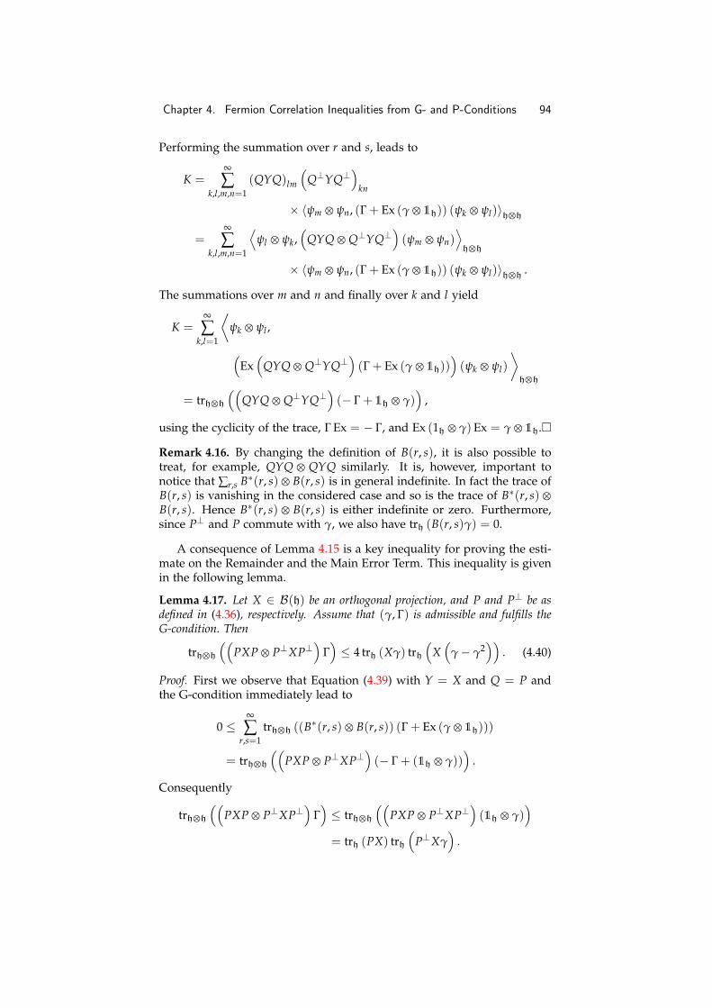
Chapter 4. Fermion Correlation Inequalities from G- and P-Conditions 94
Performing the summation over r and s, leads to
K =∞
∑k,l,m,n=1
(QYQ)lm
(Q⊥YQ⊥
)kn
× 〈ψm ψn, (Γ + Ex (γ 1h)) (ψk ψl)〉hh
=∞
∑k,l,m,n=1
⟨ψl ψk,
(QYQ Q⊥YQ⊥
)(ψm ψn)
⟩hh
× 〈ψm ψn, (Γ + Ex (γ 1h)) (ψk ψl)〉hh .
The summations over m and n and finally over k and l yield
K =∞
∑k,l=1
⟨ψk ψl ,
(Ex(
QYQ Q⊥YQ⊥)(Γ + Ex (γ 1h))
)(ψk ψl)
⟩hh
= trhh
((QYQ Q⊥YQ⊥
)(− Γ + 1h γ)
),
using the cyclicity of the trace, Γ Ex = − Γ, and Ex (1h γ)Ex = γ 1h.
Remark 4.16. By changing the definition of B(r, s), it is also possible totreat, for example, QYQ QYQ similarly. It is, however, important tonotice that ∑r,s B∗(r, s) B(r, s) is in general indefinite. In fact the trace ofB(r, s) is vanishing in the considered case and so is the trace of B∗(r, s) B(r, s). Hence B∗(r, s) B(r, s) is either indefinite or zero. Furthermore,since P⊥ and P commute with γ, we also have trh (B(r, s)γ) = 0.
A consequence of Lemma 4.15 is a key inequality for proving the esti-mate on the Remainder and the Main Error Term. This inequality is givenin the following lemma.
Lemma 4.17. Let X ∈ B(h) be an orthogonal projection, and P and P⊥ be asdefined in (4.36), respectively. Assume that (γ, Γ) is admissible and fulfills theG-condition. Then
trhh
((PXP P⊥XP⊥
)Γ)≤ 4 trh (Xγ) trh
(X(
γ− γ2))
. (4.40)
Proof. First we observe that Equation (4.39) with Y = X and Q = P andthe G-condition immediately lead to
0 ≤∞
∑r,s=1
trhh ((B∗(r, s) B(r, s)) (Γ + Ex (γ 1h)))
= trhh
((PXP P⊥XP⊥
)(− Γ + (1h γ))
).
Consequently
trhh
((PXP P⊥XP⊥
)Γ)≤ trhh
((PXP P⊥XP⊥
)(1h γ)
)= trh (PX) trh
(P⊥Xγ
).
Chapter 4. Fermion Correlation Inequalities from G- and P-Conditions 95
Secondly we permute the arguments in the trace cyclically and use thatγ is trace class and PX and P⊥X are bounded. Then we apply (4.37) toestimate the projections:
trh (PX) trh(
P⊥Xγ)= trh (XPX) trh
(X√
γP⊥√
γX)
≤ 4 trh (Xγ) trh(
X(
γ− γ2))
since γP⊥ =√
γP⊥√
γ.
Remark 4.18. Since trhh ((A B) Γ) = trhh ((B A) Γ) for any A, B ∈B(h), we also have
trhh
((P⊥XP⊥ PXP
)Γ)≤ 4 trh (Xγ) trh
(X(
γ− γ2))
.
4.2 Estimation of the Remainder
Now we consider the Remainder of Equation (4.38):
TR := trhh
((P⊥XP⊥ P⊥XP⊥
)Γ)
+ 4 Re
trhh
((P⊥XP P⊥XP⊥
)Γ)
+ 2 trhh
((P⊥XP⊥ PXP
)Γ)+ 2 trhh
((PXP⊥ P⊥XP
)Γ)
The first three terms, summed up in TR1 , and the last term, denoted byTR2 , are treated separately to derive a lower bound.
Lemma 4.19. Let X ∈ B(h) be an orthogonal projection, and P and P⊥ asin Definition 4.11. Assume that (γ, Γ) is admissible and fulfills the G- and P-conditions. Then
TR1 := trhh
((P⊥XP⊥ P⊥XP⊥
)Γ)+ 2 trhh
((P⊥XP⊥ PXP
)Γ)
+ 4 Re
trhh
((P⊥XP⊥ PXP⊥
)Γ)
≥− 8 trh (Xγ) trh(
X(
γ− γ2))
.
Proof. We use Re (ζ) ≥ − |ζ| for any complex number ζ and
P⊥XP P⊥XP⊥ =(
P⊥X P⊥X) (
XP XP⊥)
to infer
TR1 = trhh
((P⊥XP⊥ P⊥XP⊥
)Γ)+ 2 trhh
((PXP P⊥XP⊥
)Γ)
+ 4 Re
trhh
((P⊥XP P⊥XP⊥
)Γ)
≥ trhh
((P⊥XP⊥ P⊥XP⊥
)Γ)+ 2 trhh
((PXP P⊥XP⊥
)Γ)
− 4∣∣∣trhh
((P⊥X P⊥X
) (XP XP⊥
)Γ)∣∣∣ .
Chapter 4. Fermion Correlation Inequalities from G- and P-Conditions 96
Because (A, B) := trhh (A∗B Γ) defines a positive semi-definite Hermitianform on B(h h) due to Γ ≥ 0, which is the P-condition, the Cauchy–Schwarz inequality,
|(A, B)| ≤ (A, A)12 (B, B)
12 , (4.41)
holds, and we obtain
TR1 ≥ trhh
((P⊥XP⊥ P⊥XP⊥
)Γ)+ 2 trhh
((PXP P⊥XP⊥
)Γ)
− 4[trhh
((P⊥XP⊥ P⊥XP⊥
)Γ)
trhh
((PXP P⊥XP⊥
)Γ) ] 1
2.
As x2 − 4bx ≥ − 4b2 for x :=(trhh
((P⊥XP⊥ P⊥XP⊥
)Γ)) 1
2 and b :=(trhh
((PXP P⊥XP⊥
)Γ)) 1
2 , we then easily conclude
TR1 ≥ − 4 trhh
((PXP P⊥XP⊥
)Γ)+ 2 trhh
((PXP P⊥XP⊥
)Γ)
= − 2 trhh
((PXP P⊥XP⊥
)Γ)
.
The proof is completed by using Inequality (4.40):
TR1 ≥ − 2 trhh
((PXP P⊥XP⊥
)Γ)
≥ − 8 trh (Xγ) trh(
X(
γ− γ2))
.
The estimate of TR2 := − 2 trhh
((P⊥XP PXP⊥
)Γ)
is addressed inthe next lemma.
Lemma 4.20. Let X = X∗ = X2 ∈ B(h), and P and P⊥ as defined in (4.36).Assume that (γ, Γ) is admissible and fulfills the G- and P-conditions. Then
TR2 = − 2 trhh
((P⊥XP PXP⊥
)Γ)
≥ − 8 trh (Xγ) trh(
X(
γ− γ2))
. (4.42)
Proof. Estimating the l.h.s. and afterwards applying the Cauchy–Schwarzinequality (4.41) yields
− 2 trhh
((P⊥XP PXP⊥
)Γ)
≥ − 2∣∣∣trhh
((P⊥XP PXP⊥
)Γ)∣∣∣
≥ − 2[trhh
((P⊥XP⊥ PXP
)Γ)
trhh
((PXP P⊥XP⊥
)Γ) ] 1
2
= − 2 trh((
PXP P⊥XP⊥)
Γ)
. (4.43)
Again the assertion (4.42) follows from (4.40).
Summing up the results, we obtain the following estimate of the Re-mainder directly from Lemmas 4.19 and 4.20.
Chapter 4. Fermion Correlation Inequalities from G- and P-Conditions 97
Theorem 4.21 (Estimation of the Remainder). Let X ∈ B(h) be an orthogo-nal projection, and P and P⊥ the orthogonal projections defined in (4.36). Assumethat (γ, Γ) is admissible and fulfills the G- and P-conditions. Then
TR ≥ − 16 trh (Xγ) trh(
X(
γ− γ2))
.
4.3 Estimation of the Main Error Term
The main error in Theorem 4.7 results from estimating
TMET = 2 Re
trhh
((P⊥XP P⊥XP
)Γ)
. (4.44)
A key observation is that any term of the form A B ∈ B(h h) orEx (A B) ∈ B(h h) can be added to Γ in (4.44) without changing thevalue of TMET provided A and B commute with P⊥ and P. Therefore wecan consider
TMET = 2 Re
trhh
((P⊥XP P⊥XP
)(Γ + Ex (γ 1h))
)instead. This expression is estimated using a version of the Cauchy–Schwarz inequality given in the next lemma.
Lemma 4.22. Let X = X∗ = X2 ∈ B( f h), and P and P⊥ be as defined in(4.36). Assume that (γ, Γ) is admissible and fulfills the G-condition. Then
Re
trhh
((P⊥XP P⊥XP
)(Γ + Ex (γ 1h))
)≥ −
(trhh
((PXP⊥ P⊥XP
)(Γ + Ex (γ 1h))
)) 12
×(
trhh
((P⊥XP PXP⊥
)(Γ + Ex (γ 1h))
)) 12 .
(4.45)
Proof. We define
(A, B) := trhh ((A∗ B) (Γ + Ex (γ 1h)))
on B(h)×B(h) and observe that (· , ·) defines a Hermitian form on B(h)×B(h) because
trhh ((B∗ A) Γ) = trhh ((A B∗) Γ) = trhh ((A∗ B) Γ)
and
trhh ((B∗ A)Ex (γ 1h)) = trh (B∗A γ) = trh (A∗B γ)
= trhh ((A∗ B)Ex (γ 1h)).
Furthermore (· , ·) is positive semi-definite since
(A, A) = trhh ((A∗ A) (Γ + Ex (γ 1h)))
≥ |trh (Aγ)|2 ≥ 0
Chapter 4. Fermion Correlation Inequalities from G- and P-Conditions 98
by the G-condition. Hence the Cauchy–Schwarz inequality
|(A, B)| ≤ (A, A)12 (B, B)
12
holds true. Applying this with A∗ := B := P⊥XP, we obtain the assertedestimate (4.45):
Re
trhh
((P⊥XP P⊥XP
)(Γ + Ex (γ 1h))
)= Re (A∗, A) ≥ − |(A∗, A)| ≥ − (A∗, A∗)
12 (A, A)
12
= −(
trhh
((PXP⊥ P⊥XP
)(Γ + Ex (γ 1h))
)) 12
×(
trhh
((P⊥XP PXP⊥
)(Γ + Ex (γ 1h))
)) 12 .
Now the Main Error Term can be estimated.
Theorem 4.23 (Estimation of the Main Error Term). Let X ∈ B(h) be anorthogonal projection, and P and P⊥ the projections from Definition 4.11. Assumethat (γ, Γ) is admissible and fulfills the G- and P-conditions. Then
TMET ≥ − 2 trh (Xγ)[8 trh
(X(
γ− γ2)) (
1 + 4 trh(
X(
γ− γ2)) )] 1
2.
Proof. We rewrite TMET adding the necessary exchange term to allow foran application of Lemma 4.22:
TMET = 2 Re
trhh
((P⊥XP P⊥XP
)Γ)
= 2 Re
trhh
((P⊥XP P⊥XP
)(Γ + Ex (γ 1h))
)≥ − 2
(trhh
((PXP⊥ P⊥XP
)(Γ + Ex (γ 1h))
)) 12
×(
trhh
((P⊥XP PXP⊥
)(Γ + Ex (γ 1h))
)) 12 .
Note that trhh
((PXP⊥ P⊥XP
)Γ)= trhh
((P⊥XP PXP⊥
)Γ)
is al-ready estimated in (4.43). Together with (4.40) we obtain
trhh
((PXP⊥ P⊥XP
)Γ)≤ trh
((PXP P⊥XP⊥
)Γ)
≤ 4trh (Xγ) trh(
X(
γ− γ2))
.
The two exchange terms are treated separately. Using P⊥, P ≤ 1h, we find
trhh
((PXP⊥ P⊥XP
)Ex (γ 1h)
)= trh
(P⊥XPγPXP⊥
)= trh
(P⊥X
√γP√
γXP⊥)
≤ trh (Xγ) ,
Chapter 4. Fermion Correlation Inequalities from G- and P-Conditions 99
and
trhh
((P⊥XP PXP⊥
)Ex (γ 1h)
)= trh
(PXP⊥γP⊥XP
)= trh
(XPXXP⊥γP⊥X
)≤ trh (XPX) trh
(XP⊥γP⊥X
)≤ 4 trh (Xγ) trh
(X(
γ− γ2))
where cyclic permutation in the argument of the trace is used togetherwith X = X2,
(P⊥)2
= P⊥, and P2 = P to expand the argument of thetrace. Then XPX ≥ 0 and XP⊥γP⊥X ≥ 0 yield the estimate XPX ≤1h trh (XPX). Afterwards Inequalities (4.37) can be applied. Merging theresults, we arrive at the assertion.
4.4 Estimation of the Main Part
In this subsection it is shown that the remaining terms of (4.38),
TMP = trhh ((PXP PXP) Γ) + 4 Re
trhh
((PXP⊥ PXP
)Γ)
+ 4 trhh
((PXP⊥ P⊥XP
)Γ)
,
are large enough to cover the Hartree–Fock part
trhh ((X X) (1hh − Ex) (γ γ))
in (4.34). Due to this we call this terms the Main Part. As mentioned, theMain Part was extended by an additional term. This extension allows forthe following observation.
Lemma 4.24. Let X ∈ B(h) be an orthogonal projection, and P and P⊥ theorthogonal projection defined in (4.36). Then
TMP = trhh
((PX
(P + 2P⊥
)(
P + 2P⊥)
XP)
Γ)
. (4.46)
Proof. Expanding the parentheses on the right side leads to the assertionby using trhh ((A B) Γ) = trhh ((B A) Γ).
For A :=(
P + 2P⊥)
XP we have TMP = trhh ((A∗ A) Γ). This pro-vides the use of the G-condition.
Theorem 4.25 (Main Part versus Hartree–Fock). Let X, P, and P⊥ ∈ B(h)be three orthogonal projection where the later two are defined as in (4.11). Assumethat (γ, Γ) is admissible and fulfills the G-condition. Then
TMP − trhh ((X X) (1h − Ex) (γ γ))
≥ − 22 trh (Xγ) trh(
X(
γ− γ2))
. (4.47)
Chapter 4. Fermion Correlation Inequalities from G- and P-Conditions 100
Proof. The proof is split into two parts. In the first part the trace of theHartree–Fock part is calculated. In the second part the Main Part is esti-mated by applying the G-condition with A :=
(P + 2P⊥
)XP.
a) As in (4.35) the trace of the Hartree–Fock part can be written as
trhh ((X X) (1hh − Ex) (γ γ)) = (trh (Xγ))2 − trh (XγXγ) .
b) Owing to Lemma 4.24, the G-condition can be applied directly onthe Main Part:
TMP = trhh
((PX
(P + 2P⊥
)(
P + 2P⊥)
XP)
Γ)
≥∣∣∣trh (PX
(P + 2P⊥
)γ)∣∣∣2
− trh(
PX(
P + 2P⊥)
γ(
P + 2P⊥)
XP)
.
Due to cyclic permutation [γ, P] =[γ, P⊥
]= 0 and P⊥P = PP⊥ = 0
some traces vanish. The result is
TMP ≥ |trh (PXγ)|2 − trh (XPXPγ)− 4 trh(
XPXP⊥γ)
≥ (trh (PXγ))2 − trh (PXγX)− 4 trh (XP) trh(
XP⊥γ)
.
trh (XPXPγ) = trh(
PX√
γP√
γXP)≤ trh (PXγX) is implied by
[P, γ] = 0 together with P ≤ 1h. The application of XP ≤ 1htrh (XP)is possible in the last trace since, on the one hand, trh
(XPXP⊥γ
)=
trh(XPXXP⊥γX
)and, on the other hand, XP⊥γX =
∣∣XP⊥√
γ∣∣2 ≥
0 together with XPX ≥ 0.
Before adding up the estimates, we note that
trh(
P⊥XγXγ)= trh
(√γX√
γP⊥√
γX√
γ)≥ 0
and
(trh (Xγ))2 − (trh (PXγ))2
=(
trh (Xγ) + trh (PXγ))(
trh (Xγ)− trh (PXγ))
=(
trh (Xγ) + trh (PXγ))
trh(
P⊥Xγ)
. (4.48)
Furthermore trh (XP) trh(XP⊥γ
)≤ 4 trh (Xγ) trh
(X(γ− γ2)). These re-
sults can now be applied together with a) and b) to the l.h.s. of (4.47):
TMP− trhh ((X X) (1hh − Ex) (γ γ))
≥−((trh (Xγ))2 − (trh (PXγ))2
)+ trh (XγXγ)− trh (PXγX)
− 16 trh (Xγ) trh(
X(
γ− γ2))
.
Chapter 4. Fermion Correlation Inequalities from G- and P-Conditions 101
At this point we use (4.48), trh (XγXγ) = trh(
PXγXγ + P⊥XγXγ), and
rearrange:
TMP− trhh ((X X) (1hh − Ex) (γ γ))
≥− (trh (Xγ) + trh (PXγ)) trh(
P⊥Xγ)
− trh (PXγX (1h − γ)) + trh(
P⊥XγXγ)
− 16 trh (Xγ) trh(
X(
γ− γ2))
.
With P ≤ 1h, P⊥ ≤ 2 (1h − γ), and trh(
P⊥XγXγ)≥ 0 we then obtain
TMP− trhh ((X X) (1h − Ex) (γ γ))
≥− 4 trh (Xγ) trh(
X(
γ− γ2))− trh (PXγX (1h − γ))
− 16 trh (Xγ) trh(
X(
γ− γ2))
.
We can apply the inequality XγX ≤ 1hhtrh (XγX) since XγX ≥ 0,trh (PXγX (1h − γ)) = trh (XγXX (1h − γ) PX), and X (1h − γ) PX =∣∣X√1h − γP
∣∣2 ≥ 0, and obtain
TMP − trhh ((X X) (1hh − Ex) (γ γ))
≥ − 20 trh (Xγ) trh(
X(
γ− γ2))− trh (XγX) trh (X (1h − γ) PX)
≥ − 20 trh (Xγ) trh(
X(
γ− γ2))− 2 trh (Xγ) trh
(X(
γ− γ2))
= − 22 trh (Xγ) trh(
X(
γ− γ2))
.
The last inequality follows from P ≤ 2γ.
Finally the proof of Theorem 4.7 is completed by the estimations of theRemainder in Theorem 4.21, of the Main Error Term in Theorem 4.23, andof TMP − trhh ((X X) (1hh − Ex) (γ γ)) in Theorem 4.25. In eachof these theorems the G-condition is used to generate bounds. The P-condition is only applied to provide the use of the Cauchy–Schwarz in-equality. In the end it is remarkable that the Q-condition is not needed forthe proof of the correlation estimate.
5 Summary
We obtained several results in the last section which are merged in themain theorem, Theorem 4.7:
trhh ((X X) (Γ− (1hh − Ex) (γ γ))) ≥ − trh (Xγ) ,
TR ≥ − 16 trh (Xγ) trh(
X(
γ− γ2))
,
TMET ≥ − 2 trh (Xγ)[8 trh
(X(
γ− γ2)) (
1 + 4 trh(
X(
γ− γ2)) )] 1
2,
Chapter 4. Fermion Correlation Inequalities from G- and P-Conditions 102
TMP − trhh ((X X) (1hh − Ex) (γ γ))
≥ − 22 trh (Xγ) trh(
X(
γ− γ2))
.
Denoting b := trh (Xγ) and a :=√
trh (X (γ− γ2)) we can rewrite the
estimates for trhh
((X X) Γ(T)
)with Γ(T) := Γ − (1hh − Ex) (γ γ)
as
trhh
((X X) Γ(T)
)≥ − b min
1; a
(38a + 2
√8 + 32a2
). (4.49)
A suitable choice of a ≤ b in Inequality (4.49) leads to the followingcorrelation estimation.
Theorem 4.26 (Optimization of Correlation Inequality). Let X ∈ B(h) bean orthogonal projection, and P and P⊥ the orthogonal projections given in (4.36).Assume that (γ, Γ) is admissible and fulfills the G- and P-conditions. Then
trhh
((X X) Γ(T)
)≥ − trh (Xγ) min
1; 10
√trh (X (γ− γ2))
.
Proof. The minimum of the r.h.s. of (4.49) is a(
38a + 2√
8 + 32a2)
for
0 < a ≤ 1/√
94 and thus 1/a ≥(
38a + 2√
8 + 32a2)
. Since the term(38a + 2
√8 + 32a2
)is monotonously increasing in a, we find(38a + 2
√8 + 32a2
)≤√
94 < 10 (4.50)
which implies the assertion.
Remark 4.27. In Section 4.1 we have split the eigenvalues of γ in eigen-values which are greater than 1/2 and lower than or equal to 1/2. In factthis split turns out to be almost optimal and (4.50) cannot be sharpenedby another choice of P and P⊥.
Up to the constant (4.50) Theorem 4.26 is exactly the result which wasalready obtained in [Bac92]. The difference of the constants arises, on the
one hand, since the terms of trhh
((X X) Γ(T)
)are differently arranged
and, on the other hand, from the fact that in [Bac92] also the Q-conditionwas used which can be seen implicitly in estimate (68) in [Bac92]. Withthe result of Theorem 4.26 we can immediately perform the integration inthe Fefferman–de la Llave identity according to [Bac92] which leads to anestimate of trhh (V (Γ− (1hh − Ex)(γ γ))).
Chapter 5Representability Conditions by
Grassmann Integration
This chapter is the result of a joint work with V. Bach and E. Menge and aversion of it will be published separately [BKM13].
1 Introduction
The grand canonical energy (minus pressure) E0 (µ) := inf
σH− µN
at sufficiently large chemical potential µ ≥ 0 of a quantum system with aHamiltonian H and particle number operator N is given by the Rayleigh–Ritz principle as
E0 (µ) = inf
tr∧H(
ρ12
(H− µN
)ρ
12
) ∣∣∣ ρ ∈ DM
. (5.1)
The Hamiltonian is assumed to be selfadjoint and to obey stability of mat-ter, i.e., it is bounded below by −cN for some c < ∞ and at most quarticin the creation and annihilation operators [LT75, Thi08]. This is typicallythe case for models of non-relativistic matter in physics and chemistry.The Pauli principle plays a crucial role for stability of matter to hold trueand we thus restrict our attention to fermion systems. On the fermionFock space ∧H over a separable Hilbert space H, the variation on the r.h.s.of (5.1) is over the set
DM :=
ρ
∣∣∣∣ ρ ∈ L1+(∧H), tr∧H (ρ) = 1,
⟨N2⟩
ρ< ∞
,
i.e., density matrices with finite particle number variance. Here the expec-tation value of an observable A is
〈A〉ρ := tr∧H(
ρ12Aρ
12
).
More specifically, if
H− µN = ∑k,m
hkmc∗( fk)c( fm) + ∑k,l,m,n
Vklmnc∗( fl)c∗( fk)c( fm)c( fn),
103
Chapter 5. Representability Conditions by Grassmann Integration 104
then
E0 (µ) = infE(γρ, Γρ
)| ρ ∈ DM
(5.2)
where
E(γρ, Γρ
)= ∑
k,mhkm
⟨fm, γρ fk
⟩H + ∑
k,l,m,nVklmn
⟨fm fn, Γρ ( fk fl)
⟩HH
and the one- and two-particle density matrices corresponding to ρ aredefined by ⟨
f , γρg⟩H := 〈c∗(g)c( f )〉ρ and⟨
f g, Γρ
(f g
)⟩HH :=
⟨c∗(g)c∗( f )c( f )c(g)
⟩ρ
,
respectively, for all f , g, f , g ∈ H. Note that (5.2) can be rewritten as
E0 (µ) = inf E (γ, Γ) | (γ, Γ) ∈ R (5.3)
where
R :=(γ, Γ) ∈ L1(H)×L1(HH)
∣∣∣ ∃ρ ∈ DM : (γ, Γ) =(γρ, Γρ
)denotes the set of all representable one- and two-particle density matri-ces. Equation (5.3) suggests that the search for a minimizing ρ could bedrastically simplified if one would find a characterization of all represent-able reduced density matrices (γ, Γ). This was realized almost fifty yearsago [Col63, Erd78b, GP64, Löw55], but such a characterization is still un-known.
The characterization of E0 (µ) by (5.3) immediately yields lower boundsof the form
E0 (µ) =: ER (µ) ≥ ES (µ) (5.4)
for any superset S of R. For example, the positivity 〈P∗2 P2〉ρ ≥ 0 forall polynomials P2 ≡ P2 (c∗, c) in the creation and annihilation operatorsof degree two yields the so-called G-, P-, and Q-conditions on
(γρ, Γρ
)[BKM12, Col63, Erd78b, GP64]. Similarly the positivity
⟨P∗3 P3 + P3P∗3
⟩ρ≥
0 yields the T1- and generalized T2-Conditions [Erd78b]. Hence all repre-sentable reduced density matrices (γ, Γ) necessarily fulfill the G-, P-, Q-,T1-, and generalized T2-conditions, and we have
ER (µ) ≥ ES [G,P,Q,T1,T2] (µ) ≥ ES [G,P,Q] (µ) (5.5)
since R ⊆ S [G, P, Q,T1, T2] ⊆ S [G, P, Q] with
S [X] :=(γ, Γ) ∈ L1(H)×L1(HH)
∣∣∣ (γ, Γ) fulfills Conditions X
.
We have discussed (5.4)-(5.5) for S = S [G, P] in some detail in [BKM12]and refer the reader to that paper and references therein. Furthermorefor S = S [G, P, Q,T1, T2] numerical works show agreement with Full CIcomputations [CLS06, Maz02, Maz12b, ZBF+04] to high accuracy.
Chapter 5. Representability Conditions by Grassmann Integration 105
The purpose of the present paper is the reformulation of representabi-lity conditions in terms of Grassmann integrals. Such a transcription maypossibly yield new viewpoints and hopefully new insights into the repre-sentability problem. To this end we introduce a Grassmann algebra GMas a finite dimensional complex algebra. The object on GM correspond-ing to a given density matrix is an element of the form ϑ∗ ? ϑ describedin the sequel. Grassmann integration is the basic and most commonlyused method (see, e.g., [FKT02, Sal98]) in theoretical physics to computepartition functions of the form
ZΓ,λ(J) :=∫
DΓ(φ) e−SΓ+(J,φ)Γ
as a functional integral with DΓ(φ) := ∏x∈Γ dφ (x) with sources J : Γ→ R
and an action SΓ (see [Sal98] for further details).
The derivation of the G-, P-, Q-, T1-, and generalized T2-conditions isbased on the representation of the trace on ∧H in terms of Grassmannintegrals and a non-negativity condition of a Grassmann integral, namely∫
d(Ψ, Ψ) e2(Ψ,Ψ)η∗ ? η ≥ 0, (5.6)
for all η ∈ GM where∫
d(Ψ, Ψ) denotes the Grassmann integration. Thestar product refers to a product on GM and is introduced later. Consideringappropriate subspaces of GM denoted by G(n)M , the main results of thispaper are the bounds for the one-particle density matrix γϑ:
∀µ ∈ G(1)M :∫
d(Ψ, Ψ) e2(Ψ,Ψ)ϑ∗ ? ϑ ? µ ≥ 0⇔ 0 ≤ γϑ ≤ 1H
and the G-, P-, and Q-conditions as conditions for the two-particle densitymatrix Γϑ:
∀µ ∈ G(2)M :∫
d(Ψ, Ψ) e2(Ψ,Ψ)ϑ∗ ? ϑ ? µ ≥ 0
⇔ 0 ≤ γϑ ≤ 1H, G-, P-, and Q-condition
Finally we prove the validity of the T1- and generalized T2-condition byInequality (5.6).
2 Reduced Density Matrices and Representability
Before we elucidate how to derive the G-, P-, Q-, T1-, and generalized T2-conditions for the one- and two-particle density matrix (1- and 2-pdm) byGrassmann integration, we give a definition of these first two reduced den-sity matrices. For this purpose we consider a finite-dimensional index setM, an |M|-dimensional (one-particle) Hilbert space (H, 〈 · , · 〉H), and anarbitrary, but fixed orthonormal basis (ONB) ψii∈M of H where 〈 · , · 〉His linear in the second and antilinear in the first argument. Furthermore
Chapter 5. Representability Conditions by Grassmann Integration 106
we introduce the usual fermion creation and annihilation operators on thefermion Fock space ∧H over H given by c∗(ψi) ≡ c∗i and c(ψi) ≡ ci withthe canonical anticommutation relations (CAR)
c( f ), c(g) = c∗( f ), c∗(g) = 0 and c( f ), c∗(g) = 〈 f , g〉H 1∧H
for all f , g ∈ H where A, B := AB + BA denotes the anticommutator.
The 1-pdm γρ ∈ L1+(H) of a density matrix ρ, i.e., a positive trace
class operator on ∧H of unit trace (tr∧H (ρ) = 1), is defined by its matrixelements as ⟨
f , γρg⟩H := tr∧H (ρ c∗(g)c( f ))
for any f , g ∈ H. Likewise the 2-pdm Γρ ∈ L1+(HH) of ρ is defined for
any f1, f2, g1, g2 ∈ H by⟨f1 f2, Γρ(g1 g2)
⟩HH := tr∧H (ρ c∗(g2)c∗(g1)c( f1)c( f2)) .
There are several properties which can be derived directly from thedefinition of γρ and Γρ:
Lemma 5.1. Let ρ ∈ L1+(∧H) be a density matrix and N := ∑
k∈Mc∗k ck the
particle number operator with⟨N2⟩
ρ< ∞. Then the following assertions hold
true:
(i) γρ ∈ L1+(H), 0 ≤ γρ ≤ 1H, trH
(γρ
)=⟨N⟩
ρ, Γρ ∈ L1
+(HH),
0 ≤ Γρ ≤⟨N⟩
ρ1HH, and trHH
(Γρ
)=⟨N(N− 1∧H
)⟩ρ.
(ii) If ran(ρ) ⊆ ∧(N)H for some N ∈ N, then
⟨f , γρg
⟩H =
1N − 1 ∑
k∈M
⟨f ϕk, Γρ(g ϕk)
⟩HH
holds for all f , g ∈ H where ϕkk∈M is an ONB of H. Here ∧(N)Hdenotes the fermion N-particle Fock space.
(iii) Furthermore we have
ρ = |c∗(ϕ1) · · · c∗(ϕN)Ω〉 〈c∗(ϕ1) · · · c∗(ϕN)Ω| ⇔ γρ =N
∑i=1|ϕi〉 〈ϕi|
and in this case
Γρ = (1HH − Ex)(γρ γρ
)where the exchange operator Ex is given by Ex ( f g) := g f for anyf , g ∈ H and Ω ∈ ∧H denotes the vacuum vector.
Chapter 5. Representability Conditions by Grassmann Integration 107
For further details we recommend [Bac92, BKM12, Col63, GP64]. Aproof can be found in [Bac92]. Beside these properties necessary condi-tions on (γ, Γ) to be representable were derived in [Col63, Erd78b, GP64].In particular, the P-, G-, and Q-conditions are given as follows:
• (γ, Γ) fulfills the P-condition :⇔ Γ ≥ 0,
• (γ, Γ) fulfills the G-condition :⇔ For all A ∈ B(H)
trHH ((A∗ A) (Γ + Ex (γ 1H))) ≥ |trH (Aγ)|2,
• (γ, Γ) fulfills the Q-condition :⇔Γ + (1HH − Ex) (1H 1H − γ 1H − 1H γ) ≥ 0.
The T1- and the generalized T2-condition are more complicated and notgiven here. For this conditions we refer the reader to [Erd78b] or Subsec-tion 5.3 of this work.
3 Grassmann Algebras
We introduce the Grassmann algebra as the complex algebra generated byelements of the set
ψi, ψi
i∈M with |M| < ∞ modulo the anticommuta-
tion relations specified below. A product on this Grassmann algebra isdenoted by ψi · ψj ≡ ψiψj for any two generators. The unity is given as1 · ψi = ψi · 1 = ψi (and in the same manner for ψj). The anticommuta-tion relations given below allow us to find a one-to-one representation ofthe CAR of fermion creation and annihilation operators in terms of theGrassmann variables. For further details on this well-known material werecommend [CR12, dSP05, Sal98, Tak08]. In this work we use the notationof [dSP05].
Definition 5.2. For an ordered set I := i1, . . . , im ⊆ M we write
ΨI := ψi1 · · ·ψim , ΨI := ψi1 · · ·ψim .
For I = ∅ we set ΨI = ΨI = 1. Denoting the reversely ordered setcorresponding to I by I′, we write
ΨI′ := ψim · · ·ψi1 .
Definition 5.3. Given a set of generators
ψi, ψi
i∈M obeying the anticom-mutation relations
ψiψj + ψjψi = ψiψj + ψjψi = ψiψj + ψjψi = 0
for any i, j ∈ M, the Grassmann algebra GM is defined as
GM := span
ΨIΨJ
∣∣∣ I, J ⊆ M
.
Introducing the ordinary wedge product we can identify GM with theFock space ∧
(HH
)of a Hilbert space (H, 〈 · , · 〉H) with finite dimen-
sion |M|. Considering H as a subset of GM we can identify ψii∈M with afixed ONB of H and
ψi
i∈M with the corresponding ONB of H, i.e., thespace of all continuous linear functionals H → C with ψi(ψj) :=
⟨ψi, ψj
⟩H.
Chapter 5. Representability Conditions by Grassmann Integration 108
Remark 5.4. If GM is generated by
φi, φi
i∈M, we emphasize this by usingµ(φ, φ
)∈ GM instead of µ ∈ GM. We also use “mixed” generators, e.g.,
µ(ψ, φ
):= ∑
i,jαij ΨIi ΦJj
with αij ∈ C for any i, j.
Later it is necessary to link the CAR algebra of fermion annihilationand creation operators to a Grassmann algebra. For this purpose a mapbetween B(∧H) and GM that is an isomorphism between vector spaces isrequired. This map is provided below.
Definition 5.5. Let GM be generated by
ψi, ψi
i∈M and associate ψii∈Mwith a fixed ONB of H. For all z ∈ C and m, n ≤ |M| we define the linearmap Θ : B(∧H)→ GM by Θ(z) := z and
Θ(c∗(ψi1) · · · c
∗(ψim)c(ψj1) · · · c(ψjn))
:= ψi1 · · ·ψim ψj1 · · ·ψjn (5.7)
and extension to B(∧H) by linearity.
We emphasize that Θ is not multiplicative. E.g., while
Θ (c∗(ψ1)c(ψ1)) = ψ1ψ1 = Θ (c∗(ψ1))Θ (c(ψ1)) ,
we have
Θ (c(ψ1)c∗(ψ1)) = Θ (−c∗(ψ1)c(ψ1) + 1∧H)
= −ψ1ψ1 + 1 = ψ1ψ1 + 1 = Θ (c(ψ1))Θ (c∗(ψ1)) + 1.
Thus, Equation (5.7) only holds for normal-ordered monomials in creationand annihilation operators, i.e., monomials in which all creation operatorsare to the left of all annihilation operators.
Definition 5.6. For any A ∈ B(H) we set(Ψ, AΦ
):= ∑
i,j∈M
[ψi(Aψj)
]ψjφi ∈ GM.
Note that ψi(Aψj) =⟨ψi, Aψj
⟩H ∈ C. Furthermore
(Ψ, AΦ
)does not
depend on the choice of generators of GM as can be seen by a unitarychange of generators, i.e., χi := ∑j∈M Uijψj for a unitary matrix U. Animportant case is A = 1H and we then have
(Ψ, Φ
)= ∑
i∈Mψiφi. One of the
last ingredients for the Grassmann integration is the following:
Definition 5.7. The expression e±(Ψ,AΦ) ∈ GM is given by
e±(Ψ,AΦ) :=∞
∑m=0
1m![±(Ψ, AΦ
)]m .
As dim(∧H) = 2dim(H), the sum runs only over 0 ≤ m ≤ 2dim(H).
Chapter 5. Representability Conditions by Grassmann Integration 109
Remark 5.8. Since(Ψ, Φ
)= ∑α∈M ψαφα and ψαφα commutes with every
element of GM, we have
e±(Ψ,Φ) = ∏α∈M
(1± ψαφα
). (5.8)
Definition 5.9. For all i, j ∈ M we define the vector space homomorphismsδ
δψi, δ
δψi: GM → GM by
δ
δψiψj =
δ
δψiψj = δij, and
δ
δψiψj =
δ
δψiψj = 0.
Remark 5.10. The set
δδψi
, δδψi
i∈M
itself generates a Grassmann algebra.
4 Grassmann Integration
Now we are prepared to define the Grassmann integral, which is a linearoperator from the Grassmann algebra GM to the complex numbers C.
Definition 5.11. The map∫
d(Ψ, Ψ) : GM → C is defined by∫d(Ψ, Ψ) := ∏
α∈M
(δ
δψα
δ
δψα
)and referred to as the Grassmann integral.
Remark 5.12. If the factor e2(Ψ,Ψ) = ∏α∈M(1 + 2ψαψα
)is involved in the
integration, we use the abbreviation
D(Ψ, Ψ) := d(Ψ, Ψ) e2(Ψ,Ψ).
We can always write this exponential as the first factor of the integrandsince ∏α∈M
(1 + 2ψαψα
)commutes with every element of GM.
In order to state the invariance of the Grassmann integration with re-spect to a change of generators, we introduce some notations. We writetwo sets of generators,
ψi, ψi
i∈M and χi, χii∈M, as 2|M|-component
vectors a and b, respectively, where for all i ∈ M
ai := ψi and a|M|+i := ψi, and bi := χi and b|M|+i := χi. (5.9)
Furthermore we define the entries of the 2|M|-component vectors δδa and
δδb by
δ
δai:=
δ
δψiand
δ
δa|M|+i:=
δ
δψi, and
δ
δbi:=
δ
δχiand
δ
δb|M|+i:=
δ
δχi.
We denote the index set for the introduced vectors by M and therefore|M| = 2|M|. In this notation the Grassmann integration with respect to
ψi, ψi
i∈M reads
(−1)12 |M|(|M|−1) ∏
α∈M
(δ
δψα
δ
δψα
)= ∏
α∈M
δ
δψα∏
α∈M
δ
δψα= ∏
β∈M
δ
δaβ.
Chapter 5. Representability Conditions by Grassmann Integration 110
Lemma 5.13. The Grassmann integral does not depend on the choice of the ge-nerators. I.e., for a and b as defined in (5.9), and a transformation defined by
b = U a
where U is a unitary (2|M| × 2|M|)-matrix, we have
δ
δb= U
δ
δa
and for any µ ∈ GM
∏α∈M
(δ
δψα
δ
δψα
)µ(ψ, ψ
)= ∏
α∈M
(δ
δχα
δ
δχα
)µ (χ, χ) .
Proof. First we prove δδb = U δ
δa . The identity δδaj
ai = δij follows from theproperties of the generators. An equivalent identity has to be claimed forδδb b. Suppose δ
δb transforms as δδb = V δ
δa with a (2|M| × 2|M|)-matrix V.This yields
δ
δbjbi =
(∑
α∈M
Vjαδ
δaα
)(∑
β∈M
Uiβaβ
)=(
UVT)
ij.
In other words, we have to claim UVT = 1M and, thus, V = U. Finallywe can prove the invariance of the Grassmann integral. For a given set ofgenerators
ψi, ψi
i∈M any µ ∈ GM can be written as
µ ≡ µ(ψ, ψ
)= ∑
I,J⊆MαI JΨIΨJ
where the sum is over all ordered subsets I, J of M and αI J ∈ C for allordered subsets I, J ⊆ M. The Grassmann integral of µ is∫
d(Ψ, Ψ) µ(ψ, ψ
)=∫
d(Ψ, Ψ
)∑
I,J⊆MaI JΨIΨJ =
∫d(Ψ, Ψ
)αMMΨMΨM
since all other terms of µ do not contribute to the integral. If the de-composition of µ yields αMM = 0, the Grassmann integral of µ vanishes.In this case the assertion is immediate. For αMM 6= 0 we consider thetransformation of
∫d(Ψ, Ψ) and ΨMΨM separately. For
∫d(Ψ, Ψ) we use
Chapter 5. Representability Conditions by Grassmann Integration 111
δδai
δδaj
= − δδaj
δδai
for i 6= j and express δδb in terms of δ
δa :(∏
α∈M
δ
δχα
)(∏
α∈M
δ
δχα
)= ∏
β∈M
δ
δbβ
= ∑β1,...,β|M|∈M
∏j∈M
U jβ j
δ
δaβ j
= ∑π∈SM
∏j∈M
U jπ(j)δ
δaπ(j)
= ∑π∈SM
(−1)π ∏j∈M
U jπ(j)δ
δaj
= det(U)
∏j∈M
δ
δaj.
Analogously we have
∏α∈M
χM ∏α∈M
χM = ∏β∈M
bβ = det (U) ∏j∈M
aj.
Merging the results, we obtain(∏
α∈M
δ
δχα
)(∏
α∈M
δ
δχα
)∏
α∈MχM ∏
α∈MχM = |det (U)|2 ∏
j∈M
δ
δaj∏j∈M
aj.
The proof is complete with |det (U)|2 = 1 which holds since U is unitary.
Remark 5.14. The transformation U mixes ψi’s and ψi’s. For U := ( u vv u ) a
transformation without mixing is given for v = 0. In this case u has to beunitary.
For the application of the Grassmann integration on representabilityconditions we still need some tools, in particular the definition of a producton GM which induces the CAR on the Grassmann algebra.
Definition 5.15. For all µ ≡ µ(ψ, ψ
)and η ≡ η
(ψ, ψ
)∈ GM we define the
star product µ ? η ∈ GM by
(µ ? η)(ψ, ψ
):=∫
d(Φ, Φ) µ(ψ, φ
)η(φ, ψ
)e−(Ψ,Ψ)e(Ψ,Φ)e−(Φ,Φ)e(Φ,Ψ).
We calculate the star product of two monomials µ := ΨIΨJ and η :=ΨKΨL for I, J, K, L ⊆ M which determines the star product in general dueto the linearity of the Grassmann integral.
Lemma 5.16. Let I, J, K, L ⊆ M. Then we have(ΨIΨJ
)?(ΨKΨL
)= σSσJS e−(Ψ,Ψ)ΨIΨJ\SΨK\SΨL ∏
α∈M\(J∪K)
(1 + ψαψα
)(5.10)
Chapter 5. Representability Conditions by Grassmann Integration 112
where S := J ∩ K and σJS := (−1)|S|(|J\S|+ |S|−1
2
). σS is given by the identity
σSΦSΦJ\SΦSΦK\S = ΦJΦK.
Proof. Writing S := J ∩ K we face the integral(ΨIΨJ
)?(ΨKΨL
)= σS e−(Ψ,Ψ)ΨI
∫d(Φ, Φ)ΦSΦJ\SΦSΦK\S
× ∏α∈M
(1 + φαψα + ψαφα − φαφα − φαφαψαψα
)ΨL
where we use
∏α∈M
(1 + φαψα + ψαφα − φαφα − φαφαψαψα
)= e(Ψ,Φ)e−(Φ,Φ)e(Φ,Ψ)
as a consequence of (5.8). In the next step we write
M = (M \ (J ∪ K)) ∪ (J \ S) ∪ (K \ S) ∪S
(where ∪ denotes a disjoint union) and arrive at(ΨIΨJ
)?(ΨKΨL
)=σSσSJ e−(Ψ,Ψ)ΨI
∫d(Φ, Φ) ∏
α∈Sφαφα
× ∏α∈J\S
(φα + φαφαψα
)∏
α∈K\S
(φα + φαψαφα
)× ∏
α∈M\(J∪K)
(1 + φαψα + ψαφα − φαφα − φαφαψαψα
)ΨL.
The sign σJS := (−1)|S|(|J\S|+ |S|−1
2
)occurs due to the permutation of all φ’s
in ΦS with all φ’s in ΦJ\S, and ΦSΦS = (−1)12 |S|(|S|−1) (∏α∈S φαφα
). Now
we can perform the integration and arrive at(ΨIΨJ
)?(ΨKΨL
)= σSσJS e−(Ψ,Ψ)ΨI ∏
α∈J\Sψα ∏
α∈K\Sψα ∏
α∈M\(J∪K)
(1 + ψαψα
)ΨL
as claimed in (5.10) since all involved sets are disjoint.
There are several properties of the star product which follow fromLemma 5.16.
Lemma 5.17. For all µ, η, ν ∈ GM we have
µ ? (η ? ν) = (µ ? η) ? ν.
Proof. By the definition of the star product we have
µ ? (η ? ν) = µ(ψ, ψ
)?∫
d(Φ, Φ) η(ψ, φ
)ν(φ, ψ
)× e−(Ψ,Ψ)+(Ψ,Φ)−(Φ,Φ)+(Φ,Ψ)
=∫
d(Ξ, Ξ)∫
d(Φ, Φ) µ(ψ, ξ
)η(ξ, φ)
ν(φ, ψ
)× e−(Ψ,Ψ)+(Ψ,Ξ)−(Ξ,Ξ)+(Ξ,Φ)−(Φ,Φ)+(Φ,Ψ).
Chapter 5. Representability Conditions by Grassmann Integration 113
Performing the integration with respect to(φ, φ
), we gain
µ ? (η ? ν)
=∫
d(Ξ, Ξ) µ(ψ, ξ
)η(ξ, ψ
)e−(ΨΨ)+(Ψ,Ξ)−(Ξ,Ξ)+(Ξ,Ψ) ? ν
(ψ, ψ
)which is actually (µ ? η) ? ν.
As for the creation and annihilation operators on B(∧H) there is alsoan implementation of the CAR for the generators of GM.
Lemma 5.18. Let
ψi, ψi
i∈M be the generators of GM. With µ, η? := µ ?η + η ? µ we have
ψi, ψj?=
ψi, ψj
?= 0, and
ψi, ψj
?= δij
for any i, j ∈ M.
Proof. The identities follow directly from Lemma 5.16 by an appropriatechoice of I, J, K, and L. We observe that
e−(Ψ,Ψ) ∏α∈M\(J∪K)
(1 + ψαψα
)= ∏
α∈J∪K
(1− ψαψα
)
and conclude for the first identity with I = K = ∅, J = i, and L = jin (5.10) that S = ∅ and therefore σS = σJS = 1. This yields
ψi ? ψj =(1− ψiψi
)ψiψj = ψiψj. (5.11)
Setting J = j and L = i we gain ψj ? ψi = ψjψi and hence ψi ? ψj +
ψj ? ψi = ψiψj + ψjψi = 0. Equivalently we obtain ψiψj + ψjψi = 0.For the last identity we set J = K = ∅, I = i, and L = j. On the onehand, (5.10) leads to
ψi ? ψj = ψiψj
which is valid for both i = j and i 6= j. On the other hand, with I = L = ∅,J = j, and K = i we have to distinguish between the cases J = K andJ 6= K. For J 6= K we have
ψj ? ψi =(1− ψiψi
) (1− ψjψj
)ψjψi = ψjψi.
For J = K we have S = J = K and thus
ψj ? ψi =(1− ψiψi
). (5.12)
The last two results together give ψj ? ψi = δij − ψiψj. Finally we arrive atψi ? ψj + ψj ? ψi = δij. We mention that in (5.11)-(5.12) σS = σJS = 1 due tothe choice of the sets I, J, K, and L.
By a straightforward calculation using Lemma 5.16 one can also showthat for any generator
ψi, ψi
i∈M of GM we have the following:
Chapter 5. Representability Conditions by Grassmann Integration 114
Corollary 5.19. Let
ψi, ψi
i∈M be the generators of GM. Then we have
ψi1 ? · · · ? ψim ? ψj1 ? · · · ? ψjn = ψi1 · · ·ψim ψj1 · · ·ψjn .
Proof. We use the associativity(
ψi1 ? · · · ? ψim
)?(ψj1 ? · · · ? ψjn
)= ψi1 ?
· · · ? ψim ? ψj1 ? · · · ? ψjn and calculate the brackets using Lemma 5.16. Forthe first bracket we set in (5.10) I = i1, . . . , im and J = K = L = ∅. Forthe second bracket we use I = J = K = ∅ and L = j1, . . . , jn. For bothwe have σS = σJS = 1 and conclude
ψi1 ? · · · ? ψim ? ψj1 ? · · · ? ψjn =(
ψi1 · · ·ψim
)?(ψj1 · · ·ψjn
).
The last star product can be calculated by setting I = i1, . . . , im, L =j1, . . . , jn, and J = K = ∅ in (5.10). Again, σS = σJS = 1, and we arriveat the assertion.
We emphasize that
ψiψj = ψi ? ψj, but ψiψj = −ψjψi = −ψj ? ψi.
This implies that the star product can be inserted (or skipped) only if themonomial in ψ and ψ is normal-ordered (i.e., all ψ’s are to the left of allψ’s). As follows from the proof, monomials containing only ψ’s or ψ’s canalso be considered as normal-ordered in the sense that we can identifyψi1 ? · · · ? ψim = ψi1 · · ·ψim and ψj1 ? · · · ? ψjn = ψj1 · · ·ψjn .
Lemma 5.20. Let N ∈ N and Ai ∈ B(∧H) for i ∈ 1, . . . , N. Then
Θ (A1 A2 · · · AN) = Θ (A1) ? Θ (A2) ? · · · ? Θ (AN) . (5.13)
Proof. Due to the associativity of the star product it suffices to considerthe assertion for N = 2. We use the CAR to establish normal order inthe product A1 A2 ∈ B(∧H) and indicate this order by •• A1 A2
••. For some
ai1 ...imj1 ...jn
∈ C we can write
•• A1 A2
•• = ∑
m,n∑
i1 ...imj1 ...jn
∈M
ai1 ...imj1 ...jn
c∗i1 · · · c∗im cj1 · · · cjn
and apply Θ. Using Corollary 5.19 we arrive at
Θ (•• A1 A2••) = ∑
m,n∑
i1 ...imj1 ...jn
∈M
ai1 ...imj1 ...jn
ψi1 ? · · · ? ψim ? ψj1 ? · · · ? ψjm . (5.14)
Now we can use the CAR on GM to restore the same order we had in A1 A2within the r.h.s. of (5.14) and recognize that it equals Θ (A1) ? Θ (A2). Inother words we have
∑m,n
∑i1 ...imj1 ...jn
∈M
ai1 ...imj1 ...jn
ψi1 ? · · · ? ψim ? ψj1 ? · · · ? ψjm = ••Θ (A1) ? Θ (A2)
••,
which gives the assertion.
Chapter 5. Representability Conditions by Grassmann Integration 115
We can equip (GM,+, ?) with an involution (·)∗ such that (GM,+, ?, ∗)becomes a *-algebra.
Definition 5.21. For all µi ∈ GM with i ∈ N and c ∈ C the involution (·)∗on (GM,+, ?) is defined by (ψi)
∗ := ψi and(ψi)∗ := ψi for any i ∈ M, and
(c µ1 · · · µn)∗ := c µ∗n · · · µ∗1 .
Remark 5.22. For µ ≡ µ(ψ, φ
):= ∑I,J aI J ΨIΦJ and aI J ∈ C the involution
µ∗ is µ∗(φ, ψ
)= ∑I,J aI J ΦJ′ΨI′ = ∑I,J (−1)
12 |I|(|I|−1)+ 1
2 |J|(|J|−1) αI J ΦJΨI .We emphasize that
(µ(ψ, φ
))∗= µ∗
(φ, ψ
)6=(µ(φ, ψ
))∗.Lemma 5.23. The involution in Definition 5.21 is compatible with Θ, the Grass-mann integration, and the star product:
a) Θ((·)∗
)= (Θ (·))∗,
b)∫
d(Ψ, Ψ) (·)∗ =[∫
d(Ψ, Ψ) (·)]∗,
c) (µ ? η)∗ = η∗ ? µ∗.
Proof. We prove a) and b). c) is a consequence of b).
a) For any I, J ⊆ M we abbreviate C∗I := c∗i1 · · · c∗im and CJ := cj1 · · · cjn
and write any A ∈ B(H) as A = ∑I,J aI J C∗I CJ for some aI J ∈ C. Thisleads to
(Θ (A))∗ =
(∑I,J
aI J ΨIΨJ
)∗= ∑
I,JaI J ΨJ′ΨI′ = Θ
(∑I,J
aI J C∗J′CI′
)
= Θ((
∑I,J
aI J C∗I CJ
)∗)= Θ (A∗) .
b) For a fixed, but arbitrary i ∈ M and µ ∈ GM we formally have(δ
δψi
δδψi
)∗µ = δ
δψi
δδψi
µ which gives the assertion.
c) We calculate the l.h.s. of c) using b) and Remark 5.22:
(µ ? η)∗ =∫
d(Φ, Φ) η∗(ψ, φ
)µ∗(φ, ψ
)e−(Ψ,Ψ)e(Ψ,Φ)e−(Φ,Φ)e(Φ,Ψ)
= η∗ ? µ∗
since(
e(·))∗
= e(·).
A key property of the Grassmann integral for deriving representabilityconditions as in the next section is the cyclicity property which has itsequivalent in the cyclicity of the trace, i.e., tr∧H (AB) = tr∧H (BA).
Theorem 5.24. For µ, η ∈ GM we have∫D(Ψ, Ψ) (µ ? η) =
∫D(Ψ, Ψ) (η ? µ) .
Chapter 5. Representability Conditions by Grassmann Integration 116
Proof. Without loss of generality we can set
µ := ΨIΨJ and η := ΨKΨL
and observe with (5.10) and T := I ∩ L∫D(Ψ, Ψ) µ ? η = σSσTσJS
∫D(Ψ, Ψ) · e−(Ψ,Ψ)
×ΨTΨI\T ∏α∈J\S
ψα ∏α∈K\S
ψα ∏α∈M\(J∪K)
(1 + ψαψα
)ΨTΨL\T .
Afterwards, we rearrange the factors and arrive at∫D(Ψ, Ψ) µ ? η = σSσT σ
∫d(Ψ, Ψ)ΨI\TΨK\SΨJ\SΨL\T ∏
α∈Tψαψα
× ∏α∈M
(1 + ψαψα
)∏
α∈M\(J∪K)
(1 + ψαψα
)(5.15)
where σ ∈ ±1 corresponds to the signs resulting from the anticommu-tations and is
σ := (−1)|S||J\S|+|T||K\S|+12 |S|(|S|−1)+ 1
2 |T|(|T|−1)+|T||J\S|+|T||I\T|+|K\S||J\S| .
In order to go on, we need some preparation. First of all we observe that
∏α∈M
(1 + ψαψα
)∏
α∈M\(J∪K)
(1 + ψαψα
)= ∏
α∈M\(J∪K)
(1 + 2ψαψα
)∏
α∈J∪K
(1 + ψαψα
).
On the one hand, we have J ∪ K = (J \ S) ∪ (K \ S) ∪S which implies
∏α∈J∪K
(1 + ψαψα
)ΨK\SΨJ\S = ∏
α∈S
(1 + ψαψα
)ΨK\SΨJ\S.
On the other hand, we have by the same arguments
∏α∈M\(J∪K)
(1 + 2ψαψα
)ΨI\TΨK\SΨJ\SΨL\T ∏
α∈Tψαψα
= ∏α∈M
\(J∪K∪I∪L)
(1 + 2ψαψα
)ΨI\TΨK\SΨJ\SΨL\T ∏
α∈Tψαψα
since I ∪ L ≡ (I \ T) ∪ (L \ T) ∪T. Consequently our latter calculationslead in (5.15) to∫
D(Ψ, Ψ) µ ? η = σSσT σ∫
d(Ψ, Ψ)ΨI\TΨK\SΨJ\SΨL\T ∏α∈T
ψαψα
×∏α∈S
(1 + ψαψα
)∏
α∈M\(J∪K∪I∪L)
(1 + 2ψαψα
). (5.16)
Let us take a closer look at the involved sets. First of all we observe
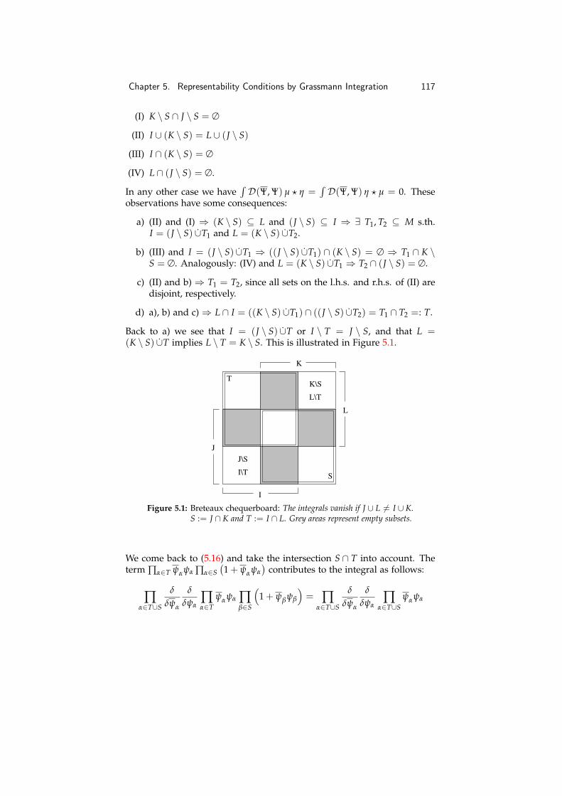
Chapter 5. Representability Conditions by Grassmann Integration 117
(I) K \ S ∩ J \ S = ∅
(II) I ∪ (K \ S) = L ∪ (J \ S)
(III) I ∩ (K \ S) = ∅
(IV) L ∩ (J \ S) = ∅.
In any other case we have∫D(Ψ, Ψ) µ ? η =
∫D(Ψ, Ψ) η ? µ = 0. These
observations have some consequences:
a) (II) and (I) ⇒ (K \ S) ⊆ L and (J \ S) ⊆ I ⇒ ∃ T1, T2 ⊆ M s.th.I = (J \ S) ∪T1 and L = (K \ S) ∪T2.
b) (III) and I = (J \ S) ∪T1 ⇒ ((J \ S) ∪T1) ∩ (K \ S) = ∅ ⇒ T1 ∩ K \S = ∅. Analogously: (IV) and L = (K \ S) ∪T1 ⇒ T2 ∩ (J \ S) = ∅.
c) (II) and b) ⇒ T1 = T2, since all sets on the l.h.s. and r.h.s. of (II) aredisjoint, respectively.
d) a), b) and c)⇒ L ∩ I = ((K \ S) ∪T1) ∩ ((J \ S) ∪T2) = T1 ∩ T2 =: T.
Back to a) we see that I = (J \ S) ∪T or I \ T = J \ S, and that L =(K \ S) ∪T implies L \ T = K \ S. This is illustrated in Figure 5.1.
T
SI\T
J\S
K\S
L\T
K
L
I
J
Figure 5.1: Breteaux chequerboard: The integrals vanish if J ∪ L 6= I ∪ K.S := J ∩ K and T := I ∩ L. Grey areas represent empty subsets.
We come back to (5.16) and take the intersection S ∩ T into account. Theterm ∏α∈T ψαψα ∏α∈S
(1 + ψαψα
)contributes to the integral as follows:
∏α∈T∪S
δ
δψα
δ
δψα∏α∈T
ψαψα ∏β∈S
(1 + ψβψβ
)= ∏
α∈T∪S
δ
δψα
δ
δψα∏
α∈T∪Sψαψα
Chapter 5. Representability Conditions by Grassmann Integration 118
since ∏α∈T∩S
ψαψα ∏β∈T∩S
(1 + ψβψβ
)= ∏
α∈T∩Sψαψα and
∏α∈S\(T∩S)
δ
δψα
δ
δψα∏
β∈S\(T∩S)
(1 + ψβψβ
)= ∏
α∈S\(T∩S)
δ
δψα
δ
δψα∏
β∈S\(T∩S)ψβψβ.
This finishes our calculations and we conclude:∫D(Ψ, Ψ) µ ? η = σSσT σ
∫d(Ψ, Ψ) ∏
α∈T∪Sψαψα
× ∏α∈M
\(J∪K∪I∪L)
(1 + 2ψαψα
)ΨI\TΨK\SΨJ\SΨL\T .
(5.17)
The r.h.s. of the assertion in Theorem 5.24 can be calculated analogously.The result is∫
D(Ψ, Ψ) η ? µ = σTσSσ∫
d(Ψ, Ψ) ∏α∈S∪T
ψαψα
× ∏α∈M
\(J∪K∪I∪L)
(1 + 2ψαψα
)ΨK\SΨI\TΨL\TΨJ\S
where the sign resulting from the anticommutations is
σ := (−1)|T||L\T|+|S||L\T|+12 |S|(|S|−1)+ 1
2 |T|(|T|−1)+|S||I\T|+|S||K\S|+|I\T||L\T| .
The l.h.s. and the r.h.s. of Theorem 5.24 are symmetric with respect to theinvolved sets. The proof is complete by the observation
σ = σ = (−1)12 |S|(|S|−1)+ 1
2 |T|(|T|−1)+|K\S||J\S|+|T||K\S|+|S||J\S|
which follows from I \ T = J \ S and L \ T = K \ S.
Remark 5.25. The integral on the r.h.s. of (5.17) can be carried out. Ab-breviating sQ := 1
2 |Q| (|Q| − 1) for Q ⊆ M, we have∫D(Ψ, Ψ) µ ? η = σSσT (−1)sS+sT+|T||K\S|+|S||J\S|+sI\T+sK\S
×∫
d(Ψ, Ψ) ∏α∈I\T
ψαψα ∏α∈K\S
ψαψα ∏α∈T∪S
ψαψα
× ∏α∈M\(I∪K)
(1 + 2ψαψα
)= σSσT (−1)sS+sT+|T||K\S|+|S||J\S|+sI\T+sK\S
× (−1)|I\T|+|K\S|+|T∪S| (−2)|M|−|I∪K| .
With |I \ T|+ |K \ S|+ |T ∪ S| = |I ∪ K| we obtain∫D(Ψ, Ψ) µ ? η = σSσT (−1)sJ+sL 2|M|−|I∪K|
for µ := ΨIΨJ and η := ΨKΨL.
Chapter 5. Representability Conditions by Grassmann Integration 119
Remark 5.26. A consequence of Lemmas 5.17 and 5.24 is the invarianceof the Grassmann integral with respect to cyclic permutations of the inte-grand:∫
d(Ψ, Ψ) (µ1 ? µ2 ? · · · ? µN) =∫
d(Ψ, Ψ) (µ2 ? · · · ? µN ? µ1) . (5.18)
This also holds true for∫D(Ψ, Ψ) ( · ) since e2(Ψ,Ψ) commutes with every
Grassmann variable.
Given an involution on (GM,+, ?), we define the property of non-negativity on GM as follows.
Definition 5.27. We call µ ∈ GM positive semi-definite, shortly µ ≥ 0, ifthere exists an η ∈ GM such that
µ = η∗ ? η.
Approaching the problem of representability by Grassmann integra-tion, an important result is the following theorem.
Theorem 5.28. For any µ ∈ GM with µ ≥ 0 we have
(−1)|M|∫D(Ψ, Ψ) µ ≥ 0. (5.19)
Proof. We use an induction in |M|. For this purpose we write any ξ ∈GM+1 := span
ψ1, . . . , ψ|M|, ψ|M|+1, ψ1, . . . , ψ|M|, ψ|M|+1
as
ξ = η00 + η01ψ|M|+1 + ψ|M|+1η10 + ψ|M|+1η11ψ|M|+1 (5.20)
for normal-ordered η00, η01, η10, η11 ∈ GM. We indicate integration withrespect to a certain index set M by writing
∫dM(Ψ, Ψ) and
∫DM(Ψ, Ψ),
respectively. Furthermore we recall that
eEM := e(Ψ,Ψ)e(Ψ,Φ)e−(Φ,Φ)e(Φ,Ψ)
=M
∏α=1
(1− φαφα + ψαψα + φαψα + ψαφα − 2ψαψαφαφα
).
In order to show (5.19) for |M| = 0, we consider µ := a∗ ? a ∈ G0 witha ∈ C, and observe that with
∫D0(Ψ, Ψ) = 1 the l.h.s. of (5.19) is non-
negative, ∫D0(Ψ, Ψ) µ = |a|2 ≥ 0.
Chapter 5. Representability Conditions by Grassmann Integration 120
Now we assume that (5.19) holds for |M| and consider the l.h.s. of (5.19)for |M|+ 1 and µ = ξ∗ ? ξ. We abbreviate ψ|M|+1 ≡ ψ′ and ψ|M|+1 ≡ ψ′.
(−1)|M|+1∫DM+1(Ψ, Ψ) (ξ∗ ? ξ)
= (−1)|M|+1∫DM+1(Ψ, Ψ)
[η∗00 ? η00 + η∗00 ?
(ψ′ η11ψ′
)+(
ψ′ η∗01
)?(η01ψ′
)+(η∗10ψ′
)?(
ψ′ η10
)+(
ψ′ η∗11ψ′)? η00
+(
ψ′ η∗11ψ′)?(
ψ′ η11ψ′) ]
.
(5.21)
Other terms like∫DM+1(Ψ, Ψ)η∗00 ? (η01ψ′) vanish, as can be seen in (5.16)
since in this case I ∪ K 6= J ∪ L.In the next step we use
∫dM+1(Ψ, Ψ) =
∫dM(Ψ, Ψ) δ
δψ′δ
δψ′ and the
definition of the star product to carry out all integrations with respect toψ′ and ψ′. We exemplify this step by the last term on the r.h.s. of (5.21):
(−1)|M|+1∫DM+1(Ψ, Ψ)
(ψ′ η∗11ψ′
)?(
ψ′ η11ψ′)
= (−1)|M|+1∫
dM+1(Ψ, Ψ)∫
dM+1(Φ, Φ
)ψ′ η∗11
(ψ, φ
)φ′
× φ′ η11(φ, ψ
)ψ′ eEM+1 .
Since η∗11(ψ, φ
)η11(φ, ψ
)is even in the variables
(ψ, ψ, φ, φ
), we continue
with
(−1)|M|+1∫DM+1(Ψ, Ψ)
(ψ′ η∗11ψ′
)?(
ψ′ η11ψ′)
= (−1)|M|+1∫
dM(Ψ, Ψ)∫
dM(Φ, Φ
)η∗11(ψ, φ
)η11(φ, ψ
)eEM
× δ
δφ′δ
δφ′δ
δψ′δ
δψ′ψ′φ′φ′ψ′
(1− φ′φ′ + ψ′ψ′ + φ′ψ′ + ψ′φ′ − 2ψ′ψ′φ′φ′
)= (−1)|M|+2
∫DM(Ψ, Ψ) η∗11 ? η11.
By analogous calculations we obtain
(−1)|M|+1∫DM+1(Ψ, Ψ) (ξ∗ ? ξ)
= (−1)|M|+2∫DM(Ψ, Ψ)
[2η∗00 ? η00 + η∗00 ? η11 + η∗01 ? η01 + η∗10 ? η10
+ η∗11 ? η00 + η∗11 ? η11
]where η11 := ∑
I,J(−1)|I|+|J| aI JΨIΨJ ∈ GM if η11 := ∑
I,JaI JΨIΨJ for some
aI J ∈ C. η11 occurs due to the anticommutations of ψM+1 with η∗11 andof ψM+1 with η11 in the second and the fifth term on the r.h.s. of (5.21),
Chapter 5. Representability Conditions by Grassmann Integration 121
respectively. Observing that∫DM(Ψ, Ψ) η∗11 ? η11
= ∑I,J,K,L
aI J aLK (−1)|I|+|J|+|K|+|L|∫DM(Ψ, Ψ)
(ΨIΨJ
)?(ΨKΨL
)=∫DM(Ψ, Ψ) η∗11 ? η11
since |I|+ |J|+ |K|+ |L| is even (otherwise both integrals vanish), we fi-nally conclude
(−1)|M|+1∫DM+1(Ψ, Ψ) (ξ∗ ? ξ)
= (−1)|M|+2∫DM(Ψ, Ψ)
[η∗00 ? η00 + (η00 + η11)
∗ ? (η00 + η11)
+ η∗01 ? η01 + η∗10 ? η10
]which is non-negative by the induction hypothesis.
Finally we can express the trace of an operator of B(∧H) and dueto Lemma 5.20 the trace of a product of such operators as a Grassmannintegral.
Theorem 5.29. For all A ∈ B(∧H) we have
tr∧H (A) = (−1)|M|∫D(Ψ, Ψ)Θ (A) . (5.22)
It is sufficient to assume that A is bounded in Theorem 5.29 for thetrace to be finite since dim(H) < ∞.
Proof. We assume that A ∈ B(∧H) is normal-ordered. Due to the linearityof the trace and the Grassmann integral it suffices to consider the trace
tr∧H(
c∗i1 · · · c∗im cj1 · · · cjn
)where I := i1, . . . , im and J := j1, . . . , jn are
ordered. For I 6= J both the l.h.s. and the r.h.s. of (5.22) vanish. For I = Jthe l.h.s. of (5.22) is given by
tr∧H(
c∗i1 · · · c∗im ci1 · · · cim
)= (−1)
12 |I|(|I|−1) 2|M|−|I|.
On the r.h.s. of Equation (5.22) we have Θ(
c∗i1 · · · c∗im ci1 · · · cim
)= ψi1 · · ·
ψim ψi1 · · ·ψim and thus∫D(Ψ, Ψ)ψi1 · · ·ψim ψi1 · · ·ψim = (−1)
12 |I|(|I|+1)
∫D(Ψ, Ψ)
m
∏α=1
(ψiα ψiα
)= (−1)|M| (−1)
12 |I|(|I|+1) 2|M|−|I|
since ∏α∈I(ψαψα
)e2(Ψ,Ψ) = ∏α∈I
(ψαψα
)∏α∈M\I
(1 + 2ψαψα
)and there-
fore
∏α∈M
(δ
δψ
δ
δψ
)∏α∈I
(ψαψα
)e2(Ψ,Ψ) = (−2)|M|−|I| .
The proof is complete by (−2)|M|−|I| = (−1)|M| (−1)|I| 2|M|−|I|.
Chapter 5. Representability Conditions by Grassmann Integration 122
Due to the restriction to a Hilbert space with even dimension, wehenceforth skip the factor (−1)|M|.
5 Representability Conditions from Grassmann Integrals
The last section allows for an application of the Grassmann integration onthe problem of representability for fermion systems. In particular, we areinterested in necessary conditions for the 1- and 2-pdm to have their originin a density matrix ρ [BKM12]. In the language of Grassmann integrationwe call the equivalents of density matrices Grassmann densities.
Definition 5.30. A Grassmann variable ϑ∗ ? ϑ ∈ GM is called Grassmanndensity if it is normalized, i.e., if it fulfills∫
D(Ψ, Ψ
)ϑ∗ ? ϑ = 1.
By definition the Grassmann density is positive semi-definite and self-adjoint. For a given state ρ the map Θ immediately provides ϑ∗ ? ϑ, namelyϑ∗ ? ϑ = Θ (ρ). Due to the product rule for Θ and the positive semi-definiteness of ρ we also have ϑ∗ ? ϑ = Θ
(ρ
12 ρ
12
)= Θ
(ρ
12
)? Θ
(ρ
12
).
Θ is a bijection and compatible with the involution. This implies thatϑ = Θ
(ρ
12
). Given a Grassmann density we can formulate the problem
of representability by Grassmann integrals using the trace-formula (5.22).
Definition 5.31. Let
ψi, ψi
i∈M be the generators of GM and associateψii∈M with a fixed ONB of H. The 1-pdm γϑ ∈ B (H) and 2-pdmΓϑ ∈ B (HH) of a Grassmann density ϑ∗ ? ϑ are defined by their respec-tive matrix elements:
〈ψk, γϑψl〉H :=∫D(Ψ, Ψ) ϑ∗ ? ϑ ? ψl ? ψk and (5.23)
〈ψm ψn, Γϑ (ψl ψk)〉HH :=∫D(Ψ, Ψ
)ϑ∗ ? ϑ ? ψk ? ψl ? ψm ? ψn .
(5.24)
Applying the trace formula (5.22) on (5.23) and (5.24), respectively, weobserve that ⟨
ψk, γρψl⟩= tr∧H
(Θ−1 (ϑ∗ ? ϑ) c∗l ck
)and⟨
ψm ψn, Γρ (ψl ψk)⟩= tr∧H
(Θ−1 (ϑ∗ ? ϑ) c∗l c∗k cncm
),
which agrees with the common definition of the 1- and 2-pdm [BKM12]if we interpret Θ−1 (ϑ∗ ? ϑ) =
(Θ−1 (ϑ)
)∗ Θ−1 (ϑ) as a density matrix ρ ∈B(∧H). The problem of representability can be formulated as follows:
Definition 5.32. We call (γ, Γ) ∈ B(H)×B(HH) representable if thereexists a Grassmann density ϑ∗ ? ϑ such that (γ, Γ) = (γϑ, Γϑ).
Chapter 5. Representability Conditions by Grassmann Integration 123
5.1 Conditions on the One-Particle Density Matrix
The lower and upper bound for the eigenvalues of the 1-pdm γϑ of aGrassmann state ϑ∗ ? ϑ arise directly from the definition of the 1-pdm (see[BKM12] for further details). Here we would like to derive the conditionsby Grassmann integration. To this end we consider certain subspaces ofGM.
Definition 5.33. For any n ∈ N with n ≤ |M| we define the subspace
G(n)M := span
ΨIΨJ | |I|, |J| ≤ n⊆ GM.
Bounds for the 1-pdm rise by considering G(1)M and are called repre-sentability conditions of first order. More general, we refer to conditionsderived by considering G(n)M as representability conditions of n-th order.
Lemma 5.34. Theorem 5.28 implies
γϑ ≥ 0.
Proof. Let
ψi, ψi
i∈M be the generators of GM and αk ∈ C ∀ k ∈ M. InTheorem 5.28 we make use of Equation (5.18) with η := φ ? ϑ∗ and φ :=∑k∈M αkψk ∈ GM. We observe that with the involution (·)∗ on GM φ∗ =∑k∈M αkψk and η∗ = (φ ? ϑ∗)∗ = ϑ ? φ∗. This leads to
0 ≤∫D(Ψ, Ψ) η∗ ? η = ∑
k,l∈Mαkαl
∫D(Ψ, Ψ) ϑ∗ ? ϑ ? ψk ? ψl = 〈 f , γϑ f 〉H
where f := ∑i∈M αiψi ∈ H is arbitrary.
The upper bound for γϑ is given by another choice of η.
Lemma 5.35. Theorem 5.28 implies
γϑ ≤ 1.
Proof. The bound can be proven by following the steps of the proof of thelower bound. Again, we have αk ∈ C ∀ k ∈ M and set φ∗ = ∑k∈M αkψk ∈GM and this time η∗ = (φ∗ ? ϑ)∗ = ϑ∗ ? φ. Before we go on, we observethat by the CAR on GM given in (5.18)
φ ? φ∗ = ∑k,l∈M
αkαlψk ? ψl = ∑k∈M
αkαk − ∑k,l∈M
αkαlψl ? ψk.
Inserting this into the inequality of Theorem 5.28 and using the associativ-ity of the star product, we obtain
0 ≤∫D(Ψ, Ψ) η∗ ? η = ∑
k∈M|αk|2 − ∑
k,l∈Mαlαk
∫D(Ψ, Ψ) ϑ∗ ? ϑ ? ψl ? ψk
= 〈g, (1H − γϑ) g〉H
where we use∫D(Ψ, Ψ) ϑ∗ ? ϑ = 1 and g := ∑k∈M αkψk ∈ H.
Chapter 5. Representability Conditions by Grassmann Integration 124
Considering the subspace G(1)M , we can summarize our last two results.
Theorem 5.36. Let ϑ ? ϑ∗ be a Grassmann density and γϑ its 1-pdm. Then thefollowing statements are equivalent:
a) 0 ≤ γϑ ≤ 1.
b) For any µ ∈ G(1)M ,∫D(Ψ, Ψ) ϑ∗ ? ϑ ? µ ≥ 0 holds.
Proof. In Theorem 3.1 of [BKM12] the analogue of this theorem has beenshown for polynomials in creation and annihilation operators of degreelower than or equal to two. Because of the bijection Θ we have a one-to-one mapping between the space of polynomials of degree lower than orequal to two and G(2)M .
5.2 G-, P-, and Q-Condition
We proceed with representability conditions of second order by consid-ering G(2)M and a star-product of ψ and ψ. In this case, for example,φ := ∑k,l∈M αklψk ? ψl ∈ GM with αkl ∈ C ∀ k, l ∈ M. This time we are in-terested in conditions on Γϑ and use the Grassmann integration to rewritethe matrix elements of the 2-pdm as in (5.24). The first condition is theP-condition.
Lemma 5.37. Theorem 5.28 implies the P-condition
Γϑ ≥ 0.
Proof. The proof is similar to the one in the last subsection. Setting φ :=∑k,l∈M αklψk ? ψl ∈ GM with αkl ∈ C ∀ k, l ∈ M, η := φ ? ϑ∗, and η∗ =
(φ ? ϑ∗)∗ = ϑ ? φ∗, we arrive at
0 ≤∫D(Ψ, Ψ) η∗ ? η
= ∑k,l,m,n∈M
αklαmn
∫D(Ψ, Ψ) ϑ∗ ? ϑ ? ψl ? ψk ? ψm ? ψn
= 〈F, ΓϑF〉HH
where F := ∑k,l∈M αkl (ψm ψn) ∈ HH is arbitrary.
The Q-condition is the next representability condition we consider. Inorder to obtain a convenient formulation of this condition, we use an ex-change operator on HH which is defined by Ex ( f g) := g f for anyf , g ∈ H.
Lemma 5.38. Theorem 5.28 implies the Q-condition
Γϑ + (1HH − Ex) (1H 1H − γϑ 1H − 1H γϑ) ≥ 0.
Chapter 5. Representability Conditions by Grassmann Integration 125
Proof. With φ := ∑k,l∈M αklψk ? ψl ∈ GM, αkl ∈ C ∀ k, l ∈ M, and η = φ ? ϑ∗
we have
0 ≤∫D(Ψ, Ψ) η∗ ? η
= ∑k,l,m,n∈M
αklαmn
∫D(Ψ, Ψ) ϑ∗ ? ϑ ? ψn ? ψm ? ψk ? ψl .
Aiming for an expression in terms of Γ and γ, we establish normal order-ing using the CAR:
ψn ? ψm ? ψk ? ψl =δmkδnl − δnkδml + δnkψl ? ψm − δmkψl ? ψn + δnlψk ? ψl
− δmlψk ? ψn − ψk ? ψl ? ψn ? ψm. (5.25)
As in the proof of Lemma 5.37 we write an arbitrary G ∈ HH as G :=∑k,l∈M αkl (ψk ψl) for some αkl ∈ C. Hence, ∑k,l,m,n∈M αklαmnδkmδln =〈G,1HHG〉HH and ∑k,l,m,n∈M αklαmnδknδlm = 〈G, Ex G〉HH. With (5.23)and (5.24) we find
0 ≤ 〈G, (Γϑ + (1HH − Ex) (1H 1H − γϑ 1H − 1H γϑ)) G〉HH
by evaluating the Grassmann integral∫D(Ψ, Ψ) (·) on the r.h.s. of Equa-
tion (5.25).
The last second order representability condition which can be derivedby the described method is the (optimal) G-condition. Deriving this condi-tion by Grassmann integration requires a choice of η that is not as obviousas before.
Lemma 5.39. Theorem 5.28 implies the G-condition:
trHH ((A∗ A) (Γϑ + Ex (γϑ 1H))) ≥ |trH (Aγϑ)|2
for any A ∈ B(HH).
Proof. This time we choose η :=(∑k,l∈M αklψk ? ψl − c
)? ϑ with αkl ∈ C
for all k, l ∈ M and c := ∑k,l∈M αkl∫D(Ψ, Ψ) ϑ∗ ? ϑ ? ψk ? ψl . Before we
apply Theorem 5.28, we emphasize that by the CAR(∑
k,l∈Mαklψkψl − c
)∗?
(∑
k,l∈Mαklψkψl − c
)= cc− c ∑
k,l∈Mαklψl ? ψk − c ∑
m,n∈Mαmnψm ? ψn
− ∑k,l∈M
αklαmnψl ? ψm ? ψk ? ψn + ∑k,l,n∈M
αklαknψl ? ψn.
(5.26)
We consider the last two lines separately and integrate. The integration ofthe line before the last line in (5.26) yields∫
D(Ψ, Ψ) ϑ∗ ? ϑ ?
(cc− c ∑
k,l∈Mαklψl ? ψk − c ∑
m,n∈Mαmnψm ? ψn
)= cc− cc− cc = −cc (5.27)
Chapter 5. Representability Conditions by Grassmann Integration 126
which follows from the definition of c. It is important to notice that cdoes not depend on ψ or ψ and therefore is a constant with respect to theGrassmann integration. In detail we have for c:
c = ∑k,l∈M
αkl
∫D(Ψ, Ψ) ϑ∗ ? ϑ ? ψk ? ψl = trH (Aγϑ) (5.28)
if we define A ∈ B(H) by 〈ψk, Aψl〉H := αkl for every k, l ∈ M. Theevaluation of the Grassmann integral of the last line in (5.26) provides
− ∑k,l∈M
αklαmn
∫D(Ψ, Ψ) ϑ∗ ? ϑ ? ψl ? ψm ? ψk ? ψn
+ ∑k,l,n∈M
αklαkn
∫D(Ψ, Ψ) ϑ∗ ? ϑ ? ψl ? ψn
= trHH ((A∗ A) (Γϑ + Ex (γϑ 1H))) . (5.29)
Summing up, calculation (5.27) together with (5.28) and (5.29) gives
trHH ((A∗ A) (Γϑ + Ex (γϑ 1H)))− |trH (Aγϑ)|2 ≥ 0
by Theorem 5.28.
We summarize our results using G(2)M :
Theorem 5.40. Let ϑ ? ϑ∗ be a Grassmann density, γϑ its 1-pdm, and Γϑ its2-pdm. Then the following statements are equivalent:
a) (γϑ, Γϑ) fulfills 0 ≤ γϑ ≤ 1 and the G-, P-, and Q-conditions.
b) For any µ ∈ G(2)M∫D(Ψ, Ψ) ϑ∗ ? ϑ ? µ ≥ 0 holds.
Proof. Again we use Theorem 3.1 of [BKM12] and the bijection property ofΘ which ensures that the space of polynomials of degree lower or equalthan four in creation and annihilation operators is mapped one-to-one toG(2)M .
5.3 T1- and Generalized T2-Condition
The last sections imply that further conditions on γϑ and Γϑ can be foundby taking into account monomials of higher order of the form ψi1 ? · · · ?ψin ? ψj1 ? · · · ? ψjn for n > 2. Here we face the problem that monomialswith n > 2 have to “decompose” into monomials with n ≤ 2. Due to thisonly some choices of higher order monomials are suitable to derive furtherrepresentability conditions. One such monomial is given by
τ1 := ∑i,j,k∈M
Tijkψi ? ψj ? ψk ∈ GM
where Tijk ∈ C is totally antisymmetric due to
ψi, ψj?= 0, i.e., Tijk =
−Tjik = Tjki. The T1-condition is the following.
Chapter 5. Representability Conditions by Grassmann Integration 127
Theorem 5.41. Let Tq ∈ B(H) be trace-class and set Tkqn :=[Tq]
kn, FTq :=∑k,n∈M Tkqn (ϕk ϕn) ∈ HH. Then Theorem 5.28 implies the T1-condition:
∑q∈M
(2trh
(∣∣Tq∣∣2)− 6trh
(∣∣Tq∣∣2 γϑ
)+ 3
⟨FTq , ΓϑFTq
⟩)≥ 0.
Proof. We begin by considering the anticommutator
τ∗1 , τ1? ∈ GM and
observe that by construction
τ∗1 , τ1? ≥ 0. Furthermore we can use the
CAR to establish normal order in
τ∗1 , τ1?. The i, j−th matrix element of
A ∈ B(H) is denoted by [A]ij :=⟨ψi, Aψj
⟩H. Using the antisymmetry of
Tijk we arrive at
τ∗1 , τ1? = 9 ∑l∈M
∑i,j,m,n∈M
Tl jmTlinψm ? ψj ? ψi ? ψn
+ 18 ∑m,l∈M
∑k,n∈M
TkmlTlmnψk ? ψn + 6 ∑l,m,n∈M
Tlmn Mlmn
= 9 ∑q∈M
∑i,j,m,n∈M
[T∗q]
mj
[Tq]
in ψm ? ψj ? ψi ? ψn
− 18 ∑q∈M
∑k,n∈M
[T∗q Tq
]kn
ψk ? ψn + 6 ∑q∈M
trh(∣∣Tq
∣∣2) .
Since
τ∗1 , τ1? ≥ 0, we have by Theorem 5.28∫
D(Ψ, Ψ) ϑ ? τ∗1 , τ1? ? ϑ∗ ≥ 0.
Together with (5.24) the latter calculations and this non-negativity of theintegral bring us to
0 ≤ 3 ∑q∈M
∑i,j,m,n∈M
[T∗q]
mj
[Tq]
in
⟨ψi ψn, Γϑ
(ψj ψm
)⟩− 6 ∑
q∈M∑
k,n∈M
[∣∣Tq∣∣2]
kn〈ψn, γϑψk〉+ 2 ∑
q∈Mtrh(∣∣Tq
∣∣2) .
Together with⟨ψi, Tqψj
⟩=:[Tq]
ij and FTq := ∑k,n∈M Tkqn (ϕk ϕn) thisyields the assertion.
The generalized T2-condition can be derived equivalently by anotherchoice of τ. Using the anticommutator with a combination of two ψ’s andone ψ (or vice versa), we have three different possibilities:
τ2a := ∑i,j,k∈M
T(a)ijk ψi ? ψj ? ψk,
τ2b := ∑i,j,k∈M
T(b)ijk ψi ? ψj ? ψk, and
τ2c := ∑i,j,k∈M
T(c)ijk ψi ? ψj ? ψk.
Chapter 5. Representability Conditions by Grassmann Integration 128
A generalization of these possibilities is given by
τ2 := ∑i,j,k∈M
Tijkψi ? ψj ? ψk + ∑i∈M
aiψi
where Tijk, ai ∈ C for all i, j, k ∈ M. This is a generalization since we
obtain τ2 = τ2a for αi ≡ 0 and Tijk ≡ T(a)ijk , τ2 = τ2b for ai = ∑j∈M T(b)
ijj
and Tijk = −T(b)ikj , and finally τ2 = τ2c for ai = ∑j∈M
(T(c)
jji − T(c)jij
)and
Tijk = T(c)kij . The identities can be seen by using the CAR. Unfortunately,
if one uses the generalization τ2, symmetry properties on Tijk like, for
example, T(a)ijk = −T(a)
jik in τ2a or T(c)ijk = −T(c)
ikj in τ2c vanish. The generalizedT2-condition rises from τ∗2 , τ2? ≥ 0. In order to state the condition in acompact form, we need some new notation.
Definition 5.42. For Tk ∈ B(H), [Tk]ij := Tijk for each i, j, k ∈ M, and
a ∈ C|M| we define GMk ∈ HH and the matrices Q1 ∈ B(HH) andQ2, Q3 ∈ B(H) by
GMk := ∑i,j∈M
[Tk]ij(ψi ψj
),
⟨ψk ψm, Q1
(ψn ψj
)⟩HH :=
[T(A)
k T(A)n
]jm
,⟨ψi, Q2ψj
⟩H := trH
((T(A)
i
)∗Tj
),⟨
ψi, Q3ψj⟩H := ∑
q∈M
([(T(A)
i
)∗]jq
aq +[
T(A)j
]iq
aq
)
where[
T(A)k
]ij
:= 12
([Tk]ij − [Tk]ji
)= −
[T(A)
k
]ji
is the antisymmetric part
of Tk.
Theorem 5.43. Let Tk, a, GTq and Q1, Q2, Q3 be as in Definition 5.42. ThenTheorem 5.28 implies the generalized T2-condition:
∑q∈M
⟨GTq , ΓϑGTq
⟩HH
+ 4trHH (Q1Γϑ) + 2trH ((Q2 + Q3) γϑ) + |a|2 ≥ 0.
Proof. The first task is to bring τ∗2 , τ2 into normal order. Afterwards thetwo terms of third order cancel. Only terms of order less than or equalto two remain. We use
(µ + η)∗ , µ + η
? = µ∗, µ? + 2Re µ∗, η? +
η∗, η? for µ := ∑i,j,k∈M Tijkψi ? ψj ? ψk and η := ∑i∈M aiψi to calculatethe anticommutator. By the CAR we have
η∗, η? = ∑i∈M|ai|2 , µ∗, η? = ∑
k,n∈M∑
q∈M
(Tqnk − Tnqk
)aqψk ? ψn
Chapter 5. Representability Conditions by Grassmann Integration 129
and
µ∗, µ? = ∑j,k,m,n∈M
∑q∈M
( (T jqk − Tqjk
) (Tqmn − Tmqn
)+ TnjqTkmq
)ψk ? ψm ? ψj ? ψn
+ ∑k,n∈M
∑p,q∈M
(Tpqk − Tqpk
)Tpqnψk ? ψn.
We set Tijq =:[Tq]
ij where Tq ∈ B(H) for any q ∈ M and observe
that[Tq]
ij =[
T∗q]
ji, Tqnk − Tnqk = 2
[(T(A)
k
)∗]nq
, and Tqmn − Tmqn =
2[
T(A)n
]qm
where T(A) is the antisymmetric part of T (see Definition 5.42).
This allows us to rewrite the anticommutators:
2Re µ∗, η? = 2 ∑k,n∈M
∑q∈M
([(T(A)
k
)∗]nq
aq +[
T(A)n
]qk
aq
)ψk ? ψn
and
µ∗, µ? = ∑j,k,m,n∈M
∑q∈M
(4[(
T(A)k
)∗]qj
[T(A)
n
]qm
+[
T∗q]
jn
[Tq]
km
)ψk ? ψm ? ψj ? ψn
+ 2 ∑k,n∈M
∑p,q∈M
[(T(A)
k
)∗]qp[Tn]pq ψk ? ψn. (5.30)
In the next step we use the notation⟨ψi, Aψj
⟩H = [A]ij for A ∈ B(H) and
the Grassmann representation of γ and Γ from (5.23) and (5.24). Defini-tion 5.42 then leads to
∑j,k,m,n∈M
∑q∈M
[T∗q]
jn
[Tq]
km
∫D(Ψ, Ψ) ϑ∗ ? ϑ ? ψk ? ψm ? ψj ? ψn
= ∑q∈M
⟨GTq , ΓϑGTq
⟩HH
for GTq := ∑i,j∈M[Tq]
ij
(ψi ψj
)∈ H H. Moreover we have by the
definition of Q1 as⟨ψm ψk, Q1
(ψj ψn
)⟩HH :=
[T(A)
k T(A)n
]jm
4 ∑j,k,m,n,q∈M
[T(A)
k
]jq
[T(A)
n
]qm
∫D(Ψ, Ψ) ϑ∗ ? ϑ ? ψk ? ψm ? ψj ? ψn
= 4trHH (Q1Γϑ) .
Furthermore
2 ∑k,n∈M
∑p,q∈M
[(T(A)
k
)∗]qp[Tn]pq
∫D(Ψ, Ψ) ϑ∗ ? ϑ ? ψk ? ψn = 2trH (Q2γϑ)
Chapter 5. Representability Conditions by Grassmann Integration 130
for [Q2]kn := trH((
T(A)k
)∗Tn
).
With [Q3]ij := ∑q∈M
([(T(A)
i
)∗]jq
aq +[
T(A)j
]qi
aq
)we finally obtain
2Re
∫D(Ψ, Ψ) ϑ∗ ? ϑ ? µ∗, η? = 2trH (Q3γϑ) .
∑i|ai|2 =: |a|2 is the squared Euclidean norm of a. The proof is completeby inserting the latter calculations into the inequality of Theorem 5.28.
As already mentioned, we have antisymmetry properties for certainchoices of a and Tijk. In τ2a, which we obtain by setting a ≡ 0 and Tijk =
T(a)ijk =
[T(a)
k
]ij
, we have [Tk]ij = − [Tk]ji or Tk ≡ T(A)k . In this case we have
a simplification of the generalized T2-condition:
Corollary 5.44. For a ≡ 0, Tk ≡ T(A)k , and
[Tk]
ij :=[Tj]
ik, we have the T2a-condition given by
∑q∈M
(⟨GTq
, ΓϑGTq
⟩HH + 4trHH
((T∗q Tq
)Γϑ
)+ 2trH
(∣∣Tq∣∣2γϑ
))≥ 0.
Proof. With a ≡ 0 we only have to consider µ∗, µ? and can use (5.30)
with Tk ≡ T(A)k .
We can also use an antisymmetry property in τ2c which leads to a condi-tion T2c. Unfortunately there is no simplification compared to the genera-lized T2-condition. There is, however, no antisymmetry property in τ2b.Since
τ∗1 , τ1
? , τ∗2 , τ2? ∈ G
(3)M , the T1- and T2-conditions are representa-
bility conditions of third order.
6 Quasifree Grassmann States
The notion of Grassmann integration allows for a calculation of traces onthe fermion Fock space by Grassmann integrals and in turn to reformu-late representability condition in terms of Grassmann integrals. At lastwe consider quasifree states, their one-particle density matrices, and theexpression of their relation in terms of Grassmann integrals.
In the following we will abbreviate the expectation value of a Grass-mann variable µ ∈ GM with respect to a Grassmann density κ ∈ GM by∫
D(Ψ, Ψ)κ ? µ =: 〈 µ 〉κ .
Definition 5.45. Let N ∈ N and ψi denote either ψi ∈ GM or ψi ∈ GMwhere
ψi, ψi
i∈M is a set of generators of GM. We call a Grassmann
density κ quasifree if
1)⟨ψ1 ? ψ2 ? · · · ? ψ2N−1
⟩κ = 0 and
Chapter 5. Representability Conditions by Grassmann Integration 131
2)⟨ψ1 ? ψ2 ? · · · ? ψ2N
⟩κ
= ∑π
′ (−1)π⟨
ψπ(1) ? ψπ(2)
⟩κ× · · · ×
⟨ψπ(2N−1) ? ψπ(2N)
⟩κ
where ∑π′ denotes the sum over all permutations π obeying π(1) <
π(3) < · · · < π(2N − 1) and π(2j− 1) < π(2j) for all 1 ≤ j ≤ N. Themaximal number of (distinct) ψi or ψi in 1) and 2) is less or equal |M|.
Remark 5.46. We have to restrict N in the latter definition or extend Msufficiently since the expressions on the l.h.s. of conditions 1) and 2) vanishif the number of ψi or ψi is larger than |M|.
As it is already known from [BLS94], there is a unique characteriza-tion of quasifree states by the 1-pdm. More precisely, assuming particlenumber-conservation and defining
γ :=(
γ 00 1H − γ
)∈ B(HH),
which is the generalized 1-pdm corresponding to γ, one has the followingtheorem.
Theorem 5.47. Let γ =(
γ 00 1H−γ
)be an operator on HH with trH (γ) <
∞ and 0 ≤ γ ≤ 1HH. Then there exists a unique quasifree state ρ withtr∧H
(ρN)< ∞ such that γ = γρ.
For a proof see [BLS94].
In the language of Grassmann integration the reverse direction, namelythat γκ , i.e., the generalized 1-pdm of a quasifree Grassmann density κ,has to fulfill 0 ≤ γκ ≤ 1HH, can be deduced by appropriate choices ofφ ∈ GM in the positivity condition
〈φ∗ ? φ〉κ ≥ 0.
The aim of this section is to determine the unique quasifree Grassmanndensity subject to Theorem 5.47, i.e., the element of a Grassmann alge-bra corresponding the state given in [BLS94]. To this end we consider anoperator γ ∈ B(H H) with 0 ≤ γ ≤ 1HH and its eigenvalues λi and(1− λi) where 0 ≤ λi ≤ 1
2 for any i ∈ M. Furthermore we define P0 to bethe projection onto the subspace of ∧H on which ∑i∈M:λi=0 c∗i ci = 0. More-over for any i ∈ M the quantity qi is given by the relation (1 + eqi )−1 = λi.Then according to [BLS94] any operator γ with 0 ≤ γ ≤ 1HH is thegeneralized 1-pdm of a unique quasifree state ρ ∈ B(∧H) given by
ρ :=G
tr∧H (G)(5.31)
where
G := P0e−H and H := ∑i∈M:λi 6=0
qic∗i ci.
Chapter 5. Representability Conditions by Grassmann Integration 132
Before we turn to the definition of the Grassmann density correspond-ing to (5.31), we introduce the abbreviations Θ0 := Θ (P0) ∈ GM and∏n
i=1?µi := µ1 ? µ2 ? · · · ? µn for µi ∈ GM. Furthermore we associate the
generators
ψi, ψi
i∈M of GM with the ONB ψii∈M of H where the ψiare the eigenvectors of γ corresponding to the eigenvalues λi and (1− λi).
Lemma 5.48. Let ψii∈M be an ONB of H such that γψi = λiψi and let GMbe generated by
ψi, ψi
i∈M. The Grassmann density κ ∈ GM corresponding to
ρ = Gtr∧H(G)
is given by
κ =1Z
(Θ0 ? ∏
i∈M:λi 6=0
? ((e−qi − 1)
ψiψi + 1))
, (5.32)
where
Z :=∫D(Ψ, Ψ)Θ0 ? ∏
i:λi 6=0
? ((e−qi − 1)
ψiψi + 1)
.
Proof. We consider Θ (ρ) subject to (5.31). We first observe that c∗i ci com-mutes with c∗k ck for every i, k. Therefore we have
e−H = ∏i∈M:λi 6=0
(∞
∑n=1
(−qi)n
n!c∗i ci + 1
)= ∏
i∈M:λi 6=0
((e−qi − 1
)c∗i ci + 1
)since
(c∗i ci
)n= c∗i ci. Thus,
Θ(
P0e−H)= Θ0 ? Θ
(∏
i∈M:λi 6=0
((e−qi − 1
)c∗i ci + 1
))= Θ0 ? ∏
i∈M:λi 6=0
? ((e−qi − 1)
ψiψi + 1)
where we have used that Θ (AB) = Θ (A) ? Θ (B).
The Grassmann state corresponding to the Grassmann density (5.32) isgiven by the map
GM → C, µ 7→ 〈 µ 〉κ .
We want to verify that the Grassmann density from Lemma 5.48 isquasifree, i.e., that it fulfills conditions 1) and 2) from Definition 5.45. Theuniqueness of κ follows from the bijection property of the map Θ.
Theorem 5.49. The Grassmann state κ given in Lemma 5.48 is quasifree.
Proof. We consider the state
κµ := ∏i∈M
? (riψiψi + 1)
where ri := e−qi(µ) − 1 and qi (µ) ≡ µ ∈ R for all i with λi = 0 andqi (µ) ≡ qi for all i with λi 6= 0. The quasifreeness of κ follows by the
Chapter 5. Representability Conditions by Grassmann Integration 133
quasifreeness of κµ and a limiting argument. The first claim of Defini-tion 5.45 is immediate for κµ since the Grassmann integral vanishes foran odd number of ψ’s. This can be seen by Remark 5.25 and the che-querboard. The validity of Equation 2) of Definition 5.45 has already beenproven in [Gau60]. Here we emphasize the main steps and transfer the no-tation of [Gau60] to Grassmann Integrals. We consider the l.h.s. of claim2) of Definition 5.45,⟨
ψa ? ψb ? ψc ? · · · ? ψ f
⟩κµ
=∫D(Ψ, Ψ)κµ ? ψa ? ψb ? ψc ? · · · ? ψ f ,
with 2N generators ψa, · · · , ψ f . In the first step we eliminate ψa fromthe expectation value by a pull through formula. To this end we use
ψa, ψb? := ψa ? ψb + ψb ? ψa which is either 1, −1 or 0. This yields⟨
ψa ? ψb ? ψc ? · · · ? ψ f
⟩κµ
=
ψa, ψb?
⟨ψc ? ψd ? · · · ? ψ f
⟩κµ
−
ψa, ψc?
⟨ψb ? ψd ? · · · ? ψ f
⟩κµ
+
ψa, ψd?
⟨ψb ? ψc ? · · · ? ψ f
⟩κµ
+ . . .
+
ψa, ψ f
?
⟨ψb ? ψc ? · · · ? ψe
⟩κµ−⟨
ψb ? ψc ? · · · ? ψ f ? ψa
⟩κµ
.
Afterwards we use the cyclicity of the Grassmann integral in the last ex-pectation value on the r.h.s. of the latter expression and the identities
ψi ?κµ = eqi κµ ? ψi and ψi ?κµ = e−qi κµ ? ψi
which follow from the fact that κµ is a star product of single states of theform riψiψi + 1 and the CAR for the star product. Thus, the last expecta-tion value can be written as⟨
ψb ? ψc ? · · · ? ψ f ? ψa
⟩κµ
= e±qa⟨
ψa ? ψb ? ψc ? · · · ? ψ f
⟩κµ
and we conclude with⟨ψa ? ψb ? ψc ? · · · ? ψ f
⟩κµ
=
ψa, ψb
?
1 + e±qa
⟨ψc ? ψd ? · · · ? ψ f
⟩κµ
−
ψa, ψc?
1 + e±qa
⟨ψb ? ψd ? · · · ? ψ f
⟩κµ
+
ψa, ψd
?
1 + e±qa
⟨ψb ? ψc ? · · · ? ψ f
⟩κµ
+ . . .
+
ψa, ψ f
?
1 + e±qa
⟨ψb ? ψc ? · · · ? ψe
⟩κµ
.
We have reduced the expectation value of 2N generators to a sum of expec-tation values of 2(N − 1) generators. As in [Gau60] the assertion followsby an induction in the number of generators. Finally the quasifreeness ofκ follows from
κ = limµ→∞
κµ∫D(Ψ, Ψ)κµ
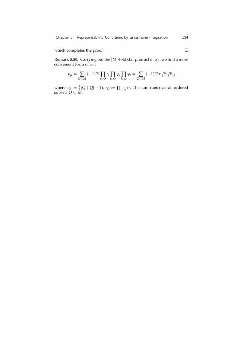
Chapter 5. Representability Conditions by Grassmann Integration 134
which completes the proof.
Remark 5.50. Carrying out the |M|-fold star product in κµ, we find a moreconvenient form of κµ:
κµ = ∑Q⊆M
(−1)sQ ∏i∈Q
ri ∏i∈Q
ψi ∏i∈Q
ψi = ∑Q⊆M
(−1)sQ rQΨQΨQ
where sQ := 12 |Q|(|Q| − 1), rQ := ∏i∈Q ri. The sum runs over all ordered
subsets Q ⊆ M.

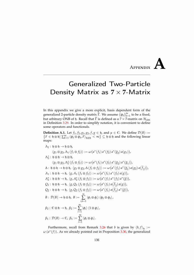
Appendix AGeneralized Two-Particle
Density Matrix as 7× 7-Matrix
In this appendix we give a more explicit, basis dependent form of thegeneralized 2-particle density matrix Γ. We assume φk∞
k=1 to be a fixed,but arbitrary ONB of h. Recall that Γ is defined as a 7× 7-matrix on Hsimin Definition 3.29. In order to simplify notation, it is convenient to definesome operators and functionals.
Definition A.1. Let f1, f2, g1, g2, f , g ∈ h, and µ ∈ C. We define D(B) :=F ∈ h h
∣∣ ∑∞k=1 〈φk φk, F〉hh < ∞
⊆ h h and the following linear
maps:
Λ1 : h h→ h h,
〈g1 g2, Λ1 ( f1 f2)〉 := ω(a∗( f1) a∗( f2) a∗(g2) a(g1)
),
Λ∗2 : h h→ h h,
〈g1 g2, Λ∗2 ( f1 f2)〉 := ω(a∗( f1) a∗( f2) a∗(g2) a∗(g1)
),
∆ : h h→ h h, 〈g1 g2, ∆ ( f1 f2)〉 := ω(a∗( f1) a∗(g1) a(g2) a( f 2)
),
A1 : h h→ h, 〈g, A1 ( f1 f2)〉 := ω(a∗( f1) a∗( f2) a(g)
),
A∗2 : h h→ h, 〈g, A∗2 ( f1 f2)〉 := ω(a∗( f1) a∗( f2) a∗(g)
),
Q1 : h h→ h, 〈g, Q1 ( f1 f2)〉 := ω(a∗( f1) a( f 2) a(g)
),
Q2 : h h→ h, 〈g, Q2 ( f1 f2)〉 := ω(a∗( f1) a( f 2) a∗(g)
),
B : D(B)→ h h, B :=∞
∑i,k=1|φi φi〉 〈φk φk| ,
β2 : C h→ h, β2 :=∞
∑i=1|φi〉 〈1 φi| ,
β1 : D(B)→ C, β1 :=∞
∑i=1〈φi φi| .
Furthermore, recall from Remark 3.26 that b is given by 〈b, f 〉h :=ω (a∗( f )). As we already pointed out in Proposition 3.30, the generalized
136
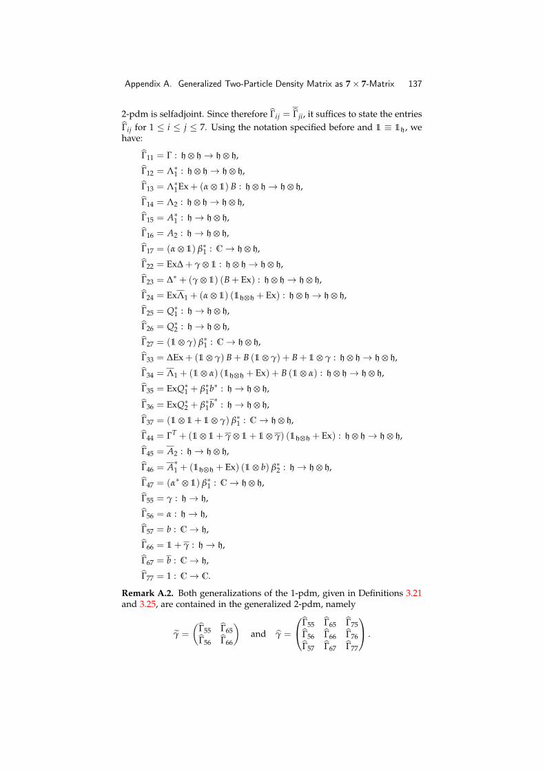
Appendix A. Generalized Two-Particle Density Matrix as 7× 7-Matrix 137
2-pdm is selfadjoint. Since therefore Γij = Γji, it suffices to state the entriesΓij for 1 ≤ i ≤ j ≤ 7. Using the notation specified before and 1 ≡ 1h, wehave:
Γ11 = Γ : h h→ h h,
Γ12 = Λ∗1 : h h→ h h,
Γ13 = Λ∗1Ex + (α 1) B : h h→ h h,
Γ14 = Λ2 : h h→ h h,
Γ15 = A∗1 : h→ h h,
Γ16 = A2 : h→ h h,
Γ17 = (α 1) β∗1 : C→ h h,
Γ22 = Ex∆ + γ 1 : h h→ h h,
Γ23 = ∆∗ + (γ 1) (B + Ex) : h h→ h h,
Γ24 = ExΛ1 + (α 1) (1hh + Ex) : h h→ h h,
Γ25 = Q∗1 : h→ h h,
Γ26 = Q∗2 : h→ h h,
Γ27 = (1 γ) β∗1 : C→ h h,
Γ33 = ∆Ex + (1 γ) B + B (1 γ) + B + 1 γ : h h→ h h,
Γ34 = Λ1 + (1 α) (1hh + Ex) + B (1 α) : h h→ h h,
Γ35 = ExQ∗1 + β∗1b∗ : h→ h h,
Γ36 = ExQ∗2 + β∗1b∗
: h→ h h,
Γ37 = (1 1+ 1 γ) β∗1 : C→ h h,
Γ44 = ΓT + (1 1+ γ 1+ 1 γ) (1hh + Ex) : h h→ h h,
Γ45 = A2 : h→ h h,
Γ46 = A∗1 + (1hh + Ex) (1 b) β∗2 : h→ h h,
Γ47 = (α∗ 1) β∗1 : C→ h h,
Γ55 = γ : h→ h,
Γ56 = α : h→ h,
Γ57 = b : C→ h,
Γ66 = 1+ γ : h→ h,
Γ67 = b : C→ h,
Γ77 = 1 : C→ C.
Remark A.2. Both generalizations of the 1-pdm, given in Definitions 3.21and 3.25, are contained in the generalized 2-pdm, namely
γ =
(Γ55 Γ65Γ56 Γ66
)and γ =
Γ55 Γ65 Γ75Γ56 Γ66 Γ76Γ57 Γ67 Γ77
.
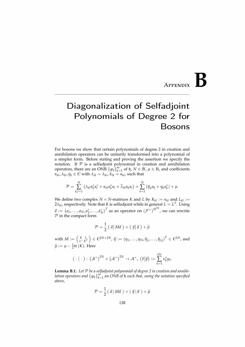
Appendix BDiagonalization of Selfadjoint
Polynomials of Degree 2 forBosons
For bosons we show that certain polynomials of degree 2 in creation andannihilation operators can be unitarily transformed into a polynomial ofa simpler form. Before stating and proving the assertion we specify thenotation. If P is a selfadjoint polynomial in creation and annihilationoperators, there are an ONB ϕk∞
k=1 of h, N ∈ N, µ ∈ R, and coefficientsκkl , λkl , ηk ∈ C with λlk = λkl , κlk = κkl , such that
P =N
∑k,l=1
(λkla∗k a∗l + κkla∗k al + λlkakal
)+
N
∑k=1
(ηkak + ηka∗k ) + µ.
We define two complex N × N-matrices K and L by Kkl := κkl and Lkl :=2λkl , respectively. Note that K is selfadjoint while in general L = LT . Using
~a :=(a1, . . . , aN , a∗1 , . . . , a∗N
)T as an operator on (F+)2N
, we can rewriteP in the compact form
P =12(~a∣∣M~a
)+(~η∣∣~a )+ µ
with M :=(
K LL∗ KT
)∈ C2N×2N , ~η := (η1, . . . , ηN , η1, . . . , ηN)
T ∈ C2N , and
µ := µ− 12 tr (K). Here
(·∣∣ · ) :
(A+)2N ×
(A+)2N → A+,
(~x∣∣~y) :=
2N
∑k=1
x∗k yk.
Lemma B.1. Let P be a selfadjoint polynomial of degree 2 in creation and annihi-lation operators and ϕk∞
k=1 an ONB of h such that, using the notation specifiedabove,
P =12(~a |M~a ) + ( ~η |~a ) + µ
138
Appendix B. Diagonalization of Selfadjoint Polynomials 139
with M :=(
K LL∗ KT
)∈ C2N×2N , K∗ = K = K, LT = L = L, ~η :=
(η1, . . . , ηN , η1, . . . , ηN)T ∈ C2N , and µ ∈ R. Moreover, we assume that there is
a constant c > 0 such that K + L ≥ c1 and K− L ≥ c1. Then, there is a unitarytransformation which maps P to a selfadjoint polynomial of the form
P = E+ a∗(τ) + a(τ) + ν, (B.1)
where ν ∈ R, E is the second quantization of a selfadjoint one-particle operatorE, and τ ∈ ran(E)⊥ ⊆ h.
The proof is a generalization of [Ber66, Section 8] and [BR86, Chapter3], where polynomials are considered which have a term quadratic in cre-ation and annihilation operators (and a constant term in [BR86]), but noterms linear in creation and annihilation operators.
Proof. First, we diagonalize the matrix M and refer to [Ber66] for this step.Afterwards, we use a Weyl transformation to cancel, at least partially,terms linear in creation and annihilation operators. Finally, we merge theremaining terms.
Theorem 8.1 of [Ber66] states that, under the conditions specified in thelemma, a purely quadratic selfadjoint polynomial can be transformed by a(unitary implementable) Bogoliubov map U into ∑N
k,l=1 κkla∗k al + ν with ν ∈C and matrix elements κkl of a selfadjoint one-particle operator K. Withoutloss of generality, we may assume that K is diagonal in the given basis,since, for a given basis, any selfadjoint matrix can be unitarily transformedinto an operator diagonal in this basis. Denoting b∗k := UUa∗kU
∗U and,
consequently, bk = UUakU∗U for any k = 1, . . . , N, we therefore have
UUPU∗U =N
∑k=1
(εkb∗k bk + ηkb∗k + ηkbk) + (ν + µ) .
Using the linearity of the creation operators and the antilinearity of theannihilation operators, we can rewrite the linear part as
N
∑k=1
(ηkb∗k + ηkbk) = b∗(η) + b(η),
where η := ∑Nk=1 ηk ϕk ∈ h, b∗(η) := UUa∗(η)U∗U and b(η) := UUa(η)U∗U .
Furthermore, the quadratic part can be considered as the second quantiza-tion E of a selfadjoint one-particle operator E with 〈ϕk, Eϕk〉h = εk, k ∈ N,and, therefore,
UUPU∗U = E+ (b∗(η) + b(η)) + (ν + µ) .
The operator E is related to K and L via U∗(
K LL∗ KT
)U =
(E 00 ET
).
In the next step, we take care of the terms linear in creation and annihi-lation operators. To this purpose, we apply a Weyl transformation given byW− f with f ∈ span ϕkN
k=1 ⊆ h to the polynomial. In the following com-putation, we determine the specific choice of f to cancel part of the linear
Appendix B. Diagonalization of Selfadjoint Polynomials 140
terms. Since W− f bkW∗− f = bk − 〈ϕk, f 〉h and W− f b∗kW
∗− f = b∗k − 〈 f , ϕk〉h,
we obtain
W− fUUPU∗UW∗− f =N
∑k=1
[εkb∗k bk − εk
(〈 f , ϕk〉h bk − 〈ϕk, f 〉h b∗k
)+ εk 〈 f , ϕk〉h 〈ϕk, f 〉h + (ηkb∗k + ηkbk)
−(
ηk 〈 f , ϕk〉h + ηk 〈ϕk, f 〉h) ]
+ (ν + µ)
and, with the notation as above,
W− fUUPU∗UW∗− f = E+ (b∗(−E f + η) + b(−E f + η))
+(〈 f , E f 〉h − 〈 f , η〉h − 〈η, f 〉h + ν + µ
).
We decompose the vector η ∈ h to obtain the linear part of (B.1). Therefore,we denote by P the orthogonal projection on ran(E) ⊆ h and by P⊥ theorthogonal projection on ran(E)⊥ ⊆ h. Then, we write
η = ζ + τ,
where ζ := Pη ∈ ran(E) and τ := P⊥η ∈ ran(E)⊥. Thus,
b∗(−E f + η) + b(−E f + η) = b∗(−E f + ζ) + b(−E f + ζ) + b∗(τ) + b(τ).(B.2)
Since ζ ∈ ran(E), there is a f ∈ h such that E f = ζ. Choosing this fas the parameter of the Weyl transformation, the first two terms on theright hand side of Equation (B.2) vanish and the other two terms yield theasserted linear part of Equation (B.1).
Finally, we note that the two terms 〈 f , η〉h + 〈η, f 〉h = 2 Re(〈η, f 〉h
)and, since E is selfadjoint, 〈 f , E f 〉h are real numbers. Thus, if we set
ν := 〈 f , E f 〉h − 2 Re(〈η, f 〉h
)+ ν + µ, P := W− fUUPU∗UW∗− f is of the
asserted form.
Bibliography
[Ara71] H. Araki, On Quasifree States of CAR and Bogoliubov Automor-phisms, Publications RIMS Kyoto University 6 (1970/71), 385–442.
[Bac91] V. Bach, Ionization Energies of Bosonic Coulomb Systems, Lettersin Mathematical Physics 21 (1991), 139–149.
[Bac92] , Error Bound for the Hartree–Fock Energy of Atomsand Molecules, Communications in Mathematical Physics 147(1992), 527–548.
[Bac93] , Accuracy of Mean Field Approximations for Atomsand Molecules, Communications in Mathematical Physics 155(1993), 295–310.
[BBKM13] V. Bach, S. Bréteaux, H. K. Knörr, and E. Menge, GeneralizedOne-Particle Density Matrices and Quasifree States, PreprintarXiv:1304.7995 (2013).
[BBT13] V. Bach, S. Bréteaux, and T. Tzaneteas, Minimization of theEnergy of the Non-Relativistic One-Electron Pauli–Fierz Modelover Quasifree States, Preprint arXiv:1301.0936 (2013).
[Ber66] F. A. Berezin, The Method of Second Quantization, AcademicPress, New York, London, 1966.
[BKM12] V. Bach, H. K. Knörr, and E. Menge, Fermion Correlation In-equalities derived from G- and P-Conditions, Documenta Mathe-matica 17 (2012), 451–481.
[BKM13] , Representability Conditions by Grassmann Integration,Preprint arXiv:1307.0465 (2013).
[BLS94] V. Bach, E. H. Lieb, and J. P. Solovej, Generalized Hartree–FockTheory and the Hubbard Model, Journal of Statistical Physics 76(1994), no. 1/2, 3–89.
[BR79] O. Bratteli and D. W. Robinson, Operator Algebras and QuantumStatistical Mechanics I – C∗ and W∗-Algebras, Symmerty Groups,Decomposition of States, Texts and Monographs in Physics,Springer-Verlag, New York, Heidelberg, Berlin, 1979.
141
Bibliography 142
[BR81] , Operator Algebras and Quantum Statistical Mechanics II– Equilibrium States, Models in Quantum Statistical Mechanics,Texts and Monographs in Physics, Springer-Verlag, New York,Heidelberg, Berlin, 1981.
[BR86] J.-P. Blaizot and G. Ripka, Quantum Theory of Finite Systems,MIT Press, Cambridge (Mass.), London (England), 1986.
[CLS06] E. Cancés, M. Lewin, and G. Stoltz, The electornic ground stateenergy problem: A new reduced density matrix approach, The Jour-nal of Chemical Physics 125 (2006), 064101.
[Col63] A. J. Coleman, Structure of Fermion Density Matrices, Reviewsof Modern Physics 35 (1963), no. 3, 668–687, Discussion pp.687–689.
[CR12] M. Combescure and D. Robert, Coherent States and Applicationsin Mathematical Physics, Theoretical and Mathematical Physics,Springer-Verlag, Dordrecht, Heidelberg, London, New York,2012.
[DL67] F. J. Dyson and A. Lenard, Stability of Matter. I, Journal ofMathematical Physics 8 (1967), no. 3, 423–434.
[dSP05] W. d. S. Pedra, Zur mathematischen Theorie der Fermiflüssigkeitenbei positiven Temperaturen, Ph.D. thesis, Universität Leipzig,2005.
[Dys67] F. J. Dyson, Ground-State Energy of a Finite System of ChargedParticles, Journal of Mathematical Physics 8 (1967), no. 8,1538–1545.
[Erd78a] R. M. Erdahl, On the Structure of the Diagonal Conditions, In-ternational Journal of Quantum Chemistry 13 (1978), no. 6,731–736.
[Erd78b] , Representability, International Journal of QuantumChemistry 13 (1978), no. 6, 697–718.
[FdlL86] C. Fefferman and R. de la Llave, Relativistic Stability of Matter –I, Revista Mathemática Iberoamericana 2 (1986), no. 1/2, 119–160.
[FKT02] J. Feldman, H. Knörrer, and E. Trubowitz, Fermionic Func-tional Integrals and the Renormalization Group, CRM MonographSeries, vol. 16, American Mathematical Society, Providence(R.I.), 2002.
[Gau60] M. Gaudin, Une Démonstation Simplifiée du Théorème de Wick enMéchanique Statistique, Nuclear Physics 15 (1960), 89–91.
[GM04] G. Gidofalvi and D. A. Mazziotti, Boson correlation energies viavariational minimization with the two-particle reduced density ma-trix: Exact N-representability conditions for harmonic interactions,Physical Review A 69 (2004), 042511.
Bibliography 143
[GP64] C. Garrod and J. K. Percus, Reduction of the N-Particle Vari-ational Problem, Journal of Mathematical Physics 5 (1964),no. 12, 1756–1776.
[GS94] G. M. Graf and J. P. Solovej, A correlation estimate with applica-tions to quantum systems with Coulomb interactions, Reviews inMathematical Physics 6 (1994), no. 5a (Special Issue), 977–997.
[HS02] C. Hainzl and R. Seiringer, General Decomposition of RadialFunctions on Rn and Applications to N-Body Quantum Systems,Letters in Mathematical Physics 61 (2002), 75–84.
[LD68] A. Lenard and F. J. Dyson, Stability of Matter. II, Journal ofMathematical Physics 9 (1968), no. 5, 698–711.
[Lie81] E. H. Lieb, Variational Principle for Many-Fermion Systems,Physical Review Letters 46 (1981), no. 7, 457–459.
[Löw55] P.-O. Löwdin, Quantum Theory of Many-Particle Systems. I.Physical Interpretations by Means of Density Matrices, NaturalSpin-Orbitals, and Convergence Problems in the Method of Con-figurational Interaction, Physical Review 97 (1955), no. 6, 1474–1489.
[LS04] E. H. Lieb and J. P. Solovej, Ground State Energy of theTwo-Component Bose Gas, Communications in MathematicalPhysics 252 (2004), 485–534.
[LS10] E. H. Lieb and R. Seiringer, The Stability of Matter in Quan-tum Mechanics, Cambridge University Press, Cambridge (UK),2010.
[LSSY05] E. H. Lieb, R. Seiringer, J. P. Solovej, and J. Yngvason, TheMathematics of the Bose Gas and its Condensation, OberwolfachSeminars, vol. 34, Birkhäuser, Basel, 2005.
[LT75] E. H. Lieb and W. Thirring, Bound for the Kinetic Energy ofFermions Which Proves the Stability of Matter, Physical ReviewLetters 35 (1975), no. 11, 687–689, (Erratum 35 (1975), no. 16,1116).
[LY98] E. H. Lieb and J. Yngvason, Ground State Energy of the LowDensity Bose Gas, Physical Review Letters 80 (1998), no. 12,2504–2507.
[Maz02] D. A. Mazziotti, Variational minimization of atomic and molecularground-state energies via the two-particle reduced density matrix,Physical Review A 65 (2002), 062511.
[Maz12a] , Significant conditions for the two-electron reduced densitymatrix from the constructive solution of N representability, Physi-cal Review A 85 (2012), 062507.
Bibliography 144
[Maz12b] , Structure of Fermionic Density Matrices: Complete N-representability Conditions, Physical Review Letters 108 (2012),263002.
[ME01] D. A. Mazziotti and R. M. Erdahl, Uncertainty relations andreduced density matrices: Mapping many-body quantum mechanicsonto four particles, Physical Review A 63 (2001), 042113.
[NAHM11] K. Naftchi-Ardebili, N. W. Hau, and D. A. Mazziotti, Rankrestriction for the variational calculation of two-electron reduceddensity matrices of many-electron atoms and molecules, PhysicalReview A 84 (2011), 052506.
[Nam11] P. T. Nam, Contributions to the rigorous study of the struc-ture of atoms, Ph.D. thesis, University of Copenhagen, 2011,(Paper III. Bogoliubov theory and bosonic atoms, PreprintarXiv:1109.2875).
[Ray78] J. W. Strutt, 3rd Baron Rayleigh, Theory of Sound, vol. I and II,Macmillan, London, 1877/78.
[Rit09a] W. Ritz, Theorie der Transversalschwingungen einer quadratischenPlatte mit freien Rändern, Annalen der Physik 333 (1909), 737–786.
[Rit09b] , Über eine neue Methode zur Lösung gewisser Variation-sprobleme der mathematischen Physik, Journal für reine undangewandte Mathematik 135 (1909), 1–61.
[RSSS12] V. Rivasseau, R. Seiringer, J. P. Solovej, and T. Spencer, Quan-tum many body systems. Cetraro, Italy 2010. Selected papers basedon the presentations at the CIME school, August 30 to September4, 2010., Lecture Notes in Mathematics - CIME FoundationSubseries, vol. 2051, Springer-Verlag, Berlin, 2012.
[Sal98] M. Salmhofer, Renormalization — An Introduction, Springer-Verlag, Berlin, Heidelberg, 1998.
[Sol06] J. P. Solovej, Upper Bounds to the Ground State Energies of theOne- and Two-Component Charged Bose Gases, Communicationsin Mathematical Physics 266 (2006), 797–818.
[Sol07] , Many Body Quantum Mechanics, Lecture Notes, 2007.
[SS65] D. Shale and W. F. Stinespring, Spinor Representation of InfiniteOrthogonal Groups, Journal of Mathematics and Mechanics 14(1965), no. 2, 315–322.
[Tak08] L. A. Takhtajan, Quantum Mechanics for Mathematicians, Grad-uate Studies in Mathematics, vol. 95, American MathematicalSociety, Providence (R.I.), 2008.
[Thi08] W. Thirring, Quantenmechanik großer Systeme, Lehrbuch derMathematischen Physik, vol. 4, Springer-Verlag, Wien, 2008.
Bibliography 145
[ZB01] V. A. Zagrebnov and J.-B. Bru, The Bogoliubov model of weaklyimperfect Bose gas, Physical Reports 350 (2001), 291–434.
[ZBF+04] Z. Zhao, B. J. Braams, M. Fukuda, M. L. Overton, and J. K.Percus, The reduced density matrix method for electronic structurecalculations and the role of three-index representability conditions,Journal of Chemical Physics 120 (2004), no. 5, 2095–2104.