H. W. Hamacher, A. Schöbel

Design of Zone TariffSystems in PublicTransportation

Berichte des Fraunhofer ITWM, Nr. 21 (2001)

© Fraunhofer-Institut für Techno- undWirtschaftsmathematik ITWM 2001

ISSN 1434-9973

Bericht 21 (2001)

Alle Rechte vorbehalten. Ohne ausdrückliche, schriftliche Genehmigungdes Herausgebers ist es nicht gestattet, das Buch oder Teile daraus inirgendeiner Form durch Fotokopie, Mikrofilm oder andere Verfahren zureproduzieren oder in eine für Maschinen, insbesondere Datenverarbei-tungsanlagen, verwendbare Sprache zu übertragen. Dasselbe gilt für dasRecht der öffentlichen Wiedergabe.

Warennamen werden ohne Gewährleistung der freien Verwendbarkeitbenutzt.

Die Veröffentlichungen in der Berichtsreihe des Fraunhofer ITWMkönnen bezogen werden über:

Fraunhofer-Institut für Techno- undWirtschaftsmathematik ITWMGottlieb-Daimler-Straße, Geb. 49

67663 Kaiserslautern

Telefon: +49 (0) 6 31/2 05-32 42Telefax: +49 (0) 6 31/2 05-41 39E-Mail: info@itwm.fhg.deInternet: www.itwm.fhg.de

Vorwort

Das Tätigkeitsfeld des Fraunhofer Instituts für Techno- und WirtschaftsmathematikITWM umfasst anwendungsnahe Grundlagenforschung, angewandte Forschungsowie Beratung und kundenspezifische Lösungen auf allen Gebieten, die fürTechno- und Wirtschaftsmathematik bedeutsam sind.

In der Reihe »Berichte des Fraunhofer ITWM« soll die Arbeit des Instituts kontinu-ierlich einer interessierten Öffentlichkeit in Industrie, Wirtschaft und Wissenschaftvorgestellt werden. Durch die enge Verzahnung mit dem Fachbereich Mathema-tik der Universität Kaiserslautern sowie durch zahlreiche Kooperationen mit inter-nationalen Institutionen und Hochschulen in den Bereichen Ausbildung und For-schung ist ein großes Potenzial für Forschungsberichte vorhanden. In die Bericht-reihe sollen sowohl hervorragende Diplom- und Projektarbeiten und Dissertatio-nen als auch Forschungsberichte der Institutsmitarbeiter und Institutsgäste zuaktuellen Fragen der Techno- und Wirtschaftsmathematik aufgenommen werden.

Darüberhinaus bietet die Reihe ein Forum für die Berichterstattung über die zahlrei-chen Kooperationsprojekte des Instituts mit Partnern aus Industrie und Wirtschaft.

Berichterstattung heißt hier Dokumentation darüber, wie aktuelle Ergebnisse ausmathematischer Forschungs- und Entwicklungsarbeit in industrielle Anwendungenund Softwareprodukte transferiert werden, und wie umgekehrt Probleme der Pra-xis neue interessante mathematische Fragestellungen generieren.

Prof. Dr. Dieter Prätzel-WoltersInstitutsleiter

Kaiserslautern, im Juni 2001

Design of Zone Tari� Systems in Public

Transportation

Horst W. Hamacher and Anita Sch�obel

Universit�at Kaiserslautern

and

Institut f�ur Techno- und Wirtschaftsmathematik

May 17, 2001

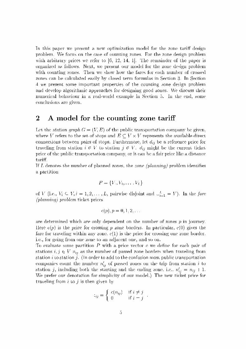
Abstract

Given a public transportation system represented by its stops and di-

rect connections between stops, we consider two problems dealing with the

prices for the customers: The fare problem in which subsets of stops are

already aggregated to zones and \good" tari�s have to be found in the

existing zone system. Closed form solutions for the fare problem are pre-

sented for three objective functions. In the zone problem the design of the

zones is part of the problem. This problem is NP hard and we therefore

propose three heuristics which prove to be very succesful in the redesign

of one of Germany's transportations systems.

1 Tari� systems in public transportation

In this paper we deal with the design of tari� systems in public transportation,

a complex real-world problem, that was brought to our attention by a regional

public transportation company several years ago. While working on the design of

a fair tari� system we both developed a mathematical theory and a visualization

tool to evaluate the e�ects of tari� changes. In this paper we present our studies

and experience over the last years in this area.

When using a bus or a train, a passenger usually has to pay for his trip. There

are several possiblities for de�ning ticket prices in public transportation.

� In a distance tari� system, the price for a trip is dependent on the length of

the trip. The longer the trip is, the higher is the fare. This system is mostly

considered as fair. To determine the ticket prices one needs the distance

between each pair of stations. This makes a distance tari� inconvenient for

the public transportation company and for the customers.

1

Figure 1: Zone tari� system with arbitrary prices

� The simplest tari� system is the unit tari�. In this case all trips cost the

same, independent of their length. A unit tari� is very easy to handle. But

it often is not accepted that a short trip between two neighbouring stations

leads to the same ticket price as a long trip through the whole system.

� A model in between these two tari� systems is a zone tari� system. To

establish a zone tari�, the whole area has to be divided into subregions (the

tari� zones). The price for a trip in a zone tari� system is only dependent

on the starting and the ending zone of the trip. If the price can be chosen

arbitrarily for each pair of zones, we call the tari� system a zone tari� with

arbitrary prices. An example for such a tari� system can, for instance, be

found north of San Francisco, see Figure 1. The prices are given in form of

a matrix, see Table 1.

The most popular variant of a zone tari� system is the counting zone tari�

system. To know his fare in this system, a customer has to count how

2

Table 1: Fares (in US-Dollar) for a one-way trip

zone 1 2 3 4 5 6 7 8 9 10

1 2.15

2 2.35 1.50

3 2.95 1.50 1.50

4 3.55 1.50 1.50 1.50

5 5.05 3.55 2.95 2.35 2.15

6 5.70 4.10 3.55 2.95 2.15 2.15

7 4.10 3.00 3.00 3.00 5.05 5.70 1.50

8 4.75 3.00 3.00 3.00 4.45 5.85 3.00 1.50

9 2.95 1.50 1.50 1.50 4.45 5.05 3.00 3.00 1.50

10 4.75 2.95 2.35 2.95 4.45 5.05 4.75 4.10 3.55 1.45

Table 2: Fares by number of zones in journey for one-way trips

number of zones 1 2 3 4 5 6 7 8 9

fare in US-Dollar 1.25 2.00 2.75 3.25 4.00 4.75 5.25 6.00 6.75

many zones his trip will pass and read o� the price assigned to the number

of crossed zones. The prices in this system are dependent on the starting

and the ending zone of the trip, but trips passing the same number of zones

must have the same price. Figure 2 shows a counting zone tari� system

south of San Francisco; the corresponding price for a single one-way trip

can be read o� Table 2.

Because of their simplicity, zone tari� systems are very popular. In Germany,

nearly all tari� associations already have zone tari� systems or are currently

introducing them. When a public transportation company wants to change its

tari� system to a zone tari�, it has to design the zones and to �x the new fares,

such that the resulting tari� system both is accepted by the customers and does

not decrease the income of the company. The goal often is to design the zones

in such a way, that the new and the old price for most of the trips are as close

as possible. This means that neither the public transportation company nor the

customers will have major disadvantages when changing the current tari� system

to a zone tari�.

Another goal can be to design fair zones. In this case we do not consider the

deviation to some old prices, but the deviation from a reference price, for instance

one which is considered to be fair, like the distance tari�. In this approach, the

public transportation company needs to estimate its new income.

3

Figure 2: Counting zone tari� system

4

In this paper we present a new optimization model for the zone tari� design

problem. We focus on the case of counting zones. For the zone design problem

with arbitrary prices we refer to [6, 12, 14, 1]. The remainder of the paper is

organized as follows. Next, we present our model for the zone design problem

with counting zones. Then we show how the fares for each number of crossed

zones can be calculated easily by closed term formulas in Section 3. In Section

4 we present some important properties of the counting zone design problem

and develop algorithmic approaches for designing good zones. We discuss their

numerical behaviour in a real-world example in Section 5. In the end, some

conclusions are given.

2 A model for the counting zone tari�

Let the station graph G = (V;E) of the public transportation company be given,

where V refers to the set of stops and E � V � V represents the available direct

connections between pairs of stops. Furthermore, let dij be a reference price for

traveling from station i 2 V to station j 2 V . dij might be the current ticket

price of the public transportation company, or it can be a fair price like a distance

tari�.

If L denotes the number of planned zones, the zone (planning) problem identi�es

a partition

P = fV1; V1; : : : ; VLg

of V (i.e., Vi � V; i = 1; 2; : : : ; L, pairwise disjoint and [Li=1 = V ). In the fare

(planning) problem ticket prices

c(p); p = 0; 1; 2; : : :

are determined which are only dependent on the number of zones p in journey.

Here c(p) is the price for crossing p zone borders. In particular, c(0) gives the

fare for traveling within any zone, c(1) is the price for crossing one zone border,

i.e., for going from one zone to an adjacent one, and so on.

To evaluate some partition P with a price vector c we de�ne for each pair of

stations i; j 2 V nij as the number of passed zone borders when traveling from

station i to station j. (In order to add to the confusion most public transportation

companies count the number n0ij of passed zones on the trip from station i to

station j, including both the starting and the ending zone, i.e., n0ij = nij + 1.

We prefer our denotation for simplicity of our model.) The new ticket price for

traveling from i to j is then given by

zij =

�c(nij) if i 6= j

0 if i = j:

5

Given the reference prices dij for a trip between stations i and j, the absolute

deviation in ticket price is calculated by

jdij � zijj = jdij � c(nij)j for all i; j 2 V:

Let wij be the number of customers traveling from station i to station j and let

W =P

i;j2V wij be the sum of all customers of the public transportation company.

The minimization of the following three objective functions is of interest.

maximum absolute deviation bmax = maxi;j2V wijjdij � zijj

average absolute deviation b1 =1W

Pi;j2V wijjdij � zijj

average squared deviation b2 =1W

Pi;j2V wij(dij � zij)

2

All three objectives lead to good results in practice. The �rst objective function,

bmax with identical weights models the fact, that the greatest deviation of ticket

prices in the two di�erent tari�s should be as small as possible. It gives a bound

for the largest change in the ticket price for any customer. In the weighted

case, bmax minimizes the maximum deviation in income over all possible trips.

b1 gives the average of all absolute deviations, and b2 the average of all squared

deviations in ticket prices. The objective function b2 leads to a smaller percentage

of strongly a�ected customers than b1. Nevertheless, from our experience, b1 is

slightly better accepted by the practitioners than b2. It also should be mentioned

that deviations in price increases and decreases are treated equally, such that the

model re ects both the interests of customers and transportation companies.

To obtain the numbers nij a shortest path algorithm, e.g., [3, 16] can be used

according to one of the following models.

Station Graph Model: We use the station graph G = (V;E), but introduce

new weights uij for all (i; j) 2 E, de�ned by

uij =

�0 if i and j are in the same zone

1 if i and j are in adjacent zones.

The length of a shortest path between two stops equals the minimum num-

ber of crossed zone borders. This approach will be needed later to update

the zone distances in the greedy heuristic in Section 4.

Zone Graph Model: To reduce the size of the network we de�ne the zone graph

G0 = (P;E 0) whose node set P is given by the zones and (Vk; Vl) 2 E 0 i�

there exist stops i 2 Vk, j 2 Vl such that (i; j) 2 E, i.e., with a direct

connection in the station graph G. All edges have weight 1. For i 2 Vk and

j 2 Vl we get the minimum number of crossed zone borders nij on a trip

from i to j as the length of a shortest path from Vk to Vl in G0.

6

� � � � �1 1 1 1

...................................................................................................................................................................................................................................................................................................................................................................................................................................................................................................................................................................................................................................................................... ...................................................................................................................................

................................................................................................................................................................................................................................... ...........................................................................

........................................................................................................

Figure 3: A station network with 5 stations and 3 zones.

The following example demonstrates the calculation of bmax, b1, and b2.

Let a station graph G with a partition into three zones V1 = f1; 2g, V2 = f3; 4g,

and V3 = f5g be given (see Figure 3).

Suppose that wij = 1 for all i; j 2 V; i 6= j, i.e., W = 20. If we assume that the

distance between any adjacent pair of nodes is 1, the matrix dij according to the

distance tari� system may be

D =

0BBBB@

0 1 2 3 4

1 0 1 2 3

2 1 0 1 2

3 2 1 0 1

4 3 2 1 0

1CCCCA :

The corresponding zone graph G0 consists of three nodes (see Figure 4).

V1 V2 V3........................................................................ ...........................................................................................................................................................................................................................................................................................................

............................................................................................................. ...................................................................................................................................................................................................................................

............................................................................................................. ...................................................................................................................................................................................................................................

.............................................................................................................

Figure 4: Zone graph with 3 zones.

The number of crossed zone borders between stations i and j is then given by

N =

0BBBB@

0 0 1 1 2

0 0 1 1 2

1 1 0 0 1

1 1 0 0 1

2 2 1 1 0

1CCCCA :

Suppose the new fares for crossing p = 0; 1; or 2 zone borders are given by

c(0) = 0:5

c(1) = 1

c(2) = 1:5:

7

Then new ticket prices can be calculated as

Z =

0BBBB@

0 0:5 1 1 1:5

0:5 0 1 1 1:5

1 1 0 0:5 1

1 1 0:5 0 1

1:5 1:5 1 1 0

1CCCCA :

The deviations between the reference prices dij and the new ticket prices zij are

D � Z =

0BBBB@

0 0:5 1 2 2:5

0:5 0 0 1 1:5

1 0 0 0:5 1

2 1 0:5 0 0

2:5 1:5 1 0 0

1CCCCA

and the objective values can be calculated as

bmax = 2:5

b1 =20

20= 1

b2 =32

20= 1:6

3 Solution for the Fare Problem with Fixed Zones

In this section we solve the fare problem with respect to a given zone partition.

Our �rst result shows that a closed form solution is possible for each of the three

objectives bmax; b1, and b2 introduced in Section 2.

Theorem 1 Let P = fV1; V2; : : : ; VLg be a given zone partition and let dij be

given reference prices. In order to minimize bmax, b1, and b2 we choose for all

p = 0; 1; : : : ; L

a)

c�max(p) := maxi;j2V :i6=j;nij=p

dij �z�p

wij

where z�p is de�ned as

z�p = maxi1;j1;i2;j22V :ni1j1=ni2j2=p

wi1j1wi2j2

wi1j1 + wi2j2

(di1j1 � di2j2):

8

b)

c�1(p) := medianfdij; : : : ; dij| {z }wij times

: i; j 2 V : i 6= j; nij = pg

c)

c�2(p) :=1

W

Xi;j2V :nij=p

wijdij

Proof: Given the zone partition P we have to �nd fares c(p) 2 IR for all p =

0; 1; : : : , minimizing bmax, b1, and b2, respectively. De�ne

Mp = f(i; j) : i; j 2 V and nij = pg

and Wp =P

m2Mpwm as the sum of all weights belonging to pairs of stations

in the set Mp. First we note that each of the three objective functions can be

separated into at most L + 1 independent subproblems, Kmax(p), K1(p), and

K2(p), respectively (for p = 0; 1; : : : ; L).

bmax = maxi;j2V

wijjdij � zijj

= maxp=0;1;::: ;L

maxm2Mp

wmjdm � c(p)j =: maxp=0;1;::: ;L

Kmax(p)

b1 =Xi;j2V

wijjdij � zijj

=

LXp=0

Xm2Mp

wmjdm � c(p)j =:

LXp=0

K1(p)

b2 =Xi;j2V

wij(dij � zij)2

=

LXp=0

Xm2Mp

wm(dm � c(p))2 =:

LXp=0

K2(p)

Consequently, to minimize bmax, b1, and b2 we determine the optimal fare c(p) for

p = 0; 1; : : : ; L separately, in each of the three objective functions.

For bmax: For all p = 0; 1; : : : ; L the problem of minimizing

Kmax(p) = maxm2Mp

wmjdm � c(p)j

is well-known from location theory when locating a point on a line such

that the maximum distance to a given set of existing facilities on the same

line is minimized. The proof for the formula given in part [a] of the theorem

can therefore be found in the location literature, see e.g. [8, 5]. Note that

Kmax(p) = z�p .

9

For b1: Since

K1(p) = minXm2M

wmjdm � c(p)j

is a one-dimensional, piecewise linear and convex fuction, its minimiza-

tion is known in statistics (see e.g., [7]) and in location theory as the

one-dimensional median problem (see, e.g. [5, 10]). It is shown that

the above problem is solved by the so-called weighted median of the set

fdm : m 2Mpg, i.e., by any real number c = c�1(p) which satis�es

Xm:dm<c

wm �Wp

2and

Xm:dm>c

wm �Wp

2:

For b2: Here we have to minimize K2(p), i.e.,

minXd2M

wd(d� c(p))2:

Using the theorem of Steiner (see e.g. [11]) of statistics, we note that the

weighted mean of the values in fdm : m 2 Mpg is the unique optimal

solution for c(p).

To demonstrate the result of Theorem 1 we continue the example of Section 2

The optimal values for the zone prices and the resulting values for the objective

functions bmax, b1, and b2 are listed in the following table.

zones cmax c1 c2 example

0 1 1 1 0:5

1 2 2 116

1

2 3:5 3 3:5 1:5

bmax 1 1 1:167 2:5

b1 8 8 8:667 20

b2 7 8 6:722 32

Calculating the objective function by using the optimal fares according to Theo-

rem 1 yields the following Corollary.

Corollary 1 Given a zone partition P = fV1; V2; : : : ; VLg and reference prices

dij the optimal values of the objective functions are given as follows.

10

a)

b�max = maxp

z�p

b)

b�1 =Xp

0@ X

(i;j)2V +p :nij=p

dij �X

(i;j)2V �p :nij=p

dij

1A

where:

V +p

:= f(i; j) : nij = p; dij > c�1(p)V �

p:= f(i; j) : nij = p; dij < c�1(p)

c)

b�2 =X

k

Varfdij : i; j 2 V; nij = pg

where Var denotes the variance of the set.

In practice, often restrictions on the new fares are given; sometimes there even

exist \politically" desired fares for the number of zones in journey that have to

be realized. With the help of Corollary 1 one can easily calculate the increase of

the objective functions when using such given fares instead of the optimal ones.

In particular, Corollary 1 shows that for the objective function bmax the optimal

fares c�max(p) are not needed to calculate the optimal objective value for a given

zone partition. This will be needed in the next section when we are going to

optimize the zone partition with respect to bmax. If, additionally, bmax is used in

the unweighted case, i.e. with wij = 1 for all i; j 2 V , we can further simplify

Theorem 1 and Corollary 1.

Corollary 2 In the case of equal weights, the optimal fares c�max(p) and the cor-

responding objective value bmax are given by

c�max(p) =1

2

�max

i;j2V :nij=pdij + min

i;j2V :nij=pdij

�

Kmax(p) =1

2

�max

i;j2V :nij=pdij � min

i;j2V :nij=pdij

�

b�max =1

2max

p=1;::: ;L

�max

i;j2V :nij=pdij � min

i;j2V :nij=pdij

�

11

Proof: We calculate z�p as

z�p = maxm1;m22Mp

wm1wm2

wm1+ wm2

(dm1� dm2

)

=1

2

�maxm2Mp

dm � minm2Mp

dm

�

and consequently,

c�p = maxm2Mp

dm �z�p

wm

= maxm2Mp

�dm �

1

2max~m2Mp

d ~m +1

2min~m2Mp

d ~m

�

=1

2

�maxm2Mp

dm + minm2Mp

dm

�

Using Corollary 1 and z�p = Kmax(p), the remaining parts follow immediately.

QED

We remark that for the zone design problem with arbitrary prices, similar results

can be derived (see [6, 13]).

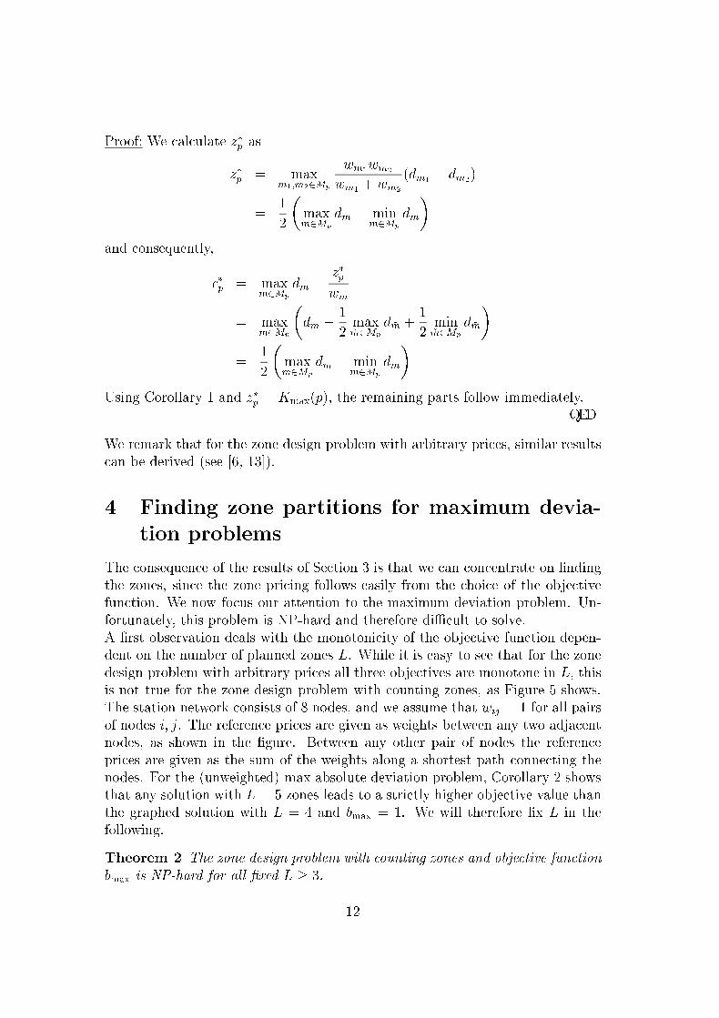
4 Finding zone partitions for maximum devia-

tion problems

The consequence of the results of Section 3 is that we can concentrate on �nding

the zones, since the zone pricing follows easily from the choice of the objective

function. We now focus our attention to the maximum deviation problem. Un-

fortunately, this problem is NP-hard and therefore diÆcult to solve.

A �rst observation deals with the monotonicity of the objective function depen-

dent on the number of planned zones L. While it is easy to see that for the zone

design problem with arbitrary prices all three objectives are monotone in L, this

is not true for the zone design problem with counting zones, as Figure 5 shows.

The station network consists of 8 nodes, and we assume that wij = 1 for all pairs

of nodes i; j. The reference prices are given as weights between any two adjacent

nodes, as shown in the �gure. Between any other pair of nodes the reference

prices are given as the sum of the weights along a shortest path connecting the

nodes. For the (unweighted) max absolute deviation problem, Corollary 2 shows

that any solution with L = 5 zones leads to a strictly higher objective value than

the graphed solution with L = 4 and bmax = 1. We will therefore �x L in the

following.

Theorem 2 The zone design problem with counting zones and objective function

bmax is NP-hard for all �xed L � 3.

12

��

�

�

� �

�

�

1

1

1 1

100

100 100

100............................................................................................

...........................................................................................................................................................................................................................................................................................................................................................................................................................................................................................................................................................................................................................................................................................................................................................

...................................................................................................................................................................................................................................

......................................................................................................................................................................................................................................................................................................................................................................

......................................................................................................................................................................................................................................................................................................................................................................

......................................................................................................................................................................................................................................................................................................................................................................

Figure 5: A station network where the objective value for L = 4 is better than the objective

value for L = 5.

The proof of Theorem 2 is given in the appendix. Note that also the zone design

problem with arbitrary prices is NP-hard, see [1].

To motivate the heuristics of this section, we �rst present the following two ob-

servations for getting upper and lower bounds on the objective value bmax.

Lemma 1

bmax �1

2

�maxi;j2V

dij � mini;j2V

dij

�

Proof: For any zone partition P and any integer p we have that

Kmax(p) =1

2

�max

i;j2V;nij=pdij � min

i;j2V;nij=pdij

�

�1

2

�maxi;j2V

dij � mini;j2V

dij

�;

yielding the result. QED

Lemma 2 Given a zone partition P let INT � E be the set of edges with both

end nodes within the same zone and BET = E n INT. Then we have:

1: bmax �1

2

�max

(i;j)2INTdij � min

(i;j)2INTdij

�

2: bmax �1

2

�max

(i;j)2BETdij � min

(i;j)2BETdij

�

Proof:

13

1. Since mini;j2V;nij=0 dij = min(i;j)2INT dij we get

bmax � Kmax(0)

�1

2

�max

i;j2V;nij=0dij � min

i;j2V;nij=0dij

�

�1

2

�max

(i;j)2INTdij � min

(i;j)2INTdij

�

2. Analogously, mini;j2V;nij=1 dij = min(i;j)2BET dij and we get the result by

using bmax � Kmax(1). QED

Lemma 2 suggests a zone design in which edges with high weights are collected

in BET and edges with small weights in INT or vice versa. To be more speci�c,

let D be the maximal diameter over all zones. Assuming that edge weights along

a path are additive, we get

Kmax(p) =1

2

�max

i;j2V;nij=pdij � min

i;j2V;nij=pdij

�

�1

2

�(p+ 1)D + p

�max

(i;j)2BETdij � min

(i;j)2BETdij

��

yielding that the maximal diameter D should be small, and consequently edges

with large weights should be in BET while edges with small weights should be in

INT.

Following these considerations, we present three heuristics for solving the zone

design problem with counting zones. As Input Data we need | for any of the

following algorithms | a set of n stations with reference prices dij and a number

L of planned zones. The Output is then given by a zone partition with L zones.

Algorithms based on Clustering Theory

The �rst algorithm is based on ideas from clustering theory and here in particular

on the SAHN (sequential agglomerative hierarchical non-overlapping) algorithms,

see e.g., [2]). The idea is to start with n zones, each of them containing one single

station and to combine in each step the two closest zones to a new one. Depending

on the particular de�nition of the distance between two zones, di�erent algorithms

can be obtained. Two of them have been applied to the zone design problem:

Single Linkage and Complete Linkage.

14

ALGORITHM 1 (Zone design using SAHN-algorithms)

1. Start with a partition P consisting of n zones each of which containing a

single station. Let d(Ci; Cj) := dij for all zones Ci; Cj 2 P .

2. Determine two zones Ci 6= Cj 2 P with minimum distance d(Ci; Cj).

3. Join Ci and Cj to a new zone Ck and get a new partition P .

4. Calculate the new distances for all C 2 P :

d(Ck; C) :=12(d(Ci; C) + d(Cj; C) + cjd(Ci; C)� d(Cj; C)j)

5. If the number of planned zones is attained, then Stop, Output P ,

else goto Step 2.

The parameter c in Step 4 determines the formula for calculating the distance

between two zones. In the context of the zone design problem, we have used

� c = �1 for the Single Linkage algorithm and

� c = 1 for the Complete Linkage algorithm.

The interpretation for Single Linkage is the following: The distance between two

zones is de�ned as the smallest distance between elements of them, and conse-

quently in each step we join along a shortest edge. Note that, in the Complete

Linkage the distance between two zones is de�ned as the maximum distance be-

tween their elements, and in each step complete linkage tries to minimize the

maximum diameter of the zones.

Greedy Approach

This approach is a variant of the SAHN algorithms discussed above, but with

more emphasis on the speci�c structure of the zone design problem. Using the

basics of Algorithm 1, we calculate for all edges (i; j) the objective value bijmax

when contracting (i; j) of the current zone graph. Finally, we contract the edge

with smallest increase in the objective function. This is rather time consuming,

but as we will show in the next section, leads to very good results in practice.

The formulation of the greedy approach is the following:

ALGORITHM 2 (Zone design by Greedy approach)

1. For all edges (i; j) 2 E with nij = 1:

Contract i and j temporally and calculate bijmax.

15

2. Contract the edge (i0; j0) permanently, where

bi0;j0

max = minf(i; j) : bijmaxg;

and let ni0j0 = 0. If the graph has L nodes, Stop.

3. For all i; j 2 V recalculate nij as shortest distance, and goto Step 1.

Spanning Tree Approach

The idea of the following heuristic is to determine a set of edges BET which

contains mostly edges with high weights.

ALGORITHM 3 (Zone design by spanning tree approach)

1. Find a maximum spanning tree T in the complete graph with edge weights

dij.

2. Omit the L� 1 largest edges of T and get a forest with L components.

3. Output: Zones are the connected components.

Note that in trees, the spanning tree approach is equivalent to the single linkage

algorithm of clustering theory. In general graphs, it is always possible to �nd a

spanning tree such that omitting its L� 1 largest edges leads to the same result

as Single Linkage. However, if we start with a spanning tree with maximal weight

(which performed best in practice) the spanning tree approach di�ers signi�cantly

from Single Linkage.

5 Theory Put to Work in Saarland, Germany

As an example for the practical value of our approach, we consider the situation

in the State of Saarland, Germany. Currently, there are six public transportation

companies operating in the Saarland, each of them with its own tari� system.

� Four public transportation companies already use a counting zone tari�

system, but their fares for crossing p zones and the structure of their zones

are completely di�erent, although they are partly operating in the same

geographical region.

� The Deutsche Bahn (German Rail) still applies its distance tari�.

16

40

45

50

55

60

65

0 100 200 300 400 500 600 700

"Greedy"Single Linkage""Spanning Tree"

Figure 6: Comparison of the heuristics: bmax graphed for any number L of planned

zones.

� There is also a public transportation company (serving the city of Saarland's

capitol, Saarbr�ucken) which uses a zone tari� with variable prices.

The traÆc association of the Saarland considers to introduce one common count-

ing zone tari� system which should be applied by all the public transportation

companies. The public transportation network in the Saarland consists of roughly

4000 stations, where a pre-clustering into 600 mini-zones is given. The goal is

to design about 100 zones and install a counting zone tari� systems in such a

way that the di�erence between the current fares and the new ones is as small

as possible. It is also important, that the new income of each of the public

transportation companies should not di�er too much from the current income.

Consequently, the reference prices in this application are the current prices for

travelling. While the current fare structure is known and therefore relatively easy

to get it is usually hard to get realistic data about the customers' behaviour. In

our project in the Saarland this was solved by using the income data of each of

the transportaion companies and to divide the income with the help of available

statistics over the origin-destination pairs used by the customers.

We tested our algorithms on the data described above. The results of Algorithms

1,2, and 3 are shown in Figure 6. This �gure shows the objective value bmax

17

31170

31130

31110

31140

31152

31120

31150

31160

31180

31220

31151

31252

31230

31260

31253

31320

31210

31310

31240

31251

31250

31651

31351

31630

31610

31620

31352

31520

31510

31640

31552

31465

31480

31460

31410

31457

31453

31440

31454

31720

31710

31551

31540

31530

31553

31490

31420

31470

31452

31430

31451

31550

31401

31450

Figure 7: Political suggestion; bmax = 5:15 DM

for any number of possible zones from 1 to 600. All objective values refer to

a single trip ticket for an adult, given in German Marks (DM). It turns out

that in this practical application the greedy heuristic (Algorithm 2) is the clear

winner in terms of the objective value: it generated the best results for any

number of desired zones. On the other hand, the running time for Algorithm

2 for all possible number of zones, i.e. from L = 1; : : : ; 600 was nearly two

weeks alltogether in our �rst implementation (on a AixJ90). The Spanning Tree

Approach (Algorithm 3) and the Single Linkage Algorithm (Algorithm 1) both

needed only a few hours, but the results are much less convincing regarding the

objective value bmax again. For a small number L of desired zones, Single Linkage

did better than the Spanning Tree approach, while for a higher number of planned

zones it was the other way round. This is due to the fact that the Spanning Tree

Approach starts with only one zone, while Single Linkage starts with 600 zones.

On a subset consisting of only 400 stations (or 54 mini-zones) the heuristics have

also been tested. In this smaller setting the running times of Algorithms 1 and

3 were within seconds, and also Algorithm 2 needed only 2 minutes to obtain

again the clearly best results. The results for 9 zones are shown graphically in

Figures 7,8, and 9. Figure 7 shows a suggestion for a zone partition which is due

to the political districts in this area of the Saarland. The objective value for this

zone partition is bmax = 5:15 DM, i.e. there exists a customer which will have a

18

31170

31130

31110

31140

31152

31120

31150

31160

31180

31220

31151

31252

31230

31260

31253

31320

31210

31310

31240

31251

31250

31651

31351

31630

31610

31620

31352

31520

31510

31640

31552

31465

31480

31460

31410

31457

31453

31440

31454

31720

31710

31551

31540

31530

31553

31490

31420

31470

31452

31430

31451

31550

31401

31450

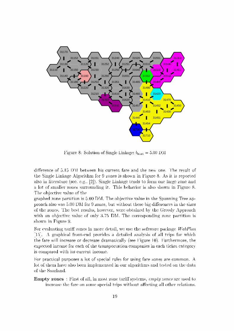
Figure 8: Solution of Single Linkage; bmax = 5:00 DM

di�erence of 5:15 DM between his current fare and the new one. The result of

the Single Linkage Algorithm for 9 zones is shown in Figure 8. As it is reported

also in literature (see, e.g., [2]), Single Linkage tends to form one large zone and

a lot of smaller zones surrounding it. This behavior is also shown in Figure 8.

The objective value of the

graphed zone partition is 5:00 DM. The objective value in the Spanning Tree ap-

proach also was 5:00 DM for 9 zones, but without these big di�erences in the sizes

of the zones. The best results, however, were obtained by the Greedy Approach

with an objective value of only 3:75 DM. The corresponding zone partition is

shown in Figure 9.

For evaluating tari� zones in more detail, we use the software package WabPlan

[15]. A graphical front-end provides a detailed analysis of all trips for which

the fare will increase or decrease dramatically (see Figure 10). Furthermore, the

expected income for each of the transportation companies in each ticket category

is compared with its current income.

For practical purposes a lot of special rules for using fare zones are common. A

lot of them have also been implemented in our algorithms and tested on the data

of the Saarland.

Empty zones : First of all, in most zone tari� systems, empty zones are used to

increase the fare on some special trips without a�ecting all other relations.

19

31170

31130

31110

31140

31152

31120

31150

31160

31180

31220

31151

31252

31230

31260

31253

31320

31210

31310

31240

31251

31250

31651

31351

31630

31610

31620

31352

31520

31510

31640

31552

31465

31480

31460

31410

31457

31453

31440

31454

31720

31710

31551

31540

31530

31553

31490

31420

31470

31452

31430

31451

31550

31401

31450

Figure 9: Solution of Greedy algorithm; bmax = 3:75 DM

This seems to make sense in practice and can easily be incorporated in the

algorithms presented in Section 4. In this way, given reference prices can

be approxinated arbitrarily close if the number L of zones is large enough.

In our model this means that the optimal objective value goes to zero for

bmax; b1, and b2 in this case.

Border stations : To avoid injustice, stations can be located on zone borders,

meaning that they belong to more than one zone, and apply the cheapest

choice for determining the fare. Since the zone tari� system should be clear

and understandable, we tried to avoid this in the Saarland. In most cases

it turned out that border stations can be avoided without loosing anything

in the objective values only by changig the zone design.

Special rules for large zones : Also, some zones might be so large that they

have to be counted twice when crossing them, and that a special fare struc-

ture has to be implemented within such a large zone.

In the Saarland, the tari� system proposed by using our methods is now in the

implementation process.

20

Figure 10: Zone planning with the software WabPlan in the state Sachsen-Anhalt.

The red lines show the (�ctional) customers which will have a change in their ticket

price which is more than 5 Percent.

6 Conclusion

We have shown that closed form solutions can be provided for the fare problem

(with �xed zones). In contrast, the zone problem, i.e. the design of zones, is NP-

hard. Three heuristics have been proposed and compared with respect to their

numerical behaviour. The practical usefulness of the approach is shown by its

actual implementation in the state Saarland, Germany. Other states of Germany

are currently using our system to evaluate their tari� structure.

Appendix

Proof of Theorem 2

We use a reduction to the problem \partition into cliques" for L = 3 Cliques,

which is NP-hard, see problem GT15 in [4]. Let a graph G = (V;E) be given.

We want to answer the question, if there exists a partition of V into 3 node sets

21

V1; V2, and V3 such that the induced subgraphs G1; G2, and G3 are complete. To

reduce this problem to a zone design problem, we consider the complete graph

G = (V; E), de�ned by

V = V [ fa1; a2; a3; b1; b2; b3g and

E = fe = (k; l) : k; l 2 Vg; k 6= l:

Furthermore, let wij = 1 for all i; j 2 V and de�ne the reference prices as the

following edge weights.

dkl =

8>>>><>>>>:

1 if (k; l) 2 E

1 if k 2 V; l 62 V12

if there exists i = 1; 2; 3 such that (k; l) = (ai; bi)

2 if k; l 2 V; (k; l) 62 E

2 if k; l 62 V; (k; l) 6= (ai; bi) for all i = 1; 2; 3:

Now we show that G can be partitioned into 3 cliques if and only if the zone

design problem in G has a solution with 3 zones and with bmax <34.

=): Let V = V1[V2[V3 the partition of G into cliques. De�ne Ci = Vi[fai; big

for i = 1; 2; 3. Using Corollary 2 and 1 we calculate

Kmax(0) =1

2

�1�

1

2

�=

1

4

Kmax(1) =1

2(2� 1) =

1

2;

such that we get bmax <34.

(=: Let C1; C2; C3 be a partition of V with bmax <34. De�ne Vi = Ci \ V for

i = 1; 2; 3. First we note, that by renaming the Ci we can assume that

ai; bi 2 Ci for i = 1; 2; 3. This can be proved by a simple case analysis (see

[9]) which veri�es the following.

1. If ai and bi do not belong to the same zone this yields bmax �34.

2. If ai; bi and another aj or bj, j 6= i belong to a single common zone,

then bmax �34.

Now let k; l 2 Vi. We have to show that the edge (k; l) 2 E. Assume the

contrary, i.e., dkl = 2. But this yields

Kmax(0) �1

2

�2�

1

2

�=

3

4;

(again using Corollary 2 and 1), a contradiction.

For more than 3 zones, the proof can be done analogously with a reduction to

partition into L > 3 cliques. QED

22

References

[1] L. Babel and H. Kellerer. Design of tari� zones in public transportation

systems: Theoretical and practical results. Technical report, Faculty of Eco-

nomics, University of Graz, 2001.

[2] B.S. Duran and P.L. Odell. Cluster Analysis | A Survey. Lecture Notes in

Economics and Mathematical Systems 100. Springer, Berlin-Heidelberg-New

York, 1974.

[3] R.W. Floyd. Algorithm 97: Shortest path. Communications of the ACM,

5:345, 1962.

[4] M.R. Garey and D.S. Johnson. Computers and Intractability | A Guide to

the Theory of NP-Completeness. H.W. Freeman and Company, San Fran-

cisco, 1979.

[5] H.W. Hamacher. Mathematische L�osungsverfahren f�ur planare Standort-

probleme (Mathematical Solution Algorithms for Planar Location Problems).

Vieweg, Braunschweig, 1995.

[6] H.W. Hamacher and A. Sch�obel. On fair zone design in public transporta-

tion. In Computer-Aided Transit Scheduling, number 430 in Lecture Notes

in Economics and Mathematical Systems, pages 8{22. Springer, 1995.

[7] W.L. Hays. Statistics. Holt, Rinehart and Winston, 3. edition, 1981.

[8] R.F. Love, J.G. Morris, and G.O. Wesolowsky. Facilities Location, chapter

3.3, pages 51{60. North-Holland, Amsterdam, 1988.

[9] K. Penner. Fahrpreisgestaltung im �o�entlichen Verkehr. Master's thesis,

Universit�at Kaiserslautern, 1997.

[10] F. Plastria. Continuous location problems. In Z. Drezner, editor, Facility

Location: A survey of applications and methods, chapter 11, pages 225{262.

Springer, New York, Inc., 1995.

[11] K. Sarkadi and I. Vincze. Mathematical Methods of Statistical Quality Con-

trol. Academic Press, New York-London, 1974.

[12] A. Sch�obel. Fair zone design in public transportation networks. In Operations

Research Proceedings 1994, pages 191{196. Springer Verlag, 1994.

[13] A. Sch�obel. Methoden der kombinatorischen Optimierung in der Tarif-

planung im �o�entllichen Personennahverkehr. Master's thesis, Universit�at

Kaiserslautern, 1994. (appeared under maiden name, A. Schumacher).

23

[14] A. Sch�obel. Zone planning in public transportation. In L. Bianco and

P. Toth, editors, Advanced Methods in Transportation Analysis, Transporta-

tion Analysis, pages 117{134. Springer Verlag, 1996.

[15] G. Sch�obel. WabPlan { a software tool for design and evaluation of tari�

systems, 1999.

[16] S. Warshall. A theorem on boolean matrices. Journal of the ACM, 9, 1962.

24

Bisher erschienene Berichtedes Fraunhofer ITWM

Die PDF-Files der folgenden Berichtefinden Sie unter:www.itwm.fhg.de/zentral/berichte.html

1. D. Hietel, K. Steiner, J. StruckmeierA Finite - Volume Particle Method forCompressible Flows

We derive a new class of particle methods for conserva-tion laws, which are based on numerical flux functions tomodel the interactions between moving particles. Thederivation is similar to that of classical Finite-Volumemethods; except that the fixed grid structure in the Fi-nite-Volume method is substituted by so-called masspackets of particles. We give some numerical results on ashock wave solution for Burgers equation as well as thewell-known one-dimensional shock tube problem.(19 S., 1998)

2. M. Feldmann, S. SeiboldDamage Diagnosis of Rotors: Applicationof Hilbert Transform and Multi-HypothesisTesting

In this paper, a combined approach to damage diagnosisof rotors is proposed. The intention is to employ signal-based as well as model-based procedures for an im-proved detection of size and location of the damage. In afirst step, Hilbert transform signal processing techniquesallow for a computation of the signal envelope and theinstantaneous frequency, so that various types of non-linearities due to a damage may be identified and classi-fied based on measured response data. In a second step,a multi-hypothesis bank of Kalman Filters is employed forthe detection of the size and location of the damagebased on the information of the type of damage provid-ed by the results of the Hilbert transform.Keywords:Hilbert transform, damage diagnosis, Kalman filtering,non-linear dynamics(23 S., 1998)

3. Y. Ben-Haim, S. SeiboldRobust Reliability of Diagnostic Multi-Hypothesis Algorithms: Application toRotating Machinery

Damage diagnosis based on a bank of Kalman filters,each one conditioned on a specific hypothesized systemcondition, is a well recognized and powerful diagnostictool. This multi-hypothesis approach can be applied to awide range of damage conditions. In this paper, we willfocus on the diagnosis of cracks in rotating machinery.The question we address is: how to optimize the multi-hypothesis algorithm with respect to the uncertainty ofthe spatial form and location of cracks and their resultingdynamic effects. First, we formulate a measure of thereliability of the diagnostic algorithm, and then we dis-cuss modifications of the diagnostic algorithm for themaximization of the reliability. The reliability of a diagnos-tic algorithm is measured by the amount of uncertaintyconsistent with no-failure of the diagnosis. Uncertainty isquantitatively represented with convex models.Keywords:Robust reliability, convex models, Kalman filtering, multi-hypothesis diagnosis, rotating machinery, crack diagnosis(24 S., 1998)

4. F.-Th. Lentes, N. SiedowThree-dimensional Radiative Heat Transferin Glass Cooling Processes

For the numerical simulation of 3D radiative heat transferin glasses and glass melts, practically applicable mathe-matical methods are needed to handle such problemsoptimal using workstation class computers. Since theexact solution would require super-computer capabilitieswe concentrate on approximate solutions with a highdegree of accuracy. The following approaches are stud-ied: 3D diffusion approximations and 3D ray-tracingmethods.(23 S., 1998)

5. A. Klar, R. WegenerA hierarchy of models for multilanevehicular trafficPart I: Modeling

In the present paper multilane models for vehicular trafficare considered. A microscopic multilane model based onreaction thresholds is developed. Based on this model anEnskog like kinetic model is developed. In particular, careis taken to incorporate the correlations between the vehi-cles. From the kinetic model a fluid dynamic model isderived. The macroscopic coefficients are deduced fromthe underlying kinetic model. Numerical simulations arepresented for all three levels of description in [10]. More-over, a comparison of the results is given there.(23 S., 1998)

Part II: Numerical and stochasticinvestigations

In this paper the work presented in [6] is continued. Thepresent paper contains detailed numerical investigationsof the models developed there. A numerical method totreat the kinetic equations obtained in [6] are presentedand results of the simulations are shown. Moreover, thestochastic correlation model used in [6] is described andinvestigated in more detail.(17 S., 1998)

6. A. Klar, N. SiedowBoundary Layers and Domain Decomposi-tion for Radiative Heat Transfer and Diffu-sion Equations: Applications to Glass Manu-facturing Processes

In this paper domain decomposition methods for radia-tive transfer problems including conductive heat transferare treated. The paper focuses on semi-transparent ma-terials, like glass, and the associated conditions at theinterface between the materials. Using asymptotic analy-sis we derive conditions for the coupling of the radiativetransfer equations and a diffusion approximation. Severaltest cases are treated and a problem appearing in glassmanufacturing processes is computed. The results clearlyshow the advantages of a domain decomposition ap-proach. Accuracy equivalent to the solution of the globalradiative transfer solution is achieved, whereas computa-tion time is strongly reduced.(24 S., 1998)

7. I. ChoquetHeterogeneous catalysis modelling andnumerical simulation in rarified gas flowsPart I: Coverage locally at equilibrium

A new approach is proposed to model and simulate nu-merically heterogeneous catalysis in rarefied gas flows. Itis developed to satisfy all together the following points:1) describe the gas phase at the microscopic scale, asrequired in rarefied flows,2) describe the wall at the macroscopic scale, to avoidprohibitive computational costs and consider not onlycrystalline but also amorphous surfaces,3) reproduce on average macroscopic laws correlatedwith experimental results and4) derive analytic models in a systematic and exact way.The problem is stated in the general framework of a nonstatic flow in the vicinity of a catalytic and non poroussurface (without aging). It is shown that the exact andsystematic resolution method based on the Laplace trans-form, introduced previously by the author to model colli-sions in the gas phase, can be extended to the presentproblem. The proposed approach is applied to the mod-elling of the Eley-Rideal and Langmuir-Hinshelwoodrecombinations, assuming that the coverage is locally atequilibrium. The models are developed considering oneatomic species and extended to the general case of sev-eral atomic species. Numerical calculations show that themodels derived in this way reproduce with accuracy be-haviors observed experimentally.(24 S., 1998)

8. J. Ohser, B. Steinbach, C. LangEfficient Texture Analysis of Binary Images

A new method of determining some characteristics ofbinary images is proposed based on a special linear filter-ing. This technique enables the estimation of the areafraction, the specific line length, and the specific integralof curvature. Furthermore, the specific length of the totalprojection is obtained, which gives detailed informationabout the texture of the image. The influence of lateraland directional resolution depending on the size of theapplied filter mask is discussed in detail. The techniqueincludes a method of increasing directional resolution fortexture analysis while keeping lateral resolution as highas possible.(17 S., 1998)

9. J. OrlikHomogenization for viscoelasticity of theintegral type with aging and shrinkage

A multi-phase composite with periodic distributed inclu-sions with a smooth boundary is considered in this con-tribution. The composite component materials are sup-posed to be linear viscoelastic and aging (of thenon-convolution integral type, for which the Laplacetransform with respect to time is not effectively applica-ble) and are subjected to isotropic shrinkage. The freeshrinkage deformation can be considered as a fictitioustemperature deformation in the behavior law. The proce-dure presented in this paper proposes a way to deter-mine average (effective homogenized) viscoelastic andshrinkage (temperature) composite properties and thehomogenized stress-field from known properties of the

components. This is done by the extension of the asymp-totic homogenization technique known for pure elasticnon-homogeneous bodies to the non-homogeneousthermo-viscoelasticity of the integral non-convolutiontype. Up to now, the homogenization theory has notcovered viscoelasticity of the integral type.Sanchez-Palencia (1980), Francfort & Suquet (1987) (see[2], [9]) have considered homogenization for viscoelastici-ty of the differential form and only up to the first deriva-tive order. The integral-modeled viscoelasticity is moregeneral then the differential one and includes almost allknown differential models. The homogenization proce-dure is based on the construction of an asymptotic solu-tion with respect to a period of the composite structure.This reduces the original problem to some auxiliaryboundary value problems of elasticity and viscoelasticityon the unit periodic cell, of the same type as the originalnon-homogeneous problem. The existence and unique-ness results for such problems were obtained for kernelssatisfying some constrain conditions. This is done by theextension of the Volterra integral operator theory to theVolterra operators with respect to the time, whose 1 ker-nels are space linear operators for any fixed time vari-ables. Some ideas of such approach were proposed in[11] and [12], where the Volterra operators with kernelsdepending additionally on parameter were considered.This manuscript delivers results of the same nature forthe case of the space-operator kernels.(20 S., 1998)

10. J. MohringHelmholtz Resonators with Large Aperture

The lowest resonant frequency of a cavity resonator isusually approximated by the classical Helmholtz formula.However, if the opening is rather large and the front wallis narrow this formula is no longer valid. Here we presenta correction which is of third order in the ratio of the di-ameters of aperture and cavity. In addition to the highaccuracy it allows to estimate the damping due to radia-tion. The result is found by applying the method ofmatched asymptotic expansions. The correction containsform factors describing the shapes of opening and cavity.They are computed for a number of standard geometries.Results are compared with numerical computations.(21 S., 1998)

11. H. W. Hamacher, A. SchöbelOn Center Cycles in Grid Graphs

Finding "good" cycles in graphs is a problem of greatinterest in graph theory as well as in locational analysis.We show that the center and median problems are NPhard in general graphs. This result holds both for the vari-able cardinality case (i.e. all cycles of the graph are con-sidered) and the fixed cardinality case (i.e. only cycleswith a given cardinality p are feasible). Hence it is of in-terest to investigate special cases where the problem issolvable in polynomial time.In grid graphs, the variable cardinality case is, for in-stance, trivially solvable if the shape of the cycle can bechosen freely.If the shape is fixed to be a rectangle one can analyzerectangles in grid graphs with, in sequence, fixed dimen-sion, fixed cardinality, and variable cardinality. In all casesa complete characterization of the optimal cycles andclosed form expressions of the optimal objective valuesare given, yielding polynomial time algorithms for all cas-es of center rectangle problems.Finally, it is shown that center cycles can be chosen as

rectangles for small cardinalities such that the center cy-cle problem in grid graphs is in these cases completelysolved.(15 S., 1998)

12. H. W. Hamacher, K.-H. KüferInverse radiation therapy planning -a multiple objective optimisation approach

For some decades radiation therapy has been provedsuccessful in cancer treatment. It is the major task of clin-ical radiation treatment planning to realize on the onehand a high level dose of radiation in the cancer tissue inorder to obtain maximum tumor control. On the otherhand it is obvious that it is absolutely necessary to keepin the tissue outside the tumor, particularly in organs atrisk, the unavoidable radiation as low as possible.No doubt, these two objectives of treatment planning -high level dose in the tumor, low radiation outside thetumor - have a basically contradictory nature. Therefore,it is no surprise that inverse mathematical models withdose distribution bounds tend to be infeasible in mostcases. Thus, there is need for approximations compromis-ing between overdosing the organs at risk and underdos-ing the target volume.Differing from the currently used time consuming itera-tive approach, which measures deviation from an ideal(non-achievable) treatment plan using recursively trial-and-error weights for the organs of interest, we go anew way trying to avoid a priori weight choices and con-sider the treatment planning problem as a multiple ob-jective linear programming problem: with each organ ofinterest, target tissue as well as organs at risk, we associ-ate an objective function measuring the maximal devia-tion from the prescribed doses.We build up a data base of relatively few efficient solu-tions representing and approximating the variety of Pare-to solutions of the multiple objective linear programmingproblem. This data base can be easily scanned by physi-cians looking for an adequate treatment plan with theaid of an appropriate online tool.(14 S., 1999)

13. C. Lang, J. Ohser, R. HilferOn the Analysis of Spatial Binary Images

This paper deals with the characterization of microscopi-cally heterogeneous, but macroscopically homogeneousspatial structures. A new method is presented which isstrictly based on integral-geometric formulae such asCrofton’s intersection formulae and Hadwiger’s recursivedefinition of the Euler number. The corresponding algo-rithms have clear advantages over other techniques. Asan example of application we consider the analysis ofspatial digital images produced by means of ComputerAssisted Tomography.(20 S., 1999)

14. M. JunkOn the Construction of Discrete EquilibriumDistributions for Kinetic Schemes

A general approach to the construction of discrete equi-librium distributions is presented. Such distribution func-tions can be used to set up Kinetic Schemes as well asLattice Boltzmann methods. The general principles arealso applied to the construction of Chapman Enskog dis-tributions which are used in Kinetic Schemes for com-

pressible Navier-Stokes equations.(24 S., 1999)

15. M. Junk, S. V. Raghurame RaoA new discrete velocity method for Navier-Stokes equations

The relation between the Lattice Boltzmann Method,which has recently become popular, and the KineticSchemes, which are routinely used in Computational Flu-id Dynamics, is explored. A new discrete velocity modelfor the numerical solution of Navier-Stokes equations forincompressible fluid flow is presented by combining boththe approaches. The new scheme can be interpreted as apseudo-compressibility method and, for a particularchoice of parameters, this interpretation carries over tothe Lattice Boltzmann Method.(20 S., 1999)

16. H. NeunzertMathematics as a Key to Key Technologies

The main part of this paper will consist of examples, howmathematics really helps to solve industrial problems;these examples are taken from our Institute for IndustrialMathematics, from research in the Technomathematicsgroup at my university, but also from ECMI groups and acompany called TecMath, which originated 10 years agofrom my university group and has already a very success-ful history.(39 S. (vier PDF-Files), 1999)

17. J. Ohser, K. SandauConsiderations about the Estimation of theSize Distribution in Wicksell’s CorpuscleProblem

Wicksell’s corpuscle problem deals with the estimation ofthe size distribution of a population of particles, all hav-ing the same shape, using a lower dimensional samplingprobe. This problem was originary formulated for particlesystems occurring in life sciences but its solution is ofactual and increasing interest in materials science. From amathematical point of view, Wicksell’s problem is an in-verse problem where the interesting size distribution isthe unknown part of a Volterra equation. The problem isoften regarded ill-posed, because the structure of theintegrand implies unstable numerical solutions. The accu-racy of the numerical solutions is considered here usingthe condition number, which allows to compare differentnumerical methods with different (equidistant) class sizesand which indicates, as one result, that a finite sectionthickness of the probe reduces the numerical problems.Furthermore, the relative error of estimation is computedwhich can be split into two parts. One part consists ofthe relative discretization error that increases for increas-ing class size, and the second part is related to the rela-tive statistical error which increases with decreasing classsize. For both parts, upper bounds can be given and thesum of them indicates an optimal class width dependingon some specific constants.(18 S., 1999)

18. E. Carrizosa, H. W. Hamacher, R. Klein,S. Nickel

Solving nonconvex planar location problemsby finite dominating sets

It is well-known that some of the classical location prob-lems with polyhedral gauges can be solved in polynomialtime by finding a finite dominating set, i. e. a finite set ofcandidates guaranteed to contain at least one optimallocation.In this paper it is first established that this result holds fora much larger class of problems than currently consideredin the literature. The model for which this result can beproven includes, for instance, location problems with at-traction and repulsion, and location-allocation problems.Next, it is shown that the approximation of general gaug-es by polyhedral ones in the objective function of ourgeneral model can be analyzed with regard to the subse-quent error in the optimal objective value. For the approx-imation problem two different approaches are described,the sandwich procedure and the greedy algorithm. Bothof these approaches lead - for fixed epsilon - to polyno-mial approximation algorithms with accuracy epsilon forsolving the general model considered in this paper.Keywords:Continuous Location, Polyhedral Gauges, Finite Dominat-ing Sets, Approximation, Sandwich Algorithm, GreedyAlgorithm(19 S., 2000)

19. A. BeckerA Review on Image Distortion Measures

Within this paper we review image distortion measures.A distortion measure is a criterion that assigns a “qualitynumber” to an image. We distinguish between mathe-matical distortion measures and those distortion mea-sures in-cooperating a priori knowledge about the imag-ing devices ( e. g. satellite images), image processing al-gorithms or the human physiology. We will consider rep-resentative examples of different kinds of distortionmeasures and are going to discuss them.Keywords:Distortion measure, human visual system(26 S., 2000)

20. H. W. Hamacher, M. Labbé, S. Nickel,T. Sonneborn

Polyhedral Properties of the UncapacitatedMultiple Allocation Hub Location Problem

We examine the feasibility polyhedron of the uncapaci-tated hub location problem (UHL) with multiple alloca-tion, which has applications in the fields of air passengerand cargo transportation, telecommunication and postaldelivery services. In particular we determine the dimen-sion and derive some classes of facets of this polyhedron.We develop some general rules about lifting facets fromthe uncapacitated facility location (UFL) for UHL and pro-jecting facets from UHL to UFL. By applying these ruleswe get a new class of facets for UHL which dominatesthe inequalities in the original formulation. Thus we get anew formulation of UHL whose constraints are all facet–defining. We show its superior computational perfor-mance by benchmarking it on a well known data set.Keywords:integer programming, hub location, facility location, validinequalities, facets, branch and cut(21 S., 2000)

21. H. W. Hamacher, A. SchöbelDesign of Zone Tariff Systems in PublicTransportation

Given a public transportation system represented by itsstops and direct connections between stops, we considertwo problems dealing with the prices for the customers:The fare problem in which subsets of stops are alreadyaggregated to zones and “good” tariffs have to befound in the existing zone system. Closed form solutionsfor the fare problem are presented for three objectivefunctions. In the zone problem the design of the zones ispart of the problem. This problem is NP hard and wetherefore propose three heuristics which prove to be verysuccessful in the redesign of one of Germany’s transpor-tation systems.(30 S., 2001)

22. D. Hietel, M. Junk, R. Keck, D. Teleaga:The Finite-Volume-Particle Method forConservation Laws

In the Finite-Volume-Particle Method (FVPM), the weakformulation of a hyperbolic conservation law is dis-cretized by restricting it to a discrete set of test functions.In contrast to the usual Finite-Volume approach, the testfunctions are not taken as characteristic functions of thecontrol volumes in a spatial grid, but are chosen from apartition of unity with smooth and overlapping partitionfunctions (the particles), which can even move along pre-scribed velocity fields. The information exchange be-tween particles is based on standard numerical flux func-tions. Geometrical information, similar to the surfacearea of the cell faces in the Finite-Volume Method andthe corresponding normal directions are given as integralquantities of the partition functions.After a brief derivation of the Finite-Volume-ParticleMethod, this work focuses on the role of the geometriccoefficients in the scheme.(16 S., 2001)

23. T. Bender, H. Hennes, J. Kalcsics,M. T. Melo, S. Nickel

Location Software and Interface with GISand Supply Chain Management

The objective of this paper is to bridge the gap betweenlocation theory and practice. To meet this objective focusis given to the development of software capable of ad-dressing the different needs of a wide group of users.There is a very active community on location theory en-compassing many research fields such as operations re-search, computer science, mathematics, engineering,geography, economics and marketing. As a result, peopleworking on facility location problems have a very diversebackground and also different needs regarding the soft-ware to solve these problems. For those interested innon-commercial applications (e. g. students and re-searchers), the library of location algorithms (LoLA can beof considerable assistance. LoLA contains a collection ofefficient algorithms for solving planar, network and dis-crete facility location problems. In this paper, a detaileddescription of the functionality of LoLA is presented. Inthe fields of geography and marketing, for instance, solv-ing facility location problems requires using largeamounts of demographic data. Hence, members of thesegroups (e. g. urban planners and sales managers) oftenwork with geographical information too s. To address thespecific needs of these users, LoLA was inked to a geo-

graphical information system (GIS) and the details of thecombined functionality are described in the paper. Finally,there is a wide group of practitioners who need to solvelarge problems and require special purpose software witha good data interface. Many of such users can be found,for example, in the area of supply chain management(SCM). Logistics activities involved in strategic SCM in-clude, among others, facility location planning. In thispaper, the development of a commercial location soft-ware tool is also described. The too is embedded in theAdvanced Planner and Optimizer SCM software devel-oped by SAP AG, Walldorf, Germany. The paper endswith some conclusions and an outlook to future activi-ties.Keywords:facility location, software development, geographicalinformation systems, supply chain management.(48 S., 2001)

24. H. W. Hamacher, S. A. TjandraMathematical Modelling of EvacuationProblems: A State of Art

This paper details models and algorithms which can beapplied to evacuation problems. While it concentrates onbuilding evacuation many of the results are applicablealso to regional evacuation. All models consider the timeas main parameter, where the travel time between com-ponents of the building is part of the input and the over-all evacuation time is the output. The paper distinguishesbetween macroscopic and microscopic evacuation mod-els both of which are able to capture the evacuees’movement over time.Macroscopic models are mainly used to produce goodlower bounds for the evacuation time and do not consid-er any individual behavior during the emergency situa-tion. These bounds can be used to analyze existing build-ings or help in the design phase of planning a building.Macroscopic approaches which are based on dynamicnetwork flow models (minimum cost dynamic flow, maxi-mum dynamic flow, universal maximum flow, quickestpath and quickest flow) are described. A special featureof the presented approach is the fact, that travel times ofevacuees are not restricted to be constant, but may bedensity dependent. Using multicriteria optimization prior-ity regions and blockage due to fire or smoke may beconsidered. It is shown how the modelling can be doneusing time parameter either as discrete or continuousparameter.Microscopic models are able to model the individualevacuee’s characteristics and the interaction among evac-uees which influence their movement. Due to the corre-sponding huge amount of data one uses simulation ap-proaches. Some probabilistic laws for individual evacuee’smovement are presented. Moreover ideas to model theevacuee’s movement using cellular automata (CA) andresulting software are presented.In this paper we will focus on macroscopic models andonly summarize some of the results of the microscopicapproach. While most of the results are applicable togeneral evacuation situations, we concentrate on build-ing evacuation.(44 S., 2001)

Stand: Juni 2001