Information, Search, and Price Dispersion�

Michael R. Baye

Kelley School of Business

Indiana University

John Morgan

Haas School of Business and Department of Economics

University of California, Berkeley

Patrick Scholten

Bentley College

This Draft: October 31, 2005. Forthcoming, Handbook on Economics and Information

Systems (Elsevier, T. Hendershott, ed.).

Abstract

We provide a uni�ed treatment of alternative models of information acquisition/transmission

that have been advanced to rationalize price dispersion in online and o­ ine markets for homo-

geneous products. These di¤erent frameworks� which include sequential search, �xed sam-

ple search, and clearinghouse models� reveal that reductions in (or the elimination of) con-

sumer search costs need not reduce (or eliminate) price dispersion. Our treatment highlights

a �duality� between search-theoretic and clearinghouse models of dispersion, and shows how

auction-theoretic tools may be used to simplify (and even generalize) existing theoretical re-

sults. We conclude with an overview of the burgeoning empirical literature. The empirical

evidence suggests that price dispersion in both online and o­ ine markets is sizeable, pervasive,

and persistent� and does not purely stem from subtle di¤erences in �rms�products or services.

�We owe a special debt to Michael Rauh and Felix Várdy for providing us with detailed hand-written comments

on earlier drafts. We also thank Ville Aalto-Setälä, Fabio Ancarani, Maria Arbatskaya, Judy Chevalier, Karen Clay,

Woody Eckard, Sara Fisher Ellison, Xianjun Geng, Rupert Gatti, Jose Moraga Gonzalez, Joe Harrington, Terry

Hendershott, Ganesh Iyer, Maarten Janssen, Ronald Johnson, Ken Judd, Ramayya Krishnan, Sol Lach, Rajiv Lal,

Preston McAfee, Xing Pan, Je¤ Perlo¤, Ivan Png, Ram Rao, Jennifer Reinganum, Nancy Rose, Venky Shankar, Jorge

Silva-Risso, Michael Smith, Alan Sorensen, Dan Spulber, Mark Stegeman, Beck Taylor, Miguel Villas-Boas, Xiaolin

Xing, and Richard Zeckhauser for encouragement, helpful comments, and suggestions. Of course, we are responsible

for any shortcomings that remain in this o¤ering.

1

1 Introduction

Simple textbook models of competitive markets for homogeneous products suggest that all-out

competition among �rms will lead to the so-called �law of one price.�Yet, empirical studies spanning

more than four decades (see Tables 1a and 1b) reveal that price dispersion is the rule rather than the

exception in many homogeneous product markets. The observation that the prices di¤erent �rms

charge for the same product often di¤er by 30 percent or more led Hal Varian to suggest that �the

�law of one price�is no law at all�(Varian, 1980, p. 651). This chapter provides a uni�ed treatment

of several theoretical models that have been developed to explain the price dispersion observed

in homogeneous product markets, and surveys the burgeoning empirical literature (including the

studies summarized in Tables 1a and 1b) which documents ubiquitous price dispersion. A key

motivation for this chapter is to dispel the erroneous view that the Internet� through its facilitation

of dramatic declines in consumer search costs� will ultimately lead to the �law of one price.�

When confronted with evidence of price dispersion, many are quick to point out that even in

markets for seemingly homogeneous products, subtle di¤erences among the �services� o¤ered by

competing �rms might lead them to charge di¤erent prices for the same product. Nobel Laureate

George Stigler�s initial response to wags making this point was philosophical: �... [While] a portion

of the observed dispersion is presumably attributable to such di¤erence[s]...it would be metaphys-

ical, and fruitless, to assert that all dispersion is due to heterogeneity� (Stigler, 1961, p. 215).

Thirty-�ve years later, the literature has amassed considerable support for Stigler�s position. As

we shall see in Sections 2 and 3, there is strong theoretical and empirical evidence that much (and

in some markets, most) of the observed dispersion stems from information costs� consumers�costs

of acquiring information about �rms, and/or �rms�costs of transmitting information to consumers.

As Figure 1 reveals, research on information, search, and price dispersion has become increas-

ingly important since the publication of Stigler�s seminal article on the Economics of Information.

Until about 1998, most studies focused on environments where consumers incur a positive cost of

obtaining each additional price quote. Search costs in these studies consist of consumers�oppor-

tunity cost of time in searching for lower prices (so-called �shoe-leather� costs), plus other costs

associated with obtaining price quotes from competing �rms (such as the incremental cost of the

postage stamps or phone calls used in acquiring price information from �rms). Consumers in these

environments weigh the cost of obtaining an additional price quote against the expected bene�ts of

searching an additional �rm. As we discuss in Section 2.1, equilibrium price dispersion can arise in

2

these environments under a variety of market conditions and search strategies (including sequential

and �xed sample search).

While marginal search costs are useful in explaining price dispersion in some markets, in many

online markets incremental search costs are very low� and in some cases, zero. For example, price

comparison sites and shopbot technologies create environments where consumers may obtain a

list of the prices that di¤erent sellers charge for the same product. Despite the fact that this

information is available to consumers in seconds, ultimately at the cost of a single �mouse click,�

the overwhelming empirical �nding is that even in these environments, price dispersion is pervasive

and signi�cant� the law of one price is egregiously violated online. In Section 2.2, we examine

an alternative line of theoretical research where marginal search costs are not the key driver for

price dispersion. Our theoretical analysis concludes in Section 2.3 with a discussion of alternative

behavioral rationales for price dispersion (including bounded rationality on the part of �rms and/or

consumers).

Section 3 provides a more detailed overview of the growing empirical literature. As one might

suspect based on the trend in Figure 1 and the research summarized in Tables 1a and 1b, most

empirical studies of price dispersion post-date the Internet and rely on online data. Our view

is that this is more an artifact of the relative ease with which data may be collected in online

markets� not an indication that price dispersion is more important (or more prevalent) in online

than o­ ine markets. For this reason, we have attempted to provide a balanced treatment of the

literatures on online and o­ ine price dispersion. As we shall argue, the overwhelming conclusion

of both literatures is that price dispersion is not purely an artifact of product heterogeneities.

2 Theoretical Models of Price Dispersion

This section presents alternative models that have been used to rationalize the price dispersion ob-

served in both o­ ine and online markets. One approach is to assume that it is costly for consumers

to gather information about prices. In these �search-theoretic�models, consumers searching for the

best price incur a positive cost of obtaining each additional price quote. Representative examples

include Stigler (1961), Rothschild (1973), Reinganum (1979), MacMinn (1980), Braverman (1980),

Burdett and Judd (1983), Carlson and McAfee (1983), Rob (1985), Stahl (1989, 1996), Dana (1994),

McAfee (1995), Janssen and Moraga-González (2004), as well as Janssen, Moraga-González, and

Wildenbeest (2005).

3

A second approach deemphasizes the marginal search cost as a source for price dispersion.

Instead, consumers access price information by consulting an �information clearinghouse�(e.g., a

newspaper or an Internet price comparison site); e.g. Salop and Stiglitz (1977), Shilony (1977),

Rosenthal (1980), Varian (1980), Narasimhan (1988), Spulber (1995), Baye and Morgan (2001),

Baye, Morgan, and Scholten (2004a).1 The distinguishing feature of �clearinghouse models� is

that a subset of consumers gain access to a list of prices charged by all �rms and purchase at the

lowest listed price. In the earliest of these models, equilibrium price dispersion stems from ex ante

heterogeneities in consumers or �rms. For example, in the Varian and Salop-Stiglitz models, some

consumers choose to access the clearinghouse to obtain price information, while others do not. In

Shilony, Rosenthal, and Narasimhan, some consumers are loyal to a particular �rm (and thus will

buy from it even if it does not charge the lowest price), while other consumers are �shoppers�and

only purchase from the �rm charging the lowest price. Spulber (1995) shows that equilibrium price

dispersion arises even when all consumers can costlessly access the clearinghouse� provided each

�rm is privately informed about its marginal cost. Baye and Morgan (2001) o¤er a clearinghouse

model that endogenizes not only the decisions of �rms and consumers to utilize the information

clearinghouse (in the previous clearinghouse models, �rms�listing decisions are exogenous), but also

the fees charged by the owner of the clearinghouse (the �information gatekeeper�) to consumers

and �rms who wish to access or transmit price information. They show that a dispersed price

equilibrium exists even in the absence of any ex ante heterogeneities in consumers or �rms.

In this section, we provide an overview of the key features and ideas underlying these literatures.

2.1 Search-Theoretic Models of Price Dispersion

We begin with an overview of search-theoretic approaches to equilibrium price dispersion. The

early literature stresses the idea that, when consumers search for price information and search is

costly, �rms will charge di¤erent prices in the market. There are two basic sorts of models used:

Models with �xed sample size search and models where search is sequential. We will discuss each

of these in turn.1A third approach deemphasizes consumer search and mainly focuses on whether price dispersion can arise when

consumers �passively� obtain price information directly from �rms (as in direct mail advertisements); cf. Butters

(1977), Grossman and Shapiro (1984), Stegeman (1991), Robert and Stahl (1993), McAfee (1994), and Stahl (1994).

A related marketing literature examines similar issues, ranging from loyalty and price promotion strategies to channel

con�icts and the Internet; see Lal and Villas-Boas (1998), Lal and Sarvary (1999), Raju, Srinivasan, and Lal (1990),

and Rao, Arjunji and Murthi (1995).

4

The search models considered in this subsection are all based on the following general envi-

ronment. A continuum of price-setting �rms (with unit measure) compete in a market selling an

identical (homogeneous) product. Firms have unlimited capacity to supply this product at a con-

stant marginal cost, m: A continuum of consumers is interested in purchasing the product. Let

the mass of consumers in the market be �; so that the number of customers per �rm is �: Each

consumer has a quasi-linear utility function, u (q) + y, where q is the quantity of the homogeneous

product and y is the quantity of some numeraire good whose price is normalized to be unity. This

implies that the indirect utility of a consumer who pays a price p per unit of the product and who

has an income of M is

V (p;M) = v (p) +M

where v (�) is nonincreasing in p: By Roy�s identity, note that the demand for the product of

relevance is q (p) � �v0 (p).

To acquire the product, a consumer must �rst obtain a price quote from a store o¤ering the

product for sale. Suppose that there is a search cost, c, per price quote.2 If, after obtaining n price

quotes, a consumer purchases q (p) units of the product from one of the �rms at price p per unit,

the consumer�s (indirect) utility is

V = v (p) +M � cn

The analysis that follows focuses on posted price markets where consumers know the distribution

of prices but do not know the prices charged by particular stores.3

2.1.1 The Stigler Model

Stigler (1961) considers the special case of this environment where:

1. Each consumer wishes to purchase K � 1 units of the product; that is, q (p) = �v0 (p) = K;

2. The consumer�s search process is �xed sample search� prior to searching, consumers deter-

mine a �xed sample size, n; of �rms from whom to obtain price quotes and then buy from

2 In what follows, we assume that consumers have identical search costs. Axell (1977) o¤ers a model of price

dispersion with heterogeneous search costs.3This assumption is relaxed in Rothschild (1974), Benabou and Gertner (1993) and Dana (1994), where buyers

learn about the distribution of prices as they search, and in Rauh (1997), where buyers� search strategies depend

on only �nitely many moments of the distribution of prices. Daughety (1992) o¤ers an alternative search-theoretic

model of equilibrium price dispersion that results from informational asymmetries and a lack of price precommitment

on the part of �rms.

5

the �rm o¤ering the lowest price; and

3. The distribution of �rms�prices is given by an exogenous non-degenerate cdf F (p) on�p; p�.

Stigler assumes that a consumer chooses a �xed sample size, n, to minimize the expected total

cost (expected purchase cost plus search cost) of purchasing K units of the product:

E [C] = KEhp(n)min

i+ cn

where Ehp(n)min

i= E [min fp1; p2; :::; png] ; that is, the expected lowest price quote obtained from n

draws from F: Since the distribution of the lowest of n draws is F (n)min (p) = 1� [1� F (p)]n ;

E [C] = K

Z p

ppdF

(n)min (p) + cn

= K

"p+

Z p

p[1� F (p)]ndp

#+ cn

where the second equality obtains from integration by parts. Notice that the term in square brackets

re�ects the expected purchase price, which is a decreasing function of the sample size, n. However,

since each additional price observation costs c > 0 to obtain, an optimizing consumer will choose

to search a �nite number of times, n�, and thus will generally stop short of obtaining the best price�p�in the market.

The distribution of transaction prices is the distribution of the lowest of n� draws from F ; that

is,

F(n�)min (p) = 1� (1� F (p))

n�

From this, Stigler concludes that dispersion in both posted prices and transactions prices arises as

a consequence of costly search.

How do transactions prices and search intensity relate to the quantity of the item being pur-

chased (or equivalently, to the frequency of purchases)?4 Stigler�s model o¤ers sharp predictions in

this dimension. Note that the expected bene�t to a consumer who increases her sample size from

n� 1 to n is

EhB(n)

i=�Ehp(n�1)min

i� E

hp(n)min

i��K; (1)

4K may be related to purchase frequency as follows. Suppose prices are �valid� for T periods, and the consumer

wishes to buy one unit every t � T periods; that is, t represents a consumer�s purchase frequency. Then the total

number of units purchased during the T periods is K � T=t: Thus, an increase in purchase frequency (t) is formally

equivalent to an increase in K in the model above.

6

which is decreasing in n. Furthermore, the expected bene�t from search are greater for products

bought in greater quantities or more frequently; that is, equation (1) is increasing in K: Since

the cost of the nth search is independent of K while the expected bene�t is increasing in K; it

immediately follows that the equilibrium search intensity, n�; is increasing in K: That is, consumers

obtain more price quotes for products they buy in greater quantities (or frequencies).

Despite the fact that the Stigler model assumes each individual inelastically purchasesK units of

the product, a version of the �law of demand�holds: Each �rm�s expected demand is a nonincreasing

function of its price. To see this, note that a �rm charging price p is visited by �n� consumers

and o¤ers the lowest price with probability (1� F (p))n��1 : Thus, a representative �rm�s expected

demand when it charges a price of p is

Q (p) = �n�K (1� F (p))n��1 (2)

which is decreasing in p:

The Stigler model implies that both the expected transactions price (Proposition 1) as well as

the expected total costs inclusive of search costs (Proposition 2 ) are lower when prices are more

dispersed (in the sense of a mean preserving spread).5

Proposition 1 Suppose that a price distribution G is a mean preserving spread of a price distri-

bution F . Then the expected transactions price of a consumer who obtains n > 1 price quotes is

strictly lower under price distribution G than under F:

Proof. Let � = EFhp(n)min

i�EG

hp(n)min

ibe the di¤erence in the expected transactions price under

F compared to G: We will show that for all n > 1; � > 0: Using the de�nition of Ehp(n)min

i;

� =

Z 1

�1pn (1� F (p))n�1 dF (p)�

Z 1

�1tn (1�G (t))n�1 dG (t)

Let u = F (p) and v = G (p) ; so that du = dF (p), dv = dG (p) ; p = F�1 (u) ; and t = G�1 (v) :

Then

� = n

Z 1

0F�1 (u) (1� u)n�1 du� n

Z 1

0G�1 (v) (1� v)n�1 dv

= n

Z 1

0

�F�1 (u)�G�1 (u)

�(1� u)n�1 du

5G is a mean preserving spread of F if (a)R1�1 [G (p)� F (p)] dp = 0 and (b)

R z�1 [G (p)� F (p)] dp � 0; with

strict inequality for some z: Note that (a) is equivalent to the fact that the means of F and G are equal. Together,

the two conditions imply that F and G cross exactly once (at the mean) on the interior of the support.

7

Since G is a mean preserving spread of F; there exists a unique interior point u� = F (EF [P ])

such that F�1 (u�) = G�1 (u�) : Further, for all u < u�; F�1 (u) � G�1 (u) > 0 and for all u >

u�; F�1 (u)�G�1 (u) < 0: Thus

� = n

Z u�

0

�F�1 (u)�G�1 (u)

�(1� u)n�1 du+

Z 1

u�

�F�1 (u)�G�1 (u)

�(1� u)n�1 du

!

Next, notice that (1� u)n�1 is strictly decreasing in u; hence

� > n

Z u�

0

�F�1 (u)�G�1 (u)

�(1� u�)n�1 du+

Z 1

u�

�F�1 (u)�G�1 (u)

�(1� u�)n�1 du

!

= n (1� u�)n�1Z 1

0

�F�1 (u)�G�1 (u)

�du

= 0

where the last equality follows from the fact that F and G have the same mean.

Proposition 2 Suppose that an optimizing consumer obtains more than one price quote when

prices are distributed according to F , and that price distribution G is a mean preserving spread of

F . Then the consumer�s expected total costs under G are strictly less than those under F:

Proof. Suppose that, under F; the optimal number of searches is n�: Then the consumer�s expected

total cost under F is

E [CF ] = EF

hp(n�)min

i�K � cn�

> EG

hp(n�)min

i�K � cn�

� E [CG]

where the strict inequality follows from Proposition 1, and the weak inequality follows from the

fact that n� searches may not be optimal under the distribution G:

At �rst blush, it might seem surprising that consumers engaged in �xed sample search pay lower

average prices and have lower expected total costs in environments where prices are more dispersed.

The intuition, however, is clear: In environments where prices are more dispersed, the prospects

for price improvement from search are higher because the left tail of the price distribution� the

part of the distribution where �bargains�are to be found� becomes thicker as prices become more

dispersed.

8

2.1.2 The Rothschild Critique and Diamond�s Paradox

While Stigler o¤ered the �rst search-theoretic rationale for price dispersion, the model has been

criticized for two reasons. First, as pointed out in Rothschild (1973), the search procedure assumed

in Stigler�s model may not be optimal. In �xed sample search, consumers commit to a �xed number,

n, of stores to search and then buy at the lowest price at the conclusion of that search. A clear

drawback to such a strategy is that it fails to incorporate new information obtained during search,

such as an exceptionally low price from an early search. Indeed, once the best price quote obtained

is su¢ ciently low, the bene�t in the form of price improvement drops below the marginal cost of

the additional search. As we will see below, sequential search results in an optimal stopping rule

such that a consumer searches until she locates a price below some threshold, called the reservation

price. Second, the distribution of prices, F; is exogenously speci�ed and is not based on optimizing

�rm behavior. In fact, in light of equation (2), a representative �rm with constant marginal cost

of m enjoys expected pro�ts of

� (p) = (p�m)Q (p) :

That is, absent any cost heterogeneities, each �rm faces exactly the same expected pro�t func-

tion. Why then, would �rms not choose the same pro�t-maximizing price or, more generally, how

could the distribution of prices generated by pro�t-maximizing �rms be consistent with the price

distribution over which consumers were searching? In short, Rothschild pointed out that it is far

from clear that information costs give rise to an equilibrium of price dispersion with optimizing

consumers and �rms; in Stigler�s model, only one side of one market, the consumers, are acting in

an optimizing fashion consistent with equilibrium. For this reason, Rothschild criticized the early

literature for its �partial-partial equilibrium�approach.

Diamond (1971) advanced this argument even further� he essentially identi�ed conditions under

costly search where the unique equilibrium in undominated strategies involves all �rms charging

the same price� the monopoly price. Diamond�s result may be readily seen in the following special

case of our environment where:

1. Consumers have identical downward sloping demand, i.e. �v00 (p) = q0 (p) < 0;

2. Consumers engage in optimal sequential search;

3. A �rm acting as a monopoly would optimally charge all consumers the unique monopoly

price, p�; and

9

4. A consumer who is charged the monopoly price earns surplus su¢ cient to cover the cost of

obtaining a single price quote; that is v (p�) > c:

In this environment, all �rms post the monopoly price and consumers visit only one store,

purchase at the posted price p�; and obtain surplus v (p�) � c > 0. Given the stopping rule of

consumers, each �rm�s best response is to charge the monopoly price; given that all �rms charge

p�, it is optimal for each consumer to search only once. To see that this is the unique equilibrium

in undominated strategies, suppose to the contrary that there is an equilibrium in which some �rm

posted a price below the monopoly price (clearly, pricing above the monopoly price is a dominated

strategy). Let p0 be the lowest such posted price. A �rm posting the lowest price could pro�tably

deviate by raising its price to the lower of p� or p0 + c: Any consumer visiting that �rm would

still rationally buy from it since the marginal bene�t of an additional search is smaller than c� the

marginal cost of an additional search. Thus, such a �rm will not lose any customers by this strategy

and will raise its earnings on each of these customers.

The Diamond paradox is striking: even though there is a continuum of identical �rms competing

in the model� a textbook condition for perfect competition� in the presence of any search frictions

whatsoever the monopoly price is the equilibrium. Rothschild�s criticism of the Stigler model,

along with the Diamond paradox, spawned several decades of research into whether costly search

could possibly generate equilibrium price dispersion � a situation where consumers are optimally

gathering information given a distribution of prices, and where the distribution of prices over which

consumers are searching is generated by optimal (pro�t-maximizing) decisions of �rms.

2.1.3 The Reinganum Model and Optimal Sequential Search

Reinganum (1979) was among the �rst to show that equilibrium price dispersion can arise in a

sequential search setting with optimizing consumers and �rms. Reinganum�s result may be seen in

the following special case of our environment where:

1. Consumers have identical demands given by �v0 (p) = q (p) = Kp", where " < �1 and K > 0;

2. Consumers engage in optimal sequential search;

3. Firms have heterogeneous marginal costs described by the atomless distribution G (m) on

[m;m];

10

4. A consumer who is charged the monopoly price by a �rm with the highest marginal cost, m;

earns surplus su¢ cient to cover the cost of obtaining a single price quote; that is v�

"1+"m

�>

c:

Reinganum shows that, under these assumptions, there exists a dispersed price equilibrium

in which �rms optimally set prices and each consumer engages in optimal sequential search. To

establish this, we �rst show how one derives the optimal reservation price in a sequential search

setting. Suppose consumers are confronted with a nondegenerate distribution of prices F (p) on�p; p�that is atomless, except possibly at p: Consumers engage in optimal sequential search with free

recall. If, following the nth search, a consumer has already found a best price z � min (p1; p2; :::; pn) ;

then, by making an additional search, such a consumer expects to gain bene�ts of

B (z) =

Z z

p(v (p)� v (z)) dF (p)

=

Z z

p�v0 (p)F (p) dp;

where the second equality obtains through integration by parts. Using Leibnitz�rule, we have

B0 (z) = �v0 (z)F (z)

= Kz"F (z) > 0 (3)

Thus, the expected bene�ts from an additional search are lower when the consumer has already

identi�ed a relatively low price. Since search is costly (c > 0), consumers must weigh the expected

bene�ts against the cost of an additional search. The expected net bene�ts of an additional search

are

h (z) � B (z)� c

If the expected bene�ts from an additional search exceed the additional cost, h (z) > 0; it is

optimal for the consumer to obtain an additional price quote. If h (z) < 0, the consumer is better

o¤ purchasing at the price z than obtaining an additional price quote.

A consumer�s optimal sequential search strategy may be summarized as follows:

Case 1. h (p) < 0 andR pp v (p) dF (p) < c: Then the consumer�s optimal strategy is to not

search.

Case 2. h (p) < 0 andR pp v (p) dF (p) dp � c: Then the consumer�s optimal strategy is to search

until she obtains a price quote at or below the reservation price, r = p:

11

Case 3. h (p) � 0: Then the consumer�s optimal strategy is to search until she obtains a price

quote at or below the reservation price, r; where r solves

h (r) =

Z r

p(v (p)� v (r)) dF (p)� c = 0 (4)

Equation (4) represents a price at which a consumer is exactly indi¤erent between buying and

making an additional search. To see that such a price is uniquely de�ned by this equation, notice

that h�p�= �c < 0, h (p) � 0, and h0 (z) = B0 (z) > 0: A consumer who observes a price that

exceeds r will optimally �reject� that price in favor of continued search, while a consumer who

observes a price below r will optimally �accept�that price and stop searching.

Case 1 is clearly not economically interesting as it leads to the absence of any market for the

product in the �rst place. Case 2 arises when the expected utility of purchasing the product exceeds

the cost of an initial search, but the distribution of prices is su¢ ciently �tight�relative to search

costs to make additional searches suboptimal. Most of the existing search literature, including

Reinganum, restricts attention to Case 3, as we shall do hereafter.

The reservation price de�ned in equation (4) has several interesting comparative static prop-

erties. Totally di¤erentiating equation (4) with respect to r and c; and using equation (3) reveals

thatdr

dc=

1

q (r)F (r)=

1

Kr"F (r)> 0

Thus, an increase in search costs leads to a higher reservation price: Other things equal, the range

of �acceptable�prices is greater for products with higher search costs. Note that, for the special

case when q (r) = 1; dr=dc = 1=F (r) > 1: In this case, a one unit increase in search costs increases

the range of acceptable prices by more than one unit� that is, there is a �magni�cation e¤ect�of

increases in search costs.6

Reinganum avoids Rothschild�s criticism and the �Diamond paradox�by introducing �rm cost

heterogeneities. Since each �rm j di¤ers in its marginal costs, mj ; prices will di¤er across �rms

even when they price as monopolists.

Suppose that a fraction 0 � � < 1 of �rms price above r and recall that there are � consumers

per �rm. A representative �rm�s expected pro�t when it prices at pj is:

E�j =

8<: (pj �mj) q (pj)�

�1��

�if pj � r

0 if pj > r

6 In general, there may be either a magni�cation or an attenuation e¤ect of a one unit increase in the cost of search.

12

Ignoring for a moment the fact that a �rm�s demand is zero if it prices above r; note that pro�t-

maximization implies the �rst-order condition

�(pj �mj) q

0 (pj) + q (pj)�� �

1� �

�= 0:

Standard manipulation of the �rst-order condition for pro�t-maximization implies that �rm j�s

(unconstrained) pro�t-maximizing price is a constant markup over its cost:

pj =

�"

1 + "

�mj :

Suppose that �rms simply ignore the consumer�s reservation price, r; and price at this markup.

This would imply that consumers face a distribution of posted prices F̂ (p) = G (p (1 + ") =") on the

interval [m"= (1 + ") ;m"= (1 + ")]. Given this distribution of prices, optimizing consumers would

set a reservation price, r; such that

h (r) =

Z r

p(v (p)� v (r)) dF̂ (p)� c = 0

Furthermore, if r < m"= (1 + ") ; �rms charging prices in the interval (r;m"= (1 + ")] would enjoy

no sales. Since the elasticity of demand is constant, �rms that would maximize pro�ts by pricing

above r in the absence of consumer search �nd it optimal to set their prices at r when consumers

search.7 Thus, the distribution of prices, F̂ (p) ; is inconsistent with optimizing behavior on the

part of �rms. In fact, given the reservation price r; optimizing behavior on the part of �rms would

imply a distribution of prices

F (p) =

8<: F̂ (p) if p < r

1 if p = r

To establish that this is, in fact, an equilibrium distribution of prices one must verify that

consumers facing this �truncated�distribution of prices have no incentive to change their reservation

price. Given this truncated distribution of prices, the net expected bene�ts of search are

h (r) =

Z r

p(v (p)� v (r)) dF (p)� c

=

Z r

p(v (p)� v (r)) dF̂ (p) +

h1� F̂ (r)

i[v (r)� v (r)]� c

=

Z r

p(v (p)� v (r)) dF̂ (p)� c = 0

7Reinganum assumes that m � m"= (1 + "), which guarantees that �rms who would otherwise price above r �nd

it pro�table to price at r.

13

where the last equality follows from the fact that r is the optimal reservation price when consumers

face the price distribution F̂ : In short, Reinganum�s assumptions of downward sloping demand and

cost heterogeneity give rise to an equilibrium of price dispersion with optimizing consumers and

�rms.

Note that downward sloping demand and cost heterogeneities together play a critical role in

generating equilibrium price dispersion in this environment. To see that both assumptions are

required, suppose �rst that costs are heterogeneous but that each consumer wished to purchase

one unit of the product, valued at v. In this case, given a reservation price of r � v, all �rms

would �nd it optimal to price at r; and the distribution of prices would be degenerate. Of course,

a reservation price of r < v is inconsistent with optimizing behavior on the part of consumers. To

see this, suppose that a consumer was unexpectedly presented with a price p0 = r+ �; where � < c:

According to the search strategy, such a consumer is supposed to reject this price and continue

searching; however, the bene�t from this additional search is less than the cost. Thus, a consumer

should optimally accept a price p0 rather than continuing to search. The upshot of this is that the

only equilibrium reservation price is r = v: However, these are precisely the conditions given in

Case 1; hence the only equilibrium is where no consumers shop at all.8

If demand were downward sloping but �rms had identical marginal costs of m, each �rm would

have an incentive to set the same price, p� = min fr;m"= (1 + ")g ; given the reservation price.

This leads back to Case 2 and one obtains the Diamond paradox: All �rms charge the monopoly

price, p� = m"= (1 + "). Indeed, in the environment above, a limiting case where the distribution

of marginal costs converges to a point is exactly the Diamond model.

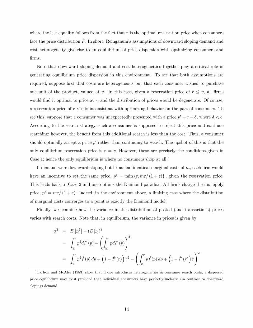
Finally, we examine how the variance in the distribution of posted (and transactions) prices

varies with search costs. Note that, in equilibrium, the variance in prices is given by

�2 = E�p2�� (E [p])2

=

Z r

pp2dF (p)�

Z r

ppdF (p)

!2

=

Z r

pp2f̂ (p) dp+

�1� F̂ (r)

�r2 �

Z r

ppf̂ (p) dp+

�1� F̂ (r)

�r

!28Carlson and McAfee (1983) show that if one introduces heterogeneities in consumer search costs, a dispersed

price equilibrium may exist provided that individual consumers have perfectly inelastic (in contrast to downward

sloping) demand.

14

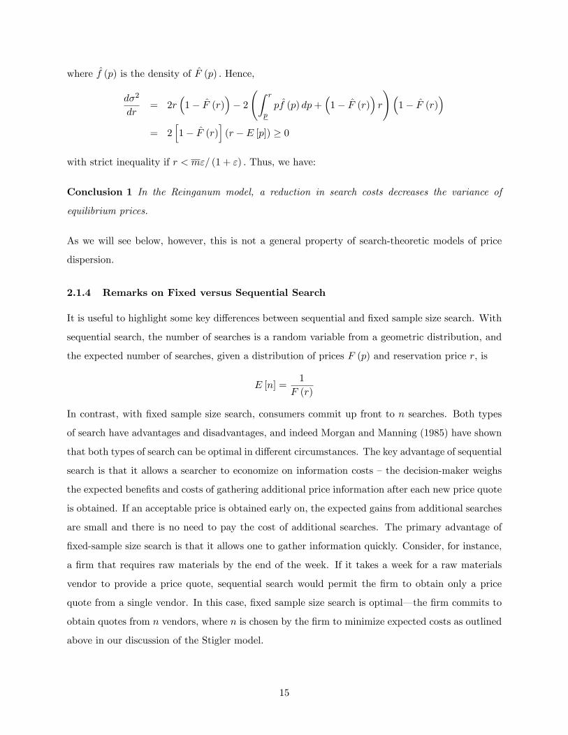
where f̂ (p) is the density of F̂ (p) : Hence,

d�2

dr= 2r

�1� F̂ (r)

�� 2

Z r

ppf̂ (p) dp+

�1� F̂ (r)

�r

!�1� F̂ (r)

�= 2

h1� F̂ (r)

i(r � E [p]) � 0

with strict inequality if r < m"= (1 + ") : Thus, we have:

Conclusion 1 In the Reinganum model, a reduction in search costs decreases the variance of

equilibrium prices.

As we will see below, however, this is not a general property of search-theoretic models of price

dispersion.

2.1.4 Remarks on Fixed versus Sequential Search

It is useful to highlight some key di¤erences between sequential and �xed sample size search. With

sequential search, the number of searches is a random variable from a geometric distribution, and

the expected number of searches, given a distribution of prices F (p) and reservation price r, is

E [n] =1

F (r)

In contrast, with �xed sample size search, consumers commit up front to n searches. Both types

of search have advantages and disadvantages, and indeed Morgan and Manning (1985) have shown

that both types of search can be optimal in di¤erent circumstances. The key advantage of sequential

search is that it allows a searcher to economize on information costs �the decision-maker weighs

the expected bene�ts and costs of gathering additional price information after each new price quote

is obtained. If an acceptable price is obtained early on, the expected gains from additional searches

are small and there is no need to pay the cost of additional searches. The primary advantage of

�xed-sample size search is that it allows one to gather information quickly. Consider, for instance,

a �rm that requires raw materials by the end of the week. If it takes a week for a raw materials

vendor to provide a price quote, sequential search would permit the �rm to obtain only a price

quote from a single vendor. In this case, �xed sample size search is optimal� the �rm commits to

obtain quotes from n vendors, where n is chosen by the �rm to minimize expected costs as outlined

above in our discussion of the Stigler model.

15

2.1.5 The MacMinn Model

In light of the fact that there are instances in which �xed sample size search is optimal, one may

wonder whether equilibrium price dispersion can arise in such a setting. MacMinn (1980) provides

an a¢ rmative answer to this question. MacMinn�s result may be seen in the following special case

of our environment where:

1. Consumers have unit demand with valuation v;

2. Consumers engage in optimal �xed sample search; and9

3. Firms have privately observed marginal costs described by the atomless distribution G (m)

on [m;m], where m < v:

At the time, MacMinn derived equilibrium pricing by solving a set of di¤erential equations under

the special case where G is uniformly distributed. However, subsequent to his paper, a key �nding

of auction theory, the Revenue Equivalence Theorem (Myerson, 1981) was developed.10 Using the

revenue equivalence theorem, we can generalize MacMinn�s results to arbitrary cost distributions.

To see this, notice that when consumers optimally engage in a �xed sample search consisting

of n� �rms, each �rm e¤ectively competes with n� � 1 other �rms to sell one unit of the product.

Of these n� �rms, the �rm posting the lowest price wins the �auction�.

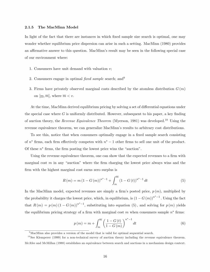
Using the revenue equivalence theorem, one can show that the expected revenues to a �rm with

marginal cost m in any �auction�where the �rm charging the lowest price always wins and the

�rm with the highest marginal cost earns zero surplus is

R (m) = m (1�G (m))n��1 +

Z m

m(1�G (t))n

��1 dt (5)

In the MacMinn model, expected revenues are simply a �rm�s posted price, p (m), multiplied by

the probability it charges the lowest price, which, in equilibrium, is (1�G (m))n��1 : Using the fact

that R (m) = p (m) (1�G (m))n��1, substituting into equation (5) ; and solving for p (m) yields

the equilibrium pricing strategy of a �rm with marginal cost m when consumers sample n� �rms:

p (m) = m+

Z m

m

�1�G (t)1�G (m)

�n��1dt (6)

9MacMinn also provides a version of the model that is valid for optimal sequential search.10See Klemperer (1999) for a non-technical survey of auction theory including the revenue equivalence theorem.

McAfee and McMillan (1988) establishes an equivalence between search and auctions in a mechanism design context.

16

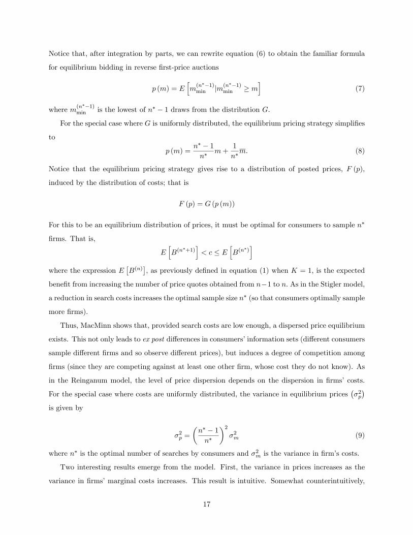
Notice that, after integration by parts, we can rewrite equation (6) to obtain the familiar formula

for equilibrium bidding in reverse �rst-price auctions

p (m) = Ehm(n��1)min jm(n��1)

min � mi

(7)

where m(n��1)min is the lowest of n� � 1 draws from the distribution G:

For the special case where G is uniformly distributed, the equilibrium pricing strategy simpli�es

to

p (m) =n� � 1n�

m+1

n�m: (8)

Notice that the equilibrium pricing strategy gives rise to a distribution of posted prices, F (p),

induced by the distribution of costs; that is

F (p) = G (p (m))

For this to be an equilibrium distribution of prices, it must be optimal for consumers to sample n�

�rms. That is,

EhB(n

�+1)i< c � E

hB(n

�)i

where the expression E�B(n)

�, as previously de�ned in equation (1) when K = 1, is the expected

bene�t from increasing the number of price quotes obtained from n�1 to n: As in the Stigler model,

a reduction in search costs increases the optimal sample size n� (so that consumers optimally sample

more �rms).

Thus, MacMinn shows that, provided search costs are low enough, a dispersed price equilibrium

exists. This not only leads to ex post di¤erences in consumers�information sets (di¤erent consumers

sample di¤erent �rms and so observe di¤erent prices), but induces a degree of competition among

�rms (since they are competing against at least one other �rm, whose cost they do not know). As

in the Reinganum model, the level of price dispersion depends on the dispersion in �rms�costs.

For the special case where costs are uniformly distributed, the variance in equilibrium prices��2p�

is given by

�2p =

�n� � 1n�

�2�2m (9)

where n� is the optimal number of searches by consumers and �2m is the variance in �rm�s costs.

Two interesting results emerge from the model. First, the variance in prices increases as the

variance in �rms�marginal costs increases. This result is intuitive. Somewhat counterintuitively,

17

note that as the sample size increases, the variance in equilibrium prices increases. This implies

that, taking into account the interaction between consumers and �rms in this �xed-sample size

search model, dispersion varies inversely with search costs.

Conclusion 2 In the MacMinn model, a reduction in search costs increases the variance of equi-

librium prices.

This conclusion is in contrast to Conclusion 1, where precisely the opposite implication is

obtained in the Reinganum sequential search model. This highlights an important feature of search-

theoretic models of price dispersion: Depending on the model, a reduction in search costs may be

associated with higher or lower levels of price dispersion. In the Reinganum model, a reduction

in search costs reduces the reservation price of consumers and thus induces marginal �high-cost�

�rms to reduce their prices from their monopoly price to the reservation price. Since the monopoly

prices of low-cost �rms are below the reservation price, their prices remain unchanged; lower search

costs thus reduce the range of prices. In the MacMinn model, lower search costs induce consumers

to sample more �rms before purchasing� in e¤ect, each �rm competes with more rivals. As a

consequence, the optimal amount of �bid shading�(pricing above marginal cost) is reduced, thus

increasing the level of price dispersion.

2.1.6 The Burdett and Judd Model

Burdett and Judd (1983) were the �rst to show that equilibrium price dispersion can arise in a

search-theoretic model with ex ante identical consumers and �rms.11 Burdett and Judd�s main

result may be seen in the following special case of our environment where:

1. Consumers have unit demand up to a price v;

2. Consumers engage in optimal �xed sample search;12

3. Each �rm has constant marginal cost, m; and would optimally charge all consumers the

unique monopoly price, p� = v; and

4. A consumer who is charged the monopoly price earns surplus su¢ cient to cover the cost of

11Janssen and Moraga-González (2004) provide an oligopolistic version of the Burdett and Judd model.12Burdett and Judd also provide a version of the model that is valid under optimal sequential search.

18

obtaining a single price quote:13

In the Burdett and Judd model, an equilibrium consists of a price distribution F (p) (based on

optimal pricing decisions by �rms) and an optimal search distribution < �n >1n=1, where < �n >1n=1

is the distribution of the number of times a consumer searches in the population. Thus, �i is the

probability that a consumer searches (or alternatively, the fraction of consumers that search) exactly

i �rms. If �1 = 1; then all consumers sample only one �rm. If �1 = 0; then all consumers sample at

least two �rms, and so on. Consumers purchase from the �rm sampled that o¤ers the lowest price.

We begin by studying optimal search on the part of consumers given a price distribution F (p) :

Recall that the expected bene�t to a consumer who increases her sample size from n� 1 to n is

EhB(n)

i= E

hp(n�1)min

i� E

hp(n)min

ias in the Stigler model. Moreover, the expected bene�t schedule is strictly decreasing in n: Thus,

an optimal number of price quotes, n; satis�es

EhB(n+1)

i< c � E

hB(n)

iFirst consider the case where all consumers obtain two or more price quotes; that is, where

�1 = 0: In this case, the optimal pricing strategy on the part of �rms is to price at marginal cost

(the Bertrand paradox) since each �rm is facing pure price competition with at least one other

�rm and all �rms are identical. Of course, if all �rms are pricing at marginal cost, then it would

be optimal for a consumer to sample only one �rm, which contradicts the hypothesis that �1 = 0.

Thus, we may conclude that, in any equilibrium �1 > 0:

Next, consider the case where consumers all obtain exactly one price quote. In that case, each

�rm would optimally charge the monopoly price, p� = v: Hence, �1 6= 1 in any dispersed price

equilibrium.

From these two arguments it follows that, in any dispersed price equilibrium, �1 2 (0; 1). In

light of the fact that consumers�expected bene�ts from search are decreasing in the sample size, it

13These assumptions are satis�ed, for example, when

q (p) =

8>>><>>>:1 if p < v

1� p�v�

if v � p � v + �

0 if p > v + �

and � > c=2:

19

follows that a consumer must be indi¤erent between obtaining one price quote and obtaining two

price quotes. That is, in any dispersed price equilibrium

EhB(1)

i> E

hB(2)

i= c > E

hB(3)

i> ::: > E

hB(n)

i:

Thus, in any dispersed price equilibrium, �1; �2 > 0 while �i = 0 for all i > 2: Let �1 = � and

�2 = 1� �:

We are now in a position to characterize an atomless dispersed price equilibrium. First, note

that since � 2 (0; 1) ; there is a positive probability that a �rm faces no competition when it sets

its price. Thus, if �rm i charges the monopoly price, it earns expected pro�ts of

E [�ijpi = v] = (v �m)� ��

In contrast, a �rm choosing some lower price �wins�when its price is below that of the other �rm

a consumer has sampled. Thus, if �rm i charges a price pi � v; it earns expected pro�ts of

E [�ijpi � v] = (pi �m)� � (� + (1� �) (1� F (pi)))

Thus, for a given distribution of searches, equilibrium price dispersion requires that the distribution

of �rm prices, F (�) ; satis�es

� + (1� �) (1� F (p)) = (v �m)(p�m)�

or

F (p) = 1� (v � p)(p�m)

�

1� � (10)

which is a well-behaved atomless cumulative distribution having support [m+ � (v �m) ; v].

Finally, it remains to determine an equilibrium value of �: Since each consumer must be indif-

ferent between searching one or two �rms,

EhB(2)

i= c

Notice that, when � = 0 or � = 1; E�B(2)

�= 0 while E

�B(2)

�> 0 for all � 2 (0; 1) : Burdett

and Judd show that E�B(2)

�is quasi-concave; thus, when c is su¢ ciently low, there are generically

two dispersed price equilibria� one involving a relatively high fraction of consumers making two

searches, the other with a relatively low fraction of consumers.14

14There is a non-dispersed price equilibrium where all consumers search once and all �rms charge the monopoly

price.

20

To summarize, Burdett and Judd show that equilibrium price dispersion can arise even when

all �rms and consumers are ex ante identical. In the equilibrium price distribution, all �rms charge

positive markups. A fraction � of consumers do not comparison shop� they simply search at one

store and purchase. The remaining fraction of consumers are �shoppers�� these consumers search

at two stores and buy from whichever o¤ers the lower price.

2.2 Models with an �Information Clearinghouse�

In search-theoretic models, consumers pay an incremental cost for each additional price quote they

obtain. These models are relevant, for example, when consumers must visit or phone traditional

sellers in order to gather information about prices. They are also relevant in online environments

where consumers must search the websites of individual retailers to gather information about the

prices they charge.

An alternative class of models is relevant when a third party � an information clearinghouse

� provides a subset of consumers with a list of prices charged by di¤erent �rms in the market.

Examples of this environment include newspapers which display prices di¤erent stores charge for

the same product or service and online price comparison sites.

In this section we provide a general treatment of clearinghouse models, and show that these

models are surprisingly similar to those that arise under �xed sample size search. One of the key

modeling di¤erences is that clearinghouse models tend to be oligopoly models; thus, there is not a

continuum of �rms in such settings.

Where possible, we shall use the same notation as in the previous section; however, for reasons

that will become clear when we compare clearinghouse models with the search models presented

above, we now let n denote the number of �rms in the market. The general treatment that follows

relies heavily on Baye and Morgan (2001) and Baye, Morgan and Scholten (2004a).

Consider the following general environment (which we will specialize to cover a variety of di¤er-

ent models). There is a �nite number, n > 1; of price-setting �rms competing in a market selling

an identical (homogeneous) product. Firms have unlimited capacity to supply this product at a

constant marginal cost, m: A continuum of consumers is interested in purchasing the product. This

market is served by a price information clearinghouse. Firms must decide what price to charge for

the product and whether to list this price at the clearinghouse. Let pi denote the price charged by

�rm i: It costs a �rm an amount � � 0 if it chooses to list its price. All consumers have unit demand

21

with a maximal willingness to pay of v > m:15 Of these, a mass, S > 0, of the consumers are price-

sensitive �shoppers.�These consumers �rst consult the clearinghouse and buy at the lowest price

listed there provided this price does not exceed v. If no prices are advertised at the clearinghouse

or all listed prices exceed v, then a �shopper�visits one of the �rms at random and purchases if its

price does not exceed v. A mass L � 0 of consumers per �rm purchase from that �rm if its price

does not exceed v. Otherwise, they do not buy the product at all.

It can be shown that if L > 0 or � > 0, equilibrium price dispersion arises in the general

model� provided of course that � is not so large that �rms refuse to list prices at the clearinghouse.

More precisely,

Proposition 3 Let 0 � � < n�1n (v �m)S. Then, in a symmetric equilibrium of the general

clearinghouse model:

1. Each �rm lists its price at the clearinghouse with probability

� = 1�� n

n�1�

(v �m)S

� 1n�1

:

2. If a �rm lists its price at the clearinghouse, it charges a price drawn from the distribution

F (p) =1

�

0@1� � nn�1�+ (v � p)L(p�m)S

� 1n�1

1A on [p0; v] ;

where

p0 = m+ (v �m)L

L+ S+

nn�1L+ S

�:

3. If a �rm does not list its price at the clearinghouse, it charges a price equal to v:

4. Each �rm earns equilibrium expected pro�ts equal to

E� = (v �m)L+ 1

n� 1�

Proof. First, observe that if a �rm does not list its price at the clearinghouse, it is a dominant

strategy to charge a price of v:

Next, notice that � 2 (0; 1] whenever

n�

(n� 1) (v �m)S < 1:

15 Baye and Morgan (2001) consider an environment with downward sloping demand.

22

This condition holds, since � < n�1n (v �m)S:

Notice that p0 > m; provided that L > 0 or � > 0: In this case, it can be shown that F is a

well-de�ned, atomless cdf on [p0; v]. When L = 0 and � = 0, notice that p0 = m. In this case, the

symmetric equilibrium distribution of prices is degenerate, with all �rms pricing at marginal cost

(the Bertrand paradox outcome).

Next, we show that, conditional on listing a price, a �rm can do no better than pricing according

to F: It is obvious that choosing a price above or below the support of F is dominated by choosing

a price in the support of F: A �rm choosing a price p in the support of F earns expected pro�ts of

E� (p) = (p�m) L+

n�1Xi=0

�n� 1i

��i (1� �)n�1�i (1� F (p))i

!S

!� �:

Using the binomial theorem, we can rewrite this as:

E� (p) = (p�m)�L+

�(1� �F (p))n�1

�S�� �

= (v �m)L+ �

n� 1 ;

where we have substituted for F to obtain the second equality. Since a �rm�s expected pro�ts are

constant on [p0; v], it follows that the mixed pricing strategy, F; is a best response to the other

n� 1 �rms pricing based on F:

When � = 0; it is a weakly dominant strategy to list. It remains to show that when � > 0 and

� 2 (0; 1), a �rm earns the same expected pro�ts regardless of whether it lists its price. But a �rm

that does not list earns expected pro�ts of

E� = (v �m)�L+

S

n(1� �)n�1

�= (v �m)L+ �

n� 1 ;

which equals the expected pro�ts earned by listing any price p 2 [p0; v]. �

We are now in a position to examine the many well-known clearinghouse models that emerge

as special cases of this general environment.

2.2.1 The Rosenthal Model

Rosenthal (1980) was among the �rst to show that equilibrium price dispersion can arise in a

clearinghouse environment when some consumers have a preference for a particular �rm. Under

his interpretation, each �rm enjoys a mass L of �loyal�consumers. Rosenthal�s main results may

be seen in the following special case of the general clearinghouse model:

23

1. It is costless for �rms to list prices on the clearinghouse: � = 0 and;

2. Each �rm has a positive mass of loyal consumers: L > 0:

Since � = 0; it follows from Proposition 3 that � = 1; that is, all of the n �rms advertise their

prices with probability one. Using this fact and Proposition 3, the equilibrium distribution of prices

is

F (p) = 1��(v � p)(p�m)

L

S

� 1n�1

on [p0; v] (11)

where

p0 = m+ (v �m)L

L+ S

The price dispersion arising in the Rosenthal model stems from exogenous di¤erences in the prefer-

ences of consumers. While shoppers view all products as identical and purchase at the lowest listed

price, each �rm is endowed with a stock of L loyals. The equilibrium price dispersion arises out of

the tension created by these two types of consumers. Firms wish to charge v to extract maximal

pro�ts from the loyal segment, but if all �rms did so a �rm could slightly undercut this price and

gain all of the shoppers. One might imagine that this �undercutting�argument would lead to the

Bertrand outcome. However, once prices get su¢ ciently low, a �rm is better o¤ simply charging

v and giving up on attracting shoppers. Thus, the only equilibrium is in mixed strategies� �rms

randomize their prices, sometimes pricing relatively low to attract shoppers and other times pricing

fairly high to maintain margins on loyals.

It is interesting to examine the equilibrium transactions prices in the market. Loyal customers

expect to pay the average price charged by �rms:

E [p] =

Z v

p0

pdF (p)

while shoppers expect to pay the lowest of n draws from F (p); that is, the expected transaction

price paid by shoppers is

Ehp(n)min

i=

Z v

p0

pdF(n)min (p)

where F (n)min (p) is the cdf associated with the lowest of n draws from F:

How do transactions prices vary with the number of competing �rms? Rosenthal�s striking

result is that, as the number of competing �rms increases, the expected transactions prices paid by

all consumers go up. As we shall see below, the result hinges on Rosenthal�s assumption that entry

24

brings more loyals into the market. Indeed, the fraction of shoppers in the market is S= (S + nL)

and it may readily be seen that as n becomes large, shoppers account for an increasingly small

fraction of the customer base of �rms. As a consequence, the incentives to compete for these

customers is attenuated and prices rise as a result. The key is to recognize that increases in n

change the distribution of prices, and this e¤ect as well as any order statistic e¤ect associated with

an increase in n must be taken into account.

Formally, notice that the equilibrium distribution of prices, F; is stochastically ordered in n:

That is, the distribution of prices when there are n + 1 �rms competing �rst-order stochastically

dominates the distribution of prices where there are n �rms competing. This implies that the

transactions prices paid by loyals increase in n. To show that the transactions prices paid by

shoppers also increase in n requires a bit more work; however, one can show that the same stochastic

ordering obtains for the cdf F (n)min (p) :

Finally, it is useful to note the similarity between the Rosenthal version of the clearinghouse

model and the search-theoretic model of Burdett and Judd. In Burdett and Judd, even though

there is a continuum of �rms, each consumer only samples a �nite number of �rms (one or two).

Further, in Burdett and Judd, a �xed fraction of consumers per �rm, ��; sample only a single

�rm. In e¤ect, these consumers are �loyal�to the single �rm sampled while the fraction (1� �)�

of customers sampling two �rms are �shoppers�� they choose the lower of the two prices. For this

reason, when n = 2 in the Rosenthal model, the equilibrium price distribution given in equation

(11) is identical to equation (10) in the Burdett and Judd model (modulo relabeling the variables

for loyals and shoppers).

2.2.2 The Varian Model

Varian (1980) was among the �rst to show that equilibrium price dispersion can arise in a clear-

inghouse environment when consumers have di¤erent ex ante information sets.16 Varian interprets

the S consumers as �informed consumers�and the L consumers as �uninformed�consumers. Thus

a mass, S; of consumers choose to access the clearinghouse while others, the mass L per �rm, do

not. Varian�s main result may be seen in the following special case of the general clearinghouse

model:

1. It is costless for �rms to list prices on the clearinghouse: � = 0; and16Png and Hirshleifer (1987), as well as Baye and Kovenock (1994), extend the Varian model by allowing �rms to

also engage in price matching or �beat or pay�advertisements.

25

2. The total measure of �uninformed�consumers lacking access to the clearinghouse is U > 0;

hence, each �rm is visited by L = Un of these consumers.

Again, since � = 0; it follows that � = 1 and hence all n �rms advertise their prices at the

clearinghouse: Using this fact and setting L = U=n in Proposition 3, the equilibrium distribution

of prices is

F (p) = 1� (v � p)(p�m)

Un

S

! 1n�1

on [p0; v]

where

p0 = m+ (v �m)Un

Un + S

The fact that this atomless distribution of prices exists whenever there is an exogenous fraction

of consumers who do not utilize the clearinghouse raises the obvious question: Can this equilibrium

persist when consumers are making optimal decisions? Varian shows that the answer to this

question is yes � provided di¤erent consumers have di¤erent costs of accessing the clearinghouse.

The easiest way to see this is to note that the value of information provided by the clearinghouse is

the di¤erence in the expected price paid by those accessing the clearinghouse, Ehp(n)min

i; and those

not, E [p]; that is;

V OI(n) = E [p]� Ehp(n)min

i(12)

where V OI denotes the value of (price) information contained at the clearinghouse. Suppose

consumers face a cost of accessing the information provided by the clearinghouse. Note that this

cost is essentially a �xed cost of gaining access to the entire list of prices, not a per price cost as in the

search-theoretic models considered above. Varian assumes that the cost to type S and L consumers

of accessing the clearinghouse is �S and �L, with �S < �L. Then provided �S � V OI(n) < �L

type S consumers will optimally utilize the clearinghouse while the type L consumers will not.

In short, if di¤erent consumers have di¤erent costs of accessing the clearinghouse, there exists

an equilibrium of price dispersion with optimizing consumers and �rms. In such an equilibrium,

informed consumers pay lower average prices than uninformed consumers.

It is important to emphasize that, when one endogenizes consumers�decisions to become in-

formed in the Varian model, the level of price dispersion is not a monotonic function of consumers�

information costs. When information costs are su¢ ciently high, no consumers choose to become

informed, and all �rms charge the �monopoly price,� v. When consumers�information costs are

zero, all consumers choose to become informed, and all �rms price at marginal cost in a symmetric

26

equilibrium� the Bertrand paradox. Thus, for su¢ ciently high or low information costs, there is no

price dispersion; for moderate information costs, prices are dispersed on the nondegenerate interval

[p0; v]. A similar result obtains in Stahl (1989), which is related to Varian as follows. Stahl assumes

a fraction of consumers have zero search costs and, as a consequence, view all �rms�prices and

purchase at the lowest price in the market. These consumers play the role of S in Varian�s model

(informed consumers). The remaining fraction of consumers correspond to the L�s in the Varian

model, but rather than remaining entirely uninformed, these consumers engage in optimal sequen-

tial search in presence of positive incremental search costs. Stahl shows that when all consumers

are shoppers, the identical �rms price at marginal cost and there is no price dispersion. When no

consumers are shoppers, Diamond�s paradox obtains and all �rms charge the monopoly price. As

the fraction of shoppers varies from zero to one, the level of dispersion varies continuously� from

zero to positive levels, and back down to zero.

Conclusion 3 In general, price dispersion is not a monotonic function of consumers�information

costs or the fraction of �shoppers� in the market.

How does the number of competing �rms a¤ect transactions prices? In the Rosenthal model,

we saw that increased �competition�led to higher expected transactions prices for all consumers.

In the Varian model, in contrast, the e¤ect of competition on consumer welfare depends on whether

or not the consumer chooses to access the clearinghouse. Morgan, Orzen, and Sefton (forthcoming)

show that as n increases, the competitive e¤ect predictably leads to lower average transaction prices

being paid by informed consumers. However, the opposite is true for uninformed consumers� as

the number of competing �rms increases, �rms face reduced incentives to cut prices in hopes of

attracting the �shoppers�and, as a consequence, the average price charged by a �rm, which is also

the average price paid by an uninformed consumer, increases. If one views the clearinghouse as

representing access to price information on the Internet, then one can interpret the price e¤ect as one

consequence of the so-called �digital divide;�see Baye, Morgan, and Scholten (2003). Consumers

with Internet access are made better o¤ by sharper online competition while those without such

access are made worse o¤.

2.2.3 The Baye and Morgan Model

All of the above models assume that it is costless for �rms to advertise their prices at the clear-

inghouse. Baye and Morgan (2001) point out that, in practice, it is generally costly for �rms to

27

advertise their prices and for consumers to gain access to the list of prices posted at the clear-

inghouse. For example, newspapers charge �rms fees to advertise their prices and may choose to

charge consumers subscription fees to access any posted information. The same is true of many

online environments. Moreover, the clearinghouse is itself an economic agent, and presumably has

an incentive to endogenously choose advertising and subscription fees to maximize its own expected

pro�ts. Thus, Baye and Morgan examine the existence of dispersed price equilibria in an environ-

ment with optimizing consumers, �rms, and a monopoly �gatekeeper�who controls access to the

clearinghouse.

Speci�cally, Baye and Morgan consider a homogeneous product environment where n identical,

but geographically distinct, markets are each served by a (single) local �rm. Distance or other

transaction costs create barriers su¢ cient to preclude consumers in one market from buying this

product in another market; thus each �rm in a local market is a monopolist. Now imagine that

an entrepreneur creates a clearinghouse to serve all markets. In the Internet age, one can view

the clearinghouse as a virtual marketplace � through its creation, the gatekeeper expands both

consumers�and �rms�opportunities for commerce. Each local �rm now has the option to pay the

gatekeeper an amount � to post a price on the clearinghouse in order to gain access to geographically

disparate consumers. Each consumer now has the option to pay the gatekeeper an amount � to

shop at the clearinghouse and thereby purchase from �rms outside the local market.

The monopoly gatekeeper �rst sets � and � to maximize its own expected pro�ts. Given these

fees, pro�t maximizing �rms make pricing decisions and determine whether or not to advertise

them at the clearinghouse. Similarly, consumers optimally decide whether to pay � to access the

clearinghouse. Following this, a consumer can simply click her mouse to research prices at the

clearinghouse (if she is a subscriber), visit the local �rm, or both. With this information in hand,

a consumer decides whether and from whom to purchase the good.

Baye and Morgan show that the gatekeeper maximizes its expected pro�ts by setting � su¢ -

ciently low that all consumers subscribe, and charging �rms strictly positive fees to advertise their

prices. Thus, Baye and Morgan�s main results may be seen in the following special case of the

general clearinghouse model:

1. The gatekeeper optimally sets positive advertising fees: � > 0 and;

2. The gatekeeper optimally sets subscription fees su¢ ciently low such that all consumers access

the clearinghouse; that is, L = 0:

28

Under these conditions, using Proposition 3, we obtain the following characterization of equilib-

rium �rm pricing and listing decisions: Each �rm lists its price at the clearinghouse with probability

� = 1�� n

n�1�

(v �m)S

� 1n�1

2 (0; 1)

When a �rm lists at the clearinghouse, it charges a price drawn from the distribution

F (p) =1

�

1�

� nn�1�

(p�m)S

� 1n�1!on [p0; v] ;

where

p0 = m+nn�1�

S:

When a �rm does not list its price, it charges a price equal to v; and each �rm earns equilibrium

expected pro�ts equal to

E� =1

n� 1�

Notice that n� represents the aggregate demand by �rms for advertising and is a decreasing

function of the fee charged by the gatekeeper. Prices advertised at the clearinghouse are dispersed

and strictly lower than unadvertised prices (v).

Several features of this equilibrium are worth noting. First, equilibrium price dispersion arises

with fully optimizing consumers, �rms, and endogenous fee-setting decisions on the part of the

clearinghouse �despite the fact that there are no consumer or �rm heterogeneities and all consumers

are �fully informed�in the sense that, in equilibrium, they always purchase from a �rm charging the

lowest price in the global market. Second, while equilibrium price dispersion in the Varian model

is driven by the fact that di¤erent consumers have di¤erent costs of accessing the clearinghouse,

Baye and Morgan show that an optimizing clearinghouse will set its fees su¢ ciently low that all

consumers will rationally access the clearinghouse. Equilibrium price dispersion arises because of

the gatekeeper�s incentives to set strictly positive advertising fees. Strikingly, despite the fact that

all consumers use the gatekeeper�s site and thus purchase at the lowest global price, �rms still

earn positive pro�ts in equilibrium. In expectation, these pro�ts are proportional to the cost, �; of

accessing the clearinghouse.

Conclusion 4 In the Baye and Morgan model, equilibrium price dispersion persists even when it

is costless for all consumers to access the information posted at the gatekeeper�s site. Indeed, price

dispersion exists because it is costly for �rms to transmit price information (advertise prices) at the

gatekeeper�s site.

29

Why does the gatekeeper �nd it optimal to set low (possibly zero) fees for consumers wishing

to access information, but strictly positive fees to �rms who wish to transmit price information?

Baye and Morgan point out that this result stems from a �free rider� problem on the consumer

side of the market that is not present on the �rm side. Recall that the gatekeeper can only extract

rents equal to the value of the outside option of �rms and consumers. For each side of the market,

the outside option consists of the surplus obtainable by not utilizing the clearinghouse. As more

consumers access the site, the number of consumers still shopping locally dwindles and the outside

option for �rms is eroded. In contrast, as more �rms utilize the clearinghouse, vigorous price

competition among these �rms reduces listed prices and leads to a more valuable outside option

to consumers not using the clearinghouse. Thus, to maximize pro�ts, the gatekeeper optimally

subsidizes consumers to overcome this �free rider problem�while capturing rents from the �rm side

of the market. No analogous �free rider problem�arises on the �rm side; indeed greater consumer

participation at the clearinghouse increases the frequency with which �rms participate (� increases)

and hence permits greater rent extraction from �rms.

2.2.4 Models with Asymmetric Consumers

In general, little is known about the general clearinghouse model with asymmetric consumers.17

However, for the special case of two �rms, results are available. Here we show how one can adapt

the general clearinghouse model to account for asymmetries in duopoly markets.

Suppose there are two �rms (i = 1; 2) competing in the market. A mass L1 of customers are

loyal to �rm 1 while L2 customers are loyal to �rm 2 where L1 � L2.

Proposition 4 Let 0 � � < 12 (v �m)S. Then, in an asymmetric dispersed price equilibrium:

1. Each �rm lists its price at the clearinghouse with probability

� = 1� 2�

S(v �m) :

2. If a �rm lists its price at the clearinghouse, it charges a price drawn from the distribution

Fi(p) =1

�

�1�

�2�+ (v � p)Lj(p�m)S

��on [p0;1; v] ;

where

p0;1 = m+ (v �m)L1

L1 + S+

2

L1 + S�:

17For speci�c clearinghouse models, some results are available. For instance, Baye, Kovenock, and de Vries (1992)

characterize all equilibria in a version of the Varian model in which �rms have asymmetric numbers of consumers.

30

3. If a �rm does not list its price at the clearinghouse, it charges a price equal to v:

4. Firm i earns equilibrium expected pro�ts equal to

E�i = (v �m)Li + �

Proof. Let Ai 2 f0; 1g denote an indicator variable for whether �rm i advertises its price at

the clearinghouse. Let �i denote the probability that Ai = 1: Thus, �rm i�s expected pro�ts from

each of the two listing decisions given the strategy (�j ; Fj) of its rival are

E[�i(pjAi = 0)] = (Li + (1� �j)S

2)(p�m)

and

E[�i(pjAi = 1)] = (Li + S (1� �jFj (p))) (p�m)� �

From the �rst equation, it is clear that the dominant strategy of a �rm not listing its price is

to charge the monopoly price, v: Furthermore, �i 2 (0; 1) requires that

E[�i(vjAi = 0)] = E[�i(pjAi = 1)] (13)

for p in the support of Fi: Suppose that the monopoly price, v; is the upper bound of the support

of prices. In this case, the above equality reduces to:

(Li + (1� �j)S

2)(v �m) = (Li + S(1� �j))(v �m)� �

The unique solution to this equation is �1 = �2 = �; where � is de�ned in Proposition 4.

Let p0;i denote the price such that, if �rm i charged the lowest price in the market and attracted

all shoppers, its expected pro�ts at price p0;i would exactly equal the pro�ts gained by simply pricing

at v. This price satis�es

(Li + (1� �)S

2)(v �m) = (Li + S) (p0;i �m)� �

Substituting for � and solving yields

p0;i = m+Li(v �m) + 2�

Li + S

Notice that p0;1 > p0;2; that is, the lowest �sale� price o¤ered to attract shoppers is higher for

the large �rm than for the small �rm. Since equilibrium price distributions must have identical

supports, it follows that Fi (p) has support [p0;1; v] for all i: Finally, substituting the expression

31

for � into equation (13) and solving for Fj ; one obtains the expression for the distributions of

advertised prices given in the proposition. It is straightforward to verify that this is a well-de�ned

cdf on [p0;1; v] ; and that neither �rm can gain by charging a price pi =2 [p0;1; v] :�

There are several noteworthy features of the equilibrium pricing and advertising strategies

given in Proposition 4. First, when � = 0; both �rms advertise prices on the clearinghouse with

probability one. Narasimhan (1988) analyzes duopoly competition where �rms have an asymmetric

number of loyal customers under the assumption that both �rms list prices at the clearinghouse

with certainty. The model presented above thus takes the main part of Narasimhan�s analysis as a

special case.

When � > 0; it is interesting to note that the propensity to advertise is less than unity and,

more surprisingly, it is exactly the same for both �rms. Thus, asymmetries in the customer base

of �rms need not lead to asymmetries in �rm propensities to advertise. In contrast, the �rms�

distributions of advertised prices do depend on their customer bases. Comparing the distributions

of prices for the two �rms, one �nds that:

F1 (p)� F2 (p) =1

�

v � p(p�m)S [L1 � L2] > 0

That is, the �rm with fewer loyals is actually less aggressive in its pricing strategy than the �rm

with more loyals. The larger the asymmetry in loyals, the larger the di¤erence in the average prices

charged by the two �rms� but in an unexpected direction. Indeed, the �rm with more loyals (�rm

1) o¤ers the lowest price, p0;1 in the market with strictly positive probability.18

As in Baye and Morgan (2001), one may endogenize the advertising fee by allowing a pro�t-

maximizing gatekeeper to determine the level of � that maximizes its expected pro�ts.19 For

example, if the only costs are �xed costs (FC) ; the expected pro�ts of the clearinghouse are simply

its expected advertising revenues minus costs:

E [�] = 2��� FC

= 2

�1� 2�

S(v �m)

��� FC

Equating the gatekeeper�s expected marginal pro�ts to zero and solving for the optimal advertising

fee yields

�� =S(v �m)

4(14)

18Since �rm 2�s distribution is atomless, a tie at price p0;1 is a zero probability event.19For simplicity, we assume the clearinghouse must set the fee charged to consumers for access at � = 0 to induce

them all to participate. This is typically the case, for example, at online price comparison sites.

32

Equation (14) shows that the gatekeeper optimally charges a fee to �rms advertising prices that is

proportional to the consumer tra¢ c (S) on its site. This fee induces equilibrium price dispersion;

indeed, as �rst noted by Baye and Morgan, price dispersion is necessary in order for the gatekeeper

to pro�tably maintain a clearinghouse.

2.2.5 Cost Heterogeneities and the Spulber Model

Spulber (1995) considers a situation where consumers have access to the complete list of prices and

buy from the �rm o¤ering the lowest price. Of course, in such a setting, if �rms were identical one

would immediately obtain the Bertrand outcome. To generate price dispersion, Spulber examines

the situation where �rms have heterogeneous costs and consumers have downward sloping demand.

However, the main economic intuition underlying the model may be seen through the following

adaptation of our general clearinghouse framework for the unit demand case:

1. All consumers are shoppers: S > 0 and L = 0;

2. There is no cost to advertise prices on the clearinghouse: � = 0; and

3. Firms have privately observed marginal costs described by the atomless distribution G (m)

on [m;m] :

Since there are no costs to advertise prices, all �rms list prices on the clearinghouse. Each �rm

faces competition from n� 1 other �rms with random marginal costs. Since the �rm charging the

lowest price wins the entire market, �rms are e¤ectively competing in an auction in which their

own costs are private information. For the special case of unit demand, the equilibrium price for a

�rm is again the familiar expression from a �rst-price auction:

p (m) = Ehm(n�1)min jm(n�1)

min � mi

(15)

where m(n�1)min is the lowest of n� 1 draws from the distribution G:

There are several noteworthy features of this equilibrium. First, equilibrium �rm pricing entails

positive markups despite the fact that all consumers are �shoppers� and have a complete list

of prices. Intuitively, there is a trade-o¤ between lowering one�s price to attract shoppers and

the pro�tability of this price. In equilibrium, this results in a markup which depends on the

number of competing �rms. As the number of �rms grows large, the equilibrium markup becomes

small. Second, notice that cost heterogeneity leads to equilibrium price dispersion despite the fact

consumers are identical and all consumers are purchasing at the lowest price.

33

It is interesting to compare the Spulber model, which occurs in the clearinghouse framework,

with the search-theoretic framework of MacMinn. Notice that, when the number of competing

�rms in Spulber, n, is equal to the optimal �xed sample size for consumers in the MacMinn model,

n�; the equilibrium distribution of prices, equations (15) and (7), are identical in the two models.

That is, cost heterogeneities are su¢ cient to generate price dispersion in oligopoly models where

all consumers obtain complete price information, as well as in models where a continuum of �rms

compete but each consumer only obtains price quotes from a �nite number n of these �rms.

2.3 Bounded Rationality Models of Price Dispersion

Several recent papers have emphasized that bounded rationality can also lead to price dispersion.

The idea is to relax the Nash equilibrium assumption �which requires that each decision maker

in the market is choosing an action (be it a price or a search strategy) that is a best response to

given actions of other market participants. Two equilibrium concepts �quantal response equilib-

rium (McKelvey and Palfrey, 1995) and epsilon equilibrium (Radner, 1980)�are particularly useful

because they nest the standard Nash equilibrium concept as a special case.

In a quantal response equilibrium (QRE), the likelihood that a particular �rm sets a speci�c

price depends on the expected pro�ts arising from that price (see Lopez-Acevedo, 1997). A �rm�s

price is determined by a stochastic decision rule, but prices leading to higher expected pro�ts are

more likely to be charged. Of course, each �rm�s expected pro�ts from di¤erent pricing decisions

depend on the probability distributions of other players�prices. A QRE requires that all �rms hold

correct beliefs about the probability distributions of other players� actions. The nondegenerate

distributions of prices resulting in a QRE may be viewed as shocks to �rms� pro�t functions.

Alternatively, nondegenerate price distributions might stem from decision errors by �rms. Such

errors may arise from limitations in managers�cognitive processing abilities or �bugs�in dynamic

pricing algorithms used by Internet retailers.

In an "-equilibrium, the prices charged by each �rm are such that no �rm can gain more than

" in additional pro�ts by changing its price. Such an equilibrium may arise because of cognitive

or motivational constraints on the part of �rms. For example, if it is costly to reprogram dynamic

pricing algorithms, managers may not be willing to incur these economic or psychic costs when the

resulting gain is small (less than ").

Recently, Baye and Morgan (2004) applied QRE and "-equilibrium concepts to pricing games

and showed that only a little bounded rationality is needed to generate the patterns of price

34

dispersion documented in laboratory experiments as well as observed on Internet price comparison

sites. In a similar vein, Rauh (2001) shows that price dispersion can arise when market participants

make small but heterogeneous mistakes in their beliefs about the distribution of prices. Ellison

(2005) provides a more detailed treatment of recent advances along these lines.

2.4 Concluding Remarks: Theory

Despite a slow start, there are now a variety of models that can be used to rationalize equilibrium

price dispersion in online and o­ ine markets. We conclude our theoretical discussion with the

following general observations:

1. There is not a �one-size-�ts-all�model of equilibrium price dispersion; di¤erent models are

appropriate for analyzing di¤erent market environments. For instance, search-theoretic mod-

els are most appropriate for analyzing environments where consumers must visit di¤erent

stores or �rms�websites to gather price information. Clearinghouse models are appropriate

when consumers are able to access a list of prices (for example, in a newspaper or at a price

comparison site).

2. The distribution of prices is determined by the interaction of all market participants� �rms,

consumers and, in the case of clearinghouse models, information gatekeepers. As a conse-

quence, the level of price dispersion depends on the structure of the market �the number of

sellers, the distribution of costs, consumers�elasticities of demand, and so on.

3. Reductions in search costs may lead to either more or less price dispersion, depending on

the market environment. Furthermore, the elimination of consumer search costs need not

eliminate price dispersion.

4. Depending on the market environment, heightened competition (increases in the number of

�rms) can increase or decrease the level of dispersion. Moreover, in some models, heightened

competition of this form leads to higher transactions prices paid by all consumers. In other

models, the e¤ect of increased competition on the welfare of consumers depends on which

side of the �digital divide�a consumer resides.

5. Price dispersion is not purely an artifact of ex ante heterogeneities in �rms or consumers.

While di¤erences in �rms� costs or base of loyal consumers (stemming from �rms�brand-

35

ing e¤orts, di¤erential service qualities, or reputations) can contribute to equilibrium price

dispersion, such di¤erences are not necessary for equilibrium price dispersion.

6. Thanks to the Internet, information gatekeepers are playing an increasingly important role

in the economy. In their attempt to maximize pro�ts and enhance the value of information

provided by their sites, information gatekeepers have an incentive to charge fees for their

services that induce equilibrium price dispersion.

7. A little bounded rationality goes a long way in explaining price dispersion.

3 Empirical Analysis of Price Dispersion

We now turn to the empirical literature on price dispersion. In Section 3.1, we discuss some of

the strengths and weaknesses of commonly used metrics for measuring price dispersion in online

and o­ ine markets. Section 3.2 provides an overview of the empirical literature, and highlights

empirical evidence suggesting that information costs (either on the consumer or �rm side of the

market) contribute to price dispersion; that is, dispersion is not purely an artifact of subtle product

heterogeneities.

3.1 Measuring Price Dispersion

The equilibrium models of price dispersion presented above each imply non-degenerate distributions

of prices, F (p) ; on some interval�p; p�. Given such a distribution, a standard measure of dispersion

is the variance in prices. For each model of equilibrium price dispersion, this measure can be directly

computed. For instance, in the MacMinn model, if �rms have uniformly distributed marginal costs,

the variance in prices is

�2p =

�n� � 1n�

�2 (m�m)212

Notice that one is then in a position to test comparative static predictions of the model using this

measure. In a similar manner, expressions for the variance in prices may be derived from the other

models previously presented.

A number of authors use the sample variance to measure price dispersion (e.g., Pratt, Wise,

and Zeckhauser (1979) and Ancarani and Shankar (2004)). The obvious advantage is that it uses

all available data. A drawback of this measure is apparent when comparing dispersion across

products or over time. For instance, suppose that, during an in�ationary period, the marginal

36

costs of all �rms in the MacMinn model increased by a factor > 1: In that case, the new variance

would simply scale up the original variance by a factor 2: Thus, this measure of price dispersion

would change even though the underlying real economics of the situation are the same after the

in�ationary period.

For this reason, if one wishes to compare levels of price dispersion either across di¤erent products

or across time, one must standardize the data in some fashion. An alternative is to use the coe¢ cient

of variation, CV = �p=E [p] (or its sample analogue), which is homogenous of degree zero in the

level of prices. The CV is particularly useful when comparing levels of price dispersion over long

periods of time (e.g., Scholten and Smith (2002) and Eckard (2004)) or across di¤erent products

(e.g., Carlson and Pescatrice (1980); Sorensen (2000); Aalto-Setälä (2003); and Baye, Morgan and

Scholten (2004a,b)). An added advantage is that, unlike some methods of standardization, the

coe¢ cient of variation may preserve the comparative static predictions of the model of interest.

For instance, in the MacMinn model, equation (8) implies that the expected price is E [p] =

n��1n�

�m+m2

�+ m

n� , and thus the coe¢ cient of variation is

CV =1p3

(n� � 1) (m�m)(n� � 1) (m+m) + 2m

One may verify that this statistic is, like the variance, decreasing in search costs, but, unlike the

variance, this statistic does not change with a multiplicative shift in �rms�costs.

Another widely used measure of price dispersion is the (sample) range; see, for instance, Pratt,

Wise, and Zeckhauser (1979) and Brynjolfsson and Smith (2000). Letting p(n)min and p(n)max denote,

respectively, the lowest and highest of n observed prices drawn from F; then the range is

R(n) = p(n)max � p(n)min

Given the equilibrium distribution of prices implied by a particular theoretical model, comparative

static predictions about changes in the range are possible based on the behavior of the highest

and lowest order statistics. That is, one can perform comparative static analysis on the expected

range:20

EhR(n)

i= E

hp(n)max

i� E

hp(n)min

iUnfortunately, all of the above measures of price dispersion su¤er from a potential theoretical

defect. Suppose that n > 2 �rms compete in a classical homogeneous product Bertrand setting.20To facilitate comparisons across di¤erent products or over time, it is sometimes useful to normalize the range by

dividing it by the minimum or average price; see Baye, Morgan, and Scholten (2004b) and Brynjolfsson and Smith

(2000).

37

Under standard conditions there will exist a unique symmetric equilibrium where all �rms price at

marginal cost. But in addition, there are asymmetric equilibria where two �rms price at marginal

cost and the remaining n � 2 �rms price strictly above marginal cost. Thus, price dispersion

can arise in a classical Bertrand environment. Yet, the apparent price dispersion is arguably not

economically relevant because the unique transactions price is marginal cost.

To remedy this theoretical defect, Baye, Morgan and Scholten (2004a) propose a measure called

�the gap,� which they de�ne to be the di¤erence between the two lowest prices in the market.

Letting p(n)2 denote the second lowest price realization from n draws from F; the (sample) gap is

de�ned as21

G(n) = p(n)2 � p(n)min

The classical Bertrand model (as well as textbook models of perfect competition) implies that the

gap between the two lowest prices is zero in any equilibrium (symmetric or otherwise). All of

the oligopoly models of price dispersion discussed above, in contrast, imply a positive gap. An

additional property of the gap is that it gives greater weight to low prices, which, in the absence

of quantity data, one might reasonably assume lead to more sales than higher prices. The key

disadvantage, shared by the range, is that it relies purely on extreme values of the data. Hence,

the range and gap are more sensitive to outliers and other forms of �noise�than measures that use

all the available data, such as the sample variance and coe¢ cient of variation.

In addition to these measures, the value of information (V OI) de�ned earlier in equation (12)

can also be used as a gauge of dispersion. This measure, which is simply the di¤erence between the

average observed price and the lowest observed price, is zero in the absence of any price dispersion

but otherwise positive. The principal advantage of this measure of dispersion is that it has a very

intuitive interpretation: Its value indicates the amount of money a consumer saves by purchasing

at the best price rather than from a randomly selected �rm in the market.

3.2 Price Dispersion in the Field

If price dispersion stems from frictions related to the acquisition and transmission of information (as

implied by the models in Section 2) rather than subtle di¤erences in �rms�service levels, observed

levels of dispersion should systematically depend on �environmental factors�present in the models.

21As with the range, one can perform comparative static analyses for any of the theoretical models using the

expected gap, and it is sometimes useful to normalize the gap by dividing by the lowest price. In this formulation, the

gap represents the di¤erence between the two lowest prices expressed as a percentage of the lowest price realization.

38

For example, in his seminal article on the economics of information, George Stigler, advanced the

following hypotheses:

�...dispersion itself is a function of the average amount of search, and this in turn is

a function of the nature of the commodity:

1. The larger the fraction of the buyer�s expenditures on the commodity, the greater

the savings from search and hence the greater the amount of search.

2. The larger the fraction of repetitive (experienced) buyers in the market, the

greater the e¤ective amount of search (with positive correlation of successive prices).

3. The larger the fraction of repetitive sellers, the higher the correlation between

successive prices, and hence, the larger the amount of accumulated search.

4. The cost of search will be larger, the larger the geographic size of the market.�

Stigler (1961, p. 219).

Stigler�s hypotheses o¤er a useful guide for understanding the empirical literature on price

dispersion. Much of this literature tests Stigler�s hypotheses by examining whether search intensity

(proxied by variables that a¤ect the bene�ts and costs of search) is correlated with levels of price

dispersion. As we have seen, however, when one takes Rothschild�s criticism into account, an

increase in search intensity can lead to increases or decreases in the level of equilibrium price

dispersion, depending on the model. Thus, one challenge for empirical researchers is choosing a

model that closely approximates the �data generating� environment. A second challenge is to

control for factors outside of the model that might in�uence levels of dispersion. A third challenge

arises because �rm optimization is absent in Stigler�s model, but is clearly present in the data.

For this reason, a number of empirical studies look beyond Stigler�s hypotheses to test hypotheses

derived from speci�c search-theoretic or clearinghouse models of equilibrium price dispersion. We

provide a broad overview of these and related strands of the literature below.

3.2.1 Dispersion and the �Bene�ts� of Search

The search-theoretic models presented in Section 2 imply that search intensity depends, in part,

on the consumer�s demand for a product. In the Stigler model, demand is represented by the

parameter, K. The greater is K; the greater the expected bene�ts of search and hence the greater

the search intensity. Stigler�s �rst two hypotheses are based on the notion that the share of an

39

item in a consumer�s overall budget, and the frequency with which an item is purchased, are good

proxies for K.

Dispersion for �Cheap�versus �Expensive� Items

Stigler (1961) provides casual evidence in support of his �rst hypothesis� that dispersion is lower

for items that account for a large expenditure share of a searcher�s consumption bundle (�expensive

items�) than those that account for a smaller expenditure share (�cheap items�). Government coal

purchases are a small percentage of the overall government budget, while a household�s expenditures

on an automobile comprise (in 1961 as well as today) a much larger percentage of its overall budget.

Stigler obtained di¤erent sellers�prices for two homogeneous products � anthracite-grade coal to

be sold to the government, and an automobile to be sold to a household. Prices for anthracite coal

ranged from $15.46 to $18.92, with an average price of $16.90 and a standard deviation of $1.15.

Prices for the automobile (based on what Stigler called �an average amount of higgling�) ranged

from $2,350 to $2,515, with an average price of $2,436 and standard deviation of $42. Stigler�s

data thus tend to support his �rst conjecture: If one calculates the implied coe¢ cient of variation

based on Stigler�s �gures, the coe¢ cient of variation for coal (which makes up a small percentage

of the government�s budget) is 14.7 percent, while that for an automobile (which makes up a large

percentage of a household�s budget) is 1.7 percent.

Pratt, Wise and Zeckhauser (1979) observe a similar pattern in a cross-section of consumer

products sold in Boston in the 1970s. They obtain the following regression result regressing the

sample (log) standard deviation of prices for a given item on the sample (log) mean price for the

same item.

ln� = �1:517 + 0:892 lnE [p] (16)

Straightforward manipulation of equation (16) reveals that a 1 percent increase in the mean price of

an item decreases the coe¢ cient of variation by 10.8 percent. Thus, the Pratt, Wise, and Zeckhauser

data also suggest that, empirically, the coe¢ cient of variation is lower for more expensive items

than cheaper items. However, equation (16) also highlights that the relationship depends crucially

on the measure of price dispersion used: If one were to use the standard deviation to measure price

dispersion, equation (16) implies that a one percent increase in the mean price of a product leads

to a 0.892 percent increase in dispersion, as measured by the standard deviation.

A number of other authors have reported similar patterns in online and o­ ine markets, both

in the US and in Europe for products ranging from consumer sundries, electronic products, and

gasoline; cf. Marvel (1976), Carlson and Pescatrice (1980), Clay and Tay (2001), Scholten and

40

Smith (2002), Johnson (2002), Gatti and Kattuman (2003), and Aalto-Setälä (2003). More re-

cently, Eckard (2004) compares price dispersion for staple products in 1901 and 2001, and reports

coe¢ cients of variation in 2001 that are almost twice those based on data from 1901. Eckard argues

that one reason for the increased dispersion is that his sample consists of staple items (such as sugar

and baking powder) that accounted for a much larger share of household budgets in 1901 than in

2001.

Dispersion and Purchase Frequency

In his second hypothesis, Stigler argues that in markets where there are more repetitive or

experienced buyers, the greater is the amount of e¤ective search. Unfortunately, it is di¢ cult

to directly test this hypotheses, since in most markets there is not a direct (objective) measure

of �buyer experience� or �purchase frequency� to use in examining its impact on levels of price

dispersion. A number of the studies mentioned above, however, provide casual evidence that

purchase frequency impacts the level of price dispersion (cf. Carlson and Pescatrice, 1980; Pratt,

Wise, and Zeckhauser, 1979).

Sorensen (2000), however, has provided a very �clean� and elegant test of Stigler�s second

hypothesis. His analysis is based on data from the market for prescription drugs. The unique

aspect of this market is that purchase frequency� the typical dosage and duration of therapy

for a given prescription drug� may be objectively measured. A consumers�bene�t per search is

clearly highest for frequently purchased drugs, and, Sorensen argues, this should lead to greater

search and lower price dispersion. His empirical analysis identi�es a strong inverse relationship

between purchase frequency and price dispersion. For example, after controlling other factors

(which together explain about one-third of the variation in prices), Sorensen �nds that the price

range for a drug that must be purchased monthly is about 30 percent lower than if it were a one-time

therapy. Importantly, Sorensen shows that the results are qualitatively similar when alternative

measures of price dispersion (such as the standard deviation) are used.

3.2.2 Dispersion and the �Cost� of Search

Researchers studying the empirical relationship between search costs and price dispersion have faced

obstacles similar to those of researchers focusing on the bene�t side of the search equation. First,

the predicted impact of search costs on levels of dispersion depends not only on the model, but

also on the metric used for measuring dispersion. Second, search costs are generally unobservable.

Some of the more in�uential papers in the area are ones that have devised innovative methods of

41

dealing with these problems.

One important example is Brown and Goolsbee (2002). Their starting point is the Stahl (1989)

model of equilibrium price dispersion, which as we noted in Section 2, predicts that price dispersion

is initially an increasing function of the fraction of �shoppers�who enjoy zero search costs, but after

a threshold, is a decreasing function of the fraction of shoppers. Brown and Goolsbee point out that

the Stahl model closely matches the market for term-life insurance during the 1992-1997 period.

Consumers who did not have an Internet connection arguably had to search sequentially to obtain

price quotes from di¤erent insurance agents, while those with Internet access could use websites

such as Quickquote.com to �costlessly�identify the company o¤ering the lowest annual premium.

In their data, variation in the fraction of �shoppers�(those who research insurance online) stems

not only from the general rise in Internet penetration during the 1990s, but more importantly, from

variation in the growth rates in Internet usage across di¤erent groups of policyholders. Brown and

Goolsbee regress the standard deviation in residuals (obtained from a price regression that controls

for observable characteristics of people and policy types) on a cubic function of their proxy for the

fraction of �shoppers.�Consistent with the prediction of the Stahl model, price dispersion initially

rises as the fraction of shoppers increases, but starts to decline once the fraction of consumers

researching insurance online exceeds about 5 percent.

A similar approach is implicit in a number of papers that have compared levels of dispersion

in online versus o­ ine markets (cf. Brynjolfsson and Smith, 2000; Carlton and Chevalier, 2001;

Ancarani and Shankar, 2004; and Scholten and Smith, 2002.) The basic premise is that search costs

are lower in online (search entails clicks) versus o­ ine markets (search entails travel costs).22 In

general, since di¤erent search models make di¤erent predictions about the impact of reductions in

search costs on levels of price dispersion, it is not too surprising that the �ndings of this literature

are decidedly mixed; for some products, dispersion is lower in online markets; for other products,

dispersion is actually higher online.23

22The view that online search is either more prevalent or cheaper than o­ ine search is a matter of some debate;

see, for instance, Adamic and Huberman (2001), Johnson, Moe, Fader, Bellman, and Lohse (2004). Bakos (1997) was

among the �rst to advance a theoretical argument that when the cost of price information is close to zero, equilibrium

price is close to marginal cost. More recently, however, Harrington (2001) has argued that Bakos�results are �awed.

Finally, the Internet itself also o¤ers opportunities for obfuscation (see Ellison and Ellison (2004)) or unobserved lack

of inventories (see Arnold & Saliba (2002)) that can raise search and/or transactions costs relative to o­ ine markets.23One may speculate that once shipping costs are accounted for, price dispersion online vanishes. This is not the

case; cf. Pan, Ratchford and Shankar (2002); Ancarani and Shankar (2004); Brynjolfsson, Dick and Smith (2004);

Brynjolfsson and Smith (2000); Smith and Brynjolfsson (2001); Dinlersoz and Li (2005).

42

Along these same lines, a number of studies compare average prices in online versus o­ ine

markets. The idea is that search costs are lower online, thus a¤ecting not only the range or

variance in prices, but also the mean price (and hence the coe¢ cient of variation through both the

mean and variance). Scott-Morton, Zettelmeyer and Silva-Risso (2001) �nd that prices are lower in

online markets for automobiles. Consumers who purchase a car through the Internet referral service

Autobytel.com reduce their purchase price by approximately 2.2 percent. A potentially confounding

explanation for this price di¤erence is that the consumers who choose to shop online may also

be skilled �higglers,� to use Stigler�s phrase and thus the price di¤erence might purely re�ect a

di¤erence in the negotiating skills of consumers across the two channels. Interestingly, Zettelmeyer,

Scott-Morton and Silva-Risso (2004) provide evidence that this is not the case: consumers who

purchase automobiles online are not typically those who negotiate well in the traditional channel.

There are a number of other studies, however, that �nd equal or higher prices online (cf. Clemons,

Hann and Hitt (2002); Bailey (1998); Goolsbee (2001); Clay, et al. (2003); Erevelles, Rolland and

Srinivasan (2001)). Further studies distinguish price levels depending on whether the retailer is a

solely online or �multichannel�(cf. Chevalier and Goolsbee (2003) and; Tang and Xing (2001)).

An alternative approach is to �recover� search costs using structural parameters from a par-

ticular model of price dispersion. For example, Hong and Shum (forthcoming) obtain search costs

estimates using restrictions imposed by theoretical search models and assuming that observed price

dispersion is an equilibrium phenomenon arising from heterogeneous consumer search costs. Their

estimation technique is applied to online price data on four economics and statistics textbooks.

They obtain search cost estimates ranging from $1.31 to $29.40 for these items. A similar approach

can be used in clearinghouse models. Villas-Boas (1995) uses the theoretical density function im-

plied by the Varian (1980) clearinghouse model to obtain estimates of the number of shoppers in

the o­ ine co¤ee and saltine cracker markets. More recently, Baye, Gatti, Kattuman, and Morgan

(2005) used a theoretical clearinghouse model as the basis for estimating the fraction of �shop-

pers�in an online market for PDAs in the UK. Their results suggest that about 13 percent of the

consumers in this market are shoppers.

3.2.3 Dispersion and the Number of Sellers

The oligopoly models presented in Section 2 reveal that equilibrium distributions of prices, and

hence levels of dispersion, vary with the number of sellers competing in the market. The direction

in which prices move as a consequence of a change in the number of sellers is, however, model speci�c,

43

as we saw in the Varian and Rosenthal models. Thus, examining the relationship between the price

dispersion and the number of competing sellers not only provides a test of whether informational

factors play a role in generating observed price dispersion, but also in making distinctions among

the various theory models.

For instance, Baye, Morgan and Scholten (2004a) examine the theoretical and empirical rela-

tionship between the number of competitors and levels of price dispersion in clearinghouse models.

They show that the theoretical relationship between number of competitors and the level of price

dispersion in clearinghouse models is, in general, ambiguous, due to competing �order statistic�

and �strategic�e¤ects. Through a calibration displayed in Figure 2, they show that the impact of

the number of sellers on price dispersion depends on the variant of the model. As the �gure shows,

in the Varian model (where �rms� information transmission costs do not drive price dispersion),

the expected gap between the two lowest prices is initially increasing in the number of sellers, and

then declines. In contrast, in the Baye and Morgan model (where �rms�information transmission

costs are the main driver of price dispersion), the expected gap is monotonically decreasing in the

number of �rms. Based on online data from a popular price comparison site for consumer elec-

tronics products, and controlling for other factors contributing to price dispersion, they �nd an

inverse relation between the gap and the number of online sellers. This relationship is depicted as

the dotted �observed� line in Figure 2. As the �gure reveals, the non-monotonicity predicted by

the Varian model, as well as the relatively �at relationship between the gap and number of �rms

predicted in the calibrated version of the Rosenthal model, is absent in the data. Speci�cally, in

markets served by between two and four �rms, the average gap (as a percentage of the lowest price)

is about 14 percent. The average percentage gap falls to about 3 percent in markets with �ve to

ten �rms, and is less than one percent in markets with more than 10 �rms.

More broadly, several empirical papers have suggested that the amount of price dispersion

observed in the market depends on various measures of the numbers of competitors. Marvel (1976)

reports that an increase in the number of competitors (measured by the ln (HHI)) reduces the range

in the price of gasoline. Barron, Taylor and Umbeck (2004) study the structural determinants of

price dispersion in the retail gasoline industry in four geographic locations, and provide empirical

evidence that, controlling for station-level characteristics, an increase in station density decreases

both price levels and price dispersion.24 Borenstein and Rose (1994) investigate the relationship

between dispersion among airfares and the number of competitors or �ight density. They �nd that

24See also Png and Reitman (1994).

44

dispersion in fares increases on routes with lower �ight density or more competition. Thus, there

is evidence that the number of sellers matters for price dispersion.

3.2.4 Dispersion and Price Persistence

Varian (1980) was the �rst to distinguish between what he referred to as �spatial�and �temporal�

price dispersion. Under spatial price dispersion, di¤erent �rms charge di¤erent prices at any point

in time, but a �rm�s position in the distribution of prices does not change over time. Absent random

cost shocks, spatial price dispersion arises in the Reinganum, MacMinn, and Spulber models. In

contrast, with temporal price dispersion, �rms charge di¤erent prices at each point in time, but

their position in the distribution of prices changes over time. Temporal price dispersion arises

in the general clearinghouse model (and various special cases) as well as in the Burdett and Judd

model. Varian critiques models of spatial price dispersion, arguing that if consumers can learn from

experience that some �rms persistently o¤er lower prices than other �rms, then models of spatial

price dispersion suggest a �convergence hypothesis�: price dispersion should diminish over time due

to the positive correlation in successive prices (to use Stigler�s terminology) and cumulative search

information. This has led to a number of studies that examine whether there is any evidence for the

convergence hypothesis and whether the temporal price dispersion predicted by the clearinghouse

models is, in fact, present in the data.

Using monthly store-level price data from Israel, and after controlling for observed and un-

observed product heterogeneities, Lach (2002) �nds some evidence of temporal price dispersion.

Lach estimates month-to-month transitions among quartiles by �rms; that is, the probability that

a �rm o¤ering a price in a given quartile at the start of the month is still o¤ering a price in the

same quartile at the end of the month. His estimates suggest that the probability of remaining in

the same quartile is 78 percent for �rms selling refrigerators and 71 percent for �rms selling �our.

These probabilities are somewhat lower for �rms selling chicken (51 percent) and co¤ee (43 per-

cent). When the transition period is extended to six months instead of one month, the probability

of remaining in the same quartile is considerably lower� falling to around 30-35 percent.

Roberts and Supina (2000) suggest that structural di¤erences in �rms� costs account for a

considerable portion of price dispersion in the o­ ine sector� as predicted by a variety of search-

theoretic models. Using plant-level US Census data, they �nd some evidence for price persistence.

The evidence is strongest in the tails of the distribution: high-price �rms tend to persistently charge

high prices, and low-price �rms tends to persistently charge low prices. A variety of other studies

45

also suggest that heterogeneities either across �rms or across markets impact price dispersion in

online markets (cf. Smith, Bailey and Brynjolfsson (1999); Clay, Krishnan and Wol¤ (2001); Smith

and Brynjolfsson (2001); Chen and Hitt (2002); Resnick and Zeckhauser (2002); and Brynjolfsson,

Dick and Smith (2004)). In all cases, however, even after controlling for various heterogeneities,

economically signi�cant levels of price dispersion remain.

There is also evidence that online prices exhibit temporal price dispersion. For instance, Baye,

Morgan and Scholten (2004b) examine turnover of the identity of the low-price and high-price �rms

using a dataset consisting of 36 popular consumer electronics products sold over a 19-month period.

They �nd considerable evidence for month-to-month changes in the identity of the low-price �rms,

but some evidence of persistence in the identity of high-priced �rms. Similarly, Iyer and Pazgal

(2003) collect bi-weekly price data on music CDs, movie videos and books from �ve price comparison

sites: MySimon, BottomDollar, EvenBetter, Bsilly and Pricescan during the period April-October

2000 and �nd empirical results suggesting that no single �rm consistently charges the low price.

Finally, Baye, Morgan and Scholten (2004a) examine the convergence hypothesis of price dis-

persion using a dataset consisting of over four million daily price observations for over one thousand

consumer electronics products sold on a popular Internet price comparison site over an eight month

period. Even allowing for a nonlinear relationship between observed price dispersion and time, they

�nd no evidence for the convergence hypothesis in this market� the level of price dispersion re-

mained stable over the period.

3.3 Concluding Remarks: Empirics

We conclude with four simple observations.

1. As is evident from the studies highlighted in Table 1, price dispersion is ubiquitous and

persistent. Regardless of the particular product (tinplate cans or PDAs), the venue in which

they are sold (online or o­ ine, in the US or abroad), or the time period (1901 or 2005), the

inescapable conclusion from the empirical literature is a validation of Stigler�s and Varian�s

initial observations: Information remains a valuable resource, and the law of one price is still

no law at all.

2. Theory is useful for understanding dispersion data, and dispersion data is useful for discrim-

inating among alternative theoretical models.

46

3. The relationship between price dispersion and economic primitives is often sensitive to the

measure of price dispersion used.

4. Despite the widespread adoption of inventions such as the automobile, the telephone, televi-

sion, and the Internet, price dispersion is still the rule rather than the exception in homoge-

neous product markets. Reductions in information costs over the past century have neither

reduced nor eliminated the levels of price dispersion observed in homogeneous product mar-

kets.

47

References

Adamic, L.A. and B.A. Huberman. 2001. �The Web�s Hidden Order.�Comm. ACM, 44 (9), 55-59.

Ancarani, F. and V. Shankar. 2004. �Price Levels and Price Dispersion Within and Across Multiple

Retailer Types: Further Evidence and Extension.�Journal of the Academy of Marketing Science,

32(2), 176-187.

Arbatskaya, M. and M.R. Baye. Forthcoming. �Are Prices �Sticky�Online? Market Structure E¤ects

and Asymmetric Responses to Cost Shocks in Online Mortgage Markets.�International Journal of

Industrial Organization.

Aalto-Setälä, V. 2003. �Explaining Price Dispersion for Homogeneous Grocery Products.�Journal

of Agricultural and Food Industrial Organization. 1, Article 9, 1-14.

Arnold, M.A. and C. Saliba. 2002. �Price Dispersion in Online Markets: The Case of College

Textbooks.�Working Paper.

Axell, B. 1977. �Search Market Equilibrium.�Scandinavian Journal of Economics, 79 (1), 20-40.

Bailey, J. 1998. �Electronic Commerce: Prices and Consumer Issues for Three Products: Books,

Compact Discs, and Software.�Organization Economics Co-Operation Development, 98 (4).

Bakos, Y. 1997. �Reducing Buyer Search Costs: Implications for Electronic Marketplaces. �Man-

agement Science, 43(2), 1676-1692.

Barron, J.M., B.A. Taylor and J.R. Umbeck. 2004. �Number of Sellers, Average Prices, and Price

Dispersion.�International Journal of Industrial Organization, 22, 1041-1066.

Baye, M.R., R. Gatti, P. Kattuman, and J. Morgan. 2005. �Estimating Firm-Level Demand at a

Price Comparison Site: Accounting for Shoppers and the Number of Competitors.�Working Paper.

Baye, M. R. and D. Kovenock. 1994. �How to Sell a Pickup Truck: Beat or Pay Advertisements as

Facilitating Devices.�International Journal of Industrial Organization, 12(1), 21-33.

Baye, M.R., D. Kovenock and C. de Vries. 1992. �It Takes Two to Tango: Equilibria in a Model of

Sales.�Games and Economic Behavior, 4, 493-510.

Baye, M.R. and J. Morgan. 2001. �Information Gatekeepers on the Internet and the Competitive-

ness of Homogeneous Product Markets.�American Economic Review, 91 (3), 454-474.

48

Baye, M.R. and J. Morgan. 2004. �Price Dispersion in the Lab and on the Internet: Theory and

Evidence.�Rand Journal of Economics, 35(3), 449-466.

Baye, M.R., J. Morgan and P. Scholten. 2003. �The Value of Information in an Online Consumer

Electronics Market.�Journal of Public Policy and Marketing, 22 (1), 17-25.

Baye, M.R., J. Morgan and P. Scholten. 2004a. �Price Dispersion in the Small and in the Large:

Evidence from an Internet Price Comparison Site.�Journal of Industrial Economics, 52 (4), 463-

496.

Baye, M.R., J. Morgan and P. Scholten. 2004b. �Temporal Price Dispersion: Evidence from an

Online Consumer Electronics Market.�Journal of Interactive Marketing, 18 (4), 101-115.

Baylis, K. and J.M. Perlo¤. 2002. �Price Dispersion on the Internet: Good Firms and Bad Firms.�

Review of Industrial Organization, 21, 305-324.

Benabou, R. and R. Gertner. 1993. �Search with Learning from Prices: Does Increased Uncertainty

Lead to Higher Markups?�Review of Economic Studies, 60 (202), 69-94.

Borenstein, S. and N.L. Rose. 1994. �Competition and Price Dispersion in the U.S. Airline Indus-

try.�Journal of Political Economy, 102 (4), 653-683.

Braverman, A. 1980. �Consumer Search and Alternative Market Equilibria.�Review of Economic

Studies 47, 487-502.

Brown, J.R. and A. Goolsbee. 2002. �Does the Internet Make Markets More Competitive? Evidence

from the Life Insurance Industry.�Journal of Political Economy, 110 (3), 481-507.

Brynjolfsson, E. and M.D. Smith. 2000. �Frictionless Commerce? A Comparison of Internet and

Conventional Retailers.�Management Science, 46(4), 563-585.

Brynjolfsson, E., A.A. Dick and M.D. Smith. 2004. �Search and Product Di¤erentiation at an

Internet Shopbot.�Working Paper.

Burdett, K. and K.L. Judd. 1983. �Equilibrium Price Dispersion.�Econometrica, 51, 955-969.

Butters, G.R. 1977. �Equilibrium Distributions of Sales and Advertising Prices.�Review of Eco-

nomic Studies, 44, 465-491.

49

Carlson, J. A. and R.P. McAfee. 1983. �Discrete Equilibrium Price Dispersion.�Journal of Political

Economy, 91 (3), 480-493.

Carlson, J.A. and D.R. Pescatrice. 1980. �Persistent Price Distributions.�Journal of Economic and

Business, 33, 21-27.

Carlton, D. and J. Chevalier. 2001. �Free Riding and Sales Strategies for the Internet.�Journal of

Industrial Economics, 49 (4), 441-461.

Chen, S. and L.M. Hitt. 2002. �Measuring Switching Costs and the Determinants of Customer

Retention in Internet-Enabled Business: A Study of the Online Brokerage Industry.� Information

Systems Research, 13 (3). 255-274.

Chevalier, J. and A. Goolsbee. 2003. �Measuring Prices and Price Competition Online: Ama-

zon.com and BarnesandNoble.com.�Quantitative Marketing and Economics, 1, 203-222.

Clay, K. and C.H. Tay. 2001. �The Cross-Country Price Di¤erentials in the Online Textbook Mar-

ket.�Working Paper.

Clay, K., R. Krishnan and E. Wol¤. 2001. �Prices and Price Dispersion on the Web: Evidence from

the Online Book Industry.�Journal of Industrial Economics, 49, 521-539.

Clay, K., R. Krishnan, E. Wol¤ and D. Fernandes. 2003. �Retail Strategies on the Web: Price and

Non-Price Competition in the Online Book Industry.� Journal of Industrial Economics, 50 (3),

351-367.

Clemons, E.I. Hann and L. Hitt. 2002. �Price Dispersion and Di¤erentiation in Online Travel: An

Empirical Investigation.�Management Science, 48, 534-549.

Dana, J.D. 1994. �Learning in an Equilibrium Search Model.�International Economic Review, 35,

745-771.

Daughety, A. 1992. �A Model of Search and Shopping by Homogeneous Consumers without Price

Precommitment by Firms,�Journal of Economics and Management Strategy 1(3), 455-473.

Diamond, P. 1971. �A Model of Price Adjustment.�Journal of Economic Theory, 3, 156-168.

Dinlersoz, E.M. and H. Li. 2005. �The Shipping Strategies of Internet Retailers: Evidence from

Internet Book Retailing.�Working Paper.

50

Eckard, E.W. 2004. �The �Law of One Price�in 1901.�Economic Inquiry, 42 (1), 101-110.

Ellison, G. 2005. �Bounded Rationality in Industrial Organization,�MIT Working Paper.

Ellison, G. and S. Ellison. 2004. �Search, Obfuscation, and Price Elasticities on the Internet.�MIT

Working Paper.

Erevelles, S., E. Rolland and S. Srinivasan. 2001. �Are Prices Really Lower on the Internet?: An

Analysis of the Vitamin Industry.�Working Paper.

Friberg, R., M. Ganslandt and M. Sandström. 2001. �Pricing Strategies in E-Commerce: Bricks vs.

Clicks.�Working Paper.

Gatti, R. and P. Kattuman. 2003. �Online Price Dispersion Within and Between Seven European

Countries.�Advances in Applied Microeconomics, 12, 107-143.

Goolsbee, A. 2001. �Competition in the Computer Industry: Online versus Retail.� Journal of

Industrial Economics, 49 (4), 498-499.

Grossman, G.M. and C. Shapiro. 1984. �Informative Advertising with Di¤erentiated Products.�

Review of Economic Studies, 51, 63-84.

Harrington, J.E. 2001. �Comment on �Reducing Buyer Search Costs: Implications for Electronic

Marketplaces.��Management Science, 47 (12), 1727-1732.

Hong, H. and M. Shum. Forthcoming. �Using Price Distributions to Estimate Search Costs.�Rand

Journal of Economics.

Iyer, G. and A. Pazgal. 2003. �Internet Shopping Agents: Virtual Colocation and Competition.�

Marketing Science, 22 (1), 85-106.

Janssen, M. and J.L. Moraga-González. 2004. �Strategic Pricing, Consumer Search , and the Num-

ber of Firms.�Review of Economic Studies, 71 (4), 1089-1118.

Janssen, M., J.L. Moraga-González and M. Wildenbeest. 2005. �Truly Costly Sequential Search

and Oligopolistic Pricing,�International Journal of Industrial Organization 23, 451-466.

Johnson, E.J., W. Moe, P. Fader, S. Bellman and J. Lohse. 2004. �On the Depth and Dynamics of

World Wide Web Shopping Behavior.�Management Science, 50 (3), 299-308.

51

Johnson, R.N. 2002. �Search Costs, Lags and Prices at the Pump.�Review of Industrial Organiza-

tion, 20, 33-50.

Klemperer, P. 1999. �Auction Theory: A Guide to the Literature.�Journal of Economic Surveys,

13, 227-286.

Lach, S. 2002. �Existence and Persistence of Price Dispersion: An Empirical Analysis.�Review of

Economics and Statistics, 84(3), 433-444.

Lal, R. and M. Villas-Boas. 1998. �Price Promotions and Trade Deals with Multiproduct Retailers.�

Management Science, 44(7), 935-949.

Lal, R. and M. Sarvary. 1999. �When and How is the Internet Likely to Decrease Price Competi-

tion.�Marketing Science, 18(4), 485-503.

Lopez-Acevedo, G. 1997. �Quantal Response Equilibria for Posted O¤er Markets.� Estudios

Económicos, 12, 95-131.

MacMinn, R.D. 1980. �Search and Market Equilibrium.� Journal of Political Economy, 88 (2),

308-327.

Marvel, H. P. 1976. �The Economics of Information and Retail Gasoline Price Behavior: An Em-

pirical Analysis.�Journal of Political Economy, 84, 1033-1080.

McAfee, R.P. 1994. �Endogenous Availability, Cartels, and Merger in an Equilibrium Price Disper-

sion.�Journal of Economic Theory, 62, 24-47.

McAfee, R.P. 1995. �Multiproduct Equilibrium Price Dispersion.� Journal of Economic Theory,

67, 83-105.

McAfee, R.P. and J. McMillan. 1988. �Search Mechanisms.� Journal of Economic Theory, 44,

99-123.

McKelvey, R. and T. Palfrey 1995. �Quantal Response Equilibria for Normal Form Games.�Games

and Economic Behavior, 10, 6-38.

Morgan, J., H. Orzen and M. Sefton. Forthcoming. �An Experimental Study of Price Dispersion.�

Games and Economic Behavior.

Morgan, P. and R. Manning. 1985. �Optimal Search.�Econometrica. 53(4), 923-944.

52

Myerson, R. 1981. �Optimal Auctions.�Mathematics of Operations Research, 6, 58-63.

Narasimhan, C. 1988. �Competitive Promotional Strategies.�Journal of Business, 61(4), 427-449.

Pan, X., B.T. Ratchford and V. Shankar. 2002. �Can Price Dispersion in Online Markets by Ex-

plained by Di¤erences in e-Tailer Service Quality?�Journal of the Academy of Marketing Science,

special issue �Marketing and Servicing Consumers through the Internet,�30 (4), 433-445.

Pan, X., V. Shankar and B. Ratchford. 2003. �The Evolution of Price Dispersion in Internet Retail

Markets.�Advances in Applied Microeconomics, 12, 85-105.

Png, I.P.L. and D. Hirschleifer. 1987. �Price Discrimination through O¤ers to Match Price.�Journal

of Business, 60 (3), 365-384.

Png, I.P.L. and D. Reitman. 1994. �Service Time Competition.�Rand Journal of Economics, 25

(4), 619-634.

Pratt, J.W., D.A. Wise and R. Zeckhauser. 1979. �Price Di¤erences in Almost Competitive Mar-

kets.�Quarterly Journal of Economics, 93 (2), 189-211.

Radner, R. 1980. �Collusive Behavior in Oligopolies with Long But Finite Lives.�Journal of Eco-

nomic Theory, 22, 136-156.

Raju, J.S., V. Srinivasan and R. Lal. 1990. �The E¤ects of Brand Loyalty on Competitive Price

Promotional Strategies.�Management Science, 36 (3), 376-404.

Rao, R.C., R.V. Arjunji and B.P.S. Murthi. 1995. �Game Theory and Empirical Generalizations

Concerning Competitive Promotions.�Marketing Science, 14 (3), G89-G100.

Rauh, M.T. 1997. �A Model of Temporary Search Market Equilibrium.� Journal of Economic

Theory, 77 (1), 128-153.

Rauh, M.T. 2001. �Heterogeneous Beliefs, Price Dispersion, and Welfare Improving Price Controls.�

Economic Theory, 18 (1), 577-603.

Reinganum, J.F. 1979. �A Simple Model of Equilibrium Price Dispersion.� Journal of Political

Economy, 87, 851-858.

Resnick, P. and R. Zeckhauser. 2002. �Trust Among Strangers in Internet Transactions: Empirical

Analysis of eBay�s Reputation System.�Advances in Applied Microeconomics, 11, 127-158.

53

Robert, J. and D.O. Stahl. 1993. �Informative Price Advertising in a Sequential Search Model.�

Econometrica, 61, 657-686.

Roberts, M.J. and D. Supina. 2000. �Output Price and Markup Dispersion in Micro Data: The

Roles of Producer Heterogeneity and Noise.�Advances in Applied Microeconomics, 9, 1-36..

Rosenthal, R.W. 1980. �A Model in Which an Increase in the Number of Sellers Leads to a Higher

Price.�Econometrica, 48(6), 1575-1580.

Rothschild, M. 1973. �Models of Market Organization with Imperfect Information: A Survey.�

Journal of Political Economy, 81(6) 1283-1308.

Rothschild, M. 1974. �Searching for the Lowest Price When the Distribution of Prices is Unknown.�

Journal of Political Economy, 82(4), 689-711

Salop, S.C. and J.E. Stiglitz. 1977. �Bargains and Ripo¤s: A Model of Monopolistically Competitive

Price Dispersion,�Review of Economic Studies, 44, 493-510.

Scholten, P. and A. Smith. 2002. �Price Dispersion Then and Now: Evidence from Retail and E-tail

Markets.� in Michael R. Baye (ed.) in The Economics of the Internet and E-commerce, Advances

in Applied Microeconomics, 11, 2002.

Scott-Morton, F., F. Zettelmeyer and J. Silva-Risso. 2001. �Internet Car Retailing.� Journal of

Industrial Economics, 49(4), 501-519.

Shilony, Y. 1977. �Mixed Pricing in Oligopoly.�Journal of Economic Theory, 14, 373-388.

Smith, M.D., J. Bailey and E. Brynjolfsson. 1999. �Understanding Digital Markets: Reviews and

Assessments� in Understanding the Digital Economy, Brynjolfsson and Kahin, eds., MIT Press,

Cambridge, MA.

Smith, M.D. and E. Brynjol¤son. 2001. �Consumer Decision-Making at an Internet Shopbot: Brand

Still Matters.�Journal of Industrial Economics, 49 (4), 541-558.

Sorensen, A. 2000. �Equilibrium Price Dispersion in Retail Markets for Prescription Drugs.�Journal

of Political Economy, 108 (4), 833-850.

Spulber, D. 1995. �Bertrand Competition when Rivals�Costs are Unknown.�Journal of Industrial

Economics, 43 (1), 1-11.

54

Stahl, D.O. 1989. �Oligopolistic Pricing with Sequential Consumer Search.�American Economic

Review, 79, 700-712.

Stahl, D.O. 1994. �Oligopolistic Pricing and Advertising.�Journal of Economic Theory, 64, 162-

177.

Stahl, D.O. 1996. �Oligopolistic Pricing with Heterogeneous Consumer Search.�International Jour-

nal of Industrial Organization, 14, 243-268.

Stegeman, M. 1991. �Advertising in Competitive Markets.�American Economic Review, 81, 210-

223.

Stigler, G. 1961. �The Economics of Information.�Journal of Political Economy, 69 (3), 213-225.

Tang, F. and X. Xing. 2001. �Will the Growth of Multi-Channel Retailing Diminish the Pricing

E¢ ciency of the Web?�Journal of Retailing, 77, 319-333.

Varian, H.R. 1980. �A Model of Sales.�American Economic Review, 70, 651-659.

Villas-Boas, M. 1995. �Models of Competitive Price Promotions: Some Empirical Evidence from

the Co¤ee and Saltine Crackers Markets.�Journal of Economics and Management Strategy, 4 (1),

85-107.

Zettelmeyer, F., F. Scott-Morton and J. Silva-Risso. 2004. �Cowboys or Cowards: Why are Internet

Car Prices Lower?�Working Paper.

55

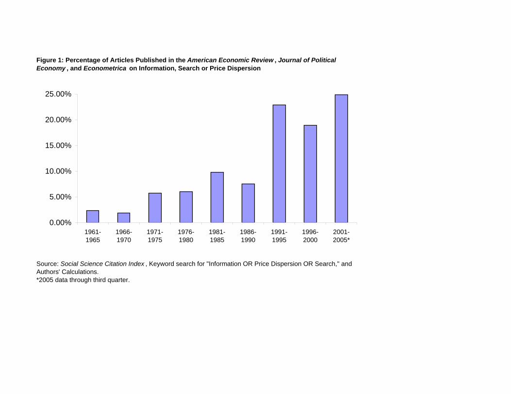
*2005 data through third quarter.

Figure 1: Percentage of Articles Published in the American Economic Review , Journal of Political Economy , and Econometrica on Information, Search or Price Dispersion

Source: Social Science Citation Index , Keyword search for "Information OR Price Dispersion OR Search," and Authors' Calculations.

0.00%

5.00%

10.00%

15.00%

20.00%

25.00%

1961-1965

1966-1970

1971-1975

1976-1980

1981-1985

1986-1990

1991-1995

1996-2000

2001-2005*

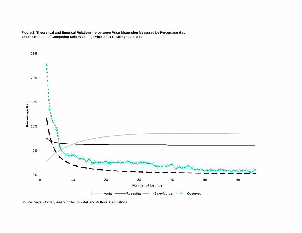
Figure 2: Theoretical and Emprical Relationship between Price Dispersion Measured by Percentage Gap and the Number of Competing Sellers Listing Prices on a Clearinghouse Site

Source: Baye, Morgan, and Scholten (2004a) and Authors' Calculations.

0%

5%

10%

15%

20%

25%

0 10 20 30 40 50 60

Number of Listings

Perc

enta

ge G

ap

Varian Rosenthal Baye-Morgan Observed

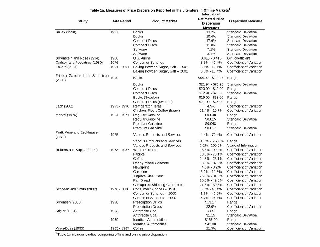
Table 1a: Measures of Price Dispersion Reported in the Literature in Offline Markets1

Study Data Period Product Market

Intervals of Estimated Price

Dispersion Measures

Dispersion Measure

Bailey (1998) 1997 Books 13.2% Standard DeviationBooks 10.4% Standard DeviationCompact Discs 17.6% Standard DeviationCompact Discs 11.0% Standard DeviationSoftware 7.1% Standard DeviationSoftware 8.1% Standard Deviation

Borenstein and Rose (1994) 1986 U.S. Airline 0.018 - 0.416 Gini coefficientCarlson and Pescatrice (1980) 1976 Consumer Sundries 3.3% - 41.4% Coefficient of VariationEckard (2004) 1901 - 2001 Baking Powder, Sugar, Salt -- 1901 3.1% - 10.1% Coefficient of Variation

Baking Powder, Sugar, Salt -- 2001 0.0% - 13.4% Coefficient of VariationFriberg, Ganslandt and Sandstrom (2001) 1999 Books $54.00 - $122.00 Range

Books $21.94 - $76.20 Standard DeviationCompact Discs $20.00 - $40.00 RangeCompact Discs $12.91 - $23.86 Standard DeviationBooks (Sweden) $19.00 - $58.00 RangeCompact Discs (Sweden) $21.00 - $46.00 Range

Lach (2002) 1993 - 1996 Refrigerator (Israel) 4.9% Coefficient of VariationChicken, Flour, Coffee (Israel) 11.4% - 19.7% Coefficient of Variation

Marvel (1976) 1964 - 1971 Regular Gasoline $0.048 RangeRegular Gasoline $0.015 Standard DeviationPremium Gasoline $0.048 RangePremium Gasoline $0.017 Standard Deviation

Pratt, Wise and Zeckhauser (1979) 1975 Various Products and Services 4.4% - 71.4% Coefficient of Variation

Various Products and Services 11.0% - 567.0% RangeVarious Products and Services 7.2% - 200.0% Value of Information

Roberts and Supina (2000) 1963 - 1987 Wood Products 13.8% - 90.2% Coefficient of VariationFabrics 18.8% - 78.1% Coefficient of VariationCoffee 14.3% - 25.1% Coefficient of VariationReady-Mixed Concrete 13.2% - 37.2% Coefficient of VariationNewsprint 4.5% - 8.2% Coefficient of VariationGasoline 6.2% - 11.8% Coefficient of VariationTinplate Steel Cans 25.0% - 31.0% Coefficient of VariationPan Bread 26.0% - 49.6% Coefficient of VariationCorrugated Shipping Containers 21.8% - 39.6% Coefficient of Variation

Scholten and Smith (2002) 1976 - 2000 Consumer Sundries -- 1976 3.3% - 41.4% Coefficient of VariationConsumer Sundries -- 2000 1.6% - 42.0% Coefficient of VariationConsumer Sundries -- 2000 5.7% - 28.4% Coefficient of Variation

Sorensen (2000) 1998 Prescription Drugs $13.17 RangePrescription Drugs 22.0% Coefficient of Variation

Stigler (1961) 1953 Anthracite Coal $3.46 RangeAnthracite Coal $1.15 Standard Deviation

1959 Identical Automobiles $165.00 RangeIdentical Automobiles $42.00 Standard Deviation

Villas-Boas (1995) 1985 - 1987 Coffee 21.5% Coefficient of Variation1 Table 1a includes studies comparing offline and online price dispersion.

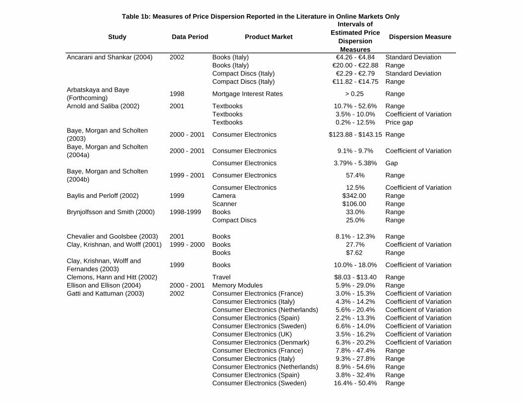
Table 1b: Measures of Price Dispersion Reported in the Literature in Online Markets Only

Study Data Period Product Market

Intervals of Estimated Price

Dispersion Measures

Dispersion Measure

Ancarani and Shankar (2004) 2002 Books (Italy) €4.26 - €4.84 Standard DeviationBooks (Italy) €20.00 - €22.88 RangeCompact Discs (Italy) €2.29 - €2.79 Standard DeviationCompact Discs (Italy) €11.82 - €14.75 Range

Arbatskaya and Baye (Forthcoming) 1998 Mortgage Interest Rates > 0.25 Range

Arnold and Saliba (2002) 2001 Textbooks 10.7% - 52.6% RangeTextbooks 3.5% - 10.0% Coefficient of VariationTextbooks 0.2% - 12.5% Price gap

Baye, Morgan and Scholten (2003) 2000 - 2001 Consumer Electronics $123.88 - $143.15 Range

Baye, Morgan and Scholten (2004a) 2000 - 2001 Consumer Electronics 9.1% - 9.7% Coefficient of Variation

Consumer Electronics 3.79% - 5.38% GapBaye, Morgan and Scholten (2004b) 1999 - 2001 Consumer Electronics 57.4% Range

Consumer Electronics 12.5% Coefficient of VariationBaylis and Perloff (2002) 1999 Camera $342.00 Range

Scanner $106.00 RangeBrynjolfsson and Smith (2000) 1998-1999 Books 33.0% Range

Compact Discs 25.0% Range

Chevalier and Goolsbee (2003) 2001 Books 8.1% - 12.3% RangeClay, Krishnan, and Wolff (2001) 1999 - 2000 Books 27.7% Coefficient of Variation

Books $7.62 RangeClay, Krishnan, Wolff and Fernandes (2003) 1999 Books 10.0% - 18.0% Coefficient of Variation

Clemons, Hann and Hitt (2002) Travel $8.03 - $13.40 RangeEllison and Ellison (2004) 2000 - 2001 Memory Modules 5.9% - 29.0% RangeGatti and Kattuman (2003) 2002 Consumer Electronics (France) 3.0% - 15.3% Coefficient of Variation

Consumer Electronics (Italy) 4.3% - 14.2% Coefficient of VariationConsumer Electronics (Netherlands) 5.6% - 20.4% Coefficient of VariationConsumer Electronics (Spain) 2.2% - 13.3% Coefficient of VariationConsumer Electronics (Sweden) 6.6% - 14.0% Coefficient of VariationConsumer Electronics (UK) 3.5% - 16.2% Coefficient of VariationConsumer Electronics (Denmark) 6.3% - 20.2% Coefficient of VariationConsumer Electronics (France) 7.8% - 47.4% RangeConsumer Electronics (Italy) 9.3% - 27.8% RangeConsumer Electronics (Netherlands) 8.9% - 54.6% RangeConsumer Electronics (Spain) 3.8% - 32.4% RangeConsumer Electronics (Sweden) 16.4% - 50.4% Range

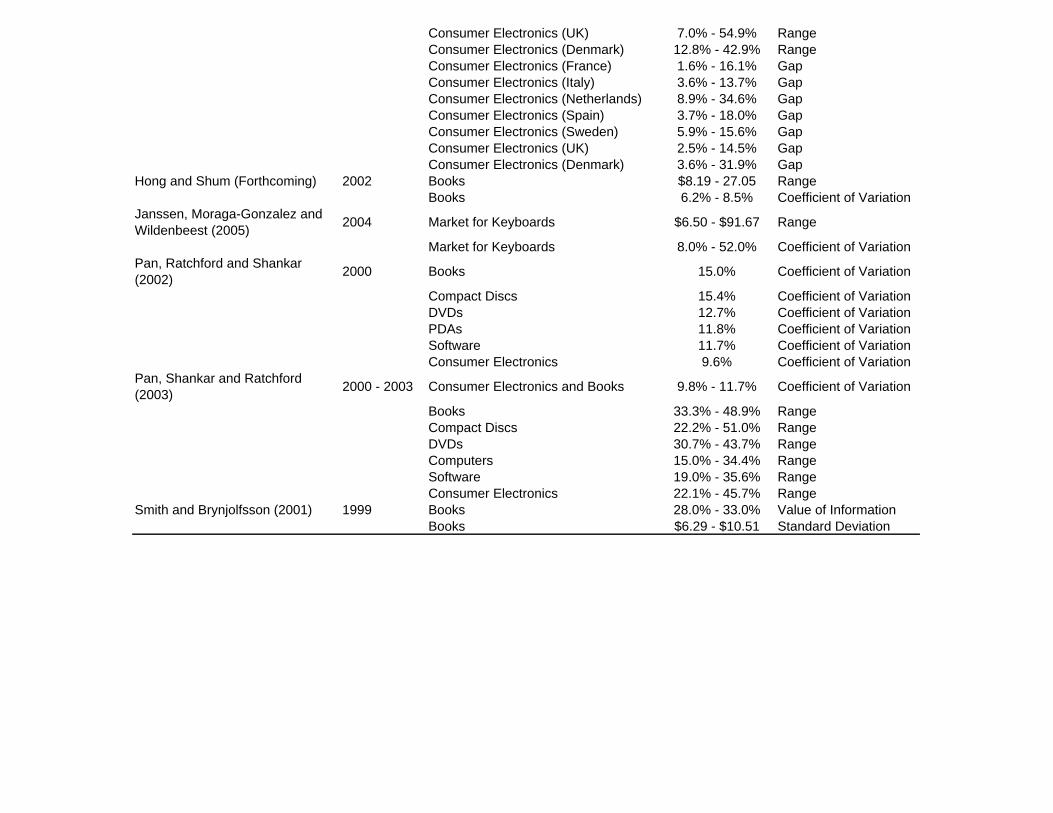
Consumer Electronics (UK) 7.0% - 54.9% RangeConsumer Electronics (Denmark) 12.8% - 42.9% RangeConsumer Electronics (France) 1.6% - 16.1% GapConsumer Electronics (Italy) 3.6% - 13.7% GapConsumer Electronics (Netherlands) 8.9% - 34.6% GapConsumer Electronics (Spain) 3.7% - 18.0% GapConsumer Electronics (Sweden) 5.9% - 15.6% GapConsumer Electronics (UK) 2.5% - 14.5% GapConsumer Electronics (Denmark) 3.6% - 31.9% Gap

Hong and Shum (Forthcoming) 2002 Books $8.19 - 27.05 RangeBooks 6.2% - 8.5% Coefficient of Variation

Janssen, Moraga-Gonzalez and Wildenbeest (2005) 2004 Market for Keyboards $6.50 - $91.67 Range

Market for Keyboards 8.0% - 52.0% Coefficient of VariationPan, Ratchford and Shankar (2002) 2000 Books 15.0% Coefficient of Variation

Compact Discs 15.4% Coefficient of VariationDVDs 12.7% Coefficient of VariationPDAs 11.8% Coefficient of VariationSoftware 11.7% Coefficient of VariationConsumer Electronics 9.6% Coefficient of Variation

Pan, Shankar and Ratchford (2003) 2000 - 2003 Consumer Electronics and Books 9.8% - 11.7% Coefficient of Variation

Books 33.3% - 48.9% RangeCompact Discs 22.2% - 51.0% RangeDVDs 30.7% - 43.7% RangeComputers 15.0% - 34.4% RangeSoftware 19.0% - 35.6% RangeConsumer Electronics 22.1% - 45.7% Range

Smith and Brynjolfsson (2001) 1999 Books 28.0% - 33.0% Value of InformationBooks $6.29 - $10.51 Standard Deviation