
Investigation of key reactions for chemiluminescence in ... · Shock-tube investigation of key...
137
Shock-tube investigation of key reactions for chemiluminescence in various combustion systems Von der Fakultät für Ingenieurwissenschaften, Abteilung Maschinenbau und Verfahrenstechnik der Universität Duisburg-Essen zur Erlangung des akademischen Grades eines Doktors der Ingenieurwissenschaften Dr.-Ing. genehmigte Dissertation von Metehan Bozkurt aus Hattingen Gutachter: Univ.-Prof. Dr. rer. nat. Christof Schulz Univ.-Prof. Dr. rer. nat. Matthias Olzmann Tag der mündlichen Prüfung: 30.07.2013
Transcript of Investigation of key reactions for chemiluminescence in ... · Shock-tube investigation of key...
Shock-tube investigation of key reactions for chemiluminescence in various combustion systems
Von der Fakultät für Ingenieurwissenschaften, Abteilung Maschinenbau und Verfahrenstechnik
der
Universität Duisburg-Essen
zur Erlangung des akademischen Grades
eines
Doktors der Ingenieurwissenschaften
Dr.-Ing.
genehmigte Dissertation
von
Metehan Bozkurt
aus
Hattingen
Gutachter: Univ.-Prof. Dr. rer. nat. Christof Schulz
Univ.-Prof. Dr. rer. nat. Matthias Olzmann Tag der mündlichen Prüfung: 30.07.2013

II

III
IV
Abstract
Existing combustion systems, especially gas turbines in power generation applications must
be optimized with regard to the reduction of pollutant emission and increase of efficiency.
Combustion under fuel-lean conditions is beneficial for a significant reduction of NOx and
soot formation. However, these operating conditions can lead to undesired combustion phe-
nomena such as combustion-induced oscillations and flame flash back which must be avoid-
ed. For this purpose, fundamental knowledge of the underlying chemical processes is
required. Non-intrusive optical methods such as the use of chemiluminescence are potential
practical approaches to provide combustion relevant information for the development of com-
bustion apparatus and process control. This requires knowledge of the formation reactions of
chemiluminescence as well as adequate kinetics models that link the light intensity to relevant
combustion parameters such as local heat release.
An accurate description of chemiluminescence fundamentally depends on the corresponding
ground-state chemistry. For small hydrocarbons such as CH4 and C2H2 detailed reaction
mechanisms already exist which were used as a base for the development of OH* and CH*
sub-mechanisms in the present work. The present work was devoted to study the formation
reactions of OH* and CH* chemiluminescence in shock tubes time-resolved detection of the
emission with a photomultiplier with narrowband interference filters. The signals were com-
pared to the corresponding excited-state species concentrations from simulations where based
on established ground-state mechanisms, OH* and CH* kinetics models were compiled and
validated with the experimental data from the present work. Based on the present work, the
reactions H + O + M = OH* + M and CH + O2 = OH* + CO are identified as the main OH*
formation channels in hydrogen and hydrocarbon oxidation and their corresponding rate coef-
ficients are determined as (1.5±0.45)×1013
exp(−25.0 kJ mol−1
/RT) cm6mol
−2s−1
and
(8.0±2.56)×1010
cm3mol
−1s−1
, respectively. For CH* chemiluminescence the reactions C2 +
OH = CH* + CO and C2H + O = CH* + CO are the most important formation reactions and
their underlying rate coefficients are (5.7±3.02)×1013
cm3mol
−1s−1
and
(1.0±0.53)×1012
exp(−10.9 kJ mol−1
/RT) cm3mol
−1s−1
, respectively.
While for small hydrocarbons well-known ground-state mechanisms are available, reliable
kinetics models for ethanol oxidation, especially for high temperatures, are sparse. Therefore,
the formation of important intermediates and products (e.g., OH, C2H2, and CO2) was studied
for ethanol oxidation by time-of-flight mass spectrometry and ring-dye laser absorption spec-
troscopy under shock-tube conditions. The experimental data were compared to simulations
using different reaction mechanisms from the literature and recommendations for the im-
provement of the corresponding mechanisms were suggested.
V
Zusammenfassung
Bestehende Verbrennungssysteme, insbesondere Gasturbinen für die Erzeugung von Strom,
müssen in Hinblick auf die Reduzierung des Rohstoffeinsatzes und des Ausstoßes von Emis-
sionen optimiert werden. Hierbei kann die Verbrennung unter mageren Mischungsbedingun-
gen zu einer signifikanten Reduzierung der Stickoxid- und Rußbildung führen. Diese
Betriebszustände führen jedoch teilweise zu unerwünschten Schwingungen und Flammen-
rückschlag innerhalb der Brennkammer, die vermieden werden müssen. Hierfür ist ein grund-
legendes Wissen über den zugrundeliegenden Verbrennungsprozess erforderlich. Nicht-
invasive optische Methoden wie das Flammenleuchten sind potentielle Ansätze zur Bereitstel-
lung von verbrennungsrelevanten Informationen für die Entwicklung von Verbrennungskon-
zepten und deren Regelung. Dies erfordert jedoch zum einen die Kenntnis über die
Bildungsreaktionen der Chemilumineszenz und zum anderen sind geeignete Kinetikmodelle
zur Beschreibung erforderlich.
Die Beschreibung der Chemilumineszenz erfordert genaue Kenntnis über die zugrundeliegen-
de Grundzustandschemie. Für einfache Kohlenwasserstoffverbindungen wie z.B. CH4 oder
C2H2 existieren bereits gut validierte Modelle, die in der vorliegenden Arbeit als Basis für die
Entwicklung von OH*- und CH*-Mechanismen verwendet wurden. Im Rahmen dieser Arbeit
wurden die Bildungsreaktionen der OH*- und CH*-Chemilumineszenz in Stoßwellenreakto-
ren mit Hilfe von Emissionsmessungen untersucht. Hierbei wurde das Flammleuchten mit
einer Kombination aus Photomultiplier und schmalbandigem Interferenzfilter zeitaufgelöst
gemessen. Basierend auf etablierten Mechanismen zur Beschreibung der Grundzustandsche-
mie wurden Kinetikmodelle für OH*- und CH*-Chemilumineszenz aufgestellt und mithilfe
der experimentellen Daten validiert. Die Reaktionen H + O + M = OH* + M und CH + O2 =
OH* + CO wurden als Hauptreaktionen für die Bildung von OH* bei der Oxidation von Was-
serstoff oder Kohlenwasserstoffen identifiziert und ihre zugrundeliegenden Geschwindig-
keitskoeffizienten wurden ermittelt mit (1.5±0.45)×1013
exp(−25.0 kJ mol−1
/RT) cm6mol
−2s−1
bzw. (8.0±2.56)×1010
cm3mol
−1s−1
. Für CH*-Chemilumineszenz wurden die Reaktionen C2 +
OH = CH* + CO und C2H + O = CH* + CO als wichtigste Bildungsreaktionen identifiziert
und mit den Geschwindigkeitskoeffizient (5.7±3.02)×1013
cm3mol
−1s−1
bzw.
(1.0±0.53)×1012
exp(−10.9 kJ mol−1
/RT) cm3mol
−1s−1
.
Während für kleine Kohlenwasserstoffe etablierte Mechanismen vorliegen, ist der Reakti-
onsmechanismus der Verbrennung von Ethanol, insbesondere bei hohen Temperaturen, nur
unzureichend bekannt. Daher wurde im Rahmen dieser Arbeit die Bildung von wichtigen In-
termediaten und Produkten (u.a. OH, C2H2, CO2) bei der Oxidation von Ethanol im Stoßwel-
lenrohr mittels Flugzeit-Massenspektrometrie und Farbstoff-Ringlaser-Absorptionsspektro-
skopie untersucht und mit verschiedenen Reaktionsmechanismen verglichen, die zusätzliche
Daten zur Verbesserung und weiteren Validierung der bestehenden Modelle liefern.
VI
Content
1. Introduction ......................................................................................................................... 1
2. Theoretical background....................................................................................................... 4
2.1. Reaction kinetics .......................................................................................................... 4
2.2. Kinetics of complex reaction systems ......................................................................... 6
2.2.1. H2 mechanism ...................................................................................................... 6
2.2.2. CH4 mechanism .................................................................................................... 7
2.2.3. C2H2 and C2H4 mechanisms ................................................................................. 7
2.2.4. C2H5OH mechanism ............................................................................................. 8
2.3. Chemiluminescence ..................................................................................................... 9
2.3.1. Fundamentals of the formation of chemiluminescent species............................ 10
2.3.2. OH* chemiluminescence .................................................................................... 13
2.3.3. CH* chemiluminescence .................................................................................... 14
2.3.4. C2* chemiluminescence ..................................................................................... 14
2.3.5. CO2* chemiluminescence................................................................................... 15
2.3.6. Spectroscopic properties of chemiluminescent species...................................... 15
2.4. Shock-tube fundamentals .......................................................................................... 16
3. Experimental ..................................................................................................................... 20
3.1. Shock-tubes for kinetics studies in highly diluted systems ....................................... 20
3.1.1. Chemiluminescence emission detection ............................................................. 21
3.1.2. Ring-dye laser absorption measurements ........................................................... 23
3.2. Shock-tube facility for the validation of reaction mechanism at percent-level
concentrations ....................................................................................................................... 30
3.2.1. Time-of-flight mass spectrometry ...................................................................... 30
4. Results and discussion ...................................................................................................... 33
4.1. Shock-tube measurements of OH* chemiluminescence ........................................... 33
4.1.1. Review of OH* kinetics ..................................................................................... 33
4.1.2. Strategy of investigating OH* chemiluminescence ........................................... 35
4.1.3. OH* chemiluminescence in H2/O2/Ar systems .................................................. 36
VII
4.1.4. OH* formation in H2/O2/CH4/Ar systems .......................................................... 45
4.1.5. OH* chemiluminescence in CH4 systems .......................................................... 48
4.1.6. OH* chemiluminescence in C2H2 systems ......................................................... 51
4.1.7. OH* chemiluminescence in C2H4 systems ......................................................... 57
4.1.8. OH* chemiluminescence in C2H5OH systems ................................................... 60
4.1.9. OH* kinetics model ............................................................................................ 62
4.1.10. Additional validation of the OH*-chemiluminescence mechanism with laminar
premixed flames .............................................................................................................. 64
4.2. Shock-tube measurements of CH* chemiluminescence ............................................ 67
4.2.1. Review of CH* kinetics ..................................................................................... 67
4.2.2. Strategy of the investigation of CH* chemiluminescence ................................. 70
4.2.3. CH* chemiluminescence in C2H2 mixtures ....................................................... 70
4.2.4. CH* chemiluminescence in C2H4 systems ......................................................... 80
4.2.5. CH* chemiluminescence in CH4 systems .......................................................... 83
4.2.6. CH* chemiluminescence in C2H5OH systems ................................................... 86
4.2.7. CH* kinetics model ............................................................................................ 91
4.2.8. Additional validation of the CH* chemiluminescence mechanism with laminar
premixed flames .............................................................................................................. 92
4.3. Validation of the ethanol ground-state chemistry ...................................................... 95
4.3.1. Time-of-flight mass spectrometry of ethanol pyrolysis and oxidation under
shock-heated conditions .................................................................................................. 96
4.3.2. Ring-dye laser measurements of OH ............................................................... 103
5. Conclusions ..................................................................................................................... 106
6. Own publications ............................................................................................................ 110
7. Bibliography ................................................................................................................... 111
8. List of abbreviations ....................................................................................................... 124
9. Symbols ........................................................................................................................... 125
10. Acknowledgement .......................................................................................................... 127

VIII
Introduction
1
1. Introduction
Ecological and economical restrictions have pushed constraints to reduce fossil fuel consump-
tion and pollutant emissions that are mainly attributed to electricity production and transporta-
tion. The prospective development of renewable power generation and low-emission internal
combustion (IC) engines technologies [1] are the most promising approaches to protect the
environment. Nevertheless, conventional combustion of hydrocarbons will still be the most
important energy source for the next decades. Therefore, optimization of existing combustion
technologies based on fossil fuels is important.
Furthermore, renewable energy sources such as wind power and solar power plants show high
fluctuations in their energy production depending on the meteorological conditions. Hence,
conventional energy production must be designed to rapidly cover the energy demand for
peak-period demand or for unfavorable weather conditions. Compared to coal-fired power
plants, gas-fired power plants have a high flexibility with regard to short starting times. Fur-
thermore, they emit up to 60% less carbon dioxide (CO2) [2], which makes them very attrac-
tive for future electricity production. However, due to higher fuel costs, gas-fired power
plants are playing only a minor role in global electricity generation. Therefore, the efficiency
of gas-turbine combustion must be increased to make them competitive with other conven-
tional combustion systems. For this purpose, operating gas turbines at low temperatures or
fuel-lean conditions is required to further reduce pollution emission and to increase fuel effi-
ciency. However, these conditions can cause unstable combustion states in terms of
thermoacoustic instabilities and flame flash-back [3] due to heat-release fluctuations which
can lead to destructive pressure oscillations within the combustor. Preventing this effect re-
quires a fundamental knowledge of the underlying chemical reactions which can be gathered
by local heat-release rate and equivalence-ratio measurements based on chemiluminescence to
avoid such undesired combustion phenomena. The knowledge of these two combustion pa-
rameters is important to improve the combustor design with regard to fuel-efficiency, pollu-
tant emission and combustion stability.
In research environments, sophisticated laser-based diagnostics are used to visualize the heat-
release distribution in lab-scale flames. A state-of-the-art technique is heat-release imaging of
formaldehyde (CH2O) by means of laser-induced fluorescence (LIF) [4-5]. The LIF technique
was successfully applied to characterize and to quantify spatially-resolved CH2O and OH
concentrations. These species are combustion-relevant intermediates and their combined con-
centrations correlate with the local heat release. The benefit of optical measurements is its
non-intrusive nature which allows to study combustion processes without disturbing them. In
harsh environments of practical applications, laser-diagnostic techniques, however, are not
suitable for in-situ measurements. These techniques require an external light source and opti-
cal ports to couple the laser beam into the combustion chamber. Common industrial combus-
Reaction kinetics
2
tors have limitations in the available geometry and are originally not designed to provide opti-
cal accessibility. Moreover, additional technical modifications would affect the combustion
process. The required laser and imaging system make optical diagnostic very complex and
expensive for practical applications. These disadvantages rule out conventional laser-based
diagnostics for many field applications. Hence, less costly and straightforward optical tech-
niques are desired. Luminescence of flames from chemical excitation of specific intermediate
species, the so called chemiluminescence (CL), is a promising tool that can potentially pro-
vide information about local heat release [6-8] and equivalence ratios [9-11] once the underly-
ing mechanisms are well enough understood.
Emission of UV- and visible light from electronically-excited species is a characteristic of
hydrocarbon combustion. The most common chemiluminescent species are OH*, CH*, C2*,
and CO2*, where the asterisk denotes electronic excitation as a consequence of chemical reac-
tions. Chemiluminescence investigation is an important tool in the field of combustion re-
search. The correlation of combustion relevant parameters such as heat release and fuel/air
ratio with the chemiluminescence emission of excited state species was subject of many in-
vestigations [6, 12-15]. These studies showed that chemiluminescence can be used to spatial-
ly-resolve flame fronts [16] and to measure heat release [5, 17] and local equivalence ratios
[6, 18-20].
Due to their simplicity, chemiluminescence sensors are desirable and can be easily designed
for practical applications. However, the fundamental chemical kinetics leading to
chemiluminescence, which is required for these applications, is still under debate. Overall, the
capability to provide combustion-relevant information in combination with the simplicity of
the detection system makes chemiluminescence very attractive for practical applications.
This, however, requires the coupling of chemiluminescence signals with the underlying chem-
ical processes in a quantitative manner. A quantitative and direct coupling between measured
light intensity and the relevant combustion parameter (chemiluminescent species concentra-
tion, heat release rate or local equivalence ratio) is not straightforward. An interpretation of
the measured signals can be done by linking the measured chemiluminescence intensities with
the corresponding species concentrations taken from kinetics mechanisms.
In conventional ground-state mechanisms, chemiluminescence and its formation pathways are
not considered because electronically excited species are several orders of magnitude less
abundant compared to ground-state species. Therefore, chemiluminescent species have no
influence on the global combustion process and are mostly not included in the ground-state
mechanisms. For a quantitative investigation of the chemiluminescence, the available ground-
state mechanisms must be extended by sub-models to describe the chemiluminescence path-
ways.
Based on the low concentrations of chemiluminescent species and the sophisticated interpreta-
tion, the characterization of the responsible formation reactions leading to chemiluminescence
Introduction
3
and determining their associate rate coefficients is challenging. This issue is also reflected in
the controversial kinetics data of chemiluminescence reactions in literature where notable
deficiencies in the proposed reaction pathways and rate coefficients can be seen. This is be-
cause of the lack of consistent concentration information and the difficulty of specifically pre-
paring species in the excited states.
Therefore, the aim of this study is to identify the key reactions forming OH* and CH* and to
determine their corresponding rate coefficients in shock-tube experiments using a model-
based calibration strategy. Here, various shock-heated mixtures were selected to selectively
initiate reactions that generate chemiluminescent species. Time-resolved chemiluminescence
emission profiles from both species were measured in various hydrogen and hydrocarbon
combustion systems. These shock-tube experiments provide important data such as ignition
delay times and concentration-time histories which are of fundamental importance for the
development of chemical reaction mechanisms. Existing ground-state mechanisms were used
as basis for the implementation of chemiluminescence formation and consumption reactions
to describe the OH* and CH* concentration histories. The strategy of the present work is (i)
Evaluation and extension of ground-state mechanism describing the underlying chemical pro-
cess. (ii) Development and validation of a kinetics model of OH* chemiluminescence for hy-
drogen and hydrocarbon combustion under shock-tube and flame conditions. (iii)
Development and validation of a kinetics model of CH* chemiluminescence for hydrocarbon
combustion under shock-tube and flame conditions.
Reaction kinetics
4
2. Theoretical background
2.1. Reaction kinetics
Classical thermodynamical equilibrium assumption can be used for the description of reaction
systems where chemical reactions are fast compared to diffusion, transport processes and heat
conduction. However, in combustion chemical reactions occur on similar time scales with
other processes and therefore, the reaction kinetics must often be considered as a rate-
determining process. The simplest combustion system is the oxidation of hydrogen. The com-
bustion process is typically summarized by the global reaction
2H2 + O2 2H2O (2.1)
which describes the overall combustion process represented by the educts hydrogen and oxy-
gen and the product water. However, combustion research revealed that the real oxidation
process is more complex and involves intermediate species (O, H, OH) being formed and
consumed during the combustion. The underlying detailed reaction mechanism is typically
described with a set of elementary reactions. These elementary reactions describe a reactive
molecular (collision) process and cannot be broken down to further reactions. A typical ele-
mentary reaction in hydrogen oxidation is the chain branching reaction of molecular oxygen
with atomic hydrogen which provides high amounts of radicals accelerating the reaction pro-
gress.
O2 + H OH + O (2.2)
Elementary reactions can be separated into three fundamental types. Unimolecular reactions
represent the decomposition or isomerization of one reactant and are usually chain initiation
reactions at the beginning of a combustion process. In a bimolecular reaction, two educts or
intermediates react together to form product(s). This type of reaction is the most common one
in combustions. Termolecular reactions incorporate three reactants and usually describe re-
combination reactions.
A reaction mechanism for combustion modeling consisting of a set of R elementary reactions
j, −j with N species (Xi) and their corresponding stoichiometric coefficients vi can be described
by the equation:
(2.3)
The rate law of each species incorporating forward and backward reactions is given by:
Theoretical background
5
(2.4)
The rate of formation Rj describes the species conversion of the reaction in which forward and
backward reactions are considered:
(2.5)
Aside from the corresponding species concentration, reactions strongly depend on the rate
coefficients kj and k−j, respectively. These rate coefficients are characteristic for elementary
reactions and therefore are essential for the fundamental knowledge of a reaction mechanism.
A rate coefficient usually depends on the temperature and is expressed by a modified Arrhe-
nius equation:
(2.6)
Aj is the pre-exponential factor, which is commonly only weakly temperature dependent. To
account for this behavior, the original Arrhenius equation is extended by the term T n. It is
essential to specify the experimental T-range where the rate coefficients have been measured.
The activation energy Ej corresponds to the energy barrier which must be overcome during
the reaction. The value of the activation energies range between the sum of bonding energies
for dissociation reactions and zero [21].
Based on the thermodynamics data (enthalpy, entropy, heat capacity) of each species, the
equilibrium constant KC can be determined which subsequently provides the rate coefficient
for the reverse reaction k−j according to equation from the rate coefficient kj (2.7):
(2.7)
Modern theoretical approaches such as Rice-Ramsperger-Kassel-Marcus (RRKM) theory [22-
23] based on the transition-state theory [24] and statistical adiabatic channel model (SACM)
[25-26] provide computational estimates for rate coefficients. Nevertheless, practical kinetics
experiments are required to determine the underlying rate coefficients. Spectroscopic tech-
niques such as absorption spectroscopy combined with shock-tube experiments are frequently
employed to investigate ultrafast elementary reactions relevant for combustion. The high sen-
sitivity of spectroscopic experiments coupled with the well-known experimental conditions
from shock tubes enables accurate measurements in highly diluted mixtures without perturba-
tion from transport processes. A detailed description of shock-tube fundamentals is given in
section 2.4. This combination is necessary for the isolated study of elementary reactions by
avoiding the influence of subsequent reactions which would interfere at high concentrations.
Kinetics of complex reaction systems
6
The corresponding time-resolved concentration profiles of the involved species are used to
determine the corresponding rate coefficient kj.
2.2. Kinetics of complex reaction systems
As introduced in the previous section, complex reaction mechanisms that describe the overall
combustion process typically consist of a subset of elementary reactions incorporating the
corresponding educts, the intermediate species and the products. The mechanism is built up as
a sequence of elementary reactions and their corresponding formation and consumption rate
coefficients. Typically, the mechanisms are validated with regard to global observables such
as ignition delay times, flame velocities or concentration-time histories of important interme-
diate species like OH and CH radicals. Even the description of the simplest combustion reac-
tion of hydrogen oxidation requires 20 reactions and 8 species [21]. For hydrocarbon
combustion the complexity increases exponentially with the chain length and therefore hun-
dreds (methane) [27] or thousands (liquid fuels) [28] of elementary reactions are required for
the description of the process. Some of the reactions are directly measured, or are calculated
based on quantum chemical calculations or are estimated. However, only a limited number of
reactions are rate determining for the overall process.
2.2.1. H2 mechanism
The common characteristic of hydrogen oxidation mechanisms is a core mechanism consist-
ing of these chain-branching and propagation reactions (i) H + O2 = OH + O, (ii) H2 + O =
OH + H, (iii) H2 + OH = H2O + H, and (iv) OH + OH = H2O + O. These four reactions are the
most prominent reactions in all hydrogen mechanisms while the existence of other reactions
can vary. In general, hydrogen as well as hydrocarbon combustion shows very strong sensitiv-
ity towards the reaction (i) which is a rate-determining reaction.
A hydrogen oxidation mechanism describing the ground-state oxidation process was taken
from Warnatz mechanism [21]. It includes temperature as well as pressure-dependent reac-
tions and has been recently documented in [29] where the rate coefficients of the elementary
reactions are based on the recommendations of Baulch et al. [30]. This mechanism is validat-
ed with respect to flame velocity (5 – 70 fuel percentage) and ignition delay times in the tem-
perature range from 950 – 3000 K. The absolute concentration of the major species (H2, O2,
H2O, H, OH, O) were in very good agreement with species concentration measurements from
[31]. This reaction mechanism was used in the present work as a base to develop an OH* sub-
mechanism in H2/O2 combustion systems.
Theoretical background
7
2.2.2. CH4 mechanism
There is a consensus in the description of the hydrocarbon oxidation which is typically initiat-
ed by chain-branching reactions where H, O, and OH radicals are formed which interact with
fuel molecules forming alkyl radicals. Especially the ignition delay time is very sensitive to-
wards the chain-branching reaction H + O2 = OH + O which controls the break-up of the fuel.
These alkyl radicals further decompose and accelerate the combustion progress. In case of
methane oxidation, CH3 radicals are thermally formed by H-atom abstraction or by chain-
branching reactions according to the above-mentioned scheme. Formaldehyde (CH2O) is
formed from CH3 which reacts instantaneously to HCO forming CO and finally generating
CO2.
In the present work, the simulations of methane combustion were performed using the state of
the art mechanism GRI3.0 [27]. This mechanism incorporates 53 species and 325 elementary
reactions, which was extensively validated for a wide range of conditions where various
shock-tube and flame experiments were considered. The validation conditions in terms of
temperature, pressure and mixture conditions are comparable to our experiments. While the
performance of the GRI3.0 mechanism [27] for highly diluted systems for low pressures and
temperatures is well, there are deficiencies in predicting the ignition delay times for pressures
above 60 bar. However, the altering performance with increasing pressure is not a methane-
specific issue and can be observed for various combustion systems.
The GRI3.0 mechanism [27] contains a comprehensive nitrogen chemistry validated with
regard to the formation of NOx. However, the model was not explicitly tested for the oxida-
tion of methane with N2O which was used as an alternative oxidizer within the present study
to generate high amounts of atomic oxygen which will be extensively described in section
4.1.5. The GRI3.0 mechanism has been established as the most reliable mechanism for the
numerical analysis of methane oxidation. Therefore, the present shock-tube measurements are
consistently simulated using the GRI mechanism.
2.2.3. C2H2 and C2H4 mechanisms
There are different well-validated comprehensive mechanism for hydrocarbon combustion
which are built up in a hierarchical manner starting from elementary hydrogen and methane
combustion towards acetylene [32-34]. According to the reaction process for methane com-
bustion, the oxidation of hydrocarbons is typically initiated by H-atom abstraction or in case
of acetylene and ethylene, by unimolecular dissociation of the fuel by C—C cleavage. In con-
trast to the available kinetics mechanisms, Wang and Laskin [35] reported that the oxidation
of acetylene or ethylene under shock-tube conditions can be initiated by a third pathway via
vinylidene which can significantly enhance the formation of the radical pool.
Kinetics of complex reaction systems
8
In the present study, the ground-state model from Wang and Laskin [35] was considered for
the interpretation of acetylene and ethylene combustion. The mechanism is especially devel-
oped for high-temperature oxidation of both fuels and it consists of 75 species and 529 reac-
tions. Chemistry of higher hydrocarbons is more complex compared to methane combustion
and thus, requires in-depth validation efforts. The mechanism was previously optimized for a
wide range of conditions with regard to shock-tube experiments, laminar burning velocity and
burner-stabilized flames. The entire validation data are published in [35].
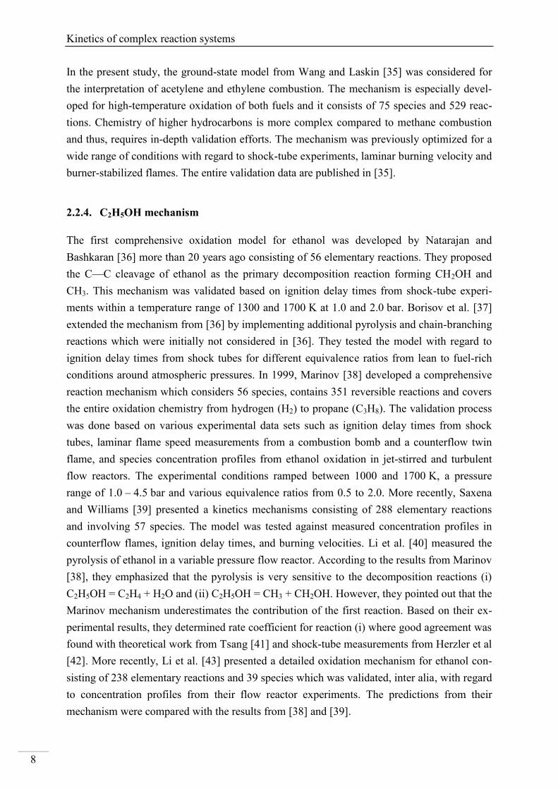
2.2.4. C2H5OH mechanism
The first comprehensive oxidation model for ethanol was developed by Natarajan and
Bashkaran [36] more than 20 years ago consisting of 56 elementary reactions. They proposed
the C—C cleavage of ethanol as the primary decomposition reaction forming CH2OH and
CH3. This mechanism was validated based on ignition delay times from shock-tube experi-
ments within a temperature range of 1300 and 1700 K at 1.0 and 2.0 bar. Borisov et al. [37]
extended the mechanism from [36] by implementing additional pyrolysis and chain-branching
reactions which were initially not considered in [36]. They tested the model with regard to
ignition delay times from shock tubes for different equivalence ratios from lean to fuel-rich
conditions around atmospheric pressures. In 1999, Marinov [38] developed a comprehensive
reaction mechanism which considers 56 species, contains 351 reversible reactions and covers
the entire oxidation chemistry from hydrogen (H2) to propane (C3H8). The validation process
was done based on various experimental data sets such as ignition delay times from shock
tubes, laminar flame speed measurements from a combustion bomb and a counterflow twin
flame, and species concentration profiles from ethanol oxidation in jet-stirred and turbulent
flow reactors. The experimental conditions ramped between 1000 and 1700 K, a pressure
range of 1.0 – 4.5 bar and various equivalence ratios from 0.5 to 2.0. More recently, Saxena
and Williams [39] presented a kinetics mechanisms consisting of 288 elementary reactions
and involving 57 species. The model was tested against measured concentration profiles in
counterflow flames, ignition delay times, and burning velocities. Li et al. [40] measured the
pyrolysis of ethanol in a variable pressure flow reactor. According to the results from Marinov
[38], they emphasized that the pyrolysis is very sensitive to the decomposition reactions (i)
C2H5OH = C2H4 + H2O and (ii) C2H5OH = CH3 + CH2OH. However, they pointed out that the
Marinov mechanism underestimates the contribution of the first reaction. Based on their ex-
perimental results, they determined rate coefficient for reaction (i) where good agreement was
found with theoretical work from Tsang [41] and shock-tube measurements from Herzler et al
[42]. More recently, Li et al. [43] presented a detailed oxidation mechanism for ethanol con-
sisting of 238 elementary reactions and 39 species which was validated, inter alia, with regard
to concentration profiles from their flow reactor experiments. The predictions from their
mechanism were compared with the results from [38] and [39].
Theoretical background
9
According to the observations from [44] where ethanol was mainly consumed during the in-
duction period, any ethanol oxidation mechanism must be developed based on the fundamen-
tal knowledge of the ethanol pyrolysis. While for temperatures below 1000 K the
decomposition of ethanol predominantly starts with H-atom abstraction, for temperatures
above 1000 K the C—C cleavage forming CH3 and CH2OH is suggested to be the major de-
composition step. However, recent studies reveal that the unimolecular decomposition of eth-
anol towards C2H4 and H2O is more important than the methyl abstraction [38, 45].
In the present work, the ethanol combustion was simulated using a detailed kinetics model
from Marinov [38]. Kiecherer et al. [45] revised the main decomposition reactions of ethanol
in the Marinov mechanism based on statistical reaction theory. These recommendations were
also used for the simulation of the ethanol-based mixtures. For additional simulations of the
ethanol oxidation, the model from Saxena and Williams [39] was used.
2.3. Chemiluminescence
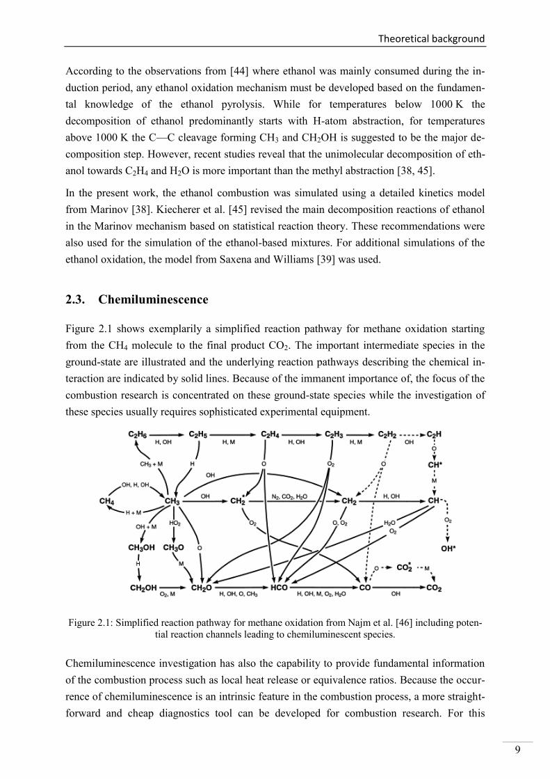
Figure 2.1 shows exemplarily a simplified reaction pathway for methane oxidation starting
from the CH4 molecule to the final product CO2. The important intermediate species in the
ground-state are illustrated and the underlying reaction pathways describing the chemical in-
teraction are indicated by solid lines. Because of the immanent importance of, the focus of the
combustion research is concentrated on these ground-state species while the investigation of
these species usually requires sophisticated experimental equipment.
Figure 2.1: Simplified reaction pathway for methane oxidation from Najm et al. [46] including poten-
tial reaction channels leading to chemiluminescent species.
Chemiluminescence investigation has also the capability to provide fundamental information
of the combustion process such as local heat release or equivalence ratios. Because the occur-
rence of chemiluminescence is an intrinsic feature in the combustion process, a more straight-
forward and cheap diagnostics tool can be developed for combustion research. For this
Chemiluminescence
10
purpose, the main challenge which has to be overcome is the linkage of the measured
chemiluminescence emission with the underlying reaction mechanism.
As illustrated by the dashed lines in Figure 2.1, chemiluminescence formation occurs aside
from the global reaction process. Because chemiluminescent species are several orders of
magnitude less abundant compared to their corresponding ground-state molecules, they have a
negligible influence on the overall reaction process and therefore, they are typically not con-
sidered within the reaction mechanism. Based on the interaction of the ground-state mecha-
nism, which provides the precursor molecules, with the chemiluminescence formation, the
correct description of the formation reactions of chemiluminescence crucially depends on the
knowledge of the underlying ground-state chemistry and the elementary reactions that quench
the electronically-excited states. Therefore, the first and most challenging issue is the contro-
versial discussion in identifying the formation reactions leading to chemiluminescence and
their corresponding rate coefficients which is briefly introduced in 2.3.2 and 2.3.3. The se-
cond challenge which must be overcome is the accurate quantitative prediction of transient
intermediate species such as CH molecules which are of fundamental importance for a relia-
ble investigation of chemiluminescence kinetics. A detailed literature review and a compre-
hensive discussion of OH* and CH* kinetics is presented in sections 4.1.1 and 4.2.1. The
present study is devoted to investigate the formation pathways of OH* and CH*
chemiluminescence and to identify their rate coefficients.
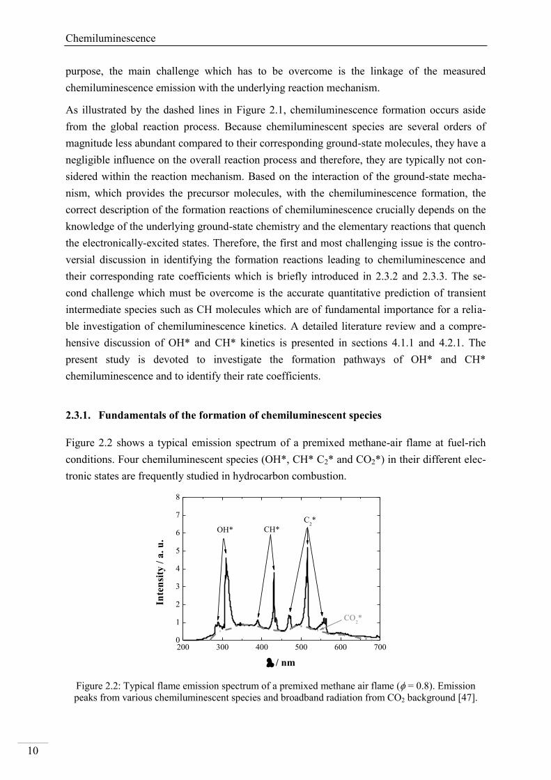
2.3.1. Fundamentals of the formation of chemiluminescent species
Figure 2.2 shows a typical emission spectrum of a premixed methane-air flame at fuel-rich
conditions. Four chemiluminescent species (OH*, CH* C2* and CO2*) in their different elec-
tronic states are frequently studied in hydrocarbon combustion.
200 300 400 500 600 7000
1
2
3
4
5
6
7
8
CO2*
C2*
CH*
Inte
nsi
ty /
a.
u.
/ nm
OH*
Figure 2.2: Typical flame emission spectrum of a premixed methane air flame ( = 0.8). Emission
peaks from various chemiluminescent species and broadband radiation from CO2 background [47].
Theoretical background
11
While the kinetics of OH* and CH* were extensively studied in the past [48-53]. Only sparse
data are available for C2* [48, 54-56] and CO2* [57-60]. Owing the large deviations in identi-
fying the key reactions leading to chemiluminescent species and their corresponding kinetics
data, chemiluminescence investigations are still in the focus of recent combustion research
[15, 61-65].
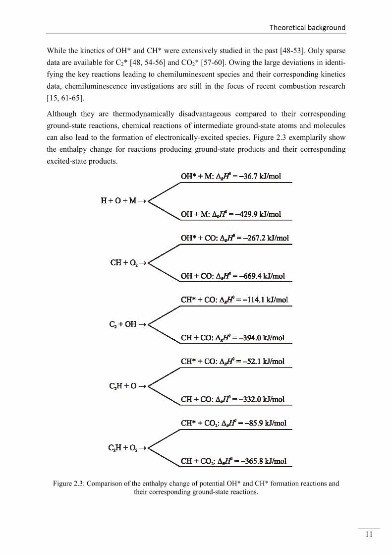
Although they are thermodynamically disadvantageous compared to their corresponding
ground-state reactions, chemical reactions of intermediate ground-state atoms and molecules
can also lead to the formation of electronically-excited species. Figure 2.3 exemplarily show
the enthalpy change for reactions producing ground-state products and their corresponding
excited-state products.
Figure 2.3: Comparison of the enthalpy change of potential OH* and CH* formation reactions and
their corresponding ground-state reactions.
Chemiluminescence
12
The excitation of chemiluminescent species is attributed to chemical excitation instead of
thermal excitation [66]. Aside from the chemical excitation, thermal activation can also occur.
However, thermal excitation of ground-state molecules is usually considered as negligible for
common experimental conditions because of energetic considerations. Thermal excitation
must be considered especially for high temperatures above 2000 K [66-67]. Due to the energy
excess of the excited-state species, these chemiluminescent species are short-lived and the
energy is partially removed by photon emission which can be characterized by the photon
energy release hv = E2 – E1. However, chemiluminescent species commonly are de-excited to
the electronic ground state via collisional quenching [68].
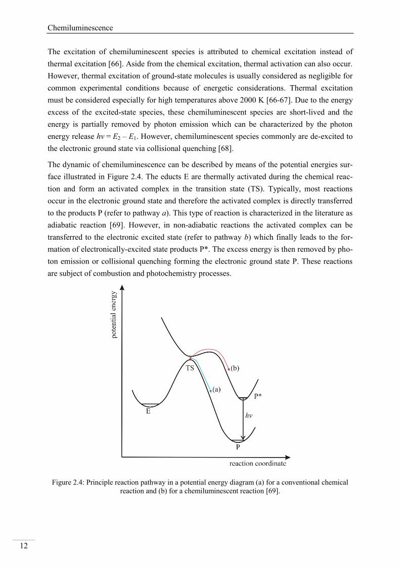
The dynamic of chemiluminescence can be described by means of the potential energies sur-
face illustrated in Figure 2.4. The educts E are thermally activated during the chemical reac-
tion and form an activated complex in the transition state (TS). Typically, most reactions
occur in the electronic ground state and therefore the activated complex is directly transferred
to the products P (refer to pathway a). This type of reaction is characterized in the literature as
adiabatic reaction [69]. However, in non-adiabatic reactions the activated complex can be
transferred to the electronic excited state (refer to pathway b) which finally leads to the for-
mation of electronically-excited state products P*. The excess energy is then removed by pho-
ton emission or collisional quenching forming the electronic ground state P. These reactions
are subject of combustion and photochemistry processes.
Figure 2.4: Principle reaction pathway in a potential energy diagram (a) for a conventional chemical
reaction and (b) for a chemiluminescent reaction [69].
Theoretical background
13
Radiative de-excitation of chemiluminescent species is characterized by A21, denoted as Ein-
stein coefficient of spontaneous emission. Compared to radiative decay of excited-state spe-
cies, the energy transfer by collisional quenching is more likely to occur. Through non-
reactive collisions with ambient molecules, excited species return to a lower state by transfer-
ring their excess energy to the collision partner.
In addition to non-radiative energy transfer of an excited-state molecule by collision quench-
ing, reactive collisions can also occur and are exemplarily reported in [70-72]. Due to lower-
ing effects of the endoergic reaction barrier, the chemical reactivity of electronically excited
molecules is several hundreds of times faster than their corresponding ground-state species
[73-74]. Recently, Starik and co-workers [75] studied the influence of vibrationally and elec-
tronically excited O2 as a combustion accelerator for hydrogen oxidation. They demonstrated
that the supersonic flow of H2/O2 mixture can be ignited within short exposure distances even
for low temperatures when excited molecules were available whereas for cases without elec-
tronic activation an ignition could not be observed. Furthermore, the reactive consumption of
OH* via the reaction OH* + H2 = H + H2O was in the scope of several studies [70-72]. For
CH* chemiluminescence, ground-state CH molecules were suggested to be more reactive
compared to excited-state CH [76] . Based on the short lifetimes of CH*, the de-excitation of
CH* towards CH is more likely than the reactive consumption of CH*. However, due to the
lack of consistent information, the consumption of chemiluminescent species via reactive col-
lisions is commonly neglected in excited-state mechanisms.
2.3.2. OH* chemiluminescence
OH* chemiluminescence is abundant in hydrogen and hydrocarbon combustion. The UV
emission at 306 nm is attributed to the OH(A2
+X
2) transition. Other potential transitions
from the B and C states are not identified in flame experiments. The key reactions responsible
for OH* in the combustion are under debate. Chemical build-up of OH* via reactions
H + O + M = OH* + M and H + OH + OH = OH* + H2O are frequently considered to be re-
sponsible for the production of OH* chemiluminescence in hydrogen combustion. Whereas in
hydrocarbon combustion, there is accordance in identifying the formation channel of OH*
chemiluminescence as CH + O2 = OH* + CO [51, 77-78]. A detailed discussion of the OH*
kinetics is given in section 4.1.1. In addition, thermal excitation must be considered also as
potential pathway transferring ground-state OH molecules into its A state for temperatures
above 2800 K. In a recent study based on an opposed oxy-methane diffusion flame from De
Leo et al. [67], 35% of the OH* was attributed to thermal excitation. It was reported that this
ratio further shifts towards thermal formation of OH* for increasing temperatures. In the pre-
sent study, the equilibrium of OH molecules was used to calibrate the optical detection system
with regard to absolute OH* concentration [79]. Based on this procedure, the chemical excita-
Chemiluminescence
14
tion pathway of OH* CL at lower temperatures was investigated and model-based recon-
structed. A detailed description will be presented in section 4.1.1.
2.3.3. CH* chemiluminescence
CH* is also an important emitter in hydrocarbon combustion. The strongest transition with an
emission in the blue-violet range at 430 nm is assigned to the CH(A2X
2) transition. Ad-
ditionally, CH* emission around 390 nm due to the CH(B2−X
2) transition was recently
investigated in flames [65]. Kathrotia et al. [65] pointed out that the A–X transition contrib-
utes about 80% of the total chemiluminescence emission whereas the residual amount is at-
tributed to the B–X transition. In previous work, various reactions were suggested to be
responsible for CH* formation. However, the available kinetics data varies in several orders
of magnitude. Recent studies presumed, that three potential reactions C2 + OH = CH* + CO,
C2H + O = CH* + CO and C2H + O2 = CH* + CO2 must be considered for CH*
chemiluminescence. Large deviations have been reported in determining the dominating for-
mation reaction and their corresponding rate coefficients. Similar to OH* chemiluminescence,
thermal excitation of CH* also occurs especially for high temperatures and was reported in a
recent diffusion flame study [67]. The authors stated that for temperatures around 3000 K
thermal excitation contributes up to 30% to the total excited state CH*. A detailed discussion
of CH* kinetics will be given in section 4.2.1.
2.3.4. C2* chemiluminescence
C2* chemiluminescence in the blue-green spectrum between 436 and 564 nm from the
C2(d3a
3) transition, also denoted as Swan bands, especially occurs under fuel-rich con-
ditions. Therefore, it can provide information about areas susceptible to soot formation.
Gaydon [48] suggested the reaction 1CH2 + C = C2* + H2 as formation reaction of C2*. Later
on, Savadatti and Broida [54] proposed the reaction C3 + O = C2* + CO. Smith and co-
workers studied C2* formation in various premixed hydrocarbon flames by laser-induced flu-
orescence (LIF) imaging measurements [56]. They developed a sub-mechanism for C2* kinet-
ics and recommended rate coefficients for the two formation reactions stated above. More
recently, Kathrotia et al. [65] studied C2* formation amongst others in various premixed me-
thane air flames. They found that their flame experiments can be reproduced when consider-
ing the two above-mentioned recommended reactions from [48] and [54]. However, their
results suffer from simulation uncertainties due to the lack of reliable precursor concentra-
tions.
Theoretical background
15
2.3.5. CO2* chemiluminescence
Flame spectra of hydrocarbons typically show a significant background emission caused by
CO2* chemiluminescence. In contrast to the narrow emission bands of OH* and CH*, CO2*
emission occurs in a broad spectral range from 300 to 650 nm. Therefore, quantitative meas-
urements of chemiluminescence under flame conditions require the knowledge of CO2* for-
mation and its contribution to the different emission band from the other chemiluminescent
species. Jachimowski [80] and later on Baulch et al. [57] observed a proportionality of CO2*
chemiluminescence and the product of [CO] and [O]. Based on this finding, they concluded
that the reaction CO + O (+ M) = CO2* (+ M) is the main formation pathway of CO2* which
was already postulated by Broida and Gaydon [81] early in 1953. Hall et al. [53] also identi-
fied the reaction above as the main source of CO2* chemiluminescence and showed that the
emission is proportional to the CO and O concentrations. They reported that the broadband
CO2* radiation interferes with the CH* emission for temperatures below 1700 K and a correc-
tion of the initial CH* signal was applied. In the present work, interference of CH* and CO2*
chemiluminescence was not observed which is attributed to lower initial concentrations of the
reactants compared to the experiments of [53]. This is potentially attributed to the lower initial
concentrations of the reactants in the present work. More recently, Kopp et al. [60, 82] studied
the broadband emission of CO2* in shock-heated H2, N2O, CO and Ar mixtures by recording
the emission signals at two wavelengths by means of separate interference filter and photo-
multiplier setups. The experiments were compared with simulations considering CO2* and
CH2O* as potential sources of the background radiation. Based on this comparison, they con-
cluded that the broadband emission is mainly attributed to CO2*. However, the agreement
between experiment and simulation was poor and they pointed out that further improvement
of the CO2* formation mechanism and the underlying rate coefficient is required.
2.3.6. Spectroscopic properties of chemiluminescent species
Brockhinke and co-workers [64] extensively studied rotationally-resolved chemiluminescence
spectra of OH*, CH* and C2* chemiluminescence under flame conditions. While their meas-
ured emission spectra for CH* and C2* are close to the computed results using LIFBASE [83]
and LASKINv2 [84] assuming thermal equilibrium, the spectral shape of OH*
chemiluminescence could not be described by assuming thermal distribution. This observation
was already reported in [85-87]. Based on the high excess energy when generating OH(A) via
chemical reaction from CH + O2 = OH* + CO, high vibrational and rotational levels (v” = 6)
are also accessible. However, for high vibrational states pre-dissociation of OH* is more like-
ly to occur, therefore, v” 2 can be considered as an upper limit of the chemical excitation of
OH. In general, higher vibrational and rotational levels are internally transferred to lower
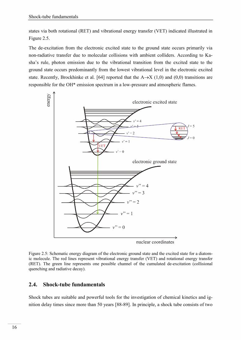
Shock-tube fundamentals
16
states via both rotational (RET) and vibrational energy transfer (VET) indicated illustrated in
Figure 2.5.
The de-excitation from the electronic excited state to the ground state occurs primarily via
non-radiative transfer due to molecular collisions with ambient colliders. According to Ka-
sha’s rule, photon emission due to the vibrational transition from the excited state to the
ground state occurs predominantly from the lowest vibrational level in the electronic excited
state. Recently, Brockhinke et al. [64] reported that the AX (1,0) and (0,0) transitions are
responsible for the OH* emission spectrum in a low-pressure and atmospheric flames.
Figure 2.5: Schematic energy diagram of the electronic ground state and the excited state for a diatom-
ic molecule. The red lines represent vibrational energy transfer (VET) and rotational energy transfer
(RET). The green line represents one possible channel of the cumulated de-excitation (collisional
quenching and radiative decay).
2.4. Shock-tube fundamentals
Shock tubes are suitable and powerful tools for the investigation of chemical kinetics and ig-
nition delay times since more than 50 years [88-89]. In principle, a shock tube consists of two
Theoretical background
17
sections divided by a diaphragm. The high-pressure section, also denoted as driver section, is
filled with the driver gas, typically hydrogen or helium. Based on the different speed of sound
for both driver gases and depending on the shock-tube design, hydrogen is used for high-
temperature experiments for temperatures above 1400 K and for lower temperatures, helium
is typically used. The low-pressure section, designated as driven section, is filled with the
sample gas and provides optical ports for spectroscopic applications and potential additional
sampling ports near the end flange. Because of the rapture of the aluminum diaphragm, a
shock wave is formed induced by the pressure pulses that build a shock front. The wave front
propagates through the test gas and causes an instantaneous pressure and temperature increase
behind the incident shock wave. At the end wall, the shock wave reflects and passes the test
gas again and induces to a second pressure and temperature increase (conditions behind the
reflected shock wave).
The thermodynamic variables density , pressure p and temperature T behind shock waves
can be calculated by gasdynamics theory. Detailed literature to shock-tube characteristics can
be found in [88-90]. For ideal gases, the step increase of pressure, density and temperature
behind the incident shock wave (T2, p2 and 2) can be described by using the conservation
equations (mass flux, flux of momentum and energy per mass) with regard to the initial condi-
tions T1, p1, and 1:
(2.8)
(2.9)
(2.10)
Assuming that the behavior of the gas in the shock tube is ideal and the heat capacity is tem-
perature independent, the upper equations can be transferred to Rankine-Hugoniot equations:
2
(2.11)
1
(2.12)
(2.13)
For ideal gases, the Mach number Ma can be determined from the shock-wave velocity:
(2.14)
The molar mass M and the heat capacity ratio depend on the mixture composition of the test
gas and can be calculated with regard to the initial conditions. Therefore, the shock-tube con-
Shock-tube fundamentals
18
ditions behind the incident shock wave only depend on the shock-wave velocity vS. Hence, for
the prediction of the shock-tube conditions the velocity is required only. This value is typical-
ly measured based on the pressure traces in the driven section due to the pressure jump behind
the shock wave.
The conditions behind the reflected shock wave (T5, p5 and 5) can be deduced based on the
ideal shock assumption:
(2.15)
(2.16)
The equations above consider ideal shock-tube conditions only. However, real-gas effects
with regard to temperature, pressure and density deviations can influence the experimental
conditions. Depending on the experimental conditions, they must be taken into account as
well.
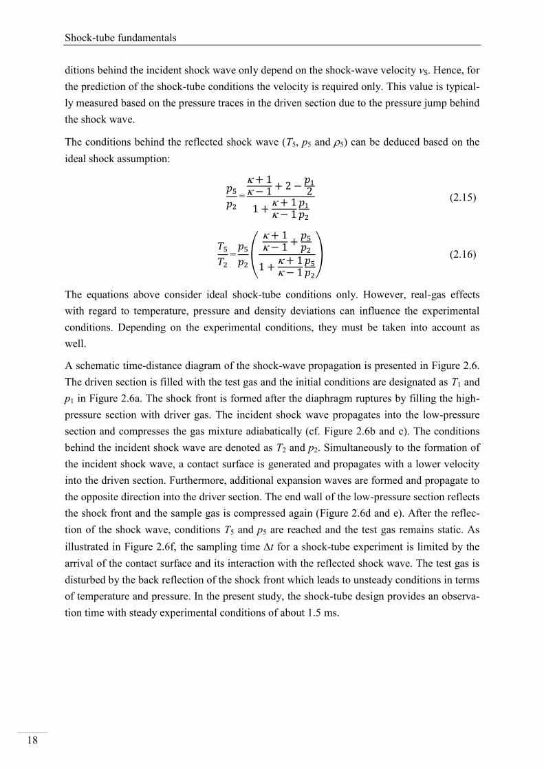
A schematic time-distance diagram of the shock-wave propagation is presented in Figure 2.6.
The driven section is filled with the test gas and the initial conditions are designated as T1 and
p1 in Figure 2.6a. The shock front is formed after the diaphragm ruptures by filling the high-
pressure section with driver gas. The incident shock wave propagates into the low-pressure
section and compresses the gas mixture adiabatically (cf. Figure 2.6b and c). The conditions
behind the incident shock wave are denoted as T2 and p2. Simultaneously to the formation of
the incident shock wave, a contact surface is generated and propagates with a lower velocity
into the driven section. Furthermore, additional expansion waves are formed and propagate to
the opposite direction into the driver section. The end wall of the low-pressure section reflects
the shock front and the sample gas is compressed again (Figure 2.6d and e). After the reflec-
tion of the shock wave, conditions T5 and p5 are reached and the test gas remains static. As
illustrated in Figure 2.6f, the sampling time t for a shock-tube experiment is limited by the
arrival of the contact surface and its interaction with the reflected shock wave. The test gas is
disturbed by the back reflection of the shock front which leads to unsteady conditions in terms
of temperature and pressure. In the present study, the shock-tube design provides an observa-
tion time with steady experimental conditions of about 1.5 ms.
Theoretical background
19
Figure 2.6: Schematic time-distance diagram of the shock-wave propagation according to [89].
Shock-tubes for kinetics studies in highly diluted systems
20
3. Experimental
The step-wise increase of the temperature and the homogeneous heat up of the test gas in a
shock tube within 1 s allows studying the kinetics of fast gas-phase reactions without the
influence of transport processes. Ideally, shock-tube conditions are characterized by a homog-
enous temperature distribution and a homogenous gas mixture. This prevents diffusion and
transport processes, which enables to decouple the chemical processes from physical ones and
allows studying chemistry under well-defined conditions. A suitable design of the shock tube
and a large diameter can significantly reduce undesired wall and boundary layer effects.
Typical experimental conditions behind shock waves of 500 K T5 4000 K and
0.1 bar p5 150 bar offer the potential to study chemical process under conditions relevant
for combustion. Nevertheless, there are some disadvantages of the shock-tube technique that
must be considered. The observation time is limited by the impact of the contact surface and
the shock wave which is depending on the shock-tube design, in particular by the length of the
shock tube. Typical experimental time scales are in the range of few milliseconds. This time
frame is typically sufficient for the investigation of many elementary reactions in convention-
al low-pressure shock tubes. Longer observation times are required for determining the igni-
tion-delay times of practical fuels at low temperatures. This can be achieved by tailoring the
driver gas [91] by conditioning the acoustic impedance to avoid a back-reflection of the con-
tact surface. Thus, the experimental observation time can be extended up to 30 ms [91]. Fur-
thermore, shock-tube experiments are single-shot type experiments and thus, averaging results
from a series of experiments is not feasible which otherwise would increase the signal-to-
noise ratio. Therefore, fast as well as sensitive measurement methods are required. Spectro-
scopic methods with laser-based diagnostics are usually applied which can fulfill the previ-
ous-mentioned requirements.
3.1. Shock-tubes for kinetics studies in highly diluted systems
The investigation of elementary reactions requires high experimental standards. Contamina-
tion of the shock tube affects the reliability of the experiments and must be prevented by the
shock-tube design. The initial pressure before conducting an experiment was below
1×10⁻⁷
mbar. The high-vacuum requirement and the low concentration commitment together
with the high purity of gases and the choice of highly-sensitive diagnostics aim at reducing
the effect of secondary reactions and enable to isolate one or two reactions and to study ultra-
fast reactions. Due to the very high sensitivity and selectivity of direct absorption spectrosco-
py, the detection limits were ranging in the ppm-range depending on the spectroscopic proper-
ties of the absorbing species.
Experimental
21
3.1.1. Chemiluminescence emission detection
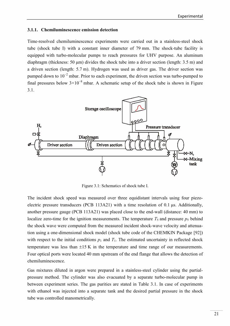
Time-resolved chemiluminescence experiments were carried out in a stainless-steel shock
tube (shock tube I) with a constant inner diameter of 79 mm. The shock-tube facility is
equipped with turbo-molecular pumps to reach pressures for UHV purpose. An aluminum
diaphragm (thickness: 50 μm) divides the shock tube into a driver section (length: 3.5 m) and
a driven section (length: 5.7 m). Hydrogen was used as driver gas. The driver section was
pumped down to 10−2
mbar. Prior to each experiment, the driven section was turbo-pumped to
final pressures below 3×10⁻⁸
mbar. A schematic setup of the shock tube is shown in Figure
3.1.
Figure 3.1: Schematics of shock tube I.
The incident shock speed was measured over three equidistant intervals using four piezo-
electric pressure transducers (PCB 113A21) with a time resolution of 0.1 μs. Additionally,
another pressure gauge (PCB 113A21) was placed close to the end-wall (distance: 40 mm) to
localize zero-time for the ignition measurements. The temperature T5 and pressure p5 behind
the shock wave were computed from the measured incident shock-wave velocity and attenua-
tion using a one-dimensional shock model (shock tube code of the CHEMKIN Package [92])
with respect to the initial conditions p1 and T1. The estimated uncertainty in reflected shock
temperature was less than 15 K in the temperature and time range of our measurements.
Four optical ports were located 40 mm upstream of the end flange that allows the detection of
chemiluminescence.
Gas mixtures diluted in argon were prepared in a stainless-steel cylinder using the partial-
pressure method. The cylinder was also evacuated by a separate turbo-molecular pump in
between experiment series. The gas purities are stated in Table 3.1. In case of experiments
with ethanol was injected into a separate tank and the desired partial pressure in the shock
tube was controlled manometrically.
Shock-tubes for kinetics studies in highly diluted systems
22
Table 3.1: Stated purities of the substances
Substance Purity / %
Argon (Ar) 99.9999
Hydrogen (H2) 99.999
Nitrous oxide (N2O) 99.999
Oxygen (O2) 99.998
Methane (CH4) 99.999
Acetylene (C2H2) 99.6
Ethylene (C2H4) 99.995
Ethanol (C2H5OH) 99.9
Ammonia (NH3) 99.998
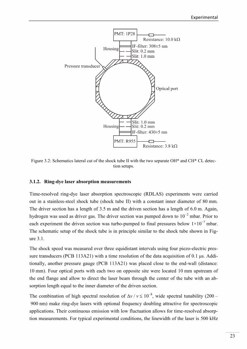
The schematics of the CL detection system for OH* and CH* is illustrated in Figure 3.2.
Measuring chemiluminescence with high temporal resolution requires the limitation of the
detection to a narrow zone within the shock tube. Hence, two vertical slits were placed at 15
and 45 mm in front of each detector to narrow the detection solid angle. Their widths of
0.2 mm and 1 mm, respectively, were selected to provide an optimal balance between signal
strength and time resolution. This setup provided a time resolution of 1 μs as determined from
the light collection angle and the passing velocity of the reflected shock wave. Interference
filters with center wavelengths of OH* = 307 nm and CH* = 430 nm, respectively, (both
10 nm FWHM) limited the emission spectra of OH* and CH* chemiluminescence to the tran-
sitions in the A–X systems. The chemiluminescence radiation was detected by two separate
photomultipliers (OH*: Hamamatsu 1P28, CH*: Hamamatsu R955) with constant amplifica-
tion voltage for all presented measurements. To achieve sufficient time resolution, appropriate
signal intensity and linearity between measured intensity and PMT current, 10 k and 3.8 k
resistors were connected in parallel to the amplifiers for the OH* and CH* detectors, respec-
tively. The time resolution of each setup was investigated for various resistors by investigat-
ing the signal recorded from the input of short square pulses (duration: 1 μs) of an LED. A
compromise between time resolution and signal intensity was chosen with selecting a time
resolution of 2 μs that matched the time resolution of the optical arrangement. Care was taken
not to change the optical configuration during one set of experiments.
Experimental
23
Figure 3.2: Schematics lateral cut of the shock tube II with the two separate OH* and CH* CL detec-
tion setups.
3.1.2. Ring-dye laser absorption measurements
Time-resolved ring-dye laser absorption spectroscopic (RDLAS) experiments were carried
out in a stainless-steel shock tube (shock tube II) with a constant inner diameter of 80 mm.
The driver section has a length of 3.5 m and the driven section has a length of 6.0 m. Again,
hydrogen was used as driver gas. The driver section was pumped down to 10−2
mbar. Prior to
each experiment the driven section was turbo-pumped to final pressures below 1×10⁻⁷
mbar.
The schematic setup of the shock tube is in principle similar to the shock tube shown in Fig-
ure 3.1.
The shock speed was measured over three equidistant intervals using four piezo-electric pres-
sure transducers (PCB 113A21) with a time resolution of the data acquisition of 0.1 μs. Addi-
tionally, another pressure gauge (PCB 113A21) was placed close to the end-wall (distance:
10 mm). Four optical ports with each two on opposite site were located 10 mm upstream of
the end flange and allow to direct the laser beam through the center of the tube with an ab-
sorption length equal to the inner diameter of the driven section.
The combination of high spectral resolution of v / v 10−8
, wide spectral tunability (200 –
900 nm) make ring-dye lasers with optional frequency doubling attractive for spectroscopic
applications. Their continuous emission with low fluctuation allows for time-resolved absorp-
tion measurements. For typical experimental conditions, the linewidth of the laser is 500 kHz
Shock-tubes for kinetics studies in highly diluted systems
24
compared to the molecular transitions (10 MHz). Thus, defined transitions can be probed
without bandwidth effect. The high sensitivity of the differential laser absorption technique
consists of the detection probe and a reference beam allows a fractional absorption of 0.1%
which corresponds to a minimum detectivity less than 1 ppm (e. g. OH). Therefore, highly
diluted mixtures can be used to separate the reaction of interest by eliminating interfering sec-
ondary reactions.
The species concentration can be directly determined from an absorption measurement ac-
cording to the Beer-Lambert law:
][exp0
XlI
I . (3.1)
The concentration of interest [X] is derived from the transmitted intensity I and the reference
intensity I0 simultaneously monitored by the detection system, the absorption path length l
and the absorption coefficient (T, p,
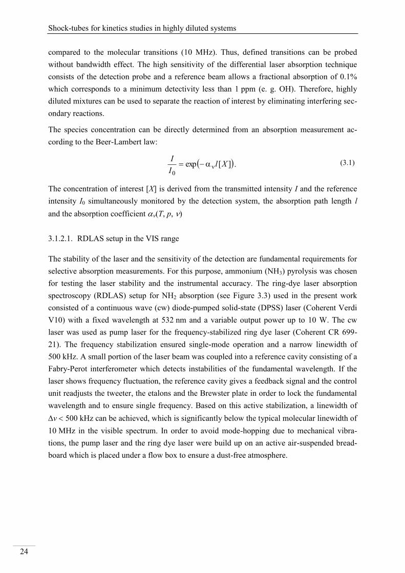
3.1.2.1. RDLAS setup in the VIS range
The stability of the laser and the sensitivity of the detection are fundamental requirements for
selective absorption measurements. For this purpose, ammonium (NH3) pyrolysis was chosen
for testing the laser stability and the instrumental accuracy. The ring-dye laser absorption
spectroscopy (RDLAS) setup for NH2 absorption (see Figure 3.3) used in the present work
consisted of a continuous wave (cw) diode-pumped solid-state (DPSS) laser (Coherent Verdi
V10) with a fixed wavelength at 532 nm and a variable output power up to 10 W. The cw
laser was used as pump laser for the frequency-stabilized ring dye laser (Coherent CR 699-
21). The frequency stabilization ensured single-mode operation and a narrow linewidth of
500 kHz. A small portion of the laser beam was coupled into a reference cavity consisting of a
Fabry-Perot interferometer which detects instabilities of the fundamental wavelength. If the
laser shows frequency fluctuation, the reference cavity gives a feedback signal and the control
unit readjusts the tweeter, the etalons and the Brewster plate in order to lock the fundamental
wavelength and to ensure single frequency. Based on this active stabilization, a linewidth of
v 500 kHz can be achieved, which is significantly below the typical molecular linewidth of
10 MHz in the visible spectrum. In order to avoid mode-hopping due to mechanical vibra-
tions, the pump laser and the ring dye laser were build up on an active air-suspended bread-
board which is placed under a flow box to ensure a dust-free atmosphere.
Experimental
25
DPSS laser:
Coherent Verdi
V10
DPSS laser:
Coherent Verdi
V10 Ring-dye laser:
Coherent 699-21
Ring-dye laser:
Coherent 699-21
= 532 nm
Pcw = 6.5 W
Wavemeter:
Burleigh
WA-20 VIS
Wavemeter:
Burleigh
WA-20 VIS
= 597.375 nm
BS
Al mirror
Quartz lens
(f = 100 mm)
BS
Quartz lens
(f = 100 mm)
Digital storage
oscilloscope
Diode II
Diff.- Amp.
Amp. I
Diode I
Amp. II
IF-filter
Collimator
Fiber
coupler
Fiber
Shock tube
Figure 3.3: Schematics of the RDLAS setup for VIS absorption measurements.
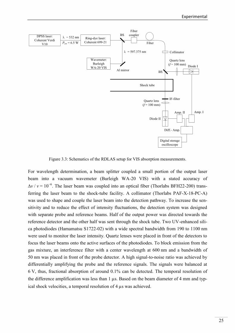
For wavelength determination, a beam splitter coupled a small portion of the output laser
beam into a vacuum wavemeter (Burleigh WA-20 VIS) with a stated accuracy of
v / v = 10−6
. The laser beam was coupled into an optical fiber (Thorlabs BFH22-200) trans-
ferring the laser beam to the shock-tube facility. A collimator (Thorlabs PAF-X-18-PC-A)
was used to shape and couple the laser beam into the detection pathway. To increase the sen-
sitivity and to reduce the effect of intensity fluctuations, the detection system was designed
with separate probe and reference beams. Half of the output power was directed towards the
reference detector and the other half was sent through the shock tube. Two UV-enhanced sili-
ca photodiodes (Hamamatsu S1722-02) with a wide spectral bandwidth from 190 to 1100 nm
were used to monitor the laser intensity. Quartz lenses were placed in front of the detectors to
focus the laser beams onto the active surfaces of the photodiodes. To block emission from the
gas mixture, an interference filter with a center wavelength at 600 nm and a bandwidth of
50 nm was placed in front of the probe detector. A high signal-to-noise ratio was achieved by
differentially amplifying the probe and the reference signals. The signals were balanced at
6 V, thus, fractional absorption of around 0.1% can be detected. The temporal resolution of
the difference amplification was less than 1 s. Based on the beam diameter of 4 mm and typ-
ical shock velocities, a temporal resolution of 4 s was achieved.
Shock-tubes for kinetics studies in highly diluted systems
26
3.1.2.2. Characterization and validation of the RDLAS setup in the VIS range
For the characterization of the RDLAS setup, Ar-diluted NH3 mixtures were shock-heated to
generate defined NH2 concentrations. Colberg [93] and Friedrichs et al. [94] extensively char-
acterized the above-mentioned NH2 transition by means of frequency modulation spectrosco-
py behind shock waves and cavity ring down measurements at room temperature,
respectively. Kohse-Höinghaus et al. [95] quantitatively studied the absorption coefficient of
NH2 by means of photolysis and pyrolysis experiments behind reflected shock waves and
provided temperature-dependent absorption coefficients. Davidson et al. [96] studied NH3
pyrolysis by measuring both NH and NH2 and developed a reaction mechanism for NH3 py-
rolysis. The results of the present work were compared with simulations using the pyrolysis
mechanism documented in [96]. The model consists of 21 reactions incorporating 9 species.
No modifications were done in the reaction set and their corresponding rate coefficients. In
analogy with [95-96], the A2A1X
2B1(090000
P Q1,N(7) transition at 16739.90 cm
−1 was
selected in the present work for quantitative evaluation.
In the present work, NH2 absorption was monitored in shock-heated NH3/argon mixtures. The
absorption of NH2 was recorded by a difference signal which is subsequently converted into
species concentration by fitting the corresponding absorption coefficient with regard to the
NH2 peak concentration. The fitted absorption coefficients were compared with the recom-
mendations for NH2 determined by 3.322×10
10/T
3 + 3.130×10
5/T
2 1.302×10
3/T (T in K)
from [95]. The measured and the simulated data agree within the stated error limits of 30%.
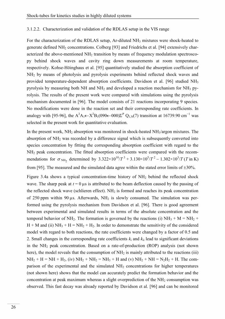
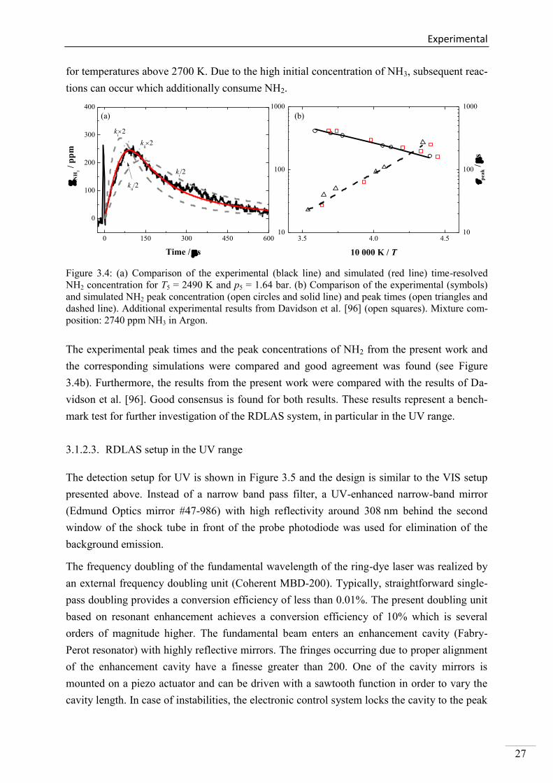
Figure 3.4a shows a typical concentration-time history of NH2 behind the reflected shock
wave. The sharp peak at t = 0 s is attributed to the beam deflection caused by the passing of
the reflected shock wave (schlieren effect). NH2 is formed and reaches its peak concentration
of 250 ppm within 90 s. Afterwards, NH2 is slowly consumed. The simulation was per-
formed using the pyrolysis mechanism from Davidson et al. [96]. There is good agreement
between experimental and simulated results in terms of the absolute concentration and the
temporal behavior of NH2. The formation is governed by the reactions (i) NH3 + M = NH2 +
H + M and (ii) NH3 + H = NH2 + H2. In order to demonstrate the sensitivity of the considered
model with regard to both reactions, the rate coefficients were changed by a factor of 0.5 and
2. Small changes in the corresponding rate coefficients ki and kii lead to significant deviations
in the NH2 peak concentration. Based on a rate-of-production (ROP) analysis (not shown
here), the model reveals that the consumption of NH2 is mainly attributed to the reactions (iii)
NH2 + H = NH + H2, (iv) NH2 + NH2 = NH3 + H and (v) NH2 + NH = N2H2 + H. The com-
parison of the experimental and the simulated NH2 concentrations for higher temperatures
(not shown here) shows that the model can accurately predict the formation behavior and the
concentration at peak maximum whereas a slight overprediction of the NH2 consumption was
observed. This fast decay was already reported by Davidson et al. [96] and can be monitored
Experimental
27
for temperatures above 2700 K. Due to the high initial concentration of NH3, subsequent reac-
tions can occur which additionally consume NH2.
Figure 3.4: (a) Comparison of the experimental (black line) and simulated (red line) time-resolved
NH2 concentration for T5 = 2490 K and p5 = 1.64 bar. (b) Comparison of the experimental (symbols)
and simulated NH2 peak concentration (open circles and solid line) and peak times (open triangles and
dashed line). Additional experimental results from Davidson et al. [96] (open squares). Mixture com-
position: 2740 ppm NH3 in Argon.
The experimental peak times and the peak concentrations of NH2 from the present work and
the corresponding simulations were compared and good agreement was found (see Figure
3.4b). Furthermore, the results from the present work were compared with the results of Da-
vidson et al. [96]. Good consensus is found for both results. These results represent a bench-
mark test for further investigation of the RDLAS system, in particular in the UV range.
3.1.2.3. RDLAS setup in the UV range
The detection setup for UV is shown in Figure 3.5 and the design is similar to the VIS setup
presented above. Instead of a narrow band pass filter, a UV-enhanced narrow-band mirror
(Edmund Optics mirror #47-986) with high reflectivity around 308 nm behind the second
window of the shock tube in front of the probe photodiode was used for elimination of the
background emission.
The frequency doubling of the fundamental wavelength of the ring-dye laser was realized by
an external frequency doubling unit (Coherent MBD-200). Typically, straightforward single-
pass doubling provides a conversion efficiency of less than 0.01%. The present doubling unit
based on resonant enhancement achieves a conversion efficiency of 10% which is several
orders of magnitude higher. The fundamental beam enters an enhancement cavity (Fabry-
Perot resonator) with highly reflective mirrors. The fringes occurring due to proper alignment
of the enhancement cavity have a finesse greater than 200. One of the cavity mirrors is
mounted on a piezo actuator and can be driven with a sawtooth function in order to vary the
cavity length. In case of instabilities, the electronic control system locks the cavity to the peak
0 150 300 450 600
0
100
200
300
400
kii2
kii2
ki2
N
H2
/ p
pm
Time / s
ki/2
3.5 4.0 4.510
100
1000
10 000 K / T
10
100
1000
pea
k /
s
(a) (b)
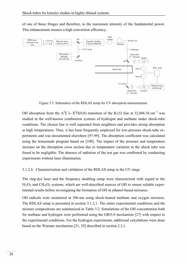
Shock-tubes for kinetics studies in highly diluted systems
28
of one of those fringes and therefore, to the maximum intensity of the fundamental power.
This enhancement ensures a high conversion efficiency.
DPSS laser:
Coherent Verdi
V10
DPSS laser:
Coherent Verdi
V10 Ring-dye laser:
Coherent 699-21
Ring-dye laser:
Coherent 699-21
= 532 nm
Pcw = 7.5 W
Wavemeter:
Burleigh
WA-20 VIS
Wavemeter:
Burleigh
WA-20 VIS
= 613.374 nm
BS
Al mirror
Quartz lens
(f = 100 mm)
BS
Quartz lens
(f = 100 mm)
Digital storage
oscilloscope
Diode II
Diff.- Amp.Amp. I
Diode I
Amp. II
UV-mirror
Collimator
Fiber
coupler
SM-fiber
Shock tube
Frequency doubler:
Coherent MBD200
Frequency doubler:
Coherent MBD200
= 307.687 nm
Figure 3.5: Schematics of the RDLAS setup for UV absorption measurements.
OH absorption from the A2
+X
2(0,0) transition of the R1(5) line at 32,606.56 cm
−1 was
studied in the well-known combustion systems of hydrogen and methane under shock-tube
conditions. The chosen line is well separated from neighbors and provides strong absorption
at high temperatures. Thus, it has been frequently employed for low-pressure shock-tube ex-
periments and was documented elsewhere [97-99]. The absorption coefficient was calculated
using the homemade program based on [100]. The impact of the pressure and temperature
increase on the absorption cross section due to temperature variation in the shock tube was
found to be negligible. The absence of radiation of the test gas was confirmed by conducting
experiments without laser illumination.
3.1.2.4. Characterization and validation of the RDLAS setup in the UV range
The ring-dye laser and the frequency doubling setup were characterized with regard to the
H2/O2 and CH4/O2 systems, which are well-described sources of OH to ensure reliable exper-
imental results before investigating the formation of OH in ethanol-based mixtures.
OH radicals were monitored at 306 nm using shock-heated methane and oxygen mixtures.
The RDLAS setup is presented in section 3.1.2.1. The entire experimental conditions and the
mixture compositions are summarized in Table 3.2. Simulations of the OH concentration both
for methane and hydrogen were performed using the GRI3.0 mechanism [27] with respect to
the experimental conditions. For the hydrogen experiments, additional calculations were done
based on the Warnatz mechanism [21, 29] described in section 2.2.1.
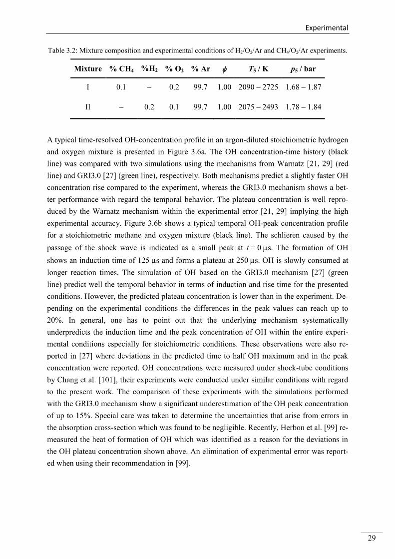
Experimental
29
Table 3.2: Mixture composition and experimental conditions of H2/O2/Ar and CH4/O2/Ar experiments.
Mixture % CH4 %H2 % O2 % Ar T5 / K p5 / bar
I 0.1 – 0.2 99.7 1.00 2090 – 2725 1.68 – 1.87
II – 0.2 0.1 99.7 1.00 2075 – 2493 1.78 – 1.84
A typical time-resolved OH-concentration profile in an argon-diluted stoichiometric hydrogen
and oxygen mixture is presented in Figure 3.6a. The OH concentration-time history (black
line) was compared with two simulations using the mechanisms from Warnatz [21, 29] (red
line) and GRI3.0 [27] (green line), respectively. Both mechanisms predict a slightly faster OH
concentration rise compared to the experiment, whereas the GRI3.0 mechanism shows a bet-
ter performance with regard the temporal behavior. The plateau concentration is well repro-
duced by the Warnatz mechanism within the experimental error [21, 29] implying the high
experimental accuracy. Figure 3.6b shows a typical temporal OH-peak concentration profile
for a stoichiometric methane and oxygen mixture (black line). The schlieren caused by the
passage of the shock wave is indicated as a small peak at t = 0 s. The formation of OH
shows an induction time of 125 s and forms a plateau at 250 s. OH is slowly consumed at
longer reaction times. The simulation of OH based on the GRI3.0 mechanism [27] (green
line) predict well the temporal behavior in terms of induction and rise time for the presented
conditions. However, the predicted plateau concentration is lower than in the experiment. De-
pending on the experimental conditions the differences in the peak values can reach up to
20%. In general, one has to point out that the underlying mechanism systematically
underpredicts the induction time and the peak concentration of OH within the entire experi-
mental conditions especially for stoichiometric conditions. These observations were also re-
ported in [27] where deviations in the predicted time to half OH maximum and in the peak
concentration were reported. OH concentrations were measured under shock-tube conditions
by Chang et al. [101], their experiments were conducted under similar conditions with regard
to the present work. The comparison of these experiments with the simulations performed
with the GRI3.0 mechanism show a significant underestimation of the OH peak concentration
of up to 15%. Special care was taken to determine the uncertainties that arise from errors in
the absorption cross-section which was found to be negligible. Recently, Herbon et al. [99] re-
measured the heat of formation of OH which was identified as a reason for the deviations in
the OH plateau concentration shown above. An elimination of experimental error was report-
ed when using their recommendation in [99].
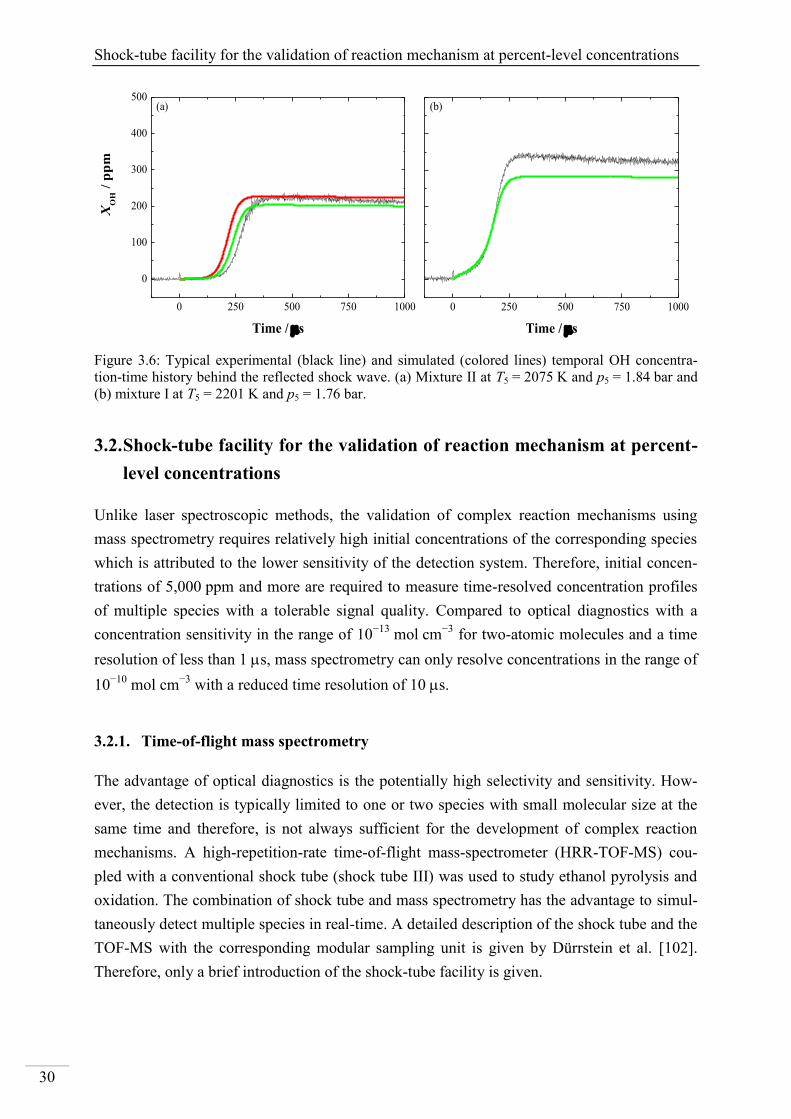
Shock-tube facility for the validation of reaction mechanism at percent-level concentrations
30
Figure 3.6: Typical experimental (black line) and simulated (colored lines) temporal OH concentra-
tion-time history behind the reflected shock wave. (a) Mixture II at T5 = 2075 K and p5 = 1.84 bar and
(b) mixture I at T5 = 2201 K and p5 = 1.76 bar.
3.2. Shock-tube facility for the validation of reaction mechanism at percent-
level concentrations
Unlike laser spectroscopic methods, the validation of complex reaction mechanisms using
mass spectrometry requires relatively high initial concentrations of the corresponding species
which is attributed to the lower sensitivity of the detection system. Therefore, initial concen-
trations of 5,000 ppm and more are required to measure time-resolved concentration profiles
of multiple species with a tolerable signal quality. Compared to optical diagnostics with a
concentration sensitivity in the range of 10−13
mol cm−3
for two-atomic molecules and a time
resolution of less than 1 s, mass spectrometry can only resolve concentrations in the range of
10−10
mol cm−3
with a reduced time resolution of 10 s.
3.2.1. Time-of-flight mass spectrometry
The advantage of optical diagnostics is the potentially high selectivity and sensitivity. How-
ever, the detection is typically limited to one or two species with small molecular size at the
same time and therefore, is not always sufficient for the development of complex reaction
mechanisms. A high-repetition-rate time-of-flight mass-spectrometer (HRR-TOF-MS) cou-
pled with a conventional shock tube (shock tube III) was used to study ethanol pyrolysis and
oxidation. The combination of shock tube and mass spectrometry has the advantage to simul-
taneously detect multiple species in real-time. A detailed description of the shock tube and the
TOF-MS with the corresponding modular sampling unit is given by Dürrstein et al. [102].
Therefore, only a brief introduction of the shock-tube facility is given.
0 250 500 750 1000
0
100
200
300
400
500
XO
H /
pp
m
Time / s
(a)
0 250 500 750 1000
Time / s
(b)
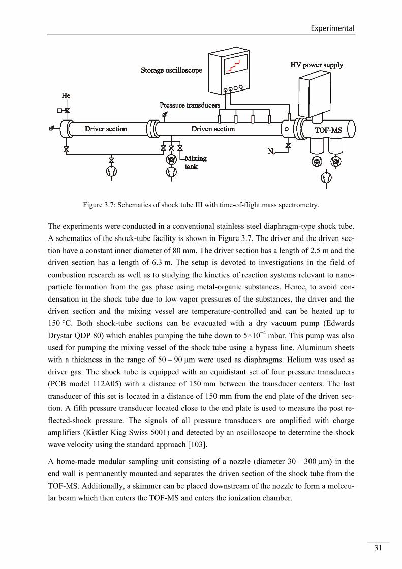
Experimental
31
Figure 3.7: Schematics of shock tube III with time-of-flight mass spectrometry.
The experiments were conducted in a conventional stainless steel diaphragm-type shock tube.
A schematics of the shock-tube facility is shown in Figure 3.7. The driver and the driven sec-
tion have a constant inner diameter of 80 mm. The driver section has a length of 2.5 m and the
driven section has a length of 6.3 m. The setup is devoted to investigations in the field of
combustion research as well as to studying the kinetics of reaction systems relevant to nano-
particle formation from the gas phase using metal-organic substances. Hence, to avoid con-
densation in the shock tube due to low vapor pressures of the substances, the driver and the
driven section and the mixing vessel are temperature-controlled and can be heated up to
150 °C. Both shock-tube sections can be evacuated with a dry vacuum pump (Edwards
Drystar QDP 80) which enables pumping the tube down to 5×10⁻⁴
mbar. This pump was also
used for pumping the mixing vessel of the shock tube using a bypass line. Aluminum sheets
with a thickness in the range of 50 – 90 μm were used as diaphragms. Helium was used as
driver gas. The shock tube is equipped with an equidistant set of four pressure transducers
(PCB model 112A05) with a distance of 150 mm between the transducer centers. The last
transducer of this set is located in a distance of 150 mm from the end plate of the driven sec-
tion. A fifth pressure transducer located close to the end plate is used to measure the post re-
flected-shock pressure. The signals of all pressure transducers are amplified with charge
amplifiers (Kistler Kiag Swiss 5001) and detected by an oscilloscope to determine the shock
wave velocity using the standard approach [103].
A home-made modular sampling unit consisting of a nozzle (diameter 30 – 300 m) in the
end wall is permanently mounted and separates the driven section of the shock tube from the
TOF-MS. Additionally, a skimmer can be placed downstream of the nozzle to form a molecu-
lar beam which then enters the TOF-MS and enters the ionization chamber.
Shock-tube facility for the validation of reaction mechanism at percent-level concentrations
32
For fast kinetics studies, the TOF-MS must be operated at high repetition rates. Therefore, the
HRR-TOF-MS (Kaesdorf) was designed for repetition rates up to 150 kHz by combining a
compact design (short flight distance) with high transmission energies (high flight velocities).
This avoids the overlap of signals caused by ions from consecutive ionization cycles. Typical-
ly, repetition rates of approximately 100 kHz are used and there is no overlap of consecutive
spectra up to masses up to 170 u. The present mass spectrometer is an advantageous com-
pared to the facility described by Tranter et al. [104] that shows overlap of successive spectra
at a repetition rate of 105 kHz. The TOF-MS is equipped with an electron impact ion source
with two-stage ion extraction. A two-stage reflectron compensates for differences in flight
time due to different initial energies of the ions up to a second-order correction of approxi-
mately 8 – 10% of the ensemble mean energy. The energy of the ionizing electrons can be
tuned from 5 to 85 eV. The ionization energy was set to 45 eV to reach a tradeoff between
signal intensities and minimization of fragmentation due to the electron bombardment. It is
possible to ionize under field-free conditions as ionization and extraction can be pulsed inde-
pendently. The maximum kinetics energy of the ions is 10 keV which is high enough to gen-
erate detectable signals for molecular weights up to 1,000 u. The HRR-TOF-MS is equipped
with two micro-channel plate (MCP) detectors: one that is used in the reflectron mode and
one that can be used in the linear TOF-mode. To eliminate the influence of chemically ionized
species from the shock tube, a positively charged lens shields the ion source against the shock
tube.
Results and discussion
33
4. Results and discussion
4.1. Shock-tube measurements of OH* chemiluminescence
The major emission band of OH* chemiluminescence is attributed to the reaction-induced
population of the OH(A) state . Aside from the strong A–X transition at 306 nm, much weak-
er emission from OH(B) and OH(C) states are accessible. However, these bands are very
weak in flames and could not be identified yet. Therefore, all studies consider the strong A–X
transition.
4.1.1. Review of OH* kinetics
Formation of OH* chemiluminescence in hydrogen combustion was first reported by Kaskan
[105] and was widely studied since [49, 106-107]. Several potential reactions in hydrogen
combustion have been suggested to be responsible for OH* formation. Kaskan [105] studied
the UV emission of OH* in rich H2/O2/N2 flames and found a proportionality of OH* with the
cube of the ground-state OH concentration. Based on this finding, he postulated the reactions
H + O + M OH* + M as well as H + OH + OH OH* + H2O to be responsible for OH*
chemiluminescence. Marques et al. [108], amongst others, studied the OH* formation in
spark-ignited C2H2/O2 mixtures in a closed chamber. Based on a comparison of their meas-
ured time-resolved emission profiles with computed normalized concentration profiles, they
suggested H + O2 OH* + O as the main channel forming 90% of the OH*. More recently,
Skrebkov et al. [109] analyzed the OH* formation channel by ab initio calculations and pro-
posed the reaction H2 + HO2 OH* + H2O to be the main OH* formation pathway.
While different reaction pathways of the OH* formation were suggested, early and recent
studies predominantly agree in identifying the three-body reaction (R1) as the main formation
reaction in hydrogen combustion. This was first proposed by Gaydon [48] and Charton and
Gaydon [110]:
H + O + M OH* + M (R1)
Based on flame experiments in various H2/O2/N2 mixtures measuring OH* emission intensi-
ties, Kaskan [105] studied the formation of OH* chemiluminescence and recommended a rate
coefficient for the above-mentioned reaction. Koike and Morinaga [66] provided the rate co-
efficient of reaction (R1) by correlating the emission intensity at various temperatures and
calculated OH* concentrations. Similarly, Hidaka and co-workers [111] identified reaction
(R1) as the main source of OH* from shock-tube experiments with diluted H2/O2/Ar mixtures
and derived a reaction rate coefficient of 1.2×10¹³
exp(−29 kJ mol−1
/RT) cm6mol
−2s−1
. Among
Shock-tube measurements of OH* chemiluminescence
34
recent studies, Smith et al. [112] examined rich hydrogen/air premixed flames. Based on sim-
ulated and experimental OH* number densities, they recommended the rate coefficient of the
reaction (R1) to be 5.5×10¹²
cm6mol
−2s−1
. Petersen and co-workers [113] applied a calibration
procedure to convert measured OH* chemiluminescence intensities into absolute species con-
centrations by relating the measured PMT voltage with the corresponding simulated OH*
concentrations. The OH* kinetics were optimized based on ignition delay times and concen-
tration time histories of OH* chemiluminescence. Later on, Hall and Petersen [78] derived a
rate coefficient for (R1) to be 3.1×10¹⁴
exp(−41.8 kJ mol−1
/RT) cm6mol
−2s−1
based on a
shock-tube study. This was done by fitting the temperature dependence of the OH* peak in-
tensity in various H2/O2 mixtures. In all these studies, the recommended rate coefficient varies
by two orders of magnitude from each other.
While OH* chemiluminescence is weak in hydrogen oxidation, it is strong in hydrocarbon
combustion. OH* chemiluminescence in hydrocarbon combustion has been studied by several
groups [55, 114-116]. There is accordance in the identified key reaction that leads to OH*
emission to be:
CH + O2 OH* + CO (R2)
Some early work on OH* chemiluminescence in hydrocarbon combustion was done by Porter
et al. [114]. Based on the correlation of CH, O2 and OH* profiles in various acetylene and
methane flames, they suggested reaction (R2) to be responsible for the OH* formation and
recommended a rate coefficient k2 = 6.0×10¹⁰
cm3mol
−1s−1
. Grebe and Homann [55] measured
time-resolved OH* concentration profiles in a low-pressure discharge flow system with reac-
tive C2H2/O/H mixtures at room temperature. Based on this study, they derived a rate coeffi-
cient of 4.8×10¹⁰
cm3mol
−1s−1
. More recently, Carl et al. [117] showed that there is a
proportionality between OH* formation and the product of CH and O2 concentrations by mo-
lecular-beam-sampling threshold-ionization mass spectrometry (MB-TIMS). Based on this
observation, they deduced that reaction (R2) is responsible for OH* emission and recom-
mended a rate coefficient of k2 = 4.8×10¹⁰
cm3mol
−1s−1
in a temperature range of 298 and
511 K. Smith et al. [51] measured absolute OH* and CH* concentrations in laminar premixed
CH4/air flames with different equivalence ratios. They calibrated their spatially-resolved and
Abel-inversed images by Rayleigh scattering with respect to computed excited-state species
concentrations and determined a rate coefficient k2 = 1.8×10¹¹
cm3mol
−1s−1
. Hall and Petersen
[78] performed a series of shock-tube experiments with H2/O2 and H2/O2/CH4 mixtures. By
fitting their computed results with regard to their experimental observations, they also identi-
fied reaction (R2) as the main channel with a temperature-dependent value for k2 of
3.2×10¹⁴
T −0.4
exp(−17.4 kJ mol−1
/RT) cm3mol
−1s−1
. Recently, Kathrotia et al. [65] studied
OH* chemiluminescence in premixed low-pressure flames for various methane-based mix-
tures. Based on their flame calculations, they supported reaction (R2) to be responsible for
Results and discussion
35
OH* CL using the rate coefficient from Smith et al. [51]. There is accordance in literature on
the determined k2 to be in the range of 4×10¹⁰
and 1.8×10¹¹
cm3mol
−1s−1
.
OH* is short lived and returns to the ground state via two channels. In the first channel, it
emits its excess energy in the form of light in a radiative decay reaction (R3) OH* OH + hv.
The rate coefficient of this reaction has been proposed by several authors [48, 111, 118]. The
second channel is the non-reactive collisional quenching reaction OH* + M = OH + M (R4).
Here, the excess energy of OH* is transferred to the collision partner M. The effect of various
collision partners has been studied at various temperatures ranging from room temperature to
flame temperature by several authors. Becker et al. [119] provided quenching rate coefficients
for M = H2, H, and Ar at room temperature. Fluorescence excitation by a dye laser was ap-
plied to measure the OH* lifetime in presence of H2, H, and Ar. Fairchild et al. [120] meas-
ured thermally-averaged collisional quenching with H2O, O2, and H2 by laser-induced
fluorescence (LIF) at about 1100 K. OH* quenching with H2O and atomic H was studied by
Jeffries et al. [121] in low-pressure stoichiometric H2/O2/N2O flames also using LIF. Recent-
ly, Bailey et al. [122] investigated the temperature dependence of OH* quenching for colli-
sion partners such as N2 and O2 at room temperature. Hemming et al. [123-124] studied the
influence of N2, O2, and H2 at and below room temperature. Heard and Henderson [125] de-
termined the OH* quenching rate coefficient with H2 at low temperatures (200 – 344 K) in a
flash-photolysis system. All these quenching rate coefficient data are in good agreement with
each other from room to flame temperature. For collision partners such as H, O, and OH, lim-
ited information is available due to the complexity of the measurement. The compilation of
data for major collision partners is given by Tamura et al. [68] and recommendations are
made for the 300 – 2500 K range. Depending on temperature, these coefficients differ by up
to three orders of magnitude.
4.1.2. Strategy of investigating OH* chemiluminescence
In the present study, OH* formation was investigated in various shock-heated hydrogen and
hydrocarbon mixtures. By using a calibration approach, which will be presented in detail in
section 4.1.3, the corresponding OH* production pathway in hydrogen oxidation was identi-
fied and was subsequently applied for the investigation of OH* chemiluminescence in hydro-
carbon combustion systems. A discussion of the results for hydrocarbon combustion will be
given in sections 4.1.4 – 4.1.8.
Due to the well-known hydrogen ground-state chemistry, the present work started with a sys-
tematic investigation of OH* chemiluminescence based on hydrogen oxidation [79]. Estab-
lished mechanisms for hydrogen oxidation (see section 2.2.1) were used. In order to link the
light emission of OH* and the corresponding species concentration, a calibration approach
was derived based on thermal excitation of ground-state OH radicals at high temperatures
Shock-tube measurements of OH* chemiluminescence
36
(around 3000 K). The determined calibration factor was then transferred to describe the chem-
ical activation via (R2). In this manner, a model-based calibration procedure was developed to
quantify the OH* concentrations and measure the rate coefficient of the underlying reaction.
Based on the calibration approach, the OH* formation reaction in hydrocarbon oxidation was
characterized. Due to the increasing complexity of hydrocarbon combustion with increasing
chain length, OH* chemiluminescence was initially studied in methane systems. Akin to hy-
drogen combustion, the oxidation of CH4 is well-known and has been extensively studied in
the past. The ground-state chemistry is accurately modeled using the GRI3.0 mechanism (see
section 2.2.2) which was widely validated. For this purpose, the OH* kinetics model adopted
from the hydrogen study was extended for the oxidation of methane. Subsequently, the OH*
model was validated with regard to more complex hydrocarbons (C2H2, C2H4 and C2H5OH).
In order to extend the validation database of the OH* sub-mechanism from the present work,
the model was compared to flame calculations from literature. For this purpose, additional
simulations were done according to recent studies dealing with OH* formation in various
premixed flames [51, 63, 65].
4.1.3. OH* chemiluminescence in H2/O2/Ar systems
Four series of shock-tube experiments with various hydrogen mixtures were conducted. OH*
chemiluminescence was observed in a wide temperature range around atmospheric pressures
(see Table 4.1). Because the measured OH* intensities cannot be directly related to the corre-
sponding species concentrations, a high-temperature calibration approach was derived for the
conversion of the signal into absolute concentrations. Based on this approach, the chemical
excitation pathway for temperatures below 2800 K was studied by combining the shock-tube
data with numerical modeling.
Table 4.1: Mixture compositions, temperature and pressure ranges of the shock-tube experiments.
Mixture Composition T5 / K p5 / bar
A 0.5 1% H2 + 1% O2 in Ar 1400 – 3300 0.85 – 1.50
B 1.0 2% H2 + 1% O2 in Ar 1440 – 3180 0.90 – 1.40
C 0.5 1% H2 + 1% O2 + 5% N2 in Ar 1400 – 3200 0.90 – 1.40
D 1.0 2% H2 + 1% O2 + 5% N2 in Ar 1450 – 3200 0.90 – 1.45
Thermal excitation of ground-state OH radicals was early reported in [66, 111]. Furthermore,
in a recent opposed flow methane oxy-flame De Leo and co-workers [67] attributed more than
35% of the OH* formation in the thermal equilibrium due to the high temperatures that went
up to 3000 K. For calibration purpose, three important aspects have to be clarified before rely-
Results and discussion
37
ing on this strategy. (i) The approach of using thermal excitation of ground-state OH mole-
cules in order to generate defined OH* concentrations and correlating them with the corre-
sponding light emission requires an accurate prediction of the absolute OH concentration at
the present experimental conditions. (ii) Additional reactions (for example collisional induced
decomposition of OH*) must have a negligible effect. (iii) It must be clarified that the meas-
ured peak intensity does not suffer from insufficient temporal resolution of the detectors (thus,
reduced sensitivity due to the convolution with the signal transfer function). (iv) The influ-
ence of emission trapping due to ground-state OH must be considered and estimated.
(i) The underlying ground-state mechanism was used to predict the thermal excitation of
OH towards OH*. Thus, the OH* concentration depends directly on the computed OH
concentrations. In order to relate experimental and simulated absolute OH concentra-
tions at elevated temperatures, additional RDLAS experiments in a stoichiometric
H2/O2/Ar mixture were performed and the agreement of measured and computed OH
concentration was demonstrated (accuracy 3%) in section 3.1.2.4. Thus, the predicted
OH* concentrations depend mainly on the accuracy of the excitation reactions (–R4)
OH + M = OH* + M which are stated with an error up to 15% [68].
(ii) Figure 4.1 exemplarily shows the normalized sensitivity analysis of OH* formation at
3000 K for mixture A. For temperatures above 2800 K, the OH* formation is over-
whelmed by thermal excitation via the reverse reaction (–R4) OH* + M OH + M
whereas the contribution of chemical excitation (R1) is found to be negligible. A reac-
tion flow analysis revealed that the contribution of OH* formation is attributed to the
collisions with M = H2O (37%) + OH (23%) + Ar (16%) + O2 (10%) + H2 (5%) +
H (4%). In comparison, the reverse of the chemical excitation reaction (–R1) contrib-
utes about to 5% to the OH* peak concentration only. Therefore, one can neglect the
contribution of reaction (–R1) at our calibration conditions.
(iii) The time resolution of the experiment is on one hand determined by the passage of the
shock wave associated with the observed solid angle and on the other hand to the elec-
tronic responses of the PMT system. Both values are in the range of 1 s which is
short enough to be considered as not influencing the signal traces.
(iv) Signal emitted from OH* chemiluminescence detected at 307 nm is partially trapped
by ground-state OH which is homogenously present in the reaction mixture. A simple
analytical approach was used to quantify signal trapping for the experimental condi-
tions that accounts for the homogeneous luminous and homogeneously absorbing gas
mixture within the shock tube for all the mixtures used in this study. To quantify sig-
nal trapping two OH lines R1(7) and R1(11) for the R-branch bandhead of the OH A–X
(0,0) band were investigated. For both lines, the peak maximum leads to a reduction in
the detected OH* signal by 10%. For all measured conditions the calculated attenua-
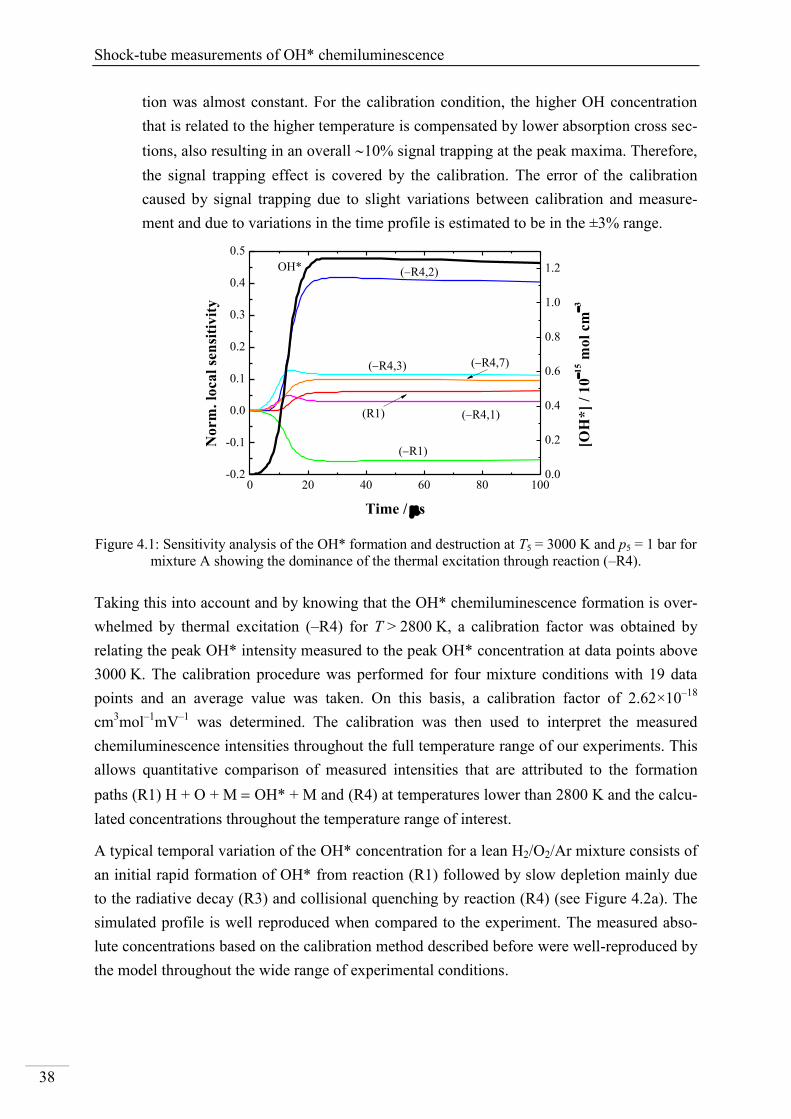
Shock-tube measurements of OH* chemiluminescence
38
tion was almost constant. For the calibration condition, the higher OH concentration
that is related to the higher temperature is compensated by lower absorption cross sec-
tions, also resulting in an overall 10% signal trapping at the peak maxima. Therefore,
the signal trapping effect is covered by the calibration. The error of the calibration
caused by signal trapping due to slight variations between calibration and measure-
ment and due to variations in the time profile is estimated to be in the ±3% range.
0 20 40 60 80 100-0.2
-0.1
0.0
0.1
0.2
0.3
0.4
0.5
0.0
0.2
0.4
0.6
0.8
1.0
1.2
No
rm
. lo
ca
l se
nsi
tiv
ity
Time / s
(R1)
(R4,1)(R1)
(R4,7)(R4,3)
(R4,2)
[OH
*]
/ 1
0
15 m
ol
cm
3
OH*
Figure 4.1: Sensitivity analysis of the OH* formation and destruction at T5 = 3000 K and p5 = 1 bar for
mixture A showing the dominance of the thermal excitation through reaction (–R4).
Taking this into account and by knowing that the OH* chemiluminescence formation is over-
whelmed by thermal excitation (–R4) for T > 2800 K, a calibration factor was obtained by
relating the peak OH* intensity measured to the peak OH* concentration at data points above
3000 K. The calibration procedure was performed for four mixture conditions with 19 data
points and an average value was taken. On this basis, a calibration factor of 2.62×10⁻¹⁸
cm3mol
–1mV
–1 was determined. The calibration was then used to interpret the measured
chemiluminescence intensities throughout the full temperature range of our experiments. This
allows quantitative comparison of measured intensities that are attributed to the formation
paths (R1) H + O + M OH* + M and (R4) at temperatures lower than 2800 K and the calcu-
lated concentrations throughout the temperature range of interest.
A typical temporal variation of the OH* concentration for a lean H2/O2/Ar mixture consists of
an initial rapid formation of OH* from reaction (R1) followed by slow depletion mainly due
to the radiative decay (R3) and collisional quenching by reaction (R4) (see Figure 4.2a). The
simulated profile is well reproduced when compared to the experiment. The measured abso-
lute concentrations based on the calibration method described before were well-reproduced by
the model throughout the wide range of experimental conditions.
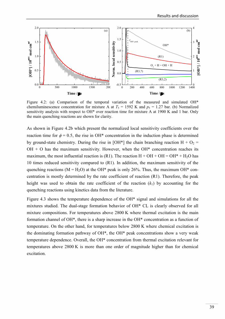
Results and discussion
39
Figure 4.2: (a) Comparison of the temporal variation of the measured and simulated OH*
chemiluminescence concentration for mixture A at T5 = 1592 K and p5 = 1.27 bar. (b) Normalized
sensitivity analysis with respect to OH* over reaction time for mixture A at 1900 K and 1 bar. Only
the main quenching reactions are shown for clarity.
As shown in Figure 4.2b which present the normalized local sensitivity coefficients over the
reaction time for = 0.5, the rise in OH* concentration in the induction phase is determined
by ground-state chemistry. During the rise in [OH*] the chain branching reaction H + O2 =
OH + O has the maximum sensitivity. However, when the OH* concentration reaches its
maximum, the most influential reaction is (R1). The reaction H + OH + OH = OH* + H2O has
10 times reduced sensitivity compared to (R1). In addition, the maximum sensitivity of the
quenching reactions (M = H2O) at the OH* peak is only 26%. Thus, the maximum OH* con-
centration is mostly determined by the rate coefficient of reaction (R1). Therefore, the peak
height was used to obtain the rate coefficient of the reaction (k1) by accounting for the
quenching reactions using kinetics data from the literature.
Figure 4.3 shows the temperature dependence of the OH* signal and simulations for all the
mixtures studied. The dual-stage formation behavior of OH* CL is clearly observed for all
mixture compositions. For temperatures above 2800 K where thermal excitation is the main
formation channel of OH*, there is a sharp increase in the OH* concentration as a function of
temperature. On the other hand, for temperatures below 2800 K where chemical excitation is
the dominating formation pathway of OH*, the OH* peak concentrations show a very weak
temperature dependence. Overall, the OH* concentration from thermal excitation relevant for
temperatures above 2800 K is more than one order of magnitude higher than for chemical
excitation.
0 200 400 600 800 1000 1200 1400-0.5
0.0
0.5
1.0
1.5
2.0
0
1
2
3
4
O2 + H = OH + H
(R3,7)
(R3,2)
(R1)
tOH*, peak
[OH
*]
/ 1
0
16 m
ol
cm
3
No
rm
. lo
ca
l se
nsi
tiv
ity
Time / s
OH*
(b)
0 500 1000 1500 20000.0
0.5
1.0
1.5
2.0
[OH
*]
/ 1
0
16 m
ol
cm
3
Time / s
(a)
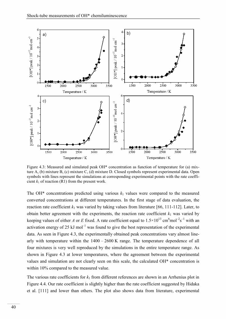
Shock-tube measurements of OH* chemiluminescence
40
Figure 4.3: Measured and simulated peak OH* concentration as function of temperature for (a) mix-
ture A, (b) mixture B, (c) mixture C, (d) mixture D. Closed symbols represent experimental data. Open
symbols with lines represent the simulations at corresponding experimental points with the rate coeffi-
cient k1 of reaction (R1) from the present work.
The OH* concentrations predicted using various k1 values were compared to the measured
converted concentrations at different temperatures. In the first stage of data evaluation, the
reaction rate coefficient k1 was varied by taking values from literature [66, 111-112]. Later, to
obtain better agreement with the experiments, the reaction rate coefficient k1 was varied by
keeping values of either A or E fixed. A rate coefficient equal to 1.5×10¹³
cm6mol
–2s–1
with an
activation energy of 25 kJ mol–1
was found to give the best representation of the experimental
data. As seen in Figure 4.3, the experimentally obtained peak concentrations vary almost line-
arly with temperature within the 1400 – 2600 K range. The temperature dependence of all
four mixtures is very well reproduced by the simulations in the entire temperature range. As
shown in Figure 4.3 at lower temperatures, where the agreement between the experimental
values and simulation are not clearly seen on this scale, the calculated OH* concentration is
within 10% compared to the measured value.
The various rate coefficients for k1 from different references are shown in an Arrhenius plot in
Figure 4.4. Our rate coefficient is slightly higher than the rate coefficient suggested by Hidaka
et al. [111] and lower than others. The plot also shows data from literature, experimental
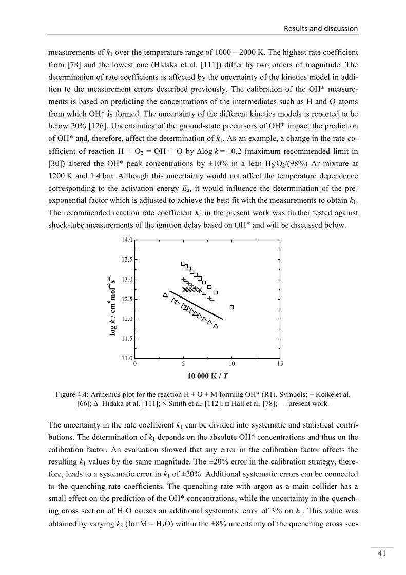
Results and discussion
41
measurements of k1 over the temperature range of 1000 – 2000 K. The highest rate coefficient
from [78] and the lowest one (Hidaka et al. [111]) differ by two orders of magnitude. The
determination of rate coefficients is affected by the uncertainty of the kinetics model in addi-
tion to the measurement errors described previously. The calibration of the OH* measure-
ments is based on predicting the concentrations of the intermediates such as H and O atoms
from which OH* is formed. The uncertainty of the different kinetics models is reported to be
below 20% [126]. Uncertainties of the ground-state precursors of OH* impact the prediction
of OH* and, therefore, affect the determination of k1. As an example, a change in the rate co-
efficient of reaction H + O2 = OH + O by log k = ±0.2 (maximum recommended limit in
[30]) altered the OH* peak concentrations by ±10% in a lean H2/O2/(98%) Ar mixture at
1200 K and 1.4 bar. Although this uncertainty would not affect the temperature dependence
corresponding to the activation energy Ea, it would influence the determination of the pre-
exponential factor which is adjusted to achieve the best fit with the measurements to obtain k1.
The recommended reaction rate coefficient k1 in the present work was further tested against
shock-tube measurements of the ignition delay based on OH* and will be discussed below.
0 5 10 1511.0
11.5
12.0
12.5
13.0
13.5
14.0
log
k /
cm
6m
ol
2s
1
10 000 K / T
Figure 4.4: Arrhenius plot for the reaction H + O + M forming OH* (R1). Symbols: + Koike et al.
[66]; Hidaka et al. [111]; × Smith et al. [112]; □ Hall et al. [78]; — present work.
The uncertainty in the rate coefficient k1 can be divided into systematic and statistical contri-
butions. The determination of k1 depends on the absolute OH* concentrations and thus on the
calibration factor. An evaluation showed that any error in the calibration factor affects the
resulting k1 values by the same magnitude. The ±20% error in the calibration strategy, there-
fore, leads to a systematic error in k1 of ±20%. Additional systematic errors can be connected
to the quenching rate coefficients. The quenching rate with argon as a main collider has a
small effect on the prediction of the OH* concentrations, while the uncertainty in the quench-
ing cross section of H2O causes an additional systematic error of 3% on k1. This value was
obtained by varying k3 (for M = H2O) within the 8% uncertainty of the quenching cross sec-
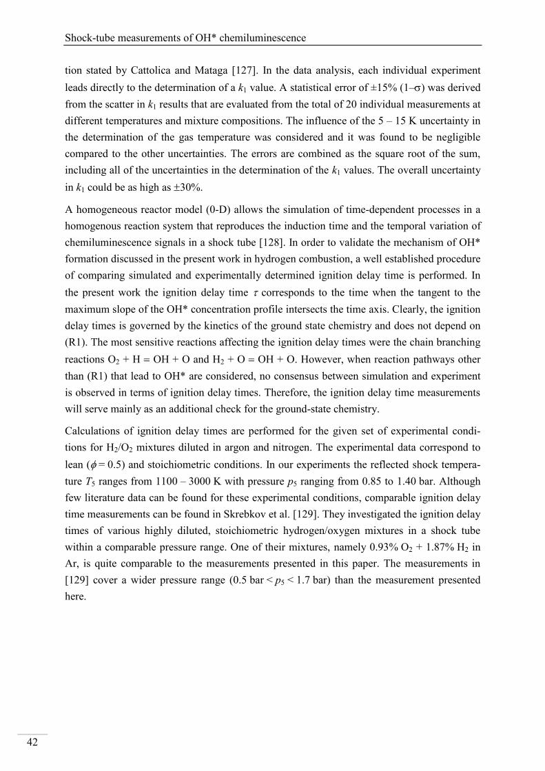
Shock-tube measurements of OH* chemiluminescence
42
tion stated by Cattolica and Mataga [127]. In the data analysis, each individual experiment
leads directly to the determination of a k1 value. A statistical error of ±15% (1–) was derived
from the scatter in k1 results that are evaluated from the total of 20 individual measurements at
different temperatures and mixture compositions. The influence of the 5 – 15 K uncertainty in
the determination of the gas temperature was considered and it was found to be negligible
compared to the other uncertainties. The errors are combined as the square root of the sum,
including all of the uncertainties in the determination of the k1 values. The overall uncertainty
in k1 could be as high as 30%.
A homogeneous reactor model (0-D) allows the simulation of time-dependent processes in a
homogenous reaction system that reproduces the induction time and the temporal variation of
chemiluminescence signals in a shock tube [128]. In order to validate the mechanism of OH*
formation discussed in the present work in hydrogen combustion, a well established procedure
of comparing simulated and experimentally determined ignition delay time is performed. In
the present work the ignition delay time corresponds to the time when the tangent to the
maximum slope of the OH* concentration profile intersects the time axis. Clearly, the ignition
delay times is governed by the kinetics of the ground state chemistry and does not depend on
(R1). The most sensitive reactions affecting the ignition delay times were the chain branching
reactions O2 + H OH + O and H2 + O OH + O. However, when reaction pathways other
than (R1) that lead to OH* are considered, no consensus between simulation and experiment
is observed in terms of ignition delay times. Therefore, the ignition delay time measurements
will serve mainly as an additional check for the ground-state chemistry.
Calculations of ignition delay times are performed for the given set of experimental condi-
tions for H2/O2 mixtures diluted in argon and nitrogen. The experimental data correspond to
lean ( = 0.5) and stoichiometric conditions. In our experiments the reflected shock tempera-
ture T5 ranges from 1100 – 3000 K with pressure p5 ranging from 0.85 to 1.40 bar. Although
few literature data can be found for these experimental conditions, comparable ignition delay
time measurements can be found in Skrebkov et al. [129]. They investigated the ignition delay
times of various highly diluted, stoichiometric hydrogen/oxygen mixtures in a shock tube
within a comparable pressure range. One of their mixtures, namely 0.93% O2 + 1.87% H2 in
Ar, is quite comparable to the measurements presented in this paper. The measurements in
[129] cover a wider pressure range (0.5 bar < p5 < 1.7 bar) than the measurement presented
here.
Results and discussion
43
Figure 4.5 shows the comparison of simulated and experimental ignition delay times at the
above-mentioned conditions. The simulated ignition times are in very good agreement with
the measurements at corresponding conditions. The ignition delay times obtained from Ar-
diluted and Ar + N2-diluted mixtures are very close to each other. The activation energy of the
experimental and simulated data matches very well.
Figure 4.5: Ignition delay time with respect to [OH*] for stoichiometric and lean H2/O2 mixtures with
(a) Ar dilution and (b) Ar + N2 dilution. Symbols: shock-tube experiments from the present work,
lines: simulations for the experimental conditions [79].
As discussed earlier, the peak concentrations of OH* are a function of the OH* formation
reaction (R1) whereas the ignition delay time depends on the ground state chemistry. It is then
assumed that the selection of the rate coefficient of reaction (R1) has no influence on the cal-
culation of ignition delay. However, we have observed that the choice of the formation reac-
tion of OH*, other than (R1), may result in differences between the simulated [OH*]
compared to the OH* signal variation that is used to derive . For example, formation of OH*
from reaction H2 + HO2 OH* + H2O [109] was discussed earlier in this thesis. We incorpo-
rated this reaction in the mechanism along with reaction (R1). Figure 4.6a shows the OH*
concentration profile with and without the above mentioned reaction incorporated in the cal-
culation along with the reaction (R1) at three different temperatures for = 0.5. Implementing
reaction H2 + HO2 = OH* + H2O with reaction (R1) in the OH* sub-scheme forms a dual
peak in the OH* profile. The first peak results from the reaction H2 + HO2 = OH* + H2O and
the second peak is caused by reaction (R1). OH* resulting from reaction H2 + HO2 OH* +
H2O is formed in the induction phase where H2 and HO2 concentrations are high. At tempera-
tures below 1600 K, the recombination reaction (R1) is dominant. However, the first peak is
prominent at temperatures above 1600 K which is also true at stoichiometric and fuel-rich
conditions. With the reaction H2 + HO2 = OH* + H2O included in the mechanism (shown in
Figure 4.6b), above 1600 K the simulated ignition delay times (obtained at the first rise in
OH* profile) were much shorter than the measured ones. In [130] dual peaks in the measured
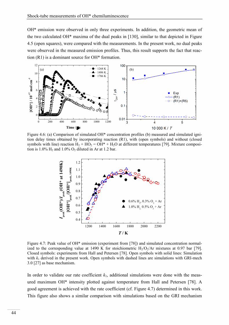
Shock-tube measurements of OH* chemiluminescence
44
OH* emission were observed in only three experiments. In addition, the geometric mean of
the two calculated OH* maxima of the dual peaks in [130], similar to that depicted in Figure
4.5 (open squares), were compared with the measurements. In the present work, no dual peaks
were observed in the measured emission profiles. Thus, this result supports the fact that reac-
tion (R1) is a dominant source for OH* formation.
0 200 400 600 800 1000 1200
0
2
4
6
8
10
12
1268 K
1406 K
1786 K
[OH
*]
/ 1
0-1
7 m
ol
cm
-3
Time / s
Figure 4.6: (a) Comparison of simulated OH* concentration profiles (b) measured and simulated igni-
tion delay times obtained by incorporating reaction (R1), with (open symbols) and without (closed
symbols with line) reaction H2 + HO2 = OH* + H2O at different temperatures [79]. Mixture composi-
tion is 1.0% H2 and 1.0% O2 diluted in Ar at 1.2 bar.
1200 1400 1600 1800 2000 2200
0.4
0.5
0.6
0.7
0.8
0.9
1.0
1.1
1.2
0.6% H2, 0.3% O
2 + Ar
1.0% H2, 0.5% O
2 + Ar
I pea
k(O
H*
)/I p
ea
k(O
H*
at
14
90
K)
[OH
*] p
ea
k/[
OH
*] p
ea
k,
14
90
K
T / K
Figure 4.7: Peak value of OH* emission (experiment from [78]) and simulated concentration normal-
ized to the corresponding value at 1490 K for stoichiometric H2/O2/Ar mixtures at 0.97 bar [79].
Closed symbols: experiments from Hall and Petersen [78]. Open symbols with solid lines: Simulation
with k1 derived in the present work. Open symbols with dashed lines are simulations with GRI-mech
3.0 [27] as base mechanism.
In order to validate our rate coefficient k1, additional simulations were done with the meas-
ured maximum OH* intensity plotted against temperature from Hall and Petersen [78]. A
good agreement is achieved with the rate coefficient (cf. Figure 4.7) determined in this work.
This figure also shows a similar comparison with simulations based on the GRI mechanism
(a) (b)
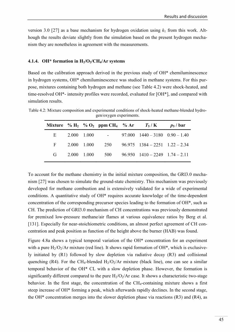
Results and discussion
45
version 3.0 [27] as a base mechanism for hydrogen oxidation using k1 from this work. Alt-
hough the results deviate slightly from the simulation based on the present hydrogen mecha-
nism they are nonetheless in agreement with the measurements.
4.1.4. OH* formation in H2/O2/CH4/Ar systems
Based on the calibration approach derived in the previous study of OH* chemiluminescence
in hydrogen systems, OH* chemiluminescence was studied in methane systems. For this pur-
pose, mixtures containing both hydrogen and methane (see Table 4.2) were shock-heated, and
time-resolved OH*- intensity profiles were recorded, evaluated for [OH*], and compared with
simulation results.
Table 4.2: Mixture composition and experimental conditions of shock-heated methane-blended hydro-
gen/oxygen experiments.
Mixture % H2 % O2 ppm CH4 % Ar T5 / K p5 / bar
E 2.000 1.000 - 97.000 1440 – 3180 0.90 – 1.40
F 2.000 1.000 250 96.975 1384 2251 1.22 – 2.34
G 2.000 1.000 500 96.950 1410 2249 1.74 – 2.11
To account for the methane chemistry in the initial mixture composition, the GRI3.0 mecha-
nism [27] was chosen to simulate the ground-state chemistry. This mechanism was previously
developed for methane combustion and is extensively validated for a wide of experimental
conditions. A quantitative study of OH* requires accurate knowledge of the time-dependent
concentration of the corresponding precursor species leading to the formation of OH*, such as
CH. The prediction of GRI3.0 mechanism of CH concentrations was previously demonstrated
for premixed low-pressure methane/air flames at various equivalence ratios by Berg et al.
[131]. Especially for near-stoichiometric conditions, an almost perfect agreement of CH con-
centration and peak position as function of the height above the burner (HAB) was found.
Figure 4.8a shows a typical temporal variation of the OH* concentration for an experiment
with a pure H2/O2/Ar mixture (red line). It shows rapid formation of OH*, which is exclusive-
ly initiated by (R1) followed by slow depletion via radiative decay (R3) and collisional
quenching (R4). For the CH4-blended H2/O2/Ar mixture (black line), one can see a similar
temporal behavior of the OH* CL with a slow depletion phase. However, the formation is
significantly different compared to the pure H2/O2/Ar case. It shows a characteristic two-stage
behavior. In the first stage, the concentration of the CH4-containing mixture shows a first
steep increase of OH* forming a peak, which afterwards rapidly declines. In the second stage,
the OH* concentration merges into the slower depletion phase via reactions (R3) and (R4), as
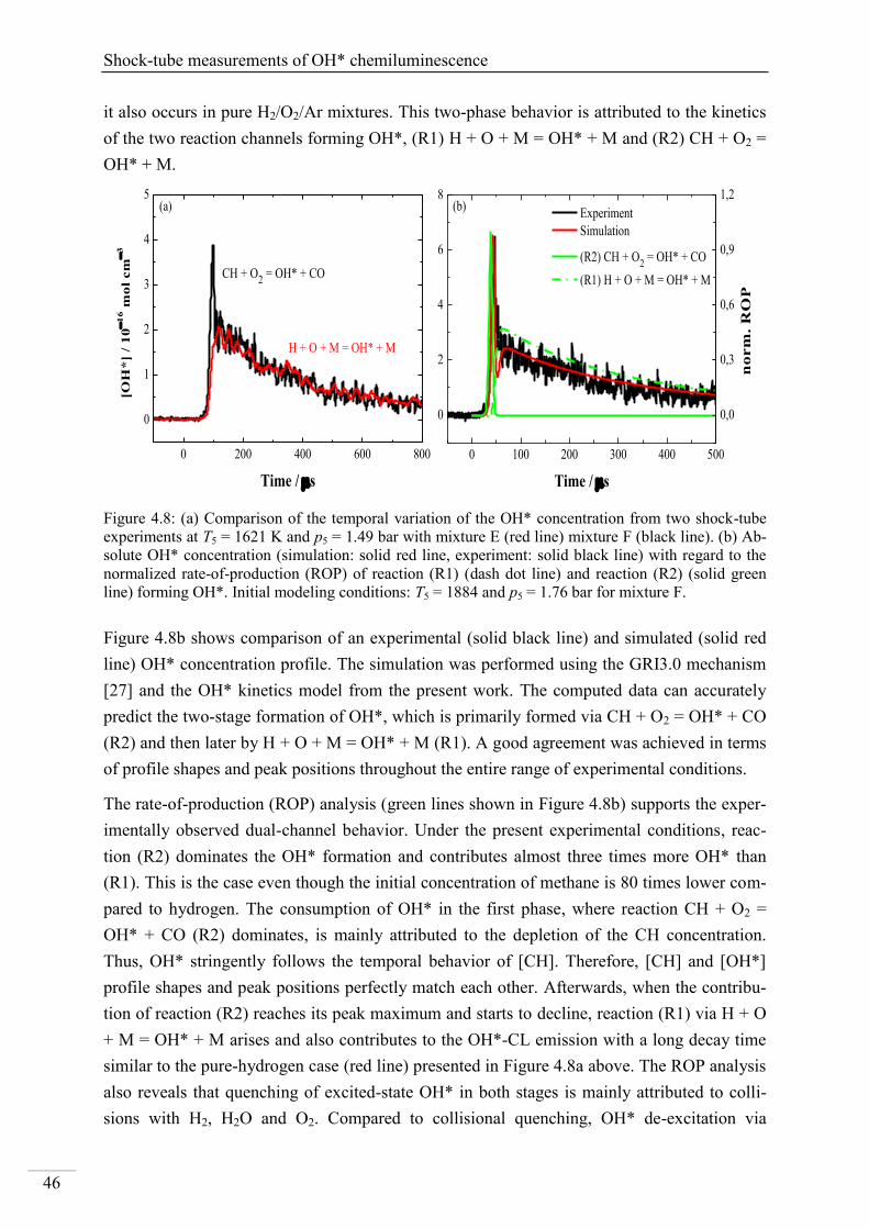
Shock-tube measurements of OH* chemiluminescence
46
it also occurs in pure H2/O2/Ar mixtures. This two-phase behavior is attributed to the kinetics
of the two reaction channels forming OH*, (R1) H + O + M = OH* + M and (R2) CH + O2 =
OH* + M.
Figure 4.8: (a) Comparison of the temporal variation of the OH* concentration from two shock-tube
experiments at T5 = 1621 K and p5 = 1.49 bar with mixture E (red line) mixture F (black line). (b) Ab-
solute OH* concentration (simulation: solid red line, experiment: solid black line) with regard to the
normalized rate-of-production (ROP) of reaction (R1) (dash dot line) and reaction (R2) (solid green
line) forming OH*. Initial modeling conditions: T5 = 1884 and p5 = 1.76 bar for mixture F.
Figure 4.8b shows comparison of an experimental (solid black line) and simulated (solid red
line) OH* concentration profile. The simulation was performed using the GRI3.0 mechanism
[27] and the OH* kinetics model from the present work. The computed data can accurately
predict the two-stage formation of OH*, which is primarily formed via CH + O2 = OH* + CO
(R2) and then later by H + O + M = OH* + M (R1). A good agreement was achieved in terms
of profile shapes and peak positions throughout the entire range of experimental conditions.
The rate-of-production (ROP) analysis (green lines shown in Figure 4.8b) supports the exper-
imentally observed dual-channel behavior. Under the present experimental conditions, reac-
tion (R2) dominates the OH* formation and contributes almost three times more OH* than
(R1). This is the case even though the initial concentration of methane is 80 times lower com-
pared to hydrogen. The consumption of OH* in the first phase, where reaction CH + O2 =
OH* + CO (R2) dominates, is mainly attributed to the depletion of the CH concentration.
Thus, OH* stringently follows the temporal behavior of [CH]. Therefore, [CH] and [OH*]
profile shapes and peak positions perfectly match each other. Afterwards, when the contribu-
tion of reaction (R2) reaches its peak maximum and starts to decline, reaction (R1) via H + O
+ M = OH* + M arises and also contributes to the OH*-CL emission with a long decay time
similar to the pure-hydrogen case (red line) presented in Figure 4.8a above. The ROP analysis
also reveals that quenching of excited-state OH* in both stages is mainly attributed to colli-
sions with H2, H2O and O2. Compared to collisional quenching, OH* de-excitation via
0 200 400 600 800
0
1
2
3
4
5
CH + O2 = OH* + CO
[OH
*]
/ 1
0
16 m
ol
cm
3
Time / s
H + O + M = OH* + M
(a)
0 100 200 300 400 500
0
2
4
6
8
Time / s
Experiment
Simulation
(b)
0,0
0,3
0,6
0,9
1,2
(R2) CH + O2 = OH* + CO
(R1) H + O + M = OH* + M
no
rm
. R
OP
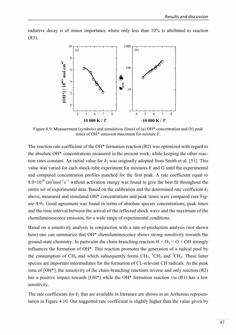
Results and discussion
47
radiative decay is of minor importance where only less than 10% is attributed to reaction
(R3).
4 5 6 7 8
0
2
4
6
8
10(b)
[OH
*]
/ 1
0
16 m
ol
cm
3
10 000 K / T
(a)
4 5 6 7 81
10
100
1000
pea
k /
s
10 000 K / T
Figure 4.9: Measurement (symbols) and simulation (lines) of (a) OH* concentration and (b) peak
times of OH* emission maximum for mixture F.
The reaction rate coefficient of the OH* formation reaction (R2) was optimized with regard to
the absolute OH* concentrations measured in the present work, while keeping the other reac-
tion rates constant. An initial value for k2 was originally adopted from Smith et al. [51]. This
value was varied for each shock-tube experiment for mixtures F and G until the experimental
and computed concentration profiles matched for the first peak. A rate coefficient equal to
8.0×10¹⁰
cm3mol
–1s–1
without activation energy was found to give the best fit throughout the
entire set of experimental data. Based on the calibration and the determined rate coefficient k2
above, measured and simulated OH* concentrations and peak times were compared (see Fig-
ure 4.9). Good agreement was found in terms of absolute species concentrations, peak times
and the time interval between the arrival of the reflected shock wave and the maximum of the
chemiluminescence emission, for a wide range of experimental conditions.
Based on a sensitivity analysis in conjunction with a rate-of-production analysis (not shown
here) one can summarize that OH* chemiluminescence shows strong sensitivity towards the
ground-state chemistry. In particular the chain-branching reaction H + O2 = O + OH strongly
influences the formation of OH*. This reaction promotes the generation of a radical pool by
the consumption of CH4 and which subsequently forms CH3, 1CH2 and
3CH2. These latter
species are important intermediates for the formation of CL-relevant CH radicals. At the peak
time of [OH*], the sensitivity of the chain-branching reactions reverse and only reaction (R2)
has a positive impact towards [OH*] while the OH* formation reaction via (R1) has a low
sensitivity.
The rate coefficients for k2 that are available in literature are shown in an Arrhenius represen-
tation in Figure 4.10. Our suggested rate coefficient is slightly higher than the value given by
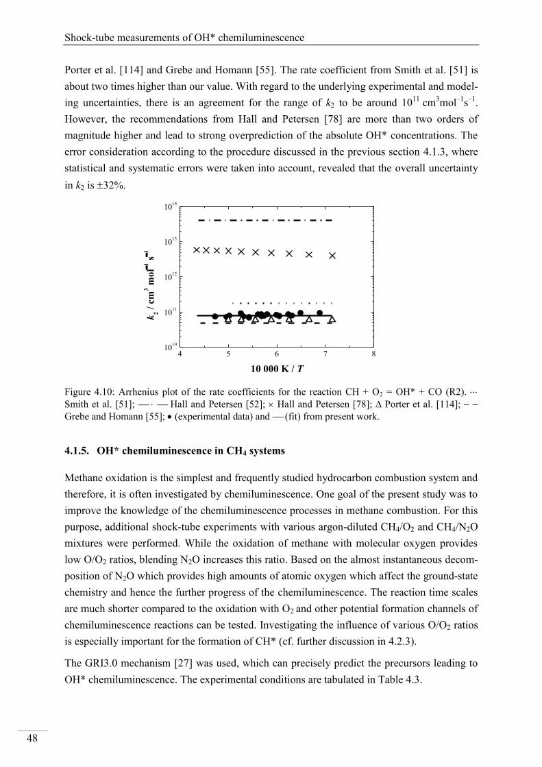
Shock-tube measurements of OH* chemiluminescence
48
Porter et al. [114] and Grebe and Homann [55]. The rate coefficient from Smith et al. [51] is
about two times higher than our value. With regard to the underlying experimental and model-
ing uncertainties, there is an agreement for the range of k2 to be around 1011
cm3mol
–1s–1
.
However, the recommendations from Hall and Petersen [78] are more than two orders of
magnitude higher and lead to strong overprediction of the absolute OH* concentrations. The
error consideration according to the procedure discussed in the previous section 4.1.3, where
statistical and systematic errors were taken into account, revealed that the overall uncertainty
in k2 is 32%.
4 5 6 7 810
10
1011
1012
1013
1014
k2 /
cm
3 m
ol
1 s
1
10 000 K / T
Figure 4.10: Arrhenius plot of the rate coefficients for the reaction CH + O2 = OH* + CO (R2).
Smith et al. [51]; Hall and Petersen [52]; Hall and Petersen [78]; Porter et al. [114];
Grebe and Homann [55]; (experimental data) and (fit) from present work.
4.1.5. OH* chemiluminescence in CH4 systems
Methane oxidation is the simplest and frequently studied hydrocarbon combustion system and
therefore, it is often investigated by chemiluminescence. One goal of the present study was to
improve the knowledge of the chemiluminescence processes in methane combustion. For this
purpose, additional shock-tube experiments with various argon-diluted CH4/O2 and CH4/N2O
mixtures were performed. While the oxidation of methane with molecular oxygen provides
low O/O2 ratios, blending N2O increases this ratio. Based on the almost instantaneous decom-
position of N2O which provides high amounts of atomic oxygen which affect the ground-state
chemistry and hence the further progress of the chemiluminescence. The reaction time scales
are much shorter compared to the oxidation with O2 and other potential formation channels of
chemiluminescence reactions can be tested. Investigating the influence of various O/O2 ratios
is especially important for the formation of CH* (cf. further discussion in 4.2.3).
The GRI3.0 mechanism [27] was used, which can precisely predict the precursors leading to
OH* chemiluminescence. The experimental conditions are tabulated in Table 4.3.
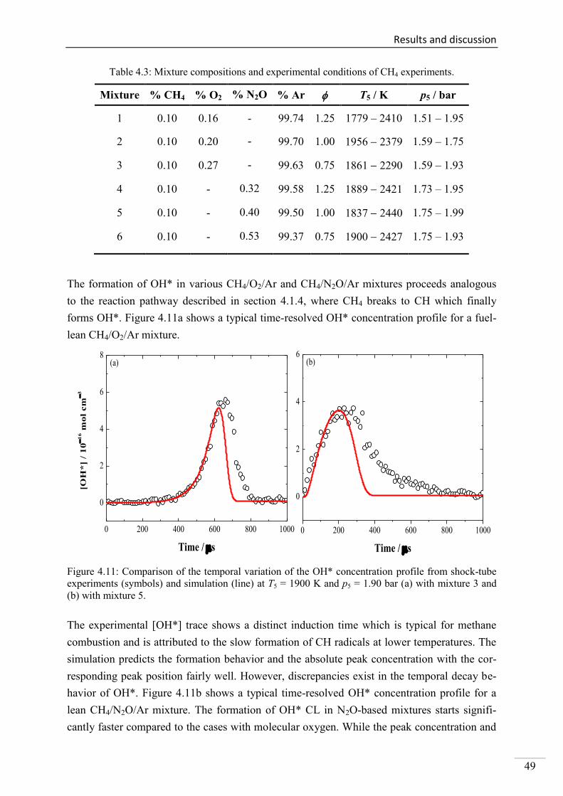
Results and discussion
49
Table 4.3: Mixture compositions and experimental conditions of CH4 experiments.
Mixture % CH4 % O2 % N2O % Ar T5 / K p5 / bar
1 0.10 0.16 - 99.74 1.25 1779 – 2410 1.51 – 1.95
2 0.10 0.20 - 99.70 1.00 1956 2379 1.59 – 1.75
3 0.10 0.27 - 99.63 0.75 1861 2290 1.59 – 1.93
4 0.10 - 0.32 99.58 1.25 1889 2421 1.73 – 1.95
5 0.10 - 0.40 99.50 1.00 1837 2440 1.75 – 1.99
6 0.10 - 0.53 99.37 0.75 1900 2427 1.75 – 1.93
The formation of OH* in various CH4/O2/Ar and CH4/N2O/Ar mixtures proceeds analogous
to the reaction pathway described in section 4.1.4, where CH4 breaks to CH which finally
forms OH*. Figure 4.11a shows a typical time-resolved OH* concentration profile for a fuel-
lean CH4/O2/Ar mixture.
Figure 4.11: Comparison of the temporal variation of the OH* concentration profile from shock-tube
experiments (symbols) and simulation (line) at T5 = 1900 K and p5 = 1.90 bar (a) with mixture 3 and
(b) with mixture 5.
The experimental [OH*] trace shows a distinct induction time which is typical for methane
combustion and is attributed to the slow formation of CH radicals at lower temperatures. The
simulation predicts the formation behavior and the absolute peak concentration with the cor-
responding peak position fairly well. However, discrepancies exist in the temporal decay be-
havior of OH*. Figure 4.11b shows a typical time-resolved OH* concentration profile for a
lean CH4/N2O/Ar mixture. The formation of OH* CL in N2O-based mixtures starts signifi-
cantly faster compared to the cases with molecular oxygen. While the peak concentration and
0 200 400 600 800 1000
0
2
4
6
Time / s
(b)
0 200 400 600 800 1000
0
2
4
6
8
[OH
*]
/ 1
0
16 m
ol
cm
3
Time / s
(a)
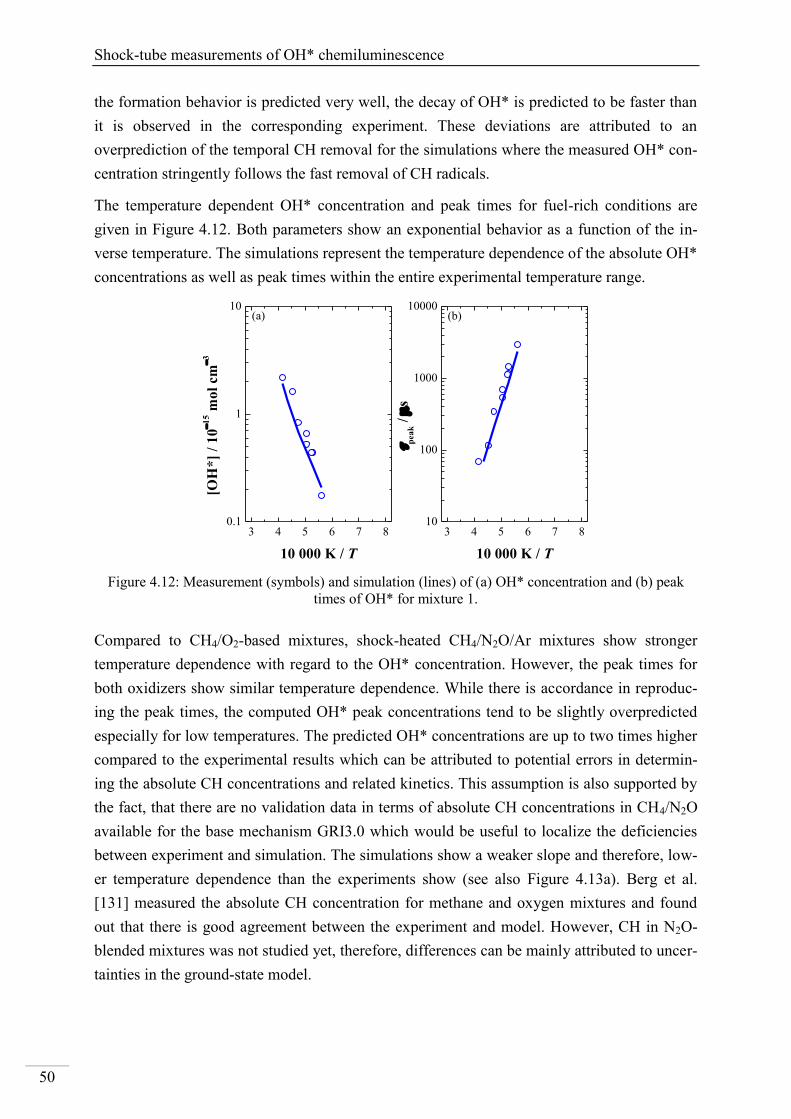
Shock-tube measurements of OH* chemiluminescence
50
the formation behavior is predicted very well, the decay of OH* is predicted to be faster than
it is observed in the corresponding experiment. These deviations are attributed to an
overprediction of the temporal CH removal for the simulations where the measured OH* con-
centration stringently follows the fast removal of CH radicals.
The temperature dependent OH* concentration and peak times for fuel-rich conditions are
given in Figure 4.12. Both parameters show an exponential behavior as a function of the in-
verse temperature. The simulations represent the temperature dependence of the absolute OH*
concentrations as well as peak times within the entire experimental temperature range.
3 4 5 6 7 80.1
1
10(b)
[OH
*]
/ 1
0
15 m
ol
cm
3
10 000 K / T
(a)
3 4 5 6 7 810
100
1000
10000
pea
k /
s
10 000 K / T
Figure 4.12: Measurement (symbols) and simulation (lines) of (a) OH* concentration and (b) peak
times of OH* for mixture 1.
Compared to CH4/O2-based mixtures, shock-heated CH4/N2O/Ar mixtures show stronger
temperature dependence with regard to the OH* concentration. However, the peak times for
both oxidizers show similar temperature dependence. While there is accordance in reproduc-
ing the peak times, the computed OH* peak concentrations tend to be slightly overpredicted
especially for low temperatures. The predicted OH* concentrations are up to two times higher
compared to the experimental results which can be attributed to potential errors in determin-
ing the absolute CH concentrations and related kinetics. This assumption is also supported by
the fact, that there are no validation data in terms of absolute CH concentrations in CH4/N2O
available for the base mechanism GRI3.0 which would be useful to localize the deficiencies
between experiment and simulation. The simulations show a weaker slope and therefore, low-
er temperature dependence than the experiments show (see also Figure 4.13a). Berg et al.
[131] measured the absolute CH concentration for methane and oxygen mixtures and found
out that there is good agreement between the experiment and model. However, CH in N2O-
blended mixtures was not studied yet, therefore, differences can be mainly attributed to uncer-
tainties in the ground-state model.
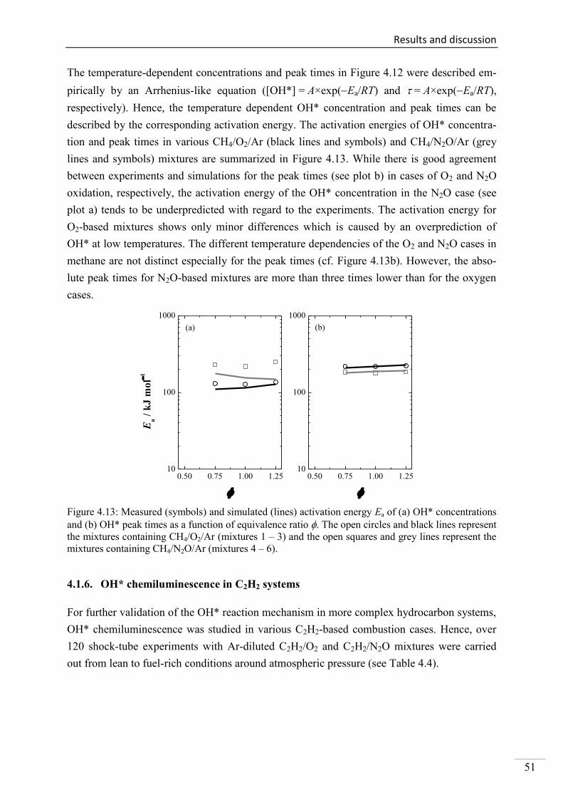
Results and discussion
51
The temperature-dependent concentrations and peak times in Figure 4.12 were described em-
pirically by an Arrhenius-like equation ([OH*] = A×exp(Ea/RT) and = A×exp(Ea/RT),
respectively). Hence, the temperature dependent OH* concentration and peak times can be
described by the corresponding activation energy. The activation energies of OH* concentra-
tion and peak times in various CH4/O2/Ar (black lines and symbols) and CH4/N2O/Ar (grey
lines and symbols) mixtures are summarized in Figure 4.13. While there is good agreement
between experiments and simulations for the peak times (see plot b) in cases of O2 and N2O
oxidation, respectively, the activation energy of the OH* concentration in the N2O case (see
plot a) tends to be underpredicted with regard to the experiments. The activation energy for
O2-based mixtures shows only minor differences which is caused by an overprediction of
OH* at low temperatures. The different temperature dependencies of the O2 and N2O cases in
methane are not distinct especially for the peak times (cf. Figure 4.13b). However, the abso-
lute peak times for N2O-based mixtures are more than three times lower than for the oxygen
cases.
0.50 0.75 1.00 1.2510
100
1000
(b)
Ea /
kJ
mo
l1
(a)
0.50 0.75 1.00 1.2510
100
1000
Figure 4.13: Measured (symbols) and simulated (lines) activation energy Ea of (a) OH* concentrations
and (b) OH* peak times as a function of equivalence ratio . The open circles and black lines represent
the mixtures containing CH4/O2/Ar (mixtures 1 – 3) and the open squares and grey lines represent the
mixtures containing CH4/N2O/Ar (mixtures 4 – 6).
4.1.6. OH* chemiluminescence in C2H2 systems
For further validation of the OH* reaction mechanism in more complex hydrocarbon systems,
OH* chemiluminescence was studied in various C2H2-based combustion cases. Hence, over
120 shock-tube experiments with Ar-diluted C2H2/O2 and C2H2/N2O mixtures were carried
out from lean to fuel-rich conditions around atmospheric pressure (see Table 4.4).
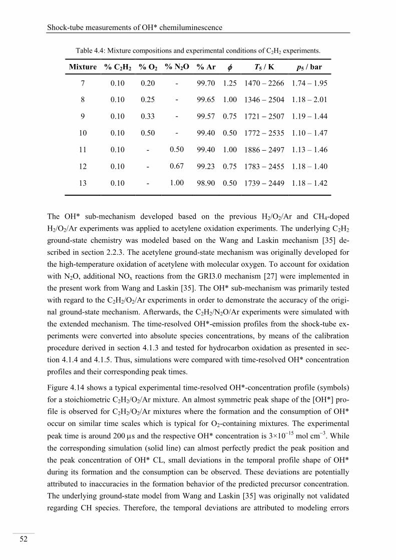
Shock-tube measurements of OH* chemiluminescence
52
Table 4.4: Mixture compositions and experimental conditions of C2H2 experiments.
Mixture % C2H2 % O2 % N2O % Ar T5 / K p5 / bar
7 0.10 0.20 - 99.70 1.25 1470 – 2266 1.74 – 1.95
8 0.10 0.25 - 99.65 1.00 1346 2504 1.18 – 2.01
9 0.10 0.33 - 99.57 0.75 1721 2507 1.19 – 1.44
10 0.10 0.50 - 99.40 0.50 1772 2535 1.10 – 1.47
11 0.10 - 0.50 99.40 1.00 1886 2497 1.13 – 1.46
12 0.10 - 0.67 99.23 0.75 1783 2455 1.18 – 1.40
13 0.10 - 1.00 98.90 0.50 1739 2449 1.18 – 1.42
The OH* sub-mechanism developed based on the previous H2/O2/Ar and CH4-doped
H2/O2/Ar experiments was applied to acetylene oxidation experiments. The underlying C2H2
ground-state chemistry was modeled based on the Wang and Laskin mechanism [35] de-
scribed in section 2.2.3. The acetylene ground-state mechanism was originally developed for
the high-temperature oxidation of acetylene with molecular oxygen. To account for oxidation
with N2O, additional NOx reactions from the GRI3.0 mechanism [27] were implemented in
the present work from Wang and Laskin [35]. The OH* sub-mechanism was primarily tested
with regard to the C2H2/O2/Ar experiments in order to demonstrate the accuracy of the origi-
nal ground-state mechanism. Afterwards, the C2H2/N2O/Ar experiments were simulated with
the extended mechanism. The time-resolved OH*-emission profiles from the shock-tube ex-
periments were converted into absolute species concentrations, by means of the calibration
procedure derived in section 4.1.3 and tested for hydrocarbon oxidation as presented in sec-
tion 4.1.4 and 4.1.5. Thus, simulations were compared with time-resolved OH* concentration
profiles and their corresponding peak times.
Figure 4.14 shows a typical experimental time-resolved OH*-concentration profile (symbols)
for a stoichiometric C2H2/O2/Ar mixture. An almost symmetric peak shape of the [OH*] pro-
file is observed for C2H2/O2/Ar mixtures where the formation and the consumption of OH*
occur on similar time scales which is typical for O2-containing mixtures. The experimental
peak time is around 200 s and the respective OH* concentration is 3×10¹⁵
mol cm3
. While
the corresponding simulation (solid line) can almost perfectly predict the peak position and
the peak concentration of OH* CL, small deviations in the temporal profile shape of OH*
during its formation and the consumption can be observed. These deviations are potentially
attributed to inaccuracies in the formation behavior of the predicted precursor concentration.
The underlying ground-state model from Wang and Laskin [35] was originally not validated
regarding CH species. Therefore, the temporal deviations are attributed to modeling errors
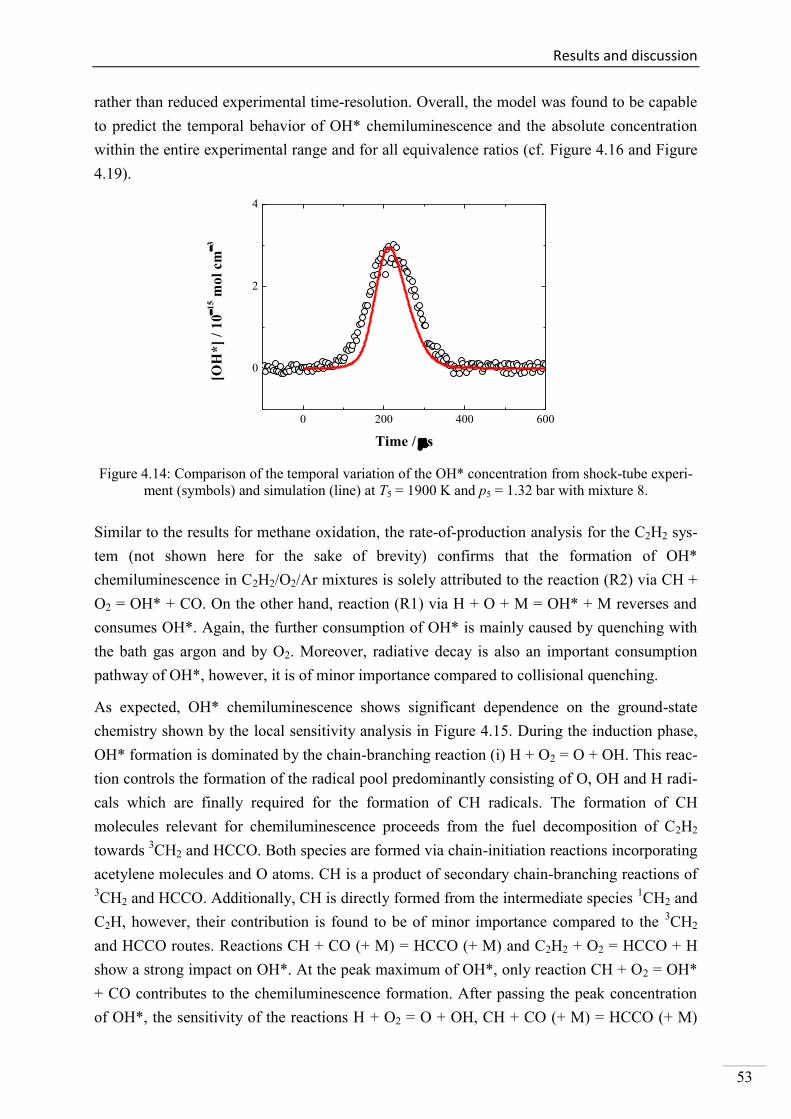
Results and discussion
53
rather than reduced experimental time-resolution. Overall, the model was found to be capable
to predict the temporal behavior of OH* chemiluminescence and the absolute concentration
within the entire experimental range and for all equivalence ratios (cf. Figure 4.16 and Figure
4.19).
0 200 400 600
0
2
4
[OH
*]
/ 1
0
15 m
ol
cm
3
Time / s
Figure 4.14: Comparison of the temporal variation of the OH* concentration from shock-tube experi-
ment (symbols) and simulation (line) at T5 = 1900 K and p5 = 1.32 bar with mixture 8.
Similar to the results for methane oxidation, the rate-of-production analysis for the C2H2 sys-
tem (not shown here for the sake of brevity) confirms that the formation of OH*
chemiluminescence in C2H2/O2/Ar mixtures is solely attributed to the reaction (R2) via CH +
O2 = OH* + CO. On the other hand, reaction (R1) via H + O + M = OH* + M reverses and
consumes OH*. Again, the further consumption of OH* is mainly caused by quenching with
the bath gas argon and by O2. Moreover, radiative decay is also an important consumption
pathway of OH*, however, it is of minor importance compared to collisional quenching.
As expected, OH* chemiluminescence shows significant dependence on the ground-state
chemistry shown by the local sensitivity analysis in Figure 4.15. During the induction phase,
OH* formation is dominated by the chain-branching reaction (i) H + O2 = O + OH. This reac-
tion controls the formation of the radical pool predominantly consisting of O, OH and H radi-
cals which are finally required for the formation of CH radicals. The formation of CH
molecules relevant for chemiluminescence proceeds from the fuel decomposition of C2H2
towards 3CH2 and HCCO. Both species are formed via chain-initiation reactions incorporating
acetylene molecules and O atoms. CH is a product of secondary chain-branching reactions of 3CH2 and HCCO. Additionally, CH is directly formed from the intermediate species
1CH2 and
C2H, however, their contribution is found to be of minor importance compared to the 3CH2
and HCCO routes. Reactions CH + CO (+ M) = HCCO (+ M) and C2H2 + O2 = HCCO + H
show a strong impact on OH*. At the peak maximum of OH*, only reaction CH + O2 = OH*
+ CO contributes to the chemiluminescence formation. After passing the peak concentration
of OH*, the sensitivity of the reactions H + O2 = O + OH, CH + CO (+ M) = HCCO (+ M)
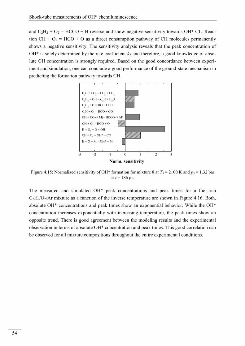
Shock-tube measurements of OH* chemiluminescence
54
and C2H2 + O2 = HCCO + H reverse and show negative sensitivity towards OH* CL. Reac-
tion CH + O2 = HCO + O as a direct consumption pathway of CH molecules permanently
shows a negative sensitivity. The sensitivity analysis reveals that the peak concentration of
OH* is solely determined by the rate coefficient k2 and therefore, a good knowledge of abso-
lute CH concentration is strongly required. Based on the good concordance between experi-
ment and simulation, one can conclude a good performance of the ground-state mechanism in
predicting the formation pathway towards CH.
-3 -2 -1 0 1 2 3
CH + CO (+ M)= HCCO (+ M)
H2CC + O
2 = CO
2 + CH
2
C2H
2 + OH = C
2H + H
2O
C2H + O
2 = HCO + CO
C2H
2 + O = HCCO + H
CH + O2 = HCO + O
H + O2 = O + OH
CH + O2 = OH* + CO
H + O + M = OH* + M
Norm. sensitivity
Figure 4.15: Normalized sensitivity of OH* formation for mixture 8 at T5 = 2100 K and p5 = 1.32 bar
at t = 186 s.
The measured and simulated OH* peak concentrations and peak times for a fuel-rich
C2H2/O2/Ar mixture as a function of the inverse temperature are shown in Figure 4.16. Both,
absolute OH* concentrations and peak times show an exponential behavior. While the OH*
concentration increases exponentially with increasing temperature, the peak times show an
opposite trend. There is good agreement between the modeling results and the experimental
observation in terms of absolute OH* concentration and peak times. This good correlation can
be observed for all mixture compositions throughout the entire experimental conditions.
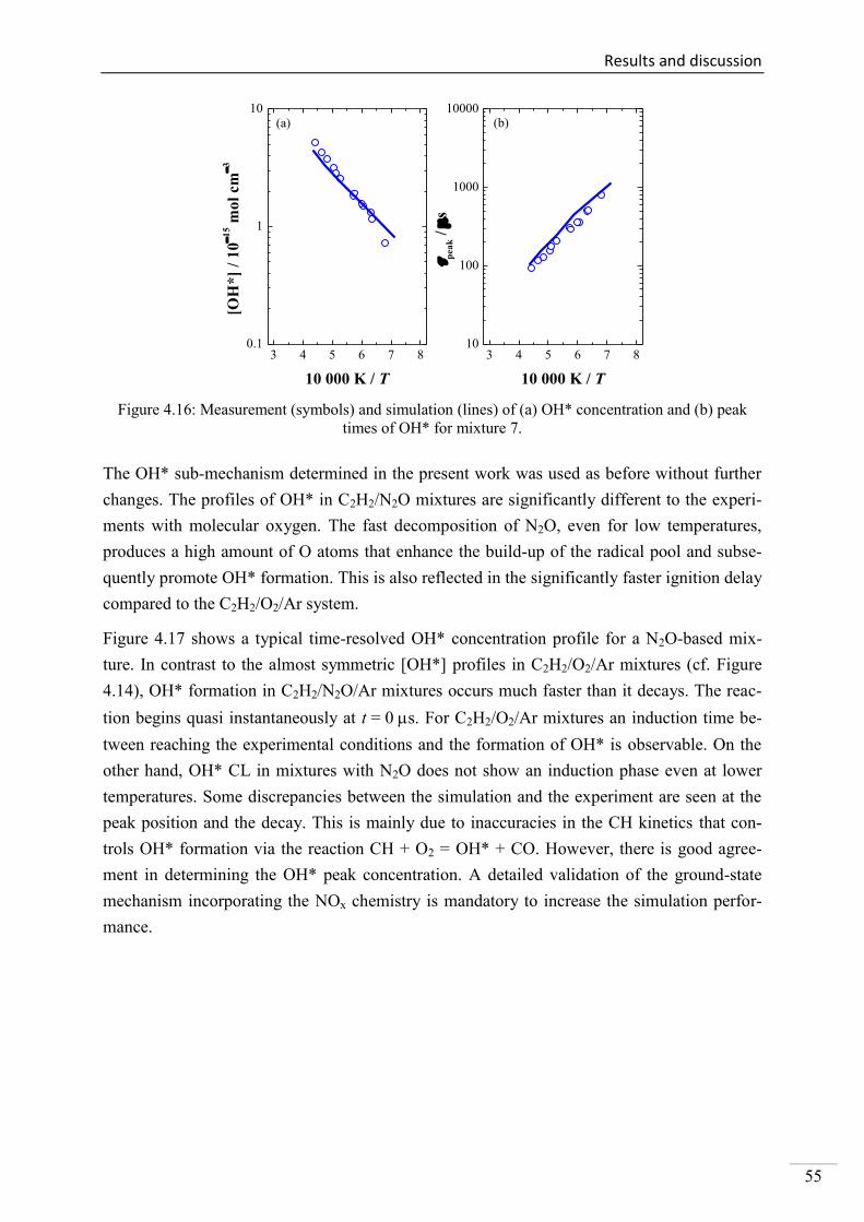
Results and discussion
55
3 4 5 6 7 80.1
1
10(b)
[OH
*]
/ 1
0
15 m
ol
cm
3
10 000 K / T
(a)
3 4 5 6 7 810
100
1000
10000
pea
k /
s
10 000 K / T
Figure 4.16: Measurement (symbols) and simulation (lines) of (a) OH* concentration and (b) peak
times of OH* for mixture 7.
The OH* sub-mechanism determined in the present work was used as before without further
changes. The profiles of OH* in C2H2/N2O mixtures are significantly different to the experi-
ments with molecular oxygen. The fast decomposition of N2O, even for low temperatures,
produces a high amount of O atoms that enhance the build-up of the radical pool and subse-
quently promote OH* formation. This is also reflected in the significantly faster ignition delay
compared to the C2H2/O2/Ar system.
Figure 4.17 shows a typical time-resolved OH* concentration profile for a N2O-based mix-
ture. In contrast to the almost symmetric [OH*] profiles in C2H2/O2/Ar mixtures (cf. Figure
4.14), OH* formation in C2H2/N2O/Ar mixtures occurs much faster than it decays. The reac-
tion begins quasi instantaneously at t = 0 s. For C2H2/O2/Ar mixtures an induction time be-
tween reaching the experimental conditions and the formation of OH* is observable. On the
other hand, OH* CL in mixtures with N2O does not show an induction phase even at lower
temperatures. Some discrepancies between the simulation and the experiment are seen at the
peak position and the decay. This is mainly due to inaccuracies in the CH kinetics that con-
trols OH* formation via the reaction CH + O2 = OH* + CO. However, there is good agree-
ment in determining the OH* peak concentration. A detailed validation of the ground-state
mechanism incorporating the NOx chemistry is mandatory to increase the simulation perfor-
mance.
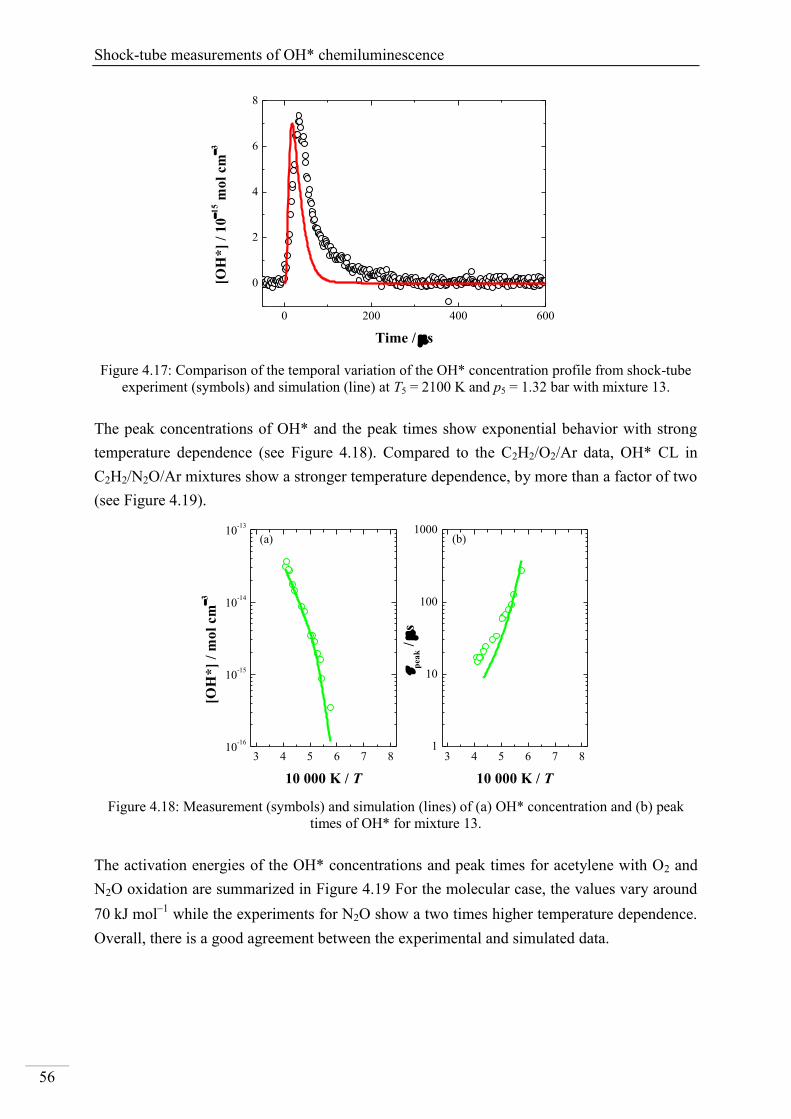
Shock-tube measurements of OH* chemiluminescence
56
0 200 400 600
0
2
4
6
8
[OH
*]
/ 1
0
15 m
ol
cm
3
Time / s
Figure 4.17: Comparison of the temporal variation of the OH* concentration profile from shock-tube
experiment (symbols) and simulation (line) at T5 = 2100 K and p5 = 1.32 bar with mixture 13.
The peak concentrations of OH* and the peak times show exponential behavior with strong
temperature dependence (see Figure 4.18). Compared to the C2H2/O2/Ar data, OH* CL in
C2H2/N2O/Ar mixtures show a stronger temperature dependence, by more than a factor of two
(see Figure 4.19).
3 4 5 6 7 810
-16
10-15
10-14
10-13
(b)
[OH
*]
/ m
ol
cm
3
10 000 K / T
(a)
3 4 5 6 7 81
10
100
1000
pea
k /
s
10 000 K / T
Figure 4.18: Measurement (symbols) and simulation (lines) of (a) OH* concentration and (b) peak
times of OH* for mixture 13.
The activation energies of the OH* concentrations and peak times for acetylene with O2 and
N2O oxidation are summarized in Figure 4.19 For the molecular case, the values vary around
70 kJ mol1
while the experiments for N2O show a two times higher temperature dependence.
Overall, there is a good agreement between the experimental and simulated data.
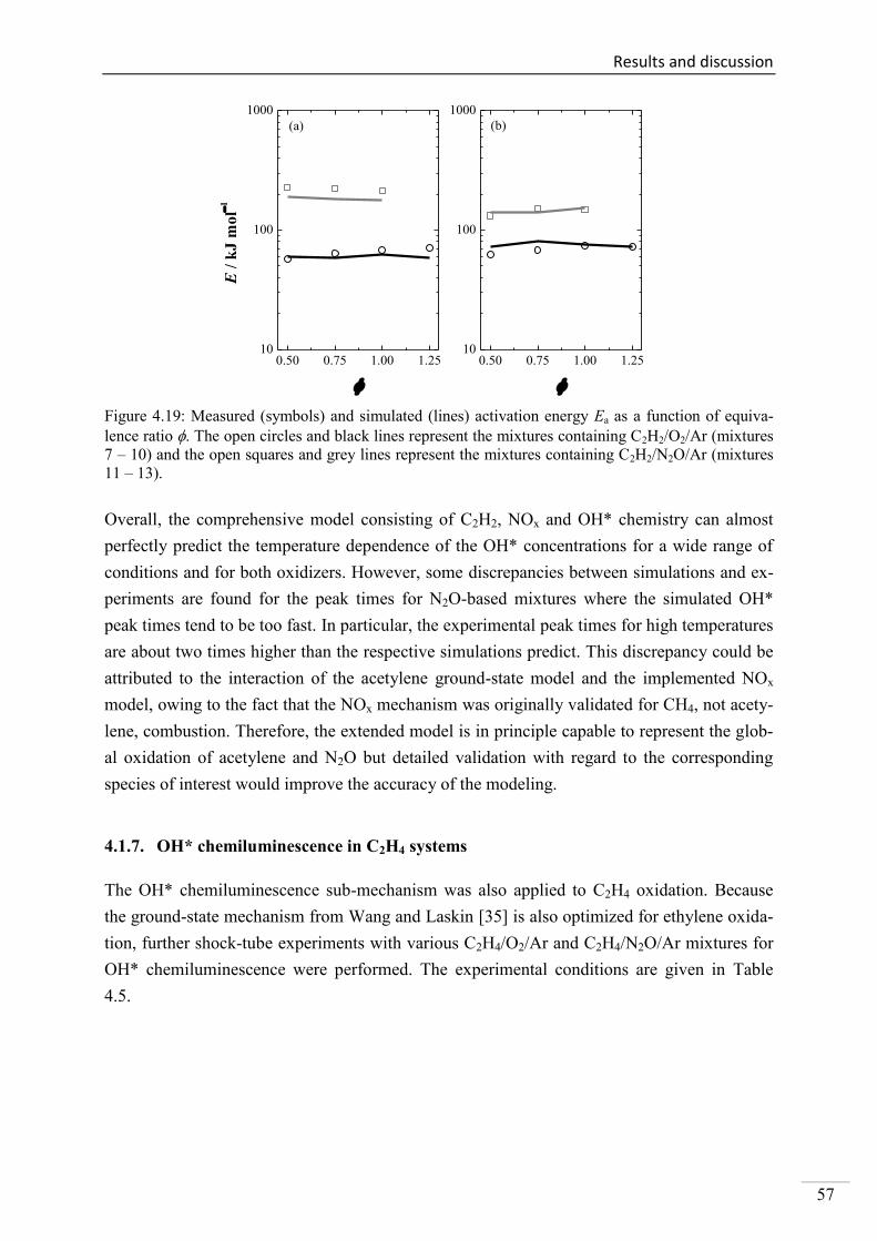
Results and discussion
57
0.50 0.75 1.00 1.2510
100
1000
(b)
E /
kJ
mo
l1
(a)
0.50 0.75 1.00 1.2510
100
1000
Figure 4.19: Measured (symbols) and simulated (lines) activation energy Ea as a function of equiva-
lence ratio . The open circles and black lines represent the mixtures containing C2H2/O2/Ar (mixtures
7 – 10) and the open squares and grey lines represent the mixtures containing C2H2/N2O/Ar (mixtures
11 – 13).
Overall, the comprehensive model consisting of C2H2, NOx and OH* chemistry can almost
perfectly predict the temperature dependence of the OH* concentrations for a wide range of
conditions and for both oxidizers. However, some discrepancies between simulations and ex-
periments are found for the peak times for N2O-based mixtures where the simulated OH*
peak times tend to be too fast. In particular, the experimental peak times for high temperatures
are about two times higher than the respective simulations predict. This discrepancy could be
attributed to the interaction of the acetylene ground-state model and the implemented NOx
model, owing to the fact that the NOx mechanism was originally validated for CH4, not acety-
lene, combustion. Therefore, the extended model is in principle capable to represent the glob-
al oxidation of acetylene and N2O but detailed validation with regard to the corresponding
species of interest would improve the accuracy of the modeling.
4.1.7. OH* chemiluminescence in C2H4 systems
The OH* chemiluminescence sub-mechanism was also applied to C2H4 oxidation. Because
the ground-state mechanism from Wang and Laskin [35] is also optimized for ethylene oxida-
tion, further shock-tube experiments with various C2H4/O2/Ar and C2H4/N2O/Ar mixtures for
OH* chemiluminescence were performed. The experimental conditions are given in Table
4.5.
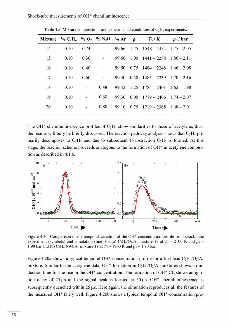
Shock-tube measurements of OH* chemiluminescence
58
Table 4.5: Mixture compositions and experimental conditions of C2H4 experiments.
Mixture % C2H4 % O2 % N2O % Ar T5 / K p5 / bar
14 0.10 0.24 - 99.66 1.25 1548 – 2452 1.75 – 2.05
15 0.10 0.30 - 99.60 1.00 1441 2288 1.86 – 2.11
16 0.10 0.40 - 99.50 0.75 1484 2248 1.66 – 2.08
17 0.10 0.60 - 99.30 0.50 1485 2339 1.70 – 2.16
18 0.10 - 0.48 99.42 1.25 1785 2401 1.62 – 1.98
19 0.10 - 0.60 99.30 0.00 1779 2406 1.74 – 2.07
20 0.10 - 0.80 99.10 0.75 1719 2365 1.68 – 2.01
The OH* chemiluminescence profiles of C2H4 show similarities to those of acetylene, thus,
the results will only be briefly discussed. The reaction pathway analysis shows that C2H4 pri-
marily decomposes to C2H3 and due to subsequent H-abstraction C2H2 is formed. At this
stage, the reaction scheme proceeds analogous to the formation of OH* in acetylene combus-
tion as described in 4.1.6.
Figure 4.20: Comparison of the temporal variation of the OH*-concentration profile from shock-tube
experiment (symbols) and simulation (line) for (a) C2H4/O2/Ar mixture 17 at T5 = 2100 K and p5 =
1.90 bar and (b) C2H4/N2O/Ar mixture 19 at T5 = 1900 K and p5 = 1.90 bar.
Figure 4.20a shows a typical temporal OH* concentration profile for a fuel-lean C2H4/O2/Ar
mixture. Similar to the acetylene data, OH* formation in C2H4/O2/Ar mixtures shows an in-
duction time for the rise in the OH* concentration. The formation of OH* CL shows an igni-
tion delay of 25 s and the signal peak is located at 50 s. OH* chemiluminescence is
subsequently quenched within 25 s. Here again, the simulation reproduces all the features of
the measured OH* fairly well. Figure 4.20b shows a typical temporal OH*-concentration pro-
0 50 100 150 200
0
2
4
6
8
10
[OH
*]
/ 1
0
15 m
ol
cm
3
Time / s
(a)
0 200 400 600
0.0
0.5
1.0
1.5
2.0
2.5
Time / s
(b)
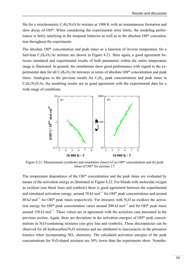
Results and discussion
59
file for a stoichiometric C2H4/N2O/Ar mixture at 1900 K with an instantaneous formation and
slow decay of OH*. When considering the experimental error limits, the modeling perfor-
mance is fairly satisfying in the temporal behavior as well as in the absolute OH* concentra-
tion throughout the experiments
The absolute OH* concentration and peak times as a function of inverse temperature for a
fuel-lean C2H4/O2/Ar mixture are shown in Figure 4.21. Here again, a good agreement be-
tween simulated and experimental results of both parameters within the entire temperature
range is illustrated. In general, the simulations show good performance with regard to the ex-
perimental data for all C2H4/O2/Ar mixtures in terms of absolute OH* concentration and peak
times. Analogous to the previous results for C2H2, peak concentrations and peak times in
C2H4/N2O/Ar, the modeling results are in good agreement with the experimental data for a
wide range of conditions.
3 4 5 6 7 80.1
1
10
(b)
[OH
*]
/ 1
0
14 m
ol
cm
3
10 000 K / T
(a)
3 4 5 6 7 810
100
1000
pea
k /
s
10 000 K / T
Figure 4.21: Measurement (symbols) and simulation (lines) of (a) OH* concentration and (b) peak
times of OH* for mixture 17.
The temperature dependence of the OH* concentration and the peak times are evaluated by
means of the activation energy as illustrated in Figure 4.22. For blends with molecular oxygen
as oxidizer (see black lines and symbols) there is good agreement between the experimental
and simulated activation energy, around 70 kJ mol1
for OH* peak concentrations and around
80 kJ mol1
for OH* peak times respectively. For mixtures with N2O as oxidizer the activa-
tion energy for OH* peak concentration varies around 200 kJ mol1
and for OH* peak times
around 150 kJ mol1
. These values are in agreement with the acetylene case presented in the
previous section. Again, there are deviations in the activation energies of OH* peak concen-
trations in N2O-containing mixtures (see grey line and symbols). These discrepancies can be
observed for all hydrocarbon/N2O mixtures and are attributed to inaccuracies in the precursor
kinetics when incorporating NOx chemistry. The calculated activation energies of the peak
concentrations for N2O-doped mixtures are 30% lower than the experiments show. Nonethe-
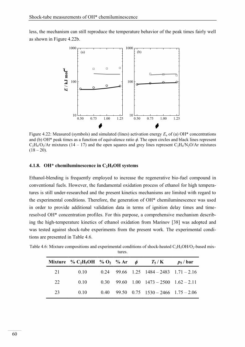
Shock-tube measurements of OH* chemiluminescence
60
less, the mechanism can still reproduce the temperature behavior of the peak times fairly well
as shown in Figure 4.22b.
0.50 0.75 1.00 1.2510
100
1000(b)
E /
kJ
mo
l1
(a)
0.50 0.75 1.00 1.2510
100
1000
Figure 4.22: Measured (symbols) and simulated (lines) activation energy Ea of (a) OH* concentrations
and (b) OH* peak times as a function of equivalence ratio . The open circles and black lines represent
C2H4/O2/Ar mixtures (14 – 17) and the open squares and grey lines represent C2H4/N2O/Ar mixtures
(18 – 20).
4.1.8. OH* chemiluminescence in C2H5OH systems
Ethanol-blending is frequently employed to increase the regenerative bio-fuel compound in
conventional fuels. However, the fundamental oxidation process of ethanol for high tempera-
tures is still under-researched and the present kinetics mechanisms are limited with regard to
the experimental conditions. Therefore, the generation of OH* chemiluminescence was used
in order to provide additional validation data in terms of ignition delay times and time-
resolved OH* concentration profiles. For this purpose, a comprehensive mechanism describ-
ing the high-temperature kinetics of ethanol oxidation from Marinov [38] was adopted and
was tested against shock-tube experiments from the present work. The experimental condi-
tions are presented in Table 4.6.
Table 4.6: Mixture compositions and experimental conditions of shock-heated C2H5OH/O2-based mix-
tures.
Mixture % C2H5OH % O2 % Ar T5 / K p5 / bar
21 0.10 0.24 99.66 1.25 1484 – 2483 1.71 – 2.16
22 0.10 0.30 99.60 1.00 1473 2500 1.62 – 2.11
23 0.10 0.40 99.50 0.75 1530 2466 1.75 – 2.06
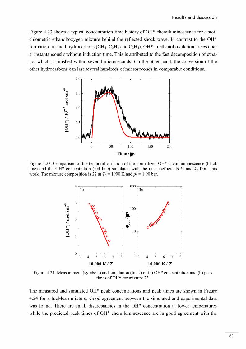
Results and discussion
61
Figure 4.23 shows a typical concentration-time history of OH* chemiluminescence for a stoi-
chiometric ethanol/oxygen mixture behind the reflected shock wave. In contrast to the OH*
formation in small hydrocarbons (CH4, C2H2 and C2H4), OH* in ethanol oxidation arises qua-
si instantaneously without induction time. This is attributed to the fast decomposition of etha-
nol which is finished within several microseconds. On the other hand, the conversion of the
other hydrocarbons can last several hundreds of microseconds in comparable conditions.
0 50 100 150 200
0.0
0.5
1.0
1.5
2.0
[OH
*]
/ 1
0
15 m
ol
cm
3
Time / s
Figure 4.23: Comparison of the temporal variation of the normalized OH* chemiluminescence (black
line) and the OH* concentration (red line) simulated with the rate coefficients k1 and k2 from this
work. The mixture composition is 22 at T5 = 1900 K and p5 = 1.90 bar.
3 4 5 6 7 80
1
2
3
4(b)
[OH
*]
/ m
ol
cm
3
10 000 K / T
(a)
3 4 5 6 7 81
10
100
1000
pea
k /
s
10 000 K / T
Figure 4.24: Measurement (symbols) and simulation (lines) of (a) OH* concentration and (b) peak
times of OH* for mixture 23.
The measured and simulated OH* peak concentrations and peak times are shown in Figure
4.24 for a fuel-lean mixture. Good agreement between the simulated and experimental data
was found. There are small discrepancies in the OH* concentration at lower temperatures
while the predicted peak times of OH* chemiluminescence are in good agreement with the
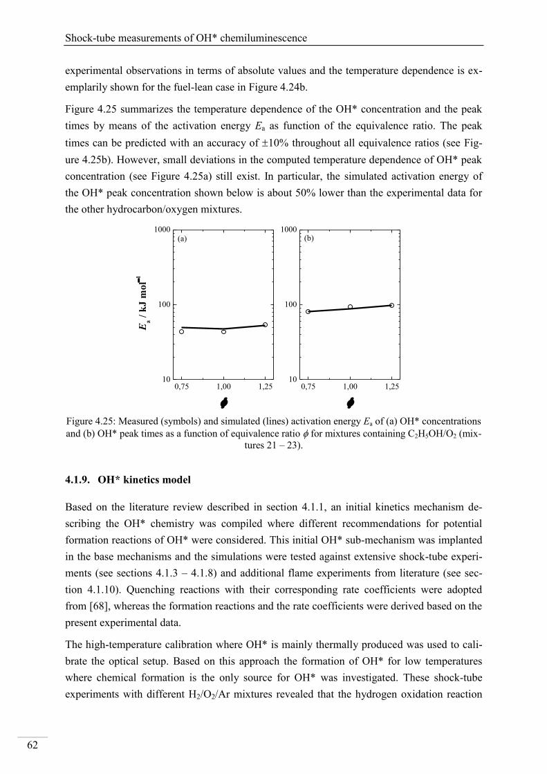
Shock-tube measurements of OH* chemiluminescence
62
experimental observations in terms of absolute values and the temperature dependence is ex-
emplarily shown for the fuel-lean case in Figure 4.24b.
Figure 4.25 summarizes the temperature dependence of the OH* concentration and the peak
times by means of the activation energy Ea as function of the equivalence ratio. The peak
times can be predicted with an accuracy of 10% throughout all equivalence ratios (see Fig-
ure 4.25b). However, small deviations in the computed temperature dependence of OH* peak
concentration (see Figure 4.25a) still exist. In particular, the simulated activation energy of
the OH* peak concentration shown below is about 50% lower than the experimental data for
the other hydrocarbon/oxygen mixtures.
0,75 1,00 1,2510
100
1000(b)
Ea /
kJ
mo
l1
(a)
0,75 1,00 1,2510
100
1000
Figure 4.25: Measured (symbols) and simulated (lines) activation energy Ea of (a) OH* concentrations
and (b) OH* peak times as a function of equivalence ratio for mixtures containing C2H5OH/O2 (mix-
tures 21 – 23).
4.1.9. OH* kinetics model
Based on the literature review described in section 4.1.1, an initial kinetics mechanism de-
scribing the OH* chemistry was compiled where different recommendations for potential
formation reactions of OH* were considered. This initial OH* sub-mechanism was implanted
in the base mechanisms and the simulations were tested against extensive shock-tube experi-
ments (see sections 4.1.3 – 4.1.8) and additional flame experiments from literature (see sec-
tion 4.1.10). Quenching reactions with their corresponding rate coefficients were adopted
from [68], whereas the formation reactions and the rate coefficients were derived based on the
present experimental data.
The high-temperature calibration where OH* is mainly thermally produced was used to cali-
brate the optical setup. Based on this approach the formation of OH* for low temperatures
where chemical formation is the only source for OH* was investigated. These shock-tube
experiments with different H2/O2/Ar mixtures revealed that the hydrogen oxidation reaction
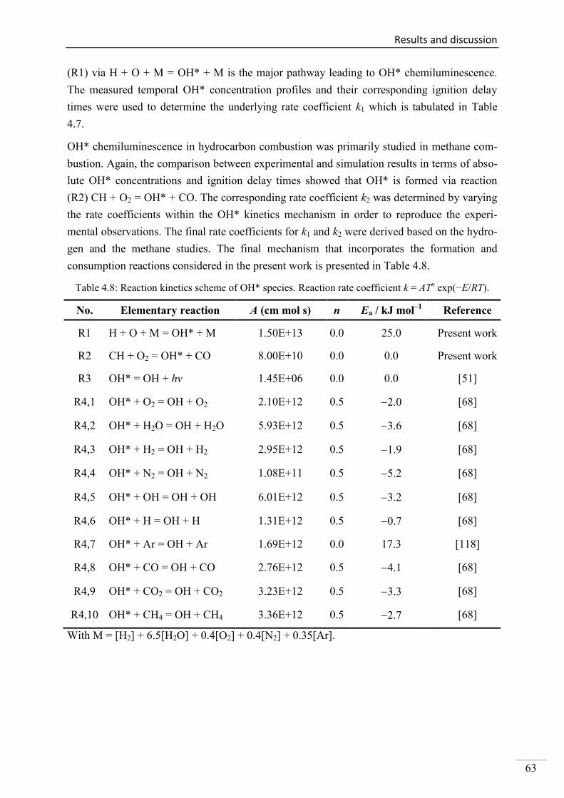
Results and discussion
63
(R1) via H + O + M = OH* + M is the major pathway leading to OH* chemiluminescence.
The measured temporal OH* concentration profiles and their corresponding ignition delay
times were used to determine the underlying rate coefficient k1 which is tabulated in Table
4.7.
OH* chemiluminescence in hydrocarbon combustion was primarily studied in methane com-
bustion. Again, the comparison between experimental and simulation results in terms of abso-
lute OH* concentrations and ignition delay times showed that OH* is formed via reaction
(R2) CH + O2 = OH* + CO. The corresponding rate coefficient k2 was determined by varying
the rate coefficients within the OH* kinetics mechanism in order to reproduce the experi-
mental observations. The final rate coefficients for k1 and k2 were derived based on the hydro-
gen and the methane studies. The final mechanism that incorporates the formation and
consumption reactions considered in the present work is presented in Table 4.8.
Table 4.8: Reaction kinetics scheme of OH* species. Reaction rate coefficient k = ATn exp(−E/RT).
No. Elementary reaction
A (cm mol s)
n
Ea / kJ mol–1
Reference
R1 H + O + M = OH* + M
1.50E+13
0.0
25.0
Present work
R2 CH + O2 = OH* + CO
8.00E+10
0.0
0.0
Present work
R3 OH* = OH + hv
1.45E+06
0.0
0.0
[51]
R4,1 OH* + O2 = OH + O2
2.10E+12
0.5
2.0
[68]
R4,2 OH* + H2O = OH + H2O
5.93E+12
0.5
3.6
[68]
R4,3 OH* + H2 = OH + H2
2.95E+12
0.5
1.9
[68]
R4,4 OH* + N2 = OH + N2
1.08E+11
0.5
5.2
[68]
R4,5 OH* + OH = OH + OH
6.01E+12
0.5
3.2
[68]
R4,6 OH* + H = OH + H
1.31E+12
0.5
0.7
[68]
R4,7 OH* + Ar = OH + Ar
1.69E+12
0.0
17.3
[118]
R4,8 OH* + CO = OH + CO
2.76E+12
0.5
4.1
[68]
R4,9 OH* + CO2 = OH + CO2
3.23E+12
0.5
3.3
[68]
R4,10 OH* + CH4 = OH + CH4
3.36E+12
0.5
2.7
[68]
With M = [H2] + 6.5[H2O] + 0.4[O2] + 0.4[N2] + 0.35[Ar].
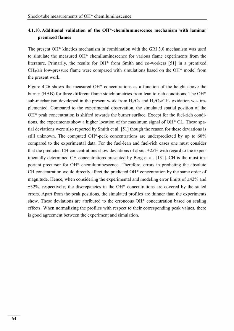
Shock-tube measurements of OH* chemiluminescence
64
4.1.10. Additional validation of the OH*-chemiluminescence mechanism with laminar
premixed flames
The present OH* kinetics mechanism in combination with the GRI 3.0 mechanism was used
to simulate the measured OH* chemiluminescence for various flame experiments from the
literature. Primarily, the results for OH* from Smith and co-workers [51] in a premixed
CH4/air low-pressure flame were compared with simulations based on the OH* model from
the present work.
Figure 4.26 shows the measured OH* concentrations as a function of the height above the
burner (HAB) for three different flame stoichiometries from lean to rich conditions. The OH*
sub-mechanism developed in the present work from H2/O2 and H2/O2/CH4 oxidation was im-
plemented. Compared to the experimental observation, the simulated spatial position of the
OH* peak concentration is shifted towards the burner surface. Except for the fuel-rich condi-
tions, the experiments show a higher location of the maximum signal of OH* CL. These spa-
tial deviations were also reported by Smith et al. [51] though the reason for these deviations is
still unknown. The computed OH*-peak concentrations are underpredicted by up to 60%
compared to the experimental data. For the fuel-lean and fuel-rich cases one must consider
that the predicted CH concentrations show deviations of about 25% with regard to the exper-
imentally determined CH concentrations presented by Berg et al. [131]. CH is the most im-
portant precursor for OH* chemiluminescence. Therefore, errors in predicting the absolute
CH concentration would directly affect the predicted OH* concentration by the same order of
magnitude. Hence, when considering the experimental and modeling error limits of 42% and
32%, respectively, the discrepancies in the OH* concentrations are covered by the stated
errors. Apart from the peak positions, the simulated profiles are thinner than the experiments
show. These deviations are attributed to the erroneous OH* concentration based on scaling
effects. When normalizing the profiles with respect to their corresponding peak values, there
is good agreement between the experiment and simulation.
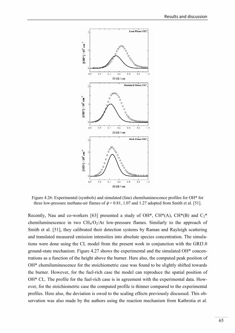
Results and discussion
65
Figure 4.26: Experimental (symbols) and simulated (line) chemiluminescence profiles for OH* for
three low-pressure methane-air flames of = 0.81, 1.07 and 1.27 adopted from Smith et al. [51].
Recently, Nau and co-workers [63] presented a study of OH*, CH*(A), CH*(B) and C2*
chemiluminescence in two CH4/O2/Ar low-pressure flames. Similarly to the approach of
Smith et al. [51], they calibrated their detection systems by Raman and Rayleigh scattering
and translated measured emission intensities into absolute species concentration. The simula-
tions were done using the CL model from the present work in conjunction with the GRI3.0
ground-state mechanism. Figure 4.27 shows the experimental and the simulated OH* concen-
trations as a function of the height above the burner. Here also, the computed peak position of
OH* chemiluminescence for the stoichiometric case was found to be slightly shifted towards
the burner. However, for the fuel-rich case the model can reproduce the spatial position of
OH* CL. The profile for the fuel-rich case is in agreement with the experimental data. How-
ever, for the stoichiometric case the computed profile is thinner compared to the experimental
profiles. Here also, the deviation is owed to the scaling effects previously discussed. This ob-
servation was also made by the authors using the reaction mechanism from Kathrotia et al.
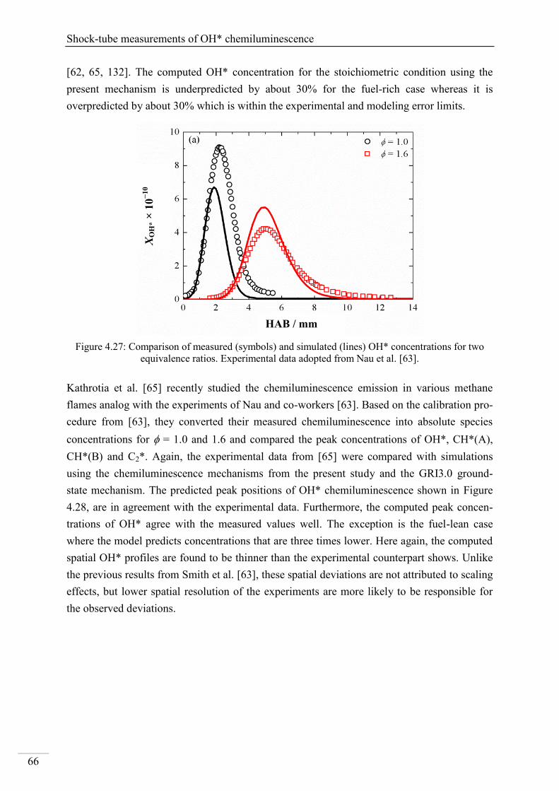
Shock-tube measurements of OH* chemiluminescence
66
[62, 65, 132]. The computed OH* concentration for the stoichiometric condition using the
present mechanism is underpredicted by about 30% for the fuel-rich case whereas it is
overpredicted by about 30% which is within the experimental and modeling error limits.
Figure 4.27: Comparison of measured (symbols) and simulated (lines) OH* concentrations for two
equivalence ratios. Experimental data adopted from Nau et al. [63].
Kathrotia et al. [65] recently studied the chemiluminescence emission in various methane
flames analog with the experiments of Nau and co-workers [63]. Based on the calibration pro-
cedure from [63], they converted their measured chemiluminescence into absolute species
concentrations for = 1.0 and 1.6 and compared the peak concentrations of OH*, CH*(A),
CH*(B) and C2*. Again, the experimental data from [65] were compared with simulations
using the chemiluminescence mechanisms from the present study and the GRI3.0 ground-
state mechanism. The predicted peak positions of OH* chemiluminescence shown in Figure
4.28, are in agreement with the experimental data. Furthermore, the computed peak concen-
trations of OH* agree with the measured values well. The exception is the fuel-lean case
where the model predicts concentrations that are three times lower. Here again, the computed
spatial OH* profiles are found to be thinner than the experimental counterpart shows. Unlike
the previous results from Smith et al. [63], these spatial deviations are not attributed to scaling
effects, but lower spatial resolution of the experiments are more likely to be responsible for
the observed deviations.
XO
H* ×
10−
10
HAB / mm
Results and discussion
67
Figure 4.28: Comparison of measured (symbols) and simulated (lines) OH* concentrations for differ-
ent equivalence ratios. Experimental data adopted from Kathrotia et al. [65].
4.2. Shock-tube measurements of CH* chemiluminescence
CH* chemiluminescence shows three major emission bands. The strongest one is attributed to
CH(A) and emits around 431 nm. This transition contributes about 80% of the total CH*
emission. The other states CH(B) and CH(C) at around 390 nm and 314 nm, respectively, are
much weaker compared to the A–X transition. The B-state typically contributes around 20%
to the CH* chemiluminescence, whereas reliable information for the C-state is not given. The
present work is devoted to the strongest band at 431 nm.
4.2.1. Review of CH* kinetics
Aside from OH* chemiluminescence, blue-light emission from CH* chemiluminescence is
frequently employed for combustion diagnostics under flame [51, 63, 116] and shock-tube
conditions [53, 61, 133]. For online measurement of the local equivalence ratio, OH* as well
as CH* chemiluminescence are employed at the same time [134-135]. Although CH* CL was
extensively studied in various previous works, the formation reactions of CH* emission are
still under debate. The present study was devoted for the systematic investigation of CH* key
reactions in various hydrocarbon combustion systems. A combined experimental and numeri-
cal study was adopted to determine the contribution of the potential formation reactions lead-
ing to CH*.
For CH* CL, there is disagreement in identifying the formation reaction(s). The dominating
pathway(s) and their suggested rate coefficients from literature also vary by several orders of
magnitude. Broida and Gaydon [136] and Bass and Broida [137] identified CH* half a centu-
XO
H* ×
10−
10
HAB / mm
Shock-tube measurements of CH* chemiluminescence
68
ry ago. The reaction producing CH* was suggested by Broida and Gaydon [136] and Gaydon
[48] as:
C2 + OH CH* + CO (R5)
Porter et al. [114] suggested a rate coefficient of (R5) to be 4.2×10¹¹
cm3mol
−1s−1
. Bleekrode
and Nieuwpoort [138] derived from CH* lifetimes a range for k5 between 6.0×10¹¹
and
6.0×10¹²
and cm3mol
−1s−1
. Bulewicz et al. [139] later supported reaction (R5) and derived a
rate coefficient of k5 = 4.8×10¹²
cm3mol
−1s−1
via absorption and emission experiments for
various species in a low-pressure burner. Based on their premixed flame experiments, Smith
et al. [51] recommended the value k5 = 1.1×10¹³
cm3mol
−1s−1
. They pointed out, however, that
reaction (R5) plays only a minor role with a contribution less than 10%. More recently, Hall
et al. [53] determined an exceptionally high rate coefficient of k5 = 2.0×10¹⁴
cm3mol
−1s−1
.
Glass et al. [140] rejected also the relevance of reaction (R5) as dominating pathway and in-
troduced the reaction of ethynyl (C2H) radicals with atomic oxygen. Also Brennen and Car-
rington [141] and Grebe and Homann [55] privileged the following reaction as the main
channel:
C2H + O CH* + CO (R6)
Recently, and based on highly-resolved spectroscopic investigations of CH* CL, Brockhinke
et al. [64] also excluded the role of (R5) for the formation scheme of CH*. They pointed out
that this formation reaction is accompanied by a large excess of free enthalpy (fH = 676 kJ
mol−1
) which would lead to high vibrational states, whereas the measured spectra did not
show such effects. Therefore, reactions (R6) and (R7) were favored. Joklik et al. [142]
showed in their low-pressure acetylene flame the dominance of the reaction (R6), but sug-
gested a value of k6 = 7.0×10¹²
cm3mol
−1s−1
which is one order of magnitude higher than the
recommended value stated in an earlier work from Grebe and Homann [55]. Reaction (R6)
was also supported by Devriendt et al. [143]. They determine the room-temperature rate coef-
ficient by means of a pulsed laser photolysis study of the C2H2/N2O system. The rate coeffi-
cient of the reaction (R6) was measured by using NO2* chemiluminescence from NO + O as
reference. The rate coefficient for reaction (R6) was found to be 1.1×10¹³
cm3mol
−1s−1
. One
year later, Devriendt and Peeters [144] presented a study of mixtures containing C2H2/O/H
using an isothermal flow reactor coupled with molecular-beam-sampling threshold-ionization
mass spectrometry (MB-TIMS) to quantify C2H and oxygen atoms. Again, CH* CL signal
intensities were linked to NO2* CL as internal standard to derive absolute CH* concentra-
tions. They found proportionality between CH* emission intensity and [C2H]×[O]. Based on
this observation, they estimated a revised rate coefficient for k6 = 1.4×10¹³exp(−1.9 kJ
mol−1
/RT) cm3mol
−1s−1
. Based on the calibration procedure of the optical detection system
described in section 4.1.1, Smith et al. [51] measured a rate coefficient k6 = 6.2×10¹²
cm3mol
−1s−1
which was considered as the main formation channel leading to CH* in premixed
CH4/air flames. Afterwards, the authors investigated CH* formation in CH4/N2O flames in
Results and discussion
69
[112] by using the same calibration procedure stated in [51]. They found, that CH* CL cannot
solely be described by reaction (R6) with their recommendation of k6 in [51]. The CH4/N2O
flame experiments revealed that a rate coefficient of k6 = 2.5×10¹²
cm3mol
−1s−1
[112] was
required which was slightly lower than their previous recommendation. Based on their shock-
tube study where they fitted simulated and normalized CH* concentrations against their ex-
perimental data as function of , Hall et al. [53] estimated a rate coefficient of k6 =
5.2×10¹¹exp(−10.9 kJ mol
−1/RT) cm
3mol
−1s−1
. The study, however, revealed that the main
reaction channel was attributed to the reaction (R5). Recently, Elsamra et al. [145] deduced
from a pulsed laser photolysis study using He-diluted C2H2/O2 mixtures a value of k6 =
6.0×10¹²exp(−1.9 kJ mol
−1/RT) cm
3mol
−1s−1
. They considered (R6) as major source of CH*
production especially for fuel-rich conditions.
A third CH* formation pathway was proposed in the early 1960s by Hand and Kistiakowsky
[146] which was supported by Gutman and Matsuda [50] and Matsuda et al. [147]. They pos-
tulate that the reaction of C2H radicals with O2 strongly contribute to the production of CH*:
C2H + O2 CH* + CO2 (R7)
Other studies were devoted to the investigation of reaction (R7). A laser photolysis study by
Renlund et al. [148] favored (R7) as important pathway for CH* formation. Hwang et al.
[149] also supported this recommendation and deduced a rate coefficient k7 =
4.10×10¹³ exp(−4.5 kJ mol
−1/RT) cm
3mol
−1s−1
based on shock-tube investigations. From time-
resolved CH* CL after laser photolysis of C2H2/N2O mixtures at room-temperature, Devriendt
et al. [143] deduced a rate coefficient k7 = 2.2×10¹⁰
cm3mol
−1s−1
which is 500 times lower
than their recommendation of k6. Smith et al. [51] primarily excluded the relevance of (R7)
based on their modeling approach for CH4/O2 flames. Later on, however, they found out that
the model overpredicts the monitored CH* in CH4/N2O flames [112] in cases where only re-
action (R6) was considered. Hence, they proposed for k7 = 3.2×10¹¹ exp(−6.7 kJ mol
−1/RT)
cm3mol
−1s−1
, which was derived from flame experiments with different [O]/[O2] ratios.
Elsamra et al. [145] published a temperature-dependent rate coefficient for (R7) of 6.0×10⁻⁴
T4.4
exp(9.6 kJ mol−1
/RT) cm3mol
−1s−1
. They denoted the importance of the latter reaction par-
ticularly for hot flames under fuel-lean conditions. Recently, Kathrotia [132] quantitatively
investigated CH*, OH* and C2* chemiluminescence in various premixed low-pressure
flames. The modeling revealed, that the available rate coefficient k7 from Elsamra et al. [145]
strongly overpredicts the CH* concentration. Depending on the equivalence ratio they revised
the recommended rate coefficients for the three potential reaction pathways (R5) – (R7). All
these studies pointed out the difficulties in undertaking quantitative measurements. There is a
large non-consensus not only in determining the major channel leading to CH* CL in various
hydrocarbon systems, but also in providing recommendations of their respective rates. There-
fore, the aim of this work was to improve the knowledge of the formation pathways leading to
Shock-tube measurements of CH* chemiluminescence
70
CH* CL and determining their corresponding kinetics data via linking shock-tube experi-
ments and numerical modeling.
4.2.2. Strategy of the investigation of CH* chemiluminescence
For the investigation of CH* chemiluminescence in hydrocarbon combustion, the well-known
acetylene oxidation mechanism (see section 2.2.3) was used to identify the potential for-
mation reactions leading to CH* CL. The combustion of acetylene provides high amounts of
C2H radicals as well as C2 radicals, which are considered as potential precursors for CH*
formation. Therefore, CH* chemiluminescence was initially studied for shock-heated
C2H2/O2/Ar mixtures and based on these results, a reaction mechanism describing CH* kinet-
ics was developed and validated. Because of the ambiguity with regard to the importance of
the reaction C2H + O = CH* + CO vs. C2H + O2 = CH* + CO2, additional experiments with
C2H2/N2O/Ar mixtures were performed in order to test the CH* formation for a higher
[O]/[O2] ratios. Aside from the C2H2 system, simulations based on the present CH* sub-
mechanism were extensively compared to measurements for various C1 and C2 hydrocarbons
(C2H4, CH4 and C2H5OH) for O2 and N2O as oxidizers.
In order to extend the validation database of the CH* sub-mechanism from the present work,
the model prediction was also tested with regard to flame measurements. For this purpose,
additional simulations were done according to recent studies of the CH* formation for various
premixed flames reported in literature [51, 63, 65].
4.2.3. CH* chemiluminescence in C2H2 mixtures
The acetylene reaction system was extensively studied in the past and thus, a well-validated
reaction mechanism (see section 2.2.3) exists which can be used for the modeling of the pre-
sent shock-tube experiments. The underlying ground-state mechanism originally did not con-
tain formation and consumption reactions of C2 molecule which is an important precursor for
the CH* formation. Therefore, a C2 sub-mechanism recommended by Williams and
Pasternack [150] that consists of 18 reactions was incorporated. We ensured that these modi-
fications did not affect the base mechanism by comparing the original and the extended
mechanism with regard to the published validation data for the relevant species (OH and CO2)
and ignition delay times. No further modifications were done. To our knowledge, an acetylene
ground-state mechanism which is validated for the oxidation with O2 and N2O does not exist
so far. Therefore, the base mechanism was extended by an additional subset of NOx reactions
adopted from the GRI 3.0 mechanism [92] in order to reproduce the shock-tube experiments
with N2O as oxidizer. This additional nitrogen chemistry was originally implemented in a
methane-combustion mechanism [92] and therefore contains cross-reactions linking nitrogen
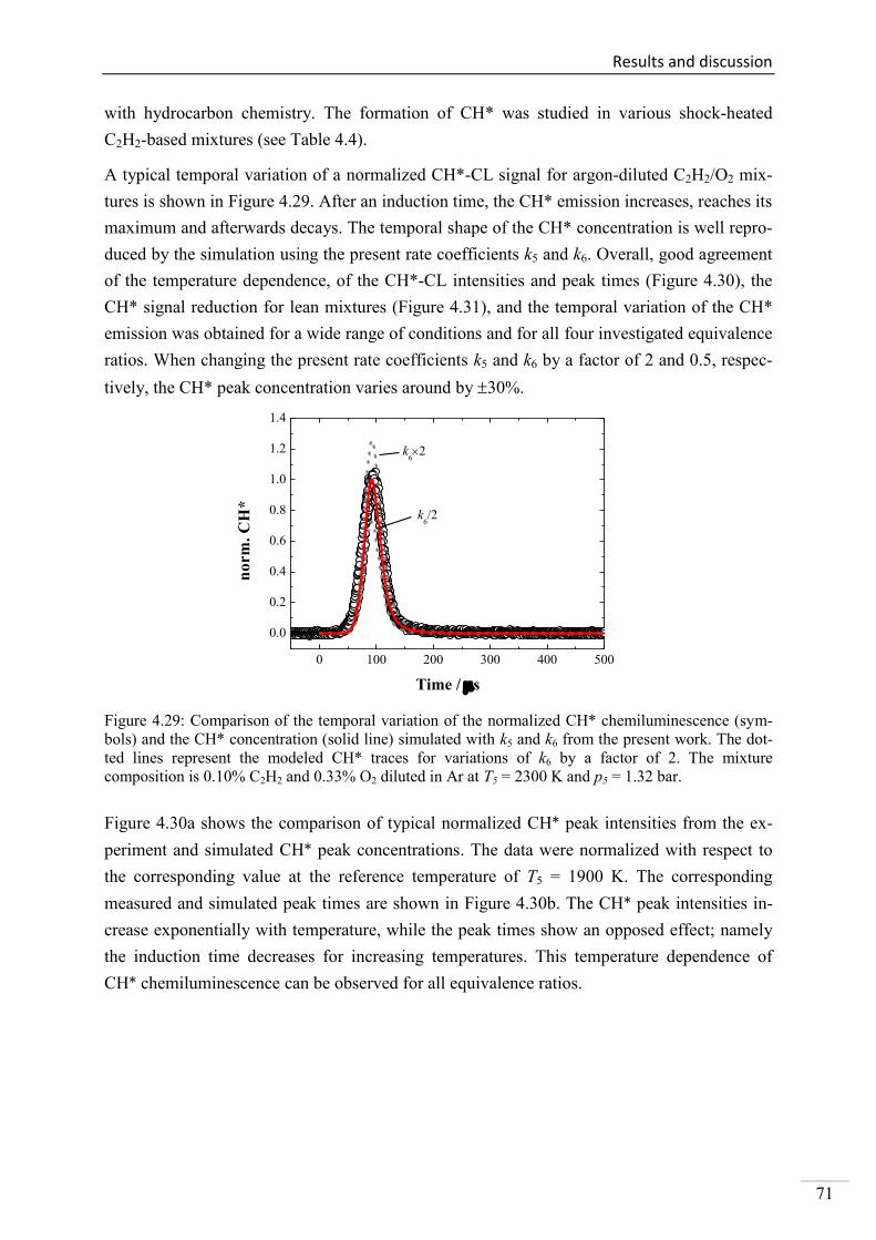
Results and discussion
71
with hydrocarbon chemistry. The formation of CH* was studied in various shock-heated
C2H2-based mixtures (see Table 4.4).
A typical temporal variation of a normalized CH*-CL signal for argon-diluted C2H2/O2 mix-
tures is shown in Figure 4.29. After an induction time, the CH* emission increases, reaches its
maximum and afterwards decays. The temporal shape of the CH* concentration is well repro-
duced by the simulation using the present rate coefficients k5 and k6. Overall, good agreement
of the temperature dependence, of the CH*-CL intensities and peak times (Figure 4.30), the
CH* signal reduction for lean mixtures (Figure 4.31), and the temporal variation of the CH*
emission was obtained for a wide range of conditions and for all four investigated equivalence
ratios. When changing the present rate coefficients k5 and k6 by a factor of 2 and 0.5, respec-
tively, the CH* peak concentration varies around by 30%.
0 100 200 300 400 500
0.0
0.2
0.4
0.6
0.8
1.0
1.2
1.4
k6/2
no
rm
. C
H*
Time / s
k62
Figure 4.29: Comparison of the temporal variation of the normalized CH* chemiluminescence (sym-
bols) and the CH* concentration (solid line) simulated with k5 and k6 from the present work. The dot-
ted lines represent the modeled CH* traces for variations of k6 by a factor of 2. The mixture
composition is 0.10% C2H2 and 0.33% O2 diluted in Ar at T5 = 2300 K and p5 = 1.32 bar.
Figure 4.30a shows the comparison of typical normalized CH* peak intensities from the ex-
periment and simulated CH* peak concentrations. The data were normalized with respect to
the corresponding value at the reference temperature of T5 = 1900 K. The corresponding
measured and simulated peak times are shown in Figure 4.30b. The CH* peak intensities in-
crease exponentially with temperature, while the peak times show an opposed effect; namely
the induction time decreases for increasing temperatures. This temperature dependence of
CH* chemiluminescence can be observed for all equivalence ratios.
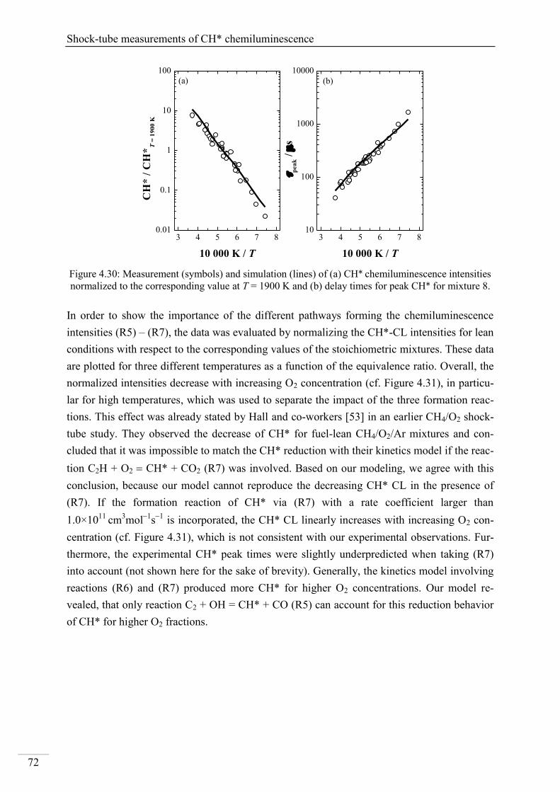
Shock-tube measurements of CH* chemiluminescence
72
3 4 5 6 7 80.01
0.1
1
10
100
(b)
CH
* /
CH
*T
= 1
90
0 K
10 000 K / T
(a)
3 4 5 6 7 810
100
1000
10000
pea
k /
s
10 000 K / T
Figure 4.30: Measurement (symbols) and simulation (lines) of (a) CH* chemiluminescence intensities
normalized to the corresponding value at T = 1900 K and (b) delay times for peak CH* for mixture 8.
In order to show the importance of the different pathways forming the chemiluminescence
intensities (R5) – (R7), the data was evaluated by normalizing the CH*-CL intensities for lean
conditions with respect to the corresponding values of the stoichiometric mixtures. These data
are plotted for three different temperatures as a function of the equivalence ratio. Overall, the
normalized intensities decrease with increasing O2 concentration (cf. Figure 4.31), in particu-
lar for high temperatures, which was used to separate the impact of the three formation reac-
tions. This effect was already stated by Hall and co-workers [53] in an earlier CH4/O2 shock-
tube study. They observed the decrease of CH* for fuel-lean CH4/O2/Ar mixtures and con-
cluded that it was impossible to match the CH* reduction with their kinetics model if the reac-
tion C2H + O2 CH* + CO2 (R7) was involved. Based on our modeling, we agree with this
conclusion, because our model cannot reproduce the decreasing CH* CL in the presence of
(R7). If the formation reaction of CH* via (R7) with a rate coefficient larger than
1.0×10¹¹
cm3mol
1s1
is incorporated, the CH* CL linearly increases with increasing O2 con-
centration (cf. Figure 4.31), which is not consistent with our experimental observations. Fur-
thermore, the experimental CH* peak times were slightly underpredicted when taking (R7)
into account (not shown here for the sake of brevity). Generally, the kinetics model involving
reactions (R6) and (R7) produced more CH* for higher O2 concentrations. Our model re-
vealed, that only reaction C2 + OH = CH* + CO (R5) can account for this reduction behavior
of CH* for higher O2 fractions.
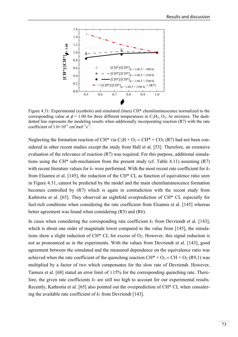
Results and discussion
73
0.5 0.6 0.7 0.8 0.9 1.00.0
0.2
0.4
0.6
0.8
1.0
1.2
1.4
1.6
[CH*]/[CH*] = 1.00,T = 1900 K
[CH*]/[CH*] = 1.00,T = 2100 K
[CH*]/[CH*] = 1.00,T = 2300 K
[CH*]/[CH*] = 1.00,T = 2300 K
+ (R7)
[CH
*]/
[CH
*]
= 1
.00
Figure 4.31: Experimental (symbols) and simulated (lines) CH* chemiluminescence normalized to the
corresponding value at = 1.00 for three different temperatures in C2H2, O2, Ar mixtures. The dash-
dotted line represents the modeling results when additionally incorporating reaction (R7) with the rate
coefficient of 1.0×10¹¹
cm3mol
1s1
.
Neglecting the formation reaction of CH* via C2H + O2 CH* + CO2 (R7) had not been con-
sidered in other recent studies except the study from Hall et al. [53]. Therefore, an extensive
evaluation of the relevance of reaction (R7) was required. For this purpose, additional simula-
tions using the CH* sub-mechanism from the present study (cf. Table 4.11) assuming (R7)
with recent literature values for k7 were performed. With the most recent rate coefficient for k7
from Elsamra et al. [145], the reduction of the CH* CL as function of equivalence ratio seen
in Figure 4.31, cannot be predicted by the model and the main chemiluminescence formation
becomes controlled by (R7) which is again in contradiction with the recent study from
Kathrotia et al. [65]. They observed an eightfold overprediction of CH* CL especially for
fuel-rich conditions when considering the rate coefficient from Elsamra et al. [145] whereas
better agreement was found when considering (R5) and (R6).
In cases when considering the corresponding rate coefficient k7 from Devriendt et al. [143],
which is about one order of magnitude lower compared to the value from [145], the simula-
tions show a slight reduction of CH* CL for excess of O2. However, this signal reduction is
not as pronounced as in the experiments. With the values from Devriendt et al. [143], good
agreement between the simulated and the measured dependence on the equivalence ratio was
achieved when the rate coefficient of the quenching reaction CH* + O2 CH + O2 (R9,1) was
multiplied by a factor of two which compensates for the slow rate of Devriendt. However,
Tamura et al. [68] stated an error limit of 15% for the corresponding quenching rate. There-
fore, the given rate coefficients k7 are still too high to account for our experimental results.
Recently, Kathrotia et al. [65] also pointed out the overprediction of CH* CL when consider-
ing the available rate coefficient of k7 from Devriendt [143].
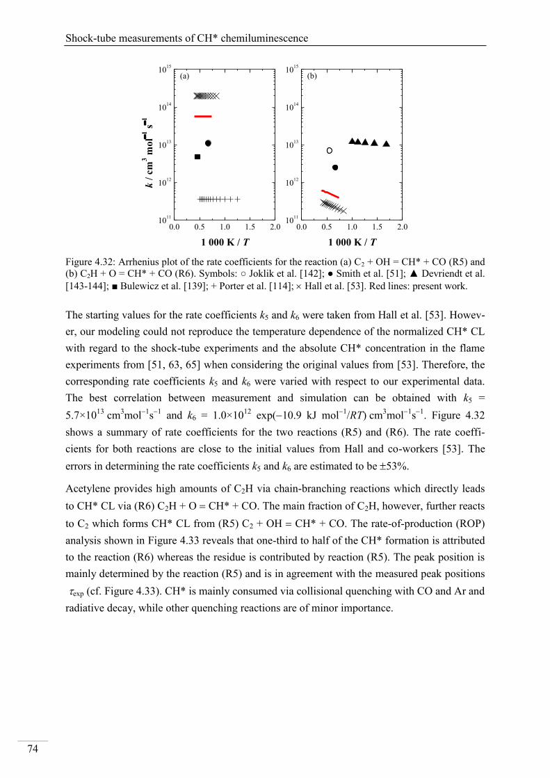
Shock-tube measurements of CH* chemiluminescence
74
0.0 0.5 1.0 1.5 2.010
11
1012
1013
1014
1015
(b)
k /
cm
3 m
ol
1 s
1
1 000 K / T
(a)
0.0 0.5 1.0 1.5 2.010
11
1012
1013
1014
1015
1 000 K / T
Figure 4.32: Arrhenius plot of the rate coefficients for the reaction (a) C2 + OH = CH* + CO (R5) and
(b) C2H + O = CH* + CO (R6). Symbols: ○ Joklik et al. [142]; ● Smith et al. [51]; ▲ Devriendt et al.
[143-144]; ■ Bulewicz et al. [139]; + Porter et al. [114]; Hall et al. [53]. Red lines: present work.
The starting values for the rate coefficients k5 and k6 were taken from Hall et al. [53]. Howev-
er, our modeling could not reproduce the temperature dependence of the normalized CH* CL
with regard to the shock-tube experiments and the absolute CH* concentration in the flame
experiments from [51, 63, 65] when considering the original values from [53]. Therefore, the
corresponding rate coefficients k5 and k6 were varied with respect to our experimental data.
The best correlation between measurement and simulation can be obtained with k5 =
5.7×10¹³
cm3mol
1s1
and k6 = 1.0×10¹²
exp(10.9 kJ mol1
/RT) cm3mol
1s1
. Figure 4.32
shows a summary of rate coefficients for the two reactions (R5) and (R6). The rate coeffi-
cients for both reactions are close to the initial values from Hall and co-workers [53]. The
errors in determining the rate coefficients k5 and k6 are estimated to be 53%.
Acetylene provides high amounts of C2H via chain-branching reactions which directly leads
to CH* CL via (R6) C2H + O CH* + CO. The main fraction of C2H, however, further reacts
to C2 which forms CH* CL from (R5) C2 + OH CH* + CO. The rate-of-production (ROP)
analysis shown in Figure 4.33 reveals that one-third to half of the CH* formation is attributed
to the reaction (R6) whereas the residue is contributed by reaction (R5). The peak position is
mainly determined by the reaction (R5) and is in agreement with the measured peak positions
exp (cf. Figure 4.33). CH* is mainly consumed via collisional quenching with CO and Ar and
radiative decay, while other quenching reactions are of minor importance.
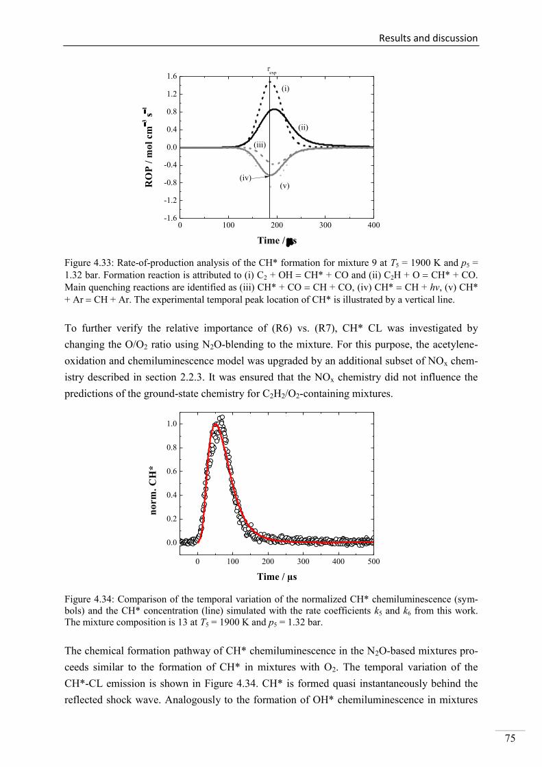
Results and discussion
75
0 100 200 300 400-1.6
-1.2
-0.8
-0.4
0.0
0.4
0.8
1.2
1.6
(iv)(v)
(iii)
(ii)
RO
P /
mo
l cm
3 s
1
Time / s
(i)
exp
Figure 4.33: Rate-of-production analysis of the CH* formation for mixture 9 at T5 = 1900 K and p5 =
1.32 bar. Formation reaction is attributed to (i) C2 + OH CH* + CO and (ii) C2H + O CH* + CO.
Main quenching reactions are identified as (iii) CH* + CO CH + CO, (iv) CH* CH + hv, (v) CH*
+ Ar CH + Ar. The experimental temporal peak location of CH* is illustrated by a vertical line.
To further verify the relative importance of (R6) vs. (R7), CH* CL was investigated by
changing the O/O2 ratio using N2O-blending to the mixture. For this purpose, the acetylene-
oxidation and chemiluminescence model was upgraded by an additional subset of NOx chem-
istry described in section 2.2.3. It was ensured that the NOx chemistry did not influence the
predictions of the ground-state chemistry for C2H2/O2-containing mixtures.
0 100 200 300 400 500
0.0
0.2
0.4
0.6
0.8
1.0
no
rm
. C
H*
Time / µs
Figure 4.34: Comparison of the temporal variation of the normalized CH* chemiluminescence (sym-
bols) and the CH* concentration (line) simulated with the rate coefficients k5 and k6 from this work.
The mixture composition is 13 at T5 = 1900 K and p5 = 1.32 bar.
The chemical formation pathway of CH* chemiluminescence in the N2O-based mixtures pro-
ceeds similar to the formation of CH* in mixtures with O2. The temporal variation of the
CH*-CL emission is shown in Figure 4.34. CH* is formed quasi instantaneously behind the
reflected shock wave. Analogously to the formation of OH* chemiluminescence in mixtures
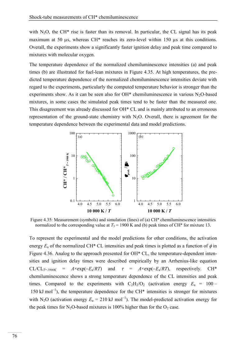
Shock-tube measurements of CH* chemiluminescence
76
with N2O, the CH* rise is faster than its removal. In particular, the CL signal has its peak
maximum at 50 s, whereas CH* reaches its zero-level within 150 s at this conditions.
Overall, the experiments show a significantly faster ignition delay and peak time compared to
mixtures with molecular oxygen.
The temperature dependence of the normalized chemiluminescence intensities (a) and peak
times (b) are illustrated for fuel-lean mixtures in Figure 4.35. At high temperatures, the pre-
dicted temperature dependence of the normalized chemiluminescence intensities deviate with
regard to the experiments, particularly the computed temperature behavior is stronger than the
experiments show. As it can be seen also for OH* chemiluminescence in various N2O-based
mixtures, in some cases the simulated peak times tend to be faster than the measured one.
This disagreement was already discussed for OH* CL and is mainly attributed to an erroneous
representation of the ground-state chemistry with N2O. Overall, there is agreement for the
temperature dependence between the experimental data and model predictions.
CH
* /
CH
*T
= 1
90
0 K
4.0 4.5 5.0 5.5 6.00.1
1
10
100(b)
10 000 K / T
(a)
4.0 4.5 5.0 5.5 6.01
10
100
1000
p
ea
k /
s
10 000 K / T
Figure 4.35: Measurement (symbols) and simulation (lines) of (a) CH* chemiluminescence intensities
normalized to the corresponding value at T5 = 1900 K and (b) peak times of CH* for mixture 13.
To represent the experimental and the model predictions for other conditions, the activation
energy Ea of the normalized CH* CL intensities and peak times is plotted as a function of in
Figure 4.36. Analog to the approach presented for OH* CL, the temperature-dependent inten-
sities and ignition delay times were described empirically by an Arrhenius-like equation
CL/CLT=1900K = A×exp(Ea/RT) and = A×exp(Ea/RT), respectively. CH*
chemiluminescence shows a strong temperature dependence of the CL intensities and peak
times. Compared to the experiments with C2H2/O2 (activation energy Ea = 100 –
150 kJ mol1
), the temperature dependence for the CH* intensities is stronger for mixtures
with N2O (activation energy Ea = 210 kJ mol1
). The model-predicted activation energy for
the peak times for N2O-based mixtures is 100% higher than for the O2 case.
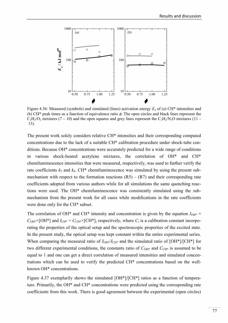
Results and discussion
77
0.50 0.75 1.00 1.2510
100
1000(b)
Ea /
kJ
mo
l1
(a)
0.50 0.75 1.00 1.2510
100
1000
Figure 4.36: Measured (symbols) and simulated (lines) activation energy Ea of (a) CH* intensities and
(b) CH* peak times as a function of equivalence ratio . The open circles and black lines represent the
C2H2/O2 mixtures (7 – 10) and the open squares and grey lines represent the C2H2/N2O mixtures (11 –
13).
The present work solely considers relative CH* intensities and their corresponding computed
concentrations due to the lack of a suitable CH* calibration procedure under shock-tube con-
ditions. Because OH* concentrations were accurately predicted for a wide range of conditions
in various shock-heated acetylene mixtures, the correlation of OH* and CH*
chemiluminescence intensities that were measured, respectively, was used to further verify the
rate coefficients k5 and k6. CH* chemiluminescence was simulated by using the present sub-
mechanism with respect to the formation reactions (R5) – (R7) and their corresponding rate
coefficients adopted from various authors while for all simulations the same quenching reac-
tions were used. The OH* chemiluminescence was consistently simulated using the sub-
mechanism from the present work for all cases while modifications in the rate coefficients
were done only for the CH* subset.
The correlation of OH* and CH* intensity and concentration is given by the equation IOH* =
COH*×[OH*] and ICH* = CCH*×[CH*], respectively, where Ci is a calibration constant incorpo-
rating the properties of the optical setup and the spectroscopic properties of the excited state.
In the present study, the optical setup was kept constant within the entire experimental series.
When comparing the measured ratio of IOH*/ICH* and the simulated ratio of [OH*]/[CH*] for
two different experimental conditions, the constants ratio of COH* and CCH* is assumed to be
equal to 1 and one can get a direct correlation of measured intensities and simulated concen-
trations which can be used to verify the predicted CH* concentrations based on the well-
known OH* concentrations.
Figure 4.37 exemplarily shows the simulated [OH*]/[CH*] ratios as a function of tempera-
ture. Primarily, the OH* and CH* concentrations were predicted using the corresponding rate
coefficients from this work. There is good agreement between the experimental (open circles)
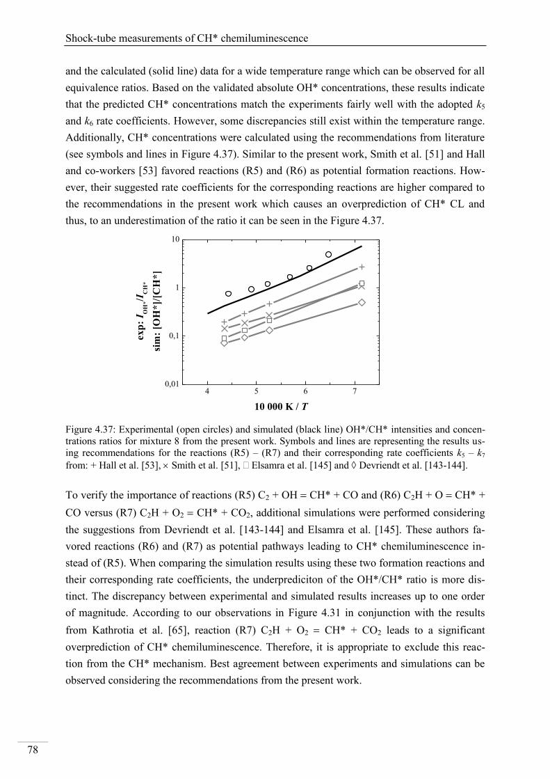
Shock-tube measurements of CH* chemiluminescence
78
and the calculated (solid line) data for a wide temperature range which can be observed for all
equivalence ratios. Based on the validated absolute OH* concentrations, these results indicate
that the predicted CH* concentrations match the experiments fairly well with the adopted k5
and k6 rate coefficients. However, some discrepancies still exist within the temperature range.
Additionally, CH* concentrations were calculated using the recommendations from literature
(see symbols and lines in Figure 4.37). Similar to the present work, Smith et al. [51] and Hall
and co-workers [53] favored reactions (R5) and (R6) as potential formation reactions. How-
ever, their suggested rate coefficients for the corresponding reactions are higher compared to
the recommendations in the present work which causes an overprediction of CH* CL and
thus, to an underestimation of the ratio it can be seen in the Figure 4.37.
4 5 6 70,01
0,1
1
10
ex
p:
I OH
*/I
CH
*
sim
: [O
H*
]/[C
H*
]
10 000 K / T
Figure 4.37: Experimental (open circles) and simulated (black line) OH*/CH* intensities and concen-
trations ratios for mixture 8 from the present work. Symbols and lines are representing the results us-
ing recommendations for the reactions (R5) – (R7) and their corresponding rate coefficients k5 – k7
from: + Hall et al. [53], Smith et al. [51], Elsamra et al. [145] and Devriendt et al. [143-144].
To verify the importance of reactions (R5) C2 + OH CH* + CO and (R6) C2H + O CH* +
CO versus (R7) C2H + O2 CH* + CO2, additional simulations were performed considering
the suggestions from Devriendt et al. [143-144] and Elsamra et al. [145]. These authors fa-
vored reactions (R6) and (R7) as potential pathways leading to CH* chemiluminescence in-
stead of (R5). When comparing the simulation results using these two formation reactions and
their corresponding rate coefficients, the underprediciton of the OH*/CH* ratio is more dis-
tinct. The discrepancy between experimental and simulated results increases up to one order
of magnitude. According to our observations in Figure 4.31 in conjunction with the results
from Kathrotia et al. [65], reaction (R7) C2H + O2 CH* + CO2 leads to a significant
overprediction of CH* chemiluminescence. Therefore, it is appropriate to exclude this reac-
tion from the CH* mechanism. Best agreement between experiments and simulations can be
observed considering the recommendations from the present work.
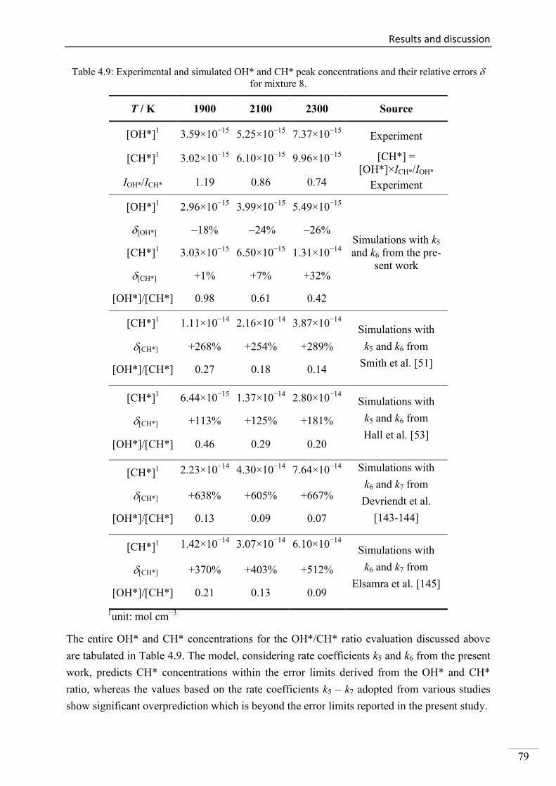
Results and discussion
79
Table 4.9: Experimental and simulated OH* and CH* peak concentrations and their relative errors
for mixture 8.
T / K 1900 2100 2300 Source
[OH*]1 3.59×10
−15 5.25×10
−15 7.37×10
−15 Experiment
[CH*]1 3.02×10
−15 6.10×10
−15 9.96×10
−15 [CH*] =
[OH*]×ICH*/IOH*
IOH*/ICH* 1.19 0.86 0.74 Experiment
[OH*]1 2.96×10
−15 3.99×10
−15 5.49×10
−15
Simulations with k5
and k6 from the pre-
sent work
[OH*] 18% 24% 26%
[CH*]1 3.03×10
−15 6.50×10
−15 1.31×10
−14
[CH*] +1% +7% +32%
[OH*]/[CH*] 0.98 0.61 0.42
[CH*]1 1.11×10
−14 2.16×10
−14 3.87×10
−14
Simulations with
k5 and k6 from
Smith et al. [51]
[CH*] +268% +254% +289%
[OH*]/[CH*] 0.27 0.18 0.14
[CH*]1 6.44×10
−15 1.37×10
−14 2.80×10
−14 Simulations with
k5 and k6 from
Hall et al. [53]
[CH*] +113% +125% +181%
[OH*]/[CH*] 0.46 0.29 0.20
[CH*]1 2.23×10
−14 4.30×10
−14 7.64×10
−14 Simulations with
k6 and k7 from
Devriendt et al.
[143-144]
[CH*] +638% +605% +667%
[OH*]/[CH*] 0.13 0.09 0.07
[CH*]1 1.42×10
−14 3.07×10
−14 6.10×10
−14
Simulations with
k6 and k7 from
Elsamra et al. [145]
[CH*] +370% +403% +512%
[OH*]/[CH*] 0.21 0.13 0.09
1unit: mol cm
−3
The entire OH* and CH* concentrations for the OH*/CH* ratio evaluation discussed above
are tabulated in Table 4.9. The model, considering rate coefficients k5 and k6 from the present
work, predicts CH* concentrations within the error limits derived from the OH* and CH*
ratio, whereas the values based on the rate coefficients k5 – k7 adopted from various studies
show significant overprediction which is beyond the error limits reported in the present study.
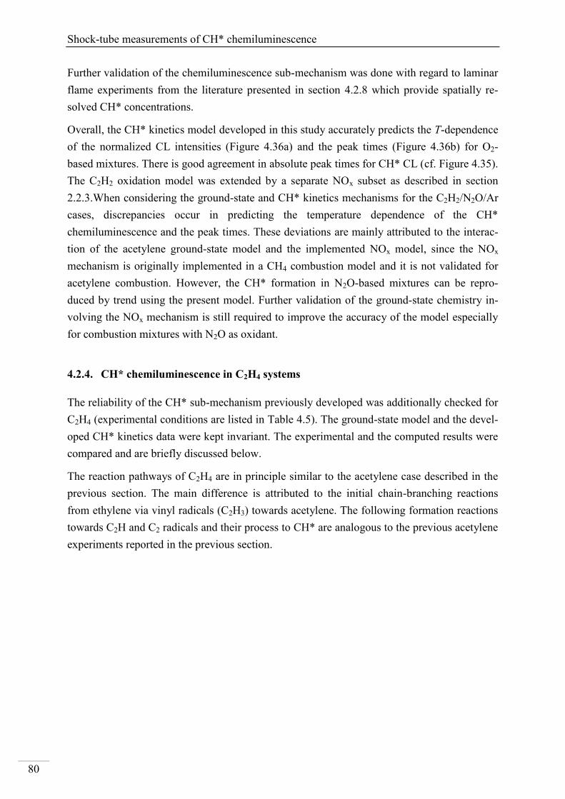
Shock-tube measurements of CH* chemiluminescence
80
Further validation of the chemiluminescence sub-mechanism was done with regard to laminar
flame experiments from the literature presented in section 4.2.8 which provide spatially re-
solved CH* concentrations.
Overall, the CH* kinetics model developed in this study accurately predicts the T-dependence
of the normalized CL intensities (Figure 4.36a) and the peak times (Figure 4.36b) for O2-
based mixtures. There is good agreement in absolute peak times for CH* CL (cf. Figure 4.35).
The C2H2 oxidation model was extended by a separate NOx subset as described in section
2.2.3.When considering the ground-state and CH* kinetics mechanisms for the C2H2/N2O/Ar
cases, discrepancies occur in predicting the temperature dependence of the CH*
chemiluminescence and the peak times. These deviations are mainly attributed to the interac-
tion of the acetylene ground-state model and the implemented NOx model, since the NOx
mechanism is originally implemented in a CH4 combustion model and it is not validated for
acetylene combustion. However, the CH* formation in N2O-based mixtures can be repro-
duced by trend using the present model. Further validation of the ground-state chemistry in-
volving the NOx mechanism is still required to improve the accuracy of the model especially
for combustion mixtures with N2O as oxidant.
4.2.4. CH* chemiluminescence in C2H4 systems
The reliability of the CH* sub-mechanism previously developed was additionally checked for
C2H4 (experimental conditions are listed in Table 4.5). The ground-state model and the devel-
oped CH* kinetics data were kept invariant. The experimental and the computed results were
compared and are briefly discussed below.
The reaction pathways of C2H4 are in principle similar to the acetylene case described in the
previous section. The main difference is attributed to the initial chain-branching reactions
from ethylene via vinyl radicals (C2H3) towards acetylene. The following formation reactions
towards C2H and C2 radicals and their process to CH* are analogous to the previous acetylene
experiments reported in the previous section.
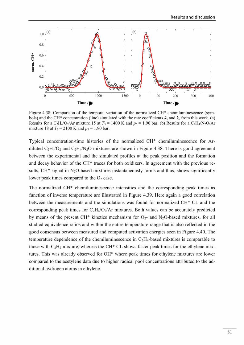
Results and discussion
81
Figure 4.38: Comparison of the temporal variation of the normalized CH* chemiluminescence (sym-
bols) and the CH* concentration (line) simulated with the rate coefficients k5 and k6 from this work. (a)
Results for a C2H4/O2/Ar mixture 15 at T5 = 1400 K and p5 = 1.90 bar. (b) Results for a C2H4/N2O/Ar
mixture 18 at T5 = 2100 K and p5 = 1.90 bar.
Typical concentration-time histories of the normalized CH* chemiluminescence for Ar-
diluted C2H4/O2 and C2H4/N2O mixtures are shown in Figure 4.38. There is good agreement
between the experimental and the simulated profiles at the peak position and the formation
and decay behavior of the CH* traces for both oxidizers. In agreement with the previous re-
sults, CH* signal in N2O-based mixtures instantaneously forms and thus, shows significantly
lower peak times compared to the O2 case.
The normalized CH* chemiluminescence intensities and the corresponding peak times as
function of inverse temperature are illustrated in Figure 4.39. Here again a good correlation
between the measurements and the simulations was found for normalized CH* CL and the
corresponding peak times for C2H4/O2/Ar mixtures. Both values can be accurately predicted
by means of the present CH* kinetics mechanism for O2- and N2O-based mixtures, for all
studied equivalence ratios and within the entire temperature range that is also reflected in the
good consensus between measured and computed activation energies seen in Figure 4.40. The
temperature dependence of the chemiluminescence in C2H4-based mixtures is comparable to
those with C2H2 mixture, whereas the CH* CL shows faster peak times for the ethylene mix-
tures. This was already observed for OH* where peak times for ethylene mixtures are lower
compared to the acetylene data due to higher radical pool concentrations attributed to the ad-
ditional hydrogen atoms in ethylene.
0 500 1000 1500
0.0
0.2
0.4
0.6
0.8
1.0
no
rm
. C
H*
Time / s
(a)
0 100 200 300 400
Time / s
(b)
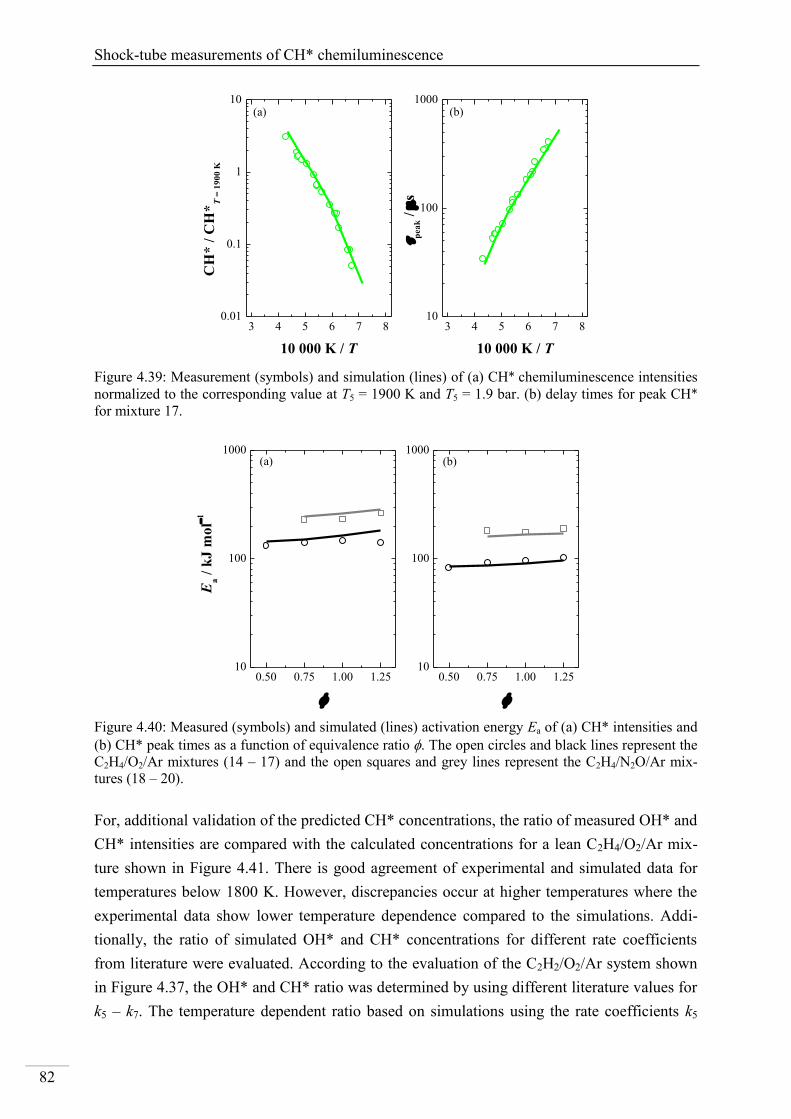
Shock-tube measurements of CH* chemiluminescence
82
3 4 5 6 7 80.01
0.1
1
10(b)(a)
CH
* /
CH
*T
= 1
90
0 K
10 000 K / T
3 4 5 6 7 810
100
1000
pea
k /
s
10 000 K / T
Figure 4.39: Measurement (symbols) and simulation (lines) of (a) CH* chemiluminescence intensities
normalized to the corresponding value at T5 = 1900 K and T5 = 1.9 bar. (b) delay times for peak CH*
for mixture 17.
0.50 0.75 1.00 1.2510
100
1000(b)
Ea /
kJ
mo
l1
(a)
0.50 0.75 1.00 1.2510
100
1000
Figure 4.40: Measured (symbols) and simulated (lines) activation energy Ea of (a) CH* intensities and
(b) CH* peak times as a function of equivalence ratio . The open circles and black lines represent the
C2H4/O2/Ar mixtures (14 – 17) and the open squares and grey lines represent the C2H4/N2O/Ar mix-
tures (18 – 20).
For, additional validation of the predicted CH* concentrations, the ratio of measured OH* and
CH* intensities are compared with the calculated concentrations for a lean C2H4/O2/Ar mix-
ture shown in Figure 4.41. There is good agreement of experimental and simulated data for
temperatures below 1800 K. However, discrepancies occur at higher temperatures where the
experimental data show lower temperature dependence compared to the simulations. Addi-
tionally, the ratio of simulated OH* and CH* concentrations for different rate coefficients
from literature were evaluated. According to the evaluation of the C2H2/O2/Ar system shown
in Figure 4.37, the OH* and CH* ratio was determined by using different literature values for
k5 – k7. The temperature dependent ratio based on simulations using the rate coefficients k5
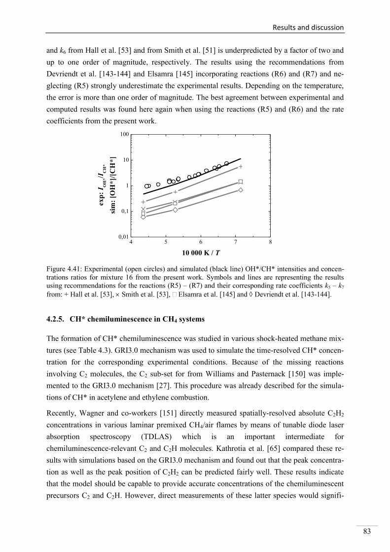
Results and discussion
83
and k6 from Hall et al. [53] and from Smith et al. [51] is underpredicted by a factor of two and
up to one order of magnitude, respectively. The results using the recommendations from
Devriendt et al. [143-144] and Elsamra [145] incorporating reactions (R6) and (R7) and ne-
glecting (R5) strongly underestimate the experimental results. Depending on the temperature,
the error is more than one order of magnitude. The best agreement between experimental and
computed results was found here again when using the reactions (R5) and (R6) and the rate
coefficients from the present work.
4 5 6 7 80,01
0,1
1
10
100
ex
p:
I OH
*/I
CH
*
sim
: [O
H*
]/[C
H*
]
10 000 K / T
Figure 4.41: Experimental (open circles) and simulated (black line) OH*/CH* intensities and concen-
trations ratios for mixture 16 from the present work. Symbols and lines are representing the results
using recommendations for the reactions (R5) – (R7) and their corresponding rate coefficients k5 – k7
from: + Hall et al. [53], Smith et al. [53], Elsamra et al. [145] and Devriendt et al. [143-144].
4.2.5. CH* chemiluminescence in CH4 systems
The formation of CH* chemiluminescence was studied in various shock-heated methane mix-
tures (see Table 4.3). GRI3.0 mechanism was used to simulate the time-resolved CH* concen-
tration for the corresponding experimental conditions. Because of the missing reactions
involving C2 molecules, the C2 sub-set for from Williams and Pasternack [150] was imple-
mented to the GRI3.0 mechanism [27]. This procedure was already described for the simula-
tions of CH* in acetylene and ethylene combustion.
Recently, Wagner and co-workers [151] directly measured spatially-resolved absolute C2H2
concentrations in various laminar premixed CH4/air flames by means of tunable diode laser
absorption spectroscopy (TDLAS) which is an important intermediate for
chemiluminescence-relevant C2 and C2H molecules. Kathrotia et al. [65] compared these re-
sults with simulations based on the GRI3.0 mechanism and found out that the peak concentra-
tion as well as the peak position of C2H2 can be predicted fairly well. These results indicate
that the model should be capable to provide accurate concentrations of the chemiluminescent
precursors C2 and C2H. However, direct measurements of these latter species would signifi-
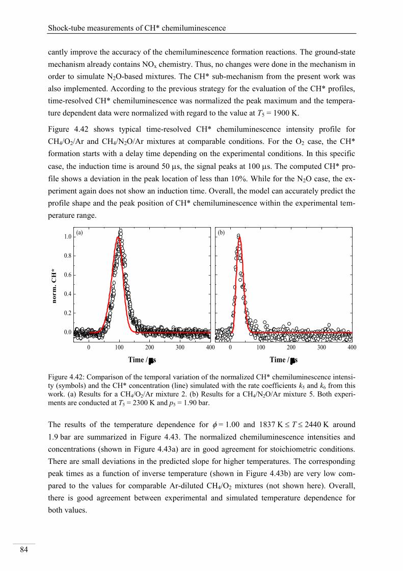
Shock-tube measurements of CH* chemiluminescence
84
cantly improve the accuracy of the chemiluminescence formation reactions. The ground-state
mechanism already contains NOx chemistry. Thus, no changes were done in the mechanism in
order to simulate N2O-based mixtures. The CH* sub-mechanism from the present work was
also implemented. According to the previous strategy for the evaluation of the CH* profiles,
time-resolved CH* chemiluminescence was normalized the peak maximum and the tempera-
ture dependent data were normalized with regard to the value at T5 = 1900 K.
Figure 4.42 shows typical time-resolved CH* chemiluminescence intensity profile for
CH4/O2/Ar and CH4/N2O/Ar mixtures at comparable conditions. For the O2 case, the CH*
formation starts with a delay time depending on the experimental conditions. In this specific
case, the induction time is around 50 s, the signal peaks at 100 s. The computed CH* pro-
file shows a deviation in the peak location of less than 10%. While for the N2O case, the ex-
periment again does not show an induction time. Overall, the model can accurately predict the
profile shape and the peak position of CH* chemiluminescence within the experimental tem-
perature range.
Figure 4.42: Comparison of the temporal variation of the normalized CH* chemiluminescence intensi-
ty (symbols) and the CH* concentration (line) simulated with the rate coefficients k5 and k6 from this
work. (a) Results for a CH4/O2/Ar mixture 2. (b) Results for a CH4/N2O/Ar mixture 5. Both experi-
ments are conducted at T5 = 2300 K and p5 = 1.90 bar.
The results of the temperature dependence for = 1.00 and 1837 K T 2440 K around
1.9 bar are summarized in Figure 4.43. The normalized chemiluminescence intensities and
concentrations (shown in Figure 4.43a) are in good agreement for stoichiometric conditions.
There are small deviations in the predicted slope for higher temperatures. The corresponding
peak times as a function of inverse temperature (shown in Figure 4.43b) are very low com-
pared to the values for comparable Ar-diluted CH4/O2 mixtures (not shown here). Overall,
there is good agreement between experimental and simulated temperature dependence for
both values.
0 100 200 300 400
Time / s
(b)
0 100 200 300 400
0.0
0.2
0.4
0.6
0.8
1.0
no
rm
. C
H*
Time / s
(a)
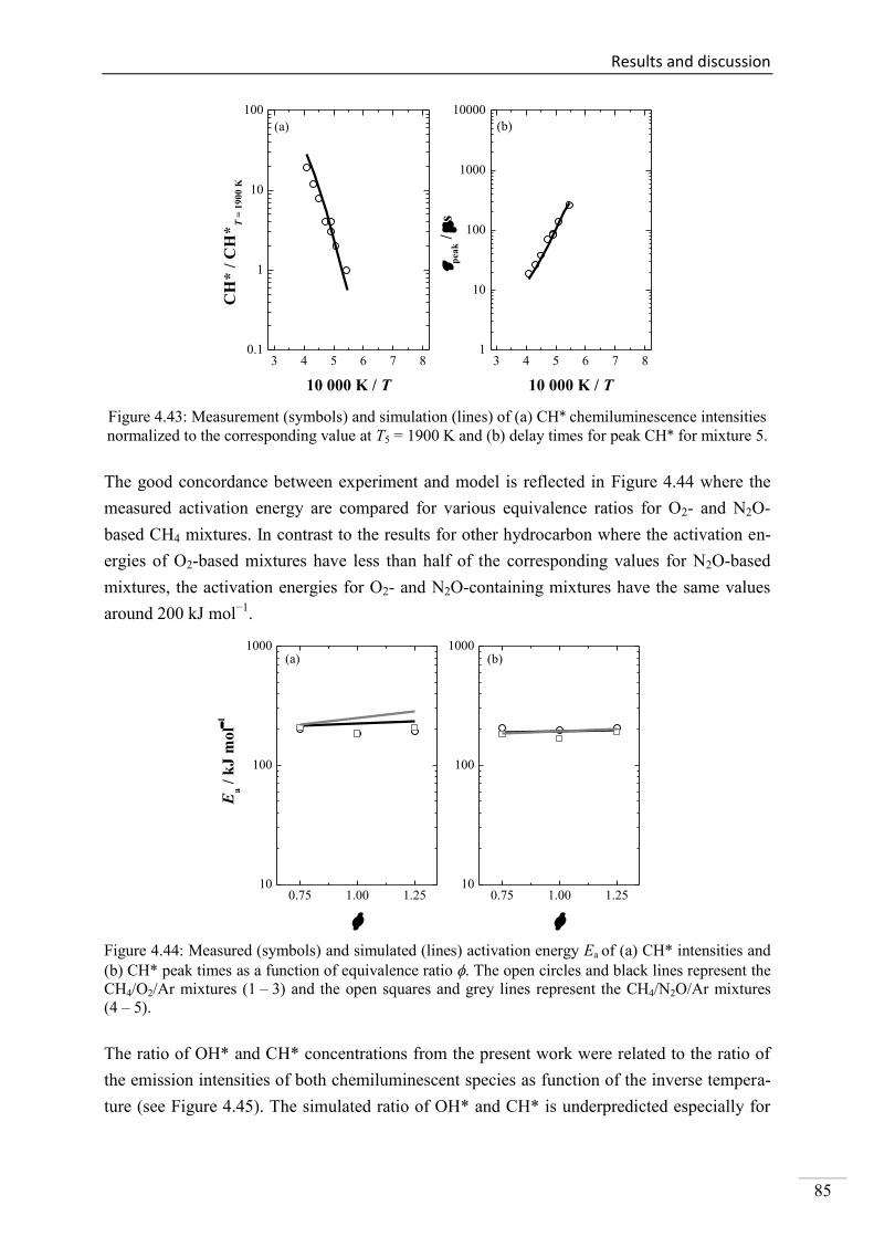
Results and discussion
85
3 4 5 6 7 80.1
1
10
100
(b)
CH
* /
CH
*T
= 1
90
0 K
10 000 K / T
(a)
3 4 5 6 7 81
10
100
1000
10000
pea
k /
s
10 000 K / T
Figure 4.43: Measurement (symbols) and simulation (lines) of (a) CH* chemiluminescence intensities
normalized to the corresponding value at T5 = 1900 K and (b) delay times for peak CH* for mixture 5.
The good concordance between experiment and model is reflected in Figure 4.44 where the
measured activation energy are compared for various equivalence ratios for O2- and N2O-
based CH4 mixtures. In contrast to the results for other hydrocarbon where the activation en-
ergies of O2-based mixtures have less than half of the corresponding values for N2O-based
mixtures, the activation energies for O2- and N2O-containing mixtures have the same values
around 200 kJ mol−1
.
0.75 1.00 1.2510
100
1000(b)
Ea /
kJ
mo
l1
(a)
0.75 1.00 1.2510
100
1000
Figure 4.44: Measured (symbols) and simulated (lines) activation energy Ea of (a) CH* intensities and
(b) CH* peak times as a function of equivalence ratio . The open circles and black lines represent the
CH4/O2/Ar mixtures (1 – 3) and the open squares and grey lines represent the CH4/N2O/Ar mixtures
(4 – 5).
The ratio of OH* and CH* concentrations from the present work were related to the ratio of
the emission intensities of both chemiluminescent species as function of the inverse tempera-
ture (see Figure 4.45). The simulated ratio of OH* and CH* is underpredicted especially for
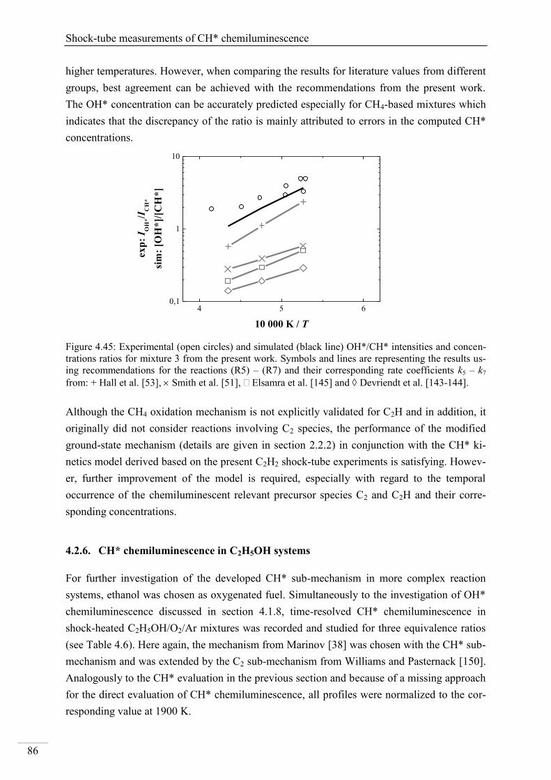
Shock-tube measurements of CH* chemiluminescence
86
higher temperatures. However, when comparing the results for literature values from different
groups, best agreement can be achieved with the recommendations from the present work.
The OH* concentration can be accurately predicted especially for CH4-based mixtures which
indicates that the discrepancy of the ratio is mainly attributed to errors in the computed CH*
concentrations.
4 5 60,1
1
10
ex
p:
I OH
*/I
CH
*
sim
: [O
H*
]/[C
H*
]
10 000 K / T
Figure 4.45: Experimental (open circles) and simulated (black line) OH*/CH* intensities and concen-
trations ratios for mixture 3 from the present work. Symbols and lines are representing the results us-
ing recommendations for the reactions (R5) – (R7) and their corresponding rate coefficients k5 – k7
from: + Hall et al. [53], Smith et al. [51], Elsamra et al. [145] and Devriendt et al. [143-144].
Although the CH4 oxidation mechanism is not explicitly validated for C2H and in addition, it
originally did not consider reactions involving C2 species, the performance of the modified
ground-state mechanism (details are given in section 2.2.2) in conjunction with the CH* ki-
netics model derived based on the present C2H2 shock-tube experiments is satisfying. Howev-
er, further improvement of the model is required, especially with regard to the temporal
occurrence of the chemiluminescent relevant precursor species C2 and C2H and their corre-
sponding concentrations.
4.2.6. CH* chemiluminescence in C2H5OH systems
For further investigation of the developed CH* sub-mechanism in more complex reaction
systems, ethanol was chosen as oxygenated fuel. Simultaneously to the investigation of OH*
chemiluminescence discussed in section 4.1.8, time-resolved CH* chemiluminescence in
shock-heated C2H5OH/O2/Ar mixtures was recorded and studied for three equivalence ratios
(see Table 4.6). Here again, the mechanism from Marinov [38] was chosen with the CH* sub-
mechanism and was extended by the C2 sub-mechanism from Williams and Pasternack [150].
Analogously to the CH* evaluation in the previous section and because of a missing approach
for the direct evaluation of CH* chemiluminescence, all profiles were normalized to the cor-
responding value at 1900 K.
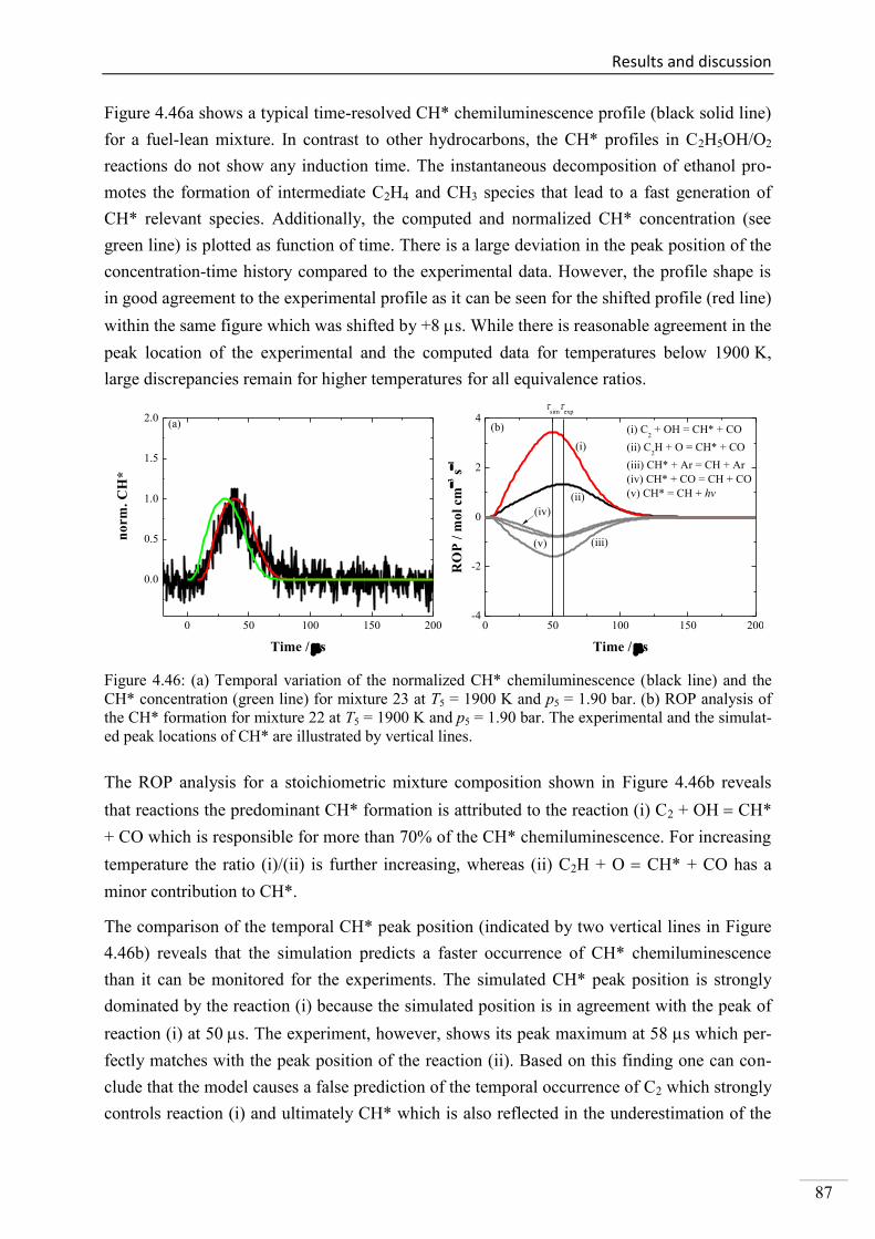
Results and discussion
87
Figure 4.46a shows a typical time-resolved CH* chemiluminescence profile (black solid line)
for a fuel-lean mixture. In contrast to other hydrocarbons, the CH* profiles in C2H5OH/O2
reactions do not show any induction time. The instantaneous decomposition of ethanol pro-
motes the formation of intermediate C2H4 and CH3 species that lead to a fast generation of
CH* relevant species. Additionally, the computed and normalized CH* concentration (see
green line) is plotted as function of time. There is a large deviation in the peak position of the
concentration-time history compared to the experimental data. However, the profile shape is
in good agreement to the experimental profile as it can be seen for the shifted profile (red line)
within the same figure which was shifted by +8 s. While there is reasonable agreement in the
peak location of the experimental and the computed data for temperatures below 1900 K,
large discrepancies remain for higher temperatures for all equivalence ratios.
Figure 4.46: (a) Temporal variation of the normalized CH* chemiluminescence (black line) and the
CH* concentration (green line) for mixture 23 at T5 = 1900 K and p5 = 1.90 bar. (b) ROP analysis of
the CH* formation for mixture 22 at T5 = 1900 K and p5 = 1.90 bar. The experimental and the simulat-
ed peak locations of CH* are illustrated by vertical lines.
The ROP analysis for a stoichiometric mixture composition shown in Figure 4.46b reveals
that reactions the predominant CH* formation is attributed to the reaction (i) C2 + OH CH*
+ CO which is responsible for more than 70% of the CH* chemiluminescence. For increasing
temperature the ratio (i)/(ii) is further increasing, whereas (ii) C2H + O CH* + CO has a
minor contribution to CH*.
The comparison of the temporal CH* peak position (indicated by two vertical lines in Figure
4.46b) reveals that the simulation predicts a faster occurrence of CH* chemiluminescence
than it can be monitored for the experiments. The simulated CH* peak position is strongly
dominated by the reaction (i) because the simulated position is in agreement with the peak of
reaction (i) at 50 s. The experiment, however, shows its peak maximum at 58 s which per-
fectly matches with the peak position of the reaction (ii). Based on this finding one can con-
clude that the model causes a false prediction of the temporal occurrence of C2 which strongly
controls reaction (i) and ultimately CH* which is also reflected in the underestimation of the
0 50 100 150 200-4
-2
0
2
4(i) C
2 + OH = CH* + CO
(ii) C2H + O = CH* + CO
(iii) CH* + Ar = CH + Ar
(iv) CH* + CO = CH + CO
(v) CH* = CH + hv
sim
(v)
(iv)
(iii)
(ii)
RO
P /
mo
l cm
3 s
1
Time / s
exp
(i)
(b)
0 50 100 150 200
0.0
0.5
1.0
1.5
2.0
no
rm
. C
H*
Time / s
(a)
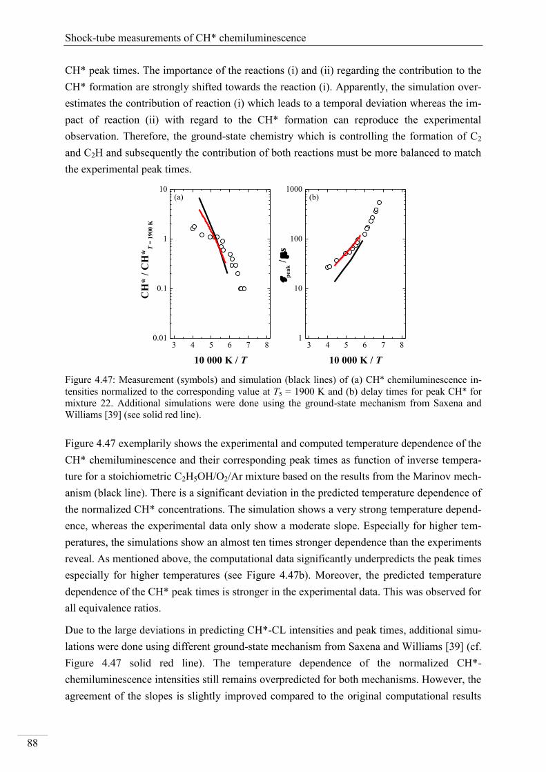
Shock-tube measurements of CH* chemiluminescence
88
CH* peak times. The importance of the reactions (i) and (ii) regarding the contribution to the
CH* formation are strongly shifted towards the reaction (i). Apparently, the simulation over-
estimates the contribution of reaction (i) which leads to a temporal deviation whereas the im-
pact of reaction (ii) with regard to the CH* formation can reproduce the experimental
observation. Therefore, the ground-state chemistry which is controlling the formation of C2
and C2H and subsequently the contribution of both reactions must be more balanced to match
the experimental peak times.
3 4 5 6 7 80.01
0.1
1
10(b)
CH
* /
CH
*T
= 1
90
0 K
10 000 K / T
(a)
3 4 5 6 7 81
10
100
1000
pea
k /
s
10 000 K / T
Figure 4.47: Measurement (symbols) and simulation (black lines) of (a) CH* chemiluminescence in-
tensities normalized to the corresponding value at T5 = 1900 K and (b) delay times for peak CH* for
mixture 22. Additional simulations were done using the ground-state mechanism from Saxena and
Williams [39] (see solid red line).
Figure 4.47 exemplarily shows the experimental and computed temperature dependence of the
CH* chemiluminescence and their corresponding peak times as function of inverse tempera-
ture for a stoichiometric C2H5OH/O2/Ar mixture based on the results from the Marinov mech-
anism (black line). There is a significant deviation in the predicted temperature dependence of
the normalized CH* concentrations. The simulation shows a very strong temperature depend-
ence, whereas the experimental data only show a moderate slope. Especially for higher tem-
peratures, the simulations show an almost ten times stronger dependence than the experiments
reveal. As mentioned above, the computational data significantly underpredicts the peak times
especially for higher temperatures (see Figure 4.47b). Moreover, the predicted temperature
dependence of the CH* peak times is stronger in the experimental data. This was observed for
all equivalence ratios.
Due to the large deviations in predicting CH*-CL intensities and peak times, additional simu-
lations were done using different ground-state mechanism from Saxena and Williams [39] (cf.
Figure 4.47 solid red line). The temperature dependence of the normalized CH*-
chemiluminescence intensities still remains overpredicted for both mechanisms. However, the
agreement of the slopes is slightly improved compared to the original computational results
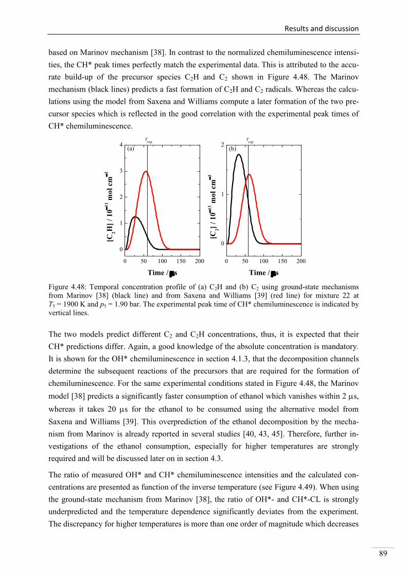
Results and discussion
89
based on Marinov mechanism [38]. In contrast to the normalized chemiluminescence intensi-
ties, the CH* peak times perfectly match the experimental data. This is attributed to the accu-
rate build-up of the precursor species C2H and C2 shown in Figure 4.48. The Marinov
mechanism (black lines) predicts a fast formation of C2H and C2 radicals. Whereas the calcu-
lations using the model from Saxena and Williams compute a later formation of the two pre-
cursor species which is reflected in the good correlation with the experimental peak times of
CH* chemiluminescence.
0 50 100 150 200
0
1
2
3
4
exp
(b)
[C2H
] /
10
11 m
ol
cm
3
Time / s
(a)
exp
0 50 100 150 200
0
1
2
[C2]
/ 1
0
13 m
ol
cm
3
Time / s
Figure 4.48: Temporal concentration profile of (a) C2H and (b) C2 using ground-state mechanisms
from Marinov [38] (black line) and from Saxena and Williams [39] (red line) for mixture 22 at
T5 = 1900 K and p5 = 1.90 bar. The experimental peak time of CH* chemiluminescence is indicated by
vertical lines.
The two models predict different C2 and C2H concentrations, thus, it is expected that their
CH* predictions differ. Again, a good knowledge of the absolute concentration is mandatory.
It is shown for the OH* chemiluminescence in section 4.1.3, that the decomposition channels
determine the subsequent reactions of the precursors that are required for the formation of
chemiluminescence. For the same experimental conditions stated in Figure 4.48, the Marinov
model [38] predicts a significantly faster consumption of ethanol which vanishes within 2 s,
whereas it takes 20 s for the ethanol to be consumed using the alternative model from
Saxena and Williams [39]. This overprediction of the ethanol decomposition by the mecha-
nism from Marinov is already reported in several studies [40, 43, 45]. Therefore, further in-
vestigations of the ethanol consumption, especially for higher temperatures are strongly
required and will be discussed later on in section 4.3.
The ratio of measured OH* and CH* chemiluminescence intensities and the calculated con-
centrations are presented as function of the inverse temperature (see Figure 4.49). When using
the ground-state mechanism from Marinov [38], the ratio of OH*- and CH*-CL is strongly
underpredicted and the temperature dependence significantly deviates from the experiment.
The discrepancy for higher temperatures is more than one order of magnitude which decreases
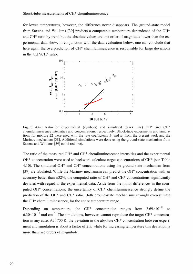
Shock-tube measurements of CH* chemiluminescence
90
for lower temperatures, however, the difference never disappears. The ground-state model
from Saxena and Williams [39] predicts a comparable temperature dependence of the OH*
and CH* ratio by trend but the absolute values are one order of magnitude lower than the ex-
perimental data show. In conjunction with the data evaluation below, one can conclude that
here again the overprediction of CH* chemiluminescence is responsible for large deviations
in the OH*/CH* ratio.
3 4 5 6 7 80,1
1
10
100
ex
p:
I OH
*/I
CH
*
sim
: [O
H*
]/[C
H*
]
10 000 K / T
Figure 4.49: Ratio of experimental (symbols) and simulated (black line) OH* and CH*
chemiluminescence intensities and concentrations, respectively. Shock-tube experiments and simula-
tions for mixture 22 were used with the rate coefficients k5 and k6 from the present work and the
Marinov mechanism [38]. Additional simulations were done using the ground-state mechanism from
Saxena and Williams [39] (solid red line).
The ratio of the measured OH* and CH* chemiluminescence intensities and the experimental
OH* concentration were used to backward calculate target concentrations of CH* (see Table
4.10). The simulated OH* and CH* concentrations using the ground-state mechanism from
[39] are tabulated. While the Marinov mechanism can predict the OH* concentration with an
accuracy better than 32%, the computed ratio of OH* and CH* concentrations significantly
deviates with regard to the experimental data. Aside from the minor differences in the com-
puted OH* concentrations, the uncertainty of CH* chemiluminescence strongly define the
prediction of the OH* and CH* ratio. Both ground-state mechanisms strongly overestimate
the CH* chemiluminescence, for the entire temperature range.
Depending on temperature, the CH* concentration ranges from 2.69×10⁻¹⁶
to
6.30×10⁻¹⁶
mol cm−3
. The simulations, however, cannot reproduce the target CH* concentra-
tion in any case. At 1700 K, the deviation in the absolute CH* concentration between experi-
ment and simulation is about a factor of 2.5, while for increasing temperature this deviation is
more than two orders of magnitude.
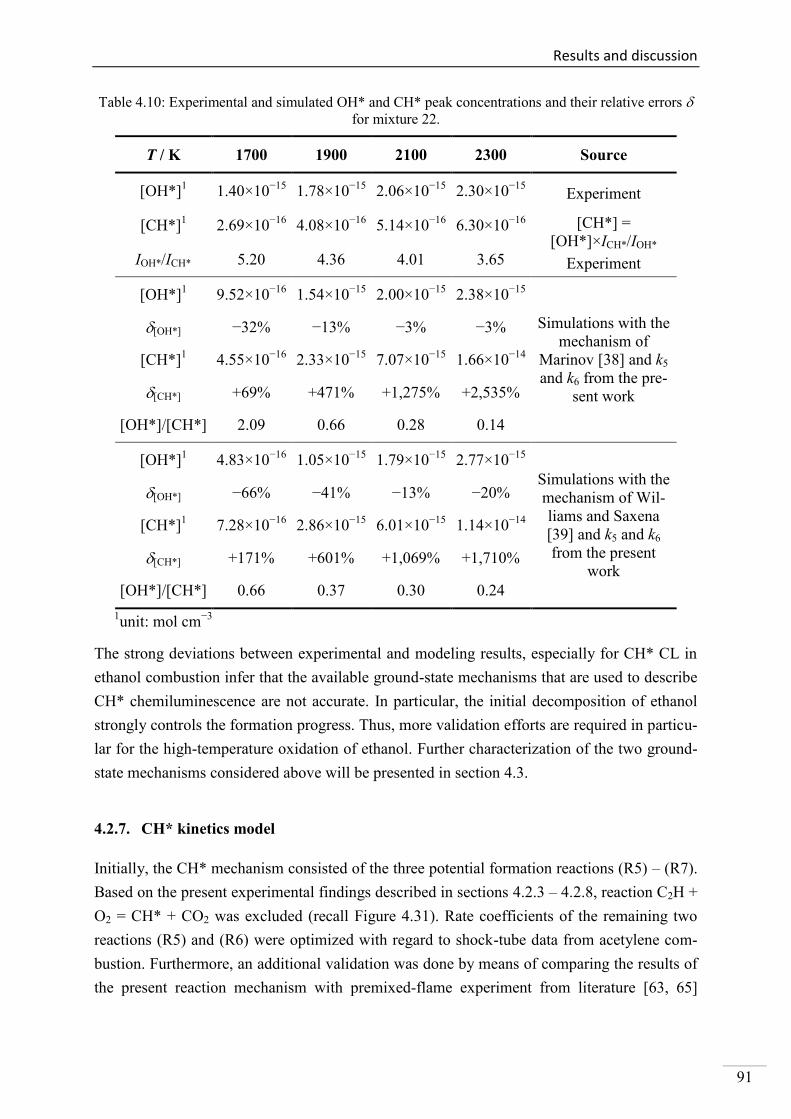
Results and discussion
91
Table 4.10: Experimental and simulated OH* and CH* peak concentrations and their relative errors
for mixture 22.
T / K 1700 1900 2100 2300 Source
[OH*]1 1.40×10
−15 1.78×10
−15 2.06×10
−15 2.30×10
−15 Experiment
[CH*]1 2.69×10
−16 4.08×10
−16 5.14×10
−16 6.30×10
−16 [CH*] =
[OH*]×ICH*/IOH*
IOH*/ICH* 5.20 4.36 4.01 3.65 Experiment
[OH*]1 9.52×10
−16 1.54×10
−15 2.00×10
−15 2.38×10
−15
Simulations with the
mechanism of
Marinov [38] and k5
and k6 from the pre-
sent work
[OH*] −32% −13% −3% −3%
[CH*]1 4.55×10
−16 2.33×10
−15 7.07×10
−15 1.66×10
−14
[CH*] +69% +471% +1,275% +2,535%
[OH*]/[CH*] 2.09 0.66 0.28 0.14
[OH*]1 4.83×10
−16 1.05×10
−15 1.79×10
−15 2.77×10
−15
Simulations with the
mechanism of Wil-
liams and Saxena
[39] and k5 and k6
from the present
work
[OH*] −66% −41% −13% −20%
[CH*]1 7.28×10
−16 2.86×10
−15 6.01×10
−15 1.14×10
−14
[CH*] +171% +601% +1,069% +1,710%
[OH*]/[CH*] 0.66 0.37 0.30 0.24
1unit: mol cm
−3
The strong deviations between experimental and modeling results, especially for CH* CL in
ethanol combustion infer that the available ground-state mechanisms that are used to describe
CH* chemiluminescence are not accurate. In particular, the initial decomposition of ethanol
strongly controls the formation progress. Thus, more validation efforts are required in particu-
lar for the high-temperature oxidation of ethanol. Further characterization of the two ground-
state mechanisms considered above will be presented in section 4.3.
4.2.7. CH* kinetics model
Initially, the CH* mechanism consisted of the three potential formation reactions (R5) – (R7).
Based on the present experimental findings described in sections 4.2.3 – 4.2.8, reaction C2H +
O2 = CH* + CO2 was excluded (recall Figure 4.31). Rate coefficients of the remaining two
reactions (R5) and (R6) were optimized with regard to shock-tube data from acetylene com-
bustion. Furthermore, an additional validation was done by means of comparing the results of
the present reaction mechanism with premixed-flame experiment from literature [63, 65]
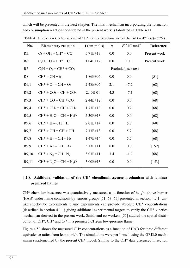
Shock-tube measurements of CH* chemiluminescence
92
which will be presented in the next chapter. The final mechanism incorporating the formation
and consumption reactions considered in the present work is tabulated in Table 4.11.
Table 4.11: Reaction kinetics scheme of CH* species. Reaction rate coefficient k = ATn exp(E/RT).
No. Elementary reaction
A (cm mol s)
n
E / kJ mol–1
Reference
R5 C2 + OH = CH* + CO
5.71E+13
0.0
0.0
Present work
R6 C2H + O = CH* + CO
1.04E+12
0.0
10.9
Present work
R7 C2H + O2 = CH* + CO2
Excluded, see text
R8 CH* = CH + h
1.86E+06
0.0
0.0
[51]
R9,1 CH* + O2 = CH + O2
2.48E+06
2.1
7.2
[68]
R9,2 CH* + CO2 = CH + CO2
2.40E-01
4.3
7.1
[68]
R9,3 CH* + CO = CH + CO
2.44E+12
0.0
0.0
[68]
R9,4 CH* + CH4 = CH + CH4
1.73E+13
0.0
0.7
[68]
R9,5 CH* + H2O = CH + H2O
5.30E+13
0.0
0.0
[68]
R9,6 CH* + H = CH + H
2.01E+14
0.0
5.7
[68]
R9,7 CH* + OH = CH + OH
7.13E+13
0.0
5.7
[68]
R9,8 CH* + H2 = CH + H2
1.47E+14
0.0
5.7
[68]
R9,9 CH* + Ar = CH + Ar 3.13E+11
0.0
0.0
[152]
R9,10 CH* + N2 = CH +N2
3.03E+11
3.4
1.7
[68]
R9,11 CH* + N2O = CH + N2O
5.00E+13
0.0
0.0
[153]
4.2.8. Additional validation of the CH* chemiluminescence mechanism with laminar
premixed flames
CH* chemiluminescence was quantitatively measured as a function of height above burner
(HAB) under flame conditions by various groups [51, 63, 65] presented in section 4.2.1. Un-
like shock-tube experiments, flame experiments can provide absolute CH* concentrations
(described in section 4.1.1) giving additional experimental targets to verify the CH* kinetics
mechanism derived in the present work. Smith and co-workers [51] studied the spatial distri-
bution of OH*, CH* and C2* in a premixed CH4/air low-pressure flame.
Figure 4.50 shows the measured CH* concentrations as a function of HAB for three different
equivalence ratios from lean to rich. The simulations were performed using the GRI3.0 mech-
anism supplemented by the present CH* model. Similar to the OH* data discussed in section
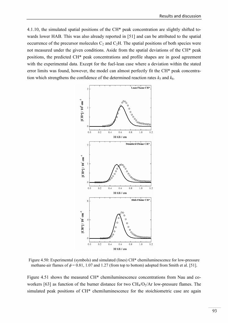
Results and discussion
93
4.1.10, the simulated spatial positions of the CH* peak concentration are slightly shifted to-
wards lower HAB. This was also already reported in [51] and can be attributed to the spatial
occurrence of the precursor molecules C2 and C2H. The spatial positions of both species were
not measured under the given conditions. Aside from the spatial deviations of the CH* peak
positions, the predicted CH* peak concentrations and profile shapes are in good agreement
with the experimental data. Except for the fuel-lean case where a deviation within the stated
error limits was found, however, the model can almost perfectly fit the CH* peak concentra-
tion which strengthens the confidence of the determined reaction rates k5 and k6.
Figure 4.50: Experimental (symbols) and simulated (lines) CH* chemiluminescence for low-pressure
methane-air flames of = 0.81, 1.07 and 1.27 (from top to bottom) adopted from Smith et al. [51].
Figure 4.51 shows the measured CH* chemiluminescence concentrations from Nau and co-
workers [63] as function of the burner distance for two CH4/O2/Ar low-pressure flames. The
simulated peak positions of CH* chemiluminescence for the stoichiometric case are again
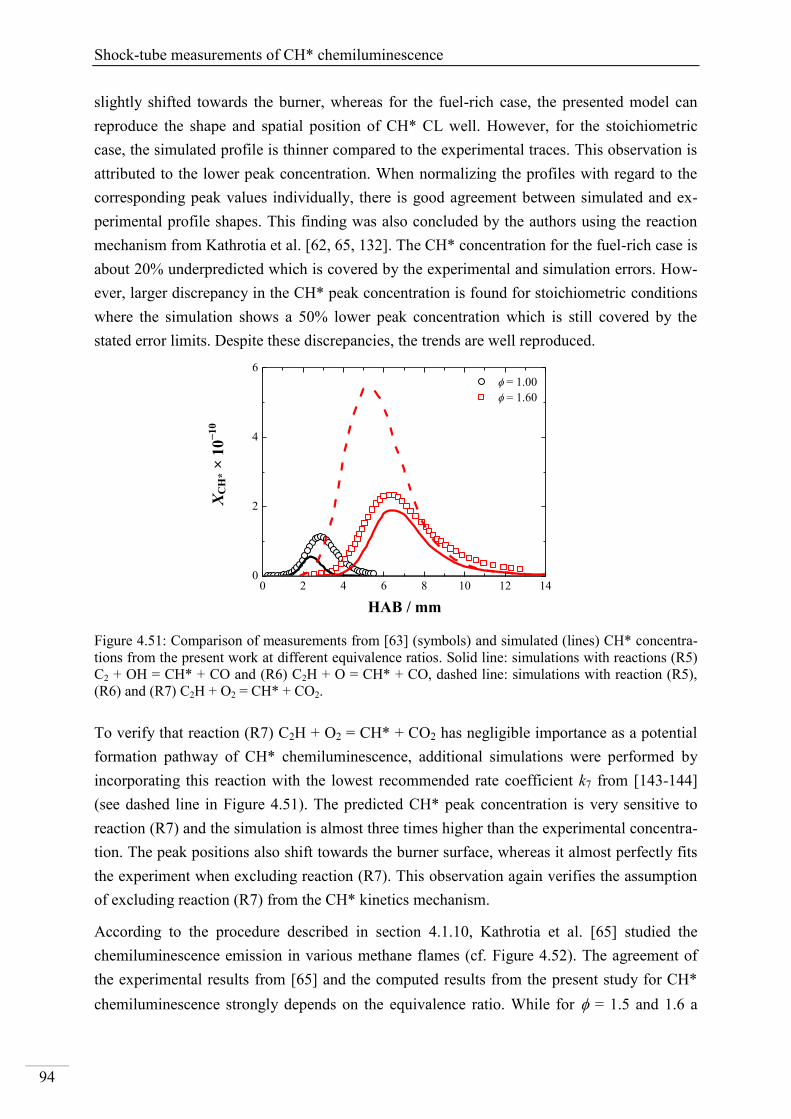
Shock-tube measurements of CH* chemiluminescence
94
slightly shifted towards the burner, whereas for the fuel-rich case, the presented model can
reproduce the shape and spatial position of CH* CL well. However, for the stoichiometric
case, the simulated profile is thinner compared to the experimental traces. This observation is
attributed to the lower peak concentration. When normalizing the profiles with regard to the
corresponding peak values individually, there is good agreement between simulated and ex-
perimental profile shapes. This finding was also concluded by the authors using the reaction
mechanism from Kathrotia et al. [62, 65, 132]. The CH* concentration for the fuel-rich case is
about 20% underpredicted which is covered by the experimental and simulation errors. How-
ever, larger discrepancy in the CH* peak concentration is found for stoichiometric conditions
where the simulation shows a 50% lower peak concentration which is still covered by the
stated error limits. Despite these discrepancies, the trends are well reproduced.
0 2 4 6 8 10 12 140
2
4
6
= 1.00
= 1.60
C
H*
10
10
HAB / mm
Figure 4.51: Comparison of measurements from [63] (symbols) and simulated (lines) CH* concentra-
tions from the present work at different equivalence ratios. Solid line: simulations with reactions (R5)
C2 + OH = CH* + CO and (R6) C2H + O = CH* + CO, dashed line: simulations with reaction (R5),
(R6) and (R7) C2H + O2 = CH* + CO2.
To verify that reaction (R7) C2H + O2 = CH* + CO2 has negligible importance as a potential
formation pathway of CH* chemiluminescence, additional simulations were performed by
incorporating this reaction with the lowest recommended rate coefficient k7 from [143-144]
(see dashed line in Figure 4.51). The predicted CH* peak concentration is very sensitive to
reaction (R7) and the simulation is almost three times higher than the experimental concentra-
tion. The peak positions also shift towards the burner surface, whereas it almost perfectly fits
the experiment when excluding reaction (R7). This observation again verifies the assumption
of excluding reaction (R7) from the CH* kinetics mechanism.
According to the procedure described in section 4.1.10, Kathrotia et al. [65] studied the
chemiluminescence emission in various methane flames (cf. Figure 4.52). The agreement of
the experimental results from [65] and the computed results from the present study for CH*
chemiluminescence strongly depends on the equivalence ratio. While for = 1.5 and 1.6 a
XC
H* ×
10−
10
HAB / mm
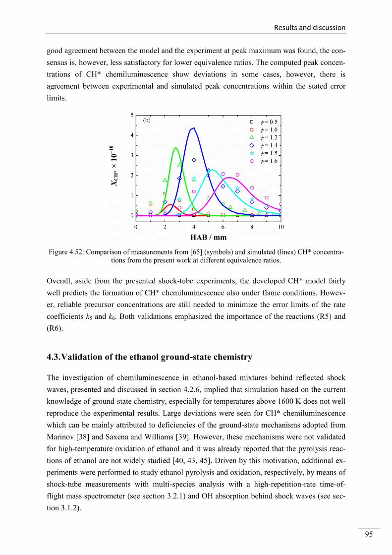
Results and discussion
95
good agreement between the model and the experiment at peak maximum was found, the con-
sensus is, however, less satisfactory for lower equivalence ratios. The computed peak concen-
trations of CH* chemiluminescence show deviations in some cases, however, there is
agreement between experimental and simulated peak concentrations within the stated error
limits.
Figure 4.52: Comparison of measurements from [65] (symbols) and simulated (lines) CH* concentra-
tions from the present work at different equivalence ratios.
Overall, aside from the presented shock-tube experiments, the developed CH* model fairly
well predicts the formation of CH* chemiluminescence also under flame conditions. Howev-
er, reliable precursor concentrations are still needed to minimize the error limits of the rate
coefficients k5 and k6. Both validations emphasized the importance of the reactions (R5) and
(R6).
4.3. Validation of the ethanol ground-state chemistry
The investigation of chemiluminescence in ethanol-based mixtures behind reflected shock
waves, presented and discussed in section 4.2.6, implied that simulation based on the current
knowledge of ground-state chemistry, especially for temperatures above 1600 K does not well
reproduce the experimental results. Large deviations were seen for CH* chemiluminescence
which can be mainly attributed to deficiencies of the ground-state mechanisms adopted from
Marinov [38] and Saxena and Williams [39]. However, these mechanisms were not validated
for high-temperature oxidation of ethanol and it was already reported that the pyrolysis reac-
tions of ethanol are not widely studied [40, 43, 45]. Driven by this motivation, additional ex-
periments were performed to study ethanol pyrolysis and oxidation, respectively, by means of
shock-tube measurements with multi-species analysis with a high-repetition-rate time-of-
flight mass spectrometer (see section 3.2.1) and OH absorption behind shock waves (see sec-
tion 3.1.2).
HAB / mm
XC
H* ×
10−
10
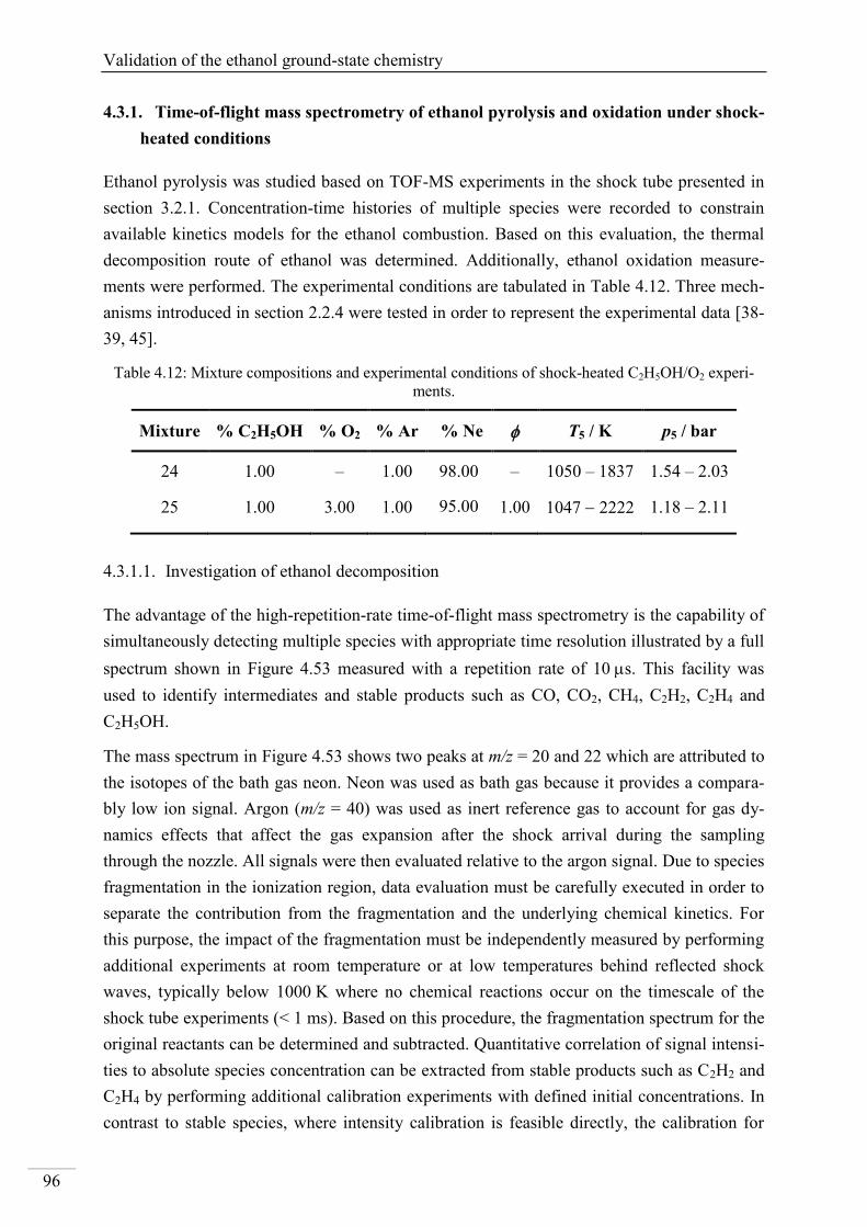
Validation of the ethanol ground-state chemistry
96
4.3.1. Time-of-flight mass spectrometry of ethanol pyrolysis and oxidation under shock-
heated conditions
Ethanol pyrolysis was studied based on TOF-MS experiments in the shock tube presented in
section 3.2.1. Concentration-time histories of multiple species were recorded to constrain
available kinetics models for the ethanol combustion. Based on this evaluation, the thermal
decomposition route of ethanol was determined. Additionally, ethanol oxidation measure-
ments were performed. The experimental conditions are tabulated in Table 4.12. Three mech-
anisms introduced in section 2.2.4 were tested in order to represent the experimental data [38-
39, 45].
Table 4.12: Mixture compositions and experimental conditions of shock-heated C2H5OH/O2 experi-
ments.
Mixture % C2H5OH % O2 % Ar % Ne T5 / K p5 / bar
24 1.00 – 1.00 98.00 – 1050 – 1837 1.54 – 2.03
25 1.00 3.00 1.00 95.00 1.00 1047 2222 1.18 – 2.11
4.3.1.1. Investigation of ethanol decomposition
The advantage of the high-repetition-rate time-of-flight mass spectrometry is the capability of
simultaneously detecting multiple species with appropriate time resolution illustrated by a full
spectrum shown in Figure 4.53 measured with a repetition rate of 10 s. This facility was
used to identify intermediates and stable products such as CO, CO2, CH4, C2H2, C2H4 and
C2H5OH.
The mass spectrum in Figure 4.53 shows two peaks at m/z = 20 and 22 which are attributed to
the isotopes of the bath gas neon. Neon was used as bath gas because it provides a compara-
bly low ion signal. Argon (m/z = 40) was used as inert reference gas to account for gas dy-
namics effects that affect the gas expansion after the shock arrival during the sampling
through the nozzle. All signals were then evaluated relative to the argon signal. Due to species
fragmentation in the ionization region, data evaluation must be carefully executed in order to
separate the contribution from the fragmentation and the underlying chemical kinetics. For
this purpose, the impact of the fragmentation must be independently measured by performing
additional experiments at room temperature or at low temperatures behind reflected shock
waves, typically below 1000 K where no chemical reactions occur on the timescale of the
shock tube experiments (< 1 ms). Based on this procedure, the fragmentation spectrum for the
original reactants can be determined and subtracted. Quantitative correlation of signal intensi-
ties to absolute species concentration can be extracted from stable products such as C2H2 and
C2H4 by performing additional calibration experiments with defined initial concentrations. In
contrast to stable species, where intensity calibration is feasible directly, the calibration for
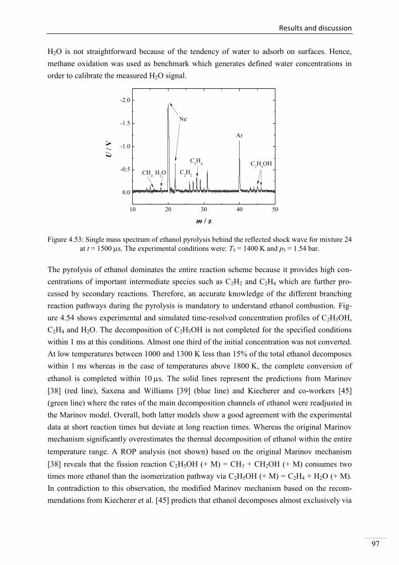
Results and discussion
97
H2O is not straightforward because of the tendency of water to adsorb on surfaces. Hence,
methane oxidation was used as benchmark which generates defined water concentrations in
order to calibrate the measured H2O signal.
10 20 30 40 50
0.0
-0.5
-1.0
-1.5
-2.0
CH4
H2O C
2H
2
C2H
4 C2H
5OH
Ar
U /
V
m / z
Ne
Figure 4.53: Single mass spectrum of ethanol pyrolysis behind the reflected shock wave for mixture 24
at t = 1500 s. The experimental conditions were: T5 = 1400 K and p5 = 1.54 bar.
The pyrolysis of ethanol dominates the entire reaction scheme because it provides high con-
centrations of important intermediate species such as C2H2 and C2H4 which are further pro-
cessed by secondary reactions. Therefore, an accurate knowledge of the different branching
reaction pathways during the pyrolysis is mandatory to understand ethanol combustion. Fig-
ure 4.54 shows experimental and simulated time-resolved concentration profiles of C2H5OH,
C2H4 and H2O. The decomposition of C2H5OH is not completed for the specified conditions
within 1 ms at this conditions. Almost one third of the initial concentration was not converted.
At low temperatures between 1000 and 1300 K less than 15% of the total ethanol decomposes
within 1 ms whereas in the case of temperatures above 1800 K, the complete conversion of
ethanol is completed within 10 s. The solid lines represent the predictions from Marinov
[38] (red line), Saxena and Williams [39] (blue line) and Kiecherer and co-workers [45]
(green line) where the rates of the main decomposition channels of ethanol were readjusted in
the Marinov model. Overall, both latter models show a good agreement with the experimental
data at short reaction times but deviate at long reaction times. Whereas the original Marinov
mechanism significantly overestimates the thermal decomposition of ethanol within the entire
temperature range. A ROP analysis (not shown) based on the original Marinov mechanism
[38] reveals that the fission reaction C2H5OH (+ M) = CH3 + CH2OH (+ M) consumes two
times more ethanol than the isomerization pathway via C2H5OH (+ M) = C2H4 + H2O (+ M).
In contradiction to this observation, the modified Marinov mechanism based on the recom-
mendations from Kiecherer et al. [45] predicts that ethanol decomposes almost exclusively via
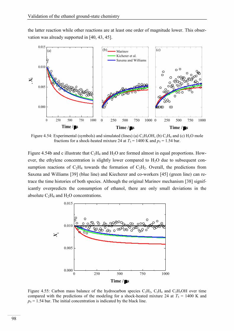
Validation of the ethanol ground-state chemistry
98
the latter reaction while other reactions are at least one order of magnitude lower. This obser-
vation was already supported in [40, 43, 45].
Figure 4.54: Experimental (symbols) and simulated (lines) (a) C2H5OH, (b) C2H4 and (c) H2O mole
fractions for a shock-heated mixture 24 at T5 = 1400 K and p5 = 1.54 bar.
Figure 4.54b and c illustrate that C2H4 and H2O are formed almost in equal proportions. How-
ever, the ethylene concentration is slightly lower compared to H2O due to subsequent con-
sumption reactions of C2H4 towards the formation of C2H2. Overall, the predictions from
Saxena and Williams [39] (blue line) and Kiecherer and co-workers [45] (green line) can re-
trace the time histories of both species. Although the original Marinov mechanism [38] signif-
icantly overpredicts the consumption of ethanol, there are only small deviations in the
absolute C2H4 and H2O concentrations.
0 250 500 750 10000.000
0.005
0.010
0.015
Xi
Time / s
Figure 4.55: Carbon mass balance of the hydrocarbon species C2H2, C2H4 and C2H5OH over time
compared with the predictions of the modeling for a shock-heated mixture 24 at T5 = 1400 K and
p5 = 1.54 bar. The initial concentration is indicated by the black line.
0 250 500 750 1000
Marinov
Kicherer et al.
Saxena and Williams
(c)
Time / s
(b)
0 250 500 750 1000
Time / s
0 250 500 750 1000
0.000
0.005
0.010
0.015
i
Time / s
(a)
Xi
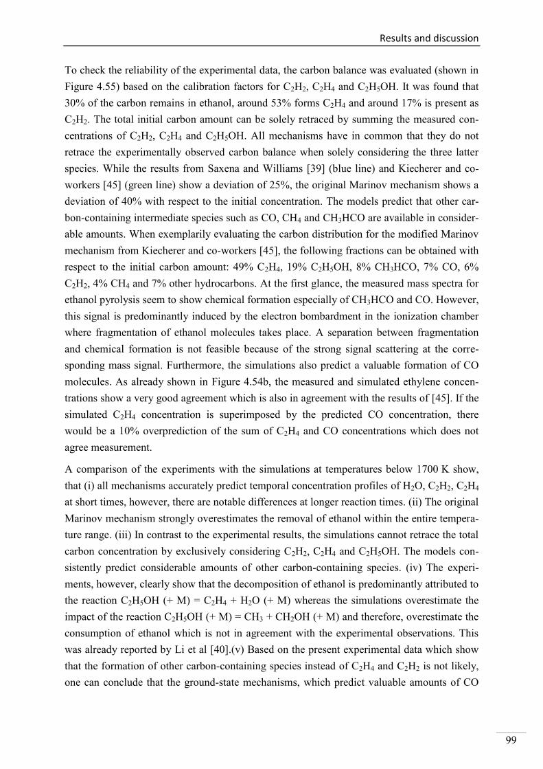
Results and discussion
99
To check the reliability of the experimental data, the carbon balance was evaluated (shown in
Figure 4.55) based on the calibration factors for C2H2, C2H4 and C2H5OH. It was found that
30% of the carbon remains in ethanol, around 53% forms C2H4 and around 17% is present as
C2H2. The total initial carbon amount can be solely retraced by summing the measured con-
centrations of C2H2, C2H4 and C2H5OH. All mechanisms have in common that they do not
retrace the experimentally observed carbon balance when solely considering the three latter
species. While the results from Saxena and Williams [39] (blue line) and Kiecherer and co-
workers [45] (green line) show a deviation of 25%, the original Marinov mechanism shows a
deviation of 40% with respect to the initial concentration. The models predict that other car-
bon-containing intermediate species such as CO, CH4 and CH3HCO are available in consider-
able amounts. When exemplarily evaluating the carbon distribution for the modified Marinov
mechanism from Kiecherer and co-workers [45], the following fractions can be obtained with
respect to the initial carbon amount: 49% C2H4, 19% C2H5OH, 8% CH3HCO, 7% CO, 6%
C2H2, 4% CH4 and 7% other hydrocarbons. At the first glance, the measured mass spectra for
ethanol pyrolysis seem to show chemical formation especially of CH3HCO and CO. However,
this signal is predominantly induced by the electron bombardment in the ionization chamber
where fragmentation of ethanol molecules takes place. A separation between fragmentation
and chemical formation is not feasible because of the strong signal scattering at the corre-
sponding mass signal. Furthermore, the simulations also predict a valuable formation of CO
molecules. As already shown in Figure 4.54b, the measured and simulated ethylene concen-
trations show a very good agreement which is also in agreement with the results of [45]. If the
simulated C2H4 concentration is superimposed by the predicted CO concentration, there
would be a 10% overprediction of the sum of C2H4 and CO concentrations which does not
agree measurement.
A comparison of the experiments with the simulations at temperatures below 1700 K show,
that (i) all mechanisms accurately predict temporal concentration profiles of H2O, C2H2, C2H4
at short times, however, there are notable differences at longer reaction times. (ii) The original
Marinov mechanism strongly overestimates the removal of ethanol within the entire tempera-
ture range. (iii) In contrast to the experimental results, the simulations cannot retrace the total
carbon concentration by exclusively considering C2H2, C2H4 and C2H5OH. The models con-
sistently predict considerable amounts of other carbon-containing species. (iv) The experi-
ments, however, clearly show that the decomposition of ethanol is predominantly attributed to
the reaction C2H5OH (+ M) = C2H4 + H2O (+ M) whereas the simulations overestimate the
impact of the reaction C2H5OH (+ M) = CH3 + CH2OH (+ M) and therefore, overestimate the
consumption of ethanol which is not in agreement with the experimental observations. This
was already reported by Li et al [40].(v) Based on the present experimental data which show
that the formation of other carbon-containing species instead of C2H4 and C2H2 is not likely,
one can conclude that the ground-state mechanisms, which predict valuable amounts of CO
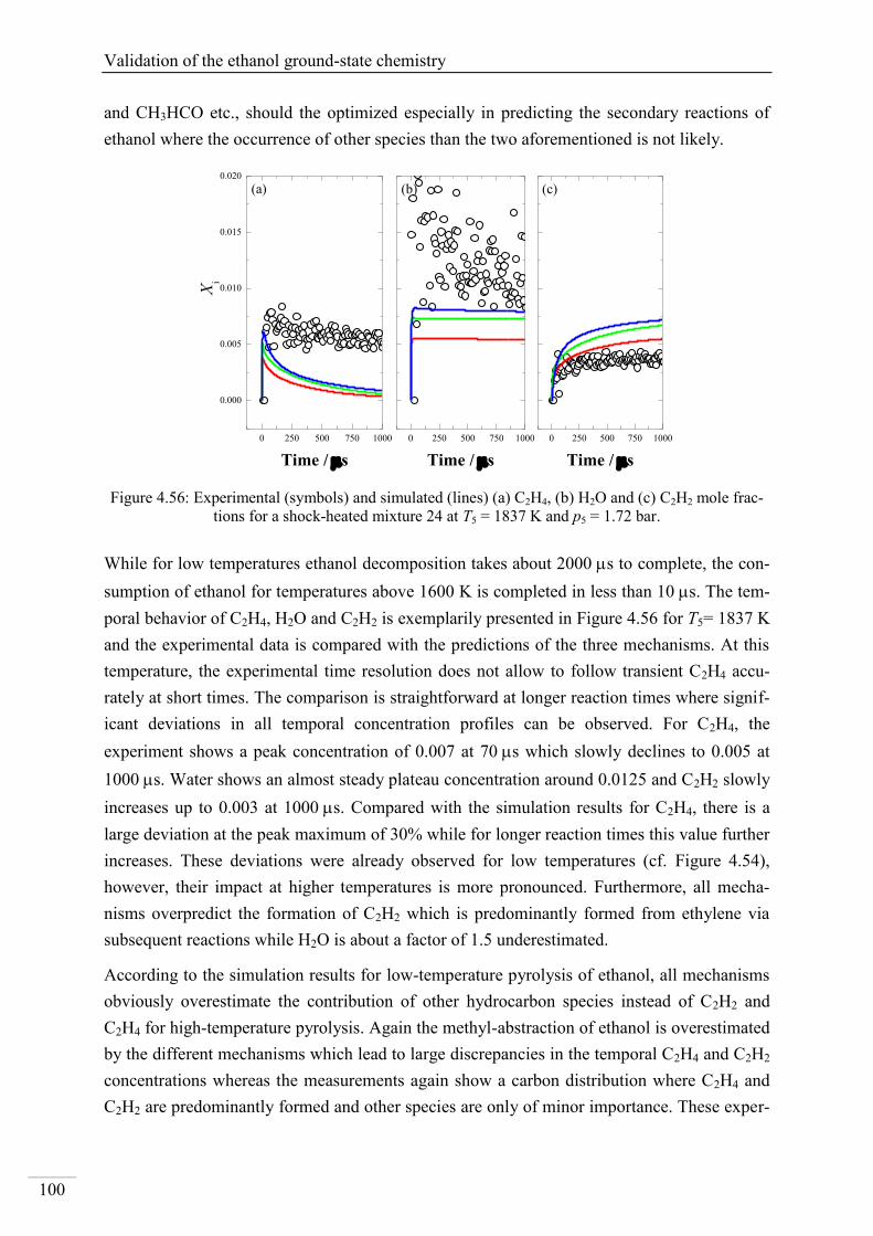
Validation of the ethanol ground-state chemistry
100
and CH3HCO etc., should the optimized especially in predicting the secondary reactions of
ethanol where the occurrence of other species than the two aforementioned is not likely.
0 250 500 750 1000
0.000
0.005
0.010
0.015
0.020
(c)(b)
Xi
Time / s
(a)
0 250 500 750 1000
Time / s
0 250 500 750 1000
Time / s
Figure 4.56: Experimental (symbols) and simulated (lines) (a) C2H4, (b) H2O and (c) C2H2 mole frac-
tions for a shock-heated mixture 24 at T5 = 1837 K and p5 = 1.72 bar.
While for low temperatures ethanol decomposition takes about 2000 s to complete, the con-
sumption of ethanol for temperatures above 1600 K is completed in less than 10 s. The tem-
poral behavior of C2H4, H2O and C2H2 is exemplarily presented in Figure 4.56 for T5= 1837 K
and the experimental data is compared with the predictions of the three mechanisms. At this
temperature, the experimental time resolution does not allow to follow transient C2H4 accu-
rately at short times. The comparison is straightforward at longer reaction times where signif-
icant deviations in all temporal concentration profiles can be observed. For C2H4, the
experiment shows a peak concentration of 0.007 at 70 s which slowly declines to 0.005 at
1000 s. Water shows an almost steady plateau concentration around 0.0125 and C2H2 slowly
increases up to 0.003 at 1000 s. Compared with the simulation results for C2H4, there is a
large deviation at the peak maximum of 30% while for longer reaction times this value further
increases. These deviations were already observed for low temperatures (cf. Figure 4.54),
however, their impact at higher temperatures is more pronounced. Furthermore, all mecha-
nisms overpredict the formation of C2H2 which is predominantly formed from ethylene via
subsequent reactions while H2O is about a factor of 1.5 underestimated.
According to the simulation results for low-temperature pyrolysis of ethanol, all mechanisms
obviously overestimate the contribution of other hydrocarbon species instead of C2H2 and
C2H4 for high-temperature pyrolysis. Again the methyl-abstraction of ethanol is overestimated
by the different mechanisms which lead to large discrepancies in the temporal C2H4 and C2H2
concentrations whereas the measurements again show a carbon distribution where C2H4 and
C2H2 are predominantly formed and other species are only of minor importance. These exper-
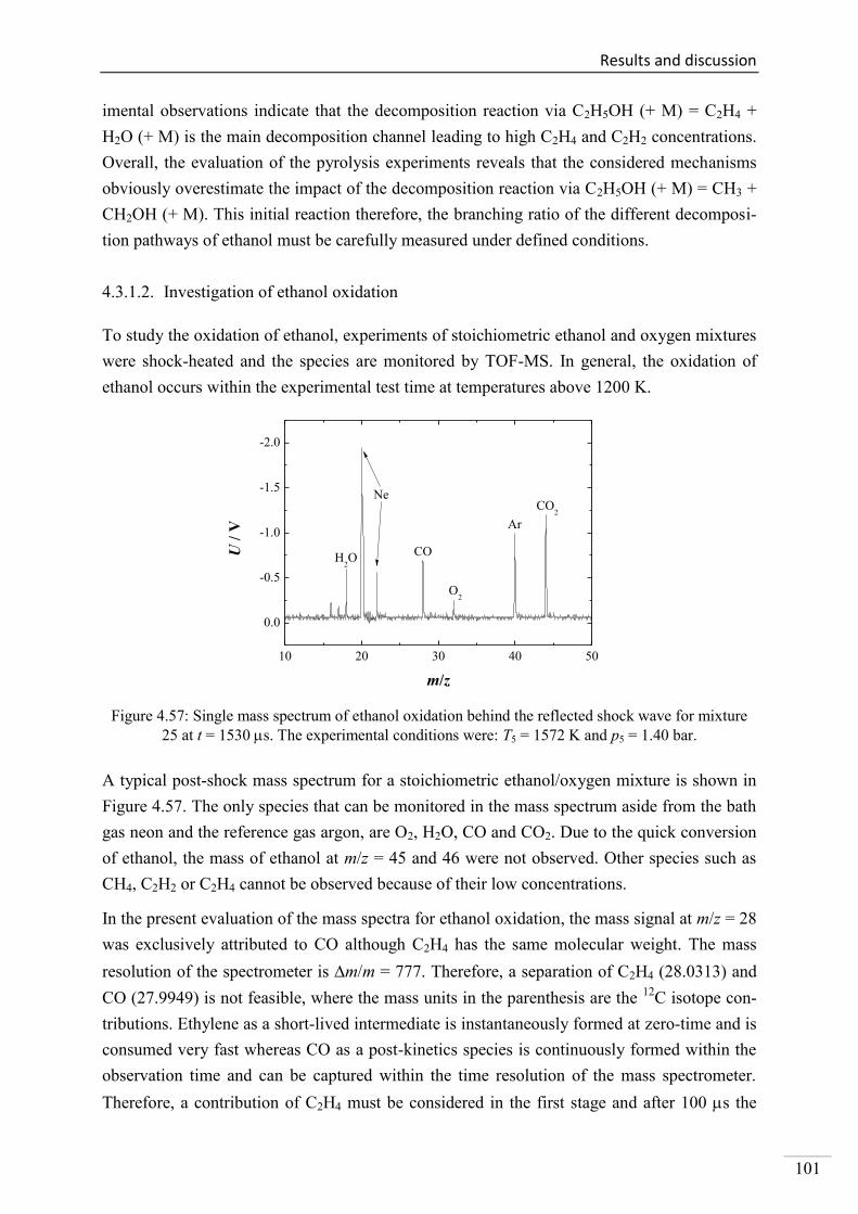
Results and discussion
101
imental observations indicate that the decomposition reaction via C2H5OH (+ M) = C2H4 +
H2O (+ M) is the main decomposition channel leading to high C2H4 and C2H2 concentrations.
Overall, the evaluation of the pyrolysis experiments reveals that the considered mechanisms
obviously overestimate the impact of the decomposition reaction via C2H5OH (+ M) = CH3 +
CH2OH (+ M). This initial reaction therefore, the branching ratio of the different decomposi-
tion pathways of ethanol must be carefully measured under defined conditions.
4.3.1.2. Investigation of ethanol oxidation
To study the oxidation of ethanol, experiments of stoichiometric ethanol and oxygen mixtures
were shock-heated and the species are monitored by TOF-MS. In general, the oxidation of
ethanol occurs within the experimental test time at temperatures above 1200 K.
10 20 30 40 50
0.0
-0.5
-1.0
-1.5
-2.0
Ar
O2
H2O
Ne
CO
U /
V
m/z
CO2
Figure 4.57: Single mass spectrum of ethanol oxidation behind the reflected shock wave for mixture
25 at t = 1530 s. The experimental conditions were: T5 = 1572 K and p5 = 1.40 bar.
A typical post-shock mass spectrum for a stoichiometric ethanol/oxygen mixture is shown in
Figure 4.57. The only species that can be monitored in the mass spectrum aside from the bath
gas neon and the reference gas argon, are O2, H2O, CO and CO2. Due to the quick conversion
of ethanol, the mass of ethanol at m/z = 45 and 46 were not observed. Other species such as
CH4, C2H2 or C2H4 cannot be observed because of their low concentrations.
In the present evaluation of the mass spectra for ethanol oxidation, the mass signal at m/z = 28
was exclusively attributed to CO although C2H4 has the same molecular weight. The mass
resolution of the spectrometer is m/m = 777. Therefore, a separation of C2H4 (28.0313) and
CO (27.9949) is not feasible, where the mass units in the parenthesis are the 12
C isotope con-
tributions. Ethylene as a short-lived intermediate is instantaneously formed at zero-time and is
consumed very fast whereas CO as a post-kinetics species is continuously formed within the
observation time and can be captured within the time resolution of the mass spectrometer.
Therefore, a contribution of C2H4 must be considered in the first stage and after 100 s the
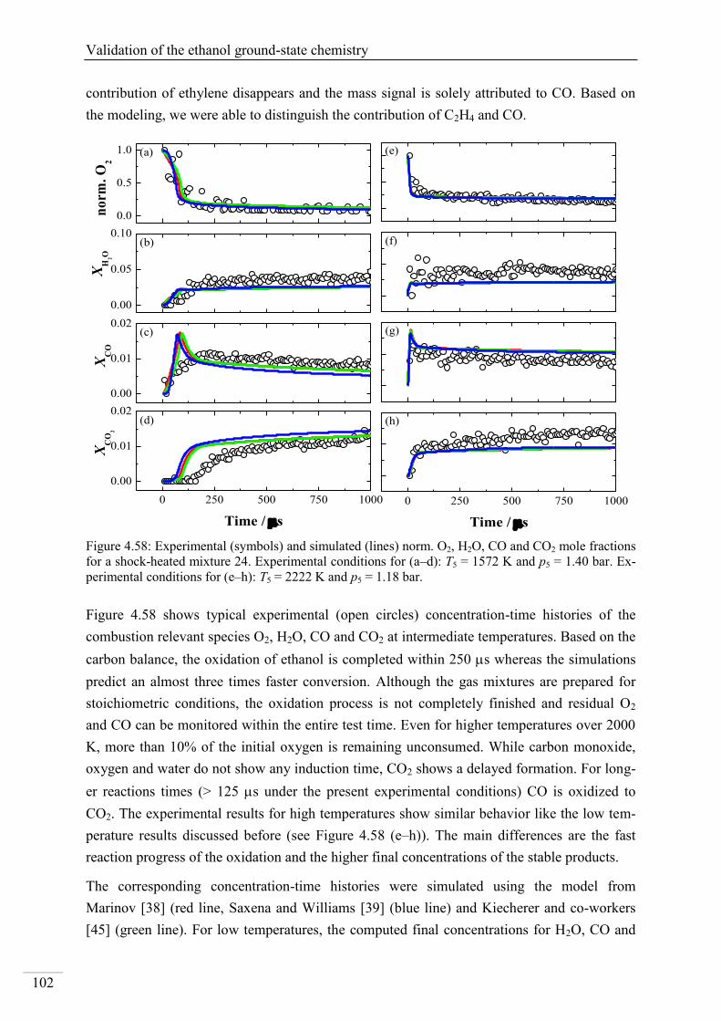
Validation of the ethanol ground-state chemistry
102
contribution of ethylene disappears and the mass signal is solely attributed to CO. Based on
the modeling, we were able to distinguish the contribution of C2H4 and CO.
Figure 4.58: Experimental (symbols) and simulated (lines) norm. O2, H2O, CO and CO2 mole fractions
for a shock-heated mixture 24. Experimental conditions for (a–d): T5 = 1572 K and p5 = 1.40 bar. Ex-
perimental conditions for (e–h): T5 = 2222 K and p5 = 1.18 bar.
Figure 4.58 shows typical experimental (open circles) concentration-time histories of the
combustion relevant species O2, H2O, CO and CO2 at intermediate temperatures. Based on the
carbon balance, the oxidation of ethanol is completed within 250 s whereas the simulations
predict an almost three times faster conversion. Although the gas mixtures are prepared for
stoichiometric conditions, the oxidation process is not completely finished and residual O2
and CO can be monitored within the entire test time. Even for higher temperatures over 2000
K, more than 10% of the initial oxygen is remaining unconsumed. While carbon monoxide,
oxygen and water do not show any induction time, CO2 shows a delayed formation. For long-
er reactions times (> 125 s under the present experimental conditions) CO is oxidized to
CO2. The experimental results for high temperatures show similar behavior like the low tem-
perature results discussed before (see Figure 4.58 (e–h)). The main differences are the fast
reaction progress of the oxidation and the higher final concentrations of the stable products.
The corresponding concentration-time histories were simulated using the model from
Marinov [38] (red line, Saxena and Williams [39] (blue line) and Kiecherer and co-workers
[45] (green line). For low temperatures, the computed final concentrations for H2O, CO and
0 250 500 750 1000
Time / s
(h)
(g)
(f)
(e)
0 250 500 750 1000
0.00
0.01
0.02
0.00
0.01
0.02
0.00
0.05
0.10
0.0
0.5
1.0
XC
O2
Time / s
XC
O
(d)
(c)
(b)
XH
2O
(a)
no
rm.
O2
Results and discussion
103
CO2 from all considered mechanisms match the experimental observations at longer reaction
times. Some deviations are, however, seen at short times. The models predict an almost sud-
den and complete consumption of oxygen within 100 s, whereas the experiment shows a
smooth consumption. As consequence of the fast oxidation behavior, the predicted concentra-
tions of CO and CO2 are significantly higher at short reaction times. Especially for CO, there
is disagreement between computed and measured time profiles at short reaction times. In par-
ticular, the simulated CO concentrations from the various mechanisms show a distinct peak
around 100 s which cannot be observed for the experimental data. While CO is
underpredicted for longer reaction times, CO2 as a direct product of CO is overpredicted.
At higher temperatures, there is better agreement between experiments and simulations for
ethanol oxidation (see Figure 4.59e–h). Here again, the simulations predict a shoulder for CO
that was not observed in the experiments. However, the measured long-term concentrations of
the considered species are in agreement with the experiments. The absolute CO concentration
at longer reaction times is slightly overpredicted, while the computed CO2 concentration is
lower.
Overall, the evaluation of the measurements at short reaction times and low temperatures is
not consistent with any reaction mechanism. There are significant temporal deviations be-
tween experimental and simulated concentration-time profiles which are potentially not
caused by simulation errors but by an insufficient time-resolution of the TOF-MS. Especially
the distinct peak in the CO concentration-time profile, which is typical for hydrocarbon com-
bustion and which was already verified for methyl formate by Ren et al. [154], cannot be re-
produced by the present experimental data. A careful verification of the present time-
resolution of the TOF-MS seems to be essential to quantitatively compare the present experi-
ments and the available reaction mechanisms.
4.3.2. Ring-dye laser measurements of OH
While C2H4 is an important intermediate species during the combustion of most hydrocar-
bons, OH is a transient species that controls branching reactions at early times. For further
validation, ethanol oxidation was monitored by measuring the OH concentration optically.
While there is substantiated knowledge available for the combustion of small hydrocarbons
such as methane, only sparse information can be found for ethanol combustion. In addition to
the shock tube/TOF-MS experiments presented in the previous section, the present study is
also devoted to provide additional validation of OH species by probing the A–X transition.
Analog to the initial OH absorption experiments in the argon-diluted H2/O2 and CH4/O2 sys-
tems described in section 3.1.2.4, additional investigations of OH formation in ethanol com-
bustion were performed.
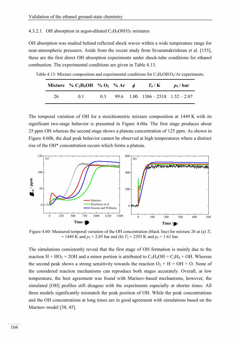
Validation of the ethanol ground-state chemistry
104
4.3.2.1. OH absorption in argon-diluted C2H5OH/O2 mixtures
OH absorption was studied behind reflected shock waves within a wide temperature range for
near-atmospheric pressures. Aside from the recent study from Sivaramakrishnan et al. [155],
these are the first direct OH absorption experiments under shock-tube conditions for ethanol
combustion. The experimental conditions are given in Table 4.13.
Table 4.13: Mixture composition and experimental conditions for C2H5OH/O2/Ar experiments.
Mixture % C2H5OH % O2 % Ar T5 / K p5 / bar
26 0.1 0.3 99.6 1.00 1386 – 2518 1.52 – 2.07
The temporal variation of OH for a stoichiometric mixture composition at 1449 K with its
significant two-stage behavior is presented in Figure 4.60a. The first stage produces about
25 ppm OH whereas the second stage shows a plateau concentration of 125 ppm. As shown in
Figure 4.60b, the dual peak behavior cannot be observed at high temperatures where a distinct
rise of the OH* concentration occurs which forms a plateau.
Figure 4.60: Measured temporal variation of the OH concentration (black line) for mixture 26 at (a) T5
= 1449 K and p5 = 2.05 bar and (b) T5 = 2293 K and p5 = 1.61 bar.
The simulations consistently reveal that the first stage of OH formation is mainly due to the
reaction H + HO2 = 2OH and a minor portion is attributed to C2H4OH = C2H4 + OH. Whereas
the second peak shows a strong sensitivity towards the reaction O2 + H = OH + O. None of
the considered reaction mechanisms can reproduce both stages accurately. Overall, at low
temperature, the best agreement was found with Marinov-based mechanisms, however, the
simulated [OH] profiles still disagree with the experiments especially at shorter times. All
three models significantly mismatch the peak position of OH. While the peak concentrations
and the OH concentrations at long times are in good agreement with simulations based on the
Marinov model [38, 45].
0 250 500 750 1000 1250 1500
0
50
100
150
O
H /
pp
m
Time / s
(a)
Marinov
Kiecherer et al.
Saxena and Williams
0 100 200 300 400 500
0
200
400
600
Time / s
(b)
Results and discussion
105
According to the measurements at temperatures above 1800 K, the dual peak in the simulated
results based on the Saxena and Williams model [39] disappears and only the second peak is
seen (see Figure 4.60b). In contrast to this observation, simulations based on the Marinov
mechanism [38, 45] still show a two stage behavior with a distinct peak at t = 0 s before
merging into the second stage. This temporal discrepancy, however, disappears afterwards
and the simulations can perfectly reproduce the experimental shape and the predicted peak
concentrations with regard to the experimental uncertanities. The erroneous prediction of the
first stage OH at high temperature is still attributed to the contribution of H + HO2 = 2OH.
Whereas for high temperatures, the Marinov-based mechanisms [38, 45] reveal that the
second stage is strongly dominated by the fission reaction of C2H5OH towards C2H5 + OH. At
low temperatures, the second stage was controlled by the chain-branching reaction O2 + H =
OH + O. Contrary to the Marinov models, Saxena and Williams [39] predicts an exclusive
production of OH via O2 + H = OH + O which explain the non-appearance of the first stage.
However, discrepancies in the temporal shape and the absolute OH concentration were found
using the latter mechanism.
Overall, none of the models can accurately and consistently predict the OH formation
throughout the entire temperature range covered herein. While the Marinov based mecha-
nisms show a good performance in predicting the absolute OH concentration, they show sig-
nificant differences in reproducing the temporal behavior. The model from Saxena and
Williams shows a slightly better performance in predicting the temporal OH behavior for high
temperatures whereas it consistently lacks in prediciting the absolute OH concentrations. An
in-depth experimental and modeling investigation of the ethanol ground-state chemistry is
necessary to further improve the predictions of OH during ethanol combustion.
Validation of the ethanol ground-state chemistry
106
5. Conclusions
The optimization and control of practical combustion systems is a prerequisite for increasing
fuel efficiency and reduction of pollutant emission. The use of chemiluminescence (CL) de-
tection has proven to be beneficial under lab-scale conditions since it is a non-expensive and
non-intrusive approach to get quantitative information of global combustion parameters. For
example, the determination of the local equivalence ratios and heat release are potential appli-
cations for combustion research. For this purpose, a quantitative link between the measured
chemiluminescence intensities and the underlying chemical reactions are necessary. However,
the formation kinetics of chemiluminescence is not thoroughly understood and the published
corresponding rate coefficients vary by several orders of magnitude. The complication origi-
nates from the difficulty to establish a quantitative relationship between measured CL intensi-
ties and corresponding species concentrations. An additional complication arises from
uncertainties intrinsic to ground-state chemical reactions of relevance to excited-state species
formation. In particular, a precise quantification of the molecules that lead towards the for-
mation of electronically-excited species is necessary. Therefore, the purpose of the work was
to identify the formation channels of chemiluminescence at atmospheric pressures, to measure
their corresponding rate coefficients, and to develop kinetics mechanisms describing the
chemiluminescence of various systems. For this task, a combination of shock-tube experi-
ments and kinetics simulations was employed where well-known ground-state mechanisms
from literature were used as base to compile kinetics mechanisms for OH* and CH*
chemiluminescence consisting of formation reactions and the corresponding collisional
quenching reactions adopted from literature.
In this thesis, the chemiluminescence of OH* and CH* were systematically investigated based
on CL emission in shock-heated hydrogen and hydrocarbon mixtures. The
chemiluminescence emission from the A–X transitions of OH* around 307 nm and of CH*
around 430 nm, respectively, were detected by two separate interference filter and photomul-
tiplier combinations. The measured temporally-resolved chemiluminescence profiles were
compared with simulated OH* and CH* concentration-time profiles. Within the frame of this
thesis the following findings were achieved.
The formation of OH* chemiluminescence was measured in various H2/O2/Ar mixtures.
Based on a high-temperature calibration where OH* is exclusively formed by OH + M = OH*
+ M, the measured OH* emission intensities were converted to time-resolved OH* concentra-
tions with an accuracy of ±20%. The measured OH* concentrations were then used for the
development and validation of a OH* kinetics mechanism. On the basis of this indirect cali-
bration, the comparison of measured and simulated data revealed that OH* in H2/O2 systems
is predominantly formed by the reaction (R1) H + O + M = OH* + M. The best agreement in
Conclusions
107
terms of absolute OH* concentrations and ignition delay times was found for a rate coeffi-
cient of k1 = (1.5±0.45)×1013
exp(−25.0 kJ mol−1
/RT) cm6mol
−2s−1
. The results were used to
describe OH* chemiluminescence build-up in a hydrocarbon system. With this approach, the
formation channel of OH* in CH4-blended H2/O2 mixtures was investigated. Again, the
measured OH* chemiluminescence was compared with simulations. It was found that the
main formation channel of OH* in hydrocarbon combustion is (R2) CH + O2 = OH* + CO.
The rate coefficient was determined as k2 = (8.0±2.56)×1010
cm3mol
−1s−1
. Collisional quench-
ing reactions and radiative reactions were adopted to account for losses in chemiluminescence
intensity. To check the flexibility of the adopted mechanism further experiments in more
complex hydrocarbon oxidation systems were carried out. Shock-tube experiments of various
hydrocarbon systems (CH4, C2H2, C2H4 and C2H5OH) at various equivalence ratios from 0.50
to 1.25 and with O2 and N2O as oxidizers were performed. Moreover, the modified OH* sub-
mechanism from the present work was tested against flame data from literature. Overall, good
agreement between experimental and modeling data was found for all experimental condi-
tions.
The ratio of OH* and CH* chemiluminescence is often evaluated to determine combustion
relevant parameters such as the local equivalence ratio and heat release. Therefore, a reliable
knowledge of CH* kinetics is important. Because calibration approach for CH*
chemiluminescence signal intensities under shock-tube conditions is not feasible so far, the
evaluation of CH* CL was done by normalizing the intensities and concentration towards the
corresponding value at 1900 K. Acetylene oxidation was chosen as benchmark because it
provides a high amount of C2 and C2H which are assumed to be important key precursors for
CH*. The results showed a significant CH* signal reduction for fuel-lean conditions which
was already reported in literature [53]. This observation was used to identify the CH* for-
mation pathways. The kinetics model could only reproduce this signal reduction when consid-
ering the reactions (R5) C2 + OH = CH* + CO and (R6) C2H + O = CH* + CO while reaction
(R7) C2H + O2 = CH* + CO2 was excluded. When incorporating the latter reaction with a rate
coefficient higher than k7 = 1.0×10¹¹
cm3mol
1s1
, the experimental results could not be re-
produced. This rate coefficient therefore can be considered as an upper limit. The rate coeffi-
cients for the two favored reactions were determined based on the temperature dependence of
the CH* chemiluminescence. The best agreement between experiment and simulations were
k5 = 5.7×10¹³
cm3mol
1s1
and k6 = 1.0×10¹²
exp(10.9 kJ mol1
/RT) cm3mol
1s1
with an
estimated error of ±53%. The CH* mechanism was additionally investigated for various hy-
drocarbon combustion systems (CH4, C2H4 and C2H5OH). While the simulated results based
on the developed CH* sub-mechanisms are in good agreement with the present shock-tube
experiments for methane, acetylene and ethylene systems and flame experiments from litera-
ture, deficiencies have been found for the CH* chemiluminescence predictions of ethanol
combustion. These deviations are mainly attributed to deficiencies of the ground-state mecha-
nisms since the present mechanisms are only validated for temperatures up to 1700 K which is
Validation of the ethanol ground-state chemistry
108
below the present experimental conditions. Therefore, the ground-state chemistry of ethanol
was investigated for pyrolysis and oxidation under shock-tube conditions using time-of-flight
mass spectrometry (TOF-MS) and ring-dye laser absorption spectroscopy (RDLAS).
Time-resolved concentration-times histories of multiple intermediate (C2H2, C2H4) and prod-
uct species (CO, CO2, H2O) were measured for ethanol pyrolysis using a shock tube/time-of-
flight mass spectrometer (TOF-MS) combination. The concentrations of C2H2, C2H4, CO and
CO2 were well-balanced within the experimental error. The carbon balance reveals that the
initial carbon concentration can be reproduced by considering C2H5OH, C2H4 and C2H2 as a
subsequent product of ethylene. Therefore, the present study proved that the pyrolysis of
C2H5OH is strongly controlled by the isomerization pathway C2H5OH (+ M) = C2H4 + H2O
(+ M) while other reactions are of minor importance, otherwise other intermediate species
would be formed and detected by the TOF-MS which was not the case within the present
work. Ground-state mechanisms from Marinov [38], Kiecherer et al. [45] and Saxena and
Williams [39] were tested with satisfactory agreement between experimental and simulated
concentration profiles for C2H5OH, C2H2, C2H4 and H2O for temperatures below 1700 K.
However, large discrepancies were found for the corresponding concentration-time histories
at higher temperatures where the simulated ethanol decomposition was much faster than ob-
served in the present experiments reveal. The mechanisms overestimate the impact of the me-
thyl-abstraction via C2H5OH (+ M) = CH3 + CH2OH (+ M) and therefore, the pyrolysis is
overwhelmed by the respective reaction. Based on the disagreement between experiments and
simulations, the present mechanism must be carefully reevaluated especially with regard to
the branching ratio of the two competeting decomposition pathways of ethanol via C2H5OH
(+ M) = CH3 + CH2OH (+ M) and C2H5OH (+ M) = C2H4 + H2O (+ M) while the present
study strongly indicates that the latter reaction is the most important for the thermal decompo-
sition of ethanol. Overall, the pyrolysis process of ethanol strongly controls the entire com-
bustion process. For an improvement of the available mechanisms, where none of them can
reproduce the experimental results for the entire temperature range of the present study, a de-
tailed evaluation is necessary in future.
Additionally, the oxidation of ethanol was measured for stoichiometric conditions behind re-
flected shock waves using the TOF-MS. While there are deviations in the short-term concen-
tration-time histories especially for CO2, the slow formation of CO, CO2 and H2O and their
absolute concentrations for the ethanol oxidation can be fairly well reproduced by the three
models. However, comparison between experiment and simulation reveal that the measured
concentration-time histories from the TOF-MS show significant deficiencies in the temporal
resolution. The short-term concentrations and fast concentration changes cannot retraced by
the present experimental configuration.
The ground-state chemistry of many hydrocarbons is controlled by OH which is responsible
for the build-up of the radical pool. Therefore, absolute OH concentrations during the oxida-
Conclusions
109
tion of ethanol were monitored by differential laser absorption in the UV at 306 nm with an
experimental accuracy better than ±5%. The considered kinetics mechanisms for ethanol oxi-
dation can predict the maximum OH concentration with an error of ±10%. However, the
models show large deficiencies in reproducing the temporal behavior of OH, especially for
low temperatures. While for temperatures up to 1800 K the simulations consistently reveal
that OH is formed in two stages via H + HO2 = 2OH and O2 + H = OH + O, respectively,
there is disparity in identifying the reaction scheme for high temperatures. All models show
deficiencies at high temperatures because of differences in the initial decomposition channels.
While the ground-state mechanisms based on Marinov favor the bond-fission reaction of
C2H5OH towards C2H5 and OH to be the main source of OH, the Saxena and Williams model
considers the chain-branching reaction O2 + H = OH + O responsible for the OH formation.
While the importance of OH for the underlying reaction mechanism was clearly demonstrat-
ed, its formation reactions in ethanol oxidation are still not clear. The different ground-state
mechanisms favor different key reactions for the formation of OH depending on the initial
decomposition step of ethanol which is chosen by the different ground-state mechanisms.
Overall, the present study reveals that the pyrolysis is of fundamental importance for a com-
prehensive investigation and modeling for the oxidation processes of ethanol. The present
study shows that the available combustion mechanisms are still under-researched and thus,
further experimental investigation and modeling validation of the ethanol combustion are
needed, in particular at high temperatures.
Validation of the ethanol ground-state chemistry
110
6. Own publications
Reviewed Publications
T. Kathrotia, M. Fikri, M. Bozkurt, M. Hartmann, U. Riedel, C. Schulz, Study of the H
+ O + M reaction forming OH*: Kinetics of OH* chemiluminescence in hydrogen
combustion systems, Combust. Flame 157, 1261 – 1273 (2010)
M. Fikri, M. Bozkurt, H. Somnitz, C. Schulz, High temperature shock-tube study of
the reaction of gallium with ammonia, Phys. Chem. Chem. Phys. 13, 4149–4154
(2011)
M. Bozkurt, M. Fikri, C. Schulz, Investigation of the kinetics of OH* and CH*
chemiluminescence in hydrocarbon oxidation behind reflected shock waves, Appl.
Physics B 107 (2012) 515-527
Conference Contributions
M. Bozkurt, M. Hartmann, T. Kathrotia, U. Riedel, M. Fikri, C. Schulz, Experimental
and numerical investigation of OH* chemiluminescence in shock tubes: Reactions of
highly diluted H2/O2 mixtures with various diluents, European Combustion Meeting
(ECM), Vienna, Austria, 2009
B. Hidding, M. Fikri, M. Bozkurt, C. Schulz, T. Soltner, A. Kornath, M. Pfitzner, M.
Lang, A.J. Adamczyk, L. Boradbelt, H. Ellerbrock, D. Simone, C. Bruno, Spiking of
hydrocarbon fuels with silanes-based combustion enhancers, Transactions of the Ja-
pan Society for Aeronautical and Space Sciences, Aerospace Technology Japan 8, 39
– 45 (2010)
B. Hindding, P. Lorenz, F. Klaus, C. Hundsdörfer, A. Kornath, A. Kaufmann, S.M.
Hadjizadeh, T. Soltner, T. Klapötke, M. Fikri, M. Bozkurt, S.H. Dürrstein, C. Schulz,
X. Zhu, M. Möller, C. Bruno, D. Simone, F. Vergine, N. Eisenreich, C.A.
Scharlemann, M. Pfitzner, M. Lang, G. Langel, H. Ellerbrock, J. Delis, R. Wagner,
Recent activities in silicone hydride research, Proceedings of the 17th
AIAA Interna-
tional. Space Planes and Hypersonic Systems and Technologies Conference, San
Francisco, USA, 2011
M. Bozkurt, M. Fikri, C. Schulz, Experimental and numerical investigation of CH*
and OH* chemiluminescence in acetylene combustion behind reflected shock waves,
28th
Intl. Symp. Shock Waves, Manchester, UK, 2011
M. Bozkurt, D. Nativel, M. Aghsaee, M. Fikri, N. Chaumeix, C. Schulz, Study of the
kinetics of ethanol pyrolysis and oxidation, 24th
ICDERS, Taipei, Taiwan, 2013
Bibliography
111
7. Bibliography
1. G. Merker, C. Schwarz, G. Stiesch, F. Otto, Internal Combustion Engines, Springer-
Verlag, Berlin, 2006.
2. H.-J. Wagner, M. K. Koch, J. Burkhardt, N. Feck, P. Kruse, CO2-Emissionen der
Stromerzeugung, BWK 59 (2007) 44-52.
3. M. P. Auer, C. Gebauer, K. G. Mosl, C. Hirsch, T. Sattelmayer, Active instability
control: feedback of combustion instabilities on the injection of gaseous fuel, J. Eng.
Gas Turbines Power 127 (2005) 748-754.
4. J. E. Harrington, K. C. Smyth, Laser-Induced Fluorescence Measurements of
Formaldehyde in a Methane/Air Diffusion Flame, Chemical Physics Letters 202
(1993) 196-202.
5. P. H. Paul, H. N. Najm, Planar laser-induced fluorescence imaging of flame heat
release rate, Proc. Combust. Inst. 27 (1998) 43-50.
6. Y. Hardalupas, M. Orain, Local measurements of the time-dependent heat release rate
and equivalence ratio using chemiluminescent emission from a flame, Combust. Flame
139 (2004) 188-207.
7. Y. Hardalupas, C. S. Panoutsos, A. M. K. P. Taylor, Spatial resolution of a
chemiluminescence sensor for local heat-release rate and equivalence ratio
measurements in a model gas turbine combustor, Exp. Fluids 49 (2010) 883-909.
8. F. V. Tinaut, M. Reyes, B. Gimenez, J. V. Pastor, Measurements of OH* and CH*
Chemiluminescence in Premixed Flames in a Constant Volume Combustion Bomb
under Autoignition Conditions, Energy Fuels 25 (2011) 119-129.
9. N. Docquier, S. Belhalfaoui, F. Lacas, N. Darabiha, C. Rolon, Experimental and
numerical study of chemiluminescence in methane/air high-pressure flames for active
control applications, Proc. Combust. Inst. 28 (2000) 1765-1774.
10. T. S. Cheng, C. Y. Wu, Y. H. Li, Y. C. Chao, Chemiluminescence measurements of
local equivalence ratio in a partially premixed flame, Combust. Sci. Technol. 178
(2006) 1821-1841.
11. V. Nori, J. M. Seitzman, Chemiluminescence Measurements and Modeling in Syngas,
Methane and Jet-A Fueled Combustors, in: 45th AIAA Aerospace Sciences Meet.
Exhib., Reno, NV, 2007.
12. N. Docquier, S. Candel, Combustion control and sensors: a review, Prog. Energy
Combust. Sci. 28 (2002) 107-150.
Validation of the ethanol ground-state chemistry
112
13. M. Lauer, T. Sattelmayer, On the Adequacy of Chemiluminescence as a Measure for
Heat Release in Turbulent Flames With Mixture Gradients, J. Eng. Gas Turbines
Power 132 (2010) 061502/1-8.
14. M. Lauer, M. Zellhuber, T. Sattelmayer, C. J. Aul, Determination of the Heat Release
Distribution in Turbulent Flames by a Model Based Correction of OH*
Chemiluminescence, J. Eng. Gas Turbines Power 133 (2011) 121501/1-8.
15. M. Roeder, T. Dreier, C. Schulz, Simultaneous measurement of localized heat release
with OH/CH2O-LIF imaging and spatially integrated OH* chemiluminescence in
turbulent swirl flames, Appl. Phys. B 107 (2012) 611-617.
16. J. Kojima, Y. Ikeda, T. Nakajima, Basic aspects of OH(A), CH(A), and C2(d)
chemiluminescence in the reaction zone of laminar methane-air premixed flames,
Combust. Flame 140 (2005) 34-45.
17. J. G. Lee, D. A. Santavicca, Experimental diagnostics for the study of combustion
instabilities in lean premixed turbine combustors, J. Propul. Power 19 (2003) 735-
750.
18. N. Docquier, F. Lacas, S. Candel, Closed-loop equivalence ratio control of premixed
combustors using spectrally resolved chemiluminescence measurements, Proc.
Combust. Inst. 29 (2002) 139-145.
19. P. G. Aleiferis, Y. Hardalupas, A. M. K. P. Taylor, K. Ishii, Y. Urata, Cyclic
variations of fuel-droplet distribution during the early intake stroke of a lean-burn
stratified-charge spark-ignition engine, Exp. Fluids 39 (2005) 789-798.
20. T. M. Muruganandam, B. H. Kim, M. R. Morrell, V. Nori, M. Patel, B. W. Romig, J.
M. Seitzman, Optical equivalence ratio sensors for gas turbine combustors, Proc.
Combust. Inst. 30 (2005) 1601-1609.
21. J. Warnatz, U. Maas, R. W. Dibble, Combustion, Springer-Verlag, Berlin Heidelberg
New York, 2006.
22. O. K. Rice, H. C. Ramsperger, Theories of Unimolecular Gas Reactions at Low
Pressures, J. Am. Chem. Soc. 49 (1927) 1617-1629.
23. L. S. Kassel, Studies in Homogeneous Gas Reactions. I, J. Phys. Chem. 32 (1928) 225-
242.
24. H. Eyring, The Activated Complex in Chemical Reactions, J. Chem. Kin. 3 (1935) 107-
115.
25. M. Quack, J. Troe, Specific Rate Constants of Unimolecular Processes II. Adiabatic
Channel Model., Ber. Bunsenges. Phys. Chem. 78 (1974) 240-252.
Bibliography
113
26. J. Troe, Specific rate constants k(E,J) for unimolecular bond fissions, J. Chem. Phys.
79 (1983) 6017-6029.
27. M. Frenklach, M. Goldenberg, N. Moriarty, C. T. Bowman, R. K. Hanson, D. F.
Davidson, W. C. Gardiner, Jr., V. Lissianski, G. P. Smith, D. M. Golden, R. V.
Serauskas, Optimized kinetics mechanism and calculator for natural gas combustion,
NOx production and reburning (GRI-MECH 3.0), Proc. Int. Gas Res. Conf. (1998)
329-336.
28. L. R. Cancino, M. Fikri, A. A. M. Oliveira, C. Schulz, Ignition delay times of ethanol-
containing multi-component gasoline surrogates: Shock-tube experiments and detailed
modeling, Fuel 90 (2011) 1238-1244.
29. C. I. Heghes, Hydrocarbon Oxidation Mechanism, PhD Thesis, University of
Heidelberg, 2007.
30. D. L. Baulch, C. T. Bowman, C. J. Cobos, R. A. Cox, T. Just, J. A. Kerr, M. J. Pilling,
D. Stocker, J. Troe, W. Tsang, R. W. Walker, J. Warnatz, Evaluated kinetic data for
combustion modeling: Supplement II, J. Phys. Chem. Ref. Data 34 (2005) 757-1397.
31. J. Vandooren, J. Bian, Validation of hydrogen/oxygen reaction mechanisms by
comparison with the experimental structure of a rich hydrogen-oxygen flame, Proc.
Combust. Inst. 23 (1991) 341-346.
32. J. Warnatz, The structure of laminar alkane-, alkene, and acetylene flames, Proc.
Combust. Inst. 18 (1981) 369-384.
33. C. K. Westbrook, F. L. Dryer, Chemical kinetic modeling of hydrocarbon combustion,
Prog. Energy Combust. Sci. 10 (1984) 1-57.
34. J. A. Miller, R. E. Mitchell, M. D. Smooke, R. J. Kee, Toward a comprehensive
chemical kinetic mechanism for the oxidation of acetylene: comparison of model
predictions with results from flame and shock tube experiments, Proc. Combust. Inst.
19th (1982) 181-196.
35. H. Wang, A. Laskin, in: A comprehensive kinetic model of ethylene and acetylene
oxidation at high temperatures, Progress Report of the Department of Mechanical
Engineering: University of Delaware.
36. K. Natarajan, K. A. Bashkaran, An experimental and analytical investigation of high-
temperarture ignition of ethanol, in: 13th International Symposium on Shock Waves,
Niagara Falls, 1981.
37. A. A. Borisov, V. M. Zamanskii, A. A. Konnov, V. V. Lissyanskii, S. A. Rusakov, G.
I. Skachkov, High-temperature ignition of mixtures of ethanol and acetaldehyde with
oxygen, Sov. J. Chem. Phys. 4 (1989) 2561-2575.
Validation of the ethanol ground-state chemistry
114
38. N. M. Marinov, A detailed chemical kinetic model for high temperature ethanol
oxidation, Int. J. Chem. Kinet. 31 (1999) 183-220.
39. P. Saxena, F. A. Williams, Numerical and experimental studies of ethanol flames,
Proc. Combust. Inst. 31 (2007) 1149-1156.
40. J. Li, A. Kazakov, F. L. Dryer, Experimental and Numerical Studies of Ethanol
Decomposition Reactions, J. Phys. Chem. A 108 (2004) 7671-7680.
41. W. Tsang, Chemical kinetic database requirements for real fuels, Chem. Phys.
Processes Combust. (2001) 15-24.
42. J. Herzler, J. A. Manion, W. Tsang, Single-Pulse Shock Tube Study of the
Decomposition of Tetraethoxysilane and Related Compounds, J. Phys. Chem. A 101
(1997) 5500-5508.
43. J. Li, A. Kazakov, M. Chaos, F. L. Dryer, Chemical Kinetics of Ethanol Oxidation, in:
5th US Combustion Meeting, San Diego, CA, 2007.
44. A. A. Borisov, V. M. Zamanskii, A. A. Konnov, V. V. Lissyanski, S. A. Rusakov, G.
I. Skachkov, A mechanism of high-temperature ethanol ignition, Sov. J. Chem. Phys. 9
(1992) 2527-2537.
45. J. Kiecherer, T. Bentz, C. Hüllemann, K. Blumenstock, M. Olzmann, Pyrolysis of
Ethanol - Shock-Tube/TOF-MS Study and Kinetic Modeling, in: 5th European
Combustion Meeting, Cardiff, UK, 2011.
46. H. N. Najm, P. H. Paul, C. J. Mueller, P. S. Wyckoff, On the adequacy of certain
experimental observables as measurements of flame burning rate, Combust. Flame
113 (1998) 312-332.
47. M. Röder, Personal communication.
48. A. G. Gaydon, The Spectroscopy of Flames, Wiley, New York, 1957.
49. D. Gutman, R. W. Lutz, N. F. Jacobs, E. A. Hardwidge, G. L. Schott, Shock-tube study
of OH chemiluminescence in the hydrogen-oxygen reaction, J. Chem. Phys. 48 (1968)
5689-5694.
50. D. Gutman, S. Matsuda, Shock-tube study of the acetylene-oxygen reaction. I.
CH(A2Delta --> X
2Pi) chemiluminescence and carbon monoxide production during
the induction period, J. Chem. Phys. 52 (1970) 4122-4132.
51. G. P. Smith, J. Luque, C. Park, J. B. Jeffries, D. R. Crosley, Low pressure flame
determinations of rate constants for OH(A) and CH(A) chemiluminescence, Combust.
Flame 131 (2002) 59-69.
Bibliography
115
52. J. M. Hall, E. L. Petersen, Kinetics of OH chemiluminescence in the presence of
hydrocarbons, in: 40th AIAA Joint Propulsion and Exhibit, Fort Lauderdale, 2004.
53. J. M. Hall, J. de Vries, A. R. Amadio, E. L. Petersen, Towards a Kinetics Model of CH
Chemiluminescence, in: 43th AIAA Aerospace Sciences Meeting and Exhibit, Reno,
NV, 2005.
54. M. I. Savadatti, H. P. Broida, Spectral study of flames of carbon vapor at low
pressure, Western States Sect. Combust. Inst., Paper WSS-CI 66-13 (1966) 12 pp.
55. J. Grebe, K. H. Homann, Blue-green chemiluminescence in the system
acetylene/atomic oxygen/atomic hydrogen. Formation of the emitters methylidyne
(A2Delta ), diatomic carbon(d
3Pig) and ethynyl (C2H*), Ber. Bunsenges. Phys. Chem.
86 (1982) 587-597.
56. G. P. Smith, C. Park, J. Schneiderman, J. Luque, C2 Swan band laser-induced
fluorescence and chemiluminescence in low-pressure hydrocarbon flames, Combust.
Flame 141 (2005) 66-77.
57. D. L. Baulch, et al., Evaluated Kinetic Data For High Temperature Reactions,
Butterworths & Co. Ltd, London/Boston, 1976.
58. A. M. Pravilov, L. G. Smirnova, Temperature dependence of the spectral distribution
of the chemiluminescence rate constant in the O(3P) + CO → CO2 + hν, Kinet. Katal.
22 (1981) 832-838.
59. M. Slack, A. Grillo, High temperature rate coefficient measurements of carbon
monoxide + atomic oxygen chemiluminescence, Combust. Flame 59 (1985) 189-196.
60. M. Kopp, M. Brower, O. Mathieu, E. Petersen, F. Guethe, CO2* chemiluminescence
study at low and elevated pressures, Appl. Phys. B 107 (2012) 529-538.
61. M. Bozkurt, M. Fikri, C. Schulz, Investigation of the kinetics of OH* and CH*
chemiluminescence in hydrocarbon oxidation behind reflected shock waves, Appl.
Phys. B 107 (2012) 515-527.
62. B. Prabasena, M. Roeder, T. Kathrotia, U. Riedel, T. Dreier, C. Schulz, Strain rate and
fuel composition dependence of chemiluminescent species profiles in non-premixed
counterflow flames: comparison with model results, Appl. Phys. B 107 (2012) 561-
569.
63. P. Nau, J. Krueger, A. Lackner, M. Letzgus, A. Brockhinke, On the quantification of
OH*, CH*, and C2* chemiluminescence in flames, Appl. Phys. B 107 (2012) 551-559.
64. A. Brockhinke, J. Krueger, M. Heusing, M. Letzgus, Measurement and simulation of
rotationally-resolved chemiluminescence spectra in flames, Appl. Phys. B 107 (2012)
539-549.
Validation of the ethanol ground-state chemistry
116
65. T. Kathrotia, U. Riedel, A. Seipel, K. Moshammer, A. Brockhinke, Experimental and
numerical study of chemiluminescent species in low-pressure flames, Appl. Phys. B
107 (2012) 571-584.
66. T. Koike, K. Morinaga, Further studies of the rate constant for chemical excitation of
hydroxyl in shock waves, Bull. Chem. Soc. Jpn. 55 (1982) 52-54.
67. M. De Leo, A. Saveliev, L. A. Kennedy, S. A. Zelepouga, OH and CH luminescence
in opposed flow methane oxy-flames, Combust. Flame 149 (2007) 435-447.
68. M. Tamura, P. A. Berg, J. E. Harrington, J. Luque, J. B. Jeffries, G. P. Smith, D. R.
Crosley, Collisional quenching of CH(A), OH(A), and NO(A) in low pressure
hydrocarbon flames, Combust. Flame 114 (1998) 502-514.
69. M. Klessinger, J. Michl, Physical Organic Chemistry, Vol. 6: Light Absorption and
Photochemistry of Organic Molecules, VCH, New York, 1990.
70. M. I. Lester, R. A. Loomis, R. L. Schwartz, S. P. Walch, Electronic Quenching of OH
A2Σ
+ (v' = 0, 1) Complexes with Hydrogen and Nitrogen, J. Phys. Chem. A 101 (1997)
9195-9206.
71. D. T. Anderson, M. W. Todd, M. I. Lester, Reactive quenching of electronically
excited OH radicals in collisions with molecular hydrogen, J. Chem. Phys. 110 (1999)
11117-11120.
72. L. P. Dempsey, C. Murray, M. I. Lester, Product branching between reactive and
nonreactive pathways in the collisional quenching of OH A2Σ
+ radicals by H2, J.
Chem. Phys. 127 (2007) 151101/1-4.
73. G. C. Light, The effect of vibrational excitation on the reaction of atomic oxygen(3P)
with molecular hydrogen and the distribution of vibrational energy in the product
hydroxyl, J. Chem. Phys. 68 (1978) 2831-2843.
74. A. Lifshitz, H. Teitelbaum, The unusual effect of reagent vibrational excitation on the
rates of endothermic and exothermic elementary combustion reactions, Chem. Phys.
219 (1997) 243-256.
75. A. M. Starik, B. I. Lukhovitskii, V. V. Naumov, N. S. Titova, On combustion
enhancement mechanisms in the case of electrical-discharge-excited oxygen
molecules, Tech. Phys. 52 (2007) 1281-1290.
76. K. H. Becker, B. Engelhardt, H. Geiger, R. Kurtenbach, P. Wiesen, Temperature
dependence of the reactions of CH radicals with NO, NH3 and N2O in the range 200-
1300 K, Chem. Phys. Lett. 210 (1993) 135-140.
77. S. L. N. G. Krishnamachari, H. P. Broida, Effect of molecular oxygen on the emission
spectra of atomic oxygen-acetylene flames, J. Chem. Phys. 34 (1960) 1709-1711.
Bibliography
117
78. J. M. Hall, E. L. Petersen, An optimized kinetics model for OH chemiluminescence at
high temperatures and atmospheric pressures, Int. J. Chem. Kinet. 38 (2006) 714-724.
79. T. Kathrotia, M. Fikri, M. Bozkurt, M. Hartmann, U. Riedel, C. Schulz, Study of the H
+ O + M reaction forming OH*: Kinetics of OH* chemiluminescence in hydrogen
combustion systems, Combust. Flame 157 (2010) 1261-1273.
80. C. J. Jachimowski, Kinetics of oxygen atom formation during the oxidation of methane
behind shock waves, Combust. Flame 23 (1974) 233-248.
81. H. P. Broida, A. G. Gaydon, Luminous reaction between carbon monoxide and atomic
oxygen, Trans. Faraday Soc. 49 (1953) 1190-1193.
82. E. Petersen, M. Kopp, N. Donato, F. Güthe, Assessment of Current
Chemiluminescence Kinetics Models at Engine Conditions, J. Eng. Gas Turbines
Power 134 (2012) 051501/1-7.
83. J. Luque, D. R. Crosley, LIFBASE (version 2.0.6), Report MP 99-009, SRI
International, Menlo Park, CA, 1999.
84. M. Letzgus, A. Brockhinke, K. Kohse-Hoeinghaus, LASKINv2. Bielefeld University,
Chemistry Department, Physical Chemistry 1, available at: http://pc1.uni-
bielefeld.de/~laskin, 2012
85. A. G. Gaydon, H. G. Wolfhard, Excitation of the OH spectrum in flames at low
pressures, Rev. Inst. Franc. Petrole 4 (1949) 405-417.
86. W. R. Kane, H. P. Broida, Rotational "temperatures" of OH in diluted flames, J.
Chem. Phys. 21 (1953) 347-354.
87. H. P. Broida, D. F. Heath, Spectroscopic survey of energy distributions of OH, C2, and
CH radicals in low pressure acetylene-oxygen flames, J. Chem. Phys. 26 (1957) 223-
229.
88. E. F. Greene, J. P. Toennies, Chemische Reaktionen in Stosswellen, Dr. Dietrich
Steinkopff Verlag, Darmstadt, 1962.
89. A. G. Gaydon, I. R. Hurle, The Shock Tube in High Temperature Chemical Physics,
Chapman and Hall Ltd., London, 1963.
90. H. Oertel, Stossrohre, Springer Verlag, Wien, New York, 1966.
91. J. Herzler, L. Jerig, P. Roth, Shock-tube study of the ignition of propane at
intermediate temperatures and high pressures, Combust. Sci. Technol. 176 (2004)
1627-1637.
92. R. J. Kee, F. M. Rupley, J. A. Miller, M. E. Coltrin, J. F. Grcar, E. Meeks, H. K.
Moffat, A. E. Lutz, G. Dixon-Lewis, M. D. Smooke, J. Warnatz, G. H. Evans, R. S.
Validation of the ethanol ground-state chemistry
118
Larson, R. E. Mitchell, L. R. Petzold, W. C. Reynolds, M. Caracotsios, W. E. Stewart,
P. Glarborg, C. Wang, O. Adigun, in: CHEMKIN Collection, San Diego, CA, 2000;
Vol. Release 3.6.
93. M. Colberg, Aufbau und Charakterisierung einer Stoßwellenapparatur zur
Untersuchung von Hochtemperaturreaktionen des Formylradikals, PhD Thesis,
University of Kiel, 2006.
94. G. Friedrichs, M. Colberg, M. Fikri, Z. Huang, J. Neumann, F. Temps, Validation of
the Extended Simultaneous Kinetics and Ringdown Model by Measurements of the
Reaction NH2 + NO, J. Phys. Chem. A 109 (2005) 4785-4795.
95. K. Kohse-Hoeinghaus, D. F. Davidson, A. Y. Chang, R. K. Hanson, Quantitative
amidogen concentration determination in shock tube laser-absorption experiments, J.
Quant. Spectrosc. Radiat. Transfer 42 (1989) 1-17.
96. D. F. Davidson, K. Kohse-Hoeinghaus, A. Y. Chang, R. K. Hanson, A pyrolysis
mechanism for ammonia, Int. J. Chem. Kinet. 22 (1990) 513-535.
97. J. T. Herbon, R. K. Hanson, D. M. Golden, C. T. Bowman, A shock tube study of the
enthalpy of formation of OH, Proc. Combust. Inst. 29 (2002) 1201-1208.
98. D. F. Davidson, M. A. Oehlschlaeger, J. T. Herbon, R. K. Hanson, Shock tube
measurements of iso-octane ignition times and OH concentration time histories, Proc.
Combust. Inst. 29 (2002) 1295-1301.
99. J. T. Herbon, Shock Tube Measurements of CH3 + O2 Kinetics and the Heat of
Formation of the OH Radical, PhD Thesis, Stanford University, 2004.
100. M. Markus, Laser-Anwendungen in der Hochtemperaturkinetik: Farbstoff-Ringlaser-
Spektroskopie und UV-Laser-Photolyse, PhD Thesis, University of Duisburg, 1995.
101. A. Y. Chang, D. F. Davidson, M. Di Rosa, R. K. Hanson, C. T. Bowman, Shock Tube
Experiments for Development and Validation of Kinetic Models of Hydrocarbon
Oxidation, in: 25th Intl. Symposium on Combustion, Poster 2-23, Irvine, CA, 1994.
102. S. H. Duerrstein, M. Aghsaee, L. Jerig, M. Fikri, C. Schulz, A shock tube with a high-
repetition-rate time-of-flight mass spectrometer for investigations of complex reaction
systems, Rev. Sci. Instrum. 82 (2011) 084103/1-7.
103. R. S. Tranter, S. J. Klippenstein, L. B. Harding, B. R. Giri, X. Yang, J. H. Kiefer,
Experimental and Theoretical Investigation of the Self-Reaction of Phenyl Radicals, J.
Phys. Chem. A 114 (2010) 8240-8261.
104. R. S. Tranter, B. R. Giri, J. H. Kiefer, Shock tube/time-of-flight mass spectrometer for
high temperature kinetic studies, Rev. Sci. Instrum. 78 (2007) 034101/1-11.
Bibliography
119
105. W. E. Kaskan, Abnormal excitation of OH in H2/O2/N2 flames, J. Chem. Phys. 31
(1959) 944-956.
106. F. E. Belles, M. R. Lauver, Origin of OH chemiluminescence during the induction
period of the H2-O2 reaction behind shock waves, J. Chem. Phys. 40 (1964) 415-422.
107. W. C. Gardiner, Jr., K. Morinaga, D. L. Ripley, T. Takeyama, Shock-tube study of OH
(2Sigma -->
2Pi) luminescence, Phys. Fluids 12 (1969) 120-124.
108. C. S. T. Marques, L. H. Benvenutti, C. A. Bertran, Kinetic modeling for
chemiluminescent radicals in acetylene combustion, J. Braz. Chem. Soc. 17 (2006)
302-315.
109. O. V. Skrebkov, Y. P. Myagkov, S. P. Karkach, V. M. Vasil'ev, A. L. Smirnov,
Formation mechanism of the excited OH(2Sigma
+) radical during the ignition of the
diluted H2-O2 mixture by shock waves, Dokl. Phys. Chem. 383 (2002) 93-96.
110. M. Charton, A. G. Gaydon, Excitation spectra of OH in hydrogen flames and its
relation to excess concentrations of free atoms, Proc. R. Soc. London, Ser. A 245
(1958) 84-92.
111. Y. Hidaka, S. Takahashi, H. Kawano, M. Suga, W. C. Gardiner, Jr., Shock-tube
measurement of the rate constant for excited hydroxyl(A2Sigma
+) formation in the
hydrogen-oxygen reaction, J. Phys. Chem. 86 (1982) 1429-1433.
112. G. P. Smith, C. Park, J. Luque, A note on chemiluminescence in low-pressure
hydrogen and methane-nitrous oxide flames, Combust. Flame 140 (2005) 385-389.
113. E. L. Petersen, D. M. Kalitan, M. J. A. Rickard, Calibration and Chemical Kinetics
Modelling of an OH Chemiluminescence Diagnostics, in: 39th AIAA Joint Propulsion
Conference and Exhibit, Huntsville, AL, 2003.
114. R. P. Porter, A. H. Clark, W. E. Kaskan, W. E. Browne, Study of hydrocarbon flames,
Proc. Combust. Inst. 11 (1967) 907-917.
115. T. Koike, Mixture dependencies of OH(2Σ) produced in the oxidations of C2H2 and
C2H6 in shock waves, Bull. Chem. Soc. Jpn. 64 (1991) 1017-1018.
116. K. T. Walsh, M. B. Long, M. A. Tanoff, M. D. Smooke, Experimental and
computational study of CH, CH*, and OH* in an axisymmetric laminar diffusion
flame, Proc. Combust. Inst. 27 (1998) 615-623.
117. S. A. Carl, M. Van Poppel, J. Peeters, Identification of the CH + O2 -> OH(A) + CO
Reaction as the Source of OH(A-X) Chemiluminescence in C2H2/O/H/O2 Atomic
Flames and Determination of Its Absolute Rate Constant over the Range T = 296 to
511 K, J. Phys. Chem. A 107 (2003) 11001-11007.
Validation of the ethanol ground-state chemistry
120
118. P. H. Paul, J. L. Durant, Jr., J. A. Gray, M. R. Furlanetto, Collisional electronic
quenching of OH A2Sigma (n' = 0) measured at high temperature in a shock tube, J.
Chem. Phys. 102 (1995) 8378-8384.
119. K. H. Becker, D. Haaks, T. Tatarczyk, Natural lifetime of
hydroxyl(2Σ
+,ν=O,N=2,J=3/2) and its quenching by atomic hydrogen, Chem. Phys.
Lett. 24 (1974) 564-567.
120. P. W. Fairchild, G. P. Smith, D. R. Crosley, Collisional quenching of A2Σ
+ hydroxyl at
elevated temperatures, J. Chem. Phys. 79 (1983) 1795-1807.
121. J. B. Jeffries, K. Kohse-Hoeinghaus, G. P. Smith, R. A. Copeland, D. R. Crosley,
Rotational-level-dependent quenching of hydroxyl(A2Σ
+) at flame temperatures, Chem.
Phys. Lett. 152 (1988) 160-166.
122. A. E. Bailey, D. E. Heard, P. H. Paul, M. J. Pilling, Collisional quenching of OH
(A2Σ
+, ν' = 0) N2, O2 and CO2 between 204 and 294 K Implications for atmospheric
measurements of OH by laser-induced fluorescence, J. Chem. Soc., Faraday Trans. 93
(1997) 2915-2920.
123. B. L. Hemming, D. R. Crosley, J. E. Harrington, V. Sick, Collisional quenching of
high rotational levels in A2Σ
+ OH, J. Chem. Phys. 115 (2001) 3099-3104.
124. B. L. Hemming, D. R. Crosley, Rotational-Level Dependence of OH A2Σ
+ Quenching
at 242 and 196 K, J. Phys. Chem. A 106 (2002) 8992-8995.
125. D. E. Heard, D. A. Henderson, Quenching of OH (A2Σ
+, v' = 0) by several collision
partners between 200 and 344 K. Cross-section measurements and model
comparisons, Phys. Chem. Chem. Phys. 2 (2000) 67-72.
126. K. Kohse-Hoeinghaus, J. B. Jeffries, Editors, Applied Combustion Diagnostics:
Combustion an International Series, CRC Press, New York, 2002.
127. R. J. Cattolica, T. G. Mataga, Rotational-level-dependent quenching of hydroxyl A2Σ
(v' = 1) by collisions with water in a low-pressure flame, Chem. Phys. Lett. 182 (1991)
623-631.
128. U. Maas, J. Warnatz, Ignition processes in hydrogen-oxygen mixtures, Combust.
Flame 74 (1988) 53-69.
129. O. V. Skrebkov, S. P. Karkach, V. M. Vasil'ev, A. L. Smirnov, Hydrogen-oxygen
reactions behind shock waves assisted by OH(2Sigma
+) formation, Chem. Phys. Lett.
375 (2003) 413-418.
130. G. D. Smekhov, L. B. Ibraguimova, S. P. Karkach, O. V. Skrebkov, O. P. Shatalov,
Numerical simulation of ignition of a hydrogen-oxygen mixture in view of
electronically excited components, High Temp. 45 (2007) 395-407.
Bibliography
121
131. P. A. Berg, D. A. Hill, A. R. Noble, G. P. Smith, J. B. Jeffries, D. R. Crosley, Absolute
CH concentration measurements in low-pressure methane flames: comparisons with
model results, Combust. Flame 121 (2000) 223-235.
132. T. Kathrotia, Reaction Kinetics Modeling of OH*, CH*, and C2* Chemiluminescence,
PhD thesis, University of Heidelberg, 2011.
133. J. D. Mertens, A shock tube study of CH* reactions kinetics in CH4 and C2H2
oxidation, in: 22nd International Symposium on Shock Waves, London, UK, 1999.
134. C. S. Panoutsos, Y. Hardalupas, A. M. K. P. Taylor, Numerical evaluation of
equivalence ratio measurement using OH* and CH* chemiluminescence in premixed
and non-premixed methane-air flames, Combust. Flame 156 (2009) 273-291.
135. M. Orain, Y. Hardalupas, Effect of fuel type on equivalence ratio measurements using
chemiluminescence in premixed flames, Comptes Rendus Mecanique 338 (2010) 241-
254.
136. H. P. Broida, A. G. Gaydon, The mechanism of formation of OH, CH, and HCO in
flame spectra with deuterium as tracer, Proc. R. Soc. London, Ser. A 218 (1953) 60-
69.
137. A. M. Bass, H. P. Broida, Spectrophotometric atlas of the spectrum of CH from 3000
to 5000 A, NBS Monogr. (U. S.) 24 (1961) 20 pp.
138. R. Bleekrode, W. C. Nieuwpoort, Absorption and emission measurements of C2 and
CH electronic bands in low-pressure oxyacetylene flames, J. Chem. Phys. 43 (1965)
3680-3687.
139. E. M. Bulewicz, P. J. Padley, R. E. Smith, Spectroscopic studies of C2, CH and OH
radicals in low pressure acetylene + oxygen flames, Proc. Roy. Soc., Ser. A 315
(1970) 129-147.
140. G. P. Glass, G. B. Kistiakowsky, J. V. Michael, H. Niki, Mechanism of the acetylene-
oxygen reaction in shock waves, J. Chem. Phys. 42 (1965) 608-621.
141. W. Brennen, T. Carrington, Chemiluminescence of CH in the O + C2H2 reaction:
rotational relaxation and quenching, J. Chem. Phys. 46 (1967) 7-18.
142. R. G. Joklik, J. W. Daily, W. J. Pitz, Measurements of methylidyne concentrations in
an acetylene/oxygen flame and comparisons to modeling calculations, Proc. Combust.
Inst. 21 (1988) 895-904.
143. K. Devriendt, H. Van Look, B. Ceursters, J. Peeters, Kinetics of formation of
chemiluminescent CH(A2Delta ) by the elementary reactions of C2H(X
2Sigma
+) with
O(3P) and O2(X
3Sigma
g-): a pulse laser photolysis study, Chem. Phys. Lett. 261 (1996)
450-456.
Validation of the ethanol ground-state chemistry
122
144. K. Devriendt, J. Peeters, Direct Identification of the C2H(X2Sigma
+) + O(
3P) ->
CH(A2Delta) + CO Reaction as the Source of the CH(A
2Delta ->X
2Pi)
Chemiluminescence in C2H2/O/H Atomic Flames, J. Phys. Chem. 101 (1997) 2546-
2551.
145. R. M. I. Elsamra, S. Vranckx, S. A. Carl, CH(A2Delta ) Formation in Hydrocarbon
Combustion: The Temperature Dependence of the Rate Constant of the Reaction C2H
+ O2 -> CH(A2Delta ) + CO2, J. Phys. Chem. A 109 (2005) 10287-10293.
146. C. W. Hand, G. B. Kistiakowsky, Ionization accompanying the acetylene-oxygen
reaction in shock waves, J. Chem. Phys. 37 (1962) 1239-1245.
147. S. Matsuda, I. R. Slagle, D. J. Fife, J. R. Marquart, D. Gutman, Shock-tube study of the
acetylene-oxygen reaction. IV. Kinetic study of CH, C2, and continuum
chemiluminescence during the induction period, J. Chem. Phys. 57 (1972) 5277-5285.
148. A. M. Renlund, F. Shokoohi, H. Reisler, C. Wittig, Gas phase reactions of ethynyl
radical(~X2Sigma
+) with oxygen, hydrogen, and methane studied via time-resolved
product emissions, Chem. Phys. Lett. 84 (1981) 293-299.
149. S. M. Hwang, W. C. Gardiner, Jr., M. Frenklach, Y. Hidaka, Induction zone
exothermicity of acetylene ignition, Combust. Flame 67 (1987) 65-75.
150. B. A. Williams, L. Pasternack, The effect of nitric oxide on premixed flames of CH4,
C2H6, C2H4, and C2H2, Combust. Flame 111 (1997) 87-110.
151. S. Wagner, M. Klein, T. Kathrotia, U. Riedel, T. Kissel, A. Dreizler, V. Ebert, In situ
TDLAS measurement of absolute acetylene concentration profiles in a non-premixed
laminar counter-flow flame, Appl. Phys. B 107 (2012) 585-589.
152. C. Chen, Y. Sheng, S. Yu, X. Ma, Investigation of the collisional quenching of
CH(A2Δ and B
2Σ
-) by Ar, O2, CS2, alcohol, and halomethane molecules, J. Chem.
Phys. 101 (1994) 5725-5730.
153. N. L. Garland, D. R. Crosley, Collisional quenching of methylidyne (CH)A2Delta, v' =
0 at 1300 K, Chem. Phys. Lett. 134 (1987) 189-194.
154. W. Ren, A. Farooq, D. F. Davidson, R. K. Hanson, CO concentration and temperature
sensor for combustion gases using quantum-cascade laser absorption near 4.7 μm,
Appl. Phys. B 107 (2012) 849-860.
155. R. Sivaramakrishnan, M. C. Su, J. V. Michael, S. J. Klippenstein, L. B. Harding, B.
Ruscic, Rate Constants for the Thermal Decomposition of Ethanol and Its Bimolecular
Reactions with OH and D: Reflected Shock Tube and Theoretical Studies, J. Phys.
Chem. A 114 (2010) 9425-9439.

Bibliography
123
Validation of the ethanol ground-state chemistry
124
8. List of abbreviations
CL Chemiluminescence
LIF Laser-induced fluorescence
LII Laser-induced incandescence
Ma Mach number
RDLAS Ring-dye laser absorption spectroscopy
RET Rotational energy transfer
TOF-MS Time-of-flight mass spectrometry
VET Vibrational energy transfer
Symbols
125
9. Symbols
A21 Einstein coefficient for spontaneous emission
cp Heat capacity
E Total energy
Ea Activation energy
h Specific enthalpy
h Planck constant
I Transmitted light intensity
I0 Reference light intensity
J Rotational quantum number
KC Equilibrium constant
k Rate coefficient
l Absorption length
M Molar mass
n Exponential factor
p Pressure
R Gas constant
R Rate of formation
T Temperature
t Time
u Specific internal energy
v Vibrational quantum number
v Stoichiometric coefficient
xi Mole fraction
Relative error
Heat capacity ratio
λ Wavelength
ν Wave number

Validation of the ethanol ground-state chemistry
126
Density
Absorption cross section
Peak time

Acknowledgement
127
10. Acknowledgement
First of all, I thankfully acknowledge my supervisor Prof. Dr. Christof Schulz for giving me
the opportunity to work in his group and to finish my dissertation. I am grateful to him for his
encouraged support and his guidance throughout my work.
I am very grateful to my group leader Dr. Mustapha Fikri, who took me under his wings and
who has continuously and energetically instructed and motivated me during my research. I
would like to express my deepest appreciation to him for his great scientific and personal sup-
port. Without his persistent patience and help this dissertation would not have been possible.
Special thanks go to my colleague Mohammad Aghsaee for his great support in performing
and evaluating the TOF-MS experiments.
Further I want to gratefully acknowledge Dr. Axel Hoffmann for his great support and his
steady engagement in reactivating and optimizing the “new” ring-dye laser and the develop-
ment of the differential detection setup. Special thanks to Jürgen Leistikow for his accurate
construction of the detection setup.
I want to acknowledge my current and former colleagues of the kinetics group: Matthias
Beuting, Leonel Cancino, Steffen Dürrstein, Bo Shu and Siavash Zabeti.
My hearty thanks to Dr. Ralf Starke for his organizational and personal guidance. It has been
a great pleasure to work alongside him for the past five years. I express my thanks to Dieter
Hermanns for his technical assistance and the fruitful non-scientific discussions. Additional
thanks to Ludger Jerig for his helpful technical hints.
I wish to thank our outstanding laboratory assistants Birgit Nelius, Natascha Schlösser and
Beate Endres for their continuous and helpful assistance in the lab. My special thanks go to
our all-round man Jörg Albrecht for his speedy technical assistance in the workshop. Further
thanks to Barbara Nota and Barbara Graf for managing the administrative tasks.
Special thanks to Dr. Khadijeh Mohri and Dr. Brandon Rotavera for doing the proof-reading.
Further thanks to the whole IVG group and to my colleagues in the ChemLum project for the
prosperous collaboration. It was a pleasure for me to work with you in a very friendly and
familiar atmosphere which will be a pleasant memory.
Special thanks to my parents Hatice and Ağahan Bozkurt and to my brother Oğuzhan Bozkurt
for their steady support and their motivation.
Finally, I would like to thank my beloved wife Burcu for her never-ending optimism, motiva-
tion, support and patience throughout my study. This thesis is dedicated to our dearest son,
Egehan, born on the 12th
December 2010


![[2 + 3] Cycloaddition Reactions of Azido Metal Complexes ...zfn.mpdl.mpg.de/data/Reihe_B/27/ZNB-1972-27b-0745.pdf · CYCLOADDITION REACTIONS OF AZIDO METAL COMPLEXES 747 tures (TCH,](https://static.fdokument.com/doc/165x107/60648a2df6edbd732a617206/2-3-cycloaddition-reactions-of-azido-metal-complexes-zfnmpdlmpgdedatareiheb27znb-1972-27b-0745pdf.jpg)