
darwin.bth.rwth-aachen.dedarwin.bth.rwth-aachen.de/opus3/volltexte/2011/3449/pdf/...Acknowledgements...
126
Goodness-of-Fit Tests for Type-II Right Censored Data: Structure Preserving Transformations and Power Studies Von der Fakultät für Mathematik, Informatik und Naturwissenschaften der RWTH Aachen University zur Erlangung des akademischen Grades eines Doktors der Naturwissenschaften genehmigte Dissertation vorgelegt von Diplom-Mathematiker Tim Fischer aus Mönchengladbach Berichter: Universitätsprofessor Dr. Udo Kamps Professor Dr. Eric Beutner Tag der mündlichen Prüfung: 24. November 2010 Diese Dissertation ist auf den Internetseiten der Hochschulbibliothek online verfügbar.
Transcript of darwin.bth.rwth-aachen.dedarwin.bth.rwth-aachen.de/opus3/volltexte/2011/3449/pdf/...Acknowledgements...

Goodness-of-Fit Tests for Type-II Right Censored Data:Structure Preserving Transformations
andPower Studies
Von der Fakultät für Mathematik, Informatik und Naturwissenschaften der RWTHAachen University zur Erlangung des akademischen Grades eines Doktors der
Naturwissenschaften genehmigte Dissertation
vorgelegt von
Diplom-Mathematiker
Tim Fischer
aus Mönchengladbach
Berichter: Universitätsprofessor Dr. Udo KampsProfessor Dr. Eric Beutner
Tag der mündlichen Prüfung: 24. November 2010
Diese Dissertation ist auf den Internetseiten der Hochschulbibliothek online verfügbar.

Acknowledgements
I would like to show my gratitude to my supervisor, Professor Udo Kamps, for giving methe opportunity to do interesting research with continued support in a cooperative atmo-sphere. It has been a special pleasure for me to experience his commitment and kindnessduring my time at the ’Institut für Statistik und Wirtschaftsmathematik’.I am grateful to my co-supervisor, Professor Eric Beutner, for many helpful discussionsand giving me valuable suggestions.I also thank Professor Marco Burkschat for always being interested in my work and helpingme with his comments and encouragement.Professor Erhard Cramer introduced me to doing mathematical research on my own duringmy diploma thesis and I would like to thank him very much for his support.I am also thankful to Dr. Wolfgang Herff for several fruitful discussions and always havingtime for me. Both as a student and as a colleague, I learned a lot from him.Furthermore, I am indebted to all of my colleagues at the ’Institut für Statistik undWirtschaftsmathematik’ for providing a stimulating and enjoyable environment. It wasa pleasure for me to work with such friendly and helpful people. In particular, I thank Mo-hammed Abujarad, Johann Alexin, Ramona Au, Katinka Fischer, Simone Gerwert, KatrinHerlé, Hassan Satvat, Bettina Schmiedt, Birgit Tegguer, Quan Nhon ’Ti’ Vuong, XiaofangWang and Sabine Weidauer.Special thanks go to my friend, colleague and former fellow student Stefan Bedbur for help-ing me get through any hard times and putting up with me anytime when I was frustratedby mathematics. I could not have done my study and work without him.Lastly, and most importantly, I thank my family, my friends and my love Katja Fitzen. Iam indescribably grateful to my parents Hildegard Fischer and Friedbert Fischer and tomy brother Kai Fischer for the unconditional support they provided me through my entirelife. I owe my deepest gratitude to all of my friends I can always count on at times of need.And to you, Katja, I am more grateful than words can say for giving me your love, yourtrust and security in my life. I am very sorry that I had so little time in the last two yearsand I thank you for understanding and always giving me encouragement. I love you.

Contents
1 Introduction 1
1.1 Preliminary Remarks . . . . . . . . . . . . . . . . . . . . . . . . . . . . . . 1
1.2 Goodness-of-Fit Tests for Complete Samples . . . . . . . . . . . . . . . . . 2
1.2.1 Probability Plots and Correlation Type Goodness-of-Fit Statistics . 2
1.2.2 Statistics Based on Spacings . . . . . . . . . . . . . . . . . . . . . . 3
1.2.3 Neyman’s Smooth and χ2 Tests . . . . . . . . . . . . . . . . . . . . 4
1.2.4 EDF Statistics . . . . . . . . . . . . . . . . . . . . . . . . . . . . . 7
1.2.5 Other Test Statistics in Literature . . . . . . . . . . . . . . . . . . . 8
1.2.6 Distributions of Test Statistics . . . . . . . . . . . . . . . . . . . . . 8
1.3 Goodness-of-Fit Tests for Type-II Right Censored Data . . . . . . . . . . . 11
1.3.1 Modified Test Statistics . . . . . . . . . . . . . . . . . . . . . . . . 11
1.3.2 Distributions of Modified Test Statistics . . . . . . . . . . . . . . . 13
1.3.3 The Alternative Approach to Goodness-of-Fit Testing for CensoredData . . . . . . . . . . . . . . . . . . . . . . . . . . . . . . . . . . . 14
1.4 Aim of This Work and Outline . . . . . . . . . . . . . . . . . . . . . . . . . 14
2 Modifications of Samples from the Uniform Distribution 15
2.1 Transformations . . . . . . . . . . . . . . . . . . . . . . . . . . . . . . . . . 15
2.2 Random Dilation and Contraction . . . . . . . . . . . . . . . . . . . . . . . 23
3 Transformations of Samples from Arbitrary Distributions 25
3.1 The Transformation of O’Reilly and Stephens . . . . . . . . . . . . . . . . 28
3.2 The Transformation of Michael and Schucany . . . . . . . . . . . . . . . . 36
3.2.1 On the Structure of the Vector of the Transformed Variables . . . . 36
3.2.2 On the Distribution of the Maximum of the Transformed Variables 44
3.3 More General Transformations . . . . . . . . . . . . . . . . . . . . . . . . . 62
3.4 Transformations into r-1 Order Statistics . . . . . . . . . . . . . . . . . . . 80
3.5 Transformations into i.i.d. Random Variables . . . . . . . . . . . . . . . . 83
4 Empirical Power Study 91
4.1 Preliminary Remarks . . . . . . . . . . . . . . . . . . . . . . . . . . . . . . 91
4.2 Classical Goodness-of-Fit Tests . . . . . . . . . . . . . . . . . . . . . . . . 93

4.3 Modified Test Statistics for Type-II Right Censored Data . . . . . . . . . . 97
4.4 Tests Based on Transformed Data . . . . . . . . . . . . . . . . . . . . . . . 102
5 Outlook 115
Appendix 117
Bibliography 119
1 Introduction 1
1 Introduction
1.1 Preliminary Remarks
When a statistician intends to examine a problem she or he always has to abstract fromreality and build a statistical model. This first step is very crucial because the relevanceof every result and conclusion based on the model for the real situation depends directlyon the adequate description of the natural circumstances.For example, in the context of quality management or product development a companyis interested in the reliability of its products. Assuming these products are more or lesscomplex machines each consisting of elementary components that are frequently used forsuch systems, it would be sensible to try making inferences from the lifetime distributionsof the components about the reliability of the more complex systems or possible new devel-opments. In this approach, it is essential (among others) to suppose appropriate lifetimedistributions for the components because otherwise the results for the products or newdevelopments are not transferable to reality, although all the rest of the statistical com-putations are correct. If, e.g., the lifetimes (in days) of the components of a 4-out-of-4system (i.e., the system consists of 4 components and it fails if one or more componentsfail) are assumed to be independent and identically exp(0.001) distributed (exponential
distribution with mean1
0.001= 1000), then, consequently, the lifetime of the system is
supposed to be exponentially distributed with mean1
0.004= 250. But, if the true lifetime
distribution of the components is wei(0.1, 0.4) then the lifetime distribution of the systemwill be wei(0.4, 0.4) with mean ≈ 33, where, for α, β > 0, wei(α, β) denotes a Weibulldistribution with densitiy function x 7→ αβxβ−1 exp(−αxβ), x > 0. I.e., even though themean of the lifetimes of the components was estimated rather accurately (the mean ofwei(0.1, 0.4) is approximately 1051) the mean of the lifetime of the system in the modeldiffers dramatically from the true value.Of course, the exponential distribution is a special case of the Weibull distribution, nev-ertheless, this example also shows, that it might not suffice to restrict oneself to consid-eration of a specific family of distributions, such that only some paramerters have to bedetermined. I.e., if there is no additional information on the unknown distributions, non-parametric models and methods must be applied.After putting n structurally identical components on a life-testing experiment and observ-ing their failure times, one might get an idea of the true lifetime distribution by histograms,kernel density estimation or the empirical distribution function, for instance. Then, agoodness-of-fit test can be conducted to assess whether this idea may be kept or should berejected.In this thesis, the term ’goodness-of-fit test’ always means a statistical test for the presenceof a certain distribution. More precisely, let X1, . . . , Xn, n ∈ N, be independent and iden-tically distributed (i.i.d.) random variables (rv’s) with absolutely continuous cumulativedistribution function (cdf) F . We wish to test the (null) hypothesis F = F0 against thealternative F 6= F0, where F0 is a completely specified absolutely continuous cdf. Then,we call such a statistical test goodness-of-fit test.

2 1.2 Goodness-of-Fit Tests for Complete Samples
1.2 Goodness-of-Fit Tests for Complete Samples
1.2.1 Probability Plots and Correlation Type Goodness-of-Fit Statistics
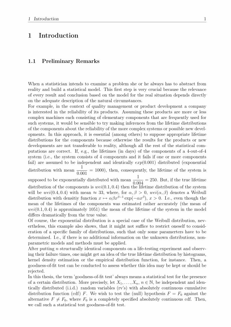
One can find many different techniques of testing goodness-of-fit in literature. Many ofthem are based on the order statistics X1:n, . . . , Xn:n corresponding to X1, . . . , Xn. To geta first idea of the deviation of the true distribution from the hypothesis a probability plotis an expressive tool (e.g. see D’Agostino and Stephens (1986)). Such a chart can beconstructed by plotting the Xi:n on the y-axis of a Cartesian coordinate system versus itshypothetical mean or median on the x-axis.
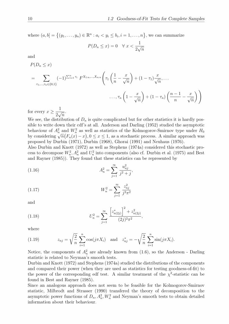
Figure 1.2.1: Example for probability plotting
Figure 1.2.1 shows an example of a probability plot for n = 7, X1:7 = 0.1138 , X2:7 =0.535 , X3:7 = 0.5848 , X4:7 = 0.6714 , X5:7 = 0.6843 , X6:7 = 0.9666 , X7:7 = 0.9925and F0 ∼ U(0, 1), where U(0, 1) denotes the standard uniform distribution. In this case,
the mean of Xi:n under H0 is given byi
n+ 1, i = 1, . . . , n (cf. e.g. David and Nagaraja
(2003), p.35). The notion of such a plot is that if the plotted points tend to lie on astraight line the sample probably stems from the hypothetical distribution and otherwiseit does not. In our example, the hypothesis of an underlying standard uniform distributionseems to be reasonable. Analogously to the construction of a probability plot, the orderstatistics X1:n, . . . , Xn:n regarded as sample quantiles can be plotted versus their theoreticalcounterparts and what we would obtain is a quantile-quantile plot.Notice, the assumption F0 ∼ U(0, 1) in the example above means no loss of generality andwe will presume this in the following. Since if we wish to test the hypothesis F = F0,where F0 is an absolutely continuous cdf with F0 U(0, 1), we may consider the rv’sXi = F0(Xi), i = 1, . . . , n, instead of X1, . . . , Xn. This mapping of rv’s is often called’probability integral transformation’, and it is well known that if X1, . . . , Xn
i.i.d.∼ F0 then

1 Introduction 3
X1, . . . , Xni.i.d.∼ U(0, 1) and vice versa. Hence, testing whether X1, . . . , Xn stem from the
standard uniform distribution is equivalent to testing the hypothesis F = F0.Certainly, a statistician wants to measure the observed linearity in a probability plot bysome meaningful number. An obvious option is to apply Pearson’s (Sample) CorrelationCoefficient
%n((x1, . . . , xn), (y1, . . . , yn)
)=
n∑i=1
(xi − x) (yi − y)√n∑i=1
(xi − x)2n∑i=1
(yi − y)2
, xi, yi ∈ R, i = 1, . . . , n,
where x =1
n
n∑i=1
xi and y =1
n
n∑i=1
yi, which leads to correlation type goodness-of-fit
statistics such as
Tn = 1−[%n
((F0(X1:n), . . . , F0(Xn:n)
),
(1
n+ 1, . . . ,
n
n+ 1
))]2
(1.1)
= 1−[%n
((X1:n, . . . , Xn:n
), (1, . . . , n)
)]2
(cf. e.g. D’Agostino and Stephens (1986), Filliben (1975) or Smith and Bain (1976)). Atest based on this statistic rejects H0 if the value of Tn is greater than a suitable threshold.
1.2.2 Statistics Based on Spacings
Another approach to testing for uniformity is to consider the spacings
D1 = X1:n , Di = Xi:n −Xi−1:n , i = 2, . . . , n, and Dn+1 = 1−Xn:n.
Here, the idea is to reject the hypothesis if the spacings seem to be more irregular thanthose from a uniform sample. This can be assessed, for instance, by the Greenwood statistic
(1.2) Gn =n+1∑i=1
D2i
(cf. D’Agostino and Stephens (1986) and Greenwood (1946)), the Q statistic of Quesen-berry and Miller (see Quesenberry and Miller (1977))
(1.3) Qn = Gn +n∑i=1
DiDi+1
or the criterion of Hartley and Pfaffenberger (see Hartley and Pfaffenberger (1972))
(1.4) S2n = (n+ 1)(n+ 2)Gn −
1
n+ 1.
4 1.2 Goodness-of-Fit Tests for Complete Samples
1.2.3 Neyman’s Smooth and χ2 Tests
Tests of the χ2-type are also very popular. Pearson’s χ2-test is one of the most famousgoodness-of-fit tests and it can also be used as a test of independence (cf. e.g. Fisz (1963),p. 436). For testing uniformity the user divides the unit interval into (say) m subintervalsand counts the number of observations in each of them. If these numbers differ too muchfrom their expected values under H0 the hypothesis is rejected. To be more precise, letI1, . . . , Im, m ∈ N, denote the considered subintervals and nj =
∣∣∣i ∈ 1, . . . , n : Xi ∈ Ij∣∣∣
the number of observations in Ij, j = 1, . . . ,m. In the case of X1, . . . , Xni.i.d.∼ U(0, 1), the
expected value of nj (denoted by E[nj]) is just n times the length of Ij, j = 1, . . . ,m, andPearson’s χ2-test statistic is given by
(1.5) χ2 =m∑j=1
(nj − E[nj]
)2
E[nj].
The name of the test is motivated by its approximate distribution under H0 which is theχ2-distribution with m− 1 degrees of freedom.Neyman’s smooth tests (see Neyman (1937)) also possess the property of an approximateχ2-distribution but they grew from a completely different idea. In addition to practicableapplicability of the test statistic a goodness-of-fit test is primarily judged by its power, i.e.,if the null hypothesis does not hold true, the test should reject it with highest possibleprobability. Since goodness-of-fit tests are regarded as omnibus tests in this thesis, whichmeans that the set of alternatives (here given by F abs. cont. cdf : F U(0, 1)) isnon-parametric and not restricted to any specific family of distribution, it is not possibleto determine the power of such a test against every distribution from the alternative. Also,one cannot expect to find a test which yields the best overall power of any goodness-of-fittest.Thus, Neyman considered subsets of alternatives defined by
Ωk =
P : P probability measure with density of the form
f(x) = c exp
(k∑i=1
Θiπi(x)
), x ∈ (0, 1) , c,Θ1, . . . ,Θk ∈ R
\ U(0, 1),
k ∈ N, whereπj(x) =
√2j + 1 Lj(2x− 1), x ∈ (0, 1) ,
and Lj denotes the Legendre polynomial of order j, j ∈ N. His aim was to develope tests ϕ∗k,k ∈ N, which are optimal in the following sense. If α ∈ (0, 1) and β(Θ1, . . . ,Θk|ϕk) denotesthe power function of a test ϕk for testing uniformity against the parametric alternativeΩk, k ∈ N, consider the following conditions
(a) β(Θ1, . . . ,Θk|ϕk) should admit partial derivatives of two first orders with regard toΘ1, . . . ,Θk,
(b) β(0, . . . , 0|ϕk) = α,
(c)∂β(Θ1, . . . ,Θk|ϕk)
∂Θi∣∣(Θ1,...,Θk)=(0,...,0)
= 0 , i = 1, . . . , k,

1 Introduction 5
(d)∂2β(Θ1, . . . ,Θk|ϕk)
∂Θi∂Θj∣∣(Θ1,...,Θk)=(0,...,0)
= 0 , i, j = 1, . . . , k , i 6= j,
(e)∂2β(Θ1, . . . ,Θk|ϕk)
∂Θ2i
∣∣(Θ1,...,Θk)=(0,...,0)
=∂2β(Θ1, . . . ,Θk|ϕk)
∂Θ21
∣∣(Θ1,...,Θk)=(0,...,0)
, i = 2, . . . , k.
Now, for k ∈ N, ϕ∗k should meet (a) - (e) and satisfy
∂2β(Θ1, . . . ,Θk|ϕ∗k)∂Θ2
1∣∣(Θ1,...,Θk)=(0,...,0)
≥ ∂2β(Θ1, . . . ,Θk|ϕk)∂Θ2
1∣∣(Θ1,...,Θk)=(0,...,0)
for all tests ϕk fulfilling (a) - (e).At this point, it should be noted that, technically speaking, each test and each test statisticis only applicable to samples of one specific sample size n ∈ N. Thus, n often appears inthe notation of the tests and test statistics (cf., e.g., Gn or Qn in Section 1.2.2), andactually we consider sequences of test statistics, such as
(Gn
)n∈N. But, when it is clear
from the context what is meant, we will sometimes not distinguish between a sequence oftest statistics and one particular member of it explicitly. In the same way, the index n willbe omitted in some situations to simplify notation.To find an asymptotic solution of the problem above (Neyman called it ’a solution validfor large values of n’), Neyman considered the functions
β(Θ1, . . . ,Θk|ϕk) = β(n−
12 Θ1, . . . , n
− 12 Θk|ϕk
)instead of β(Θ1, . . . ,Θk|ϕk). Since, as the number of observations n tends to infinity,β(Θ1, . . . ,Θk|ϕk) will tend to 1 if (Θ1, . . . ,Θk) 6= (0, . . . , 0) for every reasonable test ϕk,and hence, the derivatives in (c) - (d) will lose their meaning.He defined a sequence
(ϕ
(n)k
)n∈N
of tests based on the statistics
(1.6) Ψ2k =
k∑j=1
u2nj,
where
(1.7) unj =1√n
n∑i=1
πj(Xi), j = 1, . . . , k,
in the following way. If χk(1− α) denotes the (1− α)-quantile of the χ2-distribution withk degrees of freedom, then ϕ
(n)k rejects the null hypothesis F ∼ U(0, 1) iff Ψ2
k exceedsχk(1− α). Neyman found, that ϕ(n)
k satisfies (a) for every n ∈ N and, moreover,
(b) limn→∞
β(0, . . . , 0|ϕ(n)k ) = α,
(c) limn→∞
∂β(Θ1, . . . ,Θk|ϕ(n)k )
∂Θi∣∣(Θ1,...,Θk)=(0,...,0)
= 0, i = 1, . . . , k,
6 1.2 Goodness-of-Fit Tests for Complete Samples
(d) limn→∞
∂2β(Θ1, . . . ,Θk|ϕ(n)k )
∂Θi∂Θj∣∣(Θ1,...,Θk)=(0,...,0)
= 0, i, j = 1, . . . , k , i 6= j,
as well as
(e) limn→∞
(∂2β(Θ1, . . . ,Θk|ϕ(n)
k )
∂Θ2i
− ∂2β(Θ1, . . . ,Θk|ϕ(n)k )
∂Θ21
)∣∣(Θ1,...,Θk)=(0,...,0)
= 0,
i = 2, . . . , k.
Now, if ϕ(n) is a test with
(1) β(0, . . . , 0|ϕ(n)) = β(0, . . . , 0|ϕ(n)k ),
(2)∂β(Θ1, . . . ,Θk|ϕ(n))
∂Θi∣∣(Θ1,...,Θk)=(0,...,0)
=∂β(Θ1, . . . ,Θk|ϕ(n)
k )
∂Θi∣∣(Θ1,...,Θk)=(0,...,0)
,
i = 1, . . . , k,
(3)∂2β(Θ1, . . . ,Θk|ϕ(n))
∂Θi∂Θj∣∣(Θ1,...,Θk)=(0,...,0)
=∂2β(Θ1, . . . ,Θk|ϕ(n)
k )
∂Θi∂Θj∣∣(Θ1,...,Θk)=(0,...,0)
,
i, j = 1, . . . , k , i 6= j, and
(4)(∂2β(Θ1, . . . ,Θk|ϕ(n))
∂Θ2i
− ∂2β(Θ1, . . . ,Θk|ϕ(n))
∂Θ21
)∣∣(Θ1,...,Θk)=(0,...,0)
=
(∂2β(Θ1, . . . ,Θk|ϕ(n)
k )
∂Θ2i
− ∂2β(Θ1, . . . ,Θk|ϕ(n)k )
∂Θ21
)∣∣(Θ1,...,Θk)=(0,...,0)
, i = 2, . . . , k,
then
∂2β(Θ1, . . . ,Θk|ϕ(n)k )
∂Θ21
∣∣(Θ1,...,Θk)=(0,...,0)
≥ ∂2β(Θ1, . . . ,Θk|ϕ(n))
∂Θ21
∣∣(Θ1,...,Θk)=(0,...,0)
holds true. Thus, the tests ϕ(n)k are asymptotically optimal in some sense, and Neyman
proposed them for testing for uniformity (for details see Neyman (1937)).The problem of this approach to goodness-of-fit tests for the standard uniform distributionis that the true distribution does not have to be included in any set Ωk, k ∈ N; and evenif it is an element of Ωk for one k ∈ N, the index k0 = mink∈Nk : P ∈ Ωk is usuallyunknown. But a test only based on the first k components un1, . . . , unk is insensitive toalternatives P ∈ Ωl \Ωk, k, l ∈ N, k < l. On the other hand, a test based on the first k+ 1components is ’diluted’ in detecting alternatives P ∈ Ωk. In literature, the choice k = 4 isfrequently recommended (see, e.g., Milbrodt and Strasser (1990), Miller and Quesenberry(1979), Neyman (1937) or Rayner and Rayner (2001)).Some authors suggest modifications of the smooth tests such that k is chosen automatically

1 Introduction 7
(cf., e.g., Kallenberg and Ledwina (1995) or Ledwina (1994)), and it is also proposed touse other subsets of alternatives to derive tests of the same type with the aim to increasepower against particular interesting alternatives (cf., e.g., Kallenberg and Ledwina (1995),Ledwina (1994), Milbrodt and Strasser (1990) or Rayner and Rayner (2001)).
1.2.4 EDF Statistics
The last type of test statistics presented in this short survey is the most favored one inliterature because of two reasons. On the one hand, the corresponding tests are readilyconducted and, on the other, some of them are hardly to beat with respect to their power.The statistics considered in this section are based on the empirical distribution function(edf) defined by
Fn :
R −→ [0, 1],
x 7−→ 1n
n∑i=1
11(−∞,x](Xi),
wherefore they are called ’edf statistics’. Probably the best known of them is the Kolmogorov-Smirnov statistic
(1.8) Dn =√n
(sup
0≤x≤1|Fn(x)− x|
)(often the factor
√n is omitted (see, e.g., Fisz (1963), p. 445)). But the following three
statistics are also very famous and often yield better power than the Kolmogorov-Smirnovstatistic (cf., e.g., D’Agostino and Stephens (1986), Marhuenda et al. (2005), Quesenberryand Miller (1977) or Stephens (1974b)). One of the most frequently recommended teststatistic is certainly the Anderson - Darling statistic:
(1.9) A2n = n
1∫0
(Fn(x)− x
)2
x(1− x)dx.
Similar properties regarding the power are provided by the Cramér - von Mises statistic
(1.10) W 2n = n
1∫0
(Fn(x)− x
)2dx
and sometimes also good power is attested to the Watson statistic
(1.11) U2n = n
1∫0
Fn(x)− x−1∫
0
Fn(t)− t dt
2
dx = W 2n − n
(1
n
n∑i=1
Xi −1
2
)2
.
(1.9) and (1.10) are not very convenient for computational purpose. They can be simplifiedby calculating the integrals, which yields
(1.12) A2n =
n∑k=1
2(k − n)− 1
nln(1−Xk:n)− 2k − 1
nln(Xk:n)
− n
8 1.2 Goodness-of-Fit Tests for Complete Samples
and
(1.13) W 2n =
1
12n+
n∑k=1
(Xk:n −
2k − 1
2n
)2
.
Hence, we have for the Watson statistic by (1.11)
(1.14) U2n =
1
12n+
n∑k=1
(Xk:n −
2k − 1
2n
)2
− n(X − 1
2
)2
.
Similarly, we obtain a representation of (1.8) in terms of order statistics:
(1.15) Dn =√n max
Xi:n −
i− 1
n,i
n−Xi:n , i = 1, . . . , n
(cf. Maag and Dicatre (1971)).For some further developments regarding edf statistics the reader may refer to Zhao et al.(2010), who replaced the edf Fn in the statistics by a stochastic version in order to increasethe power of the respective tests.
1.2.5 Other Test Statistics in Literature
In literature, one can find a variety of constructions of goodness-of-fit tests and an attemptof giving a complete overview would not be successful at this point. Hence, just a few ref-erences are given, where the reader can find some other approaches than those presentedabove.An extensive survey of goodness-of-fit testing is given by D’Agostino and Stephens (1986)and also Marhuenda et al. (2005). Miller and Quesenberry (1979) as well as Quesen-berry and Miller (1977) collected various statistics for testing uniformity, too. Rényi typestatistics, which are related to Kolmogorov-Smirnov type statistics, are considered in Rényi(1953) and Birnbaum and Lientz (1969). Some more recent ideas of constructing goodness-of-fit tests can be found in Chen and Ye (2009), Glen et al. (2001), Goegebeur and Guillou(2010), Meintanis (2009), Steele and Chaseling (2006), Sürücü (2008) and Zhao et al.(2009).Since goodness-of-fit tests are always related to characterizations of distributions, in thesense that they are constructed to detect significant deviation of the data from characteriz-ing properties of the hypothetical distribution, the reader may also refer to Ghurye (1960),O’Reilly and Stephens (1982), Paul (2003) and their references.
1.2.6 Distributions of Test Statistics
Most of the statistics for goodness-of-fit tests possess very involved distributions. In liter-ature, there are explicit expressions in a few cases, only, such that most of the conclusionsare based on simulations or asymptotic theory. Here, we consider just a few statistics thatwill be focused frequently in this work.First, we derive the cdf of the Kolmogorov-Smirnov statistic. By (1.15) we have for x ∈ R:
P (Dn ≤ x) = P
(i
n− x√
n≤ Xi:n ≤
i− 1
n+
x√n, i = 1, . . . , n
).

1 Introduction 9
We see, if there is an i0 ∈ 1, . . . , n with
i0n− x√
n>
i0 − 1
n+
x√n
then P (Dn ≤ x) = 0 follows immediately. This yields
P (Dn ≤ x) = 0
for all x <1
2√n
.
Let f be a probability density function (pdf) of F (remember, F is supposed to be abso-lutely continuous). Then
fX1:n,...,Xn:n(t1, . . . , tn) = n!n∏i=1
f(ti) , t1 ≤ . . . ≤ tn,
is a pdf of (X1:n, . . . , Xn:n) (cf., e.g., David and Nagaraja (2003), p. 12). By this, we havefor x ≥ 1
2√n
P (Dn ≤ x) = n!
n−1n
+ x√n∫
1− x√n
mintn,n−2n
+ x√n∫
n−1n− x√
n
· · ·
mint2, x√n∫1n− x√
n
n∏i=1
f(ti) dt1 · · · dtn .
We can also express these probabilities by the cdf of (X1:n, . . . , Xn:n). For x1 ≤ . . . ≤ xnit is given by
FX1:n,...,Xn:n(x1, . . . , xr)
=n∑
j1=1
n−j1∑j2=(2−j1)+
· · ·n−j1−...−jn−1∑
jn=(n−j1−...−jn−1)+
n!n∏l=1
jl!
F j1(x1)
n∏p=2
[F (xp)− F (xp−1)]jp
(notice, obviously jn = n− j1 − . . .− jn−1 always holds true in this sum), where
m+ = max0,m for all m ∈ Z,
and for any unordered vector (y1, . . . , yn) ∈ Rn we have the relation
FX1:n,...,Xn:n(y1, . . . , yn) = FX1:n,...,Xn:n(z1, . . . , zn)
withzi = min(yi, . . . , yn) , i = 1, . . . , n.
Since for all a = (a1, . . . , an), b = (b1, . . . , bn) ∈ Rn with ai ≤ bi, i = 1, . . . , n, it is wellknown that P
((X1:n, . . . , Xn:n
)∈ (a, b]
)equals
∑τ1,...,τn∈0,1
(−1)∑ni=1 τi FX1:n,...,Xn:n
(τ1a1 + (1− τ1)b1, . . . , τnan + (1− τn)bn
),
10 1.2 Goodness-of-Fit Tests for Complete Samples
where (a, b] =
(y1, . . . , yn) ∈ Rn : ai < yi ≤ bi, i = 1, . . . , n, we can summarize
P (Dn ≤ x) = 0 ∀ x < 1
2√n
and
P (Dn ≤ x)
=∑
τ1,...,τn∈0,1
(−1)∑ni=1 τi FX1:n,...,Xn:n
(τ1
(1
n− x√
n
)+ (1− τ1)
x√n, . . .
. . . , τn
(1− x√
n
)+ (1− τn)
(n− 1
n− x√
n
))
for every x ≥ 1
2√n.
We see, the distribution of Dn is quite complicated but for other statistics it is hardly pos-sible to write down their cdf’s at all. Anderson and Darling (1952) studied the asymptoticbehaviour of A2
n and W 2n as well as statistics of the Kolmogorov-Smirnov type under H0
by considering√n(Fn(x)− x
), 0 ≤ x ≤ 1, as a stochastic process. A similar approach was
proposed by Durbin (1971), Durbin (1968), Ghorai (1991) and Neuhaus (1976).Also Durbin and Knott (1972) as well as Stephens (1974a) considered this stochastic pro-cess to decompose W 2
n , A2n and U2
n into components (also cf. Durbin et al. (1975) and Bestand Rayner (1985)). They found that these statistics can be represented by
(1.16) A2n =
∞∑j=1
u2nj
j2 + j,
(1.17) W 2n =
∞∑j=1
z2nj
j2π2
and
(1.18) U2n =
∞∑j=1
[z∗n(2j)
]2
+ z2n(2j)
(2j)2π2,
where
(1.19) znj =
√2
n
n∑i=1
cos(jπXi) and z∗nj = −√
2
n
n∑i=1
sin(jπXi).
Notice, the components of A2n are already known from (1.6), so the Anderson - Darling
statistic is related to Neyman’s smooth tests.Durbin and Knott (1972) and Stephens (1974a) studied the distributions of the componentsand compared their power (when they are used as statistics for testing goodness-of-fit) tothe power of the corresponding edf test. A similar treatment of the χ2-statistic can befound in Best and Rayner (1985).Since an analogous approach does not seem to be feasible for the Kolmogorov-Smirnovstatistic, Milbrodt and Strasser (1990) transfered the theory of decomposition to theasymptotic power functions of Dn, A
2n,W
2n and Neyman’s smooth tests to obtain detailed
information about their behaviour.

1 Introduction 11
1.3 Goodness-of-Fit Tests for Type-II Right Censored Data
In this work, we consider ’Type-II right censored data’. They might occur in the exampleat the beginning of this chapter (see Section 1.1) if a life-testing experiment is started withn > 1 units and stopped after the r-th unit failed, where 1 ≤ r < n. Then, only the rsmallest order statistics X1:n, . . . , Xr:n were available and the observations Xr+1:n, . . . , Xn:n
were ’censored’. The advantage of this method would be savings of time and money sincethe experiment would stop earlier, of course. Anyway, in some situations, perhaps becauseof time pressure, it might even be impossible to wait until all units fail.Type-II right censoring is the simplest case of ’progressive Type-II censoring’. In thegeneral case, a prefixed number of surviving units are removed from the sample after eachfailure. More precisely, after the first failure a number of (say) R1 surviving units areremoved, after the first failure of the remainig n − 1 − R1 units R2 surving units areremoved, and so on, till in the m-th step all of the remainig Rm = n−m−R1− . . .−Rm−1
units are censored. The vector of observations is usually denoted by (XR1:m:n, . . . , X
Rm:m:n),
where R = (R1, . . . , Rm) ∈ Nm0 and m ∈ N (for more details see, e.g., Balakrishnan andAggarwala (2000) and Fischer et al. (2008)).If there is no complete sample available for testing goodness-of-fit but only Type-II censoreddata, then one is faced with the problem that the ordinary test statistics are not applicablein this situation, and have to be adapted or replaced. Several proposals have been made inthe literature (e.g. see Barr and Davidson (1973), Castro-Kuriss et al. (2009), D’Agostinoand Stephens (1986), LaRiccia (1986), Lim and Park (2007), Lurie et al. (1974), Pettittand Stephens (1976) and Smith and Bain (1976)) and modifications of some statistics fromSection 1.2 will be presented in the following.
1.3.1 Modified Test Statistics
The idea for the modifications of the test statistics for complete samples is very intuitive,simply utilizing the available data to compute new test statistics analogously to the non-censored case. For example, as an analogue of Tn (see (1.1)) for right censored samplessuch as X1:n, . . . , Xr:n, 1 ≤ r ≤ n, Smith and Bain (1976) suggested
(1.20) Tr,n = 1−[%r
((X1:n, . . . , Xr:n
), (1, . . . , r)
)]2
,
where
%r
((X1:n, . . . , Xr:n
), (1, . . . , r)
)=
r∑i=1
(Xi:n − Xr
) (i− r+1
2
)√
r∑i=1
(Xi:n − Xr
)2r∑i=1
(i− r+1
2
)2
and Xr =1
r
r∑i=1
Xi:n. Hence, they just considered the correlation between X1:n, . . . , Xr:n
and their hypothetical expected values which yields Tn in the case of r = n.Similarly, Lurie et al. (1974) generalized the Hartley - Pfaffenberger criterion S2
n (see (1.4))which is essentially the same as the Greenwood statistic (see (1.2)) by assessing the regu-larity of the available spacings and the distance of Xr:n from 1 analogously to (1.4). They

12 1.3 Goodness-of-Fit Tests for Type-II Right Censored Data
obtained
(1.21) Gr,n = (n+ 1)(n+ 2)
r∑
k=1
(Xk:n −Xk−1:n)2 +(1−Xr:n)2
n− r + 1
− (n+ 2).
The modifications of the edf statistics are comparable to the one of Tn. Changing theupper limit for calculating the supremum in (1.8) and of the integrations in (1.9) - (1.11)from 1 to Xr:n yields
Dr,n =√n
(sup
0≤x≤Xr:n|Fn(x)− x|
)(1.22)
=√n max
Xi:n −
i− 1
n,i
n−Xi:n , i = 1, . . . , r
(cf. Barr and Davidson (1973)),
A2r,n = n
Xr:n∫0
(Fn(x)− x
)2
x(1− x)dx(1.23)
=r−1∑k=1
(2k − 1
n− 2
)ln(1−Xk:n)− 2k − 1
nln(Xk:n)
+
(2(r − 1)− (r − 1)2
n− n
)ln(1−Xr:n) +
(r − 1)2
nln(Xr:n)− nXr:n,
W 2r,n = n
Xr:n∫0
(Fn(x)− x
)2dx(1.24)
=r−1∑k=1
(X2k:n −X2
r:n
)+
1
n
r∑k=1
(1− 2k)(Xk:n −Xr:n
)+n
3X3r:n
and
U2r,n = n
Xr:n∫0
Fn(x)− x− 1
Xr:n
Xr:n∫0
Fn(t)− t dt
2
dx(1.25)
= W 2r,n − nXr:n
(1
nXr:n
r∑k=1
Xk:n +Xr:n
2− r
n
)2
(cf. Pettitt and Stephens (1976)).Smith and Bain (1976) also derived a version of the Cramér - von Mises statistic for Type-IIright censored data in a similar way from (1.13), they suggested
(1.26) SBW 2r,n =
1
12n+
r∑k=1
(Xk:n −
2k − 1
2n
)2
.
1 Introduction 13
1.3.2 Distributions of Modified Test Statistics
As one can imagine, the distributional behavior of the modified statistics is even moredifficult to investigate than the properties of the original statistics. Theoretical results arerare in literature, mostly approximative percentage points or asymptotic results are given(cf. Barr and Davidson (1973), Lurie et al. (1974), Pettitt and Stephens (1976) or Smithand Bain (1976)), and we will just add two remarks at this point.For the modified Kolmogorov-Smirnov statistic (see (1.22)) we obtain by the same approachas in Section 1.2.6
P (Dr,n ≤ x) = 0 ∀ x < 1
2√n
and if x ≥ 1
2√n
P (Dr,n ≤ x) =∑
τ1,...,τr∈0,1
(−1)∑ri=1 τi FX1:n,...,Xr:n
(τ1
(1
n− x√
n
)+ (1− τ1)
x√n, . . .
. . . , τr
(r
n− x√
n
)+ (1− τr)
(r − 1
n− x√
n
)),
where FX1:n,...,Xr:n is the cdf of (X1:n, . . . , Xr:n).Considering the Cramér - von Mises statistic, Durbin and Knott (1972) pointed out thatthe decomposition (1.17) of W 2
n can be ascribed to a Fourier sine series expansion of thefunction yn(x) =
√n(Fn(x)− x
), x ∈ [0, 1],
yn(x) =√
2∞∑j=1
sin(jπx)
jπznj, 0 ≤ x ≤ 1,
such that Parseval’s Theorem (cf. Tolstov and Silverman (1976), p. 119) yields (1.17).Replicating this approach for W 2
r,n we expand yr,n = yn∣∣[0,Xr:n]into its Fourier sine series
yr,n(x) =∞∑j=1
2
Xr:n
Xr:n∫0
yr,n(t) sin
(jπt
Xr:n
)dt
sin
(jπx
Xr:n
), 0 ≤ x ≤ Xr:n.
Again, Parseval’s Theorem applies and we find analogously to Durbin and Knott (1972)
(1.27) W 2r,n =
∞∑j=1
(zrnj)2
j2π2,
where
(1.28) zrnj =
√2Xr:n
n
(−1)j+1 (r − nXr:n) +
r∑k=1
cos
(j π
Xk:n
Xr:n
), j ∈ N.
Notice, if we substitute Xr:n by 1 and r by n in (1.28) we obtain (1.19), but to myknowledge, these components have not been examined in literature, so far, and it seemsthat meaningful theoretical results are extremely difficult to obtain.

14 1.4 Aim of This Work and Outline
1.3.3 The Alternative Approach to Goodness-of-Fit Testing for Censored Data
The modified test statistics have the disadvantage that for every specific combination of rand n new critical values have to be computed. Moreover, the presented statistics are onlyapplicable to Type-II right censored data, so for other kinds of censoring new statistics(with new critical values) would be required.Some authors approached the problem by adjusting the data, but not the test statis-tics. With respect to the restriction to testing for uniformity, they suggest to transforma censored vector of order statistics based on uniform random variables to a full vectorof uniform order statistics in a smaller dimension (see D’Agostino and Stephens (1986),Lin et al. (2008), Michael and Schucany (1979) and O’Reilly and Stephens (1988) for in-stance). Then ordinary test statistics are applied to the transformed data to obtain avariety of goodness-of-fit tests for censored data.Beside the opportunity to manage goodness-of-fit testing for more different kinds of cen-sored data (e.g., see Michael and Schucany (1979) for progressive Type-II censoring), theauthors above attested a gain in power to their approach compared with the applicationof the modified statistics.The transformations for Type-II right censored data will be presented in Chapter 2 andthey constitute the primary objects of study in the present work.
1.4 Aim of This Work and Outline
In this work, we study the transformations of order statistics which were mentioned inSection 1.3.3, aiming to clarify the structure of the joint distribution of the transformedrandom variables if the censored sample does not stem from the standard uniform distribu-tion. Since in this case, the question arises, whether the transformed sample still behaveslike order statistics of i.i.d. random variables. It will be seen, that no transformationbeing considered in literature possesses this property. At least for one transformation, it isestablished that the structure of order statistics is preserved for arbitrary power functiondistributions.The outline of the present work is the following. A comprehensive overview of transforma-tions of rv’s from the uniform distribution is given in Chapter 2. In Chapter 3 the structureof the transformed rv’s suggested in literature is investigated in a general framework whenthey do not stem from the uniform distribution. To supplement the theoretical conclusions,an empirical power study of the different methods of testing goodness-of-fit for censoredsamples was carried out and its results are reported in Chapter 4. Finally, Chapter 5 givesan outlook on possible extensions of this work.

2 Modifications of Samples from the Uniform Distribution 15
2 Modifications of Samples from the Uniform Distribu-tion
In this chapter, let for convenience U1, . . . , Un, n ∈ N, always denote independent and iden-tically distributed (i.i.d.) random variables (rv’s) from the standard uniform distribution,U1:n, . . . , Un:n the corresponding order statistics (OS’s) and for technical reasons U0:n ≡ 0as well as Un+1:n ≡ 1.
2.1 Transformations
As mentioned in the Introduction (cf. Section 1.3.3), transformations of Type-II rightcensored samples are considered in literature dealing with testing goodness-of-fit whenno complete sample is available (cf. D’Agostino and Stephens (1986), Lin et al. (2008),Michael and Schucany (1979) and O’Reilly and Stephens (1988)). In this chapter, we studythe question whether transformations of censored samples may preserve the order statisticsstructure. To be more precise, we consider mappings which transform the Type-II rightcensored sample X1:n, . . . , Xr:n to a vector of r OS’s (Y1:r, . . . , Yr:r) from a sample of size rwith some (possibly different) underlying distribution, 1 ≤ r ≤ n.We restrict ourselves to distributions which possess an absolutely continuous cumulativedistribution function (cdf). Suppose F is the underlying cdf of X1:n, . . . , Xr:n, F is an-other given absolutely continuous cdf, and we wish to transform (X1:n, . . . , Xr:n) into(Y1:r, . . . , Yr:r) as described above, such that F is the underlying cdf of the new OS’s.Then, we can first apply the probability integral transformation (cf. David and Nagaraja(2003), p. 14) to obtain(
F (X1:n), . . . , F (Xr:n))∼(U1:n, . . . , Ur:n
).
Afterwards,(F (X1:n), . . . , F (Xr:n)
)could be transformed into a full vector of uniform OS’s
(U1:r, . . . , Ur:r) of size r, and finally, utilizing the quantile transformation (cf. David andNagaraja (2003), p. 15)(
Y1:r, . . . , Yr:r)
=(F−1(U1:r), . . . , F
−1(Ur:r))
yields the desired result, where F−1 denotes the quantile function of F .Thus, it is sufficient to consider transformations of uniform OS’s
(2.1) (U1:n, . . . , Ur:n) 7−→ (U1:r, . . . , Ur:r)
such that the image(U1:r, . . . , Ur:r
)is a vector of OS’s from r i.i.d. uniformly distributed
rv’s on (0, 1).First, one might ask whether there is even a strictly increasing function v : (0, 1) −→ (0, 1)with v(Ui:n) ∼ Ui:r for all 1 ≤ i ≤ r. Such a function would satisfy for every x ∈ (0, 1)
Bi,r−i+1(x) = P(v(Ui:n) ≤ x
)= P
(Ui:n ≤ v−1(x)
)= Bi,n−i+1
(v−1(x)
),

16 2.1 Transformations
i.e.,
v = B−1i,r−i+1 Bi,n−i+1 ∀ i ∈ 1, . . . , r,(2.2)
where Bp,q denotes the cdf of the beta(p, q) distribution, p, q > 0. Obviously, if r = 1 orr = n then B1,n and the identity are the unique solutions of (2.2), respectively. But for1 < r < n, (2.2) has no solution at all, since (2.2) yields in particular for all x ∈ (0, 1)
i = r v(x) = [Br,n−r+1(x)]1r and i = 1 v(x) = 1− (1− x)
nr .
Thus, for all x ∈ (0, 1)
n∑j=r
(n
j
)xj(1− x)n−j =
[1− (1− x)
nr
]r.
But this is not true for 1 < r < n, as we can easily see:
Assume
(∗)n∑j=r
(n
j
)xj(1− x)n−j =
[1− (1− x)
nr
]r ∀ x ∈ (0, 1).
If we differentiate both sides of (∗), we obtain for every x ∈ (0, 1)
r
(n
r
)xr−1(1− x)n−r = n
[1− (1− x)
nr
]r−1(1− x)
nr−1
⇐⇒ r
(n
r
)xr−1 = n
[1− (1− x)
nr
]r−1(1− x)
(r−n)(r−1)r
⇐⇒ r−1
√r
(n
r
)x = r−1
√n[1− (1− x)
nr
](1− x)
r−nr
⇐⇒ r−1
√r
(n
r
)x = r−1
√n[(1− x)
r−nr − (1− x)
]
⇐⇒
(r−1
√r
(n
r
)− r−1√n
)x = r−1
√n[(1− x)
r−nr − 1
].
One more differentiation on both sides yields
r−1√nn− rr
(1− x)−nr = r−1
√r
(n
r
)− r−1√n ∀ x ∈ (0, 1),
but we have obviously
limx1
r−1√nn− rr
(1− x)−nr =∞ .
Hence, for all practical situations, there is no univariate transformation, that provides thedesired properties. In the following, we will consider multivariate transformations.Due to the properties of the uniform distribution as stated in the following Lemma, it ispossible to construct transformations of the type (2.1). The statements are well knownand can be found in Hajós and Rényi (1954), Malmquist (1950), Reiss (1989) and Rényi(1953).

2 Modifications of Samples from the Uniform Distribution 17
2.1 Lemma(α) Let U1:n ≤ . . . ≤ Un:n be OS’s from the standard uniform distribution. Then there
are independent rv’s Vj ∼ beta(n− j + 1, 1), 1 ≤ j ≤ n, such that
Ui:n = 1−i∏
j=1
Vj , 1 ≤ i ≤ n.
(β) V ∼ beta(p, 1) =⇒ V p ∼ beta(1, 1) = U(0, 1), p > 0.
(γ) U ∼ U(0, 1) =⇒ 1− U ∼ U(0, 1).
(δ) (1− U1:n, 1− U2:n, . . . , 1− Un:n) ∼ (Un:n, Un−1:n, . . . , U1:n).
(ε) Ui:n ∼ beta(i, n− i+ 1), 1 ≤ i ≤ n.
(ζ) U ∼ U(0, 1) =⇒ U1p ∼ beta(p, 1), p > 0.
By these elementary results, all of the well known statements and transformations collectedin Theorem 2.2 can be easily derived.
2.2 TheoremLet U1, . . . , Un be i.i.d. rv’s with standard uniform distribution, and U1:n ≤ . . . ≤ Un:n therespective OS’s.
(i) There are independent rv’s Vj ∼ beta(j, 1), 1 ≤ j ≤ n, such that
Ui:n =n∏j=i
Vj , 1 ≤ i ≤ n
(cf. Tadikamalla and Balakrishnan (1998)).
(ii) For 1 ≤ i1 < i2 < . . . < il ≤ n, l ∈ 1, . . . , n, the rv’s
Ui1:n
Ui2:n
,Ui2:n
Ui3:n
, . . . ,Uil−1:n
Uil:nand Uil:n
are independent with distributions beta(i1, i2 − i1), . . . , beta(il−1, il − il−1) andbeta(il, n− il + 1), respectively (cf. Arnold et al. (1992)).
(iii) The rv’s [Un−i+1:n
Un−i+2:n
]n−i+1
, 1 ≤ i ≤ n,
are i.i.d. uniformly distributed (cf. Arnold et al. (1992), Hajós and Rényi (1954),O’Reilly and Stephens (1988) and Rényi (1953)).

18 2.1 Transformations
(iv) Let Br,n−r+1 denote the cdf of the beta(r, n− r + 1) distribution, 1 ≤ r ≤ n. Therv’s
Br,n−r+1
(Ur:n
),
[Ur−i+1:n
Ur−i+2:n
]r−i+1
, 2 ≤ i ≤ r,
are i.i.d. uniformly distributed (cf. Arnold et al. (1992) and O’Reilly and Stephens(1988)).
(v) The rv’s W1, . . . ,Wn defined by
Wi =
[1− Ui:n
1− Ui−1:n
]n−i+1
, 1 ≤ i ≤ n,
are i.i.d. uniformly distributed (cf. Lin et al. (2008)).
(vi) The rv’s1−Wi, 1 ≤ i ≤ n,
with W1, . . . ,Wn from (v) are i.i.d. uniformly distributed (cf. O’Reilly andStephens (1988)).
(vii) For rv’s U ′1/n, . . . , U′n/n with
U ′i/n =n∏j=i
U1j
n−j+1 =n−i+1∏j=1
U1
n−j+1
j , 1 ≤ i ≤ n,
we have (U ′1/n, . . . , U
′n/n
)∼ (U1:n, . . . , Un:n)
(cf. O’Reilly and Stephens (1988)).
(viii) For rv’s U ′′1/n, . . . , U′′n/n with
U ′′i/n = 1−i∏
j=1
(1− Uj)1
n−j+1 , 1 ≤ i ≤ n,
we have (U ′′1/n, . . . , U
′′n/n
)∼ (U1:n, . . . , Un:n)
(cf. O’Reilly and Stephens (1988)).
(ix) For 2 ≤ r ≤ n, we find(U1:n
Ur:n, . . . ,
Ur−1:n
Ur:n
)∼ (U1:r−1, . . . , Ur−1:r−1) .
Moreover, (U1:n
Ur:n, . . . ,
Ur−1:n
Ur:n
)and Ur:n
are stochastically independent (cf. Arnold et al. (1992) and D’Agostino andStephens (1986)).

2 Modifications of Samples from the Uniform Distribution 19
(x) Let Br,n−r+1 denote the cdf of the beta(r, n− r + 1) distribution, 1 ≤ r ≤ n, thenthe rv’s Z1/r, . . . , Zr/r with
Zi/r =Ui:nUr:n
[Br,n−r+1(Ur:n)]1r , 1 ≤ i ≤ r,
satisfy (Z1/r, . . . , Zr/r
)∼ (U1:r, . . . , Ur:r)
(cf. Michael and Schucany (1979) and O’Reilly and Stephens (1988)).
(xi) For rv’s S1/r, . . . , Sr/r, 1 ≤ r ≤ n, with
Si/r = 1−i∏
j=1
(1− Uj:n
1− Uj−1:n
)n−j+1r−j+1
, 1 ≤ i ≤ r,
we find (S1/r, . . . , Sr/r
)∼ (U1:r, . . . , Ur:r)
(cf. O’Reilly and Stephens (1988)).
Proof.
(i) From Lemma 2.1 (α) and (δ) we obtain
(U1:n, . . . , Un:n) ∼ (1− Un:n, . . . , 1− U1:n) =
(n∏j=1
Vj, . . . ,1∏j=1
Vj
),
where Vj ∼ beta(n− j + 1, 1), 1 ≤ j ≤ n, are independent. I.e.,
Ui:n ∼n−i+1∏j=1
Vj =n∏j=i
Vn−j+1.
Since Vn−j+1 ∼ beta(j, 1) the assertion follows immediately.
(ii) Let V1, . . . , Vn be as in (i). Then(Ui1:n
Ui2:n
, . . . ,Uil−1:n
Uil:n, Uil:n
)=
i2−1∏j=i1
Vj, . . . ,
il−1∏j=il−1
Vj,
n∏j=il
Vj
.
The independence ofUi1:n
Ui2:n
, . . . ,Uil−1:n
Uil:nand Uil:n follows from the independence of
V1, . . . , Vn. Moreover, for k ∈ 1, . . . , l − 1 we see
Uik:n
Uik+1:n
=
ik+1−1∏j=ik
Vj(i)∼ Uik:(ik+1−1)
2.1 (ε)∼ beta(ik, ik+1 − ik)
andUil:n
2.1 (ε)∼ beta(il, n− il + 1).

20 2.1 Transformations
(iii) Follows directly from (ii) and Lemma 2.1 (β).
(iv) Follows directly from (ii) and Lemma 2.1 (β) and (ε).
(v) By Lemma 2.1 (α) we have1− Ui:n
1− Ui−1:n
= Vi,
where Vi ∼ beta(n − i + 1, 1), 1 ≤ i ≤ n, are independent. Thus, Lemma 2.1 (β)yields
Wi = V n−i+1i , 1 ≤ i ≤ n,
are i.i.d. uniformly distributed rv’s.
(vi) Follows directly from (v) and Lemma 2.1 (γ).
(vii) Since
U1
n−j+1
j ∼ beta(n− j + 1, 1), 1 ≤ i ≤ n, (cf. Lemma 2.1 (ζ))
we have by Lemma 2.1 (α) and (δ) for all i ∈ 1, . . . , n
(U ′1/n, . . . , U
′n/n
)=
(n∏j=1
U1
n−j+1
j , . . . ,1∏j=1
U1
n−j+1
j
)
∼ (1− Un:n, . . . , 1− U1:n) ∼ (U1:n, . . . , Un:n) .
(viii) By Lemma 2.1 (γ) and (ζ) we know
(1− Uj)1
n−j+1 ∼ beta(n− j + 1, 1), 1 ≤ i ≤ n,
such that Lemma 2.1 (α) yields the assertion.
(ix) From (i) we obtain(U1:n
Ur:n, . . . ,
Ur−1:n
Ur:n
)∼
(r−1∏j=1
Vj,r−1∏j=2
Vj, . . . , Vr−1
)∼ (U1:r−1, . . . , Ur−1:r−1) ,
where Vj ∼ beta(j, 1), 1 ≤ j ≤ r − 1, are independent and, additionally,
Ur:n ∼n∏j=r
Vj,
where Vj ∼ beta(j, 1), r ≤ j ≤ n, are independent of V1, . . . , Vr−1.
(x) From (ix) we know(U1:n
Ur:n, . . . ,
Ur−1:n
Ur:n
)and Ur:n are independent with
Ur:n ∼ beta(r, n− r + 1) (see Lemma 2.1 (ε)) and(U1:n
Ur:n, . . . ,
Ur−1:n
Ur:n
)∼
(r−1∏j=1
Vj,
r−1∏j=2
Vj, . . . , Vr−1
),

2 Modifications of Samples from the Uniform Distribution 21
where Vj ∼ beta(j, 1), 1 ≤ j ≤ r − 1, are independent.Hence, we have by probability integral transformation and Lemma 2.1 (ζ)[
Br,n−r+1(Ur:n)] 1r ∼ beta(r, 1) ∼ Vr,
such that(Z1/r, . . . , Zr/r
)=
(U1:n
Ur:n[Br,n−r+1(Ur:n)]
1r , . . . ,
Ur−1:n
Ur:n[Br,n−r+1(Ur:n)]
1r , [Br,n−r+1(Ur:n)]
1r
)
∼
(r∏j=1
Vj,r∏j=2
Vj, . . . , Vr
)(i)∼ (U1:r, . . . , Ur:r) .
(xi) From Lemma 2.1 (α) we obtain
1− Uj:n1− Uj−1:n
= Vj,
where Vj ∼ beta(n− j + 1, 1), 1 ≤ j ≤ n, are independent. Hence, Lemma 2.1 (β)and (ζ) yield (
1− Uj:n1− Uj−1:n
)n−j+1r−j+1
∼ beta(r − j + 1, 1), 1 ≤ j ≤ r.
Thus, again by Lemma 2.1 (α)(S1/r, . . . , Sr/r
)=
(1− U
nr
1:n, 1−2∏j=1
(1− Uj:n
1− Uj−1:n
)n−j+1r−j+1
, . . . , 1−r∏j=1
(1− Uj:n
1− Uj−1:n
)n−j+1r−j+1
)
∼ (U1:r, . . . , Ur:r) .
The transformations given by (iii), (iv), (vi), (vii) and (viii) of Theorem 2.2 were de-rived in O’Reilly and Stephens (1988) in a different way. They applied the transforma-tion of Rosenblatt (see Theorem 2.3 and Rosenblatt (1952)) to (Un:n, Un−1:n, . . . , U1:n),(Ur:n, Ur−1:n, . . . , U1:n) and (U1:n, U2:n, . . . , Un:n) to obtain (iii), (iv) and (vi), respectively.Then they defined the inverse of Rosenblatt’s transformation to find (vii) and (viii).
2.3 Theorem (Rosenblatt (1952))Let Y = (Y1, . . . , Yn) be a random vector with an absolutely continuous distribution func-tion F Y . Moreover, let F Y1 denote the distribution function of Y1 and F Yi|Y1,...,Yi−1 theconditional distribution function of Yi given Y1, . . . , Yi−1, 2 ≤ i ≤ n. Then Z1, . . . , Zn with
Z1 = F Y1(Y1) and Zi = F Yi|Y1,...,Yi−1(Yi|Y1, . . . , Yi−1), 2 ≤ i ≤ n,
are i.i.d. uniformly distributed.

22 2.1 Transformations
In the following lemma, which gives transformations of uniform OS’s to uniform OS’s froma smaller sample size, we introduce a notation which is used in the sequel.
2.4 LemmaLet 1 ≤ r ≤ n, t0 = 0,
Kr1 = (t1, . . . , tr) ∈ Rr : 0 < t1 < . . . < tr < 1
and for (t1, . . . , tr) ∈ Kr1
A(t1, . . . , tr) =(A(t1, . . . , tr)1, . . . , A(t1, . . . , tr)r
)as well as
C(t1, . . . , tr) =(C(t1, . . . , tr)1, . . . , C(t1, . . . , tr)r
)with
A(t1, . . . , tr)i = 1−(1−Br,n−r+1(tr)
) 1r
i∏j=2
(1−
[tr−j+1
tr−j+2
]r−j+1) 1
r−j+1
and
C(t1, . . . , tr)i =r∏j=i
(1−
[1− tj
1− tj−1
]n−j+1) 1
j
,
i ∈ 1, . . . , r, where Br,n−r+1 again denotes the cdf of the beta(r, n− r + 1) distribution.Then
A(U1:n, . . . , Ur:n) ∼ C(U1:n, . . . , Ur:n) ∼ (U1:r, . . . , Ur:r) .
Proof. By Theorem 2.2 (iv)
Br,n−r+1
(Ur:n
),
[Ur−i+1:n
Ur−i+2:n
]r−i+1
, 2 ≤ i ≤ r,
are i.i.d. uniformly distributed rv’s. Hence, we obtain from Lemma 2.1 (γ) and (ζ)
V1 =(1−Br,n−r+1(Ur:n)
) 1r , Vj =
[1−
[Ur−j+1:n
Ur−j+2:n
]r−j+1] 1r−j+1
, j = 2, . . . , r,
are mutually independent and respectively beta(r − j + 1, 1), j = 1, . . . , r, distributed.Thus, by Lemma 2.1 (α)
A(U1:n, . . . , Ur:n) =
(1−
1∏j=1
Vj, . . . , 1−r∏j=1
Vj
)∼(U1:r, . . . , Ur:r
).
From Theorem 2.2 (vi), we know
1−[
1− Uj:n1− Uj−1:n
]n−j+1
, j = 1, . . . , r,

2 Modifications of Samples from the Uniform Distribution 23
are i.i.d. uniformly distributed rv’s. Hence, by Theorem 2.2 (vii) we know
C(U1:n, . . . , Ur:n) ∼ (U1:r, . . . , Ur:r) .
Theorem 2.2 and Lemma 2.4 show there are various options to define a transformationwhich maps (U1:n, . . . , Ur:n) to a complete sample of ordered uniformly distributed rv’s.For example, from the composition of the transformations in
• (iv) and (vii) of Theorem 2.2 we obtain transformation (x),
• (vi) and (viii) of Theorem 2.2 we obtain transformation (xi),
• (iv) and (viii) of Theorem 2.2 we obtain A in Lemma 2.4 and
• (vi) and (vii) of Theorem 2.2 we obtain C in Lemma 2.4.
Moreover, if M is a transformation with M(U1, . . . , Ur) ∼ (U1, . . . , Ur), for example
M(U1, . . . , Ur) = (1− U1, . . . , 1− Ur),
then more options result based on (iv) and (vi) in Theorem 2.2.For example, the combination of (vi), M (above) and (viii) from Theorem 2.2 yields thesame transformation as the composition of (v) and (viii).
2.2 Random Dilation and Contraction
By Theorem 2.2 (ix) and (x) we know(U1:n
Ur:n, . . . ,
Ur−1:n
Ur:n
)∼(U1:r−1, . . . , Ur−1:r−1
)and (
U1:n
Ur:n
[Br,n−r+1(Ur:n)
] 1r , . . . ,
Ur−1:n
Ur:n
[Br,n−r+1(Ur:n)
] 1r
)∼(U1:r, . . . , Ur−1:r
),
where[Br,n−r+1(Ur:n)
] 1r ∼ beta(r, 1) is independent of
(U1:n
Ur:n, . . . ,
Ur−1:n
Ur:n
), 2 ≤ r ≤ n.
This leads to the concept of Random Contraction and Random Dilation (cf. Beutnerand Kamps (2008), Nevzorov (2001), p. 14, or Wesołowski and Ahsanullah (2004)) whichshould be briefly mentioned at this point.
2.5 Theorem(i) Let Vn+1 ∼ beta(n+ 1, 1) be independent of (U1:n, . . . , Un:n). Then(
Vn+1U1:n, . . . , Vn+1Un:n
)∼(U1:n+1, . . . , Un:n+1
).
24 2.2 Random Dilation and Contraction
(ii) Let 1 ≤ r < n and Vr+1 ∼ beta(n− r, 1) be independent of (U1:n, . . . , Ur:n). Then(U1:n, . . . , Ur:n, 1− (1− Ur:n)Vr+1
)∼(U1:n, . . . , Ur+1:n
).
Proof.
(i) By Theorem 2.2 (i) we can assume for all i ∈ 1, . . . , n
Ui:n =n∏j=i
Vj,
where Vj ∼ beta(j, 1), 1 ≤ j ≤ n, are independent rv’s. Then,
Vj =Uj:nUj+1:n
, 1 ≤ j ≤ n,
and hence V1, . . . , Vn+1, are independent. Again by Theorem 2.2 (i), we can con-clude(
Vn+1U1:n, . . . , Vn+1Un:n
)=
(n+1∏j=1
Vj, . . . ,n+1∏j=n
Vj
)∼(U1:n+1, . . . , Un:n+1
).
(ii) For i ∈ 1, . . . , r we can represent Ui:n by
Ui:n = 1−i∏
j=1
Vj,
where Vj ∼ beta(n− j + 1, 1), 1 ≤ j ≤ r, are independent rv’s, cf. Lemma 2.1 (α).Then
Vj =1− Uj:n
1− Uj−1:n
, 1 ≤ j ≤ r,
and hence V1, . . . , Vr+1, are independent. Thus, Lemma 2.1 (α) yields(U1:n, . . . , Ur:n, 1− (1− Ur:n)Vr+1
)=
(1−
1∏j=1
Vj, . . . , 1−r∏j=1
Vj, 1−r+1∏j=1
Vj
)
∼(U1:n, . . . , Ur+1:n
).
We see, by random dilation additional observations can be simulated from a given Type-IIright censored sample if the underlying distribution is U(0, 1) (cf. Theorem 2.5 (ii)). Thiscould be exploited for increasing the number of observations, artificially, when a censoredsample should be tested for uniformity. In Chapter 4 results of an empirical power studyare reported, where (among other things) the powers of the modified tests from Section1.3.1 of the Introduction are compared before and after the sample size was artificiallyincreased.A full sample of uniform rv’s can be similarly expanded by first applying random contrac-tion, such that the artificial sample behaves like a censored sample (cf. Theorem 2.5 (i)),and afterwards simulating a new observation by random dilation. This procedure was alsoconsidered in the power study of Chapter 4 in combination with transformation (ix) fromTheorem 2.2.
3 Transformations of Samples from Arbitrary Distributions 25
3 Transformations of Samples from Arbitrary Distribu-tions
In this chapter, let generally X1, . . . , Xn, n ∈ N, be independent and identically distributed(i.i.d.) random variables (rv’s) with an absolutely continuous cumulative distribution func-tion (cdf) F and probability density function (pdf) f . The order statistics (OS’s) ofX1, . . . , Xn are denoted by X1:n, . . . , Xn:n and we assume F (0) = 0 ≤ F (x) ≤ 1 = F (1) forall x ∈ (0, 1). For convenience, let U1, . . . , Un always denote i.i.d. uniformly distributedrv’s and U1:n, . . . , Un:n their corresponding OS’s.
Theorem 2.2 shows that we can transform a Type-II right censored sample of uniformlydistributed rv’s to a complete sample of ordered uniformly distributed rv’s of a smallersample size. Now we study whether there is a transformation with this property suchthat the transformed rv’s are distributed as order statistics from i.i.d. rv’s even if theunderlying distribution of the original sample is not U(0, 1) but possesses an arbitraryabsolutely continuous cdf F . This issue is also discussed in Fischer and Kamps (2011),where some of the statements of this chapter can be found as well.Upon goodness-of-fit testing (F ∼ U(0, 1) ←→ F U(0, 1)) based on Type-II rightcensored data, such that only the r smallest of n OS’s are available, O’Reilly and Stephens(see O’Reilly and Stephens (1988)) considered S1/r, . . . , Sr/r from Theorem 2.2 (xi), whereasMichael and Schucany (see D’Agostino and Stephens (1986) and Michael and Schucany(1979)) utilized Z1/r, . . . , Zr/r from Theorem 2.2 (x).When studying the existence of transformations of the r smallest of n OS’s that preservethe structure of OS’s, r ∈ 1, n is not interesting, since r = 1 is trivial and in case r = nthe sample is not censored. Henceforth, we will assume 1 < r < n.Our considerations will be restricted to transformations fulfilling the assumptions of thedensity transformation theorem. I.e., the following general assumption is imposed.
3.1 AssumptionLet Kr1 as in Lemma 2.4 and T : Kr1 −→ Kr1 be a bijective mapping which is continuouslydifferentiable such that the determinant of the Jacobian matrix never vanishes and
T(U1:n, . . . , Ur:n
)∼(U1:r, . . . , Ur:r
).
We will make use of a notation of projections.
3.2 NotationFor k ∈ 1, . . . , r let πk : Rr −→ R be the projection onto the k–th component:
πk(x1, . . . , xr) = xk
and for any function T : M −→ Rr, where M is an arbitrary set,
T(·)k = πk(T(·)
).

26 3 Transformations of Samples from Arbitrary Distributions
Since we are going to study the structure of transformed rv’s it should be worth notingtheir general distribution at this point. This is done in the next Lemma to which we willrefer frequently in the following.
3.3 LemmaLet T satisfy Assumption 3.1 and(
Y1/r, . . . , Yr/r)
= T (X1:n, . . . , Xr:n) .
Then, a pdf of(Y1/r, . . . , Yr/r
)is given by
fY1/r,...,Yr/r(t1, . . . , tr)
=
r!
[1− F
(T (t1, . . . , tr)r
)1− T (t1, . . . , tr)r
]n−r r∏k=1
f(T (t1, . . . , tr)k
), (t1, . . . , tr) ∈ Kr1,
0 , else,
where T = T−1.
Proof. A pdf of(X1:n, . . . , Xr:n
)is given by (e.g. see David and Nagaraja (2003), p. 12
or Arnold et al. (1992), p. 10)
fX1:n,...,Xr:n(t1, . . . , tr) =
r!
(n
r
)[1− F (tr)]
n−rr∏
k=1
f(tk) , (t1, . . . , tr) ∈ Kr1,
0 , else.
By applying density transformation we find
hY1/r,...,Yr/r(t1, . . . , tr)
=
r!
(n
r
) [1− F
(T (t1, . . . , tr)r
)]n−r|∆T
(T (t1, . . . , tr)
)|
r∏k=1
f(T (t1, . . . , tr)k
), (t1, . . . , tr) ∈ Kr1,
0 , else,
as a pdf of(Y1/r, . . . , Yr/r
).
Moreover,
fU1:r,...,Ur:r(t1, . . . , tr) =
r! , (t1, . . . , tr) ∈ Kr1,0 , else,
and
fU1:n,...,Ur:n(t1, . . . , tr) =
r!
(n
r
)[1− tr]n−r , (t1, . . . , tr) ∈ Kr1,
0 , else,
are pdf’s of(U1:r, . . . , Ur:r
)and
(U1:n, . . . , Ur:n
), respectively.
Hence, again by applying density transformation we obtain from our general assumption3.1 almost everywhere on Kr1
r! =
r!
(n
r
) [1− T (t1, . . . , tr)r
]n−r|∆T
(T (t1, . . . , tr)
)|
3 Transformations of Samples from Arbitrary Distributions 27
⇐⇒ |∆T
(T (t1, . . . , tr)
)| =
(n
r
) [1− T (t1, . . . , tr)r
]n−r.
Thus, we have
hY1/r,...,Yr/r(t1, . . . , tr) = r!
[1− F
(T (t1, . . . , tr)r
)1− T (t1, . . . , tr)r
]n−r r∏k=1
f(T (t1, . . . , tr)k
)almost everywhere on Kr1 and the proof is established.
By considering S1/r, . . . , Sr/r from Theorem 2.2 (xi), we notice that S1/r = 1− (1− U1:n)nr
only depends on U1:n. Transformations with this property will be discussed in Section 3.1.Analogously, Zr/r =
[Br,n−r+1(Ur:n)
] 1r (cf. Theorem 2.2 (x)) only depends on Ur:n, and
we will study transformations of this kind in Section 3.2.1. Section 3.3 deals with moregeneral transformations, for example A and C from Lemma 2.4.Before we start our investigations, take note of the following remark concerning the in-vertibility of the first or the last component, respectively, of the transformations in theSections 3.1 and 3.2.
3.4 RemarkConsidering transformations (x) and (xi) of Theorem 2.2 we have mappings of the form
T : Kr1 −→ Kr1 : (t1, . . . , tr) 7−→(
˜T (t1, . . . tr), b(tr)),
for some b and ˜T on the one hand and
T : Kr1 −→ Kr1 : (t1, . . . , tr) 7−→(b(t1), ˜T (t1, . . . tr)
),
for some b and ˜T on the other.Provided that T satisfies Assumption 3.1, the derivative of b never vanishes (and is con-tinuous) in both cases, otherwise the last row respectively the first row of the Jacobianmatrix of T would be a zero row. Hence, b is also invertible.Furthermore, in the first case we find for (t1, . . . , tr) ∈ Kr1
tr = T(T (t1, . . . , tr)
)r
= b(T (t1, . . . , tr)r
)⇐⇒ b(tr) = T (t1, . . . , tr)r
and in the second case
t1 = T(T (t1, . . . , tr)
)1
= b(T (t1, . . . , tr)1
)⇐⇒ b(t1) = T (t1, . . . , tr)1,
where T = T−1 and b = b−1, respectively.
28 3.1 The Transformation of O’Reilly and Stephens
3.1 The Transformation of O’Reilly and Stephens
In this section, we will show that the transformation of O’Reilly and Stephens (see O’Reillyand Stephens (1988)) given by (xi) of Theorem 2.2 will not always yield OS’s from i.i.d.rv’s. This assertion remains true even in a general setup by considering transformations,where the minimum of the transformed rv’s only depends on the minimum of the originalcensored sample.
3.5 TheoremLet Assumption 3.1 hold and(
Y1/r, . . . , Yr/r)
= T (X1:n, . . . , Xr:n) ,
where T fulfillsT (t1, . . . , tr)1 = b(t1) ∀ (t1, . . . , tr) ∈ Kr1
for a suitable function b.
(i) If b is strictly decreasing then there is a cdf F such that Y1/r, . . . , Yr/r are not dis-tributed as OS’s from r i.i.d. rv’s.
(ii) If b is strictly increasing, and conditions
(∗) limtk0
limtk−10
· · · limt10
T−1(t1, . . . , tr) exists in [0, 1]r
∀ k ∈ 1, . . . , r − 2 , ∀ 0 < tk+1 < tk+2 < . . . < tr < 1
as well as
(∗∗) limtr−10
limtr−20
· · · limt10
T−1(t1, . . . , tr)k = 0
∀ k ∈ 1, . . . , r − 1 , ∀ tr ∈ (0, 1) and
Tlim(tr) = limtr−10
limtr−20
· · · limt10
T−1(t1, . . . , tr)r
exists in [0, 1] ∀ tr ∈ (0, 1)
hold, then there is a cdf F such that Y1/r, . . . , Yr/r are not distributed as OS’s fromr i.i.d. rv’s.
Proof. Let, w.l.g., F (0) = 0 < F (x) < 1 = F (1) for all x ∈ (0, 1), T = T−1 and b = b−1
(cf. Remark 3.4).We will establish the proof by contradiction, for that we assume:Y1/r, . . . , Yr/r are distributed as OS’s from r i.i.d. rv’s Y1 . . . , Yr with cdf H and pdf h.Then a pdf of
(Y1/r, . . . , Yr/r
)is given by (e.g. see David and Nagaraja (2003), p. 12 or
Arnold et al. (1992), p. 10)
hY1/r,...,Yr/r(t1, . . . , tr) =
r!r∏
k=1
h(tk) , (t1, . . . , tr) ∈ Kr1,
0 , else,

3 Transformations of Samples from Arbitrary Distributions 29
and we obtain by Lemma 3.3
(3.1)r∏
k=1
h(tk) =
[1− F
(T (t1, . . . , tr)r
)1− T (t1, . . . , tr)r
]n−r r∏k=1
f(T (t1, . . . , tr)k
)almost everywhere (a.e.) on Kr1.In case (i), we will find a cdf F (cf. (3.6)) such that equation (3.1) is not true, yielding thecontradiction in this case. Therefore, we will first derive a representation of a possible pdfh in terms of F , f and b (cf. (3.4)).In case (ii), we will first determine Tlim(tr), tr ∈ [0, 1), by (3.1) under the assumption thatF is the cdf of a reflected power function distribution. Then, we will find a contradiction,considering (3.1) as t1, . . . , tr−1 tend to zero when F is given by (3.12).
(i) By Assumption 3.1 we haveb(U1:n) ∼ U1:r.
Then, since b is strictly decreasing,
1− (1− x)r = P(b(U1:n) ≤ x
)= P
(U1:n ≥ b(x)
)= 1− P
(U1:n ≤ b(x)
)= 1−
(1−
(1− b(x)
)n)=(1− b(x)
)nholds true for all x ∈ (0, 1). This yields
(3.2) b(x) = 1−[1− (1−x)r
] 1n and b(x) = 1−
[1− (1−x)n
] 1r ∀ x ∈ (0, 1).
Because
FX1:n(x) =
0 , x ≤ 0,
1−(1− F (x)
)n, x ∈ (0, 1),
1 , x ≥ 1,
and
HY1/r(x) =
0 , x ≤ 0,
1−(1−H(x)
)r, x ∈ (0, 1),
1 , x ≥ 1,
are the cdf’s of X1:n and Y1/r, respectively (cf. e.g. David and Nagaraja (2003),p. 9), we find for all x ∈ (0, 1)
1−(1−H(x)
)r= HY1/r(x) = P
(Y1/r ≤ x
)= P
(b(X1:n) ≤ x
)= P
(X1:n ≥ b(x)
)= 1− FX1:n
(b(x)
)= 1−
[1−
(1− F
(b(x)
))n]=(
1− F(b(x)
))n,
i.e. (cf. (3.2)),
(3.3) H(x) = b(F(b(x)
))∀ x ∈ (0, 1).
30 3.1 The Transformation of O’Reilly and Stephens
F andH are supposed to be absolutely continuous, therefore they are differentiablea.e.. It is well known that f and h are equal to the derivatives of F and H a.e.,respectively. Hence, by (3.3) we may assume w.l.g.
h(t) = b′(F(b(t)))
f(b(t))b′(t)(3.4)
=[1−
(1− F
(b(t)))n] 1−r
r(
1− F(b(t)))n−1
× f(b(t)) [
1−(1− t
)r] 1−nn (
1− t)r−1
, t ∈ (0, 1),
and thus, we find from (3.1) a.e. on Kr1r∏
k=1
[1−
(1− F
(b(tk)
))n] 1−rr(
1− F(b(tk)
))n−1
(3.5)
× f(b(tk)
)[1−
(1− tk
)r] 1−nn (
1− tk)r−1
=
[1− F
(T (t1, . . . , tr)r
)1− T (t1, . . . , tr)r
]n−r r∏k=1
f(T (t1, . . . , tr)k
).
By considering
f(x) =
12
, x ∈[0, 1
2
],
32
, x ∈(
12, 1],
0 , else,and
(3.6) F (x) =
0 , x < 0,
x2
, x ∈[0, 1
2
],
14
+ 32
(x− 1
2
), x ∈
(12, 1],
1 , x > 1,
we have(3.7)
1− F (x)
1− x=
1− 14− 3
2
(x− 1
2
)1− x
=1− x+
(12− 1
2x)
1− x= 1 +
12(1− x)
1− x=
3
2= f(x)
for all1
2< x ≤ 1.
Now let 0 < tr < b(
12
)= 1−
[1− 1
2n
] 1r .
Then, for all k ∈ 1, . . . , r and t1, . . . , tr−1 such that (t1, . . . , tr−1, tr) ∈ Kr1 we find
T (t1, . . . , tr)k ≥ T (t1, . . . , tr)1Rem. 3.4
= b(t1) ≥ b(tk) ≥ b(tr) >1
2
and hence
(3
2
)n(3.7)=
[1− F
(T (t1, . . . , tr)r
)1− T (t1, . . . , tr)r
]n−r r∏k=1
f(T (t1, . . . , tr)k
)(3.8)
3 Transformations of Samples from Arbitrary Distributions 31
(3.5)=
r∏k=1
[1−
(1− F
(b(tk)
))n] 1−rr(
1− F(b(tk)
))n−1
× f(b(tk)
)[1−
(1− tk
)r] 1−nn (
1− tk)r−1
=r∏
k=1
[1−
(3
4− 3
2
(b(tk)−
1
2
))n] 1−rr(
3
4− 3
2
(b(tk)−
1
2
))n−1
× 3
2
[1−
(1− tk
)r] 1−nn (
1− tk)r−1
.
Notice, initially this equality only holds a.e. but due to the continuity of theexpression on the right hand side it even holds for all considered (t1, . . . , tr) (i.e.,(t1, . . . , tr) ∈ Kr1 with tr < b
(12
)).
Furthermore, it is
limt0
b(t) = limt0
1−[1− (1− t)r
] 1n
= 1.
This yields
limt0
[1−
(3
4− 3
2
(b(t)− 1
2
))n] 1−rr
= 1
and
limt0
(3
4− 3
2
(b(t)− 1
2
))n−13
2
[1−
(1− t
)r] 1−nn
=3
2limt0
[34− 3
2
(b(t)− 1
2
)1− b(t)
]n−1
l’Hospital=
3
2limt0
[−32b′(t)
−b′(t)
]n−1
=
(3
2
)n.
Summarizing, we obtain (cf. (3.8))(3
2
)n= lim
tr0lim
tr−10· · · lim
t10
(3
2
)n
= limtr0
limtr−10
· · · limt10
r∏k=1
[1−
(3
4− 3
2
(b(tk)−
1
2
))n] 1−rr(
3
4− 3
2
(b(tk)−
1
2
))n−1
× 3
2
[1−
(1− tk
)r] 1−nn (
1− tk)r−1

32 3.1 The Transformation of O’Reilly and Stephens
=r∏
k=1
limtr0
limtr−10
· · · limt10
[1−
(3
4− 3
2
(b(tk)−
1
2
))n] 1−rr(
3
4− 3
2
(b(tk)−
1
2
))n−1
× 3
2
[1−
(1− tk
)r] 1−nn (
1− tk)r−1
=r∏
k=1
(3
2
)n
=
(3
2
)rncontradicting r > 1.
(ii) If b is strictly increasing, we find from b(U1:n) ∼ U1:r by analogy with (i):
1− (1− x)r = P(b(U1:n) ≤ x
)= P
(U1:n ≤ b(x)
)= 1−
(1− b(x)
)n, x ∈ (0, 1).
This yields
(3.9) b(x) = 1− (1− x)rn and b(x) = 1− (1− x)
nr ∀ x ∈ (0, 1)
and again
1−(1−H(x)
)r= P
(Y1/r ≤ x
)= P
(X1:n ≤ b(x)
)= 1−
(1− F
(b(x)
))n∀ x ∈ (0, 1)
(3.9)=⇒ H(x) = b
(F(b(x)
))∀ x ∈ (0, 1).
Hence, we can define
h(t) = b′(F(b(t)))
f(b(t))b′(t)
=(
1− F(b(t)))nr−1
f(b(t))
(1− t)rn−1 , t ∈ (0, 1),
and by (3.1) the equationr∏
k=1
(1− F
(b(tk)
))nr−1
f(b(tk)
)(1− tk)
rn−1(3.10)
=
[1− F
(T (t1, . . . , tr)r
)1− T (t1, . . . , tr)r
]n−r r∏k=1
f(T (t1, . . . , tr)k
)holds true a.e. on Kr1. Notice, if f is continuous on (0, 1) we have equality eveneverywhere on Kr1.Now, for α > 1, consider a reflected power distribution with parameter α, i.e.,
f(x) =
α(1− x)α−1 , x ∈ [0, 1],
0 , else,

3 Transformations of Samples from Arbitrary Distributions 33
and
F (x) =
0 , x < 0,
1− (1− x)α , x ∈ [0, 1],
1 , x > 1.
Sincelimt0
b(t) = limt0
1− (1− t)rn = 0,
limx0
f(x) = limx0
α(1− x)α−1 = α
andlimx0
F (x) = limx0
1− (1− x)α = 0,
we obtain for all tr ∈ (0, 1)
limtr−10
limtr−20
· · · limt10
r∏k=1
(1− F
(b(tk)
))nr−1
f(b(tk)
)(1− tk)
rn−1
= αr−1(
1− F(b(tr)
))nr−1
f(b(tr)
)(1− tr)
rn−1
= αr−1((
1− b(tr))α)nr−1
α(1− b(tr)
)α−1(1− tr)
rn−1
= αr((
1− tr) rαn
)nr−1 (
1− tr) r(α−1)
n (1− tr)rn−1
= αr(1− tr)α−1
and, on the other hand, we have for every tr ∈ (0, 1)
limtr−10
limtr−20
· · · limt10
[1− F
(T (t1, . . . , tr)r
)1− T (t1, . . . , tr)r
]n−r r∏k=1
f(T (t1, . . . , tr)k
)
= limtr−10
limtr−20
· · · limt10
[(1− T (t1, . . . , tr)r
)α1− T (t1, . . . , tr)r
]n−r r∏k=1
α(1− T (t1, . . . , tr)k
)α−1
(∗),(∗∗)= αr
(1− Tlim(tr)
)(α−1)(n−r+1).
Consequently, by (3.10)(3.11)αr(1−Tlim(t)
)(α−1)(n−r+1)= αr(1−t)α−1 ⇐⇒ Tlim(t) = 1−(1−t)
1n−r+1 ∀ t ∈ (0, 1).
Now let
f(x) =
12
, x ∈[0, 1
2
],
4x− 32
, x ∈(
12, 1],
0 , else,and
(3.12) F (x) =
0 , x < 0,
x2
, x ∈[0, 1
2
],
2x2 − 32x+ 1
2, x ∈
(12, 1],
1 , x > 1.

34 3.1 The Transformation of O’Reilly and Stephens
Then (3.10) again holds for all (t1, . . . , tr) ∈ Kr1.Because of
0 < b(t) <1
2⇐⇒ 0 < 1− (1− t)
rn <
1
2⇐⇒ 0 < t < 1− 2−
nr
and
0 < Tlim(t) <1
2⇐⇒ 0 < 1− (1− t)
1n−r+1 <
1
2⇐⇒ 0 < t < 1− 2r−n−1
we find by (3.10), (∗) and (∗∗), that for all 0 < tr < min1− 2r−n−1, 1− 2−nr =
1− 2−nr[
1
2
]r(1− tr)
rn−1
(1− 1
2b(tr)
)nr−1
=1
2(1− tr)
rn−1
(1− 1
2b(tr)
)nr−1 r−1∏
k=1
limtk0
(1− F
(b(tk)
))nr−1
f(b(tk)
)(1− tk)
rn−1
= limtr−10
limtr−20
· · · limt10
r∏k=1
(1− F
(b(tk)
))nr−1
f(b(tk)
)(1− tk)
rn−1
= limtr−10
limtr−20
· · · limt10
[1− F
(T (t1, . . . , tr)r
)1− T (t1, . . . , tr)r
]n−r r∏k=1
f(T (t1, . . . , tr)k
)
=
[r∏
k=1
limtr−10
· · · limt10
f(T (t1, . . . , tr)k
)] [lim
tr−10· · · lim
t10
1− F(T (t1, . . . , tr)r
)1− T (t1, . . . , tr)r
]n−r
=
[1
2
]r [1− 12Tlim(tr)
1− Tlim(tr)
]n−r.
That is, for all 0 < t < 1− 2−nr , we have
(1− t)rn−1
(1− 1
2b(t)
)nr−1
=
[1− 1
2Tlim(t)
1− Tlim(t)
]n−r(3.9),(3.11)⇐⇒ (1− t)
r−nn
[1
2+
1
2(1− t)
rn
]n−rr
=
[12
+ 12(1− t)
1n−r+1
(1− t)1
n−r+1
]n−r
⇐⇒ (1− t)r−1
n(n−r+1)
[1
2+
1
2(1− t)
rn
] 1r
=1
2+
1
2(1− t)
1n−r+1 .
Substituting x = 1− t and applying the natural logarithm ln on both sides yieldsfor all x ∈ (2−
nr , 1)
r − 1
n(n− r + 1)ln(x) +
1
rln
(1
2+
1
2xrn
)= ln
(1
2+
1
2x
1n−r+1
).
By differentiation, this implies for all x ∈ (2−nr , 1)
r − 1
n(n− r + 1)
1
x+
1
2n
xrn−1
12
+ 12xrn
=x
1n−r+1
−1
2(n− r + 1)
112
+ 12x
1n−r+1
,

3 Transformations of Samples from Arbitrary Distributions 35
and hence
limx1
r − 1
n(n− r + 1)
1
x+
1
2n
xrn−1
12
+ 12xrn
= limx1
x1
n−r+1−1
2(n− r + 1)
112
+ 12x
1n−r+1
⇐⇒ r − 1
n(n− r + 1)+
1
2n=
1
2(n− r + 1)
⇐⇒ 2(r − 1) + n− r + 1 = n
⇐⇒ r = 1
again contradicting r > 1.
In the particular case of the transformation of O’Reilly and Stephens we have with thenotations of Theorem 3.5 (cf. (xi) of Theorem 2.2)
(3.13) T (t1, . . . , tr) =
(b(t1), 1−
2∏j=1
[1− tj
1− tj−1
]n−j+1r−j+1
, . . . , 1−r∏j=1
[1− tj
1− tj−1
]n−j+1r−j+1
)
and
T−1(t1, . . . , tr) =
(b−1(t1), 1−
2∏j=1
[1− tj
1− tj−1
] r−j+1n−j+1
, . . . , 1−r∏j=1
[1− tj
1− tj−1
] r−j+1n−j+1
)
for all (t1, . . . , tr) ∈ Kr1 with t0 = 0 and
b(x) = 1− (1− x)nr as well as b−1(x) = 1− (1− x)
rn ∀ x ∈ (0, 1).
Because of
∂ T (t1, . . . , tr)k∂ti
=
∂
(1−
k∏j=1
[1−tj
1−tj−1
]n−j+1r−j+1
)∂ti
= 0 ∀ 1 ≤ k < i ≤ r and (t1, . . . , tr) ∈ Kr1
the Jacobian matrix of T is a lower triangular matrix. Thus, its determinant is given bythe product of the diagonal entries, i.e.,
|∆T (t1, . . . , tr)| =
∣∣∣∣∣r∏
k=1
∂ T (t1, . . . , tr)k∂tk
∣∣∣∣∣=
∣∣∣∣∣r∏
k=1
∂
∂tk
1−
k∏j=1
[1− tj
1− tj−1
]n−j+1r−j+1
∣∣∣∣∣=
r∏k=1
1
1− tk−1
n− k + 1
r − k + 1
[1− tk
1− tk−1
] n−rr−k+1
k−1∏j=1
[1− tj
1− tj−1
]n−j+1r−j+1
6= 0 ∀ (t1, . . . , tr) ∈ Kr1.
36 3.2 The Transformation of Michael and Schucany
So the transformation meets Assumption 3.1 and because of
0 = limtr−10
limtr−20
· · · limt10
1−k∏j=1
[1− tj
1− tj−1
] r−j+1n−j+1
for all k ∈ 1, . . . , r − 1 and
1− (1− tr)1
n−r+1 = limtr−10
limtr−20
· · · limt10
1−r∏j=1
[1− tj
1− tj−1
] r−j+1n−j+1
for all tr ∈ (0, 1) the transformation of O’Reilly and Stephens also fulfills (∗) and (∗∗) ofTheorem 3.5 (ii) ((∗) is obviously met).Hence, we can conclude that transformation (3.13) maps uniform OS’s into the full vector ofOS’s
(U1:r, . . . , Ur:r
)in a smaller dimension. But, in the context of goodness-of-fit testing,
leaving the (null) hypothesis of an underlying standard uniform distribution will changethe situation. For any dimension, there are always underlying distribution functions of theOS’s X1:n, . . . , Xr:n, such that the image does not have the structure of OS’s from r i.i.d.rv’s.
3.2 The Transformation of Michael and Schucany
3.2.1 On the Structure of the Vector of the Transformed Variables
In Michael and Schucany (1979), the authors considered the rv’s Z1/r, . . . , Zr/r from The-orem 2.2 (x) within goodness-of-fit tests based on censored samples, the (null) hypothesisbeing F ∼ U(0, 1). We have seen in Section 3.1 that the transformation proposed byO’Reilly and Stephens does not always yield OS’s when this hypothesis is not true. Forthe transformation of Michael and Schucany we can even show, that the transformed rv’sare OS’s if and only if the underlying distribution of the original rv’s is U(0, 1).As already mentioned, Zr/r only depends on the maximum of the observed sample. Thefollowing Theorem discusses general transformations of this kind. Again, the structure ofOS’s from i.i.d. rv’s is not preserved, in general.
3.6 TheoremLet Assumption 3.1 hold and(
Y1/r, . . . , Yr/r)
= T (X1:n, . . . , Xr:n) ,
where T fulfillsT (t1, . . . , tr)r = b(tr) ∀ (t1, . . . , tr) ∈ Kr1
for some function b.Then there is always a cdf F such that Y1/r, . . . , Yr/r are not distributed as OS’s from ri.i.d. rv’s.
Proof. Let, w.l.g., f(t) > 0 for all t ∈ (0, 1) ( =⇒ 0 < F (x) < 1 for all x ∈ (0, 1)).The structure of the proof is similar to the one of Theorem 3.5.

3 Transformations of Samples from Arbitrary Distributions 37
Let Y1/r, . . . , Yr/r be distributed as OS’s from r i.i.d. rv’s Y1, . . . , Yr with cdf H and pdf h.Again, we simplify notation by T = T−1 and b = b−1. Then, as in the proof of Theorem3.5, we find by Lemma 3.3 almost everywhere (a.e.) on Kr1
r∏k=1
h(tk) =
[1− F
(T (t1, . . . , tr)r
)1− T (t1, . . . , tr)r
]n−r r∏k=1
f(T (t1, . . . , tr)k
)(3.14)
Rem. 3.4=
[1− F
(b(tr)
)1− b(tr)
]n−r r∏k=1
f(T (t1, . . . , tr)k
).
In the following, we will show that (3.14) fails in some situations when X1, . . . , Xn stemfrom a power function distribution.Assumption 3.1 yields in particular
(3.15) b(Ur:n) ∼ Ur:r.
Since b is a bijective function (cf. Remark 3.4) we consider two cases: First we assume bto be strictly increasing. Then, we obtain from (3.15)
xr = P(b(Ur:n) ≤ x
)= P
(Ur:n ≤ b(x)
)= Br,n−r+1
(b(x)
)for all x ∈ (0, 1), where Br,n−r+1 denotes the cdf of the beta(r, n− r + 1) distribution, andthus,
(3.16) b(x) = [Br,n−r+1(x)]1r and b(x) = B−1
r,n−r+1(xr) ∀ x ∈ (0, 1).
Since Yr/r is assumed to be the maximum of r i.i.d. rv’s Y1, . . . , Yr with common cdf H,we find, analogously to the proof of Theorem 3.5,
H(x)r = P(Yr/r ≤ x
)= P
(Xr:n ≤ b(x)
)= Br,n−r+1(F (b(x))) ∀ x ∈ (0, 1),
i.e. by (3.16),H(x) = b(F (b(x))) ∀ x ∈ (0, 1).
Therefore, h can be defined by
h(t) = b′(F(b(t)))
f(b(t))b′(t)(3.17)
=
1r
[Br,n−r+1
(F(b(t)))] 1−r
rr
(n
r
)(F(b(t)))r−1(
1− F(b(t)))n−r
f(b(t))
1rt1−r r
(n
r
)[b(t)]r−1 [
1− b(t)]n−r
=tr−1
[F (b(t))
]r−1 [1− F (b(t))
]n−rf(b(t))[
b(F (b(t)))]r−1 [
b(t)]r−1 [
1− b(t)]n−r , t ∈ (0, 1).
By (3.14) and (3.17) we may conclude
tr−1r
[F (b(tr))
]r−1[b(F (b(tr)))
]r−1 [b(tr)
]r−1
[1− F
(b(tr)
)1− b(tr)
]n−rf(b(tr)
) r−1∏k=1
h(tk)

38 3.2 The Transformation of Michael and Schucany
=r∏
k=1
h(tk)
=
[1− F
(b(tr)
)1− b(tr)
]n−r r∏k=1
f(T (t1, . . . , tr)k
)
=
[1− F
(b(tr)
)1− b(tr)
]n−rf(b(tr)
) r−1∏k=1
f(T (t1, . . . , tr)k
)holds true a.e. on Kr1.Hence, we have a.e.
r−1∏k=1
f(T (t1, . . . , tr)k
)=
tr−1r
[F (b(tr))
]r−1[b(F (b(tr)))
]r−1 [b(tr)
]r−1
r−1∏k=1
h(tk).
In particular, this means for F ∼ pow(α), α 6= 1,r−1∏k=1
T (t1, . . . , tr)k
=
α1−r tr−1r
[b(tr)
]α(r−1)[b([b(tr)]α
)]r−1 [b(tr)
]r−1
r−1∏k=1
h(tk)
1
α−1
(3.17)=
α1−r tr−1r
[b(tr)
](α−1)(r−1)[b([b(tr)]α
)]r−1
r−1∏k=1
tr−1k
[b(tk)
]α(r−1)[1− [b(tk)]
α]n−r
α[b(tk)]α−1[
b([b(tk)]α
)]r−1 [b(tk)
]r−1 [1− b(tk)
]n−r
1α−1
=
r−1∏k=1
b(tr)b(tk)r
r∏
k=1
tr−1k[
b([b(tk)]α
)]r−1
1
α−1 r−1∏k=1
1−[b(tk)
]α1− b(tk)
n−rα−1
a.e. on Kr1, i.e.,
(3.18)r−1∏k=1
T(b(t1), . . . , b(tr)
)k
=
r−1∏k=1
trtrk
r∏
k=1
b(tk)
b(tαk) r−1
α−1r−1∏k=1
1− tαk1− tk
n−rα−1
a.e. on Kr1.We see, the left hand side of (3.18) is independent of α and we will show that the righthand side is not constant in α for 1 < r < n:For example, we have for all t ∈ (0, 1)
limα→0
b(tα)
= limα→0
[Br,n−r+1(tα
)] 1r = 1 =⇒ lim
α→0
b(t)
b(tα) r−1
α−1
=(b(t))1−r ∈ (1,∞),
and
limα→0
1− tα = 0 =⇒ limα→0
1− tα
1− t= 0 =⇒ lim
α→0
1− tα
1− t
n−rα−1
=∞.

3 Transformations of Samples from Arbitrary Distributions 39
This yields
limα→0
r−1∏k=1
trtrk
r∏
k=1
b(tk)
b(tαk) r−1
α−1r−1∏k=1
1− tαk1− tk
n−rα−1
=∞,
for all 0 < t1 < . . . < tr < 1, wherefore the right hand side of (3.18) cannot be constant inα which yields the contradiction in this first case (b strictly increasing).
Now let b be strictly decreasing. Then, for all x ∈ (0, 1)
xr = P(b(Ur:n) ≤ x
)= P
(Ur:n ≥ b(x)
)= 1− P
(Ur:n ≤ b(x)
)= 1−Br,n−r+1
(b(x)
).
Thus, we have
b(x) = [1−Br,n−r+1(x)]1r or b(x) = B−1
r,n−r+1(1− xr) ∀ x ∈ (0, 1).
Analogously to the calculations in the first case we obtain
H(x) = b(F (b(x))) ∀ x ∈ (0, 1)
and
h(t) =tr−1
[F (b(t))
]r−1 [1− F (b(t))
]n−rf(b(t))[
b(F (b(t)))]r−1 [
b(t)]r−1 [
1− b(t)]n−r , t ∈ (0, 1).
For F ∼ pow(α), α 6= 1, we find again
r−1∏k=1
T(b(t1), . . . , b(tr)
)k
=
r−1∏k=1
trtrk
r∏
k=1
b(tk)
b(tαk) r−1
α−1r−1∏k=1
1− tαk1− tk
n−rα−1
a.e. on Kr1, which meansr∏
k=1
b(tk)
b(tαk) r−1
α−1r−1∏k=1
1− tαk1− tk
n−rα−1
=r−1∏k=1
T(b(t1), . . . , b(tr)
)k
trtrk
for all α 6= 1 and almost all (t1, . . . , tr) ∈ Kr1. Since the expressions on both sides define con-tinuous functions on Kr1 the equality even holds true for all (t1, . . . , tr) ∈ Kr1. Consideringα→∞, we find
limα→∞
b(tα) = 1 =⇒ limα→∞
b(t)
b(tα) r−1
α−1
= 1 and, moreover, limα→∞
1− tα
1− t
n−rα−1
= 1
for every t ∈ (0, 1).So for all α 6= 1 and (t1, . . . , tr) ∈ Kr1 we conclude
1 = limα→∞
r∏
k=1
b(tk)
b(tαk) r−1
α−1r−1∏k=1
1− tαk1− tk
n−rα−1
= limα→∞
r−1∏k=1
T(b(t1), . . . , b(tr)
)k
trtrk
40 3.2 The Transformation of Michael and Schucany
=r−1∏k=1
T(b(t1), . . . , b(tr)
)k
trtrk
=
r∏
k=1
b(tk)
b(tαk) r−1
α−1r−1∏k=1
1− tαk1− tk
n−rα−1
and hence r∏
k=1
b(tk)
b(tαk)r−1
=
r−1∏k=1
1− tk1− tαk
n−r
.
But this cannot be true since the expression on the right hand side is independent of trand the expression on the left hand side is not constant in tr. For example, let α > 1.
Thenb(t)
b(tα) , t ∈ (0, 1), is not constant in t since
limt→0
b(t)
b(tα) = 1,
butb(t)
b(tα︸︷︷︸<t
) < 1 ∀ t ∈ (0, 1)
because b is assumed to be strictly decreasing.Thus,
b(tr)
b(tαr)r−1 r−1∏
k=1
b(tk)
b(tαk)r−1
=
r∏
k=1
b(tk)
b(tαk)r−1
=
r−1∏k=1
1− tk1− tαk
n−r
is not true for all α 6= 1 and (t1, . . . , tr) ∈ Kr1.
In particular, we have for the transformation suggested by Michael and Schucany with thenotations of Theorem 3.6 (cf. (x) of Theorem 2.2)
(3.19) T (t1, . . . , tr) =
(t1trb(tr),
t2trb(tr), . . . , b(tr)
), (t1, . . . , tr) ∈ Kr1,
and hence
(3.20) T−1(t1, . . . , tr) =
(t1trb−1(tr),
t2trb−1(tr), . . . , b
−1(tr)
), (t1, . . . , tr) ∈ Kr1,
withb(x) =
[Br,n−r+1(x)
] 1r and b−1(x) = B−1
r,n−r+1(xr), x ∈ (0, 1),
where Br,n−r+1 denotes the cdf of the beta(r, n− r + 1) distribution.Because of
∂ T (t1, . . . , tr)k∂ti
=∂ tk
trb(tr)
∂ti= 0 ∀ 1 ≤ i < k ≤ r and (t1, . . . , tr) ∈ Kr1
3 Transformations of Samples from Arbitrary Distributions 41
the Jacobian matrix of T is an upper triangular matrix, so its determinant is given by theproduct of the diagonal entries. Thus,
|∆T (t1, . . . , tr)| =
[b(tr)
tr
]r−1
b′(tr)
=
[b(tr)
tr
]r−11
r
[Br,n−r+1(tr)
] 1−rr r
(n
r
)tr−1r (1− tr)n−r
=
[b(tr)
tr
]r−1 [b(tr)
]1−r (nr
)tr−1r (1− tr)n−r
=
(n
r
)(1− tr)n−r 6= 0 ∀ (t1, . . . , tr) ∈ Kr1.
Hence, the transformation meets the conditions of Theorem 3.6. Thus, as in Section 3.1,we conclude that the structure of OS’s from i.i.d. rv’s is not preserved by transformation(3.19) in general.Moreover, the statement of Theorem 3.6 can be sharpened for the transformation of Michaeland Schucany: Under minor conditions, the transformed rv’s behave like OS’s only if theoriginal sample stems from the uniform distribution.To show this, first, we will derive the distribution of the transformed variables.
3.7 LemmaLet
Yi/r =Xi:n
Xr:n
[Br,n−r+1(Xr:n)]1r , 1 ≤ i ≤ r,
andb(x) = B−1
r,n−r+1(xr) , x ∈ (0, 1),
where Br,n−r+1 denotes the cdf of the beta(r, n− r + 1) distribution. Then
fY1/r,...,Yr/r(t1, . . . , tr) =
r!
[1− F
(b(tr)
)1− b(tr)
]n−r r∏k=1
f
(tktrb(tr)
), (t1, . . . , tr) ∈ Kr1,
0 , else,
is a pdf of(Y1/r, . . . , Yr/r
).
Proof. Follows directly from Lemma 3.3 and (3.20).
We also easily obtain the conditional distribution of Y1/r, . . . , Yr−1/r given Yr/r from Lemma3.7.
42 3.2 The Transformation of Michael and Schucany
3.8 LemmaLet Y1/r, . . . , Yr/r and b as in Lemma 3.7. Then
fY1/r,...,Yr−1/r|Yr/r(t1, . . . , tr−1|tr)
=
(r − 1)!
r−1∏k=1
f(tktrb(tr)
)b(tr)
F(b(tr)
)tr
11Kr1(t1, . . . , tr) , f(b(tr)
)6= 0,
fY1/r,...,Yr−1/r(t1, . . . , tr−1) , else,
is a pdf of the conditional distribution of(Y1/r, . . . , Yr−1/r
)given Yr/r, where fY1/r,...,Yr−1/r
is an arbitrary pdf of (Y1/r, . . . , Yr−1/r) and 11Kr1 the characteristic function of Kr1.
Proof. It is well known that
fXr:n(t) = r
(n
r
) [F (t)
]r−1f(t)
[1− F (t)
]n−r, t ∈ R,(3.21)
is a pdf of Xr:n (cf., e.g., David and Nagaraja (2003), p. 10).By density transformation we obtain
fYr/r(t) = fXr:n(b(t)) [(n
r
)[b(t)]r−1[
1− b(t)]n−r
t1−r]−1
(3.22)
= rtr−1
[F(b(t))]r−1
f(b(t))[
1− F(b(t))]n−r[
b(t)]r−1[
1− b(t)]n−r , t ∈ (0, 1),
as a pdf of Yr/r.W.l.g., we may assume fYr/r(t) 6= 0 ⇐⇒ f
(b(t))6= 0 for all t ∈ (0, 1), hence
fY1/r,...,Yr−1/r|Yr/r(t1, . . . , tr−1|tr)
=
fY1/r,...,Yr/r(t1, . . . , tr)
fYr/r(tr), fYr/r(tr) 6= 0,
fY1/r,...,Yr−1/r(t1, . . . , tr−1) , else,
Lem. 3.7=
(r − 1)!
r−1∏k=1
f(tktrb(tr)
)b(tr)
F(b(tr)
)tr
11Kr1(t1, . . . , tr) , f(b(tr)
)6= 0,
fY1/r,...,Yr−1/r(t1, . . . , tr−1) , else,
is a pdf of(Y1/r, . . . , Yr−1/r
)given Yr/r, where fY1/r,...,Yr−1/r is an arbitrary pdf of(
Y1/r, . . . , Yr−1/r
).
Now we pose the question, when does the transformation of Michael and Schucany yieldOS’s from i.i.d. rv’s. As already mentioned, it will be seen that this is essentially only thecase if the common distribution of X1, . . . , Xn is standard uniform.

3 Transformations of Samples from Arbitrary Distributions 43
3.9 TheoremWith the notations of Lemma 3.7, let F (0) = 0 < F (x) < 1 = F (1) for all x ∈ (0, 1).If Y1/r, . . . , Yr/r are distributed as OS’s from r i.i.d. rv’s Y1, . . . , Yr, then, for all t ∈ (0, 1),with f(t) > 0 and f continuous in t, we find
F (t) = t.
Proof. Let again b = b−1.Since b maps (0, 1) strictly increasingly into itself, we obtain immediately from the proofof Theorem 3.6 (cf. (3.14) and (3.17)) and Lemma 3.7
r∏k=1
[b(tk)
]r−1 [F (tk)
]r−1 [1− F (tk)
]n−rf(tk)[
b(F (tk))]r−1
tr−1k [1− tk]n−r
=
[1− F (tr)
1− tr
]n−r r∏k=1
f
(b(tk)
b(tr)tr
)
almost everywhere (a.e.) on Kr1.Moreover, let t ∈ (0, 1) with f(t) > 0 and f continuous in t. Then there is a neighbourhoodN1 of t with f(x) > 0 for all x ∈ N1. Let
Nr =r×i=1
N1 , S = Nr ∩ Kr1 and τ = (t, t, . . . , t) ∈ Rr.
Then there is a sequence (τi)i∈N in S with limi→∞
τi = τ and
r∏k=1
[b(τik)
]r−1 [F (τik)
]r−1 [1− F (τik)
]n−rf(τik)[
b(F (τik))]r−1
τ r−1ik
[1− τik ]n−r=
[1− F (τir)
1− τir
]n−r r∏k=1
f
(b(τik)
b(τir)τir
)
for all i ∈ N, where τi = (τi1 , τi2 , . . . , τir).Finally, as i tends to infinity, the continuity of F , b and of f in t yields[
b(t)](r−1)r [
F (t)](r−1)r [
1− F (t)](n−r)r [
f(t)]r[
b(F (t))](r−1)r
t(r−1)r [1− t](n−r)r=
[1− F (t)
1− t
]n−r [f(t)
]r
⇐⇒[b(t)](r−1)r [
F (t)](r−1)r [
1− F (t)](n−r)r
t(r−1)r [1− t](n−r)r=
[1− F (t)
1− t
]n−r [Br,n−r+1
(F (t)
)]r−1
⇐⇒ Br,n−r+1(t)
[F (t)
t
]r [1− F (t)
1− t
]n−r= Br,n−r+1
(F (t)
)⇐⇒
n∑j=r
(n
j
)tj(1− t)n−j
[F (t)
t
]r [1− F (t)
1− t
]n−r=
n∑j=r
(n
j
)[F (t)
]j[1− F (t)
]n−j⇐⇒
n∑j=r
(n
j
)tj−r(1− t)r−j =
n∑j=r
(n
j
)[F (t)
]j−r[1− F (t)
]r−j⇐⇒
n−r∑j=0
(n
j + r
)[t
1− t
]j=
n−r∑j=0
(n
j + r
)[F (t)
1− F (t)
]j.

44 3.2 The Transformation of Michael and Schucany
Since the mapping
x 7−→n−r∑j=0
(n
j + r
)xj , x > 0,
is injective because its derivative for x > 0 isn−r∑j=1
j
(n
j + r
)xj−1 > 0, this means
t
1− t=
F (t)
1− F (t)⇐⇒ F (t) = t.
As a direct consequence of Theorem 3.9 we obtain the previously announced characteriza-tion of the standard uniform distribution.
3.10 TheoremLet Br,n−r+1 denote the cdf of the beta(r, n− r + 1) distribution and f be continuous andpositive almost everywhere on (0, 1). Then the rv’s Y1/r, . . . Yr/r defined by
Yi/r =Xi:n
Xr:n
[Br,n−r+1(Xr:n)]1r , 1 ≤ i ≤ r,
are distributed as OS’s from r i.i.d. rv’s if and only if f ∼ U(0, 1).
3.2.2 On the Distribution of the Maximum of the Transformed Variables
In this subsection, we consider the maximum Yr/r of
Yi/r =Xi:n
Xr:n
[Br,n−r+1(Xr:n)]1r , 1 ≤ i ≤ r,
where Br,n−r+1 again denotes the cdf of the beta(r, n− r + 1) distribution.Let, hereafter,
b(x) = b−1(x) =
0 , x = 0,
B−1r,n−r+1(xr) , 0 < x < 1,
1 , 1 = x.
Our aim is to find a description of cdf’s F which possess the property that Yr/r behaveslike the maximum of r i.i.d. rv’s with F as underlying distribution function. I.e., we studycdf’s F with[
F (x)]r
= P (Yr/r ≤ x) = P(b(Xr:n
)≤ x
)= P
(Xr:n ≤ b(x)
)= FXr:n
(b(x)
)for all x ∈ (0, 1), where
FXr:n(x) =
0 , x < 0,
Br,n−r+1
(F (x)
), 0 ≤ x < 1,
1 , 1 ≤ x,

3 Transformations of Samples from Arbitrary Distributions 45
is the cdf of Xr:n (e.g. see David and Nagaraja (2003) p. 9).This means, for every x ∈ (0, 1)
F([Br,n−r+1(x)
] 1r
)=[Br,n−r+1
(F (x)
)] 1r(3.23)
⇐⇒ F
[ n∑j=r
(n
j
)xj(1− x)n−j
] 1r
=
[n∑j=r
(n
j
)[F (x)]j[1− F (x)]n−j
] 1r
.
The polynomials in (3.23) are known as Bernstein polynomials, and we define
p(t) ≡ pr,n(t) =n∑j=r
(n
j
)tj(1− t)n−j , t ∈ R,(3.24)
and
w(t) ≡ wr(t) = t1r , t ∈ [0,∞).(3.25)
Summarizing, by (3.23), (3.24) and (3.25) we look for cdf’s F satisfying
F b(x) = b F (x) ∀ x ∈ [0, 1],(3.26)
where
b = (w p)∣∣[0,1].(3.27)
3.11 RemarkObviously, (3.26) is equivalent to
b F (x) = F b(x) ∀ x ∈ [0, 1].
Since F (0) = 0 ≤ F (x) ≤ 1 = F (1) is a general assumption in this chapter,
F b(x) = b F (x)
holds true automatically for x ∈ 0, 1.Moreover,
x 7−→
0 , x < 0,
b(x) , 0 ≤ x < 1,
1 , 1 ≤ x,
and
x 7−→
0 , x < 0,
b(x) , 0 ≤ x < 1,
1 , 1 ≤ x,
are cdf’s themselves, hence (3.26) is true for infinitely many choices of F , namely, e.g.,(3.26) is satisfied if there is a k ∈ Z such that
F∣∣[0,1]= bk,

46 3.2 The Transformation of Michael and Schucany
where
bk =
k–fold composition of b with itself , k ∈ N,id , k = 0,
(−k)–fold composition of b−1 = b with itself , else.
Permutable functions are often considered related to formal power series and functionalequations (cf., e.g., Jennings (1954), Kautschitsch (1979) and Kuczma et al. (1990)). Dueto this, we will focus our study on solutions F of (3.26) which can be represented by theirTaylor series at least on an interval [0, RF
0 ), RF0 > 0, or on (RF
1 , 1], RF1 < 1. In the first
case, we are able to apply the following result which can be found in Kuczma et al. (1990).
3.12 Theorem (cf. Kuczma et al. (1990), Theorem 8.6.2, p. 354)Let X ⊂ R be a neighbourhood of the origin and f : X −→ X be a function of class C1 onX with f(0) = 0, such that
f′(x) = f′(0) +O(xδ) , x→ 0 , δ > 0 , 0 < |f′(0)| < 1.
Then, all functions ϕ : X −→ X which are of class C1 in a neighbourhood U ⊂ X of theorigin and satisfy
ϕ(0) = 0 and ϕ(f(x)
)= f(ϕ(x)
)∀ x ∈ X
are given byϕ(x) = σ−1
(cσ(x)
), x ∈ X,
whereσ(x) = lim
k→∞
[f′(0)
]−kfk(x) , x ∈ X,
c ∈ R is an arbitrary constant and fk is the k–fold composition of f with itself, k ∈ N.
In order to apply Theorem 3.12 to our problem, first, we have to find an appropriatefunction f to consider, since apriori b and b are only defined on [0, 1] and, e.g., it is notclear that
b′(x) = b′(0) +O(xδ), x 0, δ > 0,
holds. Furthermore, notice
b′(0) = limx0
b′(x)(3.28)
= limx0
1
r
[Br,n−r+1(x)
] 1r−1r
(n
r
)xr−1(1− x)n−r
= limx0
[n∑j=r
(n
j
)xj(1− x)n−j
] 1−rr (
n
r
)xr−1(1− x)n−r
= limx0
(n
r
)[ n∑j=r
(n
j
)xj−r(1− x)n−j
] 1−rr
(1− x)n−r

3 Transformations of Samples from Arbitrary Distributions 47
= limx0
(n
r
)[n−r∑j=0
(n
j + r
)xj(1− x)n−r−j
] 1−rr
(1− x)n−r
=
(n
r
) 1r
> 1
and hence
b′(0) =1
b′(b(0)
) =1
b′(0)=
(n
r
)− 1r
< 1.(3.29)
By the Generalized Binomial Theorem (cf. Landau (2001), p. 189) we have
w(1 + y) = (1 + y)1r =
∞∑j=0
(1r
j
)yj, ∀ y ∈ (−1, 1),(3.30)
where (1r
j
)=
1r(1r− 1) · · · (1
r− j + 1)
j!, j ∈ N,
1 , j = 0,
and for x ∈ R
p(x) =n∑j=r
(n
j
)xj(1− x)n−j = xr
n∑j=r
(n
j
)xj−r(1− x)n−j = xr
[(n
r
)+ p(x)
],(3.31)
where p(x) =n∑j=r
(n
j
)xj−r(1− x)n−j −
(n
r
)is a polynomial with
p(0) =
(n
r
)−(n
r
)= 0.
Thus, for x ∈ [0, 1],
b(x)(3.27)= w
(p(x)
) (3.31)=
[xr((
n
r
)+ p(x)
)] 1r
=
[(n
r
)xr
(1 +
p(x)(nr
) )] 1r
(3.32)
=
(n
r
) 1r
x(1 + q(x)
) 1r ,
where
q(x) =p(x)(nr
)(3.33)
is also a polynomial with q(0) = 0.We see, by (3.30) and (3.32) in a neighbourhood of the origin b can be expanded to acomposition of a power series and a polynomial multiplied by a monomial.

48 3.2 The Transformation of Michael and Schucany
Hence, we claim that b can be represented by its Taylor series in the origin, more precisely,there is Rb
0 ∈ (0, 1] such that
b(x) =∞∑j=1
τjxj with j! τj =
∂j b(x)
∂xj∣∣x=0
, j ∈ N , ∀ x ∈ [0, Rb0).(3.34)
This assertion is established by the next two propositions, cf. Krantz and Parks (2002).
3.13 Proposition (Krantz and Parks (2002), Proposition 1.1.7, p. 4)Let
∞∑j=0
aj(x− α)j and∞∑j=0
bj(x− α)j
be two power series with open intervals of convergence C1 and C2. Let f be the functiondefined by the first series on C1 and g the function defined by the second series on C2.Then, on their common domain C = C1 ∩ C2, it holds that
(1) f(x)± g(x) =∞∑j=0
(aj ± bj)(x− α)j,
(2) f(x) g(x) =∞∑m=0
∑j+k=m
(aj bk)(x− α)m.
3.14 Proposition (Krantz and Parks (2002), Proposition 1.4.2, p. 19)Let I be an open interval in R and suppose f to be real analytic on I. Assume that f takesreal values in an open interval J and that g is a real analytic function on J . Then g f isreal analytic on I.
Now, (3.34) is a direct consequence of Propositions 3.13 and 3.14. But since b′(0) =(n
r
) 1r
> 1 (cf. (3.28)) Theorem 3.12 cannot be applied to x 7−→∞∑j=1
τjxj. Hence, we
consider b and find that b can be represented by its Taylor series in the origin as well. Thisis ensured by the Real Analytic Inverse Function Theorem:
3.15 Theorem (Krantz and Parks (2002), Theorem 1.5.3, p. 22)Let f be real analytic on some open interval I ⊆ R. If α ∈ I and if f′(α) 6= 0, then thereis a neighbourhood J of α and a real analytic function g defined on some open interval Kcontaining f(α) such that g f(x) = x for x ∈ J and f g(x) = x for all x ∈ K.
We see, by (3.29) we are able to choose f in Theorem 3.12 as the function given by theTaylor series of b in the origin, such that f(x) = b(x) on some interval [0, Rb
0), Rb0 ∈ (0, 1].
Keeping this idea in mind, we formulate the following theorem.

3 Transformations of Samples from Arbitrary Distributions 49
3.16 TheoremLet X ⊂ R be a neighbourhood of the origin and f : X −→ X be a function of class C1 onX, such that f(x) = b(x) for all x ∈ X ∩ [0, 1] and
f′(x) =
(n
r
)− 1r
+O(xδ) , x→ 0 , δ > 0.
If F∣∣X∩[0,1]can be expanded to a function ϕ : X −→ X which is of class C1 in a neigh-
bourhood U ⊂ X of the origin satisfying
ϕ(f(x)
)= f(ϕ(x)
)∀ x ∈ X,
then there are real numbers c ∈ R and 0 < RF0 ≤ 1 such that for x ∈ [0, RF
0 ) F (x) isgiven by
F (x) = σ−1(cσ(x)
),
where
σ(x) = limk→∞
(n
r
) kr
bk(x)
and bk is the k–fold composition of b with itself, k ∈ N.
3.17 RemarkLet f : X −→ R be the function given by the Taylor series of b in the origin. Since f(0) = 0
and f′(0)(3.29)=
(n
r
)− 1r
< 1, let, w.l.g., f(X) ⊂ X ⊂ (−1, 1) and f(x) = b(x) for all
x ∈ X ∩ [0, 1] (otherwise shrink X).Let F satisfy equation (3.26) and limx0
F (x)x
< 1 (i.e., the right-sided derivative of F inzero should be less than 1).If F may be represented by its Taylor series on [0, R), 0 < R ≤ 1, and ϕ is thefunction induced by this series, then, again w.l.g., ϕ : X −→ X and ϕ(x) = F (x) for allx ∈ X ∩ [0, 1], such that by Proposition 3.14 and the Identity Theorem for real analyticfunctions (see, e.g., Krantz and Parks (2002), Corollary 1.2.7, p. 14)
ϕ(f(x)
)= f(ϕ(x)
)holds true for all x ∈ X. Hence, by Theorem 3.16, there are real numbers c ∈ R and0 < RF
0 ≤ 1 such that for x ∈ [0, RF0 ) F (x) is given by
F (x) = σ−1(cσ(x)
),
where
σ(x) = limk→∞
(n
r
) kr
bk(x).
Notice, if limx0F (x)x
> 1 but F is bijective on [0, 1], then the inverse of F on [0, 1] canbe considered instead of F .
By Remark 3.17, we have found a representation of some solutions F of (3.26) in a neigh-bourhood of the origin. In the following, we will derive a similar result in a neighbourhoodof 1. Therefore, we start with a helpful lemma.

50 3.2 The Transformation of Michael and Schucany
3.18 LemmaLet l : [0, 1]→ I, I ⊆ R, bijective.If we know all functions F : I→ I, which satisfy
F (l b l−1)(x) = (l b l−1) F (x) ∀ x ∈ I,
then we know all functions F satisfying (3.26) and vice versa by the relation
F (x) = l−1 F l(x) ∀ x ∈ [0, 1].
Proof. We have
F b(x) = b F (x) ∀ x ∈ [0, 1]
=⇒ F b l−1(x) = b F l−1(x) ∀ x ∈ I
=⇒ F l−1 l b l−1(x) = b l−1 l F l−1(x) ∀ x ∈ I
=⇒ F (l b l−1)(x) = (l b l−1) F (x) ∀ x ∈ I
=⇒ l−1 F l b l−1(x) = b l−1 F (x) ∀ x ∈ I
=⇒ l−1 F l b(x) = b l−1 F l(x) ∀ x ∈ [0, 1]
=⇒ F b(x) = b F (x) ∀ x ∈ [0, 1].
Henceforth, we consider the function
(3.35) b = L b L−1,
where
(3.36) L : [0, 1] −→
0,n−r
√ (nr
)n− r + 1
, L(x) =n−r
√ (nr
)n− r + 1
(1− x).
The existence of a power series representation of b is established by the next lemma.
3.19 Lemma
There is Rb0 ∈
(0,
n−r
√(nr)
n−r+1
]with
b(x) =∞∑
j=n−r+1
τjxj with j! τj =
∂j b(x)
∂xj∣∣x=0
, j ∈ N , ∀ x ∈ [0, Rb0).
In particular, τn−r+1 = 1.

3 Transformations of Samples from Arbitrary Distributions 51
Proof. First, we show the existence of a power series representation of b in [0, Rb0) for
an adequate Rb0.
We find
L−1 :
0,n−r
√ (nr
)n− r + 1
−→ [0, 1] , L−1(x) = 1− n−r
√n− r + 1(
nr
) x.
Because of (3.32), this yields for x ∈
[0,
n−r
√(nr)
n−r+1
]
b L−1(x)(3.32)=
(n
r
) 1r
(1− n−r
√n− r + 1(
nr
) x
) (1 + q
(1− n−r
√n− r + 1(
nr
) x
)) 1r
with
q
(1− n−r
√n− r + 1(
nr
) x
)∣∣∣x=0
= q(1)(3.31),(3.33)
=1−
(nr
)(nr
) ∈ (−1, 0).
Therefore, by (3.30), Proposition 3.13 and Proposition 3.14 b L−1 has a power seriesrepresentation in the origin with a positive radius of convergence.
Thus, again by Proposition 3.14, we know there is a power series representation∞∑j=0
τjxj
of b = L b L−1 in zero with a positive radius of convergence and it is just left to showthat τj = 0 for j = 0, 1, , . . . , n− r and τn−r+1 = 1.First, notice
τ0 = b(0) = L(b(1)
)= L(1) = 0
and let
ξ = n−r
√n− r + 1(
nr
) .
For j ∈ N we find
∂j b(x)
∂xj∣∣x=0
=∂j[
1ξ
(1− b
(1− ξx
))]∂xj
∣∣x=0=
1
ξ
∂j[1− b
(1− ξx
)]∂xj
∣∣x=0(3.37)
=1
ξ
∂j−1[∂[1−b(1−ξx)]
∂x
]∂xj−1
∣∣x=0=
1
ξ
∂j−1[ξ ∂b(y)
∂y |y=1−ξx
]∂xj−1
∣∣x=0
=∂j−1
[∂b(y)∂y |y=1−ξx
]∂xj−1
∣∣x=0= −ξ
∂j−2[∂2b(y)∂y2 |y=1−ξx
]∂xj−2
∣∣x=0
= . . . = (−ξ)j−1
(∂j b(y)
∂yj∣∣y=1−ξx
)∣∣x=0
=
[− n−r
√n− r + 1(
nr
) ]j−1∂j b(x)
∂xj∣∣x=1

52 3.2 The Transformation of Michael and Schucany
(3.27)=
[− n−r
√n− r + 1(
nr
) ]j−1∂j[w p(x)]
∂xj∣∣x=1
.
Thus, we consider the derivatives of w p.By the formula of Faa di Bruno (cf. Roman (1980)), we have
∂j[w p(x)]
∂xj=
∑k1+2k2+...+jkj=j
j!
k1! · · · kj!
(∂kw(y)
∂yk∣∣y=p(x)
)j∏i=1
[1
i!
∂ip(x)
∂xi
]ki, x ∈ [0, 1],
(3.38)
where j ∈ N and k = k1 + . . .+ kj.
For this, we need the derivatives of p which can be calculated by applying the formula ofLeibniz (also cf. Roman (1980)). We obtain
∂ip(x)
∂xi=
n∑ν=r
(n
ν
) i∑µ=0
(i
µ
)∂µxν
∂xµ∂i−µ(1− x)n−ν
∂xi−µ, x ∈ R, i ∈ N.(3.39)
Let 0 < i < n− r + 1. Then, for ν ∈ r, . . . , n and µ ∈ 0, . . . , i,
∂i−µ(1− x)n−ν
∂xi−µ∣∣x=16= 0 ⇐⇒ i− µ = n− ν ⇐⇒ µ = ν − n+ i.(3.40)
Notice here,ν − n+ i ≥ 0 ⇐⇒ ν ≥ n− i > r − 1.
Hence, we obtain by (3.39) and (3.40)
∂ip(x)
∂xi∣∣x=1
=
[n∑
ν=n−i
(n
ν
)(i
ν − n+ i
)∂ν−n+ixν
∂xν−n+i(−1)n−ν(n− ν)!
]∣∣x=1
(3.41)
=n∑
ν=n−i
(n
ν
)(i
ν − n+ i
)ν!
(n− i)!(−1)n−ν(n− ν)!
=n∑
ν=n−i
n!
(i
ν − n+ i
)1
(n− i)!(−1)n−ν
=n!
(n− i)!
i∑ν=0
(i
ν
)(−1)i−ν
=n!
(n− i)!(1− 1)i
= 0.
Analogously, we have for ν ∈ r, . . . , n and µ ∈ 0, . . . , n− r + 1
∂n−r+1−µ(1− x)n−ν
∂xn−r+1−µ∣∣x=16= 0 ⇐⇒ n− r + 1− µ = n− ν(3.42)

3 Transformations of Samples from Arbitrary Distributions 53
⇐⇒ µ = ν − r + 1 ∈ 1, . . . , n− r + 1.
Hence, (3.39) and (3.42) imply for the (n− r + 1)-th derivative of p
∂n−r+1p(x)
∂xn−r+1∣∣x=1
=
[n∑ν=r
(n
ν
)(n− r + 1
ν − r + 1
)∂ν−r+1xν
∂xν−r+1(−1)n−ν(n− ν)!
]∣∣x=1
(3.43)
=n∑ν=r
(n
ν
)(n− r + 1
ν − r + 1
)ν!
(r − 1)!(−1)n−ν(n− ν)!
=n∑ν=r
n!
(n− r + 1
ν − r + 1
)1
(r − 1)!(−1)n−ν
=n!
(r − 1)!
n−r+1∑ν=1
(n− r + 1
ν
)(−1)n−r+1−ν
=n!
(r − 1)!
[(1− 1)n−r+1 −
(n− r + 1
0
)(−1)n−r+1
]=
n!
(r − 1)!(−1)n−r.
For j ∈ 1, . . . , n− r, now follows from (3.38)
∂j[w p(x)]
∂xj∣∣x=1
=
∑k1+2k2+...+jkj=j
j!
k1! · · · kj!
(∂kw(y)
∂yk∣∣y=p(x)
)j∏i=1
[1
i!
∂ip(x)
∂xi
]ki∣∣x=1
(3.44)
= 0
since∂ip(x)
∂xi∣∣x=1
(3.41)= 0 ∀ i = 1, . . . , j.
For j = n− r + 1, we obtain analogously
∂j[w p(x)]
∂xj∣∣x=1
(3.45)
=
[ ∑k1+2k2+...+jkj=j
j!
k1! · · · kj!
(∂kw(y)
∂yk∣∣y=p(x)
)j∏i=1
[1
i!
∂ip(x)
∂xi
]ki︸ ︷︷ ︸
=0 for x=1 if there is i<j with ki>0
]∣∣x=1
= j!
(∂w(y)
∂y∣∣y=p(x)
)∣∣x=1
1
j!
∂jp(x)
∂xj∣∣x=1
(3.43)=
(p(1)
) 1r−1
r
n!
(r − 1)!(−1)n−r =
n!
r!(−1)n−r.

54 3.2 The Transformation of Michael and Schucany
Summarizing, we have by (3.37), (3.44) and (3.45) for j ∈ N
∂j b(x)
∂xj∣∣x=0
=
[− n−r
√n− r + 1(
nr
) ]j−1∂j[w p(x)]
∂xj∣∣x=1
(3.46)
=
0 , j < n− r + 1,
(−1)n−rn− r + 1(
nr
) n!
r!(−1)n−r = (n− r + 1)! , j = n− r + 1.
I.e., for τ0 = b(0) and j! τj =∂j b(x)
∂xj∣∣x=0
, j ∈ N,
τj = 0 , 0 ≤ j < n− r + 1 and τn−r+1 = 1.
Since 1 < r < n, we find by Lemma 3.19 b′(0) = 0. Thus, we are again facing theproblem that Theorem 3.12 is not directly applicable. Furthermore, b does not meet theassumptions of Theorem 3.15 (for α = 0), either. Hence, we cannot treat b analogously tob. A possible way to solve this problem leads us to the following results, which can alsobe found in Kuczma et al. (1990) (Theorems 8.3.1, 8.3.2, 8.3.3 and 8.6.3, p. 340, 341 and354).
3.20 Theorem (Kuczma et al. (1990), Theorem 8.3.1, p. 340)Assume
(i) X ⊂ C is a neighbourhood of the origin,
(ii) f : X −→ X is an analytic function, f(x) = xpF(x), where p > 1 is an integer andF(0) 6= 0.
Then the Böttcher equation β(f(x)
)=(β(x)
)p has a local analytic solution β0 in a neigh-bourhood of the origin such that β0(0) = 0 and
(β′0(0)
)p−1= F(0).
3.21 Theorem (Kuczma et al. (1990), Theorem 8.3.2, p. 340)Under the same assumptions as in Theorem 3.20, the only local analytic solutions β ofβ(f(x)
)=(β(x)
)p are the functions β ≡ 0 and
β(x) = εj[β0(x)]k , x ∈ X , j = 1, . . . , p− 1 , k ∈ N ∪ 0,
where ε1, . . . , εp−1 are the (p− 1)-st roots of unity and β0 is a fixed local analytic solutionwith β0(0) = 0 and β′0(0) 6= 0.
3 Transformations of Samples from Arbitrary Distributions 55
3.22 Theorem (Kuczma et al. (1990), Theorem 8.3.3, p. 341)Assume
(iii) X ∈ (0, a), (0, a] , 0 < a ≤ ∞,
(iv) f : X −→ X is continuous, 0 < f(x) < x in X. Moreover, f(x) = xpF(x), whereF approaches a finite and positive limit as x → 0, and p > 1 (not necessarily aninteger).
Then, for every t ∈ R the Böttcher equation β(f(x)
)=(β(x)
)p has an unique solutionβ : X −→ R such that limx→0 x
−tβ(x) exists, is finite and positive. This solution iscontinuous in X and given by the formula
β(x) = limk→∞
(fk(x)
)tp−k,
where fk is the k–fold composition of f with itself, k ∈ N.
(a) If F is strictly increasing in X, then so are the β for t > 0.
(b) If F is defined and of class Cs, 1 ≤ s <∞, in X ∪ 0, then so are the β in X.
3.23 Theorem (Kuczma et al. (1990), Theorem 8.6.3, p. 354)Let X ⊂ C be a neighbourhood of the origin and let f : X −→ X be an analytic functionon X of the form f(x) = xpF(x), F(0) 6= 0 , p > 1 (an integer). Then the only ϕanalytic in a neighbourhood U ⊆ X of the origin satisfying
ϕ(0) = 0 and ϕ(f(x)
)= f(ϕ(x)
)∀ x ∈ X
are ϕ ≡ 0 and
ϕ(x) = β−10
(εj[β0(x)]k
), x ∈ X , j = 1, . . . , p− 1 , k ∈ N,
where β0 is a function occuring in Theorem 3.20 and ε1, . . . , εp−1 are the (p − 1)-st rootsof unity (here, β0 is arbitrary but fixed, cf. Theorem 3.21) .
Theorems 3.20 and 3.23 are results concerning functions of a complex argument. To com-bine these statements with Theorem 3.22 and to exploit them for our problem we willutilize the following Lemma regarding the solutions β0 from Theorem 3.20, in the case off(x) ∈ R for all x ∈ X ∩ R.
3.24 LemmaWith the conditions and notations of Theorem 3.20 let
f(x) =∞∑k=p
%kxk = xpF(x), x ∈ X,
with %k ∈ R for all k ∈ p, p+ 1, . . . and %p > 0.Then there is a solution β0 of β
(f(x)
)=(β(x)
)p meeting the conditions of Theorem3.20 such that β′0(0) = p−1
√%p ∈ (0,∞), and there is Rβ0 > 0 with
β0(x) ∈ R ∀ x ∈ R with |x| < Rβ0 .

56 3.2 The Transformation of Michael and Schucany
Proof. The proof follows the lines of the one of Theorem 8.3.1 in Kuczma et al. (1990)(cf. Theorem 3.20).Let
c = p−1√
F(0) = p−1√%p ∈ (0,∞),
and let r denote this branch of the p-th root in C\(−∞, 0] for which r(cp) = c (i.e., r =main-branch of the p-th root).Now, we define
h(x, y) = r(F(x)y
)∀ (x, y) ∈ Ω,
where Ω ⊆ C2 is an open set containing the point (0, c), such that x ∈ X and F(x)y ∈C\(−∞, 0] for all (x, y) ∈ Ω (notice, c = r(cp) = r
(F(0)c
)= h(0, c)),
h1(x, y, y1) =∂h(x, y)
∂x+ f′(x)
∂h(x, y)
∂yy1
and for k ∈ N
hk+1(x, y, y1, . . . , yk+1)
=∂hk(x, y, y1, . . . , yk)
∂x+ f′(x)
(∂hk(x, y, y1, . . . , yk)
∂yy1 +
k∑j=1
∂hk(x, y, y1, . . . , yk)
∂yjyj+1
),
such that hk : Ω× Ck −→ C for all k ∈ N.Since F(0) = %p > 0, there is 0 < ε < c with F(x) > 0 for all x ∈ [0, ε) and
Ω = [0, ε)× (c− ε, c+ ε) ⊂ Ω.
We will show by induction on k,
(3.47) hk(x, y, y1, . . . , yk) ∈ R ∀ (x, y, y1, . . . , yk) ∈ Ω× Rk, k ∈ N.
k = 1: Let (x, y, y1) ∈ Ω× R. Then
h1(x, y, y1) =∂h(x, y)
∂x∣∣x=x
+ f′(x)∂h(x, y)
∂y∣∣y=y
y1
= r′(F(x)y︸ ︷︷ ︸>0
)︸ ︷︷ ︸
∈R
F′(x)y︸ ︷︷ ︸∈R
+ f′(x)︸︷︷︸∈R
r′(F(x)y︸ ︷︷ ︸>0
)︸ ︷︷ ︸
∈R
F(x)y1︸ ︷︷ ︸∈R
∈ R.
k k + 1: Let (x, y, y1, . . . , yk+1) ∈ Ω×Rk+1. Then we have analogously by the inductionhypothesis
hk+1(x, y, y1, . . . , yk+1)
=∂hk(x, y, y1, . . . , yk)
∂x∣∣x=x︸ ︷︷ ︸
∈R
+ f′(x)︸︷︷︸∈R
(∂hk(x, y, y1, . . . , yk)
∂y∣∣y=y︸ ︷︷ ︸
∈R
y1︸︷︷︸∈R
+k∑j=1
∂hk(x, y, y1, . . . , yk)
∂yj∣∣yi=yi,i=1,...,k︸ ︷︷ ︸
∈R
yj+1︸︷︷︸∈R
)∈ R.

3 Transformations of Samples from Arbitrary Distributions 57
Now, we consider in a neighbourhood of the origin the equation
ϕ(x) = h(x, ϕ
(f(x)
)).
By Theorem 5.7.1 of Kuczma et al. (1990), p. 217, this equation has an unique solution ϕsuch that
ϕ(x) = c+∞∑k=1
dkk!xk ∀ x ∈ x ∈ C : |x| < Rβ0,
for a suitable Rβ0 > 0, where
dk = hk(0, c, d1, . . . , dk) ∀ k ∈ N,
and β0(x) = xϕ(x) defines a solution of Theorem 3.20.Hence, it is sufficient to show dk ∈ R for every k ∈ N, and this will be done by anotherinduction.
k = 1:
d1 = h1(0, c, d1) =∂h(x, c)
∂x∣∣x=0
+ f′(0)︸︷︷︸=0
∂h(0, y)
∂y∣∣y=c
d1 = r′(F(0)c︸ ︷︷ ︸>0
)︸ ︷︷ ︸
∈R
F′(0)c︸ ︷︷ ︸∈R
∈ R.
k k + 1:
dk+1 = hk+1(0, c, d1, . . . , dk+1)
=∂hk(x, c, d1, . . . , dk)
∂x∣∣x=0
+ f′(0)︸︷︷︸=0
(∂hk(0, y, d1 . . . , dk)
∂y∣∣y=c
d1 +k∑j=1
∂hk(0, c, y1, . . . , yk)
∂yj∣∣yi=di,i=1,...,k
dj+1
)
=∂hk(x, c, d1, . . . , dk)
∂x∣∣x=0
∈ R,
since by (3.47), we have hk(x, c, d1, . . . , dk) ∈ R for all x ∈ [0, ε).
By means of Lemma 3.24 we are able to combine the assertion of Theorem 3.20 on theexistence of a local analytic solution β0 of the Böttcher equation β
(f(x)
)=(β(x)
)p ina neighbourhood of zero with the representation of this solution for real arguments in
Theorem 3.22, where f(x) =∞∑
j=n−r+1
τjxj, x ∈ z ∈ C : |z| < Rb
0 (cf. Lemma 3.19).
Now, the idea is to apply Theorem 3.23 to this specific f and to find in this way a descriptionof solutions F of
F b = b F
via Theorem 3.20, Theorem 3.22 and Lemma 3.24. Finally, by Lemma 3.18, we will obtainrepresentations of solutions F of (3.26) on some interval (α, 1], where α ∈ (0, 1). The resultreads as follows.

58 3.2 The Transformation of Michael and Schucany
3.25 TheoremLet F satisfy equation (3.26) and limx1
1−F (x)1−x < 1 (i.e., the left-sided derivative of F in
1 should be less than 1).If, furthermore, F can be represented by its Taylor series in 1 on some interval (RF
1 , 1] ⊂[0, 1] with RF
1 < 1, then F ≡ 1 on (RF1 , 1] or there is a real number α ∈ (0, 1) such that
F (x) for x ∈ (α, 1] is given by
F (x) = 1− n−r
√n− r + 1(
nr
) F
n−r
√ (nr
)n− r + 1
(1− x)
,
where
F (y) = β−10
(c[β0(y)
]m), y ∈
0,n−r
√ (nr
)n− r + 1
(1− α)
,
for some m ∈ N,
c
∈ −1, 1 , if n− r even,
= 1 , else,
and
β0(y) = limk→∞
(bk(y)
)(n−r+1)−k, y ∈
0,n−r
√ (nr
)n− r + 1
(1− α)
,
where bk is the k–fold composition of b with itself, k ∈ N.
Proof. Let F satisfy equation (3.26) and be represented by the power series
F (x) =∞∑j=0
ηj(x− 1)j
on some interval (RF1 , 1] ⊂ [0, 1] with RF
1 < 1. Then by Lemma 3.18
F = L F L−1
is a solution of
(3.48) F b(x) = b F (x) ∀ x ∈
0,n−r
√ (nr
)n− r + 1
,where
L : [0, 1] −→
0,n−r
√ (nr
)n− r + 1
, L(x) =n−r
√ (nr
)n− r + 1
(1− x)
and
L−1 :
0,n−r
√ (nr
)n− r + 1
−→ [0, 1] , L−1(x) = 1− n−r
√n− r + 1(
nr
) x

3 Transformations of Samples from Arbitrary Distributions 59
(cf. (3.35) and (3.36)). Since
L−1(x) ∈ (RF1 , 1] ⇐⇒ 0 ≤ x <
1−RF1
n−r√
n−r+1
(nr)
we have for RF0 =
1−RF1
n−r√
n−r+1
(nr)
and x ∈ [0, RF0 )
F (x) =n−r
√ (nr
)n− r + 1
[1− F
(1− n−r
√n− r + 1(
nr
) x
)]
=n−r
√ (nr
)n− r + 1
1−∞∑j=0
ηj
[− n−r
√n− r + 1(
nr
) x
]j=
n−r
√ (nr
)n− r + 1
+∞∑j=0
ηj
[− n−r
√n− r + 1(
nr
) ]j−1
xj.
Let
ηj = ηj
[− n−r
√n− r + 1(
nr
) ]j−1
, j ∈ N ∪ 0.
Then
1 = F (1) = η0 =⇒ η0 =
[− n−r
√n− r + 1(
nr
) ]−1
and hence,
F (x) =∞∑j=1
ηjxj , ∀ x ∈ [0, RF
0 ).
Now define
ϕ(z) =∞∑j=1
ηjzj , z ∈ C , |z| < RF
0 ,
and for p = n− r + 1 (notice, p > 1)
f(z) = zpF(z) , z ∈ C , |z| < Rb0 , with F(z) =
∞∑j=0
τj+pzj , z ∈ C , |z| < Rb
0,
where Rb0 as well as τj+p, j ∈ N ∪ 0 are defined as in Lemma 3.19.
Since ϕ(0) = 0 = f(0) there is 0 < R0 ≤ min(Rb
0, RF0
)such that
|f(z)| < RF0 and |ϕ(z)| < Rb
0 ∀ z ∈ C with |z| < R0.
Thus, we obtain from
ϕ(x) = F (x) ∀ x ∈ [0, RF0 ) , f(x) = b(x) ∀ x ∈ [0, Rb
0) , RF0 , R
b0 ≤
n−r
√ (nr
)n− r + 1

60 3.2 The Transformation of Michael and Schucany
and (3.48)ϕ(f(x)
)= f(ϕ(x)
)∀ x ∈ [0, R0).
Moreover, it is well known that Proposition 3.14 holds true analogously for complex func-tions (cf. Moskowitz (2002), Corollary 3.3.9, p. 59).I.e., ϕ f and f ϕ are analytic on
z ∈ C : |z| < R0 = X,
such that the Identity Theorem for holomorphic functions (see e.g. Moskowitz (2002),Theorem 3.3.4, p. 55) yields
ϕ(f(x)
)= f(ϕ(x)
)∀ x ∈ X.
Assume hereafter, F ≡/ 1 on (RF1 , 1], i.e., ϕ ≡/ 0. Furthermore, we have F(0) = τp = 1, and
since f′(0) = 0 and ϕ′(0) = η1 = η1 = limx11−F (x)
1−x < 1, let w.l.g. f(X) ⊂ X and ϕ(X) ⊂ X.Then we can conclude by Theorem 3.23, that there are j ∈ 1, . . . , p− 1 and m ∈ N with
ϕ(z) = β−10
(εj[β0(z)]m
), ∀ z ∈ X,(3.49)
where β0 is a function occuring in Theorem 3.20 and ε1, . . . , εp−1 are the (p − 1)-st rootsof unity. Notice, by Lemma 3.24 we may assume, w.l.g., β0(x) ∈ R for all x ∈ X ∩ R andβ′0(0) = 1.Because of the continuity of f′ we obtain from f′(0) = 0, that there is a real number a > 0such that (0, a) ⊂ X and
f′(x) < 1 , ∀ x ∈ (0, a).
Moreover, f(x) = b(x) ≥ 0 for x ∈ [0,∞) ∩ X and b(x) = 0⇐⇒ x = 0.Thus, we have by the Mean Value Theorem
0 < f(x) < x , ∀ x ∈ (0, a).
Hence, by Theorem 3.22 (with t = 1) we find for x ∈ (0, a)
β0(x) = limk→∞
(bk(x)
)p−k,
where bk is the k–fold composition of b with itself, k ∈ N, and since β0(0) = 0 = b(0) thisequation also holds true for x = 0.Furthermore, by (3.49) we have
εj[β0(z)]m = β0
(ϕ(z)
)∈ R , ∀ z ∈ X ∩ R,
such that −1 and 1 are the only possible roots of unity in the representation (3.49) of ϕ.Thus,
εj
∈ −1, 1 , if p− 1 = n− r even,
= 1 , else.
Finally, letc = εj and α = 1− a
n−r
√(nr)
n−r+1
,

3 Transformations of Samples from Arbitrary Distributions 61
then the proof is established, since we have F = L−1 F L and
F (x) = ϕ(x) = β−10
(c[β0(x)]m
), ∀ x ∈ [0, a) =
0,n−r
√ (nr
)n− r + 1
(1− α)
.
3.26 RemarkOnce again, notice, if limx1
1−F (x)1−x > 1 but F is bijective on [0, 1], then the inverse of F
on [0, 1] can be considered in Theorem 3.25 instead of F .
We will close this section with some representations of the compositions of b and b withthemselves which by Remark 3.11 satisfy (3.26).We have seen before that b and b can be represented by their Taylor series in the origin onsome interval on the right hand side of zero. Since we have for all x ∈ [0, 1]
b(x)(3.27)= (w p)(x)
(3.32)=
(n
r
) 1r
x(1 + q(x)
) 1r
and
q(1)(3.33)=
p(1)(nr
) =1−
(nr
)(nr
) ∈ (−1, 0)
we find by (3.30), Proposition 3.13 and Proposition 3.14 that b can also be represented byits Taylor series in 1 in a left-sided neighbourhood of 1.But if we consider b in a neighbourhood of 1 we find
b′(x) =1(
b)′(b(x)
) =1
w′(p(b(x)
))p′(b(x)
) =1
1r
(p(b(x)
)) 1r−1
p′(b(x)
)=
1
1
r
(p(b(x)
)) 1r−1
r
(n
r
)(b(x)
)r−1
︸ ︷︷ ︸→(nr) as x1
(1− b(x)︸︷︷︸
→1 as x1
)n−r︸ ︷︷ ︸
→0 as x1
−→ ∞ as x 1.
Hence, b is not given by its Taylor series in 1.By Remark 3.11, Proposition 3.14, Remark 3.17 and (3.29) we may conclude for everyk ∈ N, there are 0 < Rk
0 ≤ 1 and ck0 ∈ R such that for x ∈ [0, Rk0)
bk(x) = σ−1(ck0σ(x)
),
where
σ(x) = limi→∞
(n
r
) ir
bi(x)
and bk, k ∈ N, is defined as in Remark 3.11.Analogously, since b′(1) = 0, we find by Theorem 3.25 for every j ∈ N there are mj ∈ N,0 < αj < 1 and
cj1
∈ −1, 1 , if n− r even,
= 1 , else,
62 3.3 More General Transformations
such that for x ∈ (αj, 1]
bj(x) = 1− n−r
√n− r + 1(
nr
) β−10
cj1β0
n−r
√ (nr
)n− r + 1
(1− x)
mj ,
where
β0(y) = limi→∞
(bi(y)
)(n−r+1)−i, y ∈
0,n−r
√ (nr
)n− r + 1
(1− αj)
,
and
b(y)(3.35)=
n−r
√ (nr
)n− r + 1
[1− b
(1− n−r
√n− r + 1(
nr
) y
)], y ∈
0,n−r
√ (nr
)n− r + 1
.
3.3 More General Transformations
As mentioned in Chapter 2, it is possible to construct other transformations than thetwo of Michael & Schucany and O’Reilly & Stephens by forming compositions of thetransformations from Theorem 2.2. For example, the transformations from Lemma 2.4can be found in this way. They do not meet the assumptions of Theorems 3.5 or 3.6,but the results of this section show the same behavior as we found in Sections 3.1 and3.2. The structure of OS’s from i.i.d. rv’s is not preserved in general. We will considertransformations that satisfy the following assumptions.
3.27 AssumptionLet Assumption 3.1 hold and, additionally,
(∗) limtk0
limtk−10
· · · limt10
T−1(t1, . . . , tr) exists in [0, 1]r
∀ k ∈ 1, . . . , r − 2 , ∀ 0 < tk+1 < tk+2 < . . . < tr < 1,
(∗∗) limtr−10
limtr−20
· · · limt10
T−1(t1, . . . , tr)k = 0 ∀ k ∈ 1, . . . , r − 1 , ∀ tr ∈ (0, 1)
and
Tlim(tr) = limtr−10
limtr−20
· · · limt10
T−1(t1, . . . , tr)r exists in [0, 1] ∀ tr ∈ (0, 1)
as well as
(∗ ∗ ∗) limtr0
Tlim(tr) = 0.
If we utilize a transformation of the type described in Assumption 3.27 and the transformedrv’s are distributed as OS’s from r i.i.d. rv’s, we are able to define an underlying pdf ofthese OS’s in terms of f , F and Tlim, under certain conditions on F and f .

3 Transformations of Samples from Arbitrary Distributions 63
3.28 LemmaLet Assumption 3.27 hold and Y1/r, . . . , Yr/r be distributed as OS’s from r i.i.d. rv’sY1, . . . , Yr with cdf H.If the cdf F of X1, . . . , Xn is continuously differentiable on [0, 1] (in 0 and 1 only one-sided)with f∣∣[0,1]
as derivative and
F ′(t) = f(t) > 0 ∀ t ∈ [0, 1)
then there is a pdf h of H which is also continuous on (0, 1) with
limt0
h(t) = f(0).
This pdf h can be defined by
h(t) = f(Tlim(t)
) [δ(Tlim(t)
)]n−r, t ∈ (0, 1),
where
δ(x) =
1− F (x)
1− x, x ∈ [0, 1),
F ′(1) = f(1) , x = 1.
Proof. Let again for convenience T = T−1. Then, by Lemma 3.3,
fY1/r,...,Yr/r(t1, . . . , tr) =
r!
[1−F(T (t1,...,tr)r
)1−T (t1,...,tr)r
]n−r r∏k=1
f(T (t1, . . . , tr)k
), (t1, . . . , tr) ∈ Kr1,
0 , else,
is a pdf of (Y1/r, . . . , Yr/r). Hence,
fYr/r(tr) =
tr∫0
tr−1∫0
· · ·t2∫
0
r!
[1− F
(T (t1, . . . , tr)r
)1− T (t1, . . . , tr)r
]n−r r∏k=1
f(T (t1, . . . , tr)k
)dt1 · · · dtr−1, tr ∈ (0, 1),
is a pdf of Yr/r. Moreover, fYr/r is continuous on (0, 1) since we have for all t ∈ (0, 1)
limtr→t
fYr/r(tr)
= limtr→t
tr∫0
tr−1∫0
· · ·t2∫
0
r!
[1− F
(T (t1, . . . , tr)r
)1− T (t1, . . . , tr)r
]n−r r∏k=1
f(T (t1, . . . , tr)k
)dt1 · · · dtr−1
= limtr→t
∫Rr−1
r! 11Kr1(t1, . . . , tr)
[1− F
(T (t1, . . . , tr)r
)1− T (t1, . . . , tr)r
]n−r
×r∏
k=1
f(T (t1, . . . , tr)k
)dλr−1(t1, . . . , tr−1)

64 3.3 More General Transformations
(L)=
∫Rr−1
r! 11Kr1(t1, . . . , tr−1, t)
[1− F
(T (t1, . . . , tr−1, t)r
)1− T (t1, . . . , tr−1, t)r
]n−r
×r∏
k=1
f(T (t1, . . . , tr−1, t)k
)dλr−1(t1, . . . , tr−1)
= fYr/r(t),
where (L) denotes the application of Lebesgue’s Dominated Convergence Theorem and
11Kr1(t1, . . . , tr) =
1 , (t1, . . . , tr) ∈ Kr1,0 , else.
Notice here,
(t1, . . . , tr) 7−→
[1− F
(T (t1, . . . , tr)r
)1− T (t1, . . . , tr)r
]n−r r∏k=1
f(T (t1, . . . , tr)k
), (t1, . . . , tr) ∈ Kr1,
is bounded becauseT (t1, . . . , tr) ∈ Kr1 ∀ (t1, . . . , tr) ∈ Kr1,
F and f are continuous on [0, 1] by assumption and in the case of sup T (t1, . . . , tr)r :(t1, . . . , tr) ∈ Kr1 = 1 we may exploit
(3.50) limt1
1− F (t)
1− t= lim
t1
F (1)− F (t)
1− t= f(1) ∈ R.
SincehYr/r(t) = rh(t)
(H(t)
)r−1, t ∈ (0, 1),
defines a pdf of Yr/r for every pdf h of H, there is a pdf h of H such that
h(t) =fYr/r(t)
rH(t)r−1
holds true for all t with H(t) > 0.Then, h is continuous on t ∈ (0, 1) : H(t) > 0. Moreover, H is increasing and
rh(t)(H(t)
)r−1= fYr/r(t)
is true almost everywhere (a.e.) on R. Thus, we find by f(t) > 0 for all t ∈ [0, 1)
(0, 1) = t ∈ (0, 1) : fYr/r(t) > 0 = t ∈ (0, 1) : H(t) > 0,
i.e., h is continuous on (0, 1).Now, since Y1/r, . . . , Yr/r are assumed to be distributed as OS’s from r i.i.d. rv’s Y1, . . . , Yrwith pdf h, we have for all (t1, . . . , tr) ∈ Kr1 (cf. (3.1))
(3.51)r∏
k=1
h(tk) =
[1− F
(T (t1, . . . , tr)r
)1− T (t1, . . . , tr)r
]n−r r∏k=1
f(T (t1, . . . , tr)k
).

3 Transformations of Samples from Arbitrary Distributions 65
Consequently, by
limt10
r∏k=1
h(tk)
= limt10
[1− F
(T (t1, . . . , tr)r
)1− T (t1, . . . , tr)r
]n−r r∏k=1
f(T (t1, . . . , tr)k
)∀ 0 < t2 < . . . < tr < 1,
(∗) of Assumption 3.27 and (3.50) we find, limt0
h(t) exists with
[limt0
h(t)
]r= lim
tr0lim
tr−10· · · lim
t10
r∏k=1
h(tk)
= limtr0
limtr−10
· · · limt10
[1− F
(T (t1, . . . , tr)r
)1− T (t1, . . . , tr)r
]n−r r∏k=1
f(T (t1, . . . , tr)k
)3.27, (∗)−(∗∗)
=
[limt0
f(t)
]r−1
limtr0
[1− F
(Tlim(tr)
)1− Tlim(tr)
]n−rf(Tlim(tr)
)3.27, (∗∗∗)
=
[limt0
f(t)
]r,
i.e., limt0
h(t) = f(0). Moreover, by (3.50),
δ(x) =
1− F (x)
1− x, x ∈ [0, 1),
F ′(1) = f(1) , x = 1,
is continuous on [0, 1] and by (3.51) we have for every tr ∈ (0, 1)
h(tr)(f(0)
)r−1
= limtr−10
limtr−20
· · · limt10
r∏k=1
h(tk)
= limtr−10
limtr−20
· · · limt10
[δ(T (t1, . . . , tr)r
)]n−r r∏k=1
f(T (t1, . . . , tr)k
)3.27, (∗)−(∗∗)
=[δ(Tlim(tr)
)]n−rf(Tlim(tr)
) (f(0)
)r−1,
i.e.,h(t) = f
(Tlim(t)
) [δ(Tlim(t)
)]n−r ∀ t ∈ (0, 1).
First, we consider transformations satisfying Assumption 3.27 such that the range of Tlim
does not cover (0, 1) completely. These transformations do not always yield OS’s.

66 3.3 More General Transformations
3.29 TheoremLet Assumption 3.27 hold and(
Y1/r, . . . , Yr/r)
= T (X1:n, . . . , Xr:n) .
Ifsup Tlim(t) : t ∈ (0, 1) < 1
then there is always a cdf F such that Y1/r, . . . , Yr/r are not distributed as OS’s from ri.i.d. rv’s.
Proof. We assume that Y1/r, . . . , Yr/r are distributed as OS’s from r i.i.d. rv’s withunderlying cdf H and pdf h.If sup Tlim(t) : t ∈ (0, 1) < 1, then there is some τ ∈ (0, 1) with
(3.52) Tlim(t) < τ ∀ t ∈ (0, 1).
Let, for α > 0,
f(t) =
ln(α + 1)
α(α + 1)t , t ∈ [0, 1],
0 , else,
and
F (x) =
0 , x < 0,
(α + 1)x − 1
α, x ∈ [0, 1],
1 , x > 1.
For example, the graph of f with α = 1000 is shown in Figure 3.3.1, where we can seethat the corresponding distribution has its probability concentrated towards the right endof [0, 1].As α tends to infinity, this concentration increases steadily. More precisely, since
limα→∞
ln(α + 1) (α + 1)τ
α
l’Hospital= lim
α→∞
[(α + 1)τ−1 + τ(α + 1)τ−1 ln(α + 1)
]= lim
α→∞
τ ln(α + 1)
(α + 1)1−τl’Hospital
=τ
1− τlimα→∞
1
(α + 1)1−τ = 0
we can choose α to be so large that
f(τ) =ln(α + 1) (α + 1)τ
α< (1− τ)n−r.
Obviously, f is strictly increasing on [0, 1], i.e.,
f(t) < (1− τ)n−r ∀ t ∈ [0, τ ],
and F satisfies the conditions of Lemma 3.28.Thus, we can define for all t ∈ (0, 1)
h(t) = f(Tlim(t)
) [1− F(Tlim(t)
)1− Tlim(t)
]n−r,
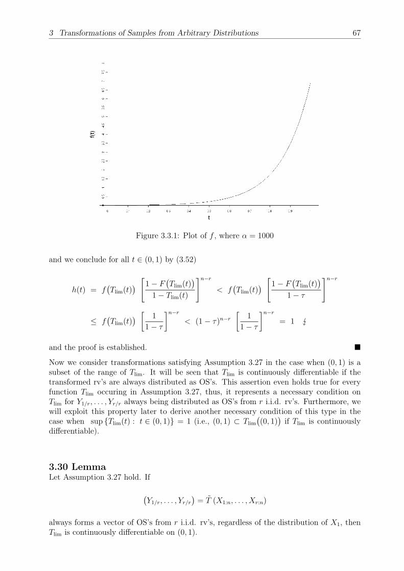
3 Transformations of Samples from Arbitrary Distributions 67
Figure 3.3.1: Plot of f , where α = 1000
and we conclude for all t ∈ (0, 1) by (3.52)
h(t) = f(Tlim(t)
) [1− F(Tlim(t)
)1− Tlim(t)
]n−r< f
(Tlim(t)
) [1− F(Tlim(t)
)1− τ
]n−r
≤ f(Tlim(t)
) [ 1
1− τ
]n−r< (1− τ)n−r
[1
1− τ
]n−r= 1
and the proof is established.
Now we consider transformations satisfying Assumption 3.27 in the case when (0, 1) is asubset of the range of Tlim. It will be seen that Tlim is continuously differentiable if thetransformed rv’s are always distributed as OS’s. This assertion even holds true for everyfunction Tlim occuring in Assumption 3.27, thus, it represents a necessary condition onTlim for Y1/r, . . . , Yr/r always being distributed as OS’s from r i.i.d. rv’s. Furthermore, wewill exploit this property later to derive another necessary condition of this type in thecase when sup Tlim(t) : t ∈ (0, 1) = 1 (i.e., (0, 1) ⊂ Tlim
((0, 1)
)if Tlim is continuously
differentiable).
3.30 LemmaLet Assumption 3.27 hold. If
(Y1/r, . . . , Yr/r
)= T (X1:n, . . . , Xr:n)
always forms a vector of OS’s from r i.i.d. rv’s, regardless of the distribution of X1, thenTlim is continuously differentiable on (0, 1).

68 3.3 More General Transformations
Proof. Let T = T−1 and, for α > 1,
f(x) =
α(1− x)α−1 , x ∈ [0, 1],
0 , else,F (x) =
0 , x < 0,
1− (1− x)α , x ∈ [0, 1],
1 , x > 1.
Furthermore, let(Y1/r, . . . , Yr/r
)= T (X1:n, . . . , Xr:n) be distributed as a vector of OS’s
from r i.i.d. rv’s with some cdf H.Obviously, F and f satisfy the conditions of Lemma 3.28, and in this case the function δfrom Lemma 3.28 is given by
δ(x) = (1− x)α−1 , x ∈ [0, 1].
Thus, we obtainh(t) = α
(1− Tlim(t)
)(α−1)(n−r+1), t ∈ (0, 1),
as a pdf of H and, as in the proof of Lemma 3.28 (cf. (3.51)),
r∏k=1
h(tk) =
[1− F
(T (t1, . . . , tr)r
)1− T (t1, . . . , tr)r
]n−r r∏k=1
f(T (t1, . . . , tr)k
)∀ (t1, . . . , tr) ∈ Kr1.
Let α > 1 and t ∈ (0, 1) be arbitrary.Then, there are t1, . . . , tr−1 ∈ (0, 1) such that (t1, . . . , tr−1, t) ∈ Kr1 and Tlim(tk) < 1 forall k ∈ 1, . . . , r − 1 (cf. (∗ ∗ ∗) of Assumption 3.27).Hence, we have
α(1− Tlim(t)
)(α−1)(n−r+1)r−1∏k=1
α(1− Tlim(tk)
)(α−1)(n−r+1)
= αr(1− T (t1, . . . , tr−1, t)r
)(α−1)(n−r)r∏
k=1
(1− T (t1, . . . , tr−1, t)k
)α−1
⇐⇒
Tlim(t) = 1−
[(1− T (t1, . . . , tr−1, t)r
)n−r r∏k=1
(1− T (t1, . . . , tr−1, t)k
)] 1n−r+1
r−1∏k=1
(1− Tlim(tk)
) .
From Assumptions 3.1 and 3.27 we obtain that T is continuously differentiable. Thismeans in particular, T (·)k is continuously partially differentiable in every component forall k ∈ 1, . . . , r. Thus,
ϑ 7−→ 1−
[(1− T (t1, . . . , tr−1, ϑ)r
)n−r r∏k=1
(1− T (t1, . . . , tr−1, ϑ)k
)] 1n−r+1
r−1∏k=1
(1− Tlim(tk)
) , ϑ ∈ (tr−1, 1),

3 Transformations of Samples from Arbitrary Distributions 69
is continuously differentiable.Consequently, Tlim is continuously differentiable in t and since t ∈ (0, 1) was arbitrary, Tlim
is continuously differentiable on (0, 1).
The corresponding result to Theorem 3.29 for transformations from Assumption 3.27 when(0, 1) is a subset of the range of Tlim now reads as follows.
3.31 TheoremLet Assumption 3.27 hold, (
Y1/r, . . . , Yr/r)
= T (X1:n, . . . , Xr:n)
andsup Tlim(t) : t ∈ (0, 1) = 1.
Additionally, presume that Tlim is monotone.
(i) If Tlim is injective with T ′lim(t) 6= 0 almost everywhere on (0, 1) then
Tlim(t) = 1− (1− t)1
n−r+1 ∀ t ∈ (0, 1)
is a necessary condition for Y1/r, . . . , Yr/r always being distributed as OS’s from ri.i.d. rv’s regardless of the distribution of X1.
(ii) If Tlim is not injective then there is always a cdf F such that Y1/r, . . . , Yr/r are notdistributed as OS’s from r i.i.d. rv’s.
Proof.
(i) We assume that Y1/r, . . . , Yr/r are always distributed as OS’s from r i.i.d. rv’sregardless of the distribution of X1.For α > 1 let
f(x) =
α(1− x)α−1 , x ∈ [0, 1],
0 , else,
and
F (x) =
0 , x < 0,
1− (1− x)α , x ∈ [0, 1],
1 , x > 1.
Obviously, F and f satisfy the conditions of Lemma 3.28 such that a pdf h of theunderlying distribution of Y1/r, . . . , Yr/r can be defined by
(3.53) h(t) = α(1− Tlim(t)
)(α−1)(n−r+1), t ∈ (0, 1).
Thus, we have
(3.54)∫
(0,1)
α[(
1− Tlim
)n−r+1]α−1
dλ1 = 1 ∀ α > 1.

70 3.3 More General Transformations
Let
(3.55) Θ(t) =(1− Tlim(t)
)n−r+1, t ∈ (0, 1).
Since Tlim is injective and limϑ0
Tlim(ϑ) = 0 (cf. Assumption 3.27, (∗ ∗ ∗)), wefind Θ is strictly decreasing with
limt0
Θ(t) = 1 and limt1
Θ(t) = 0.
Furthermore, by Lemma 3.30 and T ′lim(t) 6= 0 almost everywhere (a.e.) on (0, 1),we obtain Θ is continuously differentiable on (0, 1) with Θ′(t) < 0 a.e. on(0, 1).Let G = t ∈ (0, 1) : Θ′(t) < 0, then Θ(G) is open and Θ−1 is continuouslydifferentiable on Θ(G). Since λ1
((0, 1)\G
)= 0 and Θ continuously differentiable
on (0, 1) we have λ1(
Θ((0, 1)\G
))= 0 and thus by (3.54)
1 =
∫(0,1)
α(Θ(t)
)α−1dλ1(t) =
∫G
α(Θ(t)
)α−1dλ1(t)
=
∫Θ(G)
α tα−1
∣∣∣∣∣ 1
Θ′(Θ−1(t)
)∣∣∣∣∣ dλ1(t) =
∫Θ(G)
α tα−1 −1
Θ′(Θ−1(t)
) dλ1(t)
=
∫(0,1)
α tα−1Θ(t) dλ1(t) ∀ α > 1,
where
(3.56) Θ =
−1
Θ′(Θ−1(t)
) , t ∈ Θ(G),
0 , t ∈ (0, 1)\Θ(G).
Then,
(3.57) 0 =
∫(0,1)
α tα−1(1− Θ(t)
)dλ1(t) ∀ α > 1.
Notice, the set of all power function distributions with parameter α > 1
P = Pα ∼ pow(α) : α > 1
forms an exponential family.If ν is the restriction of the Lebesgue measure λ1 to (0, 1)∩B1, where B1 denotesthe σ-algebra of all Borel sets in R, then a ν-density of Pα is given by
pα(x) = α e(α−1) ln(x), x ∈ (0, 1), α > 1.
Hence, ln(·) is complete for P and (3.57) yields
0 =
∫ (1− Θ
)dPα =
∫ (1− Θ exp
)dP ln
α ∀ α > 1,

3 Transformations of Samples from Arbitrary Distributions 71
where P lnα is the induced measure of Pα by the natural logarithm ln(·), α > 1.
I.e., there is a set N ∈ (−∞, 0) ∩B1 with P lnα (N) = 0 for all α > 1 and
(3.58) 1−(Θ exp
)(x) = 0 ∀ x ∈ (−∞, 0)\N.
Since for α > 1
plnα (x) =
αeαx , x < 0,
0 , else,
is a λ1-density of P lnα with pln
α (x) > 0 for all x < 0, we have P lnα (N) = 0 ⇐⇒
λ1(N) = 0, such that we obtain from (3.58)
1−(Θ exp
)= 0 a.e. on (−∞, 0)
exp cont. diff.=⇒ 1− Θ = 0 a.e. on (0, 1)
=⇒ Θ = 1 a.e. on (0, 1).
Thus, there is a set N ∈ (0, 1) ∩B1 with λ1(N) = 0 and
Θ(t) = 1 ∀ t ∈ (0, 1)\N .
By (3.56), we find
(0, 1)\N ⊂ Θ(G) and−1
Θ′(t)= 1 ∀ t ∈ Θ−1
((0, 1)\N
)= (0, 1)\Θ−1(N),
whereλ1(Θ−1(N)
)= λ1
(Θ−1
(N ∩Θ(G)
))+ λ1
(Θ−1(N)\G
)= 0,
since Θ−1 is continuously differentiable on Θ(G) and λ1((0, 1)\G
)= 0. We obtain
Θ′ = −1 a.e. on (0, 1).
By the continuity of Θ′ this means
Θ′(x) = −1 ∀ x ∈ (0, 1) ⇐⇒ Θ(x) = γ − x ∀ x ∈ (0, 1),
where γ is a suitable constant.Since Θ(0) = 1 this yields
Θ(x) = 1− x ∀ x ∈ (0, 1) ⇐⇒ Tlim(t) = 1− (1− t)1
n−r+1 ∀ t ∈ (0, 1).
(ii) Now, let Tlim be not injective and Y1/r, . . . , Yr/r be distributed as OS’s from r i.i.d.rv’s with underlying pdf h. Then there are 0 ≤ c1 < c2 ≤ 1 and v ∈ [0, 1] with
(3.59) Tlim
((c1, c2)
)= v
because Tlim is monotone.
(a) If v ∈ (0, 1) then let σ > 0 be so small that
(3.60)(v − σ
√3, v + σ
√3)⊆ (0, 1) and
1
σ√
2π>
[4(1− v)
]n−rc2 − c1
.

72 3.3 More General Transformations
For
c =
1∫0
1
σ√
2πe−
(x−v)2
2σ2 dx
−1
> 1
f , defined by
f(t) =
c
σ√
2πe−
(t−v)2
2σ2 , t ∈ [0, 1],
0 , else,
forms a pdf, and the corresponding cdf reads
F (x) =
0 , x < 0,
x∫0
f(t) dt , x ∈ [0, 1],
1 , x > 1.
Obviously, f and F meet the conditions of Lemma 3.28, such that we areagain able to define
(3.61) h(t) = f(Tlim(t)
) [δ(Tlim(t)
)]n−r, t ∈ (0, 1),
where δ is defined as in Lemma 3.28.By Tschebyscheff’s inequality we know, if Z ∼ N (v, σ2) then
P(|Z − v| ≥ σ
√3)≤ σ2
3σ2=
1
3.
This yields,
1 >1
c=
1∫0
1
σ√
2πe−
(x−v)2
2σ2 dx ≥v+σ√
3∫v−σ√
3
1
σ√
2πe−
(x−v)2
2σ2 dx
= P(|Z − v| < σ
√3)
= 1− P(|Z − v| ≥ σ
√3)≥ 2
3.
Hence, we have
1 < c ≤ 3
2,
which means
F (v) =
v∫0
f(t) dt < c
v∫−∞
1
σ√
2πe−
(t−v)2
2σ2 dt =c
2≤ 3
4
and thus1− F (v) >
1
4.
We obtain for all t ∈ (c1, c2) by (3.59) – (3.61)
h(t) = f(Tlim(t)
) [δ(Tlim(t)
)]n−r= f(v)
[δ(v)
]n−r
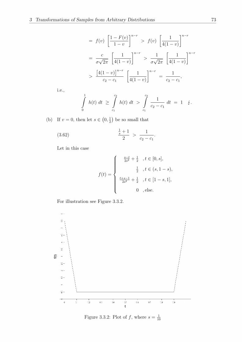
3 Transformations of Samples from Arbitrary Distributions 73
= f(v)
[1− F (v)
1− v
]n−r> f(v)
[1
4(1− v)
]n−r
=c
σ√
2π
[1
4(1− v)
]n−r>
1
σ√
2π
[1
4(1− v)
]n−r
>
[4(1− v)
]n−rc2 − c1
[1
4(1− v)
]n−r=
1
c2 − c1
,
i.e.,1∫
0
h(t) dt ≥c2∫c1
h(t) dt >
c2∫c1
1
c2 − c1
dt = 1 .
(b) If v = 0, then let s ∈(0, 1
2
)be so small that
(3.62)1s
+ 1
2>
1
c2 − c1
.
Let in this case
f(t) =
s−t2s2
+ 12
, t ∈ [0, s],
12
, t ∈ (s, 1− s),
t+s−12s2
+ 12
, t ∈ [1− s, 1],
0 , else.
For illustration see Figure 3.3.2.
Figure 3.3.2: Plot of f , where s = 110

74 3.3 More General Transformations
Then
F (x) =
0 , x < 0,
x∫0
f(t) dt , x ∈ [0, 1],
1 , x > 1,
fulfills again the conditions of Lemma 3.28 and we find (3.61) as in case (a).That is, by (3.59) and (3.62) for all t ∈ (c1, c2)
h(t) = f(v)[δ(v)
]n−r= f(0)
[1− F (0)
1− 0
]n−r
= f(0) =1s
+ 1
2>
1
c2 − c1
.
Hence, we obtain again
1∫0
h(t) dt ≥c2∫c1
h(t) dt >
c2∫c1
1
c2 − c1
dt = 1 .
(c) If v = 1, then we find analogously to (b) with the same definition of f , F andh for all t ∈ (c1, c2)
h(t) = f(v)[δ(v)
]n−r= f(1)
[f(1)
]n−r=[f(1)
]n−r+1=
[ 1s
+ 1
2
]n−r+1
>
[1
c2 − c1
]n−r+1
≥ 1
c2 − c1
.
Thus, we find as in the cases before
1∫0
h(t) dt ≥c2∫c1
h(t) dt >
c2∫c1
1
c2 − c1
dt = 1 .
Theorem 3.31 (i) suggests that if F and f meet the assumptions of Lemma 3.28 then
(3.63) h(t) =
1− F(
1− (1− t)1
n−r+1
)(1− t)
1n−r+1
n−r f (1− (1− t)1
n−r+1
), t ∈ (0, 1),
should be a pdf. And in fact, h(t) ≥ 0 holds true for all t and since
∂
∂t
(1− (1− t)
1n−r+1
)=
(1− t)r−nn−r+1
n− r + 1, t ∈ (0, 1),
we have
1∫0
h(t) dt =
1∫0
1− F(
1− (1− t)1
n−r+1
)(1− t)
1n−r+1
n−r f (1− (1− t)1
n−r+1
)dt

3 Transformations of Samples from Arbitrary Distributions 75
x=F
(1−(1−t)
1n−r+1
)=
1∫0
(n− r + 1)(1− x)n−r dx
= 1.
Moreover, we find in this case for all x ∈ (0, 1)
H(x) =
x∫0
h(t) dt =
F
(1−(1−x)
1n−r+1
)∫0
(n− r + 1)(1− t)n−r dt(3.64)
= 1−(
1− F(
1− (1− x)1
n−r+1
))n−r+1
= T−1lim
(F(Tlim(x)
))(recall, Tlim(x) = 1− (1− x)
1n−r+1 , x ∈ (0, 1)).
Thus, Theorem 3.31 (i) indeed provides a necessary condition for the transformed variablesalways being distributed as OS’s from r i.i.d. rv’s if the cdf of X1, . . . , Xn satisfies theassumptions of Lemma 3.28. But, as we can see by the transformation of O’Reilly andStephens, it is not a sufficient condition.Furthermore, if there is more than one transformation fulfilling the conditions of Theorem3.31 (i) which always yields OS’s, then, in the situation considered in Lemma 3.28, theunderlying distribution of the obtained OS’s will not depend on the specific transformation,since (3.63) will always define a corresponding pdf.Moreover, we have for every cdf F
T−1lim F Tlim = T−1
lim F Tlim ⇐⇒ F = F ,
wherefore (3.64) suggests that only OS’s of uniformly distributed rv’s would be transformedinto OS’s of uniformly distributed rv’s, considering the situation of Lemma 3.28.I.e., probably all of these transformations would be applicable for testing goodness-of-fit ofType-II right censored samples, since the null hypothesis that such a sample stems from thestandard uniform distribution should be equivalent to the hypothesis that the transformedsample is distributed as a full vector of standard uniform OS’s. But, as we have seen,at least for cdf’s F fulfilling the conditions of Lemma 3.28 the underlying distribution ofthe transformed OS’s would be the same for all transformations, such that none of themshould yield tests with better powers than the other ones.
Now, we will show that the transformations given in Lemma 2.4 do not always transforma Type-II right censored sample of i.i.d. rv’s into an ordered complete sample of i.i.d. rv’s.With the same notations as in Lemma 2.4 we find A and C are bijective with inversesA = A−1, respectively, C = C−1 given by
A(t1, . . . , tr)i = B−1r,n−r+1
(1− (1− t1)r
) r−1∏j=i
(1−
[1− tr−j+1
1− tr−j
]j) 1j
, (t1, . . . , tr) ∈ Kr1,
and
C(t1, . . . , tr)i = 1−i∏
j=1
(1−
[tjtj+1
]j) 1n−j+1
, (t1, . . . , tr) ∈ Kr1,

76 3.3 More General Transformations
i = 1, . . . , r, where tr+1 = 1.Since
∂ A(t1, . . . , tr)i∂tk
= 0 ∀ 1 ≤ k < r − i+ 1 ≤ r and (t1, . . . , tr) ∈ Kr1
we obtain
|∆A(t1, . . . , tr)| =r∏i=1
∣∣∣∣∣∂ A(t1, . . . , tr)i∂tr−i+1
∣∣∣∣∣=(1−Br,n−r+1(tr)
) 1−rr
(n
r
)tr−1r (1− tr)n−r
×r∏i=2
(1−Br,n−r+1(tr)
) 1r
[1−
(tr−i+1
tr−i+2
)r−i+1] i−rr−i+1
tr−ir−i+1
tr−i+1r−i+2
×i−1∏j=2
[1−
(tr−j+1
tr−j+2
)r−j+1] 1r−j+1
=
(n
r
)tr−1r (1− tr)n−r
r∏i=2
[1−
(tr−i+1
tr−i+2
)r−i+1] i−rr−i+1
tr−ir−i+1
tr−i+1r−i+2
×r∏i=3
i−1∏j=2
[1−
(tr−j+1
tr−j+2
)r−j+1] 1r−j+1
=
(n
r
)(1− tr)n−r
r−1∏i=2
[1−
(tr−i+1
tr−i+2
)r−i+1] i−rr−i+1
×r−1∏i=2
[1−
(tr−i+1
tr−i+2
)r−i+1] r−ir−i+1
=
(n
r
)(1− tr)n−r 6= 0 ∀ (t1, . . . , tr) ∈ Kr1.
Calculating |∆C(t1, . . . , tr)| for (t1, . . . , tr) ∈ Kr1 is more intricate. First, notice
C(t1, . . . , tr)i =r∏j=i
γj(tj−1, tj), i = 1, . . . , r,
where t0 = 0,
γ1(t0, t1) = 1− (1− t1)n , γj(tj−1, tj) =
(1−
[1− tj
1− tj−1
]n−j+1) 1
j
, j = 2, . . . , r,
and (t1, . . . , tr) ∈ Kr1.Now let (t1, . . . , tr) ∈ Kr1 be arbitrary but fixed, t0 = 0,
γj = γj(tj−1, tj) , γjk =∂γj(tj−1, tj)
∂tk∣∣∣(tj−1,tj)=(tj−1,tj)
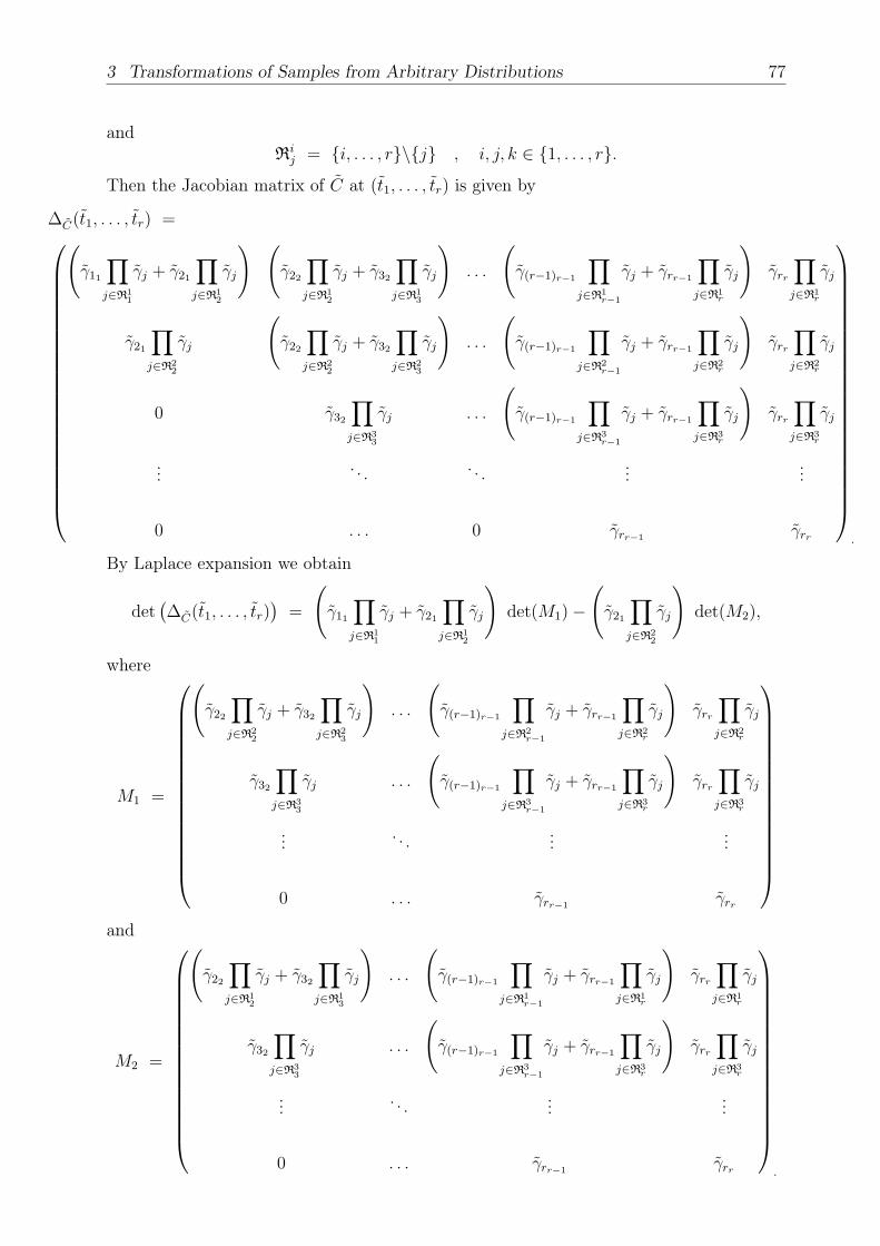
3 Transformations of Samples from Arbitrary Distributions 77
andRij = i, . . . , r\j , i, j, k ∈ 1, . . . , r.
Then the Jacobian matrix of C at (t1, . . . , tr) is given by
∆C(t1, . . . , tr) =
(γ11
∏j∈R1
1
γj + γ21
∏j∈R1
2
γj
) (γ22
∏j∈R1
2
γj + γ32
∏j∈R1
3
γj
). . .
(γ(r−1)r−1
∏j∈R1
r−1
γj + γrr−1
∏j∈R1
r
γj
)γrr∏j∈R1
r
γj
γ21
∏j∈R2
2
γj
(γ22
∏j∈R2
2
γj + γ32
∏j∈R2
3
γj
). . .
(γ(r−1)r−1
∏j∈R2
r−1
γj + γrr−1
∏j∈R2
r
γj
)γrr∏j∈R2
r
γj
0 γ32
∏j∈R3
3
γj . . .
(γ(r−1)r−1
∏j∈R3
r−1
γj + γrr−1
∏j∈R3
r
γj
)γrr∏j∈R3
r
γj
... . . . . . . ......
0 . . . 0 γrr−1 γrr
.
By Laplace expansion we obtain
det(∆C(t1, . . . , tr)
)=
(γ11
∏j∈R1
1
γj + γ21
∏j∈R1
2
γj
)det(M1)−
(γ21
∏j∈R2
2
γj
)det(M2),
where
M1 =
(γ22
∏j∈R2
2
γj + γ32
∏j∈R2
3
γj
). . .
(γ(r−1)r−1
∏j∈R2
r−1
γj + γrr−1
∏j∈R2
r
γj
)γrr∏j∈R2
r
γj
γ32
∏j∈R3
3
γj . . .
(γ(r−1)r−1
∏j∈R3
r−1
γj + γrr−1
∏j∈R3
r
γj
)γrr∏j∈R3
r
γj
... . . . ......
0 . . . γrr−1 γrr
and
M2 =
(γ22
∏j∈R1
2
γj + γ32
∏j∈R1
3
γj
). . .
(γ(r−1)r−1
∏j∈R1
r−1
γj + γrr−1
∏j∈R1
r
γj
)γrr∏j∈R1
r
γj
γ32
∏j∈R3
3
γj . . .
(γ(r−1)r−1
∏j∈R3
r−1
γj + γrr−1
∏j∈R3
r
γj
)γrr∏j∈R3
r
γj
... . . . ......
0 . . . γrr−1 γrr
.

78 3.3 More General Transformations
Sincedet(M2) = γ1 det(M1)
this yields
(3.65) det(∆C(t1, . . . , tr)
)=
(γ11
∏j∈R1
1
γj
)det(M1),
and the (r − 1) × (r − 1)-matrix M1 possesses the same form as ∆C(t1, . . . , tr). Moreprecisely,
M1 =
(˜γ11
∏j∈R1
1
˜γj + ˜γ21
∏j∈R1
2
˜γj
) (˜γ22
∏j∈R1
2
˜γj + ˜γ32
∏j∈R1
3
˜γj
). . . ˜γ(r−1)r−1
∏j∈R1
r−1
˜γj
˜γ21
∏j∈R2
2
˜γj
(˜γ22
∏j∈R2
2
˜γj + ˜γ32
∏j∈R2
3
˜γj
). . . ˜γ(r−1)r−1
∏j∈R2
r−1
˜γj
0 ˜γ32
∏j∈R3
3
˜γj . . . ˜γ(r−1)r−1
∏j∈R3
r−1
˜γj
......
......
0 . . . ˜γ(r−1)r−2˜γ(r−1)r−1
,
where
˜γjk = γ(j+1)k+1, ˜γj = γj+1 and Ri
j = i, . . . , r−1\j , i, j, k ∈ 1, . . . , r−1.
Due to this, we will proof by induction on r
(3.66) det(∆C(t1, . . . , tr)
)=
r∏j=1
(γjj (γj)
j−1).
For r = 2 we obtain
det(∆C(t1, . . . , tr)
)= det
(((γ11 γ2 + γ21 γ1
)γ22 γ1
γ21 γ22
))= γ11 γ22 γ2 X.
Now, let (3.66) be true for r − 1. Then, we have by the induction hypothesis
det(M1
)=
r−1∏j=1
(˜γjj (˜γj)
j−1).
This yields for ∆C(t1, . . . , tr)
det(∆C(t1, . . . , tr)
) (3.65)=
(γ11
∏j∈R1
1
γj
)det(M1) =
(γ11
r∏j=2
γj
)(r−1∏j=1
(γ(j+1)j+1
(γj+1)j−1))
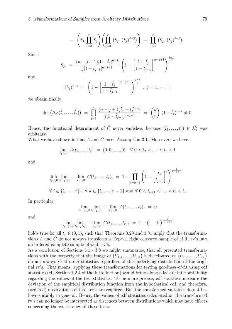
3 Transformations of Samples from Arbitrary Distributions 79
=
(γ11
r∏j=2
γj
)(r∏j=2
(γjj (γj)
j−2))
=r∏j=1
(γjj (γj)
j−1).
Since
γjj =(n− j + 1)[1− tj]n−j
j[1− tj−1]n−j+1
(1−
[1− tj
1− tj−1
]n−j+1) 1−j
j
and
(γj)j−1 =
(1−
[1− tj
1− tj−1
]n−j+1) j−1
j
, j = 1, . . . , r,
we obtain finally
det(∆C(t1, . . . , tr)
)=
r∏j=1
(n− j + 1)[1− tj]n−j
j[1− tj−1]n−j+1=
(n
r
)(1− tr)n−r 6= 0.
Hence, the functional determinant of C never vanishes, because (t1, . . . , tr) ∈ Kr1 wasarbitrary.What we have shown is that A and C meet Assumption 3.1. Moreover, we have
limt10
A(t1, . . . , tr) = (0, 0, . . . , 0) ∀ 0 < t2 < . . . < tr < 1
and
limtk0
limtk−10
· · · limt10
C(t1, . . . , tr)i = 1−i∏
j=k+1
(1−
[tjtj+1
]j) 1n−j+1
∀ i ∈ 1, . . . , r , ∀ k ∈ 1, . . . , r − 1 and ∀ 0 < tk+1 < . . . < tr < 1.
In particular,lim
tr−10lim
tr−20· · · lim
t10A(t1, . . . , tr)r = 0
andlim
tr−10lim
tr−20· · · lim
t10C(t1, . . . , tr)r = 1−
(1− trr
) 1n−r+1
holds true for all tr ∈ (0, 1), such that Theorems 3.29 and 3.31 imply that the transforma-tions A and C do not always transform a Type-II right censored sample of i.i.d. rv’s intoan ordered complete sample of i.i.d. rv’s.As a conclusion of Sections 3.1 - 3.3 we might summarize, that all presented transforma-tions with the property that the image of
(U1:n, . . . , Ur:n
)is distributed as
(U1:r, . . . , Ur:r
)do not always yield order statistics regardless of the underlying distribution of the origi-nal rv’s. That means, applying these transformations for testing goodness-of-fit using edfstatistics (cf. Section 1.2.4 of the Introduction) would bring along a lack of interpretabilityregarding the values of the test statistics. To be more precise, edf statistics measure thedeviation of the empirical distribution function from the hypothetical cdf, and therefore,(ordered) observations of i.i.d. rv’s are required. But the transformed variables do not be-have suitably in general. Hence, the values of edf statistics calculated on the transformedrv’s can no longer be interpreted as distances between distributions which may have effectsconcerning the consistency of these tests.

80 3.4 Transformations into r-1 Order Statistics
In Section 3.4 we will see, at the price of losing one dimension, i.e., only r − 1 OS’s areobtained, a transformation can be found that preserves the structure of OS’s at least forthe whole family of power function distributions. A similar result can be obtained, con-sidering mappings that transform
(U1:n, . . . , Ur:n
)into i.i.d. uniformly distributed rv’s (cf.
Section 3.5).
3.4 Transformations into r-1 Order Statistics
Up to now, all transformations considered so far led to negative results w.r.t. preservingthe structure of OS’s. One of the mappings in Theorem 2.2 has not been examined. In fact,transformation (ix) in Theorem 2.2 shows a different behavior. But also the transformationitself is of a different type. The OS’s U1:n, . . . , Ur:n from a right censored sample of standarduniform quantities are mapped to a full vector of standard uniform OS’s in a sample ofsize r − 1. In this situation, the structure of OS’s is also preserved for power functiondistributions.
3.32 TheoremLet the pdf f of X1, . . . , Xn be positive almost everywhere on (0, 1) and continuous on thesame interval. Then (
X1:n
Xr:n
, . . . ,Xr−1:n
Xr:n
)∼ (Y1:r−1, . . . , Yr−1:r−1)
for some OS’s Y1:r−1, . . . , Yr−1:r−1 from r − 1 i.i.d. rv’s with underlying pdf g and(X1:n
Xr:n
, . . . ,Xr−1:n
Xr:n
)and Xr:n are stochastically independent
if and only if g ∼ f ∼ pow(α) for some α > 0.
Proof. Since f is continuous and positive almost everywhere on (0, 1) we have F (0) =0 < F (x) < 1 = F (1) for all x ∈ (0, 1). Densities of Xr:n, respectively
(X1:n, . . . , Xr:n
), are
given by (e.g. see David and Nagaraja (2003) or Arnold et al. (1992))
fXr:n(t) =
r
(n
r
)F (t)r−1f(t) [1− F (t)]n−r , t ∈ (0, 1),
0 , else,
respectively,
fX1:n,...,Xr:n(t1, . . . , tr) =
r!
(n
r
)[1− F (tr)]
n−rr∏
k=1
f(tk) , (t1, . . . , tr) ∈ Kr1,
0 , else.
Thus, by applying density transformation we obtain
fX1:nXr:n
,...,Xr−1:nXr:n
,Xr:n(x1, . . . , xr) = xr−1r r!
(n
r
)[1− F (xr)]
n−r f(xr)r−1∏i=1
f(xixr)

3 Transformations of Samples from Arbitrary Distributions 81
= r
(n
r
)F (xr)
r−1f(xr) [1− F (xr)]n−r (r − 1)!
r−1∏i=1
xrF (xr)
f(xixr)
= fXr:n(xr) (r − 1)!r−1∏i=1
xrF (xr)
f(xixr), 0 < x1 < . . . < xr−1 < 1, xr ∈ (0, 1),
as a joint pdf ofX1:n
Xr:n
, . . . ,Xr−1:n
Xr:n
and Xr:n.
Hence,(X1:n
Xr:n
, . . . ,Xr−1:n
Xr:n
)is distributed as a vector of r − 1 i.i.d. rv’s with pdf g and
independent of Xr:n if and only if for almost all 0 < x1 < . . . < xr−1 < 1 and xr ∈ (0, 1)
(3.67) (r − 1)!r−1∏i=1
g(xi) = (r − 1)!r−1∏i=1
xrF (xr)
f(xixr).
If g(x) = f(x) = αxα−1, x ∈ (0, 1), for some α > 0 this is obviously true.On the other hand, let g be a pdf on (0, 1), Kr−1
1 as in Lemma 2.4,
N =
(x1, . . . , xr) ∈ Kr−1
1 × (0, 1) :r−1∏i=1
g(xi) 6=r−1∏i=1
xrF (xr)
f(xixr)
and for ξ ∈ Kr−11
N∣∣ξ =x ∈ (0, 1) : (ξ, x) ∈ N
.
Assume, hereafter, λr(N) = 0. Then it is well known that
N =
ξ ∈ Kr−1
1 : λ1
(N∣∣ξ)6= 0
is a λr−1-null set.For all ξ ∈ Kr−1
1 \N exist(xξk)k∈N ⊂ (0, 1)\N∣∣ξ with xξk 1 as k tends to infinity, such
that we obtain for all ξ = (x1, . . . , xr−1) ∈ Kr−11 \N by the continuity of f on the open unit
interval
(3.68)r−1∏i=1
f(xi) = limk→∞
r−1∏i=1
xξkF(xξk)f(xixξk) = lim
k→∞
r−1∏i=1
g(xi) =r−1∏i=1
g(xi).
Since (3.67) holds true for all (x1, . . . , xr) ∈(Kr−1
1 × (0, 1))\N and (3.68) for every
(x1, . . . , xr−1) ∈ Kr−11 \N , we find
(3.69)r−1∏i=1
f(xi) =r−1∏i=1
xrF (xr)
f(xixr) ∀ (x1, . . . , xr) ∈(Kr−1
1 × (0, 1))\(N ∪ N × (0, 1)
),
whereλr(N ∪ N × (0, 1)
)≤ λr(N) + λr
(N × (0, 1)
)= 0 + λr−1
(N)
= 0.
Now, let for x ∈ (0, 1)(N ∪ N × (0, 1)
)∣∣x =ξ ∈ Kr−1
1 : (ξ, x) ∈(N ∪ N × (0, 1)
).

82 3.4 Transformations into r-1 Order Statistics
Then, we have for
N =
x ∈ (0, 1) : λr−1
((N ∪ N × (0, 1)
)∣∣x)6= 0
λ1(N)
= 0, by analogy with N . Moreover, we find for every xr ∈ (0, 1)\N from (3.69)
r−1∏i=1
f(xi) =r−1∏i=1
xrF (xr)
f(xixr) almost everywhere on Kr−11 .
I.e., since f is continuous on the open unit interval we obtain for almost all xr ∈ (0, 1)
(3.70)r−1∏i=1
f(xi) =r−1∏i=1
xrF (xr)
f(xixr) ∀ 0 < x1 < . . . < xr−1 < 1.
Let x ∈ (0, 1). Calculating the limit limx1x limx2x . . . limxr−1x on both sides of (3.70)yields
f(x) =xr
F (xr)f(xxr)
and hence,
F (xr)F (y) =
y∫0
F (xr)f(t) dt =
y∫0
xrf(txr) dt = F (xry) ∀y ∈ (0, 1),
for almost all xr ∈ (0, 1). Thus, by the continuity of F , we have for ϕ(t) = F (e−t), t > 0:
ϕ(s+ t) = ϕ(s)ϕ(t) ∀ s, t > 0.
Since ϕ is continuous and positive, all solutions of this Cauchy functional equation aregiven by
ϕ(t) = ect, t > 0 : c ∈ R
(e.g. see Aczél (1966), p.38). I.e., there is an α > 0
such that F (t) = tα for all t ∈ (0, 1).
We see, at the price of losing one dimension, a transformation is found that preserves thestructure of OS’s at least for the whole family of power function distributions. This means,every ordinary parameter test for power function distributions now yields a parameter testfor power function distributions when there is only right censored data available. Moreover,because of X ∼ par(α, b) =⇒ 1− Fα,β(X) ∼ pow
(bβ
)for all α, β, b > 0, where
Fα,β : x 7−→
0 , x < α,
1− αβ
xβ, x ≥ α,
denotes the cdf of a Pareto distribution with scale parameter α and shape parameter β,every ordinary parameter test for power function distributions also yields a shape parametertest for Pareto distributions based on right censored data.

3 Transformations of Samples from Arbitrary Distributions 83
3.5 Transformations into i.i.d. Random Variables
This final section of Chapter 3 deals with mappings that transform(U1:n, . . . , Ur:n
)into
i.i.d. uniformly distributed rv’s. Lin et al. (2008) suggested to arrange W1, . . . ,Wr fromTheorem 2.2 (v) in non-decreasing order for obtaining an alternative to the transformationof Michael and Schucany (1979) (cf. Theorem 2.2 (x)). Earlier O’Reilly and Stephens(1988) found (iv) and (vi) from Theorem 2.2 as interim results establishing Theorem 2.2(x) and (xi).By an analogous approach as in Sections 3.1 and 3.2 we will find results correspondingto Theorems 3.5 and 3.6 concerning transformations into i.i.d. rv’s. They can be derivedcompletely by the same ideas as before, but due to the plain structure of i.i.d. samples theirproofs can be shortened and less assumptions are required. The considered transformationsshould satisfy the following.
3.33 AssumptionLet Kr1 as in Lemma 2.4 and T : Kr1 −→ (0, 1)r be a bijective mapping which is continu-ously differentiable such that the determinant of the Jacobian matrix never vanishes.Moreover, we postulate
T (U1:n, . . . , Ur:n) ∼ (U1, . . . , Ur) ,
i.e., the transformation of ordered standard uniform rv’s leads to i.i.d. rv’s from a standarduniform distribution.
First, we apply density transformation to obtain the general distribution of the modifiedrv’s. The proof of Lemma 3.34 is nearly the same as the one of Lemma 3.3 and only givenfor completeness.
3.34 LemmaLet T satisfy Assumption 3.33 and(
Y1, . . . , Yr)
= T (X1:n, . . . , Xr:n) .
Then, a pdf of(Y1, . . . , Yr
)is given by
fY1,...,Yr(t1, . . . , tr)
=
[
1− F(T (t1, . . . , tr)r
)1− T (t1, . . . , tr)r
]n−r r∏k=1
f(T (t1, . . . , tr)k
), (t1, . . . , tr) ∈ (0, 1)r,
0 , else,
where T = T−1.
Proof. A pdf of(X1:n, . . . , Xr:n
)is given by (e.g. see David and Nagaraja (2003), p. 12
or Arnold et al. (1992), p. 10)
fX1:n,...,Xr:n(t1, . . . , tr) =
r!
(n
r
)[1− F (tr)]
n−rr∏
k=1
f(tk) , (t1, . . . , tr) ∈ Kr1,
0 , else.

84 3.5 Transformations into i.i.d. Random Variables
By applying density transformation we find
hY1,...,Yr(t1, . . . , tr)
=
r!
(n
r
) [1− F
(T (t1, . . . , tr)r
)]n−r|∆T
(T (t1, . . . , tr)
)|
r∏k=1
f(T (t1, . . . , tr)k
), (t1, . . . , tr) ∈ (0, 1)r,
0 , else,
as a pdf of(Y1, . . . , Yr
).
Moreover,
fU1,...,Ur(t1, . . . , tr) =
1 , (t1, . . . , tr) ∈ (0, 1)r,
0 , else,
and
fU1:n,...,Ur:n(t1, . . . , tr) =
r!
(n
r
)[1− tr]n−r , (t1, . . . , tr) ∈ Kr1,
0 , else,
are pdf’s of(U1, . . . , Ur
)and
(U1:n, . . . , Ur:n
), respectively.
Hence, again by applying density transformation we obtain from Assumption 3.33 almosteverywhere on (0, 1)r
1 =
r!
(n
r
) [1− T (t1, . . . , tr)r
]n−r|∆T
(T (t1, . . . , tr)
)|
⇐⇒ |∆T
(T (t1, . . . , tr)
)| = r!
(n
r
) [1− T (t1, . . . , tr)r
]n−r.
Thus, we have
hY1,...,Yr(t1, . . . , tr) =
[1− F
(T (t1, . . . , tr)r
)1− T (t1, . . . , tr)r
]n−r r∏k=1
f(T (t1, . . . , tr)k
)almost everywhere on (0, 1)r and the proof is established.
Now we are able to establish results corresponding to Theorems 3.5 and 3.6 for transfor-mations satisfying Assumption 3.33. As already mentioned, we can proceed very similarly.But since the images of the considered transformations are not ordered in the situation ofAssumption 3.33, case distinctions as in Theorem 3.5 are no longer necessary.
3.35 TheoremLet Assumption 3.33 hold and(
Y1, . . . , Yr)
= T (X1:n, . . . , Xr:n) ,
where T fulfillsT (t1, . . . , tr)1 = b(t1) ∀ (t1, . . . , tr) ∈ Kr1
for some function b.Then there is always a cdf F such that Y1, . . . , Yr are not distributed as r i.i.d. rv’s.
3 Transformations of Samples from Arbitrary Distributions 85
Proof. Let T = T−1 and b = b−1 (cf. Remark 3.4 which holds true similarly in thesituation of Theorem 3.35).We will establish the proof by contradiction, for that we assume Y1, . . . , Yr to be distributedas r i.i.d. rv’s with cdf H and pdf h. Then a pdf of
(Y1, . . . , Yr
)is given by
hY1,...,Yr(t1, . . . , tr) =
r∏
k=1
h(tk) , (t1, . . . , tr) ∈ (0, 1)r,
0 , else,
and we obtain by Lemma 3.34
(3.71)r∏
k=1
h(tk) =
[1− F
(T (t1, . . . , tr)r
)1− T (t1, . . . , tr)r
]n−r r∏k=1
f(T (t1, . . . , tr)k
)almost everywhere (a.e.) on (0, 1)r.By Assumption 3.33 we have
b(U1:n) ∼ U1.
Since Y1, . . . , Yr are i.i.d. if and only if (1− Y1), . . . , (1− Yr) are i.i.d., we may assume byLemma 2.1 (γ), w.l.g., b to be strictly decreasing. Then
x = P(b(U1:n) ≤ x
)= P
(U1:n ≥ b(x)
)= 1− P
(U1:n ≤ b(x)
)= 1−
(1−
(1− b(x)
)n)=(1− b(x)
)nholds true for all x ∈ (0, 1). This yields
(3.72) b(x) = 1− x1n and b(x) = (1− x)n ∀ x ∈ (0, 1).
Because
FX1:n(x) =
0 , x ≤ 0,
1−(1− F (x)
)n, x ∈ (0, 1),
1 , x ≥ 1,
is the cdf of X1:n (cf. e.g. David and Nagaraja (2003), p. 9), we find for all x ∈ (0, 1)
H(x) = P(Y1 ≤ x
)= P
(b(X1:n) ≤ x
)= P
(X1:n ≥ b(x)
)= 1− FX1:n
(b(x)
)= 1−
[1−
(1− F
(b(x)
))n]=(
1− F(b(x)
))n,
i.e. (cf. (3.72)),
(3.73) H(x) = b(F(b(x)
))∀ x ∈ (0, 1).
F and H are supposed to be absolutely continuous, therefore they are differentiable a.e..Hence, we can derive a pdf h of H by differentiation on the right hand side of (3.73). Weobtain
h(t) = b′(F(b(t)))
f(b(t))b′(t) =
(1− F
(b(t)))n−1
f(b(t))t
1−nn , t ∈ (0, 1),

86 3.5 Transformations into i.i.d. Random Variables
and thus, we find from (3.71) a.e. in (0, 1)r
r∏k=1
(1− F
(b(tk)
))n−1
f(b(tk)
)t
1−nn
k(3.74)
=
[1− F
(T (t1, . . . , tr)r
)1− T (t1, . . . , tr)r
]n−r r∏k=1
f(T (t1, . . . , tr)k
).
By considering
f(x) =
12
, x ∈[0, 1
2
],
32
, x ∈(
12, 1],
0 , else,and
F (x) =
0 , x < 0,
x2
, x ∈[0, 1
2
],
14
+ 32
(x− 1
2
), x ∈
(12, 1],
1 , x > 1,
we have1− F (x)
1− x=
3
2= f(x)
for all1
2< x ≤ 1 (cf. (3.7)).
Now let 0 < tr < b(
12
)= 1
2n.
Then, for all k ∈ 1, . . . , r and t1, . . . , tr−1 such that (t1, . . . , tr−1, tr) ∈ Kr1 we find
T (t1, . . . , tr)k ≥ T (t1, . . . , tr)1 = b(t1) ≥ b(tk) ≥ b(tr) >1
2
and hence (3
2
)n=
[1− F
(T (t1, . . . , tr)r
)1− T (t1, . . . , tr)r
]n−r r∏k=1
f(T (t1, . . . , tr)k
)(3.75)
(3.74)=
r∏k=1
(1− F
(b(tk)
))n−1
f(b(tk)
)t
1−nn
k
=r∏
k=1
(3
4− 3
2
(b(tk)−
1
2
))n−13
2t
1−nn
k .
Notice, initially this equality only holds a.e., but due to the continuity of the expression onthe right hand side it even holds for all considered (t1, . . . , tr) (i.e., (t1, . . . , tr) ∈ Kr1 withtr < b
(12
)).
Furthermore, it islimt0
b(t) = limt0
1− t1n = 1.
This yields
limt0
(3
4− 3
2
(b(t)− 1
2
))n−13
2t
1−nn =
3
2limt0
[34− 3
2
(b(t)− 1
2
)1− b(t)
]n−1

3 Transformations of Samples from Arbitrary Distributions 87
l’Hospital=
3
2limt0
[−32b′(t)
−b′(t)
]n−1
=
(3
2
)n.
Summarizing, we obtain (cf. (3.75))(3
2
)n= lim
tr0lim
tr−10· · · lim
t10
(3
2
)n= lim
tr0lim
tr−10· · · lim
t10
r∏k=1
(3
4− 3
2
(b(tk)−
1
2
))n−13
2t
1−nn
k
=r∏
k=1
limtr0
limtr−10
· · · limt10
(3
4− 3
2
(b(tk)−
1
2
))n−13
2t
1−nn
k
=r∏
k=1
(3
2
)n
=
(3
2
)rncontradicting r > 1.
The result corresponding to Theorem 3.6 reads as follows.
3.36 TheoremLet Assumption 3.33 hold and(
Y1, . . . , Yr)
= T (X1:n, . . . , Xr:n) ,
where T fulfillsT (t1, . . . , tr)r = b(tr) ∀ (t1, . . . , tr) ∈ Kr1
for some function b.Then there is always a cdf F such that Y1, . . . , Yr are not distributed as r i.i.d. rv’s.
Proof. Assume Y1, . . . , Yr to be distributed as r i.i.d. rv’s with cdf H and pdf h, andlet T = T−1 and b = b−1 to simplify notation. Then, we find by Lemma 3.34 almosteverywhere (a.e.) on (0, 1)r
r∏k=1
h(tk) =
[1− F
(T (t1, . . . , tr)r
)1− T (t1, . . . , tr)r
]n−r r∏k=1
f(T (t1, . . . , tr)k
)(3.76)
=
[1− F
(b(tr)
)1− b(tr)
]n−r r∏k=1
f(T (t1, . . . , tr)k
).
Assumption 3.33 yields in particular
(3.77) b(Ur:n) ∼ Ur.

88 3.5 Transformations into i.i.d. Random Variables
As in the proof of Theorem 3.35 we assume, w.l.g., b to be strictly decreasing. Then, forall x ∈ (0, 1)
x(3.77)= P
(b(Ur:n) ≤ x
)= P
(Ur:n ≥ b(x)
)= 1− P
(Ur:n ≤ b(x)
)= 1−Br,n−r+1
(b(x)
),
where Br,n−r+1 denotes the cdf of the beta(r, n− r + 1) distribution. Thus, we have
b(x) = 1−Br,n−r+1(x) or b(x) = B−1r,n−r+1(1− x) ∀ x ∈ (0, 1).
We obtain immediately
H(x) = P(Yr ≤ x
)= P
(b(Xr:n) ≤ x
)= P
(Xr:n ≥ b(x)
)= b(F (b(x))) ∀ x ∈ (0, 1)
and
h(t) = b′(F(b(t)))
f(b(t))b′(t) =
[F (b(t))
]r−1 [1− F (b(t))
]n−rf(b(t))[
b(t)]r−1 [
1− b(t)]n−r , t ∈ (0, 1),
as a pdf of H. For F ∼ pow(α), α 6= 1, we find by (3.76) a.e. on (0, 1)r
αb(tr)α−1
r−1∏k=1
α(T (t1, . . . , tr)k
)α−1
=b(tr)
α(r−1) αb(tr)α−1
b(tr)r−1
r−1∏k=1
[b(tk)
α]r−1 [
1− b(tk)α]n−r
αb(tk)α−1[
b(tk)]r−1 [
1− b(tk)]n−r
which yields
r−1∏k=1
T(b(t1), . . . , b(tr)
)k
=
r−1∏k=1
trtrk
r−1∏k=1
1− tαk1− tk
n−rα−1
a.e. on (0, 1)r. But the right hand side of this equation tends to infinity as α tends to zerofor all t1, . . . , tr ∈ (0, 1), such that the equation cannot hold true for all α 6= 1.
Theorems 3.35 and 3.36 possess obvious generalizations. Since for all rv’s Y1, . . . , Yr andpermutations σ of 1, . . . , r holds
Y1, . . . , Yr i.i.d. ⇐⇒ Yσ(1), . . . , Yσ(r) i.i.d.,
we obtain immediately:
3.37 CorollaryLet Assumption 3.33 hold and(
Y1, . . . , Yr)
= T (X1:n, . . . , Xr:n) ,
where T fulfillsT (t1, . . . , tr)i = b(t1) ∀ (t1, . . . , tr) ∈ Kr1
orT (t1, . . . , tr)i = b(tr) ∀ (t1, . . . , tr) ∈ Kr1
for some 1 ≤ i ≤ r and a function b.Then there is always a cdf F such that Y1, . . . , Yr are not distributed as r i.i.d. rv’s.
3 Transformations of Samples from Arbitrary Distributions 89
By Corollary 3.37 it is readily seen that the transformations given by Theorem 2.2 (iv),(v) and (vi) do not always yield i.i.d. rv’s. Hence, it is established that up to now, thereis no mapping known in literature by which a censored sample can always be transformedinto a complete sample, regardless of the underlying distribution, and probably it is notpossible to construct such a transformation. But, as we have observed in Theorem 3.32,the structure of OS’s can be preserved at least for power function distributed rv’s if weaccept the loss of one dimension of the image.We close this Chapter with the corresponding remark for transformations providing i.i.d.rv’s.
3.38 RemarkLet α > 0 and Xi ∼ pow(α) = beta(α, 1), i = 1, . . . , n. Then, we have by Lemma 2.1 (ζ)(
U1α
1 , . . . , U1αn
)∼(X1, . . . , Xn
).
Hence, (X1:n
X2:n
,
[X2:n
X3:n
]2
, . . . ,
[Xr−1:n
Xr:n
]r−1
, Xr:n
)
∼
[U1:n
U2:n
] 1α
,
[(U2:n
U3:n
) 1α
]2
, . . . ,
[(Ur−1:n
Ur:n
) 1α
]r−1
,[Ur:n
] 1α
∼
[U1:n
U2:n
] 1α
,
[(U2:n
U3:n
)2] 1α
, . . . ,
[(Ur−1:n
Ur:n
)r−1] 1α
,[Ur:n
] 1α
,
and by Lemma 2.1 (β) and Theorem 2.2 (ii) we obtain[U1:n
U2:n
] 1α
,
[(U2:n
U3:n
)2] 1α
, . . . ,
[(Ur−1:n
Ur:n
)r−1] 1α
i.i.d.∼ pow(α)
with [U1:n
U2:n
] 1α
,
[(U2:n
U3:n
)2] 1α
, . . . ,
[(Ur−1:n
Ur:n
)r−1] 1α
,[Ur:n
] 1α
independent. I.e.,
X1:n
X2:n
,
[X2:n
X3:n
]2
, . . . ,
[Xr−1:n
Xr:n
]r−1
and Xr:n
are stochastically independent with
X1:n
X2:n
,
[X2:n
X3:n
]2
, . . . ,
[Xr−1:n
Xr:n
]r−1i.i.d.∼ pow(α).
Remark 3.38 and Theorem 3.32 show that it is possible to preserve the structure of i.i.d.rv’s or OS’s, respectively, for more distributions than U(0, 1), only. It is still unknown,

90 3.5 Transformations into i.i.d. Random Variables
whether there are other transformations that preserve one of these structures for differentdistributions or without losing one dimension of the image, since Theorems 3.5, 3.6, 3.29,3.31 and Corollary 3.37 only show that preserving these structures for all distributions willnot be possible.Anyway, for the transformation of Michael and Schucany (1979) (cf. Theorem 2.2 (x)) wehave seen in Section 3.2.1 that U(0, 1) is the only underlying distribution for which thetransformed rv’s behave like OS’s (cf. Theorem 3.10). But by a simulation study, which isreported in the next chapter, it was seen that the transformation of Michael and Schucany(1979) is preferable to the transformation from Theorem 3.32 for the use in goodness-of-fittests.
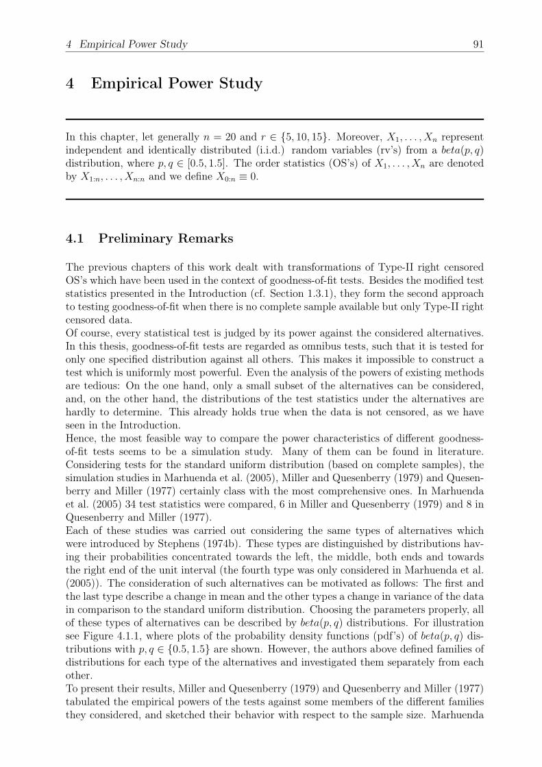
4 Empirical Power Study 91
4 Empirical Power Study
In this chapter, let generally n = 20 and r ∈ 5, 10, 15. Moreover, X1, . . . , Xn representindependent and identically distributed (i.i.d.) random variables (rv’s) from a beta(p, q)distribution, where p, q ∈ [0.5, 1.5]. The order statistics (OS’s) of X1, . . . , Xn are denotedby X1:n, . . . , Xn:n and we define X0:n ≡ 0.
4.1 Preliminary Remarks
The previous chapters of this work dealt with transformations of Type-II right censoredOS’s which have been used in the context of goodness-of-fit tests. Besides the modified teststatistics presented in the Introduction (cf. Section 1.3.1), they form the second approachto testing goodness-of-fit when there is no complete sample available but only Type-II rightcensored data.Of course, every statistical test is judged by its power against the considered alternatives.In this thesis, goodness-of-fit tests are regarded as omnibus tests, such that it is tested foronly one specified distribution against all others. This makes it impossible to construct atest which is uniformly most powerful. Even the analysis of the powers of existing methodsare tedious: On the one hand, only a small subset of the alternatives can be considered,and, on the other hand, the distributions of the test statistics under the alternatives arehardly to determine. This already holds true when the data is not censored, as we haveseen in the Introduction.Hence, the most feasible way to compare the power characteristics of different goodness-of-fit tests seems to be a simulation study. Many of them can be found in literature.Considering tests for the standard uniform distribution (based on complete samples), thesimulation studies in Marhuenda et al. (2005), Miller and Quesenberry (1979) and Quesen-berry and Miller (1977) certainly class with the most comprehensive ones. In Marhuendaet al. (2005) 34 test statistics were compared, 6 in Miller and Quesenberry (1979) and 8 inQuesenberry and Miller (1977).Each of these studies was carried out considering the same types of alternatives whichwere introduced by Stephens (1974b). These types are distinguished by distributions hav-ing their probabilities concentrated towards the left, the middle, both ends and towardsthe right end of the unit interval (the fourth type was only considered in Marhuenda et al.(2005)). The consideration of such alternatives can be motivated as follows: The first andthe last type describe a change in mean and the other types a change in variance of the datain comparison to the standard uniform distribution. Choosing the parameters properly, allof these types of alternatives can be described by beta(p, q) distributions. For illustrationsee Figure 4.1.1, where plots of the probability density functions (pdf’s) of beta(p, q) dis-tributions with p, q ∈ 0.5, 1.5 are shown. However, the authors above defined families ofdistributions for each type of the alternatives and investigated them separately from eachother.To present their results, Miller and Quesenberry (1979) and Quesenberry and Miller (1977)tabulated the empirical powers of the tests against some members of the different familiesthey considered, and sketched their behavior with respect to the sample size. Marhuenda

92 4 Preliminary Remarks
Figure 4.1.1: Pdf’s of beta distributions
et al. (2005) described for selected distributions from the families defined by Stephens(1974b) the difference between the power of a considered test and the highest observedpower among all tests in their study (so-called ’inefficiencies’). Then they determined foreach test and family the maximum inefficiency they had observed, and as comparison crite-rions for the tests they computed weighted sums of these maximum inefficiencies. Finally,these sums were tabulated and illustrated by diagrams.In this chapter, a new way of representing results of such power studies is suggested. In-stead of working with families of distributions, we consider beta(p, q) distributions, whichare able to imitate all four types of alternatives from Marhuenda et al. (2005) as describedabove. Thereby, the range of the parameters p and q will be [0.5, 1.5], and the four types ofalternatives correspond to the four quadrants characterized by p < 1, q > 1; p > 1, q > 1;p < 1, q < 1 and p > 1, q < 1, respectively (cf. Figure 4.1.1). Marhuenda et al. (2005) andQuesenberry and Miller (1977) also considered beta alternatives and most of their otheralternatives can be approximated quite well by beta distributions, as can be seen in the Ap-pendix (it is not possible to approximate all particular alternatives, for example, densitieswith a distinct upside-down peak cannot be approximated by beta densities, generally).Thus, a separated investigation of the families is evitable, such that we are able to describethe behavior of the tests as a whole and see their performances ’between’ the different typesof distributions. For this, we will use 3D plots of the empirical power functions of the testswe will consider, where the z-axis represents the power, the x-axis the parameter p andthe y-axis the parameter q of the beta(p, q) distributions. Additionally, to give a graphicaloverview, which test possesses the best power against specific beta alternatives, 2D plotswill be introduced, where the axes represent the parameters of the beta distributions andthe symbol at point (p, q) indicates the best test against beta(p, q). In the following, wewill call these plots ’power maps’.

4 Empirical Power Study 93
4.2 Classical Goodness-of-Fit Tests
First, we will show the described kind of analysis for some classical goodness-of-fit tests,which are frequently considered in power studies and are often recommended because oftheir properties (cf., e.g., Chen and Ye (2009), Glen et al. (2001), Marhuenda et al. (2005),Meintanis (2009), Miller and Quesenberry (1979), Quesenberry and Miller (1977), Stephens(1974b), Zhao et al. (2010) and Zhao et al. (2009)). The respective test statistics are theKolmogorov - Smirnov test statistic
Dn =√n max
Xi:n −
i− 1
n,i
n−Xi:n , i = 1, . . . , n
,
the Anderson - Darling test statistic
A2n =
n∑k=1
2(k − n)− 1
nln(1−Xk:n)− 2k − 1
nln(Xk:n)
− n,
the Cramér - von Mises test statistic
W 2n =
1
12n+
n∑k=1
(Xk:n −
2k − 1
2n
)2
,
the Watson test statistic
U2n = W 2
n − n
(1
n
n∑k=1
Xk:n −1
2
)2
and the statistic of Neyman’s smooth test (here with 4-th degree polynomials)
Ψ24 =
4∑j=1
1
n
(n∑k=1
πj(Xk:n
))2
(also see the Introduction).The results concerning the four types of alternatives from Marhuenda et al. (2005) are notnew and coincide with those in Marhuenda et al. (2005), Miller and Quesenberry (1979)and Quesenberry and Miller (1977). But their presentation here is clearer and the behaviorof the tests ’between’ the different types of distributions can be observed.The considered sample size in our simulation study is n = 20 and the significance levelα = 5%. First, empirical critical values were computed for the tests since they couldnot all be found in literature. For this, 1,000,000 random samples of size 20 from theuniform distribution were simulated using the Mersenne-Twister algorithm provided byR (version 2.7.2) choosing ’seed = 99’. Then the empirical critical value of a test wasdefined by the
⌈1, 000, 000 (1 − α)
⌉-th largest value of the corresponding statistic cal-
culated from the 1,000,000 samples. The empirical powers of the tests were obtainedanalogously. 1,000,000 random samples of size 20 from beta(p, q) distributions, wherep, q ∈ 0.5, 0.55, 0.6, . . . , 1.45, 1.5, were generated and the respective values of the statis-tics were compared to their critical thresholds. Then the empirical power of a test wasdefined by the relative frequency of the event that its statistic exceeds its empirical criticalvalue.In the following, the results are presented by the plots described above. They will beshown on the left-hand pages, while some corresponding comments will be given on theright-hand pages.
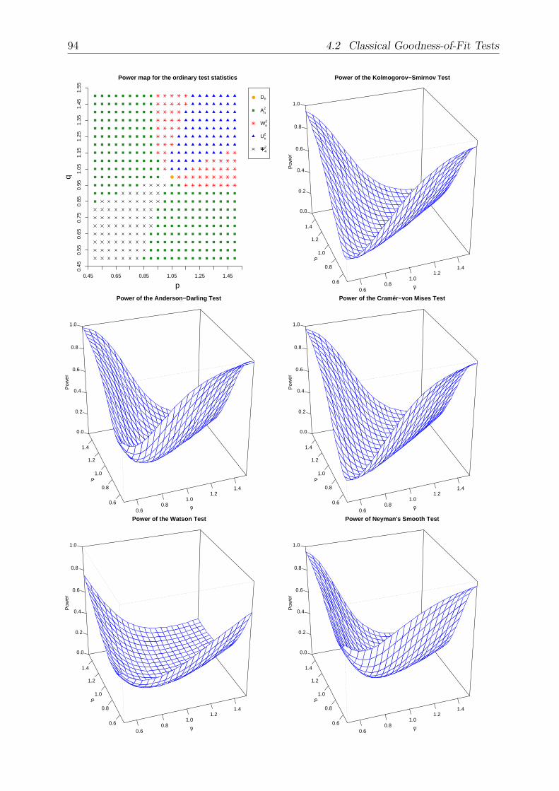
Power map for the ordinary test statistics
p
q
0.45 0.65 0.85 1.05 1.25 1.45
0.45
0.55
0.65
0.75
0.85
0.95
1.05
1.15
1.25
1.35
1.45
1.55
Dn
An2
Wn2
Un2
ΨΨ42
p0.60.8
1.01.2
1.4
q
0.6
0.8
1.0
1.2
1.4
0.0
0.2
0.4
0.6
0.8
1.0
Power of the Kolmogorov−Smirnov Test
Pow
er
p0.60.8
1.01.2
1.4
q
0.6
0.8
1.0
1.2
1.4
0.0
0.2
0.4
0.6
0.8
1.0
Power of the Anderson−Darling Test
Pow
er
p0.60.8
1.01.2
1.4
q
0.6
0.8
1.0
1.2
1.4
0.0
0.2
0.4
0.6
0.8
1.0
Power of the Cramér−von Mises Test
Pow
er
p0.60.8
1.01.2
1.4
q
0.6
0.8
1.0
1.2
1.4
0.0
0.2
0.4
0.6
0.8
1.0
Power of the Watson Test
Pow
er
p0.60.8
1.01.2
1.4
q
0.6
0.8
1.0
1.2
1.4
0.0
0.2
0.4
0.6
0.8
1.0
Power of Neyman's Smooth Test
Pow
er
94 4.2 Classical Goodness-of-Fit Tests

4 Empirical Power Study 95
At the top left we see the power map of Dn, A2n,W
2n , U
2n and Ψ2
4. It is noticeable, howeach of the four quadrants mentioned above is dominated by one of the tests. If thealternative has its power concentrated towards the left or the right end of (0, 1), but notto both, the Anderson - Darling statistic yields the best power of all considered tests. Forbathtub-shaped alternatives, i.e. p, q < 1, Neyman’s smooth test is advisable, whereas inthe opposite case, p, q > 1, the Watson test gives the best results.Anyway, the 3D plots of the empirical power functions show the similar behavior of thetests. In particular, there is almost no recognizable difference between the power propertiesof Dn (top right) andW 2
n (middle right). The Anderson - Darling test (middle left) behavesmore like Ψ2
4 (bottom right) when p, q < 1, but it is also comparable to Dn and W 2n . Only
the plot of the Watson test (bottom left) looks more distinguishable from the others. U2n
is the test statistic which distributes its power most evenly to all considered alternatives.The following two tables emphasize these observations and convey a better impression ofthe magnitudes of the differences between the powers of the tests. The first table showsthe powers in four points of the interior of the set of our beta alternatives.
Parameters of beta(p, q) Power of Dn A2n W 2
n U2n Ψ2
4
p = 0.65 , q = 1.35 0.683 0.804 0.761 0.378 0.669p = 1.35 , q = 1.35 0.045 0.029 0.038 0.105 0.042p = 0.65 , q = 0.65 0.110 0.230 0.108 0.192 0.344p = 1.35 , q = 0.65 0.684 0.804 0.762 0.379 0.670
We see, when p < 1 and q > 1 or vice versa, the power of the Anderson - Darlingtest increases most rapidly, leaving the (null) hypothesis, while the Watson test is clearlyoutperformed by the other tests. Here the power of A2
n is more than twice as high as theone of U2
n. In the case of p > 1 and q > 1, the opposite holds, but the absolute values of thedifferences are much smaller. Moreover, we see that Dn, A
2n,W
2n and Ψ2
4 are biased in thissituation. Finally, when p = 0.65 and q = 0.65 the power of Ψ2
4 is three times better thanthe powers of Dn or W 2
n , but here the differences, taken absolutely, are also less extremethan in the first two cases.The second table contains the powers ’in the corners’ of the considered set of alternatives.
Parameters of beta(p, q) Power of Dn A2n W 2
n U2n Ψ2
4
p = 0.5 , q = 1.5 0.950 0.986 0.976 0.744 0.960p = 1.5 , q = 1.5 0.048 0.028 0.038 0.154 0.058p = 0.5 , q = 0.5 0.204 0.525 0.197 0.441 0.676p = 1.5 , q = 0.5 0.950 0.987 0.976 0.746 0.960
When p, q ∈ 0.5, 1.5, p 6= q, the powers of Dn, A2n,W
2n and Ψ2
4 differ not very much anymore, only the power of the Watson test is considerably smaller. In the other cases, thedistances between the tests are larger than in the first table. In particular, in the case ofp = q = 1.5 the powers of Dn, A
2n andW 2
n are equal to their powers against beta(1.35, 1.35),Ψ2
4 is just slightly better, but the power of U2n increases by 0.049 which means a relative
gain in power of almost 50%.Summarizing, the 3D plots point out clearly, that Dn and W 2
n cannot be recommendedfor the use as omnibus tests without restrictions. They only show good performances,when the parameters of the beta alternative differ significantly, and suffer severe loss ofpower when p and q approach each other. A2
n and Ψ24 are somewhat more versatile, but U2
n
behaves like an omnibus test most, sometimes at the cost of its performance.

Power map for the ordinary test statistics
p
q
0.45 0.65 0.85 1.05 1.25 1.45
0.45
0.55
0.65
0.75
0.85
0.95
1.05
1.15
1.25
1.35
1.45
1.55
Dn
An2
Wn2
Un2
ΨΨ42
Power at p = q
p = qP
ower
00.
10.
20.
30.
40.
50.
60.
70.
80.
91
0.5 0.6 0.7 0.8 0.9 1 1.1 1.2 1.3 1.4 1.5
Dn
An2
Wn2
Un2
ΨΨ42
Power at q = 0.65
p
Pow
er0
0.1
0.2
0.3
0.4
0.5
0.6
0.7
0.8
0.9
1
0.5 0.6 0.7 0.8 0.9 1 1.1 1.2 1.3 1.4 1.5
Dn
An2
Wn2
Un2
ΨΨ42
Power at q = 1.35
p
Pow
er0
0.1
0.2
0.3
0.4
0.5
0.6
0.7
0.8
0.9
1
0.5 0.6 0.7 0.8 0.9 1 1.1 1.2 1.3 1.4 1.5
Dn
An2
Wn2
Un2
ΨΨ42
Power at p = 0.65
q
Pow
er0
0.1
0.2
0.3
0.4
0.5
0.6
0.7
0.8
0.9
1
0.5 0.6 0.7 0.8 0.9 1 1.1 1.2 1.3 1.4 1.5
Dn
An2
Wn2
Un2
ΨΨ42
Power at p = 1.35
q
Pow
er0
0.1
0.2
0.3
0.4
0.5
0.6
0.7
0.8
0.9
1
0.5 0.6 0.7 0.8 0.9 1 1.1 1.2 1.3 1.4 1.5
Dn
An2
Wn2
Un2
ΨΨ42
96 4.2 Classical Goodness-of-Fit Tests

4 Empirical Power Study 97
To demonstrate once again the differences between the powers of the test statistics, crosssections of the 3D graphs from page 94 are presented on the left hand side. The crosssections are taken along the diagonal, horizontal and vertical lines drawn into the powermap in the upper left corner. The intersections of the lines are also considered in the firsttable on page 95. Particularly conspicuous are the bad performances of Dn, A
2n,W
2n and
Ψ24 when p = q > 1 (cf. the chart top right). Here U2
n stands out notably, while the plots inthe middle, where q is fixed, and at the bottom, where p is fixed, show the superior powerof the other tests, when p and q are not both greater than 1.We also see the perfect symmetry of the considered power functions with respect to theline given by p = q, since the plots of the powers against beta(p, 0.65), p ∈ [0.5, 1.5] (middleleft), and beta(0.65, q), q ∈ [0.5, 1.5] (bottom left), look identical as well as the plots of thepowers against beta(p, 1.35), p ∈ [0.5, 1.5] (middle right), and beta(1.35, q), q ∈ [0.5, 1.5](bottom right) do. Indeed, this is not surprising because for a, b > 0
fa,b(x) =Γ(a+ b)
Γ(a)Γ(b)xa−1 (1− x)b−1, x ∈ (0, 1),
defines a pdf of beta(a, b). Hence, we have for all x ∈ (0, 1) and a, b > 0
fa,b(x) = fb,a(1− x),
such that a pdf of beta(b, a) is given by reflecting a pdf of beta(a, b) about 0.5.
4.3 Modified Test Statistics for Type-II Right Censored Data
Now, we will analyse the powers of the modified test statistics for Type-II right censoreddata presented in Section 1.3.1 of the Introduction in the same way as the powers of theclassical tests in Section 4.2. More precisely, with the notations of Section 1.3.1, we considerDr,n, A2
r,n, W 2r,n, SBW 2
r,n, U2r,n, Gr,n and Tr,n, where n = 20 and r ∈ 5, 10, 15. Some of
the modified test statistics are also considered and compared in Barr and Davidson (1973),Castro-Kuriss et al. (2009), D’Agostino and Stephens (1986), LaRiccia (1986), Lim andPark (2007), Lin et al. (2008), Lurie et al. (1974), Michael and Schucany (1979), O’Reillyand Stephens (1988), Pettitt and Stephens (1976) and Smith and Bain (1976), for instance,but there are less power studies of these tests in literature than for classical goodness-of-fittests.On the next two pages the 3D plots and power maps of the modified statistics for r =15, r = 10 and r = 5 are presented. Additionally, for the modifications of Dn, A2
n, W 2n and
U2n the graphs of the classical tests, i.e. of the corresponding tests based on a complete
sample of size n, are printed for comparison. The arrangement of the charts is as follows:On page 98 the plots of Dr,n, A2
r,n, W 2r,n, SBW 2
r,n and U2r,n are presented one below the
other, where r decreases from left to right, and the graphs of the classical statistics arealways the first in each row. On page 99 the same was done for Gr,n and Tr,n, only thecomplete sample case was omitted. Finally, below the plots of Tr,n, the power maps forr = 15, r = 10 and r = 5 (arranged from left to right) are printed. Some related commentsare given at the bottom of page 99.A more detailed discussion of the case r = 10 will follow on pages 100 and 101, where crosssections of the 3D plots of the test statistics are shown analogously to Section 4.2. Togetherwith the table on page 101 containing the powers of the tests against selected points of thealternative they will give a better idea of the differences between the performances of thetests than the 3D plots.
p0.60.8
1.01.2
1.4
q
0.6
0.8
1.0
1.2
1.4
0.0
0.2
0.4
0.6
0.8
1.0
Power of the Kolmogorov−Smirnov Test
Pow
er
p0.60.8
1.01.2
1.4
q
0.6
0.8
1.0
1.2
1.4
0.0
0.2
0.4
0.6
0.8
1.0
Power of the modified Kolmogorov−Smirnov Test, r = 15
Pow
er
p0.60.8
1.01.2
1.4
q
0.6
0.8
1.0
1.2
1.4
0.0
0.2
0.4
0.6
0.8
1.0
Power of the modified Kolmogorov−Smirnov Test, r = 10
Pow
er
p0.60.8
1.01.2
1.4
q
0.6
0.8
1.0
1.2
1.4
0.0
0.2
0.4
0.6
0.8
1.0
Power of the modified Kolmogorov−Smirnov Test, r = 5
Pow
er
p0.60.8
1.01.2
1.4
q
0.6
0.8
1.0
1.2
1.4
0.0
0.2
0.4
0.6
0.8
1.0
Power of the Anderson−Darling Test
Pow
er
p0.60.8
1.01.2
1.4
q
0.6
0.8
1.0
1.2
1.4
0.0
0.2
0.4
0.6
0.8
1.0
Power of the modified Anderson−Darling Test, r = 15
Pow
er
p0.60.8
1.01.2
1.4
q
0.6
0.8
1.0
1.2
1.4
0.0
0.2
0.4
0.6
0.8
1.0
Power of the modified Anderson−Darling Test, r = 10
Pow
er
p0.60.8
1.01.2
1.4
q
0.6
0.8
1.0
1.2
1.4
0.0
0.2
0.4
0.6
0.8
1.0
Power of the modified Anderson−Darling Test, r = 5
Pow
er
p0.60.8
1.01.2
1.4
q
0.6
0.8
1.0
1.2
1.4
0.0
0.2
0.4
0.6
0.8
1.0
Power of the Cramér−von Mises Test
Pow
er
p0.60.8
1.01.2
1.4
q
0.6
0.8
1.0
1.2
1.4
0.0
0.2
0.4
0.6
0.8
1.0
Power of the mod. Cramér−von Mises Test (by Pettitt and Stephens), r = 15
Pow
er
p0.60.8
1.01.2
1.4
q
0.6
0.8
1.0
1.2
1.4
0.0
0.2
0.4
0.6
0.8
1.0
Power of the mod. Cramér−von Mises Test (by Pettitt and Stephens), r = 10
Pow
er
p0.60.8
1.01.2
1.4
q
0.6
0.8
1.0
1.2
1.4
0.0
0.2
0.4
0.6
0.8
1.0
Power of the mod. Cramér−von Mises Test (by Pettitt and Stephens), r = 5
Pow
er
p0.60.8
1.01.2
1.4
q
0.6
0.8
1.0
1.2
1.4
0.0
0.2
0.4
0.6
0.8
1.0
Power of the Cramér−von Mises Test
Pow
er
p0.60.8
1.01.2
1.4
q
0.6
0.8
1.0
1.2
1.4
0.0
0.2
0.4
0.6
0.8
1.0
Power of the modified Cramér−von Mises Test (by Smith and Bain), r = 15
Pow
er
p0.60.8
1.01.2
1.4
q
0.6
0.8
1.0
1.2
1.4
0.0
0.2
0.4
0.6
0.8
1.0
Power of the modified Cramér−von Mises Test (by Smith and Bain), r = 10
Pow
er
p0.60.8
1.01.2
1.4
q
0.6
0.8
1.0
1.2
1.4
0.0
0.2
0.4
0.6
0.8
1.0
Power of the modified Cramér−von Mises Test (by Smith and Bain), r = 5
Pow
er
p0.60.8
1.01.2
1.4
q
0.6
0.8
1.0
1.2
1.4
0.0
0.2
0.4
0.6
0.8
1.0
Power of the Watson Test
Pow
er
p0.60.8
1.01.2
1.4
q
0.6
0.8
1.0
1.2
1.4
0.0
0.2
0.4
0.6
0.8
1.0
Power of the modified Watson Test, r = 15
Pow
er
p0.60.8
1.01.2
1.4
q
0.6
0.8
1.0
1.2
1.4
0.0
0.2
0.4
0.6
0.8
1.0
Power of the modified Watson Test, r = 10
Pow
er
p0.60.8
1.01.2
1.4
q
0.6
0.8
1.0
1.2
1.4
0.0
0.2
0.4
0.6
0.8
1.0
Power of the modified Watson Test, r = 5
Pow
er
98 4.3 Modified Test Statistics for Type-II Right Censored Data

4 Empirical Power Study 99
p0.60.8
1.01.2
1.4
q
0.6
0.8
1.0
1.2
1.4
0.0
0.2
0.4
0.6
0.8
1.0
Power of the generalized Hartley−Pfaffenberger Criterion, r = 15
Pow
er
p0.60.8
1.01.2
1.4
q
0.6
0.8
1.0
1.2
1.4
0.0
0.2
0.4
0.6
0.8
1.0
Power of the generalized Hartley−Pfaffenberger Criterion, r = 10
Pow
er
p0.60.8
1.01.2
1.4
q
0.6
0.8
1.0
1.2
1.4
0.0
0.2
0.4
0.6
0.8
1.0
Power of the generalized Hartley−Pfaffenberger Criterion, r = 5
Pow
er
p0.60.8
1.01.2
1.4
q
0.6
0.8
1.0
1.2
1.4
0.0
0.2
0.4
0.6
0.8
1.0
Power of the Correlation Type Test by Smith and Bain, r = 15
Pow
er
p0.60.8
1.01.2
1.4q
0.6
0.8
1.0
1.2
1.4
0.0
0.2
0.4
0.6
0.8
1.0
Power of the Correlation Type Test by Smith and Bain, r = 10
Pow
er
p0.60.8
1.01.2
1.4
q
0.6
0.8
1.0
1.2
1.4
0.0
0.2
0.4
0.6
0.8
1.0
Power of the Correlation Type Test by Smith and Bain, r = 5
Pow
er
Power map for the modified test statistics, r = 15
p
q
0.45 0.65 0.85 1.05 1.25 1.45
0.45
0.55
0.65
0.75
0.85
0.95
1.05
1.15
1.25
1.35
1.45
1.55
Dr,n
Ar,n2
Wr,n2
SBWr,n2
Ur,n2
Gr,n
Tr,n
Power map for the modified test statistics, r = 10
p
q
0.45 0.65 0.85 1.05 1.25 1.45
0.45
0.55
0.65
0.75
0.85
0.95
1.05
1.15
1.25
1.35
1.45
1.55
Dr,n
Ar,n2
Wr,n2
SBWr,n2
Ur,n2
Gr,n
Tr,n
Power map for the modified test statistics, r = 5
p
q
0.45 0.65 0.85 1.05 1.25 1.45
0.45
0.55
0.65
0.75
0.85
0.95
1.05
1.15
1.25
1.35
1.45
1.55
Dr,n
Ar,n2
Wr,n2
SBWr,n2
Ur,n2
Gr,n
Tr,n
We see, as the number of available observations r decreases, all of the tests only suffer aconsiderable loss of power against beta(p, q) if q ≥ p holds true, i.e., if the probability massof the underlying true distribution is concentrated towards the left end of [0, 1]. PerhapsTr,n is an exception since for r = 5 it shows its best performances generally for small p.Dr,n and A2
r,n preserve their power best. They are the only tests with acceptable poweragainst beta(0.5, 1.5) if r = 5. SBW 2
r,n loses its power later than W 2r,n but for r = 5 their
plots look almost indentical again. The generalized Hartley-Pfaffenberger criterion behavessimilar to the modified Watson test. They both first preserve some power against beta(p, q)when q < 1, in general, and their performances against beta(1.5, 0.5) are even best whenr = 10. Although the power maps of the modified test statistics show that Tr,n is the besttest against a relatively large subset of the considered beta alternatives, and this subsetincreases as r decreases, the power of Tr,n is not really satisfying. Its power functions arerather flat and the differences between Tr,n and the other test statistics at the points, whereTr,n is best, are small.The power maps for the modified test statistics cannot be subdivided into four quadrantsas in Section 4.2 and all of the tests except Gr,n appear in the charts. The tests whichdominate in most of the situations are A2
r,n, W 2r,n, SBW 2
r,n and, as already mentioned, Tr,n.We will analyze the case r = 10 more thoroughly on the next two pages and it will be seenthat the powers of different tests are often very similar.

Power map for the modified test statistics, r = 10
p
q
0.45 0.65 0.85 1.05 1.25 1.45
0.45
0.55
0.65
0.75
0.85
0.95
1.05
1.15
1.25
1.35
1.45
1.55
Dr,n
Ar,n2
Wr,n2
SBWr,n2
Ur,n2
Gr,n
Tr,n
Power at p = q
p = qP
ower
00.
10.
20.
30.
40.
50.
60.
70.
80.
91
0.5 0.6 0.7 0.8 0.9 1 1.1 1.2 1.3 1.4 1.5
Dr,n
Ar,n2
Wr,n2
SBWr,n2
Ur,n2
Gr,n
Tr,n
Power at q = 0.65
p
Pow
er0
0.1
0.2
0.3
0.4
0.5
0.6
0.7
0.8
0.9
1
0.5 0.6 0.7 0.8 0.9 1 1.1 1.2 1.3 1.4 1.5
Dr,n
Ar,n2
Wr,n2
SBWr,n2
Ur,n2
Gr,n
Tr,n
Power at q = 1.35
p
Pow
er0
0.1
0.2
0.3
0.4
0.5
0.6
0.7
0.8
0.9
1
0.5 0.6 0.7 0.8 0.9 1 1.1 1.2 1.3 1.4 1.5
Dr,n
Ar,n2
Wr,n2
SBWr,n2
Ur,n2
Gr,n
Tr,n
Power at p = 0.65
q
Pow
er0
0.1
0.2
0.3
0.4
0.5
0.6
0.7
0.8
0.9
1
0.5 0.6 0.7 0.8 0.9 1 1.1 1.2 1.3 1.4 1.5
Dr,n
Ar,n2
Wr,n2
SBWr,n2
Ur,n2
Gr,n
Tr,n
Power at p = 1.35
q
Pow
er0
0.1
0.2
0.3
0.4
0.5
0.6
0.7
0.8
0.9
1
0.5 0.6 0.7 0.8 0.9 1 1.1 1.2 1.3 1.4 1.5
Dr,n
Ar,n2
Wr,n2
SBWr,n2
Ur,n2
Gr,n
Tr,n
100 4.3 Modified Test Statistics for Type-II Right Censored Data

4 Empirical Power Study 101
The plots on the left hand side correspond to the ones for the classical test statistics onpage 96. If p = q, which means that the beta alternative is symmetric about 0.5, themodified Anderson - Darling test is the best choice. When p = q < 1, i.e. the probabilitymass is concentrated towards both ends of [0, 1], it is superior to the other tests and as pand q increase, such that more and more observations will occur in the middle of the unitinterval, it stays competitive. It is remarkable that U2
r,n is worst when p = q > 1, while U2n
is clearly the best of the classical test statistics in this situation.The lower horizontal cross section (taken along q = 0.65) emphasizes the good performanceof A2
r,n when the probability mass of the alternative is shifted to both, 0 and 1 (cf. p < 0.7),and it shows that W 2
r,n, A2r,n, SBW 2
r,n and Dr,n are comparable when the probability massis concentrated more towards the right end of [0, 1] (cf. p ≥ 0.8).If q is fixed at q = 1.35 the powers of A2
r,n, SBW 2r,n and Dr,n are hard to distinguish.
They are superior to the other tests when p < 1, i.e., when the probability is concentratedtowards the left limit of the unit interval, but suffer severe loss of power as the probabilitymass is concentrated more and more around 0.5. Here, all of the tests are biased exceptTr,n, whose power is slightly above α. Again remarkable is the bad performance of U2
r,n,which provides no power against beta(p, 1.35) when p is small.The left vertical cross section (i.e., p = 0.65) shows, as the cross sections which have alreadybeen discussed, that Ar,n is noticeable better than the other tests when it appears on thepower map. But the powers of SBW 2
r,n and Dr,n are again almost identical, such that foralternatives which have their probability concentrated towards the origin (cf. q → 1.5),both of the statistics are recommendable, while A2
r,n possesses just a bit less power.Finally, if there is little probability mass at the left end of the unit interval (cf. p fixed at1.35) then all of the tests except Tr,n have good power if the probability mass is concentratedtowards the right end of [0, 1] (cf. q → 0.5). But they lose all of it very fast as theprobability mass is shifted to the middle (i.e., as q increases).The table below contains the powers of the modified tests at some points of the alternative.These points were selected, such that each of them is located in a different portion ofthe power map on page 100. I.e., at the first point SBW 2
r,n is the best statistic, at thesecond point, Dr,n is best, and so on in a clockwise direction around the point representingbeta(1, 1) = U(0, 1). The table exemplifies once again the differences between the powersof the tests as they are already described above.
Power of the modified goodness-of-fit tests, r = 10
Parameters of beta(p, q) Dr,n A2r,n W 2
r,n SBW 2r,n U2
r,n Gr,n Tr,n
p = 0.55 , q = 1.45 0.799 0.794 0.072 0.815 0.000 0.002 0.205p = 0.85 , q = 1.45 0.223 0.170 0.008 0.194 0.002 0.004 0.068p = 1.25 , q = 1.45 0.021 0.016 0.016 0.019 0.009 0.016 0.051p = 1.35 , q = 0.65 0.731 0.768 0.795 0.766 0.647 0.535 0.100p = 0.75 , q = 0.55 0.260 0.260 0.263 0.223 0.334 0.256 0.060p = 0.6 , q = 0.95 0.324 0.430 0.042 0.334 0.012 0.019 0.143
We may conclude that the power map on page 100 shows a variety of tests being the bestin different situations. But a closer analysis of the differences between the tests makes itpossible to focus on just a few tests. If only one test statistic should be recommended, thenprobably A2
r,n is the best choice, since it is the one with the best power in many situationsand it is always competitive when it is not the best. This conclusion coincides with resultsof a similar power study carried out by Michael and Schucany (1979).

102 4.4 Tests Based on Transformed Data
4.4 Tests Based on Transformed Data
In this section, we compare the powers of Dr,n, A2r,n, W 2
r,n, SBW 2r,n and U2
r,n to the powersof the tests obtained by applying their classical counterparts to transformed samples asdescribed in the preceding chapters. I.e., we consider the problem of testing whether theunderlying distribution of X1:n, . . . , Xr:n is U(0, 1), and instead of applying the modifiedtest statistics directly to the censored sample, we first transform
(X1:n, . . . , Xr:n
)in one
of the following ways and afterwards utilize the ordinary test statistics. The consideredtransformations are given by
Transformation 1Yi/r =
Xi:n
Xr:n
[Br,n−r+1(Xr:n)]1r , 1 ≤ i ≤ r,
where Br,n−r+1 denotes the cdf of the beta(r, n − r + 1) distribution (cf. (x) of Theorem2.2),
Transformation 2
Yi =
[1−Xi:n
1−Xi−1:n
]n−i+1
, 1 ≤ i ≤ r
(cf. (v) of Theorem 2.2),
Transformation 3
Yi/r = 1−i∏
j=1
(1−Xj:n
1−Xj−1:n
)n−j+1r−j+1
, 1 ≤ i ≤ r
(cf. (xi) of Theorem 2.2),
Transformation 4
Y1 = Br,n−r+1
(Xr:n
), Yi =
[Xr−i+1:n
Xr−i+2:n
]r−i+1
, 2 ≤ i ≤ r
(cf. (iv) of Theorem 2.2),
Transformation 5
Yi/r =r∏j=i
(1−
[1−Xj:n
1−Xj−1:n
]n−j+1) 1
j
, 1 ≤ i ≤ r
(cf. Lemma 2.4),
Transformation 6
Yi/r = 1−(1−Br,n−r+1(Xr:n)
) 1r
i∏j=2
(1−
[Xr−j+1:n
Xr−j+2:n
]r−j+1) 1
r−j+1
, 1 ≤ i ≤ r
(cf. Lemma 2.4),
Transformation 7(Y1/r, . . . , Yr/r
)=
(VrX1:n
Xr:n
, . . . , VrXr−1:n
Xr:n
, 1−(
1− VrXr−1:n
Xr:n
)Vr
),
where Vr ∼ beta(r, 1) and Vr ∼ beta(1, 1) = U(0, 1) such that Vr, Vr and (X1:n, . . . , Xr:n)are independent (cf. (ix) of Theorem 2.2 and Theorem 2.5),
4 Empirical Power Study 103
Transformation 8Yi/r−1 =
Xi:n
Xr:n
, 1 ≤ i ≤ r − 1
(cf. (ix) of Theorem 2.2).
We have seen in Chapter 2 that(Y1/r, . . . , Yr/r
),(Y1/r, . . . , Yr−1/r−1
)and
(Y1, . . . , Yr
)de-
fined by these transformations are distributed as(U1:r, . . . , Ur:r
),(U1:r−1, . . . , Ur−1:r−1
)and
(U1, . . . , Ur
), respectively, if
(X1:n, . . . , Xr:n
)is distributed as
(U1:n, . . . , Ur:n
), where
U1, . . . , Um denote i.i.d. standard uniformly distributed rv’s and U1:m, . . . , Um:m their cor-responding OS’s, for every m ∈ N. Thus, testing the transformed rv’s for uniformity usingstatistics constructed for uncensored samples means the same as testing whether the un-derlying distribution of X1:n, . . . , Xr:n is U(0, 1) by statistics constructed for Type-IIright censored samples.Transformation 7 is of a special kind. Strictly speaking, it is not a transformation of(X1:n, . . . , Xr:n
), but it constructs a new random vector from
(X1:n, . . . , Xr:n
), Vr and Vr,
where Vr and Vr are as described above. First,(X1:n, . . . , Xr:n
)is transformed by Transfor-
mation 8, then random contraction is applied to the resulting vector(X1:n
Xr:n
, . . . ,Xr−1:n
Xr:n
),
which means to multiply(X1:n
Xr:n
, . . . ,Xr−1:n
Xr:n
)by Vr. Finally, random dilation yields a
random vector of size r by constructing an additional component 1−(
1− VrXr−1:n
Xr:n
)Vr.
Then, we know from Theorems 2.2 and 2.5 that this random vector is distributed as(U1:r, . . . , Ur:r
), if Xi ∼ U(0, 1), 1 ≤ i ≤ n. But in practice, only realizations of
X1:n, . . . , Xr:n are available, such that Vr and Vr must be simulated to obtain a ’real-ization’ of the random vector given by transformation 7 before a goodness-of-fit test canbe applied. Hence, transformation 7 is a very theoretical approach, which perhaps is notsuitable for application in practice. But it provides an interesting comparison to the othermethods above.In the power study, the results of which will be presented in the following, the same betaalternatives as in the preceding sections were considered. It was carried out in the sameway as described in Section 4.2 and again power maps as well as 3D plots will be used forpresentation of the results.For n = 20 and r ∈ 5, 10, 15 the power of Dr,n applied to
(X1:n, . . . , Xr:n
)directly was
compared to the power of Dr−1 combined with transformation 8 and of Dr combined witheach of the transformations 1 to 7. Moreover, by random dilation of
(X1:n, . . . , Xr:n
)an
additional oberservation was ’simulated’ and the power of Dr+1,n applied to this artificialsample was also compared to the other methods.A2r,n, W 2
r,n, SBW 2r,n, U2
r,n and their classical counterparts were treated analogously and thecorresponding power maps are shown one below the other on page 104, where r decreasesfrom left to right. Finally, Neyman’s smooth test Ψ2
4 (cf. Section 4.2) was also combinedwith each of the transformations above and the resulting power maps are printed at thetop of page 105.Michael and Schucany (1979) suggested transformation 1 for testing goodness-of-fit basedon Type-II right censored data. In their paper a power study comparing the modified teststatistics from Section 1.3.1 of the Introduction and the Anderson - Darling test combinedwith their transformation is reported. O’Reilly and Stephens (1988) proposed transforma-tion 3 and compared the combination with the Anderson - Darling test to the method ofMichael and Schucany (1979) and the modified Anderson - Darling test. Lin et al. (2008)
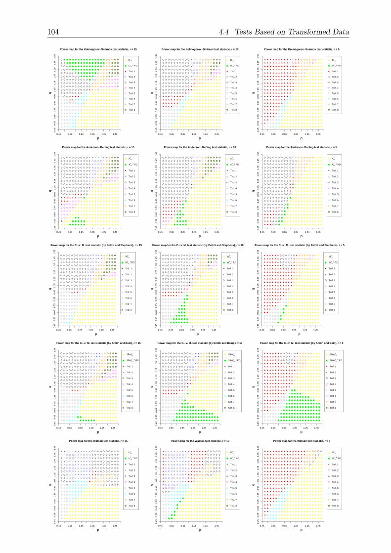
Power map for the Kolmogorov−Smirnov test statistic, r = 15
p
q
0.45 0.65 0.85 1.05 1.25 1.45
0.45
0.55
0.65
0.75
0.85
0.95
1.05
1.15
1.25
1.35
1.45
1.55
Dr,n
Dr,n °° RD
Trsf. 1
Trsf. 2
Trsf. 3
Trsf. 4
Trsf. 5
Trsf. 6
Trsf. 7
Trsf. 8
Power map for the Kolmogorov−Smirnov test statistic, r = 10
p
q
0.45 0.65 0.85 1.05 1.25 1.45
0.45
0.55
0.65
0.75
0.85
0.95
1.05
1.15
1.25
1.35
1.45
1.55
Dr,n
Dr,n °° RD
Trsf. 1
Trsf. 2
Trsf. 3
Trsf. 4
Trsf. 5
Trsf. 6
Trsf. 7
Trsf. 8
Power map for the Kolmogorov−Smirnov test statistic, r = 5
p
q
0.45 0.65 0.85 1.05 1.25 1.45
0.45
0.55
0.65
0.75
0.85
0.95
1.05
1.15
1.25
1.35
1.45
1.55
Dr,n
Dr,n °° RD
Trsf. 1
Trsf. 2
Trsf. 3
Trsf. 4
Trsf. 5
Trsf. 6
Trsf. 7
Trsf. 8
Power map for the Anderson−Darling test statistic, r = 15
p
q
0.45 0.65 0.85 1.05 1.25 1.45
0.45
0.55
0.65
0.75
0.85
0.95
1.05
1.15
1.25
1.35
1.45
1.55
Ar,n2
Ar,n2 °° RD
Trsf. 1
Trsf. 2
Trsf. 3
Trsf. 4
Trsf. 5
Trsf. 6
Trsf. 7
Trsf. 8
Power map for the Anderson−Darling test statistic, r = 10
p
q
0.45 0.65 0.85 1.05 1.25 1.45
0.45
0.55
0.65
0.75
0.85
0.95
1.05
1.15
1.25
1.35
1.45
1.55
Ar,n2
Ar,n2 °° RD
Trsf. 1
Trsf. 2
Trsf. 3
Trsf. 4
Trsf. 5
Trsf. 6
Trsf. 7
Trsf. 8
Power map for the Anderson−Darling test statistic, r = 5
p
q
0.45 0.65 0.85 1.05 1.25 1.45
0.45
0.55
0.65
0.75
0.85
0.95
1.05
1.15
1.25
1.35
1.45
1.55
Ar,n2
Ar,n2 °° RD
Trsf. 1
Trsf. 2
Trsf. 3
Trsf. 4
Trsf. 5
Trsf. 6
Trsf. 7
Trsf. 8
Power map for the C.−v. M. test statistic (by Pettitt and Stephens), r = 15
p
q
0.45 0.65 0.85 1.05 1.25 1.45
0.45
0.55
0.65
0.75
0.85
0.95
1.05
1.15
1.25
1.35
1.45
1.55
Wr,n2
Wr,n2 °° RD
Trsf. 1
Trsf. 2
Trsf. 3
Trsf. 4
Trsf. 5
Trsf. 6
Trsf. 7
Trsf. 8
Power map for the C.−v. M. test statistic (by Pettitt and Stephens), r = 10
p
q
0.45 0.65 0.85 1.05 1.25 1.45
0.45
0.55
0.65
0.75
0.85
0.95
1.05
1.15
1.25
1.35
1.45
1.55
Wr,n2
Wr,n2 °° RD
Trsf. 1
Trsf. 2
Trsf. 3
Trsf. 4
Trsf. 5
Trsf. 6
Trsf. 7
Trsf. 8
Power map for the C.−v. M. test statistic (by Pettitt and Stephens), r = 5
p
q
0.45 0.65 0.85 1.05 1.25 1.45
0.45
0.55
0.65
0.75
0.85
0.95
1.05
1.15
1.25
1.35
1.45
1.55
Wr,n2
Wr,n2 °° RD
Trsf. 1
Trsf. 2
Trsf. 3
Trsf. 4
Trsf. 5
Trsf. 6
Trsf. 7
Trsf. 8
Power map for the C.−v. M. test statistic (by Smith and Bain), r = 15
p
q
0.45 0.65 0.85 1.05 1.25 1.45
0.45
0.55
0.65
0.75
0.85
0.95
1.05
1.15
1.25
1.35
1.45
1.55
SBWr,n2
SBWr,n2 °° RD
Trsf. 1
Trsf. 2
Trsf. 3
Trsf. 4
Trsf. 5
Trsf. 6
Trsf. 7
Trsf. 8
Power map for the C.−v. M. test statistic (by Smith and Bain), r = 10
p
q
0.45 0.65 0.85 1.05 1.25 1.45
0.45
0.55
0.65
0.75
0.85
0.95
1.05
1.15
1.25
1.35
1.45
1.55
SBWr,n2
SBWr,n2 °° RD
Trsf. 1
Trsf. 2
Trsf. 3
Trsf. 4
Trsf. 5
Trsf. 6
Trsf. 7
Trsf. 8
Power map for the C.−v. M. test statistic (by Smith and Bain), r = 5
p
q
0.45 0.65 0.85 1.05 1.25 1.45
0.45
0.55
0.65
0.75
0.85
0.95
1.05
1.15
1.25
1.35
1.45
1.55
SBWr,n2
SBWr,n2 °° RD
Trsf. 1
Trsf. 2
Trsf. 3
Trsf. 4
Trsf. 5
Trsf. 6
Trsf. 7
Trsf. 8
Power map for the Watson test statistic, r = 15
p
q
0.45 0.65 0.85 1.05 1.25 1.45
0.45
0.55
0.65
0.75
0.85
0.95
1.05
1.15
1.25
1.35
1.45
1.55
Ur,n2
Ur,n2 °° RD
Trsf. 1
Trsf. 2
Trsf. 3
Trsf. 4
Trsf. 5
Trsf. 6
Trsf. 7
Trsf. 8
Power map for the Watson test statistic, r = 10
p
q
0.45 0.65 0.85 1.05 1.25 1.45
0.45
0.55
0.65
0.75
0.85
0.95
1.05
1.15
1.25
1.35
1.45
1.55
Ur,n2
Ur,n2 °° RD
Trsf. 1
Trsf. 2
Trsf. 3
Trsf. 4
Trsf. 5
Trsf. 6
Trsf. 7
Trsf. 8
Power map for the Watson test statistic, r = 5
p
q
0.45 0.65 0.85 1.05 1.25 1.45
0.45
0.55
0.65
0.75
0.85
0.95
1.05
1.15
1.25
1.35
1.45
1.55
Ur,n2
Ur,n2 °° RD
Trsf. 1
Trsf. 2
Trsf. 3
Trsf. 4
Trsf. 5
Trsf. 6
Trsf. 7
Trsf. 8
104 4.4 Tests Based on Transformed Data

4 Empirical Power Study 105
Power map for Neyman's smooth test with transformed data, r = 15
p
q
0.45 0.65 0.85 1.05 1.25 1.45
0.45
0.55
0.65
0.75
0.85
0.95
1.05
1.15
1.25
1.35
1.45
1.55
Trsf. 1
Trsf. 2
Trsf. 3
Trsf. 4
Trsf. 5
Trsf. 6
Trsf. 7
Trsf. 8
Power map for Neyman's smooth test with transformed data, r = 10
p
q
0.45 0.65 0.85 1.05 1.25 1.45
0.45
0.55
0.65
0.75
0.85
0.95
1.05
1.15
1.25
1.35
1.45
1.55
Trsf. 1
Trsf. 2
Trsf. 3
Trsf. 4
Trsf. 5
Trsf. 6
Trsf. 7
Trsf. 8
Power map for Neyman's smooth test with transformed data, r = 5
p
q
0.45 0.65 0.85 1.05 1.25 1.45
0.45
0.55
0.65
0.75
0.85
0.95
1.05
1.15
1.25
1.35
1.45
1.55
Trsf. 1
Trsf. 2
Trsf. 3
Trsf. 4
Trsf. 5
Trsf. 6
Trsf. 7
Trsf. 8
computed the Anderson - Darling statistic on transformed samples obtained by transfor-mation 2 and compared this procedure to all of the techniques considered in Michael andSchucany (1979) also in a simulation study.The power maps for Neyman’s smooth test above show a clear result. Transformation 3dominates in most of the situations. Only when the probability mass of the alternativeis concentrated towards the middle of [0, 1] (i.e., p, q > 1) transformations 5 or 6 are thebetter choice, and transformation 2 is better in some situations when the probability isshifted just slightly towards 1 (cf. q < 1, p > 1).The power maps on the left hand side for the other tests, where also the modified versionsof the respective statistics are considered, are more difficult to describe. Most conspicuousis the dominance of the modified tests when the probability mass of the alternative is con-centrated towards the right end of the unit interval (cf q < 1, p > 1). Notice, for SBW 2
r,n
it is worthwhile to simulate an additional ’observation’ by random dilation if r is smallin this situation. For the other test, except the Kolmogorov - Smirnov test when r = 15,random dilation does not play a big role in their power maps.The other technique creating artificial observations, transformation 7, appears in most ofthe power maps when the parameters of the beta(p, q) alternatives satisfy 1 < p ≤ q. But ifthis is not fulfilled, it is not the best method. The rest of the quadrant given by 1 < p, q ismostly partitioned into small areas, where transformations 2, 4, 8 or the modified versionsof the considered statistics are best. Though, as r decreases, the modified tests displacetransformations 4 and 8, such that for r = 5 the modified tests are always best if 1 < q ≤ p,in general. This also holds true for U2
r,n, but here transformation 3 is dominating in mostparts of the quadrant for r > 5, and transformations 4 and 8 do not appear at all.Transformation 3 is also the best for most of the tests if the probability mass of the al-ternative is concentrated towards the left limit of [0, 1] (i.e., p < 1 and q > 1) and r > 5.Exceptions are the Watson test, where transformation 2 dominates this quadrant, and theKolmogorov - Smirnov test if r = 15. Here, the modified test together with random dilationoften yields better results for p < 1 and q > 2− p. If r = 5 transformation 3 is the best forthe Anderson - Darling statistic, too, but for all other tests transformation 1 is superior.The last quadrant to be considered is given by p, q < 1, i.e., the alternative has its proba-bility concentrated towards both ends of the unit interval. Here, many different methodsappear in the power maps for the particular tests and choices of r, and the reader may berefered to the charts to get an idea of the situation, since written descriptions at this pointwould be either vague or rather lengthy. However, it should be mentioned that transfor-mations 5 and 6 are frequently the best choices in this quadrant because they are not thebest for the rest of the beta alternatives, considering the power maps on the left.On the following pages, 3D plots of all described methods and plots for a separate studyof the effect of random dilation to the performance of the modified tests can be found forthe case r = 10. Comments to these illustrations will be given on page 113.

p0.60.8
1.01.2
1.4
q
0.6
0.8
1.0
1.2
1.4
0.0
0.2
0.4
0.6
0.8
1.0
Power of the modified Kolmogorov−Smirnov Test, r = 10
Pow
er
p0.60.8
1.01.2
1.4
q
0.6
0.8
1.0
1.2
1.4
0.0
0.2
0.4
0.6
0.8
1.0
Power of the mod. Kolmogorov−Smirnov Test with Random Dilation, r = 10
Pow
er
p0.60.8
1.01.2
1.4
q
0.6
0.8
1.0
1.2
1.4
0.0
0.2
0.4
0.6
0.8
1.0
Power of the Kolmogorov−Smirnov Test with Trsf. 1, r = 10
Pow
er
p0.60.8
1.01.2
1.4
q
0.6
0.8
1.0
1.2
1.4
0.0
0.2
0.4
0.6
0.8
1.0
Power of the Kolmogorov−Smirnov Test with Trsf. 2, r = 10
Pow
er
p0.60.8
1.01.2
1.4
q
0.6
0.8
1.0
1.2
1.4
0.0
0.2
0.4
0.6
0.8
1.0
Power of the Kolmogorov−Smirnov Test with Trsf. 3, r = 10
Pow
er
p0.60.8
1.01.2
1.4
q
0.6
0.8
1.0
1.2
1.4
0.0
0.2
0.4
0.6
0.8
1.0
Power of the Kolmogorov−Smirnov Test with Trsf. 4, r = 10
Pow
er
p0.60.8
1.01.2
1.4
q
0.6
0.8
1.0
1.2
1.4
0.0
0.2
0.4
0.6
0.8
1.0
Power of the Kolmogorov−Smirnov Test with Trsf. 5, r = 10
Pow
er
p0.60.8
1.01.2
1.4
q
0.6
0.8
1.0
1.2
1.4
0.0
0.2
0.4
0.6
0.8
1.0
Power of the Kolmogorov−Smirnov Test with Trsf. 6, r = 10
Pow
er
p0.60.8
1.01.2
1.4
q
0.6
0.8
1.0
1.2
1.4
0.0
0.2
0.4
0.6
0.8
1.0
Power of the Kolmogorov−Smirnov Test with Trsf. 7, r = 10
Pow
er
p0.60.8
1.01.2
1.4
q
0.6
0.8
1.0
1.2
1.4
0.0
0.2
0.4
0.6
0.8
1.0
Power of the Kolmogorov−Smirnov Test with Trsf. 8, r = 10
Pow
er
106 4.4 Tests Based on Transformed Data
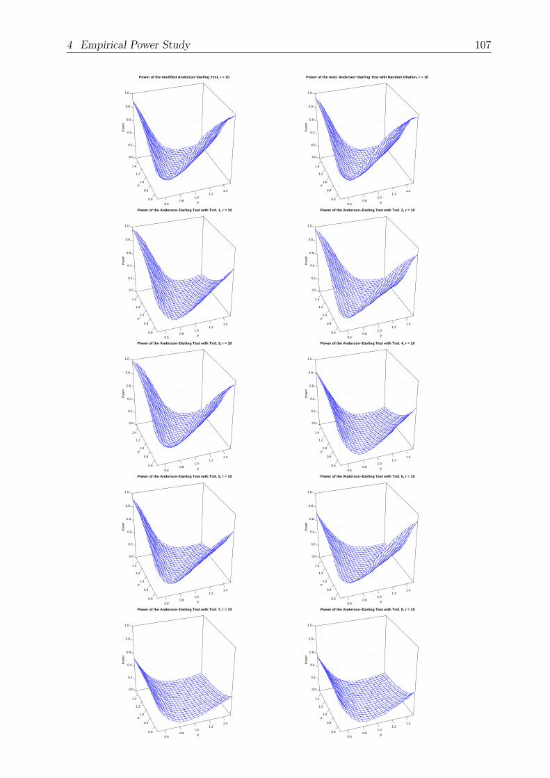
p0.60.8
1.01.2
1.4
q
0.6
0.8
1.0
1.2
1.4
0.0
0.2
0.4
0.6
0.8
1.0
Power of the modified Anderson−Darling Test, r = 10
Pow
er
p0.60.8
1.01.2
1.4
q
0.6
0.8
1.0
1.2
1.4
0.0
0.2
0.4
0.6
0.8
1.0
Power of the mod. Anderson−Darling Test with Random Dilation, r = 10
Pow
er
p0.60.8
1.01.2
1.4
q
0.6
0.8
1.0
1.2
1.4
0.0
0.2
0.4
0.6
0.8
1.0
Power of the Anderson−Darling Test with Trsf. 1, r = 10
Pow
er
p0.60.8
1.01.2
1.4
q
0.6
0.8
1.0
1.2
1.4
0.0
0.2
0.4
0.6
0.8
1.0
Power of the Anderson−Darling Test with Trsf. 2, r = 10
Pow
er
p0.60.8
1.01.2
1.4
q
0.6
0.8
1.0
1.2
1.4
0.0
0.2
0.4
0.6
0.8
1.0
Power of the Anderson−Darling Test with Trsf. 3, r = 10
Pow
er
p0.60.8
1.01.2
1.4
q
0.6
0.8
1.0
1.2
1.4
0.0
0.2
0.4
0.6
0.8
1.0
Power of the Anderson−Darling Test with Trsf. 4, r = 10
Pow
er
p0.60.8
1.01.2
1.4
q
0.6
0.8
1.0
1.2
1.4
0.0
0.2
0.4
0.6
0.8
1.0
Power of the Anderson−Darling Test with Trsf. 5, r = 10
Pow
er
p0.60.8
1.01.2
1.4
q
0.6
0.8
1.0
1.2
1.4
0.0
0.2
0.4
0.6
0.8
1.0
Power of the Anderson−Darling Test with Trsf. 6, r = 10
Pow
er
p0.60.8
1.01.2
1.4
q
0.6
0.8
1.0
1.2
1.4
0.0
0.2
0.4
0.6
0.8
1.0
Power of the Anderson−Darling Test with Trsf. 7, r = 10
Pow
er
p0.60.8
1.01.2
1.4
q
0.6
0.8
1.0
1.2
1.4
0.0
0.2
0.4
0.6
0.8
1.0
Power of the Anderson−Darling Test with Trsf. 8, r = 10
Pow
er
4 Empirical Power Study 107

p0.60.8
1.01.2
1.4
q
0.6
0.8
1.0
1.2
1.4
0.0
0.2
0.4
0.6
0.8
1.0
Power of the mod. Cramér−von Mises Test (by Pettitt and Stephens), r = 10
Pow
er
p0.60.8
1.01.2
1.4
q
0.6
0.8
1.0
1.2
1.4
0.0
0.2
0.4
0.6
0.8
1.0
Power of the mod. C.−v. M. Test (by Pettitt and Stephens) with R. D., r = 10
Pow
er
p0.60.8
1.01.2
1.4
q
0.6
0.8
1.0
1.2
1.4
0.0
0.2
0.4
0.6
0.8
1.0
Power of the Cramér−von Mises Test with Trsf. 1, r = 10
Pow
er
p0.60.8
1.01.2
1.4
q
0.6
0.8
1.0
1.2
1.4
0.0
0.2
0.4
0.6
0.8
1.0
Power of the Cramér−von Mises Test with Trsf. 2, r = 10
Pow
er
p0.60.8
1.01.2
1.4
q
0.6
0.8
1.0
1.2
1.4
0.0
0.2
0.4
0.6
0.8
1.0
Power of the Cramér−von Mises Test with Trsf. 3, r = 10
Pow
er
p0.60.8
1.01.2
1.4
q
0.6
0.8
1.0
1.2
1.4
0.0
0.2
0.4
0.6
0.8
1.0
Power of the Cramér−von Mises Test with Trsf. 4, r = 10
Pow
er
p0.60.8
1.01.2
1.4
q
0.6
0.8
1.0
1.2
1.4
0.0
0.2
0.4
0.6
0.8
1.0
Power of the Cramér−von Mises Test with Trsf. 5, r = 10
Pow
er
p0.60.8
1.01.2
1.4
q
0.6
0.8
1.0
1.2
1.4
0.0
0.2
0.4
0.6
0.8
1.0
Power of the Cramér−von Mises Test with Trsf. 6, r = 10
Pow
er
p0.60.8
1.01.2
1.4
q
0.6
0.8
1.0
1.2
1.4
0.0
0.2
0.4
0.6
0.8
1.0
Power of the Cramér−von Mises Test with Trsf. 7, r = 10
Pow
er
p0.60.8
1.01.2
1.4
q
0.6
0.8
1.0
1.2
1.4
0.0
0.2
0.4
0.6
0.8
1.0
Power of the Cramér−von Mises Test with Trsf. 8, r = 10
Pow
er
108 4.4 Tests Based on Transformed Data
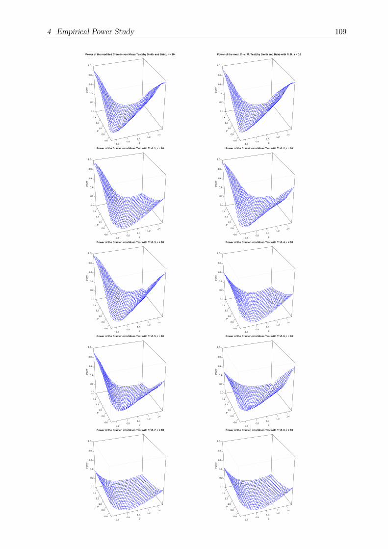
p0.60.8
1.01.2
1.4
q
0.6
0.8
1.0
1.2
1.4
0.0
0.2
0.4
0.6
0.8
1.0
Power of the modified Cramér−von Mises Test (by Smith and Bain), r = 10
Pow
er
p0.60.8
1.01.2
1.4
q
0.6
0.8
1.0
1.2
1.4
0.0
0.2
0.4
0.6
0.8
1.0
Power of the mod. C.−v. M. Test (by Smith and Bain) with R. D., r = 10
Pow
er
p0.60.8
1.01.2
1.4
q
0.6
0.8
1.0
1.2
1.4
0.0
0.2
0.4
0.6
0.8
1.0
Power of the Cramér−von Mises Test with Trsf. 1, r = 10
Pow
er
p0.60.8
1.01.2
1.4
q
0.6
0.8
1.0
1.2
1.4
0.0
0.2
0.4
0.6
0.8
1.0
Power of the Cramér−von Mises Test with Trsf. 2, r = 10
Pow
er
p0.60.8
1.01.2
1.4
q
0.6
0.8
1.0
1.2
1.4
0.0
0.2
0.4
0.6
0.8
1.0
Power of the Cramér−von Mises Test with Trsf. 3, r = 10
Pow
er
p0.60.8
1.01.2
1.4
q
0.6
0.8
1.0
1.2
1.4
0.0
0.2
0.4
0.6
0.8
1.0
Power of the Cramér−von Mises Test with Trsf. 4, r = 10
Pow
er
p0.60.8
1.01.2
1.4
q
0.6
0.8
1.0
1.2
1.4
0.0
0.2
0.4
0.6
0.8
1.0
Power of the Cramér−von Mises Test with Trsf. 5, r = 10
Pow
er
p0.60.8
1.01.2
1.4
q
0.6
0.8
1.0
1.2
1.4
0.0
0.2
0.4
0.6
0.8
1.0
Power of the Cramér−von Mises Test with Trsf. 6, r = 10
Pow
er
p0.60.8
1.01.2
1.4
q
0.6
0.8
1.0
1.2
1.4
0.0
0.2
0.4
0.6
0.8
1.0
Power of the Cramér−von Mises Test with Trsf. 7, r = 10
Pow
er
p0.60.8
1.01.2
1.4
q
0.6
0.8
1.0
1.2
1.4
0.0
0.2
0.4
0.6
0.8
1.0
Power of the Cramér−von Mises Test with Trsf. 8, r = 10
Pow
er
4 Empirical Power Study 109

p0.60.8
1.01.2
1.4
q
0.6
0.8
1.0
1.2
1.4
0.0
0.2
0.4
0.6
0.8
1.0
Power of the modified Watson Test, r = 10
Pow
er
p0.60.8
1.01.2
1.4
q
0.6
0.8
1.0
1.2
1.4
0.0
0.2
0.4
0.6
0.8
1.0
Power of the mod. Watson Test with Random Dilation, r = 10
Pow
er
p0.60.8
1.01.2
1.4
q
0.6
0.8
1.0
1.2
1.4
0.0
0.2
0.4
0.6
0.8
1.0
Power of the Watson Test with Trsf. 1, r = 10
Pow
er
p0.60.8
1.01.2
1.4
q
0.6
0.8
1.0
1.2
1.4
0.0
0.2
0.4
0.6
0.8
1.0
Power of the Watson Test with Trsf. 2, r = 10
Pow
er
p0.60.8
1.01.2
1.4
q
0.6
0.8
1.0
1.2
1.4
0.0
0.2
0.4
0.6
0.8
1.0
Power of the Watson Test with Trsf. 3, r = 10
Pow
er
p0.60.8
1.01.2
1.4
q
0.6
0.8
1.0
1.2
1.4
0.0
0.2
0.4
0.6
0.8
1.0
Power of the Watson Test with Trsf. 4, r = 10
Pow
er
p0.60.8
1.01.2
1.4
q
0.6
0.8
1.0
1.2
1.4
0.0
0.2
0.4
0.6
0.8
1.0
Power of the Watson Test with Trsf. 5, r = 10
Pow
er
p0.60.8
1.01.2
1.4
q
0.6
0.8
1.0
1.2
1.4
0.0
0.2
0.4
0.6
0.8
1.0
Power of the Watson Test with Trsf. 6, r = 10
Pow
er
p0.60.8
1.01.2
1.4
q
0.6
0.8
1.0
1.2
1.4
0.0
0.2
0.4
0.6
0.8
1.0
Power of the Watson Test with Trsf. 7, r = 10
Pow
er
p0.60.8
1.01.2
1.4
q
0.6
0.8
1.0
1.2
1.4
0.0
0.2
0.4
0.6
0.8
1.0
Power of the Watson Test with Trsf. 8, r = 10
Pow
er
110 4.4 Tests Based on Transformed Data

p0.60.8
1.01.2
1.4
q
0.6
0.8
1.0
1.2
1.4
0.0
0.2
0.4
0.6
0.8
1.0
Power of Neyman's Smooth Test with Trsf. 1, r = 10
Pow
er
p0.60.8
1.01.2
1.4q
0.6
0.8
1.0
1.2
1.4
0.0
0.2
0.4
0.6
0.8
1.0
Power of Neyman's Smooth Test with Trsf. 2, r = 10
Pow
er
p0.60.8
1.01.2
1.4
q
0.6
0.8
1.0
1.2
1.4
0.0
0.2
0.4
0.6
0.8
1.0
Power of Neyman's Smooth Test with Trsf. 3, r = 10
Pow
er
p0.60.8
1.01.2
1.4
q
0.6
0.8
1.0
1.2
1.4
0.0
0.2
0.4
0.6
0.8
1.0
Power of Neyman's Smooth Test with Trsf. 4, r = 10
Pow
er
p0.60.8
1.01.2
1.4
q
0.6
0.8
1.0
1.2
1.4
0.0
0.2
0.4
0.6
0.8
1.0
Power of Neyman's Smooth Test with Trsf. 5, r = 10
Pow
er
p0.60.8
1.01.2
1.4
q
0.6
0.8
1.0
1.2
1.4
0.0
0.2
0.4
0.6
0.8
1.0
Power of Neyman's Smooth Test with Trsf. 6, r = 10
Pow
er
p0.60.8
1.01.2
1.4
q
0.6
0.8
1.0
1.2
1.4
0.0
0.2
0.4
0.6
0.8
1.0
Power of Neyman's Smooth Test with Trsf. 7, r = 10
Pow
er
p0.60.8
1.01.2
1.4
q
0.6
0.8
1.0
1.2
1.4
0.0
0.2
0.4
0.6
0.8
1.0
Power of Neyman's Smooth Test with Trsf. 8, r = 10
Pow
er
4 Empirical Power Study 111
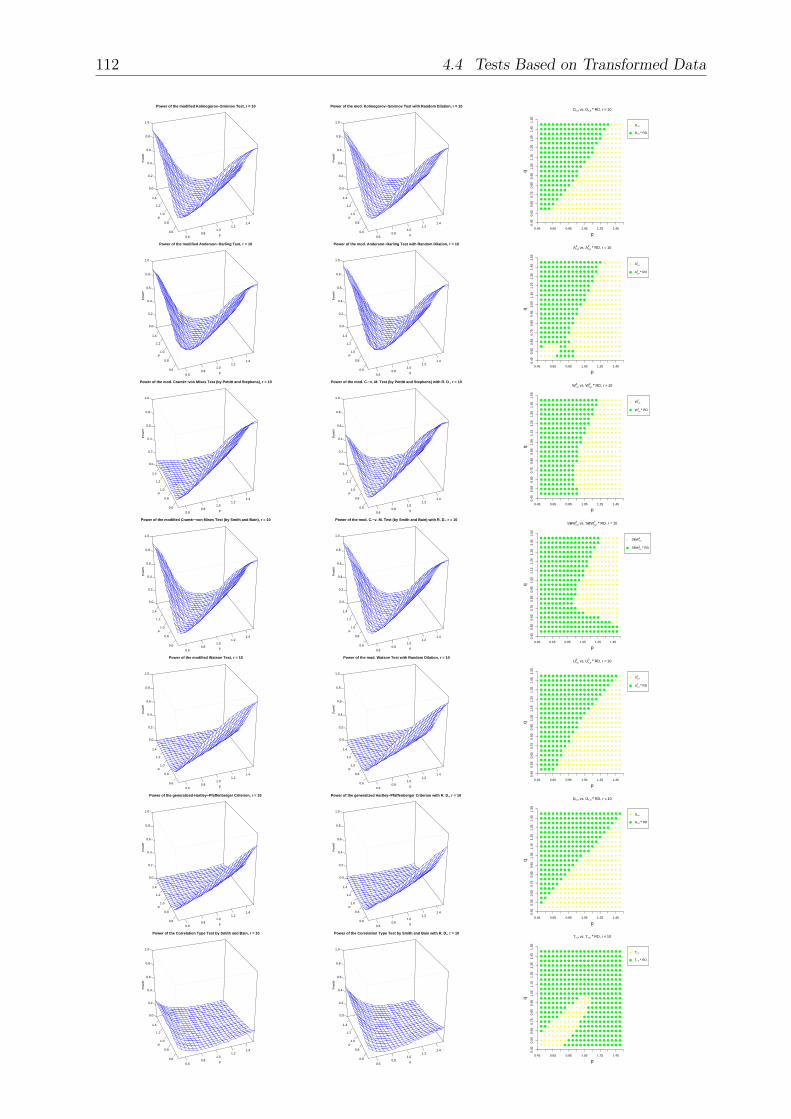
p0.60.8
1.01.2
1.4
q
0.6
0.8
1.0
1.2
1.4
0.0
0.2
0.4
0.6
0.8
1.0
Power of the modified Kolmogorov−Smirnov Test, r = 10
Pow
er
p0.60.8
1.01.2
1.4
q
0.6
0.8
1.0
1.2
1.4
0.0
0.2
0.4
0.6
0.8
1.0
Power of the mod. Kolmogorov−Smirnov Test with Random Dilation, r = 10
Pow
er
Dr,n vs. Dr,n °° RD, r = 10
p
q
0.45 0.65 0.85 1.05 1.25 1.45
0.45
0.55
0.65
0.75
0.85
0.95
1.05
1.15
1.25
1.35
1.45
1.55
Dr,n
Dr,n °° RD
p0.60.8
1.01.2
1.4
q
0.6
0.8
1.0
1.2
1.4
0.0
0.2
0.4
0.6
0.8
1.0
Power of the modified Anderson−Darling Test, r = 10
Pow
er
p0.60.8
1.01.2
1.4
q
0.6
0.8
1.0
1.2
1.4
0.0
0.2
0.4
0.6
0.8
1.0
Power of the mod. Anderson−Darling Test with Random Dilation, r = 10
Pow
er
Ar,n2 vs. Ar,n
2 °° RD, r = 10
p
q
0.45 0.65 0.85 1.05 1.25 1.45
0.45
0.55
0.65
0.75
0.85
0.95
1.05
1.15
1.25
1.35
1.45
1.55
Ar,n2
Ar,n2 °° RD
p0.60.8
1.01.2
1.4
q
0.6
0.8
1.0
1.2
1.4
0.0
0.2
0.4
0.6
0.8
1.0
Power of the mod. Cramér−von Mises Test (by Pettitt and Stephens), r = 10
Pow
er
p0.60.8
1.01.2
1.4
q
0.6
0.8
1.0
1.2
1.4
0.0
0.2
0.4
0.6
0.8
1.0
Power of the mod. C.−v. M. Test (by Pettitt and Stephens) with R. D., r = 10
Pow
er
Wr,n2 vs. Wr,n
2 °° RD, r = 10
p
q
0.45 0.65 0.85 1.05 1.25 1.45
0.45
0.55
0.65
0.75
0.85
0.95
1.05
1.15
1.25
1.35
1.45
1.55
Wr,n2
Wr,n2 °° RD
p0.60.8
1.01.2
1.4
q
0.6
0.8
1.0
1.2
1.4
0.0
0.2
0.4
0.6
0.8
1.0
Power of the modified Cramér−von Mises Test (by Smith and Bain), r = 10
Pow
er
p0.60.8
1.01.2
1.4
q
0.6
0.8
1.0
1.2
1.4
0.0
0.2
0.4
0.6
0.8
1.0
Power of the mod. C.−v. M. Test (by Smith and Bain) with R. D., r = 10
Pow
er
SBWr,n2 vs. SBWr,n
2 °° RD, r = 10
p
q
0.45 0.65 0.85 1.05 1.25 1.45
0.45
0.55
0.65
0.75
0.85
0.95
1.05
1.15
1.25
1.35
1.45
1.55
SBWr,n2
SBWr,n2 °° RD
p0.60.8
1.01.2
1.4
q
0.6
0.8
1.0
1.2
1.4
0.0
0.2
0.4
0.6
0.8
1.0
Power of the modified Watson Test, r = 10
Pow
er
p0.60.8
1.01.2
1.4
q
0.6
0.8
1.0
1.2
1.4
0.0
0.2
0.4
0.6
0.8
1.0
Power of the mod. Watson Test with Random Dilation, r = 10
Pow
er
Ur,n2 vs. Ur,n
2 °° RD, r = 10
p
q
0.45 0.65 0.85 1.05 1.25 1.45
0.45
0.55
0.65
0.75
0.85
0.95
1.05
1.15
1.25
1.35
1.45
1.55
Ur,n2
Ur,n2 °° RD
p0.60.8
1.01.2
1.4
q
0.6
0.8
1.0
1.2
1.4
0.0
0.2
0.4
0.6
0.8
1.0
Power of the generalized Hartley−Pfaffenberger Criterion, r = 10
Pow
er
p0.60.8
1.01.2
1.4
q
0.6
0.8
1.0
1.2
1.4
0.0
0.2
0.4
0.6
0.8
1.0
Power of the generalized Hartley−Pfaffenberger Criterion with R. D., r = 10
Pow
er
Gr,n vs. Gr,n °° RD, r = 10
p
q
0.45 0.65 0.85 1.05 1.25 1.45
0.45
0.55
0.65
0.75
0.85
0.95
1.05
1.15
1.25
1.35
1.45
1.55
Gr,n
Gr,n °° RD
p0.60.8
1.01.2
1.4
q
0.6
0.8
1.0
1.2
1.4
0.0
0.2
0.4
0.6
0.8
1.0
Power of the Correlation Type Test by Smith and Bain, r = 10
Pow
er
p0.60.8
1.01.2
1.4
q
0.6
0.8
1.0
1.2
1.4
0.0
0.2
0.4
0.6
0.8
1.0
Power of the Correlation Type Test by Smith and Bain with R. D., r = 10
Pow
er
Tr,n vs. Tr,n °° RD, r = 10
p
q
0.45 0.65 0.85 1.05 1.25 1.45
0.45
0.55
0.65
0.75
0.85
0.95
1.05
1.15
1.25
1.35
1.45
1.55
Tr,n
Tr,n °° RD
112 4.4 Tests Based on Transformed Data

4 Empirical Power Study 113
On pages 106 to 110 the 3D plots of the methods considered in the power maps on page104 for the case r = 10 are shown in the following order. On page 106 the graphs of theKolmogorov - Smirnov test can be found, where in the first row the plots of the modifiedversion with and without applying random dilation previously to the data are printed. Theplots of the classical version calculated on transformed data given by the transformations1 to 8 are arranged row by row beneath the first two graphs. Then, on the four subsequentpages the same is done for the Anderson - Darling test, the Cramér - von Mises test (firstwith modification W 2
r,n then with modification SBW 2r,n) and for the Watson test. On page
111 we see the corresponding graphs for Neyman’s smooth test Ψ24 combined with all of
the transformations.These illustrations are to visualize the differences between the powers of the comparedmethods, which cannot be done by the power maps on page 104. It becomes clear thatconsiderable differences particularly exist when the probability mass of the alternative isshifted to one end of the unit interval but not to both, i.e., for beta(p, q) distributions withp < 1 and q > 1 or vice versa. In the power maps, we see that the modified versions of thestatistics are the best choice if the probability is concentrated towards the right end of [0, 1](i.e., p > 1 and q < 1), whereas in the opposite case (p < 1 and q > 1) transformations 1 -3 show the best performances.For the Kolmogorov - Smirnov test the modified statistic is much better than all othermethods if p > 1 and q < 1, while transformation 3 is just slightly better than transforma-tions 1 or 2 and the modified test when p < 1 and q > 1. Moreover, the effect of randomdilation is small using the modified Kolmogorov - Smirnov statistic.This effect becomes a little bit larger when the modified Anderson - Darling statistic is uti-lized. Here random dilation increases the power against beta(p, q) alternatives if p < 1 andq > 1. Transformations 1 - 3 are still somewhat better with almost identical performancesin this situation, but transformation 3 is the only one, which also yields comparable poweras the modified test when p > 1 and q < 1.W 2r,n benefits from random dilation most. When p < 1 and q > 1 the power is improved
substantially, although transformations 1 - 3 are clearly the better choice in this situation,with similar performances. On the other hand, when p > 1 and q < 1 the modified test(with or without random dilation) outperforms the transformations considerably.The same holds true for SBW 2
r,n, but this modification of the Cramér - von Mises statisticis also almost as good as transformations 1 - 3 for p < 1 and q > 1, such that randomdilation does not make a big impact on SBW 2
r,n.It does not on U2
r,n either. The modified Watson test has no power against beta(p, q) alter-natives if p < 1 and q > 1. Here transformations 1 - 3 yield very similar results which aremuch better than those of the rest. If p > 1 and q < 1 the modified test stands out clearly.Finally, we consider Neyman’s smooth test computed on transformed data. Transforma-tions 2 and 3 yield similar results, overall. They are considerably better than the restwhen p > 1 and q < 1. In the opposite case, transformation 1 is competitive, and for therest of the considered alternatives there are no large differences between the powers of thetechniques.On the left hand side, the powers of the modified tests before and after random dilation wasapplied to a Type- II right censored sample of size r = 10 are plotted. Additionally, powermaps have been made just to compare these two methods in each case. In the particularrows (from top to bottom) we see the respective plots for the Kolmogorov - Smirnov test,the Anderson - Darling test, the Cramér - von Mises test (first W 2
r,n then SBW 2r,n), the
Watson test, the generalized Hartley-Pfaffenberger criterion and the correlation type testby Smith and Bain.

114 4.4 Tests Based on Transformed Data
For the first five tests, comments have already been given above. The effect of randomdilation on the power of the generalized Hartley-Pfaffenberger criterion is rather small,but the power of Tr,n can be increased substantially. This holds true in particular, for thepower against beta(p, q) alternatives with p < 1 and q > 1.Altogether, we may conclude for all of the modified tests that the application of randomdilation is advisable, although the power maps show better performances for the testswithout random dilation in most of the cases where p > q. But the differences between thepowers of the two methods at these points are negligible, whereas there are some situationsin which random dilation can increase power considerably, as already mentioned above.Moreover, the modified tests (with or without random dilation) can be recommended inthe cases where the probability mass of the alternative is shifted to the right limit of theunit interval (cf. beta(p, q) alternatives with p > 1 and q < 1), in general. If it is shiftedto the left limit (cf. beta(p, q) alternatives with p < 1 and q > 1) then transformations1 - 3 show the best performances regardless of the statistic being considered. In all othersituations, there is no technique which yields generally good power.Finally, it should be mentioned that transformation 8 which preserves the OS’s structurefor the whole family of power function distributions, i.e., for beta(a, 1) distributions, wherea > 0 is arbitrary (cf. Theorem 3.32), does not yield tests with better powers than theother transformations. Thus, the structure of the joint distribution of the sample beingtested is not crucial for the powers of the goodness-of-fit tests. E.g., we have seen in Sec-tion 3.2.1 (cf. Theorem 3.10) that transformation 1 only yields OS’s if the censored samplestems from the standard uniform distribution, but the use of this transformation for testinggoodness-of-fit is clearly more advisable than the use of transformation 8, regardless of thetest statistics which are applied.

5 Outlook 115
5 Outlook
The focus of this thesis is on transformations of Type-II right censored data in the con-text of goodness-of-fit tests. In Chapter 2 we have seen several examples of mappingsthat transform Type-II right censored samples of i.i.d. standard uniformly distributedrandom variables into samples behaving like (ordered or unordered) complete samples ofi.i.d. U(0, 1) random variables of a smaller sample size. But in Chapter 3 it was shownthat censored samples from other underlying distributions are not necessarily transformedinto order statistics or i.i.d. random variables by these mappings. In the case of the trans-formation suggested by Michael and Schucany (1979) (cf. Theorem 2.2 (x)) it could evenbe shown that U(0, 1) is the only distribution such that the order statistics structure ispreserved (cf. Theorem 3.10).Perhaps, it is possible to characterize the distributions, for which the transformed samplesbehave like order statistics or i.i.d. random variables, for other transformations, too. Theo-rems 3.5, 3.6, 3.29, 3.31 and Corollary 3.37 do not make any statements on this. However,the approach of density transformation pursued in this work, which was successful for thetransformation of Michael and Schucany (1979), seems to be less fruitful for other trans-formations.It might also be worth trying to relax the conditions of the theorems mentioned above.But these generalizations could be extremely tedious, such that one might prefer analyzingtransformations separately if they do not satisfy the given conditions.The power studies described in Chapter 4 should be extended to other test statistics andtransformations. Ideas for constructing new transformations are given in Chapter 2 andmany other test statistics can be found in literature. Perhaps, it is also possible to explainsome of the obtained results theoretically.Finally, other kinds of censoring should be considered in the same way as Type-II right cen-sored samples were studied here. For example, Michael and Schucany (1979) and O’Reillyand Stephens (1988) already showed how Type-I or progressively Type-II censored datacould be transformed, and Barr and Davidson (1973) as well as Pettitt and Stephens (1976)considered modified test statistics also for Type-I censored samples. But, to my know-ledge, an extensive analysis of these techniques similar to the investigations in this workfor Type-II right censoring cannot be found in literature, so far. Anyway, the case of Type-II left censored data does not have to be examined separately, since it can be traced back toType-II right censoring: If Xn−r+1:n, . . . , Xn:n are the r largest order statistics from n i.i.d.random variables X1, . . . , Xn with observations in [0, 1] then
(1−Xn:n, . . . , 1−Xn−r+1:n
)is distributed as a vector of the r smallest order statistics from n i.i.d. random variables,r, n ∈ N, 1 ≤ r ≤ n.

116

Appendix 117
Appendix
In the following plots, one can see logspline density estimates of some alternatives, con-sidered by Marhuenda et al. (2005) and Quesenberry and Miller (1977) in their simulationstudies (cf. Chapter 4), and corresponding approximations by beta distributions. First,100,000 observations of each alternative were simulated; then, the logspline density esti-mation was calculated using the function ’logspline’ of the same named R package and theparameters of the beta distributions were computed by the method of moments (cf. Fielitzand Myers (1975) and Stone et al. (1997)).The plots were generated by a Java applet which will be available on the homepage of the In-stitute of Statistics of RWTH Aachen University (http://www.stochastik.rwth-aachen.de),soon. The red line always represents the beta density and the blue line illustrates thelogspline density estimation in each graph.The first families of distributions studied by Marhuenda et al. (2005) and Quesenberry andMiller (1977), respectively, are given by beta distributions. Thus, they are not consideredat this point. Members of the families B and C from Marhuenda et al. (2005) are definedby the following distribution functions:
Family B : Bk ∼ F2,k(x) =
0 , x < 0,
2k−1xk , 0 ≤ x < 0.5,
1− 2k−1(1− x)k , 0.5 ≤ x < 1,
1 , else,
Family C : Ck ∼ F3,k(x) =
0 , x < 0,
0.5− 2k−1(0.5− x)k , 0 ≤ x < 0.5,
0.5 + 2k−1(x− 0.5)k , 0.5 ≤ x < 1,
1 , else,
where k > 0.
Alternatives B0.6 approximated by beta(0.5383, 0.5386) (left-hand side) and B1.25 approxi-mated by beta(1.3224, 1.3239) (right-hand side):
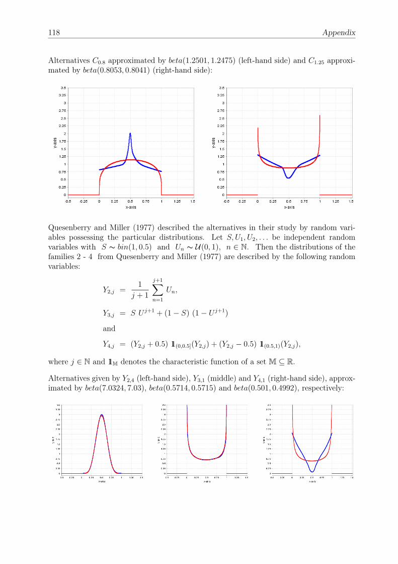
118 Appendix
Alternatives C0.8 approximated by beta(1.2501, 1.2475) (left-hand side) and C1.25 approxi-mated by beta(0.8053, 0.8041) (right-hand side):
Quesenberry and Miller (1977) described the alternatives in their study by random vari-ables possessing the particular distributions. Let S, U1, U2, . . . be independent randomvariables with S ∼ bin(1, 0.5) and Un ∼ U(0, 1), n ∈ N. Then the distributions of thefamilies 2 - 4 from Quesenberry and Miller (1977) are described by the following randomvariables:
Y2,j =1
j + 1
j+1∑n=1
Un,
Y3,j = S U j+1 + (1− S) (1− U j+1)
and
Y4,j = (Y2,j + 0.5) 11(0,0.5](Y2,j) + (Y2,j − 0.5) 11(0.5,1)(Y2,j),
where j ∈ N and 11M denotes the characteristic function of a set M ⊆ R.
Alternatives given by Y2,4 (left-hand side), Y3,1 (middle) and Y4,1 (right-hand side), approx-imated by beta(7.0324, 7.03), beta(0.5714, 0.5715) and beta(0.501, 0.4992), respectively:

BIBLIOGRAPHY 119
BibliographyAczél, J. (1966). Lectures on Functional Equations and their Applications, second edn,Academic Press.
Anderson, T. W. and Darling, D. A. (1952). Asymptotic theory of certain "goodness offit" criteria based on stochastic process, Ann. Math. Stat. 23: 193 – 212.
Arnold, B. C., Balakrishnan, N. and Nagaraja, H. N. (1992). A First Course in OrderStatistics, John Wiley & Sons, New York.
Balakrishnan, N. and Aggarwala, R. (2000). Progressive Censoring: Theory, Methods, andApplications, Birkhäuser, Boston.
Barr, D. R. and Davidson, T. (1973). A Kolmogorov-Smirnov test for censored samples,Technometrics 15: 739 – 757.
Best, D. J. and Rayner, J. C. W. (1985). Uniformity testing when alternatives have loworder, Sankhya Ser. A 47: 25 – 35.
Beutner, E. and Kamps, U. (2008). Random contraction and random dilation of generalizedorder statistics, Commun. Statist. - Theory Meth. 37: 2185 – 2201.
Birnbaum, Z. W. and Lientz, B. P. (1969). Tables of critical values of some Rényi typestatistics for finite sample sizes, J. Amer. Statist. Assoc. 64: 870 – 877.
Castro-Kuriss, C., Kelmansky, D., Leiva, V. and Martinez, E. (2009). A new goodness-of-fit test for censored data with an application in monitoring processes, Commun. Stat.,Simulation Comput. 38: 1161 – 1177.
Chen, Z. and Ye, C. (2009). An alternative test for uniformity, Int. J. Reliab. Qual. Saf.Eng. 16: 343 – 356.
D’Agostino, R. B. and Stephens, M. A. (1986). Goodness-of-fit-techniques, Marcel Dekker.
David, H. A. and Nagaraja, H. N. (2003). Order Statistics, third edn, John Wiley & Sons,New York.
Durbin, J. (1968). The probability that the sample distribution function lies between twoparallel straight lines, Ann. Math. Statist. 39: 398 – 411.
Durbin, J. (1971). Boundary-crossing probability for the Brownian motion and Poissonprocess and techniques for computing the power of the Kolmogorov-Smirnov test, J.Appl. Prob. 8: 431 – 453.
Durbin, J. and Knott, M. (1972). Components of Cramér-von Mises statistics I, J. Roy.Statist. Soc. Ser. B. 34: 290 – 307.
Durbin, J., Knott, M. and Taylor, C. C. (1975). Components of Cramér-von Mises statisticsII, J. Roy. Statist. Soc. Ser. B. 37: 216 – 237.
Fielitz, B. D. and Myers, B. L. (1975). Estimation of parameters in the beta distribution,Decision Sciences 6: 1 – 13.

120 BIBLIOGRAPHY
Filliben, J. J. (1975). The probability plot correlation coefficient test for normality, Tech-nometrics 17: 111 – 117.
Fischer, T., Balakrishnan, N. and Cramer, E. (2008). Mixture representation for orderstatistics from inid progressive censoring and its applications, J. Multivariate Anal.99: 1999 – 2015.
Fischer, T. and Kamps, U. (2011). On the existence of transformations preserving thestructure of order statistics in lower dimensions, J. Statist. Plann. Inference 141: 536 –548.
Fisz, M. (1963). Probability Theory and Mathematical Statistics, third edn, John Wiley &Sons, New York and London.
Ghorai, J. K. (1991). Cramér-von Mises statistic for testing goodness of fit under theproportional hazard model, Commun. Statist. - Theory Meth. 20: 1107 – 1126.
Ghurye, S. G. (1960). Characterization of some location and scale parameter families ofdistributions, In: Olkin, I., Ghurye, S. G., Hoeffding, W., Madow, W. G. and Mann,H. B. (eds.), Contributions to Probability and Statistics: Essays in Honor of HaroldHotelling. Stanford University Press.
Glen, A. G., Leemis, L. M. and Barr, D. R. (2001). Order statistics in goodness-of-fittesting, IEEE Transactions on Reliability 50: 209 – 213.
Goegebeur, Y. and Guillou, A. (2010). Goodness-of-fit testing for Weibull-type behavior,J. Statist. Plann. Inference 140: 1417 – 1436.
Greenwood, M. (1946). The statistical study of infectious diseases, J. Roy. Statist. Soc.109: 85 – 110.
Hajós, G. and Rényi, A. (1954). Elementary proofs of some basic facts concerning orderstatistics, Acta Mathematica Hungarica 5: 1 – 6.
Hartley, H. O. and Pfaffenberger, R. C. (1972). Quadratic forms in order statistics usedas goodness-of-fit criteria, Biometrika 59: 605 – 611.
Jennings, S. A. (1954). Substitution groups of formal power series, Canad. J. Math. 6: 325– 340.
Kallenberg, W. C. M. and Ledwina, T. (1995). Consistency and monte carlo simulation ofa data driven version of smooth goodness-of-fit tests, Ann. Statist. 23: 1594 – 1608.
Kautschitsch, H. (1979). Über vertauschbare Potenzreihen, Math. Nachr. 88: 207 – 217.
Krantz, S. G. and Parks, H. R. (2002). A Primer of Real Analytic Functions, second edn,Birkhäuser, Boston.
Kuczma, M., Choczewski, B. and Ger, R. (1990). Iterative Functional Equations, Cam-bridge University Press.
Landau, E. (2001). Differential and Integral Calculus, third edn, AMS Bookstore.
LaRiccia, V. N. (1986). Asymptotically chi-squared distributed tests of normality for typeII censored samples, J. Amer. Statist. Assoc. 81: 1026 – 1031.

BIBLIOGRAPHY 121
Ledwina, T. (1994). Data-driven version of Neyman’s smooth test of fit, J. Amer. Statist.Assoc. 89: 1000 – 1005.
Lim, J. and Park, S. (2007). Censored Kullback-Leibler information and goodness-of-fittest with type II censored data, J. Appl. Statist. 34: 1051 – 1064.
Lin, C.-T., Huang, Y.-L. and Balakrishnan, N. (2008). A new method for goodness-of-fit testing based on type-II right censored samples, IEEE Transactions on Reliability57: 633 – 642.
Lurie, D., Hartley, H. O. and Stroud, M. R. (1974). A goodness of fit test for censoreddata, Commun. Statist. 3: 745 – 753.
Maag, U. R. and Dicatre, G. (1971). On Kolmogorov-Smirnov type one-sample statistics,Biometrika 58: 653 – 656.
Malmquist, S. (1950). On a property of order statistics from a rectangular distribution,Skandinavisk Aktuarietidskrift 33: 214 – 222.
Marhuenda, Y., Morales, D. and Pardo, M. (2005). A comparison of uniformity tests,Statistics 39: 315 – 328.
Meintanis, S. G. (2009). Goodness-of-fit tests and minimum distance estimation via optimaltransformation to uniformity, J. Statist. Plann. Inference 139: 100 – 108.
Michael, J. R. and Schucany, W. R. (1979). A new approach to testing goodness of fit forcensored samples, Technometrics 21: 435 – 441.
Milbrodt, H. and Strasser, H. (1990). On the asymptotic power of the two-sidedKolmogorov-Smirnov test, J. Statist. Planning Inference 26: 1 – 23.
Miller, F. L. and Quesenberry, C. P. (1979). Power studies of some tests for uniformity, II,Commun. Statist.-Simul. Comp. 8: 271 – 290.
Moskowitz, M. A. (2002). A Course in Complex Analysis in One Variable, World Scientific.
Neuhaus, G. (1976). Asymptotic power properties of the Cramér-von Mises test undercontiguous alternatives, J. Multivariate Anal. 6: 95 – 110.
Nevzorov, V. B. (2001). Translations of Mathematical Monographs 194, Records: Mathe-matical Theory, AMS Bookstore.
Neyman, J. (1937). ’Smooth test’ for goodness of fit, Skand. Aktuarietidskr. 20: 150 – 199.
O’Reilly, F. J. and Stephens, M. A. (1982). Characterizations and goodness of fit tests, J.Roy. Statist. Soc. Ser. B 44: 353 – 360.
O’Reilly, F. J. and Stephens, M. A. (1988). Transforming censored samples for testing fit,Technometrics 30: 79 – 86.
Paul, A. (2003). Characterizations of the uniform distribution via sample spacings andnonlinear transformations, J. Math. Anal. Appl. 284: 397 – 402.
Pettitt, A. N. and Stephens, M. A. (1976). Modified Cramér-von Mises statistics forcensored data, Biometrika 63: 291 – 298.

122 BIBLIOGRAPHY
Quesenberry, C. P. and Miller, F. L. (1977). Power studies of some tests for uniformity, J.Statist. Comput. Simul. 5: 169 – 191.
Rayner, G. D. and Rayner, J. C. W. (2001). Power of the Neyman smooth tests for theuniform distribution, J. Appl. Math. Decision Sci. 5: 181 – 191.
Reiss, R.-D. (1989). Approximate Distributions of Order Statistics, Springer, New York.
Rényi, A. (1953). On the theory of order statistics, Acta Mathematica Hungarica 4: 191 –231.
Roman, S. (1980). The Formula of Faa di Bruno, Amer. Math. Monthly 87: 805 – 809.
Rosenblatt, M. (1952). Remarks on a multivariate transformation, Annals of MathematicalStatistics 28: 470 – 472.
Smith, R. M. and Bain, L. J. (1976). Correlation type goodness-of-fit statistics withcensored sampling, Commun. Statist. 5: 119 – 132.
Sürücü, B. (2008). A power comparison and simulation study of goodness-of-fit tests,Comput. Math. Appl. 56: 1617 – 1625.
Steele, M. and Chaseling, J. (2006). Powers of discrete goodness-of-fit test statistics for auniform null against a selection of alternative distributions, Commun. Stat., SimulationComput. 35: 1067 – 1075.
Stephens, M. A. (1974a). Components of goodness-of-fit statistics, Ann. Inst. HenriPoincaré 10: 37 – 54.
Stephens, M. A. (1974b). EDF statistics for goodness of fit and some comparisons, Journalof the American Statistical Association 69: 730 – 737.
Stone, C. J., Hansen, M. H., Kooperberg, C. and Truong, Y. K. (1997). Polynomial splinesand their tensor products in extended linear modeling, Ann. Statist. 25: 1371 – 1470.
Tadikamalla, P. R. and Balakrishnan, N. (1998). Computer Simulation of Order Statistics,In: Balakrishnan, N. and Rao, C. R. (eds.), Handbook of Statistics: Order Statistics:Theory & Methods. Vol. 16, chap. 3, 65 - 72, Elsevier, Amsterdam.
Tolstov, G. P. and Silverman, R. A. (1976). Fourier Series, Courier Dover Publications.
Wesołowski, J. and Ahsanullah, M. (2004). Switching order statistics through randompower contractions, Australian & New Zealand Journal of Statistics 46: 297 – 303.
Zhao, J., Xu, X. and Ding, X. (2009). Some new goodness-of-fit tests based on stochasticsample quantiles, Commun. Stat. - Simulation and Computation 38: 571 – 589.
Zhao, J., Xu, X. and Ding, X. (2010). New goodness of fit tests based on stochastic EDF,Commun. Stat. - Theory and Methods 39: 1075 – 1094.