J. Fluid Mech. (2014), vol. 757, pp. 1–32. c© Cambridge University Press 2014doi:10.1017/jfm.2014.472

1

Mean flow stability analysis of oscillating jetexperiments

Kilian Oberleithner1,†, Lothar Rukes1 and Julio Soria2,3

1Institut für Strömungsmechanik und Technische Akustik, HFI, Technische Universität Berlin,10623 Berlin, Germany

2Laboratory for Turbulence Research in Aerospace & Combustion, Monash University, Melbourne,VIC 3800, Australia

3Department of Aeronautical Engineering, King Abdulaziz University, Jeddah, Kingdom of Saudi Arabia

(Received 5 January 2014; revised 18 July 2014; accepted 11 August 2014;first published online 19 September 2014)

Linear stability analysis (LSA) is applied to the mean flow of an oscillating roundjet with the aim of investigating the robustness and accuracy of mean flow stabilitywave models. The jet’s axisymmetric mode is excited at the nozzle lip througha sinusoidal modulation of the flow rate at amplitudes ranging from 0.1 % to100 %. The instantaneous flow field is measured via particle image velocimetry(PIV) and decomposed into a mean and periodic part utilizing proper orthogonaldecomposition (POD). Local LSA is applied to the measured mean flow adopting aweakly non-parallel flow approach. The resulting global perturbation field is carefullycompared with the measurements in terms of spatial growth rate, phase velocity,and phase and amplitude distribution. It is shown that the stability wave modelaccurately predicts the excited flow oscillations during their entire growth phase andduring a large part of their decay phase. The stability wave model applies over awide range of forcing amplitudes, showing no pronounced sensitivity to the strengthof nonlinear saturation. The upstream displacement of the neutral point and thesuccessive reduction of gain with increasing forcing amplitude is very well capturedby the stability wave model. At very strong forcing (>40 %), the flow becomesessentially stable to the axisymmetric mode. For these extreme cases, the predictiondeteriorates from the measurements due to an interaction of the forced wave with thegeometric confinement of the nozzle. Moreover, the model fails far downstream in aregion where energy is transferred from the oscillation back to the mean flow. Thisstudy supports previously conducted mean flow stability analysis of self-excited flowoscillations in the cylinder wake and in the vortex breakdown bubble and extends themethodology to externally forced convectively unstable flows. The high accuracy ofmean flow stability wave models as demonstrated here is of great importance for theanalysis of coherent structures in turbulent shear flows.

Key words: absolute/convective instability, jets, nonlinearity

† Email address for correspondence: kilian.oberleithner@pi.tu-berlin.de

Dow

nloa

ded

from

htt

ps://

ww

w.c

ambr

idge

.org

/cor

e. U

nive

rsita

etsb

iblio

thek

, on

26 O

ct 2

017

at 0

7:37

:55,

sub

ject

to th

e Ca

mbr

idge

Cor

e te

rms

of u

se, a

vaila

ble

at h

ttps

://w

ww

.cam

brid

ge.o

rg/c

ore/

term

s. h

ttps

://do

i.org

/10.

1017

/jfm

.201

4.47

2

2 K. Oberleithner, L. Rukes and J. Soria

1. IntroductionInstabilities inherent to turbulent shear flows cause small perturbations to grow

significantly in space and time. This leads to the formation of large-scale coherentflow structures that play an important role for cross-flow momentum transfer, noisegeneration and mixing. The active control of shear flows is most efficient if theseinherent instabilities are exploited (Greenblatt & Wygnanski 2000).

In the last few decades, significant effort has been made to derive analytic modelsfor coherent structures and their impact on the mean and turbulent flow characteristics.The underlying methodology is typically based on a triple decomposition of thetime-dependent flow into a time-mean part, a periodic (coherent) part, and a randomlyfluctuating (turbulent) part. The mean is obtained from time-averaging, while theperiodic part is obtained from a phase average, ‘i.e. the average over a large ensembleof points having the same phase with respect to a reference oscillator’ (Reynolds& Hussain 1972). The coherent part represents fluctuations at large time and lengthscales in contrast to the small-scale turbulent fluctuations. This separation of scalesallows for the treatment of the wave-like coherent structures independently from therandom turbulent fluctuations.

Since the groundbreaking experiments of Crow & Champagne (1971) and Brown &Roshko (1974), many researches have shown that the large-scale coherent structures inopen shear flows are qualitatively similar to instability waves. As stated by Gaster, Kit& Wygnanski (1985), ‘This similarity between the patterns in laminar and turbulentstates is not very surprising in view of the fact that the basic long-wave vorticity-transport instability mechanism is mainly controlled by the mean-velocity profiles ofthe flow, and these are not too different in the two situations’.

This phenomenological reasoning leads to instability wave models, where thecoherent structures are derived from a linear stability analysis (LSA) of the meanturbulent flow. Since these models are based on the (nonlinearly modified) mean flowthey intrinsically account for the mean–coherent and mean–turbulent interactions. Theturbulent–coherent interactions are not represented by the mean flow and are eitherneglected (Gaster et al. 1985; Cohen & Wygnanski 1987; Gudmundsson & Colonius2011; Oberleithner et al. 2011) or lumped into an eddy viscosity model (Marasli,Champagne & Wygnanski 1991; Reau & Tumin 2002; Oberleithner, Paschereit &Wygnanski 2014). Reau & Tumin (2002) and Lifshitz, Degani & Tumin (2008)developed a mathematical model that incorporates all three interactions for the caseof the forced turbulent mixing layer with the goal of turbulent–coherent closure.Their model captures the interaction between the mean flow and the coherentstructures qualitatively, but the actual growth rates deviate from the measurements,particularly for higher forcing amplitudes. Lifshitz et al. (2008) suggest that theerroneous prediction is attributed to an inaccurate model of the turbulent–coherentinteractions. This conclusion is stereotypical for the LSA of turbulent flows, wherethe inaccurate prediction of the large-scale structures is typically related to a numberof causes that are difficult to separate. The reasons for an inaccurate predictioncan be an insufficient turbulent–coherent interaction model, an inaccurate mean flowrepresentation (e.g. accidental modification through finite amplitude forcing), strongnon-parallelism of the flow (for local stability analysis) or nonlinear mode–modeinteraction. Due to the multitude of error sources, the stability wave models inturbulent flows are still considered as inaccurate and are far from being generallyaccepted.

Mean flow stability wave models have significant importance in the analysis ofexperimental work. While LSA based on the unperturbed state is useful to predict the

Dow

nloa

ded

from

htt

ps://

ww

w.c

ambr

idge

.org

/cor

e. U

nive

rsita

etsb

iblio

thek

, on

26 O

ct 2

017

at 0

7:37

:55,

sub

ject

to th

e Ca

mbr

idge

Cor

e te

rms

of u

se, a

vaila

ble

at h

ttps

://w

ww

.cam

brid

ge.o

rg/c

ore/

term

s. h

ttps

://do

i.org

/10.

1017

/jfm

.201

4.47

2

Mean flow stability analysis of oscillating jet experiments 3

onset of instability, the mean flow LSA shows a great potential for the analysis of thenonlinearly saturated state that manifests in a (perturbed) experimental environment.The most prominent example of successful mean flow LSA is the prediction of thefinite vortex shedding in the cylinder wake (Pier 2002; Barkley 2006). For a widerange of post-critical Reynolds numbers, the frequency at the limit cycle is preciselypredicted by the linear global mode of the mean flow, while the prediction basedon the steady-state solution deteriorates with increasing distance from the criticalpoint. The results are perfectly in line with the mean field model proposed by Noacket al. (2003). Yet, the validity of the mean flow LSA is not rigorous and dependson the interactions between the mean flow, the fundamental and its harmonics. Asdemonstrated by Sipp & Lebedev (2007), the mean flow LSA is inaccurate in thecase of a cavity flow, due to a strong resonance of the fundamental wave with itsfirst harmonic. In this work we will clarify whether this mechanism is relevant forthe axisymmetric jet.

In this investigation, we consider an essentially laminar flow that is subjectedto external forcing. The Kelvin–Helmholtz-type convective instability causes afinite-amplitude wavetrain to grow and decay in the streamwise direction. The primaryinteractions that take place are between the mean flow and the oscillation and betweenthe oscillation and its harmonics. LSA is applied to the resulting time-averaged flowobtained from measurements with the aim to predict the oscillating flow field. Bychanging the amplitude of the forcing, we may control the intensity of the nonlinearinteractions involved in the saturation process. With this approach, we can analyse towhat extent the stability wave models are affected by these interactions, without theambiguity of a turbulence model affecting the conclusions.

Although, Pier (2002) and Barkley (2006) have already demonstrated an excellentprediction of the vortex shedding frequency based on the mean flow LSA, theseauthors did not compare the mode shapes with the actual oscillatory field and theability of the mean flow LSA in this regard remains unknown. In the present study,we undertake a comprehensive comparison of the oscillating flow field with theLSA predictions, considering growth rates, phase velocities, and phase and amplitudedistributions. For the forced jet flow considered here, perturbations are initiated atthe nozzle at precisely controlled conditions, and they are convected downstreamwhile growing and decaying at a rate that is determined by the underlying base flowstability. Hence, the amplitude of the instability wavetrain is rather a function ofspace than time, and so is the mean–coherent interaction. The same concept appliesto the flow bifurcating to a global mode, however in that scenario, the location ofthe (internal) forcing at the initiated onset of instability and at the limit cycle isless precisely known. In fact, the local LSA adopted in this work can be rigorouslyapplied to both flow classes, with the difference that for the globally unstable flows,the forcing frequency and location must be derived through a spatiotemporal typeanalysis of the flow field, while for the convectively unstable flows, it is readilydefined by the type of forcing applied (see e.g. Huerre & Monkewitz 1990; Juniper,Tammisola & Lundell 2011).

The globally stable but convectively unstable flow considered here is suitable for alocal stability analysis. We adopt the weakly non-parallel flow analysis developed byCrighton & Gaster (1976). Within the framework of multiple-scale analysis, the localamplitude function is assumed to vary slowly in the streamwise direction, allowing foran unambiguous reconstruction of the overall flow response to a localized perturbation.The same approach has been used for the inviscid analysis of turbulent jets (Strange& Crighton 1983) and mixing layers (Gaster et al. 1985; Lifshitz et al. 2008) and theviscous analysis of laminar swirling jets (Cooper & Peake 2002).

Dow

nloa

ded

from

htt

ps://

ww

w.c

ambr

idge

.org

/cor

e. U

nive

rsita

etsb

iblio

thek

, on

26 O

ct 2

017

at 0

7:37

:55,

sub

ject

to th

e Ca

mbr

idge

Cor

e te

rms

of u

se, a

vaila

ble

at h

ttps

://w

ww

.cam

brid

ge.o

rg/c

ore/

term

s. h

ttps

://do

i.org

/10.

1017

/jfm

.201

4.47

2

4 K. Oberleithner, L. Rukes and J. Soria

Camera Camera

Las

er

A B C D

E

Tank

Tank

1200550

550

550

5010

3648

27

45E

Mirrors

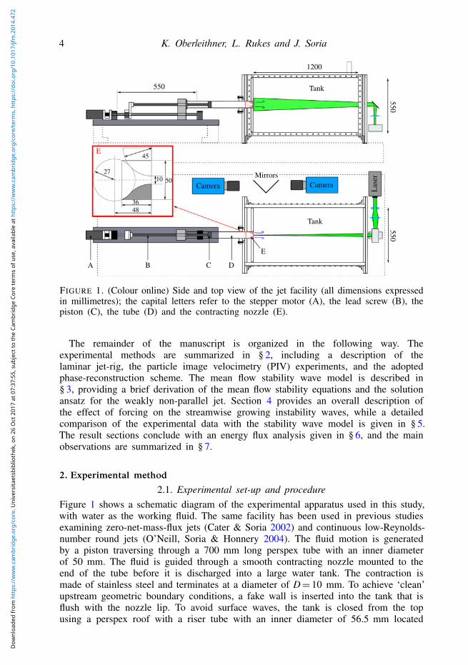
FIGURE 1. (Colour online) Side and top view of the jet facility (all dimensions expressedin millimetres); the capital letters refer to the stepper motor (A), the lead screw (B), thepiston (C), the tube (D) and the contracting nozzle (E).

The remainder of the manuscript is organized in the following way. Theexperimental methods are summarized in § 2, including a description of thelaminar jet-rig, the particle image velocimetry (PIV) experiments, and the adoptedphase-reconstruction scheme. The mean flow stability wave model is described in§ 3, providing a brief derivation of the mean flow stability equations and the solutionansatz for the weakly non-parallel jet. Section 4 provides an overall description ofthe effect of forcing on the streamwise growing instability waves, while a detailedcomparison of the experimental data with the stability wave model is given in § 5.The result sections conclude with an energy flux analysis given in § 6, and the mainobservations are summarized in § 7.

2. Experimental method2.1. Experimental set-up and procedure

Figure 1 shows a schematic diagram of the experimental apparatus used in this study,with water as the working fluid. The same facility has been used in previous studiesexamining zero-net-mass-flux jets (Cater & Soria 2002) and continuous low-Reynolds-number round jets (O’Neill, Soria & Honnery 2004). The fluid motion is generatedby a piston traversing through a 700 mm long perspex tube with an inner diameterof 50 mm. The fluid is guided through a smooth contracting nozzle mounted to theend of the tube before it is discharged into a large water tank. The contraction ismade of stainless steel and terminates at a diameter of D= 10 mm. To achieve ‘clean’upstream geometric boundary conditions, a fake wall is inserted into the tank that isflush with the nozzle lip. To avoid surface waves, the tank is closed from the topusing a perspex roof with a riser tube with an inner diameter of 56.5 mm located

Dow

nloa

ded

from

htt

ps://

ww

w.c

ambr

idge

.org

/cor

e. U

nive

rsita

etsb

iblio

thek

, on

26 O

ct 2

017

at 0

7:37

:55,

sub

ject

to th

e Ca

mbr

idge

Cor

e te

rms

of u

se, a

vaila

ble

at h

ttps

://w

ww

.cam

brid

ge.o

rg/c

ore/

term

s. h

ttps

://do

i.org

/10.

1017

/jfm

.201

4.47

2

Mean flow stability analysis of oscillating jet experiments 5

at the far end of the tank, and the facility is filled up to the roof. A lead screw isused to transfer the rotational motion of the stepper motor to the transversal motion ofthe piston, yielding a resolution of 0.2 µm per step. The motor motion is closed-loopcontrolled by feeding an encoder signal back to the motor driver. The motor driverallows the precompiled motion profiles to be run at an update rate of 2 ms.

Experiments were conducted at a facility Reynolds number of ReD=UjetD/ν = 770,with D being the nozzle diameter, Ujet the plug flow velocity at the nozzle and νthe kinematic viscosity of water. The jet is forced axisymmetrically by imposing asinusoidal motion onto the mean motion of the piston, yielding a piston velocity,

upiston = upiston (1+ A cos(2πft)) , (2.1)

with the excitation amplitude defined as

A= upiston/upiston, (2.2)

where upiston refers to the amplitude of the oscillating motion of the piston, upistonto the time-averaged velocity of the piston and f to the excitation frequency. Theamplitude of the piston motion is considered equivalent to the amplitude of the axialvelocity fluctuations at the nozzle. The phase-locked velocity fluctuations measuredat the nozzle confirm this assumption. For this study, data was recorded for forcingamplitudes ranging from A = 0 % to A = 100 %. The excitation frequency wasf = 2 Hz yielding a Strouhal number of fD/Ujet = 0.26. The frequency was selectedfrom a stability analysis of the natural flow, with the aim of exciting an instability thatreaches neutral stability in the centre of the measurement domain to capture its entiregrowth and decay phase. The frequency does not correspond to the mode with thelargest overall amplification. It is worth noting that the axisymmetric jet is generallyunstable to a wide range of modes with the axisymmetric mode being dominant inthe potential core while the single-helical mode takes over further downstream (Cohen& Wygnanski 1987; Oberleithner et al. 2014). The present focus on the axisymmetricmode is arbitrarily motivated by the facility design, but we expect a similar generalscenario when forcing the jet at a helical mode.

Before each experiment, the water in the tank was stirred using an aquarium pump,and the piston was moved to its most upstream position. After five more minutes,the flow in the tank was considered as stagnant and the forward motion of the pistonwas initiated. A statistically stationary flow was established after approximately30 seconds and flow measurements were conducted after 1 minute. This providesmore than 2 minutes for data acquisition before the end of the piston motion isreached.

2.2. Flow measurementsPlanar PIV was used for the flow velocity measurements. This image-based methodenables the instantaneous measurement of the two components of the fluid velocity inthe plane of the light sheet generated by a pulsed high-energy light source. Figure 1shows the arrangement used in this experiment.

Table 1 lists the important parameters of the PIV acquisition and analysis.The instantaneous PIV velocity fields were acquired at low frame rates and cantherefore be considered to be uncorrelated. The single-exposed image pairs wereanalysed using the multigrid cross-correlation digital PIV algorithm described bySoria, Cater & Kostas (1999), which has its origin in an iterative and adaptive

Dow

nloa

ded

from

htt

ps://

ww

w.c

ambr

idge

.org

/cor

e. U

nive

rsita

etsb

iblio

thek

, on

26 O

ct 2

017

at 0

7:37

:55,

sub

ject

to th

e Ca

mbr

idge

Cor

e te

rms

of u

se, a

vaila

ble

at h

ttps

://w

ww

.cam

brid

ge.o

rg/c

ore/

term

s. h

ttps

://do

i.org

/10.

1017

/jfm

.201

4.47

2

6 K. Oberleithner, L. Rukes and J. Soria

Dimensional Non-dimensional

Final interrogation window 24 px× 32 px 0.037D× 0.05DLaser sheet thickness <1 mm <0.1DField of view 35 mm× 100 mm 3.5D× 10DLaser pulse delay 3 ms 0.04D/Ujet

Acquisition frequency 1.15 Hz 0.19Ujet/D

TABLE 1. Parameters of PIV measurements.

cross-correlation algorithm (Soria 1994, 1996a,b). Details of the performance,precision and experimental uncertainty of the algorithm with applications to theanalysis of single exposed PIV and holographic PIV images have been reported bySoria (1998) and von Ellenrieder, Kostas & Soria (2001), respectively. The currentimplementation included window deformation (Huang, Fiedler & Wang 1993) and3× 3 points least-squares Gauss peak fitting (Soria 1996b) to determine the velocityto subpixel accuracy in addition to B-spline reconstruction. This algorithm canresolve displacements as small as 0.1 px ± 0.06 px (at the 95 % confidence level)(Soria 1996b), which corresponds to an uncertainty of the instantaneous velocityof approximately 0.5 %. The velocity vectors obtained from PIV represent averagevalues within the interrogation window and the laser sheet thickness, which causesan underestimation of the actual velocity in the presence of velocity gradients. Thisis a potential error source for the stability analysis that is based on the measuredmean flow, as the stability wave growth rates are related to the shear layer thickness.However, a preliminary study of an analytic velocity model showed that, for thepresent study, these smoothing effects have only very little impact on the growthrates derived from the stability analysis (less than 0.01 variation in αiD).

2.3. Decomposition of the velocity fieldThe flow field is expressed in cylindrical coordinates, with x having its origin at thenozzle lip and being aligned with the axis of rotation, with r = 0 representing thejet centreline, and with θ pointing in positive direction according to the right-handrule. The velocity components in the direction of the coordinates x = (x, r, θ)T areu= (u, v,w)T.

The flow field u(x,t), which features a dominant oscillatory pattern, can bedecomposed into a time-averaged (mean) part, a periodic (coherent) part, and aremainder of these two, reading

u(x, t)= u(x)+ u(x, t)+ u′′(x, t). (2.3)

The time average is defined as

u(x)= limT→∞

1T

∫ T

0u(x, t) dt. (2.4)

The wave (coherent) component u is obtained from subtracting the mean flow fromthe phase-averaged flow field, reading

u(x, t)= 〈u(x, t)〉 − u(x) (2.5)

Dow

nloa

ded

from

htt

ps://

ww

w.c

ambr

idge

.org

/cor

e. U

nive

rsita

etsb

iblio

thek

, on

26 O

ct 2

017

at 0

7:37

:55,

sub

ject

to th

e Ca

mbr

idge

Cor

e te

rms

of u

se, a

vaila

ble

at h

ttps

://w

ww

.cam

brid

ge.o

rg/c

ore/

term

s. h

ttps

://do

i.org

/10.

1017

/jfm

.201

4.47

2

Mean flow stability analysis of oscillating jet experiments 7

where the phase-average is defined as

〈u(x, t)〉 = limN→∞

1N

N∑n=0

u(x, t+ nτ), (2.6)

with τ representing the period of the wave.To study the nonlinearities involved in the saturation of the excited waves, it is

convenient to decompose the coherent velocity field into the part oscillating at thefundamental frequency f and its harmonics, yielding

u= uf + u2f + u3f + · · · (2.7)

with the corresponding complex shape function

u(nf )(x)= 12πT

∫ T

0ue−i2πnft dt, with n= 1, 2, 3 . . . . (2.8)

Fourier analysis is the method of choice to extract these quantities if time-resolveddata is available. If the flow field is given as an ensemble of uncorrelated snapshotstaken at arbitrary time increments, as it is the case for the present study, properorthogonal decomposition (POD) allows for an a posteriori reconstruction of thephase-averaged flow. This method is only applicable if a pair of POD modes canbe identified that span the subspace of the oscillatory motion. The same methodwas previously applied to reconstruct the dominant coherent structures in supersonicjets (Edgington-Mitchell et al. 2014) and in jets with swirl (Oberleithner et al.2011; Stöhr, Sadanandan & Meier 2011; Oberleithner et al. 2012). In the presentstudy, the fundamental and higher-order harmonics clearly pair in POD space withstepwise decreasing energy content. In appendix A, the phase-reconstruction schemeis demonstrated on the jet forced at A= 5 %.

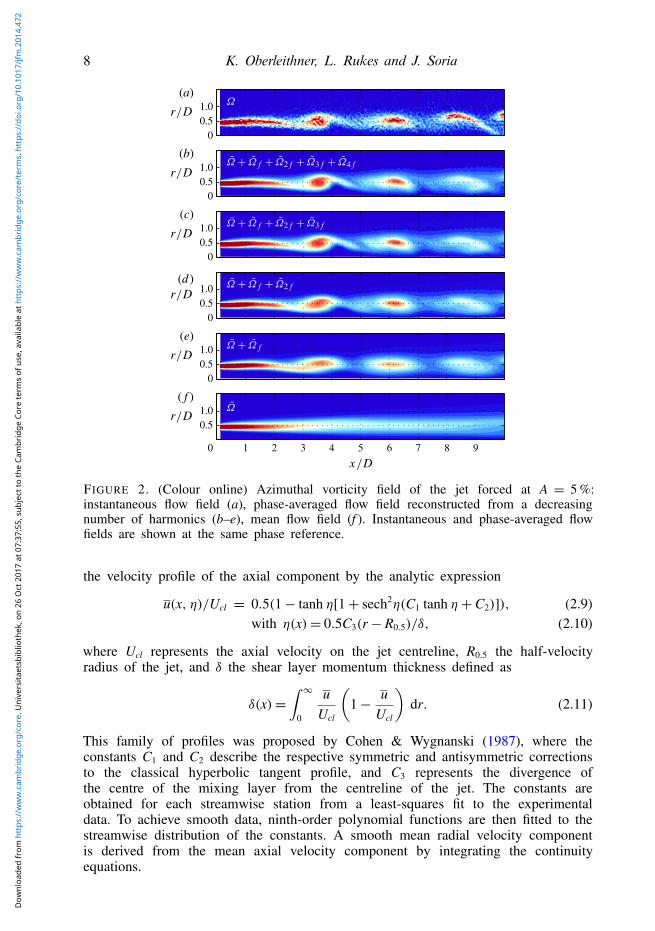
For demonstration purposes, figure 2 shows the reconstructed vorticity field for thejet forced at A = 5 %. The contours shown in figure 2(a) represent the azimuthalvorticity, Ω = ∂v/∂x− ∂u/∂r, of the instantaneous flow field obtained from a singlePIV snapshot. The streamwise growth of the excited instability is clearly visible fromthe instantaneous velocity field. The roll-up of the shear layer into a single vorticalstructure occurs at around x/D= 4 resulting in a strong agglomeration of vorticity thatsubsequently decays with downstream distance. The thin vortex sheet in between theregions of strong vorticity, sometimes referred to as the ‘braid’, is stretched during theroll-up process. Very similar structures are observed in the forced plane mixing layerreported by Weisbrot & Wygnanski (1988). The contours shown in the adjacent framesshow the same flow field reconstructed from a decreasing number of harmonics. It isapparent that the main oscillatory pattern is resolved by the fundamental frequencyoscillations (first two POD modes), while the finer details during the roll-up of theshear layer are resolved by the higher-order harmonics. It is worth noting that thebraid region is not resolved if the higher-order harmonics are neglected, although theyonly contribute to a fraction of the total kinetic energy.

2.4. Parametrization of the mean flowThe mean flow field is used as an input for the stability wave model. To avoidnumerical difficulties stemming from the use of non-smooth data, we approximate

Dow

nloa

ded

from

htt

ps://

ww

w.c

ambr

idge

.org

/cor

e. U

nive

rsita

etsb

iblio

thek

, on

26 O

ct 2

017

at 0

7:37

:55,

sub

ject

to th

e Ca

mbr

idge

Cor

e te

rms

of u

se, a

vaila

ble

at h

ttps

://w

ww

.cam

brid

ge.o

rg/c

ore/

term

s. h

ttps

://do

i.org

/10.

1017

/jfm

.201

4.47

2

8 K. Oberleithner, L. Rukes and J. Soria

( f )

(e)

(d )

(c)

(b)

(a)

1 2 3 4 5 6 7 8 90

0.51.0

00.51.0

00.51.0

00.51.0

00.51.0

00.51.0

FIGURE 2. (Colour online) Azimuthal vorticity field of the jet forced at A = 5 %:instantaneous flow field (a), phase-averaged flow field reconstructed from a decreasingnumber of harmonics (b–e), mean flow field (f ). Instantaneous and phase-averaged flowfields are shown at the same phase reference.

the velocity profile of the axial component by the analytic expression

u(x, η)/Ucl = 0.5(1− tanh η[1+ sech2η(C1 tanh η+C2)]), (2.9)with η(x)= 0.5C3(r− R0.5)/δ, (2.10)

where Ucl represents the axial velocity on the jet centreline, R0.5 the half-velocityradius of the jet, and δ the shear layer momentum thickness defined as

δ(x)=∫ ∞

0

uUcl

(1− u

Ucl

)dr. (2.11)

This family of profiles was proposed by Cohen & Wygnanski (1987), where theconstants C1 and C2 describe the respective symmetric and antisymmetric correctionsto the classical hyperbolic tangent profile, and C3 represents the divergence ofthe centre of the mixing layer from the centreline of the jet. The constants areobtained for each streamwise station from a least-squares fit to the experimentaldata. To achieve smooth data, ninth-order polynomial functions are then fitted to thestreamwise distribution of the constants. A smooth mean radial velocity componentis derived from the mean axial velocity component by integrating the continuityequations.

Dow

nloa

ded

from

htt

ps://

ww

w.c

ambr

idge

.org

/cor

e. U

nive

rsita

etsb

iblio

thek

, on

26 O

ct 2

017

at 0

7:37

:55,

sub

ject

to th

e Ca

mbr

idge

Cor

e te

rms

of u

se, a

vaila

ble

at h

ttps

://w

ww

.cam

brid

ge.o

rg/c

ore/

term

s. h

ttps

://do

i.org

/10.

1017

/jfm

.201

4.47

2

Mean flow stability analysis of oscillating jet experiments 9

3. Stability wave modelThis section outlines the theoretical framework employed for the stability wave

model. We first derive the equations that apply to infinitesimal perturbations travellingon a nonlinearly corrected mean flow and then formulate the solution ansatz for aweakly non-parallel axisymmetric jet flow. Note that two different order parametersare involved, one quantifying the perturbation amplitude and the other quantifyingthe non-parallelism of the mean flow.

3.1. Perturbation equations linearized around the mean flowWe start with the governing equations for an incompressible Newtonian fluid. Theseare the Navier–Stokes and continuity equations that are written in vector form as

∂u∂t+ u · ∇u = −∇p+ 1

Re∇2u (3.1a)

∇ · u = 0. (3.1b)

To analyse the linear stability of the steady state, the velocity and pressure field areexpressed as a sum of a steady and an infinitesimal perturbation field, yielding

u= ub + u′ and p= pb + p′, (3.2a,b)

where the base flow ub is by definition a steady solution of (3.1). The perturbationequations are obtained by substituting (3.2) into (3.1), subtracting the base flowequations, and neglecting the nonlinear term u′ · ∇u′, yielding

∂u′

∂t+ u′ · ∇ub + ub · ∇u′ = −∇p′ + 1

Re∇2u′ (3.3a)

∇ · u′ = 0. (3.3b)

This set of equations describes the initial departure of a linearly unstable flow fromits steady state before nonlinear saturation processes become active. To analyse thesaturated oscillating state, the velocity and pressure fields are decomposed into a time-averaged and a (finite-amplitude) periodic part, yielding

u= u+ u and p= p+ p. (3.4a,b)

Substituting this ansatz into the governing equations (3.1) and taking the time-averageleads to the governing equations for the mean flow, yielding

u · ∇u=−∇p+ 1Re∇2u+F (3.5a)

∇ · u= 0, (3.5b)

where the forcing term F(x)=−u · ∇u represents the Reynolds stress induced by theflow field oscillations. The mean flow is not a steady solution of (3.1), but it is asteady solution of the forced Navier–Stokes equations

∂u∂t+ u · ∇u=−∇p+ 1

Re∇2u+F∗ (3.6a)

∇ · u= 0. (3.6b)

Dow

nloa

ded

from

htt

ps://

ww

w.c

ambr

idge

.org

/cor

e. U

nive

rsita

etsb

iblio

thek

, on

26 O

ct 2

017

at 0

7:37

:55,

sub

ject

to th

e Ca

mbr

idge

Cor

e te

rms

of u

se, a

vaila

ble

at h

ttps

://w

ww

.cam

brid

ge.o

rg/c

ore/

term

s. h

ttps

://do

i.org

/10.

1017

/jfm

.201

4.47

2

10 K. Oberleithner, L. Rukes and J. Soria

To analyse the linear stability of the mean flow, the velocity and pressure fieldsare expressed as a sum of the mean flow solution and an infinitesimal perturbation,yielding

u= u+ u′ and p= p+ p′. (3.7a,b)

This ansatz is substituted into the forced Navier–Stokes equations (3.6) and subtractedfrom the mean flow equations (3.5). The forcing terms are assumed to be constantbetween the time-averaged and the perturbed state and cancel out. By neglecting thenonlinear terms −u′ · ∇u′, we obtain the perturbation equations for the mean flow

∂u′

∂t+ u′ · ∇u+ u · ∇u′ = −∇p′ + 1

Re∇2u′ (3.8a)

∇ · u′ = 0. (3.8b)

As noted by Barkley (2006), these equations only apply where the forcing term F∗ isconstant in time to leading order. Note that the modification of the mean flow stabilitythrough the coherent Reynolds stress (u · ∇u) is indirectly accounted for when solving(3.8), while any nonlinear mode–mode interaction is neglected (−u′ · ∇u′ = 0).

3.2. Solution for the slowly diverging jet

Equation (3.8) is first solved for a parallel flow u0 = (f (r), 0, 0)T. In describingthe saturated state, our interest lies in the spatial growth and decay of instabilities.Therefore, the perturbations have the form

u′(x, t)= u0(r)ei(αx+mθ−ωt) + c.c., (3.9)

with complex spatial wavenumber α= αr + iαi, integer real azimuthal wavenumber m,and real temporal oscillation frequency ω. The conjugate complex of the perturbationis indicated by ‘c.c.’. The imaginary part of α corresponds to the spatial growth rateof the parallel flow and determines whether a perturbation of a given m and ω grows(−αi> 0) or decays (−αi< 0) in the streamwise direction. Substituting the ansatz (3.9)and the equivalent for the pressure into (3.8) leads to the eigenvalue problem

D(ω)ψ0 = αE(ω)ψ0, (3.10)

with the eigenvalue α and the eigenfunction ψ0= (u0, v0, w0, p0)T, and the matrices D

and E containing the parallel flow profiles u0.The stability analysis is extended to weakly non-parallel flows by adopting the

correction scheme developed by Crighton & Gaster (1976). To account for the slowjet divergence, we introduce a slow axial scale X = εx, where ε 1, and a radialcomponent v1 = v/ε. The global perturbation field is given as

u′(X, r, θ, t; ε)=N(X)u0(X, r; ε) exp(

iε

∫ X

α(ξ)dξ + imθ − iωt)+ c.c., (3.11)

with the amplitude factor N(X) given as

dN(X)dX

G(X)+N(X)K(X)= 0. (3.12)

The parameter ε quantifies the streamwise spreading of the jet’s shear layer, withε ∼ dδ/dx. It is below 0.04 throughout this study in approximate agreement with the

Dow

nloa

ded

from

htt

ps://

ww

w.c

ambr

idge

.org

/cor

e. U

nive

rsita

etsb

iblio

thek

, on

26 O

ct 2

017

at 0

7:37

:55,

sub

ject

to th

e Ca

mbr

idge

Cor

e te

rms

of u

se, a

vaila

ble

at h

ttps

://w

ww

.cam

brid

ge.o

rg/c

ore/

term

s. h

ttps

://do

i.org

/10.

1017

/jfm

.201

4.47

2

Mean flow stability analysis of oscillating jet experiments 11

value of 0.03 reported by Crighton & Gaster (1976). The expressions G and K in(3.12) are derived from the solvability condition of the first-order problem, and theycontain the radial and streamwise derivatives of eigenfunctions and their adjoints ofthe (zero-order) parallel flow solution.

To obtain the global perturbation field u′ as given by (3.11), the eigenvalueproblem (3.10) is solved for each streamwise station separately using the fitted axialvelocity profile given by (2.9). The resulting ‘local’ eigenvalues α and eigenfunctionsψ0 and adjoints are stored on disk. The eigenfunctions are then renormalized toensure smooth gradients in the streamwise direction and the quantities G and K arecalculated. Note that the solution (3.11) is independent of the adopted normalizationof the eigenfunctions ψ0 as it is compensated by the amplitude factor N. The exactformulation of the eigenvalue problem, the derivations of G and K, and details to thenumerical scheme are given in appendix B.

The parameter ε in (3.11) is then formally dropped, and the overall shape of theinstability wave excited at the nozzle lip (x= 0) at a frequency f is given by

u′(x, t)=Re

uf e−i2πft, (3.13)

with the three-dimensional shape function

uf (x)= u0 exp(

i∫ x

0α(ξ) dξ + i

KG+ imθ

), (3.14)

where u0 and α represent the (zero-order) parallel flow solution and dependparametrically on x. In this study we focus on axisymmetric perturbations andset m= 0 throughout.

4. Impact of forcing on the stability wavesIn this section, we analyse the flow’s response to forcing over a wide range of

amplitudes. The correction of the mean flow and the change of the streamwise growthof the excited instability waves are monitored. The experimental findings are comparedto the stability wave model with the aim of detecting the potential limitations of thelinear mean flow analysis.

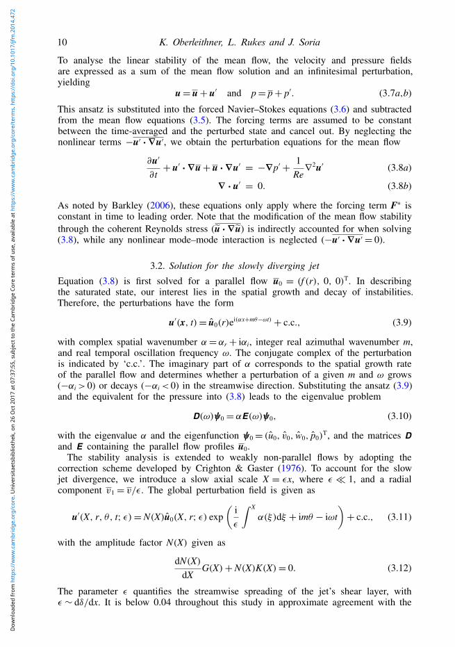
The jet is forced at amplitudes ranging from A = 0.1 to 100 %. The fundamentaloscillation of the flow field and its higher-order harmonics are derived from POD(see appendix A). The overall energy content of these oscillatory modes are shownin figure 3 as a percentage of the total fluctuating kinetic energy. Note that the x-and y-axes are in logarithmic scale indicating that the forcing amplitudes consideredas well as the flow oscillation energy vary over multiple orders of magnitude. HereA = 0.5 % is the lowest amplitude at which the POD-based approach reveals thefundamental wave with sufficient confidence. Increasing the amplitude to 4 % resultsin an increase of the relative energy content in the fundamental, which is simplycaused by an increase of the signal-to-noise ratio. The decay of the relative energycontent at higher amplitudes is attributed to the redistribution of the total kineticenergy from the fundamental to the higher-order harmonics. The first harmonic isdetectable for A> 2 %. Its energy content increases linearly with A, reaching 30 % ofthe total energy for A= 100 %. This is followed by higher-order harmonics increasingat the same rate but at lower levels. The successive appearance of higher-orderharmonics with increasing forcing amplitude reveals the strong nonlinearities that areinvolved in the saturation of the fundamental wave.

Dow

nloa

ded

from

htt

ps://

ww

w.c

ambr

idge

.org

/cor

e. U

nive

rsita

etsb

iblio

thek

, on

26 O

ct 2

017

at 0

7:37

:55,

sub

ject

to th

e Ca

mbr

idge

Cor

e te

rms

of u

se, a

vaila

ble

at h

ttps

://w

ww

.cam

brid

ge.o

rg/c

ore/

term

s. h

ttps

://do

i.org

/10.

1017

/jfm

.201

4.47

2

12 K. Oberleithner, L. Rukes and J. Soria

100 101 10210–1

100

101

102

A (%)

f

2f

3f

4f

5f

6f

K (

%)

FIGURE 3. Development of the energy contents of the fundamental and the higher-orderharmonics as the forcing amplitude is increased.

The streamwise growth of the excited instability wave is quantified by using thefollowing amplitude measure

A(x; uf )=√

2UjetD/2

(∫ ∞0|uf |2r dr

)1/2

. (4.1)

It corresponds to the amplitude of the axial velocity fluctuation at the fundamentalfrequency averaged across the shear layer. The corresponding complex shape functionuf can be derived from the measured phase-averaged axial velocity component (see(2.8)) and from the stability wave model (see (3.14)).

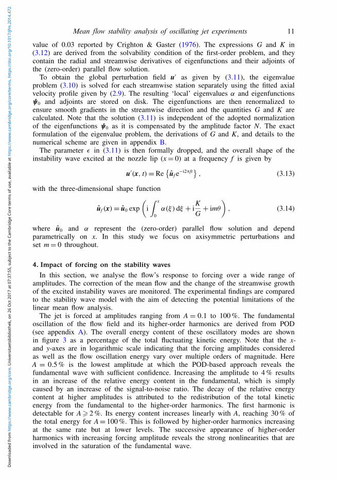
Figure 4(a) shows A derived from the measurements as a function of the forcingamplitude and streamwise location. Quantities are normalized with respect to theforcing amplitude A and represent the gain of the inlet perturbations. Note that they-axis is again shown in a logarithmic scale to magnify the low-amplitude forcingregime. Figure 4(b) shows contours of the corresponding momentum thickness δ,indicating the change of the mean flow with increasing forcing amplitude.

At very low forcing amplitudes, the amplification in the shear layer is strongand the oscillations are amplified by a factor of 15. Upon increasing the forcingamplitude, the gain in the shear layer decreases continuously and converges to alevel only slightly above 1 for A > 50 %. Simultaneously, the streamwise locationof maximum gain, indicated by a dashed line in figure 4(a), is shifted upstream tothe vicinity of the nozzle lip. Noting the logarithmic scale of the y-axis, this shiftincreases exponentially with A, demonstrating the high sensitivity of the growth ratesto changes in the forcing amplitude. Similarly, the downstream growth of the shearlayer is significantly enhanced with increasing forcing, as indicated by the increaseof δ shown in figure 4(b).

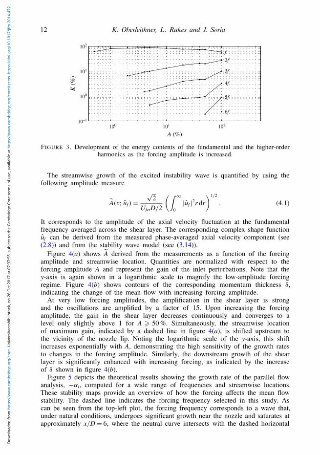
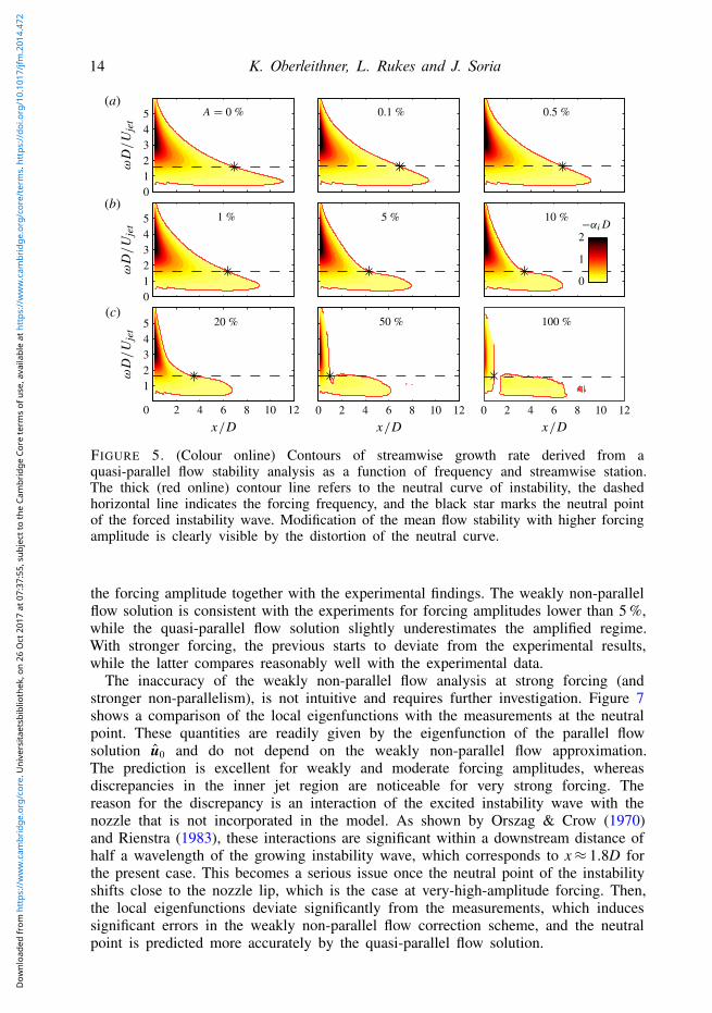
Figure 5 depicts the theoretical results showing the growth rate of the parallel flowanalysis, −αi, computed for a wide range of frequencies and streamwise locations.These stability maps provide an overview of how the forcing affects the mean flowstability. The dashed line indicates the forcing frequency selected in this study. Ascan be seen from the top-left plot, the forcing frequency corresponds to a wave that,under natural conditions, undergoes significant growth near the nozzle and saturates atapproximately x/D= 6, where the neutral curve intersects with the dashed horizontal

Dow

nloa

ded

from

htt

ps://

ww

w.c

ambr

idge

.org

/cor

e. U

nive

rsita

etsb

iblio

thek

, on

26 O

ct 2

017

at 0

7:37

:55,

sub

ject

to th

e Ca

mbr

idge

Cor

e te

rms

of u

se, a

vaila

ble

at h

ttps

://w

ww

.cam

brid

ge.o

rg/c

ore/

term

s. h

ttps

://do

i.org

/10.

1017

/jfm

.201

4.47

2

Mean flow stability analysis of oscillating jet experiments 13

(b)

(a)

A (

%)

A (

%)

0 1 2 3 4 5 6 7 8 9

0

0.1

0.2

5

10

15

0.5

1.0

2.0

5.0

20

50

100

0.5

1.0

2.0

5.0

20

50

100

FIGURE 4. (Colour online) (a) Coherent fundamental amplitude Af of the axial velocitycomponent normalized by the forcing amplitude A representing the gain of the incomingperturbations as a function of streamwise distance and forcing amplitude. The dashed linemarks the streamwise location of maximum gain. (b) Momentum thickness of the meanflow as a function of streamwise distance and forcing amplitude. All quantities are derivedfrom PIV measurements.

line. Waves at higher frequencies undergo stronger amplification near the nozzle, butsaturate at an earlier streamwise location, whereas the opposite applies for lowerfrequencies. At a downstream distance of x/D ≈ 11 all frequencies are damped,rendering the jet’s far-field stable to axisymmetric perturbations.

The weakest forcing considered (A = 0.1 %) is already sufficiently strong tonoticeably alter the stability map. The neutral point of the low-frequency wavesis shifted considerably upstream. Apparently, at such low forcing amplitudes, theexcited waves are still strong enough to alter the mean flow stability, although theyare not detected in the POD analysis.

Upon further increasing the forcing amplitude, the neutral curve is distortedsignificantly. The neutral point at the forcing frequency is shifted upstream until itreaches the proximity of the nozzle. The growth rates at the nozzle remain unaffectedover a wide range of forcing amplitudes, but ultimately decrease for the very strongforcing. The stability map for the jet forced at A> 50 % features two separate regionsof spatial growth. As discussed later, the amplification in the downstream region ofspatial amplification is not confirmed by the experiments and is not considered asphysical, rendering the strongly forced jet unstable in a very small streamwise extent.

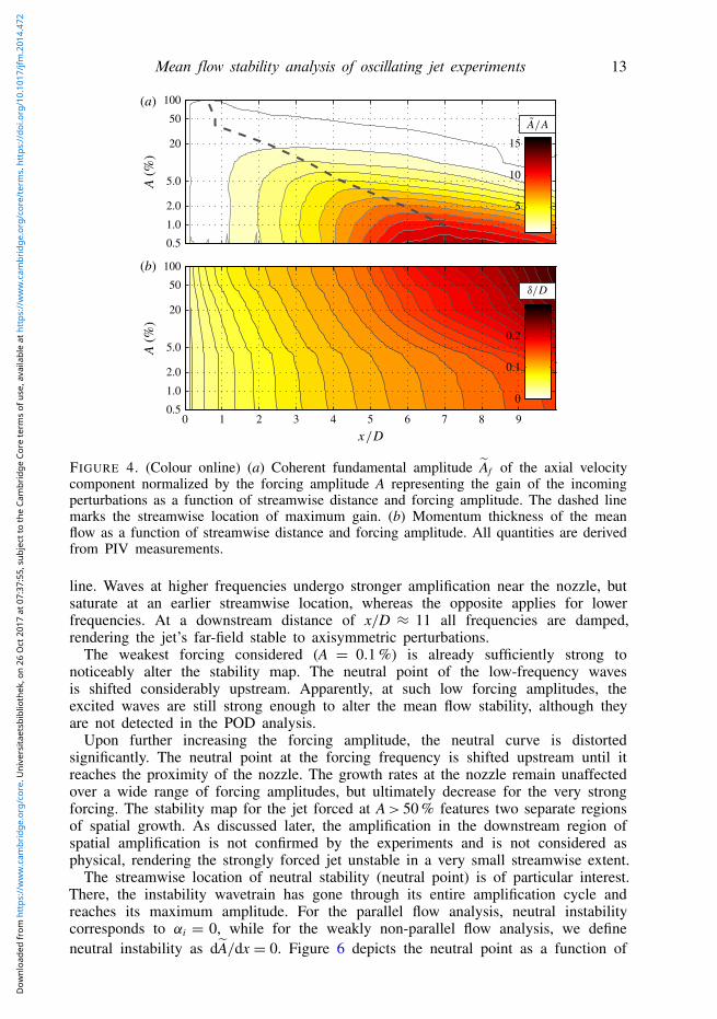
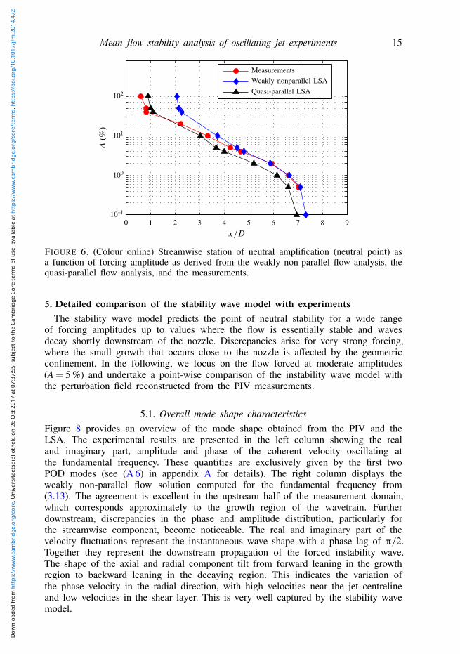
The streamwise location of neutral stability (neutral point) is of particular interest.There, the instability wavetrain has gone through its entire amplification cycle andreaches its maximum amplitude. For the parallel flow analysis, neutral instabilitycorresponds to αi = 0, while for the weakly non-parallel flow analysis, we defineneutral instability as dA/dx = 0. Figure 6 depicts the neutral point as a function of

Dow

nloa

ded

from

htt

ps://

ww

w.c

ambr

idge

.org

/cor

e. U

nive

rsita

etsb

iblio

thek

, on

26 O

ct 2

017

at 0

7:37

:55,

sub

ject

to th

e Ca

mbr

idge

Cor

e te

rms

of u

se, a

vaila

ble

at h

ttps

://w

ww

.cam

brid

ge.o

rg/c

ore/

term

s. h

ttps

://do

i.org

/10.

1017

/jfm

.201

4.47

2

14 K. Oberleithner, L. Rukes and J. Soria

100 %50 %20 %

10 %5 %1 %

0.5 %0.1 %

0 2 4 6 8 10 120 2 4 6 8 10 122 4 6 8 10 12

0

1

2

0

12345

012345

012345

(a)

(b)

(c)

0 %

FIGURE 5. (Colour online) Contours of streamwise growth rate derived from aquasi-parallel flow stability analysis as a function of frequency and streamwise station.The thick (red online) contour line refers to the neutral curve of instability, the dashedhorizontal line indicates the forcing frequency, and the black star marks the neutral pointof the forced instability wave. Modification of the mean flow stability with higher forcingamplitude is clearly visible by the distortion of the neutral curve.

the forcing amplitude together with the experimental findings. The weakly non-parallelflow solution is consistent with the experiments for forcing amplitudes lower than 5 %,while the quasi-parallel flow solution slightly underestimates the amplified regime.With stronger forcing, the previous starts to deviate from the experimental results,while the latter compares reasonably well with the experimental data.

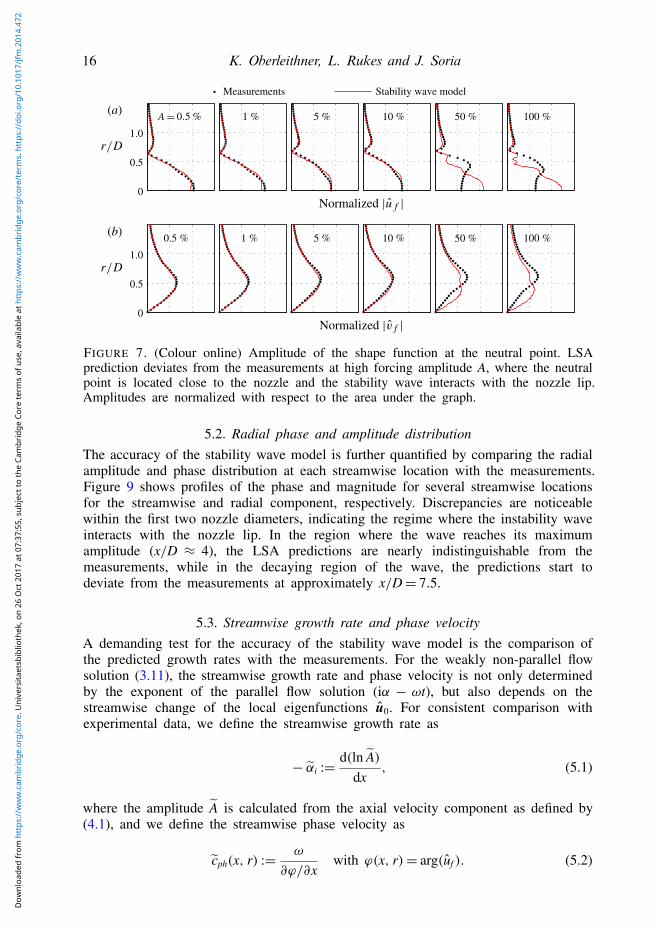
The inaccuracy of the weakly non-parallel flow analysis at strong forcing (andstronger non-parallelism), is not intuitive and requires further investigation. Figure 7shows a comparison of the local eigenfunctions with the measurements at the neutralpoint. These quantities are readily given by the eigenfunction of the parallel flowsolution u0 and do not depend on the weakly non-parallel flow approximation.The prediction is excellent for weakly and moderate forcing amplitudes, whereasdiscrepancies in the inner jet region are noticeable for very strong forcing. Thereason for the discrepancy is an interaction of the excited instability wave with thenozzle that is not incorporated in the model. As shown by Orszag & Crow (1970)and Rienstra (1983), these interactions are significant within a downstream distance ofhalf a wavelength of the growing instability wave, which corresponds to x≈ 1.8D forthe present case. This becomes a serious issue once the neutral point of the instabilityshifts close to the nozzle lip, which is the case at very-high-amplitude forcing. Then,the local eigenfunctions deviate significantly from the measurements, which inducessignificant errors in the weakly non-parallel flow correction scheme, and the neutralpoint is predicted more accurately by the quasi-parallel flow solution.

Dow

nloa

ded

from

htt

ps://

ww

w.c

ambr

idge

.org

/cor

e. U

nive

rsita

etsb

iblio

thek

, on

26 O

ct 2

017

at 0

7:37

:55,

sub

ject

to th

e Ca

mbr

idge

Cor

e te

rms

of u

se, a

vaila

ble

at h

ttps

://w

ww

.cam

brid

ge.o

rg/c

ore/

term

s. h

ttps

://do

i.org

/10.

1017

/jfm

.201

4.47

2

Mean flow stability analysis of oscillating jet experiments 15

Quasi-parallel LSA

Weakly nonparallel LSA

Measurements

A (

%)

0 1 2 3 4 5 6 7 8 910–1

100

101

102

FIGURE 6. (Colour online) Streamwise station of neutral amplification (neutral point) asa function of forcing amplitude as derived from the weakly non-parallel flow analysis, thequasi-parallel flow analysis, and the measurements.

5. Detailed comparison of the stability wave model with experiments

The stability wave model predicts the point of neutral stability for a wide rangeof forcing amplitudes up to values where the flow is essentially stable and wavesdecay shortly downstream of the nozzle. Discrepancies arise for very strong forcing,where the small growth that occurs close to the nozzle is affected by the geometricconfinement. In the following, we focus on the flow forced at moderate amplitudes(A= 5 %) and undertake a point-wise comparison of the instability wave model withthe perturbation field reconstructed from the PIV measurements.

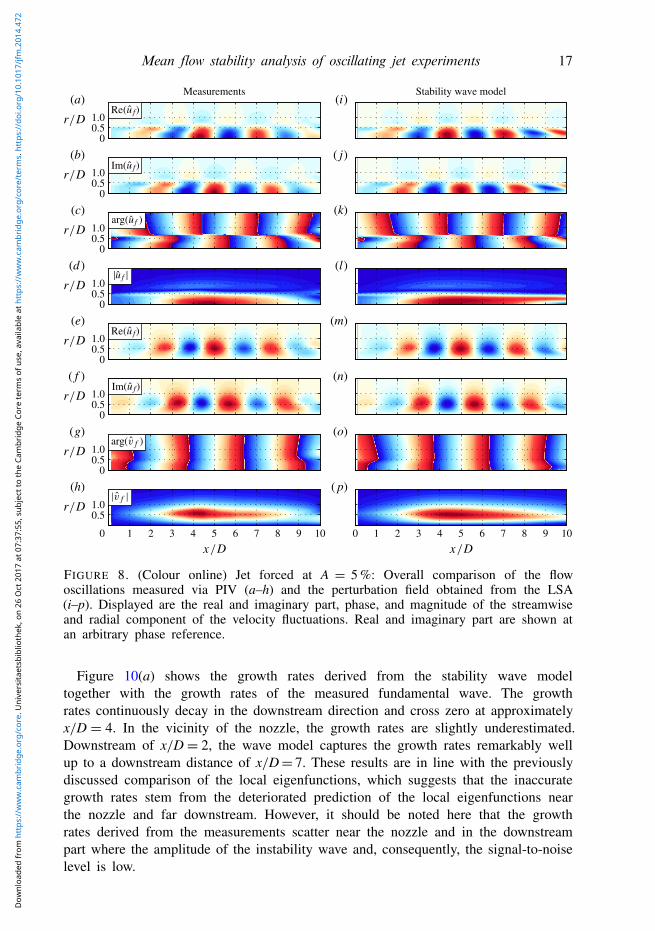
5.1. Overall mode shape characteristicsFigure 8 provides an overview of the mode shape obtained from the PIV and theLSA. The experimental results are presented in the left column showing the realand imaginary part, amplitude and phase of the coherent velocity oscillating atthe fundamental frequency. These quantities are exclusively given by the first twoPOD modes (see (A 6) in appendix A for details). The right column displays theweakly non-parallel flow solution computed for the fundamental frequency from(3.13). The agreement is excellent in the upstream half of the measurement domain,which corresponds approximately to the growth region of the wavetrain. Furtherdownstream, discrepancies in the phase and amplitude distribution, particularly forthe streamwise component, become noticeable. The real and imaginary part of thevelocity fluctuations represent the instantaneous wave shape with a phase lag of π/2.Together they represent the downstream propagation of the forced instability wave.The shape of the axial and radial component tilt from forward leaning in the growthregion to backward leaning in the decaying region. This indicates the variation ofthe phase velocity in the radial direction, with high velocities near the jet centrelineand low velocities in the shear layer. This is very well captured by the stability wavemodel.

Dow

nloa

ded

from

htt

ps://

ww

w.c

ambr

idge

.org

/cor

e. U

nive

rsita

etsb

iblio

thek

, on

26 O

ct 2

017

at 0

7:37

:55,

sub

ject

to th

e Ca

mbr

idge

Cor

e te

rms

of u

se, a

vaila

ble

at h

ttps

://w

ww

.cam

brid

ge.o

rg/c

ore/

term

s. h

ttps

://do

i.org

/10.

1017

/jfm

.201

4.47

2

16 K. Oberleithner, L. Rukes and J. Soria

Stability wave modelMeasurements

100 %50 %10 %5 %1 %0.5 %

100 %50 %10 %5 %1 %

0

0.5

1.0

0

0.5

1.0

(a)

(b)

FIGURE 7. (Colour online) Amplitude of the shape function at the neutral point. LSAprediction deviates from the measurements at high forcing amplitude A, where the neutralpoint is located close to the nozzle and the stability wave interacts with the nozzle lip.Amplitudes are normalized with respect to the area under the graph.

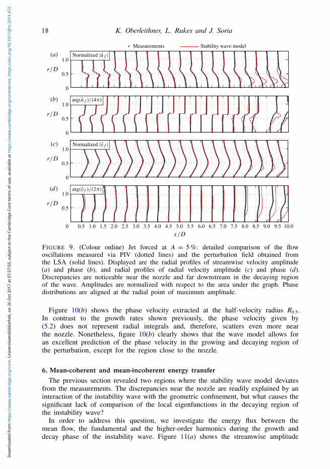
5.2. Radial phase and amplitude distributionThe accuracy of the stability wave model is further quantified by comparing the radialamplitude and phase distribution at each streamwise location with the measurements.Figure 9 shows profiles of the phase and magnitude for several streamwise locationsfor the streamwise and radial component, respectively. Discrepancies are noticeablewithin the first two nozzle diameters, indicating the regime where the instability waveinteracts with the nozzle lip. In the region where the wave reaches its maximumamplitude (x/D ≈ 4), the LSA predictions are nearly indistinguishable from themeasurements, while in the decaying region of the wave, the predictions start todeviate from the measurements at approximately x/D= 7.5.

5.3. Streamwise growth rate and phase velocityA demanding test for the accuracy of the stability wave model is the comparison ofthe predicted growth rates with the measurements. For the weakly non-parallel flowsolution (3.11), the streamwise growth rate and phase velocity is not only determinedby the exponent of the parallel flow solution (iα − ωt), but also depends on thestreamwise change of the local eigenfunctions u0. For consistent comparison withexperimental data, we define the streamwise growth rate as

− αi := d(ln A)dx

, (5.1)

where the amplitude A is calculated from the axial velocity component as defined by(4.1), and we define the streamwise phase velocity as

cph(x, r) := ω

∂ϕ/∂xwith ϕ(x, r)= arg(uf ). (5.2)

Dow

nloa

ded

from

htt

ps://

ww

w.c

ambr

idge

.org

/cor

e. U

nive

rsita

etsb

iblio

thek

, on

26 O

ct 2

017

at 0

7:37

:55,

sub

ject

to th

e Ca

mbr

idge

Cor

e te

rms

of u

se, a

vaila

ble

at h

ttps

://w

ww

.cam

brid

ge.o

rg/c

ore/

term

s. h

ttps

://do

i.org

/10.

1017

/jfm

.201

4.47

2

Mean flow stability analysis of oscillating jet experiments 17

Stability wave modelMeasurements

0 1 2 3 4 5 6 7 8 9 101 2 3 4 5 6 7 8 9 10

00.51.0

(a)

00.51.0

(b)

00.51.0

(c)

00.51.0

(d )

00.51.0

(e)

00.51.0

( f )

00.51.0

(g)

0

0.51.0

(h)

(i)

( j)

(k)

(l)

(m)

(n)

(o)

( p)

Re

Im

Re

Im

FIGURE 8. (Colour online) Jet forced at A = 5 %: Overall comparison of the flowoscillations measured via PIV (a–h) and the perturbation field obtained from the LSA(i–p). Displayed are the real and imaginary part, phase, and magnitude of the streamwiseand radial component of the velocity fluctuations. Real and imaginary part are shown atan arbitrary phase reference.

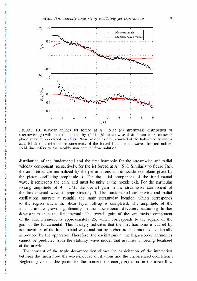
Figure 10(a) shows the growth rates derived from the stability wave modeltogether with the growth rates of the measured fundamental wave. The growthrates continuously decay in the downstream direction and cross zero at approximatelyx/D = 4. In the vicinity of the nozzle, the growth rates are slightly underestimated.Downstream of x/D= 2, the wave model captures the growth rates remarkably wellup to a downstream distance of x/D= 7. These results are in line with the previouslydiscussed comparison of the local eigenfunctions, which suggests that the inaccurategrowth rates stem from the deteriorated prediction of the local eigenfunctions nearthe nozzle and far downstream. However, it should be noted here that the growthrates derived from the measurements scatter near the nozzle and in the downstreampart where the amplitude of the instability wave and, consequently, the signal-to-noiselevel is low.

Dow

nloa

ded

from

htt

ps://

ww

w.c

ambr

idge

.org

/cor

e. U

nive

rsita

etsb

iblio

thek

, on

26 O

ct 2

017

at 0

7:37

:55,

sub

ject

to th

e Ca

mbr

idge

Cor

e te

rms

of u

se, a

vaila

ble

at h

ttps

://w

ww

.cam

brid

ge.o

rg/c

ore/

term

s. h

ttps

://do

i.org

/10.

1017

/jfm

.201

4.47

2

18 K. Oberleithner, L. Rukes and J. Soria

Stability wave modelMeasurements

0.5 1.0 1.5 2.0 2.5 3.0 3.5 4.0 4.5 5.0 5.5 6.0 6.5 7.0 7.5 8.0 8.5 9.0 9.5 10.00

0.5

1.0(d )

0

0.5

1.0(a)

0

0.5

1.0(b)

0

0.5

1.0(c)

FIGURE 9. (Colour online) Jet forced at A = 5 %: detailed comparison of the flowoscillations measured via PIV (dotted lines) and the perturbation field obtained fromthe LSA (solid lines). Displayed are the radial profiles of streamwise velocity amplitude(a) and phase (b), and radial profiles of radial velocity amplitude (c) and phase (d).Discrepancies are noticeable near the nozzle and far downstream in the decaying regionof the wave. Amplitudes are normalized with respect to the area under the graph. Phasedistributions are aligned at the radial point of maximum amplitude.

Figure 10(b) shows the phase velocity extracted at the half-velocity radius R0.5.In contrast to the growth rates shown previously, the phase velocity given by(5.2) does not represent radial integrals and, therefore, scatters even more nearthe nozzle. Nonetheless, figure 10(b) clearly shows that the wave model allows foran excellent prediction of the phase velocity in the growing and decaying region ofthe perturbation, except for the region close to the nozzle.

6. Mean-coherent and mean-incoherent energy transferThe previous section revealed two regions where the stability wave model deviates

from the measurements. The discrepancies near the nozzle are readily explained by aninteraction of the instability wave with the geometric confinement, but what causes thesignificant lack of comparison of the local eigenfunctions in the decaying region ofthe instability wave?

In order to address this question, we investigate the energy flux between themean flow, the fundamental and the higher-order harmonics during the growth anddecay phase of the instability wave. Figure 11(a) shows the streamwise amplitude

Dow

nloa

ded

from

htt

ps://

ww

w.c

ambr

idge

.org

/cor

e. U

nive

rsita

etsb

iblio

thek

, on

26 O

ct 2

017

at 0

7:37

:55,

sub

ject

to th

e Ca

mbr

idge

Cor

e te

rms

of u

se, a

vaila

ble

at h

ttps

://w

ww

.cam

brid

ge.o

rg/c

ore/

term

s. h

ttps

://do

i.org

/10.

1017

/jfm

.201

4.47

2

Mean flow stability analysis of oscillating jet experiments 19

Stability wave model

Measurements(a)

(b)

0 1 2 3 4 5 6 7 8 9

0.4

0.6

0.8

1.0

1.2

−0.5

0

0.5

1.0

FIGURE 10. (Colour online) Jet forced at A = 5 %: (a) streamwise distribution ofstreamwise growth rate as defined by (5.1); (b) streamwise distribution of streamwisephase velocity as defined by (5.2). Phase velocities are extracted at the half-velocity radiusR0.5. Black dots refer to measurements of the forced fundamental wave, the (red online)solid line refers to the weakly non-parallel flow solution.

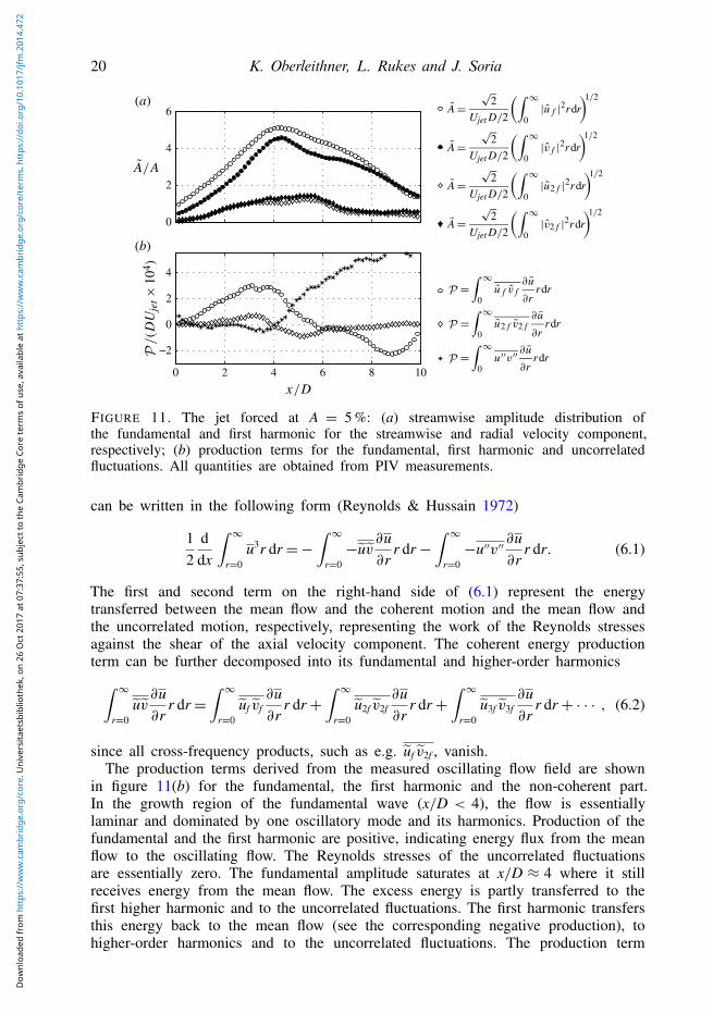
distribution of the fundamental and the first harmonic for the streamwise and radialvelocity component, respectively, for the jet forced at A= 5 %. Similarly to figure 7(a),the amplitudes are normalized by the perturbations at the nozzle exit plane given bythe piston oscillating amplitude A. For the axial component of the fundamentalwave, it represents the gain, and must be unity at the nozzle exit. For the particularforcing amplitude of A = 5 %, the overall gain in the streamwise component ofthe fundamental wave is approximately 5. The fundamental streamwise and radialoscillations saturate at roughly the same streamwise location, which correspondsto the region where the shear layer roll-up is completed. The amplitude of thefirst harmonic grows significantly in the downstream direction, saturating furtherdownstream than the fundamental. The overall gain of the streamwise componentof the first harmonic is approximately 25, which corresponds to the square of thegain of the fundamental. This strongly indicates that the first harmonic is caused bynonlinearities of the fundamental wave and not by higher-order harmonics accidentallyintroduced by the apparatus. Therefore, the oscillations at the higher-order harmonicscannot be predicted from the stability wave model that assumes a forcing localizedat the nozzle.

The concept of the triple decomposition allows the exploitation of the interactionbetween the mean flow, the wave-induced oscillations and the uncorrelated oscillations.Neglecting viscous dissipation for the moment, the energy equation for the mean flow

Dow

nloa

ded

from

htt

ps://

ww

w.c

ambr

idge

.org

/cor

e. U

nive

rsita

etsb

iblio

thek

, on

26 O

ct 2

017

at 0

7:37

:55,

sub

ject

to th

e Ca

mbr

idge

Cor

e te

rms

of u

se, a

vaila

ble

at h

ttps

://w

ww

.cam

brid

ge.o

rg/c

ore/

term

s. h

ttps

://do

i.org

/10.

1017

/jfm

.201

4.47

2

20 K. Oberleithner, L. Rukes and J. Soria

(a)

0

2

4

6

(b)

0 2 4 6 8 10

−2

0

2

4

FIGURE 11. The jet forced at A = 5 %: (a) streamwise amplitude distribution ofthe fundamental and first harmonic for the streamwise and radial velocity component,respectively; (b) production terms for the fundamental, first harmonic and uncorrelatedfluctuations. All quantities are obtained from PIV measurements.

can be written in the following form (Reynolds & Hussain 1972)

12

ddx

∫ ∞r=0

u3r dr=−∫ ∞

r=0−uv

∂u∂r

r dr−∫ ∞

r=0−u′′v′′

∂u∂r

r dr. (6.1)

The first and second term on the right-hand side of (6.1) represent the energytransferred between the mean flow and the coherent motion and the mean flow andthe uncorrelated motion, respectively, representing the work of the Reynolds stressesagainst the shear of the axial velocity component. The coherent energy productionterm can be further decomposed into its fundamental and higher-order harmonics∫ ∞

r=0uv∂u∂r

r dr=∫ ∞

r=0uf vf

∂u∂r

r dr+∫ ∞

r=0u2f v2f

∂u∂r

r dr+∫ ∞

r=0u3f v3f

∂u∂r

r dr+ · · · , (6.2)

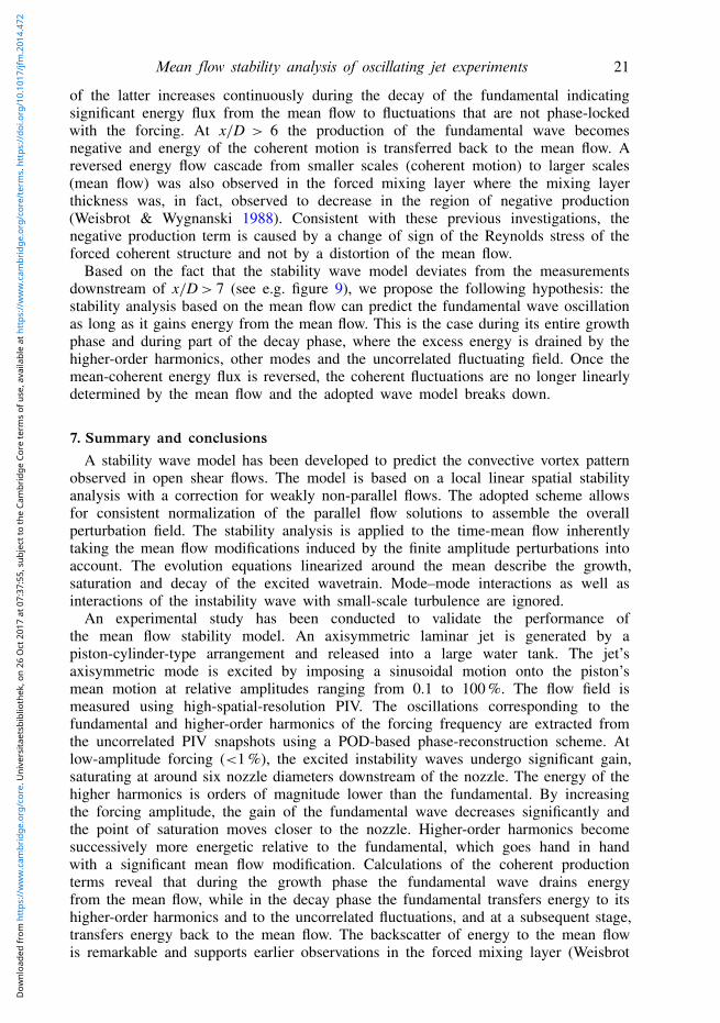
since all cross-frequency products, such as e.g. uf v2f , vanish.The production terms derived from the measured oscillating flow field are shown

in figure 11(b) for the fundamental, the first harmonic and the non-coherent part.In the growth region of the fundamental wave (x/D < 4), the flow is essentiallylaminar and dominated by one oscillatory mode and its harmonics. Production of thefundamental and the first harmonic are positive, indicating energy flux from the meanflow to the oscillating flow. The Reynolds stresses of the uncorrelated fluctuationsare essentially zero. The fundamental amplitude saturates at x/D ≈ 4 where it stillreceives energy from the mean flow. The excess energy is partly transferred to thefirst higher harmonic and to the uncorrelated fluctuations. The first harmonic transfersthis energy back to the mean flow (see the corresponding negative production), tohigher-order harmonics and to the uncorrelated fluctuations. The production term

Dow

nloa

ded

from

htt

ps://

ww

w.c

ambr

idge

.org

/cor

e. U

nive

rsita

etsb

iblio

thek

, on

26 O

ct 2

017

at 0

7:37

:55,

sub

ject

to th

e Ca

mbr

idge

Cor

e te

rms

of u

se, a

vaila

ble

at h

ttps

://w

ww

.cam

brid

ge.o

rg/c

ore/

term

s. h

ttps

://do

i.org

/10.

1017

/jfm

.201

4.47

2

Mean flow stability analysis of oscillating jet experiments 21

of the latter increases continuously during the decay of the fundamental indicatingsignificant energy flux from the mean flow to fluctuations that are not phase-lockedwith the forcing. At x/D > 6 the production of the fundamental wave becomesnegative and energy of the coherent motion is transferred back to the mean flow. Areversed energy flow cascade from smaller scales (coherent motion) to larger scales(mean flow) was also observed in the forced mixing layer where the mixing layerthickness was, in fact, observed to decrease in the region of negative production(Weisbrot & Wygnanski 1988). Consistent with these previous investigations, thenegative production term is caused by a change of sign of the Reynolds stress of theforced coherent structure and not by a distortion of the mean flow.

Based on the fact that the stability wave model deviates from the measurementsdownstream of x/D> 7 (see e.g. figure 9), we propose the following hypothesis: thestability analysis based on the mean flow can predict the fundamental wave oscillationas long as it gains energy from the mean flow. This is the case during its entire growthphase and during part of the decay phase, where the excess energy is drained by thehigher-order harmonics, other modes and the uncorrelated fluctuating field. Once themean-coherent energy flux is reversed, the coherent fluctuations are no longer linearlydetermined by the mean flow and the adopted wave model breaks down.

7. Summary and conclusions

A stability wave model has been developed to predict the convective vortex patternobserved in open shear flows. The model is based on a local linear spatial stabilityanalysis with a correction for weakly non-parallel flows. The adopted scheme allowsfor consistent normalization of the parallel flow solutions to assemble the overallperturbation field. The stability analysis is applied to the time-mean flow inherentlytaking the mean flow modifications induced by the finite amplitude perturbations intoaccount. The evolution equations linearized around the mean describe the growth,saturation and decay of the excited wavetrain. Mode–mode interactions as well asinteractions of the instability wave with small-scale turbulence are ignored.

An experimental study has been conducted to validate the performance ofthe mean flow stability model. An axisymmetric laminar jet is generated by apiston-cylinder-type arrangement and released into a large water tank. The jet’saxisymmetric mode is excited by imposing a sinusoidal motion onto the piston’smean motion at relative amplitudes ranging from 0.1 to 100 %. The flow field ismeasured using high-spatial-resolution PIV. The oscillations corresponding to thefundamental and higher-order harmonics of the forcing frequency are extracted fromthe uncorrelated PIV snapshots using a POD-based phase-reconstruction scheme. Atlow-amplitude forcing (<1 %), the excited instability waves undergo significant gain,saturating at around six nozzle diameters downstream of the nozzle. The energy of thehigher harmonics is orders of magnitude lower than the fundamental. By increasingthe forcing amplitude, the gain of the fundamental wave decreases significantly andthe point of saturation moves closer to the nozzle. Higher-order harmonics becomesuccessively more energetic relative to the fundamental, which goes hand in handwith a significant mean flow modification. Calculations of the coherent productionterms reveal that during the growth phase the fundamental wave drains energyfrom the mean flow, while in the decay phase the fundamental transfers energy to itshigher-order harmonics and to the uncorrelated fluctuations, and at a subsequent stage,transfers energy back to the mean flow. The backscatter of energy to the mean flowis remarkable and supports earlier observations in the forced mixing layer (Weisbrot

Dow

nloa

ded

from

htt

ps://

ww

w.c

ambr

idge

.org

/cor

e. U

nive

rsita

etsb

iblio

thek

, on

26 O

ct 2

017

at 0

7:37

:55,

sub

ject

to th

e Ca

mbr

idge

Cor

e te

rms

of u

se, a

vaila

ble

at h

ttps

://w

ww

.cam

brid

ge.o

rg/c

ore/

term

s. h

ttps

://do

i.org

/10.

1017

/jfm

.201

4.47

2

22 K. Oberleithner, L. Rukes and J. Soria

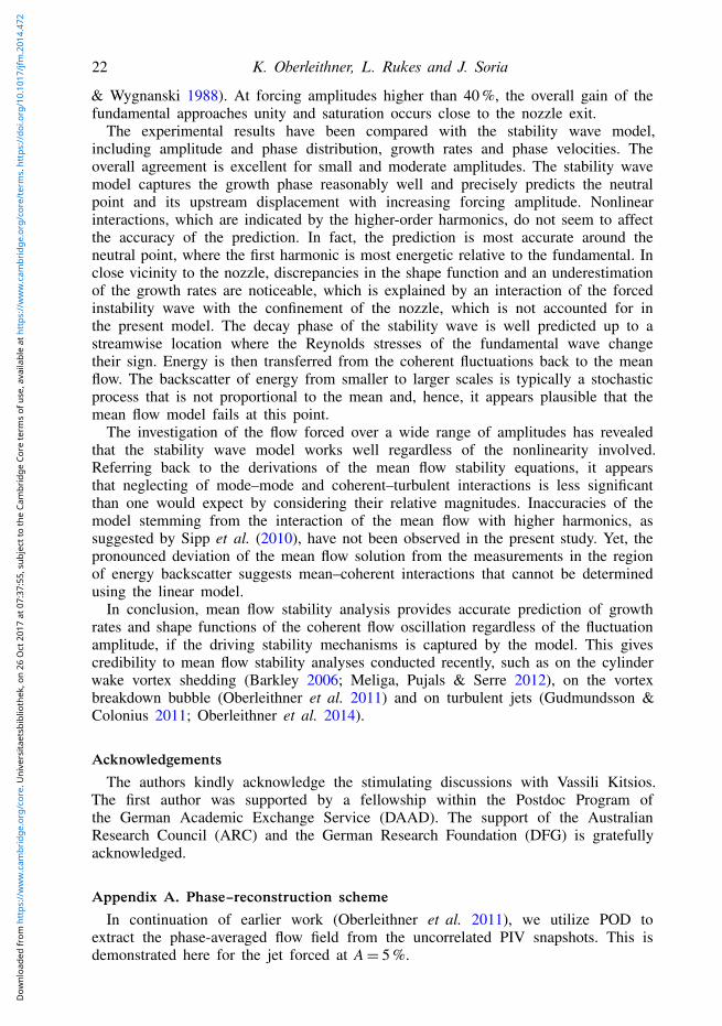
& Wygnanski 1988). At forcing amplitudes higher than 40 %, the overall gain of thefundamental approaches unity and saturation occurs close to the nozzle exit.

The experimental results have been compared with the stability wave model,including amplitude and phase distribution, growth rates and phase velocities. Theoverall agreement is excellent for small and moderate amplitudes. The stability wavemodel captures the growth phase reasonably well and precisely predicts the neutralpoint and its upstream displacement with increasing forcing amplitude. Nonlinearinteractions, which are indicated by the higher-order harmonics, do not seem to affectthe accuracy of the prediction. In fact, the prediction is most accurate around theneutral point, where the first harmonic is most energetic relative to the fundamental. Inclose vicinity to the nozzle, discrepancies in the shape function and an underestimationof the growth rates are noticeable, which is explained by an interaction of the forcedinstability wave with the confinement of the nozzle, which is not accounted for inthe present model. The decay phase of the stability wave is well predicted up to astreamwise location where the Reynolds stresses of the fundamental wave changetheir sign. Energy is then transferred from the coherent fluctuations back to the meanflow. The backscatter of energy from smaller to larger scales is typically a stochasticprocess that is not proportional to the mean and, hence, it appears plausible that themean flow model fails at this point.

The investigation of the flow forced over a wide range of amplitudes has revealedthat the stability wave model works well regardless of the nonlinearity involved.Referring back to the derivations of the mean flow stability equations, it appearsthat neglecting of mode–mode and coherent–turbulent interactions is less significantthan one would expect by considering their relative magnitudes. Inaccuracies of themodel stemming from the interaction of the mean flow with higher harmonics, assuggested by Sipp et al. (2010), have not been observed in the present study. Yet, thepronounced deviation of the mean flow solution from the measurements in the regionof energy backscatter suggests mean–coherent interactions that cannot be determinedusing the linear model.

In conclusion, mean flow stability analysis provides accurate prediction of growthrates and shape functions of the coherent flow oscillation regardless of the fluctuationamplitude, if the driving stability mechanisms is captured by the model. This givescredibility to mean flow stability analyses conducted recently, such as on the cylinderwake vortex shedding (Barkley 2006; Meliga, Pujals & Serre 2012), on the vortexbreakdown bubble (Oberleithner et al. 2011) and on turbulent jets (Gudmundsson &Colonius 2011; Oberleithner et al. 2014).

Acknowledgements

The authors kindly acknowledge the stimulating discussions with Vassili Kitsios.The first author was supported by a fellowship within the Postdoc Program ofthe German Academic Exchange Service (DAAD). The support of the AustralianResearch Council (ARC) and the German Research Foundation (DFG) is gratefullyacknowledged.

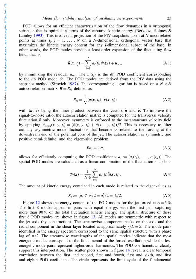
Appendix A. Phase–reconstruction scheme

In continuation of earlier work (Oberleithner et al. 2011), we utilize POD toextract the phase-averaged flow field from the uncorrelated PIV snapshots. This isdemonstrated here for the jet forced at A= 5 %.

Dow

nloa

ded

from

htt

ps://

ww

w.c

ambr

idge

.org

/cor

e. U

nive

rsita

etsb

iblio

thek

, on

26 O

ct 2

017

at 0

7:37

:55,

sub

ject

to th

e Ca

mbr

idge

Cor

e te

rms

of u

se, a

vaila

ble

at h

ttps

://w

ww

.cam

brid

ge.o

rg/c

ore/

term

s. h

ttps

://do

i.org

/10.

1017

/jfm

.201

4.47

2

Mean flow stability analysis of oscillating jet experiments 23

POD allows for an efficient characterization of the flow dynamics in a orthogonalsubspace that is optimal in terms of the captured kinetic energy (Berkooz, Holmes &Lumley 1993). This involves a projection of the PIV snapshots taken at N uncorrelatedpoints at times tj, j = 1, . . . , N on a N-dimensional orthogonal vector base thatmaximizes the kinetic energy content for any I-dimensional subset of the base. Inother words, the POD modes provide a least-order expansion of the fluctuating flowfield, that is

u(x, tj)=I∑

i=1

ai(tj)Φi(x)+ ures, (A 1)

by minimizing the residual ures. The ai(tj) is the ith POD coefficient correspondingto the ith POD mode Φi. The POD modes are derived from the PIV data using thesnapshot method (Sirovich 1987). The corresponding algorithm is based on a N × Nautocorrelation matrix R = Rkl defined as

Rkl = 1N〈u(x, tk), v(x, tl)〉 (A 2)

with 〈u, v〉 being the inner product between the vectors u and v. To improve thesignal-to-noise ratio, the autocorrelation matrix is computed for the transversal velocityfluctuation v only. Moreover, symmetry is enforced to the instantaneous velocity fieldby applying vsymm(x, y, tj) = (v(x, y, tj) + v(x, −y, tj))/2. This is necessary to filterout any asymmetric mode fluctuations that become correlated to the forcing at thedownstream end of the potential core of the jet. The autocorrelation is symmetric andpositive semi-definite, and the eigenvalue problem

Rai = λiai (A 3)

allows for efficiently computing the POD coefficients ai := [ai(t1), . . . , ai(tN)]. Thespatial POD modes are calculated as a linear combination of the fluctuation snapshots

Φi(x)= 1Nλi

N∑j=1

ai(tj)u(x, tj). (A 4)

The amount of kinetic energy contained in each mode is related to the eigenvalues as

Ki := 〈u, Φi〉2/2= a2i /2= λi/2. (A 5)

Figure 12 shows the energy content of the POD modes for the jet forced at A= 5 %.The first 8 modes appear in pairs with equal energy, with the first pair capturingmore than 90 % of the total fluctuation kinetic energy. The spatial structure of thesefirst 8 POD modes are shown in figure 13. All modes are symmetric with respect tothe jet axis (by construction). The streamwise component peaks on the axis and theradial component in the shear layer located at approximately r/D= 5. The mode pairsidentified in the energy spectrum correspond to the same spatial structure with a phaselag of π/2. The streamwise wavelengths of the spatial modes indicate that the mostenergetic modes correspond to the fundamental of the forced oscillation while the lessenergetic mode pairs represent higher-order harmonics. The POD coefficients ai clearlysupport this interpretation. The scatter plots shown in figure 14 reveal a clear temporalcorrelation between the first and second, first and fourth, first and sixth, and firstand eighth POD coefficient. The circle represents the limit cycle of the fundamental

Dow

nloa

ded

from

htt

ps://

ww

w.c

ambr

idge

.org

/cor

e. U

nive

rsita

etsb

iblio

thek

, on

26 O

ct 2

017

at 0

7:37

:55,

sub

ject

to th

e Ca

mbr

idge

Cor

e te

rms

of u

se, a

vaila

ble

at h

ttps

://w

ww

.cam

brid

ge.o

rg/c

ore/

term

s. h

ttps

://do

i.org

/10.

1017

/jfm

.201

4.47

2

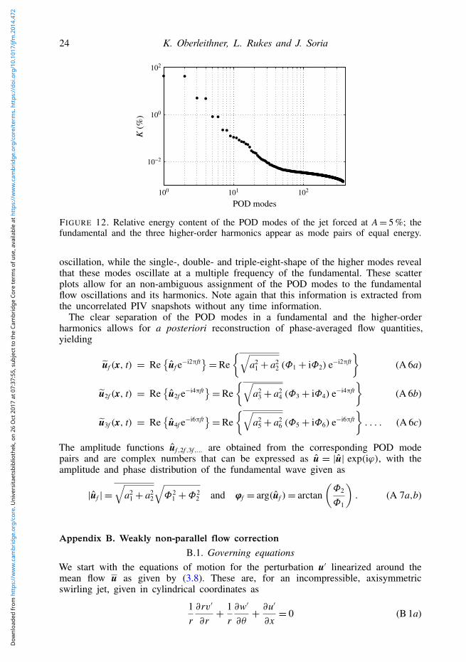
24 K. Oberleithner, L. Rukes and J. Soria

K (

%)

POD modes100 101 102

10−2

100

102

FIGURE 12. Relative energy content of the POD modes of the jet forced at A= 5 %; thefundamental and the three higher-order harmonics appear as mode pairs of equal energy.

oscillation, while the single-, double- and triple-eight-shape of the higher modes revealthat these modes oscillate at a multiple frequency of the fundamental. These scatterplots allow for an non-ambiguous assignment of the POD modes to the fundamentalflow oscillations and its harmonics. Note again that this information is extracted fromthe uncorrelated PIV snapshots without any time information.

The clear separation of the POD modes in a fundamental and the higher-orderharmonics allows for a posteriori reconstruction of phase-averaged flow quantities,yielding

uf (x, t) = Re

uf e−i2πft=Re

√a2

1 + a22 (Φ1 + iΦ2) e−i2πft

(A 6a)

u2f (x, t) = Re

u2f e−i4πft=Re

√a2

3 + a24 (Φ3 + iΦ4) e−i4πft

(A 6b)

u3f (x, t) = Re

u4f e−i6πft=Re

√a2

5 + a26 (Φ5 + iΦ6) e−i6πft

. . . . (A 6c)

The amplitude functions uf ,2f ,3f ,... are obtained from the corresponding POD modepairs and are complex numbers that can be expressed as u = |u| exp(iϕ), with theamplitude and phase distribution of the fundamental wave given as

|uf | =√

a21 + a2

2

√Φ2

1 +Φ22 and ϕf = arg(uf )= arctan

(Φ2

Φ1

). (A 7a,b)

Appendix B. Weakly non-parallel flow correctionB.1. Governing equations

We start with the equations of motion for the perturbation u′ linearized around themean flow u as given by (3.8). These are, for an incompressible, axisymmetricswirling jet, given in cylindrical coordinates as

1r∂rv′

∂r+ 1

r∂w′

∂θ+ ∂u′

∂x= 0 (B 1a)

Dow

nloa

ded

from

htt

ps://

ww

w.c

ambr

idge

.org

/cor

e. U

nive

rsita

etsb

iblio

thek

, on

26 O

ct 2

017

at 0

7:37

:55,

sub

ject

to th

e Ca

mbr

idge

Cor

e te

rms

of u

se, a

vaila

ble

at h

ttps

://w

ww

.cam

brid

ge.o

rg/c

ore/

term

s. h

ttps

://do

i.org

/10.

1017

/jfm

.201

4.47

2

Mean flow stability analysis of oscillating jet experiments 25

0 1 2 3 4 5 6 7 8 91 2 3 4 5 6 7 8 90

1

0

1(a)

0

1

0

1

0

1

0

1

0

1

0

1

(b)

FIGURE 13. (Colour online) POD modes of the jet forced at A = 5 %: spatial structureof the first (top) to the eighth (bottom) POD mode indicating the fundamental and higher-order harmonics. (a) Streamwise and (b) radial components are shown.

a2

a1

−1 0 1

−1

0

1

a4

a1

−1 0 1

−1

0

1

a6

a1

−1 0 1

−1

0

1

a8

a1

−1 0 1

−1

0

1(a) (b) (c) (d)

FIGURE 14. Scatter plot of the POD coefficients of the jet forced at A= 5 %; the phaseportrait of the fundamental (a) and higher-order harmonics is clearly indicated.

for continuity,

∂u′

∂t+(

u′∂u∂x+ v′ ∂u

∂r+ w′

r∂u∂θ

)+(

u∂u′

∂x+ v ∂u′

∂r+ w

r∂u′

∂θ

)=−∂p′

∂x+ 1

Re

(∂2u′

∂x2+ ∂

2u′

∂r2+ 1

r∂u′

∂r+ 1

r2

∂2u′

∂θ 2

)(B 1b)

Dow

nloa

ded

from

htt

ps://

ww

w.c

ambr

idge

.org

/cor

e. U

nive

rsita

etsb

iblio

thek

, on

26 O

ct 2

017

at 0

7:37

:55,

sub

ject

to th

e Ca

mbr

idge

Cor

e te

rms

of u

se, a

vaila

ble

at h

ttps

://w

ww

.cam

brid

ge.o

rg/c

ore/

term

s. h

ttps

://do

i.org

/10.

1017

/jfm

.201

4.47

2

26 K. Oberleithner, L. Rukes and J. Soria

for the axial momentum,

∂v′

∂t+(

u′∂v

∂x+ v′ ∂v

∂r+ w′

r∂v

∂θ− w′w

r

)+(

u∂v′

∂x+ v ∂v

′

∂r+ w

r∂v′

∂θ− w′w

r

)=−∂p′

∂r+ 1

Re

(∂2v′

∂x2+ ∂

2v′

∂r2+ 1

r∂v′

∂r+ 1

r2

∂2v′

∂θ 2− v

′

r2− 2

r2

∂w′

∂θ

)(B 1c)

for the radial momentum, and

∂w′

∂t+(

u′∂w∂x+ v′ ∂w

∂r+ w′

r∂w∂θ+ v

′wr

)+(

u∂w′

∂x+ v ∂w′

∂r+ w

r∂w′

∂θ+ w′v

r

)=−1

r∂p′

∂θ+ 1

Re

(∂2w′

∂x2+ ∂

2w′

∂r2+ 1

r∂w′

∂r+ 1

r2

∂2w′

∂θ 2− w′

r2+ 2

r2

∂v′

∂θ

)(B 1d)

for the azimuthal momentum.

B.2. Multiple-scale ansatzFor the multiple-scale analysis, we introduce a slow axial scale X= εx, where ε 1,and the radial component v1= v/ε. In contrast to Cooper & Peake (2002) we do notassume ε=1/Re, so the viscous terms of leading-order O(ε) remain. This is consistentwith Reau & Tumin (2002). The perturbation is assumed to have the form

[u′, v′,w′, p′](X, r, θ, t; ε)= [u, iv, w, p](X, r; ε) exp(

iε

∫ X

α(ξ) dξ + imθ − iωt)

(B 2)having a slowly varying amplitude and axial wavenumber. Partial derivatives of theperturbation with respect to x then become

∂

∂x=(

iα(X)+ ε ∂∂X

)and

∂2

∂x2=(ε2 ∂

2

∂X2+ ε2iα

∂

∂X+ iε

dαdX− α2

). (B 3a,b)

By introducing (B 2) into (B 1) and by retaining terms up to O(ε), the linearizedequations governing the disturbance field are

v

r+ ∂v∂r+ αu+ m

rw= εf1 (B 4a)

− 1Re

∂2u∂r2− 1

Re r∂ u∂r+[−iω+ imw

r+ iαu+ 1

Re

(m2

r2+ α2

)]u

+ ∂u∂r

iv + iαp= εf2 (B 4b)

− iRe

∂2v

∂r2− i

Re r∂v

∂r+[ω− mw

r− αu+ i

Re

(m2 + 1

r2+ α2

)]v

+[

i2mRe r2

− 2wr

]w+ ∂ p

∂r= εf3 (B 4c)

− 1Re

∂2w∂r2− 1

Re r∂w∂r+[−iω+ imw

r+ iαu+ 1

Re

(m2 + 1

r2+ α2

)]w

Dow

nloa

ded

from

htt

ps://

ww

w.c

ambr

idge

.org

/cor

e. U

nive

rsita

etsb

iblio

thek

, on

26 O

ct 2

017

at 0

7:37

:55,

sub

ject

to th

e Ca

mbr

idge

Cor

e te

rms

of u

se, a

vaila

ble

at h

ttps

://w

ww

.cam

brid

ge.o

rg/c

ore/

term

s. h

ttps

://do

i.org

/10.

1017

/jfm

.201

4.47

2

Mean flow stability analysis of oscillating jet experiments 27[i∂w∂r+ 2m

Re r2+ iw

r

]v + imp

r= εf4 (B 4d)

where the left-hand side is equal to the homogeneous local viscous stability problemas formulated by Khorrami, Malik & Ash (1989).

The functions on the right-hand side are

f1 = i∂ u∂X

(B 5a)

f2 = −u∂ u∂X− v1

∂ u∂r− ∂u∂X

u+ i2αRe

∂ u∂X+ i

RedαdX

u− ∂ p∂X

(B 5b)

f3 = −iu∂v

∂X− iv1

∂v

∂r− i∂v1

∂rv − 2α

Re∂v

∂X− 1

RedαdXv (B 5c)

f4 = −u∂w∂X− v1

∂w∂r− ∂w∂X

u− v1

rw+ i2α

Re∂w∂X+ i

RedαdX

w. (B 5d)

The set of (B 4) and (B 5) can also be written as

L [u, v, w, p] = εH [u, v, w, p] (B 6)

with the linear operators L and H given as

L =

α1r+ ∂

∂rmr

0

1Re

(D− 1

r2

)− iE i

∂u∂r

0 iα

0i

ReD+ E

i2mRer2− 2w

r∂

∂r

0 i∂w∂r− 2m

Rer2+ iw

r1

ReD− iE

imr

(B 7a)

and

H =

i∂

∂X0 0 0

F− ∂u∂X

0 0 − ∂

∂X

0 iF− i∂v1

∂r0 0

−∂w∂X

0 F− v1

r0

, (B 7b)

where

D = −1r∂

∂r

(r∂

∂r

)+ m2 + 1

r2+ α2 (B 7c)

E = ω− mr

w− αu (B 7d)

F = −u∂

∂X− v1

∂

∂r+ i2α

Re∂

∂X+ i

RedαdX. (B 7e)

Dow

nloa

ded

from

htt

ps://

ww

w.c

ambr

idge

.org

/cor

e. U

nive

rsita

etsb

iblio

thek

, on

26 O

ct 2

017

at 0

7:37

:55,

sub

ject

to th

e Ca

mbr

idge

Cor

e te

rms

of u

se, a

vaila

ble

at h

ttps

://w

ww

.cam

brid

ge.o

rg/c

ore/

term

s. h

ttps

://do

i.org

/10.

1017

/jfm

.201

4.47

2

28 K. Oberleithner, L. Rukes and J. Soria

B.3. Expansion schemeThe complex amplitude are now expanded in powers of ε such that

[u, v, w, p](X, r; ε)=∞∑

n=0

εn[un, vn, wn, pn](X, r). (B 8)

This expansion series is substituted into (B 7). We are interested in first-order (n= 1),yielding

L

u0v0w0p0

+ εL u1v1w1p1

= εH u0v0w0p0

+ ε2H

u1v1w1p1

. (B 9)

At leading order, the solution of L [u0, v0, w0, p0] = 0 represents the stability modesof the parallel flow. Since L does not contain any X-derivatives, the solutions can bemultiplied by an arbitrary function in X. Hence, if [u0, v0, w0, p0] is the solution ofthe homogeneous problem, a general solution is u0

v0w0p0

=N(X)

u0v0w0p0

. (B 10)

The scaling N(X) depends on how the homogeneous solutions are normalized andit connects the solutions in streamwise direction. It is derived by the fact that thefirst-order equations are solvable and that their inhomogeneous terms, which representthe dependence on X, are functions of the leading-order (homogeneous) solutions only.Hence, the solvability of the first-order equation L [u1, v1, w1, p] =H [u0, v0, w0, p0]puts a constraint on the spatial derivatives of the zero-order solutions.

The solvability condition is obtained by taking the inner product of the first-orderequations with the adjoint solution of the zero-order (homogeneous) problem. Theinner product is defined as⟨ u1

v1w1p1

, u2v2w2p2

⟩= ∫ ∞0(u1u2 + v1v2 + w1w2 + p

1p2)r dr, (B 11)

where the bar under the symbol denotes the complex conjugate. The adjoint solutionis obtained from the adjoint homogeneous problem

L ∗

u∗0v∗0w∗0p∗0

= 0. (B 12)

The solvability condition to determine N(X) is obtained from the relation

⟨u∗0v∗0w∗0p∗0

,L

u∗1v∗1w∗1p∗1

⟩=⟨

L ∗

u∗0v∗0w∗0p∗0

, u1v1w1p1

⟩ (B 13)

Dow

nloa

ded

from

htt

ps://

ww

w.c

ambr

idge

.org

/cor

e. U

nive

rsita

etsb

iblio

thek

, on

26 O

ct 2

017

at 0

7:37

:55,

sub

ject

to th

e Ca

mbr

idge

Cor

e te

rms

of u

se, a

vaila

ble

at h

ttps

://w

ww

.cam

brid

ge.o

rg/c

ore/

term

s. h

ttps

://do

i.org

/10.

1017

/jfm

.201

4.47

2

Mean flow stability analysis of oscillating jet experiments 29

which simplifies to ⟨u∗0v∗0w∗0p∗0

,H u0v0w0p0

⟩= 0. (B 14)

The terms H [u0, v0, w0, p0] consist of terms involving disturbances and axialderivatives of disturbances, and, with relation (B 10), they can be rearranged to

H

u0v0w0p0

= dNdX

H1

u0v0w0p0

+N(X)H2

u0v0w0p0

(B 15)

with the operators H1 and H2 to be

H1 =

i 0 0 0

−u+ 2iαRe

0 0 −1

0 −iu− 2αRe

0 0

0 0 −u+ 2iαRe

0

(B 16)

and

H2 =

i∂

∂X0 0 0

F− ∂u∂X

0 0 − ∂

∂X

0 iF− i∂v1

∂r0 0

−∂w∂X

0 F− v1

r0

. (B 17)

The scalar product (B 14) becomes then

dNdX

⟨u∗0v∗0w∗0p∗0

,H1

u0v0w0p0

⟩︸ ︷︷ ︸

G

+N(X)

⟨u∗0v∗0w∗0p∗0

,H2

u0v0w0p0

⟩︸ ︷︷ ︸

K

= 0 (B 18)

with

G=∫ ∞

0

(iu∗0u0 +

[−u+ 2iα

Re

](v∗0u0 + w∗0iv0 + p∗

0w0)− v∗0p0

)r dr (B 19)

and

K =∫ ∞

0

(iu∗0∂ u0

∂X+ v∗0

[F(u0)− ∂u

∂Xu0 − ∂ p0

∂X

]+ w∗0

[iF(v0)− i

∂v1

∂rv0

]+ p∗

0

[−∂w∂X

u0 + F(w0)− v1

rw0

])r dr. (B 20)

Dow

nloa

ded

from

htt

ps://

ww

w.c

ambr

idge

.org

/cor

e. U

nive

rsita

etsb

iblio

thek

, on

26 O

ct 2

017

at 0

7:37

:55,

sub

ject

to th

e Ca

mbr

idge

Cor

e te

rms

of u

se, a

vaila

ble

at h

ttps

://w

ww

.cam

brid

ge.o

rg/c

ore/

term

s. h

ttps

://do

i.org

/10.

1017

/jfm

.201

4.47

2

30 K. Oberleithner, L. Rukes and J. Soria

This can be written asG(X)

dN(X)dX=−K(X)N(X) (B 21)

and the amplitude scaling is then given by

N(X)=N0 exp(∫ X

−K(ξ)G(ξ)

dξ)

(B 22)

where N0 is an arbitrary normalization constant. By substituting (B 10) and (B 22) in(B 2), we obtain an expression for the perturbation

[u, v,w, p](X, r, θ, t; ε) = N0[u0, v0, w0, p0](X, r; ε)× exp

(iε

∫ X

α(ξ) dξ −∫ X K(ξ)

G(ξ)dξ + imθ − iωt

).

(B 23)

Using v = εv1 and ε(∂/∂X) = ∂/∂x we can drop the formal expansion parameter ε,yielding

[u, v,w,p](x, r, θ, t)=N0[u0, v0, w0, p0](x, r) exp(

i∫ x[

α(ξ)+ iK(ξ)G(ξ)

]dξ + imθ− iωt

).

(B 24)

B.4. Computing the direct and adjoint local eigenvaluesAt leading order, the set of (B 4) and (B 5) can be formulated as an eigenvalueproblem

A(ω)ψ0 = αB(ω)ψ0, (B 25)

with the eigenvalue α and eigenfunction ψ0 = (u0, v0, w0, p0)T, and the matrix A(ω)

and B(ω) containing the mean flow profiles. It is solved for the boundary conditionsat r=∞ (Khorrami et al. 1989)

u0 = v0 = w0 = p0 = 0 (B 26)

and in the limit along the centreline (r= 0)

u0 = v0 = w0 = p0 = 0 if |m|> 1 (B 27a)w0 = p0 = 0v0 +mu0 = 02dv0/dr+mdu0/dr= 0

if |m| = 1 (B 27b)

v0(0)= w0(0)= 0u0 and p0 finite

if m= 0. (B 27c)

The eigenvalue problem was discretized using a Chebyshev spectral collocationmethod and solved directly in MATLABTM. A detailed description of the numericalapproach is given by Oberleithner et al. (2011, 2014). The adjoint eigenvector v isderived by solving the adjoint eigenvalue problem

AH(ω)v = αBH(ω)v, (B 28)

Dow

nloa

ded

from

htt

ps://

ww

w.c

ambr

idge

.org

/cor

e. U

nive

rsita

etsb

iblio

thek

, on

26 O

ct 2

017

at 0

7:37

:55,

sub

ject

to th

e Ca

mbr

idge

Cor

e te

rms

of u

se, a

vaila

ble

at h

ttps

://w

ww

.cam

brid

ge.o

rg/c

ore/

term

s. h

ttps

://do

i.org

/10.

1017

/jfm

.201

4.47

2

Mean flow stability analysis of oscillating jet experiments 31

with α = α∗. The superscript H denotes the conjugate transpose and the asteriskdenotes the conjugate complex.

REFERENCES

BARKLEY, D. 2006 Linear analysis of the cylinder wake mean flow. Europhys. Lett. 75, 750–756.BERKOOZ, G., HOLMES, P. & LUMLEY, J. L. 1993 The proper orthogonal decomposition in the

analysis of turbulent flows. Annu. Rev. Fluid Mech. 25, 539–575.BROWN, G. L. & ROSHKO, A. 1974 On density effects and large structure in turbulent mixing layers.

J. Fluid Mech. 64, 775–816.CATER, J. E. & SORIA, J. 2002 The evolution of round zero-net-mass-flux jets. J. Fluid Mech. 472,

167–200.COHEN, J. & WYGNANSKI, I. 1987 The evolution of instabilities in the axisymmetric jet. Part 1.

The linear growth of disturbances near the nozzle. J. Fluid Mech. 176, 191–219.COOPER, A. J. & PEAKE, N. 2002 The stability of a slowly diverging swirling jet. J. Fluid Mech.

473, 389–411.CRIGHTON, D. G. & GASTER, M. 1976 Stability of slowly diverging jet flow. J. Fluid Mech. 77,

397–413.CROW, S. C. & CHAMPAGNE, F. H. 1971 Orderly structure in jet turbulence. J. Fluid Mech. 48,

547–591.EDGINGTON-MITCHELL, D., OBERLEITHNER, K., HONNERY, D. R. & SORIA, J. 2014 Coherent

structure and sound production in the helical mode of a screeching axisymmetric jet. J. FluidMech. 748, 822–847.

GASTER, M., KIT, E. & WYGNANSKI, I. 1985 Large-scale structures in a forced turbulent mixinglayer. J. Fluid Mech. 150, 23–39.

GREENBLATT, D. & WYGNANSKI, I. J. 2000 The control of flow separation by periodic excitation.Prog. Aerosp. Sci. 36 (7), 487–545.

GUDMUNDSSON, K. & COLONIUS, T. 2011 Instability wave models for the near-field fluctuations ofturbulent jets. J. Fluid Mech. 689, 97–128.

HUANG, H. T., FIEDLER, H. E. & WANG, J. J. 1993 Limitation and improvement of PIV. Exp.Fluids 15 (4–5), 263–273.

HUERRE, P. & MONKEWITZ, P. A. 1990 Local and global instabilities in spatially developing flows.Annu. Rev. Fluid Mech. 22, 473–537.

JUNIPER, M. P., TAMMISOLA, O. & LUNDELL, F. 2011 The local and global stability of confinedplanar wakes at intermediate Reynolds number. J. Fluid Mech. 686, 218–238.

KHORRAMI, M. R., MALIK, M. R. & ASH, R. L. 1989 Application of spectral collocation techniquesto the stability of swirling flows. J. Comput. Phys. 81 (1), 206–229.

LIFSHITZ, Y., DEGANI, D. & TUMIN, A. 2008 On the interaction of turbulent shear layers withharmonic perturbations. Flow Turbul. Combust. 80 (1), 61–80.

MARASLI, B., CHAMPAGNE, F. H. & WYGNANSKI, I. J. 1991 On linear evolution of unstabledisturbances in a plane turbulent wake. Phys. Fluids 3, 665–674.

MELIGA, P., PUJALS, G. & SERRE, É. 2012 Sensitivity of 2-d turbulent flow past a d-shaped cylinderusing global stability. Phys. Fluids 24 (6), 061701.

NOACK, B. R., AFANASIEV, K., MORZYNSKI, M., TADMOR, G. & THIELE, F. 2003 A hierarchyof low-dimensional models for the transient and post-transient cylinder wake. J. Fluid Mech.497, 335–363.

OBERLEITHNER, K., PASCHEREIT, C. O., SEELE, R. & WYGNANSKI, I. 2012 Formation of turbulentvortex breakdown: intermittency, criticality, and global instability. AIAA J. 50, 1437–1452.

OBERLEITHNER, K., PASCHEREIT, C. O. & WYGNANSKI, I. 2014 On the impact of swirl on thegrowth of coherent structures. J. Fluid Mech. 741, 156–199.

OBERLEITHNER, K., SIEBER, M., NAYERI, C. N., PASCHEREIT, C. O., PETZ, C., HEGE, H.-C.,NOACK, B. R. & WYGNANSKI, I. 2011 Three-dimensional coherent structures in a swirlingjet undergoing vortex breakdown: stability analysis and empirical mode construction. J. FluidMech. 679, 383–414.

Dow

nloa

ded

from

htt

ps://

ww

w.c

ambr

idge

.org

/cor

e. U

nive

rsita

etsb

iblio

thek

, on

26 O

ct 2

017

at 0

7:37

:55,

sub

ject

to th

e Ca

mbr

idge

Cor

e te

rms

of u

se, a

vaila

ble

at h

ttps

://w

ww

.cam

brid

ge.o

rg/c

ore/

term

s. h

ttps

://do

i.org

/10.

1017

/jfm

.201

4.47

2

32 K. Oberleithner, L. Rukes and J. Soria

O’NEILL, P., SORIA, J. & HONNERY, D. 2004 The stability of low Reynolds number round jets.Exp. Fluids 36, 473–483.

ORSZAG, S. A. S. & CROW, S. C. S. 1970 Instability of a vortex sheet leaving a semi-infiniteplate (vortex sheet instability leaving semiinfinite flat plate, considering boundary effects). Stud.Appl. Maths 49, 167–181.

PIER, B. 2002 On the frequency selection of finite-amplitude vortex shedding in the cylinder wake.J. Fluid Mech. 458, 407–417.

REAU, N. & TUMIN, A. 2002 Harmonic perturbations in turbulent wakes. AIAA J. 40, 526–530.REYNOLDS, W. C. & HUSSAIN, A. K. M. F. 1972 The mechanics of an organized wave in turbulent

shear flow. Part 3. Theoretical models and comparisons with experiments. J. Fluid Mech. 54,263–288.

RIENSTRA, S. 1983 A small strouhal number analysis for acoustic wave-jet flow-pipe interaction.J. Sound Vib. 86 (4), 539–556.

SIPP, D. & LEBEDEV, A. 2007 Global stability of base and mean flows: a general approach and itsapplications to cylinder and open cavity flows. J. Fluid Mech. 593, 333–358.

SIPP, D., MARQUET, O., MELIGA, P. & BARBAGALLO, A. 2010 Dynamics and control of globalinstabilities in open-flows: a linearized approach. Appl. Mech. Rev. 63 (3), 030801.

SIROVICH, L. 1987 Turbulence and the dynamics of coherent structures. Part I: coherent structures.Q. Appl. Maths XLV, 561–571.

SORIA, J. 1994 Digital cross-correlation particle image velocimetry measurements in the near wake ofa circular cylinder. In International Colloquium on Jets, Wakes and Shear Layers, Melbourne,Australia.

SORIA, J. 1996a An adaptive cross-correlation digital PIV technique for unsteady flow investigations.In Proceedings 1st Australian Conference on Laser Diagnostics in Fluid Mechanics andCombustion (ed. A. Masri & D. Honnery), pp. 29–48. University of Sydney.

SORIA, J. 1996b An investigation of the near wake of a circular cylinder using a video-based digitalcross-correlation particle image velocimetry technique. Exp. Therm. Fluid Sci. 12, 221–233.

SORIA, J. 1998 Multigrid approach to cross-correlation digital PIV and HPIV analysis. In Proceedingsof 13th Australasian Fluid Mechanics Conference, Monash University, Melbourne, Australia.

SORIA, J., CATER, J. & KOSTAS, J. 1999 High resolution multigrid cross-correlation digital PIVmeasurements of a turbulent starting jet using half frame image shift film recording. Opt.Laser Technol. 31, 3–12.

STÖHR, M., SADANANDAN, R. & MEIER, W. 2011 Phase-resolved characterization of vortex–flameinteraction in a turbulent swirl flame. Exp. Fluids 51, 1153–1167.

STRANGE, P. J. R. & CRIGHTON, D. G. 1983 Spinning modes on axisymmetric jets. I. J. FluidMech. 134, 231–245.

VON ELLENRIEDER, K., KOSTAS, J. & SORIA, J. 2001 Measurements of a wall-bounded turbulent,separated flow using HPIV. J. Turbul. 2, 1–15.

WEISBROT, I. & WYGNANSKI, I. 1988 On coherent structures in a highly excited mixing layer.J. Fluid Mech. 195, 137–159.

Dow

nloa

ded

from

htt

ps://

ww

w.c

ambr

idge

.org

/cor

e. U

nive

rsita

etsb

iblio

thek

, on

26 O

ct 2

017

at 0

7:37

:55,

sub

ject

to th

e Ca

mbr

idge

Cor

e te

rms

of u

se, a

vaila

ble

at h

ttps

://w

ww

.cam

brid

ge.o

rg/c

ore/

term

s. h

ttps

://do

i.org

/10.

1017

/jfm

.201

4.47

2