Jürgen Böhner & Thomas Selige - TUM

GÖTTINGER GEOGRAPHISCHE ABHANDLUNGEN VOL. 115 13

SPATIAL PREDICTION OF SOIL ATTRIBUTES USING TERRAIN ANALYSIS AND CLIMATE REGIONALISATION

Jürgen Böhner1 & Thomas Selige2

1Abteilung Physische Geographie – Geographisches Institut der Georg-August-Universität Göttingen – Goldschmidtstr. 5 – 37077 Göttingen

2Lehrstuhl für Pflanzenernährung – Department für Pflanzenwissenschaften der Technischen Universität München – Am Hochanger 2 – 85350 Freising

Abstract: A method of predicting spatial soil parameters is proposed and tested. The method uses a digital terrain model (DTM) of the area and regionalised climate data to derive the soil regionalised variables that form the basis of the prediction. The method was tested using 94 soil profile samples in the Quaternary stratum of the Schatterbach test site, a 2387 ha investigation area in the Bavarian Tertiary Hills (Germany). The approach is based on the assumption that the shape of the landscape and the late Quaternary climate history determines slope development and soil forming processes. To develop the method, a suite of terrain- indices and complex process parameters was derived from DTM and climate data. Step-wise linear regression was then used to identify which of these terrain indices and process parameters were most useful in predicting the required soil attributes. Testing of the approach showed that 88.1% of the variance was explained by a combination of the sediment transport, mass balance and solifluction parameters, providing a sound basis for the prediction of soil parameters in hilly terrain.

1 Introduction Increasing demands for environmental services and the resulting clamour for soil data affected and fostered method development in soil resource assessment and auto-mated soil mapping. Apart from univariate intepolation techniques such as kriging or trend surface analyses, there are roughly two main well established multivariate mapping approaches to be differentiated according to their yielded results, the rather knowledge based discrete approach (expert system) and the continuous regionali-sation approach (cf. BÖHNER et al. 2004). Though both are based on ‘environmental correlation’ (MCKENZIE & AUSTIN 1993) according to JENNY’s (1941) famous mechanistic model of soil development, each distinctly reflects a favoured view of soil, either as a discrete pedogenic entity (e.g. soil scape, soil type) or as a compo-sition of spatially continuous layers, represented by metric soil parameters.

Due to science-traditional commitments towards pedogenic classification schemes as the major mapping paradigm in soil survey and the resulting persistence of analogous soil maps (or its digitized derivatives) as the dominating data source, expert systems are still the most prominent instruments in automated soil mapping. Since environmental components (e.g. soil, terrain, vegetation) are intimately related within a landscape system, GIS key functionalities such as overlay and intersect ope-rations are used to identify covariance structures of soil pattern (predictand variable) and soil forming state factors (predictor variables) to define soil spatial prediction

In: SAGA - Analyses and Modelling Applications. Böhner, J., McCloy, K.R., Strobl, J. [Eds.]: Göttinger Geogr. Abh., 115 (2006)


rules. Though the descriptive rule-based approach has evolved and the assimilation of remotely sensed raster data (e.g. DOBOS et al. 2000; SOMMER et al. 2003) in this former vector domain as well as the introduction of advanced methods such as fuzzy (ZHU et al. 1996) or neuronal net based approaches (LEHMANN et al. 1999) enables an improved, spatially extended prediction of soil pattern. The resulting finite number of discrete soil entities yields a rather poor estimation of the spatially continuous variability of pedo-transfer functions.

In view of precise multiple requirements on soil information in e.g. process modelling, erosion risk assessment or precision farming, the continuous regionali-sation of soil parameter is sometimes assessed as more suitable, particularly if a proper random point data base is available (BÖHNER & KÖTHE 2003). Starting like-wise from the covariance structure of a predictand variable (e.g. horizon depth, organic matter content at random points) and a set of spatially distributed mostly continuous predictor variables (e.g. terrain or climate parameters), the determined soil variability is expressed as a function of the predictor’s variability (soil spatial prediction function) using various means of multivariate statistical analysis. Since the advent of GIS in the early 90ies, a huge number of spatially continuous mapping approaches had been published (cf. reviews of MCBRATNEY et al. 2003; SCULL et al. 2003), all with a strong emphasis on the new opportunity of GIS-based geo-statisitcal and statistical methods but with distinctly lesser commitment towards an evaluation of the involved predictors, its suitability for automated soil mapping and its inherent causal relation to the desired soil parameter.

Against this background, we aim to contribute to the debate on automated digital soil mapping by an evaluation of specific terrain-, climate- and process parameters. Starting from the terrain and its distinct influences on all environmental related processes, we make an attempt to parameterize the moisture distribution as well as the late glacial solifluvial and Holocene translocation processes which we assume are relevant for the current quaternary depth in the Schnatterbach test site. In the following section we briefly describe the study area and the considered data base. After a definition of complex terrain parameters in section 3, the possibilities of integrating climate and terrain variables to complex process parameters are discussed in 4. Spatial transfer functions for the estimation of the quaternary layer, presented in section 5 were computed, using linear regression analyses. In the conclusion section, the entire concept of terrain and process parameterizations is explicitly stated as a measure for landscapes, where terrain and climate controlled processes are the dominating determinants of soil pattern. With respect to distinct limits in the programming environments of commercial GIS, all analysis operations were performed on SAGA-GIS (System for Automated Geoscientific Analyses).

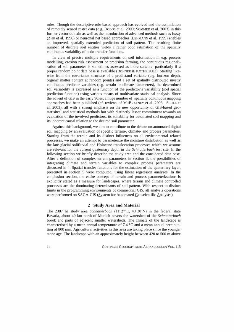
2 Study Area and Material The 2387 ha study area Schnatterbach (11°27’E, 48°30’N) in the federal state Bavaria, about 40 km north of Munich covers the watershed of the Schnatterbach brook and parts of adjacent smaller watersheds. The climate of the landscape is characterised by a mean annual temperature of 7.4 °C and a mean annual precipita-tion of 800 mm. Agricultural activities in this area are taking place since the younger stone age. The landscape with an approximately height between 420 to 500 m above


sea level is divided by a closely-meshed and finely-ramified valley network into numerous hills and crests, which rise either gently or sometimes steeply 30-60m from the bottoms of the valleys (HOFFMANN 1986). Slope gradient is up to 37%. The region is situated in the South German Molasse Basin, a sedimentary trough, which as a foredeep accumulated the debris of the rising peripheral areas the emerging Alpine chains in the Tertiary age (starting 65 million years ago). The fluvial and limnic sedimentation of the Upper Freshwater Molasse occurred during the Upper Miocene and reaches thickness of 150 to 250 m. The land surface is built by these deposits, which comprises coarse and fine sediments of the foreland. At the end of the Upper Miocene the Tertiärhügelland was further tectonically uplifted due to the continued emergence of the Alpine chains, and after the water has retreated sub-sequently, the sediments were formed under terrestrial conditions. At that time the region changed from being a sedimentation area to a denuation area and the terrain shape evolved. In the Pleistocene the area was part of the periglacial zone and was finally formed by solifluction, Loess deposition and subsequent denutation and erosion. This process is more pronounced on hills exposed to the sun. Thus, south- and east-exposed slopes became less steep. The prevailing westerly winds led to a preferred Loess and Loess-loam deposition on eastern and southern slopes (lee site). The typical valleys asymmetry in the area evolved from both processes. Up to 2 m loess cover can be found on gentle east-facing slopes, while loess is missing on the steeper west-facing slopes and usually on the hilltops. The landscape was denuded through pleistocene solifluction as well as by holocene erosion. The soil parent materials of soils originate from the Tertiary and Quaternary period, while the terrain shape results from Quaternary processes.

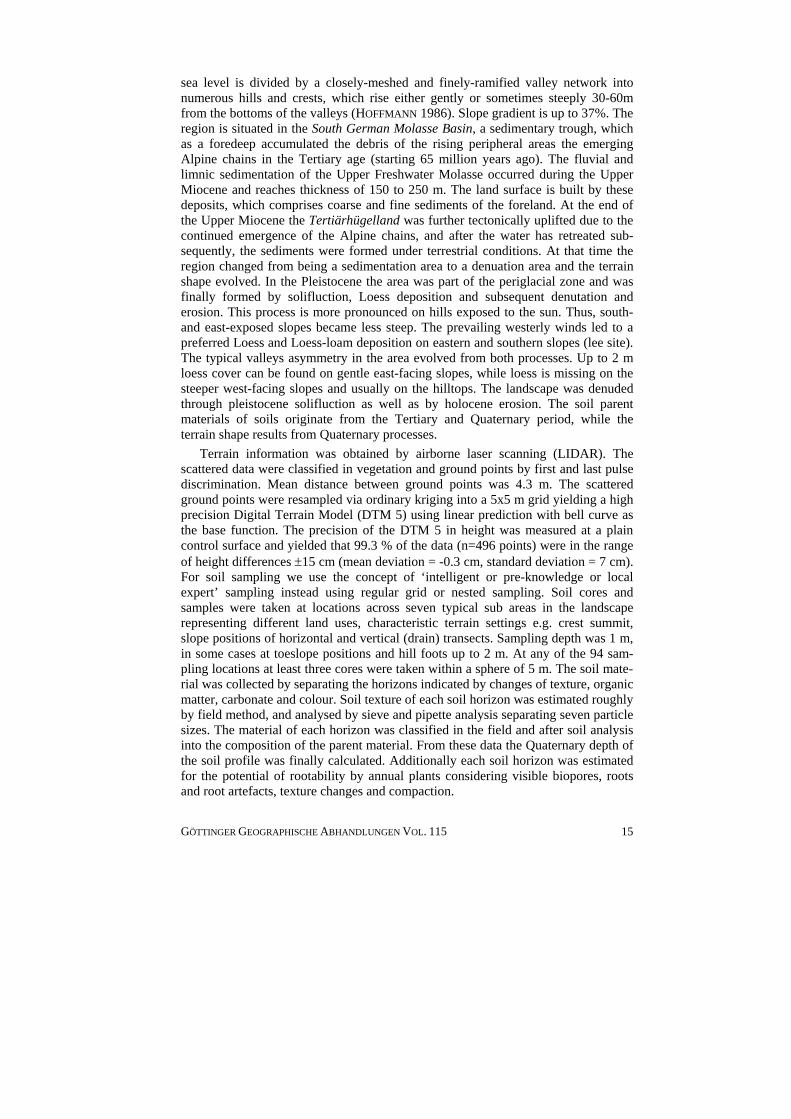
Terrain information was obtained by airborne laser scanning (LIDAR). The scattered data were classified in vegetation and ground points by first and last pulse discrimination. Mean distance between ground points was 4.3 m. The scattered ground points were resampled via ordinary kriging into a 5x5 m grid yielding a high precision Digital Terrain Model (DTM 5) using linear prediction with bell curve as the base function. The precision of the DTM 5 in height was measured at a plain control surface and yielded that 99.3 % of the data (n=496 points) were in the range of height differences ±15 cm (mean deviation = -0.3 cm, standard deviation = 7 cm). For soil sampling we use the concept of ‘intelligent or pre-knowledge or local expert’ sampling instead using regular grid or nested sampling. Soil cores and samples were taken at locations across seven typical sub areas in the landscape representing different land uses, characteristic terrain settings e.g. crest summit, slope positions of horizontal and vertical (drain) transects. Sampling depth was 1 m, in some cases at toeslope positions and hill foots up to 2 m. At any of the 94 sam-pling locations at least three cores were taken within a sphere of 5 m. The soil mate-rial was collected by separating the horizons indicated by changes of texture, organic matter, carbonate and colour. Soil texture of each soil horizon was estimated roughly by field method, and analysed by sieve and pipette analysis separating seven particle sizes. The material of each horizon was classified in the field and after soil analysis into the composition of the parent material. From these data the Quaternary depth of the soil profile was finally calculated. Additionally each soil horizon was estimated for the potential of rootability by annual plants considering visible biopores, roots and root artefacts, texture changes and compaction.

3 Terrain Analysis Since the pioneering work of MOORE et al. (1993), who probably yielded the first automated soil parameter maps for a small catchment area in Colorado, terrain analysis became a well established instrument for soil spatial prediction. Due to the vast amount and eased availability of DTM, terrain analysis had been widely used to infer terrain attributes from DTM, which particularly in a rather hilly orography are assessed as suitable representations of orographically determined lateral processes.

To date, numerous methods have been suggested for an enumeration of DTM, commonly differentiated in primary and secondary terrain attributes. Primary local terrain attributes such as slope, aspect and various curvature measures yield a local geomorphometric terrain description, whereas the so called primary complex terrain attributes describe the regional spatial interrelation of a grid-cell within the broader neighbourhood of the entire DTM-domain. Secondary terrain attributes such as the terrain wetness index (WI), the sediment transport index (STI) or stream power index (SPI) of MOORE et al. (1993) as the probably most prominent examples are subsequently inferred by combining different primary terrain attributes. Since secon-dary terrain attributes are explicitly stated as measures to estimate spatial variations of specific processes, they became a well established method in geomorphological studies, in climatology and soil related research (MORAN & BUI 2002; WILSON & GALLANT 2000). In the following section, we concentrate on the formal definition of complex primary and secondary terrain attributes, subsequently used in the process parameterization and soil regionalisation steps. To determine slope and aspect as the basic local geometries for all further terrain analyses, we generally applied the second order, central finite-difference scheme (ZEVERBERGEN & THORNE 1987).

Wetness Index: Surface and subsurface runoff is commonly parameterized by catchment area estimations. The catchment area (CA), defined as the discharge contributing upslope area of each grid cell [m²] and the specific catchment area (SCA), defined as the corresponding drainage area per unit contour width [m²·m-1] was computed using to the multiple flow direction method of FREEMAN (1991). The procedure yields a suitable representation of divergent and convergent flow pattern in hilly terrains. However, in rather flat areas and particularly in broad valleys near the talwegs, small differences in altitude cause random like flow pattern, which distinctly limit the predictive capacity of all related secondary terrain indexes in soil regionalisation. Assuming instead rather homogenous hydrologic conditions in these flat areas, the iteration form [01] was applied to modify the specific catchment area SCAM of each grid cell as a function of slope angle β [arcs] and the neighbouring maximum values SCAmax unless results remain unchanged.

[01] )15exp(

max 151

ββ

⎟⎠⎞

⎜⎝⎛= SCASCAM

for )15exp(

max 151

ββ

⎟⎠⎞

⎜⎝⎛< SCASCA

[02] ⎟⎟⎠

⎞⎜⎜⎝

⎛=

βtanln M

SSCA

WI

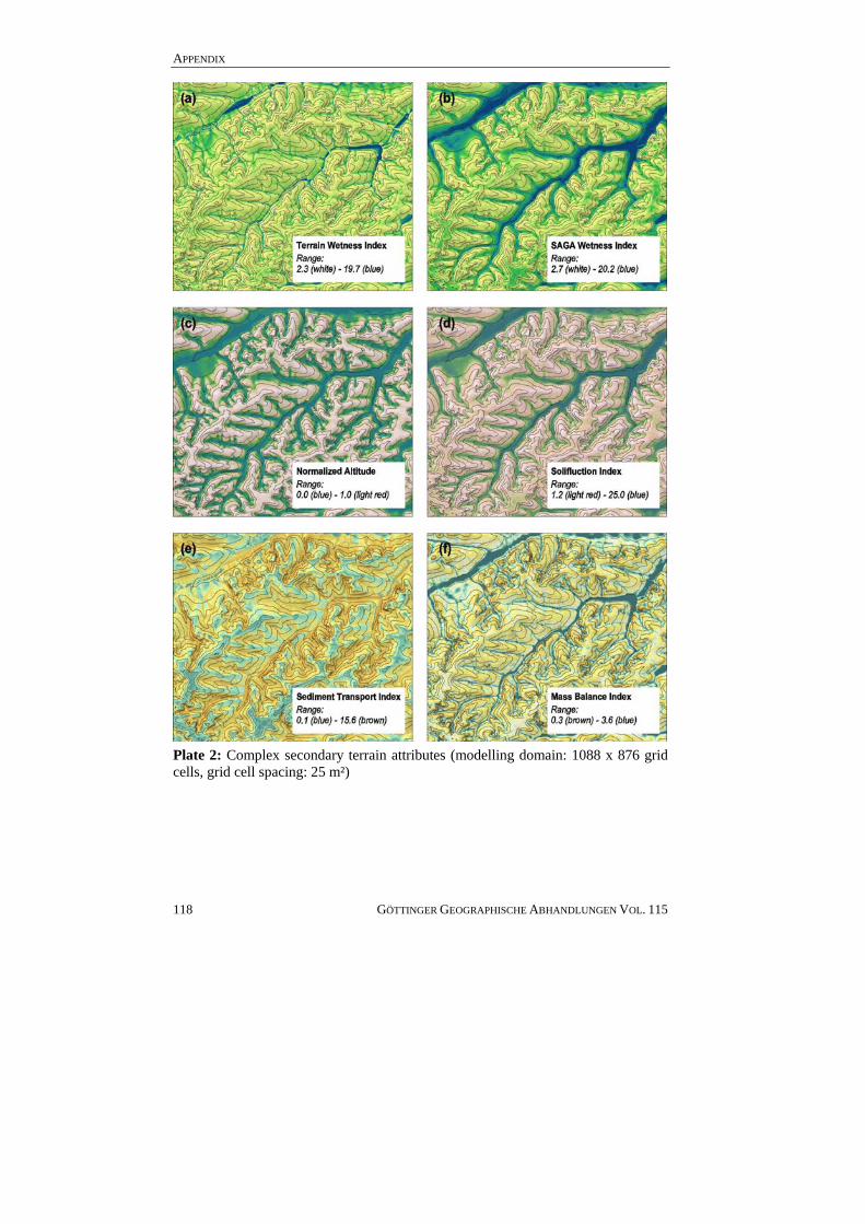
Following the notion of MOORE et al. (1993), who characterized terrain-determined spatial variations in soil moisture content by a terrain index, the SAGA wetness index WIS [02] is subsequently computed as a tangent function of slope angle β and SCAM (see Plate 2, Appendix).


Solifluction Index: Spatial variations in the depth of Late Glacial (and early Holo-cene) bed-rock deposits, mainly formed by periglacial solifluction, had been widely recognized to be correlated with the relative slope position (FRÜHAUF 1991; SEMMEL 1993; KLEBER 1997; SCHOLTEN 2004). Starting from a discrete DTM-based definition of channel networks and crest lines, BAUER et al. (1985) used overland flow path algorithm to infer vertical and horizontal distances to the drainage network and the watershed, respectively. The presupposed delineation of discrete terrain segments and particularly the definition of channel networks, however, constitute a crucial task and lead to a vivid debate on how to obtain a proper estimation of stream segments by means of terrain analyses.

Against this background, the equations [03] and [04] are an attempt towards a purely continuous estimation of altitude above drain culmination ADM and altitude below summit culmination ASM without using any basic discrete entities such as channel or crest lines. In a first step, relative altitudes are designated as the diffe-rence of a grid cells altitude zo (or the inverted altitude zi in [04]) and the weighted mean upslope altitudes zoi (or inverted altitudes zii in [04]), each weighted by the reciprocal square root of the catchment area CAi. The subscript M denotes the sub-sequently applied iteration as already defined in equation [01]. The normalized altitude NA [05] may optionally be delineated from ADM and ASM using basically the well known normalization equation of the NDVI (Normalized Difference Vegetation Index) but stretching the values from 0 (bottom) to 1 for summit positions (Plate 2c).

zoAS −=

∑

∑

=

=n

1 i

0.5i

n

1 i

0.5ii

M

1/CA

/CAzo

[03]

⎟⎟⎟⎟

⎠

⎞

⎜⎜⎜⎜

⎝

⎛

−⋅−=

∑

∑

=

= ziADM n

1 i

0.5i

n

1 i

0.5ii

1/CA

/CAzi1

[04]

( ) ( )[ ]MMMM AS AD / AS AD121NA +−+= [05]

⎟⎟⎠

⎞⎜⎜⎝

⎛⋅

++

=CA

M

M

M SCAADAS

SFIβtan1

1ln [06]

∑

∑

=

== n

1 i

0.5i

n

1 i

0.5ii

CA

CA

ββCA

[07]

The equation [06] of the solifluction index SFI attempts to combine different complex terrain attributes, relevant for solifluvial translocation processes. The ratio of ASM and ADM in [06] represents the relative gravity potential of slope positions and particularly stresses the pertinent valley floor as the major accumulation zones for periglacial deposits. Since solifluvial translocation of moist or water saturated stratum requires only low slope angles, the second term combines the specific


catchment area SCAM and the weighted mean slope angle of the upslope area βCA [07] to represent the size and slope of the entire stratum-contributing upslope area. As revealed in Plate 2d, the resulting solifluction index yields a distinct hypsometric differentiation with low values at crest and summit levels and maximum values at toeslopes and adjacent valley bottoms as well as in comparatively flat hollows at middle and lower slope levels.

Sediment Transport Index, Mass Balance Index: Although throughout the Holocene, only few episodes of enhanced geomorphic slope activity occurred, mainly induced by deforestation and cultivation activities of man, surface wash of intermixed loess-borne material in exposed upper bed-rock layers or the more recent erosion of fine stratum from bare cultivated top soils constitute important process scopes for the Holocene slope development and soil formation (e.g. YOUNG 1963; AHNERT 1973; FRIEDRICH 1996). To characterize terrain determined spatial variations of erosion and deposition processes, the transport capacity of overland flow had been frequently parameterized by combining DTM based terrain attributes such as slope and catchment area (TARBOTON 2003). Particularly the slope-length factor (LS-factor) of the famous Universal Soil Loss Equation (USLE) of WISCHMEIER & SMITH (1978) became a well established DTM-based approach, to approximate transport capacity and erosional forces as a function of the length of a slope segment and the sine of the slope angle (e.g. HENSEL 1999; HENSEL & BORK 1988; MOORE et al. 1992, 1993; SINOWSKI 1995).

Starting likewise from the LS-factor of the first revised USLE (WISCHMEIER & SMITH 1978), the equation [08] of the sediment transport index STIS integrates the weighted mean slope angle of the catchment area βCA [07], to cover the process differentiation within a slope and particularly the distinctively stronger dependence of transfer processes on the lower parts of the entire slope segment (cf. WISCHMEIER & SMITH 1978; HENSEL & BORK 1988). The continuous function for the slope length exponent was derived from corresponding exponent values for shallow slopes (< 0.505 arcs) from SCHWERTMANN et al. (1990). As suggested in HENSEL & BORK (1988), the mass balance index MBI is subsequently performed on a moving 3 by 3 grid cell window by balancing the STIS of each grid cell with the STI of the compound contributing upslope grid cells (STIin). The logarithmic modification form of the MBI in [09] is suggested for soil regionalization purposes with respect to the extreme excess in the statistic distribution of the STI differences.

[08] ( )065.0sin56.4sin14.6513.22

25.05.0

++⎟⎟⎠

⎞⎜⎜⎝

⎛= CACAS

CASTI ββ for βCA > 0.0505

( )065.0sin56.4sin14.6513.22

235.0

6.0

++⋅⎟⎟⎠

⎞⎜⎜⎝

⎛=

⋅

CACAS

CACASTI βββ

[09] ( Sin STISTIMBI )−++= 1ln1 for STIin – STIS > 0

([ )]


Sin STISTIMBI ++= 1ln11 −

The resulting MBI pattern indicates areas with a negative balance by values < 1 (in Plate 2f presented by colours from yellow to brown), particularly at steep slopes and exposed convex upper slope positions, whilst values > 1 (in Plate 2f presented in


colours from white to blue) with pronounced maximums of > 3 in hollows and toeslope positions denote accumulation zones.

4 Climate Regionalisation and Process Parameterisation Since climate variations at meso- and micro-scale are intimately related to the terrain as well, local DTM variables such as slope, aspect or altitude, to a certain extent are found to be a suitable surrogate for topoclimatic variations (SPEIGHT et al. 1974). Only a few studies explicitly used climate predictor variables for spatial estimations of e.g. organic matter (ARROUAYS et al. 1995; HENGL et al. 2002) or soil depth (RYAN et al. 2000; MCKENZI & RYAN, 1999). However, if one argues from a more model-theoretical point of view, the obvious impact of the long-standing climatic conditions on all environmental layers demands an integration of climate variables, firstly to ease the transferability and applicability of a once designed regionalization strategy to other climatic regions and secondly to obtain a more causal spatial esti-mation of soil parameters and soil pattern. Against this background we decided to consider climate variables as well. The necessary climatic data input was obtained by a regional modelling approach, developed in the context with several research projects on environmental change modelling in central Asia (BÖHNER 2004a) and studies on soil spatial prediction (BÖHNER & KÖTHE 2003; BÖHNER 2004b).

Since spatio-temporal climatic variations are widely controlled by large scale circulation modes and topographic settings, the regional climate modelling approach combines statistical downscaling of GCM (General Circulation Model) data and advanced surface parameterizations, to enable a physical consistent dynamical estimation of spatially extended climate variables. In a first step, free atmosphere predictor variables (e.g. troposphere temperature, vapour pressure, precitable water content, wind velocities) were inferred on the multiple grid point level from NCEP/NCAR reanalysis time series (KALNAY et al., 1996), a global set of troposphere parameters for different discrete free atmosphere levels (1000-200hPa layer) in T62 resolution (2.5° Latitude by 2.5° Longitude), retroactively modelled via CDAS (Climate Data Assimilation System). While the free atmosphere predictor variables yield a comprehensive 3-dimensional picture of large scale circulation modes, topographically controlled climatic variations and the magnitude of surface forced or modified boundary layer processes (e.g. pressure drag, frictional inter-actions of wind and surface roughness) were parameterized, using terrain and surface variables inferred from DTM and land use data. The spatial extended prediction of climate variables exploits the empirical relation between large scale circulation pattern and locally observed weather variations, obtained by multiple correlation and regression analyses. For the German modelling domain, the entire climate regionalization scheme considered monthly data of different climatic variables of the period 1961-1990 from the German Meteorological Network (DWD). Results comprise long term monthly and annual means of different radiation measures (actual and potential topographic radiation income) temperatures, vapour pressure, precipitation amounts, wind speeds (in 2 and 10 m above ground), alternative evapotranspiration estimations and climatic water balances. A detailed description of the entire procedure is given in BÖHNER (2004b). In the following we only concentrate on the methodical aspects of combining terrain and climate

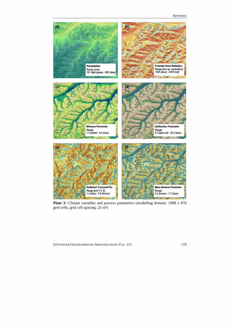
variables for soil spatial prediction. Instead of defining climofunctions separately, we attempt to extend the predictive capacity of DTM by directly integrating those climate variables, which we assume are relevant for the parameterization of soil related and soil forming processes. Wetness Parameter: The wetness parameter extends the previously defined wetness index by integrating precipitation rates and the potential topographic solar radiation (cf. Plate 3a, 3b). While the annual mean precipitation amount represents the total offer of moisture, the potential topographic solar radiation, defined as the mean annual shortwave radiation income on inclined surfaces under clear sky conditions (BÖHNER 2004b) mirrors the influence of different inclined slopes on the soil water and evaporation distribution. As defined in the equation [10], precipitation and solar radiation sums were integrated over the entire upslope area and the ratio of both parameters is subsequently considered in the wetness parameter WP, by:

[10]

⎟⎟⎟⎟

⎠

⎞

⎜⎜⎜⎜

⎝

⎛

=

∑

∑

=

=

βtan1ln

1

1n

ii

n

ii

M

s

pSCAWP

Here pi [mm y-1] is the long-term mean annual precipitation amount of the i-th upslope grid cell and si [mm y-1] is the corresponding shortwave radiation amount, given in equivalent evaporation. Instead of integrating the climatic water balance, the precipitation/radiation ratio was preferred as a rather simple but suitable surro-gate for the moisture complex, to stress the significant role of slopes and topo-climatic settings on moisture and energy fluxes in small catchment areas (BÖHNER & PÖRTGE 1997). Though slope angles and the size of upslope areas are still the dominating factors in the distribution pattern of the resulting wetness parameter (cf. Plate 3c), steep adret slopes however, show a slightly more pronounced reduction of wetness indicators than comparably steep slopes at northern aspects.

Solifluction Parameter: The relevance of terrain determined variations in the moisture and energy flux is likewise valid for most periglacial processes. Particu-larly the distribution of permafrost and thaw depth is intimately related to the solar radiation income and resulting spatial variations in the surface energy exchange and heat conduction into the ground (FUNK & HOELZLE 1992). The solifluction para-meter SFP [11] attempts to consider this causal relation by integrating the potential solar radiation income of the total upslope area SCRM [L m-1y-1] estimated for last glacial maximum (LGM) atmospheric conditions. The specific catchment radiation amount SCRM is given in L m-1y-1 inferred from equivalent evaporation. The subscript M in the SCRM again denotes the iterative modification, defined in expression [01]. Since the equation of the former DTM based solifluction index else was left unchanged major deposit positions such as flat toeslopes remain stressed in the resulting distribution pattern of the solifluction parameter (cf. Plate 3d).

[11] ⎟⎟⎠

⎞⎜⎜⎝

⎛⋅

++

=CA

M

M

M SCRADAS

SFPβtan1

1ln

LGM radiation estimates were performed by a methodical consistent assimilation of an ECHAM LGM simulation (model run with prescribed ocean temperatures: ECHAM 3.6 T42 L19 Model). Though the paleo radiation income only little differs


from the current conditions, we assume the ECHAM run to yield at least a more realistic parameterization for the radiation model than simply using current atmosphere variables. Despite the sophisticate GCM assimilation scheme, however, the entire approach yields hardly more than a rough estimation of paleo conditions. Sediment Transport Parameter, Mass Balance Parameter: The sediment transport parameter STP equation [14] consistently extends the former purely DTM based sediment transport index by the USLE R-factor (rainfall factor). The R-factor approximation of rainfall characteristics for estimating soil loss is designated as the product of the total kinetic energy of rainfall and the maximum rainfall intensity over a continuous 30 minute period. Since the computation of R-factors thus requires temporal very high resolution precipitation series, routinely recorded only at fully instrumented meteorological stations, annually integrated R-values were frequently regressed on corresponding precipitation totals. The resulting opportunity to inferring R-factor estimates from more widely available regular network obser-vations had particularly been used in the context with spatial extended long term water erosion risk assessments. The regression equation [12] from SCHWERTMANN et al. (1990) was inferred from precipitation series of the Bavarian meteorological network and is thus assumed to be a suitable estimation base for our study. Here, ri is the R-Factor at the i-th grid cell [kJ·m2·mm·y-1] and pi is the corresponding precipita-tion amount [mm·y-1].

1.77-083.0 ipri = [12]

∑

∑

=

== n

1 i

0.5i

n

1 i

0.5ii

CA

CA

rRCA

[13]

( ) 0505.0for 065.0sin56.4sin14.6513.22

25.05.0

>++⎟⎟⎠

⎞⎜⎜⎝

⎛= CACACACA

CARSTP βββ [14]

( )065.0sin56.4sin14.6513.22

235.0

6.0

++⋅⎟⎟⎠

⎞⎜⎜⎝

⎛=

⋅

CACACA

CACARSTP βββ

( ) 0for 1ln1 >−−++= Sinin STISTISTPSTPMBP [15]

( )[ ]STPSTPMBP in −++= 1ln11

Using the same weighting expression as already defined for the mean catchment slopes [13], the sediment transport parameter STP [14] integrates the weighted mean of the catchment R-factor RCA [kJ·m2·mm·y-1]. The mass balance parameter (MBP) equation [15] is almost identical with the mass balance index but integrates STP values. The resulting distribution pattern of STP and MBP are presented in Plate 3.



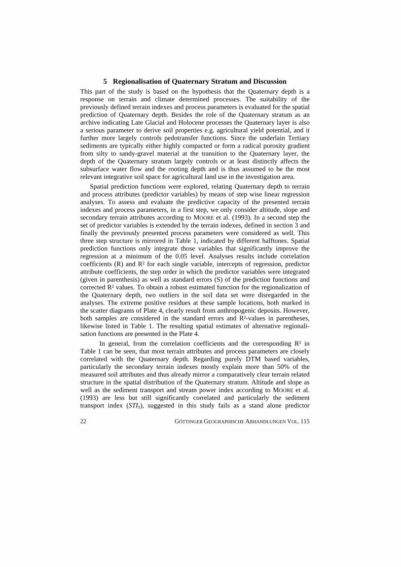
5 Regionalisation of Quaternary Stratum and Discussion This part of the study is based on the hypothesis that the Quaternary depth is a response on terrain and climate determined processes. The suitability of the previously defined terrain indexes and process parameters is evaluated for the spatial prediction of Quaternary depth. Besides the role of the Quaternary stratum as an archive indicating Late Glacial and Holocene processes the Quaternary layer is also a serious parameter to derive soil properties e.g. agricultural yield potential, and it further more largely controls pedotransfer functions. Since the underlain Tertiary sediments are typically either highly compacted or form a radical porosity gradient from silty to sandy-gravel material at the transition to the Quaternary layer, the depth of the Quaternary stratum largely controls or at least distinctly affects the subsurface water flow and the rooting depth and is thus assumed to be the most relevant integrative soil space for agricultural land use in the investigation area.

Spatial prediction functions were explored, relating Quaternary depth to terrain and process attributes (predictor variables) by means of step wise linear regression analyses. To assess and evaluate the predictive capacity of the presented terrain indexes and process parameters, in a first step, we only consider altitude, slope and secondary terrain attributes according to MOORE et al. (1993). In a second step the set of predictor variables is extended by the terrain indexes, defined in section 3 and finally the previously presented process parameters were considered as well. This three step structure is mirrored in Table 1, indicated by different halftones. Spatial prediction functions only integrate those variables that significantly improve the regression at a minimum of the 0.05 level. Analyses results include correlation coefficients (R) and R² for each single variable, intercepts of regression, predictor attribute coefficients, the step order in which the predictor variables were integrated (given in parenthesis) as well as standard errors (S) of the prediction functions and corrected R² values. To obtain a robust estimated function for the regionalization of the Quaternary depth, two outliers in the soil data set were disregarded in the analyses. The extreme positive residues at these sample locations, both marked in the scatter diagrams of Plate 4, clearly result from anthropogenic deposits. However, both samples are considered in the standard errors and R²-values in parentheses, likewise listed in Table 1. The resulting spatial estimates of alternative regionali-sation functions are presented in the Plate 4.

In general, from the correlation coefficients and the corresponding R² in Table 1 can be seen, that most terrain attributes and process parameters are closely correlated with the Quaternary depth. Regarding purely DTM based variables, particularly the secondary terrain indexes mostly explain more than 50% of the measured soil attributes and thus already mirror a comparatively clear terrain related structure in the spatial distribution of the Quaternary stratum. Altitude and slope as well as the sediment transport and stream power index according to MOORE et al. (1993) are less but still significantly correlated and particularly the sediment transport index (STIS), suggested in this study fails as a stand alone predictor


variable. This is also valid for the extended sediment transport parameter while the other process parameters extended by climate variables explain a slightly higher proportion of the predictand variance than the pure DTM based indexes.

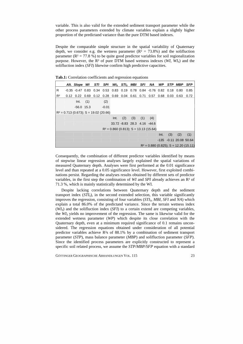
Despite the comparable simple structure in the spatial variability of Quaternary depth, we consider e.g. the wetness parameter (R² = 73.8%) and the solifluction parameter (R² = 77.8 %) to be quite good predictor variables for soil regionalization purpose. However, the R² of pure DTM based wetness indexes (WI, WIS) and the solifluction index (SFI) likewise confirm high predictive capacities. Tab.1: Correlation coefficients and regression equations

Alt. Slope WI STI SPI WIS STIS MBI SFI NA WP STP MBP SFP

R -0.35 -0.47 0.83 0.34 0.53 0.83 0.19 0.78 0.84 -0.76 0.82 0.18 0.80 0.85

R² 0.12 0.22 0.69 0.12 0.28 0.69 0.04 0.61 0.71 0.57 0.68 0.03 0.63 0.72

Int. (1) (2)

-56.0 15.3 -0.01

R² = 0.713 (0.673); S = 19.02 (20.66)

Int. (2) (3) (1) (4)

33.72 -8.83 28.3 4.16 -44.6

R² = 0.860 (0.813); S = 13.13 (15.64)

Int. (3) (2) (1)

-135 -0.11 20.08 50.64

R² = 0.880 (0.825); S = 12.20 (15.11) Consequently, the combination of different predictor variables identified by means of stepwise linear regression analyses largely explained the spatial variations of measured Quaternary depth. Analyses were first performed at the 0.01 significance level and than repeated at a 0.05 significance level. However, first exploited combi-nations persist. Regarding the analyses results obtained by different sets of predictor variables, in the first step the combination of WI and SPI already achieves an R² of 71.3 %, which is mainly statistically determined by the WI.

Despite lacking correlations between Quaternary depth and the sediment transport index (STIS), in the second extended selection, this variable significantly improves the regression, consisting of four variables (STIS, MBI, SFI and NA) which explain a total 86.0% of the predictand variance. Since the terrain wetness index (WIS) and the solifluction index (SFI) to a certain extend are competing variables, the WIS yields no improvement of the regression. The same is likewise valid for the extended wetness parameter (WP) which despite its close correlation with the Quaternary depth, even at a minimum required significance of 0.1 remains uncon-sidered. The regression equations obtained under consideration of all potential predictor variables achieve R²s of 88.1% by a combination of sediment transport parameter (STP), mass balance parameter (MBP) and solifluction parameter (SFP). Since the identified process parameters are explicitly constructed to represent a specific soil related process, we assume the STP/MBP/SFP equation with a standard


error of 12.4 cm to be a though statistical but suitable model for spatially extended predictions of Quaternary depth. Apart from the pure statistical evaluation of alternative regression equations in terms of R² and standard errors, an application of the spatial prediction functions and the resulting maps enable a further critical assessment in terms of suitability and reliability. As shown in Plate 4a, in the mapping results based on WI and SPI, major characteristics of the Quaternary variation pattern such as down slope increasing depth of the Quaternary stratum or settings with caped Quaternary layers at exposed steep slopes are only properly represented from midslope to summit positions while toeslopes and settings near the talwegs show a rather artificial pattern. The comparable high R² of the regression benefits from the sparse cover of soil sample positions in or near the valley bottoms. Instead, the mapping results obtained by the second (cf. Plate 4c) and third regression equation (cf. Plate 4e) show an overall more consistent pattern and to certain extend even yield a suitable extrapolation of Quaternary depth out of the sample limits. In both maps, Quaternary estimates thicker than 1 m cover the entire valley bottoms and adjacent flat toeslopes where slope angles are roughly below 2 degrees. With the exception of only few broad and flat summits, Quaternary stratum thicker than 50 cm is mostly confined to slope hallows and lower concave slope positions. Instead, ridges, high slopes and most summits are characterized by lower Quaternary depth and particularly at convex upper slopes, steeper than 20°, the Quaternary is often indicated to be nearly or completely capped. In Plate 4e, the latter pattern is slightly more marked at northern positions and what is more, the ridges/hollow differentiation at slopes is generally more distinct than in Plate 4c. Although the STP/MBP/SFP equation attains only slightly more explanative capacity than the STIS/MBI/SFI/NA equation, we assess this parameter combination to be a reasonable representation of late Quaternary solifluction processes and Holocene denudation and erosion processes.

6 Conclusion

Current terrain analysis techniques offer powerful opportunities for enhanced spatial extended soil attribute estimations. Particularly in a rather hilly topography, where soil forming processes are intimately related to the shape of the relief, complex secondary terrain attributes have high predictive capacities for soil mapping. Using secondary terrain indices, the distribution pattern of Quaternary stratum can be largely predicted. Linear regression analyses on complex terrain indexes yield high coefficients of determination of the order of 71-86%, which we assume are due to a comparatively clear terrain-determined spatial variation structure of the Quaternary depth at the Schnatterbach test site. Nevertheless, the predictive capacity of DTM can be distinctly extended by using terrain indexes, which are explicitly constructed in order to represent a specific process such as e.g. solifluction. Since the purely statistical evaluation of the presented terrain indexes as well as its mapping application proved suitable, we suggest the solifluction index, the sediment transport index and mass balance index as basic DTM attributes to represent translocation processes. The extension of DTM attributes by climate variables is likewise suggested in order to yield reasonable more causally justified estimates. Given the


low relief energy at the Schnatterbach test site, it is unrealistic to expect a distinct improvement of soil spatial prediction functions by integrating climate variables. Against this background, the slight improvement of the predictive capacity of DTM and climate based parameters and the obtained accurate mapping results give reason for its further use, especially if larger and more heterogeneous landscapes require a consideration of the soil forming factor climate. Further more we assume our attempt to differentiate between Late Pleistocene solifluction and Holocene denudation and erosion processes when constructing and using process parameters to be a possible measure to consider Jenny’s well known but rarely operational time factor. Although we are aware that the integration of paleoclimate estimates presented in this paper is hardly more than a first step, this aspect intends to encourage further discussion.

Apart from own studies on soil regionalization in Lower Saxony (BÖHNER et al. 2002; BÖHNER & KÖTHE 2003) the authors are not aware of any study, which rigorously has evaluated the principal visibility of spatial extended process parameterizations as the basic method for soil spatial prediction. The general emphasis on the process level in the entire approach mirrors our basic assumption, that no matter which kind of multivariate statistical or geostatistical method is used, a proper spatial estimation of continuous soil parameters has to be achieved predominantly. Although in this study, we simply use stepwise linear regression analyses to define spatial prediction functions, other multivariate statistical procedures may have been a major alternative. Acknowledgments: This paper draws on work from a range of past and recent research projects funded by the German Federal Ministry for Education and Research (BMBF) and the German Federal Office for Geoscience and Resources (BGR). These contributions are gratefully acknowledged.

References AHNERT, F. (1973): An approach towards a descriptive classification of slopes. – Zeitschrift

für Geomorphologie, N. F., Suppl. 9: 71-84. ARROUAYS, D., VION, I. & KICIN, J.L. (1995): Spatial analysis and modeling of topsoil carbon

storage in temperature forest humic loamy soils for France. – Soil Science 159: 191-198. BAUER, J., ROHDENBURG, H. & BORK, H.R. (1985): Ein Digitales Reliefmodell als Voraus-

setzung für ein deterministisches Modell der Wasser- und Stoff-Flüsse. – Landschafts-genese und Landschaftsökologie 10: 1-15.

BÖHNER, J. (2004a): Der klimatisch determinierte raum/zeitliche Wandel naturräumlicher Ressourcen Zentral- und Hochasiens: Regionalisierung, Rekonstruktion und Prognose. –In: GAMERITH W, MESSERLI P, MEUSBURGER, P. & WANNER, H. [Eds.]: Alpenwelt-Gebirgswelten. Inseln, Brücken, Grenzen. – Tagungsbericht und wissenschaftliche Abhandlungen 54. Deutscher Geographentag Bern. pp.151-160.

BÖHNER, J. (2004b): Regionalisierung bodenrelevanter Klimaparameter für das Niedersächsi-sche Landesamt für Bodenforschung (NLfB) und die Bundesanstalt für Geowissen-schaften und Rohstoffe (BGR). – Arbeitshefte Boden 2004/4: 17-66.

BÖHNER, J. & KÖTHE, R. (2003): Neue Ansätze zur Bodenregionalisierung. – Petermanns Geogr. Mitt. 147 (2003/3): 72-82.

BÖHNER, J. & PÖRTGE, K.H. (1997): Strahlungs- und expositionsgesteuerte tagesperiodische


Schwankungen des Abflusses in kleinen Einzugsgebieten. – Petermanns Geogr. Mitt.141 (1997/1): 35-42.

BÖHNER, J., KÖTHE, R. & SELIGE, T. (2004): Geographical Information Systems: Applications to Soils. – In: HILLEL, D., ROSENZWEIG, C., POWLSON, D., SCOW, K., SINGER, M., SPARKS, D. [Eds.]: Encyclopedia of Soils in the Environment. – Elsevier, Oxford, pp.121-129

BÖHNER, J., KÖTHE, R., CONRAD, O., GROSS, J., RINGELER, A. & SELIGE, T. (2002): Soil Regionalisation by Means of Terrain Analysis and Process Parameterisation. In: MICHELI, E., NACHTERGAELE, F. & MONTANARELLA, L. [Eds.]: Soil Classification 2001. – The European Soil Bureau, Joint Research Centre, EUR 20398 EN, Ispra, pp.213–222.

DEMEK, J. (1972): Manual of detailed geomorphological mapping. – Prag. DOBOS, E., MICHELI, E., BAUMGARDNER, M.F., BIEHL, L. & HELT, T. (2000): Use of combined

digital elevation model and satellite radiometric data for regional soil mapping. – Geoderma 97: 367–391.

FREEMAN, T.G. (1991): Calculating catchment area with divergent flow based on a regular grid. – Computers and Geoscience 17 (3): 413-422.

FRIEDRICH, K. (1996): Digitale Reliefgliederungsverfahren zur Ableitung bodenkundlich relevanter Flächeneinheiten. – Frankfurter Geowissenschaftliche Arbeiten, Serie D, Physische Geographie 21, 258 pp.

FRÜHAUF, M. (1991): Neue Befunde zur Lithologie, Gliederung und Genese der periglazialen Lockermaterialdecken im Harz: Erfassung und Bewertung postallerödzeitlicher decksedimentbildender Prozesse. – Petermanns Geogr. Mitt. 135: 49-60.

HENGL, T., ROSSITER, D.G. & HUSNJAK, S. (2002): Mapping soil properties from an existing national soil data set using freely available ancillary data. – 17th World Congress of Soil Science: August 14-21; Bangkok, Thailand; Paper no. 1140.

HENSEL, H. (1991): Verfahren zur EDV-gestützten Abschätzung der Erosionsgefährdung von Hängen und Einzugsgebieten. – Bodenökologie und Bodengenese 2, 113 pp.

HENSEL, H. & BORK, H.R. (1988): EDV-gestützte Bilanzierung von Erosion und Akkumulation in kleinen Einzugsgebieten unter Verwendung der modifizierten Universal Soil Loss Equation. – Landschaftsökologisches Messen und Auswerten 2, 2/3: 107-136.

JENNY, H. (1941): Factors of soil formation. A system of quantitative pedology. – New York. KALNAY, E., KANAMITSU, M., KISTLER, R., COLLINS, W., DEAVEN, D., GANDIN, L., IREDELL,

M., SAHA, S., WHITE, G., WOOLLEN, J., ZHU, Y., LEETMAA, A., REYNOLDS, R., CHELLIAH, M., EBISUZAKI, W., HIGGINS, W., JANOWIAK, J.,. MO, K.C., ROPELEWSKI, C., WANG, J., JENNE, R. & JOSEPH, D. (1996): The NCEP/NCAR 40-Year Reanalysis Project. – Bulletin of the American Meteorological Society 03.

KLEBER, A. (1997): Cover-beds as soil parent materials in mid-latitude regions. Catena 30: 197-213.

LEHMANN, D., BILLEN, N. & LENZ, R. (1999): Anwendung von Neuronalen Netzen in der Landschaftsökologie – Synthetische Bodenkartierung im GIS. – In: STROBL, J. & BLASCHKE, T. [Eds.]: Angewandte Geographische Informationsverarbeitung XI, Beiträge zum AGIT-Symposium Salzburg 1999, pp. 330-336.

MCBRATNEY, A.B., HART, G.A. & MCGARRY, D. (1991): The Use of Region Partitioning to Improove the Representation of Geostatistically Mapped Soil Attributes. – Journal of Science: 513-515.

MCBRATNEY, A.B., MENDOCA SANTOS, M.L. & MINASNY, B. (2003) On digital soil mapping. Geoderma 117: 3-52.

MCKENZIE, N.J. & AUSTIN, M.P. (1993): A quantitative Australian approach to medium and small scale surveys based on soil stratigraphy and environmental correlation. – Geoderma 57: 329-355.


MCKENZIE, N.J. & RYAN, P.J. (1999): Spatial prediction of soil properties using environmen-tal correlation. – Geoderma 89: 67-94.

MOORE, I.D., GESSLER, P.E., NIELSEN, G.A. & PETERSON, G.A. (1993): Soil Attribute Prediction Using Terrain Analysis. – Soil Sci. Soc. Am. J. 57: 443-452.

MOORE, I.D. & WILSON, J.P. (1992): Length-slope factors for the revised Universal Soil Loss Equation: simplified method of estimation. – J. Soil & Water Cons. 47: 423-428.

MORAN, J.C. & BUI, E. (2002): Spatial data mining for enhanced soil map modelling. –International Journal of Geographic Information Science 16: 533-549.

MORGAN, R.P.C., QUINTON, J.N., SMITH, R.E., GOVERS, G., POESEN, J.W.A., AUERSWALD, K., CHISCI, G., TORRI, D. & STYCZEN, M.E. (1998): The European soil erosion model (EUROSEM): A process-based approach for predicting sediment transport from fields and small catchments. –Earth Surface Processes and Landforms 23: 527-544.

NEEMANN, W. (1991): Bestimmung des Bodenerodierbarkeitsfaktors für winderosions–gefährdete Böden Norddeutschlands. – Geologisches Jahrbuch, Reihe F 25: 131 pp.

QUINN, P., BEVEN, K., CHEVALLIER, P. & PLANCHON, O. (1991): The Prediction of Hillslope Flow Paths for Distributed Hydrological Modelling Using Digital Terrain Models. – In: BEVEN, K.J. & MOORE, I.D. [Eds]: Terrain Analysis and Distributed Modelling in Hydrology. – pp. 63-84.

RYAN, P.J., MCKENZIE, N.J., O’CONNELL, D., LOUGHHEAD, A.N., LEPPERT, P.M., JACQUIER, D. & ASHTON, L. (2000): Integrating forest soils information across scales: spatial prediction of soil properties under Australian forests. - Forest Ecology & Management 138: 139-157.

SCHOLTEN, T. (2004): Beitrag zur flächendeckenden Ableitung der Verbreitungssystematik und Eigenschaften periglaziärer Lagen in deutschen Mittelgebirgen. – Relief Boden Paläoklima 19, Gebr. Bornträger: Berlin Stuttgart.

SCHWERTMANN, U., VOGL, W. & KAINZ, M. (1990): Bodenabtrag durch Wasser - Vorhersage des Abtrags und Bewertung von Gegenmaßnahmen. – 2. Aufl.: Stuttgart, 64 pp.

SCULL, P., FRANKLIN, J., CHADWICK, O.A. & MCARTHUR, D. (2003): Predictive soil mapping: a review. – Progress in Physical Geography 27: 171-197.

SEMMEL, A. (1993): Grundzüge der Bodengeographie. – Teubner Studienbücher der Geographie, 3. Aufl.: Stuttgart, 127 pp.

SINOWSKI, W. (1995): Die dreidimensionale Variabilität von Bodeneigenschaften. – FAM-Bericht 7, Aachen, 158 pp.

SOMMER, M., WEHRHAN, M., ZIPPRICH, M., WELLER, U., ZU CASTELL, W., EHRICH, S., TANDLER, B. & SELIGE, T. (2003): Hierarchial data fusion for mapping soil units at field scale. – Geoderma 112: 179-196.

SPEIGHT, J.G. (1974): A parametric approach to landform regions. – Special Publication Institute of British Geographers 7: 213-230.

TARBOTON, D. (2003): Terrain analysis using digital elevation model in hydrology. – 23rd ESRI International Users Conference: July 7-11, 2003; San Diego, California.

WILSON, J.P. & GALLANT, J.C. (2000): Secondary topographic attributes. – In: WILSON, J.P. & GALLANT, J.C. [Eds.]: Terrain Analysis-Principles and Applications. – Wiley: New York, pp. 87-132.

WISCHMEIER, W.H. & SMITH, D.D. (1978): Predicting rainfall erosion losses – A guide to conversation planning. – Agriculture Handbook No. 537: US Department of Agriculture, Washington DC.

YOUNG, A. (1963): Deductive Models of Slope Evolution. – Nachrichten der Akademie der Wissenschaften, Göttingen II, Math.-Phys. Klasse: Göttingen.

ZEVERBERGEN, L.W. & THORNE, C.R. (1987): Quantitative analysis of landsurface topography. – Earth Surface Processes and Landforms 12: 47-56.


ZHU, A., BAND, L.E., DUTTON, B. & VERTESSY, R. (1996): Soil property derivation using a Soil Land Inference Model (SoLIM). – Ecological Modelling 90: 123-124.

APPENDIX

Plate 2: Complex secondary terrain attributes (modelling domain: 1088 x 876 grid cells, grid cell spacing: 25 m²)


APPENDIX

Plate 3: Climate variables and process parameters (modelling domain: 1088 x 876 grid cells, grid cell spacing: 25 m²)


APPENDIX

Plate 4: Predicted Quaternary depth – scatter diagrams on measured versus predicted Quaternary depth (squares indicate outliers, resulting from anthropogenic deposits)


Jürgen Böhner & Thomas Selige - TUM

Documents

Transcript of Jürgen Böhner & Thomas Selige - TUM