Klausur für das CERA Modul D - aktuar.de · „Brutto“- und „Netto“-Risikokapitalien für...
45
1 Klausur für das CERA Modul D 20.05.2017 Die Klausur hat insgesamt 180 Punkte. Zum Bestehen der Klausur sind 90 Punkte notwendig. Zur Orientierung bei der Bearbeitungszeit: jeder Bewertungspunkt entspricht einer Bearbeitungszeit von ungefähr einer Minute. Sie müssen nicht immer ausformulierte Antworten geben. Sie können auch Antworten in Stichworten geben (z.B. bei Pro und Contra). Bitte beachten Sie, dass zur besseren Lesbarkeit der Aufgaben jeweils etwas leerer Platz zwischen Aufgaben steht, so dass normalerweise jede Aufgabe auf einer neuen Seite beginnt. Die Klausur hat 10 Seiten. Vorbereitung für Aufgabe 1 Die dargestellte vereinfachte Bilanz der VitaLife Lebensversicherung ist Grundlage für die Aufgabe 1. Stellen Sie sich vor, Sie sind Risikomanager in der VitaLife Lebensversicherung. Die VitaLife ist ein Versicherungsverein auf Gegenseitigkeit (VVaG). Die VitaLife vertreibt klassische Kapitallebensversicherungen mit einer Rentenoption bei garantierten Rentenfaktoren. VitaLife hat die folgende Bilanz. Gehen Sie davon aus, dass bei den Zinstiteln das Nominal dem Buchwert entspricht. Nutzen Sie für die Umbewertung von Buchwerten zu Marktwerten das vereinfachende Verfahren des Durationsansatzes, sofern keine anderen Angaben gemacht werden.
Transcript of Klausur für das CERA Modul D - aktuar.de · „Brutto“- und „Netto“-Risikokapitalien für...
1
Klausur für das CERA Modul D 20.05.2017
Die Klausur hat insgesamt 180 Punkte. Zum Bestehen der Klausur sind 90 Punkte notwendig. Zur
Orientierung bei der Bearbeitungszeit: jeder Bewertungspunkt entspricht einer Bearbeitungszeit von
ungefähr einer Minute. Sie müssen nicht immer ausformulierte Antworten geben. Sie können auch
Antworten in Stichworten geben (z.B. bei Pro und Contra). Bitte beachten Sie, dass zur besseren Lesbarkeit
der Aufgaben jeweils etwas leerer Platz zwischen Aufgaben steht, so dass normalerweise jede Aufgabe auf
einer neuen Seite beginnt. Die Klausur hat 10 Seiten.
Vorbereitung für Aufgabe 1
Die dargestellte vereinfachte Bilanz der VitaLife Lebensversicherung ist Grundlage für die Aufgabe 1.
Stellen Sie sich vor, Sie sind Risikomanager in der VitaLife Lebensversicherung. Die VitaLife ist ein Versicherungsverein auf Gegenseitigkeit (VVaG). Die VitaLife vertreibt klassische Kapitallebensversicherungen mit einer Rentenoption bei garantierten Rentenfaktoren. VitaLife hat die folgende Bilanz. Gehen Sie davon aus, dass bei den Zinstiteln das Nominal dem Buchwert entspricht.
Nutzen Sie für die Umbewertung von Buchwerten zu Marktwerten das vereinfachende Verfahren des Durationsansatzes, sofern keine anderen Angaben gemacht werden.
2
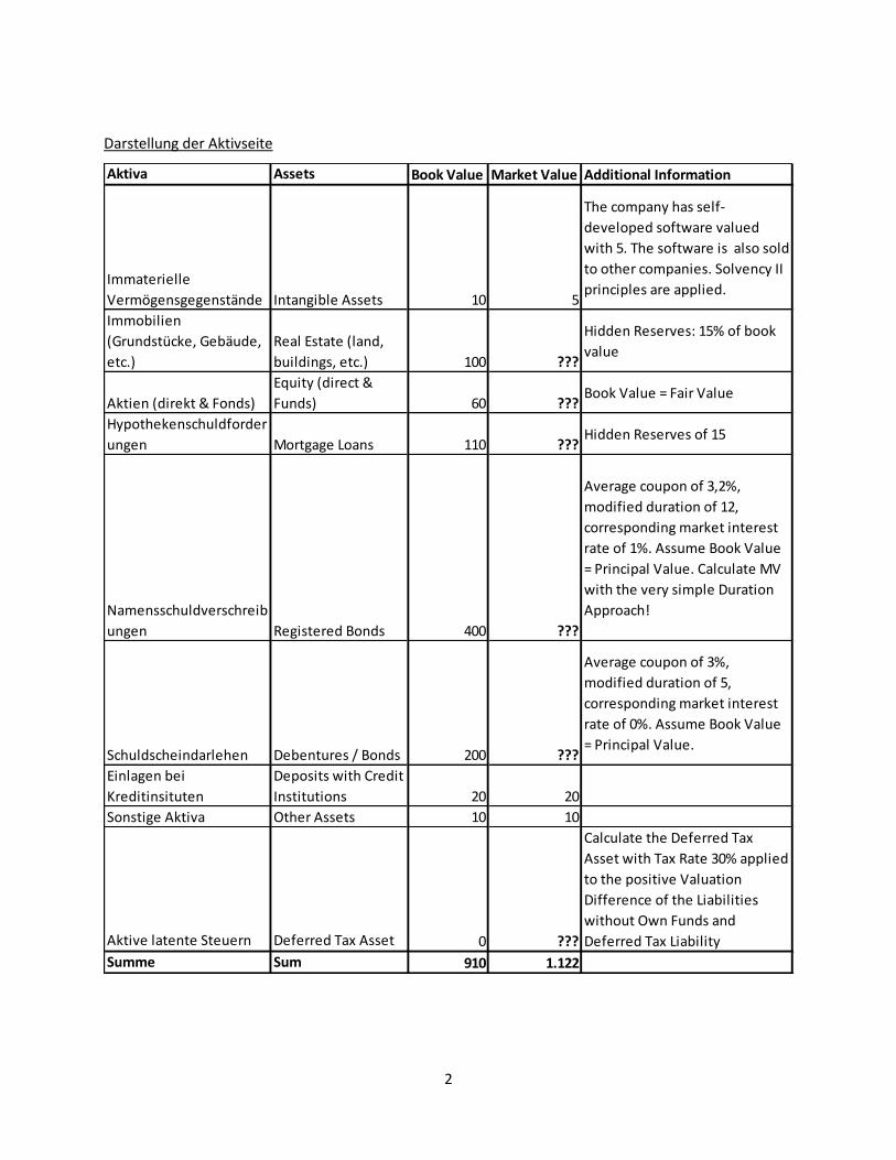
Darstellung der Aktivseite
Aktiva Assets Book Value Market Value Additional Information
Immaterielle
Vermögensgegenstände Intangible Assets 10 5
The company has self-
developed software valued
with 5. The software is also sold
to other companies. Solvency II
principles are applied.
Immobilien
(Grundstücke, Gebäude,
etc.)
Real Estate (land,
buildings, etc.) 100 ???
Hidden Reserves: 15% of book
value
Aktien (direkt & Fonds)
Equity (direct &
Funds) 60 ???Book Value = Fair Value
Hypothekenschuldforder
ungen Mortgage Loans 110 ???Hidden Reserves of 15
Namensschuldverschreib
ungen Registered Bonds 400 ???
Average coupon of 3,2%,
modified duration of 12,
corresponding market interest
rate of 1%. Assume Book Value
= Principal Value. Calculate MV
with the very simple Duration
Approach!
Schuldscheindarlehen Debentures / Bonds 200 ???
Average coupon of 3%,
modified duration of 5,
corresponding market interest
rate of 0%. Assume Book Value
= Principal Value.
Einlagen bei
Kreditinsituten
Deposits with Credit
Institutions 20 20
Sonstige Aktiva Other Assets 10 10
Aktive latente Steuern Deferred Tax Asset 0 ???
Calculate the Deferred Tax
Asset with Tax Rate 30% applied
to the positive Valuation
Difference of the Liabilities
without Own Funds and
Deferred Tax Liability
Summe Sum 910 1.122
3
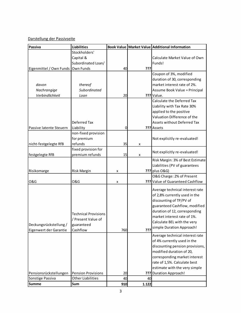
Darstellung der Passivseite
Passiva Liabilities Book Value Market Value Additional Information
Eigenmittel / Own Funds
Stockholders'
Capital &
Subordinated Loan/
Own Funds 40 ???
Calculate Market Value of Own
Funds!
davon
Nachrangige
Verbindlichkeit
thereof
Subordinated
Loan 20 ???
Coupon of 3%, modified
duration of 30, corresponding
market interest rate of 2%.
Assume Book Value = Principal
Value.
Passive latente Steuern
Deferred Tax
Liability 0 ???
Calculate the Deferred Tax
Liability with Tax Rate 30%
applied to the positive
Valuation Difference of the
Assets without Deferred Tax
Assets
nicht-festgelegte RfB
non-fixed provision
for premium
refunds 35 x
Not explicitly re-evaluated!
festgelegte RfB
fixed provision for
premium refunds 15 xNot explicitly re-evaluated!
Risikomarge Risk Margin x ???
Risk Margin: 3% of Best Estimate
Liabilities (PV of guarantees
plus O&G)
O&G O&G x ???
O&G Charge: 2% of Present
Value of Guaranteed Cashflow
Deckungsrückstellung /
Eigenwert der Garantie
Technical Provisions
/ Present Value of
guaranteed
Cashflow 760 ???
Average technical interest rate
of 2,8% currently used in the
discounting of TP/PV of
guaranteed Cashflow, modified
duration of 12, corresponding
market interest rate of 1%.
Calculate BEL with the very
simple Duration Approach!
Pensionsrückstellungen Pension Provisions 20 ???
Average technical interest rate
of 4% currently used in the
discounting pension provisions,
modified duration of 20,
corresponding market interest
rate of 1,5%. Calculate best
estimate with the very simple
Duration Approach!
Sonstige Passiva Other Liabilities 40 40
Summe Sum 910 1.122
4
Aufgabe 1. Case Study – Analyse der ökonomischen Bilanz von VitaLife (50 Bewertungspunkte) Runden Sie für die nachfolgenden Teilaufgaben a) bis c) die Einzelergebnisse jeweils ohne Nachkommastellen, bevor Sie weiterrechnen.
a) Berechnen Sie die fehlenden Positionen in der Marktwertbilanz und ersetzen Sie die Fragezeichen durch die berechneten Markwerte. (16 Punkte)
b) Szenario1 ausgehend von den Ergebnissen in Teilaufgabe a): Die Duration der Namensschuldverschreibungen wurde mit 12 auf die Duration der Deckungsrückstellung abgestimmt, so dass beide gleich sind. Berechnen Sie die Veränderung der Solvency II-Eigenmittel (Own Funds) bei einer Variation des 12-Jahreszinssatzes um plus 10 Basispunkte und um minus 10 Basispunkte. Alle anderen Zinssätze bleiben gleich. Analysieren und interpretieren Sie die Ergebnisse aus Sicht eines Risikomanagers. (10 Punkte)
c) Szenario 2 ausgehend von den Ergebnissen in Teilaufgabe a): Nehmen Sie nun an, dass die Duration der Namensschuldverschreibungen nur bei 10 liegt und die der Deckungsrückstellung bei 14. Berechnen Sie die Solvency II-Eigenmittel (Own Funds) neu. Nehmen Sie dabei an, dass der 14-jährige und der 10-jährige Zinssatz mit dem 12-jährigen aus Aufgabenteil a) identisch sind. Analysieren und interpretieren Sie die Ergebnisse aus Sicht eines Risikomanagers. (10 Punkte)
d) Nehmen Sie Szenario 2 als Ausgangspunkt. Stellen Sie das Risikoprofil von VitaLife auf und diskutieren Sie die Risikosituation der VitaLife per Expertenmeinung qualitativ. Überlegen Sie sich Maßnahmen zur Verbesserung der Risikosituation. Ziehen Sie mindestens eine Absicherungsstrategie in Betracht. (14 Punkte)

5
Aufgabe 2. Case Study – Wahl eines Bewertungsmodells für VitaLife (30 Bewertungspunkte)
VitaLife nutzt die Solvency II-Standardformel zur Berechnung der Risiken mit einem einfachen
Excelmodell. In diesem Excelmodell wird auch die Solvency II-Bilanz berechnet. Bei der Aufstellung der
Bilanz werden sowohl der Wert der Optionen und Garantien als auch die Risikomarge mit einem
pauschalen prozentualen Aufschlag auf die Berechnung des Eigenwerts der Garantie (Barwerts der
garantierten Cahsflows) berücksichtigt (siehe Aufgabe 1).
Der Vorstand der VitaLife möchte die Bewertung in der Solvency II-Bilanz verbessern und hat zwei
Modelle zur Verfügung, um die Bewertung der Optionen und Garantien zu verbessern:
A. Ein deterministisches Bewertungsmodell mit einer geschlossenen Formel zur Bewertung der
Optionen und Garantien. Nach Kalibrierung mit Kapitalmarktdaten und
unternehmensinternen Daten liefert das Modell innerhalb von 5 Minuten die Solvency II-
Bilanz. Zur Bedienung des Modells sind 30% der Arbeitszeit eines Mitarbeiters notwendig.
B. Ein stochastisches Bewertungsmodell mit einem Szenariogenerator zur Bewertung der
Optionen und Garantien. Die Kalibrierung des Szenariogenerators erfordert den Aufbau von
Fachwissen und bindet 30% der Arbeitszeit eines Mitarbeiters. Die Berechnung der Solvency
II-Bilanz mit dem stochastischen Modell dauert 12 Stunden. Zur Bedienung des Modells sind
weitere 40% der Arbeitszeit eines Mitarbeiters notwendig.
Beide Modelle stellen die Solvency II-Bilanz auf, enthalten jedoch keine Risikoberechnung. Eine
Umsetzung der Risikoberechnung im Sinne der Solvency II-Standardformel muss noch gemacht werden.
Bearbeiten Sie folgende Teilaufgaben.
a) Diskutieren Sie die Vor- und Nachteile dieser Bewertungsmodelle.
(10 Punkte)
b) Schlagen Sie zusätzliche Informationen vor, die das Unternehmen anfordern oder selbst
erzeugen, auswerten und beachten sollte, bevor es sich für ein Modell entscheidet.
(10 Punkte)
c) Entscheiden Sie sich für eine Modellvariante und machen Sie einen Vorschlag, wie die
Risikoberechnung mittels der Standardformel mit dem Bewertungsmodell verknüpft werden
kann.
Diskutieren Sie die Vor- und Nachtteile ihres Vorschlags.
(10 Punkte)
6
Aufgabe 3. Risikobewertung, Risikominderung und Wertveränderung (40 Bewertungspunkte)
a) Mehrjahressicht in der Risikobewertung
(20 Bewertungspunkte)
Runden Sie Wahrscheinlichkeiten auf 1% / 0,5%-Schritte.
Gegenwärtig hat die KULANZ-Versicherung Eigenmittel von 130 und eine Solvency-II
Solvenzanforderung von 100.
Sie möchten eine zweijährige Risikoperspektive einnehmen. Dabei nehmen Sie an, dass die
Eigenmittel nach jeweils einem Jahr normalverteilt und gemeinsam multivariat normalverteilt
sind mit Erwartung gleich den aktuellen Eigenmittel sowie gleichbleibender Volatilität.
Bearbeiten Sie folgende Fragen.
i) Angenommen, Sie behalten das Sicherheitsheitsniveau von 99,5% bei, wie sind die
Kapitalanforderung und die Solvenzbedeckung? (Hier dürfen Sie annehmen, dass die
jahresweisen Änderungen unabhängig sind.)
ii) Bei welchem Sicherheitsniveau für 2-jährigen-Horizont ergibt sich dieselbe
Kapitalanforderung wie für 1-Jahres-Horizont und 99,5% Sicherheitsniveau, wenn die
jahresweisen Änderungen unabhängig sind?
iii) Bei welcher Korrelationsannahme ist die Kapitalanforderung für 2-jährigen Horizont und
Sicherheitsniveau von 95% gleich der Kapitalanforderung für 1-Jahr und 99,5%?
iv) Wie vergleicht sich die zweijährige Kapitalanforderung im Fall von ii) mit der Forderung,
nach einem Jahr noch die Solvency II-Anforderung zu erfüllen? Berechnen Sie für
letzteres die Wahrscheinlichkeit.
v) Im Kontext von Solvency II wird das 99,5%-Perzentil oft als 1-in-200-Jahres-Ereignis
bezeichnet. Was bedeuten die obigen Varianten für diese Interpretation?
vi) Ein Kollege, der gehört hat, dass das 99,5%-Perzentil in der Solvency II-Kalibrierung sehr
schwer bestimmbar ist, schlägt daher vor, dieses über iii) und das leichter bestimmbare
2-Jahres-95%-Perzentil zu berechnen. Unterziehen sie den Vorschlag einer kritischen
Würdigung.
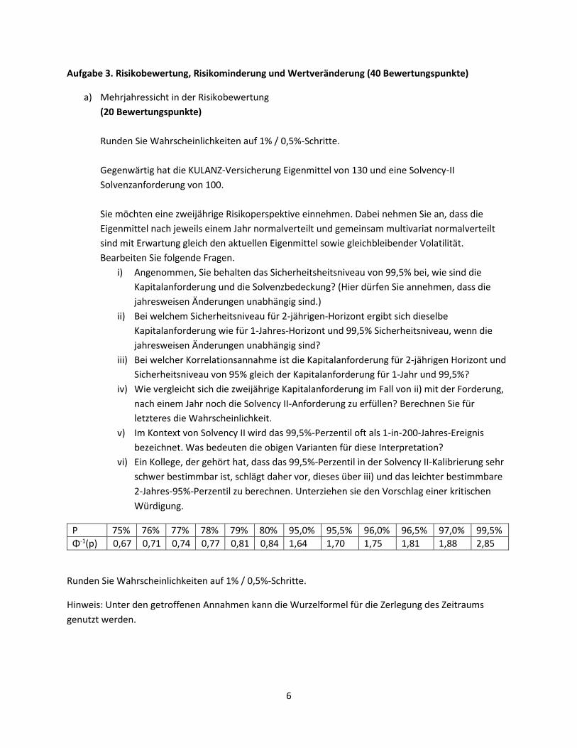
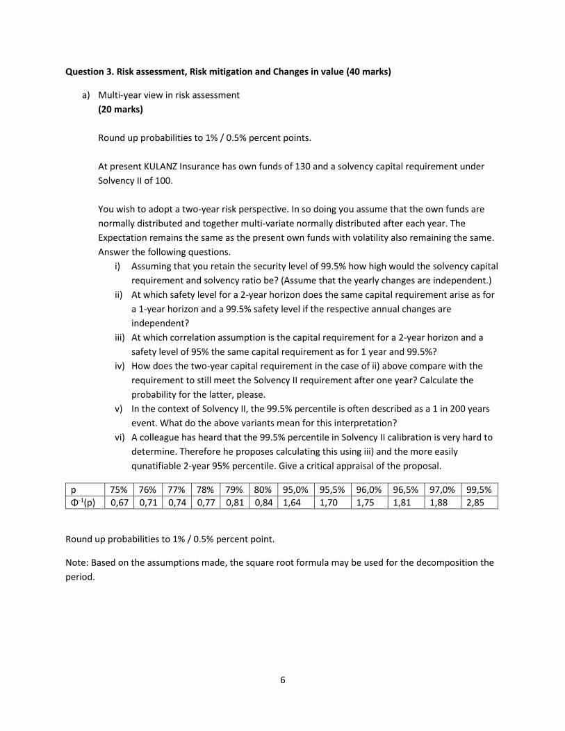
P 75% 76% 77% 78% 79% 80% 95,0% 95,5% 96,0% 96,5% 97,0% 99,5%
Φ-1(p) 0,67 0,71 0,74 0,77 0,81 0,84 1,64 1,70 1,75 1,81 1,88 2,85
Runden Sie Wahrscheinlichkeiten auf 1% / 0,5%-Schritte.
Hinweis: Unter den getroffenen Annahmen kann die Wurzelformel für die Zerlegung des Zeitraums
genutzt werden.
7
b) Ansatz von Risikominderung und Änderung des Kapitals
(20 Bewertungspunkte)
Sie sind Risikomanager der SecuraLife Lebensversicherung.
Zum vorangegangenen Stichtag 31.12.2015 betrugen die Own Funds, der Überschuss der
Aktiva über die Verbindlichkeiten 160.
Sie haben Sensitivitätsanalysen bezüglich Zins und Spread durchgeführt und festgestellt, dass
der jeweilige Quantil-Stress die Bilanz zum 31.12.2015 wie folgt ändert:
Im Zinsstress wachsen „Brutto“ der Wert der Kapitalanlagen um +10 und der Wert
der Verbindlichkeiten um +37.
Im Spreadstress wird der „Brutto“-Wert der Kapitalanlagen um 36 reduziert.
Im kombinierten Stress addieren sich diese „Brutto“-Wirkungen.
Die antizipierte Überschussbeteiligung dämpft den Eigenmittelverlust. Sie kann in jedem der
drei Stresse jeweils um 1/3 des Stresses, maximal jedoch 12, reduziert werden, um vom
„Brutto“- auf den „Netto“-Stress zu kommen.
Beantworten Sie die folgenden Fragen.
i) Das Basis-Risikokapital wird sowohl für „Brutto“ als auch für „Netto“ mit der
Wurzelformel mit Korrelation 0 aus den beiden Einzelstressen berechnet. Das „Netto“-
Risikokapital ergibt sich aus dem Maximum aus „Netto“-Basis-Risikokapital einerseits
und „Brutto“-Basis-Risikokapital abzüglich der Überschussbeteiligung von 12. D.h.
„Netto“-RK = max(„Netto“-Basis-RK, „Brutto“-Basis-RK – 12). Berechnen Sie das „Netto“-
Risikokapital. Wie beurteilen Sie die zugrundeliegenden Annahmen?
ii) Zum 31.12.2016 ist genau der kombinierte Stress eingetreten, andere Änderungen
ergaben sich nicht und die Entwicklung ist entsprechend der Stresse. Diskutieren Sie die
Gestaltungsmöglichkeiten für die Zuordnung der Gewinne und Verluste auf die
Risikotreiber mit mindestens Zahlenbeispielen zu zwei verschiedenen Zuordnungen.
(Vernachlässigen Sie andere Einflüsse wie Roll-Forward, Neugeschäft der Berichtsperiode
etc.)
iii) Die SecuraLife ist Teil der Garantia-Gruppe mit der zweiten Tochter RiskyLife. Die Holding
hat keine eigenen Bilanz- oder Risikokapital-Beiträge. Die Gruppe benutzt ebenfalls die
obige Berechnung für „Brutto“ und „Netto“-Risikokapital. Die Gruppenbilanz im Basisfall
wie in den Stressen durch Addition der Solobilanzen bestimmt, auf Gruppenebene wird
ebenfalls die Entlastung auf die zukünftige Überschussbeteiligung der Gruppe begrenzt.
(Dies ist analog zur Standardformel in Solvency II.)
Das Risikokapital beruht wieder nur auf Zins und Spread. Beide Töchter haben identische
„Brutto“- und „Netto“-Risikokapitalien für die einzelnen Module.
Ein Kollege aus dem Rechnungswesen wundert sich, warum die Gruppe dennoch ein
niedrigeres SCR hat als die Summe der Töchter.
Geben Sie eine unter den Voraussetzungen mögliche Erklärung und ein Zahlenbeispiel.
Beurteilen Sie, in wie fern der ausgewiesene Diversifikationseffekt ökonomisch
realistisch ist.

8
Wie könnte die Berechnung modifiziert werden, um unplausible Effekte zu vermeiden?
Hinweis: Für das Zahlenbeispiel dürfen Sie andere Own Funds, Überschussbeteiligungs-
und SCR-Werte unterstellen als in Fragen 3b) i)) und 3b) ii)).
9
Aufgabe 4 Mergers & Acquisitions (M&A) (60 Bewertungspunkte)
Sie sind CRO eines Unternehmens, das bislang in der Nichtlebenserstversicherung aktiv ist und die
Schwerpunkte in der Feuer- und Elementarschadenversicherung hat. In der Kfz-Versicherung haben Sie
ein kleines, volatiles Portfolio. Ihr Unternehmen unterhält ein zertifiziertes internes Modell.
Limit und Triggersystem: der NatCat-Trigger ist im mittleren gelben Bereich.
Dem Vorstand bietet sich die Gelegenheit, ein Versicherungsunternehmen kaufen zu können, das sich
auf Kfz-Versicherung spezialisiert hat und dort sehr erfolgreich ist.
Um die Kaufentscheidung zu unterstützen, sollen Sie für den Vorstand eine Stellungnahme bezüglich der
Transaktion vorbereiten. Dazu stehen Ihnen nur öffentliche Informationen zur Verfügung.
a) Um den quantitativen Einfluss der Akquise auf Ihr internes Modell abzuschätzen, führen Sie eine
Analyse auf Basis der öffentlich verfügbaren Informationen wie Geschäftsbericht oder
Analysteninformationen durch.
Welche Informationen verwenden Sie vor allem und welche Überlegungen bezüglich der
Integration in Ihr internes Modell stellen Sie an? Gehen Sie in Ihrer Beschreibung die wichtigsten
Risikokategorien durch!
(Punkte: 15)
b) Momentan ist in Ihrem Limit- und Triggersystem der Trigger für Naturkatastrophenschäden nahe
der roten Zone. Nach der Integration des zu akquirierenden Versicherungsunternehmens gehen
Sie davon aus, dass der Trigger in die rote Zone fallen würde. Diskutieren Sie Vor- und Nachteile
zweier Möglichkeiten, die Situation zu entschärfen.
(Punkte: 8)
c) Der Vorstand möchte außer dem Einfluss auf die Solvenz auch wissen, wie sich das S&P Rating
Ihres Unternehmens voraussichtlich entwickeln wird. Welche Faktoren spielen dabei eine Rolle?
Beschreiben Sie kurz die Funktionsweise des S&P Insurance Capital Models.
(Punkte: 6)
10
Im zweiten Schritt haben Sie die Möglichkeit, von dem Management des zu akquirierenden
Unternehmens Antworten auf einige Fragen und weitergehende Materialien zu erhalten. Dabei wollen
Sie ein besseres Verständnis für einzelne Risikoklassen gewinnen.
d) Welche Emerging Risks interessieren Sie in diesem Kontext und welche Punkte möchten Sie in
Erfahrung bringen? Erörtern Sie zwei Risiken.
(Punkte: 8)
e) Welche weiteren nichtmodellierbaren Risiken könnten sich durch den Kauf ergeben? Welche
Fragen stellen Sie und wie gehen Sie mit diesen Risiken um? Diskutieren Sie auch hier zwei
Risiken.
(Punkte: 8)
Die M&A Aktion war erfolgreich und das neue Unternehmen soll durch Aufnahme fusioniert werden. Sie
sollen nun die Gesellschaft in Ihr internes Modell integrieren.
f) Führen Sie die in Aufgabenteil (a) skizzierten Überlegungen weiter und machen Sie einen
Vorschlag, wie der Diversifikationseffekt durch das neue versicherungstechnische Portfolio in der
integrierten Steuerung der beiden Portfolios verwendet werden soll. Welchen Einfluss wird das
veränderte Risikomodell auf Ihre Steuerung der Portfolios haben? Diskutieren Sie ihn am Beispiel
der Steuerungsgröße RoRaC. Wie gehen Sie damit um?
(Punkte: 15)

11
Lösungsvorschlag zu Aufgabe 1:
Teil a)
Aktiva Assets Book Value Market Value Additional Information
Immaterielle
Vermögensgegenstände Intangible Assets 10 5
The company has self-developed software
valued with 5. The software is also sold to
other companies. Solvency II principles are
applied.
Immobilien (Grundstücke, Gebäude,
etc.) Real Estate (land, buildings, etc.) 100 115Hidden Reserves: 15% of book value
Aktien (direkt & Fonds) Equity (direct & Funds) 60 60 Book Value = Fair Value
Hypothekenschuldforderungen Mortgage Loans 110 125 Hidden Reserves of 15
Namensschuldverschreibungen Registered Bonds 400 506
Average coupon of 3,2%, modified duration
of 12, corresponding market interest rate
of 1%. Assume Book Value = Principal
Value. Calculate MV with the very simple
Duration Approach!
Schuldscheindarlehen Debentures / Bonds 200 230
Average coupon of 3%, modified duration
of 5, corresponding market interest rate of
0%. Assume Book Value = Principal Value.
Einlagen bei Kreditinsituten Deposits with Credit Institutions 20 20
Sonstige Aktiva Other Assets 10 10
Aktive latente Steuern Deferred Tax Asset 0 51
Calculate the Deferred Tax Asset with Tax
Rate 30% applied to the positive Valuation
Difference of the Liabilities without Own
Funds and Deferred Tax Liability
Summe Sum 910 1.122
Passiva Liabilities Book Value Market Value Additional Information
Eigenmittel / Own Funds
Stockholders' Capital &
Subordinated Loan/ Own Funds 40 34Calculate Market Value of Own Funds!
davon
Nachrangige Verbindlichkeit
thereof
Subordinated Loan 20 26
Coupon of 3%, modified duration of 30,
corresponding market interest rate of 2%.
Assume Book Value = Principal Value.
Passive latente Steuern Deferred Tax Liability 0 48
Calculate the Deferred Tax Liability with
Tax Rate 30% applied to the positive
Valuation Difference of the Assets without
Deferred Tax Assets
nicht-festgelegte RfB
non-fixed provision for premium
refunds 35 xNot explicitly re-evaluated!
festgelegte RfB
fixed provision for premium
refunds 15 xNot explicitly re-evaluated!
Risikomarge Risk Margin x 28
Risk Margin: 3% of Best Estimate Liabilities
(PV of guarantees plus O&G)
O&G O&G x 18
O&G Charge: 2% of Present Value of
Guaranteed Cashflow
Deckungsrückstellung / Eigenwert
der Garantie
Technical Provisions / Present
Value of guaranteed Cashflow 760 924
Average technical interest rate of 2,8%
currently used in the discounting of TP/PV
of guaranteed Cashflow, modified duration
of 12, corresponding market interest rate
of 1%. Calculate BEL with the very simple
Duration Approach!
Pensionsrückstellungen Pension Provisions 20 30
Average technical interest rate of 4%
currently used in the discounting pension
provisions, modified duration of 20,
corresponding market interest rate of 1,5%.
Calculate best estimate with the very
simple Duration Approach!
Sonstige Passiva Other Liabilities 40 40
Summe Sum 910 1.122
12
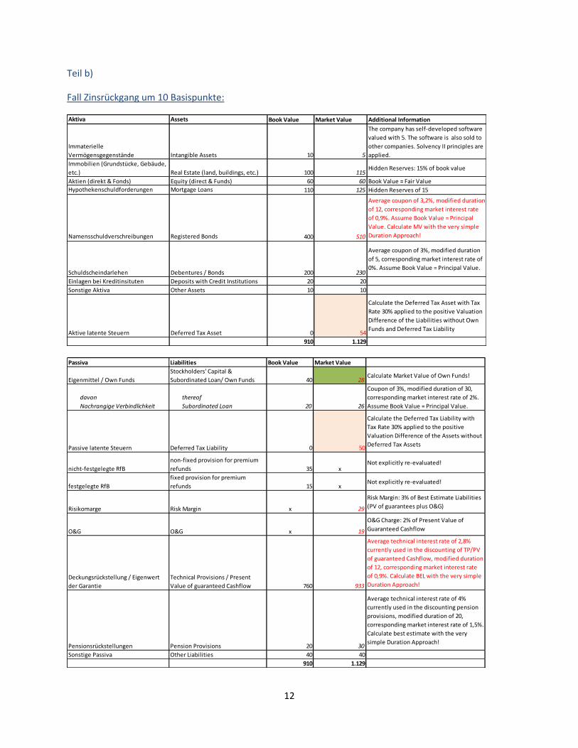
Teil b)
Fall Zinsrückgang um 10 Basispunkte:
Aktiva Assets Book Value Market Value Additional Information
Immaterielle
Vermögensgegenstände Intangible Assets 10 5
The company has self-developed software
valued with 5. The software is also sold to
other companies. Solvency II principles are
applied.
Immobilien (Grundstücke, Gebäude,
etc.) Real Estate (land, buildings, etc.) 100 115Hidden Reserves: 15% of book value
Aktien (direkt & Fonds) Equity (direct & Funds) 60 60 Book Value = Fair Value
Hypothekenschuldforderungen Mortgage Loans 110 125 Hidden Reserves of 15
Namensschuldverschreibungen Registered Bonds 400 510
Average coupon of 3,2%, modified duration
of 12, corresponding market interest rate
of 0,9%. Assume Book Value = Principal
Value. Calculate MV with the very simple
Duration Approach!
Schuldscheindarlehen Debentures / Bonds 200 230
Average coupon of 3%, modified duration
of 5, corresponding market interest rate of
0%. Assume Book Value = Principal Value.
Einlagen bei Kreditinsituten Deposits with Credit Institutions 20 20
Sonstige Aktiva Other Assets 10 10
Aktive latente Steuern Deferred Tax Asset 0 54
Calculate the Deferred Tax Asset with Tax
Rate 30% applied to the positive Valuation
Difference of the Liabilities without Own
Funds and Deferred Tax Liability
910 1.129
Passiva Liabilities Book Value Market Value
Eigenmittel / Own Funds
Stockholders' Capital &
Subordinated Loan/ Own Funds 40 28Calculate Market Value of Own Funds!
davon
Nachrangige Verbindlichkeit
thereof
Subordinated Loan 20 26
Coupon of 3%, modified duration of 30,
corresponding market interest rate of 2%.
Assume Book Value = Principal Value.
Passive latente Steuern Deferred Tax Liability 0 50
Calculate the Deferred Tax Liability with
Tax Rate 30% applied to the positive
Valuation Difference of the Assets without
Deferred Tax Assets
nicht-festgelegte RfB
non-fixed provision for premium
refunds 35 xNot explicitly re-evaluated!
festgelegte RfB
fixed provision for premium
refunds 15 xNot explicitly re-evaluated!
Risikomarge Risk Margin x 29
Risk Margin: 3% of Best Estimate Liabilities
(PV of guarantees plus O&G)
O&G O&G x 19
O&G Charge: 2% of Present Value of
Guaranteed Cashflow
Deckungsrückstellung / Eigenwert
der Garantie
Technical Provisions / Present
Value of guaranteed Cashflow 760 933
Average technical interest rate of 2,8%
currently used in the discounting of TP/PV
of guaranteed Cashflow, modified duration
of 12, corresponding market interest rate
of 0,9%. Calculate BEL with the very simple
Duration Approach!
Pensionsrückstellungen Pension Provisions 20 30
Average technical interest rate of 4%
currently used in the discounting pension
provisions, modified duration of 20,
corresponding market interest rate of 1,5%.
Calculate best estimate with the very
simple Duration Approach!
Sonstige Passiva Other Liabilities 40 40
910 1.129

13
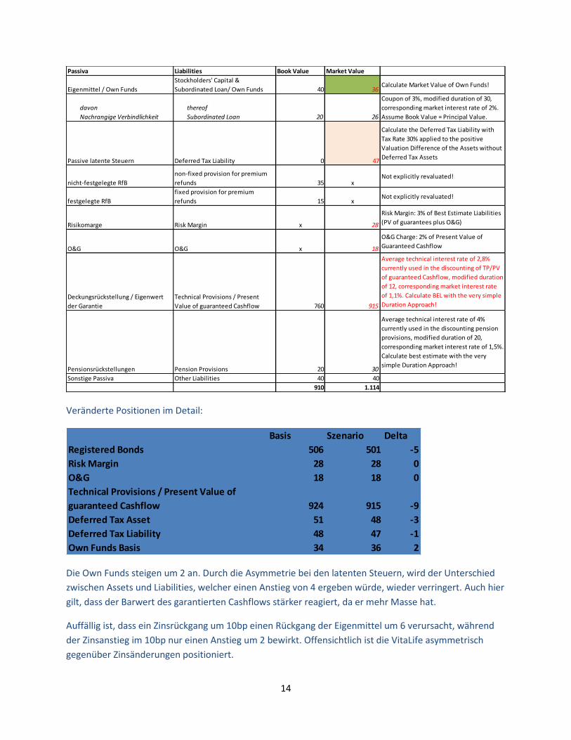
Veränderte Positionen im Detail:
Der Zinsrückgang bewirkt einen Rückgang in den Own Funds. Latente Steuern zeigen saldiert einen
positiven Effekt, da die aktiven latenten Steuern stärker anwachsen. Der Rückgang resultiert aus dem
stärkeren Anwachsen des Barwerts des garantierten Cashflows. Der Barwert hat zwar dieselbe Duration
wie die Namensschuldverschreibungen, bringt jedoch das doppelte Gewicht in die Berechnung mit ein.
Dies liegt daran, dass das Gewicht auf der Passivseite (Garantierter Cashflow plus Inklusive O&G und
Risikomarge) bei Zinsänderung mit Marktwert 970 (=924+18+28) nahezu doppelt so hoch ist wie die
Aktivseite (Namensschuldverschreibungen) mit Marktwert 506.
Fall Zinsanstieg um 10 Basispunkte:
Basis Szenario Delta
Registered Bonds 506 510 4
Risk Margin 28 29 1
O&G 18 19 1
Technical Provisions / Present Value of
guaranteed Cashflow 924 933 9
Deferred Tax Asset 51 54 3
Deferred Tax Liability 48 50 2
Own Funds Basis 34 28 -6
Aktiva Assets Book Value Market Value Additional Information
Immaterielle
Vermögensgegenstände Intangible Assets 10 5
The company has self-developed software
valued with 5. The software is also sold to
other companies. Solvency II principles are
applied.
Immobilien (Grundstücke, Gebäude,
etc.) Real Estate (land, buildings, etc.) 100 115Hidden Reserves: 15% of book value
Aktien (direkt & Fonds) Equity (direct & Funds) 60 60 Book Value = Fair Value
Hypothekenschuldforderungen Mortgage Loans 110 125 Hidden Reserves of 15
Namensschuldverschreibungen Registered Bonds 400 501
Average coupon of 3,2%, modified duration
of 12, corresponding market interest rate
of 1,1%. Assume Book Value = Principal
Value. Calculate MV with the very simple
Duration Approach!
Schuldscheindarlehen Debentures / Bonds 200 230
Average coupon of 3%, modified duration
of 5, corresponding market interest rate of
0%. Assume Book Value = Principal Value.
Einlagen bei Kreditinsituten Deposits with Credit Institutions 20 20
Sonstige Aktiva Other Assets 10 10
Aktive latente Steuern Deferred Tax Asset 0 48
Calculate the Deferred Tax Asset with Tax
Rate 30% applied to the positive Valuation
Difference of the Liabilities without Own
Funds and Deferred Tax Liability
910 1.114
14
Veränderte Positionen im Detail:
Die Own Funds steigen um 2 an. Durch die Asymmetrie bei den latenten Steuern, wird der Unterschied
zwischen Assets und Liabilities, welcher einen Anstieg von 4 ergeben würde, wieder verringert. Auch hier
gilt, dass der Barwert des garantierten Cashflows stärker reagiert, da er mehr Masse hat.
Auffällig ist, dass ein Zinsrückgang um 10bp einen Rückgang der Eigenmittel um 6 verursacht, während
der Zinsanstieg im 10bp nur einen Anstieg um 2 bewirkt. Offensichtlich ist die VitaLife asymmetrisch
gegenüber Zinsänderungen positioniert.
Passiva Liabilities Book Value Market Value
Eigenmittel / Own Funds
Stockholders' Capital &
Subordinated Loan/ Own Funds 40 36Calculate Market Value of Own Funds!
davon
Nachrangige Verbindlichkeit
thereof
Subordinated Loan 20 26
Coupon of 3%, modified duration of 30,
corresponding market interest rate of 2%.
Assume Book Value = Principal Value.
Passive latente Steuern Deferred Tax Liability 0 47
Calculate the Deferred Tax Liability with
Tax Rate 30% applied to the positive
Valuation Difference of the Assets without
Deferred Tax Assets
nicht-festgelegte RfB
non-fixed provision for premium
refunds 35 xNot explicitly revaluated!
festgelegte RfB
fixed provision for premium
refunds 15 xNot explicitly revaluated!
Risikomarge Risk Margin x 28
Risk Margin: 3% of Best Estimate Liabilities
(PV of guarantees plus O&G)
O&G O&G x 18
O&G Charge: 2% of Present Value of
Guaranteed Cashflow
Deckungsrückstellung / Eigenwert
der Garantie
Technical Provisions / Present
Value of guaranteed Cashflow 760 915
Average technical interest rate of 2,8%
currently used in the discounting of TP/PV
of guaranteed Cashflow, modified duration
of 12, corresponding market interest rate
of 1,1%. Calculate BEL with the very simple
Duration Approach!
Pensionsrückstellungen Pension Provisions 20 30
Average technical interest rate of 4%
currently used in the discounting pension
provisions, modified duration of 20,
corresponding market interest rate of 1,5%.
Calculate best estimate with the very
simple Duration Approach!
Sonstige Passiva Other Liabilities 40 40
910 1.114
Basis Szenario Delta
Registered Bonds 506 501 -5
Risk Margin 28 28 0
O&G 18 18 0
Technical Provisions / Present Value of
guaranteed Cashflow 924 915 -9
Deferred Tax Asset 51 48 -3
Deferred Tax Liability 48 47 -1
Own Funds Basis 34 36 2
15
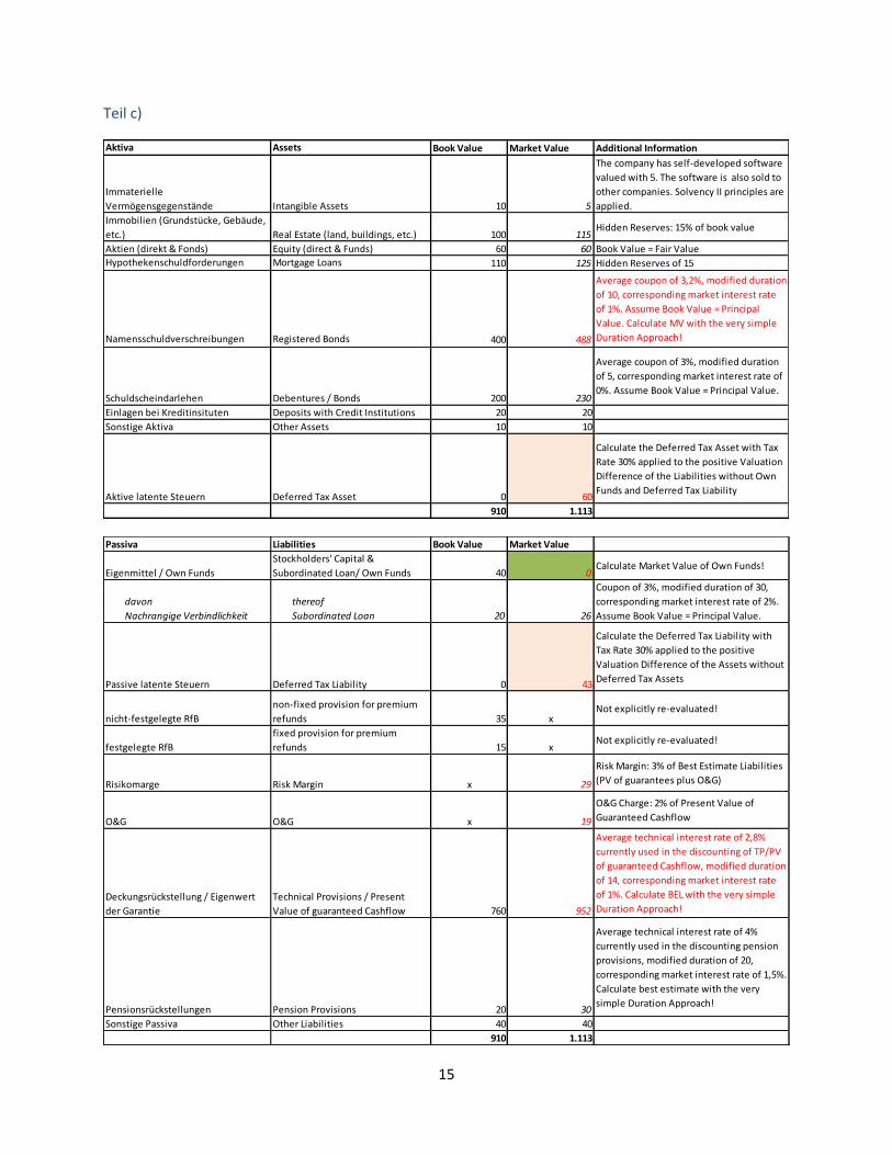
Teil c)
Aktiva Assets Book Value Market Value Additional Information
Immaterielle
Vermögensgegenstände Intangible Assets 10 5
The company has self-developed software
valued with 5. The software is also sold to
other companies. Solvency II principles are
applied.
Immobilien (Grundstücke, Gebäude,
etc.) Real Estate (land, buildings, etc.) 100 115Hidden Reserves: 15% of book value
Aktien (direkt & Fonds) Equity (direct & Funds) 60 60 Book Value = Fair Value
Hypothekenschuldforderungen Mortgage Loans 110 125 Hidden Reserves of 15
Namensschuldverschreibungen Registered Bonds 400 488
Average coupon of 3,2%, modified duration
of 10, corresponding market interest rate
of 1%. Assume Book Value = Principal
Value. Calculate MV with the very simple
Duration Approach!
Schuldscheindarlehen Debentures / Bonds 200 230
Average coupon of 3%, modified duration
of 5, corresponding market interest rate of
0%. Assume Book Value = Principal Value.
Einlagen bei Kreditinsituten Deposits with Credit Institutions 20 20
Sonstige Aktiva Other Assets 10 10
Aktive latente Steuern Deferred Tax Asset 0 60
Calculate the Deferred Tax Asset with Tax
Rate 30% applied to the positive Valuation
Difference of the Liabilities without Own
Funds and Deferred Tax Liability
910 1.113
Passiva Liabilities Book Value Market Value
Eigenmittel / Own Funds
Stockholders' Capital &
Subordinated Loan/ Own Funds 40 0Calculate Market Value of Own Funds!
davon
Nachrangige Verbindlichkeit
thereof
Subordinated Loan 20 26
Coupon of 3%, modified duration of 30,
corresponding market interest rate of 2%.
Assume Book Value = Principal Value.
Passive latente Steuern Deferred Tax Liability 0 43
Calculate the Deferred Tax Liability with
Tax Rate 30% applied to the positive
Valuation Difference of the Assets without
Deferred Tax Assets
nicht-festgelegte RfB
non-fixed provision for premium
refunds 35 xNot explicitly re-evaluated!
festgelegte RfB
fixed provision for premium
refunds 15 xNot explicitly re-evaluated!
Risikomarge Risk Margin x 29
Risk Margin: 3% of Best Estimate Liabilities
(PV of guarantees plus O&G)
O&G O&G x 19
O&G Charge: 2% of Present Value of
Guaranteed Cashflow
Deckungsrückstellung / Eigenwert
der Garantie
Technical Provisions / Present
Value of guaranteed Cashflow 760 952
Average technical interest rate of 2,8%
currently used in the discounting of TP/PV
of guaranteed Cashflow, modified duration
of 14, corresponding market interest rate
of 1%. Calculate BEL with the very simple
Duration Approach!
Pensionsrückstellungen Pension Provisions 20 30
Average technical interest rate of 4%
currently used in the discounting pension
provisions, modified duration of 20,
corresponding market interest rate of 1,5%.
Calculate best estimate with the very
simple Duration Approach!
Sonstige Passiva Other Liabilities 40 40
910 1.113
16
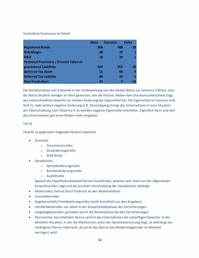
Veränderte Positionen im Detail:
Die Durationslücke von 4 bewirkt in der Umbewertung von der lokalen Bilanz zur Solvency II-Bilanz, dass
die Aktiva deutlich weniger an Wert gewinnen, wie die Passiva. Neben dem Durationsunterschied trägt
das unterschiedliche Gewicht zur starken Änderung der Eigenmittel bei. Die Eigenmittel im Szenario sind
Null (!). Jede weitere negative Änderung (z.B. Zinsrückgang) bringt das Unternehmen in eine Situation
der Überschuldung nach Solvency II. Es würden negative Eigenmittel entstehen. Eigentlich kann und darf
das Unternehmen gar keine Risiken mehr eingehen.
Teil d)
VitaLife ist gegenüber folgenden Risiken exponiert
Zinsrisiko
o Garantiezinsrisiko
o Zinsänderungsrisiko
o ALM-Risiko
Spreadrisiko
o Spreadänderungsrisiko
o Bonitätsänderungsrisiko
o Ausfallrisiko
Speziell der Hypothekenbestand hat ein Ausfallrisiko, welches sehr stark von der allgemeinen
konjunkturellen Lage und der privaten Verschuldung der Hausbesitzer abhängt.
Aktienrisiko: Verlust durch Einbruch an den Aktienmärkten
Immobilienrisiko
Gegebenenfalls Fremdwährungsrisiko (nicht ersichtlich aus den Angaben)
Sterblichkeitsrisiko: vor allem in der Anwartschaftsphase der Versicherungen
Langlebigkeitsrisiko: getrieben durch die Rentenphase bei den Versicherungen
Stornorisiko: bei erhöhtem Storno verliert das Unternehmen die zukünftigen Gewinne. In der
aktuellen Situation, in der die Marktzinsen unter der Garantieverzinsung liegt, ist allerdings ein
niedrigeres Storno risikoreich, da durch das Storno das Wiederanlagerisiko im Moment
verringert wird.
Basis Szenario Delta
Registered Bonds 506 488 -18
Risk Margin 28 29 1
O&G 18 19 1
Technical Provisions / Present Value of
guaranteed Cashflow 924 952 28
Deferred Tax Asset 51 60 9
Deferred Tax Liability 48 43 -5
Own Funds Basis 34 0 -34
17
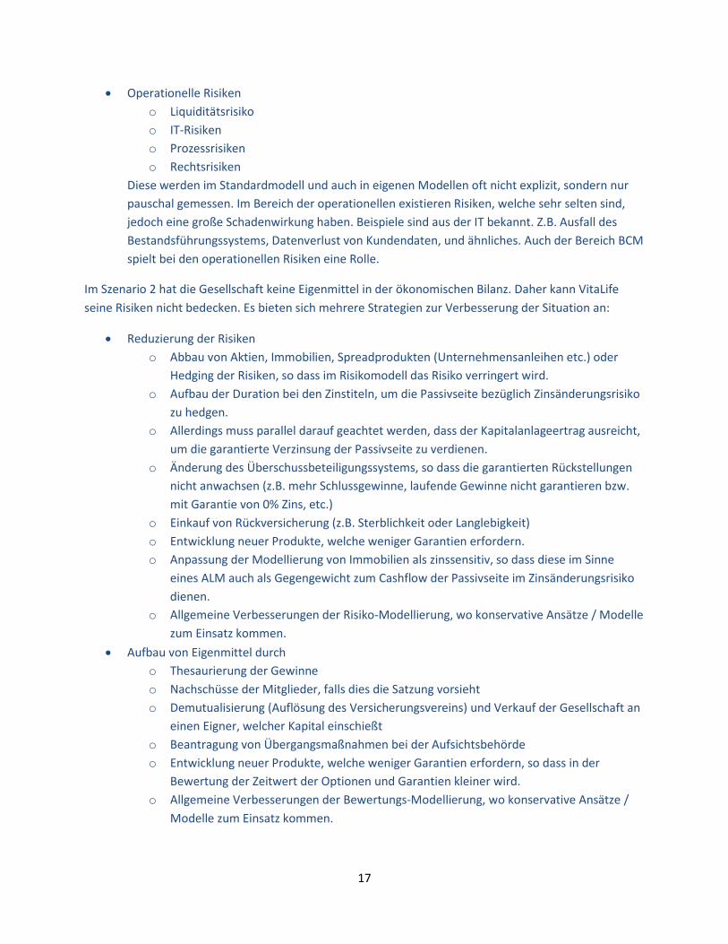
Operationelle Risiken
o Liquiditätsrisiko
o IT-Risiken
o Prozessrisiken
o Rechtsrisiken
Diese werden im Standardmodell und auch in eigenen Modellen oft nicht explizit, sondern nur
pauschal gemessen. Im Bereich der operationellen existieren Risiken, welche sehr selten sind,
jedoch eine große Schadenwirkung haben. Beispiele sind aus der IT bekannt. Z.B. Ausfall des
Bestandsführungssystems, Datenverlust von Kundendaten, und ähnliches. Auch der Bereich BCM
spielt bei den operationellen Risiken eine Rolle.
Im Szenario 2 hat die Gesellschaft keine Eigenmittel in der ökonomischen Bilanz. Daher kann VitaLife
seine Risiken nicht bedecken. Es bieten sich mehrere Strategien zur Verbesserung der Situation an:
Reduzierung der Risiken
o Abbau von Aktien, Immobilien, Spreadprodukten (Unternehmensanleihen etc.) oder
Hedging der Risiken, so dass im Risikomodell das Risiko verringert wird.
o Aufbau der Duration bei den Zinstiteln, um die Passivseite bezüglich Zinsänderungsrisiko
zu hedgen.
o Allerdings muss parallel darauf geachtet werden, dass der Kapitalanlageertrag ausreicht,
um die garantierte Verzinsung der Passivseite zu verdienen.
o Änderung des Überschussbeteiligungssystems, so dass die garantierten Rückstellungen
nicht anwachsen (z.B. mehr Schlussgewinne, laufende Gewinne nicht garantieren bzw.
mit Garantie von 0% Zins, etc.)
o Einkauf von Rückversicherung (z.B. Sterblichkeit oder Langlebigkeit)
o Entwicklung neuer Produkte, welche weniger Garantien erfordern.
o Anpassung der Modellierung von Immobilien als zinssensitiv, so dass diese im Sinne
eines ALM auch als Gegengewicht zum Cashflow der Passivseite im Zinsänderungsrisiko
dienen.
o Allgemeine Verbesserungen der Risiko-Modellierung, wo konservative Ansätze / Modelle
zum Einsatz kommen.
Aufbau von Eigenmittel durch
o Thesaurierung der Gewinne
o Nachschüsse der Mitglieder, falls dies die Satzung vorsieht
o Demutualisierung (Auflösung des Versicherungsvereins) und Verkauf der Gesellschaft an
einen Eigner, welcher Kapital einschießt
o Beantragung von Übergangsmaßnahmen bei der Aufsichtsbehörde
o Entwicklung neuer Produkte, welche weniger Garantien erfordern, so dass in der
Bewertung der Zeitwert der Optionen und Garantien kleiner wird.
o Allgemeine Verbesserungen der Bewertungs-Modellierung, wo konservative Ansätze /
Modelle zum Einsatz kommen.
18
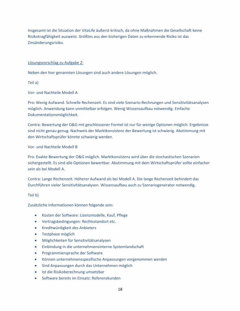
Insgesamt ist die Situation der VitaLife äußerst kritisch, da ohne Maßnahmen die Gesellschaft keine
Risikotragfähigkeit ausweist. Größtes aus den bisherigen Daten zu erkennende Risiko ist das
Zinsänderungsrisiko.
Lösungsvorschlag zu Aufgabe 2:
Neben den hier genannten Lösungen sind auch andere Lösungen möglich.
Teil a)
Vor- und Nachteile Modell A
Pro: Wenig Aufwand. Schnelle Rechenzeit. Es sind viele Szenario-Rechnungen und Sensitivitätsanalysen
möglich. Anwendung kann unmittelbar erfolgen. Wenig Wissensaufbau notwendig. Einfache
Dokumentationsmöglichkeit.
Contra: Bewertung der O&G mit geschlossener Formel ist nur für wenige Optionen möglich. Ergebnisse
sind nicht genau genug. Nachweis der Marktkonsistenz der Bewertung ist schwierig. Abstimmung mit
den Wirtschaftsprüfer könnte schwierig werden.
Vor- und Nachteile Modell B
Pro: Exakte Bewertung der O&G möglich. Marktkonsistenz wird über die stochastischen Szenarien
sichergestellt. Es sind alle Optionen bewertbar. Abstimmung mit dem Wirtschaftsprüfer sollte einfacher
sein als bei Modell A.
Contra: Lange Rechenzeit. Höherer Aufwand als bei Modell A. Die lange Rechenzeit behindert das
Durchführen vieler Sensitivitätsanalysen. Wissensaufbau auch zu Szenariogenerator notwendig.
Teil b)
Zusätzliche Informationen können folgende sein:
Kosten der Software: Lizenzmodelle, Kauf, Pflege
Vertragsbedingungen: Rechtsstandort etc.
Kreditwürdigkeit des Anbieters
Testphase möglich
Möglichkeiten für Sensitivitätsanalysen
Einbindung in die unternehmensinterne Systemlandschaft
Programmiersprache der Software
Können unternehmensspezifische Anpassungen vorgenommen werden
Sind Anpassungen durch das Unternehmen möglich
Ist die Risikoberechnung umsetzbar
Software bereits im Einsatz: Referenzkunden
19
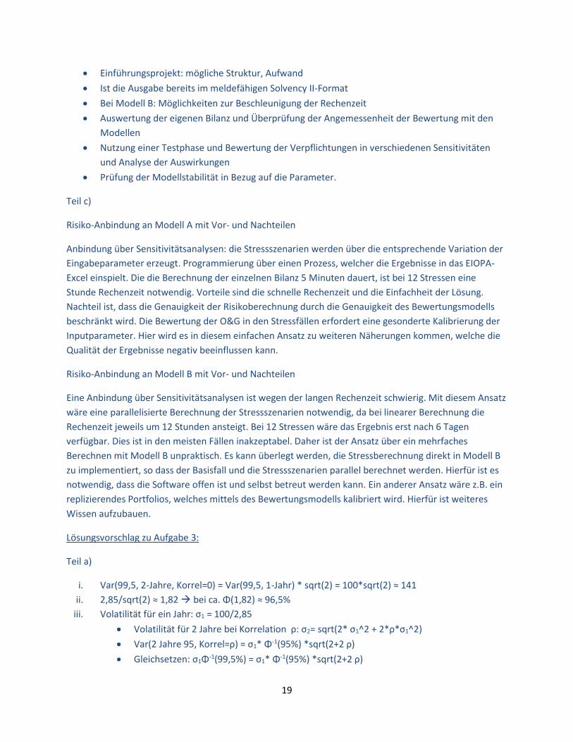
Einführungsprojekt: mögliche Struktur, Aufwand
Ist die Ausgabe bereits im meldefähigen Solvency II-Format
Bei Modell B: Möglichkeiten zur Beschleunigung der Rechenzeit
Auswertung der eigenen Bilanz und Überprüfung der Angemessenheit der Bewertung mit den
Modellen
Nutzung einer Testphase und Bewertung der Verpflichtungen in verschiedenen Sensitivitäten
und Analyse der Auswirkungen
Prüfung der Modellstabilität in Bezug auf die Parameter.
Teil c)
Risiko-Anbindung an Modell A mit Vor- und Nachteilen
Anbindung über Sensitivitätsanalysen: die Stressszenarien werden über die entsprechende Variation der
Eingabeparameter erzeugt. Programmierung über einen Prozess, welcher die Ergebnisse in das EIOPA-
Excel einspielt. Die die Berechnung der einzelnen Bilanz 5 Minuten dauert, ist bei 12 Stressen eine
Stunde Rechenzeit notwendig. Vorteile sind die schnelle Rechenzeit und die Einfachheit der Lösung.
Nachteil ist, dass die Genauigkeit der Risikoberechnung durch die Genauigkeit des Bewertungsmodells
beschränkt wird. Die Bewertung der O&G in den Stressfällen erfordert eine gesonderte Kalibrierung der
Inputparameter. Hier wird es in diesem einfachen Ansatz zu weiteren Näherungen kommen, welche die
Qualität der Ergebnisse negativ beeinflussen kann.
Risiko-Anbindung an Modell B mit Vor- und Nachteilen
Eine Anbindung über Sensitivitätsanalysen ist wegen der langen Rechenzeit schwierig. Mit diesem Ansatz
wäre eine parallelisierte Berechnung der Stressszenarien notwendig, da bei linearer Berechnung die
Rechenzeit jeweils um 12 Stunden ansteigt. Bei 12 Stressen wäre das Ergebnis erst nach 6 Tagen
verfügbar. Dies ist in den meisten Fällen inakzeptabel. Daher ist der Ansatz über ein mehrfaches
Berechnen mit Modell B unpraktisch. Es kann überlegt werden, die Stressberechnung direkt in Modell B
zu implementiert, so dass der Basisfall und die Stressszenarien parallel berechnet werden. Hierfür ist es
notwendig, dass die Software offen ist und selbst betreut werden kann. Ein anderer Ansatz wäre z.B. ein
replizierendes Portfolios, welches mittels des Bewertungsmodells kalibriert wird. Hierfür ist weiteres
Wissen aufzubauen.
Lösungsvorschlag zu Aufgabe 3:
Teil a)
i. Var(99,5, 2-Jahre, Korrel=0) = Var(99,5, 1-Jahr) * sqrt(2) = 100*sqrt(2) ≈ 141
ii. 2,85/sqrt(2) ≈ 1,82 bei ca. Φ(1,82) ≈ 96,5%
iii. Volatilität für ein Jahr: σ1 = 100/2,85
Volatilität für 2 Jahre bei Korrelation ρ: σ2= sqrt(2* σ1^2 + 2*ρ*σ1^2)
Var(2 Jahre 95, Korrel=ρ) = σ1* Φ-1(95%) *sqrt(2+2 ρ)
Gleichsetzen: σ1Φ-1(99,5%) = σ1* Φ-1(95%) *sqrt(2+2 ρ)
20
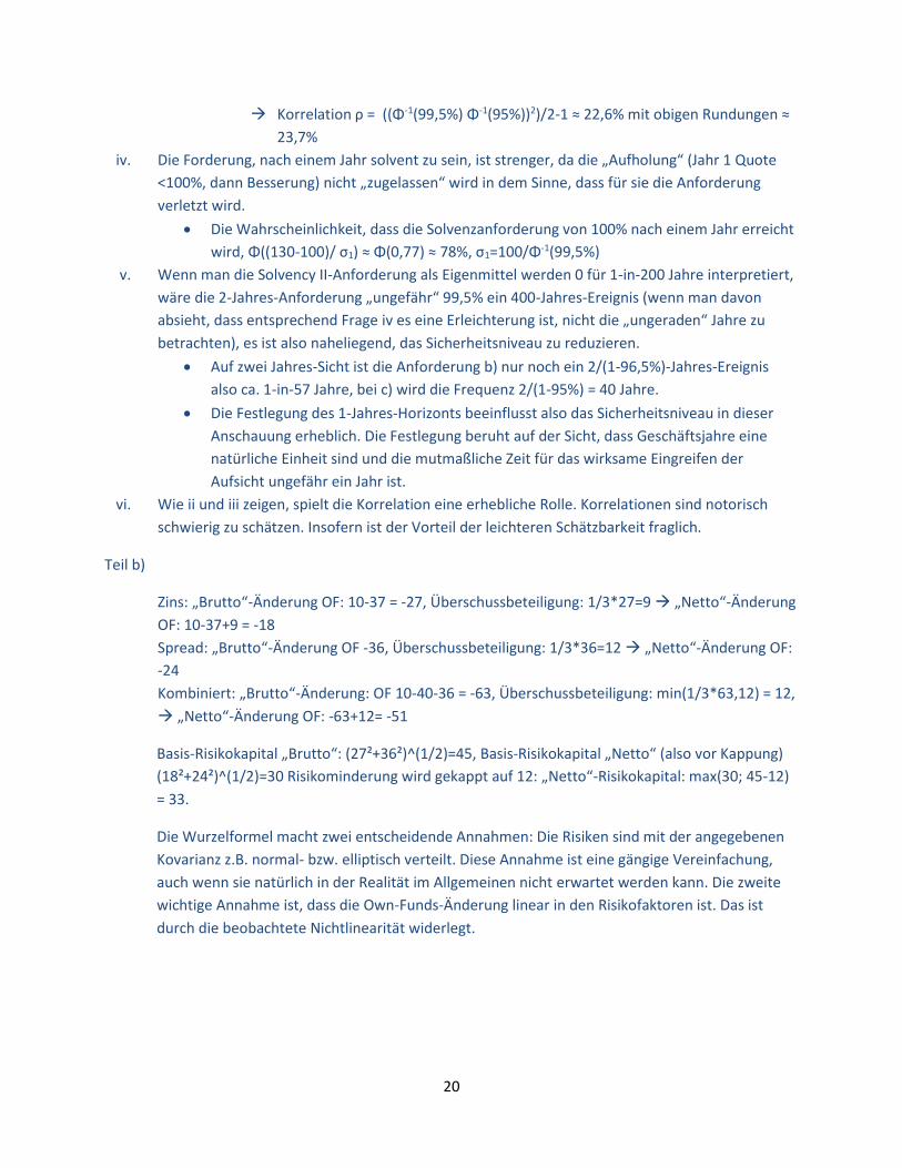
Korrelation ρ = ((Φ-1(99,5%) Φ-1(95%))2)/2-1 ≈ 22,6% mit obigen Rundungen ≈
23,7%
iv. Die Forderung, nach einem Jahr solvent zu sein, ist strenger, da die „Aufholung“ (Jahr 1 Quote
<100%, dann Besserung) nicht „zugelassen“ wird in dem Sinne, dass für sie die Anforderung
verletzt wird.
Die Wahrscheinlichkeit, dass die Solvenzanforderung von 100% nach einem Jahr erreicht
wird, Φ((130-100)/ σ1) ≈ Φ(0,77) ≈ 78%, σ1=100/Φ-1(99,5%)
v. Wenn man die Solvency II-Anforderung als Eigenmittel werden 0 für 1-in-200 Jahre interpretiert,
wäre die 2-Jahres-Anforderung „ungefähr“ 99,5% ein 400-Jahres-Ereignis (wenn man davon
absieht, dass entsprechend Frage iv es eine Erleichterung ist, nicht die „ungeraden“ Jahre zu
betrachten), es ist also naheliegend, das Sicherheitsniveau zu reduzieren.
Auf zwei Jahres-Sicht ist die Anforderung b) nur noch ein 2/(1-96,5%)-Jahres-Ereignis
also ca. 1-in-57 Jahre, bei c) wird die Frequenz 2/(1-95%) = 40 Jahre.
Die Festlegung des 1-Jahres-Horizonts beeinflusst also das Sicherheitsniveau in dieser
Anschauung erheblich. Die Festlegung beruht auf der Sicht, dass Geschäftsjahre eine
natürliche Einheit sind und die mutmaßliche Zeit für das wirksame Eingreifen der
Aufsicht ungefähr ein Jahr ist.
vi. Wie ii und iii zeigen, spielt die Korrelation eine erhebliche Rolle. Korrelationen sind notorisch
schwierig zu schätzen. Insofern ist der Vorteil der leichteren Schätzbarkeit fraglich.
Teil b)
Zins: „Brutto“-Änderung OF: 10-37 = -27, Überschussbeteiligung: 1/3*27=9 „Netto“-Änderung
OF: 10-37+9 = -18
Spread: „Brutto“-Änderung OF -36, Überschussbeteiligung: 1/3*36=12 „Netto“-Änderung OF:
-24
Kombiniert: „Brutto“-Änderung: OF 10-40-36 = -63, Überschussbeteiligung: min(1/3*63,12) = 12,
„Netto“-Änderung OF: -63+12= -51
Basis-Risikokapital „Brutto“: (27²+36²)^(1/2)=45, Basis-Risikokapital „Netto“ (also vor Kappung)
(18²+24²)^(1/2)=30 Risikominderung wird gekappt auf 12: „Netto“-Risikokapital: max(30; 45-12)
= 33.
Die Wurzelformel macht zwei entscheidende Annahmen: Die Risiken sind mit der angegebenen
Kovarianz z.B. normal- bzw. elliptisch verteilt. Diese Annahme ist eine gängige Vereinfachung,
auch wenn sie natürlich in der Realität im Allgemeinen nicht erwartet werden kann. Die zweite
wichtige Annahme ist, dass die Own-Funds-Änderung linear in den Risikofaktoren ist. Das ist
durch die beobachtete Nichtlinearität widerlegt.
21
i. Die Reihenfolge ist wichtig für die Größe der Einzeleffekte:
Mögliche Reihenfolgen sind
OF 2015: 160
Spread: -24
Zins: -27
OF 2016: 109
und
OF 2015: 160
Zins: -33
Spread: -18
OF 2016: 109
Durch anderes Aufteilen der Entlastung durch Reduktion der Überschussbeteiligung kann auch
jeder Zwischenwert erzeugt werden.
Die Reihenfolge der Schritte kann also die Gewichtung der Effekte massiv beeinflussen. Je nach
Interessenlage kann eine Darstellung attraktiver erscheinen als die andere (z.B. wenn Ereignisse
unterschiedlich als „hausgemacht“ angesehen werden).
ii. Beide Unternehmen haben Risikokapital 20 „Brutto“, 10 „Netto“ vor Kappung. SecuraLife hat 15
zukünftige Überschussbeteiligung, RiskyLife nur 5. Daher ergeben sich Risikokapitalien von 10 für
SecuraLife und 15 für RiskyLife.
Die Gruppe hat dann Risikokapital „Brutto“ 40, 20 „Netto“ vor Kappung, aber die
Gruppenentlastung wird gesamthaft auf 20 begrenzt, also nicht gekappt.
Die implizit unterstellte Fungibilität der risikomindernden Wirkung der Überschussbeteiligung ist
fraglich, solange keine Anhaltspunkte dafür bestehen, dass die Gesellschaften Verluste
gegenseitig ausgleichen.
Eine mögliche Lösung wäre, die gekappte Entlastung auf Unternehmensebene auf die
Einzelmodule zu allokieren und dann modulweise zur Gruppenentlastung zu aggregieren.
Lösungsvorschlag zu Aufgabe 4:
Teil a)
Skizze Musterlösung – abweichende Lösungen sind möglich:
Sie sollten sich zumindest die Kategorien Versicherungstechnische Risiken, Markt- und Kreditrisiken,
operationale Risiken betrachten. Pro Risikokategorie definieren Sie eine Segmentierung, die zu Ihrem
internen Modell kompatibel ist. Zu jedem Segment benutzen Sie beispielsweise ein Volumenmaß (VT z.B.
Prämien und Reserven, Markt- und Kredit z.B. Anlagevolumina, Forderungen an Rückversicherer und für
operationale Risiken z.B. Mitarbeiterzahl) und einen Faktor, den Sie aus Ihrem eigenen Modell oder der
Standardformel ableiten. Für Naturkatastrophenschäden können Sie auch historische Schäden aus dem
Geschäftsbericht verwenden. Für die Integration in das interne Modell werden Sie
Wahrscheinlichkeitsverteilungen pro Kategorie brauchen. Diese können Sie aus Ihrem internen Modell

22
übernehmen oder mit einfacheren Annahmen arbeiten. Bei der Integration sollten Sie sich außerdem
über Diversifikationseffekte bzw. Abhängigkeiten Gedanken machen. Dieser Punkt ist gerade bei Ihrem
Kfz-Portfolio relevant, wo Sie unter Umständen erwarten, dass der Ausgleich im Kollektiv die Risiken
kalkulierbarer macht. Bezüglich Marktrisiken- und Kreditrisiken ist außer der Anlagestruktur auch die
Frage relevant, wie mit eventuellen Rückversicherungsverträgen nach der Akquise verfahren werden soll.
Teil b)
Skizze Musterlösung – abweichende Lösungen sind möglich:
z.B. Rückversicherung. Pro – flexible Struktur, kurzfristig möglich und änderbar. Contra – eventuell
kostspielig.
z.B. Transfer auf den Kapitalmarkt, z.B. durch index-linked Produkte. Pro – wahrscheinlich günstig, Contra
– Basisrisiko verbleibt. Spezielles Knowhow zur Anpassung des Index an Portfolio notwendig)
Teil c)
cf Folien „Nebenbedingungen zur Ökonomischen Sicht: Restriktionen aufgrund von
Ratinganforderungen“
Teil d)
Skizze Musterlösung – abweichende Lösungen sind möglich:
z.B. Autonomes Fahren – wie sieht das Engagement des Unternehmens in diesem Segment aus? Welche
zukünftigen Entwicklungen werden erwartet? Welche Player sind momentan auf dem Markt aktiv?
z.B. Datendiebstahl – Sammelt das Unternehmen sensible Daten im Zusammenhang mit der Kfz-
Versicherung? Welche werden verwendet und welche Quellen werden dafür genutzt? Wie sieht das IT
System zur Verwaltung aus? Gab es Angriffe in der Vergangenheit?
Teil e)
Skizze Musterlösung – abweichende Lösungen sind möglich:
z.B. Reputationsrisiken – Im Zusammenhang mit der Datensammlung in der Kfz-Versicherung könnte das
Unternehmen in die Schlagzeilen geraten, wenn es sich unzulässiger Quellen bedient oder die Daten
unzulässig verwendet. Hier sollte Transparenz geschaffen werden über die verwendeten Daten und
Quellen, sowie rechtliche Fragestellungen geklärt werden.
z.B. Key person risk – Falls das zu akquirierende Unternehmen in sehr speziellen Geschäftssegmenten
aktiv ist, könnte es sein, dass der Erfolg an dem Knowhow einiger weniger Mitarbeiter liegt. Um diese zu
halten, können beispielsweise speziell für diese Mitarbeiter Entwicklungspläne für nach der Fusion
erstellt werden.
Teil f)
Skizze Musterlösung – abweichende Lösungen sind möglich:
Der Diversifikationseffekt aus der Versicherungstechnik soll dem neuen wie auch dem alten Portfolio zu
Gute kommen. Dies kann beispielsweise durch Verwendung des Kovarianzprinzips bei der
Kapitalallokation geschehen. Dies führt dazu, dass beispielsweise das dem Feuersegment zugeordnete

23
Risikokapital im Vergleich zu der Berechnung ohne das neue Portfolio sinkt. Der RoRaC für dieses
Segment erhöht sich dadurch. Dieser Effekt sollte transparent kommuniziert werden und auch
beispielsweise in der Zielerreichungsmessung und Zielsetzung berücksichtigt werden. Denkbar ist auch
ein langsameres Umsetzen in die Steuerung, um weniger abrupte Brüche zu erhalten und genauer die
Strategie ausrichten zu können. Die Kommunikation sollte frühzeitig erfolgen, damit die Strategie
vorausschauend angepasst werden kann.
1
Examination for CERA Module D 20.05.2017
The examination has a total of 180 marks. 90 marks are required to pass the examination.
For your guidance on how much time to spend on each question: for each mark you should spend
approximately one minute. You do not always need to formulate your answers in complete sentences. You
may write your answers in the form of keywords. Please note that, to make the questions easier to read,
some empty space has been left between questions. Each question begins on a new page. The examination
has 10 pages.
Preparation for Question 1
The simplified balance sheet of VitaLife life insurance company is to be used as the basis for Question 1.
Imagine that you are a risk manager at VitaLife life insurance company. VitaLife is a mutual insurance company. VitaLife sells classic endowment insurance policies with an annuity option with guaranteed annuity factors. VitaLife's balance sheet is below. Assume that, for the interest-bearing securities, the nominal is the same as the book value.
When revaluing book values to fair values use the duration approach for reasons of simplification unless other information is provided.
2
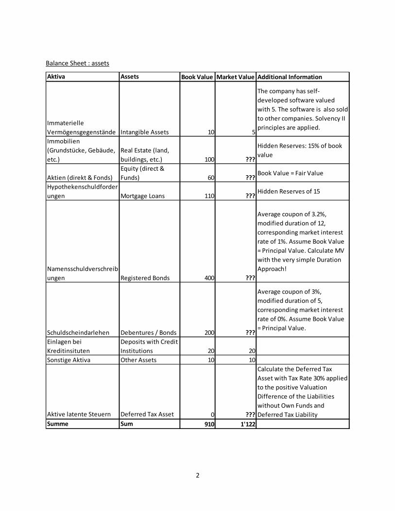
Balance Sheet : assets
Aktiva Assets Book Value Market Value Additional Information
Immaterielle
Vermögensgegenstände Intangible Assets 10 5
The company has self-
developed software valued
with 5. The software is also sold
to other companies. Solvency II
principles are applied.
Immobilien
(Grundstücke, Gebäude,
etc.)
Real Estate (land,
buildings, etc.) 100 ???
Hidden Reserves: 15% of book
value
Aktien (direkt & Fonds)
Equity (direct &
Funds) 60 ???Book Value = Fair Value
Hypothekenschuldforder
ungen Mortgage Loans 110 ???Hidden Reserves of 15
Namensschuldverschreib
ungen Registered Bonds 400 ???
Average coupon of 3.2%,
modified duration of 12,
corresponding market interest
rate of 1%. Assume Book Value
= Principal Value. Calculate MV
with the very simple Duration
Approach!
Schuldscheindarlehen Debentures / Bonds 200 ???
Average coupon of 3%,
modified duration of 5,
corresponding market interest
rate of 0%. Assume Book Value
= Principal Value.
Einlagen bei
Kreditinsituten
Deposits with Credit
Institutions 20 20
Sonstige Aktiva Other Assets 10 10
Aktive latente Steuern Deferred Tax Asset 0 ???
Calculate the Deferred Tax
Asset with Tax Rate 30% applied
to the positive Valuation
Difference of the Liabilities
without Own Funds and
Deferred Tax Liability
Summe Sum 910 1'122
3
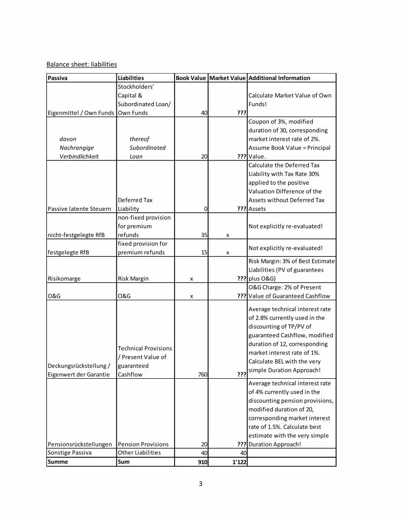
Balance sheet: liabilities
Passiva Liabilities Book Value Market Value Additional Information
Eigenmittel / Own Funds
Stockholders'
Capital &
Subordinated Loan/
Own Funds 40 ???
Calculate Market Value of Own
Funds!
davon
Nachrangige
Verbindlichkeit
thereof
Subordinated
Loan 20 ???
Coupon of 3%, modified
duration of 30, corresponding
market interest rate of 2%.
Assume Book Value = Principal
Value.
Passive latente Steuern
Deferred Tax
Liability 0 ???
Calculate the Deferred Tax
Liability with Tax Rate 30%
applied to the positive
Valuation Difference of the
Assets without Deferred Tax
Assets
nicht-festgelegte RfB
non-fixed provision
for premium
refunds 35 x
Not explicitly re-evaluated!
festgelegte RfB
fixed provision for
premium refunds 15 xNot explicitly re-evaluated!
Risikomarge Risk Margin x ???
Risk Margin: 3% of Best Estimate
Liabilities (PV of guarantees
plus O&G)
O&G O&G x ???
O&G Charge: 2% of Present
Value of Guaranteed Cashflow
Deckungsrückstellung /
Eigenwert der Garantie
Technical Provisions
/ Present Value of
guaranteed
Cashflow 760 ???
Average technical interest rate
of 2.8% currently used in the
discounting of TP/PV of
guaranteed Cashflow, modified
duration of 12, corresponding
market interest rate of 1%.
Calculate BEL with the very
simple Duration Approach!
Pensionsrückstellungen Pension Provisions 20 ???
Average technical interest rate
of 4% currently used in the
discounting pension provisions,
modified duration of 20,
corresponding market interest
rate of 1.5%. Calculate best
estimate with the very simple
Duration Approach!
Sonstige Passiva Other Liabilities 40 40
Summe Sum 910 1'122

4
Question 1. Case Study – Analysis of VitaLife's economic balance sheet (50 marks) For sections a) to c) below, please round up your individual results, with no decimal places, before you make further calculations.
a) Calculate the missing positions in the fair value balance sheet and replace the question marks (= ???) with the fair values you have calculated. (16 marks)
b) Scenario 1 based on the results from question 1 a) above: The duration of the registered bonds has been reconciled -- at 12 -- with the duration of the technical provision so that both are identical. Calculate the change in the Solvency II Own Funds if the 12-year annual interest rate varies by plus 10 basis points and by minus 10 basis. All other interest rates remain the same. Analyse and interpret the results from the perspective of a risk manager. (10 marks)
c) Scenario 2 based on the results from question 1 a) above: Assume that the duration of the registered bonds is only 10 and that the duration of the technical provision is 14. Recalculate the Solvency II Own Funds. Assume that the 14-year and the 10-year interest rate are identical to the 12-year rate from Question 1 a). Analyse and interpret the results from the perspective of a risk manager. (10 marks)
d) Take scenario 2 as a basis for your assumptions. Draw up VitaLife's risk profile and discuss VitaLife's risk situation in the form of a qualitative expert opinion. Propose measures to improve VitaLife's risk situation. Consider at least one hedging strategy. (14 marks)

5
Question 2. Case Study – Selection of a valuation model for VitaLife (30 marks)
VitaLife uses the Solvency II Standard Formula to calculate risks with a simple Excel model. The Solvency
II balance sheet is also calculated using this Excel model. When producing the economic balance sheet
both the value of the options and guarantees and of the risk margin are taken into account with a flat-
rate loading, expressed as a percentage, added to the calculation of the intrinsic value of the guarantee
(present value of guaranteed cash-flows) (See Question 1).
VitaLife's Management Board wishes to improve the valuation in the Solvency II balance sheet and has
two models available with which it could improve the valuation of the options and guarantees:
A. A deterministic valuation model with a closed formula for valuing the options and
guarantees. After calibration with capital market data and own company data the model
produces the Solvency II balance sheet within 5 minutes. Use of the model requires 30% of
the working time of one employee.
B. A stochastic valuation model with a scenario generator for valuing the options and
guarantees. Calibration of the scenario generator requires specialist know how and will tie
up 30% of the working time of one employee. Calculating the Solvency II balance sheet using
the stochastic model takes 12 hours. Use of the model requires an additional 40% of the
working time of one employee.
Both models can produce the Solvency II balance sheet but do not include a risk calculation. Performing
the risk calculation, in the sense of the Solvency II Standard Formula, must still be done.
Answer the following questions.
a) Discuss the advantages and disadvantages of these two valuation models.
(10 marks)
b) Suggest additional information that the company should obtain or produce itself, evaluate and
consider before deciding which model to select.
(10 marks)
c) Decide which model should be selected and make a proposal as to how the risk calculation by
means of the Standard Formula can be linked to the valuation model.
Discuss the advantages and disadvantages of your proposal.
(10 marks)
6
Question 3. Risk assessment, Risk mitigation and Changes in value (40 marks)
a) Multi-year view in risk assessment
(20 marks)
Round up probabilities to 1% / 0.5% percent points.
At present KULANZ Insurance has own funds of 130 and a solvency capital requirement under
Solvency II of 100.
You wish to adopt a two-year risk perspective. In so doing you assume that the own funds are
normally distributed and together multi-variate normally distributed after each year. The
Expectation remains the same as the present own funds with volatility also remaining the same.
Answer the following questions.
i) Assuming that you retain the security level of 99.5% how high would the solvency capital
requirement and solvency ratio be? (Assume that the yearly changes are independent.)
ii) At which safety level for a 2-year horizon does the same capital requirement arise as for
a 1-year horizon and a 99.5% safety level if the respective annual changes are
independent?
iii) At which correlation assumption is the capital requirement for a 2-year horizon and a
safety level of 95% the same capital requirement as for 1 year and 99.5%?
iv) How does the two-year capital requirement in the case of ii) above compare with the
requirement to still meet the Solvency II requirement after one year? Calculate the
probability for the latter, please.
v) In the context of Solvency II, the 99.5% percentile is often described as a 1 in 200 years
event. What do the above variants mean for this interpretation?
vi) A colleague has heard that the 99.5% percentile in Solvency II calibration is very hard to
determine. Therefore he proposes calculating this using iii) and the more easily
qunatifiable 2-year 95% percentile. Give a critical appraisal of the proposal.
p 75% 76% 77% 78% 79% 80% 95,0% 95,5% 96,0% 96,5% 97,0% 99,5%
Φ-1(p) 0,67 0,71 0,74 0,77 0,81 0,84 1,64 1,70 1,75 1,81 1,88 2,85
Round up probabilities to 1% / 0.5% percent point.
Note: Based on the assumptions made, the square root formula may be used for the decomposition the
period.
7
b) Risk mitigation and change in capital
(20 marks)
You are the Risk Manager at SecuraLife life insurance.
On the previous reporting date of 31.12.2015 own funds, the surplus of assets over liabilities
were 160.
You have performed sensitivity analyses concerning interest and spread and calculated that
the respective quantile stress changes the balance sheet as at 31.12.2015 as follows:
In the interest rate stress the value of assets increases "gross" by +10 and the value
of the liabilities by +37.
In the spread stress the value of the assets is reduced by 36 "gross".
In the combined stress these gross effects add up.
The anticipated with-profits surplus participation dampens the loss of own funds . In each of
the three stresses, this loss can be reduced by 1/3 of the stress, though only to a maximum
of 12, in order to get from the "gross" to the "net" stress.
Answer the following questions.
i. The “gross” as well as the “net” basic risk capital (BSCR) is calculated from the two
individual stresses with the square root formula with correlation 0. The “net” risk capital
is obtained as the maximum of the “net”-BSCR and the “gross”-BSCR minus the maximal
risk mitigation effect of with-profit surplus participation of 12, i.e. “net”-RK = max(“Net”-
BSCR, “gross”-BSCR – 12). Calculate the “net” risk capital. How do you assess the
underlying assumptions?
ii. On 31.12.2016, precisely that combined stress occurred, though there were no other
changes and the development is in line with the stresses. Argue scopes for design of
assigning the profits and losses to the risk drivers with at least figures for two different
assignments. (Ignore other influences such as roll-forward, new business during the
reporting period etc.)
iii. SecuraLife is part of the Garantia Group together with the second subsidiary, RiskyLife.
The holding company has no separate balance sheet or risk capital contributions. The
Group also uses the above calculation for "gross" and "net" risk capital. The Group
balance sheet, for the baseline case and for the stresses, is determined by adding the
individual (solo) balance sheets. At Group level any relief is limited to the Group's future
with-profits surplus participation. (This is analogous to the Standard Formula in Solvency
II.)
Once again the risk capital is only based on interest rate and spread. Both subsidiaries
have identical "gross" and "net" risk capitals for the individual modules.
A colleague from the Accounting Department wonders why the Group has a lower SCR
than the sum of the two subsidiaries.
Give a possible explanation and a numerical example, given the circumstances. Assess to
what extent the diversification effect stated is economically realistic.

8
How could the calculation be modified so as to avoid implausible effects?
Note: For the numerical example you may assume different values for own funds, with-
profits surplus participation and SCR than in Questions 3b) i) and 3b) ii).
9
Question 4. Mergers & Acquisitions (M&A) (60 marks)
You are the CRO of a company that has, until now, written primary non-life insurance and has focussed
on fire and natural disaster cover. You have a small, volatile motor insurance portfolio. Your company
uses a certified internal model.
As for limits and trigger systems the Nat Cat trigger is in the middle amber (yellow) category.
The Management Board has the opportunity to acquire an insurer that specialises in motor insurance
and is very successful in this line of business.
In order to back up its decision to acquire this insurer the Management Board asks you to prepare an
expert opinion on the transaction. You only have publicly available information at your disposal.
a) In order to assess the quantitative influence of the acquisition on your internal model you carry
out an analysis based on publicly available information such as the annual report or analysts'
research information.
Which information would you primarily use and what would you consider when it comes to
integration into your company's internal model ? In your description, please list the most
important risk categories!
(15 marks)
b) At present, in your limit and trigger system the trigger for natural catastrophes is almost at red.
Following the integration of the insurer that is to be acquired you assume that the trigger would
enter the red area. Discuss the pros and cons of two possible options to mitigate the situation.
(8 marks)
c) Apart from the impact on the company's solvency the Management Board also wishes to know
how the company's S&P rating is likely to develop. What factors are important here? Briefly
describe how the S&P Insurance Capital Model works.
(6 marks)
10
At the second stage you have the possibility to get answers to certain questions from the Management
of the insurer that is to be acquired as well as further, more detailed information. You want more
information about specific individual risk classes.
d) Which emerging risks interest you in this context and what would you like to find out? Explain
two risks.
(8 marks)
e) Which other non-modellable risk factors could arise as a result of the acquisition? What
questions would you ask and how would you deal with these risks? Discuss two risks.
(8 marks)
The M&A deal was a success and the new company is now to be merged. You have to integrate the
company into your internal model.
f) Expand on the deliberations you outlined in Question 4a) and make a proposal as to how the
diversification effect caused by the new underwriting should be used in the internal steering of
both portfolios. What impact will the changed risk model have on your steering and
management of the portfolios? Discuss this using the example of RoRaC. How would you deal
with this?
(15 marks)
11
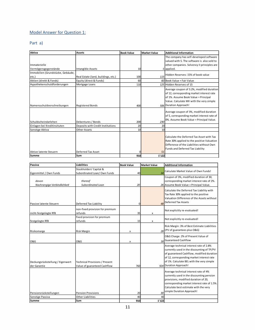
Model Answer for Question 1:
Part a)
Aktiva Assets Book Value Market Value Additional Information
Immaterielle
Vermögensgegenstände Intangible Assets 10 5
The company has self-developed software
valued with 5. The software is also sold to
other companies. Solvency II principles are
applied.
Immobilien (Grundstücke, Gebäude,
etc.) Real Estate (land, buildings, etc.) 100 115Hidden Reserves: 15% of book value
Aktien (direkt & Fonds) Equity (direct & Funds) 60 60 Book Value = Fair Value
Hypothekenschuldforderungen Mortgage Loans 110 125 Hidden Reserves of 15
Namensschuldverschreibungen Registered Bonds 400 506
Average coupon of 3.2%, modified duration
of 12, corresponding market interest rate
of 1%. Assume Book Value = Principal
Value. Calculate MV with the very simple
Duration Approach!
Schuldscheindarlehen Debentures / Bonds 200 230
Average coupon of 3%, modified duration
of 5, corresponding market interest rate of
0%. Assume Book Value = Principal Value.
Einlagen bei Kreditinsituten Deposits with Credit Institutions 20 20
Sonstige Aktiva Other Assets 10 10
Aktive latente Steuern Deferred Tax Asset 0 51
Calculate the Deferred Tax Asset with Tax
Rate 30% applied to the positive Valuation
Difference of the Liabilities without Own
Funds and Deferred Tax Liability
Summe Sum 910 1'122
Passiva Liabilities Book Value Market Value Additional Information
Eigenmittel / Own Funds
Stockholders' Capital &
Subordinated Loan/ Own Funds 40 34Calculate Market Value of Own Funds!
davon
Nachrangige Verbindlichkeit
thereof
Subordinated Loan 20 26
Coupon of 3%, modified duration of 30,
corresponding market interest rate of 2%.
Assume Book Value = Principal Value.
Passive latente Steuern Deferred Tax Liability 0 48
Calculate the Deferred Tax Liability with
Tax Rate 30% applied to the positive
Valuation Difference of the Assets without
Deferred Tax Assets
nicht-festgelegte RfB
non-fixed provision for premium
refunds 35 xNot explicitly re-evaluated!
festgelegte RfB
fixed provision for premium
refunds 15 xNot explicitly re-evaluated!
Risikomarge Risk Margin x 28
Risk Margin: 3% of Best Estimate Liabilities
(PV of guarantees plus O&G)
O&G O&G x 18
O&G Charge: 2% of Present Value of
Guaranteed Cashflow
Deckungsrückstellung / Eigenwert
der Garantie
Technical Provisions / Present
Value of guaranteed Cashflow 760 924
Average technical interest rate of 2.8%
currently used in the discounting of TP/PV
of guaranteed Cashflow, modified duration
of 12, corresponding market interest rate
of 1%. Calculate BEL with the very simple
Duration Approach!
Pensionsrückstellungen Pension Provisions 20 30
Average technical interest rate of 4%
currently used in the discounting pension
provisions, modified duration of 20,
corresponding market interest rate of 1.5%.
Calculate best estimate with the very
simple Duration Approach!
Sonstige Passiva Other Liabilities 40 40
Summe Sum 910 1'122
12
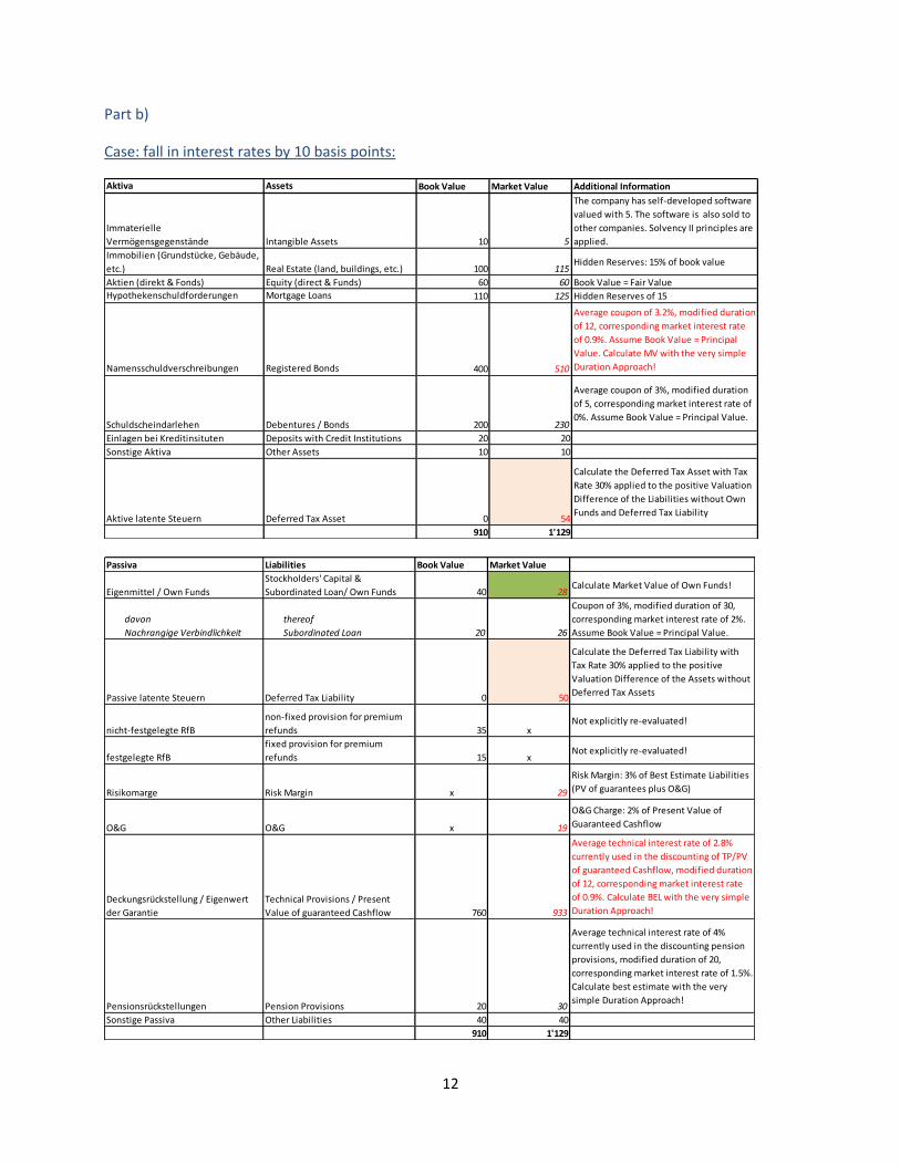
Part b)
Case: fall in interest rates by 10 basis points:
Aktiva Assets Book Value Market Value Additional Information
Immaterielle
Vermögensgegenstände Intangible Assets 10 5
The company has self-developed software
valued with 5. The software is also sold to
other companies. Solvency II principles are
applied.
Immobilien (Grundstücke, Gebäude,
etc.) Real Estate (land, buildings, etc.) 100 115Hidden Reserves: 15% of book value
Aktien (direkt & Fonds) Equity (direct & Funds) 60 60 Book Value = Fair Value
Hypothekenschuldforderungen Mortgage Loans 110 125 Hidden Reserves of 15
Namensschuldverschreibungen Registered Bonds 400 510
Average coupon of 3.2%, modified duration
of 12, corresponding market interest rate
of 0.9%. Assume Book Value = Principal
Value. Calculate MV with the very simple
Duration Approach!
Schuldscheindarlehen Debentures / Bonds 200 230
Average coupon of 3%, modified duration
of 5, corresponding market interest rate of
0%. Assume Book Value = Principal Value.
Einlagen bei Kreditinsituten Deposits with Credit Institutions 20 20
Sonstige Aktiva Other Assets 10 10
Aktive latente Steuern Deferred Tax Asset 0 54
Calculate the Deferred Tax Asset with Tax
Rate 30% applied to the positive Valuation
Difference of the Liabilities without Own
Funds and Deferred Tax Liability
910 1'129
Passiva Liabilities Book Value Market Value
Eigenmittel / Own Funds
Stockholders' Capital &
Subordinated Loan/ Own Funds 40 28Calculate Market Value of Own Funds!
davon
Nachrangige Verbindlichkeit
thereof
Subordinated Loan 20 26
Coupon of 3%, modified duration of 30,
corresponding market interest rate of 2%.
Assume Book Value = Principal Value.
Passive latente Steuern Deferred Tax Liability 0 50
Calculate the Deferred Tax Liability with
Tax Rate 30% applied to the positive
Valuation Difference of the Assets without
Deferred Tax Assets
nicht-festgelegte RfB
non-fixed provision for premium
refunds 35 xNot explicitly re-evaluated!
festgelegte RfB
fixed provision for premium
refunds 15 xNot explicitly re-evaluated!
Risikomarge Risk Margin x 29
Risk Margin: 3% of Best Estimate Liabilities
(PV of guarantees plus O&G)
O&G O&G x 19
O&G Charge: 2% of Present Value of
Guaranteed Cashflow
Deckungsrückstellung / Eigenwert
der Garantie
Technical Provisions / Present
Value of guaranteed Cashflow 760 933
Average technical interest rate of 2.8%
currently used in the discounting of TP/PV
of guaranteed Cashflow, modified duration
of 12, corresponding market interest rate
of 0.9%. Calculate BEL with the very simple
Duration Approach!
Pensionsrückstellungen Pension Provisions 20 30
Average technical interest rate of 4%
currently used in the discounting pension
provisions, modified duration of 20,
corresponding market interest rate of 1.5%.
Calculate best estimate with the very
simple Duration Approach!
Sonstige Passiva Other Liabilities 40 40
910 1'129
13
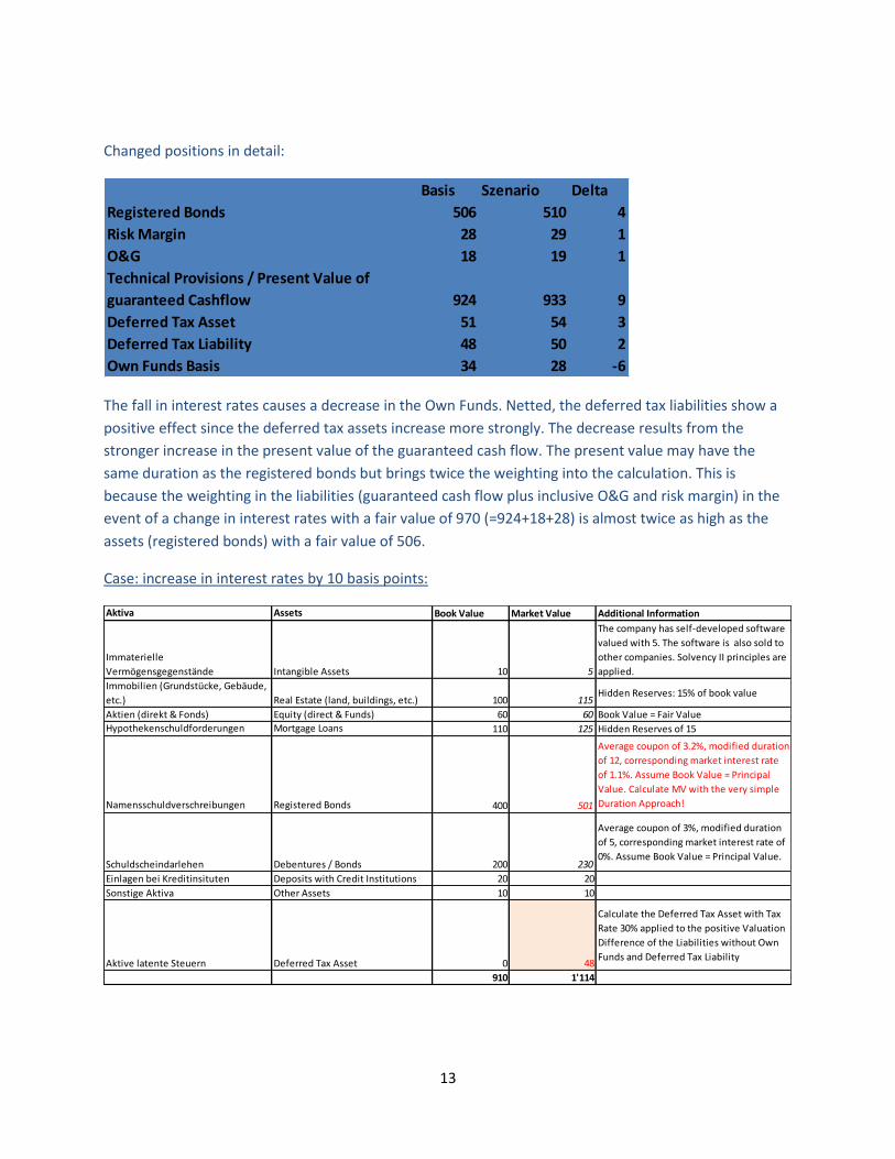
Changed positions in detail:
The fall in interest rates causes a decrease in the Own Funds. Netted, the deferred tax liabilities show a
positive effect since the deferred tax assets increase more strongly. The decrease results from the
stronger increase in the present value of the guaranteed cash flow. The present value may have the
same duration as the registered bonds but brings twice the weighting into the calculation. This is
because the weighting in the liabilities (guaranteed cash flow plus inclusive O&G and risk margin) in the
event of a change in interest rates with a fair value of 970 (=924+18+28) is almost twice as high as the
assets (registered bonds) with a fair value of 506.
Case: increase in interest rates by 10 basis points:
Basis Szenario Delta
Registered Bonds 506 510 4
Risk Margin 28 29 1
O&G 18 19 1
Technical Provisions / Present Value of
guaranteed Cashflow 924 933 9
Deferred Tax Asset 51 54 3
Deferred Tax Liability 48 50 2
Own Funds Basis 34 28 -6
Aktiva Assets Book Value Market Value Additional Information
Immaterielle
Vermögensgegenstände Intangible Assets 10 5
The company has self-developed software
valued with 5. The software is also sold to
other companies. Solvency II principles are
applied.
Immobilien (Grundstücke, Gebäude,
etc.) Real Estate (land, buildings, etc.) 100 115Hidden Reserves: 15% of book value
Aktien (direkt & Fonds) Equity (direct & Funds) 60 60 Book Value = Fair Value
Hypothekenschuldforderungen Mortgage Loans 110 125 Hidden Reserves of 15
Namensschuldverschreibungen Registered Bonds 400 501
Average coupon of 3.2%, modified duration
of 12, corresponding market interest rate
of 1.1%. Assume Book Value = Principal
Value. Calculate MV with the very simple
Duration Approach!
Schuldscheindarlehen Debentures / Bonds 200 230
Average coupon of 3%, modified duration
of 5, corresponding market interest rate of
0%. Assume Book Value = Principal Value.
Einlagen bei Kreditinsituten Deposits with Credit Institutions 20 20
Sonstige Aktiva Other Assets 10 10
Aktive latente Steuern Deferred Tax Asset 0 48
Calculate the Deferred Tax Asset with Tax
Rate 30% applied to the positive Valuation
Difference of the Liabilities without Own
Funds and Deferred Tax Liability
910 1'114
14
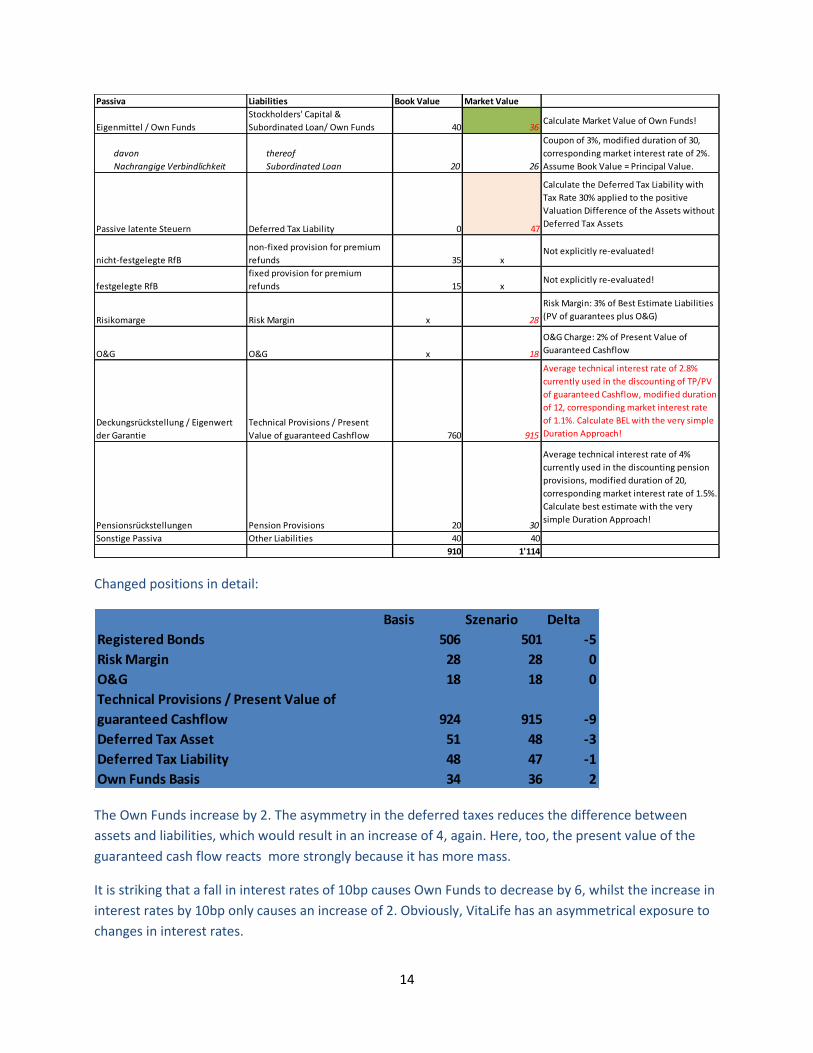
Changed positions in detail:
The Own Funds increase by 2. The asymmetry in the deferred taxes reduces the difference between
assets and liabilities, which would result in an increase of 4, again. Here, too, the present value of the
guaranteed cash flow reacts more strongly because it has more mass.
It is striking that a fall in interest rates of 10bp causes Own Funds to decrease by 6, whilst the increase in
interest rates by 10bp only causes an increase of 2. Obviously, VitaLife has an asymmetrical exposure to
changes in interest rates.
Passiva Liabilities Book Value Market Value
Eigenmittel / Own Funds
Stockholders' Capital &
Subordinated Loan/ Own Funds 40 36Calculate Market Value of Own Funds!
davon
Nachrangige Verbindlichkeit
thereof
Subordinated Loan 20 26
Coupon of 3%, modified duration of 30,
corresponding market interest rate of 2%.
Assume Book Value = Principal Value.
Passive latente Steuern Deferred Tax Liability 0 47
Calculate the Deferred Tax Liability with
Tax Rate 30% applied to the positive
Valuation Difference of the Assets without
Deferred Tax Assets
nicht-festgelegte RfB
non-fixed provision for premium
refunds 35 xNot explicitly re-evaluated!
festgelegte RfB
fixed provision for premium
refunds 15 xNot explicitly re-evaluated!
Risikomarge Risk Margin x 28
Risk Margin: 3% of Best Estimate Liabilities
(PV of guarantees plus O&G)
O&G O&G x 18
O&G Charge: 2% of Present Value of
Guaranteed Cashflow
Deckungsrückstellung / Eigenwert
der Garantie
Technical Provisions / Present
Value of guaranteed Cashflow 760 915
Average technical interest rate of 2.8%
currently used in the discounting of TP/PV
of guaranteed Cashflow, modified duration
of 12, corresponding market interest rate
of 1.1%. Calculate BEL with the very simple
Duration Approach!
Pensionsrückstellungen Pension Provisions 20 30
Average technical interest rate of 4%
currently used in the discounting pension
provisions, modified duration of 20,
corresponding market interest rate of 1.5%.
Calculate best estimate with the very
simple Duration Approach!
Sonstige Passiva Other Liabilities 40 40
910 1'114
Basis Szenario Delta
Registered Bonds 506 501 -5
Risk Margin 28 28 0
O&G 18 18 0
Technical Provisions / Present Value of
guaranteed Cashflow 924 915 -9
Deferred Tax Asset 51 48 -3
Deferred Tax Liability 48 47 -1
Own Funds Basis 34 36 2

15
Part c)
Aktiva Assets Book Value Market Value Additional Information
Immaterielle
Vermögensgegenstände Intangible Assets 10 5
The company has self-developed software
valued with 5. The software is also sold to
other companies. Solvency II principles are
applied.
Immobilien (Grundstücke, Gebäude,
etc.) Real Estate (land, buildings, etc.) 100 115Hidden Reserves: 15% of book value
Aktien (direkt & Fonds) Equity (direct & Funds) 60 60 Book Value = Fair Value
Hypothekenschuldforderungen Mortgage Loans 110 125 Hidden Reserves of 15
Namensschuldverschreibungen Registered Bonds 400 488
Average coupon of 3.2%, modified duration
of 10, corresponding market interest rate
of 1%. Assume Book Value = Principal
Value. Calculate MV with the very simple
Duration Approach!
Schuldscheindarlehen Debentures / Bonds 200 230
Average coupon of 3%, modified duration
of 5, corresponding market interest rate of
0%. Assume Book Value = Principal Value.
Einlagen bei Kreditinsituten Deposits with Credit Institutions 20 20
Sonstige Aktiva Other Assets 10 10
Aktive latente Steuern Deferred Tax Asset 0 60
Calculate the Deferred Tax Asset with Tax
Rate 30% applied to the positive Valuation
Difference of the Liabilities without Own
Funds and Deferred Tax Liability
910 1'113
Passiva Liabilities Book Value Market Value
Eigenmittel / Own Funds
Stockholders' Capital &
Subordinated Loan/ Own Funds 40 0Calculate Market Value of Own Funds!
davon
Nachrangige Verbindlichkeit
thereof
Subordinated Loan 20 26
Coupon of 3%, modified duration of 30,
corresponding market interest rate of 2%.
Assume Book Value = Principal Value.
Passive latente Steuern Deferred Tax Liability 0 43
Calculate the Deferred Tax Liability with
Tax Rate 30% applied to the positive
Valuation Difference of the Assets without
Deferred Tax Assets
nicht-festgelegte RfB
non-fixed provision for premium
refunds 35 xNot explicitly re-evaluated!
festgelegte RfB
fixed provision for premium
refunds 15 xNot explicitly re-evaluated!
Risikomarge Risk Margin x 29
Risk Margin: 3% of Best Estimate Liabilities
(PV of guarantees plus O&G)
O&G O&G x 19
O&G Charge: 2% of Present Value of
Guaranteed Cashflow
Deckungsrückstellung / Eigenwert
der Garantie
Technical Provisions / Present
Value of guaranteed Cashflow 760 952
Average technical interest rate of 2.8%
currently used in the discounting of TP/PV
of guaranteed Cashflow, modified duration
of 14, corresponding market interest rate
of 1%. Calculate BEL with the very simple
Duration Approach!
Pensionsrückstellungen Pension Provisions 20 30
Average technical interest rate of 4%
currently used in the discounting pension
provisions, modified duration of 20,
corresponding market interest rate of 1.5%.
Calculate best estimate with the very
simple Duration Approach!
Sonstige Passiva Other Liabilities 40 40
910 1'113
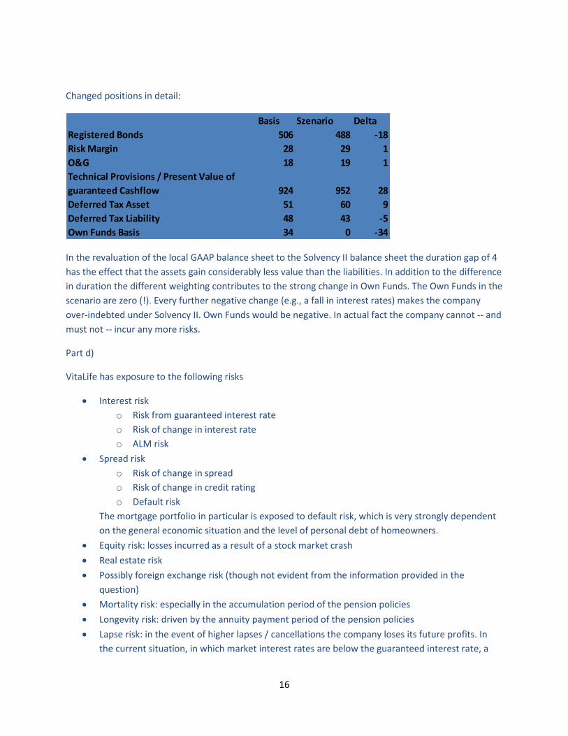
16
Changed positions in detail:
In the revaluation of the local GAAP balance sheet to the Solvency II balance sheet the duration gap of 4
has the effect that the assets gain considerably less value than the liabilities. In addition to the difference
in duration the different weighting contributes to the strong change in Own Funds. The Own Funds in the
scenario are zero (!). Every further negative change (e.g., a fall in interest rates) makes the company
over-indebted under Solvency II. Own Funds would be negative. In actual fact the company cannot -- and
must not -- incur any more risks.
Part d)
VitaLife has exposure to the following risks
Interest risk
o Risk from guaranteed interest rate
o Risk of change in interest rate
o ALM risk
Spread risk
o Risk of change in spread
o Risk of change in credit rating
o Default risk
The mortgage portfolio in particular is exposed to default risk, which is very strongly dependent
on the general economic situation and the level of personal debt of homeowners.
Equity risk: losses incurred as a result of a stock market crash
Real estate risk
Possibly foreign exchange risk (though not evident from the information provided in the
question)
Mortality risk: especially in the accumulation period of the pension policies
Longevity risk: driven by the annuity payment period of the pension policies
Lapse risk: in the event of higher lapses / cancellations the company loses its future profits. In
the current situation, in which market interest rates are below the guaranteed interest rate, a
Basis Szenario Delta
Registered Bonds 506 488 -18
Risk Margin 28 29 1
O&G 18 19 1
Technical Provisions / Present Value of
guaranteed Cashflow 924 952 28
Deferred Tax Asset 51 60 9
Deferred Tax Liability 48 43 -5
Own Funds Basis 34 0 -34
17
lower level of lapses / cancellations would constitute a high risk since the lapses / cancellations
reduce the reinvestment risk at that moment.
Operational risks
o Liquidity risk
o IT risks
o Process risks
o Legal risks
In the Standard Model and also in companies' own Models these are not measured explicitly but
rather only in a general manner. Operational risks, though very rare, have a large loss impact.
Examples from IT are well-known, for example, IT outage affecting the in-force management
system, loss of customer data and similar. BCM, too, is relevant when it comes to operational
risks.
In scenario 2 the company has no Own Funds in its economic balance sheet. Therefore, VitaLife cannot
cover its risks. Several strategies are conceivable to improve this situation:
Reducing the risks
o divesting equities, real estate, spread products (corporate bonds etc) or hedging the
risks so that the risk is reduced in the risk model.
o Increasing the duration of the interest-bearing securities in order to hedge the liabilities
against the risk of a change in interest rates.
o However, at the same time it must be assured that investment income will be sufficient
to pay the guaranteed interest on the liabilities side.
o Changing the with-profits bonus participation system so that the guaranteed reserves
will not increase (e.g., more terminal bonuses, no longer guaranteeing annual bonuses
or using a 0% guarantee etc.)
o Purchasing reinsurance (e.g., mortality or longevity)
o Developing new products that require fewer guarantees.
o Adjusting the modelling of real estate to be interest-rate sensitive so that, in the sense of
ALM, it would also serve as a counterweight to the cash flow on the liabilities side in
terms of interest rate (change) risk.
o General improvement of risk modelling and making use of conservative approaches /
models.
Building up Own Funds by
o Retaining / ploughing back profits
o Asking Members to make additional payments, if the Statutes of the insurer permit this
o Demutualisation and sale of the company to an owner who could inject capital
o Apply to the Regulatory Authority for transitional measures
o Developing new products that require fewer guarantees so that the present value of the
options and guarantees is lower in the valuation.
o General improvement of risk modelling and making use of conservative approaches /
models.
18
All in all, VitaLife's situation is extremely critical since, if it does not take urgent steps, the company does
not have any risk-bearing capacity. From the data provided thus far, the greatest risk is that of a change
in interest rates.
Model Answer for Question 2:
In addition to the answers listed here other answers are also possible.
Part a)
Advantages and Disadvantages of Model A
Advantages: Little time and effort required, quick calculation time. Many scenario calculations and
sensitivity analyses are possible. It can be used directly. There is little need for know-how to be built up.
Simple documentation.
Disadvantages: Valuation of the Os & Gs using a closed formula is only possible for few options. The
results are not precise enough. Difficult to prove that the valuation is market-consistent. Agreement with
/ Buy-in from the external auditors could be difficult.
Advantages and Disadvantages of Model B
Advantages: Exact valuation of the Os & Gs is possible. Market consistency is assured thanks to the
stochastic scenarios. All options can be valued. Agreement with / Buy-in from the external auditors
should be easier than with Model A.
Disadvantages: Long calculation time, greater time and effort than for Model A. The long calculation time
makes it difficult to perform many sensitivity analyses. It is also necessary to build up know how for the
scenario generator.
Part b)
Additional information could be the following:
Software expenses: Licensing models, purchase, maintenance
Contractual conditions: jurisdiction etc.
Creditworthiness of the supplier
Test phase possible
Opportunities for sensitivity analyses
Inclusion in the company's own system landscape
Programming language of the software
Can the software be adapted / customised to meet company-specific requirements
Is the company permitted to make adaptations / to customise the software
Can the risk calculation be implemented?
19
Is the software already in use? References?
Project roll-out: possible structure, effort and cost?
Can the results / output be reported in Solvency II format
For Model B: Is it possible to speed up the calculation time?
Evaluation of own balance sheet and review of adequacy of the valuation with the models
Use of a test phase and valuation of the obligations in various sensitivities and analysis of the
consequences
Testing of the stability of the model with regard to the parameters.
Part c)
Linking to Model A with advantages and disadvantages
Linking using sensitivity analyses: the stress scenarios are generated using the corresponding variation of
the input parameters. Programming via a process that inputs the results into the EIOPA Excel
spreadsheet. Since calculation of a single balance sheet requires 5 minutes, 12 stresses will require one
hour of calculation time. Advantages are the quick calculation time and the simplicity of the solution. The
disadvantage is that the accuracy of the risk calculation is limited by the accuracy of the valuation model.
Valuation of the Os& Gs in stress cases requires special calibration of the input parameters. This simple
approach means that further approximations will be used, which may impair the quality of the results.
Linking to Model B with advantages and disadvantages
Linking using sensitivity analyses is difficult because of the long calculation time. This approach would
require a parallel calculation of the stress scenarios since, for linear calculation, the calculation time
would increase by 12 hours in each case. For 12 stresses the results would only be available after 6 days.
In most cases, this is not acceptable. Therefore the approach is impractical using multiple calculations
with Model B. One possibility would be to implement the stress calculation directly in Model B so that
the base case and the stress scenarios are calculated in parallel. In this case the software would need to
be open and can be maintained and used by the company's employees. Another approach would be, for
example, a replicating portfolio that can be calibrated by means of the valuation model. This would
require further know how to be built up.
Model Answer for Question 3:
Part a)
i. Var(99.5, 2 years, Correl=0) = Var(99.5, 1 year) * sqrt(2) = 100*sqrt(2) ≈ 141
ii. 2.85/sqrt(2) ≈ 1.82 at approx. Φ(1,82) ≈ 96.5%
iii. Volatility for one year: σ1 = 100/2,85
Volatility for 2 years with a correlation ρ: σ2= sqrt(2* σ1^2 + 2*ρ*σ1^2)
Var(2 years 95, Correl=ρ) = σ1* Φ-1(95%) *sqrt(2+2 ρ)
Equate: σ1Φ-1(99.5%) = σ1* Φ-1(95%) *sqrt(2+2 ρ)
Correlation ρ = ((Φ-1(99.5%) Φ-1(95%))2)/2-1 ≈ 22.6% with the above roundings
≈23.7%
20
iv. It is stricter since the "catch up" (Year 1 ratio <100%, then improvement) is not "permitted" in
the sense that the required would be infringed.
The probability that the Solvency Requirement of 100% will be achieved after one year,
Φ((130-100)/ σ1) ≈ Φ(0,77) ≈ 78%, σ1=100/Φ-1(99.5%)
v. If one interprets the Solvency II requirement as Own Funds 0 for 1 in 200 years the 2-year
requirement would be "around" 99.5% of a 1 in 400-years event (if one considers that, under
Question iv, it is a relief to not consider the "odd" years), so it would be reasonable to reduce the
safety level.
From a 2-year view the requirement b) is only a 2/(1-96.5%) year event, i.e., approx. 1-
in-57 years, for c) the frequency is 2/(1-95%) = 40 years.
Setting the 1-year horizon affects the safety level considerably. It is based on the view
that business years are a natural unit and that the probable time span for an effective
intervention by the Regulatory Authority entity is approximately one year.
vi. As ii and iii show correlation plays a significant role. Correlations are notoriously difficult to
estimate. Thus, the advantage is questionable.
Part b)
i. Interest: "gross" change OF: 10-37 = -27, with-profits surplus: 1/3*27=9 "net" change OF: 10-
37+9 = -18
Spread: "gross" change OF -36, with-profits surplus: 1/3*36=12 "net" change OF: -24
Combined: "gross" change: OF 10-40-36 = -63, with-profits surplus: min(1/3*63,12) = 12,
"net" change OF: -63+12= -51
Risk capital "gross": (27²+36²)^(1/2)=45, "net" before capping (18²+24²)^(1/2)=30, risk mitigation
capped at 12: "net" risk capital: max(30; 45-12) = 33.
The root formula makes two decisive assumptions: with the given covariance, the risks are, e.g.,
normally or elliptically distributed. This assumption is a common simplification even if, of course,
it cannot be generally expected in reality. The second significant assumption is that the change
to the Own Funds is linear in the risk factors. This is disproved by the observed non-linearity.
ii. The sequence is significant for the size of the individual effects:
Possible sequences are
OF 2015: 160
Spread: -24
Interest: -27
OF 2016: 109
and
OF 2015: 160
Interest: -33
Spread: -18
OF 2016: 109
21
By different apportioning of the risk mitigation through future with-profits bonus participation
any intermediate value can be generated.
The sequence of the steps can thus have a massive influence on the weighting of the effects.
Depending on the interests in question one view seem more attractive than the other (e.g., if
events are seen differently being seen as "self-made").
iii. Both companies have "gross" risk capital of 20, 10 "net" before capping. SecuraLife has 15 future
with-profits bonus participation, RiskyLife only 5. Thus we arrive at risk capital of 10 for
SecuraLife and at 15 for RiskyLife.
The Group then has "gross" risk capital of 40, 20 "net" before capping but the Group relief is
limited to 20 in total, i.e., not capped.
The implicitly assumed fungibility of the risk-mitigating effect of the future with-profits bonus
participation is questionable so long as there are no indications that the companies mutually
offset losses.
One possible solution would be to allocate the capped relief at company level to the individual
modules and then, to aggregate module by module to relief the burden for the Group.
Model Answer for Question 4:
Part a)
Outline model answer – other answers are possible:
You should at least look at the categories underwriting risks, market and credit risks, operational risks.
Define a segmentation per risk category that is compatible with your internal model. For each segment,
for example, use a volume figure (For underwriting, for example, premiums and reserves, for market and
credit, e.g., asset volumes, claims on reinsurers and for operational risks, for example, number of
employees) and a factor that you can derive from your own model or the Standard Formula. For nat cat
losses you can also use historical loss figures from the annual report. For integration into the internal
model you will need probability distributions per category. You can take these from your internal model
or work with simpler assumptions. During the integration you should also consider diversification effects
and/or dependencies. This point is especially relevant for your motor portfolio where you may possibly
expect that the so-called "equilibrium in the collective body (of the policyholders)" makes the risks easier
to calculate. When it comes to market and credit risks, in addition to the asset structure the issue as to
how potential reinsurance treaties are to be handled following the acquisition is also relevant.
Part b)
Outline model answer – other answers are possible:
For example, reinsurance. Advantages – flexible structure, possible at short notice and can be changed.
Disadvantages – may be costly.
For example. transfer to the capital markets, e.g., via index-linked products. Advantages – probably
cheaper, Disadvantages – basic risk remains. Special know-how required to match the index to the
portfolio
22
Part c)
cf slides "Constraints of the economic view: restrictions owing to rating requirements "
Part d)
Outline model answer – other answers are possible:
For example, driverless cars – what is the company's exposure in this segment? What future
developments are expected? Which players are currently active on the market?
For example, data theft – Does the company collect sensitive data in connection with motor insurance?
Which data is used and which sources is it derived from? What is the IT system for administration like?
Have there been attacks in the past?
Part e)
Outline model answer – other answers are possible:
For example Reputational risks – In connection with data collection in motor insurance the company
could hit the headlines if is uses unreliable sources or uses the data illegally / incorrectly. In this case
there ought to be transparency about the data used and its sources; moreover legal issues should be
clarified.
For example Key person risk – If the company to be acquired operates in very specialised business
segments its success might be down to the know-how of a small number of employees. In order to retain
these employees special development plans may have to be developed for these people for the period
after the merger.
Part f)
Outline model answer – other answers are possible:
The diversification effect from underwriting should benefit both the new and the old portfolio. This may
be, for example, through use of the covariance principle during capital allocation. This leads, for
example, to the risk capital allocated to the fire segment dropping in comparison to the calculation
without the new portfolio. The RoRaC for this segment increases as a result. This effect should be
communicated transparently and, for example, also be considered when setting objectives and
measuring whether objectives and targets have been met. Longer-term implementation in steering and
management is also conceivable in order to have fewer abrupt breaks and to be able to align the
strategy more precisely. Communication should be done early to enable the strategy to be adjusted pro-
actively and in anticipation.