Komitet Redakcyjny- Editorial Boardnawfert.iung.pulawy.pl/zeszyty/pelne/30 2008.pdf · Janusz...
110
Transcript of Komitet Redakcyjny- Editorial Boardnawfert.iung.pulawy.pl/zeszyty/pelne/30 2008.pdf · Janusz...
Komitet Redakcyjny- Editorial BoardMariusz Fotyma – Redaktor naczelny – Executive Editor
Janusz Igras, Przemysław Tkaczyk
MonographySoil testing methods and fertilizer recommendations
in Central–Eastern European countriesMethoden der Bodenuntersuchung und Düngeempfehlung
der mittel- und osteuropäischen Staaten
Edited by Mariusz Fotyma, Eike Stefan Dobers – PolandErstellt durch Mariusz Fotyma und Eike Stefan Dobers (Polen)
Co-authors, Koautoren *
Gerhard Breitschuh – Germany, Valli Loide – Estonia, Regina Timbare – Latvia, Gediminas Staugaitis – Lithuania, Heide Spiegel – Austria, Dorota Pikuła – Poland,
Frantisek Kotvas – Slovak Republic, Barbara Ceh – Slovenia, Pavel Cermak – Czech Republic, Jakab Loch – Hungary
* full names and the addresses of the affiliation units are given in Appendix 8*die Namen und Adresse von alle zusamenarbeitene Anstalten sind im Appendix 8
hergestellt
Zeszyt wydany w ramach realizacji programu wieloletniego IUNG-PIB Zadanie 1.7
Copyright by Polish Fertilizer Society – CIEC
ISSN 1509 – 8095
Adres Redakcji – Adress Executive EditorZakład Żywienia Roslin i Nawozenia IUNG-PIB
Czartoryskich 8, 24-100 [email protected]
Druk: IUNG-PIB zam.24/F/08 nakł. 200 egz. B-5
Table of Contents1. COMPARISON OF METHODS FOR SOIL ANALYSIS .............................. 7
1.1 DESCRIPTION OF THE METHODS ........................................................... 71.2 QUANTITATIVE ANALYSIS OF SOIL DATE. ........................................... 81.3 CALIBRATION OF SOILS TESTS RESULTS FOR AVAILABLE P, K, MG 111.4 QUALITATIVE ANALYSIS OF SOIL DATA ............................................ 131.5 SOIL TEXTURE .......................................................................................... 16
2. COMPARISONS OF RECOMMENDED FERTILIZER RATES............... 172.1 RECOMMENDED RATES OF NUTRIENTS FOR GRAIN CROPS ........ 172.1.1 Phosphorus ................................................................................................ 172.1.2 Potassium K .............................................................................................. 192.1.3 Magnesium Mg .......................................................................................... 212.2 RECOMMENDED RATES OF NUTRIENTS FOR POTATO AND SILAGE MAIZE ................................................................................................................ 23
3. ALGORITHMS OF FERTILIZER RECOMMENDATIONS .................... 263.1 GENERAL REMARKS ................................................................................ 263.2 ALGORITHMS OF FERTILIZER RECOMMENDATIONS IN COLLABORATING COUNTRIES ....................................................................... 263.2.1 Estonia EE ................................................................................................. 263.2.2 Latvia LV .................................................................................................... 273.2.3 Lithuania LT ............................................................................................... 273.2.4 Austria AT .................................................................................................. 283.2.5 Poland PL .................................................................................................. 283.2.6 Slovenia SL................................................................................................. 293.2.7 Czech Republic CZ ..................................................................................... 293.2.8 Hungary HU .............................................................................................. 29
4. DISCUSSION AND CONCLUSIONS. .......................................................... 304.1 SOIL TESTS ................................................................................................ 304.1.1 Comparison of extraction methods ............................................................ 304.1.2 Comparison of calibration schemes. .........................................................334.2 FERTILIZER RECOMMENDATIONS. ....................................................... 354.2.1 Recommendations schemes (algorithms) ....................................................35
Nawozy i NawożenieFertilizers and Fertilization
Nr 30/2008
4.2.2 Recommended rates of fertilizers . .... ......................................................... 384.3 CONCLUSIONS ........................................... ............................................... 38
REFERENCES. ................................................................................................... 39 APPENDICES .................................................................................................... 41
1. VERGLEICH DER METHODEN DER BODENUNTERSUCHUNG........501.1BeschreiBungderMethoden........................................................................ 501.2QuantitativeanalysederuntersuchungsergeBnisse................................. 511.3einstufungderergeBnissederBodenuntersuchungenfürverfügBaresP,KundMg.541.4.QualitativeanalysederBodendaten.......................................................... 561.5Bodenarten-ansPrache................................................................................ 59
2. VERGLEICH DER DüNGUNGSEMPFEHLUNGEN................................. 602.1düngungseMPfehlungfürKörnerfrüchte................................................... 602.1.1 Phosphor ................................................................................................... 602.1.2 Kalium ....................................................................................................... 632.1.3 Magnesium ................................................................................................ 652.2düngungseMPfehlungfürKartoffelundsiloMais..................................... 67
3. ALGORITHMEN FüR DIE ERMITTLUNG DES DüNGEBEDARFS.... 70
3.1allgeMeineBeMerKungen............................................................................. 70
3.2BeschreiBungderalgorithMenfürdiejeweiligenstaaten........................ 703.2.1 Estland (EE) .............................................................................................. 703.2.2 Lettland (LV) ............................................................................................. 713.2.3 Litauen (LT) .............................................................................................. 713.2.4 Österreich (AT) ......................................................................................... 723.2.5 Polen (PL) ................................................................................................. 733.2.6 Slowenien (SL) .......................................................................................... 733.2.7 Tschechische Republik (CZ) ...................................................................... 733.2.8 Ungarn (HU) ............................................................................................. 74
4. DISkUSSION UND SCHLUSSFOLGERUNGEN........................................ 754.1Bodenuntersuchung..................................................................................... 754.1.1 Vergleich der Extraktionsmethoden .......................................................... 754.1.2 Ermittlung der Nährstoffversorgung ......................................................... 784.2dünge-eMPfehlungen.................................................................................... 804.2.1 Algorithmen zur Ableitung der Dünge-Empfehlungen ............................. 80
4.2.2 Höhe der Dünge-Empfehlungen ............................................................... 824.3schlussfolgerungen..................................................................................... 83
5.LITERATUR..................................................................................................... 85
6. ANHANG ........................................................................................................... 86
1. SUPPLEMENT ................................................................................................ 94Pikuła D., Tkaczyk P. Comparison of aerometric and laser diffraction methods for soil texture analysis......................................................................................... 94
1.1 Methods ......................................................................................................... 951.2 Results .......................................................................................................... 961.3 Discussion ..................................................................................................... 991.4 Conclusions ................................................................................................... 991.5 Literature .......................................................................................................991.6 Annexes ........................................................................................................101
1. ERGÄNZUNG ................................................................................................102Pikuła,D. Dobers, S. Vergleich der Sedimentations- und der Laser-Difraktions-methodik für die Bestimmung der Bodentextur...............................................102
1.1 Methoden ....................................................................................................1041.2 Ergebnisse ...................................................................................................1041.3 Diskussion ....................................................................................................1071.4 Schlussfolgerungen ......................................................................................1071.5 Literatur ......................................................................................................1081.6 Anhang .........................................................................................................109

From the editors
In course of the 9th meeting of the MOEL group (MOEL working group of agrochemical services in Central-Eastern Europe – Arbeitsgruppe der agrochemischer Untersuchunsdienste der mittel- und osteuropeischen Lander) in 2006 at Piran – Slovenia, it has been decided to organize the inter-laboratory exchange of soil samples with the following fertilizer recommendations between 10 collaborating countries. In each country two representative soil samples were collected, analysed for the basic properties (texture, humus content) and distributed among all participants with the task for estimating the soil’s pH and the content of available phosphorus, potassium and magnesium, using methods officially accepted in the country. Further, six crops typical for most countries e.g. winter wheat, winter rape, winter rye, grain maize, potato and silage maize have been selected with presumed yields 7 t grain, 4.5 t seeds, 6 t grain, 10 t seed, 30 t tubers and 10 t dry matter – respectively. For potato 30 t FYM and for silage maize 30 m3 slurry were to be applied. All the crops were to be grown on both “sites” where soil samples have been collected. On the base of soil indices and crop characteristics, fertilizer recommendations were launched supported by the system officially used in the country. The data concerning soil properties and recommended rates of fertilizers were collected in Excel sheets and processed by means of analysis of variance and regression using the statistical package Statgraphic 5a.
Von den Redakteuren
Während des 9. Treffens der MOEL-Gruppe (Vereinheitlichung der landwirtschaftlich-chemischen Untersuchungsdienste der mittel- und osteuropäischen Länder) in Piran (Slowenien) im Jahre 2006 wurde beschlossen, einen Ringversuch zwischen den 10 beteiligten Staaten zu organisiseren. Dieser Ringversuch hatte zum Ziel, Düngungsempfehlungen abzuleiten.
In jedem teilnehmenden Staat wurden zwei repräsentative Bodenproben gezogen, für diese die Bodenart und der Humusgehalt ermittelt, und dann an alle Teilnehmer des Ringversuchs versandt. Die Teilnehmer des Ringversuchs hatten die Aufgabe, an den Bodenproben unter Verwendung der jeweils landestypischen Methoden den pH-Wert und den Gehalt an pflanzenverfügbarem Phosphor, Kalium und Magnesium zu bestimmen. Man einigte sich ebenfalls auf die folgenden, für die beteiligten Staaten typische Fruchtarten und Ertragsziele: Winterweizen (7 t*ha-1 Korn), Winterraps (4.5 t*ha-1 Samen), Winterroggen (6 t*ha-1 Korn), Körnermais (10 t*ha-1 Korn), Kartoffel (30 t*ha-1 Knollen) und Silomais (10 t*ha-1 Trockenmasse). Für den Anbau von Kartoffel wurde die Verwendung von 30 t*ha-1 Stallmist, und für den Silomais-Anbau die Ausbringung von 30 m³ Gülle. Die Düngebedarfsermittlung fand unter der Annahme statt, dass alle Fruchtarten auf Standorten angebaut würden, die den gezogenen Bodenproben des jeweiligen Staates entsprachen. Auf der Grundlage der Analyseergebnisse und Eigenschaften der angebauten Pflanzen wurden Düngebedarfsermittlungen durchgeführt auf der Basis des jeweils landestypischen Verfahrens.
Die Ergebnisse der Bodenuntersuchung und die empfohlenen Düngermengen wurden in Excel-Tabellenblättern gesammelt und unter Verwendung des Statistik-Programms Statgraphic 5a der Varianz- und Regressionsanalyse unterzogen.
.
1. Comparison of methods for soil analysis
1.1 Description of the methods
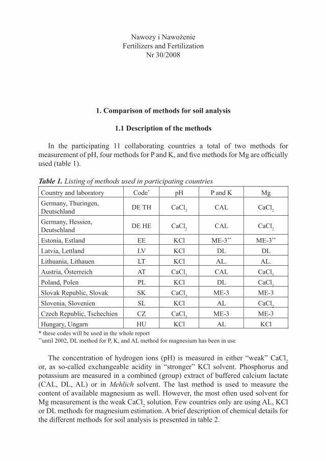
In the participating 11 collaborating countries a total of two methods for measurement of pH, four methods for P and K, and five methods for Mg are officially used (table 1).
Table 1. Listing of methods used in participating countriesCountry and laboratory Code* pH P and K MgGermany, Thuringen, Deutschland DE TH CaCl2 CAL CaCl2
Germany, Hessien, Deutschland DE HE CaCl2 CAL CaCl2
Estonia, Estland EE KCl ME-3** ME-3**
Latvia, Lettland LV KCl DL DLLithuania, Lithauen LT KCl AL. AL.Austria, Österreich AT CaCl2 CAL CaCl2
Poland, Polen PL KCl DL CaCl2
Slovak Republic, Slovak SK CaCl2 ME-3 ME-3Slovenia, Slovenien SL KCl AL CaCl2
Czech Republic, Tschechien CZ CaCl2 ME-3 ME-3Hungary, Ungarn HU KCl AL KCl
* these codes will be used in the whole report**until 2002, DL method for P, K, and AL method for magnesium has been in use
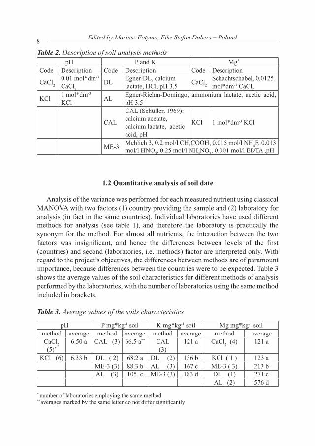
The concentration of hydrogen ions (pH) is measured in either “weak” CaCl2 or, as so-called exchangeable acidity in “stronger” KCl solvent. Phosphorus and potassium are measured in a combined (group) extract of buffered calcium lactate (CAL, DL, AL) or in Mehlich solvent. The last method is used to measure the content of available magnesium as well. However, the most often used solvent for Mg measurement is the weak CaCl2 solution. Few countries only are using AL, KCl or DL methods for magnesium estimation. A brief description of chemical details for the different methods for soil analysis is presented in table 2.
Nawozy i NawożenieFertilizers and Fertilization
Nr 30/2008
8 Edited by Mariusz Fotyma, Eike Stefan Dobers – Poland
Table 2. Description of soil analysis methodspH P and K Mg*
Code Description Code Description Code Description
CaCl20.01 mol*dm-3 CaCl2
DL Egner-DL, calcium lactate, HCl, pH 3.5 CaCl2
Schachtschabel, 0.0125 mol*dm-3 CaCl2
KCl 1 mol*dm-3 KCl AL Egner-Riehm-Domingo, ammonium lactate, acetic acid,
pH 3.5
CAL
CAL (Schüller, 1969): calcium acetate, calcium lactate, acetic acid, pH
KCl 1 mol*dm-3 KCl
ME-3 Mehlich 3, 0.2 mol/l CH3COOH, 0.015 mol/l NH4F, 0.013 mol/l HNO3, 0.25 mol/l NH4NO3, 0.001 mol/l EDTA ,pH
1.2 Quantitative analysis of soil date
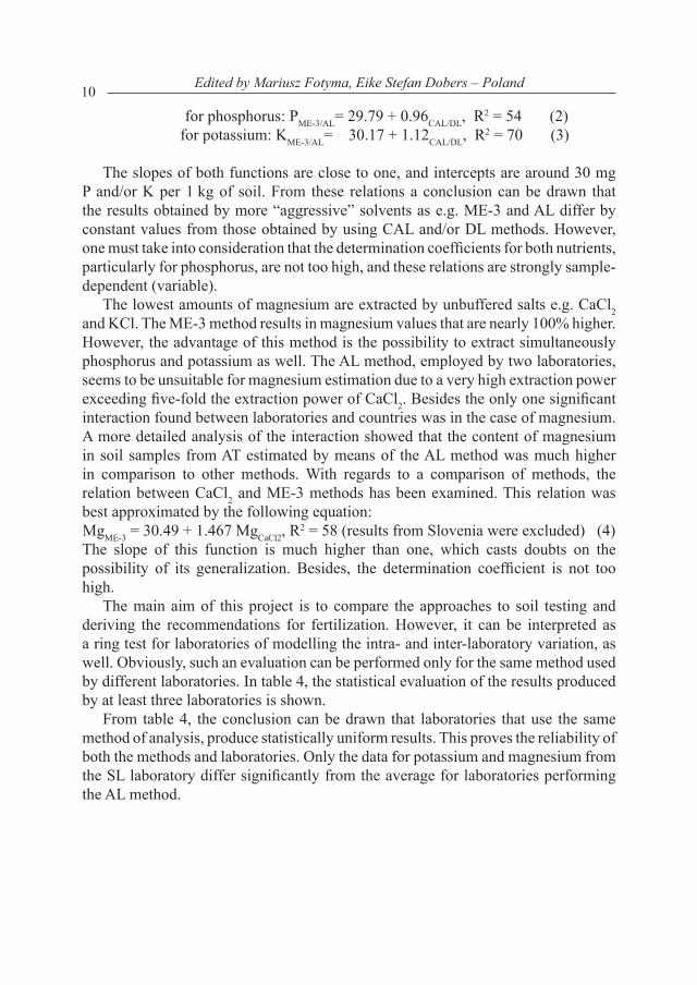
Analysis of the variance was performed for each measured nutrient using classical MANOVA with two factors (1) country providing the sample and (2) laboratory for analysis (in fact in the same countries). Individual laboratories have used different methods for analysis (see table 1), and therefore the laboratory is practically the synonym for the method. For almost all nutrients, the interaction between the two factors was insignificant, and hence the differences between levels of the first (countries) and second (laboratories, i.e. methods) factor are interpreted only. With regard to the project’s objectives, the differences between methods are of paramount importance, because differences between the countries were to be expected. Table 3 shows the average values of the soil characteristics for different methods of analysis performed by the laboratories, with the number of laboratories using the same method included in brackets.
Table 3. Average values of the soils characteristics
pH P mg*kg-1 soil K mg*kg-1 soil Mg mg*kg-1 soilmethod average method average method average method averageCaCl2 (5)*
6.50 a CAL (3) 66.5 a** CAL (3)
121 a CaCl2 (4) 121 a
KCl (6) 6.33 b DL ( 2) 68.2 a DL (2) 136 b KCl ( 1 ) 123 aME-3 (3) 88.3 b AL (3) 167 c ME-3 ( 3) 213 bAL (3) 105 c ME-3 (3) 183 d DL (1) 271 c
AL (2) 576 d * number of laboratories employing the same method**averages marked by the same letter do not differ significantly

9Monography
The average value of soil pH measured in KCl is slightly lower than in CaCl2. However, the relation between the two measures is approximated best by a double reciprocal regression function of the form:
pHCaCl2 = 1/(0.0375 + 0.735/pHKCl), R = 98 (1)
This means that in acid soils pHKCl values are by 0.5 – 0.6 units lower than pHCaCl2, for neutral soils, both measures are similar, and for alkaline soils values determined with pHKCl are slightly higher as those with pHCaCl2 (Fig 1).
However such relation concerns only the date from this research and should not be generalized. Potassium ion from KCl has higher exchange power then calcium ion from CaCl2 and replace more hydrogen ions from soil solid phase. Therefore the pH measured in KCl solution is regularly lower then in CaCl2 though this relation is not necessarily proportional.
Fig. 1. Relation between pH in CaCl2 and in KCl
The average values for phosphorus and potassium extracted with CAL and DL methods are practically the same, which means that both methods can be used likewise. The AL and ME-3 methods belong to a distinctly different group, because higher quantities of phosphorus and potassium are extracted than using CAL and DL methods. The differences between average values determined with AL and ME-3 methods are statistically significant, but they are not too big and anyhow much lower than the differences between the two groups of methods (CAL & DL versus AL & ME-3). The relation between values determined using methods from these two groups can be approximated by the linear functions:
10 Edited by Mariusz Fotyma, Eike Stefan Dobers – Poland
for phosphorus: PME-3/AL= 29.79 + 0.96CAL/DL, R2 = 54 (2)for potassium: KME-3/AL= 30.17 + 1.12CAL/DL, R2 = 70 (3)
The slopes of both functions are close to one, and intercepts are around 30 mg P and/or K per 1 kg of soil. From these relations a conclusion can be drawn that the results obtained by more “aggressive” solvents as e.g. ME-3 and AL differ by constant values from those obtained by using CAL and/or DL methods. However, one must take into consideration that the determination coefficients for both nutrients, particularly for phosphorus, are not too high, and these relations are strongly sample-dependent (variable).
The lowest amounts of magnesium are extracted by unbuffered salts e.g. CaCl2 and KCl. The ME-3 method results in magnesium values that are nearly 100% higher. However, the advantage of this method is the possibility to extract simultaneously phosphorus and potassium as well. The AL method, employed by two laboratories, seems to be unsuitable for magnesium estimation due to a very high extraction power exceeding five-fold the extraction power of CaCl2. Besides the only one significant interaction found between laboratories and countries was in the case of magnesium. A more detailed analysis of the interaction showed that the content of magnesium in soil samples from AT estimated by means of the AL method was much higher in comparison to other methods. With regards to a comparison of methods, the relation between CaCl2 and ME-3 methods has been examined. This relation was best approximated by the following equation:MgME-3 = 30.49 + 1.467 MgCaCl2, R
2 = 58 (results from Slovenia were excluded) (4)The slope of this function is much higher than one, which casts doubts on the possibility of its generalization. Besides, the determination coefficient is not too high.
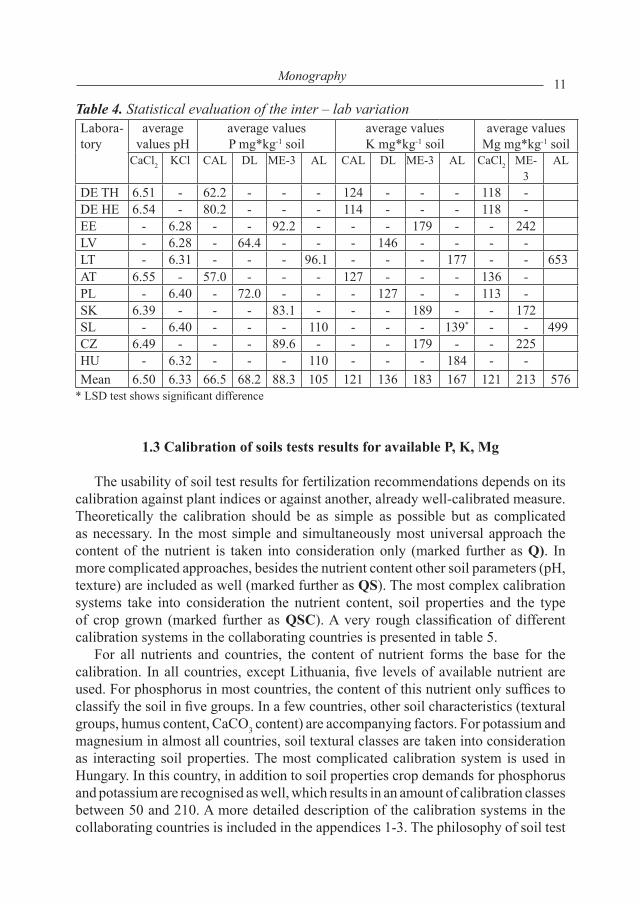
The main aim of this project is to compare the approaches to soil testing and deriving the recommendations for fertilization. However, it can be interpreted as a ring test for laboratories of modelling the intra- and inter-laboratory variation, as well. Obviously, such an evaluation can be performed only for the same method used by different laboratories. In table 4, the statistical evaluation of the results produced by at least three laboratories is shown.
From table 4, the conclusion can be drawn that laboratories that use the same method of analysis, produce statistically uniform results. This proves the reliability of both the methods and laboratories. Only the data for potassium and magnesium from the SL laboratory differ significantly from the average for laboratories performing the AL method.
11Monography
Table 4. Statistical evaluation of the inter – lab variation Labora-tory
average values pH
average values P mg*kg-1 soil
average values K mg*kg-1 soil
average values Mg mg*kg-1 soil
CaCl2 KCl CAL DL ME-3 AL CAL DL ME-3 AL CaCl2 ME-3
AL
DE TH 6.51 - 62.2 - - - 124 - - - 118 -DE HE 6.54 - 80.2 - - - 114 - - - 118 -EE - 6.28 - - 92.2 - - - 179 - - 242LV - 6.28 - 64.4 - - - 146 - - - -LT - 6.31 - - - 96.1 - - - 177 - - 653AT 6.55 - 57.0 - - - 127 - - - 136 -PL - 6.40 - 72.0 - - - 127 - - 113 -SK 6.39 - - - 83.1 - - - 189 - - 172SL - 6.40 - - - 110 - - - 139* - - 499CZ 6.49 - - - 89.6 - - - 179 - - 225HU - 6.32 - - - 110 - - - 184 - -Mean 6.50 6.33 66.5 68.2 88.3 105 121 136 183 167 121 213 576
* LSD test shows significant difference
1.3 Calibration of soils tests results for available P, k, Mg
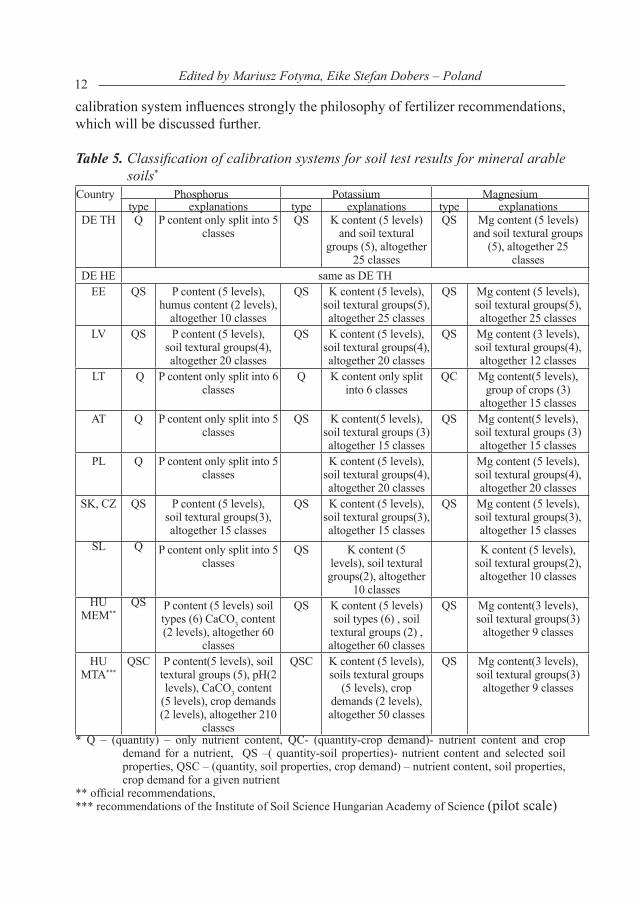
The usability of soil test results for fertilization recommendations depends on its calibration against plant indices or against another, already well-calibrated measure. Theoretically the calibration should be as simple as possible but as complicated as necessary. In the most simple and simultaneously most universal approach the content of the nutrient is taken into consideration only (marked further as Q). In more complicated approaches, besides the nutrient content other soil parameters (pH, texture) are included as well (marked further as QS). The most complex calibration systems take into consideration the nutrient content, soil properties and the type of crop grown (marked further as QSC). A very rough classification of different calibration systems in the collaborating countries is presented in table 5.
For all nutrients and countries, the content of nutrient forms the base for the calibration. In all countries, except Lithuania, five levels of available nutrient are used. For phosphorus in most countries, the content of this nutrient only suffices to classify the soil in five groups. In a few countries, other soil characteristics (textural groups, humus content, CaCO3 content) are accompanying factors. For potassium and magnesium in almost all countries, soil textural classes are taken into consideration as interacting soil properties. The most complicated calibration system is used in Hungary. In this country, in addition to soil properties crop demands for phosphorus and potassium are recognised as well, which results in an amount of calibration classes between 50 and 210. A more detailed description of the calibration systems in the collaborating countries is included in the appendices 1-3. The philosophy of soil test
12 Edited by Mariusz Fotyma, Eike Stefan Dobers – Poland
calibration system influences strongly the philosophy of fertilizer recommendations, which will be discussed further.
Table 5. Classification of calibration systems for soil test results for mineral arable soils*
Country Phosphorus Potassium Magnesiumtype explanations type explanations type explanations
DE TH Q P content only split into 5 classes
QS K content (5 levels) and soil textural
groups (5), altogether 25 classes
QS Mg content (5 levels) and soil textural groups
(5), altogether 25 classes
DE HE same as DE THEE QS P content (5 levels),
humus content (2 levels), altogether 10 classes
QS K content (5 levels), soil textural groups(5), altogether 25 classes
QS Mg content (5 levels), soil textural groups(5), altogether 25 classes
LV QS P content (5 levels), soil textural groups(4), altogether 20 classes
QS K content (5 levels), soil textural groups(4), altogether 20 classes
QS Mg content (3 levels), soil textural groups(4), altogether 12 classes
LT Q P content only split into 6 classes
Q K content only split into 6 classes
QC Mg content(5 levels), group of crops (3)
altogether 15 classesAT Q P content only split into 5
classesQS K content(5 levels),
soil textural groups (3) altogether 15 classes
QS Mg content(5 levels), soil textural groups (3) altogether 15 classes
PL Q P content only split into 5 classes
K content (5 levels), soil textural groups(4), altogether 20 classes
Mg content (5 levels), soil textural groups(4), altogether 20 classes
SK, CZ QS P content (5 levels), soil textural groups(3), altogether 15 classes
QS K content (5 levels), soil textural groups(3), altogether 15 classes
QS Mg content (5 levels), soil textural groups(3), altogether 15 classes
SL Q P content only split into 5 classes
QS K content (5 levels), soil textural groups(2), altogether
10 classes
K content (5 levels), soil textural groups(2), altogether 10 classes
HU MEM**
QS P content (5 levels) soil types (6) CaCO3 content (2 levels), altogether 60
classes
QS K content (5 levels) soil types (6) , soil
textural groups (2) , altogether 60 classes
QS Mg content(3 levels), soil textural groups(3)
altogether 9 classes
HU MTA***
QSC P content(5 levels), soil textural groups (5), pH(2 levels), CaCO3 content
(5 levels), crop demands (2 levels), altogether 210
classes
QSC K content (5 levels), soils textural groups
(5 levels), crop demands (2 levels), altogether 50 classes
QS Mg content(3 levels), soil textural groups(3)
altogether 9 classes
* Q – (quantity) – only nutrient content, QC- (quantity-crop demand)- nutrient content and crop demand for a nutrient, QS –( quantity-soil properties)- nutrient content and selected soil properties, QSC – (quantity, soil properties, crop demand) – nutrient content, soil properties, crop demand for a given nutrient
** official recommendations,*** recommendations of the Institute of Soil Science Hungarian Academy of Science (pilot scale)
13Monography
1.4 Qualitative analysis of soil data
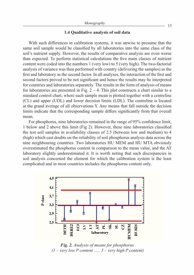
With such differences in calibration systems, it was unwise to presume that the same soil sample would be classified by all laboratories into the same class of the soil’s nutrient supply. However, the results of comparative analysis are even worse than expected. To perform statistical calculations the five main classes of nutrient content were coded into the numbers 1 (very low) to 5 (very high). The two-factorial analysis of variance was then performed with country (delivering the samples) as the first and laboratory as the second factor. In all analyses, the interaction of the first and second factors proved to be not significant and hence the results may be interpreted for countries and laboratories separately. The results in the form of analysis of means for laboratories are presented in Fig. 2 – 4. This plot constructs a chart similar to a standard control chart, where each sample mean is plotted together with a centreline (CL) and upper (UDL) and lower decision limits (LDL). The centreline is located at the grand average of all observations Y. Any means that fall outside the decision limits indicate that the corresponding sample differs significantly from that overall mean.
For phosphorus, nine laboratories remained in the range of 95% confidence limit, 1 below and 2 above this limit (Fig 2). However, these nine laboratories classified the test soil samples in availability classes of 2.5 (between low and medium) to 4 (high) which cast doubts on the reliability of soil phosphorus analysis data across the nine neighbouring countries. Two laboratories HU MEM and HU MTA obviously overestimated the phosphorus content in comparison to the mean value, and the AT laboratory slightly underestimated it. It is worth noting that such discrepancies in soil analysis concerned the element for which the calibration system is the least complicated and in most countries includes the phosphorus content only.
Fig. 2. Analysis of means for phosphorus (1 – very low P content ….. 5 – very high P content)
14 Edited by Mariusz Fotyma, Eike Stefan Dobers – Poland
From the Annex 1, the average contents of phosphorus in the “medium” class, irrespective of other soil parameters (if any), is calculated and shown in table 6. The figures for laboratories using ME-3 and AL methods have been recalculated to values for CAL and DL method using equation (2). In relation to the mean value for 11 collaborating laboratories, the content of phosphorus in the “medium” class seems to be slightly underestimated by EE, LV, and LT laboratories.
Table 6. Average contents of phosphorus in the “medium “class [expressed in CAL/ DL units]
Average content of phosphorus in “medium” class in mg P*kg-1soil extrapolated to CAL/DL units in the country
DE TH DE HE EE LV LT A T* PL SK SL CZ HU Mean 49-72 49-72 37-68 29-55 40-51 47-111 45-65 62-83 44-75 60-79 54-79 47-73
*In the latest edition of the “Austrian guidelines for appropriate fertilisation” (BMLFUW, 2006) the fact of the broad range and the high upper limit of the “medium” class was met with a reduction of fertiliser recommendation up to 50% in the “high” medium class of phosphorus and potassium (see also Spiegel et al., 2006).
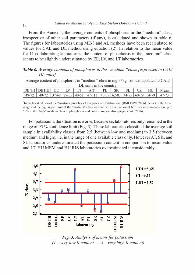
For potassium, the situation is worse, because six laboratories only remained in the range of 95 % confidence limit (Fig. 3). These laboratories classified the average soil sample in availability classes from 2.5 (between low and medium) to 3.5 (between medium and high), i.e. in the range of one available class only. However AT, SK, and SL laboratories underestimated the potassium content in comparison to mean value and LT, HU MEM and HU RIS laboratories overestimated it considerably.
Fig. 3. Analysis of means for potassium (1 – very low K content …. 5 – very high K content)

15Monography
Like phosphorus, the average contents of potassium in the “medium” class are calculated irrespective of other soil parameters and shown in table 7. The figures for laboratories using ME-3 and AL methods have been transformed to figures for CAL and DL method using equation (3). Compared to the mean value for all laboratories the content of potassium in the “medium” class is strongly overestimated in AT, SK, SL and CZ laboratories and underestimated in LV and LT laboratories.
Table 7. Average contents of potassium in “medium “class (expressed in CAL/ DL units)
Average content of potassium in “medium” class in mg K*kg-1soil extrapolated to CAL/DL units in the country
DE TH
DE HE EE LV LT A T* PL SK SL CZ HU Mean
93-148
93-148 92-132 69-137 71-97 113-212 94-150 147-207
125-182
143-215
122-172
105-163
* see explanation under table 6
For magnesium, 8 laboratories were in the range of 95 % confidence limit and this range was rather narrow from about 3 (medium content) to 4 (high content), i.e. including one availability class (Fig 4).
Fig. 4. Analysis of means for magnesium (1 – very low Mg content …5 – very high Mg content)
16 Edited by Mariusz Fotyma, Eike Stefan Dobers – Poland
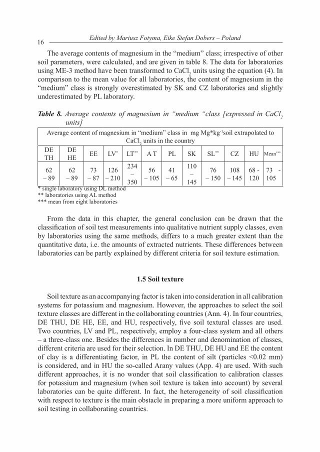
The average contents of magnesium in the “medium” class; irrespective of other soil parameters, were calculated, and are given in table 8. The data for laboratories using ME-3 method have been transformed to CaCl2 units using the equation (4). In comparison to the mean value for all laboratories, the content of magnesium in the “medium” class is strongly overestimated by SK and CZ laboratories and slightly underestimated by PL laboratory.
Table 8. Average contents of magnesium in “medium “class [expressed in CaCl2 units]
Average content of magnesium in “medium” class in mg Mg*kg-1soil extrapolated to CaCl2 units in the country
DE TH
DE HE EE LV* LT** A T PL SK SL** CZ HU Mean***
62 – 89
62 – 89
73 – 87
126 – 210
234 –
350
56 – 105
41 – 65
110 –
145
76 – 150
108 – 145
68 - 120
73 -105
* single laboratory using DL method** laboratories using AL method*** mean from eight laboratories
From the data in this chapter, the general conclusion can be drawn that the classification of soil test measurements into qualitative nutrient supply classes, even by laboratories using the same methods, differs to a much greater extent than the quantitative data, i.e. the amounts of extracted nutrients. These differences between laboratories can be partly explained by different criteria for soil texture estimation.
1.5 Soil texture
Soil texture as an accompanying factor is taken into consideration in all calibration systems for potassium and magnesium. However, the approaches to select the soil texture classes are different in the collaborating countries (Ann. 4). In four countries, DE THU, DE HE, EE, and HU, respectively, five soil textural classes are used. Two countries, LV and PL, respectively, employ a four-class system and all others – a three-class one. Besides the differences in number and denomination of classes, different criteria are used for their selection. In DE THU, DE HU and EE the content of clay is a differentiating factor, in PL the content of silt (particles <0.02 mm) is considered, and in HU the so-called Arany values (App. 4) are used. With such different approaches, it is no wonder that soil classification to calibration classes for potassium and magnesium (when soil texture is taken into account) by several laboratories can be quite different. In fact, the heterogeneity of soil classification with respect to texture is the main obstacle in preparing a more uniform approach to soil testing in collaborating countries.
17Monography
2. Comparison of recommended fertilizer rates
In two-factorial analysis of variance, countries (providing two soil samples each) were recognised as the first and laboratories (performing analysis and giving fertilizer recommendations) as the second factor. Both main factors proved to be significant while interaction was not and therefore the differences of the first order were interpreted only. Fertilizer recommendations were derived for the following crops: winter wheat (WW), winter rape (WRP), winter rye (WR), maize for grain (MAG), potatoes (POT), and maize for silage (MAS). The recommended fertilizer rates for all crops are presented in tables 9 – 14. However, due to high discrepancies between four crops grown for grain and without manure and two crops grown for fodder on manure the results for these two groups are discussed separately.
2.1 Recommended rates of nutrients for grain crops2.1.1 Phosphorus
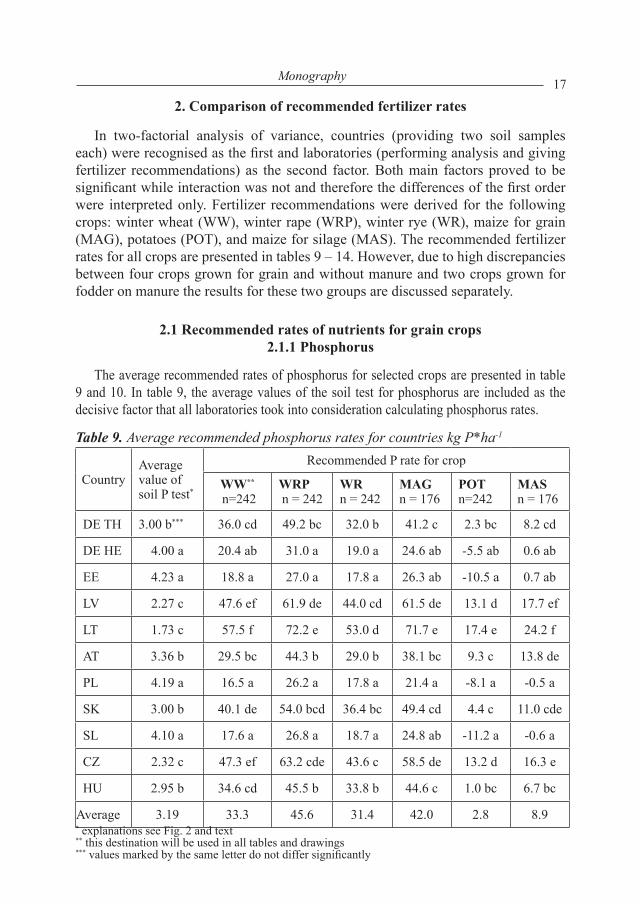
The average recommended rates of phosphorus for selected crops are presented in table 9 and 10. In table 9, the average values of the soil test for phosphorus are included as the decisive factor that all laboratories took into consideration calculating phosphorus rates.
Table 9. Average recommended phosphorus rates for countries kg P*ha-1
CountryAverage value of soil P test*
Recommended P rate for crop
WW**
.n=242WRP.n = 242
WRn = 242
MAGn = 176
POTn=242
MASn = 176
DE TH 3.00 b*** 36.0 cd 49.2 bc 32.0 b 41.2 c 2.3 bc 8.2 cd
DE HE 4.00 a 20.4 ab 31.0 a 19.0 a 24.6 ab -5.5 ab 0.6 ab
EE 4.23 a 18.8 a 27.0 a 17.8 a 26.3 ab -10.5 a 0.7 ab
LV 2.27 c 47.6 ef 61.9 de 44.0 cd 61.5 de 13.1 d 17.7 ef
LT 1.73 c 57.5 f 72.2 e 53.0 d 71.7 e 17.4 e 24.2 f
AT 3.36 b 29.5 bc 44.3 b 29.0 b 38.1 bc 9.3 c 13.8 de
PL 4.19 a 16.5 a 26.2 a 17.8 a 21.4 a -8.1 a -0.5 a
SK 3.00 b 40.1 de 54.0 bcd 36.4 bc 49.4 cd 4.4 c 11.0 cde
SL 4.10 a 17.6 a 26.8 a 18.7 a 24.8 ab -11.2 a -0.6 a
CZ 2.32 c 47.3 ef 63.2 cde 43.6 c 58.5 de 13.2 d 16.3 e
HU 2.95 b 34.6 cd 45.5 b 33.8 b 44.6 c 1.0 bc 6.7 bc
Average 3.19 33.3 45.6 31.4 42.0 2.8 8.9* explanations see Fig. 2 and text ** this destination will be used in all tables and drawings *** values marked by the same letter do not differ significantly
18 Edited by Mariusz Fotyma, Eike Stefan Dobers – Poland
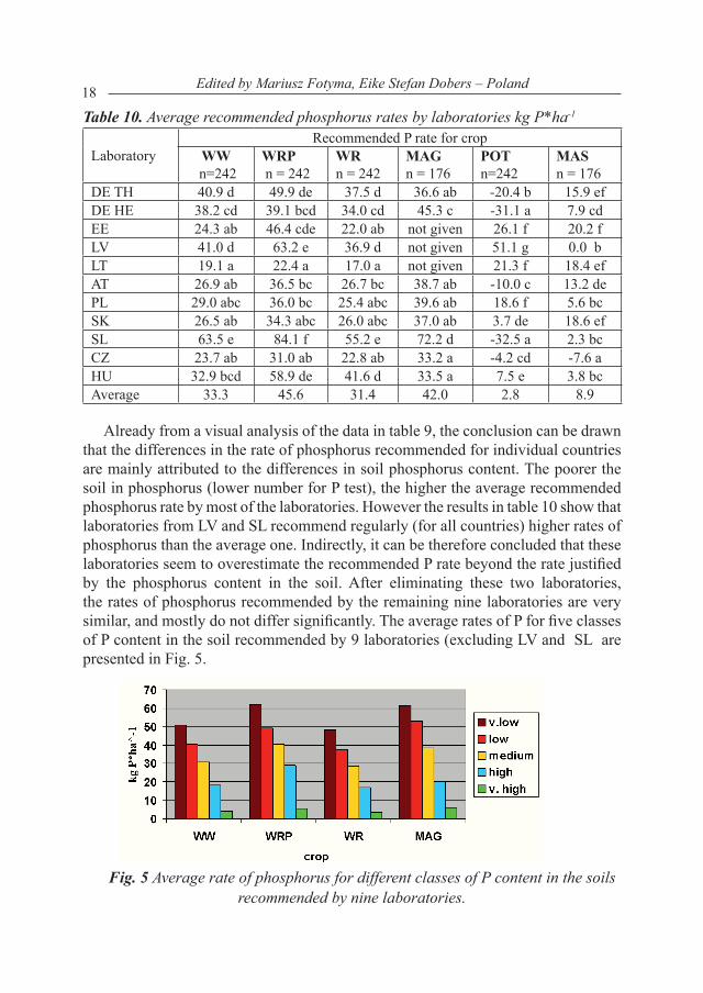
Table 10. Average recommended phosphorus rates by laboratories kg P*ha-1
Laboratory Recommended P rate for crop
WW.n=242
WRP.n = 242
WRn = 242
MAGn = 176
POTn=242
MASn = 176
DE TH 40.9 d 49.9 de 37.5 d 36.6 ab -20.4 b 15.9 efDE HE 38.2 cd 39.1 bcd 34.0 cd 45.3 c -31.1 a 7.9 cdEE 24.3 ab 46.4 cde 22.0 ab not given 26.1 f 20.2 fLV 41.0 d 63.2 e 36.9 d not given 51.1 g 0.0 bLT 19.1 a 22.4 a 17.0 a not given 21.3 f 18.4 ef AT 26.9 ab 36.5 bc 26.7 bc 38.7 ab -10.0 c 13.2 dePL 29.0 abc 36.0 bc 25.4 abc 39.6 ab 18.6 f 5.6 bcSK 26.5 ab 34.3 abc 26.0 abc 37.0 ab 3.7 de 18.6 ef SL 63.5 e 84.1 f 55.2 e 72.2 d -32.5 a 2.3 bcCZ 23.7 ab 31.0 ab 22.8 ab 33.2 a -4.2 cd -7.6 aHU 32.9 bcd 58.9 de 41.6 d 33.5 a 7.5 e 3.8 bcAverage 33.3 45.6 31.4 42.0 2.8 8.9
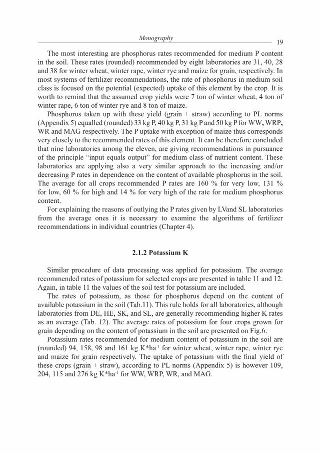
Already from a visual analysis of the data in table 9, the conclusion can be drawn that the differences in the rate of phosphorus recommended for individual countries are mainly attributed to the differences in soil phosphorus content. The poorer the soil in phosphorus (lower number for P test), the higher the average recommended phosphorus rate by most of the laboratories. However the results in table 10 show that laboratories from LV and SL recommend regularly (for all countries) higher rates of phosphorus than the average one. Indirectly, it can be therefore concluded that these laboratories seem to overestimate the recommended P rate beyond the rate justified by the phosphorus content in the soil. After eliminating these two laboratories, the rates of phosphorus recommended by the remaining nine laboratories are very similar, and mostly do not differ significantly. The average rates of P for five classes of P content in the soil recommended by 9 laboratories (excluding LV and SL are presented in Fig. 5.
Fig. 5 Average rate of phosphorus for different classes of P content in the soils recommended by nine laboratories.
19Monography
The most interesting are phosphorus rates recommended for medium P content in the soil. These rates (rounded) recommended by eight laboratories are 31, 40, 28 and 38 for winter wheat, winter rape, winter rye and maize for grain, respectively. In most systems of fertilizer recommendations, the rate of phosphorus in medium soil class is focused on the potential (expected) uptake of this element by the crop. It is worth to remind that the assumed crop yields were 7 ton of winter wheat, 4 ton of winter rape, 6 ton of winter rye and 8 ton of maize.
Phosphorus taken up with these yield (grain + straw) according to PL norms (Appendix 5) equalled (rounded) 33 kg P, 40 kg P, 31 kg P and 50 kg P for WW, WRP, WR and MAG respectively. The P uptake with exception of maize thus corresponds very closely to the recommended rates of this element. It can be therefore concluded that nine laboratories among the eleven, are giving recommendations in pursuance of the principle “input equals output” for medium class of nutrient content. These laboratories are applying also a very similar approach to the increasing and/or decreasing P rates in dependence on the content of available phosphorus in the soil. The average for all crops recommended P rates are 160 % for very low, 131 % for low, 60 % for high and 14 % for very high of the rate for medium phosphorus content.
For explaining the reasons of outlying the P rates given by LVand SL laboratories from the average ones it is necessary to examine the algorithms of fertilizer recommendations in individual countries (Chapter 4).
2.1.2 Potassium k
Similar procedure of data processing was applied for potassium. The average recommended rates of potassium for selected crops are presented in table 11 and 12. Again, in table 11 the values of the soil test for potassium are included.
The rates of potassium, as those for phosphorus depend on the content of available potassium in the soil (Tab.11). This rule holds for all laboratories, although laboratories from DE, HE, SK, and SL, are generally recommending higher K rates as an average (Tab. 12). The average rates of potassium for four crops grown for grain depending on the content of potassium in the soil are presented on Fig.6.
Potassium rates recommended for medium content of potassium in the soil are (rounded) 94, 158, 98 and 161 kg K*ha-1 for winter wheat, winter rape, winter rye and maize for grain respectively. The uptake of potassium with the final yield of these crops (grain + straw), according to PL norms (Appendix 5) is however 109, 204, 115 and 276 kg K*ha-1 for WW, WRP, WR, and MAG.
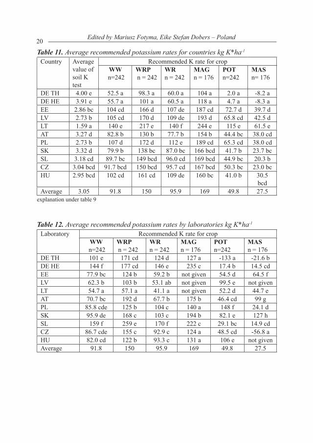
20 Edited by Mariusz Fotyma, Eike Stefan Dobers – Poland
Table 11. Average recommended potassium rates for countries kg K*ha-1
Country Average value of soil K test
Recommended K rate for cropWW
.n=242WRP.n = 242
WRn = 242
MAGn = 176
POTn=242
MASn= 176
DE TH 4.00 e 52.5 a 98.3 a 60.0 a 104 a 2.0 a -8.2 aDE HE 3.91 e 55.7 a 101 a 60.5 a 118 a 4.7 a -8.3 aEE 2.86 bc 104 cd 166 d 107 de 187 cd 72.7 d 39.7 dLV 2.73 b 105 cd 170 d 109 de 193 d 65.8 cd 42.5 dLT 1.59 a 140 e 217 e 140 f 244 e 115 e 61.5 eAT 3.27 d 82.8 b 130 b 77.7 b 154 b 44.4 bc 38.0 cdPL 2.73 b 107 d 172 d 112 e 189 cd 65.3 cd 38.0 cdSK 3.32 d 79.9 b 138 bc 87.0 bc 166 bcd 41.7 b 23.7 bcSL 3.18 cd 89.7 bc 149 bcd 96.0 cd 169 bcd 44.9 bc 20.3 bCZ 3.04 bcd 91.7 bcd 150 bcd 95.7 cd 167 bcd 50.3 bc 23.0 bcHU 2.95 bcd 102 cd 161 cd 109 de 160 bc 41.0 b 30.5
bcdAverage 3.05 91.8 150 95.9 169 49.8 27.5
explanation under table 9
Table 12. Average recommended potassium rates by laboratories kg K*ha-1
Laboratory Recommended K rate for cropWW
.n=242WRP.n = 242
WRn = 242
MAGn = 176
POTn=242
MASn = 176
DE TH 101 e 171 cd 124 d 127 a -133 a -21.6 bDE HE 144 f 177 cd 146 e 235 c 17.4 b 14.5 cd EE 77.9 bc 124 b 59.2 b not given 54.5 d 64.5 fLV 62.3 b 103 b 53.1 ab not given 99.5 e not givenLT 54.7 a 57.1 a 41.1 a not given 52.2 d 44.7 eAT 70.7 bc 192 d 67.7 b 175 b 46.4 cd 99 gPL 85.8 cde 125 b 104 c 140 a 148 f 24.1 dSK 95.9 de 168 c 103 c 194 b 82.1 e 127 h SL 159 f 259 e 170 f 222 c 29.1 bc 14.9 cdCZ 86.7 cde 155 c 92.9 c 124 a 48.5 cd -56.8 aHU 82.0 cd 122 b 93.3 c 131 a 106 e not givenAverage 91.8 150 95.9 169 49.8 27.5

21Monography
Fig. 6 Average rate of potassium for different classes of K content in the soils recommended by 11 laboratories.
Therefore, for cereals, the average recommended rates of potassium correspond quite closely to the uptake of this element, while for winter rape and grain maize recommended K rates are lower or much lower than the removal of potassium with the assumed yield of both crops. Even laboratories from DF HE, SK and SL recommending higher than average rates of potassium for winter rape and maize for grain seem to abstain from the principle “ input equals output” for these crops. All laboratories are applying a similar approach to the increasing and/or decreasing K rates in dependence on the content of available potassium in the soil. The average for all crops recommended K rates are 163 % for very low, 136 % for low, 59 % for high and 36 % for very high of the rate for medium potassium content. With exception of very high K content these increases and/or decreases of potassium rates correspond astonishingly closely to the similar figures for phosphorus.
2.1.3 Magnesium Mg
Not all laboratories are recommending magnesium rates at all, and therefore the results for this element are based on the smaller set of date than the data for phosphorus and potassium. Moreover, the magnesium rates recommended by SL laboratory (except those for AT country) seem to be unrealistically high and therefore they have been discarded from further analysis. Finally, the two-factorial analysis of variance was performed for nine laboratories. The results by countries are presented in table 13 and by laboratories in table 14.

22 Edited by Mariusz Fotyma, Eike Stefan Dobers – Poland
Table 13. Average recommended magnesium rates for countries kg Mg*ha-1
Country
Average value of soil Mg
test*
Recommended Mg rate for cropWW
.n=220WRP.n = 220
WRn = 220
MAGn = 176
POTn=220
MASn = 176
DE TH 3.83 b 8.1 bc 10.1 bc 8.5 cdef 21.4 bcde
-12.1 a 2.1 abc
DE HE 2.89 a 16.2 ef 17.2 de 13.5 fg 31.1 ef -3.6 def 10.6 eEE 2.67 a 18.8 f 21.6 e 16.9 g 35.3 f -1.9 f 8.4 bcdeLV 4.05 b 2.3 a 2.7 a 1.9 a 5.1 a -7.5 bcde -1.1 aLT 4.17 b 5.5 ab 6.2 ab 4.8 ab 12.8 ab -8.1 abc 3.3 abcdAT 3.89 b 8.9 bcd 9.0 b 7.7 cde 19.8 bcd -6.8 cde 1.9 abPL 3.11 a 14.1 def 15.9 de 12.8 efg 27.7 def -3.7 cdef 9.9 deSK 4.28 b 5.7 ab 5.6 ab 3.6 ab 11.3 ab -7.8 abcd 2.9 abcSL 3.78 b 8.1 bc 8.9 b 7.3 cd 18.8 bcd -7.0 cde 5.8 bcdeCZ 3.05 a 12.8 cde 15.5 cd 11.0 def 25.3 cdef -3.1 ef 8.9 cdeHU 4.05 b 7.3 abc 8.6 b 6.6 abc 15.3 abc -11.6 ab 4.1 abcd
Average 3.62 9.8 11.0 8.6 20.4 -6.6 5.2* explanation under table 9
Table 14. Average recommended magnesium rates by laboratories kg Mg*ha-1Laboratory Recommended Mg rate for crop
WW.n=220
WRP.n = 220
WRn = 220
MAGn = 176
POTn=220
MASn = 176
DE TH 14.2 de 16.5 de 13.4 d 19.0 bc -25.2 ab 10.3 deDE HE 14.4 de 11.4 bce 11.1 cd 34.7 d -29.5 a 0.4 bcEE 6.4 ab 7.7 bc 4.5 ab not given 3.1 cd 4.5 cd LV not given not given not given not given not given not givenLT 3.7 a 4.9 a 2.4 a not given not given not given AT 7.9 abc 7.1 bc 7.1 bc 7.1 a -29.1 a -7.4 aPL 10.4 bcd 12.0 bce 8.3 bc 22.6 c 8.1 e 4.9 cdSK 15.7 e 18.0 e 13.8 d 34.7 d 18.2 f 14.4 e SL 59.1 f 60.4 d 59.5 d 62.7 e 5.0 de 32.7 f CZ 11.6 cde 13.4 cde 11.2 cd 14.1 abc -24.5 b -5.1 abHU 4.1 a 8.2 bce 5.4 ab 10.2 ab 0.6 cd 2.0 cAverage 9.8 11.0 8.6 20.4 -6.6 5.2
In spite of a smaller amount of data, the general regularities are the same as those already presented for phosphorus and potassium. The recommended rates of Mg depend strongly on the content of available magnesium in the soils (Fig. 7). The only difference is in similar recommendations for very low and low content of magnesium. All laboratories are applying a similar approach to the increasing and/or decreasing Mg rates, dependent on the content of available magnesium in the soil.
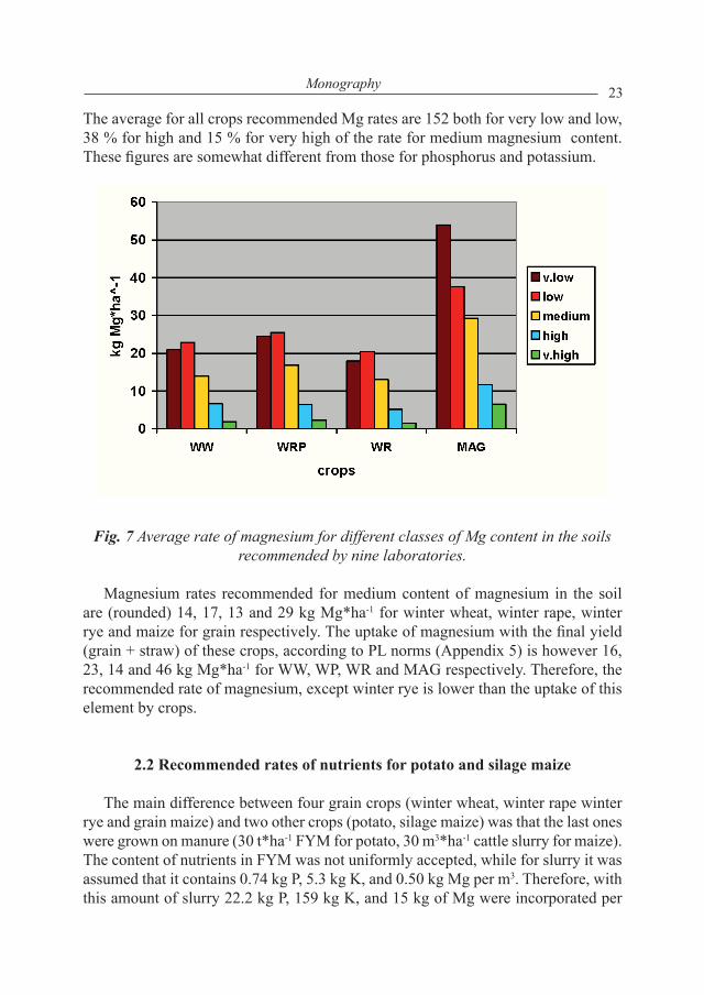
23Monography
The average for all crops recommended Mg rates are 152 both for very low and low, 38 % for high and 15 % for very high of the rate for medium magnesium content. These figures are somewhat different from those for phosphorus and potassium.
Fig. 7 Average rate of magnesium for different classes of Mg content in the soils recommended by nine laboratories.
Magnesium rates recommended for medium content of magnesium in the soil are (rounded) 14, 17, 13 and 29 kg Mg*ha-1 for winter wheat, winter rape, winter rye and maize for grain respectively. The uptake of magnesium with the final yield (grain + straw) of these crops, according to PL norms (Appendix 5) is however 16, 23, 14 and 46 kg Mg*ha-1 for WW, WP, WR and MAG respectively. Therefore, the recommended rate of magnesium, except winter rye is lower than the uptake of this element by crops.
2.2 Recommended rates of nutrients for potato and silage maize
The main difference between four grain crops (winter wheat, winter rape winter rye and grain maize) and two other crops (potato, silage maize) was that the last ones were grown on manure (30 t*ha-1 FYM for potato, 30 m3*ha-1 cattle slurry for maize). The content of nutrients in FYM was not uniformly accepted, while for slurry it was assumed that it contains 0.74 kg P, 5.3 kg K, and 0.50 kg Mg per m3. Therefore, with this amount of slurry 22.2 kg P, 159 kg K, and 15 kg of Mg were incorporated per
24 Edited by Mariusz Fotyma, Eike Stefan Dobers – Poland
ha. According to Polish norms (Appendix 5) FYM contains 0.13 % P, 0.58 % K and 0.12 % Mg and consequently with the amount of 30 t FYM *ha-1 39 kg P, 174 kg K and 36 kg Mg were incorporated under potato crop. The approach to the amount of nutrients in manure and its utilisation by crop is different in collaborating countries and it is no wonder that the rates of mineral fertilizers recommended by laboratories differ considerably (Tables 9 - 14).
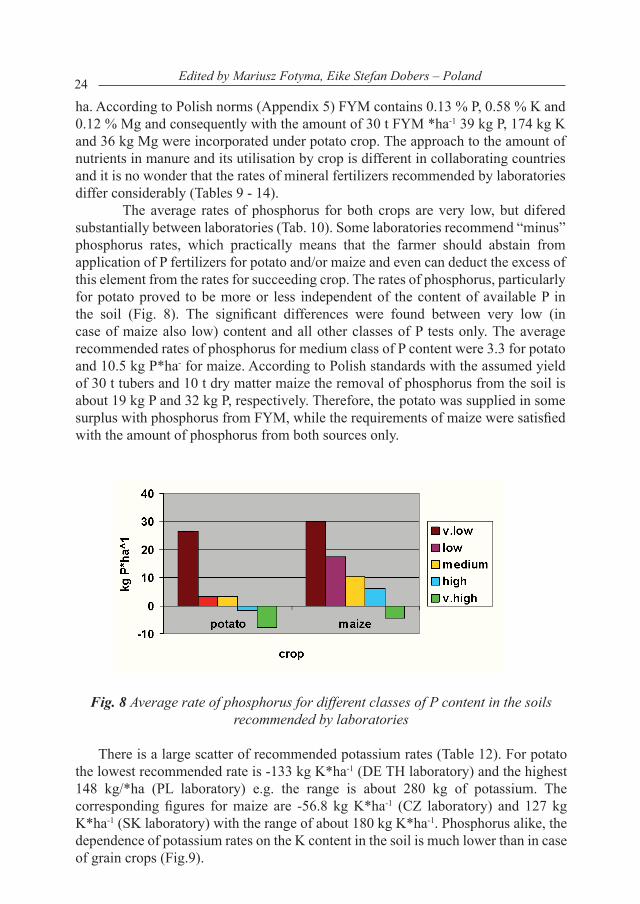
The average rates of phosphorus for both crops are very low, but difered substantially between laboratories (Tab. 10). Some laboratories recommend “minus” phosphorus rates, which practically means that the farmer should abstain from application of P fertilizers for potato and/or maize and even can deduct the excess of this element from the rates for succeeding crop. The rates of phosphorus, particularly for potato proved to be more or less independent of the content of available P in the soil (Fig. 8). The significant differences were found between very low (in case of maize also low) content and all other classes of P tests only. The average recommended rates of phosphorus for medium class of P content were 3.3 for potato and 10.5 kg P*ha- for maize. According to Polish standards with the assumed yield of 30 t tubers and 10 t dry matter maize the removal of phosphorus from the soil is about 19 kg P and 32 kg P, respectively. Therefore, the potato was supplied in some surplus with phosphorus from FYM, while the requirements of maize were satisfied with the amount of phosphorus from both sources only.
Fig. 8 Average rate of phosphorus for different classes of P content in the soils recommended by laboratories
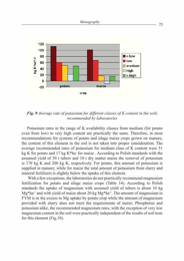
There is a large scatter of recommended potassium rates (Table 12). For potato the lowest recommended rate is -133 kg K*ha-1 (DE TH laboratory) and the highest 148 kg/*ha (PL laboratory) e.g. the range is about 280 kg of potassium. The corresponding figures for maize are -56.8 kg K*ha-1 (CZ laboratory) and 127 kg K*ha-1 (SK laboratory) with the range of about 180 kg K*ha-1. Phosphorus alike, the dependence of potassium rates on the K content in the soil is much lower than in case of grain crops (Fig.9).
25Monography
Fig. 9 Average rate of potassium for different classes of K content in the soils recommended by laboratories
Potassium rates in the range of K availability classes from medium (for potato
even from low) to very high content are practically the same. Therefore, in most recommendations for systems of potato and silage maize crops grown on manure, the content of this element in the soil is not taken into proper consideration. The average recommended rates of potassium for medium class of K content were 51 kg K for potato and 17 kg K*ha- for maize . According to Polish standards with the assumed yield of 30 t tubers and 10 t dry matter maize the removal of potassium is 170 kg K and 200 kg K, respectively. For potato, this amount of potassium is supplied in manure, while for maize the total amount of potassium from slurry and mineral fertilizers is slightly below the uptake of this element.
With a few exceptions, the laboratories do not practically recommend magnesium fertilization for potato and silage maize crops (Table 14). According to Polish standards the uptake of magnesium with assumed yield of tubers is about 10 kg Mg*ha-1 and with yield of maize about 20 kg Mg*ha-1. The amount of magnesium in FYM is in the excess to Mg uptake by potato crop while the amount of magnesium provided with slurry does not meet the requirements of maize. Phosphorus and potassium alike, the recommended magnesium rates, with the exception of very low magnesium content in the soil were practically independent of the results of soil tests for this element (Fig.10).
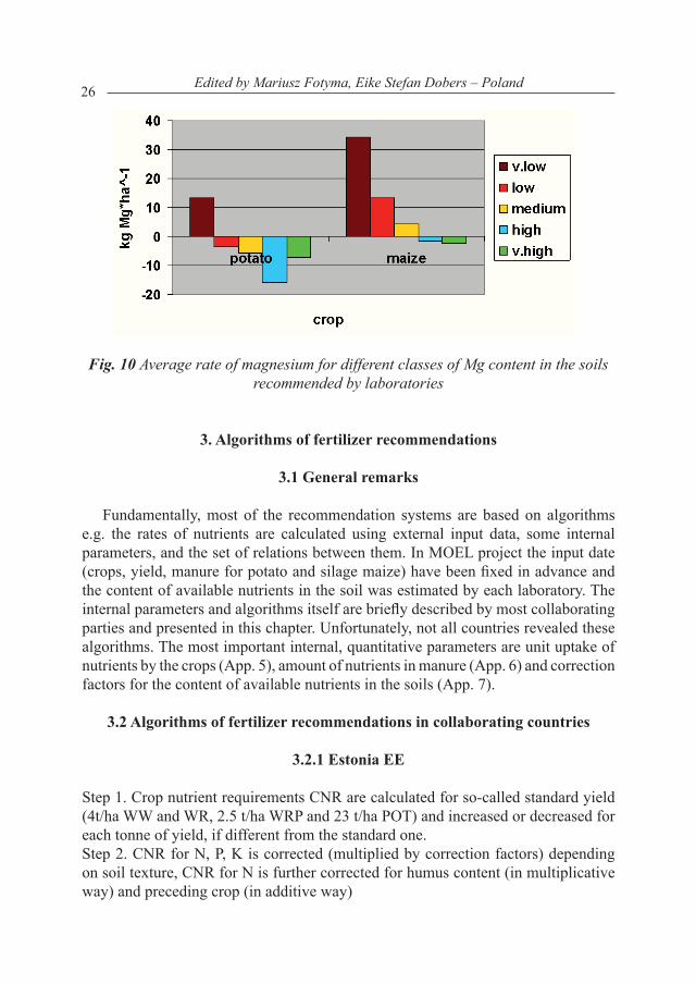
26 Edited by Mariusz Fotyma, Eike Stefan Dobers – Poland
Fig. 10 Average rate of magnesium for different classes of Mg content in the soils recommended by laboratories
3. Algorithms of fertilizer recommendations
3.1 General remarks
Fundamentally, most of the recommendation systems are based on algorithms e.g. the rates of nutrients are calculated using external input data, some internal parameters, and the set of relations between them. In MOEL project the input date (crops, yield, manure for potato and silage maize) have been fixed in advance and the content of available nutrients in the soil was estimated by each laboratory. The internal parameters and algorithms itself are briefly described by most collaborating parties and presented in this chapter. Unfortunately, not all countries revealed these algorithms. The most important internal, quantitative parameters are unit uptake of nutrients by the crops (App. 5), amount of nutrients in manure (App. 6) and correction factors for the content of available nutrients in the soils (App. 7).
3.2 Algorithms of fertilizer recommendations in collaborating countries
3.2.1 Estonia EE
Step 1. Crop nutrient requirements CNR are calculated for so-called standard yield (4t/ha WW and WR, 2.5 t/ha WRP and 23 t/ha POT) and increased or decreased for each tonne of yield, if different from the standard one.Step 2. CNR for N, P, K is corrected (multiplied by correction factors) depending on soil texture, CNR for N is further corrected for humus content (in multiplicative way) and preceding crop (in additive way)
27Monography
Step 3. After steps 1.2 the CNR for P, K is corrected depending on the content of these nutrients in the soil (App.7)Step 4. For crops grown on manure CNR is diminished by the amount of nutrients in manure (App. 6) multiplied by utilisation factor
3.2.2 Latvia LV
Step 1 Calculation crop nutrients requirements CNR (standard demand)Step 2. Correction for yieldStep 3. Correction for soil textureStep 4. Correction for soil pH (P only)Step 5. Correction for the content of P and K in soilStep 6. Correction for previous cropStep 7. Correction for manure application, taking into account nutrient utilization from manure
3.2.3 Lithuania LT
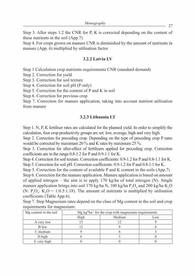
Step 1. N, P, K fertiliser rates are calculated for the planned yield. In order to simplify the calculation, four crop productivity groups are set: low, average, high and very high.Step 2. Correction for preceding crop. Depending on the type of preceding crop P rates would be corrected by maximum 20 % and K rates by maximum 25 %. Step 3. Correction for after-effect of fertilizers applied for preceding crop. Correction coefficients are in the range 0.8-1.2 for P and 0.9-1.1 for K.Step 4. Correction for soil texture. Correction coefficients: 0.9-1.2 for P and 0.8-1.1 for K.Step 5. Correction for soil pH. Correction coefficients: 0.9-1.2 for P and 0.8-1.1 for K.Step 5. Correction for the content of available P and K content in the soils (App.7) Step 6. Correction for the manure application. Manure application is based on amount of applied nitrogen – the aim is to apply 170 kg/ha of total nitrogen (N). Single manure application brings into soil 170 kg/ha N, 100 kg/ha P2O5 and 200 kg/ha K2O (N: P2O5: K2O = 1:0.5:1.18). The amount of nutrients is multiplied by utilisation coefficients (Table App.6).Step 7. Step Magnesium rates depend on the class of Mg content in the soil and crop requirements for magnesium:
Mg content in the soil Mg kg*ha-1 for the crop with magnesium requirements High Medium Low
A very low 15 12 9B low 12 9 6
C medium 9 6 3D high 6 3 0
E very high 0 0 0
28 Edited by Mariusz Fotyma, Eike Stefan Dobers – Poland
3.2.4 Austria AT
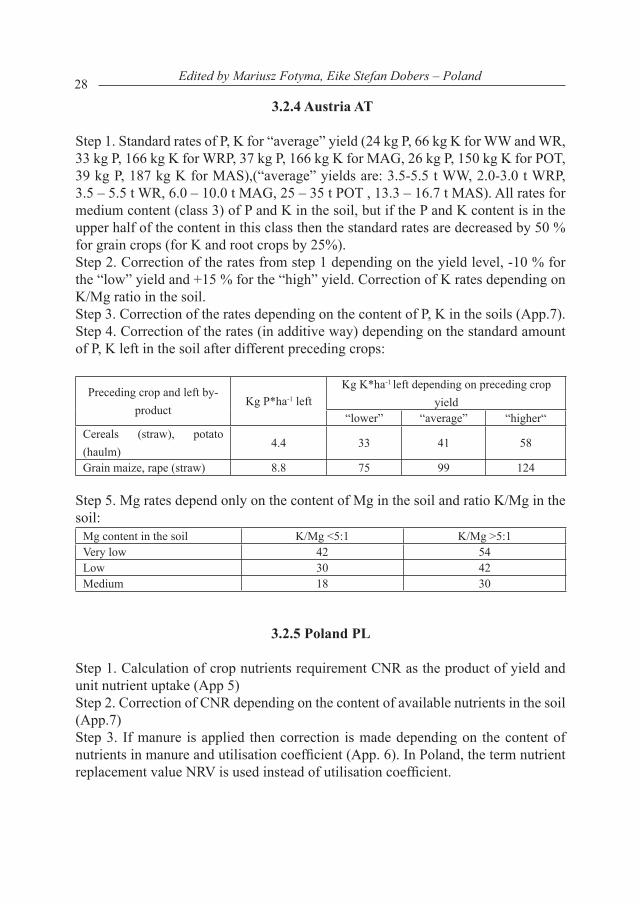
Step 1. Standard rates of P, K for “average” yield (24 kg P, 66 kg K for WW and WR, 33 kg P, 166 kg K for WRP, 37 kg P, 166 kg K for MAG, 26 kg P, 150 kg K for POT, 39 kg P, 187 kg K for MAS),(“average” yields are: 3.5-5.5 t WW, 2.0-3.0 t WRP, 3.5 – 5.5 t WR, 6.0 – 10.0 t MAG, 25 – 35 t POT , 13.3 – 16.7 t MAS). All rates for medium content (class 3) of P and K in the soil, but if the P and K content is in the upper half of the content in this class then the standard rates are decreased by 50 % for grain crops (for K and root crops by 25%). Step 2. Correction of the rates from step 1 depending on the yield level, -10 % for the “low” yield and +15 % for the “high” yield. Correction of K rates depending on K/Mg ratio in the soil. Step 3. Correction of the rates depending on the content of P, K in the soils (App.7).Step 4. Correction of the rates (in additive way) depending on the standard amount of P, K left in the soil after different preceding crops:
Preceding crop and left by-product
Kg P*ha-1 leftKg K*ha-1 left depending on preceding crop
yield“lower” “average” “higher“
Cereals (straw), potato (haulm)
4.4 33 41 58
Grain maize, rape (straw) 8.8 75 99 124
Step 5. Mg rates depend only on the content of Mg in the soil and ratio K/Mg in the soil:
Mg content in the soil K/Mg <5:1 K/Mg >5:1Very low 42 54Low 30 42Medium 18 30
3.2.5 Poland PL
Step 1..Calculation of crop nutrients requirement CNR as the product of yield and unit nutrient uptake (App 5) Step 2. Correction of CNR depending on the content of available nutrients in the soil (App.7)Step 3. If manure is applied then correction is made depending on the content of nutrients in manure and utilisation coefficient (App. 6). In Poland, the term nutrient replacement value NRV is used instead of utilisation coefficient.

29Monography
3.2.6 Slovenia SL
Step 1. Calculation of crop nutrient requirement CNR (according to the uptake)Step 2. Correction of CNR depending on the content of available nutrients in the soil (App.7) Step 3. The rates of Mg depend on the magnesium content in the soil (class of Mg content) and the relation of K/Mg:
Class of content Fertilization norm Mg kg*ha-1
A 36-48*
B 30-36*C 0-24*D 0E 0
* if the ratio between K (by AL) and Mg (by CaCl2) is wider than 6:1, then higher norm is advised, otherwise the lower
3.2.7 Czech Republic CZ
Step 1. Calculation of crop nutrients requirement CNR as the product of yield and unit nutrient uptake (App. 5) Step 2. Correction of CNR depending on the content of available nutrients in the soil (App. 7)Step 3. If manure is applied then correction is made depending on the content of nutrients in manure and utilisation coefficient (App. 6)
3.2.8 Hungary HU
Step 1. Affiliation of soil site on the base of soil properties.Step 2. Forecasting the yield level on the base of past 5 years yieldsStep 3. Quantification of P, K soil supplying capacity on the base of available nutrients content, taking into consideration soil type and other soil properties (pH. CaCO3 content)Step 4. Calculation of plant nutrient requirements using the formulae:
Nutrient requirement = Q*f
Where : Q – forecasted yield f – standard coefficient including crop, soil nutrient supply, soil typeStep 5. Correction of nutrient requirement (step 4) taking into consideration the preceding crop, manure, soil management etc.
30 Edited by Mariusz Fotyma, Eike Stefan Dobers – Poland
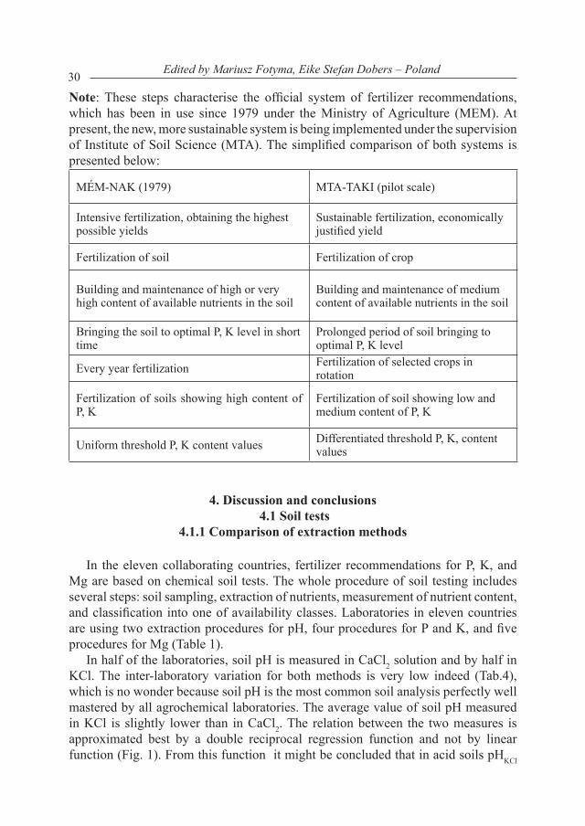
Note: These steps characterise the official system of fertilizer recommendations, which has been in use since 1979 under the Ministry of Agriculture (MEM). At present, the new, more sustainable system is being implemented under the supervision of Institute of Soil Science (MTA). The simplified comparison of both systems is presented below:
MÉM-NAK (1979) MTA-TAKI (pilot scale)
Intensive fertilization, obtaining the highest possible yields
Sustainable fertilization, economically justified yield
Fertilization of soil Fertilization of crop
Building and maintenance of high or very high content of available nutrients in the soil
Building and maintenance of medium content of available nutrients in the soil
Bringing the soil to optimal P, K level in short time
Prolonged period of soil bringing to optimal P, K level
Every year fertilization Fertilization of selected crops in rotation
Fertilization of soils showing high content of P, K
Fertilization of soil showing low and medium content of P, K
Uniform threshold P, K content values Differentiated threshold P, K, content values
4. Discussion and conclusions 4.1 Soil tests
4.1.1 Comparison of extraction methods
In the eleven collaborating countries, fertilizer recommendations for P, K, and Mg are based on chemical soil tests. The whole procedure of soil testing includes several steps: soil sampling, extraction of nutrients, measurement of nutrient content, and classification into one of availability classes. Laboratories in eleven countries are using two extraction procedures for pH, four procedures for P and K, and five procedures for Mg (Table 1).
In half of the laboratories, soil pH is measured in CaCl2 solution and by half in KCl. The inter-laboratory variation for both methods is very low indeed (Tab.4), which is no wonder because soil pH is the most common soil analysis perfectly well mastered by all agrochemical laboratories. The average value of soil pH measured in KCl is slightly lower than in CaCl2. The relation between the two measures is approximated best by a double reciprocal regression function and not by linear function (Fig. 1). From this function it might be concluded that in acid soils pHKCl
31Monography
values are by 0.5 – 0.6 units lower than pHCaCl2, for neutral soils, both measures are the same, and for alkaline soils values determined with pHKCl are slightly higher as those with pHCaCl2 (Fig 1). However such relation concerns only the date from this research and should not be generalized. Potassium ion from KCl has higher exchange power then calcium ion from CaCl2 and replace more hydrogen ions from soil solid phase. Therefore the pH measured in KCl solution is regularly lower then in CaCl2 though this relation is not necessarily proportional.
Practically both methods can be used therefore alterably, but due to the lack of linearity it would be better to agree upon one uniform extracting solution. Though most countries are using KCl, other considerations are in favour of CaCl2 solution. The ionic composition and strength of CaCl2 resembles more the composition of soil solution in soils kept in good culture. Besides, in the same extract the content of available magnesium could be measured after slight modification of original Schachtschabel method.
All laboratories are using one solution for P and K extraction, though the chemical composition of these solutions is different. Approximately half of the laboratories are using solutions containing Ca2+ in acid medium (acidified with HCl or acetic acid) e.g. DL or CAL methods. Practically the same quantities of P and K are being extracted by both solutions and they can be used likewise. The problem arises with alkaline (calcium carbonate) soils where most of the phosphorus is in the calcium phosphate forms freely soluble in the acid medium of DL and/or CAL solutions. To overcame this problem PL laboratory is using AL method for alkaline soils and laboratories from DE TH and DE HE are using the empirical formulae to modify the extracted (measured) amount of phosphorus, taking into consideration the pH of CAL solutions measured after extraction of P and K (final pH).
P,K adjusted= P,K measured*(1+0,83*(pHCAL)final-4,1)
The remaining laboratories are using either AL method or Mehlich – 3 method. The amounts of P and K extracted by these methods are significantly higher in comparison to DL and/or CAL methods (Table 3). The advantage of Mehlich method is in the possibility of simultaneous extraction of Mg (as well as micronutrients) and this method seems to gain importance in Central – Eastern European countries. Some years ago, the SK and CZ laboratories switched over to this method and in 2004, the EE laboratory changed extraction solution from DL into Mehlich-3. This possibility is also being considered in PL. There is a straight relation between the amounts of P and/or K measured by DL/CAL methods and AL/Mehlich-3 methods with the slope of regression line close to one. It gives the possibility to recalculate the values from one method to another as has been presented in Tables 6, 7. However, the determination coefficients for both nutrients, particularly for phosphorus, are not too high and these relations are strongly sample-dependent (variable).
Laboratories, which use the same method of analysis, produce statistically uniform results (Table 4). This proves the reliability of both the methods and laboratories.
32 Edited by Mariusz Fotyma, Eike Stefan Dobers – Poland
Only the data for potassium from the SL laboratory differ significantly from the average for laboratories performing AL method.
The most ambiguous results are for magnesium. The collaborating laboratories are using altogether five methods of available magnesium determination with two methods at the top (CaCl2- 5 laboratories and Mehlich-3 – 3 laboratories). From the remaining three laboratories, each is using different method, subordinated (with the exception of HU laboratory) to the idea of using the single extract for P, K, Mg (DL method by LV laboratory, and AL method for LT laboratory). The HU laboratory is using KCl as the extracting solution for Mg estimation. The amounts of Mg extracted by CaCl2 and KCl methods are very similar and the lowest among all five methods (Table 3). The amounts of Mg extracted by Mehlich-3 and DL methods are approximately double so high and extracted by AL method – almost four times so high as extracted by CaCl2/KCl methods. The relation between the amounts of Mg extracted by CaCl2 and Mehlich-3 methods was approximated the best by the linear regression. However, the determination coefficient is not high which cast doubts on the possibility of recalculation the results from one method to another. The inter-laboratory scatter of date for CaCl2 method is lower than for Mehlich -3 method, which is the argument on behalf of the former one. However, as has been already mentioned the advantage of Mehlich-3 method lies in the possibility of extracting three nutrients simultaneously. In Estonia the changing from the AL extraction method to the Mehlich 3 method was among the other reasons influenced by the results of soil magnesium content analysis. There was strong positive correlation between the results obtained by AL extraction method and soil total magnesium content (especially by alkaline soils). However the results for CaCl2, KCl, ammonium acetate and Mehlich 3 extract were not correlated to the total soil Mg-content. Also the results from soil and plant analysis showed that the content of magnesium in plants (winter wheat, potato) correlated well with content of magnesium in soil,determined by means of CaCl2, ammonium acetate and Mehlich 3 extract but for AL-extract the correlation was weak. From here we can conclude that AL-extract is not suitable for determination of plant available magnesium from alkaline soils [Loide, 2001, 2002].The AL and DL methods seem to be unsuitable for routine analysis of the soil for available magnesium content. In the years 2000-2001, PL laboratories performed the comparative analysis of Mg content in almost 3000 soil samples analysed by DL method and CaCl2 method [Boguszewska et al., 2001]. The general relation showed a big scatter of the date (low determination coefficient) and proved to be dependent on soil pH and soil texture. Generally, the acid extractants are unsuitable for estimation the content of available magnesium in soil. In acid medium Mg from the magnesium carbonate and dolomite comes into solution although these compounds are not directly absorbed by the plants and belong rather to the sources of potentially available magnesium. For this reason is also Mehlich -3 extractant is not suitable for Mg estimation. In Hungary, the comparative analysis of Mg content for AL. and CaCl2 methods has been performed on 1500 soils. It was concluded that the relation
33Monography
between amount of Mg extracted by these two methods differ considerably for the carbonate and free-carbonate soils. Therefore, for analysis of available Mg content, only the methods based on neutral extractant, like CaCl2 give reliable results [Loch, personal opinion].
Generally speaking, the “good” extraction procedure should meet the following expectations [Fotyma, Shepherd 2000]:1. the method must reflect the nutrient bio-availability. In practical terms, this means
high correlation coefficients with the plant indices as estimated in calibration procedure. This is considered more thoroughly in the next chapter.
2. it is based on some well defined soil processes of the nutrient transformations i.e. cation exchange, ion binding, ligand formation etc.
3. it is viable and reliable, i.e. it is laboratory “ friendly”, cheap and robust4. should have “universality” i.e. the possibility to extract more than one , possibly
all basic nutrientsThe “goodness” of methods used by collaborating laboratories in line with
expectations 2 to 4 is in favour of Mehlich – 3. The literature data show [Fotyma, Shepherd 2000] that by this method the comparable amounts of potassium and magnesium to those as defined as exchangeable, were extracted. Besides, this method is fully viable and reliable and universal as well with respect to extract several macro- and micro-nutrients. According to the calculations made in PL, this method is the cheapest as well and does not need any new laboratory equipment. Mehlich – 3 methods has been highly evaluated in extensive study carried on in Czech Republic by Zbiral and Nemec [Zbiral 2000, Zbiral, Nemec 2000]. It is also recommended in review paper [Ziadi, Sen Tran 2008] in the last edition of handbook on methods of soil analysis [Collective 2008]. The results of this inter-laboratory soil samples exchange confirm the high value of Mehlich-3 method.
4.1.2 Comparison of calibration schemes
Soil test has no value for agricultural services without proper calibration i.e. separation of the whole range of nutrients content into several classes which correspond to the expected crop demands for fertilizer. In all collaborating countries, with exception of LT, five levels of nutrients content in the soil are recognised. The names of the levels, translated from native language into English and/or German are somewhat different , but for the sake of simplicity in this report the following names and/or abbreviations have been used: very low (A -1), low (B-2), medium (C-3), high (D-4), very high (E-5). In LT a sixth level is separated, but in this report it has been included into the very high one. However, assigning the soil sample to the particular class depends not only on the nutrient level (in mg*kg-1soil) but in most calibration systems other soil properties (texture, humus content, pH) are taken into consideration (table 5). The simplest calibration systems recognise the content of
34 Edited by Mariusz Fotyma, Eike Stefan Dobers – Poland
nutrient only (i.e. DE TH, DE HE, LT, AT, PL SL – for phosphorus) and the most complicated ones recognise soil texture, soil pH, crop demands for a given nutrient (i.e. HU MTA system, Table 5). Taking furthermore into consideration the different methods of soil extraction it is no wonder that direct comparison of calibration systems in collaborating countries (do not even mention the principles of calibration) is practically impossible.
The key point of each calibration system is the medium class of nutrient content. In the most recommendations systems, based on nutrient balance the nutrient rate for this particular nutrient content corresponds to the plant nutrient requirements (expected yield times nutrient unit uptake). For nutrient contents differing from the medium one, correction coefficients are used to calculate the nutrients rate (App.7). For medium content this correction coefficient is of course, equal to one. In sustainable fertilization systems, the medium content of nutrient is more and more often recognised as the “safe” one from environmental point of view. For these reasons the content of nutrients in medium class, after recalculating into CAL/DL units for P and K and CaCl2 units for Mg was presented in separate tables (Tables 6-8). In the next planned stage of MOEL project focused on more compatible fertilizers recommendations system the soils samples showing medium content of nutrients will be exchanged only.
The range of phosphorus content in this class is rather narrow and quite similar in collaborating laboratories. The only exception is AT laboratory, which entertains a fairly wide range of P content, but in fertilizer recommendations this medium content is subdivided into two sub-classes (“low-medium” and “high-medium”).
The range of potassium content in medium class, again with exception of AT laboratory, is also tolerably narrow and similar among the laboratories. However, the figures for K content in medium class used by LT laboratory are much lower and used by SK and CZ laboratories somewhat higher than the average for 11 laboratories. In SK and CZ recommendation systems, the content of nutrients in each class is subdivided into two sub-classes with different coefficients for increasing or decreasing fertilizer rates.
In eight laboratories, using either CaCl2 or Mehlich-3 methods for magnesium estimation the range of Mg content in medium class (recalculated in CaCl2 units) is also rather narrow and the differences between laboratories are acceptable. However, the results for remaining three laboratories using different methods are entirely incomparable and beside one must remember the low determination coefficients for recalculating the Mg content by Mehlich-3 method into CaCl2 method.
Skipping the differences between laboratories, it seems that calibration systems meet more or less closely at the medium content of nutrient, which makes a good starting point for further work on more harmonised system in collaborating countries. Such harmonisation is very important because at the moment the same soil sample send to different laboratories would be classified to different classes of nutrients content, which is hardly to accept among the neighbouring countries with rather similar soil and climatic conditions. Of course, the longer the distance between
35Monography
the countries the more these differences can be explained by pedo-climatological factors.
Analysis for the means of phosphorus (Fig. 2) shows that nine laboratories remained in the range of 95% confidence limit, one below and two above this limit. However, these nine laboratories classified the test soil samples in availability classes of 2.5 (between low and medium) to 4 (high).
On the ground of similar analysis for potassium, six laboratories only remained in the range of 95 % confidence limit (Fig. 3). These laboratories classified the average soil sample in availability classes from 2.5 (between low and medium) to 3.5 (between medium and high), i.e. in the range of one availability class, which can be tolerated. However AT, SK and SL laboratories underestimated the potassium content in comparison to mean value and LT, HU MEM and HU MTA laboratories overestimated it considerably.
For magnesium eight laboratories using either CaCl2 method or Mehlich – 3 method, were in the range of 95 % confidence limit and this range was rather narrow from about 3 (medium content) to 4 (high content), i.e. including one availability class. Estimation of Mg content by AL method or DL methods seems to be unsuitable for characterising the availability of this nutrient for the crops.
4.2 Fertilizer recommendations 4.2.1 Recommendations schemes (algorithms)
Most of the recommendations schemes used by collaborating countries seem to be based on the nutrient balance principle, modified by the content of available nutrient in the soils [see also Bujnovsky, Fotyma 2001]. It can be described by the general equation:
Recommended rate = (nutrient uptake – nutrient in manure*utilisation coefficient)*correction factor for nutrient class
Nutrient uptake called often crop nutrient requirement CRN is usually (laboratories PL, SL, SK, CZ, HU) calculated as the product of expected total yield (grain + straw) and unit uptake of the nutrient per tonne of total yield . Some laboratories accept so-called standard yield or standard CNR approaches (EE, LV, AT) and modify it (additively or multiplicatively) depending on the yield level. Most collaborating countries provided the date on standardised nutrient uptake as one of the parameters of recommendation scheme (Table15, App. 5).
36 Edited by Mariusz Fotyma, Eike Stefan Dobers – Poland
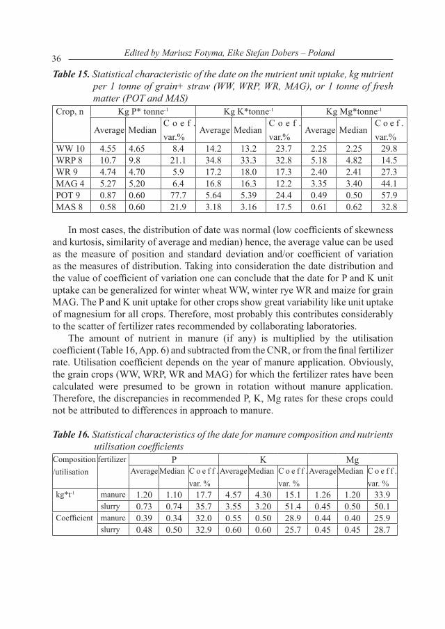
Table 15. Statistical characteristic of the date on the nutrient unit uptake, kg nutrient per 1 tonne of grain+ straw (WW, WRP, WR, MAG), or 1 tonne of fresh matter (POT and MAS)
Crop, n Kg P* tonne-1 Kg K*tonne-1 Kg Mg*tonne-1
Average MedianC o e f .var.%
Average MedianC o e f .var.%
Average MedianC o e f .var.%
WW 10 4.55 4.65 8.4 14.2 13.2 23.7 2.25 2.25 29.8WRP 8 10.7 9.8 21.1 34.8 33.3 32.8 5.18 4.82 14.5WR 9 4.74 4.70 5.9 17.2 18.0 17.3 2.40 2.41 27.3MAG 4 5.27 5.20 6.4 16.8 16.3 12.2 3.35 3.40 44.1POT 9 0.87 0.60 77.7 5.64 5.39 24.4 0.49 0.50 57.9MAS 8 0.58 0.60 21.9 3.18 3.16 17.5 0.61 0.62 32.8
In most cases, the distribution of date was normal (low coefficients of skewness
and kurtosis, similarity of average and median) hence, the average value can be used as the measure of position and standard deviation and/or coefficient of variation as the measures of distribution. Taking into consideration the date distribution and the value of coefficient of variation one can conclude that the date for P and K unit uptake can be generalized for winter wheat WW, winter rye WR and maize for grain MAG. The P and K unit uptake for other crops show great variability like unit uptake of magnesium for all crops. Therefore, most probably this contributes considerably to the scatter of fertilizer rates recommended by collaborating laboratories.
The amount of nutrient in manure (if any) is multiplied by the utilisation coefficient (Table 16, App. 6) and subtracted from the CNR, or from the final fertilizer rate. Utilisation coefficient depends on the year of manure application. Obviously, the grain crops (WW, WRP, WR and MAG) for which the fertilizer rates have been calculated were presumed to be grown in rotation without manure application. Therefore, the discrepancies in recommended P, K, Mg rates for these crops could not be attributed to differences in approach to manure.
Table 16. Statistical characteristics of the date for manure composition and nutrients utilisation coefficients
Composition/utilisation
fertilizer P K MgAverage Median C o e f f .
var. %Average Median C o e f f .
var. %Average Median C o e f f .
var. %kg*t-1 manure 1.20 1.10 17.7 4.57 4.30 15.1 1.26 1.20 33.9
slurry 0.73 0.74 35.7 3.55 3.20 51.4 0.45 0.50 50.1Coefficient manure 0.39 0.34 32.0 0.55 0.50 28.9 0.44 0.40 25.9
slurry 0.48 0.50 32.9 0.60 0.60 25.7 0.45 0.45 28.7
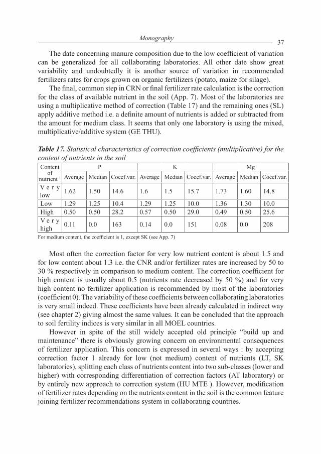
37Monography
The date concerning manure composition due to the low coefficient of variation can be generalized for all collaborating laboratories. All other date show great variability and undoubtedly it is another source of variation in recommended fertilizers rates for crops grown on organic fertilizers (potato, maize for silage).
The final, common step in CRN or final fertilizer rate calculation is the correction for the class of available nutrient in the soil (App. 7). Most of the laboratories are using a multiplicative method of correction (Table 17) and the remaining ones (SL) apply additive method i.e. a definite amount of nutrients is added or subtracted from the amount for medium class. It seems that only one laboratory is using the mixed, multiplicative/additive system (GE THU).
Table 17. Statistical characteristics of correction coefficients (multiplicative) for the content of nutrients in the soil Content
of nutrient 1
P K Mg
Average Median Coeef.var. Average Median Coeef.var. Average Median Coeef.var.
V e r y low 1.62 1.50 14.6 1.6 1.5 15.7 1.73 1.60 14.8
Low 1.29 1.25 10.4 1.29 1.25 10.0 1.36 1.30 10.0High 0.50 0.50 28.2 0.57 0.50 29.0 0.49 0.50 25.6V e r y high 0.11 0.0 163 0.14 0.0 151 0.08 0.0 208
For medium content, the coefficient is 1, except SK (see App. 7)
Most often the correction factor for very low nutrient content is about 1.5 and for low content about 1.3 i.e. the CNR and/or fertilizer rates are increased by 50 to 30 % respectively in comparison to medium content. The correction coefficient for high content is usually about 0.5 (nutrients rate decreased by 50 %) and for very high content no fertilizer application is recommended by most of the laboratories (coefficient 0). The variability of these coefficients between collaborating laboratories is very small indeed. These coefficients have been already calculated in indirect way (see chapter 2) giving almost the same values. It can be concluded that the approach to soil fertility indices is very similar in all MOEL countries.
However in spite of the still widely accepted old principle “build up and maintenance” there is obviously growing concern on environmental consequences of fertilizer application. This concern is expressed in several ways : by accepting correction factor 1 already for low (not medium) content of nutrients (LT, SK laboratories), splitting each class of nutrients content into two sub-classes (lower and higher) with corresponding differentiation of correction factors (AT laboratory) or by entirely new approach to correction system (HU MTE ). However, modification of fertilizer rates depending on the nutrients content in the soil is the common feature joining fertilizer recommendations system in collaborating countries.
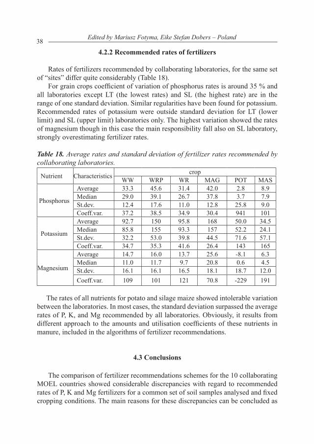
38 Edited by Mariusz Fotyma, Eike Stefan Dobers – Poland
4.2.2 Recommended rates of fertilizers
Rates of fertilizers recommended by collaborating laboratories, for the same set of “sites” differ quite considerably (Table 18).
For grain crops coefficient of variation of phosphorus rates is around 35 % and all laboratories except LT (the lowest rates) and SL (the highest rate) are in the range of one standard deviation. Similar regularities have been found for potassium. Recommended rates of potassium were outside standard deviation for LT (lower limit) and SL (upper limit) laboratories only. The highest variation showed the rates of magnesium though in this case the main responsibility fall also on SL laboratory, strongly overestimating fertilizer rates.
Table 18. Average rates and standard deviation of fertilizer rates recommended by collaborating laboratories.
Nutrient Characteristics cropWW WRP WR MAG POT MAS
Phosphorus
Average 33.3 45.6 31.4 42.0 2.8 8.9Median 29.0 39.1 26.7 37.8 3.7 7.9St.dev. 12.4 17.6 11.0 12.8 25.8 9.0Coeff.var. 37.2 38.5 34.9 30.4 941 101
Potassium
Average 92.7 150 95.8 168 50.0 34.5Median 85.8 155 93.3 157 52.2 24.1St.dev. 32.2 53.0 39.8 44.5 71.6 57.1Coeff.var. 34.7 35.3 41.6 26.4 143 165
Magnesium
Average 14.7 16.0 13.7 25.6 -8.1 6.3Median 11.0 11.7 9.7 20.8 0.6 4.5St.dev. 16.1 16.1 16.5 18.1 18.7 12.0Coeff.var. 109 101 121 70.8 -229 191
The rates of all nutrients for potato and silage maize showed intolerable variation
between the laboratories. In most cases, the standard deviation surpassed the average rates of P, K, and Mg recommended by all laboratories. Obviously, it results from different approach to the amounts and utilisation coefficients of these nutrients in manure, included in the algorithms of fertilizer recommendations.
4.3 Conclusions
The comparison of fertilizer recommendations schemes for the 10 collaborating MOEL countries showed considerable discrepancies with regard to recommended rates of P, K and Mg fertilizers for a common set of soil samples analysed and fixed cropping conditions. The main reasons for these discrepancies can be concluded as

39Monography
follows:1. Different methods of soil analysis and particularly the differences in the
calibration of the available nutrients content.2. Different approach to soils texture, based generally on the soil granulometric
composition3. Differences in the basic parameters of the generally accept system of
recommendations based on balance method i.e. unit uptake of nutrients per tonne of the product, content of nutrients in organic fertilizers, utilisation coefficients of nutrients from organic fertilizers.However most of the systems have many common aspects in their approaches
of algorithms, which offers the possibility of developing an at least partly unified or harmonized system of fertilizer recommendations for the MOEL countries. The next step to be made in further common research is an increased focus on the soils of nutrient class medium, and developing the respective recommendations..
References
1. BMLFUW (2006): Richtlinien für die sachgerechte Düngung. 6. Auflage. Fachbeirat für Bodenfruchtbarkeit und Bodenschutz. Bundesministerium für Land- und Forstwirtschaft, Umwelt- und Wasserwirtschaft, Wien.
2. Boguszewska,M., Fotyma,E., Fotyma,M. 2001. The possibility of using the Egner-DL extract for estimating the content of available magnesium in Polish soils (in Polish). Zeszyty Problemowe Postępów Nauk Rolniczych. 480: 377-383.
3. Bujnovsky,R., Fotyma,M. 2001. Fertilizer recommendation schemes officially used In Czech Republic, Latvia, Poland, Slovak Republic, and the United Kingdom. Nawozy i Nawożenie – Fertilizers and Fertilization ed. Fotyma,M., Shepherd,A. Sustainable nutrient management. MAINTAIN Report 2. .1: 5 - 31.
4. Fotyma,M., Mercik,S. 2005 Chemia Rolna, PWN, Warszawa5. Fotyma,M., Shepherd,M. edited. 2000. Soil fertility evaluation in the Czech
Republic, Latvia, Poland, Slovak Republic, and the United Kingdom. Nawozy i nawożenie - Fertilizers and Fertilization. 2(3): pp. 66.
6. Karklins A. 2003. Fertilizer recommendations to meet objectives for Good Agriculture Practice approach. Proceedings of the Latvia university of Agriculture Nr.8 (303), Jelgava, pp 13-17
7. Karklins,A. 2001. Model for the calculation of nutrient offtake by crop: OFFTAKE model. Nawozy i Nawożenie – Fertilizers and Fertilization ed. Fotyma,M., Shepherd, A. Sustainable nutrient management. MAINTAIN Report 2. .1: 63-74.
8. Kerschberger,M., Franke,G., Hess, H. 1997. Anleitung und Richtwerte fur Nahrstoffvergleiche nach Dungeverordnung. Jena.
40 Edited by Mariusz Fotyma, Eike Stefan Dobers – Poland
9. Klir,J., Cermak,P. 2001. Standard figures for manure composition and N-manure equivalents. Nawozy i Nawożenie – Fertilizers and Fertilization ed. Fotyma, M., Shepherd, A. Sustainable nutrient management. MAINTAIN Report 2. .1: 32-39.
10. Loch J. - Jászberényi I. - Vágó I. (1998): Hundredth molar calcium chloride extraction procedure. Part III: Calibration with conventional soil testing methods for magnesium. Commun. Soil Sci. Plant Anal. 29. 11-14. 1633-1640.
11. Loide, V.,2001. On the contents of available magnesium and the ratio of potassium and magnesium in field soils of Estonia. J. of Agricultural Science, 1, p. 51-55, (in Estonian, summary in English).
12. Loide, V.2002 The content of available magnesium of Estonian soils, its ratio to potassium and calcium and the effect on the yield of field crops. Thesis for applying for the doctor’s degree in agriculture. Tartu, 2002: 123 p. (In Estonian, summary in English).
13. Ristimaki,L.M. 2007. Potassium and magnesium fertilizer recommendations in some European countries. IFS Proceedings. 620. pp.31
14. Spiegel,H., Baumgarten,A., Dersch,G. 2006. Revised form of the “Austrian Guidelines for appropriate fertilisation” and the influence of “Cross Compliance” and its national implementation. Acta agriculturae Slovenica, 87-1, 93-107.
15. Timbare R., Jekabsone M., Dekovica S a.o. 2006. Study of development of soil agrochemical analysis methods. Yearbook of Agrochemical Research Centre. Riga, pp. 32-35
16. Timbare R., Reinfelde L. 2002. Comparison of phosphorus and potassium determination methods currently used to assess soil fertility status in various countries. Regional IPI Workshop “Potassium and phosphorus for sustainable agriculture”, Jelgava, p.23
17. Zbiral,J. 2000. Determination of phosphoprus in calcareous soils by Mehlich-3, Mehlich-2, CAL and Egner extractants. Commun. Soil. Sci. Plant Anal. 31: 3037-3048.
18. Zbiral,J., Nemec,P. 2000. Integrating of the Mehlich-3 extractant into the Czech soil-testing scheme. Commun. Soil. Sci. Plant Anal. 31: 2171-2182.
19. Ziadi,N., Sen Tran,T. 2005 Mehlich – 3 extractable elements in soil sampling and methods of analysis. Ed. Carter,M.R., Gregorich,E.G. Canadian Society of Soil Science
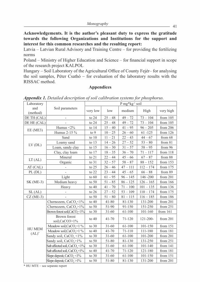
41Monography
Acknowledgements. It is the author’s pleasant duty to express the gratitude towards the following Organizations and Institutions for the support and interest for this common researches and the resulting report:Latvia – Latvian Rural Advisory and Training Centre – for providing the fertilizing normsPoland – Ministry of Higher Education and Science – for financial support in scope of the research project KALPOL Hungary – Soil Laboratory of the Agricultural Office of County Fejér– for analysing the soil samples, Péter Csathó – for evaluation of the laboratory results with the RISSAC method.
Appendices
Appendix 1. Detailed description of soil calibration systems for phosphorus. Laboratory
and (method)
Soil parametersP mg*kg-1 soil
very low low medium High very high
DE TH (CAL) - to 24 25 – 48 49 – 72 73 – 104 from 105DE HE (CAL) - to 24 25 – 48 49 – 72 73 – 104 from 105
EE (ME3)Humus <2% to 14 15 – 40 41 – 95 96 – 205 from 206
Humus 2-15 % to 9 10 – 25 26 – 60 61 -125 from 126
LV (DL)
Sand to 10 11 – 21 22 – 43 44 – 67 from 68Loamy sand to 13 14 – 26 27 – 52 53 – 80 from 81
Loam, sandy clay to 15 16 – 30 31 – 57 58 – 95 from 96Clay, clay loam to 17 18 – 35 36 – 70 71 – 117 from 118
LT (AL)Mineral to 21 22 – 44 45 – 66 67 – 87 from 88Organic to 31 32 – 57 58 – 87 88 – 152 from 153
AT (CAL) - to 25 26 – 46 47 – 111 112 – 174 from 175PL (DL) - to 22 23 – 44 45 – 65 66 – 88 from 89
SK (ME-3) Light to 60 61 – 95 96 – 145 146 -200 from 201
Medium heavy to 50 51 – 85 86 – 125 126 – 165 from 166Heavy to 40 41 – 70 71 – 100 101 – 135 from 136
SL (AL) - to 26 27 – 52 53 – 109 110 – 174 from 175CZ (ME-3) - to 50 51 – 80 81 – 115 116 – 185 from 186
HU MEM (AL)*
Chernozem, CaCO3<1% to 40 41-80 81-130 131-200 from 201Chernozem, CaCO3>1% to 50 51-90 91-150 151-250 from 251Brown forest soil,CaCO3<1% to 30 31-60 61-100 101-160 from 161
Brown forest soil,CaCO3>1% to 40 41-70 71-120 121-200- from 201
Meadow soil,CaCO3<1 % to 30 31-60 61-100 101-150 from 151Meadow soil,CaCO3>1 % to 40 41-70 71-110 111-180 from 181
Sandy soil, CaCO3 <1% to 30 31-60 61-100 101-200 from 201Sandy soil, CaCO3>1% to 50 51-80 81-130 131-250 from 251Salt affected soil, CaCO3 <1% to 30 31-60 61-100 101-140 from 141Salt affected soil, CaCO3>1% to 40 41-70 71-120 121-180 from 181Slope deposit, CaCO3 <1% to 30 31-60 61-100 101-150 from 151Slope deposit, CaCO3 >1% to 50 51-80 81-130 131-200 from 201
* HU MTE – see separate report

42 Edited by Mariusz Fotyma, Eike Stefan Dobers – Poland
Appendix 2. Detailed description of soil calibration systems for potassium.
Laboratory(method
used)
Soil parameters K mg*kg-1 soil
very low low medium High very high
DE TH (CAL)
Sand to 20 21 – 60 61 – 100 101 – 150 from 151Loamy - sand to 30 31 – 70 71 – 110 111 – 180 from 181Sandy - loam to 40 41 – 90 91 – 140 141 – 220 from 221Loam to 50 51 – 100 101 – 160 161 – 250 from 251Clay to 70 71 – 140 141 – 230 231 – 360 from 361
DE HE (CAL)
Sand to 30 31 – 60 61 – 100 101 – 150 from 151Loamy - sand to 40 41 – 70 71 – 110 111 – 180 from 181Sandy – loam to 50 51 – 90 91 – 140 141 – 220 from 221Loam to 60 61 – 100 101 – 160 161 – 250 from 251Clay to 80 81– 140 141 – 230 231 – 360 from 361Organic to 50 51 – 90 91 – 160 161 – 240 fom 241
EE (ME3)
Sand to 40 41 – 65 66 – 115 116 – 195 from 196Loamy - sand to 50 51 – 90 91 – 140 141 – 280 from 281Sandy – loam to 65 66 – 105 106 – 170 171 – 325 from 326Loam to 75 76 – 130 131 – 195 196 – 360 from 361Clay to 130 131-195 196 – 285 286 – 500 from 501
LV (DL)
Sand to 25 26 – 50 51 – 100 101 – 170 from 171Loamy sand to 33 34 – 66 67 – 133 134 – 224 from 225Loam, sandy clay to 37 38 – 75 76 – 149 150 – 253 from 254Clay, clay loam to 41 42 – 83 84 – 166 167 – 282 from 283
LT (AL)Mineral to 42 43 – 83 84 - 125 126 – 166 from 166Organic to 101 102 – 166 167 – 250 251 – 415 from 416
AT (CAL) Light to 49 50 – 87 88 – 178 179 – 191 From 292Medium to 65 66 – 112 113 – 208 209 – 332 From 332heavy to 82 83 - 137 138 – 245 246 – 374 From 375
PL (DL) Very light to 21 22 – 61 63 – 104 105 – 145 from 146Light to 41 42 – 83 84 – 124 125 – 166 from 166Medium to 62 63 – 104 105 – 166 167 – 207 from 207Heavy to 83 84 – 125 126 – 207 207 – 249 from 250
SK (ME-3) Light to 90 91 – 150 151 - 230 231 – 350 from 351Medium heavy to 130 131 – 200 201 – 300 301 – 400 from 401Heavy to 170 171 – 260 261 – 370 371 – 500 from 500
SL (AL) Light to medium heavy
to 83 84 – 158 159 – 250 251 – 330 from 330
heavy to 100 101 – 180 181 – 270 271 – 370 from 371
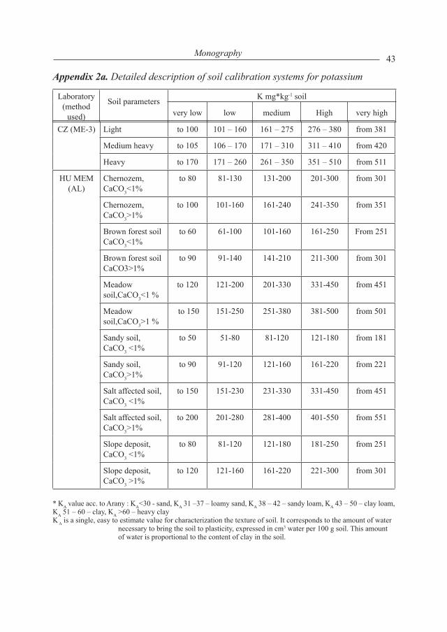
43Monography
CZ (ME-3) Light to 100 101 – 160 161 – 275 276 – 380 from 381
Medium heavy to 105 106 – 170 171 – 310 311 – 410 from 420
Heavy to 170 171 – 260 261 – 350 351 – 510 from 511
HU MEM (AL)
Chernozem, CaCO3<1%
to 80 81-130 131-200 201-300 from 301
Chernozem, CaCO3>1%
to 100 101-160 161-240 241-350 from 351
Brown forest soil CaCO3<1%
to 60 61-100 101-160 161-250 From 251
Brown forest soil CaCO3>1%
to 90 91-140 141-210 211-300 from 301
Meadow soil,CaCO3<1 %
to 120 121-200 201-330 331-450 from 451
Meadow soil,CaCO3>1 %
to 150 151-250 251-380 381-500 from 501
Sandy soil, CaCO3 <1%
to 50 51-80 81-120 121-180 from 181
Sandy soil, CaCO3>1%
to 90 91-120 121-160 161-220 from 221
Salt affected soil, CaCO3 <1%
to 150 151-230 231-330 331-450 from 451
Salt affected soil, CaCO3>1%
to 200 201-280 281-400 401-550 from 551
Slope deposit, CaCO3 <1%
to 80 81-120 121-180 181-250 from 251
Slope deposit, CaCO3 >1%
to 120 121-160 161-220 221-300 from 301
* KA value acc. to Arany : KA<30 - sand, KA 31 –37 – loamy sand, KA 38 – 42 – sandy loam, KA 43 – 50 – clay loam, KA 51 – 60 – clay, KA >60 – heavy clay K A is a single, easy to estimate value for characterization the texture of soil. It corresponds to the amount of water
necessary to bring the soil to plasticity, expressed in cm3 water per 100 g soil. This amount of water is proportional to the content of clay in the soil.
Appendix 2a. Detailed description of soil calibration systems for potassium
Laboratory(method
used)
Soil parameters K mg*kg-1 soil
very low low medium High very high
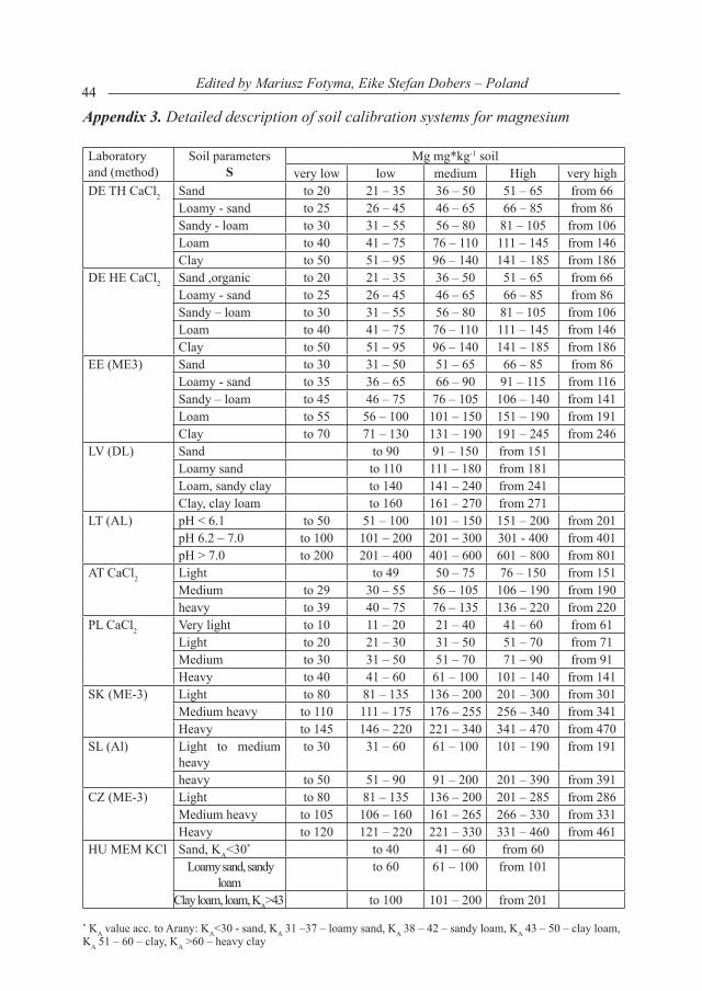
44 Edited by Mariusz Fotyma, Eike Stefan Dobers – Poland
Appendix 3. Detailed description of soil calibration systems for magnesium
Laboratory and (method)
Soil parametersS
Mg mg*kg-1 soil very low low medium High very high
DE TH CaCl2 Sand to 20 21 – 35 36 – 50 51 – 65 from 66Loamy - sand to 25 26 – 45 46 – 65 66 – 85 from 86Sandy - loam to 30 31 – 55 56 – 80 81 – 105 from 106Loam to 40 41 – 75 76 – 110 111 – 145 from 146Clay to 50 51 – 95 96 – 140 141 – 185 from 186
DE HE CaCl2 Sand ,organic to 20 21 – 35 36 – 50 51 – 65 from 66Loamy - sand to 25 26 – 45 46 – 65 66 – 85 from 86Sandy – loam to 30 31 – 55 56 – 80 81 – 105 from 106Loam to 40 41 – 75 76 – 110 111 – 145 from 146Clay to 50 51 – 95 96 – 140 141 – 185 from 186
EE (ME3) Sand to 30 31 – 50 51 – 65 66 – 85 from 86Loamy - sand to 35 36 – 65 66 – 90 91 – 115 from 116Sandy – loam to 45 46 – 75 76 – 105 106 – 140 from 141Loam to 55 56 – 100 101 – 150 151 – 190 from 191Clay to 70 71 – 130 131 – 190 191 – 245 from 246
LV (DL) Sand to 90 91 – 150 from 151Loamy sand to 110 111 – 180 from 181Loam, sandy clay to 140 141 – 240 from 241Clay, clay loam to 160 161 – 270 from 271
LT (AL) pH < 6.1 to 50 51 – 100 101 – 150 151 – 200 from 201pH 6.2 – 7.0 to 100 101 – 200 201 – 300 301 - 400 from 401pH > 7.0 to 200 201 – 400 401 – 600 601 – 800 from 801
AT CaCl2 Light to 49 50 – 75 76 – 150 from 151Medium to 29 30 – 55 56 – 105 106 – 190 from 190heavy to 39 40 – 75 76 – 135 136 – 220 from 220
PL CaCl2 Very light to 10 11 – 20 21 – 40 41 – 60 from 61Light to 20 21 – 30 31 – 50 51 – 70 from 71Medium to 30 31 – 50 51 – 70 71 – 90 from 91Heavy to 40 41 – 60 61 – 100 101 – 140 from 141
SK (ME-3) Light to 80 81 – 135 136 – 200 201 – 300 from 301Medium heavy to 110 111 – 175 176 – 255 256 – 340 from 341Heavy to 145 146 – 220 221 – 340 341 – 470 from 470
SL (Al) Light to medium heavy
to 30 31 – 60 61 – 100 101 – 190 from 191
heavy to 50 51 – 90 91 – 200 201 – 390 from 391CZ (ME-3) Light to 80 81 – 135 136 – 200 201 – 285 from 286
Medium heavy to 105 106 – 160 161 – 265 266 – 330 from 331Heavy to 120 121 – 220 221 – 330 331 – 460 from 461
HU MEM KCl Sand, KA<30* to 40 41 – 60 from 60 Loamy sand, sandy
loam to 60 61 – 100 from 101
Clay loam, loam, KA>43 to 100 101 – 200 from 201
* KA value acc. to Arany: KA<30 - sand, KA 31 –37 – loamy sand, KA 38 – 42 – sandy loam, KA 43 – 50 – clay loam, KA 51 – 60 – clay, KA >60 – heavy clay
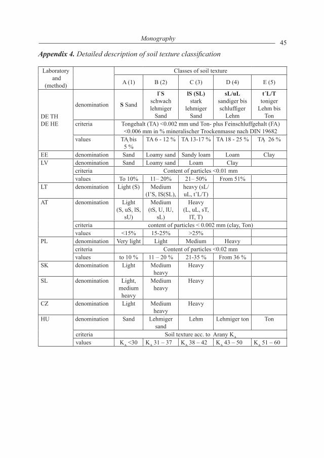
45Monography
Appendix 4. Detailed description of soil texture classification
Laboratory and
(method)
Classes of soil texture
A (1) B (2) C (3) D (4) E (5)
DE TH DE HE
denomination S Sand
l`S schwach lehmiger
Sand
lS (SL)stark
lehmiger Sand
sL/uL sandiger bis schluffiger
Lehm
t´L/T toniger
Lehm bis Ton
criteria Tongehalt (TA) <0.002 mm und Ton- plus Feinschluffgehalt (FA) <0.006 mm in % mineralischer Trockenmasse nach DIN 19682
values TA bis 5 %
TA 6 - 12 % TA 13-17 % TA 18 - 25 % TA 26 %
EE denomination Sand Loamy sand Sandy loam Loam Clay LV denomination Sand Loamy sand Loam Clay
criteria Content of particles <0.01 mmvalues To 10% 11– 20% 21– 50% From 51%
LT denomination Light (S) Medium (I’S, IS(SL),
heavy (sL/uL, t’L/T)
AT denomination Light(S, uS, lS,
sU)
Medium(tS, U, lU,
sL)
Heavy(L, uL, sT,
lT, T)criteria content of particles < 0.002 mm (clay, Ton)values <15% 15-25% >25%
PL denomination Very light Light Medium Heavy criteria Content of particles <0.02 mmvalues to 10 % 11 – 20 % 21-35 % From 36 %
SK denomination Light Medium heavy
Heavy
SL denomination Light, medium heavy
Medium heavy
Heavy
CZ denomination Light Medium heavy
Heavy
HU denomination Sand Lehmiger sand
Lehm Lehmiger ton Ton
criteria Soil texture acc. to Arany KA
values KA <30 KA 31 – 37 KA 38 – 42 KA 43 – 50 KA 51 – 60
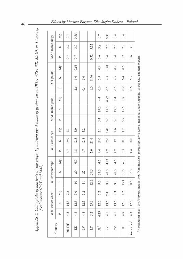
46 Edited by Mariusz Fotyma, Eike Stefan Dobers – Poland
App
endi
x 5.
Uni
t upt
ake
of n
utri
ents
by
the
crop
s, kg
nut
rien
t per
1 to
nne
of g
rain
+ st
raw
(WW
, WRP
, WR,
MAG
), or
1 to
nne
of
fres
h m
atte
r (PO
T an
d M
AS)
WW
win
ter w
heat
W
RP
win
ter r
ape
WR
win
ter r
yeM
AG
mai
ze g
rain
PO
T po
tato
MA
S m
aize
sila
ge
Cou
ntry
P
KM
gP
KM
gP
KM
gP
KM
gP
KM
gP
KM
g
DE
TH1
4.5
14.3
2.2
4.7
19.9
2.3
0.7
3.7
0.7
EE4.
812
.53.
010
206.
04.
812
.53.
02.
65.
00.
650.
73.
00.
55
LV4.
812
.53.
211
224.
712
.83.
20.
45.
0
LT5.
223
.612
.654
.55.
021
.61.
08.
960.
523.
32
PL2
4.13
12.6
2.2
9.6
33.3
4.5
4.4
18.0
2.1
5.4
19.6
4.4
0.6
5.5
0.4
0.6
3.8
0.7
SK4.
113
.62.
419.
342
.54.
824.
717
.02.
415.
015
.04.
820.
54.
50.
910.
42.
50.
91
CZ
4.1
13.6
2.3
9.3
42.5
4.6
4.7
172.
65.
017
.02.
40.
54.
50.
20.
42.
50.
4
HU
4.8
12.8
1.2
15.4
30.5
6.0
5.3
18.5
1.2
5.7
15.6
1.8
0.9
6.4
0.6
0.7
2.8
0.4
6 cou
ntrie
s34.
312
.68.
633
.34.
418
.00.
65.
50.
63.
8
1 Ker
schb
erge
r at a
ll 19
97, 2 Fo
tym
a, M
erci
k 19
95, 3 K
arkl
ins 2
001
(ave
rage
for L
atvi
a, S
lova
k R
epub
lic, C
zech
Rep
ublic
, Pol
and,
UK
. The
Net
herla
nds)
,
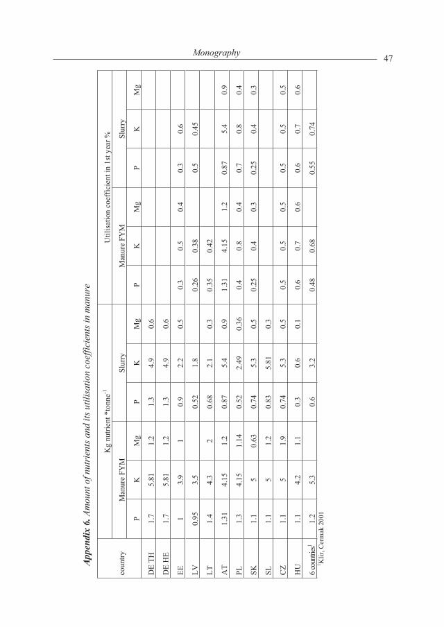
47Monography
App
endi
x 6.
Am
ount
of n
utri
ents
and
its u
tilis
atio
n co
effic
ient
s in
man
ure
Kg
nutri
ent *
tonn
e-1U
tilis
atio
n co
effic
ient
in 1
st y
ear %
Man
ure
FYM
Sl
urry
M
anur
e FY
M
Slur
ry
coun
try
PK
Mg
PK
Mg
PK
Mg
PK
Mg
DE
TH
1.7
5.81
1.2
1.3
4.9
0.6
DE
HE
1.7
5.81
1.2
1.3
4.9
0.6
EE1
3.9
10.
92.
20.
50.
30.
50.
40.
30.
6
LV0.
953.
50.
521.
80.
260.
380.
50.
45
LT1.
44.
32
0.68
2.1
0.3
0.35
0.42
AT
1.31
4.15
1.2
0.87
5.4
0.9
1.31
4.15
1.2
0.87
5.4
0.9
PL1.
34.
151.
140.
522.
490.
360.
40.
80.
40.
70.
80.
4
SK1.
15
0.63
0.74
5.3
0.5
0.25
0.4
0.3
0.25
0.4
0.3
SL1.
15
1.2
0.83
5.81
0.3
CZ
1.1
51.
90.
745.
30.
50.
50.
50.
50.
50.
50.
5
HU
1.1
4.2
1.1
0.3
0.6
0.1
0.6
0.7
0.6
0.6
0.7
0.6
6 co
untrie
s11.
25.
30.
63.
20.
480.
680.
550.
741 K
lir, C
erm
ak 2
001
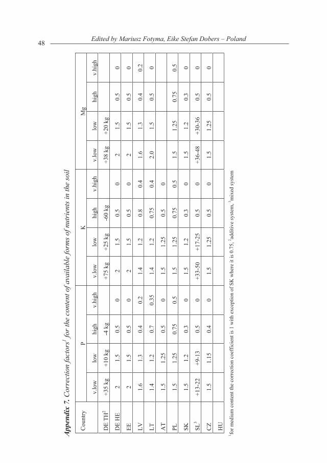
48 Edited by Mariusz Fotyma, Eike Stefan Dobers – Poland
App
endi
x 7.
Cor
rect
ion
fact
ors1 fo
r the
con
tent
of a
vaila
ble
form
s of n
utri
ents
in th
e so
il
PK
Mg
Cou
ntry
v.lo
wlo
whi
ghv.
high
v.lo
wlo
whi
ghv.
high
v.lo
wlo
whi
ghv.
high
DE
TH2
+35
kg
+10
kg
-4 k
g +7
5 kg
+2
5 kg
-6
0 kg
+3
8 kg
+2
0 kg
DE
HE
21.
50.
50
21.
50.
50
21.
50.
50
EE2
1.5
0.5
02
1.5
0.5
02
1.5
0.5
0
LV1.
61.
30.
40.
21.
41.
20.
80.
41.
61.
30.
40.
2
LT1.
41.
20.
70.
351.
41.
20.
750.
42.
01.
50.
50
AT
1.5
1.25
0.5
01.
51.
250.
50
PL1.
51.
250.
750.
51.
51.
250.
750.
51.
51.
250.
750.
5
SK1.
51.
20.
30
1.5
1.2
0.3
01.
51.
20.
30
SL3
+13-
22+9
-13
0.5
0+3
3-50
+17-
250.
50
+36-
48+3
0-36
0.5
0
CZ
1.5
1.15
0.4
01.
51.
250.
50
1.5
1.25
0.5
0
HU
1 for m
ediu
m c
onte
nt th
e co
rrec
tion
coef
ficie
nt is
1 w
ith e
xcep
tion
of S
K w
here
it is
0.7
5, 2 ad
ditiv
e sy
stem
, 3 mix
ed sy
stem
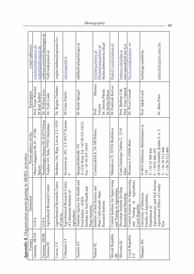
49Monography A
ppen
dix
8. O
rgan
izat
ion
part
icip
atin
g in
MO
EL a
ctiv
ities
C
ount
ry
Inst
itutio
nPo
stal
add
ress
, tel
.fax.
Pa
rtici
pant
s e-
mai
l add
ress
es
Ger
man
y D
ETH
LU
FAO
bere
Lan
ggas
se 4
0, D
– 6
7346
Sp
eyer
Pr
of. F
ranz
Wie
sler
D
r Kur
t Sei
bert
wie
sler
@lu
fa-s
peye
r.de
seib
ert@
lufa
-spe
yer.d
eG
erm
any
DEH
E LU
FAN
aum
burg
er S
trass
e 98
, D-0
7743
Jena
D
r. W
ilfrie
d Zo
rnw
ilfrie
d.zo
rn@
tll.th
uerin
gen.
de
Esto
nia
EE
Agr
icul
tura
l Res
earc
h C
entre
Te
adus
e 4/
6, S
aku
7550
1 H
arju
maa
D
r.V
alli
Loid
e V
alli.
loid
e@m
ail.e
e
Latv
ia, L
V
Agr
oche
mic
al R
esea
rch
Cen
tre
of L
atvi
a,
Stru
ktur
o 14
a, R
iga,
Lat
via,
LV
-103
9 D
r. R
egin
a Ti
mba
re
:regi
na.ti
mba
re@
apce
ntrs
.lv)
Lith
uani
a LT
A
groc
hem
ical
Res
earc
h C
entre
of
Lith
uani
an In
stitu
te o
f A
gric
ultu
re
Sava
noriu
pr.
287,
LT-
5012
7 K
auna
s 9
Dr L
inas
Put
elis
in
fo@
agro
lab.
lt
Aus
tria
AT
Aus
trian
Age
ncy
for H
ealth
and
Fo
od S
afet
y - A
GES
In
stitu
te fo
r Soi
l Hea
lth a
nd
Plan
t Nut
ritio
n
Spar
gelfe
ldst
raße
191
A
-122
6 W
ien
Tel.
+43
50 5
55 3
4121
Fa
x +4
3 50
555
341
01
Dr H
eide
Spi
egel
ad
elhe
id.sp
iege
l@ag
es.a
t
Pola
nd P
L In
stitu
te o
f Soi
l Sci
ence
and
Pl
ant C
ultiv
atio
n0- S
tate
R
esea
rch
Inst
itute
Cza
rtory
skic
h 8,
24-
100
Puaw
y Pr
of.
Mar
iusz
Fo
tym
a
Dr.
Dor
ota
Piku
aD
r Ste
fan
Dob
ers
fot@
iung
.pul
awy.
plPi
kula
@iu
ng.p
ulaw
y.pl
Stef
an.d
ober
suw
m.e
du.p
l
Slov
ak R
epub
lic
SKC
entra
l Ins
titut
e fo
r Sup
ervi
sing
an
d Te
stin
g in
Agr
icul
ture
, M
atus
kova
21,
833
16 B
ratis
lava
Dr F
rant
isek
Kot
vas
Rud
olf.v
ojte
k@uk
sup,
sk
Slov
enia
SL
Slov
enia
n In
stitu
te fo
r Hop
R
esea
rch
and
Bre
edin
g C
esta
Zal
skie
go T
abor
a 2,
331
0 Za
lec
Prof
. Bar
bara
Ceh
Pr
of. T
one
Tajn
sek
barb
ara.
ceh@
ihps
.sito
ne.ta
jnse
k@bf
.uni
-lj.si
C
zech
Rep
ublic
C
ZC
entra
l Ins
titut
e fo
r Sup
ervi
sing
an
d Te
stin
g in
A
gric
ultu
re,
Cze
ch R
epub
lic
Hro
znov
a 2,
656
06 B
rno
Dr.
Pave
l Cer
mak
Pa
vel.c
erm
ak@
ukzu
z. c
z
Hun
gary
HU
U
nive
rsity
of D
ebre
cen
Facu
lty o
f Agr
icul
ture
, D
epar
tmen
t of
Agr
oche
mis
try a
nd S
oil S
cien
ce
Agr
icul
tura
l Off
ice
of C
ount
y Pe
st
H-4
032
Deb
rece
n, B
öszö
rmén
yi ú
t 13
8.T.
:+36
52
508-
444
F.: +
3652
486
-292
H
-210
0 G
ödöl
l, K
otlá
n S.
u. 3
. T.
: +36
28
512-
440
F.: +
36 2
8 51
2-46
0
Prof
. Jak
ab L
och
Dr.
Bél
a Pi
rkó
loch
@ag
r.uni
deb.
hu
pirk
o.be
la@
pest
.ont
sz.h
u
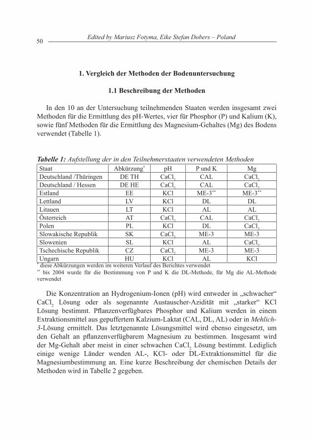
50 Edited by Mariusz Fotyma, Eike Stefan Dobers – Poland
1. Vergleich der Methoden der Bodenuntersuchung
1.1 Beschreibung der Methoden
In den 10 an der Untersuchung teilnehmenden Staaten werden insgesamt zwei Methoden für die Ermittlung des pH-Wertes, vier für Phosphor (P) und Kalium (K), sowie fünf Methoden für die Ermittlung des Magnesium-Gehaltes (Mg) des Bodens verwendet (Tabelle 1).
Tabelle 1: Aufstellung der in den Teilnehmerstaaten verwendeten Methoden Staat Abkürzung* pH P und K MgDeutschland /Thüringen DE TH CaCl2 CAL CaCl2Deutschland / Hessen DE HE CaCl2 CAL CaCl2Estland EE KCl ME-3** ME-3**
Lettland LV KCl DL DLLitauen LT KCl AL ALÖsterreich AT CaCl2 CAL CaCl2Polen PL KCl DL CaCl2Slowakische Republik SK CaCl2 ME-3 ME-3Slowenien SL KCl AL CaCl2Tschechische Republik CZ CaCl2 ME-3 ME-3Ungarn HU KCl AL KCl
* diese Abkürzungen werden im weiteren Verlauf des Berichtes verwendet** bis 2004 wurde für die Bestimmung von P und K die DL-Methode, für Mg die AL-Methode verwendet
Die Konzentration an Hydrogenium-Ionen (pH) wird entweder in „schwacher“ CaCl2 Lösung oder als sogenannte Austauscher-Azidität mit „starker“ KCl Lösung bestimmt. Pflanzenverfügbares Phosphor und Kalium werden in einem Extraktionsmittel aus gepuffertem Kalzium-Laktat (CAL, DL, AL) oder in Mehlich-3-Lösung ermittelt. Das letztgenannte Lösungsmittel wird ebenso eingesetzt, um den Gehalt an pflanzenverfügbarem Magnesium zu bestimmen. Insgesamt wird der Mg-Gehalt aber meist in einer schwachen CaCl2 Lösung bestimmt. Lediglich einige wenige Länder wenden AL-, KCl- oder DL-Extraktionsmittel für die Magnesiumbestimmung an. Eine kurze Beschreibung der chemischen Details der Methoden wird in Tabelle 2 gegeben.
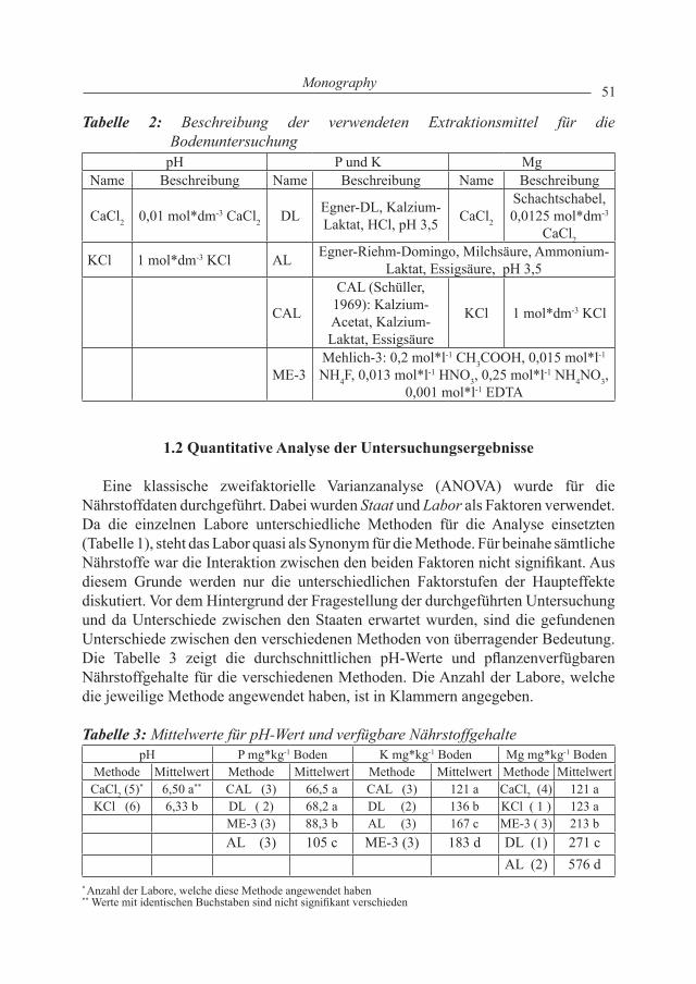
51Monography
Tabelle 2: Beschreibung der verwendeten Extraktionsmittel für die Bodenuntersuchung
pH P und K MgName Beschreibung Name Beschreibung Name Beschreibung
CaCl2 0,01 mol*dm-3 CaCl2 DL Egner-DL, Kalzium-Laktat, HCl, pH 3,5 CaCl2
Schachtschabel, 0,0125 mol*dm-3
CaCl2
KCl 1 mol*dm-3 KCl AL Egner-Riehm-Domingo, Milchsäure, Ammonium-Laktat, Essigsäure, pH 3,5
CAL
CAL (Schüller, 1969): Kalzium-Acetat, Kalzium-Laktat, Essigsäure
KCl 1 mol*dm-3 KCl
ME-3Mehlich-3: 0,2 mol*l-1 CH3COOH, 0,015 mol*l-1 NH4F, 0,013 mol*l-1 HNO3, 0,25 mol*l-1 NH4NO3,
0,001 mol*l-1 EDTA
1.2 Quantitative Analyse der Untersuchungsergebnisse
Eine klassische zweifaktorielle Varianzanalyse (ANOVA) wurde für die Nährstoffdaten durchgeführt. Dabei wurden Staat und Labor als Faktoren verwendet. Da die einzelnen Labore unterschiedliche Methoden für die Analyse einsetzten (Tabelle 1), steht das Labor quasi als Synonym für die Methode. Für beinahe sämtliche Nährstoffe war die Interaktion zwischen den beiden Faktoren nicht signifikant. Aus diesem Grunde werden nur die unterschiedlichen Faktorstufen der Haupteffekte diskutiert. Vor dem Hintergrund der Fragestellung der durchgeführten Untersuchung und da Unterschiede zwischen den Staaten erwartet wurden, sind die gefundenen Unterschiede zwischen den verschiedenen Methoden von überragender Bedeutung. Die Tabelle 3 zeigt die durchschnittlichen pH-Werte und pflanzenverfügbaren Nährstoffgehalte für die verschiedenen Methoden. Die Anzahl der Labore, welche die jeweilige Methode angewendet haben, ist in Klammern angegeben.
Tabelle 3: Mittelwerte für pH-Wert und verfügbare NährstoffgehaltepH P mg*kg-1 Boden K mg*kg-1 Boden Mg mg*kg-1 Boden
Methode Mittelwert Methode Mittelwert Methode Mittelwert Methode MittelwertCaCl2 (5)* 6,50 a** CAL (3) 66,5 a CAL (3) 121 a CaCl2 (4) 121 aKCl (6) 6,33 b DL ( 2) 68,2 a DL (2) 136 b KCl ( 1 ) 123 a
ME-3 (3) 88,3 b AL (3) 167 c ME-3 ( 3) 213 bAL (3) 105 c ME-3 (3) 183 d DL (1) 271 c
AL (2) 576 d * Anzahl der Labore, welche diese Methode angewendet haben** Werte mit identischen Buchstaben sind nicht signifikant verschieden
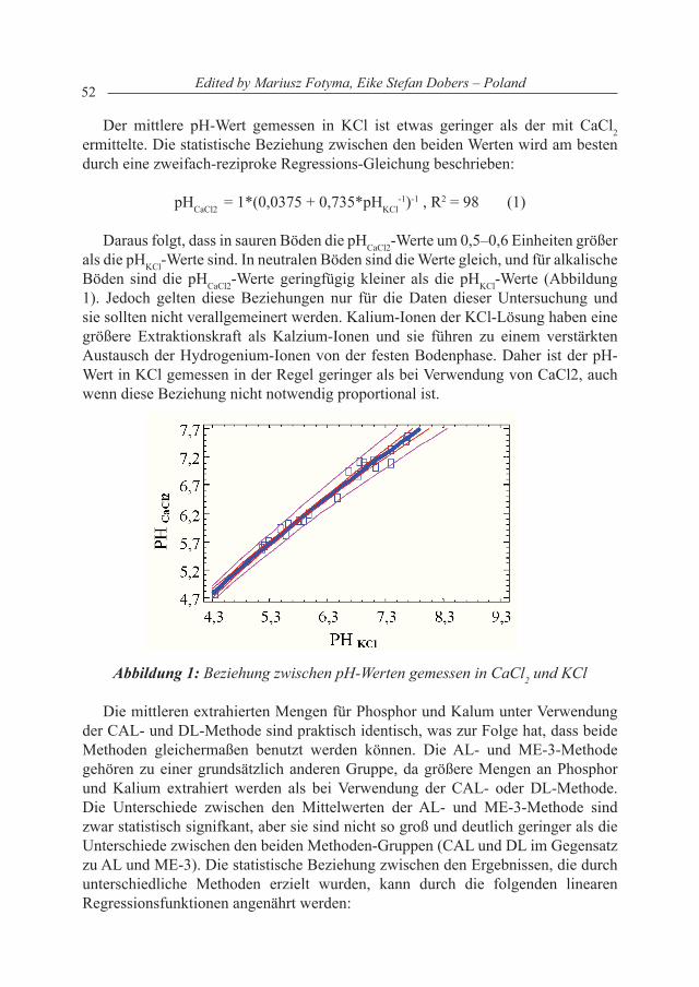
52 Edited by Mariusz Fotyma, Eike Stefan Dobers – Poland
Der mittlere pH-Wert gemessen in KCl ist etwas geringer als der mit CaCl2 ermittelte. Die statistische Beziehung zwischen den beiden Werten wird am besten durch eine zweifach-reziproke Regressions-Gleichung beschrieben:
pHCaCl2 = 1*(0,0375 + 0,735*pHKCl-1)-1 , R2 = 98 (1)
Daraus folgt, dass in sauren Böden die pHCaCl2-Werte um 0,5–0,6 Einheiten größer als die pHKCl-Werte sind. In neutralen Böden sind die Werte gleich, und für alkalische Böden sind die pHCaCl2-Werte geringfügig kleiner als die pHKCl-Werte (Abbildung 1). Jedoch gelten diese Beziehungen nur für die Daten dieser Untersuchung und sie sollten nicht verallgemeinert werden. Kalium-Ionen der KCl-Lösung haben eine größere Extraktionskraft als Kalzium-Ionen und sie führen zu einem verstärkten Austausch der Hydrogenium-Ionen von der festen Bodenphase. Daher ist der pH-Wert in KCl gemessen in der Regel geringer als bei Verwendung von CaCl2, auch wenn diese Beziehung nicht notwendig proportional ist.
Abbildung 1: Beziehung zwischen pH-Werten gemessen in CaCl2 und KCl
Die mittleren extrahierten Mengen für Phosphor und Kalum unter Verwendung der CAL- und DL-Methode sind praktisch identisch, was zur Folge hat, dass beide Methoden gleichermaßen benutzt werden können. Die AL- und ME-3-Methode gehören zu einer grundsätzlich anderen Gruppe, da größere Mengen an Phosphor und Kalium extrahiert werden als bei Verwendung der CAL- oder DL-Methode. Die Unterschiede zwischen den Mittelwerten der AL- und ME-3-Methode sind zwar statistisch signifkant, aber sie sind nicht so groß und deutlich geringer als die Unterschiede zwischen den beiden Methoden-Gruppen (CAL und DL im Gegensatz zu AL und ME-3). Die statistische Beziehung zwischen den Ergebnissen, die durch unterschiedliche Methoden erzielt wurden, kann durch die folgenden linearen Regressionsfunktionen angenährt werden:
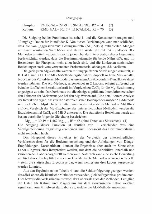
53Monography
Phosphor: PME-3/AL= 29.79 + 0.96CAL/DL, R2 = 54 (2)Kalium: KME-3/AL= 30.17 + 1.12CAL/DL, R2 = 70 (3)
Die Steigung beider Funktionen ist nahe 1, und die Konstanten betragen rund 30 mg*kg-1 Boden für P und/oder K. Von diesen Beziehungen kann man schließen, dass die von „aggressiveren“ Lösungsmitteln (AL, ME-3) extrahierten Mengen um einen konstanten Wert höher sind als die Werte, die mit CAL und/oder DL-Methoden ermittelt werden. Es sollte jedoch bei der Interpretation dieser Ergebnisse berücksichtigt werden, dass die Bestimmtheitsmaße für beide Nährstoffe, und im Besonderen für Phosphor, nicht allzu hoch sind, und die konkreten statistischen Beziehungen stark vom verwendeten Probenmaterial abhängen, d.h. variieren.
Die geringsten Mg-Gehalte werden mit ungepufferten Salzlösungen ermittelt, z. B. CaCl2 und KCl. Die ME-3-Methode ergibt nahezu doppelt so hohe Mg-Gehalte. Jedoch ist der Vorteil dieser Methode, dass in einem Ansatz ebenfalls P und K extrahiert werden können. Die AL-Methode, angewendet in 2 Labors, scheint aufgrund der beinahe fünffachen Extraktionskraft im Vergleich zu CaCl2 für die Mg-Bestimmung ungeeignet zu sein. Darüberhinaus trat die einzige signifikante Interaktion zwischen den Faktoren der Varianzanalyse bei den Mg-Werten auf. Eine detailliertere Analyse der Interaktion ergab, dass für die österreichischen Bodenproben mit der AL-Methode sehr viel höhere Mg-Gehalte ermittelt wurden als mit anderen Methoden. Mit Blick auf den Vergleich der Mg-Ergebnisse der unterschiedlichen Methoden wurden die Extraktionsmittel CaCl2 und ME-3 untersucht. Die statistische Beziehung wurde am besten durch die folgende Gleichung beschrieben:
MgME-3 = 30,49 + 1,467 MgCaCl2, R2 = 58 (ohne Daten aus Slowenien) (4)
Die Steigung dieser Funktion ist deutlich von 1 verschieden was eine Verallgemeinerung fragwürdig erscheinen lässt. Ebenso ist das Bestimmtheitsmaß nicht sonderlich hoch.
Das Hauptziel dieses Projektes ist der Vergleich der unterschiedlichen Verfahrensweisen für die Bodenuntersuchung und der Ableitungen von Dünge-Empfehlungen. Darüberhinaus können die Ergebnisse aber auch im Sinne eines Labor-Ringversuches interpretiert werden, mit dem die Variabilität innerhalb und zwischen den Labors dargestellt werden kann. Natürlich kann eine solche Bewertung nur für Labors durchgeführt werden, welche identische Methoden verwenden. Tabelle 4 stellt die statistischen Ergebnisse dar, wenn wenigstens drei Labors ausgewertet werden konnten.
Aus den Ergebnissen der Tabelle 4 kann die Schlussfolgerung gezogen werden, dass die Labore, die identische Methoden verwenden, gleiche Ergebnisse produzieren. Dies beweist die Verlässlichkeit sowohl der Labors als auch der Methoden. Lediglich die Daten für Kalium und Magnesium aus dem slowenischen Labor weichen signifikant vom Mittelwert der Labors ab, welche die AL-Methode anwenden.
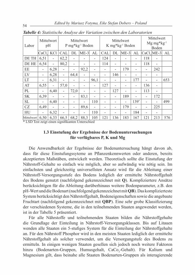
54 Edited by Mariusz Fotyma, Eike Stefan Dobers – Poland
Tabelle 4: Statistische Analyse der Variation zwischen den Laboratorien
LaborMittelwert
pHMittelwert
P mg*kg-1 BodenMittelwert
K mg*kg-1 Boden
MittelwertMg mg*kg-1
BodenCaCl2 KCl CAL DL ME-3 AL CAL DL ME-3 AL CaCl2 ME-3 AL
DE TH 6,51 - 62,2 - - - 124 - - - 118 -DE HE 6,54 - 80,2 - - - 114 - - - 118 -EE - 6,28 - - 92,2 - - - 179 - - 242LV - 6,28 - 64,4 - - - 146 - - - -LT - 6,31 - - - 96,1 - - - 177 - - 653AT 6,55 - 57,0 - - - 127 - - - 136 -PL - 6,40 - 72,0 - - - 127 - - 113 -SK 6,39 - - - 83,1 - - - 189 - - 172SL - 6,40 - - - 110 - - - 139* - - 499CZ 6,49 - - - 89,6 - - - 179 - - 225HU - 6,32 - - - 110 - - - 184 - -
Mittelwert 6,50 6,33 66,5 68,2 88,3 105 121 136 183 167 121 213 576* LSD Test zeigt einen signifikanten Unterschied
1.3 Einstufung der Ergebnisse der Bodenuntersuchungen für verfügbares P, k und Mg
Die Anwendbarkeit der Ergebnisse der Bodenuntersuchung hängt davon ab, dass für diese Einstufungssyteme an Pflanzenkennwerten oder anderen, bereits akzeptierten Maßstäben, entwickelt werden. Theoretisch sollte die Einstufung der Nährstoff-Gehalte so einfach wie möglich, aber so aufwändig wie nötig sein. Im einfachsten und gleichzeitig universellsten Ansatz wird für die Ableitung einer Nährstoff-Versorgungsstufe des Bodens lediglich der ermittelte Nährstoffgehalt des Bodens genutzt (nachfolgend gekennzeichnet mit Q). Kompliziertere Ansätze berücksichtigen für die Ableitung darüberhinaus weitere Bodenparameter, z.B. den pH-Wert und die Bodenart (nachfolgend gekennzeichnet mit QB). Das komplizierteste System berücksichtigt den Nährstoffgehalt, Bodeneigenschaften sowie die angebaute Fruchtart (nachfolgend gekennzeichnet mit QBP). Eine sehr grobe Klassifizierung der verschiedenen Systeme, die in den teilnehmenden Staaten angewendet werden, ist in der Tabelle 5 präsentiert.
Für alle Nährstoffe und teilnehmenden Staaten bilden die Nährstoffgehalte die Grundlage der Einteilung in Nährstoff-Versorgungsklassen. Bis auf Litauen wenden alle Staaten ein 5-stufiges System für die Einteilung der Nährstoffgehalte an. Für den Nährstoff Phosphor wird in den meisten Staaten lediglich der ermittelte Nährstoffgehalt als solcher verwendet, um die Versorgungstufe des Bodens zu ermitteln. In einigen wenigen Staaten gesellen sich jedoch noch weitere Faktoren hinzu (Bodenarten-Gruppen, Humusgehalt, CaCo3-Gehalt). Für Kalium und Magnesium gilt, dass beinahe alle Staaten Bodenarten-Gruppen als interagierende

55MonographyTa
belle
5:
Kla
ssifi
zier
ung
der
Syst
eme
für
die
Erm
ittlu
ng v
on K
lass
en d
er N
ährs
toff-
Vers
orgu
ng a
us d
en B
oden
unte
rsuc
hung
en f
ür
min
eral
isch
e Ac
kerb
öden
*
Phos
phor
Kal
ium
Mag
nesi
umSt
aat
Typ
Erlä
uter
unge
n Ty
p Er
läut
erun
gen
Typ
Erlä
uter
unge
n D
E TH
Q
P-G
ehal
tei
nget
eilt
in 5
Kla
ssen
Q
BK
-Geh
alt (
5 K
lass
en)
5 B
oden
arte
n-G
rupp
en
insg
esam
t 25
Kla
ssen
QB
Mg-
Geh
alt (
5 K
lass
en)
5 B
oden
arte
n-G
rupp
en
insg
esam
t 25
Kla
ssen
D
E H
E id
entis
ch w
ie D
E T
H
EEQ
BP-
Geh
alt (
5 K
lass
en)
Hum
usge
halt
(2 K
lass
en)
gesa
mt 1
0 K
lass
en
QB
K-G
ehal
t (5
Kla
ssen
) 5
Bod
enar
ten-
Gru
ppen
in
sges
amt 2
5 K
lass
en
QB
Mg-
Geh
alt (
5 K
lass
en)
5 B
oden
arte
n-G
rupp
en
insg
esam
t 25
Kla
ssen
LV
QB
P-G
ehal
t (5
Kla
ssen
) 4
Bod
enar
teng
rupp
en
insg
esam
t 20
Kla
ssen
QB
K-G
ehal
t (5
Kla
ssen
) 4
Bod
enar
teng
rupp
en
insg
esam
t 20
Kla
ssen
QB
Mg-
Geh
alt (
3 K
lass
en)
4 B
oden
arte
ngru
ppen
in
sges
amt 1
2 K
lass
en
LT Q
P-
Geh
alt
eing
etei
lt in
6 K
lass
en
QK
-Geh
alt
eing
etei
lt in
6 K
lass
en
QP
Mg-
Geh
alt (
5 K
lass
en)
3 G
rupp
en v
on P
flanz
en
insg
esam
t 15
Kla
ssen
A
TQ
P-G
ehal
tei
nget
eilt
in 5
Kla
ssen
Q
BK
-Geh
alt (
5 K
lass
en)
3 B
oden
arte
ngru
ppen
in
sges
amt 1
5 K
lass
en
QB
Mg-
Geh
alt (
5 K
lass
en)
3 B
oden
arte
ngru
ppen
in
sges
amt 1
5 K
lass
en
PL
QP-
Geh
alt
eing
etei
lt in
5 K
lass
en
K-G
ehal
t (5
Kla
ssen
) 4
Bod
enar
teng
rupp
en
insg
esam
t 20
Kla
ssen
Mg-
Geh
alt (
5 K
lass
en)
4 B
oden
arte
ngru
ppn
insg
esam
t 20
Kla
ssen
SK
QB
P-G
ehal
t (5
Kla
ssen
) 3
Bod
enar
teng
rupp
en
insg
esam
t 15
Kla
ssen
QB
K-G
ehal
t (5
Kla
ssen
) 3
Bod
enar
teng
rupp
en
insg
esam
t 15
Kla
ssen
QB
Mg-
Geh
alt (
5 K
lass
en)
3 B
oden
arte
ngru
ppen
in
sges
amt 1
5 K
lass
en
SL
QP-
Geh
alt
eing
etei
lt in
5 K
lass
en
QB
K-G
ehal
t (5
Kla
ssen
) 2
Bod
enar
teng
rupp
en
insg
esam
t 10
Kla
ssen
K-G
ehal
t (5
Kla
ssen
) 2
Bod
enar
teng
rupp
en
insg
esam
t 10
Kla
ssen
H
UM
EM**
QB
P-G
ehal
t (5
Kla
ssen
) 6
Bod
enty
pen
2 C
aCO
3-G
ehal
tskl
asse
n in
sges
amt 6
0 K
lass
en
QB
K-G
ehal
t (5
Kla
ssen
) 6
Bod
enty
pen
2 B
oden
arte
ngru
ppen
in
sges
amt 6
0 K
lass
en
QB
Mg-
Geh
alt (
3 K
lass
en)
3 B
oden
arte
ngru
ppen
in
sges
amt 9
Kla
ssen
HU
RIS
S***
QB
PP-
Geh
alt (
5 K
lass
en)
5 B
oden
arte
ngru
ppen
2
pH-S
tufe
n, 5
CaC
O3-
Geh
alts
klas
sen
2 Pf
lanz
enbe
darf
sstu
fen
insg
esam
t 210
cla
sses
QB
PK
-Geh
alt (
5 K
lass
en)
5 B
oden
arte
ngru
ppen
2
Pfla
nzen
beda
rfss
tufe
n in
sges
amt 5
0 K
lass
en
QB
Mg-
Geh
alt (
3 K
lass
en)
3 B
oden
arte
ngru
ppen
in
sges
amt 9
Kla
ssen
* Q
– (
Qua
ntitä
t) –
nur
Näh
rsto
ffge
halt,
QB
– (
Qua
ntitä
t-B
oden
) –
Näh
rsto
ffge
halt
& a
usge
wäh
lte B
oden
eige
nsch
afte
n, Q
P –
(Qua
ntitä
t-Pf
lanz
e) –
Näh
rsto
ffge
halt
&
Pfla
nzen
beda
rf, Q
BP
– (Q
uant
ität-
Bod
en-P
flan
ze) –
Näh
rsto
ffge
halt,
Bod
enei
gens
chaf
ten,
Pfl
anze
nbed
arf f
ür e
inze
lne
Näh
rsto
ffe
** o
ffiz
ielle
Em
pfeh
lung
**
* E
mpf
ehlu
ng d
es In
stitu
ts d
er U
ngar
isch
en A
kade
mie
der
Wis
sens
chaf
ten
(Pilo
t-M
aßst
ab)
Bodeneigenschaft berücksichtigen. Das komplizierteste System wird in Ungarn angewendet. In diesem System werden zusätzlich zu den Bodeneigenschaften noch Ansprüche der einzelnen Pflanzenarten bei der Ermittlung der Versorgungsklasse
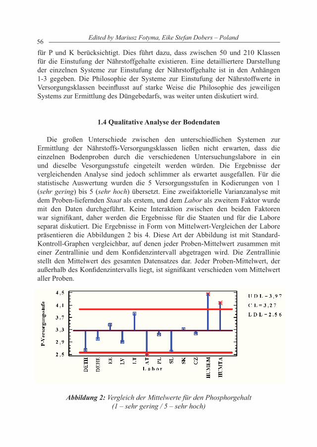
56 Edited by Mariusz Fotyma, Eike Stefan Dobers – Poland
für P und K berücksichtigt. Dies führt dazu, dass zwischen 50 und 210 Klassen für die Einstufung der Nährstoffgehalte existieren. Eine detailliertere Darstellung der einzelnen Systeme zur Einstufung der Nährstoffgehalte ist in den Anhängen 1-3 gegeben. Die Philosophie der Systeme zur Einstufung der Nährstoffwerte in Versorgungsklassen beeinflusst auf starke Weise die Philosophie des jeweiligen Systems zur Ermittlung des Düngebedarfs, was weiter unten diskutiert wird.
1.4 Qualitative Analyse der Bodendaten
Die großen Unterschiede zwischen den unterschiedlichen Systemen zur Ermittlung der Nährstoffs-Versorgungsklassen ließen nicht erwarten, dass die einzelnen Bodenproben durch die verschiedenen Untersuchungslabore in ein und dieselbe Vesorgungsstufe eingeteilt werden würden. Die Ergebnisse der vergleichenden Analyse sind jedoch schlimmer als erwartet ausgefallen. Für die statistische Auswertung wurden die 5 Versorgungsstufen in Kodierungen von 1 (sehr gering) bis 5 (sehr hoch) übersetzt. Eine zweifaktorielle Varianzanalyse mit dem Proben-liefernden Staat als erstem, und dem Labor als zweitem Faktor wurde mit den Daten durchgeführt. Keine Interaktion zwischen den beiden Faktoren war signifikant, daher werden die Ergebnisse für die Staaten und für die Labore separat diskutiert. Die Ergebnisse in Form von Mittelwert-Vergleichen der Labore präsentieren die Abbildungen 2 bis 4. Diese Art der Abbildung ist mit Standard-Kontroll-Graphen vergleichbar, auf denen jeder Proben-Mittelwert zusammen mit einer Zentrallinie und dem Konfidenzintervall abgetragen wird. Die Zentrallinie stellt den Mittelwert des gesamten Datensatzes dar. Jeder Proben-Mittelwert, der außerhalb des Konfidenzintervalls liegt, ist signifikant verschieden vom Mittelwert aller Proben.
Abbildung 2: Vergleich der Mittelwerte für den Phosphorgehalt (1 – sehr gering / 5 – sehr hoch)
57Monography
Für Phosphor lagen 9 Labore innerhalb des 95%-Konfidenzintervalls, ein Labor-Mittelwert liegt unterhalb, und zwei oberhalb der Intervallgrenzen (Abbildung 2). Die Ergebnisse der P-Einstufung liegen jedoch zwischen 2.5 (gering bis mittel) und 4 (hoch), was die Verlässlichkeit der Phosphor-Einstufung zwischen den Labors der benachbarten Staaten fraglich erscheinen läßt. Zwei Labore überschätzen den P-Gehalt offensichtlich mit Blick auf den Gesamtmittelwert (HU MEM und HU RIS), das Labor AT unterschätzte ihn leicht. Es ist wichtig hier anzumerken, dass diese Diskrepanzen für einen Nährstoff auftreten, bei dem die unterschiedlichen Einstufungssysteme der Nährstoffgehalte am unkompliziertesten sind und in den meisten Fällen nur den reinen Nährstoffgehalt berücksichtigen.
Aus den Daten des Anhang 1 wurde der Phosphorgehalt der Klasse mittel berechnet, ohne weitere Bodenparameter in Betracht zu ziehen, selbst wenn diese vorlagen. Das Ergebnis gibt Tabelle 6 wieder. Die Angaben der Labore, die ME-3 oder AL-Methoden benutzen, wurden mit der Formel (2) in Größenordnungen der CAL- und DL-Methoden umgerechnet. Im Vergleich zum Gesamtmittelwert aller Labore scheint der Phosphor-Gehalt für die Klasse mittel durch die Labore aus EE, LV und LT leicht unterschätzt zu werden.
Tabelle 6: Durschschnittliche Phosphorgehalte für die Versorgungsstufe mittel [in CAL bzw. DL Einheiten]
DE TH DE HE
EE LV LT AT* PL SK SL CZ HU Mean
[ mg P * kg-1 Boden ] 49-72 49-72 37-68 29-55 40-51 47-111 45-65 62-83 44-75 60-79 54-79 47-73
* In der letzten Ausgabe der „Richtlinien für die sachgerechte Düngung“ (BMLFUW, 2006) wurde der Tatsache, dass die Klasse mittel eine große Spannbreite und eine hohe obere Grenze hat, Rechnung getragen, indem die Düngungsempfehlung für P und K in der Klasse hoch um 50% reduziert wurde (siehe auch Spiegel et al., 2006).
Abbildung 3: Vergleich der Mittelwerte für den Kaliumgehalt (1 – sehr gering / 5 – sehr hoch)
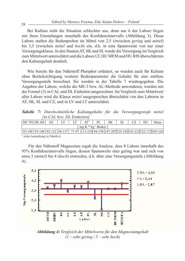
58 Edited by Mariusz Fotyma, Eike Stefan Dobers – Poland
Bei Kalium sieht die Situation schlechter aus, denn nur 6 der Labore liegen mit ihren Einstufungen innerhalb des Konfidenzintervalls (Abbildung 3). Diese Labore stuften die Bodenproben im Mittel von 2,5 (zwischen gering und mittel) bis 3,5 (zwischen mittel und hoch) ein, d.h. in eine Spannweite von nur einer Versorgungsklasse. In den Staaten AT, SK und SL wurde die Versorgung im Vergleich zum Mittelwert unterschätzt und die Labore LT, HU MEM und HU RIS überschätzten den Kaliumgehalt deutlich.
Wie bereits für den Nährstoff Phosphor erläutert, so wurden auch für Kalium ohne Berücksichtigung weiterer Bodenparameter die Gehalte für eine mittlere Versorgungsstufe berechnet. Sie werden in der Tabelle 7 wiedergegeben. Die Angaben der Labore, welche die ME-3 bzw. AL-Methode anwendeten, wurden mit der Formel (3) in CAL und DL Einheiten umgerechnet. Im Vergleich zum Mittelwert aller Labore wird die Klasse mittel ausgesprochen überschätzt von den Laboren in AT, SK, SL und CZ, und in LV und LT unterschätzt.
Tabelle 7: Durchschnittliche Kaliumgehalte für die Versorgungsstufe mittel [in CAL bzw. DL Einheiten]
DE TH DE HE EE LV LT AT* PL SK SL CZ HU Mean[ mg K * kg-1 Boden ]
93-148 93-148 92-132 69-137 71-97 113-210 94-150 147-207125-182143-215122-172105-163* siehe Anmerkung zu Tabelle 6
Für den Nährstoff Magnesium ergab die Analyse, dass 8 Labore innerhalb des 95% Konfidenzintervalls liegen, dessen Spannweite eher gering war und sich von etwa 3 (mittel) bis 4 (hoch) erstreckte, d.h. über eine Versorgungsstufe (Abbildung 4).
Abbildung 4: Vergleich der Mittelwerte für den Magnesiumgehalt (1 – sehr gering / 5 – sehr hoch)
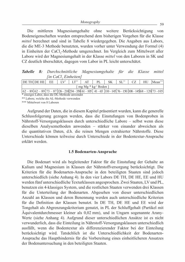
59Monography
Die mittleren Magnesiumgehalte ohne weitere Berücksichtigung von Bodeneigenschaften wurden entsprechend dem bisherigen Vorgehen für die Klasse mittel berechnet und sind in Tabelle 8 wiedergegeben. Die Angaben aus Labors, die die ME-3 Methode benutzten, wurden vorher unter Verwendung der Formel (4) in Einheiten der CaCl2-Methode umgerechnet. Im Vergleich zum Mittelwert aller Labore wird der Magnesiumgehalt in der Klasse mittel von den Laboren in SK und CZ deutlich überschätzt, dagegen vom Labor in PL leicht unterschätzt.
Tabelle 8: Durchschnittliche Magnesiumgehalte für die Klasse mittel [in CaCl2 Einheiten]
DE TH DE HE EE LV* LT** AT PL SK SL** CZ HU Mean***
[ mg Mg * kg-1 Boden ]62 – 89 62 – 89 73 – 87 126 – 210234 – 350 61 – 105 41 – 65 110 – 145 76 – 150 108 – 14568 - 120 73 -105
* einziges Labor, dass die DL-Methode anwendet** Labore, welche die AL-Methode verwenden*** Mittelwert von 8 Laboren
Aufgrund der Daten, die in diesem Kapitel präsentiert wurden, kann die generelle Schlussfolgerung gezogen werden, dass die Einstufungen von Bodenproben in Nährstoff-Versorgungsklassen durch unterschiedliche Labore – selbst wenn diese dieselben Analysemethoden anwenden – stärker von einander abweichen als die quantitativen Daten, d.h. die reinen Mengen extrahierter Nährstoffe. Diese Unterschiede können teilweise durch Unterschiede in der Bodentextur-Ansprache erklärt werden.
1.5 Bodenarten-Ansprache
Die Bodenart wird als begleitender Faktor für die Einstufung der Gehalte an Kalium und Magnesium in Klassen der Nährstoffversorgung berücksichtigt. Die Kriterien für die Bodenarten-Ansprache in den beteiligten Staaten sind jedoch unterschiedlich (siehe Anhang 4). In den vier Labors DE TH, DE HE, EE und HU werden fünf unterschiedliche Texturklassen angesprochen. Zwei Staaten, LV und PL, benutzen ein 4-klassiges System, und die restlichen Staaten verwenden drei Klassen für die Unterteilung der Bodenarten. Abgesehen von dieser unterschiedlichen Anzahl an Klassen und deren Benennung werden auch unterschiedliche Kriterien für die Definition der Klassen benutzt. In DE TH, DE HE und EE wird der Tongehalt als Abgrenzungskriterium genutzt, in PL der Schluffgehalt (Partikel mit Äquivalentdurchmesser kleiner als 0,02 mm), und in Ungarn sogenannte Arany-Werte (siehe Anhang 4). Aufgrund dieser unterschiedlichen Ansätze ist es nicht verwunderlich, dass die Einteilung in Nährstoff-Versorgungsklassen unterschiedlich ausfällt, wenn die Bodentextur als differenzierender Faktor bei der Einteilung berücksichtigt wird. Tatsächlich ist die Unterschiedlichkeit der Bodenarten-Ansprache das Haupthindernis für die Vorbereitung eines einheitlicheren Ansatzes der Bodenuntersuchung in den beteiligten Staaten.
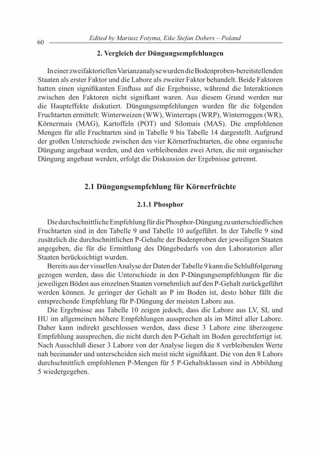
60 Edited by Mariusz Fotyma, Eike Stefan Dobers – Poland
2. Vergleich der Düngungsempfehlungen
In einer zweifaktoriellen Varianzanalyse wurden die Bodenproben-bereitstellenden Staaten als erster Faktor und die Labore als zweiter Faktor behandelt. Beide Faktoren hatten einen signifikanten Einfluss auf die Ergebnisse, während die Interaktionen zwischen den Faktoren nicht signifkant waren. Aus diesem Grund werden nur die Haupteffekte diskutiert. Düngungsempfehlungen wurden für die folgenden Fruchtarten ermittelt: Winterweizen (WW), Winterraps (WRP), Winterroggen (WR), Körnermais (MAG), Kartoffeln (POT) und Silomais (MAS). Die empfohlenen Mengen für alle Fruchtarten sind in Tabelle 9 bis Tabelle 14 dargestellt. Aufgrund der großen Unterschiede zwischen den vier Körnerfruchtarten, die ohne organische Düngung angebaut werden, und den verbleibenden zwei Arten, die mit organischer Düngung angebaut werden, erfolgt die Diskussion der Ergebnisse getrennt.
2.1 Düngungsempfehlung für körnerfrüchte
2.1.1 Phosphor
Die durchschnittliche Empfehlung für die Phosphor-Düngung zu unterschiedlichen Fruchtarten sind in den Tabelle 9 und Tabelle 10 aufgeführt. In der Tabelle 9 sind zusätzlich die durchschnittlichen P-Gehalte der Bodenproben der jeweiligen Staaten angegeben, die für die Ermittlung des Düngebedarfs von den Laboratorien aller Staaten berücksichtigt wurden.
Bereits aus der visuellen Analyse der Daten der Tabelle 9 kann die Schlußfolgerung gezogen werden, dass die Unterschiede in den P-Düngungsempfehlungen für die jeweiligen Böden aus einzelnen Staaten vornehmlich auf den P-Gehalt zurückgeführt werden können. Je geringer der Gehalt an P im Boden ist, desto höher fällt die entsprechende Empfehlung für P-Düngung der meisten Labore aus.
Die Ergebnisse aus Tabelle 10 zeigen jedoch, dass die Labore aus LV, SL und HU im allgemeinen höhere Empfehlungen aussprechen als im Mittel aller Labore. Daher kann indirekt geschlossen werden, dass diese 3 Labore eine überzogene Empfehlung aussprechen, die nicht durch den P-Gehalt im Boden gerechtfertigt ist. Nach Ausschluß dieser 3 Labore von der Analyse liegen die 8 verbleibenden Werte nah beeinander und unterscheiden sich meist nicht signifikant. Die von den 8 Labors durchschnittlich empfohlenen P-Mengen für 5 P-Gehaltsklassen sind in Abbildung 5 wiedergegeben.

61Monography
Tabelle 9: Mittlere Phosphor-Düngungsempfehlung für Bodenproben aus unterschiedlichen Staaten zu verschiedenen Fruchtarten
Staatmittlerer P-Gehalt
im Boden*
empfohlene Phosphor-Düngermenge in kg P*ha-1
WWn = 242
WRPn = 242
WRn = 242
MAGn = 176
POTn = 242
MASn = 176
DE TH 3,00 b** 36,0 cd 49,2 bc 32,0 b 41,2 c 2,3 bc 8,2 cdDE HE 4,00 a 20,4 ab 31,0 a 19,0 a 24,6 ab -5,5 ab 0,6 ab EE 4,23 a 18,8 a 27,0 a 17,8 a 26,3 ab -10,5 a 0,7 ab LV 2,27 c 47,6 ef 61,9 de 44,0 cd 61,5 de 13,1 d 17,7 efLT 1,73 c 57,5 f 72,2 e 53,0 d 71,7 e 17,4 e 24,2 f AT 3,36 b 29,5 bc 44,3 b 29,0 b 38,1 bc 9,3 c 13,8 dePL 4,19 a 16,5 a 26,2 a 17,8 a 21,4 a -8,1 a -0,5 a SK 3,00 b 40,1 de 54,0 bcd 36,4 bc 49,4 cd 4,4 c 11,0 cdeSL 4,10 a 17,6 a 26,8 a 18,7 a 24,8 ab -11,2 a -0,6 aCZ 2,32 c 47,3 ef 63,2 cde 43,6 c 58,5 de 13,2 d 16,3 e HU 2,95 b 34,6 cd 45,5 b 33,8 b 44,6 c 1,0 bc 6,7 bc Mittelwert 3,19 33,3 45,6 31,4 42,0 2,8 8,9
* siehe Erklärungen im Text und in Abbildung 2** Werte mit denselben Buchstaben sind nicht signifikant voneinander verschieden
Tabelle 10: Durchschnittliche P-Düngungsempfehlungen der beteiligten Laboratorien zu verschiedenen Fruchtarten
Labor empfohlene Phosphor-Düngermenge in kg P*ha-1
WWn = 242
WRan = 242
WRn = 242
kMan = 176
kARn = 242
SMan = 176
DE TH 40,9 d 49,9 de 37,5 d 36,6 ab -20,4 b 15,9 efDE HE 38,2 cd 39,1 bcd 34,0 cd 45,3 c -31,1 a 7,9 cdEE 24,3 ab 46,4 cde 22,0 ab keine
Angabe26,1 f 20,2 f
LV 41,0 d 63,2 e 36,9 d keine Angabe
51,1 g 0,0 b
LT 19,1 a 22,4 a 17,0 a keine Angabe
21,3 f 18,4 ef
AT 26,9 ab 36,5 bc 26,7 bc 38,7 ab -10,0 c 13,2 dePL 29,0 abc 36,0 bc 25,4 abc 39,6 ab 18,6 f 5,6 bcSK 26,5 ab 34,3 abc 26,0 abc 37,0 ab 3,7 de 18,6 ef SL 63,5 e 84,1 f 55,2 e 72,2 d -32,5 a 2,3 bcCZ 23,7 ab 31,0 ab 22,8 ab 33,2 a -4,2 cd -7,6 aHU 32,9 bcd 58,9 de 41,6 d 33,5 a 7,5 e 3,8 bcMittelwert 33,3 45,6 31,4 42,0 2,8 8,9
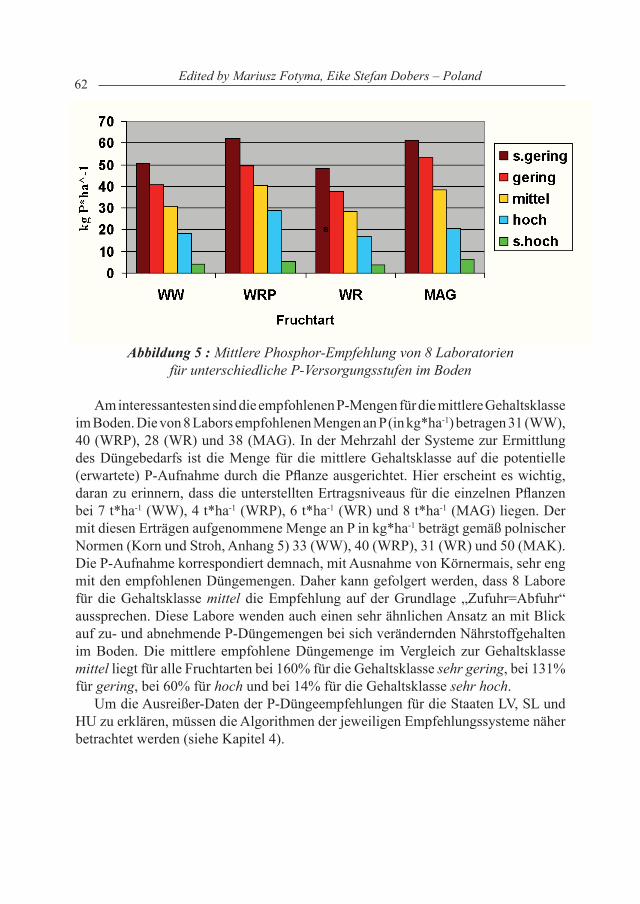
62 Edited by Mariusz Fotyma, Eike Stefan Dobers – Poland
Abbildung 5 : Mittlere Phosphor-Empfehlung von 8 Laboratorien für unterschiedliche P-Versorgungsstufen im Boden
Am interessantesten sind die empfohlenen P-Mengen für die mittlere Gehaltsklasse im Boden. Die von 8 Labors empfohlenen Mengen an P (in kg*ha-1) betragen 31 (WW), 40 (WRP), 28 (WR) und 38 (MAG). In der Mehrzahl der Systeme zur Ermittlung des Düngebedarfs ist die Menge für die mittlere Gehaltsklasse auf die potentielle (erwartete) P-Aufnahme durch die Pflanze ausgerichtet. Hier erscheint es wichtig, daran zu erinnern, dass die unterstellten Ertragsniveaus für die einzelnen Pflanzen bei 7 t*ha-1 (WW), 4 t*ha-1 (WRP), 6 t*ha-1 (WR) und 8 t*ha-1 (MAG) liegen. Der mit diesen Erträgen aufgenommene Menge an P in kg*ha-1 beträgt gemäß polnischer Normen (Korn und Stroh, Anhang 5) 33 (WW), 40 (WRP), 31 (WR) und 50 (MAK). Die P-Aufnahme korrespondiert demnach, mit Ausnahme von Körnermais, sehr eng mit den empfohlenen Düngemengen. Daher kann gefolgert werden, dass 8 Labore für die Gehaltsklasse mittel die Empfehlung auf der Grundlage „Zufuhr=Abfuhr“ aussprechen. Diese Labore wenden auch einen sehr ähnlichen Ansatz an mit Blick auf zu- und abnehmende P-Düngemengen bei sich verändernden Nährstoffgehalten im Boden. Die mittlere empfohlene Düngemenge im Vergleich zur Gehaltsklasse mittel liegt für alle Fruchtarten bei 160% für die Gehaltsklasse sehr gering, bei 131% für gering, bei 60% für hoch und bei 14% für die Gehaltsklasse sehr hoch.
Um die Ausreißer-Daten der P-Düngeempfehlungen für die Staaten LV, SL und HU zu erklären, müssen die Algorithmen der jeweiligen Empfehlungssysteme näher betrachtet werden (siehe Kapitel 4).
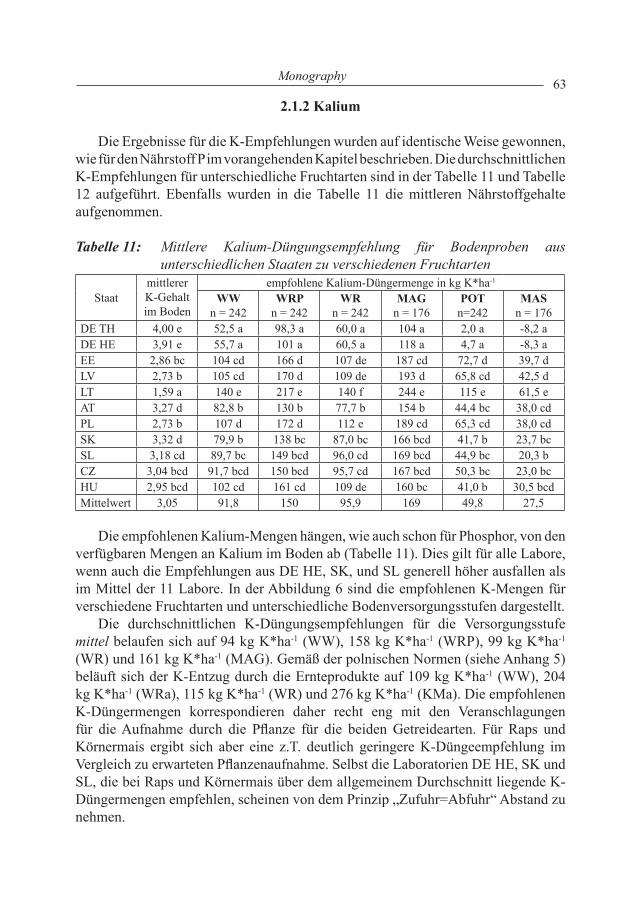
63Monography
2.1.2 kalium
Die Ergebnisse für die K-Empfehlungen wurden auf identische Weise gewonnen, wie für den Nährstoff P im vorangehenden Kapitel beschrieben. Die durchschnittlichen K-Empfehlungen für unterschiedliche Fruchtarten sind in der Tabelle 11 und Tabelle 12 aufgeführt. Ebenfalls wurden in die Tabelle 11 die mittleren Nährstoffgehalte aufgenommen.
Tabelle 11: Mittlere Kalium-Düngungsempfehlung für Bodenproben aus unterschiedlichen Staaten zu verschiedenen Fruchtarten
StaatmittlererK-Gehalt im Boden
empfohlene Kalium-Düngermenge in kg K*ha-1
WWn = 242
WRPn = 242
WRn = 242
MAGn = 176
POTn=242
MASn = 176
DE TH 4,00 e 52,5 a 98,3 a 60,0 a 104 a 2,0 a -8,2 aDE HE 3,91 e 55,7 a 101 a 60,5 a 118 a 4,7 a -8,3 aEE 2,86 bc 104 cd 166 d 107 de 187 cd 72,7 d 39,7 dLV 2,73 b 105 cd 170 d 109 de 193 d 65,8 cd 42,5 dLT 1,59 a 140 e 217 e 140 f 244 e 115 e 61,5 eAT 3,27 d 82,8 b 130 b 77,7 b 154 b 44,4 bc 38,0 cdPL 2,73 b 107 d 172 d 112 e 189 cd 65,3 cd 38,0 cdSK 3,32 d 79,9 b 138 bc 87,0 bc 166 bcd 41,7 b 23,7 bcSL 3,18 cd 89,7 bc 149 bcd 96,0 cd 169 bcd 44,9 bc 20,3 bCZ 3,04 bcd 91,7 bcd 150 bcd 95,7 cd 167 bcd 50,3 bc 23,0 bcHU 2,95 bcd 102 cd 161 cd 109 de 160 bc 41,0 b 30,5 bcdMittelwert 3,05 91,8 150 95,9 169 49,8 27,5
Die empfohlenen Kalium-Mengen hängen, wie auch schon für Phosphor, von den verfügbaren Mengen an Kalium im Boden ab (Tabelle 11). Dies gilt für alle Labore, wenn auch die Empfehlungen aus DE HE, SK, und SL generell höher ausfallen als im Mittel der 11 Labore. In der Abbildung 6 sind die empfohlenen K-Mengen für verschiedene Fruchtarten und unterschiedliche Bodenversorgungsstufen dargestellt.
Die durchschnittlichen K-Düngungsempfehlungen für die Versorgungsstufe mittel belaufen sich auf 94 kg K*ha-1 (WW), 158 kg K*ha-1 (WRP), 99 kg K*ha-1 (WR) und 161 kg K*ha-1 (MAG). Gemäß der polnischen Normen (siehe Anhang 5) beläuft sich der K-Entzug durch die Ernteprodukte auf 109 kg K*ha-1 (WW), 204 kg K*ha-1 (WRa), 115 kg K*ha-1 (WR) und 276 kg K*ha-1 (KMa). Die empfohlenen K-Düngermengen korrespondieren daher recht eng mit den Veranschlagungen für die Aufnahme durch die Pflanze für die beiden Getreidearten. Für Raps und Körnermais ergibt sich aber eine z.T. deutlich geringere K-Düngeempfehlung im Vergleich zu erwarteten Pflanzenaufnahme. Selbst die Laboratorien DE HE, SK und SL, die bei Raps und Körnermais über dem allgemeinem Durchschnitt liegende K-Düngermengen empfehlen, scheinen von dem Prinzip „Zufuhr=Abfuhr“ Abstand zu nehmen.
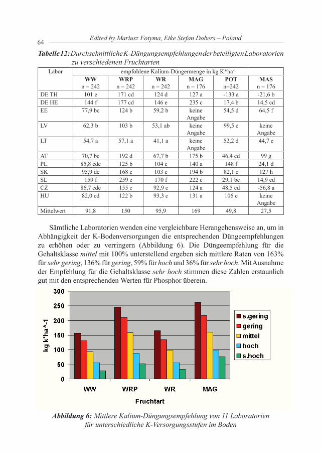
64 Edited by Mariusz Fotyma, Eike Stefan Dobers – Poland
Tabelle 12: Durchschnittliche K-Düngungsempfehlungen der beteiligten Laboratorien zu verschiedenen Fruchtarten
Labor empfohlene Kalium-Düngermenge in kg K*ha-1
WWn = 242
WRPn = 242
WRn = 242
MAGn = 176
POTn=242
MASn = 176
DE TH 101 e 171 cd 124 d 127 a -133 a -21,6 bDE HE 144 f 177 cd 146 e 235 c 17,4 b 14,5 cd EE 77,9 bc 124 b 59,2 b keine
Angabe54,5 d 64,5 f
LV 62,3 b 103 b 53,1 ab keine Angabe
99,5 e keine Angabe
LT 54,7 a 57,1 a 41,1 a keine Angabe
52,2 d 44,7 e
AT 70,7 bc 192 d 67,7 b 175 b 46,4 cd 99 gPL 85,8 cde 125 b 104 c 140 a 148 f 24,1 dSK 95,9 de 168 c 103 c 194 b 82,1 e 127 h SL 159 f 259 e 170 f 222 c 29,1 bc 14,9 cdCZ 86,7 cde 155 c 92,9 c 124 a 48,5 cd -56,8 aHU 82,0 cd 122 b 93,3 c 131 a 106 e keine
AngabeMittelwert 91,8 150 95,9 169 49,8 27,5
Sämtliche Laboratorien wenden eine vergleichbare Herangehensweise an, um in Abhängigkeit der K-Bodenversorgungen die entsprechenden Düngeempfehlungen zu erhöhen oder zu verringern (Abbildung 6). Die Düngeempfehlung für die Gehaltsklasse mittel mit 100% unterstellend ergeben sich mittlere Raten von 163% für sehr gering, 136% für gering, 59% für hoch und 36% für sehr hoch. Mit Ausnahme der Empfehlung für die Gehaltsklasse sehr hoch stimmen diese Zahlen erstaunlich gut mit den entsprechenden Werten für Phosphor überein.
Abbildung 6: Mittlere Kalium-Düngungsempfehlung von 11 Laboratorien für unterschiedliche K-Versorgungsstufen im Boden
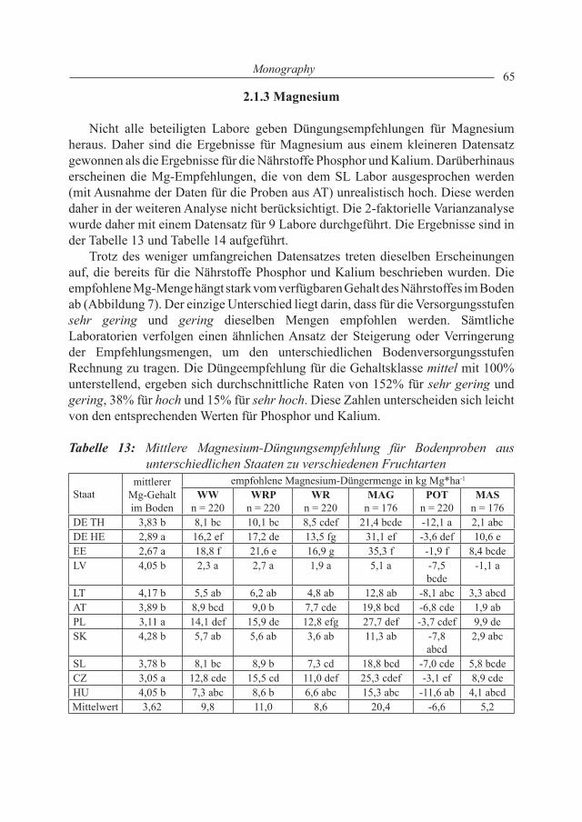
65Monography
2.1.3 Magnesium
Nicht alle beteiligten Labore geben Düngungsempfehlungen für Magnesium heraus. Daher sind die Ergebnisse für Magnesium aus einem kleineren Datensatz gewonnen als die Ergebnisse für die Nährstoffe Phosphor und Kalium. Darüberhinaus erscheinen die Mg-Empfehlungen, die von dem SL Labor ausgesprochen werden (mit Ausnahme der Daten für die Proben aus AT) unrealistisch hoch. Diese werden daher in der weiteren Analyse nicht berücksichtigt. Die 2-faktorielle Varianzanalyse wurde daher mit einem Datensatz für 9 Labore durchgeführt. Die Ergebnisse sind in der Tabelle 13 und Tabelle 14 aufgeführt.
Trotz des weniger umfangreichen Datensatzes treten dieselben Erscheinungen auf, die bereits für die Nährstoffe Phosphor und Kalium beschrieben wurden. Die empfohlene Mg-Menge hängt stark vom verfügbaren Gehalt des Nährstoffes im Boden ab (Abbildung 7). Der einzige Unterschied liegt darin, dass für die Versorgungsstufen sehr gering und gering dieselben Mengen empfohlen werden. Sämtliche Laboratorien verfolgen einen ähnlichen Ansatz der Steigerung oder Verringerung der Empfehlungsmengen, um den unterschiedlichen Bodenversorgungsstufen Rechnung zu tragen. Die Düngeempfehlung für die Gehaltsklasse mittel mit 100% unterstellend, ergeben sich durchschnittliche Raten von 152% für sehr gering und gering, 38% für hoch und 15% für sehr hoch. Diese Zahlen unterscheiden sich leicht von den entsprechenden Werten für Phosphor und Kalium.
Tabelle 13: Mittlere Magnesium-Düngungsempfehlung für Bodenproben aus unterschiedlichen Staaten zu verschiedenen Fruchtarten
Staatmittlerer
Mg-Gehalt im Boden
empfohlene Magnesium-Düngermenge in kg Mg*ha-1
WWn = 220
WRPn = 220
WRn = 220
MAGn = 176
POTn = 220
MASn = 176
DE TH 3,83 b 8,1 bc 10,1 bc 8,5 cdef 21,4 bcde -12,1 a 2,1 abcDE HE 2,89 a 16,2 ef 17,2 de 13,5 fg 31,1 ef -3,6 def 10,6 eEE 2,67 a 18,8 f 21,6 e 16,9 g 35,3 f -1,9 f 8,4 bcdeLV 4,05 b 2,3 a 2,7 a 1,9 a 5,1 a -7,5
bcde-1,1 a
LT 4,17 b 5,5 ab 6,2 ab 4,8 ab 12,8 ab -8,1 abc 3,3 abcdAT 3,89 b 8,9 bcd 9,0 b 7,7 cde 19,8 bcd -6,8 cde 1,9 abPL 3,11 a 14,1 def 15,9 de 12,8 efg 27,7 def -3,7 cdef 9,9 deSK 4,28 b 5,7 ab 5,6 ab 3,6 ab 11,3 ab -7,8
abcd2,9 abc
SL 3,78 b 8,1 bc 8,9 b 7,3 cd 18,8 bcd -7,0 cde 5,8 bcdeCZ 3,05 a 12,8 cde 15,5 cd 11,0 def 25,3 cdef -3,1 ef 8,9 cdeHU 4,05 b 7,3 abc 8,6 b 6,6 abc 15,3 abc -11,6 ab 4,1 abcdMittelwert 3,62 9,8 11,0 8,6 20,4 -6,6 5,2
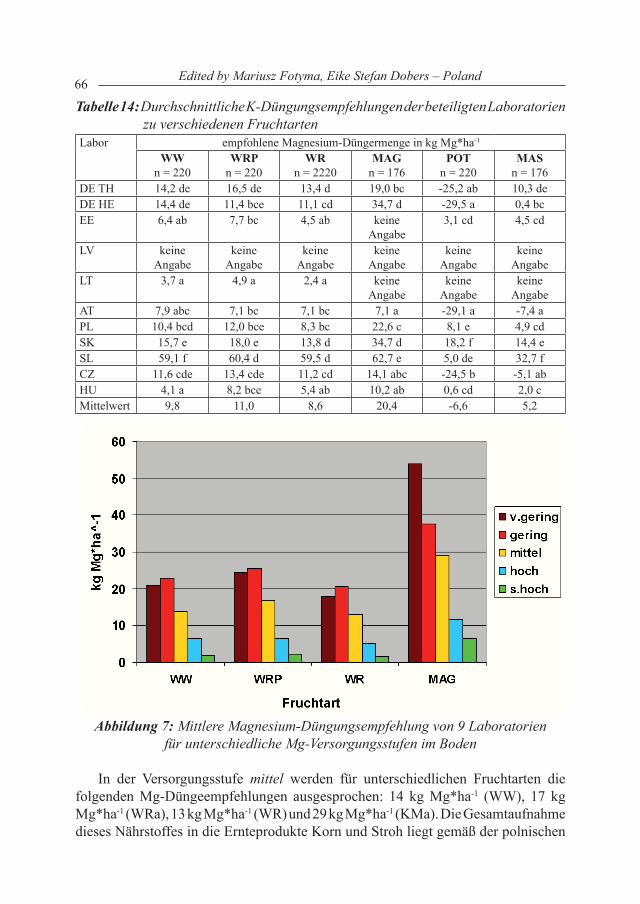
66 Edited by Mariusz Fotyma, Eike Stefan Dobers – Poland
Tabelle 14: Durchschnittliche K-Düngungsempfehlungen der beteiligten Laboratorien zu verschiedenen Fruchtarten
Labor empfohlene Magnesium-Düngermenge in kg Mg*ha-1
WWn = 220
WRPn = 220
WRn = 2220
MAGn = 176
POTn = 220
MASn = 176
DE TH 14,2 de 16,5 de 13,4 d 19,0 bc -25,2 ab 10,3 deDE HE 14,4 de 11,4 bce 11,1 cd 34,7 d -29,5 a 0,4 bcEE 6,4 ab 7,7 bc 4,5 ab keine
Angabe3,1 cd 4,5 cd
LV keine Angabe
keine Angabe
keine Angabe
keine Angabe
keine Angabe
keine Angabe
LT 3,7 a 4,9 a 2,4 a keine Angabe
keine Angabe
keine Angabe
AT 7,9 abc 7,1 bc 7,1 bc 7,1 a -29,1 a -7,4 aPL 10,4 bcd 12,0 bce 8,3 bc 22,6 c 8,1 e 4,9 cdSK 15,7 e 18,0 e 13,8 d 34,7 d 18,2 f 14,4 e SL 59,1 f 60,4 d 59,5 d 62,7 e 5,0 de 32,7 f CZ 11,6 cde 13,4 cde 11,2 cd 14,1 abc -24,5 b -5,1 abHU 4,1 a 8,2 bce 5,4 ab 10,2 ab 0,6 cd 2,0 cMittelwert 9,8 11,0 8,6 20,4 -6,6 5,2
Abbildung 7: Mittlere Magnesium-Düngungsempfehlung von 9 Laboratorien für unterschiedliche Mg-Versorgungsstufen im Boden
In der Versorgungsstufe mittel werden für unterschiedlichen Fruchtarten die folgenden Mg-Düngeempfehlungen ausgesprochen: 14 kg Mg*ha-1 (WW), 17 kg Mg*ha-1 (WRa), 13 kg Mg*ha-1 (WR) und 29 kg Mg*ha-1 (KMa). Die Gesamtaufnahme dieses Nährstoffes in die Ernteprodukte Korn und Stroh liegt gemäß der polnischen

67Monography
Normen bei 16 kg Mg*ha-1 (WW), 23 kg Mg*ha-1 (WRa), 14 kg Mg*ha-1 (WR) und 46 kg Mg*ha-1 (KMa). Die empfohlenen Mg-Düngemengen bleiben mit Ausnahme der für Winterroggen hinter den unterstellten Aufnahmen in die Ernteprodukte zurück.
2.2 Düngungsempfehlung für kartoffel und Silomais
Der Hauptunterschied zwischen den bisher vorgestellten Fruchtarten (WW, WRP, WR, MAG) und den nun folgenden (POT, MAS) liegt darin, dass letztere unter Verwendung von organischen Düngern angebaut werden. Für den Anbau von Kartoffel wurden die Ausbringung von 30 t*ha-1 Stallmist, für Silomais die Verwendung von 30 mł*ha-1 Rindergülle unterstellt. Während über die Höhe der zu veranschlagenden Nährstoffgehalte in der Rindergülle Einvernehmen zwischen den Teilnehmern bestand, war dies für Stallmist nicht der Fall. Die unterstellten Nährstoffgehalte in Rindergülle von 0.74 kg*m-3 P, 5.30 kg*m-3 K und 0.50 kg*m-3 Mg ergeben durch die angenommene Ausbringungsmenge von 30 mł eine Gesamt-Nährstoffzufuhr durch organische Düngung zu Silomais von 22 kg*ha-1 P, 159 kg*ha-
1 K und 15 kg*ha-1 Mg.Die polnische Norm geht davon aus, dass Stallmist 0.13% P, 0.58% K und
0.12% Mg enthält. Dies ergibt eine Gesamt-Nährstoffzufuhr durch organische Düngung zu Kartoffel von 39 kg*ha-1 P, 174 kg*ha-1 K und 36 kg*ha-1 Mg. Die jeweilig unterstellten Mengen der Nährstoffzufuhr über Stallmist-Düngung und die nachfolgende Ausnutzung durch die Pflanze im Verlauf der Vegetationsperiode sind in den teilnehmenden Staaten sehr unterschiedlich. Daher ist es nicht verwunderlich, dass die durch die verschiedenen Labore abgeleiteten Düngungsempfehlungen sehr unterschiedlich ausfallen (Tabellen 9-14).
Die mittleren P-Düngeempfehlungen für beide Fruchtarten sind sehr gering, unterscheiden sich aber doch grundlegend zwischen den Laboren (Tabelle 10). Einige Labore empfehlen „negative“ P-Gaben, was für die Praxis bedeuten würde, dass der Landwirt keinerlei P-Düngung durchführen sollte, und sogar die entsprechenden Mengen von den geplanten Gaben zu den nachfolgenden Fruchtarten abziehen kann. Die P-Empfehlungen, besonders zu Kartoffel, war grundsätzlich unabhängig von der jeweiligen P-Versorgung der Böden (Abbildung 8). Signifikante Unterschiede wurden nur zwischen den Empfehlungen für die Versorgungsstufe sehr gering (bei Silomais auch für die Stufe gering) und allen anderen P-Versorgungsstufen der Böden gefunden. Die durchschnittlich empfohlene P-Menge für die Versorgungsstufe mittel lag bei 3 kg*ha-1 für Kartoffel und bei 11 kg*ha-1 für Silomais. Gemäß der polnischen Standards und dem unterstellten Ertragsniveau von 30 t*ha-1 Kartoffeln bzw. 10 t*ha-1 Silomais-Trockenmasse würden 19 bzw. 32 kg P*ha-1 aufgenommen werden. Demnach wäre bei Kartoffel die P-Abfuhr bereits durch die Stallmistgabe deutlich gedeckt, während für Silomais die P-Entzugsmengen durch Güllezufuhr und P-Düngeempfehlung recht genau erreicht werden.
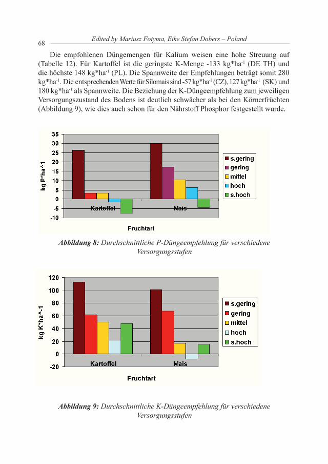
68 Edited by Mariusz Fotyma, Eike Stefan Dobers – Poland
Die empfohlenen Düngemengen für Kalium weisen eine hohe Streuung auf (Tabelle 12). Für Kartoffel ist die geringste K-Menge -133 kg*ha-1 (DE TH) und die höchste 148 kg*ha-1 (PL). Die Spannweite der Empfehlungen beträgt somit 280 kg*ha-1. Die entsprechenden Werte für Silomais sind -57 kg*ha-1 (CZ), 127 kg*ha-1 (SK) und 180 kg*ha-1 als Spannweite. Die Beziehung der K-Düngeempfehlung zum jeweiligen Versorgungszustand des Bodens ist deutlich schwächer als bei den Körnerfrüchten (Abbildung 9), wie dies auch schon für den Nährstoff Phosphor festgestellt wurde.
Abbildung 8: Durchschnittliche P-Düngeempfehlung für verschiedene Versorgungsstufen
Abbildung 9: Durchschnittliche K-Düngeempfehlung für verschiedene Versorgungsstufen
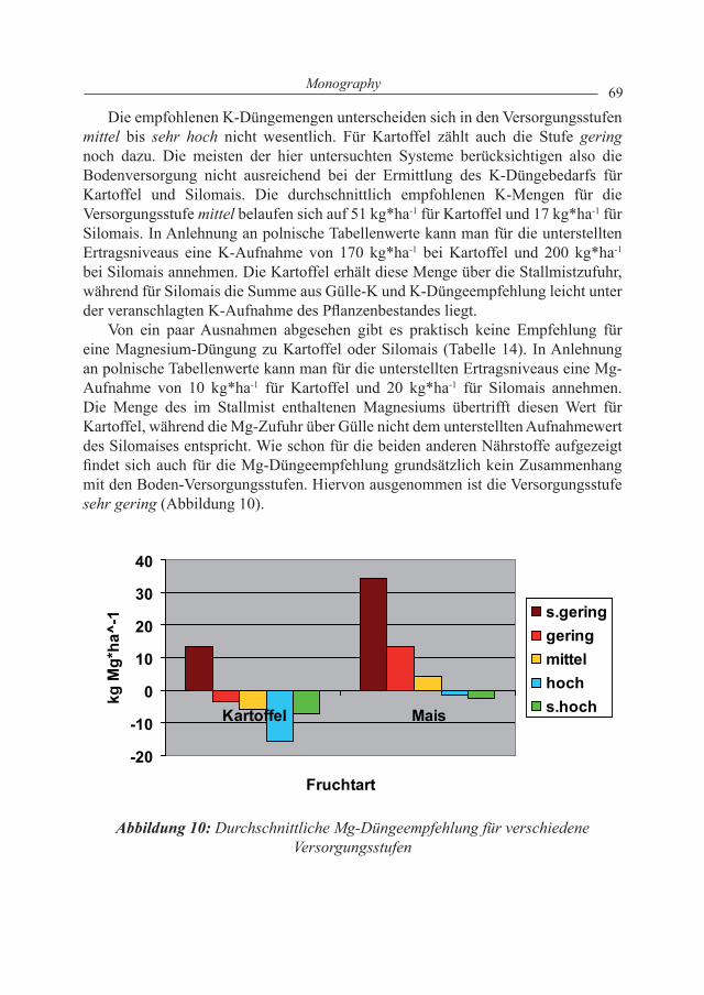
69Monography
Die empfohlenen K-Düngemengen unterscheiden sich in den Versorgungsstufen mittel bis sehr hoch nicht wesentlich. Für Kartoffel zählt auch die Stufe gering noch dazu. Die meisten der hier untersuchten Systeme berücksichtigen also die Bodenversorgung nicht ausreichend bei der Ermittlung des K-Düngebedarfs für Kartoffel und Silomais. Die durchschnittlich empfohlenen K-Mengen für die Versorgungsstufe mittel belaufen sich auf 51 kg*ha-1 für Kartoffel und 17 kg*ha-1 für Silomais. In Anlehnung an polnische Tabellenwerte kann man für die unterstellten Ertragsniveaus eine K-Aufnahme von 170 kg*ha-1 bei Kartoffel und 200 kg*ha-1 bei Silomais annehmen. Die Kartoffel erhält diese Menge über die Stallmistzufuhr, während für Silomais die Summe aus Gülle-K und K-Düngeempfehlung leicht unter der veranschlagten K-Aufnahme des Pflanzenbestandes liegt.
Von ein paar Ausnahmen abgesehen gibt es praktisch keine Empfehlung für eine Magnesium-Düngung zu Kartoffel oder Silomais (Tabelle 14). In Anlehnung an polnische Tabellenwerte kann man für die unterstellten Ertragsniveaus eine Mg-Aufnahme von 10 kg*ha-1 für Kartoffel und 20 kg*ha-1 für Silomais annehmen. Die Menge des im Stallmist enthaltenen Magnesiums übertrifft diesen Wert für Kartoffel, während die Mg-Zufuhr über Gülle nicht dem unterstellten Aufnahmewert des Silomaises entspricht. Wie schon für die beiden anderen Nährstoffe aufgezeigt findet sich auch für die Mg-Düngeempfehlung grundsätzlich kein Zusammenhang mit den Boden-Versorgungsstufen. Hiervon ausgenommen ist die Versorgungsstufe sehr gering (Abbildung 10).
-20
-10
0
10
20
30
40
Kartoffel Mais
Fruchtart
kg M
g*ha
^-1 s.gering
geringmittelhochs.hoch
Abbildung 10: Durchschnittliche Mg-Düngeempfehlung für verschiedene Versorgungsstufen
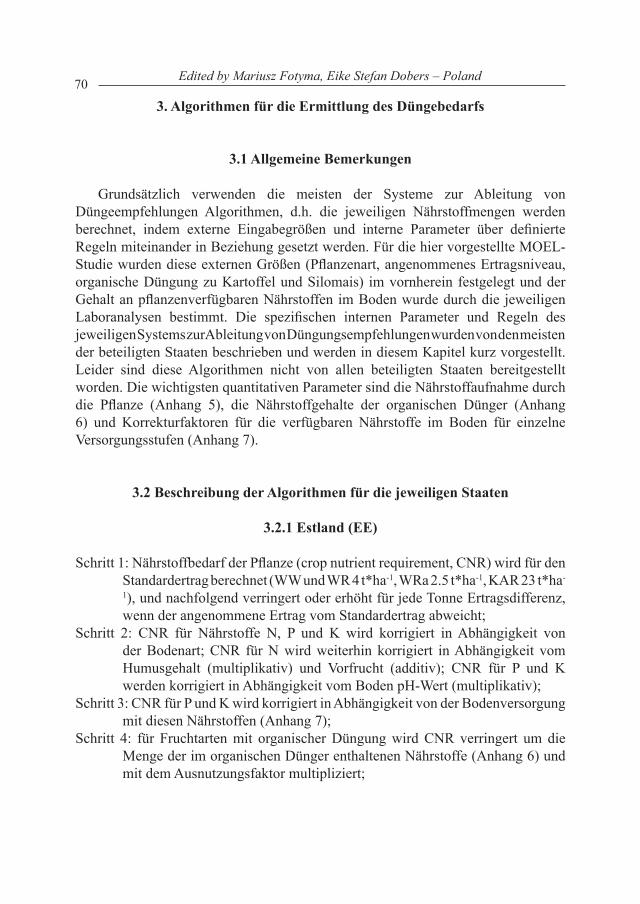
70 Edited by Mariusz Fotyma, Eike Stefan Dobers – Poland
3. Algorithmen für die Ermittlung des Düngebedarfs
3.1 Allgemeine Bemerkungen
Grundsätzlich verwenden die meisten der Systeme zur Ableitung von Düngeempfehlungen Algorithmen, d.h. die jeweiligen Nährstoffmengen werden berechnet, indem externe Eingabegrößen und interne Parameter über definierte Regeln miteinander in Beziehung gesetzt werden. Für die hier vorgestellte MOEL-Studie wurden diese externen Größen (Pflanzenart, angenommenes Ertragsniveau, organische Düngung zu Kartoffel und Silomais) im vornherein festgelegt und der Gehalt an pflanzenverfügbaren Nährstoffen im Boden wurde durch die jeweiligen Laboranalysen bestimmt. Die spezifischen internen Parameter und Regeln des jeweiligen Systems zur Ableitung von Düngungsempfehlungen wurden von den meisten der beteiligten Staaten beschrieben und werden in diesem Kapitel kurz vorgestellt. Leider sind diese Algorithmen nicht von allen beteiligten Staaten bereitgestellt worden. Die wichtigsten quantitativen Parameter sind die Nährstoffaufnahme durch die Pflanze (Anhang 5), die Nährstoffgehalte der organischen Dünger (Anhang 6) und Korrekturfaktoren für die verfügbaren Nährstoffe im Boden für einzelne Versorgungsstufen (Anhang 7).
3.2 Beschreibung der Algorithmen für die jeweiligen Staaten
3.2.1 Estland (EE)
Schritt 1: Nährstoffbedarf der Pflanze (crop nutrient requirement, CNR) wird für den Standardertrag berechnet (WW und WR 4 t*ha-1, WRa 2.5 t*ha-1, KAR 23 t*ha-
1), und nachfolgend verringert oder erhöht für jede Tonne Ertragsdifferenz, wenn der angenommene Ertrag vom Standardertrag abweicht;
Schritt 2: CNR für Nährstoffe N, P und K wird korrigiert in Abhängigkeit von der Bodenart; CNR für N wird weiterhin korrigiert in Abhängigkeit vom Humusgehalt (multiplikativ) und Vorfrucht (additiv); CNR für P und K werden korrigiert in Abhängigkeit vom Boden pH-Wert (multiplikativ);
Schritt 3: CNR für P und K wird korrigiert in Abhängigkeit von der Bodenversorgung mit diesen Nährstoffen (Anhang 7);
Schritt 4: für Fruchtarten mit organischer Düngung wird CNR verringert um die Menge der im organischen Dünger enthaltenen Nährstoffe (Anhang 6) und mit dem Ausnutzungsfaktor multipliziert;
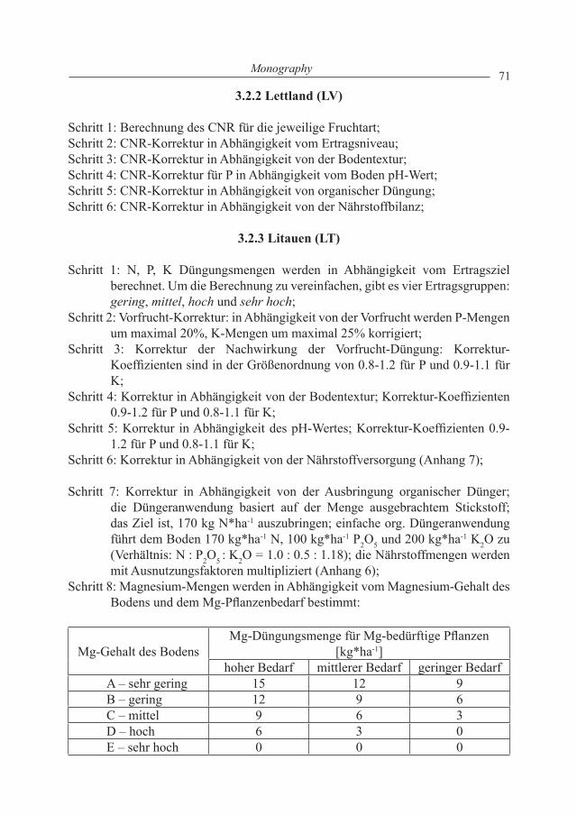
71Monography
3.2.2 Lettland (LV)
Schritt 1: Berechnung des CNR für die jeweilige Fruchtart;Schritt 2: CNR-Korrektur in Abhängigkeit vom Ertragsniveau;Schritt 3: CNR-Korrektur in Abhängigkeit von der Bodentextur;Schritt 4: CNR-Korrektur für P in Abhängigkeit vom Boden pH-Wert;Schritt 5: CNR-Korrektur in Abhängigkeit von organischer Düngung;Schritt 6: CNR-Korrektur in Abhängigkeit von der Nährstoffbilanz;
3.2.3 Litauen (LT)
Schritt 1: N, P, K Düngungsmengen werden in Abhängigkeit vom Ertragsziel berechnet. Um die Berechnung zu vereinfachen, gibt es vier Ertragsgruppen: gering, mittel, hoch und sehr hoch;
Schritt 2: Vorfrucht-Korrektur: in Abhängigkeit von der Vorfrucht werden P-Mengen um maximal 20%, K-Mengen um maximal 25% korrigiert;
Schritt 3: Korrektur der Nachwirkung der Vorfrucht-Düngung: Korrektur-Koeffizienten sind in der Größenordnung von 0.8-1.2 für P und 0.9-1.1 für K;
Schritt 4: Korrektur in Abhängigkeit von der Bodentextur; Korrektur-Koeffizienten 0.9-1.2 für P und 0.8-1.1 für K;
Schritt 5: Korrektur in Abhängigkeit des pH-Wertes; Korrektur-Koeffizienten 0.9-1.2 für P und 0.8-1.1 für K;
Schritt 6: Korrektur in Abhängigkeit von der Nährstoffversorgung (Anhang 7);
Schritt 7: Korrektur in Abhängigkeit von der Ausbringung organischer Dünger; die Düngeranwendung basiert auf der Menge ausgebrachtem Stickstoff; das Ziel ist, 170 kg N*ha-1 auszubringen; einfache org. Düngeranwendung führt dem Boden 170 kg*ha-1 N, 100 kg*ha-1 P2O5 und 200 kg*ha-1 K2O zu (Verhältnis: N : P2O5 : K2O = 1.0 : 0.5 : 1.18); die Nährstoffmengen werden mit Ausnutzungsfaktoren multipliziert (Anhang 6);
Schritt 8: Magnesium-Mengen werden in Abhängigkeit vom Magnesium-Gehalt des Bodens und dem Mg-Pflanzenbedarf bestimmt:
Mg-Gehalt des BodensMg-Düngungsmenge für Mg-bedürftige Pflanzen
[kg*ha-1]hoher Bedarf mittlerer Bedarf geringer Bedarf
A – sehr gering 15 12 9B – gering 12 9 6C – mittel 9 6 3D – hoch 6 3 0E – sehr hoch 0 0 0
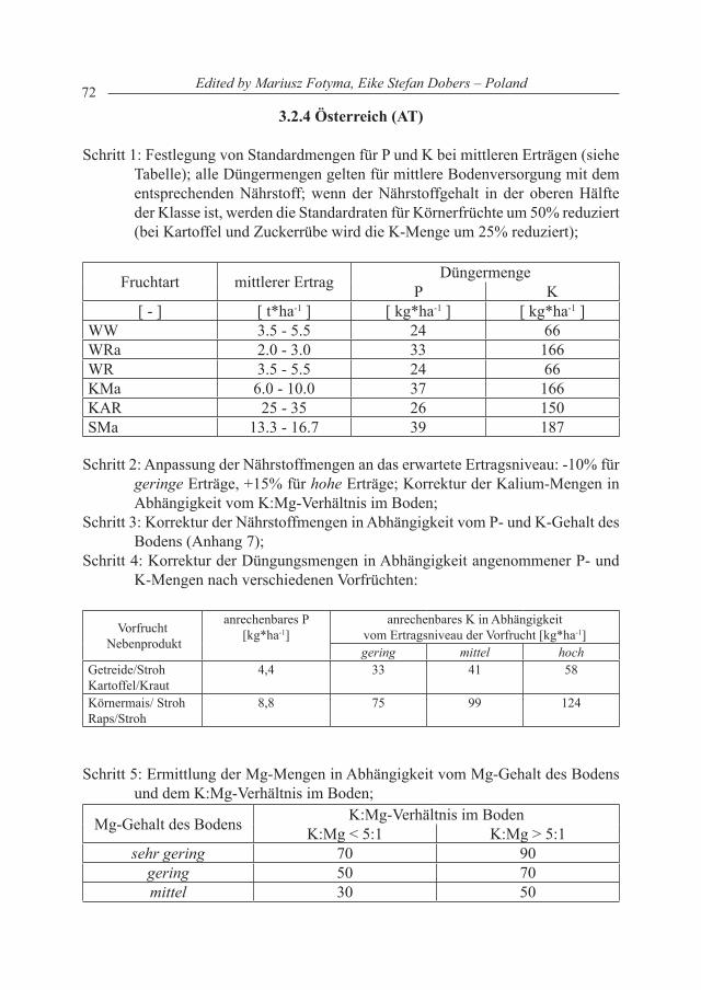
72 Edited by Mariusz Fotyma, Eike Stefan Dobers – Poland
3.2.4 Österreich (AT)
Schritt 1: Festlegung von Standardmengen für P und K bei mittleren Erträgen (siehe Tabelle); alle Düngermengen gelten für mittlere Bodenversorgung mit dem entsprechenden Nährstoff; wenn der Nährstoffgehalt in der oberen Hälfte der Klasse ist, werden die Standardraten für Körnerfrüchte um 50% reduziert (bei Kartoffel und Zuckerrübe wird die K-Menge um 25% reduziert);
Fruchtart mittlerer Ertrag DüngermengeP K
[ - ] [ t*ha-1 ] [ kg*ha-1 ] [ kg*ha-1 ]WW 3.5 - 5.5 24 66WRa 2.0 - 3.0 33 166WR 3.5 - 5.5 24 66KMa 6.0 - 10.0 37 166KAR 25 - 35 26 150SMa 13.3 - 16.7 39 187
Schritt 2: Anpassung der Nährstoffmengen an das erwartete Ertragsniveau: -10% für geringe Erträge, +15% für hohe Erträge; Korrektur der Kalium-Mengen in Abhängigkeit vom K:Mg-Verhältnis im Boden;
Schritt 3: Korrektur der Nährstoffmengen in Abhängigkeit vom P- und K-Gehalt des Bodens (Anhang 7);
Schritt 4: Korrektur der Düngungsmengen in Abhängigkeit angenommener P- und K-Mengen nach verschiedenen Vorfrüchten:
Vorfrucht Nebenprodukt
anrechenbares P[kg*ha-1]
anrechenbares K in Abhängigkeit vom Ertragsniveau der Vorfrucht [kg*ha-1]gering mittel hoch
Getreide/StrohKartoffel/Kraut
4,4 33 41 58
Körnermais/ StrohRaps/Stroh
8,8 75 99 124
Schritt 5: Ermittlung der Mg-Mengen in Abhängigkeit vom Mg-Gehalt des Bodens und dem K:Mg-Verhältnis im Boden;
Mg-Gehalt des Bodens K:Mg-Verhältnis im BodenK:Mg < 5:1 K:Mg > 5:1
sehr gering 70 90gering 50 70mittel 30 50
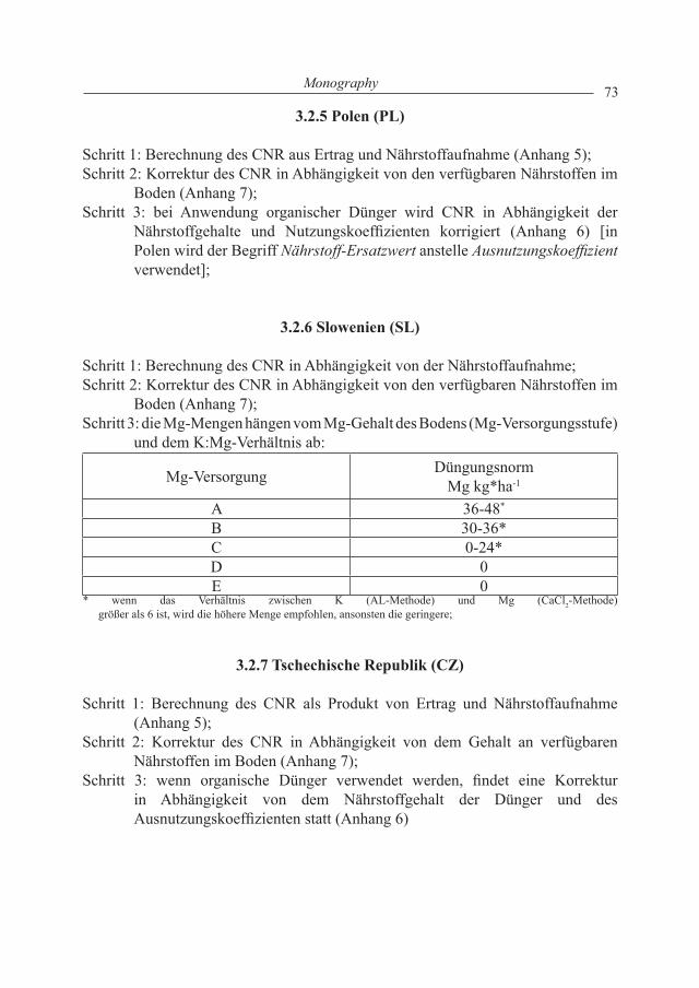
73Monography
3.2.5 Polen (PL)
Schritt 1: Berechnung des CNR aus Ertrag und Nährstoffaufnahme (Anhang 5);Schritt 2: Korrektur des CNR in Abhängigkeit von den verfügbaren Nährstoffen im
Boden (Anhang 7);Schritt 3: bei Anwendung organischer Dünger wird CNR in Abhängigkeit der
Nährstoffgehalte und Nutzungskoeffizienten korrigiert (Anhang 6) [in Polen wird der Begriff Nährstoff-Ersatzwert anstelle Ausnutzungskoeffizient verwendet];
3.2.6 Slowenien (SL)
Schritt 1: Berechnung des CNR in Abhängigkeit von der Nährstoffaufnahme;Schritt 2: Korrektur des CNR in Abhängigkeit von den verfügbaren Nährstoffen im
Boden (Anhang 7);Schritt 3: die Mg-Mengen hängen vom Mg-Gehalt des Bodens (Mg-Versorgungsstufe)
und dem K:Mg-Verhältnis ab:
Mg-Versorgung DüngungsnormMg kg*ha-1
A 36-48*
B 30-36*C 0-24*D 0E 0
* wenn das Verhältnis zwischen K (AL-Methode) und Mg (CaCl2-Methode) größer als 6 ist, wird die höhere Menge empfohlen, ansonsten die geringere;
3.2.7 Tschechische Republik (CZ)
Schritt 1: Berechnung des CNR als Produkt von Ertrag und Nährstoffaufnahme (Anhang 5);
Schritt 2: Korrektur des CNR in Abhängigkeit von dem Gehalt an verfügbaren Nährstoffen im Boden (Anhang 7);
Schritt 3: wenn organische Dünger verwendet werden, findet eine Korrektur in Abhängigkeit von dem Nährstoffgehalt der Dünger und des Ausnutzungskoeffizienten statt (Anhang 6)
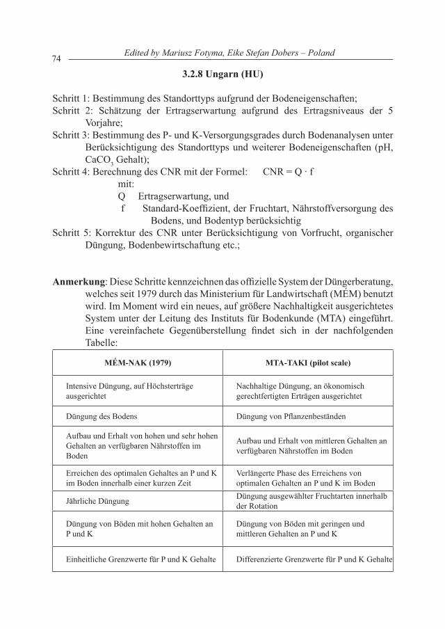
74 Edited by Mariusz Fotyma, Eike Stefan Dobers – Poland
3.2.8 Ungarn (HU)
Schritt 1: Bestimmung des Standorttyps aufgrund der Bodeneigenschaften;Schritt 2: Schätzung der Ertragserwartung aufgrund des Ertragsniveaus der 5
Vorjahre;Schritt 3: Bestimmung des P- und K-Versorgungsgrades durch Bodenanalysen unter
Berücksichtigung des Standorttyps und weiterer Bodeneigenschaften (pH, CaCO3 Gehalt);
Schritt 4: Berechnung des CNR mit der Formel: CNR = Q ∙ fmit:Q Ertragserwartung, und f Standard-Koeffizient, der Fruchtart, Nährstoffversorgung des
Bodens, und Bodentyp berücksichtigSchritt 5: Korrektur des CNR unter Berücksichtigung von Vorfrucht, organischer
Düngung, Bodenbewirtschaftung etc.;
Anmerkung: Diese Schritte kennzeichnen das offizielle System der Düngerberatung, welches seit 1979 durch das Ministerium für Landwirtschaft (MÉM) benutzt wird. Im Moment wird ein neues, auf größere Nachhaltigkeit ausgerichtetes System unter der Leitung des Instituts für Bodenkunde (MTA) eingeführt. Eine vereinfachete Gegenüberstellung findet sich in der nachfolgenden Tabelle:
MÉM-NAk (1979) MTA-TAkI (pilot scale)
Intensive Düngung, auf Höchsterträge ausgerichtet
Nachhaltige Düngung, an ökonomisch gerechtfertigten Erträgen ausgerichtet
Düngung des Bodens Düngung von Pflanzenbeständen
Aufbau und Erhalt von hohen und sehr hohen Gehalten an verfügbaren Nährstoffen im Boden
Aufbau und Erhalt von mittleren Gehalten an verfügbaren Nährstoffen im Boden
Erreichen des optimalen Gehaltes an P und K im Boden innerhalb einer kurzen Zeit
Verlängerte Phase des Erreichens von optimalen Gehalten an P und K im Boden
Jährliche Düngung Düngung ausgewählter Fruchtarten innerhalb der Rotation
Düngung von Böden mit hohen Gehalten an P und K
Düngung von Böden mit geringen und mittleren Gehalten an P und K
Einheitliche Grenzwerte für P und K Gehalte Differenzierte Grenzwerte für P und K Gehalte
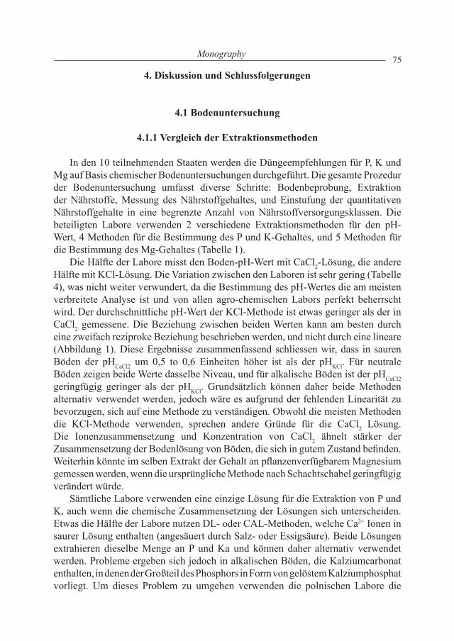
75Monography
4. Diskussion und Schlussfolgerungen
4.1 Bodenuntersuchung
4.1.1 Vergleich der Extraktionsmethoden
In den 10 teilnehmenden Staaten werden die Düngeempfehlungen für P, K und Mg auf Basis chemischer Bodenuntersuchungen durchgeführt. Die gesamte Prozedur der Bodenuntersuchung umfasst diverse Schritte: Bodenbeprobung, Extraktion der Nährstoffe, Messung des Nährstoffgehaltes, und Einstufung der quantitativen Nährstoffgehalte in eine begrenzte Anzahl von Nährstoffversorgungsklassen. Die beteiligten Labore verwenden 2 verschiedene Extraktionsmethoden für den pH-Wert, 4 Methoden für die Bestimmung des P und K-Gehaltes, und 5 Methoden für die Bestimmung des Mg-Gehaltes (Tabelle 1).
Die Hälfte der Labore misst den Boden-pH-Wert mit CaCl2-Lösung, die andere Hälfte mit KCl-Lösung. Die Variation zwischen den Laboren ist sehr gering (Tabelle 4), was nicht weiter verwundert, da die Bestimmung des pH-Wertes die am meisten verbreitete Analyse ist und von allen agro-chemischen Labors perfekt beherrscht wird. Der durchschnittliche pH-Wert der KCl-Methode ist etwas geringer als der in CaCl2 gemessene. Die Beziehung zwischen beiden Werten kann am besten durch eine zweifach reziproke Beziehung beschrieben werden, und nicht durch eine lineare (Abbildung 1). Diese Ergebnisse zusammenfassend schliessen wir, dass in sauren Böden der pHCaCl2 um 0,5 to 0,6 Einheiten höher ist als der pHKCl. Für neutrale Böden zeigen beide Werte dasselbe Niveau, und für alkalische Böden ist der pHCaCl2 geringfügig geringer als der pHKCl. Grundsätzlich können daher beide Methoden alternativ verwendet werden, jedoch wäre es aufgrund der fehlenden Linearität zu bevorzugen, sich auf eine Methode zu verständigen. Obwohl die meisten Methoden die KCl-Methode verwenden, sprechen andere Gründe für die CaCl2 Lösung. Die Ionenzusammensetzung und Konzentration von CaCl2 ähnelt stärker der Zusammensetzung der Bodenlösung von Böden, die sich in gutem Zustand befinden. Weiterhin könnte im selben Extrakt der Gehalt an pflanzenverfügbarem Magnesium gemessen werden, wenn die ursprüngliche Methode nach Schachtschabel geringfügig verändert würde.
Sämtliche Labore verwenden eine einzige Lösung für die Extraktion von P und K, auch wenn die chemische Zusammensetzung der Lösungen sich unterscheiden. Etwas die Hälfte der Labore nutzen DL- oder CAL-Methoden, welche Ca2+ Ionen in saurer Lösung enthalten (angesäuert durch Salz- oder Essigsäure). Beide Lösungen extrahieren dieselbe Menge an P und Ka und können daher alternativ verwendet werden. Probleme ergeben sich jedoch in alkalischen Böden, die Kalziumcarbonat enthalten, in denen der Großteil des Phosphors in Form von gelöstem Kalziumphosphat vorliegt. Um dieses Problem zu umgehen verwenden die polnischen Labore die
76 Edited by Mariusz Fotyma, Eike Stefan Dobers – Poland
AL Methode für diese Böden, und in Deutschland wird eine empirische Funktion angewendet, um die extrahierte Phosphormenge der tatsächlichen anzupassen. Diese Funktion berücksichtigt den finalen pH-Wert nach Extraktion von P und K:
Pangepasst = Pgemessen * (1 + 0,83 * (pH(CAL)final – 4,1)) (entsprechend für K)
Die verbleibenden Labore verwenden entweder die AL oder die Mehlich-3 Methode. Die extrahierten Mengen an P und K sind signifikant höher im Vergleich zu der DL und/oder CAL Methode (Tabelle 3). Der Vorteil der Mehlich-3 Methode entsteht durch die Möglichkeit der gleichzeitigen Extraktion von Mg (sowie anderer Mikronährstoffe). Diese Methode scheint in den Staaten Mittel-Osteuropas an Bedeutung zu gewinnen. Vor einigen Jahren übernahmen die slowakischen und tschechischen Labore diese Methode und in 2004 wechselte das estnische Labor von der DL zur Mehlich-3 Methode. Die Möglichkeit eines.Methodenwechsels wird ebenso in Polen erwogen. Es gibt eine direkte Beziehung zwischen den Mengen an P und/oder K, die mit der DL/CAL Methode und der AL/Mehlich-3 Methode ermittelt wurden. Die Steigung der Regressionsgeraden ist nahe 1. Dies eröffnet die Möglichkeit, die Werte von einer Methode in die Einheiten der anderen Methode zu transformieren, was für die Ergebnisse in Tabelle 6 und Tabelle 7 genutzt wurde. Jedoch ist das Bestimmtheitsmaß der linearen Regression für beide Nährstoffe nicht sonderlich hoch, was besonders für Phosphor gilt. Die Regressionskoeffizienten sind stark abhängig von den jeweiligs verwendeten Datensätzen. Die Labore, in denen dieselbe Methode verwendet wird, erzeugen statistisch einheitliche Ergebnisse (Tabelle 4). Dies zeugt von der Verlässlichkeit der Methoden und der Labore. Lediglich die Daten des slowenischen Labors unterscheiden sich significant vom Mittelwert der Labore, welche die AL-Methode verwenden.
Die Ergebnisse für Magnesium zeigen die größte Ambiguität. Die teilnehmenden Labore nutzen insgesamt 5 verschiedene Methoden für die Bestimmung dieses Nährstoffs. Die zwei Extraktionsverfahren CaCl2 (5 mal) und Mehlich-3 (3 mal) treten am häufigsten auf. In den verbleibenden 3 Laboren werden jeweils unterschiedliche Methoden verwendet, von denen zwei auf einer gleichzeitigen Extraktion der drei insgesamt interessierenden Nährstoffe P, K und Mg basieren (DL-Methode in Estland, AL-Methode in Litauen). Das ungarische Labor nutzt KCl-Lösung für die Mg-Extraktion. Die durch CaCl2 und KCl extrahierten Mengen an Mg sind sehr ähnlich und die geringsten unter allen verwendeten Methoden (Tabelle 3). Die Mg-Mengen nach Mehlich-3 oder DL sind ungefähr 100% größer, und die AL Methode extrahiert beinahe viermal so viel Magnesium wie die CaCl2- oder KCl-Methode. Die statistische Beziehung zwischen den durch CaCl2 und Mehlich-3 extrahierten Mg-Mengen kann durch eine lineare Regression beschrieben werden. Da das Bestimmtheitsmaß dieser Beziehung jedoch nicht sehr hoch ist, erscheint die Mögichkeit der Werte-Transformation zwischen den Methoden zumindest fraglich. Die Streuung der Werte zwischen den Laboren ist für die CaCl2-Methode
77Monography
geringer als für die Mehlich-3 Lösung. Dies spricht für die Verwendung der ersten Methode. Jedoch liegt ja wie bereits erwähnt der Vorteil der Mehlich-3 Methode in der gleichzeitigen Extraktion aller drei interessierenden Nährstoffe.
Die AL und DL Methoden erscheinen nicht geeignet für Routine-Untersuchungen des pflanzenverfügbaren Magnesiumgehaltes im Boden. In den Jahren 2000 und 2001 wurde in polnischen Laboren eine vergleichende Analyse der Mg-Gehalte von nahezu 3000 Bodenproben sowohl mit der DL als auch der CaCl2-Methode durchgeführt (Boguszewska et al. 2001). Die allgemeine Beziehung war geprägt von einer großen Streuung mit entsprechend geringem Bestimmtheitsmaß der Regression, und war darüberhinaus noch abhängig vom pH-Wert des Bodens und der Bodenart. Solche Befunde bestätigen die Resultate, welche in dieser vergleichenden Arbeit der MOEL-Staaten gefunden wurden.
Vereinfachend gesprochen sollte eine „gute“ Extraktionsmethode die folgenden Erwartungen erfüllen (Fotyma, Shepherd 2000):
1. die Methode muss die Bio-Verfügbarkeit des Nährstoffes wiedergeben. Die bedeutet für die Praxis hohe Korrelationskoeffizienten mit den Pflanzengehalten, die in einer Kalibrierungsprozedur ermittelt werden (dieser Aspekt wird ausführlicher im nächsten Kapitel diskutiert);
2. sie sollte auf einigen gut definierten Bodenprozessen der Nährstofftransformation beruhen, d.h. Kationenaustausch, Ionenbindung, Ligandenformation usw.;
3. sie sollte praktikabel und verlässlich sein, im Sinne eines Laboreinsatzes, d.h. preisgünstig und robust;
4. sie sollte vielseitig sein und damit die Möglichkeit bieten, mehr als nur einen, gegebenfalls sogar alle Nährstoffe zu extrahieren.
Die Bewertung der verschiedenen verwendeten Methoden gemäß der Kriterien 2.-4. fällt am günstigsten für die Mehlich-3 Methode aus. Aus anderen Veröffentlichungen geht hervor, dass die Mengen an extrahiertem Kalium und Magnesium anscheinend den austauschbaren Anteil dieser Nährstoffe im Boden repräsentieren (Fotyma, Shepherd 2000). Weiterhin ist diese Methode praktikabel, verlässlich und vielseitig einsetzbar für die Extraktion von einigen Makro- und Mikro-Nährstoffen. Gemäß polnischer Berechnungen ist diese Methode die preisgünstigste und es bedarf bei Umstellung keinerlei neuen Laborgerätes. Die Mehlich-3-Methode wurde in einer umfangreichen Studie in der Tschechischen Republik als sehr gut bewertet (Zbiral 2000, Zbiral, Nemec 2000). Sie wird ebenso durch einen Übersichtsartikel in der letzten Ausgabe des Handbuchs für Methoden der Bodenanalyse empfohlen (Ziadi, Sen Tran 2008). Die Ergebnisse des hier vorgestellten Probenaustausches zwischen verschiedenen Laboren bestätigt den großen Wert der Mehlich-3-Methoden.
78 Edited by Mariusz Fotyma, Eike Stefan Dobers – Poland
4.1.2 Ermittlung der Nährstoffversorgung
Bodenuntersuchungen haben keine praktische Bedeutung für landwirtschaftlich Beratung, wenn sie nicht ausreichend interpretiert (kalibriert) werden, d.h. ohne Einteilung der gesamten Spanne an auftretenden Werten in eine begrenzte Anzahl von Klassen, welche wiederum mit dem Pflanzenbedarf in Verbindung stehen. In den beteiligten Staaten – mit Ausnahme Litauens – wird ein fünfklassiges Unterteilungssstem verwendet. Die Bezeichnungen der Klassen, nach ihrer Übersetzung aus der jeweiligen Landessprache ins Englische oder Deutsche, sind leicht unterschiedlich, werden in diesem Bericht aber der Einfachheit halber folgendermaßen definiert: sehr gering (A oder 1), gering (B oder 2), mittel (C oder 3), hoch (D oder 4) und sehr hoch (E oder 5). In Litauen gibt es eine sechste Klasse, die aber für diesen Bericht in die Klasse sehr hoch integriert wurde.
Die Zuordnung des jeweiligen Analyseergebnisses in einer der benannten Klassen ist jedoch nicht nur vom reinen Wert (in mg*kg-1 Boden) abhängig, sondern die meisten Kalibrationssysteme berücksichtigen darüberhinaus noch andere Bodeneigenschaften (Bodenart, Humusgehalt, pH-Wert, Tabelle 5). Die einfachsten Systeme verwenden die reinen Analysewerte (z.B. für Phosphor in DE TH, DE HE, LT, AT, PL, SL). Das komplizierteste wiederum berücksichtigt darüberhinaus die Bodentextur der Probe, den pH-Wert und den Pflanzenbedarf für den entsprechenden Nährstoff (z.B. HU RIS system, Tabelle 5). Wenn dazu noch die jeweils unterschiedlichen verwendeten Methoden der Nährstoffextraktion betrachtet werden, ist es kein Wunder, dass ein direkter Vergleich der Kalibrationssysteme und deren Ergebnisse in den beteiligten Staaten praktisch unmöglich ist. In dieser Aussage ist noch nicht berücksichtig, dass auch noch unterschiedliche Prinzipien der Kalibration in den beteiligten Staaten zur Anwendung kommen.
Der Dreh- und Angelpunkt jedes Kalibrationssystems ist die Klasse mittel für die einzelnen Nährstoffe. In den meisten Systemen korrespondiert die für diese Klasse empfohlene Nährstoffmenge, die über Düngung zugeführt werden sollte, mit der Gesamtnährstoff-Aufnahme der Pflanzen, berechnet aus der Ertragserwartung und einem angenommenen Nährstoffgehalt in der Trocken- oder Frischmasse. Für Bodenuntersuchungs-Ergebnisse, die von der Klasse mittel abweichen, kommen Korrekturfaktoren zur Anwendung (Anhang 6). Der Korrekturfaktor für die Klasse mittel entspricht 1.
Nachhaltige Düngungssysteme betrachten zunehmend die Nährstoffgehalte der Klasse mittel als „sicher“ mit Blickpunkt auf Fragen des Umweltschutzes. Aus diesem Grund werden die jeweiligen Gehalte der Klasse mittel in getrennten Tabellen dargestellt (Tabelle 6 bis Tabelle 8; P- und K-Werte sind in Einheiten der CAL/DL-Methode transformiert, Mg-Werte in Einheiten der CaCl2-Methode). In der nächsten geplanten Phase der MOEL-Kooperation, die sich mit der Erarbeitung von vergleichbaren Systemen der Düngeberatung befasst, werden nur Bodenproben ausgetauscht, deren Nährstoffgehalte in die Klasse mittel fallen.
79Monography
Die Spannweite der Phosphorgehalte in der Klasse mittel ist eher gering und ähnlich für die beteiligten Labore. Ein Ausnahme bildet das AT Labor, welches eine weitere Spanne an P-Gehalten in dieser Klasse vereint. Für die abschliessende Düngeempfehlung wird die Klasse mittel jedoch noch in 2 Unterklassen unterteilt (gering-mittel und hoch-mittel).
Die Spanne der K-Gehalte in der Klasse mittel ist ausreichend eng und ähnlich für die beteiligten Labore, erneut mit der Ausnahme des AT Labors. Jedoch finden sich für das LT Labor deutlich geringere Grenzwerte für diese Klasse, und in SK und CZ sind die Werte höher als im Mittel aller beteiligten Staaten. In den Empfehlungssystemen in SK und CZ erfolgt eine Unterteilung jeder Klasse in 2 Unterklassen mit unterschiedlichen Koeffizienten für zunehmende oder abnehmende Düngeempfehlungen.
In den 8 Labors, die entweder CaCl2 oder die Mehlich-3-Methode für die Magnesiumbestimmung verwenden, ist die Spannweite der Grenzwerte für die Klasse mittel ebenfalls eher klein und die Unterschiede zwischen den Labors zu akzeptieren (die Werte wurden in Einheiten der CalCl2-Methode umgerechnet). Die Ergebnisse für die verbleibenden 8 Labors, die andere Methoden verwenden, sind jedoch nicht vergleichbar. Ebenfalls sollte in Erinnerung bleiben, dass das Bestimmtheitsmaß für die Regressionsgleichung zur Umrechnung der Werte zwischen Mehlich-3 und CaCl2-Methode recht gering war.
Wenn man die erwähnten Differenzen zwischen den Labors außer Acht lässt, so erscheinen die unterschiedlichen Systeme im allgemeinen ähnliche Nährstoffgehalte für die Definition der Versorgungsstufe mittel zu verwenden. Dies ist ein guter Ausgangspunkt für die weitere Arbeit an einer Vereinheitlichung der Systeme innerhalb der Gruppe der kooperierenden Staaten. Eine solche Vereinheitlichung ist sehr wichtig. Im Moment wird eine Bodenprobe, die an verschiedene Labore versendet würde, in unterschiedliche Gehaltsklassen eingestuft. Dies kann nur schwerlich akzeptiert werden, wenn es sich um benachbarte Staaten mit vergleichbaren Boden- und Klimabedingungen handelt. Natürlich muss diese Aussage zunehmend abgeschwächt werden, wenn die Staaten weiter auseinander liegen, weil dann pedo-klimatische Unterschiede stärker zum Tragen kommen.
Die Analyse der Mittelwerte für Phosphor (Abbildung 2) zeigt, dass 9 Labors innerhalb des 95%-Konfidenzintervalls, ein Labor unterhalb, und 2 oberhalb des Intervalls liegen. Jedoch wurde die Bodenprobe von diesen 9 Labors in Versorgungsstufen 2,5 (zwischen gering und mittel) bis 4 (hoch) eingestuft.
Eine vergleichbare Analyse für Kalium zeigt, dass nur 6 Labors innerhalb des Konfidenzintervalls liegen (Abbildung 3). Von diesen Labors wurde die Bodenprobe in Klassen eingestuft, die von 2,5 (zwischen gering und mittel) bis 3,5 (zwischen mittel und hoch) reichten. Dies ist eine Spannweite einer Versorgungsstufe, was akzeptabel scheint. Jedoch wurde die Kaliumversorgung im Vergleich zum Mittelwert aller Labore von den Labors in AT, SK und SL unterschätzt und von den Labors LT, HU MEM and HU RIS deutlich überschätzt.
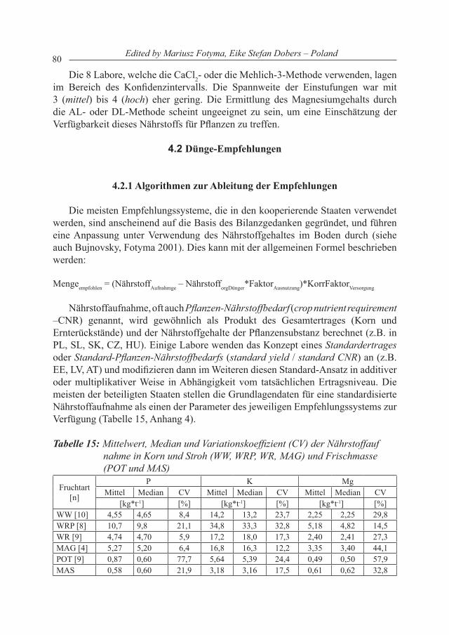
80 Edited by Mariusz Fotyma, Eike Stefan Dobers – Poland
Die 8 Labore, welche die CaCl2- oder die Mehlich-3-Methode verwenden, lagen im Bereich des Konfidenzintervalls. Die Spannweite der Einstufungen war mit 3 (mittel) bis 4 (hoch) eher gering. Die Ermittlung des Magnesiumgehalts durch die AL- oder DL-Methode scheint ungeeignet zu sein, um eine Einschätzung der Verfügbarkeit dieses Nährstoffs für Pflanzen zu treffen.
4.2 Dünge-Empfehlungen
4.2.1 Algorithmen zur Ableitung der Empfehlungen
Die meisten Empfehlungssysteme, die in den kooperierende Staaten verwendet werden, sind anscheinend auf die Basis des Bilanzgedanken gegründet, und führen eine Anpassung unter Verwendung des Nährstoffgehaltes im Boden durch (siehe auch Bujnovsky, Fotyma 2001). Dies kann mit der allgemeinen Formel beschrieben werden:
Mengeempfohlen = (NährstoffAufnahmge – NährstofforgDünger*FaktorAusnutzung)*KorrFaktorVersorgung
Nährstoffaufnahme, oft auch Pflanzen-Nährstoffbedarf (crop nutrient requirement –CNR) genannt, wird gewöhnlich als Produkt des Gesamtertrages (Korn und Ernterückstände) und der Nährstoffgehalte der Pflanzensubstanz berechnet (z.B. in PL, SL, SK, CZ, HU). Einige Labore wenden das Konzept eines Standardertrages oder Standard-Pflanzen-Nährstoffbedarfs (standard yield / standard CNR) an (z.B. EE, LV, AT) und modifizieren dann im Weiteren diesen Standard-Ansatz in additiver oder multiplikativer Weise in Abhängigkeit vom tatsächlichen Ertragsniveau. Die meisten der beteiligten Staaten stellen die Grundlagendaten für eine standardisierte Nährstoffaufnahme als einen der Parameter des jeweiligen Empfehlungssystems zur Verfügung (Tabelle 15, Anhang 4).
Tabelle 15: Mittelwert, Median und Variationskoeffizient (CV) der Nährstoffauf nahme in Korn und Stroh (WW, WRP, WR, MAG) und Frischmasse (POT und MAS)
Fruchtart[n]
P K MgMittel Median CV Mittel Median CV Mittel Median CV
[kg*t-1] [%] [kg*t-1] [%] [kg*t-1] [%]WW [10] 4,55 4,65 8,4 14,2 13,2 23,7 2,25 2,25 29,8WRP [8] 10,7 9,8 21,1 34,8 33,3 32,8 5,18 4,82 14,5WR [9] 4,74 4,70 5,9 17,2 18,0 17,3 2,40 2,41 27,3MAG [4] 5,27 5,20 6,4 16,8 16,3 12,2 3,35 3,40 44,1POT [9] 0,87 0,60 77,7 5,64 5,39 24,4 0,49 0,50 57,9MAS 0,58 0,60 21,9 3,18 3,16 17,5 0,61 0,62 32,8
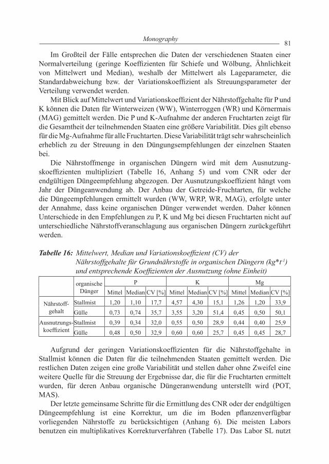
81Monography
Im Großteil der Fälle entsprechen die Daten der verschiedenen Staaten einer Normalverteilung (geringe Koeffizienten für Schiefe und Wölbung, Ähnlichkeit von Mittelwert und Median), weshalb der Mittelwert als Lageparameter, die Standardabweichung bzw. der Variationskoeffizient als Streuungsparameter der Verteilung verwendet werden.
Mit Blick auf Mittelwert und Variationskoeffizient der Nährstoffgehalte für P und K können die Daten für Winterweizen (WW), Winterroggen (WR) und Körnermais (MAG) gemittelt werden. Die P und K-Aufnahme der anderen Fruchtarten zeigt für die Gesamtheit der teilnehmenden Staaten eine größere Variabilität. Dies gilt ebenso für die Mg-Aufnahme für alle Fruchtarten. Diese Variabilität trägt sehr wahrscheinlich erheblich zu der Streuung in den Düngungsempfehlungen der einzelnen Staaten bei.
Die Nährstoffmenge in organischen Düngern wird mit dem Ausnutzung-skoeffizienten multipliziert (Tabelle 16, Anhang 5) und vom CNR oder der endgültigen Düngeempfehlung abgezogen. Der Ausnutzungskoeffizient hängt vom Jahr der Düngeanwendung ab. Der Anbau der Getreide-Fruchtarten, für welche die Düngeempfehlungen ermittelt wurden (WW, WRP, WR, MAG), erfolgte unter der Annahme, dass keine organischen Dünger verwendet werden. Daher können Unterschiede in den Empfehlungen zu P, K und Mg bei diesen Fruchtarten nicht auf unterschiedliche Nährstoffveranschlagung aus organischen Düngern zurückgeführt werden.
Tabelle 16: Mittelwert, Median und Variationskoeffizient (CV) der Nährstoffgehalte für Grundnährstoffe in organischen Düngern (kg*t-1) und entsprechende Koeffizienten der Ausnutzung (ohne Einheit)organische
DüngerP K Mg
Mittel Median CV [%] Mittel Median CV [%] Mittel Median CV [%]
Nährstoff-gehalt
Stallmist 1,20 1,10 17,7 4,57 4,30 15,1 1,26 1,20 33,9Gülle 0,73 0,74 35,7 3,55 3,20 51,4 0,45 0,50 50,1
Ausnutzungs-koeffizient
Stallmist 0,39 0,34 32,0 0,55 0,50 28,9 0,44 0,40 25,9Gülle 0,48 0,50 32,9 0,60 0,60 25,7 0,45 0,45 28,7
Aufgrund der geringen Variationskoeffizienten für die Nährstoffgehalte in Stallmist können die Daten für die teilnehmenden Staaten gemittelt werden. Die restlichen Daten zeigen eine große Variabilität und stellen daher ohne Zweifel eine weitere Quelle für die Streuung der Ergebnisse dar, die für die Fruchtarten ermittelt wurden, für deren Anbau organische Düngeranwendung unterstellt wird (POT, MAS).
Der letzte gemeinsame Schritte für die Ermittlung des CNR oder der endgültigen Düngeempfehlung ist eine Korrektur, um die im Boden pflanzenverfügbar vorliegenden Nährstoffe zu berücksichtigen (Anhang 6). Die meisten Labors benutzen ein multiplikatives Korrekturverfahren (Tabelle 17). Das Labor SL nutzt
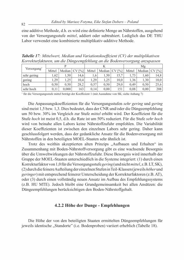
82 Edited by Mariusz Fotyma, Eike Stefan Dobers – Poland
eine additive Methode, d.h. es wird eine definierte Menge an Nährstoffen, ausgehend von der Versorgungsstufe mittel, addiert oder subtrahiert. Lediglich das DE THU Labor verwendet eine kombinierte multiplikativ-additive Methode.
Tabelle 17: Mittelwert, Median und Variationskoeffizient (CV) der multiplikativen Korrekturfakturen, um die Düngeempfehlung an die Bodenversorgung anzupassen
Versorgung1 P K MgMittel Median CV [%] Mittel Median CV [%] Mittel Median CV [%]
sehr gering 1,62 1,50 14,6 1,6 1,50 15,7 1,73 1,60 14,8gering 1,29 1,25 10,4 1,29 1,25 10,0 1,36 1,30 10,0hoch 0,50 0,50 28,2 0,57 0,50 29,0 0,49 0,50 25,6sehr hoch 0,11 0,000 163 0,14 0,00 151 0,08 0,00 208
1 für die Versorgungsstufe mittel beträgt der Koeffizient 1 (mit Ausnahme von SK; siehe Anhang 7)
Die Anpassungskoeffizienten für die Versorgungsstufen sehr gering und gering sind meist 1,5 bzw. 1,3. Dies bedeutet, dass der CNR und/oder die Düngeempfehlung um 50 bzw. 30% im Vergleich zur Stufe mittel erhöht wird. Der Koeffizient für die Stufe hoch ist meist 0,5, d.h. die Rate ist um 50% reduziert. Für die Stufe sehr hoch wird von beinahe allen Labors keine Nährstoffzufuhr empfohlen. Die Variabilität dieser Koeffizienten ist zwischen den einzelnen Labors sehr gering. Daher kann geschlussfolgert werden, dass der gedankliche Ansatz für die Bodenversorgung mit Nährstoffen in den beteiligten MOEL-Staaten sehr ähnlich ist.
Trotz des weithin akzeptierten alten Prinzips „Aufbauen und Erhalten“ im Zusammenhang mit Boden-Nährstoffversorgung gibt es eine wachsende Besorgnis über die Umweltwirkungen der Nährstoffzufuhr. Diese Besorgnis wird innerhalb der Gruppe der MOEL-Staaten unterschiedlich in die Systeme integriert: (1) durch einen Korrekturfaktor von 1,0 für die Versorgungsstufe gering (und nicht mittel, z.B. LT, SK), (2) durch die feinere Aufteilung der einzelnen Stufen in Teil-Klassen (jeweils höher und geringer) mit entsprechend feinerer Unterscheidung der Korrekturfaktoren (z.B. AT), oder (3) durch einen vollständig neuen Ansatz im Aufbau des Empfehlungssystems (z.B. HU MTE). Jedoch bleibt eine Grundgemeinsamkeit bei allen Ansätzen: die Düngeempfehlungen berücksichtigen den Boden-Nährstoffgehalt.
4.2.2 Höhe der Dunge - Empfehlungen
Die Höhe der von den beteiligten Staaten ermittelten Düngeempfehlungen für jeweils identische „Standorte” (i.e. Bodenproben) variiert erheblich (Tabelle 18).
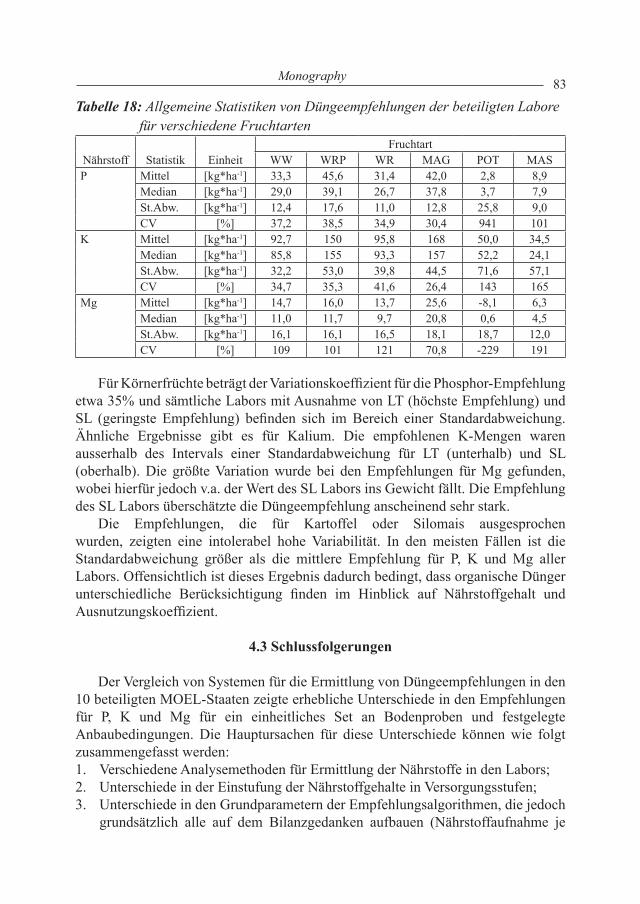
83Monography
Tabelle 18: Allgemeine Statistiken von Düngeempfehlungen der beteiligten Labore für verschiedene Fruchtarten
Nährstoff Statistik EinheitFruchtart
WW WRP WR MAG POT MASP Mittel [kg*ha-1] 33,3 45,6 31,4 42,0 2,8 8,9
Median [kg*ha-1] 29,0 39,1 26,7 37,8 3,7 7,9St.Abw. [kg*ha-1] 12,4 17,6 11,0 12,8 25,8 9,0CV [%] 37,2 38,5 34,9 30,4 941 101
K Mittel [kg*ha-1] 92,7 150 95,8 168 50,0 34,5Median [kg*ha-1] 85,8 155 93,3 157 52,2 24,1St.Abw. [kg*ha-1] 32,2 53,0 39,8 44,5 71,6 57,1CV [%] 34,7 35,3 41,6 26,4 143 165
Mg Mittel [kg*ha-1] 14,7 16,0 13,7 25,6 -8,1 6,3Median [kg*ha-1] 11,0 11,7 9,7 20,8 0,6 4,5St.Abw. [kg*ha-1] 16,1 16,1 16,5 18,1 18,7 12,0CV [%] 109 101 121 70,8 -229 191
Für Körnerfrüchte beträgt der Variationskoeffizient für die Phosphor-Empfehlung etwa 35% und sämtliche Labors mit Ausnahme von LT (höchste Empfehlung) und SL (geringste Empfehlung) befinden sich im Bereich einer Standardabweichung. Ähnliche Ergebnisse gibt es für Kalium. Die empfohlenen K-Mengen waren ausserhalb des Intervals einer Standardabweichung für LT (unterhalb) und SL (oberhalb). Die größte Variation wurde bei den Empfehlungen für Mg gefunden, wobei hierfür jedoch v.a. der Wert des SL Labors ins Gewicht fällt. Die Empfehlung des SL Labors überschätzte die Düngeempfehlung anscheinend sehr stark.
Die Empfehlungen, die für Kartoffel oder Silomais ausgesprochen wurden, zeigten eine intolerabel hohe Variabilität. In den meisten Fällen ist die Standardabweichung größer als die mittlere Empfehlung für P, K und Mg aller Labors. Offensichtlich ist dieses Ergebnis dadurch bedingt, dass organische Dünger unterschiedliche Berücksichtigung finden im Hinblick auf Nährstoffgehalt und Ausnutzungskoeffizient.
4.3 Schlussfolgerungen
Der Vergleich von Systemen für die Ermittlung von Düngeempfehlungen in den 10 beteiligten MOEL-Staaten zeigte erhebliche Unterschiede in den Empfehlungen für P, K und Mg für ein einheitliches Set an Bodenproben und festgelegte Anbaubedingungen. Die Hauptursachen für diese Unterschiede können wie folgt zusammengefasst werden:1. Verschiedene Analysemethoden für Ermittlung der Nährstoffe in den Labors;2. Unterschiede in der Einstufung der Nährstoffgehalte in Versorgungsstufen;3. Unterschiede in den Grundparametern der Empfehlungsalgorithmen, die jedoch
grundsätzlich alle auf dem Bilanzgedanken aufbauen (Nährstoffaufnahme je
84 Edited by Mariusz Fotyma, Eike Stefan Dobers – Poland
Tonne Erntegut, Nährstoffgehalte in den organischen Düngern, Ausnutzung-skoeffizienten für Nährstoffe aus organischen Düngern);
Als wichtiges Ergebnis dieser Studie muss weiterhin hervorgehoben werden, dass die meisten der Empfehlungssysteme viele gemeinsame Aspekte in den Ansätzen und Algorithmen haben. Dies bietet die Möglichkeit für eine zumindest teilweise Harmonisierung und Vereinheitlichung der Systeme für die Düngeempfehlungen in den MOEL-Staaten. Der nächste Schritt auf dem Weg zu einem solchen vereinheitlichten System muss die Konzentration auf die Versorgungsstufe mittel sein, und eine Analyse weiterer Bodenproben und Ermittlung von Düngeempfehlungen für diese Klasse.
85Monography
5. Literatur
BMLFUW 2006. Richtlinien für die sachgerechte Düngung. 6. Auflage. Fachbeirat für Bodenfruchtbarkeit und Bodenschutz. Bundesministerium für Land- und Forstwirtschaft, Umwelt- und Wasserwirtschaft, Wien.
Boguszewska, M., Fotyma, E., Fotyma, M. 2001. The possibility of using the Egner-DL extract for estimating the content of available magnesium in Polish soils (in Polish). Zeszyty Problemowe Postępów Nauk Rolniczych. 480:377-383.
Bujnovsky, R., Fotyma, M. 2001. Fertilizer recommendation schemes officially used in Czech Republic, Latvia, Poland, Slovak Republic and the United Kingdom. Nawozy i Nawożenie – Fertilizers and Fertilization. ed. Fotyma, M., Shepherd, A. Sustainable nutrient management. MAINTAIN Report 2. 1:5-31.
Fotyma, M., Mercik, S. Chemia Rolna, PWN, WarszawaFotyma, M., Shepherd, M. (eds.). 2000. Soil fertility evaluation in the Czech
Republic, Latvia, Poland, Slovak Republic and the United Kingdom. Nawozy i nawożenie – Fertilizers and Fertilization. 2(3) : pp. 66.
Karklins, A. 2001. Model for the calculation of nutrient offtake by crop : OFFTAKE model . Nawozy i Nawożenie – Fertilizers and Fertilization ed. Fotyma, M., Shepherd, A. Sustainable nutrient management. MAINTAIN Report 2. 1:63-74.
Kerschberger, M., Franke, G., Hess, H. 1997. Anleitung und Richtwerte für Nährstoffvergleiche nach Düngeverordnung. Jena.
Klir, J., Cermak, P. 2001. Standard figures for manure composition and N-manure equivalents. Nawozy i Nawożenie – Fertilizers and Fertilization ed. Fotyma, M., Shepherd, A. Sustainable nutrient management. MAINTAIN Report 2. 1:32-39.
Ristimaki, L. M. 2007. Potassium and magnesium fertilizer recommendations in some European countries. IFS Proceedings 620:31
Spiegel, H., Baumgarten, A., Dersch, G. 2006. Revised form of the “Austrian Guidelines for appropriate fertilisation” and the influence of “Cross Compliance” and its national implementation. Acta agriculturae Slovenica, 87-1, 93-107.
Zbiral, J. 2000. Determination of phosphoprus in calcareous soils by Mehlich-3, Mehlich-2, CAL and Egner extractants. Commun. Soil. Sci. Plant Anal. 31:3037-3048.
Zbiral, J., Nemec, P. 2000. Integrating of the Mehlich-3 extractant into the Czech soil testing scheme. Commun. Soil. Sci. Plant Anal. 31:2171-2182.
Ziadi, N., Sen Tran, T. 2008. Mehlich – 3 extractable elements. in. Soil sampling and methods of analysis. ed. Carter, M. R., Gregorich, E. G. Canadian Society of Soil Science
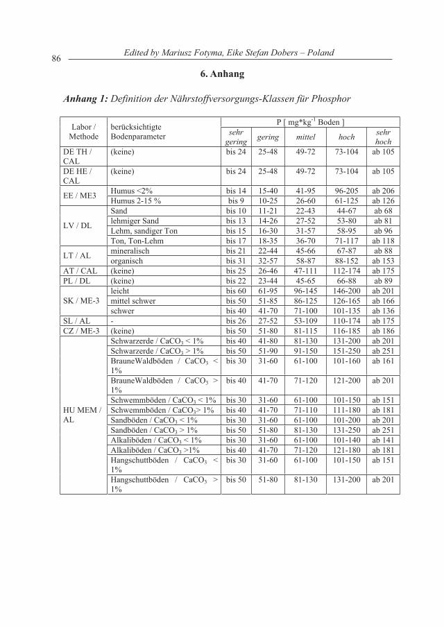
86 Edited by Mariusz Fotyma, Eike Stefan Dobers – Poland
6. Anhang
Anhang 1: Definition der Nährstoffversorgungs-Klassen für Phosphor
P [ mg*kg-1 Boden ] Labor / Methode
berücksichtigte Bodenparameter sehr
gering gering mittel hoch sehrhoch
DE TH / CAL
(keine) bis 24 25-48 49-72 73-104 ab 105
DE HE / CAL
(keine) bis 24 25-48 49-72 73-104 ab 105
Humus <2% bis 14 15-40 41-95 96-205 ab 206 EE / ME3 Humus 2-15 % bis 9 10-25 26-60 61-125 ab 126 Sand bis 10 11-21 22-43 44-67 ab 68 lehmiger Sand bis 13 14-26 27-52 53-80 ab 81 Lehm, sandiger Ton bis 15 16-30 31-57 58-95 ab 96 LV / DL
Ton, Ton-Lehm bis 17 18-35 36-70 71-117 ab 118mineralisch bis 21 22-44 45-66 67-87 ab 88 LT / AL organisch bis 31 32-57 58-87 88-152 ab 153
AT / CAL (keine) bis 25 26-46 47-111 112-174 ab 175 PL / DL (keine) bis 22 23-44 45-65 66-88 ab 89
leicht bis 60 61-95 96-145 146-200 ab 201 mittel schwer bis 50 51-85 86-125 126-165 ab 166 SK / ME-3 schwer bis 40 41-70 71-100 101-135 ab 136
SL / AL - bis 26 27-52 53-109 110-174 ab 175 CZ / ME-3 (keine) bis 50 51-80 81-115 116-185 ab 186
Schwarzerde / CaCO3 < 1% bis 40 41-80 81-130 131-200 ab 201 Schwarzerde / CaCO3 > 1% bis 50 51-90 91-150 151-250 ab 251 BrauneWaldböden / CaCO3 < 1%
bis 30 31-60 61-100 101-160 ab 161
BrauneWaldböden / CaCO3 > 1%
bis 40 41-70 71-120 121-200 ab 201
Schwemmböden / CaCO3 < 1% bis 30 31-60 61-100 101-150 ab 151 Schwemmböden / CaCO3> 1% bis 40 41-70 71-110 111-180 ab 181 Sandböden / CaCO3 < 1% bis 30 31-60 61-100 101-200 ab 201 Sandböden / CaCO3 > 1% bis 50 51-80 81-130 131-250 ab 251 Alkaliböden / CaCO3 < 1% bis 30 31-60 61-100 101-140 ab 141 Alkaliböden / CaCO3 >1% bis 40 41-70 71-120 121-180 ab 181 Hangschuttböden / CaCO3 < 1%
bis 30 31-60 61-100 101-150 ab 151
HU MEM / AL
Hangschuttböden / CaCO3 > 1%
bis 50 51-80 81-130 131-200 ab 201
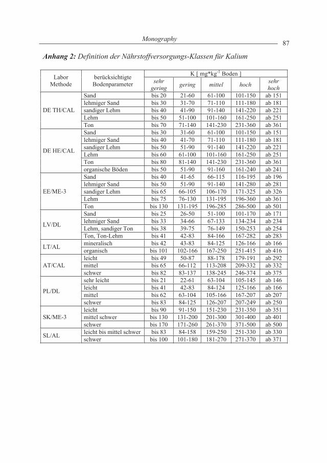
87Monography
Anhang 2: Definition der Nährstoffversorgungs-Klassen für Kalium
K [ mg*kg-1 Boden ] LaborMethode
berücksichtigte Bodenparameter sehr
gering gering mittel hoch sehrhoch
Sand bis 20 21-60 61-100 101-150 ab 151 lehmiger Sand bis 30 31-70 71-110 111-180 ab 181 sandiger Lehm bis 40 41-90 91-140 141-220 ab 221 Lehm bis 50 51-100 101-160 161-250 ab 251
DE TH/CAL
Ton bis 70 71-140 141-230 231-360 ab 361 Sand bis 30 31-60 61-100 101-150 ab 151 lehmiger Sand bis 40 41-70 71-110 111-180 ab 181 sandiger Lehm bis 50 51-90 91-140 141-220 ab 221 Lehm bis 60 61-100 101-160 161-250 ab 251 Ton bis 80 81-140 141-230 231-360 ab 361
DE HE/CAL
organische Böden bis 50 51-90 91-160 161-240 ab 241 Sand bis 40 41-65 66-115 116-195 ab 196 lehmiger Sand bis 50 51-90 91-140 141-280 ab 281 sandiger Lehm bis 65 66-105 106-170 171-325 ab 326 Lehm bis 75 76-130 131-195 196-360 ab 361
EE/ME-3
Ton bis 130 131-195 196-285 286-500 ab 501 Sand bis 25 26-50 51-100 101-170 ab 171 lehmiger Sand bis 33 34-66 67-133 134-234 ab 234 Lehm, sandiger Ton bis 38 39-75 76-149 150-253 ab 254 LV/DL
Ton, Ton-Lehm bis 41 42-83 84-166 167-282 ab 283 mineralisch bis 42 43-83 84-125 126-166 ab 166 LT/AL organisch bis 101 102-166 167-250 251-415 ab 416 leicht bis 49 50-87 88-178 179-191 ab 292 mittel bis 65 66-112 113-208 209-332 ab 332 AT/CALschwer bis 82 83-137 138-245 246-374 ab 375 sehr leicht bis 21 22-61 63-104 105-145 ab 146 leicht bis 41 42-83 84-124 125-166 ab 166 mittel bis 62 63-104 105-166 167-207 ab 207 PL/DL
schwer bis 83 84-125 126-207 207-249 ab 250 leicht bis 90 91-150 151-230 231-350 ab 351 mittel schwer bis 130 131-200 201-300 301-400 ab 401 SK/ME-3 schwer bis 170 171-260 261-370 371-500 ab 500 leicht bis mittel schwer bis 83 84-158 159-250 251-330 ab 330 SL/AL schwer bis 100 101-180 181-270 271-370 ab 371
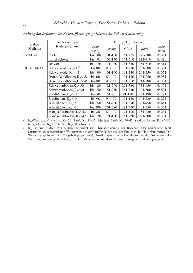
88 Edited by Mariusz Fotyma, Eike Stefan Dobers – Poland
Anhang 2a: Definition der Nährstoffversorgungs-Klassen für Kalium (Fortsetzung)
K [ mg*kg-1 Boden ] LaborMethode
berücksichtigte Bodenparameter sehr
gering gering mittel hoch sehrhoch
leicht bis 100 101-160 161-275 276-380 ab 381 mittel schwer bis 105 106-170 171-310 311-410 ab 420
CZ/ME-3
schwer bis 170 171-260 261-350 351-510 ab 511 Schwarzerde, KA<42* bis 80 81-130 131-200 201-300 ab 301 Schwarzerde, KA>42 bis 100 101-160 161-240 241-350 ab 351 BrauneWaldböden,KA<38 bis 60 61-100 101-160 161-250 ab 251 BrauneWaldböden,KA>38 bis 90 91-140 141-210 211-300 ab 301 Schwemmböden,KA<50 bis 120 121-200 201-330 331-450 ab 451 Schwemmböden,KA>50 bis 150 151-250 251-380 381-500 ab 501 Sandböden, KA<30 bis 50 51-80 81-120 121-180 ab 181 Sandböden, KA>30 bis 90 91-120 121-160 161-220 ab 221 Alkaliböden, KA<50 bis 150 151-230 231-330 331-450 ab 451 Alkaliböden, KA>50 bis 200 201-280 281-400 401-550 ab 551 Hangschuttböden, KA<42 bis 80 81-120 121-180 181-250 ab 251
HU MEM/AL
Hangschuttböden, KA>42 bis 120 121-160 161-220 221-300 ab 301 KA-Wert gemäß Arany : KA<30: Sand, KA 31–37: lehmiger Sand, KA 38–42: sandiger Lehm, KA 43–50: toniger Lehm, KA 51–60: Ton, KA>60: schwerer Ton KA ist eine einfach bestimmbare Kennzahl zur Charakterisierung der Bodenart. Der numerische Wert entspricht der aufnehmbaren Wassermenge in cm3*100-1g Boden bis zum Erreichen der Plastizitätsgrenze. Die Wassermenge ist mit dem Tongehalt proportional, obwohl keine strenge Korrelation besteht. Der numerische Wert steigt mit steigendem Tongehalt der Böden und ist somit zur Kennzeichnung der Bodenart geeignet.
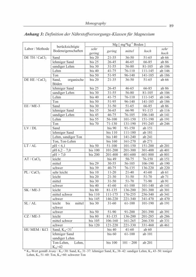
89Monography
Anhang 3: Definition der Nährstoffversorgungs-Klassen für Magnesium
Mg [ mg*kg-1 Boden ] Labor / Methode berücksichtigte
Bodeneigenschaften sehrgering gering mittel hoch sehr
hochSand bis 20 21-35 36-50 51-65 ab 66 lehmiger Sand bis 25 26-45 46-65 66-85 ab 86 sandiger Lehm bis 30 31-55 56-80 81-105 ab 106 Lehm bis 40 41-75 76-110 111-145 ab 146
DE TH / CaCl2
Ton bis 50 51-95 96-140 141-185 ab 186 Sand, organische Böden
bis 20 21-35 36-50 51-65 ab 66
lehmiger Sand bis 25 26-45 46-65 66-85 ab 86 sandiger Lehm bis 30 31-55 56-80 81-105 ab 106 Lehm bis 40 41-75 76-110 111-145 ab 146
DE HE / CaCl2
Ton bis 50 51-95 96-140 141-185 ab 186 Sand bis 30 31-50 51-65 66-85 ab 86 lehmiger Sand bis 35 36-65 66-90 91-115 ab 116 sandiger Lehm bis 45 46-75 76-105 106-140 ab 141 Lehm bis 55 56-100 101-150 151-190 ab 191
EE / ME-3
Ton bis 70 71-130 131-190 191-245 ab 246 Sand bis 90 91-150 ab 151 lehmiger Sand bis 110 111-180 ab 181 Lehm, sandiger Ton bis 140 141-240 ab 241
LV / DL
Ton, Ton-Lehm bis 160 161-270 ab 271 pH < 6,1 bis 50 51-100 101-150 151-200 ab 201 pH 6,2 – 7,0 bis 100 101-200 201-300 301-400 ab 401
LT / AL
pH > 7,0 bis 200 201-400 401-600 601-800 ab 801 leicht bis 49 50-75 76-150 ab 151 mittel bis 29 30-55 56-105 106-190 ab 190
AT / CaCl2
schwer bis 39 40-75 76-135 136-220 ab 220 sehr leicht bis 10 11-20 21-40 41-60 ab 61 leicht bis 20 21-30 31-50 51-70 ab 71 mittel bis 30 31-50 51-70 71-90 ab 91
PL / CaCl2
schwer bis 40 41-60 61-100 101-140 ab 141 leicht bis 80 81-135 136-200 201-300 ab 301 mittel schwer bis 110 111-175 176-255 256-340 ab 341
SK / ME-3
schwer bis 145 146-220 221-340 341-470 ab 470 leicht bis mittel schwer
bis 30 31-60 61-100 101-190 ab 191 SL / AL
schwer bis 50 51-90 91-200 201-390 ab 391 leicht bis 80 81-135 136-200 201-285 ab 286 mittel schwer bis 105 106-160 161-265 266-330 ab 331
CZ / ME-3
schwer bis 120 121-220 221-330 331-460 ab 461 Sand, KA<31* bis 40 41-60 ab 60 lehmiger Sand sandiger Lehm
bis 60 61-100 ab 101 HU MEM / KCl
Ton-Lehm, Lehm, KA>42
bis 100 101 – 200 ab 201
* KA-Wert gemäß Arany : KA<30: Sand, KA 31–37: lehmiger Sand, KA 38–42: sandiger Lehm, KA 43–50: toniger Lehm, KA 51–60: Ton, KA>60: schwerer Ton
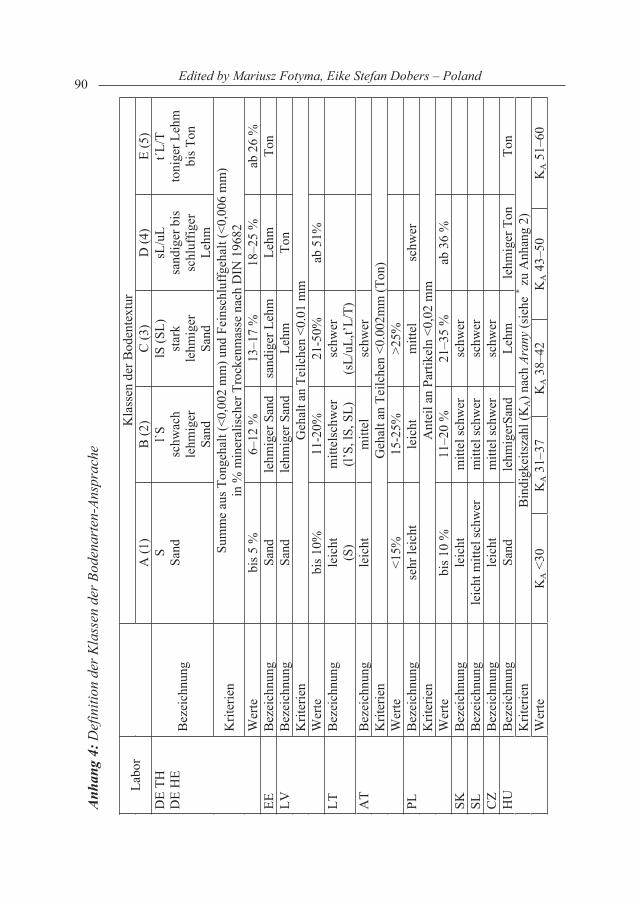
90 Edited by Mariusz Fotyma, Eike Stefan Dobers – PolandA
nhan
g 4:
Def
initi
on d
er K
lass
en d
er B
oden
arte
n-An
spra
che
Kla
ssen
der
Bod
ente
xtur
La
bor
A (1
) B
(2)
C (3
) D
(4)
E (5
)
Bez
eich
nung
SSa
ndl`S
schw
ach
lehm
iger
Sa
nd
lS (S
L)
star
kle
hmig
er
Sand
sL/u
Lsa
ndig
er b
is
schl
uffig
er
Lehm
t´L/T
to
nige
r Leh
m
bis T
on
Krit
erie
n Su
mm
e au
s Ton
geha
lt (<
0,00
2 m
m) u
nd F
eins
chlu
ffge
halt
(<0,
006
mm
) in
% m
iner
alis
cher
Tro
cken
mas
se n
ach
DIN
196
82
DE
TH
DE
HE
Wer
tebi
s 5 %
6–
12 %
13
–17
%
18–2
5 %
ab
26
%
EEB
ezei
chnu
ngSa
ndle
hmig
er S
and
sand
iger
Leh
m
Lehm
To
nB
ezei
chnu
ngSa
ndle
hmig
erSa
nd
Lehm
To
nK
riter
ien
Geh
alt a
n Te
ilche
n <0
.01
mm
LV
Wer
te
bis 1
0%
11-2
0%
21-5
0%
ab 5
1%
LTB
ezei
chnu
ngle
icht
(S)
mitt
elsc
hwer
(l’S,
lS, S
L)
schw
er(s
L/uL
,t’L/
T)
Bez
eich
nung
leic
htm
ittel
schw
erK
riter
ien
Geh
alt a
n Te
ilche
n <0
.002
mm
(Ton
) A
T
Wer
te
<15%
15
-25%
>2
5%
Bez
eich
nung
sehr
leic
htle
icht
mitt
elsc
hwer
Krit
erie
n A
ntei
l an
Parti
keln
<0,
02 m
m
PL
Wer
tebi
s 10
%
11–2
0 %
21
–35
%
ab 3
6 %
SK
Bez
eich
nung
leic
htm
ittel
schw
er
schw
erSL
Bez
eich
nung
leic
ht m
ittel
schw
er
mitt
el sc
hwer
sc
hwer
CZ
Bez
eich
nung
leic
htm
ittel
schw
er
schw
erB
ezei
chnu
ngSa
ndle
hmig
erSa
ndLe
hm
lehm
iger
Ton
To
nK
riter
ien
Bin
digk
eits
zahl
(KA) n
ach
Aran
y (s
iehe
* zu
Anh
ang
2)
HU
Wer
teK
A <
30
KA 3
1–37
K
A 3
8–42
K
A 4
3–50
K
A 5
1–60
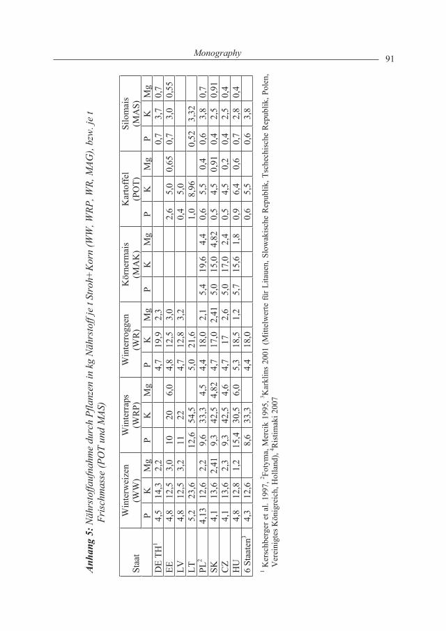
91Monography
Anh
ang
4: D
efin
ition
der
Kla
ssen
der
Bod
enar
ten-
Ansp
rach
e
Kla
ssen
der
Bod
ente
xtur
La
bor
A (1
) B
(2)
C (3
) D
(4)
E (5
)
Bez
eich
nung
SSa
ndl`S
schw
ach
lehm
iger
Sa
nd
lS (S
L)
star
kle
hmig
er
Sand
sL/u
Lsa
ndig
er b
is
schl
uffig
er
Lehm
t´L/T
to
nige
r Leh
m
bis T
on
Krit
erie
n Su
mm
e au
s Ton
geha
lt (<
0,00
2 m
m) u
nd F
eins
chlu
ffge
halt
(<0,
006
mm
) in
% m
iner
alis
cher
Tro
cken
mas
se n
ach
DIN
196
82
DE
TH
DE
HE
Wer
tebi
s 5 %
6–
12 %
13
–17
%
18–2
5 %
ab
26
%
EEB
ezei
chnu
ngSa
ndle
hmig
er S
and
sand
iger
Leh
m
Lehm
To
nB
ezei
chnu
ngSa
ndle
hmig
erSa
nd
Lehm
To
nK
riter
ien
Geh
alt a
n Te
ilche
n <0
.01
mm
LV
Wer
te
bis 1
0%
11-2
0%
21-5
0%
ab 5
1%
LTB
ezei
chnu
ngle
icht
(S)
mitt
elsc
hwer
(l’S,
lS, S
L)
schw
er(s
L/uL
,t’L/
T)
Bez
eich
nung
leic
htm
ittel
schw
erK
riter
ien
Geh
alt a
n Te
ilche
n <0
.002
mm
(Ton
) A
T
Wer
te
<15%
15
-25%
>2
5%
Bez
eich
nung
sehr
leic
htle
icht
mitt
elsc
hwer
Krit
erie
n A
ntei
l an
Parti
keln
<0,
02 m
m
PL
Wer
tebi
s 10
%
11–2
0 %
21
–35
%
ab 3
6 %
SK
Bez
eich
nung
leic
htm
ittel
schw
er
schw
erSL
Bez
eich
nung
leic
ht m
ittel
schw
er
mitt
el sc
hwer
sc
hwer
CZ
Bez
eich
nung
leic
htm
ittel
schw
er
schw
erB
ezei
chnu
ngSa
ndle
hmig
erSa
ndLe
hm
lehm
iger
Ton
To
nK
riter
ien
Bin
digk
eits
zahl
(KA) n
ach
Aran
y (s
iehe
* zu
Anh
ang
2)
HU
Wer
teK
A <
30
KA 3
1–37
K
A 3
8–42
K
A 4
3–50
K
A 5
1–60
Anh
ang
5: N
ährs
toffa
ufna
hme
durc
h Pf
lanz
en in
kg
Näh
rsto
ff je
t St
roh+
Kor
n (W
W, W
RP, W
R, M
AG),
bzw
. je
t Fr
isch
mas
se (P
OT
und
MAS
)
Win
terw
eize
n (W
W)
Win
terr
aps
(WR
P)
Win
terr
ogge
n (W
R)
Kör
nerm
ais
(MA
K)
Kar
toff
el
(PO
T)
Silo
mai
s (M
AS)
St
aat
PK
Mg
PK
Mg
PK
Mg
PK
Mg
PK
Mg
PK
Mg
DE
TH1
4,5
14,3
2,
2 4,
7 19
,92,
3 0,
7 3,
7 0,
7 EE
4,8
12,5
3,
0 10
206,
0 4,
8 12
,53,
0 2,
6 5,
0 0,
650,
7 3,
0 0,
55
LV4,
8 12
,5
3,2
1122
4,7
12,8
3,2
0,4
5,0
LT5,
2 23
,6
12,6
54
,5
5,0
21,6
1,0
8,96
0,
523,
32PL
24,
13
12,6
2,
2 9,
6 33
,3
4,5
4,4
18,0
2,1
5,4
19,6
4,4
0,6
5,5
0,4
0,6
3,8
0,7
SK4,
1 13
,6
2,41
9,
3 42
,5
4,82
4,7
17,0
2,41
5,0
15,0
4,82
0,5
4,5
0,91
0,4
2,5
0,91
C
Z 4,
1 13
,6
2,3
9,3
42,5
4,
6 4,
7 17
2,6
5,0
17,0
2,4
0,5
4,5
0,2
0,4
2,5
0,4
HU
4,8
12,8
1,
2 15
,4
30,5
6,
0 5,
3 18
,51,
2 5,
7 15
,61,
8 0,
9 6,
4 0,
6 0,
7 2,
8 0,
4 6
Staa
ten3
4,3
12,6
8,
6 33
,3
4,4
18,0
0,6
5,5
0,6
3,8
1 Ker
schb
erge
r et a
l. 19
97, 2 Fo
tym
a, M
erci
k 19
95, 3 K
arkl
ins
2001
(Mitt
elw
erte
für L
itaue
n, S
low
akis
che
Rep
ublik
, Tsc
hech
isch
e R
epub
lik, P
olen
, V
erei
nigt
es K
önig
reic
h, H
olla
nd),
4 Ris
timak
i 200
7
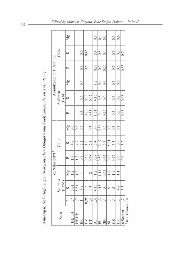
92 Edited by Mariusz Fotyma, Eike Stefan Dobers – Poland
Anh
ang
6: N
ährs
toffm
enge
n in
org
anis
chen
Dün
gern
und
Koe
ffizi
ente
n de
ren
Ausn
utzu
ng
kg N
ährs
toff
*t-1
Aus
nutz
ung
im 1
. Jah
r [%
] St
allm
ist
(FY
M)
Gül
le
Stal
lmis
t (F
YM
) G
ülle
St
aat
PK
Mg
PK
Mg
PK
Mg
PK
Mg
DE
TH
1,7
5,81
1,
2 1,
3 4,
9 0,
6 D
E H
E 1,
7 5,
81
1,2
1,3
4,9
0,6
EE1
3,9
10,
9 2,
2 0,
5 0,
3 0,
5 0,
4 0,
3 0,
6 LV
0,95
3,
5 0,
52
1,8
0,26
0,
38
0,5
0,45
LT
1,4
4,3
20,
68
2,1
0,3
0,35
0,
42
AT
1,31
4,
15
1,2
0,87
5,
4 0,
9 1,
31
4,15
1,
2 0,
87
5,4
0,9
PL1,
3 4,
15
1,14
0,
52
2,49
0,
36
0,4
0,8
0,4
0,7
0,8
0,4
SK1,
1 5
0,63
0,
74
5,3
0,5
0,25
0,
4 0,
3 0,
25
0,4
0,3
SL1,
1 5
1,2
0,83
5,
81
0,3
CZ
1,1
51,
9 0,
74
5,3
0,5
0,5
0,5
0,5
0,5
0,5
0,5
HU
1,1
4,2
1,1
0,3
0,6
0,1
0,6
0,7
0,6
0,6
0,7
0,6
6 St
aate
n11,
2 5,
3 0,
6 3,
2 0,
48
0,68
0,
55
0,74
1 K
lir, C
erm
ak 2
001
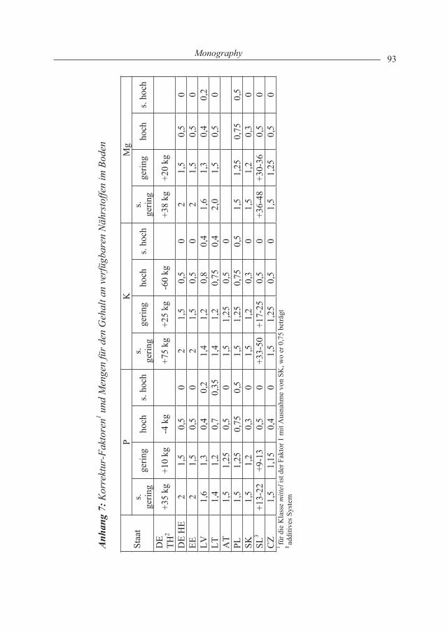
93Monography
Anh
ang
6: N
ährs
toffm
enge
n in
org
anis
chen
Dün
gern
und
Koe
ffizi
ente
n de
ren
Ausn
utzu
ng
kg N
ährs
toff
*t-1
Aus
nutz
ung
im 1
. Jah
r [%
] St
allm
ist
(FY
M)
Gül
le
Stal
lmis
t (F
YM
) G
ülle
St
aat
PK
Mg
PK
Mg
PK
Mg
PK
Mg
DE
TH
1,7
5,81
1,
2 1,
3 4,
9 0,
6 D
E H
E 1,
7 5,
81
1,2
1,3
4,9
0,6
EE1
3,9
10,
9 2,
2 0,
5 0,
3 0,
5 0,
4 0,
3 0,
6 LV
0,95
3,
5 0,
52
1,8
0,26
0,
38
0,5
0,45
LT
1,4
4,3
20,
68
2,1
0,3
0,35
0,
42
AT
1,31
4,
15
1,2
0,87
5,
4 0,
9 1,
31
4,15
1,
2 0,
87
5,4
0,9
PL1,
3 4,
15
1,14
0,
52
2,49
0,
36
0,4
0,8
0,4
0,7
0,8
0,4
SK1,
1 5
0,63
0,
74
5,3
0,5
0,25
0,
4 0,
3 0,
25
0,4
0,3
SL1,
1 5
1,2
0,83
5,
81
0,3
CZ
1,1
51,
9 0,
74
5,3
0,5
0,5
0,5
0,5
0,5
0,5
0,5
HU
1,1
4,2
1,1
0,3
0,6
0,1
0,6
0,7
0,6
0,6
0,7
0,6
6 St
aate
n11,
2 5,
3 0,
6 3,
2 0,
48
0,68
0,
55
0,74
1 K
lir, C
erm
ak 2
001
Anh
ang
7: K
orre
ktur
-Fak
tore
n1 und
Men
gen
für d
en G
ehal
t an
verf
ügba
ren
Näh
rsto
ffen
im B
oden
PK
Mg
Staa
ts.
gerin
g ge
ring
hoch
s.
hoch
s.
gerin
g ge
ring
hoch
s.
hoch
s.
gerin
g ge
ring
hoch
s.
hoch
DE
TH2
+35
kg
+10
kg
-4 k
g +7
5 kg
+2
5 kg
-6
0 kg
+3
8 kg
+2
0 kg
DE
HE
21,
5 0,
5 0
21,
5 0,
5 0
21,
5 0,
5 0
EE2
1,5
0,5
02
1,5
0,5
02
1,5
0,5
0LV
1,6
1,3
0,4
0,2
1,4
1,2
0,8
0,4
1,6
1,3
0,4
0,2
LT1,
4 1,
2 0,
7 0,
35
1,4
1,2
0,75
0,
4 2,
0 1,
5 0,
5 0
AT
1,5
1,25
0,
5 0
1,5
1,25
0,
5 0
PL1,
5 1,
25
0,75
0,
5 1,
5 1,
25
0,75
0,
5 1,
5 1,
25
0,75
0,
5 SK
1,5
1,2
0,3
01,
5 1,
2 0,
3 0
1,5
1,2
0,3
0SL
3+1
3-22
+9
-13
0,5
0+3
3-50
+17-
250,
5 0
+36-
48
+30-
36
0,5
0C
Z 1,
5 1,
15
0,4
01,
5 1,
25
0,5
01,
5 1,
25
0,5
01fü
r die
Kla
sse
mitt
el is
t der
Fak
tor 1
mit
Aus
nahm
e vo
n SK
, wo
er 0
,75
beträ
gt
2ad
ditiv
es S
yste
m
94 Edited by Mariusz Fotyma, Eike Stefan Dobers – Poland
1. Supplement
Comparison of aerometric and laser diffraction methods for soil texture analysis
Dorota Pikuła1, Przemysław Tkaczyk2
1Institute of Soil Science and Plant Cultivation – State Research Institute, Puławy, Poland
2Agrochemical Laboratory, Lublin, Poland
Introduction
In course of the 9th meeting of the MOEL group (MOEL working group of agrochemical services in Central-Eastern Europe – Arbeitsgruppe der agrochemischer Untersuchunsdienste der mittel- und osteuropeischen Lander) in 2006 at Piran – Slovenia, it has been decided to organize the inter-laboratory exchange of soil samples with the following fertilizer recommendations between 10 collaborating countries. Final report from the project is presented in the main paper in this issue of the journal. The results of soil analysis, calibration schemes and final fertilizer recommendations differ substantially between the collaborating countries. Analysis of date reveals that one main reason for these differences lies in the approach to soil texture estimation and classification. In Germany, Estonia and Hungary 5 classes of soil texture is recognised, in Lithuania and Poland 4 classes and in the remaining countries 3 classes system of soil texture classification is in force. Besides the number of textural classes the criteria for their isolation differs as well. In Germany and Estonia the % of clay ( particles < 0,002 mm), in Poland the % of so called decantable particles (<0,02 mm) and in Hungary Arany value (the amount of water necessary to bring the soil to plasticity) make the base for soil distribution among textural classes.
However, in spite of these differences in soil texture classification it seems that calibration systems in collaborating countries meet more or less closely at the medium content of nutrient. It makes a good starting point for further work on more harmonized system of fertilizer recommendations. Therefore on the 10th MOEL group meeting in 2007 at Visegrad, Hungary it has been decided to arrange the second tour of common research on soil testing and fertilizer recommendations in collaborating countries. Each country has agreed upon collecting 3 soils samples differing in texture (light, medium and heavy ones) but showing the medium content of available nutrients (P,K,Mg). The samples were distributed among other countries
95Monography
with the task to perform the soils analysis for available nutrients and to calculate the optimal P,K,Mg rates according to the system of recommendation officially used in the country. Unfortunately the suggestion of Poland to analyze the samples for granulometric composition ( texture) as well was not accepted and only our country went this way.
Soil texture is the characteristic composition of different shares of particle sizes of the solid soils sample, summing up to 100 %. It is one of the basic characteristics of soil physical and chemical properties. At the beginning of the last century Atterberg [1916] proposed the soil classification according to the share of different soil particles. However soils are very heterogeneous in granulometric composition and the results of analysis depends substantially on the used methods. At present more then 400 methods of estimation this soil feature are known and many of them employed by several laboratories [Loveland, Whalley 2001]. The most commonly used are the pipette and aerometric methods. In Poland the last mentioned method is officially used according to Cassagrande in modification of Prószyński [1996 ]. All 17 agrochemical laboratories in Poland dealing with soils sampling and fertilizers recommendations are using this method for random control of soil texture, otherwise estimated on the spot by “finger” method. The essence of aerometric method is to measure the time of sedimentation the soil particles in the water suspension. In the calculation of the share of particles of different size the principles of Stokes , assuming the spherical shape of soil particles, is recognized. Due to the considerable deviations of soil suspension from Stokes’s principle the results of aerometric analysis are burdened with unpredictable errors.
Lately the new method of soil particles distribution, based on laser diffraction procedure, has been introduced to the pedological researches [Beuselinck et al, 1998, Ryżak i in., 2004 ]. In 2006 all 17 agrochemical laboratories on Poland have been provided with laser diffraction instruments and started the procedures of adapting this method for routine soil analysis. The aim of researches presented in this paper was to compare the aerometric and laser diffraction method of estimation the soil granulometric composition using the soil samples collected by laboratories from collaborating MOEL countries.
1.1 Methods
Altogether 36 soil samples from different countries (3 samples per country), including Poland have been analyzed for the granulometric composition using aerometric methods acc. to Cassagrande in modification of Prószyński [1966] and by means of laser diffraction analyzer Mastersizer 2000 equipped with the HYDRO 2000 G device. This instrument is able to measure the soil particle distribution in the range 0- 2000um after suspending the soil samples in water. In the calculations the coefficient of light deflection equal to 1,330 and the cooefficient of light absorption
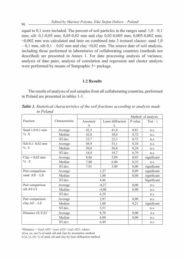
96 Edited by Mariusz Fotyma, Eike Stefan Dobers – Poland
equal to 0,1 were included. The percent of soil particles in the ranges sand: 1,0 – 0,1 mm; silt: 0,1-0,05 mm; 0,05-0,02 mm and clay 0,02-0,005 mm; 0,005-0,002 mm; <0,002 mm was calculated and later on combined into 3 textural classes: sand 1,0 – 0,1 mm, silt 0,1 – 0,02 mm and clay <0,02 mm. The source date of soil analysis, including those performed in laboratories of collaborating countries (methods not described) are presented in Annex 1. For date processing analysis of variance, analysis of date pairs, analysis of correlation and regression and cluster analysis were performed by means of Statgraphic 5+ package.
1.2 Results
The results of analysis of soil samples from all collaborating countries, performed in Poland are presented in tables 1-3.
Table 1. Statistical characteristics of the soil fractions according to analysis made in Poland
Fraction Characteristic Method of analysisAreometr
ALaser diffraction
L P value Test – t
Sand 1,0-0,1 mm% X
Average 42,3 41,0 0,81 n.s. Median 42,0 38,0 0,72 n.s.ST.dev. 23,7 22,3 0,72 n.s.
Silt 0,1- 0,02 mm% Y
Average 48,9 53,1 0,34 n.s.Median 50,0 56,0 0,24 n.s.ST.dev. 18,9 19,7 0,79 n.s.
Clay < 0,02 mm% Z
Average 8,86 5,89 0,03 significant Median 7,00 6,00 0,35 n.s.ST.dev. 7,91 3,00 0,00 significant
Pair comparison sand AX – LX
Average 1,27 0,09 significantMedian 1,00 0,08 significantST.dev. 4,46 Significant
Pair comparison silt AY-LY
Average -4,27 0,00 n.s.Median -4,00 0,00 n.s.ST.dev. 6,29 n.s.
Pair comparison clay AZ – LZ
Average 2,97 0,00 n.s.Median 1,00 0,21 significantST.dev. 5,51 n.s.
Distance (X,Y,Z)* Average 8,70 0,00 n.sMedian 6,00 0,00 n.s.ST.dev. 6,49 n.s.
*Distance = √(xa1-xl2)2 +(ya1-yl2)2+ (za1-zl2)2, where :A(xa, ya, za)-% of sand, silt and clay by areometric methodL(xl, yl, zl)- % of sand, silt and clay by laser diffraction method
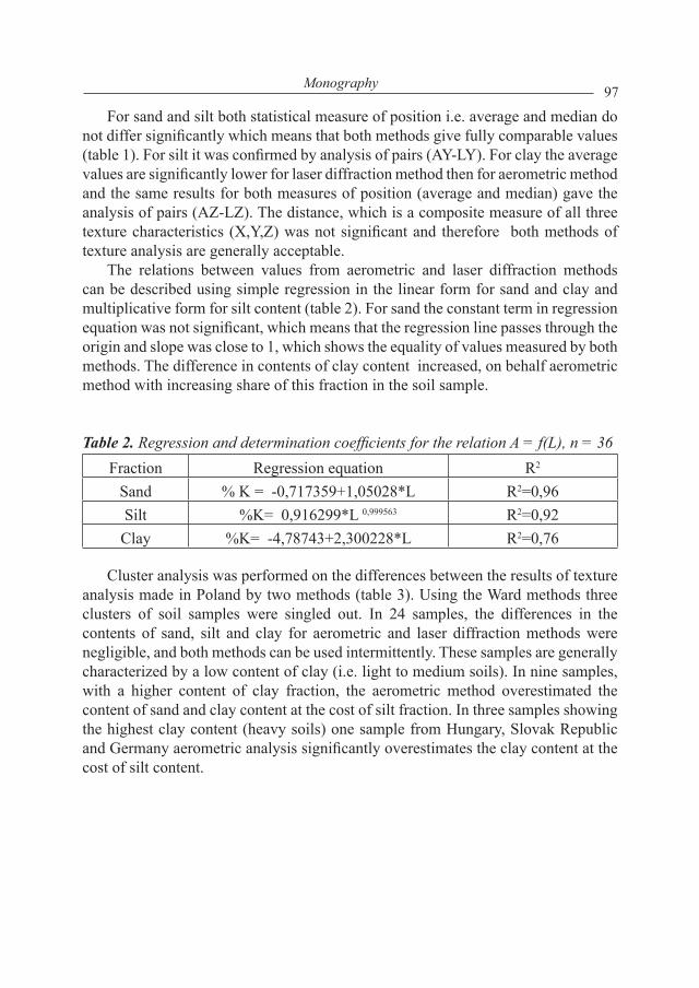
97Monography
For sand and silt both statistical measure of position i.e. average and median do not differ significantly which means that both methods give fully comparable values (table 1). For silt it was confirmed by analysis of pairs (AY-LY). For clay the average values are significantly lower for laser diffraction method then for aerometric method and the same results for both measures of position (average and median) gave the analysis of pairs (AZ-LZ). The distance, which is a composite measure of all three texture characteristics (X,Y,Z) was not significant and therefore both methods of texture analysis are generally acceptable.
The relations between values from aerometric and laser diffraction methods can be described using simple regression in the linear form for sand and clay and multiplicative form for silt content (table 2). For sand the constant term in regression equation was not significant, which means that the regression line passes through the origin and slope was close to 1, which shows the equality of values measured by both methods. The difference in contents of clay content increased, on behalf aerometric method with increasing share of this fraction in the soil sample.
Table 2. Regression and determination coefficients for the relation A = f(L), n = 36 Fraction Regression equation R2
Sand % K = -0,717359+1,05028*L R2=0,96Silt %K= 0,916299*L 0,999563 R2=0,92Clay %K= -4,78743+2,300228*L R2=0,76
Cluster analysis was performed on the differences between the results of texture analysis made in Poland by two methods (table 3). Using the Ward methods three clusters of soil samples were singled out. In 24 samples, the differences in the contents of sand, silt and clay for aerometric and laser diffraction methods were negligible, and both methods can be used intermittently. These samples are generally characterized by a low content of clay (i.e. light to medium soils). In nine samples, with a higher content of clay fraction, the aerometric method overestimated the content of sand and clay content at the cost of silt fraction. In three samples showing the highest clay content (heavy soils) one sample from Hungary, Slovak Republic and Germany aerometric analysis significantly overestimates the clay content at the cost of silt content.
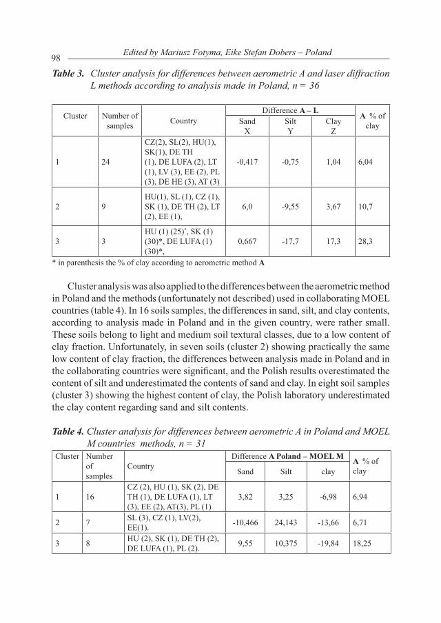
98 Edited by Mariusz Fotyma, Eike Stefan Dobers – Poland
Table 3. Cluster analysis for differences between aerometric A and laser diffraction L methods according to analysis made in Poland, n = 36
Cluster Number of samples Country
Difference A – L A % of clay Sand
XSiltY
ClayZ
1 24
CZ(2), SL(2), HU(1), SK(1), DE TH (1), DE LUFA (2), LT (1), LV (3), EE (2), PL (3), DE HE (3), AT (3)
-0,417 -0,75 1,04 6,04
2 9HU(1), SL (1), CZ (1), SK (1), DE TH (2), LT (2), EE (1),
6,0 -9,55 3,67 10,7
3 3HU (1) (25)*, SK (1) (30)*, DE LUFA (1) (30)*,
0,667 -17,7 17,3 28,3
* in parenthesis the % of clay according to aerometric method A.
Cluster analysis was also applied to the differences between the aerometric method in Poland and the methods (unfortunately not described) used in collaborating MOEL countries (table 4). In 16 soils samples, the differences in sand, silt, and clay contents, according to analysis made in Poland and in the given country, were rather small. These soils belong to light and medium soil textural classes, due to a low content of clay fraction. Unfortunately, in seven soils (cluster 2) showing practically the same low content of clay fraction, the differences between analysis made in Poland and in the collaborating countries were significant, and the Polish results overestimated the content of silt and underestimated the contents of sand and clay. In eight soil samples (cluster 3) showing the highest content of clay, the Polish laboratory underestimated the clay content regarding sand and silt contents.
Table 4. Cluster analysis for differences between aerometric A in Poland and MOEL M countries methods, n = 31
Cluster Number of samples
Country Difference A Poland – MOEL M A % of
clay Sand Silt clay
1 16CZ (2), HU (1), SK (2), DE TH (1), DE LUFA (1), LT (3), EE (2), AT(3), PL (1)
3,82 3,25 -6,98 6,94
2 7 SL (3), CZ (1), LV(2), EE(1). -10,466 24,143 -13,66 6,71
3 8 HU (2), SK (1), DE TH (2), DE LUFA (1), PL (2). 9,55 10,375 -19,84 18,25
.
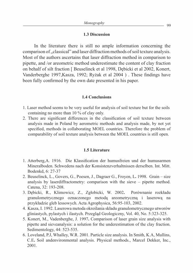
99Monography
1.3 Discussion
In the literature there is still no ample information concerning the comparison of „classical” and laser diffraction methods of soil texture analysis. Most of the authors ascertains that laser diffraction method in comparison to pipette, and /or areometric method underestimate the content of clay fraction on behalf of silt fraction [ Beuselinck et al 1998, Dębicki et al 2002, Konert, Vanderberghe 1997,Kasza, 1992; Ryżak et al 2004 ) . These findings have been fully confirmed by the own date presented in his paper.
1.4 Conclusions
1. Laser method seems to be very useful for analysis of soil texture but for the soils containing no more than 10 % of clay only.
2. There are significant differences in the classification of soil texture between analysis made in Poland by aerometric methods and analysis made, by not yet specified, methods in collaborating MOEL countries. Therefore the problem of comparability of soil texture analysis between the MOEL countries is still open.
1.5 Literature
1. Atterberg,A. 1916. . Die Klassification der humusfreien und der humusarmen Mineralboden. Schwedens nach der Konsistenzverhaltnissen derselben. Int. Mitt. Bodenkd, 6: 27-37
2. Beuselinck, L., Govers, G., Poesen, J., Dagraer G., Froyen, L..1998...Grain – size analysis by laserdiffractometry: comparison with the sieve – pipette method. Catena, 32: 193-208.
3. Dębicki, R., Klimowicz, Z., Zgłobicki, W. 2002.. . Porównanie rozkładu granulometrycznego oznaczonego metodą areometryczną i laserową na przykładzie gleb lessowych. Acta Agrophysica, 56:95-103, 2002.
4. Kasza, I. 1992..Laserowa metoda określania składu granulometrycznego utworów gliniastych, pylastych i ilastych. Przegląd Geologiczny, Vol. 40, No. 5:323-325.
5. Konert, M., Vadenberghe, J. 1997..Comparison of laser grain size analysis with pipette and sieveanalysis: a solution for the underestimation of the clay fraction. Sedimentology, 44: 523-535.
6. Loveland, P.J, Whalley, W.R. 2001..Particle size analysis. In Smith, K.A, Mullins, C.E.. Soil andenvironmental analysis. Physical methods., Marcel Dekker, Inc., 2001.
100 Edited by Mariusz Fotyma, Eike Stefan Dobers – Poland
7. Prószyński, 1996. Oznaczanie składu granulometrycznego gleb metodą Bouyoucosa- Casagrande w modyfikacji Prószyńskiego. Chemia rolna – przewodnik do ćwiczeń pod red. Kuszelewskiego, L. 127-149.
8. Ryżak, M., Walczak, R.T, Niewczas, J.2004. Porównanie rozkładu granulometrycznego cząstek glebowych metodą dyfrakcji laserowej i metodą sedymentacyjną. Acta Agrophysica, 2004, (4):509-518.
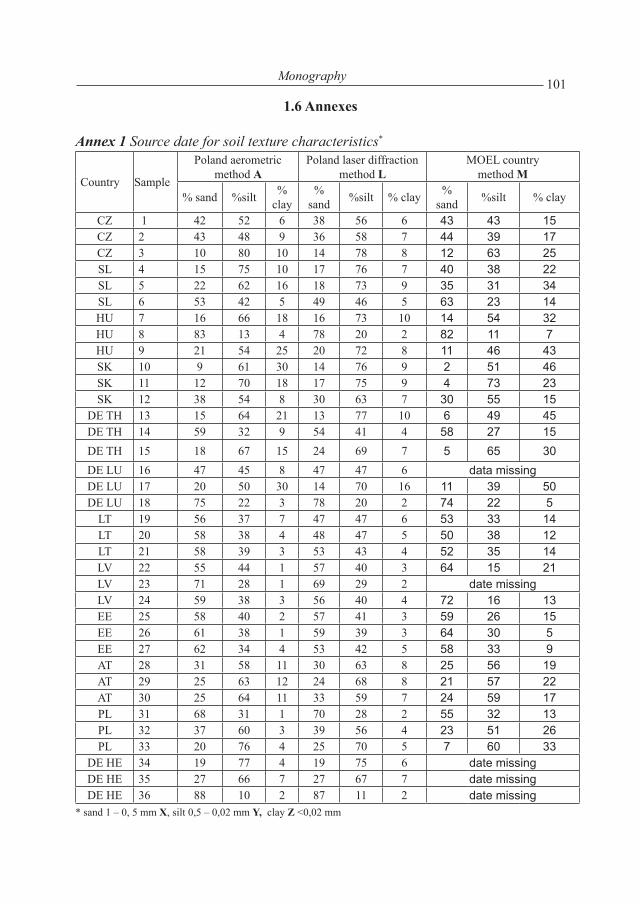
101Monography
1.6 Annexes
Annex 1 Source date for soil texture characteristics*
Country Sample
Poland aerometric method A
Poland laser diffraction method L
MOEL country method M
% sand %silt % clay
% sand %silt % clay %
sand %silt % clay
CZ 1 42 52 6 38 56 6 43 43 15CZ 2 43 48 9 36 58 7 44 39 17CZ 3 10 80 10 14 78 8 12 63 25SL 4 15 75 10 17 76 7 40 38 22SL 5 22 62 16 18 73 9 35 31 34SL 6 53 42 5 49 46 5 63 23 14HU 7 16 66 18 16 73 10 14 54 32HU 8 83 13 4 78 20 2 82 11 7HU 9 21 54 25 20 72 8 11 46 43SK 10 9 61 30 14 76 9 2 51 46SK 11 12 70 18 17 75 9 4 73 23SK 12 38 54 8 30 63 7 30 55 15
DE TH 13 15 64 21 13 77 10 6 49 45DE TH 14 59 32 9 54 41 4 58 27 15DE TH 15 18 67 15 24 69 7 5 65 30DE LU 16 47 45 8 47 47 6 data missingDE LU 17 20 50 30 14 70 16 11 39 50DE LU 18 75 22 3 78 20 2 74 22 5
LT 19 56 37 7 47 47 6 53 33 14LT 20 58 38 4 48 47 5 50 38 12LT 21 58 39 3 53 43 4 52 35 14LV 22 55 44 1 57 40 3 64 15 21LV 23 71 28 1 69 29 2 date missingLV 24 59 38 3 56 40 4 72 16 13EE 25 58 40 2 57 41 3 59 26 15EE 26 61 38 1 59 39 3 64 30 5EE 27 62 34 4 53 42 5 58 33 9AT 28 31 58 11 30 63 8 25 56 19AT 29 25 63 12 24 68 8 21 57 22AT 30 25 64 11 33 59 7 24 59 17PL 31 68 31 1 70 28 2 55 32 13PL 32 37 60 3 39 56 4 23 51 26PL 33 20 76 4 25 70 5 7 60 33
DE HE 34 19 77 4 19 75 6 date missingDE HE 35 27 66 7 27 67 7 date missingDE HE 36 88 10 2 87 11 2 date missing
* sand 1 – 0, 5 mm X, silt 0,5 – 0,02 mm Y, clay Z <0,02 mm
102 Edited by Mariusz Fotyma, Eike Stefan Dobers – Poland
1. Ergänzung
Vergleich der Sedimentations- und der Laser-Difraktionsmethodik.für die Bestimmung der Bodentextur
Dorota Pikuła1, Stefan Dobers 2
1Institut für Bodenkunde und Pflanzenernährung – Staatliches Forschungsinstitut, Puławy, 2 University of Warmia and Mazury
Polen
Einführung
Im Verlauf des 9. Treffens der Gruppe der mittelosteuropäischen Länder (Arbeitsgruppe der landwirtschaftlichen Untersuchungsdienste in Mittel-Osteuropa) in Piran, Slowenien, im Jahre 2006 wurde entschieden, dass ein Laborringversuch durchgeführt wird mit dem Thema Bodenproben-Analyse und Ableitung von Düngungsempfehlungen. Der Endbericht des ersten Ringversuches ist als Hauptbeitrag in dieser Ausgabe der Zeitschrift veröffentlicht. Die Ergebnisse der Bodenanalyse, der Einstufung der Nährstoffgehalte sowie die abgeleiteten Düngeempfehlungen sind innerhalb der 10 beteiligten Staaten sehr unterschiedlich. Die Analyse der Daten ergibt, dass der Hauptgrund für die Unterschiede in der Herangehensweise der Bodenarten-Bestimmung und Einteilung liegt. In Deutschland, Estland und Ungarn werden fünf Gruppen von Bodenarten unterschieden, in Litauen und Polen vier, und in den verbleibenden Staaten drei. Abgesehen von der Anzahl der Bodenarten-Gruppen unterscheiden sich zwischen den Ländern auch die Definitionen für die Abgrenzung der unterschiedlichen Arten. In Deutschland und Estland ist der Tongehalt bestimmend (Teilchen mit einem Äquivalentdurchmesser kleiner als 0.002 mm), in Polen der Anteil der sogenannten abschlembaren Teilchen (Teilchen mit einem Äquivalentdurchmesser kleiner als 0.02 mm) und in Ungarn entscheidet der Arany-Wert, die Wassermenge, die zum Erreichen der Plastizitätsgrenze notwendig ist, über die Einteilung in die verschiedenen Gruppen der Bodentexur.
Trotz dieser Unterschiede in der Einstufung der Bodentextur scheint es jedoch, dass die Systeme zur Einteilung der Nährstoffgehalte in Versorgungsstufen (Kalibrationssysteme) mehr oder weniger nah beieinander liegen mit Blick auf die Gehaltsklasse „mittel“. Dies ist ein guter Ausgangspunkt für die weitere Arbeit an einer Harmonisierung der Dünge-Beratungssysteme. Aus diesem Grunde wurde auf dem 10. Treffen der MOEL Gruppe in Visegrad, Ungarn, im Jahr 2007 verabredet, einen weiteren Ringversuch zu Bodenuntersuchung und Düngeempfehlungen durchzuführen. Die beteiligten Staaten stimmten darin überein, dass jeweils drei Bodenproben mit unterschiedlichen Bodentexturen (leicht, mittel und schwer) gezogen werden sollen, die allerdings mittlere Nährstoffgehalte für P, K und Mg aufweisen. Die Bodenproben wurden an alle anderen beteiligten Staaten versandt,
103Monography
um die jeweils landestypischen Methoden für die Bodenanalyse, Gehalts-Einstufung und Ermittlung der Düngeempfehlung anzuwenden. Leider wurde der polnische Vorschlag nicht angenommen, die Bodenproben auch auf die granulometrische Zusammensetzung zu untersuchen, und daher führte nur unser Land diese Untersuchungen durch.
Die Bodentextur, d.h. der Anteil unterschiedlicher Bodenteilchen-Größenklassen in der Festsubstanz, ist eine der grundlegenden Bestimmungsgrößen für bodenphysikalische und –chemische Eigenschaften. Anfang des 20. Jahrhunderts schlug Atterberg (1916) vor, Böden auf der Grundlage der verschiedenen Anteile von Partikelgrößen einzuteilen. Böden sind jedoch sehr heterogen in der granulometrischen Zusammensetzung und die Untersuchungsergebnisse hängen wesentlich von der verwendeten Bestimmungsmethodik ab. Gegenwärtig sind mehr als 400 Methoden zur Bestimmung dieser Bodeneigenschaft bekannt, und viele davon werden von einigen Labors angewendet (Loveland, Whalley 2001). Die am meisten verbreiteten Methoden sind die Pipette-Methode und die Aerometrische Methode. In Polen wird die letztere, in Anlehnung an Cassagrande und angepasst gemäß Prószyński (1996), offiziell verwendet. Alle 17 agrochemischen Untersuchungsanstalten in Polen, die mit Bodenuntersuchung und Düngungsempfehlungen beschäftigt sind, beziehen sich auf diese Methode für stichprobenhafte Kontroll-Untersuchungen der Bodentextur, bestimmen aber generell die Texturklasse vor Ort anhand der Fingerprobe. Die Grundlage der aerometrischen Methode zur Trennung der Partikelgrößen ist die Einhaltung einer unterschiedliche Zeitspanne für die Sedimentation der jeweiligen Partikelfraktion und nachfolgende Dekantierung der Suspension. Zur Berechnung der jeweiligen Anteile der Größenklassen an Bodenteilchen wird auf das Stokes‘sche Gesetz zurückgegriffen, welches unterstellt, dass die sedimentierenden Teilchen eine kugelförmige Gestalt haben. Aufgrund deutlicher Abweichungen der Suspensionseigenschaften von den Annahmen des Stook‘schen Gesetzes sind die Ergebnisse der aerometrischen Methode mit unvorhersagbaren Fehlern beladen.
Seit ein paar Jahren ist die Bestimmung der Bodenpartikelgrößen-Verteilung mit der Laser-Difraktionsmethode in die bodenkundliche Forschung eingeführt (Beuselinck et al, 1998, Ryżak i in., 2004). Im Jahre 2006 wurden sämtliche Labore der agrochemischen Untersuchungsstationen mit diesen Geräten ausgestattet und es wurde begonnen, die Methode in der Routineanalyse anzuwenden. Das Ziel der Untersuchungen, deren Ergebnisse in diesem Artikel vorgestellt werden, ist der Vergleich der aerometrischen mit der Laser-Difraktionsmethode bei der Bestimmung der granulometrischen Zusammensetzung der Bodenproben, die von den beteiligten Staaten im zweiten Ringversuch versendet wurden.

104 Edited by Mariusz Fotyma, Eike Stefan Dobers – Poland
1.1 Methoden
Insgesamt wurden 36 Bodenproben analysiert: 3 Proben je beteiligtem Staat, inklusive der Proben aus Polen. Die Proben wurden auf ihre granulometrische Zusammensetzung hin analysiert. Für dieses Ziel wurde einerseits die aerometrische Methode nach Cassagrande mit Anpassung durch Prószyński (1996) verwendet, sowie andererseits das Gerät Mastersizer 2000 für die Laser-Difraktions-Analyse, ausgestattet mit der HYDRO 2000 G Zusatzeinrichtung. Dieses Gerät kann die Bodenteilchen-Größenverteilung in Wassersuspension im Größenbereich von 0-2000 µm bestimmen. In den Berechnungen wurde ein Licht-Ablenkungskoeffezient von 1,330 und ein Licht-Absorptionskoeffizient von 0,1 verwendet. Aus den erhaltenen Daten wurde der Anteil von Bodenteilchen für die Größenbereiche 1,0-0,1 mm, 0,1-0,05 mm, 0,05-0,02 mm, 0,02-0,005 mm, 0,005-0,002 mm und Teilchen kleiner 0,002 mm berechnet. Diese Anteile wurden dann in die Bereiche Sand 1,0-0,1 mm, Schluff 0,1-0,02 mm und Ton <0,02 mm gruppiert. Die Rohdaten der Bodenanalyse, inklusive der in den beteiligten Labors ermittelten (Methoden hier nicht weiter beschrieben), sind im Anhang 1 wiedergegeben.
Um die Ergebnisse zu vergleichen, wurden eine Varianzanalyse (Tabelle 1), Mittelwert-Vergleiche (Tabelle 2), Korrelations- und Regressionsanalyse (Tabelle 3) und eine Cluster-Analyse (Tabelle 4) durchgeführt. Alle statistischen Analysen wurden unter Verwendung des Softwarepaketes Statgraphic 5+ gemacht.
1.2 Ergebnisse
Für die Größenfraktionen Sand und Schluff treten keine signifikanten Unterschiede zwischen den Methoden für die Lagemaße Mittelwert und Median auf, was bedeutet, dass beide Methoden vergleichbare Ergebnisse liefern (Tabelle 1). Für Schluff zeigte dies der Mittelwertvergleich (AY-LY). Der Vergleich der Ergebnisse für den Tongehalt ergab, dass Mittelwert und Median für die Lasermethode signifikant geringer sind (AZ-LZ). Das Distanzmaß, welches als zusammengesetzte Größe aus allen drei Fraktionen (X, Y, Z) berechnet wird, war nicht signifkant unterschiedlich, woraus geschlossen wird, dass beide Methoden generell akzeptiert werden können.
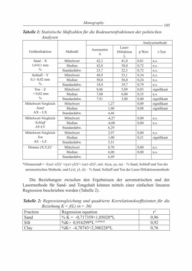
105Monography
Tabelle 1: Statistische Maßzahlen für die Bodenartenfraktionen der polnischen Analysen
Größenfraktion Maßzahl
Analysemethode
AerometrieA
Laser-Difraktion
L p Wert t-Test
Sand – X1,0-0,1 mm
%
Mittelwert 42,3 41,0 0,81 n.s. Median 42,0 38,0 0,72 n.s.
Standardabw. 23,7 22,3 0,72 n.s. Schluff – Y
0,1- 0,02 mm%
Mittelwert 48,9 53,1 0,34 n.s.Median 50,0 56,0 0,24 n.s.
Standardabw. 18,9 19,7 0,79 n.s. Ton – Z
< 0,02 mm%
Mittelwert 8,86 5,89 0,03 signifikantMedian 7,00 6,00 0,35 n.s.
Standardabw. 7,91 3,00 0,00 signifikantMittelwert-Vergleich
SandAX – LX
Mittelwert 1,27 0,09 signifikantMedian 1,00 0,08 signifikant
Standardabw. 4,46Mittelwert-Vergleich
SchluffAY-LY
Mittelwert -4,27 0,00 n.s.Median -4,00 0,00 n.s.
Standardabw. 6,29Mittelwert-Vergleich
TonAZ – LZ
Mittelwert 2,97 0,00 n.s.Median 1,00 0,21 signifikant
Standardabw. 5,51Distanz (X,Y,Z)* Mittelwert 8,70 0,00 n.s
Median 6,00 0,00 n.s.Standardabw. 6,49
*Distanzmaß = √(xa1-xl2)2 +(ya1-yl2)2+ (za1-zl2)2, mit: A(xa, ya, za) – % Sand, Schluff und Ton der aerometrischen Methode, und L(xl, yl, zl) – % Sand, Schluff und Ton der Laser-Difraktionsmethode
Die Beziehungen zwischen den Ergebnissen der aerometrischen und der Lasermethode für Sand- und Tongehalt können mittels einer einfachen linearen Regression beschrieben werden (Tabelle 2).
Tabelle 2: Regressionsgleichung und quadrierte Korrelationskoeffizienten für die Beziehung K = f(L) (n = 36)
Fraction Regression equation r2
Sand % K = -0,717359+1,05028*L 0,96Silt %K= 0,916299*L 0,999563 0,92Clay %K= -4,78743+2,300228*L 0,76
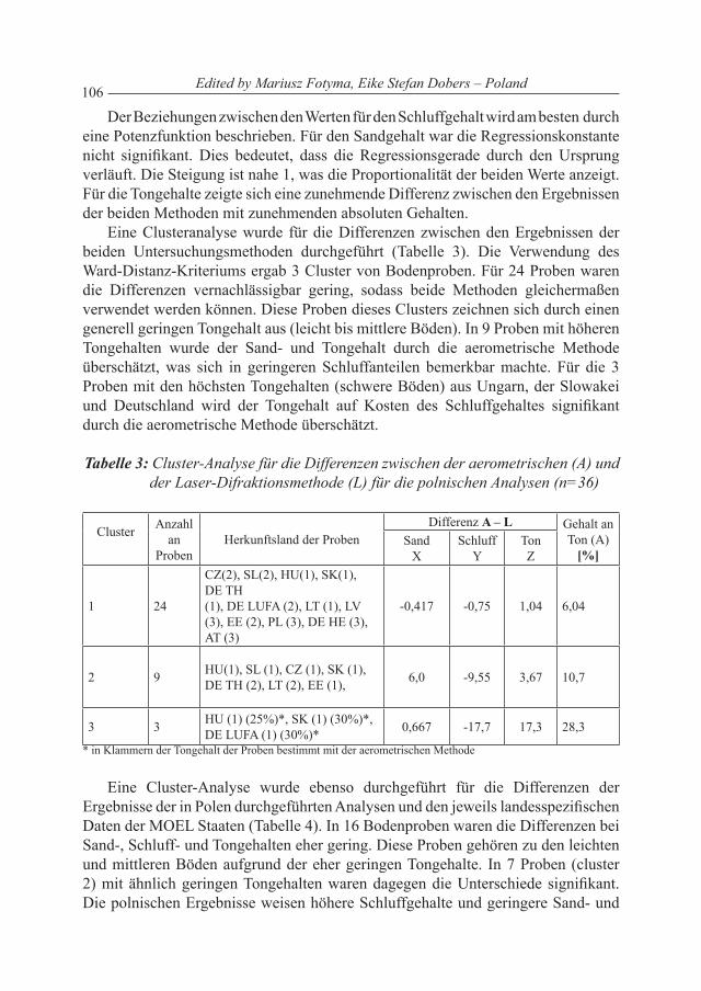
106 Edited by Mariusz Fotyma, Eike Stefan Dobers – Poland
Der Beziehungen zwischen den Werten für den Schluffgehalt wird am besten durch eine Potenzfunktion beschrieben. Für den Sandgehalt war die Regressionskonstante nicht signifikant. Dies bedeutet, dass die Regressionsgerade durch den Ursprung verläuft. Die Steigung ist nahe 1, was die Proportionalität der beiden Werte anzeigt. Für die Tongehalte zeigte sich eine zunehmende Differenz zwischen den Ergebnissen der beiden Methoden mit zunehmenden absoluten Gehalten.
Eine Clusteranalyse wurde für die Differenzen zwischen den Ergebnissen der beiden Untersuchungsmethoden durchgeführt (Tabelle 3). Die Verwendung des Ward-Distanz-Kriteriums ergab 3 Cluster von Bodenproben. Für 24 Proben waren die Differenzen vernachlässigbar gering, sodass beide Methoden gleichermaßen verwendet werden können. Diese Proben dieses Clusters zeichnen sich durch einen generell geringen Tongehalt aus (leicht bis mittlere Böden). In 9 Proben mit höheren Tongehalten wurde der Sand- und Tongehalt durch die aerometrische Methode überschätzt, was sich in geringeren Schluffanteilen bemerkbar machte. Für die 3 Proben mit den höchsten Tongehalten (schwere Böden) aus Ungarn, der Slowakei und Deutschland wird der Tongehalt auf Kosten des Schluffgehaltes signifikant durch die aerometrische Methode überschätzt.
Tabelle 3: Cluster-Analyse für die Differenzen zwischen der aerometrischen (A) und der Laser-Difraktionsmethode (L) für die polnischen Analysen (n=36)
Cluster Anzahl an
ProbenHerkunftsland der Proben
Differenz A – L Gehalt an Ton (A)
[%]Sand
XSchluff
YTonZ
1 24
CZ(2), SL(2), HU(1), SK(1), DE TH (1), DE LUFA (2), LT (1), LV (3), EE (2), PL (3), DE HE (3), AT (3)
-0,417 -0,75 1,04 6,04
2 9 HU(1), SL (1), CZ (1), SK (1), DE TH (2), LT (2), EE (1), 6,0 -9,55 3,67 10,7
3 3 HU (1) (25%)*, SK (1) (30%)*, DE LUFA (1) (30%)* 0,667 -17,7 17,3 28,3
* in Klammern der Tongehalt der Proben bestimmt mit der aerometrischen Methode
Eine Cluster-Analyse wurde ebenso durchgeführt für die Differenzen der Ergebnisse der in Polen durchgeführten Analysen und den jeweils landesspezifischen Daten der MOEL Staaten (Tabelle 4). In 16 Bodenproben waren die Differenzen bei Sand-, Schluff- und Tongehalten eher gering. Diese Proben gehören zu den leichten und mittleren Böden aufgrund der eher geringen Tongehalte. In 7 Proben (cluster 2) mit ähnlich geringen Tongehalten waren dagegen die Unterschiede signifikant. Die polnischen Ergebnisse weisen höhere Schluffgehalte und geringere Sand- und

107Monography
Tongehalte auf. Für 8 Bodenproben (cluster 3) mit den höchsten Tongehalten wurden in der polnischen Bestimmung geringere Tongehalte festgestellt mit entsprechend höheren Sand- und Schluffgehalten.
Tabelle 4: Cluster-Analyse für Differenzen zwischen der aerometrischen Analyse in Polen (A) und den Ergebnissen der einzelnen MOEL-Staaten (M) (n = 31)
Cluster Anzahl an
ProbenHerkunftsland der Proben
Differenz Polen A – MOEL M Gehalt an Ton
(A)Sand Schluff Ton
1 16 CZ (2), HU (1), SK (2), DE TH (1), DE LUFA (1), LT (3), EE (2), AT(3), PL (1)
3,82 3,25 -6,98 6,94
2 7 SL (3), CZ (1), LV(2), EE(1) -10,466 24,143 -13,66 6,71
3 8 HU (2), SK (1), DE TH (2), DE LUFA (1), PL (2). 9,55 10,375 -19,84 18,25
1.3 Diskussion
Für den Vergleich von klassischer Sedimentations- mit der Laser-Difraktions-Analyse fehlt es bislang noch in der Literatur an umfangreicher Information. Die meisten Autoren bestätigen, dass die Laser-Methode im Vergleich zur Pipette- und/oder aerometrischen Methode den Tongehalt unterschätzen mit entsprechend höheren Werten für den Schluffgehalt (Beuselinck at al , Dębicki at al 2002, Konert, Vanderberghe 1997,Kasza, 1992; Ryżak at al 2004 ). Die Ergebnisse können durch die Daten voll bestätigt werden, die in dieser Untersuchung gewonnen wurden.
1.4 Schlussfolgerungen
1. Die Lasermethode scheint sehr geeignet für die Texturbestimmung zu sein, wenn die Bodenproben weniger als 10% Ton enthalten.
2. Es gibt signifikante Unterschiede zwischen der Bodenartklassifikation durch die in Polen durchgeführte aerometrische Analyse und den jeweils in den Herkunftsländern durchgeführten Texturbestimmungen, die allerdings nicht weiter spezifiziert wurden. Daher ist die Vergleichbarkeit der Texturbestimmung zwischen den einzelnen MOEL-Staaten weiterhin nicht gegeben.
108 Edited by Mariusz Fotyma, Eike Stefan Dobers – Poland
1.5 Literatur
1. Atterberg,A. 1916. .Die Klassification der humusfreien und der humusarmen Mineralboden Schwedens nach der Konsistenzverhaltnissen derselben. Int. Mitt. Bodenkd, 6: 27-37
2. Beuselinck, L., Govers, G., Poesen, J., Dagraer G., Froyen, L.. 1998.. . Grain – size analysis by laserdiffractometry: comparison with the sieve – pipette method. Catena, 32: 193-208.
3. Dębicki, R., Klimowicz, Z., Zgłobicki, W. 2002.. . Porównanie rozkładu granulometrycznego oznaczonego metodą areometryczną i laserową na przykładzie gleb lessowych. Acta Agrophysica, 56:95-103, 2002.
4. Kasza, I. 1992.. Laserowa metoda określania składu granulometrycznego utworów gliniastych, pylastych i ilastych. Przegląd Geologiczny, Vol. 40, No. 5:323-325.
5. Konert, M., Vadenberghe, J. 1997..Comparison of laser grain size analysis with pipette and sieveanalysis: a solution for the underestimation of the clay fraction. Sedimentology, 44: 523-535.
6. Loveland, P.J, Whalley, W.R. 2001..Particle size analysis. In Smith, K.A, Mullins, C.E..Soil andenvironmental analysis. Physical methods., Marcel Dekker, Inc., 2001.
7. Prószyński, 1996. Oznaczanie składu granulometrycznego gleb metodą Bouyoucosa- Casagrande w modyfikacji Prószyńskiego. Chemia rolna – przewodnik do ćwiczeń pod red. Kuszelewskiego, L. 127-149.
8. Ryżak, M., Walczak, R.T, Niewczas, J.2004. Porównanie rozkładu granulometrycznego cząstek glebowych metodą dyfrakcji laserowej i metodą sedymentacjną. Acta Agrophysica, 2004, (4):509-518.
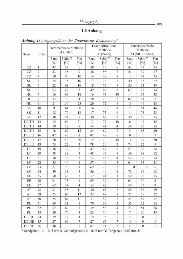
109Monography
1.6 Anhang
Anhang 1: Ausgangsdaten der Bodentextur-Bestimmung*
Staat Probe
aerometrische MethodeA (Polen)
Laser-Difraktions-MethodeL (Polen)
länderspezifische Methode
M (MOEL Staat)Sand[%]
Schluff [%]
Ton[%]
Sand[%]
Schluff[%]
Ton[%]
Sand[%]
Schluff[%]
Ton[%]
CZ 1 42 52 6 38 56 6 43 43 15CZ 2 43 48 9 36 58 7 44 39 17CZ 3 10 80 10 14 78 8 12 63 25SL 4 15 75 10 17 76 7 40 38 22SL 5 22 62 16 18 73 9 35 31 34SL 6 53 42 5 49 46 5 63 23 14HU 7 16 66 18 16 73 10 14 54 32HU 8 83 13 4 78 20 2 82 11 7HU 9 21 54 25 20 72 8 11 46 43SK 10 9 61 30 14 76 9 2 51 46SK 11 12 70 18 17 75 9 4 73 23SK 12 38 54 8 30 63 7 30 55 15
DE TH 13 15 64 21 13 77 10 6 49 45DE TH 14 59 32 9 54 41 4 58 27 15DE TH 15 18 67 15 24 69 7 5 65 30DE LU 16 47 45 8 47 47 6 0 0 7DE LU 17 20 50 30 14 70 16 11 39 50DE LU 18 75 22 3 78 20 2 74 22 5
LT 19 56 37 7 47 47 6 53 33 14LT 20 58 38 4 48 47 5 50 38 12LT 21 58 39 3 53 43 4 52 35 14LV 22 55 44 1 57 40 3 64 15 21LV 23 71 28 1 69 29 2 0 0 5LV 24 59 38 3 56 40 4 72 16 13EE 25 58 40 2 57 41 3 59 26 15EE 26 61 38 1 59 39 3 64 30 5EE 27 62 34 4 53 42 5 58 33 9AT 28 31 58 11 30 63 8 25 56 19AT 29 25 63 12 24 68 8 21 57 22AT 30 25 64 11 33 59 7 24 59 17PL 31 68 31 1 70 28 2 55 32 13PL 32 37 60 3 39 56 4 23 51 26PL 33 20 76 4 25 70 5 7 60 33
DE HE 34 19 77 4 19 75 6 0 0 0DE HE 35 27 66 7 27 67 7 0 0 0DE HE 36 88 10 2 87 11 2 0 0 0
* Sandgehalt 1,0 – 0, 5 mm X, Schluffgehalt 0,5 – 0,02 mm Y, Tongehalt <0,02 mm Z