RUHRECONOMIC PAPERS

Long-run Money Demandin OECD CountriesCross-Member Cointegration

#237

Frauke Dobnik

Imprint

Ruhr Economic Papers

Published by

Ruhr-Universität Bochum (RUB), Department of EconomicsUniversitätsstr. 150, 44801 Bochum, Germany

Technische Universität Dortmund, Department of Economic and Social SciencesVogelpothsweg 87, 44227 Dortmund, Germany

Universität Duisburg-Essen, Department of EconomicsUniversitätsstr. 12, 45117 Essen, Germany

Rheinisch-Westfälisches Institut für Wirtschaftsforschung (RWI)Hohenzollernstr. 1-3, 45128 Essen, Germany

Editors

Prof. Dr. Thomas K. BauerRUB, Department of Economics, Empirical EconomicsPhone: +49 (0) 234/3 22 83 41, e-mail: thomas.bauer@rub.de

Prof. Dr. Wolfgang LeiningerTechnische Universität Dortmund, Department of Economic and Social SciencesEconomics – MicroeconomicsPhone: +49 (0) 231/7 55-3297, email: W.Leininger@wiso.uni-dortmund.de

Prof. Dr. Volker ClausenUniversity of Duisburg-Essen, Department of EconomicsInternational EconomicsPhone: +49 (0) 201/1 83-3655, e-mail: vclausen@vwl.uni-due.de

Prof. Dr. Christoph M. SchmidtRWI, Phone: +49 (0) 201/81 49-227, e-mail: christoph.schmidt@rwi-essen.de

Editorial Offi ce

Joachim SchmidtRWI, Phone: +49 (0) 201/81 49-292, e-mail: joachim.schmidt@rwi-essen.de

Ruhr Economic Papers #237

Responsible Editor: Volker Clausen

All rights reserved. Bochum, Dortmund, Duisburg, Essen, Germany, 2011

ISSN 1864-4872 (online) – ISBN 978-3-86788-271-2The working papers published in the Series constitute work in progress circulated to stimulate discussion and critical comments. Views expressed represent exclusively the authors’ own opinions and do not necessarily refl ect those of the editors.

Ruhr Economic Papers #237

Frauke Dobnik

Long-run Money Demandin OECD Countries

Cross-Member Cointegration

Bibliografi sche Informationen der Deutschen Nationalbibliothek

Die Deutsche Bibliothek verzeichnet diese Publikation in der deutschen National-bibliografi e; detaillierte bibliografi sche Daten sind im Internet über: http://dnb.d-nb.de abrufb ar.

ISSN 1864-4872 (online)ISBN 978-3-86788-271-2

Frauke Dobnik1

Long-run Money Demand in OECD Countries – Cross-Member Cointegration

AbstractThis paper examines the long-run money demand function for 11 OECD countries from 1983 to 2006 using panel data and including wealth. The distinction between common factors and idiosyncratic components using principal component analysis allows to detect cross-member cointegration and to distinguish between international and national developments as drivers of the long-run relation between money and its determinants. Indeed, cointegration between the common factors of the underlying variables, i.e. cross-member cointegration, indicates that the long-run relationship is mainly driven by international stochastic trends. Furthermore, it is found that the impact of income on money demand is positive, while it is negative for the interest rate and stock prices. The estimated (semi-)elasticities of money are larger for the common factors than for the original variables, except the income elasticity. Finally, the results of a panel-based error-correction model suggest that money demand converges to an international cross-member equilibrium relation of the common factors.

JEL Classifi cation: E41, C22, C33

Keywords: Money demand; wealth eff ects; panel unit roots; vector error-correction models

January 2011

1 Ruhr Graduate School in Economics (RGS Econ) and University of Duisburg-Essen. – I am grateful to Ansgar Belke, Joscha Beckmann and Jonas Keil for valuable comments. Financial support provided by the Ruhr Graduate School in Economics is gratefully acknowledged.– All correspondence to Frauke Dobnik, Ruhr Graduate School in Economics, c/o University of Duisburg-Essen, Department of Economics, Chair for Macroeconomics, Prof. Dr. Ansgar Belke, Universitätsstr. 12, 45117 Essen, Germany, E-Mail: frauke.dobnik@uni-due.de.

1 IntroductionThe stability of the long-run money demand function is a widely studied research topic.

On the one hand, stable money demand is relevant for policy makers to choose a sen-

sible monetary policy instrument. For instance, unstable money demand caused by the

financial reforms of the late 1970s induced many central banks in developed countries

to switch from money targeting to the interest rate as monetary policy instrument. The

very same was proposed by Poole (1970) who showed that the interest rate should be

targeted if the money demand function is unstable. The identification of the optimal mon-

etary policy strategy has also been studied for the upcoming European System of Central

Banks (ESCB) in 1999. In this regard, many time series studies discussed the question

whether monetary targeting or inflation targeting would be better to achieve price stability

in the European Economic and Monetary Union (EMU). On the other hand, money can

play an important role in the formulation of an efficient monetary policy strategy, even

though monetary policy of developed countries typically uses an interest rate as policy

instrument. Monetary aggregates can be appropriate indicators for future inflation in the

medium term and long-run. As mentioned by Valadkhani (2006) an emerging consensus

among economists is that it is not advisable to concentrate exclusively on a single policy

instrument while neglecting another important information variable. Both the interest rate

and monetary aggregates are important in selecting appropriate monetary policy actions.

Monetary aggregates, however, will only be related to the real economy if the money de-

mand function is stable. Thus, the stability of money demand entails whether money is an

appropriate guide to policy.

Referring to that, the main purpose of this panel data study is to determine the existence

of a stable long-run money demand function of 11 OECD countries from 1983 to 2006,

taking into consideration possible cross-sectional dependencies resulting from common

factors. If cross-member cointegration is existent the non-stationarity in the variables will

stem from cross-sectional common stochastic trends only and the variables will be coin-

tegrated across the panel members. To detect cross-member cointegration the common

factors of the underlying variables are tested for unit roots and cointegration relations.

The distinction between common factors and idiosyncratic components using principal

component analysis also allows to distinguish between international and national develop-

ments as drivers of the long-run relation between money and its determinants (see Belke,

Dreger, and de Haan (2010)). Given that the idiosyncratic component is a residual, which

captures the impact of shocks affecting the respective variable of one specific country, it

can be interpreted as the part of the variable that is driven by national trends. In contrast,

the common component represents international trends in the evolution of the variable,

because it depends on a small number of common shocks, which affect the respective

4

variable of all the countries. Depending on the results of the cointegration tests, this dis-

tinction has important implications for policy makers. If the common factors cointegrate,

i.e. in the case of cross-member cointegration, the national monetary policy should take

into account international developments, for instance, to precisely predict national future

inflation. Indeed, this paper delivers empirical evidence that money and its determinants

are cointegrated in their common factors, but not in their idiosyncratic components.

Moreover, this panel data study incorporates wealth as additional determinant of money

demand as has become popular in country-specific time series studies. Friedman (1970)

already suggested in 1970 that wealth may play an important role for money demand if it

was viewed in a portfolio framework. Following Friedman (1988) and Choudhry (1996),

among others, this paper introduces stock prices as wealth variable assuming that equities

have a strong relation with money. In addition, the standard money demand function with

income as scale variable and an interest rate as measure of opportunity cost is further ex-

tended by the exchange rate capturing possible currency substitution effects. Furthermore,

this paper contributes in applying an error-correction specification using panel data to

determine long-run as well as short-run coefficients of the money demand of OECD coun-

tries. Panel data studies usually estimate only the long-run relation ignoring the short-run

dynamics except the studies by Valadkhani (2008) and Nautz and Rondorf (2010).

The remainder of this paper is organised as follows. Section 2 briefly reviews the litera-

ture on money demand using panel data. Section 3 introduces the money demand function.

Section 4 presents the data, discusses the econometric methods and presents the empirical

results. Section 5 provides conclusions.

2 Review of panel data studiesWhile there is a wide range of country-specific time series studies on money demand avail-

able, only a few studies apply panel-econometric methods so far. It is widely known that

standard unit root and cointegration tests based on individual time series have low statis-

tical power, especially when the time series is short (Campbell and Perron, 1991). Panel-

based tests represent an improvement in this respect by exploiting additional information

that results from the inclusion of the cross-sectional dimension. Table 1 summarises the

studies using panel datasets to analyse the long-run relationship between money and its

main determinants. The estimated income elasticities vary between 0.18 (Garcia-Hiernaux

and Cerno, 2006) and 2.66 (Hamori and Hamori, 2008), but are usually slightly greater

than one. The estimated interest rate (semi-) elasticities are in the range of -0.71 (Nautz

and Rondorf, 2010) and 0.008 (Arnold and Roelands, 2010), where the latter value should

be treated as an exception with a sign contrary to theory. For the exchange rate there exists

5

no clear sign which can be imposed from theory. The few panel data studies including

exchange rates come up with ambiguous results. The coefficients take values between

-1.73 (Rao et al., 2009) and +0.31 (Narayan et al., 2009). Some of these studies use fur-

ther additional explanatory variables for money beyond income, the interest rate and the

exchange rate, among them inflation or a foreign interest rate. Time series studies, how-

ever, meanwhile often employ wealth as additional explanatory variable (see, e.g. Setzer

and Greiber (2007); Boone and van den Noord (2008); de Santis et al. (2008); de Bondt

(2009); Dreger and Wolters (2010))1, but panel data studies usually do not. The studies

by Arnold and Roelands (2010) and Nautz and Rondorf (2010)) are the only exceptions.

Arnold and Roelands (2010) found a positive impact of house prices on money demand

for the whole panel of ten euro area countries, but no significant impact of stock prices.

Nautz and Rondorf (2010) cannot reject empirically that neither house prices nor stock

prices significantly affect euro area long-run money demand. Further, most panel data

studies estimated only the long-run coefficients of money demand. Valadkhani (2008) and

Nautz and Rondorf (2010) also accounted for the short-run dynamics of money demand by

estimating a panel-based error-correction model. The omission of error-correction mod-

els to capture the short-run coefficients of money demand might be due to the problem

that there exist no tests to detect instability of panel estimated regression equations which

correspond to the popular CUSUM and CUSUMSQ tests in country-specific time series

models (see Rao and Kumar (2009)).2 For a more detailed description of panel data stud-

ies on money demand including their methods and main findings see Kumar, Chowdhury,

and Rao (2010).

3 The money demand functionIn this paper a widely used specification of the money demand function is chosen as a

starting point. According to Ericsson (1998), the main body of theories of money demand

1Many time series studies on euro area money demand (e.g. Boone and van den Noord (2008)) argue

in favour of the inclusion of wealth to explain the overshooting of the ECB’s M3 target and to reestablish a

stable money demand function. What is more, some studies use a (financial) wealth variable in addition to

an income variable to take account of an income elasticity greater than one due to an omitted variables bias

(see recent surveys by Knell and Stix (2005, 2006).2Stability tests like the CUSUM and CUSUMSQ are applied in this context to test the stability of the

short-run coefficients and the adjustment coefficient of the lagged error-correction term. To test for the

stability of the long-run money demand first the cointegration relation has to be estimated. In a second step,

CUSUM and CUSUMSQ tests may be applied to test its stability.

6

Table 1: Overview of panel data studies on money demand

Study Countries M Income Interest Rate Exchange Rate

Elasticity (Semi-)Elasticity Elasticity

Mark and Sul (2003) 19 OECD count. M1 1.08 -0.02

Valadkhani and Alauddin (2003) 8 developing c. M2 n/a n/a n/a

Harb (2004) 6 GCC count. M1 0.78 -0.05 0.04

Garcia-Hiernaux and Cerno (2006) 27 countries M0 0.18 to 0.20 -0.005 to -0.004

Dreger et al. (2007) 10 EU count. M2 1.73 to 1.94 -0.09 to -0.06 -0.28 to -0.16

Elbadawi and Schmidt-Hebbel (2007) 99 countries M1 0.61 to 0.86 -1.13

Hamori (2008) 35 Sub-Saharan M1 0.86 to 0.89 -0.38 to -0.02

African count. M2 1.00 to 1.02 -0.28 to -0.01

Hamori and Hamori (2008) 11 EU count. M1 2.52 to 2.66 -0.25 to -0.08

M2 1.50 to 1.59 -0.16 to -0.05

M3 1.73 to 1.82 -0.17 to -0.05

Valadkhani (2008) 6 Asia-Pacific c. M2 1.48 -0.03 to -0.02 -0.26 to -0.12

Fidrmuc (2009) 6 CEECs M2 0.23 to 1.06 -0.009 to -0.002 -0.07 to -0.03

Narayan et al. (2009) 5 South Asian c. M2 1.23 to 1.31 -0.23 to -0.20 0.26 to 0.31

Rao and Kumar (2009) 14 Asian count. M1 0.94 to 1.14 -0.02 to -0.01

Rao et al. (2009) 11 Asian count. M1 0.94 to 1.98 -0.54 to -0.51 -1.73 to -0.87

Setzer and Wolff (2009) Euro Area M3 1.67 -0.09

Arnold and Roelands (2010) Euro Area M3 1.55 to 2.60 -0.011 to 0.008

Kumar et al. (2010) 11 OECD count. M1 0.83 to 0.87 -0.05 to -0.01 -0.03

Kumar (2010) 5 Pacific Island c. M1 0.98 to 1.06 -0.02 to -0.03

Nautz and Rondorf (2010) Euro Area M3 1.41 to 1.55 -0.71 to -0.40

7

assumes a long-run money demand function

MP= f (Y,OC) (1)

that relates real money balances M/P to a scale variable (Y), which represents real eco-

nomic transactions, and the opportunity cost of holding money (OC), reflecting the forgone

earnings due to holding alternative assets. M refers to a monetary aggregate in nominal

terms and P denotes the price level. Presenting the money demand function in real terms

of money implies that the demand for nominal money fully adjusts to price movements

in the long run, so that the desired level of real balances remains unchanged. Hence, the

use of real money balances as the dependent variable incorporates the assumption of long-

run price homogeneity as predicted by most theories. Moreover, imposing a unitary price

elasticity makes the identification problem between money demand and money supply

less serious.3 As in theoretical models, the empirical models also generally specify money

demand as a function of real money balances. In empirical analyses a semi-logarithmic

linear specification of long-run money demand is actually preferred. Panel data studies

usually estimate one of the following specifications for money demand.

ln Mi,t = αi + β1i ln Yi,t + β2iRi,t + εi,t, (2)

ln Mi,t = αi + β1i ln Yi,t + β2iRi,t + β3i ln EXi,t + εi,t, (3)

ln Mi,t = αi + β1i ln Yi,t + β2iRi,t + β3i ln EXi,t + β4iπi,t + εi,t, (4)

where the index i = 1, ...,N represents panel members and t = 1, ...,T denotes the time

period. Mi,t is the real money stock, Yi,t represents a measure of real income as a scale

variable, Ri,t is the nominal interest rate, EXi,t is the real exchange rate and πi,t stands for

the inflation rate. The disturbance term εi,t is assumed to be a white noise error process.

Usually, real GDP represents the real income and, therefore, the transactions volume in

the economy. The opportunity cost of holding money is proxied with the nominal interest

rate and the inflation rate. The parameters of the models measure the (semi-)elasticities of

money demand vis-à-vis the respective variables. The theoretically expected sign of the

income elasticity of money demand, β1i, is positive. More precisely, the quantity theory

of money proposes a value of 1 for β1i whereas the Baumol-Tobin model predicts a mag-

nitude of 0.5 for β1i. The interest rate and the inflation rate can be interpreted as rates of

3The question may be raised whether it is possible to estimate a money demand function without simul-

taneously specifying money supply as well. The problem can be avoided by assuming that money demand is

independent of the price level. Since money supply is specified invariably in nominal terms across all com-

peting theories, there exists no supply function for real balances and therefore no identification problem.

See, for instance, Laidler (1993).

8

return that economic agents abandon by holding money instead of some alternative (finan-

cial or physical) assets. Consequently, the anticipated signs for the semi-elasticities for the

interest rate and for the inflation rate are β2i < 0 and β4i < 0. The exchange rate is included

with an eye on the literature on currency substitution which suggests that portfolio shifts

between domestic and foreign money can be captured by the exchange rate. However, the

expected sign of the elasticity of the exchange rate is less obvious. Any variation in the

exchange rate can be argued to have both a positive and a negative impact on the demand

for domestic currency. On the one hand, there is a positive currency substitution effect. A

stronger domestic currency, i.e. an exchange rate appreciation, increases domestic money

demand. On the other hand, a real exchange rate appreciation is also associated with a

negative shock to economic activity and hence potentially also lowers domestic money

demand.

In contrast to most other panel data studies this study additionally includes a wealth vari-

able as it has become common place in time series studies on money demand:

ln Mi,t = αi + β1i ln Yi,t + β2iRi,t + β3i ln EXi,t + β4i ln Wi,t + εi,t, (5)

where Wi,t denotes wealth as a further determinant of money demand. Following Friedman

(1988) and Choudhry (1996), among others, this paper introduces stock prices as wealth

variable assuming that equities have a strong relation with money. According to Friedman

(1988), stock prices as a specific wealth variable may have two kinds of impacts on money

demand, a positive wealth effect and a negative substitution effect. A wealth effect occurs

in three different scenarios. First, a rise in stock prices leads to additional wealth which

may be stored in money. Second, an increase in stock prices reflects an increase in the

expected return from risky assets relative to safe assets. The resulting increase in rela-

tive risk may induce economic agents with given risk aversion/preference to hold larger

amounts of safer assets such as money in their portfolio. Third, a higher level of stock

prices may imply a rise in the volume of financial transactions, resulting in an increase in

money demand to facilitate these transactions. In contrast, the negative substitution effect

suggests that a rise in asset prices reduces the attractiveness of holding money as a com-

ponent of the portfolio. Consequently, the net impact of wealth on money demand has to

be determined empirically.

This panel data study analyses the cointegration relation between money, income, the in-

terest rate, the exchange rate and the stock prices in more precise terms. First, in order

to detect cross-sectional dependencies in terms of cross-member cointegration and to dis-

tinguish between national and international trends as potential drivers of long-run money

demand, each variable is separated into common and idiosyncratic components by a prin-

cipal component analysis. Second, this study tests common factors and idiosyncratic com-

9

ponents separately for unit roots and their cointegration properties. Third, the long-run

(semi-)elasticities of money demand are estimated. As a final step, the short-run coeffi-

cients and the adjustment coefficient are determined using a panel error-correction model.

4 Data, methodology and empirical resultsThis study is based upon seasonally adjusted quarterly data from 1983 to 2006 for 11

OECD countries: Australia, Canada, Denmark, France, Germany, Italy, Japan, the Nether-

lands, Sweden, Switzerland, and the United States. The scale variable and the opportunity

cost variable enter the benchmark specification and are represented by real GDP (Y) and

the nominal three-month interbank rate (R), respectively. In line with the literature on

currency substitution, the benchmark money demand function is extended by the real ef-

fective exchange rate (EX). Further, following Friedman (1988) and Choudhry (1996),

among others, real stock prices (W) are introduced as additional wealth variable. The de-

pendent variable, real money (M), is the log-difference between the monetary aggregate

M1 and the consumer price index (CPI). The use of a narrow monetary aggregate has sev-

eral advantages. First, M1 is a good measure of liquidity in the economy since it consists

mainly of financial assets held for transaction purposes. Second, the central bank is able

to control this aggregate more accurately than broader aggregates such as M2 and M3.

Third, M1 definitions tend to be relatively consistent across countries and, therefore, al-

low straight comparisons (Bruggeman, 2000). All variables are deflated with the CPI and

expressed in natural logarithms, except the interest rate which is nominal and expressed in

terms of levels. The CPI, the exchange rate and the stock prices have been obtained from

the International Financial Statistics of the IMF. Data for monetary aggregates and interest

rates have been taken from the Financial Indicators dataset of the OECD4 and the GDP

stems from the quarterly national accounts database of the OECD.

The use of panel datasets provides more powerful unit root and cointegration tests com-

pared to standard time series tests. It is widely known that standard unit root and cointe-

gration tests based on individual time series have low statistical power, especially when

the time series is short (Campbell and Perron, 1991). Panel-based tests rely on a broader

information set by extending the time series dimension by the cross-sectional dimension,

allowing for higher degrees of freedom. Therefore, the statistical power can substantially

be increased and tests are more accurate and reliable. However, most first generation panel

unit root and cointegration tests assume that the cross-section members are independent.

This condition is often likely to be violated, for example, because of common shocks to

4The Financial Indicators dataset is a subset of the Main Economic Indicators (MEI) database of the

OECD.

10

inflation such as those stemming from oil and food price increases. But most existing

residual based tests use the assumption of cross-sectional independence to be able to get

a nice asymptotic distribution for the test statistic. The independence of the cross-section

members allows for the use of standard asymptotic tools, such as the Central Limit Theo-

rem. Inappropriately assuming cross-sectional independence in presence of cross-member

cointegration, however, can distort the panel results (see Banerjee et al. (2004), Urbain

and Westerlund (2006)). Therefore, this study controls for cross-section dependencies by

taking into account the common factor structure

Yi,t = ξ1iF1t + E1i,t, and (6)

Xi,t = ξ2iF2t + E2i,t, (7)

where F denotes the common factors and E stands for the idiosyncratic components of the

respective variables. Gengenbach, Palm, and Urbain (2006) have proposed a sequential

testing strategy based on the factor structure under equations (6) and (7) that does not

restrict the heterogeneity and determines whether dependencies between the cross-sections

are persistent. They consider two important cases. First, the common factors are I(1),

while the idiosyncratic components are I(0). In this case non-stationarity in the panel

is solely driven by a reduced number of common stochastic trends and cross-member

cointegration may exist. A cointegration relationship between Yi,t and Xi,t

Yi,t − βiXi,t = ξ1i

(F1t − βi

ξ2i

ξ1iF2t

)+ E1i,t − βiE2i,t (8)

can then occur only if the common factors of Yi,t cointegrate with those of Xi,t. The null

hypothesis of no cointegration between these estimated factors can be investigated using

standard time series tests such as the Johansen reduced rank approach (Johansen, 1995).

The second case proposed by Gengenbach et al. (2006) denotes that both common and

idiosyncratic stochastic trends are present in the data. Both the common factors and the

idiosyncratic components are I(1) and have to be tested separately for cointegration. Coin-

tegration between Yi,t and Xi,t implies that both the common and idiosyncratic parts of the

error term are stationary, see equation (8). Since the defactored series are independent by

construction, cointegration between the idiosyncratic components can be explored by first

generation panel cointegration tests such as those of Pedroni (1999, 2004). It should be

noted, however, that the existence of cointegration relationships that annihilate both the

common and idiosyncratic stochastic trends is very unlikely (Gengenbach et al., 2006).

11

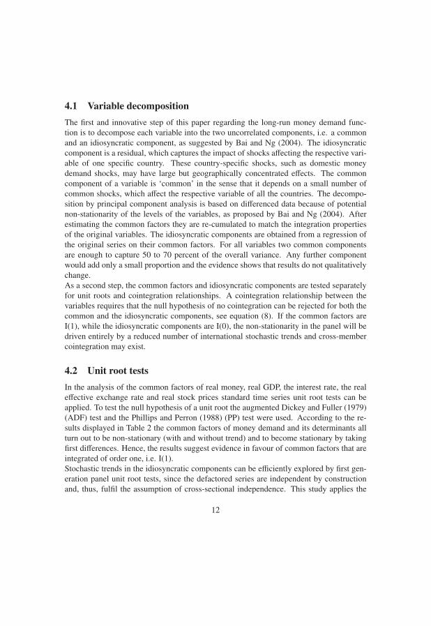
4.1 Variable decompositionThe first and innovative step of this paper regarding the long-run money demand func-

tion is to decompose each variable into the two uncorrelated components, i.e. a common

and an idiosyncratic component, as suggested by Bai and Ng (2004). The idiosyncratic

component is a residual, which captures the impact of shocks affecting the respective vari-

able of one specific country. These country-specific shocks, such as domestic money

demand shocks, may have large but geographically concentrated effects. The common

component of a variable is ‘common’ in the sense that it depends on a small number of

common shocks, which affect the respective variable of all the countries. The decompo-

sition by principal component analysis is based on differenced data because of potential

non-stationarity of the levels of the variables, as proposed by Bai and Ng (2004). After

estimating the common factors they are re-cumulated to match the integration properties

of the original variables. The idiosyncratic components are obtained from a regression of

the original series on their common factors. For all variables two common components

are enough to capture 50 to 70 percent of the overall variance. Any further component

would add only a small proportion and the evidence shows that results do not qualitatively

change.

As a second step, the common factors and idiosyncratic components are tested separately

for unit roots and cointegration relationships. A cointegration relationship between the

variables requires that the null hypothesis of no cointegration can be rejected for both the

common and the idiosyncratic components, see equation (8). If the common factors are

I(1), while the idiosyncratic components are I(0), the non-stationarity in the panel will be

driven entirely by a reduced number of international stochastic trends and cross-member

cointegration may exist.

4.2 Unit root testsIn the analysis of the common factors of real money, real GDP, the interest rate, the real

effective exchange rate and real stock prices standard time series unit root tests can be

applied. To test the null hypothesis of a unit root the augmented Dickey and Fuller (1979)

(ADF) test and the Phillips and Perron (1988) (PP) test were used. According to the re-

sults displayed in Table 2 the common factors of money demand and its determinants all

turn out to be non-stationary (with and without trend) and to become stationary by taking

first differences. Hence, the results suggest evidence in favour of common factors that are

integrated of order one, i.e. I(1).

Stochastic trends in the idiosyncratic components can be efficiently explored by first gen-

eration panel unit root tests, since the defactored series are independent by construction

and, thus, fulfil the assumption of cross-sectional independence. This study applies the

12

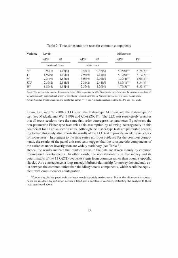
Table 2: Time series unit root tests for common components

Variable Levels Differences

ADF PP ADF PP ADF PP

without trend with trend

Mc -0.99(1) -1.03[5] -0.54(1) -0.46[5] -5.75(0)∗∗∗ -5.78[3]∗∗∗Yc -1.97(9) -1.10[5] -2.94(9) -2.12[5] -5.12(0)∗∗∗ -5.12[3]∗∗∗Rc -2.34(9) -1.67[5] -3.06(9) -2.01[5] -4.32(4)∗∗∗ -6.66[4]∗∗∗EXc -2.39(2) -2.51[5] -2.36(2) -2.44[5] -5.89(1)∗∗∗ -8.34[4]∗∗∗Wc -1.89(4) -1.96[4] -2.37(4) -2.29[4] -4.79(3)∗∗∗ -8.35[4]∗∗∗

Notes: The superscript c denotes the common factor of the respective variable. Numbers in parentheses are the maximum numbers of

lag determined by empirical realisations of the Akaike Information Criterion. Numbers in brackets represents the automatic

Newey-West bandwidth selection using the Bartlett kernel. ∗∗∗, ∗∗ and ∗ indicate significance at the 1%, 5% and 10% levels.

Levin, Lin, and Chu (2002) (LLC) test, the Fisher-type ADF test and the Fisher-type PP

test (see Maddala and Wu (1999) and Choi (2001)). The LLC test restrictively assumes

that all cross-sections have the same first order autoregressive parameter. By contrast, the

non-parametric Fisher-type tests relax this assumption by allowing heterogeneity in this

coefficient for all cross-section units. Although the Fisher-type tests are preferable accord-

ing to that, this study also reports the results of the LLC test to provide an additional check

for robustness.5 In contrast to the time series unit root evidence for the common compo-

nents, the results of the panel unit root tests suggest that the idiosyncratic components of

the variables under investigation are widely stationary (see Table 3).

Hence, the results indicate that random walks in the data are driven mainly by common

international developments. In other words, the non-stationarity in real money and its

determinants of the 11 OECD countries stems from common rather than country-specific

shocks. As a consequence, a long-run equilibrium relationship for money demand may ex-

ist between the common rather than the idiosyncratic components, which would be equiv-

alent with cross-member cointegration.

5Conducting further panel unit root tests would certainly make sense. But as the idiosyncratic compo-

nents are residuals by definition neither a trend nor a constant is included, restricting the analysis to those

tests mentioned above.

13

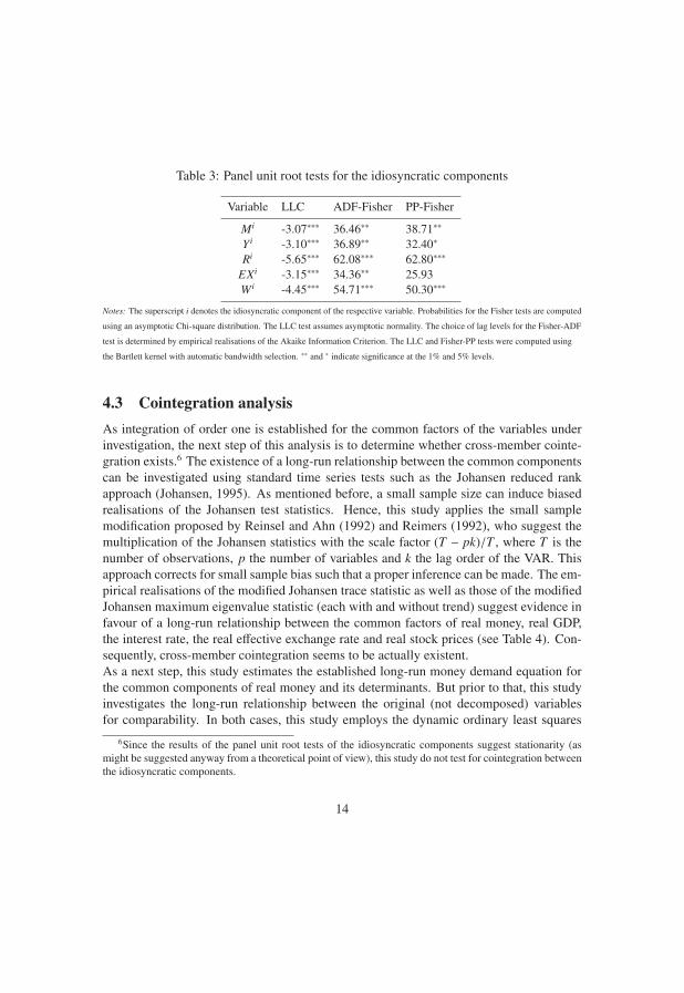
Table 3: Panel unit root tests for the idiosyncratic components

Variable LLC ADF-Fisher PP-Fisher

Mi -3.07∗∗∗ 36.46∗∗ 38.71∗∗Yi -3.10∗∗∗ 36.89∗∗ 32.40∗Ri -5.65∗∗∗ 62.08∗∗∗ 62.80∗∗∗

EXi -3.15∗∗∗ 34.36∗∗ 25.93

Wi -4.45∗∗∗ 54.71∗∗∗ 50.30∗∗∗

Notes: The superscript i denotes the idiosyncratic component of the respective variable. Probabilities for the Fisher tests are computed

using an asymptotic Chi-square distribution. The LLC test assumes asymptotic normality. The choice of lag levels for the Fisher-ADF

test is determined by empirical realisations of the Akaike Information Criterion. The LLC and Fisher-PP tests were computed using

the Bartlett kernel with automatic bandwidth selection. ∗∗ and ∗ indicate significance at the 1% and 5% levels.

4.3 Cointegration analysisAs integration of order one is established for the common factors of the variables under

investigation, the next step of this analysis is to determine whether cross-member cointe-

gration exists.6 The existence of a long-run relationship between the common components

can be investigated using standard time series tests such as the Johansen reduced rank

approach (Johansen, 1995). As mentioned before, a small sample size can induce biased

realisations of the Johansen test statistics. Hence, this study applies the small sample

modification proposed by Reinsel and Ahn (1992) and Reimers (1992), who suggest the

multiplication of the Johansen statistics with the scale factor (T − pk)/T , where T is the

number of observations, p the number of variables and k the lag order of the VAR. This

approach corrects for small sample bias such that a proper inference can be made. The em-

pirical realisations of the modified Johansen trace statistic as well as those of the modified

Johansen maximum eigenvalue statistic (each with and without trend) suggest evidence in

favour of a long-run relationship between the common factors of real money, real GDP,

the interest rate, the real effective exchange rate and real stock prices (see Table 4). Con-

sequently, cross-member cointegration seems to be actually existent.

As a next step, this study estimates the established long-run money demand equation for

the common components of real money and its determinants. But prior to that, this study

investigates the long-run relationship between the original (not decomposed) variables

for comparability. In both cases, this study employs the dynamic ordinary least squares

6Since the results of the panel unit root tests of the idiosyncratic components suggest stationarity (as

might be suggested anyway from a theoretical point of view), this study do not test for cointegration between

the idiosyncratic components.

14

Table 4: Results of Johansen’s tests for cointegration among common components

without trend with trend

H0 Trace Critical λ-max Critical Trace Critical λ-max Critical

Statistic Value Statistic Value Statistic Value Statistic Value

None 78,09∗ 76,97 45,53∗ 34,81 77,10∗ 69,82 44,70∗ 33,88

At most 1 32,56 54,08 12,44 28,59 32,41 47,86 12,37 27,58

At most 2 20,12 35,19 11,56 22,30 20,04 29,80 11,53 21,13

At most 3 8,56 20,26 5,52 15,89 8,51 15,49 5,51 14,26

At most 4 3,04 9,16 3,04 9,16 2,99 3,84 2,99 3,84

Notes: Potential small sample bias is corrected by multiplying the Johansen statistics with the scale factor (T − pk)/T , where T is the

number of observations, p the number of variables and k the lag order of the underlying VAR model in levels, see Reinsel and Ahn

(1992) and Reimers (1992). Critical values are taken from MacKinnon et al. (1999), and are also valid in case of the small sample

correction. A ∗ indicates the rejection of the null hypothesis of no cointegration at least at the 5% level of significance.

(DOLS) estimator proposed by Mark and Sul (2003) who also applied it to panel money

demand. The DOLS estimator corrects standard OLS for bias induced by endogeneity

and serial correlation. First, the endogenous variable in each equation is regressed on the

leads and lags of the first-differenced regressors from all equations to control for poten-

tial endogeneities. Then the OLS method is applied using the residuals from the first step

regression. The DOLS estimator is preferred to the non-parametric FMOLS estimator be-

cause of its better performance. According to Wagner and Hlouskova (2010), the DOLS

estimator outperforms all other studied estimators, both single equation estimators and

system estimators, even for large samples. Furthermore, Harris and Sollis (2003) suggest

that non-parametric approaches such as FMOLS are less robust if the data have significant

outliers and also have problems in cases where the residuals have large negative moving

average components, which is a fairly common occurrence in macro time series data.

First, the DOLS estimator is applied to the original variables to replicate the established

results of the literature on money demand. As a second step, this study presents the esti-

mation of the long-run relationship of the common components of the original variables.

The estimated models are:

Mi,t = αi + β1,iYi,t + β2,iRi,t + β3,iEXi,t + β4,iWi,t + εi,t, and (9)

Mci,t = αi + β1,iYc

i,t + β2,iRci,t + β3,iEXc

i,t + β4,iWci,t + ε

ci,t (10)

where i = 1, ...,N refers to each country in the panel and t = 1, ...,T denotes the time

period. αi represents the country-specific fixed effects and the superscript c in equation

(10) denotes the common components of the original variables. Since all variables, except

15

the interest rate, are specified in natural logarithms, the estimated long-run coefficients can

be interpreted as elasticities and as a semi-elasticity, respectively.

The estimated income elasticity of real money in equation (9) turns out to be 1.64 and sta-

tistically significant at the 1% level. The finding of an income elasticity greater than one

is a frequent finding in both time series and panel data studies on money demand. Regard-

ing the interest rate semi-elasticity, this study finds that larger opportunity cost of holding

money are connected with lower real balances. More precisely, the short-term interest rate

exerts a statistically significant impact on real money of -0.03 where the negative sign is

consistent with theory. In contrast, the estimated coefficient of the real effective exchange

rate has a positive sign (0.14), meaning that a real effective exchange rate appreciation

lowers domestic money demand. This pattern suggests that a possibly negative impact on

economic activity exceeds the impact of the income effect. Additionally, the statistical

significance justifies the inclusion of the exchange rate into the money demand function.

Furthermore, the statistically significant impact of real stock prices on real money under-

lines the importance of the inclusion of stock prices in modelling money demand. The

corresponding DOLS estimation reveals that a 1% increase in real stock prices decreases

money demand by 0.15%. Further, the estimated negative impact indicates that the nega-

tive substitution effect dominates the positive wealth effect, suggesting that a rise in asset

prices reduces the attractiveness of holding money compared to equities. A comparison

with the other panel data studies listed in Table 1 delivers sound evidence that our empiri-

cal results for the income elasticity and the interest rate semi-elasticity are actually within

the range of previous analyses and show signs that are consistent with money demand.

However, the finding that real stock prices are relevant determinants of money demand

contradicts those of Arnold and Roelands (2010) and Nautz and Rondorf (2010).

The estimated income elasticity of the common components of real money in equation

(10) turns out to be 1.02, close to unity and statistically significant at the 1% level. In fact,

a Wald F-test test cannot reject the null hypothesis that the income elasticity is equal to

one (F = 0.40 [0.53]). Hence, the value predicted by theory can be established by using

the common international factors of the variables under investigation. Dreger et al. (2007)

as the only further panel data study also supporting long-run income elasticities of money

demand using common components come up with similar results. Their estimated income

elasticities of the common components amount to 0.96 and 1.05. Further, the DOLS es-

timation of the study at hand reveals a coefficient of the common factors of real stock

prices which is again highly significant and negative. But this estimated coefficient of the

common factors with a value of -0.50 is absolutely larger than the coefficient of the origi-

nal stock prices (-0.15). In addition, the interest rate semi-elasticity also rises in absolute

terms compared to the previous result (-0.03) and takes a value of -0.71. Again the impact

of the interest rate on money demand is negative as anticipated. In contrast to the previous

16

result, the elasticity of real money to the real effective exchange rate is negative in the

case of the common components. This time, a 1% exchange rate appreciation increases

money demand by 0.32%. Thus, the exclusive consideration of the common components

without the idiosyncratic component of the underlying variables suggests that the positive

currency substitution effect dominates the negative impact on money demand. Moreover,

Dreger et al. (2007) also found a positive impact of the exchange rate on money demand.

The finding of the study at hand that the coefficients of the common components of the

interest rate and stock prices are larger than the coefficients of the original variables may

be due to highly integrated financial markets. The established cross-member cointegration

already indicates that the stochastic trends are common to all the countries. However, the

smaller income elasticity for the common components suggests that the national GDP still

plays a major role. Hence, the global business cycle seems not to be as relevant as the

international financial integration.

By means of an ADF unit root test this study verifies the stationarity of the established

cross-member cointegration relationship between the common components of real money,

real GDP, the interest rate, the real effective exchange rate and real stock prices (t =−2.98 [0.04]). Furthermore, the result of the Ramsey RESET test indicates that there are

no misspecifications of the long-run equation of the common components (F = 0.17 [0.68]).

At last, stability of the long-run coefficients of the common components of money demand

can be detected by recursive coefficient estimates. The stability property of any estimated

money demand relation is a critical requirement to ensure the usefulness of such a relation

for policy purposes. Figure 1 shows no significant variation in the estimated recursive co-

efficients as more data is added, suggesting that the long-run money demand coefficients

of the common components are stable. In addition, the CUSUM of squares test does not

indicate any instability of the residual variance, see Figure 2.

4.4 A panel error-correction modelHaving established a long-run relationship between the common factors, the next step is to

estimate a panel-based error-correction model to determine also the short-run coefficients

and the adjustment coefficient of money demand. A two-step procedure is applied. First,

this study employs the long-run equation specified in (10) to obtain the deviation from

the established long-run equilibrium of the common components, i.e. εci,t. Then the error-

correction model is estimated incorporating the one-period lagged residual from the first

step as dynamic error-correction term:

ΔMi,t = αi + γ1iΔYi,t + γ2iΔRi,t + γ3iΔEXi,t + γ4iΔWi,t + γ5iΔMi,t−1 + λiεci,t−1 + ui,t (11)

17

Figure 1: Results of recursive coefficient estimates - Long-run money demand in OECD

countries

18

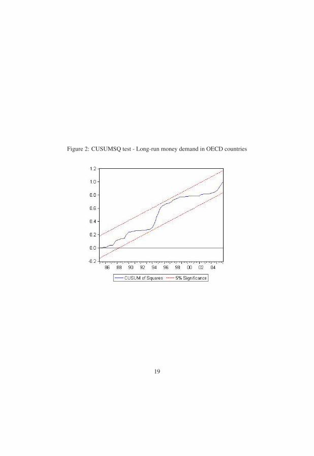
Figure 2: CUSUMSQ test - Long-run money demand in OECD countries

19

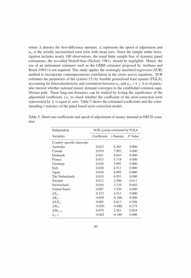
where Δ denotes the first-difference operator, λi represents the speed of adjustment and

ui,t is the serially uncorrelated error term with mean zero. Since the sample under inves-

tigation includes nearly 100 observations, the usual finite sample bias of dynamic panel

estimations, the so-called Nickell-bias (Nickell, 1981), should be negligible. Hence, the

use of an instrument estimator such as the GMM estimator proposed by Arellano and

Bond (1991) is not required. This study applies the seemingly unrelated regression (SUR)

method to incorporate contemporaneous correlation in the errors across equations. SUR

estimates the parameters of the system (15) by feasible generalised least squares (FGLS),

accounting for heteroskedasticity and correlation between ui,t and uj,t, i � j. It is of partic-

ular interest whether national money demand converges to the established common equi-

librium path. These long-run dynamics can be studied by testing the significance of the

adjustment coefficient, i.e. to check whether the coefficient of the error-correction term

represented by λi is equal to zero. Table 5 shows the estimated coefficients and the corre-

sponding t-statistics of the panel-based error-correction model.

Table 5: Short-run coefficients and speed of adjustment of money demand in OECD coun-

tries

Independent SUR system estimated by FGLS

Variables Coefficient t-Statistic P-Value

Country-specific intercept:

Australia 0.023 6.283 0.000

Canada 0.019 7.892 0.000

Denmark 0.021 6.663 0.000

France 0.013 5.718 0.000

Germany 0.018 5.991 0.000

Italy 0.020 6.511 0.000

Japan 0.018 8.092 0.000

The Netherlands 0.018 6.951 0.000

Sweden 0.012 2.560 0.011

Switzerland 0.016 3.139 0.002

United States 0.007 3.526 0.000

ΔYi,t 0.323 4.511 0.000

ΔRi,t -0.005 -6.368 0.000

ΔEXi,t 0.005 0.613 0.540

ΔWi,t -0.020 -0.888 0.375

ΔMi,t−1 0.070 2.261 0.024

εi,t−1 -0.002 -6.186 0.000

20

The estimated coefficients are small but display signs as expected from theory. Changes in

income and in the interest rate are estimated to have a highly significant positive (0.323)

and negative impact (-0.005) on money demand, respectively. The elasticities of changes

in the real effective exchange rate and the real stock prices are insignificant in the short

run. Given this result, the currency substitution hypotheses might hold only in the long

run. Furthermore, the estimated coefficient of the error-correction term is highly signif-

icant, validating the significance of the cointegration relationship of the common com-

ponents in the short-run model for money demand. Additionally, the significance of the

error-correction term indicates that money demand readjusts towards a common interna-

tional equilibrium relationship after a shock occurs. The equilibrium is ‘international’ in

the sense that the established long-run relationship is a cross-member cointegration rela-

tion and driven by common stochastic trends.

A comparison with the two further panel data studies applying an error-correction model

by Valadkhani (2008) and Nautz and Rondorf (2010) leads to the following conclusions.

First, their estimated short-run dynamics are also smaller than the long-run coefficients.

Second, Valadkhani (2008) supports that changes in the exchange rate are insignificant in

the short run and Nautz and Rondorf (2010) found an insignificant short-run coefficient

of stock prices as in this study. Third, the other short-run coefficients estimated in this

study are smaller compared to the other studies, except the impact of changes of lagged

real money which is within the range of both. The coefficient of the error-correction term

might be smaller in this analysis because it measures the speed of adjustment towards an

equilibrium relation between common factors but not to an overall equilibrium path. Real

money may adjust faster to an equilibrium relation which reflects long-run money de-

mand of not decomposed variables which in addition to the common factors also include

the country-specific idiosyncratic components and, thus, promise more power to explain

changes in real money.

5 ConclusionsThis paper studies the long-run money demand function for 11 OECD countries from

1983 to 2006 using panel data and including wealth. The applied factor decomposition

provides new empirical insights into the long-run relationship among money and its main

determinants. More precisely, the distinction between common factors and idiosyncratic

components allows to detect cross-member cointegration and to distinguish between in-

ternational and national developments as potential drivers of long-run money demand.

Indeed, the main empirical finding of this study is that cross-member cointegration is ex-

istent and, correspondingly, only the common components of real money, real GDP, the

21

interest rate, the real effective exchange rate and real stock prices are cointegrated. This

result highlights the relevance of international developments to explain money demand.

Hence, policy makers should incorporate cross-country dependencies and international

impacts on money demand when designing sensible monetary policy to achieve price sta-

bility.

A deeper analysis of the cointegration relationships of (a) the variables under investigation

and (b) their common components suggests that the estimated coefficients of the former

are within the range of previous panel data studies. The established signs of the income

and interest rate (semi-)elasticities are consistent with theoretical postulates in both mod-

els. Moreover, the significant negative impact of wealth, represented by stock prices,

indicates its importance as determinant of real balances and that the negative substitution

effect on money demand dominates the positive wealth effect. However, the relations (a)

and (b) differ in the coefficients of the ‘financial’ variables, the interest rate and the real

stock prices, which are larger for the common components. This result highlights that

especially the financial markets are highly integrated, since the established cross-member

cointegration already indicates a close relation of money and its determinants across the 11

OECD countries. By contrast, the long-run income elasticity of the common components

of money demand is smaller than the income elasticity of the original (not decomposed)

money demand. Hence, the global business cycle does not seem to be as relevant as the

international financial integration.

What is more, the stability of the long-run money demand coefficients of the common

components can be confirmed by recursive coefficient estimates. This finding is a criti-

cal requirement to ensure the usefulness of such a relation for policy purposes. Hence, the

long-run money demand relationship between the common components, the cross-member

cointegration relation, seems to be a useful reference for monetary policy. Accordingly,

the common components of the domestic money stocks may help to reliably identify risks

to price stability in addition to the domestic money stocks themselves.

Moreover, this paper presents a panel-based error-correction model capturing the short-

run coefficients of money demand and, more interestingly, the adjustment coefficient. The

estimated short-run coefficients for money demand turn out to be smaller than the long-run

elasticities and statistically insignificant for the exchange rate and stock prices. Since the

residual of the long-run equilibrium relation between the common components is used as

dynamic error-correction term, its determined significance means that money adjusts to an

international rather than a national equilibrium relationship.

22

ReferencesArellano, M. and S. Bond (1991). Some tests of specification for panel data: Monte

Carlo evidence and an application to employment equations. Review of Economic Stud-ies 58(2), 277–297.

Arnold, I. J. and S. Roelands (2010). The demand for euros. Journal of Macroeco-nomics 32(2), 674–684.

Bai, J. and S. Ng (2004). A PANIC attack on unit roots and cointegration. Economet-rica 72, 1127–1177.

Banerjee, A., M. Marcellino, and C. Osbat (2004). Some cautions on the use of panel

methods for integrated series of macroeconomic data. Econometrics Journal 7(2), 322–

340.

Belke, A., C. Dreger, and F. de Haan (2010). Energy consumption and economic growth:

New insights into the cointegration relationship. Ruhr Economic Papers No. 190.

Boone, L. and P. van den Noord (2008). Wealth effects on money demand in the euro area.

Empirical Economics 34(3), 525–536.

Bruggeman, A. (2000). The stability of EMU-Wide money demand functions and the

monetary policy strategy of the European Central Bank. Manchester School 68(2),

184–202.

Campbell, J. Y. and P. Perron (1991). Pitfalls and opportunities: What macroeconomists

should know about unit roots. In O. J. Blanchard and S. Fisher (Eds.), NBER Macroe-conomics Annual, Volume 6, pp. 141–220. Cambridge: MIT Press.

Choi, I. (2001). Unit root tests for panel data. Journal of International Money and Fi-nance 20(2), 249–272.

Choudhry, T. (1996). Real stock prices and the long-run money demand function: Evi-

dence from canada and the USA. Journal of International Money and Finance 15(1),

1–17.

de Bondt, G. J. (2009). Euro area money demand - Empirical evidence on the role of

equity and labour markets. ECB Working Paper No. 1086.

de Santis, R. A., C. A. Favero, and B. Roffia (2008). Euro area money demand and

international portfolio allocation - A contribution to assessing risks to price stability.

ECB Working Paper No. 926.

23

Dickey, D. A. and W. A. Fuller (1979). Distribution of the estimators for autoregressive

time series with a unit root. Journal of the American Statistical Association 74(366),

427–431.

Dreger, C., H. Reimers, and B. Roffia (2007). Long-run money demand in the new EU

member states with exchange rate effects. Eastern European Economics 45(2), 75–94.

Dreger, C. and J. Wolters (2010). Investigating m3 money demand in the euro area. Journalof International Money and Finance 29(1), 111–122.

Elbadawi, I. A. and K. Schmidt-Hebbel (2007). The demand for money around the end of

civil wars. The World Bank. Available at http://siteresources.worldbank.org.

Ericsson, N. R. (1998). Empirical modeling of money demand. Empirical Eco-nomics 23(3), 295–315.

Fidrmuc, J. (2009). Money demand and disinflation in selected CEECs during the acces-

sion to the EU. Applied Economics 41(10), 1259–1267.

Friedman, M. (1970). A theoretical framework for monetary analysis. Journal of PoliticalEconomy 78, 293–238.

Friedman, M. (1988). Money and the stock market. Journal of Political Economy 96,

221–245.

Garcia-Hiernaux, A. and L. Cerno (2006). Empirical evidence for a money demand func-

tion: A panel data analysis of 27 countries in 1988-98. Applied Econometrics andInternational Development 6(1).

Gengenbach, C., F. C. Palm, and J.-P. Urbain (2006). Cointegration testing in panels with

common factors. Oxford Bulletin of Economics and Statistics 68, 683–719. Supplement.

Hamori, S. (2008). Empirical analysis of the money demand function in Sub-Saharan

Africa. Economics Bulletin 15(4), 1–15.

Hamori, S. and N. Hamori (2008). Demand for money in the Euro area. Economic Sys-tems 32(3), 274–284.

Harb, N. (2004). Money demand function: a heterogeneous panel application. AppliedEconomics Letters 11(9), 551–555.

Harris, R. I. D. and R. Sollis (2003). Applied time series modelling and forecasting.

Chichester: J. Wiley.

24

Johansen, S. (1995). Likelihood-based inference in cointegrated vector autoregressivemodels. Oxford: Oxford University Press.

Knell, M. and H. Stix (2005). The income elasticity of money demand: A meta-analysis

of empirical results. Journal of Economic Surveys 19(3), 513–533.

Knell, M. and H. Stix (2006). Three decades of money demand studies: Differences and

similarities. Applied Economics 38(7), 805–818.

Kumar, S. (2010). Panel data estimates of the demand for money in the pacific island

countries. EERI Research Paper Series No. 2010-12.

Kumar, S., M. Chowdhury, and B. B. Rao (2010). Demand for money in the selected

OECD countries: A time series panel data approach and structural breaks. MPRA Pa-per No. 22204.

Laidler, D. E. (1993). The Demand for Money: Theories, Evidence and Problems (4 ed.).

New York: Harper Collins College Publishers.

Levin, A., C. Lin, and C. J. Chu (2002). Unit root tests in panel data: Asymptotic and

finite-sample properties. Journal of Econometrics 108(1), 1–24.

MacKinnon, J. G., A. A. Haug, and L. Michelis (1999). Numerical distribution functions

of likelihood ratio tests for cointegration. Journal of Applied Econometrics 14(5), 563–

577.

Maddala, G. S. and S. Wu (1999). A comparative study of unit root tests with panel data

and a new simple test. Oxford Bulletin of Economics and Statistics 61, 631–52.

Mark, N. C. and D. Sul (2003). Cointegration vector estimation by panel DOLS and long-

run money demand. Oxford Bulletin of Economics and Statistics 65(5), 655–680.

Narayan, P., S. Narayan, and V. Mishra (2009). Estimating money demand functions for

South Asian countries. Empirical Economics 36(3), 685–696.

Nautz, D. and U. Rondorf (2010). The (in)stability of money demand in the Euro Area:

Lessons from a cross-country analysis. SFB 649 Discussion Papers No. 2010-023.

Nickell, S. J. (1981). Biases in dynamic models with fixed effects. Applied Eco-nomics 49(6), 1417–1426.

Pedroni, P. (1999). Critical values for cointegration tests in heterogeneous panels with

multiple regressors. Oxford Bulletin of Economics and Statistics 61, 653–670.

25

Pedroni, P. (2004). Panel cointegration, asymptotic and finite sample properties of pooled

time series tests with an application to the PPP hypothesis. Econometric Theory 20,

597–625.

Phillips, P. C. B. and P. Perron (1988). Testing for a unit root in time series regression.

Biometrika 75(2), 335–346.

Poole, W. (1970). Optimal choice of monetary policy instruments in a simple stochastic

macro model. Quarterly Journal of Economics 84(2), 197–216.

Rao, B. B. and S. Kumar (2009). A panel data approach to the demand for money and the

effects of financial reforms in the Asian countries. Economic Modelling 26(5), 1012–

1017.

Rao, B. B., A. Tamazian, and P. Singh (2009). Demand for money in the Asian countries:

A systems GMM panel data approach and structural breaks. MPRA Paper No. 15030.

Reimers, H. (1992). Comparisons of tests for multivariate cointegration. Statistical Pa-pers 33(1), 335–359.

Reinsel, G. C. and S. K. Ahn (1992). Vector autoregressive models with unit roots and

reduced rank structure: Estimation, likelihood ratio test, and forecasting. Journal ofTime Series Analysis 13(4), 353–375.

Setzer, R. and C. Greiber (2007). Money and housing: Evidence for the euro area and the

US. Deutsche Bundesbank Discussion Paper 12/2007.

Setzer, R. and G. B. Wolff (2009). Money demand in the euro area: New insights from

disaggregated data. MPRA Paper No. 17483.

Urbain, J. and J. Westerlund (2006). Spurious regression in nonstationary panels with

Cross-Unit cointegration. METEOR Research Memoranda No. 057.

Valadkhani, A. (2006). What determines the demand for money in the Asian-Pacific coun-

tries? An empirical panel investigation. Faculty of Commerce - Economics WorkingPapers 06-11. University of Wollongong.

Valadkhani, A. (2008). Long- and short-run determinants of the demand for money in the

Asian-Pacific Countries: An empirical panel investigation. Annals of Economics andFinance 9, 77–90.

26

Valadkhani, A. and M. Alauddin (2003). Demand for M2 in developing countries: An

empirical panel investigation. School of Economics and Finance Discussion Paper No.149. Queensland University of Technology.

Wagner, M. and J. Hlouskova (2010). The performance of panel cointegration methods:

Results from a large scale simulation study. Econometric Reviews 29(2), 182–223.

27