
Recent Results of LHCD Coupling Experiments with Near Gas ...

Magnetic coupling in (GaMn)As ferromagneticsemiconductors - studied by soft x-ray
spectroscopy
vorgelegt vonDiplom PhysikerFlorian Kronast
von der Fakultat II - Mathematik und Naturwissenschaften
der Technischen Universitat Berlinzur Erlangung des akademischen Grades
Doktor der Naturwissenschaften- Dr.rer.nat. -
genehmigte Dissertation
Promotionsausschuss:
Vorsitzender: Prof. Dr. E. Sedlmayr
Berichter: Prof. Dr. W. EberhardtProf. Dr. W. Thomsen
Tag der wissenschaftlichen Aussprache 20. Dezember 2005
Berlin 2006
D 83

2
.
Dedicated to my family
Contents
1 Introduction 1
2 Soft x-ray absorption spectroscopy 5
2.1 The dipole transition . . . . . . . . . . . . . . . . . . . . . . . . . 62.1.1 X-ray magnetic circular dichroism . . . . . . . . . . . . . . 7
2.2 Analysis of XAS and XMCD spectra . . . . . . . . . . . . . . . . 112.2.1 Sum rules . . . . . . . . . . . . . . . . . . . . . . . . . . . 112.2.2 Multiplet structure . . . . . . . . . . . . . . . . . . . . . . 14
3 Ferromagnetism in dilute magnetic semiconductors 17
3.1 Introduction . . . . . . . . . . . . . . . . . . . . . . . . . . . . . . 173.2 Magnetic ordering in dilute magnetic semiconductors . . . . . . . 18
3.2.1 Zener model . . . . . . . . . . . . . . . . . . . . . . . . . . 183.2.2 RKKY coupling . . . . . . . . . . . . . . . . . . . . . . . . 193.2.3 Magnetic polarons . . . . . . . . . . . . . . . . . . . . . . 203.2.4 Double exchange . . . . . . . . . . . . . . . . . . . . . . . 21
3.3 Magnetic anisotropy . . . . . . . . . . . . . . . . . . . . . . . . . 22
4 Experimental considerations 25
4.1 Sample preparation . . . . . . . . . . . . . . . . . . . . . . . . . . 254.1.1 Annealing . . . . . . . . . . . . . . . . . . . . . . . . . . . 26
4.2 Experimental setup . . . . . . . . . . . . . . . . . . . . . . . . . . 264.3 Data recording . . . . . . . . . . . . . . . . . . . . . . . . . . . . 28
4.3.1 Total electron yield . . . . . . . . . . . . . . . . . . . . . . 284.3.2 Fluorescence yield . . . . . . . . . . . . . . . . . . . . . . . 284.3.3 Self absorption effects . . . . . . . . . . . . . . . . . . . . 30
4.4 Resonant reflectivity . . . . . . . . . . . . . . . . . . . . . . . . . 34
5 Chemical and magnetical depth profile of Ga1−xMnxAs films 39
5.1 Experimental results . . . . . . . . . . . . . . . . . . . . . . . . . 405.1.1 Surface magnetization deficit . . . . . . . . . . . . . . . . . 405.1.2 Chemical depth profile probed by resonant x-ray reflectivity 45
5.2 Discussion . . . . . . . . . . . . . . . . . . . . . . . . . . . . . . . 50
3

CONTENTS i
5.3 Conclusion . . . . . . . . . . . . . . . . . . . . . . . . . . . . . . . 53
6 Mn 3d hybridization 55
6.1 Influence of the surface . . . . . . . . . . . . . . . . . . . . . . . . 556.2 pd-hybridization of ferromagnetically coupled Mn . . . . . . . . . 576.3 Saturation magnetization . . . . . . . . . . . . . . . . . . . . . . . 606.4 Evidence for antiferromagnetic coupling of Mn . . . . . . . . . . . 626.5 Discussion . . . . . . . . . . . . . . . . . . . . . . . . . . . . . . . 666.6 Conclusion . . . . . . . . . . . . . . . . . . . . . . . . . . . . . . . 67
7 Orbital magnetic moment anisotropy 69
7.1 Introduction . . . . . . . . . . . . . . . . . . . . . . . . . . . . . . 697.2 Results . . . . . . . . . . . . . . . . . . . . . . . . . . . . . . . . . 69
7.2.1 Orbital magnetic moment anisotropy . . . . . . . . . . . . 697.2.2 Angular dependence the of ground state hybridization . . . 71
7.3 Discussion and conclusions . . . . . . . . . . . . . . . . . . . . . . 737.4 Outlook . . . . . . . . . . . . . . . . . . . . . . . . . . . . . . . . 76
8 Summary 81
Bibliography 84
Danksagung 91
.
Chapter 1
Introduction
ferromagnetic semiconductors a new material class designed for
spintronic applications
The term ”spintronics” refers to electronic devices that utilize not only the chargeof the carriers but also their magnetic moment the so called spin. The huge po-tential of this combination was impressively demonstrated by the discovery ofthe giant magneto resistance (GMR) effect in 1988. The GMR effect exploits thespin dependent scattering of conduction electrons in a structure of two ferromag-netic layers separated by a non magnetic spacer layer [75, 76]. Depending on itsmagnetic direction, a single-domain magnetic material will scatter electrons with”up” or ”down” spin differently. Thus electrons become spin polarized if theypass through a magnetic layer. When the two magnetic layers in GMR structuresare aligned anti-parallel, the resistivity is high because conduction electrons po-larized by the first magnetic layer will find a reversed magnetization direction ifthey enter the second magnetic layer and undergo additional spin-flip scattering[76]. When the layers are aligned in parallel less spin flip scattering occurs, yield-ing a lower resistance of the GMR structure [76]. Today the effect is widely usedin magnetic sensors and read heads for hard drives. It is a prominent example forthe benefit of industrial applications from fundamental research. The interest toincorporate such effects in integrated circuits, e.g. as magneto resistive randomaccess memory devices, is huge. But the implementation is hampered by thechoice of the right material. Electronic devices are mainly made of semiconduc-tors whereas only transition metals or rare earth metals show ferromagnetism e.g.spontaneous magnetic ordering with a net spin polarization. It is rather difficultto combine these two material classes in functional heterostructures [77]. On theone hand metal films can not easily be integrated in the production process ofsemiconductor plants on the other hand the injection of spin polarized carriersacross a metal-semiconductor interface is rather inefficient. The large differencein the density of states and the resulting band structure will cause scattering atthe interface that destroys the spin polarization [77].
1
2 Introduction
This explains why the discovery of ferromagnetism in III − V and II − V Idilute magnetic semiconductors (DMS) attracted such a large interest. These sys-tems are promising candidates for spintronic devices since the above describedinterface problem is avoided in a very elegant way. Spin polarized carriers areprovided by magnetic ions integrated in the semiconductor host matrix. Exper-iments performed on DMS so far show new and fascinating physical propertiesthat have not been observed in other systems yet. It has been demonstrated thatthe magnetic properties can be changed isothermally by light or electric fields in(In,Mn)As/(Al,Ga)Sb heterostructures [30]. The anisotropy in Ga1−xMnxAs canbe tailored by the choice of temperature and carrier concentration [54]. Also spininjection from Ga1−xMnxAs into a (InGa)As has been demonstrated. Unfortu-nately up to now all dilute magnetic semiconductor materials suffer from a Curietemperature far below room temperature. At the moment the world record Curietemperature for Ga1−xMnxAs is at 173K [83]. But nevertheless these materialsare an ideal test ground to study the interplay of quantization effects, magnetism,carrier dynamics and transport properties. The prospects of spintronic devicesthat allow to incorporate data processing and storage in a single chip is morethan encouraging. Thus the community investigating the magnetic properties ofDMS’s is steadily growing.
In this thesis the origin of the ferromagnetic ordering in Ga1−xMnxAs , themost prominent member of the III − V series of ferromagnetic DMS, is investi-gated by x-ray spectroscopy (XAS) in combination with x-ray magnetic circulardichroism (XMCD). The ferromagnetism in (Ga1−xMnx)As is based on two coop-erative effects caused by replacing the trivalent Ga atoms with Mn. Mn providesa local spin magnetic moment and as an acceptor it creates itinerant holes, whichmediate the long range ferromagnetic order [1]. But despite the existence ofvarious theoretical models the physics underlying the magnetic properties is stillunder discussion [2, 3]. This is partially due to the high degree of dissorder inthese systems caused by the limited solubility of Mn. The formation of As an-tisites and interstitial Mn were predicted [4]. Both defects act as double donorspartially compensating the effect of the Mn acceptors [4]. For the understandingof the ferromagnetic ordering the electronic configuration of the Mn impuritiesand the number of Mn atoms contributing to the long range ferromagnetic orderare of major interest. These parameters can be probed directly by x-ray ab-sorption spectroscopy (XAS) and x-ray magnetic circular dichroism (XMCD). Atthe Mn 2p - 3d resonance the XAS and MXCD line shapes are characteristic forthe Mn 3d electronic and magnetic ground state configuration respectively [51].This is a major advantage of the x-ray spectroscopy compared to the widely usedSQUID measurements.
This work starts with a short introduction to the principles of x-ray absorptionspectroscopy. In the following chapter we give an overview on the various theoret-ical models describing the origin of ferromagnetic coupling in Ga1−xMnxAs. Afterpresenting the experimental details the chemical and magnetic depth profiles of

3
different Ga1−xMnxAs layers are investigated. The main question at this point isthe diffusion of interstitial Mn during the growth and annealing process and itsinfluence on the ferromagnetic coupling. The signature of Mn 3d5-3d6 mixed va-lence acceptor states responsible for long-range ferromagnetic order is identifiedwith x-ray magnetic circular dichroism at all Mn concentrations. In chapter 6 wedemonstrate that an additional non-ferromagnetic Mn species with an electroncount close to 3d4 is observed at high Mn concentrations. We discuss a modelin which the latter is due to Mn-Mn antiferromagnetic nearest neighbor pairs.The last chapter deals with the orbital magnetic moment anisotropy presentin Ga1−xMnxAs films. The microscopic origin of the orbital magnetic momentanisotropy is probed by x-ray magnetic circular dichrosim spectroscopy. It pro-vides first evidence for an anisotropic pd-hybridization and, therefore, anisotropicexchange coupling.

4 Introduction
Chapter 2
Soft x-ray absorption
spectroscopy
The fundamental interactions of x-rays with matter are the photoelectric ab-sorption, scattering processes like Thompson (elastic) and Compton (inelastic)scattering and the formation of electron positron pairs (above a threshold of 1,022MeV photon energy). In the regime of soft x-rays (below 10keV photon energy)the cross section of photoelectric absorption is two to three orders of magnitudelarger than that of the scattering processes. This effect refers to the absorptionof an incoming photon by a core electron exciting the electron to a bound stateor into the continuum if the photon energy is higher than the binding energyand the work function of the solid. The photoelectric effect was discovered byHeinrich Hertz in 1887 and could not be explained within the classical theoryat this time. Albert Einstein succeeded to explain the photoelectric effect bythe quantum nature of light and received in 1921 the Nobel price for his find-ings. Today the photoelectric effect is one of the most popular tools to studythe electronic structure in solid state and surface science. Measuring the x-rayabsorption coefficient as a function of photon energy near the absorption edge ofthe element of interest is a widely used technique to obtain information on thechemical environment of the probed element, its valency, its spin state and so on.Synchrotron sources like BESSY provide soft x-rays at high brilliance, an energyresolution below 0.2eV and with full polarization control. The latter is especiallyimportant for the analysis of magnetic samples by x-ray spectroscopy. Similarto the Faraday-Kerr effect in the optical regime, the x-ray absorption coefficientfor polarized x-rays depends on the magnetization vector which also allows tostudy magnetic properties by x-ray spectroscopy. The most popular effect is thex-ray magnetic circular dichroism (XMCD) i.e. the difference of the x-ray ab-sorption coefficient between two helicities of a circular polarized incident photonbeam. The combination of x-ray absorption spectroscopy and x-ray magnetic cir-cular dichroism is ideally suited to study the 3d shell of transition metals like Nior Mn since electronic configuration and magnetic moments can be investigated
5
6 Soft x-ray absorption spectroscopy
simultaneously.
2.1 The dipole transition
The absorption cross section σ is defined as the number of excited electrons pertime unit divided by the photon flux Iph:
σ(E) =
∑
i,f Wi→f
Iph(2.1)
Whereby Wi→f denotes the probability per unit time to promote a core electronfrom the initial state |i > into the final state < f | by the absorption of a photonof the energy E = hω. This transition probability is given by Fermi’s golden rule.It describes the transition probability from the initial state |i > in to the finalstate < f | under the influence of the perturbation H ′ as
Wi→f =2π
h| < f |H ′|i > |2δ(Ef − Ei − hω). (2.2)
The δ- function represents the energy conservation; transitions are only possibleif the energy interval between initial and final state corresponds to the energy ofthe absorbed photon. The electromagnetic field of the photons can be describedby the vector potential A(r, t) = A0εe
i(ky−ωt) in terms of an electromagneticplane wave. With the wave vector k, frequency ω and the polarization vectorε. ε0 corresponds to linear and ε−1 (ε+1) to left (right) circular polarization witha polarization vector ε+1 = 1/
√2(εx + iεy) (ε−1 = 1/
√2(εx − iεy) ). Circular
polarized photons carry an angular momentum which is parallel (antiparallel) tothe wave vector k for left (right) circular polarization. The Hamiltonian becomes[38]
H =1
2m[P− e
cA(r, t)]2 + V (r)− e
mcS · (∇×A(r, t)). (2.3)
The last term describes the interaction of the magnetic moment of the electronswith the oscillating field of the electromagnetic wave. A decomposition in theundisturbed Hamiltonian of the atom and the perturbation results in:
H = H0 −e
mcP ·A(r, t)
︸ ︷︷ ︸
HI
− e
mcS · (∇×A(r, t))
︸ ︷︷ ︸
HII
+e2
2mc2A2(r, t)
︸ ︷︷ ︸
HIII
(2.4)
In a first order approximation the term quadratic in A can be neglected. Thematrix elements of term II are in the order of h ·kA0 and compare to those of theterm I like the impulse if the absorbed photon to the momentum of the electron:
HII
HI
≈ hk
p� 1. (2.5)
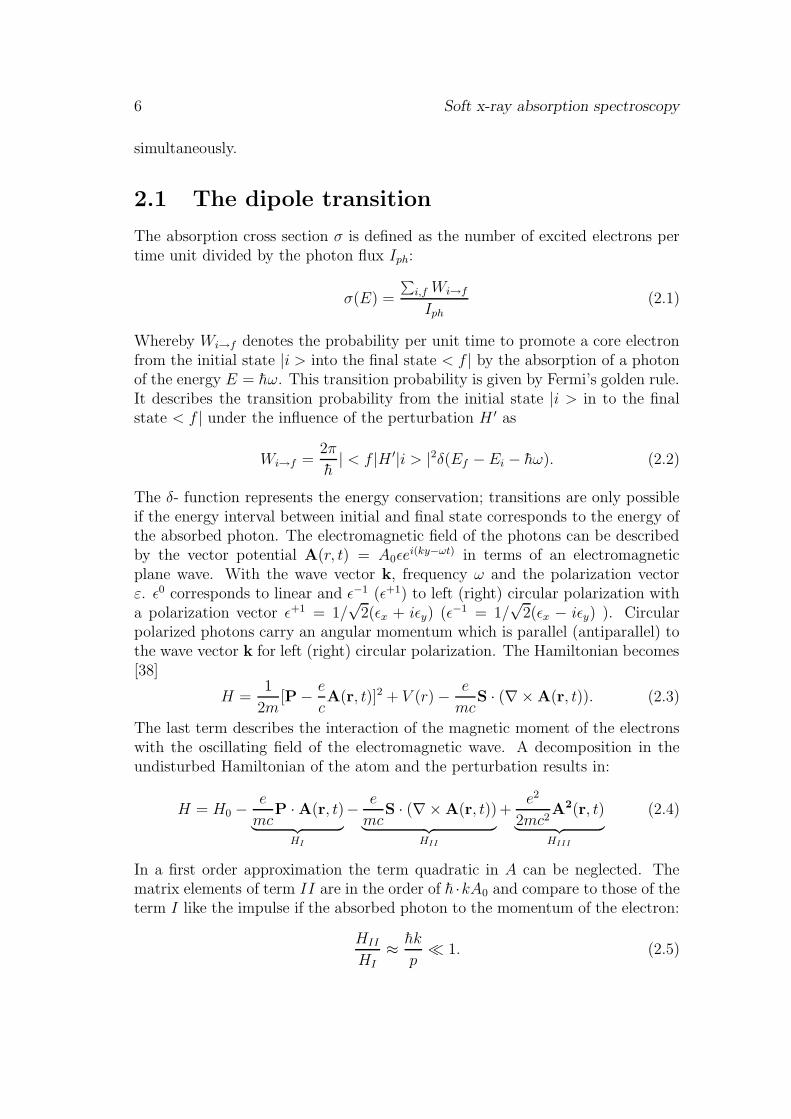
2.1 The dipole transition 7
In the energy range below 1000eV that we are interested in the momentum of thephoton can be neglected. In this approximation the transition probability can beexpressed by a dipole transition:
Wi→f =2π
h
e
mc| < f |A ·P|i > |2δ(Ef − Ei − hω). (2.6)
According to the Wigner-Eckart theorem the dipole selection rules for linearpolarized light are:
∆j = 0,±1; ∆l = ±1; ∆m = 0; ∆s = 0. (2.7)
And for circular polarized light:
∆j = 0,±1; ∆l = ±1; ∆m = ±1; ∆s = 0. (2.8)
By the selection rules we find that the dipole transitions are spin conservativeand orbital selective as ∆m is determined by the polarization of the photon(∆m = 1 (−1) for left circular (right circular) polarization. The total absorp-tion cross section in the dipole approximation is given by the sum of all initialand final states. With the incident photon flux written as the energy flux of
the electromagnetic field divided by the photon energy Iph =E2
0c
2πhω=
A20ω
2πhc, the
photoabsorption cross section in the dipole approximation reads:
σ(hω) = 4π2αhω∑
i,f
| < f |ε · r|i > |2δ(Ef − Ei − hω). (2.9)
Whereby α is the fine structure constant (α = 1/137). The electronic and mag-netic properties of the transition metals are determined by the occupation of the3d shell. Such they are ideally accessible to soft x-ray spectroscopy at the 2p−3dresonance. But the conservation of orbital angular momentum (∆l = ±1) allowstransitions from the 2p level into 3d as well as into 4s states. The absorptioncross section that we measure at the 2p − 3d resonance is, therefore, a mixtureof two transition channels as shown in Fig. 2.1. Transitions into continuum 4sstates cause a step like background whereas the intensity of the resonance peaksin the absorption spectrum is proportional to the unoccupied 3d states.
2.1.1 X-ray magnetic circular dichroism
The x-ray magnetic circular dichroism (XMCD) is defined as the difference inthe absorption cross section between left and right circularly polarized x-raylight with the wave vector k parallel to the magnetization M (the x-ray helicityε± is collinear with the propagation direction). This effect is the analogue tothe magneto optical Faraday effect in the soft x-ray regime. In 1845 Faradaydiscovered a rotation of the polarization vector of linearly polarized light upon

8 Soft x-ray absorption spectroscopy
Figure 2.1: X-ray absorption spectra recorded at the Mn L3 / L2 edges of aGa1−xMnxAs sample. The resonance peaks are due to transitions in unoccupied3d levels as indicated by the inset. Transition into continuum states (representedby the parabola) cause a step-like background.
2.1 The dipole transition 9
the transmission through silicon borate in an applied magnetic field. Due tothe exchange spitted valence states the absorption coefficient for the two circularcomponents of the incident light is different. This effect also causes a rotation ofthe linear polarization into elliptically polarized light after the transmission.
The XMCD effect occurring at the L3 and L2 edge of 3d transition metalscan be explained within a qualitative picture. The circular polarized photon getsabsorbed generating a hole in the 2p shell. The p states are split into the 2p3/2
and 2p1/2 level by the spin orbit interaction. This interaction couples the spin ofthe 2p electrons to the orbital moment. At the 2p3/2 and the 2p1/2 level the orbitalangular momentum l and the spin angular momentum s are coupled parallel andantiparallel, respectively. The spin-orbit coupling allows to excite electrons ofthe 2p shell by circular polarized light spin selective into the valence shell even ifthe dipole operator does not act on the spin. The spin polarization arises fromthe selction rule for the orbital magnetic moment depending on the polarizationon the absorbed x-ray photon. Because of the parallel coupling of l and s at the2p3/2 level and the antiparallel at the 2p1/2 level, transitions from the 2p3/2 andthe 2p1/2 levels into the valence shell occur with different spin polarization.
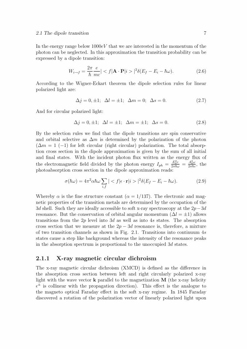
Possible final states for the photoexcitation are the unoccupied 3d and 4sstates above the Fermi level. The dipole transition is spin conservative whichmeans that and spin up electron can only be promoted in to a spin up emptystate and vice versa. In a ferromagnetic transition metal there is an imbalanceof unoccupied spin-up and spin-down states in the d-band due to the exchangecoupling (Stoner model). If the orientation of the magnetization M is parallel tothe photon wave vector k this imbalance of empty d-states leads to a spin selec-tive excitation process, i.e. the probability of an electron transition excited by acircular polarized photon is proportional to the unoccupied d-states. It causes anasymmetry in the absorption cross sections for left and right circular polarizedlight which is proportional to the difference in the unoccupied spin-up and spin-down states, i.e. the spin magnetic moment. But the photoelectron also probesthe orbital magnetic moment of the valence band. Due to the conservation ofangular momentum the change in the quantum number m is determined by thepolarization of the photon. Left circular polarized photons with the magneticmoment +h can cause only transitions with ∆m = 1 and accordingly right circu-lar polarized photons can cause only transitions with ∆m = −1. If the valencestates with quantum numbers ±ml are unequally occupied the absorption of pho-tons with opposite helicity will be different. An example of the XMCD effect isgiven in Fig. 2.2. For a magnetically almost saturated Ga1−xMnxAs sample at10K we find a huge difference between the absorption spectra recorded with leftand right circular polarized x-rays. The XMCD signal changes sign between theL3 and L2 edge because of the parallel and antiparallel coupling of l and s at the2p1/2 and 2p3/2 levels, respectively.
10 Soft x-ray absorption spectroscopy
Figure 2.2: The upper panel displays x-ray absorption spectra recorded at theMn 2p − 3d resonance exciting with left (blue line) and right (red line) circularpolarized x-rays. The sample was a Ga1−xMnxAs (x=0.017) at 10K and in 4Texternal magnetic field. A schematic picture of the absorption process is given inthe inset. The lower panel shows the XMCD spectrum (difference spectrum).

2.2 Analysis of XAS and XMCD spectra 11
2.2 Analysis of XAS and XMCD spectra
2.2.1 Sum rules
The sum rules allow under certain approximations to extract from the XAS andXMCD spectra quantitative information on the ground state spin and orbitalmagnetic moments of the atomic shell into which the core electron is excited.The sum rules presented here were derived for dipole transitions from the levelsj± = c±1/2 of the spin-orbit splitted core state c towards a valence level l with nelectrons [58]. The first sum rule was derived by Thole et al. [58]. It states thatthe integral over the XMCD signal (the difference in the absorption cross sectionbetween left (σ−) and right (σ−) circularly polarized x-ray light with the wavevector k parallel to the magnetization M) normalized to the integral over theunpolarized absorption cross section is proportional to the average expectationvalue of the orbital momentum operator Lz acting on the shell in which thephotoelectron is excited [58].
∫
j++j− σ+ − σ−dω∫
j++j− σ+ + σ− + σ0dω=
l(l + 1) + 2− c(c + 1)
2l(l + 1)(4l + 2)− n)< Lz > (2.10)
A second sum rule that relates the integrated XMCD signal to the average ex-pectation value of the spin momentum operator Sz was derived by Carra et al.later on [59].
∫
j+ σ+ − σ−dω − c+1c
∫
j− σ+ − σ−dω∫
j++j− σ+ + σ− + σ0dω=
l(l + 1)− 2− c(c + 1)
3c(4l + 2)− n)< Sz > (2.11)
+l(l + 1)[l(l + 1) + 2c(c + 1) + 4]− 3(c− 1)2(c + 2)2
6lc(l + 1)(4l + 2− n)< Tz >
Whereby < Tz > is the expectation value of the magnetic dipole operator, whichmeasures the asphericity of the spin magnetization. Such anisotropy can becaused by distortions of the valence shell due to the spin-orbit interaction or thecrystal field. It is defined as:
~T = ~S − 3~r(~r × ~S) (2.12)
In principle the sum rules are only applicable to a single transition channel.Whereas the spectra recorded at the 2p−3d resonance also contain contributionsfrom transitions into 4s states. Such a mixture of transition channels contributingto the XMCD spectra is problematic for the application of the sum rules sincethe sum rules would be different for the two channels. But fortunately the ratioof the radial dipole matrix elements for the 2p→ 4s and the 2p→ 3d transitionsis rather small, and the 2p→ 4s transitions can be neglected.
| < 4s||r||2p > |2| < 3d||r||2p > |2 ≈ 0.02 (2.13)

12 Soft x-ray absorption spectroscopy
If we take only the transitions into 3d final states (l=2) with the number ofholes n3d = 4l + 2− n into account the sum rules read [60]:
mL =µB
h< Lz >= −4
∫
L3+L2(σ+ − σ−)dω
3∫
L3+L2(σ+ + σ−)dω
(10− n3d) (2.14)
ms =2µB
h< Sz >= −6
∫
L3(σ+ − σ−)dω − 4
∫
L3+L2(σ+ − σ−)dω
∫
L3+L2(σ+ + σ−)dω
(2.15)
×(10− n3d)(1 +7 < Tz >
2 < Sz >)
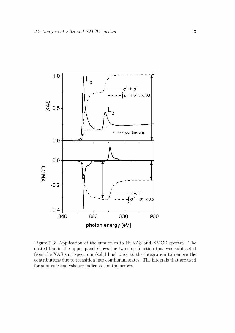
Whereby the relative cross-section for linearly polarized light, σ0, was replaced by(σ+ +σ−)/2. This is justified since usually the x-ray linear magnetic dichroism ismuch smaller than the XMCD effect [79]. An example for the application of thesum rules is given in Fig. 2.3. It shows the unpolarized absorption spectrum andthe XMCD spectrum obtained from a Nickel film. The integrals over the XMCDspectrum and the isotropic spectrum after subtraction of the step like background(to remove the contributions from transitions into continuum states) are indicatedby dashed lines. The presence of an orbital moment can be estimated directlyfrom the non vanishing integral over the XMCD spectrum (
∫
L3+L2σ+ − σ−).
A negative (positive) value corresponds to a parallel (antiparallel) alignment oforbital and spin moment.
For the derivation of the spin sum rule it is assumed that the L3 and the L2
edge are well separated. This assumption is only correct if the spin-orbit-splittingof the core hole is large compared to the coulomb interactions between the corehole and the final states that lead to a coupling of the two L2,3 absorption edges.Such coulomb interactions with the final state affects directly the ratio betweenthe absorption coefficients at the L3 and the L2 edge, the so called branchingratio. It was predicted that the intermixing of the L2 and L3 absorption edges ismainly present towards the early transition metals [64] where the electron corehole interaction increases while the spin-orbit splitting decreases. For such metals(e.g. Mn) the application of the spin sum rule can produce an error up to 30%.Whereas the determination of the orbital moment by the sum rules is not affectedby such intermixing.
A further assumption is that the radial matrix element can be taken as con-stant due to the normalization to the isotropic absorption cross-section. Wu etal. calculated for Ni that the radial part of the matrix elements of the d band| < 3d||r||2p > |2 varies linearly with the photon energy by ≈ 30% and is propor-tional to the spin-orbit coupling in the 3d shell [63]. Since the dichroic signal isproportional to the radial part of the matrix elements and Lz is proportional tothe spin-orbit coupling in the 3d shell this approximation does not have any ef-fect on the orbital sum rule. Whereas the spin sum rule is affected by the energydependent radial matrix elements [63]. However the sum rules are normalized
2.2 Analysis of XAS and XMCD spectra 13
Figure 2.3: Application of the sum rules to Ni XAS and XMCD spectra. Thedotted line in the upper panel shows the two step function that was subtractedfrom the XAS sum spectrum (solid line) prior to the integration to remove thecontributions due to transition into continuum states. The integrals that are usedfor sum rule analysis are indicated by the arrows.
14 Soft x-ray absorption spectroscopy
to the isotropic absorption cross-section which is proportional to the number ofholes in the d-shell. But also s and p (continuum states) states contribute tothe measured absorption cross-section. To eliminate these contributions a dou-ble step function is fitted below the absorption cross-section and subtracted asshown in Fig. 2.3. This procedure is likely to introduce a systematic error in thedetermination of the number of holes in the final state.
It has been shown by ref. [60] that for the transition metals Iron and Cobaltthe spin and orbtial moments determined by the application of the sum rules arein good agreement with those obtained from Einstein de Haas gyromagnetic ratiomeasurements.
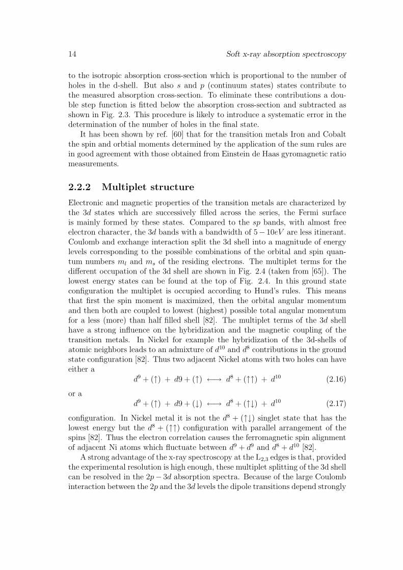
2.2.2 Multiplet structure
Electronic and magnetic properties of the transition metals are characterized bythe 3d states which are successively filled across the series, the Fermi surfaceis mainly formed by these states. Compared to the sp bands, with almost freeelectron character, the 3d bands with a bandwidth of 5− 10eV are less itinerant.Coulomb and exchange interaction split the 3d shell into a magnitude of energylevels corresponding to the possible combinations of the orbital and spin quan-tum numbers ml and ms of the residing electrons. The multiplet terms for thedifferent occupation of the 3d shell are shown in Fig. 2.4 (taken from [65]). Thelowest energy states can be found at the top of Fig. 2.4. In this ground stateconfiguration the multiplet is occupied according to Hund’s rules. This meansthat first the spin moment is maximized, then the orbital angular momentumand then both are coupled to lowest (highest) possible total angular momentumfor a less (more) than half filled shell [82]. The multiplet terms of the 3d shellhave a strong influence on the hybridization and the magnetic coupling of thetransition metals. In Nickel for example the hybridization of the 3d-shells ofatomic neighbors leads to an admixture of d10 and d8 contributions in the groundstate configuration [82]. Thus two adjacent Nickel atoms with two holes can haveeither a
d9 + (↑) + d9 + (↑) ←→ d8 + (↑↑) + d10 (2.16)
or ad9 + (↑) + d9 + (↓) ←→ d8 + (↑↓) + d10 (2.17)
configuration. In Nickel metal it is not the d8 + (↑↓) singlet state that has thelowest energy but the d8 + (↑↑) configuration with parallel arrangement of thespins [82]. Thus the electron correlation causes the ferromagnetic spin alignmentof adjacent Ni atoms which fluctuate between d9 + d9 and d8 + d10 [82].
A strong advantage of the x-ray spectroscopy at the L2,3 edges is that, providedthe experimental resolution is high enough, these multiplet splitting of the 3d shellcan be resolved in the 2p− 3d absorption spectra. Because of the large Coulombinteraction between the 2p and the 3d levels the dipole transitions depend strongly

2.2 Analysis of XAS and XMCD spectra 15
Figure 2.4: Energy distribution of the terms in the initial state configuration3dn. The terms are collected in spin manifolds, where the labels give the valuesof 2S+1 and L. The lowest energy state is at the top of the diagram. (taken from[65])
16 Soft x-ray absorption spectroscopy
on the local electronic structure [82]. Van der Laan et al. used a localizeddescription for the 3dn to 2p53dn+1 excitation that includes the 3d-3d and 2p-3d Coulomb and exchange interactions, the 2p and 3d spin-orbit interactionsand the crystal field acting on the 3d states to calculate the L2,3 absorptionspectra of different transition metals [51]. It was demonstrated that the multipletstructure at the L2,3 edges can act as an fingerprint of a particular electronicground state configuration of the 3d-shell [52]. For the case of Nickel experimentalXAS and XMCD spectra are displayed in Fig. 2.3. XAS and XMCD lineshapesare dominated by the d9 → 2p53d10 transitions. But due to the d8 admixture inthe Ni ground state configuration also d8 → 2p53d9 transitions should contribute.It has been demonstrated that those transitions cause the satellite structure inthe XMCD signal at ≈ 3.3eV above the L3 peak [72].
Also the XAS branching ratio, BR=
∫
L3σ0
∫
L3+L2σ0 , is strongly influenced by the
interactions in the 3d shell. In absence of spin-orbit coupling and electrostatic in-teractions between core hole and valence electrons on the final state the branchingratio would be statistical, BR=2/3, as expected from the quantum degeneracy2j + 1 of the 2p level. Besides a systematic change in the branching ratio for lessthan half filled 3d-shells, it has been shown that a branching ratio larger than thestatistical value is typical for high spin states [65]. Depositing Mn on Cu(110)it has been demonstrated that the multiplet structure and the branching ratioin the Mn 2p− 3d absorption spectra change with the atomic coordination [50].At low coverage detailed multiplet structures are visible which are characteristicfor an atomiclike d5 ground state accompanied by a large branching ratio of 0.8[50]. With increasing Mn coverage up to 4 monolayers the XAS spectrum be-comes smoother and the XAS spectrum approaches the statistical value of 2/3[50]. Thus in transition metals we can study the hybridization of the 3d shelland its ground state configuration by analyzing the multiplet structure and thebranching ratio of the 2p− 3d XAS spectra.

Chapter 3
Ferromagnetism in dilute
magnetic semiconductors
3.1 Introduction
Magnetic ordering is a result of the interplay between the Coulomb interactionand exchange interaction due to the Pauli principle. A simple model demon-strating this effect is given by Heitler and London for the H2 molecule with twoelectrons. In this molecule the exchange interaction favors ferromagnetic couplingwhereas the kinetic energy is favored in antiferromagnetic coupling. When bothspins are parallel the electrons are localized at one atom each and can not jumpto the neighboring site. Such antibonding state is energetically not favored. Theconfiguration with the lowest energy is the bonding state with antiferromagneticcoupling. But delocalization of electrons does not generally lead to antiferro-magnetic coupling. The coupling of magnetic moments by hybridization dependsstrongly on the electronic and magnetic ground state which is shown for the tran-sition metals in Fig. 2.4. In the already mentioned case of Nickel, for instance,the hybridization of the d-shells between atomic neighbors leads to an admixtureof d10 and d8 contributions in the otherwise 3d9 ground state configuration. Thed8 state with the lowest energy is a 3F configuration with parallel arrangement ofspins that causes a ferromagnetic coupling between adjacent Nickel atoms [82].
Itinerant metals require approximations to model the spin-spin interactions.A relatively simple approach to handle the spin-spin interactions in solids withitinerant spins is the mean field approximation. It is based on the phenomeno-logical assumption that the elusive spin-spin interaction between electrons can bereplaced by the interaction of the spins with a very strong magnetic field. Themolecular field will tend to line up the magnetic moments. In such models e.g. theStoner model ferromagnetism is described as an extreme case of paramagnetism.
So far we considered only the case of direct exchange interaction, where theorbital in which the magnetic moments reside overlap. If direct exchange is
17

18 Ferromagnetism in dilute magnetic semiconductors
not possible, e.g. the magnetic orbitals are separated too far from each otherto overlap, the magnetic moments are able to sustain magnetic interactions viaexchange interactions mediated by conduction electrons or valence holes. Thisindirect exchange coupling is responsible for the magnetism in the rare earthmetals, the interlayer exchange coupling in GMR systems or the magnetism insemiconductors doped by transition metals. For the latter we will discuss thepossible coupling mechanisms in detail.
3.2 Magnetic ordering in dilute magnetic semi-
conductors
The magnetic coupling of Mn ions in different types of semiconductors has beenstudied extensively in the recent years. In II-VI host materials, like ZnTe, Mnis divalent and assumes a d5 high spin configuration (S=5/2) [43]. Since theMn doping in II-VI host materials does not introduce any carriers, the intrinsiccarrier density is rather low and the localized Mn spins order paramagnetically.Antiferromagnetic coupling between Mn nearest neighbors, due to short rangeantiferromagnetic super exchange interactions, has been observed [73]. For highlyp-doped Zn1−xMnxTe also carrier mediated ferromagnetic interactions betweenthe Mn magnetic moments have been found [73].
In III-V host materials like GaAs where the Mn replaces trivalent Ga atomsit can be present either in a d4 configuration or a d5 configuration with a weaklybound hole, h. In GaAs it is commonly agreed that Mn is present in a d5 + hconfiguration providing not only localized spins but also acting as an acceptor [1].The pd-hybridization of the Mn 3d shell with the dangling bonds of As neighborsinduces a spin dependent coupling between the localized Mn spins and the holes[43]. The mobility of holes in the p-doped Ga1−xMnxAs changes strongly with theMn concentration, as the system undergoes a metal to insulator transition (MIT).Impurity bands start to occur at Mn concentrations of x = 0.01− 0.02 [43]. Theinterest to find a theoretical description of the ferromagnetism in Ga1−xMnxAs,which occurs on both sides of the MIT, is huge (especially the calculation of Tc).But however, there is no consensus on a common model yet. In the followingsections we give a short overview over the different models in literature, describingthe ferromagnetic ordering in Ga1−xMnxAs .
3.2.1 Zener model
In the metallic regime attempts have been made to describe the ferromagnetismby the Zener model [43]. Zener first proposed this model of ferromagnetismdriven by the local exchange coupling between carriers and localized spins. Ac-cording to the model, polarization of localized spins leads to band splitting. Inthis spin split band structure carriers become spin polarized to lower their free
3.2 Magnetic ordering in dilute magnetic semiconductors 19
energy. At sufficiently low temperature the lowering of the free energy overcom-pensates the energy that is necessary to polarize the localized spins. Below thattemperature the ferromagnetic alignment becomes energetically more favorable.For the description of ferromagnetism in metals the Zener model has been aban-doned because it does not include the quantum oscillations of the carrier spinpolarization around localized spins (Friedel oscillations). For the description offerromagnetism in dilute magnetic semiconductors the Zener mean field theoryhas been reconsidered. In Ga1−xMnxAs the carrier concentration is often foundto be significantly lower than the Mn concentration; in that case oscillations inthe carrier spin polarization can be neglected. Within these limitations the Zenermean field theory has been successfully used to describe the Tc in dilute mag-netic semiconductors [43] as a function of the Mn concentration, x, and the carrierdensity, p. The results of these calculations indicate that the Curie temperatureof Ga1−xMnxAs should scale with the number of substitutional Mn atoms andthe number of carriers like Tc ∝ x · p1/3. This led to a large experimental ef-fort devoted to increasing the hole density, which is usually much smaller thanx due to compensation effects. But more recent calculations [41], taking explic-itly into account spatial disorder and a finite mean free path in RKKY theory,showed that this simple relation between Tc and the carrier density will not holdfor high carrier densities when h is of the order of x. In that case the oscilla-tory character of the RKKY coupling can no longer be neglected and will causemagnetic frustration limiting Tc. The authors also consider the adverse effect ofantiferromagnetic exchange between Mn-Mn nearest neighbors on Tc.
3.2.2 RKKY coupling
The most prominent type of indirect exchange is known as the RKKY interaction,named after the people who developed this theory (Ruderman, Kittel, Kasuyaand Yosida). The basic idea behind this mechanism is that the interaction ofcarriers and localized magnetic moments will establish a non uniform spin densitythat leads to a oscillatory behavior of the coupling. For p-d hybridization, likein Ga1−xMnxAs, the sign of the interaction between magnetic impurities andvalence band carriers is typically antiferromagnetic, as the carriers attempt toscreen the spin of the impurity. Rather than forming a negative spin -5/2 atthe impurity site, the holes instead spin-polarize in concentric rings around theimpurity. The source of the rings of alternating polarization is that a true delta-function in space would require, in Fourier k-space, all the k-vectors from 0to infinity to be equally weighted. However, there are only k-vectors from 0to the Fermi wave vector available. The system thus cannot form a localizedscreening of the impurity spin, but does the closest alternative possibility, whichresults in an oscillatory spin density surrounding the impurity spin. A second Mnmagnetic moment will interact with this oscillatory spin density, and hence willcouple ferromagnetically or antiferromagnetically, depending on the sign of the

20 Ferromagnetism in dilute magnetic semiconductors
spin density at that point. The oscillatory character of the RKKY coupling canbe neglected as long as the average distance between carriers rc = (4πp/3)−1/3
is much larger than that between the magnetic impurities rs = (4πxN0/3)−1/3.The RKKY function changes sign the first time at r ≈ 1.17rc. Interestingly theferromagnetism does not break down at Mn concentrations below the metal toinsulator transition as one would expect from RKKY theory. To explain the originof ferromagnetism in this regime a magnetic polaron model has been proposed[3].
In the Zener model and the RKKY scheme the pd-hybridization is usuallyassumed to be spherically isotropic [2]. Only recently Mahadevan et al. predicteda strongly anisotropic pd-hybridization in Ga1−xMnxAs, taking into account thesymmetry of the Mn 3d levels hybridizing with the As p orbitals [71]. By thetetrahedral crystal field the Mn 3d levels are split into eg levels with lower energyand t2g levels with higher energy, respectively. Fully occupied t2g and ee statesinside the valence band have mainly Mn d character whereas the partially filled t2g
states at the valence band are formed of Mn 3d and As p orbitals [71]. Assumingspin conserving hopping interactions between those partially occupied levels theexchange interaction between Mn pairs at various distances along different latticeorientations has been studied by total energy ab initio calculations [71]. Themain result of these calculations is a significant orientation dependence of the pd-hybridization and therefore of the exchange coupling [71]. The exchange couplingof Mn pairs oriented along the < 110 > axis remains higher in strength comparedto that of Mn pairs oriented along other directions even if their separation issmaller [71].
3.2.3 Magnetic polarons
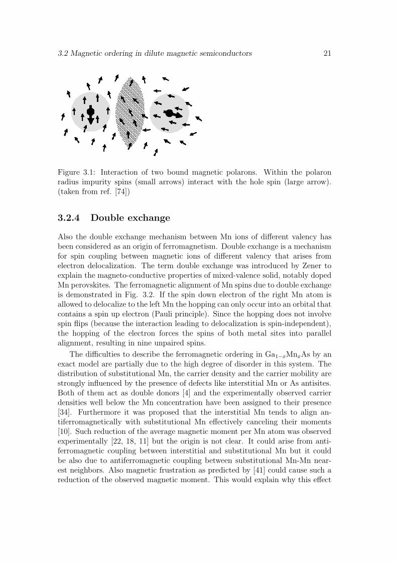
Contrary to the Zener model that assumes itinerant carriers (holes) in Ga1−xMnxAs,the idea of magnetic polarons is based on localized holes [74]. Such scenario ap-plies to Ga1−xMnxAs samples with Mn concentrations that are below the metalto insulator transition. The hole wave function is assumed to fall off exponen-tially from the localization center with the decay length aB [74]. Within thelocalization radius of the hole (aB ≈ 1nm in Ga1−xMnxAs ) exchange interac-tion with the Mn impurities lead to the formation of a bound magnetic polaron[74]. At low enough temperatures neighboring polarons begin to overlap andinteract with each other. When the cluster of correlated polarons reaches thepercolation limit the ferromagnetic transition occurs. A schematic picture of twomagnetic polarons is given in Fig. 3.1. The exponential decay of the two holewave functions defines a lens shaped region in between the two polarons which isimportant for the ferromagnetic coupling of the two polarons (indicated by thehatched area in Fig. 3.1). The polaron model predicts the existence of magneticclusters (magnetic polarons) above the Curie temperature.
3.2 Magnetic ordering in dilute magnetic semiconductors 21
Figure 3.1: Interaction of two bound magnetic polarons. Within the polaronradius impurity spins (small arrows) interact with the hole spin (large arrow).(taken from ref. [74])
3.2.4 Double exchange
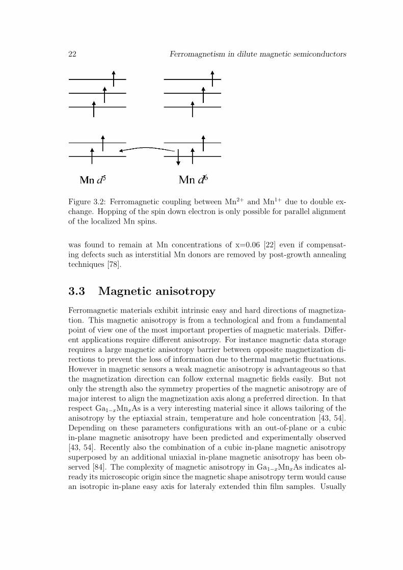
Also the double exchange mechanism between Mn ions of different valency hasbeen considered as an origin of ferromagnetism. Double exchange is a mechanismfor spin coupling between magnetic ions of different valency that arises fromelectron delocalization. The term double exchange was introduced by Zener toexplain the magneto-conductive properties of mixed-valence solid, notably dopedMn perovskites. The ferromagnetic alignment of Mn spins due to double exchangeis demonstrated in Fig. 3.2. If the spin down electron of the right Mn atom isallowed to delocalize to the left Mn the hopping can only occur into an orbital thatcontains a spin up electron (Pauli principle). Since the hopping does not involvespin flips (because the interaction leading to delocalization is spin-independent),the hopping of the electron forces the spins of both metal sites into parallelalignment, resulting in nine unpaired spins.
The difficulties to describe the ferromagnetic ordering in Ga1−xMnxAs by anexact model are partially due to the high degree of disorder in this system. Thedistribution of substitutional Mn, the carrier density and the carrier mobility arestrongly influenced by the presence of defects like interstitial Mn or As antisites.Both of them act as double donors [4] and the experimentally observed carrierdensities well below the Mn concentration have been assigned to their presence[34]. Furthermore it was proposed that the interstitial Mn tends to align an-tiferromagnetically with substitutional Mn effectively canceling their moments[10]. Such reduction of the average magnetic moment per Mn atom was observedexperimentally [22, 18, 11] but the origin is not clear. It could arise from anti-ferromagnetic coupling between interstitial and substitutional Mn but it couldbe also due to antiferromagnetic coupling between substitutional Mn-Mn near-est neighbors. Also magnetic frustration as predicted by [41] could cause such areduction of the observed magnetic moment. This would explain why this effect
22 Ferromagnetism in dilute magnetic semiconductors
Figure 3.2: Ferromagnetic coupling between Mn2+ and Mn1+ due to double ex-change. Hopping of the spin down electron is only possible for parallel alignmentof the localized Mn spins.
was found to remain at Mn concentrations of x=0.06 [22] even if compensat-ing defects such as interstitial Mn donors are removed by post-growth annealingtechniques [78].
3.3 Magnetic anisotropy
Ferromagnetic materials exhibit intrinsic easy and hard directions of magnetiza-tion. This magnetic anisotropy is from a technological and from a fundamentalpoint of view one of the most important properties of magnetic materials. Differ-ent applications require different anisotropy. For instance magnetic data storagerequires a large magnetic anisotropy barrier between opposite magnetization di-rections to prevent the loss of information due to thermal magnetic fluctuations.However in magnetic sensors a weak magnetic anisotropy is advantageous so thatthe magnetization direction can follow external magnetic fields easily. But notonly the strength also the symmetry properties of the magnetic anisotropy are ofmajor interest to align the magnetization axis along a preferred direction. In thatrespect Ga1−xMnxAs is a very interesting material since it allows tailoring of theanisotropy by the eptiaxial strain, temperature and hole concentration [43, 54].Depending on these parameters configurations with an out-of-plane or a cubicin-plane magnetic anisotropy have been predicted and experimentally observed[43, 54]. Recently also the combination of a cubic in-plane magnetic anisotropysuperposed by an additional uniaxial in-plane magnetic anisotropy has been ob-served [84]. The complexity of magnetic anisotropy in Ga1−xMnxAs indicates al-ready its microscopic origin since the magnetic shape anisotropy term would causean isotropic in-plane easy axis for lateraly extended thin film samples. Usually
3.3 Magnetic anisotropy 23
a strong magneto-crystalline anisotropy originating in the electronic structure ischaracterized by a directional dependence of the orbital magnetic moment. Thishas been predicted by Bruno [56] and experimentally verified by different groups[66, 67]. The difference of the orbital moments along easy and hard magneti-zation axis is directly proportional to the magneto-crystalline anisotropy energy[66, 67]. However for Ga1−xMnxAs the situation is more complex. The longrange ferromagnetic coupling of the Mn impurity 3d spins is mediated by valenceholes with a non-zero spin polarization. Strain effects due to a lattice mismatchbetween the Ga1−xMnxAs and the substrate can cause a large valence hole spinanisotropy due to the strong spin-orbit coupling in the GaAs valence band. Thusthe out-of-plane or cubic in-plane magnetic anisotropy of Ga1−xMnxAs films isexplained by the presence of uniaxial tensile or biaxial compressive strain, re-spectively [54, 84]. E.g. under tensile uniaxial strain the valence band splitsinto heavy-hole mj = ±3/2 and light hole mj = ±1/2 subbands. Following asimplified model described in ref. [54] the heavy or light hole character of thecarriers depending on the occupation of the two subbands determines the in- orout-of-plane orientation of sample magnetization at remanence. The exchangecoupling of valence holes and the Mn 3d impurity spins via the pd-hybridizationtransfers these complexity into the Mn 3d subsystem.
It is obvious that in Ga1−xMnxAs a detailed understanding the Mn 3d config-uration is the crucial part to separate the influence of different Mn configurationson the magnetic coupling. This information is not available to standard tech-niques like SQUID or anomalous Hall current measurements that are commonlyused to characterize the magnetic properties. These methods can even not dis-tinguish between contributions from holes or Mn atoms to the magnetization.Soft x-ray spectroscopy is an ideal tool to investigate the electronic and magneticconfiguration of the Mn 3d shell. The following chapters will demonstrate thatthis method is sensitive enough to separate the different Mn species occurring inGa1−xMnxAs and investigate their influence on the ferromagnetic coupling.

24 Ferromagnetism in dilute magnetic semiconductors

Chapter 4
Experimental considerations
4.1 Sample preparation
The challenge of growing Ga1−xMnxAs by molecular beam eptiaxy (MBE) is toovercome the limited solubility of Mn in GaAs. At the usual growth temperaturesof GaAs ( 600K), the coevaporation of Mn would lead to the formation of a secondphase with MnAs clusters [1]. The formation of MnAs can only be avoided atlower growth temperatures (180 - 300K) in the so called low-temperature MBE.Whereby the actual growth temperature varies with the Mn concentration [1].The samples presented here were grown at the university of Wurzburg at theinstitute of Prof. L.W. Molenkamp [9] using a GaAs (001) surface as substratewith 80nm low-temperature GaAs layer deposited as a buffer prior to the growthof the Ga1−xMnxAs layer. The Mn concentration x for each sample has beendetermined from the lattice constant as described in ref. [9]. In the present worksamples with Mn concentrations ranging from x=0.007 to x=0.062 that havebeen investigated as listed in table 4.1. Most of the Ga1−xMnxAs films are ratherthick compared to literature. Samples that reach a Tc above 140K after annealingusually have a thickness of 50nm or less. This is ascribed to the diffusion of defectslike interstitial Mn to the surface during the annealing which is less efficient inthicker samples [15]. Results from ref. [80] indicate that also in the as grown statethinner samples can reach a higher Tc. For the x-ray spectroscopy and especiallythe fluorescence measurements a thicker Ga1−xMnxAs layer ensures that the bulkproperties can be probed with not too much disturbance from the surface layer.
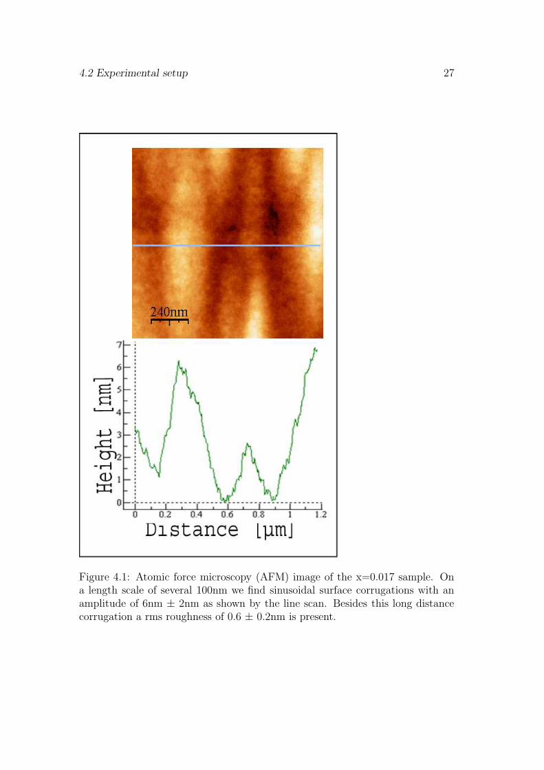
The surface of the Ga1−xMnxAs layer was characterized in situ by RHEEDmeasurements showing a nice epitactic growth and a (2 x 1) surface reconstruction[9]. In addition the roughness of the surface has been analyzed ex-situ by atomicforce microscopy (AFM). This topographic information is a valuable input forthe evaluation of reflectivity spectra as explained at the end of this chapter. Atypical AFM image of the x=0.017 sample is shown in Fig. 4.1. On a length scaleof several 100nm the surface shows a sinusoidal corrugation with an amplitude
25

26 Experimental considerations
of 6 ± 2nm. Very similar corrugations were present in all other samples exceptthe x=0.062 sample which had a flatter surface. This corrugation is most likelycaused by thickness variations of the low-temperature GaAs buffer layer [70]. Inaddition to the buffer layer corrugation all samples have a rms surface roughnessof 0.6 ± 0.2nm that we assign to thickness variations of the Ga1−xMnxAs layer.
Mn concetration x: 0.008 0.017 0.051 0.062Curie temperature Tc: 12K 25K 55K 65Kthickness : 350nm 300nm 500nm 180nm
4.1.1 Annealing
A disadvantage of the low-temperature growth is the large number of defectsthat are introduced. In literature mainly interstitial Mn and As antisites arediscussed, because both defects act as double donors and compensate the effectof the Mn acceptors [4]. To remove such defects the samples have to undergo apost growth annealing procedure [15]. The optimum annealing temperature isbelow the activation threshold of substitutional Mn diffusion but above that ofinterstitial Mn (≈ 180oC). Most of the annealing experiments in the literaturehave been performed ex situ in air [15]. It has been demonstrated that by low-temperature annealing the carrier concentration and thus Tc can be raised [15]. Itis generally agreed that this is due to the removal of interstitial Mn by diffusion.The record values of Tc, so far, were obtained by the annealing of samples thinnerthan 50nm. It is still an open question whether the annealing of thicker samplesis inefficient because of the limited diffusion length, or whether the formation ofa layer of interstitial Mn at the surface, passivated by oxidation prevents the out-diffusion of the remaining interstitial Mn. The interest of x-ray spectroscopy isto distinguish interstitial Mn from substitutional Mn by its different ground statehybridization. To keep the influence of surface oxidation as small as possible thex = 0.062 sample was annealed at 185oC for 24h in vacuum.
4.2 Experimental setup
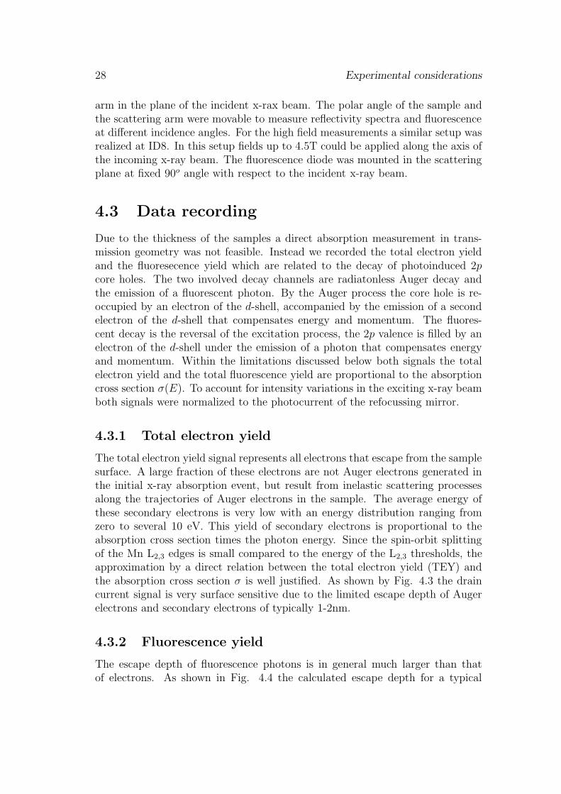
The experiments described here were performed at the BESSY UE46 Hahn-Meitner-Institute beamline and at the high field magnet at ID8 at the ESRF.A schematic view of the experimental setup inside the ultra high vacuum cham-ber at BESSY is given in Fig. 4.2. The sample was mounted on a He cryostatthat allowed for temperatures between 10 and 300K. At BESSY the sample holderwas equipped with small permanent magnet applying a field of 100- 200 Oe alongthe horziontal inplane direction of the sample to align the magnetization by fieldcooling. The fluorescence diode was mounted inside the cold shield collecting thefluorescence photons at an fixed angle of 30o from above with respect to the sam-ple surface. Scattered x-rays were detected by a diode mounted on a scattering
4.2 Experimental setup 27
Figure 4.1: Atomic force microscopy (AFM) image of the x=0.017 sample. Ona length scale of several 100nm we find sinusoidal surface corrugations with anamplitude of 6nm ± 2nm as shown by the line scan. Besides this long distancecorrugation a rms roughness of 0.6 ± 0.2nm is present.
28 Experimental considerations
arm in the plane of the incident x-rax beam. The polar angle of the sample andthe scattering arm were movable to measure reflectivity spectra and fluorescenceat different incidence angles. For the high field measurements a similar setup wasrealized at ID8. In this setup fields up to 4.5T could be applied along the axis ofthe incoming x-ray beam. The fluorescence diode was mounted in the scatteringplane at fixed 90o angle with respect to the incident x-ray beam.
4.3 Data recording
Due to the thickness of the samples a direct absorption measurement in trans-mission geometry was not feasible. Instead we recorded the total electron yieldand the fluoresecence yield which are related to the decay of photoinduced 2pcore holes. The two involved decay channels are radiatonless Auger decay andthe emission of a fluorescent photon. By the Auger process the core hole is re-occupied by an electron of the d-shell, accompanied by the emission of a secondelectron of the d-shell that compensates energy and momentum. The fluores-cent decay is the reversal of the excitation process, the 2p valence is filled by anelectron of the d-shell under the emission of a photon that compensates energyand momentum. Within the limitations discussed below both signals the totalelectron yield and the total fluorescence yield are proportional to the absorptioncross section σ(E). To account for intensity variations in the exciting x-ray beamboth signals were normalized to the photocurrent of the refocussing mirror.
4.3.1 Total electron yield
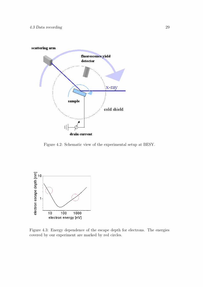
The total electron yield signal represents all electrons that escape from the samplesurface. A large fraction of these electrons are not Auger electrons generated inthe initial x-ray absorption event, but result from inelastic scattering processesalong the trajectories of Auger electrons in the sample. The average energy ofthese secondary electrons is very low with an energy distribution ranging fromzero to several 10 eV. This yield of secondary electrons is proportional to theabsorption cross section times the photon energy. Since the spin-orbit splittingof the Mn L2,3 edges is small compared to the energy of the L2,3 thresholds, theapproximation by a direct relation between the total electron yield (TEY) andthe absorption cross section σ is well justified. As shown by Fig. 4.3 the draincurrent signal is very surface sensitive due to the limited escape depth of Augerelectrons and secondary electrons of typically 1-2nm.
4.3.2 Fluorescence yield
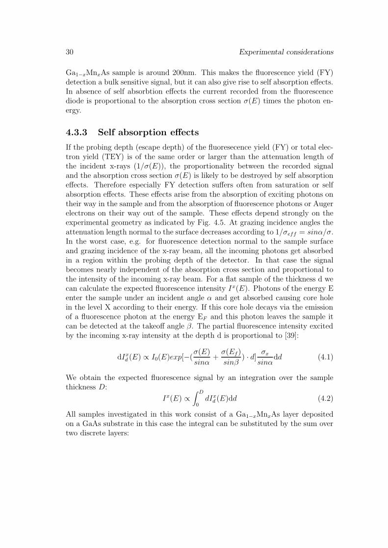
The escape depth of fluorescence photons is in general much larger than thatof electrons. As shown in Fig. 4.4 the calculated escape depth for a typical
4.3 Data recording 29
Figure 4.2: Schematic view of the experimental setup at BESY.
Figure 4.3: Energy dependence of the escape depth for electrons. The energiescovered by our experiment are marked by red circles.
30 Experimental considerations
Ga1−xMnxAs sample is around 200nm. This makes the fluorescence yield (FY)detection a bulk sensitive signal, but it can also give rise to self absorption effects.In absence of self absorbtion effects the current recorded from the fluorescencediode is proportional to the absorption cross section σ(E) times the photon en-ergy.
4.3.3 Self absorption effects
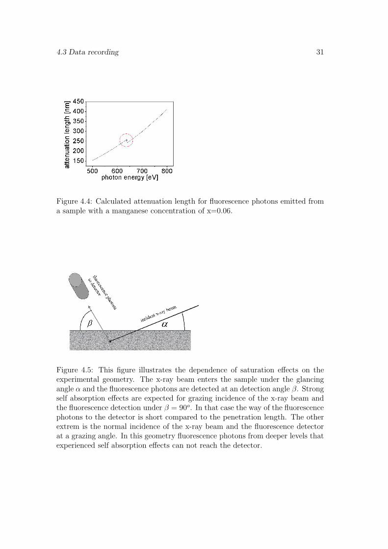
If the probing depth (escape depth) of the fluoresecence yield (FY) or total elec-tron yield (TEY) is of the same order or larger than the attenuation length ofthe incident x-rays (1/σ(E)), the proportionality between the recorded signaland the absorption cross section σ(E) is likely to be destroyed by self absorptioneffects. Therefore especially FY detection suffers often from saturation or selfabsorption effects. These effects arise from the absorption of exciting photons ontheir way in the sample and from the absorption of fluorescence photons or Augerelectrons on their way out of the sample. These effects depend strongly on theexperimental geometry as indicated by Fig. 4.5. At grazing incidence angles theattenuation length normal to the surface decreases according to 1/σeff = sinα/σ.In the worst case, e.g. for fluorescence detection normal to the sample surfaceand grazing incidence of the x-ray beam, all the incoming photons get absorbedin a region within the probing depth of the detector. In that case the signalbecomes nearly independent of the absorption cross section and proportional tothe intensity of the incoming x-ray beam. For a flat sample of the thickness d wecan calculate the expected fluorescence intensity Ix(E). Photons of the energy Eenter the sample under an incident angle α and get absorbed causing core holein the level X according to their energy. If this core hole decays via the emissionof a fluorescence photon at the energy EF and this photon leaves the sample itcan be detected at the takeoff angle β. The partial fluorescence intensity excitedby the incoming x-ray intensity at the depth d is proportional to [39]:
dIxd (E) ∝ I0(E)exp[−(
σ(E)
sinα+
σ(Ef )
sinβ) · d]
σx
sinαdd (4.1)
We obtain the expected fluorescence signal by an integration over the samplethickness D:
Ix(E) ∝∫ D
0dIx
d (E)dd (4.2)
All samples investigated in this work consist of a Ga1−xMnxAs layer depositedon a GaAs substrate in this case the integral can be substituted by the sum overtwo discrete layers:
4.3 Data recording 31
Figure 4.4: Calculated attenuation length for fluorescence photons emitted froma sample with a manganese concentration of x=0.06.
Figure 4.5: This figure illustrates the dependence of saturation effects on theexperimental geometry. The x-ray beam enters the sample under the glancingangle α and the fluorescence photons are detected at an detection angle β. Strongself absorption effects are expected for grazing incidence of the x-ray beam andthe fluorescence detection under β = 90o. In that case the way of the fluorescencephotons to the detector is short compared to the penetration length. The otherextrem is the normal incidence of the x-ray beam and the fluorescence detectorat a grazing angle. In this geometry fluorescence photons from deeper levels thatexperienced self absorption effects can not reach the detector.

32 Experimental considerations
Ix(E) ∝ I0(E) ·[σx(E)
sinα× (1− e−(
σtot(E)sinα
+σtot(Ef )
sinβ)d)
σtot(E)sinα
+σtot(Ef )
sinβ
(4.3)
+σsub(E)
sinα× (e−(
σtot(E)sinα
+σtot(Ef )
sinβ)d)
σsub(E)sinα
+σsub(Ef )
sinβ
]
Where σx is the absorption coefficient related to the production of a core holein the investigated level X of the Mn impurities and σtot is the total absorptioncoefficient of the Ga1−xMnxAs layer which is the sum of σX and σother the lat-ter describe the absorption due to shallower core levels, valence levels and otheratomic species. The absorption coefficient of the GaAs substrate enters as σsub
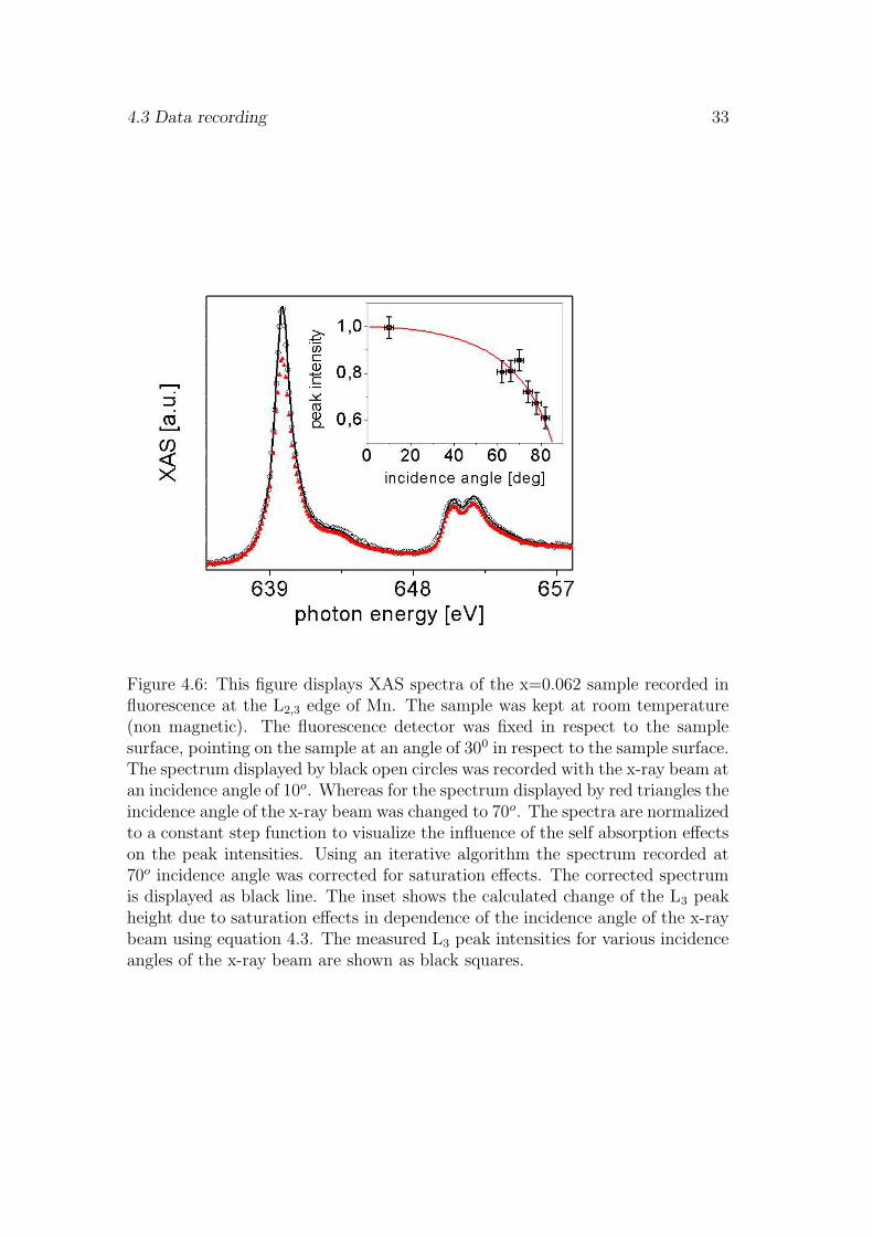
and IO denotes the intensity of the incoming x-ray light. To identify the presenceany self absorption effects in our FY signal we compared spectra recorded atdifferent experimental geometries (i.e. varying the incidence angle of x-ray beamwith fixed geometry between sample and detection diode as shown in Fig. 4.2).Fig. 4.6 shows two XAS spectra of the x=0.062 sample recorded with the flu-orescence diode in a fixed detection geometry (constant acceptance angle), onlythe incidence angle of the exciting x-ray beam was changed. The spectra arenormalized to a constant step edge before and after the L2,3 absorption edges.This step in the absorption cross section is caused by transition into continuumstates. Comparing the XAS spectrum recorded at an incidence angle of 70o (redtriangles) to that obtained at an incidence angle of 10o (black circles) we find adecreased peak intensity. This indicates that the fluorescence signal is no longerproportional to the absorption cross section σ(E) due to the presence of self ab-sorption effects. The dependence of the self absorption effects on the incidenceangle of the x-ray beam is demonstrated in the inset of Fig. 4.6. It displaysthe measured L3 peak intensity for various incidence angles of the x-ray beam(solid squares). If we scale the measured fluorescence intensities to absolute ab-sorption cross sections, according to the literature data provided by the Centerof X-ray Optics [14], we can use equation 4.3 to calculate the intensity seen bythe fluorescence diode in dependence on the absorption cross section of the Mnspecies, the sample thickness and the experimental geometry [39]. We assumedthat σother and σsub are constant within the probed energy interval (from 620eVto 670eV). Thus the energy dependence of saturation effects is determined by theMn absorption cross section. The calculated reduction of the L3 peak intensitydue to self absorption effects indicated by the red line in the inset of Fig. 4.6agrees well with the measurements.
To correct for the saturation effects we can use an iterative algorithm. In thefirst step we apply equation 4.3 to the measured absorption cross sections andcalculate the ratio of measured and saturation reduced intensities at differentdetection angles. If the ratio is always one no saturation effects are present, if not
4.3 Data recording 33
Figure 4.6: This figure displays XAS spectra of the x=0.062 sample recorded influorescence at the L2,3 edge of Mn. The sample was kept at room temperature(non magnetic). The fluorescence detector was fixed in respect to the samplesurface, pointing on the sample at an angle of 300 in respect to the sample surface.The spectrum displayed by black open circles was recorded with the x-ray beam atan incidence angle of 10o. Whereas for the spectrum displayed by red triangles theincidence angle of the x-ray beam was changed to 70o. The spectra are normalizedto a constant step function to visualize the influence of the self absorption effectson the peak intensities. Using an iterative algorithm the spectrum recorded at70o incidence angle was corrected for saturation effects. The corrected spectrumis displayed as black line. The inset shows the calculated change of the L3 peakheight due to saturation effects in dependence of the incidence angle of the x-raybeam using equation 4.3. The measured L3 peak intensities for various incidenceangles of the x-ray beam are shown as black squares.
34 Experimental considerations
the measured absorption cross sections multiplied by the ratio are used as inputfor the next iteration. The iterations are stopped if the calculated saturation ofthe input intensities is identical with the measured absorption intensities. Noweach point in the measured spectra is multiplied by a intensity dependent factordetermined by the algorithm. To confirm the result of our saturation correctionwe compared the corrected spectra to those recorded at geometries or samplethicknesses for which no saturation effects have been found. In Fig. 4.6 wefind excellent agreement between the spectrum of the x=0.06 sample measuredat normal incidence and the calculated correction (solid line) of the spectrumrecorded at 70o incidence angle (solid triangle).
4.4 Resonant reflectivity
In order to obtain structural information on the Mn distribution in our sampleswe recorded x-ray resonant reflectivity spectra at the Mn 2p → 3d resonance.The reflectivity is given by:
I ∝|∑
i
fi × exp(iqri) |2 (4.4)
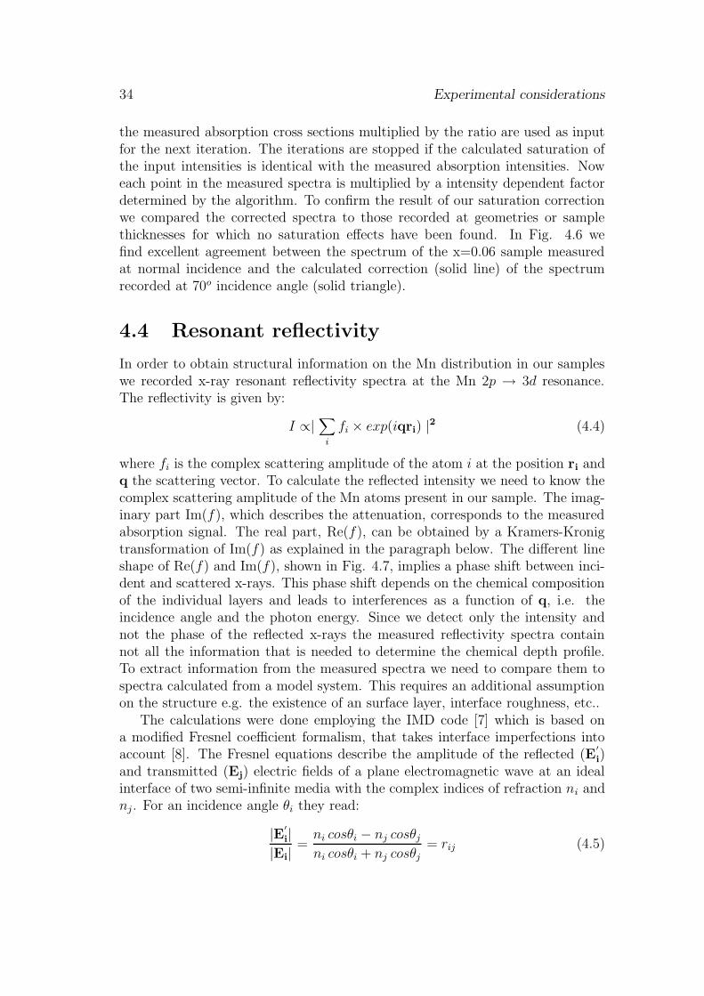
where fi is the complex scattering amplitude of the atom i at the position ri andq the scattering vector. To calculate the reflected intensity we need to know thecomplex scattering amplitude of the Mn atoms present in our sample. The imag-inary part Im(f), which describes the attenuation, corresponds to the measuredabsorption signal. The real part, Re(f), can be obtained by a Kramers-Kronigtransformation of Im(f) as explained in the paragraph below. The different lineshape of Re(f) and Im(f), shown in Fig. 4.7, implies a phase shift between inci-dent and scattered x-rays. This phase shift depends on the chemical compositionof the individual layers and leads to interferences as a function of q, i.e. theincidence angle and the photon energy. Since we detect only the intensity andnot the phase of the reflected x-rays the measured reflectivity spectra containnot all the information that is needed to determine the chemical depth profile.To extract information from the measured spectra we need to compare them tospectra calculated from a model system. This requires an additional assumptionon the structure e.g. the existence of an surface layer, interface roughness, etc..
The calculations were done employing the IMD code [7] which is based ona modified Fresnel coefficient formalism, that takes interface imperfections intoaccount [8]. The Fresnel equations describe the amplitude of the reflected (E
′
i)and transmitted (Ej) electric fields of a plane electromagnetic wave at an idealinterface of two semi-infinite media with the complex indices of refraction ni andnj. For an incidence angle θi they read:
|E′
i||Ei|
=ni cosθi − nj cosθj
ni cosθi + nj cosθj= rij (4.5)

4.4 Resonant reflectivity 35
|Ej||Ei|
=2ni cosθi
ni cosθi + nj cosθj= tij (4.6)
Where θj is the angle of refraction and rij and tij are the Fresnel reflection andtransmission coefficients, respectively. Interface imperfections like roughness ordiffuseness are included in the Fresnel equations following a formalism developedby Stearns [8]. In this formalism the interface is described by a profile functionp(z) (z along the surface normal). The profile function is defined as the normalizedaverage value of the dielectric function ε(x) (with n =
√ε) along the z-direction.
P (z) =
∫ ∫
ε(x)dxdy
(εi − εj)∫ ∫
dxdy(4.7)
As demonstrated in ref. [8] the loss in specular reflectivity resulting from interfaceimperfections can be approximated by multiplying the Fresnel coefficients withthe Fourier transform of the function wz = dp/dz. The new Fresnel coefficientsare now:
r′
ij = rijw(si), (4.8)
with si = 4πθi/λ and λ the wavelength of the light. Four different profile functionshave been developed in ref. [8], describing the interface profile by a error function,exponential function, linear function or sinusoidal function. The explicit termsare given in ref. [8]. The width of the interface is described by the parameter σ,for a purely rough interface σ corresponds to the rms roughness.
In the case of a multilayer system consisting of N layers and N + 1 interfacesin which the i-th layer has the thickness di the roughness σi and the index ofrefraction ni, the net reflection and transmission coefficients of the i-th layer aregiven by [40]:
ri =rij + rj e2iβi
1 + rij rje2iβi; with βi = 2πdiniθi/λ (4.9)
ti =tij tj e2iβi
1 + rij rje2iβi(4.10)
To compute the net reflection and transmission coefficients of the multilayer theIMD code applies equations 4.9 and 4.10 recursively, starting at the bottom layer.
Kramers Kronig Transformation
The imaginary part of the scattering factor Im(f) can be determined from thetotal absorption cross section σ(ω) that is proportional to the measured total elec-tron yield and fluorescence yield signal. Their relation is given by: Im(f)(ω) =ωσ(ω)/4πr0c. Where r0 is the classical electron radius, c the speed of light and ωthe incident x-ray frequency. To obtain the absolute absorption cross section thenormalized absorption spectra were multiplied by a scaling factor. We choose a
36 Experimental considerations
Figure 4.7: The figure shows the real (panel A) and the imganinary (panel B)part of the optical constants for substitutional Mn (black line) and Mn in a 3d5
configuration (red line). The imagninary part was determined by x-ray absorptionspectroscopy, the real part was calculated by a Kramers Kronig relation usingequation 4.11.
4.4 Resonant reflectivity 37
scaling factor that forced the measured absorption cross section before and af-ter the L2,3 resonances to be identical with the data provided by the Center ofX-ray Optics at the Berkley Lab [14]. Then we calculated the real part of thescattering factor Re(f) from the imaginary part using a Kramers Kronig relation.These dispersion relations couple the real and the imaginary part of the atomicscattering amplitude by a Hilbert transformation:
Re(f)(ω0) = 1 +2
πP
∫∞
0
ω Im(f)(ω)
ω20 − ω2
dω. (4.11)
Two obstacles for the practical application of the Kramers-Kronig relations exist.First we need to know the absorption coefficient at all energies to determine thereal part. And second a singularity in the Cauchy principal value integral occurs.In our experiment we measure the absorption coefficient only in a short energyrange from 620− 670eV photon energy covering the L2,3 absorption edges of Mn.To calculate the real part of f with the above formula we extended the energyrange of the measured data set to several hundred eV. We did this by addingliterature data obtained from the Center of X-ray Optics on the low and the highenergy side of the measured data set. Values outside the integration limits arereplaced by a constant.
The presence of the singularity at ω0 in the cauchy intrgal requires that theequation is manipulated to allow numerical integration. The integral can be splitinto three parts with the singulatity in the second part, where a and b denote theadjacent points below and above the singularity.
38 Experimental considerations
2
πP
∫∞
0
ω · Im(f)(ω)
ω20 − ω2
=2
π
∫ a
0
ω · Im(f)(ω)
ω20 − ω2
(4.12)
+2
πP
∫ b
a
ω · Im(f)(ω)
ω20 − ω2
+2
π
∫∞
b
ω · Im(f)(ω)
ω20 − ω2
The integral containing the singulatity can be rewritten as:
2
πP
∫ b
a
ω · Im(f)(ω)
ω20 − ω2
=1
π
(
− P∫ b
a
Im(f)(ω)
ω0 − ω− P
∫ b
a
Im(f)(ω)
ω − ω0
)
(4.13)
Hoyt et al. [5] deomstrated that if we expand Re(f)(ω) in a Taylor series aboutω0 the integral on the interval a → b becomes numerically calculable. It readsnow [5]:
2
πP
∫ b
a
ω · Im(f)(ω)
ω20 − ω2
=1
π
[
P∫ b
a
−Im(f)(ω)
ω0 + ωdω (4.14)
−{
ln|b− ω0| − ln|a− ω0|}
− d Im(f)
dω
∣∣∣ω0(b− a)
−∞∑
n=2
1
(n)n!
dnIm(f)
dωn
∣∣∣ω0(b− ω0)
n − (a− ω0)n]
By substituting 4.14 into 4.12 we can now use equation 4.11 to calculate the realpart of the atomic scattering factor. Results obtained from the Kramers Kronigtransformation are shown in Fig. 4.7. In this case we applied the transformationto two differnt Mn electronic configurations present in our Ga1−xMnxAs samples.The figure displays the index of refraction n which we used as input for the IMDcode. The index of refraction can be calculated from the atomic scattering factorby (Re(n) + iIm(n))(ω) = 1−Nr0(c/ω)2 · (Re(f) + iIm(f))(ω)/2π. Where N isthe number of atoms per unit.

Chapter 5
Chemical and magnetical depth
profile of Ga1−xMnxAs films
For the understanding of the ferromagnetic ordering the electronic configura-tion of the Mn impurities and the number of Mn atoms contributing to thelong range ferromagnetic order are of major interest. These parameters can beprobed directly by x-ray absorption spectroscopy (XAS) and x-ray magnetic cir-cular dichroism (XMCD). At the Mn 2p - 3d resonance the XAS and MXCD lineshapes are characteristic for the Mn 3d electronic and magnetic configurationrespectively [51]. Although these techniques have been applied to Ga1−xMnxAspreviously [11, 18, 13, 16, 21] the results are in some points inconsistent. Thefirst experiments [11, 18] found a pronounced multiplet structure in the Mn XASspectra characteristic of a highly localized state. The weak XMCD signal indi-cated that only a fraction of 13% of the Mn atoms participate in the long rangeferromagnetic ordering. Changes in the line shape of the Mn XAS spectra be-fore and after annealing have been observed indicating that more than one Mnspecies must be present in Ga1−xMnxAs [13]. More recently XAS spectra withless pronounced multiplet structure have been reported [16] in combination withremarkably high numbers (66%) of ferromagnetically aligned Mn impurities inGa1−xMnxAs [16]. It has been proposed very recently [21] that this discrepancymay be caused by a Mn rich surface layer.
In this chapter we study the chemical depth profile of as-grown and anneledGa1−xMnxAs samples. As-grown refers to MBE grown samples that were trans-ported through air and measured in our UHV setup without surface preparation.The annealing was done in a separate vacuum chamber with a short exposure toair during the transfer into the measurement chamber. The presented XAS andXMCD experiments exploit the different probing depth of flourescence and elec-tron yield detection to resolve bulk and surface properties of the Mn impurities.Comparing bulk and surface sensitive XAS and XMCD spectra two Mn speciescan be identified. The bulk is dominated by ferromagnetic Mn in a mixed valence3d5 - 3d6 electronic configuration. This has been assigned to substitutional Mn
39
40 Chemical and magnetical depth profile of Ga1−xMnxAs films
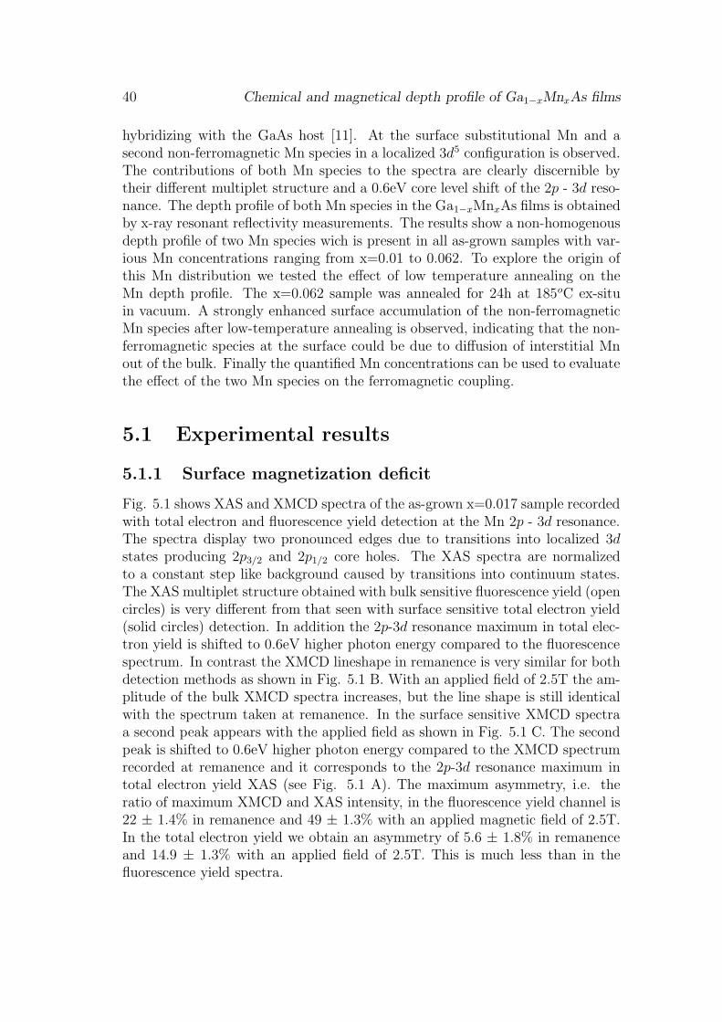
hybridizing with the GaAs host [11]. At the surface substitutional Mn and asecond non-ferromagnetic Mn species in a localized 3d5 configuration is observed.The contributions of both Mn species to the spectra are clearly discernible bytheir different multiplet structure and a 0.6eV core level shift of the 2p - 3d reso-nance. The depth profile of both Mn species in the Ga1−xMnxAs films is obtainedby x-ray resonant reflectivity measurements. The results show a non-homogenousdepth profile of two Mn species wich is present in all as-grown samples with var-ious Mn concentrations ranging from x=0.01 to 0.062. To explore the origin ofthis Mn distribution we tested the effect of low temperature annealing on theMn depth profile. The x=0.062 sample was annealed for 24h at 185oC ex-situin vacuum. A strongly enhanced surface accumulation of the non-ferromagneticMn species after low-temperature annealing is observed, indicating that the non-ferromagnetic species at the surface could be due to diffusion of interstitial Mnout of the bulk. Finally the quantified Mn concentrations can be used to evaluatethe effect of the two Mn species on the ferromagnetic coupling.
5.1 Experimental results
5.1.1 Surface magnetization deficit
Fig. 5.1 shows XAS and XMCD spectra of the as-grown x=0.017 sample recordedwith total electron and fluorescence yield detection at the Mn 2p - 3d resonance.The spectra display two pronounced edges due to transitions into localized 3dstates producing 2p3/2 and 2p1/2 core holes. The XAS spectra are normalizedto a constant step like background caused by transitions into continuum states.The XAS multiplet structure obtained with bulk sensitive fluorescence yield (opencircles) is very different from that seen with surface sensitive total electron yield(solid circles) detection. In addition the 2p-3d resonance maximum in total elec-tron yield is shifted to 0.6eV higher photon energy compared to the fluorescencespectrum. In contrast the XMCD lineshape in remanence is very similar for bothdetection methods as shown in Fig. 5.1 B. With an applied field of 2.5T the am-plitude of the bulk XMCD spectra increases, but the line shape is still identicalwith the spectrum taken at remanence. In the surface sensitive XMCD spectraa second peak appears with the applied field as shown in Fig. 5.1 C. The secondpeak is shifted to 0.6eV higher photon energy compared to the XMCD spectrumrecorded at remanence and it corresponds to the 2p-3d resonance maximum intotal electron yield XAS (see Fig. 5.1 A). The maximum asymmetry, i.e. theratio of maximum XMCD and XAS intensity, in the fluorescence yield channel is22 ± 1.4% in remanence and 49 ± 1.3% with an applied magnetic field of 2.5T.In the total electron yield we obtain an asymmetry of 5.6 ± 1.8% in remanenceand 14.9 ± 1.3% with an applied field of 2.5T. This is much less than in thefluorescence yield spectra.

5.1 Experimental results 41
Figure 5.1: A) Normalized XAS spectra of (Ga1−xMnx)As with x=0.017 recordedat x-ray incidence of Θ = 23o using fluorescence yield (open circles) and totalelectron yield (solid squares) detection. B) shows the corresponding XMCD spec-tra in remanence and C) at an external field of 2.5T applied along the photonincidence direction.
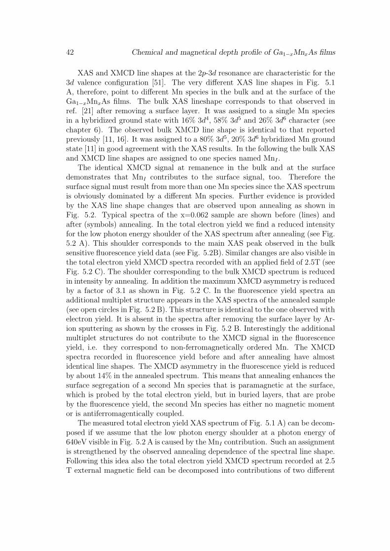
42 Chemical and magnetical depth profile of Ga1−xMnxAs films
XAS and XMCD line shapes at the 2p-3d resonance are characteristic for the3d valence configuration [51]. The very different XAS line shapes in Fig. 5.1A, therefore, point to different Mn species in the bulk and at the surface of theGa1−xMnxAs films. The bulk XAS lineshape corresponds to that observed inref. [21] after removing a surface layer. It was assigned to a single Mn speciesin a hybridized ground state with 16% 3d4, 58% 3d5 and 26% 3d6 character (seechapter 6). The observed bulk XMCD line shape is identical to that reportedpreviously [11, 16]. It was assigned to a 80% 3d5, 20% 3d6 hybridized Mn groundstate [11] in good agreement with the XAS results. In the following the bulk XASand XMCD line shapes are assigned to one species named MnI .
The identical XMCD signal at remanence in the bulk and at the surfacedemonstrates that MnI contributes to the surface signal, too. Therefore thesurface signal must result from more than one Mn species since the XAS spectrumis obviously dominated by a different Mn species. Further evidence is providedby the XAS line shape changes that are observed upon annealing as shown inFig. 5.2. Typical spectra of the x=0.062 sample are shown before (lines) andafter (symbols) annealing. In the total electron yield we find a reduced intensityfor the low photon energy shoulder of the XAS spectrum after annealing (see Fig.5.2 A). This shoulder corresponds to the main XAS peak observed in the bulksensitive fluorescence yield data (see Fig. 5.2B). Similar changes are also visible inthe total electron yield XMCD spectra recorded with an applied field of 2.5T (seeFig. 5.2 C). The shoulder corresponding to the bulk XMCD spectrum is reducedin intensity by annealing. In addition the maximum XMCD asymmetry is reducedby a factor of 3.1 as shown in Fig. 5.2 C. In the fluorescence yield spectra anadditional multiplet structure appears in the XAS spectra of the annealed sample(see open circles in Fig. 5.2 B). This structure is identical to the one observed withelectron yield. It is absent in the spectra after removing the surface layer by Ar-ion sputtering as shown by the crosses in Fig. 5.2 B. Interestingly the additionalmultiplet structures do not contribute to the XMCD signal in the fluorescenceyield, i.e. they correspond to non-ferromagnetically ordered Mn. The XMCDspectra recorded in fluorescence yield before and after annealing have almostidentical line shapes. The XMCD asymmetry in the fluorescence yield is reducedby about 14% in the annealed spectrum. This means that annealing enhances thesurface segregation of a second Mn species that is paramagnetic at the surface,which is probed by the total electron yield, but in buried layers, that are probeby the fluorescence yield, the second Mn species has either no magnetic momentor is antiferromagentically coupled.
The measured total electron yield XAS spectrum of Fig. 5.1 A) can be decom-posed if we assume that the low photon energy shoulder at a photon energy of640eV visible in Fig. 5.2 A is caused by the MnI contribution. Such an assignmentis strengthened by the observed annealing dependence of the spectral line shape.Following this idea also the total electron yield XMCD spectrum recorded at 2.5T external magnetic field can be decomposed into contributions of two different
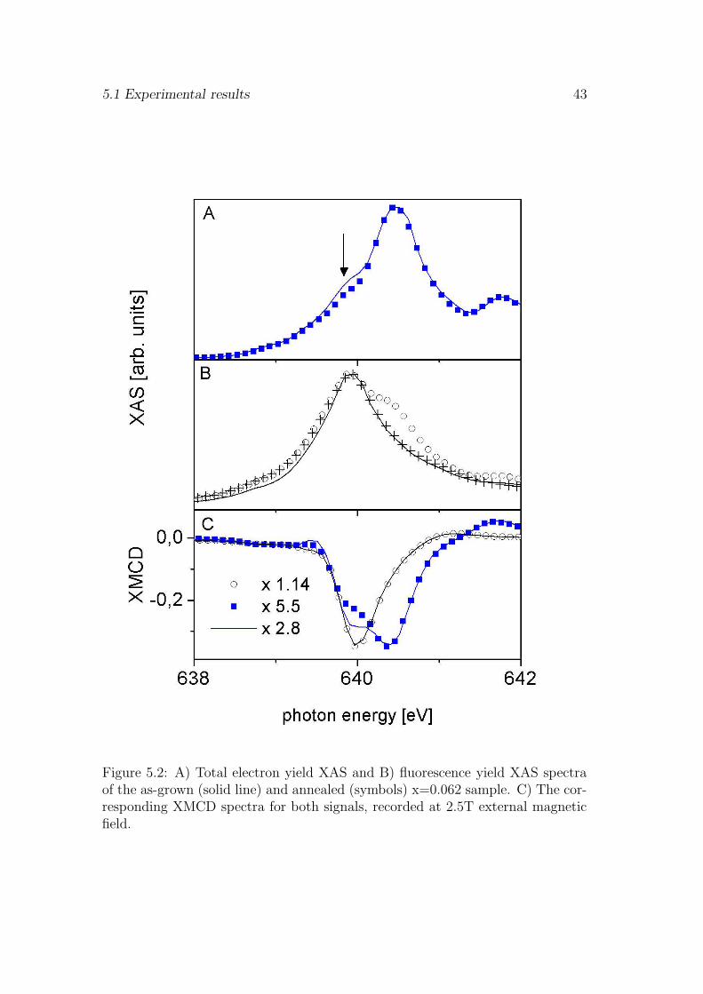
5.1 Experimental results 43
Figure 5.2: A) Total electron yield XAS and B) fluorescence yield XAS spectraof the as-grown (solid line) and annealed (symbols) x=0.062 sample. C) The cor-responding XMCD spectra for both signals, recorded at 2.5T external magneticfield.
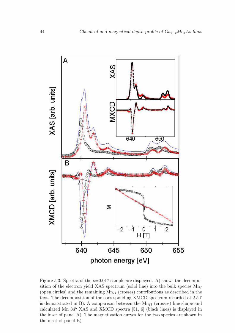
44 Chemical and magnetical depth profile of Ga1−xMnxAs films
Figure 5.3: Spectra of the x=0.017 sample are displayed. A) shows the decompo-sition of the electron yield XAS spectrum (solid line) into the bulk species MnI
(open circles) and the remaining MnII (crosses) contributions as described in thetext. The decomposition of the corresponding XMCD spectrum recorded at 2.5Tis demonstrated in B). A comparison between the MnII (crosses) line shape andcalculated Mn 3d5 XAS and XMCD spectra [51, 6] (black lines) is displayed inthe inset of panel A). The magnetization curves for the two species are shown inthe inset of panel B).
5.1 Experimental results 45
Mn species, since only in the surface sensitive spectrum an external magneticfield causes a dramatic change in the line shape. This decomposition was doneaccording to that of the XAS spectrum by assuming that the low photon energyshoulder in the XMCD signal recorded at 2.5T corresponds to the bulk XMCDpeak of MnI atoms (see Fig. 5.2 C). The results of this analysis are displayed inFigs. 5.3 A and B. The remaining surface XAS and XMCD lineshapes agree withmultiplet calculations for a 3d5 configuration [51] as shown in the inset of Fig.5.3 A. No other decomposition gives a similar agreement. This Mn 3d5 speciesis denoted as MnII in the following. The magnetization curves versus appliedmagnetic field for the two Mn species are shown in the inset of Fig. 5.3 B. Forthe MnI species we find a mixture of ferromagnetic and paramagnetic moments.The ferromagnetic coupling increases at higher Mn concentrations (magnetiza-tion curves for different Mn concentrations are shown in the next chapter in Fig.6.5). Atoms of the MnII species have an uncompensated magnetic moment onlyat the surface (probed only by total electron yield) which is paramagnetic in allsamples.
5.1.2 Chemical depth profile probed by resonant x-ray
reflectivity
So far the XAS spectra demonstrated the existence of two Mn species. MnII ob-viously accumulates at the surface and can be distinguished from the bulk MnI
species by XAS. The aim is now to obtain more detailed information on the depthprofile of the two Mn species. This was done by using x-ray resonant reflectivityat the Mn 2d − 3d resonance. Reflectivity spectra for the x = 0.017 sample aredisplayed in Fig. 5.4 A. The spectral line shape differs from the XAS spectrameasured by fluorescence and total electron yield since the reflected intensity ismodulated by interference between incident and reflected photons. As indicatedby equation 4.4 the scattering phase shifts and the resulting interference are de-termined by the spatial Mn distribution and the scattering vector i.e. the photonenergy and the incidence angle. The dependence on the latter is demonstrated inFig. 5.4 A. With decreasing incidence angle we observe a decreasing resonancepeak height and the development of a dip on its low energy side. The sensitiv-ity to changes in the Mn distribution is obvious if we compare the signal of theas-grown and the annealed x=0.062 sample in Fig. 5.4 B. At identical incidenceangle we find a change in the reflectivity spectrum caused by a rearrangement ofinterstitial Mn during annealing.
As mentioned in chapter 4 the reflectivity spectra cannot be transformeddirectly into a distribution of Mn atoms, since only the reflected intensity isrecorded while the phase information is lost. For the evaluation a fitting algo-rithm is used, comparing the measured reflectivity spectra to those calculatedfrom a model structure, using the Mn distribution as a fit parameter. Because

46 Chemical and magnetical depth profile of Ga1−xMnxAs films
Figure 5.4: A) X-ray resonant reflectivity spectra of the x=0.0175 sample (opencircles) recorded at incidence angles of (a=27o,b=23o,c=19o). For clarity a ver-tical offset has been applied to the spectra. The fits to the spectra are shown asblack lines. B) Reflectivity spectra of the x=0.062 sample before (open triangles)and after (solid squares) annealing. The fits to the spectra are shown as blacklines. The inset shows the enlarged the pre edge part of the spectra.
5.1 Experimental results 47
the specular reflectivity is sensitive only to the vertical Mn distribution, it isreasonable to model the reflectivity data by a system of different layers that areassumed to be homogenous in the lateral directions. The model describes thesample by three layers, the simplest configuration that is in agreement with theabsorption measurements. As shown in the inset of Fig. 5.6 A) the three lay-ers are: (i) the low-temperature GaAs substrate with semi-infinite thickness, (ii)the bulk Ga1−xMnxAs layer with given thickness and MnI concentration (x) and(iii) a surface layer with variable thickness and concentrations of MnII and MnI .Predetermined input parameters of the model are the bulk MnI concentration,the thickness of the Ga1−xMnxAs layer, the interface roughness, and the index ofrefraction for both Mn species and the GaAs substrate. The rms roughness forthe investigated samples was determined by atomic force microscopy as shown inFig. 4.1. The index of refraction for two Mn species was determined from theabsorption coefficient as explained in chapter 4. The explicit energy dependenceof the indices of refraction for MnI and MnII used in the calculations are shown inFig. 4.7. The index of refraction of the GaAs substrate was taken from literature[14]. The thickness of the surface layer and the concentrations of MnI and MnII
in the surface layer were used as fit parameters. For the calculations and fittingof the reflectivity spectra the IMD code [7] was employed.
Within the model two scenarios are possible. The simplest case would be thatthe surface layer is formed only by MnII atoms. But if MnI is excluded from thesurface layer the resulting fit is of very poor quality indicating that this modelis incorrect. The measured reflectivity spectra can only be fitted if we assumethat MnII and MnI coexist in the surface layer. In this case we find a perfectagreement between the measured spectra and the fit at all measured angles andphoton energies as demonstrated in Fig. 5.4 B. An example how sensitive thecalculated reflectivity spectrum depends on the the MnI concentration in thesurface layer is given by Fig. 5.5. It shows the measured reflectivity spectrum ofthe x=0.62 sample recorded at an incidence angle of θ = 22o (open circles). Bythe fit the MnI surface concentration was determined to be x=0.09 (solid line).Keeping the MnI concentration fixed at a value of 20% away from the optimumcauses a rather large error in the fit, as visible by the line shapes obtained withthe MnI concentration fixed at x=0.11 (dashed line) or x=0.07 (dotted line).Such tests were preformed for each of the three fit parameters to estimate theerror of this method.
The thickness of the surface layer and the Mn concentrations, that were de-termined by the fit, are summarized for all samples in Fig. 5.6. All as-grownsamples have a surface layer of similar thickness (1.5 - 2nm). The MnI concen-tration in the surface layer (solid circles in Fig. 5B) is found to be slightly higherthan in the bulk. As expected from the XAS data we find additionally a highconcentration of MnII atoms in the surface layer, which is well above the bulkconcentration of MnI atoms in all samples. As mentioned above MnI and MnII
coexist in the surface layer which means that the total density of Mn in the sur-
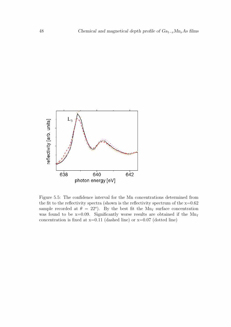
48 Chemical and magnetical depth profile of Ga1−xMnxAs films
Figure 5.5: The confidence interval for the Mn concentrations determined fromthe fit to the reflectivity spectra (shown is the reflectivity spectrum of the x=0.62sample recorded at θ = 22o). By the best fit the MnI surface concentrationwas found to be x=0.09. Significantly worse results are obtained if the MnI
concentration is fixed at x=0.11 (dashed line) or x=0.07 (dotted line)
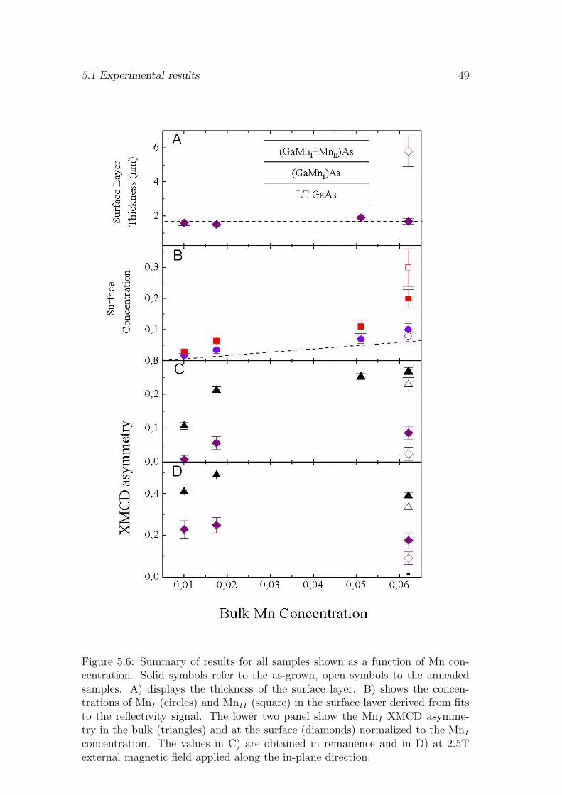
5.1 Experimental results 49
Figure 5.6: Summary of results for all samples shown as a function of Mn con-centration. Solid symbols refer to the as-grown, open symbols to the annealedsamples. A) displays the thickness of the surface layer. B) shows the concen-trations of MnI (circles) and MnII (square) in the surface layer derived from fitsto the reflectivity signal. The lower two panel show the MnI XMCD asymme-try in the bulk (triangles) and at the surface (diamonds) normalized to the MnI
concentration. The values in C) are obtained in remanence and in D) at 2.5Texternal magnetic field applied along the in-plane direction.
50 Chemical and magnetical depth profile of Ga1−xMnxAs films
face layer is more than two times above the bulk value. After annealing we findthe MnII concentration in the surface layer strongly enhanced accompanied by anincrease in thickness of the surface layer from below 2nm to around 6nm (see Fig.5.6). Obviously the total amount of MnII at the surface has strongly increased,whereas the MnI distribution is hardly affected by the annealing process.
It is important to note that the measured and calculated reflectivity spectraare influenced by interface roughness. This is demonstrated by the reflectivityspectra of the x = 0.062 sample, recorded before and after annealing, which aredisplayed in the inset of Fig. 5.5 B. In the as-grown state (open triangles) rela-tively smooth interfaces lead to interference fringes caused by the finite thicknessof the Ga1−xMnxAs layer. This is visible as intensity oscillations in the insetof Fig. 5.5 B. The oscillations can be fitted for an interface roughness of 0.65± 0.1nm and a bulk layer thickness of 171 ± 8nm. These values are in perfectagreement with the surface roughness of 0.6 ± 0.2nm obtained by atomic forcemicroscopy and the Ga1−xMnxAs layer thickness known from the growth param-eters, respectively. After annealing these oscillations disappear (solid squares).This can only be reproduced by our model if we assume an interface regionbetween Ga1−xMnx and the LT GaAs layer with a gradual change of the Mnconcentration. To suppress the oscillations completely, as observed in the ex-periment, the width of this region has to be 3nm or more. This indicates thatdiffusion of interstitial Mn during the low temperature annealing does not onlytake place towards the surface but also into the substrate.
5.2 Discussion
The experimental results presented in this chapter are summarized in Fig. 5.6.Panels A and B contain results from the reflectivity measurements while panels Cand D summarize the XMCD results. Although the Ga1−xMnxAs layer thicknessdiffers from sample to sample, the thickness of the surface layer of 1.5 - 2nmis quite uniform for all as-grown samples (see Fig. 5.6 A). After annealing thesurface layer thickness increases strongly. All samples exhibit a coexistence ofMnI and MnII in the surface layer. The total Mn concentration in the surface ismore than two times higher than that in the bulk. Even the MnII concentrationitself (solid squares in Fig. 5.6 B) is higher than the bulk MnI concentrationfor all samples (dotted line in Fig. 5.6 B). Low-temperature annealing leads toa strong enhancement of the MnII surface concentration (see Fig. 5.6 B). Nosignificant changes in the MnI surface concentration are observed (open circle inFig. 5.6 B). The ratio of MnI and MnII in the surface layer obtained from thereflectivity data (Fig. 5.6 B) agrees with that obtained from decomposition ofthe electron yield XAS spectra. Also the changes upon annealing are reflectedin the total electron and fluorescence yield XAS spectra displayed in the Fig.5.2 A and B, respectively. The change in the ratio between MnI and MnII

5.2 Discussion 51
at the surface reduces the weight of the MnI peak in the surface signal. Theshoulder corresponding to the MnI 2p-3d resonance peak (marked by the arrowin Fig. 5.2 A) is less pronounced in the annealed electron yield spectrum. Thefluorescence yield signal averages over a large probing depth compared to thetotal electron yield. In the as-grown sample the surface layer is obviously only aminor contribution to the fluorescence signal and below the detection limit. Afterannealing the MnII surface concentration is enhanced by six times and becomesvisible in the annealed fluorescence yield XAS spectrum (open circles) as a secondpeak that corresponds to the MnII 2p-3d resonance peak.
The XMCD results for MnI are summarized in Figs. 5.6 C and D. The bulkXMCD asymmetries (triangles) were directly taken from the fluorescence yielddata. The surface XMCD values (diamonds) correspond to the measured totalelectron yield XMCD asymmetries normalized to the fraction of surface MnI . Inremanence we observe a decline of the bulk magnetization (solid triangles in Fig.5.6 C) with lower Mn concentration. This is most likely due to the reduction ofthe magnetic ordering temperature. At an external magnetic field of 2.5T the lowconcentration samples exhibit the highest asymmetry of 0.49 ± 0.013 as shownin Fig. 5.6 D. Using the calculated XMCD asymmetries in ref. [11] this wouldcorrespond to 83 ± 4 % of the Mn atoms that are magnetically orderd if everyMn atom carries a magnetic moment of 4.6µB. Interestingly the bulk saturationmagnetization of the x=0.062 sample in the as-grown state is smaller than thisvalue of the low concentration sample. Annealing causes a somewhat lower bulkmagnetic moment (open triangle) even though it raises the Curie temperature ofthis sample by 13K. A lower magnetic moment per Mn atom in high concentrationsamples and its reduction upon annealing has also been observed in ref. [22]. Theorigin of this effect is discussed in detail in chapter 6. In remanence and with anexternal magnetic field we find a clearly reduced magnetic moment of surface MnI
(solid diamonds in Fig. 5.6 C and D) which is further reduced after annealing(open diamond). The ferromagnetic exchange coupling of MnI atoms is obviouslyweaker in the presence of MnII . Possible mechanisms that could cause this effectare discussed below.
The XAS data of Fig. 2 and the resonant reflectivity data summarized in Fig.5.6 B show an inhomogeneous distribution of two Mn species. From its ferromag-netic and electronic configuration MnI can be clearly identified as substitutionalMn replacing the Ga atoms. MnI is the dominant species in the bulk of all films.The consistently higher surface concentration of substitutional Mn points to anon-equilibrium MBE growth process as the reason for disorder. Possible siteexchanges are then energetically more favorable [20]. Post growth annealing pro-duces hardly any change in the MnI surface species (open and solid circles in ofFig. 5.6 B).
It is tempting to assign the second observed Mn species, MnII , character-ized by a 3d5 electronic configuration to interstitial Mn. The growth process isknown to provide pathways for the generation of interstitial Mn [20], i.e. the
52 Chemical and magnetical depth profile of Ga1−xMnxAs films
concentration of interstitial Mn at the surface should be significantly higher. Inaddition the diffusion of interstitial Mn from bulk to the surface during anneal-ing has been observed [15]. This is consistent with the increased accumulation ofMnII at the surface of the x=0.062 sample after annealing. Assuming that theaccumulation of MnII at the surface is due to diffusion of interstitials out of thebulk one can estimate that 5 ± 1 % of interstitial Mn was present in the bulk ofthe as-grown sample. Such an amount of interstitial Mn is less than the value of17% recently obtained from ion channeling in the bulk of a Ga1−xMnxAs sample[19]. However, the number of interstitial Mn in the bulk may strongly depend onthe growth conditions. On the other hand the reflectivity data indicate that Mndiffuses not only to the surface but also into the substrate. The accumulationof MnII in the surface layer is accompanied by magnetization deficit of the MnI
residing in that layer. It has been proposed that interstitial Mn should couple an-tiferromagnetically with substitutional Mn and hybridize less with the substrate[10]. The latter seems to be reflected in the 3d5 configuration of MnII which ismore localized than that of substitutional Mn (MnII). But the XMCD spectraprovide only little evidence of antiferromagnetic coupling between MnII and sub-stitutional Mn. Only a small change in the XMCD lineshape that is present inthe as-grown x=0.062 sample and dissappears after the annealing is visible inFig. 6.3. It is more likely that the double exchange between substitutional Mnis influenced via interstitial Mn acting as electron donor. This could lead to areduced carrier concentration in the surface layer, thus reducing Tc.
The presence of MnII at the surface and its enhancement upon annealing isclearly due to the diffusion of interstitial Mn, but the observed lineshape cannot be unambiguously identified as interstitial Mn since one can not rule out theinfluence of surface oxidation as reported previously [15]. In some publicationit is argued that the complete out diffusion of interstitial Mn is only possible inthe presence of oxygen or nitrogen passivating intersitial Mn at the surface [62].The annealing of the x=0.062 sample was done under vacuum. Following thisargument would mean that possibly not all interstitial Mn was removed, becauseof the limited amount of oxygen that was present at the surface. Interestingly thedata indicate that two different magnetic configurations of the MnII species arepresent in the surface layer after the annealing. The outer MnII atoms accessibleto the electron yield, which are probaly oxidized, carry a paramagnetic moment.But the buried MnII atoms visible in the fluorescence yield after annealing haveno paramagnetic moment or are strongly antiferromagnetically aligned even at2.5T external field. This and the coexistence of ferromagnetically ordered MnI atthe same depth below the surface indicates that the surface layer is not completelyoxidized.
Also the Mn bulk spectra could possibly answer the question whether theMnII configuration is formed at the surface or is also present in the bulk in a verydilute form. If we assume that the MnII atoms were homogenously distributedin the bulk before the annealing, we can estimate the change of the bulk XAS
5.3 Conclusion 53
lineshape upon their removal. The FY spectrum of the as-grown sample and thatof the annealed sample after removing the surface layer by Ar sputtering shouldshow a slight difference due to the missing MnII in the bulk. These two FYspectra are displayed in Fig. 5.7 (normalized to the same step like backgound).They are compared to a reference spectrum (opens squares) that was generated bysubtracting the MnII lineshape from the as-grown bulk XAS spectrum, accordingto a spectral weight of 5% MnII . As indicated by the reference signal the removalof 5% MnII from the bulk should cause a small change in the FY signal at thehigh energy side of the MnI 2p−3d resonance which is above the detection limit.Interestingly the experimental data show an obvious deviation in the spectrallineshape between the as-grown and the annealed and sputtered sample on thelow energy side of the MnI 2p− 3d resonance. This effect will be discussed in thenext chapter in detail. But the expected change on the high energy side of theMnI 2p − 3d resonance is not observed. This points to the influence of surfaceoxidation. But still, the surface could be altered by sputtering or the MnII notcompletely removed.
It is interesting to compare this results to recent neutron scattering experi-ments [12] which studied depth dependent the magnetic and structural propertiesof Mn in a x=0.073 sample as-grown and after annealing. The XAS and reflec-tivity data demonstrate an increased Mn surface concentration in the as-grownsamples which is strongly increased upon annealing. By neutron scattering suchsurface accumulation of Mn could only be found after annealing. In contradic-tion to the neutron scattering data the XMCD measurements can not confirma zero magnetic moment of the Mn surface atoms. Their magnetic moment isonly reduced compared to the bulk Mn. In addition the bulk magnetic momentmeasured by XMCD was found to decrease slightly after annealing whereas anincrease was seen by neutron scattering. The inconsistent results that both meth-ods obtain for the surface layer may be due to the limited sensitivity of neutronscattering experiments to layers of a few nm. Whether the bulk magnetic momentof Mn is increased or decreased by annealing may also depend on the annealingconditions as time and temperature and the presence of ambient gases. In thatrespect the annealing conditions were not identical. However, the decrease uponannealing has been also observed by SQUID measurements [22].
5.3 Conclusion
The analysis of the chemical and magnetical depth profile of the Ga1−xMnxAssamples revealed the presence of two different Mn species with different XASand XMCD line shapes in our samples. The bulk of the Ga1−xMnxAs samplesis dominated by substitutional Mn. This species can easily be identified by itsferromagnetic properties and a mixed valence 3d5 - 3d6 electronic configurationwhich is characteristic for the hybridization with GaAs valence orbitals. At the
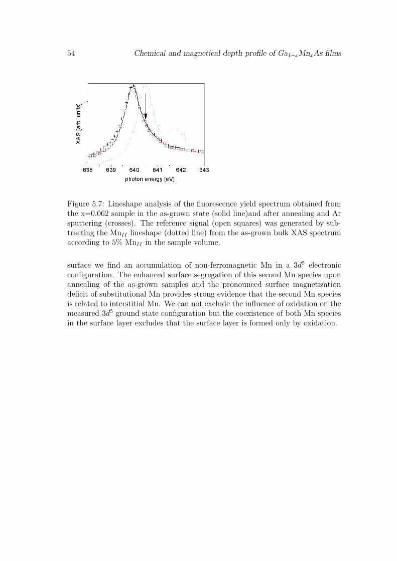
54 Chemical and magnetical depth profile of Ga1−xMnxAs films
Figure 5.7: Lineshape analysis of the fluorescence yield spectrum obtained fromthe x=0.062 sample in the as-grown state (solid line)and after annealing and Arsputtering (crosses). The reference signal (open squares) was generated by sub-tracting the MnII lineshape (dotted line) from the as-grown bulk XAS spectrumaccording to 5% MnII in the sample volume.
surface we find an accumulation of non-ferromagnetic Mn in a 3d5 electronicconfiguration. The enhanced surface segregation of this second Mn species uponannealing of the as-grown samples and the pronounced surface magnetizationdeficit of substitutional Mn provides strong evidence that the second Mn speciesis related to interstitial Mn. We can not exclude the influence of oxidation on themeasured 3d5 ground state configuration but the coexistence of both Mn speciesin the surface layer excludes that the surface layer is formed only by oxidation.

Chapter 6
Mn 3d hybridization
In this chapter the hybridization of Mn 3d with Ga/As 4sp valence orbitals isstudied systematically using high resolution XAS and XMCD spectroscopy forsamples with different Mn concentrations. The spectral XAS and XMCD line-shape is known to be characteristic for the electronic 3dn valence configuration[11, 50, 51, 6, 21]. Most models of exchange coupling presently discussed in theliterature are based on a localized Mn 3d5 electronic configuration which interactswith holes via impurity states consisting of mainly Ga/As 4sp orbitals [45, 46, 44].Population analysis indicates that the number of Mn 3d electrons is actually be-tween 3d5 and 3d6 [47]. This is in agreement with experimental investigationsusing x-ray magnetic circular dichroism (XMCD) [11, 21]. However, there arealso experimental reports that Mn is present in a 3d4 configuration [61]. In ref.[61] the 3d4 component was even considered essential to establish ferromagneticorder. The presence of Mn interstitials close to clusters of substitutional Mnwas theoretically predicted to strongly modify the exchange coupling betweenthe latter as well as their charge state [20, 49]. Finally, in contrast to II-VI basedmagnetic semiconductors no antiferromagnetic exchange between Mn-Mn nearestneighbors has been considered for Ga1−xMnxAs due to a lack of experimental ev-idence despite its possibly adverse effect on a high ferromagnetic Tc [2]. Here wepresent experimental evidence for antiferromagnetic exchange between Mn-Mnnearest neighbors in Ga1−xMnxAs at high Mn concentrations.
6.1 Influence of the surface
As demonstrated before, using the fluorescence yield detection in XAS and XMCDis the ideal choice to probe the bulk properties of dilute Ga1−xMnxAs samples.But of course also the surface contributes to some extend to the signal. To elimi-nate or minimize the influence of any modified surface layer (see chapter 5) on thebulk measurements the sample surfaces were prepared by in situ Ar-ion sputter-ing to remove the surface layer and any contaminants. The surface preparation
55
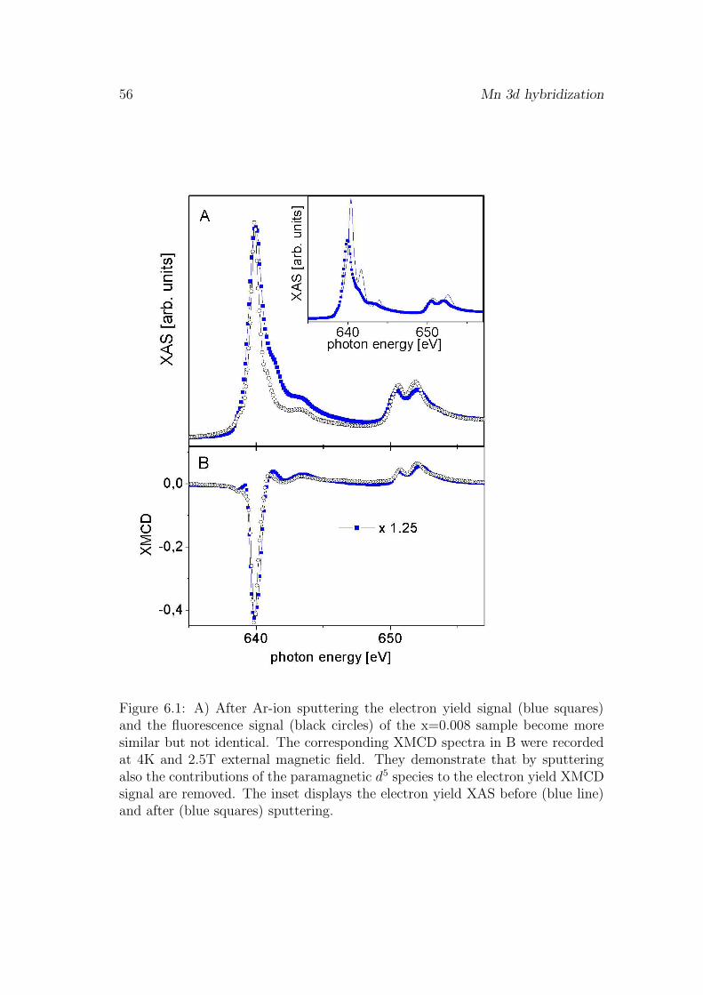
56 Mn 3d hybridization
Figure 6.1: A) After Ar-ion sputtering the electron yield signal (blue squares)and the fluorescence signal (black circles) of the x=0.008 sample become moresimilar but not identical. The corresponding XMCD spectra in B were recordedat 4K and 2.5T external magnetic field. They demonstrate that by sputteringalso the contributions of the paramagnetic d5 species to the electron yield XMCDsignal are removed. The inset displays the electron yield XAS before (blue line)and after (blue squares) sputtering.
6.2 pd-hybridization of ferromagnetically coupled Mn 57
can be monitored in XAS and XMCD by total electron yield detection. TypicalXAS spectra before and after sputtering are shown in the inset of Fig. 6.1 A) Thed5 multiplet (solid line in the inset) characteristic for the as grown sample (seeFig. 5.1) disappears after the surface layer is removed (blue squares in the inset).As visible in Fig. 6.1 A) the lineshape of the total electron yield spectrum (solidsquares) is then similar to that of the fluorescence yield (open circles). But adistinct broadening of the electron yield XAS spectrum remains compared to thefluorescence yield data. The origin of that broadening could be due to disorder atthe surface which is of course increased by the Ar-ion sputtering. Also the totalelectron yield XMCD signal (solid squares in Fig. 6.1 B) is broadened comparedto the fluorescence XMCD signal (open circles in Fig. 6.1 B) and the surfaceXMCD amplitude is reduced compared to that of the bulk. For an external mag-netic field of 4T the slight broadening at the high energy side of the L3 peak,visible in Fig. 6.1 B), indicates the presence of paramagnetic Mn atoms which areabsent in the bulk. A difference in the fluorescence yield spectra before and afterremoving the surface layer was only observed in case of the annealed x=0.062sample where the Mn d5 containing surface layer was (5.8 ± 0.9)nm thick, i.e.much thicker than in the as-grown state. In all other cases the influence of thesurface layer to the bulk spectra was negligible. In the literature also HCl etchingis used to remove the surface layers from Ga1−xMnxAs samples [21]. The resultsof this method are very similar to sputtering. Fig. 6.2 presents the electron yieldspectrum of a sample prepared by HCl etching taken from ref. [21] (red line)compared to that of a sputtered sample (blue squares). Both spectra are iden-tical indicating the same influence of disorder. This underlines the advantage ofthe fluorescence signal probing the undisturbed bulk properties.
6.2 pd-hybridization of ferromagnetically coupled
Mn
Typical Mn L3,2 XAS and XMCD spectra for two different Mn concentrations,the x=0.008 sample (black line) and the x=0.062 sample after annealing (redline) are shown in Fig. 6.3 A) and b), respectively. The spectra were recordedat 10K with saturation magnetic fields (see Fig. 6.5) of 4.5T (x=0.008) and2.5T (x=0.062) applied along one of the two equivalent in-plane hard magnetic< 110 > axes. The spectra are normalized to a constant step like backgroundcaused by transitions into continuum states. The observed XMCD lineshape isidentical to the one reported previously [11, 21, 17]. Only the as-grown x=0.062XMCD spectrum (green line in the inset of Fig. 6.3 B)) displays lineshape changeswhich, however, disappear after interstitial Mn atoms are removed by annealing(see red line in the inset of Fig. 6.3 B)).
At low Mn concentrations of x=0.008 and x=0.017 (not displayed in Fig. 6.3)
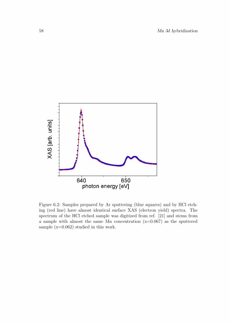
58 Mn 3d hybridization
Figure 6.2: Samples prepared by Ar sputtering (blue squares) and by HCl etch-ing (red line) have almost identical surface XAS (electron yield) spectra. Thespectrum of the HCl etched sample was digitized from ref. [21] and stems froma sample with almost the same Mn concentration (x=0.067) as the sputteredsample (x=0.062) studied in this work.
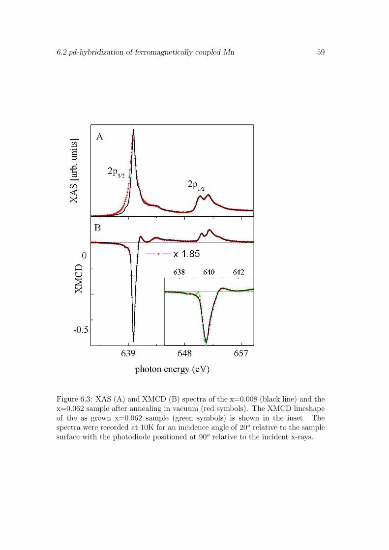
6.2 pd-hybridization of ferromagnetically coupled Mn 59
Figure 6.3: XAS (A) and XMCD (B) spectra of the x=0.008 (black line) and thex=0.062 sample after annealing in vacuum (red symbols). The XMCD lineshapeof the as grown x=0.062 sample (green symbols) is shown in the inset. Thespectra were recorded at 10K for an incidence angle of 20o relative to the samplesurface with the photodiode positioned at 90o relative to the incident x-rays.
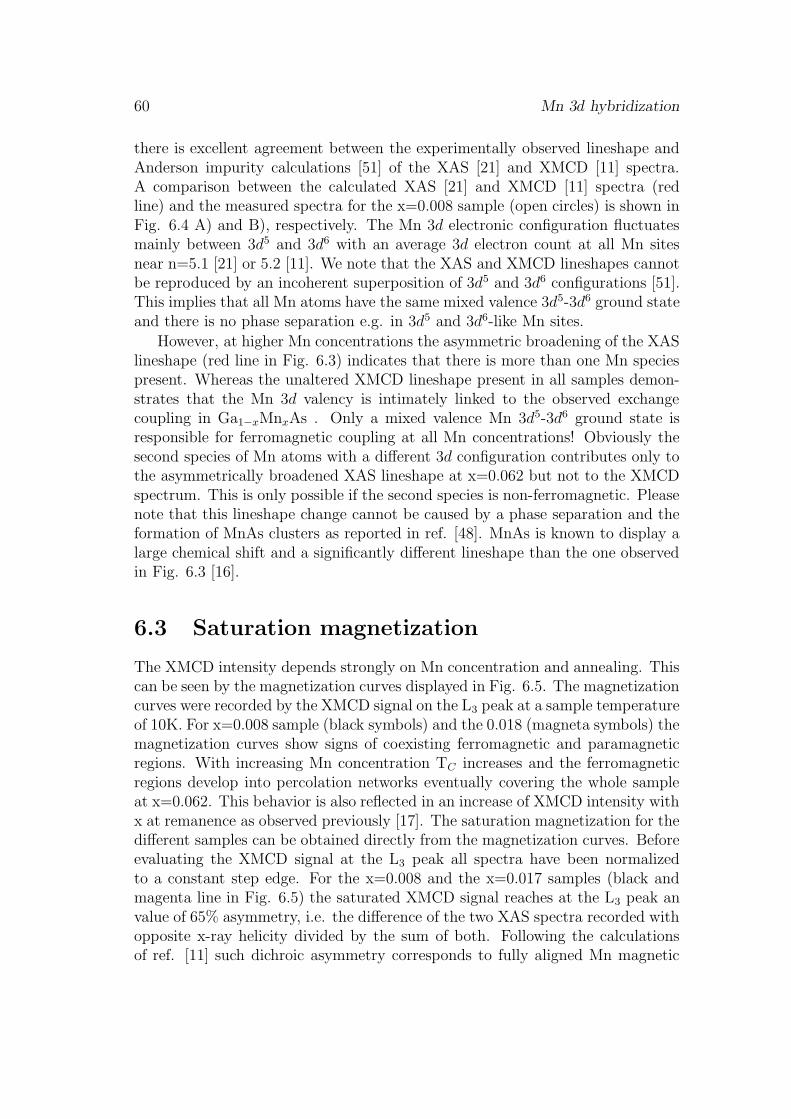
60 Mn 3d hybridization
there is excellent agreement between the experimentally observed lineshape andAnderson impurity calculations [51] of the XAS [21] and XMCD [11] spectra.A comparison between the calculated XAS [21] and XMCD [11] spectra (redline) and the measured spectra for the x=0.008 sample (open circles) is shown inFig. 6.4 A) and B), respectively. The Mn 3d electronic configuration fluctuatesmainly between 3d5 and 3d6 with an average 3d electron count at all Mn sitesnear n=5.1 [21] or 5.2 [11]. We note that the XAS and XMCD lineshapes cannotbe reproduced by an incoherent superposition of 3d5 and 3d6 configurations [51].This implies that all Mn atoms have the same mixed valence 3d5-3d6 ground stateand there is no phase separation e.g. in 3d5 and 3d6-like Mn sites.
However, at higher Mn concentrations the asymmetric broadening of the XASlineshape (red line in Fig. 6.3) indicates that there is more than one Mn speciespresent. Whereas the unaltered XMCD lineshape present in all samples demon-strates that the Mn 3d valency is intimately linked to the observed exchangecoupling in Ga1−xMnxAs . Only a mixed valence Mn 3d5-3d6 ground state isresponsible for ferromagnetic coupling at all Mn concentrations! Obviously thesecond species of Mn atoms with a different 3d configuration contributes only tothe asymmetrically broadened XAS lineshape at x=0.062 but not to the XMCDspectrum. This is only possible if the second species is non-ferromagnetic. Pleasenote that this lineshape change cannot be caused by a phase separation and theformation of MnAs clusters as reported in ref. [48]. MnAs is known to display alarge chemical shift and a significantly different lineshape than the one observedin Fig. 6.3 [16].
6.3 Saturation magnetization
The XMCD intensity depends strongly on Mn concentration and annealing. Thiscan be seen by the magnetization curves displayed in Fig. 6.5. The magnetizationcurves were recorded by the XMCD signal on the L3 peak at a sample temperatureof 10K. For x=0.008 sample (black symbols) and the 0.018 (magneta symbols) themagnetization curves show signs of coexisting ferromagnetic and paramagneticregions. With increasing Mn concentration TC increases and the ferromagneticregions develop into percolation networks eventually covering the whole sampleat x=0.062. This behavior is also reflected in an increase of XMCD intensity withx at remanence as observed previously [17]. The saturation magnetization for thedifferent samples can be obtained directly from the magnetization curves. Beforeevaluating the XMCD signal at the L3 peak all spectra have been normalizedto a constant step edge. For the x=0.008 and the x=0.017 samples (black andmagenta line in Fig. 6.5) the saturated XMCD signal reaches at the L3 peak anvalue of 65% asymmetry, i.e. the difference of the two XAS spectra recorded withopposite x-ray helicity divided by the sum of both. Following the calculationsof ref. [11] such dichroic asymmetry corresponds to fully aligned Mn magnetic

6.3 Saturation magnetization 61
Figure 6.4: XAS (A) and XMCD (B) spectra of the x=0.008 (open circles) com-pared to Anderson impurity calculations [51] of the XAS [21] and XMCD [11]assuming a Mn 3d electronic 3d5 configuration with an admixture of 3d6 contri-butions. The average 3d electron count at all Mn sites was set to n=5.1 [21] or5.2 [11] (red line).
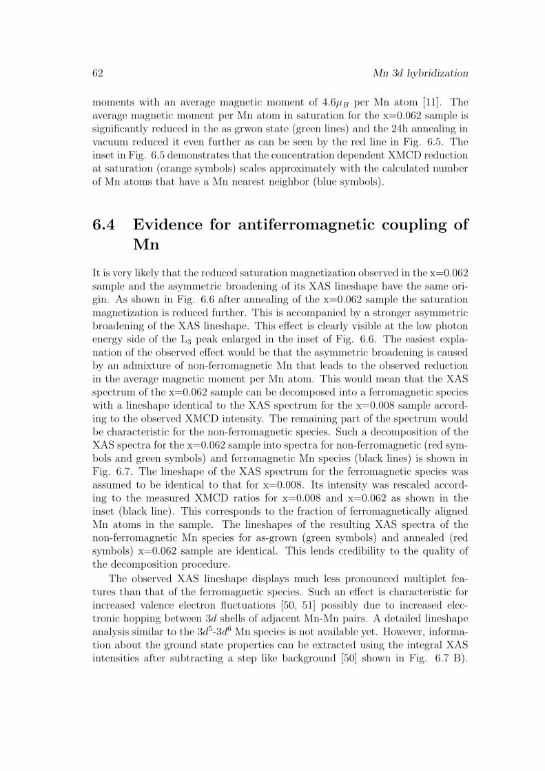
62 Mn 3d hybridization
moments with an average magnetic moment of 4.6µB per Mn atom [11]. Theaverage magnetic moment per Mn atom in saturation for the x=0.062 sample issignificantly reduced in the as grwon state (green lines) and the 24h annealing invacuum reduced it even further as can be seen by the red line in Fig. 6.5. Theinset in Fig. 6.5 demonstrates that the concentration dependent XMCD reductionat saturation (orange symbols) scales approximately with the calculated numberof Mn atoms that have a Mn nearest neighbor (blue symbols).
6.4 Evidence for antiferromagnetic coupling of
Mn
It is very likely that the reduced saturation magnetization observed in the x=0.062sample and the asymmetric broadening of its XAS lineshape have the same ori-gin. As shown in Fig. 6.6 after annealing of the x=0.062 sample the saturationmagnetization is reduced further. This is accompanied by a stronger asymmetricbroadening of the XAS lineshape. This effect is clearly visible at the low photonenergy side of the L3 peak enlarged in the inset of Fig. 6.6. The easiest expla-nation of the observed effect would be that the asymmetric broadening is causedby an admixture of non-ferromagnetic Mn that leads to the observed reductionin the average magnetic moment per Mn atom. This would mean that the XASspectrum of the x=0.062 sample can be decomposed into a ferromagnetic specieswith a lineshape identical to the XAS spectrum for the x=0.008 sample accord-ing to the observed XMCD intensity. The remaining part of the spectrum wouldbe characteristic for the non-ferromagnetic species. Such a decomposition of theXAS spectra for the x=0.062 sample into spectra for non-ferromagnetic (red sym-bols and green symbols) and ferromagnetic Mn species (black lines) is shown inFig. 6.7. The lineshape of the XAS spectrum for the ferromagnetic species wasassumed to be identical to that for x=0.008. Its intensity was rescaled accord-ing to the measured XMCD ratios for x=0.008 and x=0.062 as shown in theinset (black line). This corresponds to the fraction of ferromagnetically alignedMn atoms in the sample. The lineshapes of the resulting XAS spectra of thenon-ferromagnetic Mn species for as-grown (green symbols) and annealed (redsymbols) x=0.062 sample are identical. This lends credibility to the quality ofthe decomposition procedure.
The observed XAS lineshape displays much less pronounced multiplet fea-tures than that of the ferromagnetic species. Such an effect is characteristic forincreased valence electron fluctuations [50, 51] possibly due to increased elec-tronic hopping between 3d shells of adjacent Mn-Mn pairs. A detailed lineshapeanalysis similar to the 3d5-3d6 Mn species is not available yet. However, informa-tion about the ground state properties can be extracted using the integral XASintensities after subtracting a step like background [50] shown in Fig. 6.7 B).
6.4 Evidence for antiferromagnetic coupling of Mn 63
Figure 6.5: The XMCD signal at a photon energy of 640eV is used to probe thesample magnetization versus applied magnetic field for as-grown (Ga1−xMnx)Assamples with x=0.008, 0.017 and 0.062 (solid black, solid magenta, and solidgreen symbols). The magnetization curve for the annealed x=0.062 sample isdisplayed by open red symbols. All spectra were taken at 10K which is onlyslightly below TC for the x=0.008 sample. The upper inset shows the relativesaturation magnetization, Msat (orange symbols) and the calculated number ofMn atoms that have nearest neighbors, NMn−Mn, (blue symbols) vs x.

64 Mn 3d hybridization
Figure 6.6: The bulk XAS and XMCD spectra of the x=0.008 sample (black line)are compared to those of the x=0.062 sample at different stages of annealing: asgrown (green) and after annealing under vacuum (red). As demonstrated in A)the XAS lineshapes are not identical, especially at the low energy side of the L3
peak (enlarged in the inset) differences between the x=0.008 sample (black line)and the x=0.062 (red symbols) are obvious. The saturation magnetization of thex = 0, 062 sample annealed under vacuum is reduced by a factor of 0.54 comparedthe x=0.008 sample, but the XMCD lineshapes of both are exactly identical asdemonstrated in B). The inset in A) visualizes how the XAS lineshape of thex = 0, 062 sample varies with the stage of annealing. This corresponds to achange of the saturation magnetization that is shown in the inset of B). TheXAS and XMCD spectra of the x=0.017 sample (not shown) were identical tothe x=0.008 case.
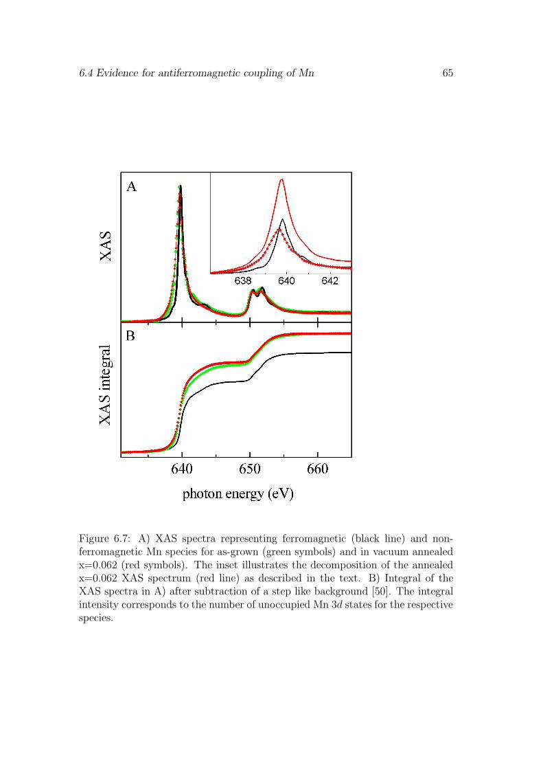
6.4 Evidence for antiferromagnetic coupling of Mn 65
Figure 6.7: A) XAS spectra representing ferromagnetic (black line) and non-ferromagnetic Mn species for as-grown (green symbols) and in vacuum annealedx=0.062 (red symbols). The inset illustrates the decomposition of the annealedx=0.062 XAS spectrum (red line) as described in the text. B) Integral of theXAS spectra in A) after subtraction of a step like background [50]. The integralintensity corresponds to the number of unoccupied Mn 3d states for the respectivespecies.
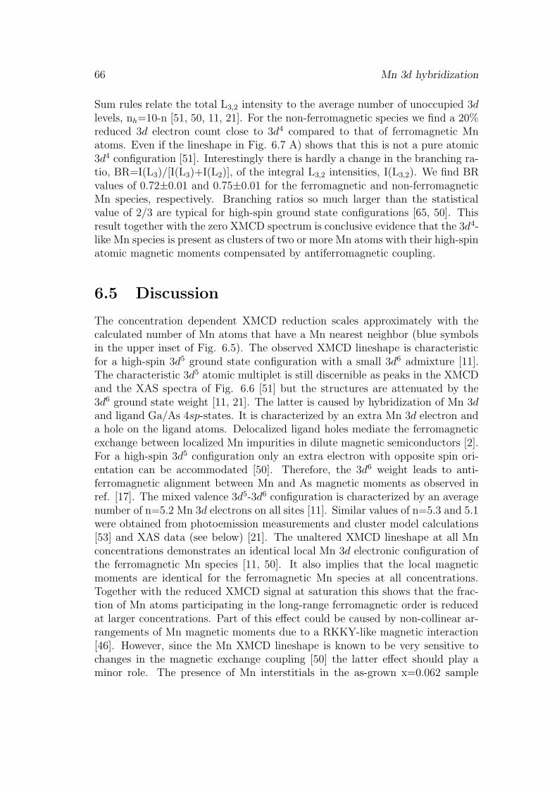
66 Mn 3d hybridization
Sum rules relate the total L3,2 intensity to the average number of unoccupied 3dlevels, nh=10-n [51, 50, 11, 21]. For the non-ferromagnetic species we find a 20%reduced 3d electron count close to 3d4 compared to that of ferromagnetic Mnatoms. Even if the lineshape in Fig. 6.7 A) shows that this is not a pure atomic3d4 configuration [51]. Interestingly there is hardly a change in the branching ra-tio, BR=I(L3)/[I(L3)+I(L2)], of the integral L3,2 intensities, I(L3,2). We find BRvalues of 0.72±0.01 and 0.75±0.01 for the ferromagnetic and non-ferromagneticMn species, respectively. Branching ratios so much larger than the statisticalvalue of 2/3 are typical for high-spin ground state configurations [65, 50]. Thisresult together with the zero XMCD spectrum is conclusive evidence that the 3d4-like Mn species is present as clusters of two or more Mn atoms with their high-spinatomic magnetic moments compensated by antiferromagnetic coupling.
6.5 Discussion
The concentration dependent XMCD reduction scales approximately with thecalculated number of Mn atoms that have a Mn nearest neighbor (blue symbolsin the upper inset of Fig. 6.5). The observed XMCD lineshape is characteristicfor a high-spin 3d5 ground state configuration with a small 3d6 admixture [11].The characteristic 3d5 atomic multiplet is still discernible as peaks in the XMCDand the XAS spectra of Fig. 6.6 [51] but the structures are attenuated by the3d6 ground state weight [11, 21]. The latter is caused by hybridization of Mn 3dand ligand Ga/As 4sp-states. It is characterized by an extra Mn 3d electron anda hole on the ligand atoms. Delocalized ligand holes mediate the ferromagneticexchange between localized Mn impurities in dilute magnetic semiconductors [2].For a high-spin 3d5 configuration only an extra electron with opposite spin ori-entation can be accommodated [50]. Therefore, the 3d6 weight leads to anti-ferromagnetic alignment between Mn and As magnetic moments as observed inref. [17]. The mixed valence 3d5-3d6 configuration is characterized by an averagenumber of n=5.2 Mn 3d electrons on all sites [11]. Similar values of n=5.3 and 5.1were obtained from photoemission measurements and cluster model calculations[53] and XAS data (see below) [21]. The unaltered XMCD lineshape at all Mnconcentrations demonstrates an identical local Mn 3d electronic configuration ofthe ferromagnetic Mn species [11, 50]. It also implies that the local magneticmoments are identical for the ferromagnetic Mn species at all concentrations.Together with the reduced XMCD signal at saturation this shows that the frac-tion of Mn atoms participating in the long-range ferromagnetic order is reducedat larger concentrations. Part of this effect could be caused by non-collinear ar-rangements of Mn magnetic moments due to a RKKY-like magnetic interaction[46]. However, since the Mn XMCD lineshape is known to be very sensitive tochanges in the magnetic exchange coupling [50] the latter effect should play aminor role. The presence of Mn interstitials in the as-grown x=0.062 sample

6.6 Conclusion 67
causes a slightly different XMCD lineshape. This is a strong indication that sub-stitutional and interstitial Mn occupy neighbor sites and form magnetic clusters[49, 10].
Ferromagnetism is connected only to the d5-d6 Mn species as, for instance,evidenced by the temperature dependent hysteresis loop changes in Fig. 6.5. Inthis case the exchange of holes mediates ferromagnetic coupling and long rangeferromagnetic order sets in as the Mn concentration increases [45, 46, 49]. On av-erage there is much less than one hole per ferromagnetic Mn acceptor [2, 45, 20].Theoretical models indicate that compensation of the negative charge for neigh-boring Mn-Mn acceptor pairs by up to two holes can lead to antiferromagneticinteraction between Mn neighbors [20]. It is tempting to explain the identifiedantiferromagnetic d4-like Mn clusters by this scenario. The observed increase inthe number of d4-like Mn atoms by removal of Mn interstitials is in agreementwith first principles calculations which predict interstitial Mn to cluster with twoor more substitutional Mn atoms [49]. This proximity of interstitial and sub-stitutional Mn is also thought to affect the ferromagnetic coupling between thelatter [49]. We surmise that this could explain the observed 10% change in Mnmagnetization upon the removal of 5% Mn interstitials (described in the previouschapter). We can presently only speculate that the electric charge of substitu-tional Mn-Mn acceptor clusters might be screened by valence holes. The resultscould then indicate that some of these holes are tightly bound around antiferro-magnetic Mn-Mn pairs and may even hop onto the Mn 3d shell as reflected inthe experimentally observed 20% reduced Mn 3d electron count for this species.It will be interesting to see a first-principles description of such an effect developin the future.
6.6 Conclusion
The signature of Mn 3d5-3d6 mixed valence acceptor states, responsible for long-range ferromagnetic order, was identified with x-ray magnetic circular dichroismat all Mn concentrations. With increasing Mn content an increasing amount ofMn atoms is observed exhibiting a significantly reduced number of 3d electrons ofclose to 3d4. Their number scales approximately with the number of Mn nearestneighbor pairs expected for a statistical Mn distribution. Both observations canbe explained by the presence of Mn-Mn nearest neighbor pairs. We also finda corresponding reduction of the number of ferromagnetic Mn atoms at highMn concentrations. Contrary to II-VI based materials this represents the firstobservation of antiferromagnetic order in III-V dilute magnetic semiconductorswith possibly a similar adverse effect to the ferromagnetic ordering temperature.

68 Mn 3d hybridization

Chapter 7
Orbital magnetic moment
anisotropy
7.1 Introduction
The local exchange coupling between the GaAs valence states and the Mn d statesis very important for the understanding of the long range ferromagnetic couplingin Ga1−xMnxAs. The valence holes are exchange coupled to the Mn impurity 3dspins by pd-hybridization. In this chapter we present angle dependent XMCDmeasurements that show a variation of the Mn 3d orbital moment with the in-plane azimuthal lattice direction. Correlated spectroscopic lineshape changes inthe XMCD spectra can be interpreted as an anisotropy in the spatial overlap ofMn 3d and As 4sp states that is probed by the spin-orbit coupling, present inthe Mn 3d shell. This interpretation is in agreement with recent calculations pre-dicting a strongly anisotropic pd-hybridization [71]. This is the first experimentalevidence for an orientation dependent pd-hybridization in Ga1−xMnxAs.
7.2 Results
7.2.1 Orbital magnetic moment anisotropy
In this chapter we will focus on the annealed sample with x=0.062. At lowtemperature (5-10K) this sample exhibits two in-plane easy-axis of the mag-netization which are oriented along the equivalent < 100 > lattice directionsas determined by SQUID measurements [68]. Analyzing the magnetization byXMCD spectroscopy we find an obvious difference between XMCD spectra thatwere recorded with the magnetization aligned along the equivalent < 100 > andthe equivalent < 110 > lattice directions. The Fig. 7.1 B). shows two XMCDspectra that were recorded in magnetic saturation with an external magnetic fieldof 4T applied. For the red spectrum the magnetic field and the incoming x-ray
69
70 Orbital magnetic moment anisotropy
Figure 7.1: This figure displays spectra of the annealed x=0.062 sample recordedat 5K and an incidence angle of 20o relative to the surface. In panel B) twoXMCD spectra are displayed: for the red XMCD spectrum the magnetizationwas saturated along a hard magnetic < 110 > axis whereas the black spectrumwas recorded with the magnetization saturated along an easy magnetic < 100 >axis. The integrals over the XMCD spectra are shown as dashed lines. Panel A)shows the corresponding isotropic XAS spectra (solid lines) and their integrals(dashed lines) after subtraction of the indicated step function (dotted line). Onlythe XAS spectra were normalized to an identical height of the step edge.
7.2 Results 71
beam were aligned along the < 110 > lattice direction (hard axis) whereas forthe black XMCD spectrum the azimuth of the sample was rotated by 45o so thatthe magnetization was aligned along the < 100 > direction (easy axis). Theincidence angle was in both cases 20o and the sample temperature 5K.
By sum rule analysis (see chapter 2) we find for both directions a non-zeroorbital moment residing on the Mn 3d shell. In both cases the orbital momentis positive, which means that spin and orbital moment are aligned parallel. Ac-cording to Hund’s rule this is expected for a more than half filled 3d shell andagrees very well with a d6 admixture to the mainly d5 ground state (see chapter2). As described in chapter 2 only the d6 contribution carries an orbital momentwhich is zero for a high-spin d5 configuration. Our experimental data demon-strate that the size of the orbital moment strongly depends along which axis themagnetization is aligned. The absolute orbital moments were calculated usingequation 2.14. Where the occupation of the d-shell was assumed to be 5.2 elec-trons as determined from the ground state hybridization analysis in chapter 6.From the integrated XMCD and XAS spectra shown in Fig. 7.1 we obtain orbitalmoments of 0.02± 0.01µB per Mn atom if the magnetization is aligned along theeasy axis which is significantly lower than the value of 0.055±0.01µB obtained forthe magnetization aligned along the hard axis. This is in contradiction with anincreased orbital moment along the easy axis as described by Bruno’s model dueto magneto crystalline anisotropy [56]. This contradiction points to a differentorigin of the orbital moment anisotropy. In the next section we will demonstratethat the orbital magnetic moment anisotropy is correlated to clear differencesin the XMCD lineshape. The two observed XMCD lineshapes provide a directaccess to a different ground state hybridization.
7.2.2 Angular dependence the of ground state hybridiza-
tion
The XMCD lineshapes measured with the magnetization saturated along the< 110 > lattice directions (red line) and the < 100 > lattice directions (blackline) are different. This is shown in Fig. 7.2. The insets show enlarged regionsof the spectra with the distinct lineshape changes. The two XMCD spectra werenot scaled relative to each other. They match each other perfectly except forthe regions enlarged in the insets. Inset a) shows that the small positive peakat the high energy side of the negative XMCD L3 main peak is increased if themagnetization is saturated along a < 100 > lattice direction. In this configurationalso the low energy side of the L2 doublet is increased in combination with asharpening of the rising edge as shown in the inset b).
Fig. 7.3 A) demonstrates that this effect depends only on the alignmentof the magnetization and is not due to any artifact introduced by the samplerotation. The figure shows two XMCD spectra measured along the < 110 > hard

72 Orbital magnetic moment anisotropy
Figure 7.2: A) This figure compares XMCD spectra of the annealed x=0.062sample recorded at 5K and 4T magnetic field applied along two different latticedirections to calculated XMCD spectra. For the red XMCD spectrum displayedin panel A) the magnetization was saturated along a < 110 > direction (hardmagnetic axis) whereas the black spectrum was recorded with the magnetizationsaturated along a < 100 > direction (easy magnetic axis). The insets enlargeparts of the two spectra which exhibit lineshape variations. The XMCD spectradisplayed in panel B) were calculated for a pure Mn 3d5 configuration (blue line)and for a Mn 3d5 configuration with an admixture of 3d6 (magenta line) (takenfrom [51, 11])
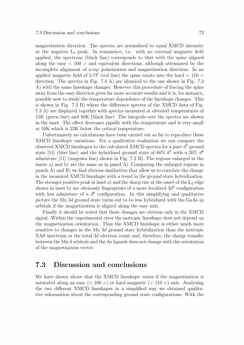
7.3 Discussion and conclusions 73
magnetization direction. The spectra are normalized to equal XMCD intensityat the negative L3 peak. In remanence, i.e. with no external magnetic fieldapplied, the spectrum (black line) corresponds to that with the spins alignedalong the easy < 100 > and equivalent directions, although attenuated by theincomplete alignment of x-ray polarization and magnetization direction. In anapplied magnetic field of 2.5T (red line) the spins rotate into the hard < 110 >direction. The spectra in Fig. 7.3 A) are identical to the one shown in Fig. 7.2A) with the same lineshape changes. However this procedure of forcing the spinsaway from the easy direction gives far more accurate results and it is, for instance,possible now to study the temperature dependence of the lineshape changes. Thisis shown in Fig. 7.3 B) where the difference spectra of the XMCD data of Fig.7.3 A) are displayed together with spectra measured at elevated temperatures of15K (green line) and 50K (black line). The integrals over the spectra are shownin the inset. The effect decreases rapidly with the temperature and is very smallat 50K which is 22K below the critical temperature.
Unfortunately no calculations have been carried out so far to reproduce theseXMCD lineshape variations. For a qualitative evaluation we can compare theobserved XMCD lineshapes to the calculated XMCD spectra for a pure d5 groundstate [51] (blue line) and the hybridized ground state of 80% d5 with a 20% d6
admixture [11] (magenta line) shown in Fig. 7.2 B). The regions enlarged in theinsets a) and b) are the same as in panel A). Comparing the enlarged regions inpanels A) and B) we find obvious similarities that allow us to correlate the changein the measured XMCD lineshape with a trend in the ground state hybridization.The stronger positive peak in inset a) and the sharp rise at the onset of the L2 edgeshown in inset b) are obviously fingerprints of a more localized 3d5 configurationwith less admixture of a d6 configuration. In this simplifying and qualitativepicture the Mn 3d ground state turns out to be less hybridized with the GaAs sporbitals if the magnetization is aligned along the easy axis.
Finally it should be noted that these changes are obvious only in the XMCDsignal. Within the experimental error the isotropic lineshape does not depend onthe magnetization orientation. Thus the XMCD lineshape is either much moresensitive to changes in the Mn 3d ground state hybridization than the isotropicXAS spectrum or the total 3d electron count and, therefore, the charge transferbetween the Mn d orbitals and the As ligands does not change with the orientationof the magnetization vector.
7.3 Discussion and conclusions
We have shown above that the XMCD lineshape varies if the magnetization issaturated along an easy (< 100 >) or hard magnetic (< 110 >) axis. Analyzingthe two different XMCD lineshapes in a simplified way we obtained qualita-tive information about the corresponding ground state configurations. With the
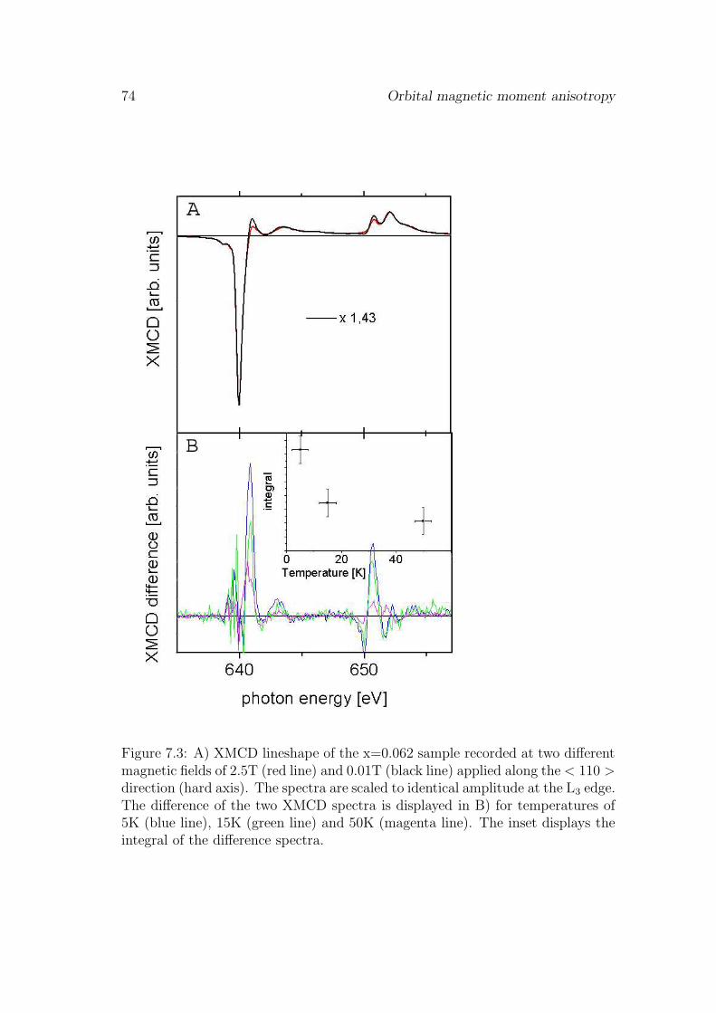
74 Orbital magnetic moment anisotropy
Figure 7.3: A) XMCD lineshape of the x=0.062 sample recorded at two differentmagnetic fields of 2.5T (red line) and 0.01T (black line) applied along the < 110 >direction (hard axis). The spectra are scaled to identical amplitude at the L3 edge.The difference of the two XMCD spectra is displayed in B) for temperatures of5K (blue line), 15K (green line) and 50K (magenta line). The inset displays theintegral of the difference spectra.
7.3 Discussion and conclusions 75
magnetization oriented along an easy axis the XMCD lineshape indicates a morelocalized d5 like configuration whereas for the magnetization aligned along a hardaxis the corresponding ground state configuration appears to be more hybridizedi.e. it shows stronger mixing of d5 and d6 configurations. Evaluating the orbitalmoment with sum rules we found that the change in the XMCD lineshape is cor-related with a change in the orbital moment. Surprisingly for the magnetizationaligned along the hard magnetic axis the orbital moment is found to be largerthan for an alignment along the easy axis. From that observation it can be ex-cluded that the anisotropy of the orbital magnetic moment is caused by magnetocrystalline anisotropy effects which should result in a different variation of theorbital moment. To understand the observed effect it is important to consider theMn 3d orbitals involved in the pd-hybridization. The Mn 3d levels are split by thetetrahedral crystal field into an E-symmetric doublet and a T2-symmetric triplet[69]. Fully occupied t2g and eg states inside the valence band have mainly Mn dcharacter whereas the partially filled t2g states at the valence band are formed ofMn 3d and As p orbitals [71]. The absolute values of the t2g wave functions areshown in Fig. 7.4. Assuming spin conserving hopping interactions between thosepartially occupied orbitals the exchange interaction Jij(R) between Mn pairs atthe distance R along different lattice orientations has been studied [71]. In con-trast to RKKY calculations assuming a spherical pd-hybridization the exchangeintensities were found to depend on the specific lattice orientation [71]. A schemeof the t2g energy levels of two interacting Mn atoms is given at the top of Fig.7.5. Spin-up and spin-down states of the Mn atoms interact by spin conservinghopping and form a set for bonding and antibonding states. The results of theab initio total energy calculations are shown in the lower panel of Fig. 7.5. Theferromagnetic stabilization energy EAFM − EFM is found to be highest if thehopping interaction occurs along the < 110 > lattice direction [71]. Calculationsusing large cells of up to 256 atoms could demonstrate a significant dominationof the orientation dependence over the distance dependence in the exchange cou-pling [71]. The exchange coupling of Mn pairs oriented along the < 110 > axis
Figure 7.4: Absolute values of the Mn 3d t2g wave functions in respect to thecrystallographic axes. Open circles indicate the As ligands of the central Mnatom.
76 Orbital magnetic moment anisotropy
remains higher in strength compared to Mn pairs oriented along other directionseven if their separation R is smaller [71]. In the previous chapters it has beendemonstrated that the pd-hybridization introduces a 20% d6 admixture to theMn 3d5 ground which is characteristic for substitutional Mn. This admixtureof d6 is also the origin of the orbital magnetic moment residing on the Mn 3dshell ( a pure d5 high-spin state is spherically symmetric and possesses no orbitalmoment). The angular dependence of the orbital moment and the change in theground state hybridization indicated by the XMCD lineshape are obviously notdue to magneto-crystalline anisotropy but reflect the spatial anisotropy of thehybridization between Mn d states and the dangling sp3 hybrids of neighboringAs atoms. The ab initio total energy calculations based on pd-hopping interac-tions predicted that a significant feature of the Jij exchange-coupling strengthis a pronounced orientation dependence [71]. Dominant contributions stabilizingthe ferromagnetic state are maximal along the < 110 > directions and minimalalong the < 100 > directions i.e. the hopping strength along the < 110 > di-rection is found to be larger than along the < 100 > direction. It is temptingto correlate this predicted anisotropy of the pd-hybridization with the directionaldependence of the d6 ground state weight observed in XMCD. As an effect of theMn 3d spin-orbit coupling XMCD, therefore, is sensitive to the directional depen-dence of valence fluctuations. In agreement with the preferred hopping along the< 110 > directions we observe the higher XMCD d6 ground state weight alongthis direction.
The conclusion of the above described effect is that due to the spin-orbit cou-pling in the Mn 3d shell XMCD spectroscopy is able to map the spatial anisotropyof the pd-hybridization in Ga1−xMnxAs. By XMCD spectroscopy we can identifydistinct spectroscopic features that are related to the spatial overlap of Mn 3dand As sp states influencing the ferromagnetic ordering. This is exactly whatis needed for a detailed understanding of the origin of ferromagnetism in thesesystems. In future this effect could be used to test theoretical models.
7.4 Outlook
So far we studied the effect of the anisotropic pd-hybridization on the XMCDlineshape by changing the orientation of the magnetization axis. Within theexperimental uncertainty the isotropic XAS signal was not affected by that. Thisindicates that we probe the anisotropy of the pd-hybridization via the spin-orbitinteraction but the charge transfer between the Mn d orbitals and the As ligandsdoes not change with the magnetization direction or the changes are too smallto be resolved in our experiment. As an outlook on future projects we presentdata that possibly indicate changes in the charge transfer between the Mn dorbitals and the As ligands occurring between the ferromagnetic state at lowtemperature and an non ferromagnetic state above the critical temperature. The
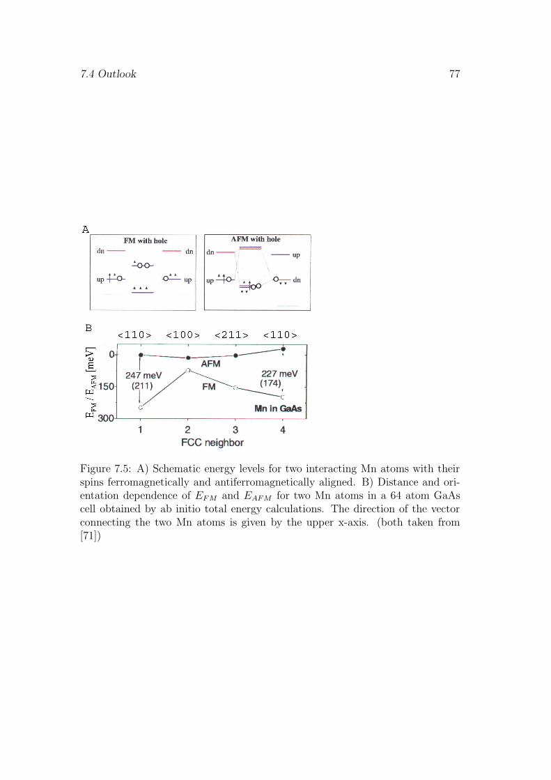
7.4 Outlook 77
Figure 7.5: A) Schematic energy levels for two interacting Mn atoms with theirspins ferromagnetically and antiferromagnetically aligned. B) Distance and ori-entation dependence of EFM and EAFM for two Mn atoms in a 64 atom GaAscell obtained by ab initio total energy calculations. The direction of the vectorconnecting the two Mn atoms is given by the upper x-axis. (both taken from[71])

78 Orbital magnetic moment anisotropy
data were recorded on the x=0.017 sample which exhibited the same anisotropyand the same the dependence of the XMCD lineshape on the magnetization axisbut less pronounced than the x=0.062 sample. In Fig. 7.6 A) the isotropic XASof the x=0.017 spectrum is displayed and in Fig. 7.6 C) the difference of twoXMCD spectra comparable to that in Fig. 7.3 is shown. As for the x=0.062sample one XMCD spectrum was recorded in remanence and the other one with4T magnetic field applied along the hard axis. Prior to subtraction both spectrawere normalized to identical L3 peak height. The shown XAS data are the averageof more than fifty single spectra, thus we could reduce the noise to less 0.5 permilof the peak intensity. The interesting result is, that the isotropic XAS spectrumrecorded at 5K differs from XAS spectra recorded at 40K which is above thecritical temperature. The difference of these two XAS spectra (high minus lowtemperature) is shown in Fig. 7.6 B). It was of course tested that these minimalvariations can not originate from a small energy shift between the two spectra.Most interestingly the changes in the XAS intensity occur mainly at positions ofthe spectrum where the XMCD lineshape was found to be sensitive to the spatialstructure of the pd-hybridization. This coincidence makes it possible that theobserved changes in the XAS lineshape reflect a general change pd-hybridizationat the onset of ferromagnetism. By the positive integral of the difference spectrumshown as a dashed line in Fig. 7.6 B) we can determine that the number of d holesis larger at 40K than at 5K. This would mean that the charge transfer betweenthe Mn d orbitals and the ligands is reduced above the critical temperature. Itwill be the purpose of future projects to study these promising observations inmore detail.
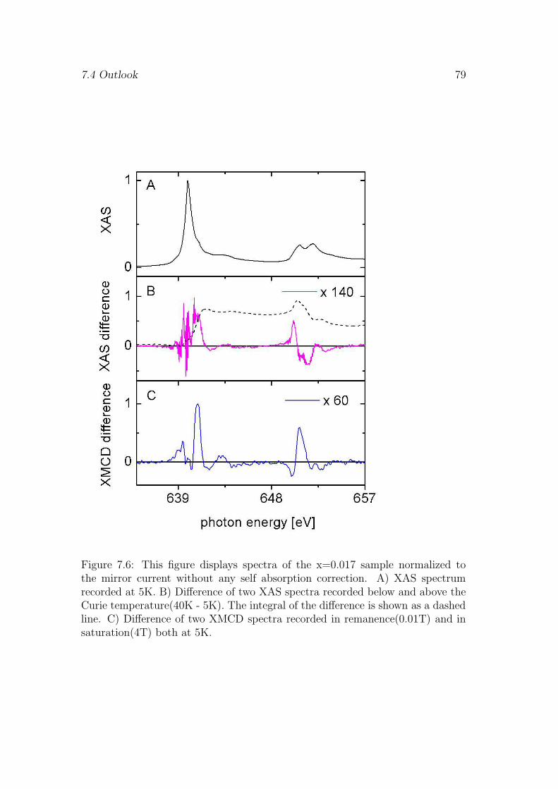
7.4 Outlook 79
Figure 7.6: This figure displays spectra of the x=0.017 sample normalized tothe mirror current without any self absorption correction. A) XAS spectrumrecorded at 5K. B) Difference of two XAS spectra recorded below and above theCurie temperature(40K - 5K). The integral of the difference is shown as a dashedline. C) Difference of two XMCD spectra recorded in remanence(0.01T) and insaturation(4T) both at 5K.

80 Orbital magnetic moment anisotropy

Chapter 8
Summary
In the recent years a large field of research emerged, exploring the possibilitieshow to introduce and handle spin polarized carriers in semiconductor materials.One of the goals is to incorporate spintronic devices in conventional semiconduc-tor technology. Very promising systems are the dilute magnetic semiconductors,where the spin polarized carriers arise from magnetic ions doped into the semi-conductor host.
In this thesis we studied the origin of the ferromagnetic ordering in Ga1−xMnxAs,the most prominent member of the III − V series of ferromagnetic DMS. Theferromagnetism in Ga1−xMnxAs is based on two cooperative effects, caused byreplacing the trivalent Ga atoms with Mn. Mn provides a local spin magneticmoment and as an acceptor it creates itinerant holes, which mediate the longrange ferromagnetic order [1]. But the limited solubility of Mn can lead to a highnumber of defects e.g. As antisites and interstitial Mn [4]. Due to the complexityof Ga1−xMnxAs and the high degree of disorder, the physics underlying its mag-netic properties is still under discussion, even if various theoretical models exist[2, 3]. For further understanding of the ferromagnetic ordering the electronicconfiguration of the Mn impurities and the number of Mn atoms contributingto the long range ferromagnetic order are of major interest. We probed theseparameters directly by x-ray absorption spectroscopy (XAS) and x-ray magneticcircular dichroism (XMCD). The spectral XAS and XMCD lineshape is known tobe characteristic for the electronic 3dn valence configuration [11, 50, 51, 52, 21].
In contrast to previous attempts we combined surface and bulk sensitive de-tection methods with additional reflectivity measurements to resolve a chemicaland magnetical depth profile of the (GaMn)As layer. This analysis revealed thepresence of two different Mn species with different XAS and XMCD line shapesin our samples. The bulk of the Ga1−xMnxAs samples is dominated by substi-tutional Mn residing at the Ga sites. This species can easily be identified byits ferromagnetic properties and a mixed valence 3d5 - 3d6 electronic configu-ration which is characteristic for the hybridization with GaAs valence orbitals.At the surface we find an accumulation of non-ferromagnetic Mn in a 3d5 elec-
81
82 Summary
tronic configuration. The enhanced surface segregation of this second Mn speciesupon annealing, causing a large surface magnetization deficit of substitutionalMn, provides strong evidence that the second Mn species is related to intersti-tial Mn. Acting as a double donor interstitial Mn should strongly reduce thecarrier density and, therefore, also the ferromagnetic coupling between substitu-tional Mn. Our results demonstrate that XAS and XMCD spectra representingthe bulk properties of Ga1−xMnxAs can only be obtained if the influence of thesurface layer is excluded.
Using the bulk sensitive XAS and XMCD spectra we studied the hybridiza-tion of Mn 3d with GaAs 4sp valence orbitals systematically for samples withdifferent Mn concentrations. We find a signature of Mn 3d5-3d6 mixed valenceacceptor states responsible for long-range ferromagnetic order at all Mn concen-trations. This is in agreement with previous experimental investigations [11, 81]and with theoretical models based on a localized Mn 3d5 electronic configurationwhich interacts with holes via impurity states, consisting of mainly GaAs 4sporbitals [45, 46, 44]. In addition we find experimental evidence for an antiferro-magnetic exchange between Mn-Mn nearest neighbors in (GaMn)As at high Mnconcentrations. With increasing Mn concentration an increasing amount of Mnatoms not participating in the ferromagnetic ordering is observed. Their numberscales approximately with the number of Mn nearest neighbor pairs expected fora statistical Mn distribution. For the Mn atoms not participating in the ferro-magnetic ordering we also find a reduced number of 3d electrons of close to 3d4.Both observations can be explained by the presence of Mn-Mn nearest neighborpairs. It has been predicted theoretically that the exchange coupling and thecharge state of Mn in clusters of substitutional Mn can be strongly modified bythe presence of interstitial Mn [20, 49]. Contrary to II-VI based materials thisrepresents the first observation of antiferromagnetic order in III-V dilute mag-netic semiconductors with possibly a similar adverse effect to the ferromagneticordering temperature.
In angle resolved XMCD measurements we studied the hybridization of theMn 3d shell with GaAs valence orbitals. The pd-hybridization is usually assumedto be spherically isotropic [2]. But we find a variation of the Mn 3d orbitalmoment with the in-plane azimuthal lattice direction that is correlated with dis-tinct spectroscopic features. The observed dependence of the orbital magneticmoment on the lattice directions is contrary to what is expected from the mag-neto crystalline anisotropy contribution. Thus the magneto crystalline anisotropycan be ruled out to cause this effect. The spectroscopic features in the XMCDspectra and the correlated change in the orbital moment can be interpreted byan anisotropy in the spatial overlap of Mn 3d and As 4sp states influencing theferromagnetic ordering. This interpretation is in agreement with recent calcu-lations predicting a strongly anisotropic pd-hybridization [71]. This is the firstexperimental indication for an anisotropic pd-hybridization in (GaMn)As and,therefore, magnetic exchange coupling. The spectroscopic features related with

83
this effect could be used in future to test theoretical models.

84 Summary
Bibliography
[1] H. Ohno, Science, 281, 951, (1998)
[2] T. Dietl, H. Ohno, F. Matsukura, J. Cibert and D. Ferrand, Science, 287,1019, (2000)
[3] A. Kaminski and S. DasSarma, Phys. Rev. Lett., 88, 247202, (2002)
[4] F. Mca and J. Masek, Phys. Rev. B, 65, 235209, (2002)
[5] J.J. Hoyt, D.de Fontaine and W.K. Warburton, J. Apply. Cryst, 17, 344 -351, (1984)
[6] G. van der Laan and I. W. Kirkman, J. Phys.: Condens. Matter, 4, 4189,(1992)
[7] written by D. L. Windt (1997-1998)
[8] D. G. Stearns, J. Appl. Phys. 65, 491, (1989)
[9] G. M. Schott, G. Schmidt, G. Karczewski, L. W. Molenkamp, R. Jakiela, A.Barcz and G. Karczewski, Appl. Phys. Lett., 82, 4678, (2003)
[10] J. Blinowski and P. Kacman, Phys. Rev. B, 67, 121204(R), (2003)
[11] H. Ohldag, V. Solinus, F.U. Hillebrecht, J.B. Goedkoop, M. Finazzi, F.Matsukura and H. Ohno, Applied Physics Letters, 76, 2928, (2000)
[12] B. J. Kirby, J. A. Borchers, J. J. Rhyne, S. G. E. te Velthuis, A. Hoffmann,K. V. ODonovan, T. Wojtowicz, X. Liu, W. L. Lim and J. K. Furdyna, Phys.Rev. B, 69, 081307(R), (2004)
[13] Y. Ishiwata, M. Watanabe, R. Eguchi, T. Takeuchi, Y. Harada, A. Chainani,S. Shin, T. Hayashi, Y. Hashimoto, S. Katsumoto and Y. Iye, Phys. Rev. B,65, 233201, (2002)
[14] Center for X-Ray Optics, http://www-cxro.lbl.gov
85
86 BIBLIOGRAPHY
[15] K. W. Edmonds, P. Boguslawski, K. Y. Wang, R. P. Campion, S. N. Novikov,N. R. S. Farley, B. Gallagher, C. T. Foxon, M. Sawicki, T. Dietl, M. Buon-giorno Nardelli and J. Bernholc, Phys. Rev. Lett., 92, 037201-1, (2004)
[16] Y. L. Soo, G. Kioseoglou, S. Kim, X. Chen, H. Luo, Y. H.Kao, H. J. Lin,H. H. Hsieh, T.Y. Hou, C. T. Chen, Y. Sasaki, X. Liu and J. K. Furdyna,Phys. Rev. B, 67, 214401-1 , (2003)
[17] D. J. Keavney, D. Wu, J. W. Freeland, E. Johnston-Halperin, D. D.Awschalom and J. Shi, Phys. Rev. Lett., 91, 187203, (2003)
[18] S. Ueda, S. Imada, T. Muro, Y. Saitoh, S. Suga, F. Matsukura and H. Ohno,Physica E, 10, 210, (2001)
[19] K. M. Yu, W. Walukiewicz, T. Wojtowicz, I. Kuryliszyn, X. Liu, Y. Sasakiand J. K. Furdyna, Phys. Rev. B, 65, 201303(R), (2002)
[20] Steven C. Erwin and A. G. Petukhov, Phys. Rev. Lett., 89, 227201, (2002)
[21] K. W. Edmonds, P. Boguslawski, K. Y. Wang, R. P. Campion, S. N. Novikov,N. R. S. Farley, B. L. Gallagher, C. T. Foxon, M. Sawicki, M. BuongiornoNardelli and J. Bernholc, Appl. Phys. Lett., 84, 4065, (2004)
[22] S. J. Potashnik, K. C. Ku, R. Mahendiran, S. H. Chun, R. F. Wang, N.Samarth and P. Schiffer, Phys. Rev. B, 66, 012408, (2002)
[23] A. Oiwa, Y. Mitsumori, R. Moriya, T. Slupinski and H. Munekata, Phys.Rev. Lett., 88, 137202, (2002)
[24] A. Oiwa, T. Slupinski and H. Munekata, Appl. Phys. Lett., 78, 518, (2001)
[25] H. Munekata, T. Abe, S. Koshihara, A. Oiwa, M. Hirasawa, S. Katsumoto,Y. Iye, C. Urano and H. Takagi., J. Appl. Phys., 81, 4862, (1997)
[26] H. Ohno, D. Chiba, F. Matsukura, T. Omiya, E. Abe, T. Dietl, Y. Ohnoand K. Ohtani, Nature, 408, 944, (2000)
[27] H. Krenn, W. Zawadzki and G. Bauer, Phys. Rev. Lett., 55, 1510, (1985)
[28] H. Krenn, K. Kaltenegger, T. Dietl, J. Spalek and G. Bauer, Phys. Rev. B,39, 10918, (1989)
[29] D.D. Awschalom, J. Warnock and S. von Molnr, Phys. Rev. Lett., 58, 812,(1987)
[30] S. Koshihara, A. Oiwa, M. Hirasawa, S. Katsumoto, Y. Iye, C. Urano, H.Takagi and H. Munekata, Phys. Rev. Lett., 58, 812, (1987)

BIBLIOGRAPHY 87
[31] D.J. Hilton and C.L. Tang, Phys. Rev. Lett., 89, 146601, (2002)
[32] G.A. Khodaparast, J. Wang, J. Kono, A. Oiwa and H. Munekata, cond-mat/0305017 v2,(2004)
[33] A.V. Kimel, G.M. Schott, A. Kirilyuk, D.R. Yakovlev, G. Kraczewski, W.Ossau, G. Schmidt, L.W. Molenkamp and T.h. Rasing, Phys. Rev. Lett., 92,237203, (2004)
[34] F. Matsukura, H. Ohno, A. Shen and Y. Sugawara, Phys. Rev. B, 57, R2037,(1998)
[35] A. Cavaleri, C.W. Siders, C. Rose-Petruck, R. Jimenez, Cs. Toth, J.A.Squier, C.P.J. Barty, K.R. Wilson, K. Sokolowski-Tinten, M. Horn vanHeogen and D. van der Linde, Phys. Rev. B, 63, 193306, (2001)
[36] Pablo J. Sez, Ph.D. thesis, Stanford University, (1997)
[37] S. J. Potashnik, K. C. Ku , S. H. Chun, J. J. Berry, N. Samarth and P.Schiffer, Appl. Phys. Lett., 79, 1495, (2001)
[38] Claude Cohen-Tannoudji, Bernard Diu and Franck Laloe, Quantenmechanik,de Gruyter Berlin York
[39] S. Eisebitt, T. Boeske, J.-E. Rubensson and W. Eberhardt, Phys. Rev. B,47, 14103, (1993)
[40] M. Born and E. Wolf, Principles of Optics; Pergamon Press Oxford, (1980)
[41] S. Das Sarma, E.H. Hwang and D.J. Priour Jr., Phys. Rev. B, 70, 161203(R),(2004)
[42] W. Heisenberg, Z. Physik, 49, 619, (1928)
[43] T. Dietl, H. Ohno and F. Matsukura, Phys. Rev. B, 63, 195205, (2000)
[44] J.-M. Tang and M.E. Flatte, Phys. Rev. Lett., 92, 047201, (2004)
[45] C. Timm, J. Phys.: Condens. Matter, 15, R1865, (2003)
[46] P. Mahadevan, A. Zunger D.D. Sarma, Phys. Rev. Lett., 93, 177201, (2004)
[47] S. Sanvito, P. Ordejon, N.A. Hill, Phys. Rev. B, 63, 165206, (2001)
[48] M. Moreno, B.Jenichen, V. Kaganer, W. Braun, A. Trampert, L. Daweritzand K.H. Ploog , Phys. Rev. B, 67, 235206, (2003)
[49] P. Mahadevan and A. Zunger, Phys. Rev. B, 68, 075202, (2003)

88 BIBLIOGRAPHY
[50] H.A. Durr, G. van der Laan, D. Spanke, F.U. Hillebrecht and N.B. Brookes,Phys. Rev. B, 56, 8156, (1997)
[51] G. van der Laan and B.T. Thole, Phys. Rev. B, 43, 13401, (1991)
[52] G. van der Laan and B.T. Thole, J. Phys.: Condens. Matter, 4, 4181, (1992)
[53] J. Okabayashi, A. Kimura, T. Mizokawa, A. Fujimori, T. Hayashi and M.Tanaka, Phys. Rev. B, 59, R2486, (1999)
[54] M. Sawicki, Acta Physica Polonica A, 106, 119, (2004)
[55] A. M. Yakunin, A. Yu. Silov, P.M. Koenraad, J.H. Wolter, W. Van Roy,J. De Boeck, J.-M. Tang and M. E. Flatte, Phys. Rev. Lett., 92, 216806,(2004)
[56] P. Bruno, Phys. Rev. B, 39, 865, (1989)
[57] C. Ruster, C. Gould, T. Jungwirth, J. Sinova, G. M. Schott, R. Giraud, K.Brunner, G. Schmidt and L. W. Molenkamp, cond-mat/0408532, (2004)
[58] B.T. Thole, P. Carra, F. Sette and G. van der Laan, Phys. Rev. Lett., 68,1943, (1992)
[59] P. Carra, B.T. Thole , M. Altarelli and X. Wang, Phys. Rev. Lett., 70, 694,(1993)
[60] C.T. Chen, Y.U. Idzerda, H.-J. Lin, N.V. Smith, G. Meigs, E. Chaban, G.H.Ho, E. Pellegrin and F. Sette, Phys. Rev. Lett., 75, 152, (1995)
[61] V. F. Sapega, M. Moreno, M. Ramsteiner, L. Daweritz and K. Ploog, Phys.Rev. B, 66, 075217, (2002)
[62] M. Adell, J. Kaminski, L. Ilver, J. Sadowski, V. Stanciu and P. Svedlindh,comment in Phys. Rev. Lett.,94, 139701, (2005)
[63] R. Wu, D. Wang and A.J. Freeman, Phys. Rev. Lett., 71, 3581, (1993)
[64] J. Schwitalla and H. Ebert, comment in Phys. Rev. Lett., 80, 4586, (2005)
[65] B.T. Thole and G. van der Laan, Phys. Rev. B., 38, 3158, (1988)
[66] H.A. Durr, Y. Guo, G. van der Laan, J. Lee, G. Lauhoff and J.A.C. Bland,Science, 277, 213, (1997)
[67] D. Weller, J. Stohr, R. Nakajima, A. Carl, M.G. Samant, C. Chappert, R.Megy, P. Beauvillian, P. Veillet and G.A. Held, Phys. Rev. Lett.,75, 3752,(1995)
BIBLIOGRAPHY 89
[68] Charles Gould, private communication, (2005)
[69] Jian-Ming Tang and Michael E. Flatte, Phys. Rev. Lett., 92, 47201, (2004)
[70] Giesela Schott, private communication, (2004)
[71] Priya Mahadevan, Alex Zunger and D.D. Sarma, Phys. Rev. Lett., 93,177201, (2004)
[72] S.S. Dhesi, H.A. Durr, G. van der Laan, E. Dudzik and N.B. Brookes, Phys.Rev. B., 60, 12852, (1999)
[73] D. Ferrand, J. Cibert, A. Wasiela, C. Bourgognon, S. Tatarenko, G. Fishman,T.,rearczyk, J. Jaroszynski, S. Kolesnik, T. Dietl, B. Barbara and D. Dufeu,Phys. Rev. B., 63, 085201, (2001)
[74] A. Kaminski and S. Das Sarma, Phys. Rev. Lett., 88, 247202, (2002)
[75] M.N. Baibich, J.M. Broto, A. Fert, F. Nguyen Van Dau, F. Petroff, P.Eitenne, G. Creuzet, A. Friederich and J. Chalezas, Phys. Rev. Lett., 61,2472, (1988)
[76] G. Binasch, P. Gruenberg, F. Saurenbach, and W. Zinn, Phys. Rev. B, 39,4828, (1989)
[77] G. Schmidt, D. Ferrand, L.W. Molenkamp, A.T. Filip and B.J. van Wees,Phys. Rev. B, 62, R4790, (2000)
[78] K.W. Edmonds, K.Y. Wang, R.P. Campion, A.C. Neumann, N.R.S. Farley,B.L. Gallagher, and C.T. Foxon, Appl. Phys. Lett., 81, 4991, (2002)
[79] M.M. Schwickert, G.Y. Guo, M.A. Tomaz, W.L. O’Brien and G.R. Harp,Phys. Rev. B, 58, 4289, (1998)
[80] PhD thesis of Gisela Schott, Universitat Wurzburg, (2004)
[81] K.W. Edmonds, N.R.S. Farley, T.K. Johal, G. van der Laan, R.P. Campion,B.L. Gallagher, and C.T. Foxon, Phys. Rev. B, 71, 064418, (2005)
[82] G. van der Laan, ”Quantitative microbeam analysis” SUSSP 40/NATO ASI,Ed. A.G. Fitzgerlad, B.E. Storey and D Fabian, IOP Publ., London 1992,p. 95 - 119
[83] B.L. Gallagher, T. Jungwirth, J. Masek, J. Koenig, M. Polini, J. Sinova,A.H. MacDonald, K.Y. Wang, K.W. Edmonds, R.P. Campion, L.X. Zhao,C.T. Foxon, abstract to Spintech III conference, JAPAN, August 2005

90 BIBLIOGRAPHY
[84] M. Sawicki, K.-Y Wang, K.W. Edmonds, R.P. Campion, C.R. Staddon,N.R.S. Farley, C.T. Foxon, E. Papis, E. Kaminska, A. Piotrowska, T. Dietland B.L. Gallagher, Phys. Rev. B, 71, 121302(R), (2005)

Danksagung
Diese Arbeit wurde bei BESSY in Berlin durchgefuhrt. Ich mochte allen BESSYMitarbeitern fur die gute Arbeitsatmosphare danken und speziell denen, die amZustandekommen der Arbeit beteiligt waren.
Mein besonderer Dank gilt Herrn Prof. Dr. W. Eberhardt, der es mir ermoglichthat diese Arbeit anzufertigen und der jederzeit fur fruchtbare Diskussionen zurVerfugung stand.
Ganz besonders mochte ich Herrn Dr. H.A. Durr fur seine ausdauernde und fre-undschaftliche Unterstutzung danken. Er hat mir bei der Arbeit mit Anregungenund Ideen stets zur Seite gestanden.
An den in der Arbeit vorgestellten Messungen waren insbesondere Frau Dr.A. Vollmer und Herr R. Ovsyannikov beteiligt. Ich mochte mich fur ihre Un-terstutzung bedanken.
Auch den Beamline- und Experiment-Betreuern, Frau Dr. C. Boegelin, Herrn Dr.D. Schmitz, Herrn Dr. P. Imperia und Herrn Dr. J. Cezar, die mich bei meinenMessungen bei BESSY und an der ESRF nach Kraften unterstutzt haben gebuhrtmein besonderer Dank.
Ich mochte weiterhin Herrn Prof. Dr. C. Thomsen fur die Ubernahme des Ko-referats danken.
Zuletzt ein ganz grosses Dankeschon an meine Familie fur ihre Unterstutzung inallen Lebenslagen.