Master Thesis Development and implementa- tion of - UPCommons
104
Master Thesis von cand. Ing. JORDI BASSAS Matrikelnummer: 03283589 Development and implementa- tion of a Nuclear Power Plant steam turbine model in the system code ATHLET Betreuer TUM: Betreuer GRS: Ausgegeben: Abgegeben: Prof. Dr. Rafael Macián-Juan Dipl.-Phys. Philipp Schöffel 15.01.2011 22.07.2011
Transcript of Master Thesis Development and implementa- tion of - UPCommons
Master Thesis
von cand. Ing. JORDI BASSAS Matrikelnummer: 03283589
Development and implementa-tion of a Nuclear Power Plant steam turbine model in the system code ATHLET
Betreuer TUM:
Betreuer GRS:
Ausgegeben:
Abgegeben:
Prof. Dr. Rafael Macián-Juan
Dipl.-Phys. Philipp Schöffel
15.01.2011
22.07.2011

ii

iii
Erklärung
Hiermit versichere ich, die vorliegende Arbeit selbstständig und ohne
Hilfe Dritter angefertigt zu haben. Gedanken und Zitate, die ich aus
fremden Quellen direkt oder indirekt übernommen habe, sind als solche
kenntlich gemacht. Diese Arbeit hat in gleicher oder ähnlicher Form
noch keiner Prüfungsbehörde vorgelegen und wurde bisher nicht veröf-
fentlicht.
Ich erkläre mich damit einverstanden, dass die Arbeit durch den Lehr-
stuhl für Nukleartechnik der Öffentlichkeit zugänglich gemacht werden
kann.
München, den 22. Juli 2011
JORDI BASSAS

iv
v
Abstract
In order to improve the simulation of the whole secondary loop with the system
code ATHLET a steam turbine model has to be implemented. This paper deals
with the development of a thermo-hydraulic model of a Nuclear Power Plant
steam turbine and its implementation in the system code ATHLET.
The model is based on Stodola’s cone law and simulates the pressure drop
and the enthalpy drop along the different turbine stages as well as the steam
and water extractions.
The influence of the steam and water extractions on the turbine behaviour as
well as the importance of an accurate model for the steam and water extrac-
tions are carefully explained.
Heat and mass balances of the Nuclear Power Plant Philippsburg 2 are used
for reference purposes as well as for validation purposes of the implemented
model. The comparison between steady state simulations and the real plant
data indicate a satisfactory accuracy of the model and of the thermodynamic
approach used.

vi
vii
List of Contents
Erklärung ................................................................................................................. iii
Abstract .................................................................................................................. v
List of Contents ........................................................................................................ vii
List of Figures ............................................................................................................ xi
List of Tables............................................................................................................. xv
Acknowledgments .................................................................................................. xvii
List of Acronyms ..................................................................................................... xix
1 Introduction .............................................................................................. 1
2 Steam turbines ......................................................................................... 3
2.1 The Rankine Cycle .................................................................................... 3
2.2 Types and construction of turbines ............................................................ 5
2.3 Particularities of steam turbines in Nuclear Power Plants; the saturated
steam process ........................................................................................... 8
2.3.1 Steam production in a Nuclear Power Plant ............................................... 8
2.3.2 The saturated steam process..................................................................... 9
3 Physical models ..................................................................................... 11
3.1 Stodola’s cone law ................................................................................... 11
3.2 Steam properties across the turbine ........................................................ 14
3.3 Extractions ............................................................................................... 18

viii
4 Data base................................................................................................ 19
4.1 Reference plant ....................................................................................... 19
4.2 Available data on the reference plant ....................................................... 20
5 ATHLET .................................................................................................. 28
5.1 Description of ATHLET ............................................................................ 28
5.1.1 Modules of ATHLET ................................................................................ 28
5.1.2 The Thermo-Fluid dynamic Module ......................................................... 29
6 Implementation of the turbine model ................................................... 36
6.1 Alternative implementation strategies ...................................................... 36
6.2 Chosen modelling strategy ...................................................................... 38
6.2.1 Pressure drop model ............................................................................... 38
6.2.2 Power extraction model ........................................................................... 39
6.3 Implementation in ATHLET ...................................................................... 42
6.3.1 The pump model as a basis ..................................................................... 43
6.3.2 Modelling of the water and steam extractions .......................................... 47
6.3.3 Momentum Flux term ............................................................................... 50
6.3.4 Basic thermo-fluid dynamic models used ................................................. 52
6.3.5 Turbine data required by user input ......................................................... 52
7 Results ................................................................................................... 54
7.1 Simulation of all the stages separately ..................................................... 57
7.1.1 Pressure at the inlet of every stage .......................................................... 57
7.1.2 Enthalpy at the outlet of every stage ........................................................ 60
7.2 Simulation of the whole LP-turbine with steam and water extractions,
and constant diameter of the “turbine pipe” .............................................. 61
7.2.1 Pressure evolution along the LP-turbine .................................................. 62
7.2.2 Enthalpy evolution along the LP-turbine ................................................... 64
ix
7.2.3 Evaluation of results ................................................................................ 65
7.3 Simulation of the whole LP-turbine with steam and water extractions
and conic geometry ................................................................................. 67
7.3.1 Pressure evolution along the LP-turbine .................................................. 68
7.3.2 Enthalpy evolution along the LP-turbine ................................................... 69
7.3.3 Evaluation of results ................................................................................ 70
7.4 Simulation of the whole LP-turbine with steam and water extractions
and conic geometry with qualitative water extractions .............................. 70
7.4.1 Pressure evolution along the LP-turbine .................................................. 71
7.4.2 Enthalpy evolution along the LP-turbine ................................................... 72
7.4.3 Water extractions ..................................................................................... 73
7.4.4 Evaluation of results ................................................................................ 74
8 Assessment ........................................................................................... 76
8.1 Geometry data ......................................................................................... 76
8.2 Application of the cone law ...................................................................... 76
8.3 Enthalpy calculation ................................................................................. 76
8.4 Models to be developed ........................................................................... 77
8.5 Extension ................................................................................................. 77
9 Summary and Outlook ........................................................................... 80
10 Bibliography ........................................................................................... 81

x

xi
List of Figures
Figure 2.1 T-s diagram of the Rankine cycle (Ainsworth, 2007). ................................. 3
Figure 2.2 Schematic image of a turbine (Lehrstuhl für Energiesysteme , 2010)
(Kleinedler, 2002). ..................................................................................... 6
Figure 2.3 Difference between impulse and reaction turbine (Ainsworth, 2007) .......... 7
Figure 2.4 Schematic configuration of NPP (PWR type) (Kleinedler, 2002). ............... 8
Figure 2.5 Schematic T-s diagram of the Rankine cycle in a NPP. ............................. 9
Figure 3.1 Graphic representation of the cone law (Stodola, 1922)........................... 13
Figure 3.2 Turbine with several extraction lines, on the right the subdivision in
sections can be seen. .............................................................................. 14
Figure 3.3 Comparison between the real process and the ideal process in the hs-
Diagram ................................................................................................... 15
Figure 3.4 Calculation of the enthalpy at the exhaust of a turbine when inlet properties
(sub index a), the exhaust pressure (sub index b) and the isentropic
efficiency of the turbine are known. .......................................................... 16
Figure 3.5 Evolution of the isentropic efficiency depending of the isentropic enthalpy
difference for constant angular velocity. ................................................... 17
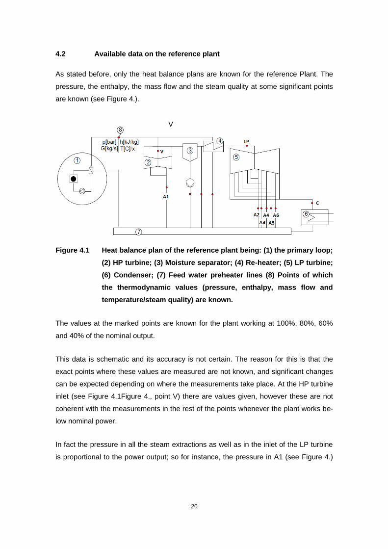
Figure 4.1 Heat balance plan of the reference plant being: (1) the primary loop; (2) HP
turbine; (3) Moisture separator; (4) Re-heater; (5) LP turbine; (6)
Condenser; (7) Feed water preheater lines (8) Points of which the
thermodynamic values (pressure, enthalpy, mass flow and
temperature/steam quality) are known. .................................................... 20
xii
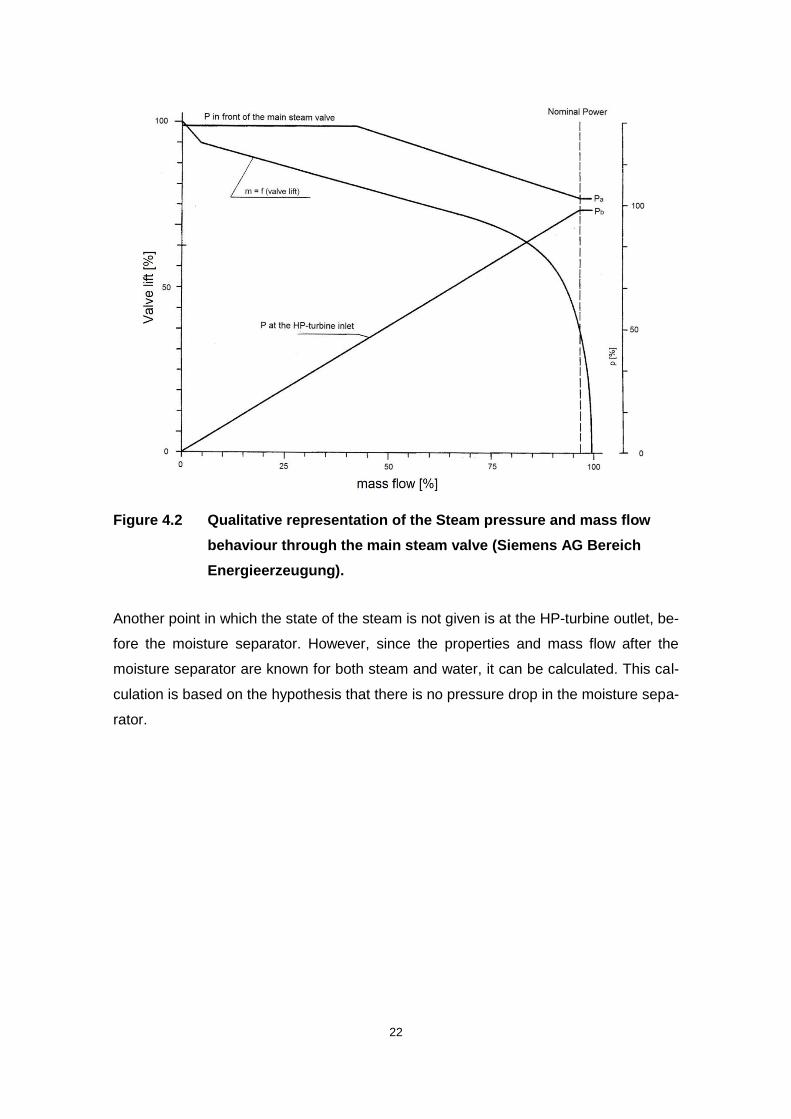
Figure 4.2 Qualitative representation of the Steam pressure and mass flow behaviour
through the main steam valve (Siemens AG Bereich Energieerzeugung).22
Figure 4.3 Schematic of the turbine. The circles are points in which the mass flow, the
enthalpy, the pressure and the steam quality or temperature are known.
T1-8 are the indexes for every stage. ....................................................... 23
Figure 4.4 Schematic water and steam extraction between two stages. ................... 25
Figure 5.1 Staggered grid with CV and junctions (GRS, 2009) ................................. 30
Figure 6.1 Turbine as a storage-throttle system ........................................................ 37
Figure 6.2 TFD system. Fill on the left, pipe in the middle and TDV on the right. The
turbine junction is in the middle of the pipe. ............................................. 43
Figure 6.3 Part of the subroutine dkturb.f. Comments are in green. .......................... 45
Figure 6.4 Subroutine ktutr.f calculates the pressure drop and the power extraction. 46
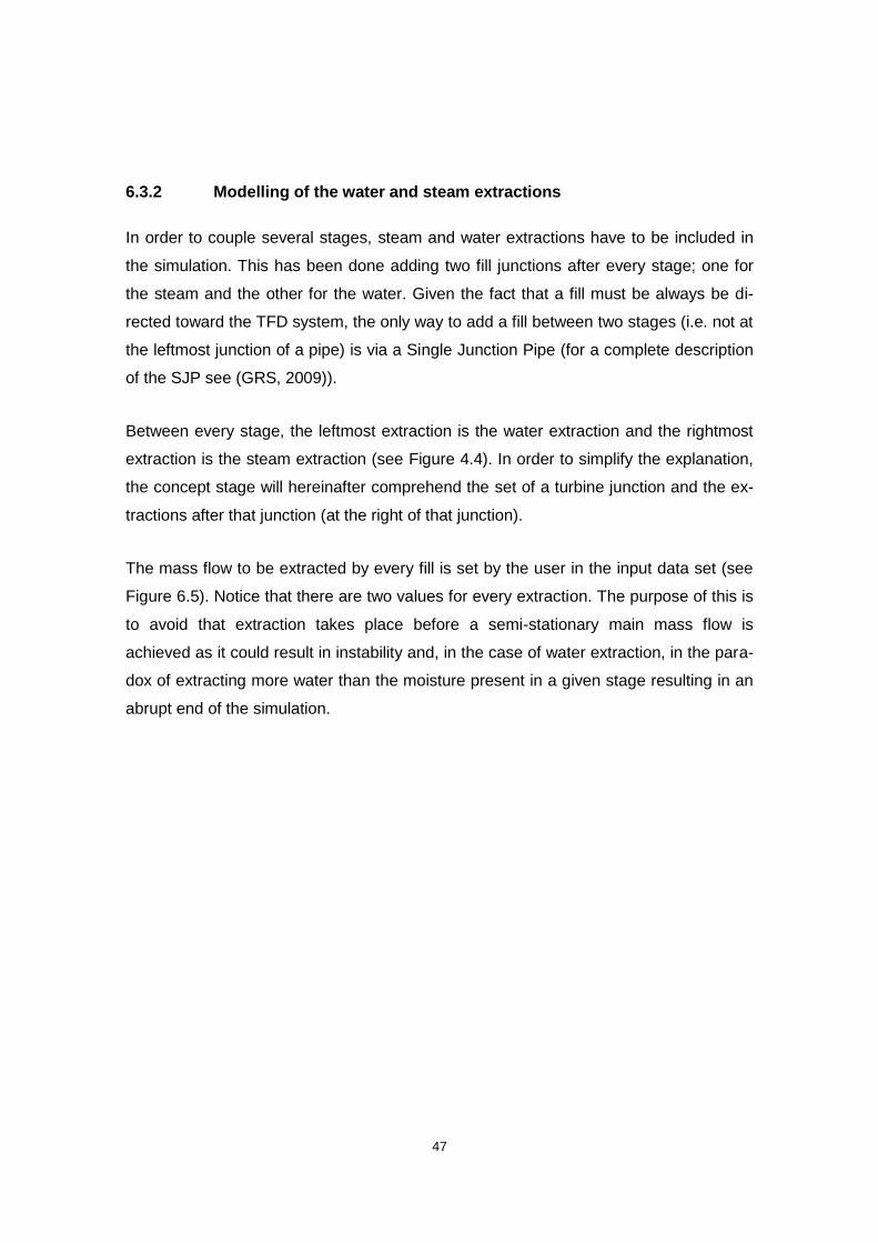
Figure 6.5 Detail of input data set. Mass flows in every extraction. WGSTART/
GSTART and WGENDE/GENDE are the mass flows of water/steam
extractions at the beginning and after a given time of the simulation. ....... 48
Figure 6.6 Detail of subroutine dfk1ha.f where the quality of the steam to be extracted
can be set. ............................................................................................... 49
Figure 6.7 Detail of the input data set for a water extraction. ISANZ equal to one
implies that it is a water extraction and ABGRAD is the percentage of water
in the stage to be extracted. ..................................................................... 50
Figure 6.8 Detail of subroutine dfk1ha.f where the water mas flow to be extracted is
set by a percentage of the water flow through the stage. ......................... 50
xiii
Figure 6.9 Final configuration of the ‘turbine pipe’. The vertical black lines with the
brown dots represent the turbine junctions and the arrows represent the
steam and water extractions. ................................................................... 51
Figure 6.10 Detail of input dataset. Input of a turbine stage nominal values being P0E
the pressure before the stage, P0A the pressure after the stage, M0 the
mass flow, T0IN the temperature before the stage, and ETA0 the efficiency
of the stage. ............................................................................................. 53
Figure 7.1 Fill, pipe-with-turbine, TDV system with input variables in blue. ............... 55
Figure 7.2 Calculated pressure behaviour along stages T3, T4 and T5 of the LP
turbine ..................................................................................................... 59
Figure 7.3 Calculated enthalpy along stages T3, T4 and T5 of the LP turbine .......... 59
Figure 7.4 TFD system. The points are the turbine junctions and the arrows the steam
and water extractions. .............................................................................. 62
Figure 7.5 Detail of Figure 7.4. Turbine junctions and extractions can be seen clearly.
Between some stages, there is only one extraction as only steam (between
stages T3 and T4) or only water (between stages T6 and T7) is extracted.
................................................................................................................ 62
Figure 7.6 Calculated pressure behaviour along the LP turbine, plant working at 80%,
60% and 40% of the nominal power......................................................... 63
Figure 7.7 Calculated enthalpy behaviour along the LP-turbine, plant working at 80%,
60% and 40% of the nominal power......................................................... 65
Figure 7.8 Image of the geometry used. The fill and the TDV can be seen at the left
and at the right end respectively. ............................................................. 67
Figure 7.9 Calculated pressure behaviour along the LP turbine, plant working at 80%
of the nominal power. .............................................................................. 68

xiv
Figure 7.10 Enthalpy along the LP turbine, plant working at 80% of the nominal power.
................................................................................................................ 69
Figure 7.11 Pressure behaviour along the LP turbine, plant working at 80% of the
nominal power. ........................................................................................ 71
Figure 7.12 Enthalpy along the LP turbine, plant working at 80% of the nominal power.
................................................................................................................ 72
Figure 7.13 Qualitative steam quality evolution across the LP-turbine. Notice the
increase after every extraction. ................................................................ 74
Figure 8.1 Moisture separator (detail of Figure 4.) .................................................... 78
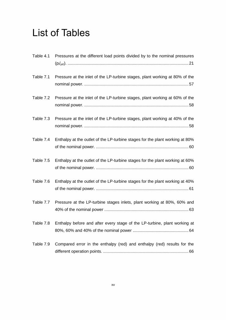
xv
List of Tables
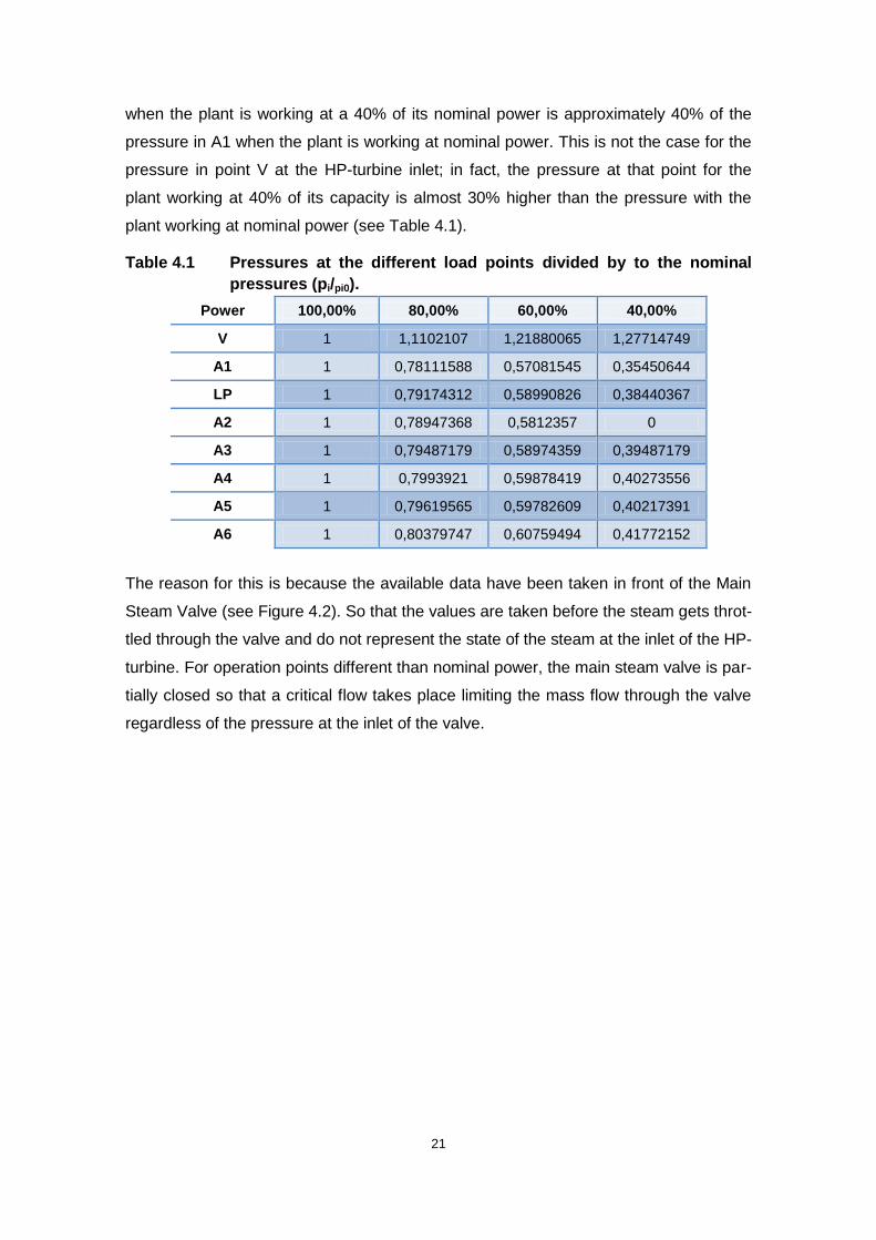
Table 4.1 Pressures at the different load points divided by to the nominal pressures
(pi/pi0). ...................................................................................................... 21
Table 7.1 Pressure at the inlet of the LP-turbine stages, plant working at 80% of the
nominal power. ........................................................................................ 57
Table 7.2 Pressure at the inlet of the LP-turbine stages, plant working at 60% of the
nominal power. ........................................................................................ 58
Table 7.3 Pressure at the inlet of the LP-turbine stages, plant working at 40% of the
nominal power. ........................................................................................ 58
Table 7.4 Enthalpy at the outlet of the LP-turbine stages for the plant working at 80%
of the nominal power. .............................................................................. 60
Table 7.5 Enthalpy at the outlet of the LP-turbine stages for the plant working at 60%
of the nominal power. .............................................................................. 60
Table 7.6 Enthalpy at the outlet of the LP-turbine stages for the plant working at 40%
of the nominal power. .............................................................................. 61
Table 7.7 Pressure at the LP-turbine stages inlets, plant working at 80%, 60% and
40% of the nominal power ....................................................................... 63
Table 7.8 Enthalpy before and after every stage of the LP-turbine, plant working at
80%, 60% and 40% of the nominal power ............................................... 64
Table 7.9 Compared error in the enthalpy (red) and enthalpy (red) results for the
different operation points. ........................................................................ 66

xvi
Table 7.10 Pressure at the LP-turbine stages inlets, plant working at 80%, 60% and
40% of the nominal power ....................................................................... 68
Table 7.11 Enthalpy before and after every stage of the LP-turbine, plant working at
80%, 60% and 40% of the nominal power................................................ 69
Table 7.12 Compared error in the enthalpy (red) and enthalpy (red) results for the
different operation points. ........................................................................ 70
Table 7.13 Pressure at the LP-turbine stages inlets, plant working at 80%, 60% and
40% of the nominal power. ...................................................................... 71
Table 7.14 Enthalpy before and after every stage of the LP-turbine, plant working at
80%, 60% and 40% of the nominal power:............................................... 72
Table 7.15 Water extracted for the plant working at 80%, 60% and 40% of the nominal
power ....................................................................................................... 73
Table 7.16 Compared error in the enthalpy (red) and pressure (blue) results for the
different operation points ......................................................................... 75
Table 7.17 Error in the water mass flow extracted in the third fourth and fifth extraction
of the LP-turbine (extractions A3, A5 and A6) .......................................... 75

xvii
Acknowledgments
This paper was developed during my practicum at GRS.
I want to thank my supervisors in GRS, Dipl.-Phys. Philipp Schöffel and Dr. Ing. Fabian
Weyermann for their constant support and invaluable help during the development of
this paper as well as to Dipl. Ing. (FH) Georg Lerchl for his help with ATHLET. My grati-
tude also to my tutor Professor Rafael Macián-Juan from the Technische Universität
München for his support during my progress and for making the development of my
Master Thesis at GRS possible. Thanks also to all the workers and friends at GRS for
their readiness to help me at any time and for their support.
I also would like to express to Ms Imogen Helen Sexton Kakuschky my sincere grati-
tude for her correction of this Master Thesis and for her support.
Finally I want to thank my friends and family for being there, and my parents for making
it all possible.

xviii
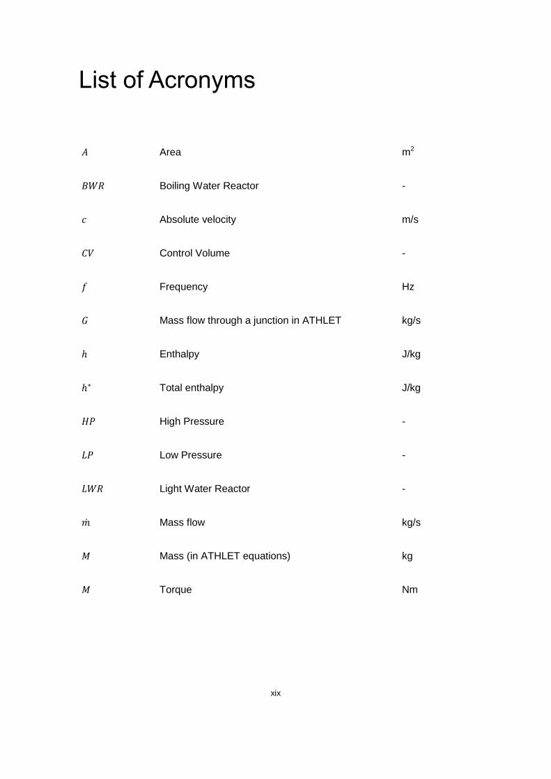
xix
List of Acronyms
Area m2
Boiling Water Reactor -
Absolute velocity m/s
Control Volume -
Frequency Hz
Mass flow through a junction in ATHLET kg/s
Enthalpy J/kg
Total enthalpy J/kg
High Pressure -
Low Pressure -
Light Water Reactor -
Mass flow kg/s
Mass (in ATHLET equations) kg
Torque Nm

xx
Polytropic exponent kg/s
Rotational Speed 1/min
Nuclear Power Plant -
Pressure bar
Power W
Pressurized Water Reactor -
Heat J
Entropy J/(kg·K)
Single Junction Pipe -
Evaporation Enthalpy -
Graphite‐moderated boiling water reactor (Russian
type) -
Temperature K
Time Dependent Volume -
Thermo-Fluid dynamic -
Thermo-Fluid dynamic Object -
Internal energy m3/kg
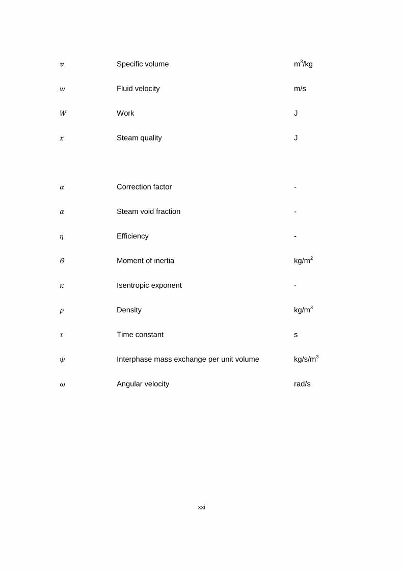
xxi
Specific volume m3/kg
Fluid velocity m/s
Work J
Steam quality J
Correction factor -
Steam void fraction -
Efficiency -
Moment of inertia kg/m2
Isentropic exponent -
Density kg/m3
Time constant s
Interphase mass exchange per unit volume kg/s/m3
Angular velocity rad/s

xxii

1
1 Introduction
All the thermal power plants need an element to transform the heat power into electri-
cal power. In a Nuclear Power Plant the heat produced by the nuclear fission is used to
produce high pressure steam. This steam expands through a turbine in which the heat
stored in the steam is transformed into mechanical energy used to drive a generator
thus producing electricity.
In the field of nuclear safety, so called system codes (e.g. RELAP, TRACE, CATHARE
or ATHLET) have been developed to simulate the behaviour of the plant. The aim of
this paper is to develop a model for the steam turbine of a Nuclear Power Plant in the
computer code ATHLET (acronym for Analysis of Thermal-hydraulics of Leaks and
Transients) developed by the company Gesellschaft für Anlagen- und Reaktorsicher-
heit (GRS).
ATHLET is a 1-D best estimate code and therefore the whole cooling system including
the steam turbine should be simulated with the maximum accuracy. In order to do that,
and to be able to simulate the behaviour of the plant as a whole in situations such as
full and partial load, and abnormal situations such as load rejections, and the operation
of the plant supplying energy only for the plant itself isolated from the net, the devel-
opment of the steam turbine model is necessary. Also the users of ATHLET have being
asking for a turbine model in the past.
As the aim of this paper is to model the steam turbine of a Nuclear Power Plant in op-
eration, a short and simple description of the basic NPP features will be given. The
chosen thermodynamic approach, with the model delivering a pressure drop and a
power extraction makes the presentation of the basic thermodynamic background nec-
essary. The concepts of the Rankine cycle and its particularities for the case of a Nu-
clear Power Plant as well as the principles behind the operation of steam turbines will
also be explained. The system code ATHLET will be presented and described in order
to improve the understanding of the chosen approach.
2
Turbine manufacturers do not publish any relevant data about steam turbines, this
makes the development of a model quite complicated. The goal of this paper is to de-
velop a model which requires only data accessible by the final user.
The reference turbine used (the Low Pressure turbine of the Nuclear Power Plant
Philippsburg 2) will be described and analysed and the assumptions and hypotheses
made will be developed and justified.
The models developed will be explained and justified before alternative approaches are
commented. Finally the implementation in ATHLET will be presented as well as the re-
sults of the simulations. The application range of the model as well as the possible ex-
tensions will be explained in the last part of this paper.

3
2 Steam turbines
2.1 The Rankine Cycle
The cycle described by the steam in a NPP is known as the Rankine cycle. In the Ran-
kine cycle a working fluid is alternatively condensed at low pressure and evaporated at
high pressure, water being the most common working fluid. Water steam is produced in
a high pressure boiler and then expanded through a turbine (where the conversion into
mechanical work is produced). The low pressure steam is condensed in a condenser.
The condensate is then pumped into the boiler thus closing the cycle.
Figure 2.1 T-s diagram of the Rankine cycle (Ainsworth, 2007).
The Rankine cycle consists of four processes; the red numbers in Figure 2.1 indicate
the different states:
Process 1-2: The pump compresses the working fluid from the low condenser pressure
to the high boiler pressure.

4
Process 2-3: In the boiler the liquid is heated at constant pressure and evaporates pro-
ducing saturated steam.
Process 3-4: The saturated steam expands through the turbine converting the heat
power into mechanical power. The pressure and the temperature decrease;
condensation occurs.
Process 4-1: The wet steam enters the condenser where it is condensed at constant
pressure and constant temperature.
In the ideal turbine the expansion would be isentropic; however losses such as the fric-
tion between the steam and the turbine increase the entropy thus reducing the isen-
tropic efficiency of the turbine.
The thermodynamic efficiency of the whole process is calculated by the formula:
| | | |
| |
(2.1)
is the mechanical power produced in the turbine, i.e. the power delivered by the
system, the power used by the pump, i.e. the mechanical power consumed by
the system and the heat power given to the system.
The calculation of the power delivered by the system or to the system is the difference
between inlet and outlet enthalpies multiplied by the mass flow.
The formulas for the specific powers are:
(2.2)
(2.3)
5
(2.4)
(2.5)
The power produced by the system is positive and the power received by the system is
negative.
The isentropic efficiency of the turbine compares the ideal (isentropic) enthalpy differ-
ence and the real enthalpy difference.
(2.6)
The sub index s stands for the enthalpy corresponding to the isentropic process.
2.2 Types and construction of turbines
Large power plants use steam turbines for converting heat energy into mechanical en-
ergy which is converted into electric energy by the generator. A turbine transforms the
internal energy of the fluid through kinetic energy into mechanical energy. Steam with
high pressure and high temperature (potential energy) expands through the turbine
thus reducing its temperature and pressure. The resulting enthalpy difference between
the inlet and the outlet steam is converted into rotational energy on the shaft which
spins a generator thus producing electricity.
If steam with high pressure and high temperature expands through a nozzle into a low
pressure area, the pressure reduction will increase its velocity. In this way the enthalpy
of the steam decreases but its kinetic energy increases, the total enthalpy however re-
mains constant (provided that the expansion occurs without losses). The total enthalpy
of a fluid (equation (2.7)) computes the energy content of the fluid as well as the kinetic
energy of the streaming fluid.
6
(2.7)
In a turbine there are stationary blades which are fixed to the casing and moving
blades which are fixed to the shaft. A line of stationary blades followed by its corre-
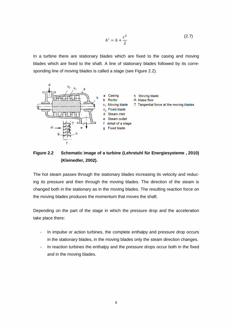
sponding line of moving blades is called a stage (see Figure 2.2).
Figure 2.2 Schematic image of a turbine (Lehrstuhl für Energiesysteme , 2010)
(Kleinedler, 2002).
The hot steam passes through the stationary blades increasing its velocity and reduc-
ing its pressure and then through the moving blades. The direction of the steam is
changed both in the stationary as in the moving blades. The resulting reaction force on
the moving blades produces the momentum that moves the shaft.
Depending on the part of the stage in which the pressure drop and the acceleration
take place there:
- In impulse or action turbines, the complete enthalpy and pressure drop occurs
in the stationary blades, in the moving blades only the steam direction changes.
- In reaction turbines the enthalpy and the pressure drops occur both in the fixed
and in the moving blades.

7
Figure 2.3 Difference between impulse and reaction turbine (Ainsworth, 2007)
Depending on the exhaust conditions turbines can be classified into:
Back pressure turbines, in which the exhaust pressure is atmospheric or higher.
Condensate turbines, in which the exhaust pressure is lower than the atmos-
pheric pressure, normally close to vacuum.

8
2.3 Particularities of steam turbines in Nuclear Power Plants; the saturat-
ed steam process
2.3.1 Steam production in a Nuclear Power Plant
In a Pressurized Water Reactor (see Figure 2.4) the nuclear reaction takes place in the
reactor pressure vessel where it heats the primary coolant, the hot primary coolant wa-
ter goes through the steam generators were its heat is transferred to the lower pres-
sure secondary loop water which evaporates to pressurized steam. The steam pro-
duced at the steam generators then expands partially through the HP-turbine. This
steam then gets through a moisture separator which increases the steam quality and a
re-heater which increases the temperature of the steam. This overheated steam enters
into the LP-turbine, and exits to the condenser.
As the volumetric flow rises due to the steam expansion, so does the diameter of the
turbine. However, the length of the blades is limited by the speed of sound, therefore, it
is usual to divide the low pressure steam between 4 or 6 LP-turbines as it can be seen
in Figure 2.4.
Figure 2.4 Schematic configuration of NPP (PWR type) (Kleinedler, 2002).

9
2.3.2 The saturated steam process
The main difference between a NPP and conventional thermal power plants is the fact
that steam of NPP enters in the turbine as saturated steam and not as superheated
steam. This has implications in the efficiency of the whole thermodynamic cycle and in
the design of the turbine. These particularities apply to PWR as well as to BWR.
Figure 2.5 Schematic T-s diagram of the Rankine cycle in a NPP.
As it can be seen in Figure 2.5, the expansion occurs mostly in the saturated steam ar-
ea. The saturated steam exits the steam generator and enters the HP-turbine. It ex-
10
pands and its thermal energy is transformed into kinetic energy and then into mechani-
cal energy in the turbine as detailed before. This loss of heat of the steam results in
condensation of the steam thus decreasing the steam quality. The humidity in form of
water drops causes energy losses and, should it be allowed to increase, could result in
a rapid erosion of the turbine blades. In order to avoid this, the water is partly extracted
after every stage. This water extraction results in an increase of the specific enthalpy of
the remaining steam as the water extracted has a much lower enthalpy than the steam.
The fluid enthalpy, that is, the specific enthalpy multiplied by the steam mass has de-
creased in the amount of the absolute enthalpy of the extracted water.
Before entering the LP-turbine the steam gets through a moisture separator and a re-
heater, entering into the turbine as superheated steam. This increases the efficiency of
the cycle; however this improvement is minimal (Strauß, 2006) as part of the high quali-
ty steam from the steam generator has to be used for this re-heating instead of ex-
panding through the turbine. The main objective of the reheating is to minimize the ap-
pearance of moisture in the LP-turbine thus reducing the erosion of the blades.
A much more effective measure to improve the efficiency of the plant is the feed water
preheating. This is done by extracting steam from the turbine and using it to preheat
the feed water. The steam extracted from the low pressure stages from the turbine has
all its condensation heat but only a fraction of its original capacity to perform work at
the turbine.

11
3 Physical models
In order to simulate the turbine a series of key physical models have to be developed.
The development of these models has to be directed towards the proper representation
of those variables relevant for the purpose of the modelling. In this case, the model is
expected to represent the turbine behaviour in the thermo-hydraulics simulation code
ATHLET. In order to integrate this model into ATHLET, it has to provide a series of var-
iables as pressure drop across the turbine, enthalpy drop across the turbine, power
output, pressure at the extraction lines, etc.
Given the data available (see Chapter 4) and that only the above stated variables are
necessary a detailed fluid dynamics model of the behaviour of the fluid through the
moving and fixed blades is not necessary. Instead of that, a simpler thermodynamic
approach is used.
3.1 Stodola’s cone law
Stodola’s Cone Law (Stodola, 1922), and its different versions (Traupel, 2001) display,
given the design parameters, the relationship between the inlet- and outlet pressure at
the turbine and the mass flow through the turbine.
The cone law equation is (Traupel, 2001):
√
√
(
)
(
)
(3.1)
‘n’ being the polytrophic exponent, ‘p’ the pressure and ‘v’ the specific volume. The sub
index “a” stands for the inlet value, “b” for the outlet value and “0” for the design values.
For wet steam the calculation of the polytrophic exponent is (Traupel, 2001):
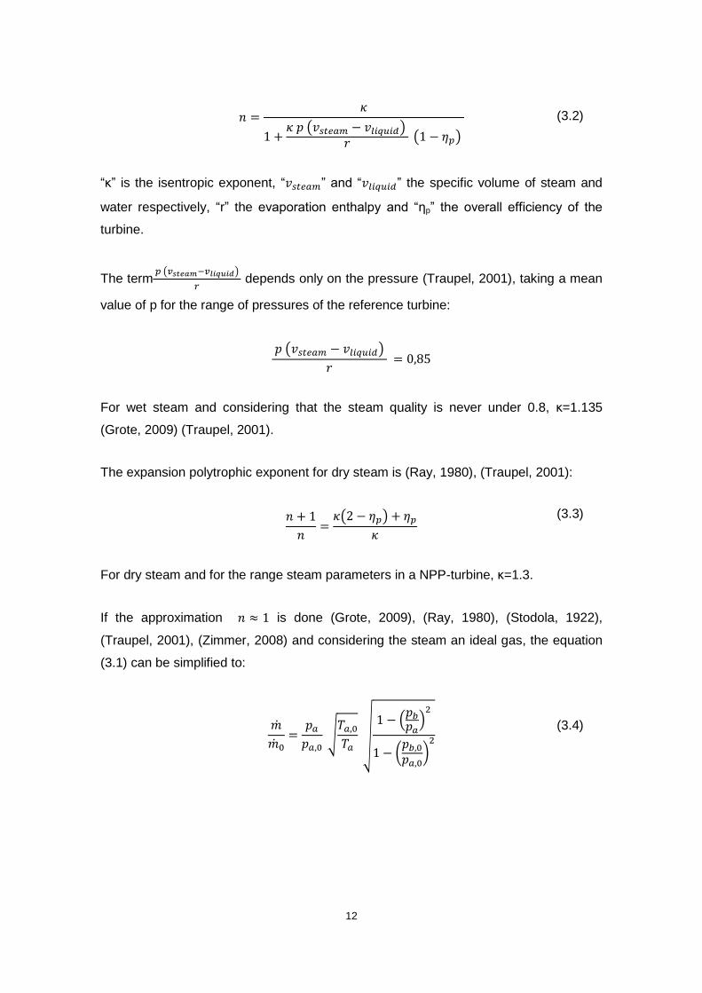
12
( )
( )
(3.2)
“κ” is the isentropic exponent, “ ” and “ ” the specific volume of steam and
water respectively, “r” the evaporation enthalpy and “ηp” the overall efficiency of the
turbine.
The term ( )
depends only on the pressure (Traupel, 2001), taking a mean
value of p for the range of pressures of the reference turbine:
( )
For wet steam and considering that the steam quality is never under 0.8, κ=1.135
(Grote, 2009) (Traupel, 2001).
The expansion polytrophic exponent for dry steam is (Ray, 1980), (Traupel, 2001):
( )
(3.3)
For dry steam and for the range steam parameters in a NPP-turbine, κ=1.3.
If the approximation is done (Grote, 2009), (Ray, 1980), (Stodola, 1922),
(Traupel, 2001), (Zimmer, 2008) and considering the steam an ideal gas, the equation
(3.1) can be simplified to:
√
√
(
)
(
)
(3.4)

13
Figure 3.1 Graphic representation of the cone law (Stodola, 1922)
If the temperature varies moderately from the design temperature, the influence of the
temperature is rather limited (about 5%). The same analogy can be done without con-
sidering the ideal gas simplification for the product of pressure and specific volume.
However, in order to maintain the accuracy it has been chosen not to neglect the influ-
ence of temperature variations.
In order to describe the changes in the operating conditions, the mass flow has to be
constant throughout the whole group of stages, making the application of equation (3.4)
only possible in those sections of the turbine with the same mass flow i.e. stages be-
tween two consecutive extractions1. Steam turbines in NPP have several extraction
lines which extract steam and/or condensate for feed water preheating and also to limit
the quantity of condensate in the turbine (see Figure 3.2). This means that in order to
describe faithfully the behaviour of the whole turbine, several interconnected sections
will be necessary.
1 For practical reasons, every group of stages will be referred to as a stage (see section 4.2).

14
Figure 3.2 Turbine with several extraction lines, on the right the subdivision in
sections can be seen.
3.2 Steam properties across the turbine
The thermodynamic state of water can be defined by two thermodynamic properties.
For overheated steam or undercooled pressure and temperature give a definite state of
the steam, for humid vapour, pressure and temperature are dependent on each other
thus making the use of a third variable necessary, e.g. steam quality or specific vol-
ume.
The steam expansion through a turbine is a polytrophic process; therefore the isentrop-
ic enthalpy drop Δhs has to be multiplied by an internal efficiency factor ηi, called isen-
tropic efficiency (see equation (2.6)).
(3.5)
Or, what is the same:
(3.6)
An isentropic process occurs at constant entropy, whereas in the real process the en-
tropy increases. This implies that the final enthalpy is higher than the isentropic enthal-
py (see Figure 3.3). At the end of the real process this can be seen as a higher tem-
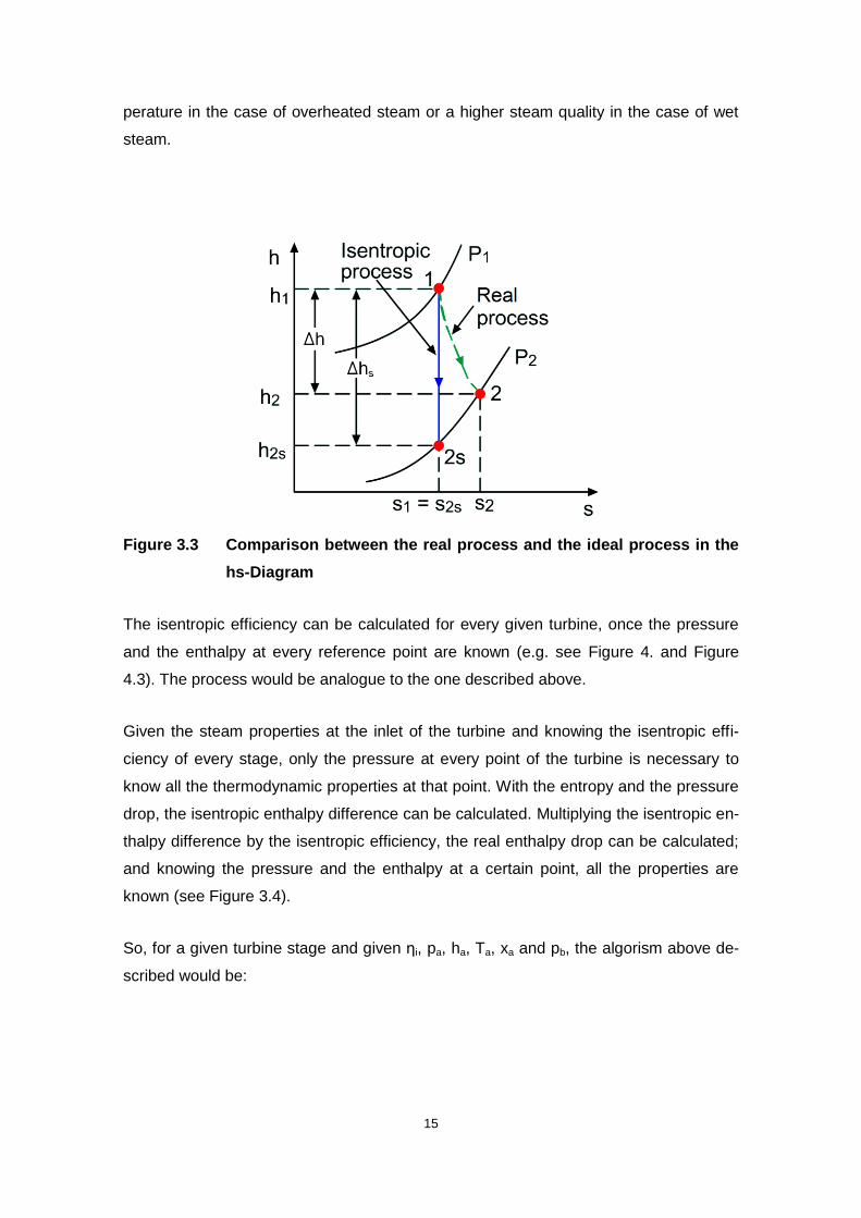
15
perature in the case of overheated steam or a higher steam quality in the case of wet
steam.
Figure 3.3 Comparison between the real process and the ideal process in the
hs-Diagram
The isentropic efficiency can be calculated for every given turbine, once the pressure
and the enthalpy at every reference point are known (e.g. see Figure 4. and Figure
4.3). The process would be analogue to the one described above.
Given the steam properties at the inlet of the turbine and knowing the isentropic effi-
ciency of every stage, only the pressure at every point of the turbine is necessary to
know all the thermodynamic properties at that point. With the entropy and the pressure
drop, the isentropic enthalpy difference can be calculated. Multiplying the isentropic en-
thalpy difference by the isentropic efficiency, the real enthalpy drop can be calculated;
and knowing the pressure and the enthalpy at a certain point, all the properties are
known (see Figure 3.4).
So, for a given turbine stage and given ηi, pa, ha, Ta, xa and pb, the algorism above de-
scribed would be:

16
Figure 3.4 Calculation of the enthalpy at the exhaust of a turbine when inlet
properties (sub index a), the exhaust pressure (sub index b) and
the isentropic efficiency of the turbine are known.
As stated above, the internal efficiency can be calculated, provided that the rest of the
parameters are given. However, when simulating off design operation, these parame-
ters are not known. The internal efficiency is influenced by many design factors includ-
ing blade construction and operation point and it reaches its maximum at nominal load.
Equation (3.7) is a semi-empirical formula that describes the variations of the internal
efficiency as a function of the angular velocity; the design efficiency and the isentropic
enthalpy drop (Ray, 1980).
[ √
√
]
(3.7)

17
Where α is a positive constant. For the purpose of this paper it can be considered that
α=2 and ηi,0=0.87.
In (Grote, 2009) equation (3.8) is used; however he quotes (Ray, 1980).
[
√
]
(3.8)
Although both equations behave similarly in the surroundings of the design point be-
yond a certain point, they give very different results. The simplest hypothesis is that
there was a spelling mistake.
Figure 3.5 Evolution of the isentropic efficiency depending of the isentropic
enthalpy difference for constant angular velocity.

18
In Figure 3.5 both equations plotted. The red line corresponds to equation (3.7) and the
blue one to equation (3.8). Notice that if instead of plotting after (Δhs /Δhs,0) the plot is
done after (Δhs,0 / Δhs), the plot resulting then is identical but corresponding the red line
to equation (3.8) and the blue one to equation (3.7).
For the purpose of this paper, equation (3.7) will be used and the above stated
hypothesis will be accepted.
3.3 Extractions
Extractions are of great importance to this paper (see section 4.2). It will be considered
that there are two different kinds of extractions, the steam extraction and the water ex-
traction. The extractions increase the efficiency of the cycle by preheating the feed wa-
ter and extracting the condensed water of the turbine keeping the quality of the steam
in it inside the margins thus avoiding erosion problems in the blades and minimizing the
efficiency losses due to condensation. The extraction of water increases the quality of
the remaining steam in the turbine, which increases the enthalpy. This steam with
higher quality is partly extracted by the steam extraction and the rest of it enters the fol-
lowing stage.

19
4 Data base
An unexpected difficulty was the unavailability of reliable and abundant turbine data.
There were a few heat balances of NPP available, but mostly only for the full power
output configuration, so reference data was partly available, but no possibility to com-
pare the results with real data.
Manufacturers are very reserved with their data. Considering the fact that the potential
user of ATHLET is expected to have a very limited access to relevant data; it has been
decided to develop a model which relies as much as possible on data obtainable by the
user.
This lack of detailed data had a great influence in the development of this work making
the first fluid dynamic approaches developed unpractical. All the geometry based mod-
els had to be abandoned as the geometry was completely unknown. Even if access to
detailed geometry would have been granted, ATHLET is a 1-D code and a blade ge-
ometry based solution would have required a 3-D approach.
4.1 Reference plant
The reference data for this paper has mainly been the heat and mass balances of the
Nuclear Power Plant Phillipsburg 2 with the old turbine. For this NPP we have data
about more operation points that for any other, namely for 100%, 80%, 60% and 40%
power output. The plant consists of one 2-flow HP turbine and 3 identical 2-flow LP tur-
bines.
For comparison purposes the reference turbine in (Grote, 2009) has also been used. It
is an industrial extraction turbine in a steel mill in Salzgitter used for the production of
electricity and process steam, it was installed in 2006 by MAN Turbo and its generator
has an electrical power output of 45-55 MW.
20
4.2 Available data on the reference plant
As stated before, only the heat balance plans are known for the reference Plant. The
pressure, the enthalpy, the mass flow and the steam quality at some significant points
are known (see Figure 4.).
Figure 4.1 Heat balance plan of the reference plant being: (1) the primary loop;
(2) HP turbine; (3) Moisture separator; (4) Re-heater; (5) LP turbine;
(6) Condenser; (7) Feed water preheater lines (8) Points of which
the thermodynamic values (pressure, enthalpy, mass flow and
temperature/steam quality) are known.
The values at the marked points are known for the plant working at 100%, 80%, 60%
and 40% of the nominal output.
This data is schematic and its accuracy is not certain. The reason for this is that the
exact points where these values are measured are not known, and significant changes
can be expected depending on where the measurements take place. At the HP turbine
inlet (see Figure 4.1Figure 4., point V) there are values given, however these are not
coherent with the measurements in the rest of the points whenever the plant works be-
low nominal power.
In fact the pressure in all the steam extractions as well as in the inlet of the LP turbine
is proportional to the power output; so for instance, the pressure in A1 (see Figure 4.)
V
21
when the plant is working at a 40% of its nominal power is approximately 40% of the
pressure in A1 when the plant is working at nominal power. This is not the case for the
pressure in point V at the HP-turbine inlet; in fact, the pressure at that point for the
plant working at 40% of its capacity is almost 30% higher than the pressure with the
plant working at nominal power (see Table 4.1).
Table 4.1 Pressures at the different load points divided by to the nominal
pressures (pi/pi0).
Power 100,00% 80,00% 60,00% 40,00%
V 1 1,1102107 1,21880065 1,27714749
A1 1 0,78111588 0,57081545 0,35450644
LP 1 0,79174312 0,58990826 0,38440367
A2 1 0,78947368 0,5812357 0
A3 1 0,79487179 0,58974359 0,39487179
A4 1 0,7993921 0,59878419 0,40273556
A5 1 0,79619565 0,59782609 0,40217391
A6 1 0,80379747 0,60759494 0,41772152
The reason for this is because the available data have been taken in front of the Main
Steam Valve (see Figure 4.2). So that the values are taken before the steam gets throt-
tled through the valve and do not represent the state of the steam at the inlet of the HP-
turbine. For operation points different than nominal power, the main steam valve is par-
tially closed so that a critical flow takes place limiting the mass flow through the valve
regardless of the pressure at the inlet of the valve.
22
Figure 4.2 Qualitative representation of the Steam pressure and mass flow
behaviour through the main steam valve (Siemens AG Bereich
Energieerzeugung).
Another point in which the state of the steam is not given is at the HP-turbine outlet, be-
fore the moisture separator. However, since the properties and mass flow after the
moisture separator are known for both steam and water, it can be calculated. This cal-
culation is based on the hypothesis that there is no pressure drop in the moisture sepa-
rator.
23
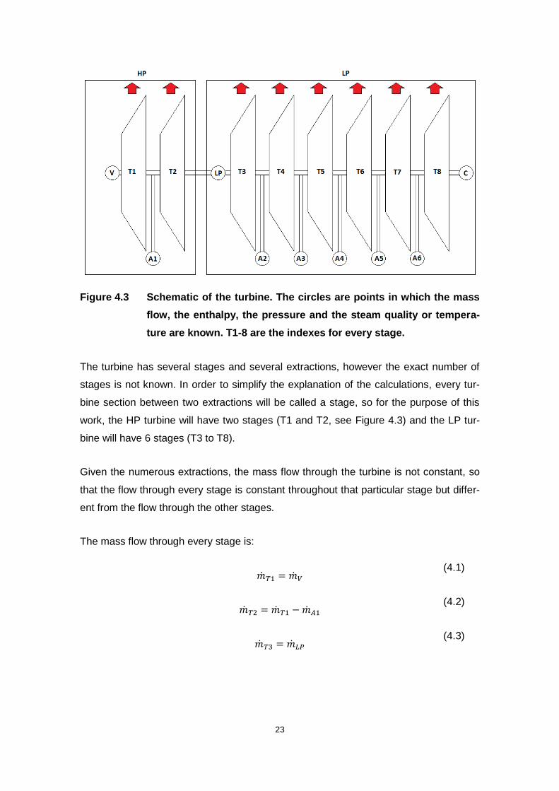
Figure 4.3 Schematic of the turbine. The circles are points in which the mass
flow, the enthalpy, the pressure and the steam quality or tempera-
ture are known. T1-8 are the indexes for every stage.
The turbine has several stages and several extractions, however the exact number of
stages is not known. In order to simplify the explanation of the calculations, every tur-
bine section between two extractions will be called a stage, so for the purpose of this
work, the HP turbine will have two stages (T1 and T2, see Figure 4.3) and the LP tur-
bine will have 6 stages (T3 to T8).
Given the numerous extractions, the mass flow through the turbine is not constant, so
that the flow through every stage is constant throughout that particular stage but differ-
ent from the flow through the other stages.
The mass flow through every stage is:
(4.1)
(4.2)
(4.3)
24
(4.4)
(4.5)
(4.6)
(4.7)
(4.8)
At extraction A5 (see Figure 4.3) only water is extracted, so that the steam properties
at that point are not known. However the water mass extracted at A5 ( ) is about
1.5% of the mass flow through the next stage ( ) so that it could be neglected and
stages T6 and T7 considered as one single stage. Another approach is to interpolate
the steam quality at the point A5, knowing that the pressure of the steam is the same
as the pressure of the extracted water. With the interpolated steam quality after the ex-
traction, all the properties of the steam are known. The latter has been the one chosen
in the frame of this paper.
Once the enthalpy drop and the mass flow through every stage are known, the power
output of every stage can be calculated. However, once this calculation is done, the re-
sulting global power (see equation (4.9)) is below the nominal power of the generator.
The way of considering the extraction A5 and the stage T6 has little influence on this
result, the difference between both approaches being minimal.
∑
(4.9)
The reason for this is because the improvement of the specific enthalpy due to the wa-
ter extractions has not been taken into account. As stated before, the water extractions
at every stage result in an increase of the specific enthalpy, this means that the steam
entering a given stage has a higher enthalpy that the steam that leaves the preceding
stage.
25
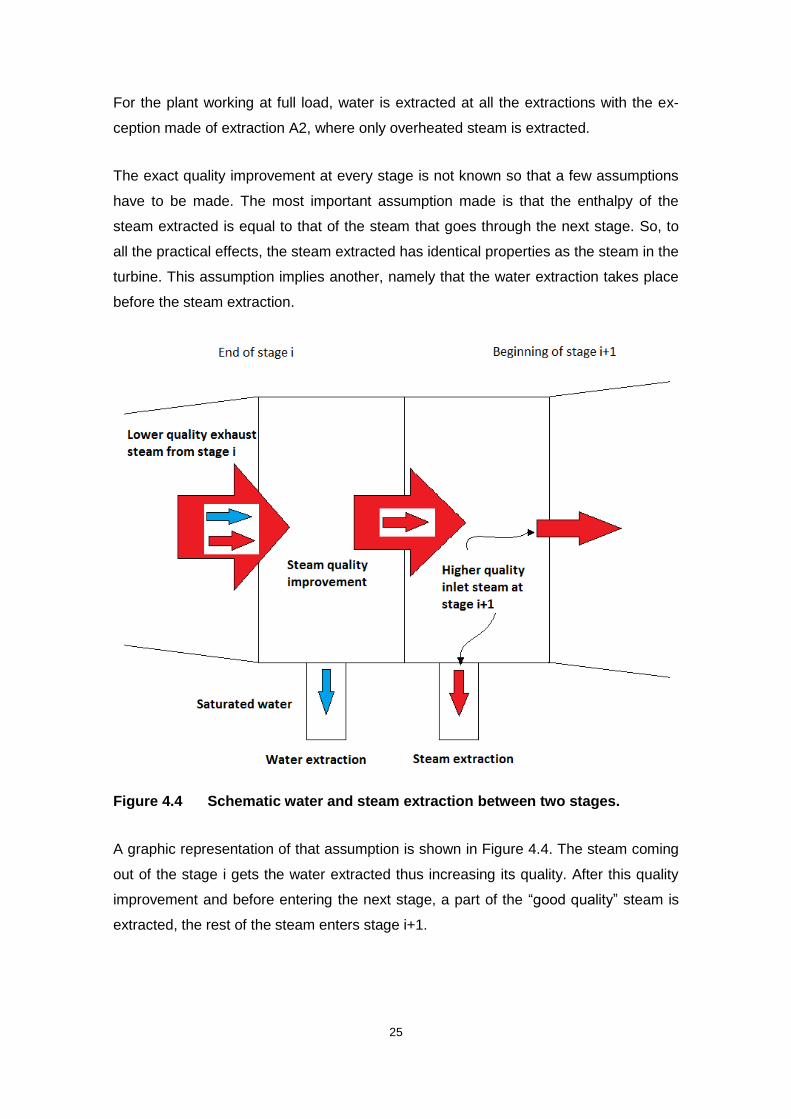
For the plant working at full load, water is extracted at all the extractions with the ex-
ception made of extraction A2, where only overheated steam is extracted.
The exact quality improvement at every stage is not known so that a few assumptions
have to be made. The most important assumption made is that the enthalpy of the
steam extracted is equal to that of the steam that goes through the next stage. So, to
all the practical effects, the steam extracted has identical properties as the steam in the
turbine. This assumption implies another, namely that the water extraction takes place
before the steam extraction.
Figure 4.4 Schematic water and steam extraction between two stages.
A graphic representation of that assumption is shown in Figure 4.4. The steam coming
out of the stage i gets the water extracted thus increasing its quality. After this quality
improvement and before entering the next stage, a part of the “good quality” steam is
extracted, the rest of the steam enters stage i+1.

26
Taking this into account, the specific enthalpy after every stage has to be recalculated.
At every extraction a known quantities of steam and water are extracted. The pressure,
the enthalpy, and the mass flow of both steam and water are known. The mass flow
through stage i (the stage before the extractions) is also known. So to calculate the
specific enthalpy of the steam coming out of stage T1 (in the HP turbine):
(4.10)
Being:
the enthalpy at the outlet of stage T1.
the mass flow through T1 (stage before the extraction).
the mass flow of water extracted at A1
the enthalpy of the water extracted at A1
the enthalpy of the steam extracted at A1
After recalculating the enthalpy after every stage, the power output is slightly above the
generator power. The resulting efficiency of the turbine and the generator together is of
98%. This efficiency is very high but not much higher than the expected efficiency (95
to 97%). Although it is considered acceptable, there are some factors which could ex-
plain this high efficiency.
The main reason is the assumption that the quality of the steam extracted is identical to
the quality of the steam remaining in the turbine, so that only the water extraction itself
is responsible for the steam quality improvement. This assumption does not take into
consideration the centrifugal forces in the turbine. Due to these forces, it is expected
that the steam extracted has a lower quality than the steam remaining in the turbine.
This fact means that the steam quality improvement at every stage is greater than cal-
culated.

27
The internal efficiency of the turbine stages calculated after these assumptions varies
greatly depending on the stage. For stage T5 it almost reaches a value of 1, which is
impossible. This is because the enthalpy after stage T5 is actually higher than the en-
thalpy calculated supposing an identical enthalpy of the steam extracted and the steam
in the turbine. At the last stage, the internal efficiency is 0,4, the reason for this is that
the steam coming out of the last stage (as well as the steam along the turbine) has a
high velocity and therefore a high kinetic energy and as it enters the condenser it loses
its velocity which then results in an enthalpy increase (see equation (2.7)). Despite of
this, it has been decided to maintain the steam enthalpy at the last stage equal to the
enthalpy of the steam in the condenser.
The fact that the results are within the margins, and that there is no way to determine
the real quality improvement, are considered sound arguments in favour of maintaining
all the aforenamed assumptions and considerations in this paper.
An interesting fact is that the total power output of the turbine remains constant no mat-
ter what steam quality value is used in the extraction A5, as a higher steam quality
brings an increase of the power output at the stage T7 but this increase is compen-
sated by the decrease of the power output in the stage T6 and vice versa.
This seems to be true for all the extractions, as what are important for the power calcu-
lation are the total mass extraction and the quality improvement resulting of the extrac-
tion.
In (Grote, 2009) a large number of geometrical data of the reference turbine was avail-
able, such as Volumes of the spaces between stages, exact enthalpies and pressure at
the inlet and at the outlet of every stage and isentropic efficiencies of every stage at
one of the design points, however, the information for other design points was limited
(Grote, 2009) and it could not be used as reference data to be compared with the re-
sults provided by the implemented models.

28
5 ATHLET
The turbine model is to be developed in ATHLET, so a general description of ATHLET
is necessary in order to justify the solutions chosen. For those areas necessary to un-
derstand the development of the model, a detailed description is provided.
For further detail see (GRS, 2009).
5.1 Description of ATHLET
The thermal-hydraulic computer code ATHLET (Analysis of Thermal-Hydraulics of
LEaks and Transients), developed by the Gesellschaft für Anlagen- und Reaktorsicher-
heit (GRS), aims to cover the whole spectrum of design basis and beyond design basis
accidents (without core degradation) for light water reactors such as PWR, BWR,
VVER and RBMK.
5.1.1 Modules of ATHLET
ATHLET is composed of several basic modules which simulate the phenomena in-
volved in the operation of LWR. These basic modules are:
Thermo-fluid dynamics: This module is based upon a 5-equation model with a mix-
ture momentum equation, and separate conservation equations for vapour and liquid,
or a 2-fluid model with 6-equations which has a momentum equation for vapour and
another for liquid.
Heat Transfer and Heat Conduction: This module allows the simulation of the heat
conduction in all those components needed.
Neutron Kinetics: Models the nuclear heat generation.
General Control Simulation Module: Is a block-oriented simulation language for the
description of control, protection and auxiliary systems. GCSM allows the representa-

29
tion of fluid dynamic systems in a very simplified way requiring very little computation
time to do so. So far, the turbine has been modelled by a large number of GCSM sig-
nals.
The solution of the differential equation system is performed implicitly by the ODE-
solver FEBE. The coupling of other independent modules can easily be performed in
the general interface.
Although major plant components can be modelled by connecting TFOs and HCO via
input data, some of them are available as special objects. These special objects are
simplified and compact models.
Additional models for the simulation of valves, pumps, accumulators, steam separators,
single ended breaks, double ended breaks, fills, leaks and boundary conditions for
pressure and enthalpy, are provided. The purpose of this paper is to add a turbine to
this list.
5.1.2 The Thermo-Fluid dynamic Module
The leading module in ATHLET is the thermo-fluid-dynamic (TFD) module. Given that
the turbine model is to be a thermodynamic model, the TFD module has to be ex-
plained comprehensibly in order to fully understand the proposed solution.
The basic equations describing the thermal-hydraulic behaviour of the system are
based on the conservation laws of mass, energy and momentum. They are time and
space dependant partial differential equations which have to be solved numerically, as
it is not possible to solve them analytically.
The system configuration to be simulated is modelled connecting basic thermo-fluid
dynamic objects (TFO) and heat conduction objects (HCO) via input data. There are
different TFOs categories; however only the pipe objects are relevant for this paper.
Pipe objects apply for a one-dimensional TFD-Model with partial differential equations
describing the transport of fluid. In the input data the nodalization is defined. Beyond
that point a pipe object is treated as consecutive Control Volumes united to each other
30
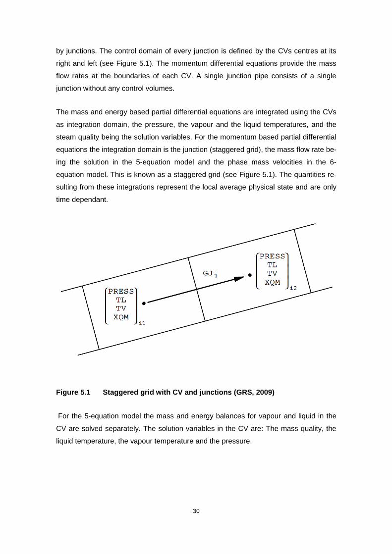
by junctions. The control domain of every junction is defined by the CVs centres at its
right and left (see Figure 5.1). The momentum differential equations provide the mass
flow rates at the boundaries of each CV. A single junction pipe consists of a single
junction without any control volumes.
The mass and energy based partial differential equations are integrated using the CVs
as integration domain, the pressure, the vapour and the liquid temperatures, and the
steam quality being the solution variables. For the momentum based partial differential
equations the integration domain is the junction (staggered grid), the mass flow rate be-
ing the solution in the 5-equation model and the phase mass velocities in the 6-
equation model. This is known as a staggered grid (see Figure 5.1). The quantities re-
sulting from these integrations represent the local average physical state and are only
time dependant.
Figure 5.1 Staggered grid with CV and junctions (GRS, 2009)
For the 5-equation model the mass and energy balances for vapour and liquid in the
CV are solved separately. The solution variables in the CV are: The mass quality, the
liquid temperature, the vapour temperature and the pressure.

31
Integrating the mass conservation equations over a CV Vi, liquid mass balance equa-
tion (5.1) and vapour mass balance equation (5.2) are obtained.
∑
∑
(5.1)
∑
∑
(5.2)
With:
(5.3)
(5.4)
With:
(5.5)
From the phase mass balances above the differential equation for the mass quality is
derived:
(5.6)
With
(5.7)
(5.8)

32
Integrating the energy balance equations over the CV Vi and after making some simpli-
fications, the ordinary differential equations for the phase temperatures (5.9) and (5.10)
are obtained.
(
|
)
(5.9)
(
|
)
(5.10)
Where
∑
(
) ∑ (
)
(
)
(5.11)
∑
(
) ∑ (
)
(
)
(5.12)
QEI is the interfacial heat exchange due to condensation or evaporation, QI the heat
source to the control volume and wi the average fluid velocity in the CV.
The differential equation for the pressure is:
(5.13)
With:

33
|
|
And
[
|
|
(
|
)] [
|
|
(
|
)]
In the junction a mixture momentum balance is solved. (5.14) is the differential equa-
tion for the mixture flow rate over a junction j connecting CVs i1 and i2.
∫
[ ] (5.14)
∫
(5.15)
ΔpI is the pressure difference between the CVs at both sides of the junction
ΔpMF is the momentum flux term
ΔpWR is the relative velocity term
Δpgrav is the elevation term
Δpfric is the friction and loss pressure drop
Δpρ is the density derivative term
ΔpI is the external source term, e.g. pump differential pressure term
34
From all these terms and in the context of this paper, only the external source term, the
friction and loss pressure drop term, and the momentum flux term need a further analy-
sis.
The external source term and its influence and importance in the solution chosen will
be explained in chapter 6.2.
The friction and loss pressure drop term is:
∫
(5.16)
The momentum flux is calculated as follows:
∫
(5.17)
Where:
And
|
| (
)
( ) [
]
With
35
[
]
Two models relevant for this paper are FILLs and Pressure‐Enthalpy Boundary Com-
ponent.
Fills are junction related models used for the simulation of mass sources and sinks. If it
is to be a mass source, the mass flow to be injected in the system has to be defined in
the GCSM module as well as the total specific enthalpy. If a sink is to be simulated, the
mass flow has to have a negative sign and the enthalpy does not need to be defined as
it is calculated as in normal junctions, i.e. they are calculated from the upstream condi-
tions.
Pressure‐Enthalpy Boundary Component - also referred to as 'time dependent volume
(TDV)’ – is a CV related model which permits to establish, via GCSM signals, a pres-
sure enthalpy boundary at the edge of the system. In this way and depending upon the
conditions in the system, mass will flow into the TDV or from the TDV into the system.

36
6 Implementation of the turbine model
The implementation of the turbine model has been chosen taking into consideration the
characteristics of ATHLET in order to make it coherent with the solving strategy of
ATHLET and as simple as possible.
Various approaches for the simulation of a turbine are proposed in literature and out-
lined in section 6.1. Taking into account the characteristics of the ATHLET solution
strategy a new method had to be developed that is based on a finite volume discretiza-
tion and a staggered grid method with solution variables defined in control volumes and
junctions. The method, as well as the details of the implementation, is thoroughly dis-
cussed in section 6.2.
6.1 Alternative implementation strategies
An approach suggested by some authors (Plavšić, 2008) is to develop a model taking a
detailed geometry configuration such as turbine blade angles into account. In order to
develop such a model, detailed information about blade geometries and fluid velocities
in the turbine are needed, this information however is only in the power of turbine man-
ufacturers and the access to it is highly limited as it is regarded as industrial secret.
Besides, the solution of such a model would need to be performed in 3-D and ATHLET
is a 1-D code.
Several authors have proposed different modelling strategies for simulating steam tur-
bines (Grote, 2009), (Zimmer, 2008). The thermodynamic basis and the physical mod-
els are the ones exposed in chapter 3.
The thermodynamic systems are designed as storage-throttle-systems where the inter-
nal volume of the turbine is divided into several steam storages (internal volumes of
pipes and between turbine stages) which are linked together by throttle devices (tur-
bines and valves) governed by valve or turbine models, depending on the case (see
Figure 6.1).
37
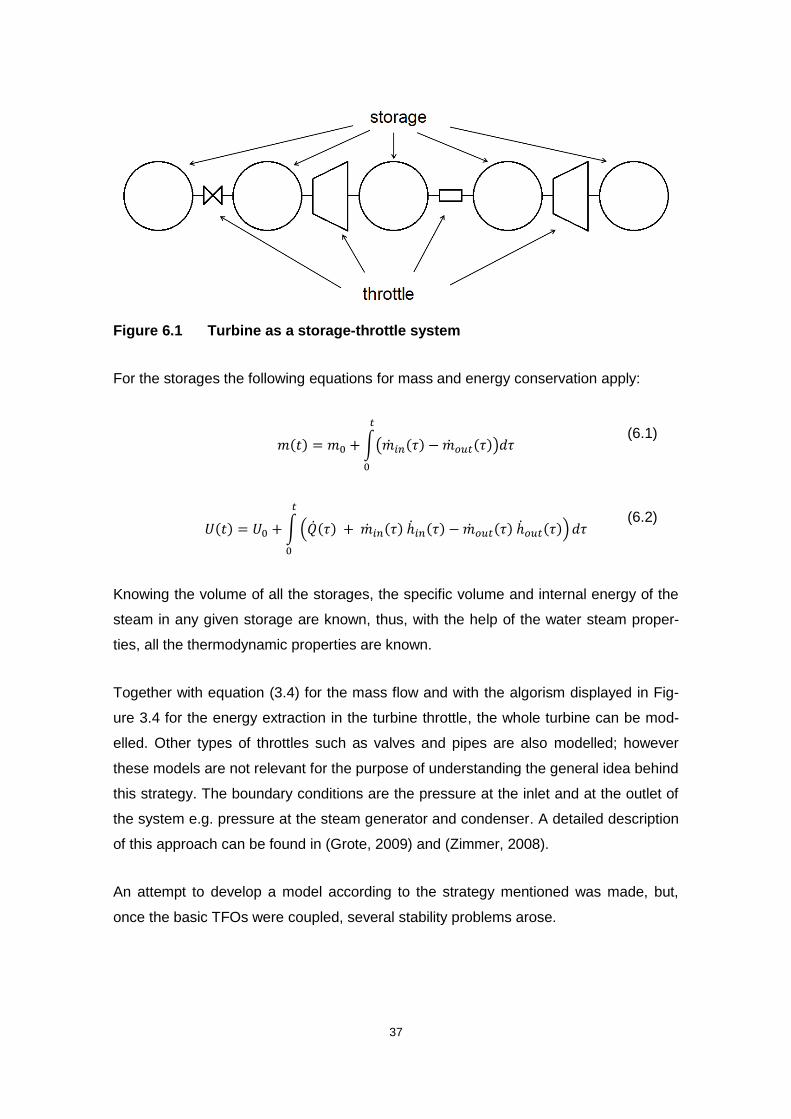
Figure 6.1 Turbine as a storage-throttle system
For the storages the following equations for mass and energy conservation apply:
∫( )
(6.1)
∫( )
(6.2)
Knowing the volume of all the storages, the specific volume and internal energy of the
steam in any given storage are known, thus, with the help of the water steam proper-
ties, all the thermodynamic properties are known.
Together with equation (3.4) for the mass flow and with the algorism displayed in Fig-
ure 3.4 for the energy extraction in the turbine throttle, the whole turbine can be mod-
elled. Other types of throttles such as valves and pipes are also modelled; however
these models are not relevant for the purpose of understanding the general idea behind
this strategy. The boundary conditions are the pressure at the inlet and at the outlet of
the system e.g. pressure at the steam generator and condenser. A detailed description
of this approach can be found in (Grote, 2009) and (Zimmer, 2008).
An attempt to develop a model according to the strategy mentioned was made, but,
once the basic TFOs were coupled, several stability problems arose.
38
The configuration was of two TDV (with the pressure and enthalpy before and after the
turbine) connected to each other by a pipe object representing the turbine. In the mid-
dle of the pipe object a modified junction was to provide the mass flow depending on
the pressures. Even fixing the pressure and enthalpy drop in this primitive turbine junc-
tion via GCSM signals, the simulation proved to be unstable. This, together with the
modelling difficulty resulted in abandoning of this strategy.
6.2 Chosen modelling strategy
As described chapter 5, ATHLET equation system consists of balance equations
solved in control volumes and junctions. In ATHLET, several so-called junction-based
component models already exist (e.g. pump…). These models basically provide addi-
tional source terms, that are added to the right hand side of the presented equations
(see subsection 5.1.2). The idea is to model a turbine stage by a pressure drop across
a junction and by a power extraction from the adjacent control volume. Adding the
terms to the corresponding equations, a turbine stage could be simulated by a junction
of a basic thermo-fluid pipe object. Corresponding models are presented in the follow-
ing chapters. The extraction lines have to be modelled separately.
The boundary conditions of the chosen strategy are: fill providing mass flow and en-
thalpy in the main steam line, and a TDV (p-h-boundary) for the pressure in the con-
denser.
6.2.1 Pressure drop model
Given the limited data available (see chapter 4) and the characteristics of ATHLET, the
chosen strategy has been to develop the turbine model taking the pump model as a
basis.
For the turbine model a new junction type which adds a negative pressure in the term
ΔpI of equation (5.14) has been developed. To do that, the mass flow has been consid-
ered an input data, it being the steam mass flow from the steam generator, considering
valid the hypothesis exposed in chapter 4.
39
So, defining ΔpI as:
(6.3)
And isolating pb in equation (3.4):
√ ( √
√
)
( (
)
) (6.4)
So, in the turbine junction, between CVs i1 and i2 the term ΔpI in the differential equa-
tion (5.14) is:
√ ( √
√
)
( (
)
) (6.5)
The terms pa and pb are the pressure terms in CVs i1 and i2 respectively (see Figure
5.1).
6.2.2 Power extraction model
The enthalpy drop in the turbine has been modelled as an energy extraction over the
junction. However the entropy in a given control volume is not one of the solution vari-
ables and could not be obtained, so the algorism of Figure 2.3 could not be applied.
Thus an alternative way to calculate the energy extraction has been chosen:
The second law of thermodynamics can be formulated as follows:
(6.6)
Adding an ideal heat quantity dQ’ to equation (6.6):
40
(6.7)
Equation (6.7) is explained by exchanging the process in equation (6.6) by a reversible
process which departs from the same starting point and ending point. In that case and
dQ being the heat added in the irreversible process, a reversible heat quantity dQ’ has
to be added.
In the case of a closed volume in which a fluid changes its volume exchanging heat
with the environment and under a given pressure, the first law of thermodynamics can
be formulated as follows:
(6.8)
The term pdV is the work done by the pressure on the surface of the element, the term
dAη is the dissipated work (due to friction, deformation, etc.) and dQ the heat added.
Given the fact that work gets dissipated, the process is irreversible. If the process is
conducted with infinite slowness, no work is dissipated, so this new process becomes
reversible. If this substitute reversible process is to achieve the same state modification
as the irreversible one (dU has to be the same for both processes), and the dissipation
work no longer being present, an additional heat quantity dQ’ (equal to dAη of the real
process) has to be added. So, equation (6.8) can be rewritten as:
(6.9)
With equation (6.7) and dividing all the extensive units by the mass (U, S and V):
(6.10)
The definition of enthalpy is:
(6.11)

41
Deriving equation (6.11):
(6.12)
(6.13)
With equation (6.10)
(6.14)
Assuming an isentropic process, i.e. ds=0:
(6.15)
Equivalent to:
(6.16)
Assuming constant density before and after the turbine stage (Ray, 1980), and integrat-
ing equation (6.16), one obtains:
(6.17)
Taking for ρ the average of density before and after the stage and Δp being the pres-
sure drop of the turbine ΔpI (equation (6.5) difference between CVs i1 and i2.
With equation (3.6) and assuming that ηi is known, the heat extracted by the turbine
junction to the fluid can be approximated by the equation (6.18):
(6.18)
42
This approach relies on the use of an average density. While this can be accepted in
the case of incompressible fluids where the density variation can be neglected, the
density variation throughout a turbine stage is considerable2. This density variation
makes the assumption implied in equation (6.17) quite bold. However, the accuracy of
the achieved results endorses the applicability of the proposed approach.
6.3 Implementation in ATHLET
Once the equations have been developed, the next step has been the implementation
in ATHLET of the proposed model. Before starting with the implementation in ATHLET,
all the equations have been tried in MATLAB in order to observe the response of the
model. Although the results are not free of errors, the decision has been taken to carry
on the implementation in ATHLET and to make any further modifications there.
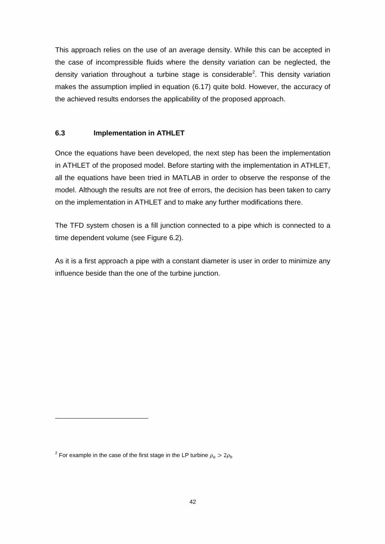
The TFD system chosen is a fill junction connected to a pipe which is connected to a
time dependent volume (see Figure 6.2).
As it is a first approach a pipe with a constant diameter is user in order to minimize any
influence beside than the one of the turbine junction.
2 For example in the case of the first stage in the LP turbine

43
Figure 6.2 TFD system. Fill on the left, pipe in the middle and TDV on the right.
The turbine junction is in the middle of the pipe.
In order to observe the behaviour of the turbine junction and of the whole TFD, the first
simulation has been made by setting in the turbine junction, the pressure and enthalpy
drop. After observing the adequacy of the configuration, further modifications have
been done in order to implement the model.
6.3.1 The pump model as a basis
The turbine model has been developed taking the pump model as a basis. What the
pump junction does is to introduce a pressure difference as part of the momentum
equation of the junction (see equation (5.14)) and adding a pump power to the fluid in
both adjacent CVs (see equations (5.11) and (5.12)).
The development of the turbine model taking the pump model as a basis is much sim-
pler and takes much less modifications in the code than choosing the approach sug-
gested in 6.1. That approach, besides of the initial instability problems explained, would
have taken major modifications in the code including the development of entirely new
subroutines.

44
All what is required is to modify the power extraction to the fluid and the way the pres-
sure drop is inserted by introducing the equations (6.5) and (6.18) in the corresponding
subroutines.
6.3.1.1 The modifications in the pump model
In the pump junction the power of the pump is added at both adjacent CV. In the tur-
bine junction, instead of adding power, it is subtracted thus only a sign modification is
necessary to represent the work performed by the steam in the shaft.
In a steam turbine the power transfer from the steam to the shaft takes place at that
stage; however the present model does not model that stage internally. Instead it mod-
els a new junction type which is then accommodated in a pipe object. The pressure
drop is added as part of the momentum equation of the junction; however the power
extraction from the fluid cannot take place in the junction as the energy balance equa-
tion is not solved in the junction (see chapter 5). The power must therefore be extract-
ed from the fluid in the CV after the turbine. The difference with the energy added in the
pump model is that in the latter the pump energy is added to the CV before the pump
and to the CV after the pump; in the turbine model all the energy is extracted from one
single CV after the turbine junction.
In the turbine the work is done only by the steam; water in the turbine has a lower ve-
locity than steam and actually receives energy from the turbine. Therefore, instead of
extracting power from the liquid and steam phase, the energy extraction takes place
only in the steam phase.
The modifications done in order to achieve this can be seen in Figure 6.3. The energy
extraction done by the pump in the CV left of the junction (index JILJ) as well as the
energy extraction to the liquid (QLI) in both CV have been turned off. Instead all the
power extraction takes place in the CV right of the turbine junction and only to the
steam.

45
Figure 6.3 Part of the subroutine dkturb.f. Comments are in green.
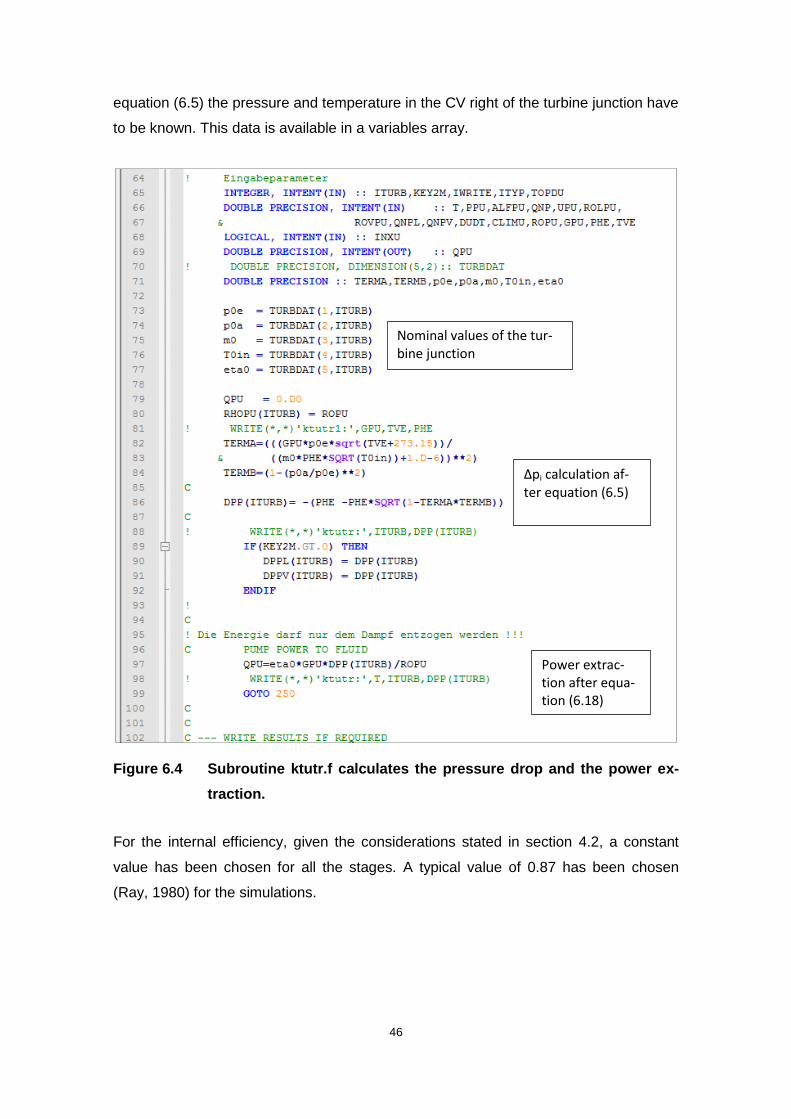
The calculation of the pressure drop and the power extraction is calculated in subrou-
tine ktutr.f (see Figure 6.4). In order to perform the power drop calculation after the
46
equation (6.5) the pressure and temperature in the CV right of the turbine junction have
to be known. This data is available in a variables array.
Figure 6.4 Subroutine ktutr.f calculates the pressure drop and the power ex-
traction.
For the internal efficiency, given the considerations stated in section 4.2, a constant
value has been chosen for all the stages. A typical value of 0.87 has been chosen
(Ray, 1980) for the simulations.
Nominal values of the tur-bine junction
Δpi calculation af-ter equation (6.5)
Power extrac-tion after equa-tion (6.18)
47
6.3.2 Modelling of the water and steam extractions
In order to couple several stages, steam and water extractions have to be included in
the simulation. This has been done adding two fill junctions after every stage; one for
the steam and the other for the water. Given the fact that a fill must be always be di-
rected toward the TFD system, the only way to add a fill between two stages (i.e. not at
the leftmost junction of a pipe) is via a Single Junction Pipe (for a complete description
of the SJP see (GRS, 2009)).
Between every stage, the leftmost extraction is the water extraction and the rightmost
extraction is the steam extraction (see Figure 4.4). In order to simplify the explanation,
the concept stage will hereinafter comprehend the set of a turbine junction and the ex-
tractions after that junction (at the right of that junction).
The mass flow to be extracted by every fill is set by the user in the input data set (see
Figure 6.5). Notice that there are two values for every extraction. The purpose of this is
to avoid that extraction takes place before a semi-stationary main mass flow is
achieved as it could result in instability and, in the case of water extraction, in the para-
dox of extracting more water than the moisture present in a given stage resulting in an
abrupt end of the simulation.
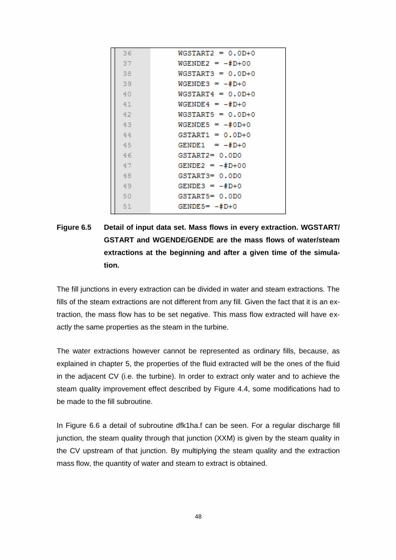
48
Figure 6.5 Detail of input data set. Mass flows in every extraction. WGSTART/
GSTART and WGENDE/GENDE are the mass flows of water/steam
extractions at the beginning and after a given time of the simula-
tion.
The fill junctions in every extraction can be divided in water and steam extractions. The
fills of the steam extractions are not different from any fill. Given the fact that it is an ex-
traction, the mass flow has to be set negative. This mass flow extracted will have ex-
actly the same properties as the steam in the turbine.
The water extractions however cannot be represented as ordinary fills, because, as
explained in chapter 5, the properties of the fluid extracted will be the ones of the fluid
in the adjacent CV (i.e. the turbine). In order to extract only water and to achieve the
steam quality improvement effect described by Figure 4.4, some modifications had to
be made to the fill subroutine.
In Figure 6.6 a detail of subroutine dfk1ha.f can be seen. For a regular discharge fill
junction, the steam quality through that junction (XXM) is given by the steam quality in
the CV upstream of that junction. By multiplying the steam quality and the extraction
mass flow, the quantity of water and steam to extract is obtained.

49
Figure 6.6 Detail of subroutine dfk1ha.f where the quality of the steam to be
extracted can be set.
The modification consists in adding a new input camp in the declaration of a fill junction
in the input data set. This input value set by the user is to be one in the case of a water
extraction and zero for all other cases.
In the case of a water extraction, the steam quality is automatically set to zero, thus ex-
tracting only water, being the mass flow of water extracted determined by GCSM sig-
nals, i.e. by the user.
The real water extractions occur as a consequence of the internal conditions in the tur-
bine and the operation mode, therefore a more realistic option has been developed as
an alternative (see Figure 6.7 and Figure 6.8) where the user only has to fill in the input
data of the percentage of water in a stage to be extracted (i.e. the steam quality im-
provement).
The way this model operates is quite simple; the steam quality in the CV at the outlet of
the closest (upstream) turbine junction together with the mass flow through that same
turbine junction is read by the subroutine thus calculating the water mass flow. The
mass flow to be extracted results from the product of the water mass flow and the
ABGRAD variable set by the user (proportion of water)
A model for these percentages is still to be developed so that the user does not have to
set these values for every operation point.
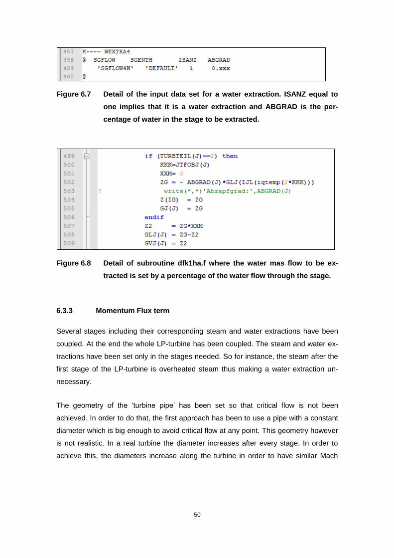
50
Figure 6.7 Detail of the input data set for a water extraction. ISANZ equal to
one implies that it is a water extraction and ABGRAD is the per-
centage of water in the stage to be extracted.
Figure 6.8 Detail of subroutine dfk1ha.f where the water mas flow to be ex-
tracted is set by a percentage of the water flow through the stage.
6.3.3 Momentum Flux term
Several stages including their corresponding steam and water extractions have been
coupled. At the end the whole LP-turbine has been coupled. The steam and water ex-
tractions have been set only in the stages needed. So for instance, the steam after the
first stage of the LP-turbine is overheated steam thus making a water extraction un-
necessary.
The geometry of the ‘turbine pipe’ has been set so that critical flow is not been
achieved. In order to do that, the first approach has been to use a pipe with a constant
diameter which is big enough to avoid critical flow at any point. This geometry however
is not realistic. In a real turbine the diameter increases after every stage. In order to
achieve this, the diameters increase along the turbine in order to have similar Mach
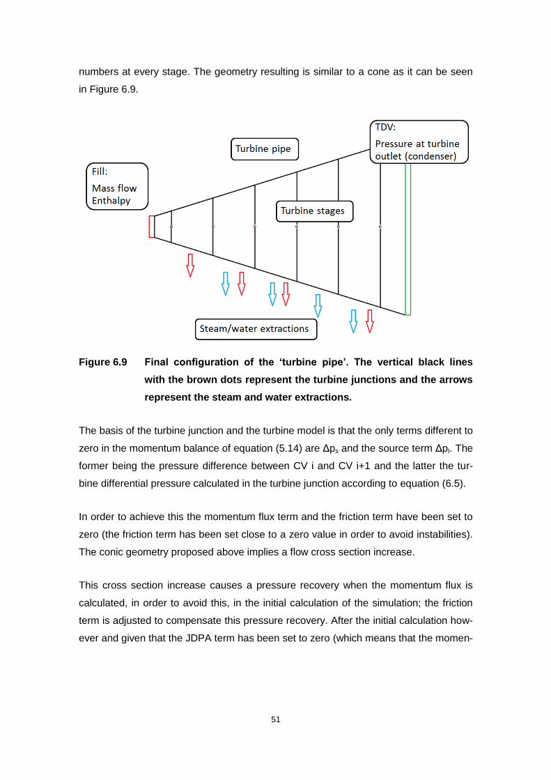
51
numbers at every stage. The geometry resulting is similar to a cone as it can be seen
in Figure 6.9.
Figure 6.9 Final configuration of the ‘turbine pipe’. The vertical black lines
with the brown dots represent the turbine junctions and the arrows
represent the steam and water extractions.
The basis of the turbine junction and the turbine model is that the only terms different to
zero in the momentum balance of equation (5.14) are Δps and the source term ΔpI. The
former being the pressure difference between CV i and CV i+1 and the latter the tur-
bine differential pressure calculated in the turbine junction according to equation (6.5).
In order to achieve this the momentum flux term and the friction term have been set to
zero (the friction term has been set close to a zero value in order to avoid instabilities).
The conic geometry proposed above implies a flow cross section increase.
This cross section increase causes a pressure recovery when the momentum flux is
calculated, in order to avoid this, in the initial calculation of the simulation; the friction
term is adjusted to compensate this pressure recovery. After the initial calculation how-
ever and given that the JDPA term has been set to zero (which means that the momen-

52
tum flux term is not to be calculated during the simulation), the momentum flux term is
zero, the modified friction term however, remains modified thus adding a unwanted
pressure term due to the friction losses.
In order to avoid any pressure drop due to factors different from the turbine junction,
the initial calculation subroutines had to be modified in order to avoid the initial calcula-
tion of the pressure recovery in the case of the turbine thus avoiding the friction term
adjustment.
6.3.4 Basic thermo-fluid dynamic models used
The thermo fluid dynamics module chosen is the one based on the 5-equation model.
This has been done because of the small amount of water in the turbine and because
given the lack of information about the turbine’s internal geometry, a proper modelling
of the phase frontier is not possible. The effects of moisture in the performance of the
turbine are considered in the overall efficiency factor.
The friction throughout the turbine model (i.e. pipe and turbine junction) is set to a very
low factor close to zero. This is done because the internal geometry of the turbine
(number of blades, hydraulic diameters, and length) is not known. So, setting the fric-
tion factor to a close to a zero value eliminates any pressure drop other than the one
due to the turbine junction. This minimizes the influence of the error committed by the
approximation of values such as the diameter and the length of the turbine.
6.3.5 Turbine data required by user input
The nominal values for equation (6.5) (mass flow, steam temperature, and pressure
before and after the turbine, and stage efficiency) have to be input by the user in the
input dataset (see Figure 6.10).
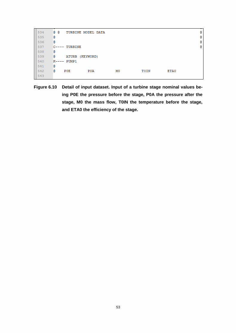
53
Figure 6.10 Detail of input dataset. Input of a turbine stage nominal values be-
ing P0E the pressure before the stage, P0A the pressure after the
stage, M0 the mass flow, T0IN the temperature before the stage,
and ETA0 the efficiency of the stage.
54
7 Results
As explained in chapter 4 the database is limited to the heat mass flow charts of the
NPP Phillipsburg 2. Therefore, and considering valid all the assumptions made in chap-
ter 4, the output variables are the pressure, the enthalpy, the temperature, the mass
flow and the steam quality.
All the simulations presented below have been carried out for steady state conditions
Figure 7.1 displays the simplest configuration of the model, (Fill, pipe object with tur-
bine junction in the middle and TDV, with no extractions)
The mass flow is determined as boundary condition by the input data, as are the en-
thalpy at the turbine inlet (both variables determined by the fill junction) and the pres-
sure at the turbine outlet (determined by the pressure set by the user at the TDV). The
nominal values of every turbine stage are to be provided by the user in the input data
set.
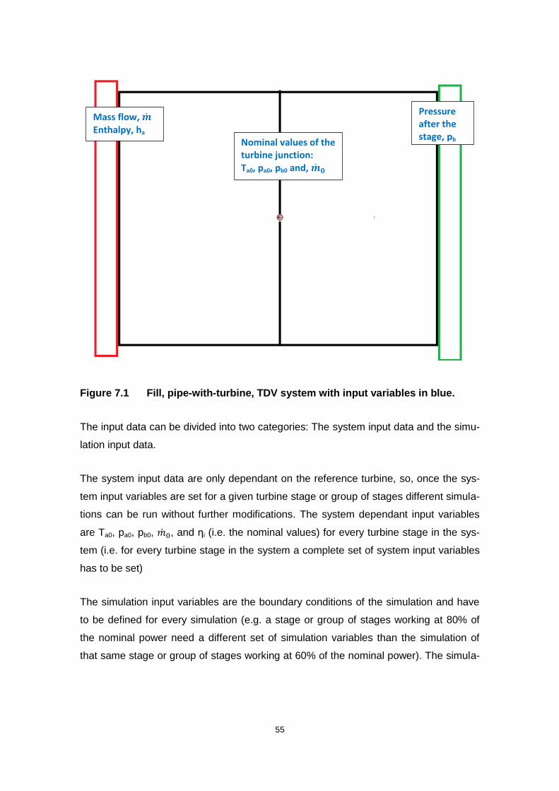
55
Figure 7.1 Fill, pipe-with-turbine, TDV system with input variables in blue.
The input data can be divided into two categories: The system input data and the simu-
lation input data.
The system input data are only dependant on the reference turbine, so, once the sys-
tem input variables are set for a given turbine stage or group of stages different simula-
tions can be run without further modifications. The system dependant input variables
are Ta0, pa0, pb0, , and ηi (i.e. the nominal values) for every turbine stage in the sys-
tem (i.e. for every turbine stage in the system a complete set of system input variables
has to be set)
The simulation input variables are the boundary conditions of the simulation and have
to be defined for every simulation (e.g. a stage or group of stages working at 80% of
the nominal power need a different set of simulation variables than the simulation of
that same stage or group of stages working at 60% of the nominal power). The simula-
Mass flow, �� Enthalpy, ha
Pressure after the stage, pb Nominal values of the
turbine junction: Ta0, pa0, pb0 and, ��𝟎
56
tion input variables are (steam entering the turbine), ha (defined at the fill junction), pb
(defined in the TDV) and (steam mass flow extracted), and (water
mass flow extracted) or water in the stage proportion to be extracted. The extracted
water and steam mass flows have to be defined for every extraction in the system and
only if the system includes extractions.
The solution variables are the pressure before each turbine stage, the enthalpy after
each enthalpy stage, and, for the last simulation with the quality improvement oriented
water extractions also the extracted water mass flow.
GRS does not have permission of KWU to publish the data of the reference power
plant and therefore all the data will be represented divided by the parameters of the
steam at the inlet of the LP turbine (see point LP in Figure 4.). So instead of having
values such as p1, p2, h1, h2 etc. the results will be p1/p1,100, p2/p1,100, h1/h1,100, h2/h2,100
etc. All the values presented in this paper are normalized values (hereinafter referred to
as ‘values’)
The per cent error has been calculated after the formula:
For the HP-turbine the inlet steam is wet steam and its pressure is not known. So, giv-
en that it only has two stages and that the conditions at the inlet are not known for sim-
ulation purposes the HP-turbine has only one stage because it is not possible to com-
pare the results of the simulation with real values, besides even the nominal values of
the first stage of the HP-turbine seem to be inaccurate (see Figure 4.2). At the begin-
ning it was not clear that the cone law with its simplification for ideal gas (see equation
(3.4)) would work for wet steam and therefore it was decided to make the first trials with
stages working with overheated steam and where the errors implied in the initial as-
sumptions made (see section 4.2) would have as little influence in the results as possi-
ble; it is for this reason that the first trials and simulations haven been made with the
first stages of the LP-turbine, where the steam is overheated and where all the parame-
ters of the inlet steam are known.
(7.1)

57
7.1 Simulation of all the stages separately
The first step has been to model every stage of the turbine separately without any ex-
tractions in order to observe solely the behaviour of the turbine junction for steady state
conditions (Figure 7.1 is a graphic representation of the system).
7.1.1 Pressure at the inlet of every stage
All the stages of the LP turbine have been simulated separately. The results for the
pressure and the error committed at every stage are shown in Table 7.1, Table 7.2 and
Table 7.3, for 80%, 60% and 40% of nominal power, respectively. A graphic represen-
tation of the pressure and the enthalpy along the stages T3, T4 and T5 of the LP-
turbine for the 80% case can be seen in Figure 7.2 and Figure 7.3.
Table 7.1 Pressure at the inlet of the LP-turbine stages, plant working at 80%
of the nominal power.
Stage Simulation inlet pres-
sure Real inlet pressure Per cent error
T3 0,791788991 0,79174312 0,006%
T4 0,319001468 0,31651376 0,786%
T5 0,141114495 0,14220183 -0,765%
T6 0,047221495 0,04825688 -2,146%
T7 0,026403156 0,02688073 -1,777%
T8 0,011666459 0,01165138 0,129%

58
Table 7.2 Pressure at the inlet of the LP-turbine stages, plant working at 60%
of the nominal power.
Stage Simulation inlet pres-
sure Real inlet pressure Per cent error
T3 0,58711156 0,58990826 -0,474%
T4 0,2379122 0,23302752 2,096%
T5 0,10404303 0,10550459 -1,385%
T6 0,03512752 0,03614679 -2,820%
T7 0,0184393 0,02018349 -8,642%
T8 0,00791484 0,00880734 -10,134%
Table 7.3 Pressure at the inlet of the LP-turbine stages, plant working at 40%
of the nominal power.
Stage Simulation inlet pres-
sure Real inlet pressure Per cent error
T5 0,06948744 0,0706422 -1,635%
T6 0,02341212 0,02431193 -3,701%
T7 0,01208187 0,01357798 -11,019%
T8 0,00533608 0,00605505 -11,874%
Notice that the pressure at stages T3 and T4 has not been simulated; the reason for
this is that there is no real data available about these stages at 40% power output and
comparison with the simulation is therefore not possible.
As it can be seen the error is only significant for the last stages for the 60% and 40 %
operation points. As a first approximation, however, it is considered acceptable.

59
Figure 7.2 Calculated pressure behaviour along stages T3, T4 and T5 of the
LP turbine
Figure 7.3 Calculated enthalpy along stages T3, T4 and T5 of the LP turbine
0
0,1
0,2
0,3
0,4
0,5
0,6
0,7
0,8
0,9
0 0,2 0,4 0,6 0,8 1 1,2 1,4 1,6 1,8 2
Pre
ssu
re a
s p
/p1
00
Length
LP 1st stage
LP 2nd stage
LP 3rd stage
0,84
0,86
0,88
0,9
0,92
0,94
0,96
0,98
1
1,02
0 0,2 0,4 0,6 0,8 1 1,2 1,4 1,6 1,8 2
Enth
alp
y as
h/h
10
0
Length
LP 1st stage
LP 2nd stage
LP 3rd stage

60
7.1.2 Enthalpy at the outlet of every stage
The results for the enthalpy after every stage can be seen in Table 7.4, Table 7.5 and
Table 7.6, for 80%, 60% and 40%, respectively.
Table 7.4 Enthalpy at the outlet of the LP-turbine stages for the plant working
at 80% of the nominal power.
Stage Simulation outlet
enthalpy Real outlet enthalpy Per cent error
T3 0,95214298 0,95340749 -0,133%
T4 0,91037398 0,91053411 -0,018%
T5 0,8619126 0,85296453 1,049%
T6 0,83476118 0,82358954 1,356%
T7 0,79694549 0,8055026 -1,062%
T8 0,75333379 0,79496539 -5,237%
Table 7.5 Enthalpy at the outlet of the LP-turbine stages for the plant working
at 60% of the nominal power.
Stage Simulation outlet
enthalpy Real outlet enthalpy Per cent error
T3 0,959080547 0,96029478 -0,126%
T4 0,91702779 0,91690485 0,013%
T5 0,868961741 0,86247058 0,753%
T6 0,772795206 0,77378909 -0,128%
T7 0,805454733 0,80837214 -0,361%
T8 0,778101519 0,79606736 -2,257%

61
Table 7.6 Enthalpy at the outlet of the LP-turbine stages for the plant working
at 40% of the nominal power.
Stage Simulation outlet
enthalpy Real outlet enthalpy Per cent error
T5 0,87594752 0,873446055 0,286%
T6 0,84850339 0,759540481 11,713%
T7 0,81307931 0,811627977 0,179%
T8 0,7861073 0,799269947 -1,647%
The error for the enthalpy is also acceptable, except after stage T6 operating at a 40%
of nominal power. The real value of the enthalpy after stage T6 is not known as in ex-
traction A5 only water is extracted (see section 4.2). Therefore it can be only said that
there is a deviation from the interpolated value, not necessarily an error.
Although the errors in the simulation of every separate stage cannot be neglected, it
can be accepted that the proposed turbine junction model is accurate enough to pro-
ceed to the coupling of several stages with their corresponding water and steam ex-
tractions.
7.2 Simulation of the whole LP-turbine with steam and water extractions,
and constant diameter of the “turbine pipe”
A new TFD system has been developed including all the stages and its corresponding
extractions. As it can be seen in Figure 7.4, the turbine pipe configuration remains un-
changed except by the addition of the turbine junctions and the extractions.

62
Figure 7.4 TFD system. The points are the turbine junctions and the arrows
the steam and water extractions.
Figure 7.5 Detail of Figure 7.4. Turbine junctions and extractions can be seen
clearly. Between some stages, there is only one extraction as only
steam (between stages T3 and T4) or only water (between stages
T6 and T7) is extracted.
7.2.1 Pressure evolution along the LP-turbine
Because the pressure drop occurs only at the turbine junctions (i.e. at the stages), the
pressure after one stage is exactly the same as the pressure before the next stage.

63
The pressure after stage T8 (i.e. in the condenser) is not displayed as it is a boundary
condition and is not calculated by the TFD system, but set by the user.
Table 7.7 Pressure at the LP-turbine stages inlets, plant working at 80%, 60%
and 40% of the nominal power
80% 60% 40%
Stage
Simulation pressure
Real pres-sure
Per cent error
Simulation pressure
Real pressure
Per cent error
Simulation pressure
Real pres-sure
Per cent error
T3 0,7937 0,7917 0,251% 0,5897 0,5899 -0,038% 0,3843 0,3844 -0,037%
T4 0,3217 0,3165 1,647% 0,2397 0,2330 2,870% 0,1609 N/A N/A
T5 0,1488 0,1422 4,653% 0,1096 0,1055 3,882% 0,0732 0,0706 3,684%
T6 0,0480 0,0483 -0,532% 0,0357 0,0361 -1,276% 0,0238 0,0243 -2,073%
T7 0,0270 0,0269 0,399% 0,0201 0,0202 -0,356% 0,0135 0,0136 -0,568%
T8 0,0119 0,0117 1,723% 0,0089 0,0088 0,596% 0,0061 0,0061 0,217%
Figure 7.6 Calculated pressure behaviour along the LP turbine, plant working
at 80%, 60% and 40% of the nominal power.
As can be seen in Table 7.7 the results are significantly better for the simulation of the
whole turbine than for the simulation of the stages separately, the error being below 5%
in all the three simulations. Figure 7.6 displays clearly the pressure drop after every
stage. Notice that the main pressure drop takes place at the first stage.
0
0,1
0,2
0,3
0,4
0,5
0,6
0,7
0,8
0 0,5 1 1,5 2 2,5 3 3,5 4 4,5 5
Pre
ssu
re a
s p
/p1
00
Length
80% of Nominal power
60% of Nominal power
40% of Nominal power
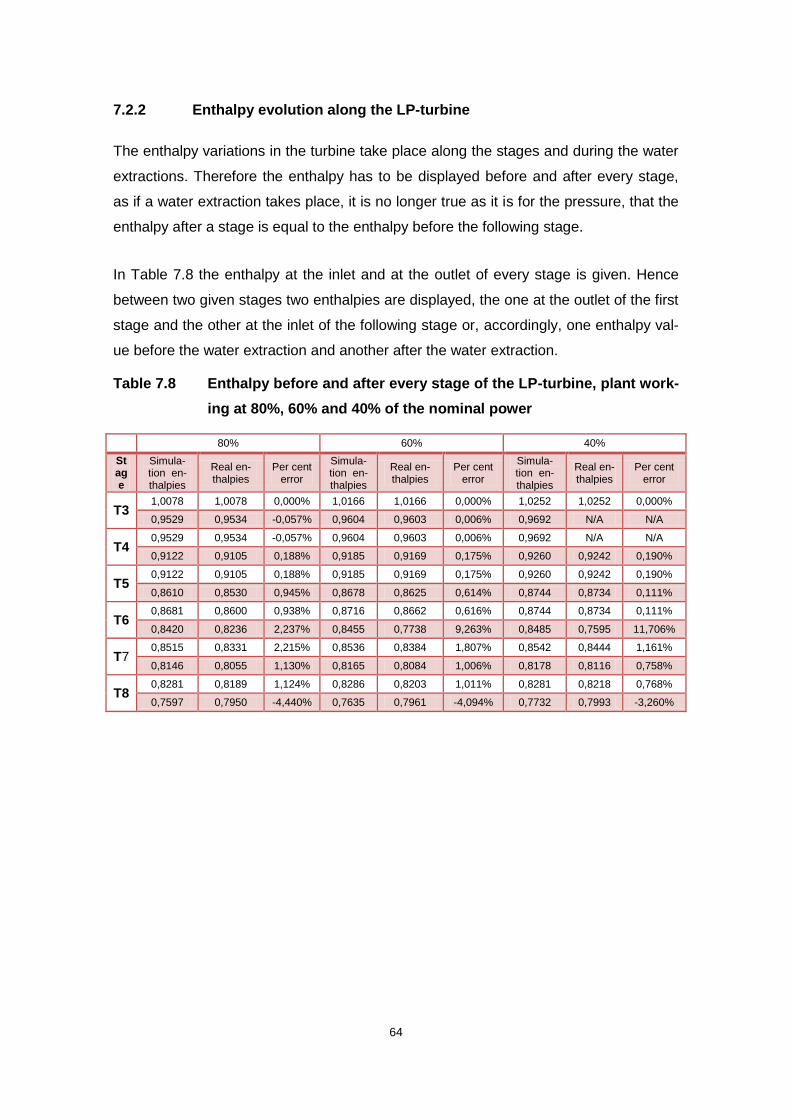
64
7.2.2 Enthalpy evolution along the LP-turbine
The enthalpy variations in the turbine take place along the stages and during the water
extractions. Therefore the enthalpy has to be displayed before and after every stage,
as if a water extraction takes place, it is no longer true as it is for the pressure, that the
enthalpy after a stage is equal to the enthalpy before the following stage.
In Table 7.8 the enthalpy at the inlet and at the outlet of every stage is given. Hence
between two given stages two enthalpies are displayed, the one at the outlet of the first
stage and the other at the inlet of the following stage or, accordingly, one enthalpy val-
ue before the water extraction and another after the water extraction.
Table 7.8 Enthalpy before and after every stage of the LP-turbine, plant work-
ing at 80%, 60% and 40% of the nominal power
80% 60% 40%
Stage
Simula-tion en-thalpies
Real en-thalpies
Per cent error
Simula-tion en-thalpies
Real en-thalpies
Per cent error
Simula-tion en-thalpies
Real en-thalpies
Per cent error
T3 1,0078 1,0078 0,000% 1,0166 1,0166 0,000% 1,0252 1,0252 0,000%
0,9529 0,9534 -0,057% 0,9604 0,9603 0,006% 0,9692 N/A N/A
T4 0,9529 0,9534 -0,057% 0,9604 0,9603 0,006% 0,9692 N/A N/A
0,9122 0,9105 0,188% 0,9185 0,9169 0,175% 0,9260 0,9242 0,190%
T5 0,9122 0,9105 0,188% 0,9185 0,9169 0,175% 0,9260 0,9242 0,190%
0,8610 0,8530 0,945% 0,8678 0,8625 0,614% 0,8744 0,8734 0,111%
T6 0,8681 0,8600 0,938% 0,8716 0,8662 0,616% 0,8744 0,8734 0,111%
0,8420 0,8236 2,237% 0,8455 0,7738 9,263% 0,8485 0,7595 11,706%
T7 0,8515 0,8331 2,215% 0,8536 0,8384 1,807% 0,8542 0,8444 1,161%
0,8146 0,8055 1,130% 0,8165 0,8084 1,006% 0,8178 0,8116 0,758%
T8 0,8281 0,8189 1,124% 0,8286 0,8203 1,011% 0,8281 0,8218 0,768%
0,7597 0,7950 -4,440% 0,7635 0,7961 -4,094% 0,7732 0,7993 -3,260%

65
Figure 7.7 Calculated enthalpy behaviour along the LP-turbine, plant working
at 80%, 60% and 40% of the nominal power.
In Figure 7.7 the effect of the water extractions can be clearly seen after stages T5, T6
and T7, and how the importance of these extractions in the enthalpy increase after eve-
ry extraction cannot be neglected.
7.2.3 Evaluation of results
Table 7.9 shows the error made at every stage. Compared with the results obtained
from the simulation of the stages separately (section 7.1), there is a substantial im-
provement.
0,75
0,8
0,85
0,9
0,95
1
1,05
0 0,5 1 1,5 2 2,5 3 3,5 4 4,5 5
Enth
alp
y as
h/h
10
0
Length
80% of Nominal power
60% of Nominal power
40% of Nominal power
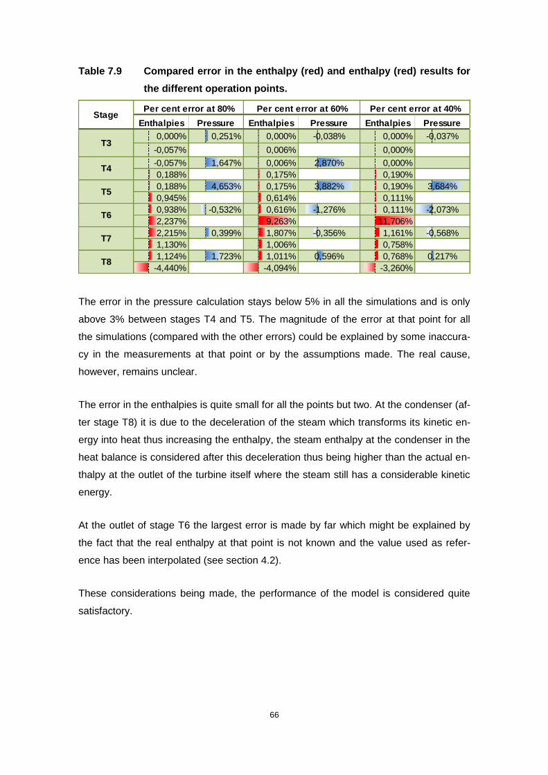
66
Table 7.9 Compared error in the enthalpy (red) and enthalpy (red) results for
the different operation points.
The error in the pressure calculation stays below 5% in all the simulations and is only
above 3% between stages T4 and T5. The magnitude of the error at that point for all
the simulations (compared with the other errors) could be explained by some inaccura-
cy in the measurements at that point or by the assumptions made. The real cause,
however, remains unclear.
The error in the enthalpies is quite small for all the points but two. At the condenser (af-
ter stage T8) it is due to the deceleration of the steam which transforms its kinetic en-
ergy into heat thus increasing the enthalpy, the steam enthalpy at the condenser in the
heat balance is considered after this deceleration thus being higher than the actual en-
thalpy at the outlet of the turbine itself where the steam still has a considerable kinetic
energy.
At the outlet of stage T6 the largest error is made by far which might be explained by
the fact that the real enthalpy at that point is not known and the value used as refer-
ence has been interpolated (see section 4.2).
These considerations being made, the performance of the model is considered quite
satisfactory.
Enthalpies Pressure Enthalpies Pressure Enthalpies Pressure
0,000% 0,251% 0,000% -0,038% 0,000% -0,037%
-0,057% 0,006% 0,000%
-0,057% 1,647% 0,006% 2,870% 0,000%
0,188% 0,175% 0,190%
0,188% 4,653% 0,175% 3,882% 0,190% 3,684%
0,945% 0,614% 0,111%
0,938% -0,532% 0,616% -1,276% 0,111% -2,073%
2,237% 9,263% 11,706%
2,215% 0,399% 1,807% -0,356% 1,161% -0,568%
1,130% 1,006% 0,758%
1,124% 1,723% 1,011% 0,596% 0,768% 0,217%
-4,440% -4,094% -3,260%
T6
StagePer cent error at 60% Per cent error at 40%
T3
T4
T5
Per cent error at 80%
T7
T8

67
7.3 Simulation of the whole LP-turbine with steam and water extractions
and conic geometry
The next step has been to adjust the geometry of the turbine pipe to a cone adjusting it
to the changing conditions of the steam along it. As explained in subsection 6.3.3 the
diameters at the inlet and at the outlet of the “turbine pipe” have been set in order to
avoid a critical flow at any point.
The reference power plant has a 6 flow LP-turbine, so that there are 6 LP-turbines.
This has also been reflected in the model, the dimensions of it being the corresponding
to only one of these 6 LP-turbines. The simulation has been set so that the steam mass
flow is divided between 6 identical turbines.
Figure 7.8 Image of the geometry used. The fill and the TDV can be seen at the
left and at the right end respectively.
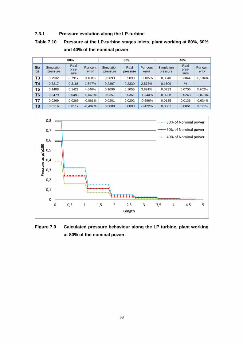
68
7.3.1 Pressure evolution along the LP-turbine
Table 7.10 Pressure at the LP-turbine stages inlets, plant working at 80%, 60%
and 40% of the nominal power
80% 60% 40%
Stage
Simulation pressure
Real pres-sure
Per cent error
Simulation pressure
Real pressure
Per cent error
Simulation pressure
Real pres-sure
Per cent error
T3 0,7932 0,7917 0,188% 0,5893 0,5899 -0,105% 0,3840 0,3844 -0,104%
T4 0,3217 0,3165 1,647% 0,2397 0,2330 2,873% 0,1609 %
T5 0,1488 0,1422 4,646% 0,1096 0,1055 3,891% 0,0733 0,0706 3,702%
T6 0,0479 0,0483 -0,669% 0,0357 0,0361 -1,340% 0,0238 0,0243 -2,073%
T7 0,0269 0,0269 -0,061% 0,0201 0,0202 -0,596% 0,0135 0,0136 -0,634%
T8 0,0116 0,0117 -0,402% 0,0088 0,0088 -0,422% 0,0061 0,0061 0,021%
Figure 7.9 Calculated pressure behaviour along the LP turbine, plant working
at 80% of the nominal power.
0
0,1
0,2
0,3
0,4
0,5
0,6
0,7
0,8
0 0,5 1 1,5 2 2,5 3 3,5 4 4,5 5
Pre
ssu
re a
s p
/p1
00
Length
80% of Nominal power
60% of Nominal power
40% of Nominal power
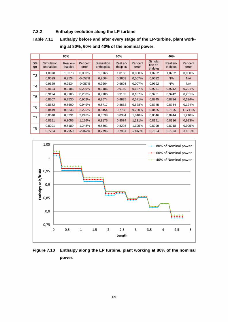
69
7.3.2 Enthalpy evolution along the LP-turbine
Table 7.11 Enthalpy before and after every stage of the LP-turbine, plant work-
ing at 80%, 60% and 40% of the nominal power.
80% 60% 40%
Stage
Simulation enthalpies
Real en-thalpies
Per cent error
Simulation enthalpies
Real en-thalpies
Per cent error
Simula-tion en-thalpies
Real en-thalpies
Per cent error
T3 1,0078 1,0078 0,000% 1,0166 1,0166 0,000% 1,0252 1,0252 0,000%
0,9529 0,9534 -0,057% 0,9604 0,9603 0,007% 0,9692 N/A N/A
T4 0,9529 0,9534 -0,057% 0,9604 0,9603 0,007% 0,9692 N/A N/A
0,9124 0,9105 0,200% 0,9186 0,9169 0,187% 0,9261 0,9242 0,201%
T5 0,9124 0,9105 0,200% 0,9186 0,9169 0,187% 0,9261 0,9242 0,201%
0,8607 0,8530 0,902% 0,8674 0,8625 0,571% 0,8745 0,8734 0,124%
T6 0,8682 0,8600 0,949% 0,8717 0,8662 0,628% 0,8745 0,8734 0,124%
0,8419 0,8236 2,225% 0,8454 0,7738 9,260% 0,8485 0,7595 11,711%
T7 0,8518 0,8331 2,246% 0,8539 0,8384 1,848% 0,8546 0,8444 1,210%
0,8151 0,8055 1,196% 0,8175 0,8084 1,131% 0,8191 0,8116 0,923%
T8 0,8291 0,8189 1,248% 0,8301 0,8203 1,195% 0,8299 0,8218 0,995%
0,7754 0,7950 -2,462% 0,7796 0,7961 -2,068% 0,7864 0,7993 -1,613%
Figure 7.10 Enthalpy along the LP turbine, plant working at 80% of the nominal
power.
0,75
0,8
0,85
0,9
0,95
1
1,05
0 0,5 1 1,5 2 2,5 3 3,5 4 4,5 5
Enth
alp
y as
h/h
10
0
Length
80% of Nominal power
60% of Nominal power
40% of Nominal power
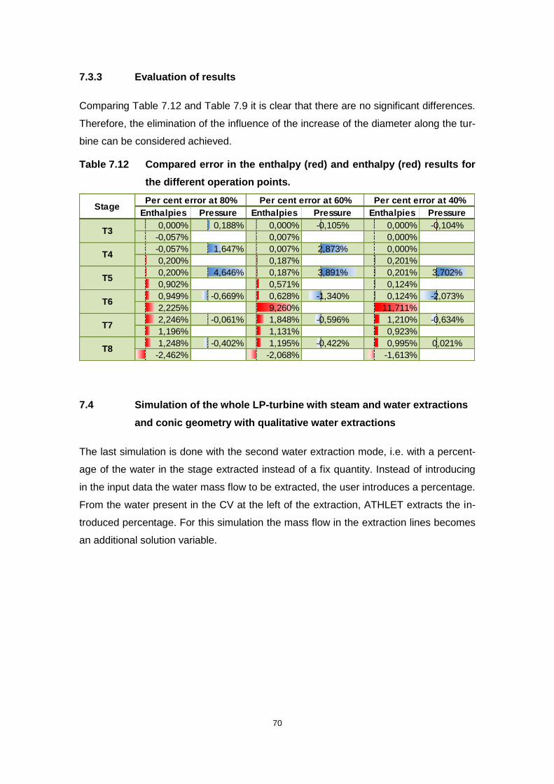
70
7.3.3 Evaluation of results
Comparing Table 7.12 and Table 7.9 it is clear that there are no significant differences.
Therefore, the elimination of the influence of the increase of the diameter along the tur-
bine can be considered achieved.
Table 7.12 Compared error in the enthalpy (red) and enthalpy (red) results for
the different operation points.
7.4 Simulation of the whole LP-turbine with steam and water extractions
and conic geometry with qualitative water extractions
The last simulation is done with the second water extraction mode, i.e. with a percent-
age of the water in the stage extracted instead of a fix quantity. Instead of introducing
in the input data the water mass flow to be extracted, the user introduces a percentage.
From the water present in the CV at the left of the extraction, ATHLET extracts the in-
troduced percentage. For this simulation the mass flow in the extraction lines becomes
an additional solution variable.
Enthalpies Pressure Enthalpies Pressure Enthalpies Pressure
0,000% 0,188% 0,000% -0,105% 0,000% -0,104%
-0,057% 0,007% 0,000%
-0,057% 1,647% 0,007% 2,873% 0,000%
0,200% 0,187% 0,201%
0,200% 4,646% 0,187% 3,891% 0,201% 3,702%
0,902% 0,571% 0,124%
0,949% -0,669% 0,628% -1,340% 0,124% -2,073%
2,225% 9,260% 11,711%
2,246% -0,061% 1,848% -0,596% 1,210% -0,634%
1,196% 1,131% 0,923%
1,248% -0,402% 1,195% -0,422% 0,995% 0,021%
-2,462% -2,068% -1,613%
Per cent error at 60% Per cent error at 40%
T8
StagePer cent error at 80%
T3
T4
T5
T6
T7
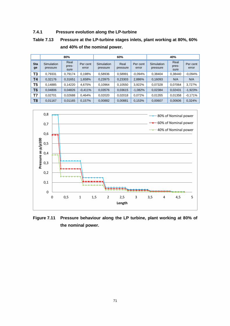
71
7.4.1 Pressure evolution along the LP-turbine
Table 7.13 Pressure at the LP-turbine stages inlets, plant working at 80%, 60%
and 40% of the nominal power.
80% 60% 40%
Stage
Simulation pressure
Real pres-sure
Per cent error
Simulation pressure
Real pressure
Per cent error
Simulation pressure
Real pres-sure
Per cent error
T3 0,79331 0,79174 0,198% 0,58936 0,58991 -0,094% 0,38404 0,38440 -0,094%
T4 0,32176 0,31651 1,658% 0,23975 0,23303 2,886% 0,16093 N/A N/A
T5 0,14885 0,14220 4,675% 0,10964 0,10550 3,922% 0,07328 0,07064 3,727%
T6 0,04806 0,04826 -0,411% 0,03576 0,03615 -1,082% 0,02384 0,02431 -1,923%
T7 0,02701 0,02688 0,464% 0,02020 0,02018 0,072% 0,01355 0,01358 -0,171%
T8 0,01167 0,01165 0,157% 0,00882 0,00881 0,153% 0,00607 0,00606 0,324%
Figure 7.11 Pressure behaviour along the LP turbine, plant working at 80% of
the nominal power.
0
0,1
0,2
0,3
0,4
0,5
0,6
0,7
0,8
0 0,5 1 1,5 2 2,5 3 3,5 4 4,5 5
Pre
ssu
re a
s p
/p1
00
Length
80% of Nominal power
60% of Nominal power
40% of Nominal power
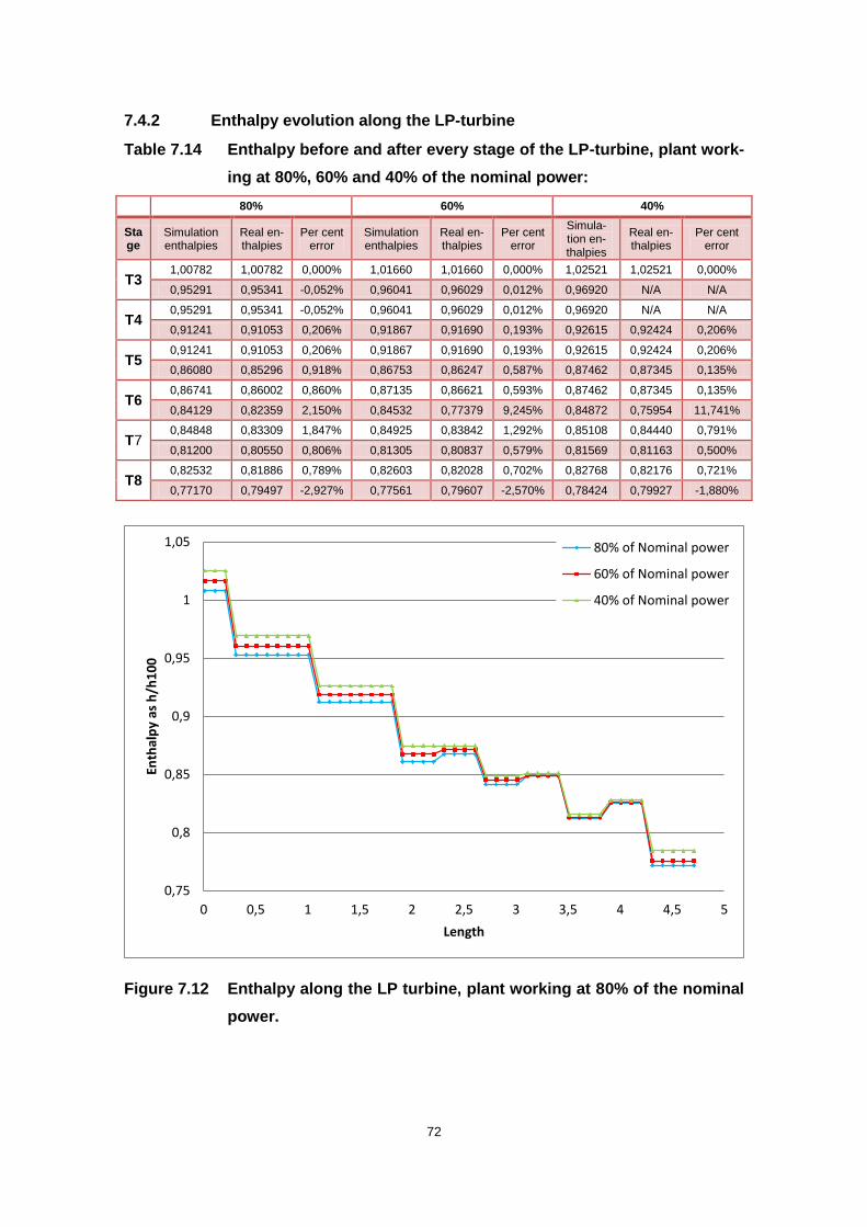
72
7.4.2 Enthalpy evolution along the LP-turbine
Table 7.14 Enthalpy before and after every stage of the LP-turbine, plant work-
ing at 80%, 60% and 40% of the nominal power:
80% 60% 40%
Stage
Simulation enthalpies
Real en-thalpies
Per cent error
Simulation enthalpies
Real en-thalpies
Per cent error
Simula-tion en-thalpies
Real en-thalpies
Per cent error
T3 1,00782 1,00782 0,000% 1,01660 1,01660 0,000% 1,02521 1,02521 0,000%
0,95291 0,95341 -0,052% 0,96041 0,96029 0,012% 0,96920 N/A N/A
T4 0,95291 0,95341 -0,052% 0,96041 0,96029 0,012% 0,96920 N/A N/A
0,91241 0,91053 0,206% 0,91867 0,91690 0,193% 0,92615 0,92424 0,206%
T5 0,91241 0,91053 0,206% 0,91867 0,91690 0,193% 0,92615 0,92424 0,206%
0,86080 0,85296 0,918% 0,86753 0,86247 0,587% 0,87462 0,87345 0,135%
T6 0,86741 0,86002 0,860% 0,87135 0,86621 0,593% 0,87462 0,87345 0,135%
0,84129 0,82359 2,150% 0,84532 0,77379 9,245% 0,84872 0,75954 11,741%
T7 0,84848 0,83309 1,847% 0,84925 0,83842 1,292% 0,85108 0,84440 0,791%
0,81200 0,80550 0,806% 0,81305 0,80837 0,579% 0,81569 0,81163 0,500%
T8 0,82532 0,81886 0,789% 0,82603 0,82028 0,702% 0,82768 0,82176 0,721%
0,77170 0,79497 -2,927% 0,77561 0,79607 -2,570% 0,78424 0,79927 -1,880%
Figure 7.12 Enthalpy along the LP turbine, plant working at 80% of the nominal
power.
0,75
0,8
0,85
0,9
0,95
1
1,05
0 0,5 1 1,5 2 2,5 3 3,5 4 4,5 5
Enth
alp
y as
h/h
10
0
Length
80% of Nominal power
60% of Nominal power
40% of Nominal power
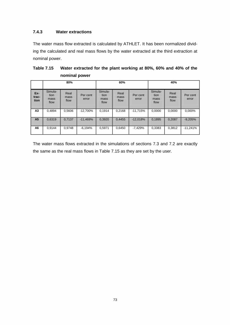
73
7.4.3 Water extractions
The water mass flow extracted is calculated by ATHLET. It has been normalized divid-
ing the calculated and real mass flows by the water extracted at the third extraction at
nominal power.
Table 7.15 Water extracted for the plant working at 80%, 60% and 40% of the
nominal power
80% 60% 40%
Ex-trac-tion
Simula-tion
mass flow
Real mass flow
Per cent error
Simula-tion
mass flow
Real mass flow
Per cent error
Simula-tion
mass flow
Real mass flow
Per cent error
A3 0,4894 0,5606 -12,700% 0,1914 0,2168 -11,715% 0,0000 0,0000 0,000%
A5 0,6319 0,7137 -11,469% 0,3920 0,4455 -12,018% 0,1895 0,2087 -9,205%
A6 0,9144 0,9748 -6,194% 0,5971 0,6450 -7,429% 0,3383 0,3812 -11,241%
The water mass flows extracted in the simulations of sections 7.3 and 7.2 are exactly
the same as the real mass flows in Table 7.15 as they are set by the user.
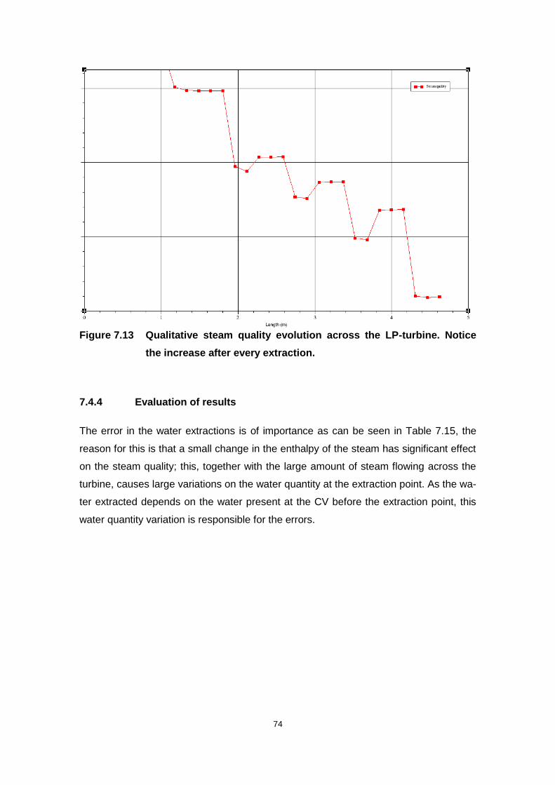
74
Figure 7.13 Qualitative steam quality evolution across the LP-turbine. Notice
the increase after every extraction.
7.4.4 Evaluation of results
The error in the water extractions is of importance as can be seen in Table 7.15, the
reason for this is that a small change in the enthalpy of the steam has significant effect
on the steam quality; this, together with the large amount of steam flowing across the
turbine, causes large variations on the water quantity at the extraction point. As the wa-
ter extracted depends on the water present at the CV before the extraction point, this
water quantity variation is responsible for the errors.

75
Table 7.16 Compared error in the enthalpy (red) and pressure (blue) results for
the different operation points
Table 7.17 Error in the water mass flow extracted in the third fourth and fifth
extraction of the LP-turbine (extractions A3, A5 and A6)
Despite the errors in the water mass flow extractions, there is no qualitative and little
quantitative difference from the errors committed in the pressures and the enthalpies in
the fixed extraction simulations (see Table 7.12), the main error being in the enthalpy
after stage T6.
Enthalpy Pressure Enthalpy Pressure Enthalpy Pressure
0,000% 0,198% 0,000% -0,094% 0,000% -0,094%
-0,052% 1,658% 0,012% 2,886% 0,000%
-0,052% 1,658% 0,012% 2,886% 0,000%
0,206% 4,675% 0,192% 3,922% 0,206% 3,727%
0,206% 4,675% 0,192% 3,922% 0,206% 3,727%
0,933% -0,411% 0,599% -1,082% 0,129% -1,923%
0,857% -0,411% 0,587% -1,082% 0,129% -1,923%
2,153% 0,464% 9,236% 0,072% 11,736% -1,923%
2,010% 0,464% 1,693% 0,072% 1,155% -0,171%
1,009% 0,157% 1,008% 0,153% 0,897% 0,324%
0,929% 0,157% 0,935% 0,153% 0,850% 0,324%
-2,790% 0,000% -2,333% 0,000% -1,748% 0,000%
Percent error at 60% Percent error at 40%
T8
StagePercent error at 80%
T3
T4
T5
T6
T7
Extraction Mass flow error at 80% Mass flow error at 60% Mass flow error at 40%
A3 -12,700% -11,715% 0,000%
A5 -11,469% -12,018% -9,205%
A6 -6,194% -7,429% -11,241%

76
8 Assessment
8.1 Geometry data
The two conic models developed have their geometrical data set in order to avoid a
critical flow of the steam and are not based on real data. The knowledge of the geome-
try and the size of the turbine are necessary for the transient calculation, as the speed
with which changes in the inlet steam conditions reflect on the conditions across the
turbine depends on the quantity of steam stored in the turbine at a given point, i.e. the
turbine internal volume.
The lack of geometry data and the unavailability of transient data made it impossible to
assess the adequacy of the model for transient calculations.
8.2 Application of the cone law
The representation of the pressure behaviour has been seen in chapter 7, the error al-
ways being below 5%. Considering the absolute deviations, the accuracy of the model
seems to improve as the largest deviation takes place between the second and the
third stages (T4 and T5) and it is below 0,075 bar which could be in the area of the
measurement tolerances (Grote, 2009). It can therefore be considered that the cone
law in the form it has been used in the present model (see equation (6.5)) as well as
the model as a whole depict the steady state pressure behaviour through the turbine
with great accuracy.
8.3 Enthalpy calculation
The representation of the enthalpy behavior presents the main problems and errors.
Despite the simplified model used for its calculation (see equation (6.18)), the problems
seem to arise due to an incomplete knowledge of some relevant data (see Chapter 4)
and due to some of the assumptions made. However, should accurate data be availa-
77
ble, it is to be expected that the model would depict the enthalpies steady state behav-
ior with an even more satisfactory accuracy.
8.4 Models to be developed
A model for the extractions still needs to be developed. Some empirical formula should
be able to describe the amount of fluid extracted and the improvement of the steam
quality in the turbine resulting from this extraction. The modifications made in the water
extractions (via the fill junction, see Figure 6.8) allow the implementation of this rela-
tionship once it is developed.
In the present simulation, given the lack of reliable data (see subchapter 6.3.1.1), a
constant efficiency has been used and the variation of this efficiency depending on the
power output of the turbine has been neglected. The real internal enthalpy drop at eve-
ry stage at nominal power is not known, and therefore, given the available data, it has
not been possible to adjust the internal efficiency of every stage according to equation
(3.7).
Should the extraction model be developed and the nominal stage efficiencies be
known, it would be possible to introduce in the subroutine ktutr.f (see Figure 6.4) a cal-
culation for the real internal efficiency of a given stage after equation (3.7).
In order to display the total power extracted from the fluid or, accordingly, the total
power output of the turbine, a variable has to be developed which adds the energy ex-
tracted from the fluid at every stage (equation (6.18)) and makes it possible to directly
see the power output of the turbine (see equation (8.1) ).
∑ (8.1)
8.5 Extension
Although not part of the turbine itself, some models need to be developed in order to
successfully couple the turbine model with a plant simulation.
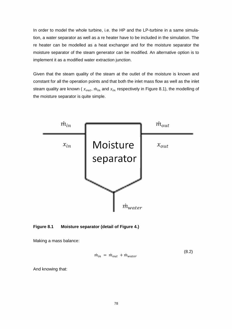
78
In order to model the whole turbine, i.e. the HP and the LP-turbine in a same simula-
tion, a water separator as well as a re heater have to be included in the simulation. The
re heater can be modelled as a heat exchanger and for the moisture separator the
moisture separator of the steam generator can be modified. An alternative option is to
implement it as a modified water extraction junction.
Given that the steam quality of the steam at the outlet of the moisture is known and
constant for all the operation points and that both the inlet mass flow as well as the inlet
steam quality are known ( , and respectively in Figure 8.1), the modelling of
the moisture separator is quite simple.
Figure 8.1 Moisture separator (detail of Figure 4.)
Making a mass balance:
(8.2)
And knowing that:
79
(8.3)
The water mass flow to be extracted is:
(
)
(8.4)
All the variables on the right side of equation (8.5) are known. So that the moisture
separator can be easily modelled using the modified fill junctions used for the water ex-
tractions in the turbine (see subsection 6.3.2)
For the transient calculations that involve a variation of the angular speed of the tur-
bine, such as load rejection and rump up, a momentum balance determines the varia-
tion of angular speed.
The power in a rotational system, i.e. a turbine is defined by the product of the torque
M and the angular velocity ω.
(8.5)
The momentum balance equation of the whole system equation (8.6) results from a
breaking torque, the moment of inertia Θ of the whole rotating machine and the torque
provided by the turbine.
(8.6)
(
)
(8.7)
Equation (8.7) describes the angular velocity variation. The breaking torque term Mbr
includes all the components of the equation different from the turbine torque and have
to be modelled.
80
9 Summary and Outlook
The object of this paper was to develop and to implement a turbine model in ATHLET.
Although some aspects of the turbine have not been considered yet, the basic equa-
tions and the general layout of the model have been successfully implemented.
The thermo-hydraulic model developed needs only the thermodynamic properties of
the steam at some points of the plant (basically extractions, turbine inlet as well as tur-
bine outlet) operating at nominal power. The performed steady-state simulations pre-
dict the behaviour of the steam pressure as well as the enthalpy with very good preci-
sion, the error being below 5% at all the simulations. The fact that almost all the neces-
sary input data is to be found at the plant heat and mass balances easies the use of
the model as it is data to which the potential user is expected to have access.
So far steady state calculations for a KONVOI LP-turbine have been successfully car-
ried out. In principle the model should describe the transient conditions with the similar
accuracy as it describes the steady state conditions. However, the fact that the water
extraction model needs to be improved is expected to diminish the accuracy of the re-
sults. In order to perform such calculations, variables such as the geometry of the tur-
bine (internal volume), the real isentropic efficiency of every stage, the moment of iner-
tia of the turbine-generator complex as well as the nominal pressure at the HP-turbine
inlet are necessary.
In order to couple the turbine model with the secondary loop, the models for the water
extractions still need to be improved. The final result however is more than satisfactory
as the main aspects of the turbine modelling have been successfully addressed thus
laying the basis for the implementation of the whole turbine once the necessary refer-
ence and validation data is available.
The Steam turbine being one of the most complex components of the secondary loop,
the simulation capabilities of ATHLET regarding the secondary loop have been signifi-
cantly extended by the provision of a turbine model.
81
10 Bibliography
Ainsworth, A. (2007, August 21). English Wikipedia. Retrieved May 21, 2010, from
http://en.wikipedia.org/wiki/File:Rankine_cycle_Ts.png.
E.ON. (n.d.). http://www.eon.com/en/businessareas/35214.jsp. Retrieved July 2, 2011
Grote, W. (2009). Ein Beitrag zur modellbasierten Regelung von
Entahmedampfturbinen. Ruhr-Universitäat Bochum.
GRS. (2009). AHTLET Code Manuals Mod 2.2 Cycle A. Gesellschaft für Anlagen- und
Reaktorsicherheit mbH.
Kleinedler, M. (2002). Heft 28 Aufbau von Kernkraftwerken (DWR). KWS - Fachhefte
für den Kraftwerksbetrieb, zweite Auflage. Verlag technisch-wissenschaftlicher
Schriften.
Lehrstuhl für Energiesysteme . (2010, Oktober 20). Skript der Vorlesung
Dampfturbinen.
Plavšić, D. (2008). Methodolical Investigation into Turbine Modelling for LWR System
Codes. ISaR GmbH.
Ray, A. (1980, April). Dynamic modelling of power plant turbines for controller design.
Applied Mathematical Modelling, Vol. 4, pp. 109-112.
Siemens AG Bereich Energieerzeugung. (n.d.). Kundenschulung.
Stodola, A. (1922). Dampf- und Gasturbinen, 5. Auflage. Berlin: Springer.
Strauß, K. (2006). Kraftwerkstechnik: zur Nutzung fossiler, nuklearer und regenerativer
Energiequellen, 5. Auflage. Berlin: Springer-Verlag.
Traupel, W. (2001). Thermische Turbomaschinen, 4. Auflage. Berlin/Heidelberg/New
York: Springer-Verlag.

82
Zimmer, G. (2008, Dezember). Modelling and simulation of steam turbine processes:
individual models for individual tasks. Mathematical and Computer Modelling of
Dynamical Systems, Vol. 14, No. 6, pp. 469-493.