
Matthias Pertl, BSc - diglib.tugraz.at
100
Matthias Pertl, BSc Evaluation of hydraulic boundary conditions in Plaxis 2D to achieve the university degree of MASTER'S THESIS Master's degree programme: Civil Engineering Sciences, Geotechnics and Hydraulics submitted to Graz University of Technology Ao.Univ.-Prof. Dipl.-Ing. Dr.techn. M.Sc. tit.Univ.-Prof. Helmut Schweiger Institute of Soil Mechanics and Foundation Engineering Computational Geotechnics Group Diplom-Ingenieur Supervisor Dipl.-Ing. BSc, Patrick Pichler Graz, September 2017
Transcript of Matthias Pertl, BSc - diglib.tugraz.at

Matthias Pertl, BSc
Evaluation of hydraulic boundary conditions in Plaxis 2D
to achieve the university degree of
MASTER'S THESIS
Master's degree programme: Civil Engineering Sciences, Geotechnics and Hydraulics
submitted to
Graz University of Technology
Ao.Univ.-Prof. Dipl.-Ing. Dr.techn. M.Sc. tit.Univ.-Prof. Helmut Schweiger
Institute of Soil Mechanics and Foundation Engineering Computational Geotechnics Group
Diplom-Ingenieur
Supervisor
Dipl.-Ing. BSc, Patrick Pichler
Graz, September 2017

05.09.2017
05.09.2017
Eidesstattliche Erklärung
Ich erkläre an Eides statt, dass ich die vorliegende Arbeit selbstständig verfasst, andere
als die angegebenen Quellen/Hilfsmittel nicht benutzt, und die den benutzten Quellen
wörtlich und inhaltlich entnommenen Stellen als solche kenntlich gemacht habe. Das in
TUGRAZonline hochgeladene Textdokument ist mit der vorliegenden Diplomarbeit
identisch.
Graz, am ……………………… ………………………………………………….
(Unterschrift)
Statutory declaration
I declare that I have authored this thesis independently, that I have not used other than
the declared sources / resources, and that I have explicitly marked all material which has
been quoted either literally or by content from the used sources. The uploaded document
is identic with the present Master’s thesis.
Graz, ………………………… ………………………………………………….
(signature)

Danksagung
An erster Stelle möchte ich mich bei meinen Betreuern Herrn Professor Helmut
Schweiger, sowie Dipl.-Ing. Patrick Pichler bedanken. Ich bin ihnen für die intensive
Zusammenarbeit und die fachliche Expertise in der numerischen Disziplin der
Bodenmechanik dankbar. Der Technischen Universität Graz bin ich ebenfalls zu großen
Dank verpflichtet. Diese Institution hat es mir ermöglicht, meine Berufswünsche zu
verwirklichen und vor allem hat sie mir einen freien Zugang zu einer fundierten Bildung
gewährt, welcher ohne tiefgreifende finanzielle Aufwände möglich war.
Ein besonderer Dank gilt meinen Studienkollegen Andreas, Christopher, Daniel, Moritz,
Paul und Rita. Mit ihnen habe ich schöne und prägende Momente während dem Studium
und abseits erlebt. Meinen Arbeitszimmerkollegen Carla, Christine, David, Magdalena,
Laurin und Simon, möchte ich Danke sagen, dass sie während des Schreibens dieser
Arbeit, den Alltag mit interessanten Diskussionen und lustigen Augenblicken ausfüllten.
Auch ein herzliches Dankeschön an Hannes und seinem Team.
Auch Danke sagen möchte ich meinen Freunden Alex, Chris, Lenz, ManU, Mario und
Steve zuhause in der Heimat. Sie waren stets meine treuen Weggefährten und haben
mich immer durch ihre eigene professionelle Initiative angespornt. All meinen Freunden
und Kollegen, die ich während der Zeit meines Studiums kennenlernte, danke ich für die
gemeinsamen Abenteuer und unvergesslichen Zeit.
Zu guter Letzt gilt ein außerordentlicher Dank meiner Familie! Meine Eltern Maria und
Josef standen mir immer in allem Belangen zur Seite Sie haben mir vieles ermöglicht
und haben mich stets dabei unterstützt. Ich bin meinen Eltern besonders dankbar für die
schönen Wochenenden zuhause und meiner Mama für die gute Küche, die immer ein
Lichtblick am Horizont im studentischen Leben war. Meinen Brüdern Markus, Gregor
und Christoph mit Familie gebührt auch ein großes Dankeschön, weil sie ein starker
Impuls waren großartiges zu erreichen.


Abstract
In the present master’s thesis, the available hydraulic boundary conditions in Plaxis 2D
have been evaluated. Thereby the application and effects of the conditions for the
boundary value problems in accordance to the associated calculations have been
investigated. Particularly, the numerical analysis of unsaturated and undrained material
have been discussed. Hereof, the numerical method of unsaturated soil properties by
means of the soil water characteristic curve is prescribed. The latter method and other
numerical features have been elaborated on different geotechnical problems.
Keywords: Finite Element Method, hydraulic boundary conditions, undrained soil
behaviour, unsaturated soil behaviour, precipitation, deep excavation


Kurzfassung
In der vorliegenden Diplomarbeit wurden die vorhanden hydraulischen
Randbedingungen in Plaxis 2D evaluiert. Dabei wurde die Anwendung und ihre
Auswirkungen in Übereinstimmung mit den entsprechen Berechnungsmethoden eruiert.
Besonders die numerische Analyse von undrainierten und teilgesättigten Böden wurde
eingehendes untersucht. Diesbezüglich wird die numerische Methode von teilgesättigten
Bodeneigenschaften in Hinsicht auf die Wasserretentionskurve genauer beschrieben.
Diese und andere Methoden wurden letztendlich anhand von verschiedenen
geotechnischen Problemstellungen ausgearbeitet.
Schlüsselwörter: Finite Elemente Methode, hydraulische Randwertbedingungen,
undrainierte Böden, teilgesättigte Böden, Niederschlag, tiefe Baugruben


Table of contents
1 Introduction ........................................................................................................... 1
2 Hydraulic boundary conditions in Plaxis 2D ........................................................... 2
2.1 Soil mode ....................................................................................................... 3
2.1.1 Create borehole – tabsheet water ........................................................... 4
2.1.2 Show materials – tabsheet Material sets ................................................. 5
2.1.3 Tabsheet General – drainage types ........................................................ 6
2.1.4 Tabsheet Groundwater – hydraulic parameters ....................................... 6
2.2 Hydraulic boundary conditions ....................................................................... 8
2.2.1 Hydraulic model boundary conditions – Model explorer ........................... 8
2.2.2 Selective hydraulic boundary conditions – Selection explorer................ 12
3 Soil water characteristic curve ............................................................................. 17
3.1 Approximation of laboratory data .................................................................. 18
3.2 Implementation in Plaxis 2D ......................................................................... 20
4 Types of analyses and output .............................................................................. 23
4.1 Calculation types .......................................................................................... 23
4.2 Pore pressure calculation type ..................................................................... 25
4.3 Stress and pore pressure output .................................................................. 25
5 Application of hydraulic boundary conditions ....................................................... 30
5.1 Precipitation ................................................................................................. 30
5.1.1 Aim of geotechnical model .................................................................... 30
5.1.2 Model configuration and material parameters ........................................ 31
5.1.3 Output ................................................................................................... 35
5.1.4 Summary and concluding remarks ........................................................ 39
5.2 Bearing capacity ........................................................................................... 40
5.2.1 Aim of geotechnical model .................................................................... 40
5.2.2 Model configuration and material parameters ........................................ 40
5.2.3 Output ................................................................................................... 43
5.2.4 Summary and concluding remarks ........................................................ 47
5.3 Deep excavation ...........................................................................................48
5.3.1 Aim of geotechnical model .....................................................................48
5.3.2 Model configuration and material parameters .........................................48
5.3.3 Output ....................................................................................................56
5.3.4 Summary and concluding remarks .........................................................64
6 Summary and conclusion .....................................................................................65
7 Literature ..............................................................................................................67
Appendix ....................................................................................................................... I

List of figures
Figure 1: Plaxis 2D Version 2016.01 – GUI .................................................................. 3
Figure 2: Plaxis 2D – Modes ........................................................................................ 3
Figure 3: Plaxis 2D – Command Create Borehole: tabsheet Water .............................. 4
Figure 4: Plaxis 2D – Tabsheet Water: corresponding results ...................................... 4
Figure 5: Plaxis 2D – Material data set ......................................................................... 5
Figure 6: Plaxis 2D – Tabsheet Groundwater ............................................................... 6
Figure 7: SWCC: Standard (Hypres, Topsoils) ............................................................. 7
Figure 8: Plaxis 2D – Model explorer ............................................................................ 8
Figure 9: Plaxis 2D – Flow functions............................................................................. 9
Figure 10: GroundwaterFlow: Closed versus Open .................................................... 10
Figure 11: Comparison: Precipitation and Infiltration .................................................. 11
Figure 12: Plaxis 2D – Selection explorer ................................................................... 12
Figure 13: GWFlowBaseBC: Infiltration ...................................................................... 13
Figure 14: Active model boundary (TM Plaxis 2D, 2016) ............................................ 14
Figure 15: WaterConditions: Head: 23.0m (TM Plaxis 2D, 2016) ................................ 15
Figure 16: WaterConditions: Head – Result psteady (TM Plaxis 2D, 2016) .................... 15
Figure 17: WaterConditions: Dry (TM Plaxis 2D, 2016) .............................................. 16
Figure 18: WaterConditions: Dry – Result psteady (TM Plaxis 2D, 2016) ....................... 16
Figure 19: SWCC – Zones and Values ....................................................................... 17
Figure 20: SWCC – Equations .................................................................................... 18
Figure 21: SWCC – Adsorption and desorption .......................................................... 19
Figure 22: SWCC – Variable variation ........................................................................ 20
Figure 23: Matric suction coefficient and saturation trend ........................................... 21
Figure 24: Soil classification: (a) USDA and (b) Hypres .............................................. 22
Figure 25: Precipitation: Model ................................................................................... 30
Figure 26: Precipitation: Model dimension .................................................................. 31
Figure 27: Precipitation: Model (a) UserWaterLevel and (b) GWFlowBaseBC ............ 32
Figure 28: Precipitation: Fixities in model (a) and (b) .................................................. 33
Figure 29: Precipitation: Active pore pressure in model (a) and (b) ............................ 33
Figure 30: Precipitation: Recharge ............................................................................. 34
Figure 31: Precipitation: DischargeFunction ............................................................... 34
Figure 32: Result precipitation: Section – (a) UserWaterLevel .................................... 35
Figure 33: Result precipitation: Section – (b) GWFlowBaseBC ................................... 36
Figure 34: Result precipitation: Depth points – (a) UserWaterLevel ............................ 37
Figure 35: Result precipitation: (a) UserWaterLevel and (b) GWFlowBaseBC ............ 38

Figure 36: Result precipitation: Section suction – UserWaterLevel ..............................38
Figure 37: Bearing capacity: Model dimension ............................................................40
Figure 38: Bearing capacity: SWCC O5 and O12 ........................................................41
Figure 39: Bearing capacity: Connectivity plot .............................................................42
Figure 40: Bearing capacity: Composition of pore pressure (CPP) ..............................43
Figure 41: Results bearing capacity: CPP CASE 2 – before loading ...........................44
Figure 42: Results bearing capacity: CPP CASE 4 – before loading ...........................44
Figure 43: Results bearing capacity: CPP CASE 2 – after loading ..............................45
Figure 44: Results bearing capacity: CPP CASE 4 – after loading; Part 1 ...................46
Figure 45: Results bearing capacity: CPP CASE 4 – after loading; Part 2 ...................46
Figure 46: Deep excavation: Model .............................................................................48
Figure 47: Deep excavation: Connectivity plot .............................................................51
Figure 48: Deep excavation: Plastic – calculation phases ...........................................52
Figure 49: Deep excavation: Hydraulic boundary conditions for FCFD ........................53
Figure 50: Deep excavation: FCFD – calculation phases ............................................54
Figure 51: Deep excavation: Bore pile wall 26.0 m ......................................................56
Figure 52: Results deep excavation: Excess pore pressure comparison .....................57
Figure 53: Results deep excavation: Pore water pressure comparison........................57
Figure 54: Results deep excavation: Section – Pore water pressure ...........................58
Figure 55: Results deep excavation: Section – Displacements in excavation pit .........59
Figure 56: Results deep excavation: Section – Displacements of adjacent surface .....59
Figure 57: Results deep excavation: Section – Structural force ...................................60
Figure 58: Results deep excavation: Section – Wall deflection ....................................61
Figure 59: Results deep excavation: Sections – Embedded length .............................62
Figure 60: Results deep excavation: Incremental deviatoric strains – CASE 5 ............63
Figure 61: Results deep excavation: FOS – CASE 5 and CASE 12 ............................64

List of tables
Table 1: Hydraulic boundary conditions in Plaxis 2D – Overview .................................. 2
Table 2: Hypres series with van Genuchten parameters (RM Plaxis 2D, 2016) .......... 22
Table 3: Calculation and pore pressure calculation type ............................................. 24
Table 4: Drainage types – Overview ........................................................................... 27
Table 5: Bulk modulus of water – Overview ................................................................ 28
Table 6: Specification of saturation ............................................................................. 29
Table 7: Precipitation: Soil parameters ....................................................................... 31
Table 8: Precipitation: SWCC parameters .................................................................. 32
Table 9: Bearing capacity: Soil parameters ................................................................ 41
Table 10: Bearing capacity: SWCC parameters.......................................................... 41
Table 11: Bearing capacity: Calculation cases ........................................................... 43
Table 12: Results bearing capacity: CPP CASE 2 – pore pressures........................... 45
Table 13: Results bearing capacity: CPP CASE 4 – pore pressures........................... 46
Table 14: Results bearing capacity: Failure loads....................................................... 47
Table 15: Deep excavation: Soil parameter ................................................................ 50
Table 16: Deep excavation: Strut parameter .............................................................. 51
Table 17: Deep excavation: Calculation types ............................................................ 52
Table 18: Deep excavation: Construction time schedule ............................................ 54
Table 19: Deep excavation: Calculations .................................................................... 56
Table 20: Deep excavation: Calculation cases ........................................................... 62


List of symbols and abbreviations
Capital letters
A [m²] Cross section area
B [-] Strain interpolation matrix
C [-] Coupling matrix for degree of saturation
D [m] Drainage path
E [N/m2] Young’s modulus
E‘ [N/m2] Effective Young’s modulus
𝐸50 [N/m2] Secant stiffness in standard drained triaxial test
𝐸50𝑟𝑒𝑓
[N/m2] Reference value of secant stiffness in standard drained triaxial test
𝐸𝑜𝑒𝑑 [N/m2] Tangent stiffness for primary oedometer loading
𝐸𝑜𝑒𝑑𝑟𝑒𝑓
[N/m2] Reference value of tangent stiffness for primary oedometer loading
𝐸𝑈𝑅 [N/m2] Unloading/ Reloading stiffness
𝐸𝑈𝑅𝑟𝑒𝑓
[N/m2] Reference value of Unloading/ Reloading stiffness
G [m/s²] Gravity vector
G [N/m2] Shear modulus
𝐺0 [N/m2] Shear modulus at very small strain
𝐺0𝑟𝑒𝑓
[N/m2] Reference value of shear modulus at very small strain
𝐺𝑈𝑅𝑟𝑒𝑓
[N/m2] Reference value of shear modulus at Unloading/ Reloading
H [m/s] Permeability matrix
I [m4] Moment of inertia
𝐾0 [-] Coefficient of lateral earth pressure (initial stress state)
𝐾0𝑛𝑐 [-] Coefficient of lateral earth pressure for a normally consolidated stress
𝐾𝑤 [N/m²] Bulk modulus of water
L [-] Differential operator
M [Nm] Bending moment
M [N/m²] Material stiffness matrix
N [N] Normal force
N [-] Matrix with shape function
OCR [-] Over consolidation ratio
POP [N/m²] Pre-overburden pressure
Q [N] Shear force
Q [N/m²] Coupling matrix for stress components
𝑅𝑖𝑛𝑡𝑒𝑟 [-] Strength reduction factor for interfaces
𝑅𝑓 [-] Failure ratio
S [N/m²] Compressibility matrix
𝑆 [-] Degree of saturation
𝑆𝑒𝑓𝑓 [-] Effective or normalized degree of saturation
𝑆𝑟𝑒𝑠 [-] Residual degree of saturation
𝑆𝑠𝑎𝑡 [-] Fully saturated degree of saturation
𝑇𝑣 [-] Dimensionless time factor according 1D-consolidation theory
V [m³] Volume
Small letters
c [N/m²] Cohesion
𝑐𝑣 [1/s] Consolidation coefficient according 1D-consolidation theory
d [m] Thickness
e [-] Void ratio
f [-] Yield function
𝑓𝑢 [N/m] Vector of loads
g [-] Plastic potential function
g [m/s2] Gravitational acceleration
𝑔𝑎 [1/m] Fitting parameter for van Genuchten-Mualem SWCC-approximation in
in Plaxis 2D
𝑔𝑐 [-] Fitting parameter for van Genuchten-Mualem SWCC-approximation in
in Plaxis 2D
𝑔𝑛 [-] Fitting parameter for van Genuchten-Mualem SWCC-approximation in
in Plaxis 2D
ℎ𝑟𝑒𝑓 [m] Reference head value
ℎ𝑖𝑛𝑐 [m/m] Increment value of head
𝑘𝑖 [m/s] Coefficient of permeability
𝑘𝑓 [m/s] Hydraulic conductivity
m [kg] Mass
m [-] Vector containing unity terms for normal and shear stress components
𝑚𝐺 [-] Fitting parameter for van Genuchten approximation
n [-] Coefficient of porosity
𝑛𝐺 [-] Fitting parameter for van Genuchten approximation
t [s] Time
p [N/m²] Isotropic or mean stress
𝑝𝑤 [N/m²] Pore water pressure
𝑝𝑎𝑐𝑡𝑖𝑣𝑒 [N/m²] Active pore pressure in Plaxis 2D
𝑝𝑒𝑥𝑐𝑒𝑠𝑠 [N/m²] Excess pore pressure in Plaxis 2D
𝑝𝑟𝑒𝑓 [N/m²] Reference stress for stiffness (default value 100 kN/m²)
𝑝𝑠𝑡𝑒𝑎𝑑𝑦 [N/m²] Steady state pore pressure in Plaxis 2D
𝑝𝑤𝑎𝑡𝑒𝑟 [N/m²] Pore water pressure in Plaxis 2D
q [N/m²] Equivalent shear stress or deviatoric stress
q [m³/s] Flux matrix
u [N/m²] Pore water pressure according to Terzaghi’s stress theory
u [m] Displacements
v [m] Vector with displacements component
w [-] Gravimetric water content
𝑥𝑟𝑒𝑓 [m] Reference value in x-direction
𝑦𝑟𝑒𝑓 [m] Reference value in y-direction
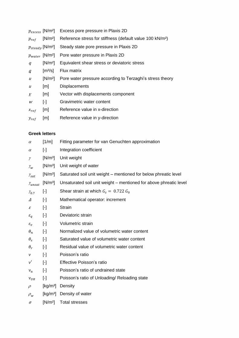
Greek letters
[1/m] Fitting parameter for van Genuchten approximation
[-] Integration coefficient
[N/m³] Unit weight
𝑤
[N/m³] Unit weight of water
𝑠𝑎𝑡
[N/m³] Saturated soil unit weight – mentioned for below phreatic level
𝑢𝑛𝑠𝑎𝑡
[N/m³] Unsaturated soil unit weight – mentioned for above phreatic level
0.7
[-] Shear strain at which 𝐺𝑠 = 0.722 𝐺0
Δ [-] Mathematical operator: increment
ε [-] Strain
𝜀𝑞 [-] Deviatoric strain
𝜀𝑣 [-] Volumetric strain
𝜃𝑛 [-] Normalized value of volumetric water content
𝜃𝑠 [-] Saturated value of volumetric water content
𝜃𝑟 [-] Residual value of volumetric water content
𝜈 [-] Poisson’s ratio
𝜈′ [-] Effective Poisson’s ratio
𝜈𝑢 [-] Poisson’s ratio of undrained state
𝜈𝑈𝑅 [-] Poisson’s ratio of Unloading/ Reloading state
[kg/m³] Density
𝑤 [kg/m³] Density of water
σ [N/m²] Total stresses
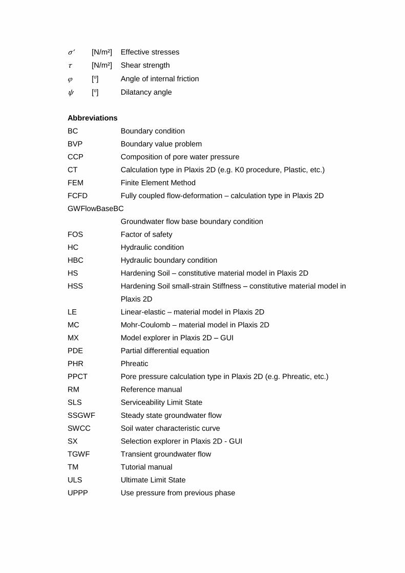
σ‘ [N/m²] Effective stresses
τ [N/m²] Shear strength
[o] Angle of internal friction
ψ [o] Dilatancy angle
Abbreviations
BC Boundary condition
BVP Boundary value problem
CCP Composition of pore water pressure
CT Calculation type in Plaxis 2D (e.g. K0 procedure, Plastic, etc.)
FEM Finite Element Method
FCFD Fully coupled flow-deformation – calculation type in Plaxis 2D
GWFlowBaseBC
Groundwater flow base boundary condition
FOS Factor of safety
HC Hydraulic condition
HBC Hydraulic boundary condition
HS Hardening Soil – constitutive material model in Plaxis 2D
HSS Hardening Soil small-strain Stiffness – constitutive material model in
Plaxis 2D
LE Linear-elastic – material model in Plaxis 2D
MC Mohr-Coulomb – material model in Plaxis 2D
MX Model explorer in Plaxis 2D – GUI
PDE Partial differential equation
PHR Phreatic
PPCT Pore pressure calculation type in Plaxis 2D (e.g. Phreatic, etc.)
RM Reference manual
SLS Serviceability Limit State
SSGWF Steady state groundwater flow
SWCC Soil water characteristic curve
SX Selection explorer in Plaxis 2D - GUI
TGWF Transient groundwater flow
TM Tutorial manual
ULS Ultimate Limit State
UPPP Use pressure from previous phase


1 Introduction
Computational Geotechnics Group 1
1 Introduction
This master’s thesis discusses the specific topic about numerical features with respect
to hydraulic boundary conditions, unsaturated soil behaviour, pore pressure
determination, drainage types, which are available in the finite element code of Plaxis
2D v.2016 (Plaxis 2D Manual, 2016). Hereof, the definition of hydraulic boundary
conditions should be investigated and evaluated. Furthermore the hydraulic properties
for unsaturated soil behaviour should be discussed.
In the second chapter all available hydraulic boundary conditions in Plaxis 2D,
particularly their applications and featured modifications in accordance of the associated
calculations are described. The third chapter discusses the hydraulic properties of
unsaturated soils. The hydraulic conductivity is determined by means of the soil water
characteristic curve, which is implemented in Plaxis 2D. In chapter four the different
types of analysis are described. In chapter five are finally assessed some of the
aforementioned definitions and specifications by means of three different geotechnical
models. The first model discusses the modelling of precipitation with respect to a partial
saturated soil. The next model computes the bearing capacity concerning undrained and
unsaturated soil behaviour. In the final model the analysis conditioning the ultimate state
in accordance to undrained soil behaviour is computed. The chapter six concludes a
summary of the shortcomings with respect to the assessed hydraulic boundary
conditions. In the Appendix are given the conducted simplified models of various
hydraulic boundary conditions.

2 Hydraulic boundary conditions in Plaxis 2D
2 Computational Geotechnics Group
2 Hydraulic boundary conditions in Plaxis 2D
The specification of initial and hydraulic boundary conditions (HBC) is an essential part
of discretising and modelling a geotechnical problem with any form of water impact, e.g.
phreatic level within the soil strata, precipitation onto the soil surface and seepage
through a dam embankment. Hence by using a FEM software, e.g. the commercial
available software Plaxis 2D Version 2016.01, the hydraulic conditions have to be
considered carefully and appropriately chosen (Table 1). The computation of pore
pressures involves the specified BVP conditions.
Table 1: Hydraulic boundary conditions in Plaxis 2D – Overview
Head - BoreholeWaterLevel
Water
Drainage types
Groundwater
Flow functions
Water levels
GroundwaterFlow
Extremes Open
Extremes Closed
Precipitation
Recharge
Water
GlobalWaterLevel
Seepage
Closed
Head
Inflow
Outflow
Infiltration
WaterConditions
Global level
Costum level
Head
User-defined
Interpolate
Dry
Unsaturated
GWFlowBaseBC
Attributes libary
Create borehole
SOIL MODE
MODEL EXPLORER
SELECTION EXPLORER
Show materials - Material sets

2 Hydraulic boundary conditions in Plaxis 2D
Computational Geotechnics Group 3
2.1 Soil mode
When starting the software Plaxis 2D, after the setup of the project properties, the Soil
mode (Figure 1) is the first graphical user interface (GUI), wherein the specification of
soil stratigraphy by means of the command Create borehole is available. Furthermore
the command Show materials obtains the Material set. Next to the Soil mode, the modes
Structure, Mesh, Flow conditions and Staged construction are listed (Figure 2).
Figure 1: Plaxis 2D Version 2016.01 – GUI
Figure 2: Plaxis 2D – Modes
2 Hydraulic boundary conditions in Plaxis 2D
4 Computational Geotechnics Group
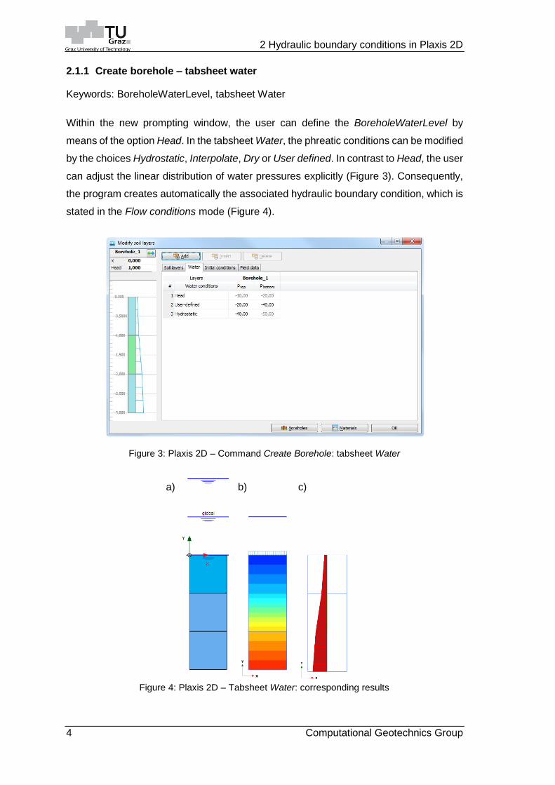
2.1.1 Create borehole – tabsheet water
Keywords: BoreholeWaterLevel, tabsheet Water
Within the new prompting window, the user can define the BoreholeWaterLevel by
means of the option Head. In the tabsheet Water, the phreatic conditions can be modified
by the choices Hydrostatic, Interpolate, Dry or User defined. In contrast to Head, the user
can adjust the linear distribution of water pressures explicitly (Figure 3). Consequently,
the program creates automatically the associated hydraulic boundary condition, which is
stated in the Flow conditions mode (Figure 4).
Figure 3: Plaxis 2D – Command Create Borehole: tabsheet Water
Figure 4: Plaxis 2D – Tabsheet Water: corresponding results
a) b) c)
2 Hydraulic boundary conditions in Plaxis 2D
Computational Geotechnics Group 5
In Figure 4 (a), the associated specification of HBC in the Flow conditions mode is shown.
Note that the specified water levels are BoreholeWaterLevel’s. The figures (b) and (c)
are the result of an initial calculation phase with the corresponding pore pressure
calculation type (PPCT), e.g. Initial Phase – PPCT Phreatic. This results can be
computed by means of the command Preview phase in the Flow conditions mode.
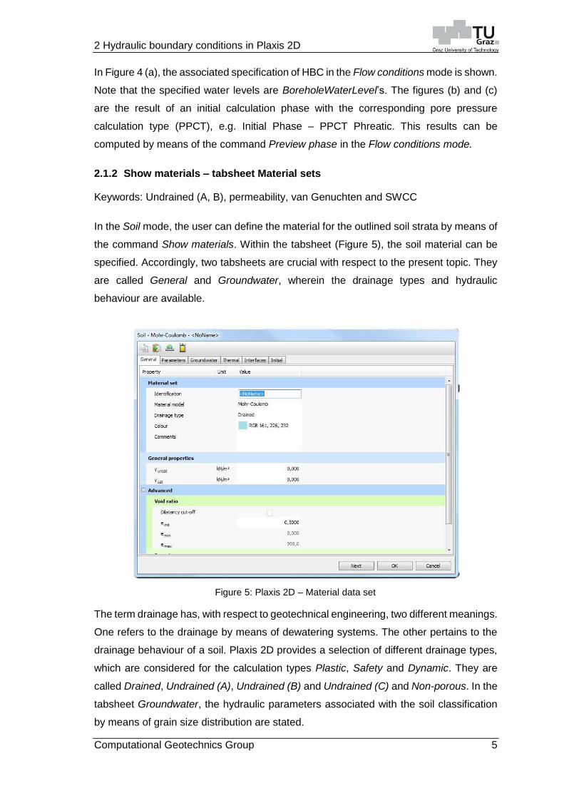
2.1.2 Show materials – tabsheet Material sets
Keywords: Undrained (A, B), permeability, van Genuchten and SWCC
In the Soil mode, the user can define the material for the outlined soil strata by means of
the command Show materials. Within the tabsheet (Figure 5), the soil material can be
specified. Accordingly, two tabsheets are crucial with respect to the present topic. They
are called General and Groundwater, wherein the drainage types and hydraulic
behaviour are available.
The term drainage has, with respect to geotechnical engineering, two different meanings.
One refers to the drainage by means of dewatering systems. The other pertains to the
drainage behaviour of a soil. Plaxis 2D provides a selection of different drainage types,
which are considered for the calculation types Plastic, Safety and Dynamic. They are
called Drained, Undrained (A), Undrained (B) and Undrained (C) and Non-porous. In the
tabsheet Groundwater, the hydraulic parameters associated with the soil classification
by means of grain size distribution are stated.
Figure 5: Plaxis 2D – Material data set
2 Hydraulic boundary conditions in Plaxis 2D
6 Computational Geotechnics Group
2.1.3 Tabsheet General – drainage types
All of the aforementioned drainage types describe the water-soil skeleton interaction and
is set for fully saturated soils. A material, which is specified as drained develops no
excess pore pressures. Non-porous material compute either no pore water pressures.
These two do not assist an associated calculation type. In comparison the undrained
material Undrained (A), Undrained (B) and Undrained (C) will only model undrained soil
behaviour, if a plastic analyses is conducted. In contrast to the calculation types (CT)
Consolidation and Fully coupled flow-deformation, which are not dealing with the
drainage types but rather take into account the permeability, stiffness and time. However,
an undrained analysis can be conducted by Undrained (A) and Undrained (B) with
respect to computation of effective stresses. In contrast Undrained (C) will compute total
stresses, hence no effective stresses and excess pore pressures are calculated.
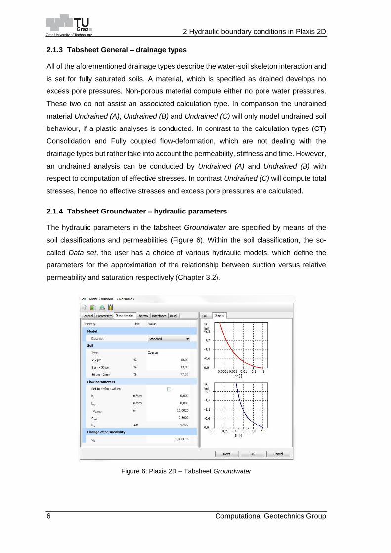
2.1.4 Tabsheet Groundwater – hydraulic parameters
The hydraulic parameters in the tabsheet Groundwater are specified by means of the
soil classifications and permeabilities (Figure 6). Within the soil classification, the so-
called Data set, the user has a choice of various hydraulic models, which define the
parameters for the approximation of the relationship between suction versus relative
permeability and saturation respectively (Chapter 3.2).
Figure 6: Plaxis 2D – Tabsheet Groundwater

2 Hydraulic boundary conditions in Plaxis 2D
Computational Geotechnics Group 7
The mentioned approximation is determined by means of a statistical regression analysis
of laboratory data involving the associated function of van Genuchten-Mualem. The
hydraulic models are listed as Standard, Hypres (Hydraulic Properties of European
Soils), USDA (United States Department of Agriculture), Staring (H.C.W Staring, 1842)
and User-defined. The data set Standard (Figure 7) is based on the data of Hypres and
features Topsoils. The so-called Topsoils are within the first 100 centimetres below the
ground surface and after this limit the so-called Subsoils are given. The parameters for
Hypres, USDA and Staring are based on a collaborative database including the diversity
and spatial variability of soils. Whenever possible the permeability should be obtained
from field and laboratory testing and can be different in vertical and horizontal directions.
Plaxis 2D provides also the possibility to specify a hydraulic model involving laboratory
data by means of User-defined.
Figure 7: SWCC: Standard (Hypres, Topsoils)

2 Hydraulic boundary conditions in Plaxis 2D
8 Computational Geotechnics Group
2.2 Hydraulic boundary conditions
Plaxis 2D provides as many ways to determine the hydraulic boundary conditions. In the
Flow conditions mode, the user can specify the hydraulic boundary conditions by
selecting the desired elements, i.e. adjustment by the Selection explorer. Furthermore
the HBC can be defined globally in the Model explorer.
2.2.1 Hydraulic model boundary conditions – Model explorer
Keywords: Flow functions, Water levels, GroundwaterFlow, Precipitation, Water
Figure 8: Plaxis 2D – Model explorer
The Model explorer (MX) is located on the left lower part of the GUI. The subtrees
Attributes library with Flow functions and Water levels are relevant. Furthermore the
subtree Model conditions including GroundwaterFlow, Precipitation and Water are of
interest. The options of the Model explorer affect the numerical model globally. Thus, for
example the specified precipitation is applied to the whole model surface.
In the subtree Attributes library (Figure 8), the user can define and edit the Flow
functions. Two relevant functions are available, which are called HeadFunction and
DischargeFunction. The HeadFunction can model a water level variation including a
UserWaterLevel and GWFlowBaseBC, but not a BoreholeWaterLevel. Note that a
HeadFunction on inclined elements is not admissible. The DischargeFunction defines a
recharge on the associated surface, e.g. GWFlowBaseBC. Both functions are computed
when the hydraulic boundary condition is stated as Time dependent and a flow
calculation is conducted. In both functions, the user can model a linear or harmonic water
head change. Furthermore a change of water head by means of table values is feasible
(Figure 9).

2 Hydraulic boundary conditions in Plaxis 2D
Computational Geotechnics Group 9
Figure 9: Plaxis 2D – Flow functions
The time value in the subtree Signal always refers to the cumulated time of a consecutive
calculation. This means that in case of a complete flow analysis, e.g. precipitation, each
calculation phase will only use the corresponding part of the flow function.
The subtree Water levels allows the user to navigate and adjust the specified phreatic
levels more conveniently. The user can adjust two different water levels, the
BoreholeWaterLevel and the UserWaterLevel. The BoreholeWaterLevel is assigned by
the borehole Head specification and the UserWaterLevel is defined by means of the
command Create water level in the Flow conditions mode. Note that a
BoreholeWaterLevel cannot be modified by a Flow functions. In order to avoid the
BoreholeWaterLevel, the soil stratigraphy can be modelled by means of soil polygons in
the Structure mode and a UserWaterLevel can be alternatively applied. Corresponding
definitions of hydraulic conditions in the soil polygons can be found in the chapter 2.2.2
in the section Global level and Custom level.
The subtree Model conditions (Figure 8), obtains the option GroundwaterFlow. Therein,
the model extremes XMin, XMax, YMin and YMax are stated, which include the hydraulic
boundary conditions Open and Closed. When modelling the soil stratigraphy the bottom
boundary YMin is automatically set to Closed. In Figure 10, the difference between an
opened and closed boundary is displayed. In this case, the left model extreme XMin
should be closed in order to obtain the appropriate water head of an axisymmetric
geotechnical model.

2 Hydraulic boundary conditions in Plaxis 2D
10 Computational Geotechnics Group
Figure 10: GroundwaterFlow: Closed versus Open
A further option to define a HBC in the subtree Model Conditions is the Precipitation.
Likewise, this option is affecting all the associated model surfaces. Note that all
boundaries, which represent the ground surface should not be specified with other HBC
options, e.g. Closed, Head, etc. Otherwise, the precipitation in the associated ground
surface will be not calculated. The precipitation is modelled on a horizontal and an
inclined surface by means of defining the parameter recharge 𝑞 and maximum and
minimum water pressure referred to the affected boundary, which are stated as water
head 𝜓𝑚𝑎𝑥 and 𝜓𝑚𝑖𝑛. In the case of an inclined surface, the parameter 𝑞 will be computed
in the magnitude of 𝑞 ∙ cos 𝛼, where 𝛼 is the angle of the inclined surface. Accordingly,
the term represents the recharge perpendicular to the model surface. The recharge 𝑞
can be specified by means of a constant value or a time-dependent recharge. The latter
option can be modelled by defining a DischargeFunction in the subtree Flow functions.
Due to the periodic character of the meteorological incidence the function should be
stated as intermittently step function. Thus the input by means of a table is the
appropriate approach. Generally a meteorological phenomenon has a periodic
character, because infiltration, stated as precipitation, and drying, encompassing
evaporation and evapotranspiration, occur. In consequence, the recharge can be defined
with a positive value for precipitation and a negative value for evapotranspiration. The
variable 𝜓𝑚𝑎𝑥 represents the height of the water head above the ground surface. Above
this value 𝜓𝑚𝑎𝑥, a water run-off is simulated, when the initial water head due to the
recharge increases until the associated head is reached. The parameter 𝜓𝑚𝑖𝑛 defines
the depth within the top soil. It is associated with a negative recharge, i.e. evaporation or
evapotranspiration respectively. When the resulting minimum head is reached at the
defined limit, the negative recharge is supposed to stop. The default value for the
maximum water head is equal to 0.1 m and should describe the water storage capacity
due to the uneven surface and plant cover. The minimum water head is specified by

2 Hydraulic boundary conditions in Plaxis 2D
Computational Geotechnics Group 11
default equal to minus 1.0 m and bounds the impact due to drying (Figure 11). The option
Infiltration is discussed in chapter 2.2.2 in the corresponding section.
MX: Precipitation SX: Infiltration
Model with Precipitation Model with Infiltration
Initial phase – Step 0 Initial phase – Step 0
Positive recharge/ 𝜓𝑚𝑎𝑥 – Step 48 Positive recharge/ 𝜓𝑚𝑎𝑥 – Step 185
Negative recharge/ 𝜓𝑚𝑖𝑛 – Step 130 Negative recharge - 𝜓𝑚𝑖𝑛 267
Figure 11: Comparison: Precipitation and Infiltration
2 Hydraulic boundary conditions in Plaxis 2D
12 Computational Geotechnics Group
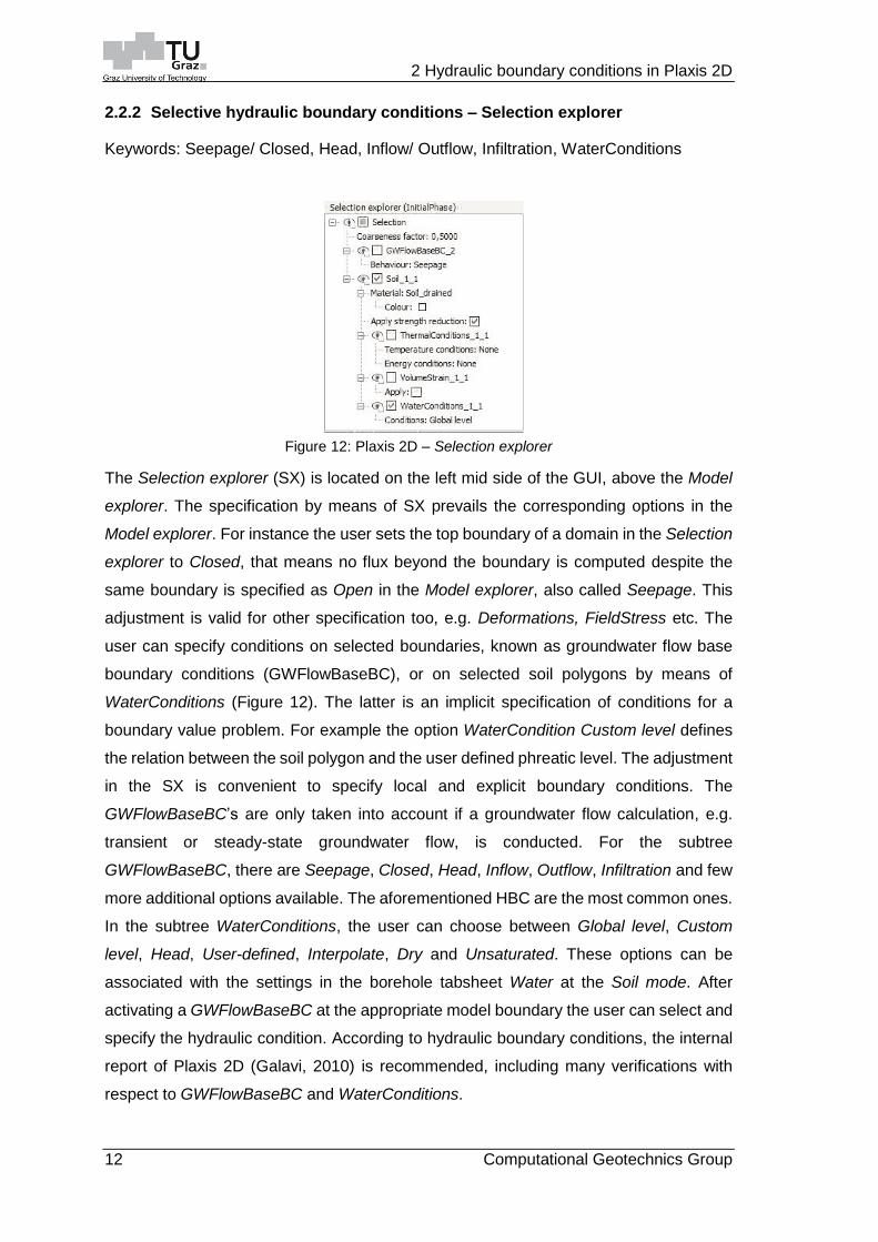
2.2.2 Selective hydraulic boundary conditions – Selection explorer
Keywords: Seepage/ Closed, Head, Inflow/ Outflow, Infiltration, WaterConditions
Figure 12: Plaxis 2D – Selection explorer
The Selection explorer (SX) is located on the left mid side of the GUI, above the Model
explorer. The specification by means of SX prevails the corresponding options in the
Model explorer. For instance the user sets the top boundary of a domain in the Selection
explorer to Closed, that means no flux beyond the boundary is computed despite the
same boundary is specified as Open in the Model explorer, also called Seepage. This
adjustment is valid for other specification too, e.g. Deformations, FieldStress etc. The
user can specify conditions on selected boundaries, known as groundwater flow base
boundary conditions (GWFlowBaseBC), or on selected soil polygons by means of
WaterConditions (Figure 12). The latter is an implicit specification of conditions for a
boundary value problem. For example the option WaterCondition Custom level defines
the relation between the soil polygon and the user defined phreatic level. The adjustment
in the SX is convenient to specify local and explicit boundary conditions. The
GWFlowBaseBC’s are only taken into account if a groundwater flow calculation, e.g.
transient or steady-state groundwater flow, is conducted. For the subtree
GWFlowBaseBC, there are Seepage, Closed, Head, Inflow, Outflow, Infiltration and few
more additional options available. The aforementioned HBC are the most common ones.
In the subtree WaterConditions, the user can choose between Global level, Custom
level, Head, User-defined, Interpolate, Dry and Unsaturated. These options can be
associated with the settings in the borehole tabsheet Water at the Soil mode. After
activating a GWFlowBaseBC at the appropriate model boundary the user can select and
specify the hydraulic condition. According to hydraulic boundary conditions, the internal
report of Plaxis 2D (Galavi, 2010) is recommended, including many verifications with
respect to GWFlowBaseBC and WaterConditions.

2 Hydraulic boundary conditions in Plaxis 2D
Computational Geotechnics Group 13
The options Seepage and Closed are similar to the GroundwaterFlow specifications in
the MX (chapter 2.2.1). Consequently, any specification in the SX prevails the
corresponding boundary conditions. Seepage means flux beyond the boundary and
Closed avoids any flux.
The option Head can model a hydrostatic water head referred to its level, i.e. if the
GWFlowBaseBC within the model is specified, then the pore pressure at the associated
level is zero and the pore pressure below is not affected by any recharge (chapter 5.1.3).
Within the option Head, several distributions, e.g. Uniform, Vertical increment etc. are
available. The specifics will be not discussed here, but its application and results can be
found the Appendix. The HBC can be used to directly generate a phreatic level, which
confines a fully saturated soil layer without any flux beyond its surface.
The options Inflow and Outflow describe the same boundary conditions but have
opposite effects. The GWFlowBaseBC Inflow or Outflow are strongly dependent on the
hydraulic behaviour of the soil and the specification of flux. Accordingly, the user can
define a local outflow in the tunnel wall by specifying uniform discharges involving field
data.
The last mentioned GWFlowBaseBC is the Infiltration, which has the same specification
of the HBC Precipitation in the Model Explorer. The application is differently. The user
need to specify the infiltration by means of activating the GWFlowBaseBC at the
boundary. Thereby, the corresponding ground surface should be determined and
activated. (Figure 13, violet).
Figure 13: GWFlowBaseBC: Infiltration

2 Hydraulic boundary conditions in Plaxis 2D
14 Computational Geotechnics Group
The hydraulic boundary conditions, Head, Inflow, Outflow and Infiltration can be specified
with a constant flux or a time-dependent recharge, hence the user needs to define time
dependency and specify the recharge by means of a HeadFunction or
DischargeFunction respectively.
The aforementioned WaterConditions, which are an implicitly modification of boundary
conditions with respect to the soil polygon, can be defined by selecting the soil cluster
and changing the options in the SX. The options Global level and Custom level
encompass the same application, i.e. relates to the associated water level, but have
different meanings. The soil polygon, which should be specified with the option Global
level, computes the internal water pressures with respect to the corresponding water
level (Figure 14, dark blue zone). The water level is marked as global and specified in
the Model explorer in the subtree Model conditions Water. In contrast, the specification
by means of Custom level defines the computation of internal water pressure with
respect to the UserWaterLevel. A UserWaterLevel could be defined by the command
Create water level. Consequently, the user can define many water levels but must take
care in applying the corresponding soil polygons.
The phreatic level and the active model boundary require an intersection point. An
intersection point means where the phreatic level and the activated model boundary
coincide. For instance, a model boundary is active after an excavation step is conducted.
Thus an intersection point must be always created in order to take into account the
associated phreatic level for the pore water pressure calculation in the soil clusters
(Figure 14, light blue zone).
Figure 14: Active model boundary (TM Plaxis 2D, 2016)
2 Hydraulic boundary conditions in Plaxis 2D
Computational Geotechnics Group 15
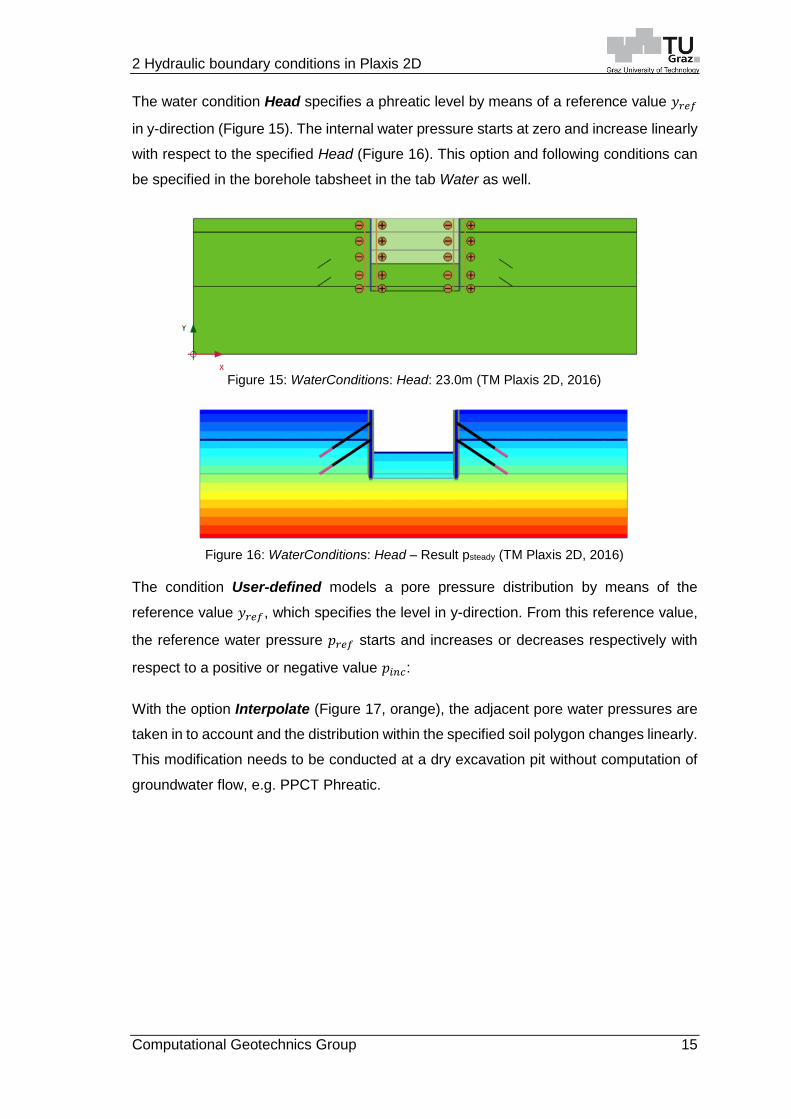
The water condition Head specifies a phreatic level by means of a reference value 𝑦𝑟𝑒𝑓
in y-direction (Figure 15). The internal water pressure starts at zero and increase linearly
with respect to the specified Head (Figure 16). This option and following conditions can
be specified in the borehole tabsheet in the tab Water as well.
Figure 15: WaterConditions: Head: 23.0m (TM Plaxis 2D, 2016)
Figure 16: WaterConditions: Head – Result psteady (TM Plaxis 2D, 2016)
The condition User-defined models a pore pressure distribution by means of the
reference value 𝑦𝑟𝑒𝑓, which specifies the level in y-direction. From this reference value,
the reference water pressure 𝑝𝑟𝑒𝑓 starts and increases or decreases respectively with
respect to a positive or negative value 𝑝𝑖𝑛𝑐:
With the option Interpolate (Figure 17, orange), the adjacent pore water pressures are
taken in to account and the distribution within the specified soil polygon changes linearly.
This modification needs to be conducted at a dry excavation pit without computation of
groundwater flow, e.g. PPCT Phreatic.

2 Hydraulic boundary conditions in Plaxis 2D
16 Computational Geotechnics Group
The option Dry (Figure 17, grey zone) will not compute any pore water pressure. Thus,
it has the relevant behaviour of non-porous material. An application of this hydraulic
condition in accordance to the PPCT Phreatic is following model. Further models are
shown in the Appendix.
Figure 17: WaterConditions: Dry (TM Plaxis 2D, 2016)
Figure 18: WaterConditions: Dry – Result psteady (TM Plaxis 2D, 2016)
A partial saturation to the soil polygon is explicitly introduced by means of the water
condition Unsaturated. The saturation throughout the soil clusters is uniform by the
specified value. It is possible to deal with unsaturated soil cluster, if the option Ignore
suction in the Deformation control parameters subtree is deselected. Hence the resulting
pore water pressures involving suction will be computed according the water conditions
and the specifications in the Groundwater tabsheet.
3 Soil water characteristic curve
Computational Geotechnics Group 17
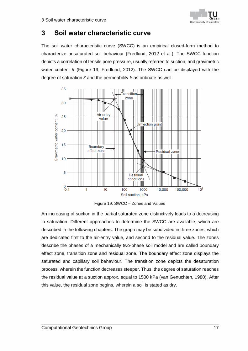
3 Soil water characteristic curve
The soil water characteristic curve (SWCC) is an empirical closed-form method to
characterize unsaturated soil behaviour (Fredlund, 2012 et al.). The SWCC function
depicts a correlation of tensile pore pressure, usually referred to suction, and gravimetric
water content 𝜃 (Figure 19, Fredlund, 2012). The SWCC can be displayed with the
degree of saturation 𝑆 and the permeability 𝑘 as ordinate as well.
An increasing of suction in the partial saturated zone distinctively leads to a decreasing
in saturation. Different approaches to determine the SWCC are available, which are
described in the following chapters. The graph may be subdivided in three zones, which
are dedicated first to the air-entry value, and second to the residual value. The zones
describe the phases of a mechanically two-phase soil model and are called boundary
effect zone, transition zone and residual zone. The boundary effect zone displays the
saturated and capillary soil behaviour. The transition zone depicts the desaturation
process, wherein the function decreases steeper. Thus, the degree of saturation reaches
the residual value at a suction approx. equal to 1500 kPa (van Genuchten, 1980). After
this value, the residual zone begins, wherein a soil is stated as dry.
Figure 19: SWCC – Zones and Values

3 Soil water characteristic curve
18 Computational Geotechnics Group
3.1 Approximation of laboratory data
The relationship between suction and gravimetric water content can be measured by
means of laboratory tests. Consequently, the experimental data cloud is fitted by means
of the least square regression analysis in order to enhance an implementation of
unsaturated soil properties in computational geotechnical models. Various researchers
(Gardner 1958, Mualem 1976, van Genuchten 1980, Fredlund and Xing 1994, Pharm
and Fredlund 2005 et al.) had carried out methods to best fit the experimental data
(Figure 20, Fredlund 2012).
Figure 20: SWCC – Equations
Each equation is written in terms of the dimensionless water content 𝜃𝑑, normalized
water content 𝜃𝑛 or gravimetric water content 𝑤(𝜓) in relation to the soil suction 𝜓.
3 Soil water characteristic curve
Computational Geotechnics Group 19
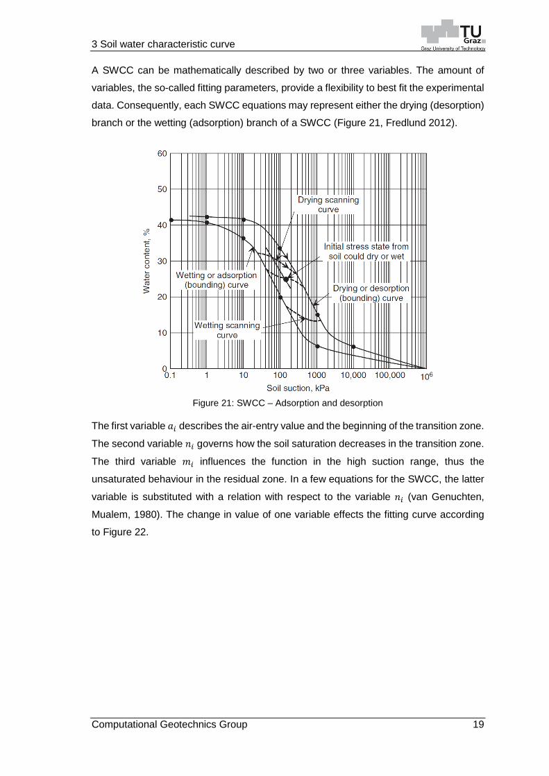
A SWCC can be mathematically described by two or three variables. The amount of
variables, the so-called fitting parameters, provide a flexibility to best fit the experimental
data. Consequently, each SWCC equations may represent either the drying (desorption)
branch or the wetting (adsorption) branch of a SWCC (Figure 21, Fredlund 2012).
Figure 21: SWCC – Adsorption and desorption
The first variable 𝑎𝑖 describes the air-entry value and the beginning of the transition zone.
The second variable 𝑛𝑖 governs how the soil saturation decreases in the transition zone.
The third variable 𝑚𝑖 influences the function in the high suction range, thus the
unsaturated behaviour in the residual zone. In a few equations for the SWCC, the latter
variable is substituted with a relation with respect to the variable 𝑛𝑖 (van Genuchten,
Mualem, 1980). The change in value of one variable effects the fitting curve according
to Figure 22.

3 Soil water characteristic curve
20 Computational Geotechnics Group
Figure 22: SWCC – Variable variation
3.2 Implementation in Plaxis 2D
In Plaxis 2D the SWCC is implemented by means of hydraulic models in the tabsheet
Groundwater and is used to model unsaturated soil behaviour. Hereof, Bishop presented
a theory to calculate effective stresses for unsaturated soils. The effective stresses are
composed of total stresses and pore water pressures of all fluids in a three-phase model:
𝜎′ = (𝜎 − 𝑢𝑎) − 𝜒 ∙ (𝑢𝑎 − 𝑢𝑤) [1]
where 𝜎 is called the total stresses, 𝑢𝑎 is the pore air pressure, 𝜒 is called matric suction
coefficient and 𝑢𝑤 is the pore water pressure. By using Bishop’s Theory as basic
calculation for effective stresses in Plaxis 2D, the distinction can still be made between
fully saturated and partial saturated soil behaviour. In Plaxis it is assumed that the pore
air pressure 𝑢𝑎 is zero and the matric suction coefficient 𝜒 is specified with the
relationship 𝜒 = 𝑆𝑒𝑓𝑓 (Figure 23, Nuth, 2007 et al.).

3 Soil water characteristic curve
Computational Geotechnics Group 21
Figure 23: Matric suction coefficient and saturation trend
The equation [1], with the aforementioned preconditions and the denotation of pore water
pressure 𝑝𝑤𝑎𝑡𝑒𝑟 in Plaxis 2D for the term 𝑢𝑤, now reads:
𝜎′ = 𝜎 − 𝑆𝑒𝑓𝑓 ∙ 𝑝𝑤𝑎𝑡𝑒𝑟 [2]
wherein the effective degree of saturation 𝑆𝑒𝑓𝑓 is written as an equation with the terms
of an actual degree of saturation 𝑆, the residual value 𝑆𝑟𝑒𝑠 and the saturated value 𝑆𝑠𝑎𝑡:
𝑆𝑒𝑓𝑓 =𝑆 − 𝑆𝑟𝑒𝑠
𝑆𝑠𝑎𝑡 − 𝑆𝑟𝑒𝑠 [3]
The actual degree of saturation 𝑆 is computed with the derivative (equation [4]), by
means of the hydraulic model and the actual pore water pressures 𝑝𝑤 in the geotechnical
model. The computation of tensile pore pressures must be conducted by disabling the
Deformation control parameter Ignore Suction in the tabsheet Phases.
𝜕𝑆(𝑝𝑤)
𝜕𝑝𝑤= (𝑆𝑠𝑎𝑡 − 𝑆𝑟𝑒𝑠) [
1 − 𝑔𝑛
𝑔𝑛] [𝑔𝑛 (
𝑔𝑎
𝛾𝑤)
𝑔𝑛
𝑝𝑤(𝑔𝑛−1) ] [1 + (𝑔𝑎
𝑝𝑤
𝛾𝑤)
𝑔𝑛
](
1−𝑔𝑛𝑔𝑛
)
[4]
The hydraulic model contains a framework of soil classes (Figure 24 – Source: Internet)
and fitting parameters (Table 2, Plaxis 2D, 2016). The fitting parameters 𝑔𝑎 , 𝑔𝑛 are
determined for the van Genuchten-Mualem approximation according to the soil
classification, e.g. Standard, Hypres, USDA, Staring and User-defined.

3 Soil water characteristic curve
22 Computational Geotechnics Group
Figure 24: Soil classification: (a) USDA and (b) Hypres
Table 2: Hypres series with van Genuchten parameters (RM Plaxis 2D, 2016)
a) b)

4 Types of analyses and output
Computational Geotechnics Group 23
4 Types of analyses and output
The numerical analysis can be divided into several calculation phases. One phase
corresponds to a particular loading stage or construction sequence respectively. Hereof,
Plaxis 2D provides different calculation types (CT) and pore pressure calculation types
(PPCT) in order to compute deformations and pore water pressures. In consequence,
the associated specifications of HBC are involved as well.
4.1 Calculation types
The calculation type relates to the geotechnical procedure, e.g. construction of a dam,
excavation of a pit, lowering groundwater or dissipate excess pore pressures. At the
beginning of every geotechnical model, the initial state must be defined by means of a
parent phase. Additionally, the following calculation steps, also known as child phases,
can carry out the geotechnical procedure. Table 3 shows an overview of all available
calculation types and its possible applications. Furthermore the pore pressure calculation
type with its abbreviations Phreatic (PHR), Use pressure from previous phase (UPPP),
Steady state groundwater flow (SSGWF) and Transient groundwater flow (TGWF) is
displayed. The PPCT pertains to the conducting Calculation type in a phase and is
strongly dependent on the Loading type Staged Construction. The pore pressure
calculation type UPPP adopts the pore water pressures from the previous phase, thus
no pore water pressure calculation is conducted. Further this PPCT takes over the status
quo of the activated and deactivated soil polygons from the previous phase although a
new status quo in the present phase is considered. The TGWF is only available in the
child phases, if the parent phase is specified with the calculation type Flow only. The CT
Fully coupled flow-deformation has no PPCT.

4 Types of analyses and output
24 Computational Geotechnics Group
Parent phase
Specification Application PPCT
K0 procedure Direct generation of initial
effective stresses, pore
pressures and state
parameters
Set up of geotechnical
model
PHR,
SSGWF
Field stress Direct generation of initial
effective stresses, pore
pressures and state
parameters
Set up of geotechnical
model
PHR,
SSGWF
Gravity loading Initial stresses from finite
element calculation
Set up of geotechnical
model with inclined
soil strata
PHR,
SSGWF
Flow only No effective stress
calculation
Flow calculation for
the geotechnical
model
PHR,
SSGWF,
TGWF
Child phase
Plastic Elastoplastic drained or
undrained analysis
e.g. failure load
prediction, drained
excavation sequence
PHR,
UPPP,
SSGWF
Consolidation Time-dependent analysis
of deformation and
excess pore pressure
e.g. dissipation of
excess pore pressure
after a plastic analysis
PHR,
UPPP,
SSGWF
Fully coupled
flow-deformation
Time-dependent analysis
of deformation and pore
water pressure
e.g. coupled analysis
involving flow and
deformation
-
Safety Calculation of global
factor of safety
Prediction of failure
mechanism
UPPP
Dynamic Dynamic analysis in the
time domain
e.g. deformation
analysis involving
earthquake scenario
UPPP
Table 3: Calculation and pore pressure calculation type

4 Types of analyses and output
Computational Geotechnics Group 25
4.2 Pore pressure calculation type
The pore water pressure is part of the total stresses and is denoted as active pore
pressure 𝑝𝑎𝑐𝑡𝑖𝑣𝑒 in Plaxis 2D. This pore pressure is a result of the effective degree of
saturation multiplied by the pore water pressure 𝑝𝑤𝑎𝑡𝑒𝑟. In turn, 𝑝𝑤𝑎𝑡𝑒𝑟 is composed of
steady-state pore pressure and excess pore pressure. In Plaxis 2D four types of pore
pressure calculations are available. They are called Phreatic, Use pressure from
previous phase, Steady-state groundwater flow and Transient groundwater flow. The
PPCT Phreatic generates directly steady-state pore pressure in consequence of the
specified water levels and WaterConditions in the soil polygons. The pore pressure
calculation type UPPP does not compute pore pressures, because it takes into account
the already calculated pore pressures from the previous phase. The PPCT SSGWF and
TGWF are actually computing pore pressures by means of groundwater flow involving
the defined flow parameters and specified hydraulic boundary conditions.
4.3 Stress and pore pressure output
In the previous chapter the computation of stresses and pore pressures involving
different calculation types have been discussed. Now the results and its specifications
will be discussed.
The total stresses 𝜎 are composed of effective stresses 𝜎′ and the pore water
pressures ∆𝑢 according to Terzaghi (Terzaghi, 1925). Following equations show it
clearly:
𝜎 = 𝜎′ + 𝑢𝑤 … total stresses [5]
𝜎′ = 𝜎 − 𝑢𝑤 … effective stresses [6]
Bishop introduced to pore water pressure the matric suction hence the formulation is
described by the following equation:
𝜎′ = (𝜎 − 𝑢𝑎) − 𝜒 ∙ (𝑢𝑎 − 𝑢𝑤) … effective stresses [7]

4 Types of analyses and output
26 Computational Geotechnics Group
In Plaxis 2D two assumptions are postulated. The pore air pressure 𝑢𝑎 is equal to zero
and the matric suction coefficient is defined as 𝜒 = 𝑆𝑒𝑓𝑓. Thus, the equation [7] now
reads:
𝜎′ = 𝜎 − 𝑆𝑒𝑓𝑓 ∙ 𝑢𝑤 … effective stresses [8]
Where the effective degree of saturation 𝑆𝑒𝑓𝑓 is a normalized factor containing the actual
degree of saturation 𝑆 in the soil, the residual degree of saturation 𝑆𝑒𝑓𝑓 and the fully
saturated degree 𝑆𝑠𝑎𝑡 (equation [9]).
𝑆𝑒𝑓𝑓 = 𝑆 − 𝑆𝑟𝑒𝑠
𝑆𝑠𝑎𝑡 − 𝑆𝑟𝑒𝑠 … effective degree of saturation [9]
In Plaxis 2D the pore pressure 𝑢𝑤 in equation [8] is denoted as pore water pressure
𝑝𝑤𝑎𝑡𝑒𝑟 (equation [10]).
𝜎′ = 𝜎 − 𝑆𝑒𝑓𝑓 ∙ 𝑝𝑤𝑎𝑡𝑒𝑟 … effective stresses [10]
Further the term of pore pressure including 𝑆𝑒𝑓𝑓 and 𝑝𝑤𝑎𝑡𝑒𝑟 can be specified as active
pore pressure 𝑝𝑎𝑐𝑡𝑖𝑣𝑒.
𝜎′ = 𝜎 − 𝑝𝑎𝑐𝑡𝑖𝑣𝑒 … effective stresses [11]
In case of 𝑆 = 1.0, 𝑆𝑠𝑎𝑡 = 1.0 and 𝑆𝑟𝑒𝑠 = 0.0, i.e. fully saturation of the soil, the effective
degree of saturation 𝑆𝑒𝑓𝑓 is equal to 1.0, thus entail the active pore pressure correlates
with the pore water pressure. Further the effective stresses according to Bishop coincide
with Terzaghi’s effective stresses.
4 Types of analyses and output
Computational Geotechnics Group 27
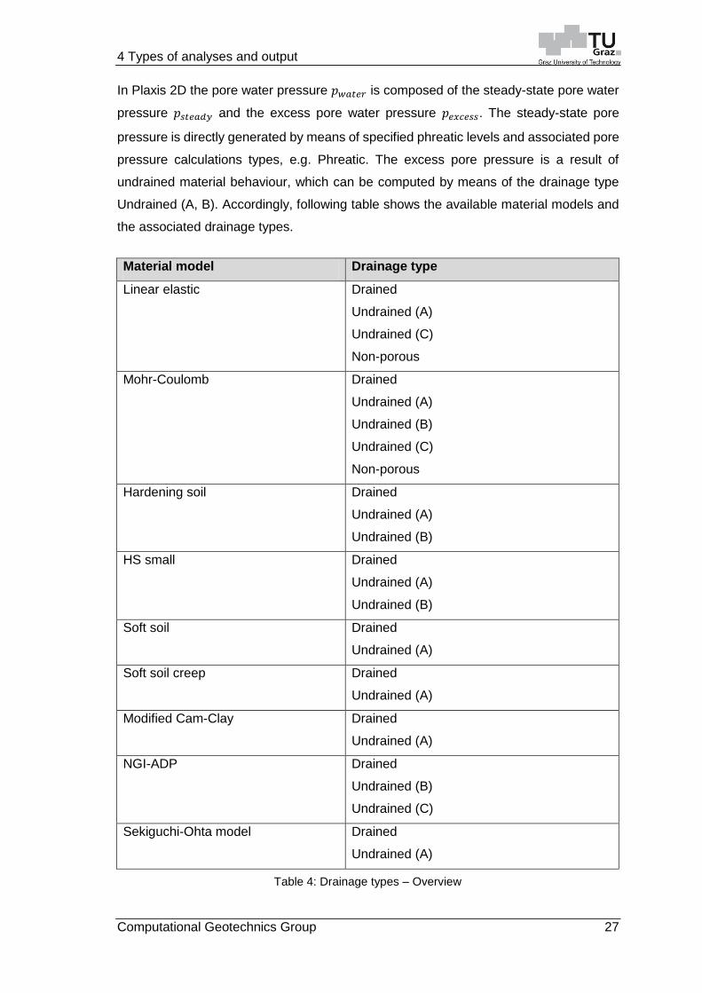
In Plaxis 2D the pore water pressure 𝑝𝑤𝑎𝑡𝑒𝑟 is composed of the steady-state pore water
pressure 𝑝𝑠𝑡𝑒𝑎𝑑𝑦 and the excess pore water pressure 𝑝𝑒𝑥𝑐𝑒𝑠𝑠. The steady-state pore
pressure is directly generated by means of specified phreatic levels and associated pore
pressure calculations types, e.g. Phreatic. The excess pore pressure is a result of
undrained material behaviour, which can be computed by means of the drainage type
Undrained (A, B). Accordingly, following table shows the available material models and
the associated drainage types.
Material model Drainage type
Linear elastic Drained
Undrained (A)
Undrained (C)
Non-porous
Mohr-Coulomb Drained
Undrained (A)
Undrained (B)
Undrained (C)
Non-porous
Hardening soil Drained
Undrained (A)
Undrained (B)
HS small Drained
Undrained (A)
Undrained (B)
Soft soil Drained
Undrained (A)
Soft soil creep Drained
Undrained (A)
Modified Cam-Clay Drained
Undrained (A)
NGI-ADP Drained
Undrained (B)
Undrained (C)
Sekiguchi-Ohta model Drained
Undrained (A)
Table 4: Drainage types – Overview

4 Types of analyses and output
28 Computational Geotechnics Group
An undrained analysis can also be conducted by the calculation type Fully coupled flow-
deformation. Hereof this CT takes only into account the time, the permeability and
stiffness. Depending on the calculation type, the bulk modulus will be stated in the
stiffness matrix (Table 5, Plaxis 2D, 2016)
Table
5:
Bu
lk m
odu
lus o
f w
ate
r – O
verv
iew

4 Types of analyses and output
Computational Geotechnics Group 29
The bulk modulus of water changes according to the degree of saturation. Generally the
saturation of a soil coincides with the phreatic level. Above the phreatic level (𝑝𝑤 > 0)
the saturation is equal to 0 % and below (𝑝𝑤 < 0) it is specified with 100 %. For fully
saturated soils the phreatic level should be equal to the soil surface. In the undrained
material, e.g. Undrained (A) or Undrained (B), the saturation is automatically 100 %. Note
that the saturation can be redefined by a numerical analysis involving suction in the
unsaturated zone and the soil water characteristic curve. In the following table, the
associated saturation in accordance to the drainage type and relation to the phreatic
level are postulated.
Table 6: Specification of saturation
Calculation type Drainage type Phreatic leveleffective
Satuarion SeffNotation
Plastic Undrained (A,B) above 1.0* overruling specification
Consolidation Undrained (A,B) above 1.0* overruling specification
FCFD Undrained (A,B) above 0.0*
* Saturation could be modified by means of hydraulic model and enabled suction
5 Application of hydraulic boundary conditions
30 Computational Geotechnics Group
5 Application of hydraulic boundary conditions
In the previous chapters the hydraulic boundary conditions, soil water characteristic
curve, undrained analysis and the type of analyses are prescribed. These features are
now applied in the following chapter.
5.1 Precipitation
By using the Model condition’s Precipitation or Infiltration it is possible to compute a
moisture flux boundary condition on the model surface. It exist a distinction of two
boundary conditions. One boundary condition (BC) is specified as hydraulic head
(Dirichlet BC), the second BC is stated as infiltration respectively recharge (Neumann
BC). The specifics are the water pressure head 𝜓𝑚𝑎𝑥 and 𝜓𝑚𝑖𝑛 and the recharge 𝑞. The
quantification of moisture flux is related to hydro-meteorological and hydrogeological
data survey. The evaluation of moisture flux involves infiltration rate, evaporation rate
and evapotranspiration rate respectively.
5.1.1 Aim of geotechnical model
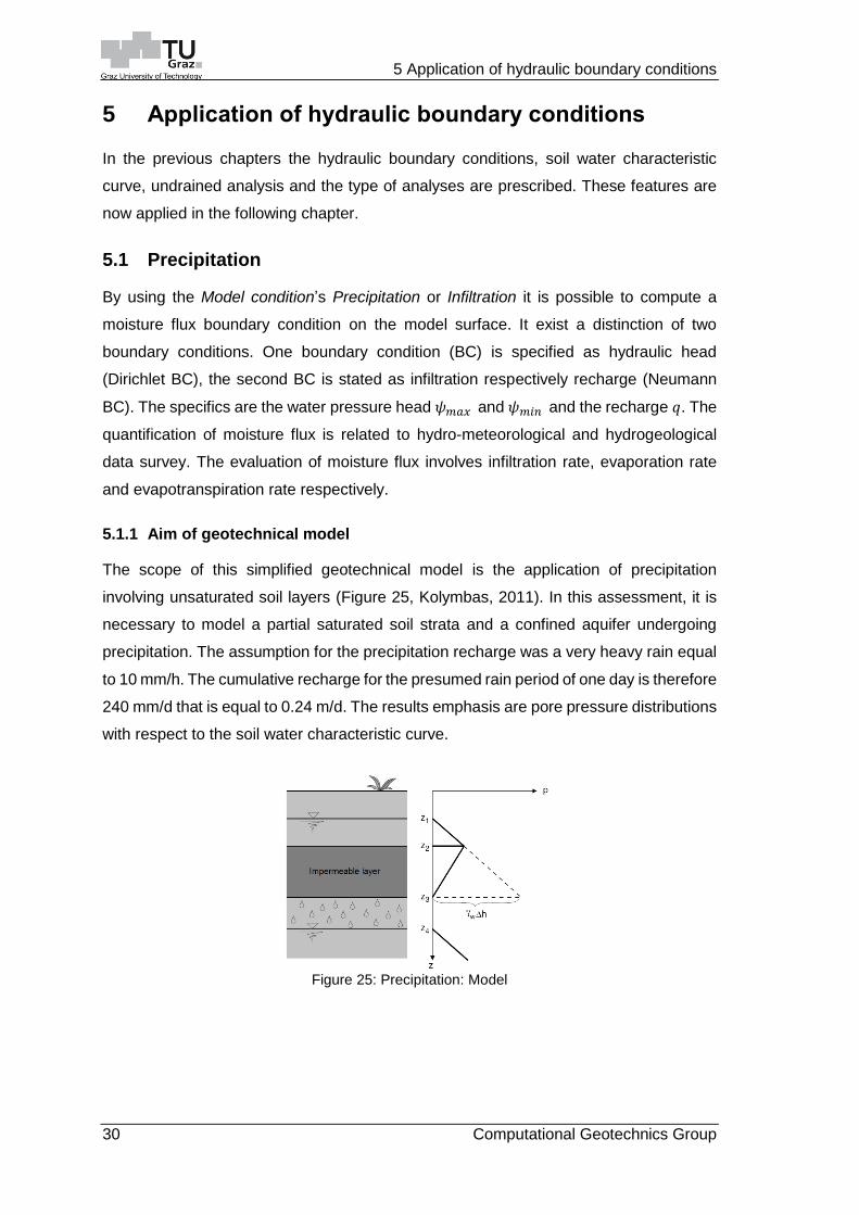
The scope of this simplified geotechnical model is the application of precipitation
involving unsaturated soil layers (Figure 25, Kolymbas, 2011). In this assessment, it is
necessary to model a partial saturated soil strata and a confined aquifer undergoing
precipitation. The assumption for the precipitation recharge was a very heavy rain equal
to 10 mm/h. The cumulative recharge for the presumed rain period of one day is therefore
240 mm/d that is equal to 0.24 m/d. The results emphasis are pore pressure distributions
with respect to the soil water characteristic curve.
Figure 25: Precipitation: Model
5 Application of hydraulic boundary conditions
Computational Geotechnics Group 31
5.1.2 Model configuration and material parameters
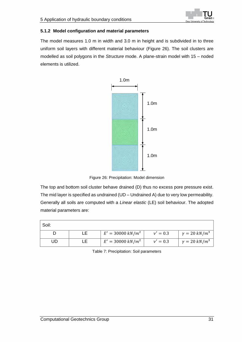
The model measures 1.0 m in width and 3.0 m in height and is subdivided in to three
uniform soil layers with different material behaviour (Figure 26). The soil clusters are
modelled as soil polygons in the Structure mode. A plane-strain model with 15 – noded
elements is utilized.
Figure 26: Precipitation: Model dimension
The top and bottom soil cluster behave drained (D) thus no excess pore pressure exist.
The mid layer is specified as undrained (UD – Undrained A) due to very low permeability.
Generally all soils are computed with a Linear elastic (LE) soil behaviour. The adopted
material parameters are:
Soil:
D LE 𝐸′ = 30000 𝑘𝑁/𝑚² 𝜈′ = 0.3 𝛾 = 20 𝑘𝑁/𝑚³
UD LE 𝐸′ = 30000 𝑘𝑁/𝑚² 𝜈′ = 0.3 𝛾 = 20 𝑘𝑁/𝑚³
Table 7: Precipitation: Soil parameters
1.0m
1.0m
1.0m
1.0m

5 Application of hydraulic boundary conditions
32 Computational Geotechnics Group
Further both soil material parameters for unsaturated soil properties according to the
hydraulic model Standard (Hypres Topsoils) are used. The adopted SWCC parameters
are:
Soil: Data set Standard, soil types coarse (D), fine (UD)
D vGA 𝑘 = 86. m/d 𝜃𝑟 = 0.025 𝜃𝑠 = 0.403 𝑔𝑎 = 3.83. 𝑔𝑛 = 1.3774
UD vGA 𝑘 = 0.0086 m/d 𝜃𝑟 = 0.010 𝜃𝑠 = 0.520 𝑔𝑎 = 3.67 𝑔𝑛 = 1.1012
Table 8: Precipitation: SWCC parameters
In the Mesh mode the Very Fine option is selected and a soil cluster refinement is used.
The coarseness factor is equal to 0.5, thus the mesh quality is high (Figure 26).
In virtue of a one-dimensional flow, the top model boundary is specified with the model
conditions GroundwaterFlow Open in the Model explorer; i.e. seepage is admissible.
This specification is obligatory in order to allow a precipitation recharge. All other
boundaries at the left, bottom and right of the model are closed. In consequence of a
ground water flow calculation, this boundaries avoid flux, i.e. 𝑞 = 0, beyond the model
boundaries. Within the three soil cluster a water level by means of UserWaterLevel
(model a) and GWFlowBaseBC Head (model b) respectively in the top and bottom layer
is defined. Both phreatic levels occur in the middle of the soil layer. The soil cluster are
designated to the water level by means of the associated specification WaterCondition
in the Selection explorer. In addition the mid-layer interpolates the adjacent pore
pressures (Figure 27).
Figure 27: Precipitation: Model (a) UserWaterLevel and (b) GWFlowBaseBC
a) b)

5 Application of hydraulic boundary conditions
Computational Geotechnics Group 33
Both models (a) and (b) are computed in the same Plaxis 2D analysis in order to conduct
the relevant precipitation calculation. Hereof, further specifications with respect to initial
boundary state are defined (Figure 28).
Figure 28: Precipitation: Fixities in model (a) and (b)
The initial state of geotechnical model is computed with the CT K0 procedure and the
PPCT Phreatic. According to the selected pore pressure calculation type, the specified
GWFlowBaseBC’s in model (b) will be not computed. Hence the initial state is different
in contrast to model (a) (FIGURE),
Figure 29: Precipitation: Active pore pressure in model (a) and (b)
Note that this setup for both models with respect to following computation is not relevant
yet, because the output (5.1.3) of the model (b) will compute unexpected results.
a) b)

5 Application of hydraulic boundary conditions
34 Computational Geotechnics Group
The calculation type for the following phase is set to Fully coupled flow–deformation. In
order to introduce the SWCC in the calculation, the option Ignore suction in the
Deformation control parameter should be disabled.
The precipitation recharge cumulates 0.24 m/d by the end of a period equal to one day
(Figure 30). The recharge is specified by means of a DischargeFunction in the Model
Explorer (Figure 31).
A step function represent the alternate recharge within a precipitation incidence thus the
recharge function cannot be modelled as linear function. Therefore a function with the
Signal Table is defined.
Figure 31: Precipitation: DischargeFunction
Figure 30: Precipitation: Recharge
5 Application of hydraulic boundary conditions
Computational Geotechnics Group 35
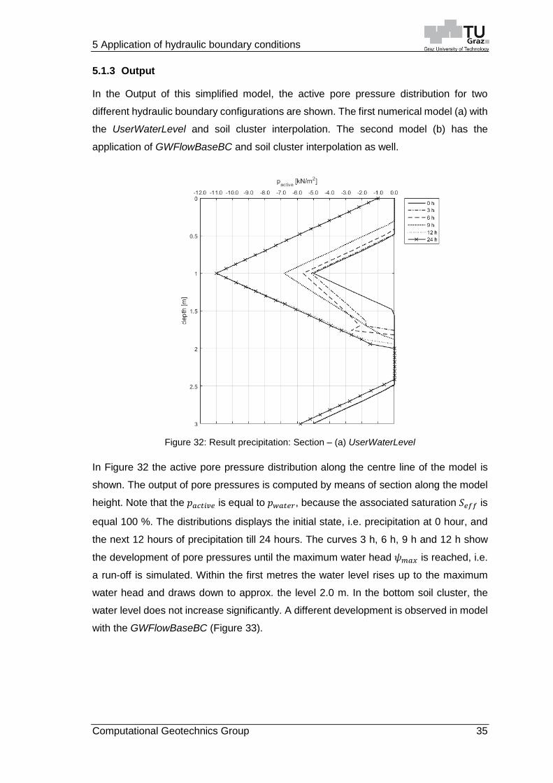
5.1.3 Output
In the Output of this simplified model, the active pore pressure distribution for two
different hydraulic boundary configurations are shown. The first numerical model (a) with
the UserWaterLevel and soil cluster interpolation. The second model (b) has the
application of GWFlowBaseBC and soil cluster interpolation as well.
Figure 32: Result precipitation: Section – (a) UserWaterLevel
In Figure 32 the active pore pressure distribution along the centre line of the model is
shown. The output of pore pressures is computed by means of section along the model
height. Note that the 𝑝𝑎𝑐𝑡𝑖𝑣𝑒 is equal to 𝑝𝑤𝑎𝑡𝑒𝑟, because the associated saturation 𝑆𝑒𝑓𝑓 is
equal 100 %. The distributions displays the initial state, i.e. precipitation at 0 hour, and
the next 12 hours of precipitation till 24 hours. The curves 3 h, 6 h, 9 h and 12 h show
the development of pore pressures until the maximum water head 𝜓𝑚𝑎𝑥 is reached, i.e.
a run-off is simulated. Within the first metres the water level rises up to the maximum
water head and draws down to approx. the level 2.0 m. In the bottom soil cluster, the
water level does not increase significantly. A different development is observed in model
with the GWFlowBaseBC (Figure 33).

5 Application of hydraulic boundary conditions
36 Computational Geotechnics Group
Figure 33: Result precipitation: Section – (b) GWFlowBaseBC
Within this model configuration, the active pore pressure distribution show unexpected
results. As mentioned above, the initial hydraulic state for this model is not correct, but
this has no crucial shortcomings so far. More of interest is that in the upper and lower
soil polygon, i.e. between 0.0 m and 1.0 m or 2.0 m and 3.0 m, the pore pressure is equal
to the hydrostatic state. No water level rises due to the precipitation recharge. Therefore,
the modification by means of GWFlowBaseBC is not appropriate for modelling this
simplified geotechnical model.

5 Application of hydraulic boundary conditions
Computational Geotechnics Group 37
Figure 34: Result precipitation: Depth points – (a) UserWaterLevel
In Figure 34, the development of the active pore pressures within one day is showed.
The results are computed by means of stress points at every depth of 0.5 m along the
centre of the model. The run-off starts after 12.0 hour, i.e. at an amount of 0.12 m/d
precipitation. Hereof, the pore pressure of level y = 0.0 m match with the maximum water
head 𝜓𝑚𝑎𝑥 = 0.1 𝑚. For the depths y equal to 0.5 m, 1.0 m and 1.5 m the pore pressures
shift about -6.0 kPa. The curve at the level 2.0 m displays zero pore pressures because
no water pressure occur in this region. The last two curves, 2.5 m and 3.0 m increase
within the last 12 hours, because the bottom water level rises up.

5 Application of hydraulic boundary conditions
38 Computational Geotechnics Group
Figure 35: Result precipitation: (a) UserWaterLevel and (b) GWFlowBaseBC
In Figure 35 the active pore pressure distribution with the phreatic levels is shown. On
the right is the model (a) with UserWaterLevel and on the left model (b) with
GWFlowBaseBC.
As mentioned in the previous section, suction will be enabled and can be observed in
Figure 36. The curves are plotted for every third hour starting from initial state 0 h and
show the influence of the soil water characteristic curve within 0.0 m to 0.5 m and 2.0 m
to 2.5 m, thus always above the phreatic level. In the coarse material the curves in the
suction region, i.e. 0.0 m to 0.5 m and 2.0 m to 2.5 m incline distinctively. Within the fine
Figure 36: Result precipitation: Section suction – UserWaterLevel

5 Application of hydraulic boundary conditions
Computational Geotechnics Group 39
material, at 1.0 m to 2.0 m, the effect of the SWCC is hardly noticeable, because of the
saturation of the pertained soil layer. At level 2.0 m, a numerical issue occur, because of
the linking of nodal values from adjacent nodes.
5.1.4 Summary and concluding remarks
As mentioned before the model with the GWFlowBaseBC shows unexpected result. On
one side the associated adjustment need to be considered for complete flow analysis
thus the correct pore pressures are calculated. Then again the GWFlowBaseBC HEAD
can be used to specify a constant water head within the geotechnical model, e.g. water
level in fully coupled analysis according to the deep excavation in chapter 5.3.3. In
consequence of computing many model configurations with respect to a recharge was
observed that the difference between two different soil permeabilities should not exceed
10−3. In the Plaxis 2D manual, for instance, was stated the value 10−5, which can be
obtained if groundwater flow is not computed (Appendix).

5 Application of hydraulic boundary conditions
40 Computational Geotechnics Group
5.2 Bearing capacity
A simple geotechnical problem was chosen for demonstrating the consequences of
different assumptions with respect to the drainage conditions. By using the appropriate
drainage types in Plaxis 2D, the computation of excess pore pressures regarding to the
corresponding calculation type entail different results. Furthermore the application of
numerical methods for unsaturated soils influences the results significantly.
5.2.1 Aim of geotechnical model
A shallow foundation on a uniform soil layer was used to compute the available drainage
types. Hereof, the soil water characteristic curve with respect to unsaturated soil
behaviour was utilized as well. All calculations have been computed with the calculation
type Plastic in consideration the material was set to Undrained (A). Occasionally the
suction was enabled. The bearing capacity involving undrained and unsaturated soil
behaviour was determined.
5.2.2 Model configuration and material parameters
The concrete foundation slab lays on a 5.0 m thick soil strata (Figure 37). The foundation
is 3.0 m x 3.0 m and has a thickness of 0.5 m. A plane-strain model with 15 – noded
elements is utilized. A phreatic level exist at 2.0 m below the surface, hence a partial
saturation is present. The applied load is depending on the bearing capacity of the
underground.
Figure 37: Bearing capacity: Model dimension
The strength parameters for concrete slab are equal to Eurocode 2 concrete strength
class C25/30 and a linear elastic material model is adopted. For the soil material the
linear elastic - perfectly plastic constitutive model Mohr-Coulomb (MC) is defined. The
drainage type is specified with Undrained (A). The dilitancy angle 𝜓 is set to zero. The
soil consists of coarse sand and heavy clay respectively. According to Staring’s soil
classification the sand is called O5 and the clay is specified as O12. Furthermore, within
the soil classification, the fitting parameter for van Genuchten’s approximation (vGA) of
the SWCC are defined as well.

5 Application of hydraulic boundary conditions
Computational Geotechnics Group 41
The strength and stiffness parameters are:
Material:
Concrete LE 𝐸 = 31 ∙ 106 𝑘𝑁/𝑚² 𝜈 = 0.2
O5 MC 𝐸′ = 50000 𝑘𝑁/𝑚² 𝜈′ = 0.3 𝑐′ = 0.0 𝑘𝑁/𝑚³ 𝜑′ = 30.0 °
O12 MC 𝐸′ = 5000 𝑘𝑁/𝑚² 𝜈′ = 0.3 𝑐′ = 1.0 𝑘𝑁/𝑚³ 𝜑′ = 30.0 °
Table 9: Bearing capacity: Soil parameters
The properties for unsaturated soils are:
Soil:
O5 vGA 𝑘 = 0.0102 m/d 𝜃𝑟 = 0.01 𝜃𝑠 = 0.320 𝑔𝑎 = 5.210 𝑔𝑛 = 2.374
O12 vGA 𝑘 = 0.2497 m/d 𝜃𝑟 = 0.01 𝜃𝑠 = 0.560 𝑔𝑎 = 0.950 𝑔𝑛 = 1.158
Table 10: Bearing capacity: SWCC parameters
Unsaturated soils can be modelled with a soil water characteristic curve and Bishop’s
effective stresses, wherein suction is a stress component of pore water pressure.
Figure 38: Bearing capacity: SWCC O5 and O12

5 Application of hydraulic boundary conditions
42 Computational Geotechnics Group
In the Mesh mode, the shallow foundation and the surrounding zone with 11.0 m x 3.0
m is refined by a coarseness factor of 0.35 and the Mesh option Fine is used (Figure 39).
Figure 39: Bearing capacity: Connectivity plot
According to the drainage type Undrained (A), the numerical analysis must be computed
with the CT Plastic. The initial state is calculated by means of a parent phase with the
CT K0 Procedure. The following child phases are plastic analysis, wherein the load will
be applied. When dealing with suction in the numerical analysis, within the complete
computation, the deformation control parameter Ignore Suction in the phase window
should be disabled.

5 Application of hydraulic boundary conditions
Computational Geotechnics Group 43
5.2.3 Output
In total this assessment includes 8 cases. The differences between the cases are the
soil materials O5 and O12, drainage types Drained and Undrained (A) and the
computation with or without suction in the unsaturated zone. In Table 11, the cases with
the soil parameter O5 are shown. Accordingly, the specifications of the computation are
presented. Here, the results of CASE 2 and 4 will be discussed. Furthermore, in both
cases, the distinction between the states before loading and after loading are displayed.
Table 11: Bearing capacity: Calculation cases
The pore pressure in a plastic analysis is composed of the steady-state pore pressure
𝑝𝑠𝑡𝑒𝑎𝑑𝑦, the excess pore pressure 𝑝𝑒𝑥𝑐𝑒𝑠𝑠, the pore water pressure 𝑝𝑤𝑎𝑡𝑒𝑟 and the active
pore pressure 𝑝𝑎𝑐𝑡𝑖𝑣𝑒. The relation between each component is following. The pore
pressure 𝑝𝑠𝑡𝑒𝑎𝑑𝑦 is a direct generation of water pressure with respect to the existing
hydraulic conditions, i.e. in this particular case the hydrostatic state is computed. The
pore pressure 𝑝𝑒𝑥𝑐𝑒𝑠𝑠, is a result of the undrained analysis in context of the material set
Undrained (A) and CT Plastic. These two components reckon the pore pressure 𝑝𝑤𝑎𝑡𝑒𝑟.
Furthermore, the pore pressure 𝑝𝑎𝑐𝑡𝑖𝑣𝑒 is composed of 𝑝𝑤𝑎𝑡𝑒𝑟 and the effective degree
of saturation 𝑆𝑒𝑓𝑓. The Figure 40 shows the simple composition of the active pore
pressure.
The effective saturation is determined according to the equation [3] in chapter 3.2.
Figure 40: Bearing capacity: Composition of pore pressure (CPP)

5 Application of hydraulic boundary conditions
44 Computational Geotechnics Group
In case of the material set Undrained (A), the saturation is uniform equal 100 % above
the phreatic level. The degree of saturation can be redefined by means of the specified
hydraulic model, if suction is enabled in the numerical analysis. In the following figures
the composition of pore pressures with respect to undrained soil behaviour before
loading are shown.
Figure 41: Results bearing capacity: CPP CASE 2 – before loading
In Figure 41, the associated pore pressures of CASE 2 without suction above the
phreatic level are displayed. No excess pore pressure are computed, because no load
is applied. The effective degree of saturation is equal to 100 %. Thus the steady-state
pore pressure is equal to pore water pressure and likewise equal to the active pore
pressure.
Figure 42: Results bearing capacity: CPP CASE 4 – before loading
Figure 42 shows the same pore pressure composition like in the figure above. The
difference now is, the suction above the water level is computed (CASE 4). Hence, the
saturation decrease with respect to the suction of the steady-state pore pressure and the
SWCC of the soil material O5. Furthermore the effective degree of saturation is reduced
as well. Thus the active pore pressure above the phreatic level is computed lower. The
excess pore pressures are zero because no load is applied. Interestingly the saturation
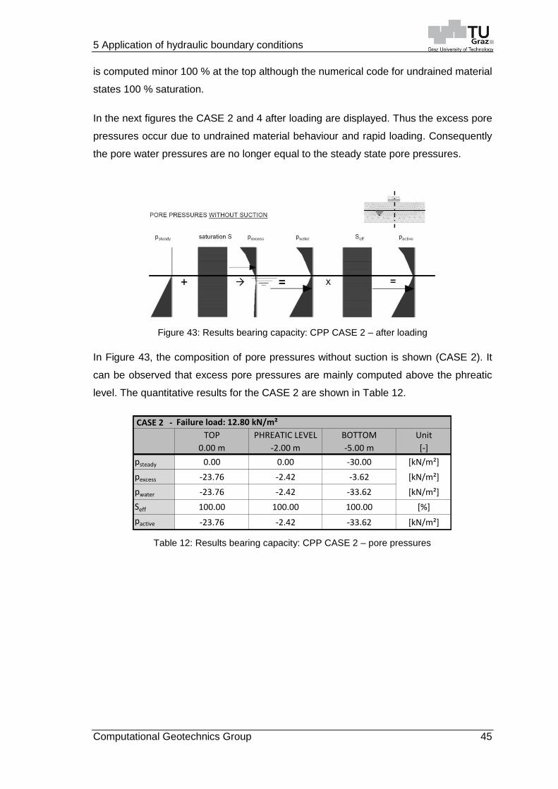
5 Application of hydraulic boundary conditions
Computational Geotechnics Group 45
is computed minor 100 % at the top although the numerical code for undrained material
states 100 % saturation.
In the next figures the CASE 2 and 4 after loading are displayed. Thus the excess pore
pressures occur due to undrained material behaviour and rapid loading. Consequently
the pore water pressures are no longer equal to the steady state pore pressures.
Figure 43: Results bearing capacity: CPP CASE 2 – after loading
In Figure 43, the composition of pore pressures without suction is shown (CASE 2). It
can be observed that excess pore pressures are mainly computed above the phreatic
level. The quantitative results for the CASE 2 are shown in Table 12.
Table 12: Results bearing capacity: CPP CASE 2 – pore pressures
CASE 2 -
TOP PHREATIC LEVEL BOTTOM Unit
0.00 m -2.00 m -5.00 m [-]
0.00 0.00 -30.00 [kN/m²]
-23.76 -2.42 -3.62 [kN/m²]
-23.76 -2.42 -33.62 [kN/m²]
100.00 100.00 100.00 [%]
-23.76 -2.42 -33.62 [kN/m²]
Failure load: 12.80 kN/m²
psteady
pexcess
pwater
Seff
pactive
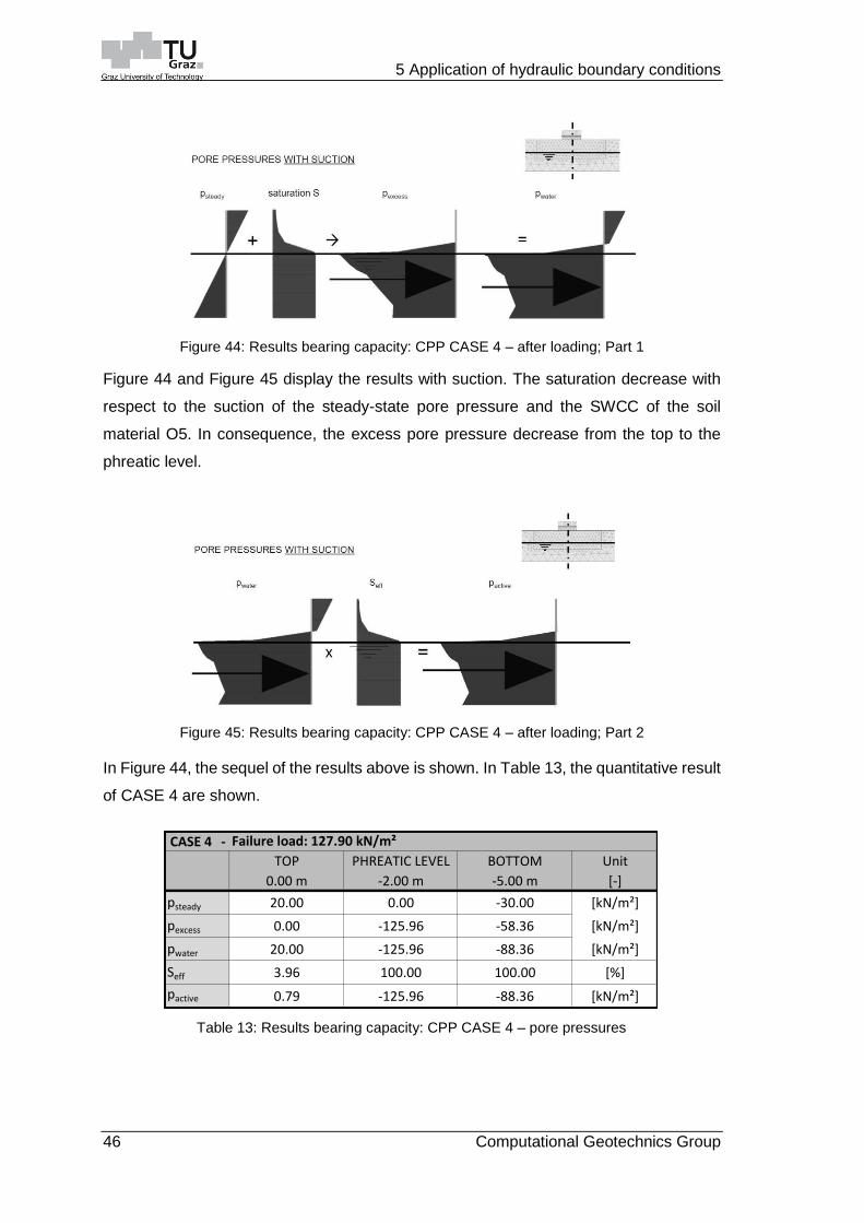
5 Application of hydraulic boundary conditions
46 Computational Geotechnics Group
Figure 44: Results bearing capacity: CPP CASE 4 – after loading; Part 1
Figure 44 and Figure 45 display the results with suction. The saturation decrease with
respect to the suction of the steady-state pore pressure and the SWCC of the soil
material O5. In consequence, the excess pore pressure decrease from the top to the
phreatic level.
Figure 45: Results bearing capacity: CPP CASE 4 – after loading; Part 2
In Figure 44, the sequel of the results above is shown. In Table 13, the quantitative result
of CASE 4 are shown.
Table 13: Results bearing capacity: CPP CASE 4 – pore pressures
CASE 4 -
TOP PHREATIC LEVEL BOTTOM Unit
0.00 m -2.00 m -5.00 m [-]
20.00 0.00 -30.00 [kN/m²]
0.00 -125.96 -58.36 [kN/m²]
20.00 -125.96 -88.36 [kN/m²]
3.96 100.00 100.00 [%]
0.79 -125.96 -88.36 [kN/m²]
Failure load: 127.90 kN/m²
psteady
pexcess
pwater
Seff
pactive

5 Application of hydraulic boundary conditions
Computational Geotechnics Group 47
5.2.4 Summary and concluding remarks
In this assessment the primary focus was on the pore water pressure composition and
its calculation. The assessed model concluded undrained and unsaturated soil
behaviour. The steady state pore pressure 𝑝𝑠𝑡𝑒𝑎𝑑𝑦 is directly generated from the
specified phreatic level. The excess pore pressures 𝑝𝑒𝑥𝑐𝑒𝑠𝑠 is a result of an undrained
analysis. The sum of them both are denoted as pore water pressure 𝑝𝑤𝑎𝑡𝑒𝑟. Furthermore
the active pore pressure 𝑝𝑎𝑐𝑡𝑖𝑣𝑒 is composed of 𝑝𝑤𝑎𝑡𝑒𝑟 and the effective saturation 𝑆𝑒𝑓𝑓,
which has a significant influence on the pore water pressure distribution. Hereof, the bulk
modulus of water correlates with the effective degree of saturation. Plaxis 2D provides
two options to define unsaturated material properties. One specification can be defined
in the material data at the tabsheet Parameter in the subtree Advanced undrained
behaviour. This calculation option directly specifies the bulk modulus as input parameter.
The second option to modify the bulk modulus is the computation by means of the soil
water characteristic curve and tensile pore pressure in the geotechnical model. Exact
this procedure is taken into account at the present assessment. Depending on the
calculation type the bulk modulus is specified in the stiffness matrix (Table 5). The
following table shows the associated failure load with respect to the different
configurations in accordance of drainage type and tensile pore pressure (suction).
Table 14: Results bearing capacity: Failure loads
Cases Soil material Drainage type Suction
[-] [-] [-] [-]
CASE 1 O5 Drained NO 128.90
CASE 2 O5 Undrained (A) NO 12.80
CASE 3 O5 Drained YES 292.30
CASE 4 O5 Undrained (A) YES 127.90
CASE 5 O12 Drained NO 277.00
CASE 6 O12 Undrained (A) NO 21.70
CASE 7 O12 Drained YES 544.20
CASE 8 O12 Undrained (A) YES 143.10
[kN/m²]
Bearing capacity

5 Application of hydraulic boundary conditions
48 Computational Geotechnics Group
5.3 Deep excavation
The geotechnical model is based on an already built structure in Vienna, the so-called
underground parking Rudolfinerhaus. The geometry and strength parameter are given,
but particularly the geometry have been modified. The missing stiffness parameters were
adopted.
5.3.1 Aim of geotechnical model
The emphasis of this analyses were investigating the state conditioning the ultimate limit
with respect to the time-dependent dissipation of excess pore pressure in undrained
soils. Tensile excess pore pressures develop due to unloading and have a positive
influence with respect to strength. Therefore the appropriate computation of pore
pressures are important, particularly the specification of the hydraulic conditions
regarding to the associated groundwater flow model. Hereof, an undrained analysis with
the material data set Undrained (A) and the corresponding calculation type was
conducted. Furthermore, a fully coupled flow-deformation with the associated hydraulic
boundary conditions was computed in order to double-check the aforementioned
analysis.
5.3.2 Model configuration and material parameters
The excavation pit is 24.0 m wide and 13.0 m deep. Due to the symmetric geometry only
half of the excavation is modelled (Figure 46). The model has a dimension of 65.0 m in
width and 48.0 m in depth. A plane-strain model with 15 noded-elements is utilized.
Figure 46: Deep excavation: Model

5 Application of hydraulic boundary conditions
Computational Geotechnics Group 49
The soil stratigraphy consist of three horizontal layers. The top layer is called Fill and is
5.0 m thick. The middle soil layer is specified as Sand and is located between GL -5.0 m
and GL -12.70 m. The last layer consist of Wiener Tegel, starts at GL -12.70 m and
reaches the bottom model boundary at GL -48.0 m. Further at GL -3.0 m exist a phreatic
level. All materials are assumed as undrained and specified with the constitutive model
Hardening soil-small strain stiffness (HSS). The brace system is a bore pile wall with
diameters of 0.80 m and embedded 7.0 m deep in the Wiener Tegel, thus the total length
is 20.0 m. The bore pile wall is modelled by means of continuous elements. A strut at the
level GL -1.50 is installed in order to minimize the top deflection. The whole brace system
is specified as linear elastic. The material parameter are summarized in the following
tables.

5 Application of hydraulic boundary conditions
50 Computational Geotechnics Group
Table 15: Deep excavation: Soil parameter
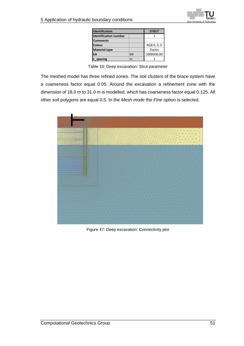
5 Application of hydraulic boundary conditions
Computational Geotechnics Group 51
Table 16: Deep excavation: Strut parameter
The meshed model has three refined zones. The soil clusters of the brace system have
a coarseness factor equal 0.05. Around the excavation a refinement zone with the
dimension of 18.0 m to 31.0 m is modelled, which has coarseness factor equal 0.125. All
other soil polygons are equal 0.5. In the Mesh mode the Fine option is selected.
Figure 47: Deep excavation: Connectivity plot
Identification STRUT
Identification number 1
Comments
Colour RGB 0, 0, 0
Material type Elastic
EA kN 2000000,00
L_spacing m 1

5 Application of hydraulic boundary conditions
52 Computational Geotechnics Group
The excavation work will be executed in four steps. Within the four steps the water level
in the excavation zone is lowered always 0.5 m below the actual depth. Generally an
undrained analysis will be computed by means of CT Plastic (Figure 48, green).
Figure 48: Deep excavation: Plastic – calculation phases
In order to double-check the results a fully coupled flow-deformation analysis with the
same calculation procedure is conducted as well. The Table 17 shows an overview about
the calculation types and the associated specifications.
Table 17: Deep excavation: Calculation types
CASE PL CASE FCFD
2 water levels1 inclined water level and
GWFlowBase BC
Symmetry boundary closed Symmetry boundary closed
Phasesno time interval, interest of
sequenced results
Concept of construction time
with respect to soil behaviour
Calculation type
(CT)Plastic FCFD
Undrained
behaviour (UD)Undrained [A] Permeability, stiffness, time
Pore pressure
calculation type
(PPCT)
Phreatic TGWF*
Hydraulic
conditions (HC)
ULS
* Implicity transient flow calculation
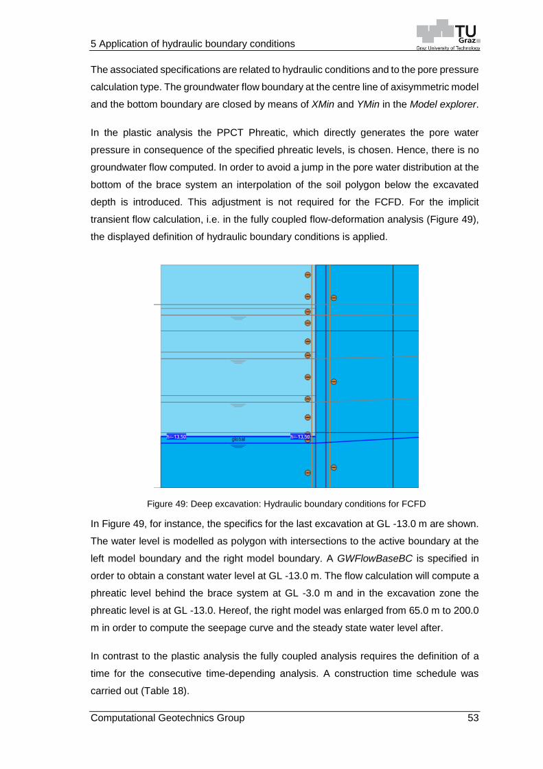
5 Application of hydraulic boundary conditions
Computational Geotechnics Group 53
The associated specifications are related to hydraulic conditions and to the pore pressure
calculation type. The groundwater flow boundary at the centre line of axisymmetric model
and the bottom boundary are closed by means of XMin and YMin in the Model explorer.
In the plastic analysis the PPCT Phreatic, which directly generates the pore water
pressure in consequence of the specified phreatic levels, is chosen. Hence, there is no
groundwater flow computed. In order to avoid a jump in the pore water distribution at the
bottom of the brace system an interpolation of the soil polygon below the excavated
depth is introduced. This adjustment is not required for the FCFD. For the implicit
transient flow calculation, i.e. in the fully coupled flow-deformation analysis (Figure 49),
the displayed definition of hydraulic boundary conditions is applied.
Figure 49: Deep excavation: Hydraulic boundary conditions for FCFD
In Figure 49, for instance, the specifics for the last excavation at GL -13.0 m are shown.
The water level is modelled as polygon with intersections to the active boundary at the
left model boundary and the right model boundary. A GWFlowBaseBC is specified in
order to obtain a constant water level at GL -13.0 m. The flow calculation will compute a
phreatic level behind the brace system at GL -3.0 m and in the excavation zone the
phreatic level is at GL -13.0. Hereof, the right model was enlarged from 65.0 m to 200.0
m in order to compute the seepage curve and the steady state water level after.
In contrast to the plastic analysis the fully coupled analysis requires the definition of a
time for the consecutive time-depending analysis. A construction time schedule was
carried out (Table 18).

5 Application of hydraulic boundary conditions
54 Computational Geotechnics Group
According to the time schedule the groundwater lowering takes 1/24 of daytime in
consideration to compute steady state pore pressures with respect to hydraulic boundary
conditions (Figure 49). The excavation time for 3.1 m to 3.3 m deep layer is specified
with 7/50 d by means of the ratio excavation sequence time and an assumed length.
Afterwards a consolidation with 7 days is conducted.
Figure 50: Deep excavation: FCFD – calculation phases
Table 18: Deep excavation: Construction time schedule

5 Application of hydraulic boundary conditions
Computational Geotechnics Group 55
After all specifications for hydraulic conditions, pore pressure calculation and soil
behaviour are defined, the results of this two different calculation are presented in the
next chapter. Further informations about the excavation sequence can be found in the
Appendix.

5 Application of hydraulic boundary conditions
56 Computational Geotechnics Group
5.3.3 Output
First computations showed that the ultimate limit state for the current brace system was
not given, hence the embedded depth was enlarged with 6.0 m. Thus the total length of
the bore pile is equal to 26.0 m instead of 20.0 m in the initial model (Figure 51).
Figure 51: Deep excavation: Bore pile wall 26.0 m
Two cases of calculations with same geometry were carried out. The CASE 5 was a
plastic analysis and CASE 7 was a fully coupled analysis (Table 19).
Table 19: Deep excavation: Calculations
In the table the results of the final consolidation after the last excavation are mentioned.
The final consolidation was computed for 28 days with respect to the finished work of a
future concrete slab.
ΣMStage FailureConsolidation
(28d)
Max. bending
moments (28d)
Max. shear force
(28d)
Max. displacements
(28d)
[-] [-] [kN/m²] [kNm/m] [kN/m] [m]
CASE 5 0.9998
NO
4th Excavation does
not reached MStage
27.45 1977.4 612.50 0.037
CASE 7 1.0000 NO 17.63 1977.00 605.50 0.045
Ultimate Limit State analysis (ULS)

5 Application of hydraulic boundary conditions
Computational Geotechnics Group 57
Figure 52: Results deep excavation: Excess pore pressure comparison
In Figure 52 the excess pore pressure for CASE 5 (a) and for CASE 7 (b) are displayed.
The maximum value in figure (a) is 27.45 kN/m² in contrast to CASE 5 the maximum
value is equal to 17.63 kN/m² for CASE 7. In consideration that the excess pore pressure
show similar results, the pore water pressure should display similar results too, because
𝑝𝑤𝑎𝑡𝑒𝑟 in the CT Consolidation is composed of 𝑝𝑒𝑥𝑐𝑒𝑠𝑠 and 𝑝𝑠𝑡𝑒𝑎𝑑𝑦.
Figure 53: Results deep excavation: Pore water pressure comparison
In Figure 53 the pore water pressures of the plastic analysis (a) and of a fully coupled
(b) analysis are displayed. Hereof, the next Figure 54 present a section at the centre of
the excavation pit, i.e. at 6.0m in x-direction.
a) b)
a) b)
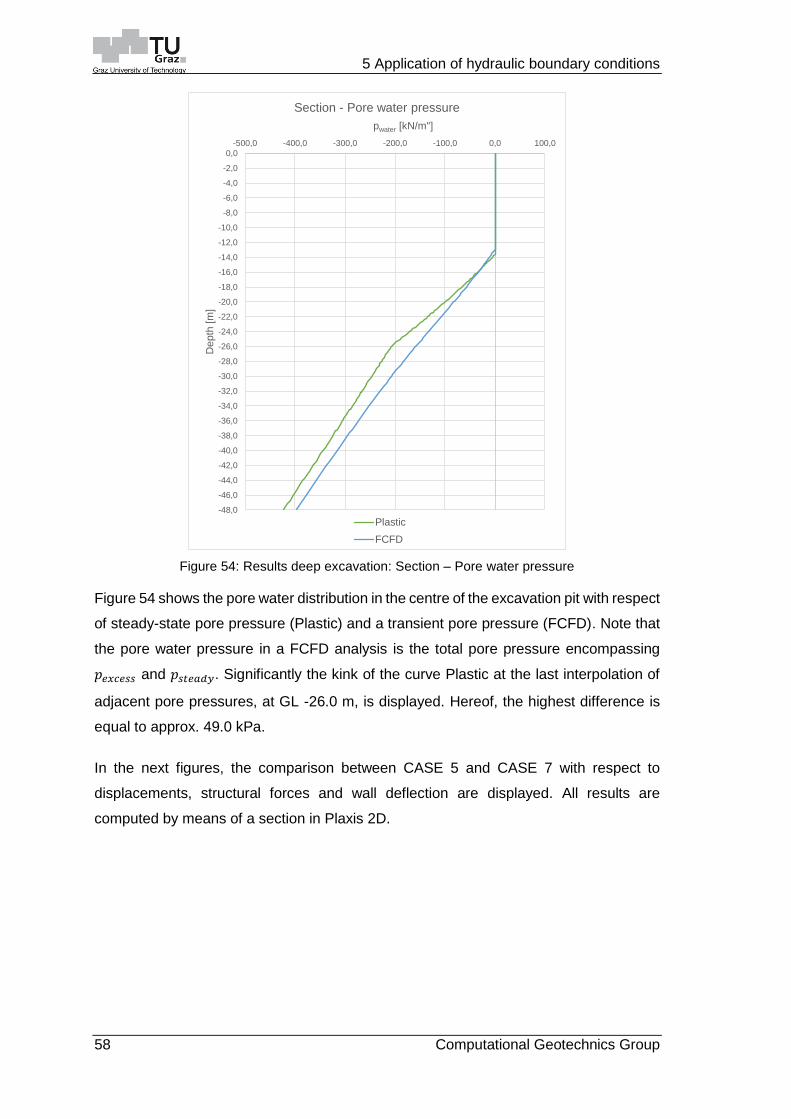
5 Application of hydraulic boundary conditions
58 Computational Geotechnics Group
Figure 54: Results deep excavation: Section – Pore water pressure
Figure 54 shows the pore water distribution in the centre of the excavation pit with respect
of steady-state pore pressure (Plastic) and a transient pore pressure (FCFD). Note that
the pore water pressure in a FCFD analysis is the total pore pressure encompassing
𝑝𝑒𝑥𝑐𝑒𝑠𝑠 and 𝑝𝑠𝑡𝑒𝑎𝑑𝑦. Significantly the kink of the curve Plastic at the last interpolation of
adjacent pore pressures, at GL -26.0 m, is displayed. Hereof, the highest difference is
equal to approx. 49.0 kPa.
In the next figures, the comparison between CASE 5 and CASE 7 with respect to
displacements, structural forces and wall deflection are displayed. All results are
computed by means of a section in Plaxis 2D.
-48,0
-46,0
-44,0
-42,0
-40,0
-38,0
-36,0
-34,0
-32,0
-30,0
-28,0
-26,0
-24,0
-22,0
-20,0
-18,0
-16,0
-14,0
-12,0
-10,0
-8,0
-6,0
-4,0
-2,0
0,0
-500,0 -400,0 -300,0 -200,0 -100,0 0,0 100,0
Depth
[m
]
pwater [kN/m"]
Section - Pore water pressure
Plastic
FCFD
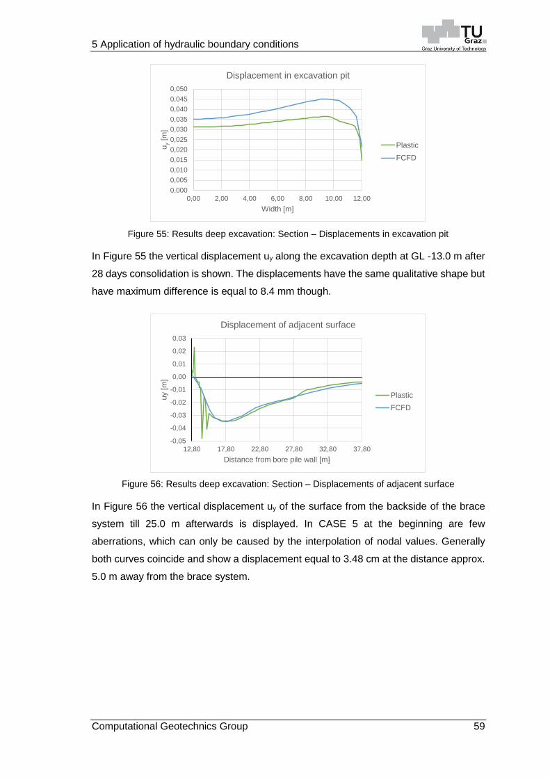
5 Application of hydraulic boundary conditions
Computational Geotechnics Group 59
Figure 55: Results deep excavation: Section – Displacements in excavation pit
In Figure 55 the vertical displacement uy along the excavation depth at GL -13.0 m after
28 days consolidation is shown. The displacements have the same qualitative shape but
have maximum difference is equal to 8.4 mm though.
Figure 56: Results deep excavation: Section – Displacements of adjacent surface
In Figure 56 the vertical displacement uy of the surface from the backside of the brace
system till 25.0 m afterwards is displayed. In CASE 5 at the beginning are few
aberrations, which can only be caused by the interpolation of nodal values. Generally
both curves coincide and show a displacement equal to 3.48 cm at the distance approx.
5.0 m away from the brace system.
0,000
0,005
0,010
0,015
0,020
0,025
0,030
0,035
0,040
0,045
0,050
0,00 2,00 4,00 6,00 8,00 10,00 12,00
uy
[m]
Width [m]
Displacement in excavation pit
Plastic
FCFD
-0,05
-0,04
-0,03
-0,02
-0,01
0,00
0,01
0,02
0,03
12,80 17,80 22,80 27,80 32,80 37,80
uy [
m]
Distance from bore pile wall [m]
Displacement of adjacent surface
Plastic
FCFD

5 Application of hydraulic boundary conditions
60 Computational Geotechnics Group
Figure 57: Results deep excavation: Section – Structural force
The figures above show the structural forces bending moment and shear force, which
are computed by means of a section along the centre line of the bore pile wall. In both
cases, the forces coincide perfectly. The maximum bending moment is equal to approx.
1977.00 kNm. The quantitative results of the shear forces are slightly different. The
maximum value of CASE 5 is equal to 612.50 kN and in CASE 7 the shear force is 605.50
kN. A reason could be the output by means of a section, because it takes into account
the adjacent nodal values and stress points.
-26,0
-25,0
-24,0
-23,0
-22,0
-21,0
-20,0
-19,0
-18,0
-17,0
-16,0
-15,0
-14,0
-13,0
-12,0
-11,0
-10,0
-9,0
-8,0
-7,0
-6,0
-5,0
-4,0
-3,0
-2,0
-1,0
0,0
-1000,0 0,0 1000,0 2000,0 3000,0
De
pth
[m
]Bending moment [kNm]
Section - Bending moment
Plastic
FCFD
-26,0
-25,0
-24,0
-23,0
-22,0
-21,0
-20,0
-19,0
-18,0
-17,0
-16,0
-15,0
-14,0
-13,0
-12,0
-11,0
-10,0
-9,0
-8,0
-7,0
-6,0
-5,0
-4,0
-3,0
-2,0
-1,0
0,0
-1000,00 0,00 1000,00
De
pth
[m
]
Shear force [kN]
Section - Shear force
Plastic
FCFD

5 Application of hydraulic boundary conditions
Computational Geotechnics Group 61
Figure 58: Results deep excavation: Section – Wall deflection
In Figure 58 the horizontal displacements of the bore pile wall are displayed. The results
are computed by means of a section in the centre line. The maximum deflection is 5.50
cm, which is located at the depth of approx. 10.50 m below the surface.
Note that the present total length of the pore pile wall is equal to 26.0 m, thus the
embedded length in the soil layer Tegel is equal to 13.0 m. In consequence of the
influence of tensile pore pressures with respect to the strength, the strength of the
associated soil layer decreases due to the dissipation of pore pressures to a minimum.
Hereof, a final consolidation with a minimum excess pore pressure equal to 1.0 kPa
instead of 28 days is computed. While performing this calculation, the state conditioning
the ultimate limit may be reached with respect to the embedded length. Consequently,
the embedded length could be modified. Accordingly these final calculations have been
performed and show following results.
-26,00
-25,00
-24,00
-23,00
-22,00
-21,00
-20,00
-19,00
-18,00
-17,00
-16,00
-15,00
-14,00
-13,00
-12,00
-11,00
-10,00
-9,00
-8,00
-7,00
-6,00
-5,00
-4,00
-3,00
-2,00
-1,00
0,00
-0,06 -0,04 -0,02 0,00 0,02
De
pth
[m
]
Displacement ux [m]
Section - wall deflection
Plastic
FCFD

5 Application of hydraulic boundary conditions
62 Computational Geotechnics Group
Table 20: Deep excavation: Calculation cases
Table 20 shows the computed plastic analyses with respect to different embedded
lengths. The embedded length was reduced by 1.0 m from the initial state of 13.0 m
length. In CASE 12, the embedded length is the minimum length, because in CASE 13
the brace system fails and the surrounding soil collapses in phases before the final
consolidation can be computed. Furthermore the reached time of dissipating excess pore
pressure to the minimum equal to 1.0 kPa are displayed. The results concluding wall
deflections, bending moments and factor of safety with respect to the fulfilled analyses
conditioning limit state are shown in the following figures.
Figure 59: Results deep excavation: Sections – Embedded length
Calculation type Embedded length
[m]
Failure Reached total time
[day]
CASE 5 Plastic 13.0 m NO 189
CASE 12 Plastic 12.0 m NO 241
CASE 13 Plastic 11.0 m YES 0
-26,0
-25,0
-24,0
-23,0
-22,0
-21,0
-20,0
-19,0
-18,0
-17,0
-16,0
-15,0
-14,0
-13,0
-12,0
-11,0
-10,0
-9,0
-8,0
-7,0
-6,0
-5,0
-4,0
-3,0
-2,0
-1,0
0,0
-0,10 -0,05 0,00 0,05
Depth
[m
]
Wall deflection [m]
Section - Wall deflection
CASE 5
CASE 12
-26,0
-25,0
-24,0
-23,0
-22,0
-21,0
-20,0
-19,0
-18,0
-17,0
-16,0
-15,0
-14,0
-13,0
-12,0
-11,0
-10,0
-9,0
-8,0
-7,0
-6,0
-5,0
-4,0
-3,0
-2,0
-1,0
0,0
-1000,0 0,0 1000,0 2000,0 3000,0
De
pth
[m
]
Bending moment [kNm]
Section - Bending moment
CASE 5
CASE 12

5 Application of hydraulic boundary conditions
Computational Geotechnics Group 63
In Figure 59, the wall deflection and bending moments with respect to the CASE 5 and
CASE 12 are displayed. The results are computed by means of a section in the centre
line of the bore pile wall. The CASE 12 show slightly higher values in contrast to CASE
5, for instance, the maximum difference between the associated wall deflections is 5.0
mm. The difference between the bending moments is 102.40 kNm.
The next figures show the computations of global safety regarding to CASE 5 and CASE
12. The factor of safety (FOS) have been computed by means of a safety analysis,
wherein the undrained behaviour was ignored in order to calculate a constant FOS.
Figure 60: Results deep excavation: Incremental deviatoric strains – CASE 5
Figure 60 displays the incremental deviatoric strains with respect to CASE 5.
Furthermore the associated point for the FOS analyses is depicted (red point).
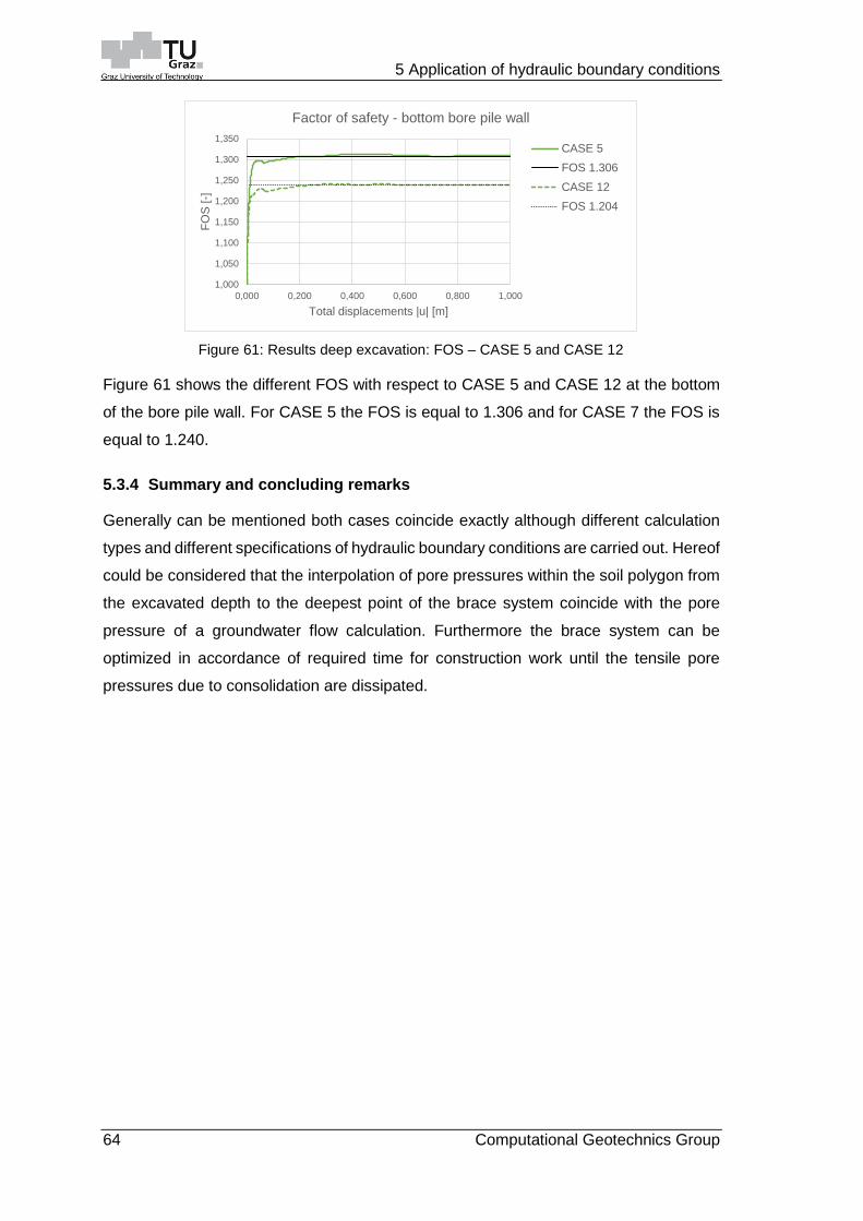
5 Application of hydraulic boundary conditions
64 Computational Geotechnics Group
Figure 61: Results deep excavation: FOS – CASE 5 and CASE 12
Figure 61 shows the different FOS with respect to CASE 5 and CASE 12 at the bottom
of the bore pile wall. For CASE 5 the FOS is equal to 1.306 and for CASE 7 the FOS is
equal to 1.240.
5.3.4 Summary and concluding remarks
Generally can be mentioned both cases coincide exactly although different calculation
types and different specifications of hydraulic boundary conditions are carried out. Hereof
could be considered that the interpolation of pore pressures within the soil polygon from
the excavated depth to the deepest point of the brace system coincide with the pore
pressure of a groundwater flow calculation. Furthermore the brace system can be
optimized in accordance of required time for construction work until the tensile pore
pressures due to consolidation are dissipated.
1,000
1,050
1,100
1,150
1,200
1,250
1,300
1,350
0,000 0,200 0,400 0,600 0,800 1,000
FO
S [-]
Total displacements |u| [m]
Factor of safety - bottom bore pile wall
CASE 5
FOS 1.306
CASE 12
FOS 1.204

6 Summary and conclusion
Computational Geotechnics Group 65
6 Summary and conclusion
Generally the available hydraulic boundary condition in the borehole command,
Selection explorer, the Model explorer and the material data tabsheet can be used to
define the appropriate groundwater model in accordance with the geotechnical model.
Thereby should considered some specifications in context of the available hydraulic
boundary conditions, which can cause shortcomings.
In the Selection explorer, the hydraulic model conditions, e.g. GWFlowBaseBC and
WaterConditions are utilized, which can be enabled by selecting and specifying the
hydraulic condition for the boundary value problem in the FEM analysis. For instance the
HBC Closed or Head define the BVP condition by means of the specified value. This
value is computed as a constant with possible numerical deviations due to a coarse mesh
next to the associated boundary. Thus, when specifying a GWFlowBaseBC or phreatic
level, a mesh refinement is advisable. By modelling a water reservoir with a dam
structure the pertained water level within the dam structure will be not affected by the
global precipitation, i.e. no rise of water level is computed. Likewise the pore pressure
below the water level will not change in the soil polygons. In order to compute a water
level rise the corresponding HeadFunction can be used. However, the specified
GWFlowBaseBC will be only computed if a groundwater flow calculation is conducted.
The option in the WaterConditions of a soil polygon correlates with the tabsheet Water
in the command Create borehole. By using this modification for a soil stratigraphy the
associated HBC will be automatically stated in the Flow conditions mode. Note that the
specified water levels are BoreholeWaterlevel’s, which cannot be modified anyway with
the features Flow functions. The three most important water conditions for soil clusters
are Global level, Custom level and Interpolate. They need to be specified if more than
two water levels are defined in the geotechnical model. Particularly the option Interpolate
must be used, if for instance an impermeable structure is present between two water
levels and direct generation of pore pressures, e.g. PPCT Phreatic is utilized.
Furthermore, the specified water levels, e.g. one BoreholeWaterLevel and one
UserWaterLevel or two UserWaterLevel respectively, need an intersection with an active
model boundary. The intersection must be specified in order to postulate the hydraulic
condition in the BVP. Note for inclined water levels the model boundaries need to be
extended in accordance of a flow calculation, because Plaxis 2D will compute an
inflowing water table, which converge with the horizontal water level at larger distance
from the structure.
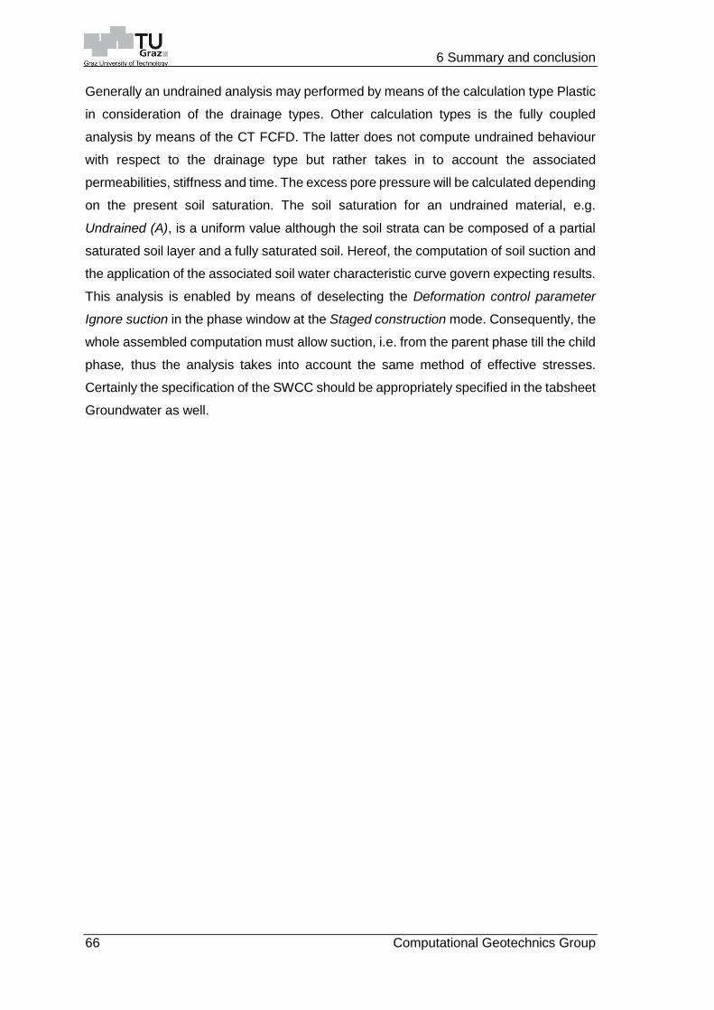
6 Summary and conclusion
66 Computational Geotechnics Group
Generally an undrained analysis may performed by means of the calculation type Plastic
in consideration of the drainage types. Other calculation types is the fully coupled
analysis by means of the CT FCFD. The latter does not compute undrained behaviour
with respect to the drainage type but rather takes in to account the associated
permeabilities, stiffness and time. The excess pore pressure will be calculated depending
on the present soil saturation. The soil saturation for an undrained material, e.g.
Undrained (A), is a uniform value although the soil strata can be composed of a partial
saturated soil layer and a fully saturated soil. Hereof, the computation of soil suction and
the application of the associated soil water characteristic curve govern expecting results.
This analysis is enabled by means of deselecting the Deformation control parameter
Ignore suction in the phase window at the Staged construction mode. Consequently, the
whole assembled computation must allow suction, i.e. from the parent phase till the child
phase, thus the analysis takes into account the same method of effective stresses.
Certainly the specification of the SWCC should be appropriately specified in the tabsheet
Groundwater as well.

7 Literature
Computational Geotechnics Group 67
7 Literature
Fredlund, D. G.; Rahardjo, H.; Fredlund, Murray D. (2012) Unsaturated soil mechanics in engineering practice; Hoboken N.J., John Wiley&Son
Galavi V., (2010) Groundwater flow, fully coupled flow deformation and undrained analyses in Plaxis 2D and 3D; Internal Report, Delft, Plaxis
Kolymbas D, (2011) Geotechnik, Bodenmechanik, Grundbau und Tunnelbau, 3. Auflage, Heidelberg, Springer
Nuth M., Laloui L., (2007), Effective stress concept in unsaturated soils: Clarification and validation of a unified framework; International Journal for Numerical and Analytical Methods In Geomechanics, Wiley InterScience, Vol. 32, p. 771-801
Plaxis 2D Manual, (2016), Plaxis 2D, Version 2016.01, Tutorial Manual, Reference Manual, Scientific Manual; Delft
Staring H.C.W, (1842) Handboek voor verdrinkenden en liefhebbers van varen, 1842
Terzaghi K., (1925) Theoretical Soil Mechanics, New York, John Wiley & Sons, Inc.


Appendix

Appendix
II Computational Geotechnics Group

Appendix
Computational Geotechnics Group III
SX - GWFlowBaseBC: Head – Uniform and Start/End
GWFlowBase BC Head: Uniform – a) psteady, b) pexcess, c) pwater
a) b) c)

Appendix
IV Computational Geotechnics Group
GWFlowBase BC Head: Start/ End – a) psteady, b) pexcess, c) pwater
a) b) c)

Appendix
Computational Geotechnics Group V
WaterConditions: Dry
Geotechnical model: dry cluster
Output : Pore water pressure 𝑝𝑤𝑎𝑡𝑒𝑟
Section: Pore water pressure
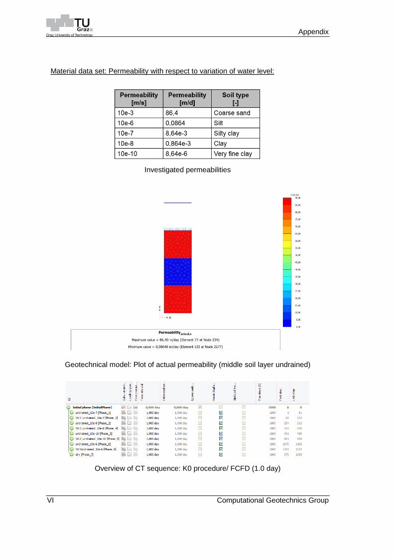
Appendix
VI Computational Geotechnics Group
Material data set: Permeability with respect to variation of water level:
Investigated permeabilities
Geotechnical model: Plot of actual permeability (middle soil layer undrained)
Overview of CT sequence: K0 procedure/ FCFD (1.0 day)

Appendix
Computational Geotechnics Group VII
Actual permeability 10-6 vs excess pore pressure: a) constant WL, b) WL rise
Actual permeability 10-7 vs excess pore pressure: a) constant WL, b) WL rise
Actual permeability 10-8 vs excess pore pressure: a) constant WL, b) WL rise
a) b)
a)
b)
a)
b)

Appendix
VIII Computational Geotechnics Group
Water level: Important specifications:
Plaxis 2D Tutorial: Dry excavation – Intersection point
Dry excavation: Incorrect PPCT - Phreatic

Appendix
Computational Geotechnics Group IX
Dry Excavation: PCCT Steady-State groundwater flow
Dry Excavation: PCCT Transient groundwater flow
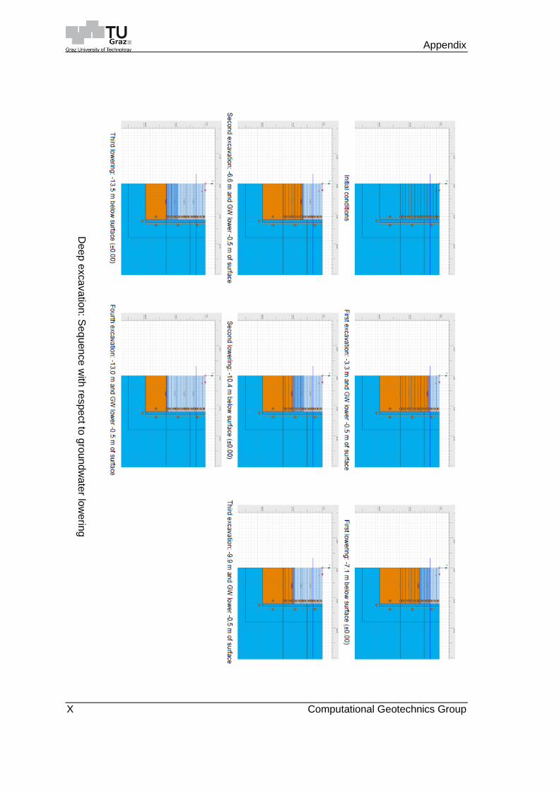
Appendix
X Computational Geotechnics Group
De
ep
exca
va
tion: S
equ
en
ce w
ith re
spe
ct to
gro
un
dw
ate
r low
erin
g

Appendix
Computational Geotechnics Group XI
De
ep
exca
va
tion:
Se
qu
en
ce w
ith
re
spe
ct to
gro
un
dw
ate
r lo
we
ring