
Modeling History to Understand Software Evolution
190
to Understand Software Evolution Modeling History vorgelegt von Tudor Gîrba von Rumänien Inauguraldissertation der Philosophisch-naturwissenschaftlichen Fakultät der Universität Bern Leiter der Arbeit: Prof. Dr. Stéphane Ducasse Prof. Dr. Oscar Nierstrasz Institut für Informatik und angewandte Mathematik
Transcript of Modeling History to Understand Software Evolution

to Understand Software Evolution
Modeling History
vorgelegt von
Tudor Gîrbavon Rumänien
Inauguraldissertation der Philosophisch-naturwissenschaftlichen
Fakultät der Universität Bern
Leiter der Arbeit:
Prof. Dr. Stéphane DucasseProf. Dr. Oscar Nierstrasz
Institut für Informatik und angewandte Mathematik


to Understand Software Evolution
Modeling History
vorgelegt von
Tudor Gîrbavon Rumänien
Inauguraldissertation der Philosophisch-naturwissenschaftlichen Fakultät der Universität Bern
Leiter der Arbeit:
Prof. Dr. Stéphane DucasseProf. Dr. Oscar Nierstrasz
Institut für Informatik und angewandte Mathematik
Von der Philosophisch-naturwissenschaftlichen Fakultät angenommen.
Bern, 14.11.2005 Der Dekan: Prof. Dr. P. Messerli


Acknowledgments
The work presented here goes well beyond the words and pictures, and into thevery intimate corners of my existence. This work only holds what can be repre-sented, while the real value lies somewhere in between me and the people thatsurrounded me.
I am grateful to Stephane Ducasse and to Oscar Nierstrasz for giving me the op-portunity to work at Software Composition Group based only on my engagementthat I will be an “even better student.” Stef, you were always energetic and sup-ported me in so many ways. Oscar, you gave me the balance I needed at difficulttimes. Thank you both for being more than my supervisors.
I thank Harald Gall for promptly accepting to be an official reviewer, as well as forthe good time we had at various meetings. I thank Gerhard Jager for accepting tochair the examination.
Radu Marinescu was my first contact with research, yet it was not only researchthat he introduced me to. We had great and fruitful times together. Radu, I amgrateful for many things, but most of all for the time we spent around a blackliquid.
Michele Lanza pushed and promoted me with every occasion he could find. Michele,thank you for all the discussions, projects and the cool trips. I hope they will neverstop.
Roel Wuyts encouraged me all along the way, and together with his wife, Inge,shared their house with me during my first days in Berne. Roel and Inge, thankyou for making me feel like at home in a foreign country.
Jean-Marie Favre was always fun to work with. Jean-Marie, thank you for intro-

ducing me to the different facets of the meta world.
I thank Serge Demeyer for offering to review this dissertation. Serge, I was sur-prised and I was delighted.
Many thanks go to the Software Composition Group members. I thank Orla Greevyfor trusting me and for reviewing this dissertation. I thank Gabriela Arevalo forthe patience of sharing her incredible skills of dealing with the curse of the mod-ern man: the bureaucracy. I thank Alex Bergel for not being tired of playingchess, Markus Galli for the small-but-not-short-talks, Marcus Denker for alwaysbeing calm and supportive, Laura Ponisio for encouraging me to eat healthier,Matthias Rieger for the best movie discussions, and Juan Carlos Cruz for thenice parties. Thanks go to Sander Tichelaar for never being upset with my badjokes, Adrian Lienhard and Nathanael Scharli for showing me the Swiss way, andTherese Schmid for her kindness throughout the years.
Much of this work came out from the collaboration with my diploma students:Thomas Buhler, Adrian Kuhn, Mircea Lungu, Daniel Ratiu, Mauricio Seeberger.Daniel was my first diploma student and he had the patience of transforming myindecision from the beginning into something constructive. Mircea always founda way to make me exercise other perspectives. Thomas was a hard worker. Adrianand Mauricio made a great and joyful team together. Thank you all for treatingme as your peer.
I am grateful to my Hilfsassistants – Niklaus Haldiman, Stefan Ott and StefanReichhart – for making my life so easy during the ESE lecture.
I thank the people at the LOOSE Research Group: Iulian Dragos, Razvan Fil-ipescu, Cristina Marinescu, Petru Mihancea, Mircea Trifu. I also thank the peoplethat I met throughout my computer related existence, and that influenced me inone way or another: Bobby Bacs, Dan Badea, Dan Corneanu, Stefan Dicu, DannyDig, Bogdan Hodorog, Radu Jurca, Gerry Kirschner, Razvan Pocaznoi, Adi Pop,Adi Trifu.
Much of me roots in the years of high-school, and for that I thank: Ciprian Ghir-dan, Sorin Kertesz, Serban Filip, Bogdan Martin, Cosmin Mocanu, Sergiu Tent. Ithank Andrei Mitrasca for not being tired of talking nonsense with me, and I thankCodrut and Bianca Morariu for being the best “finuti” me and Oana have.
I thank Razvan and Silvia Tudor for the many visits to Bern, and I hope thesevisits will not stop.

Sorin and Camelia Ciocan took me in their home when I was alone. Thank you forbeing the friends you are for both me and Oana.
Nothing would have been possible were it not for my beloved parents. I thank youfor being patient with me when I did not understand, and for believing in me whenyou did not understand. Thank you for keeping me safe and happy.
I thank Sorin, Corina and Ovidiu for taking care of my parents.
I will never forget the countless trips to and from Budapest together with Adinaand Claudiu Pantea. Thank you for the support and cheer.
Aura and Ionica Popa made me part of their family as if this was the most naturalthing of all. Thank you for being the great in-laws that you are.
The joy of these years came from the love of my wife, and if I had success itwas due to her unconditional support. Oana, my thanks to you extend beyondreasons, although there are plenty of reasons. This work is dedicated to you andyour smile.
October 23, 2005Tudor Gırba


To Oana


Abstract
Over the past three decades, more and more research has been spent on under-standing software evolution. The development and spread of versioning systemsmade valuable data available for study. Indeed, versioning systems provide richinformation for analyzing software evolution, but it is exactly the richness of theinformation that raises the problem. The more versions we consider, the moredata we have at hand. The more data we have at hand, the more techniques weneed to employ to analyze it. The more techniques we need, the more generic theinfrastructure should be.
The approaches developed so far rely on ad-hoc models, or on too specific meta-models, and thus, it is difficult to reuse or compare their results. We argue for theneed of an explicit and generic meta-model for allowing the expression and com-bination of software evolution analyses. We review the state-of-the-art in softwareevolution analysis and we conclude that:
To provide a generic meta-model for expressing software evolu-tion analyses, we need to recognize the evolution as an explicitphenomenon and model it as a first class entity.
Our solution is to encapsulate the evolution in the explicit notion of history as asequence of versions, and to build a meta-model around these notions: Hismo. Toshow the usefulness of our meta-model we exercise its different characteristics bybuilding several reverse engineering applications.
This dissertation offers a meta-model for software evolution analysis yet, the con-cepts of history and version do not necessarily depend on software. We show howthe concept of history can be generalized and how we can obtain our meta-modelby transformations applied on structural meta-models. As a consequence, ourapproach of modeling evolution is not restricted to software analysis, but can beapplied to other fields as well.

Table of Contents
1 Introduction 11.1 The Problem of Meta-Modeling Software Evolution . . . . . . . . . . . 21.2 Our Approach in a Nutshell . . . . . . . . . . . . . . . . . . . . . . . . 41.3 Contributions . . . . . . . . . . . . . . . . . . . . . . . . . . . . . . . . . 51.4 Structure of the Dissertation . . . . . . . . . . . . . . . . . . . . . . . . 7
2 Approaches to Understand Software Evolution 112.1 Introduction . . . . . . . . . . . . . . . . . . . . . . . . . . . . . . . . . 122.2 Version-Centered Approaches . . . . . . . . . . . . . . . . . . . . . . . 13
2.2.1 Analyzing the Changes Between Two Versions . . . . . . . . . . 132.2.2 Analyzing Property Evolutions: Evolution Chart . . . . . . . . . 142.2.3 Evolution Matrix Visualization . . . . . . . . . . . . . . . . . . . 162.2.4 Discussion of Version-Centered Approaches . . . . . . . . . . . 18
2.3 History-Centered Approaches . . . . . . . . . . . . . . . . . . . . . . . 192.3.1 History Measurements . . . . . . . . . . . . . . . . . . . . . . . 192.3.2 Manipulating Historical Relationships: Historical
Co-Change . . . . . . . . . . . . . . . . . . . . . . . . . . . . . . 212.3.3 Manipulating Historical Entities: Hipikat and Release
Meta-Models . . . . . . . . . . . . . . . . . . . . . . . . . . . . . 232.3.4 Discussion of History-Centered Approaches . . . . . . . . . . . 24
2.4 Towards a Common Meta-Model for Understanding Software Evolution 252.5 Roadmap . . . . . . . . . . . . . . . . . . . . . . . . . . . . . . . . . . . 27
3 Hismo: Modeling History as a First Class Entity 293.1 Introduction . . . . . . . . . . . . . . . . . . . . . . . . . . . . . . . . . 30

3.2 Hismo . . . . . . . . . . . . . . . . . . . . . . . . . . . . . . . . . . . . . 303.3 Building Hismo Based on a Snapshot Meta-Model . . . . . . . . . . . 323.4 Mapping Hismo to the Evolution Matrix . . . . . . . . . . . . . . . . . 343.5 History Properties . . . . . . . . . . . . . . . . . . . . . . . . . . . . . . 353.6 Grouping Histories . . . . . . . . . . . . . . . . . . . . . . . . . . . . . . 393.7 Modeling Historical Relationships . . . . . . . . . . . . . . . . . . . . . 413.8 Generalization . . . . . . . . . . . . . . . . . . . . . . . . . . . . . . . . 433.9 Summary . . . . . . . . . . . . . . . . . . . . . . . . . . . . . . . . . . . 45
4 Yesterday’s Weather 474.1 Introduction . . . . . . . . . . . . . . . . . . . . . . . . . . . . . . . . . 484.2 Yesterday’s Weather in a Nutshell . . . . . . . . . . . . . . . . . . . . . 494.3 Yesterday’s Weather in Detail . . . . . . . . . . . . . . . . . . . . . . . 504.4 Validation . . . . . . . . . . . . . . . . . . . . . . . . . . . . . . . . . . . 54
4.4.1 Yesterday’s Weather in Jun, CodeCrawler and JBoss . . . . . . 554.4.2 The Evolution of Yesterday’s Weather in Jun . . . . . . . . . . . 59
4.5 Variation Points . . . . . . . . . . . . . . . . . . . . . . . . . . . . . . . 604.6 Related Work . . . . . . . . . . . . . . . . . . . . . . . . . . . . . . . . . 634.7 Summarizing Yesterday’s Weather . . . . . . . . . . . . . . . . . . . . . 644.8 Hismo Validation . . . . . . . . . . . . . . . . . . . . . . . . . . . . . . . 65
5 History-Based Detection Strategies 675.1 Introduction . . . . . . . . . . . . . . . . . . . . . . . . . . . . . . . . . 685.2 The Evolution of Design Flaw Suspects . . . . . . . . . . . . . . . . . . 695.3 Detection Strategies . . . . . . . . . . . . . . . . . . . . . . . . . . . . . 69
5.3.1 God Class Detection Strategy . . . . . . . . . . . . . . . . . . . . 705.3.2 Data Class Detection Strategy . . . . . . . . . . . . . . . . . . . 715.3.3 Detection Strategy Discussion . . . . . . . . . . . . . . . . . . . 71
5.4 History Measurements . . . . . . . . . . . . . . . . . . . . . . . . . . . 725.4.1 Measuring the Stability of Classes . . . . . . . . . . . . . . . . . 725.4.2 Measuring the Persistency of a Design Flaw . . . . . . . . . . . 73
5.5 Detection Strategies Enriched with Historical Information . . . . . . . 745.6 Validation . . . . . . . . . . . . . . . . . . . . . . . . . . . . . . . . . . . 775.7 Variation Points . . . . . . . . . . . . . . . . . . . . . . . . . . . . . . . 825.8 Related Work . . . . . . . . . . . . . . . . . . . . . . . . . . . . . . . . . 835.9 Summarizing History-Based Detection Strategies . . . . . . . . . . . . 84

5.10Hismo Validation . . . . . . . . . . . . . . . . . . . . . . . . . . . . . . . 85
6 Characterizing the Evolution of Hierarchies 876.1 Introduction . . . . . . . . . . . . . . . . . . . . . . . . . . . . . . . . . 886.2 Characterizing Class Hierarchy Histories . . . . . . . . . . . . . . . . . 89
6.2.1 Modeling Class Hierarchy Histories . . . . . . . . . . . . . . . . 896.2.2 Detecting Class Hierarchies Evolution Patterns . . . . . . . . . 89
6.3 Class Hierarchy History Complexity View . . . . . . . . . . . . . . . . 916.4 Validation . . . . . . . . . . . . . . . . . . . . . . . . . . . . . . . . . . . 93
6.4.1 Class Hierarchies of JBoss . . . . . . . . . . . . . . . . . . . . . 946.4.2 Class Hierarchies of Jun . . . . . . . . . . . . . . . . . . . . . . 96
6.5 Variation Points . . . . . . . . . . . . . . . . . . . . . . . . . . . . . . . 986.6 Related Work . . . . . . . . . . . . . . . . . . . . . . . . . . . . . . . . . 1016.7 Summary of the Approach . . . . . . . . . . . . . . . . . . . . . . . . . 1026.8 Hismo Validation . . . . . . . . . . . . . . . . . . . . . . . . . . . . . . . 103
7 How Developers Drive Software Evolution 1057.1 Introduction . . . . . . . . . . . . . . . . . . . . . . . . . . . . . . . . . 1067.2 Data Extraction From the CVS Log . . . . . . . . . . . . . . . . . . . . 107
7.2.1 Measuring File Size . . . . . . . . . . . . . . . . . . . . . . . . . 1087.2.2 Measuring Code Ownership . . . . . . . . . . . . . . . . . . . . 109
7.3 The Ownership Map View . . . . . . . . . . . . . . . . . . . . . . . . . . 1097.3.1 Ordering the Axes . . . . . . . . . . . . . . . . . . . . . . . . . . 1107.3.2 Behavioral Patterns . . . . . . . . . . . . . . . . . . . . . . . . . 112
7.4 Validation . . . . . . . . . . . . . . . . . . . . . . . . . . . . . . . . . . . 1137.4.1 Outsight . . . . . . . . . . . . . . . . . . . . . . . . . . . . . . . . 1147.4.2 Ant, Tomcat, JEdit and JBoss . . . . . . . . . . . . . . . . . . . 118
7.5 Variation Points . . . . . . . . . . . . . . . . . . . . . . . . . . . . . . . 1207.6 Related Work . . . . . . . . . . . . . . . . . . . . . . . . . . . . . . . . . 1217.7 Summarizing the Approach . . . . . . . . . . . . . . . . . . . . . . . . . 1237.8 Hismo Validation . . . . . . . . . . . . . . . . . . . . . . . . . . . . . . . 124
8 Detecting Co-Change Patterns 1258.1 Introduction . . . . . . . . . . . . . . . . . . . . . . . . . . . . . . . . . 1268.2 History Measurements . . . . . . . . . . . . . . . . . . . . . . . . . . . 1278.3 Concept Analysis in a Nutshell . . . . . . . . . . . . . . . . . . . . . . . 128

8.4 Using Concept Analysis to Identify Co-Change Patterns . . . . . . . . 1298.4.1 Method Histories Grouping Expressions. . . . . . . . . . . . . . 1308.4.2 Class Histories Grouping Expressions . . . . . . . . . . . . . . 1318.4.3 Package Histories Grouping Expression . . . . . . . . . . . . . 132
8.5 Validation . . . . . . . . . . . . . . . . . . . . . . . . . . . . . . . . . . . 1328.6 Related Work . . . . . . . . . . . . . . . . . . . . . . . . . . . . . . . . . 1348.7 Summary of the Approach . . . . . . . . . . . . . . . . . . . . . . . . . 1348.8 Hismo Validation . . . . . . . . . . . . . . . . . . . . . . . . . . . . . . . 135
9 Van: The Time Vehicle 1379.1 Introduction . . . . . . . . . . . . . . . . . . . . . . . . . . . . . . . . . 1389.2 Architectural Overview . . . . . . . . . . . . . . . . . . . . . . . . . . . 1399.3 Browsing Structure and History . . . . . . . . . . . . . . . . . . . . . . 1399.4 Combining Tools . . . . . . . . . . . . . . . . . . . . . . . . . . . . . . . 1419.5 Summary . . . . . . . . . . . . . . . . . . . . . . . . . . . . . . . . . . . 145
10 Conclusions 14710.1Discussion: How Hismo Supports Software Evolution Analysis . . . . 14910.2Open Issues . . . . . . . . . . . . . . . . . . . . . . . . . . . . . . . . . . 150
A Definitions 155
Bibliography 156
List of Figures
1.1 Details of the relationship between the History, the Version and the Snapshot. 5
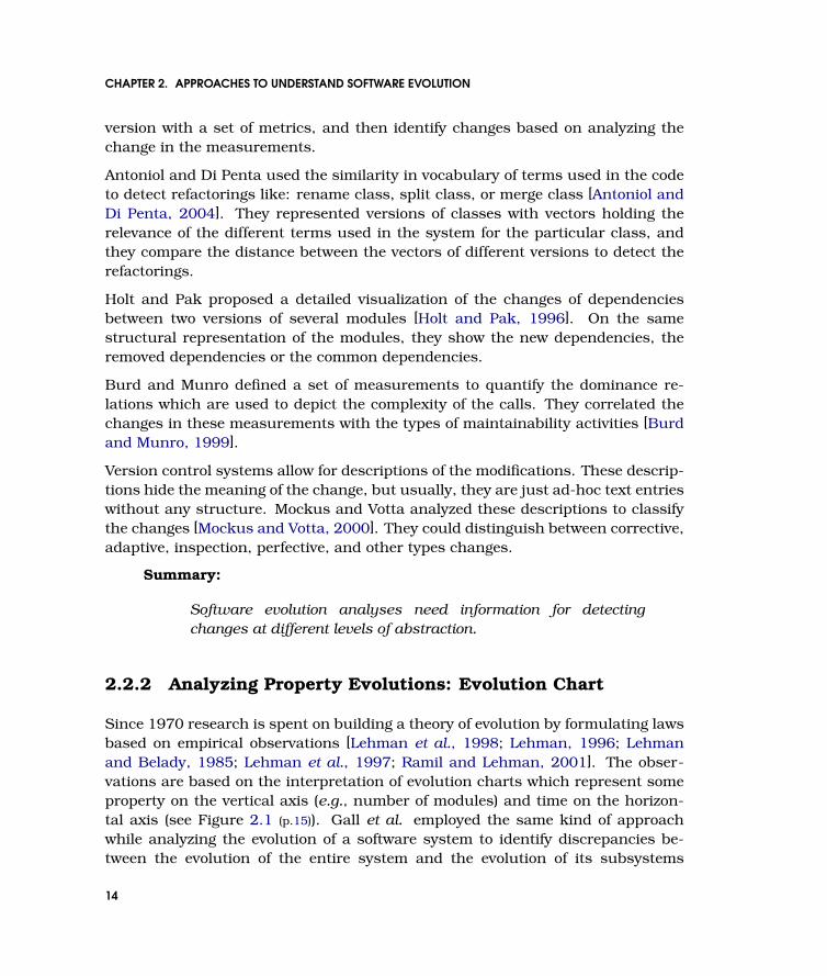
2.1 The evolution chart shows a property P on the vertical and time on the hori-zontal. . . . . . . . . . . . . . . . . . . . . . . . . . . . . . . . . . . . . . . . . . . 15
2.2 The Evolution Matrix shows versions nodes in a matrix. The size of the nodesis given by structural measurements. . . . . . . . . . . . . . . . . . . . . . . . . 16
2.3 Historical co-change example. Each ellipse represents a module and eachedge represents a co-change relationship. The thickness of the edge is givenby the number of times the two modules changed together. . . . . . . . . . . . 22
2.4 The Release History Meta-Model shows how Feature relates to CVSItem. . . . 24
2.5 The different analyses built using Hismo and the different features of Hismothey use. . . . . . . . . . . . . . . . . . . . . . . . . . . . . . . . . . . . . . . . . . 27
3.1 Details of the relationship between the History, the Version and the Snapshot.A History has a container of Versions. A Version wraps a Snapshot and addsevolution specific queries. . . . . . . . . . . . . . . . . . . . . . . . . . . . . . . . 31
3.2 Hismo applied to Packages and Classes. . . . . . . . . . . . . . . . . . . . . . . . 33
3.3 An excerpt of Hismo as applied to FAMIX, and its relation with a snapshotmeta-model: Every Snapshot (e.g., Class) is wrapped by a corresponding Ver-sion (e.g., ClassVersion), and a set of Versions forms a History (e.g., ClassHis-tory). We did not represent all the inheritance and association relationshipsto not affect the readability of the picture. . . . . . . . . . . . . . . . . . . . . . 33
3.4 Mapping Hismo to the Evolution Matrix. Each cell in the Evolution Matrixrepresents a version of a class. Each column represents the version of apackage. Each line in the Evolution Matrix represents a history. The entirematrix displays the package history. . . . . . . . . . . . . . . . . . . . . . . . . . 35

3.5 Examples of history measurements and how they are computed based onstructural measurements. . . . . . . . . . . . . . . . . . . . . . . . . . . . . . . . 38
3.6 Examples of EP, LEP and EEP history measurements. The top part shows themeasurements computed for 5 histories. The bottom part shows the compu-tation details. . . . . . . . . . . . . . . . . . . . . . . . . . . . . . . . . . . . . . . 38
3.7 HistoryGroup as a first class entity. . . . . . . . . . . . . . . . . . . . . . . . . . 40
3.8 Using Hismo for modeling historical relationships. . . . . . . . . . . . . . . . . . 42
3.9 Using Hismo for co-change analysis. On the bottom-left side, we show 6 ver-sions of 4 modules: a grayed box represent a module that has been changed,while a white one represents a module that was not changed. On the bottom-right side, we show the result of the evolution of the 4 modules as in Figure 2.3(p.22). . . . . . . . . . . . . . . . . . . . . . . . . . . . . . . . . . . . . . . . . . . . 42
3.10Transforming the Snapshot to obtain corresponding History and Version andderiving historical properties. . . . . . . . . . . . . . . . . . . . . . . . . . . . . 44
3.11Obtaining the relationships between histories by transforming the snapshotmeta-model. . . . . . . . . . . . . . . . . . . . . . . . . . . . . . . . . . . . . . . 44
4.1 The detection of a Yesterday’s Weather hit with respect to classes. . . . . . . . 52
4.2 The computation of the overall Yesterday’s Weather. . . . . . . . . . . . . . . . 53
4.3 YW computed on classes with respect to methods on different sets of versionsof Jun, CodeCrawler and JBoss and different threshold values. . . . . . . . . . 56
4.4 The class histories that provoked a hit when computing YW(Jun40,NOM,10,10)and their number of methods in their last version. In this case study, the bigclasses are not necessarily relevant for the future changes. . . . . . . . . . . . 57
4.5 The class histories that provoked a hit when computing YW(CC40,NOM,5,5)and their number of methods in their last version. In this case study, the bigclasses are not necessarily relevant for the future changes. . . . . . . . . . . . 58
4.6 YW computed on packages with respect to the total number of methods ondifferent sets of versions of JBoss and different threshold values. . . . . . . . . 59
4.7 The package histories provoking a hit when computing YW(JBoss40,NOM,10,10)and their number of methods in their last version. In this case study, the bigpackages are not necessarily relevant for the future changes. . . . . . . . . . . 59
4.8 The evolution of the values of YW(Jun40,NOM,10,10) when applied to classes.The diagram reveals phases in which the predictability increases and duringwhich changes are more focused (e.g., the first part of the history) and phasesin which the predictability decreases and changes are more unfocused (e.g.,the second part of the history). . . . . . . . . . . . . . . . . . . . . . . . . . . . . 60
5.1 Examples of the computation of the Stab and Pers measurements. . . . . . . . 74
5.2 God Classes detected in version 200 of Jun case-study and their history prop-erties. . . . . . . . . . . . . . . . . . . . . . . . . . . . . . . . . . . . . . . . . . . 78
5.3 Data Classes detected in version 200 of the Jun case study and their historyproperties. . . . . . . . . . . . . . . . . . . . . . . . . . . . . . . . . . . . . . . . . 80
5.4 Summary of the results of the history-based detection strategies as applied onJun. . . . . . . . . . . . . . . . . . . . . . . . . . . . . . . . . . . . . . . . . . . . 81
6.1 An example of the Hierarchy Evolution Complexity View. Hierarchy EvolutionComplexity View (right hand side) summarizes the hierarchy history (left handside). . . . . . . . . . . . . . . . . . . . . . . . . . . . . . . . . . . . . . . . . . . . 92
6.2 A Hierarchy Evolution Complexity View of the evolution of the largest hierarchyfrom 14 versions of JBoss. . . . . . . . . . . . . . . . . . . . . . . . . . . . . . . 95
6.3 A Hierarchy Evolution Complexity View of the evolution of five hierarchies from14 versions of JBoss. . . . . . . . . . . . . . . . . . . . . . . . . . . . . . . . . . 96
6.4 A Hierarchy Evolution Complexity View of the evolution of six hierarchies fromthe 40 versions of Jun. . . . . . . . . . . . . . . . . . . . . . . . . . . . . . . . . 97
6.5 A modified Hierarchy Evolution Complexity View of the evolution of six hierar-chies from the Jun case study. The node width is given by the instability ofnumber of methods and the height is given by the last number of methods. . . 99
7.1 Snapshot from a CVS log. . . . . . . . . . . . . . . . . . . . . . . . . . . . . . . . 108
7.2 The computation of the initial size. . . . . . . . . . . . . . . . . . . . . . . . . . . 108
7.3 Example of ownership visualization of two files. . . . . . . . . . . . . . . . . . . 110
7.4 Example of the Ownership Map view. The view reveals different patterns:Monologue, Familiarization, Edit, Takeover, Teamwork, Bug-fix. . . . . . . . . . 111
7.5 Number of commits per team member in periods of three months. . . . . . . . 115
7.6 The Ownership Map of the Outsight case study. . . . . . . . . . . . . . . . . . . 117
7.7 The Ownership Map of Ant, Tomcat, JEdit, and JBoss. . . . . . . . . . . . . . . 119
8.1 Example of applying formal concept analysis: the concepts on the right areobtained based on the incidence table on the left. . . . . . . . . . . . . . . . . . 128
8.2 Example of applying concept analysis to group class histories based on thechanges in number of methods. The Evolution Matrix on the left forms the in-cidence table where the property Pi of element X is given by “history X changedin version i.” . . . . . . . . . . . . . . . . . . . . . . . . . . . . . . . . . . . . . . . 129
8.3 Parallel inheritance detection results in JBoss. . . . . . . . . . . . . . . . . . . . 133
9.1 VAN and MOOSE. MOOSE is an extensible reengineering environment. Dif-ferent tools have been developed on top of it (e.g.,VAN is our history analysistool). The tools layer can use and extend anything in the environment in-cluding the meta-model. The model repository can store multiple models inthe same time. Sources written in different languages can be loaded eitherdirectly or via intermediate data formats. . . . . . . . . . . . . . . . . . . . . . . 140
9.2 VAN gives the historical semantic to the MOOSE models. . . . . . . . . . . . . . 1419.3 Screenshots showing the Group Browser the Entity Inspector. On the top part,
the windows display snapshot entities, while on the bottom part they displayhistorical entities. . . . . . . . . . . . . . . . . . . . . . . . . . . . . . . . . . . . 142
9.4 Screenshots showing CODECRAWLER. On the top part, it displays class hi-erarchies in a System Complexity View, while on the bottom part it displaysclass hierarchy histories in a Hierarchy Evolution Complexity View. . . . . . . . 143
9.5 Screenshots showing CHRONIA in action: interaction is crucial. . . . . . . . . . 144
Chapter 1
Introduction
The coherence of a trip is given by the clearness of the goal.
During the 1970’s it became more and more apparent that keeping track of soft-ware evolution was important, at least for very pragmatic purposes such as un-doing changes. Early versioning systems like the Source Code Control System(SCCS) made it possible to record the successive versions of software products[Rochkind, 1975]. At the same time, text-based delta algorithms were developed[Hunt and McIlroy, 1976] for understanding where, when and what changes ap-peared in the system. Some basic services were also added to model extra or metainformation such as who changed files and why. However only very rudimentarymodels were used to represent this information – typically a few unstructuredlines of text to be inserted in a log file.
While versioning systems recorded the history of each source file independently,configuration management systems attempted to record the history of softwareproducts as a collection of versions of source files. This arose research inter-ests on the topic of configuration management during 1980’s and 1990’s, but theemphasis was still on controlling and recording software evolution.
The importance of modeling and analyzing software evolution was pioneered inthe early 1970’s with the work of Lehman [Lehman and Belady, 1985], yet, it wasonly in recent years that extensive research has been carried out on exploiting the

CHAPTER 1. INTRODUCTION
wealth of information residing in versioning repositories for purposes like reverseengineering or cost estimation. Problems like software aging [Parnas, 1994] andcode decay [Eick et al., 2001] gained increasing recognition both in academia andin industry.
The research effort spent on the issue of software evolution shows the importanceof the domain. Various valuable approaches have been proposed to analyze as-pects of software evolution for purposes like identifying driving forces in softwareevolution [Buckley et al., 2005; Capiluppi et al., 2004; Lehman and Belady, 1985],like prediction [Hassan and Holt, 2004; Zimmermann et al., 2004], or like reverseengineering [Ball and Eick, 1996; Collberg et al., 2003; Fischer et al., 2003b;Lanza and Ducasse, 2002; Van Rysselberghe and Demeyer, 2004; Wu et al.,2004b]. However, if we are to understand software evolution as a whole, we needmeans to combine and compare the results of the different analyses.
1.1 The Problem of Meta-Modeling Software Evolu-tion
To combine or compare analyses we need a common meta-model, because a com-mon meta-model allow for a uniform expression of analyses.
Short Incursion into Meta-Modeling
To model is to create a representation of a subject so that reasonings can be for-mulated about the subject. The model is a simplification of the subject, and itspurpose is to answer some particular questions aimed towards the subject [Bezivinand Gerbe, 2001]. In other words, the model holds the elements of the subject thatare relevant for the purpose of the reasoning. For example, a road map is a modelof the actual physical space, and its purpose is to answer questions regarding theroute to be taken. The same map is completely useless, when one would want toanswer the question of where is the maximum precipitation point.
Several classes of models may exist for a given subject, each of these classes ofmodels being targeted for some particular reasonings. Hence, not all models rep-resent the same elements of the subject. That is to say, a model is built accordingto a description of what can go into a class of models: the meta-model [Seidewitz,2003]. For example, we can have several types of maps representing the same
2

1.1. THE PROBLEM OF META-MODELING SOFTWARE EVOLUTION
physical space. Each of these types of maps will represent characteristics of thephysical space based on a specification: a road map might only show circles torepresent places and lines to represent roads, while a precipitation map will usecolors to represent the amount of precipitation in a region.
To understand a model one must understand its meta-model. A particular reason-ing is dependent on what can be expressed on the respective underlying model,that is, it is dependent on the meta-model. Given an unknown reasoning, thebasic step towards understanding it is to understand the meta-model.
In our map example, we need to understand the map to understand the reason-ings built on it, and for understanding the map we need to understand what isrepresented in the map. For example, someone looks at the map to find the pathfrom A to B, and she decides that the next step is to get to C. If we want to questionwhy she chose C, we need to first understand the notation of the map and then tocheck if indeed C is the right choice.
The Problem of Meta-Modeling Software Evolution
Current approaches to analyze software evolution typically focus on only sometraits of software evolution, and they either rely on ad-hoc models (i.e., models thatare not described by an explicit meta-model), or their meta-models are specific tothe goals of the supported analysis.
A meta-model describes the way the domain can be represented by the model,that is, it provides bricks for the analysis. An explicit meta-model allows for un-derstanding those bricks. Understanding the bricks allows for the comparison ofthe analyses built on top. Without an explicit meta-model, the comparison andcombination of results and techniques becomes difficult.
Many approaches rely on the meta-model provided by the versioning system, andoften no semantic units are represented (e.g., packages, classes or methods), andthere is no information about what exactly changed in a system. For example, itis difficult to identify classes which did not add any method recently, but changedtheir internal implementation.
There is no explicit entity to which to assign the properties characterizing howthe entity evolved, and because of that, it is difficult to combine the evolutioninformation with the version information. For example, we would like to knowwhether a large class was also changed a lot.
3

CHAPTER 1. INTRODUCTION
Problem Statement:
Because current approaches to analyze software evolution relyon ad-hoc models or on too specific meta-models, it is difficult tocombine or compare their results.
The more versions we consider, the more data we have at hand. The more data wehave at hand, the more difficult it is to analyze it. The more data we have, the moretechniques we need to employ on understanding this data. The more techniqueswe need, the more generic the infrastructure (either theoretical or physical) shouldbe.
Research Question:
How can we build a generic meta-model that enables the expres-sion and combination of software evolution analyses?
1.2 Our Approach in a Nutshell
Thesis:
To provide a generic meta-model for expressing software evolu-tion analyses, we need to recognize the evolution as an explicitphenomenon and model it as a first class entity.
In this dissertation we propose Hismo as an explicit meta-model for software evo-lution. Hismo is centered around the notion of history as a sequence of ver-sions.
Figure 1.1 (p.5) displays the core of our meta-model displaying three entities: His-tory, Version and Snapshot. The Snapshot is a placeholder for the entities whoseevolution is under study (e.g., class, file). A History holds a set of Versions, wherethe Version adds the notion of time to the Snapshot.
With this scheme, time information is added on top of the structural information,that is, the structural information can exist without any reference to history, butcan still be manipulated in the historical context. In other words, Hismo can bebuilt on top of any snapshot meta-model without interfering with the existingmeta-model. In this way, with Hismo we can reuse analyses at the structural leveland extend them in the context of evolution analysis.
4

1.3. CONTRIBUTIONS
Snapshot
A Version adds the notion of time to a Snapshot
a Snapshot is a placeholder for File, Class etc.
AbstractEntity
History1* Version
date: Date
History, Version and Snapshot are all Entities
History is an ordered set of Versions accordging to the dates
Figure 1.1: Details of the relationship between the History, the Version and the Snapshot.
History and Version are generic entities, and they need to be specialized for partic-ular Snapshot entities. That is, for each Snapshot entity we have a correspondingHistory and Version entity. Building the historical representation for differentSnapshot entities is a process that depends only on the type of the entities. Be-cause of this property, we can generalize our approach of obtaining Hismo througha transformation applied to the snapshot meta-model. In this way, Hismo is notnecessarily tied to software evolution analysis, but it is applicable to any snapshotmeta-model.
To show the expressiveness of Hismo we describe how several software evolutionanalyses can be expressed with it. As a simple use of Hismo, we define differ-ent measurements for histories that describe how software artifacts evolved. Wepresent different examples of historical measurements and history manipulationsand show different reverse engineering analyses we have built over the years.Each of these examples exercises different parts of Hismo (see next Section fordetails).
1.3 Contributions
The novelty of this dissertation resides in providing a generic meta-model for soft-ware evolution [Gırba et al., 2004c; Ducasse et al., 2004]. Our meta-model con-
5

CHAPTER 1. INTRODUCTION
tinuously evolved as a result of exercising it from the points of view of differentreverse engineering analyses that we built over time:
1. Knowing where to start the reverse engineering process can be a dauntingtask due to size of the system. Yesterday’s Weather is a measurement show-ing the retrospective empirical observation that the parts of the system whichchanged the most in the recent past also suffer important changes in the nearfuture. We use Yesterday’s Weather for guiding the first steps of reverse engi-neering by pin-pointing the parts that are likely to change in the near future[Gırba et al., 2004a].
2. Traditionally, design problems are detected based on structural information.Detection strategies are expressions that combine several measurements todetect design problems. We define history-based detection strategies to usehistorical measurements to refine the detection of design problems [Ratiu etal., 2004].
3. Understanding the evolution of software systems is a difficult undertakingdue to the size of the data. Hierarchies typically group classes with similarsemantics. Grasping an overview of the system by understanding hierarchiesas a whole reduces the complexity of understanding as opposed to under-standing individual classes. We developed the Hierarchy Evolution Complex-ity View visualization to make out different characteristics of the evolution ofhierarchies [Gırba et al., 2005b; Gırba and Lanza, 2004].
4. Conway’s law states that “Organizations which design systems are constrainedto produce designs which are copies of the communication structures ofthese organizations” [Conway, 1968]. Hence, to get the entire picture onemust understand the interaction between the organization and the system.We exploit the author information related to a commit in the versioning sys-tem to detect what are the zones of influence of developers and what are theirbehaviors [Gırba et al., 2005a].
5. As systems evolve, changes can happen to crosscut the system’s structurein a way not apparent at the structural level. Understanding how changesappear in the system can reveal hidden dependencies between different partsof the system. We used concept analysis to detect co-change patterns, likeparallel inheritance [Gırba et al., 2004b].
6. Hismo is implemented in VAN, a tool built on top of the MOOSE reengineer-ing environment [Ducasse et al., 2005]. MOOSE supports the integration ofdifferent reengineering tools by making the meta-model explicit and by pro-
6

1.4. STRUCTURE OF THE DISSERTATION
viding mechanisms to extend the meta-model as needed by the particularanalysis [Nierstrasz et al., 2005]. The tools built on top, take as input en-tities with their properties and relationships. VAN extends the meta-modelwith the Hismo and provides several evolution analyses also by using toolsbuilt on MOOSE. For example, it uses CODECRAWLER to visualize the histo-ries.
1.4 Structure of the Dissertation
Chapter 2 (p.11) browses the state-of-the-art in the analysis of software evolu-tion, the focus being on making explicit the underlying meta-models of thedifferent approaches. The result of the survey is summarized in a set of re-quirements for a meta-model for software evolution: (1) different abstractionand detail levels, (2) comparison of property evolutions, (3) combination ofproperty evolutions, (4) historical selection, (5) historical relationships, and(6) historical navigation.
Chapter 3 (p.29) introduces Hismo, our meta-model for understanding softwareevolution. We show how Hismo centers around the notion of history as afirst class entity, and how one can obtain a history representation startingfrom the meta-model of the structure. The following chapters show severalapproaches for software evolution analysis, each of them exercising a part ofHismo.
Chapter 4 (p.47) describes the Yesterday’s Weather measurement as an exam-ple of how to combine several historical properties into one analysis. Theproblem addressed is to identify the parts of the system to start the reverseengineering process from, and the assumption is that the parts that are likelyto get changed in the near future are the most important ones. Yesterday’sWeather shows the retrospective empirical observation that the parts of thesystem which changed the most in the recent past also suffer importantchanges in the near future. We apply this approach to three case studieswith different characteristics, and show how we can obtain an overview ofthe evolution of a system and pinpoint the parts that might change in thenext versions.
A detection strategy is a an expression that combines measurements to detect de-sign problems [Marinescu, 2004]. In Chapter 5 (p.67) we extend the concept
7

CHAPTER 1. INTRODUCTION
of detection strategy with historical information to form history-based detec-tion strategies. That is, we include historical measurements to refine thedesign flaws detection. History-based detection strategies show how, basedon Hismo, we can express predicates that combine properties observable atthe structural level with properties observable in time.
Chapter 6 (p.87) presents an approach to understand how a set of given classhierarchies as a whole have evolved over time. The approach builds on acombination of historical relationships and historical properties. We proposea set of queries to detect several characteristics of hierarchies: how old theyare, how much were the classes changed, and how were the inheritancerelationships changed.
As systems change, the knowledge of the developers becomes critical for the pro-cess of understanding the system. Chapter 7 (p.105) presents an approach tounderstand how developers changed the system. We visualize how files werechanged, by displaying the history of a file as a line and coloring the lineaccording to the owners of the file over the time. To detect zones of influenceof a particular developer, we arrange the files according to a clustering de-pending on the historical distance given by how developers changed the file:two files are closer together if they are changed in approximately the sameperiods.
Chapter 8 (p.125) introduces our approach of using Formal Concept Analysis togroup entities that change in similar ways. Formal Concept Analysis takesas input elements with properties and returns concepts formed by elementswith a set of common properties. As elements we use histories, and foreach history we consider it has the property i if it “was changed in the ithversion.” We use the detailed information to distinguish different types ofchanges according to the different types of concepts we are interested in.
Much of the development of Hismo comes from our experience with implementingour assumptions in our prototype named VAN, built on top of the MOOSE
reengineering environment [Ducasse et al., 2005; Nierstrasz et al., 2005].Chapter 9 (p.137) describes our prototype infrastructure. It implements Hismoand our approaches to understand software evolution. The chapter em-phasizes how the usage of Hismo allows for the combination of techniques.For example, we show how we use two other tools (CodeCrawler [Lanza andDucasse, 2005] and ConAn [Arevalo, 2005]) for building evolution analysis.
In Chapter 10 (p.147) we discuss how Hismo leverages software evolution analysis
8
1.4. STRUCTURE OF THE DISSERTATION
by re-analyzing the requirements identified in Chapter 2 (p.11) from the pointof view of analyses built on Hismo . The chapter ends with an outlook on thefuture work opened by our approach.
We use several evolution and meta-modeling related terms throughout the dis-sertation (e.g., evolution). In Appendix A (p.155) we provide the definitions forthe most important of these terms.
9

CHAPTER 1. INTRODUCTION
10
Chapter 2
Approaches to UnderstandSoftware Evolution
Things are what we make of them.
Current approaches to understand software evolution typically rely on ad-hoc mod-els, or their meta-models are specific to the goals of the supported analysis. We aimto offer a meta-model for software evolution analysis. We review the state of the artin software evolution analysis and we discuss the meta-models used. As a resultwe identified several activities the meta-model should support:
1. It should provide information at different abstraction and detail levels,
2. It should allow comparison of how properties changed,
3. It should allow combination of information related to how different propertieschanged,
4. It should allow analyses to be expressed on any group of versions,
5. It should provide information regarding the relationships between the evolutionof different entities, and
6. It should provide means to navigate through evolution.

CHAPTER 2. APPROACHES TO UNDERSTAND SOFTWARE EVOLUTION
2.1 Introduction
In the recent years much research effort have been dedicated to understand soft-ware evolution, showing the increasing importance of the domain. The main chal-lenge in software evolution analysis is the size of the data to be studied: the moreversions are taken into account, the more data. The more data we have at hand,the more techniques we need to analyze it.
Many valuable approaches have been developed to analyze different traits of soft-ware evolution. However, if we are to understand software evolution as a whole, weneed means to combine and compare the results of the different analyses.
The approaches developed so far rely on ad-hoc models, or their meta-models arespecific to the goals of the supported analysis. Because of this reason it is difficultto combine or compare the results of the analyses.
Our goal is to build on the current state-of-the-art and to offer a common infras-tructure meta-model for expressing software evolution analyses. To accomplishthis task, we review several approaches for analyzing software evolution, the tar-get being to identify the requirements of the different analyses from the point ofview of a common evolution meta-model.
The most straightforward way to gather the requirements would be to analyze thedifferent meta-models. Unfortunately, in most of the cases, the meta-models arenot detailed (most of the time they are not even mentioned). In these cases weinfer the minimal meta-models required for the particular analysis.
From our literature survey we identified two major categories of approaches de-pending on the granularity level of information representation: version-centeredapproaches and history-centered approaches. Version-centered approaches con-sider version as a representation unit, while the history-centered approaches con-sider history (i.e., an ordered set of versions) as representation unit.
While in the version-centered approaches, the means is to present the version in-formation and let the user detect the patterns, in the version-centered approachesthe aim is to summarize what happened in the history according to a particularpoint of view. For example, a graphic plotting the values of a property in timeis a version-centered approach; on the other hand, a measure of how a propertyevolved over time is a history-centered approach.
12
2.2. VERSION-CENTERED APPROACHES
Structure of the Chapter
We discuss the version-centered approaches in Section 2.2 (p.13), and the history-centered approaches in Section 2.3 (p.19). While discussing the different ap-proaches, we emphasize their requirements from the point of view of a commonmeta-model. Each of the two sections ends with a discussion of the approaches.Section 2.4 (p.25) concludes the chapter with an overall description of the gatheredrequirements
2.2 Version-Centered Approaches
The version-centered analyses use a version as a representation granularity. Ingeneral, they target the detection of when something happened in history. Weidentify three classes of approaches and we take a look at each.
2.2.1 Analyzing the Changes Between Two Versions
Comparing two versions is the basis of any evolution analysis. We enumerateseveral approaches that focus on finding different types of changes.
Diff was the first tool used for comparing the differences between two versions ofa file [MacKenzie et al., 2003]. Diff is able to detect addition or deletion of lines oftext and it provides the position of these lines in the file. This tool is not usefulwhen the analysis requires finer grained data about what happened in the system,because it does not provide any semantic information of what exactly changed inthe system (e.g., in terms of classes or functions).
In another work, Xing and Stroulia used a Diff-like approach to detect differenttypes of fine-grained changes between two versions of a software system. Theyrepresented each version of the system in an XMI format [XMI 2.0, 2005] and thenapplied UML Diff to detect changes like: addition/removal of classes, methods andfields; moving of classes, methods, fields; renaming of classes, methods, fields.Several applications have been based on this approach [Xing and Stroulia, 2004a;Xing and Stroulia, 2004b; Xing and Stroulia, 2004c].
Demeyer et al. used the structural measurements to detect refactorings like re-name method, or move method [Demeyer et al., 2000]. They represented each
13
CHAPTER 2. APPROACHES TO UNDERSTAND SOFTWARE EVOLUTION
version with a set of metrics, and then identify changes based on analyzing thechange in the measurements.
Antoniol and Di Penta used the similarity in vocabulary of terms used in the codeto detect refactorings like: rename class, split class, or merge class [Antoniol andDi Penta, 2004]. They represented versions of classes with vectors holding therelevance of the different terms used in the system for the particular class, andthey compare the distance between the vectors of different versions to detect therefactorings.
Holt and Pak proposed a detailed visualization of the changes of dependenciesbetween two versions of several modules [Holt and Pak, 1996]. On the samestructural representation of the modules, they show the new dependencies, theremoved dependencies or the common dependencies.
Burd and Munro defined a set of measurements to quantify the dominance re-lations which are used to depict the complexity of the calls. They correlated thechanges in these measurements with the types of maintainability activities [Burdand Munro, 1999].
Version control systems allow for descriptions of the modifications. These descrip-tions hide the meaning of the change, but usually, they are just ad-hoc text entrieswithout any structure. Mockus and Votta analyzed these descriptions to classifythe changes [Mockus and Votta, 2000]. They could distinguish between corrective,adaptive, inspection, perfective, and other types changes.
Summary:
Software evolution analyses need information for detectingchanges at different levels of abstraction.
2.2.2 Analyzing Property Evolutions: Evolution Chart
Since 1970 research is spent on building a theory of evolution by formulating lawsbased on empirical observations [Lehman et al., 1998; Lehman, 1996; Lehmanand Belady, 1985; Lehman et al., 1997; Ramil and Lehman, 2001]. The obser-vations are based on the interpretation of evolution charts which represent someproperty on the vertical axis (e.g., number of modules) and time on the horizon-tal axis (see Figure 2.1 (p.15)). Gall et al. employed the same kind of approachwhile analyzing the evolution of a software system to identify discrepancies be-tween the evolution of the entire system and the evolution of its subsystems
14

2.2. VERSION-CENTERED APPROACHES
P
t
Figure 2.1: The evolution chart shows a property P on the vertical and time on the hori-zontal.
[Gall et al., 1997]. Recently, the same approach has been used to characterizethe evolution of open source projects [Godfrey and Tu, 2000; Capiluppi, 2003;Capiluppi et al., 2004].
This approach is useful when we need to reason about the evolution of a singleproperty, but it makes it difficult to reason in terms of more properties at the sametime, and provides only limited ways to compare how the same property evolvedin different entities. That is why, typically, the charts are used to reason aboutthe entire system, though the chart can represent any type of entity.
In Figure 2.1 (p.15) we give an example of how to use the evolution charts to com-pare multiple entities. In the left part of the figure we display a graph with theevolution of a property P of an entity – for example it could represent number ofmethods in a class (NOM). From the figure we can draw the conclusion that P isgrowing in time. In the right part of the figure we display the evolution of thesame property P in 12 entities. Almost all graphs show a growth of the P propertybut they do not have the same shape. Using the graphs alone it is difficult to saywhich are the differences between the evolution of the different entities.
Summary:
Software evolution analyses need to compare the information onhow properties evolved.
If we want to correlate the evolution of property P with another property Q, wehave an even more difficult problem, and the evolution chart does not ease thetask significantly. Chuah and Eick used so called “timewheel glyphs” to displayseveral evolution charts where each chart was rotated around a circle [Chuahand Eick, 1998]. Each evolution chart plotted a different property: number oflines added, the errors recorded between versions, number of people working etc..
15

CHAPTER 2. APPROACHES TO UNDERSTAND SOFTWARE EVOLUTION
versions
shrinking
growing
idle
growing/shrinking
class
# ofattributes
# ofmethods
1 2 3 4 5
Class A
Class B
Class C
Class D
Legend:
Figure 2.2: The Evolution Matrix shows versions nodes in a matrix. The size of the nodesis given by structural measurements.
They indeed used several evolution charts to allow the analysis to combine theinformation of how different properties evolved, but they only made use of theoverall charts shape, and not the detailed differences.
Summary:
Software evolution analyses need to combine the information onhow properties evolved.
2.2.3 Evolution Matrix Visualization
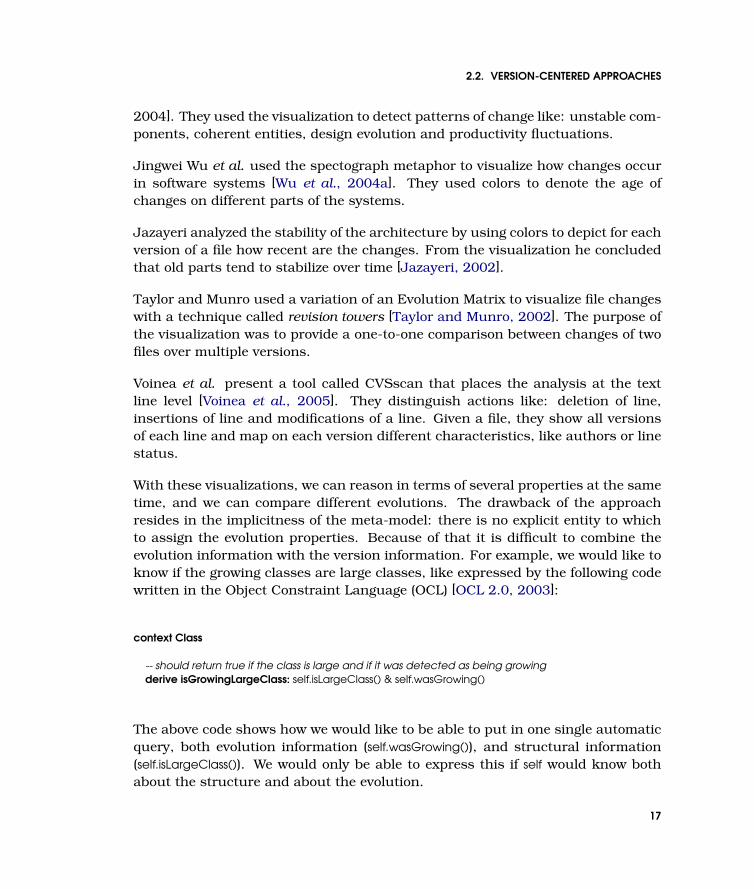
Visualization has been also used to reason about the evolution of multiple prop-erties and to compare the evolution of different entities. Lanza and Ducasse ar-ranged the classes of the history in an Evolution Matrix shown in Figure 2.2 (p.16)
[Lanza and Ducasse, 2002]. Each rectangle represents a version of a class andeach line holds all the versions of that class (the alignment is realized based onthe name of the class). Furthermore, the size of the rectangle is given by differentmeasurements applied on the class version. From the visualization different evo-lution patterns can be detected such as continuous growth, growing and shrinkingphases etc.
Rysselberghe and Demeyer used a scatter plot visualization of the changes toprovide an overview of the evolution of systems [Van Rysselberghe and Demeyer,
16
2.2. VERSION-CENTERED APPROACHES
2004]. They used the visualization to detect patterns of change like: unstable com-ponents, coherent entities, design evolution and productivity fluctuations.
Jingwei Wu et al. used the spectograph metaphor to visualize how changes occurin software systems [Wu et al., 2004a]. They used colors to denote the age ofchanges on different parts of the systems.
Jazayeri analyzed the stability of the architecture by using colors to depict for eachversion of a file how recent are the changes. From the visualization he concludedthat old parts tend to stabilize over time [Jazayeri, 2002].
Taylor and Munro used a variation of an Evolution Matrix to visualize file changeswith a technique called revision towers [Taylor and Munro, 2002]. The purpose ofthe visualization was to provide a one-to-one comparison between changes of twofiles over multiple versions.
Voinea et al. present a tool called CVSscan that places the analysis at the textline level [Voinea et al., 2005]. They distinguish actions like: deletion of line,insertions of line and modifications of a line. Given a file, they show all versionsof each line and map on each version different characteristics, like authors or linestatus.
With these visualizations, we can reason in terms of several properties at the sametime, and we can compare different evolutions. The drawback of the approachresides in the implicitness of the meta-model: there is no explicit entity to whichto assign the evolution properties. Because of that it is difficult to combine theevolution information with the version information. For example, we would like toknow if the growing classes are large classes, like expressed by the following codewritten in the Object Constraint Language (OCL) [OCL 2.0, 2003]:
context Class
-- should return true if the class is large and if it was detected as being growingderive isGrowingLargeClass: self.isLargeClass() & self.wasGrowing()
The above code shows how we would like to be able to put in one single automaticquery, both evolution information (self.wasGrowing()), and structural information(self.isLargeClass()). We would only be able to express this if self would know bothabout the structure and about the evolution.
17

CHAPTER 2. APPROACHES TO UNDERSTAND SOFTWARE EVOLUTION
Summary:
Software evolution analyses need to combine the information onhow properties evolved with the information from the structurallevel.
Another drawback here is that the more versions we have, the more nodes wehave, the more difficult it gets to detect patterns when they are spread over alarge space.
2.2.4 Discussion of Version-Centered Approaches
The version-centered models allow for the comparison between two versions, andthey provide insights into when a particular event happened in the evolution (e.g.,a class grew instantly). The visual technique is to represent time on an axisand place different versions along this axis and make visible where the changeoccurred (e.g., using color, size, position).
Some of the analyses also used version-based techniques to compare the way dif-ferent entities evolved over time. For example, the evolution chart was used tocompare the evolution of different systems to detect patterns of change like con-tinuously growing systems. The Evolution Matrix was also used to detect changepatterns like growing classes or idle classes (i.e., classes that do not change). Amajor technical problem is that the more versions we have the more informationwe have to interpret.
Furthermore, when patterns are detected, they are attached to structural entities.For example, the authors said that they detected growing and idle classes, yet,taking a closer look at the Evolution Matrix, we see that it is conceptually incor-rect because a class is just one rectangle while growing and idle characterize asuccession of rectangles. That is, we can say a class is big or small, but grow-ing and idle characterizes the way a class has evolved. From a modeling point ofview, we would like to have an explicit entity to which to assign the growing or idleproperty: the history as an encapsulation of evolution.
18

2.3. HISTORY-CENTERED APPROACHES
2.3 History-Centered Approaches
History-centered approaches have history as an ordered set of versions as rep-resentation granularity. In general, they are not interested in when somethinghappened, but they rather seek to detect what happened and where it happened.In these approaches, the individual versions are no longer represented, they areflattened.
The main idea behind having a history as the unit of representation is to sum-marize the evolution according to a particular point of view. History-centeredapproaches often gather measurements of the history to support the understand-ing of the evolution. However, they are often driven by the information containedin repositories like Concurrent Versioning System (CVS)1, and lack fine-grainedsemantic information. For example, some approaches offer file and folder changesbut give no semantic information about what exactly changed in a system (e.g.,classes or methods).
We present three approaches characterizing the work done in the context of history-centered evolution analyses.
2.3.1 History Measurements
The history measurements aim to quantify what happened in the evolution ofan entity. Examples of history measurements are: age of an entity, number ofchanges in an entity, number of authors that changed the system etc.
Ball and Eick developed multiple visualizations for showing changes that appearin the source code [Ball and Eick, 1996]. For example, they show what is thepercentage of bug fixes and feature addition in files, or which lines were changedrecently.
Eick et al. described Seesoft, a tool for visualizing line oriented software statistics[Eick et al., 1992]. They proposed several types of visualization: number of modi-fication reports touching a line of code, age, stability of a line of code etc..
Mockus et al. implemented a tool called SoftChange for characterizing softwareevolution in general [Mockus et al., 1999]. They used history measurements like:the age of a file, the average lines of code added/deleted in a change, the totalnumber of changes happening at a certain hour etc.
1See https://www.cvshome.org/.
19
CHAPTER 2. APPROACHES TO UNDERSTAND SOFTWARE EVOLUTION
Mockus and Weiss used history measurements for developing a method for pre-dicting the risk of software changes [Mockus and Weiss, 2000]. Examples of themeasurements were: the number of modules touched, the number of developersinvolved, or the number of changes.
Eick et al. proposed several visualizations to show how developers change usingcolors and third dimension [Eick et al., 2002]. For example they showed a matrixwhere each row corresponds to an author, each column corresponds to a mod-ule, and each cell in the matrix shows the size of the changes performed by thedeveloper to the module.
Collberg et al. used graph-based visualizations to display which parts of classhierarchies were changed [Collberg et al., 2003]. They provide a color scale todistinguish between newer and older changes.
Xiaomin Wu et al. visualized the change log information to provide for an overviewof the active places in the system as well as of the authors activity [Wu et al.,2004b]. They display measurements like the number of times an author changeda file, or the date of the last commit.
Chuah and Eick presented a way to visualize project information in a so called“infobug” [Chuah and Eick, 1998]. The name of the visualization comes from afigure looking like a bug. They mapped on the different parts of the “infobug”different properties: evolution aspects, programming languages used, and errorsfound in a software component. They also presented a time wheel visualization toshow the evolution of a given characteristic over time.
Typically, in the literature we find measurements which are very close to the typeof information available in the versioning systems. As versioning systems providetextual information like lines of code added/removed, the measurements too onlymeasure the size of the change in lines of code. Even though lines of code canbe a good indicator for general overviews, it is not a good indicator when moresensitive information is needed. For example, if 10 lines of code are added in afile, this approach does not distinguish whether the code was added to an existentmethod, or if several completely new methods were added.
Summary:
Software evolution analyses need to combine the information onhow properties evolved.
20

2.3. HISTORY-CENTERED APPROACHES
2.3.2 Manipulating Historical Relationships: HistoricalCo-Change
Gall et al. aimed to detect logical coupling between parts of the system [Gall et al.,1998] by identifying the parts of the system which change together. They use thisinformation to define a coupling measurement based on the fact that the moretimes two modules were changed at the same time, the more strongly they werecoupled.
Pinzger and coworkers present a visualization of evolution data using a combi-nation of Kiviat diagrams and a graph visualization [Pinzger et al., 2005]. Eachnode represents a module in the system and an edge connecting two nodes thehistorical dependencies between the two modules. For example, to the width ofthe edge the authors map the co-change history of the two modules. Each nodein the graph is displayed using a Kiviat diagram to show how different measure-ments evolved. They use both code and file measurements. In this model, theauthors see the nodes and edges from both the structural perspective and fromthe evolution perspective.
Hassan et al. analyzed the types of data that are good predictors of change prop-agation, and came to the conclusion that historical co-change is a better mech-anism than structural dependencies like call-graphs [Hassan and Holt, 2004].Zimmermann et al. defined a measurement of coupling based on co-changes [Zim-mermann et al., 2003].
Zimmermann et al. aimed to provide a mechanism to warn developers about thecorrelation of changes between functions. The authors placed their analysis atthe level of entities in the meta-model (e.g., methods) [Zimmermann et al., 2004].They presented the problems residing in mining the CVS repositories, but they didnot present the meta-model [Zimmermann and Weißgerber, 2004].
Similar work was carried out by Ying et al. [Ying et al., 2004]. The authors ap-plied the approach on two large case studies and analyzed the effectiveness ofthe recommendations. They concluded that although the “precision and recallare not high, recommendations can reveal valuable dependencies that may not beapparent from other existing analyses.”
Xing and Stroulia used the fine-grained changes provided by UML Diff to look forclass co-evolution [Xing and Stroulia, 2004a; Xing and Stroulia, 2004b]. They tookthe type of changes into account when reasoning, and they distinguished betweenintentional co-evolution and “maintenance smells” (e.g., Shotgun Surgery).
21

CHAPTER 2. APPROACHES TO UNDERSTAND SOFTWARE EVOLUTION
D
A
B
C
Legend:
X module X
co change relationship
Figure 2.3: Historical co-change example. Each ellipse represents a module and each edgerepresents a co-change relationship. The thickness of the edge is given by the number oftimes the two modules changed together.
Eick et al. used the number of files changed in the same time as an one indicatorof code decay [Eick et al., 2001]. They reported on a large case study that changesare more dispersed at the end of the project, which they interpreted as a sign ofcode decay.
Burch visualized the co-change patterns in a matrix correlation [Burch et al.,2005]. In their visualization, each line and column is given by a file, and the colorof each point is given by the confidence of the co-change relationship between thetwo files. The confidence is a historical measurement and it is computed as the“number of changes of a pair of items relative to the number of changes of a singleitem.”
In general, the result of the co-change analysis is that two entities (e.g., files)have a relationship if they were changed together. Gall et al. provided a visual-ization, as in Figure 2.3 (p.22), to show how modules changed in the same time[Gall et al., 2003]. The circles represent modules, and the edges represent the co-change relationship: the thicker the edge, the more times the two modules werechanged in the same time. In this representation the structural elements fromthe last version (i.e., the modules) are linked via a historical relationship (i.e., theco-change relationship). In a similar visualization Eick et al. used the color todenote the strength of the relationship between the co-changed modules [Eick etal., 2002].
As in the case of the Evolution Matrix (e.g., where classes were said to be growing),in this case too there is a conceptual problem from the modeling point of view: co-change actually links the evolution of the entities and not a particular version ofthe entities. We would like to have a reification of the evolution (i.e., history), to beable to relate it to the co-change relationship.
22
2.3. HISTORY-CENTERED APPROACHES
Summary:
Software evolution analyses need information about how historiesare related from a historical perspective.
2.3.3 Manipulating Historical Entities: Hipikat and ReleaseMeta-Models
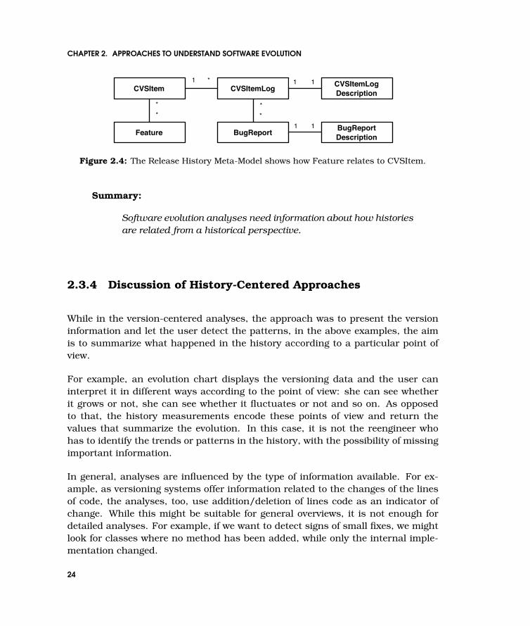
Fischer et al. modeled bug reports in relation to version control system (CVS)items [Fischer et al., 2003b]. Figure 2.4 (p.24) presents an excerpt of the ReleaseHistory meta-model. The purpose of this meta-model is to provide a link betweenthe versioning system and the bug reports database. This meta-model recognizesthe notion of the history (i.e., CVSItem) which contains multiple versions (i.e.,CVSItemLog). The CVSItemLog is related to a Description and to BugReports.Furthermore, it also puts the notion of Feature in relation with the history of anitem. The authors used this meta-model to recover features based on the bug re-ports [Fischer et al., 2003a]. These features get associated with a CVSItem.
The main drawback of this meta-model is that the system is represented with onlyfiles and folders, and it does not take into consideration the semantic softwarestructure (e.g., classes or methods). Because it gives no information about whatexactly changed in a system, this meta-model does not offer support for analyzingthe different types of change. Recently, the authors started to investigate how toenrich the Release History Meta-Model with source code information [Antoniol etal., 2004].
Cubranic and Murphy bridged information from several sources to form whatthey call a “group memory” [Cubranic and Murphy, 2003]. Cubranic detailed themeta-model to show how they combined CVS repositories, mails, bug reports anddocumentation [Cubranic, 2004].
Draheim and Pekacki presented the meta-model behind Bloof [Draheim and Pekacki,2003]. The meta-model is similar to CVS: a File has several Revisions and eachRevision has attached a Developer. They used it for defining several measure-ments like the Developer cumulative productivity measured in changed LOC perday.
23
CHAPTER 2. APPROACHES TO UNDERSTAND SOFTWARE EVOLUTION
CVSItem CVSItemLog CVSItemLogDescription
Feature BugReport BugReportDescription
**
11*1
11
**
Figure 2.4: The Release History Meta-Model shows how Feature relates to CVSItem.
Summary:
Software evolution analyses need information about how historiesare related from a historical perspective.
2.3.4 Discussion of History-Centered Approaches
While in the version-centered analyses, the approach was to present the versioninformation and let the user detect the patterns, in the above examples, the aimis to summarize what happened in the history according to a particular point ofview.
For example, an evolution chart displays the versioning data and the user caninterpret it in different ways according to the point of view: she can see whetherit grows or not, she can see whether it fluctuates or not and so on. As opposedto that, the history measurements encode these points of view and return thevalues that summarize the evolution. In this case, it is not the reengineer whohas to identify the trends or patterns in the history, with the possibility of missingimportant information.
In general, analyses are influenced by the type of information available. For ex-ample, as versioning systems offer information related to the changes of the linesof code, the analyses, too, use addition/deletion of lines code as an indicator ofchange. While this might be suitable for general overviews, it is not enough fordetailed analyses. For example, if we want to detect signs of small fixes, we mightlook for classes where no method has been added, while only the internal imple-mentation changed.
24

2.4. TOWARDS A COMMON META-MODEL FOR UNDERSTANDING SOFTWARE EVOLUTION
2.4 Towards a Common Meta-Model for Understand-ing Software Evolution
A common meta-model for software evolution analysis should allow the expressionof all of the above analyses and more. Below we present the list with the differentneeds of software evolution analyses:
Software evolution analyses need detailed information for detect-ing changes at different levels of abstraction.
Software evolution analyses need to compare the information onhow properties evolved.
Software evolution analyses need to combine the information onhow properties evolved with the information from the structurallevel.
Software evolution analyses need to combine the information onhow properties evolved.
Software evolution analyses need information about how historiesare related from a historical perspective.
Taking the above list as an input we synthesize a list of features an evolutionmeta-model should support:
Different abstraction and detail levels. The meta-model should provide informa-tion at different levels of abstraction such as files, packages, classes, meth-ods for each analyzed version. For example, CVS meta-model offers informa-tion about how source code changed (e.g., addition, removals of lines of code),but it does not offer information about additions or removals of methods inclasses.
The meta-model should support the expression of detailed information aboutthe structural entity. For example, knowing the authors that changed theclasses is an important information for understanding evolution of code own-ership.
Comparison of property evolutions. The meta-model should offer means to easilyquantify and compare how different entities evolved with respect to a certainproperty. For example, we must be able to compare the evolution of numberof methods in classes, just like we can compare the number of methods in
25

CHAPTER 2. APPROACHES TO UNDERSTAND SOFTWARE EVOLUTION
classes. For that, we need a way to quantify how the number of methodsevolve and afterwards we need to associate such a property with an entity.
Combination of different property evolutions. The meta-model should allow foran analysis to be based on the evolution of different properties. Just likewe reason about multiple structural properties, we want to be able to reasonabout how these properties have evolved. For example, when a class has onlya few methods, but has a large number of lines of code, we might conclude itshould be refactored. At the same time, adding or removing the lines of codein a class while preserving the methods might lead us to conclude that thechange was a bug-fix.
Historical relationships. The meta-model should provide information regardingthe relationships between the evolution of different entities. For example,we should be able to reason about how two classes changed the number ofchildren in the same time.
Besides the above ones, we introduce two additional generic requirements:
Historical navigation. The meta-model should provide relations between historiesto allow for navigation. For example, we should be able to ask our modelwhich methods ever existed in a particular class, or which classes in a par-ticular package have been created in the last period of time.
Historical selection. The analysis should be applicable on any group of versions(i.e., we should be able to select any period in the history).
26

2.5. ROADMAP
2.5 Roadmap
In Chapter 3 (p.29), we present Hismo, our meta-model for software evolution. Tovalidate Hismo we used it in several novel analyses that we present in Chapters4-8.
In each of these chapters we present the analysis in detail, and at the end of thechapter we discuss which part of Hismo does the analysis exercise in a sectioncalled Hismo Validation. Figure 2.5 (p.27) shows schematically the chapters, thetitles of the analyses, and the different features of Hismo they use.
Chapter 4.Yesterday's Weather
Chapter 5.History-Based Detection Strategies
Chapter 6.Understanding Hierarchies Evolution
Chapter 7.How Developers Drive Software Evolution
Chapter 8.Detecting Co-Change Patterns
Different abstraction and detail levels
History selection
Historical navigation
Comparison of properties evolution
Combination of properties evolution
Historical relationships
Figure 2.5: The different analyses built using Hismo and the different features of Hismothey use.
27

CHAPTER 2. APPROACHES TO UNDERSTAND SOFTWARE EVOLUTION
28

Chapter 3
Hismo: Modeling History as aFirst Class Entity
Every thing has its own flow.
Our solution to model software evolution is to model history as a first class entity.A history is an ordered set of versions and it encapsulates the evolution. Historyand version are generic concepts and they must be applied to particular entities likepackages or classes. We show how starting from any snapshot meta-model we canobtain the historical meta-model through meta-model transformation.

CHAPTER 3. HISMO: MODELING HISTORY AS A FIRST CLASS ENTITY
3.1 Introduction
The previous chapter reviews several approaches to understanding software evo-lution and discusses their needs from the meta-model point of view. We identifiedseveral characteristics of a meta-model that supports all these analyses: (1) differ-ent abstraction and detail levels, (2) comparison of property evolutions, (3) combi-nation of property evolutions, (4) historical selection, (5) historical relationships,and (6) historical navigation.
In this chapter we introduce Hismo, our solution of modeling history to supportsoftware evolution analyses: explicitly model history as an ordered set of ver-sions.
Structure of the chapter
In the next section we introduce the generic concepts of history, version and snap-shot, and discuss their generic relationships. In Section 3.6 (p.39) we introduce thenotion of group as a first class entity and we discuss the properties of a group ofhistories. In Section 3.3 (p.32) we show how we build Hismo based on a snapshotmeta-model, and in Section 3.4 (p.34) we provide an example of how Hismo can bemapped to the Evolution Matrix. In Section 3.5 (p.35) we define historical propertiesand we show how they summarize the evolution. In Section 3.7 (p.41) we discussthe problem of modeling historical relationships. In Section 3.8 (p.43) we generalizeHismo by showing how it is possible to generate the historical meta-model startingfrom the snapshot meta-model.
3.2 Hismo
The core of Hismo is based on three entities: History, Version and Snapshot. Fig-ure 3.1 (p.31) shows the relationships between these entities in a UML 2.0 diagram[Fowler, 2003]:
Snapshot. This entity is a placeholder that represents the entities whose evolu-tion is studied i.e., file, package, class, methods or any source code artifacts.The particular entities are to be sub-typed from Snapshot as shown in Fig-ure 3.3 (p.33).
30
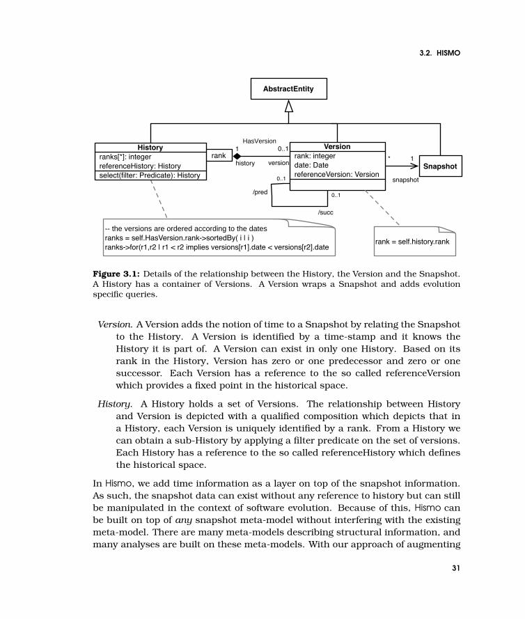
3.2. HISMO
snapshot
* 1
0..1
0..1
/succ
/pred
rankVersion
rank: integerdate: DatereferenceVersion: Version
1
history
0..1
version
HasVersion
Snapshot
-- the versions are ordered according to the dates ranks = self.HasVersion.rank->sortedBy( i | i )ranks->for(r1,r2 | r1 < r2 implies versions[r1].date < versions[r2].date
rank = self.history.rank
AbstractEntity
Historyranks[*]: integerreferenceHistory: Historyselect(filter: Predicate): History
Figure 3.1: Details of the relationship between the History, the Version and the Snapshot.A History has a container of Versions. A Version wraps a Snapshot and adds evolutionspecific queries.
Version. A Version adds the notion of time to a Snapshot by relating the Snapshotto the History. A Version is identified by a time-stamp and it knows theHistory it is part of. A Version can exist in only one History. Based on itsrank in the History, Version has zero or one predecessor and zero or onesuccessor. Each Version has a reference to the so called referenceVersionwhich provides a fixed point in the historical space.
History. A History holds a set of Versions. The relationship between Historyand Version is depicted with a qualified composition which depicts that ina History, each Version is uniquely identified by a rank. From a History wecan obtain a sub-History by applying a filter predicate on the set of versions.Each History has a reference to the so called referenceHistory which definesthe historical space.
In Hismo, we add time information as a layer on top of the snapshot information.As such, the snapshot data can exist without any reference to history but can stillbe manipulated in the context of software evolution. Because of this, Hismo canbe built on top of any snapshot meta-model without interfering with the existingmeta-model. There are many meta-models describing structural information, andmany analyses are built on these meta-models. With our approach of augmenting
31
CHAPTER 3. HISMO: MODELING HISTORY AS A FIRST CLASS ENTITY
time information on top of structural information, we can reuse the analyses atstructural level and incorporate them in the evolution analysis.
History, Version and Snapshot are abstract and generic entities, and as such,the core of Hismo is not tied to any meta-model. These concepts are generic inthe sense that they do not hold any specific information for a particular analysis.They provide a framework in which evolution information is represented, but toactually make the meta-model useful one has to apply these concepts on specificentities.
For example, we argued that we need detailed information about the different en-tities in the system such as packages, classes, methods. Figure 3.3 (p.33) shows anexample of how Hismo looks like when applied to the FAMIX meta-model [Demeyeret al., 2001].
3.3 Building Hismo Based on a Snapshot Meta-Model
In this section we unveil the details of how to apply the generic concepts of History,Version and Snapshot to specific snapshot meta-models.
We start by taking a detailed look at Hismo applied to Packages and Classes (seeFigure 3.2 (p.33)). There is a parallelism between the version entities and the his-tory entities: Each version entity has a corresponding history entity. Also, therelationship at version level (e.g., a Package has more Classes) has a correspon-dent at the history level (e.g., a PackageHistory has more ClassHistories).
Figure 3.3 (p.33) shows an overview of the history meta-model based on a largersource-code meta-model. Here we use FAMIX, a language independent sourcecode meta-model [Demeyer et al., 2001]. The details of the full meta-model aresimilar to the one in Figure 3.2 (p.33).
The snapshot entities (e.g., Method) are wrapped by a Version correspondent (e.g.,MethodVersion) and the Versions are contained in a History (e.g., MethodHistory).A History does not have direct relation with a Snapshot entity, but through aVersion wrapper as shown in Figure 3.1 (p.31). We create Versions as wrappers forSnapshotEntities because in a Version we store the relationship to the History:a Version is aware of the containing History and of its position in the History(i.e., it knows the predecessor and the successor). Thus, we are able to computeproperties for a particular Version in the context of the History. For example,having a Version we can navigate to the previous or the next Version.
32

3.3. BUILDING HISMO BASED ON A SNAPSHOT META-MODEL
ClassVersionname
1package
0..1class
PackageHistory
name
rank0..1
version
1
historyPackageVersion
name
ClassHistory rank0..1
version
1
history
1packageHistory
0..1classHistory
Classname
1package
0..1class
Package
name
1
snapshot
*
1
snapshot
*
Figure 3.2: Hismo applied to Packages and Classes.
rank
AbstractEntity
Class Method
Attribute Access
Snapshot
Inheritance ...
0..1
1Version
*
1
ClassHistory
MethodHistory
AttributeHistory
AccessHistory
InheritanceHistory ...
ClassVersion
MethodVersion
AttributeVersion
AccessVersion
InheritanceVersion ...
History
Figure 3.3: An excerpt of Hismo as applied to FAMIX, and its relation with a snapshotmeta-model: Every Snapshot (e.g., Class) is wrapped by a corresponding Version (e.g.,ClassVersion), and a set of Versions forms a History (e.g., ClassHistory). We did not rep-resent all the inheritance and association relationships to not affect the readability of thepicture.
33

CHAPTER 3. HISMO: MODELING HISTORY AS A FIRST CLASS ENTITY
The Entity Identity Problem
A problem raised in the literature is that of what we call entity identity: havingtwo entities at two different moments of time, how do we know whether they aretwo versions of the same history. This problem can also be found in the literatureunder the name of origin analysis [Antoniol and Di Penta, 2004; Zou and Godfrey,2003].
The most common way to recover the identity is by the name of the entity, thatis, if we have two entities with the same name and the same type in two versions,then they are considered to be two versions of the same history. Of course, suchapproaches fail to recognize refactorings like renaming or moving. Various ap-proaches have been proposed to solve this problem: using information retrievaltechniques [Antoniol and Di Penta, 2004], using string matching or entities fin-gerprints [Zou and Godfrey, 2003].
In our definition, the history is a set of versions, therefore, it also encapsulatesthe entity identity. We did not specify the algorithm to be used when determiningentity, because it is the responsibility of the implementation to determine howthe identity is defined. For example, it is possible to first determine the historiesbased on names and then detect renaming refactorings and merge the historiesthat are detected as being renamed.
3.4 Mapping Hismo to the Evolution Matrix
In this section we describe how Hismo maps to the Evolution Matrix (see Figure 3.4(p.35)). In the upper part of the figure we represent Hismo applied to Packages andClasses where a package contains several classes, while in the lower part we showtwo Evolution Matrices. As described in Section 2.2.3 (p.16), a row represents theevolution of an entity, a class in this case, and a column all the entities of oneversion – package in this case. As such, In Figure 3.4 (p.35) each cell in the matrixrepresents a ClassVersion and each column represents a PackageVersion.
In Hismo, a history is a sequence of versions, thus, each line in an Evolution Matrixrepresents a ClassHistory (left matrix). Moreover, the whole matrix is actually aline formed by PackageVersions (right matrix), which means that the whole matrixcan be seen as a PackageHistory (left matrix).
In the upper part we also represent the relations we have between the entities. On
34

3.5. HISTORY PROPERTIES
Hismo
EvolutionMatrix
ClassVersion/rankname
1package
0..1class
PackageHistory
name
rank0..1
version
1
historyPackageVersion
name
ClassHistory rank0..1
version
1
history
1packageHistory
0..1classHistory
Figure 3.4: Mapping Hismo to the Evolution Matrix. Each cell in the Evolution Matrixrepresents a version of a class. Each column represents the version of a package. Eachline in the Evolution Matrix represents a history. The entire matrix displays the packagehistory.
the right part we show that a PackageVersion has multiple ClassVersions, whileon the left side we show that in a PackageHistory there are multiple ClassHisto-ries.
3.5 History Properties
As discussed in Section 2.3.1 (p.19), history measurements quantify the changesin the history according to a particular interest. The benefit of the historical mea-surements is that we can understand what happened with an entity without adetailed look at each version – i.e., the measurements summarize changes intonumbers which are assigned to the corresponding histories.
The shortcoming with most of the existing measurements is that they do not takeinto account the semantic meaning of the system structure, but they typically relyon primary data like lines of code, files and folders. Such measurements are of
35

CHAPTER 3. HISMO: MODELING HISTORY AS A FIRST CLASS ENTITY
limited use when we need fine grained information.
Figure 3.5 (p.38) gives an example how we can use the detailed information inHismo to define historical measurements:
Evolution of a property P (EP). This measurement is defined both for a Versionand for a History (H). For a Version, it is defined as the absolute differenceof P with the previous version:
(i > 1) EPi(H,P ) = |Pi(H)− Pi−1(H)| (3.1)
For a History it is defined as the sum of the absolute difference of P in sub-sequent versions. This measurement can be used as an overall indicator ofchange.
(1 6 j < k 6 n) EPj..k(H,P ) =∑k
i=j+1 EPi(H,P ) (3.2)
Latest Evolution of P (LEP). While EP treats each change the same, with LEPwe focus on the latest changes by a weighting function 2i−maxRank whichdecreases the importance of a change as the version i in which it occurs ismore distant from the latest considered version maxRank.
(1 6 j < k 6 n) LEPj..k(H,P ) =∑k
i=j+1 EPi(H,P )2i−k (3.3)
Earliest Evolution of P (EEP). It is similar to LEP, only that it emphasizes the earlychanges by a weighting function 2i−minRank which decreases the importanceof a change as the version i in which it occurs is more distant from the firstconsidered version minRank.
(1 6 j < k 6 n) EEPj..k(H,P ) =∑k
i=j+1 EPi(H,P )2k−i+1 (3.4)
Given a History we can obtain a sub-History based on a filtering predicate appliedon the versions. Therefore, whichever properties we can compute on Histories, we
36

3.5. HISTORY PROPERTIES
can also compute on the sub-Histories.
In Figure 3.6 (p.38) we show an example of applying the defined history measure-ments to 5 histories of 5 versions each.
— During the displayed history of D (5 versions) P remained 2. That is the reasonwhy all three history measurements were 0.
— Throughout the histories of class A, of class B and of class E the P property waschanged the same as shown by the Evolution of P (EP = 7). The Latest and theEarliest Evolution of P (LEP and EEP) values differ for the three class historieswhich means that (i) the changes are more recent in the history of class B (ii)the changes happened in the early past in the history of class E and (iii) in thehistory of class A the changes were scattered through the history more evenly.
— The histories of class C and E have almost the same LEP value, because of thesimilar amount of changes in their recent history. The EP values differ heavilybecause class E was changed more throughout its history than class C.
The above measurements depend on the P property. For example, P can be thenumber of methods of a class (NOM), or the number of lines of code of a method(LOC). As a consequence, in the case of EP we talk about ENOM, when P is NOM,or about ELOC when P is LOC. We use the above measurements in Chapter 4 (p.47)
and in Chapter 6 (p.87).
In a similar fashion, we define other measurements. Here is a non-exhaustivelist:
Age. It counts the number of versions in the history. We use this measurementin Chapter 6 (p.87).
Additions of P / Removals of P. These measurements sum the additions or re-movals of a property P. Additions are a sign of increase in functionality, whileremovals are a sign of refactoring. We use the Additions of P measurementin Chapter 8 (p.125).
Number of Changes of P. It counts in how many versions the property P changedwith respect to the previous version.
Stability of P. It divides the Number of Changes of P by the number of versions -1 (i.e., the number of versions in which P could have changed). We use thismeasurement in Chapter 5 (p.67).
History Maximum / Minimum / Average. These measures the maximum, mini-
37

CHAPTER 3. HISMO: MODELING HISTORY AS A FIRST CLASS ENTITY
rankHistory
/EP: Real/LEP:Real/EEP: RealminRank: IntegermaxRank: Integerselect(filter: Predicate): History
Version/EP: Real
history
1
versions
0..1
EP = Sequence {minRank+1..maxRank}->collect(i | self.versions[i]. EP)->sum()LEP = Sequence {minRank+1..maxRank}->collect(i | self.versions[i]. EP*2.exp(i-maxRank))->sum()EEP = Sequence {minRank+1..maxRank}->collect(i | self.versions[i]. EP*2.exp(minRank-i+1))->sum()
*
EP = (prev.P-self.P).abs()
DerivedFrom
0..1
*
root
subHistories
SnapshotP: real
1*
Figure 3.5: Examples of history measurements and how they are computed based onstructural measurements.
2 3 4
2 24 2
2 2
B
C
D
EP LEP7
7
0
3.50
5.75
3 1.25
0
2 4 3 5A
2E 7 1.50
2 2
0 4
9
3
3
1 2 3 4 5
EEP3.25
1.37
2.12
0
5.25
2
7
3
2
versions
EP =
LEP =
= 7
= 3.50
2 4 3 5A 7
2 212
2*2-1 2*201*2-22*2-3
+++
+++
EEP = = 3.252*2-2 2*2-31*2-12*20 +++
Legend:
x a version withproperty P=x
Figure 3.6: Examples of EP, LEP and EEP history measurements. The top part shows themeasurements computed for 5 histories. The bottom part shows the computation details.
38

3.6. GROUPING HISTORIES
mum or the average value of P over the versions. We use these measurementsin Chapter 6 (p.87).
Persistence of a version Condition. It counts the number of versions in which theCondition is true over the total number of versions. We use this measurementin Chapter 5 (p.67).
Beisdes measurements, other historical properties can be defined. Here are someexamples of boolean properties [Lanza and Ducasse, 2002]:
Persistent. A persistent entity is an entity that was present in all versions of thesystem. We use this property in Chapter 6 (p.87).
Removed. A history is removed if its last version is not part of the system history’slast version. We use this property in Chapter 6 (p.87).
Day-fly. Day-fly denotes a history that is Removed and that is 1 version old.
The above measurements and properties do not make use of the actual time infor-mation from the versions. For example, Age is measured in number of versions,while it could be measured in the actual time spanned from the beginning untilthe end of the history. In the context of this dissertation we use the measurementsand properties as described above, however we believe there is great potential inconsidering the actual time dimension.
3.6 Grouping Histories
One important feature when analyzing entities is grouping. It is important becausewe need to be able to reason about a collection of entities like we reason aboutindividual entities. For example, having at hand a group of classes, we would liketo identify the root class of the classes in the group, or to get the average of aproperty P.
In the same way, we want to be able to manipulate a group of histories. For exam-ple, we would like to know which are the top three most changed class historiesin the latest period.
Figure 3.7 (p.40) shows the UML diagram of our model in which an AbstractGroup,Group and HistoryGroup are first class entities. In general, we can ask an Ab-stractGroup for the average of a numerical property P, or we can select the entitieswith the highest values of a property P.
39
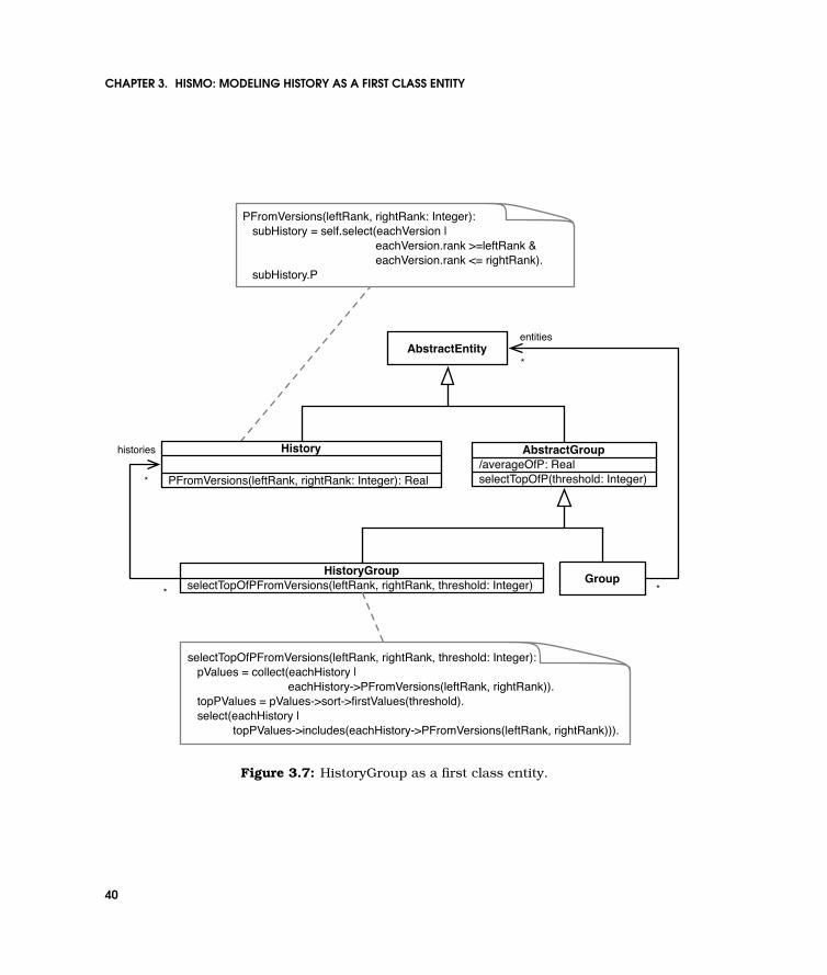
CHAPTER 3. HISMO: MODELING HISTORY AS A FIRST CLASS ENTITY
AbstractEntity
Group*
histories
*
entities
*
*HistoryGroup
selectTopOfPFromVersions(leftRank, rightRank, threshold: Integer)
selectTopOfPFromVersions(leftRank, rightRank, threshold: Integer): pValues = collect(eachHistory | eachHistory->PFromVersions(leftRank, rightRank)). topPValues = pValues->sort->firstValues(threshold). select(eachHistory | topPValues->includes(eachHistory->PFromVersions(leftRank, rightRank))).
PFromVersions(leftRank, rightRank: Integer): subHistory = self.select(eachVersion | eachVersion.rank >=leftRank & eachVersion.rank <= rightRank). subHistory.P
AbstractGroup/averageOfP: RealselectTopOfP(threshold: Integer)
History
PFromVersions(leftRank, rightRank: Integer): Real
Figure 3.7: HistoryGroup as a first class entity.
40
3.7. MODELING HISTORICAL RELATIONSHIPS
A HistoryGroup is a Group that holds histories instead of generic entities andit defines specific queries. In the figure, we give the example of selecting thehistories that have the highest historical property P computed only on a selectionof histories based on specified versions. This particular query is used in Chapter 4(p.47).
3.7 Modeling Historical Relationships
In this section we detail how we model relationships between histories.
Modeling Historical Relationships Recovered From Explicit Snapshot Rela-tionships
In the previous sections we showed how to model the history of a snapshot entitylike classes or packages. But, in a snapshot meta-model we can model explicitlystructural relationships like inheritance or invocations. Having the relationshipas a first class entity, allows us to model the corresponding history in exactly thesame fashion as we did for structural entities.
Figure 3.8 (p.42) shows an example of how to model inheritance relationships.Starting from “an InheritanceSnapshot links two Classes”, we build the versionrepresentation “an InheritanceVersion links two ClassVersions” and the historyrepresentation “an InheritanceHistory links two ClassHistories.” In Chapter 6 (p.87)
we give an example of how we can use this meta-model for understanding howhierarchies as a whole evolved.
Modeling Historical Relationships Recovered From Evolution
We can infer historical relationships not only from explicit structural relationships,but from how different entities evolved. In Section 2.3.2 (p.21) we reviewed a num-ber of evolution analyses based on the assumption that two entities are related ifthey are changed in the same time. We dedicate this section in showing how wemodel co-change as explicit historical relationships.
Two versions of two entities are related through co-change relationship if theyare both changed with respect to their respective previous versions. In the same
41

CHAPTER 3. HISMO: MODELING HISTORY AS A FIRST CLASS ENTITY
2 classVersions
* inheritanceVersions
ClassVersion
InheritanceVersion
2 classHistories
* inheritanceHistories
ClassHistory
InheritanceHistory
rank
rank ClassSnapshot
InheritanceSnapshot
2 classes
* inheritances
Figure 3.8: Using Hismo for modeling historical relationships.
D
A
B
C
2 moduleVersions
* coChangeVersions
ModuleVersion
CoChangeModuleVersion
2 moduleHistories
* coChangeHistories
ModuleHistory
CoChangeModuleHistory
rank
rank
Hismo
Co-Change
ModuleSnapshot
ver 1 ver 2 ver 3 ver 4 ver 5 ver 6
Figure 3.9: Using Hismo for co-change analysis. On the bottom-left side, we show 6 ver-sions of 4 modules: a grayed box represent a module that has been changed, while a whiteone represents a module that was not changed. On the bottom-right side, we show theresult of the evolution of the 4 modules as in Figure 2.3 (p.22).
42
3.8. GENERALIZATION
line, we define a CoChangeHistory to represent the relationship between two his-tories.
Figure 3.9 (p.42) shows an example of how to model co-changes between mod-ules. On the bottom part we represent the example from Figure 2.3 (p.22): Onthe bottom-left side we show 6 versions of 4 modules (A, B, C, D) and how theychanged from one version to the other (a change is marked with gray). On thebottom-right we show the historical representation. The resulting picture is thesame as in Figure 2.3 (p.22) only the meta-model is different. We no longer repre-sent the Modules as ellipses, but ModuleHistories, and the co-change is an explicithistorical relationship (i.e., CoChangeModuleHistory).
From the historical point of view, co-change and inheritance are similar, as theyboth transform into relationships between histories. The only difference betweenthem is that in the case of co-change relationship there is no snapshot entitywrapped by the CoChangeVersion.
3.8 Generalization: Transforming Snapshot Meta-Models into History Meta-Models
In the previous sections we gave examples of how to build the history meta-modelbased on a snapshot meta-model. In this section, we generalize the approachand show how we can use meta-model transformations for obtaining the historymeta-model.
In Figure 3.10 (p.44) we show in details the transformation which generates froma Class entity in the snapshot meta-model the corresponding ClassHistory andClassVersion entities. Thus, a ClassHistory is a sequence of ClassVersions. Alsothe model allows us to define history properties based on structural properties.
The bold text in the figure shows how the result only depends on the Snapshotand its properties. For example, having the number of Lines of Code (LOC) as anattribute in a Class, we can derive the minimum or the maximum lines of code inthe history. In the figure we show how we derive the Evolution of Lines of Code,as the sum of the absolute differences of the lines of code in subsequent versions.The history properties obtained in this manner, characterize and summarize theevolution.
Figure 3.11 (p.44) shows how we can obtain the relationships between the meta-
43

CHAPTER 3. HISMO: MODELING HISTORY AS A FIRST CLASS ENTITY
ClassVersion/versionId/evolutionOfLOC: integer
0..1
version
1
historyClass
LOC: integermodel
transformation
ClassHistory/maxLOC: integer/minLOC: integer/evolutionOfLOC: integer...
rank
evolutionOfLOC = Sequence {minId+1..maxId}->collect(i | self.versions[i]. evolutionOfLOC)->sum()
evolutionOfLOC = (prev.value(LOC)-self.value(LOC)).abs()
Figure 3.10: Transforming the Snapshot to obtain corresponding History and Version andderiving historical properties.
ClassVersion/versionIdname
1package
0..1class
PackageHistory
name
versionId0..1
version
1
historyPackageVersion
name
ClassHistory versionId0..1
version
1
history
1 /packageHistory
0..1 /classHistory
Classname
1package
0..1class
Package
namemodel
transformation
code generation
PackageHistory>>classHistories histories := Dictionary new. self versions do: [:eachPackageVersion | eachPackageVersion classes do:[ :eachClass | history := histories at: eachClass uniqueName ifAbsentPut: [ClassHistory new]. history addLast: eachClass ] ] ^histories values.
Figure 3.11: Obtaining the relationships between histories by transforming the snapshotmeta-model.
44
3.9. SUMMARY
model entities starting from the structural relationships. On the left side of thefigure we have a Package containing multiple Classes. After the transformationwe have the PackageHistory as containing multiple ClassHistories. On the down-right side of the figure we see the generated code in Smalltalk for obtaining theClassHistories starting from a PackageHistory. Similarly to Figure 3.10 (p.44), thebold text in the figure shows how the algorithm only depends on the Snapshotsand their relationships.
3.9 Summary
In this chapter we introduced Hismo, our meta-model which explicitly models his-tory as a collection of versions. In Hismo, the historical perspective is added ontop of the snapshot perspective. As a result, we can reuse the analyses built atstructural level in the historical context.
We gave examples of different historical properties, and we gave evidence of howsuch measurements can be used to characterize histories. We introduced the no-tion of grouping histories and we showed how we can define queries that takeinto account the historical properties. We completed the meta-model picture byshowing how we build historical relationships based both on snapshot relation-ships (e.g., inheritance history) and on evolution (e.g., co-change). Furthermore,we generalized our approach, by showing how the historical meta-model can beobtained by transforming the snapshot meta-model.
The next chapters discuss several evolution analyses, each one exercising a dif-ferent part of the meta-model (see Section 2.5 (p.27)). Each chapter has a similarstructure: first we discuss in detail the approach to show its relevance for reverseengineering, and in the end we show how Hismo supports the expression of theapproach.
45

CHAPTER 3. HISMO: MODELING HISTORY AS A FIRST CLASS ENTITY
46

Chapter 4
Yesterday’s WeatherSelecting Histories and Combining Historical Properties
Yesterday is a fact.Tomorrow is a possibility.
Today is a challenge.
Knowing where to start reverse engineering a large software system, when no in-formation other than the system’s source code itself is available, is a daunting task.Having the history of the code could be of help if this would not imply analyzing ahuge amount of data. In this chapter we present an approach for identifying can-didate parts of the system for reverse engineering and reengineering efforts. Oursolution is based on summarizing the changes in the evolution of object-orientedsoftware systems by defining history measurements. Our approach, named Yester-day’s Weather, is a measurement based on the retrospective empirical observationthat the parts of the system which changed the most in the recent past also sufferimportant changes in the near future. We apply this approach on three case studieswith different characteristics and show how we can obtain an overview of the evolu-tion of a system and pinpoint the parts that might change in the next versions.
Yesterday’s Weather is an example of how to build complex historical measurementsby combining historical properties computed on selections of histories.

CHAPTER 4. YESTERDAY’S WEATHER
4.1 Introduction
When starting a reverse engineering effort, knowing where to start is a key ques-tion. When only the code of the application is available, the history of a softwaresystem could be helpful as it holds valuable information about the life of the sys-tem, its growth, decay, refactoring operations, and bug-fixing phases. However,analyzing a software system’s history is difficult due to the large amount of com-plex data that needs to be interpreted. Therefore, history analysis requires one tocreate higher level views of the data.
The basic assumption of this dissertation is that the parts of the system that needto change are those that need to be understood first. We can find out about thetendencies of changes by looking at the past ones. However, not every change inthe history of the system is relevant for the future changes. For example, the partsof a system which changed in its early versions are not necessarily important1 forthe near future: Mens and Demeyer suggested that the evolution-prone partsof a system are those which have changed a lot recently [Mens and Demeyer,2001].
We aim to measure how relevant it is to start reverse engineering the parts of thesystem which changed the most in the recent past. Based on historical infor-mation, we identify the parts of the system that changed the most in the recentpast and check the assumption that they are likely to be among the most changedones in the near future. If this assumption held many times in the system history,then the recently changed parts are good candidates for reverse engineering. Ourexperiments show that important changes do not necessarily imply that they onlyoccur in the largest parts (e.g., in terms of lines of code). Therefore identifying thebig parts in the last version of a software system is not necessarily a good indicatorfor future changes.
We concentrate on the evolution of object-oriented systems, where by the parts ofa system we understand structural entities like packages, classes or methods. Weidentify the parts that are likely to change by defining evolutionary measurementsthat summarize the history of those parts. We show the relevance of these mea-surements in our approach which we name Yesterday’s Weather. Our approachis similar to the historical observation of the weather: a way of guessing whatthe weather will be like today is to think it will stay the same as yesterday. Thisheuristic can have very high success rates, however, its success is not the same inall places: In the Sahara desert the chance that the weather stays the same from
1By important we denote the fact that these parts will be affected by changes.
48

4.2. YESTERDAY’S WEATHER IN A NUTSHELL
one day to the next is higher than in Belgium, where the weather can change ina few hours. Therefore, to use such a heuristic for “successful weather forecasts”,we need to know how relevant the heuristic is for the place we want to use it. Weobtain the relevancy by analyzing the historical information about the climate ofthe place we are interested in.
Yesterday’s Weather is a measurement applied on a system history and it charac-terizes the “climate” of a software system. More specifically, Yesterday’s Weatherprovides an indication that allows one to evaluate the relevance of starting reverseengineering from the classes that changed the most recently.
Structure of the Chapter
We start by presenting an overview of Yesterday’s Weather in Section 4.2 (p.49). InSection 4.3 (p.50) we go into the details of computing and interpreting Yesterday’sWeather. In Section 4.4 (p.54) we present the results obtained on three case studiesand then discuss the variation points of our approach. In Section 4.5 (p.60) wediscuss different variation points of our approach. Section 4.6 (p.63) presents therelated work. In Section 4.7 (p.64) we summarize the approach, and we concludethe chapter with a discussion on how the usage of Hismo makes the expression ofYesterday’s Weather simple (Section 4.8 (p.65)).
4.2 Yesterday’s Weather in a Nutshell
We define Yesterday’s Weather (YW ) to be the retrospective empirical observationof the phenomenon that at least one of the heavily changed parts in the recenthistory is also among the most changed parts in the near future.
Our approach consists in identifying, for each version of a subject system, theparts that were changed the most in the recent history and in checking if theseare also among the most changed parts in the successive versions. We countthe number of versions in which this assumption holds and divide it by the totalnumber of analyzed versions to obtain the value of Yesterday’s Weather.
Example. Suppose that we want to analyze how classes change and for a sys-tem YW yields a value of 50%. This means that the history of the system hasshown that in 50% of the cases at least one of the classes that was changed a
49
CHAPTER 4. YESTERDAY’S WEATHER
lot in the recent past would also be among the most changed classes in the nearfuture.
YW characterizes the history of a system and is useful from a reverse engineeringpoint of view to identify parts that are likely to change in the next version. On onehand we use such information to make out progressive development phases inthe evolution of the system (e.g., what is/was the current focus of development?).In phases where the developers concentrate on a certain part of the system, theevolution would be fairly easy to predict. During repairing phases due to bugreports or little fixes the developers change the software system apparently at ran-dom places which leads to a decrease of predictability (i.e., the weather becomesunstable). On the other hand it also gives a general impression of the system (i.e.,how stable is the climate of the whole system?). By interpreting the YW we identifythat the changes are either focused on some parts over a certain period of time, orthey move unpredictably from one place to another.
Example. If the YW value of a software system S1 is 10%, this implies that thechanges in the system were rather discontinuous – maybe due to new developmentor bug fix phases. If the YW yields an 80% value for a system S2, this implies thechanges in the system were continuous. In such a system, we say it is relevant tostart the reverse engineering from the classes which were heavily changed lately,while this is not the case in system S1.
4.3 Yesterday’s Weather in Detail
Before defining the YW function, we introduce the notion of top n of entities out ofan original set S of entities with the highest P property value:
(0 < n < 1) TopP (S, n) = S′
˛˛ S′ ⊆ S,
|S′| = n
∀x ∈ S′, ∀y ∈ S − S′
P (x) > P (y)
(4.1)
To check the Yesterday’s Weather assumption with respect to classes, for a systemversion i, we compare the set of class histories with the highest LENOM1..i values(the candidates set) with the set of the class histories with the highest EENOM i..n
values (the really-changed set). The Yesterday’s Weather assumption holds if theintersection of these sets is not empty, that is at least one class history belongs
50

4.3. YESTERDAY’S WEATHER IN DETAIL
to both sets. This means that for the classes in version i at least one of therecently most changed classes is among the most changed classes in the nearfuture relative to version i. If the assumption holds for version i we have a hit (asshown in Equation 4.2 (p.51) and Figure 4.1 (p.52)).
In general, we formally define the Yesterday’s Weather hit function at version i
applied to a set of histories S with respect to a property P and given two thresholdvalues t1 and t2 as follows:
(i > 1; t1, t2 ≥ 1)
Y Wi(S, P, t1, t2) =
1, T opLEP1..i
(S, t1) ∩ TopEEPi..n(S, t2) 6= ∅
0, T opLEP1..i(S, t1) ∩ TopEEPi..n
(S, t2) = ∅ (4.2)
The overall Yesterday’s Weather is computed by counting the hits for all versionsand dividing them by the total number of possible hits. Thus, we obtain the resultas a percentage with values between 0% and 100%.
We formally define the Yesterday’s Weather applied to n versions of a set of histo-ries S with respect to a property P and given two threshold values t1 and t2 as inEquation 4.3 (p.51).
(n > 2; t1, t2 ≥ 1)
Y W1..n(S, P, t1, t2) =
Pn−1i=2 Y Wi(S, P, t1, t2)
n− 2(4.3)
Example. In Figure 4.1 (p.52) we present an example of how we check Yesterday’sWeather with respect to a certain version. We display 6 versions of a system with7 classes (A-G). We want to check Yesterday’s Weather when considering the 4thversion to be the present one. Therefore, the versions between 1 to 3 are the pastversions, and the 5th and 6th are the future ones.
We also consider the dimensions of the candidates and the really-changed set tobe 3, that is, we want to check the assumption that at least one of the top threeclasses which were changed in the recent history will also be among the top threemost changed classes in the near future. We draw circles with a continuous linearound the A, C and F classes to mark them as being the top three classes whichchanged the most in the recent history with respect to the 4th version. A, C and Fare candidates for a Yesterday’s Weather hit: While B changed recently, it is not
51

CHAPTER 4. YESTERDAY’S WEATHER
hit
Legend:
a candidate history (i.e., in TopLENOM1..i
)
a really-changed history(i.e., in TopEENOMi..n
)
2 4 3 5 6 7
2 3 4 9 9
1 3 3 4
2 2 2 2 2 2
1 5 4
1 2 4 7 3 6
3 4 5 4 6 3
pastversions
presentversion
futureversions
A
B
C
D
E
F
G
Figure 4.1: The detection of a Yesterday’s Weather hit with respect to classes.
a candidate because A, C and F changed more than B and in this case we onlyconcentrate on the top three most changed classes. We marked with a dotted circlethe classes which change the most in the next versions after the 4th one. We geta hit if the intersection between the continuous line circles and the dotted circlesis not empty. In the presented example we get a hit because of class F.
In Figure 4.2 (p.53) we show how we compute the overall Yesterday’s Weather fora system history with 10 versions. The grayed figures show that we had a hit inthat particular version, while the white ones show we did not. In the examplewe have 6 hits out of possible 10, making the value of Yesterday’s Weather to be60%.
Yesterday’s Weather Interpretation
Suppose we have to analyze a system history with 40 versions, where each versionconsists on average of 400 classes, and suppose we compute YW(S1,NOM,20,20)and get a result of 10%: The “climate” of the system is unpredictable with respectto the important changes. In such a “climate” it is not relevant to consider the
52

4.3. YESTERDAY’S WEATHER IN DETAIL
System
Versions
2 3 4 5 6 7 8 9 10 11
YW1..12 = 6 hits
10 possible hits= 60%
Figure 4.2: The computation of the overall Yesterday’s Weather.
latest changed classes to be important for the next versions.
If, on the other hand, we compute the YW(S2,NOM,5,5) and get a result of 80%, itmeans that during the analyzed period in 80% of the versions at least one of the5 classes that changed the most in the recent past is among the 5 classes thatchange the most in the near future. Therefore, we have a great chance to find,among the first 5 classes which were heavily changed recently, at least one classwhich would be important (from a reverse engineering point of view) for the nextversion.
The value of YW depends on the dimensions of the sets we want to compare. Forexample, on each line in the table in Figure 4.3 (p.56) we display different resultswe obtained, on the same history, depending on the sizes of the sets. For example,for 40 versions of Jun, when we considered the LENOM1..i set size to be 5 and theEENOM i..n set size to be 5, the YW was 50% (i.e., YW(Jun, NOM,5,5) = 50%). Whenthe LENOM1..i set size was 10 and the EENOM i..n set size was 10, the YW was 79%(YW(Jun, NOM,10,10) = 79%).
In YW(S, candidates, really-changed) the dimensions of the candidates and really-changed sets represent thresholds that can be changed to reduce or enlarge thescope of the analysis. Thus, using higher thresholds increases the chance of a hitbut also increases the scope, while by using lower tresholds we reduce the scope,but we also reduce the probability to have a hit. Both thresholds have specificinterpretations:
1. The candidates set threshold represents the number of the parts which changedthe most in the recent past. The lower this threshold is the more accuratethe assumption is. For example, imagine that for one system we choose a LE
53
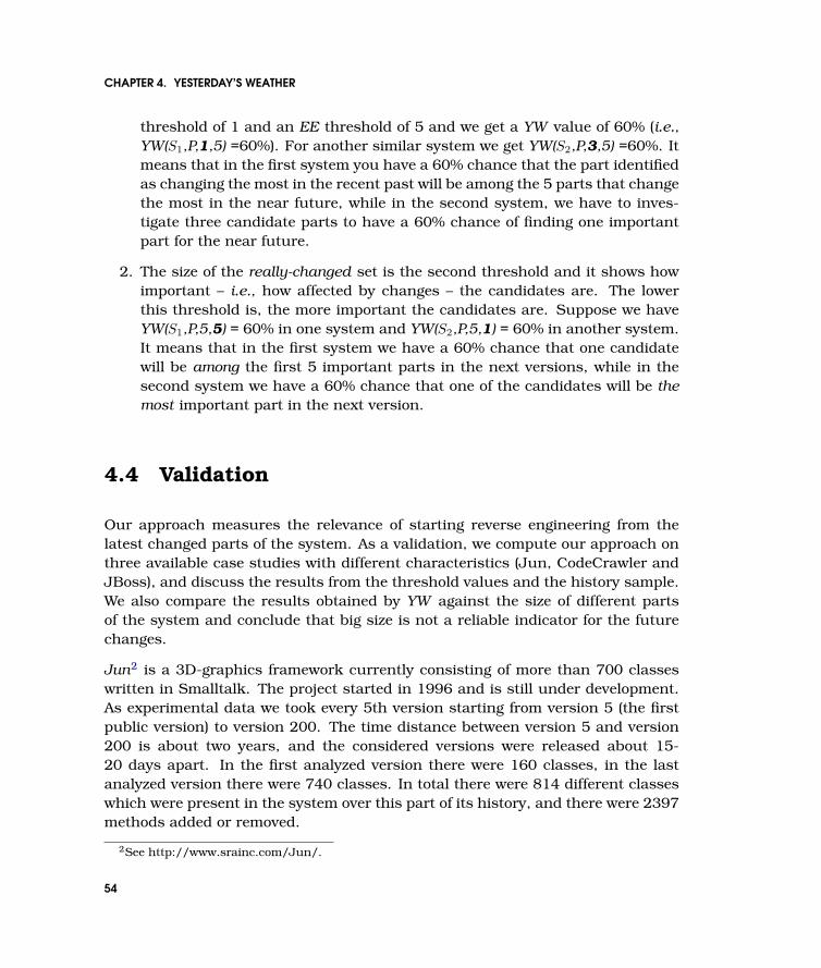
CHAPTER 4. YESTERDAY’S WEATHER
threshold of 1 and an EE threshold of 5 and we get a YW value of 60% (i.e.,YW(S1,P,1,5) =60%). For another similar system we get YW(S2,P,3,5) =60%. Itmeans that in the first system you have a 60% chance that the part identifiedas changing the most in the recent past will be among the 5 parts that changethe most in the near future, while in the second system, we have to inves-tigate three candidate parts to have a 60% chance of finding one importantpart for the near future.
2. The size of the really-changed set is the second threshold and it shows howimportant – i.e., how affected by changes – the candidates are. The lowerthis threshold is, the more important the candidates are. Suppose we haveYW(S1,P,5,5) = 60% in one system and YW(S2,P,5,1) = 60% in another system.It means that in the first system we have a 60% chance that one candidatewill be among the first 5 important parts in the next versions, while in thesecond system we have a 60% chance that one of the candidates will be themost important part in the next version.
4.4 Validation
Our approach measures the relevance of starting reverse engineering from thelatest changed parts of the system. As a validation, we compute our approach onthree available case studies with different characteristics (Jun, CodeCrawler andJBoss), and discuss the results from the threshold values and the history sample.We also compare the results obtained by YW against the size of different partsof the system and conclude that big size is not a reliable indicator for the futurechanges.
Jun2 is a 3D-graphics framework currently consisting of more than 700 classeswritten in Smalltalk. The project started in 1996 and is still under development.As experimental data we took every 5th version starting from version 5 (the firstpublic version) to version 200. The time distance between version 5 and version200 is about two years, and the considered versions were released about 15-20 days apart. In the first analyzed version there were 160 classes, in the lastanalyzed version there were 740 classes. In total there were 814 different classeswhich were present in the system over this part of its history, and there were 2397methods added or removed.
2See http://www.srainc.com/Jun/.
54

4.4. VALIDATION
CodeCrawler3 is a language independent reverse engineering tool which combinesmetrics and software visualization. In the first analyzed version there were 92classes and 591 methods, while in the last analyzed version there were 187 classesand 1392 methods. In the considered history, there were 298 different classespresent in the system over the considered history and 1034 methods added orremoved in subsequent versions.
JBoss4 is an open source J2EE application server written in Java. The versions weselected for the experiments were at two weeks distance from one another startingfrom the beginning of 2001 until 2003. The first version has 632 classes and 102packages, the last one has 4015 classes and 509 packages.
We chose these case studies because of their differences. Jun and JBoss havebeen developed by a team of developers while CodeCrawler is a single developerproject. Furthermore, Jun and CodeCrawler are written in Smalltalk, while JBossis written in Java.
4.4.1 Yesterday’s Weather in Jun, CodeCrawler and JBoss
Figure 4.3 (p.56) presents the results of the YW for the case studies for differentnumber of versions while keeping the thresholds constant. High values (e.g., 79%for Jun or more than 90% for CodeCrawler) denote a stable climate of the casestudies: the changes either went slowly from one part to another of the system, orthe changes were concentrated into some classes.
When we choose more distance between releases, we take into consideration theaccumulation of changes between the releases: the candidate parts are not nec-essarily heavily changed in just one version, but they could be changed over moreversions.
Jun. When we doubled the thresholds when analyzing 40 versions of Jun, weobtained 29% more in the YW value (i.e., YW(Jun40, NOM, 5, 5) = 50% becomesYW(Jun40, NOM, 10, 10) = 79%). Moreover, when we doubled the thresholds whenanalyzing 10 versions, we more than doubled the YW value (i.e., YW(Jun10, NOM,5, 5) = 37% becomes YW(Jun10, NOM, 10, 10) = 87%). These facts show that inJun there were classes which were changed over a long period of time, but thesechanges are not identified when we analyze versions which are closer to eachother.
3See http://www.iam.unibe.ch/ scg/Research/CodeCrawler/.4See http://sourceforge.net/projects/jboss/.
55
CHAPTER 4. YESTERDAY’S WEATHER
History sample YW(3,3)
40 versions of Jun (Jun40) 40%
20 versions of Jun (Jun20) 39%
10 versions of Jun (Jun10) 37%
40 versions of CodeCrawler (CC40) 68%
20 versions of CodeCrawler (CC20) 61%
10 versions of CodeCrawler (CC10) 62%
40 versions of JBoss (JBoss40) 11%
20 versions of JBoss (JBoss20) 28%
10 versions of JBoss (JBoss10) 50%
YW(5,5)
50%
55%
37%
92%
94%
100%
26%
38%
63%
YW(10,10)
79%
77%
87%
100%
100%
100%
53%
67%
63%
Figure 4.3: YW computed on classes with respect to methods on different sets of versionsof Jun, CodeCrawler and JBoss and different threshold values.
To show the relevance of YW we display the class histories that provoked a hitwhen computing YW(Jun40,NOM,10,10) for 40 versions of Jun (see Figure 4.4(p.57)). We focused on the size of the classes in terms of number of methodsand determined that YW predicts changes in classes which are not necessarilybig classes (e.g., JunOpenGLPerspective). We grayed the classes which provokeda hit when computing YW and which were not in the top 10 of the biggest classesin the last version. 17 out of 22 classes are not in the first 10 classes in termsof number of method: in Jun a big class is not necessarily an important class interms of future changes.
CodeCrawler. CodeCrawler is a project developed mainly by one developer, andas such can be considered a system with a focused and guided development withlittle external factors. This assumption is backed up by the data which reveals veryhigh YW values for low thresholds, resulting in a “stable climate” of the system.Note that CodeCrawler is much smaller than Jun, the thresholds must thus beseen as relatively lax.
Figure 4.5 (p.58) displays, using the same notation as in Figure 4.4 (p.57), the classhistories that provoked a hit in YW(5,5). As in the case of Jun, the hits were notnecessarily provoked by big classes and not all big classes provoked a hit. This
56

4.4. VALIDATION
YW(Jun40, NOM, 10,10) Hit Classes NOM
JunOpenGLDisplayModel 150JunWin32Interface 104JunBody 85JunOpenGL3dObject 75JunOpenGL3dObject_class 71JunOpenGL3dNurbsSurface 55JunLoop 55Jun3dLine 51JunOpenGLProjection 48JunUNION 47JunOpenGL3dCompoundObject 41JunPolygon 34JunBody_class 31JunVertex 30JunOpenGL3dVertexesObject 23JunOpenGL3dCompoundObject_class 21JunOpenGL3dVertex 19JunUNION_class 19JunOpenGL3dPolygon 15JunOpenGLPerspective 12JunOpenGLTestController 9JunOpenGLTestView 1
In top 10 biggestclasses in the last version
NOT in top 10 biggestclasses in the last version
Figure 4.4: The class histories that provoked a hit when computing YW(Jun40,NOM,10,10)and their number of methods in their last version. In this case study, the big classes arenot necessarily relevant for the future changes.
57

CHAPTER 4. YESTERDAY’S WEATHER
YW(CC40, NOM, 5,5) Hit Classes NOM
CCDrawing 123CCAbstractGraph 99CCGraph 69CCNode 47CodeCrawler 42CCConstants_class 39CCEdge 36CCControlPanel 29CCGroupNodePlugIn 25CCModelSelector 24CCRepositorySubcanvas 17CodeCrawler_class 15CCService 0
In top 10 biggestclasses in the last version
NOT in top 10 biggestclasses in the last version
Figure 4.5: The class histories that provoked a hit when computing YW(CC40,NOM,5,5) andtheir number of methods in their last version. In this case study, the big classes are notnecessarily relevant for the future changes.
shows that in CodeCrawler there is not always a relationship between changes andsize. Therefore, identifying the big classes from the last version, is not necessarilya good indicator for detecting classes which are important, in terms of change, forthe next versions.
JBoss. JBoss is a significantly larger system than the Jun. When we applied YWon the classes of JBoss, we did not obtain a high value: In JBoss it is less relevantto start reverse engineering from the latest changed classes.
The highest values were obtained when analyzing versions 2 months apart fromeach other (i.e., 10 versions in total). This is an indicator that there are classesthat change over a longer period of time, and that these changes do not showwhen analyzing more finer grained versions.
We applied YW on the packages of JBoss with respect to methods and we displayedthe results in Figure 4.6 (p.59). In Figure 4.7 (p.59) we show the packages thatprovoked a hit. In this case too, we see that the hits are not only provoked by thelargest packages.
58

4.4. VALIDATION
History sample YW(3,3)
40 versions of JBoss (JBoss40) 21%
20 versions of JBoss (JBoss20) 17%
10 versions of JBoss (JBoss10) 13%
YW(5,5)
45%
50%
63%
YW(10,10)
82%
100%
100%
Figure 4.6: YW computed on packages with respect to the total number of methods ondifferent sets of versions of JBoss and different threshold values.
YW(JBoss40,NOM,10,10) Hit Packages NOM
org::jboss::util 715org::jboss::ejb 513org::jboss::management::j2ee 436org::jboss::ejb::plugins::cmp::jdbc 396org::jboss::security 172org::jboss::system 140org::jboss::naming 100
In top 10 biggestpackages in the last version
NOT in top 10 biggestpackages in the last version
Figure 4.7: The package histories provoking a hit when computing YW(JBoss40,NOM,10,10)and their number of methods in their last version. In this case study, the big packages arenot necessarily relevant for the future changes.
In all three considered case studies we detected that the size of different parts ofthe systems is not necessarily a good indicator for predicting future changes.
4.4.2 The Evolution of Yesterday’s Weather in Jun
In Figure 4.8 (p.60) we represent a chart which shows Jun’s evolution of Yesterday’sWeather over time. The points in the chart show the value of Yesterday’s Weatheruntil that version: in version 15 Yesterday’s Weather is 100%, drops in version25, grows again until version 100 and then finally has an oscillating descendingshape.
Based on this view we can detect phases in the evolution where the changes werefocused and followed by other changes in the same part of the system (the ascend-ing trends in the graph) and phases where the changes were rather unfocused (thedescending trends in the graph). In the first half of the analyzed versions, in 90%
59
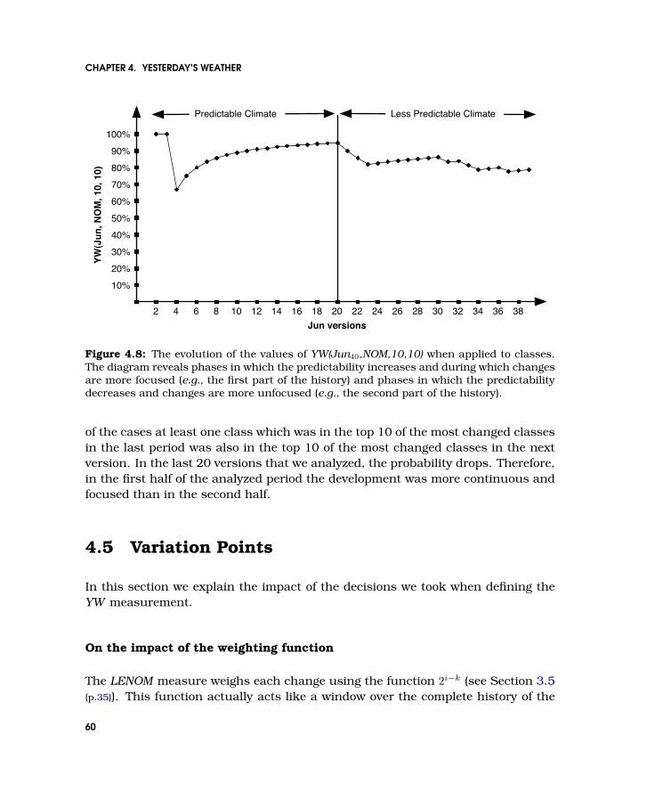
CHAPTER 4. YESTERDAY’S WEATHER
100%90%80%70%60%50%40%30%20%10%
2 4 6 8 10 12 14 16 18 20 22 24 26 28 30 32 34 36 38
Predictable Climate Less Predictable Climate
Jun versions
YW(J
un, N
OM
, 10,
10)
Figure 4.8: The evolution of the values of YW(Jun40,NOM,10,10) when applied to classes.The diagram reveals phases in which the predictability increases and during which changesare more focused (e.g., the first part of the history) and phases in which the predictabilitydecreases and changes are more unfocused (e.g., the second part of the history).
of the cases at least one class which was in the top 10 of the most changed classesin the last period was also in the top 10 of the most changed classes in the nextversion. In the last 20 versions that we analyzed, the probability drops. Therefore,in the first half of the analyzed period the development was more continuous andfocused than in the second half.
4.5 Variation Points
In this section we explain the impact of the decisions we took when defining theYW measurement.
On the impact of the weighting function
The LENOM measure weighs each change using the function 2i−k (see Section 3.5(p.35)). This function actually acts like a window over the complete history of the
60
4.5. VARIATION POINTS
changes by considering as relevant only the last four versions. This window isimportant as it lowers the impact of early development. For example, if a big classwas developed in the early versions but now suffers only bug-fixes, it will not beselected as a candidate for future important changes. Increasing the window sizefavors the candidacy of the large classes in the system, even if they are not chang-ing anymore, and reduces the relevancy of the prediction. Note that although thevalue of LENOM takes into account only the last four versions, the YW measure-ment is computed over the complete history.
On the impact of the at least condition
With the current YW assumption we consider to have a hit if at least one partwhich was heavily changed recently also gets changed a lot in the next versions. Ifwe have YW(S,P,10,10) = 60%, we do not know if the assumption held for 10 out ofthe 10 candidate part histories or just for one of them. YW gives relevant resultsin two cases:
1. High value of YW when considering low thresholds. Low thresholds (e.g., 5)mean low scope (both of candidates or of the importance of the really-changedentities), and if for such low thresholds we obtain a high YW value, we cancharacterize the changes as being continuous, and therefore it is relevant tolook at the most recently changed classes to detect one which will probablyundergo an important change during the near future, e.g., the next versions.
2. Low value of YW when considering high thresholds. When obtaining low YWvalues for high thresholds, we can characterize the changes as being dis-continuous, and therefore looking at the most recently changed parts is notnecessarily relevant for the future changes in the system.
In Figure 4.1 (p.52) the hit is provoked by one out of three candidates. Yet, inanother version the hit could be provoked by more candidates. A possible en-hancement of Yesterday’s Weather would be to compute an average of the numberof parts that matched the YWi assumption. The result of this average would com-plement the YW value, by showing its overall accuracy. For example, if the YWvalue is high, then the higher the value of this average is, the more importantparts for reengineering are likely to be identified with the YW heuristic.
61

CHAPTER 4. YESTERDAY’S WEATHER
On the impact of the release period
Another variation point when computing Yesterday’s Weather is the release period.If we consider the release period of one week, we focus the analysis on immediatechanges. If, on the other hand, we consider the release period of half a year, weemphasize the size of the changes that accumulate in the histories.
Example. Suppose that when we consider the release period of a big system of oneweek we obtain YW(S,P,5,5) = 60% and when we consider the release period of halfa year we obtain YW(S,P,5,5) = 20%. It means that from one week to another thedevelopment is quite focused, and the bigger parts of the system tend to stabilizeover a long period of time, thus leading to apparently unexpected changes, e.g.,bug-fixing, patching, small functionality increase all over the system.
The variation of YW allows one to fine-tune the information. It is the combinationof short and focused releases and the decrease of YW that allows one to concludethat the system stabilizes - that is, the parts that were changed in the past areno longer changed in the future. Note that, by considering longer release periods,the additions and removals of methods from the same class between consecutivereleases will not show in the history measurements.
On the impact of the number of versions
The number of versions represents another variation point when computing YW .Increasing or decreasing the number of versions affects the overall YW , but haslittle effect on the value of individual YWi. The longer the considered history, theless important is a hit/non-hit in the overall YW . By increasing the number ofversions while keeping the same period between versions, we let the early changesaffect the overall YW . Therefore, when keeping the period between versions con-stant, by increasing the number of versions we obtain a long-term trend, while bydecreasing the number of versions we concentrate on the short-term trend.
On the impact of the granularity level
YW can be applied at any level of abstraction. We showed the results we obtainedon classes and packages with respect to adding and removing methods. Suchanalysis requires the knowledge about the structure of the system. When such
62

4.6. RELATED WORK
information is not available, YW can be applied, for example, on files and folderswith respect to adding and removing lines of code.
4.6 Related Work
Measurements have traditionally been used to deal with the problem of analyzingthe history of software systems. Ramil and Lehman explored the implication of theevolution metrics on software maintenance [Ramil and Lehman, 2001]. They usedthe number of modules to describe the size of a version and define evolutionarymeasurements which take into account differences between consecutive versions.Recently, the same approach has been employed to characterize the evolution ofopen source projects [Godfrey and Tu, 2000; Capiluppi, 2003; Capiluppi et al.,2004].
Jazayeri analyzed the stability of the architecture by using colors to depict thechanges. Based on the visualization he analyzed how the old code tends to stabi-lize over time [Jazayeri, 2002].
Rysselberghe and Demeyer used a simple visualization to provide an overview ofthe evolution of systems: they displayed a plot chart, where each dot representsa commit of the corresponding file [Van Rysselberghe and Demeyer, 2004]. Basedon the visualization they detected patterns of evolution.
Jingwei Wu et al. used the spectograph metaphor to visualize how changes occurin software systems [Wu et al., 2004a]. They used colors to denote the age ofchanges on different parts of the systems.
These approaches make use of raw data provided by the versioning system: fold-ers, files and lines of text. As opposed to that, our approach takes into considera-tion the structure of the system and makes use of the semantics of changes.
Burd and Munro defined a set of measurements to quantify the dominance re-lations which are used to depict the complexity of the calls. They correlated thechanges in these measurements with the types of maintainability activities [Burdand Munro, 1999].
Gold and Mohan defined a framework to understand the conceptual changes inan evolving system [Gold and Mohan, 2003]. Based on measuring the detectedconcepts they could differentiate between different maintenance activities.
63
CHAPTER 4. YESTERDAY’S WEATHER
Grosser, Sahraoui and Valtchev applied Case-Based Reasoning on the history ofobject-oriented system as a solution to a complementary problem to ours: to pre-dict the preservation of the class interfaces [Grosser et al., 2002]. They also con-sidered the interfaces of a class to be the relevant indicator of the stability of aclass. Sahraoui et al. employed machine learning combined with a fuzzy approachto understand the stability of the class interfaces [Sahraoui et al., 2000].
Our approach differs from the above mentioned ones because we consider the his-tory to be a first class entity and define history measurements which are applied tothe whole history of the system and which summarize the evolution of that system.Thus we do not have to analyze manually in detail evolution charts. The drawbackof our approach consists in the inherent noise which resides in compressing largeamounts of data into numbers.
Fischer et al. analyzed the evolution of systems in relation with bug reports totrack the hidden dependencies between features [Fischer et al., 2003a]. Demeyeret al. proposed practical assumptions to identify where to start a reverse engineer-ing effort: working on the most buggy part first or focusing on clients most impor-tant requirements [Demeyer et al., 2002]. These approaches, are based on infor-mation that is outside the code, while our analysis is based on code alone.
In a related approach, Hassan et al. analyzed the types of data that are goodpredictors of change propagation, and came to the conclusion that historical co-change is a better mechanism than structural dependencies like call-graph [Has-san and Holt, 2004].
4.7 Summarizing Yesterday’s Weather
One of the most important issues when starting reverse engineering is knowingwhere to start. When only the code of the application is available, the historyof a software system could be of help. However, analyzing the history is difficultbecause of the interpretation of large quantities of complex data. We presented ourapproach of summarizing the history by defining history measurements.
We use the term Yesterday’s Weather to depict the retrospective empirical obser-vation that at least one of the parts of the system that were heavily changed inthe last period will also be among the most changed parts in the near future. Wecomputed it on three case studies and showed how it can summarize the changesin the history of a system. We use the approach to pinpoint parts of the system in
64

4.8. HISMO VALIDATION
the latest version which would make good candidates for a first step in reverse en-gineering. We looked closely at how the big changes are related with the size of theclasses and packages, and validated our approach by showing that big changescan occur in classes and packages which are not big in terms of size (i.e., numberof methods). Thus, our approach is useful to reveal candidates for reengineeringwhich are otherwise undetectable if we only analyze the size of the different partsof the system’s last version.
When reverse engineering, we should take the auxiliary development informationinto account. For example, we could correlate the shape of the evolution of Yester-day’s Weather with the changes in the team or with the changes in the develop-ment process. An example of an analysis of the history of the developers is shownin Chapter 7 (p.105). In the future, we would like to correlate Yesterday’s Weatherwith such information from outside the source code.
4.8 Hismo Validation
The approach consists of identifying, for each version of a subject system, theparts that were changed the most in the recent history and in checking if theseare also among the most changed parts in the successive versions. The YW valueis given by the number of versions in which this assumption holds divided by thetotal number of analyzed versions. Below we give an OCL code for computing YWfor a SystemHistory with respect to classes:
context SystemHistory
-- returns true if the YW assumption holds for a given version versionRankderive versionYW(versionRank):
yesterdayTopHistories = self.classHistories->selectTopLENOMFromVersions(minRank, versionRank-1).todayTopHistories = self.classHistories->selectTopEENOMFromVersions(versionRank, maxRank).yesterdayTopHistories->intersectWith(todayTopHistories)->isNotEmpty().
-- answers the number of versions in which the assumption holds-- divided by the total number of analyzed versionsderive overallYW:
ywVersionResults = Sequence(minRank+2..maxRank-1)->collect(i | self.versionYW(i).ywVersionResults->sum() / (maxRank-minRank-2)
65

CHAPTER 4. YESTERDAY’S WEATHER
The code reveals several features of Hismo :
— We navigate the meta-model by asking a SystemHistory for all the ClassHisto-ries (self.classHistories).
— classHistories->selectTopLENOMFromVersions(minRank, versionRank-1) returns the classhistories that are in the top of LENOM (Latest Evolution of Number of Meth-ods) in the period between the first version (minRank) and the version before thewanted version (versionRank-1). That is, it returns the classes that were changedthe most in the recent history. This predicate implies applying a historicalmeasurement (i.e., LENOM) on a selection of a history, and then ordering thehistories according to the results of the measurement.
— Similarly, classHistories->selectTopEENOMFromVersions(versionRank, maxRank) returnsthe class histories that are the most changed in the early history between thewanted version (versionRank) and the last version (maxRank).
— The result of versionYW is given by the intersection of the past changed class his-tories and the future changed class histories yesterdayTopHistories->intersectWith(todayTopHistories)->isNotEmpty(). This simple intersection is possible because theyesterdayTopHistories and todayTopHistories are subsets of all classHistories.
66

Chapter 5
History-Based DetectionStrategiesCombining Historical Properties with Structural Properties
From an abstract enough point of view,any two things are similar.
As systems evolve and their structure decays, maintainers need accurate and au-tomatic identification of the design problems. Current approaches for automaticdetection of design problems take into account only a single version of a system,and consequently, they miss essential information as design problems appear andevolve over time. Our approach is to use the historical information of the suspectedflawed structure to increase the accuracy of the automatic problem detection. Ourmeans is to define measurements which summarize how persistent the problem wasand how much maintenance effort was spent on the suspected structure. We applyour approach to a large scale case study and show how it improves the accuracy ofthe detection of God Classes and Data Classes, and additionally how it adds valu-able semantic information about the evolution of flawed design structures.
This approach shows how to combine historical properties with snapshot proper-ties.

CHAPTER 5. HISTORY-BASED DETECTION STRATEGIES
5.1 Introduction
Maintenance effort is reported to be more than half of the overall developmenteffort and most of the maintenance effort is spent on adapting and introducingnew requirements, rather than in repairing errors [Bennett and Rajlich, 2000;Sommerville, 2000]. One important source of maintainability problems is theaccumulation of poor or improper design decisions. This is the reason why, duringthe past years, the issue of identifying and correcting design problems became animportant concern for the object-oriented community [Fowler et al., 1999; Riel,1996; Demeyer et al., 2002].
Various analysis approaches have been developed to automatically detect wherethe object-oriented design problems are located, but these approaches only makeuse of the information found in the last version of the system (i.e., the versionwhich is maintained) [Ciupke, 1999; Marinescu, 2001]. For example, they look forimproper distribution of functionality among classes of a system without askingwhether or not it raised maintenance problems in the past.
We argue that the evolution information of the problematic classes over their life-time can give useful information to system maintainers. We propose a new ap-proach which enriches the detection of design problems by combining the analy-sis based on a single version with the information related to the evolution of thesuspected flawed classes over time.
We show how we apply our approach when detecting two of the most well knowndesign flaws: Data Class and God Class. Marinescu detected these flaws by ap-plying measurement-based rules to a single version of a system [Marinescu, 2002;Marinescu, 2004]. He named these rules detection strategies. The result of a de-tection strategy is a list of suspects: design structures (e.g., classes) which aresuspected of being flawed. We enlarge the concept of detection strategies by tak-ing into account the history of the suspects (i.e., all versions of the suspects). Wedefine history measurements which summarize the evolution of the suspects andcombine the results with the classical detection strategies.
Structure of the Chapter
After we present the metaphor of our approach, we briefly describe the conceptof detection strategy and discuss the detection of Data Classes and God Classes(Section 5.3 (p.69)). In Section 5.5 (p.74) we define the history measurements needed
68
5.2. THE EVOLUTION OF DESIGN FLAW SUSPECTS
to extend the detection strategies and discuss the way we use historical informa-tion in detection strategies. We then apply the new detection strategies on a largeopen source case study and discuss in detail the results (Section 5.6 (p.77)).We givean overview of the related work in Section 5.8 (p.83), we summarize the approachin Section 5.9 (p.84). In Section 5.10 (p.85) we discuss the approach pointing outthe benefits of using Hismo.
5.2 The Evolution of Design Flaw Suspects
Design flaws (e.g., God Class or Data Class) are like human diseases - each of themevolves in a special way. Some diseases are hereditary, others are acquired duringthe life-time. The hereditary diseases are there since we were born. If physiciansare given a history of our health status over time they can give their diagnostic ina more precise way. Moreover there are diseases (e.g., benign tumors) with whichour organism is accustomed and thus, they represent no danger for our healthand we don’t even consider them to be diseases any more.
In a similar fashion we use the system’s evolution to increase the accuracy of thedesign flaw detection. We analyze the history of the suspects to see whether theflaw caused problems in the past. If in the past the flaw proved not to be harmfulthen it is less dangerous. For example, in many cases, the generated code needsno maintenance so the system which incorporates it can live a long and serenelife no matter how the generated code appears in the sources (e.g., large classesor unreadable code).
The design flaws evolve with the system they belong to. As systems get older theirdiseases are more and more prominent and need to be more and more taken intoaccount.
5.3 Detection Strategies
A detection strategy is a generic mechanism for analyzing a source code modelusing metrics. It is defined by its author as the quantifiable expression of a rule,by which design fragments that are conformant to that rule can be detected in thesource code [Marinescu, 2002].
Detection strategies allow one to work with measurements at a more abstract level,
69
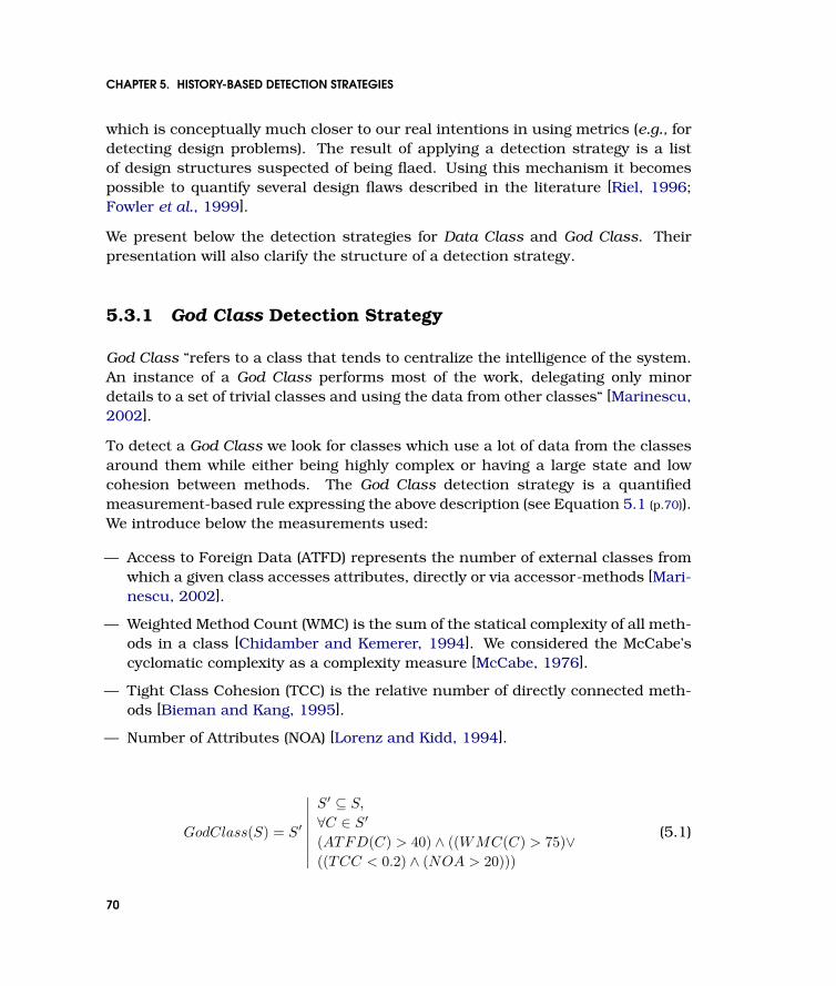
CHAPTER 5. HISTORY-BASED DETECTION STRATEGIES
which is conceptually much closer to our real intentions in using metrics (e.g., fordetecting design problems). The result of applying a detection strategy is a listof design structures suspected of being flaed. Using this mechanism it becomespossible to quantify several design flaws described in the literature [Riel, 1996;Fowler et al., 1999].
We present below the detection strategies for Data Class and God Class. Theirpresentation will also clarify the structure of a detection strategy.
5.3.1 God Class Detection Strategy
God Class “refers to a class that tends to centralize the intelligence of the system.An instance of a God Class performs most of the work, delegating only minordetails to a set of trivial classes and using the data from other classes“ [Marinescu,2002].
To detect a God Class we look for classes which use a lot of data from the classesaround them while either being highly complex or having a large state and lowcohesion between methods. The God Class detection strategy is a quantifiedmeasurement-based rule expressing the above description (see Equation 5.1 (p.70)).We introduce below the measurements used:
— Access to Foreign Data (ATFD) represents the number of external classes fromwhich a given class accesses attributes, directly or via accessor-methods [Mari-nescu, 2002].
— Weighted Method Count (WMC) is the sum of the statical complexity of all meth-ods in a class [Chidamber and Kemerer, 1994]. We considered the McCabe’scyclomatic complexity as a complexity measure [McCabe, 1976].
— Tight Class Cohesion (TCC) is the relative number of directly connected meth-ods [Bieman and Kang, 1995].
— Number of Attributes (NOA) [Lorenz and Kidd, 1994].
GodClass(S) = S′
∣∣∣∣∣∣∣∣S′ ⊆ S,
∀C ∈ S′
(ATFD(C) > 40) ∧ ((WMC(C) > 75)∨((TCC < 0.2) ∧ (NOA > 20)))
(5.1)
70

5.3. DETECTION STRATEGIES
5.3.2 Data Class Detection Strategy
Data Classes “are classes that have fields, getting and setting methods for thefields, and nothing else. Such classes are dumb data holders and are almostcertainly being manipulated in far too much detail by other classes” [Fowler et al.,1999].
To detect a Data Class we look for classes which have a low complexity and highexposure to their internal state (i.e., a lot of either accessor methods or publicattributes). The Data Class detection strategy in Equation 5.2 (p.71) uses the fol-lowing measurements:
— Weight of a Class (WOC) is the number of non-accessor methods in the inter-face of the class divided by the total number of interface members [Marinescu,2001].
— Number of Methods (NOM) [Lorenz and Kidd, 1994].
— Weighted Method Count (WMC) [Chidamber and Kemerer, 1994].
— Number of Public Attributes (NOPA) is defined as the number of non-inheritedattributes that belong to the interface of a class [Marinescu, 2001].
— Number of Accessor Methods (NOAM) is defined as the number of the non-inherited accessor-methods declared in the interface of a class [Marinescu,2001].
DataClass(S) = S′
∣∣∣∣∣∣∣∣∣S′ ⊆ S,
∀C ∈ S′
((WMC(C)NOM(C) < 1.1) ∧ (WOC(C) < 0.5))∧
((NOPA(C) > 4) ∨ (NOAM(C) > 4))
(5.2)
5.3.3 Detection Strategy Discussion
As shown in the Equation 5.1 (p.70) and Equation 5.2 (p.71) the detection strategiesare based on a skeleton of measurements and thresholds for each measurement(e.g., ATFD > 40). While the measurements skeleton can be obtained by translat-ing directly the available informal rules (e.g., heuristics or bad smells), the partic-ular sets of thresholds are mainly chosen based on the experience of the analyst.
71

CHAPTER 5. HISTORY-BASED DETECTION STRATEGIES
As this experience can differ from person to person the thresholds represent theweak point of the detection strategies.
The process of using detection strategies to detecting design flaws is not fully au-tomated. Indeed, detection strategies are automated, but the result of a detectionstrategy is a list of suspects which requires further human intervention to verifythe flaw.
5.4 History Measurements
We refine the detection of design flaws by taking into consideration how stable thesuspects were in the past and how long they have been suspected of being flawed.We name persistently flawed1 the entities which were suspects a large part oftheir life-time (i.e., more than 95% of their life time). Thus we further introducetwo measurements applied on the history of a suspect: Stab and Pers.
5.4.1 Measuring the Stability of Classes
We consider that a class was stable with respect to a measurement M betweenversion i − 1 and version i if there was no change in the measurement. As anoverall indicator of stability, we define the Stab measurement applied on a classhistory H as a fraction of the number of versions in which there was a changein the M measurement over the total number of versions - 1 (see Equation 5.3(p.72)).
(i > 1) Stabi(H,M) ={
1, Mi(H)−Mi−1(H) = 00, Mi(H)−Mi−1(H) 6= 0
(n > 2) Stab1..n(H,M) =∑n
i=2 Stabi(H,M)n− 1
(5.3)
The Stab measurement returns a value between 0 and 1, where 0 means that thehistory was changed in all versions and 1 means that it was never changed.
1The adjective persistent is a bit overloaded. In this dissertation we use its first meaning: existingfor a long or longer than usual time or continuously. Merriam-Webster Dictionary
72
5.4. HISTORY MEASUREMENTS
The functionality of classes is defined in their methods. For the purpose of thecurrent analysis, we consider that a class was changed if at least one method wasadded or removed. Thus, we will use Stab with respect to the Number of Methodsof a class (NOM).
5.4.2 Measuring the Persistency of a Design Flaw
We define the Pers measurement of a flaw F for a class history H with n ver-sions, i.e., 1 being the oldest version and n being the most recent version (seeEquation 5.4).
(i ≥ 1) Suspecti(H,F ) ={
1, Hi is suspect of flaw F
0, Hi is not suspect of flaw F
(n > 2) Pers1..n(H,F ) =∑n
i=1 Suspecti(H,F )n
(5.4)
The Pers measurement returns a value between 0 and 1, and it tells us in whatmeasure the birth of the flaw is related with the design stage or with the evolutionof the system. For example, if for a history Pers is 1, it means that the flaw waspresent from the very beginning of the history.
Example. The top part of Figure 5.1 (p.74) presents 5 class histories and the resultsof the Stab and Pers measurements, and the bottom part shows in details how weobtain the values for the two measurements in the case of A. We can interpret thepersistent flaws in one of the following ways:
1. The developers are conscious of these flaws and they could not avoid makingthem. This could happen because of particularities of the modeled system -the essential complexities [Brooks, 1987] - or the need to meet other qualitycharacteristics (e.g., efficiency).
2. The developers are not conscious of the flaws. The cause for this can beeither the lack of expertise in object-oriented design or the trade-offs theprogrammers had to do due to external constraints (e.g., time pressure).
The flaws which are not persistent are named volatile, and are the result of thesystem’s evolution. These situations are usually malignant because they reveal
73
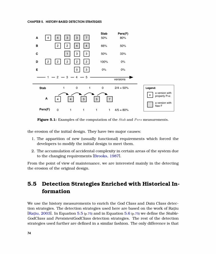
CHAPTER 5. HISTORY-BASED DETECTION STRATEGIES
2 2 4
1 3
2 2
B
C
D
Stab Pers(F)50%
66%
100%
80%
50%
50% 33%
0%
4 4 3 3A
E 0% 0%
2 2
4
3
0
1 2 3 4 5
2
7
3
versions
Stab
Pers(F)
2/4 = 50%
4/5 = 80%
4 4 3 3A 7
1 001 Legend:
x a version withproperty P=x
a version withflaw F
0 1 1 1 1
Figure 5.1: Examples of the computation of the Stab and Pers measurements.
the erosion of the initial design. They have two major causes:
1. The apparition of new (usually functional) requirements which forced thedevelopers to modify the initial design to meet them.
2. The accumulation of accidental complexity in certain areas of the system dueto the changing requirements [Brooks, 1987].
From the point of view of maintenance, we are interested mainly in the detectingthe erosion of the original design.
5.5 Detection Strategies Enriched with Historical In-formation
We use the history measurements to enrich the God Class and Data Class detec-tion strategies. The detection strategies used here are based on the work of Ratiu[Ratiu, 2003]. In Equation 5.5 (p.75) and in Equation 5.6 (p.75) we define the Stable-GodClass and PersistentGodClass detection strategies. The rest of the detectionstrategies used further are defined in a similar fashion. The only difference is that
74
5.5. DETECTION STRATEGIES ENRICHED WITH HISTORICAL INFORMATION
while stability is measured for a class in isolation, the instability for a class ismeasured relatively to the other classes within the system.
StableGodClass(S1..n) = S′
∣∣∣∣∣∣S′ ⊆ GodClass(Sn),∀C ∈ S′
Stab(C) > 95%(5.5)
PersGodClass(S1..n) = S′
∣∣∣∣∣∣S′ ⊆ GodClass(Sn),∀C ∈ S′
Pers(C,GodClass) > 95%(5.6)
God Classes and Stability. God Classes are big and complex classes which en-capsulate a great amount of system’s knowledge. They are known to be a sourceof maintainability problems [Riel, 1996]. However, not all God Classes raise prob-lems for maintainers. The stable God Classes are a benign part of the God Classsuspects because the system’s evolution was not disturbed by their presence. Forexample, they could implement a complex yet very well delimited part of the sys-tem containing a strongly cohesive group of features (e.g., an interface with alibrary).
On the other hand, the changes of a system are driven by changes in its fea-tures. Whenever a class implements more features it is more likely to be changed.God Classes with a low stability were modified many times during their life-time.Therefore, we can identify God Classes which have produced maintenance prob-lems during their life from the set of all God Classes identified within the system.The unstable God Classes are the malignant sub-set of God Class suspects.
God Classes and Persistency. The persistent God Class are those classes whichhave been suspects for almost their entire life. Particularizing the reasons givenabove for persistent suspects in general, a class is usually born God Class becauseone of the following reasons:
1. It encapsulates some of the essential complexities of the modeled system.For example, it can address performance problems related to delegation or itcan belong to a generated part of the system.
2. It is the result of a bad design because of the procedural way of regardingdata and functionality, which emphasis a functional decomposition insteadof a data centric one.
75

CHAPTER 5. HISTORY-BASED DETECTION STRATEGIES
It is obvious that God Classes which are problematic belong only to the latter cate-gory because in the first category the design problem can not be eliminated.
God Class suspects which are volatile obtained the God Class status during theirlifetime. We argue that persistent God Classes are less dangerous than thosewhich are not persistent. The former were designed to be large and importantclasses from the beginning and thus are not so dangerous. The latter more likelyoccur due to the accumulation of accidental complexity resulted from the repeatedchanges of requirements and they degrade the structure of the system.
Data Classes and Stability. Data Classes are lightweight classes which containonly little functionality. While God Classes carry on the work, Data Classes areonly dumb data providers whose data is used from within other (possible many)classes. Modifications within Data Classes require a lot of work from program-mers, as the principle of locality of change is violated. Thus, regarding the effortsimplied by their change, programmers are less likely to change Data Classes.Based on this, we infer that the more relevant functionality a Data Class containsthe higher are its chances to become the subject of a change. From this point ofview, “classic” Data Classes, which are nothing else but dumb data carriers witha very light functionality, should be rather stable.
Data Classes and Persistency. Persistent Data Classes represent those classeswhich were born with this disease. They break from the beginning of their life thefundamental rule of object-oriented programming which states that data and itsassociated functionality should stay together. Particularizing the reasons whichcould lead to persistent Data Classes we obtain that:
1. The class is used only as a grouping mechanism to put together some data.For example such a class can be used where is necessary to transmit someunrelated data through the system.
2. There was a design problem as Data Classes do not use any of the mecha-nisms specific to object-oriented programming (i.e., encapsulation, dynamicbinding or polymorphism). The data of these classes belong together but thecorresponding functionality is somewhere else.
Data Classes which are volatile are classes which got to be Data Class duringtheir life. A class can become a Data Class either by requirements change inthe direction of functionality removal or by refactorings. Functionality removalwhile keeping the data is unlikely to happen. Furthermore by properly applyingthe refactorings as defined in [Fowler et al., 1999] we can not get classes withrelated data but no functionality (i.e., the malignant set of Data Classes). The only
76

5.6. VALIDATION
Data Classes we are likely to get are those which belong to the harmless category,because the class is used only as a modularization mechanism for moving easilyunrelated data.
5.6 Validation
We applied our approach to three case studies: two in-house projects and Jun2,a large open source 3D-graphics framework written in Smalltalk. As experimentaldata we chose every 5th version starting from version 5 (the first public version) toversion 200. In the first analyzed version there were 160 classes while in the lastanalyzed version there were 694 classes. There were 814 different classes whichwere present in the system over this part of its history. Within these classes 2397methods were added or removed through the analyzed history.
We first applied the detection strategies and then the suspects were both manuallyinspected at the source-code level and looked-up in Jun’s user manual. Based onthe manual inspection we determined which suspects were false positives, how-ever we did not have access to any internal expertise.
The history information allowed us to distinguish among the suspects provided bysingle-version detection strategies, the harmful and harmless ones. This distinc-tion among suspects drives the structure of the entire section.
The analysis shows how, by adding information related to the evolution of classes,the accuracy of the detection results was improved on this case-study, both forGod Classes and Data Classes. Additionally, it shows that the history of thesystem adds valuable semantic information about the evolution of flawed designstructures.
Harmless God Classes. The God Classes which are persistent and stable duringtheir life are the most harmless ones. They lived in symbiosis with the systemalong its entire life and raised no maintainability problems in the past.
When taking a closer look at the Figure 5.2 (p.78) which present the God Classsuspects we observe that more than 20% of them are persistent and stable (5out of 24). These classes in spite of their large size, did not harm the system’smaintainability in the past, because the developers did not need to change them,so it is unlikely that they will harm it in the future. Almost all of these classes
2See http://www.srainc.com/Jun/.
77
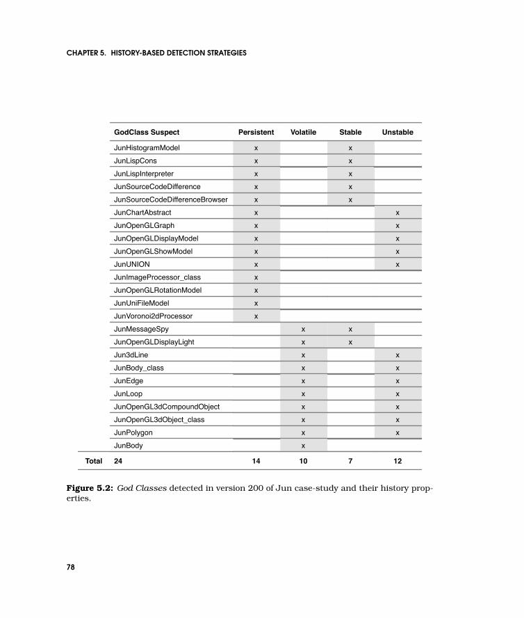
CHAPTER 5. HISTORY-BASED DETECTION STRATEGIES
GodClass Suspect Persistent
JunHistogramModel xJunLispCons xJunLispInterpreter xJunSourceCodeDifference xJunSourceCodeDifferenceBrowser xJunChartAbstract x
Volatile Stable
xxxxx
Unstable
xJunOpenGLGraph x xJunOpenGLDisplayModel x xJunOpenGLShowModel x xJunUNION x xJunImageProcessor_class x
24 14 10 7 12
JunOpenGLRotationModel xJunUniFileModel xJunVoronoi2dProcessor xJunMessageSpyJunOpenGLDisplayLightJun3dLine
xxx
xx
xJunBody_class x xJunEdge x xJunLoop x xJunOpenGL3dCompoundObject x xJunOpenGL3dObject_class x xJunPolygon x xJunBody x
Total
Figure 5.2: God Classes detected in version 200 of Jun case-study and their history prop-erties.
78

5.6. VALIDATION
belong to particular domains which are weakly related with the main purpose ofthe application. We can observe this even by looking at their names. In Jun theseclasses belong to a special category named “Goodies” which means that they areoptional add-ons.
— JunLispInterpreter is a class that implements a Lisp interpreter, one of thesupplementary utilities of Jun. This is an example of a GodClass that modelsa matured utility part of the system.
— JunSourceCodeDifferenceBrowser is used to support the evolution of Jun. Itbelongs to the effort of the developers to support the evolution of the libraryitself.
Continuing to look at the Figure 5.2 (p.78) we notice that some of the God Classeswere stable during their lifetime even if they were not necessarily persistent. Themanual inspection revealed that some of these classes were born as skeletons ofGod Classes and waited to be filled with functionality at a later time. Anotherpart of them was not detected to be persistent because of the hard thresholds ofthe detection strategies. We can consider these classes to be a less dangerouscategory of God Classes.
— JunOpenGLDisplayLight is a GUI class (i.e., a descendant of UI.ApplicationModel),which suddenly grew in version 195.
— JunMessageSpy is a helper class which is used for displaying profiling infor-mation for messages. It also belongs to the ’Goodies’ category. This class wasdetected as being God Class from the beginning because of the hard thresholdsused in the detection strategy.
Harmful God Classes. The God Classes which were both volatile and unstableare the most dangerous ones. Looking at the Figure 5.2 (p.78) we can easily seethat almost 30% of the God Classes are harmful (7 out of 24). They grew as aresult of complexity accumulation over the system’s evolution and presented a lotof maintainability problems in the past. The inspection of volatile unstable GodClasses reveals that they all belong to the core of the modeled domain, which isin this case graphics.
— JunOpenGL3dCompoundObject implements the composition of more 3D ob-jects. Its growth is the result of a continuous accumulation of complexity fromversion 75 to version 200.
— JunBody models a single 3D solid element. Between version 100 and 150 its
79

CHAPTER 5. HISTORY-BASED DETECTION STRATEGIES
DataClass Suspect Persistent
JunParameter xJunPenTransformation xJunVoronoi2dTriangle xJunVrmlTexture2Node xJun3dTransformation xJunVrmlIndexedFaceSetNode20 x
Volatile Stable
xxxx
Unstable
JunVrmlTransformNode xJunHistoryNode xJunVrmlMaterialNode xJunVrmlNavigationInfoNode xJunVrmlViewPointNode x
11 7 4 4 0Total
Figure 5.3: Data Classes detected in version 200 of the Jun case study and their historyproperties.
complexity grew by a factor of 3.
— JunEdge element represents a section where 2 faces meet. It had a continuousgrowth of WMC complexity between versions 10 and 155.
Harmless Data Classes. We consider volatile Data Classes to be less dangerous.The manual inspection revealed that the accessor methods of these classes are notused from exterior classes. They are used only as local wrappers for their instancevariables or as instance initializers from their meta-classes.
Harmful Data Classes. The most dangerous Data Classes are those which weredesigned that way from the beginning. The manual inspection revealed that 3 outof 7 of these Data Classes (i.e., almost 50% of persistent Data Classes) are usedfrom within other classes.
— JunVoronoi2dTriangle has its accessors used from within JunVoronoi2dProcessorwhich is a persistent God Class.
— Jun3dTransformation is used from JunOpenGL3dObject class which is a volatileGod Class.
— JunParameter is used from within JunParameterModel.
80
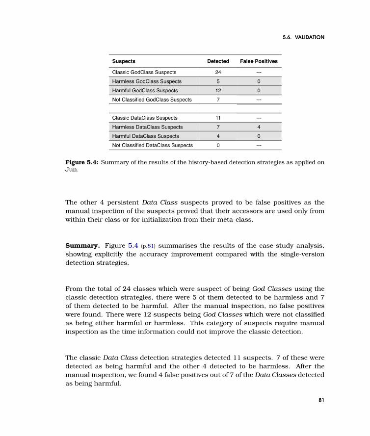
5.6. VALIDATION
Suspects Detected
Classic GodClass Suspects 24Harmless GodClass Suspects 5Harmful GodClass Suspects 12Not Classified GodClass Suspects 7
Classic DataClass Suspects 11
False Positives
---00---
---Harmless DataClass Suspects 7 4Harmful DataClass Suspects 4 0Not Classified DataClass Suspects 0 ---
Figure 5.4: Summary of the results of the history-based detection strategies as applied onJun.
The other 4 persistent Data Class suspects proved to be false positives as themanual inspection of the suspects proved that their accessors are used only fromwithin their class or for initialization from their meta-class.
Summary. Figure 5.4 (p.81) summarises the results of the case-study analysis,showing explicitly the accuracy improvement compared with the single-versiondetection strategies.
From the total of 24 classes which were suspect of being God Classes using theclassic detection strategies, there were 5 of them detected to be harmless and 7of them detected to be harmful. After the manual inspection, no false positiveswere found. There were 12 suspects being God Classes which were not classifiedas being either harmful or harmless. This category of suspects require manualinspection as the time information could not improve the classic detection.
The classic Data Class detection strategies detected 11 suspects. 7 of these weredetected as being harmful and the other 4 detected to be harmless. After themanual inspection, we found 4 false positives out of 7 of the Data Classes detectedas being harmful.
81

CHAPTER 5. HISTORY-BASED DETECTION STRATEGIES
5.7 Variation Points
During the experiments we had to choose among many different possibilities todeal with the time information. We consider necessary a final discussion centeredon the possible variations of this approach. Thus, the purpose of this section is toput the chosen approach in a larger context driving in the same time the directionsfor future work.
On the variations of the stability measurement
We consider a class unstable if at least one method was added or removed re-gardless of the kind of method. Therefore, we ignored the changes produced at alower level (e.g., bug-fixes) and do not distinguish the quality of changes. A pos-sible solution would be to sum the number of changes in successive versions andcomplement the Stab measurement with size information.
Also, the Stab measurement considers all changes equal, regardless of the periodof time in which they appeared. Another possible extension is to consider just thelatest changes by weighting each change with the distance from the last versionanalyzed.
On the impact of the number of analyzed versions
The more versions we consider in our analysis, the more we favor the capture ofthe small changes in the Stab measurement.
On the impact of the starting point of the analyzed history
We found out that persistent and stable God Classes are harmless because theyusually implement an optional and standalone feature (e.g., a code browser in a3D framework). These classes are part of the initial design, as persistency meansthe existence of the flaw almost since the very beginning of the class life. If weconsider the analyzed period to be from the middle of their actual life, we cannotdetect whether they were really persistent. Therefore, for persistency we need toconsider the history from the beginning of the system’s history.
82

5.8. RELATED WORK
On the impact of the threshold values
The thresholds represent the weakest point of the detection strategies becausethey are established mainly using the human experience. In this chapter thetime information is used to supplement the lack of precision for particular sets ofthresholds [Ratiu, 2003].
Mihancea developed a “tuning machine” which tries to infer automatically theproper threshold values [Mihancea and Marinescu, 2005]. This approach is basedon building a repository of design fragments that have been identified by engineersas being affected by a particular design problem, and based on this referencesamples, the “tuning machine” selects those threshold values that maximize thenumber of correctly detected samples. The drawback of the approach is that theexamples repository must be large enough to allow a proper tuning, and collectingthese samples is not easy.
Another approach to deal with setting the thresholds is based on statistical analy-sis of the common values found in a database of projects [Lanza et al., 2006].
5.8 Related Work
During the past years, different approaches have been developed to address theproblem of detecting design flaws. Ciupke employed queries usually implementedin Prolog to detect “critical design fragments” [Ciupke, 1999]. Tourwe et al. alsoexplored the use of logic programming to detect design flaws. van Emden etal. detected bad smells by looking at code patterns [van Emden and Moonen,2002]. As mentioned earlier, Marinescu defined detection strategies which aremeasurement-based rules aimed to detect design problems [Marinescu, 2001;Marinescu, 2002; Marinescu, 2004]. Visualization techniques have also been usedto understand design [Demeyer et al., 1999].
These approaches have been applied on one single version alone, therefore miss-ing useful information related to the history of the system. Our approach is tocomplement the detection of design fragments with history information of the sus-pected flawed structure.
Demeyer et al. analyzed the history of three systems to detect “refactorings viachange metrics” [Demeyer et al., 2000]. Krajewski defined a methodology for ana-lyzing the history of software systems [Krajewski, 2003].
83

CHAPTER 5. HISTORY-BASED DETECTION STRATEGIES
These approaches used measurements as an indicator of changes from one ver-sion to another. We consider history to be a first class entity and define historymeasurements which summarize the entire evolution of that entity.
Visualization techniques in combination with measurements were also used tounderstand history information [Lanza and Ducasse, 2002; Jazayeri et al., 1999;Jazayeri, 2002]. As opposed to visualization, our approach is automatic and itreduces the scope of analysis, yet we believe that the two approaches are comple-mentary.
In [Fischer et al., 2003a] the authors used information outside the code historyand looked for feature tracking, thus gaining semantic information for softwareunderstanding. Our approach differs as we only make use of the code history.Another approach was developed by Gall et al. to detect hidden dependenciesbetween modules, but they considered the module as unit of analysis while webase our analysis on detailed structural information from the code [Gall et al.,1998].
Jun has been the target of evolution research, however the focus was to use thehistory information to describe the development process and the lessons learntfrom developing Jun [Aoki et al., 2001].
5.9 Summarizing History-Based Detection Strategies
We refined the original concept of detection strategy, by using historical infor-mation of the suspected flawed structures. Using this approach we showed howthe detection of God Classes and Data Classes can become more accurate. Ourapproach leads to a twofold benefit:
1. Elimination of false positives by filtering out, with the help of history informa-tion, the harmless suspects from those provided by a single-version detectionstrategy.
2. Identification of most dangerous suspects by using additional information onthe evolution of initial suspects over their analyzed history.
To consolidate and refine the results obtained on the Jun case study, the approachneeds to be applied further on large-scale systems. We also intend to extendour investigations towards the usage of historical information for detecting otherdesign flaws.
84

5.10. HISMO VALIDATION
The Stab measurement does not take into consideration the sizes of the change.We would like to investigate how this indicator of stability could be improved byconsidering the number of methods changed between successive versions. Otherinteresting investigation issues are: the impact on stability of other change mea-surements (e.g., lines of code) and the detection of periodic appearing and disap-pearing of flaws.
5.10 Hismo Validation
Originally, the detection strategies only took into account structural measure-ments. We used Hismo to extend the detection strategies with the time dimension.For example, we use the historical information to qualify God Classes as beingharmless if they were stable for a large part of their history. Below we present howwe define the expression with Hismo:
context ClassHistory
-- returns true if the ClassHistory is a GodClass in the last version and-- it did not change the number of methods in more then 95% of the versionsderive isHarmlessGodClass:
(self.versions->last().isGodClass()) &(self.stabilityOfNOM > 0.95)
The code shows the predicate isHarmlessGodClass defined in the context of a ClassHis-tory. The predicate is an example of how we can use in a single expression bothhistorical information (i.e., stability of number of methods) and structural informa-tion (i.e., God Class characteristic in the last version) to build the reasoning.
One variation of the approach is in using other stability indicators than the changesin the number of methods. For example, we can use changes in the number ofstatements of the class. The simplicity of the above OCL code, easily allows for thereplacement of the self.stabilityOfNOM with self.stabilityOfNOS.
85

CHAPTER 5. HISTORY-BASED DETECTION STRATEGIES
86

Chapter 6
Characterizing the Evolutionof HierarchiesCombining Historical Relationships and HistoricalProperties
Problem solving efficiency growswith the abstractness level of problem understanding.
Analyzing historical information can show how a software system evolved intoits current state, which parts of the system are stable and which have changedmore. However, historical analysis implies processing a vast amount of informationmaking the interpretation of the results difficult. Rather than analyzing individualclasses, we aim to analyze class hierarchies as they group classes according to sim-ilar semantics. We use historical measurements to define rules by which to detectdifferent characteristics of the evolution of class hierarchies. Furthermore, we dis-cuss the results we obtained by visualizing them using a novel polymetric view. Weapply our approach on two large open source case studies and classify their classhierarchies based on their history.
With this analysis we show how to use relationship histories and how to combinehistory properties.

CHAPTER 6. CHARACTERIZING THE EVOLUTION OF HIERARCHIES
6.1 Introduction
History holds useful information that can be used when reverse engineering a sys-tem. However, analyzing historical information is difficult due to the vast amountof information that needs to be processed, transformed, and understood. There-fore, we need higher level views of the data which allow the reverse engineer toignore the irrelevant details.
We concentrate on describing and characterizing the evolution of class hierarchies.Class hierarchies provide a grouping of classes based on similar semantics thus,characterizing a hierarchy as a whole reduces the complexity of understanding bigsystems. In particular, we seek answers to the following questions:
1. How old are the classes of a hierarchy? On one hand, the old classes maybe part of the original design and thus hold useful information about thesystem’s design. On the other hand, a freshly introduced hierarchy mightindicate places where future work will be required.
2. Were there changes in the inheritance relationships? Changes in the inheri-tance relationships might indicate class renaming refactorings, introductionof abstract classes, or removal of classes.
3. Are classes from one hierarchy modified more than those from another one?Understanding which parts of the system changed more is important becausethey might be also changed in the future [Gırba et al., 2004a].
4. Are the changes evenly distributed among the classes of a hierarchy? If wefind that the root of the hierarchy is often changed, it might indicate thateffort was spent to factor out functionality from the subclasses and to pushit to the superclass, but it might also be a sign of violations of the open-closedprinciple [Meyer, 1988].
We are set to detect four characteristics of class hierarchy evolution: (1) the ageof the hierarchy, (2) the inheritance relationship stability, (3) the class size sta-bility, and (4) the change balance. We quantify these characteristics in a set ofmeasurements-based rules, and define a language for describing different evolu-tion patterns of class hierarchies.
To analyze the obtained results we developed a visualization called Hierarchy Evo-lution Complexity View, an evolutionary polymetric view [Lanza, 2003]. We usesoftware visualization because visual displays allow the human brain to studymultiple aspects of complex problems – like reverse engineering – in parallel [Stasko
88
6.2. CHARACTERIZING CLASS HIERARCHY HISTORIES
et al., 1998]. We validated our approach on two open source case studies writtenin Java and Smalltalk.
The contributions of this chapter are: (1) the characterization of class hierarchyevolution based on explicit rules which detect different change characteristics, and(2) the definition of a new polymetric view which takes into account the history ofentities.
Structure of the chapter
In Section 6.2 (p.89) we define rules to detect different evolution patterns of theevolution of class hierarchies and in Section 6.3 (p.91) we introduce the visualiza-tion based on the historical measurements measurements. In Section 6.4 (p.93) weapply our approach on two large case studies. We discuss variation points of ourapproach (Section 6.5 (p.98)) and we browse the related work (Section 6.6 (p.101)).We summarize the chapter in Section 6.7 (p.102) and in Section 6.8 (p.103) we endwith a discussion of the approach from the point of view of using Hismo.
6.2 Characterizing Class Hierarchy Histories
6.2.1 Modeling Class Hierarchy Histories
We consider a class hierarchy history as being a group of class histories anda group of inheritance histories. To measure class hierarchy histories, we ap-ply group operators like average (Avg), maximum (Max) and total (Tot). Thus wehave the average age of the class histories in a class hierarchy Ch as given by:Avg(ClassAge,Ch).
6.2.2 Detecting Class Hierarchies Evolution Patterns
We formulate a vocabulary based on four characteristics: (1) hierarchy age, (2)inheritance relationship stability, (3) class size stability, and (4) change balance.These four characteristics are orthogonal with each other. For example, the samehierarchy can be old but at the same time can have unstable classes.
We use the history measurements to define rules to qualify a class hierarchy basedon the four characteristics:
89
CHAPTER 6. CHARACTERIZING THE EVOLUTION OF HIERARCHIES
1. How old is a hierarchy? We distinguish the following types of hierarchy his-tories based on the average age of their class histories:
— Newborn. A newborn hierarchy is a freshly introduced hierarchy (i.e., onthe average the age of the class histories is no more than a tenth of theage of the system).
Avg(ClassAge, Ch) < 0.1 ∗ SystemAge
— Young. A young hierarchy is older than a newborn hierarchy, but its ageis less than half of the system age.
Avg(ClassAge, Ch) > 0.1 ∗ SystemAge ∧Avg(ClassAge, Ch) < 0.5 ∗ SystemAge
— Old. Old hierarchies have been in the system for a long time, but not forthe entire life of the system.
Avg(ClassAge, Ch) > 0.5 ∗ SystemAge ∧Avg(ClassAge, Ch) < 0.9 ∗ SystemAge
— Persistent. We say a hierarchy is persistent if the classes were present inalmost all versions of the system (i.e., in more than 90% of the systemversions).
Avg(ClassAge, Ch) > 0.9 ∗ SystemAge
2. Were there changes in the inheritance relationship? We divide the hierarchiesinto two categories:
— Solid. We define a hierarchy as being solid when the inheritance relation-ships between classes are stable and old.
Tot(RemovedInh, Ch) < 0.3 ∗NOInh(Ch)
— Fragile. A hierarchy is fragile when there are many inheritance relation-ships which disappear.
Tot(RemovedInh, Ch) > 0.3 ∗NOInh(Ch)
90
6.3. CLASS HIERARCHY HISTORY COMPLEXITY VIEW
3. Are classes from one hierarchy modified more than classes from anotherhierarchy? From the stability of size point of view we detect two kinds ofhierarchies:
— Stable. In a stable hierarchy the classes have few methods and statementsadded or removed compared with the rest of the system.
Avg(ENOM, Ch) < Avg(ENOM, S) ∧Avg(ENOS, Ch) < Avg(ENOS, S)
— Unstable. In an unstable hierarchy many methods are being added andremoved during its evolution.
Avg(ENOM, Ch) > Avg(ENOM, S) ∨Avg(ENOS, Ch) > Avg(ENOS, S)
4. Are the changes evenly distributed among the classes of a hierarchy? Wedistinguish two labels from the change balance point of view:
— Balanced. In a balanced hierarchy, the changes are evenly performedamong its classes.
Avg(ENOM, Ch) > 0.8 ∗Max(ENOM, Ch)
— Unbalanced. An unbalanced hierarchy is one in which the changes arenot equally distributed in the classes.
Avg(ENOM, Ch) < 0.8 ∗Max(ENOM, Ch)
6.3 Class Hierarchy History Complexity View
To analyze the results we obtain when applying the rules defined in the previoussection, we use visualization as it allows one to identify cases where differentcharacteristics apply at the same time for a given hierarchy. The visualization wepropose is called Hierarchy Evolution Complexity View and is a polymetric view
91

CHAPTER 6. CHARACTERIZING THE EVOLUTION OF HIERARCHIES
A
B
D
C
E
ver .1 ver. 2 ver. 3 ver. 4 ver. 5
A A A A A
B B B B BC C C
D D D E
Figure 6.1: An example of the Hierarchy Evolution Complexity View. Hierarchy EvolutionComplexity View (right hand side) summarizes the hierarchy history (left hand side).
[Lanza, 2003]. Hierarchy Evolution Complexity View uses a simple tree layout toseemingly display classes and inheritance relationships. What is new is that itactually visualizes the histories of classes and of inheritance relationships.
Nodes and edges which have been removed while the system was evolving (i.e.,they are not present anymore) have a cyan color. The color of the class historynodes, and the width of the inheritance edges represent their age: the darker thenodes and the wider the edges, the more grounded in time they are, i.e., the longerthey have been present in the system. Thus, lightly colored nodes and thin edgesrepresent younger classes and inheritance relationships.
The width of the class history node is given by the Evolution of Number of Methods(i.e., ENOM ) while the height is given by the fifth part of the Evolution of Numberof Statements (i.e., ENOS/5). We chose to divide ENOS by 5 because in the casestudies we analyzed there was an average of 5 statements per method. Thus, thewider a node is, the more methods were added or removed in subsequent versionsin that class history; the greater the height of a node is, the more statements wereadded or removed in subsequent versions in that class history.
We chose to use ENOM and ENOS because we wanted to see the correlation be-tween changes in the behavior of a class and its internal implementation changes.
Example. In Figure 6.1 (p.92) we show an example of such a view in which wedisplay an imaginary hierarchy history. From the figure we infer the followinginformation:
— Classes A and B are in the system from the very beginning, and they appear
92
6.4. VALIDATION
colored in black. The inheritance relationship between these classes is blackand thick marking that the relationship is old. Class E is small and white,because it was recently introduced in the system.
— Class C was removed from the system and is colored in cyan. Class D has beenintroduced after several versions as a subclass of C, but in the last version ithas become a subclass of A.
— Class B is small because there were no changes detected in it. Classes A andD have the same width, but class D appears to have less statements addedor removed because the node is more wide than tall. Class C is much tallercompared to its width, denoting a greater implementation effort.
Based on the visualization we can detect two more characteristics:
— Heterogeneous. We characterize a class hierarchy history as being heteroge-neous if the class histories have a wide range of ages. Such a hierarchy willappear colored with a wide range of grays.
— Unstable Root. In a hierarchy with an unstable root, the root node is largecompared with the rest of the nodes.
6.4 Validation
For our experiments we chose two open source systems: JBoss1 and Jun2.
JBoss. For the first case study, we chose 14 versions of JBoss. JBoss is anopen source J2EE application server written in Java. The versions we selected forthe experiments were at two months distance from one another starting from thebeginning of 2001 until the end of 2003. The first version has 628 classes, thelast one has 4975 classes.
Jun. As a second case study we selected 40 versions of Jun. Jun is a 3D-graphicsframework written in Smalltalk currently consisting of more than 700 classes.As experimental data we took every 5th version starting from version 5 (the firstpublic version) to version 200. The time distance between version 5 and version200 is about two years, and the considered versions were released about 15-20days apart. In terms of number of classes, in version 5 of Jun there are 170classes while in version 200 there are 740 classes.
1See http://www.jboss.org.2See http://www.srainc.com/Jun/.
93

CHAPTER 6. CHARACTERIZING THE EVOLUTION OF HIERARCHIES
Figure 6.3 (p.96) and Figure 6.4 (p.97) show some of the results we obtained onsix large hierarchies of both case studies. The results are accompanied by thevisualizations.
6.4.1 Class Hierarchies of JBoss
Figure 6.2 (p.95) shows the largest hierarchy in JBoss (ServiceMBeanSupport), andFigure 6.3 (p.96) shows five other hierarchies from JBoss: JBossTestCase, Stats, J2EE-ManagedObject, MetaData and SimpleNode (we name the hierarchies according tothe names of their root classes). On the bottom part of the figure we show thecharacterization of each hierarchy according to the proposed characteristics. Forspace reasons Figure 6.2 (p.95) is scaled with a 0.5 ratio (i.e., zoomed out) as com-pared with the Figure 6.3 (p.96).
ServiceMBeanSupport is a large hierarchy with nodes and edges of different colorsand shapes: As a whole, we classify it as heterogeneous from the age point ofview, fragile from the inheritance relationship point of view, and unstable andunbalanced from the changes point of view.
The J2EEManagedObject is a sub-hierarchy of ServiceMBeanSupport and is heteroge-neous and unbalanced from the point of view of performed changes and is fragilein terms of inheritance. In the visualization the hierarchy is displayed with nodescolored in various grays and with many cyan edges and nodes.
JBossTestCase is composed of classes of different age. On average, the nodes arerather small, meaning that the classes were stable. The hierarchy is heteroge-neous from the class age point of view which shows that the tests were continu-ously developed along the project. Also, because most of the nodes are small itmeans that most of the classes are stable both from the methods and from theimplementation point of view. In the unstable classes there were more implemen-tation changes than methods added or removed. Also, once the test classes werecreated not many test methods were added or removed afterwards.
The Stats hierarchy has been recently introduced and did not yet experience majorchanges.
MetaData is represented with nodes of different sizes colored either in dark colorsor in cyan: It is an old hierarchy which is unstable and unbalanced from theperformed changes point of view. The edges are either thick and dark or cyan,and as the number of removed edges are not high, we characterize the inheritancerelationships as being solid.
94

6.4. VALIDATION
ServiceMBeanSupport
J2EEManagedObject
Figure 6.2: A Hierarchy Evolution Complexity View of the evolution of the largest hierarchyfrom 14 versions of JBoss.
95
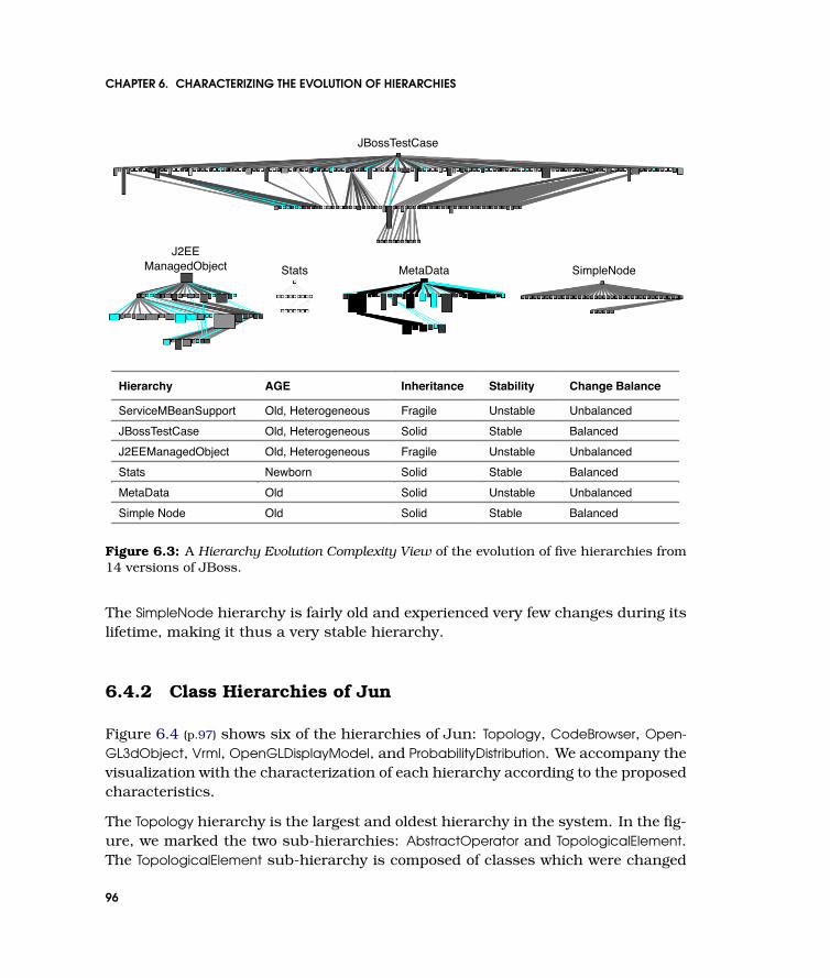
CHAPTER 6. CHARACTERIZING THE EVOLUTION OF HIERARCHIES
JBossTestCase
Stats MetaData SimpleNodeJ2EE
ManagedObject
Hierarchy AGE
ServiceMBeanSupport Old, HeterogeneousJBossTestCase Old, HeterogeneousJ2EEManagedObject Old, HeterogeneousStats NewbornMetaData OldSimple Node Old
Inheritance
FragileSolidFragileSolidSolidSolid
Stability
UnstableStableUnstableStableUnstableStable
Change Balance
UnbalancedBalancedUnbalancedBalancedUnbalancedBalanced
Figure 6.3: A Hierarchy Evolution Complexity View of the evolution of five hierarchies from14 versions of JBoss.
The SimpleNode hierarchy is fairly old and experienced very few changes during itslifetime, making it thus a very stable hierarchy.
6.4.2 Class Hierarchies of Jun
Figure 6.4 (p.97) shows six of the hierarchies of Jun: Topology, CodeBrowser, Open-GL3dObject, Vrml, OpenGLDisplayModel, and ProbabilityDistribution. We accompany thevisualization with the characterization of each hierarchy according to the proposedcharacteristics.
The Topology hierarchy is the largest and oldest hierarchy in the system. In the fig-ure, we marked the two sub-hierarchies: AbstractOperator and TopologicalElement.The TopologicalElement sub-hierarchy is composed of classes which were changed
96

6.4. VALIDATION
ProbabilityDistribution
Vrml
TopologyOpenGL
DisplayModelCode
BrowserTopological
ElementAbstractOperator
Chart
Hierarchy AGE
Topology OldCodeBrowser NewbornOpenGL3dObject OldVrml PersistentOpenGLDisplayModel OldProbabilityDistribution Old
Inheritance
SolidSolidFragileFragileSolidSolid
Stability
UnstableStableUnstableStableStableStable
Change Balance
UnbalancedBalancedUnbalanced, Unstable RootBalancedBalanced, Unstable RootBalanced
OpenGL3dObject
OpenGL3dPrimitiveObject
Figure 6.4: A Hierarchy Evolution Complexity View of the evolution of six hierarchies fromthe 40 versions of Jun.
a lot during their life time. Three of the leaf classes were detected as being GodClasses (see Chapter 5 (p.67)). A large part of the AbstractOperator hierarchy hasbeen in the system from the first version, but there is a young sub-hierarchy whichlooks different.
The CodeBrowser hierarchy is thin and lightly colored, meaning that it has beenrecently added to the system.
The OpenGL3dObject hierarchy experienced three times an insertion of a class inthe middle of the hierarchy: There are removed inheritance relationships coloredin cyan.
The Vrml hierarchy proved to have undergone extensive renaming refactorings: We
97

CHAPTER 6. CHARACTERIZING THE EVOLUTION OF HIERARCHIES
see many removed nodes and removed inheritance relationships. Even the rootclass has been removed at a certain point in time: The original hierarchy has thusbeen split into two distinct hierarchies.
The OpenGLDisplayModel hierarchy has an old and unstable root. This is denotedby a large rectangle colored in dark gray. The Chart sub-hierarchy is thin andlightly colored denoting it is newborn.
ProbabilityDistribution is an old hierarchy and very stable from the inheritance rela-tionships point of view. Also, the classes in the hierarchy were changed very littleduring their history.
6.5 Variation Points
On the impact of the release period
A variation point when computing E measurement is the release period. If, forexample, we consider the release period of one week, we focus the analysis toimmediate changes. If we consider the release period of half a year, we emphasizethe size of the changes that accumulate in the class histories.
On the impact of the number of analyzed versions
The number of versions is another variation point when computing the measure-ments. By increasing the number of analyzed versions we obtain a long-termindicator of effort, while by decreasing the number of versions we concentrate onthe short-term indicator of effort.
On the impact of the threshold values
Changing the threshold used for characterizing the evolution is also a variationpoint. For example, instead of using 10% of the total number of system versionsfor qualifying a class hierarchy as young, we can use 3 versions as the threshold(that is the classes should be introduced no later than 2 versions ago).
98
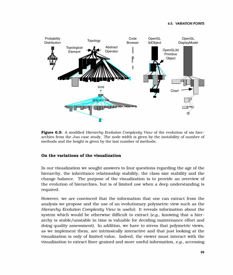
6.5. VARIATION POINTS
OpenGL3dObject
ProbabilityDistribution
Vrml
Topology OpenGLDisplayModel
CodeBrowser
Chart
TopologicalElement
AbstractOperator OpenGL3d
PrimitiveObject
Figure 6.5: A modified Hierarchy Evolution Complexity View of the evolution of six hier-archies from the Jun case study. The node width is given by the instability of number ofmethods and the height is given by the last number of methods.
On the variations of the visualization
In our visualization we sought answers to four questions regarding the age of thehierarchy, the inheritance relationship stability, the class size stability and thechange balance. The purpose of the visualization is to provide an overview ofthe evolution of hierarchies, but is of limited use when a deep understanding isrequired.
However, we are convinced that the information that one can extract from theanalysis we propose and the use of an evolutionary polymetric view such as theHierarchy Evolution Complexity View is useful: It reveals information about thesystem which would be otherwise difficult to extract (e.g., knowing that a hier-archy is stable/unstable in time is valuable for deciding maintenance effort anddoing quality assessment). In addition, we have to stress that polymetric views,as we implement them, are intrinsically interactive and that just looking at thevisualization is only of limited value. Indeed, the viewer must interact with thevisualization to extract finer-grained and more useful information, e.g., accessing
99

CHAPTER 6. CHARACTERIZING THE EVOLUTION OF HIERARCHIES
the source code.
Example. In Figure 6.4 (p.97) one would like to know what class has been removedfrom the Topology hierarchy and also why, since this quite large hierarchy hasbeen very stable in terms of inheritance relationships. The viewer can do so bypointing and inspecting the cyan class history node.
Figure 6.5 (p.99) shows a modified Hierarchy Evolution Complexity View applied onthe Jun hierarchies. In this view we used for the width and the height of thenodes other measurements, namely the last number of methods (NOM) as theheight and the instability of the number of methods (INOM) as the width. Theinstability of the number of methods is computed as the number of versions inwhich the number of methods changed over the total number of versions in whichit could have changed.
While in the original view the nodes dimensions show the correlation betweenimplementation effort, and the behavior addition and removal effort, this viewshows the correlation of the actual size in terms of number of methods and thenumber of times methods were added or removed in the classes. Thus, in thisview we can detect whether the instability is correlated with actual size.
In Figure 6.5 (p.99), the CodeBrowser hierarchy, is newborn and appears small inthe original view, but the modified view shows that the classes are among thetallest displayed, meaning that the classes are rather big in size, but there wereno changes in them.
In the Topology hierarchy the TopologicalElement hierarchy appeared to be unstablein the original view, but in the modified view it appears as the classes were notchanged many times, because the nodes are not very wide. The rest of the Topologyhierarchy is stable, except for one class which, even if it is younger than the rest,was changed many times.
In the OpenGLDisplayModel hierarchy there is a correlation of the instability ofnumber of methods and the size of the root class because the node is tall andwide. On the other hand, the Chart hierarchy is newborn and appears small inthe original view, while in this view the root is tall meaning that it is a largeclass.
The OpenGL3dObject hierarchy also has a large and unstable root. The OpenGL3d-PrimitiveObject class appears as being small in size, but it changed its numberof methods many times, because it is not tall, but it is wide. Also, its directsubclasses have about the same width, but their height differs. This means that
100

6.6. RELATED WORK
those classes changed their number of methods about the same amount of timesalthough their actual size differs.
The classes in the ProbabilityDistribution hierarchy appear small and stable. In theVrml hierarchy the size of the classes vary, but the classes are stable.
6.6 Related Work
Burd and Munro analyzed the influence of changes on the maintainability of soft-ware systems. They defined a set of measurements to quantify the dominancerelations which are used to depict the complexity of the calls [Burd and Munro,1999].
Lanza’s Evolution Matrix visualized the system’s history in a matrix in which eachrow is the history of a class [Lanza and Ducasse, 2002]. A cell in the EvolutionMatrix represents a class and the dimensions of the cell are given by evolutionarymeasurements computed on subsequent versions. Jazayeri analyzed the stabilityof the architecture by using colors to depict the changes [Jazayeri, 2002]. Jing-wei Wu et al. used the spectograph metaphor to visualize how changes occur insoftware systems [Wu et al., 2004a]. Rysselberghe and Demeyer use a simple vi-sualization based on information in version control systems to provide an overviewof the evolution of systems [Van Rysselberghe and Demeyer, 2004].
Our approach differs from the above mentioned ones because we consider historyto be a first class entity and define history measurements which are applied on thewhole history of an entity and which summarize the evolution of that entity. Theauthors already used the notion of history to analyze how changes appear in thesoftware systems [Gırba et al., 2004a]. The drawback of our approach consistsin the inherent noise which resides in compressing large amounts of data intonumbers.
Taylor and Munro visualized CVS data with a technique called revision towers[Taylor and Munro, 2002]. Ball and Eick developed visualizations for showingchanges that appear in the source code [Ball and Eick, 1996]. These approachesreside at a different granularity level, i.e., files, and thus does not display sourcecode artifacts as in our approach.
Gulla proposed different visualizations of C code versions, but to our knowledgethere was no implementation [Gulla, 1992]. For example, he displayed several ver-sions of the structure and let the user identify the changes, by superimposing the
101

CHAPTER 6. CHARACTERIZING THE EVOLUTION OF HIERARCHIES
figures. Holt and Pak proposed a detailed visualization of the old and new depen-dencies between modules [Holt and Pak, 1996]. Collberg et al. used graph-basedvisualizations to display the changes authors make to class hierarchies [Collberget al., 2003]. However, they did not give any representation of the dimension ofthe effort and of the removals of entities.
Another metrics-based approach to detect refactorings of classes was developed byDemeyer et al. [Demeyer et al., 2000]. While they focused on detecting refactor-ings, we focus on offering means to understand where and how the developmenteffort was spent in a hierarchy.
6.7 Summary of the Approach
This approach set to answer four questions: (1) How old are the classes of ahierarchy?, (2) Were there changes in the inheritance relationship?, (3) Are classesfrom one hierarchy modified more than those from another one?, and (4) Are thechanges evenly distributed among the classes of a hierarchy?
The history of a system holds the information necessary for answering the abovequestions, but the analysis is difficult due to the large amount of data. We ap-proached this problem by defining the history as a first class entity and then wedefined history measurements which summarize the evolution of an entity.
Based on the questions we formulated a vocabulary of terms and we used themeasurements to formulate rules to characterize the evolution of class hierachies.Furthermore, we displayed the results using a new polymetric view of the evolutionof class hierarchies called Hierarchy Evolution Complexity View.
We applied our approach on two large open source projects and showed how wecould describe the evolution of class hierarchies.
In the future, we want to investigate possibilities of using other measurementsand of adding more semantic information to the view we propose. For example,we want to add information like refactorings that have been performed.
102

6.8. HISMO VALIDATION
6.8 Hismo Validation
The presented approach exercises several characteristics of Hismo: it combineshistorical properties with historical relationships.
Originally, polymetric views were only used for analyzing structural information(e.g., the hierarchy of classes). Figure 6.1 (p.92) shows an example of how theevolution over 5 versions of a hierarchy (left side) is summarized in one polymetricview (right side). On the left hand side we represent the hierarchy structure ineach version – i.e., classes as nodes and inheritance relationships as edges. Onthe right hand side we display ClassHistories as nodes and InheritanceHistoriesas edges. The color of each node represents the age of the ClassHistory: the darkerthe node the older the ClassHistory. The size of the node denotes how much it waschanged: the larger the node, the more the ClassHistory was changed. Both thethickness and the color of the edge represent the age of the InheritanceHistory.Furthermore, the cyan color denotes removed histories.
Below we show how the queries presented can be expressed with Hismo. Forexample, the Newborn query:
Avg(ClassAge, Ch) < 0.1 ∗ SystemAge
. . . can be expressed like:
context HistoryGroup
-- returns true if the average age of the class histories is lower than 10% of the system agederive newborn:
self.averageOfAge < 0.1 * self.referenceHistory->age
103

CHAPTER 6. CHARACTERIZING THE EVOLUTION OF HIERARCHIES
104

Chapter 7
How Developers DriveSoftware EvolutionManipulating Historical Relationships
In the end, no two things are truly independent.
As systems evolve their structure change in ways not expected upfront, and theknowledge of the developers becomes more and more critical for the process of un-derstanding the system. That is, when we want to understand a certain issue ofthe system we ask the knowledgeable developers. Yet, in large systems, not everydeveloper is knowledgeable in all the details of the system. Thus, we would wantto know which developer is knowledgeable in the issue at hand. In this chapter wemake use of the mapping between the changes and the author identifiers providedby versioning repositories to recover their zones and periods of influence in the sys-tem. We first define a measurement for the notion of code ownership. We use thismeasurement to define the Ownership Map visualization to understand when andhow different developers interacted in which way and in which part of the system.We report the results we obtained on several large systems.
The Ownership Map visualization is an example of how to use historical relation-ships.

CHAPTER 7. HOW DEVELOPERS DRIVE SOFTWARE EVOLUTION
7.1 Introduction
Software systems need to change in ways that challenge the original design. Evenif the original documentation exists, it might not reflect the code anymore. Insuch situations, it is crucial to get access to developer knowledge to understandthe system. As systems grow larger, not all developers know about the entiresystem, thus, to make the best use of developer knowledge, we need to knowwhich developer is knowledgeable in which part of the system.
From another perspective, Conway’s law states that “Organizations which designsystems are constrained to produce designs which are copies of the communica-tion structures of these organizations” [Conway, 1968]. That is, the shape of theorganization reflects on the shape of the system. As such, to understand the sys-tem, one also has to understand the interaction between the developers and thesystem [Demeyer et al., 2002].
In this chapter we aim to understand how the developers drove the evolution ofthe system. In particular we provide answers to the following questions:
— How many authors developed the system?
— Which author developed which part of the system and in which period?
— What were the behaviors of the developers?
In our approach, we assume that the original developer of a line of code is themost knowledgeable in that line of code. We use this assumption to determinethe owner of a piece of code (e.g., a file) as being the developer that owns thelargest part of that piece of code. We make use of the ownership to provide avisualization that helps to understand how developers interacted with the system.The visualization represents files as lines, and colors these lines according to theownership over time.
Contrary to similar approaches (e.g., [Van Rysselberghe and Demeyer, 2004]), wegive a semantic order to the file axis (i.e., we do not rely on the names of the files)by clustering the files based on their history of changes: files committed in thesame period are related [Gall et al., 1998].
We implemented our approach in Chronia, a tool built on top of the Moose reengi-neering environment [Ducasse et al., 2005]. As CVS is a de facto versioning sys-tem, our implementation relies on the CVS model. Our aim was to provide asolution that gives fast results, therefore, our approach relies only on information
106
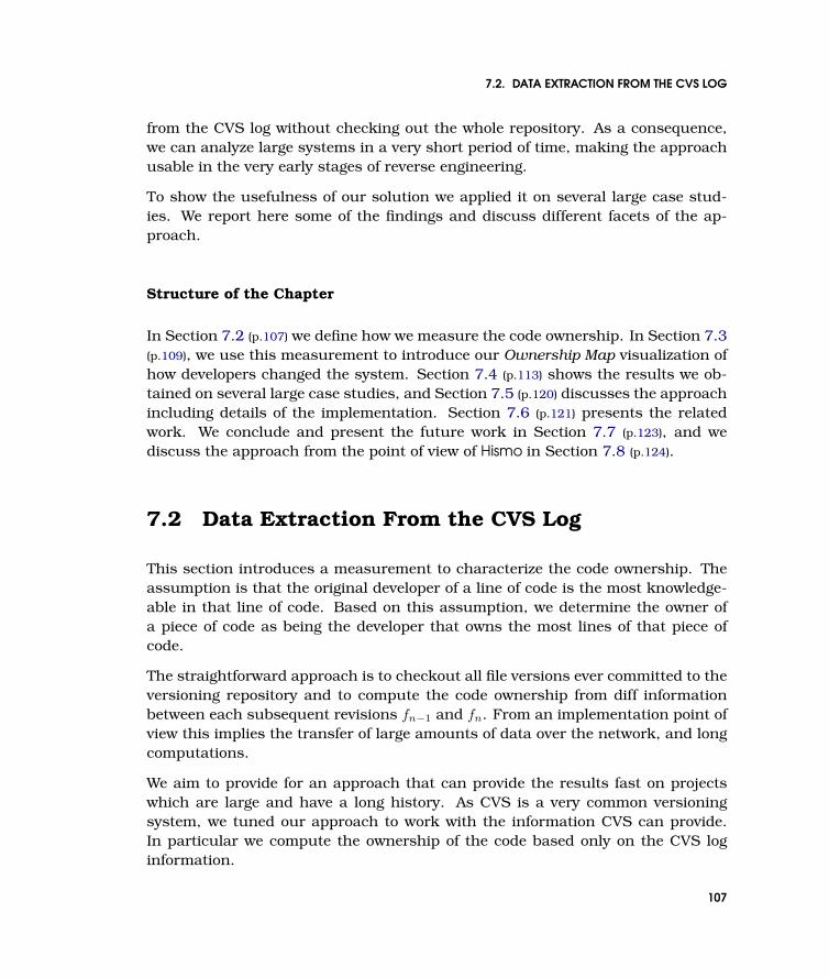
7.2. DATA EXTRACTION FROM THE CVS LOG
from the CVS log without checking out the whole repository. As a consequence,we can analyze large systems in a very short period of time, making the approachusable in the very early stages of reverse engineering.
To show the usefulness of our solution we applied it on several large case stud-ies. We report here some of the findings and discuss different facets of the ap-proach.
Structure of the Chapter
In Section 7.2 (p.107) we define how we measure the code ownership. In Section 7.3(p.109), we use this measurement to introduce our Ownership Map visualization ofhow developers changed the system. Section 7.4 (p.113) shows the results we ob-tained on several large case studies, and Section 7.5 (p.120) discusses the approachincluding details of the implementation. Section 7.6 (p.121) presents the relatedwork. We conclude and present the future work in Section 7.7 (p.123), and wediscuss the approach from the point of view of Hismo in Section 7.8 (p.124).
7.2 Data Extraction From the CVS Log
This section introduces a measurement to characterize the code ownership. Theassumption is that the original developer of a line of code is the most knowledge-able in that line of code. Based on this assumption, we determine the owner ofa piece of code as being the developer that owns the most lines of that piece ofcode.
The straightforward approach is to checkout all file versions ever committed to theversioning repository and to compute the code ownership from diff informationbetween each subsequent revisions fn−1 and fn. From an implementation point ofview this implies the transfer of large amounts of data over the network, and longcomputations.
We aim to provide for an approach that can provide the results fast on projectswhich are large and have a long history. As CVS is a very common versioningsystem, we tuned our approach to work with the information CVS can provide.In particular we compute the ownership of the code based only on the CVS loginformation.
107
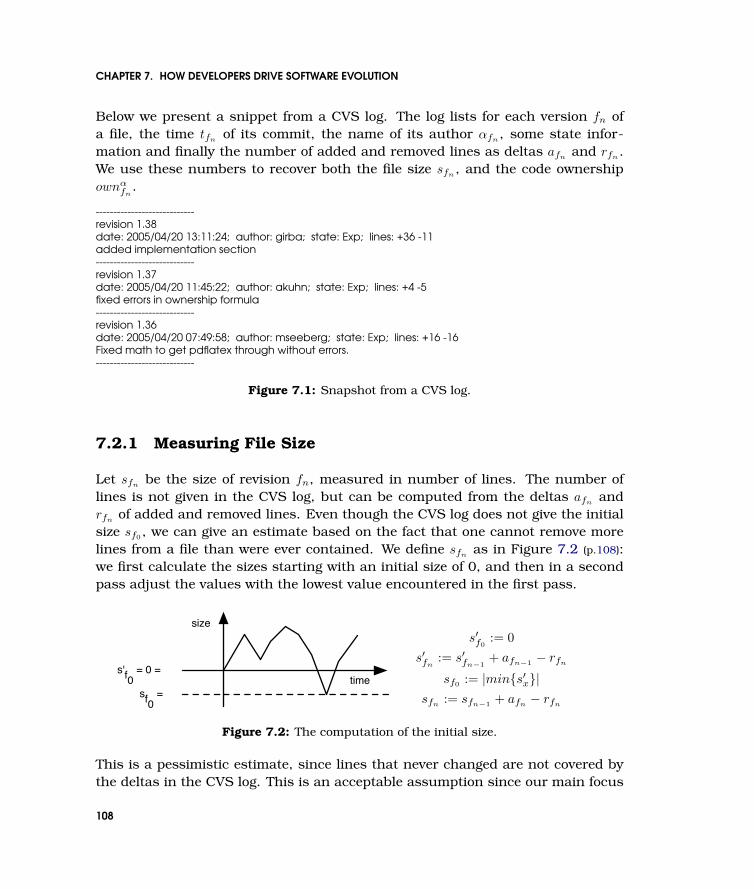
CHAPTER 7. HOW DEVELOPERS DRIVE SOFTWARE EVOLUTION
Below we present a snippet from a CVS log. The log lists for each version fn ofa file, the time tfn of its commit, the name of its author αfn , some state infor-mation and finally the number of added and removed lines as deltas afn
and rfn.
We use these numbers to recover both the file size sfn, and the code ownership
ownαfn
.
----------------------------revision 1.38date: 2005/04/20 13:11:24; author: girba; state: Exp; lines: +36 -11added implementation section----------------------------revision 1.37date: 2005/04/20 11:45:22; author: akuhn; state: Exp; lines: +4 -5fixed errors in ownership formula----------------------------revision 1.36date: 2005/04/20 07:49:58; author: mseeberg; state: Exp; lines: +16 -16Fixed math to get pdflatex through without errors.----------------------------
Figure 7.1: Snapshot from a CVS log.
7.2.1 Measuring File Size
Let sfnbe the size of revision fn, measured in number of lines. The number of
lines is not given in the CVS log, but can be computed from the deltas afnand
rfnof added and removed lines. Even though the CVS log does not give the initial
size sf0 , we can give an estimate based on the fact that one cannot remove morelines from a file than were ever contained. We define sfn as in Figure 7.2 (p.108):we first calculate the sizes starting with an initial size of 0, and then in a secondpass adjust the values with the lowest value encountered in the first pass.
time
size
s'f0 = 0 =
sf0 =
s′f0:= 0
s′fn:= s′fn−1
+ afn−1 − rfn
sf0 := |min{s′x}|sfn
:= sfn−1 + afn− rfn
Figure 7.2: The computation of the initial size.
This is a pessimistic estimate, since lines that never changed are not covered bythe deltas in the CVS log. This is an acceptable assumption since our main focus
108

7.3. THE OWNERSHIP MAP VIEW
is telling the story of the developers, not measuring lines that were never touchedby a developer. Furthermore in a long-living system the content of files is entirelyreplaced or rewritten at least once if not several times. Thus the estimate matchesthe correct size of most files.
7.2.2 Measuring Code Ownership
A developer owns a line of code if he was the last one that committed a change tothat line. In the same way, we define file ownership as the percentage of lines heowns in a file. And the overall owner of a file is the developer that owns the largestpart of it.
Let ownαfn
be the percentage of lines in revision fn owned by author α. Given the filesize sfn
, and both the author αfnthat committed the change and afn
the numberof lines he added, we defined ownership as:
ownαf0
:={
1, α = αf0
0, else
ownαfn
:= ownαfn−1
sfn− afn
sfn
+
{afn
sfn, α = αfn
0, else
In the definition we assume that the removed lines rfn are evenly distributed overthe ownership of the predecessor developers fn−1.
7.3 The Ownership Map View
We introduce a the Ownership Map visualization as in Figure 7.3 (p.110). Thevisualization is similar to the Evolution Matrix [Lanza and Ducasse, 2002]: eachline represents a history of a file, and each circle on a line represents a change tothat file.
The color of the circle denotes the author that made the change. The size of thecircle reflects the proportion of the file that got changed i.e., the larger the change,the larger the circle. And the color of the line denotes the author who owns mostof the file.
Bertin assessed that one of the good practices in information visualization is tooffer to the viewer visualizations that can be grasped at one glance [Bertin, 1974].
109

CHAPTER 7. HOW DEVELOPERS DRIVE SOFTWARE EVOLUTION
The colors used in our visualizations follow visual guidelines suggested by Bertin,Tufte and Ware - e.g., we take into account that the human brain is capable ofprocessing fewer than a dozen distinct colors [Tufte, 1990; Ware, 2000].
In a large system, we can have hundreds of developers. Because the human eye isnot capable of distinguishing that many colors, we only display the authors whocommitted most of all changes using distinct colors; the remaining authors arerepresented in gray. Furthermore, we also represent with gray files that came intothe CVS repository with the initial import, because these files are usually sourcesfrom another project with unknown authors and are thus not necessarily createdby the author that performed the import. In short, a gray line represents eitheran unknown owner, or an unimportant one.
File A
File B
commit by the green authorfollowed by the ownership
small commit by the blue author.the file is still ownedby the green author
file removed by the blue author
file present fromthe first import
file created by thegreen author
Time
Figure 7.3: Example of ownership visualization of two files.
In the example from Figure 7.3 (p.110), each line represents the lifetime of a file;each circle represents a change. File A appears gray in the first part as it originatesfrom the initial import. Later the green author significantly changed the file, andhe became the owner of the file. In the end, the blue author deleted the file. File Bwas created by the green author. Afterwards, the blue author changed the file, butstill the green author owned the largest part, so the line remains green. At somepoint, the red author committed a large change and took over the ownership. Thefile was not deleted.
7.3.1 Ordering the Axes
Ordering the Time Axis. Subsequent file revisions committed by the same au-thor are grouped together to form a transaction of changes i.e., a commit. We usea single linkage clustering with a threshold of 180 seconds to obtain these groups.This solution is similar to the sliding time window approach of Zimmerman et al.
110

7.3. THE OWNERSHIP MAP VIEW
Takeoverby the Green author
Teamworkbetween the Green and Red authors
Familiarizationof the Blue author
Editby the Green author
Bug-fixby the Yellow author
Expansionof the Blue author
Monologueof the Green author
Figure 7.4: Example of the Ownership Map view. The view reveals different patterns:Monologue, Familiarization, Edit, Takeover, Teamwork, Bug-fix.
when they analyzed co-changes in the system [Zimmermann et al., 2004]. Thedifference is that in our approach the revisions in a commit do not have to havethe same log comment, thus any quick subsequent revisions by the same authorare grouped into one commit.
Ordering the Files Axis. A system may contain thousands of files; furthermore,an author might change multiple files that are not near each other if we wouldrepresent the files in an alphabetical order. Likewise, it is important to keep anoverview of the big parts of the system. Thus, we need an order that groupsfiles with co-occurring changes near each other, while still preserving the overallstructure of the system. To meet this requirement we split the system into high-level modules (e.g., the top level folders), and order inside each module the files bythe similarity of their history. To order the files in a meaningful way, we define adistance metric between the commit signature of files and order the files based ona hierarchical clustering.
Let Hf be the commit signature of a file, a set with all timestamps tfn of each of itsrevisions fn. Based on this the distance between two commit signatures Ha andHb can be defined as the modified Hausdorff distance 1 δ(Ha,Hb):
D(Hn,Hm) :=∑
n∈Hn
min2{|m− n| : m ∈ Hm}
1The Hausdorff metric is named after the german mathematician Felix Hausdorff (1868-1942) andis used to measure the distance between two sets with elements from a metric space.
111

CHAPTER 7. HOW DEVELOPERS DRIVE SOFTWARE EVOLUTION
δ(Ha,Hb) := max{D(Ha,Hb), D(Hb,Ha)}
With this metric we can order the files according to the result of a hierarchicalclustering algorithm [Jain et al., 1999]. From this algorithm a dendrogram canbe built: this is a hierarchical tree with clusters as its nodes and the files as itsleaves. Traversing this tree and collecting its leaves yields an ordering that placesfiles with similar histories near each other and files with dissimilar histories farapart from each other.
The files axes of the Ownership Map views are ordered with average linkage clus-tering and larger-clusters-first tree traversal. Nevertheless, our tool Chronia allowscustomization of the ordering.
7.3.2 Behavioral Patterns
The Overview Map reveals semantic information about the work of the developer.Figure 7.4 (p.111) shows a part of the Ownership Map of the Outsight case study(for more details see Section 7.4.1 (p.114)). In this view we can identify severaldifferent behavioral patterns of the developers:
Monologue. Monologue denotes a period during which all changes and most filesbelong to the same author. It shows on a Ownership Map as a unicoloredrectangle with change circles in the same color.
Dialogue. As opposed to Monologue, Dialogue denotes a period with changesdone by multiple authors and mixed code ownership. On a Ownership Mapit is denoted by rectangles filled with circles and lines in different colors.
Teamwork. Teamwork is a special case of Dialogue, where two or more developerscommit a quick succession of changes to multiple files. On a Ownership Mapit shows as circles of alternating colors looking like a bunch of bubbles. Inour example, we see in the bottom right part of the figure a collaborationbetween Red and Green.
Silence. Silence denotes an uneventful period with nearly no changes at all. Itis visible on an Ownership Map as a rectangle with constant line colors andnone or just few change circles.
Takeover. Takeover denotes a behavior where a developer takes over a largeamount of code in a short amount of time - i.e., the developer seizes owner-ship of a subsystem in a few commits. It is visible on a Ownership Map as a
112
7.4. VALIDATION
vertical stripe of single color circles together with an ensuing change of thelines to that color. A Takeover is commonly followed by subsequent changesdone by the same author. If a Takeover marks a transition from activity toSilence we classify it as an Epilogue.
Familiarization. As opposed to Takeover, Familiarization characterizes an ac-commodation over a longer period of time. The developer applies selectiveand small changes to foreign code, resulting in a slow but steady acquisitionof the subsystem. In our example, Blue started to work on code originallyowned by Green, until he finally took over ownership.
Expansion. Not only changes to existing files are important, but also the expan-sion of the system by adding new files. In our example, after Blue familiarizedhimself with the code, he began to extend the system with new files.
Cleaning. Cleaning is the opposite of expansion as it denotes an author thatremoves a part of the system. We do not see this behavior in the example.
Bugfix. By bug fix we denote a small, localized change that does not affect theownership of the file. On a Ownership Map it shows as a sole circle in a colordiffering from its surrounding.
Edit. Not every change necessarily fulfills a functional role. For example, clean-ing the comments, changing the names of identifiers to conform to a namingconvention, or reshaping the code are sanity actions that are necessary butdo not add functionality. We call such an action Edit, as it is similar to thework of a book editor. An Edit is visible on a Ownership Map as a verticalstripe of unicolored circles, but in difference to a Takeover neither the owner-ship is affected nor is it ensued by further changes by the same author. If anEdit marks a transition from activity to Silence we classify it as an Epilogue.
7.4 Validation
We applied our approach on several large case studies: Outsight, Ant, Tomcat,JEdit and JBoss. Due to the space limitations we report the details from theOutsight case study, and we give an overall impression on the other four well-known open source projects.
Outsight. Outsight is a commercial web application written in Java and JSP. TheCVS repository goes back three years and spans across two development iterations
113
CHAPTER 7. HOW DEVELOPERS DRIVE SOFTWARE EVOLUTION
separated by half a year of maintenance. The system is written by four developersand has about 500 Java files and about 500 JSP files.
Open-source Case Studies. We choose Ant, Tomcat, JEdit, and JBoss to illustratedifferent fingerprints systems can have on an Ownership Map. Ant has about 4500files, Tomcat about 1250 files, JEdit about 500 files, and JBoss about 2000 files.The CVS repository of each project goes back several years.
7.4.1 Outsight
The first step to acquire an overview of a system is to build a histogram of theteam to get an impression about the fluctuations of the team members over time.Figure 7.5 (p.115) shows that a team of four developers is working on the sys-tem. There is also a fifth author contributing with changes in the last two periodsonly.
Figure 7.6 (p.117) shows the Ownership Map of our case study. The upper half areJava files, the bottom half are JSP pages. The files of both modules are orderedaccording to the similarity of their commit signature. For the sake of readability weuse S1 as a shorthand for the Java files part of the system, and S2 as a shorthandfor the JSP files part. Time is cut into eight periods P1 to P8, each covering threemonths. The paragraphs below discuss each period in detail, and show how toread the Ownership Map in order to answer our initial questions.
The shorthands in paranthesis denote the labels R1 to R15 as given on Figure 7.6(p.117).
Period 1. In this period four developers are working on the system. Their collab-oration maps the separation of S1 and S2: while Green is working by himselfon S2 (R5), the others are collaborating on S1. This is a good example of Mono-logue versus Dialogue. A closer look on S1 reveals two hotspots of Teamworkbetween Red and Cyan (R1,R3), as well as large mutations of the file struc-ture. In the top part multiple Cleanings happen (R2), often accompanied byExpansions in the lower part.
Period 2. Green leaves the team and Blue takes over responsibility of S2. He startsdoing this during a slow Familiarization period (R6) which lasts until the endof P3. In the meantime Red and Cyan continue their Teamwork on S1 (R4)and Red starts adding some files, which foreshadow the future Expansion inP3.
114

7.4. VALIDATION
RedCyanGreenBlue
710 278 969 3 5 0 1062 297223 251 265 158 11 34 141 651427 7 0 0 0 0 1431 401216 125 501 471 66 100 2 00 0 0 0 0 0 8 16
P1 P2 P3 P4 P5 P6 P7 P8
Yellow
3000commits
Figure 7.5: Number of commits per team member in periods of three months.
Period 3. This period is dominated by a big growth of the system, the number offiles doubles as large Expansions happen in both S1 and S2. The histogramin Figure 7.5 (p.115) identifies Red as the main contributor. The Expansion ofS1 evolves in sudden steps (R9), and as their file base grows the Teamworkbetween Red and Cyan becomes less tight. The Expansion of S2 happens insmall steps (R8), as Blue continues to familiarize himself with S2 and slowlybut steady takes over the ownership of most files in this subsystem (R6). Alsoan Edit of Red in S2 can be identified (R7).
Period 4. Activity moves down from S1 to S2, leaving S1 in a Silence only brokenby selective changes. Table 7.5 (p.115) shows that Red left the team, whichconsists now of Cyan and Green only. Cyan acts as an allrounder providingchanges to both S1 and S2, and Blue is further working on S2. The work ofBlue culminates in an Epilogue marking the end of this period (R8). He hasnow completely taken over ownership of S2, while the ownership of subsystemS1 is shared between Red and Cyan.
Period 5 and 6. Starting with this period the system goes into maintenance. Onlysmall changes occur, mainly by author Blue.
Period 7. After two periods of maintenance the team resumes work on the system.In Table 7.5 (p.115) we see how the composition of the team changed: Blueleaves and Green comes back. Green restarts with an Edit in S2 (R11), later
115
CHAPTER 7. HOW DEVELOPERS DRIVE SOFTWARE EVOLUTION
followed by a quick sequence of Takeovers (R13) and thus claiming back theownership over his former code. Simultaneously, he starts expanding S2 inTeamwork with Red (R12).
First we find in S1 selective changes by Red and Cyan scattered over the sub-system, followed by a period of Silence, and culminating with a Takeover byRed in the end i.e., an Epilogue (R14). The Takeover in S1 stretches down intoS2, but there being a mere Edit. Furthermore we can identify two selectiveBug-fixes (R10) by author Yellow who is a new team member.
Period 8. In this period, the main contributors are Red and Green: Red works inboth S1 and S2, while Green remains true to S2. As Red mainly finished inthe previous period his work on S1 with an Epilogue, his activity now movesdown to S2. There we find an Edit (R15) as well as the continuation of theTeamwork between Red and Green (R12) in the Expansion started in P7. Yetagain, as in the previous period, we find small Bug-fixes applied by Yellow.
To summarize these finding we give a description of each author’s behavior, andin what part of the system he is knowledgeable.
Red author. Red is working mostly on S1, and acquires in the end some knowl-edge of S2. He commits some edits and may thus be a team member beingresponsible for ensuring code quality standards. As he owns a good part ofS1 during the whole history and even closed that subsystem at the end of P7with an Epilogue, he is the most knowledgeable developer in S1.
Cyan author. Cyan is the only developer that was in the team during all periods,thus he is the developer most familiar with the history of the system. Heworked mostly on S1 and he owned large parts of this subsystem till the endof P7. His knowledge of S2 depends on the kind of changes Red introducedin his Epilogue. A quick look into the CVS log messages reveals that Red’sEpilogue was in fact a larger than usual Edit and not a real Takeover: Cyanis as knowledgeable in S1 as Red.
Green author. Green only worked in S2, and he has only little impact on S1. Hefounded S2 with a Monologue, lost his ownership to Blue during P2 to P6, butin P7 he claimed back again the overall ownership of this subsystem. He isdefinitely the developer most knowledgeable with S2, being the main expertof this subsystem.
Blue author. Blue left the team after P4, thus he is not familiar with any changesapplied since then. Furthermore, although he became an expert on S2 through
116

7.4. VALIDATION
perio
ds
P1P2
P3P4
P5-6
P7P8
S2: JSP FilesS1: Java Files
R1:
Team
wor
kR2
: Cl
eani
ng
R3-4
: Te
amw
ork
R9:
Expa
nsio
n
R5:
Mon
olog
ueR6
: Fa
mili
ariz
atio
n
R7:
Edit
R8:
Expa
nsio
n
R10:
Bu
g-fix
R11:
Edi
t
R12:
Exp
ansi
on,
Team
wor
k
R13:
Tak
eove
rR14:
Tak
eove
r, Ep
ilog
R15: Edit
Figure 7.6: The Ownership Map of the Outsight case study.
117

CHAPTER 7. HOW DEVELOPERS DRIVE SOFTWARE EVOLUTION
Familiarization, his knowledge might be of little value since Green claimedthat subsystem back with multiple Takeovers and many following changes.
Yellow author. Yellow is a pure Bug-fix provider.
7.4.2 Ant, Tomcat, JEdit and JBoss
Figure 7.6 (p.117) shows the Ownership Map of four open-source projects: Ant,Tomcat, JEdit, and JBoss. The views are plotted with the same parameters asthe map in the previous case study, the only difference is that vertical lines slicethe time axis into periods of twelve instead of three months. Ant has about 4500files with 60000 revisions, Tomcat about 1250 files and 13000 revisions, JEditabout 500 files and 11000 revisions, and JBoss about 2000 files with 23000 revi-sions.
Each view shows a different but common pattern. The paragraphs below discusseach pattern briefly.
Ant. The view is dominated by a huge Expansion. After a development period,the very same files fall victim to a huge Cleaning. This pattern is found in manyopen-source projects: Developers start a new side-project and after growing up, itmoves to an own repository, or the side-project ceases and is removed from therepository. In this case, the spin-off is the ceased Myrmidon project, a develop-ment effort as potential implementation of Ant2, a successor to Ant.
Tomcat. The colors in this view are, apart from some large blocks of Silence, wellmixed. The Ownership Map shows much Dialogue and hotspots with Teamwork.Thus this project has developers that collaborate well.
JEdit. This view is dominated by one sole developer who is the driving forcebehind the project. This pattern is also often found in open-source projects: asingle author contributes with about 80% of the code.
JBoss. The colors in this view indicate that the team underwent large fluctuations.We see twice a sudden change in the color of both commits and code ownership:once mid 2001 and once mid 2003. Both changes are accompained by Cleaningsand Expansions. Thus the composition of the team changed twice significantly,and the new teams restructured the system.
118
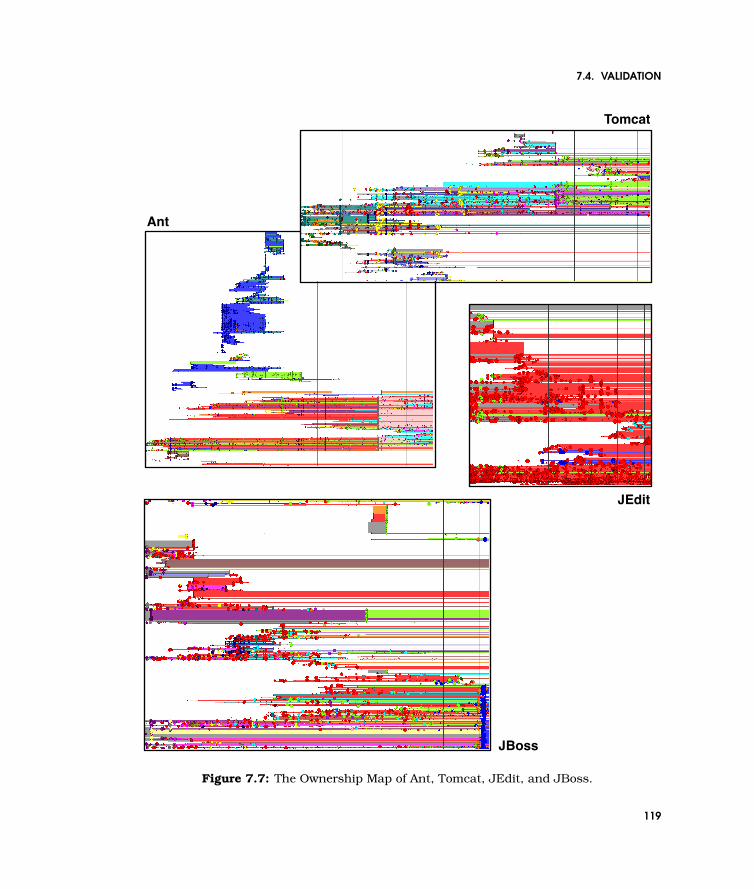
7.4. VALIDATION
Ant
JBoss
JEdit
Tomcat
Figure 7.7: The Ownership Map of Ant, Tomcat, JEdit, and JBoss.
119

CHAPTER 7. HOW DEVELOPERS DRIVE SOFTWARE EVOLUTION
7.5 Variation Points
On the exploratory nature of the implementation
We implemented our approach in CHRONIA, a tool built on top of the MOOSE
reengineering environment [Ducasse et al., 2005]. Figure 9.5 (p.144) emphasizesthe interactive nature of our tool.
On the left hand side of Figure 9.5 (p.144) we show CHRONIA visualizing the overallhistory of the project, which provides a first overview. Since there is too muchdata we cannot give the reasoning only from this view, thus, CHRONIA allowsfor interactive zooming. For example, in the window on the lower right, we seeCHRONIA zoomed into the bottom right part of the original view. Furthermore,when moving the mouse over the Ownership Map, we complement the view by alsohighlighting in the lists on the right the current position on both time and file axis.These lists show all file names and the timestamps of all commits. As CHRONIA
is built on top of MOOSE, it makes use of the MOOSE contextual menus to opendetailed views on particular files, modules or authors. For example, in the top rightwindow we see a view with metrics and measurements of a file revision.
On the scalability of the visualization
Although CHRONIA provides zooming interaction, one may lose the focus on theinteresting project periods. A solution would be to further abstract the time andgroup commits to versions that cover longer time periods. The same applies to thefile axis grouping related files into modules.
On the decision to rely on CVS log only
Our approach relies only on the information from the CVS log without checkingout the whole repository. There are two main reasons for that decision.
First, we aim to provide a solution that gives fast results; e.g., building the Own-ership Map of JBoss takes 7,8 minutes on a regular 3 GHz Pentium 4 machine,including the time spent fetching the CVS log information from the Apache.orgserver.
120

7.6. RELATED WORK
Second, it is much easier to get access to closed source case studies from industry,when only metainformation is required and not the source code itself. We considerthis an advantage of our approach.
On the shortcomings of CVS as a versioning system
As CVS lacks support for true file renaming or moving, this information is notrecoverable without time consuming calculations. To move a file, one must removeit and add it later under another name. Our approach identifies the author doingthe renaming as the new owner of the file, where in truth she only did rename it.For this reason, renaming directories impacts the computation of code ownershipin a way not desired.
On the perspective of interpreting the Ownership Map
In our visualization we sought answers to questions regarding the developers andtheir behaviors. We analyzed the files from an author perspective point of view,and not from a file perspective point of view. Thus the Ownership Map tells thestory of the developers and not of the files e.g., concerning small commits: subse-quent commits by different author to one file do not show up as a hotspot, whilea commit by one author across multiple files does. The later being the pattern wetermed Edit.
7.6 Related Work
Analyzing the way developers interact with the system has attracted only few re-search. A visualization similar to Ownership Map is used to visualize how authorschange a wiki page [Viegas et al., 2004].
Xiaomin Wu et al. visualized the change log information to provide an overview ofthe active places in the system as well as of the authors activity [Wu et al., 2004b].They display measurements like the number of times an author changed a file, orthe date of the last commit.
Measurements and visualization have long been used to analyze how softwaresystems evolve.
121
CHAPTER 7. HOW DEVELOPERS DRIVE SOFTWARE EVOLUTION
Ball and Eick developed multiple visualizations for showing changes that appearin the source code [Ball and Eick, 1996]. For example, they showed what is thepercentage of bug fixes and feature addition in files, or which lines were changedrecently.
Chuah and Eick proposed three visualizations for comparing and correlating dif-ferent evolution information like the number of lines added, the errors recordedbetween versions, number of people working etc. [Chuah and Eick, 1998].
Rysselberghe and Demeyer used a scatter plot visualization of the changes toprovide an overview of the evolution of systems and to detect patterns of change[Van Rysselberghe and Demeyer, 2004].
Jingwei Wu et al. used the spectrograph metaphor to visualize how changes occurin software systems [Wu et al., 2004a]. They used colors to denote the age ofchanges on different parts of the systems.
Jazayeri analyzed the stability of the architecture by using colors to depict thechanges [Jazayeri, 2002]. From the visualization he concluded that old parts tendto stabilize over time.
Lanza and Ducasse visualized the evolution of classes in the Evolution Matrix[Lanza and Ducasse, 2002]. Each class version is represented using a rectangle.The size of the rectangle is given by different measurements applied on the classversion. From the visualization different evolution patterns can be detected suchas continuous growth, growing and shrinking phases etc.
The difference between our approach and the above visualizations is that we dodisplay the files as they appear in the system structure, but we order them basedon the how they were committed to help the reverse engineer make out devel-opment phases. Furthermore, our analysis focuses on authors and not on thestructure of the system.
Another relevant reverse engineering domain is the analysis of the co-change his-tory.
Gall et al. aimed to detect logical coupling between parts of the system by iden-tifying the parts of the system which change together [Gall et al., 1998]. Theyused this information to define a coupling measurement based on the fact thatthe more times two modules were changed at the same time, the more they werecoupled.
Zimmerman et al. aimed to provide mechanism to warn developers about the cor-
122

7.7. SUMMARIZING THE APPROACH
relation of changes between functions. The authors placed their analysis at thelevel of entities in the meta-model (e.g., methods) [Zimmermann et al., 2004]. Thesame authors defined a measurement of coupling based on co-changes [Zimmer-mann et al., 2003].
Hassan et al. analyzed the types of data that are good predictors of change prop-agation, and came to the conclusion that historical co-change is a better mecha-nism than structural dependencies like call-graph [Hassan and Holt, 2004].
The difference between our approach and the co-change analysis is that we mea-sure the distance between files based on the Hausdorf metric of the commit timestamps, and not only based on the exact co-change.
7.7 Summarizing the Approach
In this chapter we set out to understand how the developers drove the evolutionof the system. In particular we ask the following questions:
— How many authors developed the system?
— Which author developed which part of the system?
— What were the behaviors of the developers?
To answer them, we define the Ownership Map visualization based on the notion ofcode ownership. In addition we semantically group files that have a similar commitsignature leading to a visualization that is not based on alphabetical ordering ofthe files but on co-change relationships between the file histories. The OwnershipMap helps in answering which author is knowledgeable in which part of the systemand also reveals behavioral patterns. To show the usefulness we implemented theapproach and applied it on several case studies. We reported some of the findingsand we discussed the benefits and the limitations as we perceived them duringthe experiments.
In the future, we would like to investigate the application of the approach at otherlevels of abstraction besides files, and to take into consideration types of changesbeyond just the change of a line of code.
123
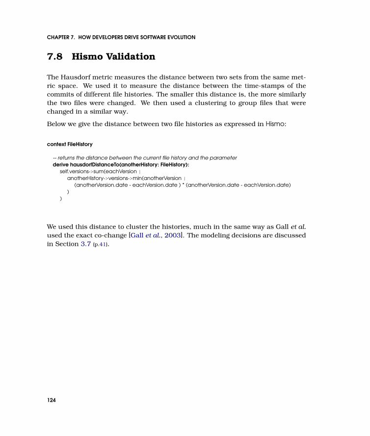
CHAPTER 7. HOW DEVELOPERS DRIVE SOFTWARE EVOLUTION
7.8 Hismo Validation
The Hausdorf metric measures the distance between two sets from the same met-ric space. We used it to measure the distance between the time-stamps of thecommits of different file histories. The smaller this distance is, the more similarlythe two files were changed. We then used a clustering to group files that werechanged in a similar way.
Below we give the distance between two file histories as expressed in Hismo:
context FileHistory
-- returns the distance between the current file history and the parameterderive hausdorfDistanceTo(anotherHistory: FileHistory):
self.versions->sum(eachVersion |anotherHistory->versions->min(anotherVersion |
(anotherVersion.date - eachVersion.date ) * (anotherVersion.date - eachVersion.date))
)
We used this distance to cluster the histories, much in the same way as Gall et al.used the exact co-change [Gall et al., 2003]. The modeling decisions are discussedin Section 3.7 (p.41).
124
Chapter 8
Detecting Co-ChangePatternsDetecting Historical Relationships Through VersionComparison
Correlations are where we see them.
Software systems need to change over time to cope with new requirements, anddue to design decisions, the changes happen to crosscut the system’s structure. Un-derstanding how changes appear in the system can reveal hidden dependenciesbetween different parts of the system. We propose the usage of concept analysis toidentify the parts of the system that change in the same way and in the same time.We apply our approach at different levels of abstraction (i.e., method, class, pack-age) and we detect fine grained changes (i.e., statements were added in a class,but no method was added there). Concept analysis is a technique that identifiesentities that have the same properties, but it requires manual inspection due to thelarge candidates it detects. We propose a heuristic that dramatically eliminates thequality of the detection. We apply our approach on one large case study and showhow we can identify hidden dependencies and detect bad smells.
We show how we detect co-change relationships by analyzing similar changes usingdetailed version comparison.

CHAPTER 8. DETECTING CO-CHANGE PATTERNS
8.1 Introduction
Software systems need to change over time to cope with the new requirements[Lehman and Belady, 1985]. As the requirements happen to crosscut the system’sstructure, changes will have to be made in multiple places. Understanding howchanges appear in the system is important for detecting hidden dependenciesbetween its parts.
In the recent period work has been carried out to detect and interpret groupsof software entities that change together [Gall et al., 1998; Itkonen et al., 2004;Zimmermann et al., 2004]. Yet, the detection is based on change informationconcerning one property, and is mostly based on file level information.
We propose the use of formal concept analysis to detect groups of entities thatchanged in the same way in several versions. Formal concept analysis is a tech-nique that identifies sets of elements with common properties based on an in-cidence table that specifies the elements and their properties [Ganter and Wille,1999].
To identify how entities changed in the same way, we use historical measurementsto detect changes between two versions. We build an Evolution Matrix [Lanza andDucasse, 2002] annotated with the detected changes, and we use the matrix asan incidence table where history represents the elements and changed in versionx represents the xth property of the element.
Also, for building the matrix of changes, we make use of logical expressions whichcombine properties with thresholds and which run on two versions of the systemto detect interesting entities. In this way, we can detect changes that take intoaccount several properties.
Example. ShotgunSurgery appears when every time we have to change a class,we also have to change a number of other classes [Fowler et al., 1999]. We wouldsuspect a group of classes of such a bad smell, when they repeatedly keep theirexternal behavior constant and change the implementation. We can detect thiskind of change in a class in the versions in which the number of methods did notchange, while the number of statements changed.
We can apply our approach on any type of entities we have defined in the meta-model. In this chapter we show how we detect groups of packages, classes andmethods.
126

8.2. HISTORY MEASUREMENTS
Structure of the Chapter
In the next section we briefly define two generic historical measurements. Wedescribe Formal Concept Analysis in a nutshell in Section 8.3 (p.128). We show howwe use FCA to detect co-change patterns, and we show how we apply it on differentlevels of abstractions (Section 8.4 (p.129)). We discuss the results we obtained whenapplying our approach on a large open source case study (Section 8.5 (p.132)). InSection 8.7 (p.134) we conclude and present the future work, and in Section 8.8(p.135) we discuss the approach from the point of view of Hismo.
8.2 History Measurements
We use two generic historical measurements to distinguish between different typesof changes.
Addition of a Version Property (A). We define a generic measurement, calledaddition of a version property P , as the addition of that property between versioni− 1 and i of the history H:
(i > 1) Ai(P, H) =
(Pi(H)− Pi−1(H), Pi(H)− Pi−1(H) > 0
0, Pi(H)− Pi−1(H) 6 0(8.1)
Evolution of a Version Property (E). We define a generic measurement, calledevolution of a version property P , as being the absolute difference of that propertybetween version i− 1 and i:
(i > 1) Ei(P, H) = |Pi(H)− Pi−1(H)| (8.2)
We instantiate the above mentioned measurements by applying them on differentversion properties of different types of entities:
— Method: NOS (number of statements), CYCLO (MCCabe cyclomatic number[McCabe, 1976]).
— Class: NOM (number of methods), WNOC (number of all subclasses).
127

CHAPTER 8. DETECTING CO-CHANGE PATTERNS
Legend:
a binary relation between the element on the row and the property on the column
X
{all elem}{no prop}
{D, B}{P2, P4}
{A, D}{P2, P6}
{A, E, C}{P5, P6}
{A, D, B}{P2}
{A, E, C, D}{P6}
{D}{P2 P4,P6}
{A}{P2,P5,P6}
{C}{P3,P5,P6}
{no elem}{all prop}
Legend:a concept representing X and Y having in common property P1 and P2
{X, Y}{P1, P2}
FCA
P1 P2 P3 P4 P5 P6
X X X
X X
X X X
X X X
X X
A
B
C
D
E
elem
ents
properties
Incidence Table Concept Latice
Figure 8.1: Example of applying formal concept analysis: the concepts on the right areobtained based on the incidence table on the left.
— Package: NOCls (number of classes), NOM (number of methods).
The E measurement shows a change of a certain property, while the A measure-ment shows the additions of a certain version property.
8.3 Concept Analysis in a Nutshell
Formal concept analysis is a technique that identifies meaningful groupings ofelements that have common properties.
Figure 8.1 (p.128) gives a schematic example of the technique. The input is specifiedin the form of a so called incidence table which encodes binary relations betweenthe set of elements and the set of properties. The output is a lattice of concepts,where each concept is a tuple of a set of elements and a set of common properties.For example, elements A and D have two properties in common: P2 and P6.
128

8.4. USING CONCEPT ANALYSIS TO IDENTIFY CO-CHANGE PATTERNS
2 3 3 3 4 6
3 3 5 5 8 9
1 3 3 4 4 6
Legend:
a class version with x methodsx
1 2 3 4 5 6versions
A
B
C
D
E
a class version in which the number of methods changed from the previous version
x
{all hist}{no ver}
{D, B}{v2, v4}
{A, D}{v2, v6}
{A, E, C}{v5, v6}
{A, D, B}{v2}
{A, E, C, D}{v6}
{D}{v2, v4, v6}
{A}{v2, v5, v6}
{C}{v3, v5, v6}
{no hist}{all ver}
Legend:a concept representing X and Y changing together in version v1 and v2
6 5 6 7
4 5 5 6 6
{X, Y}{v1, v2}
FCA
Incidence Table Concept Latice
Figure 8.2: Example of applying concept analysis to group class histories based on thechanges in number of methods. The Evolution Matrix on the left forms the incidence tablewhere the property Pi of element X is given by “history X changed in version i.”
Formal concept analysis is a generic technique working with elements and prop-erties in general. To apply it in a particular context we need to map our interestson the elements and properties. We present in the next section the mapping weuse to detect co-change patterns.
8.4 Using Concept Analysis to Identify Co-ChangePatterns
On the left side of Figure 8.2 (p.129) we display an example of an Evolution Matrix inwhich each square represents a class version and the number inside a square rep-resents the number of methods in that particular class version. A grayed squareshows a change in the number of methods of a class version as compared with the
129
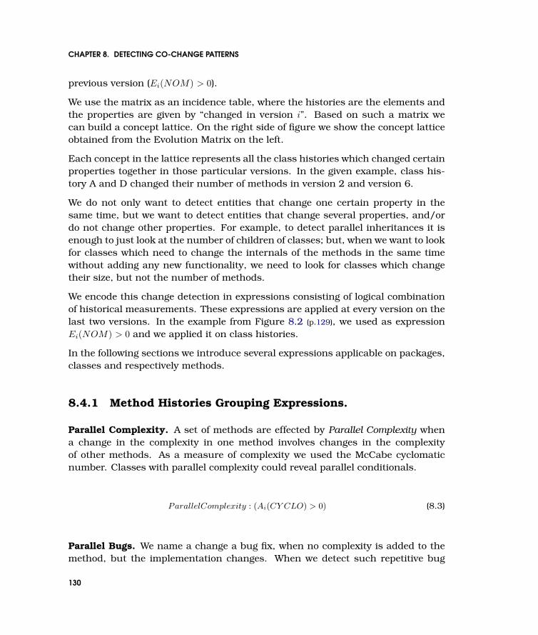
CHAPTER 8. DETECTING CO-CHANGE PATTERNS
previous version (Ei(NOM) > 0).
We use the matrix as an incidence table, where the histories are the elements andthe properties are given by “changed in version i”. Based on such a matrix wecan build a concept lattice. On the right side of figure we show the concept latticeobtained from the Evolution Matrix on the left.
Each concept in the lattice represents all the class histories which changed certainproperties together in those particular versions. In the given example, class his-tory A and D changed their number of methods in version 2 and version 6.
We do not only want to detect entities that change one certain property in thesame time, but we want to detect entities that change several properties, and/ordo not change other properties. For example, to detect parallel inheritances it isenough to just look at the number of children of classes; but, when we want to lookfor classes which need to change the internals of the methods in the same timewithout adding any new functionality, we need to look for classes which changetheir size, but not the number of methods.
We encode this change detection in expressions consisting of logical combinationof historical measurements. These expressions are applied at every version on thelast two versions. In the example from Figure 8.2 (p.129), we used as expressionEi(NOM) > 0 and we applied it on class histories.
In the following sections we introduce several expressions applicable on packages,classes and respectively methods.
8.4.1 Method Histories Grouping Expressions.
Parallel Complexity. A set of methods are effected by Parallel Complexity whena change in the complexity in one method involves changes in the complexityof other methods. As a measure of complexity we used the McCabe cyclomaticnumber. Classes with parallel complexity could reveal parallel conditionals.
ParallelComplexity : (Ai(CY CLO) > 0) (8.3)
Parallel Bugs. We name a change a bug fix, when no complexity is added to themethod, but the implementation changes. When we detect such repetitive bug
130

8.4. USING CONCEPT ANALYSIS TO IDENTIFY CO-CHANGE PATTERNS
fixes in more methods in the same versions, we group those methods in a Paral-lel Bugs group. Such a group, might give indications of similar implementationwhich could be factored out. As an implementation measure we used number ofstatements.
ParallelBugs : (Ei(NOS) > 0) ∧ Ei(CY CLO) = 0) (8.4)
8.4.2 Class Histories Grouping Expressions
Shotgun Surgery. The Shotgun Surgery bad-smell is encountered when a changeoperated in a class involves a lot of small changes to a lot of different classes[Fowler et al., 1999]. We detect this bad smell, by looking at the classes which donot change their interface, but change their implementation together.
ShotgunSurgery = (Ei(NOM) = 0 ∧ Ei(NOS) > 0) (8.5)
Parallel Inheritance. Parallel Inheritance is detected in the classes which changetheir number of children together [Fowler et al., 1999]. Such a characteristic isnot necessary a bad smell, but gives indications of a hidden link between twohierarchies. For example, if we detect a main hierarchy and a test hierarchy asbeing parallel, it gives us indication that the tests were developed in parallel withthe code.
ParallelInheritance = (Ai(WNOC) > 0) (8.6)
Parallel Semantics. Methods specify the semantics of a class. With ParallelSemantics we detect classes which add methods in parallel. Such a characteristiccould reveal hidden dependencies between classes.
ParallelSemantics = (Ai(NOM) > 0) (8.7)
131

CHAPTER 8. DETECTING CO-CHANGE PATTERNS
8.4.3 Package Histories Grouping Expression
Package Parallel Semantics. If a group of classes is detected, as having parallelsemantics, we would want to relate the containing packages as well. PackageParallel Semantics detects packages in which some methods have been added, butno classes have been added or removed.
PackageParallelSemantics = (Ei(NOCls) = 0) ∧ (Ai(NOM) > 0) (8.8)
8.5 Validation
For our experiments we chose 41 versions of JBoss1. JBoss is an open sourceJ2EE application server written in Java. The versions we selected for the exper-iments are at two weeks distance from one another starting from the beginningof 2001 until the end of 2002. The first version has 632 classes, the last onehas 4276 classes (we took into consideration all test classes, interfaces and innerclasses).
In the followings we will only discuss the ParallelInheritance results we obtainedon JBoss.
After applying the mechanism described above, we obtained 68 groups of classhistories which added subclasses in the same time. Manual inspection showedthere were a lot of repetitions (due to the way the concept lattice is built), andjust a limited number of groups were useful. Furthermore, inside a group not allclasses were relevant for that particular group.
For example, in 19 versions a class was added in the JBossTestCase hierarchy(JBossTestCase is the root of the JBoss test cases). Another example is ServiceM-BeanSupport which is the root of the largest hierarchy of JBoss. In this hierarchy,classes were added in 18 versions. That means that both JBossTestCase and Ser-viceMBeanSupport were present in a large number of groups, but they were notnecessarily related to the other classes in these groups.
1See http://www.jboss.org.
132

8.5. VALIDATION
ClassHistories Versions
org::jboss::system::ServiceMBeanSupport24org::jboss::test::JBossTestCase 19 20 27 28 29 30 32 33 34 37 38 39 40 41
javax::ejb::EJBLocalHomejavax::ejb::EJBLocalObject 24 41 28 30 32 36 37 38 23
Figure 8.3: Parallel inheritance detection results in JBoss.
These results showed that applying only concept analysis produced too many falsepositives. That is why we added a filtering step. The filtering step consists in iden-tifying and removing from the groups the entities that changed their relevant prop-erties (i.e., according to the expression) more times than the number of propertiesdetected in a group:
FilteringRule =groupV ersions
totalChangedV ersions> threshold (8.9)
In our experiments, we chose the threshold to be 3/4. For example, if JBossTestCasewas part of a group of classes which changed their number of subclasses in 10versions, we would rule the class out of the group. We chose an aggressive thresh-old to reduce the number of false positives as much as possible, in the detrimentof having true negatives.
After the filtering step, we obtained just two groups. In Figure 8.3 (p.133) we showthe class histories and the versions in which they changed the number of chil-dren.
In the first group we have two classes which changed their number of children15 times: ServiceMBeanSupport and JBossTestCase. The interpretation of this groupis that the largest hierarchy in JBoss is highly tested. A similar observation wasmade in Chapter 6 (p.87). With that occasion we detected that the JBossTestCasehierarchy is heterogeneous from the age of the classes point of view.
The second group detects a relationship between the EJB interfaces: EJBLocalHomeand EJBLocalObject. This is due to the architecture of EJB which requires that abean has to have a Home and an Object component.
133

CHAPTER 8. DETECTING CO-CHANGE PATTERNS
8.6 Related Work
The first work to study the entities that change together was performed by Gallet al. [Gall et al., 1998]. The authors used the change information to define aproximity measurement which they use to cluster related entities. The work hasbeen followed up by the same authors [Gall et al., 2003] and by Itko et al. [Itkonenet al., 2004].
Shirabad et al. employed machine learning techniques to detect files which arelikely to need to be changed when a particular file is changed [Shirabad et al.,2003].
As opposed to the previous approaches, Zimmerman et al. placed their analysisat the level of classes and methods [Zimmermann et al., 2004]. Their focus was toprovide a mechanism to warn developers that: “Programmers who changed thesefunctions also changed . . . ”. Their approach differs from ours because they onlylook at syntactic changes, while we identify changes based on the semantics of thechanges. Furthermore, our approach takes into consideration different changesin the same time.
Davey and Burd proposed the usage of concept analysis to detect evolutionary con-cepts, but there was no implementation evidence [Davey and Burd, 2001].
Detection of problems in the source code structure has long been a main issue inthe quality assurance community. Marinescu [Marinescu, 2002] detected designflaws by defining detection strategies. Ciupke employed queries usually imple-mented in Prolog to detect “critical design fragments” [Ciupke, 1999]. Tourwe etal. also explored the use of logic programming to detect design flaws [Mens etal., 2002]. van Emden and Moonen detected bad smells by looking at code pat-terns [van Emden and Moonen, 2002]. These approaches differ from ours becausethey use only the last version of the code, while we take into account historicalinformation. Furthermore, van Emden and Moonen proposed as future researchthe usage of historical information to detect Shotgun Surgery or Parallel Inheri-tance.
8.7 Summary of the Approach
Understanding how a system changes can reveal hidden dependencies betweendifferent parts of the system. Moreover, such dependencies might reveal bad
134

8.8. HISMO VALIDATION
smells in the design.
Analyzing the history of software systems can reveal parts of the system thatchange in the same time and in the same way. We proposed the usage of for-mal concept analysis, a technique that identifies elements with common proper-ties based on an incidence table specifying binary relations between elements andproperties.
To detect the changes in a version, we used expressions that combine differentproperties to detect complex changes. By applying these queries on every versionwe obtained an Evolution Matrix annotated with the change information which wethen used as input for a concept analysis machine. In other words, we used aselements histories and as properties we used the knowledge of “changed in versioni”. The results were groups of histories that change together and the versions inwhich they changed.
An important contribution of our approach is given by the automatic filtering ofthe raw results of the concept analysis machine: a history is relevant to a concept,if it was not changed in much more versions than the ones in the concept.
According to our algorithm the effectiveness of the approach is highly affectedby the value of the threshold. When the threshold is high (i.e., close to 1) weaggressively remove the false positives but we risk missing true negatives. Furtherwork is required to identify the best value for the threshold.
In the future we would also like to apply our approach on more case studies andanalyze in depth the results we obtain at different levels of abstraction.
8.8 Hismo Validation
Having history as a first class entity, allowed a straight forward mapping to theelements of the incidence table. To identify the xth property, we computed forthe xth version the expression detecting the change. Having historical propertiesmade it easy to encode the expressions.
Below we give the OCL code expressed on Hismo for the ShotgunSurgery expres-sion defined for a ClassVersion:
135

CHAPTER 8. DETECTING CO-CHANGE PATTERNS
context ClassVersion
-- returns true if the the number of methods did not change-- and the number of statements changed with respect to the previous versionderive hasShotgunSurgerySymptom:
(self.ENOM = 0) &(self.ENOS > 0)
136

Chapter 9
Van: The Time VehicleImplementing Hismo to Combine Analysis Tools
Every successful trip needs a suitable vehicle.
In the end, a meta-model is just a specification. The claim of this dissertation isthat a common meta-model allows for the combination of analyses. In this chapterwe detail VAN, our software evolution analysis tool which implements Hismo as theunderlying meta-model. Hismo offers a space in which both time and structure arerepresented in a uniform way. We show how we can use the same tools to buildanalyses both on time and on structure. We also show how several analyses canbe combined.
CHAPTER 9. VAN: THE TIME VEHICLE
9.1 Introduction
From our experience, when it comes to understanding systems, it is not enoughto have prefabricated report generators, but it is crucial to have the ability tointeractively investigate the system under discussion. The investigation becomesmore difficult as more data is involved, because the more data we need to analyze,the more analyses we need to apply, and different analyses are implemented bydifferent people in different tools. To make all these tools work together, we needa generic infrastructure that integrates them in a dynamic way.
MOOSE is an environment for integrating such tools [Ducasse et al., 2005; Nier-strasz et al., 2005]. The philosophy of MOOSE is to build one space in which all en-tities are described explicitly and in which all analysis tools coexist. MOOSE grownto be a generic environment for reverse engineering exactly because it changedcontinuously to integrate all the tools built on top of it in a coherent infrastruc-ture.
Some of the tools built on MOOSE are:
CODECRAWLER – CODECRAWLER is a visualization tool implementing polymetricviews [Lanza and Ducasse, 2003; Ducasse and Lanza, 2005]. It is based on agraph notion where the nodes and edges in the graph can wrap the entities inthe model. For example, the Hierarchy Evolution Complexity View presentedin Chapter 6 (p.87) is a polymetric view.
CONAN – CONAN is a concept analysis tool that manipulates concepts as firstclass entities [Arevalo et al., 2004; Arevalo et al., 2005]. Its target is to de-tect different kinds of patterns in the model based on combining elementsand properties. An example of the usage of concept analysis is shown inChapter 8 (p.125).
CHRONIA – CHRONIA is an implementation of a CVS protocol to allow direct con-nectivity to CVS repositories, and it implements several CVS analyses [Gırbaet al., 2005a]. An example, is presented in Chapter 7 (p.105).
HAPAX – HAPAX implements information retrieval techniques for analyzing thesemantical information residing in the names of the identifiers and in thecomments from the source code [Kuhn et al., 2005].
TRACESCRAPER – TRACESCRAPER analyzes the dynamic traces from differentperspectives. For example it offers measurements and visualizations for dy-namic traces [Greevy and Ducasse, 2005a]. TRACESCRAPER uses VAN to
138

9.2. ARCHITECTURAL OVERVIEW
analyze the evolution of dynamic traces.
VAN – VAN is our software evolution analysis tool. It implements Hismo andseveral analyses presented in this dissertation. It interacts with several othertools for implementing different analyses.
In this chapter we pay special attention to the internal implementation of VAN
and its influence on Hismo, We also show how the capabilities of MOOSE allowfor the combination of tools and how the central meta-model plays a major role.For example, VAN interacts with other tools like CODECRAWLER and CONAN toimplement some of the analyses presented in this dissertation.
Structure of the Chapter
In the next section we provide an overview of position of VAN in the overall architec-ture of MOOSE. Section 9.3 (p.139) shows how we use the same tools to manipulateboth structure and history. We present how we used other tools in Section 9.4(p.141), and we conclude in Section 9.5 (p.145).
9.2 Architectural Overview
Figure 9.2 (p.141) shows the position of VAN in the overall architecture of MOOSE.The default meta-model of MOOSE is FAMIX, a language independent meta-model[Demeyer et al., 2001]. MOOSE has a repository that can store multiple modelsproviding the necessary infrastructure for holding and managing multiple ver-sions.
At the core of VAN is the implementation of Hismo . In our implementation, Hismois built on top of FAMIX. The first step towards using the historical analyses isto manually set the history. After selecting the versions we want to analyze,all the histories are computed (e.g., ClassHistories, MethodHistories) based onnames.
9.3 Browsing Structure and History
MOOSE offers generic tools for manipulating entities and properties. The GENERIC
BROWSER allows one to manipulate a list of entities in an spreadsheet like way,
139

CHAPTER 9. VAN: THE TIME VEHICLE
Model Repository
Import / Export Interface
CodeCrawler
PolymetricViews
Van
HismoHistory Tools
FAMIXMeta Model
Basic Analysis
Tools
Moose
Tools
Conan
ConceptAnalysis
Figure 9.1: VAN and MOOSE. MOOSE is an extensible reengineering environment. Differenttools have been developed on top of it (e.g., VAN is our history analysis tool). The toolslayer can use and extend anything in the environment including the meta-model. Themodel repository can store multiple models in the same time. Sources written in differentlanguages can be loaded either directly or via intermediate data formats.
and it also allows for expressions of detection strategies (see Chapter 5 (p.67)) toobtain a sub-group. Each entity has properties, and MOOSE provides an ENTITY
INSPECTOR to view these properties.
As in Hismo histories are a explicit entities, we can manipulate them exactly like wedo with snapshot entities. Figure 9.3 (p.142) emphasizes the parallelism betweenmanipulating structure and history: on the top part we show snapshot entities,and on the bottom part we show historical entities. On each part, we display aGROUP BROWSER and an ENTITY INSPECTOR. The differences are marked with boldlabels on the figure. For example, in the GROUP BROWSER on the top, we displaya group of Classes sorted by NOM, while in the ENTITY INSPECTOR on the bottomwe display a group of ClassHistories ordered by ENOM.
Chapter 5 (p.67) presents history-based detection strategies as extensions to regu-lar detection strategies. On the bottom part of each GROUP BROWSER there is aneditor for detection strategies. For example, on the top part of the figure, we haveselected the GodClass detection strategy to be applied on the group of classes.Similarly, on the bottom part, we have selected the Stable GodClass detectionstrategy.
In Chapter 6 (p.87) we present the Hierarchy Evolution Complexity View, a poly-
140

9.4. COMBINING TOOLS
Figure 9.2: VAN gives the historical semantic to the MOOSE models.
metric view showing ClassHistories and InheritanceHistories. CODECRAWLER im-plements the polymetric views and displays them based on a graph representa-tion of the data. Originally, CODECRAWLER used the polymetric views to displaystructural entities. One of these views was the System Complexity View, whichdisplays classes as nodes and inheritances as edges. Figure 9.4 (p.143) shows theparallelism between the two views.
MOOSE aims to integrate the tools built on top by providing a registration mech-anism that allows the tool to register itself to the context that it knows how tomanipulate. This information is used to generate the menu for an entity. For ex-ample, CODECRAWLER registers the System Complexity View to a group of classes.In this way, every time we select a group of classes we can invoke CODECRAWLER
to visualize them in a System Complexity View. Having history as an explicit en-tity, we use the registration mechanism to allow tools to manipulate histories.For example, we register the Hierarchy Evolution Complexity View for a group ofClassHistories.
9.4 Combining Tools
VAN uses CODECRAWLER for visualizing the Hierarchy Evolution Complexity View.As described before, CODECRAWLER relies on a graph model and it typically mapsentities to nodes and relationships to edges. Using Hismo, the mapping wasstraight forward: ClassHistories map to nodes and InheritanceHistories map toedges.
We also use CONAN, a Formal Concept Analysis tool, to detect co-change patterns(see Chapter 8 (p.125). In this case too, the bridge was straight forward, because
141

CHAPTER 9. VAN: THE TIME VEHICLE
Entity Inspector
The list of properties of the class
The different types of entitiesin the snapshot model Group Browser The list of classes ordered by NOM
The NOMvalues
The GodClass detection strategy to be applied on the class group
Entity Inspector
The list of properties of the class history
The different types of historiesin the reference history Group Browser The list of class histories ordered by ENOM
The ENOMvalues
The Stable GodClass detection strategy to be applied on the class history group
SnapshotView
HistoryView
Figure 9.3: Screenshots showing the Group Browser the Entity Inspector. On the top part,the windows display snapshot entities, while on the bottom part they display historicalentities.
142

9.4. COMBINING TOOLS
CodeCrawler
Classes and inheritance relationships
CodeCrawler
Class histories and inheritance relationship histories
SnapshotView
HistoryView
Figure 9.4: Screenshots showing CODECRAWLER. On the top part, it displays class hier-archies in a System Complexity View, while on the bottom part it displays class hierarchyhistories in a Hierarchy Evolution Complexity View.
143

CHAPTER 9. VAN: THE TIME VEHICLE
Chronia - the overall picture
Chronia - a zoomed part and a contextual menu
Moose Entity Browser - details on the selected File
Figure 9.5: Screenshots showing CHRONIA in action: interaction is crucial.
CONAN manipulates entities and properties. We provided histories as entities and“changed in version i” as properties.
Chapter 7 (p.105) introduces the Ownership Map visualization to display how au-thors changed the files in a CVS repository. We implemented the visualization inCHRONIA. To do so, we first implemented a CVS-like meta-model and we imple-mented the visualization on top. Due to the size of the data, it was not enough tojust build a static visualization tool, but we needed an interactive tool. Figure 9.5(p.144) shows the interactive nature of the tool. In particular, the explicitness ofthe meta-model allows us to use the MOOSE default tools. For example, we caninspect the FileHistory from the visualization in the ENTITY INSPECTOR.
Another tool built on Van was QUALA [Buhler, 2004]. QUALA aimed to detect
144
9.5. SUMMARY
phases in history, by defining a phase as being a first class entity. QUALA usedCODECRAWLER to display the detected phases.
9.5 Summary
MOOSE is an environment for reengineering, and several tools are built on top of it.The philosophy of MOOSE is to integrate reengineering tools by making the meta-model explicit. VAN is a version analysis tool implementing Hismo and severalevolution analyses. By making history an explicit entity, we used the mechanismsof MOOSE to integrate tools for analyzing software evolution.
145

CHAPTER 9. VAN: THE TIME VEHICLE
146

Chapter 10
Conclusions
What we can governs what we wish.
Understanding software evolution is important as evolution holds information thatcan be used in various analyses like reverse engineering, prediction, change im-pact, or in developing general laws of evolution.
We have reviewed various approaches used to exploit the history of data regardingthe evolution of software systems. These approaches typically focus on only sometraits of the evolution and most of them do not rely on explicit an meta-model, andbecause of that, it is difficult to compare and combine the results.
In this dissertation we argue for the need for an explicit meta-model that allowsfor the expression and combination of software evolution. Based on our literaturesurvey we have gathered requirements for such a meta-model: (1) different ab-straction and detail levels, (2) comparison of property evolutions, (3) combinationof different property evolutions, (4) historical selection, (5) historical relationships,and (6) historical navigation.
Our solution is to model evolution explicitly. We introduced Hismo, a meta-modelcentered around the notion of history as an encapsulation of evolution. We arguedthat Hismo is not tightly dependent on any particular structural construct andthat it can be obtained by transforming the snapshot meta-model. In this way,our approach is not even restricted to software analysis, but can be applied to

CHAPTER 10. CONCLUSIONS
other fields as well.
As a validation of our meta-model we showed several analyses build on Hismo:
History properties show how to summarize the evolution into properties attachedto histories. Historical measurements like Evolution of Number of Methods,are an example of such properties. Such properties allow for historical com-parison.
Yesterday’s Weather is a complex historical measurement based on the assump-tion that the latest changed parts also change in the near future. It showshow relevant it is to start reverse engineering from the latest changed partsof the system.
History-based detection strategies are expressions that combine measurementsat the snapshot level with historical measurements. We show how usingthem we can refine the detection of design flaws.
Hierarchy Evolution Complexity View combines the manipulation of historical re-lationships with historical properties to offer a means to understand the evo-lution of class hierarchies as a whole.
We built the Ownership Map visualization to detect how developers drive softwareevolution. The analysis is placed at the file level and it shows how developerschanged the system. We made use of historical relationships to order thefiles to provide for a meaningful visualization.
Co-change analysis attracted extensive research. Besides showing how the cur-rent state-of-the-art research can be expressed in terms on Hismo, we alsoproposed a novel approach that makes use of concept analysis to detect co-change patterns. We showed how we can group histories to detect patternslike parallel inheritance.
Several other analyses were built using our approach, but were not covered in thisdissertation:
Phase detection. Buehler developed an approach to detect phases in histories[Buhler, 2004]. A phase is a selection of a history in which each versioncomplies to a certain expression. For example, he detected growth phasesby looking for versions that present additions as compared with the previousversion.
Trace evolution. Greevy et al. analyzed the evolution of execution traces to char-acterize the evolution of features [Greevy et al., 2005]. The authors recovered
148

10.1. DISCUSSION: HOW HISMO SUPPORTS SOFTWARE EVOLUTION ANALYSIS
the mapping between the features and the code by analyzing the executiontraces of the features [Greevy and Ducasse, 2005b]. They modeled the Traceas first class entity, and they analyzed the evolution of the traces by definingTraceHistories, and by using historical measurements. For example, theydetect how classes changed from being used in only one feature, to beingused in several features.
Refactorings detection. Dig and Johnson used version information to detect refac-torings based on different heuristics [Dig and Johnson, 2005]. The goal wasto analyze how many of the changes that break the API are due to refactor-ings. They performed the experiment using our VAN tool.
We implemented Hismo and the presented history analyses in our tool called VAN.VAN is built on top of the MOOSE reengineering environment. MOOSE philosophyrecognizes that successful reengineering needs to combine several techniques.Several tools have been built over the years in the MOOSE environment, VAN beingone of them. We showed how the implementation of Hismo made it possible tocombine several tools for accomplishing the required analysis.
10.1 Discussion: How Hismo Supports Software Evo-lution Analysis
The above applications show how Hismo satisfies the desired activities:
Different abstraction and detail levels. Hismo takes into account the structureof the system. We gave examples of history measurements which take intoaccount different semantics of change (e.g., changes in number of methods,number of statements) on different entities (e.g., packages, classes, meth-ods). As we show Hismo can be applied on any software entities which canplay the role of a Snapshot. In this dissertation we present analyses at dif-ferent levels of abstractions: system, class, method or file.
Furthermore, having detailed information about each version, we can alsodefine the version properties (e.g., number of methods) in terms of history(e.g., “number of methods in version i”). Thus, all the things we can find outfrom one version can be found out having the entire history. This allows forcombining structural data with evolution data in the same expression. Forexample, we can detect the harmless God Classes by detecting those that didnot add or remove methods (Chapter 5 (p.67)).
149
CHAPTER 10. CONCLUSIONS
Comparison of property evolutions. History describes the evolution. History mea-surements are a way to quantify the changes and they allow for the com-parison of different entity evolutions. For example, the Evolution of Numberof Methods lets us assess which classes changed more in terms of added orremoved methods.
Combination of different property evolutions. Some of the evolution analyses needto combine property evolutions with structural properties. For example, theHierarchy Evolution Complexity View combines different property evolutions(Chapter 6 (p.87)), and the history-based detection strategies combines prop-erty evolutions with structural information (Chapter 5 (p.67)).
Historical selection. Given a history we can filter it to obtain a sub-history. Asthe defined analyses are applicable on a history, and a selection of a historyis another history, the analyses described in this dissertation can be appliedon any selection. For example, Yesterday’s Weather (Chapter 4 (p.47)) appliesthe measurements on selections of histories to identify latest changed partsor early changed parts.
Historical relationships. In the same way we reason about the relationships be-tween structural relationships, we can reason about the historical relation-ships. In Chapter 6 (p.87) we present Hierarchy Evolution Complexity View asan example of how to reason about the inheritance histories between classhistories.
Historical navigation. Based on the structural relationship “a Package has Classes”we can build the relationship “a PackageHistory has ClassHistories”. Thiscan be generalized to any structural relationship and thus, at the history levelwe can ask a PackageHistory to return all ClassHistories – i.e., all Classeswhich ever existed in that Package. An example of the usefulness of thisfeature is given in Chapter 4 (p.47), where we show how we can implementYesterday’s Weather for a SystemHistory.
10.2 Open Issues
On the Types of Data Taken Under Study
Most of the analyses deal with source code alone. Yet, reverse engineering needsinformation about the physical and social environment in which the software was
150

10.2. OPEN ISSUES
developed.
Chapter 7 (p.105) presents an example of how to use the author information torecover development patterns. A promising research has been carried out in theHipikat project [Cubranic and Murphy, 2003]. Other interesting projects correlatethe bug information with the change information [Fischer et al., 2003a; Fischer etal., 2003b].
For example an interesting path was explored by the work on analyzing the se-mantics of code to recover domain concepts [Kuhn et al., 2005]. We would liketo employ similar techniques to correlate these concepts with the author and buginformation to identify what type of work each concept required.
We believe that to elevate the quality of the analysis, we need to take more typesof data into account. In this direction, we believe that Hismo opens the possibilityfor such an undertaking because it provides the modeling solution.
On How History Could Influence Forward Engineering
We modeled history as being a collection of versions. We took this decision becauseour focus was reverse engineering and the current state-of-the-art in versioningtools only gave us individual versions.
In fact, a better solution would be to manipulate the entire spectrum of changes asthey happen in the development environment, and not just manipulate arbitrarysnapshots. That is, a better solution would be to analyze the actual evolution,rather than rebuilding the evolution out of individual versions and recovering thechanges based on diff analysis. Although the current data was not available, webelieve that this is the next step in managing software evolution.
On the Different Ways to Recover and Manipulate Entity Identity
We refer to entity identity as being the mechanism through which two versionsare decided to be part of the same history. In the applications presented here, wereduced entity identity to name identity. That is, when two entities of the sametype have the same name in two different versions, they are considered to be partof the same history.
According to this algorithm, when an entity is renamed, its identity is lost. InChapter 3 (p.29), we discussed two heuristics to deal with this problem [Antoniol
151

and Di Penta, 2004; Zou and Godfrey, 2003]). These heuristics recover the identitybased on some internal properties of the entity. A possibility to complement theseheuristics would be to allow the reverse engineer to manually check the resultsand to take different decisions like merging the histories.
Entity identity is a problem because versioning system do not consider evolutionto be a continuous process, but a discrete one. In this case too, keeping thechanges as they happened (including their semantics) would make the analysiseasier and more precise.
On the Manipulation of Branches
In this dissertation, we modeled history as a sequence of versions which impliesa linear version alignment. In the future, we would like to investigate the impli-cations of modeling history as a partially ordered set of versions to represent timeas a graph. Such a model would allow manipulation of branches.
152

Closing Words
We cannot find the flow of things unless we let go.
This entire work is about providing for a model to better understand softwareevolution. Models are the way we understand the world. They provide a finiterepresentation and they answer questions instead of the real world by allowing forexecutable reasonings to be expressed on them.
Yet, models are not an end, they are a means. No matter how good a model is, itis still a finite representation, while the real world is infinite.
Modeling is just a step in the process of understanding. To understand the worldin its entirety, we need to go beyond models. We need to resonate with the all itsdetails.
October 23, 2005Tudor Gırba

154

Appendix A
Definitions
Entity
— An entity is something that has separate and distinct existence in objective orconceptual reality [Soanes, 2001].
Snapshot, Version, Evolution and History
— A snapshot is the structure of an entity at a particular moment in time.
Examples of snapshots are classes, methods etc.
— A version is a snapshot of an entity placed in the context of time.
For example, in the context of CVS, version is denoted by revision.
— The evolution is the process that leads from one version of an entity to another.
— A history is the reification which encapsulates the knowledge about evolutionand version information.
Following the above definitions, we say that we use the history of a system tounderstand its evolution. Furthermore, the evolution refers to all changes from aversion of an entity to another. Sometimes, however, we need to refer to only thechange of a particular property of that entity. That is why we define:
— Property evolution denotes how a particular property evolved in an entity.
— Historical property denotes a characteristic of a history.

For example, the age of a file in CVS is a historical property.
Model and Meta-model
— A model is a simplification of a system built with an intended goal in mind. Themodel should be able to answer questions in place of the actual system [Bezivinand Gerbe, 2001].
— A meta-model is a specification model for a class of systems under study whereeach system under study in the class is itself a valid model expressed in acertain modeling language [Seidewitz, 2003].
We use different terms for different types of models and meta-models:
— A snapshot meta-model, or a structural meta-model is a meta-model which de-scribes the structure of a class of systems at a certain moment in time.
Examples of snapshot meta-models are UML or FAMIX.
— An evolution model is a simplified view on the evolution of a system.
Examples of evolution models include the date sequence of each release, a chartshowing team allocation over time for a given set of modules, the modificationsperformed etc.
— An evolution meta-model is a meta-model which describes a family of evolutionmodels.
For instance, in each versioning systems there is an evolution meta-model thatspecifies which kind of information is kept about evolution.
— A history meta-model is an evolution meta-model which models history as afirst class entity.
Entity identity
— Entity identity denotes the mechanism through which two versions are decidedto be part of the same history.
156

Bibliography
[Antoniol and Di Penta, 2004] Giuliano Antoniol and Massimiliano Di Penta. Anautomatic approach to identify class evolution discontinuities. In IEEE Inter-national Workshop on Principles of Software Evolution (IWPSE04), pages 31–40,September 2004.
[Antoniol et al., 2004] Giuliano Antoniol, Massimiliano Di Penta, Harald Gall, andMartin Pinzger. Towards the integration of versioning systems, bug reports andsource code meta-models. In Workshop on Software Evolution Through Transfor-mation (SETra 2004), pages 83–94, 2004.
[Aoki et al., 2001] Atsushi Aoki, Kaoru Hayashi, Kouichi Kishida, KumiyoNakakoji, Yoshiyuki Nishinaka, Brent Reeves, Akio Takashima, and YasuhiroYamamoto. A case study of the evolution of jun: an object-oriented open-source3d multimedia library. In Proceedings of International Conference on SoftwareEngineering (ICSE), 2001.
[Arevalo et al., 2004] Gabriela Arevalo, Frank Buchli, and Oscar Nierstrasz. De-tecting implicit collaboration patterns. In Proceedings of WCRE ’04 (11th Work-ing Conference on Reverse Engineering), pages 122–131. IEEE Computer SocietyPress, November 2004.
[Arevalo et al., 2005] Gabriela Arevalo, Stephane Ducasse, and Oscar Nierstrasz.Discovering unanticipated dependency schemas in class hierarchies. In Pro-ceedings of CSMR ’05 (9th European Conference on Software Maintenance andReengineering), pages 62–71. IEEE Computer Society Press, March 2005.
[Arevalo, 2005] Gabriela Arevalo. High Level Views in Object Oriented Systemsusing Formal Concept Analysis. PhD thesis, University of Berne, January 2005.

[Ball and Eick, 1996] Timothy Ball and Stephen Eick. Software visualization inthe large. IEEE Computer, pages 33–43, 1996.
[Bennett and Rajlich, 2000] Keith Bennett and Vaclav Rajlich. Software mainte-nance and evolution:a roadmap. In ICSE — Future of SE Track, pages 73–87,2000.
[Bertin, 1974] Jacques Bertin. Graphische Semiologie. Walter de Gruyter, 1974.
[Bezivin and Gerbe, 2001] Jean Bezivin and Olivier Gerbe. Towards a precise def-inition of the omg/mda framework. In Proceedings of Automated Software Engi-neering (ASE 2001), pages 273–282. IEEE Computer Society, 2001.
[Bieman and Kang, 1995] J.M. Bieman and B.K. Kang. Cohesion and reuse in anobject-oriented system. In Proceedings ACM Symposium on Software Reusability,April 1995.
[Brooks, 1987] Frederick P. Brooks. No silver bullet. IEEE Computer, 20(4):10–19,April 1987.
[Buckley et al., 2005] Jim Buckley, Tom Mens, Matthias Zenger, Awais Rashid,and Gunter Kniesel. Towards a taxonomy of software change. Journal on Soft-ware Maintenance and Evolution: Research and Practice, pages 309–332, 2005.
[Buhler, 2004] Thomas Buhler. Detecting and visualizing phases in software evo-lution. Diploma thesis, University of Bern, September 2004.
[Burch et al., 2005] Michael Burch, Stephan Diehl, and Peter Weißgerber. Visualdata mininng in software archives. In Proceedings of 2005 ACM Symposium onSoftware Visualization (Softviz 2005), pages 37–46, St. Louis, Missouri, USA,May 2005.
[Burd and Munro, 1999] Elizabeth Burd and Malcolm Munro. An initial approachtowards measuring and characterizing software evolution. In Proceedings of theWorking Conference on Reverse Engineering, WCRE ’99, pages 168–174, 1999.
[Capiluppi et al., 2004] Andrea Capiluppi, Maurizio Morisio, and Patricia Lago.Evolution of understandability in OSS projects. In Proceedings of the 8th Eu-ropean Conference on Software Maintenance and Reengineering (CSMR 2004),pages 58–66, 2004.
[Capiluppi, 2003] Andrea Capiluppi. Models for the evolution of OS projects.In Proceedings of the International Conference on Software Maintenance (ICSM2003), pages 65–74, 2003.
158

[Chidamber and Kemerer, 1994] Shyam R. Chidamber and Chris F. Kemerer. Ametrics suite for object oriented design. IEEE Transactions on Software Engi-neering, 20(6):476–493, June 1994.
[Chuah and Eick, 1998] Mei C. Chuah and Stephen G. Eick. Information richglyphs for software management data. IEEE Computer Graphics and Applica-tions, pages 24–29, July 1998.
[Ciupke, 1999] Oliver Ciupke. Automatic detection of design problems in object-oriented reengineering. In Proceedings of TOOLS 30 (USA), pages 18–32, 1999.
[Collberg et al., 2003] Christian Collberg, Stephen Kobourov, Jasvir Nagra, JacobPitts, and Kevin Wampler. A system for graph-based visualization of the evo-lution of software. In Proceedings of the 2003 ACM Symposium on SoftwareVisualization, pages 77–86. ACM Press, 2003.
[Conway, 1968] Melvin E. Conway. How do committees invent ? Datamation,14(4):28–31, April 1968.
[Davey and Burd, 2001] John Davey and Elizabeth Burd. Clustering and conceptanalysis for software evolution. In Proceedings of the 4th international Work-shop on Principles of Software Evolution (IWPSE 2001), pages 146–149, Vienna,Austria, 2001.
[Demeyer et al., 1999] Serge Demeyer, Stephane Ducasse, and Michele Lanza. Ahybrid reverse engineering platform combining metrics and program visualiza-tion. In Francoise Balmas, Mike Blaha, and Spencer Rugaber, editors, Proceed-ings WCRE ’99 (6th Working Conference on Reverse Engineering). IEEE, October1999.
[Demeyer et al., 2000] Serge Demeyer, Stephane Ducasse, and Oscar Nierstrasz.Finding refactorings via change metrics. In Proceedings of OOPSLA ’2000 (Inter-national Conference on Object-Oriented Programming Systems, Languages andApplications), pages 166–178, 2000.
[Demeyer et al., 2001] Serge Demeyer, Sander Tichelaar, and Stephane Ducasse.FAMIX 2.1 — The FAMOOS Information Exchange Model. Technical report,University of Bern, 2001.
[Demeyer et al., 2002] Serge Demeyer, Stephane Ducasse, and Oscar Nierstrasz.Object-Oriented Reengineering Patterns. Morgan Kaufmann, 2002.
159
[Dig and Johnson, 2005] Daniel Dig and Ralph Johnson. The role of refactoringsin API evolution. In Proceedings of 21st International Conference on SoftwareMaintenance (ICSM 2005), pages 389–398, September 2005.
[Draheim and Pekacki, 2003] Dirk Draheim and Lukasz Pekacki. Process-centricanalytical processing of version control data. In International Workshop on Prin-ciples of Software Evolution (IWPSE 2003), pages 131–136, 2003.
[Ducasse and Lanza, 2005] Stephane Ducasse and Michele Lanza. The classblueprint: Visually supporting the understanding of classes. IEEE Transactionson Software Engineering, 31(1):75–90, January 2005.
[Ducasse et al., 2004] Stephane Ducasse, Tudor Gırba, and Jean-Marie Favre.Modeling software evolution by treating history as a first class entity. In Work-shop on Software Evolution Through Transformation (SETra 2004), pages 71–82,2004.
[Ducasse et al., 2005] Stephane Ducasse, Tudor Gırba, Michele Lanza, and SergeDemeyer. Moose: a collaborative and extensible reengineering Environment. InTools for Software Maintenance and Reengineering, RCOST / Software Technol-ogy Series, pages 55–71. Franco Angeli, 2005.
[Eick et al., 1992] Stephen G. Eick, Joseph L. Steffen, and Sumner Eric E., Jr.SeeSoft—a tool for visualizing line oriented software statistics. IEEE Transac-tions on Software Engineering, 18(11):957–968, November 1992.
[Eick et al., 2001] Stephen G. Eick, Todd L. Graves, Alan F. Karr, J. S. Marron,and Audris Mockus. Does code decay? assessing the evidence from changemanagement data. IEEE Transactions on Software Engineering, 27(1):1–12,2001.
[Eick et al., 2002] Stephen G. Eick, Todd L. Graves, Alan F. Karr, Audris Mockus,and Paul Schuster. Visualizing software changes. Software Engineering,28(4):396–412, 2002.
[Fischer et al., 2003a] Michael Fischer, Martin Pinzger, and Harald Gall. Analyz-ing and relating bug report data for feature tracking. In Proceedings of the 10thWorking Conference on Reverse Engineering (WCRE 2003), pages 90–99, Novem-ber 2003.
[Fischer et al., 2003b] Michael Fischer, Martin Pinzger, and Harald Gall. Populat-ing a release history database from version control and bug tracking systems.
160

In Proceedings of the International Conference on Software Maintenance (ICSM2003), pages 23–32, September 2003.
[Fowler et al., 1999] Martin Fowler, Kent Beck, John Brant, William Opdyke, andDon Roberts. Refactoring: Improving the Design of Existing Code. Addison Wes-ley, 1999.
[Fowler, 2003] Martin Fowler. UML Distilled. Addison Wesley, 2003.
[Gall et al., 1997] Harald Gall, Mehdi Jazayeri, Rene R. Klosch, and Georg Traus-muth. Software evolution observations based on product release history. InProceedings of the International Conference on Software Maintenance 1997 (ICSM’97), pages 160–166, 1997.
[Gall et al., 1998] Harald Gall, Karin Hajek, and Mehdi Jazayeri. Detection of logi-cal coupling based on product release history. In Proceedings of the InternationalConference on Software Maintenance 1998 (ICSM ’98), pages 190–198, 1998.
[Gall et al., 2003] Harald Gall, Mehdi Jazayeri, and Jacek Krajewski. Cvs releasehistory data for detecting logical couplings. In International Workshop on Princi-ples of Software Evolution (IWPSE 2003), pages 13–23, 2003.
[Ganter and Wille, 1999] Bernhard Ganter and Rudolf Wille. Formal Concept Anal-ysis: Mathematical Foundations. Springer Verlag, 1999.
[Gırba and Lanza, 2004] Tudor Gırba and Michele Lanza. Visualizing and charac-terizing the evolution of class hierarchies. In WOOR 2004 (5th ECOOP Workshopon Object-Oriented Reengineering), 2004.
[Gırba et al., 2004a] Tudor Gırba, Stephane Ducasse, and Michele Lanza. Yes-terday’s Weather: Guiding early reverse engineering efforts by summarizing theevolution of changes. In Proceedings of ICSM 2004 (20th International Conferenceon Software Maintenance), pages 40–49. IEEE Computer Society Press, 2004.
[Gırba et al., 2004b] Tudor Gırba, Stephane Ducasse, Radu Marinescu, andDaniel Ratiu. Identifying entities that change together. In Ninth IEEE Workshopon Empirical Studies of Software Maintenance, 2004.
[Gırba et al., 2004c] Tudor Gırba, Jean-Marie Favre, and Stephane Ducasse. Us-ing meta-model transformation to model software evolution, 2004. 2nd Interna-tional Workshop on Meta-Models and Schemas for Reverse Engineering (ATEM2004).
[Gırba et al., 2005a] Tudor Gırba, Adrian Kuhn, Mauricio Seeberger, andStephane Ducasse. How developers drive software evolution. In Proceedings of
161
International Workshop on Principles of Software Evolution (IWPSE), pages 113–122. IEEE Computer Society Press, 2005.
[Gırba et al., 2005b] Tudor Gırba, Michele Lanza, and Stephane Ducasse. Char-acterizing the evolution of class hierarchies. In Proceedings of CSMR 2005 (9thEuropean Conference on Software Maintenance, pages 2–11, 2005.
[Godfrey and Tu, 2000] Michael Godfrey and Qiang Tu. Evolution in open sourcesoftware: A case study. In Proceedings of the International Conference on Soft-ware Maintenance (ICSM 2000), pages 131–142. IEEE Computer Society, 2000.
[Gold and Mohan, 2003] Nicolas Gold and Andrew Mohan. A framework for un-derstanding conceptual changes in evolving source code. In Proceedings of Inter-national Conference on Software Maintenance 2003 (ICSM 2003), pages 432–439,September 2003.
[Greevy and Ducasse, 2005a] Orla Greevy and Stephane Ducasse. Characteriz-ing the functional roles of classes and methods by analyzing feature traces.In Proceedings of WOOR 2005 (6th International Workshop on Object-OrientedReengineering), July 2005.
[Greevy and Ducasse, 2005b] Orla Greevy and Stephane Ducasse. Correlatingfeatures and code using a compact two-sided trace analysis approach. In Pro-ceedings of CSMR 2005 (9th European Conference on Software Maintenance andReengineering, pages 314–323. IEEE Computer Society Press, 2005.
[Greevy et al., 2005] Orla Greevy, Stephane Ducasse, and Tudor Gırba. Analyz-ing feature traces to incorporate the semantics of change in software evolutionanalysis. In Proceedings of ICSM 2005 (21th International Conference on Soft-ware Maintenance), pages 347–356. IEEE Computer Society Press, September2005.
[Grosser et al., 2002] David Grosser, Houari A. Sahraoui, and Petko Valtchev. Pre-dicting software stability using case-based reasoning. In Proceedings of the 17thIEEE International Conference on Automated Software Engienering (ASE ’02),pages 295–298, 2002.
[Gulla, 1992] Bjorn Gulla. Improved maintenance support by multi-version visu-alizations. In Proceedings of the 8th International Conference on Software Main-tenance (ICSM 1992), pages 376–383. IEEE Computer Society Press, November1992.
162

[Hassan and Holt, 2004] Ahmed Hassan and Richard Holt. Predicting changepropagation in software systems. In Proceedings of 20th IEEE International Con-ference on Software Maintenance (ICSM’04), pages 284–293. IEEE Computer So-ciety Press, September 2004.
[Holt and Pak, 1996] Richard Holt and Jason Pak. GASE: Visualizing softwareevolution-in-the-large. In Proceedings of Working Conference on Reverse Engi-neering (WCRE 1996), pages 163–167, 1996.
[Hunt and McIlroy, 1976] James Hunt and Douglas McIlroy. An algorithm for dif-ferential file comparison. Technical Report CSTR 41, Bell Laboratories, MurrayHill, NJ, 1976.
[Itkonen et al., 2004] Jonne Itkonen, Minna Hillebrand, and Vesa Lappalainen.Application of relation analysis to a small java software. In Proceedings ofthe Conference on Software Maintenance and Reengineering (CSMR 2004), pages233–239, 2004.
[Jain et al., 1999] A. K. Jain, M. N. Murty, and P. J. Flynn. Data clustering: Areview. ACM Computing Surveys, 31(3):264–323, September 1999.
[Jazayeri et al., 1999] Mehdi Jazayeri, Harald Gall, and Claudio Riva. VisualizingSoftware Release Histories: The Use of Color and Third Dimension. In Pro-ceedings of ICSM ’99 (International Conference on Software Maintenance), pages99–108. IEEE Computer Society Press, 1999.
[Jazayeri, 2002] Mehdi Jazayeri. On architectural stability and evolution. InReliable Software Technlogies-Ada-Europe 2002, pages 13–23. Springer Verlag,2002.
[Krajewski, 2003] Jacek Krajewski. QCR - A methodology for software evolutionanalysis. Master’s thesis, Information Systems Institute, Distributed SystemsGroup, Technical University of Vienna, April 2003.
[Kuhn et al., 2005] Adrian Kuhn, Stephane Ducasse, and Tudor Gırba. Enrichingreverse engineering with semantic clustering. In Proceedings of Working Con-ference On Reverse Engineering (WCRE 2005), pages ??–??, November 2005. toappear.
[Lanza and Ducasse, 2002] Michele Lanza and Stephane Ducasse. Understand-ing software evolution using a combination of software visualization and soft-ware metrics. In Proceedings of LMO 2002 (Langages et Modeles a Objets, pages135–149, 2002.
163
[Lanza and Ducasse, 2003] Michele Lanza and Stephane Ducasse. Polymetricviews — a lightweight visual approach to reverse engineering. IEEE Transac-tions on Software Engineering, 29(9):782–795, September 2003.
[Lanza and Ducasse, 2005] Michele Lanza and Stephane Ducasse. Codecrawler— an extensible and language independent 2d and 3d software visualizationtool. In Tools for Software Maintenance and Reengineering, RCOST / SoftwareTechnology Series, pages 74–94. Franco Angeli, 2005.
[Lanza et al., 2006] Michele Lanza, Radu Marinescu, and Stephane Ducasse.Object-Oriented Metrics in Practice. Springer-Verlag, 2006. to appear.
[Lanza, 2003] Michele Lanza. Object-Oriented Reverse Engineering — Coarse-grained, Fine-grained, and Evolutionary Software Visualization. PhD thesis, Uni-versity of Berne, May 2003.
[Lehman and Belady, 1985] Manny Lehman and Les Belady. Program Evolution –Processes of Software Change. London Academic Press, 1985.
[Lehman et al., 1997] Manny Lehman, Dewayne Perry, Juan Ramil, WladyslawTurski, and Paul Wernick. Metrics and laws of software evolution – the ninetiesview. In Metrics ’97, IEEE, pages 20–32, 1997.
[Lehman et al., 1998] Manny Lehman, Dewayne Perry, and Juan Ramil. Impli-cations of evolution metrics on software maintenance. In Proceedings of theInternational Conference on Software Maintenance (ICSM 1998), pages 208–217,1998.
[Lehman, 1996] Manny Lehman. Laws of software evolution revisited. In Euro-pean Workshop on Software Process Technology, pages 108–124, 1996.
[Lorenz and Kidd, 1994] Mark Lorenz and Jeff Kidd. Object-Oriented Software Met-rics: A Practical Guide. Prentice-Hall, 1994.
[MacKenzie et al., 2003] David MacKenzie, Paul Eggert, and Richard Stallman.Comparing and Merging Files With Gnu Diff and Patch. Network Theory Ltd.,2003.
[Marinescu, 2001] Radu Marinescu. Detecting design flaws via metrics in object-oriented systems. In Proceedings of TOOLS, pages 173–182, 2001.
[Marinescu, 2002] Radu Marinescu. Measurement and Quality in Object-OrientedDesign. Ph.D. thesis, Department of Computer Science, ”Politehnica” Universityof Timisoara, 2002.
164

[Marinescu, 2004] Radu Marinescu. Detection strategies: Metrics-based rules fordetecting design flaws. In Proceedings of ICSM ’04 (International Conference onSoftware Maintenance), pages 350–359. IEEE Computer Society Press, 2004.
[McCabe, 1976] T.J. McCabe. A measure of complexity. IEEE Transactions onSoftware Engineering, 2(4):308–320, December 1976.
[Mens and Demeyer, 2001] Tom Mens and Serge Demeyer. Future trends in soft-ware evolution metrics. In Proceedings IWPSE2001 (4th International Workshopon Principles of Software Evolution), pages 83–86, 2001.
[Mens et al., 2002] Kim Mens, Tom Mens, and Michel Wermelinger. Maintainingsoftware through intentional source-code views. In Proceedings of SEKE 2002,pages 289–296. ACM Press, 2002.
[Meyer, 1988] Bertrand Meyer. Object-oriented Software Construction. Prentice-Hall, 1988.
[Mihancea and Marinescu, 2005] Petru Mihancea and Radu Marinescu. Towardsthe optimization of automatic detection of design flaws in object-oriented soft-ware systems. In Proceedings of European Conference on Software Maintenance(CSMR 2005), pages 92–101, 2005.
[Mockus and Votta, 2000] Audris Mockus and Lawrence Votta. Identifying rea-sons for software change using historic databases. In Proceedings of the In-ternational Conference on Software Maintenance (ICSM 2000), pages 120–130.IEEE Computer Society Press, 2000.
[Mockus and Weiss, 2000] Audris Mockus and David Weiss. Predicting risk ofsoftware changes. Bell Labs Technical Journal, 5(2), April 2000.
[Mockus et al., 1999] Audris Mockus, Stephen Eick, Todd Graves, and Alan Karr.On measurements and analysis of software changes. Technical report, NationalInstitute of Statistical Sciences, 1999.
[Nierstrasz et al., 2005] Oscar Nierstrasz, Stephane Ducasse, and Tudor Girba.The story of Moose: an agile reengineering environment. In Proceedings ofESEC/FSE 2005, pages 1–10. ACM, 2005. Invited paper.
[OCL 2.0, 2003] Uml 2.0 object constraint language (ocl) specification, 2003.http://www.omg.org/docs/ptc/03-10-14.pdf.
[Parnas, 1994] David Lorge Parnas. Software Aging. In Proceedings of ICSE ’94(International Conference on Software Engineering), pages 279–287. IEEE Com-puter Society / ACM Press, 1994.
165

[Pinzger et al., 2005] Martin Pinzger, Harald Gall, Michael Fischer, and MicheleLanza. Visualizing multiple evolution metrics. In Proceedings of SoftVis 2005(2nd ACM Symposium on Software Visualization), pages 67–75, St. Louis, Mis-souri, USA, May 2005.
[Ratiu et al., 2004] Daniel Ratiu, Stephane Ducasse, Tudor Gırba, and RaduMarinescu. Using history information to improve design flaws detection. InProceedings of CSMR 2004 (European Conference on Software Maintenance andReengineering), pages 223–232, 2004.
[Ratiu, 2003] Daniel Ratiu. Time-based detection strategies. Master’s thesis, Fac-ulty of Automatics and Computer Science, ”Politehnica” University of Timisoara,September 2003. Supervised by Tudor Gırba and defended at Politehnica Uni-versity of Timisoara, Romania.
[Ramil and Lehman, 2001] Juan F. Ramil and Meir M. Lehman. Defining andapplying metrics in the context of continuing software evolution. In Proceedingsof the Seventh International Software Metrics Symposium (Metrics 2001), pages199–209, 2001.
[Riel, 1996] Arthur J. Riel. Object-Oriented Design Heuristics. Addison Wesley,1996.
[Rochkind, 1975] Marc Rochkind. The source code control system. IEEE Trans-actions on Software Engineering, 1(4):364–370, 1975.
[Sahraoui et al., 2000] Houari A. Sahraoui, Mounir Boukadoum, Hakim Lounis,and Frederic Etheve. Predicting class libraries interface evolution: an inves-tigation into machine learning approaches. In Proceedings of 7th Asia-PacificSoftware Engineering Conference, 2000.
[Seidewitz, 2003] Ed Seidewitz. What models mean. IEEE Software, 20:26–32,September 2003.
[Shirabad et al., 2003] Jelber Sayyad Shirabad, Timothy C. Lethbridge, and StanMatwin. Mining the maintenance history of a legacy software system. In Inter-national Conference on Software Maintenance (ICSM 2003), pages 95–104, 2003.
[Soanes, 2001] Catherine Soanes, editor. Oxford Dictionary of Current English.Oxford University Press, July 2001.
[Sommerville, 2000] Ian Sommerville. Software Engineering. Addison Wesley,sixth edition, 2000.
166
[Stasko et al., 1998] John T. Stasko, John Domingue, Marc H. Brown, andBlaine A. Price, editors. Software Visualization — Programming as a Multime-dia Experience. The MIT Press, 1998.
[Taylor and Munro, 2002] Christopher M. B. Taylor and Malcolm Munro. Revisiontowers. In Proceedings of the 1st International Workshop on Visualizing Softwarefor Understanding and Analysis, pages 43–50. IEEE Computer Society, 2002.
[Tufte, 1990] Edward R. Tufte. Envisioning Information. Graphics Press, 1990.
[Cubranic and Murphy, 2003] Davor Cubranic and Gail Murphy. Hipikat: Rec-ommending pertinent software development artifacts. In Proceedings of the 25thInternational Conference on Software Engineering (ICSE 2003), pages 408–418,Washington, DC, USA, 2003. IEEE Computer Society.
[Cubranic, 2004] Davor Cubranic. Project History as a Group Memory: LearningFrom the Past. Ph.D. thesis, University of British Columbia, December 2004.
[van Emden and Moonen, 2002] Eva van Emden and Leon Moonen. Java qualityassurance by detecting code smells. In Proc. 9th Working Conf. Reverse Engi-neering, pages 97–107. IEEE Computer Society Press, October 2002.
[Van Rysselberghe and Demeyer, 2004] Filip Van Rysselberghe and Serge De-meyer. Studying software evolution information by visualizing the change his-tory. In Proceedings of The 20th IEEE International Conference on Software Main-tenance (ICSM 2004), September 2004.
[Viegas et al., 2004] Fernanda Viegas, Martin Wattenberg, and Kushal Dave.Studying cooperation and conflict between authors with history flow visual-izations. In In Proceedings of the Conference on Human Factors in ComputingSystems (CHI 2004), pages 575–582, April 2004.
[Voinea et al., 2005] Lucian Voinea, Alex Telea, and Jarke J. van Wijk. CVSscan:visualization of code evolution. In Proceedings of 2005 ACM Symposium on Soft-ware Visualization (Softviz 2005), pages 47–56, St. Louis, Missouri, USA, May2005.
[Ware, 2000] Colin Ware. Information Visualization. Morgan Kaufmann, 2000.
[Wu et al., 2004a] Jingwei Wu, Richard Holt, and Ahmed Hassan. Exploring soft-ware evolution using spectrographs. In Proceedings of 11th Working Confer-ence on Reverse Engineering (WCRE 2004), pages 80–89. IEEE Computer SocietyPress, November 2004.
167

[Wu et al., 2004b] Xiaomin Wu, Adam Murray, Margaret-Anne Storey, and RobLintern. A reverse engineering approach to support software maintenance: Ver-sion control knowledge extraction. In Proceedings of 11th Working Conference onReverse Engineering (WCRE 2004), pages 90–99. IEEE Computer Society Press,November 2004.
[Xing and Stroulia, 2004a] Zhenchang Xing and Eleni Stroulia. Data-mining insupport of detecting class co-evolution. In Proceedings of the 16th InternationalConference on Software Engineering & Knowledge Engineering (SEKE 2004),pages 123–128, 2004.
[Xing and Stroulia, 2004b] Zhenchang Xing and Eleni Stroulia. Understandingclass evolution in object-oriented software. In Proceedings of the 12th Interna-tional Workshop on Program Comprehension (IWPC 2004), pages 34–43, 2004.
[Xing and Stroulia, 2004c] Zhenchang Xing and Eleni Stroulia. Understandingphases and styles of object-oriented systems’ evolution. In Proceedings of the20th International Conference on Software Maintenance (ICSM 2004), pages 242–251. IEEE Computer Society Press, 2004.
[XMI 2.0, 2005] Xml metadata interchange (xmi), v2.0, 2005.http://www.omg.org/cgi-bin/doc?formal/05-05-01.
[Ying et al., 2004] Annie Ying, Gail Murphy, Raymond Ng, and Mark Chu-Carroll.Predicting source code changes by mining change history. Transactions on Soft-ware Engineering, 30(9):573–586, 2004.
[Zimmermann and Weißgerber, 2004] Thomas Zimmermann and Peter Weißger-ber. Preprocessing cvs data for fine-grained analysis. In Proceedings 1st Inter-national Workshop on Mining Software Repositories, pages 2–6, 2004.
[Zimmermann et al., 2003] Thomas Zimmermann, Stephan Diehl, and AndreasZeller. How history justifies system architecture (or not). In 6th InternationalWorkshop on Principles of Software Evolution (IWPSE 2003), pages 73–83, 2003.
[Zimmermann et al., 2004] Thomas Zimmermann, Peter Weißgerber, StephanDiehl, and Andreas Zeller. Mining version histories to guide software changes.In 26th International Conference on Software Engineering (ICSE 2004), pages563–572, 2004.
[Zou and Godfrey, 2003] Lijie Zou and Michael W. Godfrey. Detecting merging andsplitting using origin analysis. In Proceedings of the 10th Working Conference onReverse Engineering (WCRE 2003), pages 146–154, November 2003.
168


2002-2005PhD student and assistant at Software Composition Group,University of Berne,Switzerland
2001-2002Co-Founder of theLOOSE Research Group, Politehnica Universityof Timișoara, Romania
1996-2001Student at the Politehnica Universityof Timișoara, Romania
Tudor Gîrba is born in Romania, on August 8, 1977, and he is a Romanian citizen.
2001-2002Software engineer and coach at Sava Technologies SRL, Timișoara, Romania
1997-2000Programmer and designer at Piron, an independent group of game developers
2005Consultant at Sweng. Software Engineering GmbH, Berne, Switzerland
Over the past three decades, more and more research has been spent on understanding software evolution. The development and spread of versioning systems made valuable data available for study. Indeed, versioning systems provide rich information for analyzing software evolution, but it is exactly the richness of the information that raises the problem. The more versions we consider, the more data we have at hand. The more data we have at hand, the more techniques we need to employ to analyze it. The more techniques we need, the more generic the infrastructure should be.
The approaches developed so far rely on ad-hoc models, or on too specific meta-models, and thus, it is dif ficult to reuse or compare their results. We argue for the need of an explicit and generic meta-model for allowing the expression and combination of software evolution analyses. We review the state-of-the-art in software evolution analysis and we conclude that:
To provide a generic meta-model for expressing software evolution analyses, we need to recognize the evolution as an explicit phenomenon and model it as a first class entity.
Our solution is to encapsulate the evolution in the explicit notion of history as a sequence of versions, and to build a meta-model around these notions: Hismo. To show the usefulness of our meta-model we exercise its different characteristics by building several reverse engineering applications.
This dissertation offers a meta-model for software evolution analysis yet, the concepts of history and version do not necessarily depend on software. We show how the concept of history can be generalized and how we can obtain our meta-model by transformations applied on structural meta-models. As a consequence, our approach of modeling evolution is not restricted to software analysis, but can be applied to other fields as well.
to Understand Software Evolution
Modeling History