
Modeling signal transduction pathways and their ...
134
Modeling signal transduction pathways and their transcriptional response Ewa Szczurek Oktober 2010 Dissertation zur Erlangung des Grades eines Doktors der Naturwissenschaften (Dr. rer. nat.) am Fachbereich Mathematik und Informatik der Freien Universit¨ at Berlin
Transcript of Modeling signal transduction pathways and their ...

Modeling signal transduction pathways
and their transcriptional response
Ewa Szczurek
Oktober 2010
Dissertation zur Erlangung des Gradeseines Doktors der Naturwissenschaften (Dr. rer. nat.)
am Fachbereich Mathematik und Informatikder Freien Universitat Berlin

1. Referent: Prof. Dr. Martin Vingron2. Referent: Prof. Dr. Jerzy Tiuryn
Tag der Promotion: 29 April 2011

Preface
Acknowledgements I am grateful to my supervisor Martin Vingron for his sci-entific support, and his wise advice and help whenever I was in trouble. Martinand Jerzy Tiuryn were my true mentors and I am deeply grateful for the chance ofworking under their guidance. I thank Alexander Bockmayr for fruitful discussionsand the opportunity to assist him in his teaching class. I am indebted to Alexander,Jerzy and Martin for their counsel as members of my PhD committee.
My very special thanks go to Irit Gat-Viks, who in many ways influenced my scientificthinking and shared her advice both as a collaborator and as a friend. I learned a lotduring my work with Przemys law Biecek and with Florian Markowetz. My biologicalinterests were largely shaped by the collaboration with Christine Sers and AndreaSolf, who deepened my knowledge with patient explanations and discussions. I owemy gratitude to Julia Lassere for sharing her expertise on mixture models. During mydoctorial work I benefitted from discussions with Roman Brinzanik, Szymon Kie lbasa,and Christine Steinhoff. I want to acknowledge my dear office mates, Marta Luksza,Matthias Heining and Marcel Schulz in Berlin as well as Bogus law Kluge, Miko lajRybinski and Maciej Sykulski in Warsaw, for all enjoyable moments of work and funtogether.
This thesis was proof-read and greatly improved by Marcin Grynberg (chapter 1)Przemys law Biecek (chapter 2), Marta Luksza (chapter 3), Ruben Schilling (chap-ter 3), Matthias Heinig (chapter 4), and Roman Brinzanik (chapters 1 and 5). TheGerman abstract of the thesis (Zusammenfassung) was prepared with the help ofRoman Brinzanik, Kirsten Kelleher, Roland Krause and Florian Markowetz.
I thank Stas Szczurek for comments on the introduction to the thesis, and for hisencouragement and constant support of my scientific ambitions throughout the entirecourse of doctorial work.
Publications Chapters of this thesis grew out of papers that I worked on duringmy doctorial studies. Chapter 2 was published in Journal of Computational Biol-ogy [118]. Chapter 3 appeared in Molecular Systems Biology [117], and chapter 4 isnow submitted.
Ewa Szczurek Berlin, Oktober 2010
i

ii

Contents
Preface i
1 Introduction 11.1 Signaling pathway and downstream gene regulation . . . . . . . . . . 11.2 Pathway-targeted perturbation experiments . . . . . . . . . . . . . . 41.3 Interconnected problems faced in this thesis . . . . . . . . . . . . . . 8
2 Introducing knowledge into differential expression analysis 112.1 Mixture modeling variants: the aspect of incorporating knowledge . . 112.2 Partially supervised belief-based mixture modeling . . . . . . . . . . . 152.3 Mixture model-based clustering . . . . . . . . . . . . . . . . . . . . . 182.4 Extant mixture modeling methods in application to differential expres-
sion analysis . . . . . . . . . . . . . . . . . . . . . . . . . . . . . . . . 182.5 Partially supervised differential expression analysis . . . . . . . . . . 212.6 Validation on synthetic data . . . . . . . . . . . . . . . . . . . . . . . 222.7 Finding Ste12 target genes . . . . . . . . . . . . . . . . . . . . . . . . 262.8 Distinguishing miR-1 from miR-124 targets . . . . . . . . . . . . . . . 282.9 Clustering cell cycle gene profiles . . . . . . . . . . . . . . . . . . . . 292.10 Discussion . . . . . . . . . . . . . . . . . . . . . . . . . . . . . . . . . 31
3 Elucidating Gene Regulation With Informative Experiments 333.1 The MEED framework . . . . . . . . . . . . . . . . . . . . . . . . . . 333.2 Predictive logical model of Gat-Viks et al. . . . . . . . . . . . . . . . 343.3 Regulatory programs and their predicted profiles . . . . . . . . . . . . 383.4 The Experimental Design problem . . . . . . . . . . . . . . . . . . . . 433.5 The MEED algorithm . . . . . . . . . . . . . . . . . . . . . . . . . . 463.6 Approximation factor of the MEED algorithm . . . . . . . . . . . . . 473.7 Expansion procedure . . . . . . . . . . . . . . . . . . . . . . . . . . . 523.8 Alternative ED approaches . . . . . . . . . . . . . . . . . . . . . . . . 533.9 Experimental design validated on synthetic data . . . . . . . . . . . . 603.10 The MEED framework applied to a yeast signaling model . . . . . . . 623.11 Discussion . . . . . . . . . . . . . . . . . . . . . . . . . . . . . . . . . 75
4 Gene deregulation revealed using perturbation experiments and knowl-edge 774.1 Quantifying deregulation . . . . . . . . . . . . . . . . . . . . . . . . . 774.2 Deregulated genes group into biologically relevant functional clusters 82
iii

Contents
4.3 Deregulated pathways and complexes elucidate cooperation within func-tional clusters . . . . . . . . . . . . . . . . . . . . . . . . . . . . . . . 90
4.4 Genes most activated in damaged cells work in the damage response . 944.5 RelA and p53 are the key deregulators of genes in functional clusters 964.6 Deregulation can be explained by a hierarchy of direct TF-DNA bind-
ing events . . . . . . . . . . . . . . . . . . . . . . . . . . . . . . . . . 964.7 Discussion . . . . . . . . . . . . . . . . . . . . . . . . . . . . . . . . . 99
5 Conclusions and discussion 101
Bibliography 105
Appendix Figures 117
Notation and Definitions 119
Zusammenfassung 123
Curriculum Vitae 125
iv

Chapter 1
Introduction
This thesis is concerned with revealing regulation of gene expression. The basic motivationbehind our work is that gene regulation can be better resolved when analyzed in a cellularcontext of the upstream signaling pathway and known regulatory targets. Our sourceof data are perturbation experiments, which are performed on pathway components andinduce changes in gene expression. In such a way, they connect the signaling pathway toits downstream target genes. This chapter starts with an introduction to the cellular con-text considered in the thesis (section 1.1) and the principles of perturbation experiments(section 1.2). We end with a concise summary of three approaches that comprise thisthesis. The approaches tackle various problems in the process of revealing context-specificregulatory networks (section 1.3). We deal with differential expression analysis of the per-turbation data, enhanced with known transcription factor targets serving as examples ofdifferential genes (chapter 2), pathway model-based planning of informative perturbationexperiments (chapter 3), and finally, with deregulation analysis, i.e., comparing changesin gene regulation between two different cell populations (chapter 4).
1.1 Signaling pathway and downstream generegulation
Basic biological notions Following a comprehensive book by Alberts et al. [3], weshortly introduce the basic components and processes present in the cell that are im-portant for this thesis. We analyze eukaryotic cells of yeast and human. A simplifiedscheme of an eukaryotic cell in Fig.1.1 A presents the surrounding plasma membrane,the interior cytoplasm and nucleus in the center (we ignore other organelles). Thenucleus stores a deoxyribonucleic acid (DNA) molecule, which is the cellular carrierof genetic information, inherited by the daughter of a dividing cell in a process ofreplication. Chemically, DNA is a helical structure built from two long polymers,called DNA strands. Each strand is composed of a sequence of four basic molecules,called nucleotides : adenine, guanine, cytosine and thymine. Each nucleotide on onestrand forms a bond with only one other nucleotide on the other strand. This iscalled sequence complementarity. Within the nucleus, DNA is organized into long
1

Chapter 1 Introduction
structures called chromosomes. This chromosomal DNA is differentiated from sepa-rate DNA molecules in the cell, like plasmids. A plasmid is a double-stranded DNAmolecule, which is not part of the chromosomal DNA, but it can survive and bereplicated independently in the cell.
The central dogma of molecular biology postulates that portions of the chromosomalDNA, called genes, serve as templates for production of messenger RNA (mRNA).An enzyme called RNA polymerase transcribes the sequence of the gene into themRNA sequence. The amount of mRNA defines the level of gene expression. Ex-periments performing thousands of simultaneous measurements on a population ofcells are called high-throughput. For example, we analyze data from high-throughputgene expression experiments, also called genome-wide experiments. The process oftranslation utilizes the mRNA sequences to produce proteins. Proteins play a role inalmost all processes in the cell.
Signaling pathways The cell membrane acts as a filter to the outside environment,transmitting selected stimulatory cues. Examples of such stimulation are hormones,growth factors, cytokines or chemokines. The stimulation may also come from theinside of the cell. Stimulation is recognized by receptors, which include G-proteincoupled receptors (recognizing e.g., chemokines) or receptor tyrosine kinases, (e.g.,growth factor receptors), and many other types. Activated receptors in turn induceactivation of a signaling pathway, which conveys the signal further through a cascadeof interactions between cellular molecules. In this thesis, we focus on a broad classof signaling pathways with protein components, which regulate each other’s activity,for example by phosphorylation. We say that the regulating and the regulated pro-teins are in a signaling relation. The signal is commuted down to a special kind ofproteins: transcription factors, which then regulate expression of genes. Therefore,transcription factors (abbreviated TFs throughout the text) are the biological con-nection between the signaling pathway and the genes. Fig.1.1 A presents a simplesignaling pathway with three components, A, B and C in the cytoplasm, A and Cbeing TFs. Four exemplary genes g1–g4 are shown in the nucleus, with the TF Aregulating g1 and g3. We say that the gene regulation occurring due to activation ofa certain signaling pathway happens downstream of the pathway and determines theresponse of the cell to the signal. The signaling pathway is said to be upstream ofthis gene regulation. Below we describe the details of this process.
Transcription factors Transcription factors control expression of genes by rec-ognizing and binding to specific sequences of DNA, called binding motifs, in thepromoter or enhancer regions of the genes. Those regions are portions of the DNA,placed adjacent or distant to the gene, respectively, and are together called regulatoryregions. Binding of TFs to regulatory regions influences recruitment of RNA poly-merase to the gene. The control of RNA polymerase recruitment is not due to theTF alone, but requires involvement of a complex of many other proteins. Transcrip-tion factors are distinguished from the other members of this complex by domains,
2

1.1 Signaling pathway and downstream gene regulation
g4g1 g2 g3
C
B
A
g4g1 g2 g3
C
B
DA
Stimulation
Signalingpathway
Generegulation
Genes
A
g4g1 g2 g3
DC
DB
B
C
g4g1 g2 g3g4g1 g2 g3
DCell population I Cell population II
Cellmembrane
Cytoplasm
Nucleus
DA
D DC
DB
DA DC
DB
DA
Figure 1.1: Problems in resolving context-specific gene regulation. (A) The cellular contextof gene regulation. The oval is a schematic representation of an eukaryotic cell with a signal-ing pathway (solid edges) and its downstream regulatory relations (dashed edges, pointedarrows indicating activation and blunted arrows indicating inhibition). In our studies, wedeal with populations of such cells. ∆A – an experiment, where A is perturbed. Genes arecolored according to the effect of the perturbation. In this example, the perturbation is aknockout or a knockdown, where the regulator A is repressed. In such a case gene g1, whichis activated by A, is down-regulated by the perturbation (colored in blue), where as geneg3, which is inhibited by A, is up-regulated (colored in yellow). Genes not dependent on Ado not change their expression (marked in white). (B–D) Problems solved in chapters 2–4.In each problem, the question is illustrated with green items. Items marked in red representparts of the cellular context which are known and given as input. Black items are part ofthe context but are neither known nor asked. (B) Partially supervised differential expres-sion analysis of the perturbation data (chapter 2). For some of the TFs their regulatoryrelations are known (e.g., here we know that A inhibits g3 and C activates g3). We aregiven data from each performed perturbation experiment. The task is to analyze the dataand correctly identify up- and down-regulated genes. Note that here the pathway structureis ignored. (C) Planning of pathway-targeted perturbation experiments (chapter 3). Theregulatory relations in the pathway are given. The question is which perturbation experi-ments to perform in order to unambiguously recover downstream regulatory relations. (D)Deregulation analysis (chapter 4). We consider two different cell populations, knowing boththeir pathway topologies, and the regulatory relations for selected TFs. We are given datafrom perturbations of each pathway component in both cell populations. Our aim is tocharacterize changes in gene regulation that occur between the populations.
3

Chapter 1 Introduction
which enable binding to the DNA in the regulatory regions. Combinatorial regulationhappens when several TFs bind together and collaborate to control expression of aspecific gene.
A gene regulated by a given TF is referred to as its target gene. We say that thegene and the TF are in a regulator-target relation or, shortly, in a regulatory relation(as we shall see in section 1.2, also proteins in the signaling pathway may act asregulators). The actual effect the activity of a TF has on its target gene’s expressionis described by a regulatory mechanism. A bound TF may act as gene expressionactivator or inhibitor, by either promoting or repressing the RNA polymerase. Thereare different ways in which activation or inhibition is carried out, either by a single,or by several TFs. Thus, the regulatory relations state “who regulates who” and theregulatory mechanisms state “how”.
Gene regulatory networks In this thesis, a gene regulatory network refers toregulatory relations for a set of TFs and their target genes. Note that in general, agene activated by a given TF may code for a TF itself and regulate transcription ofmany other genes. Regulatory networks show such hierarchy of regulatory relations.
1.2 Pathway-targeted perturbation experiments
Perturbation experiments considered in this work are molecular interventions in theform of single gene knockout, knockdown or overexpression, combined with high-throughput gene expression measurement (referred to as perturbation data). Geneperturbation changes expression of the gene: knockdown and (more drastically)knockout decrease its expression level, while overexpression increases it. The ex-pression of genes which are either directly or indirectly regulated by the perturbedgene also changes. To determine this effect, the accompanying genome-wide expres-sion measurement is always a comparison between the populations of perturbed andnormal cells. In chapters 2 and 3 we analyze perturbation data from yeast, wherecompendia of knockouts [92, 57] or overexpressions [21] of multiple genes are avail-able. In chapter 4 we work with knockdown data in human cells [32].
Basic experimental techniques [3] Most perturbation experiments are carriedout with the use of plasmid vectors. Plasmid vectors are DNA sequences artificiallyengineered from natural plasmids that occur in bacterial cells or in viruses. Theycontain DNA sequence fragments, inserted into the plasmid at wish of the researcher.Plasmid vectors, which serve as means to introduce a specific gene into target cells arecalled expression vectors. Expression vectors carry inserted DNA fragments codingfor the gene itself and for its promoter region, from which expression of the gene maybe very efficiently controlled.
4

1.2 Pathway-targeted perturbation experiments
The desired DNA fragments can be introduced into the plasmid by a cutting andsealing machinery of the cell, carried out by the restriction endonucleases and DNAligases, respectively. Restriction nucleases are bacterial enzymes, which cut the DNAat specific sites, called recognition sites, defined by a local sequence of nucleotides.Some of the nucleases make “uneven” cuts, leaving single-stranded tails hanging atthe end of each fragment. Those tails are called cohesive ends, as they can bind to anyother complementary tail produced by the restriction nuclease. To insert a specificDNA fragment into the plasmid, both the inserted fragment and the plasmid haveto have recognition sites for the same restriction nuclease. First, the fragment has tobe cut out from a larger portion of DNA using the restriction nuclease. Second, therestriction nuclease has to cut the plasmid. Finally, the complementary cohesive endsof the plasmid are bound by complementarity with the ends of the DNA fragment.The resulting recombinant molecule is then covalently sealed together by the DNAligase.
To increase the efficiency of inserting the desired DNA fragment into the plasmid, thefragment can be multiplied via a polymerase chain reaction (PCR). PCR, carried outin vitro, generates an exponential number of copies of the given DNA fragment. First,two short DNA sequences, called primers, which flank the fragment are identified.Two sets of these primers are next synthesized by chemical methods. The DNA isthen heated in order to separate its strands. Primers bind to ends of the cloned DNAfragment on both strands, thereby initiating synthesis of complementary strands by aDNA polymerase. These steps of DNA synthesis are repeated in rounds, each rounddoubling the DNA fragments serving as templates for the next (hence the term “chainreaction”).
Insertion of a plasmid vector into the target cell is called transfection. Accordingly,the target cells are called transfected. Once the vector is placed inside the cell, cellularmachinery takes up its replication, and, in case of expression vectors, expression ofthe carried gene and production of the protein. To select for transfected cells in alarger mixture, the mixture is treated with a selective agent. The selective agent is asubstance normally able to kill or suppress cellular growth. An example of selectiveagent used for bacterial cells is an antibiotic, to which the cells are sensitive. Theselection is made possible by a selectable marker gene carried by the plasmid vector.The selectable marker (e.g., a gene for the antibiotic resistance) protects the cellswhich contain the vector from the selective agent. From the mixture of cells, onlythose that either took up the plasmid vector, or inherited it, survive the treatmentwith the selective agent.
Before transfecting the final target cells, (e.g. yeast), the vectors may be replicated toobtain their multiple copies in bacterial cells. Bacterial cells, which are competent toaccept exogenous DNA are transfected with the plasmid vector. Next, in a naturalprocess of bacterial growth and division, the inserted plasmids are replicated. Asa result, the number of plasmid vector copies may be doubled every 30 minutes.Finally, the resulting mixture of cells is treated with a selective agent to select forthose bacterial cells, which contain a copy of the plasmid.
5
Chapter 1 Introduction
Knockout A gene knockout is a genetic mutation method in which the gene isforced to loose its function. A knockout experiment can be carried out in two ways:
1. Gene deletion Gene deletion is a construction of a mutant cell that is missing thegene. To establish a gene deletion mutant in yeast [131] the following procedureis employed: First, short regions of DNA surrounding the perturbed gene areidentified. In the next step, an expression vector is constructed, which containsthe identified surrounding regions and a selectable marker gene in between. Finally,this expression vector replaces the perturbed gene in the yeast genome in a naturalcellular process of homologous recombination. In short, the replacement is enabledby the fact that the regions at the ends of the selectable marker gene on the vectormatch the regions surrounding the original gene to be deleted. As a result, morethan 95% of the resulting yeast cells have the expression vector in place of theperturbed gene. As a selective agent is added to the pool of all cells, only the oneswhich carry the deletion remain.
2. Promoter replacement In contrast to gene deletion, the promoter replacement ex-periment maintains the gene itself in the DNA. An expression vector carrying apromoter sequence, which enables easy control of the gene’s expression is placedinstead of the original gene promoter in the genome. In yeast, a tetracycline-regulatable promoter is applied [39], and gene repression can be controlled byaddition of doxycycline (a member of the tetracycline antibiotics group) to thegrowth medium.
Overexpression To overexpress a gene in yeast, expression vectors containing thisgene and an easily controllable promoter region are utilized. Exemplary expressionvectors [143, 142] contain the promoter of a gene GAL1 incorporated alongside thesequence of the gene. The promoter of GAL1 is induced and starts transcription ofthe nearby gene at high rate in the presence of galactose, and is shut down, repress-ing transcription, in a glucose medium. Galactose induction results in an intensiveproduction of the protein coded by the gene carried by the expression vectors.
Knockdown Gene knockdown is a perturbation technique which reduces the ex-pression of the perturbed gene by a mechanism other than genetic modification. Herewe discuss gene knockdown experiments, which degrade the gene’s mRNA transcript,exploiting the process of RNA interference (RNAi) [48]. RNAi utilizes a double-stranded RNA (dsRNA) with a sequence similar to the gene to be knocked down.Once the dsRNA enters the cell, a RNAi pathway proceeds in four steps. First, anenzyme named Dicer recognizes and cleaves the long dsRNA molecules into shortfragments of around twenty nucleotides, called short interfering RNAs (siRNAs). Ineach resulting fragment, one of the two strands can be distinguished as the guidestrand. In the second step, the guide strand is incorporated into so-called RNA-induced silencing complex (RISC). In the third step this strand “guides” RISC to themRNA that is transcribed from the gene to be knocked down. To this end, the guidestrand binds by complementarity to the mRNA molecule. Knockdown of the gene
6

1.2 Pathway-targeted perturbation experiments
is obtained in the fourth step by cleavage of its mRNA molecule, carried out by thecatalytic component of the RISC complex called Argonaute.
In mammalian cells introduction of dsRNA may result in an anti-viral interferonresponse, disturbing protein synthesis in the cell [9]. To avoid this problem, syn-thetic siRNAs, already around twenty nucleotides in length, can be used instead.Finally, transfecting the cells with vectors expressing so called small hairpin RNAs(shRNAs) has been shown to induce gene knockdown effects on longer time scales.The name comes from the fact that the structure of shRNAs makes a sharp hair-pin turn. Such expression vectors are equipped with easily controllable promoters(e.g., the tetracycline-regulated U6 promoter), which ensure that the shRNAs areabundantly expressed [91].
Basis for regulatory network reconstruction In our work, perturbation experi-ments are at focus because of their applicability in the task of gene regulatory networkreconstruction [86, 85, 121]. The basic principle is that genes, being in a regulatoryrelation with a TF, respond by showing an effect in their expression when this TF isperturbed.
Importantly, transcriptional effects of perturbation are observed also on target genesthat are indirectly connected to the perturbed gene through a series of direct signalingor regulatory relations. When the perturbed gene is not a TF, but codes for anycomponent of a signaling pathway, its perturbation has an effect first on TFs andnext on the target genes downstream of the pathway. In general, in this thesiswe define a set of regulators, which is the subset of all pathway components andrepresents proteins having a direct or indirect transcriptional control over responseof target genes. In this generalized view we assume that the regulators may be in aregulatory relation with a target gene and control its expression via the same paletteof regulatory mechanisms as TFs (see section 1.1).
Table 1.1 summarizes the expected effect of a target gene depending on the type ofperturbation of the regulator and on the type of regulatory mechanism (here, for twosimple mechanisms of activation and inhibition) controlling the gene’s expression.The possible effects are assessed by comparison of expression level of the target geneupon the regulator perturbation with the expression level in wild-type cells. The effectcan either be down-regulation of the gene (when its expression goes down compared towild-type), or up-regulation (expression goes up), or, finally there can be no effect (theexpression is unchanged in comparison to wild-type). For example, as illustrated inFig. 1.1 A, if the TF A is knocked-out, its activated target gene g1 is down-regulated.More advanced regulatory mechanisms are considered in chapter 3.
7

Chapter 1 Introduction
Perturbation of aregulator
Regulatory mechanism Perturbation effect onthe target gene
knockout or knockdown activation down-regulationinhibition up-regulation
overexpression activation up-regulationinhibition down-regulation
Table 1.1: Summary of perturbation effects depending on the type of regulator perturbationand regulatory mechanism. Such effects are expected for the target genes of the regulatorwhich is perturbed.
1.3 Interconnected problems faced in this thesis
The primary goal of this thesis is discovering regulatory relations, taking into accountavailable knowledge about their cellular context : the upstream signaling pathwayand TF targets (Fig. 1.1 A). In chapters 2–4 we tackle three different problems, eachdealing with different aspects of this general goal.
Differential expression analysis with examples High-throughput gene expressionexperiments allow for a comparison between two different experimental conditions.The measurements need to be analyzed statistically in order to determine sets ofgenes that are up-, or down-regulated, or unchanged in a chosen condition. Re-searcher’s expertise, often based on literature knowledge and experimental intuition,can suggest examples of genes which may belong to one of these sets. Established dif-ferential expression analysis tools [27, 113, 114] do not take such imprecise examplesinto account. In chapter 2 we put forward a novel methodology that systematicallyincorporates imprecise knowledge into differential expression analysis. We use par-tially supervised mixture modeling that separates one-dimensional expression datainto clusters of differentially expressed and unchanged genes, and utilizes impreciseexamples to find these clusters.
The proposed methodology is of special importance for the analysis of perturbationdata. Here, the sets of genes that are up-regulated, down-regulated and unchangedupon the perturbation are interpreted as genes that are inhibited, activated, or notdependent on the perturbed gene, respectively. Researchers can often provide ex-amples from the sets of up-/down-regulated, or unchanged genes in the analyzedexperiment. This knowledge is rarely certain and can rather be quantified in distri-butions over those sets. Fig. 1.1 B presents the setup of the problem presented in thecellular context assumed in this thesis. In a particular cell population under study,some of the TFs may be believed to bind promoters and regulate some of the genes.Expression of such genes is expected, but not sure, to change after their believedtranscription activator is knocked out. The methodology introduced in chapter 2is an important step towards utilizing this knowledge for the reconstruction of theremaining regulator-target relations.
8

1.3 Interconnected problems faced in this thesis
Planning perturbation experiments In chapter 3, we introduce an algorithmcalled MEED (model expansion experimental design). MEED is meant to guide ex-perimentalists who focus their research on a chosen signaling pathway and are in-terested in the regulation of its downstream targets. We assume that the researcherhas initial qualitative knowledge about the signaling relations in the studied pathwayand wishes to systematically perturb the pathway components to characterize theresponse of the downstream target genes. In contrast to large compendia of pertur-bation data, such experimental studies [104, 138, 97] are focused on perturbing aspecific signaling system to infer its downstream regulation mechanisms. Gat-Viksand Shamir [41] improve this inference using a formal model of the perturbed pathwayin their approach called model expansion.
All these approaches heavily depend on which and how particular pathway compo-nents were perturbed. In chapter 3 we bring up and tackle the problem of ambiguityin the identification of regulatory relations. For example, it is possible that a TFis not affected and remains inactive in all experiments and therefore its targets can-not be revealed. Alternatively, consider two TFs located in different parts of thesignaling pathway, with a different role and different target genes. In a given set ofexperiments, if their target genes have similar expression profiles, they will be falselyconsidered as co-regulated. Moreover, taking any of the two TFs as the commonregulator of these targets will be equally supported by the experimental data, lead-ing to ambiguous hypothesis about their transcriptional regulation. To avoid suchproblems, the experiments must generate enough information to draw unambiguousconclusions about regulatory relations.
Fig. 1.1 C presents the biological setup of the problem solved in chapter 3. Here,we know the relations between components of the upstream signaling pathway andwe want to know which perturbation experiments to perform. Given a model of thepathway, the MEED algorithm aims to select the smallest number of experiments,which together allow for unambiguous identification of regulatory relations down-stream of the pathway. In the end, the experiments designed using MEED are usedin a model expansion procedure. Building on ideas of Gat-Viks and Shamir [41],the procedure reconciles experimental data with model predictions to elucidate theregulatory relations downstream of the given pathway model.
Deregulation analysis In chapter 4 we put forward an approach for joint deregulationanalysis, abbreviated JODA. Our aim is to delineate deregulation, defined as changesin gene regulation between two different populations. Extant deregulation analysisapproaches [84, 120, 34, 56, 134] do not take the cellular context of these changesinto account.
JODA combines cell-specific perturbation data and knowledge presented in Fig. 1.1 D.The data comes from perturbation experiments that need to be performed on the samegenes in both cell populations. We assume that knowledge about the cellular con-text of gene regulation is given by: signaling relations in the upstream pathway andestablished relations between the TFs in the pathway and their target genes. This
9

Chapter 1 Introduction
cellular context is provided for both cell populations. The approach combines ideasintroduced in the previous chapters. The known TF targets are utilized as exam-ples of up- or down-regulated genes in the partially supervised differential expressionanalysis of the perturbation data (chapter 2). Information about the topology of thesignaling pathways active in the two cell populations is formalized in two simple mod-els. Next, the models are used for reconstruction of regulatory relations as describedin chapter 3.
1.3.1 Software
Our partially supervised mixture modeling approach is implemented in an R packagebgmm, freely available from http://bgmm.molgen.mpg.de, together with the dataused for the analysis presented in the thesis. The package provides practical supportin the application of our methodology to differential data analysis.
The MEED framework software is freely available from http://meed.molgen.mpg.
de/. The software supports:
• building a logical model of the signaling pathway under study, and using it toprovide predictions for a set of candidate experiments,
• selecting perturbation experiments on the pathway components from the set ofcandidates,
• elucidating gene regulation downstream of the pathway.
The steps of the JODA algorithm are implemented and available in an R packagejoda, available from http://joda.molgen.mpg.de.
10

Chapter 2
Introducing knowledge intodifferential expression analysis
This chapter discusses our novel knowledge-based methodology for differential expressionanalysis. The approach is implemented by two partially supervised mixture modelingmethods: a newly introduced belief-based modeling, and soft-label modeling, a methodproved efficient in other applications. Our methodology benefits from knowledge aboutgenes that should be up- or down-regulated in the analyzed expression data. To introducethe theory, we bring together variants of utilizing labeled data by extant mixture modelingmethods, including the soft-label method (section 2.1). Next, we describe our belief-basedmodeling (section 2.2). To introduce the application, we first cover existing mixturemodel-based methods for differential expression analysis (section 2.4). Next, we showhow the soft-label and belief-based methods can be applied for this task (section 2.5).In section 2.6, the performance of the two partially supervised methods is validated onsynthetic data. Finally, we show three applications of the methods to gene expression data:first, identification of targets of Ste12 from knockout data in yeast, given knowledge froma Ste12 DNA-binding experiment (section 2.7); second, distinguishing miR-1 from miR-124 human target genes based on expression data from transfection experiments of eithermicroRNAs, with the use of their predicted targets (section 2.8); third, clustering of cellcycle genes based on their time-course expression profiles (section 2.9).
2.1 Mixture modeling variants: the aspect ofincorporating knowledge
In the problem of clustering, a dataset of observations X = {x1, ..., xN} is given,and one looks for an assignment of the observations to clusters in Y = {1, ..., K}.In this thesis we assume that the number of clusters K is known, and that the datapoints xi ∈ X are one-dimensional. In our application the clusters correspond todifferentially expressed (shortly, differential) or unchanged genes, and data consist ofexpression ratios comparing measurements from two conditions. To find the clusters,mixture modeling is applied. Mixture modeling associates each cluster with a modelcomponent, which is defined by an underlying distribution estimated from the data.
11

Chapter 2 Introducing knowledge into differential expression analysis
Mixture modeling variants differ in the way they utilize additional knowledge. Weassume the knowledge is available for a subset of first M observations {x1, ..., xM},called examples. The knowledge about an example can either be precise and giveexactly one cluster the example belongs to, or can be imprecise and described by aprobability distribution over the clusters in Y . The precisely assigned cluster or themost probable cluster for an example is also called a label, and the examples are alsoreferred to as labeled data.
Mixture modeling assumes that the cluster labels are realizations of random variablesY1, ..., YN that take values in Y and follow a multinomial distribution M(1, π1, ..., πK),so πk = P (Yi = k), for i ∈ {1, ..., N} and k ∈ Y . The πks are called mixingproportions, or priors, and satisfy
∑Kk=1 πk = 1. The observations in X are as-
sumed to be generated by continuous random variables X1, ..., XN with values in Rand a conditional density function f(xi|Yi = k) = f(xi; θk), where i ∈ {1, ..., N},k ∈ Y , while θk denotes the parameters of the density function. We are con-cerned with Gaussian mixtures, where θk = (µk, σ
2k). The model parameters, denoted
Ψ = {π1, ..., πK , θ1, ..., θK}, are usually estimated from the data.
Unsupervised mixture modeling In unsupervised modeling, no cluster labelsare known for the input data X = {x1, ..., xN}. Fig.2.1 A shows a graphicalrepresentation of this model. Model parameters are estimated by maximizing the loglikelihood of the data given the model, referred to as the incomplete data likelihood:
l(Ψ, X) =N∑i=1
log( K∑
k=1
πkf(xi; θk)). (2.1)
To estimate the model parameters, the Expectation Maximization (EM) algorithm [29,144] is applied. The algorithm starts by initializing the parameters in step 0. Next,the E and M steps are iterated until stop criteria are met. The standard stop criteriaare given by user-defined parameters: a (small) interval ε and a (large) number Q.The iterations stop either when the consecutive incomplete likelihood values differby less than ε or when the number of iterations exceeds Q. In the E step of the(q + 1)−th iteration we compute the posterior probabilities for each data point xi tobelong to cluster k:
t(q+1)ik =
π(q)k f(xi; θ
(q)k )∑K
k′=1 π(q)k′ f(xi; θ
(q)k′ )
. (2.2)
In the M step we update the parameters, assuring that with the new values the incom-plete likelihood will be higher than in the previous step. For the mixing proportionsand the Gaussian parameters the update formulas are:
π(q+1)k =
N∑i=1
t(q+1)ik /N, (2.3)
12

2.1 Mixture modeling variants: the aspect of incorporating knowledge
Yi
Xi
p
q
i<N
Supervised
Yi
Xi
p
q
i<N
Unsupervised Semi-supervised
Yi
Xi
i<M.
Yi
Xi
p
q
M<i<N
Belief-based
Yi
Xi
i<M.
Yi
Xi
p
q
M<i<N
bYi
Xi
pp
q
i<N
Soft-label
A B C
D E
Figure 2.1: Graphical representation of mixture model variants discussed in this chap-ter. Graphical model representation [16] illustrates random variables (or sets of randomvariables) as open nodes, and parameters as small solid nodes. Here, θ = {θ1, ..., θK} de-notes the set of Gaussian parameters for all components, π = {π1, ..., πK} denotes the setof mixing proportions, b = {b1, ..., bK} the set of beliefs, and p = {p1, ..., pK} the set ofplausibilities. Apart from user-defined b and p, all parameters are estimated from the data.Directed edges point either from nodes corresponding to variables on which the distributionof the target node is conditioned, or from the parameters of the target node’s distribution.Large rounded box called a plate denotes a set of nodes, with one of them shown explicitly.The set of nodes is defined with the running index indicated with a label in the lower partof the plate. Here, the index i always satisfies i ≥ 1. Shaded nodes represent random vari-ables that are set to their observed values. (A) The unsupervised mixture model, whereall variables {Y1, ..., YN}, representing cluster labels assigned to the data points, are notknown. (B) The fully supervised mixture model, with all label variables set to their knownvalues. (C) The semi-supervised mixture model, with the variables Yi (i ≤M), represent-ing cluster labels assigned to the examples, set to their known values, and the remainingvariables (i > M) not known. (D) The soft-label mixture model, with all label variables notknown, but with their prior weighted by the plausibilities. (E) Graphical representation ofthe belief-based mixture model, with all label variables not known, but with priors for theexample label variables Yi (i ≤M) changed to their belief values.
13

Chapter 2 Introducing knowledge into differential expression analysis
µ(q+1)k =
( N∑i=1
xit(q+1)ik
)/( N∑
i=1
t(q+1)ik
), (2.4)
(σ2)(q+1)k =
( N∑i=1
t(q+1)ik (xi − µ
(q+1)k )2
)/( N∑
i=1
t(q+1)ik
). (2.5)
For parameter initialization two procedures are applied. First, EM algorithm canbe run many times with random initial parameters, possibly reaching different localincomplete likelihood maxima. Second, in the case of multivariate data, initial pa-rameters can be computed from clusters obtained by hierarchical pre-clustering ofthe data. Univariate data can simply be divided into quantiles [137].
Fully supervised mixture modeling In the fully supervised variant, at input allobservations have precise labels, as represented in a graphical form in Fig.2.1 B. Theinput dataset can be defined as Xs = {(x1, z1), ..., (xN , zN)}, where for observationxi the function zi, given as argument cluster k, returns value 1 if Yi = k, and value 0otherwise. We denote this value zik. Given the zi functions, the log likelihood, calledhere the complete data likelihood, can be written as:
l(Ψ, Xs) =N∑i=1
K∑k=1
zik log(πkf(xi; θk)
). (2.6)
In the fully supervised case, it is easy to give the maximum likelihood estimates ofthe model parameters. For a mixture of Gaussians, we simply calculate the mean ofall observations that are in each cluster k, µk =
(∑i xizik)/
(∑i zik), their variance
σ2k =
(∑i zik(xi − µk)2
)/(∑
i zik) and their number in proportion to the numberof all observations πk =
∑i zik/N . McLachlan and Peel [89] as well as Zhu and
Goldberg [144] provide more details about the fully supervised mixture modeling.
Semi-supervised mixture modeling In the semi-supervised mixture modeling vari-ant (Fig.2.1 C), we know the precise labels for the first M observations. Therefore thelikelihood for the input set Xss = {(x1, z1), ..., (xM , zM), xM+1, ..., xN} is a mixtureof the complete (Eq.2.6) and the incomplete (Eq.2.1) log likelihoods [144]:
l(Ψ, Xss) =M∑i=1
K∑k=1
zik log(πkf(xi; θk)
)(2.7)
+N∑
i=M+1
log( K∑
k=1
πkf(xi; θk)).
Accordingly, in the E step of the EM algorithm, the posterior probabilities are ob-tained by setting tik = zik for examples (i ∈ {1, ...,M}), and using Eq.(2.2) for the
14

2.2 Partially supervised belief-based mixture modeling
remaining observations. Having this, the update equations in the M step are thesame as in Eq.(2.3–2.5).
Soft-label mixture modeling Soft-label mixture modeling was recently introducedin machine learning by Come et al. [22] and shown to improve model-based clusteringof general benchmark datasets. It formulates the given imprecise knowledge withbelief functions [110]. In our application, each observation is labeled with a singlecluster. In general, the soft-label method allows labels defined as subsets of clusters.Therefore, we consider only a particular case in their approach. In this case, theinput dataset is defined as Xp = {(x1, p1), ..., (xN , pN)}, where for an example xi(i ≤ M), a plausibility pik for each cluster k is given, satisfying
∑Kk=1 pik = 1. For
the remaining observations (i > M) it is assumed that this distribution is uniform,i.e., pik = 1/K. Come et al. use the plausibilities to weight the priors. This modelvariant is represented in Fig.2.1 D. In this case, the log likelihood for the input datasetreads:
l(Ψ, Xp) =N∑i=1
log( K∑
k=1
pikπkf(xi; θk)). (2.8)
Therefore, in the E step of the EM algorithm we compute:
t(q+1)ik =
pikπ(q)k f(xi; θ
(q)k )∑K
k′=1 pik′π(q)k′ f(xi; θ
(q)k′ ).
(2.9)
The update equation for the mixing proportion in the M step reads:
π(q+1)k =
N∑i=1
t(q+1)ik /N, (2.10)
i.e., the mixing proportions are computed based on the posterior probabilities of alldata points, including the examples. The Gaussian parameters are updated as inEq.(2.4) and Eq.(2.5).
2.2 Partially supervised belief-based mixturemodeling
We propose our own partially supervised mixture modeling method that handlesimprecise knowledge about the examples. The idea of the method is to set an equiv-alent of the prior πk differently for each example xi (i ≤ M) to the value of ourbelief, understood as the certainty about the example belonging to a particular clus-ter k. The belief is defined as a probability distribution over the clusters in Y ,given by a vector bi, where bik = P (Yi = k), satisfying
∑Kk=1 bik = 1. The belief-
based model variant is represented in Fig.2.1 E. The input set to our method is
15

Chapter 2 Introducing knowledge into differential expression analysis
Xb = {(x1, b1), ..., (xM , bM), xM+1, ..., xN}. Accordingly, the log likelihood for thisdataset reads:
l(Ψ, Xb) =M∑i=1
log( K∑
k=1
bikf(xi; θk))
(2.11)
+N∑
i=M+1
log( K∑
k=1
πkf(xi; θk)).
The maximum likelihood estimate of the parameters Ψ is obtained using the EMalgorithm. In the E step of the (q + 1)-th iteration the posterior probabilities arecomputed by:
t(q+1)ik =
bikf(xi; θ
(q)k )/
∑Kk′=1 bik′f(xi; θ
(q)k′ ), i ≤M
πkf(xi; θ(q)k )/
∑Kk′=1 πk′f(xi; θ
(q)k′ ), i > M.
(2.12)
In the M step, in contrast to soft-label modeling, the update equation for the mixingproportions does not depend on examples and reads:
π(q+1)k =
N∑i=M+1
t(q+1)ik /(N −M), (2.13)
The Gaussian parameters are updated using the equations Eq.(2.4) and Eq.(2.5).
Key differences to soft-label modeling The two partially supervised belief-basedand soft-label methods differ in the way they incorporate imprecise knowledge. Beliefvalues should be interpreted as the actual certainties with which the examples belongto each particular cluster. The plausibilities weight the mixing proportions, givinghigher weights to more likely clusters. Consider a model with two components ofequal proportions and variances, but different means (as on Fig.2.2 A). A belief value0.5 for an example indicates that in the data this example lies exactly in the middlebetween the two means. The plausibility value 0.5 states that there is no certaintyabout the cluster which the example belongs to, and does not suggest any likelyposition for the corresponding data point.
The difference in mixing proportion estimation between the belief-based and soft-labelmodeling (Eq. 2.13 versus Eq. 2.10) has a crucial practical consequence. In the caseof soft-label modeling, examples with high plausibilities have higher influence on theestimation than the remaining observations. In the case of belief-based modeling, onlythe remaining observations are used to estimate the mixing proportions. This impliesthat the soft-label method is susceptible to bias in the proportion of given examples,whereas belief-based modeling is susceptible to bias in the remaining observations’
16

2.2 Partially supervised belief-based mixture modeling
proportions. Consider a dataset with two clusters of 1000 elements each (cluster sizeproportion 1:1, mixing proportions (0.5,0.5)). For very low example numbers it iseasy to give biased example proportions affecting the soft-label model estimation. Forinstance, 10 examples for one and and 100 for the other cluster gives a 1:10 exampleproportion (and a 99:90 proportion between the remaining observations, close to thedesired 1:1). On the other extreme, taking 990 and 900 known examples for thetwo clusters respectively, hampers the belief-based model estimation in two ways.First, the sample of remaining observations may be too small for proper estimationof the mixing proportions, and in turn, other model parameters in the EM iterations.Second, the remaining observations’ proportion 10:1 is biased. Note here that when allexamples for a given cluster are known, the belief-based method is not even applicable.To summarize, in comparison to soft-label modeling, belief-based modeling is tailoredfor the more realistic input sets where the number of examples is small, compared tothe amount of unlabeled data required for robust estimation of mixing proportions.However, for high example numbers soft-label modeling should be applied.
Parameter initialization of the supervised methods The semi-supervised and thepartially supervised methods take as input examples with cluster labels. Implicitly,they require that the user assumes an order on the clusters to be found in the data.The user labels each example with the number of its believed cluster in the assumedorder. On the other hand, the EM algorithm estimates the model components (i.e.,clusters) in the order of their initial parameters. Consequently, for the EM algorithmto utilize the examples properly, the initial parameters of each component k shouldcorrespond to the cluster labeled k by the user, k ∈ Y . There are various ways ofdefining the initial parameters. We describe two of them.
One way is to compute the initial parameters from the examples. For a Gaussianmixture model component k one can compute the mean, variance and proportion ofthe examples labeled k. Automatically, the initial parameters of component k willcorrespond to examples from cluster k. However, initialization from examples is notalways the best choice, especially when there are only a few of them. Also, for someclusters there might be no example available.
Another common way is to run the same initialization procedures as for unsupervisedmodeling (section 2.1), returning parameters for clusters in an order not necessarilythe same as the one assumed by the user. Next, initial parameters for the EMalgorithm are obtained from this clustering. Given any such initialization procedure(in this thesis initialization using quantiles for univariate data), we run the EMalgorithm for all possible permutations of initial parameters, and the estimated modelwith the highest likelihood is returned.
17

Chapter 2 Introducing knowledge into differential expression analysis
2.3 Mixture model-based clustering
Re-clustering ability In mixture model-based clustering, once the model is esti-mated, each observation is assigned to its most probable cluster (from equally prob-able, one is chosen at random). Note that by this maximum a posteriori (MAP)criterion, semi-supervised modeling clusters the examples always in the same way asthey are labeled in the input (see section 2.1). In contrast, the partially supervisedmethods are able to “re-cluster” the examples: an example, although assigned withthe highest certainty to a particular cluster k, can have as a result of the EM algo-rithm the highest posterior probability to belong to a cluster k′ 6= k. In the case ofsoft-label modeling, the posterior probability to belong to cluster k can be low foran example xi if the mixing proportion πk or the density function f(xi; θk) are small,even if the plausibility pik is high (see Eq. 2.9). Belief-based modeling does not takeinto account the mixing proportions when deciding the cluster label. For a givenexample, the belief about the example “competes” only with the value of the den-sity function (see Eq. 2.12). In summary, semi-supervised model estimation is moststrongly influenced by the examples and, unlike the partially supervised methods,cannot correct for mislabeled examples. Thus, if the data group into clear clusters,the given examples are in ideal proportions and constitute a representative samplefrom each component, then the semi-supervised method is expected to perform bestin estimating the true model. In the more realistic case the knowledge is impreciseand uncertain, and both belief-based and soft-label methods are applicable instead.
Evaluation of clustering accuracy Note, that after assigning to the most proba-ble clusters the clustering is no longer probabilistic but partitional. Thus, when trueclustering is available, we evaluate the model-based clustering using standard accu-racy (number of correctly labeled observations over the number of all observations)or adjusted Rand index [55]. The latter measure takes values in the (0, 1) interval,and for random clusterings gives values close to 0. High values of the Rand indexindicate significant agreement of a given clustering with the correct clustering. Cal-culating the agreement on any pair of observations, the measure scores: (i) the factthat the observations are clustered together in both clusterings, and (ii) the fact thatthe observations are not clustered together in both clusterings.
2.4 Extant mixture modeling methods in applicationto differential expression analysis
High-throughput gene expression measurements provide for a comparison betweentwo experimental conditions. After proper normalization, sets of up- or down-regulatedgenes (together: differentially expressed) can be determined. Established differentialexpression analysis tools are based on examining the fold-change of gene expression
18
2.4 Extant mixture modeling methods in application to differential expression analysis
level and/or performing a t-test [27, 113, 114]. Typically, a threshold cutting off thedifferentially expressed genes in the resulting ranked gene list is determined based onthe false discovery rate (FDR, [122]). We do not cover the most standard differentialanalysis approaches as t-test, SAM [122], Cyber-T [7], and LIMMA [115].
Before we describe methods for differential expression analysis, which we either applyor compare to in this thesis, we note application of mixture modeling in related areas.Mixture modeling was widely used in multidimensional clustering of gene expressionprofiles [137, 90, 43, 31], proving that it is well suited for expression data. In this fieldof gene expression clustering several approaches extend mixture modeling to includeprior knowledge. Costa et al. [24, 25] and Pan et al. [101] incorporate pairwiseconstraints known for a subset of the observations and perform penalized mixturemodeling ensuring that the constraints are not violated. In a second paper, WeiPan [99] takes into account a grouping of genes, defined by functional relations ontop of the clustering. Alexandridis et al. [4] perform semi-supervised model-basedclustering and tumor sample classification using tumor samples whose classes areknown precisely. None of these methods, however, can easily be adapted to utilizeimprecise examples in differential expression analysis. Below we provide details aboutextant differential expression analysis approaches, which all differ from our partiallysupervised methodology by the fact that they do not benefit from labeled data.
NorDi The Normal Discretization (NorDi) algorithm, proposed by Martinez etal. [87], identifies differential genes by normalizing and discretizing gene expressionmeasures in a given experiment into under-expressed, unexpressed and over-expressedclasses. This algorithm first fits the data to a single Gaussian component, iterativelyremoving outliers, and next calculates the under- and over-expressed thresholds. Ineach step of the iterative normalization procedure, outliers detected by the Grubbsoutliers method [46] are removed from the data, and the Jarque-Bera normality test[61] is performed. The procedure runs until no significant outliers are detected orthere is a lower goodness-of-fit with the normal distribution than in the previousiteration. The normality of the obtained distribution is assessed using the Lillieforsnormality test [79]. Having the normalized data, and setting a 1 − α confidencedegree, the thresholds for under- and over-expression cutoffs for data discretizationare defined using the lower and upper α/2 quantiles. Finally, these cutoffs are usedto discretize all values of the initial sample. NorDi is reviewed here and comparedto mixture-model based methods in the result sections 2.7 and 2.9 becouse of itsdistinctive way of modeling the data. Mixture model-based approaches assume thatthe differentially expressed genes have a different distribution than the unchangedgenes. In contrast, NorDi defines differentially expressed genes as those lying on thetails of a distribution common for all genes.
Unsupervised model-based clustering Here we cover the approach proposed byPan et al. [100], which is one of many methods [40, 95, 30] that use unsupervisedmodel-based clustering for the task of detecting genes differentially expressed between
19

Chapter 2 Introducing knowledge into differential expression analysis
two conditions. First, a two-sample t-statistic for each gene is computed. Next, fora given K, unsupervised mixture modeling of the obtained t-statistics into K com-ponents is performed (Eq.2.2–2.5 in section 2.1). Finally, the genes are clustered bytheir posterior probabilities to the most probable model components. The approachdoes not a priori set the number of model components K. Instead, to determine K,Pan et al. apply model selection criteria, namely the Akaike Information Criterion(AIC [1]) and the Bayeasian Information Criterion (BIC [107]):
AIC = −2l(ΨK , X) + 2|ΨK |BIC = −2l(ΨK , X) + 2 log(|X|),
where ΨK is the set of model parameters with the number of components fixed to K,X is the input data (here, the computed t-statistics), and l(ΨK , X) is the incompletelog likelihood (Eq.2.1). To apply the criteria, first series of model estimations fordifferent component numbers are performed, and next the K resulting in the leastAIC or BIC is chosen. By freeing the number of clusters, Pan et al. may obtain amodel, which better fits the underlying data, but is more difficult to interpret. Inour results section we fix the number of clusters so that the results are comparablewith our approach.
POE The Probability Of Expression (POE) method consists of a gene expressionmixture model together with a Bayesian estimation approach, and is described indetail by Garret and Parmigiani [40]. Here we cover the basics of the mixture model.POE is applied to multiple-experiment data, with the assumption that the expressionis different for different subsets of the experiments. Thus, the input data matrix Xconsists of G rows for the genes and E columns for the experiments. Matrix entryxij is the intensity of expression measurement of gene i ∈ {1, ..., G} in experimentj ∈ {1, ..., E}, or a transformation of this entity, for example log expression ratio withrespect to some control. The datasetX is assumed to be normalized and preprocessed.Three latent categories for xij are defined:
eij = −1 if gene i has abnormally low expression in experiment j
eij = 0 if gene i has baseline expression in experiment j
eij = 1 if gene i has abnormally high expression in experiment j
The baseline expression is identified by a large class of experiments with relativelylow variability.
For each gene i the uniform distributions are used to model the “abnormal” expressionand a normal is used to model the “baseline” expression:
P (xij|(eij = −1)) ∼ U(−κ−i + αj + µi, αj + µi)
P (xij|(eij = 0)) ∼ N (αj + µi, σ2i )
P (xij|(eij = 1)) ∼ U(αj + µi, αj + µi + κ+i ),
20

2.5 Partially supervised differential expression analysis
where αj + µi is the center of the baseline expression distribution for gene i in ex-periment j, with µi measuring the gene effect and αj measuring the sample effect fornormal expression levels of gene i in experiment j. The parameters κ−i and κ+
i denotethe lower and upper limits for the abnormal distributions of gene i. A constraint isadded that both κ−i > rσi and κ+
i > rσi, for a user-defined r, ensuring that the uni-form distributions are able to capture differential expression (in practice, r satisfiesr ≥ 5).
The model parameters are given hierarchical distributions (see Garret and Parmigiani[40] for the distribution functions) and the obtained Bayesian hierarchical model isestimated using a Metropolis-Hastings MCMC approach to obtain posterior distri-butions of the parameters.
The basic difference to our approach is that POE gains power from estimating theparameters using the entire data matrix over multiple experiments. It proved efficientin our application to large datasets of yeast knockout data (chapter 3). For a lowernumber of experiments, as the ATM pathway dataset in Human (chapter 4), we applyour partially supervised methods, gaining from known examples instead.
2.5 Partially supervised differential expressionanalysis
Input data Our approach takes as input data and imprecise examples of differ-ential and unchanged genes. The data are log expression ratios computed for twoconditions, referred to as treatment and control, respectively. When replicate ex-periments are available, log mean ratios or t-statistics should be analyzed. Negativeobservations refer to lower, while positive observations refer to higher expression val-ues in treatment versus control. The differential genes comprise a small fraction of allgenes and their observations are expected to lie on the extremes of the data range.
Analysis There are two analysis scenarios supported: first, clustering into twoclusters of differential and of unchanged genes, and second, clustering into three clus-ters of down- , up-regulated and unchanged genes. Practically, in the first scenario,the differential cluster is defined as the one with the higher variance. In the secondscenario, we sort the three estimated model components increasingly by their means.The down- and up-regulated clusters have the lowest and the highest mean, respec-tively. Our implementation in an R package bgmm ( http://bgmm.molgen.mpg.de)provides support for fitting a mixture modeling method of choice in both scenarios.As a result, the estimated model parameters, probabilities of belonging to each clus-ter, and a label of the differential cluster are returned. Additionally, the user canplot the obtained model to verify whether the data clusters as expected. We use thefirst scenario of two clusters throughout this thesis.
21

Chapter 2 Introducing knowledge into differential expression analysis
2.6 Validation on synthetic data
In this section we validate the performance of our approach on synthetic data, wherethe true labels for all observations are known. We compare our partially supervisedmethodology to other methods in two different aspects: (i) accuracy of model-basedclustering and (ii) differential expression analysis.
2.6.1 Evaluation of model-based clustering
First, we evaluate the accuracy of model-based clustering by three methods thatutilize labeled data: the partially supervised belief-based and soft-label (section 2.2),as well as semi-supervised modeling (section 2.1).
Input data and examples We consider two different Gaussian mixture models(Model 1 and Model 2), with two components each (Fig.2.2 A, C). In both modelsthe mixing proportions are equal, π = (π1, π2) = (0.5, 0.5). The Gaussian modelparameters are denoted θ = (µ1, µ2, σ
21, σ
22). We run three tests on 1000 random
samples of 1000 observations each: first, assuming Model 1 and choosing a pool of 14examples per component, second, Model 2 and 14 examples per component, and third,Model 2 and 450 examples per component. The examples are given belief/plausibilityof belonging to their cluster equal to 0.95, and of belonging to the other cluster equalto 0.05. In each test, to generate one sample from the assumed model, we drawthe number of observations in the first component from the binomial distributionN1 ∼ B(1000, π), and set the number in the second component to N2 = 1000 − N1.Next, we draw N1 observations from the normal distribution N (µ1, σ
21) and N2 from
N (µ2, σ22). For every observation in the sample its true label is derived: observations
are assigned to the most probable cluster under the assumed model (either Model 1or 2). Note, that a true label of a given data point is not the true component label,but the true cluster label. It does not necessarily agree with the original modelcomponent used to generate the data point. Instead, it agrees with the the clusterto which this point is assigned by the original model. The compared methods maketheir predictions of the true labels by first estimating the model of the data sample,given the examples, and next model-based clustering of the data. In each test, theaccuracy of assigning true labels to observations that are not used as examples isaveraged over the 1000 samples.
Advantage of partial supervision The first test (Fig.2.2 A, B) shows advantageof considering imprecise knowledge (discussed theoretically in section 2.3). Model 1(Fig.2.2 A), with well separated components and sets of examples per component,is easy to estimate. Using all given examples correctly labeled, all methods findtrue cluster labels accurately (first three bars in Fig.2.2 B). In contrast to semi-supervised modeling, both partially supervised belief-based and soft-label methods
22

2.6 Validation on synthetic data
Figure 2.2: Partially supervised model-based clustering of simulated data. (A) Model 1assumed in the first test, with two well separated components (drawn in black and gray),gaussian parameters as indicated on the plot, and separated sets of 14 examples per com-ponent (marked below). (B) y-axis: average accuracy of belief-based, soft-label and semi-supervised methods in putting data into the same clusters as the true model in A. x-axis:different accuracy bar plots for increasing number of examples that are mislabeled (out ofthe pool of 14 per component). Both partially supervised methods deal significantly betterwith mislabeled examples than the semi-supervised method. (C) Model 2 assumed in thesecond test, with overlapping components and small example sets (14 per component), plot-ted as in A. (D) The plot as in B, but the x-axis shows the numbers of examples, correctlylabeled, used per component (from those indicated in C). The example numbers proportions(from left to right 1:1, 1:2, 1:3 and 1:4) are increasingly biased with respect to the modelmixing proportions (1:1). Applied to cluster the data from the model in C, belief-basedmodeling is more resistant to such bias than both soft-label and semi-supervised modeling.(E) Model 2 with a large number of 450 examples per component assumed in the thirdtest, ploted as in C. (F) The plot as in D, but here the increasing bias is introduced in theproportions of observations that are not used as examples (from left to right 1:1, 2:3, 1:2,2:5). Applied to cluster the data from the model in E and given large example numbers,belief-based modeling less accurately estimates the model and is less resistant to such biasthan both soft-label and semi-supervised modeling.
23
Chapter 2 Introducing knowledge into differential expression analysis
are highly accurate even when examples are mislabeled by switching their labels toother clusters (remaining bars in Fig.2.2 B).
Belief-based versus soft-label modeling Fig.2.2 C–F shows on Model 2 thedifferences in performance between the belief-based and soft-label modeling (discussedtheoretically in section 2.2). The components of Model 2 largely overlap, and we useoverlapping subsets of examples per component. In the second test, for small examplenumbers (Fig.2.2 C) and equal example proportions the model is well estimatedby all methods (first three bars in Fig.2.2 D). However, when the example numberproportions disagree with the assumed model mixing proportions, only belief-basedmodeling achieves high clustering accuracy (remaining bars in Fig.2.2 D). In the thirdtest, with large example numbers (Fig.2.2 E) and equal example proportions, thebelief-based method lacks enough observations to estimate the model as good as thesoft-label and semi-supervised methods (first three bars in Fig.2.2 F). Additionally,the larger the bias in representation of observations not used as examples, the poorerthe accuracy of the belief-based method (remaining bars in Fig.2.2 F). In both casessoft-label modeling behaves similarly to semi-supervised modeling.
2.6.2 Partially supervised differential expression analysis
Next, we show the improvement obtained by using our partially supervised approachin differential expression analysis.
Input data We generated 100 datasets, each simulating expression of 200 differen-tial and 1800 unchanged genes in the control and treatment conditions. Each datasetconsists of two data matrices, control and treatment, both with three columns (ex-perimental repeats) and 2000 rows (genes). The basal gene log intensity values inthe control matrix are drawn from a normal distribution N (10, 1). The values in thetreatment matrix for the unchanged genes come from the same basal distribution,whereas for the differential genes are drawn from N (10, 16). This reflects the biolog-ical reality where the differentially expressed genes change their expression betweenthe control and treatment condition, but each to a different extent.
Compared methods On these synthetic datasets we compare the partially su-pervised and semi-supervised modeling with standard differential analysis methods:t-test, SAM [122], Cyber-T [7], and LIMMA [115]. Additionally, we run unsupervisedmixture model-based clustering of t-statistic, proposed by Pan et al. (section 2.4).The standard differential analysis approaches are applied directly to the simulatedcontrol and treatment matrices and return p-values of differential expression. Next,we set the commonly applied p-value thresholds 0.01 and 0.05 to define the differ-entially expressed genes. The unsupervised clustering is applied to the t-statisticcomputed using LIMMA. The partially supervised and semi-supervised methods are
24

2.6 Validation on synthetic data
Figure 2.3: Partially supervised differential expression analysis on synthetic data. Given 8examples of differential and 72 examples of unchanged genes (a 0.04 fraction of all elementsin each cluster), the partially supervised belief-based and soft-label methods, as well as semi-supervised modeling achieve superior accuracy (red boxplots) over the standard differentialanalysis approaches (light blue for the 0.01 p-value cut-off and dark blue for the 0.05 cut-off). Increasing the number of examples used by the supervised methods to 50 and 450 (a0.25 fraction; brown boxplots) yields similar results. Belief-based method maintains highperformance also when the known examples are given in reversed proportion 9:1 (orangeboxplots), or are mislabeled (25 examples switched between the 50 differential and 450unchanged genes, respectively; violet boxplots).
applied to log mean treatment versus control intensity ratios (section 2.5). Appli-cation of those methods to the t-statistic yielded the same results and is thus notreported. Examples for the supervised methods are uniformly drawn at random fromthe set of differential and unchanged genes and assigned belief/plausibility values ofbelonging to their true clusters equal 0.95.
Accuracy of differential expression analysis We evaluate the compared methodsby their accuracy (measured with the adjusted Rand index, section 2.3) of identifyingthe true differential and unchanged genes. Fig.2.3 shows the adjusted Rand indexdistributions obtained over the 100 synthetic datasets. Given correct examples in trueproportions, the partially supervised and semi-supervised methods most accuratelyclassify the differential and unchanged genes by their simulated expression values.Proportional increase in the number of given examples did not change the results;we show performance with 0.04 (8 for the differential and 72 for the unchangedgenes) and 0.25 (50 and 450) of all elements in a cluster used as examples. Theunsupervised clustering of the t-statistic performs worse, showing the improvementgained with incorporating knowledge in the analysis. Recall that the model-basedmethods perform MAP clustering (section 2.3) and do not require setting cut-offthresholds. In contrast, the accuracy of the standard methods depends on p-valuecut-off used. For example, the accuracy obtained by SAM with a p-value cut-off 0.01is the highest among standard approaches, but it drops dramatically for the p-value0.05. Finally, we show two extreme cases of misleading input example settings thathamper the accuracy of the soft-label, and to a higher extent, the semi-supervisedmethod (section 2.2). First, we give the examples in proportion 9:1, inverted with
25

Chapter 2 Introducing knowledge into differential expression analysis
respect to the actual proportion of cluster sizes. Second, we again give 50 and 450examples for the differential and unchanged genes (a 0.25 fraction), but we mislabel25 of them by switching their labels to the other clusters. The belief-based methodproves robust to both misleading input settings.
2.7 Finding Ste12 target genes
Next, we apply the partially supervised approach (section 2.5) to identify pheromoneenvironment-specific target genes of Ste12, a transcription factor in yeast.
Input data We use expression data from four types of cells: untreated wild-typeand Ste12 mutants, as well as wild-type and Ste12 mutants treated with 50nM of α-factor treatment for 30min [104]. To focus on transcriptional changes triggered bypheromone stimulation, we limit the analysis to 602 genes that show a 1.5 foldup- or down-regulation upon pheromone treatment of wild-type cells. The ana-lyzed data consists of log2 expression ratios, pheromone-treated Ste12 mutants versuspheromone-treated wild-type cells. In this dataset, we seek to distinguish the set ofdifferential genes from a set of genes that remain unchanged.
Input examples We utilize high-throughput experiments to define examples fromthe set of differential genes: we take 42 genes that have their promoter bound bySte12 in pheromone environment with a p-value of 0.0001 [49], and that are at leasttwo-fold up-regulated upon pheromone treatment as compared to wild type [104].We further use the significance of Ste12-DNA binding to reflect the level of certaintyabout those examples in the belief/plausibility values. The Ste12-DNA binding p-values of the example genes correlate with the logarithm of the changes in expressionupon Ste12 knockout in pheromone environment (Pearson correlation coefficient 0.42,p-value 0.0045). We set the belief/plausibility of belonging to the set of differentialgenes accordingly: the belief values lie in the (0.5, 0.95) interval and are proportionalto the log binding p-values. We do not use any examples for the second cluster ofunchanged genes.
Compared methods For a comparison to the partially supervised belief-based(section 2.2) and soft-label modeling, we test also the semi-supervised and unsuper-vised mixture modeling (section 2.1). All these methods are initialized using quantiles(section 2.2) and applied to find two clusters: one for the differential genes, and onefor the unchanged. Additionally, we compare to the single-Gaussian NorDi algorithm(section 2.4). To compare to the traditional differential expression analysis, we usethe p-values for the genes provided by Roberts et al. [104]. Based on the p-values, wedefine two sets of differential genes, first with the common p-value threshold 0.01, andsecond with the threshold 0.05. Using each threshold, we first select only genes that
26
2.7 Finding Ste12 target genes
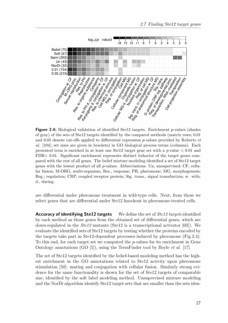
Figure 2.4: Biological validation of identified Ste12 targets. Enrichment p-values (shadesof gray) of the sets of Ste12 targets identified by the compared methods (matrix rows; 0.01and 0.05 denote cut-offs applied to differential expression p-values provided by Roberts etal. [104]; set sizes are given in brackets) in GO biological process terms (columns). Eachpresented term is enriched in at least one Ste12 target gene set with a p-value < 0.01 andFDR< 0.01. Significant enrichment represents distinct behavior of the target genes com-pared with the rest of all genes. The belief mixture modeling identified a set of Ste12 targetgenes with the lowest product of all p-values. Abbreviations: Un, unsupervised; CF, cellu-lar fusion; M-ORG, multi-organism, Res., response; PH, pheromone; MG, morphogenesis;Reg.; regulation; CRP, coupled receptor protein; Sig. trans., signal transduction; w. with;d., during.
are differential under pheromone treatment in wild-type cells. Next, from those weselect genes that are differential under Ste12 knockout in pheromone-treated cells.
Accuracy of identifying Ste12 targets We define the set of Ste12 targets identifiedby each method as those genes from the obtained set of differential genes, which aredown-regulated in the Ste12 mutants (Ste12 is a transcriptional activator [69]). Weevaluate the identified sets of Ste12 targets by testing whether the proteins encoded bythe targets take part in Ste12-dependent processes induced by pheromone (Fig.2.4).To this end, for each target set we computed the p-values for its enrichment in GeneOntology annotations (GO [5]), using the TermFinder tool by Boyle et al. [17].
The set of Ste12 targets identified by the belief-based modeling method has the high-est enrichment in the GO annotations related to Ste12 activity upon pheromonestimulation [50]: mating and conjugation with cellular fusion. Similarly strong evi-dence for the same functionality is shown for the set of Ste12 targets of comparablesize, identified by the soft label modeling method. Unsupervised mixture modelingand the NorDi algorithm identify Ste12 target sets that are smaller than the sets iden-
27

Chapter 2 Introducing knowledge into differential expression analysis
Figure 2.5: Different impact of examples on the models estimated by different supervisedmethods. Model estimated by the partially supervised belief-based (A), and by the semi-supervised mixture modeling (B). The plots as in Fig.2.2 A.
tified by the two partially supervised methods, leaving out many genes that are func-tionally related to the pheromone-triggered and Ste12-dependent processes (Fig.2.4).Semi-supervised modeling, in contrast, includes all given examples in the cluster ofdifferential genes. As opposed to belief-based modeling, the semi-supervised methodshifts this cluster towards low change in expression upon Ste12 knockout (Fig.2.5).Therefore, its set of identified Ste12 targets contains half of all analyzed genes, and in-corporates most superfluous genes, e.g. genes taking part in the transposition process.Also relatively big, the sets of Ste12 targets identified using the two p-value cut-offshave better enrichment scores than the set identified by semi-supervised modeling,but worse than the sets identified by the partially supervised methods (Fig.2.4).
2.8 Distinguishing miR-1 from miR-124 targets
To further evaluate the partially supervised mixture modeling methods, we checktheir accuracy of distinguishing miR-1 from miR-124 target genes in human, basedon two expression datasets from transfections of these microRNAs (shortly, miRNAs[81]) and knowledge from computational miRNA target predictions.
Input data and examples We use the subset of the genes measured by Lim et al.[81], which can be divided into two distinct clusters with rigorous experimental ver-ification: 90 miR-1 targets [108, 141], and 35 miR-124 targets [127, 75, 63]. Amongthem, we use as examples 16 miR-1 and 11 miR-124 target genes that have compu-tationally predicted binding sites of miR-1 and miR-124, respectively. We take onlythe examples that are predicted as respective targets by both computational methodsthat we used: MirTarget2 [126, 125] and miRanda [13]. The belief/plausibility valuesfor examples to belong to their clusters are set to 0.95.
Accuracy of distinguishing miR-1 from miR-124 target genes In both trans-fection datasets, we expect to see down-regulation of one miRNA’s target genes (e.g.,miR-1 targets upon miR-1 transfection) and the other target genes unchanged by the
28
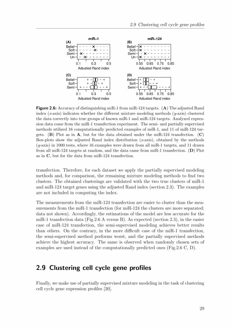
2.9 Clustering cell cycle gene profiles
Figure 2.6: Accuracy of distinguishing miR-1 from miR-124 targets. (A) The adjusted Randindex (x-axis) indicates whether the different mixture modeling methods (y-axis) clusteredthe data correctly into true groups of known miR-1 and miR-124 targets. Analyzed expres-sion data come from the miR-1 transfection experiment. The semi- and partially supervisedmethods utilized 16 computationally predicted examples of miR-1, and 11 of miR-124 tar-gets. (B) Plot as in A, but for the data obtained under the miR-124 transfection. (C)Box-plots show the adjusted Rand index distribution (x-axis), obtained by the methods(y-axis) in 1000 tests, where 16 examples were drawn from all miR-1 targets, and 11 drawnfrom all miR-124 targets at random, and the data came from miR-1 transfection. (D) Plotas in C, but for the data from miR-124 transfection.
transfection. Therefore, for each dataset we apply the partially supervised modelingmethods and, for comparison, the remaining mixture modeling methods to find twoclusters. The obtained clusterings are validated with the two true clusters of miR-1and miR-124 target genes using the adjusted Rand index (section 2.3). The examplesare not included in computing the index.
The measurements from the miR-124 transfection are easier to cluster than the mea-surements from the miR-1 transfection (for miR-124 the clusters are more separated;data not shown). Accordingly, the estimations of the model are less accurate for themiR-1 transfection data (Fig.2.6 A versus B). As expected (section 2.3), in the easiercase of miR-124 transfection, the semi-supervised modeling achieves better resultsthan others. On the contrary, in the more difficult case of the miR-1 transfection,the semi-supervised method performs worst, and the partially supervised methodsachieve the highest accuracy. The same is observed when randomly chosen sets ofexamples are used instead of the computationally predicted ones (Fig.2.6 C, D).
2.9 Clustering cell cycle gene profiles
Finally, we make use of partially supervised mixture modeling in the task of clusteringcell cycle gene expression profiles [20].
29
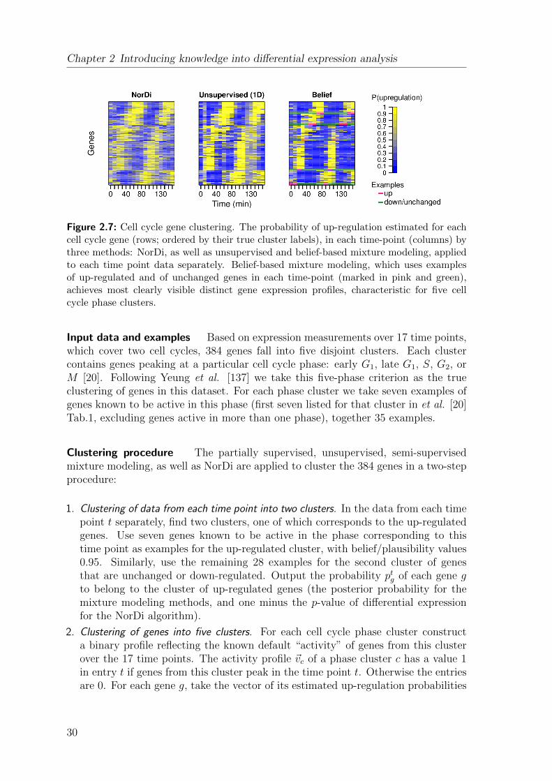
Chapter 2 Introducing knowledge into differential expression analysis
Figure 2.7: Cell cycle gene clustering. The probability of up-regulation estimated for eachcell cycle gene (rows; ordered by their true cluster labels), in each time-point (columns) bythree methods: NorDi, as well as unsupervised and belief-based mixture modeling, appliedto each time point data separately. Belief-based mixture modeling, which uses examplesof up-regulated and of unchanged genes in each time-point (marked in pink and green),achieves most clearly visible distinct gene expression profiles, characteristic for five cellcycle phase clusters.
Input data and examples Based on expression measurements over 17 time points,which cover two cell cycles, 384 genes fall into five disjoint clusters. Each clustercontains genes peaking at a particular cell cycle phase: early G1, late G1, S, G2, orM [20]. Following Yeung et al. [137] we take this five-phase criterion as the trueclustering of genes in this dataset. For each phase cluster we take seven examples ofgenes known to be active in this phase (first seven listed for that cluster in et al. [20]Tab.1, excluding genes active in more than one phase), together 35 examples.
Clustering procedure The partially supervised, unsupervised, semi-supervisedmixture modeling, as well as NorDi are applied to cluster the 384 genes in a two-stepprocedure:
1. Clustering of data from each time point into two clusters. In the data from each timepoint t separately, find two clusters, one of which corresponds to the up-regulatedgenes. Use seven genes known to be active in the phase corresponding to thistime point as examples for the up-regulated cluster, with belief/plausibility values0.95. Similarly, use the remaining 28 examples for the second cluster of genesthat are unchanged or down-regulated. Output the probability ptg of each gene gto belong to the cluster of up-regulated genes (the posterior probability for themixture modeling methods, and one minus the p-value of differential expressionfor the NorDi algorithm).
2. Clustering of genes into five clusters. For each cell cycle phase cluster constructa binary profile reflecting the known default “activity” of genes from this clusterover the 17 time points. The activity profile ~vc of a phase cluster c has a value 1in entry t if genes from this cluster peak in the time point t. Otherwise the entriesare 0. For each gene g, take the vector of its estimated up-regulation probabilities
30

2.10 Discussion
Figure 2.8: The accuracy of cell cycle gene clustering. From all compared methods, thepartially supervised have higher accuracy (measured by adjusted Rand index, y-axis) ingrouping genes into five cell-cycle gene clusters, than the semi-supervised and unsupervisedmethods. The partially supervised modeling methods were initialized in two ways: eitherquantile or example-based (section 2.2).
~pg = (p1g, ..., p
17g ) from step 1, and assign g to the cluster with the most similar
activity profile. Formally, we assign gene g to cluster
c∗ = arg maxc
(~vTc ~pg + (1− ~vc)T (1− ~pg)
),
where 1 denotes a vector of length 17 filled with 1s.
Advantage of supervised methods Fig.2.7 compares the clusterings obtainedin the first step by the unsupervised algorithms, to the clusterings obtained by ourbelief-based modeling. The examples used by our method help to clearly distinguishpatterns of genes from each phase cycle peaking at their characteristic time points.
Fig.2.8 shows that all supervised modeling methods, regardless of the parameter ini-tialization, outperform the unsupervised methods in clustering cell cycle gene profilesusing the two-step procedure. For comparison, we applied also a one step analysiswith multidimensional Gaussian mixture modeling ([137], denoted Un(nD)) to sep-arate the entire dataset at once into five clusters. Interestingly, multidimensionalclustering obtained the least accuracy, measured with the adjusted Rand index (sec-tion 2.3). Best results are obtained for the two-step procedure, using either belief-based or soft-label modeling in the first step.
2.10 Discussion
Mixture modeling is an established technique in machine learning, and proved suc-cessful in the field of gene expression analysis. The two partially supervised methodspresented in this paper extend mixture model-based clustering, adding the abilityto utilize imprecise examples. In contrast to other mixture modeling methods that
31

Chapter 2 Introducing knowledge into differential expression analysis
incorporate knowledge, both belief-based and soft-label modeling can be customizedfor differential expression analysis guided by examples of genes that are believed to beup, down or unchanged. The known examples usually constitute only a small subsetof all genes and are themselves not 100% certain. The presented applications showa rich variety of possible knowledge sources for examples: high-throughput TF-DNAbinding experiments, computational predictions of miRNA targets, and literatureknowledge of genes active in different cell cycle phases. The known examples aretraditionally used to verify experimental outcome after it is defined by differentialexpression analysis. Our partially supervised methodology incorporates such priorbiological knowledge into the analysis itself, making the outcome more reliable.
The methodology enables confronting available uncertain knowledge with the data.On the one hand, the partially supervised methods profit from the examples to bettercluster the remaining data. On the other hand, they use the entire data to verify theknowledge about the examples. For instance, the signal in the data may contradictthe prior belief about a gene to be up-regulated in a knockout experiment. Bothpartially supervised methods may “re-cluster” the examples with such improbableinitial cluster labels. In this way, they are more flexible than semi-supervised mixturemodeling, which assumes that the example labels are fixed.
The application of the proposed methodology to the problem of differential analysisimposes two natural restrictions, which could easily be abandoned for the needs of dif-ferent applications. First, here we analyze only one-dimensional data, but in generalthe approach can as well be extended to multidimensional clustering given exampleswith imprecise cluster labels. Similarly, we restrict ourselves only to consider two-or three-component models, although it is common to use tools of model selection tochoose out of models with arbitrary numbers of clusters. Here it is also dictated bythe nature of the problem: we assume the clusters to be interpreted, and the knownexamples to be assigned to each of the clusters. Intuitively, we expect examples ofdifferential or unchanged genes (two clusters), alternatively, of up-, down-regulated,or unchanged genes (three clusters). It would be difficult to assign those examples toclusters in a model with more than three components.
32

Chapter 3
Elucidating Gene Regulation WithInformative Experiments
This chapter puts forward a framework for elucidating gene regulation downstream of agiven signaling pathway using an optimal set of experiments. The framework, introducedin sections 3.1–3.7, benefits from prior knowledge about the pathway formalized in a log-ical model (section 3.2). The model predictions are utilized by our experimental design(ED) algorithm called MEED (sections 3.3–3.6). Section 3.7 describes how the measure-ments in the experiments proposed by MEED are matched with the model predictionsin order to elucidate the regulator-target relations downstream of the modeled pathway.In section 3.8.2 we cover alternative ED approaches, which we compare to our MEEDframework on synthetic data (section 3.9) and in application to a signaling pathway inyeast (section 3.10).
3.1 The MEED framework
The proposed framework consists of three components: modeling of the studied sig-naling pathway, an experimental design algorithm MEED and an expansion pro-cedure. The framework aims to discover regulatory relations and mechanisms oftranscriptional control downstream of the given signaling pathway using an optimalset of perturbation experiments (see sections 1.1 and 1.2 for biological semanticsof these notions). Software implementing our framework is freely available fromhttp://meed.molgen.mpg.de/.
The first component, the model, formalizes prior knowledge about signaling relationsbetween the molecules in the given pathway. The model is predictive: For a givenexperiment (i.e., extracellular stimulation and genetic perturbation), the model pre-dicts the activation states of the regulators in the pathway. Here, we assume thatboth the signaling and regulatory relations are discrete logical functions and thatthe model describes the steady state of the system after exposure to the experiment.In addition, we predefine a repertoire of logical functions that formalize regulationmechanisms, such as activation or repression (regulation by only a single pathway
33
Chapter 3 Elucidating Gene Regulation With Informative Experiments
component is considered). By applying all predefined logical functions to the model-predicted state of a given regulator under a given experiment, we obtain predictionsabout all possible readouts of the regulator’s target genes. This is done for all regu-lators and all candidate experiments. In this way, we calculate predicted expressionprofiles for all potential targets of the regulators. The modeling formalism appliedhere was introduced by Gat-Viks et al. [42]. The expansion procedure utilizing agiven signaling pathway model for predicting expression profiles was proposed byGat-Viks and Shamir [41].
Our contribution consists of proposing a model expansion experimental design (MEED)algorithm, and embedding it in the general framework. The MEED algorithm aimsto select from the set of candidate experiments optimizing two objectives: (i) tominimize the number of selected experiments and (ii) to maximize diversity betweenthe predicted expression profiles. The second condition aims to avoid an ambiguoussituation in which two genes with distinct regulatory mechanisms attain the sameexpression profile under the suggested experiments. Only in the case in which thetwo genes have two distinct expression profiles, it is possible to distinguish their reg-ulatory mechanisms. Next, the chosen experiments should be carried out in a laband used to identify regulator–target relations. To this end, the expansion procedurematches the model-predicted expression profiles of putative targets for the set of ex-periments selected by MEED with real expression measurements observed under thesame experiments. The building blocks of our framework are illustrated in Fig.3.1and described in sections 3.1–3.7.
3.2 Predictive logical model of Gat-Viks et al.
First, we formalize the available qualitative information about a given pathway ina logical model (Fig.3.1 A, left) with discrete variables, proposed by Gat-Viks etal. [42]. A modelM consists of a set V of variables, a set U = {u1, ..., uk} of discretestates that the variables may attain, and a set of discrete logical regulation functionsfv : U |Pa(v)| → U , for each v ∈ V . fv defines the state of variable v as a functionof the states of a subset Pa(v) of all variables, referred to as the set of parents ofv. A graphical representation of the model is a digraph G = (V,A), where eachnode v ∈ V is connected by incoming edges in A with the nodes in Pa(v), i.e.,(w, v) ∈ A iff w ∈ Pa(v). The set of stimulators I includes all variables with zeroindegree.
Biological semantics of the model The model formalizes signaling relations in agiven pathway. The set of model stimulators I represents the environmental signals,which trigger the pathway. Remaining model variables correspond to the signalingmolecules. In our analysis (sections 3.9–3.10.4), we assume that all variables mayhave three states: 1 (activated), −1 (deactivated) or 0 (unchanged).
34

3.2 Predictive logical model of Gat-Viks et al.
MEED: EXPERIMENTAL DESIGNBLOGICAL MODELING
e: S=0,P=-1
max not
0
0 1
A
EXPANSIONC
S
P
A B
-1notmax
Regulationfunctions
e2
e3
e6
Microarray data e2 e3 e6
A,B 1,-1 0,1 -1,0
f1(A) 1 0 -1 f2(A) 1 0 0 f3(A) 0 0 -1 f1(B) -1 1 0 f2(B) 0 1 0 f3(B) -1 0 0
Predicted profilesObserved profiles
max
f1
g4
f3 f3
g2g5 g6
Candidate experiments
Re
gu
lato
ryp
rog
ram
s
e1 e2 e3 e4 e5 e6 A,B 1,1 1,-1 0,1 0,0 0,-1 -1,0
f1(A) 1 1 0 0 0 -1 f2(A) 1 1 0 0 0 0 f3(A) 0 0 0 0 0 -1 f1(B) 1 -1 1 0 -1 0 f2(B) 1 0 1 0 0 0 f3(B) 0 -1 0 0 -1 0
e2 e3 e6
Observedprofiles
Predictedprofiles
e2 e3 e6
g1 1 1 1 g2 0 0 -1 g3 0 0 0 g4 0 -1 0 g5 0 0 -1 g6 -1 1 0
e2 e3 e6
e2 e3 e6
s2 s3 s6s1 s4 s5
f1 f2 f3
-1 -1 0 -1
0 0 0 0
1 1 1 0
f1 f2 f3
Chosenexperiments
S
P
A Bnot
Predictedstates
Figure 3.1: (A) Logical modeling. Left: a toy model. S – a stimulator variable representingthe environmental signal, P – a variable representing a signaling molecule. A, B – regula-tors representing transcription factors. max, not: regulation functions. Right: predictionof regulator states. e – experiment, in which environmental signal is medium (stimulationS = 0) and the signaling molecule is knocked out (perturbed variable P , perturbation state−1). (B) Our MEED algorithm. Right: three exemplary regulation functions, f1, f2 andf3, represented by a truth table, in which the first column contains the states of a regulator,and each other column i contains the predicted responses of a target gene controlled bythe regulator using fi. For example, f1 determines that activated (state = 1) regulatorup-regulates (state = 1) its target, and deactivated (state = −1) regulator down-regulates(state = −1) its target. Left: matrix of predicted responses. Rows – regulatory programs,each represents a chosen regulator (A or B) acting on a target gene through a chosen regu-lation function. Columns – predicted model states s1–s6 in the set of candidate experimentsgiven as input to MEED. The predicted states of regulators A and B appear below. Forexample, the third column corresponds to a model state s3 predicted for experiment e3,with predicted states A = 0 and B = 1. A matrix entry – a predicted response of a potentialtarget gene assuming it is regulated by its row’s regulatory program in its column’s exper-iment. Hence, each row of the matrix is a predicted profile for a given regulatory program.If the predicted profiles are different, they are referred to as distinguished. MEED aims tofind the smallest subset of candidate experiments, which distinguishes between the samepairs of regulatory programs as the full set of candidate experiments. Here, MEED choosesthree out of the candidate experiments: e2, e3, and e6, which distinguish all regulatoryprograms (the remaining ones are marked as deleted). (C) The expansion procedure. Theexperiments proposed by MEED are carried out and the measurements are used in theexpansion procedure. Left: the measurements of gene expression in the chosen experimentsare referred to as observed profiles of the genes (rows). Middle: a matrix as in B, includingonly experiments chosen by MEED. The expansion procedure identifies regulatory programsfor the genes by matching of predicted and observed profiles (marked as dashed gray lines).Right: genes matching identical regulatory programs constitute regulatory modules. Here,two regulatory modules are found: the regulatory program f3(A) controls the module of g2
and g5, and regulatory program f1(B) controls g6.
35

Chapter 3 Elucidating Gene Regulation With Informative Experiments
Experiment Predicted model states e1: S=-1 s1: S=-1 A=-1 B=-1
e2: S=0 s2
1: S=0 A=0 B=0 s2
2: S=0 A=-1 B=-1 e3: S=1, B=1 s3: S=1 A=1 B=1 e4: S=-1, B=1 s4: S=-1 A=-1 B=1 e5: S=0, B=1 s5: S=0 A=0 B=1
S
A B
min min
A
T(s2
1)= {r1, r3, r4, r6} {r2, r5} T(s2
2)= {r1, r4} {r2, r5} {r3, r6}
T(e2)= {r1, r3, r4, r6} {r2, r5}
C
s1 s2
1 s3 s4 s5 A,B -1,-1 0,0 1,1 -1,1 0,1 r1 f1(A) -1 0 0 -1 0 r2 f2(A) 0 1 1 0 1 r3 f3(A) 1 0 1 1 0 r4 f1(B) -1 0 0 0 0 r5 f2(B) 0 1 1 1 1 r6 f3(B) 1 0 1 1 1
Candidate experiments
Re
gu
lato
ryp
rog
ram
s
B
s1 s22 s3 s4 s5
-1,-1 -1,-1 1,1 -1,1 0,1 -1 -1 0 -1 0 0 0 1 0 1 1 1 1 1 0 -1 -1 0 0 0 0 0 1 1 1 1 1 1 1 1
Candidate experimentsPredictedstates
T(e1): {r1, r4} {r2, r5} {r3, r6}
T(e1) ÇT(e4): {r1} {r2} {r3, r6} {r4} {r5}
T(e1) ÇT(e4) ÇT(e5): {r1} {r2} {r3} {r4} {r5} {r6}
T(e1)= {r1, r4} {r2, r5} {r3, r6} T(e2)= {r1, r3, r4, r6} {r2, r5} T(e3)= {r1, r4} {r2, r3, r5 r6} T(e4)= {r1} {r2, r4} {r3, r5 , r6} T(e5)= {r1, r3 , r4} {r2, r5, r6}
e1
e4 e5
D
Chosen experiments
Figure 3.2: (A) Left: A toy logical model with cycles. Right: Predicted model states forexemplary experiments. There are two model states, s1
2 and s22, predicted for experiment e2.
(B) Matrices of predicted responses, as in Fig.3.1 B. Each matrix corresponds to one modelstate predicted for e2 (in the left matrix, the second column corresponds to s1
2, in the rightmatrix to s2
2). The regulators, their predicted states as well as the candidate experiments aretaken from A. Regulation functions are the same as in Fig.3.1 B. Note that in this example,each regulatory program has two possible predicted profiles, one for each matrix. (C) Eachpredicted model state induces a partition on the set of regulatory programs according totheir predicted response. Left: the partitions T (s1
2) and T (s22). T (s1
2) corresponds to acolumn marked in yellow in the left matrix in B. It divides regulatory programs into twoblocks {r1, r3, r4, r6}, and {r2, r5}, which have predicted response 0 and 1, respectively.Therefore, r1 and r4 are not distinguished by s1
2, as opposed to r2 and r6. The partition foran experiment is a supremum over partitions for its predicted model states. Here, T (e2)is given on the right. (D) The partition for a set of experiments is the intersection of thepartitions for each of the experiments. Left: partitions for candidate experiments e1–e6.The partition T (ex) for each experiment except e2 (x ∈ {1, 3, 4, 5}) equals the partition forits predicted model state T (sx). Right: partitions obtained in each step of MEED. In thefirst step, MEED considers partitions for all candidate experiments and chooses the onethat has the highest entropy score (in this example, e1). In the second step, it extends thelist of chosen experiments by adding an experiment that provides the highest entropy gain(e4). The joint ability of experiments e1 and e4 to distinguish between regulatory programsis represented by an intersection of their partitions. Adding e5 further partitions the block{r3, r6} into single-variable blocks. The partition for the chosen experiments e1, e4, and e5
has only single-variable blocks. Therefore, in this example it is possible to distinguish allregulatory programs using the chosen set of experiments.36

3.2 Predictive logical model of Gat-Viks et al.
Representation of experiments in the model An experiment on the modelM isformalized by defining: (i) stimulation – an assignment of states to all model stim-ulators in I (fixed according to the levels of environmental signals applied in theexperiment); (ii) perturbed variables – a set P ⊆ V \ I of model variables that aresubject to perturbation; and (iii) perturbation states – fixed states of the perturbedvariables, which represent the type of experimental manipulation, such as knockout(perturbation state is -1) or over-expression (perturbation state is 1). In this the-sis, we consider only experiments, in which either none or exactly one variable isperturbed. Assuming in general that k perturbation states are possible for each vari-able, having |I| stimulators and |P | variables that can be perturbed in the modelM,the number of all possible experiments onM is k|I|(|P |k+ 1). There are k|I| possiblestimulation states, |P |k ways of perturbing one variable, and one where no variableis perturbed.
Model states A model state s (illustrated in Fig.3.1 A right), is an assignmentof states to each of the variables in the model, s : V → U . We say that s agreeswith the model M on variable v if the state s(v) of variable v equals the outputof its regulation function when applied to its parents’ states, fv(s(Pa(v))) = s(v).For a given experiment e, we call a model state se predicted for experiment e if (i)the stimulators in I are assigned their stimulation and the perturbed variables inP are assigned their perturbation state as defined by e, and (ii) the state se(v) ofeach variable v ∈ U \ I \ P agrees with M on v. The state se(v), assigned to eachvariable v ∈ V by a given model state s predicted for e, is called an e-predicted stateof the variable v. A predicted model state for a given experiment is a predictionabout a steady state of the biological system, describing the states of the pathwaycomponents under this experiment.
In the case when the model M is acyclic, each experiment e on M has exactly onepossible model state se predicted for e, defining a unique e-predicted state for eachvariable. In this case, the unique model state se can easily be computed (claim 1in Gat-Viks et al. [42]). se is calculated iterating over the variables v ∈ V \ I \ Pin a topological order defined by the acyclic model graph, and obtaining the stateof each v by applying fv to its parents’ states. The first variables will have theirparents’ states fixed according to stimulation and perturbation states defined by theexperiment e. The running time of this procedure is linear in the number of nodesplus the number of edges: O(|V | + |A|), which is the time required to compute thetopological order [23].
However, for a model whose graph contains feedback loops, it is possible to obtainzero, one or several possible predicted model states (see Fig.3.2 A for an example).In this case, in order to compute the predicted model states, the cyclic model M isfirst transformed into an acyclic model MF using its feedback set. A feedback set ina directed graph is a set of nodes whose removal renders the graph acyclic [35]. ToobtainMF , given a feedback set F inM, the regulation functions of the variables inF are changed to null, and the edges incoming to F in the model graph are removed
37

Chapter 3 Elucidating Gene Regulation With Informative Experiments
accordingly. Note that for a given experiment e, if a state se of the new model MF
predicted for e agrees with M on every variable v ∈ F , se is also a predicted stateof the model M. Given a state of the model MF , it is easy to check the agreementby calculating fv for each v ∈ F . Following Gat-Viks et al. [42], we provide theprocedure for computing the states of M predicted for a given experiment e, usingits feedback set F and a topological ordering on the model graph.Generate each possible state assignment to F . For each assignment sF : F → S:
• Generate an experiment e′ for MF by joining the stimulation in e with sF .
• Use a topological ordering to compute a (unique) model state se predicted for e′.
• If se agrees withM on every v ∈ F , add it to the set of states ofM predicted fore.
The procedure runs in O(k|F |(|V | + |A|)) time, since it requires checking k|F | stateassignments to F , and for each assignment computing a unique model state as de-scribed before. Thus, the restrictive element for the efficiency of this procedure isthe size of the feedback set. Computing a minimal feedback set is NP hard [64], andGat-Viks et al. [42] use known heuristics [109] for this task.
Discrepancy between the predicted and observed model states For a givenexperiment e on model M, Gat-Viks et al. [42] define an observed partial state eSas a set of measurements for some of the model variables during the experiment,where eS(v) = null for those variables v that were not observed. The model Mcan be used to compare the possible model states predicted for e with the observedpartial state. In the case when more than one predicted model state exists, we expectthe correct one to be the most similar to the observed partial state. To assess thissimilarity, a discrepancy D(se, e) between the experiment e and a given model statese predicted for e is measured: D(se, e) =
∑v∈V,eS(v)6=null(se(v) − eS(v))2. The state
with the smallest discrepancy is considered the unique model state predicted for theexperiment e, with the assumption that this state corresponds to the steady statereached by the biological system when e is performed.
3.3 Regulatory programs and their predicted profiles
Discrepancy compares predicted and observed states of the variables in the model.Here, we introduce a tool to connect predicted model states with observed statesof variables that represent target genes and are not included in the model, but arepotentially transcriptionally regulated by the modeled pathway components. Belowwe formalize the particular mechanisms of this regulation.
Regulators and a repertoire of regulation functions First, we define a set V ′ ofregulators, which is the subset of all model variables, V ′ ⊆ V and represents proteins
38
3.3 Regulatory programs and their predicted profiles
having transcriptional control over response of target genes. Next, we predefine aset of regulation functions F that describe biologically relevant logical relationshipsbetween a subset of regulators and its target. Here, we consider transcriptional controlby only a single regulator, which can attain one of three possible states u ∈ {−1, 0, 1}.Thus, we adapt six biologically relevant functions introduced by Yeang and Jaakkola[136] to define a repertoire F = {aN , aS, aB, iN , iS, iB} of six one-argument regulationfunctions with the following formulas and biological semantics:
• Necessary activation
aN(u) =
−1, iff u = −1
0 otherwise.(3.1)
Deactivation of the regulator forces down-regulation of the target. The targetremains unchanged upon the activation of the regulator.
• Sufficient activation
aS(u) =
{1, iff u = 10 otherwise.
(3.2)
Activation of the regulator forces up-regulation of the target. The target remainsunchanged upon the deactivation of the regulator.
• Activation bothaB(u) = u (3.3)
Both the deactivation of the regulator forces down-regulation of the target, andthe activation of the regulator forces up-regulation of the target.
• Necessary inhibition
iN(u) =
1, iff u = −1
0 otherwise.(3.4)
Deactivation of the regulator forces up-regulation of the target. The target remainsunchanged upon the activation of the regulator.
• Sufficient inhibition
iS(u) =
{−1, iff u = 10 otherwise.
(3.5)
Activation of the regulator forces up-regulation of the target. The target remainsunchanged upon the deactivation of the regulator.
• Inhibition bothiB(u) = −u (3.6)
Both the deactivation of the regulator forces up-regulation of the target, and theactivation of the regulator forces down-regulation of the target.
Regulatory programs A regulatory program r = (v, f) consists of a regulatorv ∈ V ′ from the model and a regulation function chosen from the repertoire F .The regulator tells “who” regulates, whereas the regulation function formalizes the
39

Chapter 3 Elucidating Gene Regulation With Informative Experiments
regulatory mechanism and tells “how” (e.g., Fig.3.1 B). For a given model state sepredicted for an experiment e, the value f(se(v)) defines an (e, r)-predicted responseof a potential target gene to the regulatory program r in experiment e. Biologically,the predicted response specifies whether the target gene is in state 1 (up-regulated),−1 (down-regulated) or 0 (unchanged) in the experiment e. Finally, a vector of pre-dicted responses in a given ordered set of experiments E defines an (E, r)-predictedprofile. Assuming the model is correct, the predicted profile reflects the transcrip-tional response of a potential target gene controlled by the program r in the givenset of experiments E. Given the set of regulators V ′ and the repertoire of regulationfunctions F , the set of predicted profiles R contains V ′ ×F elements. Fig.3.1 B leftpresents the set of predicted profiles as rows of a matrix, referred to as a matrix ofpredicted responses. The columns of this matrix correspond to predicted model statesfor a set of experiments, and entries to predicted responses.
In a general case, one experiment may define several predicted model states, givingseveral predicted states per regulator. Given that there are at most m model statespredicted for each experiment in E, there are pessimistically m|E| different predictedprofiles for each regulatory program. These predicted profiles are determined by thedifferent combinations of model states predicted for experiments in E. Fig.3.2 Billustrates two predicted profile sets as two matrices of predicted responses, one pereach of the two model states predicted for experiment e2 (the remaining experimentsinduce unique model states).
3.3.1 Requirements for the experiments
For a given set of experiments E and a set of regulatory programs R, the expansionprocedure (section 3.7) matches the (E, r)-predicted profiles, for all r ∈ R, with theobserved profiles of the measured genes. For the matching to proceed unambiguously,two requirements need to be satisfied:
1. A single predicted profile per regulatory program Before designing and carrying outexperiments, we cannot anticipate which combination of their predicted modelstates will fit best the steady states reached in the biological system. In ourframework, this problem is overcome by the MEED algorithm by taking into ac-count all possible sets of predicted profiles (section 3.3.2). However, the expansionprocedure requires a single set of predicted profiles. In the input to the expansionprocedure the measurements in the designed experiments are already available.The required single profile set can be obtained using the experimental measure-ments to choose the predicted model states with the least discrepancy with theobserved states.
2. All pairs of regulatory programs, in all combinations of predicted model states, shouldhave different predicted profiles. We deal with this requirement using the MEEDalgorithm (section 3.5). To this end, below (section 3.3.2) we introduce auxiliarynotions of distinguishability between two regulatory programs.
40
3.3 Regulatory programs and their predicted profiles
3.3.2 Distinguishing regulatory programs
We start by defining how a given pair of regulatory programs is distinguished by apredicted model state, next we extend the definition for a single experiment (whichmight induce several predicted model states), and finally, we generalize by statinghow two programs are distinguished by a set of experiments.
Distinguishing by a predicted model state Recall that a model state se predictedfor a given experiment e assigns to each regulator its e-predicted state (section 3.2).From this state we can compute the (e, r)-predicted response for each regulatoryprogram r ∈ R. In this way, state se induces a natural partition of R. The partitioncontains two regulatory programs r1 = (v1, f1) and r2 = (v2, f2) in the same blockif and only if f1(se(v1)) = f2(se(v2)), i.e., they have the same e-predicted responses.Regulatory programs contained in different blocks of this partition are said to bedistinguished by the predicted model state se (exemplified in Fig.3.2 C).
Distinguishing by an experiment An experiment e may in general define a numberof model states predicted for e (section 3.2). We consider a partition T (e) of the setof regulatory programs R induced by an experiment e as the supremum over theset of partitions induced by its predicted model states. To compute the supremum,we first generate a relation, where two regulatory programs are related when theyare contained in a common block of at least one partition. Next, we compute atransitive closure of this relation. The resulting equivalence relation has equivalenceclasses which define the blocks of the supremum partition. The regulatory programscontained in different blocks of T (e) are called distinguished by the experiment e. Bythe definition of a supremum over partitions, the following holds:
• If two regulatory programs are distinguished by an experiment, they are distin-guished by all its predicted model states. For example, in Fig.3.2 C, T (e2) containsr2 and r6 in separate blocks, implying that they are distinguished by e2 and by bothmodel states predicted for e2. This fact is essential for the correctness of our ap-proach (see “Importance of distinguishing regulatory programs in our framework”below).
• The fact that two regulatory programs are distinguished by all predicted modelstates of an experiment does not always imply that they are also distinguishedby the experiment itself. For example, consider a set of regulatory programs{x, y, z}, and partitions for hypothetic predicted model states T1 = {x, y}{z}and T2 = {x, z}{y}. z and y are distinguished by both these predicted modelstates. The supremum over T1 and T2 is {x, y, z} and it contains z and y in acommon block. From the second implication it follows, that our MEED algorithm(section 3.5), which selects experiments that are needed to distinguish betweenpairs of regulatory programs, may choose experiments that are superfluous forthe requirement of differentiating between all their possible predicted profiles (sec-tion 3.3.1). This may happen only in the case of cyclic models, which can generate
41

Chapter 3 Elucidating Gene Regulation With Informative Experiments
more than one predicted model state for an experiment.
If an experiment has no predicted model states, it is not informative and its partitionincludes only one block containing all regulatory programs.
Distinguishing by a set of experiments We call a pair of regulatory programsdistinguished by a set of experiments E = {e1, ..., en} if and only if they are distin-guished by at least one of its experiments. Equivalently, we say that E distinguishesbetween regulatory programs that are contained in separate blocks of a partitionS(E) = T (e1) ∩ ... ∩ T (en) (exemplified in Fig.3.2 D). The partition for an emptyset of experiments is a full, one-block partition containing all regulatory programs.Regulatory programs contained in the same block of the partition S(E) are not dis-tinguished by any of the experiments, whereas regulatory programs in different blocksare distinguished by at least one experiment. We say that an experiment set E dis-tinguishes all regulatory programs, if its corresponding partition S(E) contains onlysingle-element blocks.
Importance of distinguishing regulatory programs in our framework Note thatif E distinguishes between two regulatory programs r1 = (v1, f1) and r2 = (v2, f2),their predicted profiles will be different (i.e., have at least one different predictedresponse) in all possible combinations of model states predicted for experiments inE. Indeed, by the definition of distinguishing by a set of experiments, there existsan experiment e ∈ E, which distinguishes between r1 and r2. Take any possiblemodel state se predicted for e. By the definition of distinguishing by an experimentf1(se(v1)) 6= f2(se(v2)). Therefore, the predicted profiles for r1 and r2 are also differ-ent in any combination of predicted model states (since they always differ by at leastone component, which corresponds to the experiment e). This essential fact ensuresthat the predicted profiles of any two regulatory programs, which are distinguishedby a given set of experiments E, are also different for the predicted model statesused by the expansion procedure (chosen by the least discrepancy and correspondingto the steady states the biological system has reached under the experiments; seesections 3.2 and 3.3.1). Thus, by maximizing the number of distinguished regulatoryprograms, MEED (section 3.5) maximizes also the diversity of predicted profiles usedin the expansion procedure.
The FUP score In sections 3.9–3.10.2 we report the performance of a set ofexperiments E with the fraction of undistinguished pairs (FUP). The score is givenby the proportion of regulatory program pairs undistinguished by E out of all possiblepairs of regulatory programs:
FUP (E) =
∑c nc(nc − 1)
|R|(|R| − 1)
where nc is the size of the c-th block of the corresponding partition S(E) of the set ofregulatory programs R. FUP (E) attains values between 0 (all regulatory programs
42

3.4 The Experimental Design problem
are distinguished) and 1 (no pair of regulatory programs is distinguished). The morepairs of regulatory programs distinguished by a given set of experiments, the smallerits FUP score. Unlike the ambiguity score (section 3.7), which evaluates the resultsof expansion utilizing experimental data, FUP evaluates a given ED method basedonly on model predictions.
3.4 The Experimental Design problem
The task for our algorithm is to select an economical subset of a given set of candidateexperiments E that under a given pathway model M yields different (E, r1)- and(E, r2)-predicted profiles for each pair of regulatory programs r1 and r2 in a givenset R, regardless the combination of model states predicted for the experiments inE. The candidate experiments contain a full set of experiments to choose from; forexample, only those experiments that can be conducted in a lab.
Formulation of the ED problem To fulfill the task, MEED aims to select thesmallest subset of the candidate experiments, which can distinguish all regulatoryprograms in R. From the previous section 3.3.2 we know that for cyclic modelssuch a subset of experiments may be superfluous, but it guarantees that predictedprofiles of two different regulatory programs will be different in any combinationof predicted model states. In the case when the candidate experiments themselvescannot distinguish all regulatory programs, the identified subset should distinguishbetween the same pairs of regulatory programs as the full candidate set. We formalizethis problem and show that its decision version is NP-complete. To be more general,we relax the setup kept in our analysis. We allow all model variables to have anumber of states, which can be different than three, and all regulatory programs tohave several (i.e., also more than one) regulators.
Problem 1. ED(M, R,E, l)INSTANCE: A logical modelM, a set of regulatory programs R with regulators fromthe model, a set of candidate experiments E on M, and a number l ≤ |E|.QUESTION: Is there a subset of size l of E which distinguishes all regulatory pro-grams in R.
Proposition 1. The ED problem is NP-complete.
Proof. It is easy to see that ED∈NP, since a nondeterministic algorithm would onlyneed to guess a subset E ′ ⊆ E of size l, in polynomial time construct a partitionS(E ′) (section 3.3.2) and verify whether it is an identity partition on R.
We show that the ED problem is NP-complete by reduction of the 3-DIMENSIONALMATCHING (3DM) problem [38]. An instance of 3DM is defined by a set M ⊆X × Y × Z, where X ∩ Y = X ∩ Z = Y ∩ Z = ∅ and |X| = |Y | = |Z| = m. A
43

Chapter 3 Elucidating Gene Regulation With Informative Experiments
Figure 3.3: Construction of the ED problem for the 3DM problem. (A) Themodel. The nodes correspond to variables and arrows to regulation functions. S – thestimulator variable. There are triplet variables corresponding to the triplets inM and twoadditional variables (X,x0) and (Y, y0). id – the identity function. (B) The regulatoryprograms. Left column of the table – identifiers of the programs, right column – theirregulation functions and regulators (specified as function arguments). < xi, •, • > denotesall (possibly several) triplet variables with xi on the first coordinate.
solution to 3DM is a matching for M of size m, i.e., a subset M ′ ⊆ M such that noelements of M ′ agree on any coordinate. Let X = {x1, ..., xm}, Y = {y1, ..., ym} andZ = {z1, ..., zm}. For a given 3DM problem we define an instance (M, R,E,m + 2)of the ED problem and prove that there exists a matching of size m if and only ifthere exists a set of m + 2 experiments in E for M which distinguish all regulatoryprograms in R.
We now define an instance M, R,E,m + 2 of the ED problem for a given instanceM of the 3DM problem. The set of variables V in model M contains stimulatorvariable S, a set of |M | variables corresponding to the triplets in M (referred toas the triplet variables) and two additional variables, labeled (X, x0) and (Y, y0),V = M ∪ {S, (X, x0), (Y, y0)}. All variables can be in one of the two states: 0 and 1.The regulation functions are defined in Boolean logic. The states of the stimulator Sdetermine the states of all remaining variables through an identity function, i.e., fora given model state s, fv(s(S)) = s(S), for each v ∈ V \ {S} (Fig.3.3 A). We definethe set of regulators to be all variables in the model.
Next, we define a set R of 3m + 3 regulatory programs for the model M, eachwith the same regulation function: the Boolean alternative (logical “∨”). Intuitively,the regulatory programs correspond to the elements in the sets X, Y , and Z andthree additional entities denoted x0, y0 and z0. Each regulatory program denoted xi,1 ≤ i ≤ m, has a set of regulators: S, (X, x0) and all triplet variables, which have xion the first coordinate. The regulatory program x0 has two regulators: S and (X, x0).Each regulatory program denoted yj, 1 ≤ j ≤ m, has the regulators: S, (Y, y0) andall triplet variables, which have yj on the second coordinate. The regulatory programy0 has two regulators: S and (Y, y0). Finally, each regulatory program denoted zl,1 ≤ l ≤ m has the regulators: S, and all triplet variables, which have zl on the thirdcoordinate. The regulatory program z0 has one regulator S (Fig.3.3 B).
44

3.4 The Experimental Design problem
Finally, we define the set of candidate experiments E on the model M. Recall fromsection 3.2 that an experiment is given by the stimulation, perturbed variable and itsperturbation state. We assume that the set P = V \{S} of all non-stimulator variablescan be perturbed. Since S determines by identity the state of all other model variablesand is an alternative regulator in all regulatory programs, the following experimentsdo not distinguish between any pairs of regulatory programs: for v ∈ P and i ∈ {0, 1},the experiments of the form: S = i, ∅ (an experiment with any stimulation i, where novariable is perturbed), as well as S = 1, v = i (an experiment where the stimulation ishigh, with any perturbed variable v and any perturbation state i), and S = 0, v = 0.Thus, from all possible experiments, it suffices to consider only the set of candidatesE = {ev : v ∈ P}, where ev denotes an experiment of the form: S = 0, v = 1.
Assume there exists a 3D-matching M ′ = {t1, ..., tm} for M. We show that in thiscase the set of m + 2 experiments E ′ = {et1 , ..., etm , e(X,x0), e(Y,y0)} on the model Mdistinguishes all regulatory programs in R. Indeed, the experiments e(X,x0) and e(Y,y0)
together induce a partition S({e(X,x0), e(Y,y0)}) on R into three blocks: {x0, x1, ...xm},{y0, y1, ..., ym}, and {z0, z1, ..., zm}. Since M ′ is a 3D-matching, for each xi ∈ X itcontains a single triplet t =< xi, y, z >∈ M ′ with xi on the first coordinate. Thecorresponding experiment et ∈ E ′ induces a partition T (et) on R into two blocks:{xi, y, z} and R \ {xi, y, z}. Intersecting T (et) with S({e(X,x0), e(Y,y0)}) results in apartition which contains a singleton {xi}. Since all regulatory programs with labelsfrom X have their corresponding experiments in E ′, they are distinguished by E ′
from all other regulatory programs, in particular from x0. Similar argument holdsfor any regulatory program with labels from Y or Z.
Assume there exists a set of m+ 2 experiments E ′ ⊆ E distinguishing all regulatoryprograms in R. We show that in this case there exists a matching of size m for the3DM problem. Note that e(X,x0) ∈ E ′ and e(Y,y0) ∈ E ′. Otherwise either the regula-tory program x0 would not be distinguished from z0 or y0 would not be distinguishedfrom z0. In the remaining m experiments the triplet variables are perturbed. Denotethe set of m perturbed triplets as M ′ = {t ∈M : et ∈ E ′ \ {e(X,x0), e(Y,y0)}}. Supposethat for some x ∈ X there exist no triplet in M ′ with x on the first coordinate. Thenthe regulatory programs x and x0 are not distinguished by E ′, which contradicts ourassumption. Similar argument holds for any y ∈ Y and z ∈ Z on the second andthird coordinate, respectively. Thus M ′ contains m triplets that together have all melements from X on the first, all elements of Y on the second, and all elements ofZ on the third coordinate. Thus, the triplets in M ′ do not agree on any coordinate,and M ′ is a solution to the given 3DM .
45

Chapter 3 Elucidating Gene Regulation With Informative Experiments
3.5 The MEED algorithm
Notions of entropy used in the algorithm To evaluate the ability of a set ofexperiments to distinguish regulatory programs, MEED uses an entropy score. LetE be a given set of experiments and R a set of regulatory programs. Assume thatE induces a partition S(E) of R into C disjoint blocks (section 3.3.2). The score isdefined as
H(E) = −C∑c=1
nc
|R|log
(nc
|R|
),
where nc is the number of regulatory programs in block c, 1 ≤ c ≤ C. If all regulatoryprograms are distinguished by the set of experiments E, then C = |R| and the cor-responding score is H(E) = log(|R|). If all regulatory programs are undistinguishedby E, there is only one block in the partition, C = 1 and H(E) = 0. Intuitively, thehigher the entropy score, the higher the ability of the set of experiments to distinguishbetween the regulatory programs. Accordingly, an entropy gain H(e|E) is given byH(e|E) = H(E ∪ e) − H(E), where S(E ∪ e) = S(E) ∩ T (e) (i.e., the additionalexperiment introduces a finer partition of the set of regulatory programs). Entropygain evaluates how much the joint ability to distinguish between regulatory programsimproves when the experiment e is added to the set of experiments E.
The algorithm To obtain a practical solution for the untractable ED problem,MEED implements a greedy approximation algorithm.
MEED(E,R)1 E∗ ← ∅2 while H(E∗) < log(|R|)3 do e← arg maxe∈E H(e|E∗)4 if H(e|E∗) = 05 then break6 E∗ ← E∗ ∪ e7 return E∗
The algorithm takes as input a set of candidate experiments E to select from, andthe set of regulatory programs R that it has to distinguish (indicated in the head-ing). The procedure starts from an empty set of experiments E∗, corresponding toa full partition on the set of regulatory programs (line 1), and keeps choosing newexperiments one by one. In each greedy step, experiment e that maximizes the en-tropy gain for the current experiment list E∗ is chosen (line 3) and added to E∗ (line6; equivalently, its corresponding partition is intersected with the partition for E∗).The iteration finishes either when all regulatory programs are distinguished (line 2)
46

3.6 Approximation factor of the MEED algorithm
or when no additional experiment can give improvement (line 4). The latter casemeans that the selected list E∗ does not distinguish all regulatory programs, but thesame as the candidate experiments in E. The output of MEED is the ordered subsetE∗ ⊆ E of chosen experiments.
The upper bound computational cost of this algorithm is O(|R| ∗ |E|2). This es-timation assumes a pessimistic scenario that the iteration does not end until allexperiments from E are added one by one to E∗, and that in each step all unusedexperiments are tried to select the best one. The factor |R| comes from the fact thatin order to compute the entropy gain, intersection of two partitions of the set R needsto be generated, which can be implemented in O(|R|).
3.6 Approximation factor of the MEED algorithm
In this section we prove the correctness of our algorithm MEED and derive its ap-proximation factor. Below we refer to the optimization version of the experimentaldesign problem as ED(M, R,E).
Proposition 2. For a given instance (M, R,E) of the ED optimization problem,the MEED algorithm returns a set E∗ ⊆ E of the candidate experiments, whichdistinguishes the same pairs of regulatory programs as E. Moreover, |E∗| ≤ |Eopt|(1+ln(|R|) + ln(log(k))), where Eopt is the smallest-size solution of the ED problem andk is the number of states each variable can have.
By Proposition 2 it holds that if E distinguishes all regulatory programs in R, alsoE∗ will distinguish all regulatory programs in R.
To prepare grounds for the proof of Proposition 2, we define an auxiliary optimizationproblem on partitions. Adapting the reasoning schema of Konwar et al. [74], wepropose a generic heuristic GENERIC-GREEDY solving the partition problem andderive its approximation factor. Our proof of Proposition 2 relies on the fact that EDcan be viewed as the problem on partitions and that the MEED algorithm implementsthis generic heuristic.
Notation and basic notions Let P denote a set of partitions of a given set R andlet P+ be the closure of P under finite intersections. The intersection of all partitionsfrom a set P is denoted by
⋂P . We keep the following convention: T, T ′, T ′′ range
over P and S, S ′, S ′′ range over P+. Full (one block) partition of R is denoted {R}and the identity partition into singletons is denoted idR. For two partitions T ′ andT ′′ we write T ′′ ≤ T ′ and say T ′′ is included in T ′ if for any block T ′′i ∈ T ′′, thereexists a block T ′j ∈ T ′ such that T ′′i ⊆ T ′j (see example illustrated in Fig.3.4). Notethat, for any pair of partitions S and T , S ∩ T ≤ S.
47

Chapter 3 Elucidating Gene Regulation With Informative Experiments
Figure 3.4: Partition inclusion. Example. T ′ and T ′′ are partitions of set R satisfyingT ′′ ≤ T ′.
Let Φ : P+ → {x ∈ R : x ≥ 0} be a given strictly increasing function, which satisfiesthe following conditions:(A0) Φ(S) = 0⇔ S = idR.(A1) For each T ∈ P and S ∈ P+, let ∆T (S) = Φ(S)− Φ(S ∩ T ) be a gain functiondetermined by Φ. If ∆T (S) > 0, then ∆T (S) ≥ 1.Note that by definition ∆T is strictly increasing.
An auxiliary problem on partitionsWe now define an auxiliary optimization problem on partitions.
Problem 2. PARTITION(P , R)INSTANCE: A set P of partitions on a set R.QUESTION: Find a subset Popt ⊆ P of minimal size such that
⋂Popt =
⋂P .
Of course, a solution Popt of a given instance (P , R) of the PARTITION problemsatisfies
⋂Popt = idR if and only if
⋂P = idR.
A greedy heuristic for solving the PARTITION problem Below we present ageneric greedy heuristic for solving the PARTITION problem for a given set P ofpartitions of a set R.
GENERIC-GREEDY(P, R)1 P∗ ← ∅2 S ← {R}3 while Φ(S) > 04 do T ← arg maxT∈P ∆T (S)5 if ∆T (S) = 06 then break7 S ← S ∩ T8 P∗ ← P∗ ∪ {T}9 return P∗
48

3.6 Approximation factor of the MEED algorithm
Lemma 1. Given an instance (P , R) of the PARTITION problem, the GENERIC-GREEDY algorithm finds a set of partitions P∗ ⊆ P , which satisfies: (i)
⋂P∗ =
⋂P
and (ii) |P∗| ≤ 1 + ln(∆max), where Popt is the smallest-size solution of the PARTI-TION problem and ∆max = maxT∈P ∆T ({R}).
Proof. (i) We show that GENERIC-GREEDY stops and returns a set of partitionsP∗ with
⋂P∗ =
⋂P . The case of |R| = 1 is trivial: the while loop of the algorithm
is never entered since at the entry Φ(S) = Φ({R}) = 0 and⋂P∗ =
⋂P = {R}.
Consider |R| > 1. By condition (A0), in this case Φ(S) > 0 and the loop is entered.Assume first, that the condition in line 5 is never satisfied. In this case, in eachgreedy step a partition T ∈ P giving a positive non zero ∆T (S) for the currentpartition S can be found (line 4; if several T maximize ∆T (S), the algorithm choosesone at random). Intersection of the current S with the found T will give a new Sthat is included in the previous one (line 7). Thus by the monotonicity of Φ thevalue of Φ(S) decreases. Therefore the while loop terminates in a finite numberof steps, and upon termination we have Φ(S) = 0. By (A0) we know that then⋂P∗ = S = idR. Since P∗ ⊆ P , then also
⋂P = idR and (i) holds. Next, assume
otherwise, that at some point of the iteration the condition in line 5 is satisfied andthe break statement is executed. With this assumption for any T ∈ P it holds thatΦ(⋂P∗)− Φ(
⋂P∗ ∩ T ) = ∆T (
⋂P∗) = 0. Since
⋂P∗ ∩ T ≤
⋂P∗ and Φ is strictly
increasing then⋂P∗ ∩T =
⋂P∗. Thus we have
⋂P =
⋂P∗ ∩ (P \P∗) =
⋂P∗ and
(i) holds.
(ii) To prove the approximation factor for the GENERIC-GREEDY algorithm, wefirst introduce notions needed to evaluate the cost of the optimal and greedy solutionsPopt and P∗. Let |Popt| = n and |P∗| = m. For 1 ≤ g ≤ m, Tg denotes the partitionselected in the g-th step of GENERIC-GREEDY, whereas T opt
i , 1 ≤ i ≤ n, is thei-th element of the optimal solution, taking any order on Popt. For 1 ≤ g ≤ m weconsider the intersections of g partitions selected by the greedy algorithm, denoted bySg = T1∩ ...∩Tg. Similarly, for the optimal partitions we define Sopt
i = T opt1 ∩ ...∩T
opti ,
where 1 ≤ i ≤ n. We set S0 = Sopt0 = {R}. We denote the gain for the greedy choice
of Tg in the g-th step of GENERIC-GREEDY towards a given intersection of greedyand optimal partitions by ∆g
i = ∆Tg(Sg−1 ∩ Sopti ), where 1 ≤ g ≤ m and 0 ≤ i ≤ n.
Similarly, let the gain for the optimal choice of T opti towards the intersection of the
greedy and optimal partitions be denoted δgi = ∆T opti
(Sg ∩ Sopti−1), where 1 ≤ i ≤ n,
and 0 ≤ g ≤ m.
Note that ∆g0 ≥ ∆g
1 ≥ ... ≥ ∆gn = 0 for 1 ≤ g ≤ m. Indeed, for every such g and
0 ≤ i ≤ n − 1, by the fact that Sg−1 ∩ Sopti+1 ≤ Sg−1 ∩ Sopt
i , and by the monotonicity
of ∆ we have ∆gi+1 = ∆Tg(Sg−1 ∩ Sopt
i+1) ≤ ∆Tg(Sg−1 ∩ Sopti ) = ∆g
i .
Similarly, δ0i ≥ ... ≥ δmi = 0 for every 1 ≤ i ≤ n.
Moreover, the following inequalities hold:
∆g0 ≥ ∆T opt
i(Sg−1) ≥ ∆T opt
i(Sg−1 ∩ Sopt
i−1) = δg−1i (3.7)
49

Chapter 3 Elucidating Gene Regulation With Informative Experiments
for every 1 ≤ g ≤ m and 1 ≤ i ≤ n. The first inequality follows from the fact that∆g
0 = ∆Tg(Sg−1) is obtained by the greedy partition selection in the g-th step of theGENERIC-GREEDY algorithm and thus must be at least as high as ∆T (Sg−1) forany T ∈ P , also T opt
i . The second inequality follows from the monotonicity of ∆.
For the analysis of the size of the greedy solution as compared to the optimal one,we assign a cost to each pair of optimal and greedy partitions T opt
i , Tg:
cgi =
ln(δg−1
i )− ln(δgi ) if δg−1i ≥ δgi > 0
ln(δg−1i ) + 1 if δg−1
i > δgi = 0
0 if δg−1i = δgi = 0
By definition every δ when positive, is higher than 1 (condition (A1)), and thus everycost is nonnegative.
From now on, our reasoning can follow exactly the one of Konwar et al. [74]. Sinceδmi = 0, the total cost assigned to a given optimal partition T opt
i is a telescopic sum∑mg=1 c
gi = 1+ln(δ0
i ) ≤ 1+ln(∆max). The cost of all partitions of the optimal solutionis the same, so the overall cost of the optimal solution is at most n(1 + ln(∆max)).We show that at the same time the cost of each greedily chosen Tg is at least equal to1. By Eq.(3.7) for every 1 ≤ i ≤ n it holds that cgi ≥ (δg−1
i − δgi )/∆g0 (refer to Figure
3 by Konwar et al. [74] for a graphical explanation). By δg−1i − δgi = ∆g
i−1 −∆gi and
∆gn = 0, we have
∑ni=1 c
gi ≥
∑ni=1 (∆g
i−1 −∆gi )/∆
g0 = 1.
Thus, m ·1 ≤∑m
g=1
∑ni=1 c
gi =
∑ni=1
∑mg=1 c
gi ≤ n(1 + ln(∆max)), which completes the
proof.
An example function satisfying conditions (A0) and (A1) In the following, wewill use a function ρ : P+ → {x ∈ R : x ≥ 0}, defined as ρ(S) =
∑Cc=1 nc log(nc),
where partition S contains C blocks and nc is the number of elements in block c (1 ≤c ≤ C).
Proposition 3. For every instance (P , R) of the PARTITION problem the functionρ satisfies (A0) and (A1).
Proof. The function ρ satisfies (A0) and (A1) for any P . ρ is related to an entropymeasure H(T ) for a partition of the set R into C blocks:
H(T ) = −C∑c=1
nc
|R|log
(nc
|R|
)= log(|R|)− 1
|R|ρ(T ). (3.8)
Thus, small values of ρ are equivalent to high partition entropy. We base on theproperties of entropy (see Cover and Thomas [26]) to prove the properties of ρ.
50

3.6 Approximation factor of the MEED algorithm
For any partitions T and T ′, such that T < T ′, the properties of entropy implythat H(T ) > H(T ′), and by Eq.(3.8) ρ(T ) < |R| log(|R|)− |R|H(T ′) = ρ(T ′), whichproves that ρ is strictly increasing. For the identity partition we obtain ρ(idR) =∑|R|
c=1 log(1) = 0. For any partition T , if ρ(T ) = 0, then the entropy obtains itsmaximum value H(T ) = log(|R|) and this is true only for T = idR. Therefore, ρsatisfies (A0).
By monotonicity of ρ, functions ∆T determined by ρ assume only nonnegative values.Let S ∈ P+ be such that ρ(S) > 0. For any T ∈ P if S = T then ∆T (S) = 0. ForS 6= T , ∆T (S) > 0. The gain ∆T (S) can be obtained by a sum of the gains onthe separate blocks of S when intersected with T . Thus the minimal non-zero gainis obtained when only one block of S contributes the smallest possible nonzero gainwhen intersected with T 6= S. Let c be the index of such a block of S of size nc
which by the intersection is divided into B blocks of size nb each, 1 ≤ b ≤ B and∑Bb=1 nb = nc. Note that such a division into blocks defines a partition T c on a set
of elements in the c-th block. Then the minimal nonzero gain
min ∆T 6=S(S) = nc log(nc)−B∑b=1
nb log(nb) = −nc
B∑b=1
nb
nc
log
(nb
nc
)= ncH(T c).
By relation of entropy to the maximum probability (Property 1.24 in the book byTanieja [119]) 1
2H(T c) > 1 − pmax ≥ 1/nc. The second inequality holds since in
our case pmax can at most be equal to (nc − 1)/nc (the ratio of the size largestpossible block of the partition T c to the size of the whole c-th block of S). Thereforemin ∆T 6=S(S) > 2 which proves that ρ satisfies the condition (A1).
MEED implements GENERIC-GREEDY Having Lemma 1 and Proposition 3,we prove Proposition 2.
Proof. Proposition 2. Recall from section 3.3.2 that every experiment e on a givenmodel defines a partition T (e) on the set of regulatory programs R and a set ofexperiments E defines a partition S(E). Therefore a given instance (M, R,E) of theED problem, where E = {e1, ..., en}, defines an instance (P , R) of the PARTITIONproblem, where P = {T (e1), ..., T (en)}.
We show line by line that the MEED algorithm (section 3.5) implements the GENERIC-GREEDY algorithm. The set E∗ returned by MEED corresponds to P∗ returned byGENERIC-GREEDY and S(E∗) corresponds to S. With S(∅) = {R}, line 1 in theformer algorithm implements lines 1 and 2 in the latter. As shown in the proof ofProposition 3, ρ belongs to the class of functions Φ. First, by definition, the en-tropy score (section 3.5) satisfies H(E∗) = log(|R|) − 1
|R|ρ(S(E∗)), i.e., H is only alinear function of ρ. Therefore the conditions of the while statements in the twoalgorithms are equivalent: H(E∗) reaches its maximum value log(|R|) if and only if
51
Chapter 3 Elucidating Gene Regulation With Informative Experiments
ρ(S(E∗)) = 0. Note also, that H(e|E∗) = 1|R|∆T (e)(S(E)), where the function ∆T (e)
is determined by ρ. Therefore the lines 3–5 of the MEED algorithm implement thelines 4–6 in GENERIC-GREEDY. Line 6 in our algorithm implements lines 7 and 8in the generic heuristic: adding e to E∗ corresponds to P∗ ∪ T (e) and S(E∗) ∩ T (e).
Therefore, by Proposition 3 and Lemma 1, MEED stops and finds an approximatesolution. To derive the approximation factor, we calculate ∆max = maxT ∆T ({R}),determined by the function ρ, knowing that T = T (e) for some experiment e ∈E. Recall that each of the regulators in a given model can have k possible states.Therefore also for each regulatory program there can be k possible responses of itspotential target and for any experiment e, its partition T (e) can divide R into at mostk blocks. By the relation to entropy, for a given e, ρ(T (e)) obtains minimal valuefor partition T (e) having maximum entropy. By the maximality property of entropy(Property 1.15 in the book by Tanieja [119]) ∆max = ρ({R}) − ρ(T (e)), where T (e)is a partition into k sets of equal sizes. Thus ∆max = |R| log(|R|)− |R| log(|R|/k) =|R| log(k) and from Lemma 1, 1 + ln(|R| log(k)) is the approximation factor for ouralgorithm.
3.7 Expansion procedure
The expansion procedure aims to detect which of the genes measured in a given set ofexperiments E could be regulated by the predefined regulatory programs in a set R.The procedure applies probabilistic matching between each (E, r)-predicted profile(r ∈ R), and the observed expression profiles of the measured genes. Let P (~xg = ~y)denote the probability of a match between a given observed profile ~xg of a gene gand a given (E, r)-predicted profile ~y of a certain regulatory program r in a set ofexperiments E. This probability depends on probabilities of a match between theobserved and predicted responses to experiment e in E:
P (~xg = ~y) =∏e∈E
P (~xg(e) = ~y(e)),
where ~xg(e) and ~y(e) denote the observed and the predicted response to experimente, respectively. For the expansion procedure, we can assume that there is a uniquepredicted response to each experiment. The response is defined by the model statewith the least discrepancy to the observed state (sections 3.2 and 3.3.1).
The probabilities P (~xg(e) = ~y(e)) are estimated using the probabilities of differentialexpression in experiment e, given by the POE method (section 2.4). The outcome ofapplying POE to the data are the probabilities of low, baseline and high expressionof each gene g in experiment e, which we directly translate to probabilities of gbeing: down-regulated in e (denoted p−1
g,e), unchanged (p0g,e), and up-regulated (p1
g,e),respectively. The probabilities satisfy min (p−1
g,e, p1g,e) = 0 and p0
g,e = 1−max (p−1g,e, p
1g,e).
Having this, we set P (~xg(e) = ~y(e)) = p~y(e)g,e .
52

3.8 Alternative ED approaches
For each gene g, we find the (E, r)-predicted profile ~y that matches its observedprofile ~xg with the highest probability P (~xg = ~y). We conclude that the gene iscontrolled by r if this probability exceeds a threshold defined as p|E|, where p isa user-defined parameter that corresponds to the cut-off for matching probabilityof each of the responses and |E| is the profile length (in our analysis, we set theparameter p = 0.7). In such a case, we say that the regulatory program matchesthe gene. A group of genes that match the same regulatory program constitutes aregulatory module (Fig.3.1 C). Hence, a regulatory module corresponds to a clusterof genes that are co-expressed and are predicted to be co-regulated by the sameregulator in the model and through a common regulatory mechanism.
Of course, matching of profiles in the expansion procedure can be hampered. If anytwo regulatory programs cannot be distinguished by the input experiments (section3.3.2), their predicted profiles are identical. In such a case, a single observed profileof genes in a regulatory module could match more than one predicted profile, makingit impossible to identify a unique regulatory program for this module. Such regula-tory module is called an ambiguous module. To evaluate expansion quality, we usean ambiguity score reporting the average number of regulatory programs that wereidentified for each gene. Intuitively, the more regulatory programs matching eachambiguous module, and the more genes it contains, the higher the overall ambiguityscore.
In our framework, to uniquely identify regulatory modules downstream of a givenmodel, the expansion procedure uses experiments E∗ suggested by MEED (Fig.3.2 B,C). Both MEED and the expansion procedure utilize the same model and regulatoryprograms. Therefore, if experiments in E∗ distinguish between all pairs of regulatoryprograms, all identified regulatory modules are unambiguous.
3.8 Alternative ED approaches
In this section we first cover alternative ideas for selecting experiments based only onthe prior model of a given signaling pathway. Next, we compare our ED frameworkto extant ED approaches, which build models of the system and utilize perturbationdata.
3.8.1 Alternative ways of model-based ED
Independent entropy-based experiment scoring Recall that MEED scores asubset of experiments according to their joint ability to distinguish between regulatoryprograms. In the results sections 3.9–3.10.2 we compare our algorithm to independentexperiment scoring, referred to as INDEP. INDEP ranks the experiments accordingto the same score as MEED (the entropy score, section 3.5), but the score is assigned
53

Chapter 3 Elucidating Gene Regulation With Informative Experiments
only to each experiment independently and experiments are ordered by decreasingscore. For example, in Fig.3.1 B experiment e2 has the best (i.e., the highest) entropyscore, whereas experiments e1, e3, e5 and e6 all have equal entropy scores, lower thanthe entropy score of e2 but higher than of e4. Here, INDEP prioritizes the experimentsin the following way: e2, next e1, e3, e5 and e6 in random order, and last, e4. Notethat experiment e5, with the second best score, is dispensable given the first chosenexperiment e2: the pairs of regulatory programs distinguished by e5 are a subset ofpairs distinguished by e2 (compare the predicted responses in respecting columns fore5 and e2 in Fig.3.1 B). In this way, INDEP prioritizes highly informative experiments,but several of them might be redundant and distinguish between the same pairs ofregulatory programs. In contrast, after choosing e2 as the first experiment, MEEDdiscards e5 since it gives no entropy gain when added to e2 (i.e., no improvement indistinguishing regulatory programs, section 3.3).
Network-based ED methods. MEED is also compared to network-based meth-ods, which prioritize the perturbed variables according to key topological featuresof the model graph: in- and out-degree, total number of connections, topologicaland reverse topological order (referred to as IN-DEGREE, OUT-DEGREE, CON-NECTIONS, TOPOL and REV-TOPOL, respectively). In each step, an experimentchosen in a given order includes exactly one perturbed variable and there are no twoexperiments with the same perturbed variable. In case of ties (e.g., in IN-DEGREE,if two nodes have the same number of incoming edges and therefore the same rank-ing), the variables are chosen at random. The topological order on a cyclic graph iscomputed following the standard zero-indegree algorithm for topological sorting ondirected acyclic graphs [23], with the exception that when a cycle is detected (i.e.,there are no zero-indegree nodes), a randomly chosen node from the cycle is firstadded to the order, and next removed from the graph together with all its adjacentedges, and the standard iteration is continued.
In each step of experiment selection, the order on model variables assumed by a givennetwork-based method defines only the variable to be perturbed in this step. To fullydefine the experiment in this step, the stimulation and perturbation states need tobe fixed. With this respect, we divide the network-based methods into two types:
• random network-based methods assign the perturbed variable a random perturba-tion state and pick random stimulation,
• hybrid network-based methods follow the reasoning and scoring of our algorithmMEED: first, a set of all those experiments that perturb the specified variable iscollected. From this candidate set, the hybrid methods choose the experiment thatgives the highest entropy gain when added to the previous experiments.
54

3.8 Alternative ED approaches
Figure 3.5: MEED framework versus extant ED frameworks
3.8.2 Comparison to extant ED approaches
Here, we discuss the differences between our MEED framework and the approachesof Barrett and Pallson [10], Ideker et al. [59], Yeang et al. [136], and Vatcheva et al.[124].
An “on-line” framework of the extant ED approaches versus a “batch mode”of the MEED framework Fig.3.5 summarizes the general differences betweenour MEED framework and the solutions common to the extant ED frameworks. Ina standard systems biology framework, readily available data is gathered to gener-ate initial alternative models of the biological system (for the method of Barrettand Pallson (2006), there is only one initial model). Next, an experiment selectionmethod (specific for each approach) is used to rank each individual candidate exper-iment. The common framework is an iterative “on-line” learning process: The topranked experiment is chosen to be performed in a lab and the outcome is utilized tore-compute the model(s). The MEED framework extends this common approach bytaking advantage of a prior model. MEED can design experiments solely based on themodel predictions without access to previous experimental data. Most importantly,the algorithm works in a “batch mode”: it provides a whole set of non-redundant, in-formative experiments that can be performed together in a lab and finally utilized bythe expansion procedure. Results of the expansion can be iteratively improved by ap-plying MEED to choose from a different set of candidate experiments to complementthose that were already performed.
Differences in the ED algorithms Tab. 3.1 summarizes in detail the basic prin-ciples of MEED and the extant ED procedures. The main methodological differencebetween the MEED algorithm and other ED approaches that also use the notion ofentropy (all reviewed here but Barrett and Palsson, 2006) is the following: MEED
55

Chapter 3 Elucidating Gene Regulation With Informative Experiments
Method “B
atc
hm
od
e”
Pri
or
mod
el
Model Pri
or
data
Selecting next experiment e Stop criterionMEED + + Logical - e maximizes entropy gain of the
current set of experiments, in-creasing the diversity of statespredicted by the model for po-tential target genes.
Chosen set of experimentshas the maximum entropyscore, /no unused exper-iment gives entropy gain,/all experiments used.
Barrett - + ODEs, B, e is a change of environment and All unused experimentsand rFBA, E a knockout of a group of TFs involve environments
Palsson, Boolean that are most interconnected activating TFs without2006 and differentially activated in
these environments.predicted target genes,/all experiments used.
Ideker - - Boolean E e gives maximum expected No unused experimentet al., decrease in entropy of alternative gives entropy decrease,2000 models. Computed based on
model states predicted for e oneach of the models.
/all experiments used.
Yeang - - Physical B, Expected information gain: Minimum entropy onet al., network P, e maximizes difference in models: One model has2005 models E entropy of alternative models be-
fore and after performing e. Cal-culated based on model predic-tions of change of model statesupon e.
high, whereas other mod-els have zero probabil-ity, /no unused experi-ment gives entropy reduc-tion,/all experiments used.
Vatcheva - - Semi– V Expected information increment: Minimum entropy onet al., quanti- e maximizes expected difference models: One model2006 tative in entropy of alternative models reaches cut-off, whereas
before and after performing e. others have probabilityCalculated based on model e. zero,predictions for the temporal /no unused experimentevolution of the system state. gives entropy reduction,
/all experiments used.
Table 3.1: Comparison table of MEED and extant the ED algorithms. The table summa-rizes the methods by the following features: Batch mode – taking into account dependen-cies between the experiments and the ability to provide a non–redundant set of experimentson output, Prior model – utilizing a prior model of the studied system in the decisionprocess, Model – the modeling mathematical formalism (rFBA – regulated Flux BalanceAnalysis, ODEs – Ordinary Differential Equations), Prior data – experimental data (B –binding, E – expression, P – protein-protein interactions, V – varies depending on the appli-cation of the theoretical approach; in the original case study the data consisted of amountof phytoplankton biomass and concentration of the remaining substrate) required prior toED procedure and for each next experiment to be selected, Selecting an experiment e– a criterion for selecting the next experiment, and a Stop criterion for the algorithm.
56
3.8 Alternative ED approaches
pre-calculates a set of possible regulatory programs and requires from the new exper-iment to increase the entropy of the set of experiments (so that the extended set ofexperiments imposes the most “even” partition on the set of regulatory programs),while the other approaches work with an ensemble of alternative models and aim todecrease the entropy of this ensemble (so that, with the new experiment, one or fewmodels have significantly higher probability than the remaining ones).
Implementation of the methods by Ideker et al. (2000) and by Barrett andPallson (2006). To perform comparative analysis in section 3.10.2 we imple-mented two extant ED methods, introduced by Ideker et al. (2000) and by Barrettand Pallson (2006). The two methods have their own modeling approach and differin the way they utilize prior experimental data and measurements from each selectedexperiment. To focus the comparison exclusively on experimental design (Tab.3.1,“Selection of next experiment e” and “Stop criterion”), we utilized the expansionprocedure to unify the modeling part of the two methods. First, to give initial infor-mation required by both methods, we took the regulatory modules identified by modelexpansion using the four highest priority experiments proposed by MEED. Second,the regulator-target relations required in each “on-line”iteration were re-calculatedby the expansion procedure after selecting each experiment and given as input to thenext design iteration. Note that the additional information coming from expansionat each step is not utilized by MEED, which designs the whole set of experiments atonce, solely based on the prior model of the signaling pathway (Fig.3.5).
3.8.3 Future work: solution by integer programming
Recall from section 3.3, that for a given set of candidate experiments E and a given setof regulators R, predicted profiles for the regulators in R can be presented in matricesof predicted responses. Each matrix is defined by one combination of predicted modelstates for the experiments in E and corresponds to a set of predicted profiles thatneed to be distinguished. For those matrices, the requirement for experiments insection 3.3.1 can be formulated in terms of selecting the smallest-size common subsetof columns (i.e., experiments). Consider matrices with columns restricted to theselected subset. Each such matrix is required to have all rows pairwise different(assuring that the predicted profiles for each combination of predicted model statesare different).
Simple ED problem For a simple case, when there is a unique model state pre-dicted for each experiment in E, there is only one matrix of predicted responses.Denote this matrix P. We now formally define the requirement in this simple case.
Problem 3. SIMPLE ED(P)INSTANCE: An integer matrix P with columns indexed by the elements of a set Eand rows with the elements of a set R.
57

Chapter 3 Elucidating Gene Regulation With Informative Experiments
QUESTION: Find a minimal subset E∗ ⊆ E such that in a matrix with the columnsrestricted to E∗ each pair of rows is different.
Let M be an m× n matrix, where m =(|R|
2
)and n = |E|. Denote the i-th row of M
by Mi (1 ≤ i ≤ m). The rows of M are the absolute values of the differences of rows ofthe matrix P. That is, for each pair Pk,Pl of rows of P ((k, l) ∈ R×R), there existsa row Mi in M such that Mi = |Pk − Pl|. Let x ∈ Rn. A straightforward integerlinear programming (ILP) formulation of the SIMPLE ED problem in a canonicalform [102] is defined by:
min∑
e xe,
Mx ≥ 1, (3.9)
x ≥ 0,
x integer
We are looking for solutions where x is a binary vector with entries xe equal to 1 ifand only if e ∈ E∗ (1 ≤ e ≤ n). The inequalities (3.9) assure that each pair of rowsof the matrix P differs by at least one entry. Such formulated ILP problem can besolved by the branch and bound strategy [93].
Known problems similar to SIMPLE ED The SIMPLE ED problem resembles ageneral group of test set problems, defined by Berman et al. [12]. One such problem isthe classical MINIMUM TEST SET described by Garey and Johnson [38]. Informally,the test set problems deal with an universe of objects, a group of subsets (“tests”)of the universe and a notion of “distinguishability” of pairs of objects of the universeby a set of the tests. The goal is to select a minimum size subset of the tests, whichdistinguishes every pair of elements of the universe. Note that the instance of a testset problem can be represented as a matrix, with rows corresponding to the universeand columns to the tests. The entries of this matrix denote inclusion of objects inthe tests. Unlike the matrix P given as input to our problem, this matrix is binary.Berman et al. [12] review the test set problems which arise in Bioinformatics. Forexample, Karp et al. [65] challenge experimental design (with an experimental designobjective that is different than ours), and formulate a subproblem, which we heredescribe in matrix terms:
Problem 4. CONDITION COVER(P, c)INSTANCE: A binary matrix P with columns annotated by the elements of a set Eand rows with the elements of a set R, and a cost function c : E → N , assigning anatural number or 0 to each column.QUESTION: Find a minimal cost subset E∗ ⊆ E, such that in a matrix with the
58

3.8 Alternative ED approaches
columns restricted to E∗, for each pair of rows, there is (i) at least one entry for whichthey disagree and (ii) at least one entry for which they agree.
The problem of Karp et al. [65] is an extension of ILP for the SIMPLE ED problem,with two inequalities per each pair of rows: inequality identical to (3.9) for therequirement (i) and an additional inequality for requirement (ii). To solve the problemthey use the branch and bound approach.
In addition to the problems reviewed by Berman et al. [12], Klau et al. [71, 72]deal with a problem of probe selection. They first consider an easier version of theproblem, which we refer to as SIMPLE PROBE SELECTION and which also belongsto the class of the test set problems. We formulate this problem abstracting from itsbiological meaning:
Problem 5. SIMPLE PROBE SELECTION(P, c, h)INSTANCE: A binary matrix P with columns annotated by the elements of a set Eand rows with the elements of a set R, parameters c and h.QUESTION: Find a minimal subset E∗ ⊆ E, such that in a matrix with the columnsrestricted to E∗, (i) for each pair of rows there are at least d entries for which theydisagree, and (ii) each row has at least c entries equal to 1.
Here, we do not compare to the full PROBE SELECTION problem, which not onlyrequires that each pair of rows is different on d entries, but also that pairs of smallgroups of rows are different.
The ILP of Klau et al. [71, 72] minimizes the same objective function as our programand includes two sets of inequalities. To satisfy requirement (i), a set of inequalitiesfor all pairs of rows of P is similar to (3.9) and given by:
Mx ≥ d,
where M is the same as defined for our ILP, and d ∈ Rm is a vector with all entriesequal to the distance parameter d. For requirement (ii), a set of R additional in-equalities is added. Klau et al. [71, 72] solve the full PROBE SELECTION problemusing a branch-and-cut strategy [132], which can shortly be described as a branchand bound with dynamic adding of violated inequalities.
Future work: the full ED problem In the general case, there are several matricesof predicted responses. The matrices have different entries but the same row andcolumn annotations (the elements of a set E for rows and the elements of a setR for columns). The ED problem is then to find the smallest-size common subsetof columns, which solves the SIMPLE ED problem for each matrix. The numberof matrices is pessimistically exponential in the number of experiments. Due to thismajor obstacle we do not discuss integer programming-based solution to this problem,leaving it as an open challenge.
59

Chapter 3 Elucidating Gene Regulation With Informative Experiments
3.9 Experimental design validated on synthetic data
To assess the performance of our algorithm, we first compare it with alternative EDmethods in four tests on 1000 synthetic inputs each (Fig 3.6).
Synthetic input To define the input for the ED methods in each test, we generatea random model, a repertoire of regulation functions, a set of regulators, and a set ofcandidate experiments on the model (section 3.3):
• Random model Construction of a model requires a definition of its structure andregulation functions. First, to assure that the topologies of the randomly generatedmodels have realistic biological properties, we obtain them based on the graph ofthe canonical human Tumor Necrosis Factor (TNF) pathway [45]. Each topologyis generated by a hundred edge-switching operations on the TNF pathway graphin such a way that the nodes preserve their degrees [6, 88]). Each resulting modelgraph has one stimulator node, which corresponds to the node in the TNF pathwaythat does not have incoming edges. All variables are assumed to have three possiblestates. Next, for each variable in the randomized model, its regulatory functionis drawn at random from a uniformly distributed set of possible logical functions.We use only functions whose number of inputs exactly equals to the in-degree ofthe variable’s node. The logical functions were restricted to ensure that the outputis dependent on each input.
• A repertoire of regulation functions The repertoire of regulation functions for theregulatory programs contains only the activation both function aB (Eq.3.3).
• A set of regulators We assume that all variables are regulators, except for thestimulator variables.
• A set of candidate experiments on the model For each generated model we take allthe possible experiments as the set of candidates. Given that a model generatedbased on the TNF pathway graph contains nineteen nodes, has one stimulator,and that perturbation can be done on any regulator, but at most one at a time,there are in total 165 possible experiments on this model (section 3.2).
Evaluation of the proposed experiments The experiments proposed by the an-alyzed methods were evaluated with respect to their efficiency in distinguishing be-tween regulatory programs using the FUP score (section 3.3). Preferably, a givenED method not only proposes an experiment list containing a small number of ex-periments with the minimal FUP score, but also obtains low FUP scores for eachnumber of only highest priority experiments from this list. This overall performance,referred to as cumulative FUP, is evaluated as the sum of FUP scores over all groupsof the highest priority experiments.
Performance of MEED Fig 3.6 A, B presents the FUP score averaged over allrandom models, obtained by experiments suggested by MEED and the alternative ED
60
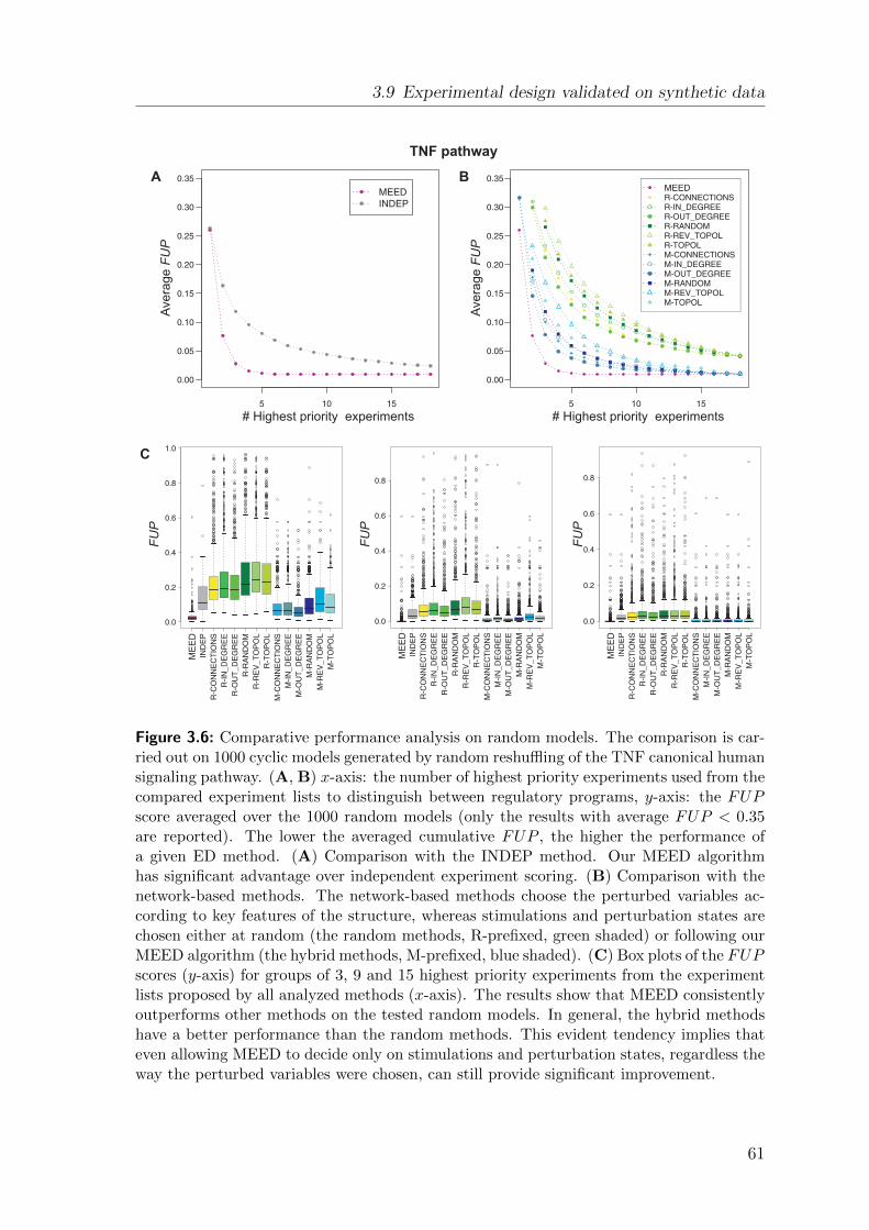
3.9 Experimental design validated on synthetic data
Ave
rag
e F
UP
# Highest priority experiments
Ave
rag
e F
UP
TNF pathwayF
UP
ME
ED
ME
ED
ME
ED
ME
ED
FU
P
FU
P
A B
C
# Highest priority experiments
Figure 3.6: Comparative performance analysis on random models. The comparison is car-ried out on 1000 cyclic models generated by random reshuffling of the TNF canonical humansignaling pathway. (A, B) x-axis: the number of highest priority experiments used from thecompared experiment lists to distinguish between regulatory programs, y-axis: the FUPscore averaged over the 1000 random models (only the results with average FUP < 0.35are reported). The lower the averaged cumulative FUP , the higher the performance ofa given ED method. (A) Comparison with the INDEP method. Our MEED algorithmhas significant advantage over independent experiment scoring. (B) Comparison with thenetwork-based methods. The network-based methods choose the perturbed variables ac-cording to key features of the structure, whereas stimulations and perturbation states arechosen either at random (the random methods, R-prefixed, green shaded) or following ourMEED algorithm (the hybrid methods, M-prefixed, blue shaded). (C) Box plots of the FUPscores (y-axis) for groups of 3, 9 and 15 highest priority experiments from the experimentlists proposed by all analyzed methods (x-axis). The results show that MEED consistentlyoutperforms other methods on the tested random models. In general, the hybrid methodshave a better performance than the random methods. This evident tendency implies thateven allowing MEED to decide only on stimulations and perturbation states, regardless theway the perturbed variables were chosen, can still provide significant improvement.
61

Chapter 3 Elucidating Gene Regulation With Informative Experiments
methods. MEED proposes only a few experiments on average and obtains the lowestaverage cumulative FUP (the area under curve). Next, we investigate the distributionof FUP scores over the 1000 synthetic inputs (Fig 3.6 C). With increasing numberof highest priority experiments used from the list proposed by MEED to distinguishregulatory programs, its FUP variance quickly declines and becomes negligible.
Advantage of MEED over INDEP The first compared method, called INDEP(section 3.8), applies the same measure as MEED, but the score is assigned to eachexperiment independently, ignoring potential dependencies between experiments. Incontrast to INDEP, each consecutive experiment designed by MEED radically in-creases the number of distinguished regulatory program pairs. With this ability,MEED significantly outperforms INDEP, showing the importance of scoring a set ofexperiments together rather than each experiment independently (Fig 3.6 A, C).
Advantage of MEED over network-based methods Next, MEED is comparedwith network-based ED methods, which choose the perturbed variables accordingto key topological features of the model structure (section 3.8). These methodsare divided into random (prefix R) and hybrid (prefix M), according to how theydetermine stimulation and perturbation states for a predefined perturbed variable:either at random, or with the use of reasoning and scoring of our MEED algorithm,respectively. Fig 3.6 B, C shows the advantage of our algorithm over all network-based methods, indicating that MEED reduces the amount of experimental effortrequired to distinguish between regulatory programs. Notably, the hybrid methodsperform better than the random methods (e.g., both the hybrid method M-TOPOLand the random method R-TOPOL prioritize the variables to be perturbed basedon topological order, but M-TOPOL has better performance). Hence, even havingpredetermined specific molecules to be perturbed, the experimenter can still gain fromconsulting MEED regarding the type of perturbation and the level of stimulation.
3.10 The MEED framework applied to a yeastsignaling model
A yeast signaling model In this section we utilize our framework for the inves-tigation of the yeast cellular response to hyperosmotic and pheromone triggers. Theresponse is mediated by signaling cascades that involve the PKA pathway, as wellas the HOG and mating/pseudohyphal growth pathways. The model of the system(based on Gat-Viks and Shamir [41]) is referred to as the yeast signaling model or, inshort, the yeast model. Fig 3.7 shows the model graph and Appendix Fig. .1 presentsits regulation functions. The model contains two stimulators: environmental osmoticconcentration (EOC) and pheromone. In this study, we focus on the regulation ofthe immediate response, exploring only the system state before the potential feedback
62

3.10 The MEED framework applied to a yeast signaling model
Sln1/Ypd1
Ssk1/2/22
Sho1
Ste11
Msn1
Sko1Hog1
Pbs2
EOC
Ste7
Fus3/Kss1
Ste12Hot1Msn2/4
PKA Hog scaffold
Ste20
Pheromone
# Stimulation Perturbation
1. 0.5M KCl 40min — 2. Control sko1 3. 0.5M KCl 40min pbs2 4. 50aF 30min fus3D 5. Control sln1 6. 0.5M KCl 40min hog1 7. 0.5M KCl 40min ssk1 8. 0.5M KCl 40min sho1 9. Control STE12 10. 0.5M KCl 40min ste11 11. Control MSN2
A B
Figure 3.7: Experiment list proposed by MEED for the yeast signaling model. The modelis depicted on the left as a network with nodes (ovals) corresponding to environmentalconditions (dark gray) and signaling components (light gray). Arrows represent signalingrelations. The list of experiments designed by MEED is given in a table on the right, listingstimulation (Control – YPD) and perturbation (green: knock-out and red: over-expression).
mechanisms affect the signaling pathway. Therefore, the model does not contain sev-eral possible mechanisms of feedback control (e.g., Hog1 protein phosphatases whoseproduction is stimulated after the osmotic shock, or glycerol production that leads torestoration of turgor pressure and stops further activation of the HOG pathway [52])and we utilize only measurements that were made shortly after stimulation.
Regulators and regulatory functions We consider only transcriptional controlby single regulators. With this restriction, there are 27 (33) possible one-argumentregulation functions reflecting different means of regulation. To avoid the problemof overfitting (described by Gat-Viks and Shamir [41]), we limit ourselves to sixbiologically relevant regulation functions (section 3.3). We take all variables (apartfrom the Hog-scaffold variable; altogether fifteen variables) as the set of regulators.In total, we consider 90 regulatory programs (six for each regulator).
3.10.1 Experimental design on the yeast model
Candidate experiments To have access to experimental data for expansion, werestricted all analyzed ED methods to choose only from candidate experiments thatare available in microarray databases. Our candidate set of experiments consists of25 genome-wide profiles that are reported in five publications [104, 47, 92, 97, 21],and listed in Appendix Fig. .2.
63
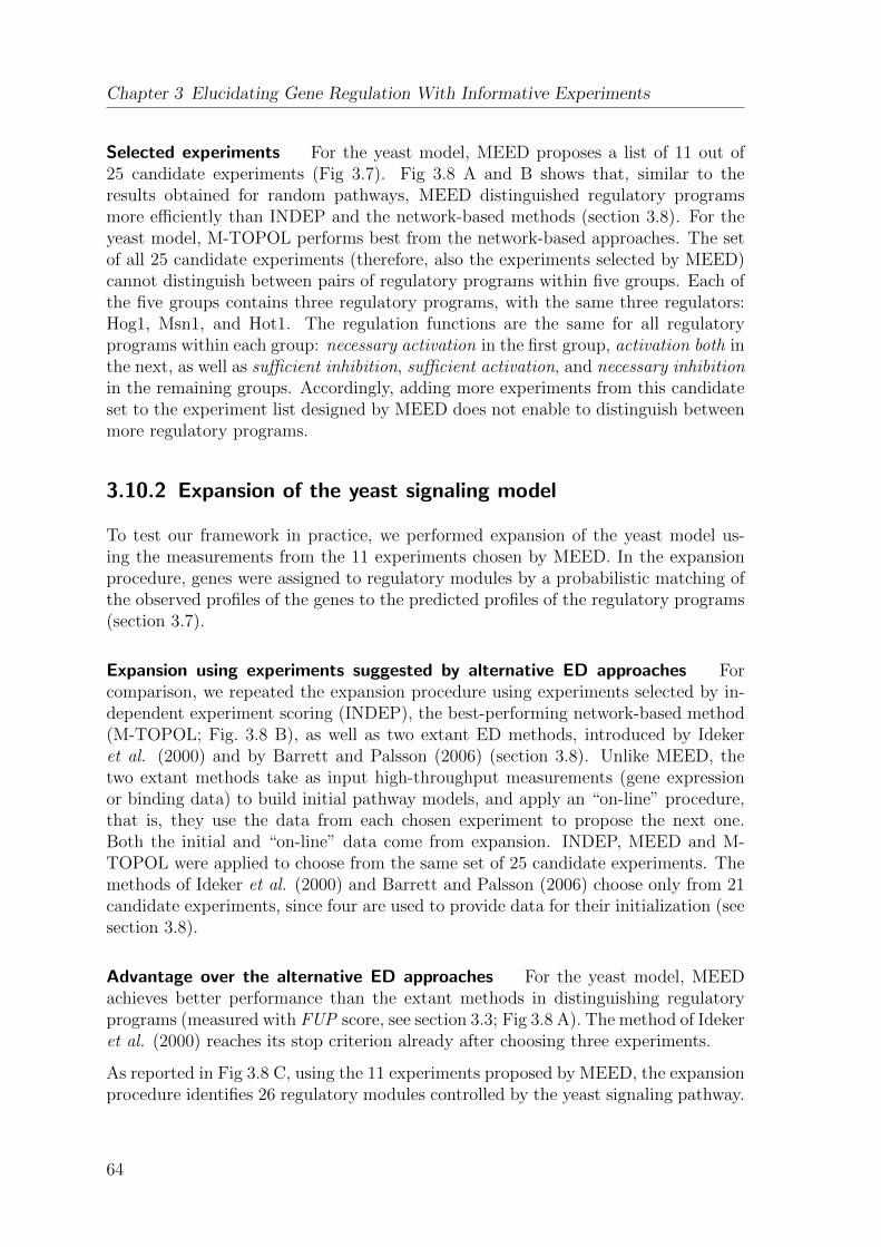
Chapter 3 Elucidating Gene Regulation With Informative Experiments
Selected experiments For the yeast model, MEED proposes a list of 11 out of25 candidate experiments (Fig 3.7). Fig 3.8 A and B shows that, similar to theresults obtained for random pathways, MEED distinguished regulatory programsmore efficiently than INDEP and the network-based methods (section 3.8). For theyeast model, M-TOPOL performs best from the network-based approaches. The setof all 25 candidate experiments (therefore, also the experiments selected by MEED)cannot distinguish between pairs of regulatory programs within five groups. Each ofthe five groups contains three regulatory programs, with the same three regulators:Hog1, Msn1, and Hot1. The regulation functions are the same for all regulatoryprograms within each group: necessary activation in the first group, activation both inthe next, as well as sufficient inhibition, sufficient activation, and necessary inhibitionin the remaining groups. Accordingly, adding more experiments from this candidateset to the experiment list designed by MEED does not enable to distinguish betweenmore regulatory programs.
3.10.2 Expansion of the yeast signaling model
To test our framework in practice, we performed expansion of the yeast model us-ing the measurements from the 11 experiments chosen by MEED. In the expansionprocedure, genes were assigned to regulatory modules by a probabilistic matching ofthe observed profiles of the genes to the predicted profiles of the regulatory programs(section 3.7).
Expansion using experiments suggested by alternative ED approaches Forcomparison, we repeated the expansion procedure using experiments selected by in-dependent experiment scoring (INDEP), the best-performing network-based method(M-TOPOL; Fig. 3.8 B), as well as two extant ED methods, introduced by Idekeret al. (2000) and by Barrett and Palsson (2006) (section 3.8). Unlike MEED, thetwo extant methods take as input high-throughput measurements (gene expressionor binding data) to build initial pathway models, and apply an “on-line” procedure,that is, they use the data from each chosen experiment to propose the next one.Both the initial and “on-line” data come from expansion. INDEP, MEED and M-TOPOL were applied to choose from the same set of 25 candidate experiments. Themethods of Ideker et al. (2000) and Barrett and Palsson (2006) choose only from 21candidate experiments, since four are used to provide data for their initialization (seesection 3.8).
Advantage over the alternative ED approaches For the yeast model, MEEDachieves better performance than the extant methods in distinguishing regulatoryprograms (measured with FUP score, see section 3.3; Fig 3.8 A). The method of Idekeret al. (2000) reaches its stop criterion already after choosing three experiments.
As reported in Fig 3.8 C, using the 11 experiments proposed by MEED, the expansionprocedure identifies 26 regulatory modules controlled by the yeast signaling pathway.
64

3.10 The MEED framework applied to a yeast signaling model
B
FU
P
AF
UP
# Highest priority experiments # Highest priority experiments
D
Am
big
uity
# Highest priority experiments# Highest priority experiments
Nu
mb
er
of m
od
ule
s
C
Figure 3.8: Comparative performance on the yeast signaling model: FUP scores and am-biguity of expansion. MEED (plotted in magenta) is compared to INDEP (gray), network-based methods, as well as two extant ED approaches (Barret and Pallson (2006) - orange;Ideker et al. (2000) - red). Since the two extant methods take as input results of expansionusing the first four experiments proposed by MEED, their report starts from the fifth exper-iment. The method of Ideker et al. (2000) reaches its stop criterion already after choosingthree experiments (fifth to seventh experiment). x-axis in all plots (A–D): the number ofhighest priority experiments. For comparison with MEED, we present up to eleven experi-ments chosen by the other methods. (A,B) FUP scores. y-axis: the FUP score measuringthe ability of the experiments to distinguish between regulatory programs (only the re-sults for FUP < 0.35 are reported). With the lowest FUP for every number of highestpriority experiments, MEED outperforms all alternative methods. The best performing ofthe network-based methods is M-TOPOL. (C) Regulatory modules. y-axis: the number ofmodules identified in expansion. The proportion of ambiguous modules is marked in gray.In comparison with the method of Barret and Pallson (2006), more modules are obtainedusing the same number of highest priority experiments proposed by MEED (the results forthe method of Ideker et al. (2000) are similar to the results of MEED and are not plottedfor clarity). (D) Ambiguity of expansion. y-axis: ambiguity score (i.e., the average numberof regulatory programs per gene; plotted in log scale). With lower ambiguity score for mostnumbers of highest priority experiments, MEED outperforms M-TOPOL and the methodof Barret and Pallson (2006) on the yeast model.
65

Chapter 3 Elucidating Gene Regulation With Informative Experiments
More regulatory modules are identified using any number of highest priority exper-iments proposed by MEED than the same number of experiments proposed by themethod of Barrett and Palsson (2006). Moreover, the eleven experiments chosen byMEED enable lower percentage (2 out 26) of ambiguous modules (modules that werematched to more than one regulatory program). The method of Ideker et al. (2000)achieves similar results as MEED (not shown).
The quality of expansion is further evaluated by the ambiguity score (section 3.7),reporting the average number of regulatory programs that were identified for eachgene. Unlike the FUP score, which evaluates a given ED method based only onmodel predictions, the ambiguity score evaluates results of expansion, which utilizesexperimental data. Fig 3.8 D indicates that MEED outperforms M-TOPOL and(except when the six highest priority experiments are used) the extant methods withrespect to ambiguity scores. Taken together, the presented results indicate practicalapplicability as a strong advantage of MEED, which performs comparably or betterthan the extant approaches although it does not require the data from each chosenexperiment to propose the next one (section 3.8).
Model specificity of MEED In Fig. 3.9, we use the ambiguity score to show thespecificity of the set of experiments chosen by MEED for the particular yeast model.To this end, we compare the ambiguity of the regulatory modules obtained in expan-sion of the original yeast model with the expansion of its randomized version usingthe same experiment list proposed by MEED for the original model. Structure andregulation functions of the randomized model were obtained as in section 3.9. Thenodes of the randomized model are the same as in the original model and the setof regulatory programs is also identical. Expansion of the original model results instrikingly less ambiguous regulatory modules as compared to the modules identifiedfor the randomized model. This result indicates high specificity of our algorithmin choosing experiments for a particular model. The regulatory modules identifiedfor the original model obtain better ambiguity scores than the regulatory modulesfound for the randomized model. This tendency can be explained by the fact thatthe randomized model does not represent the true signaling pathway. For all ex-periments, the randomized model predicts states of regulators in the pathway thatare not “compatible” with the actual measured gene response. As a consequence,there is a poor match between the model-dependent predicted profiles and the realobserved profiles, resulting in ambiguous regulatory modules. Moreover, the experi-ments proposed by MEED for the original model cannot be expected to distinguishthe regulatory programs in the randomized model.
Stability of model expansion Next, we validate the expansion of the yeast path-way by conducting expansion with additional experiments on top of the eleven ex-periments suggested by MEED. In this way, we test the stability of gene assignment,that is, whether with more experiments there is a dramatic rearrangement of genesbetween regulatory modules, or whether the genes are added to or removed from themodules.
66
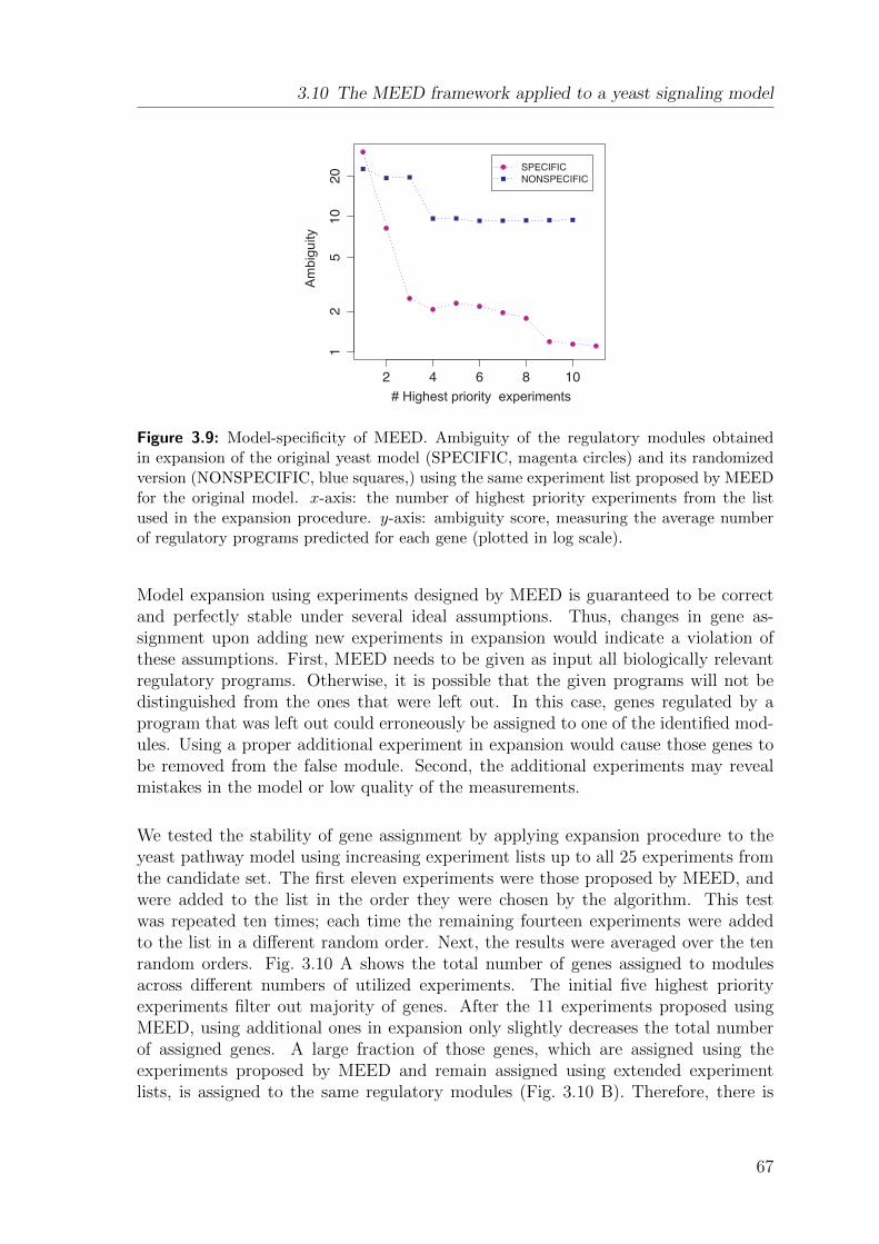
3.10 The MEED framework applied to a yeast signaling model
Am
big
uity
# Highest priority experiments
Figure 3.9: Model-specificity of MEED. Ambiguity of the regulatory modules obtainedin expansion of the original yeast model (SPECIFIC, magenta circles) and its randomizedversion (NONSPECIFIC, blue squares,) using the same experiment list proposed by MEEDfor the original model. x-axis: the number of highest priority experiments from the listused in the expansion procedure. y-axis: ambiguity score, measuring the average numberof regulatory programs predicted for each gene (plotted in log scale).
Model expansion using experiments designed by MEED is guaranteed to be correctand perfectly stable under several ideal assumptions. Thus, changes in gene as-signment upon adding new experiments in expansion would indicate a violation ofthese assumptions. First, MEED needs to be given as input all biologically relevantregulatory programs. Otherwise, it is possible that the given programs will not bedistinguished from the ones that were left out. In this case, genes regulated by aprogram that was left out could erroneously be assigned to one of the identified mod-ules. Using a proper additional experiment in expansion would cause those genes tobe removed from the false module. Second, the additional experiments may revealmistakes in the model or low quality of the measurements.
We tested the stability of gene assignment by applying expansion procedure to theyeast pathway model using increasing experiment lists up to all 25 experiments fromthe candidate set. The first eleven experiments were those proposed by MEED, andwere added to the list in the order they were chosen by the algorithm. This testwas repeated ten times; each time the remaining fourteen experiments were addedto the list in a different random order. Next, the results were averaged over the tenrandom orders. Fig. 3.10 A shows the total number of genes assigned to modulesacross different numbers of utilized experiments. The initial five highest priorityexperiments filter out majority of genes. After the 11 experiments proposed usingMEED, using additional ones in expansion only slightly decreases the total numberof assigned genes. A large fraction of those genes, which are assigned using theexperiments proposed by MEED and remain assigned using extended experimentlists, is assigned to the same regulatory modules (Fig. 3.10 B). Therefore, there is
67
Chapter 3 Elucidating Gene Regulation With Informative Experiments
Ave
rag
e fra
ctio
n
A B
# experiments # experiments
not rearranged
Ave
rag
e #
ta
rge
ts
commonly assigned
Figure 3.10: Stability of assignment of target genes to regulatory modules. (A) Numberof target genes assigned to any regulatory module (red: using experiment lists up to theeleven experiments chosen by MEED; green: using extended experiment lists, average overten random orders of adding extra experiments). x-axis: the number of experiments usedin the expansion procedure. y-axis: the number of identified target genes. Using onlya few experiments, expansion procedure identifies a large fraction of genes as regulatorytargets. The number of assigned target genes decreases for the chosen eleven experiments,and stays in the same order of magnitude, but not on an equal level, when additionalexperiments are added. Therefore the numbers of assigned targets do not change drasticallyonce reasonable length (more than just a few) experiment lists are used. (B) Rearrangementof genes upon addition of experiments. We define commonly assigned genes as all genesassigned to regulatory modules both with the extended experiment list and with elevenexperiments suggested by MEED. x-axis: the number of experiments used in the expansionprocedure. y-axis, blue: the fraction of commonly assigned genes out of all genes assignedto any regulatory module with the extended experiment list (average over the ten randomorders). The fraction of commonly assigned genes goes down when more experiments areused, which indicates that some new genes are added to the modules and some genes areremoved. y-axis, violet: out of the commonly assigned genes, the fraction of genes thatare assigned to the same regulatory module both with eleven and with more experiments(average over the ten random orders, referred to as not rearranged). Remarkably, a largefraction of commonly assigned genes is not rearranged between the modules when addingadditional experiments.
only little rearrangement between the modules when more experiments are used.
3.10.3 Regulatory modules in the yeast signaling model
To assess the biological findings resulting from application of our framework to theyeast signaling model, we focused further analysis on the obtained regulatory mod-ules. As small modules could have been generated at random, given the large number
68

3.10 The MEED framework applied to a yeast signaling model
of potential regulatory programs, we restricted the analysis to fourteen modules con-taining at least seven genes. Fig.3.11 presents a map of the expansion, including theidentified regulatory modules, their regulatory programs, predicted profiles and theexpression matrices of the target genes. The map clearly shows high agreement be-tween predicted profiles and observed profiles. Cases of disagreement (e.g., observedand predicted responses to the second experiment, sko1 mutant, in two regulatorymodules, inhibited by Kss1/Fus3 or Ste12, respectively) show faults in our under-standing and incompleteness of the yeast signaling pathway model.
The identified versus known regulatory programs The expansion analysis pro-vides hypotheses regarding the regulatory relations and their mechanisms downstreamof the yeast signaling model. Tab.3.2 summarizes a detailed comparison between theidentified regulatory programs to known programs based on a comprehensive review[52]. The known regulatory relations include four cases of transcriptional control by asingle regulator and four combinatorial regulations (not considered in this study). Allfour single-regulator programs were detected by our analysis (activation by Msn2/4,activation by Ste12, inhibition by Sko1 and activation by Hot1–here ambiguous withMsn1 and Hog1), confirming the quality of our predictions. In a number of cases, well-characterized target genes were identified by the expansion analysis, thereby servingas positive controls. For example, our analysis indicates that CTT1 and HSP12 areactivated by Msn2/4, and FUS1, FUS3 and FIG1 are activated by Ste12, both con-sistent with the known transcriptional control of these target genes. In total, out ofsixteen target genes, known to be regulated by a single TF, eight genes have beenassigned correctly and no gene has been assigned to a wrong regulatory module. Ascombinatorial regulation was not taken into consideration in our analysis, we expectthat target genes with more than one known regulator will not be assigned to anyof the regulatory modules. Indeed, all six combinatorially regulated target genes didnot match any of the regulatory programs.
Indirect gene regulation by kinases in the modeled yeast pathway Interestingly,four kinases, including Kss1/Fus3, PKA, Sho1 and Ste7, were identified as generegulators (Fig. 3.11). The hypothesized regulation might be explained by an indirectinfluence on the target genes through alternative signaling pathways and downstreamTFs that are not part of the model. Several such alternative pathways are known butwere omitted from the model. For example, PKA regulates transcription throughthe TFs Msn2/4 and Sko1 (part of the model) or through Adr1, Rap1 and Crz1[52, 138] (not modeled), Kss1/Fus3 mediates transcription through the Far1 kinaseindependently of Ste12 [94], and the Sln1/Ypd1 kinases regulate an alternative hypo-osmotic stress pathway through the TF Skn7 [52] (not modeled). There is no knownalternative pathway downstream the signaling molecules Sho1 and Ste7. Our resultssuggest that these signaling molecules have an indirect effect on gene expressionthrough an additional pathway, independent of the model.
69

Chapter 3 Elucidating Gene Regulation With Informative Experiments
Sln1/Ypd1
Ssk1/2/22
Sho1
Ste11
Msn1
Sko1Hog1
Pbs2
EOC
Ste7
Fus3/Kss1
Ste12Hot1Msn2/4
PKA Hog scaffold
Ste20
Pheromone
necessary activation
sufficient activation
activation both inhibition both
sufficient inhibition
necessary inhibitionlog(expression ratios)
-
Figure 3.11: Expansion of the yeast signaling model using the experiments proposed byMEED. The yeast model is depicted in the center of the figure. The identified modules arepresented, with additional dashed edges connecting the regulators in the pathway to theirregulatory programs (nodes labeled with regulators and having a boundary color-codedaccording to their regulation function). The ambiguous modules, highlighted with dashedyellow rectangles, are presented as gray-filled nodes, labeled with their size and connectedby edges to all their matching regulatory program nodes. The two ambiguous moduleswere subject to an additional MEED iteration, which succeeds to distinguish their regu-latory programs using only two additional experiments. A matrix showing the expressionmeasurements of target genes (rows) across the eleven experiments proposed by MEED(columns) is presented only for the modules that contain at least seven genes. The columnsof the expression matrices are ordered from left to right according to the order proposed byMEED. For clarity, only subsets of the large Ste12 and Kss1/Fus3 matrices are shown. Thepredicted profiles appear as a separate row above the matrix. For most modules, the ex-pression profiles agree well with the predicted profiles. Blue arrows exemplify experimentswhere all module genes jointly disagree with the predicted profile.
70

3.10 The MEED framework applied to a yeast signaling model
Known regulatory Predicted Known gene PredictedType program regulatory target target
programCHA1 not predictedPHO84 not predicted
activation by Hot1 correct YGR043C correct**YGR052W not predictedYHR087W not predictedCTT1 correctHSP12 correct
single activation by Msn2/4 correct HSP26 not predictedregulator DCS2 correct
GCY1 not predictedinhibition by Sko1 correct AHP1 not predicted
HAL1 not predictedFUS3 correct
activation by Ste12 correct FUS1 correct(without Tec1) FIG1 correct
YPL192C correctSko1+Crz1* ENA1 not predicted
activation by Msn1+Hot1 STL1 not predictedcombinatorial activation by GPD1 not predicted
regulation Msn2/4+Msn1+Hot1 GPP2/HOR2 not predictedinhibition by Sko1 GRE2 not predictedtogether with Hog1 GLR1 not predicted
Table 3.2: Identified versus known regulatory programs. The table summarizes the pro-grams reviewed by Hohmann [52], reporting whether they were rediscovered by our MEEDframework. Type – states whether the regulation is combinatorial or not. Known reg-ulatory program – the known regulator(s) and the regulatory mechanism, Predictedregulatory program – states whether the known regulatory program was correctly iden-tified (does not refer to combinatorial regulation, which was not a subject of our analysis),Known gene target – known target genes of the regulatory program, Predicted target– states whether the known target gene was correctly included in the regulatory moduleassigned to the regulatory program (genes marked as not predicted were not assigned to anymodule). *Crz1 is downstream to the PKA variable, therefore represents indirect regulationof PKA independently of Sko1. **assigned to an ambiguous module Hot1-Msn1-Hog1.
Biological evaluation of the regulatory modules We evaluated all fourteen mod-ules to test whether the proteins encoded by the target genes had a related functionor a shared transcriptional regulation. To that end, we scored each module accordingto its enrichment in GO annotations (using the Ontologizer tool designed by Baueret al., 2008 [11]) and sets of transcription targets identified by protein-DNA bindingexperiments [49, 103, 139] (computed using a hypergeometric test). Out of the fourlarge modules (containing at least 100 target genes), three modules obtained enrich-ments below a p-value threshold 0.001 (Bonferroni corrected; Fig.3.12). All othermodules did not obtain significant enrichment, probably because of their small size(each of these modules contains less than 26 genes, including genes that were notannotated yet).
71

Chapter 3 Elucidating Gene Regulation With Informative Experiments
Ste
12
, fu
s3S
te1
2D
ig1
Ste
12
, te
c1S
te1
2, ks
s1S
te1
2S
te1
2, te
c1S
te1
2, te
c1S
te1
2, fu
s3S
te1
2S
te1
2, ks
s1D
ig1
Ste
12
, ks
s1/fu
s3Te
c1D
ig1
resp
on
se to
ph
ero
mo
ne
Ste
12
Ste
12
, ks
s1/fu
s3re
pro
du
ctio
nS
mp
1P
dr1
Azf
1T
pk1
Sp
t16
Ya
p5
Ra
p1
ES
A1
Po
l_II
Ra
p1
Fh
l1G
at3
RB
Pc
BG
& a
sse
mb
lyg
en
e e
xpre
ssio
nT
pk2
Rg
m1
cellu
lar
ma
cro
mo
lecu
le B
Sce
llula
r B
Sb
iop
oly
me
r B
S
fus3
tec1
tec1
tec1
fus3
kss1
kss1
/fu
s3
kss1
/fu
s3
01
e-2
51
e-2
01
e-1
51
e-1
01
e-0
91
e-0
81
e-0
71
e-0
61
e-0
51
e-0
40
.00
1 1
Zeitlinger
Harbison
Pokholok
GO
YPD
Butanol
Pheromone
kss1
Enrichment p-values
Figure 3.12: Functional coherence of identified regulatory modules. Enrichment of the tar-get genes from each of four large identified modules (rows) in various experiments (columns).Significant enrichment (Bonferroni-corrected hyper-geometric p-value; indicated by shadesof red) represents distinct behavior of the genes in a module compared to the rest of thegenome. Enrichment p-values in TF-DNA binding targets [49, 103, 139] and gene ontologyannotation (GO [5]) are reported. The different data sets and experiments’ environmentalconditions are color-coded above and below the matrix, respectively. The profiles usedfor the enrichment tests were not part of our original dataset. RPBc – Ribonucleoproteincomplex, BG – biogenesis, BS – biosynthesis.
The enrichment analysis supports and provides insights into the identified modules.For example, it justifies the division of the genes downstream of the mating pathwayinto two activation modules: a module activated by the transcription factor Ste12and a module activated by the kinases Kss1/Fus3. According to our enrichment anal-ysis, the genes activated by Ste12 are characterized by several annotations, which areall related to the known functionality of Ste12 as a key TF of the mating pathway(Fig.3.12). However, the Kss1/Fus3 targets are not enriched in any of these anno-tations, confirming that Ste12 does not control those targets. To provide additionalevidence that these two transcriptional modules are distinct, we performed promotersequence analysis using the Amadeus tool [82]. The known binding motif of Ste12 washighly enriched in the module under sufficient activation by Ste12 (p-value < 10−12),whereas the module under sufficient activation by Kss1/Fus3 was not enriched in thismotif. Taken together, our analysis provides evidence for transcriptional regulationby Kss1/Fus3, independently of Ste12 control.
We next asked what is the regulatory pathway mediating the regulatory programof sufficient activation by Kss1/Fus3 on its gene targets. Kss1 and Fus3 have nopreferential binding to the promoters of the Kss1/Fus3 module [103] (data not shown),ruling out the possibility that Kss1/Fus3 have a direct effect on their targets. Onepotential indirect transcriptional control by Kss1/Fus3 is mediated through the kinaseFar1, which mediates cell-cycle arrest in response to pheromone, independently ofSte12. However, our module is not enriched in cell-cycle annotations (Fig.3.12),indicating that Far1 is unlikely to mediate the observed gene activation downstream ofKss1/Fus3. As more experimental investigations of the pathway connectivity become
72
3.10 The MEED framework applied to a yeast signaling model
available, the mechanisms by which Kss1/Fus3 control its targets should be furtherrevealed.
3.10.4 Ambiguity networks and iterative experimental design
Ambiguity network To facilitate the inspection of ambiguous modules in a givenexpanded model, we devised the concept of an ambiguity network. Recall that anunambiguous module matches exactly one regulatory program, and an ambiguousmodule matches strictly more than one program (section 3.7). We define an ambigu-ity network as a graph whose nodes represent regulatory programs that matched oneof the regulatory modules. One additional node is added for each ambiguous module,labeled by the number of genes it contains. There are edges between the ambiguousmodule nodes and their matching regulatory program nodes. In this way, the am-biguity network highlights the ambiguous modules and provides details on their sizeand the alternative regulation hypotheses.
Ambiguity network versus ambiguity score Fig.3.13 compares two ambiguitynetworks for two sets of regulatory modules that differ significantly in their ambiguityscore. The networks were generated based on the yeast model expansion using twogroups of five and six highest priority experiments from the experiment list proposedby M-TOPOL. Adding the sixth experiment (knockout of Pbs2 in high osmotic stress)lowers the ambiguity of the identified regulatory modules (compare Fig 3.8 D). Recallthat the ambiguity score is proportional both to the number of regulatory programsmatching each ambiguous module and to its size. Therefore, such a strong drop ofambiguity score can be explained by the fact that with the added experiment, theambiguous modules either: (i) match fewer regulatory programs, or (ii) contain fewergenes. As an example of the former case, using the five highest priority experiments,the expansion procedure identifies one of the ambiguous modules to be controlled byseven regulatory programs. With the sixth experiment added, this module is replacedby two, matching four and three regulatory programs, respectively (Fig.3.13, redrectangles). As an example of the latter case, consider the largest ambiguous modulecontaining 3233 genes in expansion performed using five experiments. With the sixthexperiment added, this module is replaced by two smaller modules. These modulesmatch three regulatory programs each and contain only 307 and 677 genes (Fig.3.13,blue rectangles).
Iterative ED in our framework Our framework can be used in iterations of theMEED algorithm and expansion procedure. Experiments chosen by MEED from therestricted set of 25 candidate experiments do not distinguish all regulatory programsin the yeast model. Five groups of regulatory modules remain undistinguished (listedin section 3.10.1). Accordingly, expansion performed using these experiments gener-ates two ambiguous modules (the remaining three groups of regulatory programs are
73

Chapter 3 Elucidating Gene Regulation With Informative Experiments
5 highest priorityexperiments
pbs2 mutantin osmotic stress
E1 E2 E3 E4 E5 E6
E1 E2 E3 E4 E5 E6
E1 E2 E3 E4 E5 E6E1 E2 E3 E4 E5 E6
E1 E2 E3 E4 E5 E6BE1 E2 E3 E4 E5
E1 E2 E3 E4 E5
A
6 highest priorityexperiments
Necessary activation
Sufficient activation
Activation both Inhibition both
Sufficient inhibition
Necessary inhibitionlog(expression ratios)
8
42
30
22
23
37
307
677
56
5
18
8
27
14
7
-
Figure 3.13: Illustrating expansion results with ambiguity networks. Ambiguity networksfor regulatory modules obtained in expansion of the yeast model using the first five (A)and six (B) experiments on the list proposed by M-TOPOL (i.e., A and B differ only byone additional sixth experiment from the list). The ambiguity network provides a detailedinsight into the ambiguous modules. Each white-filled node represents a regulatory programmatching one of the identified modules. It is labeled with its regulator, and has a boundarycolor-coded according to its regulation function. Unambiguous modules are presented onlyby their unique matching regulatory program, without indicating their size. Ambiguousmodules are presented as gray-filled nodes, labeled with their size and connected by edgesto all their matching regulatory program nodes. Exemplary modules (highlighted withdashed rectangles) are shown together with their predicted profile (colored vector above therectangle). Red rectangles: an ambiguous module controlled by seven regulatory programscontaining a large set of genes in A is replaced in B by two smaller ambiguous modulescontrolled by four and three regulatory programs, respectively. The two modules differ inthe gene response to the additional sixth experiment. Matrices showing expression profilesof the target genes (rows) across the experiments (columns) are plotted next to the modules.Blue rectangles: A large ambiguous module whose genes did not respond in any of the firstfive experiments (the corresponding predicted profile is filled with black in A). Using thesixth experiment, the large module is replaced by two smaller ones in B. One modulecontains genes that were down-regulated in the sixth experiment, whereas another containsgenes that were up-regulated (can be seen in green vs. red entries in the predicted profilesof the modules). A large group of genes, whose expression has not changed in the sixthexperiment, does not match any profile and therefore is not contained in any regulatorymodule.
74
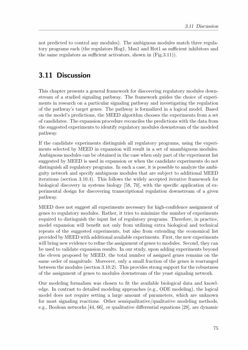
3.11 Discussion
not predicted to control any modules). The ambiguous modules match three regula-tory programs each (the regulators Hog1, Msn1 and Hot1 as sufficient inhibitors andthe same regulators as sufficient activators, shown in (Fig.3.11)).
3.11 Discussion
This chapter presents a general framework for discovering regulatory modules down-stream of a studied signaling pathway. The framework guides the choice of experi-ments in research on a particular signaling pathway and investigating the regulationof the pathway’s target genes. The pathway is formalized in a logical model. Basedon the model’s predictions, the MEED algorithm chooses the experiments from a setof candidates. The expansion procedure reconciles the predictions with the data fromthe suggested experiments to identify regulatory modules downstream of the modeledpathway.
If the candidate experiments distinguish all regulatory programs, using the experi-ments selected by MEED in expansion will result in a set of unambiguous modules.Ambiguous modules can be obtained in the case when only part of the experiment listsuggested by MEED is used in expansion or when the candidate experiments do notdistinguish all regulatory programs. In such a case, it is possible to analyze the ambi-guity network and specify ambiguous modules that are subject to additional MEEDiterations (section 3.10.4). This follows the widely accepted iterative framework forbiological discovery in systems biology [58, 70], with the specific application of ex-perimental design for discovering transcriptional regulation downstream of a givenpathway.
MEED does not suggest all experiments necessary for high-confidence assignment ofgenes to regulatory modules. Rather, it tries to minimize the number of experimentsrequired to distinguish the input list of regulatory programs. Therefore, in practice,model expansion will benefit not only from utilizing extra biological and technicalrepeats of the suggested experiments, but also from extending the economical listprovided by MEED with additional available experiments. First, the new experimentswill bring new evidence to refine the assignment of genes to modules. Second, they canbe used to validate expansion results. In our study, upon adding experiments beyondthe eleven proposed by MEED, the total number of assigned genes remains on thesame order of magnitude. Moreover, only a small fraction of the genes is rearrangedbetween the modules (section 3.10.2). This provides strong support for the robustnessof the assignment of genes to modules downstream of the yeast signaling network.
Our modeling formalism was chosen to fit the available biological data and knowl-edge. In contrast to detailed modeling approaches (e.g., ODE modeling), the logicalmodel does not require setting a large amount of parameters, which are unknownfor most signaling reactions. Other semiqualitative/qualitative modeling methods,e.g., Boolean networks [44, 66], or qualitative differential equations [28], are dynamic
75

Chapter 3 Elucidating Gene Regulation With Informative Experiments
modeling approaches that require time-course data. Here, unlike these approaches,we assume that the regulatory relations are discrete logical functions and the modeldescribes the steady state of the system, thereby enabling to utilize single time pointexpression measurements.
In the proposed framework, there is a distinction between the model-based exper-imental design and data-based expansion procedure: The MEED algorithm selectsthe experiments independent of the data and relies only on the non-stochastic modelpredictions of discrete states reflecting responses of putative regulatory targets. Thestochastic nature of the data is considered only in the expansion, once the mea-surements from the experiments proposed by MEED are available. We expect thatbased on the proposed framework, it will be possible to develop techniques handlingstochastic model formalisms, such as a Bayesian network model, which represent theprior belief in the logical functions (as implemented in Gat-Viks and Shamir [41]).
In this contribution, we considered only regulatory programs with single regulatorsand experiments with perturbations of one molecule. Our approach is general and canbe extended to investigate combinatorial control by taking into account regulatoryprograms with multiple regulators and experiments with more than one perturbedvariable. The MEED algorithm, which is linear in the number of regulatory programs,will scale to the enlarged problem, with the condition that only a small selectionof a vast number of all combinatorial possibilities is considered. For example, fortwo regulators, and three possible states of the variables, the number of all possibleregulation functions is 3(32) = 19683. Already in the case of single regulator programswe choose six biologically relevant regulation functions (out of 27 possible). Applyingthe same selection criteria, one could consider only a handful of biologically relevantcombinatorial functions (e.g., the combinatorial schemas proposed by Buchler et al.,[19] or Yeang and Jaakkola [135]).
76
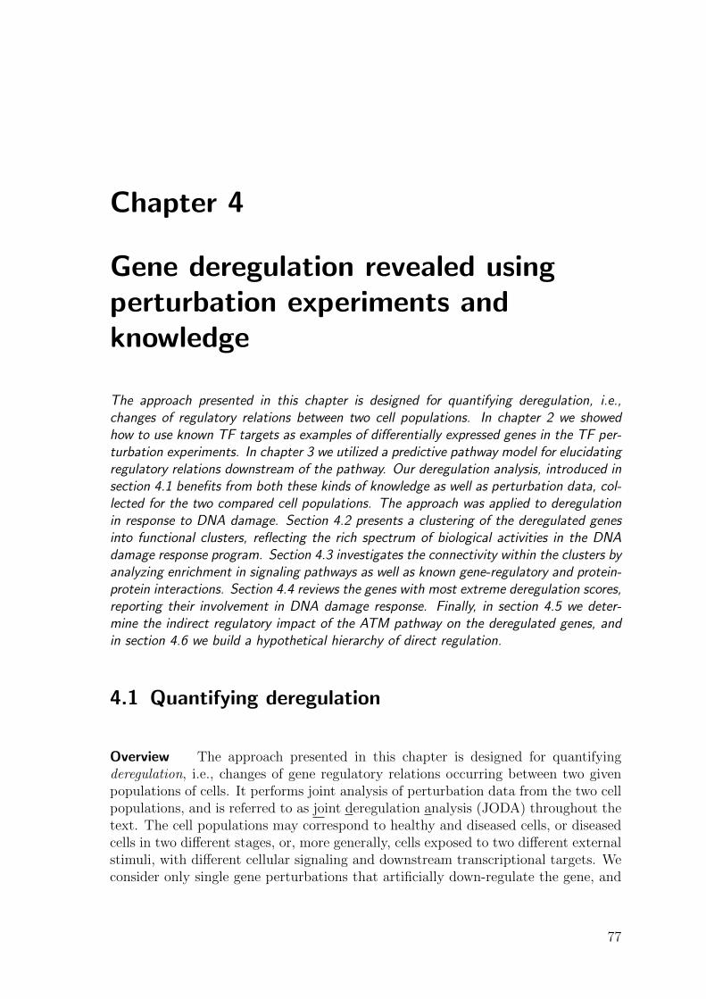
Chapter 4
Gene deregulation revealed usingperturbation experiments andknowledge
The approach presented in this chapter is designed for quantifying deregulation, i.e.,changes of regulatory relations between two cell populations. In chapter 2 we showedhow to use known TF targets as examples of differentially expressed genes in the TF per-turbation experiments. In chapter 3 we utilized a predictive pathway model for elucidatingregulatory relations downstream of the pathway. Our deregulation analysis, introduced insection 4.1 benefits from both these kinds of knowledge as well as perturbation data, col-lected for the two compared cell populations. The approach was applied to deregulationin response to DNA damage. Section 4.2 presents a clustering of the deregulated genesinto functional clusters, reflecting the rich spectrum of biological activities in the DNAdamage response program. Section 4.3 investigates the connectivity within the clusters byanalyzing enrichment in signaling pathways as well as known gene-regulatory and protein-protein interactions. Section 4.4 reviews the genes with most extreme deregulation scores,reporting their involvement in DNA damage response. Finally, in section 4.5 we deter-mine the indirect regulatory impact of the ATM pathway on the deregulated genes, andin section 4.6 we build a hypothetical hierarchy of direct regulation.
4.1 Quantifying deregulation
Overview The approach presented in this chapter is designed for quantifyingderegulation, i.e., changes of gene regulatory relations occurring between two givenpopulations of cells. It performs joint analysis of perturbation data from the two cellpopulations, and is referred to as joint deregulation analysis (JODA) throughout thetext. The cell populations may correspond to healthy and diseased cells, or diseasedcells in two different stages, or, more generally, cells exposed to two different externalstimuli, with different cellular signaling and downstream transcriptional targets. Weconsider only single gene perturbations that artificially down-regulate the gene, and
77
Chapter 4 Gene deregulation revealed using perturbation experiments and knowledge
refer to them as knockdown experiments (although the approach is equally well appli-cable to knockout data). Introduction to essential biological notions, e.g., regulatoryrelation and mechanism, signaling relation and perturbation experiment are given insections 1.1 and 1.2.
We distinguish two sets of genes: the regulators, and all remaining genes (shortly,genes). The regulators are components of a signaling pathway, which is importantfor the switch between the cell populations and may have a different topology in onecell population than in the other. We require that each regulator is knocked down ineach cell population. The remaining genes show effects of the knockdowns in theirexpression. We are interested in regulatory relations connecting regulators to theremaining genes and how these relations change between the cell populations.
In addition to the knockdown data, for both cell populations separately, JODA takesas input two kinds of qualitative knowledge, described in detail below: (i) a pathwaytopology, which describes the signaling relations between all regulators within thepathway, and (ii) regulator-target relations, between some regulators, which are alsotranscription factors, and some remaining genes. The output of JODA are dereg-ulation scores that quantify deregulation using the difference of knockdown effectsbetween the two cell populations. An up-regulation effect indicates (possibly indi-rect) inhibition, and down-regulation indicates activation of the genes by the regula-tor, which was knocked down. The most extreme deregulation scores are assigned tothose genes which switch regulatory mechanism and show different knockdown effectsbetween the cell populations.
Extant approaches Extant deregulation studies combine gene expression dataavailable for two compared cell populations with additional information. For ex-ample, known pathways are incorporated into the deregulation analysis to explorechanging functionality [15, 37, 54, 83, 128]. On a network level, the switch be-tween cell populations was characterized by deregulated sets of gene interconnections[84, 120, 34, 56]. Analyzing deregulation, these extant approaches do not take intoaccount available knowledge about cellular signaling pathways nor their transcrip-tional targets, which may differ between the cell populations. For example, Mani etal. [84] and Taylor et al. [120] take as input a static interactome, which is not specificfor the two cell populations, to discover loss or gain of expression correlation betweenits nodes. Workman et al. [134] showed extensive re-wiring of gene regulatory net-works in yeast cells undergoing DNA damage using genome-wide measurements ofgene expression upon transcription factor (TF) knockdowns, as well as TF bindingto DNA. This advanced approach could be further improved by incorporating priorinformation about the signaling pathways that are differentially activated upstreamof the re-wired gene regulatory network, and the complementarity between the TFDNA-binding and the TF knockdown data.
Input pathway topologies The first kind of knowledge are two pathway topologies,which describe the signaling relations between all regulators within the pathway in the
78

4.1 Quantifying deregulation
two cell populations. The set of the regulators is the same for the two cell populations,but their signaling relations may be different. We assume that researcher’s expertise,literature findings or external experimental data provide qualitative knowledge aboutthe signaling relations, describing “who signals to whom” in both cell populations.This knowledge is given to the input of JODA in a form of two directed graphs (oneper each cell population). The nodes in the graphs correspond to the regulators(pathway components). There is an edge between two nodes in a given pathwaytopology whenever it is known that the pathway component corresponding to onenode activates the component corresponding to the other node.
We denote the set of regulators as V = {v1, ..., vn}. Formally, a pathway topologyin a cell population t is a graph Gt = (V,At) with the set of nodes V and directededges At. Gt may be cyclic and may have several connected components. There isan edge (vi, vj) ∈ At whenever it is known that the pathway component vi activatesvj in the cell population t. Examples of two given ATM pathway topologies, one inthe healthy cells (denoted h) and second in cells undergoing DNA damage (shortly,damaged cells, denoted d), are illustrated in Fig.4.1 A.
Model predictions of knockdown effects In each cell population separately, theknown pathway topology can be utilized to predict effects of knockdown experiments.Consider an experiment ∆tv, where a given regulator v is knocked down in a givencell population t. The regulator v together with all regulators, which are reachablefrom v in the pathway topology t, are called affected by the experiment ∆tv. The setof all experiments knocking down the regulators in V in cell population t is denotedEt. The predictions of affected regulators for all knockdowns in Et are given by thetransitive reflexive closure G∗t = (V,A∗t ) of the pathway topology Gt. To compute G∗t ,we add an edge (vi, vj) ∈ A∗t whenever there exists a directed path from vi to vj in thepathway topology Gt (allowing vi = vj, i.e., the path may be empty). The incidencematrix for G∗t is called the model matrix, or shortly, the model, and denoted Mt.There is an entry 1 in row vi and column vj of the model matrix when (vi, vj) ∈ A∗,otherwise the entries are 0. In this way, an entry 1 tells that its row’s knockdownaffects its column’s regulator. Thus, the set Ev,t of all knockdown experiments thataffect regulator v in cell population t is given by the rows ofMt which have an entry1 in column v:
Ev,t = {∆tw ∈ Et|Mw,vt = 1}. (4.1)
In other words, the set of affecting experiments Ev,t contains both the knockdownof the regulator itself, and knockdowns of its upstream activators in the pathway.Assuming the model Mt is correct, the experiments in Ev,t are expected to havesimilar effect on the target genes of v. The effects on the genes, which are targets ofother regulators upstream of v, should be different between the experiments. Examplemodel matrices for the ATM pathway in the healthy and in the damaged cells areshown in Fig.4.1 B.
79
Chapter 4 Gene deregulation revealed using perturbation experiments and knowledge
The input TF-targets The second kind of knowledge, the known TF-target re-lations, is also given separately for each cell population. It originates from reportsabout established individual TF targets, or from high-throughput TF DNA-bindingdata. The known TF targets are expected to show an effect, i.e., either be up- ordown-regulated by the knockdown experiments. Those targets serve as examples ofgenes that are differentially expressed upon their TF knockdown. This kind of knowl-edge is rarely certain and in our approach is given as a belief (chapter 2) about theTF-target relationships rather than a fixed statement.
Processing steps JODA processes given data and knowledge in three steps (Fig.4.1B):
1. In the first step, we analyze the input data from each knockdown experiment toestimate the effect of the knockdown on the genes. To this end, we apply ourbelief-based differential expression analysis method (chapter 2), implemented inthe R package bgmm [118]. Our method assigns each gene a probability that itwas differentially expressed in the experiment. In this step, the knowledge aboutthe known TF targets is used. To improve the analysis for a knockdown of eachregulator v in each cell population t, the known targets of v in t are given a highprior of differential expression in this knockdown. We add a sign to each returnedprobability to indicate whether the effect of the knockdown was up- or down-regulation. The signed probability lies in the [−1, 1] interval. The resulting vectorof signed differential expression probabilities of the genes in a knockdown of v int is denoted pt
v. Together, we obtain 2|V | such vectors, one for each regulator inV and for each of the two cell populations.
2. In the second step, for each regulator v in each cell population t, we obtain avector Rt
v of regulation scores that quantify the effect of v on the genes in t. Inthis step, the input knowledge about the pathway topologies is used. Recall thatthe pathway model Mt defines the set Ev,t (Eq.4.1) of knockdown experimentsthat affect the regulatory activity of v in t. Each target gene of v is expected tohave pronouncedly high or low signed differential expression probabilities in theknockdown of v that are consistent between all experiments in Ev,t. The regulationscores (each lying in the [−1, 1] interval) reconcile the signed probabilities in theexperiments in Ev,t by taking an average:
Rtv =
∑w∈{vi|∆tvi∈Ev,t} p
tw
|Ev,t|. (4.2)
For example, in Fig.4.1 B the regulation scores RdRelA for RelA in the damaged
cells are an average of the signed probabilities for the knockdowns of RelA and ofits upstream activator ATM. In the healthy cells, only its own knockdown affectsRelA, and its regulation scores Rh
RelA are the same as its signed probabilities phRelA.
As explained above, under the condition that the model is correct, the experimentsaffecting a given regulator should have a common effect on this regulator’s targetgenes. In other words, each target gene is expected to have either high or low signed
80

4.1 Quantifying deregulation
A
g4g1 g2 g3 g4g1 g2 g3
p53
ATMDRelAp53
ATMDRelA
h d
p RelA
h
.9
.7
.8-.1
g1g2g3g4
hR RelA
p RelA
d
-.8-.21
-.3
p ATM
d
-10.6.3
dR RelA -.9-.1.80
Avg
Examples
g1g2g3g4
g1g2g3g4
.9
.7
.8-.1
g1g2g3g4
DRelA
-1.8-.80.1
g1g2g3g4
B
Deregulation scores D v
Avg(D affecting v)
bgmm
Signed probabilities of differential expression
hR v
dR v Regulation scores
d hR - Rv v
TF targets
pathway models:
Perturbation data
Knowledge:
1 0 00 1 00 0 1
Re
lAA
TM
p5
3
DRelADATM
Dp53
1 0 01 1 10 0 1
Re
lAA
TM
p5
3
1
2
3
hp v
dp v
Figure 4.1: Method overview. (A) The ovals illustrate two different cells: a healthy cell hin a neutral environment (left) and a damaged cell d treated with neocarzinostatin (right).Inside each oval: a signaling pathway with regulators RelA, ATM and p53, and a set ofremaining genes g1–g4. In d, ATM signals down to RelA and p53. In h the ATM pathway isinactive. ∆ RelA – an experiment, where RelA is knocked down. Genes are colored accord-ing to the effect of the knockdown: up-regulation in red (indicating inhibition by RelA),down-regulation in green (activation by RelA) and no change in white. Dashed edges con-nect RelA to its target genes. (B) The JODA approach. Input: (i) knockdown data (here,together six knockdown experiments, for three regulators in two cell populations, h and d),(ii) known targets of those regulators, which are TFs and control gene expression directly,and (iii) known pathway models encoded in matrices with an entry 1 when a knockdownexperiment (rows) affects the regulator (columns; otherwise the entries are 0). Experimentsaffecting RelA are marked in blue. The input is processed for the healthy (left) and thedamaged cells (right) separately in three steps, until merged in deregulation scores, as indi-cated by the white and yellow flow arrows, respectively. Examples on the right illustrate thesteps leading to deregulation scores for RelA. In the first step, we apply our method bgmm(chapter 2; [118]), which utilizes the known TF targets to better identify probabilities ofdifferential expression of the genes in knockdown of each regulator v ∈ {RelA, ATM, p53}(denoted ph
v and pdv for the two cell populations h and d). The probabilities are signed to
indicate whether the effect of knockdown was down- (negative sign) or up-regulation (posi-tive). In the second step we obtain regulation scores Rh
v and Rdv, which quantify the effect
of each regulator v on the genes in a given cell population. In the last step, we subtractregulation scores in the healthy cells from regulation scores in the damaged cells to obtainderegulation scores Dv, quantifying how strongly each regulator v deregulates the genes.
81

Chapter 4 Gene deregulation revealed using perturbation experiments and knowledge
probabilities of differential expression that are consistent between all affectingexperiments. Thus, taking an average yields either high or low regulation scoresfor the true targets, and rules out those genes which respond to the perturbationexperiments in a model-independent manner.Note that a negative regulation score indicates (possibly indirect) activation of atarget gene, and a positive score indicates inhibition. This rule, counter-intuitiveat first sight, is motivated by the fact that genes with positive regulation scoreshave mostly positive probabilities of differential expression, i.e., tend to be up-regulated in those perturbation experiments that affect their regulator. The geneswith negative scores have mostly negative probabilities, i.e., are down-regulated.Accordingly, we define genes more activated in a given cell population (e.g., dam-aged d), as having lower regulation score in this cell population than in the other(e.g., healthy h). For example, genes g1 and g2 in Fig.4.1 are more activated in d.g1 is (indirectly) inhibited by RelA in h, and (indirectly) activated by RelA in d.g2 is (indirectly) inhibited by RelA in h, and does not depend on RelA in d.
3. In the third step, to quantify deregulation of genes by a given regulator v, wedefine a vector Dv of deregulation scores as the difference of the regulation scoresfor v between the two cell populations. In this way, each deregulation score lies inthe [−2; 2] interval. Fig.4.1 illustrates these notions by a toy example. Two genes,g1 and g2, are deregulated between the healthy and damaged cells, while gene g3stays regulated the same way, and g4 is unrelated to the pathway. Accordingly,g1 and g2 have dominant deregulation scores, which are well discriminated fromthe scores of g3 and g4 (Fig.4.1 B). Note that in the case when regulation scoresfor cell population h are subtracted from scores for cell population d, genes moreactivated in d (e.g., genes g1 and g2 in Fig.4.1) obtain negative deregulation scores,whereas genes more activated in h obtain positive scores.
4.2 Deregulated genes group into biologically relevantfunctional clusters
JODA was applied to identify genes deregulated in response to DNA damage inducedby neocarzinostatin (NCS). NCS is a drug known to cause double strand breaks inthe DNA. Our analysis aimed at a biological verification of the deregulation scoresproduced by JODA.
Input knockdown data We analyzed transcriptional effects of silencing the reg-ulators ATM, RelA and p53, performed by Elkon et al. [32] on the healthy andthe damaged cells. The raw dataset consists of 30 expression measurements, in nor-mal and in NCS-treated human HEK293 cells, composed of three replicates for eachsiRNA knockdown of ATM, RelA, and p53, and six for control, in both cell popula-tions (GEO series GSE1676, with 8794 genes measured). The raw data was normal-ized using quantile normalization and transformed into robust multi-array average
82

4.2 Deregulated genes group into biologically relevant functional clusters
expression values [60]. Quality of the expression measurements was assessed witharrayQualityMetrics [67]. Four low-quality measurements were removed. We filteredout all genes without an ENTREZ identifier. In the case of multiple genes with thesame identifier, we selected the one with the highest interquartile range (leaving 8498genes). Consequent removal of outliers left 8463 genes. To provide input to JODA,we calculated vectors of log mean expression ratios for each knockdown versus controlin both cell populations (averaging over repeats; together six).
Input knowledge Additionally, we provided two kinds of knowledge. First, theATM pathway topologies in the damaged and in the healthy cells. As presented inFig.4.1 A, in the damaged cells NCS triggers a cellular pathway, where the centralkinase ATM signals down to TFs RelA and p53. This pathway is inactive in thehealthy cells [76]. Second, known target genes were collected for p53 in both healthyand damaged cells, and for RelA only in the healthy cells. For p53 in the damagedcells, we composed a set of 47 known targets by selecting genes that have a DNArepair or chromatin modification function from experimentally verified p53 targetscollected by Horvath et al. [53], the direct p53 targets detected with ChIP-PET andconfirmed by expression analysis by Wei et al. [129], and finally by adding genestargeted by p53 upon ionizing radiation [62]. For p53 knockdown in the healthy cells,we took those verified targets of Horvath et al., and those direct p53 targets of Wei etal., which were not selected as targets in the damaged cells. Finally, for the analysisof RelA knockdown in the healthy cells we utilized a set of genes, identified using theChIP-PET technology by Lim et al. [80], whose promoters are bound by RelA andcontain an NF-κB consensus motif.
Analysis of the deregulation lists Application of the approach resulted in threelists of deregulation scores (shortly, deregulation lists), one for each of the regulatorsRelA, ATM and p53. We sorted the lists decreasingly, so that the one extreme ofeach list contains genes more activated in the healthy cells, and the other containsgenes more activated in the damaged cells. We performed Gene Set EnrichmentAnalysis (GSEA [116]) with default parameters to identify gene sets significantlyoverrepresented on the extremes of the sorted deregulation lists. Sets with fewerthan 15 and more than 500 genes were excluded from the analysis. Only results withFDR ≤ 0.01 and FWER ≤ 0.5 were considered significant. We focused the analysisfirst on Gene Ontology (GO [5]) term, and second on pathway enrichment (bothtaken from the MSigDB database [116] that is utilized by GSEA). We discuss theoverrepresented MSigDB pathways in section 4.3.
Functional clusters Fig.4.3 presents the identified overrepresented GO terms (to-gether, 51) and their enrichment in the deregulation lists. The terms were groupedby similarity into functional clusters. Similarity between the GO terms was assessedusing GOsim [36] with the ’relevance’ measure [105]. Next, the terms were hierar-chically clustered by this similarity. We checked the possible clusterings with thenumber of clusters from five to twenty (Fig.4.3 A,B). For an assumed number of
83

Chapter 4 Gene deregulation revealed using perturbation experiments and knowledge
Functional cluster
Amino acidtransport
Potassium iontransport
Chromatinorganization
Nucleotidemetabolism
Cell cycle
Transport
Translationinitiation
DNA repair
Transcriptionregulation
Transcriptioninitiation
Complexassembly
MRNA/RNAprocessing
DNA damage
GO term
Protein folding
Healthy
r
neg reg of tr
estab
MRNA metbl procMRNA processing
RNA splicingRNA splicing via transesterification reactions
protein DNA complex assemblyprotein RNA complex assembly
iboncprotein complex biogenesis and assemblyspliceosome assembly
transcription initiationtranscription initiation from RNA pol II promoter
protein foldingtranscription from RNA pol II promoter
reg of transcription from RNA pol II promoterreg of RNA metbl proc
reg of transcription DNA dependentanscription from RNA pol II promoter
reg of nnnna metbl procreg of transcription
neg reg of transcription DNA dependentneg reg of nnnna metbl proc
neg reg of RNA metbl procneg reg of metbl proc
neg reg of cellular metbl procneg reg of transcription
DNA replicationDNA repair
DNA dependent DNA replicationresponse to DNA damage stimulus
DNA metbl proctranslational initiation
reg of translational initiationintracellular protein transport
protein transportintracellular transport
nuclear exportnccytoplasmic transport
nuclear transportprotein targeting
mitochondrial transportG1 S transition of mitotic cell cycle
reg of cyclin dependent protein kinase activitynctide metbl proc
lishment or maintenance of chromatin archchromatin modification
covalent chromatin modificationchromosome organization and biogenesis
histone modificationmitochondrion organization and biogenesis
potassium ion transportamino acid transport
FDR
Figure 4.2: Functional enrichment. The matrix shows GO terms enriched with high confi-dence (FDR ≤ 0.01, indicated in blue, and FWER ≤ 0.5; identified using GSEA; [116]) inthe genes more activated in the damaged cells by ATM, RelA and p53 (left three columns)and more activated in the healthy cells (right three columns). Each GO term shown is en-riched in at least one column. The terms were grouped into functional clusters with namesindicated on the left, and sorted by the average enrichment in the first three columns.The GO term enrichment is mutually exclusive for the genes more activated in the healthyand in the damaged cells. Eleven functional clusters of terms are enriched exclusively ingenes more activated in the damaged, and two exclusively in the healthy cells. Abbrevi-ations: mtbl, metabolic; nc, nucleo; pol, polymerase; reg, regulation; neg, negative; pos,positive; proc, process; arch, architecture; nnnna, nucleobase, nucleoside, nucleotide, andnucleic acid. The identified clusters confirm that the dominant deregulation scores are cor-related with a functionality which is highly relevant to the switch between the comparedcell populations.84

4.2 Deregulated genes group into biologically relevant functional clusters
OverlapsSizeM
RN
A/R
NA
pro
cess
ing
Co
mp
lex
ass
em
bly
Tra
nsc
rip
tion
initi
atio
n
Pro
tein
fo
ldin
g
Tra
nsc
rip
tion
re
gu
latio
n
DN
A r
ep
air
Tra
nsl
atio
n in
itia
tion
Tra
nsp
ort
Ce
ll cy
cle
Amino acid transport 8Potassium ion transport 24Chromatin organization 63 5 3 1 21 17 12 1Nucleotide metabolizm 17 1
Cell cycle 34 1 12 8 1Transport 82 2 1 2 9 7
Translation initiation 22 8 2DNA repair 117 2 1 36
Transcription regulation 301 3 7 13 1Protein folding 31
Transcription initiation 14 6Complex assembly 39 19
MRNA/RNA processing 59
150
250
350
# Clusters
# S
ha
red
A
5 7 9 11 13 15 17 19
0.04
0.06
0.08
# Clusters
# C
lust
ers
/ #
sh
are
d
B
5 7 9 11 13 15 17 19
C
Figure 4.3: Choice of the number of clusters. (A) The total number of unique genes sharedbetween the clusters, traced over all clusterings with the numbers of clusters from five totwenty. The set of genes shared between the clusters is obtained as the union of all pairwisecluster intersections. The number of shared genes increases with the number of clusters.(B) The number of clusters in our functional clustering is selected from the [5; 20] intervalso that the ratio of the number of clusters over the number of shared genes is maximized.The more clusters, the more functions is represented in the clustering (one cluster groups aset of GO terms). The less shared genes, the smaller overall overlap between the clusters.Gray dashed line in A, B marks the selected cluster number (thirteen). (C) Functionalgene cluster sizes and overlaps. The matrix represents the clusters (rows), their sizes (Sizecolumn), and their pairwise overlaps (Overlaps matrix). Columns of the overlaps matrixcorrespond only to those clusters that do overlap with any other cluster. Entries show thenon-zero number of genes in the overlap and otherwise are empty.
clusters, the GO term clusters were formed by cutting the hierarchical clustering treeon a corresponding level. Next, from the functional clustering of GO terms, we ob-tained a functional clustering of genes, where each gene cluster corresponds to oneGO term cluster. To this end, we collected the deregulated genes that are annotatedwith the terms from the GO term clusters, using the following procedure: First, foreach GO term, we collected the corresponding deregulated genes in three steps: (i)
85
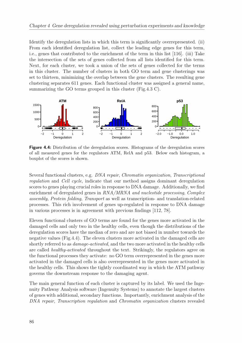
Chapter 4 Gene deregulation revealed using perturbation experiments and knowledge
Identify the deregulation lists in which this term is significantly overrepresented. (ii)From each identified deregulation list, collect the leading edge genes for this term,i.e., genes that contributed to the enrichment of the term in this list [116]. (iii) Takethe intersection of the sets of genes collected from all lists identified for this term.Next, for each cluster, we took a union of the sets of genes collected for the termsin this cluster. The number of clusters in both GO term and gene clusterings wasset to thirteen, minimizing the overlap between the gene clusters. The resulting geneclustering separates 611 genes. Each functional cluster was assigned a general name,summarizing the GO terms grouped in this cluster (Fig.4.3 C).
Deregulation
0
500
1000
1500
−2 −1 0 1 2
● ●● ●●●● ●● ●●●●●● ●●●●● ● ●●●● ●●●● ●●●●● ●● ●● ●● ●● ●●●●● ●● ● ●● ●●● ●●●●●●●●●●●●●●●● ●● ●●●●●●●●● ●●●●● ●●● ●● ● ●● ●●● ● ●● ●
ATM
Deregulation
0
200
400
600
800
−2 −1 0 1 2
●●●●●●● ●●● ●● ●●●● ●● ●● ●●●
RelA
Deregulation
0
200
400
600
800
−2.0 −1.0 0.0 1.0
p53
Figure 4.4: Distribution of the deregulation scores. Histograms of the deregulation scoresof all measured genes for the regulators ATM, RelA and p53. Below each histogram, aboxplot of the scores is shown.
Several functional clusters, e.g. DNA repair, Chromatin organization, Transcriptionalregulation and Cell cycle, indicate that our method assigns dominant deregulationscores to genes playing crucial roles in response to DNA damage. Additionally, we findenrichment of deregulated genes in RNA/MRNA and nucleotide processing, Complexassembly, Protein folding, Transport as well as transcription- and translation-relatedprocesses. This rich involvement of genes up-regulated in response to DNA damagein various processes is in agreement with previous findings [112, 78].
Eleven functional clusters of GO terms are found for the genes more activated in thedamaged cells and only two in the healthy cells, even though the distributions of thederegulation scores have the median of zero and are not biased in number towards thenegative values (Fig.4.4). The eleven clusters more activated in the damaged cells areshortly referred to as damage-activated, and the two more activated in the healthy cellsare called healthy-activated throughout the text. Strikingly, the regulators agree onthe functional processes they activate: no GO term overrepresented in the genes moreactivated in the damaged cells is also overrepresented in the genes more activated inthe healthy cells. This shows the tightly coordinated way in which the ATM pathwaygoverns the downstream response to the damaging agent.
The main general function of each cluster is captured by its label. We used the Inge-nuity Pathway Analysis software (Ingenuity Systems) to annotate the largest clustersof genes with additional, secondary functions. Importantly, enrichment analysis of theDNA repair, Transcription regulation and Chromatin organization clusters revealed
86
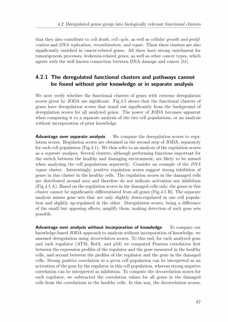
4.2 Deregulated genes group into biologically relevant functional clusters
that they also contribute to cell death, cell cycle, as well as cellular growth and prolif-eration and DNA replication, recombination, and repair. These three clusters are alsosignificantly enriched in cancer-related genes. All three have strong enrichment fortumorigenesis processes, leukemia-related genes, as well as other cancer types, whichagrees with the well known connection between DNA damage and cancer [51].
4.2.1 The deregulated functional clusters and pathways cannotbe found without prior knowledge or in separate analysis
We next verify whether the functional clusters of genes with extreme deregulationscores given by JODA are significant. Fig.4.5 shows that the functional clusters ofgenes have deregulation scores that stand out significantly from the background ofderegulation scores for all analyzed genes. The power of JODA becomes apparentwhen comparing it to a separate analysis of the two cell populations, or an analysiswithout incorporation of prior knowledge.
Advantage over separate analysis We compare the deregulation scores to regu-lation scores. Regulation scores are obtained in the second step of JODA, separatelyfor each cell population (Fig.4.1). We thus refer to an analysis of the regulation scoresas a separate analysis. Several clusters, although performing functions important forthe switch between the healthy and damaging environment, are likely to be missedwhen analyzing the cell populations separately. Consider an example of the DNArepair cluster. Interestingly, positive regulation scores suggest strong inhibition ofgenes in this cluster in the healthy cells. The regulation scores in the damaged cellsare distributed around zero and therefore do not indicate activation nor inhibition(Fig.4.5 A). Based on the regulation scores in the damaged cells only, the genes in thiscluster cannot be significantly differentiated from all genes (Fig.4.5 B). The separateanalysis misses gene sets that are only slightly down-regulated in one cell popula-tion and slightly up-regulated in the other. Deregulation scores, being a differenceof the small but opposing effects, amplify them, making detection of such gene setspossible.
Advantage over analysis without incorporation of knowledge To compare ourknowledge-based JODA approach to analysis without incorporation of knowledge, weassessed deregulation using decorrelation scores. To this end, for each analyzed geneand each regulator (ATM, RelA, and p53) we computed Pearson correlation firstbetween the expression profiles of the regulator and the gene measured in the healthycells, and second between the profiles of the regulator and the gene in the damagedcells. Strong positive correlation in a given cell population can be interpreted as anactivation of the gene by the regulator in this cell population, whereas strong negativecorrelation can be interpreted as inhibition. To compute the decorrelation scores foreach regulator, we subtracted the correlation values for all genes in the damagedcells from the correlations in the healthy cells. In this way, the decorrelation scores,
87

Chapter 4 Gene deregulation revealed using perturbation experiments and knowledge
belonging to the interval [−2, 2], can be read similarly as the deregulation scores:strongly negative decorrelation scores indicate more activation in the damaged cells,and strongly positive indicate more activation in the healthy cells. The decorrelationscores are a simple implementation of the ideas applied by Taylor et al. [120] andMani et al. [84]. Taylor et al. used Pearson correlation of interactome hubs to theirinteraction partners to verify whether these interactions are context-specific. Mani etal. investigated gain and loss of correlation between cell populations using a mutualinformation-based approach.
Although interpreted in the same way, the deregulation scores differ from the decor-relation scores by the ability to incorporate given prior knowledge about the knowncell population-specific pathway topology and target genes downstream of the path-way. JODA outperforms also deregulation analysis assessed with the decorrelationscores. Using the decorrelation scores, the same two clusters can be identified ashealthy-activated and eleven as damage-activated, but they are less significant thanwhen deregulation scores are used (Fig.4.5 B).
88

4.2 Deregulated genes group into biologically relevant functional clusters
-1.5 -0.5 0.5
DeregulationA
-1.5 -0.5 0.5
Regulation, healthy
-1.5 - .50 0.5
Regulation, damage
-1.5 -0.5 0.5
Decorrelation
0
20
40
60
80
-lo
g1
0(p-
va
lue )
B
l
DeregulationHealthyDamageHealthy vs DamageDecorrelation
all genesMRNA/RNA processing
complex assemblytranscription initiation
protein foldingtranscription regulation
DNA repairtranslation initiation
transportcell cycle
nucleotide metabolismchromatin organization
potassium ion transportamino acid transport
MR
NA
/RN
A p
roce
ssin
g
com
ple
x a
sse
mbly
tra
nsc
rip
tion
initi
atio
n
pro
tein
fo
ldin
g
tra
nsc
rip
tion
re
gu
latio
n
DN
A r
ep
air
tra
nsl
atio
n in
itia
tion
tra
nsp
ort
cell
cycl
e
nu
cle
otid
e m
eta
bo
lism
chro
ma
tin o
rga
niz
atio
n
po
tass
ium
ion
tra
nsp
ort
am
ino
aci
d tra
nsp
ort
Figure 4.5: Significance of the deregulation scores. (A) Distributions of deregulation scoresof genes in the functional clusters (averaged over the three regulators, ATM, RelA andp53) strongly deviate from the distribution of averaged deregulation scores for all genes(left plot). The distributions of average regulation scores in the healthy (middle left) andin the damaged cells (middle right), as well as of average decorrelation scores (right) aremore similar to the distributions of the same scores for all genes. Gray dashed vertical linesmark score 0 in each plot. Decorrelation scores do not incorporate prior knowledge andassess the difference of expression correlations between the regulators and the genes. Tocompare significance between the clusters, the mean of averaged cluster deregulation scores(left, light gray crosses) can be used. The eleven damage-activated clusters are assignednegative deregulation and decorrelation scores and have names printed in bold. Healthy-activated clusters have positive deregulation and decorrelation scores. Separately for eachcell population, negative regulation scores indicate activation of the clusters, whereas pos-itive regulation scores indicate inhibition. (B) A t-test comparing the cluster deregulationscores with the deregulation scores for all genes (Deregulation; red squares) gives for major-ity of the clusters the most significant p-values, when contrasted with: the p-values obtainedin a t-test comparing cluster regulation scores to regulation scores of all genes in the healthycells (Regulation, Healthy; blue pluses), and the same t-test but in the damaged cells (Reg-ulation, Damage; light blue crosses), the p-values in a t-test comparing cluster regulationscores in the healthy directly to regulation scores in the damaged cells (Healthy vs Damage;green diamonds), and in a t-test comparing the cluster decorrelation scores with the decor-relation scores for all genes (Decorrelation, yellow triangles). All tests are two-sided. Thep-values evaluate the differentiating power of the scores for each cluster. They depend oncluster sizes and therefore should not be compared between the clusters. Taken together,our joint and knowledge-based approach assigns more significant scores to the functionalclusters than a separate analysis, or analysis without incorporation of knowledge.
89

Chapter 4 Gene deregulation revealed using perturbation experiments and knowledge
4.3 Deregulated pathways and complexes elucidatecooperation within functional clusters
Deregulated pathways and complexes Since the genes in each cluster share thesame functionality, they may interact in a common cellular pathway or complex. Todetermine these interactions we first identified pathways and complexes that are over-represented on the extremes of the deregulation lists. Next, we checked their overlapwith the functional clusters. The enrichment in pathways was assessed using GSEA(see section 4.2). The identified pathways are stored in the MSigDB database as setsof genes, but their signaling relations are well described in the literature. Eleven iden-tified MSigDB pathways significantly overlap with our functional clusters (Fig.4.6 A).For example, the apoptosis pathway contains genes from the DNA repair and Tran-scription regulation clusters. To test enrichment in complexes, we downloaded setsof genes forming each complex from the Reactome database ([123]; together, 2816complexes). For a set of genes in a given complex, and for a given deregulation list,we performed higher-tail hypergeometric enrichment tests iteratively for a numberof 10 up to 500 most extreme (top or bottom) deregulated genes. Finally, the mini-mum resulting p-value was selected to signify the enrichment of this complex in thisderegulation list. To focus on big complexes containing a considerable number ofderegulated genes, we excluded complexes with fewer than 15 genes, overlapping byless than 10 with the current set of deregulated genes in each iteration. The size ofthe universe was set to all genes analyzed on the array (8498). Only results with theenrichment p-value ≤ 10−5 were considered significant. We found the Exon junctioncomplex and several spliceosome complexes (Fig.4.6 B) significantly overrepresentedin the genes more activated in the damaged cells. Interestingly, these complexesoverlap (hyper-geometric higher tail p-value 1.1 · 10−29) with the MRNA processingcluster. Similarly as pathway interactions, membership in complexes explains theway the genes in the clusters are connected and collaborate to exhibit the commonfunction.
Connectivity within the DNA repair cluster Finally, we focused on the DNArepair cluster, which is of pivotal interest in the context of the switch between thehealthy and the damaged cells. We investigated physical relations connecting geneswithin this cluster. The cluster is strongly enriched in eight canonical pathwaysinvolved in the DNA damage response (p-values from 1.33 ·10−41 to 8.17 ·10−11; iden-tified using SPIKE [32]). SPIKE is a database and an analysis tool, storing manuallycurated pathways playing key roles in response to damage. The table in Fig.4.7 Alists 51 genes from the DNA repair cluster, which belong to those canonical pathwaysstored in SPIKE as well as three additional pathways, described in a comprehen-sive review on DNA damage response by Wood et al. [133]. The position of thelisted genes in the well known damage response pathways describes their role in theresponse, as well as their interaction partners in the cluster.
90

4.3 Deregulated pathways and complexes elucidate cooperation within functional clusters
A
RN
A tra
nscri
ptio
na
po
pto
sis
tra
nsl
atio
n fa
cto
rsM
TO
R p
ath
way
SI in
ve
sicu
lar
tra
nsp
ort
TN
F p
ath
way
cell
cycle ay
MRNA/RNA processingcomplex assembly
transcription initiationtranscription regulation
DNA repairtranslation initiation
transportcell cycle
chromatin organization
U
1.3 0.5 0
- Avg deregulation gene
complex
membership
B
SC
SA
SFRS9
SF3A1
SFRS4
PRPF4
SFRS3
HNRNPD
SNRPD3
GTF2F1
SMC1A CD2BP2
RBM5
PCBP1
SNRPA1HNRNPU
SFRS1PRPF8
SFRS7TXNL4A
CSTF2
NCBP2
RBM8A
CLP1
SB
SE
SNRPG
SNRPD1
POLR2J
POLR2E
POLR2F
ATAC B/C
PTBP1
EJ
POLR2L
EJSASBSCSE
ATAC B/C
- log (hypergeometric p-value) 10
3 28
Figure 4.6: (A) Connectivity between genes in functional clusters explained with dereg-ulated pathways stored in the MSigDB database. Matrix shows pathways enriched inthe genes more activated in the damaged cells (columns) that overlap significantly withfunctional clusters (rows). Only pathways and clusters overlapping with higher-tail hyper-geometric p-value at most 0.001 (indicated in red) are reported. Abbreviations of pathwaynames: SI, snare interactions; U, ubiquitin. (B). Deregulated complexes. Top left: Theexon junction (EJ) complex and five spliceosome complexes (rows) are overrepresented inthe genes more activated in DNA-damage by the regulators ATM, RelA and p53 (columns).Only complexes with a p-value at most 10−5 (indicated in red) are reported. Genes in thosecomplexes overlap significantly with the functional cluster MRNA/RNA processing. Right:Graph representation of the genes (round nodes shaded in violet by their average deregu-lation scores) in the complexes (rounded square nodes). Edges represent gene - complexmembership. Abbreviations of complex names: EJ, exon junction; SA, spliceosomal A; SB,spliceosomal B; SC, spliceosomal Active C/ spliceosomal intermediate C/ spliceosomal ac-tive C with lariat containing 5-end cleaved pre-mRNP:CBC; ATAC B/C, ATAC B/ ATACC/ ATAC C with lariat containing 5-end cleaved mRNA (“/” lists complexes sharing com-mon genes that have identical enrichment p-values and thus are abbreviated with the samename). Pathways and complexes carry information about relations between their membergenes. Therefore, these enrichment results broaden our view on the connectivity within thesets of genes in the functional clusters.
To further infer the cooperation between the 66 remaining genes in the DNA re-pair cluster, we collected their interactions using SPIKE and Ingenuity (Fig.4.7 B).Together, we identified 126 relations connecting 52 of those genes either with eachother or with other intermediate genes, complexes and protein families. SPIKE wasapplied to find all direct connections that are stored in the SPIKE database that jointhe set of 66 genes, allowing connection via a single intermediate node not included
91

Chapter 4 Gene deregulation revealed using perturbation experiments and knowledge
in the set. The connections may represent membership in a complex or regulationof different biochemical types, e.g. phosphorylation, protein-DNA (transcriptional)regulation, activation and protein-protein interaction. Ingenuity was applied to findinterconnections between the 66 genes in two different ways, always restricting thateach relationship was reported for Human molecules, and that it is of one of the follow-ing types: expression, transcription, protein-DNA (all summarized as transcriptionalregulation), activation, inhibition, membership, modification, phosphorylation, orprotein-protein interaction. We collected all such direct relationships that are storedin the Ingenuity database. In addition, we applied Ingenuity to score known networksbased on their enrichment in the input set of genes and collected all direct interactionspresent in the top three scoring networks (with scores 57, 45 and 18, respectively).The top scoring networks are related mostly to DNA replication, recombination, andrepair, as well as tumor morphology, cell cycle and cell death. The networks haveadditional nodes that are not included in the input set but are highly connected tothe genes in the set.
The analysis revealed a number of complexes, like the Origin of Replication com-plex (ORC) containing five DNA repair genes, which join subsets of genes together.Grouping the complexes by common functionality, we selected functional sub-partsof the network. For example, we identified a sub-network of genes belonging to theRFC, DNA polymerase epsilon, and the ORC complexes, which are involved in theDNA replication process (marked with a light grey background in Fig.4.7 B).
92
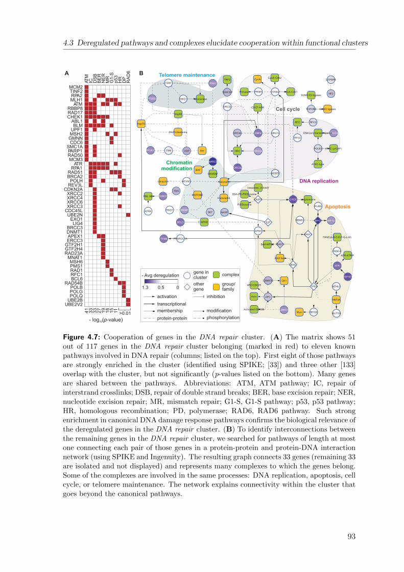
4.3 Deregulated pathways and complexes elucidate cooperation within functional clusters
A B
1.3 0.5 0
- Avg deregulationgene incluster
complex
group/family
membership
protein-protein
othergene
activation inhibition
modification
phosphorylation
transcriptional
Apoptosis
Chromatinmodification
Telomere maintenance
DNA replication
Cell cycle
TP53 NTHL1
MUTYHMyo
ATR-ATRIP
ATR
MYO6
BAX
HNF4A
EEF1E1
Axin
CSNK1E
APC/CDC20
CK1
APC
Activated GSK3B CSNK1D
CYCS
NAP1L1
FANCA
MYC
PURA
APAF1
RBMS1
FANC(A-B-C-E-F-G-L-M)
apoptosome
BAX fam
MYST2
E2F
BAK-MFN2 BAK1
CCNA2 CycA-Cdk1
CycA-Cdk2
DBF4 ORC1L
ORC5L
POLE2DNA polymerase epsilon
RFC4
RFC3
ATAC-(p/CAF)POLE3
ATAC-type
RFC
TERT
PTGES3
Hsp90
DKC1
26sProteasome
Hsp70
TSNPPP1R15A VCP
ATXN3Ubiquitin
TDG
HMGB1
TFAM
ATRX
SUMO1
BCL3
RAG1
PML-NB
PPARGC1A
TOPORS
NF2SUMO E3 ligases
GTPBP4
SUMO ligases
SET
PIDDosome
NFKB
AIFM1
caspases, initiator
HISTONE DNA-PK-PIDDosome
HistoneH3
HistoneH4CASP2
NASP
ORC4L
Akt
SWI/SNF
ORC3L
ORC
SMARCB1
BAF
PRIM1
CDC7-ASK
TRF2
TERF2IP
RAN
ORC2L
CycA
Primase
Telomerase
UBE2V2UBE2BPOLQPOLGPOLB
RAD54BBCL6RFC1RAD1PMS1MSH6
MNAT1RAD23AGTF2H4GTF2H1ERCC3APEX1DNMT1BRCC3
LIG4EXO1
UBE2NCDC45LXRCC3XRCC6XRCC4XRCC2
CDKN2AREV3LPOLH
BRCA2RAD51
RPA1ATR
MCM3RAD50PARP1
SMC1ACDC6
GMNNMSH2UPF1BLM
ABL1CHEK1RAD17RBBP8
ATMMLH1RPA2
TINF2MCM2
ATM
IC DS
BB
ER
NE
RM
RG
1-S
p5
3H
RD
PR
AD
6
41
33
33
27
19
18
15
11
- log (p-value) 10
>0.01
Figure 4.7: Cooperation of genes in the DNA repair cluster. (A) The matrix shows 51out of 117 genes in the DNA repair cluster belonging (marked in red) to eleven knownpathways involved in DNA repair (columns; listed on the top). First eight of those pathwaysare strongly enriched in the cluster (identified using SPIKE; [33]) and three other [133]overlap with the cluster, but not significantly (p-values listed on the bottom). Many genesare shared between the pathways. Abbreviations: ATM, ATM pathway; IC, repair ofinterstrand crosslinks; DSB, repair of double strand breaks; BER, base excision repair; NER,nucleotide excision repair; MR, mismatch repair; G1-S, G1-S pathway; p53, p53 pathway;HR, homologous recombination; PD, polymerase; RAD6, RAD6 pathway. Such strongenrichment in canonical DNA damage response pathways confirms the biological relevance ofthe deregulated genes in the DNA repair cluster. (B) To identify interconnections betweenthe remaining genes in the DNA repair cluster, we searched for pathways of length at mostone connecting each pair of those genes in a protein-protein and protein-DNA interactionnetwork (using SPIKE and Ingenuity). The resulting graph connects 33 genes (remaining 33are isolated and not displayed) and represents many complexes to which the genes belong.Some of the complexes are involved in the same processes: DNA replication, apoptosis, cellcycle, or telomere maintenance. The network explains connectivity within the cluster thatgoes beyond the canonical pathways.
93

Chapter 4 Gene deregulation revealed using perturbation experiments and knowledge
4.4 Genes most activated in damaged cells work inthe damage response
Functionality of the top hundred most activated genes Functional clusterscontain deregulated genes that accumulate within the extremes of the deregulationlists, but not on the strict top or bottom. We investigated the composition of threesets of the strict top one hundred genes that are most activated in the damagedcells by each regulator RelA, ATM and p53. All three sets are significantly enrichedin genes involved in transcription, with five common genes active in this process:CHD4, RBM14, RCAN1, SMAD4, and UBN1. Interestingly, some of the genes mostactivated by RelA are interaction partners (for example, SMARCB1) of the genesmost activated by p53 (SMARCB4). Apart from transcription, the set most activatedby ATM is also enriched in cell death, cell cycle and growth and proliferation-relatedgenes. Additionally, both the sets of genes most activated by ATM and p53 areenriched in cancer-related genes.
PLK2
ZNF148
MED23MED16
UBE2D3
PRKAB1
PIN1 SRRM2
SDC4
PPP1R15A
RELA
IER2GEMIN4
DNAJB6
NFKB2
PTX3
SS18
HSPA8
UBE2H
SMARCB1
MFAP2
TP53
FBN2
BTG1
ATM
JUN
CREB1 JUNB
SMAD4
CCNL1
JUND
transcriptionregulator
kinase
regulatorRelA, p53 or ATM
membership
protein-protein
other
activation
inhibition
modification
transcriptional
enzyme
Figure 4.8: Network of genes most activated in DNA damage. A network of known regula-tory and interaction relations (edges) connecting genes (nodes) from the lists of top twentymost activated by RelA, ATM or p53 in DNA damage. The relations are collected fromthe Ingenuity Pathway Analysis (Ingenuity Systems) database. The nodes are labeled withgene names and colored according to gene functions, whereas relations are given edge stylesaccording to their type.
Regulatory relations between the top twenty most activated genes Next, wereviewed the individual examples out of three shorter lists of twenty genes, that are
94
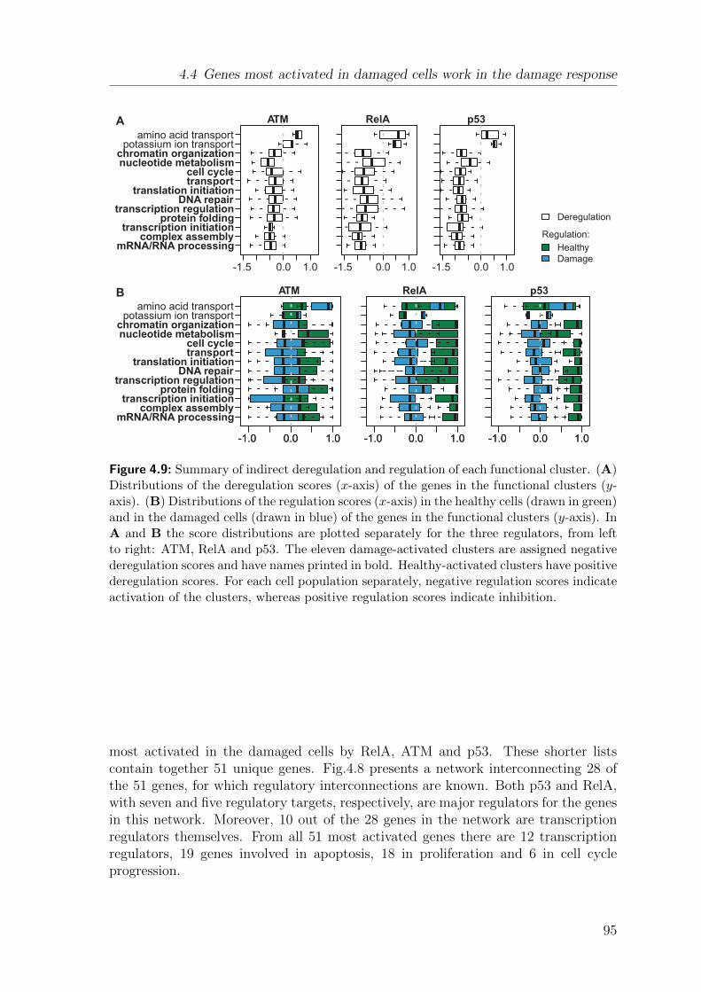
4.4 Genes most activated in damaged cells work in the damage response
mRNA/RNA processingcomplex assembly
transcription initiationprotein folding
transcription regulationDNA repair
translation initiationtransportcell cycle
nucleotide metabolismchromatin organization
potassium ion transportamino acid transport
mRNA/RNA processingcomplex assembly
transcription initiationprotein folding
transcription regulationDNA repair
translation initiationtransportcell cycle
nucleotide metabolismchromatin organization
potassium ion transportamino acid transport
-1.5 0.0 1.0
ATM
-1.5 0.0 1.0
RelA
-1.5 0.0 1.0
p53
l
Deregulation
HealthyDamage
-1.0 0.0 1.0
ATM
-1.0 0.0 1.0 -1.0 0.0 1.0
RelA
-1.0 0.0 1.0 -1.0 0.0 1.0
p53
-1.0 0.0 1.0
Regulation:
A
B
Figure 4.9: Summary of indirect deregulation and regulation of each functional cluster. (A)Distributions of the deregulation scores (x-axis) of the genes in the functional clusters (y-axis). (B) Distributions of the regulation scores (x-axis) in the healthy cells (drawn in green)and in the damaged cells (drawn in blue) of the genes in the functional clusters (y-axis). InA and B the score distributions are plotted separately for the three regulators, from leftto right: ATM, RelA and p53. The eleven damage-activated clusters are assigned negativederegulation scores and have names printed in bold. Healthy-activated clusters have positivederegulation scores. For each cell population separately, negative regulation scores indicateactivation of the clusters, whereas positive regulation scores indicate inhibition.
most activated in the damaged cells by RelA, ATM and p53. These shorter listscontain together 51 unique genes. Fig.4.8 presents a network interconnecting 28 ofthe 51 genes, for which regulatory interconnections are known. Both p53 and RelA,with seven and five regulatory targets, respectively, are major regulators for the genesin this network. Moreover, 10 out of the 28 genes in the network are transcriptionregulators themselves. From all 51 most activated genes there are 12 transcriptionregulators, 19 genes involved in apoptosis, 18 in proliferation and 6 in cell cycleprogression.
95

Chapter 4 Gene deregulation revealed using perturbation experiments and knowledge
4.5 RelA and p53 are the key deregulators of genes infunctional clusters
Deregulation is inferred from knockdown effects, and as such can be due to an indirectimpact of the regulators on the genes. Here, we summarize these possibly indirecteffects on functional clusters of the deregulated genes identified by JODA.
Fig.4.9 reports deregulation and regulation scores of the genes in functional clusters,for each regulator ATM, RelA and p53. The per cluster distributions of deregulationscores for RelA and p53 are shifted further away from zero than for ATM, suggestinga stronger deregulatory impact on the clusters (Fig.4.9 A). Indeed, Fig.4.9 B showsthat the distributions of regulation scores for ATM in the healthy and in the damagedcells are generally less separated than for RelA and for p53. Interestingly, for all threeregulators, the regulation scores indicate that the damage-activated clusters are onlyslightly (possibly indirectly) activated in the damaged cells. Instead, these clustersare strongly (possibly indirectly) inhibited in the healthy cells both by RelA andby p53, as indicated by the respective distributions shifted towards value 1. Theinhibitory impact of ATM on these clusters in the healthy cells is less prominent. Inthe case of the two healthy-activated clusters, a strong, possibly indirect inhibitionin the damaged cells is observed for all three regulators. Distinctively, the Potassiumion transport cluster is also (possibly indirectly) activated in the healthy cells byRelA and p53.
4.6 Deregulation can be explained by a hierarchy ofdirect TF-DNA binding events
Finally, we investigate the hierarchy of direct regulatory relations, which could explainthe effect of the ATM pathway on the deregulated target genes. The first expectedscenario would involve regulation by direct binding of the regulators in the pathwayto the gene promoters. Alternatively, the most parsimonious hierarchy would connectthe regulators to the genes via a single TF. To investigate these hypotheses, we followa two step procedure. In the first step we computationally predict the TFs directlybinding to the promoters of the genes. In the second step we verify whether the TFsare the regulators themselves, or whether they are controlled by the regulators.
TF-DNA binding predictions To implement the first step, we applied Trans-Find [68] to search the promoters of the genes in each functional cluster for over-representation of high-affinity binding of human TFs, which is conserved in theirmouse orthologs (Fig.4.10 A). Since the genes in each cluster share the same func-tionality, they can be expected to be directly regulated by a common TF. Given a setof genes, TransFind predicts TFs with affinities to the gene promoters significantlyhigher compared to a background set of genes (by default, all genes in the Ensembl57
96

4.6 Deregulation can be explained by a hierarchy of direct TF-DNA binding events
database). Affinities are computed from a physical model, based on positional TFweight matrices. We tested a reduced set of human TRANSFAC [130] matrices, con-taining only a single, the most informative matrix for each TRANSFAC TF, settingall parameters to default. TransFind assesses the significance of binding to the pro-moters of a set of input genes with a multiple-testing-corrected (FDR) version ofthe Fisher’s exact test. Only results with FDR ≤ 0.05 were considered significant.Among the identified TFs, CREB has binding sites significantly enriched in the pro-moters of genes in the DNA repair cluster. Neither RelA nor p53 were predicted tobind directly to the promoters of the genes in the functional clusters.
CREB as the intermediate factor in the hierarchy In the second step, we considerthe hypothesis of the parsimonious hierarchy. Here, we focus on CREB, leaving otherpredicted TFs as candidates for future investigation. The hypothesis consists of aderegulatory connection from the ATM pathway to CREB, implemented by RelAor p53 directly binding to CREB promoter in the damaged cells and not binding inthe healthy cells. To complete the picture, we collected the most likely direct targetgenes of CREB. Based on high-throughput CREB binding data in HEK293T cells byZhang et al. [140], seven out of top twenty predicted CREB targets in the DNA repaircluster bear evidence of CREB binding (Fig.4.10 B). Additionally, we report two genesoutside of the cluster, PWP1 and NOLC1. Both are deregulated in our system, aswell as have yeast homologs, which according to the study by Workman et al. [134]are deregulated by SKO1, an yeast homolog of CREB. PWP1 is also reported asbound by CREB in HEK293T cells [140]. Fig.4.10 C brings together these piecesof evidence in a hypothetical regulatory network. The network shows a two-stephierarchy, going from the ATM pathway, via CREB, to the nine most likely CREBtarget genes, which are deregulated between healthy and the damaged cells.
97
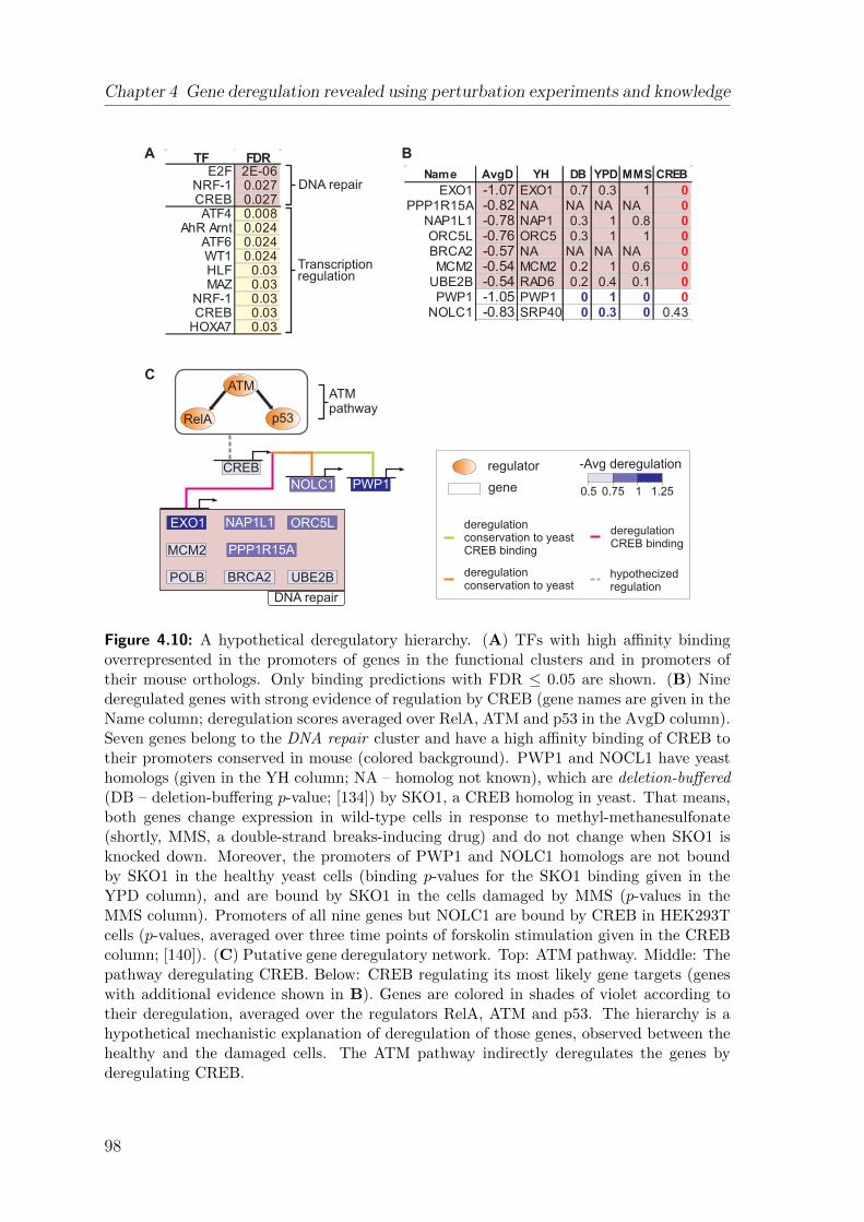
Chapter 4 Gene deregulation revealed using perturbation experiments and knowledge
0.5 0.75 1 1.25
-Avg deregulation
deregulationconservation to yeastCREB binding
deregulationconservation to yeast
deregulationCREB binding
hypothecizedregulation
CREB
ATMpathway
NOLC1
ATM
RelA p53
DNA repair
EXO1 NAP1L1
PPP1R15AMCM2
BRCA2 UBE2B
ORC5L
POLB
regulator
gene
A B
Name AvgD YH DB YPD MMS CREB
EXO1 -1.07 EXO1 0.7 0.3 1 0PPP1R15A -0.82 NA NA NA NA 0
NAP1L1 -0.78 NAP1 0.3 1 0.8 0ORC5L -0.76 ORC5 0.3 1 1 0BRCA2 -0.57 NA NA NA NA 0MCM2 -0.54 MCM2 0.2 1 0.6 0
UBE2B -0.54 RAD6 0.2 0.4 0.1 0PWP1 -1.05 PWP1 0 1 0 0
NOLC1 -0.83 SRP40 0 0.3 0 0.43
C
DNA repair
Transcriptionregulation
TF FDRE2F 2E-06
NRF-1 0.027CREB 0.027ATF4 0.008
AhR Arnt 0.024ATF6 0.024WT1 0.024HLF 0.03MAZ 0.03
NRF-1 0.03CREB 0.03
HOXA7 0.03
PWP1
Figure 4.10: A hypothetical deregulatory hierarchy. (A) TFs with high affinity bindingoverrepresented in the promoters of genes in the functional clusters and in promoters oftheir mouse orthologs. Only binding predictions with FDR ≤ 0.05 are shown. (B) Ninederegulated genes with strong evidence of regulation by CREB (gene names are given in theName column; deregulation scores averaged over RelA, ATM and p53 in the AvgD column).Seven genes belong to the DNA repair cluster and have a high affinity binding of CREB totheir promoters conserved in mouse (colored background). PWP1 and NOCL1 have yeasthomologs (given in the YH column; NA – homolog not known), which are deletion-buffered(DB – deletion-buffering p-value; [134]) by SKO1, a CREB homolog in yeast. That means,both genes change expression in wild-type cells in response to methyl-methanesulfonate(shortly, MMS, a double-strand breaks-inducing drug) and do not change when SKO1 isknocked down. Moreover, the promoters of PWP1 and NOLC1 homologs are not boundby SKO1 in the healthy yeast cells (binding p-values for the SKO1 binding given in theYPD column), and are bound by SKO1 in the cells damaged by MMS (p-values in theMMS column). Promoters of all nine genes but NOLC1 are bound by CREB in HEK293Tcells (p-values, averaged over three time points of forskolin stimulation given in the CREBcolumn; [140]). (C) Putative gene deregulatory network. Top: ATM pathway. Middle: Thepathway deregulating CREB. Below: CREB regulating its most likely gene targets (geneswith additional evidence shown in B). Genes are colored in shades of violet according totheir deregulation, averaged over the regulators RelA, ATM and p53. The hierarchy is ahypothetical mechanistic explanation of deregulation of those genes, observed between thehealthy and the damaged cells. The ATM pathway indirectly deregulates the genes byderegulating CREB.
98

4.7 Discussion
4.7 Discussion
Reprogramming of cellular character manifests itself in different cellular signaling,and, in a consequence, changes of the downstream regulatory relations. In this chap-ter we presented an approach for quantifying these changes. JODA combines cellpopulation-specific data and prior information from the interconnected levels of thepathway and of gene regulation.
The information about the pathway topology in a given cell populations is formalizedin a simple model. Note that neither the pathway topologies nor the pathway modelsare intended to capture the dynamics and full spectrum of molecular interactions insignaling pathways. Instead, they are static and limited only to activatory signalingrelations. The chosen modeling formalism is adjusted to the analyzed ATM pathwayand available qualitative knowledge. The model in a simplified way represents howthe perturbations interrupt the flow of activations in the modeled pathway. The per-turbations are required to turn the targeted regulator down (i.e., we do not modelover-expressions). To relax these constraints the approach could be adapted to incor-porate logical models introduced in chapter 3, formalizing a broad range of signalingrelations and allowing all possible perturbation experiments. Such extension wouldrequire distinguishing the experiments affecting a given regulator into two classes:one of experiments which down-regulate, and one of experiments which up-regulatethe target genes of this regulator. Logical models represent deterministic knowledge.To incorporate a probabilistic formalism in our approach, a Bayesian network modelcould be applied instead.
Note that, unlike numerous approaches inferring gene regulation from expressiondata [86, 85], we do not measure the activity of the regulators from their expressionlevels. Concluding activity from expression has several drawbacks. First, transcrip-tion factors are often expressed on low mRNA levels and thus detection of theiractivity profile based on expression measurements may fail due to noise in the data.Second, regulator activity is modulated in many ways on post-translational level ofsignaling, by phosphorylation, ligand binding, degradation, etc. Thus, we follow Gat-Viks and Shamir [41] and Szczurek et al. [117] and derive the regulator activity froma given model of signaling pathway. The regulators are treated as proteins, and theiractivity in a given perturbation experiment depends on the perturbation and on sig-naling relations which exist on post-translational level. Thus, assuming the inputpathway topologies are correct, the pathway models should encompass all means ofinfluencing the regulators present in the two cell populations, such as phosphorylationor ligand binding.
This dependence on the pathway models implies that the correctness of the modelsis critical for the correctness of our results. JODA may fail when the input pathwaytopologies are insufficient. To assure high quality of the pathway models, they shouldfirst be confronted with available data and corrected using refinement procedures (see,for example, refinement strategy introduced by Gat-Viks and Shamir [41]). Moreover,the remaining genes (not the regulators) are measured from their expression levels,
99

Chapter 4 Gene deregulation revealed using perturbation experiments and knowledge
and their regulation is judged based on their transcriptional response to the perturba-tions of the regulators. The current view of regulation of gene expression in molecularbiology [111] is more complex and includes, for example, post-transcriptional degra-dation by microRNAs. Ideally, our approach should integrate evidence of all means ofgene regulation. We hope such integrative methods will be developed in the future.
Importantly, our analysis can still be performed without any input knowledge. Thisoption is valuable particularly in non-model organisms or under unusual experimentalcircumstances, where not much more is available other than newly generated expres-sion data. In case when signaling relations between the regulators are not known,the input topologies given to JODA should be fully disconnected graphs. This corre-sponds to inferring regulator-target gene relations for each regulator independently,only based on the perturbation data for this regulator. In case when no regulator-target gene relations are given, JODA evaluates probabilities of differential expression(see the first step of the algorithm above) using unsupervised, instead of partially su-pervised mixture modeling. However, as we show below, incorporation of knowledgegreatly improves the quality of deregulation analysis. Therefore, even if only par-tial information is available either about the signaling pathways, or about the targetgenes, it is still beneficial to provide it as input to JODA.
100

Chapter 5
Conclusions and discussion
In this final chapter we summarize the improvements brought by the solutions proposedin this thesis. We contrast the simplifying assumptions made in the thesis with thebiochemistry of cellular processes. We conclude by placing our approach in the generalcontext of systems biology.
Advantages of our knowledge-based approach Methods proposed in this thesisbring several important improvements in different aspects of the solved problems.
In chapter 2 we develop a novel belief-based approach for partially supervised mixturemodeling. Partially supervised modeling utilizes examples of observations that arelabeled with their known mixture model component. The examples can be impreciseand are treated as probable rather than certain. The newly introduced belief-basedmodeling is compared to previously proposed soft-label modeling. The results favorapplication of the belief-based method in case when there are only a few examples anda large amount of unlabeled data. We show that the belief-based mixture estimationis less susceptible to bias in numbers of examples per cluster than the soft-labelmodeling. We demonstrate the advantage of both partially supervised methods overother mixture modeling variants which differ with respect to incorporating knowledge:from unsupervised and semi-supervised modeling to fully supervised modeling. Incontrast to the semi- and fully supervised methods, partially supervised modelinghandles even erroneous examples. Such examples may not fit with the rest of thedata in their believed cluster and can get “re-clustered” in the output. In this way,partially supervised modeling tells which of the examples are incorrect according tothe data.
We propose the application of both belief-based and soft-label methods to partiallysupervised differential expression analysis. The analysis utilizes given examples ofgenes that are believed to be differentially expressed. The examples guide model-based clustering to more precisely delineate genes that are down- or up-regulatedfrom genes that are unchanged in one experimental condition compared to the other.Thus, the partially supervised approach itself decides on cut-off thresholds betweenexpression measurements of these clusters of genes, which otherwise have to be setad-hoc. Our results on synthetic and real data argue for the use of both belief-based
101

Chapter 5 Conclusions and discussion
and soft-label methods in determining the differentially expressed genes. We showthree applications of our partially supervised approach to gene expression data: First,we identify targets of Ste12 using knockout data in yeast, given knowledge from aSte12 binding experiment. Second, we distinguish miR-1 from miR-124 targets basedon expression data from transfection experiments, with the use of computationally-predicted targets of either microRNAs. Third, we improve the clustering of cell cyclegene time-course expression profiles by using our approach in a pre-processing step:data from each time point in a particular cycle phase is analyzed to find probabilityof up-regulation, given literature examples of genes active in this cycle phase.
In chapter 3 we present a new systems biology framework guiding the choice of per-turbation experiments in research on a particular signaling pathway, investigatingthe regulation of the pathway’s target genes. The framework iterates design of ex-periments and identification of regulatory relationships. To avoid ambiguity in theidentification process, the experimental design algorithm MEED chooses the experi-ments that maximize diversity between expression profiles of genes regulated throughdifferent mechanisms. MEED takes advantage of qualitative knowledge about signal-ing relations in the pathway, formalized in a simple logical model. Basing on themodel predictions, the algorithm has the ability to choose experiments without ac-cess to high-throughput experimental data. The novelty of MEED lies in consideringpotential dependencies between the suggested experiments. With this innovative fea-ture, unlike extant approaches, MEED can design at once a set of informative, non-redundant experiments that can be efficiently performed together in a lab. MEEDinstructs the researcher about both environmental conditions and eventual perturba-tions to be performed on the pathway. The expansion procedure reconciles the modelpredictions with the data from the designed experiments to provide rich regulatoryhypothesis: a set of identified target gene modules, their regulators in the pathwayand their regulatory mechanisms.
These features of our framework make up a practical research procedure, which wasextensively analyzed (both computationally and biologically) and applied to identifygene regulatory modules downstream of interconnected yeast MAPK pathways. Ourresults show that MEED can significantly reduce the amount of experimental workrequired to elucidate regulatory mechanisms downstream of a given pathway. More-over, we demonstrated that even having a predefined set of perturbed molecules, anexperimenter can significantly benefit from consulting MEED with regard to possibleenvironmental stimulations and the type of genetic perturbations. Taken together,our approach opens the way to practical experimental design based on well-establishedqualitative biological knowledge.
Deregulation analysis of knockdown data with JODA (chapter 4) quantifies changesof gene regulation between two cell populations. The practical benefit from our ap-proach is that ut keeps the deregulation analysis in the strict biological context ofpathway-induced gene regulation in the cell populations under study. For each cellpopulation separately, the approach incorporates given information about: (i) sig-naling topology active upstream of the studied regulatory relations and (ii) known
102

relations between TFs in the pathway and their target genes. To our knowledge, weare the first to consider that such prior information can be different for the comparedcell populations. JODA proceeds in three steps. In the first step, we employ the par-tially supervised approach introduced in chapter 2 for differential expression analysisof the knockdown data. Here, the known target genes are utilized as examples ofdifferential genes. In the second step, we use signaling pathway topologies, formal-ized in two simple models, one per each cell population. The models tell which of theknockdown experiments affect regulatory activity of a given regulator in the pathway.Given data from those experiments, we compute regulation scores summarizing theregulatory impact of each regulator on the target genes downstream of the pathway.In the third step, the regulatory signal from the two different cell populations isjoined into one deregulation score by taking a difference of the regulation scores. Ourresults show advantage of JODA over investigating each cell population separatelyor without incorporation of prior knowledge.
In our analysis we focused on deregulation between healthy cells and cells with NCS-induced DNA double strand breaks. The obtained deregulation scores were furtheranalyzed, first validating their congruence with the existing biological knowledge andnext bringing new results. By finding functional clusters of the deregulated genes, weshowed that the method assigns dominant deregulation scores to the genes playingimportant roles in the program of general response to DNA damage. Additionally, weinvestigated cooperativity between these deregulated genes, identifying known path-ways and complexes in which the genes participate. We reviewed the DNA-damagerelated functionality of the genes with most extreme deregulation scores. Finally, weanalyzed the indirect regulatory impact of the regulators in the ATM pathway onthe genes in the functional clusters. An important advantage of our methodologyis that it leads to testable mechanistic hypotheses. Here, we proposed a hierarchyof direct regulatory interactions by connecting the pathway to the deregulated DNArepair genes via the transcription factor CREB. Our analysis shows that JODA is astep forward to a systems level, mechanistic understanding of the of changes in generegulation between different cellular environments.
Our simplifying assumptions versus cellular biochemistry In this work, we makeseveral simplifying assumptions.
• Known signaling pathway Both the MEED framework (chapter 3) and the dereg-ulation analysis (chapter 4) can fail when the input signaling pathway modelsare insufficient. The models are always treating signaling as a part isolated fromthe rest of the cell entity. In reality, there are many molecular interactions be-tween both parts. To assure high quality of the input models, they should firstbe confronted with available data and corrected using refinement procedures (e.g.,introduced by Gat-Viks and Shamir [41]).
• Measurement errors Errors in gene expression data may distort the partially su-pervised differential expression analysis proposed in chapter 2. The quality of thedata influences reconstruction of regulatory relations both by the MEED frame-
103
Chapter 5 Conclusions and discussion
work (chapter 3) and the deregulation analysis (chapter 4), where gene expressionmeasurements are processed using POE ([40]; section 2.4) and the partially super-vised approach, respectively.
• Separation of time scales Reasoning about gene regulation based on perturbationdata is limited to the immediate gene expression response that is secondary tosignaling. We rely on the assumption that the system state can be explored be-fore transcriptional feedback mechanisms are activated and affect the pathway.Indeed, in our case studies, the signaling models do not include slower temporalprocesses such as feedback loops, and are integrated with expression profiles mea-sured shortly after stimulation, during the immediate gene expression response.
• Gene regulation The current view of regulation of gene expression in molecularbiology [77, 111] is more complex than the pure dependence of mRNA levels ontranscription factor activity. Other means of regulation include, for example, post-transcriptional degradation by microRNAs. Ideally, our approaches should inte-grate measurements from high-throughput microRNA activity screens. Such datais not available now, but hopefully will be a subject of future experimental studies.
Setting in systems biology Systems biology paradigm states that the biologicalfunction of a given system can only emerge from interconnection of basic system com-ponents on multiple levels [2]. Bruggeman and Westerhoff [18] divide systems biologyinto two classes of either bottom-up or top-down approaches. The approach admin-istrated in this thesis belongs rather to the top-down class, extended by the input ofadditional knowledge. In plain words, our approach can be described as “grasping abasic system component by placing it in a bigger picture”. The basic component inour focus is gene regulation. The bigger picture is the cellular context of upstreamsignaling pathway and regulatory relations already established by previous studies(see section 1.1). Information about this context is collected from various sources,from literature reports about individual genes to high-throughput experimental mea-surements of gene expression or transcription factor-DNA binding.
Empowered by the additional sources of knowledge, our approach naturally yieldsincreased biological specificity and robustness of our findings. Importantly, ourthinking leads beyond standard applications of modeling in systems biology. Thedominant holistic trend promotes building and improving elaborate models of thebiological system per se (e.g. series of ever advancing models of the EGF MAPKpathway [106, 14, 73, 96, 98]). Such models are applied to provide experimentallytestable predictions of system behavior and are refined if the predictions do not agreewith the data [58, 70]. In contrast, our approach opens an opportunity to utilizesuch optimized models to infer other components of the biological system. For ex-ample, both in the MEED framework (chapter 3) and in the deregulation analysis(chapter 4) we expand a given signaling pathway model with downstream regulatoryrelations. Similarly, outcomes of numerous approaches for inferring regulatory net-works [8, 86] may provide input knowledge for our partially supervised differentialexpression analysis (chapter 2).
104

Bibliography
[1] Akaike, H. (1973). Information Theory and an Extension of the MaximumLikelihood Principle. In International Symposium on Information Theory, 2 nd,Tsahkadsor, Armenian SSR, pages 267–281.
[2] Alberghina, L. and Westerhoff, H. (2007). Systems Biology : Definitions andPerspectives (Topics in Current Genetics). Springer.
[3] Alberts, B., Johnson, A., Lewis, J., Raff, M., Roberts, K., and Walter, P. (2007).Molecular Biology of the Cell . Garland Science, 5 edition.
[4] Alexandridis, R., Lin, S., and Irwin, M. (2004). Class discovery and classifica-tion of tumor samples using mixture modeling of gene expression data - a unifiedapproach. Bioinformatics , 20(16), 2545–2552.
[5] Ashburner, M., Ball, C. A., Blake, J. A., Botstein, D., Butler, H., Cherry, J. M.,Davis, A. P., Dolinski, K., Dwight, S. S., Eppig, J. T., Harris, M. A., Hill, D. P.,Issel-Tarver, L., Kasarskis, A., Lewis, S., Matese, J. C., Richardson, J. E., Ring-wald, M., Rubin, G. M., and Sherlock, G. (2000). Gene ontology: tool for theunification of biology. The Gene Ontology Consortium. Nat Genet , 25(1), 25–9.
[6] Ashburner, M., Ball, C. A., Blake, J. A., Botstein, D., Butler, H., Cherry, J. M.,Davis, A. P., Dolinski, K., Dwight, S. S., Eppig, J. T., Harris, M. A., Hill, D. P.,Issel-Tarver, L., Kasarskis, A., Lewis, S., Matese, J. C., Richardson, J. E., Ring-wald, M., Rubin, G. M., and Sherlock, G. (2007). Network motifs: theory andexperimental approaches. Nat Rev Genet , 8, 450–461.
[7] Baldi, P. and Long, A. D. (2001). A bayesian framework for the analysis ofmicroarray expression data: regularized t -test and statistical inferences of genechanges. Bioinformatics , 17(6), 509–519.
[8] Bansal, M., Belcastro, V., Ambesi-Impiombato, A., and di Bernardo, D. (2007).How to infer gene networks from expression profiles. Mol Syst Biol , 3(NIL), 78.
[9] Bantounas, I., Phylactou, L. A., and Uney, J. B. (2004). RNA interference andthe use of small interfering RNA to study gene function in mammalian systems. JMol Endocrinol , 33(3), 545–57.
[10] Barret, C. L. and Palsson, B. O. (2006). Iterative reconstruction of transcrip-tional regulatory networks: an algorythmic approach. Plos Comput Biol , 2(5),e53.
105

Bibliography
[11] Bauer, S., Grossmann, S., Vingron, M., and Robinson, P. N. (2008). Ontologizer2.0–a multifunctional tool for GO term enrichment analysis and data exploration.Bioinformatics , 24(14), 1650–1.
[12] Berman, P., DasGupta, B., and Kao, M.-Y. (2005). Tight approximability resultsfor test set problems in bioinformatics. J. Comput. Syst. Sci., 71(2), 145–162.
[13] Betel, D., Wilson, M., Gabow, A., Marks, D. S., and Sander, C. (2008). ThemicroRNA.org resource: targets and expression. Nucl. Acids Res., 36, D149–D153.
[14] Bhalla, U. S. (2004). Models of cell signaling pathways. Curr Opin Genet Dev ,14(4), 375–81.
[15] Bild, A. H., Yao, G., Chang, J. T., Wang, Q., Potti, A., Chasse, D., Joshi, M.-B.,Harpole, D., Lancaster, J. M., Berchuck, A., Olson, J. A., Marks, J. R., Dressman,H. K., West, M., and Nevins, J. R. (2006). Oncogenic pathway signatures in humancancers as a guide to targeted therapies. Nature, 439(7074), 353–357.
[16] Bishop, C. M. (2007). Pattern Recognition and Machine Learning . Springer.
[17] Boyle, E. I., Weng, S., Gollub, J., Jin, H., Botstein, D., Cherry, J. M., andSherlock, G. (2004). GO::TermFinder–open source software for accessing GeneOntology information and finding significantly enriched Gene Ontology terms as-sociated with a list of genes. Bioinformatics , 20(18), 3710–3715.
[18] Bruggeman, F. J. and Westerhoff, H. V. (2007). The nature of systems biology.Trends Microbiol., 15, 45–50.
[19] Buchler, N. E., Gerland, U., and Hwa, T. (2003). On schemes of combinatorialtranscription logic. Proc. Natl. Acad. Sci. U.S.A., 100, 5136–5141.
[20] Cho, R., Campbell, M., Winzeler, E., Steinmetz, L., Conway, A., Wodicka, L.,Wolfsberg, T., Gabrielian, A., Landsman, D., Lockhart, D., and Davis, R. (1998).A genome-wide transcriptional analysis of the mitotic cell cycle. Molecular Cell ,2(1), 65–73.
[21] Chua, G., Morris, Q. D., Sopko, R., Robinson, M. D., Ryan, O., Chan, E. T.,Frey, B. J., Andrews, B. J., Boone, C., and Hughes, T. R. (2006). Identifyingtranscription factor functions and targets by phenotypic activation. Proc NatlAcad Sci U S A, 103(32), 12045–50.
[22] Come, E., Oukhellou, L., Denux, T., and Aknin, P. (2009). Learning from par-tially supervised data using mixture models and belief functions. Pattern Recog-nition, 42(3), 334–348.
[23] Cormen, T. H., Leiserson, C. E., Rivest, R. L., and Stein, C. (2001). Introductionto Algorithms, Second Edition. The MIT Press.
106

Bibliography
[24] Costa, I. G., Krause, R., Opitz, L., and Schliep, A. (2007). Semi-supervisedlearning for the identification of syn-expressed genes from fused microarray and insitu image data. BMC Bioinformatics , 8 Suppl 10, S3.
[25] Costa, I. G., Schonhuth, A., Hafemeister, C., and Schliep, A. (2009). Constrainedmixture estimation for analysis and robust classification of clinical time series.Bioinformatics , 25(12), i6–i14.
[26] Cover, T. M. and Thomas, J. A. (1991). Elements of Information Theory . WileySeries in Telecommunication.
[27] Cui, X. and Churchill, G. A. (2003). Statistical tests for differential expressionin cDNA microarray experiments. Genome Biol , 4(4), 210–210.
[28] de Jong, H. (2002). Modeling and simulation of genetic regulatory systems: aliterature review. J. Comput. Biol., 9, 67–103.
[29] Dempster, A. P., Laird, N. M., and Rubin, D. B. (1977). Maximum likelihoodfrom incomplete data via the EM algorithm. Journal of the Royal Statistical Soci-ety. Series B (Methodological), 39(1), 1–38.
[30] Do, K.-A., Muller, P., and Tang, F. (2005). A bayesian mixture model fordifferential gene expression. Journal Of The Royal Statistical Society Series C ,54(3), 627–644.
[31] Dortet-Bernadet, J.-L. and Wicker, N. (2008). Model-based clustering on theunit sphere with an illustration using gene expression profiles. Biostat , 9(1), 66–80.
[32] Elkon, R., Rashi-Elkeles, S., Lerenthal, Y., Linhart, C., Tenne, T., Amariglio,N., Rechavi, G., Shamir, R., and Shiloh, Y. (2005). Dissection of a DNA-damage-induced transcriptional network using a combination of microarrays, RNA inter-ference and computational promoter analysis. Genome Biol , 6(5), R43.
[33] Elkon, R., Vesterman, R., Amit, N., Ulitsky, I., Zohar, I., Weisz, M., Mass,G., Orlev, N., Sternberg, G., Blekhman, R., Assa, J., Shiloh, Y., and Shamir, R.(2008). SPIKE–a database, visualization and analysis tool of cellular signalingpathways. BMC Bioinformatics , 9, 110.
[34] Ergun, A., Lawrence, C. A., Kohanski, M. A., Brennan, T. A., and Collins, J. J.(2007). A network biology approach to prostate cancer. Mol Syst Biol , 3, 82.
[35] Even, S. (1979). Graph algorithms . Computer Science Press, Potomac, Mary-land.
[36] Frohlich, H., Speer, N., Poustka, A., and Beissbarth, T. (2007). GOSim–an R-package for computation of information theoretic GO similarities between termsand gene products. BMC Bioinformatics , 8, 166.
107
Bibliography
[37] Furge, K. A., Tan, M. H., Dykema, K., Kort, E., Stadler, W., Yao, X., Zhou, M.,and Teh, B. T. (2007). Identification of deregulated oncogenic pathways in renalcell carcinoma: an integrated oncogenomic approach based on gene expressionprofiling. Oncogene, 26(9), 1346–1350.
[38] Garey, M. R. and Johnson, D. S. (1979). Computers and Intractability: A Guideto the Theory of NP-Completeness. W. H. Freeman.
[39] Gari, E., Piedrafita, L., Aldea, M., and Herrero, E. (1997). A set of vectorswith a tetracycline-regulatable promoter system for modulated gene expression inSaccharomyces cerevisiae. Yeast , 13(9), 837–48.
[40] Garrett, E. S. and Parmigiani, G. (2003). POE: statistical methods for qual-itative analysis of gene expression. In R. A. I. Giovanni Parmigiani, ElizabethS. Garrett and S. L. Zeger, editors, The Analysis of Gene Expression Data, chap-ter 16, pages 362–387. Springer London.
[41] Gat-Viks, I. and Shamir, R. (2007). Refinement and expansion of signalingpathways: the osmotic response network in yeast. Genome Res , 17(3), 358–367.
[42] Gat-Viks, I., Tanay, A., and Shamir, R. (2004). Modeling and analysis of het-erogeneous regulation in biological networks. Journal of Computational Biology ,11(6), 1034–1049.
[43] Ghosh, D. and Chinnaiyan, A. M. (2002). Mixture modelling of gene expressiondata from microarray experiments. Bioinformatics , 18(2), 275–286.
[44] Glass, L. and Kauffman, S. A. (1973). The logical analysis of continuous, non-linear biochemical control networks. J. Theor. Biol., 39, 103–129.
[45] Goeddel, D. V. and Chen, G. (2007). Tumor necrosis factor pathway. . Science’sSTKE (Connections Map, as seen November 2007).
[46] Grubbs, F. E. (1969). Procedures for detecting outlying observations in samples.Technometrics , 11(1), 1–21.
[47] Hahn, J.-S., Hu, Z., Thiele, D. J., and Iyer, V. R. (2004). Genome-wide analysisof the biology of stress responses through heat shock transcription factor. Mol CellBiol , 24(12), 5249–56.
[48] Hannon, G. J. (2002). RNA interference. Nature, 418(6894), 244–51.
[49] Harbison, C. T., Gordon, D. B., Lee, T. I., Rinaldi, N. J., Macisaac, K. D.,Danford, T. W., Hannett, N. M., Tagne, J.-B., Reynolds, D. B., Yoo, J., Jennings,E. G., Zeitlinger, J., Pokholok, D. K., Kellis, M., Rolfe, P. A., Takusagawa, K. T.,Lander, E. S., Gifford, D. K., Fraenkel, E., and Young, R. A. (2004). Transcrip-tional regulatory code of a eukaryotic genome. Nature, 431(7004), 99–104.
108

Bibliography
[50] Herskowitz, I. (1995). MAP kinase pathways in yeast: for mating and more.Cell , 80(2), 187–197.
[51] Hoeijmakers, J. H. J. (2009). DNA damage, aging, and cancer. N Engl J Med ,361(15), 1475–85.
[52] Hohmann, S. (2002). Osmotic stress signaling and osmoadaptation in yeasts.Microbiol Mol Biol Rev , 66(2), 300–72.
[53] Horvath, M. M., Wang, X., Resnick, M. A., and Bell, D. A. (2007). Divergentevolution of human p53 binding sites: cell cycle versus apoptosis. PLoS Genet ,3(7), e127.
[54] Huang, E., Ishida, S., Pittman, J., Dressman, H., Bild, A., Kloos, M., D’Amico,M., Pestell, R. G., West, M., and Nevins, J. R. (2003). Gene expression phenotypicmodels that predict the activity of oncogenic pathways. Nat Genet , 34(2), 226–230.
[55] Hubert, L. and Arabie, P. (1985). Comparing partitions. Journal of classifica-tion, 2(1), 193–218.
[56] Hudson, N. J., Reverter, A., and Dalrymple, B. P. (2009). A differential wiringanalysis of expression data correctly identifies the gene containing the causal mu-tation. PLoS Comput Biol , 5(5), e1000382.
[57] Hughes, T. R., Marton, M. J., Jones, A. R., Roberts, C. J., Stoughton, R.,Armour, C. D., Bennett, H. A., Coffey, E., Dai, H., He, Y. D., Kidd, M. J., King,A. M., Meyer, M. R., Slade, D., Lum, P. Y., Stepaniants, S. B., Shoemaker, D. D.,Gachotte, D., Chakraburtty, K., Simon, J., Bard, M., and Friend, S. H. (2000).Functional discovery via a compendium of expression profiles. Cell , 102(1), 109–26.
[58] Ideker, T., Galitski, T., and Hood, L. (2001). A new approach to decoding life:systems biology. Annu Rev Genomics Hum Genet , 2, 343–72.
[59] Ideker, T. E., Thorsson, V., and Karp, R. M. (2000). Discovery of regulatoryinteractions through perturbation: Inference and experimental design. In In PacificSymposium on Biocomputing 5 , pages 302–313.
[60] Irizarry, R. A., Bolstad, B. M., Collin, F., Cope, L. M., Hobbs, B., and Speed,T. P. (2003). Summaries of Affymetrix GeneChip probe level data. Nucleic AcidsRes , 31(4), e15.
[61] Jarque, C. M. and Bera, A. K. (1980). Efficient tests for normality, homoscedas-ticity and serial independence of regression residuals. Economics Letters , 6(3),255–259.
[62] Jen, K.-Y. and Cheung, V. G. (2005). Identification of novel p53 target genes inionizing radiation response. Cancer Res , 65(17), 7666–73.
109

Bibliography
[63] Karginov, F. V., Conaco, C., Xuan, Z., Schmidt, B. H., Parker, J. S., Mandel,G., and Hannon, G. J. (2007). A biochemical approach to identifying microRNAtargets. Proceedings of the National Academy of Sciences , 104(49), 19291–19296.
[64] Karp, R. M. (1972). Reducibility among combinatorial problems. In R. E. Millerand J. W. Thatcher, editors, Complexity of Computer Computations , pages 85–103.Plenum Press.
[65] Karp, R. M., Stoughton, R., and Yeung, K. Y. (1999). Algorithms for choosingdifferential gene expression experiments. In RECOMB ’99: Proceedings of thethird annual international conference on Computational molecular biology , pages208–217, New York, NY, USA. ACM.
[66] Kauffman, S. (1969). Homeostasis and differentiation in random genetic controlnetworks. Nature, 224, 177–178.
[67] Kauffmann, A., Gentleman, R., and Huber, W. (2009). arrayQualityMetrics–abioconductor package for quality assessment of microarray data. Bioinformatics ,25(3), 415–6.
[68] Kielbasa, S., Klein, H., Roider, H., Vingron, M., and Bluthgen, N. (2010).Transfind–predicting transcriptional regulators for gene sets. Nucleic Acids Re-search, 38(Web Server issue), W275–W280.
[69] Kirkman-Correia, C., Stroke, I. L., and Fields, S. (1993). Functional domains ofthe yeast STE12 protein, a pheromone-responsive transcriptional activator. MolCell Biol , 13(6), 3765–72.
[70] Kitano, H. (2002). Systems biology: a brief overview. Science, 295(5560),1662–4.
[71] Klau, G. W., Rahmann, S., Schliep, A., Vingron, M., and Reinert, K. (2004).Optimal robust non-unique probe selection using Integer Linear Programming.Bioinformatics , 20 Suppl 1(NIL), i186–93.
[72] Klau, G. W., Rahmann, S., Schliep, A., Vingron, M., and Reinert, K. (2007).Integer linear programming approaches for non-unique probe selection. DiscreteAppl. Math., 155(6-7), 840–856.
[73] Kolch, W. (2005). Coordinating ERK/MAPK signalling through scaffolds andinhibitors. Nat Rev Mol Cell Biol , 6(11), 827–37.
[74] Konwar, K. M., Mandoiu, I. I., Russell, A., and Shvartsman, A. A. (2005). Im-proved algorithms for multiplex pcr primer set selection with amplification lengthconstraints. In APBC , pages 41–50.
[75] Krek, A., Grun, D., Poy, M. N., Wolf, R., Rosenberg, L., Epstein, E. J., MacMe-namin, P., da Piedade, I., Gunsalus, K. C., Stoffel, M., and Rajewsky, N. (2005).Combinatorial microRNA target predictions. Nat Genet , 37(5), 495–500.
110
Bibliography
[76] Kurz, E. U. and Lees-Miller, S. P. (2004). DNA damage-induced activation ofATM and ATM-dependent signaling pathways. DNA Repair (Amst.), 3, 889–900.
[77] Latchman, D. (2005). Gene Regulation - A Eukaryotic Perspective (AdvancedTexts). Taylor & Francis, 5 edition.
[78] Lavin, M. F. and Kozlov, S. (2007). ATM activation and DNA damage response.Cell Cycle, 6(8), 931–42.
[79] Lilliefors, H. (1967). On the kolmogorovsmirnov test for normality with meanand variance unknown. Journal of the American Statistical Association, 62, 399–402.
[80] Lim, C.-A., Yao, F., Wong, J. J.-Y., George, J., Xu, H., Chiu, K. P., Sung,W.-K., Lipovich, L., Vega, V. B., Chen, J., Shahab, A., Zhao, X. D., Hibberd,M., Wei, C.-L., Lim, B., Ng, H.-H., Ruan, Y., and Chin, K.-C. (2007). Genome-wide mapping of RELA(p65) binding identifies E2F1 as a transcriptional activatorrecruited by NF-kappaB upon TLR4 activation. Mol Cell , 27(4), 622–35.
[81] Lim, L. P., Lau, N. C., Garrett-Engele, P., Grimson, A., Schelter, J. M., Castle,J., Bartel, D. P., Linsley, P. S., and Johnson, J. M. (2005). Microarray analy-sis shows that some microRNAs downregulate large numbers of target mRNAs.Nature, 433(7027), 769–773.
[82] Linhart, C., Halperin, Y., and Shamir, R. (2008). Transcription factor andmicroRNA motif discovery: the Amadeus platform and a compendium of metazoantarget sets. Genome Res , 18(7), 1180–9.
[83] Liu, Y. and Ringner, M. (2007). Revealing signaling pathway deregulation byusing gene expression signatures and regulatory motif analysis. Genome Biol , 8(5).
[84] Mani, K. M., Lefebvre, C., Wang, K., Lim, W. K., Basso, K., Dalla-Favera, R.,and Califano, A. (2008). A systems biology approach to prediction of oncogenesand molecular perturbation targets in B-cell lymphomas. Mol Syst Biol , 4, 169.
[85] Markowetz, F. (2010). How to understand the cell by breaking it: networkanalysis of gene perturbation screens. PLoS Comput Biol , 6(2), e1000655.
[86] Markowetz, F. and Spang, R. (2007). Inferring cellular networks–a review. BMCBioinformatics , 8 Suppl 6, S5.
[87] Martinez, R., Pasquier, C., and Pasquier, N. (2007). GenMiner: Mining Infor-mative Association Rules from Genomic Data. In BIBM ’07: Proceedings of the2007 IEEE International Conference on Bioinformatics and Biomedicine, pages15–22, Los Alamitos, CA, USA. IEEE Computer Society.
[88] Maslov, S. and Sneppen, K. (2002). Specificity and stability in topology ofprotein networks. Science, 296(5569), 910–913.
111

Bibliography
[89] McLachlan, G. J. and Peel, D. (2000). Finite Mixture Models . Wiley Series inProbability and Statistics. Wiley-Interscience.
[90] McLachlan, G. J., Bean, R. W., and Peel, D. (2002). A mixture model-basedapproach to the clustering of microarray expression data . Bioinformatics , 18(3),413–422.
[91] Miyagishi, M. and Taira, K. (2002). U6 promoter-driven siRNAs with foururidine 3’ overhangs efficiently suppress targeted gene expression in mammaliancells. Nat Biotechnol , 20(5), 497–500.
[92] Mnaimneh, S., Davierwala, A. P., Haynes, J., Moffat, J., Peng, W.-T., Zhang,W., Yang, X., Pootoolal, J., Chua, G., Lopez, A., Trochesset, M., Morse, D.,Krogan, N. J., Hiley, S. L., Li, Z., Morris, Q., Grigull, J., Mitsakakis, N., Roberts,C. J., Greenblatt, J. F., Boone, C., Kaiser, C. A., Andrews, B. J., and Hughes,T. R. (2004). Exploration of essential gene functions via titratable promoter alleles.Cell , 118(1), 31–44.
[93] Nemhauser, G. L. and Wolsey, L. A. (1988). Integer and combinatorial optimiza-tion. Wiley-Interscience, New York, NY, USA.
[94] Nern, A. and Arkowitz, R. A. (1999). A Cdc24p-Far1p-Gbetagamma proteincomplex required for yeast orientation during mating. J Cell Biol , 144(6), 1187–202.
[95] Newton, M. A., Noueiry, A., Sarkar, D., and Ahlquist, P. (2004). Detectingdifferential gene expression with a semiparametric hierarchical mixture method.Biostat , 5(2), 155–176.
[96] Oda, K., Matsuoka, Y., Funahashi, A., and Kitano, H. (2005). A comprehensivepathway map of epidermal growth factor receptor signaling. Mol Syst Biol , 1(NIL),2005.0010.
[97] O’Rourke, S. M. and Herskowitz, I. (2004). Unique and redundant roles for HOGMAPK pathway components as revealed by whole-genome expression analysis. MolBiol Cell , 15(2), 532–42.
[98] Orton, R. J., Sturm, O. E., Vyshemirsky, V., Calder, M., Gilbert, D. R.,and Kolch, W. (2005). Computational modelling of the receptor-tyrosine-kinase-activated MAPK pathway. Biochem J , 392(Pt 2), 249–61.
[99] Pan, W. (2006). Incorporating gene functions as priors in model-based clusteringof microarray gene expression data. Bioinformatics , 22(7), 795–801.
[100] Pan, W., Lin, J., and Le, C. (2002). Model-based cluster analysis of microarraygene-expression data. Genome Biology , 3(2), research0009.1–research0009.8.
112

Bibliography
[101] Pan, W., Shen, X., Jiang, A., and Hebbel, R. P. (2006). Semi-supervisedlearning via penalized mixture model with application to microarray sample clas-sification. Bioinformatics , 22(19), 2388–2395.
[102] Papadimitriou, C. H. and Steiglitz, K. (1982). Combinatorial optimization:algorithms and complexity . Prentice-Hall, Inc., Upper Saddle River, NJ, USA.
[103] Pokholok, D. K., Zeitlinger, J., Hannett, N. M., Reynolds, D. B., and Young,R. A. (2006). Activated signal transduction kinases frequently occupy target genes.Science, 313(5786), 533–6.
[104] Roberts, C. J., Nelson, B., Marton, M. J., Stoughton, R., Meyer, M. R., Ben-nett, H. A., He, Y. D., Dai, H., Walker, W. L., Hughes, T. R., Tyers, M., Boone,C., and Friend, S. H. (2000). Signaling and Circuitry of Multiple MAPK PathwaysRevealed by a Matrix of Global Gene Expression Profiles. Science, 287(5454),873–880.
[105] Schlicker, A., Domingues, F. S., Rahnenfuhrer, J., and Lengauer, T. (2006). Anew measure for functional similarity of gene products based on Gene Ontology.BMC Bioinformatics , 7, 302.
[106] Schoeberl, B., Eichler-Jonsson, C., Gilles, E. D., and Mller, G. (2002). Compu-tational modeling of the dynamics of the MAP kinase cascade activated by surfaceand internalized EGF receptors. Nature Biotechnology , 20, 370 – 375.
[107] Schwarz, G. (1978). Estimating the dimension of a model. The annals ofstatistics , 6(2), 461–464.
[108] Selbach, M., Schwanhausser, B., Thierfelder, N., Fang, Z., Khanin, R., and Ra-jewsky, N. (2008). Widespread changes in protein synthesis induced by microRNAs.Nature, 455(7209), 58–63.
[109] Seymour, P. D. (1995). Packing directed circuits fractionally. Combinatorica,15, 281–288.
[110] Shafer, G. (1976). A mathematical theory of evidence. Princeton universitypress.
[111] Shafer, G., editor (2008). Post-transcriptional gene regulation. Humana press.
[112] Shiloh, Y. (2006). The ATM-mediated DNA-damage response: taking shape.Trends Biochem Sci , 31(7), 402–10.
[113] Slonim, D. K. and Yanai, I. (2002). From patterns to pathways: gene expressiondata analysis comes of age. Nat Genet , 32, Suppl502–508.
[114] Slonim, D. K. and Yanai, I. (2009). Getting started in gene expression microar-ray analysis. PLoS Computational Biology , 5(10), e1000543+.
113
Bibliography
[115] Smyth, G. K. (2005). Limma: linear models for microarray data. In R. Gentle-man, V. Carey, S. Dudoit, and W. H. R. Irizarry, editors, Bioinformatics and Com-putational Biology Solutions using R and Bioconductor , pages 397–420. Springer,New York.
[116] Subramanian, A., Tamayo, P., Mootha, V. K., Mukherjee, S., Ebert, B. L.,Gillette, M. A., Paulovich, A., Pomeroy, S. L., Golub, T. R., Lander, E. S.,and Mesirov, J. P. (2005). Gene set enrichment analysis: a knowledge-based ap-proach for interpreting genome-wide expression profiles. Proc Natl Acad Sci U SA, 102(43), 15545–15550.
[117] Szczurek, E., Gat-Viks, I., Tiuryn, J., and Vingron, M. (2009). Elucidatingregulatory mechanisms downstream of a signaling pathway using informative ex-periments. Molecular Systems Biology , 5.
[118] Szczurek, E., Biecek, P., Tiuryn, J., and Vingron, M. (2010). Introducingknowledge into differential expression analysis. Journal of Computational Biology ,17(8), 953–967.
[119] Taneja, I. (2001). Generalized Information Measures and Their Applications .http://www.mtm.ufsc.br/∼taneja/book/book.html.
[120] Taylor, I. W., Linding, R., Warde-Farley, D., Liu, Y., Pesquita, C., Faria, D.,Bull, S., Pawson, T., Morris, Q., and Wrana, J. L. (2009). Dynamic modularityin protein interaction networks predicts breast cancer outcome. Nat Biotechnol ,27(2), 199–204.
[121] Tegner, J. and Bjorkegren, J. (2007). Perturbations to uncover gene networks.Trends Genet , 23(1), 34–41.
[122] Tusher, V. G., Tibshirani, R., and Chu, G. (2001). Significance analysis ofmicroarrays applied to the ionizing radiation response. Proc Natl Acad Sci U S A,98(9), 5116–21.
[123] Vastrik, I., D’Eustachio, P., Schmidt, E., Joshi-Tope, G., Gopinath, G., Croft,D., de Bono, B., Gillespie, M., Jassal, B., Lewis, S., Matthews, L., Wu, G., Birney,E., and Stein, L. (2007). Reactome: a knowledge base of biologic pathways andprocesses. Genome Biol , 8(3), R39.
[124] Vatcheva, I., de Jong, H., Bernard, O., and Mars, N. J. I. (2006). Experimentselection for the discrimination of semi-quantitative models of dynamical systems.Artif. Intell., 170(4-5), 472–506.
[125] Wang, X. (2008). miRDB: a microRNA target prediction and functional anno-tation database with a wiki interface. RNA (New York, N.Y.), 14(6), 1012–1017.
[126] Wang, X. and El (2007). Prediction of both conserved and nonconserved mi-croRNA targets in animals. Bioinformatics , 24(3), 325–332.
114

Bibliography
[127] Wang, X. and Wang, X. (2006). Systematic identification of microRNA func-tions by combining target prediction and expression profiling. Nucleic Acids Res ,34(5), 1646–52.
[128] Watters, J. W. and Roberts, C. J. (2006). Developing gene expression signaturesof pathway deregulation in tumors. Mol Cancer Ther , 5(10), 2444–9.
[129] Wei, C.-L., Wu, Q., Vega, V. B., Chiu, K. P., Ng, P., Zhang, T., Shahab, A.,Yong, H. C., Fu, Y., Weng, Z., Liu, J., Zhao, X. D., Chew, J.-L., Lee, Y. L.,Kuznetsov, V. A., Sung, W.-K., Miller, L. D., Lim, B., Liu, E. T., Yu, Q., Ng,H.-H., and Ruan, Y. (2006). A global map of p53 transcription-factor binding sitesin the human genome. Cell , 124(1), 207–19.
[130] Wingender, E., Dietze, P., Karas, H., and Knppel, R. (1996). Transfac: adatabase on transcription factors and their dna binding sites. Nucleic Acids Res ,24(1), 238–241.
[131] Winzeler, E. A., Shoemaker, D. D., Astromoff, A., Liang, H., Anderson, K.,Andre, B., Bangham, R., Benito, R., Boeke, J. D., Bussey, H., Chu, A. M., Con-nelly, C., Davis, K., Dietrich, F., Dow, S. W., Bakkoury, M. E., Foury, F., Friend,S. H., Gentalen, E., Giaever, G., Hegemann, J. H., Jones, T., Laub, M., Liao, H.,Liebundguth, N., Lockhart, D. J., Lucau-Danila, A., Lussier, M., M’Rabet, N.,Menard, P., Mittmann, M., Pai, C., Rebischung, C., Revuelta, J. L., Riles, L.,Roberts, C. J., Ross-MacDonald, P., Scherens, B., Snyder, M., Sookhai-Mahadeo,S., Storms, R. K., Veronneau, S., Voet, M., Volckaert, G., Ward, T. R., Wysocki,R., Yen, G. S., Yu, K., Zimmermann, K., Philippsen, P., Johnston, M., and Davis,R. W. (1999). Functional characterization of the S. cerevisiae genome by genedeletion and parallel analysis. Science, 285(5429), 901–6.
[132] Wolsey, L. A. (1998). Integer Programming . Wiley-Interscience, 1 edition.
[133] Wood, R. D., Mitchell, M., and Lindahl, T. (2005). Human dna repair genes,2005. Mutat Res , 577(1-2), 275–283.
[134] Workman, C. T., Mak, H. C., McCuine, S., Tagne, J.-B., Agarwal, M., Ozier,O., Begley, T. J., Samson, L. D., and Ideker, T. (2006). A systems approach tomapping dna damage response pathways. Science, 312(5776), 1054–1059.
[135] Yeang, C.-H. and Jaakkola, T. (2006). Modeling the combinatorial functionsof multiple transcription factors. J Comput Biol , 13(2), 463–80.
[136] Yeang, C.-H., Mak, H. C., McCuine, S., Workman, C., Jaakkola, T., and Ideker,T. (2005). Validation and refinement of gene-regulatory pathways on a network ofphysical interactions. Genome Biol , 6(7), R62.
[137] Yeung, K. Y., Fraley, C., Murua, A., Murua, R., Raftery, A. E., and Ruzzo,W. L. (2001). Model-based clustering and data transformations for gene expressiondata. Bioinformatics , 17(10), 977–987.
115

Bibliography
[138] Yoshimoto, H., Saltsman, K., Gasch, A. P., Li, H. X., Ogawa, N., Botstein, D.,Brown, P. O., and Cyert, M. S. (2002). Genome-wide analysis of gene expressionregulated by the calcineurin/Crz1p signaling pathway in Saccharomyces cerevisiae.J Biol Chem, 277(34), 31079–88.
[139] Zeitlinger, J., Simon, I., Harbison, C. T., Hannett, N. M., Volkert, T. L., Fink,G. R., and Young, R. A. (2003). Program-specific distribution of a transcrip-tion factor dependent on partner transcription factor and MAPK signaling. Cell ,113(3), 395–404.
[140] Zhang, X., Odom, D. T., Koo, S.-H., Conkright, M. D., Canettieri, G., Best,J., Chen, H., Jenner, R., Herbolsheimer, E., Jacobsen, E., Kadam, S., Ecker, J. R.,Emerson, B., Hogenesch, J. B., Unterman, T., Young, R. A., and Montminy, M.(2005). Genome-wide analysis of cAMP-response element binding protein occu-pancy, phosphorylation, and target gene activation in human tissues. Proc NatlAcad Sci U S A, 102(12), 4459–4464.
[141] Zhao, Y., Samal, E., and Srivastava, D. (2005). Serum response factor regulatesa muscle-specific microRNA that targets Hand2 during cardiogenesis. Nature,436(7048), 214–20.
[142] Zhu, H., Klemic, J. F., Chang, S., Bertone, P., Casamayor, A., Klemic, K. G.,Smith, D., Gerstein, M., Reed, M. A., and Snyder, M. (2000). Analysis of yeastprotein kinases using protein chips. Nat Genet , 26(3), 283–9.
[143] Zhu, H., Bilgin, M., Bangham, R., Hall, D., Casamayor, A., Bertone, P., Lan,N., Jansen, R., Bidlingmaier, S., Houfek, T., Mitchell, T., Miller, P., Dean, R. A.,Gerstein, M., and Snyder, M. (2001). Global analysis of protein activities usingproteome chips. Science, 293(5537), 2101–5.
[144] Zhu, X. and Goldberg, A. B. (2009). Introduction to semi-supervised learning.Synthesis Lectures on Artificial Intelligence and Machine Learning , 3(1), 1–130.
116
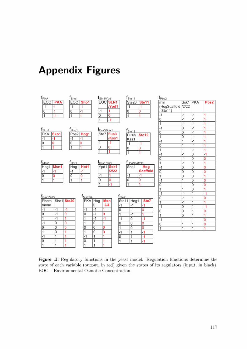
Appendix Figures
fPKA
EOC PKA
-1 1 0 1 1 -1
fSho1 EOC Sho1
-1 -1 0 -1 1 1
fSln1/Ypd1 EOC SLN1
/Ypd1
-1 1 0 0 1 -1
fSte11 Ste20 Ste11
-1 -1 0 0 1 1
fSko1 PKA Sko1
-1 -1 0 0 1 1
fHog1
Pbs2 Hog1
-1 -1 0 0 1 1
fFus3/Kss1 Ste7 Fus3
/Kss1
1 -1 0 0 1 1
fSte12
Fus3/ Kss1
Ste12
-1 -1 0 0 1 1
fMsn1 Hog1 Msn1
-1 -1 0 0 1 1
fHot1 Hog1 Hot1
-1 -1 0 0 1 1
fSsk1/2/22 Ypd1 Ssk1
/2/22
-1 1 0 0 1 -1
fHogScaffold Sho1 Hog
Scaffold
-1 -1 0 0 1 1
fSsk1/2/22 Pheromone
Sho1 Ste20
-1 -1 -1 0 -1 0 1 -1 1 -1 0 0 0 0 0 1 0 1 -1 1 1 0 1 1 1 1 1
fMsn2/4 PKA Hog
0 Msn 2/4
-1 -1 1 0 -1 0 1 -1 -1 1 0 1 0 0 0 1 0 0 -1 1 1 0 1 1 1 1 1
fSte7 Ste11 Hog1 Ste7
-1 -1 -1 0 -1 0 1 -1 1 -1 0 -1 0 0 0 1 0 0 -1 1 -1 0 1 -1 1 1 -1
fPbs2 min (HogScaffold, Ste11)
Ssk1/2/22
PKA Pbs2
-1 -1 -1 1 0 -1 -1 1 1 -1 -1 1 -1 0 -1 1 0 0 -1 1 1 0 -1 1 -1 1 -1 1 0 1 -1 1 1 1 -1 1 -1 -1 0 -1 0 -1 0 0 1 -1 0 1 -1 0 0 0 0 0 0 0 1 0 0 1 -1 1 0 0 0 1 0 0 1 1 0 1 -1 -1 1 -1 0 -1 1 0 1 -1 1 1 -1 0 1 -1 0 0 1 0 1 0 1 1 -1 1 1 0 0 1 1 0 1 1 1 1
Figure .1: Regulatory functions in the yeast model. Regulation functions determine thestate of each variable (output, in red) given the states of its regulators (input, in black).EOC – Environmental Osmotic Concentration.
117

Appendix Figures
Performed Experiment Modeled experiment Experimental
Study ED***
# Stimulation**** Perturbation Stimulation Perturbation
ME
ED
M-T
OP
OL
Barr
et
and
Pals
son
Ideker
et
al.
1 Control STE11 KO* EOC:0 Pheromone:0 Ste11:0 (Roberts et al., 2000)
2 Control SLN1 KO EOC:0 Pheromone:0 Sln1Ypd1:0 (Mnaimneh et al., 2004)
5 4 6
3 Control HOG1 KO EOC:0 Pheromone:0 Hog1:0 (Hahn et al., 2004)
4 Control STE7 KO EOC:0 Pheromone:0 Ste7:0 (Roberts et al., 2000)
8
5 Control KSS1 KO EOC:0 Pheromone:0 Kss1/Fus3:0 (Roberts et al., 2000)
6 Control STE12 KO EOC:0 Pheromone:0 Ste12:0 (Roberts et al., 2000)
7 Control STE12 OE EOC:0 Pheromone:0 Ste12:2 (Chua et al., 2006) 9 10 6 8 Control MSN1 KO EOC:0 Pheromone:0 Msn1:0 (Hahn et al., 2004) 11 9 Control SKO1 KO EOC:0 Pheromone:0 Sko1:0 (Hahn et al., 2004) 2 12
10 Control MSN2 KO EOC:0 Pheromone:0 Msn2Msn4:0 (Hahn et al., 2004) 11 Control MSN2 OE** EOC:0 Pheromone:0 Msn2Msn4:2 (Chua et al., 2006) 11 13 11 7
12 50aF in 30min - EOC:0 Pheromone:2 - (Roberts et al., 2000)
13 50aF in 30min STE20 KO EOC:0 Pheromone:2 Ste20:0 (Roberts et al., 2000)
2 9
14 50aF in 30min FUS3D KO EOC:0 Pheromone:2 Kss1/Fus3:0 (Roberts et al., 2000)
4 9
15 50aF in 30min STE12 KO EOC:0 Pheromone:2 Ste12:0 (Roberts et al., 2000)
5
16 0.125M KCl in
20min - EOC:1 Pheromone:0 -
(O'Rourke and Herskowitz, 2004)
17 0.125M KCl in
20min STE11 KO EOC:1 Pheromone:0 Ste11:0
(O'Rourke and Herskowitz, 2004)
18 0.125M KCl in
20min SSK1 KO EOC:1 Pheromone:0 Ssk1/2/22:0
(O'Rourke and Herskowitz, 2004)
10
19 0.125M KCl in
20min HOG1 KO EOC:1 Pheromone:0 Hog1:0
(O'Rourke and Herskowitz, 2004)
20 0.5M KCl in
40min - EOC:2 Pheromone:0 -
(O'Rourke and Herskowitz, 2004)
1
21 0.5M KCl in
40min SHO1 KO EOC:2 Pheromone:0 Sho1:0
(O'Rourke and Herskowitz, 2004)
8 1
22 0.5M KCl in
40min STE11 KO EOC:2 Pheromone:0 Ste11:0
(O'Rourke and Herskowitz, 2004)
10 3 8
23 0.5M KCl in
40min SSK1 KO EOC:2 Pheromone:0 Ssk1/2/22:0
(O'Rourke and Herskowitz, 2004)
7 5
24 0.5M KCl in
40min PBS2 KO EOC:2 Pheromone:0 Pbs2:0
(O'Rourke and Herskowitz, 2004)
3 6
25 0.5M KCl in
40min HOG1 KO EOC:2 Pheromone:0 Hog1:0
(O'Rourke and Herskowitz, 2004)
6 7 7 5
ME
ED
M-T
OP
OL
Ba
rre
t a
nd
P
alls
on
Ide
ker
et a
l.
Figure .2: 25 candidate experiments on the yeast model. *KO – knock-out; **OE – over-expression; ***The numbers indicate the order in which the experiments were chosen byeach method; ****The time point between 20 and 40min is the peak immediate gene ex-pression response to the pathway.
118

Notation and Definitions
All chapters
BGMM . . . . . . . . belief-based Gaussian mixture modelingMEED . . . . . . . . . model expansion experimental designJODA. . . . . . . . . . joint deregulation analysisFDR . . . . . . . . . . . false discovery ratePOE . . . . . . . . . . Probability Of ExpressionGO . . . . . . . . . . . . Gene Onthology
Chapter 1
DNA . . . . . . . . . . . deoxyribonucleic acidRNA . . . . . . . . . . . ribonucleic acidmRNA . . . . . . . . . messenger RNATF . . . . . . . . . . . . . transcription factorPCR . . . . . . . . . . . polymerase chain reactionRNAi . . . . . . . . . . RNA interferencedsRNA . . . . . . . . . double-stranded RNAsiRNA . . . . . . . . . short interfering RNAshRNA . . . . . . . . . small hairpin RNARISC. . . . . . . . . . . RNA-induced silencing complex
119

Appendix Figures
Chapter 2
X = {x1, ..., xN} dataset of N observationsY = {1, ..., K} . . set of K clustersk . . . . . . . . . . . . . . . cluster or model component, k ∈ YM . . . . . . . . . . . . . number of examplesP . . . . . . . . . . . . . probability of an eventY1, ..., YN . . . . . . random variables with values in Yπk . . . . . . . . . . . . . . mixing proportion or prior of the mixture component kM(1, π1, ..., πK) . multinomial distribution with probabilities π1, ..., πKπ = {π1, ..., πK} set of mixing proportions for all componentsR . . . . . . . . . . . . . . set of real numbersX1, ..., XN . . . . . random variables with values in Rf(xi|Yi = k) . . . . density function of the variable Xi given the value of variable Yiθk . . . . . . . . . . . . . . parameters of the density function f (in chapter 2 Gaussian with
mean µk and variance σ2k)
θ = {θ1, ..., θK} set of Gaussian parameters for all componentsΨ = {π, θ} . . . . . all parameters of a mixture modelΨK . . . . . . . . . . . . . all parameters of a mixture model with K componentsε . . . . . . . . . . . . . . . minimal accepted change in log likelihood in subsequent itera-
tions (stop criterion)Q . . . . . . . . . . . . . . maximal number of iterations (stop criterion)q . . . . . . . . . . . . . . . iteration numberXs . . . . . . . . . . . . . input dataset in the fully supervised modelingzi . . . . . . . . . . . . . . indicator function, for observation xi, its cluster label yi and
cluster k returns value 1 if yi = k, and 0 otherwise.zik . . . . . . . . . . . . . value of function zi for cluster kl(·) . . . . . . . . . . . . . log likelihoodtik . . . . . . . . . . . . . . posterior probability for observation xi to belong to cluster kXs . . . . . . . . . . . . . input dataset in fully supervised modelingXss . . . . . . . . . . . . input dataset in semi-supervised modelingXp . . . . . . . . . . . . . input dataset in soft-label modelingXb . . . . . . . . . . . . . input dataset in belief-based modelingbik = P (Yi = k) . belief for observation xi and cluster kb = {b1, ..., bK} . set of all beliefsp = {p1, ..., pK} set of all plausibilitiesU(·, ·) . . . . . . . . . Uniform distributionG(·, ·) . . . . . . . . . . Gaussian distributionmiRNA . . . . . . . . microRNAdifferential . . . . . differentially expressedEM . . . . . . . . . . . . Expectation MaximizationMAP. . . . . . . . . . . maximum a posterioriNorDi . . . . . . . . . . Normal DiscretizationAIC . . . . . . . . . . . . Akaike Information CriterionBIC . . . . . . . . . . . Bayesian Information Criterion
120

Chapter 3
M . . . . . . . . . . . . . logical modelV . . . . . . . . . . . . . model variablesU = {1, ..., k} . . . discrete states that the model variables may attainPa(v) . . . . . . . . . . parents of a model variable v ∈ Vfv . . . . . . . . . . . . . . regulation function, defines state of v ∈ V given its parents’
statesF . . . . . . . . . . . . . set of regulation functionsG = (V,A) . . . . . model graph with nodes in V and edges in AI . . . . . . . . . . . . . . . model stimulatorsP . . . . . . . . . . . . . . model variables that are subject to perturbatione . . . . . . . . . . . . . . . experimentE . . . . . . . . . . . . . . set of experimentss . . . . . . . . . . . . . . . model statese . . . . . . . . . . . . . . model state predicted for experiment ese(v) . . . . . . . . . . . e-predicted state of variable vF . . . . . . . . . . . . . feedback seteS . . . . . . . . . . . . . observed partial state for experiment eD(se, e) . . . . . . . . discrepancy between experiment e and model state seR . . . . . . . . . . . . . . set of regulatorsr . . . . . . . . . . . . . . regulatory programT (e). . . . . . . . . . . . partition induced by experiment eS(E) . . . . . . . . . . partition induced by set of experiments EM . . . . . . . . . . . . . matchingH(E) . . . . . . . . . . entropy score of experiment set EH(e|E) . . . . . . . . entropy gain with adding experiment e to experiment set EP . . . . . . . . . . . . . set of partitionsP+ . . . . . . . . . . . . . closure of a set of partitions P under finite intersections⋂P . . . . . . . . . . . . intersection of all partitions from a set P
T, T ′, T ′′ . . . . . . . . partition in PS, S ′, S ′′ . . . . . . . . partition in P+
{R} . . . . . . . . . . . full (one block) partition of a set RidR . . . . . . . . . . . . identity partition of a set R into singletonsT ′′ ≤ T ′ . . . . . . . partition T ′′ is included in T ′
Φ . . . . . . . . . . . . . . class of strictly increasing functions satisfying (A0) and (A1)∆T . . . . . . . . . . . . . gain function determined by a function in Φ and a partition Tρ . . . . . . . . . . . . . . a function in ΦED. . . . . . . . . . . . . experimental designFUP . . . . . . . . . . . fraction of undistinguished pairsNP . . . . . . . . . . . . . nondeterministic polynomial time class of problem complexity3DM . . . . . . . . . . . 3-DIMENSIONAL MATCHINGILP . . . . . . . . . . . . integer linear programmingTNF . . . . . . . . . . . Tumor Necrosis FactorEOC . . . . . . . . . . . environmental osmotic concentration
121

Appendix Figures
Chapter 4
t . . . . . . . . . . . . . . . cell populationV = {v1, ..., vn} set of regulatorsGt = (V,At) . . . . pathway topology in a cell population t with set of nodes V and
directed edges At
∆tv . . . . . . . . . . . . perturbation of v in a given cell population tEt . . . . . . . . . . . . . . set of all experiments perturbing regulators in V in cell popula-
tion tG∗t . . . . . . . . . . . . . transitive reflexive closure of given pathway topology Gt
Mt . . . . . . . . . . . . model matrixEv,t . . . . . . . . . . . . set of all perturbation experiments that affect regulator v in cell
population th . . . . . . . . . . . . . . population of healthy cellsd . . . . . . . . . . . . . . population of damaged cellsptv . . . . . . . . . . . . . vector of signed differential expression probabilities of the genes
for perturbation of v in cell population tRt
v . . . . . . . . . . . . vector of regulation scores of the genes for regulator v in cellpopulation t
Dv . . . . . . . . . . . . vector of deregulation scores of the genes for regulator vNCS . . . . . . . . . . . neocarzinostatinderegulation list list of deregulation scoresGSEA. . . . . . . . . . Gene Set Enrichment AnalysisORC . . . . . . . . . . origin of replication complex
122

Zusammenfassung
Die vorliegende Doktorarbeit befasst sich mit der Aufklarung der Regulierung vonGenexpression im Kontext von bekannten zellularen Signalwegen und reguliertenGenen. Wir analysieren Daten von experimentellen Interventionen, die auf Sig-nalkomponenten zielen. Solche Experimente verursachen Anderungen in der Genex-pression der durch den Signalweg regulierten Genen. Die in dieser Doktorarbeit en-twickelten Ansatze losen verschiedene Probleme im Bereich der Kontext-spezifischenGenregulierung.
In Kapitel 2 entwickeln wir eine Methode zur differentiellen Expressionsanalyse der In-terventionsdaten, die vorgegebene Beispiele differentieller Gene nutzt. Hochdurchsatz-Genexpressionsexperimente ermoglichen einen Vergleich zweier experimenteller Be-dingungen. Die Messungen werden einer Analyse unterzogen, um die Gruppen vonGenen zu bestimmen, die unter einer der Bedingungen hoch- oder herunterreguliertwerden, oder deren Expression gleich bleibt. Mittels Expertenwissen konnen bes-timmte Gene diesen verschiedenen Gruppen zuordnen werden. Zum Beispiel er-wartet man, dass Gene, die von einem transkriptionellen Aktivator reguliert werden,nach dem Ausschalten dieses Aktivators herunterreguliert werden. Etablierte Metho-den zur differentiellen Expressionsanalyse ignorieren solch unprazise Beispiele, unsereschließt sie systematisch mit ein. Wir benutzen sogennante partially supervised Mis-chmodellierung, die eindimensionale Expressionsdaten in Gruppen von differentiellregulierten und unveranderten Genen aufteilt und dabei von unprazisen Beispielenprofitiert. Dieser Ansatz wird von zwei Methoden realisiert: einer neuen belief-basedMischmodellierung, die wir hier vorstellen, und der fruher entwickelte soft-label Mis-chmodellierung. Tests zeigen, dass sowohl die belief-based als auch die soft-label Meth-ode falsche Beispiele besser korrigieren als die semi-supervised Mischmodellierung.Wir vergleichen unsere partially supervised Methodik auch mit alternativen Ansatzenzur differentiellen Expressionsanalyse und zeigen, dass die Aufnahme von unprazisemWissen bessere Ergebnisse erzeugt. Wir prasentieren verschiedene Anwendungen derMethodik.
In Kapitel 3 befassen wir uns mit der Planung von Interventionsexperimenten fureinen gegebenen Signalweg. Fur die systematische Rekonstruktion der Genregula-tion durch einen Signalweg werden informative experimentelle Daten benotigt. Wirstellen einen allgemeinen Ansatz fur diese Rekonstruktion vor. MEED, eine experi-mentelle Design-Komponente unseres Ansatzes, schlagt eine moglichst kleine Anzahlvon gezielten Interventionsexperimenten in dem Signalweg vor. Um Mehrdeutigkeit inder Identifizierung der Regulierungsverhaltnisse zu vermeiden, maximiert die Auswahl
123

Zusammenfassung
der Experimente den Unterschied zwischen Expressionsprofilen von Genen, die durchverschiedene Mechanismen reguliert werden. Mittels eines pradiktiven logischen Mod-ells bezieht dieser Ansatz auch Expertenwissen uber die Signalwege mit ein. MEEDberucksichtigt prognostizierte Abhangigkeiten zwischen Experimenten und kann soeinen ganzen Satz Experimente vorschlagen, die gleichzeitig durchgefuhrt werdenkonnen. Wir wenden unseren Ansatz auf verbundene Signalwege in der Hefe Sac-charomyces cerevisiae an. Im Vergleich zu anderen Methoden schlagt MEED dieinformativsten Experimente fur unzweideutige Identifizierung von transkriptionellerRegulation in diesem System vor.
In Kapitel 4 stellen wir eine Anwendung zur Deregulationsanalyse vor, d.h., zumVergleich von Anderungen in der Genregulierung zwischen zwei Zellpopulationen.Vorhandene Deregulationsstudien lassen verfugbares Wissen uber den zellularen Kon-text dieser Anderungen außer acht. Wir untersuchen Deregulation mittels zellpopu-lationsspezifische Interventionsdaten, und mittels zusatzlichen Wissens, das fur beideZellpopulationen uber der Signalweg-Topologien und Gene, die von diesem Signal-weg reguliert werden, gegeben ist. Unser Ansatz verbindet Ideen aus den vorherigenKapiteln. Die bekannten regulierten Gene werden als Beispiele von differentiellenGenen in der partially supervised differentiellen Expressionsanalyse der Interventions-daten (Kapitel 2) benutzt. Die Signalweg-Topologien werden als einfache Modelleformalisiert und in der Rekonstruktion der Genregulierung wie in Kapitel 3 genutzt.Wir quantifizieren Deregulation durch die Zusammenfassung von Regulierungssig-nalen der zwei Zellpopulationen in einen Wert. Unser Ansatz, JODA, stellt sich alsvorteilhaft gegenuber separater Analyse der Zellpopulationen, sowie Analyse ohneAufnahme von verfugbarem Wissen heraus. Mittels JODA charakterisieren wir weitverbreitete Veranderungen der regulatorischen Netzwerke, die durch DNA Schadenin menschlichen Zellen verursacht sind.
124

Curriculum Vitae
For reasons of data protection,the curriculum vitae is not included in the online version.
125

Curriculum Vitae
For reasons of data protection,the curriculum vitae is not included in the online version.
126

For reasons of data protection,the curriculum vitae is not included in the online version
127

Ehrenwortliche Erklarung
Hiermit erklare ich, dass ich diese Arbeit selbststandig verfasst und keine anderen alsdie angegebenen Hilfsmittel und Quellen verwendet habe.
Berlin, Oktober 2010 Ewa Szczurek