Zurich Open Repository andArchiveUniversity of ZurichMain LibraryStrickhofstrasse 39CH-8057 Zurichwww.zora.uzh.ch

Year: 2012

Monitoring the spectral performance of the APEX imaging spectrometer forinter-calibration of satellite missions

D’Odorico, Petra

Abstract: Die Fernerkundung ist heutzutage wahrscheinlich die wertvollste Methode um Parameter, dieProzesse unserer Umwelt definieren, quantitativ und global zu messen. Für eine korrekte Interpretationdieser Messungen ist das Verständnis aller Faktoren die den Messprozess beeinflussen entscheidend. ImIdealfall beinhaltet die Messung des reflektierten Sonnenlichts ausschließlich Informationen über das re-flektierende Objekt oder Phänomen. Dies ist jedoch selten der Fall, da Interaktionen mit der Atmosphäre,eine Kontaminierung durch den Hintergrund und die Instrumenteigenschaften die Zusammensetzung undAusbreitung der Sonnenstrahlung verändern. Für spektroskopiedaten-basierte Anwendungen sind diespektralen Eigenschaften des Instruments normalerweise die wichtigsten Parameter um eine korrekte In-terpretation der Messung zu gewährleisten. Das spektrale Ansprechverhalten einzelner Detektorpixelwird über deren Zentrumswellenlänge sowie der Halbwertsbreite beschrieben und definiert damit diespektralen Eigenschaften des Instruments. Um die spektralen Eigenschaften des Instruments zu bestim-men, werden entsprechend Charakterisierung Messungen im Labor durchgeführt. Das Instrument ist je-doch an Bord einer luft- oder weltraumgestützten Plattform variierenden umweltbedingten Stressfaktorenausgesetzt (z. B. Vibrationen, Temperatur und Druckkraft Schwankungen). Diese führen, zusammenmit dem natürlichen Alterungsprozess, zur Veränderung der spektralen Eigenschaften und Performancedes Instruments. Werden solche Veränderungen nicht berücksichtigt, sondern weiterhin die im Laborcharakterisierten spektralen Parameter zur Verarbeitung der Daten verwendet, kann das zu signifikantenFehlern im Datensatz und der daraus abgeleiteten Produkte führen. Diese Dissertation untersucht dieEigenschaften und Ursachen für Änderungen der Charakteristik eines Spektrometers unter realen Bedin-gungen im Flugzeug. Dazu wurden neue Ansätze zum Monitoring der spektralen Eigenschaften einesflugzeuggestützten Sensors entwickelt und validiert. Die durch die Messungen beobachteten Abweichun-gen im Vergleich zu den Labormessungen werden genutzt um die Rohdaten vor einer Produktgenerierungentsprechend zu korrigieren. Das abbildende Spektrometer APEX (Airborne Prism EXperiment) stehtim Fokus dieser Recherche. APEX ist ein dispersives, abbildendes pushbroom Spektrometer, das denWellenlängenbereich zwischen 380 und 2500 nm abdeckt. APEX wurde entwickelt um gegenwärtige sowiezukünftige weltraumgestützte Missionen bei der Simulation, Kalibration und Validation zu unterstützen.Die Möglichkeit der in-flight Charakterisierung mittels eines auf APEX integrierten CharakterisierungsEquipments, bekannt als In-Flight Characterization (IFC) facility, ermöglicht die Messung der spektralenEigenschaften des Sensors ausserhalb von Laborbedingungen. Gezielte Erfassung von IFC Messungen undProzessierung mit Hilfe von ad-hoc entwickelten Algorithmen ermöglichte die Schätzung repräsentativerspektraler Parameter für ein luftgestütztes Instrument zu jedem Zeitpunkt. Ausserdem werden atmo-sphärische Absorptionsbanden aus Luftbilddaten verwendet, um die Schätzung der spektralen Parameterzusätzlich zu ergänzen und zu validieren. Dadurch konnte die Korrektur der Wellenlängenpositionenplausibel auf die APEX Datensätze angewendet werden. Die so kalibrierten APEX Daten werden er-folgreich für eine Simulation und Kalibration ausgewählter weltraumgestützter Missionen verwendet. Inder Diskussion der Forschungsergebnisse werden die Vor- und Nachteile der entwickelten Ansätze be-sprochen und es wird auf mögliche Verbesserungen hingewiesen. Abschliessend wird ein Ausblick fürweiterführende Arbeiten gegeben.

Posted at the Zurich Open Repository and Archive, University of ZurichZORA URL: https://doi.org/10.5167/uzh-71668DissertationPublished Version

Originally published at:D’Odorico, Petra. Monitoring the spectral performance of the APEX imaging spectrometer for inter-calibration of satellite missions. 2012, University of Zurich, Faculty of Science.

2

v

Remote Sensing LaboratoriesDepartment of Geography University of Zurich, 2012

Remote SenSing SeRieS 63

ISBN Nr. 978-3-03703-029-5 63

Pet

Ra D

’oD

oR

ico

Mon

itori

ng th

e Sp

ectr

al P

erfo

rman

ce o

f the

APE

X Im

agin

g Sp

ectr

omet

er

PetRa D’oDoRico

Monitoring the Spectral Performance of the APEX Imaging Spectrometer for Inter-Calibration of Satellite Missions

Remote Sensing LaboratoriesDepartment of Geography University of Zurich, 2012

Remote SenSing SeRieS 63

PetRa D’oDoRico

Monitoring the Spectral Performance of the APEX Imaging Spectrometer for Inter-Calibration of Satellite Missions

Front page: picture of refracted rainbow (source: http://www.lightingsciences.ca/).

Editorial board of the Remote Sensing Series: Prof. Dr. Michael E. Schaepman, Dr. Erich Meier, Dr. Mathias Kneubühler, Dr. David Small, Dr. Felix Morsdorf.

This work was approved as a PhD thesis by the Faculty of Science of the University of Zurich in the spring semester 2012. Doctorate committee: Prof. Dr. Michael E. Schaepman (chair), Dr. Mathias Kneubühler, Dr. Michael Jehle. External examiner: Dr. Nigel Fox, National Physical Laboratory (NPL), UK.

© 2012 Petra D’Odorico, University of Zurich. All rights reserved.

D’Odorico, Petra

Monitoring the Spectral Performance of the APEX Imaging Spectrometer for Inter-Calibration of Satellite Missions.

Remote Sensing Series, Vol. 63 Remote Sensing Laboratories, Department of Geography, University of Zurich Switzerland, 2012

ISBN: 978-3-03703-029-5

!III!

!

SUMMARY Remote sensing is possibly the most valuable technique available today to quantitatively measure variables defining our Earth system and processes. However, understanding all factors influencing the measurement process is required before a correct interpretation of the measurement can take place. Ideally, the measurement of solar radiation reflected by the surface carries information exclusively about the object or phenomenon under study. This is however never the case as interaction with the atmosphere, contamination by the background, and the instrument characteristics are responsible for changing the properties of the measured radiation.

For applications relying on spectroscopy data, instrument spectral characteristics are arguably the most important piece of information required for a correct interpretation of measurement. The Spectral Response Function (SRF), associated with each detector pixel and described by a center wavelength and a Full-Width-at-Half-Maximum (FWHM), synthesizes the spectral characteristics of the instrument. Measurements required to define instrument’s SRF are firstly carried out during laboratory characterization. It is however acknowledged that once the instrument becomes spaceborne or airborne, the stresses of the operational environment (e.g., vibrations, temperature and pressure variations) and the natural aging of the system lead to changes in instrument spectral characteristics and related performance. Ignoring these changes and relying on nominal spectral parameters characterized in the laboratory, can lead to errors in the final data sets and derived products.

This dissertation investigates the properties and the causes of instrument spectral performance changes in an airborne environment. A new approach has been developed and validated for monitoring in-flight instrument spectral characteristics, which has eventually been used to compensate the observed variations during spectroscopy data processing. The Airborne Prism EXperiment (APEX) imaging spectrometer is at the center of this investigation. APEX is an airborne dispersive pushbroom imaging spectrometer operating in the wavelength domain between 380 and 2500 nm. It is designed to serve as a simulation, validation and calibration sensor for current and future spaceborne missions. APEX’s unique feature is the inclusion of onboard characterization equipment in the instrument design, known as the In-Flight Characterization (IFC) facility. By targeted acquisition of IFC measurements and processing via ad-hoc developed algorithms, it is possible to estimate the in-flight updated spectral parameters of the instrument. Vicarious (i.e., scene-based) calibration approaches relying on atmospheric absorption features were employed to complement and validate the estimation of instrument spectral parameters. The compensation of the in-flight wavelength position shifts has been demonstrated to produce reliable results when applied to APEX operational data. Calibrated APEX data were successfully employed for the simulation and cross-calibration of current and future satellite sensors spectral performances. A discussion of the main findings highlights advantages and limitations of the proposed techniques and suggests possible improvements as well as future perspectives for the continuation of this work.

!

!

!V!

!

ZUSAMMENFASSUNG Die Fernerkundung ist heutzutage wahrscheinlich die wertvollste Methode um Parameter, die Prozesse unserer Umwelt definieren, quantitativ und global zu messen. Für eine korrekte Interpretation dieser Messungen ist das Verständnis aller Faktoren die den Messprozess beeinflussen entscheidend. Im Idealfall beinhaltet die Messung des reflektierten Sonnenlichts ausschließlich Informationen über das reflektierende Objekt oder Phänomen. Dies ist jedoch selten der Fall, da Interaktionen mit der Atmosphäre, eine Kontaminierung durch den Hintergrund und die Instrumenteigenschaften die Zusammensetzung und Ausbreitung der Sonnenstrahlung verändern.

Für spektroskopiedaten-basierte Anwendungen sind die spektralen Eigenschaften des Instruments normalerweise die wichtigsten Parameter um eine korrekte Interpretation der Messung zu gewährleisten. Das spektrale Ansprechverhalten einzelner Detektorpixel wird über deren Zentrumswellenlänge sowie der Halbwertsbreite beschrieben und definiert damit die spektralen Eigenschaften des Instruments. Um die spektralen Eigenschaften des Instruments zu bestimmen, werden entsprechend Charakterisierung Messungen im Labor durchgeführt. Das Instrument ist jedoch an Bord einer luft- oder weltraumgestützten Plattform variierenden umweltbedingten Stressfaktoren ausgesetzt (z. B. Vibrationen, Temperatur und Druckkraft Schwankungen). Diese führen, zusammen mit dem natürlichen Alterungsprozess, zur Veränderung der spektralen Eigenschaften und Performance des Instruments. Werden solche Veränderungen nicht berücksichtigt, sondern weiterhin die im Labor charakterisierten spektralen Parameter zur Verarbeitung der Daten verwendet, kann das zu signifikanten Fehlern im Datensatz und der daraus abgeleiteten Produkte führen.

Diese Dissertation untersucht die Eigenschaften und Ursachen für Änderungen der Charakteristik eines Spektrometers unter realen Bedingungen im Flugzeug. Dazu wurden neue Ansätze zum Monitoring der spektralen Eigenschaften eines flugzeuggestützten Sensors entwickelt und validiert. Die durch die Messungen beobachteten Abweichungen im Vergleich zu den Labormessungen werden genutzt um die Rohdaten vor einer Produktgenerierung entsprechend zu korrigieren. Das abbildende Spektrometer APEX (Airborne Prism EXperiment) steht im Fokus dieser Recherche. APEX ist ein dispersives, abbildendes pushbroom Spektrometer, das den Wellenlängenbereich zwischen 380 und 2500 nm abdeckt. APEX wurde entwickelt um gegenwärtige sowie zukünftige weltraumgestützte Missionen bei der Simulation, Kalibration und Validation zu unterstützen. Die Möglichkeit der in-flight Charakterisierung mittels eines auf APEX integrierten Charakterisierungs Equipments, bekannt als In-Flight Characterization (IFC) facility, ermöglicht die Messung der spektralen Eigenschaften des Sensors ausserhalb von Laborbedingungen. Gezielte Erfassung von IFC Messungen und Prozessierung mit Hilfe von ad-hoc entwickelten Algorithmen ermöglichte die Schätzung repräsentativer spektraler Parameter für ein luftgestütztes Instrument zu jedem Zeitpunkt. Ausserdem werden atmosphärische Absorptionsbanden aus Luftbilddaten verwendet, um die Schätzung der spektralen Parameter zusätzlich zu ergänzen und zu validieren. Dadurch konnte die Korrektur der Wellenlängenpositionen plausibel auf die APEX Datensätze angewendet werden. Die so kalibrierten APEX Daten werden erfolgreich für eine Simulation und Kalibration ausgewählter weltraumgestützter Missionen verwendet. In der Diskussion der Forschungsergebnisse werden die Vor- und Nachteile der entwickelten Ansätze besprochen und es wird auf mögliche Verbesserungen hingewiesen. Abschliessend wird ein Ausblick für weiterführende Arbeiten gegeben.

!

!

!VII!

!

TABLE OF CONTENTS SUMMARY'............................................................................................................................'III!

ZUSAMMENFASSUNG'............................................................................................................'V!

TABLE'OF'CONTENTS'...........................................................................................................'VII!

1! INTRODUCTION'...............................................................................................................'9!

1.1! OPTICAL'REMOTE'SENSING'.................................................................................................'9!1.2! SPECTRAL'RESPONSE'MODEL'FOR'IMAGING'SPECTROMETERS'....................................................'10!1.3! CALIBRATION'OF'SPECTRAL'PERFORMANCE'...........................................................................'13!1.4! MONITORING'OF'SPECTRAL'PERFORMANCE'IN'AN'OPERATIONAL'ENVIRONMENT'...........................'15!1.5! OBJECTIVE'AND'RESEARCH'QUESTIONS'................................................................................'17!1.6! STRUCTURE'OF'THE'DISSERTATION'......................................................................................'18!1.7! REFERENCES'..................................................................................................................'19!

2! APEX'E'CURRENT'STATUS,'PERFORMANCE'AND'PRODUCT'GENERATION'.......................'23!

3! INEFLIGHT'SPECTRAL'PERFORMANCE'MONITORING'OF'APEX'........................................'31!

4! PERFORMANCE'ASSESSMENT'OF'ONBOARD'AND'SCENEEBASED'METHODS'FOR'APEX'SPECTRAL'CHARACTERIZATION'............................................................................................'43!

5! EXPERIMENTAL'EVALUATION'OF'SENTINELE2'SPECTRAL'RESPONSE'FUNCTION'FOR'NDVI'TIMEESERIES'CONTINUITY'....................................................................................................'55!

6! SYNOPSIS'......................................................................................................................'71!

6.1! MAIN'RESULTS'...............................................................................................................'71!6.2! CONCLUSIONS'AND'OUTLOOKS'..........................................................................................'74!6.3! REFERENCES'..................................................................................................................'77!

CURRICULUM'VITAE'............................................................................................................'79!

ACKNOWLEDGEMENTS'........................................................................................................'83!

!

!

!9!

!

1 INTRODUCTION

1.1 Optical remote sensing

Remote sensing is the science of obtaining information about an object, area, or phenomenon through the analysis of data acquired by a device that is not in proximity of the object, area, or phenomenon under study (Lillesand et al., 2004). The remotely collected data can be of many forms, including force distribution, acoustic wave distributions, or electromagnetic energy distributions. In remote sensing of electromagnetic (EM) energy, a wide branch is dedicated to the optical region of the EM spectrum traditionally encompassing the wavelength range from 10 nm to 1000 µm. This range includes the measurements of the reflective spectral radiances in ultraviolet, visible and infrared sub-regions (approximately from 350 to 2500 nm) commonly used for land remote sensing. In this region of the EM spectrum, the sun acts as a natural source of radiation and provides all the necessary energy for physical and chemical processes on Earth (Palmer et al., 2009).

Spectral radiance is the radiometric measure that describes the amount of electromagnetic radiation that passes through or is emitted from a particular area, and falls within a given solid angle in a specified direction at a certain wavelength (Kostkowski, 1997). It is expressed in W m-2 sr-1 nm-1. It is used to characterize both emission from diffuse sources (e.g., the sun) and reflection from diffuse surfaces (e.g., the target). By integrating over the solid angle, other radiometric measures may be derived from radiance. Irradiance (W m-2) refers to the power per unit area that is incident on a surface and radiant exitance (W m-2) to the power per unit area leaving a source. The ratio between radiance exitance and irradiance is known as reflectance (Martonchik et al., 2000). Each material interacting with solar radiation reflects (or emits), transmits and absorbs energy according to its atomic structure such that it can be characterized through its reflectance profile, referred to as spectral signature (Price, 1994).

To fully understand the measurement of a spectral signature characterizing a certain material, we must understand the process of generation, transmission and detection of optical radiation. This process usually involves a system composed of a radiation source, a propagation medium, a target interacting with the radiation and a sensor measuring the radiation (Lillesand et al., 2004). Ideally, in such a system, the measurement of the signal by a specific sensor would result in complete and exclusive information about the target or phenomenon being observed. In reality, however, a number of factors other than the target are known to play a role in determining what is being measured (Jones et al., 2010). As both source and detector are ‘remote’ from the target, the characteristics of the radiation detected by the sensor are affected not only by its reflection/emission from the target but also by interactions with the intervening atmosphere (de Haan et al., 1991). Attenuation and scattering of solar radiation in the atmosphere both on its way to the surface and, after reflection back to the detector lead to a change in the radiation intercepted by the sensor as compared to the hypothetical (atmosphere-free) observation (Tanre et al., 1979). When the atmosphere is not itself the subject of investigation, its contribution is regarded as noise and has to be removed in order to isolate the useful signal from the surface target (Jones et al., 2010). This effort is referred to as atmospheric correction (Gao et al., 2009). An additional source of unwanted radiation comes from the surrounding ground pixels that may be in or in proximity of the instrumental field of view. This leads to an unwanted effect known as adjacency effect, and contributes towards the at-sensor radiance over a target pixel. The adjacency effect is low when the surface reflectance of the target ground pixel is at least as large as that of the surrounding ground pixels, but greater when the target pixel reflectance is lower than that of the surrounding (Jones et al., 2010). Apposite correction procedures are applied to correct for this effect often in combination with atmospheric correction (Kerekes, 2009; Tanre et al., 1981). Last but not least, the radiation reflected/emitted by the target is influenced by the sensor design. The limits of instrument

!10!

!

characteristics and associated performance can affect the accuracy, validity, consistency and inter-comparability of acquired data (Gaddis et al., 1996; Nieke et al., 2008). Technological advancements in instrument design constantly force these instrument-derived limits, opening ways for new Earth observation data products. An important advancement was the realization, beginning of the eighties, that it was technically feasible to fly imaging spectrometers from aircraft and spacecraft. This enabled the remote measurement of laboratory-like spectra allowing the quantification of earth materials based on their biogeochemical composition (Goetz et al., 1985). The increased spectral detail in the signature of a material acquired by a spectrometer, derives from measuring the reflected light in many, narrow, contiguous wavelength intervals. This however implies more stringent spectral performance requirements, as even the slightest change in instrument spectral performance would significantly impact data and product integrity (Green, 1998; Nieke et al., 2008). An accurate and frequent instrument characterization is therefore critical to guarantee an up-to-date instrument calibration and thus reliable measurements of reflectance of a target of interest. Moreover, accurately calibrated spectrometers operated in the field or from airborne platforms represent an indispensable source of data for the simulation, cross-calibration and validation of spaceborne observations (Green et al., 2003; Teillet et al., 2001; Teillet et al., 2007).

1.2 Spectral response model for imaging spectrometers

Instrument characteristics inevitably transform the physical properties of the incoming radiation. This transformation corresponds to a degradation of the signal since no instrument is able to measure a physical quantity with infinite precision (Jansson, 1997). The limit in the amount of detail the instrument can capture is referred to as the instrument’s resolution (Schowengerdt, 1997). Understanding the nature of the signal degradation in relation to instrument’s resolution is crucial for enhanced sensor and algorithm design (Kerekes et al., 2005). A correct interpretation of the resulting information further depends on it. A discussion of these aspects can be found in Teillet et al. (1997) and more recently in Damm et al. (2011).

For remote sensing systems, resolution can refer to different domains, such as spectral, spatial and temporal. Moreover, there is a radiometric resolution associated to the gain values as a function of wavelength (Schowengerdt, 1997). In this dissertation, the main focus is on the spectral characteristics of an imaging spectrometer determining its spectral resolution and overall performance. Instrument spectral performance is arguably the most critical aspect of knowledge required for reliable spectroscopy (Bender et al., 2011). The American Society for Testing and Materials (ASTM) defines spectral resolution as the ratio λ/Δλ, where λ is the wavelength of radiant energy being examined and Δλ is the spectral width over which this energy is integrated expressed in wavelength units. By the Rayleigh criterion, which is often considered the working definition of resolution, two peaks are considered resolved when the maximum of one falls on the first minimum of the other (Jansson, 1997). Revisiting the definition of spectral resolution - and more in general the problem of instrument induced signal degradation - from an instrument point of view implies to familiarize oneself with a number of concepts, the most relevant of which are presented hereafter.

The response of the instrument as a function of wavelength is known as Spectral Response Function (SRF). Following Mouroulis et al. (2000a), we define the SRF of an instrument by a center wavelength position and a response shape (usually normalized to one). For spectrometers, acquiring radiation in many contiguous spectral bands, SRFs are commonly approximated by Gaussian shapes and the Full-Width-at-Half-Maximum (FWHM) is used to define the covered wavelength interval. The Spectral Sampling Interval (SSI) defines the spectral distance between the centers of adjacent spectral pixels (Brazile et al., 2008; Swayze et al., 2003) (Figure 1).

!11!

!

620 622 624 626 628 630 632 6340

0.1

0.2

0.3

0.4

0.5

0.6

0.7

0.8

0.9

1

wavelength (nm)

spectr

al re

sponse (

norm

aliz

ed)

Center Wavelength

Full-Width-at-Half-Maximum

(FWHM)

Spectral Sampling Interval

(SSI)

Figure 1 Spectral Response Function (SRF) and Spectral Sampling Interval (SSI).

From an instrument point of view, SRFs originate from the spectrally selective effects in the slit, the optics, the spectral selection elements and the detector spectral responsivity (Kerekes, 2009). A schematic view of the instrument components, leading to the definition of the SRF in a prism spectrometer, is shown in Figure!2.

light source

slit spectral dispersive element

collimating optics

2D detector array

target

camera optics

SPECTROMETER

Figure 2 A simple schematic of a spectrometer. All dispersive spectrometers have a spectral selection element, either a prism (this figure) or a grating, dispersing white light into its individual wavelengths.

We can think of the SRF as originating from the convolution of the slit image with the pixel response function, where the latter is simply assumed to be a rectangular function (rect(w2)). The slit image is itself a convolution of the slit, again a rectangular function (rect(w1)), and the optical Line Spread Function (LSF) in the tangential direction (Mouroulis et al., 2000a). Thus we have:

SRF = rect(w1) ⊗ LSF

T ⊗ rect(w

2) (1)

where w1 and w2 represent the width of the projected slit and of the detector pixel, respectively,

!12!

!

while ⊗ denotes convolution. In this work we will thus use the term slit image for the response of a spectrometer to the light source up to where it reaches the array detector and the term Spectral Response Function (SRF) for the slit image convolved with the detector pixel response.

As seen in the simplified spectrometer diagram shown in Figure 2, the white light reflected by the target entering the spectrometer slit is dispersed into its individual constituent wavelengths by means of a spectral selection element. Dispersive spectral selection works by spatially spreading out the radiation spectrum before focusing by the camera lenses on a linear or area array (Schmidt, 2005). The wavelength dispersive element can be a grating (diffraction) or a prism (refraction). The collimating optics (e.g., lenses, mirrors) deployed to obtain a parallel beam toward the dispersive element, the dispersive element itself and finally the camera optics focusing the spectrum on the detector, determine the optical quality of the system as defined by the LSF. Figure 3, adapted from an illustration by Lerner (2006), visualizes this concept.

FWHM

λ0 λ0

λ0 λ λ λ

Ｉλ Ｉλ

Ｉλ

a

b c

Natural spectrum of a monochromatic light

source.

Spectrum of a monochromatic light source recorded by a perfect

instrument.

Spectrum of a monochromatic light source recorded by a real

instrument. Figure 3 The natural spectrum of a monochromatic light source (a); the same light source imaged through a theoretically ‘perfect’ spectrometer (b); the monochromatic light imaged through a real spectrometer (c) (modified after Lerner 2006, p.719).

In Figure 3, the natural spectrum of an infinitely narrow monochromatic emission line is compared with its image on the focal plane of a ‘theoretical’ ideal instrument and of a real instrument. The center wavelength is defined as the peak response of the detector element to the emission line. For an ideal instrument the natural spectral width of the monochromatic light would be preserved when imaged on the focal plane, a real instrument, however, broadens it. This broadening is caused by the optical system itself and its inability to measure at infinitive precision (Lerner, 2006).

Eventually the slit image, dispersed by the dispersion element (e.g., prism) and possibly further spread by the optics, is sampled by the detector. The majority of spectrometers deploy array detectors where each detector element in the direction of the light dispersion (i.e., spectral pixel) provides a single reading, i.e., an individual measure of the amount of light incident upon it. The ratio between the width of the slit image (representing the resolution of our instrument, the FWHM in Figure 3c) and the SSI (i.e., pixel spacing on the array detector) in the same units (e.g., nm) is known as sampling ratio (Roscoe et al., 1996). The sampling ratio is what ultimately determines how well a spectrum can be reconstructed. If the resolution (FWHM) of the spectrometer is comparable or smaller than the pixel spacing, the spectrum is undersampled.

!13!

!

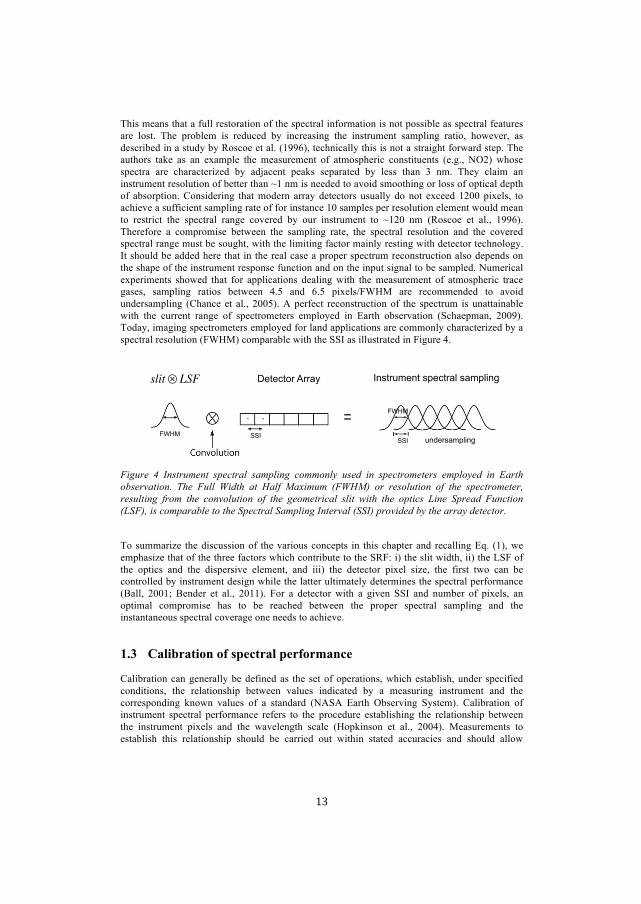
This means that a full restoration of the spectral information is not possible as spectral features are lost. The problem is reduced by increasing the instrument sampling ratio, however, as described in a study by Roscoe et al. (1996), technically this is not a straight forward step. The authors take as an example the measurement of atmospheric constituents (e.g., NO2) whose spectra are characterized by adjacent peaks separated by less than 3 nm. They claim an instrument resolution of better than ~1 nm is needed to avoid smoothing or loss of optical depth of absorption. Considering that modern array detectors usually do not exceed 1200 pixels, to achieve a sufficient sampling rate of for instance 10 samples per resolution element would mean to restrict the spectral range covered by our instrument to ~120 nm (Roscoe et al., 1996). Therefore a compromise between the sampling rate, the spectral resolution and the covered spectral range must be sought, with the limiting factor mainly resting with detector technology. It should be added here that in the real case a proper spectrum reconstruction also depends on the shape of the instrument response function and on the input signal to be sampled. Numerical experiments showed that for applications dealing with the measurement of atmospheric trace gases, sampling ratios between 4.5 and 6.5 pixels/FWHM are recommended to avoid undersampling (Chance et al., 2005). A perfect reconstruction of the spectrum is unattainable with the current range of spectrometers employed in Earth observation (Schaepman, 2009). Today, imaging spectrometers employed for land applications are commonly characterized by a spectral resolution (FWHM) comparable with the SSI as illustrated in Figure 4.

!

Detector Array Instrument spectral sampling slit! LSF !

!! !

SSI

FWHM

FWHM

. .

SSI undersampling

Figure 4 Instrument spectral sampling commonly used in spectrometers employed in Earth observation. The Full Width at Half Maximum (FWHM) or resolution of the spectrometer, resulting from the convolution of the geometrical slit with the optics Line Spread Function (LSF), is comparable to the Spectral Sampling Interval (SSI) provided by the array detector.

To summarize the discussion of the various concepts in this chapter and recalling Eq. (1), we emphasize that of the three factors which contribute to the SRF: i) the slit width, ii) the LSF of the optics and the dispersive element, and iii) the detector pixel size, the first two can be controlled by instrument design while the latter ultimately determines the spectral performance (Ball, 2001; Bender et al., 2011). For a detector with a given SSI and number of pixels, an optimal compromise has to be reached between the proper spectral sampling and the instantaneous spectral coverage one needs to achieve.

1.3 Calibration of spectral performance

Calibration can generally be defined as the set of operations, which establish, under specified conditions, the relationship between values indicated by a measuring instrument and the corresponding known values of a standard (NASA Earth Observing System). Calibration of instrument spectral performance refers to the procedure establishing the relationship between the instrument pixels and the wavelength scale (Hopkinson et al., 2004). Measurements to establish this relationship should be carried out within stated accuracies and should allow

!14!

!

traceability through an unbroken chain of comparisons to designed wavelength standards (Kostkowski, 1997; Fox, 2011). For a spectrometer, this means characterizing the SRF associated with each spectral pixel of the detector by specifying a center wavelength and a FWHM value. Both, the center wavelength of the pixel SRF and its FWHM, must be known to within a small fraction of the nominal FWHM associated with the pixel, typically less than a few percent (Green, 1998; Mouroulis et al., 2000b).

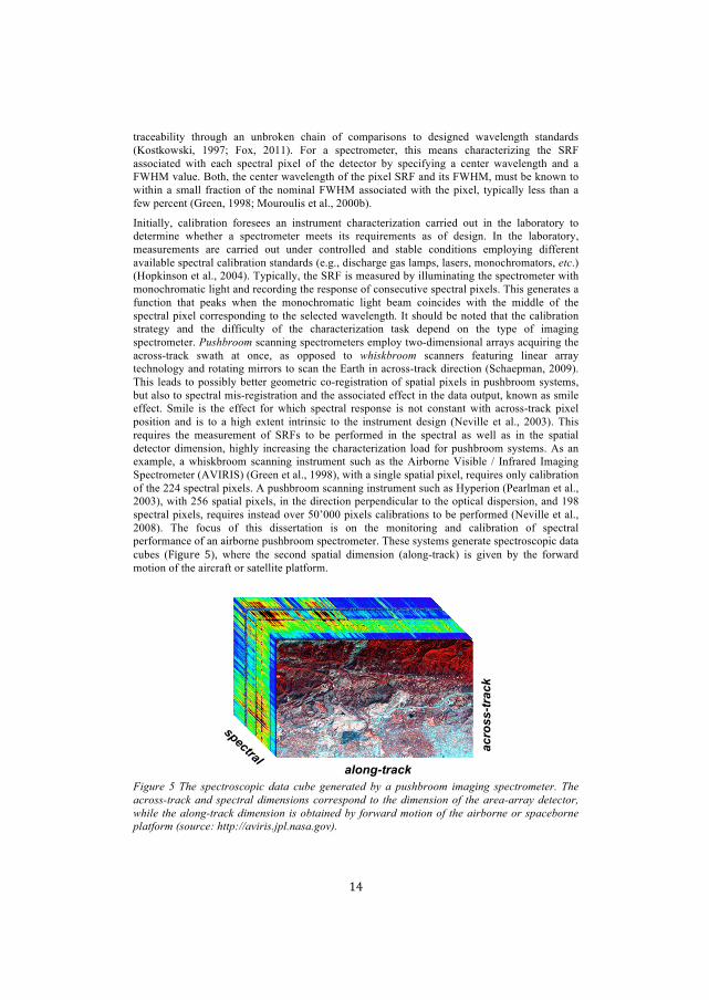
Initially, calibration foresees an instrument characterization carried out in the laboratory to determine whether a spectrometer meets its requirements as of design. In the laboratory, measurements are carried out under controlled and stable conditions employing different available spectral calibration standards (e.g., discharge gas lamps, lasers, monochromators, etc.) (Hopkinson et al., 2004). Typically, the SRF is measured by illuminating the spectrometer with monochromatic light and recording the response of consecutive spectral pixels. This generates a function that peaks when the monochromatic light beam coincides with the middle of the spectral pixel corresponding to the selected wavelength. It should be noted that the calibration strategy and the difficulty of the characterization task depend on the type of imaging spectrometer. Pushbroom scanning spectrometers employ two-dimensional arrays acquiring the across-track swath at once, as opposed to whiskbroom scanners featuring linear array technology and rotating mirrors to scan the Earth in across-track direction (Schaepman, 2009). This leads to possibly better geometric co-registration of spatial pixels in pushbroom systems, but also to spectral mis-registration and the associated effect in the data output, known as smile effect. Smile is the effect for which spectral response is not constant with across-track pixel position and is to a high extent intrinsic to the instrument design (Neville et al., 2003). This requires the measurement of SRFs to be performed in the spectral as well as in the spatial detector dimension, highly increasing the characterization load for pushbroom systems. As an example, a whiskbroom scanning instrument such as the Airborne Visible / Infrared Imaging Spectrometer (AVIRIS) (Green et al., 1998), with a single spatial pixel, requires only calibration of the 224 spectral pixels. A pushbroom scanning instrument such as Hyperion (Pearlman et al., 2003), with 256 spatial pixels, in the direction perpendicular to the optical dispersion, and 198 spectral pixels, requires instead over 50’000 pixels calibrations to be performed (Neville et al., 2008). The focus of this dissertation is on the monitoring and calibration of spectral performance of an airborne pushbroom spectrometer. These systems generate spectroscopic data cubes (Figure! 5), where the second spatial dimension (along-track) is given by the forward motion of the aircraft or satellite platform.

acro

ss-t

rack

spectral along-track

Figure 5 The spectroscopic data cube generated by a pushbroom imaging spectrometer. The across-track and spectral dimensions correspond to the dimension of the area-array detector, while the along-track dimension is obtained by forward motion of the airborne or spaceborne platform (source: http://aviris.jpl.nasa.gov).

!15!

!

As reported in Gege et al. (2009) the characterization measurements carried out in the laboratory are further processed to derive the parameters describing the instrument spectral response model. These are listed in Table 1. The FWHM parameter corresponds to what is defined as spectral resolution in earlier sections. The spectral response is usually fitted to a known curve during processing, which in the case of spectrometers is typically a Gaussian. Laboratory characterization measurements procedures are described in Gege et al. (2009) and Hopkinson et al. (2004) whereas for greater detail on the processing of these measurements to derive calibration parameters we refer to Brazile et al. (2003) and Hüni et al. (2009).

Table 1 Spectral parameters describing the instrument spectral response model.

Parameters Description SRFi,x(λ) Spectral Response Function of a

selected spectral (i) and spatial (x) pixel

Normalized signal vs. wavelength λ

λi,x Center wavelength of a selected

spectral (i) and spatial (x) pixel Peak maximum of SRFi,x(λ)

Smile effect

Spectral smile of a selected spectral pixel

Center wavelength λi,x vs. pixel number x

SSI Spectral Sampling Interval of

selected spectral and spatial pixels Wavelength difference |λi+1,x–λi,x| of adjacent spectral pixels

Spectral range

Spectral range of selected pixels Wavelength difference |λN,x–λ1,x| of first and last spectral pixel

FWHM Full Width at Half Maximum of a

selected spectral and spatial pixel

Wavelength interval corresponding to ½ SRFi,x(λ)

1.4 Monitoring of spectral performance in an operational environment

Although every attempt is made to ensure that pre-flight laboratory characteristics remain in place, once the instrument becomes airborne or spaceborne, it is acknowledged that for optical sensors this is rarely the case (Fox et al., 2011). It is therefore in the operational (air or space) environment where a re-characterization of the instrument performance needs to take place and where the real challenge of calibration sets in (Fox et al., 2003). Mechanical and environmental stresses, coupled with natural instrument aging, are known to lead to change and degradation of sensor performance (Gao et al., 2004). In the spectral domain, this change shows as modifications of the SRF with respect to the position (i.e., shift of center wavelength) and, to a much less extent, shape (i.e., change in FWHM) determined during laboratory characterization (Brazile et al., 2006; Guanter et al., 2006). In the attempt to monitor such performance changes, different post-launch (in-flight) spectral calibration approaches are being implemented for spaceborne and airborne instruments. The majority of these approaches are based on the evaluation of sharp absorption features present in the observed radiance spectra as compared to the same feature present in a well-known reference spectrum. The common baseline to these

!16!

!

methods is the high sensitivity of the measured spectrum to the instrument spectral performance in spectral windows where abrupt radiance changes occur (D'Odorico et al., 2011b; Guanter et al., 2009).

This section presents a brief review of a representative selection of in-orbit and in-flight spectral performance monitoring strategies implemented for spaceborne and airborne spectrometers, respectively. Perhaps the most important difference, to be taken into account when monitoring performance of spaceborne vis-à-vis airborne instruments is the respective operational environment. Space instruments have to survive the launch vibration but can count on a relatively stable environment thereafter. Airborne instruments however must maintain their characteristics in the face of constant vibration, temperature and pressure changes, and further tolerate several cold cycles as they are powered off and on (Bender et al., 2010). While spaceborne missions commonly rely on a combination of onboard and vicarious approaches, the monitoring of airborne systems is usually exclusively and critically depending on the latter.

The MEdium Resolution Imaging Spectrometer (MERIS) (Rast et al., 1999) onboard the ENVISAT platform is equipped with an erbium doped ‘pink’ diffuser, which illuminated by solar irradiance produces a radiance spectrum rich in absorption features. This approach is able to characterize MERIS spectral bands within the nominal mission accuracy requirements of 1 nm. It is however not suited for the near infrared due to the absence of useful erbium absorption lines in this spectral region. The use of Fraunhofer lines complements these measurements by providing the necessary reference in the violet and near infrared parts of the spectrum. Earth or ‘white’ diffuser observations are used to detect these lines. In Earth observations, oxygen absorption features originating in the atmosphere can additionally be exploited. MERIS spectral programmability, i.e., fifteen spectral bands selectable by ground command with a programmable width and spectral location, represent an advantage not only for Earth imaging but also for calibration. Dedicated calibration acquisitions can be performed with continuous narrow bands programmed to sample specific absorption features (Delwart et al., 2007).

The Hyperion (Pearlman et al., 2003) instrument mounted on the EO-1 spacecraft monitors spectral performance and related calibration based on data of the Earth’s atmospheric limb. The atmospheric limb collection is essentially the same as a solar calibration but scheduled such that the instrument views the sun through different tangent heights of the atmosphere. The spacecraft performs a yaw maneuver to view the sun and allow the sunlight to be reflected off the solar calibration panel into the instrument aperture. The incoming radiance is uniform across the field of view and contains spectral features corresponding to solar lines, atmospheric features and absorption features originating from the paint on the instrument cover (Barry et al., 2002).

The MODerate resolution Imaging Spectroradiometer (MODIS) (Salomonson et al., 1989) system onboard the Terra and Aqua satellites exhibit a rather unconventional on-orbit spectral calibration concept. A light source, a spherical integration sphere and a grating monochromator provide the needed reference signal. Monochromators are rarely deployed in space environments, as they require regular wavelength re-calibration due to possible performance changes. For MODIS, a stable didymium glass with known transmission peaks is provided to establish the relationship between monochromator step and wavelength when the grating is located at a series of positions. The measured MODIS band responses versus grating step number are then scaled to wavelengths. A reference silicon photo-diode is used to normalize the didymium signal as well as the MODIS response signal to remove the light source spectral shape (Montgomery et al., 2000).

The Environmental Mapping and Analysis Program (EnMAP) mission (Stuffler et al., 2009) scheduled for launch in 2013 bases its in-orbit spectral performance monitoring on similar principles as those of previously reviewed missions. The proposed design foresees the use of an integrating sphere with light originating from a tungsten halogen lamp, housed outside of the sphere. The light is filtered through a didymium-doped glass, which provides a number of

!17!

!

spectral features across the visible and infrared range. In addition to the on-board approach EnMAP will carry out atmospheric limb observations in a similar fashion as Hyperion. Limb observations are performed through the solar port used for the direct sun imaging therefore no special maneuver is required as it is constantly pointing to the sun.

Currently, the on-orbit calibration strategies vary widely in both frequency and type of measurements as discussed in this chapter. The Committee on Earth Observation Satellites (CEOS) through its working group on calibration and validation (CalVal) is aiming to establish a consensus within the international remote sensing community so that calibration, validation and quality assurance processes are harmonized across satellite missions. Planned initiatives, such as the satellite mission TRUTHS (Fox et al., 2003) envisaged by ESA or the analogous CLARREO (Wielicki, 2011) mission planned by NASA, might aid this objective by complementing or fully replacing calibration efforts by individual missions. These satellite missions are meant to enable, for the first time, high-accuracy Système International d'unités (SI) traceability to be established in orbit. The direct use of primary standards and replication of the terrestrial traceability chain is meant to extend the SI into space and allow establishing a metrology laboratory in orbit (Fox et al., 2011).

Airborne instruments face a slightly different reality, with only very few instruments featuring onboard characterization sources. Operational since the early 90s, the AVIRIS spectrometer (Green et al., 1990) represents one such exception. Equipped with an onboard quartz halogen lamp and a set of spectral filters, AVIRIS represents the first airborne system designed to allow for in-flight spectral performance monitoring by means of targeted calibration acquisitions (Chrien et al., 1995). At the end of the 90s, the Reflective Optics System Imaging Spectrometer (ROSIS) (Kunkel et al., 1991) followed a similar path, including a mercury lamp for in-flight spectral performance monitoring in its design (Thiemann et al., 2001). However, the absence of literature reporting on the use of these airborne onboard characterization strategies leaves room only for speculations on their deployment up to the current day. A broad range of publications can instead be reviewed dealing with vicarious approaches, often referred to as scene-based approaches for they rely on the Earth observation scene itself. These methods exploit stable natural absorption features originating from atmospheric constituents (predominantly O2 and CO2) and, depending on instrument spectral resolution, solar Fraunhofer lines. Examples for AVIRIS, CASI, ROSIS and HyMap airborne spectrometers can be found in Guanter et al. (2007; 2006), Green et al. (2001) and Brazile et al. (2008).

The Airborne Prism EXperiment (APEX) imaging spectrometer features a unique in-flight calibration concept (Itten et al., 2008; Jehle et al., 2010). It is equipped with an In-Flight Characterization (IFC) facility allowing the characterization of radiometric, spectral, and geometric system performance, both in-flight and on ground covering the full Field Of View (FOV). The inclusion of a NIST Standard Reference Material (SRM) filter for spectral performance monitoring allows the transfer of state-of-the-art calibration standards and SI traceability methodologies into the airborne environment. The main focus of this dissertation is on the spectral performance monitoring of the APEX spectrometer.

1.5 Objective and research questions

The present dissertation contributes to the understanding of instrument-induced modifications of the measured spectral radiation. This understanding is critical for the improvement of instrument design, algorithm optimization, and for correct interpretation of remote sensing data and products. This dissertation should answer the following five research questions, grouped into two topical domains.

!18!

!

Monitoring in-flight spectral performance of the APEX imaging spectrometer.

Develop and validate an operational strategy aimed at the in-flight spectral performance and calibration monitoring of ESA’s airborne imaging spectrometer APEX (chapters 3-4).

• Is APEX spectral performance measured during laboratory characterization still valid in an operational environment, if not, which are the causes of deviation?

• Is it feasible to monitor and characterize in-flight spectral performance based on the In-Flight Characterization (IFC) facility onboard APEX?

• What are the feasibilities and utilities of employing vicarious approaches to complement onboard methods for the purpose of spectral performance monitoring?

Exploitation of APEX calibrated data for the simulation, calibration and validation of space missions.

Investigate the potential of using APEX calibrated dataset to simulate, calibrate and validate existing and upcoming space missions for cross-sensor spectral calibration (chapter 5).

• Can APEX calibrated data be used to simulate satellite sensor radiances?

• Can APEX calibrated data be used for the spectral cross-calibration and validation of satellite observations?

1.6 Structure of the dissertation

Chapter 1 provides the framework and the definitions required for the understanding of the peer-reviewed contributions. It familiarizes the reader with the problem of imaging spectrometer spectral performance in an operational environment and briefly reviews the state-of-the-art in the field of in-flight (and in-orbit) monitoring. Research questions and outline of the present dissertation are also presented.

Chapter 2 is based on a co-authored publication (Jehle et al. 2010). It provides an overview of the APEX airborne imaging spectrometer, representing the main instrument in this dissertation. The publication is self-contained in terms of structure and content.

Chapter 3 is based on a first-authored peer-reviewed scientific publication (D'Odorico et al., 2010) addressing the first three research questions of the present dissertation. A series of experiments evaluating APEX spectral performance in function of different environmental conditions are presented. The publication is self-contained in terms of structure and content.

Chapter 4 is based on a first-authored peer-reviewed scientific publications (D'Odorico et al., 2011b) addressing the first three research questions of the present dissertation. A strategy for APEX spectral performance monitoring in-flight is proposed, based on onboard and vicarious measurements. The publication is self-contained in terms of structure and content.

Chapter 5 is based on a first-authored peer-reviewed scientific publication (D'Odorico et al., 2011a) addressing the last two research questions of the present dissertation. A study evaluating the potential of APEX to serve the simulation and spectral cross-calibration of satellite missions is presented. The publication is self-contained in terms of structure and content.

Chapter 6 summarizes the main findings from the publications presented in chapters 3-5, provides concluding remarks and an outlook.

!19!

!

1.7 References

Ball, D.W., 2001. The Basic of Spectroscopy SPIE - The International Society of Optical Engineering, 142 p.

Barry, P.S., Shepanski, J. and Segal, C., 2002. Hyperion on-orbit validation of spectral calibration using atmospheric lines and an on-board system. Proceedings of SPIE, 4480: 231-235.

Bender, H.A., Mouroulis, P., Eastwood, M.L., Green, R.O., Geier, S. and Hochberg, E.B., 2011. Alignment and characterization of high uniformity imaging spectrometers. Proceedings of SPIE, 81580J-11.

Bender, H.A., Mouroulis, P.Z., Green, R.O. and Wilson, D.W., 2010. Optical design, performance, and tolerancing of next-generation airborne imaging spectrometers. Proceedings of SPIE, 78120P-12.

Brazile, J., Kohler, P. and Hefti, S., 2003. A software architecture for in-flight acquisition and offline scientific post-processing of large volume hyperspectral data, Proceeding of the 10th USENIX Tcl/Tk Conference, Ann Arbor, MI.

Brazile, J., Neville, R.A., Staenz, K., Schlaepfer, D., Sun, L. and Itten, K.I., 2006. Scene-based spectral response function shape discernibility for the APEX imaging spectrometer. IEEE Geoscience and Remote Sensing Letters, 3(3): 414-418.

Brazile, J., Neville, R.A., Staenz, K., Schläpfer, D., Sun, L. and Itten, K., 2008. Towards scene-based retrieval of spectral response functions for hyperspectral imagers using Frauenhofer features. Canadian Journal of Remote Sensing, 34(1): S43-S58.

Chance, K., Kurosu, T.P. and Sioris, C.E., 2005. Undersampling correction for array detector-based satellite spectrometers. Applied Optics 44(7): 1296-1304.

Chrien, T., Eastwood, M., Green, R., Sarture, C., Johnson, H., Chovit, C. and Hajek, P., 1995. Airborne Visible/Infrared Imaging Spectrometer (AVIRIS) onboard calibration system. Fifth Annual JPL Airborne Earth Science Workshop Proceedings, Jet Propulsion Laboratory, Pasadena, CA.

D'Odorico, P., Alberti, E. and Schaepman, M.E., 2010. In-flight spectral performance monitoring of the Airborne Prism Experiment. Applied Optics 49(16): 3082-3091.

D'Odorico, P., Gonsamo, A., Damm, A. and Schaepman, M.E., 2011a. Experimental evaluation of Sentinel-2 spectral response function for NDVI time-series continuity. IEEE Transactions on Geoscience and Remote Sensing, submitted.

D'Odorico, P., Guanter, L., Schaepman, M.E. and Schläpfer, D., 2011b. Performance assessment of onboard and scene-based methods for Airborne Prism Experiment spectral characterization. Applied Optics, 50(23): 4755-4764.

Damm, A., Erler, A., Hillen, W., Meroni, M., Schaepman, M.E., Verhoef, W. and Rascher, U., 2011. Modeling the impact of spectral sensor configurations on the FLD retrieval accuracy of sun-induced chlorophyll fluorescence. Remote Sensing of Environment, 115(8): 1882-1892.

de Haan, J.F., Hovenier, J.W., Kokke, J.M.M. and van Stokkom, H.T.C., 1991. Removal of atmospheric influences on satellite-borne imagery: A radiative transfer approach. Remote Sensing of Environment, 37(1): 1-21.

Delwart, S., Preusker, R., Bourg, L., Santer, R., Ramon, D. and Fischer, J., 2007. MERIS In-flight Spectral Calibration. International Journal of Remote Sensing, 28(3): 479-496.

Fox, N., Aiken, J., Barnett, J.J., Briottet, X., Carvell, R., Frohlich, C., Groom, S.B., Hagolle, O., Haigh, J.D., Kieffer, H.H., Lean, J., Pollock, D.B., Quinn, T., Sandford, M.C.W., Schaepman, M., Shine, K.P., Schmutz, W.K., Teillet, P.M., Thome, K.J., Verstraete, M.M. and Zalewski, E., 2003. Traceable radiometry underpinning terrestrial- and helio-studies

!20!

!

(TRUTHS). Advances in Space Research, 32(11): 2253-2261. Fox, N., Kaiser-Weiss, A., Schmutz, W., Thome, K., Young, D., Wielick, B., Winkler, R. and

Woolliams, E., 2011. Accurate radiometry from space: an essential tool for climate studies. The Royal Society of London. Philosophical Transactions. Series A. Mathematical, Physical and Engineering Sciences, 369(1953): 4028-4063.

Gaddis, L.R., Soderblom, L.A., Kieffer, H.H., Becker, K.J., Torson, J. and Mullins, K., 1996. Decomposition of AVIRIS spectra: extraction of surface-reflectance, atmospheric, and instrumental components. IEEE Transactions on Geoscience and Remote Sensing, 34(1): 163 - 178.

Gao, B.-C., Montes, M.J., Davis, C.O. and Goetz, A.F.H., 2009. Atmospheric correction algorithms for hyperspectral remote sensing data of land and ocean. Remote Sensing of Environment, 113(1): S17-S24.

Gao, B.C., Montes, M. and Davis, C., 2004. Refinement of wavelength calibrations of hyperspectral imaging data using a spectrum-matching technique. Remote Sensing of Environment, 90(4): 424-433.

Gege, P., Fries, J., Haschberger, P., Schoetz, P., Schwarzer, H., Strobl, P., Suhr, B., Ulbrich, G. and Jan Vreeling, W., 2009. Calibration facility for airborne imaging spectrometers. ISPRS Journal of Photogrammetry and Remote Sensing, 64(4): 387-397.

Goetz, A.F.H., Vane, G., Solomon, J.E. and Rock, B.N., 1985. Imaging spectrometry for Earth remote sensing, Science, 228: 1147.

Green, R., 1998. Spectral calibration requirements for Earth-looking imaging spectrometers in the solar-reflected spectrum. Applied Optics, 37(4): 683-690.

Green, R., Eastwood, M., Sarture, C., Chrien, T., Aronsson, M., Chippendale, B., Faust, J., Pavri, B., Chovit, C., Solis, M., Olah, M. and Williams, O., 1998. Imaging spectroscopy and the Airborne Visible/Infrared Imaging Spectrometer (AVIRIS). Remote Sensing of Environment, 65(3): 227–248.

Green, R. and Pavri, B., 2001. AVIRIS inflight calibration experiment measurements, analysis and results in 2000. Proceedings of the tenth JPL airborne earth science workshop. JPL Pub., Pasadena, CA, pp. 205-219.

Green, R.O., Pavri, B. and Chrien, T., 2003. On-orbit radiometric and spectral calibration characteristics of EO-1 Hyperion derived with an underflight of AVIRIS and in situ measurements at Salar de Arizaro, Argentina. IEEE Transactions on Geoscience and Remote Sensing, 41(6): 1194 - 1203.

Green, R.O., Conel, J.E., Margolis, J.S., Carrere, V., Bruegge, C.J., Rast, M. and Hoover, G., 1990. In-flight validation and calibration of the spectral and radiometric characteristics of the Airborne Visible/Infrared Imaging Spectrometer (AVIRIS), Proceedings of SPIE. Imaging Spectroscopy of the Terrestrial Environment, pp. 18-36.

Guanter, L., Estellés, V. and Moreno, J., 2007. Spectral calibration and atmospheric correction of ultra-fine spectral and spatial resolution remote sensing data. Application to CASI-1500 data. Remote Sensing of Environment, 109(1): 54-65.

Guanter, L., Richter, R. and Moreno, J., 2006. Spectral calibration of hyperspectral imagery using atmospheric absorption features. Applied Optics, 45(10): 2360-2370.

Guanter, L., Segl, K., Sang, B., Alonso, L., Kaufmann, H. and Moreno, J., 2009. Scene-based spectral calibration assessment of high spectral resolution imaging spectrometers. Optics Express, 17(14): 11594-11606.

Hopkinson, G.R., Goodman, T.M. and Prince, S.R., 2004. A Guide to the Use and Calibration of Detector Array Equipment, PM142. SPIE Press, 234 p.

Hüni, A., Biesemans, J., Meuleman, K., Dell'Endice, F., Schläpfer, D., Adriaensen, S., Kempenaers, S., Odermatt, D., Kneubühler, M. and Nieke, J., 2009. Structure, components and interfaces of the Airborne Prism Experiment (APEX) Processing and Archiving Facility.

!21!

!

IEEE Transactions on Geoscience and Remote Sensing, 47(1): 1-4. Itten, K., Dell'Endice, F., Hueni, A., Kneubuehler, M., Schlaepfer, D., Odermatt, D., Seidel, F.,

Huber, S., Schopfer, J., Kellenberger, T., Buehler, Y., D'Odorico, P., Nieke, J., Alberti, E. and Meuleman, K., 2008. APEX - the Hyperspectral ESA Airborne Prism Experiment. Sensors, 8(10): 6235-6259.

Jansson, P.A., 1997. Deconvolution of Images and Spectra. Academic Press, 514 p. Jehle, M., Hueni, A., Damm, A., D’Odorico, P., Weyermann, J., Kneubühler, M., Schläpfer, D.

and Schaepman, M.E., 2010. APEX - current status, performance and product generation. IEEE Sensors 2010, Waikoloa (HI), pp. 533 - 537.

Jones, H.G. and Vaughan, R.A., 2010. Remote Sensing of Vegetation: Principles, Techniques, and Applications. 1st Ed., Oxford University Press, 400 p.

Kerekes, J.P., 2009. Optical sensor technology. In: T.A. Warner, M.D. Nellis and G. Foody (Editors), The SAGE Handbook of Remote Sensing, pp. 95-107.

Kerekes, J.P. and Baum, J.E., 2005. Full-spectrum spectral imaging system analytical model. IEEE Transactions on Geoscience and Remote Sensing, 43(3): 571 - 580.

Kostkowski, H.J., 1997. Reliable Spectroradiometry. Spectroradiometry Consulting, Maryland, 605 p.

Kunkel, B., Blechinger, F., Viehmann, D., Van Der Piepen, H. and Doerffer, R., 1991. ROSIS imaging spectrometer and its potential for ocean parameter measurements (airborne and space-borne). International Journal of Remote Sensing, 12(4): 753-761.

Lerner, J.M., 2006. Imaging spectrometer fundamentals for researchers in the biosciences - A tutorial. Cytometry, Part A 69A: 712–734.

Lillesand, T., Kiefer, R.W. and Chipman, J.W., 2004. Remote Sensing and Image Interpretation. 5th Ed., J. Wiley & Sons, 720 p.

Martonchik, J.V., Bruegge, C.J. and Strahler, A., 2000. A review of reflectance nomenclature used in remote sensing. Remote Sensing Reviews, 19: 9-20.

Montgomery, H., Che, N., Parker, K. and Bowser, J., 2000. The algorithm for MODIS wavelength on-orbit calibration using the SRCA. IEEE Transactions on Geoscience and Remote Sensing, 38(2): 877-884.

Mouroulis, P., Green, R. and Chrien, T., 2000a. Design of pushbroom imaging spectrometer for optimum recovery of spectroscopic and spatial information. Applied Optics, 39(13): 2210-2220.

Mouroulis, P. and McKerns, M.M., 2000b. Pushbroom imaging spectrometer with high spectroscopic data fidelity: experimental demonstration. Optical Engineering, 39(3): 808-816.

Neville, R.A., Sun, L. and Staenz, K., 2003. Detection of spectral line curvature in imaging spectrometer data. Proceedings of SPIE, 5093: 144-154.

Neville, R.A., Sun, L. and Staenz, K., 2008. Spectral calibration of imaging spectrometers by atmospheric absorption feature matching. Canadian Journal of Remote Sensing, 34(1): S29–S42.

Nieke, J., Schlaepfer, D., Dell'Endice, F., Brazile, J. and Itten, K.I., 2008. Uniformity of imaging spectrometry data products. IEEE Transactions on Geoscience and Remote Sensing, 46(10): 3326-3336.

Palmer, J.M. and Grant, B.G., 2009. The Art of Radiometry, PM184. SPIE, 386 p. Pearlman, J.S., Barry, P.S., Segal, C.C., Shepanski, J., Beiso, D. and Carman, S.L., 2003.

Hyperion, a space-based imaging spectrometer. IEEE Transactions on Geoscience and Remote Sensing, 41(6): 1160-1173.

Price, J.C., 1994. How unique are spectral signatures? Remote Sensing of Environment, 49(3): 181-186.

!22!

!

Rast, M., Bezy, J.L. and Bruzzi, S., 1999. The ESA Medium Resolution Imaging Spectrometer MERIS a review of the instrument and its mission. International Journal of Remote Sensing, 20(9): 1681-1702.

Roscoe, H.K., Fish, D.J. and Jones, R.L., 1996. Interpolation errors in UV - visible spectroscopy for stratospheric sensing: implications for sensitivity, spectral resolution, and spectral range. Applied Optics, 35(3): 427-432.

Salomonson, V.V., Barnes, W.L., Maymon, P.W., Montgomery, H.E. and Ostrow, H., 1989. MODIS: advanced facility instrument for studies of the Earth as a system. IEEE Transactions on Geoscience and Remote Sensing, 27(2): 145-153.

Schaepman, M.E., 2009. Imaging spectrometers. In: T.A. Warner, M.D. Nellis and G. Foody (Editors), The SAGE Handbook of Remote Sensing, pp. 166-178.

Schmidt, W., 2005. Optical Spectroscopy in Chemistry and Life Sciences - An Introduction. Wiley, 384 p.

Schowengerdt, R.A., 1997. Remote Sensing - Model and Methods for Image Processing. 2nd Ed., Academic Press, 522 p.

Stuffler, T., Förster, K., Hofer, S., Leipold, M., Sang, B., Kaufmann, H., Penne, B., Mueller, A. and Chlebek, C., 2009. Hyperspectral imaging - An advanced instrument concept for the EnMAP mission (Environmental Mapping and Analysis Programme). Acta Astronautica, 65(7-8): 1107-1112.

Swayze, G., Clark, R., Goetz, A., Chrien, T. and Gorelick, N., 2003. Effects of spectrometer band pass, sampling, and signal-to-noise ratio on spectral identification using the Tetracorder algorithm. Journal of Geophysical Research, 108(E9 5105).

Tanre, D., Herman, M. and Deschamps, P.Y., 1981. Influence of the background contribution upon space measurements of ground reflectance. Applied Optics, 20(20): 3676-3684.

Tanre, D., Herman, M., Deschamps, P.Y. and de Leffe, A., 1979. Atmospheric modeling for space measurements of ground reflectances, including bidirectional properties. Applied Optics, 18(21): 3587-3594.

Teillet, P.M., Fedosejevs, G., Gauthier, R.P., O'Neill, N.T., Thome, K.J., Biggar, S.F., Ripley, H., Meygret, A., 2001. A generalized approach to the vicarious calibration of multiple Earth observation sensors using hyperspectral data. Remote Sensing of Environment, 77(3): 304-327.

Teillet, P.M., Fedosejevs, G., Thome, K.J. and Barker, J.L., 2007. Impacts of spectral band difference effects on radiometric cross-calibration between satellite sensors in the solar-reflective spectral domain. Remote Sensing of Environment, 110(3): 393-409.

Teillet, P.M., Staenz, K. and William, D.J., 1997. Effects of spectral, spatial, and radiometric characteristics on remote sensing vegetation indices of forested regions. Remote Sensing of Environment, 61(1): 139-149.

Thiemann, S., Strobl, P., Gege, P., Stahl, N., Mooshuber, W. and van der Piepen, H., 2001. Das abbildende Spektrometer ROSIS. Publikationen der Deutschen Gesellschaft für Photogrammetrie und Fernerkundung, 10: 147-153.

Wielicki, B.A., 2011. Climate Absolute Radiance and Refractivity Observatory (CLARREO): achieving climate change absolute accuracy in orbit. Bulletin of the American Meteorological Society, submitted.

!23!

!

2 APEX - CURRENT STATUS, PERFORMANCE AND PRODUCT GENERATION

This chapter has been published as: Jehle, M., Hueni, A., Damm, A., D’Odorico, P., Weyermann, J., Kneubühler, M., Schläpfer, D., and Schaepman, M.E., 2010. APEX - current status, performance and product generation. IEEE Sensors 2010, Waikoloa (HI), pp. 533 - 537.

The article is reprinted with kind permission of the Institute of Electrical and Electronics Engineers (IEEE).

!

!

!25!

!

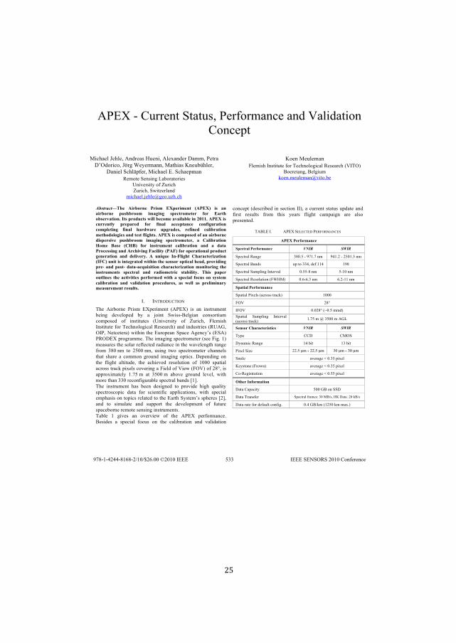
!"#$%&%'())*+,%-,.,(/0%"*)12)3.+4*%.+5%6.785.,82+%

'2+4*9,%%

:84;.*7%<*;7*0%!+5)*./%=(*+80%!7*>.+5*)%?.330%"*,).%

?@A52)8420%<B)C%D*E*)3.++0%:.,;8./%F+*(GH;7*)0%

?.+8*7%-4;7I91*)0%:84;.*7%#J%-4;.*93.+%

K*32,*%-*+/8+C%L.G2).,2)8*/%

M+8N*)/8,E%21%O()84;%

O()84;0%-P8,Q*)7.+5%

384;.*7JR*;7*SC*2J(Q;J4;%

%

F2*+%:*(7*3.+%

T7*38/;%U+/,8,(,*%12)%V*4;+272C84.7%K*/*.)4;%W6UVAX%

Y2*)*,.+C0%Y*7C8(3%

Z2*+J3*(7*3.+SN8,2JG*%

%

%

%

!"#$%&'$!"#$% &'()*(+$% ,('-.% /01$('.$+2% 3&,/04% '-% 5+%

5'()*(+$% 16-#)(**.% '.57'+7% -1$82(*.$2$(% 9*(% /5(2#%

*)-$(:52'*+;%<2-%1(*=682-%>'??%)$8*.$%5:5'?5)?$%'+%@ABB;%&,/0%'-%

86(($+2?C% 1($15($=% 9*(% 9'+5?% 588$125+8$% 8*+9'76(52'*+%

8*.1?$2'+7% 9'+5?% #5(=>5($% 617(5=$-D% ($9'+$=% 85?')(52'*+%

.$2#*=*?*7'$-%5+=%2$-2%9?'7#2-;%&,/0%'-%8*.1*-$=%*9%5+%5'()*(+$%

='-1$(-':$% 16-#)(**.% '.57'+7% -1$82(*.$2$(D% 5% E5?')(52'*+%

F*.$% G5-$% 3EFG4% 9*(% '+-2(6.$+2% 85?')(52'*+% 5+=% 5% =525%

,(*8$--'+7%5+=%&(8#':'+7%H58'?'2C%3,&H4%9*(%*1$(52'*+5?%1(*=682%

7$+$(52'*+% 5+=% =$?':$(C;% &% 6+'I6$% <+JH?'7#2% E#5(582$('K52'*+%

3<HE4%6+'2%'-%'+2$7(52$=%>'2#'+%2#$%-$+-*(%*12'85?%#$5=D%1(*:'='+7%

1($J%5+=%1*-2J%=525J58I6'-'2'*+%8#5(582$('K52'*+%.*+'2*('+7% 2#$%

'+-2(6.$+2-% -1$82(5?% 5+=% (5='*.$2('8% -25)'?'2C;% "#'-% 151$(%

*62?'+$-% 2#$%582':'2'$-%1$(9*(.$=%>'2#%5%-1$8'5?% 9*86-%*+% -C-2$.%

85?')(52'*+% 5+=% :5?'=52'*+% 1(*8$=6($-D% 5-% >$??% 5-% 1($?'.'+5(C%

.$5-6($.$+2%($-6?2-;%

UJ! U[VKA?M'VUA[%

V;*% !8)G2)+*% ")8/3% #$9*)83*+,% W!"#$X% 8/% .+% 8+/,)(3*+,%

G*8+C% 5*N*729*5% GE% .% R28+,% -P8//&Y*7C8.+% 42+/2),8(3%

42392/*5% 21% 8+/,8,(,*/% WM+8N*)/8,E% 21% O()84;0% T7*38/;%

U+/,8,(,*%12)%V*4;+272C84.7%K*/*.)4;X%.+5%8+5(/,)8*/%WKM!\0%

AU"0%[*,4*,*).X%P8,;8+% ,;*%#()29*.+%-9.4*%!C*+4E@/% W#-!X%

"KA?#$%9)2C).33*J%V;*%83.C8+C%/9*4,)23*,*)%W/**%T8CJ%]X%

3*./()*/%,;*%/27.)%)*17*4,*5%).58.+4*%8+%,;*%P.N*7*+C,;%).+C*%

1)23% ^_`%+3% ,2% ab``%+30% (/8+C% ,P2% /9*4,)23*,*)% 4;.++*7/%

,;.,% /;.)*% .% 42332+% C)2(+5% 83.C8+C% 29,84/J% ?*9*+58+C% 2+%

,;*% 178C;,% .7,8,(5*0% ,;*% .4;8*N*5% )*/27(,82+% 21% ]```% /9.,8.7%

.4)2//%,).4Z%98>*7/%42N*)8+C%.%T8*75%21%68*P%WTA6X%21%a_c0%8/%

.99)2>83.,*7E% ]Jdb%3% .,% ^b``%3% .G2N*% C)2(+5% 7*N*70% P8,;%

32)*%,;.+%^^`%)*42+18C().G7*%/9*4,).7%G.+5/%e]fJ%%

V;*% 8+/,)(3*+,% ;./% G**+% 5*/8C+*5% ,2% 9)2N85*% ;8C;% g(.78,E%

/9*4,)2/42984% 5.,.% 12)% /48*+,8184% .99784.,82+/0% P8,;% /9*48.7%

*39;./8/%2+%,2984/%)*7.,*5%,2%,;*%#.),;%-E/,*3@/%/9;*)*/%eaf0%

.+5% ,2% /83(7.,*% .+5% /(992),% ,;*% 5*N*7293*+,% 21% 1(,()*%

/9.4*G2)+*%)*32,*%/*+/8+C%8+/,)(3*+,/J%%

V.G7*% ]% C8N*/% .+% 2N*)N8*P% 21% ,;*% !"#$% 9*)12)3.+4*J%

Y*/85*/% .% /9*48.7% 124(/% 2+% ,;*% 4.78G).,82+% .+5% N.785.,82+%

42+4*9,% W5*/4)8G*5% 8+%/*4,82+%UUX0%.%4())*+,%/,.,(/%(95.,*%.+5%

18)/,% )*/(7,/% 1)23% ,;8/% E*.)/% 178C;,% 4.39.8C+% .)*% .7/2%

9)*/*+,*5J%

V!YL#%UJ%! !"#$%-#L#'V#?%"#KTAK:!['#-%

&,/0%,$(9*(.5+8$%

L1$82(5?%,$(9*(.5+8$% ()*+, -.*+,

-9*4,).7%K.+C*% ^_`Jb%&%hd]Jd%+3% hi]Ja%&%ab`]Jb%+3%

-9*4,).7%Y.+5/% (9%,2%^^i0%5*1J]]i% ]h_%

-9*4,).7%-.3978+C%U+,*)N.7% `Jbb&_%+3% b&]`%+3%

-9*4,).7%K*/27(,82+%WTD=:X% `Jj&jJ^%+3% jJa&]]%+3%

L152'5?%,$(9*(.5+8$% %

-9.,8.7%"8>*7/%W.4)2//%,).4ZX% ]```%

TA6% a_c%

UTA6% `J`a_c%Wk`Jb%3).5X%

-9.,8.7% -.3978+C% U+,*)N.7%

W.4)2//%,).4ZX%]Jdb%3%S%^b``%3%!\L%

L$+-*(%E#5(582$('-2'8-% ()*+, -.*+,

VE9*% ''?% ':A-%

?E+.384%K.+C*% ]i%G8,% ]^%G8,%

"8>*7%-8Q*% aaJ!"#3"!"$$Jb%#3% ^`%#3"!"%&"#3%

-387*% .N*).C*%l%`J^b%98>*7%

F*E/,2+*%WT)2P+X% .N*).C*%l%`J^b%98>*7%

'2&K*C8/,).,82+% .N*).C*%l%`Jbb%98>*7%

M2#$(%<+9*(.52'*+% %

?.,.%'.9.48,E% b``%\Y%2+%--?%

?.,.%V).+/1*)% -9*4,).7%1).3*/m%^`%:Yn/0%=F%?.,.m%a`%ZYn/%

?.,.%).,*%12)%5*1.(7,%42+18CJ% `Ji%\YnZ3%W]ab`%Z3%3.>JX%

!"#$%$&'&&$#%(#$')%*)+'(,**-.'*%*-/000 !"" !"""#$"%$&'$#()*)#+,-./0/-1/

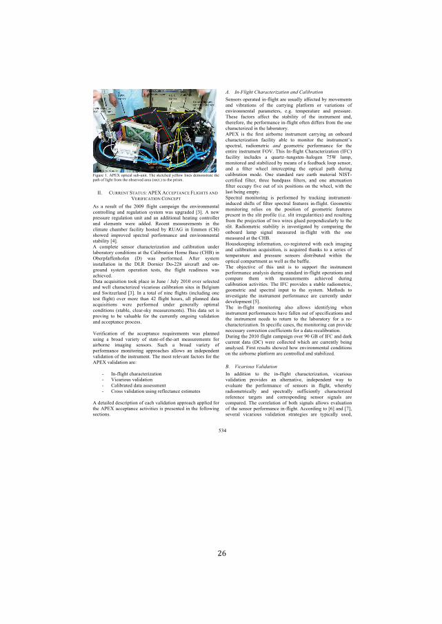
!26!

!

!"#$%&'!()!*+,-!./0#123!4%56%7#0)!89'!4:'019';!<'33.=!3#7'4!;'>.740&20'!09'!

/209!.?!3#$90!?&.>!09'!.54'&@';!2&'2!A&'10)B!0.!09'!/&#4>)!

!

CC)! DEFF,G8!H8*8EHI!*+,-!*DD,+8*GD,!"JCKL8H!*GM!

N,FC"CD*8COG!DOGD,+8!

*4! 2! &'4%30! .?! 09'! PQQR! ?3#$90! 12>/2#$7! 09'! '7@#&.7>'7023!

1.70&.33#7$! 27;! &'$%320#.7! 4<40'>!=24! %/$&2;';! STU)!*! 7'=!

/&'44%&'! &'$%320#.7! %7#0! 27;! 27! 2;;#0#.723! 9'20#7$! 1.70&.33'&!

27;! '3'>'704! ='&'! 2;;';)! F'1'70! >'24%&'>'704! #7! 09'!

13#>20'! 192>5'&! ?21#3#0<! 9.40';! 5<! FE*K! #7! ,>>'7! ADLB!

49.=';! #>/&.@';! 4/'10&23! /'&?.&>271'! 27;! '7@#&.7>'7023!

4025#3#0<!SVU)!

*! 1.>/3'0'! 4'74.&! 192&210'&#W20#.7! 27;! 123#5&20#.7! %7;'&!

325.&20.&<!1.7;#0#.74!20!09'!D23#5&20#.7!L.>'!X24'!ADLXB!#7!

O5'&/?2??'79.?'7! AMB! =24! /'&?.&>';)! *?0'&! 4<40'>!

#74023320#.7! #7! 09'! MJF! M.&7#'&! M.6PPY! 2#&1&2?0! 27;! .76

$&.%7;! 4<40'>! ./'&20#.7! 0'404Z! 09'! ?3#$90! &'2;#7'44! =24!

219#'@';)!!

M202!21[%#4#0#.7!0..:!/321'!#7!\%7'!]!\%3<!PQ(Q!.@'&!4'3'10';!

27;!='33!192&210'&#W';!@#12&#.%4!123#5&20#.7!4#0'4! #7!X'3$#%>!

27;!H=#0W'&327;! STU)! C7!2! 0.023!.?!7#7'! ?3#$904! A#713%;#7$!.7'!

0'40! ?3#$90B! .@'&!>.&'! 0927! VP! ?3#$90! 9.%&4Z! 233! /3277';! ;202!

21[%#4#0#.74! ='&'! /'&?.&>';! %7;'&! $'7'&233<! ./0#>23!

1.7;#0#.74! A40253'Z! 13'2&64:<!>'24%&'>'704B)!89#4! ;202! 4'0! #4!

/&.@#7$! 0.! 5'! @23%253'! ?.&! 09'! 1%&&'703<! .7$.#7$! @23#;20#.7!

27;!211'/0271'!/&.1'44)!

!

N'&#?#120#.7! .?! 09'! 211'/0271'! &'[%#&'>'704! =24! /3277';!

%4#7$! 2! 5&.2;! @2&#'0<! .?! 4020'6.?609'62&0! >'24%&'>'704! ?.&!

2#&5.&7'! #>2$#7$! 4'74.&4)! H%19! 2! 5&.2;! @2&#'0<! .?!

/'&?.&>271'! >.7#0.&#7$! 2//&.219'4! 233.=4! 27! #7;'/'7;'70!

@23#;20#.7!.?!09'!#740&%>'70)!89'!>.40!&'3'@270!?210.&4!?.&!09'!

*+,-!@23#;20#.7!2&'I!

!

6! C76?3#$90!192&210'&#W20#.7!

6! N#12&#.%4!@23#;20#.7!

6! D23#5&20';!;202!244'44>'70!

6! D&.44!@23#;20#.7!%4#7$!&'?3'10271'!'40#>20'4!

!

*!;'02#3';!;'41&#/0#.7!.?!'219!@23#;20#.7!2//&.219!2//3#';!?.&!

09'!*+,-!211'/0271'!210#@#0#'4!#4!/&'4'70';!#7!09'!?.33.=#7$!

4'10#.74)!!

!"! #$%&'()*+,-*./.0+1/(2.+(3$,.$4,-.'(5/.+(3$,

H'74.&4!./'&20';!#76?3#$90!2&'!%4%233<!2??'10';!5<!>.@'>'704!

27;! @#5&20#.74! .?! 09'! 12&&<#7$! /320?.&>! .&! @2&#20#.74! .?!

'7@#&.7>'7023! /2&2>'0'&4Z! ')$)! 0'>/'&20%&'! 27;! /&'44%&')!

89'4'! ?210.&4! 2??'10! 09'! 4025#3#0<! .?! 09'! #740&%>'70! 27;Z!

09'&'?.&'Z!09'!/'&?.&>271'!#76?3#$90!.?0'7!;#??'&4!?&.>!09'!.7'!

192&210'&#W';!#7!09'!325.&20.&<)!!

*+,-! #4! 09'! ?#&40! 2#&5.&7'! #740&%>'70! 12&&<#7$! 27! .75.2&;!

192&210'&#W20#.7! ?21#3#0<! 253'! 0.! >.7#0.&! 09'! #740&%>'70^4!

4/'10&23Z! &2;#.>'0&#1! .$4! $'.>'0&#1! /'&?.&>271'! ?.&! 09'!

'70#&'! #740&%>'70!"ON)!89#4! C76?3#$90!D92&210'&#W20#.7! AC"DB!

?21#3#0<! #713%;'4! 2! [%2&0W_0%7$40'7_923.$'7! `ab! 32>/Z!

>.7#0.&';!27;!4025#3#W';!5<!>'274!.?!2!?'';521:!3../!4'74.&Z!

27;! 2! ?#30'&! =9''3! #70'&1'/0#7$! 09'! ./0#123! /209! ;%&#7$!

123#5&20#.7! >.;')! O7'! 4027;2&;! &2&'! '2&09! >20'&#23! GCH86

1'&0#?#';! ?#30'&Z! 09&''! 527;/244! ?#30'&4Z! 27;! .7'! 200'7%20#.7!

?#30'&!.11%/<!?#@'!.%0!.?!4#c!/.4#0#.74!.7! 09'!=9''3Z!=#09! 09'!

3240!5'#7$!'>/0<)!!

H/'10&23! >.7#0.&#7$! #4! /'&?.&>';! 5<! 0&21:#7$! #740&%>'706

#7;%1';! 49#?04! .?! ?#30'&! 4/'10&23! ?'20%&'4! #76?3#$90)!K'.>'0&#1!

>.7#0.&#7$! &'3#'4! .7! 09'! /.4#0#.7! .?! $'.>'0&#1! ?'20%&'4!

/&'4'70!#7!09'!43#0!/&.?#3'!A#)')!43#0!#&&'$%32&#0#'4B!27;!&'4%30#7$!

?&.>!09'!/&.d'10#.7!.?!0=.!=#&'4!$3%';!/'&/'7;#1%32&3<!0.!09'!

43#0)! F2;#.>'0&#1! 4025#3#0<! #4! #7@'40#$20';! 5<! 1.>/2&#7$! 09'!

.75.2&;! 32>/! 4#$723! >'24%&';! #76?3#$90! =#09! 09'! .7'!

>'24%&';!20!09'!DLX)!!

L.%4':''/#7$! #7?.&>20#.7Z! 1.6&'$#40'&';! =#09! '219! #>2$#7$!

27;! 123#5&20#.7! 21[%#4#0#.7Z! #4! 21[%#&';! 0927:4! 0.! 2! 4'&#'4! .?!

0'>/'&20%&'! 27;! /&'44%&'! 4'74.&4! ;#40&#5%0';! =#09#7! 09'!

./0#123!1.>/2&0>'70!24!='33!24!09'!52??3')!!

89'! .5d'10#@'! .?! 09#4! %7#0! #4! 0.! 4%//.&0! 09'! #740&%>'70!

/'&?.&>271'!2723<4#4!;%&#7$!4027;2&;!#76?3#$90!./'&20#.74!27;!

1.>/2&'! 09'>! =#09! >'24%&'>'704! 219#'@';! ;%&#7$!

123#5&20#.7!210#@#0#'4)!89'! C"D!/&.@#;'4! 2! 40253'! &2;#.>'0&#1Z!

$'.>'0&#1! 27;! 4/'10&23! #7/%0! 0.! 09'! 4<40'>)! e'09.;4! 0.!

#7@'40#$20'! 09'! #740&%>'70! /'&?.&>271'! 2&'! 1%&&'703<! %7;'&!

;'@'3./>'70!SaU)!

89'! #76?3#$90! >.7#0.&#7$! 234.! 233.=4! #;'70#?<#7$! =9'7!

#740&%>'70!/'&?.&>271'4!92@'!?233'7!.%0!.?!4/'1#?#120#.74!27;!

09'! #740&%>'70! 7'';4! 0.! &'0%&7! 0.! 09'! 325.&20.&<! ?.&! 2! &'6

192&210'&#W20#.7)!C7!4/'1#?#1!124'4Z!09'!>.7#0.&#7$!127!/&.@#;'!

7'1'442&<!1.&&'10#.7!1.'??#1#'704!?.&!2!;202!&'123#5&20#.7)!!

M%&#7$!09'!PQ(Q!?3#$90!12>/2#$7!.@'&!RQ!KX!.?!C"D!27;!;2&:!

1%&&'70! ;202! AMDB! ='&'! 1.33'10';! =9#19! 2&'! 1%&&'703<! 5'#7$!

2723<4';)!"#&40!&'4%304!49.=';!9.=!'7@#&.7>'7023!1.7;#0#.74!

.7!09'!2#&5.&7'!/320?.&>!2&'!1.70&.33';!27;!4025#3#W';)!

!

6"! 7(0./(389,7.'(4.+(3$,

C7! 2;;#0#.7! 0.! 09'! #76?3#$90! 192&210'&#W20#.7Z! @#12&#.%4!

@23#;20#.7! /&.@#;'4! 27! 230'&720#@'Z! #7;'/'7;'70! =2<! 0.!

'@23%20'! 09'! /'&?.&>271'! .?! 4'74.&4! #7! ?3#$90Z! =9'&'5<!

&2;#.>'0&#1233<! 27;! 4/'10&233<! 4%??#1#'703<! 192&210'&#W';!

&'?'&'71'! 02&$'04! 27;! 1.&&'4/.7;#7$! 4'74.&! 4#$7234! 2&'!

1.>/2&';)!89'! 1.&&'320#.7! .?! 5.09! 4#$7234! 233.=4! '@23%20#.7!

.?!09'!4'74.&!/'&?.&>271'!#76?3#$90)!*11.&;#7$!0.!SfU!27;!S`UZ!

4'@'&23! @#12&#.%4! @23#;20#.7! 40&20'$#'4! 2&'! 0</#1233<! %4';Z!

!"#

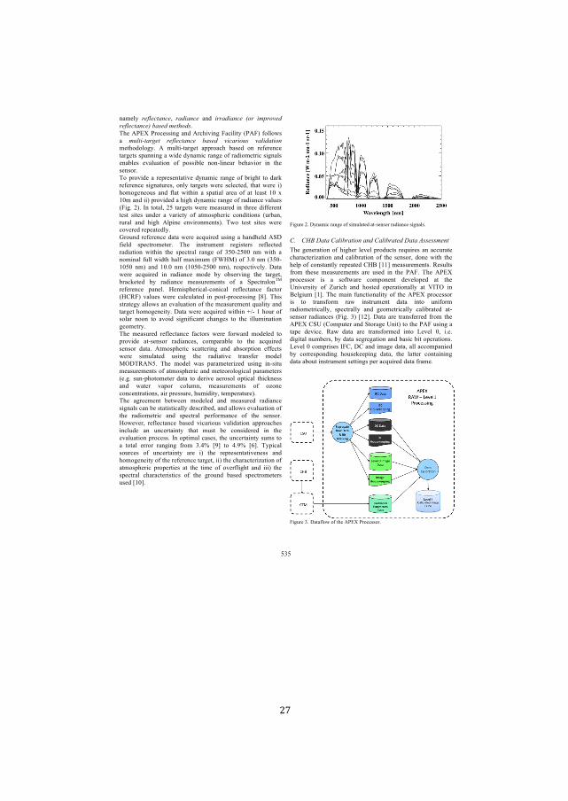
!27!

!

!"#$%&' !"#$"%&'(%"(' !')*'(%"+ "!)' *!!')*'(%"+ ,-!+ *./!-0")+

!"#$"%&'(%"1+2'3")+."&4-)3*''

+,$'-./0'.123$445!6'"!)'-13,575!6'8"35%59&':.-8;'<2%%2=4'

"' .5$&*6&'!7"&+ !"#$"%&'(%"+ 2'3")+ 0*%'!*-53+ 0'$*)'&*-('

#$9,2)2%26&*' -' #>%95?9"16$9' "@@12"3,' A"4$)' 2!' 1$<$1$!3$'

9"16$94'4@"!!5!6'"'=5)$')&!"#53'1"!6$'2<'1")52#$9153'456!"%4'

$!"A%$4' $7"%>"952!' 2<' @2445A%$' !2!?%5!$"1' A$,"7521' 5!' 9,$'

4$!421*''

+2'@1275)$'"' 1$@1$4$!9"957$')&!"#53' 1"!6$'2<'A156,9' 92')"1B'

1$<$1$!3$' 456!"9>1$4(' 2!%&' 9"16$94'=$1$' 4$%$39$)(' 9,"9'=$1$' 5;'

,2#26$!$2>4' "!)' <%"9' =59,5!' "' 4@"95"%' "1$"' 2<' "9' %$"49' CD' E'

CD#'"!)'55;'@1275)$)'"',56,')&!"#53'1"!6$'2<'1")5"!3$'7"%>$4'

:856*'F;*'G!'929"%('FH'9"16$94'=$1$'#$"4>1$)'5!'9,1$$')5<<$1$!9'

9$49' 459$4' >!)$1' "' 7"15$9&' 2<' "9#24@,$153' 32!)5952!4' :>1A"!('

1>1"%' "!)' ,56,' -%@5!$' $!7512!#$!94;*' +=2' 9$49' 459$4' =$1$'

327$1$)'1$@$"9$)%&*'

I12>!)'1$<$1$!3$')"9"'=$1$'"3J>51$)'>45!6'"',"!),$%)'-KL'

<5$%)' 4@$3912#$9$1*' +,$' 5!491>#$!9' 1$6549$14' 1$<%$39$)'

1")5"952!' =59,5!' 9,$' 4@$391"%' 1"!6$' 2<' MHD?FHDD' !#' =59,' "'

!2#5!"%'<>%%'=5)9,',"%<'#"E5#>#':8NOP;'2<'M*D'!#':MHD?

CDHD' !#;' "!)' CD*D' !#' :CDHD?FHDD' !#;(' 1$4@$3957$%&*' L"9"'

=$1$' "3J>51$)' 5!' 1")5"!3$' #2)$' A&' 2A4$175!6' 9,$' 9"16$9('

A1"3B$9$)' A&' 1")5"!3$' #$"4>1$#$!94' 2<' "' K@$391"%2!+P'

1$<$1$!3$' @"!$%*' O$#54@,$153"%?32!53"%' 1$<%$39"!3$' <"3921'

:OQR8;' 7"%>$4'=$1$' 3"%3>%"9$)' 5!' @249?@123$445!6' STU*' +,54'

491"9$6&'"%%2=4'"!'$7"%>"952!'2<'9,$'#$"4>1$#$!9'J>"%59&'"!)'

9"16$9',2#26$!$59&*'L"9"'=$1$'"3J>51$)'=59,5!'VW?'C',2>1'2<'

42%"1' !22!' 92' "725)' 456!5<53"!9' 3,"!6$4' 92' 9,$' 5%%>#5!"952!'

6$2#$91&*''

+,$' #$"4>1$)' 1$<%$39"!3$' <"39214' =$1$' <21="1)' #2)$%$)' 92'

@1275)$' "9?4$!421' 1")5"!3$4(' 32#@"1"A%$' 92' 9,$' "3J>51$)'

4$!421' )"9"*' -9#24@,$153' 43"99$15!6' "!)' "A421@952!' $<<$394'

=$1$' 45#>%"9$)' >45!6' 9,$' 1")5"957$' 91"!4<$1' #2)$%'

PXL+R-YH*' +,$' #2)$%' ="4' @"1"#$9$15Z$)' >45!6' 5!?459>'

#$"4>1$#$!94'2<'"9#24@,$153'"!)'#$9$212%2653"%'@"1"#$9$14'

:$*6*' 4>!?@,292#$9$1')"9"' 92')$157$' "$1242%'2@953"%' 9,53B!$44'

"!)' ="9$1' 7"@21' 32%>#!(' #$"4>1$#$!94' 2<' 2Z2!$'

32!3$!91"952!4('"51'@1$44>1$(',>#5)59&('9$#@$1"9>1$;*'

+,$' "61$$#$!9' A$9=$$!' #2)$%$)' "!)' #$"4>1$)' 1")5"!3$'

456!"%4'3"!'A$'49"954953"%%&')$4315A$)('"!)'"%%2=4'$7"%>"952!'2<'

9,$' 1")52#$9153' "!)' 4@$391"%' @$1<21#"!3$' 2<' 9,$' 4$!421*'

O2=$7$1(' 1$<%$39"!3$' A"4$)' 753"152>4' 7"%5)"952!' "@@12"3,$4'

5!3%>)$' "!' >!3$19"5!9&' 9,"9' #>49' A$' 32!45)$1$)' 5!' 9,$'

$7"%>"952!'@123$44*'G!'2@95#"%'3"4$4(' 9,$'>!3$19"5!9&'4>#4'92'

"' 929"%' $1121' 1"!65!6' <12#' M*[\' S]U' 92' [*]\' S^U*' +&@53"%'

42>13$4' 2<' >!3$19"5!9&' "1$' 5;' 9,$' 1$@1$4$!9"957$!$44' "!)'

,2#26$!$59&'2<'9,$'1$<$1$!3$'9"16$9('55;'9,$'3,"1"39$15Z"952!'2<'

"9#24@,$153' @12@$195$4' "9' 9,$' 95#$' 2<' 27$1<%56,9' "!)' 555;' 9,$'

4@$391"%' 3,"1"39$1549534' 2<' 9,$' 612>!)' A"4$)' 4@$3912#$9$14'

>4$)'SCDU*'

'

'856>1$'F*'L&!"#53'1"!6$'2<'45#>%"9$)'"9?4$!421'1")5"!3$'456!"%4*'

'

89! 8:;+<'&'+8'$*2!'&*-(+'()+8'$*2!'&")+<'&'+=33"33."(&+

+,$'6$!$1"952!'2<',56,$1' %$7$%'@12)>394' 1$J>51$4'"!'"33>1"9$'

3,"1"39$15Z"952!' "!)' 3"%5A1"952!'2<' 9,$' 4$!421(' )2!$'=59,' 9,$'

,$%@'2<'32!49"!9%&'1$@$"9$)'QO_'SCCU'#$"4>1$#$!94*'R$4>%94'

<12#' 9,$4$' #$"4>1$#$!94' "1$' >4$)' 5!' 9,$' .-8*' +,$' -./0'

@123$4421' 54' "' 42<9="1$' 32#@2!$!9' )$7$%2@$)' "9' 9,$'

`!57$1459&' 2<' a>153,' "!)' ,249$)' 2@$1"952!"%%&' "9' bG+X' 5!'

_$%65>#'SCU*'+,$'#"5!' <>!3952!"%59&'2<' 9,$'-./0'@123$4421'

54' 92' 91"!4<21#' 1"=' 5!491>#$!9' )"9"' 5!92' >!5<21#'

1")52#$9153"%%&(' 4@$391"%%&' "!)' 6$2#$9153"%%&' 3"%5A1"9$)' "9?

4$!421' 1")5"!3$4' :856*'M;' SCFU*'L"9"' "1$' 91"!4<$11$)' <12#' 9,$'

-./0'QK`':Q2#@>9$1'"!)'K921"6$'`!59;'92'9,$'.-8'>45!6'"'

9"@$' )$753$*' R"=' )"9"' "1$' 91"!4<21#$)' 5!92' c$7$%' D(' 5*$*'

)5659"%'!>#A$14('A&')"9"'4$61$6"952!'"!)'A"453'A59'2@$1"952!4*'

c$7$%'D'32#@154$4'G8Q('LQ'"!)'5#"6$')"9"('"%%'"332#@"!5$)'

A&' 3211$4@2!)5!6' ,2>4$B$$@5!6' )"9"(' 9,$' %"99$1' 32!9"5!5!6'

)"9"'"A2>9'5!491>#$!9'4$995!64'@$1'"3J>51$)')"9"'<1"#$*'

'

'

'856>1$'M*!L"9"<%2='2<'9,$'-./0'.123$4421*'

'

!"!

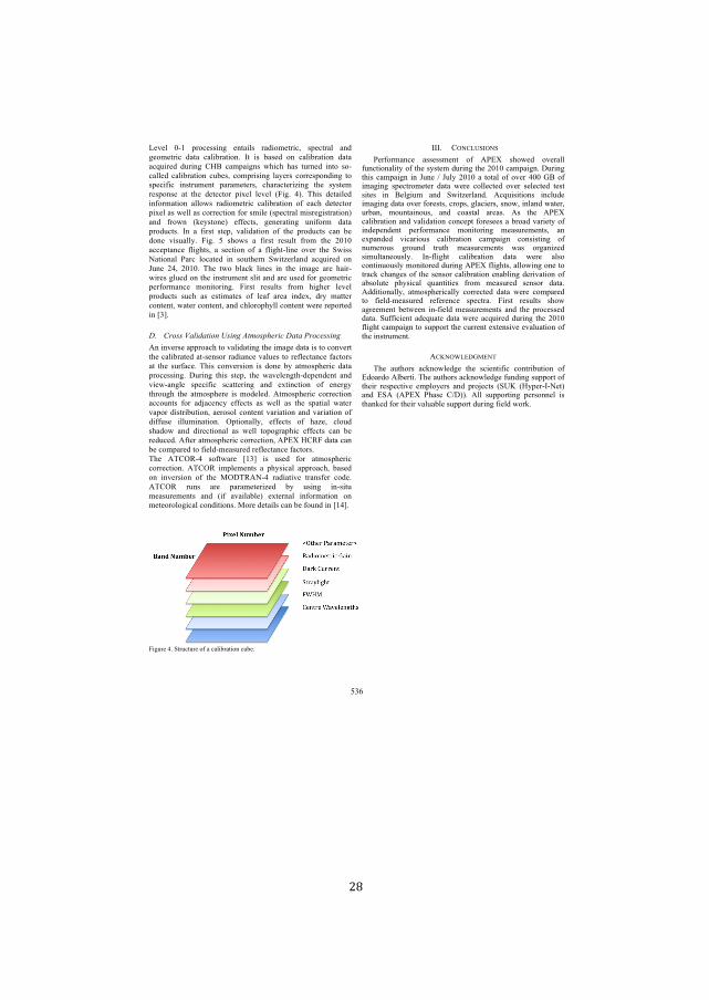
!28!

!

!"#"$% &'(% )*+,"--./0% "/12.$-% *23.+4"1*.,5% -)",1*2$% 2/3%

0"+4"1*.,% 3212% ,2$.6*21.+/7% 81% .-% 62-"3% +/% ,2$.6*21.+/% 3212%

2,9:.*"3% 3:*./0% ;<=% ,24)2.0/-% >?.,?% ?2-% 1:*/"3% ./1+% -+'

,2$$"3% ,2$.6*21.+/% ,:6"-5% ,+4)*.-./0% $2@"*-% ,+**"-)+/3./0% 1+%

-)",.A.,% ./-1*:4"/1% )2*24"1"*-5% ,?2*2,1"*.B./0% 1?"% -@-1"4%

*"-)+/-"% 21% 1?"% 3"1",1+*% ).C"$% $"#"$% DE.07% FG7% H?.-% 3"12.$"3%

./A+*421.+/% 2$$+>-% *23.+4"1*.,% ,2$.6*21.+/% +A% "2,?% 3"1",1+*%

).C"$%2-%>"$$%2-%,+**",1.+/%A+*%-4.$"%D-)",1*2$%4.-*"0.-1*21.+/G%

2/3% A*+>/% DI"@-1+/"G% "AA",1-5% 0"/"*21./0% :/.A+*4% 3212%

)*+3:,1-7% 8/% 2% A.*-1% -1")5% #2$.321.+/% +A% 1?"% )*+3:,1-% ,2/% 6"%

3+/"% #.-:2$$@7% E.07% J% -?+>-% 2% A.*-1% *"-:$1% A*+4% 1?"% K&(&%

2,,")12/,"% A$.0?1-5% 2% -",1.+/% +A% 2% A$.0?1'$./"% +#"*% 1?"% L>.--%

M21.+/2$% N2*,% $+,21"3% ./% -+:1?"*/% L>.1B"*$2/3% 2,9:.*"3% +/%

O:/"% KF5% K&(&7% H?"% 1>+% 6$2,I% $./"-% ./% 1?"% .420"% 2*"% ?2.*'

>.*"-%0$:"3%+/%1?"%./-1*:4"/1%-$.1%2/3%2*"%:-"3%A+*%0"+4"1*.,%

)"*A+*42/,"% 4+/.1+*./07% E.*-1% *"-:$1-% A*+4% ?.0?"*% $"#"$%

)*+3:,1-% -:,?% 2-% "-1.421"-% +A% $"2A% 2*"2% ./3"C5% 3*@% 4211"*%

,+/1"/15%>21"*%,+/1"/15%2/3%,?$+*+)?@$$%,+/1"/1%>"*"%*")+*1"3%

./%PQR7%

%

!"! #$%&&'()*+,)-+%.'/&+.0'1-2%&345$+6'!)-)'7$%65&&+.0'

S/%./#"*-"%2))*+2,?%1+%#2$.321./0%1?"%.420"%3212%.-%1+%,+/#"*1%

1?"%,2$.6*21"3%21'-"/-+*%*23.2/,"%#2$:"-%1+%*"A$",12/,"%A2,1+*-%

21% 1?"% -:*A2,"7% H?.-% ,+/#"*-.+/% .-% 3+/"% 6@% 214+-)?"*.,% 3212%

)*+,"--./07% T:*./0% 1?.-% -1")5% 1?"% >2#"$"/01?'3")"/3"/1% 2/3%

#.">'2/0$"% -)",.A.,% -,211"*./0% 2/3% "C1./,1.+/% +A% "/"*0@%

1?*+:0?% 1?"% 214+-)?"*"% .-%4+3"$"37%S14+-)?"*.,% ,+**",1.+/%

2,,+:/1-% A+*% 23U2,"/,@% "AA",1-% 2-% >"$$% 2-% 1?"% -)21.2$% >21"*%

#2)+*%3.-1*.6:1.+/5% 2"*+-+$% ,+/1"/1%#2*.21.+/%2/3%#2*.21.+/%+A%

3.AA:-"% .$$:4./21.+/7% V)1.+/2$$@5% "AA",1-% +A% ?2B"5% ,$+:3%

-?23+>% 2/3% 3.*",1.+/2$% 2-% >"$$% 1+)+0*2)?.,% "AA",1-% ,2/% 6"%

*"3:,"37%SA1"*%214+-)?"*.,%,+**",1.+/5%SNWX%<;YE%3212%,2/%

6"%,+4)2*"3%1+%A."$3'4"2-:*"3%*"A$",12/,"%A2,1+*-7%%

H?"% SH;VY'F% -+A1>2*"% P(QR% .-% :-"3% A+*% 214+-)?"*.,%

,+**",1.+/7% SH;VY% .4)$"4"/1-% 2% )?@-.,2$% 2))*+2,?5% 62-"3%

+/% ./#"*-.+/% +A% 1?"% ZVTHYSM'F% *23.21.#"% 1*2/-A"*% ,+3"7%

SH;VY% *:/-% 2*"% )2*24"1"*.B"3% 6@% :-./0% ./'-.1:%

4"2-:*"4"/1-% 2/3% D.A% 2#2.$26$"G% "C1"*/2$% ./A+*421.+/% +/%

4"1"+*+$+0.,2$%,+/3.1.+/-7%Z+*"%3"12.$-%,2/%6"%A+:/3%./%P(FR7%

%

%

%E.0:*"%F7!L1*:,1:*"%+A%2%,2$.6*21.+/%,:6"7!

%

%

8887! ;VM;![L8VML%

N"*A+*42/,"% 2--"--4"/1% +A% SNWX% -?+>"3% +#"*2$$%A:/,1.+/2$.1@%+A%1?"%-@-1"4%3:*./0%1?"%K&(&%,24)2.0/7%T:*./0%1?.-% ,24)2.0/% ./% O:/"% \% O:$@%K&(&%2% 1+12$%+A%+#"*%F&&%]=%+A%.420./0% -)",1*+4"1"*% 3212% >"*"% ,+$$",1"3% +#"*% -"$",1"3% 1"-1%-.1"-% ./% ="$0.:4% 2/3% L>.1B"*$2/37% S,9:.-.1.+/-% ./,$:3"%.420./0%3212%+#"*%A+*"-1-5%,*+)-5%0$2,."*-5%-/+>5%./$2/3%>21"*5%:*62/5% 4+:/12./+:-5% 2/3% ,+2-12$% 2*"2-7% S-% 1?"% SNWX%,2$.6*21.+/%2/3%#2$.321.+/%,+/,")1%A+*"-""-%2%6*+23%#2*."1@%+A%./3")"/3"/1% )"*A+*42/,"% 4+/.1+*./0% 4"2-:*"4"/1-5% 2/%"C)2/3"3% #.,2*.+:-% ,2$.6*21.+/% ,24)2.0/% ,+/-.-1./0% +A%/:4"*+:-% 0*+:/3% 1*:1?% 4"2-:*"4"/1-% >2-% +*02/.B"3%-.4:$12/"+:-$@7% 8/'A$.0?1% ,2$.6*21.+/% 3212% >"*"% 2$-+%,+/1./:+:-$@%4+/.1+*"3%3:*./0%SNWX%A$.0?1-5%2$$+>./0%+/"%1+%1*2,I%,?2/0"-%+A% 1?"%-"/-+*%,2$.6*21.+/%"/26$./0%3"*.#21.+/%+A%26-+$:1"% )?@-.,2$% 9:2/1.1."-% A*+4% 4"2-:*"3% -"/-+*% 32127%S33.1.+/2$$@5% 214+-)?"*.,2$$@% ,+**",1"3% 3212% >"*"% ,+4)2*"3%1+% A."$3'4"2-:*"3% *"A"*"/,"% -)",1*27% E.*-1% *"-:$1-% -?+>%20*""4"/1% 6"1>""/% ./'A."$3%4"2-:*"4"/1-% 2/3% 1?"% )*+,"--"3%32127%L:AA.,."/1%23"9:21"%3212%>"*"%2,9:.*"3%3:*./0% 1?"%K&(&%A$.0?1%,24)2.0/%1+%-:))+*1%1?"%,:**"/1%"C1"/-.#"%"#2$:21.+/%+A%

1?"%./-1*:4"/17%

S;^MV_!WT]ZWMH%

H?"% 2:1?+*-% 2,I/+>$"30"% 1?"% -,."/1.A.,% ,+/1*.6:1.+/% +A%W3+2*3+%S$6"*1.7%H?"%2:1?+*-%2,I/+>$"30"%A:/3./0%-:))+*1%+A%1?".*% *"-)",1.#"% "4)$+@"*-% 2/3% )*+U",1-% DL[^% D<@)"*'8'M"1G%2/3% WLS% DSNWX% N?2-"% ;\TGG7% S$$% -:))+*1./0% )"*-+//"$% .-%

1?2/I"3%A+*%1?".*%#2$:26$"%-:))+*1%3:*./0%A."$3%>+*I7%

%

!"#

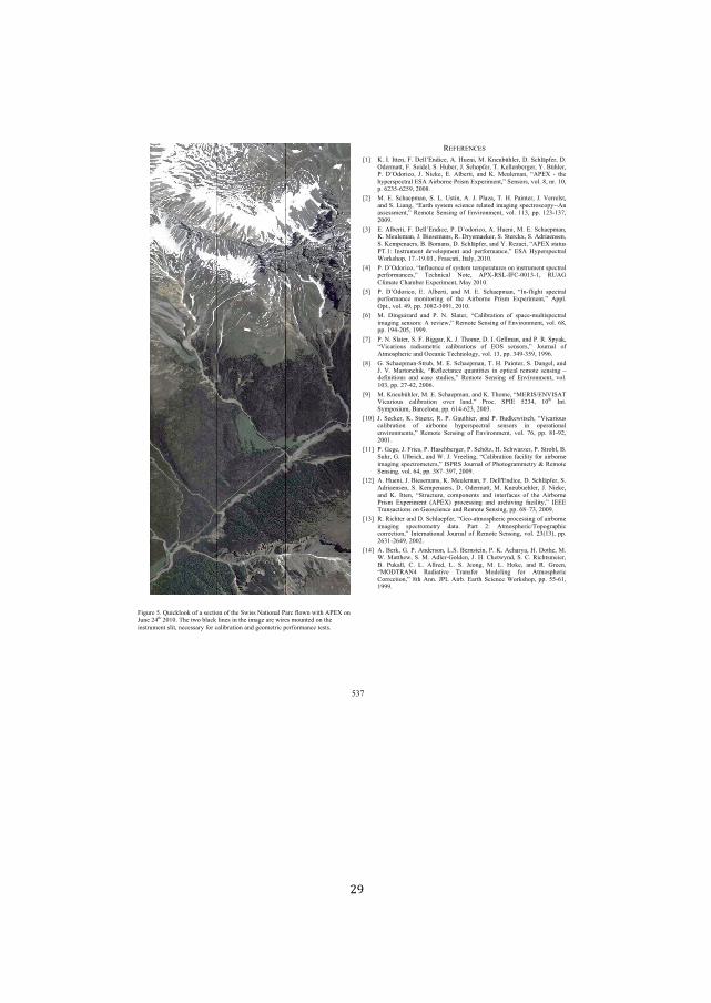
!29!

!

!

"#$#"#%&#'!

()*! +,!-,!-../01!$,!2/334#0567/1!8,!9:/061!;,!+0/:<=>3/?1!2,!'7>3@AB/?1!2,!

C5/?DE..1!$,!'/65/31!',!9:</?1!F,!'7>GAB/?1!H,!+/33/0</?I/?1!J,!K=>3/?1!L,! 24C5G?67G1! F,! %6/M/1! #,! 83</?.61! E05! +,!;/:3/DE01! N8L#O! P! .>/!

>QA/?RA/7.?E3!#'8!86?<G?0/!L?6RD!#SA/?6D/0.1T!'/0RG?R1!UG3,!V1!0?,!)W1!A,!XYZ[PXY[\1!YWWV,!

(Y*! ;,!#,!'7>E/ADE01!',!],!^R.601!8,! F,! L3E_E1!H,!9,!LE60./?1! F,!`/??/3R.1!

E05!',!]6E0I1!N#E?.>!RQR./D!R76/07/!?/3E./5!6DEI60I!RA/7.?GR7GAQPP80!ERR/RRD/0.1T!"/DG./!'/0R60I! GB!#0U6?G0D/0.1! UG3,!))Z1! AA,! )YZP)Za1!

YWW\,!

(Z*! #,!83</?.61!$,!2/334#0567/1!L,!24G5G?67G1!8,!9:/061!;,!#,!'7>E/ADE01!+,!;/:3/DE01!F,!K6/R/DE0R1!",!2?Q/DE/M/?1!',!'./?7MS1!',!85?6E/0R/01!

',!+/DA/0E/?R1!K,!KGDE0R1!2,!'7>3@AB/?1!E05!J,!"/_E/61!N8L#O!R.E.:R!LH,)b! -0R.?:D/0.! 5/U/3GAD/0.! E05! A/?BG?DE07/1T! #'8!9QA/?RA/7.?E3!

cG?MR>GA1!)a,P)\,WZ,1!$?ER7E.61!-.E3Q1!YW)W,!

(d*! L,!24C5G?67G1!N-0B3:/07/!GB!RQR./D!./DA/?E.:?/R!G0!60R.?:D/0.!RA/7.?E3!A/?BG?DE07/R1T! H/7>067E3! %G./1! 8LOP"']P-$&PWW)ZP)1! "^8e!

&36DE./!&>ED</?!#SA/?6D/0.1!;EQ!YW)W,!

([*! L,! 24C5G?67G1! #,! 83</?.61! E05! ;,! #,! '7>E/ADE01! N-0PB36I>.! RA/7.?E3!A/?BG?DE07/! DG06.G?60I! GB! .>/! 86?<G?0/! L?6RD! #SA/?6D/0.1T! 8AA3,!

CA.,1!UG3,!d\1!AA,!ZWVYPZW\)1!YW)W,!

(X*! ;,! 260I:6?E?5! E05! L,! %,! '3E./?1! N&E36<?E.6G0! GB! RAE7/PD:3.6RA/7.?E3!

6DEI60I!R/0RG?Rb!8!?/U6/f1T!"/DG./!'/0R60I!GB!#0U6?G0D/0.1!UG3,!XV1!AA,!)\dPYW[1!)\\\,!

(a*! L,!%,!'3E./?1!',!$,!K6IIE?1!+,!F,!H>GD/1!2,!-,!e/33DE01!E05!L,!",!'AQEM1!

N`67E?6G:R! ?E56GD/.?67! 7E36<?E.6G0R! GB! #C'! R/0RG?R1T! FG:?0E3! GB!8.DGRA>/?67!E05!C7/E067!H/7>0G3GIQ1!UG3,!)Z1!AA,!Zd\PZ[\1!)\\X,!

(V*! e,!'7>E/ADE0P'.?:<1!;,!#,!'7>E/ADE01!H,!9,!LE60./?1!',!2E0I/31!E05!

F,!`,!;E?.G07>6M1! N"/B3/7.E07/! g:E0.6.6/R! 60! GA.67E3! ?/DG./! R/0R60I!h!5/B606.6G0R! E05! 7ER/! R.:56/R1T! "/DG./! '/0R60I! GB! #0U6?G0D/0.1! UG3,!

)WZ1!AA,!YaPdY1!YWWX,!

(\*! ;,!+0/:<=>3/?1!;,!#,!'7>E/ADE01!E05!+,!H>GD/1!N;#"-'i#%`-'8H!`67E?6G:R! 7E36<?E.6G0! GU/?! 3E051T! L?G7,! 'L-#! [YZd1! )W

.>! -0.,!

'QDAGR6:D1!KE?7/3G0E1!AA,!X)dPXYZ1!YWWZ,!

()W*! F,! '/7M/?1!+,! '.E/0_1!",! L,!eE:.>6/?1! E05!L,!K:5M/f6.R7>1! N`67E?6G:R!7E36<?E.6G0! GB! E6?<G?0/! >QA/?RA/7.?E3! R/0RG?R! 60! GA/?E.6G0E3!

/0U6?G0D/0.R1T! "/DG./! '/0R60I! GB! #0U6?G0D/0.1! UG3,! aX1! AA,! V)P\Y1!YWW),!

())*! L,!e/I/1!F,!$?6/R1!L,!9ER7></?I/?1!L,!'7>j._1!9,!'7>fE?_/?1!L,!'.?G<31!K,!

':>?1!e,!^3<?67>1!E05!c,!F,!`?//360I1!N&E36<?E.6G0!BE7636.Q!BG?!E6?<G?0/!6DEI60I!RA/7.?GD/./?R1T!-'L"'!FG:?0E3!GB!L>G.GI?EDD/.?Q!k!"/DG./!

'/0R60I"!UG3,!Xd1!AA,!ZVahZ\a1!YWW\,!

()Y*! 8,!9:/061!F,!K6/R/DE0R1!+,!;/:3/DE01!$,!2/33l#0567/1!2,!'7>3@AB/?1!',!

85?6E/0R/01! ',!+/DA/0E/?R1!2,!C5/?DE..1!;,!+0/:<:/>3/?1! F,!%6/M/1!E05! +,! -../01! N'.?:7.:?/1! 7GDAG0/0.R! E05! 60./?BE7/R! GB! .>/! 86?<G?0/!

L?6RD! #SA/?6D/0.! m8L#On! A?G7/RR60I! E05! E?7>6U60I! BE7636.Q1T! -###!H?E0RE7.6G0R!G0!e/GR76/07/!E05!"/DG./!'/0R60I1!AA,!XVhaZ1!YWW\,!

()Z*! ",!"67>./?!E05!2,!'7>3E/AB/?1!Ne/GPE.DGRA>/?67!A?G7/RR60I!GB!E6?<G?0/!

6DEI60I! RA/7.?GD/.?Q! 5E.E,! LE?.! Yb! 8.DGRA>/?67iHGAGI?EA>67!7G??/7.6G01T! -0./?0E.6G0E3! FG:?0E3! GB!"/DG./!'/0R60I1! UG3,! YZm)Zn1! AA,!

YXZ)PYXd\1!YWWY,!!

()d*! 8,!K/?M1!e,!L,!805/?RG01!],',!K/?0R./601!L,!+,!87>E?QE1!9,!2G.>/1!;,!c,!;E..>/f1!',!;,!853/?PeG35/01!F,!9,!&>/.fQ051!',!&,!"67>.RD/6/?1!

K,! L:ME331! &,! ],! 833?/51! ],! ',! F/G0I1! ;,! ],! 9GM/1! E05! ",! e?//01!N;C2H"8%d! "E56E.6U/! H?E0RB/?! ;G5/360I! BG?! 8.DGRA>/?67!

&G??/7.6G01T! V.>!800,! FL]!86?<,! #E?.>! '76/07/!cG?MR>GA1! AA,! [[PX)1!)\\\,!

!

!

$6I:?/![,!o:67M3GGM!GB!E!R/7.6G0!GB!.>/!'f6RR!%E.6G0E3!LE?7!B3Gf0!f6.>!8L#O!G0!!

F:0/!Yd.>!YW)W,!H>/!.fG!<3E7M!360/R!60!.>/!6DEI/!E?/!f6?/R!DG:0./5!G0!.>/!!

60R.?:D/0.!R36.1!0/7/RRE?Q!BG?!7E36<?E.6G0!E05!I/GD/.?67!A/?BG?DE07/!./R.R,!

!

!"#

!

!

!31!

!

3 IN-FLIGHT SPECTRAL PERFORMANCE MONITORING OF APEX

This chapter has been published as: D'Odorico, P., Alberti, E. and Schaepman, M.E., 2010. In-flight spectral performance monitoring of the Airborne Prism Experiment. Applied Optics 49(16): 3082-3091.

The article is reprinted with kind permission of the Optical Society of America (OSA).

!

!

!33!

!

In-flight spectral performance monitoringof the Airborne Prism Experiment

Petra D’Odorico,* Edoardo Alberti, and Michael E. SchaepmanRemote Sensing Laboratories, University of Zurich. Winterthurerstrasse 190, CH-8057 Zurich, Switzerland

*Corresponding author: petra.dodorico@geo.uzh.ch

Received 22 February 2010; revised 23 April 2010; accepted 23 April 2010;posted 26 April 2010 (Doc. ID 124554); published 26 May 2010

Spectral performance of an airborne dispersive pushbroom imaging spectrometer cannot be assumed tobe stable over a whole flight season given the environmental stresses present during flight. Spectralperformance monitoring during flight is commonly accomplished by looking at selected absorption fea-tures present in the Sun, atmosphere, or ground, and their stability. The assessment of instrumentperformance in two different environments, e.g., laboratory and airborne, using precisely the same cali-bration reference, has not been possible so far. The Airborne Prism Experiment (APEX), an airbornedispersive pushbroom imaging spectrometer, uses an onboard in-flight characterization (IFC) facility,which makes it possible to monitor the sensor’s performance in terms of spectral, radiometric, and geo-metric stability in flight and in the laboratory. We discuss in detail a new method for the monitoring ofspectral instrument performance. The method relies on the monitoring of spectral shifts by comparinginstrument-inducedmovements of absorption features on ground and in flight. Absorption lines originatefrom spectral filters, which intercept the full field of view (FOV) illuminated using an internal lightsource. A feature-fitting algorithm is used for the shift estimation based on Pearson’s correlation co-efficient. Environmental parameter monitoring, coregistered on board with the image andcalibration data, revealed that differential pressure and temperature in the baffle compartment arethe main driving parameters explaining the trend in spectral performance deviations in the timeand the space (across-track) domains, respectively. The results presented in this paper show that thesystem in its current setup needs further improvements to reach a stable performance. Findings provideduseful guidelines for the instrument revision currently under way. The main aim of the revision is thestabilization of the instrument for a range of temperature and pressure conditions to be encounteredduring operation. © 2010 Optical Society of AmericaOCIS codes: 280.0280, 110.0110, 300.0300, 120.4640.

1. Introduction

Imaging spectroscopy [1] data are being increasinglydistributed to the user community at different qual-ity levels. Uncertainties originating from acquisition,calibration, and processing reduce their usability atdifferent levels of the data product chain. Nieke et al.[2] estimate the level of uncertainty to as high as 10%of the total radiance due to imperfections in the dataresulting from punctual effects [3] (e.g., bad pixels),spectral and spatial misregistration [4], and sensorstability and degradation related effects, among

other things. Since the advent of the first imagingspectrometers at the beginning of the 1980s [5], in-creasing attention has been devoted to the monitor-ing of these uncertainties and to improving thequality of the spectral data. Thanks to improvedcalibration concepts [6], new approaches [7,8], andadvanced technology [9], it was possible to generatemore accurate, i.e., uniform, imaging spectroscopydata and products. The same study [2] estimated howuncertainties of nonimaging and imaging instru-ments used in Earth observation could be reducedto values of <5%.

Focusing on the spectral domain, we refer to spec-tral calibration as the process in which spectral re-sponse functions (SRF), associated with individual

0003-6935/10/163082-10$15.00/0© 2010 Optical Society of America

3082 APPLIED OPTICS / Vol. 49, No. 16 / 1 June 2010

!34!

!

pixel elements across both dimension of the focalplane, are being defined. The latter usually foreseesmaking an assumption on the shape of SRFs (e.g.,Gaussian) and determining the center wavelengths(CW) as well as the full width at half-maximum(FWHM) describing each SRF. Spectral calibrationis usually performed prior to a flight season in a stan-dardization laboratory bymeans of a monochromatordevice [9]. A study by Green [10] estimated that aspectral calibration accuracy approaching 1% of theSRF’s FWHM is required to obtain radiances withoutsignificant spectrally distinct errors. Spectral nonu-niformities are usually present in the data in theform of band shifts or broadening [11], causing mod-ification of the SRF with respect to the position andshape determined during the initial laboratory char-acterization. These effects are expected to vary withtime and operation conditions. Pushbroom instru-ments present additional problems related to thespatial direction. In these systems, area arrays areused as focal planes generating three-dimensionalimaging spectroscopy cubes corresponding to theparameters time, center wavelength position, andacross-track view angle. For a uniform data set, theresponse curve in one dimension should be constantin the other two dimensions, e.g., the spectral re-sponse shall be constant with time and across-trackview angle [12]. The effect for which spectral re-sponse is not constant with across-track pixel posi-tion is known as spectral misregistration or smileand is to a high extent intrinsic to the instrumentdesign [10].

By not correcting systematically for these errors,and by relying on the initial nominal spectral labora-tory calibration, artifacts will arise when convertingthe signal into physical meaningful units [13].Guanter et al. [14] estimated that, for a syntheticdata set, a shift of 1nm for channels with a FWHMof 10nm results in an error in the measured radianceof up to !25% in the proximity of strong water vaporabsorption bands [14].

Different strategies are chosen to monitor instru-ment stability and uniformity in the resultingspectral data. For spaceborne systems, these usuallyare based on an onboard calibration mechanism.The moderate-resolution imaging spectroradiometer(MODIS) system employs a light source in combina-tion with a monochromator to monitor the spectralperformance in orbit [15]. In a similar fashion, themedium resolution imaging spectrometer (MERIS)instruments make use of an erbium-doped Spectra-lon diffuser plate, which offers a number of spectralabsorption features in the visible range. For charac-terization in the violet and near infrared, selectedFraunhofer lines and atmospheric features are cov-ered by MERIS channels thanks to the instrument’sspectral programmability [16]. The Hyperion systemlooks at the Sun rising through the limb of the Earth.In this way, light passes through the atmosphere be-fore reflecting off the solar calibration panel into theinstrument aperture, providing a spectrum rich in

solar lines, atmospheric lines, and absorption linesfrom the paint that coats the panel [17].

Airborne imaging spectrometers face a dif-ferent operational scenario than their spacebornecounterparts. Twomajor differences influence the ca-libration strategy to be adopted: the first is that air-borne instruments can return on ground to undergo arecharacterization in the laboratory; the second isthat being airborne implies a higher exposure tostresses caused by variation of environmental factors(e.g., pressure/temperature). This eventually meantthat differences between the laboratory setting andthe airborne platform, in terms of environmentalconditions, observational geometry, mechanical, elec-trical, and operational interfaces [18], could no long-er be neglected in the data calibration process. Theneed for an in-flight monitoring approach was thusaddressed by so-called scene-based methods, as pre-sented extensively for airborne sensors, such as thecompact airborne spectrographic imager (CASI) [14]and the airborne visible/infrared imaging spectro-meter (AVIRIS) [18]. These methods rely on featurespresent in the imagined spectra, which by nature al-ways occur at the same wavelength; these are atmo-spheric absorption features and solar Fraunhoferlines [14,19]. In short, a scene-based approach worksby comparing a spectrum acquired by the sensor inflight with a simulated reference spectrum (S). Thesimulated references result from the convolution ofthe highly resolved incoming signal with instrumentSRF, which are shifted by iterating on Δλ:

S "Z

SRF#λ$Δλ% ! L#λ% ! T#λ%dλ; #1%

where SRF#λ$Δλ% are the “new” SRF of the in-strument, L#λ% is the incoming signal, and T#λ% isthe atmospheric transmission function. The processreaches a halt when the best match between the ac-quired and a simulated spectrum is found, wherebythe corresponding Δλ represents the shift.

Three fundamental limitations are associated withscene-based methods. The first is the disputable as-sumption for which the variability in time and het-erogeneity in space of the atmospheric layer [14], aswell as the directional effects in the scene, are neg-ligible compared to spectral nonuniformities intro-duced by the instrument instability. The secondconstraint is seen in the inability to establish trace-ability between characterization measurements per-formed in flight and characterization measurementacquired on ground by using the same measurementtechniques and references. Last but not least, thegeneration of simulated reference spectra obtainedby iterating on SRF position and/or width, requiresthe nominal SRFs from laboratory characterization.Thus, the uncertainties linked with the determina-tion of the latter are propagated throughout theestimation of the new spectral parameters.

An alternative approach able to overcome theselimitations is technically feasible by including

1 June 2010 / Vol. 49, No. 16 / APPLIED OPTICS 3083

!35!

!

characterization equipment in the instrument designconcept, as previously presented for spacebornesystems. In the early 1990s, the use of onboard char-acterization equipment was first attempted withAVIRIS. In this instrument, the onboard signalsource is given by a 10W quartz halogen lamp stabi-lized by a silicon detector feedback circuit. The lightis transmitted through optical fibers to the back ofthe foreoptics shutter and reflected from there to theAVIRIS spectrometer [20,21]. Similarly, in 1997 arevision of the reflective optics system imaging spec-trometer (ROSIS) airborne instrument brought theinclusion of a mercury lamp for onboard spectral ca-libration before and after each flight line [22]. Sincethen—to the best of our knowledge—no furtherdevelopment has taken place in this direction.

The Airborne Prism Experiment (APEX) imagingspectrometer [23] is, to the best of our knowledge,the first pushbroom instrument including an in-flight characterization (IFC) facility that allows a fullcharacterization of system properties, i.e., radio-metric, spectral, and geometric, during flight as wellas on ground for the full instrument field of view(FOV). In this paper, we present the findings of a ser-ies of ground and flight experiments in which dataacquired with the IFC are used to understand thesystem behavior in different operational conditions.A spectral performance monitoring methodology,using IFC filter features to monitor spectral datauniformity, has been developed in this context.

2. APEX and Its In-Flight Characterization Facility

TheAPEXproject started in1997 [24] byperformingafeasibility study on the design of an imaging spectro-meter. System specifications were defined based onuser requirements and on a subsequently derived for-ward-performancemodel built on these requirements[25]. Key instrument requirements are reported inTable 1. APEX serves amultitude of purposes, includ-ing future sensor simulation, regional-scale biogeo-chemical cycle assessment, and technology studies.In the summer of 2009, the first extensive flightand field campaigns were carried out in Europe aspart of the instrument acceptance process.

APEX mechanical and thermal design is conceivedto minimize the impact of environmental param-eters, such as pressure, temperature, and vibrations.During exploitation, airborne instruments experi-ence a standard atmosphere at 5:5km a.s.l., an exter-nal temperature of about !21 °C, and an absolutepressure of 50kPa. The APEX mechanical interfaceplate (MIP) allows the installation and interface ofthe instrument, for example, with the aircraft orthe calibration bench. The APEX optical baseplate (OBP), the supporting core of the instrument,is linked to the MIP by a system of six studs withspherical head joints, aiming at minimizing thedistortions on the OBP itself induced by externalthermo-mechanical effects. A carbon fiber cover,which is gas tight by means of an O-ring, is mountedon the MIP. The aim is to seal the optical subunit in a

nitrogen atmosphere, protecting the optical instru-ment from contamination and degradation (e.g.,chemicals, condensation) during flight operations.The internal pressure at takeoff ranges between 110and 130kPa. An optical windowmounted on the MIPallows the radiance input inside the optical system.To support instrument thermal conditioning withinthe operating temperature range, the aircraft instal-lation includes an environmental control box (ETC)to generate a stabilized temperature environmentsurrounding the page. The instrument baffle is con-nected to the MIP with a system designed to mini-mize thermal conduction through the mechanicalstructure. Nevertheless, convective heat exchangehappens by means of airflow streaming throughthe optical baffle aperture, reaching the bottom ofthe MIP plate and streaming inside the ETC box.The instrument is installed on a Leica PAV30 stabi-lizing platform, allowing it to be a nadir-looking sys-tem within !5° of roll and pitch angles.

The instrument design is a dispersive pushbroomspectrometer, acquiring the spectral and across-trackdomain on area detectors. Imaging is performedthrough the forward motion of the aircraft. The FOVis projected by the ground imager onto the spectro-meter slit using a path folding mirror. To minimizethe polarization sensitivity, a scrambler can be in-serted to randomize the polarization of the incominglight at the expense of spatial resolution. A collima-tor lens group directs the light on the first prism. Adichroic coating separates the short-wave infrared(SWIR) and visible near infrared (VNIR) channels.The VNIR channel is then dispersed further usinga second prism. The VNIR detector is a commercialcharged coupled device (CCD) ranging from 380–1000nm. For the SWIR channel, a specific comple-

Table 1. APEX Instrument—Key Requirements

Parameter Requirement

Field of view (FOV)—pushbroom techniques

Swath: !14 deg with1000 across-track pixels

Instantaneous fieldof view (IFOV)

0:028 deg.

Flight altitude range 3:5–10km a.s.l.Standard aircraftinterface

For Dornier Do-228 onstabilizing platform PAV-30

Spectral coverage VNIR: 380–970, SWIR: 940–2500Spectral channels VNIR: 334 (prior binning) or 114

(default binning). SWIR: 198Spectral samplinginterval (SSI)

VNIR: 0:5–8nm. SWIR: 5–10nm

FWHM "1:5 SSICenter wavelengthaccuracy

<0:2nm

Smile/Keystone <0:35 pixelCoregistration <0:9 pixelInstrument temporalradiometric uncertaintywithin a flight section

<2%

Interval for instrumentrecalibration

Before and after a completeflight season.

3084 APPLIED OPTICS / Vol. 49, No. 16 / 1 June 2010

!36!

!

mentary metal oxide semiconductor (CMOS)mercury cadmium telluride (MCT) detector arraywas developed [26] ranging from 940–2500nm. Thetwo spectrometer channels are aligned to minimizethe geometric coregistration error.

An integral part of the APEX spectrometer is abuilt-in IFC facility (Fig. 1). During the in-flight char-acterization operation, the main instrument shutteris closed to avoid any light penetrating from the out-side. A stabilized quartz–tungsten–halogen (QTH)75W lamp in a dedicated housing is attached to anoptical fiber. The optical fiber guides the light fromthe lamp through the calibration shutter, which isusually closed to prevent the IFC light from enteringthe spectrometer during image acquisition. Diffusersare placed before and after a fixed folding mirror toimprove the uniformity of the illumination. A sensoris used to monitor the light level and to control thelamppoweraccordingly ina closed control loop.A slid-ing foldingmirror is moved into the optical path to re-

flect the light generated by the IFC toward a filterwheel mounted in front of the ground imager. Thewheel holds four spectral filters to be used for instru-ment spectral stability monitoring; these are threebandpass filters (Spectrogon) with absorption fea-tures at 700, 1000, and 2218nm and a standard refer-encematerial (SRM) filter fromtheNational Institutefor Standards and Technology (NIST) (Fig. 2). TheNIST certified SRM filter holdsmany distinct absorp-tion features and can be used as a secondary spectralcalibration standard. A fifth filter, an NG4 attenua-tion filter, is used to avoid saturation in the VNIRchannel at maximum radiance levels (image acquisi-tion over snow). The sixth filter wheel position is leftempty for standard data acquisition. Deterioration ofthe spectral filters is not expected as they are locatedinside the enclosed and temperature-stabilizedoptical subunit.

For each filter used, the IFC light is dispersed ontothe detectors in exactly the same fashion as groundobservations. With this design, all relevant opticalelements of APEX can be calibrated in flight. A de-fault IFC spectral calibration measurement consistsof 316 ! 1000 ! 20 pixels, where 316 is the combina-tion of VNIR (117) and SWIR (199) spectral pixels,1000 is the number of across-track detector pixels,and 20 is the average number of frames per defaultmeasurement. IFCmeasurements can be acquired atdifferent integration times (ITs), with a default of29ms. Once the instrument becomes operational, itis planned to perform IFC measurements regularlyduring each laboratory and flight campaign.

3. Materials and Methods

A. Methods

Spectral monitoring techniques that rely on the posi-tion of stable and known spectral features, are allbased on a common assumption. The latter statesthat a shift in SRFs (i.e., center wavelength) causesspectral features to be sampled differently, namely,higher or lower in the absorption slopes. As a result,features which, “by nature,” are always found at thesame wavelengths, happen to be “apparently” shiftedtoward lower or higher wavelengths. As an example,SRFs shifted toward the lower wavelength slope of

Fig. 1. (Color online) IFC facility onboard APEX: (1) QTH lamp;(2) optical fiber; (3) fiber output; (4) calibration shutter; (5) fixedfolding mirror; (6) diffusers; (7) feedback loop sensor; (8) slidingfolding mirror; (9) filter wheel; (10) fixed folding mirror; (11) globalshutter; ! temperature sensor; ! temperature sensor on opticalbase plate (averaged); " differential temperature sensors.

Fig. 2. (Color online) Transmission of the spectral filtersmounted on the IFC facility onboard the APEX imaging spectro-meter (SRM NIST, black; BP700, red; BP1000, blue; BP2218,green).

1 June 2010 / Vol. 49, No. 16 / APPLIED OPTICS 3085

!37!

!

the absorption feature, i.e., wavelengths are de-creased, result in an apparent feature shift towardhigher wavelengths as seen in Fig. 3. This is ex-plained by the fact that SRFs shifted toward lowerwavelengths cause a higher signal to be sampled forthe lower wavelength slope and a lower signal to besampled for the higher wavelength slope (i.e., justimagine sampling the same feature slightly to theleft of the original points). It is thus possible to esti-mate the shift in the instrument SRFs by retrievingthe observed shift in the imagined features.

The approach proposed for the APEX instrumentforesees looking at the same IFC feature-rich spec-trum on ground and at different moments duringflight and searching for the spectral shift of the nom-inal channel positions by finding the best fit. Toachieve the best sensitivity, the fitting is evaluatedonly around predefined spectral regions where thefilter’s features occur. Features located in a regionof the spectrum characterized by too low a signalwere excluded from the analysis.

The fundamental difference between the metho-dology proposed here and the scene-based approachdescribed earlier is that in the former, spectra di-rectly measured by the instrument are used for theestimation, while in the latter, modeled quantitiesobtained by moderate resolution atmospheric trans-mission (MODTRAN) simulations and convolutionoperations are taken as a reference. To better under-

stand this difference, a more detailed algorithmdescription is provided in the following.

It is assumed that for an operational instrumentspectral shifts occur mostly at the subpixel level.Estimation at this resolution requires the measuredIFC spectra to be resampled to a finer sampling in-terval. This was achieved by linear interpolation ofspectra. A brief assessment of other interpolationtechniques (e.g., spline) showed negligible differ-ences between techniques. In a first step, spectralfeatures in the reference IFC onground spectrum areidentified. Features usually extend over 5–10 spec-tral bands. Individual features are indexed by defin-ing a lower (xL) and an upper (xU) spectral pixelnumber. While xL and xU remain fixed for the groundspectrum, they are iteratively changed for the flightspectrum for which the feature position shall be de-termined. In practice, this step is carried out by em-ploying a sliding window, which scans across theflight spectrum as shown in Fig. 4. The step Δx sizeby which the window moves corresponds to the stepdefined earlier for the interpolation of the spectrumand represents the resolution of the algorithm (i.e.,the minimum shift that can be retrieved). The stepsize Δx was set to a value of 0:01pixels. This thresh-old was determined using a sensitivity analysisaccounting for system intrinsic fluctuations (e.g.,random noise) during spectra acquisition and meth-od uncertainty [27,28]. Each spectral interval identi-fied by the sliding window is iteratively comparedwith the reference feature using feature matching.The best feature match is identified by means ofan optimization procedure that minimizes the devia-tion between the ground reference feature and thefeature in the flight spectrum. Different merit func-tions can be used to assess the goodness of each itera-tive match, such as position of the feature’s peak,position of the feature’s center of gravity (COG), stan-dard deviation, or Pearson’s correlation coefficient.Pearson’s correlation coefficient has been chosenfor this study as the merit function to be maximized;reasons for this choice lie in the results obtained bymeans of a sensitivity study [27] and on a review ofliterature [16,17,29–32]. In the sensitivity analysis,

Fig. 3. Example of an absorption feature seen by a sensor withnominal (continuous) and with shifted (discontinuous) SRF: where□ points sampled with nominal SRF and ▵ point sampled withshifted SRF.

Fig. 4. Sliding window progressively shifting ofΔx and defining alower !xL "Δx# and an upper !xU "Δx# spectral pixel position bywhich a portion of the flight spectrum is indexed. The sliding win-dow is shown for two iteration steps.

3086 APPLIED OPTICS / Vol. 49, No. 16 / 1 June 2010

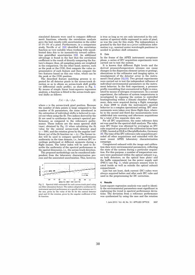
!38!

!

simulated datasets were used to compare differentmerit functions, whereby the correlation analysisgave the best results with uncertainties in the orderof 1%–3% of a pixel. Furthermore, in a comparisonstudy, Neville et al. [33] identified the correlationfunction as very suitable when working with uncali-brated data due to its insensitivity toward calibra-tion gain/offset uncertainties [32]. An additionaladvantage is found in the fact that the correlationcoefficient is the result of directly comparing the fea-ture’s shapes; thus, all sampling points are weightedin the comparison. On the other hand, metrics, suchas the peak or the COG, first compute the value re-presentative of each feature and then compare thetwo features based on this one value, which can bethe peak or the COG position.

The described feature matching process is re-peated for all detector pixels in the across-track di-rection so as to obtain an across-track shift profile(or differential smile profile), as shown in Fig. 5.By means of simple linear least-squares regressionanalysis, a function is fitted to the across-track spec-tral shifts as follows:

f !x" # !0 $ !1x; !2"

where x is the across-track pixel position. Becausethe number of data points is large compared to thenumber of fit parameters, the noise introduced inthe estimation of individual shifts is believed to can-cel out when using the fit. Two indices derived by thefit are used to synthesize the system’s spectral per-formance as compared to the reference’s perfor-mance. These indices are the mean spectral shift(mss), obtained by Eq. (2) when calculating the fitvalue for the central across-track detector pixel(x # 500), and the rotation given by the angular coef-ficient (ac) of the fit function (ac # !1). The former in-dex will be used to compare spectral performanceuniformity in the time domain, i.e., between IFC re-cordings performed at different moments during aflight season. The latter index will be used to de-scribe the uniformity of the spectral performance inthe spatial dimension, i.e., the across-track direction.

The proposed methodology can be considered inde-pendent from the laboratory characterization pro-cess and the associated uncertainties. This, however,

is true as long as we are only interested in the esti-mation of spectral shifts expressed in units of pixel,as was the case for this study. The independence isgranted by the fact that no a priori calibration infor-mation (e.g., nominal center wavelength positions) isneeded to produce shift estimates.

B. Data

In the frame of the APEX instrument acceptancephase, a series of IFC acquisition experiments werecarried out to test the system.

It is known that different flight levels and thederived pressure/temperature stresses can causechanges in the dispersion element (prism or grating),aberrations in the collimator and imaging optics, ormisalignment of the detector array in the instru-ment’s focal plane [32,33]. Two ground experimentswere carried out to test the independent influence ofindividual environmental parameters on the instru-ment behavior. In the first experiment, a pressureprofile resembling that encountered in flight is simu-lated by means of nitrogen overpressure. In a secondexperiment, the influence of system temperatures isinvestigated by exposing the system to controlledheating/cooling within a climate chamber. Further-more, data were acquired during a flight campaignin June 2009 to study the instrument’s spectralbehavior in a complex operational setting. IFC mea-surements were taken over three flight days, where-by in the second and third day measurements weresubdivided into morning and afternoon acquisitionsfor a total of five separate data sets.

For all IFC acquisitions, the same reference dataset was used for the spectral shift analysis. The refer-ence IFC frame was obtained by averaging an IFCcube acquired on ground at the calibration home base(CHB), located atDLR inOberpfaffenhofen,Germany[9]. The timeof the IFCreference cubeacquisitionpre-ceded all other acquisitions and coincided with themost recent APEX laboratory characterizationcampaign.

Coregistered onboard with the image and calibra-tion data were environmental parameters, reflectingthe state of the system during a particular acquisi-tion. For this purpose, a number of temperature sen-sors were positioned within the optical subunit (e.g.,on both detectors, on the optical base plate) andthe baffle compartment [on the power supply unit(PSU)] (see Fig. 1), while pressure sensors were lo-cated inside as well as outside the optical subunitcompartment.

Last but not least, dark current (DC) cubes werealways acquired before and after each IFC cube andused in the preprocessing for DC correction.

4. Results

Least-square regression analysis was used to identi-fy the environmental parameters most significant inexplaining the trend in spectral performance devia-tions. The deviation from a reference performancewas synthesized by using the mss and the rotation

Fig. 5. Spectral shift estimated for each across-track pixel usingone filter absorption feature. The indices adopted to synthesize theinstrument spectral performance at a specific time instance are (1)the mss, given by the value of the fit for the central detectorpixel and (2) the rotation, given by the angular coefficient of thefit function.

1 June 2010 / Vol. 49, No. 16 / APPLIED OPTICS 3087

!39!

!

(ac) indices. In the controlled ground experiment, thevariation of differential pressure (dP), calculated asthe difference between pressures registered intern-ally and externally the optical subunit, was foundto explain the spectral performance nonuniformitiesin time (mean r2 ! 0:98). For dP ranging from −100to 550 mbar, a linear absolute increase of mss wasestimated, where the highest absolute shifts of about1:6pixels occurred in concomitance with maximal dPconditions. Results are depicted in Fig. 6, where tri-angles represent the mss associated with an IFCmeasurement performed at a specific time and dPcondition. Standard deviations (size of the verticalbars) provide an indication of the dispersion ofacross-track shifts around the mean shift, i.e., theshift associated with the central detector pixel.

The correlation analysis carried out between eachhousekeeping parameter and the mss for the flight

data confirmed dP as being the most influentialparameter. The comparison with the relation foundfor the ground experiment revealed, however, a lesssteep drop in spectral performance with rising dP.The latter can be ascribed to the fact that on groundthe influence of dP was assessed in an independentmanner, i.e., all other environmental parameterswere kept stable, while in-flight joint dynamics influ-ence system behavior. Residual analysis showed howthis relationship, when modeled for a complex opera-tional setting, is best described by an exponentialregression model (Fig. 6).

The analysis was repeated for four spectral regionsin the VNIR and four in the SWIR, based on the dataacquired over the three flight days. The day-to-daydifferences in dP values can be ascribed to the differ-ent IFC measuring scenarios, in terms of flight alti-tude and time elapsed since takeoff.

The results of the trend analysis presented in Fig. 7evidenced good agreement for all investigated spec-tral regions, with mss increasing exponentially as afunction of the rising dP. Small shift differences alongthe spectral domain were expected because, for eachspectral region, a different filter feature was used inthe estimation. The difference in feature shape, aswell as in number of points encompassed by each fea-ture, is responsible for the small variations.

A constant absolute shift in the range of 0:2–0:4pixels in the VNIR and 0:4–0:6pixels in the SWIRwas estimated for dP below 400mbar. It is assumedthat the climbing of the dP beyond this value re-leased the system from what was a state of staticequilibrium and provoked an exponential increaseof the shift, reaching 1pixel in the VNIR and 1:3pixelin the SWIR for dP of 550mbar.

Fig. 6. Spectral mean shifts estimated for flight data (∘) and foron-ground data (▵) acquired at different pressure regimes. Thesize of the vertical bar (|) represents the standard deviation ofthe estimates. Linear (continuous line) and exponential (discontin-uous line) regression models have been fitted to the data. Resultsare for the feature at 784–815nm.

Fig. 7. Mean spectral shift estimates for four spectral regions of the VNIR (top) and SWIR (bottom) detector, plotted against the differ-ential pressure trend. Data were acquired over three flight days: ∘17/06, □18/06 AM, ▵18/06 PM, *23/06 AM, !23=06 PM. Data wereacquired with the NIST SRM and with the bandpass filters. The size of the vertical bar (|) represents the standard deviation of theestimates. The dotted horizontal lines enclose the interval corresponding to one unbinned detector pixel and report the nanometersfor the specific wavelength region.

3088 APPLIED OPTICS / Vol. 49, No. 16 / 1 June 2010

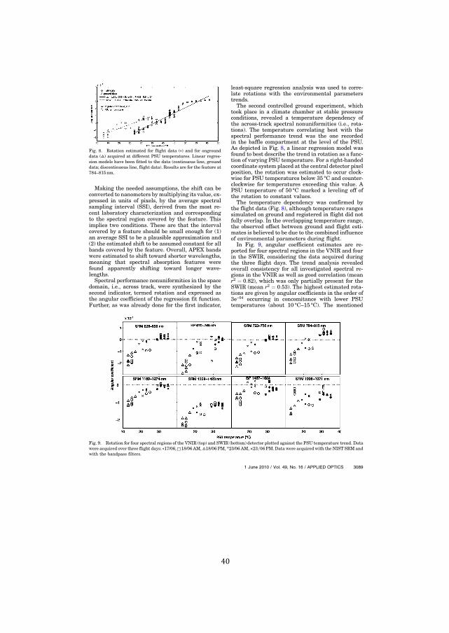
!40!

!

Making the needed assumptions, the shift can beconverted to nanometers bymultiplying its value, ex-pressed in units of pixels, by the average spectralsampling interval (SSI), derived from the most re-cent laboratory characterization and correspondingto the spectral region covered by the feature. Thisimplies two conditions. These are that the intervalcovered by a feature should be small enough for (1)an average SSI to be a plausible approximation and(2) the estimated shift to be assumed constant for allbands covered by the feature. Overall, APEX bandswere estimated to shift toward shorter wavelengths,meaning that spectral absorption features werefound apparently shifting toward longer wave-lengths.

Spectral performance nonuniformities in the spacedomain, i.e., across track, were synthesized by thesecond indicator, termed rotation and expressed asthe angular coefficient of the regression fit function.Further, as was already done for the first indicator,

least-square regression analysis was used to corre-late rotations with the environmental parameterstrends.

The second controlled ground experiment, whichtook place in a climate chamber at stable pressureconditions, revealed a temperature dependency ofthe across-track spectral nonuniformities (i.e., rota-tions). The temperature correlating best with thespectral performance trend was the one recordedin the baffle compartment at the level of the PSU.As depicted in Fig. 8, a linear regression model wasfound to best describe the trend in rotation as a func-tion of varying PSU temperature. For a right-handedcoordinate system placed at the central detector pixelposition, the rotation was estimated to occur clock-wise for PSU temperatures below 35 °C and counter-clockwise for temperatures exceeding this value. APSU temperature of 50 °C marked a leveling off ofthe rotation to constant values.

The temperature dependency was confirmed bythe flight data (Fig. 8), although temperature rangessimulated on ground and registered in flight did notfully overlap. In the overlapping temperature range,the observed offset between ground and flight esti-mates is believed to be due to the combined influenceof environmental parameters during flight.

In Fig. 9, angular coefficient estimates are re-ported for four spectral regions in the VNIR and fourin the SWIR, considering the data acquired duringthe three flight days. The trend analysis revealedoverall consistency for all investigated spectral re-gions in the VNIR as well as good correlation (meanr2 ! 0:82), which was only partially present for theSWIR (mean r2 ! 0:53). The highest estimated rota-tions are given by angular coefficients in the order of3e−04 occurring in concomitance with lower PSUtemperatures (about 10 °C–15 °C). The mentioned

Fig. 8. Rotation estimated for flight data (∘) and for ongrounddata (▵) acquired at different PSU temperatures. Linear regres-sion models have been fitted to the data (continuous line, grounddata; discontinuous line, flight data). Results are for the feature at784–815nm.

Fig. 9. Rotation for four spectral regions of the VNIR (top) and SWIR (bottom) detector plotted against the PSU temperature trend. Datawere acquired over three flight days: ∘17/06,□18/06 AM,▵18/06 PM, *23/06 AM, !23=06 PM. Data were acquired with the NIST SRM andwith the bandpass filters.

1 June 2010 / Vol. 49, No. 16 / APPLIED OPTICS 3089

!41!

!

angular coefficient value corresponds to angles ofabout 0:017 deg (angle ! arctan"ac# $ 180=!) or tomaximal rotations of 0:3pixels.

It should be noted at this point that what was heretermed rotation is in reality a change in the intrinsicsmile profile. The latter can have two main origins.The first, most likely source, is a mechanical mis-alignment causing the image of the slit to beprojected differently on the detector array (i.e., thewhole detector is rotating). The second source islinked to aberrations in the instrument optics andusually causes spectrally dependent nonuniformi-ties. The contributions of these two sources to theoverall change in smile profile are difficult to sepa-rate based exclusively on the current analysis. Thefact that mechanical misalignments are more likelyto occur than optical aberrations, coupled with a re-latively good spectral independence of the results,made us prefer the term rotation.

Further work is needed to confirm these hypoth-eses, such as the integration with results comingfrom the geometric analysis, in which the positionof the features intrinsic to the slit across-track pro-file are monitored in the same fashion as spectralfeatures.

5. Conclusion

In this paper, the potential of built-in characteri-zation equipment for monitoring system spectral per-formances over a wide range of operational condi-tions is shown for the first time, to the best of ourknowledge, for an airborne dispersive pushbroomimaging spectrometer. The presented methodologywas found suitable for the monitoring and quantifi-cation of spectral nonuniformities in the time andspace (across-track) domains. Two indices, synthesiz-ing the instrument spectral performance comparedto a reference (on ground) performance, were used;these are the mean shift and the rotation.

The system spectral performance during flight wasfound to deviate from the reference performancecharacterized on ground prior to flight. Maximalmean shift of about 1pixel and maximal rotation ofabout 0:017 deg were estimated on average for bothdetectors. The availability of housekeeping informa-tion (e.g., temperatures and pressure), associatedwith the system at each acquisition, was funda-mentally important for the study. As a result, envir-onmental performance dependencies advanced theunderstanding of the system behavior during opera-tion. This study showed the importance of havingwell-distributed thermal sensors within the instru-ment. The relevance of monitoring the internaland external pressure as a possible instrument per-formance driver was further evidenced.

A trend analysis of data acquired in a controlledenvironment in the frame of two ground experimentsrevealed that differential pressure and temperaturein the baffle compartment were the driving factorsfor spectral performance deviations in the time andthe spatial domains, respectively. These findings

provide valuable information for the realization ofinstrument design changes aimed at minimizingthe effects investigated in this study.

Future work foresees the integration of results ob-tained from scene-based approaches, using spectralfeatures present in the image scene itself (e.g., atmo-spheric features and solar Fraunhofer lines), as wellas geometric stability monitoring, based on featurespresent in the across-track slit profile (slit irregula-rities). These may further improve the interpretationof the system behavior in regard to external factorsas treated within this study.

This work has been done in the frame of theAPEX project funded by an ESA/PRODEX contract.P. D’Odorico acknowledges the support of a MarieCurie Fellowship awarded in the frame of the SixthFramework Program through the Hyper-I-Net net-work. The authors thank A. Hüni and F. Dell’Endicefrom University of Zurich for data collection andV. Mogulsky from Kayser Threde and D. Schläpferfrom ReSe for beneficial discussions. A specialthanks goes to A. Gonsamo for valuable commentson an earlier version of this paper. Last but not least,we acknowledge the thoughtful comments of threeanonymous reviewers.

References1. M. E. Schaepman, S. L. Ustin, A. J. Plaza, T. H. Painter,

J. Verrelst, and S. Liang, “Earth system science related ima-ging spectroscopy-an assessment,” Remote Sens. Environ.113, S123–S137 (2009).

2. J. Nieke, D. Schlaepfer, F. Dell’Endice, J. Brazile, andK. I. Itten, “Uniformity of imaging spectrometry data pro-ducts,” IEEE Trans. Geosci. Remote Sens. 46, 3326–3336(2008).

3. D. Schlaepfer, J. Nieke, and K. I. Itten, “Spatial PSF nonuni-formity effects in airborne pushbroom imaging spectrometrydata,” IEEE Trans. Geosci. Remote Sens. 45, 458–468 (2007).

4. F. Dell’Endice, J. Nieke, D. Schlaepfer, and K. I. Itten, “Scene-based method for spatial misregistration detection in hyper-spectral imagery,” Appl. Opt. 46, 2803–2816 (2007).

5. G. Vane, A. F. H. Goetz, and J. B. Wellman, “Airborne imagingspectrometer: a new tool for remote sensing,” IEEE Trans.Geosci. Remote Sens. GE-22, 546–549 (1983).

6. M. E. Schaepman and S. Dangel, “Solid laboratory calibra-tion of a nonimaging spectroradiometer,” Appl. Opt. 39,3754–3764 (2000).

7. N. Fox, J. Aiken, J. J. Barnett, X. Briottet, R. Carvell,C. Frohlich, S. B. Groom, O. Hagolle, J. D. Haigh, H. H. Kieffer,J. Lean, D. B. Pollock, T. Quinn, M. C. W. Sandford, M. Schaep-man, K. P. Shine, W. K. Schmutz, P. M. Teillet, K. J. Thome,M. M. Verstraete, and E. Zalewski, “Traceable radiometry un-derpinning terrestrial- and helio-studies (TRUTHS),” Adv.Space Res. 32, 2253–2261 (2003).

8. P. N. Slater, S. F. Biggar, J. M. Palmer, and K. J. Thome, “Uni-fied approach to absolute radiometric calibration in the solar-reflective range,” Remote Sens. Environ. 77, 293–303 (2001).

9. P. Gege, J. Fries, P. Haschberger, P. Schötz, H. Schwarzer,P. Strobl, B. Suhr, G. Ulbrich, and W. J. Vreeling, “Calibrationfacility for airborne imaging spectrometers,” ISPRS J. Photo-gramm. Remote Sens. 64, 387–397 (2009).

10. R. Green, “Spectral calibration requirements for Earth-looking imaging spectrometers in the solar-reflectedspectrum,” Appl. Opt. 37, 683–690 (1998).

3090 APPLIED OPTICS / Vol. 49, No. 16 / 1 June 2010

!42!

!

11. P. Mouroulis, R. Green, and T. Chrien, “Design of pushbroomimaging spectrometer for optimum recovery of spectroscopicand spatial information,” Appl. Opt. 39, 2210–2220 (2000).

12. D. Schläpfer, J. Nieke, and K. I. Itten, “Spatial PSF non-uniformity effects in airborne pushbroom imaging spectrome-try data,” IEEE Trans. Geosci. Remote Sens. 45, 458–468(2007).

13. L. Guanter, K. Segl, B. Sang, L. Alonso, H. Kaufmann, andJ. Moreno, “Scene-based spectral calibration assessment ofhigh spectral resolution imaging spectrometers,”Opt. Express17, 11594–11606 (2009).

14. L. Guanter, V. Estellès, and J. Moreno, “Spectral calibrationand atmospheric correction of ultra-fine spectral and spatialresolution remote sensing data. Application to CASI-1500data,” Remote Sens. Environ. 109, 54–65 (2007).

15. H. Montgomery, N. Che, K. Parker, and J. Bowser, “The algo-rithm for MODIS wavelength on-orbit calibration using theSRCA,” IEEE Trans. Geosci. Remote Sens. 38, 877–884(2000).

16. S. Delwart, R. Preusker, L. Bourg, R. Santer, D. Ramon, andJ. Fischer, “MERIS in-flight spectral calibration,” Int. J.Remote Sens. 28, 479–496 (2007).

17. P. S. Barry, J. Shepanski, and C. Segal, “Hyperion on-orbitvalidation of spectral calibration using atmospheric linesand an on-board system,” Proc. SPIE 4480, 231–235 (2002).

18. R. Green and B. Pavri, “AVIRIS inflight calibration experi-ment measurements, analysis and results in 2000,” in Pro-ceedings of the Tenth JPL Airborne Earth Science Workshop(Jet Propulsion Laboratory, 2001), pp. 205–219.

19. L. Guanter, R. Richter, and J. Moreno, “Spectral calibration ofhyperspectral imagery using atmospheric absorption fea-tures,” Appl. Opt. 45, 2360–2370 (2006).

20. R. Green, M. Eastwood, C. Sarture, T. Chrien, M. Aronsson,B. Chippendale, J. Faust, B. Pavri, C. Chovit, M. Solis,M. Olah, and O. Williams, “Imaging spectroscopy and theairborne visible/infrared imaging spectrometer (AVIRIS),”Remote Sens. Environ. 65, 227–248 (1998).

21. T. Chrien, M. Eastwood, R. Green, C. Sarture, H. Johnson,C. Chovit, and P. Hajek, “airborne visible/infrared imagingspectrometer (AVIRIS) onboard calibration system,” in Sum-maries of the Fifth Annual JPL Airborne Earth Science Work-shop (Jet Propulsion Laboratory, 1995), pp. 31–32.

22. P. S. S. Thiemann, P. Gege, N. Stahl, W. Mooshuber, andH. van der Piepen, “Das abbildende spektrometer ROSIS,”in Publikationen der Deutschen Gesellschaft für Photogram-

metrie und Fernerkundung, E. Seyfert, ed. (DLR, 2001), pp.147–153.

23. K. Itten, F. Dell Endice, A. Hueni, M. Kneubuehler,D. Schlaepfer, D. Odermatt, F. Seidel, S. Huber, J. Schopfer,T. Kellenberger, Y. Buehler, P. D’Odorico, J. Nieke, E. Alberti,and K. Meuleman, “APEX—the hyperspectral ESA airborneprism experiment,” Sensors 8, 6235–6259 (2008).

24. K. I. Itten, M. Schaepman, L. De Vos, L. Hermans,H. Schlaepfer, and F. Droz, “APEX—airborne PRISM experi-ment: a new concept for an airborne imaging spectrometer,” inProceedings of the Third International Airborne RemoteSensing Conference and Exhibition (Environmental ResearchInstitute of Michigan, 1997), pp. 181–188.

25. D. Schläpfer and M. Schaepman, “Modelling the noise equiva-lent radiance requirements of imaging spectrometers basedon scientific applications,” Appl. Opt. 41, 5691–5701 (2002).

26. P. Chorier and P. Tribolet, “High performance HgCdTe SWIRdetectors for hyperspectral instruments,” Proc. SPIE 4540,328–341 (2001).

27. P. D’Odorico, E. Alberti, F. Dell’Endice, A. Hüni, and K. Itten,“An algorithm for tracking APEX spectral stability by meansof the in-flight characterizarion facility (IFC),” in Proceedingsof the 6th EARSeL Workshop on Imaging Spectroscopy(EARSeL, 2009), p. 5.

28. P. D’Odorico, E. Alberti, F. Dell’Endice, A. Hüni, andM. Schaepman, “Spectral stability monitoring of an imagingspectrometer by means of onboard sources.,” in Proceedingsof IEEE International Geoscience and Remote Sensing Sympo-sium (IEEE, 2009), I-72–I-75.

29. C. Zhu and L. M. Hanssen, “Comparison and development ofabsorption peak determination algorithms for wavelengthstandards,” Proc. SPIE 4103, 62–68 (2000).

30. C. Zhu and L. M. Hanssen, “Absorption-line evaluation meth-ods for wavelength standards,” Proc. SPIE 3425, 111–118(1998).

31. B. C. Gao, M. Montes, and C. Davis, “Refinement of wave-length calibrations of hyperspectral imaging data using aspectrum-matching technique,” Remote Sens. Environ. 90,424–433 (2004).

32. R. A. Neville, L. Sun, and K. Staenz, “Spectral calibration ofimaging spectrometers by atmospheric absorption featurematching,” Can. J. Remote Sens. Suppl. 1 34, S29–S42 (2008).

33. R. A. Neville, L. Sun, and K. Staenz, “Detection of spectral linecurvature in imaging spectrometer data,” Proc. SPIE 5093,144–154.

1 June 2010 / Vol. 49, No. 16 / APPLIED OPTICS 3091

!43!

!

4 PERFORMANCE ASSESSMENT OF ONBOARD AND SCENE-BASED METHODS FOR APEX SPECTRAL CHARACTERIZATION

This chapter has been published as: D'Odorico, P., Guanter, L., Schaepman, M.E. and Schläpfer, D., 2011. Performance assessment of onboard and scene-based methods for Airborne Prism Experiment spectral characterization. Applied Optics, 50(23): 4755-4764. The article is reprinted with kind permission of the Optical Society of America (OSA).

!

!

!45!

!

Performance assessment of onboard and scene-basedmethods for Airborne Prism Experiment

spectral characterization

Petra D’Odorico,1,* Luis Guanter,2 Michael E. Schaepman,1 and Daniel Schläpfer31Remote Sensing Laboratories, University of Zurich, Winterthurerstrasse 190, CH-8057 Zurich, Switzerland

2Atmospheric, Oceanic and Planetary Physics, University of Oxford, Parks Road, OX1 3PU Oxford, UK3ReSe Applications, Langeggweg3, CH-9500 Wil SG, Switzerland

*Corresponding author: petra.dodorico@geo.uzh.ch

Received 4 February 2011; revised 23 May 2011; accepted 17 July 2011;posted 18 July 2011 (Doc. ID 142221); published 12 August 2011

Accurate spectral calibration of airborne and spaceborne imaging spectrometers is essential for properpreprocessing and scientific exploitation of high spectral resolution measurements of the land andatmosphere. A systematic performance assessment of onboard and scene-based methods for in-flightmonitoring of instrument spectral calibration is presented for the first time in this paper. Onboardand ground imaging data were collected at several flight altitudes using the Airborne Prism Experiment(APEX) imaging spectrometer. APEX is equipped with an in-flight characterization (IFC) facility allow-ing the evaluation of radiometric, spectral, and geometric system properties, both in-flight and on-groundfor the full field of view. Atmospheric and onboard filter spectral features present in at-sensor radiancesare compared with the same features in reference transmittances convolved to varying instrumentspectral configurations. A spectrum-matching algorithm, taking advantage of the high sensitivity of mea-surements around sharp spectral features toward spectrometer spectral performance, is used to retrievechannel center wavelength and bandwidth parameters. Results showed good agreement betweenspectral parameters estimated using onboard IFC and ground imaging data. The average difference be-tween estimates obtained using the O2 and H2O features and those obtained using the correspondingfilter features amounted to about 0:3nm (0.05 of a spectral pixel). A deviation from the nominal labora-tory instrument spectral calibration and an altitude-dependent performance was additionally identified.The relatively good agreement between estimates obtained by the two approaches in similar spectralwindows suggests they can be used in a complementary fashion: while the method relying onatmospheric features can be applied without the need for dedicated calibration acquisitions, the IFCallows assessment at user-selectable wavelength positions by custom filters as well as for the systemon-ground. © 2011 Optical Society of AmericaOCIS codes: 280.0280, 110.0110, 300.0300, 120.4640.

1. Introduction

A large variety of imaging spectrometers exists [1],and they are successfully being used to simulta-neously retrieve variables from different spheres ofthe Earth [2]. However, numerous studies evidencedsevere inaccuracies in retrieved reflectance and high-

er level products due to errors in instrument spec-tral calibration [3–5]. The conversion of at-sensorradiance to physical surface reflectance quantityrequires compensating for the presence of the at-mosphere and its effects, such as absorption andscattering [6,7]. An erroneous instrument spectralcalibration would induce compensation at the wrongwavelengths, causing the appearance of atmosphericresidual features in the reflectance spectrum.The subsequent exploitation of the spectral features

0003-6935/11/244755-10$15.00/0© 2011 Optical Society of America

20 August 2011 / Vol. 50, No. 24 / APPLIED OPTICS 4755

!46!

!

present in the retrieved surface reflectance spectrawould also introduce a bias in the further analysisand propagate uncertainties into final products.

Errors in spectral calibration parameters aredefined as deviations from the nominal parametervalues assigned during previous instrument charac-terization. Errors may occur as shifts in center wave-lengths and/or changes in bandwidth i.e., full widthat half-maximum (FWHM) of spectral response func-tions (SRF) associated with individual detector pix-els. For area detectors, a further artifact is causedby a variation in dispersion along the dimensionof the entrance slit. This leads to a spectral shiftthat depends on the pixel location along the cross-dispersion direction of the detector, causing a changein detector smile [8]. Technical limitations of instru-ment design, mechanical tolerances, vibrations, andchanges in instrument temperature and pressure areamong the most common causes generating devia-tions in spectral calibration of pushbroom dispersiveairborne and spaceborne systems [4].

Due to the high sensitivity of the measured spec-trum to the instrument spectral performance in spec-tral windows where abrupt radiance changes occur,most of the methods for in-flight spectral character-ization of imaging spectrometers are based on theevaluation of sharp absorption features present ingiven radiance spectra used as a reference [9,10].Typical strategies for in-flight spectral characteriza-tion are broadly divided into two groups. The firstcompares the position of a spectral feature in the ob-served spectrum to the position of the same featurein a modeled reference spectrum and calculates mod-el parameters producing the best match [4,10]. Thesecond group builds on the notion that links a smoothreflectance-spectrum appearance with an accurateatmospheric compensation model, which in turnis associated with a valid wavelength calibration[5,9,11]. Hence, it looks for the set of spectral param-eters, which, when used as an input in the atmo-spheric correction, results in the smoothest surfacereflectance spectrum. Smoothing techniques workwell if instrument spectral deviations are small. Forlarger band shifts, the operation of smoothing, usual-ly performed bymoving average, might fail to removeresidual features in the smoothed reference spec-trum used as surrogate for the true surface [9,12].

To be able to use feature-matching approaches inthe spectral domain, the measured spectrum musthave distinguishable features occurring at the spec-tral resolution limit of the instrument at hand andtransferable to a known reference spectrum. Whenrelying solely on image data, the reference spectrumis usually given by the modeled at-sensor radiance[5], transmittance, or irradiance [4] signals contain-ing atmospheric absorption features. When avail-able, onboard spectral calibration sources mayprovide a valid alternative to image data as wellas a useful complement covering spectral regions de-void of atmospheric features; reference signals are

then usually diffuser plates’ absorption lines or dedi-cated filter transmittances [13–16].

In this paper, a systematic evaluation and compar-ison of two independent approaches aimed at instru-ment in-flight spectral characterization is presentedfor the first time. The first approach relies on dedi-cated calibration acquisitions performed with char-acterization equipment onboard the APEX imagingspectrometer. The second approach uses atmosphericfeatures present in standard ground imaging. The in-vestigation focused on the APEX instrument [17], yetoutcomes are considered relevant for other opera-tional and upcoming sensor systems holding onboardcharacterization equipment, such as the Environ-mental Mapping and Analysis Program (EnMAP)[18]. Among other existing airborne systems, AVIRIS[16,19] and ROSIS [20] also hold internal character-ization sources, both used before and after acquisi-tion of a flight line.

2. Materials and Methods

A. APEX Imaging Spectrometer

APEX is an airborne dispersive pushbroom imagingspectrometer developed by a joint Swiss–Belgianconsortium in the frame of the European SpaceAgency’s (ESA) PRODEX (PROgramme de Dévelop-pement d'EXpériences scientifiques) programme. Itis designed to validate and calibrate spaceborne mis-sions and contribute to advanced product de-velopment. Table 1 presents an overview of APEXperformances.

Table 1. APEX Instrument Performance

Spectral PerformanceVNIR SWIR

Spectral range 375–983nm 991–2500nmSpectral bands 334 (unbinned),

114 (def. binned)198

Spectral sampling interval 0:45–7:5nm 5–10nmSpectral resolution (FWHM) 0:7–9:7nm 6:2–12nm

Spatial PerformanceSpatial pixels (across track) 1000FOV 28°IFOV 0:028° (!0:5mrad)Spatial sampling interval

(across track)1:75m at 3500m

above ground levelDetector Characteristics

VNIR SWIRType CCD CMOSDynamic range 14bit 13bitPixel size 22:5 μm

by 22:5 μm30 μm

by 30 μmSmile average < 0:35pixelKeystone (frown) average < 0:35pixelCoregistration average < 0:55pixel

Other InformationData capacity 500GB on solid state disksData transfer Spectral frames: 30MB=sData rate for

default configuration0:4GB=km (1250km max.)

4756 APPLIED OPTICS / Vol. 50, No. 24 / 20 August 2011

!47!

!

The instrument design (Fig. 1) is a dispersivepushbroom spectrometer acquiring the spectral andacross-track domain on area detectors. Imaging isperformed through forward motion of the aircraft.The field of view (FOV) is projected by the ground im-ager onto the spectrometer slit using a path foldingmirror. To minimize the polarization sensitivity, ascrambler can be inserted to randomize the polariza-tion of the incoming light at the expense of spatialresolution. A collimator lens group directs the lighton the first prism. A dichroic coating separates the

short-wave infrared (SWIR) and visible and near-infrared (VNIR) channels. The VNIR channel is thendispersed further using a second prism. TheVNIRde-tector is a commercial charged coupled device (CCD)ranging from 380–1000nm, as of instrument design.For the SWIR channel, a specific complementarymetal oxide semiconductor (CMOS) mercury cad-mium telluride detector array was developed rangingfrom 940–2500nm. The two spectrometer channelsare aligned to minimize the geometric coregistrationerror.

Fig. 1. (Color online) IFC facility onboard APEX: (1) QTH lamp, (2) optical fiber, (3) fiber output (4) calibration shutter, (5) fixed foldingmirror, (6) diffusers, (7) feedback loop sensor, (8) sliding folding mirror, (9) filter wheel, (10) fixed folding mirror, (11) global shutter, !temperature sensor, ! temperature sensor on optical base plate (averaged)," differential temperature sensors.

20 August 2011 / Vol. 50, No. 24 / APPLIED OPTICS 4757

!48!

!

APEX holds an IFC facility (Fig. 1) allowingthe characterization of radiometric, spectral, andgeometric system properties, both in-flight and onground covering the full FOV. During in-flight char-acterization operation, the main instrument shutteris closed to avoid any light penetrating from the out-side. A stabilized quartz tungsten halogen (QTH)75W lamp in a dedicated housing is attached toan optical fiber. The optical fiber guides the lightfrom the lamp through the calibration shutter, whichis usually closed to prevent the IFC light from enter-ing the spectrometer during image acquisition. Diffu-sers are placed before and after a fixed folding mirrorto improve the uniformity of the illumination. A sen-sor is used to monitor the light level and to controlthe lamp power accordingly in a closed control loop.A sliding folding mirror is moved into the opticalpath to reflect the light generated by the IFC towarda filter wheel mounted in front of the ground imager.The wheel holds four spectral filters to be usedfor instrument spectral stability monitoring, theseare three bandpass filters (Spectrogon) with trans-mission features at 700, 1000, and 2218nm; and astandard reference material (SRM) filter from theNational Institute for Standards and Technology(NIST) holding many distinct absorption featuresthroughout the VNIR and SWIR spectral range. Afifth filter, an NG4 attenuation filter, is used to avoidsaturation in the VNIR channel at maximum radi-ance levels (image acquisition over snow). The sixthfilter wheel position is left empty for standard dataacquisition. Deterioration of the spectral filters is notexpected as they are located inside the enclosed andtemperature stabilized optical subunit.

For each filter position, the IFC light is dispersedonto the detectors in exactly the same fashion asground observations. With this design, the most rele-vant parameters of APEX’s optical performance canbe characterized in-flight. IFC measurements willbe carried out during each laboratory and flightcampaign.

Coregistered onboard with the image and IFC datathe system measures environmental parameters,reflecting the state of the instrument during a parti-cular acquisition. For the collection of these house-keeping (HK) data, a number of temperaturesensors are placed within the optical subunit (e.g.,on both detectors, on the optical base plate) andthe baffle compartment (on the power supply unit),while pressure sensors are located inside as wellas outside the optical subunit compartment (Fig. 1).In 2009, the recording of HK data coregistered withIFC measurements during targeted on-ground andin-flight experiments allowed identification of a tem-perature and pressure driven trend on instrumentspectral performance. The highest correlation wasfound with the temperature in the baffle and withthe differential pressure [17]. Following these find-ings an instrument revision took place, aimed atthe stabilization of the system for a range of tempera-ture and pressure conditions to be encountered

during operation. The revision included the manu-facturing of a pressure regulation mechanism forthe automatic release or fill-in of nitrogen accordingto the change in-flight altitude and an optimizationof the system heating/cooling regulation.

B. APEX Data

APEX data acquired during a flight campaign inJune 2010 were used in this study. APEX has an elec-tronic binning pattern implemented, allowing vari-able spectral sampling intervals in the 375–616nmVNIR spectral region for which lower signal-to-noiseratios (SNRs) are expected. In this study, data ac-quired using the default VNIR binning pattern wereused; however, the data analysis focused on spectralregions falling outside of the binned region. A total of114 and of 198 spectral bands were acquired in thisconfiguration for the VNIR and SWIR, respectively.

Fourdifferent flight heights, corresponding to2500,3500, 4100, and 6500mabove sea level, were selectedbased on previous experience suggesting differentialpressure and system temperatures having an impacton instrument performance [17]. IFC data were ac-quired before and after each flight line. The timelyproximity of ground imaging and IFC data-takes se-cured acquisition under comparable environmentalconditions verified by means of the coregisteredHK data.

Flight lines were flown on consecutive days andslightly differing acquisition times and locationswithin Switzerland. Simultaneously, vicarious mea-surements were performed on ground. Before dataacquisition, a full laboratory characterization wasperformed at the Calibration Home Base located atDLR Oberpfaffenhofen in Germany. Laboratorycalibration resulted in nominal sensor spectral pa-rameters, i.e., center wavelength and FWHM, mea-sured under controlled conditions. These providedthe initial calibration parameters toward which esti-mates by both in-flight approaches were compared.Data preprocessing included radiometric calibration,spatial resampling, detector coregistration, bad pixelreplacement, and a smear correction. For the spectralcalibration task, along-track averaging of image datais performed to reduce spatial heterogeneity effects.

C. Estimation of Spectral Parameters

In this study, amethodology was devised aimed at theestimation of instrument spectral parameters (centerwavelength and FWHM) by monitoring the positionand shape of spectral features, which by nature occuralways at the same wavelengths in an APEX spec-trum. Three atmospheric absorption features werechosen for the approach relying on ground imaging,these are theO2-A feature at 760nm, theH2O featureat 1135nm, and the CO2 feature at 2010nm. For theIFC-basedapproach, absorption featureswere chosenoverlapping with atmospheric features as well as inspectral regions devoid of atmospheric features.Figure 2 shows the distribution of spectral featuresavailable from the atmosphere and from IFC filters

4758 APPLIED OPTICS / Vol. 50, No. 24 / 20 August 2011

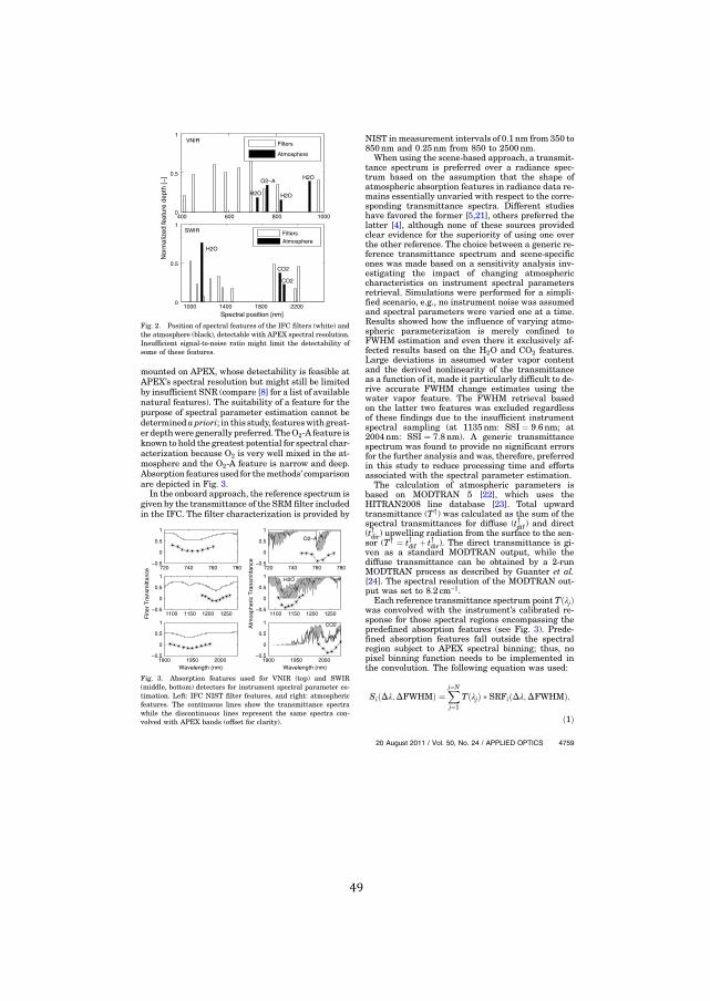
!49!

!

mounted on APEX, whose detectability is feasible atAPEX’s spectral resolution but might still be limitedby insufficient SNR (compare [8] for a list of availablenatural features). The suitability of a feature for thepurpose of spectral parameter estimation cannot bedeterminedapriori; in this study, featureswith great-er depthwere generally preferred. TheO2-A feature isknown to hold the greatest potential for spectral char-acterization because O2 is very well mixed in the at-mosphere and the O2-A feature is narrow and deep.Absorption featuresused for themethods’ comparisonare depicted in Fig. 3.

In the onboard approach, the reference spectrum isgiven by the transmittance of the SRM filter includedin the IFC. The filter characterization is provided by

NIST inmeasurement intervals of 0:1nm from 350 to850nm and 0:25nm from 850 to 2500nm.

When using the scene-based approach, a transmit-tance spectrum is preferred over a radiance spec-trum based on the assumption that the shape ofatmospheric absorption features in radiance data re-mains essentially unvaried with respect to the corre-sponding transmittance spectra. Different studieshave favored the former [5,21], others preferred thelatter [4], although none of these sources providedclear evidence for the superiority of using one overthe other reference. The choice between a generic re-ference transmittance spectrum and scene-specificones was made based on a sensitivity analysis inv-estigating the impact of changing atmosphericcharacteristics on instrument spectral parametersretrieval. Simulations were performed for a simpli-fied scenario, e.g., no instrument noise was assumedand spectral parameters were varied one at a time.Results showed how the influence of varying atmo-spheric parameterization is merely confined toFWHM estimation and even there it exclusively af-fected results based on the H2O and CO2 features.Large deviations in assumed water vapor contentand the derived nonlinearity of the transmittanceas a function of it, made it particularly difficult to de-rive accurate FWHM change estimates using thewater vapor feature. The FWHM retrieval basedon the latter two features was excluded regardlessof these findings due to the insufficient instrumentspectral sampling (at 1135nm: SSI ! 9:6nm; at2004nm: SSI ! 7:8nm). A generic transmittancespectrum was found to provide no significant errorsfor the further analysis and was, therefore, preferredin this study to reduce processing time and effortsassociated with the spectral parameter estimation.

The calculation of atmospheric parameters isbased on MODTRAN 5 [22], which uses theHITRAN2008 line database [23]. Total upwardtransmittance (T!) was calculated as the sum of thespectral transmittances for diffuse (t!dif ) and direct(t!dir) upwelling radiation from the surface to the sen-sor (T! ! t!dif " t!dir). The direct transmittance is gi-ven as a standard MODTRAN output, while thediffuse transmittance can be obtained by a 2-runMODTRAN process as described by Guanter et al.[24]. The spectral resolution of the MODTRAN out-put was set to 8:2 cm!1.

Each reference transmittance spectrum point T#λj$was convolved with the instrument’s calibrated re-sponse for those spectral regions encompassing thepredefined absorption features (see Fig. 3). Prede-fined absorption features fall outside the spectralregion subject to APEX spectral binning; thus, nopixel binning function needs to be implemented inthe convolution. The following equation was used:

Si#Δλ;ΔFWHM$ !Xj!N

j!1

T#λj$ % SRFi#Δλ;ΔFWHM$;

#1$

400 600 800 10000

0.5

1

Nor

mal

ized

feat

ure

dept

h [!

]

1000 1400 1800 22000

0.5

1

Spectral position [nm]

Filters

Atmosphere

FiltersAtmosphere

VNIR

SWIR

H2O

CO2

CO2

O2!A

H2O

H2O

H2O

Fig. 2. Position of spectral features of the IFC filters (white) andthe atmosphere (black), detectable with APEX spectral resolution.Insufficient signal-to-noise ratio might limit the detectability ofsome of these features.

720 740 760 780!0.5

0

0.5

1

1100 1150 1200 1250!0.5

0

0.5

1

Filt

er T

rans

mitt

ance

1900 1950 2000!0.5

0

0.5

1

Wavelength (nm)

720 740 760 780!0.5

0

0.5

1

1100 1150 1200 1250!0.5

0

0.5

1

Atm

osph

eric

Tra

nsm

ittan

ce

1900 1950 2000!0.5

0

0.5

1

Wavelength (nm)

O2!A

H2O

CO2

Fig. 3. Absorption features used for VNIR (top) and SWIR(middle, bottom) detectors for instrument spectral parameter es-timation. Left: IFC NIST filter features, and right: atmosphericfeatures. The continuous lines show the transmittance spectrawhile the discontinuous lines represent the same spectra con-volved with APEX bands (offset for clarity).

20 August 2011 / Vol. 50, No. 24 / APPLIED OPTICS 4759

!50!

!

where SRFi!Δλ;ΔFWHM" stands for an SRF ap-proximated by a Gaussian function to which a spec-tral shift (Δλ) and a bandwidth change (ΔFWHM)have been applied and where N is the number ofspectral points at which the input reference spec-trum was originally sampled.

The convolved transmittances are iteratively fedinto an optimization loop, which searches for theband shift and width change that results in the smal-lest difference between the references and the mea-sured APEX spectra. The optimization is performedbased on the Nelder–Mead simplex algorithm as de-scribed in Lagarias et al. [25]. In order to achieve thebest sensitivity, the best match is evaluated usingcorrelation analysis in the region of the absorptionfeatures. Features in both the reference and the mea-sured spectrum are continuum normalized assuminga linear continuum. Changes to the spectral param-eters fed into the convolution are defined with re-spect to the initial parameter grids coming fromthe laboratory characterization. The search uses zeroas a starting deviation value for both parameterswithout upper constraining thresholds for the mag-nitude of deviations. In few cases, the process endedbefore the function converged into its optimal valueand corresponding estimates were thus removedfrom the final output.

3. Results and Discussion

A. Spectral Parameters Estimation

Results of the APEX spectral parameter estimationfor selected acquisitions are presented in this sec-tion. For each detector, we first cross-validated esti-mates obtained for the same wavelength regionusing IFC filter features and corresponding atmo-spheric features. Next, the linearity of retrievedshifts over the detector’s spectral dimension was in-vestigated using IFC filter features at differentwavelength positions. This second set of results ismeant to assess whether the spectral shift derivedby one single wavelength position can be used to up-date the entire spectral range. Estimates obtainedwith the IFC for the instrument on-ground, beforeand after the flight, are also presented.

Figure 4 shows the nominal versus the updatedsmile profiles obtained over four flight altitudes forthe VNIR band centered at 760nm. Estimationsbased on the O2-A and corresponding NIST filter fea-ture yield comparable results, differing in average of0:3nm, corresponding to 0.05 of a spectral pixel inthis particular wavelength region. A deviation fromthe nominal instrument spectral calibration and analtitude-dependent performance are evident, con-firming the unsolved pressure/temperature depen-dency of the system. For prism-based instrumentsas APEX, performance changes with altitude areoften connected to pressure-dependant dispersionchanges of the prism. Results were remarkablyreproducible when the instrument was flown atthe same altitude on different dates and sites (figures

not included here). In the future, the development ofa correction model in function of flight height is thussomething worth investigating. System performanceestimated at the highest flight altitude of 6:5kmshows the greatest deviation from nominal value.A shift of 4:1nm (0.70 of a spectral pixel) and 4:4nm(0.75 of a spectral pixel) for the central detector pixelposition was estimated by the onboard-based andscene-based approaches, respectively. An increasein smile is further identified by both approaches.Smile, computed as the greatest difference found be-tween the center wavelength values of two detectorpixels, amounts to 1:5nm (0.26 of a spectral pixel)and 2nm (0.34 of a spectral pixel) for onboard-basedand scene-based estimates, respectively, compared tothe 0:6nm (0.1 of a spectral pixel) nominal value.

Figure 5 shows a good overlap between estimatesbased on the three IFC filter features centered at644nm, 743nm, and 803nm, respectively. For theVNIR detector, the shift estimates in one wavelengthregion can thus be considered representative for theentire spectral range. Further, measurements takenwith the IFC on-ground before and after the flightsindicate a good correspondence with the instrumentlaboratory characterization with across-track spec-tral shifts close to zero.

For the SWIR detector, two wavelength regionswere identified for which NIST-filter and atmo-spheric features are partly overlapping. Agreementbetween the estimates obtained with the two ap-proaches is observable in the first of the two exam-ined regions, encompassing the H2O feature at1130nm (Fig. 6). Deviation from nominal perfor-mances is greater for the lower of the flown altitude,reaching values of !13nm, being the equivalent of1 spectral pixel in this particular wavelength regionfeaturing FWHM of about 12nm. Values refer to theposition of the central detector pixel. A shift amount-ing to !2nm (0.17 of a spectral pixel) is estimated

0 500 1000758

760

762

764

766

Across!track pixel (#)

Ban

d #7

6, C

ente

r W

VL

(nm

)

0 500 1000758

760

762

764

766

Across!track pixel (#)

Ban

d #7

6, C

ente

r W

VL

(nm

)

0 500 1000758

760

762

764

766

Across!track pixel (#)

Ban

d #7

6, C

ente

r W

VL

(nm

)

0 500 1000758

760

762

764

766

Across!track pixel (#)

Ban

d #7

6, C

ente

r W

VL

(nm

)

ASL: 2.5 km ASL: 3.5 km

ASL: 4.1 km ASL: 6.5 km

Fig. 4. (Color online) Smile characterization at 760nm for fourflight altitudes. The continuous black line represents the nominalsmile as measured in the lab, while the dotted lines represent theestimates based on the O2-A absorption feature (blue) and on theNIST filter absorption feature (red).

4760 APPLIED OPTICS / Vol. 50, No. 24 / 20 August 2011

!51!

!

when the system is flown at 6:5km. The smile for theinvestigated spectral region amounts to 2nm (0.17 ofa spectral pixel) and 3nm (0.25 of a spectral pixel) foronboard-based and scene-based estimates, respec-tively, compared to the 1nm (0.08 of a spectral pixel)nominal value found in laboratory conditions. In thesecond SWIR region, estimations based on the CO2feature at 2001nm and analogous NIST-filter fea-ture, confirmed the general direction of the shift evi-denced in the former SWIR region, with shifts goingfrom shorter to higher wavelengths with increasingflight altitude (Fig. 7), but significantly differed inmagnitude. Smile profiles are characterized bya noisy appearance in the across-track direction

particularly for the IFC-based estimates. The two ap-proaches yield estimates diverging in average by2nm (0.2 of a spectral pixel), with the exception ofthe flight performed at the highest altitude for whicha nearly perfect overlap of smile profiles is provided.The low at-sensor signal within this absorption fea-ture and the overlap between water vapor and CO2absorption (double feature) may have led to the lessstable parameter retrieval.

Estimates for three IFC SWIR features confirmedand added to these findings. Results in Fig. 8 showthat the two IFC NIST features at 1381nm and1934nm provide concurring shift estimates, whilethose based on the feature at 1222nm systematically

0 500 10001155

1160

1165

1170

1175

Across!track pixel (#)

Ban

d #2

0, C

ente

r W

VL

(nm

)

0 500 10001155

1160

1165

1170

1175

Across!track pixel (#)

Ban

d #2

0, C

ente

r W

VL

(nm

)

0 500 10001155

1160

1165

1170

1175

Across!track pixel (#)

Ban

d #2

0, C

ente

r W

VL

(nm

)

0 500 10001155

1160

1165

1170

1175

Across!track pixel (#)

Ban

d #2

0, C

ente

r W

VL

(nm

)

ASL: 2.5 km ASL: 3.5 km

ASL: 4.1 km

ASL: 6.5 km

Fig. 6. (Color online) Smile characterization at 1175nm for fourflight altitudes. The continuous black line represents the nominalsmile as measured in the lab, while the dotted lines represent theestimates based on the water vapor absorption feature centered at1130nm (blue) and a NIST filter absorption feature centered at1222nm (red).

0

0.5

1

0

0.5

1V

NIR

shi

ft (p

x)

0

0.5

1

0 200 400 600 800 1000

0

0.5

1

Across!track pixel (#)

on ground pre!flight

ASL: 4.1 km

ASL: 6.5 km

on ground post!flight

Fig. 5. Estimated spectral shift in the across-track directionexpressed as fraction of spectral pixel. Retrieval based on IFC dataacquired on ground before (top) and after (bottom) the flight, aswell as for two different flight heights. Three VNIR wavelengthregions are considered: 630–658nm (black), 726–760nm (lightgray), 788–819nm (dark gray).

0 500 1000

1970

1975

1980

Across!track pixel (#) Ban

d #1

10, C

ente

r W

VL

(nm

)

0 500 1000

1970

1975

1980

Across!track pixel (#) Ban

d #1

10, C

ente

r W

VL

(nm

)

0 500 1000

1970

1975

1980

Across!track pixel (#)

Ban

d #1

10, C

ente

r W

VL

(nm

)

0 500 1000

1970

1975

1980

Across!track pixel (#)

Ban

d #1

10, C

ente

r W

VL

(nm

)

ASL: 2.5 km ASL: 3.5 km

ASL: 4.1 km

ASL: 6.5 km

Fig. 7. (Color online) Smile characterization at 1974nm for fourflight altitudes. The continuous black line represents the nominalsmile as measured in the lab, while the dotted lines represent theestimates based on the CO2 absorption feature centered at2004nm (blue) and a NIST filter absorption feature centered at1934nm (red).

!1

0

1

!1

0

1

SW

IR s

hift

(px)

!1

0

1

0 200 400 600 800 1000!1

0

1

Across!track pixel (#)

ASL: 6.5 km

on ground post!flight

ASL: 4.1 km

on ground pre!flight

Fig. 8. Estimated spectral shift in the across-track directionexpressed as fraction of spectral pixel. Retrieval based on IFC dataacquired on ground before (top) and after (bottom) the flight, aswell as for two different flight heights. Three SWIR wavelengthregions are considered: 1193–1269nm (black), 1339–1423nm(light gray), and 1909–1974nm (dark gray).

20 August 2011 / Vol. 50, No. 24 / APPLIED OPTICS 4761

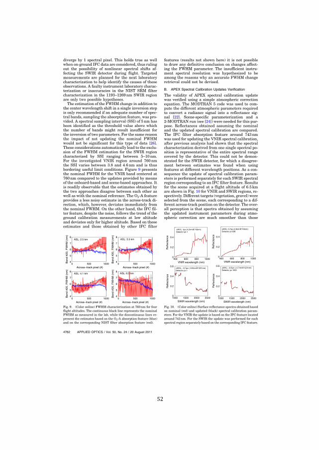
!52!

!

diverge by 1 spectral pixel. This holds true as wellwhen on-ground IFC data are considered, thus rulingout the possibility of nonlinear spectral shifts af-fecting the SWIR detector during flight. Targetedmeasurements are planned for the next laboratorycharacterization to help identify the causes of theseobservations. A faulty instrument laboratory charac-terization or inaccuracies in the NIST SRM filtercharacterization in the 1193–1269nm SWIR regionare only two possible hypotheses.

The estimation of the FWHM change in addition tothe center wavelength shift in a single inversion stepis only recommended if an adequate number of spec-tral bands, sampling the absorption feature, was pro-vided. A spectral sampling interval (SSI) of 5nm hasbeen identified as the threshold value above whichthe number of bands might result insufficient forthe inversion of two parameters. For the same reasonthe impact of not updating the nominal FWHMwould not be significant for this type of data [26].These considerations automatically lead to the exclu-sion of the FWHM estimation for the SWIR regioncharacterized by SSI ranging between 5–10nm.For the investigated VNIR region around 760nmthe SSI varies between 3.8 and 4:6nm and is thusbordering useful limit conditions. Figure 9 presentsthe nominal FWHM for the VNIR band centered at760nm compared to the updates provided by meansof the onboard-based and scene-based approaches. Itis readily observable that the estimates obtained bythe two approaches disagree between each other aswell as with the nominal reference. The O2-A featureprovides a less noisy estimate in the across-track di-rection, which, however, deviates immediately fromthe nominal FWHM. On the other hand, the IFC fil-ter feature, despite the noise, follows the trend of theground calibration measurements at low altitudeand deviates only for higher altitude. Based on theseestimates and those obtained by other IFC filter

features (results not shown here) it is not possibleto draw any definitive conclusion on changes affect-ing the FWHM parameter. The insufficient instru-ment spectral resolution was hypothesized to beamong the reasons why an accurate FWHM changeretrieval could not be devised.

B. APEX Spectral Calibration Updates Verification

The validity of APEX spectral calibration updatewas verified using a simple atmospheric correctionequation. The MODTRAN 5 code was used to com-pute the different atmospheric parameters requiredto convert a radiance signal into a reflectance sig-nal [22]. Scene-specific parameterization and a2-MODTRAN run (see [24]) were needed for this pur-pose. Reflectances obtained assuming the nominaland the updated spectral calibration are compared.The IFC filter absorption feature around 743nmwas used for updating the VNIR spectral calibration,after previous analysis had shown that the spectralcharacterization derived from one single spectral po-sition is representative of the entire spectral rangecovered by the detector. This could not be demon-strated for the SWIR detector, for which a disagree-ment between estimates was found when usingfeatures at different wavelength positions. As a con-sequence the update of spectral calibration param-eters is performed separately for each SWIR spectralregion corresponding to an IFC filter feature. Resultsfor the scene acquired at a flight altitude of 6:5kmare shown in Fig. 10 for VNIR and SWIR regions, re-spectively. Different targets (vegetation, gravel) wereselected from the scene, each corresponding to a dif-ferent across-track position on the detector. The over-all perception is that spectra obtained by assumingthe updated instrument parameters during atmo-spheric correction are much smoother than those

0 500 10004

5

6

7

8

Across!track pixel (#)

Ban

d #2

0, F

WH

M (

nm)

0 500 10004

5

6

7

8

Across!track pixel (#)

Ban

d #2

0, F

WH

M (

nm)

0 500 10004

5

6

7

8

Across!track pixel (#)

Ban

d #2

0, F

WH

M (

nm)

0 500 10004

5

6

7

8

Across!track pixel (#)

Ban

d #2

0, F

WH

M (

nm)

ASL: 2.5 km ASL: 3.5 km

ASL: 4.1 km ASL: 6.5 km

Fig. 9. (Color online) FWHM characterization at 760nm for fourflight altitudes. The continuous black line represents the nominalFWHM as measured in the lab, while the discontinuous lines re-present the estimates based on the O2-A absorption feature (blue)and on the corresponding NIST filter absorption feature (red).

400 600 800 10000

0.2

0.4

VNIR wavelength (nm)

Ref

lect

ance

!WVL: 1px (4.2nm@743nm)Detector px 1

400 600 800 10000

0.2

0.4

VNIR wavelength (nm)

Ref

lect

ance

!WVL: 0.7px (2.9nm@743nm)Detector px 636

1000 1500 2000 25000

0.2

0.4

0.6

SWIR wavelength (nm)

Ref

lect

ance

!WVL: !0.1px (!0.9nm@1231nm)Detector px 1

1000 1500 2000 25000

0.2

0.4

0.6

SWIR wavelength (nm)

Ref

lect

ance

!WVL: !0.5px (!4.7nm@1231nm)Detector px 1000

Fig. 10. (Color online) Surface reflectance spectra obtained basedon nominal (red) and updated (black) spectral calibration param-eters. For the VNIR the update is based on the IFC feature locatedaround 743nm. For the SWIR the update was performed for eachspectral region separately based on the corresponding IFC feature.

4762 APPLIED OPTICS / Vol. 50, No. 24 / 20 August 2011

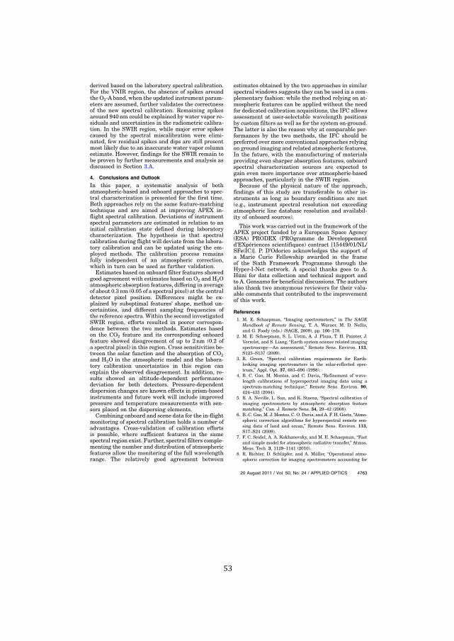
!53!

!

derived based on the laboratory spectral calibration.For the VNIR region, the absence of spikes aroundthe O2-A band, when the updated instrument param-eters are assumed, further validates the correctnessof the new spectral calibration. Remaining spikesaround 940nm could be explained by water vapor re-siduals and uncertainties in the radiometric calibra-tion. In the SWIR region, while major error spikescaused by the spectral miscalibration were elimi-nated, few residual spikes and dips are still presentmost likely due to an inaccurate water vapor columnestimate. However, findings for the SWIR remain tobe proven by further measurements and analysis asdiscussed in Section 3.A.

4. Conclusions and Outlook

In this paper, a systematic analysis of bothatmospheric-based and onboard approaches to spec-tral characterization is presented for the first time.Both approaches rely on the same feature-matchingtechnique and are aimed at improving APEX in-flight spectral calibration. Deviations of instrumentspectral parameters are estimated in relation to aninitial calibration state defined during laboratorycharacterization. The hypothesis is that spectralcalibration during flight will deviate from the labora-tory calibration and can be updated using the em-ployed methods. The calibration process remainsfully independent of an atmospheric correction,which in turn can be used as further validation.

Estimates based on onboard filter features showedgood agreement with estimates based on O2 and H2Oatmospheric absorption features, differing in averageof about 0:3nm (0.05 of a spectral pixel) at the centraldetector pixel position. Differences might be ex-plained by suboptimal features’ shape, method un-certainties, and different sampling frequencies ofthe reference spectra. Within the second investigatedSWIR region, efforts resulted in poorer correspon-dence between the two methods. Estimates basedon the CO2 feature and its corresponding onboardfeature showed disagreement of up to 2nm (0.2 ofa spectral pixel) in this region. Cross sensitivities be-tween the solar function and the absorption of CO2and H2O in the atmospheric model and the labora-tory calibration uncertainties in this region canexplain the observed disagreement. In addition, re-sults showed an altitude-dependent performancedeviation for both detectors. Pressure-dependentdispersion changes are known effects in prism-basedinstruments and future work will include improvedpressure and temperature measurements with sen-sors placed on the dispersing elements.

Combining onboard and scene data for the in-flightmonitoring of spectral calibration holds a number ofadvantages. Cross-validation of calibration effortsis possible, where sufficient features in the samespectral region exist. Further, spectral filters comple-menting the number and distribution of atmosphericfeatures allow the monitoring of the full wavelengthrange. The relatively good agreement between

estimates obtained by the two approaches in similarspectral windows suggests they can be used in a com-plementary fashion: while the method relying on at-mospheric features can be applied without the needfor dedicated calibration acquisitions, the IFC allowsassessment at user-selectable wavelength positionsby custom filters as well as for the system on-ground.The latter is also the reason why at comparable per-formances by the two methods, the IFC should bepreferred over more conventional approaches relyingon ground imaging and related atmospheric features.In the future, with the manufacturing of materialsproviding even sharper absorption features, onboardspectral characterization sources are expected togain even more importance over atmospheric-basedapproaches, particularly in the SWIR region.

Because of the physical nature of the approach,findings of this study are transferable to other in-struments as long as boundary conditions are met(e.g., instrument spectral resolution not exceedingatmospheric line database resolution and availabil-ity of onboard sources).

This work was carried out in the framework of theAPEX project funded by a European Space Agency(ESA) PRODEX (PROgramme de Développementd'EXpériences scientifiques) contract [15449/01/NL/SFe(IC)]. P. D’Odorico acknowledges the support ofa Marie Curie Fellowship awarded in the frameof the Sixth Framework Programme through theHyper-I-Net network. A special thanks goes to A.Hüni for data collection and technical support andto A. Gonsamo for beneficial discussions. The authorsalso thank two anonymous reviewers for their valu-able comments that contributed to the improvementof this work.

References1. M. E. Schaepman, “Imaging spectrometers,” in The SAGE

Handbook of Remote Sensing, T. A. Warner, M. D. Nellis,and G. Foody (eds.) (SAGE, 2009), pp. 166–178.

2. M. E. Schaepman, S. L. Ustin, A. J. Plaza, T. H. Painter, J.Verrelst, and S. Liang, “Earth system science related imagingspectroscopy—An assessment,” Remote Sens. Environ. 113,S123–S137 (2009).

3. R. Green, “Spectral calibration requirements for Earth-looking imaging spectrometers in the solar-reflected spec-trum,” Appl. Opt. 37, 683–690 (1998).

4. B. C. Gao, M. Montes, and C. Davis, “Refinement of wave-length calibrations of hyperspectral imaging data using aspectrum-matching technique,” Remote Sens. Environ. 90,424–433 (2004).

5. R. A. Neville, L. Sun, and K. Staenz, “Spectral calibration ofimaging spectrometers by atmospheric absorption featurematching,” Can. J. Remote Sens. 34, 29–42 (2008).

6. B.-C. Gao, M. J. Montes, C. O. Davis, and A. F. H. Goetz, “Atmo-spheric correction algorithms for hyperspectral remote sen-sing data of land and ocean,” Remote Sens. Environ. 113,S17–S24 (2009).

7. F. C. Seidel, A. A. Kokhanovsky, and M. E. Schaepman, “Fastand simple model for atmospheric radiative transfer,” Atmos.Meas. Tech. 3, 1129–1141 (2010).

8. R. Richter, D. Schläpfer, and A. Müller, “Operational atmo-spheric correction for imaging spectrometers accounting for

20 August 2011 / Vol. 50, No. 24 / APPLIED OPTICS 4763

!54!

!

the smile effect,” IEEE Trans. Geosci. Remote Sens. 49,1772–1780 (2011).

9. L. Guanter, R. Richter, and J. Moreno, “Spectral calibration ofhyperspectral imagery using atmospheric absorption fea-tures,” Appl. Opt. 45, 2360–2370 (2006).

10. J. Brazile, R. A. Neville, K. Staenz, D. Schläpfer, L. Sun, andK. Itten, “Towards scene-based retrieval of spectral responsefunctions for hyperspectral imagers using Frauenhofer fea-tures,” Can. J. Remote Sens. 34, S43–S58 (2008).

11. Z. Qu, B. C. Kindel, and A. F. H. Goetz, “The high accuracyatmospheric correction for hyperspectral data (HATCH)model,” IEEE Trans. Geosci. Remote Sens. 41, 1223–1231(2003).

12. A. Rodger, “SODA: A new method of in-scene atmosphericwater vapor estimation and post-flight spectral recalibrationfor hyperspectral sensors: Application to the HyMap sensor attwo locations,” Remote Sens. Environ. 115, 536–547 (2011).

13. S. Delwart, R. Preusker, L. Bourg, R. Santer, D. Ramon, and J.Fischer, “MERIS in-flight spectral calibration,” Int. J. RemoteSens. 28, 479–496 (2007).

14. H. Montgomery, N. Che, K. Parker, and J. Bowser, “Thealgorithm for MODIS wavelength on-orbit calibration usingthe SRCA,” IEEE Trans. Geosci. Remote Sens. 38, 877–884(2000).

15. P. S. Barry, J. Shepanski, and C. Segal, “Hyperion on-orbitvalidation of spectral calibration using atmospheric linesand an on-board system,” Proc. SPIE 4480, 231–235 (2002).

16. T. Chrien, M. Eastwood, R. Green, C. Sarture, H. Johnson, C.Chovit, and P. Hajek, “Airborne visible/infrared imaging spec-trometer (AVIRIS) onboard calibration system,” in Proceedingof the Fifth Annual JPL Airborne Earth Science Workshop(Jet Prop. Lab., 1995), pp. 31–32.

17. P. D’Odorico, E. Alberti, andM. Schaepman, “In-flight spectralperformance monitoring of the Airborne Prism Experiment,”Appl. Opt. 49, 3082–3091 (2010).

18. B. Sang, J. Schubert, S. Kaiser, V.Mogulsky, C. Neumann, K. P.Forster, S. Hofer, T. Stuffler, H. Kaufmann, A. Muller, T.Eversberg, and C. Chlebek, “The EnMAP hyperspectralimaging spectrometer: instrument concept, calibration, and

technologies,” in Imaging Spectrometry XIII (SPIE, 2008),708605–708615.

19. R. Green, M. Eastwood, C. Sarture, T. Chrien, M. Aronsson, B.Chippendale, J. Faust, B. Pavri, C. Chovit, M. Solis, M. Olah,and O. Williams, “Imaging Spectroscopy and the AirborneVisible/Infrared Imaging Spectrometer (AVIRIS),” RemoteSens. Environ. 65, 227–248 (1998).

20. S. Thiemann, P. Strobl, P. Gege, N. Stahl, W. Mooshuber, andH. van der Piepen, “Das abbildende spektrometer ROSIS,” inPublikationen der Deutschen Gesellschaft für Photogramme-trie und Fernerkundung, E. Seyfert (ed.) (DLR, 2001), pp.147–153.

21. R. O. Green, “Determination of the in-flight spectral calibra-tion of AVIRIS using atmospheric absorption features,” in Pro-ceedings of the Fifth Annual JPL Airborne Earth ScienceWorkshop, Vol. 1, R. O. Green, ed. (Jet Prop. Lab., 1995),pp. 71–74.

22. A. Berk, G. P. Anderson, P. K. Acharya, L. S. Bernstein, L.Muratov, J. Lee, M. Fox, S. M. Adler-Golden, J. H. Chetwynd,M. L. Hoke, R. B. Lockwood, J. A. Gardner, T. W. Cooley, C. C.Borel, and P. E. Lewis, “MODTRAN 5, a reformulated atmo-spheric bandmodel with auxiliary species and practical multi-ple scattering options: Update,” Proc. SPIE 5806, 662–667(2005).

23. L. S. Rothman, I. E. Gordon, and A. Barbe, “The HITRAN2008 molecular spectroscopic database,” J. Quant. Spectrosc.Radiat. Transfer 110, 533–572 (2009).

24. L. Guanter, R. Richter, and H. Kaufmann, “On the applicationof the MODTRAN 4 atmospheric radiative transfer code to op-tical remote sensing,” Int. J. Remote Sens. 30, 1407–1424(2009).

25. J. C. Lagarias, J. A. Reeds, M. H. Wright, and P. E. Wright,“Convergence properties of the Nelder–Mead simplexmethod in low dimensions,” SIAM J. Optim. 9, 112–147(1998).

26. L. Guanter, K. Segl, B. Sang, L. Alonso, H. Kaufmann, and J.Moreno, “Scene-based spectral calibration assessment of highspectral resolution imaging spectrometers,” Opt. Express 17,11594–11606 (2009).

4764 APPLIED OPTICS / Vol. 50, No. 24 / 20 August 2011

!55!

!

5 EXPERIMENTAL EVALUATION OF SENTINEL-2 SPECTRAL RESPONSE FUNCTION FOR NDVI TIME-SERIES CONTINUITY

This chapter has been submitted as: D'Odorico, P., Gonsamo, A., Damm, A. and Schaepman, M.E., 2011. Experimental evaluation of Sentinel-2 spectral response function for NDVI time-series continuity. IEEE Transactions on Geoscience and Remote Sensing, submitted.

!

!

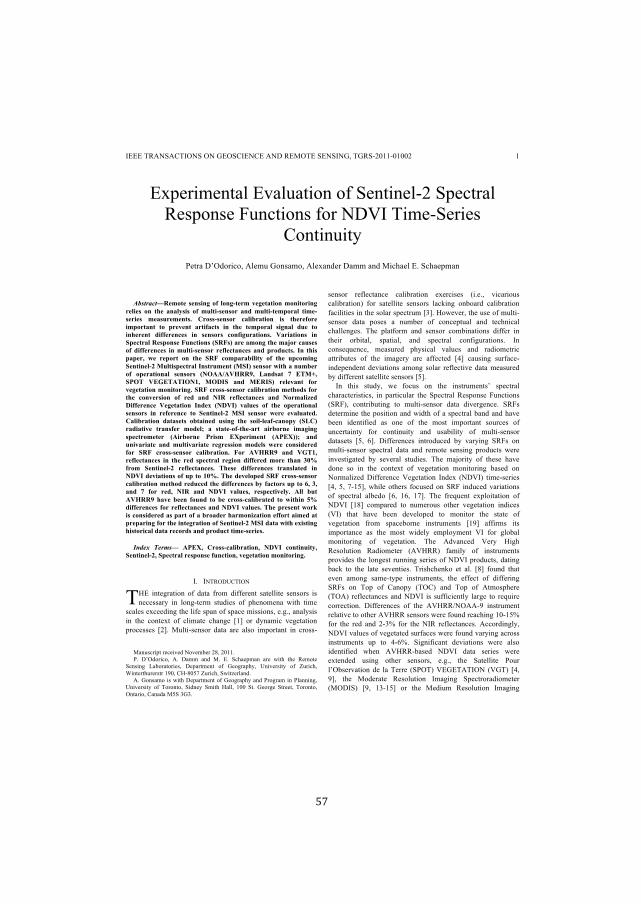
!57!

!

IEEE TRANSACTIONS ON GEOSCIENCE AND REMOTE SENSING, TGRS-2011-01002

1

Abstract—Remote sensing of long-term vegetation monitoring

relies on the analysis of multi-sensor and multi-temporal time-

series measurements. Cross-sensor calibration is therefore

important to prevent artifacts in the temporal signal due to

inherent differences in sensors configurations. Variations in

Spectral Response Functions (SRFs) are among the major causes

of differences in multi-sensor reflectances and products. In this

paper, we report on the SRF comparability of the upcoming

Sentinel-2 Multispectral Instrument (MSI) sensor with a number

of operational sensors (NOAA/AVHRR9, Landsat 7 ETM+,

SPOT VEGETATION1, MODIS and MERIS) relevant for

vegetation monitoring. SRF cross-sensor calibration methods for

the conversion of red and NIR reflectances and Normalized

Difference Vegetation Index (NDVI) values of the operational

sensors in reference to Sentinel-2 MSI sensor were evaluated.

Calibration datasets obtained using the soil-leaf-canopy (SLC)

radiative transfer model; a state-of-the-art airborne imaging

spectrometer (Airborne Prism EXperiment (APEX)); and

univariate and multivariate regression models were considered

for SRF cross-sensor calibration. For AVHRR9 and VGT1,

reflectances in the red spectral region differed more than 30%

from Sentinel-2 reflectances. These differences translated in

NDVI deviations of up to 10%. The developed SRF cross-sensor

calibration method reduced the differences by factors up to 6, 3,

and 7 for red, NIR and NDVI values, respectively. All but

AVHRR9 have been found to be cross-calibrated to within 5%

differences for reflectances and NDVI values. The present work

is considered as part of a broader harmonization effort aimed at

preparing for the integration of Sentinel-2 MSI data with existing

historical data records and product time-series.

Index Terms— APEX, Cross-calibration, NDVI continuity,

Sentinel-2, Spectral response function, vegetation monitoring.

I. INTRODUCTION

HE integration of data from different satellite sensors is

necessary in long-term studies of phenomena with time

scales exceeding the life span of space missions, e.g., analysis

in the context of climate change [1] or dynamic vegetation

processes [2]. Multi-sensor data are also important in cross-

Manuscript received November 28, 2011.

P. D’Odorico, A. Damm and M. E. Schaepman are with the Remote

Sensing Laboratories, Department of Geography, University of Zurich,

Winterthurerstr 190, CH-8057 Zurich, Switzerland.

A. Gonsamo is with Department of Geography and Program in Planning,

University of Toronto, Sidney Smith Hall, 100 St. George Street, Toronto,

Ontario, Canada M5S 3G3.

sensor reflectance calibration exercises (i.e., vicarious

calibration) for satellite sensors lacking onboard calibration

facilities in the solar spectrum [3]. However, the use of multi-

sensor data poses a number of conceptual and technical

challenges. The platform and sensor combinations differ in

their orbital, spatial, and spectral configurations. In

consequence, measured physical values and radiometric

attributes of the imagery are affected [4] causing surface-

independent deviations among solar reflective data measured

by different satellite sensors [5].

In this study, we focus on the instruments’ spectral

characteristics, in particular the Spectral Response Functions

(SRF), contributing to multi-sensor data divergence. SRFs

determine the position and width of a spectral band and have

been identified as one of the most important sources of

uncertainty for continuity and usability of multi-sensor

datasets [5, 6]. Differences introduced by varying SRFs on

multi-sensor spectral data and remote sensing products were

investigated by several studies. The majority of these have

done so in the context of vegetation monitoring based on

Normalized Difference Vegetation Index (NDVI) time-series

[4, 5, 7-15], while others focused on SRF induced variations

of spectral albedo [6, 16, 17]. The frequent exploitation of

NDVI [18] compared to numerous other vegetation indices

(VI) that have been developed to monitor the state of

vegetation from spaceborne instruments [19] affirms its

importance as the most widely employment VI for global

monitoring of vegetation. The Advanced Very High

Resolution Radiometer (AVHRR) family of instruments

provides the longest running series of NDVI products, dating

back to the late seventies. Trishchenko et al. [8] found that

even among same-type instruments, the effect of differing

SRFs on Top of Canopy (TOC) and Top of Atmosphere

(TOA) reflectances and NDVI is sufficiently large to require

correction. Differences of the AVHRR/NOAA-9 instrument

relative to other AVHRR sensors were found reaching 10-15%

for the red and 2-3% for the NIR reflectances. Accordingly,

NDVI values of vegetated surfaces were found varying across

instruments up to 4-6%. Significant deviations were also

identified when AVHRR-based NDVI data series were

extended using other sensors, e.g., the Satellite Pour

l’Observation de la Terre (SPOT) VEGETATION (VGT) [4,

9], the Moderate Resolution Imaging Spectroradiometer

(MODIS) [9, 13-15] or the Medium Resolution Imaging

Experimental Evaluation of Sentinel-2 Spectral

Response Functions for NDVI Time-Series

Continuity

Petra D’Odorico, Alemu Gonsamo, Alexander Damm and Michael E. Schaepman

T

!58!

!

IEEE TRANSACTIONS ON GEOSCIENCE AND REMOTE SENSING, TGRS-2011-01002

2

Spectrometer (MERIS) [12]. The European Space Agency’s

(ESA) upcoming Sentinel-2 Multi Spectral Instrument (MSI)

[20, 21] is considered as the follow-up mission to SPOT and

Landsat type of instruments and is intended to provide

continuity of remote sensing products. The placement and the

number of Sentinel-2 MSI spectral bands are, however,

defined to offer an increased performance compared to

analogous bands in SPOT and Landsat sensors. These

refinements will, hence, cause deviations of NDVI values

obtained from the Sentinel-2 MSI sensor compared to existing

satellite sensors and will require adjustments to allow

extending actual NDVI time series.

Cross-sensor calibration efforts directly based on the

comparison of measured satellite imagery face several

limitations. Their applicability is limited to sensor

combinations for which temporally and spatially overlapping

data exist. Moreover, other sources of deviation, e.g., spatial

sampling and radiometric resolution, influence the comparison

and prevent quantifying the isolated impact of SRF differences

in the total uncertainty budget [4, 14, 17]. Cross-sensor

calibration strategies incorporating either Radiative Transfer

Model (RTM) simulations or airborne and in-situ

measurements allow overcoming such restrictions. Other

sources of difference, such as those linked with the spectral

convolution operation to broadband SRFs, are however

inherent to the latter approach. This difference was ignored in

previous studies [5, 8], which used airborne measurements for

developing SRF cross-sensor calibration models. Further

weaknesses of existing cross-sensor SRF calibration

approaches arise from the land cover dependency of the SRFs

difference effect, which are not accounted for when using

radiative transfer modeling [4, 13, 22, 23], and the dependency

on data availability when using airborne [5, 8] or in-situ

measurements [7, 11, 15]. To the best of our knowledge, none

of the past efforts systematically compared strategies for

cross-sensor SRF calibration.

The goal of this study is to quantify differences that can be

expected in the red, NIR and NDVI time series expansion

through Sentinel-2 MSI measurements caused by the isolated

impact of spectral sensor properties, i.e., the sensor SRF.

Results are considered being one important component of the

total uncertainty budget related to the integration of multi-

sensor data for establishing continuous time series of earth

observation products. We deliberately neglect uncertainties

caused by effects of the atmosphere, spatial sampling, or other

sources of variability, as they require individual

comprehensive analysis. The specific objectives of our

analysis are: i) to investigate cross-sensor differences of the

frequently used NDVI vegetation index and thus of cross-

sensor differences in position and width of the red and the

near-infrared (NIR) bands; ii) to propose a simple approach to

minimize the effect of land cover on the SRF cross-calibration

based on multivariate regression analysis; and iii) to evaluate a

number of cross-sensor calibration data sets and the validity of

the use of airborne measurement to replicate the satellite

observation based on the Airborne Prism EXperiment (APEX)

airborne imaging spectrometer.

NDVI time-series derivation is not a primary objective of

the Sentinel-2 mission, since it samples the red-edge

chlorophyll absorption region with three narrow bands in

addition to those used for NDVI computation (Fig. 1).

Nonetheless, it is essential to use Sentinel-2 based NDVI data

given the high temporal resolution compared to SPOT HRG or

Landsat type of instruments and the cross-calibration

opportunity it offers for any given large swath sensor. The

present work is considered as part of a broader harmonization

effort aimed at preparing for the integration of Sentinel-2 MSI

data with existing historical data records and product time-

series.

II. DATA AND METHODS

A. Satellite sensors and their SRFs considered in this study

The upcoming Sentinel-2 MSI [21] was taken as the

reference comparison instrument. Sentinel-2 is one of a series

of five ESA missions aimed at addressing the operational

needs of the Global Monitoring for Environment and Security

programme (GMES). The mission is scheduled for launch in

2013 and among its objectives is providing enhanced

continuity of data acquisition of SPOT and Landsat types of

TABLE I

SATELLITE SENSORS CHARACTERISTICS CONSIDERED IN THIS STUDY.

ID Sensor Operational period Revisit frequency Nominal band nr

and wvl (nm)

Nominal pixel size

Red NIR

SEN-2 Sentinel-2 MSI 2013! 2-5 days #4: 640!690 #8: 780!910 10 m

AVHRR9 NOAA/AVHRR9 1989!1994 daily #1: 580!680 #2: 725!1100 1 km

ETM7 Landsat 7 ETM+ 1999!present 16 days #3: 630!690 #4: 750!900 30 m

VGT1 SPOT5 VGT1 1998!present daily #2: 610!680 #3: 780!890 1 km

MER MERIS 2002!present 3 days #7: 657!672 #13: 852!877 260m x 300m

MOD MODIS 1999!present 2 days #3: 620!670 #4: 841!876 250 m

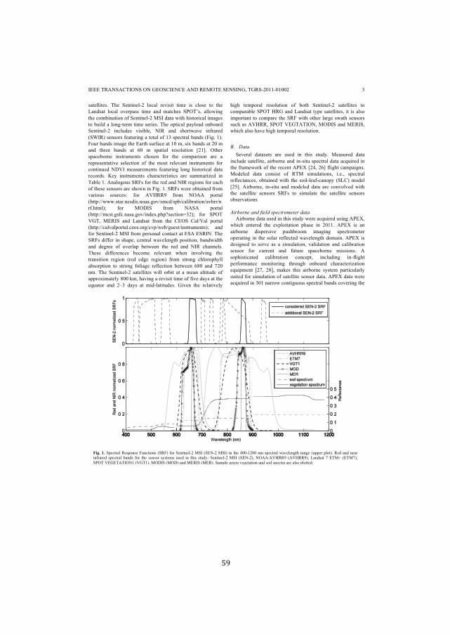
!59!

!

IEEE TRANSACTIONS ON GEOSCIENCE AND REMOTE SENSING, TGRS-2011-01002

3

satellites. The Sentinel-2 local revisit time is close to the

Landsat local overpass time and matches SPOT’s, allowing

the combination of Sentinel-2 MSI data with historical images

to build a long-term time series. The optical payload onboard

Sentinel-2 includes visible, NIR and shortwave infrared

(SWIR) sensors featuring a total of 13 spectral bands (Fig. 1).

Four bands image the Earth surface at 10 m, six bands at 20 m

and three bands at 60 m spatial resolution [21]. Other

spaceborne instruments chosen for the comparison are a

representative selection of the most relevant instruments for

continued NDVI measurements featuring long historical data

records. Key instruments characteristics are summarized in

Table 1. Analogous SRFs for the red and NIR regions for each

of these sensors are shown in Fig. 1. SRFs were obtained from

various sources: for AVHRR9 from NOAA portal

(http://www.star.nesdis.noaa.gov/smcd/spb/calibration/avhrr/n

rf.html); for MODIS from NASA portal

(http://mcst.gsfc.nasa.gov/index.php?section=32); for SPOT

VGT, MERIS and Landsat from the CEOS Cal/Val portal

(http://calvalportal.ceos.org/cvp/web/guest/instruments); and

for Sentinel-2 MSI from personal contact at ESA ESRIN. The

SRFs differ in shape, central wavelength position, bandwidth

and degree of overlap between the red and NIR channels.

These differences become relevant when involving the

transition region (red edge region) from strong chlorophyll

absorption to strong foliage reflection between 680 and 720

nm. The Sentinel-2 satellites will orbit at a mean altitude of

approximately 800 km, having a revisit time of five days at the

equator and 2–3 days at mid-latitudes. Given the relatively

high temporal resolution of both Sentinel-2 satellites to

comparable SPOT HRG and Landsat type satellites, it is also

important to compare the SRF with other large swath sensors

such as AVHRR, SPOT VEGTATION, MODIS and MERIS,

which also have high temporal resolution.

B. Data

Several datasets are used in this study. Measured data

include satellite, airborne and in-situ spectral data acquired in

the framework of the recent APEX [24, 26] flight campaigns.

Modeled data consist of RTM simulations, i.e., spectral

reflectances, obtained with the soil-leaf-canopy (SLC) model

[25]. Airborne, in-situ and modeled data are convolved with

the satellite sensors SRFs to simulate the satellite sensors

observations.

Airborne and field spectrometer data

Airborne data used in this study were acquired using APEX,

which entered the exploitation phase in 2011. APEX is an

airborne dispersive pushbroom imaging spectrometer

operating in the solar reflected wavelength domain. APEX is

designed to serve as a simulation, validation and calibration

sensor for current and future spaceborne missions. A

sophisticated calibration concept, including in-flight

performance monitoring through onboard characterization

equipment [27, 28], makes this airborne system particularly

suited for simulation of satellite sensor data. APEX data were

acquired in 301 narrow contiguous spectral bands covering the

Fig. 1. Spectral Response Functions (SRF) for Sentinel-2 MSI (SEN-2 MSI) in the 400-1200 nm spectral wavelength range (upper plot). Red and near

infrared spectral bands for the sensor systems used in this study: Sentinel-2 MSI (SEN-2), NOAA/AVHRR9 (AVHRR9), Landsat 7 ETM+ (ETM7),

SPOT VEGETATION1 (VGT1), MODIS (MOD) and MERIS (MER). Sample green vegetation and soil spectra are also plotted.

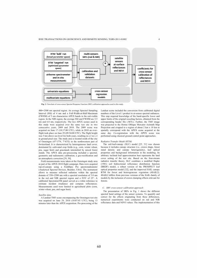
!60!

!

IEEE TRANSACTIONS ON GEOSCIENCE AND REMOTE SENSING, TGRS-2011-01002

4

400!2500 nm spectral region. An average Spectral Sampling

Interval (SSI) of 4 nm and a Full-Width-at-Half-Maximum

(FWHM) of 5 nm characterize APEX bands in the red-visible

region. In the NIR region, the average SSI and FWHM are 5.5

nm and 6.8 nm, respectively. The two APEX scenes used in

this study were acquired over the same test site in two

consecutive years, 2009 and 2010. The 2009 scene was

acquired on June 17 (10:17:00 UTC), while in 2010 an over-

flight took place on June 29 (09:54:00 UTC). The flight height

was 5 km above sea level for both years, resulting in a 2 m x 2

m ground pixel size. The study area is located south of the city

of Oensingen (47°17"N, 7°43"E) in the northwestern part of

Switzerland. It is characterized by heterogeneous land cover,

dominated by cultivated crop fields (e.g., corn, winter wheat,

pea, sugar beet) and grasslands intermitted by mixed forest

stands. The APEX data pre-processing included a spectral,

geometric and radiometric calibration, a geo-rectification and

an atmospheric correction [29, 30].

Field measurements were taken at the Oensingen study area

as part of the APEX 2010 flight campaign. Data were acquired

top-of-canopy using a FieldSpec Pro spectroradiometer

(Analytical Spectral Devices, Boulder, USA). The instrument

allows to measure reflected radiation within the spectral

domain of 350!2500 nm with a spectral resolution of 3.0 nm

in the red and NIR spectral region and a FOV of 25°. A

calibrated SpectralonTM panel served as a white reference to

estimate incident irradiance and compute reflectances.

Measurements used were limited to agricultural plots (corn,

winter wheat, pea, and sugar beet).

Satellite data

A Landsat TM5 scene encompassing the Oensingen test site

was acquired on June 29, 2010 (10:07:03 UTC), being 13

minutes later than the APEX acquisition. Pre-processing of the

Landsat scene included the conversion from calibrated digital

numbers of the Level 1 product to at-sensor spectral radiances.

This step required knowledge of the band-specific lower and

upper limits of the original rescaling factors, obtained from the

corresponding header file (.MTL). Further, the TM5 image

was projected to the Hotine Oblique Mercator Azimuth Map

Projection and cropped to a region of about 2 km x 10 km to

spatially correspond with the APEX scene acquired at the

same day. Co-registration with the APEX scene was

performed using classical ground control point approaches.

Radiative Transfer Model (RTM)

The soil-leaf-canopy (SLC) model [25, 31] was chosen

because it includes canopy structure (i.e., crown shape, forest

stand density and canopy heterogeneity), leaf optical

properties and background information in the modeling. Its

arbitrary inclined leaf approximation best represents the land

cover setting of the test site. Based on the four-stream

radiative transfer theory, SLC combines a modified Hapke

(1981) soil bidirectional reflectance distribution function

(BRDF) model, a robust version of the PROSPECT leaf

optical properties model [32], and the improved SAIL canopy

RTM for forest and heterogeneous vegetation (4SAIL2).

4SAIL2 differs from previous versions of the SAIL-family of

models by the inclusion of crown clumping effects relevant for

forests.

C. SRF cross-sensor calibration approach

The presentation of SRFs in Fig. 1 shows the different

spectral band settings of the sensor systems. To quantify and

correct for the effects originating from these differences,

numerical experiments were conducted on red and NIR

reflectance data and NDVI values. The implementation of this

Fig. 2. Flowchart of cross-sensor Spectral Response Function (SRF) calibration approaches used in this study.

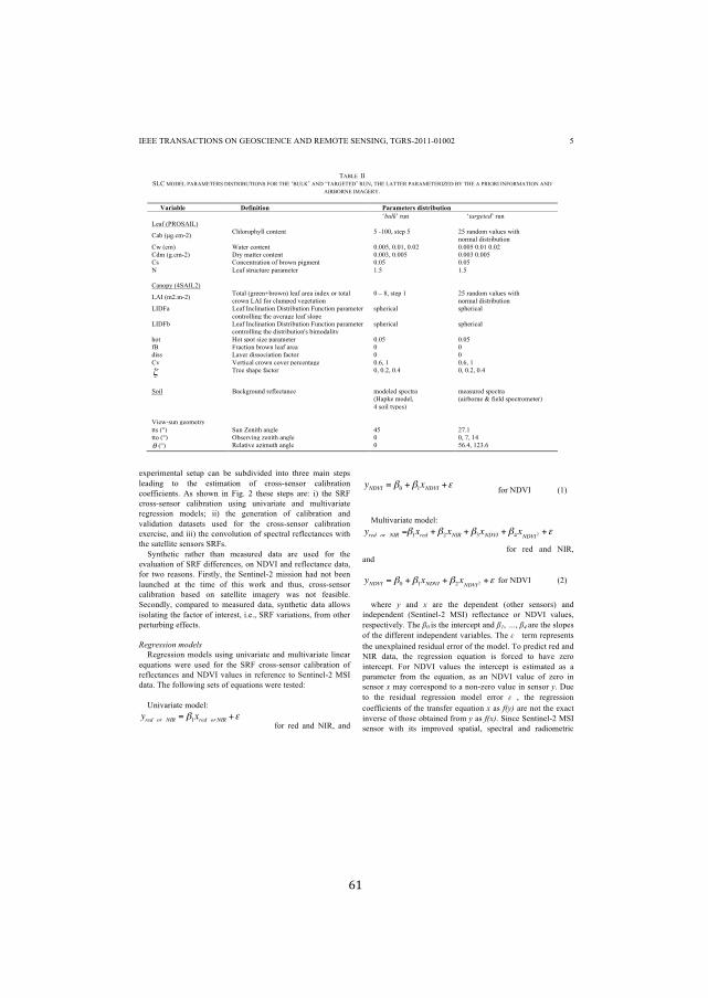
!61!

!

IEEE TRANSACTIONS ON GEOSCIENCE AND REMOTE SENSING, TGRS-2011-01002

5

experimental setup can be subdivided into three main steps

leading to the estimation of cross-sensor calibration

coefficients. As shown in Fig. 2 these steps are: i) the SRF

cross-sensor calibration using univariate and multivariate

regression models; ii) the generation of calibration and

validation datasets used for the cross-sensor calibration

exercise, and iii) the convolution of spectral reflectances with

the satellite sensors SRFs.

Synthetic rather than measured data are used for the

evaluation of SRF differences, on NDVI and reflectance data,

for two reasons. Firstly, the Sentinel-2 mission had not been

launched at the time of this work and thus, cross-sensor

calibration based on satellite imagery was not feasible.

Secondly, compared to measured data, synthetic data allows

isolating the factor of interest, i.e., SRF variations, from other

perturbing effects.

Regression models

Regression models using univariate and multivariate linear

equations were used for the SRF cross-sensor calibration of

reflectances and NDVI values in reference to Sentinel-2 MSI

data. The following sets of equations were tested:

Univariate model:

yred or NIR = !1xred or NIR +" for red and NIR, and

yNDVI

= !0+!

1xNDVI

+" for NDVI (1)

Multivariate model:

yred or NIR =!1xred +!2xNIR +!3xNDVI +!4xNDVI 2 +"

for red and NIR,

and

yNDVI

= !0+!

1xNDVI

+!2xNDVI

2 +" for NDVI (2)

where y and x are the dependent (other sensors) and

independent (Sentinel-2 MSI) reflectance or NDVI values,

respectively. The !0 is the intercept and !1, …, !4 are the slopes

of the different independent variables. The " term represents

the unexplained residual error of the model. To predict red and

NIR data, the regression equation is forced to have zero

intercept. For NDVI values the intercept is estimated as a

parameter from the equation, as an NDVI value of zero in

sensor x may correspond to a non-zero value in sensor y. Due

to the residual regression model error " , the regression

coefficients of the transfer equation x as f(y) are not the exact

inverse of those obtained from y as f(x). Since Sentinel-2 MSI

sensor with its improved spatial, spectral and radiometric

TABLE II

SLC MODEL PARAMETERS DISTRIBUTIONS FOR THE ‘BULK’ AND ‘TARGETED’ RUN, THE LATTER PARAMETERIZED BY THE A PRIORI INFORMATION AND

AIRBORNE IMAGERY.

Variable Definition Parameters distribution

‘bulk’ run ‘targeted’ run

Leaf (PROSAIL)

Cab (µg.cm-2) Chlorophyll content 5 -100, step 5 25 random values with

normal distribution

Cw (cm) Water content 0.005, 0.01, 0.02 0.005 0.01 0.02

Cdm (g.cm-2) Dry matter content 0.003, 0.005 0.003 0.005

Cs Concentration of brown pigment 0.05 0.05

N Leaf structure parameter 1.5 1.5

Canopy (4SAIL2)

LAI (m2.m-2) Total (green+brown) leaf area index or total

crown LAI for clumped vegetation

0 – 8, step 1 25 random values with

normal distribution

LIDFa Leaf Inclination Distribution Function parameter

controlling the average leaf slope

spherical spherical

LIDFb Leaf Inclination Distribution Function parameter

controlling the distribution's bimodality

spherical spherical

hot Hot spot size parameter 0.05 0.05

fB Fraction brown leaf area 0 0

diss Layer dissociation factor 0 0

Cv Vertical crown cover percentage 0.6, 1 0.6, 1

! Tree shape factor 0, 0.2, 0.4 0, 0.2, 0.4

Soil Background reflectance modeled spectra

(Hapke model,

4 soil types)

measured spectra

(airborne & field spectrometer)

View-sun geometry

tts (°) Sun Zenith angle 45 27.1

tto (°) Observing zenith angle 0 0, 7, 14

! (°) Relative azimuth angle 0 56.4, 123.6

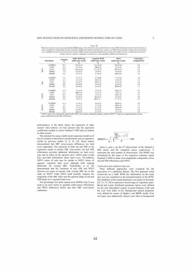
!62!

!

IEEE TRANSACTIONS ON GEOSCIENCE AND REMOTE SENSING, TGRS-2011-01002

6

performances, is the likely choice for expansion of other

sensors’ data archives, we here present only the regression

coefficients needed to correct Sentinel-2 MSI data in relation

to other sensors.

The rationale for using a multivariate regression model as of

Eq.(2) is based on theoretical considerations and on supportive

results by previous studies [3, 8, 14, 23]. These studies

demonstrated that SRF cross-sensors differences are land

cover dependent. The inclusion of both red and NIR in the

regression model to predict SRF cross-sensor red and NIR

reflectances provides additional information on land cover

type and its effect on the spectral curve. NDVI alone would

have provided information about land cover. Nevertheless

NDVI values of soils may be similar to NDVI values of

sparsely vegetated land cover although both respond

differently for varying SRF. Trishchenko et al. [8]

demonstrated that the variations of red, NIR and NDVI

between two pairs of sensors with varying SRF are in the

order of NDVI2

while NDVI itself partially explains the

magnitude of the SRF effect and the spectral shape of red and

NIR bands over vegetated land cover.

The percentage root mean square error (RMSE) (Eq.3) was

used as an error metric to quantify multi-sensor reflectances

and NDVI differences before and after SRF cross-sensor

calibration.

!

RMSE% =1

µxref

yn " xnref( )

2

n=1

n=N

#

N*100 (3)

where xn and yn are the nth

observations of the Sentinel-2

MSI sensor and the compared sensor, respectively. N

represents the total number of observations. The RMSE was

normalized by the mean of the respective reference signal

(Sentinel-2 MSI) to make error magnitudes comparable across

red and NIR reflectances and NDVI.

Calibration and validation data sets

Three different approaches were evaluated for the

generation of a calibration dataset. The first approach relied

exclusively on a ‘bulk’ RTM run. Information on the study

area was not considered in the parameterization of the RTM.

The definition of the model parameters was based on literature

[25, 31, 33, 34] to represent a broad range of vegetation types.

Broad and evenly distributed parameter spaces were defined

for the leaf chlorophyll content of green biomass (Cab) and

the Leaf Area Index (LAI). Background optical properties

were defined by means of Hapke’s soil BRDF model. Four

soil types were additionally chosen, rock, litter as background

TABLE III

PERCENTAGE ROOT-MEAN-SQUARE-ERROR (RMSE) RESULTING FROM SPECTRAL RESPONSE FUNCTION (SRF) DIFFERENCES BETWEEN SENTINEL-2

AND A NUMBER OF OTHER OPERATIONAL SENSORS. RMSE ARE SHOWN FOR ORIGINAL AS WELL AS SRF CROSS-SENSOR CALIBRATED VALIDATION

DATA. RMSE (%) FOR MULTIVARIATE(UNIVARIATE) SRF CROSS-SENSOR REGRESSION EQUATIONS AND THREE SETS OF CALIBRATION DATASETS:

MODEL (‘BULK’), MODEL+AIRBORNE (‘TARGETED’), AND AIRBORNE (APEX) ARE PRESENTED.

Instrument Original

%

‘bulk’ RTM run

multi (uni) variate

%

‘targeted’ RTM

multi (uni) variate

%

APEX

multi (uni) variate

%

Gain factor

(original/best)

RE

D

AVHRR9 33.1 9.4 (23.1) 8.5 (23.6) 7.4 (23.4) 4.5

ETM7 8.5 3.2 (5.5) 2.8 (5.8) 3.5 (5.6) 3.0

VGT1 33.6 10.6 (22.6) 8.1 (22.7) 5.3 (21.5) 6.3

MERIS 1.4 0.5 (0.5) 1.0 (0.5) 0.8 (0.8) 2.8

MODIS

8.2

4.9 (7.5)

5.7 (6.8)

4.6 (6.9)

1.8

NIR

AVHRR9 7.3 3.1 (3.3) 2.7 (2.4) 2.7 (2.8) 3.0

ETM7 2.3 2.3 (1.5) 1.5 (1.5) 1.8 (1.9) 1.5

VGT1 2.4 2.3 (1.5) 1.5 (1.5) 1.9 (1.9) 1.6

MERIS 0.0 0.0 (0.0) 0.0 (0.0) 0.0 (0.0) 0.0

MODIS

0.6

0.8 (0.4)

0.4 (0.4)

0.4 (0.4)

1.5

ND

VI*

AVHRR9 11.3 3.5 (3.0) 2.5 (2.6) 2.4 (2.5) 4.7

ETM7 3.1 0.8 (1.4) 1.3 (1.3) 1.0 (1.1) 3.9

VGT1 10.1 3.4 (3.6) 3.5 (3.5) 1.5 (1.5) 6.7

MERIS 0.4 0.2 (0.2) 0.1 (0.2) 0.2 (0.2) 4.0

MODIS

2.4

1.4 (1.1)

1.0 (1.1)

1.1 (1.3)

2.4

ND

VI*

* AVHRR9 11.3 3.1 (8.1) 5.4 (8.2) 2.5 (8.2) 4.5

ETM7 3.1 1.5 (1.7) 1.7 (1.9) 1.0 (1.6) 3.1

VGT1 10.1 3.7 (7.3) 5.1 (7.4) 1.6 (6.9) 6.3

MERIS 0.4 0.2 (0.2) 0.3 (0.2) 0.2 (0.2) 2.0

MODIS 2.4 1.2 (1.9) 2.3 (1.9) 1.3 (1.9) 2.0

* NDVI values were obtained by applying the NDVI cross-sensor calibration equation whereas NDVI** values are computed based on cross-

sensor calibrated red and NIR reflectances.

!63!

!

IEEE TRANSACTIONS ON GEOSCIENCE AND REMOTE SENSING, TGRS-2011-01002

7

for meadows, forest understory, and snow. Parameters

describing the sun-observation geometry were set to resemble

typical values encountered for acquisitions at central European

latitudes. The parameter distribution for the RTM ‘bulk’ run

are given in Table 2.

In the second approach, a ‘targeted’ RTM run was intended

to simulate the variety of vegetation properties resembling

those of a pre-selected study area, i.e., the Oensingen test site.

Model inversion based on a look-up-table (LUT) approach

was performed to meet this objective [34, 35]. The 2009

APEX scene was used as an input to the inversion. A total of

10’000 reflectance spectra were selected from the airborne

scene, which had been stratified in NDVI classes. Pixels with

a NDVI value < 0.3 were excluded, representing non-

vegetative surfaces. Random points with NDVI values typical

for vegetated surfaces were sampled above this threshold. The

LUT spectra were convolved to APEX SRFs before entering

the search for the best fit. The background reflectance was

approximated by three soil spectra extracted from the APEX

scene and the illumination-observation geometry was set

according to the airborne acquisition. The view zenith angle

was defined for nadir (0°) as well as two off-nadir (7°, 14°)

positions to simulate APEX ±14° FOV. The relative azimuth

angle was computed for two different view azimuth angles,

90° and 270°, corresponding to the right and left half of the

swath, respectively. In a second step, the parameter space

resulting from the model inversion was used for a forward

simulation aimed at generating the calibration dataset

representative of the study site, i.e., a ‘targeted’ run. The

parameter distribution for the RTM ‘targeted’ run is given in

Table 2.

In the third approach, the calibration dataset was directly

obtained from the 2009 APEX data. Spectra were selected in

the same fashion as described above, i.e., NDVI stratification

and random sampling, thus granting representativeness of

vegetation dynamics in the dataset.

Two validation datasets were further compiled. The first

was obtained by sampling the 2010 APEX scene as previously

described, while the second was obtained by compiling field

measurements acquired simultaneously with the 2010 airborne

campaign.

Convolution and deconvolution of spectral reflectances and

radiances

Calibration and validation datasets obtained from RTM

simulations, airborne and in-situ measurements, were

convolved to satellite sensor spectral response functions for

the red and NIR bands. It should be noted that in this study we

evaluated the isolated impact of sensor properties and

intentionally excluded additional atmospheric effect, which

have to be addressed in targeted studies. Spectral convolution

was applied as follows:

(4)

where is the convolved spectral reflectance (or

radiance) as measured by the satellite sensor, and is the

reflectance (or radiance) at high spectral sampling.

The validity of the adopted spectral convolution approach

for input spectra sampled below Nyquist frequency was tested

in this context. The objective was to determine how well

APEX data can be used to reproduce broadband acquisitions,

i.e., to assess the impact of in-band averaging and under-

sampling effects introduced by APEX SRFs on the broadband

convolution. This is also a prerequisite for the use of APEX

for SRF cross-sensor calibration. To meet this objective,

broadband at-sensor radiances simulated starting from original

Table IV SRF CROSS-SENSOR CALIBRATION COEFFICIENTS NEEDED FOR THE CONVERSION OF SENTINEL-2 (X) REFLECTANCES AND NDVI VALUES INTO

THOSE OF THE INVESTIGATED SENSORS (Y). COEFFICIENTS WERE OBTAINED BASED ON THE BEST PERFORMING DATA-MODEL COMBINATION

PRESENTED IN TABLE 3. COEFFICIENTS ARE USED WITH EQUATIONS 1-2.

Prediction Instrument Regression Coefficients

intercept red NIR NDVI NDVI2

RED

N9 0.8618 0.0533 0.0230 -0.0287

ETM7 0.9786 0.0104 0.0060 -0.0076

VGT1 0.9185 0.0499 0.0123 -0.0159

MER 0.9988 -0.0008 -0.0006 0.0008

MOD 0.9423 0.0137 0.0131 -0.0167

NIR

N9 0.9196

ETM7 0.9717

VGT1 0.9699

MER 1.0000

MOD 0.9940

NDVI

N9 0.1056 0.5847 0.2282

ETM7 0.0207 0.8678 0.1028

VGT1 0.0309 0.7962 0.0954

MER 0.0004 1.0052 -0.0045

MOD 0.0572 0.8146 0.1215

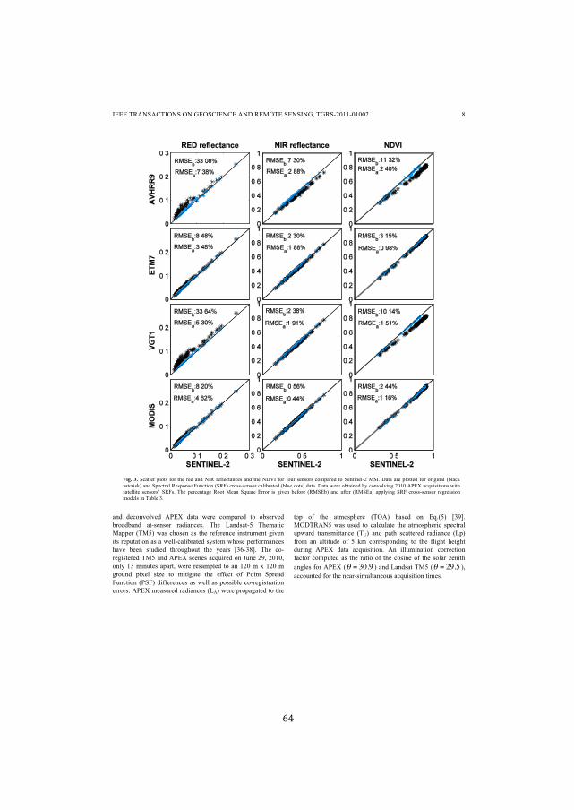
!64!

!

IEEE TRANSACTIONS ON GEOSCIENCE AND REMOTE SENSING, TGRS-2011-01002

8

and deconvolved APEX data were compared to observed

broadband at-sensor radiances. The Landsat-5 Thematic

Mapper (TM5) was chosen as the reference instrument given

its reputation as a well-calibrated system whose performances

have been studied throughout the years [36-38]. The co-

registered TM5 and APEX scenes acquired on June 29, 2010,

only 13 minutes apart, were resampled to an 120 m x 120 m

ground pixel size to mitigate the effect of Point Spread

Function (PSF) differences as well as possible co-registration

errors. APEX measured radiances (LA) were propagated to the

top of the atmosphere (TOA) based on Eq.(5) [39].

MODTRAN5 was used to calculate the atmospheric spectral

upward transmittance (TU) and path scattered radiance (Lp)

from an altitude of 5 km corresponding to the flight height

during APEX data acquisition. An illumination correction

factor computed as the ratio of the cosine of the solar zenith

angles for APEX (! = 30.9 ) and Landsat TM5 (! = 29.5 ),

accounted for the near-simultaneous acquisition times.

Fig. 3. Scatter plots for the red and NIR reflectances and the NDVI for four sensors compared to Sentinel-2 MSI. Data are plotted for original (black

asterisk) and Spectral Response Function (SRF) cross-sensor calibrated (blue dots) data. Data were obtained by convolving 2010 APEX acquisitions with

satellite sensors’ SRFs. The percentage Root Mean Square Error is given before (RMSEb) and after (RMSEa) applying SRF cross-sensor regression

models in Table 3.

!65!

!

IEEE TRANSACTIONS ON GEOSCIENCE AND REMOTE SENSING, TGRS-2011-01002

9

LATOA =cos(!A )

cos(!TM 5 )(LATU + Lp ) (5)

A similar procedure was applied to APEX spectra that had

been deconvolved. The Van Cittert iterative deconvolution

technique [40, 41] was used to derive the most accurate

approximation of the true radiance, l, by decorrelating the

SRFs from the observed radiance, L. It is given as:

l̂k+1= l̂

k+ (L !SRF" l̂

k) (6)

where l̂k

is the kth estimate of l. The correction factor

(L !SRF" l̂k) used to adjust the kth estimate of l is

interpolated to match the 1 nm sampling step of l̂k

. Cubic

spline interpolation is used to get the continuous delta

spectrum as well as to derive a first estimation, l̂0

, of the

observed spectrum. For more details on the Van Cittert

iterative deconvolution technique we refer to [42].

Eventually, APEX TOA original and deconvolved radiances

were convolved with Landsat TM5 SRFs (Eq. (4)).

III. RESULTS AND DISCUSSION

A. SRF difference effects

Results of the reflectance and NDVI cross-sensor

comparison are reported in Table 3. Results are obtained by

applying the regression coefficients on the independent

airborne validation dataset and consider the different

calibration datasets and regression models.

The first column of Table 3 shows the differences we can

expect if no SRF cross-sensor calibration is performed. One

should note that the differences only capture discrepancies in

nominal instrument spectral responses. This means that

performance drifts occurring over time are not considered,

assuming an insignificant change of SRFs through the life

span of satellite sensors. MERIS is the only instrument for

which continuity with Sentinel-2 MSI can be established with

differences in reflectances and NDVI below 1.5%. Broadband

instruments such as AVHRR9 and VGT1exhibit the highest

SRF based differences with RMSEs greater than 33% and

10% for the red band and NDVI, respectively. Similarly,

ETM+ and MODIS data differed from Sentinel-2 MSI data in

the red visible region with a RMSE greater 8%, whereas for

NIR and NDVI the RMSE was around 3% (Table 3). For all

sensors, position and shape of the red spectral band was the

most critical for sensor cross-comparison subsequently

contributing to the NDVI differences. This is in line with

findings by [5] which identified the width of the red spectral

band having the most significant impact due to the relatively

narrow spectral width of the red absorption feature of

chlorophyll. The same study found the position of the NIR

band less critical provided that the bandwidth (FWHM) is no

more than 50 nm and the atmospheric correction is accurate.

The latter aspect relates with the significant influence of

atmospheric gas absorption, in particular of water vapor, on

the spectral region of the near-infrared plateau.

B. SRF cross-sensor regression models

Band-to-band univariate and multivariate regression models

were tested for SRF cross-sensor calibration and the choice of

the regression model equations was found having an influence

on the correction of SRF difference effects. The multivariate

regression model showed overall better results. The spectral

comparability in the red spectral region improved up to a

factor of 4.5 and 6.3, for AVHRR9 and VGT1, respectively.

For ETM7 and MODIS, the improvement in the red band

compared to the original difference was threefold (6th column

Table 3). The observed improvements can be explained with

the inclusion of information from the NIR region, in form of

NIR reflectance and NDVI values. Both information sources

account for the impact of changing land cover and amount of

existing biomass on the spectral overlap between visible and

NIR bands over the red-edge region (around 700 nm). The

NDVI is a good indicator of the shape of surface spectra,

explaining its sensitivity to the dependency of cross-

calibration accuracy on land cover changes. NIR reflectances

are also included in the set of red band cross-sensor calibration

because NDVI alone cannot differentiate between land cover

types featuring similar NDVI values, e.g., soil and sparse

vegetation. For the cross-sensor calibration of the NIR signal,

the inclusion of information from the red spectral region in

form of red or NDVI was instead found having no benefit.

One can thus conclude that the band-to-band SRF cross-sensor

calibration in the NIR region can be made effectively using

the univariate linear regression model. For NDVI, regression

models were either applied directly on NDVI values or the

NDVI was derived from the red and NIR for which the SRF

cross-sensor calibration was performed. The former gave

slightly better results besides being preferable from an

operational point of view given that the global products

generally do not provide red and NIR reflectances from which

NDVI time-series were computed. SRF based differences of

NDVI values were improved by a factor 4.7 and 6.7 for

AVHRR9 and VGT1, respectively after the applied cross-

sensor calibration. A fourfold improvement was reached for

ETM7 and MERIS. It can be observed that NDVI multi-sensor

differences are only marginally affected by land cover type as

the NDVI per se partially compensates this effect. However,

NDVI multi-sensor differences can be affected non-linearly by

variations in the optical thickness of photosynthetic biomass.

This effects can be represented by including NDVI2 (Eq.2;

[8]).

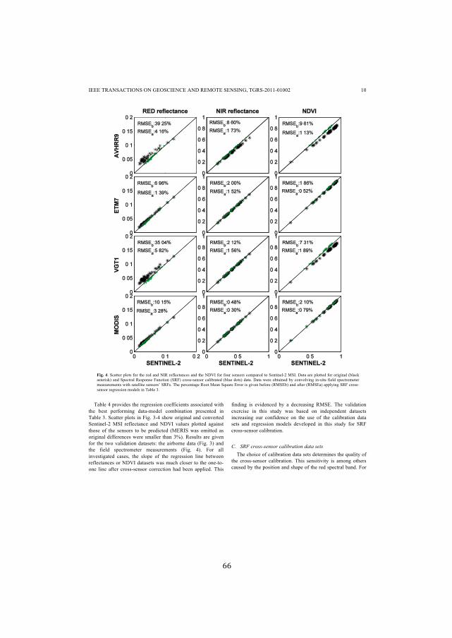
!66!

!

IEEE TRANSACTIONS ON GEOSCIENCE AND REMOTE SENSING, TGRS-2011-01002

10

Table 4 provides the regression coefficients associated with

the best performing data-model combination presented in

Table 3. Scatter plots in Fig. 3-4 show original and converted

Sentinel-2 MSI reflectance and NDVI values plotted against

those of the sensors to be predicted (MERIS was omitted as

original differences were smaller than 3%). Results are given

for the two validation datasets: the airborne data (Fig. 3) and

the field spectrometer measurements (Fig. 4). For all

investigated cases, the slope of the regression line between

reflectances or NDVI datasets was much closer to the one-to-

one line after cross-sensor correction had been applied. This

finding is evidenced by a decreasing RMSE. The validation

exercise in this study was based on independent datasets

increasing our confidence on the use of the calibration data

sets and regression models developed in this study for SRF

cross-sensor calibration.

C. SRF cross-sensor calibration data sets

The choice of calibration data sets determines the quality of

the cross-sensor calibration. This sensitivity is among others

caused by the position and shape of the red spectral band. For

Fig. 4. Scatter plots for the red and NIR reflectances and the NDVI for four sensors compared to Sentinel-2 MSI. Data are plotted for original (black

asterisk) and Spectral Response Function (SRF) cross-sensor calibrated (blue dots) data. Data were obtained by convolving in-situ field spectrometer

measurements with satellite sensors’ SRFs. The percentage Root Mean Square Error is given before (RMSEb) and after (RMSEa) applying SRF cross-

sensor regression models in Table 3.

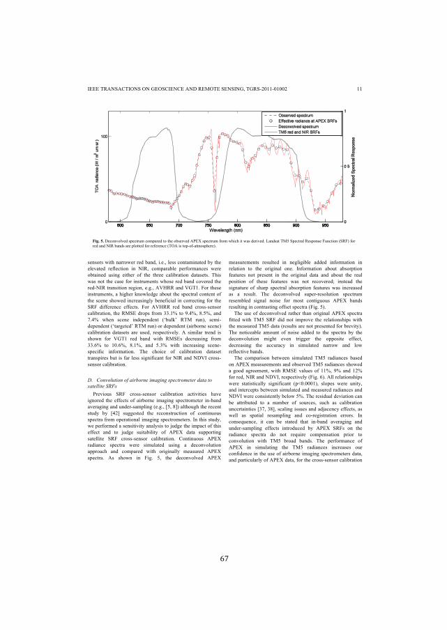
!67!

!

IEEE TRANSACTIONS ON GEOSCIENCE AND REMOTE SENSING, TGRS-2011-01002

11

sensors with narrower red band, i.e., less contaminated by the

elevated reflection in NIR, comparable performances were

obtained using either of the three calibration datasets. This

was not the case for instruments whose red band covered the

red-NIR transition region, e.g., AVHRR and VGT1. For these

instruments, a higher knowledge about the spectral content of

the scene showed increasingly beneficial in correcting for the

SRF difference effects. For AVHRR red band cross-sensor

calibration, the RMSE drops from 33.1% to 9.4%, 8.5%, and

7.4% when scene independent (‘bulk’ RTM run), semi-

dependent (‘targeted’ RTM run) or dependent (airborne scene)

calibration datasets are used, respectively. A similar trend is

shown for VGT1 red band with RMSEs decreasing from

33.6% to 10.6%, 8.1%, and 5.3% with increasing scene-

specific information. The choice of calibration dataset

transpires but is far less significant for NIR and NDVI cross-

sensor calibration.

D. Convolution of airborne imaging spectrometer data to

satellite SRFs

Previous SRF cross-sensor calibration activities have

ignored the effects of airborne imaging spectrometer in-band

averaging and under-sampling (e.g., [5, 8]) although the recent

study by [42] suggested the reconstruction of continuous

spectra from operational imaging spectrometers. In this study,

we performed a sensitivity analysis to judge the impact of this

effect and to judge suitability of APEX data supporting

satellite SRF cross-sensor calibration. Continuous APEX

radiance spectra were simulated using a deconvolution

approach and compared with originally measured APEX

spectra. As shown in Fig. 5, the deconvolved APEX

measurements resulted in negligible added information in

relation to the original one. Information about absorption

features not present in the original data and about the real

position of these features was not recovered; instead the

signature of sharp spectral absorption features was increased

as a result. The deconvolved super-resolution spectrum

resembled signal noise for most contiguous APEX bands

resulting in contrasting offset spectra (Fig. 5).

The use of deconvolved rather than original APEX spectra

fitted with TM5 SRF did not improve the relationships with

the measured TM5 data (results are not presented for brevity).

The noticeable amount of noise added to the spectra by the

deconvolution might even trigger the opposite effect,

decreasing the accuracy in simulated narrow and low

reflective bands.

The comparison between simulated TM5 radiances based

on APEX measurements and observed TM5 radiances showed

a good agreement, with RMSE values of 11%, 9% and 12%

for red, NIR and NDVI, respectively (Fig. 6). All relationships

were statistically significant (p<0.0001), slopes were unity,

and intercepts between simulated and measured radiances and

NDVI were consistently below 5%. The residual deviation can

be attributed to a number of sources, such as calibration

uncertainties [37, 38], scaling issues and adjacency effects, as

well as spatial resampling and co-registration errors. In

consequence, it can be stated that in-band averaging and

under-sampling effects introduced by APEX SRFs on the

radiance spectra do not require compensation prior to

convolution with TM5 broad bands. The performance of

APEX in simulating the TM5 radiances increases our

confidence in the use of airborne imaging spectrometers data,

and particularly of APEX data, for the cross-sensor calibration

Fig. 5. Deconvolved spectrum compared to the observed APEX spectrum from which it was derived. Landsat TM5 Spectral Response Function (SRF) for

red and NIR bands are plotted for reference (TOA is top-of-atmosphere).

!68!

!

IEEE TRANSACTIONS ON GEOSCIENCE AND REMOTE SENSING, TGRS-2011-01002

12

of operational and upcoming satellite sensors. Nonetheless,

additional investigations including narrow band sensors

simulations are needed to further strengthen this hypothesis.

IV. CONCLUSIONS

As of 2013, ESA’s Sentinel-2 mission will start delivering

high-resolution optical images on a global scale. To assure

that existing satellite based historical data records and product

time-series can be complemented and expanded using

Sentinel-2 MSI data, uncertainties linked with differences in

instrument performances need to be addressed accordingly. In

this study we investigated uncertainties originating from

differences in position and width of the red and NIR spectral

bands and on their implication on NDVI time-series

continuity.

Findings showed that differences in SRFs are significant

and have to be taken into account to integrate Sentinel-2

NDVI time-series with those of other sensors. Expanding

AVHRR NDVI time-series via original Sentinel-2 data is

possible with an 11% uncertainty without SRF cross sensor

calibration. Similarly, continuing NDVI time-series of the

SPOT VGT heritage instrument is related to an uncertainty of

10%. These uncertainties are not acceptable considering the

subtle magnitude of natural surface variations we aim at

monitoring in vegetation studies. This study demonstrates that

compensating for SRF difference effects in the data improves

the Sentinel-2 NDVI time series consistency with AVHRR9

and SPOT VGT1 NDVI time series of up to a factor of five

and a factor of seven, respectively. The spectral band

difference effect was found to be dependent on the surface

reflectance spectrum. The inclusion of knowledge about the

spectral content of the scene and about the overall shape of the

spectrum improved the correction.

The use of multivariate regression improved the SRF cross-

sensor calibration, particularly for the red band covering the

spectral region with the largest spectral contrast. Multivariate

over univariate band-to-band regression improved results by

up to a factor six (e.g. Sentinel-2 vs. VGT1 in Table 3). This

effect also spreads to the computed NDVI after applying

multivariate cross-sensor SRF calibration in the red region,

resulting in improved NDVI cross-sensor comparability. We,

therefore, recommend an ensemble of regression models for

the red and the NIR cross-sensor calibration. In the red region,

the use of NIR, NDVI and NDVI2 as multivariate predictor

variables improves the comparability of the reflectances

between two given sensors. For the NIR region, simple band-

to-band SRF cross-sensor calibration suffices the desired level

of comparability.

The choice of the calibration data source plays a marginal

role in the performance of SRF cross-sensor calibration.

Overall, the use of measured airborne data performed best

followed by the targeted RTM simulations. However, both

airborne measurements and fully parameterized RTMs are

often not available for an extended study area. In such cases,

the ‘bulk’ run is the only alternative for cross-sensor SRF

calibration, as the parameterization can be performed by a

priori guess or by setting large parameter ranges. Our study

further indicates that, if the SRF based reflectance differences

are below 3%, the cross-sensor calibration is not required or

does not necessarily improve the comparability (e.g., Sentinel-

2 MSI vs. MERIS in Table 3).

NDVI time series cross-calibration has represented a great

challenge within the global climate change community. Once

spaceborne, Sentinel-2 will allow for acquisition of

comprehensive and extended NDVI time series and can

Fig. 6. Comparison between Landsat TM5 observed and simulated Top Of

Atmosphere (TOA) radiances and derived NDVI values. Simulated radiances

were obtained from APEX data, which were propagated to TOA. The

discontinuous line represents the one-to-one line, while the continuous line

represents the regression fit.

!69!

!

IEEE TRANSACTIONS ON GEOSCIENCE AND REMOTE SENSING, TGRS-2011-01002

13

provide the needed reference tool for cross-calibration of any

given large swath sensor. We have demonstrated that –

sufficient stability of all other sensor parameters given –

substantial improvement can be achieved by using regression

models to secure spectral continuity of NDVI time-series.

ACKNOWLEDGMENT

The authors would like to thank J. Timmermans and W.

Verhoef for providing and supporting the use of SLC. We

acknowledge the support of A. Hüni and M. Jehle of the

APEX team.

REFERENCES

[1] S. L. Lewis, P. M. Brando, O. L. Phillips, G. M. F. van der Heijden, and

D. Nepstad, "The 2010 Amazon Drought," Science, vol. 331, no. 6017,

p. 554, Feb. 2011.

[2] R. de Jong, S. de Bruin, A. de Wit, M. E. Schaepman, and D. L. Dent,

"Analysis of monotonic greening and browning trends from global

NDVI time-series," Remote Sens. Environ., vol. 115, no. 2, pp. 692-702,

Feb. 2011.

[3] P. M. Teillet, J. L. Barker, B. L. Markham, R. R. Irish, G. Fedosejevs,

and J. C. Storey, "Radiometric cross-calibration of the Landsat-7 ETM+

and Landsat-5 TM sensors based on tandem data sets," Remote Sens.

Environ.,vol. 78, no.1-2, pp. 39-54, Apr. 2001.

[4] E. Swinnen and F. Veroustraete, "Extending the SPOT-VEGETATION

NDVI Time Series (1998-2006) Back in Time With NOAA-AVHRR

Data (1985-1998) for Southern Africa," IEEE Trans. Geosci. Remote

Sens., vol. 46, no. 2, pp. 558-572, Feb. 2008.

[5] P. M. Teillet, K. Staenz, and D. J. William, "Effects of spectral, spatial,

and radiometric characteristics on remote sensing vegetation indices of

forested regions," Remote Sens. Environ., vol. 61, no. 1, pp. 139-149,

Jul. 1997.

[6] P. M. Teillet, G. Fedosejevs, K. J. Thome, and J. L. Barker, "Impacts of

spectral band difference effects on radiometric cross-calibration between

satellite sensors in the solar-reflective spectral domain," Remote Sens.

Environ., vol. 110, no. 3, pp. 393-409, Oct. 2007.

[7] K. L. Castro-Esau, G. A. Sanchez-Azofeifa, and B. Rivard, "Comparison

of spectral indices obtained using multiple spectroradiometers," Remote

Sens. Environ., vol. 103, no. 3, pp. 276-288, Aug. 2006.

[8] A. P. Trishchenko, J. Cihlar, and Z. Li, "Effects of spectral response

function on surface reflectance and NDVI measured with moderate

resolution satellite sensors," Remote Sens. Environ., vol. 81, no. 1, pp. 1-

18, Jul. 2002.

[9] A. P. Trishchenko, "Effects of spectral response function on surface

reflectance and NDVI measured with moderate resolution satellite

sensors: Extension to AVHRR NOAA-17, 18 and METOP-A," Remote

Sens. Environ, vol. 113, no. 2, pp. 335-341, Feb. 2009.

[10] P. M. Teillet and X. Ren, "Spectral band difference effects on vegetation

indices derived from multiple satellite sensor data," Can. J. Remote

Sensing, vol. 34, no. 3, pp. 159-173, Aug. 2008.

[11] M. D. Steven, T. J. Malthus, F. Baret, H. Xu, and M. J. Chopping,

"Intercalibration of vegetation indices from different sensor systems,"

Remote Sens. Environ., vol. 88, no. 4, pp. 412-422, Dec. 2003.

[12] K. P. Günther and S. W. Maier, "AVHRR compatible vegetation index

derived from MERIS data," Int. J. of Remote Sens., vol. 28, no. 3-4, pp.

693-708, Feb. 2007.

[13] W. J. D. van Leeuwen, B. J. Orr, S. E. Marsh, and S. M. Herrmann,

"Multi-sensor NDVI data continuity: Uncertainties and implications for

vegetation monitoring applications," Remote Sens. Environ., vol. 100,

no. 1, pp. 67-81, Jan. 2006.

[14] K. Gallo, L. Ji, B. Reed, J. Eidenshink, and J. Dwyer, "Multi-platform

comparison of MODIS and AVHRR normalized difference vegetation

index data," Remote Sens. Environ., vol. 99, no. 3, pp. 221-231, Aug.

2005.

[15] A. A. Gitelson and Y. J. Kaufman, "MODIS NDVI Optimization To Fit

the AVHRR Data Series ! Spectral Considerations," Remote Sens.

Environ., vol. 66, no. 3, pp. 343-350, Dec. 1998.

[16] O. Samain, B. Geiger, and J.-L. Roujean, "Spectral Normalization and

Fusion of Optical Sensors for the Retrieval of BRDF and Albedo:

Application to VEGETATION, MODIS, and MERIS Data Sets," IEEE

Trans. Geosci. Remote Sens., vol. 44, no. 11, Nov. 2006.

[17] A. P. Trishchenko, Y. Luo, K. V. Khlopenkov, and S. Wang, "A Method

to Derive the Multispectral Surface Albedo Consistent with MODIS

from Historical AVHRR and VGT Satellite Data," J. Appl. Meteor.

Climatol., vol. 47, no. 4, pp. 1199-1221, Apr. 2008.

[18] C. J. Tucker, "Red and photographic infrared linear combinations for

monitoring vegetation," Remote Sens. Environ., vol. 8, no. 2, pp. 127-

150, May 1979.

[19] N. Gobron, B. Pinty, M. Verstraete, and J.-L. Widlowski, "Advanced

Vegetation Indices Optimized for Up-Coming Sensors: Design,

Performance and Applications.," IEEE Trans. Geosci. Remote Sens., vol.

38, no.6, pp. 2489-2505, Nov. 2000.

[20] Z. Malenovsk", H. Rott, J. Cihlar, M. E. Schaepman, G. García-Santos,

R. Fernandes, and M. Berger, "Sentinels for Science: Potential of

Sentinel-1, -2, and -3 missions for scientific observations of ocean,

cryosphere, and land.," Remote Sens. Environ, accepted Dec. 2011.

[21] M. Drusch, U. Del Bello, S. Carlier, O. Colin, V. Fernandez, F. Gascon,

B. Hoersch, C. Isola, P. Laberinti, P. Martimort, A. Meygret, F. Spoto,

O. Sy, F. Marchese, and P. Bargellini, "Sentinel -2: ESA’s Optical High-

Resolution Mission for GMES Operational Services," Remote Sens.

Environ, accepted Dec. 2011.

[22] A. Prieto-Blanco, P. R. J. North, M. J. Barnsley, and N. Fox, "Satellite-

driven modelling of Net Primary Productivity (NPP): Theoretical

analysis," Remote Sens. Environ., vol. 113, no. 1, pp. 137-147, Jan.

2009.

[23] A. Gonsamo and J. M. Chen, "Spectral response cross-calibration among

21 satellite sensors for global vegetation monitoring," IEEE Trans.

Geosci. Remote Sens., submitted 2011.

[24] M. Jehle, A. Hueni, A. Damm, P. D’Odorico, J. Weyermann, M.

Kneubühler, D. Schläpfer, and M. E. Schaepman, "APEX - current

status, performance and product generation. ," in IEEE Sensors 2010

Conference, Waikoloa (HI), 2010.

[25] W. Verhoef and H. Bach, "Coupled soil-leaf-canopy and atmosphere

radiative transfer modeling to simulate hyperspectral multi-angular

surface reflectance and TOA radiance data," Remote Sens. Environ., vol.

109, no. 2, pp. 166-182, Jul. 2007.

[26] K. Itten, F. Dell Endice, A. Hueni, M. Kneubuehler, D. Schlaepfer, D.

Odermatt, F. Seidel, S. Huber, J. Schopfer, T. Kellenberger, Y. Buehler,

P. DOdorico, J. Nieke, E. Alberti, and K. Meuleman, "APEX - the

Hyperspectral ESA Airborne Prism Experiment," Sensors, vol. 8, no. 10,

pp. 6235-6259, Oct. 2008.

[27] P. D'Odorico, E. Alberti, and M. E. Schaepman, "In-flight spectral

performance monitoring of the Airborne Prism Experiment,," Appl. Opt.

, vol. 49, no. 16, pp. 3082-3091, May 2010.

[28] P. D'Odorico, L. Guanter, M. E. Schaepman, and D. Schläpfer,

"Performance assessment of onboard and scene-based methods for

APEX spectral characterization," Appl. Opt., vol. 50, no. 24, pp. 4755-

4764, Aug. 2011.

[29] D. Schläpfer and R. Richter, "Geo-atmospheric processing of airborne

imaging spectrometry data. Part 1: Parametric orthorectification," Int. J.

Remote Sens., vol. 23, no. 13, pp. 2609-2630, 2002.

[30] R. Richter and D. Schläpfer, "Geo-atmospheric processing of airborne

imaging spectrometry data. Part 2: Atmospheric/topographic correction,"

Int. J. Remote Sens., vol. 23, no. 13, pp. 2631-2649, 2002.

[31] W. Verhoef and H. Bach, "Simulation of hyperspectral and directional

radiance images using coupled biophysical and atmospheric radiative

transfer models," Remote Sens. Environ., vol. 87, no. 1, pp. 23-41, Sep.

2003.

[32] S. Jacquemoud and F. Baret, "PROSPECT: A model of leaf optical

properties spectra," Remote Sens. Environ., vol. 34, no. 2, pp. 75-91,

Nov. 1990.

[33] V. Laurent, W. Verhoef, J. Clevers, and M. Schaepman, "Estimating

forest variables from top-of-atmosphere radiance satellite measurements

using coupled radiative transfer models," Remote Sens. Environ., vol.

115, no. 4, pp. 1043-1052, Apr. 2011.

[34] R. Darvishzadeh, A. Skidmore, M. Schlerf, and C. Atzberger, "Inversion

of a radiative transfer model for estimating vegetation LAI and

chlorophyll in a heterogeneous grassland," Remote Sens. Environ., vol.

112, no. 5, pp. 2592-2604, May 2008.

[35] M. Schlerf and C. Atzberger, "Inversion of a forest reflectance model to

estimate structural canopy variables from hyperspectral remote sensing

data," Remote Sens. Environ., vol. 100, no. 3, pp. 281-294, Feb. 2006.

!70!

!

IEEE TRANSACTIONS ON GEOSCIENCE AND REMOTE SENSING, TGRS-2011-01002

14

[36] D. L. Helder, B. Markham, K. J. Thome, J. A. Barsi, G. Chander, and R.

Malla, "Updated Radiometric Calibration for the Landsat-5 Thematic

Mapper Re!ective Bands," IEEE Trans. Geosci. Remote Sens., vol. 46,

no. 10, Oct. 2008.

[37] G. Chander, B. L. Markham, and D. L. Helder, "Summary of current

radiometric calibration coefficients for Landsat MSS, TM, ETM+, and

EO-1 ALI sensors," Remote Sens. Environ., vol. 113, no. 5, pp. 893-903,

May 2009.

[38] G. Chander, B. Markham, and J. A. Barsi, "Revised Landsat-5 Thematic

Mapper Radiometric Calibration," IEEE Geosci. Remote Sens. Lett., vol. 4, no. 3, Jul. 2007.

[39] R. O. Green, B. Pavri, and T. Chrien, "On-Orbit Radiometric and

Spectral Calibration Characteristics of EO-1 Hyperion derived with an

underflight of AVIRIS and In Situ Measurements at Salar de Arizaro,

Argentina," IEEE Trans. Geosci. Remote Sens., vol. 41, no. 6, Jun. 2003.

[40] P. B. Crilly, "A quantitative evaluation of various iterative

deconvolution algorithms," IEEE Trans. Instrum. Meas., vol. 40, no. 3,

pp. 558-562, Jun. 1991.

[41] P. A. Jansson, Deconvolution of Images and Spectra, Second Edition

ed.: Academic Press, 1997.

[42] H. Zhao, G. Jia, and N. Li, "Transformation from hyperspectral radiance

data to data of other sensors based on spectral superresolution," IEEE

Trans. Geosci. Remote Sens., vol. 48, no. 11, Nov. 2010.

Petra D'Odorico received the degree in

forestry and environmental technologies from

the University of Padua, Italy, in 2004 and the

M.Sc. degree in geo-information science from

Wageningen University, The Netherlands, in

2006. She is currently working toward the

Ph.D. degree at the Department of Geography,

Remote Sensing Laboratories, of the University

of Zurich, Switzerland.

Since 2008, she has been working on data

and instrument calibration and validation, with

a focus on the spectral domain. She is part of the scientific team responsible

for the calibration of the APEX (Airborne Prism Experiment) imaging

spectrometer and she is in charge of the in-flight performance monitoring. Her

recent interests include remote sensing of bio-/geophysical and ecological

parameters for vegetation monitoring studies.

Alemu Gonsamo studied forestry at Wondo

Genet College of Forestry, Debub University,

Ethiopia, and graduated in 2002 with a B.Sc.

degree (great distinction). He received the

M.Sc. degree in geo-information science from

Wageningen University, The Netherlands, in

2006, and the Ph.D. degree in geography at the

Department of Geography, University of

Helsinki, Finland, in 2010.

From 2002 to 2004, he worked as a

GRADUATE ASSISTANT and ACADEMIC

COORDINATOR. In 2010, he was a

Postdoctoral Fellow at the Department of Geography and Geosciences. He is

currently a Postdoctoral Fellow with the University of Toronto, Toronto, ON.

His recent research interests are in the remote sensing of bio-geophysical

parameters, plant canopy radiation modeling, optical satellite sensor cross

calibration, remote sensing of plant phenology, and territorial carbon cycle

modeling.

Alexander Damm received the Diploma

(M.Sc.) and Ph.D. degree in geography from

the Humboldt-University Berlin, Germany, in

2004 and 2008, respectively. Since December

2008, he has been as a postdoctoral researcher

with the Remote Sensing Laboratories,

University of Zurich, Zurich, Switzerland. He

currently acts as the responsible project

manager for the largest APEX (Airborne Prism

Experiment) exploitation programme aiming at

supporting advanced product development

using spectroscopy based approaches.

His research interests are in earth observation, with particular focus on

biosphere-atmosphere interactions using imaging spectroscopy. His recent

research is on the quantitative assessment of plant photosynthesis and related

ecosystem processes such as GPP by exploiting sun-induced chlorophyll

fluorescence at leaf, canopy and regional scale.

Michael E. Schaepman holds MSc (1993) and

PhD degrees (1998) in remote sensing from the

University of Zurich. Following his PhD, he

spent his PostDoc at the Optical Science Center

of the University of Arizona (Tucson, AZ,

USA). In 2000, he was appointed project

manager of the ESA APEX (Airborne Prism

Experiment) spectrometer. In 2003, he

accepted a position as full chair of geo-

information science and remote sensing at

Wageningen University (Wageningen, The

Netherlands). In 2009 he was appointed full

chair of remote sensing at the University of Zurich. Michael's interests are in

the computational Earth sciences using remote sensing and physical models.

Michael is co-founder and board member of Netcetera Group AG in Zurich.

He serves on several national and international boards focusing on the use of

Earth Observation instruments and methods.

!71!

!

6 SYNOPSIS

6.1 Main results

The main achievements of this dissertation are structured according to the publications (chapter 3-5) and their respective research questions presented in chapter 1.5. The first publication (chapter 2) gives a general overview of the APEX spectrometer, and is therefore not discussed hereafter.

6.1.1 Feasibility of monitoring in-flight spectral performance of the APEX imaging spectrometer

• Is APEX spectral performance measured during laboratory characterization still valid in an operational environment, if not, which are the causes of deviation?

A series of ground and in-flight experiments carried out starting from 2009 underlined the change of APEX spectral performance when operated in an airborne, or alike, environment. These changes imply that spectral laboratory calibration does not hold during in-flight and that an update of instrument nominal spectral parameters is essential if high-quality APEX data and products should be delivered to the user.

Chapter 3 reported on a series of findings showing how center wavelength positions change up to one spectral pixel during a flight campaign, for both, VNIR and SWIR spectral regions (D'Odorico et al., 2010). Depending on the considered spectral region, the change corresponding to one spectral pixel can range between 3−9 nm and between 6−12 nm for VNIR and SWIR, respectively.

The causes of the APEX spectral performance changes in an operational environment were investigated by means of targeted laboratory experiments. During these experiments, housekeeping data were acquired concurrently with onboard characterization measurements, while the system was exposed to environmental conditions resembling airborne settings. Differential pressure and temperature in the baffle compartment were found to be the housekeeping parameters best explaining APEX’s spectral performance changes. The correlation of center wavelengths shifts with one parameter (temperature or pressure) while keeping the other parameters constant, proved to be very robust in the controlled ground settings. Correlation was weaker in the flight setting due to the combined variation of multiple parameters (D'Odorico et al., 2010).

These findings led to an instrument revision aimed at the stabilization of the system for a range of temperature and pressure conditions to be encountered during operation. The revision included the manufacturing of a pressure regulation mechanism for the automatic release or fill-in of nitrogen according to the change in flight altitude. An optimization of the system heating/cooling regulation was further implemented. However, experiments carried out in the following year (2010), revealed that the implemented design revisions did not fully solve the pressure/temperature dependency of the system. As reported in chapter 4, spectral shifts in the range of one spectral pixel were yet again estimated in-flight for both, VNIR and SWIR detectors. A correlating trend between spectral performance change and flight altitude was identified, whereas housekeeping parameters did not show as indicative as prior to the instrument design revision (D'Odorico et al., 2011b).

In summary, APEX spectral performance measured during laboratory characterization cannot be assumed for the operational environment. Causes of deviations are to be sought in the airborne operational environment, the most significant of which are pressure and temperature excursions.

!72!

!

Moreover, changes in instrument spectral performance cannot always be minimized by instrument design, thus onboard characterization measurements must be employed in combination with sophisticated algorithms to detect and compensate for these changes during higher-level processing.

• Is it feasible to monitor and characterize in-flight spectral performance based on the In-Flight Characterization (IFC) facility onboard APEX?

On-ground and in-flight IFC measurements were acquired and successively processed to estimate APEX spectral parameters in-flight. Two approaches were evaluated for this purpose. The first approach, presented in chapter 3, used IFC measurements acquired under controlled laboratory conditions as the reference towards which analogous in-flight IFC measurements were compared. This approach holds the advantage of being completely independent of the nominal parameters (center wavelength and FWHM) estimated during laboratory calibration (D'Odorico et al., 2010), as long as the spectral shift is expressed in units of spectral pixels (i.e., fraction of pixel). In the second approach, described in chapter 4, the reference was given by the transmission spectrum of the NIST Standard Reference Material (SRM) filter, characterized by the NIST standardization laboratory. The NIST filter transmission spectrum was convolved with APEX SRFs to simulate the resolution at which measurements were made (D'Odorico et al., 2011b). An advantage of this approach is that it allows distinguishing between changes affecting center wavelength positions and resolution (i.e., FWHM) as both parameters can be varied in the convolution. The starting values for these parameters are the nominal values as determined during laboratory characterization. Thus a disadvantage of this approach is that estimates will inherit uncertainties linked with the laboratory characterization and subsequent nominal parameters derivation.

The processing of IFC measurements using both approaches resulted in an accurate estimation of center wavelength shifts. The estimation of resolution (i.e., FWHM) changes in addition to center wavelength shifts with the second approach proved more critical. The high inaccuracy associated with the estimation of FWHM suggests that this should only be attempted if an adequate number of spectral bands sampling the absorption features is provided. In line with previous studies (Green et al., 2003; Guanter et al., 2009; Neville et al., 2008) a SSI of 5 nm has been identified as the threshold value above which the number of bands might result insufficient for the estimation of two instrument spectral parameters. It should however be noted that for the same reason, the impact of not updating the nominal FWHM parameter is insignificant for this type of data (Guanter et al., 2009).

A limitation of the APEX IFC based monitoring approach is seen in the number and distribution of IFC spectral filter features to be used for the estimation of APEX spectral parameters. The combination of three bandpass and one NIST SRM filter provides a number of features distributed across the VNIR and SWIR spectral regions. Although most of the available features can be detected at APEX’s spectral resolution, insufficient Signal-to-Noise-Ratio (SNR) limits their usability for spectral parameter estimation. A total of four suitable spectral features were identified per detector (for VNIR at: 645 nm, 718 nm, 745 nm, 800 nm; for SWIR at: 1230 nm, 1380 nm, 1545 nm, 1940 nm). The agreement in spectral shift estimated across the different spectral regions proved the representativeness of an estimate derived from one single spectral position for the entire spectral range covered by the spectrometer. This is however not the case when investigating effects caused by non-linear optical aberrations as for instance those causing change in center wavelength position in the across-track detector dimension (i.e., smile). Therefore, multiple features should be used, provided they are available.

In summary, it is feasible to monitor and characterize APEX in-flight spectral performance based on the In-Flight Characterization (IFC) facility. Spectral performance changes are expected to occur as changes in the position of center wavelengths, whereas resolution (i.e.,

!73!

!

FWHM) changes are assumed to be negligible for this particular instrument. The main limitation of the IFC-based monitoring approach is currently seen in the insufficient number and distribution of suitable spectral filter features.

• What are the feasibilities and utilities of employing vicarious approaches to complement onboard methods for the purpose of spectral performance monitoring?

The combination of onboard (IFC) and vicarious (scene-based) approaches was shown to be feasible and beneficial for APEX in-flight spectral performance monitoring. Vicarious approaches, also known as scene-based approaches, rely on the evaluation of absorption features present in the scene and driven by surface and atmospheric constituents. Scene-based approaches are widely used for monitoring airborne spectral performance in-flight (Brazile et al., 2008; Gao et al., 2004; Guanter et al., 2009; Neville et al., 2008). In the study presented in chapter 4, the reference towards which APEX acquired Earth observation spectra are compared is obtained by convolving a MODTRAN 5 (Berk et al., 2005) modeled atmospheric transmission spectrum with APEX nominal SRFs. Comparability of instrument spectral parameters estimated via onboard and vicarious approaches was assessed for those data sets featuring timely proximity and matching flight altitudes between IFC measurements and Earth observation imaging. These requirements originated from the dependency of performance towards environmental parameters trends demonstrated in chapter 3.

The analysis showed good agreement for shifts in center wavelength positions estimated by vicarious and onboard approaches in nearly all investigated analogous spectral regions. Estimates obtained by the oxygen (O2-A at 760 nm) and the water vapor (H2O at 1135 nm) features differed in average of 0.3 nm (~0.05 spectral pixels) from estimates obtained by the analogous IFC filter features. Using the CO2 feature at 2010 nm and analogous IFC filter feature resulted in slightly worse results, with inconsistency up to 2 nm (i.e., 0.2 spectral pixels). The low at-sensor signal within this absorption features and the overlap between water vapor and CO2 absorption (double feature) is hypothesized to be responsible for the less stable parameter retrieval (D'Odorico et al., 2011b).

This study demonstrated the feasibility to combine onboard and scene-based approaches for APEX in-flight spectral performance monitoring. The agreement between estimates obtained by the two approaches in similar spectral windows suggests they can be used in a complementary fashion so as to exploit the individual advantage each offer. While the method relying on atmospheric features can be applied without the need for dedicated calibration acquisitions, IFC measurements allow assessment at user-selectable wavelength positions by custom filters as well as for the system on-ground. In the future, with the manufacturing of materials providing even sharper absorption features, onboard spectral characterization sources are expected to gain even more importance over scene-based approaches, particularly in the SWIR region (D'Odorico et al., 2011b).

6.1.2 Potential of APEX calibrated data for the simulation, calibration and validation of space missions

• Can APEX calibrated data be used to simulate satellite sensor radiances?

APEX data sets, which have been compensated for the in-flight variations of center wavelength positions, were found suitable to accurately reproduce analogous satellite sensor observations. First findings presented in chapter 5 showed that the correlation between observed Landsat TM5 radiances and simulated radiances obtained using APEX data was altogether satisfactory. Root-mean-square-error (RMSE) values of 11%, 9% and 12% for the red band, the NIR band and NDVI values were found, respectively. All relationships were statistically significant

!74!

!

(p<0.0001), slopes of unity, and intercepts were consistently below 5% (D'Odorico et al., 2011a). The residual deviations existing between observed TM5 radiances and simulated using APEX can be attributed to a number of sources. Radiometric calibration uncertainty for both sensors represents a known issue (Chander et al., 2007; Chander et al., 2009; Jehle et al., 2010). Spatial effects, such as scaling issues, adjacency effects, spatial resampling and co-registration errors, are further hypothetical causes requiring targeted investigations. Spectral effects introduced by APEX performance could as well affect the broadband convolution to satellite sensor SRFs. However, this is considered unlikely, as the in-flight monitoring and consequent update of APEX spectral performance guarantees the accuracy of the data in terms of spectral integrity. Initial tests presented in chapter 5 have confirmed this hypothesis (D'Odorico et al., 2011a).

• Can APEX calibrated data be used for the spectral cross-calibration and validation of satellite observations?

The study in chapter 5 further reports on the use of calibrated APEX data for the cross-calibration of satellite sensors SRFs in the red and NIR region and in their combination in the form of NDVI values. Sensor cross-calibration directly based on the comparison of measured satellite imagery is limited to sensor combinations for which temporally and spatially overlapping data exist (Gallo et al., 2005; Swinnen et al., 2008). Alternatively, airborne data (Teillet et al., 1997; Trishchenko et al., 2002) or radiative transfer model (RTM) simulations (Prieto-Blanco et al., 2009; van Leeuwen et al., 2006) are used to simulate the satellite sensors observations and derive cross-calibration coefficients. Results presented in chapter 5 showed that in overall APEX data performed better as compared to RTM simulations for multi-sensor SRF cross-calibration. These findings were supported by previous studies (Teillet et al., 2007; Teillet et al., 2008; Trishchenko, 2009; Trishchenko et al., 2002), which identified land cover variation and thus the spectral content of the scene having an impact on cross-sensor SRF difference effects.

Generally speaking, it was concluded that data from airborne imaging spectrometers and in particular from the APEX instrument, when available, are the preferred choice for the cross-calibration and validation of operational and upcoming satellite sensors spectral performances.

6.2 Conclusions and outlooks

Remote sensing is today perhaps the most important source of data to obtain a quantitative understanding on how the Earth systems works and evolved to its current state as well as predicting its future (ESA 2006). Remote Sensing data time series represent fundamental climate data records; processing and assimilation of these data allow the generation of products, which can be used as change indicators. An example of change indicators largely dependent on satellite observations are the Essential Climate Variables (ECVs) defined by the Global Climate Observing System (GCOS) for the monitoring of long term changes in the atmospheric, oceanic and terrestrial domains (GCOS, 2009). The central role of remote sensing places severe demands on the instrumentation used, which needs to ensure accurate physical measurements. To allow reliable judgments to be made decades apart, measurements need to be consistent across sensors as well as in time and must therefore be traceable to recognized reference standards. A framework monitoring the fulfillment of these conditions and providing key guidelines derived from best practices is thus highly desirable. The establishment in 2008 of the Quality Assurance Framework for Earth Observation (QA4EO) represents one major step in this direction.

Imaging spectroscopy data hold an increased potential for information retrieval from the Earth

!75!

!

system. Spectrometers mounted on airborne or spaceborne platforms are characterized by finer and better-defined bands as well as contiguous spectral sampling, enabling the extraction of subtle differences in spectral signatures (Schaepman et al., 2009). However, spectroscopy measurements are known to be one of the least reliable of all physical measurements (Kostkowski, 1997). Under ideal laboratory conditions, measurement errors can reach up to a few percent while higher errors are expected in operational environments (Gege et al., 2009; Green, 1998; Nieke et al., 2008). It is understood that even the slightest measurement error can compromise the detection of the already subtle natural variability interesting the observed target or phenomenon. The most important source of error in spectroscopic measurements can be sought in the instability of the measuring sensor. The rigors of the instrument operational environment are for the most part to be held responsible for this instability. Effects of temperature, pressure, mechanical vibration, significantly add to the natural performance degradation caused by system aging (Neville et al., 2008).

The evaluation of spectral performance stability of an imaging spectrometer deployed on an airborne platform was the central theme of this dissertation. The APEX instrument was chosen for the envisaged investigation allowing the exploitation of an unprecedented large amount of calibration data acquired throughout the various steps of instrument operation. The sophisticated calibration concept designed around this instrument allowed data to be collected from a multitude of sources: i) laboratory characterization and targeted ground experiments (e.g., climate chamber) taking place at different times (i.e., before and after the flight campaign); ii) onboard IFC measurements acquired on-ground and in-flight; iii) Earth observation images (for vicarious assessments); and iv) housekeeping data, co-registered with the Earth observation imaging and with the IFC measurements, reflecting the environmental conditions to which the sensor is exposed.

This dissertation has proved the feasibility and the benefit of combining laboratory, onboard and scene-based data for monitoring spectral performance of the APEX airborne imaging spectrometer in flight. Correction algorithms allowing compensating for the in-flight variations of spectral parameters during post-processing were developed based on these calibration datasets and applied to APEX data. Eventually, calibrated APEX data were successfully used for the simulation and cross-calibration of operational and upcoming satellite sensors spectral performances. APEX represents one of the best examples on how airborne instruments can effectively provide the missing link between on ground reference standards and instrument performance in space.

In future, to optimize even further the usage of the information available to the APEX calibration we recommend exploiting data assimilation methods. An assimilation model should allow combining multiple calibration data sources more effectively. The estimation of APEX spectral parameters could then occur also where calibration measurements are missing or for prediction purposes, based on their past and current values. Moreover, it should allow adjustable and iterative weighting of contributions by different data sources based on their reliability. This in turn implies the development of error propagation models quantifying the uncertainty conveyed by each individual calibration data source to the final parameter estimation. Data assimilation and error models, embedded in APEX’ Processing and Archiving Facility (PAF) (Hüni et al., 2009), will lead to better accuracies of calibrated data sets. This in turn will benefit higher-level product generation and the deployment of APEX for satellite mission calibration and validation.

The main focus of this dissertation rested on the spectral dimension of the measuring problem. Although substantial contribution in the understanding and correction of the instrument-derived measurement error was achieved, it is acknowledged that the inclusion of other error dimensions is essential for a comprehensive picture. The error affecting the measurement of the radiometric quantity is known to originate from spectral, temporal, spatial, and radiometric factors (Böttger et al., 2006; Mouroulis et al., 2000; Nieke et al., 2008). The

!76!

!

multidimensionality of the problem of spectroscopic measurements needs therefore to be considered in the development of instrument performance monitoring and calibration strategies (Kostkowski, 1997).

Last but not least, the scarce dissemination of the principles and techniques used for monitoring instrument performances and eliminating or minimizing the instrument-induced measurement errors is seen as a critical reason for errors in spectroscopy measurements (Kostkowski, 1997). The work presented in this dissertation will contribute to fill this information gap.

!77!

!

6.3 References

Berk, A., Anderson, G.P., Acharya, P.K., Bernstein, L.S., Muratov, L., Lee, J., Fox, M., Adler-Golden, S.M., Chetwynd, J.H., Hoke, M.L., Lockwood, R.B., Gardner, J.A., Cooley, T.W., Borel, C.C. and Lewis, P.E., 2005. MODTRAN 5, a reformulated atmospheric band model with auxiliary species and practical multiple scattering options. Proceeding of SPIE, 5806: 662-667.

Böttger, U., Nieke, J. and Schläpfer, D., 2006. Assessing polarization effects for the Airborne imaging spectrometer APEX. Advances in Radio Science, 4: 323-328.

Brazile, J., Neville, R.A., Staenz, K., Schläpfer, D., Sun, L. and Itten, K., 2008. Towards scene-based retrieval of spectral response functions for hyperspectral imagers using Frauenhofer features. Canadian Journal of Remote Sensing, 34(1): S43-S58.

Chander, G., Markham, B. and Barsi, J.A., 2007. Revised Landsat-5 Thematic Mapper radiometric calibration. IEEE Geoscience and Remote Sensing Letters, 4(3): 490 - 494.

Chander, G., Markham, B.L. and Helder, D.L., 2009. Summary of current radiometric calibration coefficients for Landsat MSS, TM, ETM+, and EO-1 ALI sensors. Remote Sensing of Environment, 113(5): 893-903.

D'Odorico, P., Alberti, E. and Schaepman, M.E., 2010. In-flight spectral performance monitoring of the Airborne Prism Experiment,. Applied Optics 49(16): 3082-3091

D'Odorico, P., Gonsamo, A., Damm, A. and Schaepman, M.E., 2011a. Experimental evaluation of Sentinel-2 spectral response function for NDVI time-series continuity. IEEE Transactions on Geoscience and Remote Sensing, submitted.

D'Odorico, P., Guanter, L., Schaepman, M.E. and Schläpfer, D., 2011b. Performance assessment of onboard and scene-based methods for Airborne Prism Experiment spectral characterization. Applied Optics, 50(23): 4755-4764.

ESA, 2006. The Changing Earth. SP-1304:84. Gallo, K., Ji, L., Reed, B., Eidenshink, J. and Dwyer, J., 2005. Multi-platform comparison of

MODIS and AVHRR normalized difference vegetation index data. Remote Sensing of Environment, 99(3): 221-231.

Gao, B.C., Montes, M. and Davis, C., 2004. Refinement of wavelength calibrations of hyperspectral imaging data using a spectrum-matching technique. Remote Sensing of Environment, 90(4): 424-433.

GCOS, 2009. Guidelines for the generation of satellite-based datasets and products meeting GCOS requirements. GCOS-128 (WMO/TD No. 1488), World Meteorological Organization (WMO).

Gege, P., Fries, J., Haschberger, P., Schoetz, P., Schwarzer, H., Strobl, P., Suhr, B., Ulbrich, G. and Jan Vreeling, W., 2009. Calibration facility for airborne imaging spectrometers. ISPRS Journal of Photogrammetry and Remote Sensing, 64(4): 387-397.

Green, R., 1998. Spectral calibration requirements for Earth-looking imaging spectrometers in the solar-reflected spectrum. Applied Optics, 37(4): 683-690.

Green, R.O., Pavri, B. and Chrien, T., 2003. On-orbit radiometric and spectral calibration characteristics of EO-1 Hyperion derived with an underflight of AVIRIS and in situ measurements at Salar de Arizaro, Argentina. IEEE Transactions on Geoscience and Remote Sensing, 41(6): 1194 - 1203.

Guanter, L., Segl, K., Sang, B., Alonso, L., Kaufmann, H. and Moreno, J., 2009. Scene-based spectral calibration assessment of high spectral resolution imaging spectrometers. Optics Express, 17(14): 11594-11606.

Hüni, A., Biesemans, J., Meuleman, K., Dell'Endice, F., Schläpfer, D., Adriaensen, S.,

!78!

!

Kempenaers, S., Odermatt, D., Kneubühler, M. and Nieke, J., 2009. Structure, components and interfaces of the Airborne Prism Experiment (APEX) Processing and Archiving Facility. IEEE Transactions on Geoscience and Remote Sensing, 47(1): 1-4.

Jehle, M., Hueni, A., Damm, A., D’Odorico, P., Weyermann, J., Kneubühler, M., Schläpfer, D. and Schaepman, M.E., 2010. APEX - current status, performance and product generation. IEEE Sensors 2010, Waikoloa (HI), pp. 533 - 537.

Kostkowski, H.J., 1997. Reliable Spectroradiometry. Spectroradiometry Consulting, Maryland, 605 p.

Mouroulis, P., Green, R. and Chrien, T., 2000. Design of pushbroom imaging spectrometer for optimum recovery of spectroscopic and spatial information. Applied Optics, 39(13): 2210-2220.

Neville, R.A., Sun, L. and Staenz, K., 2008. Spectral calibration of imaging spectrometers by atmospheric absorption feature matching. Canadian Journal of Remote Sensing, 34(1): S29–S42.

Nieke, J., Schlaepfer, D., Dell'Endice, F., Brazile, J. and Itten, K.I., 2008. Uniformity of imaging spectrometry data products. IEEE Transactions on Geoscience and Remote Sensing, 46(10): 3326-3336.

Prieto-Blanco, A., North, P.R.J., Barnsley, M.J. and Fox, N., 2009. Satellite-driven modelling of Net Primary Productivity (NPP): Theoretical analysis. Remote Sensing of Environment, 113(1): 137-147.

Schaepman, M.E., Ustin, S.L., Plaza, A.J., Painter, T.H., Verrelst, J. and Liang, S., 2009. Earth system science related imaging spectroscopy - An assessment. Remote Sensing of Environment 113(1): S123-S137.

Swinnen, E. and Veroustraete, F., 2008. Extending the SPOT-VEGETATION NDVI time series (1998-2006) back in time with NOAA-AVHRR data (1985-1998) for southern Africa. IEEE Transactions on Geoscience and Remote Sensing, 46(2): 558-572.

Teillet, P.M., Fedosejevs, G., Thome, K.J. and Barker, J.L., 2007. Impacts of spectral band difference effects on radiometric cross-calibration between satellite sensors in the solar-reflective spectral domain. Remote Sensing of Environment, 110(3): 393-409.

Teillet, P.M. and Ren, X., 2008. Spectral band difference effects on vegetation indices derived from multiple satellite sensor data. Canadian Journal of Remote Sensing, 34(3): 159-173.

Teillet, P.M., Staenz, K. and William, D.J., 1997. Effects of spectral, spatial, and radiometric characteristics on remote sensing vegetation indices of forested regions. Remote Sensing of Environment, 61(1): 139-149.

Trishchenko, A.P., 2009. Effects of spectral response function on surface reflectance and NDVI measured with moderate resolution satellite sensors: Extension to AVHRR NOAA-17, 18 and METOP-A. Remote Sensing of Environment, 113(2): 335-341.

Trishchenko, A.P., Cihlar, J. and Li, Z., 2002. Effects of spectral response function on surface reflectance and NDVI measured with moderate resolution satellite sensors. Remote Sensing of Environment, 81(1): 1-18.

van Leeuwen, W.J.D., Orr, B.J., Marsh, S.E. and Herrmann, S.M., 2006. Multi-sensor NDVI data continuity: Uncertainties and implications for vegetation monitoring applications. Remote Sensing of Environment, 100(1): 67-81.

!79!

!

CURRICULUM VITAE

Education

2008�2012 Ph.D. University of Zurich (Switzerland), Department of Geography, Remote Sensing Laboratories (RSL). Thesis: Monitoring the Spectral Performance of the APEX Imaging Spectrometer for Inter-Calibration of Satellite Missions.

2004�2006 MSc Geo-Information Sciences, Wageningen University (The Netherlands). Thesis: Land Cover Monitoring by means of Medium Resolution Satellite Imagery.

2000�2004 BSc Forestry and Environmental Technologies, University of Padua (Italy), Department of Agriculture. Thesis: Correction for Topographic Effects on Satellite Images.

1996�2000 European Baccalaureate, European School of Munich (Germany).

Professional experience

2008�2012 Research assistant and APEX CalVal Team Scientist, University of Zurich, Department of Geography, Remote Sensing Laboratories (RSL), Zurich, Switzerland.

2007�2008 Visiting Scientist, Kayser Threde GmbH, Munich, Germany.

2007�2007 GIS technician, GAF AG, Munich, Germany.

2006�2006 Internship, Global Land Cover 2000 (GLC 2000) Project, Global Environment Monitoring (GEM) unit, Joint Research Centre (JRC), European Commission (EC), Ispra, Italy.

Competitive grants

2012�2013 EMRP EURAMET Researcher Excellence Grant (REG) in Earth Observation Metrology (calibration and validation of sensors and products).

2007�2010 Early Stage Researcher (ESR) Marie Curie Fellowship, Hyperspectral Imaging Network (HYPER-I-NET).

2002�2003 Erasmus mobility grant, Department of Remote Sensing and Landscape Information Systems (FeLis), University of Freiburg, Germany.

!80!

!

Graduate courses and professional training

o IDL programming o Matlab programming o Scientific Writing o Graduate Seminar I & II o Hyper-I-Net summer schools (Caceres, Spain, 2008; Pavia, Italy, 2009) o ESA summer school (Frascati, Italy, 2010)

Poster and oral contributions:

o EARSeL SIG workshop imaging spectroscopy (Tel Aviv, Israel, 2009) o IGARSS conference (Cape Town, South Africa, 2009) o ESA hyperspectral workshop (Frascati, Italy, 2010) o Swiss Geo Science meeting (Zurich, Switzerland, 2011)

!81!

!

Publications

Peer-reviewed publications

D'Odorico, P., Gonsamo, A., Damm, A. and Schaepman, M.E., 2011. Experimental evaluation of Sentinel-2 spectral response function for NDVI time-series continuity. IEEE Transactions on Geoscience and Remote Sensing, submitted.

D'Odorico, P., Guanter, L., Schaepman, M.E. and Schläpfer, D., 2011. Performance assessment of onboard and scene-based methods for Airborne Prism Experiment spectral characterization. Applied Optics, 50(23): 4755-4764.

D'Odorico, P., Alberti, E. and Schaepman, M.E., 2010. In-flight spectral performance monitoring of the Airborne Prism Experiment. Applied Optics, 49(16): 3082-3091.

Itten, K., Dell Endice, F., Hueni, A., Kneubuehler, M., Schlaepfer, D., Odermatt, D., Seidel, F., Huber, S., Schopfer, J., Kellenberger, T., Buehler, Y., D'Odorico, P., Nieke, J., Alberti, E. and Meuleman, K., 2008. APEX - the Hyperspectral ESA Airborne Prism Experiment. Sensors, 8(10): 6235-6259.

Other scientific publications

Jehle, M., Hueni, A., Damm, A., D’Odorico, P., Weyermann, J., Kneubühler, M., Schläpfer, D. and Schaepman, M. E., 2010. APEX - current status, performance and product generation. IEEE Sensors 2010, Waikoloa (HI), pp. 533 - 537.

Alberti, E., Dell’Endice, F., D'Odorico, P., Hueni, A., Schaepman, M. E., Schläpfer, D., Meuleman, K., Bomans, B., Raymaeckers, D., Vreys, K., Kempenaers, S., Sterckx, S., Knaeps, E., Damm, A., Kneubuehler, M., Rezaei, Y., Malenovsky, Z., Weyermann, J. and Seidel, F., 2010. APEX status Pt.1: Instrument development and performance. ESA Hyperspectral Workshop, Frascati, Italy.

Meuleman, K., Bomans, B., Vreys, K., Kempenaers, S., Deroose, T., Biesemans, J., Hueni, A., Alberti, E., Dell'Endice, F., D'Odorico, P., Schaepman, M. and Schläpfer, D., 2010. APEX status part 2: Operations and product generation. ESA Hyperspectral Workshop, Frascati, Italy.

D'Odorico, P., Alberti, E., Dell'Endice F., Hüni A. and Schaepman, M., 2009. Spectral stability monitoring of an imaging spectrometer by means of onboard sources. IEEE International Geoscience & Remote Sensing Symposium, Cape Town, pp. I-72 - I-75.

D'Odorico, P., Alberti, E., Dell'Endice, F., Hüni, A. and Itten, K., 2009. An algorithm for tracking APEX spectral stability by means of the In-Flight Characterizarion facility (IFC). 6th EARSeL SIG IS workshop on Imaging Spectroscopy, Tel Aviv, Israel.

Itten, K., Meuleman, K., Schaepman, M., Alberti, E., Bomans, B., Dell'Endice, F., D'Odorico, P., Hueni, A., Nieke, J., Schläpfer, D. and Ulbrich, G., 2009. First test results of the airborne dispersive pushbroom imaging spectrometer APEX. EARSeL SIG IS workshop on Imaging Spectroscopy, Tel Aviv, Israel.

!82!

!

!83!

!

ACKNOWLEDGEMENTS A major part of the research relevant for the presented dissertation was funded by the Hyper-spectral Imaging Network (HYPER-I-NET), an FP6 Marie Curie Research Training Network of the European Commission. A special thanks goes to the network coordinator Prof. Antonio Pla-za (University of Extremadura) for allowing me to modify my scholarly visits according to my research interests. Thanks for taking all the administrative burdens on you!

I greatly appreciate the willingness of Dr. Nigel Fox (National Physical Laboratory) to review the present dissertation. I would also like to thank the members of my dissertation committee who supervised and contributed in various ways to this dissertation.

I would like to thank Prof. Klaus Itten and Dr. Jens Nieke for giving me the opportunity to start working at RSL.

I would like to extend my gratitude to Prof. Michael Schaepman for providing the guidance and at the same time the freedom to pursue my research interests. Thanks for making RSL an inter-esting place to be! A special thanks goes to the SpectroLab leader Dr. Mathias Kneubühler for his availability and for always clearing my way of problems that could distract from my work.

My appreciation further goes to my colleagues of the RSL APEX team (Edo, Andy, Francesco, Yousef, Michael) for sharing their knowledge, challenges and achievements. I particularly would like to express my sincere gratitude to Edo and Andy for their patience and enthusiasm, for never feeling tired to discuss a new result or a new problem, for all the hours spent writing on blackboards. I enjoyed working with you guys! I also owe my gratitude to Andy and Daniel for the highly valued support in programming, which essentially contributed to the efficiency of my work. A big thanks goes to Damien, our enthusiastic technician, and to the IT staff for their support in dealing with software and hardware adversities.

I am thankful to all of my co-authors and reviewers for the constructive criticism and com-ments. I am also grateful for the stimulating discussions I shared with collaborators and fellow scientists on different occasions. Special thanks go to: Dr. Valery Mogulsky (Kayser Threde GmbH), Dr. Daniel Schläpfer (ReSe) and Dr. Luis Guanter (University of Berlin).

I really appreciated the friendly working atmosphere created by RSL and GIUZ administrative and scientific staffs, students and visiting scholars. I will be forever thankful for the beautiful friendships I developed during these years in Zurich. I will miss my office with Lucia, Valérie, Lucie, Charity (visiting), Parviz (visiting) and Hossein.

Last but not least, my heart felt thanks goes to my family and in particular to my parents, Anna and Sandro, and my sister Sara, for their irreplaceable support and love. I further owe my loving thanks to Alemu for so many reasons. Discussing my research with you motivated and encour-aged me each time anew. Thanks for being such an inspiration, for the brilliance and generosity you put in every step.

To those that I have forgotten here, please take it as a flaw of the mind and not as one of the heart.

v

Remote Sensing LaboratoriesDepartment of Geography University of Zurich, 2012

Remote SenSing SeRieS 63

ISBN Nr. 978-3-03703-029-5 63

Pet

Ra D

’oD

oR

ico

Mon

itori

ng th

e Sp

ectr

al P

erfo

rman

ce o

f the

APE

X Im

agin

g Sp

ectr

omet

er

PetRa D’oDoRico

Monitoring the Spectral Performance of the APEX Imaging Spectrometer for Inter-Calibration of Satellite Missions