Multiple Hypothesentests

Multiple Hypothesentests

Markus Pauly and Thilo Welz

Wintersemester 2021

Markus Pauly and Thilo Welz (TU Dortmund) Multiple Hypothesentests Wintersemester 2021

Regularien

Vorlesung: 1x pro Woche 2h

Voraussetzung Mind. einen Schein ausWahrscheinlichkeitstheorie oder Entscheidungstheorie

Materialien: Auf Moodle

Prüfung:I Die Prüfungsform wird zu Beginn des Semester festgelegt


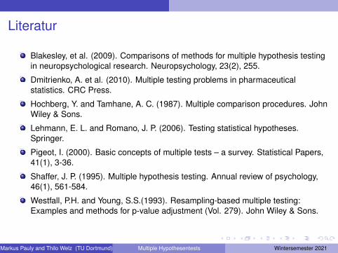
Literatur

Blakesley, et al. (2009). Comparisons of methods for multiple hypothesis testingin neuropsychological research. Neuropsychology, 23(2), 255.

Dmitrienko, A. et al. (2010). Multiple testing problems in pharmaceuticalstatistics. CRC Press.

Hochberg, Y. and Tamhane, A. C. (1987). Multiple comparison procedures. JohnWiley & Sons.

Lehmann, E. L. and Romano, J. P. (2006). Testing statistical hypotheses.Springer.

Pigeot, I. (2000). Basic concepts of multiple tests – a survey. Statistical Papers,41(1), 3-36.

Shaffer, J. P. (1995). Multiple hypothesis testing. Annual review of psychology,46(1), 561-584.

Westfall, P.H. and Young, S.S.(1993). Resampling-based multiple testing:Examples and methods for p-value adjustment (Vol. 279). John Wiley & Sons.


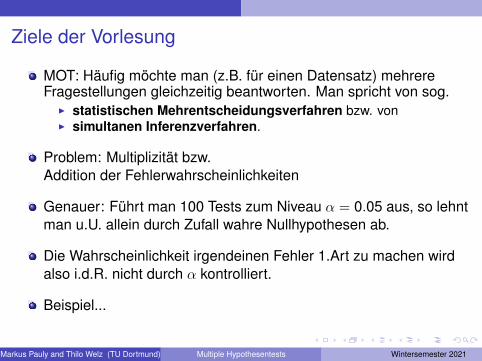
Ziele der Vorlesung

MOT: Häufig möchte man (z.B. für einen Datensatz) mehrereFragestellungen gleichzeitig beantworten. Man spricht von sog.

I statistischen Mehrentscheidungsverfahren bzw. vonI simultanen Inferenzverfahren.

Problem: Multiplizität bzw.Addition der Fehlerwahrscheinlichkeiten

Genauer: Führt man 100 Tests zum Niveau α = 0.05 aus, so lehntman u.U. allein durch Zufall wahre Nullhypothesen ab.

Die Wahrscheinlichkeit irgendeinen Fehler 1.Art zu machen wirdalso i.d.R. nicht durch α kontrolliert.

Beispiel...


Motivation

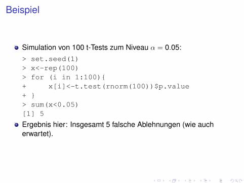
Beispiel

Simulation von 100 t-Tests zum Niveau α = 0.05:> set.seed(1)> x<-rep(100)> for (i in 1:100){+ x[i]<-t.test(rnorm(100))$p.value+ }> sum(x<0.05)[1] 5

Ergebnis hier: Insgesamt 5 falsche Ablehnungen (wie aucherwartet).

Beispiel 1.1 (Balanced One-Way ANOVA):Seien Xij

iid∼ N(µi , σ2) mit 1 ≤ i ≤ k , 1 ≤ j ≤ n, µi ∈ R, σ2 > 0

unbekanntIn diesem Fall überprüft der F-Test der klassischen Varianzanalyse dieNullhypothese

H0 : {µ1 = µ2 = · · · = µk}

Frage: Was macht man, wenn H0 zum Niveau α (z.N. α) abgelehntwird? Dies führt auf folgende Problemstellungen:


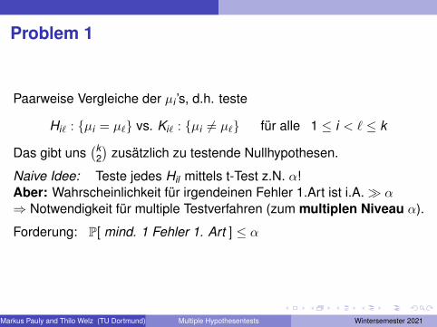
Problem 1

Paarweise Vergleiche der µi ’s, d.h. teste

Hi` : {µi = µ`} vs. Ki` : {µi 6= µ`} für alle 1 ≤ i < ` ≤ k

Das gibt uns ... zusätzlich zu testende Nullhypothesen.

Naive Idee: Teste jedes Hi` mittels t-Test z.N. α!Aber: Wahrscheinlichkeit für irgendeinen Fehler 1.Art ist i.A.� α⇒ Notwendigkeit für multiple Testverfahren zum multiplen Niveau α.

Forderung: P[ mind. 1 Fehler 1. Art ] ≤ α


Problem 1

Paarweise Vergleiche der µi ’s, d.h. teste

Hi` : {µi = µ`} vs. Ki` : {µi 6= µ`} für alle 1 ≤ i < ` ≤ k

Das gibt uns(k

2

)zusätzlich zu testende Nullhypothesen.

Naive Idee: Teste jedes Hil mittels t-Test z.N. α!Aber: Wahrscheinlichkeit für irgendeinen Fehler 1.Art ist i.A.� α⇒ Notwendigkeit für multiple Testverfahren (zum multiplen Niveau α).

Forderung: P[ mind. 1 Fehler 1. Art ] ≤ α


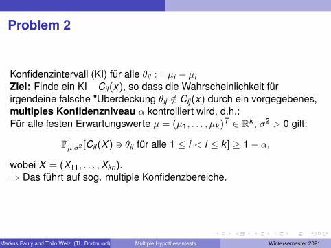
Problem 2

Konfidenzintervall (KI) für alle θil := µi − µlZiel: Finde ein KI Cil(x), so dass die Wahrscheinlichkeit fürirgendeine falsche "Uberdeckung θij /∈ Cij(x) durch ein vorgegebenes,multiples Konfidenzniveau α kontrolliert wird, d.h.:Für alle festen Erwartungswerte µ = (µ1, . . . , µk )

T ∈ Rk , σ2 > 0 gilt:

Pµ,σ2 [Cil(X ) 3 θil für alle 1 ≤ i < l ≤ k ] ≥ 1− α,

wobei X = (X11, . . . ,Xkn).⇒ Das führt auf sog. multiple Konfidenzbereiche.


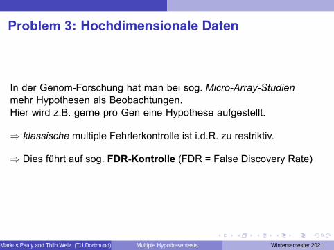
Problem 3: Hochdimensionale Daten

In der Genom-Forschung hat man bei sog. Micro-Array-Studien mehr Hypothesen als Beobachtungen.Hier wird z.B. gerne pro Gen eine Hypothese aufgestellt.

⇒ klassische multiple Fehrlerkontrolle ist i.d.R. zu restriktiv.

⇒ Dies führt auf sog. FDR-Kontrolle (FDR = False Discovery Rate)


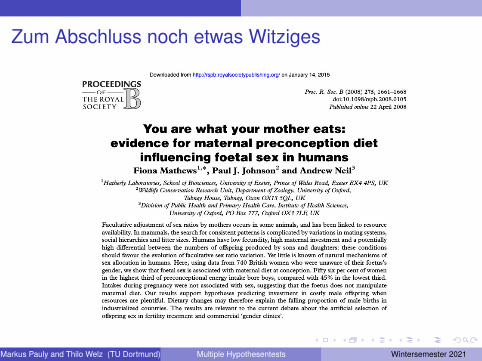
Zum Abschluss noch etwas Witziges


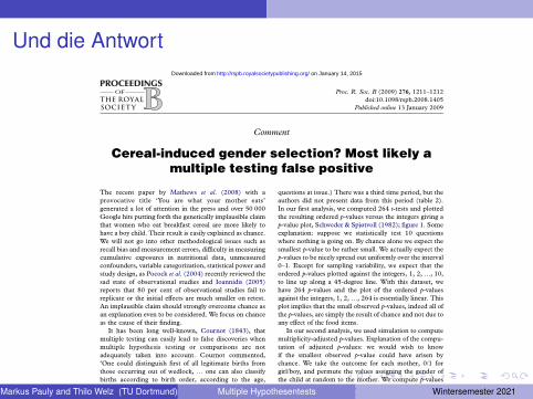
Und die Antwort

Comment

Cereal-induced gender selection? Most likely a

multiple testing false positive

The recent paper by Mathews et al. (2008) with a

provocative title ‘You are what your mother eats’

generated a lot of attention in the press and over 50 000

Google hits putting forth the genetically implausible claim

that women who eat breakfast cereal are more likely to

have a boy child. Their result is easily explained as chance.

We will not go into other methodological issues such as

recall bias andmeasurement errors, difficulty in measuring

cumulative exposures in nutritional data, unmeasured

confounders, variable categorization, statistical power and

study design, as Pocock et al. (2004) recently reviewed the

sad state of observational studies and Ioannidis (2005)

reports that 80 per cent of observational studies fail to

replicate or the initial effects are much smaller on retest.

An implausible claim should strongly overcome chance as

an explanation even to be considered. We focus on chance

as the cause of their finding.

It has been long well-known, Cournot (1843), that

multiple testing can easily lead to false discoveries when

multiple hypothesis testing or comparisons are not

adequately taken into account. Cournot commented,

‘One could distinguish first of all legitimate births from

those occurring out of wedlock, . one can also classify

births according to birth order, according to the age,

profession, wealth or religion of the parents.’ Cournot

goes on to point out that as one increases the number of

such ‘cuts’ (of the material into two or more categories) it

becomes more and more likely that by pure chance for at

least one pair of opposing categories the observed

difference will be significant. Based on a careful reading

of the paper by Mathews et al. (2008), a counting of the

questions under consideration and an analysis that better

takes multiple testing into account, we strongly believe

that themainfinding in this paper tobea falsediscovery/type

I error. Hundreds of comparisons were conducted; there

also seems to be hidden multiple testing as many additional

tests were computed and reported in other papers.

Specifically, the authors state in the abstract of their

paper ‘Fifty six per cent of women in the highest third of

preconceptional energy intake bore boys, compared with

45 per cent in the lowest third’ and assert that this result

is statistically significant. They go on to the point of

breakfast cereal consumption for the prediction of infant

gender. The authors provided the dataset and we

conducted our own analysis looking at the individual

food items for time periods one and two, 132!2Z264

statistical tests. (Note that there are actually three time

periods and only 132 food items were actually present in

the supplied dataset, so there are nominally 132!3Z396

questions at issue.) There was a third time period, but the

authors did not present data from this period (table 2).

In our first analysis, we computed 264 t-tests and plotted

the resulting ordered p-values versus the integers giving a

p-value plot, Schweder & Spjøtvoll (1982); figure 1. Some

explanation: suppose we statistically test 10 questions

where nothing is going on. By chance alone we expect the

smallest p-value to be rather small. We actually expect the

p-values to be nicely spread out uniformly over the interval

0–1. Except for sampling variability, we expect that the

ordered p-values plotted against the integers, 1, 2,., 10,

to line up along a 45-degree line. With this dataset, we

have 264 p-values and the plot of the ordered p-values

against the integers, 1, 2,., 264 is essentially linear. This

plot implies that the small observed p-values, indeed all of

the p-values, are simply the result of chance and not due to

any effect of the food items.

In our second analysis, we used simulation to compute

multiplicity-adjusted p-values. Explanation of the compu-

tation of adjusted p-values: we would wish to know

if the smallest observed p-value could have arisen by

chance. We take the outcome for each mother, 0/1 for

girl/boy, and permute the values assigning the gender of

the child at random to the mother. We compute p-values

for all the food items and the smallest p-value in the

permuted dataset is clearly a chance value. We do this

permutation thousands of times and get the distribution of

the smallest p-value. We note where the observed smallest

p-value falls in this distribution. Within sampling error

that can be made arbitrarily small, the adjusted p-value is

the correct probability of seeing a p-value as small when

observed, Westfall & Young (1993). The method takes

into account multiple testing, the correlation structure

among the variables and the distributional characteristics

of the variables. For the preconception time period,

the unadjusted p-value for breakfast cereal 0.0034 has a

multiple testing adjusted p-value of 0.2813. This adjusted

p-value is interpreted as follows: one would expect to see a

p-value as small as 0.0034 approximately 28 per cent of the

time when nothing is going on. So looking at both time

periods using the p-value plot and at the individual food

items in the preconception period using multiple-testing

adjusted p-values, the claimed effects are readily explainable

by chance. In addition, the motivating small p-values in

table 2, are also explainable by chance. The authors report

an unadjusted p-value of 0.029 for total energy. Among 54

tests, a p-value of 0.029 is not unusual, so total energy is not

statistically significant. Interestingly, sodium gave the

smallest p-value in table 2, an unadjusted p-value of 0.003

(which the authors dismiss); this p-value is also not

statistically significant when adjusted for multiple testing.

Proc. R. Soc. B (2009) 276, 1211–1212

doi:10.1098/rspb.2008.1405

Published online 13 January 2009

The accompanying reply can be viewed on page 1213 or at http://dx.

doi.org/doi:10.1098/rspb.2008.1781.

Received 29 September 2008

Accepted 24 October 2008 1211 This journal is q 2009 The Royal Society

on January 14, 2015http://rspb.royalsocietypublishing.org/Downloaded from


Multiple Hypothesentests

Documents

Transcript of Multiple Hypothesentests