Optimal Inventory Control and Distribution Network...
165
Optimal Inventory Control and Distribution Network Design of Multi- Echelon Supply Chains Von der Fakultät für Ingenieurwissenschaften, Abteilung Maschinenbau und Verfahrenstechnik der Universität Duisburg-Essen zur Erlangung des akademischen Grades eines Doktors der Ingenieurwissenschaften Dr.-Ing. genehmigte Dissertation von Mustafa Güller aus Gaziantep, der Türkei 1. Gutachter: Prof. Dr.-Ing. Bernd Noche 2. Gutachter: Prof. Dr. Michael Henke Tag der mündlichen Prüfung: 27.04.2016
Transcript of Optimal Inventory Control and Distribution Network...
Optimal Inventory Control and Distribution Network Design of Multi-Echelon Supply Chains
Von der Fakultät für Ingenieurwissenschaften,
Abteilung Maschinenbau und Verfahrenstechnik der
Universität Duisburg-Essen
zur Erlangung des akademischen Grades
eines
Doktors der Ingenieurwissenschaften
Dr.-Ing.
genehmigte Dissertation
von
Mustafa Güller aus
Gaziantep, der Türkei
1. Gutachter: Prof. Dr.-Ing. Bernd Noche
2. Gutachter: Prof. Dr. Michael Henke
Tag der mündlichen Prüfung: 27.04.2016
ii
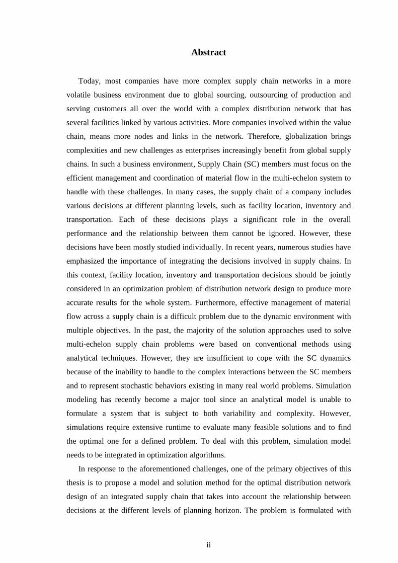
Abstract
Today, most companies have more complex supply chain networks in a more
volatile business environment due to global sourcing, outsourcing of production and
serving customers all over the world with a complex distribution network that has
several facilities linked by various activities. More companies involved within the value
chain, means more nodes and links in the network. Therefore, globalization brings
complexities and new challenges as enterprises increasingly benefit from global supply
chains. In such a business environment, Supply Chain (SC) members must focus on the
efficient management and coordination of material flow in the multi-echelon system to
handle with these challenges. In many cases, the supply chain of a company includes
various decisions at different planning levels, such as facility location, inventory and
transportation. Each of these decisions plays a significant role in the overall
performance and the relationship between them cannot be ignored. However, these
decisions have been mostly studied individually. In recent years, numerous studies have
emphasized the importance of integrating the decisions involved in supply chains. In
this context, facility location, inventory and transportation decisions should be jointly
considered in an optimization problem of distribution network design to produce more
accurate results for the whole system. Furthermore, effective management of material
flow across a supply chain is a difficult problem due to the dynamic environment with
multiple objectives. In the past, the majority of the solution approaches used to solve
multi-echelon supply chain problems were based on conventional methods using
analytical techniques. However, they are insufficient to cope with the SC dynamics
because of the inability to handle to the complex interactions between the SC members
and to represent stochastic behaviors existing in many real world problems. Simulation
modeling has recently become a major tool since an analytical model is unable to
formulate a system that is subject to both variability and complexity. However,
simulations require extensive runtime to evaluate many feasible solutions and to find
the optimal one for a defined problem. To deal with this problem, simulation model
needs to be integrated in optimization algorithms.
In response to the aforementioned challenges, one of the primary objectives of this
thesis is to propose a model and solution method for the optimal distribution network
design of an integrated supply chain that takes into account the relationship between
decisions at the different levels of planning horizon. The problem is formulated with
iii
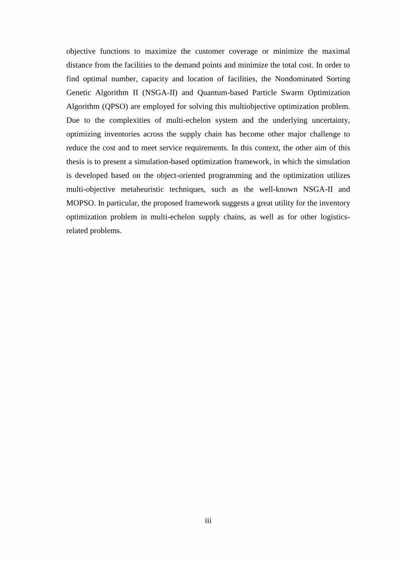
objective functions to maximize the customer coverage or minimize the maximal
distance from the facilities to the demand points and minimize the total cost. In order to
find optimal number, capacity and location of facilities, the Nondominated Sorting
Genetic Algorithm II (NSGA-II) and Quantum-based Particle Swarm Optimization
Algorithm (QPSO) are employed for solving this multiobjective optimization problem.
Due to the complexities of multi-echelon system and the underlying uncertainty,
optimizing inventories across the supply chain has become other major challenge to
reduce the cost and to meet service requirements. In this context, the other aim of this
thesis is to present a simulation-based optimization framework, in which the simulation
is developed based on the object-oriented programming and the optimization utilizes
multi-objective metaheuristic techniques, such as the well-known NSGA-II and
MOPSO. In particular, the proposed framework suggests a great utility for the inventory
optimization problem in multi-echelon supply chains, as well as for other logistics-
related problems.

iv
Acknowledgements
First and foremost, I would like to express my deepest gratitude to my supervisor
Prof. Dr.-Ing. Bernd Noche for the patience, the inspirational discussions and guidance
needed to complete this work successfully. Without his illuminating discussions and
intellectual comments, this thesis would not have been possible. He has also been a
supportive and respectful friend socially, financially, and spiritually.
Special thanks to all academic and technical staff of Transport System and Logistic
Institute for their many helpful suggestions and administrative support.
I also owe a special thanks to my parents, who pray for me anytime and from whom
I always get psychological strength during my studies. Their loving care and endless
patience enabled me to finish this dissertation.
Lastly, and most importantly, I would like to thank all my friends, who have always
been supportive of my academic pursuits and who have helped me through the most
difficult stages of this work. Your support and willingness to listen to plenty of
complaining is truly appreciated.

v
Abbreviation
ABS Agent-Based Simulation
APS Advanced Planning Systems
CD Coverage Distance
CFLP Capacitated Facility Location Problem
CV Coefficient Of Variation
DCs Distribution Centers
DES Discrete-Event Simulation
FIFO First In-First Out
FTL Full Truckload
GA Genetic Algorithm
LIFO Last In-Last Out
LTL Less-Than-Truckload
MILP Mixed Integer Linear Programming
MMP Multi-Site Master Planning
MOPSO Multiobjective Particle Swarm Optimization
MOPSO-SO Simulation-Based Optimization Based On MOPSO
MTS Make-To-Stock
NP Non-Deterministic Polynomial-Time
NSGA-II Non-Dominated Sorting Genetic Algorithm II
NSGA-II-SO Simulation-Based Optimization Based On NSGA-II
OOB Object Oriented Programming
PSO Particle Swarm Optimization
QPSO Quantum-Based Particle Swarm Optimization
RMS Response Surface Methodology
SBO Simulation-Based Optimization
SC Supply Chain
SCM Supply Chain Management
SCP Set Covering Problem
SD System Dynamics
SND Strategic Network Design
TSP Travelling Salesman Problem
VRP Vehicle Routing Problem
WR Warehouse
vi
Contents
Acknowledgements iv
Abbreviation v
Contents vi
List of Figures x
List of Tables xiii
Introduction 1 Chapter 1
1.1 Background and Motivation .................................................................................... 1
1.2 Decision Levels in Supply Chains .......................................................................... 4
1.3 Integrated Supply Chain Network Design .............................................................. 6
1.4 Research Questions and Objectives of the Dissertation .......................................... 8
1.5 Outline of Thesis ..................................................................................................... 9
Literature Review 12 Chapter 2
2.1 Literature Review on Integrated Supply Chain Network Design ......................... 12
2.2 Literature Review on Multi Echelon Inventory System ....................................... 13
2.3 Literature Review on Metaheuristic Techniques for Multi-Echelon Supply
Chain Problems ........................................................................................................... 15
Metaheuristic Techniques for Complex Optimization Problems 19 Chapter 3
3.1 Introduction to Genetic Algorithm ........................................................................ 19
3.1.1 Genetic Algorithm Operations ....................................................................... 21
3.2 Introduction to Particle Swarm Optimization ....................................................... 24
3.2.1 Parameter Selection of PSO ........................................................................... 26
3.2.2 Quantum Particle Swarm Optimization for Combinatorial Problems ............ 27
3.3 Multi-Objective Optimization ............................................................................... 29
3.3.1 Multi-Objective Optimization with Genetic Algorithm ................................. 30
3.3.2 Multi-Objective Optimization with Swarm Intelligence ................................ 33
Integrated Strategic Network Design for Multi-level Supply Chains 36 Chapter 4
4.1 Integrated Supply Chain Network Design ............................................................ 37
4.2 Model Notations and Problem Formulation .......................................................... 39

vii
4.2.1 Analysis of Facility Location Cost ................................................................. 40
4.2.2 Analysis of Transportation Costs ................................................................... 43
4.2.3 Analysis of Inventory Cost ............................................................................. 46
4.2.4 Integrated Supply Chain Network Design Function ...................................... 48
4.3 Solution Methodology ........................................................................................... 50
4.3.1 Application of Quantum-PSO for Location-Inventory Problem .................... 50
4.4 The Strategic Network Design Tool and Description of Experiment ................... 51
4.4.1 Description of Strategic Network Design Experiment ................................... 53
4.5 Model Results........................................................................................................ 55
4.6 Summary ............................................................................................................... 59
Object-Oriented Modeling for Inventory of Multi-Echelon Supply Chapter 5
Chain 61
5.1 Major Supply Chain Simulation Approaches ....................................................... 62
5.1.1 Spreadsheet-Based Simulation ....................................................................... 62
5.1.2 Systems Dynamics Based Simulation (SDS) ................................................. 63
5.1.3 Discrete-Event Simulation (DES) .................................................................. 64
5.1.4 Agent-Based Simulation (ABS) ..................................................................... 64
5.2 Object-Oriented Framework for Multi-Echelon Inventory Simulation ................ 65
5.3 Some Object Classes for Simulation of Multi-echelon Inventory System ........... 67
5.3.1 The Simulation Class ...................................................................................... 69
5.3.2 The NodeEvent and Queue Classes ................................................................ 69
5.3.3 The StockPoint Class ...................................................................................... 70
5.3.4 The Customer Class ........................................................................................ 70
5.3.5 The Retailer Class........................................................................................... 71
5.3.6 The Warehouse Class ..................................................................................... 72
5.3.7 The Inventory Class ........................................................................................ 74
5.4 The Simulation Model Cost Structure ................................................................... 74
5.4.1 Inventory Cost Structure................................................................................. 74
5.4.2 Activity-Based Cost Structure ........................................................................ 75
5.4.3 Transportation Cost Structure......................................................................... 75
5.5 Supply Chain Performance Measures ................................................................... 79
5.5.1 Notations......................................................................................................... 79
5.5.2 Measure Based on Cost .................................................................................. 80
viii
5.5.3 Measure Based on Customer Service Level ................................................... 81
5.5.4 Measure based on Order Response Time ....................................................... 82
5.6 Summary ............................................................................................................... 83
Multi-echelon Supply Chain Inventory Simulation Tool 84 Chapter 6
6.1 Simulation Environment ....................................................................................... 84
6.1.1 Simulation Tool Input Parameters .................................................................. 84
6.1.2 Simulation Tool Outputs ................................................................................ 85
6.2 Illustrative Example and Simulation Settings ....................................................... 87
6.2.1 Simulation Model Assumptions ..................................................................... 90
6.2.2 Simulation Scenarios ...................................................................................... 90
6.3 Simulation Results and Analysis ........................................................................... 93
6.3.1 Analysis of Replenishment Strategies without Information Sharing ............. 95
6.3.2 Analysis of Order Fulfillment Strategy .......................................................... 97
6.4 Summary ............................................................................................................. 100
Simulation-Based Optimization for Multi-echelon Inventory Chapter 7
Problems 102
7.1 Introduction to Simulation-Based Optimization ................................................. 102
7.2 Classification of the Simulation-Based Optimization Methods .......................... 104
7.3 Multi-Objective Optimization via Simulation .................................................... 106
7.3.1 Multi-Objective Simulation-based Optimization based on GA (NSGA-II-
SO) ......................................................................................................................... 108
7.3.2 Multi-Objective Simulation-based Optimization based on PSO (MOPSO-
SO) ......................................................................................................................... 108
7.4 Implementation of Simulation-Based Optimization for Inventory Problems ..... 110
7.4.1 Model Assumptions ...................................................................................... 111
7.4.2 Experimental Results and Discussion .......................................................... 112
7.4.3 Comparison of NSGA-II-SO and MOPSO-SO ............................................ 116
7.5 Summary ............................................................................................................. 120
Conclusion and Future Research 122 Chapter 8
8.1 Future Research ................................................................................................... 123
References 125
Appendix A 142
ix
1. Overview of Inventory Theory .......................................................................... 142
Classical Lot Size Model (EOQ) ........................................................................... 142
Continuous Review Inventory Model ................................................................... 142
Appendix B 145
Appendix C 150
Appendix D 151

x
List of Figures
Figure 1-1: Structure of a typical multi-echelon supply chain (Ghiani et al., 2004) ........ 2
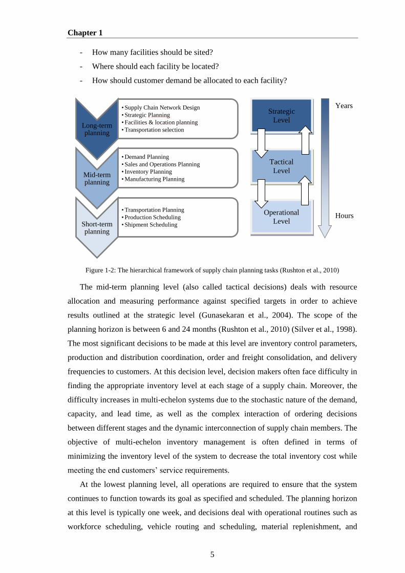
Figure 1-2: The hierarchical framework of supply chain planning tasks (Rushton et
al., 2010) ........................................................................................................................... 5
Figure 1-3: Typical APS modules covering the SCM matrix (Meyr et al., 2008) ............ 7
Figure 3-1: Flowchart of a simple Genetic Algorithm (adapted from (Gen & Cheng,
2000)) .............................................................................................................................. 20
Figure 3-2: Crossover ..................................................................................................... 23
Figure 3-3: Mutation ....................................................................................................... 24
Figure 3-4 Concept of modification of a searching point by PSO .................................. 25
Figure 3-5: Polar plot of rotation gate for qubit individuals ........................................... 28
Figure 3-6 Components of a general stochastic search algorithm (Zitzler et al.,
2004) ............................................................................................................................... 29
Figure 3-7: The Pareto front of a set of solutions in a two objective space (adapted
from (Sastry, 2007)) ........................................................................................................ 30
Figure 3-8: An example of the NSGA-II non-dominated sorting procedure (Sastry,
2007) ............................................................................................................................... 31
Figure 3-9: Crowding distance calculation (Raquel & Naval, 2005) ............................. 32
Figure 4-1: Relationship between number of facilities and logistics cost (Chopra,
2003) ............................................................................................................................... 38
Figure 4-2: Coordination and information flows between decision levels for
strategic network design tool (adapted from (Meyr et al., 2005)) .................................. 39
Figure 4-3: Fixed costs as a function of the warehouse capacity (Simchi-Levi et al.,
2004) ............................................................................................................................... 41
Figure 4-4: Operating Cost 𝐹𝑉𝑘 of potential facility k versus facility size .................... 42
Figure 4-5: Inbound and Outbound Transportation of DCs ........................................... 43
Figure 4-6: Approximation of average tour length ......................................................... 45
Figure 4-7: Strategic network optimization tool with metaheuristics ............................. 50
Figure 4-8: Structure of a supply chain network optimizer ............................................ 53
Figure 4-9: Supply Chain distribution network of the case study .................................. 54
Figure 4-10: Candidate DCs and customers’ location .................................................... 54
Figure 4-11: Location-Allocation Result of Integrated Network Design ....................... 55
Figure 4-12: Non-dominated solutions of the model — first objective is to minimize
the total cost and second objective is to minimize the distance between uncovered
demand and opened DCs ................................................................................................ 56
Figure 4-13: Cost components performance comparison for the two configurations .... 57
Figure 4-14: The trade-off between the cost and coverage distance .............................. 57
xi
Figure 4-15: Comparison of integrated and non-integrated (without inventory cost)
network design ................................................................................................................ 58
Figure 5-1: Forrester’s Supply Chain Dynamics Model (Forrester, 1961) ..................... 63
Figure 5-2: UML class diagrams of simulation package (Güller et al., 2015) ............... 66
Figure 5-3: Flowchart of (R, Q) Inventory Policy for Retailer Class ............................. 71
Figure 5-4: The supply operation flow chart for warehouse class .................................. 72
Figure 5-5: Flowchart of Process for Warehouse Inventory Control ............................. 73
Figure 5-6: Two Transportation Cost Structures ............................................................ 76
Figure 5-7: Distance-dependent Unit cost function (Janic, 2007) .................................. 77
Figure 5-8: Examples of Freight Rates (Distance-Shipment Based) (Güller et al.,
2015) ............................................................................................................................... 78
Figure 5-9: A dual-mode transportation cost structure for 1000 km distance (Güller
et al., 2015) ..................................................................................................................... 78
Figure 6-1: Inventory Simulation Output Screen ........................................................... 86
Figure 6-2: Example simulation graph outputs ............................................................... 87
Figure 6-3: Given structure of the distribution network ................................................. 88
Figure 6-4: Two echelon production-inventory system .................................................. 88
Figure 6-5: Percentage of each Probability Distribution of Demand for a Warehouse
(Housein, 2007) .............................................................................................................. 89
Figure 6-6: Aggregated Average Daily Demand of DCs ............................................... 90
Figure 6-7: Multiple Demand Classes Inventory System ............................................... 92
Figure 6-8: Simulated Total Supply Chain Costs of Plant-Warehouses for Base
Experiment ...................................................................................................................... 94
Figure 6-9: Simulated Total Supply Chain Costs of Each Local-DC ............................. 94
Figure 6-10: The Gap between Target Service Level and Simulated Service Level of
DCs ................................................................................................................................. 95
Figure 6-11: Measures of performance for each uncoordinated strategy ....................... 96
Figure 6-12: Customer service level of each distribution center with different
replenishment policy ....................................................................................................... 97
Figure 6-13: Performance of different order fulfillment strategies for RSDT
replenishment policy ....................................................................................................... 98
Figure 6-14: Performance of different order fulfillment strategies for RQMAX
replenishment policy ....................................................................................................... 99
Figure 6-15: The Gap between Target Service Level and Simulated Service Level
among the whole Supply Chain under RSDT replenishment policy .............................. 99
Figure 6-16: Comparison of Customer Prioritization on Performance ......................... 100
Figure 7-1: Simulation-Based Optimization Scheme (adapted from (Borshchev &
Filippov, 2004)) ............................................................................................................ 103
xii
Figure 7-2: Taxonomy of existing simulation-based optimization approaches
(Carson & Maria, 1997) ................................................................................................ 105
Figure 7-3 Simulation-Based Optimization Scheme for Inventory Problem ............... 107
Figure 7-4: Flowchart of the simulation optimization based on NSGA-II (NSGA-II-
SO) ................................................................................................................................ 109
Figure 7-5: Flowchart of the simulation-optimization based on MOPSO (MOPSO-
SO) ................................................................................................................................ 110
Figure 7-6: Two-echelon divergent production-inventory system ............................... 111
Figure 7-7: Final Pareto front of MOPSO-SO for the network of Plant-WR1 ............. 113
Figure 7-8: Final Pareto front of MOPSO-SO for the network of Plant-WR2 ............. 113
Figure 7-9: Final Pareto front of MOPSO-SO for the network of plant-WR3 ............. 114
Figure 7-10: The Pareto Fronts generated by Two Algorithms .................................... 117
Figure 7-11: The position of non-dominated solutions for RDC5 and RDC 11 in the
search space .................................................................................................................. 119
Figure 7-12: Pareto Fronts obtained for different Generation Number ........................ 120
Figure 7-13: Comparison of the Pareto Fronts obtained by different Swarm Sizes ..... 120
Figure 0-1: Change in inventory over time for the EOQ model ................................... 142
Figure 0-2 Continuous Review Inventory System ........................................................ 143
xiii
List of Tables
Table 4-1: Computational results of varying weight factors .......................................... 59
Table 4-2: Solution times of different problem sets ....................................................... 59
Table 5-1: List of classes in supply chain simulation framework (Güller et al., 2015) . 66
Table 5-2 Supply chain inventory simulator packages ................................................... 68
Table 5-3 Main supply chain structural objects and entities (Biaswas & Narahari,
2004) ............................................................................................................................... 68
Table 5-4: Activity- based Cost Parameters at DCs ....................................................... 75
Table 5-5: Notation explanation for the simulation model ............................................. 79
Table 6-1: Simulation performance summary for replenishment policies ..................... 96
Table 6-2: Cost Performance Measures of Exp-Set-1 under Different Queueing
Policy .............................................................................................................................. 97
Table 6-3: Cost Performance Measures of Exp-Set-3 under Different Queueing
Policy .............................................................................................................................. 98
Table 6-4: Service Level Performance Results for RDC6, RDC15, and RDC17
under Different Replenishment Policy and Order Fulfillment Strategy ....................... 100
Table 7-1: Search control parameters for NSGA-II and MOPSO ................................ 112
Table 7-2: The Best Cost and Best Service Level of proposed MOPSO-SO for
Network of Plant-WR1, Plant-WR2, and Plant-WR3 .................................................. 114
Table 7-3: Comparison of results between NSGA-II-SO and MOPSO-SO ................. 118
Table 7-4: Comparison of CPU time between NSGA-II and MOPSO ........................ 118

Chapter 1
Introduction
1.1 Background and Motivation
Increased competition, globalization in today’s market, products with shorter life
cycles, and the high level of customer service have forced businesses to invest in, and
focus attention, on their supply chains (Simchi-Levi et al., 2004). Generally, a supply
chain (SC) is referred to as a network of facilities and business activities consisting of
the design of new products, procurement of raw materials, transformation of such
materials into semi-finished and finished products, and delivery of such products to the
end customer. This definition, or a modified version of it, has been used by several
researchers (see (Lee & Billington, 1993), (Swaminathan et al., 1998), and (Ganeshan &
Harrison, 1995)). Companies face a set of supply chain challenges due to some kind of
uncertainty and variability. Today, most companies source globally, produce in various
plants and serve customers dispersed over a large geography with a complex
distribution network which has several stock points linked by various activities. This
increase in globalization brings new challenges as well benefits. Decisions along a
supply chain that should be coordinated contribute to the complexity of global logistic
networks. In response to these challenges, companies need efficient approaches and
methods helping in addressing uncertainty in their distribution network and validating
their decisions that lead to achieve their objectives.
The current trend in logistics is supply chain management (SCM) concerned with
the coordination and synchronization of the material, informational and financial flows
in a distribution network (Chopra & Meindl, 2004). Due to the growing complexity of
these networks and rapid development of new technologies to manage them, interest in
SCM has grown among both academicians and the practitioners over the last decades.
One major issue of SCM is to find the best possible network configuration so that
organizations can achieve effective and efficient logistics operations that improve the
1.1 Background and Motivation
2
performance of the company. This objective supports integrating facility location with
different supply chain processes such as procurement, production, inventory,
distribution, and transportation (Melo et al., 2008).
If an item moves through more than one step before reaching the final customer, the
supply chain is called multi-echelon or a multi-level production/distribution system
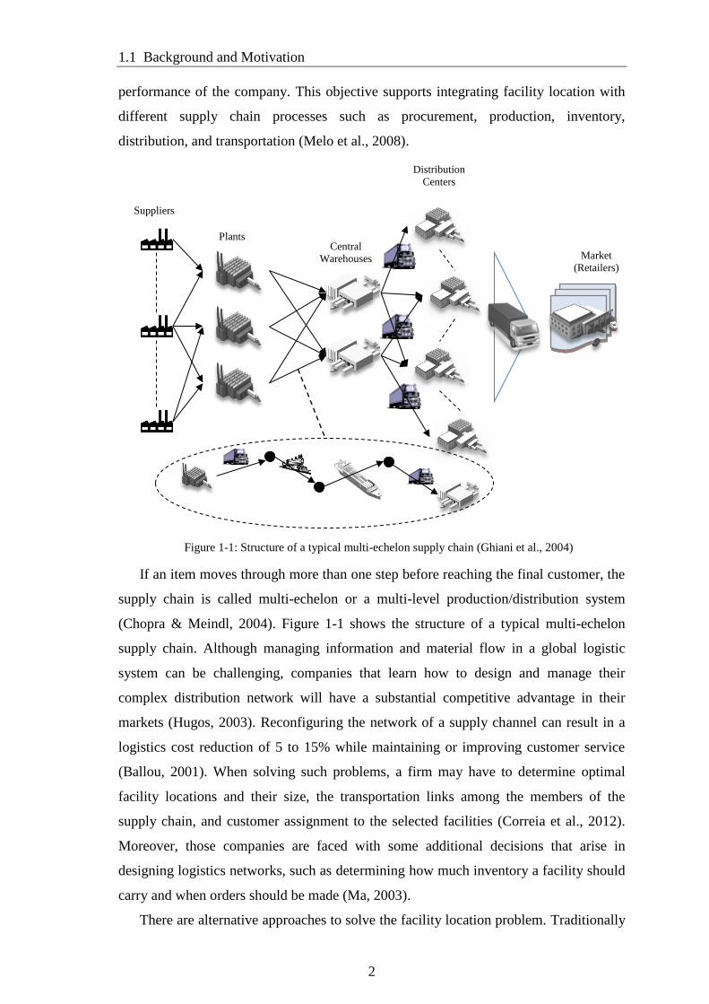
(Chopra & Meindl, 2004). Figure 1-1 shows the structure of a typical multi-echelon
supply chain. Although managing information and material flow in a global logistic
system can be challenging, companies that learn how to design and manage their
complex distribution network will have a substantial competitive advantage in their
markets (Hugos, 2003). Reconfiguring the network of a supply channel can result in a
logistics cost reduction of 5 to 15% while maintaining or improving customer service
(Ballou, 2001). When solving such problems, a firm may have to determine optimal
facility locations and their size, the transportation links among the members of the
supply chain, and customer assignment to the selected facilities (Correia et al., 2012).
Moreover, those companies are faced with some additional decisions that arise in
designing logistics networks, such as determining how much inventory a facility should
carry and when orders should be made (Ma, 2003).
There are alternative approaches to solve the facility location problem. Traditionally
Central
Warehouses
Plants
Suppliers
Distribution
Centers
Market
(Retailers)
Figure 1-1: Structure of a typical multi-echelon supply chain (Ghiani et al., 2004)
Chapter 1
3
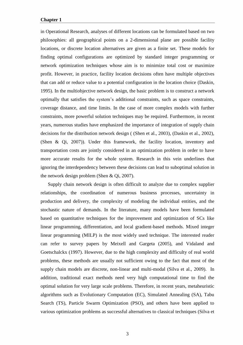
in Operational Research, analyses of different locations can be formulated based on two
philosophies: all geographical points on a 2-dimensional plane are possible facility
locations, or discrete location alternatives are given as a finite set. These models for
finding optimal configurations are optimized by standard integer programming or
network optimization techniques whose aim is to minimize total cost or maximize
profit. However, in practice, facility location decisions often have multiple objectives
that can add or reduce value to a potential configuration in the location choice (Daskin,
1995). In the multiobjective network design, the basic problem is to construct a network
optimally that satisfies the system’s additional constraints, such as space constraints,
coverage distance, and time limits. In the case of more complex models with further
constraints, more powerful solution techniques may be required. Furthermore, in recent
years, numerous studies have emphasized the importance of integration of supply chain
decisions for the distribution network design ( (Shen et al., 2003), (Daskin et al., 2002),
(Shen & Qi, 2007)). Under this framework, the facility location, inventory and
transportation costs are jointly considered in an optimization problem in order to have
more accurate results for the whole system. Research in this vein underlines that
ignoring the interdependency between these decisions can lead to suboptimal solution in
the network design problem (Shen & Qi, 2007).
Supply chain network design is often difficult to analyze due to complex supplier
relationships, the coordination of numerous business processes, uncertainty in
production and delivery, the complexity of modeling the individual entities, and the
stochastic nature of demands. In the literature, many models have been formulated
based on quantitative techniques for the improvement and optimization of SCs like
linear programming, differentiation, and local gradient-based methods. Mixed integer
linear programming (MILP) is the most widely used technique. The interested reader
can refer to survey papers by Meixell and Gargeta (2005), and Vidaland and
Goetschalckx (1997). However, due to the high complexity and difficulty of real world
problems, these methods are usually not sufficient owing to the fact that most of the
supply chain models are discrete, non-linear and multi-modal (Silva et al., 2009). In
addition, traditional exact methods need very high computational time to find the
optimal solution for very large scale problems. Therefore, in recent years, metaheuristic
algorithms such as Evolutionary Computation (EC), Simulated Annealing (SA), Tabu
Search (TS), Particle Swarm Optimization (PSO), and others have been applied to
various optimization problems as successful alternatives to classical techniques (Silva et

1.2 Decision Levels in Supply Chains
4
al., 2003) (Altiparmak et al., 2006).
Two modeling approaches are widely used to evaluate the performance of such
systems: simulation techniques and analytical modeling (Svensson, 1996). The
operations research community also uses mathematical programming techniques (also
called analytical or optimization techniques) such as Linear Programming and Mixed
Integer Programming to formulate solutions to supply chain problems. However, these
techniques are not able to deal efficiently with the uncertainty and SC dynamics because
of their inability to represent stochastic behaviors or highly complex relations between
the different entities existing in real-world problems (Mele et al., 2006). Unlike the
traditional analytical methods, researchers also use simulation as a decision support tool
to analyze the overall performance of a system without limiting assumptions. Since it
can model the compound effects of uncertainty and non-linear relations in the system,
the simulation model is normally preferable when an analytical model is not be able to
formulate the system that is subject to both variability and complexity. However,
simulation provides no concrete solutions to optimization problems, and users need to
evaluate many feasible solutions in order to find an optimal solution to a problem
(Güller et al., 2015). Thus researchers have attempted to combine simulation and
optimization procedure. This approach is called simulation-optimization or simulation-
based optimization. Simulation-based optimization (SBO) can be defined as the process
of finding the best input variable values from among all possibilities without explicitly
evaluating each possibility and integrating optimization techniques into simulation
where the simulation model is regarded as the evaluation mechanism (Carson & Maria,
1997).
1.2 Decision Levels in Supply Chains
Planning processes of a SC are divided into three levels in terms of planning
horizon: strategic level, tactical level and operational level (see Figure 1-2) (Chopra &
Meindl, 2004). Designing the distribution network in an optimal way is at the core of
strategic planning in supply chain management (SCM) and crucial for firms. According
to Harrison (2005), up to 80% of the total cost of a product is driven by network design
decisions. Furthermore, companies need to improve their network strategy in order to be
more responsive to customer demand in today’s highly dynamic and competitive
environment. This issue involves a number of questions to be addressed (Jayaraman,
1998):
Chapter 1
5
- How many facilities should be sited?
- Where should each facility be located?
- How should customer demand be allocated to each facility?
Figure 1-2: The hierarchical framework of supply chain planning tasks (Rushton et al., 2010)
The mid-term planning level (also called tactical decisions) deals with resource
allocation and measuring performance against specified targets in order to achieve
results outlined at the strategic level (Gunasekaran et al., 2004). The scope of the
planning horizon is between 6 and 24 months (Rushton et al., 2010) (Silver et al., 1998).
The most significant decisions to be made at this level are inventory control parameters,
production and distribution coordination, order and freight consolidation, and delivery
frequencies to customers. At this decision level, decision makers often face difficulty in
finding the appropriate inventory level at each stage of a supply chain. Moreover, the
difficulty increases in multi-echelon systems due to the stochastic nature of the demand,
capacity, and lead time, as well as the complex interaction of ordering decisions
between different stages and the dynamic interconnection of supply chain members. The
objective of multi-echelon inventory management is often defined in terms of
minimizing the inventory level of the system to decrease the total inventory cost while
meeting the end customers’ service requirements.
At the lowest planning level, all operations are required to ensure that the system
continues to function towards its goal as specified and scheduled. The planning horizon
at this level is typically one week, and decisions deal with operational routines such as
workforce scheduling, vehicle routing and scheduling, material replenishment, and
Long-term planning
• Supply Chain Network Design
• Strategic Planning
• Facilities & location planning
• Transportation selection
Mid-term planning
• Demand Planning
• Sales and Operations Planning
• Inventory Planning
• Manufacturing Planning
Short-term planning
• Transportation Planning
• Production Scheduling
• Shipment Scheduling
Years
Hours
Strategic Level
Tactical Level
Operational
Level

1.3 Integrated Supply Chain Network Design
6
packaging (Azambuja & O'Brien, 2008). These decisions obviously affect the
distribution strategy and transportation cost. Transportation and inventory costs
constitute the largest proportion of the total supply chain cost (Ballou, 2004). Based on
estimates for the U.S. in 2002, transportation costs were $577 billion, and inventory
carrying costs and warehousing costs were $298 billion. The total logistics costs were
$910 billion, which was equivalent to 8.7% of the U.S. gross domestic product in 2002
(Akca, 2010).
The right combination of these decisions is vital for the optimization of overall
supply chain performance. Traditionally, most approaches to supply chain network
optimization in the literature consider decisions at different levels separately. For
example, most of the optimization models concerning the configuration of the supply
chain network focus their attention on trade-offs between transportation and fixed
facility costs, disregarding inventory control decisions (Daskin, 1995). On the other
hand, inventory decisions are optimized to balance the trade-off between inventory
holding and fixed replenishment costs under a fixed supply chain network structure.
However, there is a clear relationship between the inventory cost, transportation cost
and the supply chain’s physical structure. This highlights a need for models that
integrates strategic, tactical and operational decisions, known as an integrated supply
chain design.
1.3 Integrated Supply Chain Network Design
Integration of the decision levels can be useful for different aspects of a company’s
supply chain. According to Shapiro (2001), there are three dimensions to integration.
a) Functional integration is concerned with purchasing, manufacturing,
warehousing, and distribution activities within the company, and between the
company and its suppliers and customers.
b) Spatial integration is done over a target group of supply chain entities – vendors,
manufacturing facilities, warehouses, and markets.
c) Inter-temporal integration refers to integration of the overlapping decisions in
the strategic, tactical and operational planning horizons.
Goetschalckx and Fleischmann (2005) describe two key planning decisions for
network design. These decisions are i) status of a particular facility or manufacturing
line and relationships or allocations during a specific planning period and ii) the product
flows and storage quantities (inventory) in the supply chain during a planning period.

Chapter 1
7
Planning decisions of the strategic network design have both interrelated spatial and
temporal characteristics. However, the planning and integration of decisions along a
supply chain are difficult and complex tasks. Advanced Planning Systems (APS) can be
used as a tool in order to provide reliable supply chain planning. APS is described as a
decision support system that uses advanced optimization techniques and a planning
matrix that decomposes the planning functions into the commonly used software
modules. Furthermore, it introduces a hierarchical integration of different decision
among various supply chain operations (Meyr et al., 2008). Figure 1-3 shows the
interaction among value chains for optimizing a supply chain by using APS. APS uses
advanced mathematical algorithms (e.g., genetic algorithms, linear programming, etc.)
in order to provide nearly optimal solutions for supply chain planning issues (Selcuk,
2007). These algorithms simultaneously consider a range of constraints to perform the
optimization.
Figure 1-3: Typical APS modules covering the SCM matrix (Meyr et al., 2008)
This dissertation focuses on the strategic and tactical levels, i.e. strategic network
design (SND) module and multi-site master planning (MMP) module as shown in
Figure 1-3. The SND module determines the number of plants and distribution centers,
their location and capacity, and the assignment of customers to each facility in the
supply chain, as well as possible distribution channels as described in the previous
section (Jonsson & Kjellsdotter, 2007). The Master Planning module synchronizes the
flow of materials along the entire supply chain and coordinates production,
Op
erat
ional
Multi-site Master Planning
Purchasing &
Material
Requirements
Planning
Production
Planning
Scheduling
Distribution
Planning
Transport
Planning
Demand
Planning
Demand
Fulfillment
Procurement Production Distribution Sales
Str
ateg
ic
Tac
tica
l
Supply
Management Production
Management Distribution
Management Demand
Management
Strategic Network Design

1.4 Research Questions and Objectives of the Dissertation
8
transportation, supply capacities, and seasonal stock. It also balances supply and
demand. The decisions on production, inventory and transport quantities need to be
addressed simultaneously (Jens & Michael, 2005). As a result of this synchronization,
production and transportation entities are able to reduce the inventory level at stock
points.
Combining the relevant decisions that arise at the strategic, tactical and operational
levels, one must consider all relevant costs including location, inventory and
transportation costs in an integrated system. These three costs are highly related and,
ideally, should be considered jointly when making network design decisions (Daskin et
al., 2005). For example, a high number of distribution centers (DCs) reduces the cost of
transporting product to retailers and ensures better service. However, under this model
pooling effects increase the cost of holding inventory and increase the fixed costs
associated with operating DCs (Erlebacher & Meller, 2000). The challenge is to find the
right balance between installation DCs, inventory, and transportation costs that achieves
customer service goals at the minimum total system-wide cost. Once the supply chain
network is determined, the focus shifts to decisions at the Master Planning module
(Shen, 2005). One of the major decisions related to the Master Planning module is
inventory control. In this module, the goal is to determine the optimal number of
shipments, shipment sizes, and inventory and transportation costs (Meyr et al., 2008).
1.4 Research Questions and Objectives of the Dissertation
Although there has been tremendous interest in supply chain design and inventory
management for decades, the research on integrated approaches is quite scarce. Most
practical optimization problems involve multiple and conflicting objectives that must be
optimized simultaneously. Furthermore, uncertainty in demand and cost parameters is
other factor that can contribute to the complexity of location/inventory problem and
influence the effectiveness and responsiveness of the logistic network. In this context,
the primary objective of this dissertation is firstly to propose a model and solution
method for the optimal distribution network design of an integrated supply chain that
takes into account the relationship between decisions at the different levels of planning
horizon. The other purpose of the dissertation is to provide a modeling framework that
integrates simulation models and multiobjective optimization methods to find the
optimal inventory allocation policy for each facility in the supply chain under a
stochastic environment. More specifically, this research proposes two multiobjective
Chapter 1
9
metaheuristic optimization algorithms that find Pareto optimal solutions to the facility
location problem and the multi echelon inventory allocation problem.
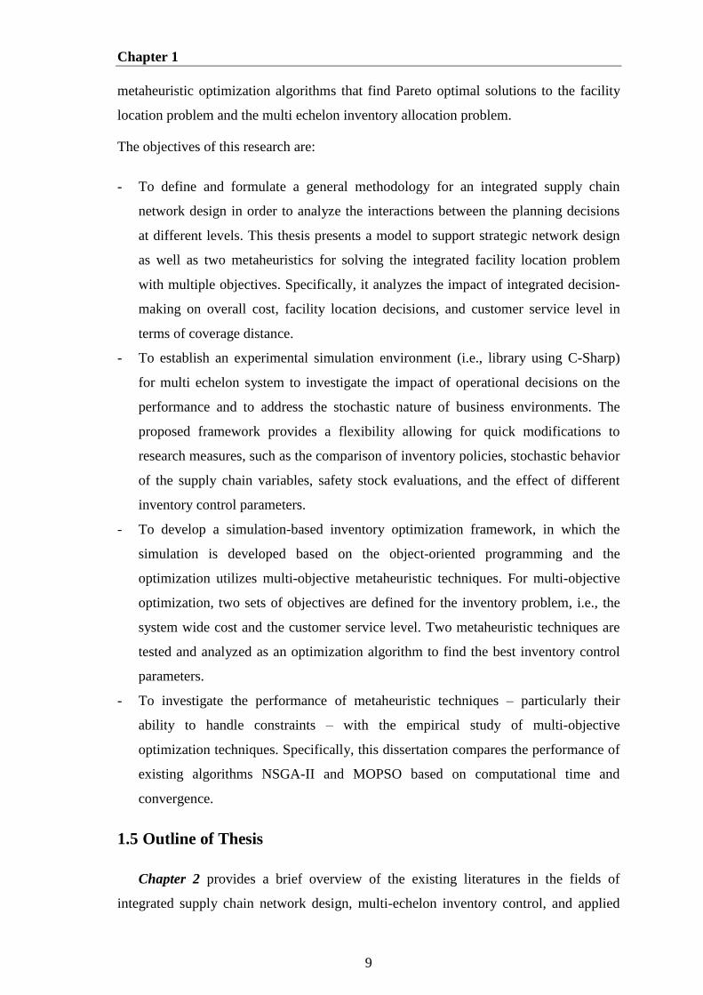
The objectives of this research are:
- To define and formulate a general methodology for an integrated supply chain
network design in order to analyze the interactions between the planning decisions
at different levels. This thesis presents a model to support strategic network design
as well as two metaheuristics for solving the integrated facility location problem
with multiple objectives. Specifically, it analyzes the impact of integrated decision-
making on overall cost, facility location decisions, and customer service level in
terms of coverage distance.
- To establish an experimental simulation environment (i.e., library using C-Sharp)
for multi echelon system to investigate the impact of operational decisions on the
performance and to address the stochastic nature of business environments. The
proposed framework provides a flexibility allowing for quick modifications to
research measures, such as the comparison of inventory policies, stochastic behavior
of the supply chain variables, safety stock evaluations, and the effect of different
inventory control parameters.
- To develop a simulation-based inventory optimization framework, in which the
simulation is developed based on the object-oriented programming and the
optimization utilizes multi-objective metaheuristic techniques. For multi-objective
optimization, two sets of objectives are defined for the inventory problem, i.e., the
system wide cost and the customer service level. Two metaheuristic techniques are
tested and analyzed as an optimization algorithm to find the best inventory control
parameters.
- To investigate the performance of metaheuristic techniques – particularly their
ability to handle constraints – with the empirical study of multi-objective
optimization techniques. Specifically, this dissertation compares the performance of
existing algorithms NSGA-II and MOPSO based on computational time and
convergence.
1.5 Outline of Thesis
Chapter 2 provides a brief overview of the existing literatures in the fields of
integrated supply chain network design, multi-echelon inventory control, and applied
1.5 Outline of Thesis
10
metaheuristic approaches. This chapter also surveys relevant literatures in the
methodology of simulation on inventory control and simulation-based optimization.
Chapter 3 introduces the basic concepts of metaheuristic techniques and different
multiobjective optimization methods that are used to find Pareto optimal solutions. This
work is mostly based on Genetic Algorithm (GA) and Particle Swarm Optimization
(PSO). The chapter also presents a brief introduction to Non-dominated Sorting
Genetic Algorithm-II (NSGA-II) and Multi-Objective Particle Swarm Optimization
(MOPSO).
Chapter 4 presents the integrated distribution network design model for the food
industry in detail and explains the solution technique using discrete metaheuristic
optimization techniques. In this chapter, we present the problem statement and the
mathematical formulation of the proposed integrated model. In this research we will
apply the Non-dominated Sorting Genetic Algorithm (NSGA-II) and the Quantum-
based Multiobjective Particle Swarm Optimization to approximate the Pareto front to
generate valid solutions for the network design problem. The applicability of the
proposed algorithm and the efficiency of the proposed integrated approach are presented
in a computational experiment for a large-scale network involving several factories’
warehouses, regional distribution centers and customers. To analyze the impact of
optimization algorithm parameters and supply chain cost parameters, we empirically
compare solutions over several variations.
Chapter 5 discusses the framework architecture of the simulation model and the
detailed structure of each individual package through a simplified model of inventory in
a multi-echelon supply chain. It discusses the development and implementation of an
object-oriented simulation package.
Chapter 6 contains a brief description of the assumptions made during the
simulations and experiments: in other words, input and output parameters of the
simulation tool. The supply chain models that represent different inventory coordination
mechanisms are developed and analyzed to compare their performances.
Chapter 7 describes the methodology of simulation-based multi-objective
optimization, which integrates the optimization tool into the simulation, and the
simulation model is regarded as an objective function. After introducing the proposed
optimization concepts for the stochastic inventory problem, the chapter presents several
numerical examples. It compares different evolutionary approaches, such as NSGA-II
and MOPSO, due to their ability to lead to efficient generation of Pareto sets and
Chapter 1
11
computational time.
Chapter 8 concludes the thesis by summarizing the main development, major
contributions, and limitations of this study. Possible directions for further research and
indications for potential applications are offered as well.
Chapter 2
Literature Review
This literature review is divided into three sections: integrated supply chain network
design, multi-echelon inventory system, and supply chain optimization models based on
metaheuristic techniques. The review of integrated supply chain network design
includes the models and algorithms of network design in an integrated environment and
facility location problems, while the review of supply chain optimization models
focuses on the metaheuristic techniques for global supply chain design and planning.
2.1 Literature Review on Integrated Supply Chain Network Design
In general, the classical facility location problem is concerned with selecting sites to
install facilities and assign customers to these facilities in a way that minimizes the
fixed facility location and transportation costs as well as all other relevant expenses.
Shen (2007), (Daskin et al., 2002), Snyder (2007) and Melo et al. (2008) offer a
comprehensive review in the research area of supply chain design. There are several
papers in the area of integrated facility location and inventory control. Nozick et al.
(1998) present a linear approximation to the total safety stock in terms of the function of
the number of DCs. Nozick et al. (2001) extend their previous model by considering the
service responsiveness and uncertainty in delivery time to the DC. The solution model
consists of two sub-models. They first specify a minimum inventory level necessary to
ensure a specified out-of-stock probability for a given product and propose an iterative
updating scheme for solving optimal facility location. Shen et al. (2003) consider an
integrated facility location/inventory location model to include nonlinear working
inventory and safety stock costs for a two-stage network with multiple retailers under
stochastic demand. The problem in their work is determining which retailers should
serve as DCs and how much inventory these stocking points should hold. The model is
initially formulated as a mixed integer nonlinear location allocation and solved with a
column generation method.
Chapter 2
13
The location-inventory problem has been solved widely by using Lagrangian
relaxation based algorithms in literature ( (Daskin et al., 2002), (Shen et al., 2003),
(Snyder et al., 2007), (Miranda & Garrido, 2006)). Daskin et al. (2002) consider a
model similar to the one addressed in Shen et al. (2003), where the model incorporates
working inventory and safety stock inventory costs at the distribution centers. They
formulated the model as a non-linear integer-programming problem with binary
assignment variables, and propose a Lagrangian relaxation method for the case in which
the ratio of the variance of demand at the retailers to the mean demand is the same for
all retailers. Snyder et al. (2007) introduce the stochastic location model with risk
pooling that optimizes location, inventory, and allocation decisions simultaneously.
Miranda and Garrido (2006) also propose solution methods based on Lagrangian
relaxation for mixed-integer nonlinear models. They consider the order quantity for
each warehouse as a decision variable that they are trying to optimize. The variable is
transformed into a series of Capacitated Facility Location Problem (CFLP) and
proposed solution involves a Lagrangian relaxation and the sub-gradient method.
Erlebacher and Meller (2000) develop a non-linear integer inventory-location model
for designing a two-level distribution system where customer demands are stochastic
and rectilinear distances are used to represent the distances between the locations. The
aim of their model is to decide on the number of distribution centers, their location and
customer allocations that minimize the sum of the fixed operating costs of open DCs,
inventory holding costs at DCs, total transportation costs from plants to DCs, and
transportation costs from DCs to customers.
Recently, Shu et al. (2005) propose a two-stage stochastic model for the design of
integrated supply chain network decisions related to strategic sourcing and distribution,
warehouse-retailer assignment, and facility location in an integrated multi-echelon
supply chain distribution network. They consider the joint replenishment of inventory at
both warehouses’ and retailers’ level to minimize the total expected system-wide multi-
echelon inventory, transportation, and facility location costs.
2.2 Literature Review on Multi Echelon Inventory System
Researchers have developed models to deal with a simplified single-vendor, single-
buyer inventory problem. However, it is not practical for the supply chain network to
have only one vendor and one buyer all the time in real-world business. The purpose of
this section is to introduce the modeling philosophy and convention of the multi-

2.2 Literature Review on Multi Echelon Inventory System
14
echelon inventory studies under a continuous review system. For a recent overview, see
e.g. Axsäter (2003).
A good review of the models dealing with continuous review policies for multi
echelon inventory system can be found in Axsäter (1993). A well-known approach for
multi-echelon inventory models is the METRIC method developed by Sherbrooke
(1968). He describes a methodology for managing a two-echelon system for repairable
items; however, the principles apply equally well to consumable items. The system
consists of N identical retailers or bases at lower echelon and one warehouse at upper
echelon that supplies the bases with repaired parts. It is assumed demand occurs only at
the lower echelon and follows a simple Poisson process. All stock points apply a one-
for-one replenishment control policy (S-1, S). In this case, the warehouse observes a
Poisson demand process. The objective of the model is to identify stocking policies at
the bases and the depot to minimize backorders at the base level subject to a constraint
on the inventory investment. Later, Deuermeyer and Schwarz (1981) develop an
inventory model for a two-echelon inventory system that consists of one warehouse and
N identical retailers that implement (R, Q) policies. They present an approximate model
to calculate the system service levels, and develop an optimization framework to
maximize the system fill-rate subject to a system safety stock constraint.
De Bodt and Graves (1985) consider a multi-stage, serial inventory system under
continuous review (Q, R) policy. They derive approximate performance measures with
set-up cost under a nested policy assumption: whenever a stage receives a shipment, a
batch must be immediately sent to its downstream stage. They do not make an
assumption about the form of the demand distribution. In other words, the demand for
the end item is stochastic and stationary.
Andersson and Marklund (2000) study decentralized inventory control in a two-
level distribution system with a central warehouse and multiple non-identical retailers.
In their model, all installations use continuous review installation stock (R, Q) policies.
They present an approximate cost evaluation technique to minimize total inventory cost
which also contains safety stock and backorder costs.
Hoque (2006) focuses on a two-echelon serial inventory system consisting of a
warehouse and a retailer under constant demand. Each inventory location follows a
continuous review (s, Q) policy, and unfilled demands are completely backordered on a
first-come, first-served basis. He extended the existing model by taking into account the
transportation time of a batch. Mitra (2009) analyzes a two-echelon inventory system
Chapter 2
15
with returns under generalized conditions, and developed a deterministic and a
stochastic model for the system.
There are other papers in the literature that present exact and approximate methods
for a two-level inventory system consisting of one warehouse and multiple retailers
under a continuous review (R, Q) policy. Forsberg (1996) evaluated holding and
shortage costs for a two-level inventory system with one warehouse and different
retailers. Axsäter (1998) presents methods for the exact evaluation of two retailers’
cases and an approximate evaluation for the case of more than two retailers.
Moinzadeh (2002) considers a single product supply chain consisting of one
supplier and multiple identical retailers. He proposed a supplier replenishment policy
that incorporates information about the inventory position at each of the retailers and
provides an exact analysis of the operating measures for such systems. Based on the
numerical study, parameter settings are identified under which information sharing is
most beneficial. Gürbüz et al (2007) present coordinated replenishment in a distribution
system with multiple retailers, a single outside supplier, and one warehouse that holds
no inventory. They considered both inventory and transportation costs in a supply chain
under stochastic demand and proposed a new policy – the hybrid policy – which
combines a traditional echelon policy with a special type of can-order policy. They
analyzed three coordinated replenishment policies (installation-based, echelon-based
and time-based) and compared their performance. The numerical results suggest that the
hybrid policy provides significant improvement over other replenishment policies.
2.3 Literature Review on Metaheuristic Techniques for Multi-Echelon
Supply Chain Problems
Industrial decision makers face complex problems, including large numbers of
integer or binary variables, non-linearities, stochasticity, non-standard underlying utility
functions, and logical or non-standard constraints and feasibility conditions (Jones et al.,
2002). Researchers have proposed a variety of heuristic algorithms to address them.
Heuristic algorithms are solution methods that do not guarantee an optimal solution, but
in general can generate a near-optimal solution relatively quickly. In recent years,
metaheuristic algorithms such as Ant Colony Optimization (ACO), Evolutionary
Computation (EC), Simulated Annealing (SA), Tabu Search (TS), Stochastic
Partitioning Methods (SPM), and others, are widely used to solve important logistic and
combinatorial optimization problems that include in their mathematical formulation

2.3 Literature Review on Metaheuristic Techniques for Multi-Echelon Supply Chain
Problems
16
uncertain, stochastic and dynamic information (Bianchi et al., 2006). They have been
successful alternatives to the classical approach. According to Osman and Laporte
(1996), the term metaheuristic describes an iterative search process that guides a
subordinate heuristic by intelligently combining different concepts for exploring and
exploiting the search space. The searcher employs learning strategies to structure
information and find near-optimal solutions efficiently.
The major problems in supply chain belong to the category of NP-hard problems
and they are computationally difficult (Jaramillo et al., 2002). As a result, much
research effort has been devoted to develop an efficient solution methodology to find
the optimal or near-optimal solution in the minimum computational time. Over the last
few years, metaheuristic algorithms were successfully applied to large-scale and real-
life network design problems: tabu search (see (Lee & Dong, 2009), (Tuzun & Burke,
1999)), genetic algorithms (see (Ko & Evans, 2007), (Min et al., 2006)), simulated
annealing (see (Jayaraman et al., 2003)). Tuzun and Burke (1999) introduce a two-
phase tabu search approach. The first phase searches for a good facility configuration,
and the second phase searches for a good routing that corresponds to that configuration.
Wu et al. (2002) proposed a decomposition-based heuristic method for solving the
location-routing problem with capacitated depots. They used simulating annealing
algorithm to solve decisions variables.
Evolutionary algorithms are a particularly important subset of population-based
metaheuristic search approaches. Among these methods, Genetic Algorithm (GA) is a
solution method that was formally introduced in the United States in the 1970s by John
Holland at University of Michigan. GA is an intelligent optimization technique that has
the capacity to solve difficult problems in a variety of disciplines. Its simplicity permits
us to use GA to solve NP-hard problems in acceptable computational time.
GA has been applied to numerous supply chain management problems in many
different configurations (Zhao & Xie, 2002). New algorithms based on the GAs have
been developed for the set-covering problem ( (Al-Sultan et al., 1996); (Beasley & Chu,
1996)), and for location-allocation problems ( (Jaramillo et al., 2002); (Zhou et al.,
2002)). Zhou and Liu (2003) proposed a capacitated location-allocation problem with
stochastic demands. For solving these stochastic models efficiently, the network
simplex algorithm, stochastic simulation and genetic algorithm are integrated to produce
a hybrid intelligent algorithm. Lin et al. (2007) compared flexible supply chains and
traditional supply chains with a hybrid genetic algorithm. Liao and Hsieh (2009)
Chapter 2
17
optimized the location decision for distribution centers with two objectives:
minimization of total cost and maximization of customer service by using NSGA II
algorithm.
GAs has also been successfully used to find the optimal solutions for inventory
optimization. Sarker and Newton (2002) investigate the use of genetic GAs for solving
the batch size problem for a product, and purchasing policy of associated raw materials.
In the mathematical model for this problem, they considered a constrained nonlinear
integer program. Abdelmaguid et. al. (2006) have offered a fresh Genetic Algorithm
(GA) approach for the Integrated Inventory Distribution Problem (IIDP). They have
developed a genetic representation and utilized a randomized version of a previously
developed construction heuristic in order to produce the initial random population.
Their experimental results showed the significance of the GA approach. On average,
GA outperforms the previously construction algorithm and generates solutions that are
within 20% of the optimal solution.
A genetic algorithm which has been adopted to cope with the production-inventory
problem with backlog in the real situations was presented by Lo (2008). Lo offered a
model that considers a dynamic production-inventory environment. Besides optimizing
the number of production cycles to generate a (R, Q) inventory policy, an aggregate
production plan can also minimize the total inventory cost on the basis of reproduction
interval in a given time horizon. Daniel and Rajendran (2006) addressed the problem of
determining base stock levels to be held at the different stages in a serial supply chain
under a controlled periodic review inventory system. A GA is proposed to determine the
best base-stock levels. They also considered different supply chain settings
(deterministic and stochastic lead time) to simulate and analyze the performance of the
supply chain; their result showed the proposed GA algorithm is not significantly
different from the optimal solution.
Radhakrishnan et. al. (2009) develop a novel and efficient approach using genetic
algorithm to solve the complex inventory problem of the situation of multiple products
and multiple members of the supply chain. They obtained the optimized stock levels for
each member of the supply chain. Their approach to inventory management has
minimized the total supply chain cost and determined the products that caused the
supplier to incur additional holding cost or shortage cost.
Particle swarm optimization (PSO) is a stochastic optimization technique based on
population inspired by social behavior (Kennedy & Eberhart, 1995). Bachlaus et al
2.3 Literature Review on Metaheuristic Techniques for Multi-Echelon Supply Chain
Problems
18
(2008) explored the integration of production, distribution and logistics activities at the
strategic decision making level where the objective is to design a multi-echelon supply
chain network considering agility as a key design criterion. They formulated the
problem mathematically as a multi-objective optimization model that aims to minimize
the cost (fixed and variable) and maximizes the plant flexibility and volume flexibility.
In order to solve the underlying problem, they proposed a novel algorithm entitled
hybrid taguchi-particle swarm optimization (HTPSO). Huang et al (2008) designed a
supply chain network in uncertain environment, in which the demands of the customer
are taken as random variables and the operation costs involved are programmed using
fuzzy neural network and optimized by particle swarm optimization to solve the
established model. Silva and Choelho (2007) developed an optimization model of a
simplified supply chain, including stocks, production, transportation and distribution, in
an integrated production-inventory-distribution system, introducing PSO in supply
chain issues.
Chapter 3
Metaheuristic Techniques for Complex
Optimization Problems
Many well-known optimization problems with industrial applications are
intractable. They are known as NP-Hard problems. For NP-hard optimization problems,
it is often impossible to apply exact algorithms to large instances in order to obtain
optimal solutions in a reasonable amount of computation time. Thus, in the past few
decades, many heuristic algorithms have been proposed to solve complex combinatorial
problems. Heuristic algorithms are solution methods that do not guarantee an optimal
solution, but in general can generate a near-optimal solution relatively quickly,
compared to exact algorithms. An important subclass of heuristics is metaheuristic
algorithms, which was first introduced by Glover (1977). One of the definitions for
metaheuristic is given by Osman and Laporte (1996):
“A metaheuristic is an iterative generation process which guides a subordinate
heuristic by combining intelligently different concepts for exploring and exploiting the
search space, learning strategies are used to structure information in order to find
efficiently near-optimal solutions.”
In this chapter, the basic concepts of some metaheuristics such as Genetic Algorithm
(GA) and Particle Swarm Optimization (PSO) are introduced. A brief description of GA
and PSO is provided in Section 3.1 and Section 3.2 respectively. Section 3.3 briefly
highlights Pareto-based multiobjective metaheuristics algorithms to achieve trade-off
between conflicting objectives.
3.1 Introduction to Genetic Algorithm
Since the 1960s metaheuristics that are based on artificial reasoning have been
widely used to develop powerful algorithms for difficult optimization problems (Gen &
Cheng, 2000). Evolutionary algorithms are an important subset of random-based
3.1 Introduction to Genetic Algorithm
20
solution space searching methods. These algorithms are derived from the process of
evolution in biology. Among these methods, Genetic Algorithm (GA) is a metaheuristic
search technique that belongs to the class of Evolutionary Algorithms inspired by
principles from natural selection which had been formally introduced in the United
States in the 1970s by John Holland at University of Michigan (Holland, 1975). Once
the theoretical foundations of GAs were established, GAs became an intelligent
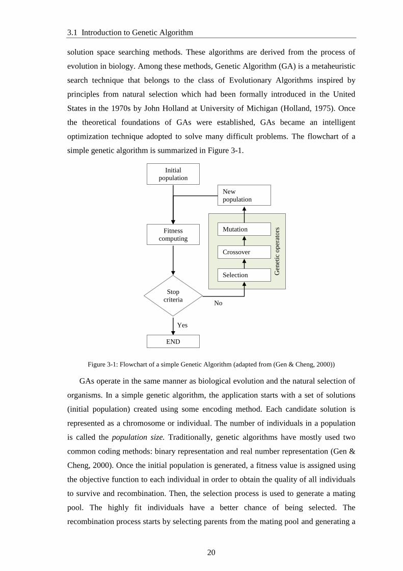
optimization technique adopted to solve many difficult problems. The flowchart of a
simple genetic algorithm is summarized in Figure 3-1.
Figure 3-1: Flowchart of a simple Genetic Algorithm (adapted from (Gen & Cheng, 2000))
GAs operate in the same manner as biological evolution and the natural selection of
organisms. In a simple genetic algorithm, the application starts with a set of solutions
(initial population) created using some encoding method. Each candidate solution is
represented as a chromosome or individual. The number of individuals in a population
is called the population size. Traditionally, genetic algorithms have mostly used two
common coding methods: binary representation and real number representation (Gen &
Cheng, 2000). Once the initial population is generated, a fitness value is assigned using
the objective function to each individual in order to obtain the quality of all individuals
to survive and recombination. Then, the selection process is used to generate a mating
pool. The highly fit individuals have a better chance of being selected. The
recombination process starts by selecting parents from the mating pool and generating a
Gen
etic
op
erat
ors
Initial
population
Fitness
computing
Mutation
Crossover
Selection
New
population
Stop
criteria
END
Yes
No
Chapter 3
21
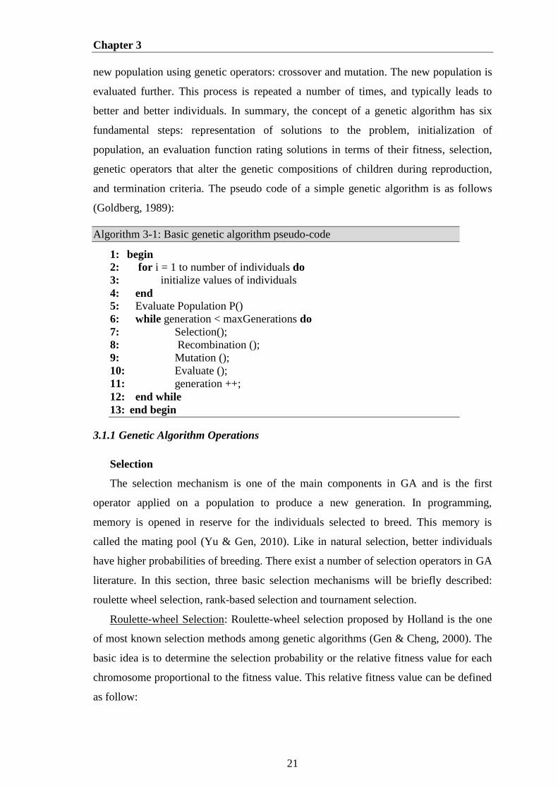
new population using genetic operators: crossover and mutation. The new population is
evaluated further. This process is repeated a number of times, and typically leads to
better and better individuals. In summary, the concept of a genetic algorithm has six
fundamental steps: representation of solutions to the problem, initialization of
population, an evaluation function rating solutions in terms of their fitness, selection,
genetic operators that alter the genetic compositions of children during reproduction,
and termination criteria. The pseudo code of a simple genetic algorithm is as follows
(Goldberg, 1989):
Algorithm 3-1: Basic genetic algorithm pseudo-code
1: begin
2: for i = 1 to number of individuals do
3: initialize values of individuals
4: end
5: Evaluate Population P()
6: while generation < maxGenerations do
7: Selection();
8: Recombination ();
9: Mutation ();
10: Evaluate ();
11: generation ++;
12: end while
13: end begin
3.1.1 Genetic Algorithm Operations
Selection
The selection mechanism is one of the main components in GA and is the first
operator applied on a population to produce a new generation. In programming,
memory is opened in reserve for the individuals selected to breed. This memory is
called the mating pool (Yu & Gen, 2010). Like in natural selection, better individuals
have higher probabilities of breeding. There exist a number of selection operators in GA
literature. In this section, three basic selection mechanisms will be briefly described:
roulette wheel selection, rank-based selection and tournament selection.
Roulette-wheel Selection: Roulette-wheel selection proposed by Holland is the one
of most known selection methods among genetic algorithms (Gen & Cheng, 2000). The
basic idea is to determine the selection probability or the relative fitness value for each
chromosome proportional to the fitness value. This relative fitness value can be defined
as follow:
3.1 Introduction to Genetic Algorithm
22
𝑝𝑖 =𝑓𝑖
∑ 𝑓𝑖𝑝𝑜𝑝𝑠𝑖𝑧𝑒𝑖=1
3-1
In roulette wheel selection, the process is based on spinning the wheel a number of
times equal to the population size by applying a random experiment, each time selecting
an individual chosen by the roulette-wheel pointer. After obtaining a random number,
whenever we find an individual that satisfies the random number between ∑ 𝑝𝑖𝑘𝑖
and ∑ 𝑝𝑖𝑘+1𝑖 , the individual is selected into the mating pool (Yu & Gen, 2010).
Rank-Based Selection: Baker (1985) introduced ranking selection. The population is
sorted from best to worst based on the objective function value in order to rank
individuals. Rather than using absolute values, selection probabilities are computed
based on rank values. Ranking might be needed under two conditions (Gen & Cheng,
2000). The first is that the exact fitness values cannot be determined. The second
condition is that the population has an extremely fit individual. In that case, the
extremely fit individual has a very high selection chance over all other individuals.
Tournament Selection: Tournament selection operates by selecting m individuals
randomly from the population. The value m is called the tournament size. The
individual with the highest fitness is termed the winner. The best one wins the
tournament and is selected into the mating pool (Miller & Goldberg, 1995). Tournament
selection process is repeated until the mating pool equals the size of the population. For
m=2, the selection procedure is called binary tournament selection. The main
characteristics of tournament selection make it quite useful in some situations, such as
multiobjective optimization (Yu & Gen, 2010). These properties are defined as follow:
- Tournament selection only uses local information.
- Tournament selection is very easy to implement and its time complexity is
small.
- Tournament selection can be easily implemented in a parallel environment.
Selection pressure is an important factor of a selection algorithm because it directly
affects the average problem-solving quality of the population (Xie et al., 2007). In
tournament selection, selection pressure is easily adjusted by using different tournament
sizes; the larger the tournament size, the higher the selection pressure. At low selection
pressure, the rate of convergence towards the optimum is likely to be slow (Legg et al.,
2004). At high selection pressure, the genetic algorithm converges too fast and it
typically results in obtaining local optima.
Recombination
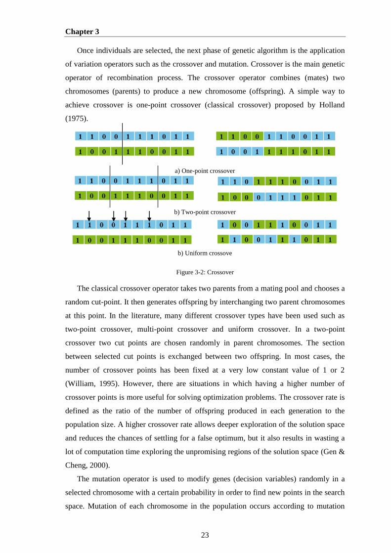
Chapter 3
23
Once individuals are selected, the next phase of genetic algorithm is the application
of variation operators such as the crossover and mutation. Crossover is the main genetic
operator of recombination process. The crossover operator combines (mates) two
chromosomes (parents) to produce a new chromosome (offspring). A simple way to
achieve crossover is one-point crossover (classical crossover) proposed by Holland
(1975).
a) One-point crossover
b) Two-point crossover
b) Uniform crossove
Figure 3-2: Crossover
The classical crossover operator takes two parents from a mating pool and chooses a
random cut-point. It then generates offspring by interchanging two parent chromosomes
at this point. In the literature, many different crossover types have been used such as
two-point crossover, multi-point crossover and uniform crossover. In a two-point
crossover two cut points are chosen randomly in parent chromosomes. The section
between selected cut points is exchanged between two offspring. In most cases, the
number of crossover points has been fixed at a very low constant value of 1 or 2
(William, 1995). However, there are situations in which having a higher number of
crossover points is more useful for solving optimization problems. The crossover rate is
defined as the ratio of the number of offspring produced in each generation to the
population size. A higher crossover rate allows deeper exploration of the solution space
and reduces the chances of settling for a false optimum, but it also results in wasting a
lot of computation time exploring the unpromising regions of the solution space (Gen &
Cheng, 2000).
The mutation operator is used to modify genes (decision variables) randomly in a
selected chromosome with a certain probability in order to find new points in the search
space. Mutation of each chromosome in the population occurs according to mutation

3.2 Introduction to Particle Swarm Optimization
24
rate which is chosen by the user. Therefore, it is not applied to every chromosome in the
population. The choice of mutation rate critically affects the performance of GAs.
Figure 3-3 shows the main two mutation operations: one-point mutation and uniform
mutation. In binary coded chromosomes, genes can have a value of either 0 or 1. On the
other hand, for real-encoded chromosomes, the mutation operator may be uniform
mutation, boundary mutation, real number creep mutation, or dynamic mutation (Park,
2008).
a) Point Mutation
b) Uniform Mutation
Figure 3-3: Mutation
3.2 Introduction to Particle Swarm Optimization
Swarm is generally used to describe social insects or social animals, e.g., ant
colonies, bee colonies, fish schools, and bird flocks (Yu & Gen, 2010). Particle swarm
optimization (PSO) is another stochastic population-based metaheuristic inspired by
social behaviors of bird flocking or fish schooling (Kennedy & Eberhart, 1995). The
main concept of PSO is very similar to other evolutionary computation techniques like
GAs. However, it does not have genetic operators like mutation and crossover. The PSO
algorithm consists of a swarm of particles, each represents a solution point in a
multidimensional, real valued search space of possible solutions. These particles fly
across the hyperspace based on the social psychological tendencies of individuals
(Baghel, 2009). The position of each particle changes according to its own experience
and the experience of neighboring particles.
In the PSO algorithm, each particle maintains its position in the search space with
the velocity influenced by the best solution found so far by each particle (the personal
best) and the best solution found so far by the whole swarm (the global best) (Shi &
Eberhart, 1999). The last part of the velocity considered in the algorithm is inertia: the
particle’s memory of its previous velocity. Once the particle’s velocity along a
dimension is adjusted, a new position is computed based on Equation 3-3. Each particle
in a swarm begins randomly in the domain space of the function to be optimized. Once
the particles are initialized, a loop starts to find an optimum solution. In the loop, the
particles’ velocity and positions are updated as described above. The algorithm is
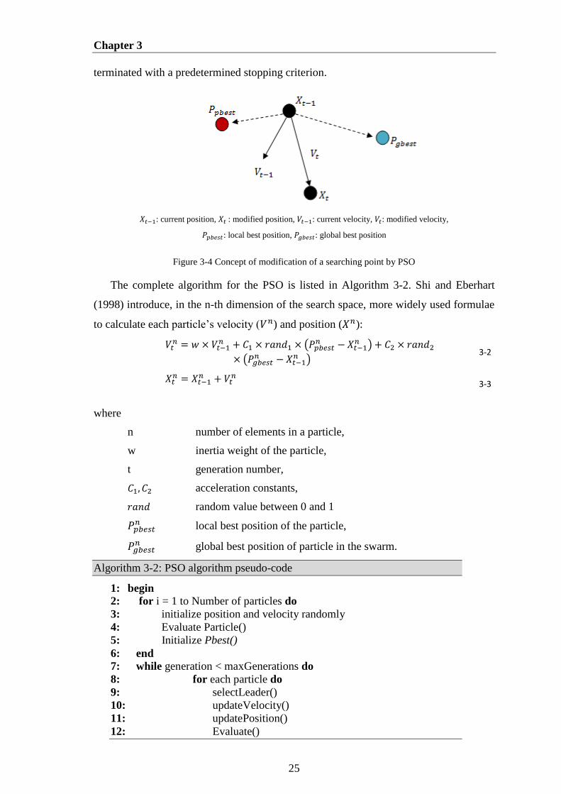
Chapter 3
25
terminated with a predetermined stopping criterion.
𝑋𝑡−1: current position, 𝑋𝑡 : modified position, 𝑉𝑡−1: current velocity, 𝑉𝑡: modified velocity,
𝑃𝑝𝑏𝑒𝑠𝑡: local best position, 𝑃𝑔𝑏𝑒𝑠𝑡: global best position
Figure 3-4 Concept of modification of a searching point by PSO
The complete algorithm for the PSO is listed in Algorithm 3-2. Shi and Eberhart
(1998) introduce, in the n-th dimension of the search space, more widely used formulae
to calculate each particle’s velocity (𝑉𝑛) and position (𝑋𝑛):
𝑉𝑡
𝑛 = 𝑤 × 𝑉𝑡−1𝑛 + 𝐶1 × 𝑟𝑎𝑛𝑑1 × (𝑃𝑝𝑏𝑒𝑠𝑡
𝑛 − 𝑋𝑡−1𝑛 ) + 𝐶2 × 𝑟𝑎𝑛𝑑2
× (𝑃𝑔𝑏𝑒𝑠𝑡𝑛 − 𝑋𝑡−1
𝑛 ) 3-2
𝑋𝑡𝑛 = 𝑋𝑡−1
𝑛 + 𝑉𝑡𝑛
3-3
where
n number of elements in a particle,
w inertia weight of the particle,
t generation number,
𝐶1, 𝐶2 acceleration constants,
𝑟𝑎𝑛𝑑 random value between 0 and 1
𝑃𝑝𝑏𝑒𝑠𝑡𝑛 local best position of the particle,
𝑃𝑔𝑏𝑒𝑠𝑡𝑛 global best position of particle in the swarm.
Algorithm 3-2: PSO algorithm pseudo-code
1: begin
2: for i = 1 to Number of particles do
3: initialize position and velocity randomly
4: Evaluate Particle()
5: Initialize Pbest()
6: end
7: while generation < maxGenerations do
8: for each particle do
9: selectLeader()
10: updateVelocity()
11: updatePosition()
12: Evaluate()
3.2 Introduction to Particle Swarm Optimization
26
13: Update Pbest()
14: end for 15: Update Pgbest()
16: generation ++
17: end while
18: end begin
3.2.1 Parameter Selection of PSO
The inertia weight 𝑤 has an important role in the PSO algorithm. It is used to
control the impact of the previous history of velocities on the current velocity. A large
inertia weight factor encourages exploration of the entire search space while a lower
value of inertia weight facilitates local exploration (Akbari & Ziarati, 2011). Therefore,
the inertia weight proposed by Shi and Eberhard (1998) decrease linearly with the
number of generations. This can be done using:
𝑤 = 𝑤𝑚𝑎𝑥 −𝑤𝑚𝑎𝑥 − 𝑤𝑚𝑖𝑛
𝑡𝑚𝑎𝑥× 𝑡 3-4
where 𝑤𝑚𝑎𝑥, 𝑤𝑚𝑖𝑛 is the maximum and minimum inertia weight, 𝑡 is iteration
number and 𝑡𝑚𝑎𝑥 is the maximum iteration.
Particles' velocities on each dimension are clamped by 𝑉𝑚𝑎𝑥, the maximum
allowable velocity for particles to keep particles from moving too far beyond the search
space. If 𝑉𝑚𝑎𝑥 is very low, a particle may not explore sufficiently, and if is too high,
then particles may move beyond a good solution. In case the velocity of the particle
exceeds 𝑉𝑚𝑎𝑥, then it is reduced to 𝑉𝑚𝑎𝑥. A maximum velocity 𝑉𝑚𝑎𝑥 proposed by Abido
(2007) is calculated with a user-specified velocity clamping factor 𝑘 where the search
space is bounded by [𝑋𝑚𝑖𝑛, 𝑋𝑚𝑎𝑥] in the following formula:
𝑉𝑚𝑎𝑥 = 𝑘 × (𝑋𝑚𝑎𝑥 − 𝑋𝑚𝑖𝑛
𝑁) 3-5
where N is a selected number of intervals.
Parameters 𝐶1 and 𝐶2 control the movement of each particle towards its best
position and the global best position, respectively. In other words, these two rates
control the relative influence of the memory of the neighborhood and the memory of the
particle. Recent work reports that choosing larger cognitive parameter, 𝐶1, than social
parameter, 𝐶2, but with 𝐶1 + 𝐶1 ≤ 4, produce a better performance (Ozcan & Mohan,
1998). In this dissertation, the acceleration constants 𝐶1 and 𝐶2 are chosen 2 as default
values.
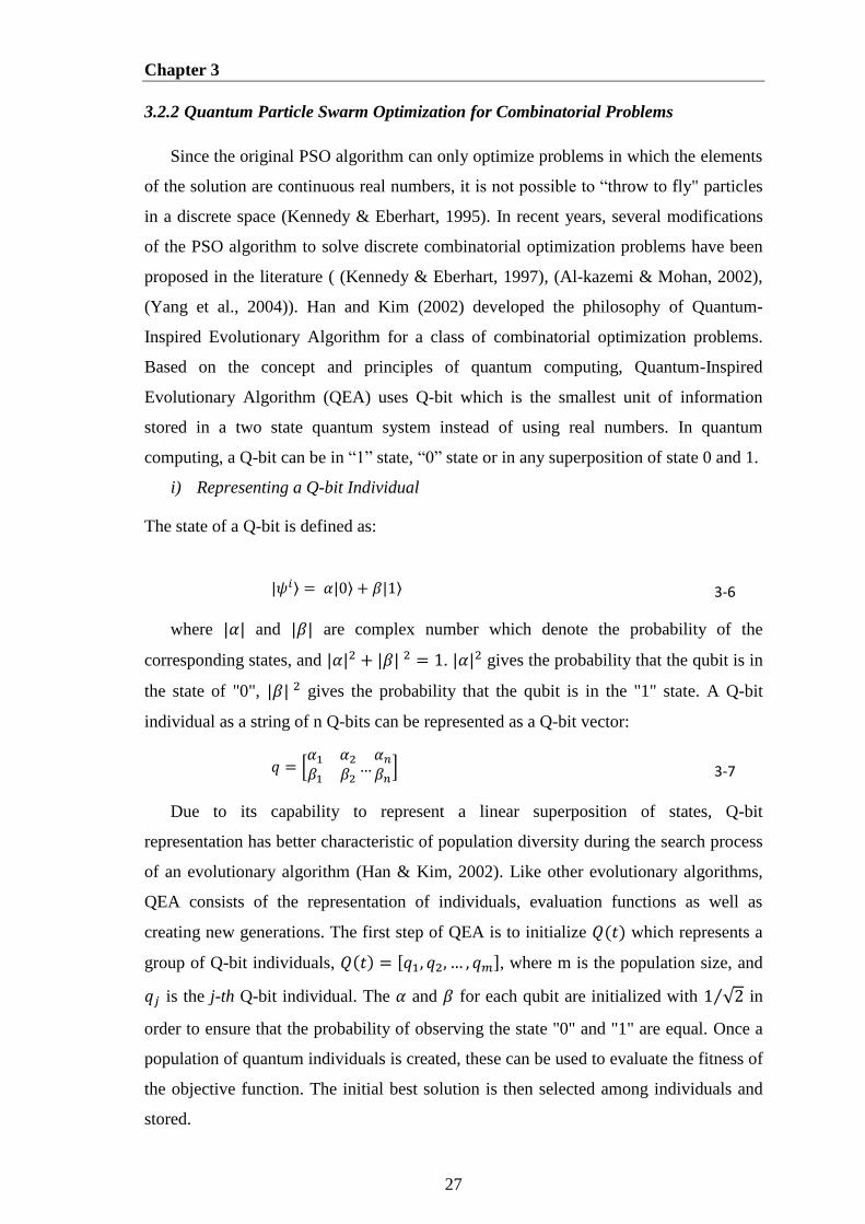
Chapter 3
27
3.2.2 Quantum Particle Swarm Optimization for Combinatorial Problems
Since the original PSO algorithm can only optimize problems in which the elements
of the solution are continuous real numbers, it is not possible to “throw to fly" particles
in a discrete space (Kennedy & Eberhart, 1995). In recent years, several modifications
of the PSO algorithm to solve discrete combinatorial optimization problems have been
proposed in the literature ( (Kennedy & Eberhart, 1997), (Al-kazemi & Mohan, 2002),
(Yang et al., 2004)). Han and Kim (2002) developed the philosophy of Quantum-
Inspired Evolutionary Algorithm for a class of combinatorial optimization problems.
Based on the concept and principles of quantum computing, Quantum-Inspired
Evolutionary Algorithm (QEA) uses Q-bit which is the smallest unit of information
stored in a two state quantum system instead of using real numbers. In quantum
computing, a Q-bit can be in “1” state, “0” state or in any superposition of state 0 and 1.
i) Representing a Q-bit Individual
The state of a Q-bit is defined as:
|𝜓𝑖⟩ = 𝛼|0⟩ + 𝛽|1⟩ 3-6
where |𝛼| and |𝛽| are complex number which denote the probability of the
corresponding states, and |𝛼|2 + |𝛽| 2 = 1. |𝛼|2 gives the probability that the qubit is in
the state of "0", |𝛽| 2 gives the probability that the qubit is in the "1" state. A Q-bit
individual as a string of n Q-bits can be represented as a Q-bit vector:
𝑞 = [𝛼1 𝛼2
𝛽1 𝛽2…
𝛼𝑛
𝛽𝑛] 3-7
Due to its capability to represent a linear superposition of states, Q-bit
representation has better characteristic of population diversity during the search process
of an evolutionary algorithm (Han & Kim, 2002). Like other evolutionary algorithms,
QEA consists of the representation of individuals, evaluation functions as well as
creating new generations. The first step of QEA is to initialize 𝑄(𝑡) which represents a
group of Q-bit individuals, 𝑄(𝑡) = [𝑞1, 𝑞2, … , 𝑞𝑚], where m is the population size, and
𝑞𝑗 is the j-th Q-bit individual. The 𝛼 and 𝛽 for each qubit are initialized with 1 √2⁄ in
order to ensure that the probability of observing the state "0" and "1" are equal. Once a
population of quantum individuals is created, these can be used to evaluate the fitness of
the objective function. The initial best solution is then selected among individuals and
stored.
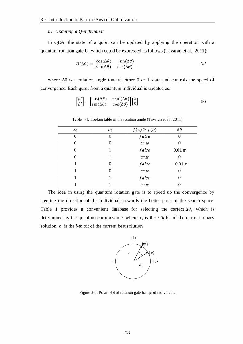
3.2 Introduction to Particle Swarm Optimization
28
ii) Updating a Q-individual
In QEA, the state of a qubit can be updated by applying the operation with a
quantum rotation gate U, which could be expressed as follows (Tayaran et al., 2011):
𝑈(Δ𝜃) = [cos (Δ𝜃) −sin (Δ𝜃)sin (Δ𝜃) cos (Δ𝜃)
] 3-8
where Δθ is a rotation angle toward either 0 or 1 state and controls the speed of
convergence. Each qubit from a quantum individual is updated as:
[𝛼′
𝛽′] = [cos (Δ𝜃) −sin (Δ𝜃)sin (Δ𝜃) cos (Δ𝜃)
] [𝛼𝛽] 3-9
Table 4-1: Lookup table of the rotation angle (Tayaran et al., 2011)
𝑥𝑖 𝑏𝑖 𝑓(𝑥) ≥ 𝑓(𝑏) Δ𝜃
0 0 𝑓𝑎𝑙𝑠𝑒 0
0 0 𝑡𝑟𝑢𝑒 0
0 1 𝑓𝑎𝑙𝑠𝑒 0.01 𝜋
0 1 𝑡𝑟𝑢𝑒 0
1 0 𝑓𝑎𝑙𝑠𝑒 −0.01 𝜋
1 0 𝑡𝑟𝑢𝑒 0
1 1 𝑓𝑎𝑙𝑠𝑒 0
1 1 𝑡𝑟𝑢𝑒 0
The idea in using the quantum rotation gate is to speed up the convergence by
steering the direction of the individuals towards the better parts of the search space.
Table 1 provides a convenient database for selecting the correct Δ𝜃, which is
determined by the quantum chromosome, where 𝑥𝑖 is the i-th bit of the current binary
solution, 𝑏𝑖 is the i-th bit of the current best solution.
| �0⟩
| �1⟩
| �𝜓⟩
| �𝜓′ ⟩
α
β
Figure 3-5: Polar plot of rotation gate for qubit individuals
Chapter 3
29
3.3 Multi-Objective Optimization
In many real-world situations, decision-makers have encountered problems that are
very complex and quite hard to solve using classical optimization techniques. It is easy
to see that most practical optimization problem involve multiple and conflicting
objectives that must be optimized simultaneously. For example, consider retailer stores
stocked with inventories of material and replenished by a warehouse where one is trying
to determine the optimal inventory control parameters. It is one of the most difficult
planning decisions in all of logistics. Minimizing the overall cost will ultimately lead to
reduced cycle stock at each stock point. But lower cycle stock leads to increase the
number of cycles per year and correspondingly the number of times the company is
exposed to the possibility for a stockout to occur. When only looking at one objective,
the other objective suffers. However, in this case the goal may be to establish a policy
that minimizes the level of their stocks without reducing availability. Thus, for such
problems, multiple objectives need to be optimized together while satisfying the
imposed constraints. A multiobjective optimization problem can be defined as follows
(Gen & Cheng, 2000):
𝑚𝑎𝑥𝑖𝑚𝑖𝑧𝑒 / 𝑚𝑖𝑛𝑖𝑚𝑖𝑧𝑒 {𝑧1 = 𝑓1(𝑥), 𝑧2 = 𝑓2(𝑥), … , 𝑧𝑚 = 𝑓𝑚(𝑥)}
𝑠. 𝑡. 𝑔𝑖(𝑥) ≤ 0, 𝑖 = 1, … , 𝑞
ℎ𝑗(𝑥) = 0 𝑗 = 𝑞 + 1, … , 𝑘
where x is called the decision vector, 𝑓𝑖 is objective 𝑖, 𝑔𝑖 is inequality constraint and
ℎ𝑗 is equality constraint j.
Figure 3-6 Components of a general stochastic search algorithm (Zitzler et al., 2004)
Several solution methods have been used to solve multiobjective optimization
problems in the literature. A general stochastic search algorithm consists of three parts:
i) a working memory that contains the currently considered solution candidates, ii) a
Mating Selection
Environmental Selection
Memory Selection Variation

3.3 Multi-Objective Optimization
30
selection module, and iii) a variation module as shown in Figure 3-6 (Zitzler et al.,
2004). There is usually a set of solutions for the multiple objective cases that cannot
simply be compared to one another. Such kinds of solutions are called non-dominated
solutions or Pareto optimal solutions, for which no improvement in any objective
function is possible without sacrificing at least one of the other objective functions (Gen
& Cheng, 2000).
Figure 3-7: The Pareto front of a set of solutions in a two objective space (adapted from (Sastry, 2007))
The non-dominated solutions are defined as solutions that dominate others but do
not dominate themselves. A Solution X in objective space is said to be a Pareto-optimal
(non-dominated solution), if and only if there is no other solution Y in the search space
that could dominate X. In other words, X dominates Y if X is better than Y in at least
one objective function and not worse with respect to all other objective functions (Yu &
Gen, 2010). The set including all Pareto-optimal solutions is termed the Pareto set and
represents the optimal trade-offs between objectives. Figure 3-7 illustrates these
concepts for a two-objective minimization problem, where it is desirable to have small
values for each objective.
3.3.1 Multi-Objective Optimization with Genetic Algorithm
Over the last two decades, many efficient multiobjective evolutionary algorithms
that are possible to find Pareto optimal solutions have been proposed based on non-
dominated sorting suggested by Goldberg (1989). Among the most widespread
methods, the algorithms maybe classified as follow: VEGA (Vector Evaluated Genetic
Algorithm) (Schaffer, 1985), MOGA (Multi Objective Genetic Algorithm) (Fonseca &
Fleming, 1993), NSGA (Non-dominated Sorting in Genetic Algorithm) (Srinavas &
Deb, 1994) and SPEA (Strength Pareto Evolutionary Algorithm) (Zitzler & Thiele,
y2
y1Convergence
Non-Dominated
SolutionsWORSE
BETTER
Indifferent
Indefferent
Diversity
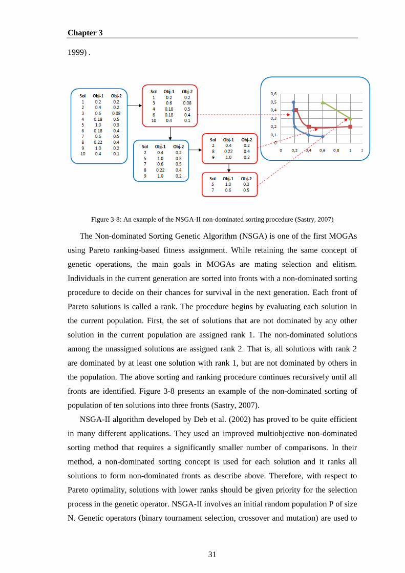
Chapter 3
31
1999) .
Figure 3-8: An example of the NSGA-II non-dominated sorting procedure (Sastry, 2007)
The Non-dominated Sorting Genetic Algorithm (NSGA) is one of the first MOGAs
using Pareto ranking-based fitness assignment. While retaining the same concept of
genetic operations, the main goals in MOGAs are mating selection and elitism.
Individuals in the current generation are sorted into fronts with a non-dominated sorting
procedure to decide on their chances for survival in the next generation. Each front of
Pareto solutions is called a rank. The procedure begins by evaluating each solution in
the current population. First, the set of solutions that are not dominated by any other
solution in the current population are assigned rank 1. The non-dominated solutions
among the unassigned solutions are assigned rank 2. That is, all solutions with rank 2
are dominated by at least one solution with rank 1, but are not dominated by others in
the population. The above sorting and ranking procedure continues recursively until all
fronts are identified. Figure 3-8 presents an example of the non-dominated sorting of
population of ten solutions into three fronts (Sastry, 2007).
NSGA-II algorithm developed by Deb et al. (2002) has proved to be quite efficient
in many different applications. They used an improved multiobjective non-dominated
sorting method that requires a significantly smaller number of comparisons. In their
method, a non-dominated sorting concept is used for each solution and it ranks all
solutions to form non-dominated fronts as describe above. Therefore, with respect to
Pareto optimality, solutions with lower ranks should be given priority for the selection
process in the genetic operator. NSGA-II involves an initial random population P of size
N. Genetic operators (binary tournament selection, crossover and mutation) are used to

3.3 Multi-Objective Optimization
32
create an offspring population Q of size N. It then combines the parent population and
the newly generated offspring population to create a combined population of size 2N.
The combined population (P+Q) is sorted according to non-domination. Next, solutions
from better non-dominated sets are chosen until N solutions have been chosen for the
new population. To choose a new population with exactly N individuals, the solutions
of the last front are sorted by using the crowded-comparison operator in descending
order and choosing the best solutions needed to fill all population slots (see Figure 3-9).
The resulting population is used for genetic operators to create the child population.
Figure 3-9: Crowding distance calculation (Raquel & Naval, 2005)
Apart from finding solutions in the Pareto front, it is essential to maximize the
diversity of the achieved Pareto set approximation (Zitzler et al., 2004). While most
recent multiobjective GAs (MOGA) use a niching mechanism to maintain the diversity
among solutions in the objective space, the crowding distance technique, which is an
estimate of the size of the largest cuboids enclosing that point without including any
other point in the population, is applied in NSGA-II. It is calculated by taking the
average distance of the two points on either side of the point in question along each of
the objectives (Deb et al., 2002). The complete algorithm for NSGA-II is as follow:
Algorithm 3-3: NSGA-II pseudo-code
1: begin
2: for i = 1 to Number of individuals do
3: initialize values of individuals
4: end
5: while generation < maxGenerations do
6: Evaluate Population P(t)
7: Generate child population
8: Tournament Selection()
9: Recombination()
10: Mutation()
Objective 1
Ob
ject
ive
2
i-1
i
I+1
0
1Cuboid
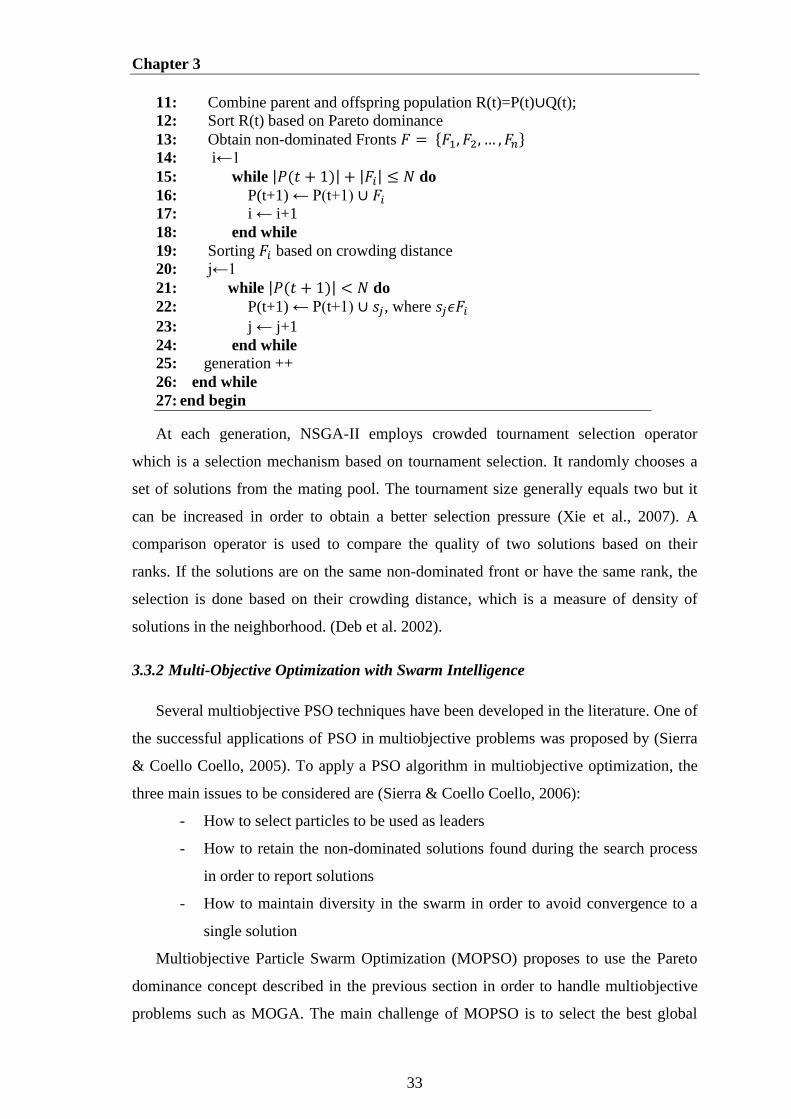
Chapter 3
33
11: Combine parent and offspring population R(t)=P(t)∪Q(t);
12: Sort R(t) based on Pareto dominance
13: Obtain non-dominated Fronts 𝐹 = {𝐹1, 𝐹2, … , 𝐹𝑛}
14: i←1
15: while |𝑃(𝑡 + 1)| + |𝐹𝑖| ≤ 𝑁 do
16: P(t+1) ← P(t+1) ∪ 𝐹𝑖
17: i ← i+1
18: end while
19: Sorting 𝐹𝑖 based on crowding distance
20: j←1
21: while |𝑃(𝑡 + 1)| < 𝑁 do
22: P(t+1) ← P(t+1) ∪ 𝑠𝑗, where 𝑠𝑗𝜖𝐹𝑖
23: j ← j+1
24: end while
25: generation ++
26: end while
27: end begin
At each generation, NSGA-II employs crowded tournament selection operator
which is a selection mechanism based on tournament selection. It randomly chooses a
set of solutions from the mating pool. The tournament size generally equals two but it
can be increased in order to obtain a better selection pressure (Xie et al., 2007). A
comparison operator is used to compare the quality of two solutions based on their
ranks. If the solutions are on the same non-dominated front or have the same rank, the
selection is done based on their crowding distance, which is a measure of density of
solutions in the neighborhood. (Deb et al. 2002).
3.3.2 Multi-Objective Optimization with Swarm Intelligence
Several multiobjective PSO techniques have been developed in the literature. One of
the successful applications of PSO in multiobjective problems was proposed by (Sierra
& Coello Coello, 2005). To apply a PSO algorithm in multiobjective optimization, the
three main issues to be considered are (Sierra & Coello Coello, 2006):
- How to select particles to be used as leaders
- How to retain the non-dominated solutions found during the search process
in order to report solutions
- How to maintain diversity in the swarm in order to avoid convergence to a
single solution
Multiobjective Particle Swarm Optimization (MOPSO) proposes to use the Pareto
dominance concept described in the previous section in order to handle multiobjective
problems such as MOGA. The main challenge of MOPSO is to select the best global

3.3 Multi-Objective Optimization
34
particle for each particle of the swarm to update its position (Durillo et al., 2009).
Compared with the original PSO, multiobjective PSO (MOPSO) uses a set of leaders
usually stored separately from the swarm, which is called an external archive (leaders
archive). The leaders archive includes the best non-dominated solutions found since the
beginning of the optimization. These solutions are used to update the positions of
particles in the swarm (Sierra & Coello Coello, 2006). In that case, the quality measure
plays an important role in the selection of one leader from the archive. The most
common approach to select a leader from the archive is the tournament selection in
which every non-dominated solution is considered as a potential leader. The pseudo
code of MOPSO is described as follows (Abido, 2010):
Algorithm 3-4: MOPSO pseudo-code
1: begin
2: for i = 1 to Number of particles do
3: initialize position and velocity randomly
4: end
5: Evaluate Particle Swarm()
6: Initialize Leaders External Archive()
7: Compute Crowding Distance Values()
8: Sort the non-dominated solutions according to crowding distance()
9: generation = 0
10: while generation < maxGenerations do
11: for each particle do
12: selectLeader()
13: updateVelocity()
14: updatePosition()
15: evaluation()
16: updatePbest()
17: end for 18: Update External Leaders Archive()
19: Compute Crowding Distance Values()
20: Sort archive according to the crowding distance()
21: generation ++
22: end while 23: returnArchive()
24: end begin
Note that the external archive is limited in size in order to reduce computational
time. The maximum size of the archive set is specified in advance. When the archive set
is empty enough and a new non-dominated solution is detected, the new solution will
enter the archive set. To decide which particles should remain in the archive when the
maximum limit imposed on the size is reached, techniques such as the crowding
distance concept are applied. The MOPSO steps can be defined as follow (Abido,
Chapter 3
35
2010):
Step 1: Initialize the population. Set the generation = 0 and generate randomly n
Particles.
Step 2: Time Updating. Update the iteration t = t+1.
Step 3: Weight Updating. Update the inertia weight (Equation 3-4)
Step 4: Velocity Updating. Compute the speed of each particle using the equation 3-
2. If a particle violates the velocity limits, set its velocity equal to the proper limit.
Step 5: Position Updating. Compute the new positions of the particles adding the
speed produced from the previous step according to the equation 3-3.
Step 6: Non-Dominated Local Set Updating. The criterion for deciding what
position from memory to retain is Pareto dominance (i.e., if the current position is
dominated by the position in memory, then the position in memory is kept, otherwise,
the current position replaces the one in memory. If neither of them is dominated by the
other, then we select one of them randomly)
Step 7: External Set Updating. This update consists of inserting all the currently
non-dominated solutions into the leaders archive. The external particles are sorted into
Pareto set and all dominated solutions are removed from the archive set. If the number
of the individuals externally stored in the Pareto set exceeds the maximum size, the set
is reduced according to the crowding distance concept.
Step 8: Stop Criteria. If the number of iterations exceeds the maximum, then stop.
Otherwise, go to step 2.
Chapter 4
Integrated Strategic Network Design for
Multi-level Supply Chains
Network design is a strategic decision that has a long-lasting impact on a company.
To achieve an efficient supply chain, integrated distribution network design is essential.
In this regard, suitable facility locations are a core part for a supply chain in the design
of logistics systems (Li et al., 2011) (Blanchard, 2010). In general, optimally solving
such an integrated network design problem in a reasonable computation time is a
challenge, especially when inventory and routing are involved (Lei et al., 2003). In
order to find out a good solution effectively, there is a need for new solution
methodologies. The purpose of this chapter is to introduce an optimization model that
explicitly captures the interdependency between different decision levels in supply
chain (SC), while fulfilling the demand requirement, and to present computational
results from extensive experiments that investigate the effects of several dynamic
factors including stochastic demand and nonlinear cost functions. The network design
problem is formulated as a multiobjective optimization problem taking into account the
trade-off among transportation costs, facility location costs, inventory replenishment
costs, and the service efficiency in terms of coverage distance. The service efficiency
objective is to minimize the maximum distance between each covered customer and its
closest opened DC to maximize demand satisfaction in a defined structure. The
particular problem considered in this study contains a set of geographically dispersed
retailers whose locations are known, and regional DCs located to help consolidate
shipments and pool risk whose locations are unknown. Each retailer faces an
independent distributed demand for a single product that must be met without shortage.
This chapter begins with Section 4.1 presenting the formulation of integrated network
design and logistic cost components. The next section introduces the notation and also
provides a detailed formulation of the problem. Section 4.3 describes the solution
Chapter 4
37
methodology based on multiobjective metaheuristic techniques. A decision support tool
to optimize the problem under consideration is developed and the case study is
introduced in Section 4.4. Finally, the key results are summarized in Section 4.5 and
4.6.
4.1 Integrated Supply Chain Network Design
Integrated planning and control of a supply chain has three important dimensions
(Shapiro, 2001). The first dimension is called as functional integration dealing with
issues related to integration of purchasing, manufacturing and distribution activities
within the company, between the company and its suppliers, and customers. The
geographical integration refers to integration of these functions across various
geographically distributed vendors, facilities and market. The third dimension is inter-
temporal integration, which also is called hierarchical planning, involves coordinating
decisions across strategic, tactical and operational levels of the supply chain.
Distribution network design is one of the major strategic level issues that influence
tactical and operational decisions due to the interdependence between these levels
(Goetschalckx & Fleischmann, 2005). However, most literatures on network design
have traditionally considered strategic, tactical, and operational decisions separately.
This classical approach leads to considerable excess costs because the supply chain is
optimized locally but does not guarantee the global optimum for the whole system.
However, in global optimization, the objective is to coordinate all supply chain
activities so as to maximize system performance by reducing cost, increasing service
level, reducing the bullwhip effect, and using resources more effectively (Simchi-Levi
et al., 2004). Moreover, to sustain competitive advantage in highly volatile market,
inter-temporal integration is critical to the firm (Shapiro, 2001).
The integration and coordination of decisions at different planning horizons are
quite difficult because it requires a complex trade-off analysis between various costs.
For example, as the number of facilities in a supply chain increases, the inventory costs
also increase due to increased safety stocks required to protect each distribution center
against uncertainties in customer demands as shown in Figure 4-1 (Simchi-Levi et al.,
2004) (Teo & Shu, 2004). Increasing the number of facilities increases the inbound
transportation cost. On the other hand, the outbound transportation costs decrease
because facilities are located closer to the market. Thus, if the number of facilities is
increased to a point where there is a significant loss of economies of scale in inbound
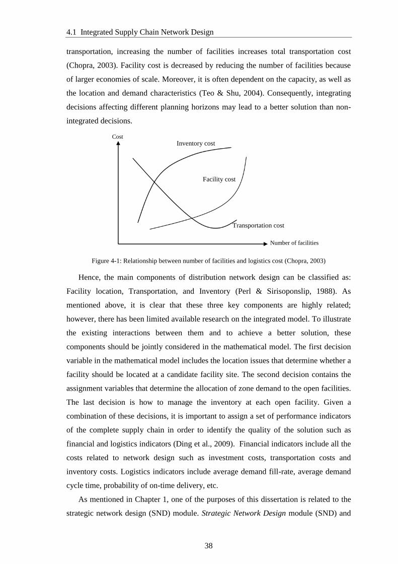
4.1 Integrated Supply Chain Network Design
38
transportation, increasing the number of facilities increases total transportation cost
(Chopra, 2003). Facility cost is decreased by reducing the number of facilities because
of larger economies of scale. Moreover, it is often dependent on the capacity, as well as
the location and demand characteristics (Teo & Shu, 2004). Consequently, integrating
decisions affecting different planning horizons may lead to a better solution than non-
integrated decisions.
Figure 4-1: Relationship between number of facilities and logistics cost (Chopra, 2003)
Hence, the main components of distribution network design can be classified as:
Facility location, Transportation, and Inventory (Perl & Sirisoponslip, 1988). As
mentioned above, it is clear that these three key components are highly related;
however, there has been limited available research on the integrated model. To illustrate
the existing interactions between them and to achieve a better solution, these
components should be jointly considered in the mathematical model. The first decision
variable in the mathematical model includes the location issues that determine whether a
facility should be located at a candidate facility site. The second decision contains the
assignment variables that determine the allocation of zone demand to the open facilities.
The last decision is how to manage the inventory at each open facility. Given a
combination of these decisions, it is important to assign a set of performance indicators
of the complete supply chain in order to identify the quality of the solution such as
financial and logistics indicators (Ding et al., 2009). Financial indicators include all the
costs related to network design such as investment costs, transportation costs and
inventory costs. Logistics indicators include average demand fill-rate, average demand
cycle time, probability of on-time delivery, etc.
As mentioned in Chapter 1, one of the purposes of this dissertation is related to the
strategic network design (SND) module. Strategic Network Design module (SND) and
Inventory cost
Facility cost
Transportation cost
Number of facilities
Cost
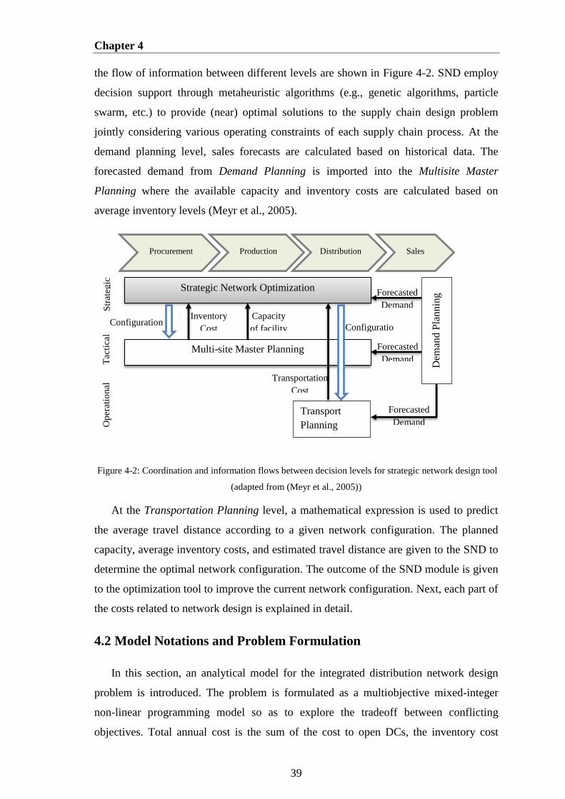
Chapter 4
39
the flow of information between different levels are shown in Figure 4-2. SND employ
decision support through metaheuristic algorithms (e.g., genetic algorithms, particle
swarm, etc.) to provide (near) optimal solutions to the supply chain design problem
jointly considering various operating constraints of each supply chain process. At the
demand planning level, sales forecasts are calculated based on historical data. The
forecasted demand from Demand Planning is imported into the Multisite Master
Planning where the available capacity and inventory costs are calculated based on
average inventory levels (Meyr et al., 2005).
Figure 4-2: Coordination and information flows between decision levels for strategic network design tool
(adapted from (Meyr et al., 2005))
At the Transportation Planning level, a mathematical expression is used to predict
the average travel distance according to a given network configuration. The planned
capacity, average inventory costs, and estimated travel distance are given to the SND to
determine the optimal network configuration. The outcome of the SND module is given
to the optimization tool to improve the current network configuration. Next, each part of
the costs related to network design is explained in detail.
4.2 Model Notations and Problem Formulation
In this section, an analytical model for the integrated distribution network design
problem is introduced. The problem is formulated as a multiobjective mixed-integer
non-linear programming model so as to explore the tradeoff between conflicting
objectives. Total annual cost is the sum of the cost to open DCs, the inventory cost
Inventory
Cost Capacity
of facility
Transportation
Cost
Forecasted
Demand
Forecasted
Demand
Configuration Configuratio
n
Op
erat
ion
al
Strategic Network Optimization
Multi-site Master Planning
Transport
Planning D
eman
d P
lann
ing
Procurement Production Distribution Sales
Str
ateg
ic
Tac
tica
l
Forecasted
Demand
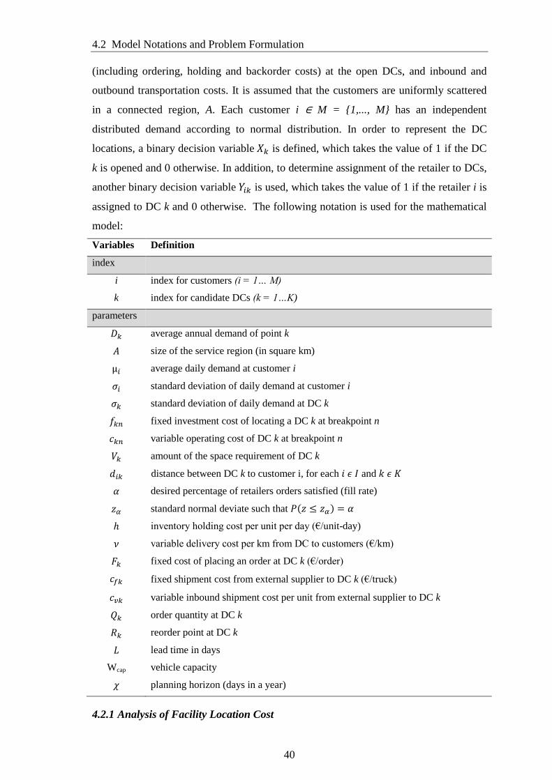
4.2 Model Notations and Problem Formulation
40
(including ordering, holding and backorder costs) at the open DCs, and inbound and
outbound transportation costs. It is assumed that the customers are uniformly scattered
in a connected region, A. Each customer i ∈ M = {1,..., M} has an independent
distributed demand according to normal distribution. In order to represent the DC
locations, a binary decision variable 𝑋𝑘 is defined, which takes the value of 1 if the DC
k is opened and 0 otherwise. In addition, to determine assignment of the retailer to DCs,
another binary decision variable 𝑌𝑖𝑘 is used, which takes the value of 1 if the retailer i is
assigned to DC k and 0 otherwise. The following notation is used for the mathematical
model:
Variables Definition
index
i index for customers (i = 1… M)
k index for candidate DCs (k = 1…K)
parameters
𝐷𝑘 average annual demand of point k
𝐴 size of the service region (in square km)
µ𝑖 average daily demand at customer i
𝜎𝑖 standard deviation of daily demand at customer i
𝜎𝑘 standard deviation of daily demand at DC k
𝑓𝑘𝑛 fixed investment cost of locating a DC k at breakpoint n
𝑐𝑘𝑛 variable operating cost of DC k at breakpoint n
𝑉𝑘 amount of the space requirement of DC k
𝑑𝑖𝑘 distance between DC k to customer i, for each 𝑖 𝜖 𝐼 and 𝑘 𝜖 𝐾
𝛼 desired percentage of retailers orders satisfied (fill rate)
𝑧𝛼 standard normal deviate such that 𝑃(𝑧 ≤ 𝑧𝛼) = 𝛼
ℎ inventory holding cost per unit per day (€/unit-day)
𝜈 variable delivery cost per km from DC to customers (€/km)
𝐹𝑘 fixed cost of placing an order at DC k (€/order)
𝑐𝑓𝑘 fixed shipment cost from external supplier to DC k (€/truck)
𝑐𝑣𝑘 variable inbound shipment cost per unit from external supplier to DC k
𝑄𝑘 order quantity at DC k
𝑅𝑘 reorder point at DC k
𝐿 lead time in days
Wcap vehicle capacity
𝜒 planning horizon (days in a year)
4.2.1 Analysis of Facility Location Cost
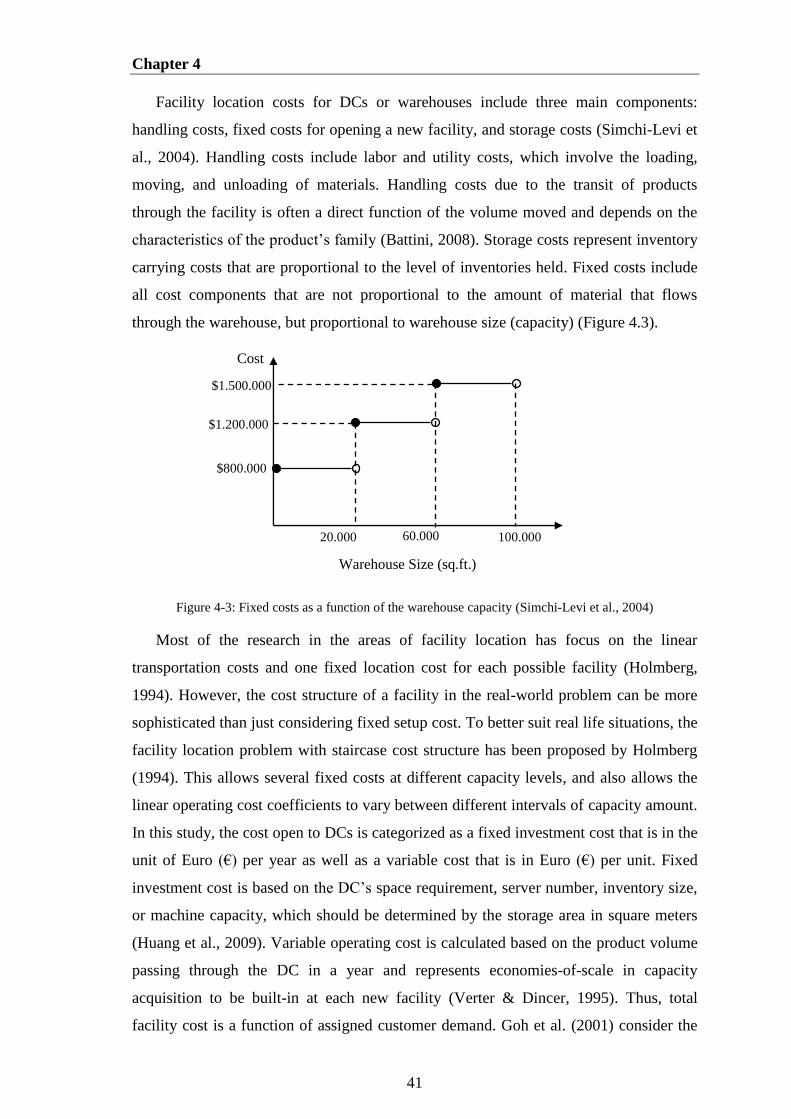
Chapter 4
41
Facility location costs for DCs or warehouses include three main components:
handling costs, fixed costs for opening a new facility, and storage costs (Simchi-Levi et
al., 2004). Handling costs include labor and utility costs, which involve the loading,
moving, and unloading of materials. Handling costs due to the transit of products
through the facility is often a direct function of the volume moved and depends on the
characteristics of the product’s family (Battini, 2008). Storage costs represent inventory
carrying costs that are proportional to the level of inventories held. Fixed costs include
all cost components that are not proportional to the amount of material that flows
through the warehouse, but proportional to warehouse size (capacity) (Figure 4.3).
Figure 4-3: Fixed costs as a function of the warehouse capacity (Simchi-Levi et al., 2004)
Most of the research in the areas of facility location has focus on the linear
transportation costs and one fixed location cost for each possible facility (Holmberg,
1994). However, the cost structure of a facility in the real-world problem can be more
sophisticated than just considering fixed setup cost. To better suit real life situations, the
facility location problem with staircase cost structure has been proposed by Holmberg
(1994). This allows several fixed costs at different capacity levels, and also allows the
linear operating cost coefficients to vary between different intervals of capacity amount.
In this study, the cost open to DCs is categorized as a fixed investment cost that is in the
unit of Euro (€) per year as well as a variable cost that is in Euro (€) per unit. Fixed
investment cost is based on the DC’s space requirement, server number, inventory size,
or machine capacity, which should be determined by the storage area in square meters
(Huang et al., 2009). Variable operating cost is calculated based on the product volume
passing through the DC in a year and represents economies-of-scale in capacity
acquisition to be built-in at each new facility (Verter & Dincer, 1995). Thus, total
facility cost is a function of assigned customer demand. Goh et al. (2001) consider the
$800.000
$1.200.000
$1.500.000
20.000 60.000 100.000
Cost
Warehouse Size (sq.ft.)
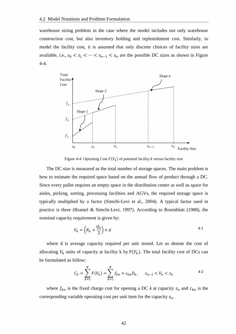
4.2 Model Notations and Problem Formulation
42
warehouse sizing problem in the case where the model includes not only warehouse
construction cost, but also inventory holding and replenishment cost. Similarly, to
model the facility cost, it is assumed that only discrete choices of facility sizes are
available, i.e., 𝑠0 < 𝑠1 < ⋯ < 𝑠𝑛−1 < 𝑠𝑛 are the possible DC sizes as shown in Figure
4-4.
𝑠0 𝑠1 𝑠2 𝑠𝑛−1 𝑠𝑛
Total
Facility
Cost
Slope 1
𝑓1
𝑓2
𝑓𝑛
Facility Size
Slope 2
Slope n
Figure 4-4: Operating Cost 𝐹(𝑉𝑘) of potential facility k versus facility size
The DC size is measured as the total number of storage spaces. The main problem is
how to estimate the required space based on the annual flow of product through a DC.
Since every pallet requires an empty space in the distribution center as well as space for
aisles, picking, sorting, processing facilities and AGVs, the required storage space is
typically multiplied by a factor (Simchi-Levi et al., 2004). A typical factor used in
practice is three (Bramel & Simchi-Levi, 1997). According to Rosenblatt (1988), the
nominal capacity requirement is given by:
𝑉𝑘 = (𝑅𝑘 +𝑄𝑘
2) × 𝑑 4-1
where d is average capacity required per unit stored. Let us denote the cost of
allocating 𝑉𝑘 units of capacity at facility k by F(𝑉𝑘). The total facility cost of DCs can
be formulated as follow:
𝐶𝑂 = ∑ 𝐹(𝑉𝑘) =
𝐾
𝑘=1
∑ 𝑓𝑘𝑛 + 𝑐𝑘𝑛𝐷𝑘
𝐾
𝑘=1
, 𝑠𝑛−1 < 𝑉𝑘 < 𝑠𝑛 4-2
where 𝑓𝑘𝑛 is the fixed charge cost for opening a DC k at capacity 𝑠𝑛 and 𝑐𝑘𝑛 is the
corresponding variable operating cost per unit item for the capacity 𝑠𝑛.
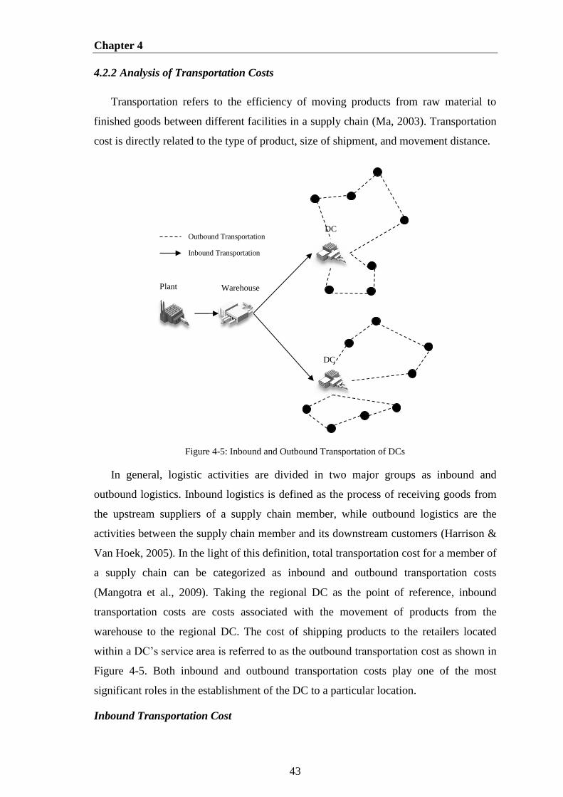
Chapter 4
43
4.2.2 Analysis of Transportation Costs
Transportation refers to the efficiency of moving products from raw material to
finished goods between different facilities in a supply chain (Ma, 2003). Transportation
cost is directly related to the type of product, size of shipment, and movement distance.
Figure 4-5: Inbound and Outbound Transportation of DCs
In general, logistic activities are divided in two major groups as inbound and
outbound logistics. Inbound logistics is defined as the process of receiving goods from
the upstream suppliers of a supply chain member, while outbound logistics are the
activities between the supply chain member and its downstream customers (Harrison &
Van Hoek, 2005). In the light of this definition, total transportation cost for a member of
a supply chain can be categorized as inbound and outbound transportation costs
(Mangotra et al., 2009). Taking the regional DC as the point of reference, inbound
transportation costs are costs associated with the movement of products from the
warehouse to the regional DC. The cost of shipping products to the retailers located
within a DC’s service area is referred to as the outbound transportation cost as shown in
Figure 4-5. Both inbound and outbound transportation costs play one of the most
significant roles in the establishment of the DC to a particular location.
Inbound Transportation Cost
DC
DC
Warehouse Plant
Outbound Transportation
Inbound Transportation

4.2 Model Notations and Problem Formulation
44
The inbound transportation costs are classified into two categories (Bowersox et al.,
2002). The first category comprises fixed costs, which are not directly influenced by the
shipment volume. Fixed costs include vehicles, terminals, rights-of-way, information
systems, and support equipment. The second category is variable transportation cost,
which depends on volume, distance, and services provided, and it includes the direct
carrier cost associated with the movement of each load. Variable transportation cost is
generally measured as a cost per mile or per unit of weight. The inbound transport costs
can be modeled as the one-origin/one-destination situation (Daganzo, 2005).
𝐶𝐼𝑇 = ∑(𝑐𝑓𝑘 + 𝑐𝑣𝑘𝑄𝑘)𝐷𝑘
𝑄𝑘
𝐾
𝑘=1
4-3
𝑐𝑓𝑘 is a fixed cost per shipment, 𝑐𝑣𝑘 is the rate at which the variable cost per
shipment increases size. ( 𝑐𝑓𝑘 + 𝑐𝑣𝑘𝑄𝑘) express the inbound transportation cost incurred
in a single shipment to a DC and 𝐷𝑘 𝑄𝑘⁄ is the expected number of inbound shipments
to a DC during a year.
Outbound Transportation Cost
Outbound transportation refers to the movement of finished products to each retailer
within the serving area of that particular DC. In many of distribution network design
models, outbound transportation cost is simplified to the direct shipment (Shen & Qi,
2007), which refers to delivering freight directly from the origin to the destination
without visiting any intermediate point. If each vehicle visits more than one customer,
the problem is termed a Vehicle Routing Problem (VRP). VRP is a problem of finding
the optimal routes of delivery for vehicles to minimize the total distance traveled, where
a route is a tour that starts at the DC, visits a subset of the customers and ends at the
DC. All customers must be visited exactly once by one vehicle and the sum of the
demands of the visited customers on a route must not exceed the vehicle capacity.
A vehicle routing problem (VRP) is a well-known NP-hard (Non-deterministic
Polynomial-time hard) problem and computational experience indicates that the VRP is
difficult to solve to optimality within acceptable computation time. In the network
design phase, it is only needed to estimate the total expected routing costs as a result of
different facility locations instead of detailed route plan of vehicles (Shen & Qi, 2007).
In this context, using continuous approximations, Daganzo ( (1984), (2005)) proposed a
simple closed mathematical expression to predict the travel distance in capacitated
vehicle routing problems. In Daganzo’s approach, the optimal tour length is estimated
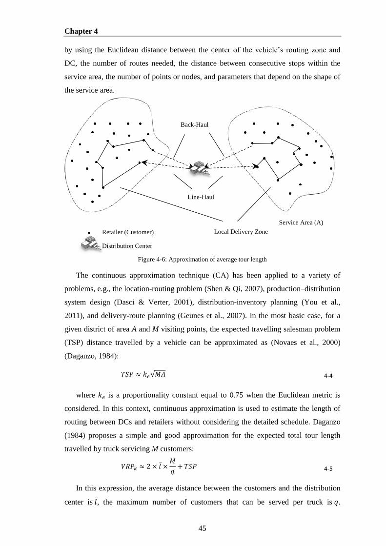
Chapter 4
45
by using the Euclidean distance between the center of the vehicle’s routing zone and
DC, the number of routes needed, the distance between consecutive stops within the
service area, the number of points or nodes, and parameters that depend on the shape of
the service area.
Figure 4-6: Approximation of average tour length
The continuous approximation technique (CA) has been applied to a variety of
problems, e.g., the location-routing problem (Shen & Qi, 2007), production–distribution
system design (Dasci & Verter, 2001), distribution-inventory planning (You et al.,
2011), and delivery-route planning (Geunes et al., 2007). In the most basic case, for a
given district of area A and M visiting points, the expected travelling salesman problem
(TSP) distance travelled by a vehicle can be approximated as (Novaes et al., 2000)
(Daganzo, 1984):
𝑇𝑆𝑃 ≈ 𝑘𝑒√𝑀𝐴 4-4
where 𝑘𝑒 is a proportionality constant equal to 0.75 when the Euclidean metric is
considered. In this context, continuous approximation is used to estimate the length of
routing between DCs and retailers without considering the detailed schedule. Daganzo
(1984) proposes a simple and good approximation for the expected total tour length
travelled by truck servicing M customers:
𝑉𝑅𝑃𝑘 ≈ 2 × 𝑙 ̅ ×𝑀
𝑞+ 𝑇𝑆𝑃 4-5
In this expression, the average distance between the customers and the distribution
center is 𝑙,̅ the maximum number of customers that can be served per truck is 𝑞.
Local Delivery Zone
Back-Haul
Line-Haul
Distribution Center
Retailer (Customer)
Service Area (A)
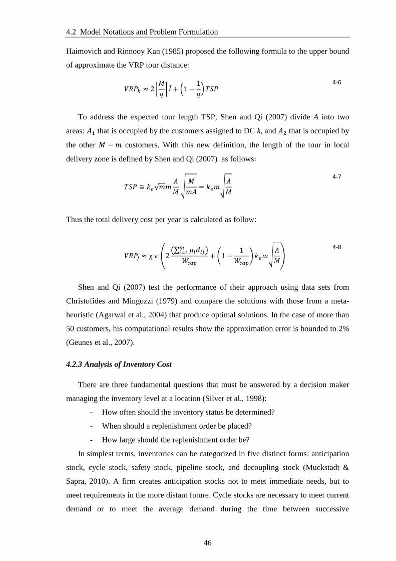
4.2 Model Notations and Problem Formulation
46
Haimovich and Rinnooy Kan (1985) proposed the following formula to the upper bound
of approximate the VRP tour distance:
𝑉𝑅𝑃𝑘 ≈ 2 ⌈𝑀
𝑞⌉ 𝑙 ̅ + (1 −
1
𝑞) 𝑇𝑆𝑃
4-6
To address the expected tour length TSP, Shen and Qi (2007) divide A into two
areas: 𝐴1 that is occupied by the customers assigned to DC k, and 𝐴2 that is occupied by
the other 𝑀 − 𝑚 customers. With this new definition, the length of the tour in local
delivery zone is defined by Shen and Qi (2007) as follows:
𝑇𝑆𝑃 ≅ 𝑘𝑒√𝑚𝑚𝐴
𝑀√
𝑀
𝑚𝐴= 𝑘𝑒𝑚√
𝐴
𝑀
4-7
Thus the total delivery cost per year is calculated as follow:
𝑉𝑅𝑃𝑗 ≈ χ ν (2(∑ 𝜇𝑖𝑑𝑖𝑗
𝑚𝑖=1 )
𝑊𝑐𝑎𝑝+ (1 −
1
𝑊𝑐𝑎𝑝) 𝑘𝑒𝑚√
𝐴
𝑀)
4-8
Shen and Qi (2007) test the performance of their approach using data sets from
Christofides and Mingozzi (1979) and compare the solutions with those from a meta-
heuristic (Agarwal et al., 2004) that produce optimal solutions. In the case of more than
50 customers, his computational results show the approximation error is bounded to 2%
(Geunes et al., 2007).
4.2.3 Analysis of Inventory Cost
There are three fundamental questions that must be answered by a decision maker
managing the inventory level at a location (Silver et al., 1998):
- How often should the inventory status be determined?
- When should a replenishment order be placed?
- How large should the replenishment order be?
In simplest terms, inventories can be categorized in five distinct forms: anticipation
stock, cycle stock, safety stock, pipeline stock, and decoupling stock (Muckstadt &
Sapra, 2010). A firm creates anticipation stocks not to meet immediate needs, but to
meet requirements in the more distant future. Cycle stocks are necessary to meet current
demand or to meet the average demand during the time between successive
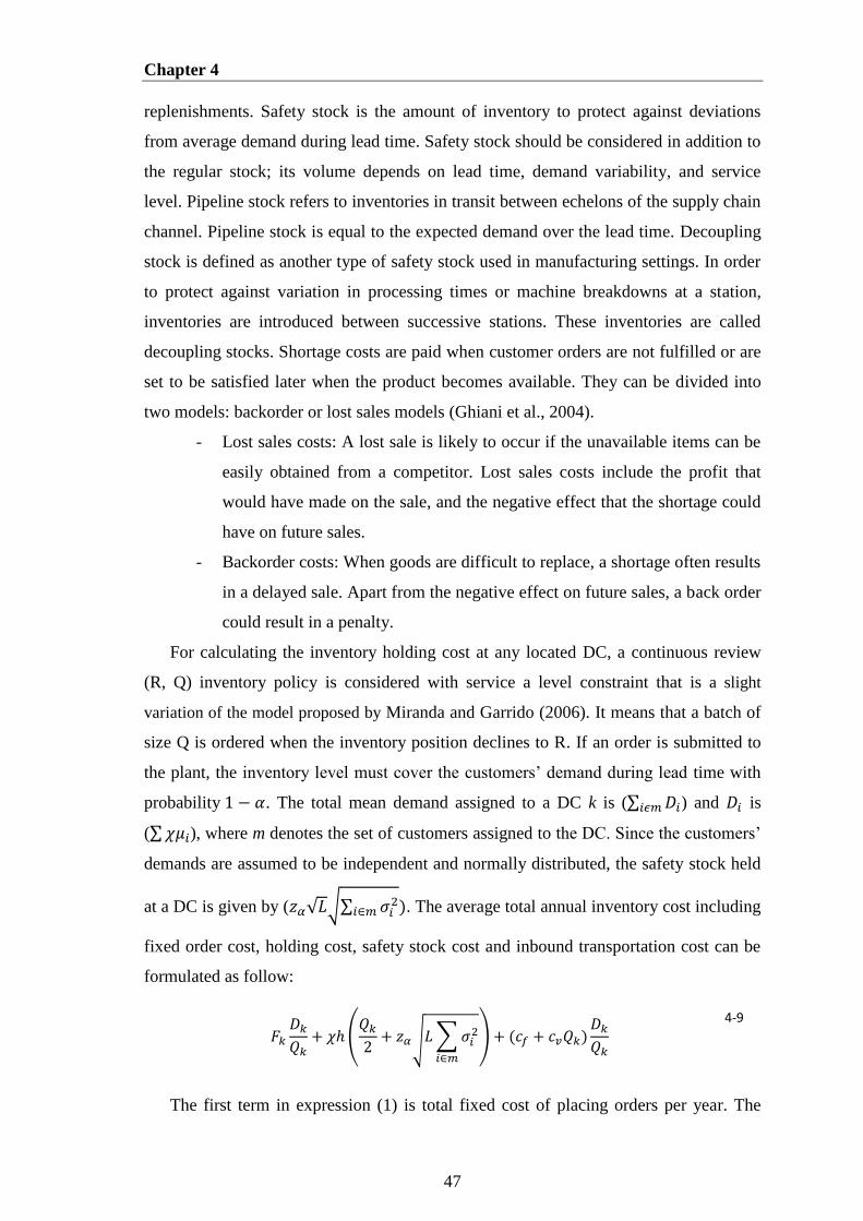
Chapter 4
47
replenishments. Safety stock is the amount of inventory to protect against deviations
from average demand during lead time. Safety stock should be considered in addition to
the regular stock; its volume depends on lead time, demand variability, and service
level. Pipeline stock refers to inventories in transit between echelons of the supply chain
channel. Pipeline stock is equal to the expected demand over the lead time. Decoupling
stock is defined as another type of safety stock used in manufacturing settings. In order
to protect against variation in processing times or machine breakdowns at a station,
inventories are introduced between successive stations. These inventories are called
decoupling stocks. Shortage costs are paid when customer orders are not fulfilled or are
set to be satisfied later when the product becomes available. They can be divided into
two models: backorder or lost sales models (Ghiani et al., 2004).
- Lost sales costs: A lost sale is likely to occur if the unavailable items can be
easily obtained from a competitor. Lost sales costs include the profit that
would have made on the sale, and the negative effect that the shortage could
have on future sales.
- Backorder costs: When goods are difficult to replace, a shortage often results
in a delayed sale. Apart from the negative effect on future sales, a back order
could result in a penalty.
For calculating the inventory holding cost at any located DC, a continuous review
(R, Q) inventory policy is considered with service a level constraint that is a slight
variation of the model proposed by Miranda and Garrido (2006). It means that a batch of
size Q is ordered when the inventory position declines to R. If an order is submitted to
the plant, the inventory level must cover the customers’ demand during lead time with
probability 1 − 𝛼. The total mean demand assigned to a DC k is (∑ 𝐷𝑖𝑖𝜖𝑚 ) and 𝐷𝑖 is
(∑ 𝜒𝜇𝑖), where m denotes the set of customers assigned to the DC. Since the customers’
demands are assumed to be independent and normally distributed, the safety stock held
at a DC is given by (𝑧𝛼√𝐿√∑ 𝜎𝑖2
𝑖∈𝑚 ). The average total annual inventory cost including
fixed order cost, holding cost, safety stock cost and inbound transportation cost can be
formulated as follow:
𝐹𝑘
𝐷𝑘
𝑄𝑘+ 𝜒ℎ (
𝑄𝑘
2+ 𝑧𝛼√𝐿 ∑ 𝜎𝑖
2
𝑖∈𝑚
) + (𝑐𝑓 + 𝑐𝑣𝑄𝑘)𝐷𝑘
𝑄𝑘
4-9
The first term in expression (1) is total fixed cost of placing orders per year. The
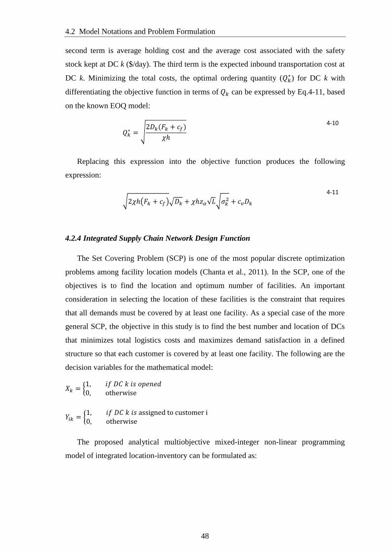
4.2 Model Notations and Problem Formulation
48
second term is average holding cost and the average cost associated with the safety
stock kept at DC k ($/day). The third term is the expected inbound transportation cost at
DC k. Minimizing the total costs, the optimal ordering quantity (𝑄𝑘∗) for DC k with
differentiating the objective function in terms of 𝑄𝑘 can be expressed by Eq.4-11, based
on the known EOQ model:
𝑄𝑘∗ = √
2𝐷𝑘(𝐹𝑘 + 𝑐𝑓)
𝜒ℎ
4-10
Replacing this expression into the objective function produces the following
expression:
√2𝜒ℎ(𝐹𝑘 + 𝑐𝑓)√𝐷𝑘 + 𝜒ℎ𝑧𝛼√𝐿√𝜎𝑘2 + 𝑐𝑣𝐷𝑘
4-11
4.2.4 Integrated Supply Chain Network Design Function
The Set Covering Problem (SCP) is one of the most popular discrete optimization
problems among facility location models (Chanta et al., 2011). In the SCP, one of the
objectives is to find the location and optimum number of facilities. An important
consideration in selecting the location of these facilities is the constraint that requires
that all demands must be covered by at least one facility. As a special case of the more
general SCP, the objective in this study is to find the best number and location of DCs
that minimizes total logistics costs and maximizes demand satisfaction in a defined
structure so that each customer is covered by at least one facility. The following are the
decision variables for the mathematical model:
𝑋𝑘 = {1, 𝑖𝑓 𝐷𝐶 𝑘 𝑖𝑠 𝑜𝑝𝑒𝑛𝑒𝑑0, otherwise
𝑌𝑖𝑘 = {1, 𝑖𝑓 𝐷𝐶 𝑘 𝑖𝑠 assigned to customer i0, otherwise
The proposed analytical multiobjective mixed-integer non-linear programming
model of integrated location-inventory can be formulated as:
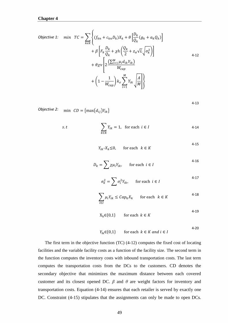
Chapter 4
49
Objective 1: 𝑚𝑖𝑛 𝑇𝐶 = ∑ {(𝑓𝑘𝑛 + 𝑐𝑘𝑛𝐷𝑘)𝑋𝑘 + 𝜃 [𝐷𝑘
𝑄𝑘
(𝑔𝑘 + 𝑎𝑘𝑄𝑘)]
𝑘𝜖𝐾
+ 𝛽 [𝐹𝑘
𝐷𝑘
𝑄𝑘+ 𝜒ℎ (
𝑄𝑘
2+ 𝑧𝛼√𝐿√𝜎𝑘
2)]
+ 𝜃𝜒𝜈 [2(∑ 𝜇𝑖𝑑𝑖𝑘𝑌𝑖𝑘
𝑀𝑖=1 )
𝑊𝑐𝑎𝑝
+ (1 −1
𝑊𝑐𝑎𝑝) 𝑘𝑒 ∑ 𝑌𝑖𝑘
𝑀
𝑖=1
√𝐴
𝑀]}
4-12
Objective 2: min 𝐶𝐷 = {max(𝑑𝑖𝑗)𝑌𝑖𝑘}
4-13
𝑠. 𝑡 ∑ 𝑌𝑖𝑘 = 1,
𝑘∈𝐾
for each 𝑖 ∈ 𝐼 4-14
𝑌𝑖𝑘-𝑋𝑘≤0, for each 𝑘 ∈ 𝐾
4-15
𝐷𝑘 = ∑ 𝜒𝜇𝑖𝑌𝑖𝑘 , for each 𝑖 ∈ 𝐼
4-16
𝜎𝑘
2 = ∑ 𝜎𝑖2𝑌𝑖𝑘 , for each 𝑖 ∈ 𝐼
4-17
∑ 𝜇𝑖𝑌𝑖𝑘 ≤ 𝐶𝑎𝑝𝑘𝑋𝑘
𝑖∈𝐼
for each 𝑘 ∈ 𝐾 4-18
Xk∈{0,1} for each 𝑘 ∈ 𝐾
4-19
𝑌ik∈{0,1} for each 𝑘 ∈ 𝐾 𝑎𝑛𝑑 𝑖 ∈ 𝐼
4-20
The first term in the objective function (TC) (4-12) computes the fixed cost of locating
facilities and the variable facility costs as a function of the facility size. The second term in
the function computes the inventory costs with inbound transportation costs. The last term
computes the transportation costs from the DCs to the customers. CD denotes the
secondary objective that minimizes the maximum distance between each covered
customer and its closest opened DC. β and θ are weight factors for inventory and
transportation costs. Equation (4-14) ensures that each retailer is served by exactly one
DC. Constraint (4-15) stipulates that the assignments can only be made to open DCs.
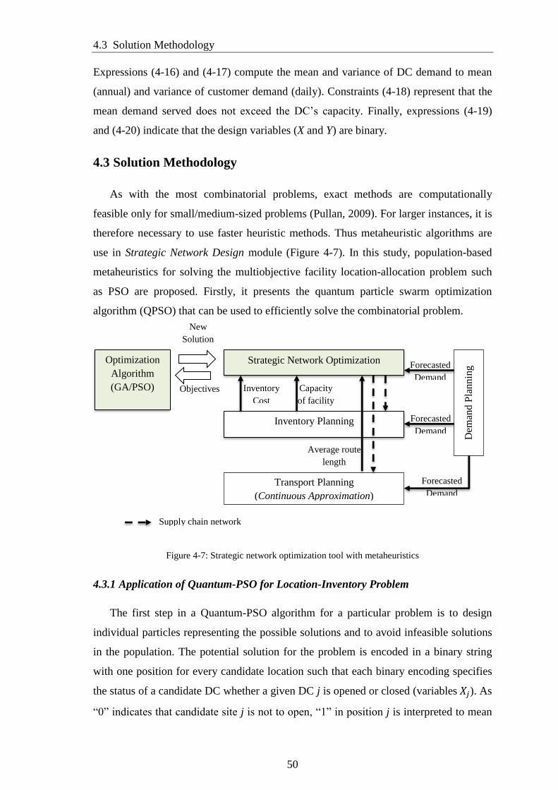
4.3 Solution Methodology
50
Expressions (4-16) and (4-17) compute the mean and variance of DC demand to mean
(annual) and variance of customer demand (daily). Constraints (4-18) represent that the
mean demand served does not exceed the DC’s capacity. Finally, expressions (4-19)
and (4-20) indicate that the design variables (X and Y) are binary.
4.3 Solution Methodology
As with the most combinatorial problems, exact methods are computationally
feasible only for small/medium-sized problems (Pullan, 2009). For larger instances, it is
therefore necessary to use faster heuristic methods. Thus metaheuristic algorithms are
use in Strategic Network Design module (Figure 4-7). In this study, population-based
metaheuristics for solving the multiobjective facility location-allocation problem such
as PSO are proposed. Firstly, it presents the quantum particle swarm optimization
algorithm (QPSO) that can be used to efficiently solve the combinatorial problem.
Figure 4-7: Strategic network optimization tool with metaheuristics
4.3.1 Application of Quantum-PSO for Location-Inventory Problem
The first step in a Quantum-PSO algorithm for a particular problem is to design
individual particles representing the possible solutions and to avoid infeasible solutions
in the population. The potential solution for the problem is encoded in a binary string
with one position for every candidate location such that each binary encoding specifies
the status of a candidate DC whether a given DC j is opened or closed (variables 𝑋𝑗). As
“0” indicates that candidate site j is not to open, “1” in position j is interpreted to mean
Supply chain network
Objectives
New
Solution
Inventory
Cost Capacity
of facility
Average route
length
Forecasted
Demand
Forecasted
Demand
Strategic Network Optimization
Inventory Planning
Transport Planning
(Continuous Approximation)
Dem
and P
lannin
g
Forecasted
Demand
Optimization
Algorithm
(GA/PSO)

Chapter 4
51
that candidate site j is selected to open. Each particle of QPSO described consists of
binary values whose length is equal to the number of candidate DC nodes in the
problem. For example the 𝑘𝑡ℎ particle of the population for an n-location problem could
be given as,
𝐼𝑘 = {1, 0 , 0, 1, 0, 1, 0, 1, 1, 0}
The above particle represents 10 candidate DCs such that DCs are identified by 1, 4,
6, 8, 9 have been selected to open on the ten possible locations. The steps of algorithm
QPSO applied to solve the problem is given below:
Step 1: Initialize parameters. Load the parameters of M customers and K candidate
DCs.
Step 2: Initialize particle swarm. Randomly generate a particle swarm based on
single dimensional array, which consists of K binary values representing decision
variables related to open or close the DC.
Step 3: Allocate customers to the open DC. A greedy heuristics used to assign
customer to open DCs. This procedure assigns each customer to its nearest DCs. If it is
not possible to assign a customer to its nearest DC because of excessive capacity, it is
assigned to the second nearest DC with sufficient capacity, and so on.
Step 4: Compute the fitness value. After allocation process, fitness values of each
particle in swarm are calculated by using Equation 4-11 and 4-12.
Step 5: Apply quantum particle swarm optimization steps described in previous
section.
Step 6: Obtain the optimal solution and the total cost of integrated facility location-
inventory problem.
In this research, local search was not used, which improves the solution with the k-
change neighborhoods procedure. Daskin et al. (2005) introduced three main reasons for
not considering the improvement of the cost by shifting assignments of customer to
DCs: solution times remain relatively low; the number of demand nodes assigned to a
site other than the nearest site is often very small; and the cost penalty paid for
assigning demand volumes to the nearest facility as opposed to assigning them
optimally is only a fraction of a percent.
4.4 The Strategic Network Design Tool and Description of Experiment
In making decisions concerning the strategic network design and identifying
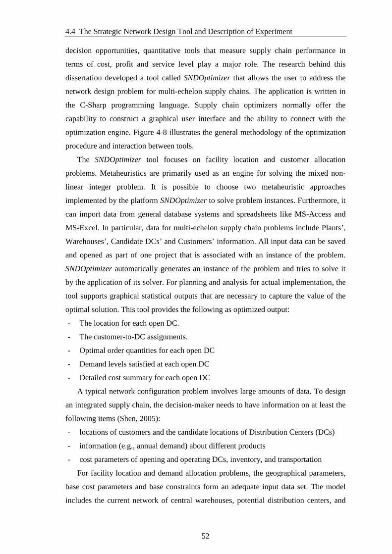
4.4 The Strategic Network Design Tool and Description of Experiment
52
decision opportunities, quantitative tools that measure supply chain performance in
terms of cost, profit and service level play a major role. The research behind this
dissertation developed a tool called SNDOptimizer that allows the user to address the
network design problem for multi-echelon supply chains. The application is written in
the C-Sharp programming language. Supply chain optimizers normally offer the
capability to construct a graphical user interface and the ability to connect with the
optimization engine. Figure 4-8 illustrates the general methodology of the optimization
procedure and interaction between tools.
The SNDOptimizer tool focuses on facility location and customer allocation
problems. Metaheuristics are primarily used as an engine for solving the mixed non-
linear integer problem. It is possible to choose two metaheuristic approaches
implemented by the platform SNDOptimizer to solve problem instances. Furthermore, it
can import data from general database systems and spreadsheets like MS-Access and
MS-Excel. In particular, data for multi-echelon supply chain problems include Plants’,
Warehouses’, Candidate DCs’ and Customers’ information. All input data can be saved
and opened as part of one project that is associated with an instance of the problem.
SNDOptimizer automatically generates an instance of the problem and tries to solve it
by the application of its solver. For planning and analysis for actual implementation, the
tool supports graphical statistical outputs that are necessary to capture the value of the
optimal solution. This tool provides the following as optimized output:
- The location for each open DC.
- The customer-to-DC assignments.
- Optimal order quantities for each open DC
- Demand levels satisfied at each open DC
- Detailed cost summary for each open DC
A typical network configuration problem involves large amounts of data. To design
an integrated supply chain, the decision-maker needs to have information on at least the
following items (Shen, 2005):
- locations of customers and the candidate locations of Distribution Centers (DCs)
- information (e.g., annual demand) about different products
- cost parameters of opening and operating DCs, inventory, and transportation
For facility location and demand allocation problems, the geographical parameters,
base cost parameters and base constraints form an adequate input data set. The model
includes the current network of central warehouses, potential distribution centers, and
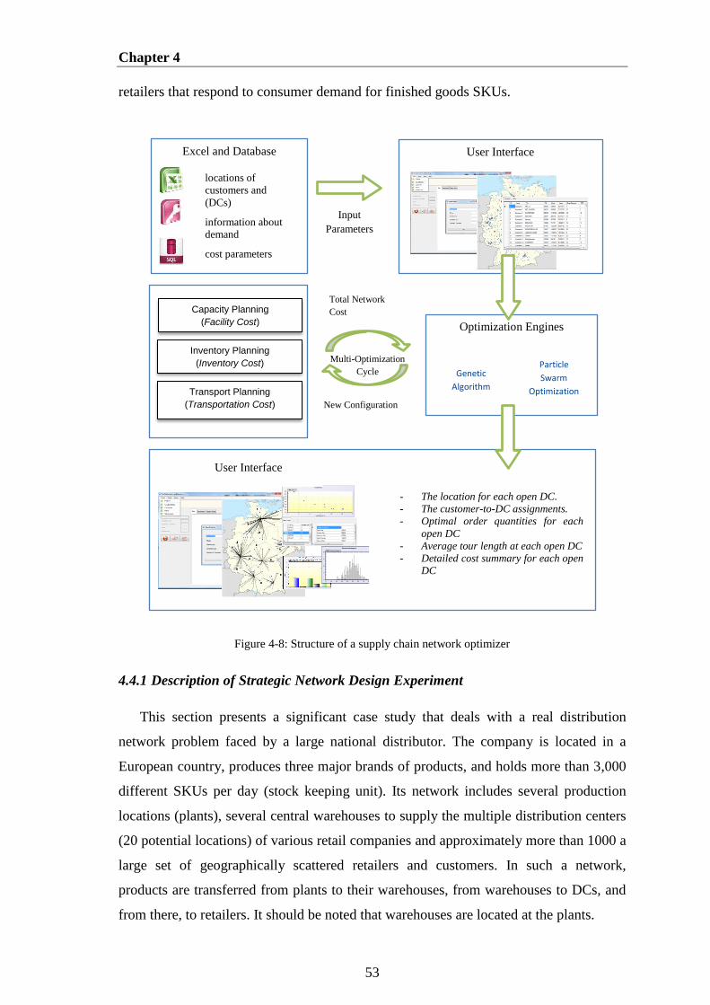
Chapter 4
53
retailers that respond to consumer demand for finished goods SKUs.
Figure 4-8: Structure of a supply chain network optimizer
4.4.1 Description of Strategic Network Design Experiment
This section presents a significant case study that deals with a real distribution
network problem faced by a large national distributor. The company is located in a
European country, produces three major brands of products, and holds more than 3,000
different SKUs per day (stock keeping unit). Its network includes several production
locations (plants), several central warehouses to supply the multiple distribution centers
(20 potential locations) of various retail companies and approximately more than 1000 a
large set of geographically scattered retailers and customers. In such a network,
products are transferred from plants to their warehouses, from warehouses to DCs, and
from there, to retailers. It should be noted that warehouses are located at the plants.
Multi-Optimization
Cycle
Total Network
Cost Coverage Distance
New Configuration
Input
Parameters
Excel and Database
locations of
customers and
(DCs)
information about
demand
cost parameters
User Interface
Optimization Engines
Genetic
Algorithm
Particle
Swarm
Optimization
- The location for each open DC.
- The customer-to-DC assignments.
- Optimal order quantities for each
open DC
- Average tour length at each open DC
- Detailed cost summary for each open
DC
User Interface
Inventory Planning (Inventory Cost)
Transport Planning
(Transportation Cost)
Capacity Planning (Facility Cost)
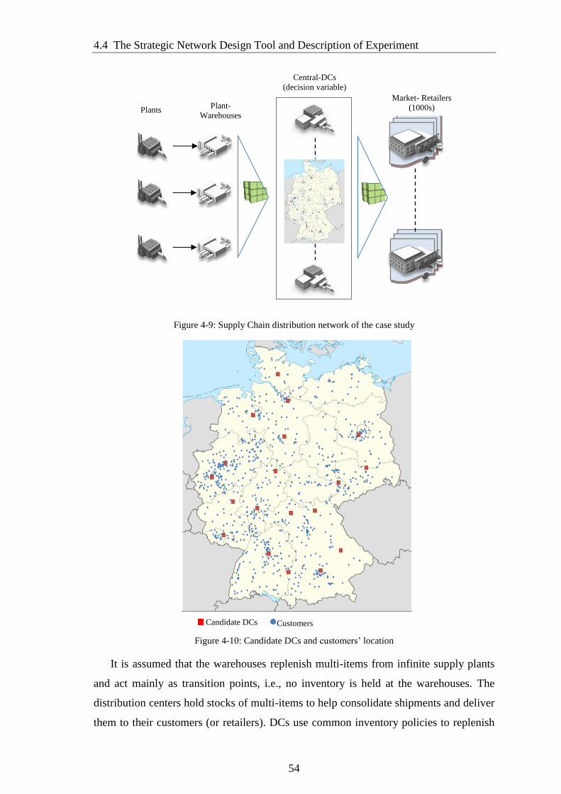
4.4 The Strategic Network Design Tool and Description of Experiment
54
Figure 4-9: Supply Chain distribution network of the case study
Figure 4-10: Candidate DCs and customers’ location
It is assumed that the warehouses replenish multi-items from infinite supply plants
and act mainly as transition points, i.e., no inventory is held at the warehouses. The
distribution centers hold stocks of multi-items to help consolidate shipments and deliver
them to their customers (or retailers). DCs use common inventory policies to replenish
Market- Retailers
(1000s) Plants Plant-
Warehouses
Central-DCs (decision variable)
Candidate DCs Customers

Chapter 4
55
their inventory levels. Each distribution center faces a stochastic customer demand from
stores who carry negligible inventory of the products. Figure 4-10 illustrates the
geographic location of candidate DCs (red square dots) and the location of demand
points (blue circle dots). The main question is to find the optimal number, size, location,
and service area of facilities that minimize the costs and maximize service efficiency to
serve the customers.
4.5 Model Results
The goal of this section is to show the application of the mathematical model by
numerical results obtained by solving instances of the location-inventory problem as a
practical case study and to highlight several insights in response to varying the
parameters. For each experiment, it is examined that how the network design decisions
change with variable test parameters. These test parameters include the number of
customers in the system, the average unit inventory holding cost, and the average unit
transportation cost per km. All other parameters are considered common parameters and
remain constant for all sample problems and the experimental data used is defined in
Appendix D. All computational work was performed on a personal computer (32-bit
operating system, 2.70 GHz CPU, and 8.00 GB.
Figure 4-11: Location-Allocation Result of Integrated Network Design
A typical experimental result for two optimization criteria incurred in designing the
Cost: 3 049 635 € Coverage Distance: 221 km
Cost: 2 610 228 € Coverage Distance: 432 km

4.5 Model Results
56
distribution network is illustrated in Figure 4-11. The red squares represent DCs used in
the solution as the black squares represent DCs that are located not to open. Allocation
of demand to the corresponding DCs is shown with straight line. From the observed
result, the cost is measured in 2,610,228 € for minimum cost criteria, while the cost is
measured in 3,049,635 € for minimum coverage distance criteria. Figure 4-12 shows all
the solution points in the Pareto front line that are found by minimizing the total cost
while decreasing the maximum distance between uncovered demand and opened DCs.
For example, it can be seen in the figure that two DCs are finally selected for
minimizing cost, while 6 DCs are required for minimizing the maximum customer
coverage distance. From the Figure 4-12, it can be also seen that for the cost values
between 2,610,228 € and 3,049,635 € result in maximum coverage ranging between 432
km and 221 km. Figure 4-13 shows the difference in performance for each cost
component, based on the solutions with 2 DCs and 6 DCs opened. Clearly, and
supported by the results, it can be seen the impacts of two decision criteria on the cost
components and the number of the DC selection. Figure 4-14 illustrates the solution
points of the model in terms of the trade-off between coverage and cost. According to
Figure 4-14, a 48.84 % reduction in coverage distance is offset by a 16.83 % increase
the total cost. It is worth mentioning solution 9 and solution 10, a 13.2 % reduction in
coverage distance can be offset by a 0.1 % increase in total cost. The trade-off between
coverage distance and cost provides a guideline for decision makers in selecting an
efficient solution generated from a multi-objective facility location model.
Figure 4-12: Non-dominated solutions of the model — first objective is to minimize the total cost and
second objective is to minimize the distance between uncovered demand and opened DCs
2610228 €
432 km
3049635 €
221 km
0
50
100
150
200
250
300
350
400
450
500
255
00
00
265
00
00
275
00
00
285
00
00
295
00
00
305
00
00
Co
ver
age
Dis
tan
ce (
km
)
Cost (€)

Chapter 4
57
Figure 4-13: Cost components performance comparison for the two configurations
To evaluate the influence of transportation and inventory costs factors on DC
selection and customer assignment, the values of β (weight factor for inventory cost)
and θ (weight factor for transportation cost) are varied. To analyze the ratio between the
unit transportation cost and the unit inventory cost, the case study scenario is modeled
with 200 customers. Changing the weights of the costs leads the model to present a new
optimal design, which is depicted in the Table 4-1.
Figure 4-14: The trade-off between the cost and coverage distance
It is observed from the computational result based on the objective of cost
minimization that as the proportion of transportation cost goes up, the number of open
DCs increase. Increasing θ will increase the impact of the sum of location and
€4
13
.332
€9
63
.995
€9
64
.547
€7
07
.760
€2
13
.697
€1
.13
8.6
22
€5
60
.033
€6
97
.875
€-
€200.000
€400.000
€600.000
€800.000
€1.000.000
€1.200.000
Open Cost Routing Cost Inventory Cost Inbound Cost
6 DC
2 DC14%
32% 32%
23%
8%
44%
21%
27%
0 0,4%
4,0% 4,3% 4,7% 5,1% 5,1% 7,8% 8,5% 8,6%
13,0% 13,1% 16,8%
0 -0,5%
-10,9% -13,2% -13,9%
-22,0% -25,7%
-28,5% -29,9%
-43,1% -44,7%
-47,5% -48,8% -60%
-50%
-40%
-30%
-20%
-10%
0%
10%
20%
30%
1 2 3 4 5 6 7 8 9 10 11 12 13
Per
cen
tage
of
chan
gin
g i
n o
bje
ctiv
es
The solution in final pareto front
Cost Coverage Distance
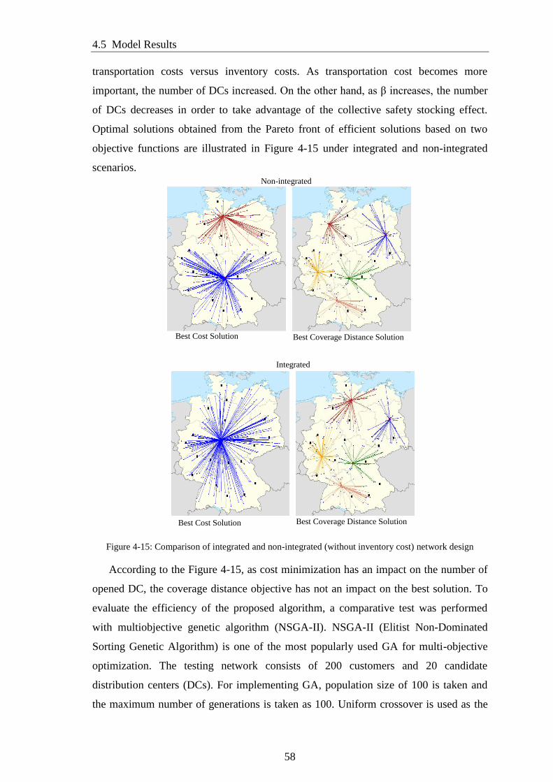
4.5 Model Results
58
transportation costs versus inventory costs. As transportation cost becomes more
important, the number of DCs increased. On the other hand, as β increases, the number
of DCs decreases in order to take advantage of the collective safety stocking effect.
Optimal solutions obtained from the Pareto front of efficient solutions based on two
objective functions are illustrated in Figure 4-15 under integrated and non-integrated
scenarios.
Figure 4-15: Comparison of integrated and non-integrated (without inventory cost) network design
According to the Figure 4-15, as cost minimization has an impact on the number of
opened DC, the coverage distance objective has not an impact on the best solution. To
evaluate the efficiency of the proposed algorithm, a comparative test was performed
with multiobjective genetic algorithm (NSGA-II). NSGA-II (Elitist Non-Dominated
Sorting Genetic Algorithm) is one of the most popularly used GA for multi-objective
optimization. The testing network consists of 200 customers and 20 candidate
distribution centers (DCs). For implementing GA, population size of 100 is taken and
the maximum number of generations is taken as 100. Uniform crossover is used as the
Non-integrated
Best Coverage Distance Solution Best Cost Solution
Best Coverage Distance Solution Best Cost Solution
Integrated
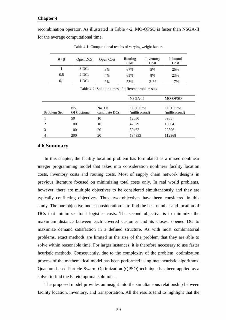
Chapter 4
59
recombination operator. As illustrated in Table 4-2, MO-QPSO is faster than NSGA-II
for the average computational time.
Table 4-1: Computational results of varying weight factors
θ / β Open DCs Open Cost Routing
Cost
Inventory
Cost
Inbound
Cost
1 3 DCs 3% 67% 5% 25%
0,5 2 DCs 4% 65% 8% 23%
0,1 1 DCs 9% 53% 21% 17%
Table 4-2: Solution times of different problem sets
NSGA-II MO-QPSO
Problem Set
No.
Of Customer
No. Of
candidate DCs
CPU Time
(millisecond)
CPU Time
(millisecond)
1 50 10 12030 3933
2 100 10 47029 15004
3 100 20 59462 22596
4 200 20 184853 112368
4.6 Summary
In this chapter, the facility location problem has formulated as a mixed nonlinear
integer programming model that takes into consideration nonlinear facility location
costs, inventory costs and routing costs. Most of supply chain network designs in
previous literature focused on minimizing total costs only. In real world problems,
however, there are multiple objectives to be considered simultaneously and they are
typically conflicting objectives. Thus, two objectives have been considered in this
study. The one objective under consideration is to find the best number and location of
DCs that minimizes total logistics costs. The second objective is to minimize the
maximum distance between each covered customer and its closest opened DC to
maximize demand satisfaction in a defined structure. As with most combinatorial
problems, exact methods are limited in the size of the problem that they are able to
solve within reasonable time. For larger instances, it is therefore necessary to use faster
heuristic methods. Consequently, due to the complexity of the problem, optimization
process of the mathematical model has been performed using metaheuristic algorithms.
Quantum-based Particle Swarm Optimization (QPSO) technique has been applied as a
solver to find the Pareto optimal solutions.
The proposed model provides an insight into the simultaneous relationship between
facility location, inventory, and transportation. All the results tend to highlight that the
4.6 Summary
60
distribution network design in the real world may be better analyzed when considering
the interdependence between decision levels rather than considering each decision level
individually. It has been also observed that the optimal network structure is quite
different with (integrated) and without (non-integrated) considering inventory in the
supply chain design. In this chapter, a strategic network design tool (SNDOptimizer)
has been presented for the purpose of solving the multiobjective integrated supply chain
problem. The proposed approach and models implemented by SNDOptimizer
developed in C-Sharp to find feasible solutions closed as possible to the optimality.
Chapter 5
Object-Oriented Modeling for Inventory of
Multi-Echelon Supply Chain
In recent years, the efficient and effective management of material flow throughout
the supply chain has become more important in order to improve customer service level
and reduce costs for the whole system. In the past, the majority of the solution
approaches used to solve multi-echelon supply chain problems were based on
conventional methods using analytical techniques. However, they are insufficient to
cope with the SC dynamics because of the inability to handle to the complex
interactions between the SC members and to represent stochastic behaviors existing in
many real world problems. Unlike the traditional methods, simulation has recently
become a major computer-based tool that enables us to model complex systems without
limiting assumptions, which are subject to both variability and complexity (Banks,
2000). This chapter describes the design of an object-oriented simulation framework to
analyze different inventory control strategies within a given supply chain. The primary
objective of this chapter is the development and creation of a multi-echelon supply
chain simulation framework primarily for use in inventory applications. A secondary
objective is to describe an overview of how an object-oriented library for simulating
inventory is implemented. The simulation toolbox is developed using Microsoft Visual
C-Sharp programming language, which is one of the several languages that support
object-oriented programming. The library classes consist of objects representing the
nodes, an interconnection structure for a multi-echelon system, and a management
system for moving the material between different nodes within the network. A brief
description of different simulation modeling approaches is presented in Section 5.1.
Section 5.2 presents a conceptual model to describe inventory processes of multi-
echelon supply chains. The details of the proposed object-oriented simulation model are
given in Section 5.3. Section 5.4 presents the cost components of the simulation model.
5.1 Major Supply Chain Simulation Approaches
62
In Section 5.5, we describe the performance measures identified through simulation.
5.1 Major Supply Chain Simulation Approaches
In today’s business environment, supply chains are faced with challenges to deliver
high quality products and to bring products to the customer on time to achieve a
competitive advantage. Demand variance, uncertainties in lead-time, forecast errors, and
a dramatically changing production environment make supply chains more complicated
to analyze. Developing a model that represents the supply chain characteristics and
dynamics is an important issue to understand the mechanics and processes of a supply
chain (Ramakrishnan & Wysk, 2002). In the literature, modeling of SC is classified into
two main categories: analytical models and simulation models. According to Min and
Zhou (2002), supply chain models can be classified as deterministic (non-probabilistic),
stochastic (probabilistic), hybrid, and IT-driven. On the other hand, Sabri and Beamon
(2000) classify supply chain modeling into four groups of deterministic analytical
models, stochastic analytical models, economic models and simulation models. Since
many analytical models are inadequate for the realistic representation of the system due
to the fact that they lack the capability of handling variability and uncertainty,
simulation is used as an effective way to model the supply chain because of its ability to
incorporate uncertainties and dynamics of supply chain.
Recently, simulation has been considered as a decision support tool offering an
alternative method for detailed analysis of the complex real world systems and is
defined as a representation of a real system that usually takes the form of a set of
assumptions concerning the operation of that system (Banks, 2000) (Douraid et al.,
2012). There is several simulation methods used to study the dynamics that result from
decisions made in such systems. In this context, four simulation types are distinguished
by Kleijnen (2003): spreadsheet simulation, system dynamics (SD), discrete-event
simulation (DES), and business games. Although the object-oriented simulation
framework is chosen in this study, this section first discusses four common simulation
methods known as spreadsheet simulation, SD, DES and agent-based simulation (ABS).
5.1.1 Spreadsheet-Based Simulation
Spreadsheet simulation refers to the use of a spreadsheet to represent the model and
perform the simulation experiment (Seila, 2001). This kind of simulation is quite
suitable for the user and an attractive platform for simulation, since developers and
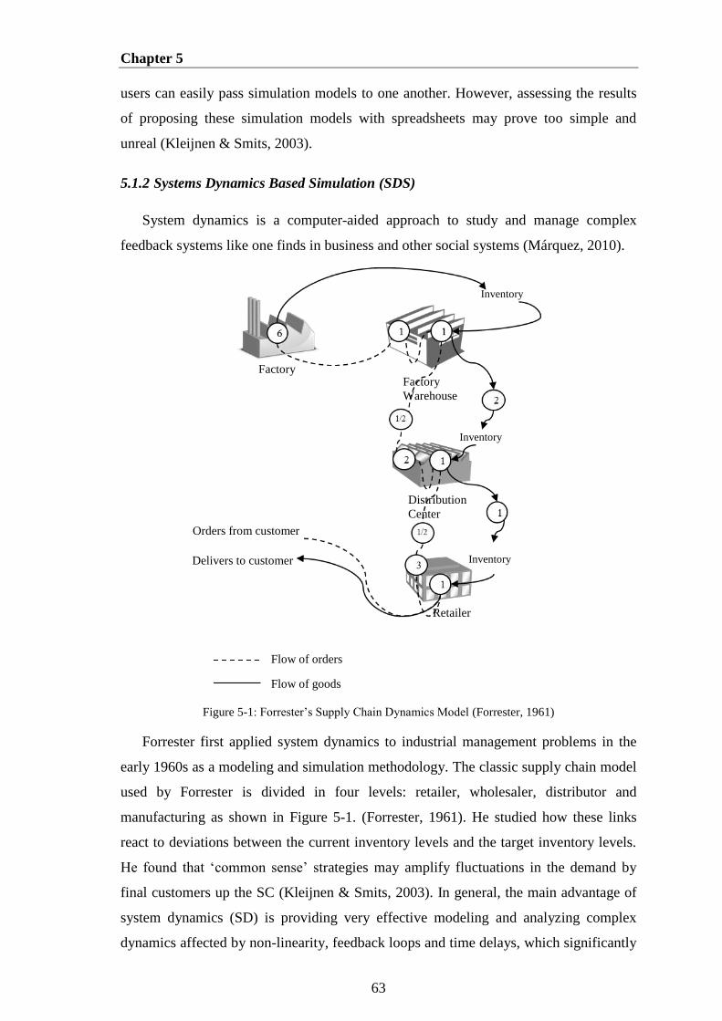
Chapter 5
63
users can easily pass simulation models to one another. However, assessing the results
of proposing these simulation models with spreadsheets may prove too simple and
unreal (Kleijnen & Smits, 2003).
5.1.2 Systems Dynamics Based Simulation (SDS)
System dynamics is a computer-aided approach to study and manage complex
feedback systems like one finds in business and other social systems (Márquez, 2010).
Figure 5-1: Forrester’s Supply Chain Dynamics Model (Forrester, 1961)
Forrester first applied system dynamics to industrial management problems in the
early 1960s as a modeling and simulation methodology. The classic supply chain model
used by Forrester is divided in four levels: retailer, wholesaler, distributor and
manufacturing as shown in Figure 5-1. (Forrester, 1961). He studied how these links
react to deviations between the current inventory levels and the target inventory levels.
He found that ‘common sense’ strategies may amplify fluctuations in the demand by
final customers up the SC (Kleijnen & Smits, 2003). In general, the main advantage of
system dynamics (SD) is providing very effective modeling and analyzing complex
dynamics affected by non-linearity, feedback loops and time delays, which significantly
Delivers to customer
Orders from customer
Inventory
Inventory
Inventory
Distribution
Center
Retailer
Factory Factory
Warehouse
Flow of goods
Flow of orders
5.1 Major Supply Chain Simulation Approaches
64
impact the behavior of the whole system (Sterman, 2000). However, variables in SD
models are generally usually represented as deterministic average values (Tako &
Robinson, 2006).
5.1.3 Discrete-Event Simulation (DES)
Another widely used simulation technique is discrete-even simulation (DES). The
use of DES for strategic, tactical and operational problems in manufacturing, logistics,
and supply chain management has grown in recent decades. It has been used widely for
network optimization, policy optimization, identification of the causes of uncertainties
and their impact, and in the development of methods to reduce/eliminate these
uncertainties (Ramakrishnan & Wysk, 2002). In DES, the simulation model has a given
state at any point in time, and the simulation state remains unchanged unless a
simulation event occurs (Altiok & Melamed, 2007). Each event is implemented as a
procedure (computer code) whose execution can change state variables and possibly
schedule other events. Main challenges in DES that supply chain analyst faces are (Lee
et al., 2002): i) reflection of the continuous nature of the process is not possible, ii)
growing complexity for more detailed models, iii) too much simplification for small
scaled models.
5.1.4 Agent-Based Simulation (ABS)
Recently, Agent Based Simulation (ABS) has been increasingly used to analyze
business systems and supply chain management as a new modeling paradigm. In ABS,
the model consists of a set of agents that represent the behaviors of the different
individuals or entities within the supply chain network, e.g. customers, retailer,
wholesaler, manufacturer, supplier or any other entity (Tah, 2005). In order to satisfy its
own objectives, each agent has its own behaviors or algorithms to make its own
decisions, a number of parameters or indicators to express its status (Sarker et al.,
2005). For example, a retailer (an agent) determines its market demand, calculates its
own ordering quantity, places orders, receives products from the distributors, updates its
status, calculates cost and sells to the market. According to Kodia (2010), the main
advantages of the agent based simulation can be summarized as follows: i) it considers
individual behavior, ii) takes into account actions and interactions between individuals,
and iii) examines the emergence of collective phenomena.
Chapter 5
65
5.2 Object-Oriented Framework for Multi-Echelon Inventory
Simulation
As mentioned in the previous section, supply chain modeling commonly implies
simplified representation of the system with components or building blocks. To
facilitate the modeling and analysis of different supply chain settings, an inventory
simulation library is developed using an object oriented programming language that
implement a set of suitable object classes. These classes are used as building blocks and
a subsystem that can encapsulate a large number of system parameters within given
instances. The class diagrams of the simulation framework in details are illustrated in
Appendix B. The traditional approach in the simulation of a supply chain is to define
the system as a network of different nodes (i.e., factories, warehouses, retailers and
customers) and each of these nodes performs different functions. A link between nodes
represents the flow of materials and information among the whole supply chain that
makes possible the functions of procurement, processing (or manufacturing), storage,
and distribution (Beamon & Chen, 2001). In the developed simulation framework,
different object classes are defined to represent each type of node in the supply chain,
such as customer class, retailer class, warehouse class, and factory class. Figure 5-2 and
Table 5-1 provide a brief description of important classes in the presented simulation
framework. This class hierarchy can be extended in many ways. Customer, which is at
the lowest in the supply chain network, is an object class that represents the source of
the original downstream demands. Factory is an object class that is responsible for
transforming raw material into intermediate or finished products. In general, a factory
receives orders from the warehouse. The main activity of the warehouse class is to
manage storage and handling processes, and the retailer class is where an external
customer buys the product. Transportation class represents the link between nodes,
which is used to move product from one node to another in a supply chain. Every class
object sends demands or order requests to the next class object in the upstream direction
and ship products to the node that is downstream in the network. At the end of the
simulation, every object related to inventory computes the service level and costs of the
current scenario and adds the result to the value of overall costs. The following sections
will discuss the classes within the inventory simulation tool.
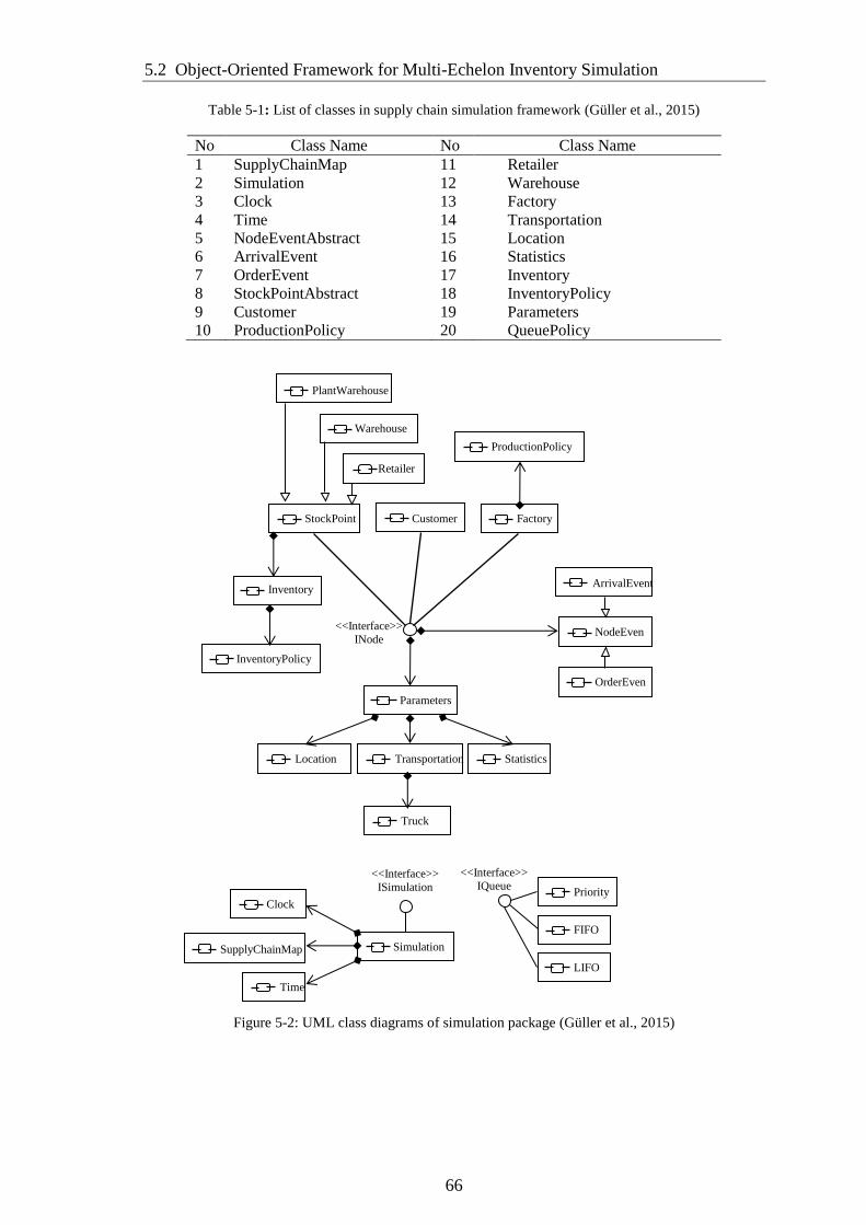
5.2 Object-Oriented Framework for Multi-Echelon Inventory Simulation
66
Table 5-1: List of classes in supply chain simulation framework (Güller et al., 2015)
No Class Name No Class Name
1 SupplyChainMap 11 Retailer
2 Simulation 12 Warehouse
3 Clock 13 Factory
4 Time 14 Transportation
5 NodeEventAbstract 15 Location
6 ArrivalEvent 16 Statistics
7 OrderEvent 17 Inventory
8 StockPointAbstract 18 InventoryPolicy
9 Customer 19 Parameters
10 ProductionPolicy 20 QueuePolicy
Figure 5-2: UML class diagrams of simulation package (Güller et al., 2015)
<<Interface>> ISimulation
Simulation
Clock
Time
SupplyChainMap
<<Interface>> IQueue
FIFO
LIFO
Priority
InventoryPolicy
PlantWarehouse
Warehouse
Retailer
StockPoint Factory Customer
Inventory
NodeEvent
ArrivalEvent
OrderEven
t Parameters
Location Transportation Statistics
Truck
<<Interface>> INode
ProductionPolicy
Chapter 5
67
5.3 Some Object Classes for Simulation of Multi-echelon Inventory
System
The object-oriented approach is one of the popular modeling techniques to design
and simulate complex systems. According to Barcio (1996), the main advantages of
using object-oriented techniques in modeling and simulation are: “(i) software reuse is
enhanced when object-oriented techniques are applied efficiently in defining the system
objects, (ii) objects in the system can be defined in close correspondence to real-world
objects, (iii) the rapid development of new software is promoted, (iv) the use of
inheritance enables the creation of new objects and associated methods with minimal
effort, and, (v) the use of encapsulation provides the appropriate distinction between
object boundaries and is effective in identifying and controlling the propagation of
errors”. The general principle of Object Oriented Programming (OOP) is to formulate
problem using interacting objects rather than a set of functions and to define these
objects in terms of their attributes and methods (Güller et al., 2015) (Alfons et al.,
2010). In OOP, objects are categorized into classes and class hierarchies. The behavior
and interactions of these objects are modeled with generic functions and methods
(PressMan, 1997). Each supply chain members in the object-oriented framework of the
multi-echelon system, such as supplier, factory, warehouse and customer, can be
modeled independently from the coordinating simulation tool. Hence, object-oriented
design makes it easier to customize individual elements, thereby allowing more
flexibility in the design (Richardson, 2006). The most important concepts in OOP
supporting the design of such systems are encapsulation, class inheritance, subclasses,
and polymorphism (PressMan, 1997). Inheritance provides defining new classes from
existing classes and allows inheriting the attributes and methods of their base classes to
the new classes (Garrido, 2009). In addition to the attributes and operations shared with
base classes, subclasses (derived classes) can be defined by additional features. The
encapsulation principle refers to information and the attributes of an object hiding and is
considered as a protected mechanism with an imaginary protection wall. Hence, all data
and functions in a class are protected from any unauthorized access.
The specification of the object-oriented framework of a system begins with the
identification of the key elements within the system, their roles, attributes, relationships
with each other, and modeling and implementation issues (Rosetti & Nangia, 2007).
The main packages needed within a generic inventory simulation in the framework are
5.3 Some Object Classes for Simulation of Multi-echelon Inventory System
68
the following: Event, Node, Queue, Simulation, and SupplyChain summarized in Table
5-2. Since it is beyond the scope of this section to discuss in detail the implementation
of packages and all classes, a brief description of important classes is provided in this
chapter.
Table 5-2 Supply chain inventory simulator packages
Package Functional Description
Node Classes that represent locations within the supply chain, such as a warehouse.
Event
The package consists of a collection of event classes, such as customer arrival,
transportation, and order processing. Each event objects change a state and is
responsible for scheduling other events that depend on that event.
Queue The package consists of different kind of queue logic such as FIFO, LIFO and
priority list.
Simulation The package responsible for the scheduling and execution of simulation events.
SupplyChain Classes represent the connections between nodes and structure of SC
According to Biswas and Narahari (2004), the elements of the object library in a
simulation model of multi-echelon supply chain can be classified into two categories:
structural objects and policy objects. Whereas the structural objects define the physical
entities of the network, the policy objects define the protocols used in logistics
processes such procurement, manufacturing, transportation, and distribution (Biaswas &
Narahari, 2004). The main classes of the structural object in the presented simulation
framework are factory, warehouse, retailer, supplier, customer and vehicles. Table 5-3
illustrates the responsibilities of these objects.
Table 5-3 Main supply chain structural objects and entities (Biaswas & Narahari, 2004)
Customer
A customer can be either an internal customer that is the various entities of the
network like the plants and the distributors or an external customer that is the
consumers of the products (finished or semi-finished). This class may also contain
information related to demand data.
Supplier
(Factory)
A supplier provides a plant with raw materials or sub-assemblies. A supplier could
be a manufacturing plant or a late-customization center or a full-fledged supply
chain.
Retailer
An external customer generally buys the products from the retailer. A retailer has an
associated stocking warehouse, where the inventories of the products are stored. A
retailer can receive deliveries from distributor or plant central warehouses or late-
customization center or from some other retailer. The product is delivered to
customer if it is available in the retailer's warehouse. Otherwise the order is added to
a queue for the particular product, according to a pre-assigned priority. The order is
delivered when the product is received (from distributor or plant or late-

Chapter 5
69
customization center as the case may be).
Warehouse
A warehouse is a storage facility that is characterized by the nature and capacity of
the products it can store. It can be attached to the plant, the distributor, and the
retailer.
Vehicle
(Truck)
Vehicles transport products from one node of the network to another. Each vehicle
has characteristics in terms of products it can carry, capacity (in volume or weight),
costs, and speed.
5.3.1 The Simulation Class
To manage the simulation experiments and communicate with the optimization tool,
a general control class, called Simulation, is utilized in this thesis. The Simulation class
contains the definition of parameters that might be necessary within a simulation such
as the period, number of nodes, location of nodes etc. (Güller et al., 2015). This class
maintains a simulator’s clock recording the current simulation time and the next event
that is retrieved from the event list, and starts executing the events in the appropriate
order. Its methods serve to trigger the clock for simulation, stop the simulator’s clock,
initialize the simulation, and read the simulation clock. One of methods used in this
class is the Run method that starts the execution of simulation based on the desired
number of replications and run length. The simulation process continues until some pre-
specified stopping condition or no more items are on the event list. The parameter
simulationPeriod defining the duration of a simulation experiment is a user-defined
value. Execution ends with the creation of a Statistical Results window.
5.3.2 The NodeEvent and Queue Classes
The abstract class NodeEvent is being used to represent the collection of processes
(events) related to the flow of material through a supply chain. Events are the result of a
structural object’s action and are processed from the environment simulator. Each type
of event should be defined as a subclass of the NodeEvent class. The fundamental
constructed events in the library, occurring at supply chain members, are “order event”
and “arrival event” (Güller et al., 2015). The main recorded data in such an order event
are the quantity of ordered item, type of the sender and the receiver, and time properties
associated with this event. When an order event is constructed, it is scheduled based on
the duration of process and current simulation time. Arrival event is the process of
accepting an order that has been filled.
During the simulation run events are sorted on a time axis in increasing order of

5.3 Some Object Classes for Simulation of Multi-echelon Inventory System
70
simulation clock time. For this purpose, the IQueue interface is created with some queue
policies, e.g. FIFO, LIFO and priority. According to the selected policy, the event list is
sorted from top to bottom by ascending time or ascending priority in order to select
future event to execute. As a result, the Queue class provides a mechanism to select
events from the future event queue.
5.3.3 The StockPoint Class
The StockPoint abstract class and interface INode that encapsulates logistic activities
are used to model the member of a supply chain that hold stocks, such as warehouses
and retailers. User-defined stock point classes must be declared as extensions of the
StockPoint class and INode interface. The class structure consists of the data
declarations that will define the characteristics of the objects created from this class.
Examples of StockPoint methods that are responsible for the functions and data related
to the inventory are CheckIniventory(), StockGeneration(), MakeReplenishment(), and
Initialize().
5.3.4 The Customer Class
When dealing with modeling a supply chain, one of the most important issues is to
define customer demand structure. The Customer class is an object class that is
responsible for the functions and data related to the end-customer of a supply chain
network. The Customer class generates the sampling of random demand by providing
details of the customer requirements within the system. The demand inter-arrival time
(or demand per unit time) and demand order sizes require three inputs: distribution,
mean, and coefficient of variation (CV) or standard deviation. Distribution related to
demand can follow either a discrete or continuous distribution. The normal distribution
assumption is known to be a very good fit to describe many demand functions at the
different levels of supply chains for the cases of fast-demand items. However, for very
slow moving items, it is usually assumed that the demand process is Poisson distributed.
A large number of studies assume a homogeneous normal distribution demand pattern
in supply chain problems because of its convenient mathematical properties. However,
actual customer demand may be better modelled with distributions that are asymmetric
and positive skew shape (Cobb et al., 2013). Thus, the lognormal distribution is more
suitable than the normal distribution when modelling non-negative demands (Juan et al.,
2014). As a result, Gamma, Beta and Lognormal distributions have been found to be of

Chapter 5
71
considerable value in describing demand functions. For simplicity, customer demand is
generated as accumulated demand per day, per week, per month, etc.
5.3.5 The Retailer Class
The Retailer class is an object class which represents a member in SC. The new
Retailer object inherits from abstract class StockPoint and deals with external
customers, but also deals with suppliers.
Figure 5-3: Flowchart of (R, Q) Inventory Policy for Retailer Class
The retailer object receives demands from the instance of its external customer as an
input and places orders for stock replenishment based on inventory control policy to its
supplier as an output. If a demand is received through the customer, the object tries to
satisfy the demand as soon as possible. If the amount exceeds the current inventory
Arriving of
customer
Determine total
demand size
Fill demand
Recalculate
stock
No
order
Backorder the
demand
Queue of
backorders
Place
replenishment
order
Assign lead-
time
Recalculation
the stock
END
Check if the
stock is enough
Check the
inventory
position
Check the
inventory
position
Yes
If
backorder
exist
Yes
Yes
No
No
Lead-
time

5.3 Some Object Classes for Simulation of Multi-echelon Inventory System
72
level, the demand is backordered, and inserted into a list called BackorderItems, which
corresponds to a waiting queue for unsatisfied demands. The demand does not allow
partial filling. Accumulated backorders in a queue are satisfied on the queue rule after
the arrival of a replenishment order. The retailer objects are characterized by a list of
parameters such as replenishment policy, leadtime, fixed order costs, stock holding
costs, shortage costs, delivery costs, etc. For the purpose of supply chain inventory
simulation, an inventory (replenishment) policy is assigned to a certain retailer object.
Based on the inventory policy, the retailer places an order to its supplier (or its
warehouse), whenever the inventory position goes below the predefined reorder point.
An overview of the inventory control logic of retailer object is shown in Figure 5-3.
5.3.6 The Warehouse Class
This class models the warehouse, which is one of the structural objects of a supply
chain. Warehouses, which are connected to the supplier and the retailer, go through a
process of receiving products from the supplier, storing them and sending them to the
retailer. The same architecture of the retailer class is implemented for the warehouse
class with some different variables and modified methods. Objects of this class have an
input to receive orders for products from retailers and an output to send requests to its
suppliers. The two main logics implemented in warehouse objects are supplying retailer
orders and controlling inventory.
Figure 5-4: The supply operation flow chart for warehouse class
Order from
retailer Check if the
stock is enough Backorder the
demand
Queue of
backorders Fill demand
Reduce
inventory level
by the amount
of filled demand
Inventory
control logic
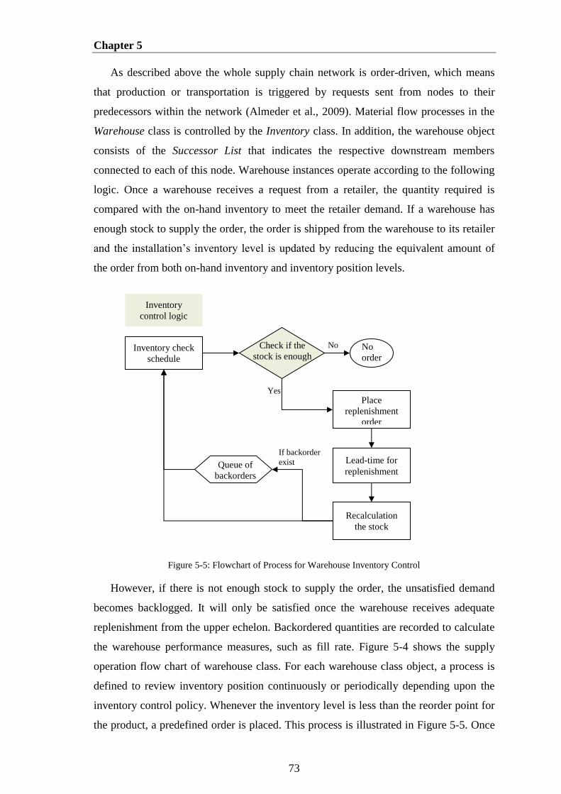
Chapter 5
73
As described above the whole supply chain network is order-driven, which means
that production or transportation is triggered by requests sent from nodes to their
predecessors within the network (Almeder et al., 2009). Material flow processes in the
Warehouse class is controlled by the Inventory class. In addition, the warehouse object
consists of the Successor List that indicates the respective downstream members
connected to each of this node. Warehouse instances operate according to the following
logic. Once a warehouse receives a request from a retailer, the quantity required is
compared with the on-hand inventory to meet the retailer demand. If a warehouse has
enough stock to supply the order, the order is shipped from the warehouse to its retailer
and the installation’s inventory level is updated by reducing the equivalent amount of
the order from both on-hand inventory and inventory position levels.
Figure 5-5: Flowchart of Process for Warehouse Inventory Control
However, if there is not enough stock to supply the order, the unsatisfied demand
becomes backlogged. It will only be satisfied once the warehouse receives adequate
replenishment from the upper echelon. Backordered quantities are recorded to calculate
the warehouse performance measures, such as fill rate. Figure 5-4 shows the supply
operation flow chart of warehouse class. For each warehouse class object, a process is
defined to review inventory position continuously or periodically depending upon the
inventory control policy. Whenever the inventory level is less than the reorder point for
the product, a predefined order is placed. This process is illustrated in Figure 5-5. Once
Inventory
control logic
Inventory check
schedule Check if the
stock is enough No
order
Place
replenishment
order
Lead-time for
replenishment
Recalculation
the stock
Queue of
backorders
If backorder
exist
Yes
No
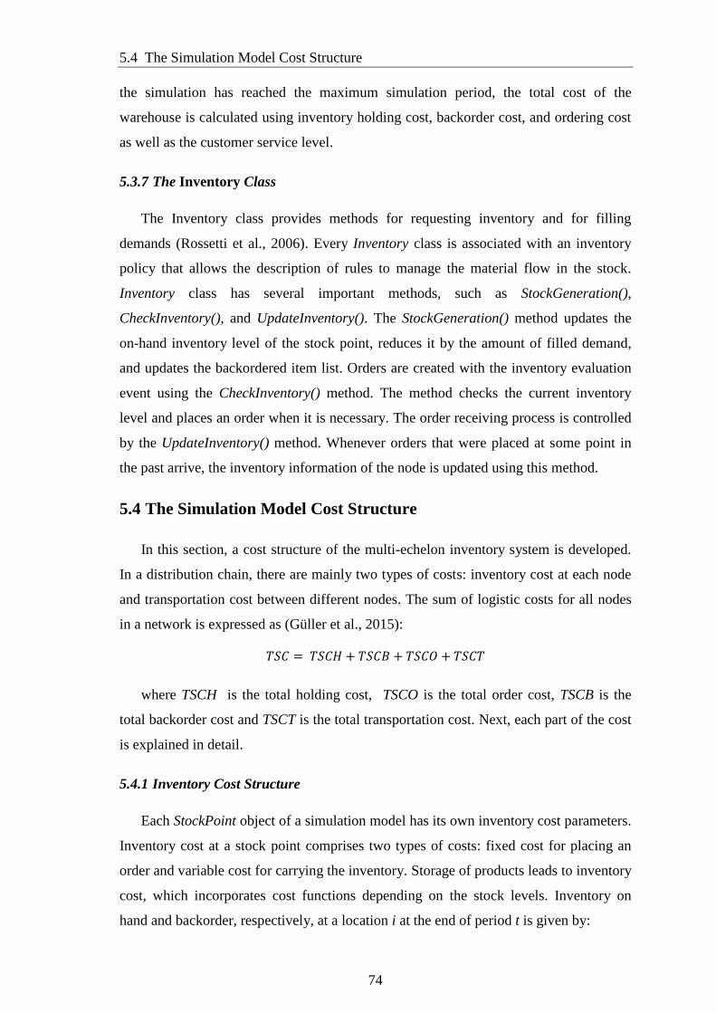
5.4 The Simulation Model Cost Structure
74
the simulation has reached the maximum simulation period, the total cost of the
warehouse is calculated using inventory holding cost, backorder cost, and ordering cost
as well as the customer service level.
5.3.7 The Inventory Class
The Inventory class provides methods for requesting inventory and for filling
demands (Rossetti et al., 2006). Every Inventory class is associated with an inventory
policy that allows the description of rules to manage the material flow in the stock.
Inventory class has several important methods, such as StockGeneration(),
CheckInventory(), and UpdateInventory(). The StockGeneration() method updates the
on-hand inventory level of the stock point, reduces it by the amount of filled demand,
and updates the backordered item list. Orders are created with the inventory evaluation
event using the CheckInventory() method. The method checks the current inventory
level and places an order when it is necessary. The order receiving process is controlled
by the UpdateInventory() method. Whenever orders that were placed at some point in
the past arrive, the inventory information of the node is updated using this method.
5.4 The Simulation Model Cost Structure
In this section, a cost structure of the multi-echelon inventory system is developed.
In a distribution chain, there are mainly two types of costs: inventory cost at each node
and transportation cost between different nodes. The sum of logistic costs for all nodes
in a network is expressed as (Güller et al., 2015):
𝑇𝑆𝐶 = 𝑇𝑆𝐶𝐻 + 𝑇𝑆𝐶𝐵 + 𝑇𝑆𝐶𝑂 + 𝑇𝑆𝐶𝑇
where TSCH is the total holding cost, TSCO is the total order cost, TSCB is the
total backorder cost and TSCT is the total transportation cost. Next, each part of the cost
is explained in detail.
5.4.1 Inventory Cost Structure
Each StockPoint object of a simulation model has its own inventory cost parameters.
Inventory cost at a stock point comprises two types of costs: fixed cost for placing an
order and variable cost for carrying the inventory. Storage of products leads to inventory
cost, which incorporates cost functions depending on the stock levels. Inventory on
hand and backorder, respectively, at a location i at the end of period t is given by:
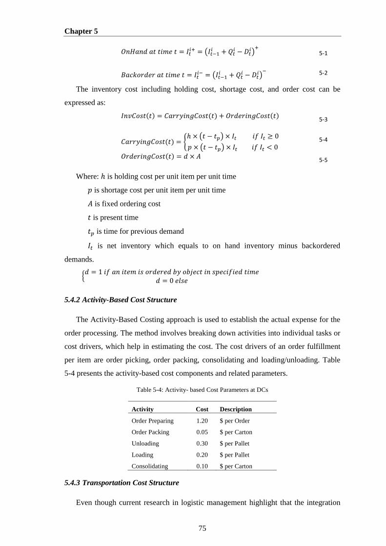
Chapter 5
75
𝑂𝑛𝐻𝑎𝑛𝑑 𝑎𝑡 𝑡𝑖𝑚𝑒 𝑡 = 𝐼𝑡𝑖+ = (𝐼𝑡−1
𝑖 + 𝑄𝑡𝑖 − 𝐷𝑡
𝑖)+
5-1
𝐵𝑎𝑐𝑘𝑜𝑟𝑑𝑒𝑟 𝑎𝑡 𝑡𝑖𝑚𝑒 𝑡 = 𝐼𝑡𝑖− = (𝐼𝑡−1
𝑖 + 𝑄𝑡𝑖 − 𝐷𝑡
𝑖)−
5-2
The inventory cost including holding cost, shortage cost, and order cost can be
expressed as:
𝐼𝑛𝑣𝐶𝑜𝑠𝑡(𝑡) = 𝐶𝑎𝑟𝑟𝑦𝑖𝑛𝑔𝐶𝑜𝑠𝑡(𝑡) + 𝑂𝑟𝑑𝑒𝑟𝑖𝑛𝑔𝐶𝑜𝑠𝑡(𝑡) 5-3
𝐶𝑎𝑟𝑟𝑦𝑖𝑛𝑔𝐶𝑜𝑠𝑡(𝑡) = {ℎ × (𝑡 − 𝑡𝑝) × 𝐼𝑡 𝑖𝑓 𝐼𝑡 ≥ 0
𝑝 × (𝑡 − 𝑡𝑝) × 𝐼𝑡 𝑖𝑓 𝐼𝑡 < 0 5-4
𝑂𝑟𝑑𝑒𝑟𝑖𝑛𝑔𝐶𝑜𝑠𝑡(𝑡) = 𝑑 × 𝐴 5-5
Where: ℎ is holding cost per unit item per unit time
𝑝 is shortage cost per unit item per unit time
𝐴 is fixed ordering cost
𝑡 is present time
𝑡𝑝 is time for previous demand
𝐼𝑡 is net inventory which equals to on hand inventory minus backordered
demands.
{𝑑 = 1 𝑖𝑓 𝑎𝑛 𝑖𝑡𝑒𝑚 𝑖𝑠 𝑜𝑟𝑑𝑒𝑟𝑒𝑑 𝑏𝑦 𝑜𝑏𝑗𝑒𝑐𝑡 𝑖𝑛 𝑠𝑝𝑒𝑐𝑖𝑓𝑖𝑒𝑑 𝑡𝑖𝑚𝑒
𝑑 = 0 𝑒𝑙𝑠𝑒
5.4.2 Activity-Based Cost Structure
The Activity-Based Costing approach is used to establish the actual expense for the
order processing. The method involves breaking down activities into individual tasks or
cost drivers, which help in estimating the cost. The cost drivers of an order fulfillment
per item are order picking, order packing, consolidating and loading/unloading. Table
5-4 presents the activity-based cost components and related parameters.
Table 5-4: Activity- based Cost Parameters at DCs
Activity Cost Description
Order Preparing 1.20 $ per Order
Order Packing 0.05 $ per Carton
Unloading 0.30 $ per Pallet
Loading 0.20 $ per Pallet
Consolidating 0.10 $ per Carton
5.4.3 Transportation Cost Structure
Even though current research in logistic management highlight that the integration

5.4 The Simulation Model Cost Structure
76
Tra
nsp
ort
Cost
Shipment Quantity
𝐶𝑎𝑝𝑇 2𝐶𝑎𝑝𝑇
2) TL Transport Cost Structure 1) LTL Transport Cost Structure T
ransp
ort
Cost
Shipment Quantity
𝑄1 𝑄2 𝑄3
of production, inventory and transportation arising in a supplier–retailer logistic system
has an increased importance, classical inventory management strategies usually have
ignored transportation costs in the formulations or typically assumed that transportation
cost is included in another cost such as setup cost (Mendoza & Ventura, 2011) (Zhao et
al., 2004). Inventory models without taking into consideration quantity discounts are
insufficient to analyze the impact of the shipment quantity on the per-shipment cost of
transportation. Hence, inventory decisions made in supply chains, in which
transportation cost, is neglected would fail to take advantage of the economies of scale
(Güller et al., 2015). Moreover, the interrelationship between transportation cost,
shipment sizes and transportation distance adds another dimension of complexity to
incorporate the transportation cost into the inventory analysis. One of the fundamental
issues of the incorporation of transportation costs into the analysis of order quantities is
to assign the appropriate freight rate structure (Mendoza & Ventura, 2011).
Figure 5-6: Two Transportation Cost Structures
Different structure of shipping freight cost are typically categorized as non-linear
Less-than-truckload (LTL) transportation cost function and Full Truckload (FTL)
transportation cost function (see Figure 5-6). The LTL cost function includes multiple
breakpoints in the quantity shipped where the per unit cost decreases. In contrast to
LTL, the FTL rate is independent of the quantity shipped as it has a fixed cost that is
incurred for each load up to a given capacity (Riksts & Ventura, 2010). If shipment
quantities between supply chain members are relatively small and less than the vehicle
capacity, multiple incremental quantity discounts are applied to the additional shipment
quantities beyond the predetermined breakpoint (Xin, 2007). In this situation, decision-
makers face a basic tradeoff: make smaller shipments from the supplier more frequently
at a higher per-unit shipping cost, or make larger shipments less frequently, which
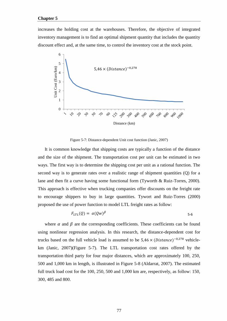
Chapter 5
77
increases the holding cost at the warehouses. Therefore, the objective of integrated
inventory management is to find an optimal shipment quantity that includes the quantity
discount effect and, at the same time, to control the inventory cost at the stock point.
Figure 5-7: Distance-dependent Unit cost function (Janic, 2007)
It is common knowledge that shipping costs are typically a function of the distance
and the size of the shipment. The transportation cost per unit can be estimated in two
ways. The first way is to determine the shipping cost per unit as a rational function. The
second way is to generate rates over a realistic range of shipment quantities (Q) for a
lane and then fit a curve having some functional form (Tyworth & Ruiz-Torres, 2000).
This approach is effective when trucking companies offer discounts on the freight rate
to encourage shippers to buy in large quantities. Tywort and Ruiz-Torres (2000)
proposed the use of power function to model LTL freight rates as follow:
𝐹𝐿𝑇𝐿(𝑄) = 𝛼(𝑄𝑤)𝛽 5-6
where 𝛼 and 𝛽 are the corresponding coefficients. These coefficients can be found
using nonlinear regression analysis. In this research, the distance-dependent cost for
trucks based on the full vehicle load is assumed to be 5,46 × (𝐷𝑖𝑠𝑡𝑎𝑛𝑐𝑒)−0,278 vehicle-
km (Janic, 2007)(Figure 5-7). The LTL transportation cost rates offered by the
transportation third party for four major distances, which are approximately 100, 250,
500 and 1,000 km in length, is illustrated in Figure 5-8 (Aldarrat, 2007). The estimated
full truck load cost for the 100, 250, 500 and 1,000 km are, respectively, as follow: 150,
300, 485 and 800.
0
1
2
3
4
5
6U
nit
Co
st (
Euro
/km
)
Distance (km)
5,46 × 𝐷𝑖𝑠𝑡𝑎𝑛𝑐𝑒 −0,278
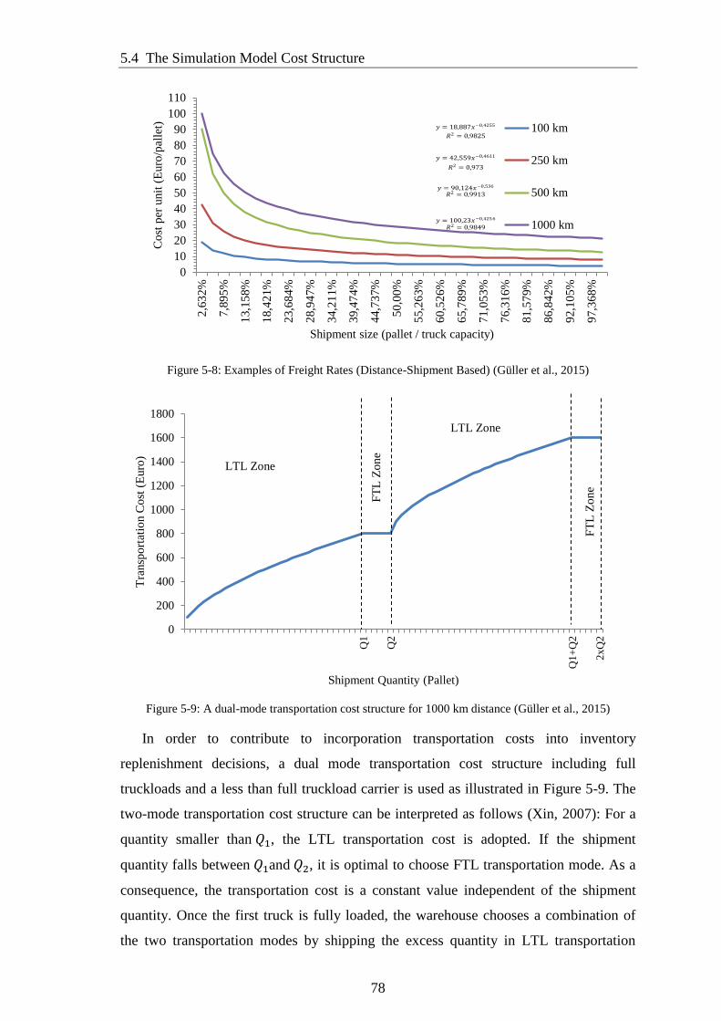
5.4 The Simulation Model Cost Structure
78
Figure 5-8: Examples of Freight Rates (Distance-Shipment Based) (Güller et al., 2015)
Figure 5-9: A dual-mode transportation cost structure for 1000 km distance (Güller et al., 2015)
In order to contribute to incorporation transportation costs into inventory
replenishment decisions, a dual mode transportation cost structure including full
truckloads and a less than full truckload carrier is used as illustrated in Figure 5-9. The
two-mode transportation cost structure can be interpreted as follows (Xin, 2007): For a
quantity smaller than 𝑄1, the LTL transportation cost is adopted. If the shipment
quantity falls between 𝑄1and 𝑄2, it is optimal to choose FTL transportation mode. As a
consequence, the transportation cost is a constant value independent of the shipment
quantity. Once the first truck is fully loaded, the warehouse chooses a combination of
the two transportation modes by shipping the excess quantity in LTL transportation
0
10
20
30
40
50
60
70
80
90
100
110
2,6
32
%
7,8
95
%
13,1
58%
18,4
21%
23,6
84%
28,9
47%
34,2
11%
39,4
74%
44,7
37%
50,0
0%
55,2
63%
60,5
26%
65,7
89%
71,0
53%
76,3
16%
81,5
79%
86,8
42%
92,1
05%
97,3
68%
Co
st p
er u
nit
(E
uro
/pal
let)
Shipment size (pallet / truck capacity)
100 km
250 km
500 km
1000 km
𝑦 = 18,887𝑥−0,4255
𝑅2 = 0,9825
𝑦 = 42,559𝑥−0,4611
𝑅2 = 0,973
𝑦 = 90,124𝑥−0,536 𝑅2 = 0,9913
𝑦 = 100,23𝑥−0,4256 𝑅2 = 0,9849
0
200
400
600
800
1000
1200
1400
1600
1800
Q1
Q2
Q1
+Q
2
2xQ
2
Tra
nsp
ort
atio
n C
ost
(E
uro
)
Shipment Quantity (Pallet)
FT
L Z
on
e
LTL Zone
LTL Zone
FT
L Z
on
e
Chapter 5
79
mode.
5.5 Supply Chain Performance Measures
It is important to define appropriate performance measures in logistic network
design and analysis. A performance measure, or a set of performance measures,
describes the feedback information to determine the efficiency and/or effectiveness of
an existing system, or to compare alternative systems (Beoman, 1998). According to
Beamon (1999), performance measures can be categorized as qualitative and
quantitative. Qualitative performance measures are the measures that cannot be directly
described numerically, such as customer satisfaction, flexibility, and supplier
performance. Quantitative performance measures can be presented in numerical format.
Quantitative supply chain performance measures may be associated with the objectives
of the supply chain: cost, profit, and customer responsiveness. In this research, the
performance measures identified through simulation are total system-wide cost, average
waiting time in the system, average number of backorders and customer responsiveness.
5.5.1 Notations
In this section, the notations used in the multi-echelon inventory system are
introduced as follows:
Table 5-5: Notation explanation for the simulation model
Variables Definition
index
j Plants index
k Warehouse index
l Distribution center index
t Time index
parameters
J Number of plants
K Number of warehouses
L Number of distribution center
𝐼𝑡𝑖 Average inventory level of location i at time t
𝐵𝑡𝑘 Average backordered items of location i at time t
T Planning period
𝑂𝑡𝑖 Number of placed order by location i at period t
ℎ𝑖 Holding cost per item per time at location i

5.5 Supply Chain Performance Measures
80
𝑝𝑖 Stockout cost per item per time at location i
𝐴𝑖 Fixed order cost at location i
𝑇𝑅𝑐 Truck Capacity
𝑄𝑖 Replenishment quantity of location i in pallet unit
𝐹𝑘𝑗() Transportation cost function between location k and j
𝐷𝑡𝑖 Total demand in location i’s customer zone during a period t
𝑊𝑡 Waiting time
𝐿𝑡 Lead-time
𝑅𝑡 Replenishment time
𝑃𝑡 Order placed time
𝑂𝑃𝐾𝑖 Number of order-picking cartons at location i
𝑂𝑃𝐾𝐶𝑖 Order-picking cost per carton at location i
𝐿𝑜𝑎𝑑𝐶𝑖 Loading cost at location i
𝑈𝐿𝑜𝑎𝑑𝐶𝑖 Unloading cost at location i
𝑃𝑎𝑐𝑘𝐶𝑖 Packing cost at location i
5.5.2 Measure Based on Cost
The total cost function consists of five costs: holding cost, backorder cost, ordering
cost, warehousing cost and shipping cost. The holding and backorder costs are
composed of costs due to warehouses’ inventory and retailers’ inventory. Supply chain
costs in this model consist of the following components:
- Total Supply Chain Holding cost of products at all stock points.
𝐴𝑣𝑒𝑟𝑎𝑔𝑒𝐼𝑛𝑣𝑒𝑛𝑡𝑜𝑟𝑦 = 𝐼𝐴𝑙𝑙,𝑡 =∑ ∑ 𝐼𝑡
𝑖𝑇𝑡=1
𝐾𝑘=1
𝑇+
∑ ∑ 𝐼𝑡𝑙𝑇
𝑡=1𝐿𝑙=1
𝑇 5-7
𝑇𝑆𝐶𝐻 = ∑ ∑(𝐼𝑡
𝑘 × ℎ𝑘)
𝐾
𝑘=1
𝑇
𝑡=1
+ ∑ ∑(𝐼𝑡𝑙 × ℎ𝑙)
𝐿
𝑙=1
𝑇
𝑡=1
5-8
- Total Supply Chain Stock-out cost of products.
𝐴𝑣𝑒𝑟𝑎𝑔𝑒𝐵𝑎𝑐𝑘𝑜𝑟𝑑𝑒𝑟 = 𝐵𝐴𝑙𝑙,𝑡 =∑ ∑ 𝐵𝑡
𝑘𝑇𝑡=1
𝐾𝑘=1
𝑇+
∑ ∑ 𝐵𝑡𝑙𝑇
𝑡=1𝐿𝑙=1
𝑇 5-9
𝑇𝑆𝐶𝐵 = ∑ ∑(𝐵𝑡
𝑘 × 𝑝𝑘)
𝐾
𝑘=1
𝑇
𝑡=1
+ ∑ ∑(𝐵𝑡𝑙 × 𝑝𝑙)
𝐿
𝑙=1
𝑇
𝑡=1
5-10
- Total Supply Chain Ordering Cost (TSCO)
𝑇𝑆𝐶𝑂 = ∑ ∑ 𝑂𝑡𝑘
𝑇
𝑡=1
× 𝐴𝑘
𝐾
𝑘=1
+ ∑ ∑ 𝑂𝑡𝑙 × 𝐴𝑙
𝑇
𝑡=1
𝐿
𝑙=1
5-11
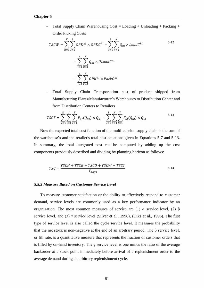
Chapter 5
81
- Total Supply Chain Warehousing Cost = Loading + Unloading + Packing +
Order Picking Costs
𝑇𝑆𝐶𝑊 = ∑ ∑ 𝑂𝑃𝐾𝑘𝑙
𝐿
𝑙=1
× 𝑂𝑃𝐾𝐶𝑘𝑙
𝐾
𝑘=1
+ ∑ ∑ 𝑄𝑘𝑙 ×
𝐾
𝑘=1
𝐿
𝑙=1
𝐿𝑜𝑎𝑑𝐶𝑘𝑙
+ ∑ ∑ 𝑄𝑘𝑙 ×
𝐾
𝑘=1
𝐿
𝑙=1
𝑈𝐿𝑜𝑎𝑑𝐶𝑘𝑙
+ ∑ ∑ 𝑂𝑃𝐾𝑘𝑙 ×
𝐾
𝑘=1
𝐿
𝑙=1
𝑃𝑎𝑐𝑘𝐶𝑘𝑙
5-12
- Total Supply Chain Transportation cost of product shipped from
Manufacturing Plants/Manufacturer’s Warehouses to Distribution Center and
from Distribution Centers to Retailers
𝑇𝑆𝐶𝑇 = ∑ ∑ ∑ 𝐹𝑘𝑗(𝑄𝑘𝑗) × 𝑄𝑘𝑗
𝑇
𝑡=1
𝐽
𝑖=1
𝐾
𝑘=1
+ ∑ ∑ ∑ 𝐹𝑙𝑘(𝑄𝑙𝑘) × 𝑄𝑙𝑘
𝑇
𝑡=1
𝐾
𝑘=1
𝐿
𝑙=1
5-13
Now the expected total cost function of the multi-echelon supply chain is the sum of
the warehouse’s and the retailer's total cost equations given in Equations 5-7 and 5-13.
In summary, the total integrated cost can be computed by adding up the cost
components previously described and dividing by planning horizon as follows:
𝑇𝑆𝐶 =𝑇𝑆𝐶𝐻 + 𝑇𝑆𝐶𝐵 + 𝑇𝑆𝐶𝑂 + 𝑇𝑆𝐶𝑊 + 𝑇𝑆𝐶𝑇
𝑇𝑑𝑎𝑦𝑠 5-14
5.5.3 Measure Based on Customer Service Level
To measure customer satisfaction or the ability to effectively respond to customer
demand, service levels are commonly used as a key performance indicator by an
organization. The most common measures of service are (1) α service level, (2) β
service level, and (3) γ service level (Silver et al., 1998), (Diks et al., 1996). The first
type of service level is also called the cycle service level. It measures the probability
that the net stock is non-negative at the end of an arbitrary period. The β service level,
or fill rate, is a quantitative measure that represents the fraction of customer orders that
is filled by on-hand inventory. The γ service level is one minus the ratio of the average
backorder at a stock point immediately before arrival of a replenishment order to the
average demand during an arbitrary replenishment cycle.
5.5 Supply Chain Performance Measures
82
𝛽𝑖 = ( 1
𝐿∑ 𝛽
𝑖
𝐿
𝑖
+ 1
𝐾∑ 𝛽
𝑖
𝐾
𝑖
) /2
= (1
𝐿(∑ (1 −
total number of backorders
total number of orders
𝐿
𝑖
))
+1
𝐾(∑ (1 −
total number of backorders
total number of orders
𝐾
𝑖
))) /2
= (1
𝐿∑ (1 −
∑ 𝐵𝑖𝑡𝑇
𝑡=1
∑ 𝐷𝑖𝑡𝑇
𝑡=1
) +1
𝐾∑ (1 −
∑ 𝐵𝑖𝑡𝑇
𝑡=1
∑ 𝐷𝑖𝑡𝑇
𝑡=1
)𝐾
𝑖
𝐿
𝑖
) /2
5-15
5.5.4 Measure based on Order Response Time
A node of a supply chain has five basic actions with regard to the life cycle of an
order which may be performed differently depending on the type of node: order
creation, order placement, order processing, order shipping, and order receiving
(Chatfield et al., 2006). The length of time between the placement of an order and its
receipt is called replenishment leadtime. Note that the replenishment leadtime is
potentially variable and depends on the availability of on-hand inventory at the
upstream supplier (Kaboli, 2013). In the event the central warehouse is out of stock, the
DC waits an additional time, 𝑊𝑡, the time until the warehouse is replenished by one of
its suppliers. Therefore, the total replenishment time of the distribution center, 𝑅𝑡, is:
𝑅𝑡 = 𝐿𝑡 + 𝑊𝑡 5-16
In Equation 5.16, Lt is the transportation between the central warehouse and the DC.
Again, even if the transportation time is deterministic, the waiting time is a random
variable and therefore so is the actual lead time. The random variable lead-time demand
is the key to determine the optimal inventory strategy (Zipkin, 2000). Since order
response time is a time-based measure, it is also a key indicator of performance.
Consequently, a service level measure based on response time for an order can be
defined as the total number of products delivered on time:
𝑅𝑒𝑠𝑇𝑖𝑚𝑒𝑖 =∑ (𝑅𝑡
𝑛 − 𝑃𝑡𝑛)𝑁
𝑛=1
𝑁 5-17

Chapter 5
83
5.6 Summary
In this chapter, a special library is described for the inventory simulation of multi-
echelon supply chain by using the object-oriented modeling approach (i.e., library using
Microsoft Visual C-Sharp), in which any part of the system with a set of classes is
presented. These classes include operations and objects representing nodes, interactions
between nodes, and the management of moving material between the different nodes
within the network. To define the performance measure of the supply chain, a cost
structure and other indicators are introduced. The total cost function consists of five
costs: holding cost, backorder cost, ordering cost, warehousing cost and transportation
cost. For the transportation cost, two types of freight rate structures are presented: a
non-linear Less-than-truckload (LTL) transportation cost function and a Full Truckload
(FTL) transportation cost function.
Chapter 6
Multi-echelon Supply Chain Inventory
Simulation Tool
This chapter addresses the development of a graphical user interface that depicts the
planning, managing and controlling of an inventory system; provides a brief description
of input and output parameters of the simulation model; outlines the assumptions made
during the simulation; and displays a pilot simulation environment for analyzing the
behavior of different inventory control strategies. As an application example of
developed object-oriented simulation framework a case study from the logistics domain
is briefly introduced. The main purpose for the experiments and case study in this
section is to show the effectiveness of the simulation model. By means of this
simulation framework economic implications of alternative replenishment and queue
strategies are analyzed and evaluated. The simulation experiment consists of the basic
supply chain nodes, each of which has its own customers, suppliers, and inventory
policy. The benefits of the tool are its capability to link with databases to import and
export information, graphical user interface, and integration of the optimization tool.
This tool provides broad functionality for optimization and analysis of output files. The
rest of this chapter is organized as follows. Section 6.1 presents the simulation
environment. Section 6.2 introduces the supply chain simulation case study and the
experimental settings. The simulation study with numerical results is the subject of
Section 6.3.
6.1 Simulation Environment
6.1.1 Simulation Tool Input Parameters
Several input parameters are required to run the simulation model correctly. In
particular, data on plants, central warehouses, DCs, retailers, and the transportation
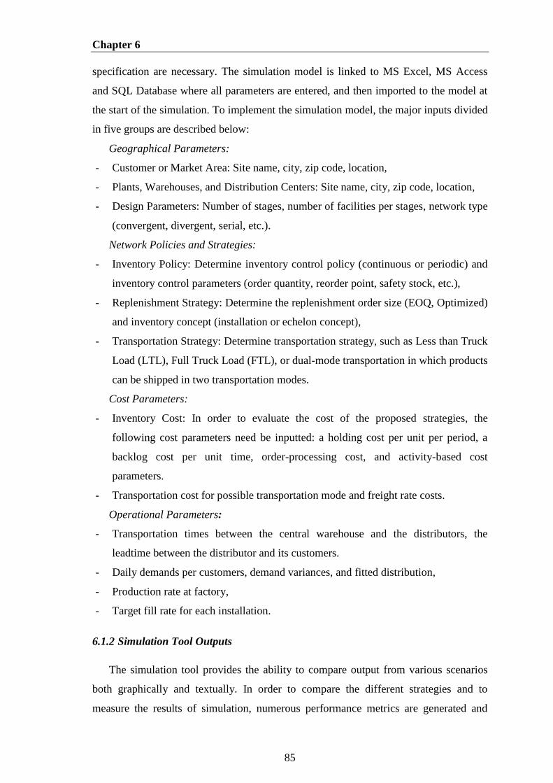
Chapter 6
85
specification are necessary. The simulation model is linked to MS Excel, MS Access
and SQL Database where all parameters are entered, and then imported to the model at
the start of the simulation. To implement the simulation model, the major inputs divided
in five groups are described below:
Geographical Parameters:
- Customer or Market Area: Site name, city, zip code, location,
- Plants, Warehouses, and Distribution Centers: Site name, city, zip code, location,
- Design Parameters: Number of stages, number of facilities per stages, network type
(convergent, divergent, serial, etc.).
Network Policies and Strategies:
- Inventory Policy: Determine inventory control policy (continuous or periodic) and
inventory control parameters (order quantity, reorder point, safety stock, etc.),
- Replenishment Strategy: Determine the replenishment order size (EOQ, Optimized)
and inventory concept (installation or echelon concept),
- Transportation Strategy: Determine transportation strategy, such as Less than Truck
Load (LTL), Full Truck Load (FTL), or dual-mode transportation in which products
can be shipped in two transportation modes.
Cost Parameters:
- Inventory Cost: In order to evaluate the cost of the proposed strategies, the
following cost parameters need be inputted: a holding cost per unit per period, a
backlog cost per unit time, order-processing cost, and activity-based cost
parameters.
- Transportation cost for possible transportation mode and freight rate costs.
Operational Parameters:
- Transportation times between the central warehouse and the distributors, the
leadtime between the distributor and its customers.
- Daily demands per customers, demand variances, and fitted distribution,
- Production rate at factory,
- Target fill rate for each installation.
6.1.2 Simulation Tool Outputs
The simulation tool provides the ability to compare output from various scenarios
both graphically and textually. In order to compare the different strategies and to
measure the results of simulation, numerous performance metrics are generated and
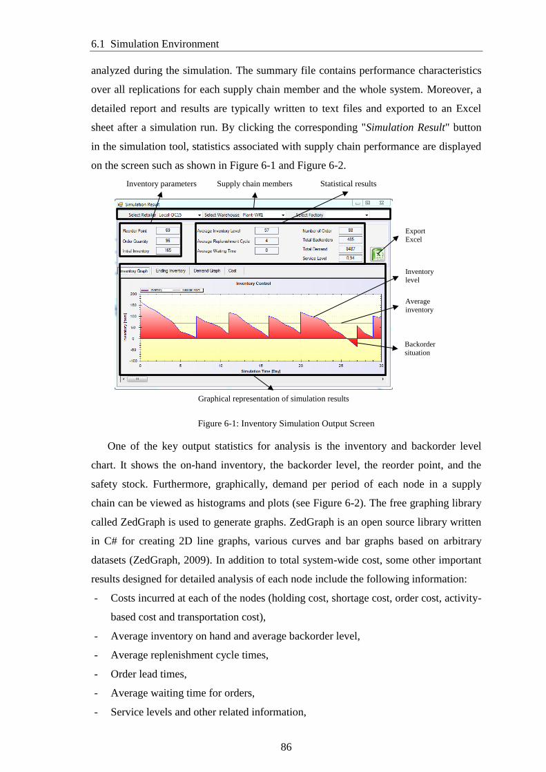
6.1 Simulation Environment
86
analyzed during the simulation. The summary file contains performance characteristics
over all replications for each supply chain member and the whole system. Moreover, a
detailed report and results are typically written to text files and exported to an Excel
sheet after a simulation run. By clicking the corresponding "Simulation Result" button
in the simulation tool, statistics associated with supply chain performance are displayed
on the screen such as shown in Figure 6-1 and Figure 6-2.
Figure 6-1: Inventory Simulation Output Screen
One of the key output statistics for analysis is the inventory and backorder level
chart. It shows the on-hand inventory, the backorder level, the reorder point, and the
safety stock. Furthermore, graphically, demand per period of each node in a supply
chain can be viewed as histograms and plots (see Figure 6-2). The free graphing library
called ZedGraph is used to generate graphs. ZedGraph is an open source library written
in C# for creating 2D line graphs, various curves and bar graphs based on arbitrary
datasets (ZedGraph, 2009). In addition to total system-wide cost, some other important
results designed for detailed analysis of each node include the following information:
- Costs incurred at each of the nodes (holding cost, shortage cost, order cost, activity-
based cost and transportation cost),
- Average inventory on hand and average backorder level,
- Average replenishment cycle times,
- Order lead times,
- Average waiting time for orders,
- Service levels and other related information,
Statistical results Inventory parameters
Graphical representation of simulation results
Supply chain members
Backorder
situation
Average
inventory
Inventory
level
Export
Excel

Chapter 6
87
- Number of orders placed on the upstream stage for the selected period.
Figure 6-2: Example simulation graph outputs
6.2 Illustrative Example and Simulation Settings
In this section, a case study is conducted with the proposed simulation model. The
modeling methodology is applied to the supply chain of a major food product company
in Europe. A make-to-stock (MTS) supply chain network with manufacturers, finished
goods warehouses, regional distribution centers with planned inventories and retailers
were all considered. The given network consists of 3 manufacturing sites, 3 plant
warehouses, 19 regional distribution centers, and approximately more than 1,000
retailers spread over the country. From the plants’ warehouses the goods are shipped to
the regional distribution centers from which they are delivered to the retail stores
(Güller et al., 2015). Figure 6-3 illustrates the network considered under the study.
Under the given supply chain network, products at plants are produced according to a
constant production rate that is larger than the DC’s demand rate (𝑃 > 𝐷 where
𝐷 = ∑ 𝐷𝑙). In other words, items are produced in batches at a finite rate at plants. The
plants do not produce the same product types. Historical sales data reveals that the DCs’
a) Total Cost b) Demand Histogram
c) Daily Demand
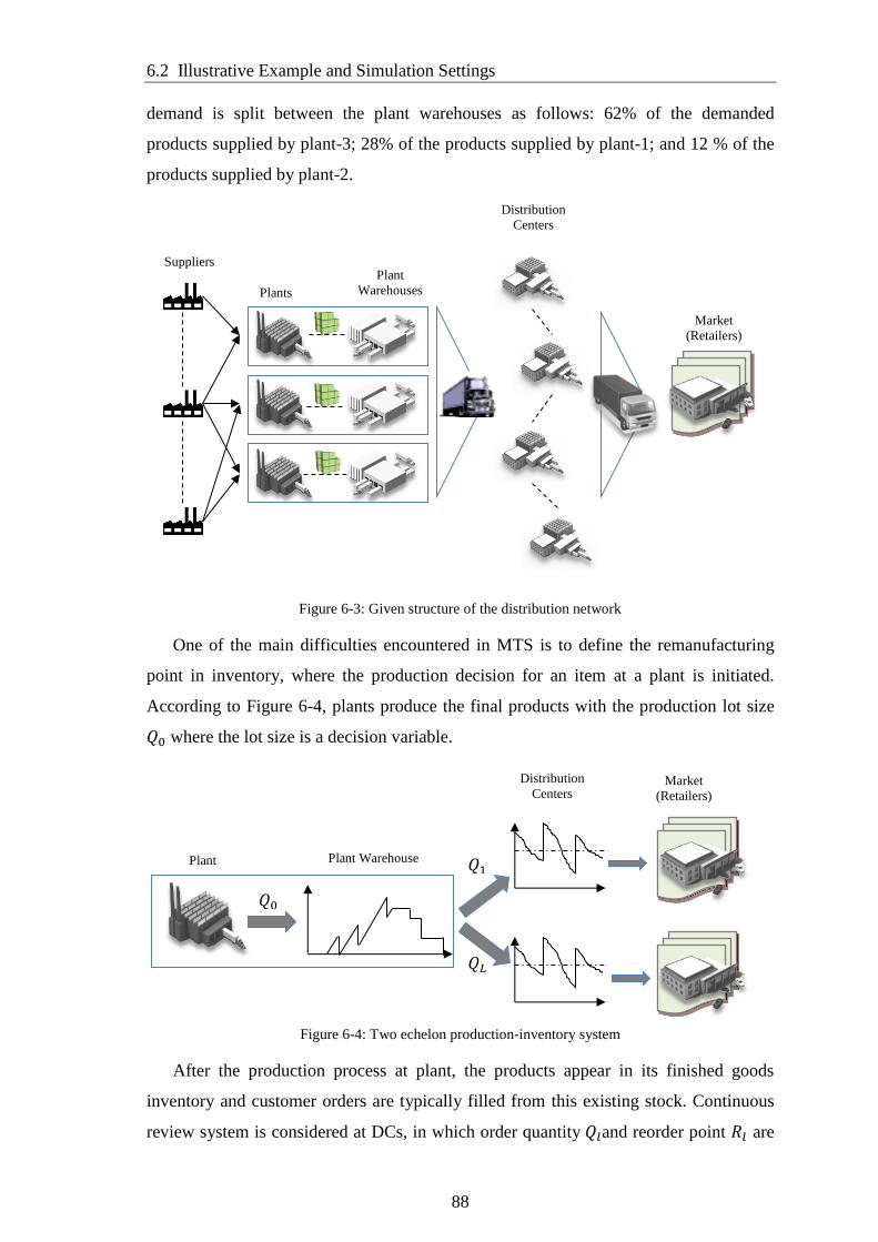
6.2 Illustrative Example and Simulation Settings
88
demand is split between the plant warehouses as follows: 62% of the demanded
products supplied by plant-3; 28% of the products supplied by plant-1; and 12 % of the
products supplied by plant-2.
Figure 6-3: Given structure of the distribution network
One of the main difficulties encountered in MTS is to define the remanufacturing
point in inventory, where the production decision for an item at a plant is initiated.
According to Figure 6-4, plants produce the final products with the production lot size
𝑄0 where the lot size is a decision variable.
Figure 6-4: Two echelon production-inventory system
After the production process at plant, the products appear in its finished goods
inventory and customer orders are typically filled from this existing stock. Continuous
review system is considered at DCs, in which order quantity 𝑄𝑙and reorder point 𝑅𝑙 are
Plant Warehouse Plant
𝑄0
𝑄1
𝑄𝐿
Distribution
Centers Market
(Retailers)
Plant
Warehouses Plants
Suppliers
Distribution
Centers
Market
(Retailers)

Chapter 6
89
main decision variables. In this context, whenever the inventory level in DCs drops
below the reorder point 𝑅𝑙, it triggers an order 𝑄𝑙. It is assumed that the replenishment
orders are always placed at the end of the day and each distribution center receives daily
orders of items from retailers. Any customer order that cannot be filled immediately is
backordered.
Data collection is a critical supply chain activity to quantify the associated system
variables (De Sensi et al., 2008). The Data Collection step takes care of collecting data
in each member of the supply chain as well as finding the most suitable input parameter
for the simulation model. Each distribution center receives daily orders of different
items from retailers and customers. The average daily demand for each item is fitted to
some theoretical probability distributions using historical sales data of DCs.
Figure 6-5: Percentage of each Probability Distribution of Demand for a Warehouse (Housein, 2007)
A large number of studies assume a homogeneous normal distribution demand
pattern in supply chain problems because of its convenient mathematical properties.
However, actual customer demand may be better modelled with distributions that are
asymmetric and positive skew shape (Cobb et al., 2013). According to Tyworth and
O’Neill (1997), the normal approximation can lead to significant errors in safety stock.
Figure 6-5 presents the percentage of fitted probability distribution of a domestic
product for DCs. As shown in Figure 6-5, items are not homogeneous in terms of
demand distribution. Figure 6-6 shows the aggregated daily average demand, the
standard deviation, and the coefficient of variation (CV). Appendix C presents the fitted
probability distribution for each distribution center in the considered supply chain.
0%
5%
10%
15%
20%
25%
30%
35%
40%
45%
50%
No
rmal
Lo
gN
orm
al
Po
isso
n
Wei
bull
Gam
ma
Erl
ang
Bet
a
46%
13%
4% 4%
17%
8% 8%
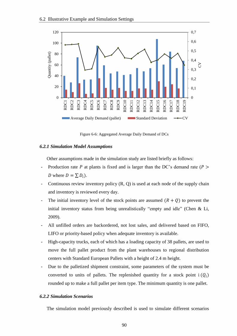
6.2 Illustrative Example and Simulation Settings
90
Figure 6-6: Aggregated Average Daily Demand of DCs
6.2.1 Simulation Model Assumptions
Other assumptions made in the simulation study are listed briefly as follows:
- Production rate 𝑃 at plants is fixed and is larger than the DC’s demand rate (𝑃 >
𝐷 where 𝐷 = ∑ 𝐷𝑖).
- Continuous review inventory policy (R, Q) is used at each node of the supply chain
and inventory is reviewed every day.
- The initial inventory level of the stock points are assumed (𝑅 + 𝑄) to prevent the
initial inventory status from being unrealistically “empty and idle” (Chen & Li,
2009).
- All unfilled orders are backordered, not lost sales, and delivered based on FIFO,
LIFO or priority-based policy when adequate inventory is available.
- High-capacity trucks, each of which has a loading capacity of 38 pallets, are used to
move the full pallet product from the plant warehouses to regional distribution
centers with Standard European Pallets with a height of 2.4 m height.
- Due to the palletized shipment constraint, some parameters of the system must be
converted to units of pallets. The replenished quantity for a stock point i (𝑄𝑖)
rounded up to make a full pallet per item type. The minimum quantity is one pallet.
6.2.2 Simulation Scenarios
The simulation model previously described is used to simulate different scenarios
0
0,1
0,2
0,3
0,4
0,5
0,6
0,7
0
20
40
60
80
100
120
RD
C1
RD
C2
RD
C3
RD
C4
RD
C5
RD
C6
RD
C7
RD
C8
RD
C9
RD
C1
0
RD
C1
1
RD
C1
2
RD
C1
3
RD
C1
4
RD
C1
5
RD
C1
6
RD
C1
7
RD
C1
8
RD
C1
9
CV
Quan
tity
(p
alle
t)
Average Daily Demand (pallet) Standard Deviation CV
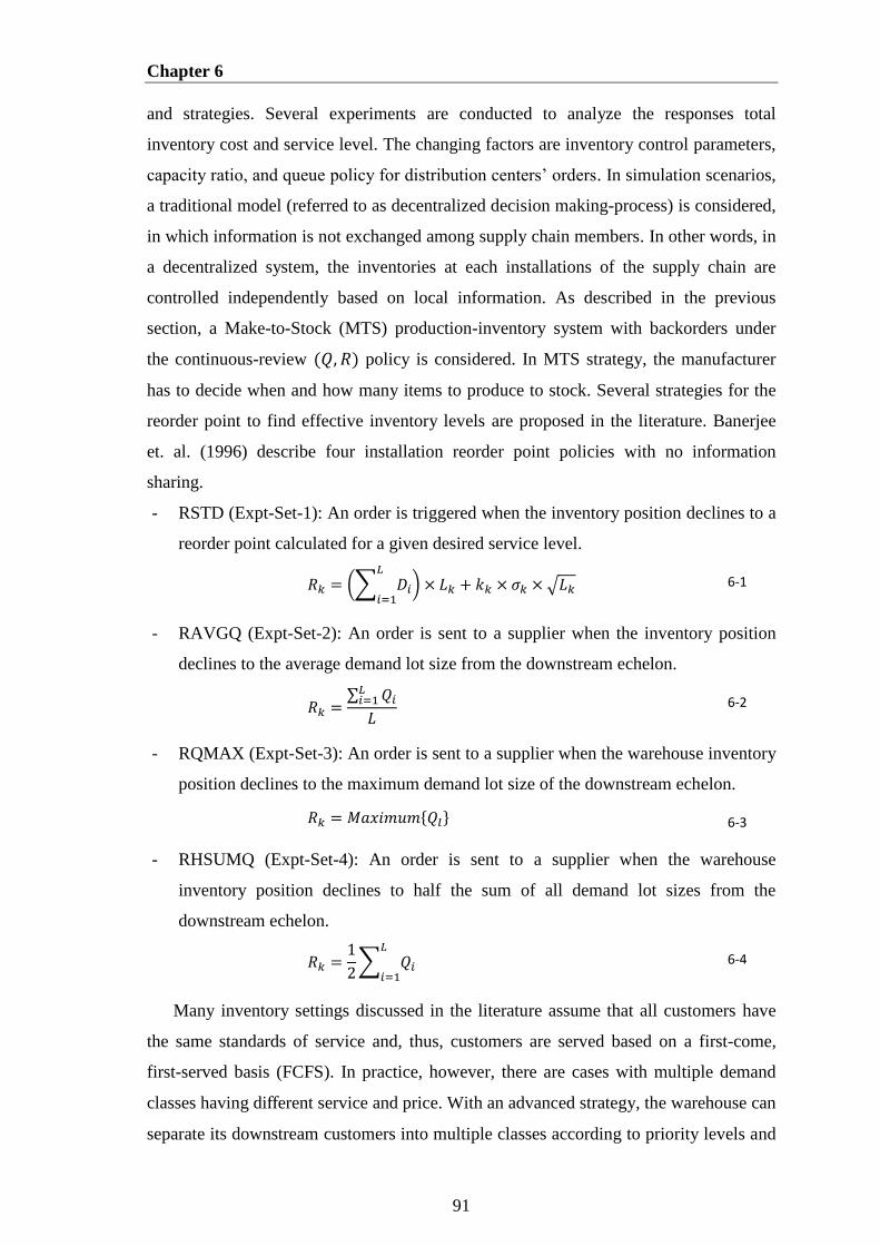
Chapter 6
91
and strategies. Several experiments are conducted to analyze the responses total
inventory cost and service level. The changing factors are inventory control parameters,
capacity ratio, and queue policy for distribution centers’ orders. In simulation scenarios,
a traditional model (referred to as decentralized decision making-process) is considered,
in which information is not exchanged among supply chain members. In other words, in
a decentralized system, the inventories at each installations of the supply chain are
controlled independently based on local information. As described in the previous
section, a Make-to-Stock (MTS) production-inventory system with backorders under
the continuous-review (𝑄, 𝑅) policy is considered. In MTS strategy, the manufacturer
has to decide when and how many items to produce to stock. Several strategies for the
reorder point to find effective inventory levels are proposed in the literature. Banerjee
et. al. (1996) describe four installation reorder point policies with no information
sharing.
- RSTD (Expt-Set-1): An order is triggered when the inventory position declines to a
reorder point calculated for a given desired service level.
𝑅𝑘 = (∑ 𝐷𝑖
𝐿
𝑖=1) × 𝐿𝑘 + 𝑘𝑘 × 𝜎𝑘 × √𝐿𝑘 6-1
- RAVGQ (Expt-Set-2): An order is sent to a supplier when the inventory position
declines to the average demand lot size from the downstream echelon.
𝑅𝑘 =∑ 𝑄𝑖
𝐿𝑖=1
𝐿 6-2
- RQMAX (Expt-Set-3): An order is sent to a supplier when the warehouse inventory
position declines to the maximum demand lot size of the downstream echelon.
𝑅𝑘 = 𝑀𝑎𝑥𝑖𝑚𝑢𝑚{𝑄𝑙} 6-3
- RHSUMQ (Expt-Set-4): An order is sent to a supplier when the warehouse
inventory position declines to half the sum of all demand lot sizes from the
downstream echelon.
𝑅𝑘 =1
2∑ 𝑄𝑖
𝐿
𝑖=1 6-4
Many inventory settings discussed in the literature assume that all customers have
the same standards of service and, thus, customers are served based on a first-come,
first-served basis (FCFS). In practice, however, there are cases with multiple demand
classes having different service and price. With an advanced strategy, the warehouse can
separate its downstream customers into multiple classes according to priority levels and
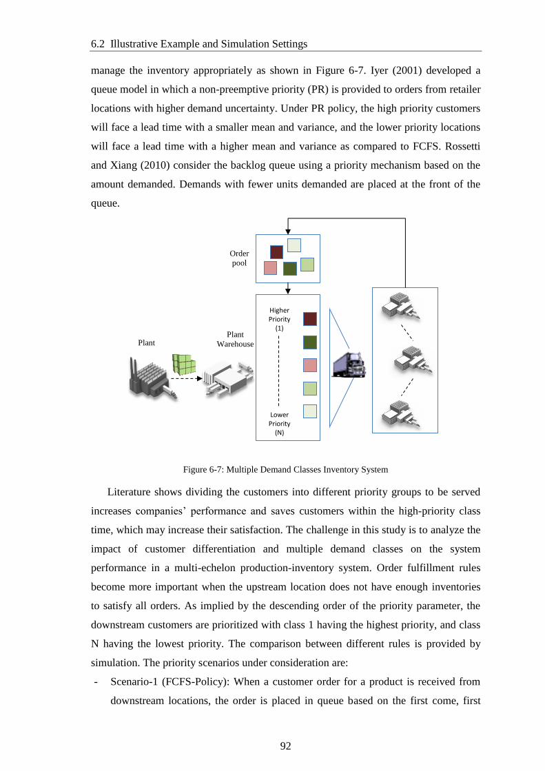
6.2 Illustrative Example and Simulation Settings
92
manage the inventory appropriately as shown in Figure 6-7. Iyer (2001) developed a
queue model in which a non-preemptive priority (PR) is provided to orders from retailer
locations with higher demand uncertainty. Under PR policy, the high priority customers
will face a lead time with a smaller mean and variance, and the lower priority locations
will face a lead time with a higher mean and variance as compared to FCFS. Rossetti
and Xiang (2010) consider the backlog queue using a priority mechanism based on the
amount demanded. Demands with fewer units demanded are placed at the front of the
queue.
Figure 6-7: Multiple Demand Classes Inventory System
Literature shows dividing the customers into different priority groups to be served
increases companies’ performance and saves customers within the high-priority class
time, which may increase their satisfaction. The challenge in this study is to analyze the
impact of customer differentiation and multiple demand classes on the system
performance in a multi-echelon production-inventory system. Order fulfillment rules
become more important when the upstream location does not have enough inventories
to satisfy all orders. As implied by the descending order of the priority parameter, the
downstream customers are prioritized with class 1 having the highest priority, and class
N having the lowest priority. The comparison between different rules is provided by
simulation. The priority scenarios under consideration are:
- Scenario-1 (FCFS-Policy): When a customer order for a product is received from
downstream locations, the order is placed in queue based on the first come, first
Plant
Warehouse
Order
pool
Higher Priority
(1)
Lower Priority
(N)
Plant

Chapter 6
93
served policy. Therefore, under this policy, completed items are allocated to the DC
based on whose order has waited the longest time in the system.
- Scenario-2 (Priority-CV-Policy): To develop a multiple demand-class inventory
model, customers are prioritized based on demand uncertainty. As implied by the
descending order of demand uncertainty, we prioritize downstream customers with
class 1 having the highest priority, and class N having the lowest priority.
- Scenario-3 (Priority-QMin-Policy): In this scenario the warehouse is assumed to
meet the demands of its customers based on amount demanded. With this scheme
the warehouse assigns a higher priority to its customer with lower batches
demanded within a period.
- Scenario-4 (Priority-QMax-Policy): In this scenario the warehouse assigns a higher
priority to its customer with highest batches within a period.
- Scenario-5 (Priority-QFreq-Policy): In this experiment, customers are prioritized
based on order frequency.
6.3 Simulation Results and Analysis
In our experimental settings, each simulation run is replicated ten times. Simulation
results are collected after running the model where the planning horizon is one year. It is
out of the scope of this chapter to report all simulation results in detail. Some simulation
results are reported and discussed at following sections. The base scenario is an
experiment with the determination of the optimal safety stock setting given a 95%
service level and order quantity calculated based on EOQ model (Appendix A). Figure
6-9 and Figure 6-8 indicate the results from the base experiment. The target service
level is compared with simulated service level of each RDC in Figure 6-10. The figure
clearly demonstrates the simulated service levels differ from the target service level.
Each bar represents the interval expected fill rate to the simulated fill rate at RDCs.
Values larger than zero indicate that the service level reached is higher than expected.
On the other hand, values smaller than zero (with red color) means that the target
service level is not reached.
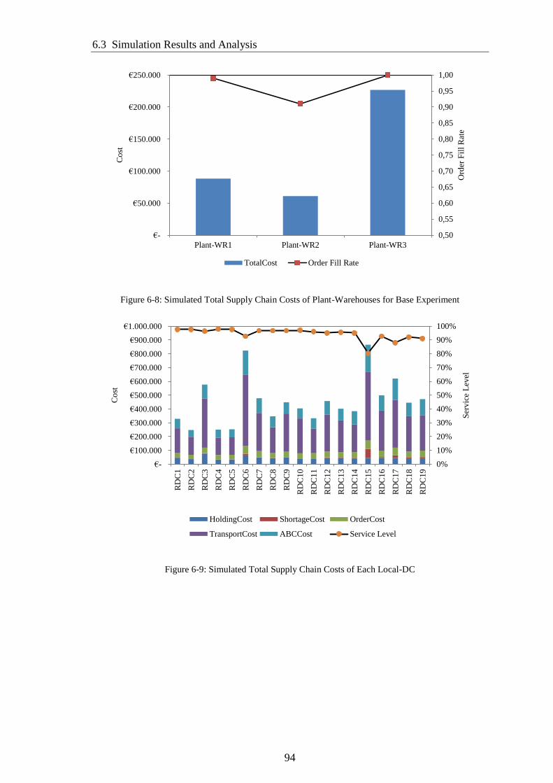
6.3 Simulation Results and Analysis
94
Figure 6-8: Simulated Total Supply Chain Costs of Plant-Warehouses for Base Experiment
Figure 6-9: Simulated Total Supply Chain Costs of Each Local-DC
0,50
0,55
0,60
0,65
0,70
0,75
0,80
0,85
0,90
0,95
1,00
€-
€50.000
€100.000
€150.000
€200.000
€250.000
Plant-WR1 Plant-WR2 Plant-WR3
Ord
er F
ill
Rat
e
Co
st
TotalCost Order Fill Rate
0%
10%
20%
30%
40%
50%
60%
70%
80%
90%
100%
€-
€100.000
€200.000
€300.000
€400.000
€500.000
€600.000
€700.000
€800.000
€900.000
€1.000.000
RD
C1
RD
C2
RD
C3
RD
C4
RD
C5
RD
C6
RD
C7
RD
C8
RD
C9
RD
C1
0
RD
C1
1
RD
C1
2
RD
C1
3
RD
C1
4
RD
C1
5
RD
C1
6
RD
C1
7
RD
C1
8
RD
C1
9
Ser
vic
e L
evel
Co
st
HoldingCost ShortageCost OrderCost
TransportCost ABCCost Service Level
Chapter 6
95
Figure 6-10: The Gap between Target Service Level and Simulated Service Level of DCs
6.3.1 Analysis of Replenishment Strategies without Information Sharing
The results of experimental sets are summarized in Table 6-1, where the numerical
performance measures represent an arithmetic average of the ten replications. For
continuous review policy without information sharing, we found that the best
performance of the system is achieved with RHSUMQ policy. Although in this case the
end-customer fill rate is better, the total system-wide cost is relatively small because of
the lower stock-out level. The change in the relative fill rate performance of Exp-Set-4
compared to the base experiment seems to be significant as the change in the cost is
relatively low. In Figure 6-11, it can be seen that, under RQMAX (Exp-Set-3) and
RAVGQ (Exp-Set-2) strategies, the average customer service level at RDCs decreases
while total cost dramatically increases as a result of stockout penalties.
In all the ordering policies without information sharing, there is a direct correlation
between a warehouse’s order fill rate and a DC’s customer service level. Interestingly,
some distribution centers perform very low in terms of service level in most of the
experiments due to high variations in demand rate and stockout conditions at plant
warehouses as shown in Figure 6-12 (for example RDC15). In other words, stockout
level at Plant-WR has a significant impact on customer service level, depending on the
order response time at the warehouse. In the event a warehouse goes out of stock, the
regional-DCs wait an additional time. Since lead time of the DC’s replenishment order
is a function of the expected waiting time due to a lack of stock at the higher echelon,
the backorder fraction increases at the lower echelon by increasing lead time
uncertainty.
-16%
-14%
-12%
-10%
-8%
-6%
-4%
-2%
0%
2%
4%
RD
C1
RD
C2
RD
C3
RD
C4
RD
C5
RD
C6
RD
C7
RD
C8
RD
C9
RD
C1
0
RD
C1
1
RD
C1
2
RD
C1
3
RD
C1
4
RD
C1
5
RD
C1
6
RD
C1
7
RD
C1
8
RD
C1
9
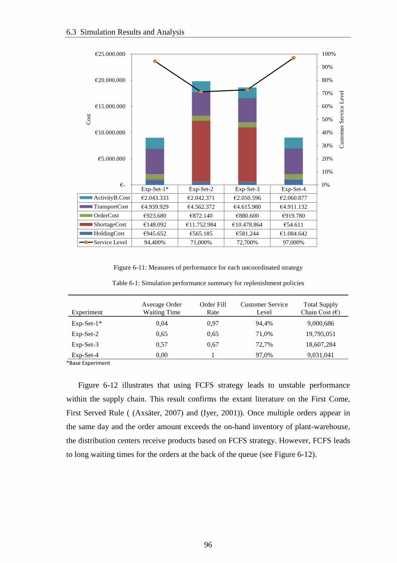
6.3 Simulation Results and Analysis
96
Figure 6-11: Measures of performance for each uncoordinated strategy
Table 6-1: Simulation performance summary for replenishment policies
Experiment
Average Order
Waiting Time
Order Fill
Rate
Customer Service
Level
Total Supply
Chain Cost (€)
Exp-Set-1* 0,04 0,97 94,4% 9,000,686
Exp-Set-2 0,65 0,65 71,0% 19,795,051
Exp-Set-3 0,57 0,67 72,7% 18,607,284
Exp-Set-4 0,00 1 97,0% 9,031,041
*Base Experiment
Figure 6-12 illustrates that using FCFS strategy leads to unstable performance
within the supply chain. This result confirms the extant literature on the First Come,
First Served Rule ( (Axsäter, 2007) and (Iyer, 2001)). Once multiple orders appear in
the same day and the order amount exceeds the on-hand inventory of plant-warehouse,
the distribution centers receive products based on FCFS strategy. However, FCFS leads
to long waiting times for the orders at the back of the queue (see Figure 6-12).
Exp-Set-1* Exp-Set-2 Exp-Set-3 Exp-Set-4
ActivityB.Cost €2.043.333 €2.042.371 €2.050.596 €2.060.877
TransportCost €4.939.929 €4.562.372 €4.615.980 €4.911.132
OrderCost €923.680 €872.140 €880.600 €919.780
ShortageCost €148.092 €11.752.984 €10.478.864 €54.611
HoldingCost €945.652 €565.185 €581.244 €1.084.642
Service Level 94,400% 71,000% 72,700% 97,000%
0%
10%
20%
30%
40%
50%
60%
70%
80%
90%
100%
€-
€5.000.000
€10.000.000
€15.000.000
€20.000.000
€25.000.000
Cu
sto
mer
Ser
vic
e L
evel
Co
st
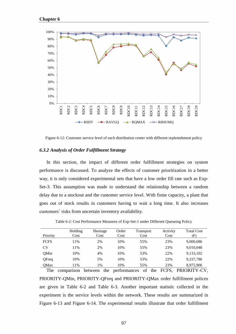
Chapter 6
97
Figure 6-12: Customer service level of each distribution center with different replenishment policy
6.3.2 Analysis of Order Fulfillment Strategy
In this section, the impact of different order fulfillment strategies on system
performance is discussed. To analyze the effects of customer prioritization in a better
way, it is only considered experimental sets that have a low order fill rate such as Exp-
Set-3. This assumption was made to understand the relationship between a random
delay due to a stockout and the customer service level. With finite capacity, a plant that
goes out of stock results in customers having to wait a long time. It also increases
customers’ risks from uncertain inventory availability.
Table 6-2: Cost Performance Measures of Exp-Set-1 under Different Queueing Policy
Priority
Holding
Cost
Shortage
Cost
Order
Cost
Transport
Cost
Activity
Cost
Total Cost
(€)
FCFS 11% 2% 10% 55% 23% 9,000,686
CV 11% 2% 10% 55% 23% 9,010,048
QMin 10% 4% 10% 53% 22% 9,133,102
QFreq 10% 5% 10% 53% 22% 9,337,786
QMax 11% 1% 10% 55% 23% 8,975,906
The comparison between the performances of the FCFS, PRIORITY-CV,
PRIORITY-QMin, PRIORITY-QFreq and PRIORITY-QMax order fulfillment polices
are given in Table 6-2 and Table 6-3. Another important statistic collected in the
experiment is the service levels within the network. These results are summarized in
Figure 6-13 and Figure 6-14. The experimental results illustrate that order fulfillment
0%
10%
20%
30%
40%
50%
60%
70%
80%
90%
100%
RD
C1
RD
C2
RD
C3
RD
C4
RD
C5
RD
C6
RD
C7
RD
C8
RD
C9
RD
C1
0
RD
C1
1
RD
C1
2
RD
C1
3
RD
C1
4
RD
C1
5
RD
C1
6
RD
C1
7
RD
C1
8
RD
C1
9
RSDT RAVGQ RQMAX RHSUMQ
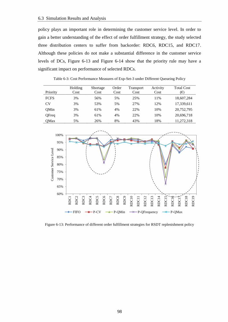
6.3 Simulation Results and Analysis
98
policy plays an important role in determining the customer service level. In order to
gain a better understanding of the effect of order fulfillment strategy, the study selected
three distribution centers to suffer from backorder: RDC6, RDC15, and RDC17.
Although these policies do not make a substantial difference in the customer service
levels of DCs, Figure 6-13 and Figure 6-14 show that the priority rule may have a
significant impact on performance of selected RDCs.
Table 6-3: Cost Performance Measures of Exp-Set-3 under Different Queueing Policy
Priority
Holding
Cost
Shortage
Cost
Order
Cost
Transport
Cost
Activity
Cost
Total Cost
(€)
FCFS 3% 56% 5% 25% 11% 18,607,284
CV 3% 53% 5% 27% 12% 17,339,611
QMin 3% 61% 4% 22% 10% 20,752,795
QFreq 3% 61% 4% 22% 10% 20,696,718
QMax 5% 26% 8% 43% 18% 11,272,318
Figure 6-13: Performance of different order fulfillment strategies for RSDT replenishment policy
60%
65%
70%
75%
80%
85%
90%
95%
100%
RD
C1
RD
C2
RD
C3
RD
C4
RD
C5
RD
C6
RD
C7
RD
C8
RD
C9
RD
C1
0
RD
C1
1
RD
C1
2
RD
C1
3
RD
C1
4
RD
C1
5
RD
C1
6
RD
C1
7
RD
C1
8
RD
C1
9
Cu
sto
mer
Ser
vic
e L
evel
FIFO P-CV P-QMin P-QFrequency P-QMax
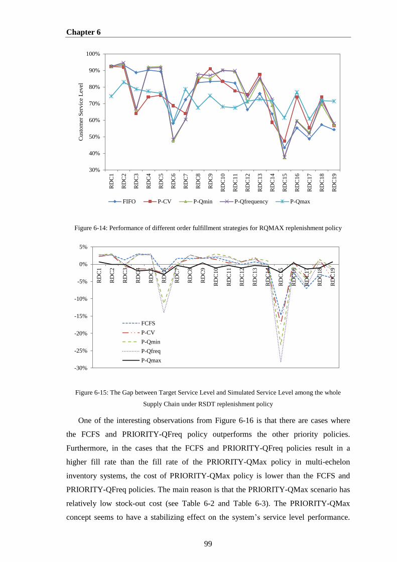
Chapter 6
99
Figure 6-14: Performance of different order fulfillment strategies for RQMAX replenishment policy
Figure 6-15: The Gap between Target Service Level and Simulated Service Level among the whole
Supply Chain under RSDT replenishment policy
One of the interesting observations from Figure 6-16 is that there are cases where
the FCFS and PRIORITY-QFreq policy outperforms the other priority policies.
Furthermore, in the cases that the FCFS and PRIORITY-QFreq policies result in a
higher fill rate than the fill rate of the PRIORITY-QMax policy in multi-echelon
inventory systems, the cost of PRIORITY-QMax policy is lower than the FCFS and
PRIORITY-QFreq policies. The main reason is that the PRIORITY-QMax scenario has
relatively low stock-out cost (see Table 6-2 and Table 6-3). The PRIORITY-QMax
concept seems to have a stabilizing effect on the system’s service level performance.
30%
40%
50%
60%
70%
80%
90%
100%
RD
C1
RD
C2
RD
C3
RD
C4
RD
C5
RD
C6
RD
C7
RD
C8
RD
C9
RD
C1
0
RD
C1
1
RD
C1
2
RD
C1
3
RD
C1
4
RD
C1
5
RD
C1
6
RD
C1
7
RD
C1
8
RD
C1
9
Cu
sto
mer
Ser
vic
e L
evel
FIFO P-CV P-Qmin P-Qfrequency P-Qmax
-30%
-25%
-20%
-15%
-10%
-5%
0%
5%
RD
C1
RD
C2
RD
C3
RD
C4
RD
C5
RD
C6
RD
C7
RD
C8
RD
C9
RD
C1
0
RD
C1
1
RD
C1
2
RD
C1
3
RD
C1
4
RD
C1
5
RD
C1
6
RD
C1
7
RD
C1
8
RD
C1
9
FCFS
P-CV
P-Qmin
P-Qfreq
P-Qmax
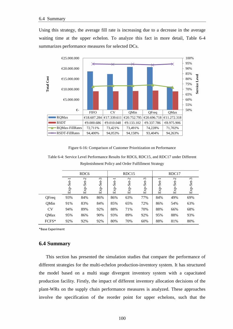
6.4 Summary
100
Using this strategy, the average fill rate is increasing due to a decrease in the average
waiting time at the upper echelon. To analyze this fact in more detail, Table 6-4
summarizes performance measures for selected DCs.
Figure 6-16: Comparison of Customer Prioritization on Performance
Table 6-4: Service Level Performance Results for RDC6, RDC15, and RDC17 under Different
Replenishment Policy and Order Fulfillment Strategy
RDC6
RDC15
RDC17
Ex
p-S
et-1
Ex
p-S
et-2
Ex
p-S
et-3
Ex
p-S
et-1
Ex
p-S
et-2
Ex
p-S
et-3
Ex
p-S
et-1
Ex
p-S
et-2
Ex
p-S
et-3
QFreq 93% 84% 86% 86% 63% 77% 84% 49% 69%
QMin 91% 83% 84% 85% 65% 72% 86% 54% 63%
CV 94% 89% 92% 88% 71% 70% 88% 66% 68%
QMax 95% 86% 90% 93% 89% 92% 95% 88% 93%
FCFS* 92% 92% 92% 80% 70% 60% 88% 81% 80%
*Base Experiment
6.4 Summary
This section has presented the simulation studies that compare the performance of
different strategies for the multi-echelon production-inventory system. It has structured
the model based on a multi stage divergent inventory system with a capacitated
production facility. Firstly, the impact of different inventory allocation decisions of the
plant-WRs on the supply chain performance measures is analyzed. These approaches
involve the specification of the reorder point for upper echelons, such that the
FIFO CV QMin QFreq QMax
RQMax €18.607.284 €17.339.611 €20.752.795 €20.696.718 €11.272.318
RSDT €9.000.686 €9.010.048 €9.133.102 €9.337.786 €8.975.906
RQMax-FillRates 72,711% 73,421% 73,491% 74,228% 71,702%
RSDT-FillRates 94,400% 94,053% 94,158% 93,404% 94,263%
50%
55%
60%
65%
70%
75%
80%
85%
90%
95%
100%
€-
€5.000.000
€10.000.000
€15.000.000
€20.000.000
€25.000.000
Ser
vic
e L
evel
Tota
l C
ost
Chapter 6
101
predetermined lot size is triggered whenever the net stock position drops to the reorder
point. It is found that for similar operating conditions and for similar performance
records, the RHSUMQ policy tends to perform better than the corresponding reorder
point policies. The change in the relative fill rate performance of RHSUMQ compared
to the base experiment seems to be significant since the change in the cost is relatively
low. In addition, a relationship between the order fulfillment policy and the customer
service level has been showed. According to the experimental results, customer
prioritization polices can reduce the total system cost in comparison to FCFS as they
increase the customer service level. One of the key findings in this chapter is that using
FCFS strategy can lead to unstable performance within the supply chain.
Chapter 7
Simulation-Based Optimization for Multi-
echelon Inventory Problems
Simulation modeling has recently become a major tool since an analytical model is
unable to formulate a system that is subject to both variability and complexity.
However, simulations require extensive runtime to evaluate many feasible solutions and
to find the optimal one for a defined problem. To deal with this problem, simulation
model needs to be integrated in optimization algorithms. (Keskin et al., 2010). This
chapter describes the design of a framework to carry out simulation-based optimization
of the inventory parameters of a multi-echelon production-inventory system. A brief
description of simulation-based optimization approach is presented in Section 7.1.
Section 7.2 presents the classification of simulation-based optimization methods. The
details of the proposed multi-objective metaheuristics for simulation-based optimization
approach are given in Section 7.3. Section 7.4 demonstrates the application of the
introduced framework for a simulation-based optimization with a real case study.
7.1 Introduction to Simulation-Based Optimization
Simulation-based optimization (SBO) is the process of obtaining optimal set of
control variables, where the objective functions and performance of the system are
generated as a result of the simulation model over the system (Olafsson & Kim, 2002).
Figure 7-1 illustrates the general scheme of the simulation-based optimization
procedure. In the context of SBO, the optimization engine includes upper and lower
bounds for input parameter, the optimization objectives with corresponding constraints,
and the optimization algorithms, while the simulation model incorporates the system
parameters, the representation of the real system with its boundaries, the internal and
external factors, and their relationship within the system (Aslam, 2013). In contrast to
traditional optimization approaches, in SBO, the performance measure generated by a
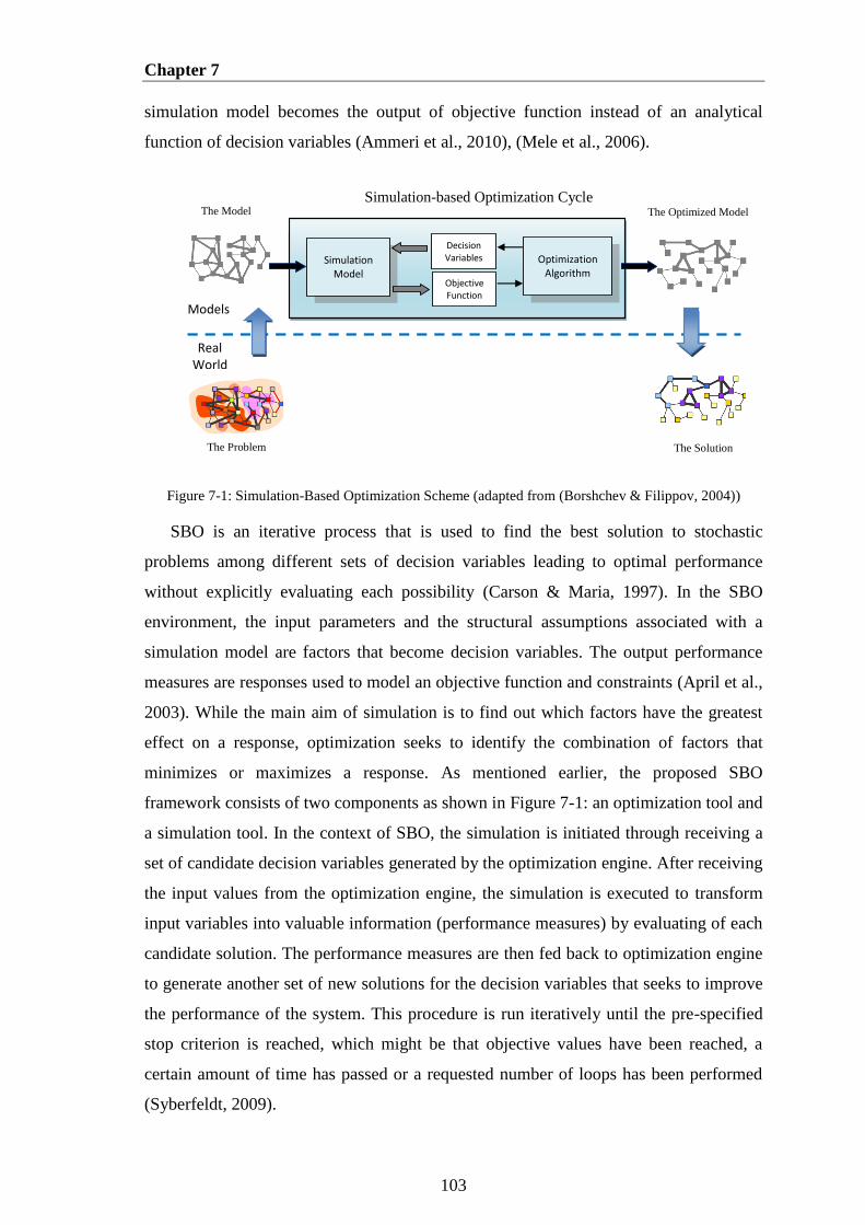
Chapter 7
103
simulation model becomes the output of objective function instead of an analytical
function of decision variables (Ammeri et al., 2010), (Mele et al., 2006).
Figure 7-1: Simulation-Based Optimization Scheme (adapted from (Borshchev & Filippov, 2004))
SBO is an iterative process that is used to find the best solution to stochastic
problems among different sets of decision variables leading to optimal performance
without explicitly evaluating each possibility (Carson & Maria, 1997). In the SBO
environment, the input parameters and the structural assumptions associated with a
simulation model are factors that become decision variables. The output performance
measures are responses used to model an objective function and constraints (April et al.,
2003). While the main aim of simulation is to find out which factors have the greatest
effect on a response, optimization seeks to identify the combination of factors that
minimizes or maximizes a response. As mentioned earlier, the proposed SBO
framework consists of two components as shown in Figure 7-1: an optimization tool and
a simulation tool. In the context of SBO, the simulation is initiated through receiving a
set of candidate decision variables generated by the optimization engine. After receiving
the input values from the optimization engine, the simulation is executed to transform
input variables into valuable information (performance measures) by evaluating of each
candidate solution. The performance measures are then fed back to optimization engine
to generate another set of new solutions for the decision variables that seeks to improve
the performance of the system. This procedure is run iteratively until the pre-specified
stop criterion is reached, which might be that objective values have been reached, a
certain amount of time has passed or a requested number of loops has been performed
(Syberfeldt, 2009).
Performance Measures
Decoding
Real World
Models
Simulation-based Optimization Cycle
Decision Variables
Objective Function
Simulation Model
Optimization Algorithm
The Problem
The Model The Optimized Model
The Solution
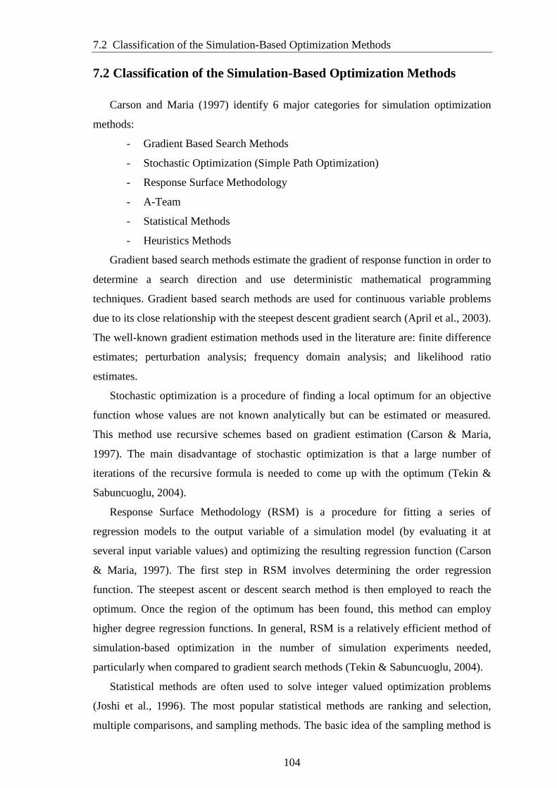
7.2 Classification of the Simulation-Based Optimization Methods
104
7.2 Classification of the Simulation-Based Optimization Methods
Carson and Maria (1997) identify 6 major categories for simulation optimization
methods:
- Gradient Based Search Methods
- Stochastic Optimization (Simple Path Optimization)
- Response Surface Methodology
- A-Team
- Statistical Methods
- Heuristics Methods
Gradient based search methods estimate the gradient of response function in order to
determine a search direction and use deterministic mathematical programming
techniques. Gradient based search methods are used for continuous variable problems
due to its close relationship with the steepest descent gradient search (April et al., 2003).
The well-known gradient estimation methods used in the literature are: finite difference
estimates; perturbation analysis; frequency domain analysis; and likelihood ratio
estimates.
Stochastic optimization is a procedure of finding a local optimum for an objective
function whose values are not known analytically but can be estimated or measured.
This method use recursive schemes based on gradient estimation (Carson & Maria,
1997). The main disadvantage of stochastic optimization is that a large number of
iterations of the recursive formula is needed to come up with the optimum (Tekin &
Sabuncuoglu, 2004).
Response Surface Methodology (RSM) is a procedure for fitting a series of
regression models to the output variable of a simulation model (by evaluating it at
several input variable values) and optimizing the resulting regression function (Carson
& Maria, 1997). The first step in RSM involves determining the order regression
function. The steepest ascent or descent search method is then employed to reach the
optimum. Once the region of the optimum has been found, this method can employ
higher degree regression functions. In general, RSM is a relatively efficient method of
simulation-based optimization in the number of simulation experiments needed,
particularly when compared to gradient search methods (Tekin & Sabuncuoglu, 2004).
Statistical methods are often used to solve integer valued optimization problems
(Joshi et al., 1996). The most popular statistical methods are ranking and selection,
multiple comparisons, and sampling methods. The basic idea of the sampling method is
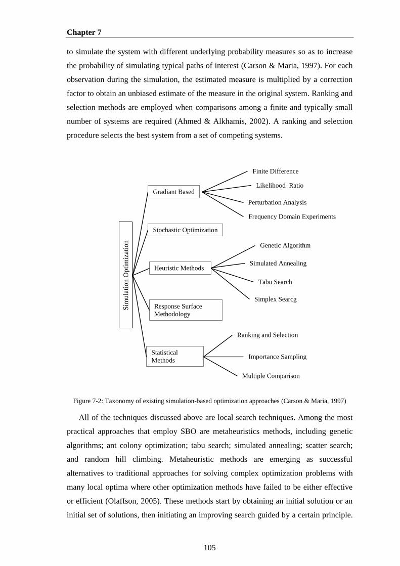
Chapter 7
105
to simulate the system with different underlying probability measures so as to increase
the probability of simulating typical paths of interest (Carson & Maria, 1997). For each
observation during the simulation, the estimated measure is multiplied by a correction
factor to obtain an unbiased estimate of the measure in the original system. Ranking and
selection methods are employed when comparisons among a finite and typically small
number of systems are required (Ahmed & Alkhamis, 2002). A ranking and selection
procedure selects the best system from a set of competing systems.
Figure 7-2: Taxonomy of existing simulation-based optimization approaches (Carson & Maria, 1997)
All of the techniques discussed above are local search techniques. Among the most
practical approaches that employ SBO are metaheuristics methods, including genetic
algorithms; ant colony optimization; tabu search; simulated annealing; scatter search;
and random hill climbing. Metaheuristic methods are emerging as successful
alternatives to traditional approaches for solving complex optimization problems with
many local optima where other optimization methods have failed to be either effective
or efficient (Olaffson, 2005). These methods start by obtaining an initial solution or an
initial set of solutions, then initiating an improving search guided by a certain principle.
Sim
ula
tion O
pti
miz
atio
n
Met
hods
Gradiant Based
Stochastic Optimization
Response Surface
Methodology
Heuristic Methods
Statistical
Methods
Finite Difference
Estimation Likelihood Ratio
Estimation
Perturbation Analysis
Frequency Domain Experiments
Genetic Algorithm
Simulated Annealing
Tabu Search
Simplex Searcg
Importance Sampling
Ranking and Selection
Multiple Comparison

7.3 Multi-Objective Optimization via Simulation
106
In the following we focus our interest on the metaheuristics approaches to the inventory
optimization problem.
7.3 Multi-Objective Optimization via Simulation
Optimization problems with two or more conflicting objectives arise in the design,
modeling, and planning of many complex real systems. One of the most important aims
of multi-objective optimization is to obtain feasible solutions that balance several
conflicting objectives. However, it is difficult to find such a solution due to the realities
of addressing real-world problems. The time required to solve multi-objective supply
chain problems stretches to become unpalatably long as the number of variables
increases. To overcome this challenge, the use of metaheuristics has received increasing
attention from the research community over the last decade. The motivation for using
metaheuristic algorithms is to produce efficient solutions to supply chain optimization
problems with a reasonable amount of computational time. One simple example of a
class of supply chain multi-objective optimization problems is the inventory control
problem. This section investigates the possibility of applying multi-objective
metaheuristic algorithms to a simulation-based optimization approach for a multi-
echelon production-inventory system. Chapter 3 reviewed a number of general
metaheuristic algorithms in the literature. An introduction to multi-objective
metaheuristic algorithms based on GA and PSO used to find optimal solutions was
given in Section 3.3. The two metaheuristic algorithms, which are under investigation in
this section, are NSGA-II and MOPSO, which show strong performance in solving
multi-objective optimization problems. In this study, both algorithms are developed in
an object-oriented manner using C-Sharp for modeling flexibility and execution
efficiency. Figure 7-3 shows the black-box approach to simulation based optimization
for inventory problems. The methodology used for solving multi-objective inventory
problems involves two phases (Niranjan, 2008):
- At the first phase, to generate possible the reorder point and the order
quantity of each stock point in the network based on the upper and lower
bounds, NSGA-II and MOPSO algorithms are.
- At the second phase, the developed object-oriented simulation model is used
to compare the performance of system under different decision variables.
The performance is measured according to different criteria: customer
service level, fill rate, number of backordered items, and total cost.
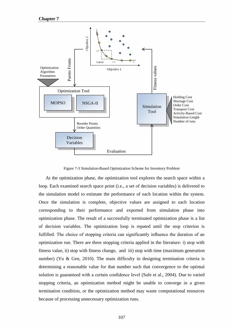
Chapter 7
107
Figure 7-3 Simulation-Based Optimization Scheme for Inventory Problem
At the optimization phase, the optimization tool explores the search space within a
loop. Each examined search space point (i.e., a set of decision variables) is delivered to
the simulation model to estimate the performance of each location within the system.
Once the simulation is complete, objective values are assigned to each location
corresponding to their performance and exported from simulation phase into
optimization phase. The result of a successfully terminated optimization phase is a list
of decision variables. The optimization loop is repated until the stop criterion is
fulfilled. The choice of stopping criteria can significantly influence the duration of an
optimization run. There are three stopping criteria applied in the literature: i) stop with
fitness value, ii) stop with fitness change, and iii) stop with time (maximum generation
number) (Yu & Gen, 2010). The main difficulty in designing termination criteria is
determining a reasonable value for that number such that convergence to the optimal
solution is guaranteed with a certain confidence level (Safe et al., 2004). Due to varied
stopping criteria, an optimization method might be unable to converge in a given
termination condition, or the optimization method may waste computational resources
because of processing unnecessary optimization runs.
Fit
nes
s val
ues
Reorder Points Order Quantities
Optimization Tool
Holding Cost Shortage Cost Order Cost Transport Cost Activity-Based Cost Simulation Length Number of runs
MOPSO
Decision
Variables
Evaluation
NSGA-II Simulation
Tool
Par
eto
Fro
nts
Optimization
Algorithm
Parameters
7.3 Multi-Objective Optimization via Simulation
108
7.3.1 Multi-Objective Simulation-based Optimization based on GA (NSGA-II-SO)
The proposed framework named multi-objective simulation-based optimization
using genetic algorithms (NSGA-II-SO) utilizes a population-based evolutionary
algorithm. Each solution of NSGA-II algorithm is represented by an n-dimensional
vector 𝑋 = (𝑥1, 𝑥2, … , 𝑥𝑛), where n is equal to the number of decision variables of the
problem under study. A decision variable 𝑥𝑖 is randomly generated according to a given
lower bound and upper bound. Figure 7-4 shows the flowchart of NSGA-II-SO. In
Phase 1, which is the NSGA-II run, the algorithm starts the search by generating a
population of candidate solutions. Each chromosome in the population is evaluated
through simulation in Phase 2 and ranked to form non-dominated fronts according to the
dominance concept. Evaluated and sorted chromosomes are then selected for
recombination by using binary tournament selection. Under this scheme, two
chromosomes are selected at random from the current population, and their fronts are
compared. The chromosome, which is in a lower domination frontier set, is selected as a
parent for crossover. During the selection, the crowding distance comparator is used to
select chromosomes, if both chromosomes belong to the same front. Next, the algorithm
applies crossover and mutation operators on selected parents to generate the next
generation. The algorithm runs until user-defined termination is satisfied.
7.3.2 Multi-Objective Simulation-based Optimization based on PSO (MOPSO-SO)
Another metaheuristic under consideration in this research is multi-objective
Particle Swarm Optimization (MOPSO). Using MOPSO as the mechanism to perform
multi-objective simulation-based optimization requires implementing the form of
NSGA-II-SO described in previous section with some modifications. Particle Swarm
Optimization (PSO) is similar to the Genetic Algorithm (GA) in the sense that these two
techniques are population-based search methods and they search for the optimal
solution by updating generations (Panda & Padhy, 2008). Like NSGA-II-SO, MOPSO-
SO begins its search from a randomly generated population. After the positions and
velocities of particles are initialized, the objective functions are evaluated via simulation
for each particle, as described in NSGA-II-SO. The concept of Pareto dominance is
applied to sort the solutions. The set of non-dominated solutions are all stored in an
external archive, in which the best non-dominated solutions are kept. MOPSO-SO
applies two operators to obtain its new population: velocity update and position update.
Each particle randomly selects a non-dominated solution from the archive for the social

Chapter 7
109
influence to update its velocity and position. The general flowchart of the simulation-
optimization based on MOPSO is illustrated in Figure 7-5. We refer the reader to the
Section 3.3.2 for more details.
Figure 7-4: Flowchart of the simulation optimization based on NSGA-II (NSGA-II-SO)
Recombination
Input
Output
Yes
No
Recombination
NSG
A-I
I
Yes
No
Parameter
Settings
Create Random Population
Evaluate Individuals
Assign Rank based on Pareto
Dominance and Crowding Distance
Termination Condition Satisfied
Tournament Selection
Crossover & Mutation
Combine Individuals with Previous
Population
Generate New Population
Elitism
End
Report Best Solutions
OPTIMIZATION PHASE SIMULATION PHASE
Simulate
Objective Functions
Fitness Values
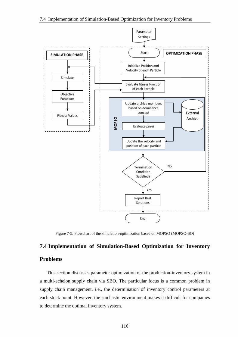
7.4 Implementation of Simulation-Based Optimization for Inventory Problems
110
Figure 7-5: Flowchart of the simulation-optimization based on MOPSO (MOPSO-SO)
7.4 Implementation of Simulation-Based Optimization for Inventory
Problems
This section discusses parameter optimization of the production-inventory system in
a multi-echelon supply chain via SBO. The particular focus is a common problem in
supply chain management, i.e., the determination of inventory control parameters at
each stock point. However, the stochastic environment makes it difficult for companies
to determine the optimal inventory system.
Yes
No
SIMULATION PHASE
Simulate
Objective Functions
Fitness Values
OPTIMIZATION PHASE
Initialize Position and Velocity of each Particle
Evaluate fitness function of each Particle
Update archive members based on dominance
concept External
Archive
Evaluate pbest
Update the velocity and position of each particle
Termination Condition Satisfied?
End
Report Best Solutions
Start
MO
PSO
Parameter
Settings
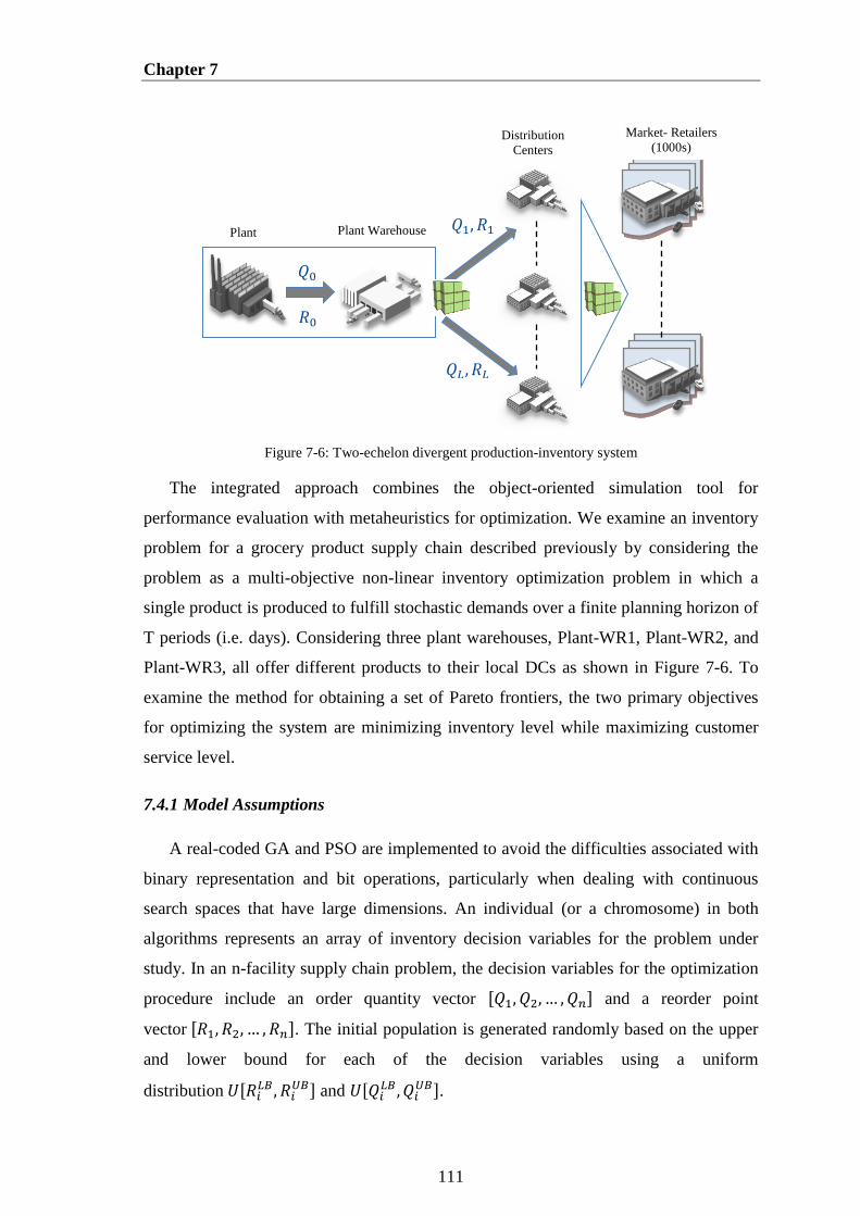
Chapter 7
111
Figure 7-6: Two-echelon divergent production-inventory system
The integrated approach combines the object-oriented simulation tool for
performance evaluation with metaheuristics for optimization. We examine an inventory
problem for a grocery product supply chain described previously by considering the
problem as a multi-objective non-linear inventory optimization problem in which a
single product is produced to fulfill stochastic demands over a finite planning horizon of
T periods (i.e. days). Considering three plant warehouses, Plant-WR1, Plant-WR2, and
Plant-WR3, all offer different products to their local DCs as shown in Figure 7-6. To
examine the method for obtaining a set of Pareto frontiers, the two primary objectives
for optimizing the system are minimizing inventory level while maximizing customer
service level.
7.4.1 Model Assumptions
A real-coded GA and PSO are implemented to avoid the difficulties associated with
binary representation and bit operations, particularly when dealing with continuous
search spaces that have large dimensions. An individual (or a chromosome) in both
algorithms represents an array of inventory decision variables for the problem under
study. In an n-facility supply chain problem, the decision variables for the optimization
procedure include an order quantity vector [𝑄1, 𝑄2, … , 𝑄𝑛] and a reorder point
vector [𝑅1, 𝑅2, … , 𝑅𝑛]. The initial population is generated randomly based on the upper
and lower bound for each of the decision variables using a uniform
distribution 𝑈[𝑅𝑖𝐿𝐵, 𝑅𝑖
𝑈𝐵] and 𝑈[𝑄𝑖𝐿𝐵, 𝑄𝑖
𝑈𝐵].
Plant Warehouse Plant
𝑄0
𝑄1,𝑅1
Distribution
Centers
𝑅0
𝑄𝐿 ,𝑅𝐿
Market- Retailers
(1000s)
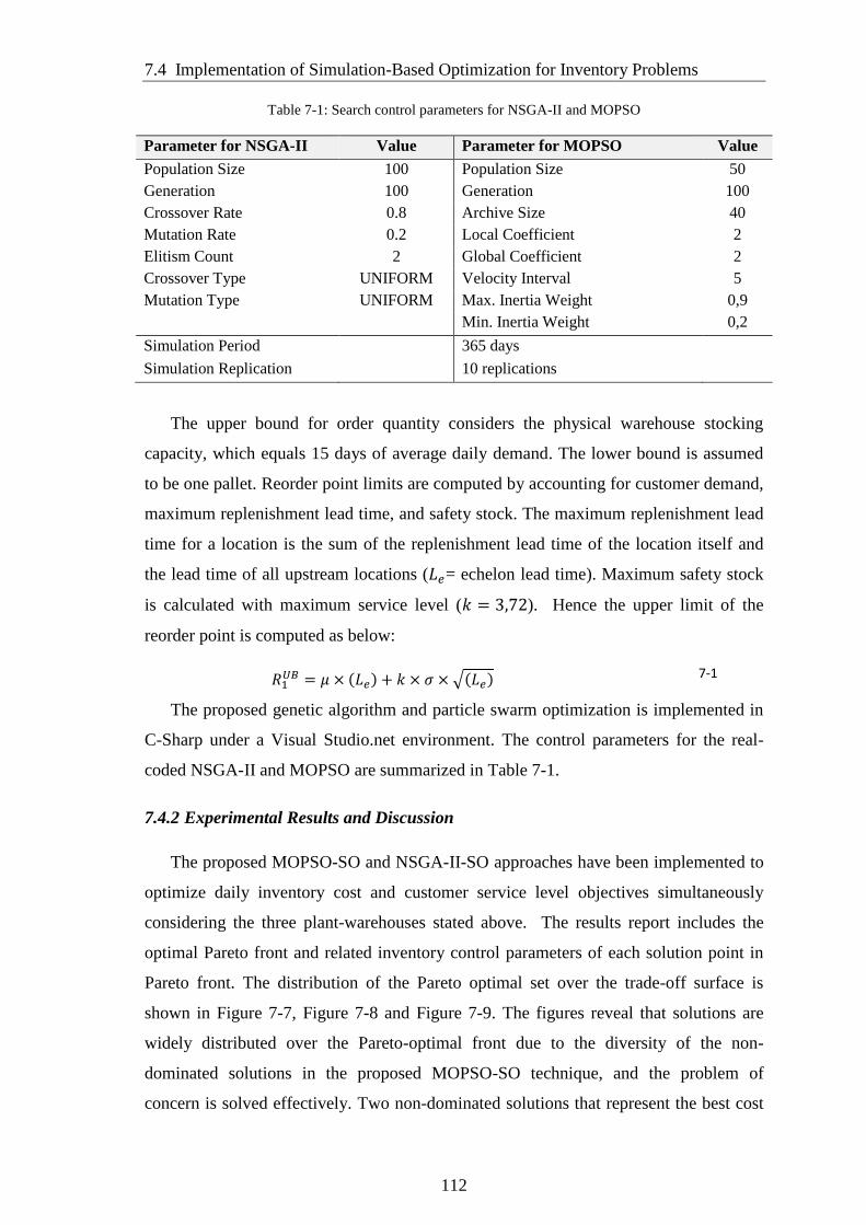
7.4 Implementation of Simulation-Based Optimization for Inventory Problems
112
Table 7-1: Search control parameters for NSGA-II and MOPSO
Parameter for NSGA-II Value Parameter for MOPSO Value
Population Size 100 Population Size 50
Generation 100 Generation 100
Crossover Rate 0.8 Archive Size 40
Mutation Rate 0.2 Local Coefficient 2
Elitism Count 2 Global Coefficient 2
Crossover Type UNIFORM Velocity Interval 5
Mutation Type UNIFORM Max. Inertia Weight 0,9
Min. Inertia Weight 0,2
Simulation Period 365 days
Simulation Replication 10 replications
The upper bound for order quantity considers the physical warehouse stocking
capacity, which equals 15 days of average daily demand. The lower bound is assumed
to be one pallet. Reorder point limits are computed by accounting for customer demand,
maximum replenishment lead time, and safety stock. The maximum replenishment lead
time for a location is the sum of the replenishment lead time of the location itself and
the lead time of all upstream locations (𝐿𝑒= echelon lead time). Maximum safety stock
is calculated with maximum service level (𝑘 = 3,72). Hence the upper limit of the
reorder point is computed as below:
𝑅1
𝑈𝐵 = 𝜇 × (𝐿𝑒) + 𝑘 × 𝜎 × √(𝐿𝑒) 7-1
The proposed genetic algorithm and particle swarm optimization is implemented in
C-Sharp under a Visual Studio.net environment. The control parameters for the real-
coded NSGA-II and MOPSO are summarized in Table 7-1.
7.4.2 Experimental Results and Discussion
The proposed MOPSO-SO and NSGA-II-SO approaches have been implemented to
optimize daily inventory cost and customer service level objectives simultaneously
considering the three plant-warehouses stated above. The results report includes the
optimal Pareto front and related inventory control parameters of each solution point in
Pareto front. The distribution of the Pareto optimal set over the trade-off surface is
shown in Figure 7-7, Figure 7-8 and Figure 7-9. The figures reveal that solutions are
widely distributed over the Pareto-optimal front due to the diversity of the non-
dominated solutions in the proposed MOPSO-SO technique, and the problem of
concern is solved effectively. Two non-dominated solutions that represent the best cost
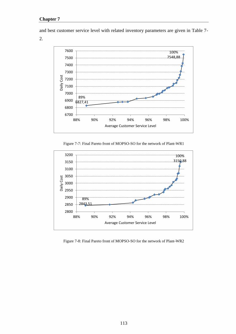
Chapter 7
113
and best customer service level with related inventory parameters are given in Table 7-
2.
Figure 7-7: Final Pareto front of MOPSO-SO for the network of Plant-WR1
Figure 7-8: Final Pareto front of MOPSO-SO for the network of Plant-WR2
89% 6827,41
100% 7548,88
6700
6800
6900
7000
7100
7200
7300
7400
7500
7600
88% 90% 92% 94% 96% 98% 100%
Dai
ly C
ost
Average Customer Service Level
89% 2843,51
100% 3150,88
2800
2850
2900
2950
3000
3050
3100
3150
3200
88% 90% 92% 94% 96% 98% 100%
Dai
ly C
ost
Average Customer Service Level
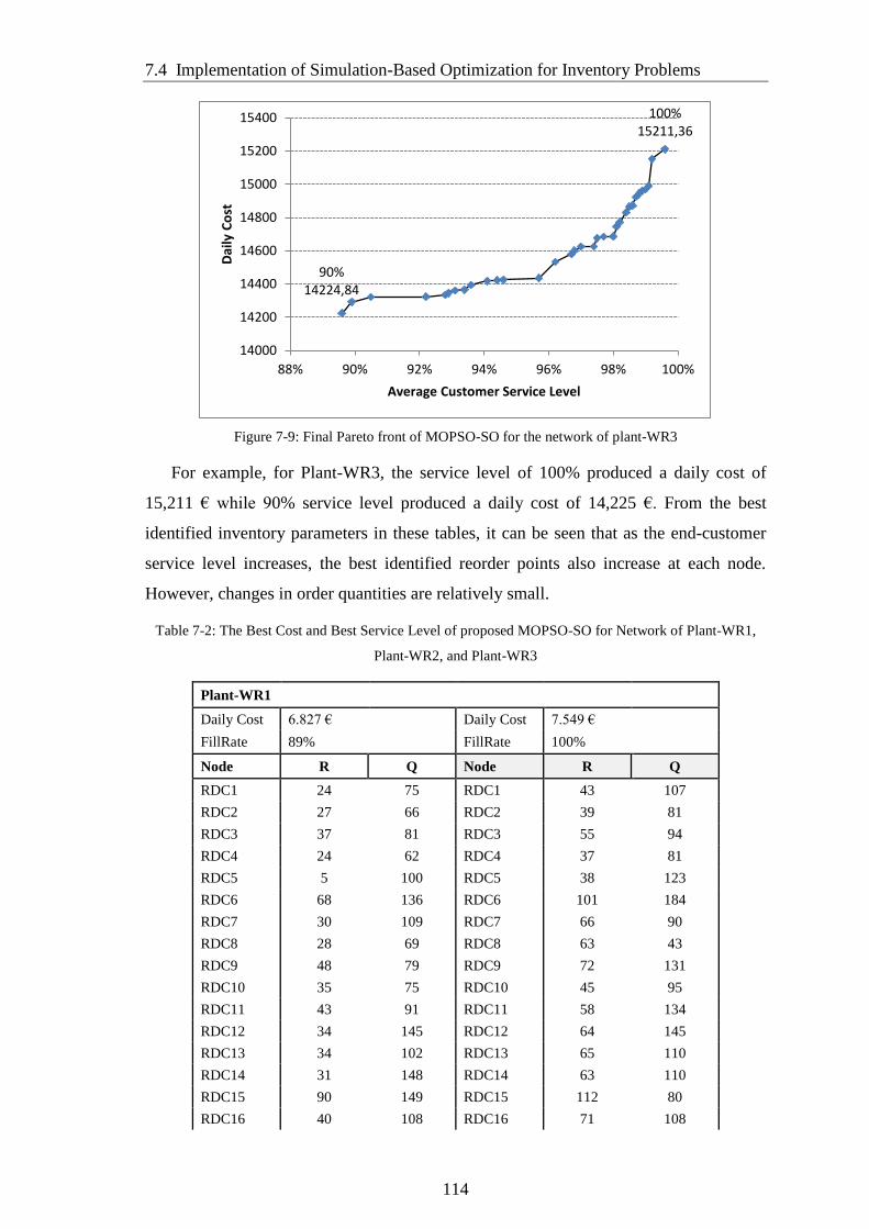
7.4 Implementation of Simulation-Based Optimization for Inventory Problems
114
Figure 7-9: Final Pareto front of MOPSO-SO for the network of plant-WR3
For example, for Plant-WR3, the service level of 100% produced a daily cost of
15,211 € while 90% service level produced a daily cost of 14,225 €. From the best
identified inventory parameters in these tables, it can be seen that as the end-customer
service level increases, the best identified reorder points also increase at each node.
However, changes in order quantities are relatively small.
Table 7-2: The Best Cost and Best Service Level of proposed MOPSO-SO for Network of Plant-WR1,
Plant-WR2, and Plant-WR3
Plant-WR1
Daily Cost 6.827 € Daily Cost 7.549 €
FillRate 89% FillRate 100%
Node R Q Node R Q
RDC1 24 75 RDC1 43 107
RDC2 27 66 RDC2 39 81
RDC3 37 81 RDC3 55 94
RDC4 24 62 RDC4 37 81
RDC5 5 100 RDC5 38 123
RDC6 68 136 RDC6 101 184
RDC7 30 109 RDC7 66 90
RDC8 28 69 RDC8 63 43
RDC9 48 79 RDC9 72 131
RDC10 35 75 RDC10 45 95
RDC11 43 91 RDC11 58 134
RDC12 34 145 RDC12 64 145
RDC13 34 102 RDC13 65 110
RDC14 31 148 RDC14 63 110
RDC15 90 149 RDC15 112 80
RDC16 40 108 RDC16 71 108
90% 14224,84
100% 15211,36
14000
14200
14400
14600
14800
15000
15200
15400
88% 90% 92% 94% 96% 98% 100%
Dai
ly C
ost
Average Customer Service Level
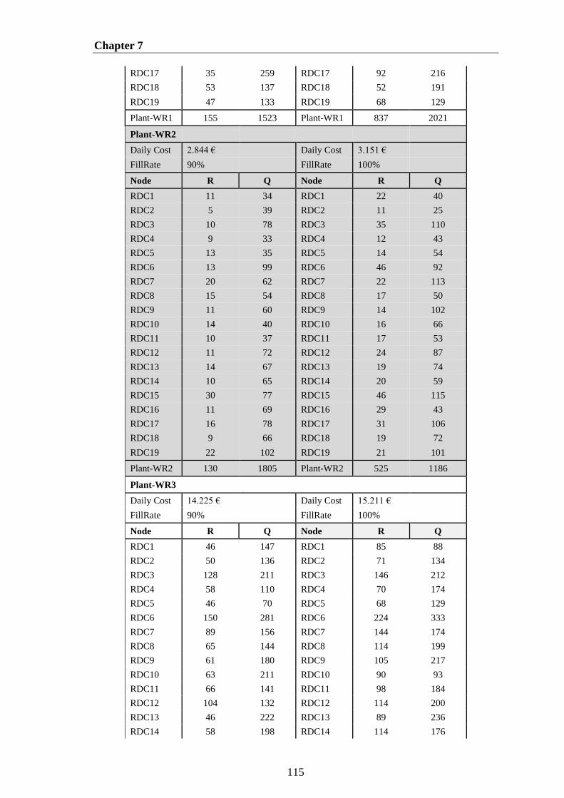
Chapter 7
115
RDC17 35 259 RDC17 92 216
RDC18 53 137 RDC18 52 191
RDC19 47 133 RDC19 68 129
Plant-WR1 155 1523 Plant-WR1 837 2021
Plant-WR2
Daily Cost 2.844 € Daily Cost 3.151 €
FillRate 90% FillRate 100%
Node R Q Node R Q
RDC1 11 34 RDC1 22 40
RDC2 5 39 RDC2 11 25
RDC3 10 78 RDC3 35 110
RDC4 9 33 RDC4 12 43
RDC5 13 35 RDC5 14 54
RDC6 13 99 RDC6 46 92
RDC7 20 62 RDC7 22 113
RDC8 15 54 RDC8 17 50
RDC9 11 60 RDC9 14 102
RDC10 14 40 RDC10 16 66
RDC11 10 37 RDC11 17 53
RDC12 11 72 RDC12 24 87
RDC13 14 67 RDC13 19 74
RDC14 10 65 RDC14 20 59
RDC15 30 77 RDC15 46 115
RDC16 11 69 RDC16 29 43
RDC17 16 78 RDC17 31 106
RDC18 9 66 RDC18 19 72
RDC19 22 102 RDC19 21 101
Plant-WR2 130 1805 Plant-WR2 525 1186
Plant-WR3
Daily Cost 14.225 € Daily Cost 15.211 €
FillRate 90% FillRate 100%
Node R Q Node R Q
RDC1 46 147 RDC1 85 88
RDC2 50 136 RDC2 71 134
RDC3 128 211 RDC3 146 212
RDC4 58 110 RDC4 70 174
RDC5 46 70 RDC5 68 129
RDC6 150 281 RDC6 224 333
RDC7 89 156 RDC7 144 174
RDC8 65 144 RDC8 114 199
RDC9 61 180 RDC9 105 217
RDC10 63 211 RDC10 90 93
RDC11 66 141 RDC11 98 184
RDC12 104 132 RDC12 114 200
RDC13 46 222 RDC13 89 236
RDC14 58 198 RDC14 114 176
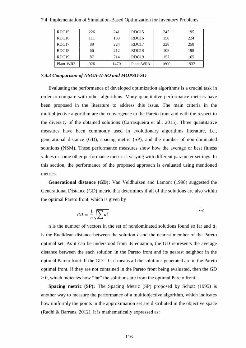
7.4 Implementation of Simulation-Based Optimization for Inventory Problems
116
RDC15 226 241 RDC15 245 195
RDC16 111 183 RDC16 150 224
RDC17 88 224 RDC17 228 258
RDC18 66 212 RDC18 108 198
RDC19 87 214 RDC19 157 165
Plant-WR3 926 1470 Plant-WR3 1600 1932
7.4.3 Comparison of NSGA-II-SO and MOPSO-SO
Evaluating the performance of developed optimization algorithms is a crucial task in
order to compare with other algorithms. Many quantitative performance metrics have
been proposed in the literature to address this issue. The main criteria in the
multiobjective algorithm are the convergence to the Pareto front and with the respect to
the diversity of the obtained solutions (Carrasqueira et al., 2015). Three quantitative
measures have been commonly used in evolutionary algorithms literature, i.e.,
generational distance (GD), spacing metric (SP), and the number of non-dominated
solutions (NSM). These performance measures show how the average or best fitness
values or some other performance metric is varying with different parameter settings. In
this section, the performance of the proposed approach is evaluated using mentioned
metrics.
Generational distance (GD): Van Veldhuizen and Lamont (1998) suggested the
Generational Distance (GD) metric that determines if all of the solutions are also within
the optimal Pareto front, which is given by
𝐺𝐷 =
1
𝑛√∑ 𝑑𝑖
2 7-2
n is the number of vectors in the set of nondominated solutions found so far and 𝑑𝑖
is the Euclidean distance between the solution 𝑖 and the nearest member of the Pareto
optimal set. As it can be understood from its equation, the GD represents the average
distance between the each solution in the Pareto front and its nearest neighbor in the
optimal Pareto front. If the GD = 0, it means all the solutions generated are in the Pareto
optimal front. If they are not contained in the Pareto front being evaluated, then the GD
> 0, which indicates how “far” the solutions are from the optimal Pareto front.
Spacing metric (SP): The Spacing Metric (SP) proposed by Schott (1995) is
another way to measure the performance of a multiobjective algorithm, which indicates
how uniformly the points in the approximation set are distributed in the objective space
(Radhi & Barrans, 2012). It is mathematically expressed as:

Chapter 7
117
𝑆𝑃 = √
1
𝑛 − 1∑(�̅� − 𝑑𝑖)
2
7-3
where 𝑑𝑖 represents the Euclidean distance between two consecutive members in
Pareto front and �̅� is the mean value of the distance measure. A smaller value for this
metric is the ideal one and it indicates that all members of the Pareto front obtained so
far are uniformly spread among the Pareto front.
Non-dominated Solutions Metric (NSM): This metric compares the number of
non-dominated solutions that are obtained by each algorithm.
Figure 7-10 depicts the Pareto surfaces obtained using MOSP and NSGA-II to
optimize daily inventory cost and customer service level. According to the Figure 7-10,
it shown graphically that MOPSO-SO is able to finds better spread of solution set along
the front and a better convergence measure than NSGA-II-SO. Table 7-3 show the
means, variances and statistics of three performance metrics obtained over the 10
independent runs using the two optimization algorithms. A point that should be
highlighted from the table is that the MOPSO-SO gives better results with good
diversity and convergence for lower number of population.
Figure 7-10: The Pareto Fronts generated by Two Algorithms
Performance metrics mentioned above are generally related to the diversity and
spread of the solutions in the objective space. However, these methods are not able to
6.700 €
6.800 €
6.900 €
7.000 €
7.100 €
7.200 €
7.300 €
7.400 €
7.500 €
91% 92% 93% 94% 95% 96% 97% 98% 99% 100%
Dai
ly C
ost
Service Level
MOPSO
NSGA-II
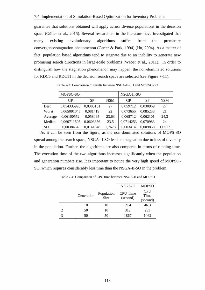
7.4 Implementation of Simulation-Based Optimization for Inventory Problems
118
guarantee that solutions obtained will apply across diverse populations in the decision
space (Güller et al., 2015). Several researchers in the literature have investigated that
many existing evolutionary algorithms suffer from the premature
convergence/stagnation phenomenon (Carter & Park, 1994) (Hu, 2004). As a matter of
fact, population based algorithms tend to stagnate due to an inability to generate new
promising search directions in large-scale problems (Weber et al., 2011). In order to
distinguish how the stagnation phenomenon may happen, the non-dominated solutions
for RDC5 and RDC11 in the decision search space are selected (see Figure 7-11).
Table 7-3: Comparison of results between NSGA-II-SO and MOPSO-SO
MOPSO-SO NSGA-II-SO
GP SP NSM GP SP NSM
Best 0,054335995 0,0385161 27 0,059712 0,038969 27
Worst 0,065091045 0,081419 22 0,073655 0,085233 21
Average 0,06100552 0,058095 23,63 0,068712 0,062101 24,3
Median 0,060711505 0,0603356 23,5 0,0714253 0,070983 24
SD 0,0038454 0,0141848 1,7678 0,003414 0,009858 1,6517
As it can be seen from the figure, as the non-dominated solutions of MOPS-SO
spread among the search space, NSGA-II-SO leads to stagnation due to loss of diversity
in the population. Further, the algorithms are also compared in terms of running time.
The execution time of the two algorithms increases significantly when the population
and generation numbers rise. It is important to notice the very high speed of MOPSO-
SO, which requires considerably less time than the NSGA-II-SO in the problem.
Table 7-4: Comparison of CPU time between NSGA-II and MOPSO
NSGA-II MOPSO
Generation Population
Size
CPU Time
(second)
CPU
Time
(second)
1 10 10 59.4 46.3
2 50 10 312 233
3 50 50 1867 1462
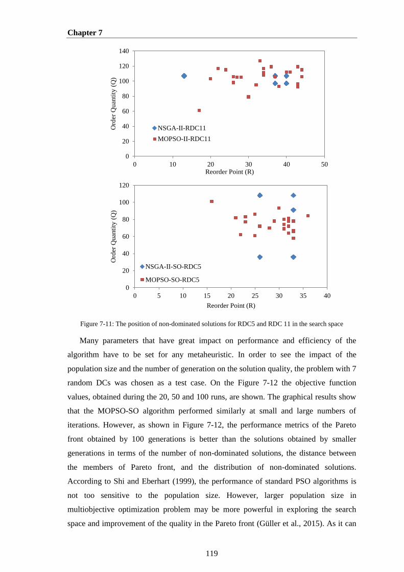
Chapter 7
119
Figure 7-11: The position of non-dominated solutions for RDC5 and RDC 11 in the search space
Many parameters that have great impact on performance and efficiency of the
algorithm have to be set for any metaheuristic. In order to see the impact of the
population size and the number of generation on the solution quality, the problem with 7
random DCs was chosen as a test case. On the Figure 7-12 the objective function
values, obtained during the 20, 50 and 100 runs, are shown. The graphical results show
that the MOPSO-SO algorithm performed similarly at small and large numbers of
iterations. However, as shown in Figure 7-12, the performance metrics of the Pareto
front obtained by 100 generations is better than the solutions obtained by smaller
generations in terms of the number of non-dominated solutions, the distance between
the members of Pareto front, and the distribution of non-dominated solutions.
According to Shi and Eberhart (1999), the performance of standard PSO algorithms is
not too sensitive to the population size. However, larger population size in
multiobjective optimization problem may be more powerful in exploring the search
space and improvement of the quality in the Pareto front (Güller et al., 2015). As it can
0
20
40
60
80
100
120
140
0 10 20 30 40 50
Ord
er Q
uan
tity
(Q
)
Reorder Point (R)
NSGA-II-RDC11
MOPSO-II-RDC11
0
20
40
60
80
100
120
0 5 10 15 20 25 30 35 40
Ord
er Q
uan
tity
(Q
)
Reorder Point (R)
NSGA-II-SO-RDC5
MOPSO-SO-RDC5
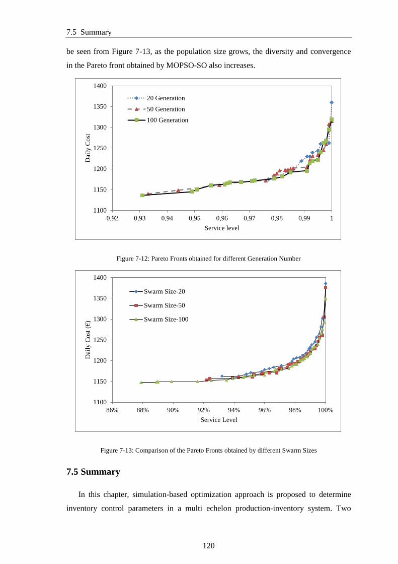
7.5 Summary
120
be seen from Figure 7-13, as the population size grows, the diversity and convergence
in the Pareto front obtained by MOPSO-SO also increases.
Figure 7-12: Pareto Fronts obtained for different Generation Number
Figure 7-13: Comparison of the Pareto Fronts obtained by different Swarm Sizes
7.5 Summary
In this chapter, simulation-based optimization approach is proposed to determine
inventory control parameters in a multi echelon production-inventory system. Two
1100
1150
1200
1250
1300
1350
1400
0,92 0,93 0,94 0,95 0,96 0,97 0,98 0,99 1
Dai
ly C
ost
Service level
20 Generation
50 Generation
100 Generation
1100
1150
1200
1250
1300
1350
1400
86% 88% 90% 92% 94% 96% 98% 100%
Dai
ly C
ost
(€
)
Service Level
Swarm Size-20
Swarm Size-50
Swarm Size-100
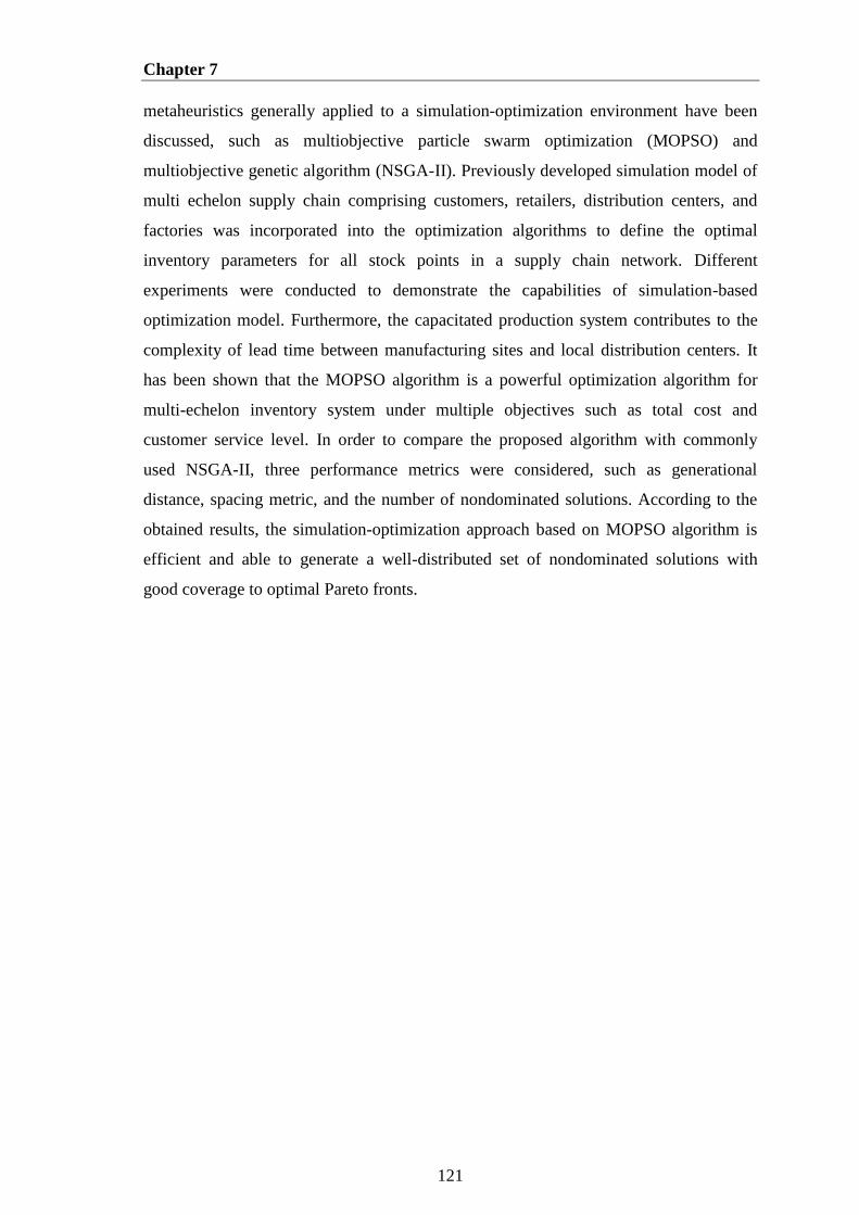
Chapter 7
121
metaheuristics generally applied to a simulation-optimization environment have been
discussed, such as multiobjective particle swarm optimization (MOPSO) and
multiobjective genetic algorithm (NSGA-II). Previously developed simulation model of
multi echelon supply chain comprising customers, retailers, distribution centers, and
factories was incorporated into the optimization algorithms to define the optimal
inventory parameters for all stock points in a supply chain network. Different
experiments were conducted to demonstrate the capabilities of simulation-based
optimization model. Furthermore, the capacitated production system contributes to the
complexity of lead time between manufacturing sites and local distribution centers. It
has been shown that the MOPSO algorithm is a powerful optimization algorithm for
multi-echelon inventory system under multiple objectives such as total cost and
customer service level. In order to compare the proposed algorithm with commonly
used NSGA-II, three performance metrics were considered, such as generational
distance, spacing metric, and the number of nondominated solutions. According to the
obtained results, the simulation-optimization approach based on MOPSO algorithm is
efficient and able to generate a well-distributed set of nondominated solutions with
good coverage to optimal Pareto fronts.
Chapter 8
Conclusion and Future Research
This research contributes to two areas. First, it contributes to decision support for
supply chain network decisions in an integrated environment. Most literatures on
distribution network design have traditionally considered strategic, tactical, and
operational decisions separately. This classical approach leads to considerable excess
costs because the supply chain is optimized locally but does not guarantee the global
optimum for the whole system. Moreover, in real world problems, there are multiple
objectives that must be considered simultaneously, but that often have conflicting
underlying objectives. This is a challenging problem due to the complexity of the
problems, the presence of uncertainty, and the interdependency between decisions. In
this research, we discussed how to determine the number and the locations of DCs
needed in an integrated supply chain. We formulated a mixed nonlinear mathematical
model with objective functions to minimize total logistics costs and minimize the
maximum distance from the opened facilities to the customers.
Furthermore, we presented a heuristic based on Quantum-behaved Particle Swarm
Optimization (QPSO) to solve the multi-objective location problems in an efficient
manner. The solution was tested in the case of a major food product company in
Germany. Our results indicate that QPSO can be used effectively to solve
multiobjective optimization problems in a relatively simple way. The proposed
approach for the multi-objective location problems performs reasonably in terms of
computation time. Computational results demonstrate that optimal network structure of
an integrated model is quite different from the nonintegrated supply chain. The results
suggest that as the ratio between the unit transportation cost and the unit inventory cost
decreases, the benefit of integrating the decisions becomes greater.
Another main part of this dissertation is the simulation and optimization of a multi-
echelon production/inventory system. We implemented a toolbox developed by using an
object-oriented simulation framework. The toolbox is capable of creating simulation

Chapter 8
123
models for any kind of supply chain network setting and analyzing the inventory control
policies of a given supply chain. The analysis was three fold: i) identified the impact of
inventory allocation decisions on the supply chain performance measures under
different coordination mechanisms; ii) identified the impact of different order
fulfillment strategies on the system performance; and iii) developed the simulation-
optimization approach to obtain the best inventory parameters in the supply chain
system that satisfy the required service level. We analyzed how the system would
behave under different inventory allocation decisions and different order fulfillment
policies at the upper echelon. In particular, we noted that FCFS strategy leads to
unstable performance among the supply chain. According to the experimental results,
customer prioritization polices can reduce the total cost of the system in comparison to
FCFS as they increase the customer service level.
In an effort to improve the performance of the multi-echelon supply chain, we
presented a multiobjective simulation-based optimization approach in which the cost of
all nodes in the system is minimized while the customer service level is maximized.
This research presents two metaheuristics algorithms (fast NSGA-II and MOPSO) for
dealing with the multiobjective inventory optimization problem. It has been shown that
metaheuristic algorithms are powerful, intelligent optimization algorithms that are able
to obtain non-dominated solutions of the multiobjective problem. Numerical results for
the production/inventory problem with different Pareto optimality characteristics
indicate that NSGA-II-SO and MOPSO-SO are capable of efficiently and effectively
exploring the solution search space.
8.1 Future Research
The location model in this research has been limited to two objectives: minimizing
total logistics costs and minimizing the maximum distance from the opened facilities to
the customers. Although these objectives are important for network design, they are not
the only important ones. This work did not discuss the sustainable design of supply
chain networks given environmental restraints and concerns. An extension of this work
could develop an adaptive model for the tradeoff between economic and environmental
concerns in decision making framework. Another area for future research is how to
improve the performance of the proposed multi-objective QPSO method. This method
could improve in several ways. For example, this thesis has assumed that freight
transport costs are proportional to the amount of commodities carried. Dismantling this
8.1 Future Research
124
assumption and focusing on optimizing supply chains with variable transportation costs
is yet another research topic for exploration.
In this research we consider a system of manufacturers, warehouses, distribution
centers, and retail outlets aiming to solve the inventory problem of a multi-echelon
supply chain. It would be interesting to relax some of the assumptions to match the real-
world scenarios, such as capacity limitations, uncertain costs, raw material availabilities,
and inventory allocation policies. Our model assumed a single product with random
demand at each customer location. This assumption can be relaxed for multiple
products. The simulation system may be extended to the network level with several
supplier tiers in order to analyze the impact of the supplier selection process on the
inventory system.
125
References
Abdelmaguid, T.F. & Dessouky, M.M., 2006. A genetic algorithm approach to the
integrated inventory-distribution problem. International Journal of Production
Research, 44(21), pp.4445-64.
Abido, M.A., 2007. Two-level of non-dominated solutions approach to multiobjective
particle swarm optimization. In Proceedings of the 2007 genetic and evolutionary
computation conference. London, UK, 2007.
Abido, M.A., 2010. Multiobjective particle swarm optimization with nondominated
local and global sets. Natural Computing, 9(3), pp.747-66.
Agarwal, R., Ahuja, R.K., Laporte, G. & Shen, Z.J., 2004. A composite very large-scale
neighborhood search algorithm for the vehicle routing problem. In J.Y.-T. Leung, ed.
Handbook of Scheduling: Algorithms, Models, and Performance Analysis.
ChapmanHall/CRC.
Ahmed, M.A. & Alkhamis, T.M., 2002. Simulation-based optimization using simulated
annealing with ranking and selection. Computers & Operations Research, 29(4),
pp.387-402.
Akbari, A. & Ziarati, K., 2011. A rank based particle swarm optimization algorithm
with dynamic adaptation. Journal of Computational and Applied Mathematics, 235(8),
pp.2694–714.
Akca, Z., 2010. Integrated location, routing and scheduling problems: Models and
algorithms. PhD Thesis. Industrial and Systems Engineering, , Lehigh University.
Aldarrat, H.S.M., 2007. Modeling and controlling of an integrated distribution supply
chain: Simulation-based shipment consolidation heuristics. PhD Thesis. Germany:
University of Duisburg-Essen.
Alfons, A., Templ, M. & Filzmoser, P., 2010. An object-oriented framework for
statistical simulation: The R package simFrame. Journal of Statistical Software, 37(3),
pp.1-36.
Al-kazemi, B. & Mohan, C.K., 2002. Multi-phase Discrete Particle Swarm
Optimization. In Fourth International Workshop on Frontiers in Evolutionary
Algorithms. Kinsale, Ireland, 2002.
126
Almeder, C., Preusser, M. & Hartl, R.F., 2009. Simulation and optimization of supply
chains: alternative or complementary approaches. OR Spectrum, 31(1), pp.95-119.
Al-Sultan, K.S., Hussain, M.F. & Nizami, J.S., 1996. A genetic algorithm for the set
Covering Problem. Journal of the Operational Research Society, 47(5), pp.702-09.
Altiok, T. & Melamed, B., 2007. Simulation modeling and analysis with arena. Elsevier
Inc.
Altiparmak, F., Gen, M., Lin, L. & Paksoy, T.., 2006. A genetic algorithm approach for
multiobjective optimization of supply chain networks. Computer and Industrial
Engineering, 51(1), pp.196 – 215.
Ammeri, A., XChabchoub, H., Hachicha, W. & Masmoudi, F., 2010. A Comprehensive
Literature Classification of Simulation Optimization Method. In The 9th International
Conference on Multiple Objective Programming and Goal Programming. Tunisia,
2010.
Andersson, J. & Marklund, J., 2000. Decentralized inventory control in a two-level
distribution system. European journal of operations research, 127(3), pp.483-506.
April, J., Glover, F., Kelly, J.P. & Laguna, M., 2003. Practical Introduction to
Simulation Optimization. In Proc. Winter Simulation Conference. New Orleans,
Louisiana, USA, 2003.
Aslam, T., 2013. Analysis of manufacturing supply chains using system dynamics and
multiobjective optimization. Dissertation. Sweden: University of Skövde.
Axsäter, S., 1993. Exact and approximate evaluation of batch ordering policies for two-
level inventory systems. Operation Research, 41(4), pp.777–85.
Axsäter, S., 1998. Evaluation of Installation Stock Based (R, Q)-Policies for Two-Level
Inventory Systems with Poisson Demand. Operations Research, 46(3), pp.135-45.
Axsäter, S., 2000. Inventory Control. Boston: Kluwer Academic Publishers.
Axsäter, S., 2003. Supply chain operations: Serial and distribution inventory systems. In
Graves, S.C. & Kok, T.d. Handbooks in Operations. Boston: Elseiver.
Axsäter, S., 2006. A simple procedure for determining order quantities under a fill rate
constraint and normally distributed demand. European Journal of Operational Research
, 174(1), pp.480-91.
Axsäter, S., 2007. On the First Come – First Served rule in multi-echelon inventory
control. Naval Research Logistics NRL, 54(5), pp.485-91.
Azambuja, M. & O'Brien, W.J., 2008. Construction supply chain modelling: Issues and
perspectives. In O'Brien, W.J..F.C.T..V.R.a.L.K.A. Construction supply chain
management handbook. CRC Press. pp.2-1-2-31.
127
Bachlaus, M., Pandey, M.K., Mahajan, C. & Shankar, R., 2008. Designing an integrated
multi-echelon agile supply chain network: a hybrid taguchi-particle swarm optimization
approach. Journal of Intelligent Manufacturing, 19(6), pp.747–61.
Baghel, V., 2009. Multiobjective optimization-New formulation and application to
radar signal processing. Msc Thesis. India: National Institute of Technology.
Baker, J.E., 1985. Adaptive selection methods for genetic algorithms. In Grefenstette,
J.J., ed. International Conference on Genetic Algorithms and Their Applications.
Pittsburgh, PA, USA, 1985.
Ballou, R.H., 2001. Unresolved issues in supply chain network design. Information
Systems Frontiers, 3(4), pp.417–26.
Ballou, R.H., 2004. Business logistics/supply chain management: Planning, organizing
and controlling the supply chain. 5th ed. N.J.: Prentice Hall.
Banerjee, A. & Jonathan, B.a.B.S., 1996. Heuristic production triggering mechanisms
under discrete unequal inventory withdrawal. International Journal of Production
Research, 45(3), pp.83 - 90.
Banks, J., 2000. Introduction to Simulation. In Proceedings of the 2000 Winter
Simulation Conference. Atlanta, GA, USA, 2000.
Barcio , B.T., Ramaswamy, S., Macfadzean , R. & Barber, K.S., 1996. Object-oriented
analysis, modeling, and simulation of a notional air defense system. SIMULATION,
66(1), pp.5-21.
Battini, D., 2008. Dynamic modeling of networks and logistic compex systems.
Dissertation. Italy: University of Padova.
Beamon, B.M. & Chen, V.C.P., 2001. Performance analysis of conjoined supply chains.
International Journal of Production Research, 39(14), pp.3195-218.
Beasley, J.E. & Chu, P.C., 1996. A genetic algorithm for the set covering problem.
European Journal of Operational Research, 94(2), pp.392-404.
Beoman, B.M., 1998. Supply chain design and analysis: Models and methods.
International Journal of Production Economics, 55(3), pp.281-94.
Beoman, B.M., 1999. Measuring supply chain performance. International Journal of
Operations & Production Management, 19(3), pp.2752-92.
Bianchi, L., Dorigo, M., Gambardella, L.M. & Gujahr, W.J., 2006. Metaheuristics in
stochastic combinatorial optimization: a survey. Technical Report IDSIA-08-06.
Biaswas, S. & Narahari, Y., 2004. Object oriented modeling and decision support for
supply chain. European Journal of Operational Research, 153(3), pp.704-26.
128
Blanchard, D., 2010. Supply chain management best practices. New Jersey: Wiley,
Hoboken.
Borshchev, A. & Filippov, A., 2004. From system dynamics and discrete event to
practical agent based modeling: Reasons, techniques, tools. In Proceedings of the 22nd
International Conference of the System Dynamics Society. Oxford, ENGLAND, 2004.
Bowersox, D.J., Closs, D.J. & Cooper, M.B., 2002. Supply chain logistics management.
New York: McGraw-Hill.
Bramel, J. & Simchi-Levi, D., 1997. The Logic of Logistics: Theory, Algorithms and
Applications for Logistics Management. NewYork: Springer-Verlag.
Carrasqueira, P., Alves, M.J. & Antunes, C.H., 2015. A bi-level multiobjective PSO
algorithm. In A. Gaspar-Cunha, C. Henggeler Antunes & C. Coello-Coello, eds.
Evolutionary Multi-Criterion Optimization. Switzerland: Springer International
Publishing. pp.263–76.
Carson, Y. & Maria, A., 1997. Simulation optimization: Methods and applications. In
Proceedings of the 1997 Winter Simulation Conference. Atlant, USA, 1997.
Carter, B. & Park, K., 1994. Scalability problems of genetic search. In IEEE
International Conference on Systems, Man, and Cybernetics. San Antonio, TX, USA,
1994.
Chanta, , Mayorga , M.E. & McLay, L.A., 2011. Improving emergency service in rural
areas:a bi-objective covering location model for EMS systems. Annals of Operations
Research , 221(1), pp.133–59.
Chatfield, D.C., Harrison, T.P. & Hayya, J.C., 2006. SISCO: An object-oriented supply
chain simulation system. Decision Support Systems, 42(1), pp.422-434.
Chen, Y. & Li, X., 2009. The Effect Of Customer Segmentation On An Inventory
System In The Presence Of Supply Disruption. In In Proceedings of the 2009 Winter
Simulation Conference., 2009.
Chopra, S., 2003. Designing the distribution network in a supply chain. Transportation
Research Part E: Logistics and Transportation Review, 39(2), pp.123-40.
Chopra, S. & Meindl, P., 2004. Supply chain management. 2nd ed. New Jersey:
Prentice-Hall.
Christofides, N., Mingozzi, A. & Toth, P., 1979. The vehicle routing problem. In N.
Christofides, A. Mingozzi, P. Toth & C. Sandi, eds. Combinatorial Optimization.
Chichester: Wiley. pp.315-38.
Cobb, B.R., Rumí, R. & Salmerón, A., 2013. Inventory management with log-normal
demand per unit time. Computers & Operations Research, 40(7), pp.1842–51.

129
Correia, I., Melo, T. & Saldanha da Gama, F., 2012. Comparing classical performance
measures for a multi-period, two-echelon supply chain network design problem with
sizing decisions. Technical report. Germany: Saarland Business School.
Daganzo, C.F., 1984. The distance traveled to visit N points with a maximum of C stops
per vehicle: An analytic model and an application. Transportation Science, 18(4),
pp.331–50.
Daganzo, C.F., 2005. Logistics systems analysis. 4th ed. Heidelberg: Springer-Verlag.
Daniel, J.S.R. & Rajendran, C., 2006. Heuristic approaches to determine base-stock
levels in a serial supply chain with a single objective and with multiple objectives.
European Journal of Operational Research, 175(1), pp.566-90.
Dasci, A. & Verter, V., 2001. A continuous model for production–distribution system
design. European Journal of Operational Research, 129(2), pp.287–98.
Daskin, M.S., 1995. Network and discrete Location: models, algorithms and
applications. New York: John Wiley and Sons, Inc.
Daskin, M.S., Coullard, C.R. & Shen, Z.-J.M., 2002. An inventory-location model:
Formulation, solution algorithm and computational results. Annals of Operations
Research, 110(1-4), pp.83-106.
Daskin, M.S., Snyder, L.V. & Berger, R.T., 2005. Facility location in supply chain
design. In A. Langevin & D. Riopel, eds. Logistics Systems: Design and Optimization.
Kluwer. Ch. 2. pp.39-65.
De Bodt, M. & Graves, S., 1985. Continuous review policies for a multiechelon
inventory problem with stochastic demand. Management Science, 31(10), pp.1286–95.
De Sensi, G., Longo, F. & Mirabelli, G., 2008. Inventory policies analysis under
demand patterns and lead times constraints in a real supply chain. International Journal
of Production Research, (46), pp.6997-7016.
Deb, K., Pratap, A., Agarwal, S. & Meyaviran, T., 2002. A fast and elitist
multiobjective genetic algorithm: NSGA-II. IEEE Transactions on Evolutionary
Computation, 6(2), pp.182-97.
Deuermeyer, B.L. & Schwarz, L., 1981. A model for the analysis of system service
level in warehouse retailer distribution systems: the identical retailer case. In Schwarz
Multi-Level Production lnventory Systems: Theory and Practice. pp.163-95.
Diks, E., De Kok., A. & Lagodimos, A., 1996. Multi-echelon systems: A service
measure Perspective. European Journal of Operational Research, 95(1), pp.241–63.
130
Ding, H., Benyoucef, L. & Xie, X., 2009. Stochastic multi-objective production-
distribution network design using simulation-based optimization. International Journal
of Production Research, 47(2), pp.479 - 505.
Douraid, A., Elhaq, S.L. & Ech-cheikh , H., 2012. A conceptual and UML models of
procurement process for simulation framework. International Journal of Computer
Science Issues, 9(6), pp.120-27.
Durillo, J.J. et al., 2009. Multiobjective particle swarm optimizers: An experimental
comparison. In 5th International Conference, EMO 2009. Nantes, FRANCE, 2009.
Erlebacher, S.J. & Meller, R.D., 2000. The interaction of location and inventory in
designing distribution systems. IIE Transactions, 32(2), pp.155-66.
Fonseca, C. & Fleming, P., 1993. Genetic algorithms for multiobjective optimization:
formulation, discussion and generalisation. In Proceedings of the 5th International
Conference on Genetic Algorithms. San Francisco, USA, 1993.
Forrester, J.W., 1961. Industrial Dynamics. New York: MIT Press and Wiley & Sons,
Inc.
Forsberg, R., 1996. Exact evaluation of (R,Q)-policies for two-level inventory systems
with Poisson demand. European Journal of Operational Research, 96(1), pp.130-38.
Ganeshan, R. & Harrison, T.P., 1995. An introduction to supply chain management.
[Online] Available at: http://silmaril.smeal.psu.edu/misc/supply_chain_intro.htm
[Accessed 1999].
Garrido, J.M., 2009. Object oriented simulation: a modeling and programming
perspective. 1st ed. Springer US.
Gen, M. & Cheng, R., 2000. Genetic algoithms and egineering optimization. John
Wiley & Sons, Inc.
Geunes, J., Shen, Z.J. & Emir, A., 2007. Planning and approximation models for
delivery route based services with price-sensitive demands. European Journal of
Operational Research , 183(1), pp.460-71.
Ghiani, G., Laporte, G. & Musmanno, R., 2004. Introduction to logistics systems
planning and control. England: John Wiley & Sons Ltd.
Glover, F., 1977. Heuristics for integer programming using surrogate constraints.
Decision Sciences , 8(1), pp.156-66.
Goetschalckx, M. & Fleischmann, B., 2005. Strategic network planning. In H.a.K.C.
Stadtler, ed. Supply Chain Management and Advanced Planning, Concepts, Models,
Software and Case Studies. 3rd ed. Springer. pp.117-38.
131
Goh, M., Jihong, O. & Chung-Piaw, T., 2001. Warehouse sizing to minimize inventory
and storage costs. Naval Research Logistics, 48(4), pp.299–312.
Goldberg, D.E., 1989. Genetic algorithms in search, optimization, and machine
learning. 1st ed. Boston: Addison-Wesley Longman Publishing.
Güller, M., Uygun, Y. & Noche, B., 2015. Simulation-based optimization for a
capacitated multi-echelon production-inventory system. Journal of Simulation, 17 April
2015(doi:10.1057/jos.2015.5).
Gunasekaran, A., Patel, C. & McGaughey, R.E., 2004. A framework for supply chain
performance measurement. International Journal of Production Economics, 87(3),
pp.333–47.
Gürbüz, C.M., Moinzadeh, K. & Zhou, Y.-p., 2007. Coordinated Replenishment
Strategies in Inventory/Distribution Systems. Management Science, 53(2), pp.293-307.
Hadley, G. & Whitin, T.M., 1963. Analysis of Inventory Systems. Englewood Cliffs, NJ:
Prentice Hall.
Haimovich, M. & Rinnooy Kan, A.H.G., 1985. Bounds and heuristics for capacitated
routing problems. Mathematics of Operations Research, 10(4), pp.527–42.
Han, K.H. & Kim, J.H., 2002. Quantum-inspired evolutionary algorithm for a class of
combinatorial optimization. IEEE Transactionson Evolutionary Computation, 6(6),
pp.580–93.
Harrison, A. & Van Hoek, R., 2005. Logistics management and strategy. 2nd ed.
Harlow: FT prentice Hall.
Holland, J., 1975. Adaptation in Natural and Artificial Systems. SIAM Review, 18(3),
pp.529–30.
Holmberg, K., 1994. Solving the staircase cost facility location problem with
decomposition and piecewise linearization. European Journal of Operational Research,
75(1), pp.41–61.
Hoque, M.A., 2006. A Optuimal Policy for a Two-Echelon Inventory/Distribution
System. International Journal of the Information Systems for Logistics and
Management, 2(1), pp.17-25.
Housein, T.A., 2007. Optimizing Coordination Strategies in a Real Supply Chain:
Simulation Approach. PhD Thesis. Universität Duisburg-Essen.
Hu, J., 2004. Sustainable Evolutionary Algorithms and Scalable Evolutionary Synthesis
of Dynamic Systems. PhD Thesis. Michigan State University: Department of Computer
Science and Engineering.
132
Huang, S., Batta, R. & Nagi, R., 2009. Simultaneous siting and sizing of distribution
centers on a plane. Annals of Operations Research, 167(1), pp.157-17.
Huang, Y., Qiu, Z. & Liu, Q., 2008. Supply chain network design based on fuzzy neural
network and PSO. In IEEE International Conference on Automation and Logistics.
Qingdao, China, 2008.
Hugos, M., 2003. Essentials of supply chain management. New Jersey: John Wiley &
Sons, Inc.
Iyer, A.V., 2001. Inventory Cost Impact of Order Processing Priorities Based on
Demand Uncertainty. Naval Research Logistics, 49(4), pp.376-90.
Janic, M., 2007. Modelling the full costs of an intermodal and road freight transport
network. Transportation Research Part D, 12(1), pp.33-44.
Jaramillo, J.H., Bhadury, J. & Batta, R., 2002. On the use of genetic algorithms to solve
location problems. Computers & Operations Research, 29(6), pp.761–79.
Jayaraman, V., 1998. Transportation, facility location and inventory issues in
distribution network design. International Journal of Operations & Production
Management, 18(5), pp.471 - 494.
Jayaraman, V., Patterson, R.A. & Rolland, E., 2003. he design of reverse distribution
networks: Models and solution procedures. European Journal of Operational Research,
150(1), pp.128–49.
Jens, R. & Michael, W., 2005. Master planning. In Hartmut , S. & Christoph, K. Supply
Chain Management and Advanced Planning. Berlin: Springer.
Jones, D., Mirrazavi, S. & Tamiz, M., 2002. Multi-objective meta-heuristics: An
overview of the current state-of-the-art. European Journal of Operational Research,
137(1), pp.1-9.
Jonsson, P. & Kjellsdotter, L., 2007. Applying advanced planning systems for supply
chain planning: three case studies. International Journal of Physical Distribution &
Logistics Management, 37(10), pp.816-34.
Joshi, B., Morris, D., Whites, N. & Unal, R., 1996. Optimization of Operations
Resources via Discrete Event Simulation Modeling. In Proceedings of 6th
AIAA/USAF/NASA/ISSMO Symposium on Multidisciplinary Analysis and Optimization.,
1996.
Juan, A.A., Grasman, S.E., Caceres-Cruz, J. & Bektas, T., 2014. A simheuristic
algorithm for the single-period stochastic inventory-routing problem with stock-outs.
Simulation Modelling Practice and Theory, 46, pp.40-52.
133
Kaboli, A., 2013. Trust and inventory replenishment decision under continuous review
system. PhD Thesis. Switzerland: Ecole Polytechnique Fédérale de Lausanne.
Kennedy, J. & Eberhart, R., 1995. Particle swarm optimization. In Proceedings of the
IEEE International Conference on Neural Networks. Piscataway, NJ, 1995.
Kennedy, I. & Eberhart, R.C., 1997. A discrete binary version of the panicle swarm
algorithm. In Proceedings of the 1997 Conference on System, Man, and Cybemetics.
Piscataway, NJ, 1997.
Keskin, B.B., Melouk, S.H. & Meyer, I.L., 2010. A simulation-optimization approach
for integrated sourcing and inventory decisions. Computers & Operations Research,
37(9), pp.1648–61.
Kleijnen, J.P.C. & Smits, M.T., 2003. Performance metrics in supply chain
management. Journal of the Operational Research Society, 54(5), pp.507-14.
Kodia, Z., Said, L.B. & Ghedira, K., 2010. A multi-agent based pricing : A virtual stock
market simulation. In 8th International Conference of Modeling and Simulation.
Hammamet - Tunisia, 2010.
Ko, H.J. & Evans, G.W., 2007. A genetic algorithm-based heuristic for the dynamic
integrated forward/reverse logistics network for 3PLs. Computers & Operations
Research, 34(2), pp.346–66.
Lee, H.L. & Billington, C., 1993. Material management in decentralized supply chains.
Operations Research, 41(5), pp.835-47.
Lee, Y.H., Cho, M.K., Kim, S.J. & Kim, Y.B., 2002. Supply chain simulation with
discrete–continuous combined modeling. Computers & Industrial Engineering, 43(1-2),
pp.375–92.
Lee, D.H. & Dong, M., 2009. Dynamic network design for reverse logistics operations
under uncertainty. Transportation Research Part E: Logistics and Transportation
Review, 45(1), pp.61–71.
Legg, S., Hutter, M. & Kumar, A., 2004. Tournament versus fitness uniform selection.
In Proceedings of the 2004 Congress on Evolutionary Computation., 2004. IEEE.
Lei, L., Liu, S., Ruszczynski, A. & Park, S., 2003. On the integrated production,
inventory, and distribution routing problem. Research Report. New Jersey: Rutgers
Business Schoo.
Liao, S.H. & Hsieh, C.L., 2009. A capacitated inventory-locationmodel: formulation,
solution approach and preliminary computational results. In Chien, B.C., Hong, T.P.,
Chen, S.M. & Ali, M., eds. 22nd International Conference on Industrial, Engineering
and Other Applications of Applied Intelligent Systems, IEA/AIE 2009. Tainan, Taiwan,
2009.

134
Lin, L., Gen, M. & Wang, X., 2007. A hybrid genetic algorithm for logistics network
design with flexible multistage model. International Journal of Information Systems for
Logistics and Management, 3(1), pp.1-12.
Li, F., Peter, J. & Tan, H., 2011. Location problems for supply chain. In S. Renko, ed.
Supply Chain Management - New Perspectives. InTech. pp.321-37.
Lo, C.Y., 2008. Advance of dynamic production-inventory strategy for multiple policies
using genetic algorithm. Information Technology Journal , 7(4), pp.647-53.
Ma, H., 2003. An integrated methodology for design of distribution chain. PhD Thesis.
Narvik, Norway: Narvik University College.
Mangotra, D., Lu, J.H. & Tsao, Y.C., 2009. A Fill-rate service level model for
integrated network design and inventory allocation problem. Technical Report. Atlanta:
Georgia Institute of Technology.
Márquez, A.C., 2010. Dynamic Modelling for Supply Chain Management. London:
Springer-Verlag.
Meixell, M.J. & Gargeta, V.B., 2005. Global supply chain design: A literature review
and critique. Transportation Research Part E, 41(6), pp.531–50.
Mele, F.D., Guillen, G., Espuna, A. & Puigjaner, L., 2006. A simulation-based
optimization framework for parameter optimization of supply chain networks.
Industrial & Engineering Chemistry Research, 45(9), pp.3133-48.
Melo, M.T., Nickel, S. & Saldanha-da-Gama, F., 2008. Network design decisions in
supply chain planning. Technical Report. Kaiserslautern, Germany: Fraunhofer-Institut
für Techno- und Wirtschaftsmathematik.
Mendoza, A. & Ventura, J.A., 2011. Modeling actual transportation costs in supplier
selection and order quantity allocation decisions. Operational Research, 13(1), pp.5-25.
Meyr, , Rohde, J., Wagner, M. & Wetterauer, , 2005. Architecture of selected APS. In
Stadtler, & Kilger, C. Supply Chain Management and Advanced Planning. Berlin:
Springer. pp.241–49.
Meyr, H., Wagner, M. & Rohde, J., 2008. Structure of Advanced Planning Systems. In
Stadtler, H. & C., K. Supply Chain Management and Advanced Planning - Concepts,
Models, Software. Berlin: Springer.
Miller, B.L. & Goldberg, D.E., 1995. Genetic Algorithms, tournament selection, and the
effects of noise. Complex Systems, 9(3), pp.193-212.
Min, H., Ko, C.S. & Ko, H.J., 2006. The spatial and temporal consolidation of returned
products in a closed-loop supply chain network. Computers & Industrial Engineering,
51(2), pp.309–20.

135
Min, H. & Zhou, G., 2002. Supply chain modeling: past, present and future. Computers
& Industrial Engineering, 43(1-2), pp.231–49.
Miranda, P.A. & Garrido, R.A., 2006. A Simultaneous Inventory Control and Facility
Location Model with Stochastic Capacity Constraint. Networks and Spatial Economics,
6(1), pp.39-53.
Mitra, S., 2009. Analysis of a two-echelon inventory system with returns. OMEGA,
37(1), pp.106-15.
Moinzadeh, K., 2002. A Multi-Echelon Inventory System with Information Exchange.
Management Science, 46(3), pp.414-26.
Muckstadt, J.A. & Sapra, A., 2010. Principles of Inventory Management. Heidelberg:
Springer.
Niranjan, S., 2008. A Study of Multi-Echelon Inventory Systems with Stochastic
Capacity And Intermediate Product Demand. Phd Thesis. Wright State University.
Novaes, A.G.N., de Cursi, J.E.S. & Graciolli, O.D., 2000. A continuous approach to the
design of physical distribution systems. Computers & Operations Research, 27(9),
pp.877–93.
Nozick, L. & Turnquist, M., 1998. Integrating inventory impacts into a fixed-charge
model for locating distribution centers.. Transportation Research-E, 34(3), pp.173–86.
Nozick, L. & Turnquist, M., 2001. Inventory, transportation, service quality and the
location of distribtuion centers. European Journal of Operational Research, 129(2),
pp.362–71.
Olaffson, S., 2005. Metaheuristics. In Henderson, S.G. & Nelson, B.L. Handbooks.
Amsterdam: Elseiver.
Olafsson, S. & Kim, J., 2002. Simulation optimization. In Proceedings of the 34th
Conference on Winter Simulation: Exploring New Frontiers, 2002. San Diego,
California, 2002.
Osman, I.H. & Laporte, G., 1996. Metaheuristics: a bibliography. In I.H.Osman, G.L.&.
Annals of Operational Research: Metaheuristics in Combinatorial Optimization.
Baltzer Science Publications. pp.513-628.
Ozcan, E. & Mohan, C.K., 1998. Analysis of a simple particle swarm optimization
system. Intelligent Engineering Systems Through Artificial Neural Networks, 8, pp.253-
58.
Panda, S. & Padhy, N.P., 2008. Comparison of particle swarm optimisation and genetic
algorithm for FACTS-based controller design. Applied Soft Computing, 8(4), pp.1418–
27.
136
Park, K.-J., 2008. The Application of Real-Coded Genetic Algorithm and Simulation
for System Optimization. International Journal of Global Business, 1(1), pp.214-36.
Perl, J. & Sirisoponslip, S., 1988. Distribution networks: Facility location,
transportation, and inventory. International Journal of Physical Distribution &
Materials Management, 18(6), pp.18–26.
PressMan, R.S., 1997. Software Engineering: A Practitioner’s Approach. 4th ed. New
York, NY, USA: The McGraw-Hill Companies, Inc.
Pullan, W.J., 2009. A population based hybrid meta-heuristic for the uncapacitated
facility location problem. In Proceedings of the first ACM/SIGEVO Summit on Genetic
and Evolutionary Computation., 2009.
Radhakrishnan, P., Prasad, V.M. & Gopalan, M.R., 2009. optimization in supply chain
management using genetic algorithm. International Journal of Computer Science and
Network Security, 9(1), pp.1-8.
Radhi, & Barrans, S., 2012. Comparison between multiobjective optimization
algorithms. In Proceedings of The Queen’s Diamond Jubilee Computing and
Engineering Annual Researchers’ Conference 2012: CEARC’12. University of
Huddersfield, Huddersfield, 2012.
Ramakrishnan, S. & Wysk, R.A., 2002. A Real-time simulation-based control
architecture for supply chain interactions. In Winter Simulation Conference., 2002.
Raquel, R.C. & Naval, P.C., 2005. An effective use of crowding distance in
multiobjective particle swarm. In Proceedings of the 2005 Conference on Genetic and
Evolutionary Computation (GECCO 05). New York, 2005. ACM.
Richardson, D., 2006. An object oriented simulation framework for steady-state
analysis of vapor compression refrigeration systems and components. Dissertation.
USA: University of Maryland.
Riksts, B.Q. & Ventura, J.A., 2010. Two-stage inventory models with a bi-modal
transportation cost. Computers & Operations Research, 37(1), pp.20-31.
Rosenblatt, M.J. & Roll, Y., 1988. Warehouse capacity in a stochastic environment.
26(12), pp.1847-51.
Rosetti, M.D. & Nangia, S., 2007. An object-oriented framework for simulating full
truckload transportation networks. In Proceedings of the 2007 Winter Simulation
Conference. Washington, D.C., 2007. IEEE.
Rossetti, M.D., Miman, M., Varghese, V. & Xiang, Y., 2006. An object-oriented
framework for simulating multi-echelon inventory systems. In Proceedings of the 2006
Winter Simulation Conference. Monterey, CA, 2006. IEEE.

137
Rossetti, M.D. & Xiang, Y., 2010. Simulating backlog and load building processes in a
two-echelon inventory system. In Proceedings of the 2010 Winter Simulation
Conference. Baltimore, MD, 2010.
Rushton, A., Chroucher, P. & Baker, P., 2010. Handbook of logistics and distribution
management. 4th ed. London: Kogan Page Ltd.
Sabri, E.H. & Beoman, B.M., 2000. A multi-objective approach to simultaneous
strategic and operational planning in supply chain design. OMEGA, 28(5), pp.581-98.
Safe, M., Carballido, J., Ponzoni, I. & Brignole, N., 2004. On stopping. In in Advances
in Artificial Intelligence –. Berlin/Heidelberg: Springer. pp.405–13.
Sarker, R. et al., 2005. A multi-agent simulation study for supply chain operation. In
International Conference on Computational Intelligence for Modelling, Control and
Automation and International Conference on Intelligent Agents, Web Technologies and
Internet Commerce. Vienne, Austria, 2005. IEEE.
Sarker, R. & Newton, C., 2002. Algorithm for Solving Economic Lot Size Scheduling
Problem. Computers & Industrial Engineering, 42(2), pp.189-98.
Sastry, K., 2007. Genetic algorithms and genetic programming for multiscale modeling:
applications in materials science and chemistry and advances in scalability.
Dissertation. IlliGAL Report No. 2007019.
Schaffer, J.D., 1985. Multiple objective optimization with vector evaluated genetic
algorithms. In Grefenstette, J.J., ed. Proceedings of an International Conference on
Genetic Algorithms and Their Applications. Pittsburgh, PA, 1985.
Schott, J.R., 1995. Fault tolerant design using single and multicriteria genetic
algorithms optimization. Msc Thesis. Massachusetts.
Seila, A.F., 2001. Spreadsheet Simulation. In Peters, B.A., Smith, J.S., Medeiros, D.J. &
Rohrer, M.W., eds. Proceedings of the 2001 Winter Simulation Conference., 2001.
IEEE.
Selcuk, B., 2007. Dynamic performance of hierarchical planning systems:Modeling and
avaluation with dynamic planned lead times. Phd Thesis. Netherlanand: Technische
Universiteit Eindhoven.
Shapiro, J.F., 2001. Modeling and IT perspectives on supply chain integration.
Information Systems Frontiers, 3(4), pp.455–64.
Shapiro, J.F., 2001. Modeling the supply chain. Duxbury Press.
Shen, Z.J., 2005. A multi-Ccommodity supply chain design problem. IIE Transactions,
37(8), pp.753-62.
138
Shen, Z.J.M., Coullard, D. & Daskin, M.S., 2003. A joint location-inventory model.
Transportation Science, 37(1), pp.40-55.
Shen, Z.-J.M. & Qi, L., 2007. Incorporating inventory and routing costs in strategic
location models. European Journal of Operational Research, 179(2), pp.372-389.
Sherbrooke, C.C., 1968. METRIC: A Multi-Echelon Technique for Recoverable Item
Control. Operation Research, 16(1), pp.122-41.
Shi, Y. & Eberhart, R.C., 1998. A modified particle swarm opitimizer. In IEEE
International Conference of Evolutionary Computation. Anchorage, AK, 1998. IEEE.
Shi, Y. & Eberhart, R.C., 1999. Empirical study of particle swarm optimization. In
Angeline, P.J. et al., eds. Proceedings of the Congress on Evolutionary Computation.
Washington, DC, 1999. IEEE.
Shu, J., Teo CP, C.P. & Shen, Z., 2005. Stochastic transportation-inventory network
design problem. Operation Research, 53(1), pp.48-60.
Sierra, M.R. & Coello Coello, C.A., 2005. Improving PSO-based multi-objective
optimization using crowding, mutation and ε-dominance. In Third International
Conference on Evolutionary Multi-Criterion Optimization. Guanajuato, Mexico, 2005.
Springer-Verlag.
Sierra, M.R. & Coello Coello, C.A., 2006. Multiobjective particle swarm optimizers: A
survey of the state-of-the-art. International Journal of Computational Intelligence
Research, 2(3), pp.287-308.
Silva, L.A.W. & Coelho, L.d.S., 2007. An Adaptive Particle Swarm Approach Applied
to Optimization of a Simplified Supply Chain. In Proc. of 19th Int. Conf. on Production
Research. Valparaiso, Chile, 2007.
Silva, C.A., Sousa, J.M.C., Runkler, T.A. & Sa da Costa, J.M.G., 2003. Optimization of
logistic processes in supply chains using metaheuristics. In Pires, F.M. & Abreu, S., eds.
11th Portuguese Conference on Artificial Intelligence. Beja, Portugal, 2003.
SpringerVerlag.
Silva, C.A., Sousa, J.M.C., Runkler, T.A. & Sa da Costa, J.M.G., 2009. Distributed
supply chain management using ant colony optimization. European Journal of
Operational Research, 199(2), pp.349–58.
Silver, E.A., Pyke, D.F. & Peterson, R., 1998. Inventory management and production
planning and scheduling. 3rd ed. NewYork: Wiley.
Simchi-Levi, D., Kaminsky, P. & Simchi-Levi, E., 2004. Managing the supply chain.
New York: The McGraw-Hill Companies.
139
Snyder, L.V., Daskin, M.S. & Teo, C.-P., 2007. The stochastic location model with risk
pooling. European Journal of Operational Research, 179(3), pp.1221-38.
Srinavas, D. & Deb, K., 1994. Multiobjective optimization using nondominated sorting
in genetic algorithm. Evolutionary Computation, 2(3), pp.221-48.
Sterman, J., 2000. Business Dynamics: Systems Thinking and Modeling for a Complex
World. Irwin/McGraw-Hill.
Svensson, A., 1996. Performance analysis and optimization via simulation. Technical
Report. Sweden: Lund Institute of Technology.
Swaminathan, J.M., Smith, S.F. & Sadeh, N.M., 1998. Modeling supply chain
dynamics: a multiagent approach. Decision Sciences, 29(3), pp.607-32.
Syberfeldt, A., 2009. A multi-objective evolutionary approach to simulation-based
optimization of real world problems. Dissertation. Leicester, UK: De Montfort
University.
Tah, J.H.M., 2005. Towards an agent-based construction supply network modelling and
simulation platform. Automation in Construction, 14(3), pp.353– 359.
Tako, R. & Robinson, S., 2006. Comparing discrete-event simulation and system
dynamics: users’ perceptions. Journal of the Operational Research Society, 60(3),
pp.296 - 312.
Tayaran, M.H., Prugel-Bennet, N.A. & Mohammadi, H., 2011. A novel magnetic
update operator for quantum evolutionary algorithms. In H. Gaspar-Cunha, R.
Takahashi , G. Schaefer & L. Costa, eds. Soft Computing in Industrial Applications.
Berlin Heidelberg: Springer-Verlag. pp.67-76.
Tekin, E. & Sabuncuoglu, I., 2004. Simulation optimization: A comprehensive review
on theory and applications. IIE Transactions, 36(11), pp.1067–81.
Teo, C.P. & Shu, J., 2004. Warehouse-retailer network design problem. Operation
Research, 52(3), pp.396–408.
Tuzun, D. & Burke, L.I., 1999. A two-phase tabu search approach to the location
routing problem. European Journal of Operational Research, 116(1), pp.87–99.
Tyworth, J.E. & O’Neill, L., 1997. Robustness of the normal approximation of lead-
time demand in a distribution setting. Naval Research Logistics, 44(2), pp.165–86.
Tyworth, J.E. & Ruiz-Torres, A., 2000. Transportation's role in the sole- versus dual-
sourcing decision. International Journal of Physical Distribution & Logistics
Management, 30(2), pp.128-44.
Van Veldhuizen, D.A. & Lamont, G.B., 1998. Multiobjective evolutionary algorithm
research: A history and analysis. Tech. Rep. Air Force Inst. Technol.
140
Verter, V. & Dincer, M.C., 1995. Facility location and capacity acquisition: An
integrated approach. Naval Research Logistics, 42(8), pp.1141-60.
Vidal, C.J. & Goetschalckx, M., 1997. Strategic production-distribution models: A
critical review with emphasis on global supply chain models. European Journal of
Operations Research, 98(1), pp.1-18.
Weber, M., Neri, F. & Tirronen, V., 2011. Shuffle or update parallel differential
evolution for large-scale optimization. Soft Computing, 15(11), pp.2089-107.
William, M.S., 1995. Adapting crossover in evolutionary algorithms. In Proceedings of
the Fourth Annual Conference on Evolutionary Programming., 1995. MIT Press.
Wu, T.-H., Low, C. & Bai, J.-W., 2002. Heuristic solutions to multi-depot location-
routing problems. Computers & Operations Research, 29(10), pp.1393–415.
Xie, H., Zhang, M. & Andreae, P., 2007. An analysis of constructive crossover and
selection pressure in genetic programming. In In Proceedings of Genetic and
Evolutionary Computation Conference (GECCO-2007). London, 2007. ACM Press.
Xin, W.Y., 2007. Logistics coordination in vendor-buyer systems. PhD Thesis.
Singapore: Singapore-MIT Alliance.
Yang, S., Wang, M. & Jiao, L., 2004. A Quantum Particle Swarm Optimization. In
Proceedings of CEC2004, the Congress on Evolutionary Computing., 2004.
You, F., Pinto, J.M., Grossmann, I.E. & Megan, L., 2011. Optimal Distribution-
Inventory Planning of Industrial Gases. II. MINLP Models and Algorithms for
Stochastic Cases. Industrial and Engineering Chemistry Research, 50(5), pp.2928–
2945.
Yu, X. & Gen, M., 2010. Introduction to the evolutionary algorithms. London:
Springer-Verlag.
ZedGraph, 2009. ZedGraph class library developed in C#. [Online] Available at:
http://sourceforge.net/projects/zedgraph [Accessed September 2009].
Zhao, Q.H., Wang, S.Y., Lai, K.K. & Xia, G.P., 2004. Model and algorithm of an
inventory problem with the consideration of transportation cost. Computers & Industrial
Engineering, 46(2), pp.389-97.
Zhao, X. & Xie, J., 2002. Forecasting errors and the value of information sharing in a
supply chain. International Journal of Production Research, 40(2), pp.311-35.
Zhou, J. & Liu, B., 2003. New stochastic models for capacitated location-allocation
problem. Computers and Industrial Engineering, 45(1), pp.111-25.

141
Zhou, G., Min, H. & Gen, M.., 2002. The balanced allocation of customers to multiple
distribution centers in the supply chain network: A genetic algorithm approach.
Computers & Industrial Engineering , 43, pp.252–61.
Zipkin, P.H., 2000. Foundations of Inventory Management. New York, NY: McGraw-
Hill.
Zitzler, E., Laumanns, M. & Bleuler, S., 2004. A tutorial on evolutionary multiobjective
optimization. In X. Gandibleux, M. Sevaux, C. Sörensen & V. T’kindt , eds.
Metaheuristics for Multiobjective Optimisation. Berlin Heidelberg: Springer. pp.3-37.
Zitzler, E. & Thiele, L., 1999. Multiobjective evolutionary algorithms: a comparative
case study and the strength Pareto approach. IEEE Transactions on Evolutionary
Computation, 3(4), pp.257-71.

142
Appendix A
1. Overview of Inventory Theory
One of the main problems of supply chain resource planning is the optimization of
lot sizes in order to minimize the costs of ordering and storage.
Classical Lot Size Model (EOQ)
The classic Economic Order Quantity (EOQ) developed by Harris in 1913 is the
most fundamental model used to calculate lot sizes. The EOQ model describes an
important conflict of costs between fixed ordering and holding costs.
Figure 0-1: Change in inventory over time for the EOQ model
In the EOQ model, since all the parameters are stationary over time, the order
quantity, denoted by Q, also remains stationary. The EOQ can be easily determined by
the formula:
𝐸𝑂𝑄 = √2𝐾𝜆
ℎ
where, λ = annual usage
K= fixed ordering (setup) cost
h = inventory carrying cost per unit of product per year
Then, the optimal total cost per year TC* is
𝑇𝐶∗ = √2𝐾𝜆ℎ
Continuous Review Inventory Model

143
Figure 0-2 Continuous Review Inventory System
EOQ model assume that demand is constant and known. In the majority of cases,
though, demand is not constant but varies from day to day. One of the main functions of
inventory management is to plan safety stock to protect each stock point uncertainties in
customer demands. Considering a single-echelon inventory system with a continuous
review control policy, a reorder point of R and batch size of Q, a constant lead time for
replenishing orders, demand (per unit time) as a normal distribution with mean 𝜇 and
standard deviation 𝜎 and backordered unsatisfied demand, formulae for the average
stock level 𝐷(𝑄, 𝑅) and the average stockout level 𝐵(𝑄, 𝑅) (see (Axsäter, 2000),
(Axsäter, 2006) and (Hadley & Whitin, 1963) for more details):
𝐷(𝑄, 𝑅) =𝑄
2+ 𝑅 − 𝜇′ + 𝐵(𝑄, 𝑅)
The reorder level consists of two quantities: the first is the average demand during
lead time, and the second is the safety stock, which depends on lead time, demand
variability, and service level. The expected number of backorders at the location is
given by defined as:
𝐸𝐵(𝑅) = ∫ (𝑥 − 𝑅)𝑓(𝑥)𝑑𝑥∞
𝑅
= ∫ 𝑥𝑓(𝑥)𝑑𝑥∞
𝑅
− 𝑅𝐻(𝑥)
= (𝜇𝐿 − 𝑅)[1 − 𝜙(𝑧)] + 𝜎𝐿𝜑(𝑧) 𝑤ℎ𝑒𝑟𝑒 𝑧 = (𝑅 − 𝜇𝐿)
𝜎𝐿
𝚽(𝐳): is the distribution function of the standardized normal distribution with mean
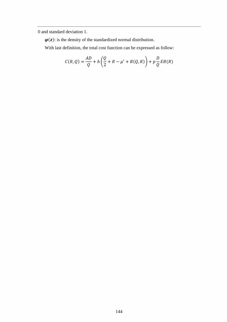
144
0 and standard deviation 1.
𝝋(𝒛): is the density of the standardized normal distribution.
With last definition, the total cost function can be expressed as follow:
𝐶(𝑅, 𝑄) =𝐴𝐷
𝑄+ ℎ (
𝑄
2+ 𝑅 − 𝜇′ + 𝐵(𝑄, 𝑅)) + 𝑝
𝐷
𝑄𝐸𝐵(𝑅)
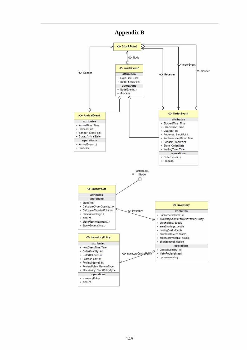
145
Appendix B
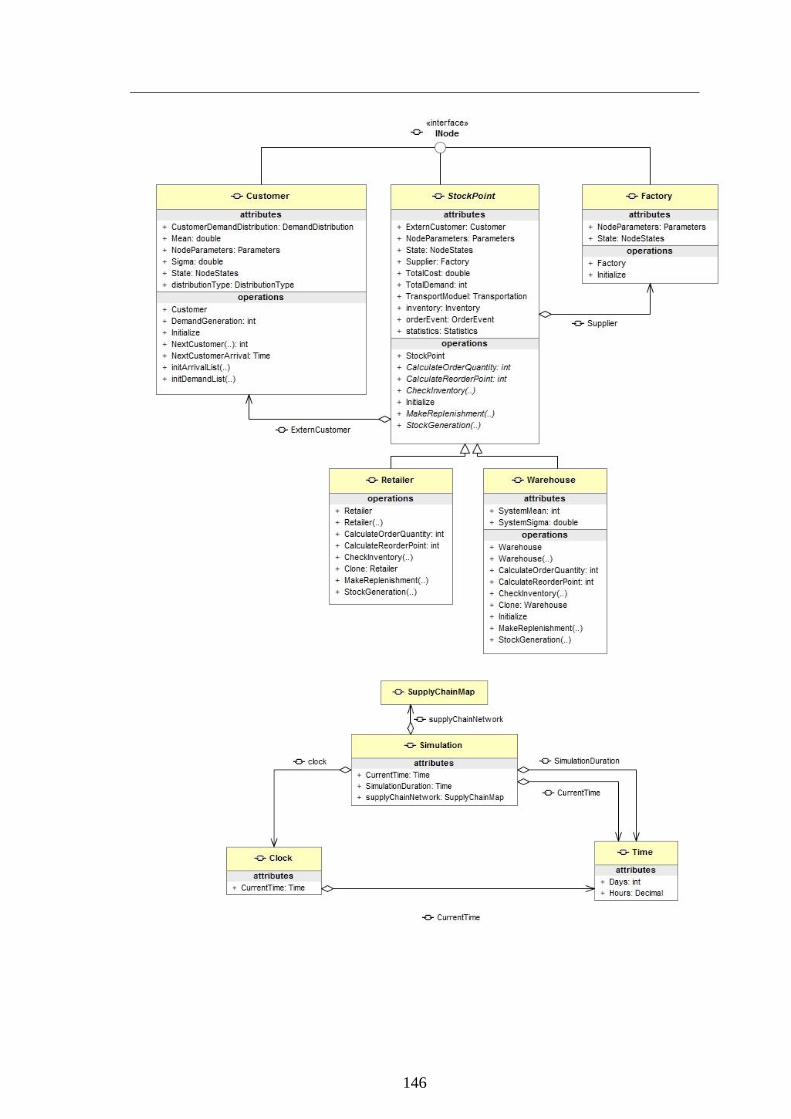
146

147
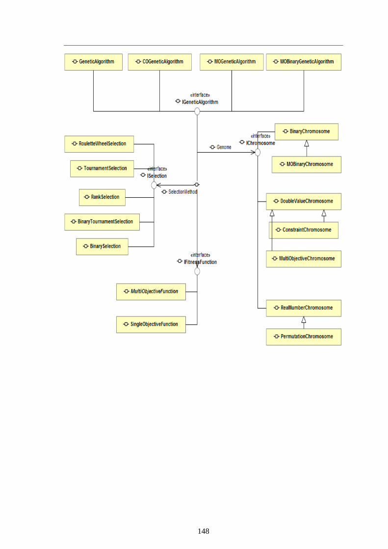
148
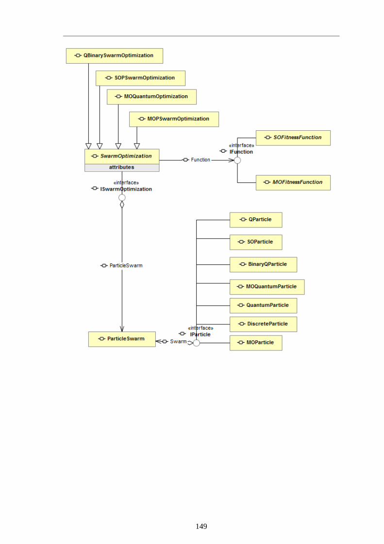
149
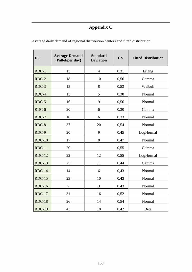
150
Appendix C
Average daily demand of regional distribution centers and fitted distribution:
DC Average Demand
(Pallet/per day)
Standard
Deviation CV Fitted Distribution
RDC-1 13 4 0,31 Erlang
RDC-2 18 10 0,56 Gamma
RDC-3 15 8 0,53 Weibull
RDC-4 13 5 0,38 Normal
RDC-5 16 9 0,56 Normal
RDC-6 20 6 0,30 Gamma
RDC-7 18 6 0,33 Normal
RDC-8 37 20 0,54 Normal
RDC-9 20 9 0,45 LogNormal
RDC-10 17 8 0,47 Normal
RDC-11 20 11 0,55 Gamma
RDC-12 22 12 0,55 LogNormal
RDC-13 25 11 0,44 Gamma
RDC-14 14 6 0,43 Normal
RDC-15 23 10 0,43 Normal
RDC-16 7 3 0,43 Normal
RDC-17 31 16 0,52 Normal
RDC-18 26 14 0,54 Normal
RDC-19 43 18 0,42 Beta
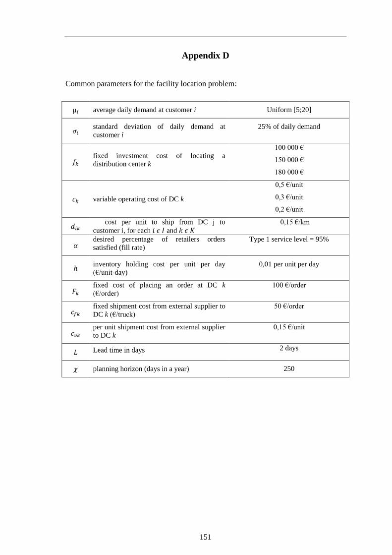
151
Appendix D
Common parameters for the facility location problem:
µ𝑖 average daily demand at customer i Uniform [5;20]
𝜎𝑖 standard deviation of daily demand at
customer i
25% of daily demand
𝑓𝑘 fixed investment cost of locating a
distribution center k
100 000 €
150 000 €
180 000 €
𝑐𝑘 variable operating cost of DC k
0,5 €/unit
0,3 €/unit
0,2 €/unit
𝑑𝑖𝑘 cost per unit to ship from DC j to
customer i, for each 𝑖 𝜖 𝐼 and 𝑘 𝜖 𝐾
0,15 €/km
𝛼 desired percentage of retailers orders
satisfied (fill rate)
Type 1 service level = 95%
ℎ inventory holding cost per unit per day
(€/unit-day)
0,01 per unit per day
𝐹𝑘 fixed cost of placing an order at DC k
(€/order)
100 €/order
𝑐𝑓𝑘 fixed shipment cost from external supplier to
DC k (€/truck)
50 €/order
𝑐𝑣𝑘 per unit shipment cost from external supplier
to DC k
0,15 €/unit
𝐿 Lead time in days 2 days
𝜒 planning horizon (days in a year) 250


![OPTIMAL A2 [Lehrbuch]](https://static.fdokument.com/doc/165x107/55171d57497959a3308b47c0/optimal-a2-lehrbuch.jpg)