
Planetesimal dynamics in the presence of a...
91
Transcript of Planetesimal dynamics in the presence of a...
Planetesimal dynamics in the
presence of a growing planet
Diplomarbeit
der Philosophischnaturwissenschaftlichen Fakultätder Universität Bern
vorgelegt von
Dominik Hofer
2006
Leiter der Arbeit:Prof. Dr. W. Benz
Abteilung Weltraumforschung und PlanetologiePhysikalisches Institut
Universität Bern

Contents
1 Introduction 5
2 Prerequisites for this work 92.1 Theoretical background . . . . . . . . . . . . . . . . . . . . . . . . . . . . . 9
2.1.1 System of reference . . . . . . . . . . . . . . . . . . . . . . . . . . . 92.1.2 Gravity . . . . . . . . . . . . . . . . . . . . . . . . . . . . . . . . . 102.1.3 Gas drag . . . . . . . . . . . . . . . . . . . . . . . . . . . . . . . . . 102.1.4 Thermal ablation . . . . . . . . . . . . . . . . . . . . . . . . . . . . 102.1.5 Fragmentation . . . . . . . . . . . . . . . . . . . . . . . . . . . . . . 112.1.6 Equation of motion . . . . . . . . . . . . . . . . . . . . . . . . . . . 112.1.7 Energy . . . . . . . . . . . . . . . . . . . . . . . . . . . . . . . . . . 112.1.8 Solid accretion rate and enhanced radius . . . . . . . . . . . . . . . 12
2.2 Model setup . . . . . . . . . . . . . . . . . . . . . . . . . . . . . . . . . . . 122.2.1 Planetesimals . . . . . . . . . . . . . . . . . . . . . . . . . . . . . . 122.2.2 The protoplanet . . . . . . . . . . . . . . . . . . . . . . . . . . . . . 13
2.3 Simulation setup . . . . . . . . . . . . . . . . . . . . . . . . . . . . . . . . 13
3 The three-body problem 153.1 Three-body gravity . . . . . . . . . . . . . . . . . . . . . . . . . . . . . . . 153.2 The circular restricted three-body problem - "Problème restreint" . . . . . 16
3.2.1 Jacobian constant . . . . . . . . . . . . . . . . . . . . . . . . . . . . 173.2.1.1 Calculation of the Jacobian constant . . . . . . . . . . . . 183.2.1.2 Hill's curves and Lagrange points . . . . . . . . . . . . . . 18
3.2.2 Bound criterion for the planetesimal . . . . . . . . . . . . . . . . . 203.3 Implications for the simulation . . . . . . . . . . . . . . . . . . . . . . . . . 20
3.3.1 Implementation of the Jacobian constant . . . . . . . . . . . . . . . 203.3.2 Conditions of the applicability of the CR3BP . . . . . . . . . . . . 21
3.3.2.1 The eect of the reduced gravitational potential on the Ja-cobian constant . . . . . . . . . . . . . . . . . . . . . . . . 22
3.3.2.2 The eect of the gas drag on the Jacobian constant . . . . 233.3.2.3 Final remarks . . . . . . . . . . . . . . . . . . . . . . . . . 24
3.4 Other changes for the three-body case . . . . . . . . . . . . . . . . . . . . 253.4.1 Initial conditions . . . . . . . . . . . . . . . . . . . . . . . . . . . . 26

2 CONTENTS
3.4.2 The enhancement factor of the capture cross section . . . . . . . . . 263.4.3 Integrating routine . . . . . . . . . . . . . . . . . . . . . . . . . . . 273.4.4 Criteria to terminate the integration . . . . . . . . . . . . . . . . . 27
4 Model setup 314.1 Models of the bodies . . . . . . . . . . . . . . . . . . . . . . . . . . . . . . 31
4.1.1 The Sun . . . . . . . . . . . . . . . . . . . . . . . . . . . . . . . . . 314.1.2 The protoplanet . . . . . . . . . . . . . . . . . . . . . . . . . . . . . 314.1.3 The planetesimal . . . . . . . . . . . . . . . . . . . . . . . . . . . . 32
4.2 Distributions of the orbital elements of the planetesimals . . . . . . . . . . 324.2.1 Semimajor axis . . . . . . . . . . . . . . . . . . . . . . . . . . . . . 324.2.2 Eccentricity and inclination . . . . . . . . . . . . . . . . . . . . . . 334.2.3 The other elements . . . . . . . . . . . . . . . . . . . . . . . . . . . 34
5 Overview of the program 375.1 Basic information . . . . . . . . . . . . . . . . . . . . . . . . . . . . . . . . 375.2 Structure of the program . . . . . . . . . . . . . . . . . . . . . . . . . . . . 39
5.2.1 Program units . . . . . . . . . . . . . . . . . . . . . . . . . . . . . . 395.2.2 Subsidiary programs . . . . . . . . . . . . . . . . . . . . . . . . . . 40
6 Tests of the gravitational model 436.1 Gravitational model in the two-body case . . . . . . . . . . . . . . . . . . . 436.2 Gravitational model in the three-body case . . . . . . . . . . . . . . . . . . 446.3 Comparison with Greenzweig and Lissauer, 1990 . . . . . . . . . . . . . . . 45
6.3.1 Initial conditions . . . . . . . . . . . . . . . . . . . . . . . . . . . . 456.3.2 Results . . . . . . . . . . . . . . . . . . . . . . . . . . . . . . . . . . 476.3.3 Conclusion . . . . . . . . . . . . . . . . . . . . . . . . . . . . . . . . 50
6.4 Comparison with Greenzweig and Lissauer, 1992 . . . . . . . . . . . . . . . 506.4.1 Initial conditions . . . . . . . . . . . . . . . . . . . . . . . . . . . . 506.4.2 Results . . . . . . . . . . . . . . . . . . . . . . . . . . . . . . . . . . 506.4.3 Conclusion . . . . . . . . . . . . . . . . . . . . . . . . . . . . . . . . 54
7 Results 557.1 Investigation of a set of protoplanets . . . . . . . . . . . . . . . . . . . . . 55
7.1.1 Comparison of the calculation of the enhancement factor . . . . . . 567.1.1.1 Initial conditions . . . . . . . . . . . . . . . . . . . . . . . 567.1.1.2 Results . . . . . . . . . . . . . . . . . . . . . . . . . . . . 577.1.1.3 Conclusion . . . . . . . . . . . . . . . . . . . . . . . . . . 63
7.1.2 Investigation of a selected case . . . . . . . . . . . . . . . . . . . . . 647.1.2.1 Initial conditions . . . . . . . . . . . . . . . . . . . . . . . 647.1.2.2 Results . . . . . . . . . . . . . . . . . . . . . . . . . . . . 647.1.2.3 Conclusion . . . . . . . . . . . . . . . . . . . . . . . . . . 66
7.1.3 Eccentricity distribution under the inuence of the protoplanet . . . 66
CONTENTS 3
7.1.3.1 Initial conditions . . . . . . . . . . . . . . . . . . . . . . . 677.1.3.2 Results . . . . . . . . . . . . . . . . . . . . . . . . . . . . 677.1.3.3 Conclusion . . . . . . . . . . . . . . . . . . . . . . . . . . 71
8 Discussion of the results 73
A The ratio of the enhancement factors 77

Chapter 1
Introduction
The formation and evolution of our solar system, or generally speaking of any solar system,is an interesting process that is yet not fully understood. There are dierent theories ofhow parts of this could have been happened, but none of them is able to explain everythingand there are still a lot of open questions. One of the most important processes in theevolution of the solar system was denitely the formation of the giant planets1, especiallythe one of Jupiter and Saturn. They represent a large part of the mass and the angularmomentum of the planets. Besides, they probably inuenced the formation and evolutionof the other planets and hence also the evolution of the Earth. Therefore the understandingof the processes that lead to giant planets is interesting not only from a scientic point ofview, but also from a general one. If the existence of our giant planets had an eect on theorigin and evolution of life on Earth, similar processes may have happened in other solarsystems with giant planets. So a better understanding of the formation of giant planetsmay even help in the search for extraterrestrial life.There is another reason for the increased interest in researching the formation of planetarysystems. Almost all extrasolar planets, of which the majority of the known ones are giantplanets, have been detected in the last decade. Currently, about 180 extrasolar planetsare known. Due to this huge amount of new data, existing models had to be adaptedor rejected. A nal model should not only be able to explain the formation of the giantplanets in our solar system, but also the formation of the extrasolar giant planets, whosephysical properties can be quite dierent.In this work, I will concentrate on one small part of the formation of giant planets. In thecontext of the core-accretion model, that will be discussed later in this chapter, the inuenceof the envelope around the giant planet and the gravitational inuence of the central starand the planet itself on the motion and capture of planetesimals2 have been investigated.The two processes, gravity and gas drag, aect the trajectory of a planetesimal in such away, that the planetesimal is more likely to be accreted by the protoplanet, i.e. the collision
1In our solar system Jupiter and Saturn are generally referred to as gas giants and Uranus and Neptuneare referred to as ice giants.
2In this work, a planetesimal is a body with a radius between 10 cm and 1000 km, which has beenformed out of the materials in the gas and dust disk around the sun.
6 1 Introduction
cross section of the protoplanet is enhanced. Until now, the two eects that lead to thisenhancement have never been studied in one simulation - at least not for the general case.[Inaba and Ikoma, 2003] considered both eects for the case that the eccentricities andinclinations of the planetesimals are zero, but they did not investigate their results anyfurther. Instead, they still used the separate calculations. The general approach is to usetwo dierent modules for the two eects ([Pollack et al., 1996] hereafter referred to as P96;[Alibert et al., 2005]). The eect of the atmosphere in the two-body case is calculated rstand then introduced in the calculation of the three-body gravitational focusing by simplyreplacing the real radius of the giant planet's core by an enhanced radius to simulate thepresence of the atmosphere and its inuence on the accretion cross section. The two eectsare important, because they are needed to calculate the solid accretion rate of giant planets,which aects the time scale for the formation. One of the main points of this work is tocheck if the simplication used for the calculation is really valid. In general, I want toinvestigate how the trajectory of a planetesimal is aected if both eects are considered inthe same simulation.As a starting point, the already well tested program of Christoph Mordasini (hereafterreferred to as CM; [Mordasini, 2004]) was used. The code was developed to simulate theinteraction between the atmosphere and the planetesimal in the two-body case (planetesi-mal and planet) and it was used in the simulation of the giant planet formation according tothe core-accretion scenario by Dr. Yann Alibert (hereafter referred to as YA). Additionally,CM had already started to implement the Sun as the third body in the simulation. Takingthis half-developed code, the main goal of this study was to get a working simulation ofthe motion of a planetesimal in the presence of the Sun and of a growing giant planetwith an envelope. To save computational time, a circular restricted three-body gravitymodel was implemented (see chapter 3). Outside of the atmosphere, only the gravitationalattraction of the Sun and of the protoplanet are considered. If the planetesimal entersthe atmosphere, the same mechanisms as in [Mordasini, 2004] are considered, namely gasdrag, ablation and mechanical eects. This already points at a weak part of the program:the gas drag due to the solar nebula is not included. For large planetesimals and shorttime-scales the eect can be neglected and a Keplerian velocity can be assumed, but thesmaller the planetesimals are, the more dominant the inuence of the gas drag becomes.As the angular velocity of the gas in the solar nebula is slightly smaller than the Keplerianvelocity, planetesimals up to meter size will be carried with the gas at its angular velocity([Weidenschilling, 1977]). Unfortunately this eect is not included at the moment and forall planetesimal sizes Keplerian velocities are assumed. However, this is not as bad, sincethe planetesimals we are interested in for the calculation of the collision cross section arelarger (radius>10-100 m).The strongest point of the program is in my opinion denitely the complete three-bodycalculation. No two-body approximations have to be used. To completely adapt theprogram to three bodies, one major diculty had to be surmounted. A new criterion todetermine if a planetesimal is gravitationally bound to the proximity of the protoplanet hadto be found, because the old criterion was no longer usable for the restricted three-bodycase. As a solution, the Jacobian constant is used. In this work, the Jacobian constant
7
plays a decisive role. The use of the Jacobian constant oers some advantages, but alsointroduces some problems (see chapter 3). Overall, I think the advantages exceed thedisadvantages and that is why this approach was chosen.
The core-accretion model
The core-accretion model has become the most favoured formation scenario for giant plan-ets in the last decade. In this model, the formation process is subdivided into severalstages. First, a rocky and icy core in the disk around the central star is formed by accre-tion of planetesimals, which have themselves grown from dust particles ([Safronov, 1969]).The core grows by accreting planetesimals inside its feeding zone, which extends to aboutfour or ve Hill's radii. During this phase, the gas accretion rate is much smaller than thesolid accretion rate and the mass of the atmosphere is very low compared to the mass ofthe core. As the core grows, it can then gravitationally bind more and more of the solarnebula gas of the disk, which leads to an increase in the gas accretion rate. Due to thedepletion of the feeding zone, the solid accretion rate is highly reduced. Further accretionof gas and solids results in the mass of the envelope increasing faster than that of thecore. For a long time the gas and solid accretion rate remain approximately stable, untilthe cross-over mass (matm ≈ mcore) is reached ([Perri and Cameron, 1974]; [Mizuno et al.,1978]; [Mizuno, 1980]). In the next stage, runaway gas accretion occurs, as the envelope isno longer able to maintain quasi-static equilibrium. In contrast to the gas accretion rate,the solid accretion rate remains relatively small. In this stage, the gas accretion rate islimited only by the rate at which the solar nebula can transport gas to the proximity ofthe protoplanet. When this phase ends, the giant planet has reached its nal mass and itslowly contracts and cools down ([Bodenheimer and Pollack, 1986]).Dierent simulations of the formation of giant planets based on the core-accretion modelhave been made. [Bodenheimer and Pollack, 1986] were the rst to simulate the whole sce-nario, but with the assumption of a constant solid accretion rate. In P96 a more detailedapproach was presented including a non-constant solid accretion rate, which was calcu-lated from three-body accretion cross section ([Greenzweig and Lissauer, 1992] hereafterreferred to as GL92). There have also been more recent simulations with in situ formation([Bodenheimer et al., 2000]; [Hubickyj et al., 2005]) or including the eect of migration([Alibert et al., 2005]).The core-accretion model is able to predict dierent quantities that are inferred fromobservational data, e.g. the enrichment of heavy elements in the atmosphere of giantplanets or the mass of the core, even though the newest models predict lower core masses(according to [Guillot, 2005] Jupiter has a core mass of only 0-10 M⊕). But there isone main problem that any core-accretion model has to handle, namely the time-scale.The giant planets have to reach their nal mass before the solar nebula dissipates, whichtakes no more than 107 years ([Hillenbrand, 2005]). Nevertheless, the rst simulations by[Safronov, 1969] led to formation times much longer than 107 years and even in P96 thetime to form a giant planet is still around 107 years - close to the upper limit. In general,
8 1 Introduction
the problem occurs in the second stage before runaway growth starts. There are dierentapproaches to reduce the timescale of this stage. One is by increasing the surface massdensity of solids ([Hubickyj et al., 2005]), another one is to include the inward migrationof the protoplanet ([Alibert et al., 2005]). In this work, I will concentrate on the secondapproach, as this is the one that is pursued in our group at Bern3.Apart from the core-accretion model, other formation scenarios are discussed in the lit-erature, particularly the disk instability model where gravitational instability of the solarnebula leads to a rapid formation of a giant gaseous protoplanet ([DeCampi and Cameron,1979]; [Bodenheimer, 1985]; [Boss, 2000]). This model has the advantage that the forma-tion time is much shorter than the typical disk lifetime. However, it needs protoplanetarydisks with highly atypical physical properties and, in contrast to the core-accretion model,the formation of ice giants and terrestrial planets can not be explained.
Additional informations
This work is structured as followed: In chapter two, the parts of [Mordasini, 2004], thatare important for this work, are summarized to give the reader an idea of the calculationsinside the atmosphere. Chapter three deals with all the changes due to the inclusion ofthe Sun, especially the ones related to the circular restricted three-body problem. In thefourth chapter the model setup is explained and in the fth one the structure of the codeis presented. Chapters six and seven are for tests and new results, respectively. In thelast chapter the obtained results are discussed and in the appendix additional results arepresented.The nomenclature for the three bodies in the simulation is not always the same. In generalthere are the Sun (also referred to as central star), the protoplanet consisting of a core andpotentially of an atmosphere (also referred to as planet, giant planet, gas giant, protojupiteror Jupiter) and the planetesimal (also referred to as particle, test mass or impactor). Allthree of them are sometimes referred to as bodies.In any formulae in this work vectors are denoted with bold letters.
3The code presented in this work is not restricted to this case. But the results in chapter 7 are calculatedfor a migrating protoplanet.
Chapter 2
Prerequisites for this work
This chapter is a short summary of the diploma thesis of CM [Mordasini, 2004]. A re-capitulation is needed, because the code developed for this diploma thesis is based uponCM's code. In particular, the treatment of the whole interaction between planetesimaland atmosphere remains unchanged. The summary is not meant to explain everything,but to give a rough overview of CM's work, so that the reader knows the most importantparts. Nevertheless it is recommended to have a look at [Mordasini, 2004] for more detailedexplanation of the physical events inside the atmosphere.The main goal of [Mordasini, 2004] was to study the eect of an atmosphere on an in-coming planetesimal in the two-body approximation (protoplanet and planetesimal). Thesimulation allows to examine how deep a planetesimal penetrates into the atmosphere andwhere it deposits any mass and energy. Furthermore, the code also computes the eectivecapture radius (also known as enhanced radius). This radius, due to the presence of theatmosphere, is larger than the radius of the solid part (see e.g. P96).
2.1 Theoretical background
In this section a general overview of the formulae used and the eects considered arepresented.
2.1.1 System of reference
The simulations are performed in a Cartesian, planetocentric coordinate system. Theatmospheric models are perfectly central symmetric.
r =
x1
x2
x3
(2.1)
is the position vector, r and r are the velocity and acceleration of the planetesimal in thissystem and |r| =
√x2
1 + x22 + x2
3 is the distance between the centres of the two bodies.
10 2 Prerequisites for this work
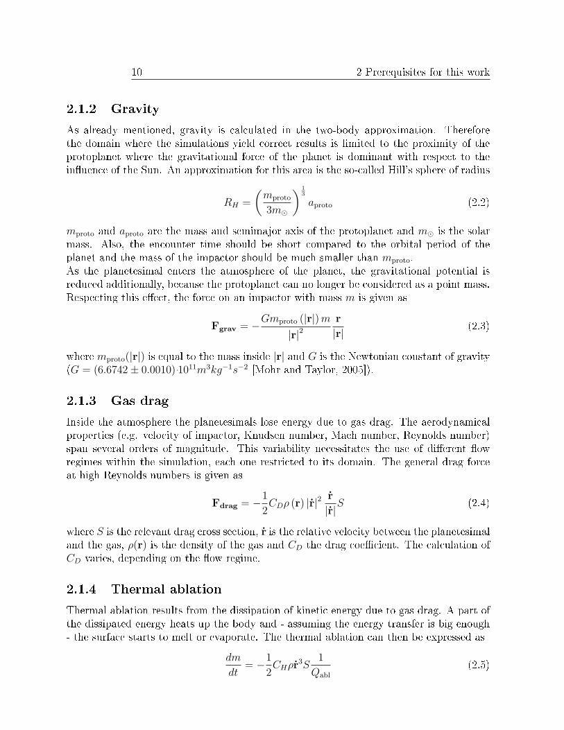
2.1.2 Gravity
As already mentioned, gravity is calculated in the two-body approximation. Thereforethe domain where the simulations yield correct results is limited to the proximity of theprotoplanet where the gravitational force of the planet is dominant with respect to theinuence of the Sun. An approximation for this area is the so-called Hill's sphere of radius
RH =
(mproto
3m
) 13
aproto (2.2)
mproto and aproto are the mass and semimajor axis of the protoplanet and m is the solarmass. Also, the encounter time should be short compared to the orbital period of theplanet and the mass of the impactor should be much smaller than mproto.As the planetesimal enters the atmosphere of the planet, the gravitational potential isreduced additionally, because the protoplanet can no longer be considered as a point mass.Respecting this eect, the force on an impactor with mass m is given as
Fgrav = −Gmproto (|r|) m
|r|2r
|r|(2.3)
where mproto(|r|) is equal to the mass inside |r| and G is the Newtonian constant of gravity(G = (6.6742± 0.0010) ˙1011m3kg−1s−2 [Mohr and Taylor, 2005]).
2.1.3 Gas drag
Inside the atmosphere the planetesimals lose energy due to gas drag. The aerodynamicalproperties (e.g. velocity of impactor, Knudsen number, Mach number, Reynolds number)span several orders of magnitude. This variability necessitates the use of dierent owregimes within the simulation, each one restricted to its domain. The general drag forceat high Reynolds numbers is given as
Fdrag = −1
2CDρ (r) |r|2 r
|r|S (2.4)
where S is the relevant drag cross section, r is the relative velocity between the planetesimaland the gas, ρ(r) is the density of the gas and CD the drag coecient. The calculation ofCD varies, depending on the ow regime.
2.1.4 Thermal ablation
Thermal ablation results from the dissipation of kinetic energy due to gas drag. A part ofthe dissipated energy heats up the body and - assuming the energy transfer is big enough- the surface starts to melt or evaporate. The thermal ablation can then be expressed as
dm
dt= −1
2CHρr3S
1
Qabl
(2.5)

2.1 Theoretical background 11
Qabl is the amount of energy per unit mass needed to bring body material from its initialtemperature to the point where melting or vaporization occurs plus the specic heat neededfor the phase change. CH is the heat transfer coecient which depends on the velocity,ow regime etc. This coecient indicates the fraction of the incoming kinetic energy uxof the gas that is available for the ablation.
2.1.5 Fragmentation
Aerodynamical fragmentation occurs when the pressure gradient across the planetesimalovercomes the internal material strength. First the body starts to deform and at its frontend Rayleigh-Taylor instabilities start to grow. When they reach a sucient size theplanetesimal breaks up. Depending upon the thickness of the atmosphere and the sizeof the planetesimals, either aerodynamical fragmentation or thermal ablation can be thedominant process by which mass is lost. For bigger bodies fragmentation is more important,whereas for smaller ones, most of the mass is lost due to thermal ablation. The absolutevalue for the change of regime depends on the internal structure of the atmosphere.
2.1.6 Equation of motion
The equation of motion is given by the gravitational term and the gas drag. Thermalablation and aerodynamical fragmentation aect the equation of motion only indirectly byreducing m, the mass of the planetesimal or its fragments.
mr = −Gmproto (|r|) m
|r|2r
|r|− 1
2CDρ |r|2 r
|r|S (2.6)
2.1.7 Energy
If we include the eect of the reduced gravitational potential Φ, the total energy of theplanetesimal is given as
Etot =1
2mr2 + mΦ (|r|) (2.7)
Outside of the atmosphere Φ is dened as −Gmproto
|r| and there is no gas drag (at least in thissimulation). Therefore the total energy is constant. The kinetic energy is transformed intogravitational energy and vice versa. Inside the atmosphere the planetesimal loses someenergy due to gas drag. In the calculation of the enhanced radius one needs to know ifthis loss of energy is big enough, so that the planetesimal can't anymore escape from theprotoplanet. It is possible to dene an minimum escape energy
Eesc = −3mΩ2R2H = −mGmproto
RH
(2.8)
that is equal to the energy of a motionless body at distance RH . Here, Ω is the orbitalfrequency of the protoplanet. This equation is completely correct only for an escape along
12 2 Prerequisites for this work
the Sun-protoplanet line (P96). However, the minimum energy is close to zero in alldirections. If the total energy of a planetesimal inside the atmosphere drops below Eesc, itis bound by the planet, because it can never leave the Hill's sphere around the planet,whereas it is not bound if the total energy is higher than Eesc after one pass through theatmosphere.
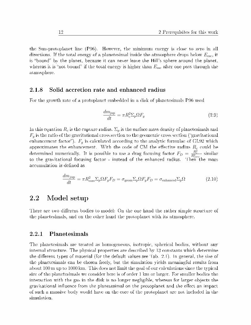
2.1.8 Solid accretion rate and enhanced radius
For the growth rate of a protoplanet embedded in a disk of planetesimals P96 used
dmjup
dt= πR2
cΣpΩFg (2.9)
In this equation Rc is the capture radius, Σp is the surface mass density of planetesimals andFg is the ratio of the gravitational cross section to the geometric cross section (gravitationalenhancement factor). Fg is calculated according to the analytic formulae of GL92 whichapproximates the enhancement. With the code of CM the eective radius Rc could bedetermined numerically. It is possible to use a drag focusing factor FD = R2
c
R2core
- similarto the gravitational focusing factor - instead of the enhanced radius. Then the massaccumulation is dened as
dmjup
dt= πR2
coreΣpΩFgFD = σgeomΣpΩFgFD = σenhancedΣpΩ (2.10)
2.2 Model setup
There are two dierent bodies to model: On the one hand the rather simple structure ofthe planetesimals, and on the other hand the protoplanet with its atmosphere.
2.2.1 Planetesimals
The planetesimals are treated as homogeneous, isotropic, spherical bodies, without anyinternal structure. The physical properties are described by 13 constants which determinethe dierent types of material (for the default values see Tab. 2.1). In general, the size ofthe planetesimals can be chosen freely, but the simulation yields meaningful results fromabout 100 m up to 1000 km. This does not limit the goal of our calculations since the typicalsize of the planetesimals we consider here is of order 1 km or larger. For smaller bodies theinteraction with the gas in the disk is no longer negligible, whereas for larger objects thegravitational inuence from the planetesimal on the protoplanet and the eect an impactof such a massive body would have on the core of the protoplanet are not included in thesimulation.
2.3 Simulation setup 13
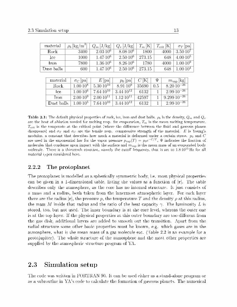
material ρb [kg/m3] Qm [J/kg] Qv [J/kg] Tm [K] Tcrit [K] σT [pa]Rock 3400 2.03 ˙106 8.08 ˙106 1800 4000 3.50 ˙107
Ice 1000 1.47 ˙106 2.50 ˙106 273.15 648 4.00 ˙105
Iron 7800 1.36 ˙106 8.26 ˙106 1780 4000 1.00 ˙109
Dust balls 600 1.47 ˙106 2.50 ˙106 273.15 648 1.00 ˙104
material σC [pa] E [pa] p0 [pa] C [K] Ψ mvap [kg]Rock 1.00 ˙108 5.30 ˙1010 8.91 ˙109 35690 0.5 8.20 ˙10−26
Ice 1.00 ˙106 7.64 ˙1010 3.44 ˙1012 6132 1 2.99 ˙10−26
Iron 2.00 ˙109 2.00 ˙1011 1.12 ˙1011 42597 1 9.299 ˙10−26
Dust balls 1.00 ˙105 7.64 ˙1010 3.44 ˙1012 6132 1 2.99 ˙10−26
Table 2.1: The default physical properties of rock, ice, iron and dust balls. ρb is the density, Qm and Qv
are the heat of ablation needed for melting resp. for evaporation, Tm is the mean melting temperature,Tcrit is the temperate at the critical point (where the dierence between the uid and gaseous phasesdisappears) and σT and σC are the tensile resp. compressive strength of the material. E is Young'smodulus, a constant that describes how much a material is deformed under a certain stress. p0 and Care used in the exponential law for the vapor pressure pvap(T ) = p0e
−C/T , Ψ indicates the fraction ofmolecules that condense upon impact with the surface and mvap is the mean mass of an evaporated bodymolecule. There is a thirteenth constant, namely the cuto frequency, that is set to 1.8˙1015 Hz for allmaterial types considered here.
2.2.2 The protoplanet
The protoplanet is modelled as a spherically symmetric body, i.e. most physical propertiescan be given in a 1-dimensional table, listing the values as a function of |r|. The tabledescribes only the atmosphere, as the core has no internal structure. It just consists ofa mass and a radius, both taken from the innermost atmospheric layer. For each layerthere are the radius |r|, the pressure p, the temperature T and the density ρ at this radius,the mass M inside that radius and the ratio of the heat capacity γ. The luminosity L isstored, too, but not used. The inner boundary is at the core level, whereas the outer oneis at the top layer. If the physical properties at this outer boundary are too dierent fromthe gas disk, additional layers are added to smooth out the transition. Apart from theradial structure some other basic properties must be known, e.g. which gases are in theatmosphere, what is the mean mass of a gas molecule etc. (Table 2.2 is an example for aprotojupiter). The whole structure of the atmosphere and the most other properties aresupplied by the atmospheric structure program of YA.
2.3 Simulation setup
The code was written in FORTRAN 90. It can be used either as a stand-alone program oras a subroutine in YA's code to calculate the formation of gaseous planets. The numerical
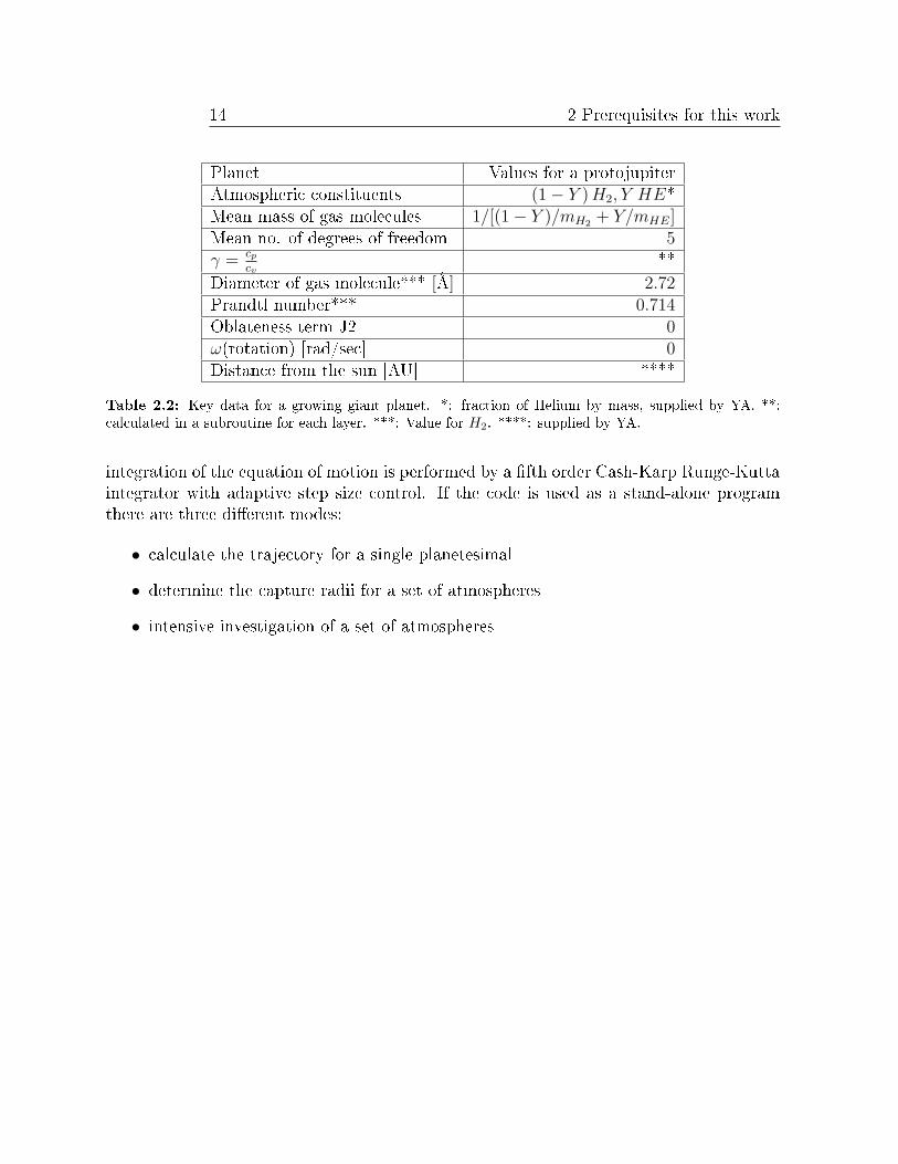
14 2 Prerequisites for this work
Planet Values for a protojupiterAtmospheric constituents (1− Y ) H2, Y HE*Mean mass of gas molecules 1/[(1− Y )/mH2 + Y/mHE]Mean no. of degrees of freedom 5γ = cp
cv**
Diameter of gas molecule*** [Å] 2.72Prandtl number*** 0.714Oblateness term J2 0ω(rotation) [rad/sec] 0Distance from the sun [AU] ****
Table 2.2: Key data for a growing giant planet. *: fraction of Helium by mass, supplied by YA. **:calculated in a subroutine for each layer. ***: Value for H2. ****: supplied by YA.
integration of the equation of motion is performed by a fth order Cash-Karp Runge-Kuttaintegrator with adaptive step size control. If the code is used as a stand-alone programthere are three dierent modes:
• calculate the trajectory for a single planetesimal
• determine the capture radii for a set of atmospheres
• intensive investigation of a set of atmospheres

Chapter 3
The three-body problem
The two-body simplication can be used only for short periods of time and for trajectoriesthat are mostly inside the protoplanet's Hill's sphere. To overcome these restrictions, weneed to take into account the eect of solar gravity. Then we have to deal with three bodies,namely the Sun, the protoplanet and the planetesimal. In the general case this leads toa much more complicated equation of motion that will heavily slow down the simulation.To reduce the complexity of the problem - and simultaneously the computational time -we consider only cases where the mass of the planetesimal is much smaller than the othertwo masses. The rst part of this chapter discusses the theoretical background of the(restricted) three-body problem and its consequences, the second one shows the practicalinuence on the model, i.e. how it is implemented in the code.
3.1 Three-body gravity
In the general three-body problem the motion of the bodies is determined by a nonlinearsystem of second-order dierential equations:
mixi = −G3∑
j=1, j 6=i
mimj (xi − xj)
|xi − xj|3(3.1)
i = 1, 2, 3
Given a set of initial conditions xi (t0) and xi (t0), there exist no exact analytical solutions(apart from a few special cases). However, it is possible to calculate approximate solutionsusing perturbation methods. As the computational time for this calculation would be toolong, another - faster - method had to be found, which is discussed in the following section.

16 3 The three-body problem
3.2 The circular restricted three-body problem - "Prob-
lème restreint"
In the circular restricted three-body problem (hereafter referred to as CR3BP) - alsoknown as "Problème restreint" - we neglect the inuence of the smallest body. It istreated as a massless test particle moving in the gravitational eld of the two mainbodies with mass m0 and m1, that are xed in circular orbits around their commoncentre of mass. All three bodies are considered as point masses and gravity is the onlyeect that is included. The equation of motion for the test particle in an inertial,barycentric 3-d coordinate system (referred to as sidereal) is given as
x = −G
m0
x− x0
|x− x0|3+ m1
x− x1
|x− x1|3
(3.2)
where x , x0 and x1 are the position vectors of the test particles m0 and m1 respectively.As can be found e.g. in [Beutler, 1999] the positions of the other two mass points aredened as
x0 = − m1
m0 + m1
a01
cos n01tsin n01t
0
(3.3)
x1 =m0
m0 + m1
a01
cos n01tsin n01t
0
(3.4)
Here, a01 is the distance between m0 and m1, and n01 is the angular velocity of their motionaround the centre of mass.Transforming this equation into a coordinate system that is rotating with the angularvelocity n01 around the centre of mass (this coordinate system will be referred assynodic), we get
y + 2n01
−y2
y1
0
= n201
y1
y2
0
−G
m0
y − y0
r30
+ m1y − y1
r31
(3.5)
with r0 = |y − y0| and r1 = |y − y1|. For a comparison of the two coordinate systems seeFig. 3.1.Without loss of generality the synodic frame can be chosen so that the position of m0 andm1 are xed on the abscissa. The advantage of this reference frame will be shown in thenext subsection.
3.2 The circular restricted three-body problem - "Problème restreint" 17
x1
x2
y1
y2
m0(t1)
m1(t1)
planetesimal
t1n01
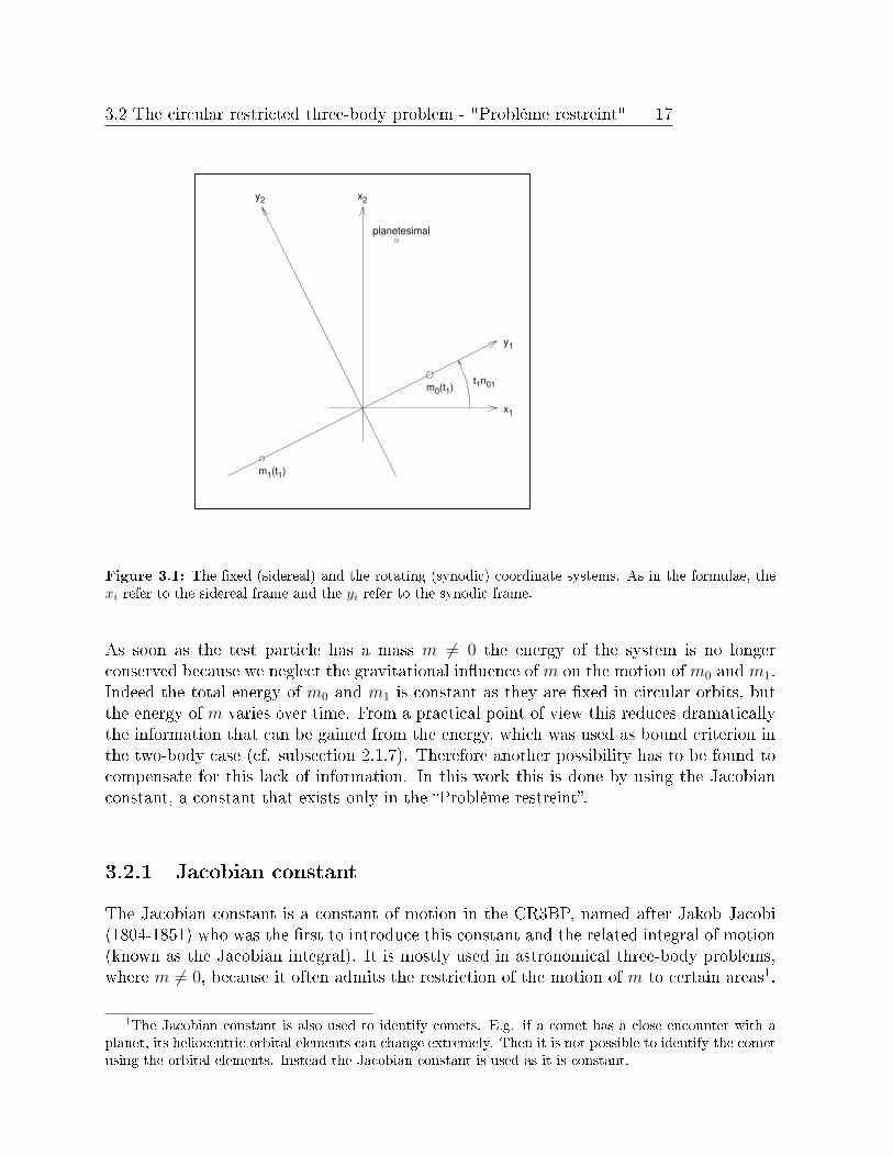
Figure 3.1: The xed (sidereal) and the rotating (synodic) coordinate systems. As in the formulae, thexi refer to the sidereal frame and the yi refer to the synodic frame.
As soon as the test particle has a mass m 6= 0 the energy of the system is no longerconserved because we neglect the gravitational inuence of m on the motion of m0 and m1.Indeed the total energy of m0 and m1 is constant as they are xed in circular orbits, butthe energy of m varies over time. From a practical point of view this reduces dramaticallythe information that can be gained from the energy, which was used as bound criterion inthe two-body case (cf. subsection 2.1.7). Therefore another possibility has to be found tocompensate for this lack of information. In this work this is done by using the Jacobianconstant, a constant that exists only in the Problème restreint.
3.2.1 Jacobian constant
The Jacobian constant is a constant of motion in the CR3BP, named after Jakob Jacobi(1804-1851) who was the rst to introduce this constant and the related integral of motion(known as the Jacobian integral). It is mostly used in astronomical three-body problems,where m 6= 0, because it often admits the restriction of the motion of m to certain areas1.
1The Jacobian constant is also used to identify comets. E.g. if a comet has a close encounter with aplanet, its heliocentric orbital elements can change extremely. Then it is not possible to identify the cometusing the orbital elements. Instead the Jacobian constant is used as it is constant.

18 3 The three-body problem
3.2.1.1 Calculation of the Jacobian constant
The Jacobian constant J is calculated from Eq. 3.5 which is scalar multiplied with 2y andafterwards integrated. According to [Beutler, 1999] the Jacobian integral is then denedas
y2 = n201
y2
1 + y22
+ 2G
m0
r0
+m1
r1
− J (3.6)
in the synodic and
x2 = 2n01 x1x2 − x1x2+ 2G
m0
r0
+m1
r1
− J (3.7)
retransformed to the sidereal frame. For better usability [Szebehely, 1967] used dimension-less coordinates Xi = xi
a01, time T = tn01 and mass µ = m1
m0+m1. For symmetry reasons he
added a new term µ (1− µ) that just shifts the value of the Jacobian constant. Finally theshifted Jacobian constants J ′ in the sidereal and synodic coordinate system's are denedas
J ′ = −X2 + 2
X1X2 − X1X2
+ 2
1− µ
R0
+µ
R1
+ µ (1− µ) (3.8)
J ′ = −Y2 + (1− µ) R20 + µR2
1 + 2
1− µ
R0
+µ
R1
(3.9)
Hereafter vectors and coordinates in capital letter always refer to dimensionless quantities.
3.2.1.2 Hill's curves and Lagrange points
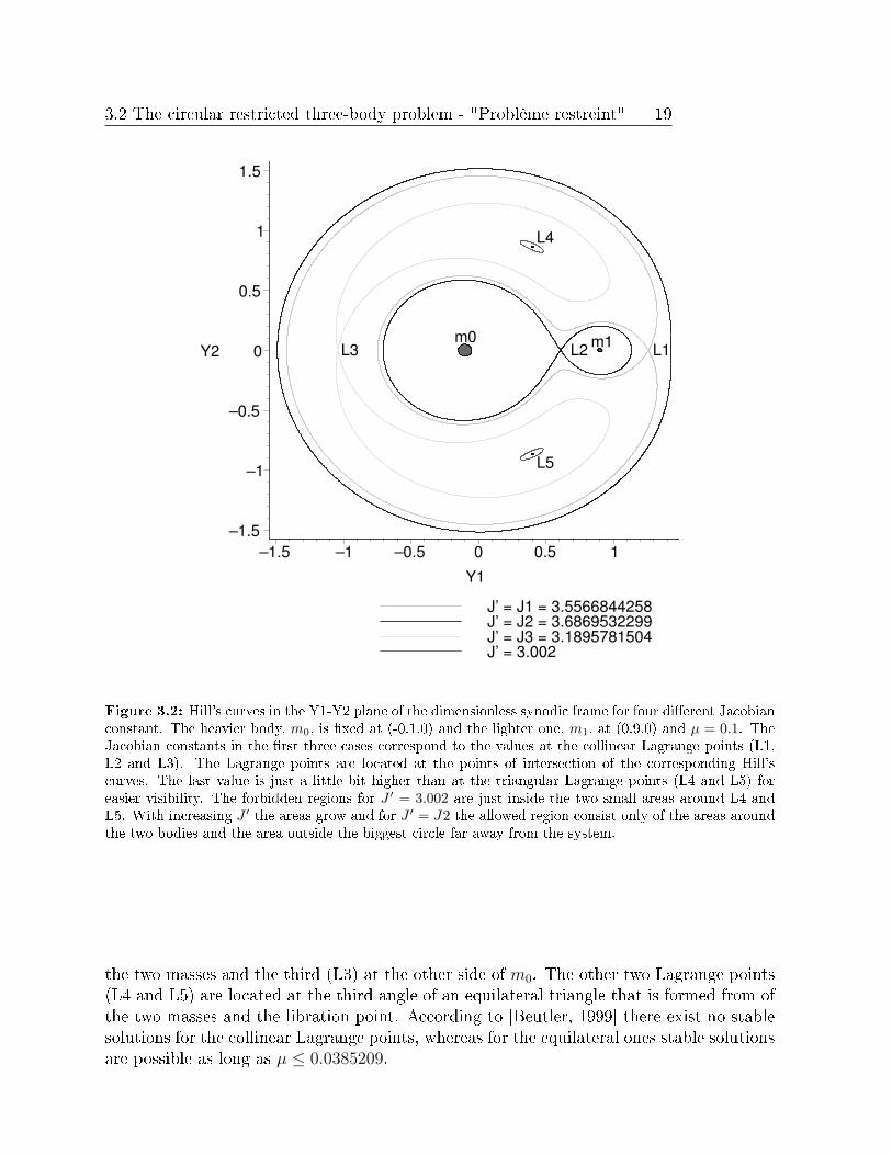
From Eq. 3.9 it is possible to evaluate the areas where a test particle can theoretically be.We just have to set the velocity with respect to the rotating coordinate system to zero andsolve the Jacobian integral for a certain value of J ′. The resulting spheres separate theforbidden2 regions from the allowed ones. In this work the spheres are called Hill's curves(from the 2-d case), even though they are spheres, to be distinguishable from the Hill'ssphere radius RH (see Eq. 2.2). In Fig. 3.2 four curves for dierent Jacobian constantsare shown.
In the CR3BP there exist ve stationary solutions called Lagrange points (also known aslibration points). At these points a test particle could be placed in the synodic frame andwould remain in its position relative to the two other bodies. In literature the denitionof these points is not consistent. In this work the denitions of [Szebehely, 1967] are used.Three libration points are located collinearly to m0 and m1. The rst (referred to as L1)is situated at the same side of m0 as m1, but farther away, the second (L2) lies between
2In the forbidden areas the solved Jacobian integral yield an imaginary velocity (Y2 < 0), whereas inthe allowed areas the velocity is real (Y2 > 0).
3.2 The circular restricted three-body problem - "Problème restreint" 19
J’ = J1 = 3.5566844258J’ = J2 = 3.6869532299J’ = J3 = 3.1895781504J’ = 3.002
m0 m1
L5
L4
L3 L2 L1
–1.5
–1
–0.5
0
0.5
1
1.5
Y2
–1.5 –1 –0.5 0 0.5 1Y1
Figure 3.2: Hill's curves in the Y1-Y2 plane of the dimensionless synodic frame for four dierent Jacobianconstant. The heavier body, m0, is xed at (-0.1,0) and the lighter one, m1, at (0.9,0) and µ = 0.1. TheJacobian constants in the rst three cases correspond to the values at the collinear Lagrange points (L1,L2 and L3). The Lagrange points are located at the points of intersection of the corresponding Hill'scurves. The last value is just a little bit higher than at the triangular Lagrange points (L4 and L5) foreasier visibility. The forbidden regions for J ′ = 3.002 are just inside the two small areas around L4 andL5. With increasing J ′ the areas grow and for J ′ = J2 the allowed region consist only of the areas aroundthe two bodies and the area outside the biggest circle far away from the system.
the two masses and the third (L3) at the other side of m0. The other two Lagrange points(L4 and L5) are located at the third angle of an equilateral triangle that is formed from ofthe two masses and the libration point. According to [Beutler, 1999] there exist no stablesolutions for the collinear Lagrange points, whereas for the equilateral ones stable solutionsare possible as long as µ ≤ 0.0385209.
20 3 The three-body problem
3.2.2 Bound criterion for the planetesimal
One of the main points of this work is to determine the enhanced capture cross sectiondue to the eect of the protoplanet's atmosphere and the gravitational inuence of thecentral star. To reach this goal a fast way to decide if a planetesimal will get accreted bythe protoplanet (also referred as bound, because in the problème restreint a planetesimalthat is bound to the proximity of the protoplanet will eventually get accreted) is needed.So it is not important what happens to the planetesimal, e.g. if it is ablated, hits the coreetc. In this context the only important point is whether it is bound or not. There aretwo opposed requirements for the bound criterion to be determined. On one hand, theintegration should stop as soon as possible to save computational time, and on the otherhand, the program has to ensure that it does proceed until it is clear that the planetesimalgets accreted. In the CR3BP the energy can't be used as a criterion when to stop, as wasused in the two-body situation. Instead the Jacobian constant is chosen.In Fig. 3.2 among other things the zero velocity curves for J ′ = J ′(L2) are shown. Theallowed areas consist of the drop shaped regions around m0 and m1 and the region outsidethe biggest circle3. If a test particle is inside the area around m1 and has a Jacobianconstant that is just slightly above J ′(L2) there is no way of getting out of this region. Theparticle is bound to the proximity of this body and will therefore get accreted. This impliesthat the zero velocity value of the Jacobian constant at L2 can be used as a terminationcondition for the integration.For J ′(L1) there is a similar meaning. In this case the particle is bound to the entire systemthat consists of the masses m0 and m1.
3.3 Implications for the simulation
The Jacobian constant should be used as a criterion to determine whether a particle isbound or not. As the CR3BP yields meaningful results only if several restrictions arefullled, we have to check their validity for the conditions of this work.
3.3.1 Implementation of the Jacobian constant
Because the code was initially written to compute the evolution of a two-body system, thecoordinate system is planetocentric and the Sun is then implemented as a body rotatingaround the protoplanet. Therefore the calculation for the Jacobian constant has to beadapted by transforming all coordinates to a barycentric frame. This is done using the
3This region is not considered in this work, as we are not interested in planetesimals that far away.

3.3 Implications for the simulation 21
following set of equations:
X1 = X ′1 − (1− µ) cos n01t (3.10)
X1 = X ′1 + n01(1− µ) sin n01t (3.11)
X2 = X ′2 − (1− µ) sin n01t (3.12)
X2 = X ′2 − n01(1− µ) cos n01t (3.13)
Here the planetocentric coordinates are denoted with a prime. Then Eq. 3.8 can be usedto calculate the Jacobian constant of the planetesimal.
3.3.2 Conditions of the applicability of the CR3BP
Without loss of generality we set the Sun to be represented by the mass m0 and theprotoplanet by the mass m1. Of course, the test particle represents the planetesimal.Then the restrictions for the applicability of the CR3BP are:
• The mass of the planetesimal is much smaller compared to the other masses.
• The Sun and the protoplanet move on circular orbits around their common centre ofmass.
• The gravitational potential of the Sun and the protoplanet are like the gravitationalpotential of point masses with constant masses.
• Only gravitational forces are considered.
To always fulll the rst condition the mass of the largest planetesimals considered inthe simulations has to be always much smaller than the mass of the smallest protoplanetconsidered. Actually, this is not a real limitation of the model, as this is always satisedin the situations we are considering. The signicance of the results for impacts of hugebodies would have been problematic, anyway. Therefore the upper limit is set to 1000 km,similarly to the limit used by CM.At the moment the second point is implemented in the code, i.e. the distance between theSun and the protoplanet is xed for the whole simulation. This simplication is often usedin the literature (GL92; P96; [Inaba and Ikoma, 2003]) and seems acceptable at least inthe case for present day Jupiter (mean eccentricity according to [2004]: 0.049 ). For theknown exoplanets with higher eccentricity (e > 0.1) the simplication of circular orbitsmay not be appropriated.The third condition is problematic. In fact, it can't be observed as soon as the planetesimalenters the atmosphere of the protoplanet. Outside of the atmosphere the gravitationalinuence of the Sun and the protoplanet can be replaced by the corresponding potentialsof point masses. But when the planetesimal is inside the atmosphere the gravitationalpotential of the protoplanet is changed because only the part of the protoplanet's massthat is inside the actual position of the planetesimal is contributing to the gravitational
22 3 The three-body problem
force (cf. Eq. 2.3). As the exact trajectories of the planetesimals through the atmosphereare essential for this work, it makes no sense to restrict the investigations to orbits thatnever cross the atmosphere. It will be discussed in subsection 3.3.2.1 how the CR3BP isaected by the reduced gravitational potential4 of the protoplanet.The last point is again not strictly fullled by the simulation. Inside the atmosphere themotion of the planetesimal is aected not only by gravity, but also by gas drag. The eectof this perturbation is analysed in subsection 3.3.2.2.
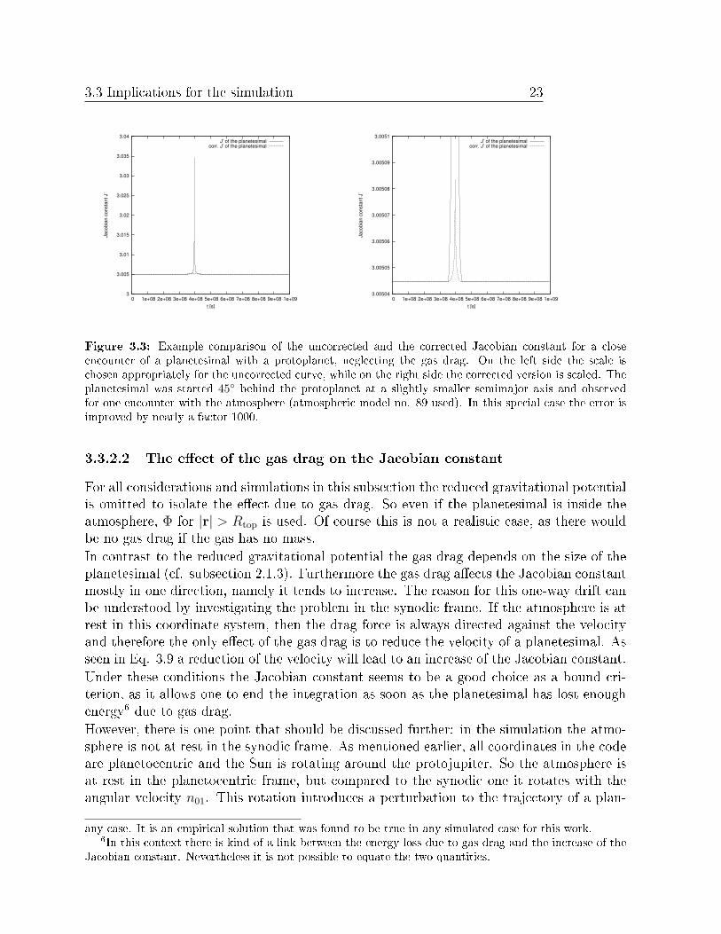
3.3.2.1 The eect of the reduced gravitational potential on the Jacobian con-stant
In this subsection the inuence of gas drag is neglected. We therefore temporarily assumethat if a planetesimal enters the atmosphere, the reduction of the gravitational potentialis the only eect occurring. One can easily understand that this reduction will aect theJacobian constant, because the trajectory of the planetesimal is changed. The inuence ofthe protoplanet on the trajectory will be smaller, as the gravitational force is reduced. Ingeneral, this means that the planetesimal will not approach as close to the core and thatthe velocity increase for incoming and the velocity decrease for outgoing planetesimals dueto the protoplanet's gravity will be slightly smaller. Both of this eects will lead to ahigher Jacobian constant. Therefore a correction to the calculation is needed. My attemptis to introduce a new, eective mass meff (|r|) that replaces the one of the protoplanet,which is incorrect inside the atmosphere. The value of this eective mass is dened as themass that would be needed to cause the same gravitational potential at the location ofthe planetesimal with a point mass at the planet's centre of mass. Then a local µ can becalculated:
µloc (|r|) =
µ for |r| ≥ Rtop
meff(|r|)m0+meff(|r|) otherwise
(3.14)
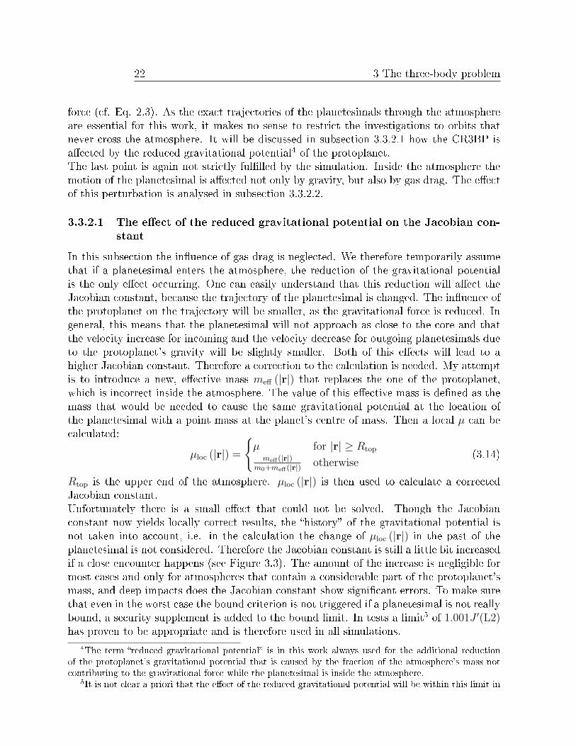
Rtop is the upper end of the atmosphere. µloc (|r|) is then used to calculate a correctedJacobian constant.Unfortunately there is a small eect that could not be solved. Though the Jacobianconstant now yields locally correct results, the history of the gravitational potential isnot taken into account, i.e. in the calculation the change of µloc (|r|) in the past of theplanetesimal is not considered. Therefore the Jacobian constant is still a little bit increasedif a close encounter happens (see Figure 3.3). The amount of the increase is negligible formost cases and only for atmospheres that contain a considerable part of the protoplanet'smass, and deep impacts does the Jacobian constant show signicant errors. To make surethat even in the worst case the bound criterion is not triggered if a planetesimal is not reallybound, a security supplement is added to the bound limit. In tests a limit5 of 1.001J ′(L2)has proven to be appropriate and is therefore used in all simulations.
4The term reduced gravitational potential is in this work always used for the additional reductionof the protoplanet's gravitational potential that is caused by the fraction of the atmosphere's mass notcontributing to the gravitational force while the planetesimal is inside the atmosphere.
5It is not clear a priori that the eect of the reduced gravitational potential will be within this limit in
3.3 Implications for the simulation 23
3
3.005
3.01
3.015
3.02
3.025
3.03
3.035
3.04
0 1e+08 2e+08 3e+08 4e+08 5e+08 6e+08 7e+08 8e+08 9e+08 1e+09
Jaco
bian
con
stan
t J’
t [s]
J’ of the planetesimalcorr. J’ of the planetesimal
3.00504
3.00505
3.00506
3.00507
3.00508
3.00509
3.0051
0 1e+08 2e+08 3e+08 4e+08 5e+08 6e+08 7e+08 8e+08 9e+08 1e+09
Jaco
bian
con
stan
t J’
t [s]
J’ of the planetesimalcorr. J’ of the planetesimal
Figure 3.3: Example comparison of the uncorrected and the corrected Jacobian constant for a closeencounter of a planetesimal with a protoplanet, neglecting the gas drag. On the left side the scale ischosen appropriately for the uncorrected curve, while on the right side the corrected version is scaled. Theplanetesimal was started 45 behind the protoplanet at a slightly smaller semimajor axis and observedfor one encounter with the atmosphere (atmospheric model no. 89 used). In this special case the error isimproved by nearly a factor 1000.
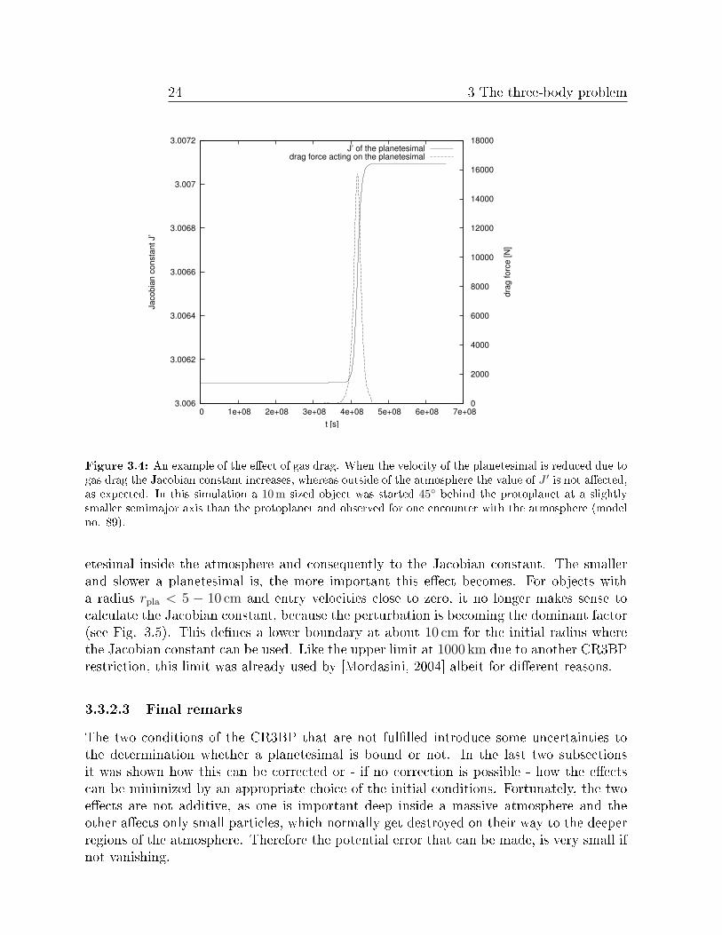
3.3.2.2 The eect of the gas drag on the Jacobian constant
For all considerations and simulations in this subsection the reduced gravitational potentialis omitted to isolate the eect due to gas drag. So even if the planetesimal is inside theatmosphere, Φ for |r| > Rtop is used. Of course this is not a realistic case, as there wouldbe no gas drag if the gas has no mass.In contrast to the reduced gravitational potential the gas drag depends on the size of theplanetesimal (cf. subsection 2.1.3). Furthermore the gas drag aects the Jacobian constantmostly in one direction, namely it tends to increase. The reason for this one-way drift canbe understood by investigating the problem in the synodic frame. If the atmosphere is atrest in this coordinate system, then the drag force is always directed against the velocityand therefore the only eect of the gas drag is to reduce the velocity of a planetesimal. Asseen in Eq. 3.9 a reduction of the velocity will lead to an increase of the Jacobian constant.Under these conditions the Jacobian constant seems to be a good choice as a bound cri-terion, as it allows one to end the integration as soon as the planetesimal has lost enoughenergy6 due to gas drag.However, there is one point that should be discussed further: in the simulation the atmo-sphere is not at rest in the synodic frame. As mentioned earlier, all coordinates in the codeare planetocentric and the Sun is rotating around the protojupiter. So the atmosphere isat rest in the planetocentric frame, but compared to the synodic one it rotates with theangular velocity n01. This rotation introduces a perturbation to the trajectory of a plan-
any case. It is an empirical solution that was found to be true in any simulated case for this work.6In this context there is kind of a link between the energy loss due to gas drag and the increase of the
Jacobian constant. Nevertheless it is not possible to equate the two quantities.
24 3 The three-body problem
3.006
3.0062
3.0064
3.0066
3.0068
3.007
3.0072
0 1e+08 2e+08 3e+08 4e+08 5e+08 6e+08 7e+08 0
2000
4000
6000
8000
10000
12000
14000
16000
18000Ja
cobi
an c
onst
ant J
’
drag
forc
e [N
]
t [s]
J’ of the planetesimaldrag force acting on the planetesimal
Figure 3.4: An example of the eect of gas drag. When the velocity of the planetesimal is reduced due togas drag the Jacobian constant increases, whereas outside of the atmosphere the value of J ′ is not aected,as expected. In this simulation a 10 m sized object was started 45 behind the protoplanet at a slightlysmaller semimajor axis than the protoplanet and observed for one encounter with the atmosphere (modelno. 89).
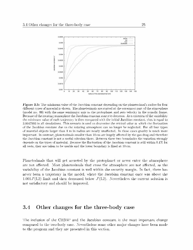
etesimal inside the atmosphere and consequently to the Jacobian constant. The smallerand slower a planetesimal is, the more important this eect becomes. For objects witha radius rpla < 5 − 10 cm and entry velocities close to zero, it no longer makes sense tocalculate the Jacobian constant, because the perturbation is becoming the dominant factor(see Fig. 3.5). This denes a lower boundary at about 10 cm for the initial radius wherethe Jacobian constant can be used. Like the upper limit at 1000 km due to another CR3BPrestriction, this limit was already used by [Mordasini, 2004] albeit for dierent reasons.
3.3.2.3 Final remarks
The two conditions of the CR3BP that are not fullled introduce some uncertainties tothe determination whether a planetesimal is bound or not. In the last two subsectionsit was shown how this can be corrected or - if no correction is possible - how the eectscan be minimized by an appropriate choice of the initial conditions. Fortunately, the twoeects are not additive, as one is important deep inside a massive atmosphere and theother aects only small particles, which normally get destroyed on their way to the deeperregions of the atmosphere. Therefore the potential error that can be made, is very small ifnot vanishing.
3.4 Other changes for the three-body case 25
3.001
3.0015
3.002
3.0025
3.003
3.0035
3.004
3.0045
3.005
3.0055
0 10 20 30 40 50 60 70 80 90 100 110 120 130 140 150
Jaco
bian
con
stan
t J’
radius of the planetesimal [cm]
stoneice
irondustballs
Figure 3.5: The minimum value of the Jacobian constant depending on the planetesimal's radius for fourdierent types of material is shown. The planetesimals are started at the outermost part of the atmosphere(model no. 89) with the same semimajor axis as the protoplanet and zero velocity in the synodic frame.Because of the rotating atmosphere the Jacobian constant starts to decrease. As a criterion of the variabilitythe minimum value of each trajectory is then compared with the initial Jacobian constant, that is equal to3.0047993 in all simulations. This scenario is used to determine the critical value at which the uctuationof the Jacobian constant due to the rotating atmosphere can no longer be neglected. For all four typesof material objects larger than 1 m in radius are nearly unaected. In these cases gravity is much moreimportant. In contrast, planetesimals smaller than 10 cm are hugely aected by the gas drag and thereforethe Jacobian constant is not a useful criterion there. Between these two boundaries the variation stronglydepends on the types of material. Because the uctuation of the Jacobian constant is still within 0.1% forall tests, they are taken to be usable and the lower boundary is xed at 10 cm.
Planetesimals that will get accreted by the protoplanet or never enter the atmosphereare not aected. Most planetesimals that cross the atmosphere are not aected, as thevariability of the Jacobian constant is well within the security margin. In fact, there hasnever been a trajectory in the model, where the Jacobian constant once was above the1.001J ′(L2) limit and then decreased below J ′(L2). Nevertheless the current solution isnot satisfactory and should be improved.
3.4 Other changes for the three-body case
The inclusion of the CR3BP and the Jacobian constant is the most important changecompared to the two-body case. Nevertheless some other major changes have been madeto the program and they are presented in this section.

26 3 The three-body problem
3.4.1 Initial conditions
The initial position and velocity of the planetesimal have been changed. Instead of theplanetocentric position vector xpla and the velocity vector relative to the protoplanet vpla,the heliocentric orbital elements (semimajor axis a, numerical eccentricity e, inclinationi, argument of perigee ω, right ascension of the ascending node Ω and the time of thelast perigee passing t) are used as initial conditions. There are two main reasons forthis modication. First, in the three-body case it is more practical to use these initialconditions, especially if a wide range of parameters is to be examined. Second, it allows abetter comparison to other work about three-body motion, because most publications useheliocentric orbital elements (e.g. GL92 or [Nakazawa et al., 1989] ).
3.4.2 The enhancement factor of the capture cross section
The enhancement factor of the capture cross section is dened as
Fenhancement =number of accreted planetesimals including all the considered effects
number of accreted planetesimals by gravity for the 1− body case
Until now, the enhancement factor has been calculated in two nearly independent steps.The enhancement due to the eect of the atmosphere was determined and then the en-hancement for the 3-body case was numerically calculated (P96; [Alibert et al. (2005)]).With the code presented in this work it will now be possible to determine the total en-hancement factor in one simulation. Therefore the determine capture radius-mode for thetwo-body case has been replaced. In the three-body case it is no longer useful to determinean enhanced capture radius, because the eect of the three-body gravity and the eect ofthe atmosphere are combined. Instead of two separate factors FD and Fg for the enhance-ment due to the atmosphere and due to the gravity, respectively, there is just one factor7Fg+D. So the determine capture radius-mode is replaced by a determine enhancementfactor-mode. For this mode a huge number of computational runs is needed, i.e. from atleast 10000 up to a few million depending on the initial conditions. In general, the moreruns that are made, the better the accuracy of the resulting enhancement factor becomes.According to Eq. 2.10 the enhanced capture cross section for the calculation of the growthrate of a planet accreting from surrounding planetesimals is given as
σenhanced = πR2coreFgFD (3.15)
or, if the combined enhancement factor is used, as
σenhanced = πR2coreFg+D (3.16)
In chapter 7 we will investigate if Fg+D can really be replaced by FgFD, as it was done inP96.
7For a protoplanet without an atmosphere Fg+D simply reduces to Fg.

3.4 Other changes for the three-body case 27
3.4.3 Integrating routine
Computational time is the most severe restriction on the calculation of the enhancementfactor. For a faster integration of the equation of motion a new integrator was implemented.Outside of the atmosphere the equation of motion is now integrated by a Bulirsch-Stoer(referred to as B-S) integrator with monitoring of the local truncation error to ensureaccuracy. The use of this integrator allows one to save up to 70% of the time comparedto the Runge-Kutta algorithm8. Unfortunately, it is not possible to use the B-S routineinside the atmosphere, because there the equation of motion contains non smooth functions,which can't be handled by the B-S integrator.Using two dierent types of integrators introduces a new problem, as the boundary betweenthem has to be dened. On one hand, the faster, B-S integrator should be used as long aspossible, on the other hand, the Runge-Kutta routine has to be used when the planetesimalenters the atmosphere. In this case, accuracy is preferred to speed, because the overallreduction of the computational time is minimal, as most of the time is used by calculationsinside the atmosphere. So the step size in the B-S routine is reduced more than neededto assure that the planetesimal can not get into the atmosphere. If the planetesimalgets within a certain range of the atmosphere (at the moment this is set to 0.05 RH), theintegrator is changed from B-S to Runge-Kutta.
3.4.4 Criteria to terminate the integration
There are several criteria that may be used to determine, when to stop the integration ofa trajectory. Some of them are used only in the determine enhancement factor mode,whereas others are universally valid.A trajectory always ends, if one of the following three conditions is fullled:
1. The maximum integration time has been reached.
2. The planetesimal hits the core of the protoplanet.
3. The planetesimal was completely melted or ablated in the atmosphere.
These conditions are the same as in the two-body case and they are still valid. For thedetermination of the enhancement factor mode, there are new termination criteria:
1. The planetesimal is not accreted by the protoplanet:
(a) The planetesimal was destroyed in a close encounter with the Sun.(b) The planetesimal is bound within the Hill's sphere of the Sun.
8Tests have been performed for the two and the three-body case with a protoplanet without an at-mosphere. The accuracy was set to 10−9 for both integrators. In most simulations the B-S routine was40% to 60% faster. Several tests including an atmosphere have also been made, but no comparison waspossible, because the B-S integrator sometimes yields incorrect results.
28 3 The three-body problem
-10
-5
0
5
10
-10 -5 0 5 10
AU
AU
atmospherea/2
a = 7.65 AUa = 7.45 AU
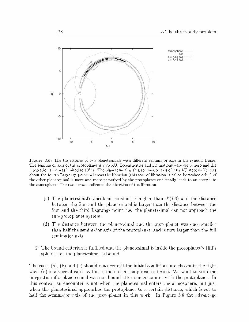
Figure 3.6: The trajectories of two planetesimals with dierent semimajor axis in the synodic frame.The semimajor axis of the protoplanet is 7.75 AU. Eccentricities and inclinations were set to zero and theintegration time was limited to 1011 s. The planetesimal with a semimajor axis of 7.65 AU steadily libratesabout the fourth Lagrange point, whereas the libration (this sort of libration is called horseshoe orbit) ofthe other planetesimal is more and more perturbed by the protoplanet and nally leads to an entry intothe atmosphere. The two arrows indicates the direction of the libration.
(c) The planetesimal's Jacobian constant is higher than J ′(L3) and the distancebetween the Sun and the planetesimal is larger than the distance between theSun and the third Lagrange point, i.e. the planetesimal can not approach thesun-protoplanet system.
(d) The distance between the planetesimal and the protoplanet was once smallerthan half the semimajor axis of the protoplanet, and is now larger than the fullsemimajor axis.
2. The bound criterion is fullled and the planetesimal is inside the protoplanet's Hill'ssphere, i.e. the planetesimal is bound.
The cases (a), (b) and (c) should not occur, if the initial conditions are chosen in the rightway. (d) is a special case, as this is more of an empirical criterion. We want to stop theintegration if a planetesimal was not bound after one encounter with the protoplanet. Inthis context an encounter is not when the planetesimal enters the atmosphere, but justwhen the planetesimal approaches the protoplanet to a certain distance, which is set tohalf the semimajor axis of the protoplanet in this work. In Figure 3.6 the advantage
3.4 Other changes for the three-body case 29
of such a criterion is shown. A planetesimal approaches the protoplanet several timeswithout entry into the atmosphere, but because its orbit is perturbed by the protoplanet,the planetesimal is nally accreted. Such cases have to be excluded in the simulations inorder to not overestimate the enhanced collision cross section.The value of this boundary is set to half the semimajor axis, because this covers all libra-tion orbits that could be strongly perturbed, at least for low eccentricity and inclination.According to [Borcherds, 1996] there are not only long-period libration (as shown in Figure3.6), but also short-period libration orbits. Therefore trajectories are not excluded untilthe distance between the planetesimal and the protoplanet reaches aproto. A more detaileddiscussion of the stability of libration orbits can be found in [Szebehely, 1967] for dier-ent 2-dimensional cases, and in [Barrabés and Mikkola, 2005] for 3-dimensional horseshoeorbits.


Chapter 4
Model setup
This chapter is divided in two parts. First, the models of the bodies involved are presented.In the second part, the dierent distributions for the orbital elements of the planetesimalsare explained.
4.1 Models of the bodies
There are three dierent bodies to model: The Sun, the protoplanet and the planetesimal.
4.1.1 The Sun
The only characteristic of the Sun which we use in these simulations is its mass (m =1.9891 ˙1030 kg). There is also another property that is linked to the Sun, the sphere ofinuence. At this distance to the Sun a planetesimal would be strongly aected by solareects that are not included in the simulation, so that the integration is stopped. At themoment, the radius of this sphere is set to one solar radius.
4.1.2 The protoplanet
The model of the protoplanet has not been changed compared to the one used in the two-body case (cf. subsection 2.2.2). Therefore it is not discussed here with one exception,namely the properties of four dierent atmospheres are presented. These atmosphereswere taken from a set of 89 atmospheres produced by the atmospheric structure programof Yann Alibert, and they were used for a comparison of the enhancement factor of thecollision cross section. The set of atmospheres describe the evolution of a forming giantgas planet from the point where the mass of the atmosphere around the planet reachesabout 1/1000 of the core mass, up to the point where runaway growth occurs.To cover a wide range of dierent initial conditions, the 1st, 30th, 60th and 89th atmo-spheres have been chosen for a more detailed investigation. In Tab. 4.1 some generalinformation about these atmospheres is specied.

32 4 Model setup
Model no. 1 30 60 89no. of layers 989 1227 1384 1677fraction of Helium 0.24 0.24 0.24 0.24semimajor axis [AU] 11.50 11.09 10.50 7.75Rcore [m] 6.45 ˙106 1.13 ˙107 1.51 ˙107 2.20 ˙107
mcore [kg] 3.60 ˙1024 1.92 ˙1025 4.65 ˙1025 1.42 ˙1026
Rtop[m] 3.12 ˙109 1.66 ˙1010 3.23 ˙1010 4.29 ˙1010
matmo[kg] 3.12 ˙1021 5.36 ˙1023 5.07 ˙1024 1.57 ˙1026
matmo/mcore 0.0009 0.0279 0.1090 1.1056mtot/m⊕ 0.60 3.29 8.63 50.00
Table 4.1: General information about the four investigated atmospheric models.
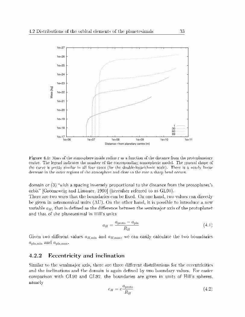
As one can see from the change in the semimajor axis, the growing protoplanet is slowlymigrating towards the Sun. This eect is not included in the program, because the semi-major axis remains nearly constant over the time scale used in one simulation. The totalmass of the modelled protoplanets spreads from 0.6 m⊕ for the rst atmosphere to 50 m⊕for the last one. For the mass of the atmosphere the spread is even bigger.On the following pages, the characteristics of the mass, the pressure, the temperature andthe density inside the atmosphere are presented (Figure 4.1, 4.2, 4.3 and 4.4, respectively).The boundaries are set at the core on the inner side and at about the Hill's radius on theouter side.
4.1.3 The planetesimal
The model of the planetesimal was completely taken from CM's program. Therefore itis not discussed here. The important information can be found in subsection 2.2.1 or in[Mordasini, 2004].
4.2 Distributions of the orbital elements of the planetes-
imals
For the determination of the enhancement factor of the collision cross section, a largenumber of simulations are needed. For each run the initial orbital elements are changeddepending on the distribution that has been chosen.
4.2.1 Semimajor axis
There are three dierent distributions for the semimajor axes. All of them need twoboundaries, that dene the domain that will be investigated. Then the semimajor axescan be distributed: (1) uniformly between the two boundaries, (2) randomly within the
4.2 Distributions of the orbital elements of the planetesimals 33
1e+17
1e+18
1e+19
1e+20
1e+21
1e+22
1e+23
1e+24
1e+25
1e+26
1e+27
1e+06 1e+07 1e+08 1e+09 1e+10 1e+11
Mas
s [k
g]
Distance r from planetary centre [m]
1306089
Figure 4.1: Mass of the atmosphere inside radius r as a function of the distance from the protoplanetarycentre. The legend indicates the number of the corresponding atmospheric model. The general shape ofthe curve is pretty similar in all four cases (for the double-logarithmic scale). There is a nearly lineardecrease in the outer regions of the atmosphere and close to the core a sharp bend occurs.
domain or (3) with a spacing inversely proportional to the distance from the protoplanet'sorbit [Greenzweig and Lissauer, 1990] (hereafter referred to as GL90).There are two ways that the boundaries can be xed. On one hand, two values can directlybe given in astronomical units (AU). On the other hand, it is possible to introduce a newvariable aH , that is dened as the dierence between the semimajor axis of the protoplanetand that of the planetesimal in Hill's units
aH =aproto − apla
RH
(4.1)
Given two dierent values aH,min and aH,max, we can easily calculate the two boundariesapla,min and apla,max.
4.2.2 Eccentricity and inclination
Similar to the semimajor axis, there are three dierent distributions for the eccentricitiesand the inclinations and the domain is again dened by two boundary values. For easiercomparison with GL90 and GL92, the boundaries are given in units of Hill's spheres,namely
eH = eaproto
RH
(4.2)
34 4 Model setup
0.01
1
100
10000
1e+06
1e+08
1e+10
1e+06 1e+07 1e+08 1e+09 1e+10 1e+11
Pres
sure
[pa]
Distance r from planetary centre [m]
1306089
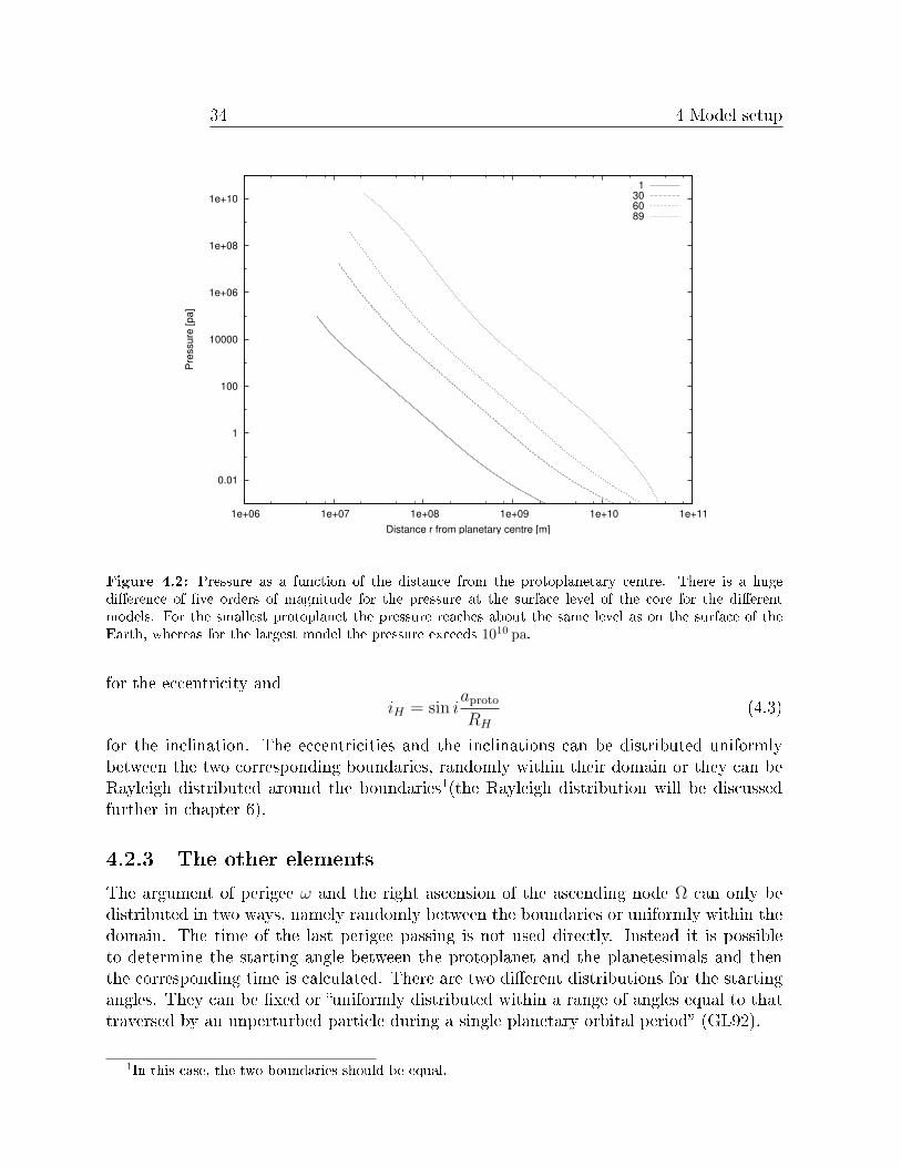
Figure 4.2: Pressure as a function of the distance from the protoplanetary centre. There is a hugedierence of ve orders of magnitude for the pressure at the surface level of the core for the dierentmodels. For the smallest protoplanet the pressure reaches about the same level as on the surface of theEarth, whereas for the largest model the pressure exceeds 1010 pa.
for the eccentricity andiH = sin i
aproto
RH
(4.3)
for the inclination. The eccentricities and the inclinations can be distributed uniformlybetween the two corresponding boundaries, randomly within their domain or they can beRayleigh distributed around the boundaries1(the Rayleigh distribution will be discussedfurther in chapter 6).
4.2.3 The other elements
The argument of perigee ω and the right ascension of the ascending node Ω can only bedistributed in two ways, namely randomly between the boundaries or uniformly within thedomain. The time of the last perigee passing is not used directly. Instead it is possibleto determine the starting angle between the protoplanet and the planetesimals and thenthe corresponding time is calculated. There are two dierent distributions for the startingangles. They can be xed or uniformly distributed within a range of angles equal to thattraversed by an unperturbed particle during a single planetary orbital period (GL92).
1In this case, the two boundaries should be equal.
10
100
1000
10000
100000
1e+06 1e+07 1e+08 1e+09 1e+10 1e+11
Tem
pera
ture
[K]
Distance r from planetary centre [m]
1306089
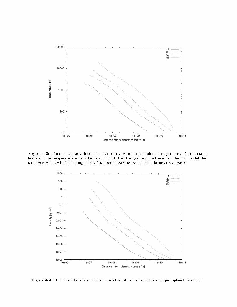
Figure 4.3: Temperature as a function of the distance from the protoplanetary centre. At the outerboundary the temperature is very low matching that in the gas disk. But even for the rst model thetemperature exceeds the melting point of iron (and stone, ice or dust) at the innermost parts.
1e-08
1e-07
1e-06
1e-05
1e-04
0.001
0.01
0.1
1
10
100
1000
1e+06 1e+07 1e+08 1e+09 1e+10 1e+11
Dens
ity [k
g/m
3 ]
Distance r from planetary centre [m]
1306089
Figure 4.4: Density of the atmosphere as a function of the distance from the protoplanetary centre.


Chapter 5
Overview of the program
In this short chapter some general information about the program and its internal structureare presented. The emphasis is on the improvements made in this work compared to thetwo-body case. For a more detailed discussion of the two-body code see Chapter 7 of[Mordasini, 2004].
5.1 Basic information
The computer program is written in Fortran 90, but some routines have been transformedfrom Fortran 77. Compilation is done with the free Intel ifc compiler on a computer usingthe Linux operating system. The program uses double precision oating point variables.Overall, the code consists of about 8000 lines of which about 1000 are used once perrun (main program), about 2000 once per atmosphere (calculation of the atmosphericstructure) and the other 5000 are generally used more often, depending on the initialconditions (calculation of the motion of the planetesimal and everything that is relatedto it). To run the main program does not take a considerable amount of time, but thepreparation of the atmosphere needs about half a minute per atmosphere. The biggest partof the computational time is used for the calculation of the trajectories. For a typical set1of planetesimals, and if the integration is stopped as soon as the fate of the planetesimalsis clear, the average computational time on a standard computer2 for one trajectory isbetween 0.01 s and 0.02 s. So a run with one million planetesimals, which will returnsuciently exact results in most cases, will take about ve to ten hours. This time canincrease by more than a factor of two, if more information than just a few key data perrun are to be stored. Anyway, it is not recommended to make an output le for eachplanetesimal with such a huge number of planetesimals.
1A typical set means a set where about 10% to 30% of the planetesimals enter the atmosphere andabout half of them get bound.
2ISIS, the cluster of our theoretical astrophysics and planetary science group, oers at the moment IntelDual Xeon processors (2.4 to 3.06 GHz).

38 5 Overview of the program
Figure 5.1: Schematic overview of the program. Each box represents a subroutine. The rst line indicatesthe name of the routine and the subroutines and functions that are called by this routine are listed belowin the order of appearance. The highest routine, i. e. the main program, is situated at the left side. Theshifted subroutines are subroutines of the routine that is written right on top of them, e.g. in the RKQSbox, DERIVS is called by RKCK.
5.2 Structure of the program 39
5.2 Structure of the program
Overall, the code can be divided in three parts: (1) The main program (CALLTCDGA), (2)everything that has to do with the structure of the atmosphere (ATMO and subroutines)and (3) the planetesimal and the calculations that are related to its motion (DRAGGRAVand subroutines). In a simple picture, the main program CALLTCDGA initialises the datafor the run, calls ATMO to calculate the atmospheric structure and calls DRAGGRAV tocalculated the trajectory. In Fig. 5.1 an overview of all routines and subroutines is given.
5.2.1 Program units
In this subsection the changes to the subroutines of the program are presented. To allowfor an easier comparison, the same order as in [Mordasini, 2004] is used.
• CALLTCDGA (1534 lines)The main program of the code was nearly completely rewritten. It still calls thesubroutines ATMO and DRAGGRAV. Now, there are two dierent modes to runinstead of three. In the rst mode only one trajectory can be examined. This is usedfor a detailed investigation of a trajectory and in this mode either the heliocentricorbital elements and the position and velocity vector can be used as initial conditions.The second mode is used to determine the enhancement factor of the collision crosssection due to the three-body gravity and the gas drag. It can also be used toinvestigate a range of parameters for any given task.
• ATMO, LININTPOL, POTNUM, QSIMP, TRAPZD, FUNC, POLINT, LOCATE,POSTSHOCK1, ZBRENT, FUNC, MAININV, RTSAFE, RHOSEARCH, LOAD-EOS and EOSNo changes.
• DRAGGRAV (839 lines)Besides the other input/output, the value of the Jacobian constant at the Lagrangepoints L1 and L2 is determined here. The values are given by a table based on theresults of [Szebehely, 1967].
• CGSTOSINo changes.
• ODEINT (1008 lines)This subroutine was initially a driver for the Runge-Kutta method with adaptive stepsize control based on an algorithm of [Press et al., 1996] to integrate the equationof motion. This routine was extended to allow two dierent integration methods,namely Runge-Kutta inside the atmosphere and Bulirsch-Stoer outside. Also, thecriteria of when the program should be stopped have been extended to cover the

40 5 Overview of the program
three-body cases. Furthermore, several minor changes due to three-body calculationshave been made.
• SAVEASTEP (668 lines)
The routine was adapted to also include the Sun and the output les were changedto the needs of the determine enhancement factor mode.
• DERIVS (197 lines) and DERIVINNER (972 lines)
The calculation of the gravity was adapted to include the gravitational eect of theSun.
• TWALLSEARCH, HUNT, RKQS, RKCK and REDIM7
No changes.
New subroutines
• GRITOC (36 lines)
This routine was developed by T.J. Pearson and converts an integer into a characterstring. In the program it is used for the nomenclature of the output les.
• EPHEM (74 lines)
Computes the position and velocity vectors from the orbital elements (a, e, i, ω, Ω,t). The method was originally written by G. Beutler in Fortran 77 and adapted toFortran 90 for this work. This subroutine is used if the orbital elements are given asinitial conditions.
• XYZELE (51 lines)
The complementary subroutine to EPHEM, also written by G. Beutler and convertedto Fortran 90. Calculates the orbital elements out of the position and velocity vectors.This subroutine is used in the determine enhancement factor mode to convert backthe position and velocity at the end of the simulation.
• JACOBI (54 lines)
Calculates the Jacobian constant of a body in the restricted three-body problem.The subroutine uses jovicentric coordinates.
5.2.2 Subsidiary programs
For the analysis of the raw output data two small subsidiary programs where used. Theyare briey presented here:
5.2 Structure of the program 41
• CHECKHITS (48 lines)Checks in the output le if the closest approach of a planetesimal to the protoplanet issmaller than a given value. This is done for all planetesimals of a run and the numberof planetesimals, whose closest approach was smaller than the given value, is saved.The program was used for the comparison with GL90 and GL92 to count the numberof planetesimals that hit the virtual protoplanets of radius Rcore = 0.005 RH andRcore = 0.1 RH .
• HISTOMAKER (105 lines)Creates a new output le in which the whole interval of likely eccentricities and incli-nations is divided into subintervals and for each subinterval only the number of naleccentricities and inclinations that lie within the boundaries are saved. The programalso dierentiates between planetesimals that never entered the atmosphere, plan-etesimals that passed the atmosphere, and planetesimals that got bound. The mainfunction of this program was to examine the change in eccentricities and inclinationsof planetesimals in the presence of a giant planet.

Chapter 6
Tests of the gravitational model
As the whole interaction between the planetesimal and the atmosphere was taken fromCM's well tested code, no more tests have been performed in this domain. Instead, theemphasis was on testing the three-body gravitational model. In this chapter these testsare presented.
6.1 Gravitational model in the two-body case
With the inclusion of the Sun, the equation of motion of the planetesimal was changed.Therefore it is necessary to check if the simulation still yields correct results for the two-body case. This can be done by setting either the mass of the Sun or the one of theprotoplanet to zero and then integrating the equation of motion.Two dierent kinds of tests have been investigated. In a rst set of runs, the planetesimalwas started at 10 AU from the Sun or the protoplanet with no relative velocity to the otherbody. The equation of motion was then integrated for a certain amount of time, whichcould be determined by an equation found in [Saletan and Cromer, 1974]:
t =
∫ x0
x
dx′√−2Gm
(1x′ − 1
x0
) (6.1)
The equation is 1-dimensional and x0 and x are the start and end position, respectively.With this equation, the time to reach a certain distance from the Sun was calculated.1Then the integration was performed and the distance reached in the simulation and theone predicted theoretically were compared. The results of these tests are shown in Fig.6.1.In a second set of tests, circular orbits were investigated. The planetesimal was startedwith a Keplerian velocity, either around the Sun or the protoplanet, and then the orbitwas monitored for a very long time (up to 1012 seconds) to check for truncation errors that
1Maple, a tool for solving mathematical problems, was used to solve the integral.
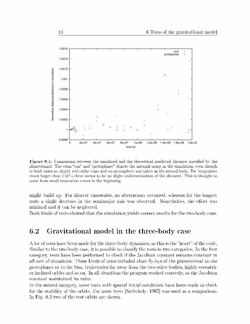
44 6 Tests of the gravitational model
0.9998
1
1.0002
1.0004
1.0006
1.0008
1.001
1.0012
1.0014
1.0016
0 2e+07 4e+07 6e+07 8e+07 1e+08 1.2e+08 1.4e+08 1.6e+08 1.8e+08
theo
retic
al d
istan
ce/d
istan
ce in
sim
ulat
ion
time [s]
sunprotoplanet
Figure 6.1: Comparison between the simulated and the theoretical predicted distance travelled by theplanetesimal. The term sun and protoplanet denote the internal usage in the simulation, even thoughin both cases an object with solar mass and no atmosphere was taken as the second body. For integrationtimes larger than 1˙107 s there seems to be an slight underestimation of the distance. This is thought tocome from small truncation errors in the beginning.
might build up. For shorter timescales, no aberrations occurred, whereas for the longesttests a slight decrease in the semimajor axis was observed. Nonetheless, the eect wasminimal and it can be neglected.Both kinds of tests showed that the simulation yields correct results for the two-body case.
6.2 Gravitational model in the three-body case
A lot of tests have been made for the three-body dynamics, as this is the heart of the code.Similar to the two-body case, it is possible to classify the tests in two categories. In the rstcategory, tests have been performed to check if the Jacobian constant remains constant inall sort of situations. These kinds of tests included close y-bys of the planetesimal to theprotoplanet or to the Sun, trajectories far away from the two other bodies, highly eccentricor inclined orbits and so on. In all situations the program worked correctly, as the Jacobianconstant maintained its value.In the second category, some tests with special initial conditions have been made to checkfor the stability of the orbits. For most tests [Szebehely, 1967] was used as a comparison.In Fig. 6.2 two of the test orbits are shown.
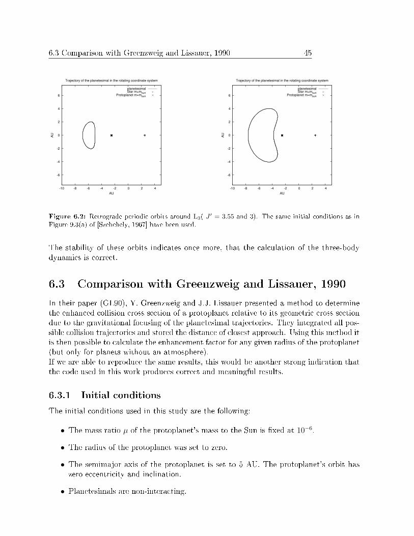
6.3 Comparison with Greenzweig and Lissauer, 1990 45
-6
-4
-2
0
2
4
6
-10 -8 -6 -4 -2 0 2 4
AU
AU
Trajectory of the planetesimal in the rotating coordinate system
planetesimalStar m=msunProtoplanet m=msun
-6
-4
-2
0
2
4
6
-10 -8 -6 -4 -2 0 2 4
AU
AU
Trajectory of the planetesimal in the rotating coordinate system
planetesimalStar m=msunProtoplanet m=msun
Figure 6.2: Retrograde periodic orbits around L3( J ′ = 3.55 and 3). The same initial conditions as inFigure 9.3(a) of [Szebehely, 1967] have been used.
The stability of these orbits indicates once more, that the calculation of the three-bodydynamics is correct.
6.3 Comparison with Greenzweig and Lissauer, 1990
In their paper (GL90), Y. Greenzweig and J.J. Lissauer presented a method to determinethe enhanced collision cross section of a protoplanet relative to its geometric cross sectiondue to the gravitational focusing of the planetesimal trajectories. They integrated all pos-sible collision trajectories and stored the distance of closest approach. Using this method itis then possible to calculate the enhancement factor for any given radius of the protoplanet(but only for planets without an atmosphere).If we are able to reproduce the same results, this would be another strong indication thatthe code used in this work produces correct and meaningful results.
6.3.1 Initial conditions
The initial conditions used in this study are the following:
• The mass ratio µ of the protoplanet's mass to the Sun is xed at 10−6.
• The radius of the protoplanet was set to zero.
• The semimajor axis of the protoplanet is set to 5 AU. The protoplanet's orbit haszero eccentricity and inclination.
• Planetesimals are non-interacting.

46 6 Tests of the gravitational model
• The planetesimals are started with a mean longitude approximately 45o from theprotoplanet.
• For each run, the semimajor axes of the test particles are distributed with a spacinginversely proportional to the distance from the protoplanet's orbit, over two intervals(superior and inferior orbits) that cover the entire range of possible collision orbits.
• The argument of the perigee and the longitude of the ascending node are randomlydistributed with uniform probability over the intervals [0, 2π) and [0, π), respectively.
• The eccentricity and inclination of the planetesimals are varied from run to run tocover a few dierent cases. Within a run, they remain constant.
• The trajectories of the planetesimals are integrated until their nal angular separationfrom the protoplanet reaches about 60o.
Apart from the semimajor axis of the protoplanet, that was not specied in the paper,and the nal angular separation, that was set to 60o instead of 45o, all initial conditionsare the same as in GL90. The unknown semimajor axis does not matter, as in their papereverything is given in units of RH . To allow for an easier comparison, we use the variablesin Hill's units:
eH = eaproto
RH
(6.2)
iH = sin iaproto
RH
(6.3)
aH =apla − aproto
RH
(6.4)
ds =Rpla + Rproto
RH
(6.5)
e and i are the eccentricity and inclination of the planetesimal, a is the semimajor axisand RX the radius of X. eH , iH and aH are called the reduced eccentricity, inclination andsemimajor axis, respectively.There is just a small band of initial semimajor axes where collisions are possible. For theupper bound, the following equation can be used:
3
4a2
H − e2H − i2H ≤ 9 (6.6)
If the inequality is satised by the orbital elements of the planetesimal, no collision canoccur. GL90 stated that the absolute value of the upper limit aHf can even be a bit smallerthan predicted by Equation 6.6.The lower bound aHn was found experimentally by integrating the equation of motion.For |aH | < |aHn| the planetesimals can not enter the protoplanet's Hill's sphere. Theparticle paths appear horseshoe shaped in the frame rotating with the protoplanet. Inall simulations the two boundaries are chosen exactly as in GL90.

6.3 Comparison with Greenzweig and Lissauer, 1990 47
The planetesimals' size and material type do not aect the simulation, because there isno atmosphere to interact with. Nevertheless, they have to be specied. In all runs 1 kmsized planetesimals consisting of ice have been used.
6.3.2 Results
Two sets of runs have been made. In the rst set, the inclination iH was xed to halfthe value of the eccentricity eH , which was varied from zero up to eight. For each of theten runs the number of bound planetesimals for two dierent radii of the protoplanet werecounted.2ds = 0.005 is the value for the core of a typical protoplanet, whereas ds = 0.1 representsa protoplanet with a greatly distended atmosphere. From the number of bound planetesi-mals, it is then possible to calculate the enhancement factor of the collision cross section:
Fg (ds) =3π
F (I)
a2Hf − a2
Hn
d2s
∆n3B (ds)
Ntot
(6.7)
where F (I) = 4√
1+I2
IE (k), E (k) =
∫ π2
0
√1− k2 sin2 θdθ, k =
√3
2√
1+I2 and I = sin ie.
∆n3B (ds) is the number of bound planetesimals.Additionally, GL90 calculated a collision probability, which is dened as
〈P (e, i, ds)〉 =3
2
∆n3B (ds)
Ntot
(a2
Hf − a2Hn
)(6.8)
Both values, the enhancement factor and the collision probability, for ds = 0.005 aregiven in Tab. 6.1. In Fig. 6.3 the values of Fg are compared to the ones of GL90. Thestatistical error in determining ∆n3B, which is essentially the only source of numerical errorin determining Fg, was estimated by GL90 to be of order
√∆n3B. Therefore the error bars
in all gures in this section are set to 1√∆n3B
of the value. Unfortunately, it was notpossible to check the correctness of this estimated statistical error within the frameworkof this diploma thesis, as a deeper investigation of it would have taken too much time.Altogether, the simulations took about 10 days of computational time. So, about 1000days of computational time would have been needed to improve the accuracy of the resultsby a factor of 10.In general, the results for the enhancement factor and the collision probability coincidequite well with the ones from GL90. First it seemed, that there may be a small aberrationfor smaller eccentricities and inclinations (up to eH = 0.5), because the values of this studyall exceed the ones from the study of Greenzweig and Lissauer, even though they are stillwithin the estimated error bars. But some additional tests proved this assumption to bewrong. For the rst set of runs, there is no dierence between the results of this study andthe ones from GL90.
2As for each planetesimal the whole trajectory was calculated and the closest approach to the proto-planet was stored, this could be done by simply count the planetesimal of which the closest approach wassmaller than a certain value.
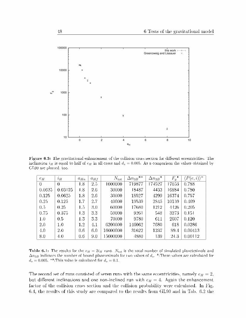
48 6 Tests of the gravitational model
10
100
1000
10000
100000
0 2 4 6 8 10
F g
eH
this workGreenzweig and Lissauer
Figure 6.3: The gravitational enhancement of the collision cross section for dierent eccentricities. Theinclination iH is equal to half of eH in all cases and ds = 0.005. As a comparison the values obtained byGL90 are plotted, too.
eH iH aHn aHf Ntot ∆n3B** ∆n3B* Fg* 〈P (e, i)〉*0 0 1.8 2.5 1000000 719877 174527 17053 0.7880.0625 0.03125 1.8 2.6 30000 18487 4433 16884 0.7800.125 0.0625 1.8 2.6 30000 18527 4299 16374 0.7570.25 0.125 1.7 2.7 40000 19539 2845 10159 0.4690.5 0.25 1.5 3.0 60000 17680 1212 4426 0.2050.75 0.375 1.3 3.3 50000 9261 548 3273 0.1511.0 0.5 1.3 3.3 70000 9780 611 2607 0.1202.0 1.0 1.2 4.1 6200000 146062 7680 618 0.02864.0 2.0 0.6 6.0 16000000 31622 1237 89.4 0.004138.0 4.0 0.6 9.0 15000000 4880 139 24.3 0.00112
Table 6.1: The results for the eH = 2iH runs. Ntot is the total number of simulated planetesimals and∆n3B indicates the number of bound planetesimals for two values of ds. *:These values are calculated fords = 0.005. **:This value is calculated for ds = 0.1.
The second set of runs consisted of seven runs with the same eccentricities, namely eH = 2,but dierent inclinations and one non-inclined run with eH = 4. Again the enhancementfactor of the collision cross section and the collision probability were calculated. In Fig.6.4, the results of this study are compared to the results from GL90 and in Tab. 6.2 the
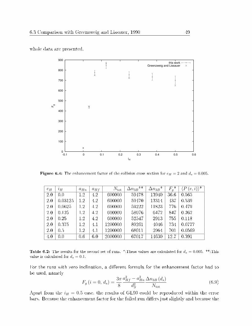
6.3 Comparison with Greenzweig and Lissauer, 1990 49
whole data are presented.
0
100
200
300
400
500
600
700
800
900
-0.1 0 0.1 0.2 0.3 0.4 0.5 0.6
F g
iH
this workGreenzweig and Lissauer
Figure 6.4: The enhancement factor of the collision cross section for eH = 2 and ds = 0.005.
eH iH aHn aHf Ntot ∆n3B** ∆n3B* Fg* 〈P (e, i)〉*2.0 0.0 1.2 4.2 600000 59478 13940 36.6 0.5652.0 0.03125 1.2 4.2 600000 59470 13314 437 0.5392.0 0.0625 1.2 4.2 600000 59222 11823 776 0.4792.0 0.125 1.2 4.2 600000 58076 6472 847 0.2622.0 0.25 1.2 4.2 600000 52547 2913 755 0.1182.0 0.375 1.2 4.1 1200000 89261 4046 734 0.07772.0 0.5 1.2 4.1 1200000 68011 2964 701 0.05694.0 0.0 0.6 6.0 2000000 67017 14630 12.7 0.391
Table 6.2: The results for the second set of runs. *:These values are calculated for ds = 0.005. **:Thisvalue is calculated for ds = 0.1.
For the runs with zero inclination, a dierent formula for the enhancement factor had tobe used, namely
Fg (i = 0, ds) =3π
8
a2Hf − a2
Hn
d2S
∆n3B (ds)
Ntot
(6.9)
Apart from the iH = 0.5 case, the results of GL90 could be reproduced within the errorbars. Because the enhancement factor for the failed run diers just slightly and because the

50 6 Tests of the gravitational model
error of Fg is only estimated with √n3B, the aberration is believed to come from statisticaleects.
6.3.3 Conclusion
The code developed for this work is able to reproduce the results obtained by GL90. Thisimplies that three-body dynamics for a set of planetesimals with xed eccentricity andinclination is calculated in a correct way and that the code can be used to determine theenhancement factor of the collision cross section.
6.4 Comparison with Greenzweig and Lissauer, 1992
In their second paper (GL92), Greenzweig and Lissauer used Rayleigh distributed eccen-tricities and inclinations within a run, instead of constant ones.
6.4.1 Initial conditions
The initial conditions are the same as explained in subsection 6.3.1 with few exceptions.The planetesimals' eccentricities and the sine of the inclinations are Rayleigh distributed.This means the distribution function is given by
f(e, sin i; e∗, sin i∗) =4e sin i
e2∗ sin2 i∗
exp
−e2
e2∗− sin2 i
sin2 i∗
(6.10)
where e∗ and sin i∗ are the root mean square (r.m.s.) values of e and sin i, respectively.Besides, the two boundaries in semimajor axes, aHn and aHf , are chosen dierently. Thelower bound|aHn| is xed at 0.6 for all runs, and the upper bound was |aHf | = 2.5eH∗ + 3for all runs except eH∗ = 8. In the eH∗ = 8 case, an upper limit of |aHf | = 15 was chosen.
6.4.2 Results
Again, two sets of runs have been made. First, nine runs with eH∗ = 2iH∗ and eccentricitieseH∗ from zero to eight have been simulated. The results for these runs are presented inTab. 6.3. The calculation of the enhancement factor is pretty similar to the one in thelast section, but F (I) in Eq. 6.7 is replaced by 〈F (I)〉. According to GL92 the equationfor the three-body gravitational enhancement of the mass accretion rate of a protoplanetembedded within a disk of planetesimals that have Rayleigh-distributed eccentricities andinclination is then dened as
Fg∗ =3π
〈F (I)〉a2
Hf − a2Hn
d2s
∆n3B
Ntot
(6.11)
As 〈F (I)〉 cannot be calculated analytically, the second order approximation presented inappendix C of GL92 is used.
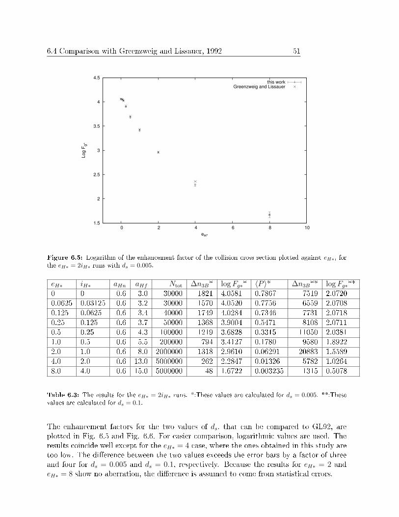
6.4 Comparison with Greenzweig and Lissauer, 1992 51
1.5
2
2.5
3
3.5
4
4.5
0 2 4 6 8 10
Log
F g*
eH*
this workGreenzweig and Lissauer
Figure 6.5: Logarithm of the enhancement factor of the collision cross section plotted against eH∗, forthe eH∗ = 2iH∗ runs with ds = 0.005.
eH∗ iH∗ aHn aHf Ntot ∆n3B* log Fg∗* 〈P 〉* ∆n3B** log Fg∗**0 0 0.6 3.0 30000 1821 4.0581 0.7867 7519 2.07200.0625 0.03125 0.6 3.2 30000 1570 4.0520 0.7756 6559 2.07080.125 0.0625 0.6 3.4 40000 1749 4.0284 0.7346 7731 2.07180.25 0.125 0.6 3.7 50000 1368 3.9004 0.5471 8108 2.07110.5 0.25 0.6 4.3 100000 1219 3.6828 0.3315 11050 2.03811.0 0.5 0.6 5.5 200000 794 3.4127 0.1780 9580 1.89222.0 1.0 0.6 8.0 2000000 1318 2.9610 0.06291 20883 1.55894.0 2.0 0.6 13.0 5000000 262 2.2847 0.01326 5782 1.02648.0 4.0 0.6 15.0 5000000 48 1.6722 0.003235 1315 0.5078
Table 6.3: The results for the eH∗ = 2iH∗ runs. *:These values are calculated for ds = 0.005. **:Thesevalues are calculated for ds = 0.1.
The enhancement factors for the two values of ds, that can be compared to GL92, areplotted in Fig. 6.5 and Fig. 6.6. For easier comparison, logarithmic values are used. Theresults coincide well except for the eH∗ = 4 case, where the ones obtained in this study aretoo low. The dierence between the two values exceeds the error bars by a factor of threeand four for ds = 0.005 and ds = 0.1, respectively. Because the results for eH∗ = 2 andeH∗ = 8 show no aberration, the dierence is assumed to come from statistical errors.
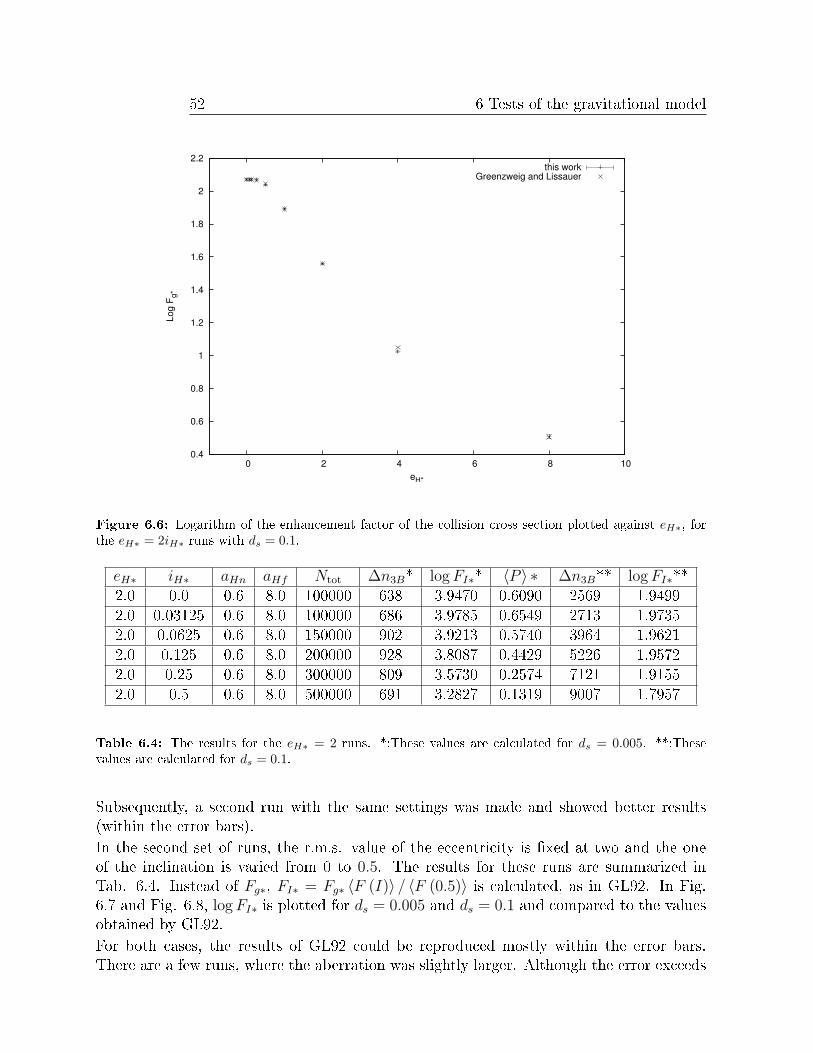
52 6 Tests of the gravitational model
0.4
0.6
0.8
1
1.2
1.4
1.6
1.8
2
2.2
0 2 4 6 8 10
Log
F g*
eH*
this workGreenzweig and Lissauer
Figure 6.6: Logarithm of the enhancement factor of the collision cross section plotted against eH∗, forthe eH∗ = 2iH∗ runs with ds = 0.1.
eH∗ iH∗ aHn aHf Ntot ∆n3B* log FI∗* 〈P 〉 ∗ ∆n3B** log FI∗**2.0 0.0 0.6 8.0 100000 638 3.9470 0.6090 2569 1.94992.0 0.03125 0.6 8.0 100000 686 3.9785 0.6549 2713 1.97352.0 0.0625 0.6 8.0 150000 902 3.9213 0.5740 3964 1.96212.0 0.125 0.6 8.0 200000 928 3.8087 0.4429 5226 1.95722.0 0.25 0.6 8.0 300000 809 3.5730 0.2574 7121 1.91552.0 0.5 0.6 8.0 500000 691 3.2827 0.1319 9007 1.7957
Table 6.4: The results for the eH∗ = 2 runs. *:These values are calculated for ds = 0.005. **:Thesevalues are calculated for ds = 0.1.
Subsequently, a second run with the same settings was made and showed better results(within the error bars).In the second set of runs, the r.m.s. value of the eccentricity is xed at two and the oneof the inclination is varied from 0 to 0.5. The results for these runs are summarized inTab. 6.4. Instead of Fg∗, FI∗ = Fg∗ 〈F (I)〉 / 〈F (0.5)〉 is calculated, as in GL92. In Fig.6.7 and Fig. 6.8, log FI∗ is plotted for ds = 0.005 and ds = 0.1 and compared to the valuesobtained by GL92.For both cases, the results of GL92 could be reproduced mostly within the error bars.There are a few runs, where the aberration was slightly larger. Although the error exceeds
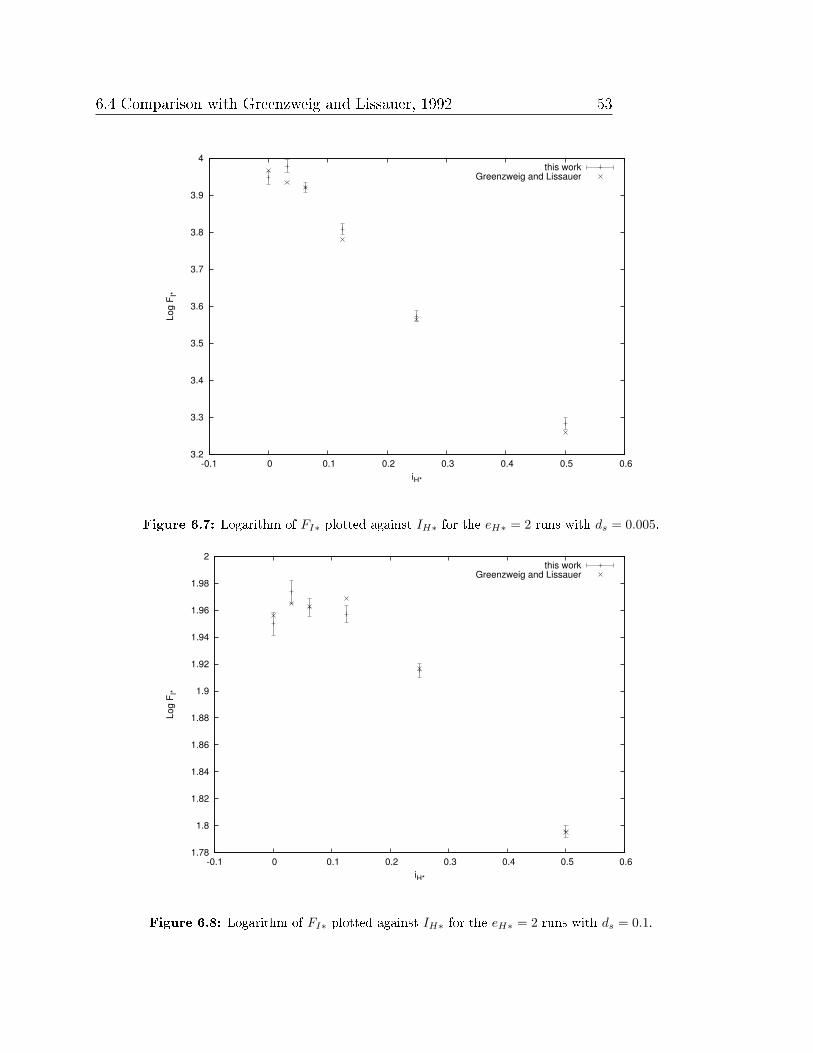
6.4 Comparison with Greenzweig and Lissauer, 1992 53
3.2
3.3
3.4
3.5
3.6
3.7
3.8
3.9
4
-0.1 0 0.1 0.2 0.3 0.4 0.5 0.6
Log
F I*
iH*
this workGreenzweig and Lissauer
Figure 6.7: Logarithm of FI∗ plotted against IH∗ for the eH∗ = 2 runs with ds = 0.005.
1.78
1.8
1.82
1.84
1.86
1.88
1.9
1.92
1.94
1.96
1.98
2
-0.1 0 0.1 0.2 0.3 0.4 0.5 0.6
Log
F I*
iH*
this workGreenzweig and Lissauer
Figure 6.8: Logarithm of FI∗ plotted against IH∗ for the eH∗ = 2 runs with ds = 0.1.
54 6 Tests of the gravitational model
the error bars, this is believed to come from statistical eects. Support for this belief comesfrom the iH∗ = 0.125 run, where the value of log FI∗ diers in both cases, but in dierentdirections. For ds = 0.005 the value is too high, whereas for ds = 0.1 it is too low (alwayscompared to the values obtained by GL92).In general, the dierences for Fg∗ are larger than for Fg. So, it seems that the error ofFg∗ due to statistical eects is underestimated, if we are using the same error as for Fg.This increased uncertainty is believed to be due to the use of the Rayleigh distribution ofeccentricities and inclinations.
6.4.3 Conclusion
Even if a Rayleigh distribution of planetesimal eccentricities and inclinations is assumed,the program developed for this work is generally able to reproduce the results obtained byGL92. There are few dierences, but never to an extent that could not be explained bystatistical eects. As a concluding remark, it can be stated that there are no systematicaldierences between this work and GL92.

Chapter 7
Results
In the last chapter, it was shown that the program is able to correctly calculate solutionsto the restricted three-body problem and the enhancement factor of the collision crosssection. In this chapter, it is now used to investigate the problem it was initially intendedfor: the motion of a planetesimal in the presence of a growing gas giant that is orbiting acentral star.
7.1 Investigation of a set of protoplanets
In Chapter 4 the properties of a set of four protoplanets and their atmospheres havebeen presented. Now, these planets are investigated: rst, the validity of the simpliedcalculation for the enhancement factor is checked for a wide range of parameters; Then, adeeper investigation for one special case is made; Finally, the change of the distribution ofthe eccentricities of a set of planetesimals is investigated.
The four protoplanets that have been used for this simulations were not chosen at ran-dom, but with a denitive goal in mind. They cover a large fraction of the formationstage during which the solid accretion rate is important to the protoplanet's evolution andwhere the atmosphere still aects this rate. Unfortunately, the beginning of this phase,where the atmosphere just starts to aect the trajectories of the planetesimals, could notbe investigated, because YA's atmospheric structure les of the protoplanets starts at aminimum core mass of mcore = 0.6m⊕. So, even though the mass of the atmosphere of therst protoplanet (1) is only 1/100 of the mass of the core, it is already too heavy, as theatmosphere hugely aects the motion of the (smaller) planetesimals. But from this point,the next three models (30, 60 and 89) allow the investigation of the enhancement factorup to the start of runaway growth, after which the solid accretion rate is not so importantanymore.
56 7 Results
7.1.1 Comparison of the calculation of the enhancement factor
The enhancement factor of the capture cross section is calculated in two dierent ways.Either, the standard approximation is used, which means the enhanced radius, and as FD =
R2c
R2core
also the enhancement of the cross section due to the atmosphere, is determined withthe program of CM and then the three-body gravitational enhancement, Fg, is calculatedwith this program (hereafter referred to as the old method). In CM's program the onlyinitial parameter, apart from the structures of the protoplanet and of the planetesimal, isthe starting velocity of the planetesimal. The average relative encounter velocity betweena planetesimal and a protoplanet is given by P96 as
v =1√2
√5e2
8+ i2vkepl (7.1)
where e and i are the eccentricity and inclination of the planetesimal and vkepl is theKeplerian velocity around the sun at the semimajor axis of the protoplanet. We comparethis old method of computation of the enhancement factor with the new integrationmethod developed here, which consideres simultaneously the eect of the atmosphere andthe motion about the sun (hereafter referred to as the new method). In the end, thetwo enhancement factors, FgFD for the old method and Fg+D for the new one, arecompared.
7.1.1.1 Initial conditions
The characteristics of the protoplanets can be found in Tab. 4.1. The mass of the Sun isset to 1.9891 ˙1030 kg. The planetesimals are made of rock, ice, iron or dust (see Tab. 2.1for the physical properties of the materials) and their size spreads from 10 cm to 1000 km.Similar to the comparison with GL92, the semimajor axis of the planetesimals is takenfrom two bands, one with smaller and one with larger semimajor axis. The boundariesare xed at aHn = ±0.6 and aHf = ±(2.5eH∗ + 3), where eH∗ is the r.m.s. eccentricityof a Rayleigh distribution in Hill's units, and within each band the semimajor axis aredistributed inversely proportional to the distance between the semimajor axis of the pro-toplanet and that of the planetesimal. The eccentricities and the sine of the inclinationsare Rayleigh distributed. Overall, four dierent r.m.s. values for the eccentricity havebeen investigated, namely eH∗ = 0.25, eH∗ = 1, eH∗ = 2 and eH∗ = 8. In all cases ther.m.s. value of the inclination was set to half the value of eH∗. Unfortunately, it wasnot possible to compare the enhancement factor for circular planetesimal orbits, becausethere the initial velocity in CM's program would be zero and then the enhanced radius cannot be determined. The circular case would have been interesting, because it has alreadybeen investigated in [Inaba and Ikoma, 2003]. The right ascension of the ascending nodeand the argument of the perigee are randomly distributed within the interval [0,π] and[0,2π], respectively. The separation of the starting angles between the protoplanet and theplanetesimal is distributed around 45o. For each protoplanet every possible combination ofmaterials, eccentricities and sizes (8 dierent) have been simulated both for the protoplanet
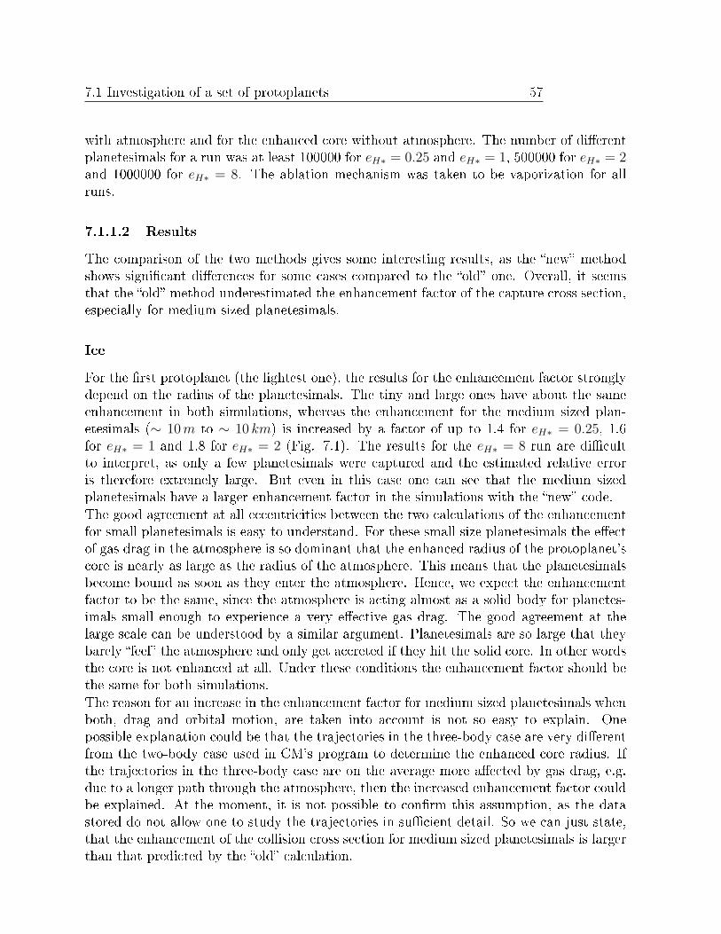
7.1 Investigation of a set of protoplanets 57
with atmosphere and for the enhanced core without atmosphere. The number of dierentplanetesimals for a run was at least 100000 for eH∗ = 0.25 and eH∗ = 1, 500000 for eH∗ = 2and 1000000 for eH∗ = 8. The ablation mechanism was taken to be vaporization for allruns.
7.1.1.2 Results
The comparison of the two methods gives some interesting results, as the new methodshows signicant dierences for some cases compared to the old one. Overall, it seemsthat the old method underestimated the enhancement factor of the capture cross section,especially for medium sized planetesimals.
Ice
For the rst protoplanet (the lightest one), the results for the enhancement factor stronglydepend on the radius of the planetesimals. The tiny and large ones have about the sameenhancement in both simulations, whereas the enhancement for the medium sized plan-etesimals (∼ 10 m to ∼ 10 km) is increased by a factor of up to 1.4 for eH∗ = 0.25, 1.6for eH∗ = 1 and 1.8 for eH∗ = 2 (Fig. 7.1). The results for the eH∗ = 8 run are dicultto interpret, as only a few planetesimals were captured and the estimated relative erroris therefore extremely large. But even in this case one can see that the medium sizedplanetesimals have a larger enhancement factor in the simulations with the new code.The good agreement at all eccentricities between the two calculations of the enhancementfor small planetesimals is easy to understand. For these small size planetesimals the eectof gas drag in the atmosphere is so dominant that the enhanced radius of the protoplanet'score is nearly as large as the radius of the atmosphere. This means that the planetesimalsbecome bound as soon as they enter the atmosphere. Hence, we expect the enhancementfactor to be the same, since the atmosphere is acting almost as a solid body for planetes-imals small enough to experience a very eective gas drag. The good agreement at thelarge scale can be understood by a similar argument. Planetesimals are so large that theybarely feel the atmosphere and only get accreted if they hit the solid core. In other wordsthe core is not enhanced at all. Under these conditions the enhancement factor should bethe same for both simulations.The reason for an increase in the enhancement factor for medium sized planetesimals whenboth, drag and orbital motion, are taken into account is not so easy to explain. Onepossible explanation could be that the trajectories in the three-body case are very dierentfrom the two-body case used in CM's program to determine the enhanced core radius. Ifthe trajectories in the three-body case are on the average more aected by gas drag, e.g.due to a longer path through the atmosphere, then the increased enhancement factor couldbe explained. At the moment, it is not possible to conrm this assumption, as the datastored do not allow one to study the trajectories in sucient detail. So we can just state,that the enhancement of the collision cross section for medium sized planetesimals is largerthan that predicted by the old calculation.
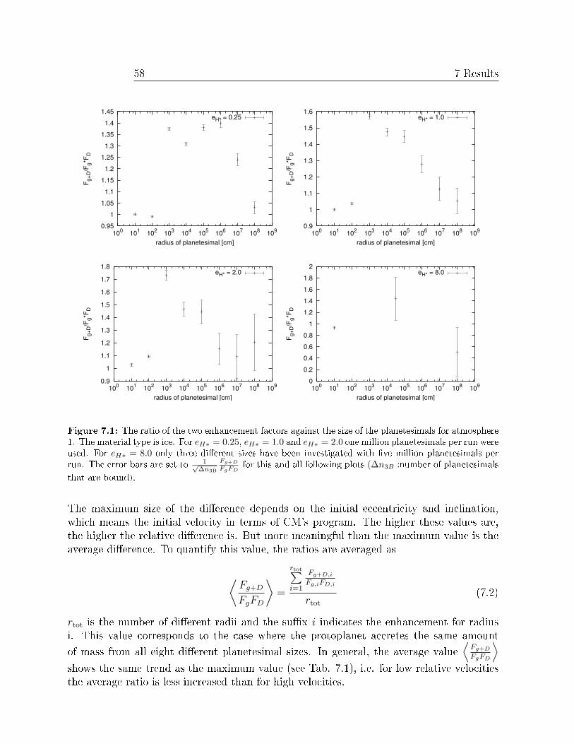
58 7 Results
0.95 1
1.05 1.1
1.15 1.2
1.25 1.3
1.35 1.4
1.45
100 101 102 103 104 105 106 107 108 109
F g+D
/Fg*
F D
radius of planetesimal [cm]
eH* = 0.25
0.9
1
1.1
1.2
1.3
1.4
1.5
1.6
100 101 102 103 104 105 106 107 108 109
F g+D
/Fg*
F D
radius of planetesimal [cm]
eH* = 1.0
0.9
1
1.1
1.2
1.3
1.4
1.5
1.6
1.7
1.8
100 101 102 103 104 105 106 107 108 109
F g+D
/Fg*
F D
radius of planetesimal [cm]
eH* = 2.0
0 0.2 0.4 0.6 0.8
1 1.2 1.4 1.6 1.8
2
100 101 102 103 104 105 106 107 108 109
F g+D
/Fg*
F D
radius of planetesimal [cm]
eH* = 8.0
Figure 7.1: The ratio of the two enhancement factors against the size of the planetesimals for atmosphere1. The material type is ice. For eH∗ = 0.25, eH∗ = 1.0 and eH∗ = 2.0 one million planetesimals per run wereused. For eH∗ = 8.0 only three dierent sizes have been investigated with ve million planetesimals perrun. The error bars are set to 1√
∆n3B
Fg+D
FgFDfor this and all following plots (∆n3B :number of planetesimals
that are bound).
The maximum size of the dierence depends on the initial eccentricity and inclination,which means the initial velocity in terms of CM's program. The higher these values are,the higher the relative dierence is. But more meaningful than the maximum value is theaverage dierence. To quantify this value, the ratios are averaged as
⟨Fg+D
FgFD
⟩=
rtot∑i=1
Fg+D,i
Fg,iFD,i
rtot
(7.2)
rtot is the number of dierent radii and the sux i indicates the enhancement for radiusi. This value corresponds to the case where the protoplanet accretes the same amountof mass from all eight dierent planetesimal sizes. In general, the average value
⟨Fg+D
FgFD
⟩shows the same trend as the maximum value (see Tab. 7.1), i.e. for low relative velocitiesthe average ratio is less increased than for high velocities.
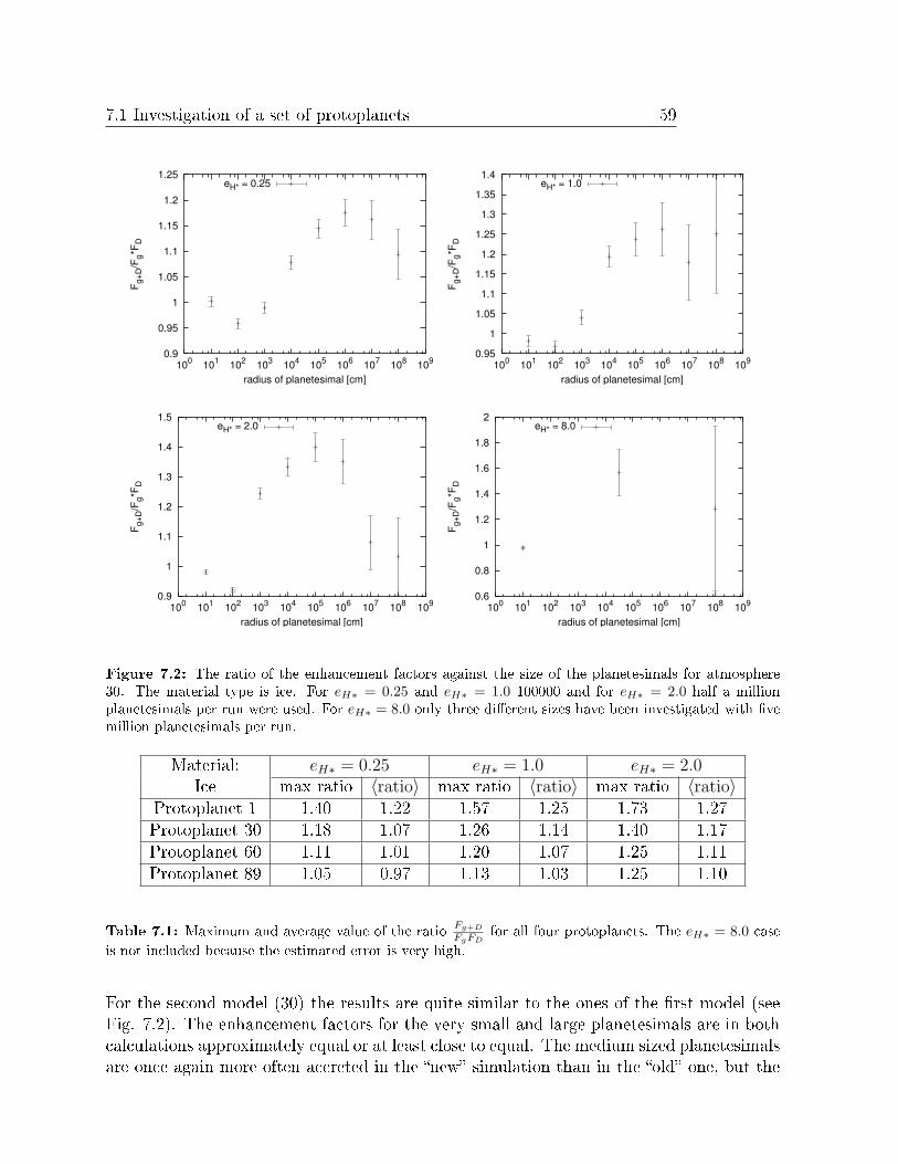
7.1 Investigation of a set of protoplanets 59
0.9
0.95
1
1.05
1.1
1.15
1.2
1.25
100 101 102 103 104 105 106 107 108 109
F g+D
/Fg*
F D
radius of planetesimal [cm]
eH* = 0.25
0.95
1
1.05
1.1
1.15
1.2
1.25
1.3
1.35
1.4
100 101 102 103 104 105 106 107 108 109
F g+D
/Fg*
F D
radius of planetesimal [cm]
eH* = 1.0
0.9
1
1.1
1.2
1.3
1.4
1.5
100 101 102 103 104 105 106 107 108 109
F g+D
/Fg*
F D
radius of planetesimal [cm]
eH* = 2.0
0.6
0.8
1
1.2
1.4
1.6
1.8
2
100 101 102 103 104 105 106 107 108 109
F g+D
/Fg*
F D
radius of planetesimal [cm]
eH* = 8.0
Figure 7.2: The ratio of the enhancement factors against the size of the planetesimals for atmosphere30. The material type is ice. For eH∗ = 0.25 and eH∗ = 1.0 100000 and for eH∗ = 2.0 half a millionplanetesimals per run were used. For eH∗ = 8.0 only three dierent sizes have been investigated with vemillion planetesimals per run.
Material: eH∗ = 0.25 eH∗ = 1.0 eH∗ = 2.0Ice max ratio 〈ratio〉 max ratio 〈ratio〉 max ratio 〈ratio〉
Protoplanet 1 1.40 1.22 1.57 1.25 1.73 1.27Protoplanet 30 1.18 1.07 1.26 1.14 1.40 1.17Protoplanet 60 1.11 1.01 1.20 1.07 1.25 1.11Protoplanet 89 1.05 0.97 1.13 1.03 1.25 1.10
Table 7.1: Maximum and average value of the ratio Fg+D
FgFDfor all four protoplanets. The eH∗ = 8.0 case
is not included because the estimated error is very high.
For the second model (30) the results are quite similar to the ones of the rst model (seeFig. 7.2). The enhancement factors for the very small and large planetesimals are in bothcalculations approximately equal or at least close to equal. The medium sized planetesimalsare once again more often accreted in the new simulation than in the old one, but the
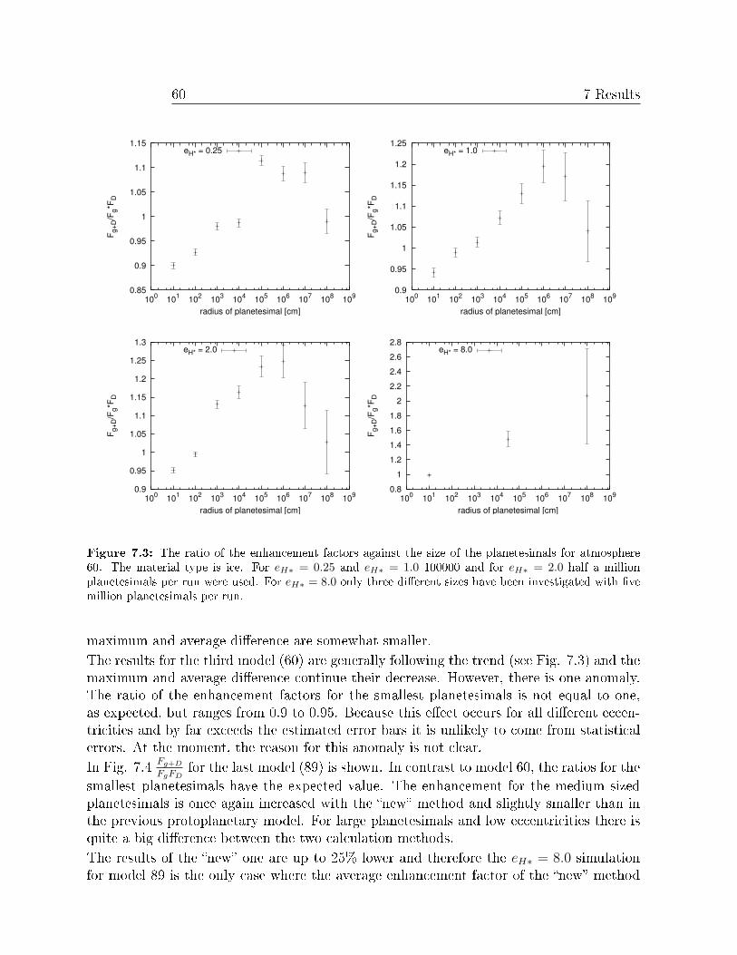
60 7 Results
0.85
0.9
0.95
1
1.05
1.1
1.15
100 101 102 103 104 105 106 107 108 109
F g+D
/Fg*
F D
radius of planetesimal [cm]
eH* = 0.25
0.9
0.95
1
1.05
1.1
1.15
1.2
1.25
100 101 102 103 104 105 106 107 108 109
F g+D
/Fg*
F D
radius of planetesimal [cm]
eH* = 1.0
0.9
0.95
1
1.05
1.1
1.15
1.2
1.25
1.3
100 101 102 103 104 105 106 107 108 109
F g+D
/Fg*
F D
radius of planetesimal [cm]
eH* = 2.0
0.8 1
1.2 1.4 1.6 1.8
2 2.2 2.4 2.6 2.8
100 101 102 103 104 105 106 107 108 109
F g+D
/Fg*
F D
radius of planetesimal [cm]
eH* = 8.0
Figure 7.3: The ratio of the enhancement factors against the size of the planetesimals for atmosphere60. The material type is ice. For eH∗ = 0.25 and eH∗ = 1.0 100000 and for eH∗ = 2.0 half a millionplanetesimals per run were used. For eH∗ = 8.0 only three dierent sizes have been investigated with vemillion planetesimals per run.
maximum and average dierence are somewhat smaller.The results for the third model (60) are generally following the trend (see Fig. 7.3) and themaximum and average dierence continue their decrease. However, there is one anomaly.The ratio of the enhancement factors for the smallest planetesimals is not equal to one,as expected, but ranges from 0.9 to 0.95. Because this eect occurs for all dierent eccen-tricities and by far exceeds the estimated error bars it is unlikely to come from statisticalerrors. At the moment, the reason for this anomaly is not clear.In Fig. 7.4 Fg+D
FgFDfor the last model (89) is shown. In contrast to model 60, the ratios for the
smallest planetesimals have the expected value. The enhancement for the medium sizedplanetesimals is once again increased with the new method and slightly smaller than inthe previous protoplanetary model. For large planetesimals and low eccentricities there isquite a big dierence between the two calculation methods.The results of the new one are up to 25% lower and therefore the eH∗ = 8.0 simulationfor model 89 is the only case where the average enhancement factor of the new method
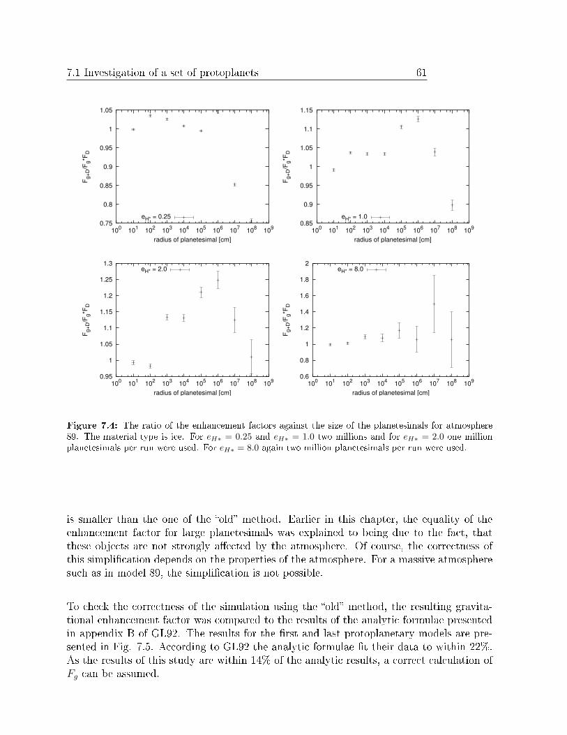
7.1 Investigation of a set of protoplanets 61
0.75
0.8
0.85
0.9
0.95
1
1.05
100 101 102 103 104 105 106 107 108 109
F g+D
/Fg*
F D
radius of planetesimal [cm]
eH* = 0.25 0.85
0.9
0.95
1
1.05
1.1
1.15
100 101 102 103 104 105 106 107 108 109
F g+D
/Fg*
F D
radius of planetesimal [cm]
eH* = 1.0
0.95
1
1.05
1.1
1.15
1.2
1.25
1.3
100 101 102 103 104 105 106 107 108 109
F g+D
/Fg*
F D
radius of planetesimal [cm]
eH* = 2.0
0.6
0.8
1
1.2
1.4
1.6
1.8
2
100 101 102 103 104 105 106 107 108 109
F g+D
/Fg*
F D
radius of planetesimal [cm]
eH* = 8.0
Figure 7.4: The ratio of the enhancement factors against the size of the planetesimals for atmosphere89. The material type is ice. For eH∗ = 0.25 and eH∗ = 1.0 two millions and for eH∗ = 2.0 one millionplanetesimals per run were used. For eH∗ = 8.0 again two million planetesimals per run were used.
is smaller than the one of the old method. Earlier in this chapter, the equality of theenhancement factor for large planetesimals was explained to being due to the fact, thatthese objects are not strongly aected by the atmosphere. Of course, the correctness ofthis simplication depends on the properties of the atmosphere. For a massive atmospheresuch as in model 89, the simplication is not possible.
To check the correctness of the simulation using the old method, the resulting gravita-tional enhancement factor was compared to the results of the analytic formulae presentedin appendix B of GL92. The results for the rst and last protoplanetary models are pre-sented in Fig. 7.5. According to GL92 the analytic formulae t their data to within 22%.As the results of this study are within 14% of the analytic results, a correct calculation ofFg can be assumed.
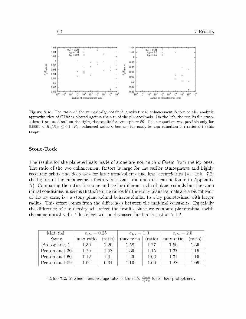
62 7 Results
0.86 0.88 0.9
0.92 0.94 0.96 0.98
1 1.02 1.04 1.06
100 101 102 103 104 105 106 107 108 109
F g/F
g,G
L92
radius of planetesimal [cm]
eH* = 0.25eH* = 1.0eH* = 2.0
0.86
0.88
0.9
0.92
0.94
0.96
0.98
1
1.02
1.04
100 101 102 103 104 105 106 107 108 109
F g/F
g,G
L92
radius of planetesimal [cm]
eH* = 0.25eH* = 1.0eH* = 2.0
Figure 7.5: The ratio of the numerically obtained gravitational enhancement factor to the analyticapproximation of GL92 is plotted against the size of the planetesimals. On the left, the results for atmo-sphere 1 are used and on the right, the results for atmosphere 89. The comparison was possible only for0.0001 < Rc/RH ≤ 0.1 (Rc: enhanced radius), because the analytic approximation is restricted to thisrange.
Stone/Rock
The results for the planetesimals made of stone are not much dierent from the icy ones.The ratio of the two enhancement factors is large for the earlier atmospheres and highlyeccentric orbits and decreases for later atmospheres and low eccentricities (see Tab. 7.2;the gures of the enhancement factors for stone, iron and dust can be found in AppendixA). Comparing the ratios for stone and ice for dierent radii of planetesimals but the sameinitial conditions, it seems that often the ratios for the stony planetesimals are a bit aheadof the icy ones, i.e. a stony planetesimal behaves similar to a icy planetesimal with largerradius. This eect comes from the dierences between the material constants. Especiallythe dierence of the density will aect the results, since we compare planetesimals withthe same initial radii. This eect will be discussed further in section 7.1.2.
Material: eH∗ = 0.25 eH∗ = 1.0 eH∗ = 2.0Stone max ratio 〈ratio〉 max ratio 〈ratio〉 max ratio 〈ratio〉
Protoplanet 1 1.39 1.20 1.58 1.27 1.60 1.30Protoplanet 30 1.20 1.08 1.36 1.15 1.37 1.19Protoplanet 60 1.12 1.01 1.20 1.06 1.31 1.10Protoplanet 89 1.04 0.94 1.13 1.00 1.28 1.09
Table 7.2: Maximum and average value of the ratio Fg+D
FgFDfor all four protoplanets.
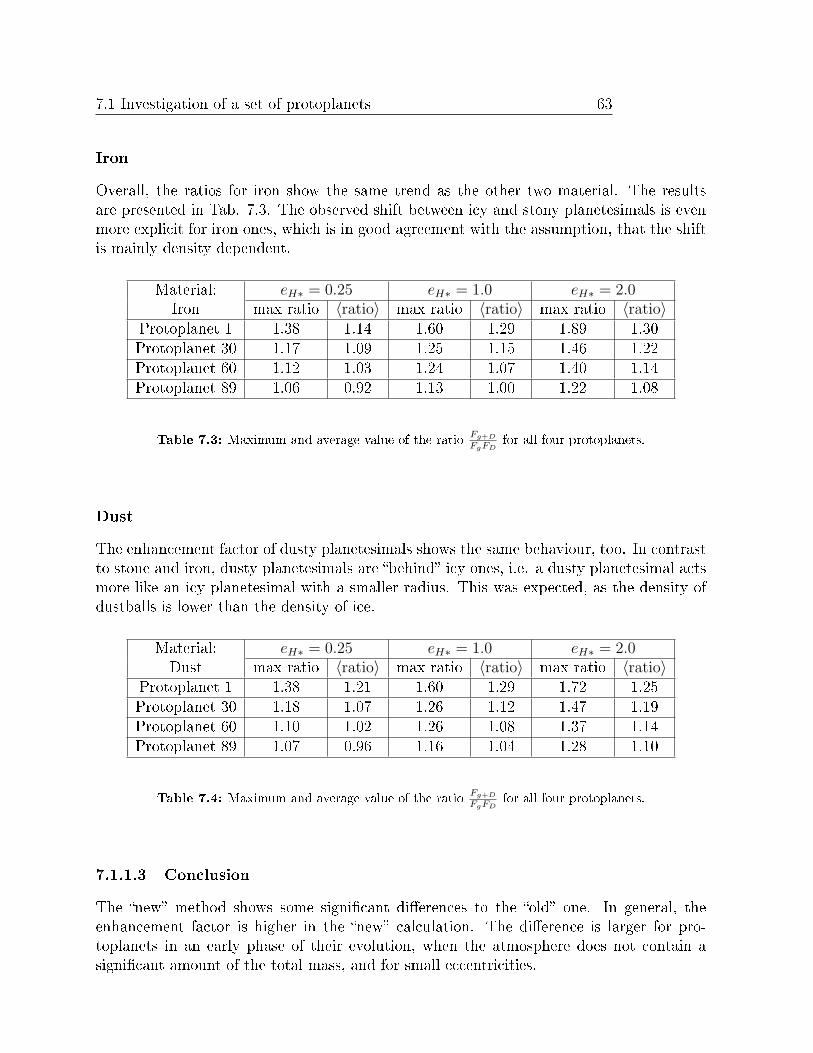
7.1 Investigation of a set of protoplanets 63
Iron
Overall, the ratios for iron show the same trend as the other two material. The resultsare presented in Tab. 7.3. The observed shift between icy and stony planetesimals is evenmore explicit for iron ones, which is in good agreement with the assumption, that the shiftis mainly density dependent.
Material: eH∗ = 0.25 eH∗ = 1.0 eH∗ = 2.0Iron max ratio 〈ratio〉 max ratio 〈ratio〉 max ratio 〈ratio〉
Protoplanet 1 1.38 1.14 1.60 1.29 1.89 1.30Protoplanet 30 1.17 1.09 1.25 1.15 1.46 1.22Protoplanet 60 1.12 1.03 1.24 1.07 1.40 1.14Protoplanet 89 1.06 0.92 1.13 1.00 1.22 1.08
Table 7.3: Maximum and average value of the ratio Fg+D
FgFDfor all four protoplanets.
Dust
The enhancement factor of dusty planetesimals shows the same behaviour, too. In contrastto stone and iron, dusty planetesimals are behind icy ones, i.e. a dusty planetesimal actsmore like an icy planetesimal with a smaller radius. This was expected, as the density ofdustballs is lower than the density of ice.
Material: eH∗ = 0.25 eH∗ = 1.0 eH∗ = 2.0Dust max ratio 〈ratio〉 max ratio 〈ratio〉 max ratio 〈ratio〉
Protoplanet 1 1.38 1.21 1.60 1.29 1.72 1.25Protoplanet 30 1.18 1.07 1.26 1.12 1.47 1.19Protoplanet 60 1.10 1.02 1.26 1.08 1.37 1.14Protoplanet 89 1.07 0.96 1.16 1.04 1.28 1.10
Table 7.4: Maximum and average value of the ratio Fg+D
FgFDfor all four protoplanets.
7.1.1.3 Conclusion
The new method shows some signicant dierences to the old one. In general, theenhancement factor is higher in the new calculation. The dierence is larger for pro-toplanets in an early phase of their evolution, when the atmosphere does not contain asignicant amount of the total mass, and for small eccentricities.
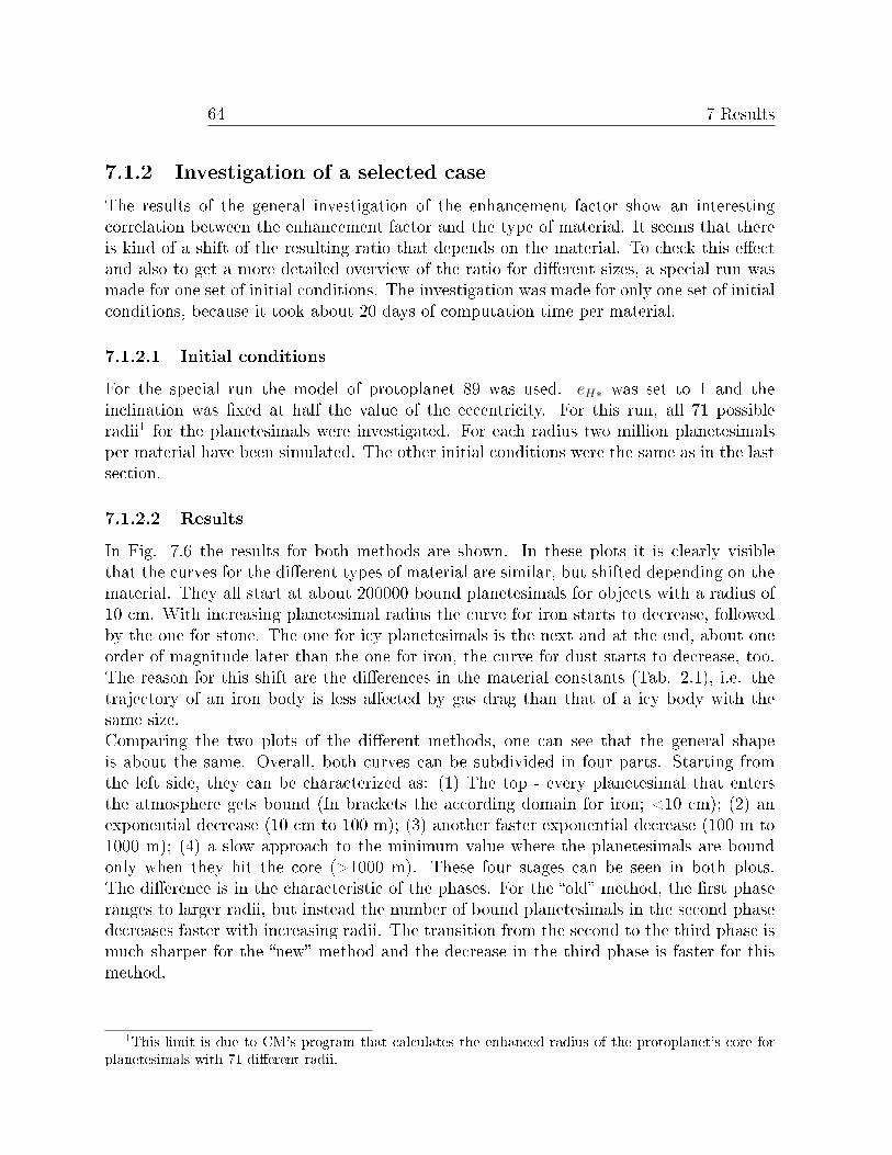
64 7 Results
7.1.2 Investigation of a selected case
The results of the general investigation of the enhancement factor show an interestingcorrelation between the enhancement factor and the type of material. It seems that thereis kind of a shift of the resulting ratio that depends on the material. To check this eectand also to get a more detailed overview of the ratio for dierent sizes, a special run wasmade for one set of initial conditions. The investigation was made for only one set of initialconditions, because it took about 20 days of computation time per material.
7.1.2.1 Initial conditions
For the special run the model of protoplanet 89 was used. eH∗ was set to 1 and theinclination was xed at half the value of the eccentricity. For this run, all 71 possibleradii1 for the planetesimals were investigated. For each radius two million planetesimalsper material have been simulated. The other initial conditions were the same as in the lastsection.
7.1.2.2 Results
In Fig. 7.6 the results for both methods are shown. In these plots it is clearly visiblethat the curves for the dierent types of material are similar, but shifted depending on thematerial. They all start at about 200000 bound planetesimals for objects with a radius of10 cm. With increasing planetesimal radius the curve for iron starts to decrease, followedby the one for stone. The one for icy planetesimals is the next and at the end, about oneorder of magnitude later than the one for iron, the curve for dust starts to decrease, too.The reason for this shift are the dierences in the material constants (Tab. 2.1), i.e. thetrajectory of an iron body is less aected by gas drag than that of a icy body with thesame size.Comparing the two plots of the dierent methods, one can see that the general shapeis about the same. Overall, both curves can be subdivided in four parts. Starting fromthe left side, they can be characterized as: (1) The top - every planetesimal that entersthe atmosphere gets bound (In brackets the according domain for iron; <10 cm); (2) anexponential decrease (10 cm to 100 m); (3) another faster exponential decrease (100 m to1000 m); (4) a slow approach to the minimum value where the planetesimals are boundonly when they hit the core (>1000 m). These four stages can be seen in both plots.The dierence is in the characteristic of the phases. For the old method, the rst phaseranges to larger radii, but instead the number of bound planetesimals in the second phasedecreases faster with increasing radii. The transition from the second to the third phase ismuch sharper for the new method and the decrease in the third phase is faster for thismethod.
1This limit is due to CM's program that calculates the enhanced radius of the protoplanet's core forplanetesimals with 71 dierent radii.
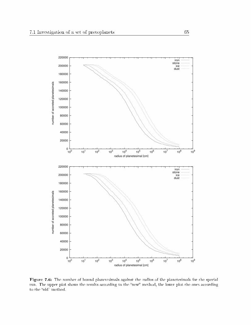
7.1 Investigation of a set of protoplanets 65
0
20000
40000
60000
80000
100000
120000
140000
160000
180000
200000
220000
100 101 102 103 104 105 106 107 108 109
num
ber o
f acc
rete
d pl
anet
esim
als
radius of planetesimal [cm]
ironstone
icedust
0
20000
40000
60000
80000
100000
120000
140000
160000
180000
200000
220000
100 101 102 103 104 105 106 107 108 109
num
ber o
f acc
rete
d pl
anet
esim
als
radius of planetesimal [cm]
ironstone
icedust
Figure 7.6: The number of bound planetesimals against the radius of the planetesimals for the specialrun. The upper plot shows the results according to the new method, the lower plot the ones accordingto the old method.
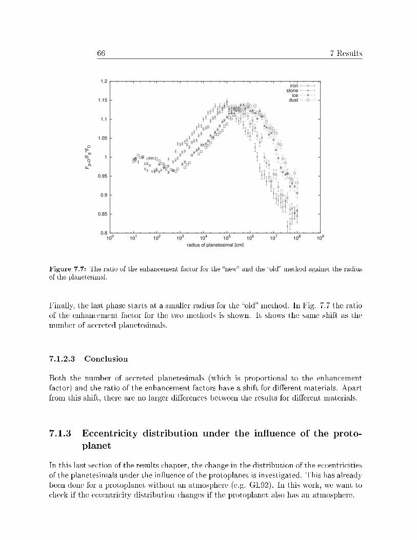
66 7 Results
0.8
0.85
0.9
0.95
1
1.05
1.1
1.15
1.2
100 101 102 103 104 105 106 107 108 109
F g+D
/Fg*
F D
radius of planetesimal [cm]
ironstone
icedust
Figure 7.7: The ratio of the enhancement factor for the new and the old method against the radiusof the planetesimal.
Finally, the last phase starts at a smaller radius for the old method. In Fig. 7.7 the ratioof the enhancement factor for the two methods is shown. It shows the same shift as thenumber of accreted planetesimals.
7.1.2.3 Conclusion
Both the number of accreted planetesimals (which is proportional to the enhancementfactor) and the ratio of the enhancement factors have a shift for dierent materials. Apartfrom this shift, there are no larger dierences between the results for dierent materials.
7.1.3 Eccentricity distribution under the inuence of the proto-
planet
In this last section of the results chapter, the change in the distribution of the eccentricitiesof the planetesimals under the inuence of the protoplanet is investigated. This has alreadybeen done for a protoplanet without an atmosphere (e.g. GL92). In this work, we want tocheck if the eccentricity distribution changes if the protoplanet also has an atmosphere.
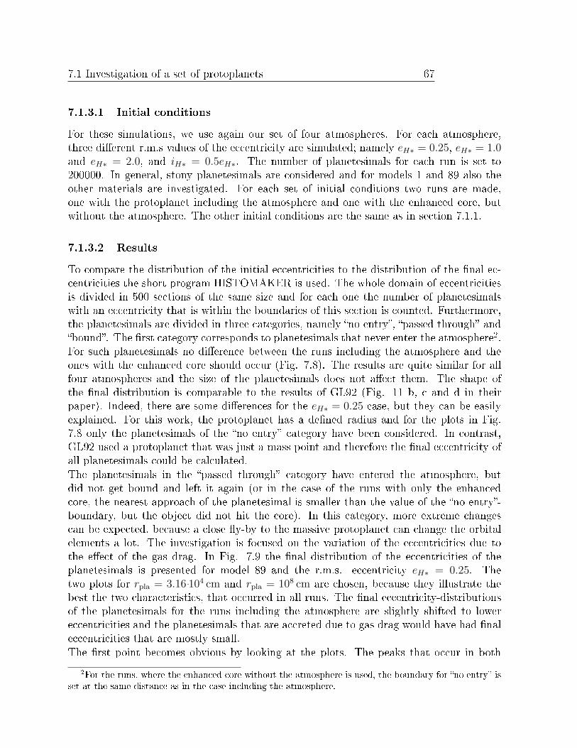
7.1 Investigation of a set of protoplanets 67
7.1.3.1 Initial conditions
For these simulations, we use again our set of four atmospheres. For each atmosphere,three dierent r.m.s values of the eccentricity are simulated; namely eH∗ = 0.25, eH∗ = 1.0and eH∗ = 2.0, and iH∗ = 0.5eH∗. The number of planetesimals for each run is set to200000. In general, stony planetesimals are considered and for models 1 and 89 also theother materials are investigated. For each set of initial conditions two runs are made,one with the protoplanet including the atmosphere and one with the enhanced core, butwithout the atmosphere. The other initial conditions are the same as in section 7.1.1.
7.1.3.2 Results
To compare the distribution of the initial eccentricities to the distribution of the nal ec-centricities the short program HISTOMAKER is used. The whole domain of eccentricitiesis divided in 500 sections of the same size and for each one the number of planetesimalswith an eccentricity that is within the boundaries of this section is counted. Furthermore,the planetesimals are divided in three categories, namely no entry, passed through andbound. The rst category corresponds to planetesimals that never enter the atmosphere2.For such planetesimals no dierence between the runs including the atmosphere and theones with the enhanced core should occur (Fig. 7.8). The results are quite similar for allfour atmospheres and the size of the planetesimals does not aect them. The shape ofthe nal distribution is comparable to the results of GL92 (Fig. 11 b, c and d in theirpaper). Indeed, there are some dierences for the eH∗ = 0.25 case, but they can be easilyexplained. For this work, the protoplanet has a dened radius and for the plots in Fig.7.8 only the planetesimals of the no entry category have been considered. In contrast,GL92 used a protoplanet that was just a mass point and therefore the nal eccentricity ofall planetesimals could be calculated.The planetesimals in the passed through category have entered the atmosphere, butdid not get bound and left it again (or in the case of the runs with only the enhancedcore, the nearest approach of the planetesimal is smaller than the value of the no entry-boundary, but the object did not hit the core). In this category, more extreme changescan be expected, because a close y-by to the massive protoplanet can change the orbitalelements a lot. The investigation is focused on the variation of the eccentricities due tothe eect of the gas drag. In Fig. 7.9 the nal distribution of the eccentricities of theplanetesimals is presented for model 89 and the r.m.s. eccentricity eH∗ = 0.25. Thetwo plots for rpla = 3.16 ˙104 cm and rpla = 108 cm are chosen, because they illustrate thebest the two characteristics, that occurred in all runs. The nal eccentricity-distributionsof the planetesimals for the runs including the atmosphere are slightly shifted to lowereccentricities and the planetesimals that are accreted due to gas drag would have had naleccentricities that are mostly small.The rst point becomes obvious by looking at the plots. The peaks that occur in both
2For the runs, where the enhanced core without the atmosphere is used, the boundary for no entry isset at the same distance as in the case including the atmosphere.
68 7 Results
0
1000
2000
3000
4000
5000
6000
7000
8000
0 1 2 3 4 5 6 7
num
ber o
f pla
nete
simal
s
eH*
rpla=10 cm, initialrpla=10 cm, final
0
1000
2000
3000
4000
5000
6000
7000
8000
0 1 2 3 4 5 6 7
num
ber o
f pla
nete
simal
s
eH*
rpla=10 cm, initialrpla=10 cm, final
0
500
1000
1500
2000
2500
0 1 2 3 4 5 6 7
num
ber o
f pla
nete
simal
s
eH*
rpla=10 cm, initialrpla=10 cm, final
0
500
1000
1500
2000
2500
0 1 2 3 4 5 6 7
num
ber o
f pla
nete
simal
s
eH*
rpla=10 cm, initialrpla=10 cm, final
0
200
400
600
800
1000
1200
0 1 2 3 4 5 6 7
num
ber o
f pla
nete
simal
s
eH*
rpla=10 cm, initialrpla=10 cm, final
0
200
400
600
800
1000
1200
0 1 2 3 4 5 6 7
num
ber o
f pla
nete
simal
s
eH*
rpla=10 cm, initialrpla=10 cm, final
Figure 7.8: The distributions of the initial and nal eccentricities for atmosphere 89. For these plotsonly no entry-planetesimals have been considered. On the left, the results for a protoplanet with anatmosphere and on the right, the results for a protoplanet without an atmosphere are shown. As expected,there is no signicant dierence between the two cases. The results for other radii are equivalent andtherefore they are not shown here.
simulations (in the one with the protoplanet and its atmosphere and in the other one withthe enhanced core only) are not at the same position in the plot. For the run including the
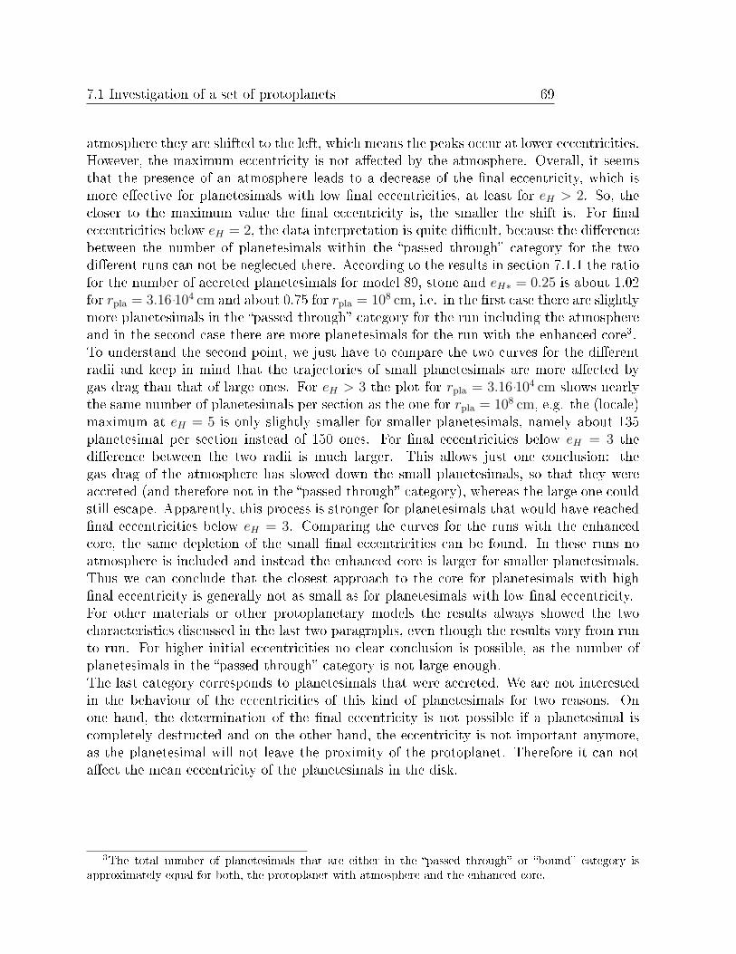
7.1 Investigation of a set of protoplanets 69
atmosphere they are shifted to the left, which means the peaks occur at lower eccentricities.However, the maximum eccentricity is not aected by the atmosphere. Overall, it seemsthat the presence of an atmosphere leads to a decrease of the nal eccentricity, which ismore eective for planetesimals with low nal eccentricities, at least for eH > 2. So, thecloser to the maximum value the nal eccentricity is, the smaller the shift is. For naleccentricities below eH = 2, the data interpretation is quite dicult, because the dierencebetween the number of planetesimals within the passed through category for the twodierent runs can not be neglected there. According to the results in section 7.1.1 the ratiofor the number of accreted planetesimals for model 89, stone and eH∗ = 0.25 is about 1.02for rpla = 3.16 ˙104 cm and about 0.75 for rpla = 108 cm, i.e. in the rst case there are slightlymore planetesimals in the passed through category for the run including the atmosphereand in the second case there are more planetesimals for the run with the enhanced core3.To understand the second point, we just have to compare the two curves for the dierentradii and keep in mind that the trajectories of small planetesimals are more aected bygas drag than that of large ones. For eH > 3 the plot for rpla = 3.16 ˙104 cm shows nearlythe same number of planetesimals per section as the one for rpla = 108 cm, e.g. the (locale)maximum at eH = 5 is only slightly smaller for smaller planetesimals, namely about 135planetesimal per section instead of 150 ones. For nal eccentricities below eH = 3 thedierence between the two radii is much larger. This allows just one conclusion: thegas drag of the atmosphere has slowed down the small planetesimals, so that they wereaccreted (and therefore not in the passed through category), whereas the large one couldstill escape. Apparently, this process is stronger for planetesimals that would have reachednal eccentricities below eH = 3. Comparing the curves for the runs with the enhancedcore, the same depletion of the small nal eccentricities can be found. In these runs noatmosphere is included and instead the enhanced core is larger for smaller planetesimals.Thus we can conclude that the closest approach to the core for planetesimals with highnal eccentricity is generally not as small as for planetesimals with low nal eccentricity.For other materials or other protoplanetary models the results always showed the twocharacteristics discussed in the last two paragraphs, even though the results vary from runto run. For higher initial eccentricities no clear conclusion is possible, as the number ofplanetesimals in the passed through category is not large enough.The last category corresponds to planetesimals that were accreted. We are not interestedin the behaviour of the eccentricities of this kind of planetesimals for two reasons. Onone hand, the determination of the nal eccentricity is not possible if a planetesimal iscompletely destructed and on the other hand, the eccentricity is not important anymore,as the planetesimal will not leave the proximity of the protoplanet. Therefore it can notaect the mean eccentricity of the planetesimals in the disk.
3The total number of planetesimals that are either in the passed through or bound category isapproximately equal for both, the protoplanet with atmosphere and the enhanced core.
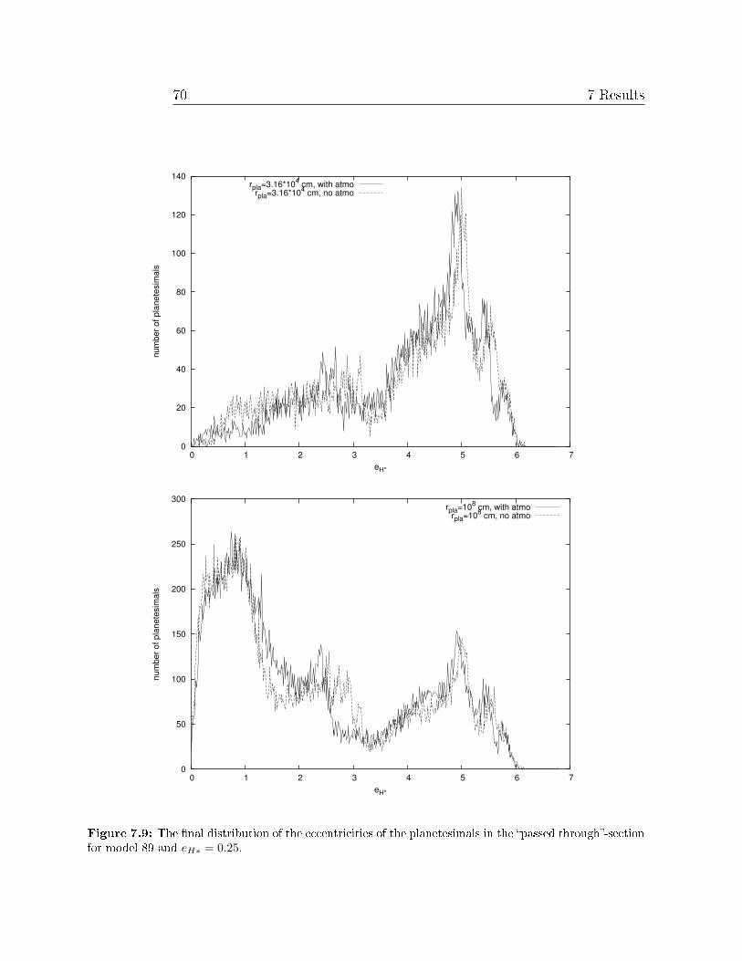
70 7 Results
0
20
40
60
80
100
120
140
0 1 2 3 4 5 6 7
num
ber o
f pla
nete
simal
s
eH*
rpla=3.16*104 cm, with atmorpla=3.16*104 cm, no atmo
0
50
100
150
200
250
300
0 1 2 3 4 5 6 7
num
ber o
f pla
nete
simal
s
eH*
rpla=108 cm, with atmorpla=108 cm, no atmo
Figure 7.9: The nal distribution of the eccentricities of the planetesimals in the passed through-sectionfor model 89 and eH∗ = 0.25.
7.1 Investigation of a set of protoplanets 71
7.1.3.3 Conclusion
The presence of an atmosphere has an eect on the evolution of the distribution of theplanetesimals' eccentricities. The eccentricities of the planetesimals that pass through theatmosphere are slightly less increased than the ones of the runs without an atmosphere. Forthe four investigated atmospheres, the dierence is larger for the more massive atmospheres.

Chapter 8
Discussion of the results
The comparison of the enhancement factor of the collision cross section shows some signif-icant dierences between the two methods. Except for the case of large planetesimals anda massive atmosphere (89), the resulting enhancement factor of the simulations in whichboth drag and orbital motion are taken into account, is generally higher than that of theold method, i.e. the enhancement factor for the collision cross section of a protoplanetwas previously underestimated. Especially for protoplanets in an early phase of their evo-lution, when the atmosphere does not contain a signicant amount of the total mass, thenew method indicates an average enhancement that is higher by a factor of about 1.2 to1.3. The maximum dierence between the two methods is obtained for small to mediumsized planetesimals and atmosphere 1. In this case the dierence is up to a factor of 1.9.For the formation of giant planets, those planetesimals with radii between 100 m and1000 km are the most important ones, as the main fraction of the solid mass accreted bythe protoplanet comes from these planetesimals. The average dierence of the enhancementfactor considering only the larger planetesimals (rpla > 100 m) is about the same as the onefor all sizes. If we further take into account that the mean eccentricity of the planetesimalsin the disk in P96 is estimated as eH = max(2iH , 2), the enhancement factors for oureH∗ = 2 runs seem a good approximation. Under these conditions the average ratio of theenhancement factors is about 1.3 for the rst protoplanet and slowly decreases to 1.1 forthe last model.The increased enhancement factor for the new method means that the formation timeof giant planet was overestimated using the old calculation, as the solid accretion rate isactually higher than predicted and therefore the core can grow faster. The overall eect ofthis dierence for the formation time depends on the formation scenario for giant planets.If we think of in situ formation (no migration), the impact of the increased solid accretionrate on the formation time scale will be quite small, because it mostly aects the time todeplete the feeding zone of the protoplanet. However, the time scale problem for the insitu formation is due to the phase after the feeding zone of the protoplanet was depleted.So, if there are no more planetesimals to accumulate, the predicted increased solid accretionrate does not change anything. For the migrating scenario, which is investigated in thiswork, the increased solid accretion rate will aect the time scale of the formation. Because

74 8 Discussion of the results
the protoplanet is migrating, the feeding zone is never depleted and therefore the increasedsolid accretion rate helps to reduce the time to reach a sucient amount of mass forrunaway growth. At the moment, it is not clear how much the formation time will bereduced due to this change. Therefore a simulation of the formation of a migrating giantplanet with the increased enhancement factor is planned.The detailed investigation of one atmosphere showed that the enhancement factors of thefour dierent materials behave quite similarly. The general shape of the curves in Fig.7.6 shows no signicant dierence between the materials apart from a shift of the curves.The shift is believed to be due to the dierence of the densities, as one initial parameteris the radius. This assumption is conrmed by the size of the shift. The curve of stonyplanetesimals overlaps1 the one of iron planetesimals, if the radii of the rst one are dividedby the factor ρiron
ρstone(the same applies for ice and dust). Because the enhancement factors
for the materials are approximatively just shifted by a known factor, it is not necessary tosimulate all four types to get meaningful results.
1There are a few aberrations for small planetesimals, which are believed to come from the dierencesof the other physical properties of the materials. But overall the curves coincide quite well.
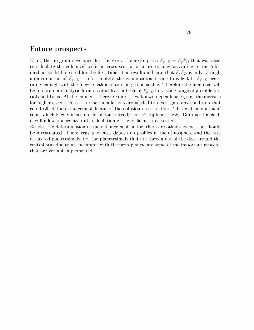
75
Future prospects
Using the program developed for this work, the assumption Fg+D = FgFD that was usedto calculate the enhanced collision cross section of a protoplanet according to the oldmethod could be tested for the rst time. The results indicate that FgFD is only a roughapproximation of Fg+D. Unfortunately, the computational time to calculate Fg+D accu-rately enough with the new method is too long to be usable. Therefore the nal goal willbe to obtain an analytic formula or at least a table of Fg+D for a wide range of possible ini-tial conditions. At the moment, there are only a few known dependencies, e.g. the increasefor higher eccentricities. Further simulations are needed to investigate any condition thatcould aect the enhancement factor of the collision cross section. This will take a lot oftime, which is why it has not been done already for this diploma thesis. But once nished,it will allow a more accurate calculation of the collision cross section.Besides the determination of the enhancement factor, there are other aspects that shouldbe investigated. The energy and mass deposition proles in the atmosphere and the rateof ejected planetesimals, i.e. the planetesimals that are thrown out of the disk around thecentral star due to an encounter with the protoplanet, are some of the important aspects,that are yet not implemented.

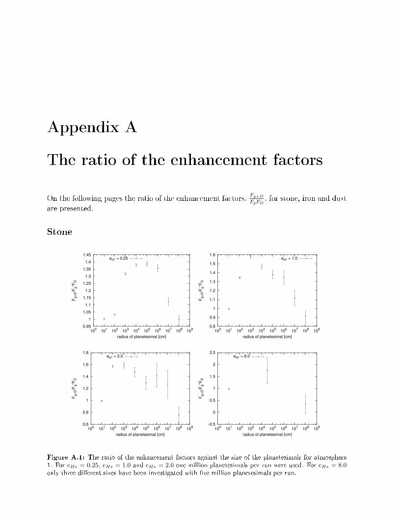
Appendix A
The ratio of the enhancement factors
On the following pages the ratio of the enhancement factors, Fg+D
FgFD, for stone, iron and dust
are presented.
Stone
0.95 1
1.05 1.1
1.15 1.2
1.25 1.3
1.35 1.4
1.45
100 101 102 103 104 105 106 107 108 109
F g+D
/Fg*
F D
radius of planetesimal [cm]
eH* = 0.25
0.8
0.9
1
1.1
1.2
1.3
1.4
1.5
1.6
100 101 102 103 104 105 106 107 108 109
F g+D
/Fg*
F D
radius of planetesimal [cm]
eH* = 1.0
0.6
0.8
1
1.2
1.4
1.6
1.8
100 101 102 103 104 105 106 107 108 109
F g+D
/Fg*
F D
radius of planetesimal [cm]
eH* = 2.0
-0.5
0
0.5
1
1.5
2
2.5
100 101 102 103 104 105 106 107 108 109
F g+D
/Fg*
F D
radius of planetesimal [cm]
eH* = 8.0
Figure A.1: The ratio of the enhancement factors against the size of the planetesimals for atmosphere1. For eH∗ = 0.25, eH∗ = 1.0 and eH∗ = 2.0 one million planetesimals per run were used. For eH∗ = 8.0only three dierent sizes have been investigated with ve million planetesimals per run.
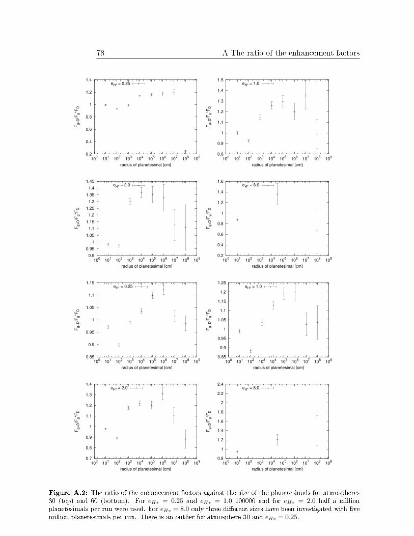
78 A The ratio of the enhancement factors
0.2
0.4
0.6
0.8
1
1.2
1.4
100 101 102 103 104 105 106 107 108 109
F g+D
/Fg*
F D
radius of planetesimal [cm]
eH* = 0.25
0.8
0.9
1
1.1
1.2
1.3
1.4
1.5
100 101 102 103 104 105 106 107 108 109
F g+D
/Fg*
F D
radius of planetesimal [cm]
eH* = 1.0
0.9 0.95
1 1.05 1.1
1.15 1.2
1.25 1.3
1.35 1.4
1.45
100 101 102 103 104 105 106 107 108 109
F g+D
/Fg*
F D
radius of planetesimal [cm]
eH* = 2.0
0.2
0.4
0.6
0.8
1
1.2
1.4
1.6
100 101 102 103 104 105 106 107 108 109
F g+D
/Fg*
F D
radius of planetesimal [cm]
eH* = 8.0
0.85
0.9
0.95
1
1.05
1.1
1.15
100 101 102 103 104 105 106 107 108 109
F g+D
/Fg*
F D
radius of planetesimal [cm]
eH* = 0.25
0.85
0.9
0.95
1
1.05
1.1
1.15
1.2
1.25
100 101 102 103 104 105 106 107 108 109
F g+D
/Fg*
F D
radius of planetesimal [cm]
eH* = 1.0
0.7
0.8
0.9
1
1.1
1.2
1.3
1.4
100 101 102 103 104 105 106 107 108 109
F g+D
/Fg*
F D
radius of planetesimal [cm]
eH* = 2.0
0.8
1
1.2
1.4
1.6
1.8
2
2.2
2.4
100 101 102 103 104 105 106 107 108 109
F g+D
/Fg*
F D
radius of planetesimal [cm]
eH* = 8.0
Figure A.2: The ratio of the enhancement factors against the size of the planetesimals for atmospheres30 (top) and 60 (bottom). For eH∗ = 0.25 and eH∗ = 1.0 100000 and for eH∗ = 2.0 half a millionplanetesimals per run were used. For eH∗ = 8.0 only three dierent sizes have been investigated with vemillion planetesimals per run. There is an outlier for atmosphere 30 and eH∗ = 0.25.

79
0.7
0.75
0.8
0.85
0.9
0.95
1
1.05
1.1
100 101 102 103 104 105 106 107 108 109
F g+D
/Fg*
F D
radius of planetesimal [cm]
eH* = 0.25
0.8
0.85
0.9
0.95
1
1.05
1.1
1.15
100 101 102 103 104 105 106 107 108 109
F g+D
/Fg*
F D
radius of planetesimal [cm]
eH* = 1.0
0.9
0.95
1
1.05
1.1
1.15
1.2
1.25
1.3
1.35
100 101 102 103 104 105 106 107 108 109
F g+D
/Fg*
F D
radius of planetesimal [cm]
eH* = 2.0
0.4
0.6
0.8
1
1.2
1.4
1.6
100 101 102 103 104 105 106 107 108 109
F g+D
/Fg*
F D
radius of planetesimal [cm]
eH* = 8.0
Figure A.3: The ratio of the enhancement factors against the size of the planetesimals for atmosphere89. The material type is ice. For eH∗ = 0.25 and eH∗ = 1.0 two millions and for eH∗ = 2.0 one millionplanetesimals per run were used. For eH∗ = 8.0 again two million planetesimals per run were used.
.

80 A The ratio of the enhancement factors
Iron
0
0.2
0.4
0.6
0.8
1
1.2
1.4
100 101 102 103 104 105 106 107 108 109
F g+D
/Fg*
F D
radius of planetesimal [cm]
eH* = 0.25 0.9
1
1.1
1.2
1.3
1.4
1.5
1.6
1.7
100 101 102 103 104 105 106 107 108 109
F g+D
/Fg*
F D
radius of planetesimal [cm]
eH* = 1.0
0.6
0.8
1
1.2
1.4
1.6
1.8
2
100 101 102 103 104 105 106 107 108 109
F g+D
/Fg*
F D
radius of planetesimal [cm]
eH* = 2.0
0.2
0.4
0.6
0.8
1
1.2
1.4
1.6
100 101 102 103 104 105 106 107 108 109
F g+D
/Fg*
F D
radius of planetesimal [cm]
eH* = 8.0
Figure A.4: The ratio of the enhancement factors against the size of the planetesimals for atmosphere 1.For eH∗ = 0.25, eH∗ = 1.0 and eH∗ = 2.0 one million planetesimals per run were used. For eH∗ = 8.0 onlythree dierent sizes have been investigated with ve million planetesimals per run. There are two outliersfor eH∗ = 0.25. The third ratio for eH∗ = 8.0 is missing, because FgFD was zero for rpla = 108 cm.
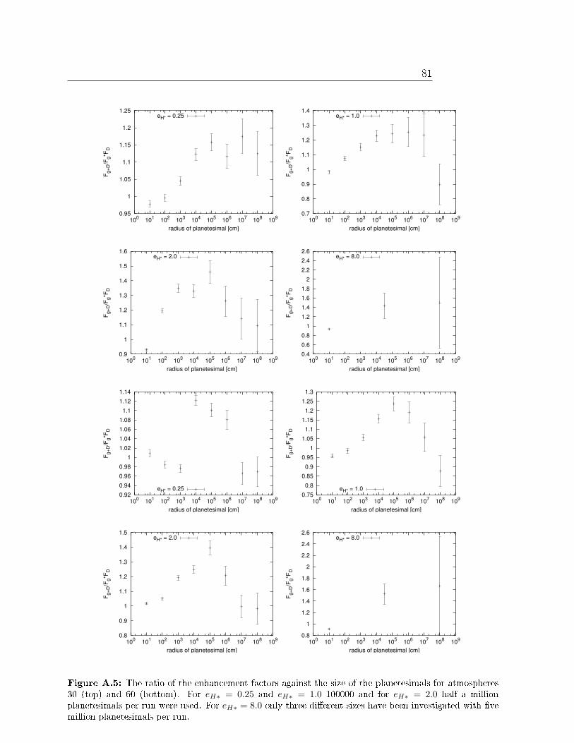
81
0.95
1
1.05
1.1
1.15
1.2
1.25
100 101 102 103 104 105 106 107 108 109
F g+D
/Fg*
F D
radius of planetesimal [cm]
eH* = 0.25
0.7
0.8
0.9
1
1.1
1.2
1.3
1.4
100 101 102 103 104 105 106 107 108 109
F g+D
/Fg*
F D
radius of planetesimal [cm]
eH* = 1.0
0.9
1
1.1
1.2
1.3
1.4
1.5
1.6
100 101 102 103 104 105 106 107 108 109
F g+D
/Fg*
F D
radius of planetesimal [cm]
eH* = 2.0
0.4 0.6 0.8
1 1.2 1.4 1.6 1.8
2 2.2 2.4 2.6
100 101 102 103 104 105 106 107 108 109
F g+D
/Fg*
F D
radius of planetesimal [cm]
eH* = 8.0
0.92 0.94 0.96 0.98
1 1.02 1.04 1.06 1.08 1.1
1.12 1.14
100 101 102 103 104 105 106 107 108 109
F g+D
/Fg*
F D
radius of planetesimal [cm]
eH* = 0.25 0.75 0.8
0.85 0.9
0.95 1
1.05 1.1
1.15 1.2
1.25 1.3
100 101 102 103 104 105 106 107 108 109
F g+D
/Fg*
F D
radius of planetesimal [cm]
eH* = 1.0
0.8
0.9
1
1.1
1.2
1.3
1.4
1.5
100 101 102 103 104 105 106 107 108 109
F g+D
/Fg*
F D
radius of planetesimal [cm]
eH* = 2.0
0.8
1
1.2
1.4
1.6
1.8
2
2.2
2.4
2.6
100 101 102 103 104 105 106 107 108 109
F g+D
/Fg*
F D
radius of planetesimal [cm]
eH* = 8.0
Figure A.5: The ratio of the enhancement factors against the size of the planetesimals for atmospheres30 (top) and 60 (bottom). For eH∗ = 0.25 and eH∗ = 1.0 100000 and for eH∗ = 2.0 half a millionplanetesimals per run were used. For eH∗ = 8.0 only three dierent sizes have been investigated with vemillion planetesimals per run.
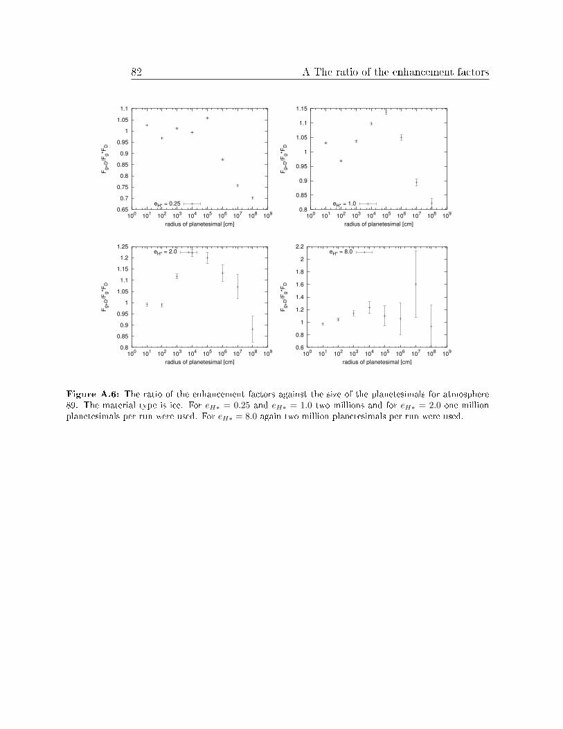
82 A The ratio of the enhancement factors
0.65
0.7
0.75
0.8
0.85
0.9
0.95
1
1.05
1.1
100 101 102 103 104 105 106 107 108 109
F g+D
/Fg*
F D
radius of planetesimal [cm]
eH* = 0.25 0.8
0.85
0.9
0.95
1
1.05
1.1
1.15
100 101 102 103 104 105 106 107 108 109
F g+D
/Fg*
F D
radius of planetesimal [cm]
eH* = 1.0
0.8
0.85
0.9
0.95
1
1.05
1.1
1.15
1.2
1.25
100 101 102 103 104 105 106 107 108 109
F g+D
/Fg*
F D
radius of planetesimal [cm]
eH* = 2.0
0.6
0.8
1
1.2
1.4
1.6
1.8
2
2.2
100 101 102 103 104 105 106 107 108 109
F g+D
/Fg*
F D
radius of planetesimal [cm]
eH* = 8.0
Figure A.6: The ratio of the enhancement factors against the size of the planetesimals for atmosphere89. The material type is ice. For eH∗ = 0.25 and eH∗ = 1.0 two millions and for eH∗ = 2.0 one millionplanetesimals per run were used. For eH∗ = 8.0 again two million planetesimals per run were used.
.
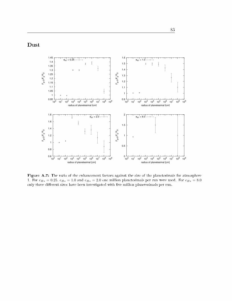
83
Dust
0.95 1
1.05 1.1
1.15 1.2
1.25 1.3
1.35 1.4
1.45
100 101 102 103 104 105 106 107 108 109
F g+D
/Fg*
F D
radius of planetesimal [cm]
eH* = 0.25
0.9
1
1.1
1.2
1.3
1.4
1.5
1.6
100 101 102 103 104 105 106 107 108 109
F g+D
/Fg*
F D
radius of planetesimal [cm]
eH* = 1.0
0.6
0.8
1
1.2
1.4
1.6
1.8
100 101 102 103 104 105 106 107 108 109
F g+D
/Fg*
F D
radius of planetesimal [cm]
eH* = 2.0
0
0.5
1
1.5
2
100 101 102 103 104 105 106 107 108 109
F g+D
/Fg*
F D
radius of planetesimal [cm]
eH* = 8.0
Figure A.7: The ratio of the enhancement factors against the size of the planetesimals for atmosphere1. For eH∗ = 0.25, eH∗ = 1.0 and eH∗ = 2.0 one million planetesimals per run were used. For eH∗ = 8.0only three dierent sizes have been investigated with ve million planetesimals per run.
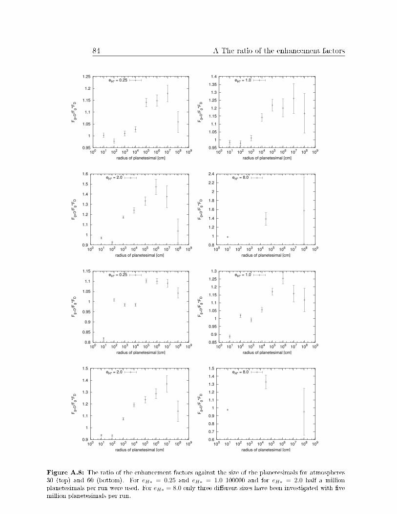
84 A The ratio of the enhancement factors
0.95
1
1.05
1.1
1.15
1.2
1.25
100 101 102 103 104 105 106 107 108 109
F g+D
/Fg*
F D
radius of planetesimal [cm]
eH* = 0.25
0.95
1
1.05
1.1
1.15
1.2
1.25
1.3
1.35
1.4
100 101 102 103 104 105 106 107 108 109
F g+D
/Fg*
F D
radius of planetesimal [cm]
eH* = 1.0
0.9
1
1.1
1.2
1.3
1.4
1.5
1.6
100 101 102 103 104 105 106 107 108 109
F g+D
/Fg*
F D
radius of planetesimal [cm]
eH* = 2.0
0.8
1
1.2
1.4
1.6
1.8
2
2.2
2.4
100 101 102 103 104 105 106 107 108 109
F g+D
/Fg*
F D
radius of planetesimal [cm]
eH* = 8.0
0.8
0.85
0.9
0.95
1
1.05
1.1
1.15
100 101 102 103 104 105 106 107 108 109
F g+D
/Fg*
F D
radius of planetesimal [cm]
eH* = 0.25
0.85
0.9
0.95
1
1.05
1.1
1.15
1.2
1.25
1.3
100 101 102 103 104 105 106 107 108 109
F g+D
/Fg*
F D
radius of planetesimal [cm]
eH* = 1.0
0.9
1
1.1
1.2
1.3
1.4
1.5
100 101 102 103 104 105 106 107 108 109
F g+D
/Fg*
F D
radius of planetesimal [cm]
eH* = 2.0
0.6
0.7
0.8
0.9
1
1.1
1.2
1.3
1.4
1.5
100 101 102 103 104 105 106 107 108 109
F g+D
/Fg*
F D
radius of planetesimal [cm]
eH* = 8.0
Figure A.8: The ratio of the enhancement factors against the size of the planetesimals for atmospheres30 (top) and 60 (bottom). For eH∗ = 0.25 and eH∗ = 1.0 100000 and for eH∗ = 2.0 half a millionplanetesimals per run were used. For eH∗ = 8.0 only three dierent sizes have been investigated with vemillion planetesimals per run.
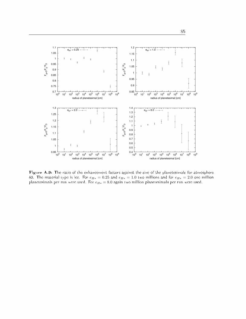
85
0.7
0.75
0.8
0.85
0.9
0.95
1
1.05
1.1
100 101 102 103 104 105 106 107 108 109
F g+D
/Fg*
F D
radius of planetesimal [cm]
eH* = 0.25
0.85
0.9
0.95
1
1.05
1.1
1.15
1.2
100 101 102 103 104 105 106 107 108 109
F g+D
/Fg*
F D
radius of planetesimal [cm]
eH* = 1.0
0.95
1
1.05
1.1
1.15
1.2
1.25
1.3
100 101 102 103 104 105 106 107 108 109
F g+D
/Fg*
F D
radius of planetesimal [cm]
eH* = 2.0
0.4 0.5 0.6 0.7 0.8 0.9
1 1.1 1.2 1.3 1.4
100 101 102 103 104 105 106 107 108 109
F g+D
/Fg*
F D
radius of planetesimal [cm]
eH* = 8.0
Figure A.9: The ratio of the enhancement factors against the size of the planetesimals for atmosphere89. The material type is ice. For eH∗ = 0.25 and eH∗ = 1.0 two millions and for eH∗ = 2.0 one millionplanetesimals per run were used. For eH∗ = 8.0 again two million planetesimals per run were used.
.

Bibliography
Alibert, Y., Mordasini, C., Benz, W., and Winisdoerer, C. (2005). Models of giant planetformation with migration and disc evolution. Astronomy & Astrophysics, 434:343353.
Barrabés, E. and Mikkola, S. (2005). Families of periodic horseshoe orbits in the restrictedthree-body problem. Astronomy & Astrophysics, 432:11151129.
Beutler, G. (1999). Himmelsmechanik des Planetensystems. Druckerei der UniversitätBern, Bern.
Bodenheimer, P. (1985). Evolution of the Giant Planets. In: Protostars and Planets II.University of Arizona Press, Tucson.
Bodenheimer, P., Hubickyj, O., and Lissauer, J. J. (2000). Models of the in situ formationof detected extrasolar giant planets. Icarus, 143:214.
Bodenheimer, P. and Pollack, J. B. (1986). Calculation of the accretion and evolution ofgiant planets. Icarus, 67:391408.
Borcherds, P. H. (1996). The restricted gravitational three-body problem: trajectoriesassociated with lagrange xed points. European Journal of Physics, 17:6370.
Boss, A. P. (2000). Possible rapid gas giant formation in the solar nebula and otherprotoplanetary disks. Astrophysical Journal, 536:L101L104.
DeCampi, W. M. and Cameron, A. G. W. (1979). Structure and evolution of isolated giantgaseous protoplanets. Icarus, 38:367391.
Greenzweig, Y. and Lissauer, J. J. (1990). Accretion rates of protoplanets. Icarus, 87:4077.
Greenzweig, Y. and Lissauer, J. J. (1992). Accretion rates of protoplanets: Ii. gaussiandistributions of planetesimal velocities. Icarus, 100:440463.
Guillot, T. (2005). The interiors of giant planets: Models and outstanding questions.Annual Review of Earth and Planetary Science, 33:493530.
Hillenbrand, L. A. (2005). Observational constraints on dust disk lifetimes: Implicationsfor planet formation.

88 BIBLIOGRAPHY
Hubickyj, O., Bodenheimer, P., and Lissauer, J. J. (2005). Evolution of gas giant planetsusing the core accretion model. Icarus, 179:415431.
Inaba, S. and Ikoma, M. (2003). Enhanced collisional growth of a protoplanet that has anatmosphere. Astronomy & Astrophysics, 410:711723.
Mizuno, H. (1980). Formation of the giant planets. Progress of Theoretical Physics, 64:544557.
Mizuno, H., Nakazawa, K., and Hayashi, C. (1978). Instability of a gaseous envelopesurrounding a planetary core and formation of giant planets. Progress of Theoretical
Physics, 60:699710.
Mohr, P. J. and Taylor, B. N. (2005). Cotada recommended values of the fundamentalphysical constants: 2002. Review of Modern Physics, 77:1107.
Mordasini, C. A. (2004). Planetesimale Einschläge auf Jupiter. Universität Bern, Bern.
Nakazawa, K., Ida, S., and Nakagawa, Y. (1989). Collisional probability of planetesimalsrevolving in the solar gravitational eld, i. basic formulation. Astronomy & Astrophysics,220:293300.
Observatory, U. S. N. (2004). The astonomical almanac for the year 2004. U.S. Governmentprinting oce.
Perri, F. and Cameron, A. G. W. (1974). Hydrodynamic instability of the solar nebula inthe presence of a planetary core. Icarus, 22:846849.
Pollack, J. B., Hubicklyj, O., Bodenheimer, P., Lissauer, J. J., Podolak, M., and Green-zweig, Y. (1996). Formation of the giant planets by concurrent accretion of solids andgas. Icarus, 124:6285.
Press, W. H., Teukolsky, S. A., Vetterling, W. T., and Flannery, B. P. (1996). Numerical
Recipes in Fortran 90 - The art of parallel scientic computing. Cambridge UniversityPress, New York.
Safronov, V. S. (1969). Evolution of the Protoplanetary Cloud and Formation of the Earth
and Planets. Nauka Press, Moscow, translation NASA-TT-F-677, 1972.
Saletan, E. and Cromer, A. (1974). Theoretische Mechanik. R. Oldenbourg Verlag GmbH,München.
Szebehely, V. (1967). Theory of orbits. Academy press inc., New York.
Weidenschilling, S. J. (1977). Aerodynamics of solid bodies in the solar nebula. Mon. Not.
Royal Astronomical Society, 180:5770.
Acknowledgements
First of all, I'd like to thank Prof. Willy Benz who gave me the opportunity to do thisdiploma project. He always took the time to discuss any problem that arose and with hiswide experience helped me not to lose the main thread of the work.A big thank you goes to Christoph Mordasini without whom this work would not havebeen possible, as the program is based on his work. He was always willing to answer anyquestion about his program and to share his knowledge. The numerous discussions withhim were protable for me and often resulted in an improvement of my work.Furthermore, I'd like to thank Dr. James Whitby, who helped me with the english in thiswork, Dr. Yann Alibert, who provided me with the atmospheric structure les, my ocemates, with whom I had a lot of interesting discussions, and my fellow student DieterLüthi, who motivated me during the studies.Last but not least, I'd like to thank my family, who have always supported me and aordedme the opportunity to do what I wanted.