Polymer-Based Systems for Drug Delivery Studies
157
Polymer-Based Systems for Drug Delivery Studies Dissertation zur Erlangung des Grades "Doktor der Naturwissenschaften" im Promotionsfach Chemie am Fachbereich Chemie, Pharmazie und Geowissenschaften der Johannes Gutenberg-Universität in Mainz vorgelegt von Jennifer Schultze geboren in Schwerin Mainz, Mai 2018
Transcript of Polymer-Based Systems for Drug Delivery Studies

Polymer-Based Systems
for Drug Delivery Studies
Dissertation
zur Erlangung des Grades
"Doktor der Naturwissenschaften"
im Promotionsfach Chemie
am Fachbereich Chemie, Pharmazie und Geowissenschaften
der Johannes Gutenberg-Universität in Mainz
vorgelegt von
Jennifer Schultze
geboren in Schwerin
Mainz, Mai 2018

Die vorliegende Arbeit wurde im Zeitraum von Januar 2015 bis Mai 2018 am
Max-Planck-Institut für Polymerforschung in Mainz unter der Anleitung von
Herrn Prof. Dr. Hans-Jürgen Butt und Herrn Dr. Kaloian Koynov angefertigt.
Erster Gutachter: Prof. Dr. Hans-Jürgen Butt
Zweiter Gutachter: Prof. Dr. Rudolf Zentel
Tag der müdlichen Prüfung: 21.06.2018

III
“Life isn’t about waiting for the storm to pass...
It’s about learning to dance in the rain”
Vivian Greene

V
Zusammenfassung
Nanopartikel-basierte Wirkstofftransportsysteme sind sehr vielversprechend
für die Behandlung verschiedenster Krankheiten. Mithilfe von Nanopartikeln
können Wirkstoffe eingeschlossen, transportiert und freigesetzt werden.
Trotz vieler vorhandener Systeme, ist ein tieferes Verständis der Prozesse
notwendig. Das Ziel dieser Dissertation war es, einen tieferen Einblick in
zwei hierfür relevante Themen zu erhalten: (i) eine Herstellungsmethode für
nanopartikuläre Wirkstofftransportsysteme und (ii) ein neues
Zellmembranmodell für Untersuchungen auf zellulärer Ebene.
Für ein besseres Verständnis der Wirkstoffaufnahme in Zellen und der
Passage der Membran werden Zellmodelle verwendet. Ein beliebtes Modell
sind die gigantischen unilamellaren Vesikel (GUV). Diese Arbeit stellt eine
neue Methode vor, mit der GUV mithilfe eines oberflächenstrukturierten
Polymerhydrogels größenspezifisch hergestellt werden können. Die
Herstellung hunderter verankerter GUV in drei verschiedenen Größen und
der Nutzen dieser Herstellungsmethode wird anhand von zwei
Anwendungsbeispielen in dieser Dissertation veranschaulicht.
Im zweiten Projekt liegt der Fokus auf einer Herstellungsmethode für
Polystyrol (PS)-Nanopartikel als Wirkstoffträgersysteme. Der Verlauf der
Partikelbildung aus Nanotropfen wurde untersucht. Die Veränderung dieser
Tropfen und deren PS-Anteil konnte mithilfe von fluoreszierenden
Rotormolekülen, deren Fluoreszenzlebenszeit sich abhängig von der
Viskosität ändert, beobachtet und analysiert werden.
In beiden Projekten dieser Arbeit wird die Fluoreszenzspektroskopie zur
Analyse genutzt.
In Kooperationsprojekten innerhalb des Sonderforschungsbereichs 1066
wurde die Fluoreszenzkorrelationsspektroskopie zur Analyse von
verschiedenen Polymersystems für Wirkstofftransportanwendungen
eingesetzt. Die Projekte sind am Ende dieser Dissertation zusammengefasst.

VII
Abstract
Nanocarrier-based drug delivery is a promising approach for treating various
diseases. Nanocarriers can encapsulate and deliver drug molecules and a lot
of work has been done in developing new systems. But still, a deeper
understanding of the processes is needed. The aim of this thesis is to look
deeper into two relevant processes for drug delivery studies: (i) on the
extracellular level - studying the formation of polymer nanoparticles as
nanocarriers and (ii) on the cellular level – developing a new cell membrane
model.
In this regard, a new cell-model formation method is introduced in the first
part of the thesis. Giant unilamellar vesicles (GUVs) serve as cell membrane
models. Based on a functionalized polymer hydrogel, anchored GUVs of a
defined size were produced using a very fast procedure. Three different sizes
of GUVs were prepared on the pre-structured polymer hydrogel surface. Two
application examples show the advantages of the array of hundreds of
uniform anchored vesicles.
Polymer nanoparticles for drug carrier systems can be prepared in a diversity
of methods. In the second part of this thesis, the physico-chemical
underpinnings of the preparation and development of polystyrene (PS)
nanoparticles by solvent evaporation from emulsion droplets (SEED) were
studied to understand the process. The formation of the nanodroplets and
the fraction of PS inside the droplets was monitored via fluorescence
spectroscopy measurements of a fluorescent molecular rotor in the system.
Both projects profit from the usage of fluorescence molecules and their
analysis via fluorescence spectroscopy.
As joint work with the collaborative research center 1066, fluorescence
correlation spectroscopy (FCS) was used in many cooperative projects to
analyze different polymer-based systems for drug delivery applications. The
projects are summarized at the end of the thesis.


IX
Contents
Zusammenfassung ...................................................................................................... V
Abstract ..................................................................................................................... VII
1 Introduction ......................................................................................................... 1
2 Physico-Chemical Concepts and Methods .......................................................... 5
2.1 Fluorescence ................................................................................................ 6
2.2 Fluorescent Molecular Rotors ...................................................................... 9
2.3 Fluorescence Spectroscopy via Time-Correlated Single Photon Counting 12
2.4 Confocal Laser Scanning Microscopy ......................................................... 14
2.5 Fluorescence Correlation Spectroscopy ..................................................... 16
3 Polymer Gel-Assisted Formation of Giant Unilamellar Vesicles ........................ 21
3.1 Chemical Concepts and Methods .............................................................. 22
3.1.1 Giant Unilamellar Vesicles .................................................................. 22
3.1.2 Common Methods for Preparing Giant Unilamellar Vesicles ............. 24
3.1.3 Gel-Assisted Formation of Giant Unilamellar Vesicles ....................... 26
3.1.4 Poly(N-isopropylacrylamide) .............................................................. 30
3.2 Experiments und Materials ........................................................................ 34

X
3.2.1 Materials .............................................................................................. 34
3.2.2 4-Methacryloyloxybenzophenone (MABP) ......................................... 35
3.2.3 Functionalization of the Glass Substrates ........................................... 35
3.2.4 Poly(N-isopropylacrylamide) Based Terpolymer ................................. 35
3.2.5 Preparation of the Polymer Template ................................................. 36
3.2.6 Giant Unilamellar Anchored Vesicle (GUAV) Formation ..................... 37
3.2.7 Confocal Laser Scanning Microscopy .................................................. 37
3.2.8 Determination of the Lipids Diffusion Coefficient via FCS .................. 37
3.2.9 Photo-Oxidation .................................................................................. 38
3.3 Results and Discussion ................................................................................ 39
3.3.1 Preparation of Flat PNIPAAm Terpolymer Films ................................. 39
3.3.2 Properties of Flat PNIPAAm Terpolymer Films .................................... 41
3.3.3 GUV Formation on Flat PNIPAAm Terpolymer Films .......................... 45
3.3.4 Preparation of Patterned PNIPAAm Terpolymer Films ....................... 48
3.3.5 Properties of Patterned PNIPAAm Terpolymer Films ......................... 51
3.3.6 GUV Formation on Patterned PNIPAAm Terpolymer Films ................ 52
3.3.7 Size Control .......................................................................................... 55
3.3.8 Applications ......................................................................................... 57
3.4 Summary and Outlook ................................................................................ 62

XI
4 Monitoring Polymer Nanoparticle Formation using a Fluorescent Molecular
Rotor ......................................................................................................................... 65
4.1 Chemical Concepts and Methods .............................................................. 66
4.1.1 Polystyrene Nanoparticles .................................................................. 66
4.1.2 Nanoparticle Formation Techniques .................................................. 67
4.1.3 Solvent Evaporation from Emulsion Droplets .................................... 69
4.2 Experiments und Materials ........................................................................ 70
4.2.1 Materials ............................................................................................. 70
4.2.2 Time-Correlated Single Photon Counting (TCSPC) .............................. 70
4.2.3 TCSPC Measurements of the Molecular Rotor in Toluene ................. 71
4.2.4 TCSPC Measurements of Atto425 in Water ........................................ 71
4.2.5 TCSPC Measurements in Polystyrene Solutions ................................. 71
4.2.6 Polystyrene Nanoparticle Formation via SEED in Toluene ................. 72
4.2.7 Dried Polystyrene Nanoparticles ........................................................ 73
4.2.8 SEED Process Without Polymer for Studying SDS Influence ............... 73
4.2.9 Polystyrene Nanoparticle Formation via SEED in Chloroform............ 74
4.2.10 Fluorescence Correlation Spectroscopy (FCS) .................................... 74
4.3 Results and Discussion ............................................................................... 75
4.3.1 Fluorescence Lifetime of Molecular Rotor LBX37 in Toluene ............ 75
4.3.2 Master Curve for Polystyrene Toluene Mixtures ............................... 77

XII
4.3.3 Monitoring the Polystyrene Nanoparticle Formation via SEED .......... 82
4.3.4 Monitoring the Nanoparticle Formation in a Droplet ......................... 86
4.3.5 Polystyrene Nanoparticles in Dry Environment .................................. 90
4.3.6 Long Term Study of the Drying Process .............................................. 91
4.3.7 Influence of SDS ................................................................................... 92
4.3.8 A Closer Look Inside the Nanodroplets ............................................... 94
4.3.9 Polystyrene Nanoparticles from SEED with Chloroform ..................... 96
4.4 Summary and Outlook .............................................................................. 100
4.5 Appendix – Additional Datasets................................................................ 102
5 Concluding Remarks ......................................................................................... 107
6 FCS Analysis of Polymer-Based Systems - Cooperative Projects ..................... 109
6.1 Fluorescence Correlation Spectroscopy (FCS) Characterizes Antibody-
Polyplex-Conjugates for Cell Targeting ................................................................ 110
6.2 Fluorescence Correlation Spectroscopy Confirms Successful Coating of
Dendritic Mesoporous Silica Nanoparticles (DMSN) with a pH-Responsive Block
Copolymer for Drug Delivery ............................................................................... 112
6.3 Fluorescence Cross-Correlation Spectroscopy (FCCS) Verifies the
Functionalization of Dual Labeled Block Copolymers .......................................... 114
6.4 Fluorescence Correlation Spectroscopy Demonstrates the Covalent Linkage
of Functional Groups to Polymersomes .............................................................. 116
6.5 Fluorescence Correlation Spectroscopy Determines the Critical Micelle
Concentration ...................................................................................................... 118

XIII
6.6 Fluorescence Correlation Spectroscopy Studies of Molecular Tracer
Diffusion .............................................................................................................. 120
7 Bibliography ..................................................................................................... 123
8 Abbreviations ................................................................................................... 133
9 Symbols ............................................................................................................ 137
Danksagung ............................................................................................................. 139
Curriculum Vitae ..................................................................................................... 143


1
1 Introduction
Polymer science is present in various research areas, ranging from medical
applications to electronics. Polymers are not only plastic bottles made from
polyethylene terephthalate (PET) or polystyrene (PS) in the form of Styrofoam.
Polymers also play a significant role in biology and medicine. Natural
polymers are for example DNA molecules or proteins, which are essential for
every living species. Both types, natural and synthetic polymers, are highly
interesting for researchers of different fields and studies on polymers are
growing year after year.
One research area, in which polymers gain more and more importance, is
the field of biomedical systems. The natural polymers, such as the DNA or
the variety of proteins, are mainly investigated in the biological sciences. But
in terms of polymer research it is not possible to define the main natural
sciences’ discipline, in which polymers are studied. Polymers bring many
disciplines together and lead to interdisciplinary work.
A very popular interdisciplinary topic is the research of polymeric drug
delivery systems.[1] New innovative drug molecules show high potential to
treat specific diseases, but researchers often face the problem of bringing the
drug molecules to the body area of interest. In this regard, polymers are often
selected to work as nanocarrier systems.[2–7] In some cases the cargo or drug
is attached to the polymer nanoparticle, in other cases the drug is
encapsulated by a polymer shell, that can be opened in the appropriate area
in the body by external stimuli.[8] The diversity of nanocarrier systems is
huge: copolymer micelles, polymer nanoparticles, nanohydrogel particles,
polymer capsules, liposomes or dendritic polymers.[9] In every case, the
carrier together with the cargo needs to be brought to a certain place in the
body. This uptake ensures the best treatment.[1,5–7,10]

2
Regarding the research on nanocarrier-based drug delivery, two main
research areas exist. One area deals with the studies in aqueous solutions,
including all studies performed outside the body or the cells. Here, the
researchers look at the particle formation, the encapsulation of the drug
molecules and the biocompatibility of the carrier systems. Also important in
this field is the analysis of the carrier’s properties, such as size, stability or
drug loading efficiency.[9,11–13] The other research area looks at the cellular
level of the nanocarrier-based drug delivery. Here, questions about targeted
delivery, cellular uptake and drug release play an important role.[14] The
systems must ensure, that the cargo is attached to the (nano-)carrier, and
that the whole carrier systems reaches the place where the cargo should be
released. Furthermore, it is important that the cargo can be released and
that the carrier, the uptake and the whole process does not harm the healthy
cells or the body in any way. In this challenging field, many research groups
focus on the synthesis of the carriers, on drug loading, release and cellular
uptake.
This thesis deals with two topics that play an important role in the field of
polymer systems for drug delivery. The first topic is related to research on
cellular level, whereas the second topic belongs to the category of ex-vivo
studies of nanoparticles and their characterization.
The first part of the thesis describes a newly developed method for the
preparation of a cell membrane model. This method is based on a polymer
system, more precisely a (poly(N-isopropylacrylamide) (PNIPAAm) terpolymer
hydrogel. PNPAAm was polymerized with functional comonomers and cross-
linked to a covalently bound swellable network. Via photo-lithography this
polymer network can be patterned, in order to form a template for the
preparation of size-defined cell membrane models on its surface. The type of
cell model is called giant unilamellar vesicle (GUV) and was formed from
phospholipids. These size-defined GUVs can be used as cell models for an
easier understanding of the cell membrane. Furthermore, model systems are
useful for gaining insight into drug delivery research.
3
In the second topic the focus is on the research of the nanoparticle systems
and the understanding of their formation processes. A lot of work has been
done regarding the synthesis or preparation of nanoparticles as well as their
applications, especially in drug delivery studies. This project focuses on the
physico-chemical understanding of the process of polymer nanoparticle
formation via so-called “solvent evaporation from emulsion droplets (SEED)”.
Polystyrene nanoparticles were prepared with this kind of formation method
and the process of solvent evaporation from the nanodroplets was monitored
with the help of a fluorescent molecular rotor. This type of molecule changes
its fluorescence lifetime depending on the microenvironment. The lifetime
was measured via time-correlated single photon counting (TCSPC)
experiments. Furthermore, the size and concentration of the nanodroplets
during the evaporation process was monitored via fluorescence correlation
spectroscopy. Both studies were obtained simultaneously in a single
experiment. Polymer nanoparticles for drug delivery can be prepared by the
SEED process. Therefore, it is important to understand the process and the
particle formation, in order to control the method to obtain ideal drug
delivery systems.
The analysis of polymer-based systems for drug delivery studies via
fluorescence correlation spectroscopy (FCS) was a third part of this work.
FCS was used in many cooperative projects to determine the diffusion
coefficients, hydrodynamic radii and aggregation behavior or to confirm
successful chemical reactions. In the last chapter, the joint projects are
presented.


2 Physico-Chemical Concepts and Methods
For the characterization and the physico-chemical understanding of
molecules, it is necessary to understand the underlying physical and
physico-chemical concepts. Furthermore, various characterization methods,
which are used in chemical, biomedical or material sciences, are based on
physical phenomena. In this work, the main physical concept was the
fluorescence of molecules. The first part of the thesis used confocal laser
scanning microscopy (CLSM) as main method for imaging. This required
samples, which were labeled with fluorescent dyes. Additionally,
fluorescence correlation spectroscopy (FCS) was used to demonstrate the
application of the developed method. In the second part of this work, the
fluorescence was even more important, because a fluorescent molecular
rotor was used, which changed the fluorescence lifetime depending on the
microenvironment. The formation of polystyrene nanoparticles and
concentration changes in the nanodroplets were monitored with the help of
this rotor molecule by fluorescence spectroscopy via time-correlated single
photon counting and fluorescence correlation spectroscopy.
This chapter briefly explains the physico-chemical concept of fluorescence
and the fluorescence based methods that were used in this work.

Physico-Chemical Concepts and Methods
6
2.1 Fluorescence
Fluorescence is a widely used phenomenon, not only in nature, but also in
research. The fluorescence of molecules gains a lot of interest in many
disciplines and fluorescence spectroscopy methods are research tools in
chemistry, physics, biotechnology or medical diagnostics.[15]
Fluorescence is a phenomenon of luminescence, which is the emission of
light from electronically excited states. Depending on the nature of this
excited state, the emission is either called fluorescence or
phosphorescence.[15] The emission and absorption of light is only possible in
discrete increments of energy and can be explained using photons, if light is
considered as discrete particles.[16] Molecules, that are able to absorb and
emit photons, are called fluorophores. The absorption and emission
processes are illustrated in the Jablonski diagram (Figure 1). This diagram
schematically explains the electronic states as well as absorption and
emission processes of a molecule. In Figure 1 the singlet electronic states
(S0, S1, S2) and their numerous vibrational levels (0,1,2,…) as well as the
triplet state (T1) are shown. When a fluorophore absorbs light, different
processes occur. Usually, the molecule is excited to some higher vibrational
levels of the S1 or S2 state. When the fluorophore relaxes to the lowest
vibrational level of S1, the process is called internal conversion. Another
process can occur when a molecule in the S1 state undergoes a spin
conversion, called intersystem crossing, to the T1 state. In general, the
emission from this state is shifted to longer wavelengths and is described as
phosphorescence. The emission of a fluorophore from the lowest energy
vibrational level of S1 to S0 state is described as fluorescence. In case of
fluorescence, the electron in the excited orbital of the excited singlet state is
paired to the electron in the ground state orbital. Hence, the return of the
excited electron to the ground state is very fast and leads to the emission of
a photon. The general fluorescence emission rates are around 108 s-1.
Typically, the absorption energy is higher than the emission energy, and

Fluorescence
7
fluorescence appears at lower energies and longer wavelengths,
respectively.[15]
Figure 1: Jablonski diagram, showing the absorption and emission characteristics of fluorescence and phosphorescence processes. The singlet electronic states (S0, S1, S2) and their numerous vibrational levels (0,1,2,…) as well as the triplet state (T1) are shown. When a fluorophore absorbs light, it is excited to some higher vibrational levels of the S1 or S2 state. Relaxation to the lowest vibrational level of S1 is called internal conversion. When a molecule in the S1 state undergoes a spin conversion to the T1 state it is called intersystem crossing. Emission from this state is shifted to longer wavelengths and is called phosphorescence. The emission of a fluorophore from the lowest energy vibrational level of S1 to S0 state is called fluorescence.
The fluorescence lifetime τ of a fluorophore is the average time that the
molecule is in the excited state before returning to the ground state.
Typically, fluorescence lifetimes are around 10 ns.[15]
Fluorescence is the basic concept of various analytical methods, such as
fluorescence spectroscopy or microscopy. It is also the underlying concept
for other phenomena, such as Förster resonance energy transfer (FRET).
The fluorescence of a molecule can be different, depending on the
environment, such as the solvent, if the molecule is in a solution. Additional
substances in the solution can also influence the fluorescence behavior. They
are often reacting as quencher molecules.[15]

Physico-Chemical Concepts and Methods
8
Typical commercially available fluorescent dyes for fluorescence
spectroscopy or microscopy are sold under the brand names Alexa Fluor and
Atto. Usually these dye molecules have conjugated double bond systems,
often in form of aromatic ring system. Small changes in the functionalities of
the molecules lead to different excitation and emission spectra of these dyes.
In case of Alexa Fluor dyes, a variety of different structure exist, which can
be excited at wavelengths from 350 nm up to 790 nm.[17]
Besides the commercial fluorescent dyes used for spectroscopy and
microscopy, many other fluorescent molecules are of interest. One special
example will be discussed in the next section.
2.2 Fluorescent Molecular Rotors
Commercially available fluorescent dyes are very useful for various
applications and studies in the fields of microscopy and spectroscopy.
Especially in biomedical sciences fluorescent molecules are of high interest.
This chapter introduces a special type of fluorescent dyes: fluorescent
molecular rotors.
Fluorescence molecular rotors are fluorophores which undergo twisted
intramolecular charge transfer (TICT).[18,19] These molecules consist of an
electron-donating unit and an electron-accepting unit. Typically a π-
conjugated moiety allows electron transfer in the planar conformation.[18,19]
Upon irradiation, electrostatic forces occur and result in the formation of a
twisted state around the σ-bond between both parts of the molecule. This
twisted conformation has a lower excited-state energy and can either show a
red-shifted fluorescence emission or can show a non-radiative process.[18–21]
The TICT of the rotor molecule strongly depends on the environment.[18,21,22]
Inside a high viscosity environment, the intramolecular rotation is hindered
and the non-radiative pathway is prevented. This results in the relaxation of
the molecule via the radiative pathway, restoring the fluorescence.[18–21] A
scheme of the excitation pathway is shown in Figure 2.[23]

Physico-Chemical Concepts and Methods
10
Figure 2: Scheme of the electronic states and possible relaxation process for a fluorescent molecular rotor. If the electron donor part (D) of the molecular rotor and the acceptor (A) are in the planar state, the excitation and emission process is the same as for conventional fluorophores. This is the case for a high viscosity environment, resulting in longer fluorescence lifetimes. For the twisted state of molecular rotors (in low viscosity environment), the Jablonski diagram needs to be extended. The excited-state energy for a twisting molecule is lower in the TICT state, whereas the ground-state energy is higher. The energy gab between these states is lower and the fluorescence lifetime is shorter. Adapted from [19].
The spectroscopic properties of the molecular rotor are dependent on several
aspects. Besides the viscosity and the polarity of the solvent, the formation
of hydrogen bonds and the excimer formation should be taken into account.
Polar solvents, for example, stabilize the TICT state of the molecule and
increase the relaxation time from this state. The polarity is linked to the
ability to build hydrogen bonds. And the formation of these bonds between
the molecule and the solvent increases the TICT formation rate. Nevertheless,
the viscosity, predominantly the viscosity of the microenvironment of the
molecule, is often the dominating factor.[19]
Molecular rotors can be found in several chemical classes. Examples of
molecular rotors are benzylidene malononitriles, stilbenes or benzonitrile-
based fluorophores.[24–26] The molecule that was used in this project is called

Fluorescent Molecular Rotors
11
LBX37 and pictured in Figure 3. It is composed of a naphthalene unit, the
electron-acceptor and a dibenzoazepine unit, the electron-donor.[27]
Figure 3: Chemical structure of the molecular rotor LBX37 used in this work. The molecule rotates around the axis of the C-N-bond between the naphthalene unit, which is the electron-acceptor (red, upper part) and the dibenzoazepine unit, which is the electron-donor (green, lower part).
Fluorescence molecular rotors are often applied for real-time monitoring of
polymerization reactions or aggregation phenomena. Furthermore, the usage
for reporting protein conformation changes was reported.[28] In biological
research fields, molecular rotors have the advantage to result in a
quantitative fluorescence response, compared to qualitative data for other
fluorescent probes.[19]
In this work, the fluorescence molecular rotor was used to monitor the
formation of nanoparticles via a solvent evaporation (SEED) process. The fast
response of its fluorescence lifetime to changes in the microenvironment
enabled determination of the concentration in the nanodroplets during
SEED.

Physico-Chemical Concepts and Methods
12
2.3 Fluorescence Spectroscopy via Time-Correlated Single Photon Counting
Fluorescence spectroscopy methods are of high interest in all natural science
disciplines. Especially time-resolved fluorescence spectroscopy is a powerful
tool in the analysis of molecules. In this regard, time-correlated single photon
counting (TCSPC) enables temporal resolution to obtain fluorescence
lifetimes as well as the decay shape, in order to resolve not only mono-
exponential, but multi-exponential decays.[29] The arrival time of every
individual photon is measured by TCSPC.[16] The method works as following:
A fluorescent sample is excited repetitively by short laser pulses and the time
between excitation and emission is measured.[29] The principle of TCSPC
(Figure 4) can be described with a stop-watch. The laser pulse resembles the
start of the clock, whereas the clock stops when the first photon arrives at
the detector. This process is repeated many times to count the number of
photons arriving at a certain time or time rage (bin). According to their arrival
time, the photons are sorted into a histogram.
Figure 4: Principle of time-correlated single photon counting (TCSPC). (A) A fluorescent sample is excited repetitively by short laser pulses and the time between excitation and emission is measured. The laser pulse is the start and the photon arrival time at the detector is the stop. The time in between is measured. (B) This process is repeated many times to count the number of photons arriving at a certain time or time rage. (C) According to their arrival time, the photons are sorted into a histogram. Adapted from [15,16,29].

Fluorescence Spectroscopy via Time-Correlated Single Photon Counting
13
The counts or the intensity I is plotted against the photon arrival time t and
the fluorescence lifetime τ can be determined from the slope of the
exponential decay fit function (equation 1).[30]
𝐼𝑡 = 𝐼0 · 𝑒−𝑡
𝜏 (1)
In case the measured sample shows two different fluorescence lifetimes (τ1,
τ2), the decay curve is the sum of two intensity decay curves and can be
expressed as following (equation 2) to obtain both fluorescence lifetimes:
𝐼𝑡 = 𝐼1,𝑡=0 · 𝑒−
𝑡
𝜏1 + 𝐼2,𝑡=0 · 𝑒−
𝑡
𝜏2 (2)
The general term (equation 3) for samples with more than one lifetime is
described with the amplitude A as:
𝐼𝑡 = ∑ 𝐴𝑖𝑛𝑖=1 · 𝑒
−𝑡
𝜏𝑖 (3)
The resolution of TCSPC experiments is given by its instrument response
function (IRF), that contains the pulse shape of the laser, the temporal
dispersion in the optical system, the detector as well as the electronic
characteristics.[16] Ideally, the IRF is infinitely narrow, due to an infinitely
sharp excitation pulse and infinitely accurate detectors and electronics.
To define an average fluorescence lifetime value for each measurement or
each decay curve, the weighted average fluorescence lifetime τwa can be used.
This lifetime takes the different single lifetimes τi as well as their amplitudes
Ai into account as described in equation 4.
𝜏𝑤𝑎 =∑ 𝐴𝑖·𝑛𝑖=1 𝜏𝑖
∑ 𝐴𝑖𝑛𝑖=1
(4)
In this work, TCSPC was used to determine the fluorescence lifetime of the
fluorescent molecular rotor LBX37, in order to monitor the formation process
of nanoparticles via a solvent evaporation process.

Physico-Chemical Concepts and Methods
14
2.4 Confocal Laser Scanning Microscopy
Confocal laser scanning microscopy (CLSM) is a versatile tool to image
fluorescently labeled probes.[31] The confocal scanning microscope was first
invented in the 1950s by M. Minsky and was improved from that time on
until today.[32]
The universal application of CLSM is caused by the advantages of the
method. High resolution images and relatively high frame rates are among
the main features of CLSM.[31,33,34] The main advantage is 3D sectioning.
Confocal laser scanning microscopy can visualize details of fluorescently
labeled probes in a 3D image: details, that previously were only seen in very
thin samples with the conventional epifluorescence microscopes. In thick
samples the fluorescence background overwhelmed the focal plane signal.[31]
In contrast to standard epifluorescence microscopy, CLSM images only show
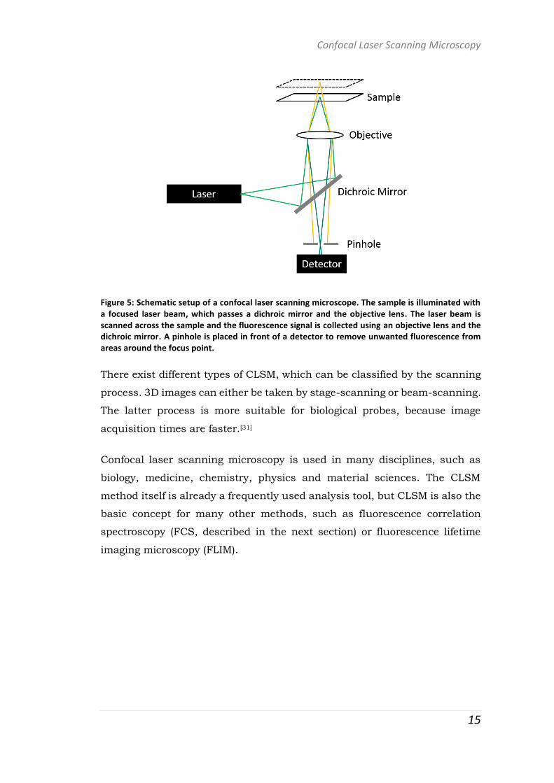
the focal plane. The principle (Figure 5) is based on scanning the sample
point by point using a laser beam that is focused into the sample. The laser
light is scanned across the sample and the fluorescence signal is collected
using the single objective lens. With a lens of 1.4 numerical aperture (NA)
the theoretical lateral resolution is 0.14 µm and the vertical resolution is
0.23 µm.[31] Additionally, a spatial filter (pinhole) is needed to remove
unwanted fluorescence light coming from the background.[31,34] The signal is
detected by a photodetector, like a photomultiplier tube (PMT) or Avalanche
photodiode (APD), behind the pinhole. Only light focused at the pinhole and
therefore coming from the focal plane within the sample is detected. A
stepper motor or piezo-drive is used to go small steps along the z-axis to
obtain three-dimensional information and images.[34]
Confocal Laser Scanning Microscopy
15
Figure 5: Schematic setup of a confocal laser scanning microscope. The sample is illuminated with a focused laser beam, which passes a dichroic mirror and the objective lens. The laser beam is scanned across the sample and the fluorescence signal is collected using an objective lens and the dichroic mirror. A pinhole is placed in front of a detector to remove unwanted fluorescence from areas around the focus point.
There exist different types of CLSM, which can be classified by the scanning
process. 3D images can either be taken by stage-scanning or beam-scanning.
The latter process is more suitable for biological probes, because image
acquisition times are faster.[31]
Confocal laser scanning microscopy is used in many disciplines, such as
biology, medicine, chemistry, physics and material sciences. The CLSM
method itself is already a frequently used analysis tool, but CLSM is also the
basic concept for many other methods, such as fluorescence correlation
spectroscopy (FCS, described in the next section) or fluorescence lifetime
imaging microscopy (FLIM).

Physico-Chemical Concepts and Methods
16
2.5 Fluorescence Correlation Spectroscopy
Fluorescence correlation spectroscopy (FCS) was first introduced by Madge,
Elson and Webb in the 1970s and became more and more interesting for
researchers, especially in the fields of physical chemistry or biophysics.[35–46]
FCS investigates the dynamics of fluorescent or fluorescently labeled
molecules, nanoparticles or macromolecules and is compatible with a variety
of solvents. This allows to study the dynamical behavior of fluorescent
molecules in various environments.[46]
Different from conventional fluorescence spectroscopy studies, the principle
of FCS is based on the small statistical fluctuations of the light intensity of
a fluorescent species diffusing through a very small observation volume.[36]
This observation volume is determined by the focus of a confocal microscope
and typically has a volume of around 1 µm³. The intensity fluctuations are
correlated to analyze the dynamics of the sample system. Therefore, diffusion
coefficients, hydrodynamic radii, aggregation behavior or chemical reactions
can be observed by fluorescence correlation spectroscopy.[38] Due to
fluorescence, this technique is very sensitive, and individual molecules can
be analyzed.[36] FCS also has a high selectivity. Different from dynamic light
scattering techniques, FCS only detects fluorescent probes. So, it is possible
to selectively label single component of the measured system. Another
advantage is the short measurement time, which is usually a few seconds,
enabling the investigation of time-dependent processes.
The FCS setup is based on a confocal microscope as shown in Figure 6. A
laser is used as light source to excite the fluorescent sample. The wavelength
needs to match the excitation wavelength of the fluorescent species.
Commonly used lasers are argon ion lasers or helium-neon lasers. The laser
light passes a dichroic mirror before it is focused by the objective into the
sample. As soon as the fluorescent molecules diffuse inside the observation
volume, they are excited by the laser light and emit light, which passes back

Fluorescence Correlation Spectroscopy
17
through the objective, the dichroic mirror, an emission filter and the pinhole,
before it arrives at the detector. Often Avalanche photodiode (APD) detectors
are used in FCS setups.
Figure 6: Fluorescence correlation spectroscopy (FCS) setup, based on a confocal microscope. A laser is used as light source to excite the fluorescent sample. The laser light passes a dichroic mirror before it is focused by the objective into the sample. Fluorescent molecules are excited by the laser light and emit light, which passes back through the objective, the dichroic mirror, an emission filter and the pinhole, before it arrives at the detector.
Even though many solvents can be used for FCS experiments, mainly
samples are dissolved in aqueous solutions. The ideal concentration of the
fluorescent species is around 10 nM to observe in average one molecule that
is diffusing through the observation volume at a time. The observation
volume Vobs shows a Gaussian profile and can be described by its radial r0
and axial z0 dimensions:[45]
𝑉𝑜𝑏𝑠 = 𝜋32 ∙ 𝑟0
2 ∙ 𝑧0 (5)
The fluorescent molecules diffuse into and out of the observation volume,
because of Brownain motion and cause a variation in the light intensity,
which is detected by the APD. This signal is a time trace as depicted in Figure
7 (left).

Physico-Chemical Concepts and Methods
18
Figure 7: Principle of fluorescence correlation spectroscopy (FCS) measurements: Intensity fluctuations from the excited fluorescent species (left) are transferred into an autocorrelation function (right) and fitted with an appropriate model function to gain information about the diffusion time τD and the number of particles N in the observation volume. Adapted from [44,45].
The fluorescence intensity signal F(t) is fluctuating around a temporal
average:[36,45,46]
𝐹(𝑡) = ⟨𝐹(𝑡)⟩ + 𝛿𝐹(𝑡). (6)
To gain information out of the light intensity fluctuation signal it is necessary
to auto-correlate the signal for any delay time τ*, in order to obtain the
normalized fluctuation autocorrelation function G(τ*) (Figure 7):[36,45,46]
𝐺(𝜏∗) =⟨𝛿𝐹(𝑡)𝛿𝐹(𝑡+𝜏∗)⟩
⟨𝐹(𝑡)⟩2 (7)
To extract parameters as the diffusion coefficient D or the concentration c,
experimental autocorrelation must be fitted with a mathematical model
function. Therefore, the approximation is made for measurements in
solution: the detection volume can be seen as a three-dimensional Gaussian
profile, as described in equation 5. If the fluorescence fluctuations are cause
by only one type of molecules, which is significantly smaller than the
observation volume, and if the molecules are able to diffuse freely in three
dimensions, the autocorrelation function is describes as:[44–46]
𝐺(𝜏∗) = 1 +1
𝑁
1
(1+𝜏∗
𝜏𝐷)
1
√1+𝜏∗
𝑆2𝜏𝐷
(8)

Fluorescence Correlation Spectroscopy
19
The autocorrelation function in three dimensions contains the number of
particles N in the observation volume and the structural parameter S, which
is the ratio of the axial z0 to the radial r0 dimension, describing Vobs.
Equation 8 depends on the diffusion time τD of the fluorescent species, which
is the decay time of the correlation curve. It can be calculated from the
diffusion coefficient D:[44,46]
𝜏𝐷 =𝑟02
4𝐷 (9)
The Stokes-Einstein equation (10) describes the relation between the
hydrodynamic radius RH of the molecule and its diffusion coefficient D taking
the temperature T, the Boltzmann constant k as well as the viscosity of the
solution η into account.
𝑅𝐻 =𝑘𝑇
6𝜋𝜂𝐷 (10)
Fluorescence correlation spectroscopy is frequently used in the study of
nanoparticle systems for drug delivery. Examples of FCS studies in different
cooperation projects are shown in chapter 6 of this thesis.


3 Polymer Gel-Assisted Formation of Giant Unilamellar Vesicles
Every single human being consists of trillions of cells[47] – our smallest living
building units. Even though there exist different types of cells, such as
eukaryotic and prokaryotic cells, they all have a protection against their
direct environment - the cell membrane. This membrane consists of a lipid
double layer, also called bilayer.[48] It consists mostly of phospholipids, which
have an amphiphilic character, and therefore form the characteristic double
layer. In case of eukaryotic cells, the lipid double layer contains other
components, such as proteins or protein channels.[49] Because of the
complexity of cells and cell membranes, it is very important to understand
our smallest building units. Hence, cell membrane model systems are used
in biological, medical or biochemical studies.[49,50] There are different types of
models, for example black lipids membranes, solid supported bilayers or
vesicles.[51–56] Probably the most relevant among these model systems are
giant unilamellar vesicles (GUVs). They resemble the basic structure of all
living cells, mimicking the closed cell membrane.[53,57–61] GUVs and their
preparation are well known, but still the size-controlled formation is missing.
Desirably, hundreds of vesicles with defined diameters can be prepared in
an easy and comparably low-priced way. To address this problem, a polymer
gel-based system was used in this project to create uniform and well-defined
giant unilamellar vesicles.

Polymer Gel-Assisted Formation of Giant Unilamellar Vesicles
22
3.1 Chemical Concepts and Methods
The theoretical concepts of cell membrane models as well as the chemical
background of the polymer hydrogel, used in this work, is explained in this
chapter. Confocal laser scanning microscopy and fluorescence correlation
spectroscopy as the analytical methods of choice for this work, are explained
in section 2.4 and section 2.5.
3.1.1 Giant Unilamellar Vesicles
The word vesicle describes a structure of one or more spherical bilayers that
enclose a small aqueous volume.[57–61] The bilayers consist of amphiphilic
molecules that self-assemble into the vesicle structure. The amphiphiles
contain a hydrophilic part, which is in contact with the aqueous solution,
and a hydrophobic part, which interacts to form the inner part of the
bilayer.[62] In case of vesicles that have lipids as amphiphiles, they are called
liposomes. These lipids are often phospholipids, which have hydrophobic,
non-polar hydrocarbon chains and a hydrophilic, polar phosphate head
group.[49,63]
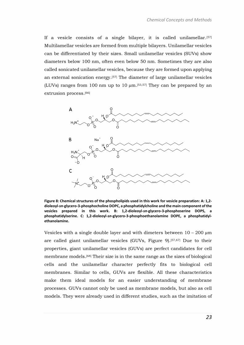
A variety of phospholipids is existing. One prominent example is 1,2-dioleoyl-
sn-glycero-3-phosphocholine (DOPC, Figure 8A) that belongs to the
phosphatidylcholines, a major component of biological cell membranes. This
phospholipid is the main lipid component used for vesicles formation in this
work. Two other phospholipids were also used: 1,2-dioleoyl-sn-glycero-3-
phosphoserine (DOPS, Figure 8B) belongs to the group of
phosphatidylserines, which play an important role in blood coagulation.[64]
1,2-dioleoyl-sn-glycero-3-phosphoethanolamine (DOPE, Figure 8C) is a
phosphatidylethanolamine and can mainly be found in the cytoplasmic side
of the membrane bilayer.[65]
Chemical Concepts and Methods
23
If a vesicle consists of a single bilayer, it is called unilamellar.[57]
Multilamellar vesicles are formed from multiple bilayers. Unilamellar vesicles
can be differentiated by their sizes. Small unilamellar vesicles (SUVs) show
diameters below 100 nm, often even below 50 nm. Sometimes they are also
called sonicated unilamellar vesicles, because they are formed upon applying
an external sonication energy.[57] The diameter of large unilamellar vesicles
(LUVs) ranges from 100 nm up to 10 µm.[53,57] They can be prepared by an
extrusion process.[66]
Figure 8: Chemical structures of the phospholipids used in this work for vesicle preparation: A: 1,2-dioleoyl-sn-glycero-3-phosphocholine DOPC, a phosphatidylcholine and the main component of the vesicles prepared in this work. B: 1,2-dioleoyl-sn-glycero-3-phosphoserine DOPS, a phosphatidylserine. C: 1,2-dioleoyl-sn-glycero-3-phosphoethanolamine DOPE, a phosphatidyl-ethanolamine.
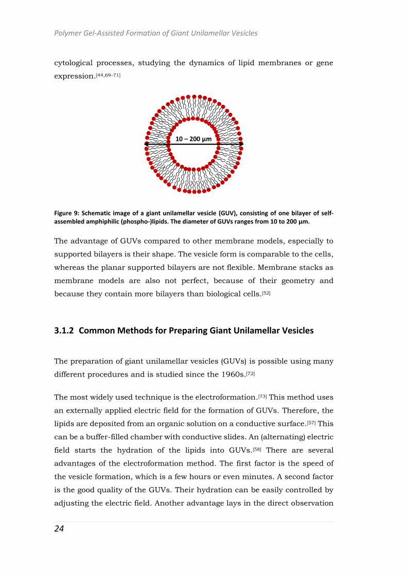
Vesicles with a single double layer and with dimeters between 10 – 200 µm
are called giant unilamellar vesicles (GUVs, Figure 9).[57,67] Due to their
properties, giant unilamellar vesicles (GUVs) are perfect candidates for cell
membrane models.[68] Their size is in the same range as the sizes of biological
cells and the unilamellar character perfectly fits to biological cell
membranes. Similar to cells, GUVs are flexible. All these characteristics
make them ideal models for an easier understanding of membrane
processes. GUVs cannot only be used as membrane models, but also as cell
models. They were already used in different studies, such as the imitation of
Polymer Gel-Assisted Formation of Giant Unilamellar Vesicles
24
cytological processes, studying the dynamics of lipid membranes or gene
expression.[44,69–71]
Figure 9: Schematic image of a giant unilamellar vesicle (GUV), consisting of one bilayer of self-assembled amphiphilic (phospho-)lipids. The diameter of GUVs ranges from 10 to 200 µm.
The advantage of GUVs compared to other membrane models, especially to
supported bilayers is their shape. The vesicle form is comparable to the cells,
whereas the planar supported bilayers are not flexible. Membrane stacks as
membrane models are also not perfect, because of their geometry and
because they contain more bilayers than biological cells.[52]
3.1.2 Common Methods for Preparing Giant Unilamellar Vesicles
The preparation of giant unilamellar vesicles (GUVs) is possible using many
different procedures and is studied since the 1960s.[72]
The most widely used technique is the electroformation.[73] This method uses
an externally applied electric field for the formation of GUVs. Therefore, the
lipids are deposited from an organic solution on a conductive surface.[57] This
can be a buffer-filled chamber with conductive slides. An (alternating) electric
field starts the hydration of the lipids into GUVs.[58] There are several
advantages of the electroformation method. The first factor is the speed of
the vesicle formation, which is a few hours or even minutes. A second factor
is the good quality of the GUVs. Their hydration can be easily controlled by
adjusting the electric field. Another advantage lays in the direct observation

Chemical Concepts and Methods
25
of the formed vesicles under a microscope, if suitable chambers are used in
the process. The reproducibility of the process is high and results in
unilamellar and spherical vesicles.[57,74,75] But there are also disadvantages
in the electroformation technique: For this process a special equipment is
needed. The formation is very sensitive to charged lipids and may not work
if too many charged lipids are present. Furthermore, this procedure forms
interconnected vesicles, which may exchange their lipids with their
neighbors.[57,74] The formation process in shown in Figure 10. The procedure
is also possible without an electric field. In this case, the method is called
gentle hydration. The procedure is similar to electroformation: lipids are
deposited on a solid surface, but here the vesicles form by spontaneous
swelling and not from the influence of an electric field. The addition of water
or solvent to the already pre-organized lipids (into bilayers) results in swelling
of the bilayers. Upon disturbance (e.g. mechanical shaking) parts of the
bilayer release to the bulk solution and self-close.
Figure 10: Scheme of the preparation of giant unilamellar vesicles by lipid film hydration on a solid surface. The process starts from (A) a multilayer stack of lipid bilayers that is (B) hydrated by a solvent and grows (C-E) into (F) a self-closed vesicle. In case of electroformation, the solid surface is conductive and an electric field is applied, whereas the method is called gentle hydration when there is no electric field present. Adapted from [57,59,76].

Polymer Gel-Assisted Formation of Giant Unilamellar Vesicles
26
The advantages of the gentle hydration are the simplicity, because no special
equipment is needed, and the possibility to use charged lipids for the GUV
preparation. Disadvantageously, the formation is difficult to control and
takes a few days.[57,74] Both processes, electroformation and gentle hydration,
are lipid film hydration methods and were optimized and improved in the last
decades. The control of the vesicles’ size is a challenge in lipid film hydration
methods. Tao et al. found a way for preparing GUVs via electroformation with
low polydispersity by adding Ca2+ or CaCO3 to the lipid film surface.[77] But
the presence of these ions or molecules may influence the membrane
behavior.
Another possibility for GUV formation is the fusion or coalescence of small
vesicles. In one method, small vesicles are stored in suspension for several
days to form GUVs.[57,78] The reasons for their coalescence could be the usage
of oppositely charged lipids, the addition of fusogenic peptides or additional
polyethylene glycol (PEG).[79–81] This technique is simple, does not need
special equipment and is free from organic solvents, but the vesicle size and
the lamellarity are not controllable. Furthermore, this method is not suitable
for every type of lipids.
The formation of GUVs is also possible from a micellar lipid solution. In this
process, the lipids are forces into micellar structures due to a high amount
of micelle-forming surfactants, which are present in the lipid solution. When
the surfactant is removed, the micelles form into giant vesicles.[82] This
method is simple and does not require special equipment. But it does not
control of the vesicles’ size and is limited to certain lipids.[57]
3.1.3 Gel-Assisted Formation of Giant Unilamellar Vesicles
Besides the commonly used GUV preparation methods such as
electroformation or gentle hydration, which are performed on a solid surfaces
from lipid bilayers, other methods were established in the last years.

Chemical Concepts and Methods
27
In 2008 Horger et al. improved the gentle hydration technique. They used a
layer of agarose gel on glass to form the vesicles on a gel substrate. For this
process, three steps were relevant. First, a film of an ultralow melting agarose
was deposited on a glass slide. Second, lipids were added to generate an
agarose-lipid hybrid film. And third, the film was hydrated, so vesicles are
forming. This method has many advantages, especially compared to the
gentle formation on solid substrates. With the agarose gel-assisted GUV
formation process, it was possible to work in the presence of physiological
buffer, such as phosphate buffered saline (PBS). The vesicles formed within
minutes in remarkably high yields. Furthermore, no special equipment or an
electric field was needed and no additional pre-hydration step required. This
method works for a variety of lipids and lipid mixtures. Besides all the
advantages of this method, there still remain some problems. The agarose
can dissolve in the aqueous solution and ended up inside in the giant
vesicles. Additionally, this procedure generated unilamellar as well as
multilamellar giant vesicles.[83]
To improve the gel-assisted GUV formation, Weinberger et al. changed the
agarose gel by a fully hydrolyzed high-molecular weight polyvinyl alcohol
(PVA). This polymer was used as a dry but swellable film on a glass substrate.
The lipids for the vesicle formation were spread on this gel surface and
hydrated in an aqueous (buffer) solution. GUVs formed very fast from a film,
which was composed of lipids in the fluid state. From this process, many
unilamellar vesicles can be prepared within two minutes. Small vesicles as
well as large ones can be obtained from (Figure 11). During the growing
process, small vesicles fused into large vesicles.

Polymer Gel-Assisted Formation of Giant Unilamellar Vesicles
28
Figure 11: Confocal laser scanning images (XZ plane) of DOPC-GUVs labeled with 0.5 mol% RhodamineB-PE, grown on unlabeled PVA film. Scale bars are 20 µm. Reprinted from [59].
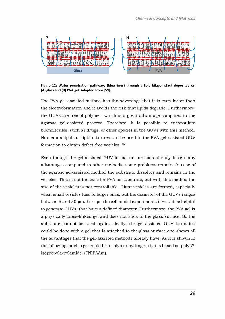
The mechanism of the GUV formation is not fully understood, yet.
Weinberger et al. described the possible pathway for GUV formation on solid
(glass) substrate and gel substrate as the following: The water penetration
on glass into pre-ordered lipid bilayers has two main water transport ways.
On the one hand, water approaches the interlamellar regions from the edges
and swells the bilayer stack. On the other hand, water can permeate the
bilayer directly, because a phospholipid bilayer has a certain water
permeability (Figure 12A). In the case of GUV formation on a gel surface, the
same water transport modes occur, but there is an additional pathway from
the gel side. The PVA gel takes up water and creates a chemical potential
gradient between the dry gel and the outer region. This circumstance drives
water across the membrane stack (Figure 12B).[59]
Chemical Concepts and Methods
29
Figure 12: Water penetration pathways (blue lines) through a lipid bilayer stack deposited on (A) glass and (B) PVA gel. Adapted from [59].
The PVA gel-assisted method has the advantage that it is even faster than
the electroformation and it avoids the risk that lipids degrade. Furthermore,
the GUVs are free of polymer, which is a great advantage compared to the
agarose gel-assisted process. Therefore, it is possible to encapsulate
biomolecules, such as drugs, or other species in the GUVs with this method.
Numerous lipids or lipid mixtures can be used in the PVA gel-assisted GUV
formation to obtain defect-free vesicles.[59]
Even though the gel-assisted GUV formation methods already have many
advantages compared to other methods, some problems remain. In case of
the agarose gel-assisted method the substrate dissolves and remains in the
vesicles. This is not the case for PVA as substrate, but with this method the
size of the vesicles is not controllable. Giant vesicles are formed, especially
when small vesicles fuse to larger ones, but the diameter of the GUVs ranges
between 5 and 50 µm. For specific cell model experiments it would be helpful
to generate GUVs, that have a defined diameter. Furthermore, the PVA gel is
a physically cross-linked gel and does not stick to the glass surface. So the
substrate cannot be used again. Ideally, the gel-assisted GUV formation
could be done with a gel that is attached to the glass surface and shows all
the advantages that the gel-assisted methods already have. As it is shown in
the following, such a gel could be a polymer hydrogel, that is based on poly(N-
isopropylacrylamide) (PNIPAAm).

Polymer Gel-Assisted Formation of Giant Unilamellar Vesicles
30
3.1.4 Poly(N-isopropylacrylamide)
Poly(N-isopropylacrylamide), or short PNIPAAm, is one of the most widely
used and known thermos-responsive polymers. Research on PNIPAAm deals
with its solution properties, phase transitions or functionalization and its
applications.[84–87] A simple search for this polymer in the chemical reaction
database SciFinder results in 14687 references containing poly(N-
isopropylacrylamide) (status January 18, 2018). Many research areas are
interested in the molecule, so the studies and publications about PNIPAAm
increased in the last decades, as summarized in Figure 13.
Figure 13: Number of references found for poly(N-isopropylacryamide) on the database SciFinder for the decades from 1950 until today, increasing exponentially (y-axis in logarithmic scale). The chemical structure of PNIPAAm is presented within the graphics.
To understand why PNIPAAm is so interesting, it is necessary to take a look
at its chemical structure (Figure 13). PNIPAAm is a polymer that is composed
of the monomer unit N-isopropylacrylamide (NIPAAm), which is an N-
substituted acrylamide with an isopropyl group at its nitrogen atom.
PNIPAAm is a hydrophilic polymer with a special property. It has a transition
temperature close to the physiological temperature. The structure of
PNIPAAm in aqueous solutions changes rapidly from a more hydrophilic to
a more hydrophobic behavior between 30 and 35°C, which defines its lower
Chemical Concepts and Methods
31
critical solution temperature (LCST).[86–89] In this transition, the hydrophobic
isopropyl groups of the polymer and their local environment play the most
important role. In water or other aqueous solutions, which are able to form
strong hydrogen bonds, PNIPAAm is soluble. Temperature dependent
interactions between the polymer and the solvent arise because of changes
in the local environment around the hydrophobic isopropyl domains. Below
the LCST, only water molecules surround the isopropyl groups, building
hydrogen bonds, whereas above the LCST the isopropyl groups interact with
the water molecules and with the polymer chain segments. Hence, above
35°C the hydrogen bonds are repealed and PNIPAAm phase separates and
precipitates. PNIPAAm is a thermo-responsive polymer that shows inverse
solubility upon heating.[86–89]
Poly(N-isopropylacrylamide) is known since the 1950s, when its monomer
unit N-isopropylacrylamide (NIPAAm) was first synthesized and
polymerized.[87,90] PNIPAAm can be synthesized by various methods, but the
most widely used synthesis procedure is free radical polymerization.[87] In
this procedure, the monomer NIPAAm is dissolved in an organic solvent and
the reaction is started with an initiator molecule upon heating. Here, the
initiation reaction generates free radicals, which are the active center from
which the polymer chain is growing (propagation) by adding one monomer
after the other to the radical chain. The polymer chains do not start
simultaneously. The growing of the polymer chains can be stopped by
recombination, disproportionation or conversion.[91]
The thermo-responsive PNIPAAm is of high interest for many research areas
and a variety of applications. Depending on the architecture of the polymer,
different studies have been published. If PNIPAAm is used as a solid it can
be coated onto glass surfaces, which should then absorb and release water
vapor as humidity sensors or for use in greenhouses.[87] In the biological field,
PNIPAAm chains in solution could be used as immunoassay technology
because of its thermos-responsive behavior in the physiological temperature
regime.[92] The combination of PNIPAAm and polystyrene (PS) can give a fully
reversible thermo-responsive block copolymer membrane.[93] Furthermore,
Polymer Gel-Assisted Formation of Giant Unilamellar Vesicles
32
PNIPAAm can also occur in a micellar form. Together with polylactic acid
PNIPAAm can control drug delivery from core-shell nano-sized micelles.[94]
As already mentioned in some of the application examples, the thermo-
responsive property of PNIPAAm is often combined with the properties of
another polymer unit. Hence, it is possible to combine two or more polymers
to a copolymer. This can be a block copolymer, a grafted polymer or a
statistical copolymer. One interesting candidate is a PNIPAAm-based
terpolymer (polymerized from three different monomers), which is already
used for a few years in different studies.[95,96] It is a statistical copolymer and
the main part of this terpolymer is NIPAAm, to retain the temperature-
responsive solubility behavior. The second monomer is methacrylic acid
(MAA). This ionizable function is needed for a higher hydrophilicity. The polar
MAA groups increase the swelling ratio and ensure a homogeneous swelling
behavior.[95] The third part in the terpolymer is the hydrophobic molecule 4-
methacryloyloxybenzophenone (MABP). The benzophenone group is needed
to cross-link the terpolymer. MABP is photo-reactive, so aliphatic groups
from the polymer chain react with the benzophenone moieties under UV
(365 nm) irradiation.
Figure 14 shows the cross-linking mechanism: Through UV irradiation a
photon absorbs and promotes one electron on the oxygen from a nonbonding
sp²-like n-orbital to the antibonding π*-orbital of the carbonyl. The n-orbital
on the oxygen is electron-deficient and interacts with the weak C-H σ-bonds.
This results in hydrogen abstraction. The two new radicals rapidly recombine
and form a new C-C bond and cross-link the two polymer chains.[97]

Chemical Concepts and Methods
33
Figure 14: Photochemical cross-linking mechanism of benzophenone units by UV irradiation with 365 nm. UV light promotes one electron on the oxygen from a nonbonding sp²-like n-orbital to the antibonding π*-orbital of the carbonyl. The n-orbital on the oxygen interacts with the weak C-H σ-bonds, resulting in hydrogen abstraction. The two new radicals rapidly recombine and form a new C-C bond and cross-link the two polymer chains. Adapted from [97,98].
Once the terpolymer is irradiated with UV light, the benzophenone units of
the MABP moiety react with the aliphatic groups and form a chemically
cross-linked polymer network. This network can absorb a high amount of
water by swelling into a hydrogel. Hydrogels are defined as materials that
have the ability to swell in water and keep a high amount of water within
their network structure due to the presence of high amounts of hydrophilic
groups in the structure.[99] The PNIPAAm terpolymer has exactly this
behavior. The network structure arises from the cross-linked benzophenone
groups and the NIPAAm groups as well as the MAA groups are hydrophilic
to retain the water inside the polymer. PNIPAAm hydrogels and many other
hydrogels are often used in biomedical applications or bioscience studies,
because their high water content leads to a good biocompatibility.[100–103]
Polymer Gel-Assisted Formation of Giant Unilamellar Vesicles
34
3.2 Experiments und Materials
In this section, the chemicals and materials as well as the analytical setups
that were used for this work are summarized. Furthermore, the chemical
reactions and the experiments with all important parameters are described
in detail.
3.2.1 Materials
4-Hydroxybenzophenone (98 %), anhydrous dichloromethane (DCM,
≥ 99.8 %), methacryloyl chloride (≥ 97 %), trimethylamine (TEA, ≥ 99 %),
diethyl ether (≥ 99.7 %), sodium sulfate (Na2SO4, ≥ 99 %), anhydrous hexane
(99 %), azobisisobutyronitrile (AIBN, 98 %) and anhydrous 1,4-dioxane
(99.8 %) were purchased from Sigma-Aldrich and used as received. Ethanol
(≥ 99.8 %) was purchased from VWR Chemicals and chloroform (≥ 99 %)
from Acros Organics. Methanol (≥ 99.8 %) was purchased from Alfa Aesar.
All solvents were used as received. Phosphate buffered saline (PBS), N-
isopropylacrylamide (NIPAAm) and methacrylic acid (MAA) were purchased
from Sigma-Aldrich. PBS was received as powder and dissolved in deionized
water to obtain a 0.01 M solution with a pH of 7.4. N-isopropylacrylamide
(NIPAAm) was recrystallized from toluene/hexane 1:1 and MAA was
distillated before use. Phospholipids were purchased from Sigma-Aldrich as
powders. 1,2-dioleoyl-sn-glycero-3-phosphocholine (DOPC) and 1,2-dioleoyl-
sn-glycero-3-phosphoserine (DOPS) were dissolved in chloroform (c = 1 g/L).
As fluorescent markers Atto488- and Atto633-labeled 1,2-dioleoyl-sn-
glycero-3-phosphoethanolamine (Atto488-DOPE and Atto633-DOPE) were
used and dissolved in DCM and methanol 4:1 (c = 1 g/L). Erythrosine was
purchased from Sigma-Aldrich as a powder and diluted in PBS to a
concentration of 50 µM. The synthesis of benzophenone triethoxysilane was
performed by G. Kircher (MPI-P) according to the literature.[98]

Experiments und Materials
35
3.2.2 4-Methacryloyloxybenzophenone (MABP)
10 g (50 mmol) of 4-hydroxybenzophenone were dissolved in 100 mL of DCM,
the mixture was cooled in an ice bath and a solution of 5.1 mL (53 mmol) of
methacryloyl chloride and 7.7 mL (56 mmol) of TEA in 20 mL of dry DCM
were added dropwise. The reaction was stirred at room temperature for 4 h.
The solvent was evaporated and the residue was dissolved in diethyl ether.
The non-soluble triethylammonium salt was removed by filtration. The
organic phase was washed with water three times and afterwards dried over
Na2SO4. The solvent was evaporated and the crude product was
chromatographed over DCM/hexane 7:3. The product was recrystallized
from a mixture of DCM and hexane (1:4).
1H NMR (CDCl3, δ): 2.01 (3 H, s), 5.74 (1 H, q), 6.32 (1 H, t), 7.15–7.22 (2 H,
m), 7.37–7.48 (2 H, m), 7.48–7.57 (1 H, m), 7.69–7.76 (2 H, m), 7.76– 7.85
(2 H, m).
3.2.3 Functionalization of the Glass Substrates
Round microscope cover slides (diameter: 25 mm, thickness: 160 µm) were
used as substrates for the polymer films. The glass slides were cleaned in an
ultrasound bath, 4x 15 min (i) in a 2 vol% Hellmanex solution (Hellmanex®
II, Hellma GmbH, Müllheim), (ii) in ultrapure water (Milli-Q water,
18.2 MΩ·cm) and (iii) 2x in ethanol. Afterwards the glass slides were stored
for at least 24 h in a 6 % solution of benzophenone triethoxysilane in ethanol
under argon in the dark. Finally, the slides were washed with ethanol and
dried under vacuum for 1 h at 50 °C.
3.2.4 Poly(N-isopropylacrylamide) Based Terpolymer
10 g (88 mmol) NIPAAm, 380 mg (0.37 mL, 4.4 mmol) MAA and 235 mg
(0.88 mmol) MABP were dissolved in 68 mL dioxane. Argon was flown

Polymer Gel-Assisted Formation of Giant Unilamellar Vesicles
36
through the solution for 1 h. 67 mg (0.41 mmol) AIBN were added to the
solution and the reaction was stirred at 60 °C under argon for 48 h. For
purification, the reaction solvent was evaporated and the product
precipitated from methanol in ice cold diethyl ether. The molecular weight of
the product was Mw = 221 kg/mol and the polydispersity index is PDI = 1.55,
as obtained from gel permeation chromatography.
3.2.5 Preparation of the Polymer Template
Polymer films were prepared from a 10 wt% PNIPAAm terpolymer solution in
ethanol. The solution was spin-coated at room temperature onto the pre-
functionalized round microscope glass substrates at a spinning speed of
2500 rpm for 30 s. After spin-coating the samples were solvent vapor
annealed for 1 h in ethanol vapor and afterwards temperature annealed for
1 h at 170 °C in vacuum. Then, the samples were dried for 24 h at 50 °C
under vacuum. The polymer was cross-linked and anchored to the glass
substrate by irradiation with UV light (365 nm), using an LED (LCS-0365-
02-22 High-Power LED Collimator Source, 365nm, 13W, 22mm aperture,
Type-B). The distance between the light source and the sample was always
kept to 13 cm. To homogenize the light, a glass diffuser (DGUV10-1500,
Thorlabs, Newtown, USA) and a 12 cm tube were mounted between the
LED and the sample holder. With this setup, 1 min illumination time
corresponds to an energy dose of 1.68 J/cm² at the sample position.
For micro-patterning different photolithography masks (Table 2) with
appropriate structure were positioned onto the samples.
The total irradiation energy dose for the cross-linking was 4.2 J/cm²,
0.28 J/cm² without and 3.92 J/cm² with photolithography mask.
Subsequently, the samples were rinsed with pure ethanol and dried at 50 °C
for 1 h under vacuum.

Experiments und Materials
37
3.2.6 Giant Unilamellar Anchored Vesicle (GUAV) Formation
Lipid solutions were stored at -20 °C before use. The final lipid solution for
GUV formation was prepared from DOPC solution with 20 % DOPS and
0.5 % Atto488-DOPE. 30 µL of the lipid solution were added to the polymer
sample. After evaporation of chloroform, 600 µL PBS were used to grow
GUVs.
3.2.7 Confocal Laser Scanning Microscopy
Confocal laser scanning microscopy CLSM experiments were performed with
a commercial setup (Carl Zeiss, Jena), consisting of an inverted microscope
model Axiovert 200, the module LSM510 and a Zeiss C-Apochromat
40×/1.2 W water immersion objective. The Atto488-labelded lipids were
excited with an argon ion laser with a wavelength of 488 nm. The samples
were measured in Attofluor cell chambers at room temperature.
3.2.8 Determination of the Lipids Diffusion Coefficient via FCS
To the mixture of phospholipids for the GUAV formation 0.05 % Atto633-
DOPE were added and the GUAVs were prepared as describes before. FCS
experiments were performed on an LSM 880 (Carl Zeiss, Jena, Germany)
setup. Excitation laser light was focused on the samples using a Zeiss C-
Apochromat 40×/1.2 W water immersion objective. Emission was collected
with the same objective and, after passing through a confocal pinhole,
directed to a spectral detection unit (Quasar, Carl Zeiss). In this unit,
emission is spectrally separated by a grating element on a 32 channel array
of GaAsP detectors operating in a single photon counting mode. A HeNe laser
( = 633 nm) was used for excitation of Atto633-labeled lipids and emission
in the range from 650 to 696 nm was detected. An AttoFluor metal chamber
was used as a sample cell. For each sample, 10 measurements (30 seconds
Polymer Gel-Assisted Formation of Giant Unilamellar Vesicles
38
each) were performed. Obtained experimental autocorrelation curves were
fitted with a theoretical 2D model function.[44]
3.2.9 Photo-Oxidation
For imaging an LSM 880 confocal laser scanning microscope (Carl Zeiss,
Jena, Germany) was used. Atto488-DOPE lipids were excited by an argon
ion laser with a wavelength of 488 nm. Excitation laser light was focused on
the sample using a Zeiss C-Apochromat 40×/1.2 W water immersion
objective. Emission light was collected with the same objective and, after
passing through a confocal pinhole, directed to a spectral detection unit
(Quasar, Carl Zeiss). In this unit, emission is spectrally separated by a
grating element on a 32 channel array of GaAsP detectors operating in a
single photon counting mode. For irradiation of the photo-oxidizer
erythrosine a mercury lamp (HXP 120 C, FSet43wf) was used. Image
analyzation was performed with the software ImageJ.
3.3 Results and Discussion
As explained above, the gel-assisted formation of giant unilamellar vesicles
(GUVs) is a new, promising method that offers numerous advantages
compared to classical methods. It is faster than the most widely used
methods, such as electroformation, and does not require special and
expensive equipment. Furthermore, a variety of different lipids can be
processed to defect-free GUVs. The vesicles are free of gel polymer molecules,
while various biomolecules can be purposefully encapsulated. However, this
method has two main disadvantages: (i) the physical polymer gel is not
permanently attached to the glass substrate and thus can be only used once
and (ii) the formed GUVs are polydisperse, their size can not be controlled or
tuned. The following section describes a PNIAAm-based hydrogel system that
overcomes both disadvantages and can be used for the preparation of
uniform giant unilamellar vesicles with pre-defined size.
3.3.1 Preparation of Flat PNIPAAm Terpolymer Films
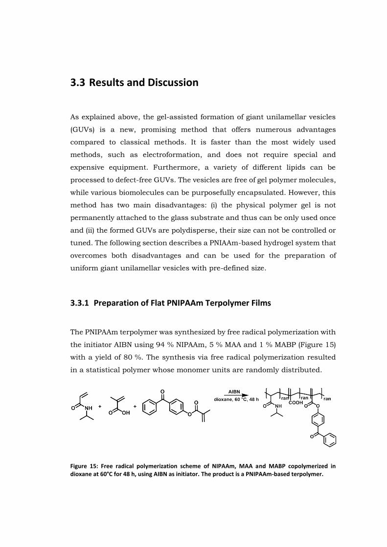
The PNIPAAm terpolymer was synthesized by free radical polymerization with
the initiator AIBN using 94 % NIPAAm, 5 % MAA and 1 % MABP (Figure 15)
with a yield of 80 %. The synthesis via free radical polymerization resulted
in a statistical polymer whose monomer units are randomly distributed.
Figure 15: Free radical polymerization scheme of NIPAAm, MAA and MABP copolymerized in dioxane at 60°C for 48 h, using AIBN as initiator. The product is a PNIPAAm-based terpolymer.

Polymer Gel-Assisted Formation of Giant Unilamellar Vesicles
40
The amount of the cross-linking unit MABP is only 1 %, meaning that the
molecular weight of the final polymer needed to be higher than 113 kg/mol
to ensure that at least ten cross-linking units were present in each polymer
chain to obtain a sufficient network as soon as the polymer was cross-linked.
The polymer was synthesized with Mw = 221 kg/mol and a polydispersity
index PDI of 1.55. This molecular weight was high enough to build a
sufficient network after cross-linking, because statistically around 20 cross-
linking units are present in each polymer chain.
This work was based on the previously published gel-assisted methods for
giant vesicle formation and had the goal to improve them.[59,83] These
methods were based on gel-films on glass substrate. In this work, the
PNIPAAm terpolymer was spin-coated from a 10 wt% solution in ethanol on
glass substrates to gain a polymer film with a thickness of about 1 µm.
In contrast to the existing gel-assisted methods, the PNIPAAm hydrogel was
anchored to the supporting glass substrate. To this end, the glass substrates
were functionalized before usage. The functionalization was needed to
covalently bind the polymer chains to the functional groups on the glass
support upon UV irradiation.[104,105] The glass surface was coated with
benzophenone units, which react with the polymer chains trough UV light
activation as described in section 3.1.4. The glass surface was covered with
a benzophenone-functionalized silane through self-assembly, resulting in
replacement of the alkoxy groups of the silane by the hydroxyl groups of the
glass, forming covalent Si-O-Si bonds.[98] This process was easily done by
placing cleaned glass substrates in an ethanolic solution of benzophenone
silane. Numerous glass substrates were functionalized in one step.
After spin-coating the PNIPAAm films to the functionalized glass substrates,
one more step was required: solvent vapor annealing. Laying the sample in
a closed chamber with ethanol vapor, resulted in partial re-solubilization of
the film and flattening of the surface. The solvent vapor annealing process
was of high importance to reduce the roughness and to gain a flat film
surface, because it was necessary for the subsequent procedure: The UV
light in the cross-linking step should arrive perpendicular to the film surface
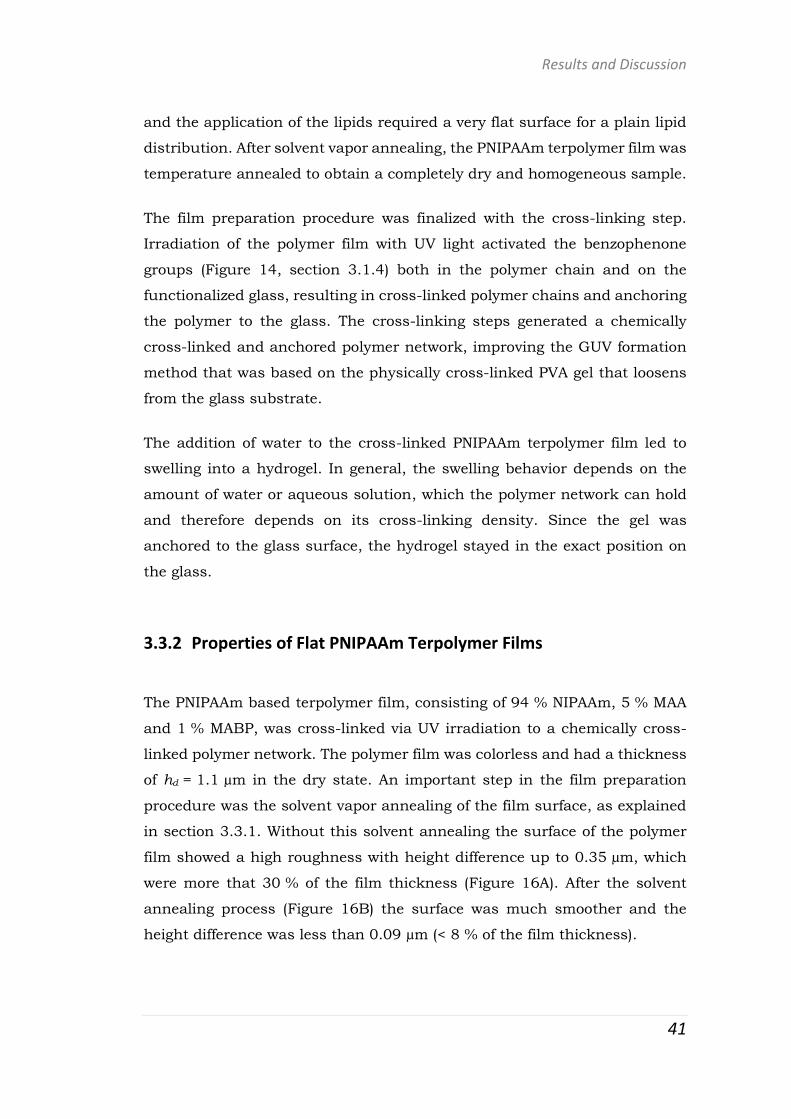
Results and Discussion
41
and the application of the lipids required a very flat surface for a plain lipid
distribution. After solvent vapor annealing, the PNIPAAm terpolymer film was
temperature annealed to obtain a completely dry and homogeneous sample.
The film preparation procedure was finalized with the cross-linking step.
Irradiation of the polymer film with UV light activated the benzophenone
groups (Figure 14, section 3.1.4) both in the polymer chain and on the
functionalized glass, resulting in cross-linked polymer chains and anchoring
the polymer to the glass. The cross-linking steps generated a chemically
cross-linked and anchored polymer network, improving the GUV formation
method that was based on the physically cross-linked PVA gel that loosens
from the glass substrate.
The addition of water to the cross-linked PNIPAAm terpolymer film led to
swelling into a hydrogel. In general, the swelling behavior depends on the
amount of water or aqueous solution, which the polymer network can hold
and therefore depends on its cross-linking density. Since the gel was
anchored to the glass surface, the hydrogel stayed in the exact position on
the glass.
3.3.2 Properties of Flat PNIPAAm Terpolymer Films
The PNIPAAm based terpolymer film, consisting of 94 % NIPAAm, 5 % MAA
and 1 % MABP, was cross-linked via UV irradiation to a chemically cross-
linked polymer network. The polymer film was colorless and had a thickness
of hd = 1.1 µm in the dry state. An important step in the film preparation
procedure was the solvent vapor annealing of the film surface, as explained
in section 3.3.1. Without this solvent annealing the surface of the polymer
film showed a high roughness with height difference up to 0.35 µm, which
were more that 30 % of the film thickness (Figure 16A). After the solvent
annealing process (Figure 16B) the surface was much smoother and the
height difference was less than 0.09 µm (< 8 % of the film thickness).

Polymer Gel-Assisted Formation of Giant Unilamellar Vesicles
42
Figure 16: Surfaces of PNIPAAm terpolymer films, prepared (A) without and (B) with solvent vapor annealing. Images (320x320 µm) were taken with a white light confocal microscope based profilometer (NanoFocus®, µSurf®, NanoFocus AG, Oberhausen).
By the addition of water or aqueous solutions to the polymer film, the system
swells into a hydrogel and absorbs the added water inside the polymer chain
network, whereas the whole network extends (Figure 17).
Figure 17: Swelling scheme. The dry terpolymer film with a thickness hd was anchored to the glass substrate and swelled into a hydrogel upon addition of water. The polymer chains extended to absorb the water inside the network with the thickness hs of the swollen polymer film.
Since the polymer is cross-linked to the glass substrate, the dry film as well
as the hydrogel were anchored to the glass. Therefore, the swelling process
was mainly in one direction: vertically upwards. On the bottom the gel
swelling was hindered by the glass. In the horizontal direction the swelling
was hindered, because the polymer chains are fixed to the glass and the gel
can only extend little. The anchored parts of the polymer confined it in the
swelling process.
The energy dose that was used to cross-link the polymer can vary, resulting
in different cross-linking degrees and therefore in different swelling behavior

Results and Discussion
43
of the hydrogel. The less the polymer chains were cross-linked (low energy
dose), the weaker was the network, the more the gel could swell. The
thickness of the swollen polymer hs was determined by z-scans performed on
a confocal microscope (LSM510, Zeiss, Jena) in the fluorescence mode.
Therefore, the fluorescent tracer dye Rhodamine 6G was added to the
hydrogel. This weakly hydrophobic dye interacted with the hydrophobic
segments on the polymer chains of the hydrogel and partitions more into the
gel than in the supernatant water above it.[96] By z-scanning from the glass
surface through the gel, into the supernatant aqueous solution, there was a
visible difference in fluorescence intensity and the thickness hs of the gel
could be determined. The ratio between the thickness hs in the swollen state
and the thickness in the dry state hd is defined as the swelling ratio Rs. The
polymer films were cross-linked with various energy doses to obtain different
swelling ratios (Figure 18). The minimum energy dose ν that was needed for
this polymer to anchor it to the glass and to create a chemically cross-linked
network was ν ≈ 0.2 J/cm². In this case, the hydrogel was weakly cross-
linked and it is not possible to determine the hydrogel thickness, because
the Rhodamine 6G concentration difference between the gel and the
supernatant was not observable anymore. But, it is proved that the polymer
was cross-linked, because it was already attached to the glass and could not
be removed by rinsing with ethanol, which would be the case for non-cross-
linked polymer. And if this low energy dose activated the benzophenone units
on the glass surface it also activated the benzophenone units in the polymer.
Below the energy dose of ν ≈ 0.2 J/cm² the polymer was completely removed
from the glass by rinsing with ethanol. The lowest swelling ratio for this
terpolymer hydrogel is 2.4. It needed an energy dose of ν ≈ 84.6 J/cm². In
this state, the polymer network was as dense as possible.

Polymer Gel-Assisted Formation of Giant Unilamellar Vesicles
44
Figure 18: Swelling ratios Rs for flat PNIPAAm terpolymer hydrogel films at different cross-linking energy doses ν. Below 5 J/cm² a linear dependency was observed, caused by a fast consumption of benzophenone units and efficient cross-linking. Above 5 J/cm² less benzophenone units remained for cross-linking and further cross-linking was less efficient.
In the low energy range (ν < 5 J/cm²) was a linear dependency of the swelling
ratio on the energy dose, caused by a fast consumption of benzophenone
units and efficient cross-linking. This linear dependency in the lower energy
regime was also described in the literature.[106] In the higher energy range
(ν > 5 J/cm²), less benzophenone units remained for cross-linking, resulting
in slower and less efficient further cross-linking.
Table 1 summarizes the energy dose that was used for cross-linking and the
resulting swelling ratios and polymer volume fractions (φ = 1/Rs) of the
PNIPAAm terpolymer films.

Results and Discussion
45
Table 1: Energy doses ν, that were used for the cross-linking of PNIPAAm terpolymer films, resulting swelling ratios Rs and polymer volume fractions φ.
Energy dose ν [J/cm²] Swelling ratio Rs Polymer volume fraction φ
1.7 10.6 0.09
2.5 8.3 0.12
4.2 5.9 0.17
8.4 4.3 0.23
16.8 3.7 0.27
25.2 3.5 0.29
50.4 3.0 0.33
84.6 2.4 0.42
With the PNIPAAm based terpolymer hydrogel there was already a huge
variety in the swelling behavior. It was tuned by adjusting the energy that
was used in the cross-linking step. To change the cross-linking density even
more, another possibility could be to polymerize more benzophenone units
into the terpolymer. The more cross-linking units are present, the denser the
network would be. This was not necessary for this work, so no further studies
were performed in this direction, but it is a possibility for other purposes.
3.3.3 GUV Formation on Flat PNIPAAm Terpolymer Films
For the preparation of giant unilamellar vesicles via a gel-assisted method, a
solution of lipids was essential. Within this work the main lipid component
was 1,2-dioleoyl-sn-glycero-3-phosphocholine (DOPC, see Figure 8A). The
second lipid type that was used in this work is 1,2-dioleoyl-sn-glycero-3-
phosphoserine (DOPS, see Figure 8B). These types of lipids were used,
because they are major components of biological cell membranes. To make
the lipids and GUVs visible for confocal laser scanning microscopy (CLSM),
a third kind of lipids was added – an Atto488-labeled 1,2-dioleoyl-sn-glycero-
3-phosphoethanolamine (Atto488-DOPE). This is a commercially available
labeled lipid and perfectly suitable for CLSM imaging. The lipids were used
from a chloroform solution with 80 % DOPC and 20 % DOPS. The amount of
labeled lipids was 0.5 %.
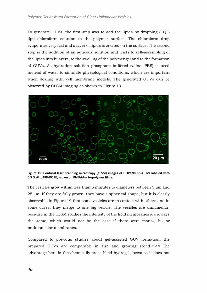
Polymer Gel-Assisted Formation of Giant Unilamellar Vesicles
46
To generate GUVs, the first step was to add the lipids by dropping 30 µL
lipid-chloroform solution to the polymer surface. The chloroform drop
evaporates very fast and a layer of lipids is created on the surface. The second
step is the addition of an aqueous solution and leads to self-assembling of
the lipids into bilayers, to the swelling of the polymer gel and to the formation
of GUVs. As hydration solution phosphate buffered saline (PBS) is used
instead of water to simulate physiological conditions, which are important
when dealing with cell membrane models. The generated GUVs can be
observed by CLSM imaging as shown in Figure 19.
Figure 19: Confocal laser scanning microscopy (CLSM) images of DOPC/DOPS-GUVs labeled with 0.5 % Atto488-DOPE, grown on PNIPAAm terpolymer films.
The vesicles grow within less than 5 minutes to diameters between 5 µm and
25 µm. If they are fully grown, they have a spherical shape, but it is clearly
observable in Figure 19 that some vesicles are in contact with others and in
some cases, they merge to one big vesicle. The vesicles are unilamellar,
because in the CLSM studies the intensity of the lipid membranes are always
the same, which would not be the case if there were mono-, bi- or
multilamellar membranes.
Compared to previous studies about gel-assisted GUV formation, the
prepared GUVs are comparable in size and growing speed.[59,83] The
advantage here is the chemically cross-liked hydrogel, because it does not
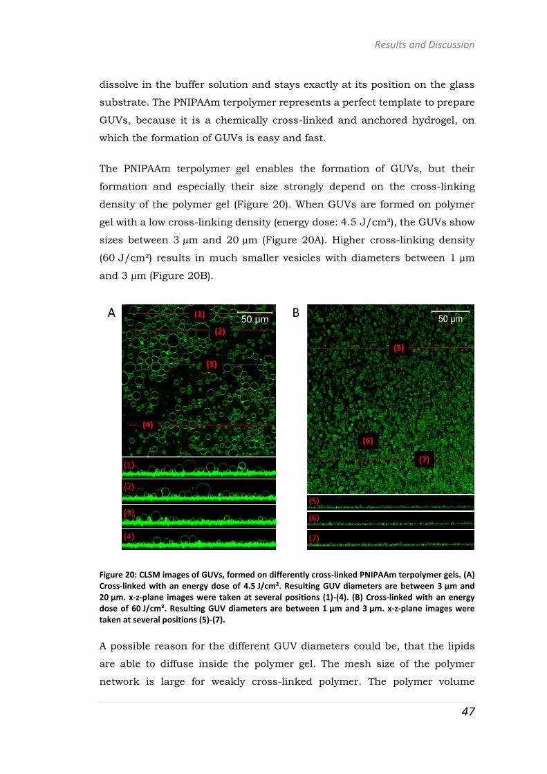
Results and Discussion
47
dissolve in the buffer solution and stays exactly at its position on the glass
substrate. The PNIPAAm terpolymer represents a perfect template to prepare
GUVs, because it is a chemically cross-linked and anchored hydrogel, on
which the formation of GUVs is easy and fast.
The PNIPAAm terpolymer gel enables the formation of GUVs, but their
formation and especially their size strongly depend on the cross-linking
density of the polymer gel (Figure 20). When GUVs are formed on polymer
gel with a low cross-linking density (energy dose: 4.5 J/cm²), the GUVs show
sizes between 3 µm and 20 µm (Figure 20A). Higher cross-linking density
(60 J/cm²) results in much smaller vesicles with diameters between 1 µm
and 3 µm (Figure 20B).
Figure 20: CLSM images of GUVs, formed on differently cross-linked PNIPAAm terpolymer gels. (A) Cross-linked with an energy dose of 4.5 J/cm². Resulting GUV diameters are between 3 µm and 20 µm. x-z-plane images were taken at several positions (1)-(4). (B) Cross-linked with an energy dose of 60 J/cm². Resulting GUV diameters are between 1 µm and 3 µm. x-z-plane images were taken at several positions (5)-(7).
A possible reason for the different GUV diameters could be, that the lipids
are able to diffuse inside the polymer gel. The mesh size of the polymer
network is large for weakly cross-linked polymer. The polymer volume

Polymer Gel-Assisted Formation of Giant Unilamellar Vesicles
48
fraction is around 10 % for the sample from Figure 20A, so the amount of
aqueous solution is very high and the network very wide. Hence, the lipids
have enough space to diffuse into the gel. The less lipids remain on the
polymer surface, the less material remains for the vesicle formation, so the
vesicles grow larger. The lipids inside the gel are also the reason why the
polymer gel looks green in x-z-CLSM images. The polymer is not labeled, but
the lipids are and they are inside the polymer gel.
3.3.4 Preparation of Patterned PNIPAAm Terpolymer Films
As already discussed, the PNIPAAm-based method to prepare GUVs is very
successful and exhibits advantages to other methods. The aim of this work
was the size-defined formation of GUVs. If GUVs are used as cell membrane
models, it would be very advantageously if the size of the vesicles can be
defined during the preparation process. This could be achieved by growing
the vesicles on a patterned polymer gel.
Therefore, the PNIPAAm terpolymer film is prepared as described in section
3.3.1: a thin film is generated by spin-coating an ethanolic PNIPAAm
terpolymer solution on a functionalized glass substrate. The difference lies
in the cross-linking step. A pattern is generated on the polymer film by micro-
patterning via structured illumination with a photolithography mask. For
this procedure the before mentioned solvent annealing step is even more
important. Because for the photolithography, the mask is laying directly on
the polymer surface. It is important that the film is completely flat, so that
the photolithography mask is in full contact with the polymer. Only if this is
the case, the UV light illuminates only the parts of the film, which are not
covered by the mask.
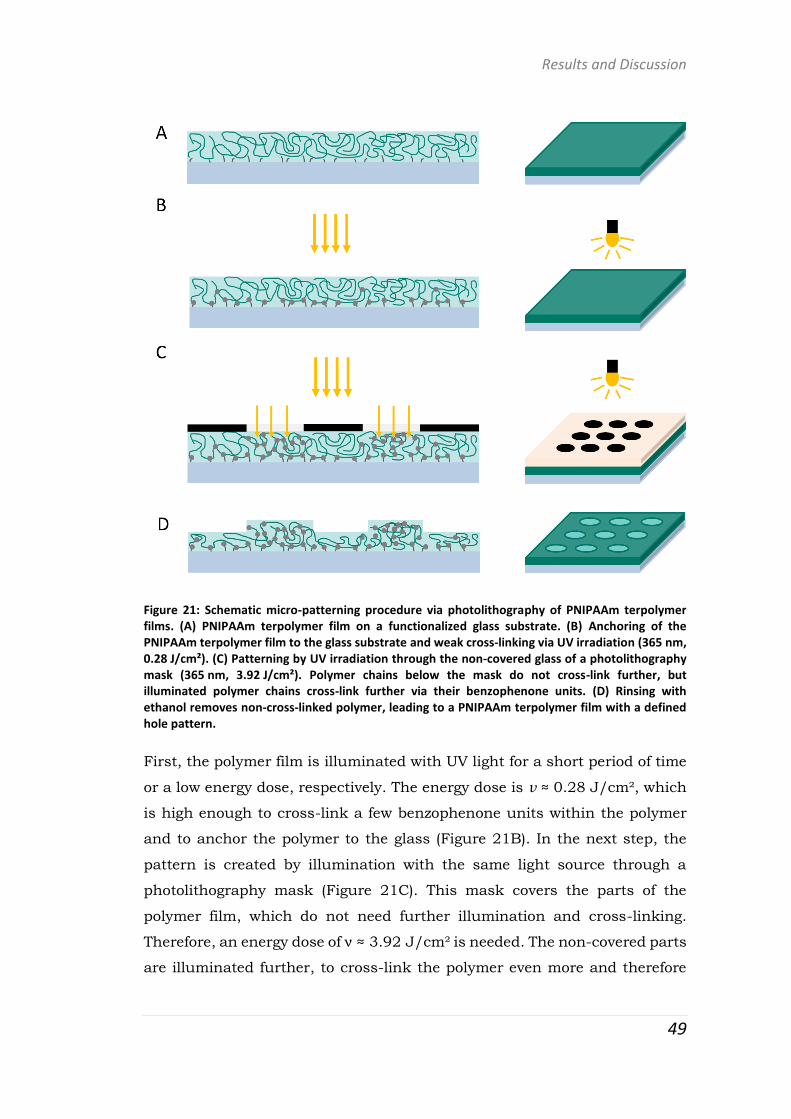
Results and Discussion
49
Figure 21: Schematic micro-patterning procedure via photolithography of PNIPAAm terpolymer films. (A) PNIPAAm terpolymer film on a functionalized glass substrate. (B) Anchoring of the PNIPAAm terpolymer film to the glass substrate and weak cross-linking via UV irradiation (365 nm, 0.28 J/cm²). (C) Patterning by UV irradiation through the non-covered glass of a photolithography mask (365 nm, 3.92 J/cm²). Polymer chains below the mask do not cross-link further, but illuminated polymer chains cross-link further via their benzophenone units. (D) Rinsing with ethanol removes non-cross-linked polymer, leading to a PNIPAAm terpolymer film with a defined hole pattern.
First, the polymer film is illuminated with UV light for a short period of time
or a low energy dose, respectively. The energy dose is ν ≈ 0.28 J/cm², which
is high enough to cross-link a few benzophenone units within the polymer
and to anchor the polymer to the glass (Figure 21B). In the next step, the
pattern is created by illumination with the same light source through a
photolithography mask (Figure 21C). This mask covers the parts of the
polymer film, which do not need further illumination and cross-linking.
Therefore, an energy dose of ν ≈ 3.92 J/cm² is needed. The non-covered parts
are illuminated further, to cross-link the polymer even more and therefore

Polymer Gel-Assisted Formation of Giant Unilamellar Vesicles
50
create areas in the polymer film with different cross-linking densities. After
the illumination all uncross-linked and not anchored polymer is removed by
rinsing the film with ethanol. This process results in a polymer film with
holes in a defined pattern with defined diameters (Figure 21D).
The procedure to form the patterned PNIPAAm films is straight forward and
not very time consuming. The UV illumination step takes around three
minutes and the rinsing with ethanol to remove non-cross-linked parts of
the film take three more minutes. To dry the film completely one hour in the
vacuum oven is necessary, but then the film is ready to be used. The final
patterned PNIPAAm terpolymer sample shows a defined pattern with holes
in the dry film that have a weakly cross-linked polymer layer on the bottom
(Figure 22).
Figure 22: 3D image of a PNIPAAm terpolymer film that was micro-patterned via photolithography with a special photolithography mask. Images were taken with a white light confocal microscope based profilometer (NanoFocus®, µSurf®, NanoFocus AG, Oberhausen).
The PNIPAAm terpolymer is ideal to create GUVs on flat films, but due to the
possibility to cross-link it chemically, a pattern can be created. This is a great
advantage compared to previous gel-assisted GUV formation methods.
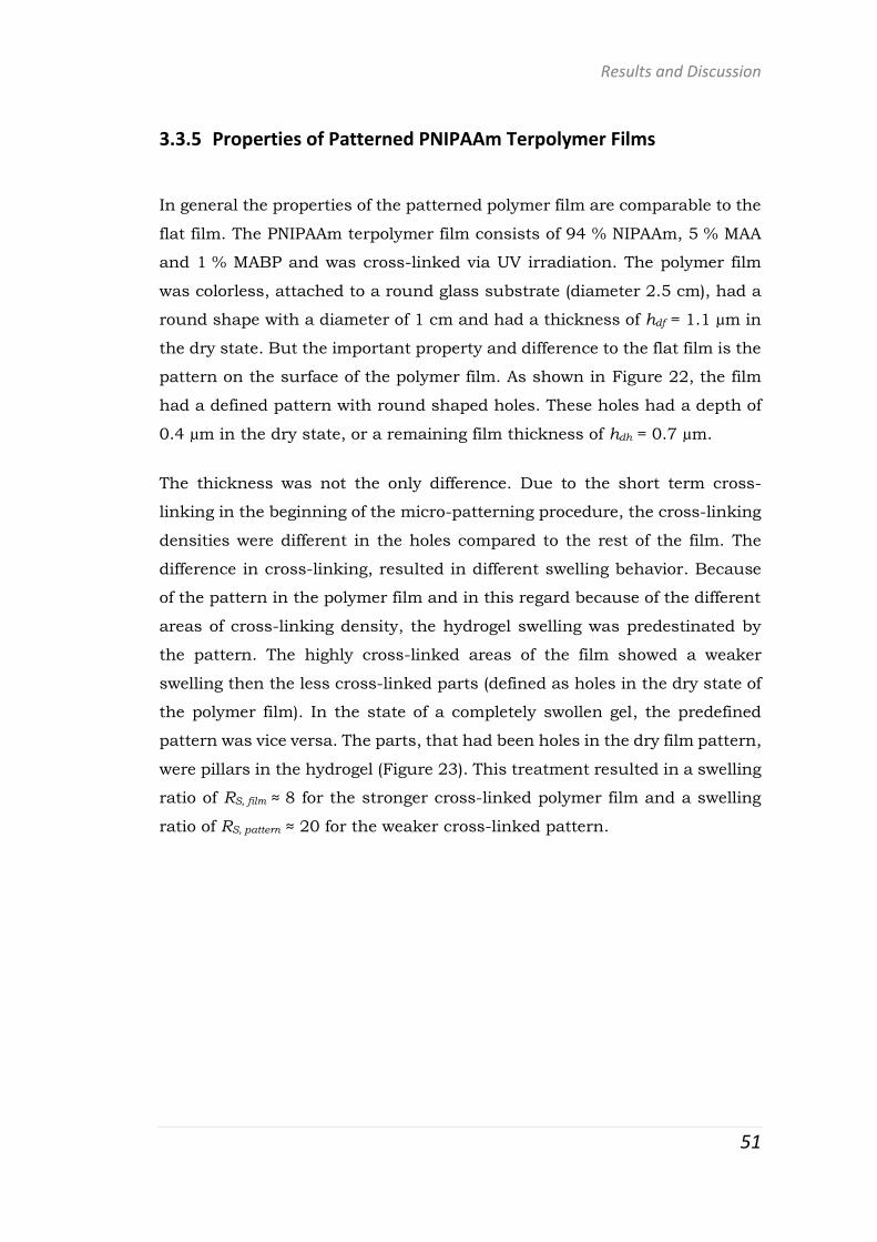
Results and Discussion
51
3.3.5 Properties of Patterned PNIPAAm Terpolymer Films
In general the properties of the patterned polymer film are comparable to the
flat film. The PNIPAAm terpolymer film consists of 94 % NIPAAm, 5 % MAA
and 1 % MABP and was cross-linked via UV irradiation. The polymer film
was colorless, attached to a round glass substrate (diameter 2.5 cm), had a
round shape with a diameter of 1 cm and had a thickness of hdf = 1.1 µm in
the dry state. But the important property and difference to the flat film is the
pattern on the surface of the polymer film. As shown in Figure 22, the film
had a defined pattern with round shaped holes. These holes had a depth of
0.4 µm in the dry state, or a remaining film thickness of hdh = 0.7 µm.
The thickness was not the only difference. Due to the short term cross-
linking in the beginning of the micro-patterning procedure, the cross-linking
densities were different in the holes compared to the rest of the film. The
difference in cross-linking, resulted in different swelling behavior. Because
of the pattern in the polymer film and in this regard because of the different
areas of cross-linking density, the hydrogel swelling was predestinated by
the pattern. The highly cross-linked areas of the film showed a weaker
swelling then the less cross-linked parts (defined as holes in the dry state of
the polymer film). In the state of a completely swollen gel, the predefined
pattern was vice versa. The parts, that had been holes in the dry film pattern,
were pillars in the hydrogel (Figure 23). This treatment resulted in a swelling
ratio of RS, film ≈ 8 for the stronger cross-linked polymer film and a swelling
ratio of RS, pattern ≈ 20 for the weaker cross-linked pattern.
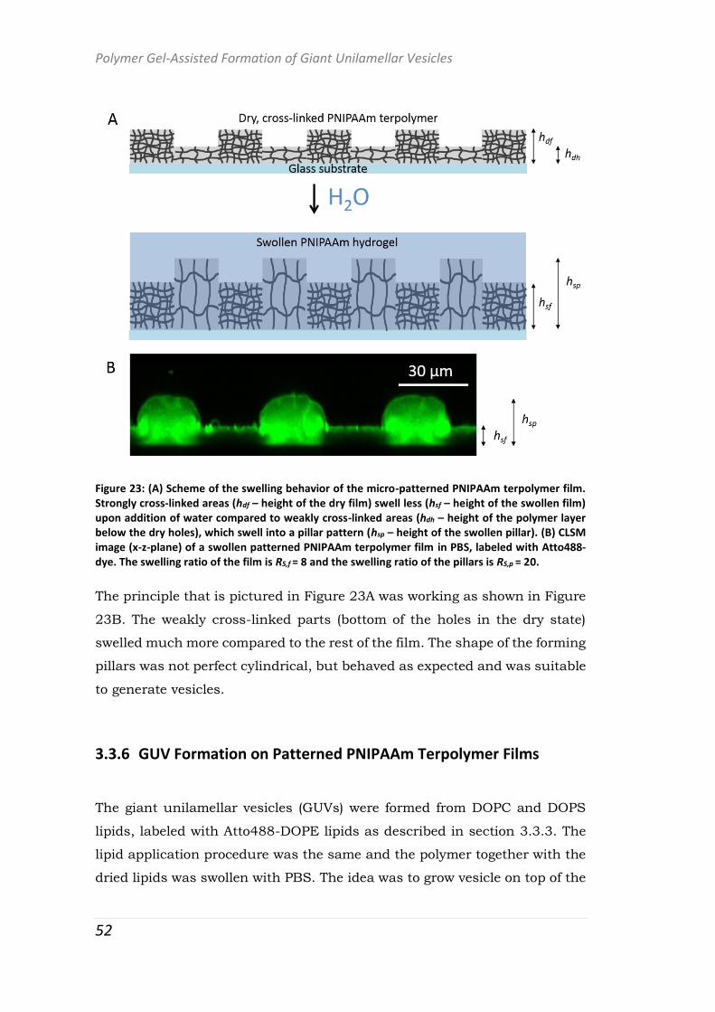
Polymer Gel-Assisted Formation of Giant Unilamellar Vesicles
52
Figure 23: (A) Scheme of the swelling behavior of the micro-patterned PNIPAAm terpolymer film. Strongly cross-linked areas (hdf – height of the dry film) swell less (hsf – height of the swollen film) upon addition of water compared to weakly cross-linked areas (hdh – height of the polymer layer below the dry holes), which swell into a pillar pattern (hsp – height of the swollen pillar). (B) CLSM image (x-z-plane) of a swollen patterned PNIPAAm terpolymer film in PBS, labeled with Atto488-dye. The swelling ratio of the film is RS,f = 8 and the swelling ratio of the pillars is RS,p = 20.
The principle that is pictured in Figure 23A was working as shown in Figure
23B. The weakly cross-linked parts (bottom of the holes in the dry state)
swelled much more compared to the rest of the film. The shape of the forming
pillars was not perfect cylindrical, but behaved as expected and was suitable
to generate vesicles.
3.3.6 GUV Formation on Patterned PNIPAAm Terpolymer Films
The giant unilamellar vesicles (GUVs) were formed from DOPC and DOPS
lipids, labeled with Atto488-DOPE lipids as described in section 3.3.3. The
lipid application procedure was the same and the polymer together with the
dried lipids was swollen with PBS. The idea was to grow vesicle on top of the

Results and Discussion
53
patterned polymer gel, on the areas that swell into pillars and remain in the
same size as the pillar diameter. Experiments on flat PNIPAAm terpolymer
film showed, that GUVs grow better on weakly cross-linked gel areas with
swelling ratios above 10. Therefore, the GUVs formed on the weakly cross-
linked pillars. Their size defined the maximum size of the vesicles. Within
5 min the gel swelled to a thickness of around 9 µm with a pillar size of about
15 µm and numerous vesicle formed (Figure 24). Vesicle formation speed was
comparable to that observed on PVA-gels or agarose substrate.[59,83]
With the patterned PNIPAAm terpolymer films it was possible to generate
hundreds of uniform GUVs with a diameter size that was defined by the
polymer pattern (Figure 24A). The vesicles grew on the polymer pillar top and
their growing was restricted by the pillar diameter. Hence, every polymer
pillar hosted one GUV (Figure 24B/C). A few small vesicles also grew on the
film surface and on the pillar side surface. These vesicles were very small
compared to the GUVs and are in the size range of LUVs. The GUVs on the
pillars showed diameters that were comparable to the pattern sizes. When
the pattern diameter of the photolithography mask was 30 µm, the formed
vesicles had a diameter of 30.9 ± 2.4 µm. This PNIPAAm-based technique
can create GUVs with desired diameters to use them as cell membrane
models. The advantage of this method is not only the fast, easy and size-
defined preparation of GUVs, but also the fact, that the vesicles were
anchored to the polymer substrate. The so-called giant unilamellar anchored
vesicles (GUAVs) did not need to be immobilized for further studies, because
they were already attached to the polymer during the formation. With an
array of hundreds of vesicles different studies could be performed
simultaneously (see section 3.3.8).

Polymer Gel-Assisted Formation of Giant Unilamellar Vesicles
54
Figure 24: CLSM images of DOPC/DOPS GUVs formed on micro-patterned PNIPAAm terpolymer films. (A) 2D image of an array of hundreds of uniform GUVs. (B) 3D image of a 4x4 array of swollen PNIPAAm terpolymer pillars with GUVs formed on the top of the pillars. (C) 3D image of a single GUV on a PNIPAAm hydrogel pillar.

Results and Discussion
55
3.3.7 Size Control
The diameter of the vesicles was defined by the micro-patterned PNIPAAm
terpolymer film. The growing process was limited to the surface area of the
pre-defined pattern, which was the top of the pillars. Consequently, the size
of the swollen polymer pattern defined the size of the GUVs. Within this
study, three different pattern sizes and vesicle diameters were prepared. The
diameters were chosen in the range of cell and cell membrane sizes to obtain
ideal models for cell membrane experiments. Defined by the
photolithography mask, the pattern diameters were 15 µm for mask 1, 30
µm for mask 2 and 50 µm for mask 3 (see Table 2). The distances between
the centers of the patterns were 40 µm for mask 1, 60 µm for mask 2 and
100 µm for mask 3. For every pattern GUVs were prepared. The mean
diameter for GUVs on the 15 µm pattern was 17.6 ± 2.9 µm, on the 30 µm
pattern it was 30.9 ± 2.4 µm and on the 50 µm pattern it was 46.4 ± 2.4 µm.
Figure 25 shows the results of the new method for PNIPAAm gel-assisted
formation of GUVs. Their size was comparable to the pattern size, giving the
ability to create vesicles that are uniform and have a desired size between 15
and 50 µm.
Table 2: Specifications of the photolithography masks for micro-patterning of the PNIPAAm terpolymer films.
Mask
Pattern diameter a
[µm]
Pattern distance d
[µm]
1 15 40
2 30 60
3 50 100

Polymer Gel-Assisted Formation of Giant Unilamellar Vesicles
56
Figure 25: Left: CLSM images (x-y-plane and x-z-plane) of uniform giant unilamellar vesicles prepared by PNIPAAm gel-assisted swelling for (A) 15 µm, (B) 30 µm and (C) 50 µm pattern size. Right: Histograms of the vesicle size distribution.

Results and Discussion
57
The PNIPAAm gel-assisted formation of GUVs has several advantages
compared to other methods. As already explained, the polymer film cannot
dissolve in the solvent, because it is an anchored network. That means there
is no freely diffusing polymer inside the GUVs as it was the case for GUV
preparation with agarose gel. Furthermore, this method enables the
formation of hundreds of uniform and size defined vesicles within a few
minutes. The next advantage of this technique is the immobilization of the
vesicles. Usually the immobilization of GUVs as cell models is a big challenge,
but with this method, the vesicles were already in a controlled position,
anchored to the PNIPAAm substrate. This new type of giant unilamellar
anchored vesicles (GUAVs) easily enables further investigations on an array
of hundreds of vesicles simultaneously.
3.3.8 Applications
With the PNIPAAm gel-assisted method, size-defined giant unilamellar
anchored vesicles were prepared. Hundreds of vesicles were in a defined and
controlled position. The GUAVs did not move or flow in the solution, which
is an advantage compared to cell-mimicking GUVs that were prepared with
other methods, such as electroformation. These GUVs needed to be
immobilized after their preparation of perform further experiments.
This chapter shows two different application examples for giant unilamellar
anchored vesicles (GUAVs). The first application used the advantage that the
vesicles were immobilized and did not move from their position. Hence,
fluorescence correlation spectroscopy measurements could easily be
performed to determine the diffusion coefficient of the lipids in the
membrane. The second example used the advantage to have tens or
hundreds of GUAVs immobilized and together in order to investigate the
photo-oxidation behavior of the lipids in the membrane.

Polymer Gel-Assisted Formation of Giant Unilamellar Vesicles
58
Application 1: Investigating the Diffusion of DOPE lipids in Giant Unilamellar Anchored Vesicles
Biological membranes are not only a barrier between the exterior and interior
of cells, but also segregate into specialized functional domains.[107,108] The
membrane forms a structural matrix, providing mechanical stability.[107]
Already in 1972 Singer and Nicolson described the importance of
understanding the dynamics of cell membranes.[109] The diffusion coefficient
of membrane lipids belongs to the most important parameters regarding the
dynamical studies, because it is closely related to the structure of the
biological membrane.[107] To characterize the diffusion of lipids in biological
membranes or membrane models, various experimental techniques are
useful. Mainly, fluorescence correlation spectroscopy is used, but
fluorescence recovery after photobleaching, single particle tracking or
nuclear magnetic resonance measurements are other possible
methods.[107,110]
Herein, fluorescence correlation spectroscopy (FCS) measurements were
used to investigate the dynamics of the GUAV lipid bilayer that represents
the cell membrane.[44] For these measurement 0.01 % of fluorescently labeled
lipids (Atto633-DOPE: Atto633-1,2-dioleoyl-sn-glycero-3-phosphoethanol-
amine) were added to the standard lipid mixture that was used for the GUAV
formation. Via confocal laser scanning microscopy and z-scanning in the
fluorescence mode, the laser beam was focused on the membrane. Once the
focus was fixed, measurements could be performed for several minutes in
the same position, because the vesicle membrane did not move and the only
diffusion was coming from the lipids inside the membrane. Measurements
were done in three different samples and 12 different vesicles. Figure 26
represents an autocorrelation (AC) curve of the DOPE lipid diffusion in the
GUV membrane, as determined by FCS measurements. The experimental
autocorrelation curve was fitted with a single component model, showing
only one type of species diffusing in the membrane. The diffusion coefficient
of this species was found to be D = 1.01·10-11 ± 0.14·10-11 m2/s, which is in
the same order of magnitude as described in the literature for comparable
systems.[107,111,112]
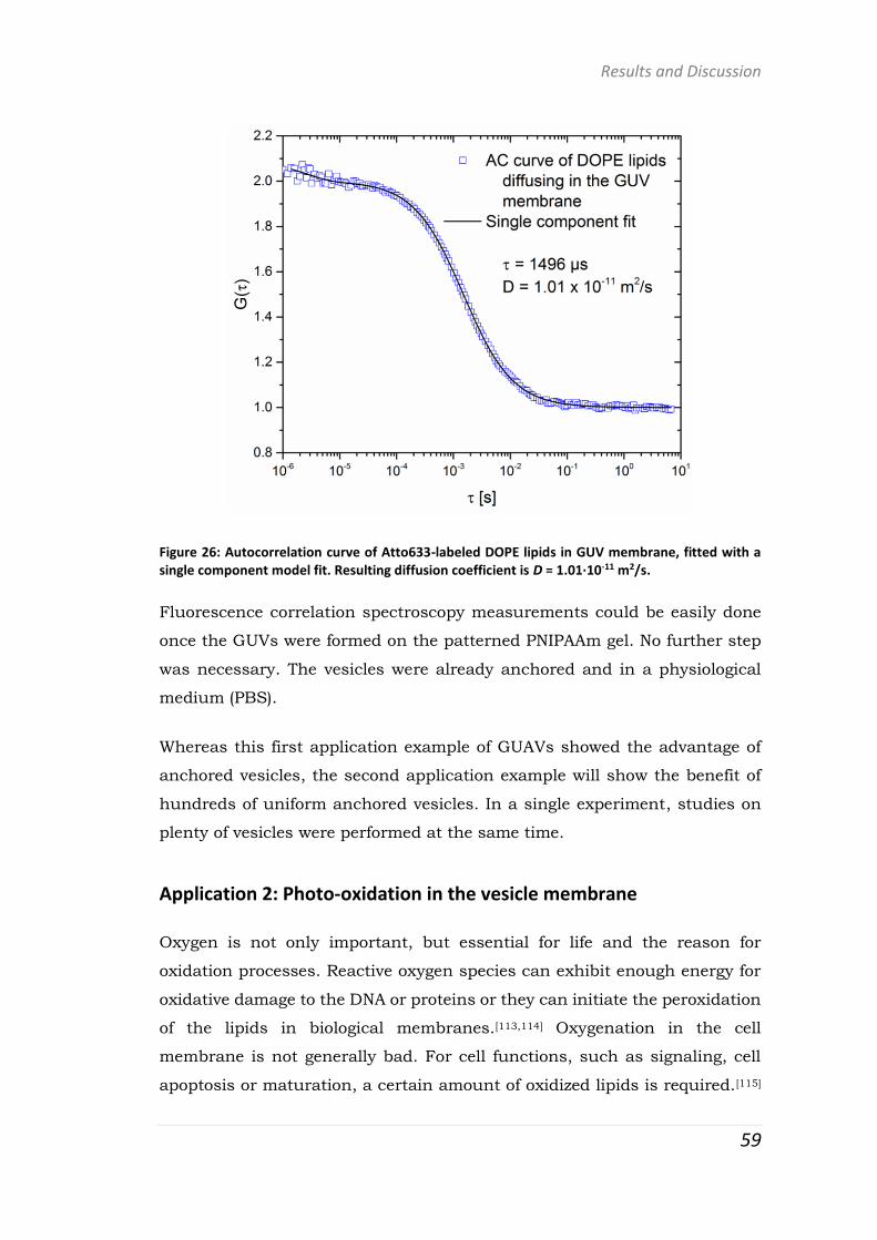
Results and Discussion
59
Figure 26: Autocorrelation curve of Atto633-labeled DOPE lipids in GUV membrane, fitted with a single component model fit. Resulting diffusion coefficient is D = 1.01·10-11 m2/s.
Fluorescence correlation spectroscopy measurements could be easily done
once the GUVs were formed on the patterned PNIPAAm gel. No further step
was necessary. The vesicles were already anchored and in a physiological
medium (PBS).
Whereas this first application example of GUAVs showed the advantage of
anchored vesicles, the second application example will show the benefit of
hundreds of uniform anchored vesicles. In a single experiment, studies on
plenty of vesicles were performed at the same time.
Application 2: Photo-oxidation in the vesicle membrane
Oxygen is not only important, but essential for life and the reason for
oxidation processes. Reactive oxygen species can exhibit enough energy for
oxidative damage to the DNA or proteins or they can initiate the peroxidation
of the lipids in biological membranes.[113,114] Oxygenation in the cell
membrane is not generally bad. For cell functions, such as signaling, cell
apoptosis or maturation, a certain amount of oxidized lipids is required.[115]
Polymer Gel-Assisted Formation of Giant Unilamellar Vesicles
60
Nevertheless, uncontrolled oxidation of lipids can lead to diseases, such as
Parkinson or Alzheimer.[115] Therefore, the investigation of the photo
oxidation process in the membrane is of high importance.
In this study, the oxidation of lipids in the vesicles membrane was
investigated and monitored using confocal laser scanning microscopy. This
study was based on the hydroperoxidation of the double bonds in the lipids
tails by inserting OOH groups, that led to changes in the chain conformation
and therefore to an increase of the area per lipid inside the vesicles. To
generate hydroperoxide groups, the photo-oxidizer molecule erythrosine was
used. Irradiation of erythrosine at 547 nm created singlet oxygen, that
reacted with the unsaturated lipid bonds to hydroperoxide.[116,117]
GUAV were formed on patterned PNIPAAm gels as describes before. A 50 µM
solution of the photo-sensitizer molecule erythrosine in phosphate buffered
saline (PBS) was used for the GUAV formation. After the formation process,
the area increase of the vesicles was studied without further preparation.
The area increase occurred upon irradiation of erythrosine and subsequent
hydroperoxidation of the lipids. The area increase was monitored by confocal
laser scanning microscopy (CLSM) at the equator of the GUAVs after different
irradiation times and irradiation doses, respectively. The results are shown
in Figure 27: an increase in radius and area of the vesicles as well as a
deformation of the round shape was observed. The more energy was used,
the more singlet oxygen was generated by the erythrosine molecules. This
led to the deformation and area increase of the GUAVs. Before the irradiation
the vesicles were uniform and completely round shaped. After 1 min or
3.1 kJ/cm2 irradiation of the photo-oxidizer erythrosine, the GUAVs were
larger, deformed and moved from their positions. After 3 min (9.3 kJ/cm2)
the GUAVs grew even larger and even more of them deformed or moved from
their position. After 11 min (33.9 kJ/cm2) the GUAVs reached their final size
and most of them have moved from their initial position. The CLSM images
in Figure 27 clearly show the advantage of this GUAV formation method: The
sample can be used for further studies directly after GUAV preparation and
gives the ability to monitor and analyze the behavior of dozens of vesicles
simultaneously.

Results and Discussion
61
Figure 27: Results of the photo-oxidation experiments on GUAVs with the photo-oxidizer molecule erythrosine. (A) Area Increase of the GUAVs equator at different irradiation energy doses. (B-E) Confocal laser scanning images of the equator of GUAVs at different irradiation times: (B) Before irradiation the GUAVs are uniform and completely round shaped. (C) After 1 min irradiation of the photo-oxidizer erythrosine (corresponds to an energy dose of 3.1 kJ/cm2) the GUAVs are larger, deform and move from their positions. (D) After 3 min (9.3 kJ/cm2) the GUAVs are even larger and more of them deform and move from their position. (E) After 11 min (33.9 kJ/cm2) the GUAVs reach their final size and most of them have moved from their initial position.

Polymer Gel-Assisted Formation of Giant Unilamellar Vesicles
62
3.4 Summary and Outlook
Research on biological cells, our smallest living building units, is important
to understand life in general, but also to understand and treat diseases. For
a better research on cells and cell membranes, model systems are useful
tools. Very promising cell model systems are giant unilamellar vesicles
(GUVs). They can be prepared from different procedures. All of them have
their advantages and disadvantages. The presented method for GUV
formation is polymer hydrogel based and overcame the disadvantages of the
known gel-based methods. This GUV formation was based on a
functionalized PNIPAAm terpolymer hydrogel film. A benzophenone unit
inside the polymer chain allowed to cross-link the polymer and anchored it
to a glass substrate by UV irradiation. Hence, the polymer gel stayed at its
position and did not dissolve. Hence, no free polymer was found in the GUVs
after their formation. The formation of GUVs was possible on the surface of
the polymer film by spreading phospholipids on the film and growing them
with a buffer solution (simulating physiological conditions). Furthermore, the
GUV growing process worked without the addition of organic solvents. Only
the addition of the lipids beforehand was done from a lipid-chloroform
solution, because of the solubility of the used phospholipids. The greatest
development of this method was the GUV size control. GUVs were grown in
a size-defined manner, by forming them from a micro-patterned PNIPAAm
terpolymer hydrogel. The GUV diameter corresponded to the pattern
diameter. In this procedure, hundreds of uniform vesicles were prepared
within a few minutes. Additionally, this method resulted in GUVs, which
were anchored to the polymer gel, enabling studies on hundreds of vesicle
simultaneously, without the necessity to immobilize them as it is needed for
other GUV formation methods.
The PNIPAAm gel-assisted method for GUV preparation is very promising
and overcomes several disadvantages that other methods have, but it is still
in the fledgling stages. In the future work, it could be interesting to test the

Summary and Outlook
63
method with a large variety of phospholipids and phospholipid mixtures as
well as amphiphilic polymers to generate polymersomes. For studies on the
cell membrane model it might be interesting to encapsulate particles, such
as drug molecules into the GUVs and study their behavior to pass the
membrane. The same could be interesting for polymersomes as drug delivery
vehicles. Another future work could be the detachment of the GUVs. Even
though the advantage of anchored vesicles is part of this method, it would
be good to have the possibility to detach the GUVs. This might be achieved
by temperature changes. PNIPAAm is a thermo-responsive polymer with an
LCST around 30-35 °C. Above this temperature, the polymer collapses and
this can result in GUV detachment.
The PNIPAAm terpolymer hydrogel-assisted method enables the formation of
size-defined giant unilamellar vesicles within a few minutes. On a micro-
patterned polymer, hundreds of anchored cell membrane models were
generated.

4 Monitoring Polymer Nanoparticle Formation using a Fluorescent Molecular Rotor
Nanoparticles are objects with a size between 1 nm and a few 100 nm and
they are of high interest in many disciplines.[2,3] Because of their small size,
nanoparticles show different properties compared to their bulk materials.[4]
The particles can be synthesized either biologically or chemically.[4] One of
the extensively studied groups of nanoparticles are the polymer
nanoparticles.[2] Many studies were performed, focusing on the preparation
of a diversity of different polymer particles and a lot of effort was put on their
applications.[2,3,118] The preparation and characterization of polymer
nanoparticles is of large interest in the fields of chemistry, material science
and biomedicine, e.g. in tumor therapy.[8,119] The polymer nanoparticles can
be synthesized from micelles or emulsion droplet templates or they can be
prepared from pre-synthesized polymers from emulsified solutions of the
polymer (e.g. by SEED - solvent evaporation from emulsion droplets).[119,120]
Polymer nanoparticles are small and show a fast diffusion. Hence, it is very
difficult to get information on how the formation process is taking place. In
the SEED procedure, the drying process of the nanodroplets is not fully
understood yet. This project investigated the drying process of polystyrene
nanoparticles prepared by solvent evaporation. Herein, polystyrene was a
model system to test and develop the method. In this project, fluorescence
correlation spectroscopy and fluorescence lifetime measurements were used
to monitor both size and concentration changes in the nanodroplets with the
help of a fluorescent molecular rotor molecule.
Monitoring Polymer Nanoparticle Formation using a Fluorescent Molecular Rotor
66
4.1 Chemical Concepts and Methods
This chapter introduces the chemical background about nanoparticles,
especially polystyrene and the preparation methods of nanoparticles with a
focus on the formation via solvent evaporation from emulsion droplets. The
physical concepts of fluorescence, fluorescent molecules and the analytical
methods are explained in section 2.
4.1.1 Polystyrene Nanoparticles
Polystyrene (PS) is one of the most extensively studied polymers. This
aromatic polymer is a commodity plastic and has been widely used in
research reports because it is relatively chemically inert. It can be
synthesized from its monomer styrene by many different polymerization
types. Often free radical polymerization (Figure 28) is used.[121] In this
method, styrene can function as electron acceptor or electron donor and the
polymerization does not necessarily need to be started with an initiator.
Styrene can form the initiating radicals itself.[121–123] The chain growth
process mainly terminates with a recombination step.[121] The resulting
polymer is a linear hydrocarbon chain with phenyl side groups, which is
soluble in aromatic and halogenated hydrocarbons, esters, ketones and
aliphatic ethers, but not in aliphatic hydrocarbons and alcohols.[121]
Amorphous atactic PS homopolymers are durable and transparent and
commonly used as molded or expanded foams. Other applications of PS can
be found in the food industry, because PS is hardly biodegradable.
Furthermore, the usage of PS in medical products and laboratory equipment
is of interest, because it is very cheap and biocompatible.[124] The special
properties of PS results in a very wide range of applications and make PS to
one of the most quantitatively important chemicals. It is produced in
industrial process since the 1920s.[121]

Chemical Concepts and Methods
67
Figure 28: Synthesis of polystyrene (PS) from its monomer styrene (vinyl benzene).
Considering PS nanoparticles, the properties and applications differ from the
bulk material. The surface area is very high compared to their volume,
affecting the mechanical, electrical and optical properties as well as the
chemical reactivity. PS nanoparticles are used in self-assembling
nanostructures or as biosensors.[125,126] One of the most promising
application field for nanoparticles and -carriers is drug delivery.
Biocompatible nanoparticles are needed. Often, drug molecules are poorly
soluble in biological media, due to their hydrophobicity. This can be solved
by encapsulating these drugs into protective nanocarriers, generating a
hydrophilic surface and enabling drug delivery.
4.1.2 Nanoparticle Formation Techniques
Nanoparticles as well as their preparation techniques are manifold. The
material of the particle can vary from proteins or polysaccharides to synthetic
polymers, on which this work is focused. The choice of nanoparticle
formation method depends on numerous factors that define the desired
properties for particular applications. Size, size distribution, solubility and
stability, surface characteristics as well as biocompatibility and
biodegradability are factors to take into account when choosing the
nanoparticle preparation technique.[2,3,127]
In general, there are two main methods for the formation of polymer
nanoparticles (Figure 29): direct polymerization of monomers and dispersion
of preformed polymers. Other possibilities are ionic gelation or coacervation
of hydrophilic polymers or particle replication in non-wetting templates,
giving an absolute control of particle size and shape.[2,3]
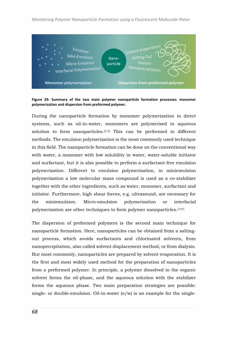
Monitoring Polymer Nanoparticle Formation using a Fluorescent Molecular Rotor
68
Figure 29: Summary of the two main polymer nanoparticle formation processes: monomer polymerization and dispersion from preformed polymer.
During the nanoparticle formation by monomer polymerization in direct
systems, such as oil-in-water, monomers are polymerized in aqueous
solution to form nanoparticles.[2,3] This can be performed in different
methods. The emulsion polymerization is the most commonly used technique
in this field. The nanoparticle formation can be done on the conventional way
with water, a monomer with low solubility in water, water-soluble initiator
and surfactant, but it is also possible to perform a surfactant-free emulsion
polymerization. Different to emulsion polymerization, in miniemulsion
polymerization a low molecular mass compound is used as a co-stabilizer
together with the other ingredients, such as water, monomer, surfactant and
initiator. Furthermore, high shear forces, e.g. ultrasound, are necessary for
the miniemulsion. Micro-emulsion polymerization or interfacial
polymerization are other techniques to form polymer nanoparticles.[127]
The dispersion of preformed polymers is the second main technique for
nanoparticle formation. Here, nanoparticles can be obtained from a salting-
out process, which avoids surfactants and chlorinated solvents, from
nanoprecipitation, also called solvent displacement method, or from dialysis.
But most commonly, nanoparticles are prepared by solvent evaporation. It is
the first and most widely used method for the preparation of nanoparticles
from a preformed polymer. In principle, a polymer dissolved in the organic
solvent forms the oil-phase, and the aqueous solution with the stabilizer
forms the aqueous phase. Two main preparation strategies are possible:
single- or double-emulsion. Oil-in-water (o/w) is an example for the single-

Chemical Concepts and Methods
69
emulsion preparation, whereas (water-in-oil)-in-water (w/o)/w is an example
for the double-emulsion preparation.[127]
4.1.3 Solvent Evaporation from Emulsion Droplets
One possible way to prepare polymer nanporaticles is decribed in detail with
the solvent evaporation from emulsion droplets (SEED) process. Herein, a
presynthesized polymer is dissolved in a good organic solvent and then
emulsified in water with the help of a stabilizer or surfactant. High-speed
homogenization or ultrasound are necessary to obtain the emulsion. In the
next step the organic solvent is evaporated through the continious aqueous
phase and so a polymeric emulsion is formed. Therefore, contineous
magentic stirring or reduced pressure are needed. The solvent evaporation
leads to the formation of surfactant stabilized polymer nanoparticles
dispersed in the aqueous phase (Figure 30).[119,120,127]
Figure 30: Solvent evaporation from emulsion droplets (SEED) process. A pre-synthesized polymer is dissolved in a good organic solvent and emulsified with an aqueous surfactant solution, giving stabilized polymer/organic solvent-droplets. Solvent evaporation leads to polymer nanoparticles. Adapted from [119,120].
The SEED process has the great advantage that it is free from impurities in
the final product, e.g. monomers, catalyst or even toxic residuals.[120]
Additionally, the process is easy and very fast. The particle size can be
influenced by the process parameters, such as type and concentration of the
stabilizer, polymer concentration or speed of homogenization or
ultrasonication.[3]

Monitoring Polymer Nanoparticle Formation using a Fluorescent Molecular Rotor
70
4.2 Experiments und Materials
In this section, the chemicals and materials as well as the analytical setups
that were used for this work are summarized. Furthermore, the experiments
with all important parameters are described in detail.
4.2.1 Materials
Chloroform (≥ 99 %) was purchased from Acros Organics and anhydrous
toluene (100 %) from VWR Chemicals. The solvents were used as received.
Sodium dodecyl sulfate (SDS, 99 %) was purchased from AlfaAesar and
diluted in ultrapure water (Milli-Q water, 18.2 MΩ·cm) to a concentration of
1 g/L. The fluorescent dye Atto425 was purchased from ATTO-TEC GmbH
(Siegen, Germany) and diluted in ultrapure water (Milli-Q, 18.2 MΩ·cm).
Polystyrene (Mw = 75 kg/mol, PDI = 1.03) was provided by J. Thiel (MPI-P).
The molecular rotor LBX37 was provided in a 5·10-4 M solution in toluene
from the group of Roberto Simonutti (Department of Materials Science,
University of Milano-Bicocca, Italy).
4.2.2 Time-Correlated Single Photon Counting (TCSPC)
Time-correlated single photon counting (TCSPC) data were recorded on a
confocal setup. A PicoQuant diode laser (405 nm) was coupled into a Zeiss
LSM 880 microscope (Carl Zeiss, Jena, Germany) using a MBS405 dichroic
mirror (Carl Zeiss, Jena, Germany). The laser beam was focused through a
Zeiss C-Apochromat 40×/1.2 W water immersion objective into the sample
solutions. Emitted fluorescence light was collected with the same objective,
passed through a pinhole and a band pass filter EM525/50 (Chroma
Technology, Vermont, USA), detected by a PDM SPAD (Micro Photon Devices,
Bolzano, Italy) and processed using a TimeHarp 260. An eight-well
Experiments und Materials
71
polystyrene, chambered cover glass (Laboratory-Tek, Nalge Nunc
International) was used as a sample cell for aqueous samples and an
Attofluor® cell chamber (Invitrogen, Paisley, UK) was used for organic
solutions and dry samples. If not mentioned in particular, the focus of the
beam was positioned 30 µm inside the solution or emulsion, above the glass
surface. Analysis of the TCSPC data was performed using the PicoQuant
SymPhoTime 64 software. The instrument response function (IRF) was
reconstructed with the PicoQuant SymPhoTime 64 software by directly
evaluating the onset of the decay.
4.2.3 TCSPC Measurements of the Molecular Rotor in Toluene
A 500 nM solution of LBX37 in toluene was prepared. The sample was
measured in an Attofluor® cell chamber at room temperature (T = 22 °C).
The setup specifications are described in section 4.2.2. The sample was
measured for 120 s and the resulting decay curve was fitted with a single
exponential reconvolution fit (see equation 1). The experiment was repeated
five times.
4.2.4 TCSPC Measurements of Atto425 in Water
A 50 nM solution of Atto425 in water was prepared. The sample was
measured in a NUNC chamber at room temperature (T = 22 °C). The setup
specifications are described in section 4.2.2. The sample was measured for
120 s and the resulting decay curve was fitted with a single exponential
reconvolution fit (see equation 1). The experiment was repeated five times.
4.2.5 TCSPC Measurements in Polystyrene Solutions
Polystyrene (PS, 75 kg/mol) was dissolved in toluene. The PS fractions were
ranging from 10 % PS in toluene up to 90 % PS in toluene. To each solution

Monitoring Polymer Nanoparticle Formation using a Fluorescent Molecular Rotor
72
the molecular rotor LBX37 was added in a concentration of
5·10-6 M. Polystyrene solutions below 60 % were prepared by dissolving PS
in the appropriate amount of toluene. The solutions were stirred for 24 h to
obtain homogeneous solutions. For samples with PS concentrations above
60 %, the viscosity was too high to dissolve the polymer appropriately in the
comparably low amount of toluene. The high viscosity also precludes stirring.
To overcome this problem, samples with a high PS concentration were
prepared from a sample with initial 50 % PS. This sample was dried at
ambient atmosphere and room temperature. The resulting PS concentration
was calculated from the weight of the initial sample and the dried sample.
Since the weight loss only appeared from evaporated toluene, the
concentration could be determined. With this preparation method, it was
possible to obtain samples with PS concentrations up to 90 %. To measure
the rotor molecule in pure polystyrene, a polymer film was prepared from the
50 % PS solution by drying it for 72 h at 50 °C under vacuum. Samples were
measured in Attofluor® cell chambers at 22 °C as describes in section 4.2.2.
The measurement time was 180 s and the obtained decay curves were fitted
with a biexponential reconvolution fit (equation 2) for the PS toluene
mixtures and a monoexponential reconvolution fit for pure PS (equation 1).
4.2.6 Polystyrene Nanoparticle Formation via SEED in Toluene
50 mg PS (Mw = 75 kg/mol) were dissolved in 1.44 mL toluene. The solvent
contained the molecular rotor LBX37 in a concentration of 1·10-6 M. 10 mL
of an aqueous solution of SDS (1 g/L) were added to the organic solution. A
macroemulsion was obtained by stirring for 1 h at 1250 rpm at room
temperature. The macroemulsion was sonicated using a Branson W450-D
sonifier with ½-inch tip in a pulsed regime (30 s sonication, 10 s pause) for
2 min at 70 % amplitude under ice cooling. The obtained emulsion was either
directly measured or stirred at 40 °C at 500 rpm to evaporate the organic
solvent. For the kinetic measurements from the large volume, after specific
time intervals 100 µL of the emulsion were diluted 5x in water and measured.
In case of the droplet measurement, 150 µL of the diluted emulsion were

Experiments und Materials
73
used for the measurement. The samples were measured in a NUNC chamber
at room temperature (T = 22 °C). The setup specifications are described in
section 4.2.2. The samples were measured for 120 s and the resulting decay
curves were fitted with a biexponential reconvolution fit (see equation 2).
4.2.7 Dried Polystyrene Nanoparticles
Polystyrene nanoparticles were prepared as explained in section 4.2.6. To
study the fluorescence lifetime of the molecular rotor in dry PS nanoparticles,
the dispersions from the final SEED step were dried from small dispersion
droplets on round microscope cover slides. The drops were dried for 30 min
under vacuum at 50 °C and then a next portion of droplet was added to the
dry thin layer. The process was repeated five times to obtain a layer of PS
nanoparticles. The beam was focused into the nanoparticle layer and TCSPC
measurements were performed as describes above. The decay curves were
fitted with a single exponential reconvolution fit (equation 1). Four samples
were prepared and measured.
4.2.8 SEED Process Without Polymer for Studying SDS Influence
1.44 mL toluene, containg the molecular rotor LBX37 in a concentration of
1·10-6 M were added to 10 mL of an aqueous solution of SDS (1 g/L). A
macroemulsion was obtained by stirring for 1 h at 1250 rpm at room
temperature. The macroemulsion was sonicated using a Branson W450-D
sonifier with ½-inch tip in a pulsed regime (30 s sonication, 10 s pause) for
2 min at 70 % amplitude under ice cooling. The obtained emulsion was
stirred at 40 °C at 500 rpm to evaporate the organic solvent. The sample was
measured in a NUNC chamber at room temperature (T = 22 °C). The setup
specifications are described in section 4.2.2. The sample was measured for
120 s and the resulting decay curve was fitted with a single exponential
reconvolution fit (see equation 1).

Monitoring Polymer Nanoparticle Formation using a Fluorescent Molecular Rotor
74
4.2.9 Polystyrene Nanoparticle Formation via SEED in Chloroform
50 mg PS (Mw = 75 kg/mol) were dissolved in 0.84 mL chloroform. The
solvent contained the molecular rotor LBX37 in a concentration of 1·10-6 M.
10 mL of an aqueous solution of SDS (1 g/L) were added to the organic
solution. A macroemulsion was obtained by stirring for 1 h at 1250 rpm at
room temperature. The macroemulsion was sonicated using a Branson
W450-D sonifier with ½-inch tip in a pulsed regime (30 s sonication, 10 s
pause) for 2 min at 70 % amplitude under ice cooling. The obtained emulsion
was either directly measured or stirred at 40 °C at 500 rpm to evaporate the
organic solvent. For the kinetic measurements from the large volume, after
specific time intervals 100 µL of the emulsion were diluted 5x in water and
measured. In case of the droplet measurement, 150 µL of the diluted
emulsion were used for the measurement. The samples were measured in a
NUNC chamber at room temperature (T = 22 °C). The setup specifications
are described in section 4.2.2. The samples were measured for 120 s and the
resulting decay curves were fitted with a biexponential reconvolution fit (see
equation 2).
4.2.10 Fluorescence Correlation Spectroscopy (FCS)
Fluorescence correlation spectroscopy data were recorded with the same
setup as describes for TCSPC measurements. The recorded photon data were
correlated to FCS autocorrelation curves, giving the diffusion times of the
nanoparticles, according to equation 6. The observation volume was
calibrated using Atto425 as reference dye. FCS Data were analyzed using the
software ZEN. The hydrodynamic radii were calculated from the measured
diffusion coefficients using the Stokes-Einstein relation (equation 10).

75
4.3 Results and Discussion
This chapter focuses on the formation of polystyrene nanoparticles. A lot of
work was done regarding the synthesis and preparation of nanoparticles and
their applications, especially as drug delivery systems. Understanding the
process and its physico-chemical properties is another important aspect to
study. The formation of polystyrene nanoparticles from solvent evaporation
from emulsion droplets (SEED) was monitored by using a fluorescence
molecular rotor. With the help of the rotor, it was possible to monitor the size
and concentration change of the nanodroplets by fluorescence correlation
spectroscopy and time-correlated single photon counting experiments.
4.3.1 Fluorescence Lifetime of Molecular Rotor LBX37 in Toluene
A fluorescent molecular rotor was used to study the formation of polystyrene
nanoparticles. This rotor is called LBX37 and is composed of a naphthalene
part, acting as the electron-acceptor, and a dibenzoazepine part, which is
the electron-donor (Figure 2C and Figure 31). Its fluorescence lifetime
depends on the microenvironment, mostly defined by the viscosity (see
section 2.2). To understand the behavior of the rotor, the fluorescence
lifetime was measured in pure toluene. Toluene was chosen, because it is a
good solvent for the molecular rotor and it is suitable for the following
nanoparticle formation experiments. The fluorescence lifetime was
determined using time-correlated single photon counting (TCSPC)
experiments. The decay curve of this experiment is pictured in Figure 31.
From the experimental decay a single exponential fit gave a fluorescence
lifetime of 0.6 ns.

Monitoring Polymer Nanoparticle Formation using a Fluorescent Molecular Rotor
76
Figure 31: Experimental decay curve (black) of the fluorescent molecular rotor LBX37 in toluene, together with the single exponential fit (red) and the instrument response function (IRF, grey). The fluorescence lifetime was found to be 0.6 ns. The chemical structure of the molecular rotor LBX37 is depicted in the figure.
The fluorescence lifetime of LBX37 in toluene was quite small compared to
conventional fluorescent dyes, such as Atto425. The reason was the special
property of the molecular rotor, as discussed in section 2.2. The
intramolecular rotation of the molecule is high in a low-viscosity
environment, such as pure toluene, resulting in a short fluorescence lifetime.
To assure, that the method and setup worked correctly, an additional
experiment with a fluorescent dye with known fluorescence lifetime was
measured. Atto425 is a commercially available fluorescent dye with a
fluorescence lifetime of τ = 3.6 ns.[128] The decay curve of the Atto425
measurement is shown in Figure 32. The fluorescence lifetime was found to
be 3.6 ns, which corresponds to the literature value. This measurement
reassured the method for the fluorescence lifetime determination.

Results and Discussion
77
Figure 32: Experimental decay curve (black) of the fluorescent dye Atto425 in water, together with the single exponential fit (red) and the instrument response function (IRF, grey). The fluorescence lifetime was found to be 3.6 ns, as it is described in the literature. The chemical structure of the dye Atto425 is depicted in the figure.
4.3.2 Master Curve for Polystyrene Toluene Mixtures
The aim of this work was to monitors the formation process of polystyrene
(PS) nanoparticles from the solvent evaporation from emulsion droplets
(SEED) process. During this process, toluene evaporated from surfactant
stabilized toluene-polystyrene droplets, forming polystyrene nanoparticles.
The concentration of PS inside the droplets was investigated during the
drying process.
Before performing the SEED experiments, a master curve was created by
measuring the fluorescence lifetime of the molecular rotor present in
polystyrene toluene solutions of different concentrations.
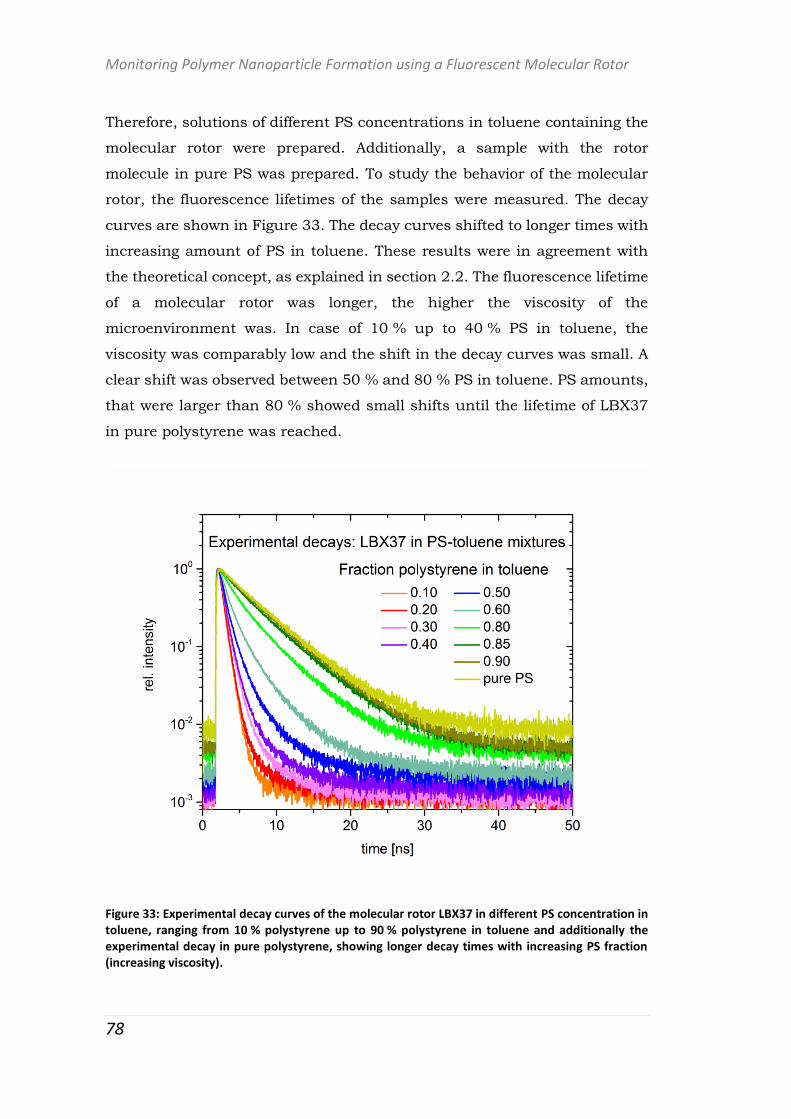
Monitoring Polymer Nanoparticle Formation using a Fluorescent Molecular Rotor
78
Therefore, solutions of different PS concentrations in toluene containing the
molecular rotor were prepared. Additionally, a sample with the rotor
molecule in pure PS was prepared. To study the behavior of the molecular
rotor, the fluorescence lifetimes of the samples were measured. The decay
curves are shown in Figure 33. The decay curves shifted to longer times with
increasing amount of PS in toluene. These results were in agreement with
the theoretical concept, as explained in section 2.2. The fluorescence lifetime
of a molecular rotor was longer, the higher the viscosity of the
microenvironment was. In case of 10 % up to 40 % PS in toluene, the
viscosity was comparably low and the shift in the decay curves was small. A
clear shift was observed between 50 % and 80 % PS in toluene. PS amounts,
that were larger than 80 % showed small shifts until the lifetime of LBX37
in pure polystyrene was reached.
Figure 33: Experimental decay curves of the molecular rotor LBX37 in different PS concentration in toluene, ranging from 10 % polystyrene up to 90 % polystyrene in toluene and additionally the experimental decay in pure polystyrene, showing longer decay times with increasing PS fraction (increasing viscosity).
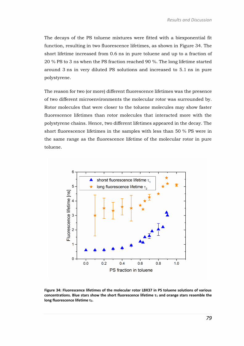
Results and Discussion
79
The decays of the PS toluene mixtures were fitted with a biexponential fit
function, resulting in two fluorescence lifetimes, as shown in Figure 34. The
short lifetime increased from 0.6 ns in pure toluene and up to a fraction of
20 % PS to 3 ns when the PS fraction reached 90 %. The long lifetime started
around 3 ns in very diluted PS solutions and increased to 5.1 ns in pure
polystyrene.
The reason for two (or more) different fluorescence lifetimes was the presence
of two different microenvironments the molecular rotor was surrounded by.
Rotor molecules that were closer to the toluene molecules may show faster
fluorescence lifetimes than rotor molecules that interacted more with the
polystyrene chains. Hence, two different lifetimes appeared in the decay. The
short fluorescence lifetimes in the samples with less than 50 % PS were in
the same range as the fluorescence lifetime of the molecular rotor in pure
toluene.
Figure 34: Fluorescence lifetimes of the molecular rotor LBX37 in PS toluene solutions of various concentrations. Blue stars show the short fluorescence lifetime τ1 and orange stars resemble the long fluorescence lifetime τ2.

Monitoring Polymer Nanoparticle Formation using a Fluorescent Molecular Rotor
80
The accuracy of the small lifetime τ1 was much better in the low PS fraction
range, whereas the accuracy for the larger lifetime τ2 was low, as the error
bars in Figure 34 indicate. This occurs from the fractions of the two lifetimes,
which are defined as their amplitudes, as they will be called in the rest of the
thesis. The corresponding amplitudes for the PS-toluene samples are
presented in Figure 35.
Figure 35: Amplitudes of the fluorescence lifetimes of the molecular rotor LBX37 in PS toluene solutions of various concentrations. Blue triangles show the amplitude A1 of the short fluorescence lifetime τ1 and orange stars resemble the amplitude A2 of the long fluorescence lifetime τ2.
In the regime of 10 % to 30 % PS in the solution, the short fluorescence
lifetime is dominant and the long lifetime is almost negligible. That was the
reason for the low accuracy of the value for the long lifetime in the low PS
fraction range. Between 40 % and 70 % PS concentration the short lifetimes
was still dominant, but the amplitude and the influence of the long lifetime
increased. At concentrations about 80 % PS in toluene the amplitudes of
both lifetimes were equal and the long lifetime dominated in regimes higher
than 80 % PS concentration.

Results and Discussion
81
To define one fluorescence lifetime value for each measurement or each
decay curve, the weighted average fluorescence lifetime τwa can be used (see
equation 4). This lifetime takes the different single lifetimes τi as well as their
amplitudes Ai into account. The weighted average fluorescence lifetime is a
helpful value to simplify very complex systems and to be able to compare
data more easily, as it was shown in the literature, e.g. for the polymerization
of PMMA.[129]
The dataset of the fitted curves can be found in Table 3 in the appendix. The
weighted average fluorescence lifetimes of the above shown samples’ decay
curves were plotted against the PS fraction in toluene to obtain a master
curve (Figure 36).
Figure 36: Master curve. Weighted average fluorescence lifetimes of the molecular rotor LBX37 in solutions of polystyrene in toluene in various concentrations.
The fluorescence lifetime of LBX37 in pure toluene was 0.6 ns, which did not
change significantly when 10 – 20 % polystyrene were present. Until a PS
fraction of 0.4 was reached, the lifetime was still below 1 ns. A stronger

Monitoring Polymer Nanoparticle Formation using a Fluorescent Molecular Rotor
82
change was observed from 50 % PS with a lifetime of 1.1 ns to 70 % PS and
2.5 ns up to 90 % PS with a lifetime of 4.8 ns. In pure polystyrene the
fluorescence lifetime was found to be 5.1 ns.
The weighted average fluorescence lifetimes in the master curve clearly
confirm the trend that the fluorescence lifetime increased with increasing
amount of polystyrene in the solution, due to higher viscosity in the
molecular rotors microenvironment. The fluorescence lifetimes from the
master curve were used in the following to determine the PS concentration
in the nanodroplets of the SEED process.
4.3.3 Monitoring the Polystyrene Nanoparticle Formation via SEED
The aim of this project was to monitor the formation of polystyrene
nanoparticles, which were formed in a solvent evaporation process (SEED).
The formation process and especially the drying process of the nanodroplets
is not fully understood, yet. From sections 4.3.1 and 4.3.2 the basic
parameters as well as the range of fluorescence lifetimes were known.
Therefore, polystyrene with the molecular rotor LBX37 was dissolved in
toluene. To the organic solution an aqueous surfactant (SDS) solution was
added and emulsified, in order to obtain surfactant-stabilized toluene-
droplets that contained the polymer and the rotor molecule. The process of
interest was the evaporation of toluene from these nanodroplets, forming PS
nanoparticles. Herein, the solvent evaporation process itself was studied.
Therefore, the fluorescence lifetimes were determined at several time
intervals during the evaporation process to obtain kinetic information.
Additionally to the fluorescence lifetime, which was obtained from TCSPC
experiments, the hydrodynamic radius of the toluene-PS-rotor-droplets was
determined by fluorescence correlation spectroscopy (FCS). During the
evaporation process, the droplet was expected to shrink due to the loss of
the solvent. In the case that no coalescence was happening in the process,
as described in the literature, the droplet had a larger size in the beginning
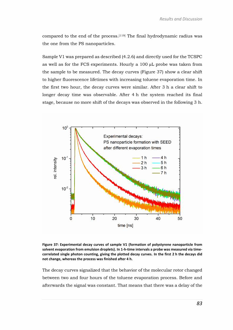
Results and Discussion
83
compared to the end of the process.[119] The final hydrodynamic radius was
the one from the PS nanoparticles.
Sample V1 was prepared as described (4.2.6) and directly used for the TCSPC
as well as for the FCS experiments. Hourly a 100 µL probe was taken from
the sample to be measured. The decay curves (Figure 37) show a clear shift
to higher fluorescence lifetimes with increasing toluene evaporation time. In
the first two hour, the decay curves were similar. After 3 h a clear shift to
longer decay time was observable. After 4 h the system reached its final
stage, because no more shift of the decays was observed in the following 3 h.
Figure 37: Experimental decay curves of sample V1 (formation of polystyrene nanoparticle from solvent evaporation from emulsion droplets). In 1-h-time intervals a probe was measured via time-correlated single photon counting, giving the plotted decay curves. In the first 2 h the decays did not change, whereas the process was finished after 4 h.
The decay curves signalized that the behavior of the molecular rotor changed
between two and four hours of the toluene evaporation process. Before and
afterwards the signal was constant. That means that there was a delay of the
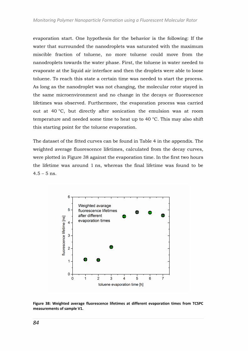
Monitoring Polymer Nanoparticle Formation using a Fluorescent Molecular Rotor
84
evaporation start. One hypothesis for the behavior is the following: If the
water that surrounded the nanodroplets was saturated with the maximum
miscible fraction of toluene, no more toluene could move from the
nanodroplets towards the water phase. First, the toluene in water needed to
evaporate at the liquid air interface and then the droplets were able to loose
toluene. To reach this state a certain time was needed to start the process.
As long as the nanodroplet was not changing, the molecular rotor stayed in
the same microenvironment and no change in the decays or fluorescence
lifetimes was observed. Furthermore, the evaporation process was carried
out at 40 °C, but directly after sonication the emulsion was at room
temperature and needed some time to heat up to 40 °C. This may also shift
this starting point for the toluene evaporation.
The dataset of the fitted curves can be found in Table 4 in the appendix. The
weighted average fluorescence lifetimes, calculated from the decay curves,
were plotted in Figure 38 against the evaporation time. In the first two hours
the lifetime was around 1 ns, whereas the final lifetime was found to be
4.5 – 5 ns.
Figure 38: Weighted average fluorescence lifetimes at different evaporation times from TCSPC measurements of sample V1.

Results and Discussion
85
Comparisons of these fluorescence lifetimes to the master curve showed that
the evaporation process started with a polystyrene concentration of around
45 – 50 %. From the preparation process, the initial PS fraction was 5 %.
Hence, there was a significant loss of toluene between the preparation and
the evaporation step. Most likely, toluene evaporated during the sonication
process. During this step, the glass bottle with the sample was open and
even with ice cooling, the sample heated up during the sonication. Within
the 2.5 min sonication a large amount of toluene evaporated, so PS toluene
nanodroplets with roughly 50 % PS were present at the beginning of the
actual evaporation process.
From the weighted average fluorescence lifetimes and the master curve, the
PS concentration of the nanodroplets was determined. Black squares in
Figure 39 show the PS concentration plotted against the evaporation time.
As already discussed the evaporation process starts with 50 % PS. Regarding
the data calculated from the master curve, the fluorescence lifetime for the
final state (after 4 h and more), only reaches 90 % PS, but not 100 %, as it
was expected for the final PS nanoparticles. One reason might be, that even
after 7 h evaporation time, toluene did not evaporate completely and that the
last 10 % toluene evaporate very slowly or not at all.
Two more experiments (V2 and V3) were performed in the same way as
described here, giving comparable results, which are shown in the appendix.
One difference was the delay time of the evaporation start. In both cases the
delay was more than 4.5 h and the evaporation process was finished after
24 h.
One great advantage of the applied method of fluorescence spectroscopy is,
that the diffusion coefficient of the nanodroplets can be determined
simultaneously to the TCSPC measurements via fluorescence correlation
spectroscopy (FCS). The hydrodynamic radius and therefore the droplet size
can thus be determined via FCS. Assuming that the size, measured in the
final state of the process, was the actual nanoparticle size, without toluene,
the PS concentration inside the nanodroplet was recalculated from the
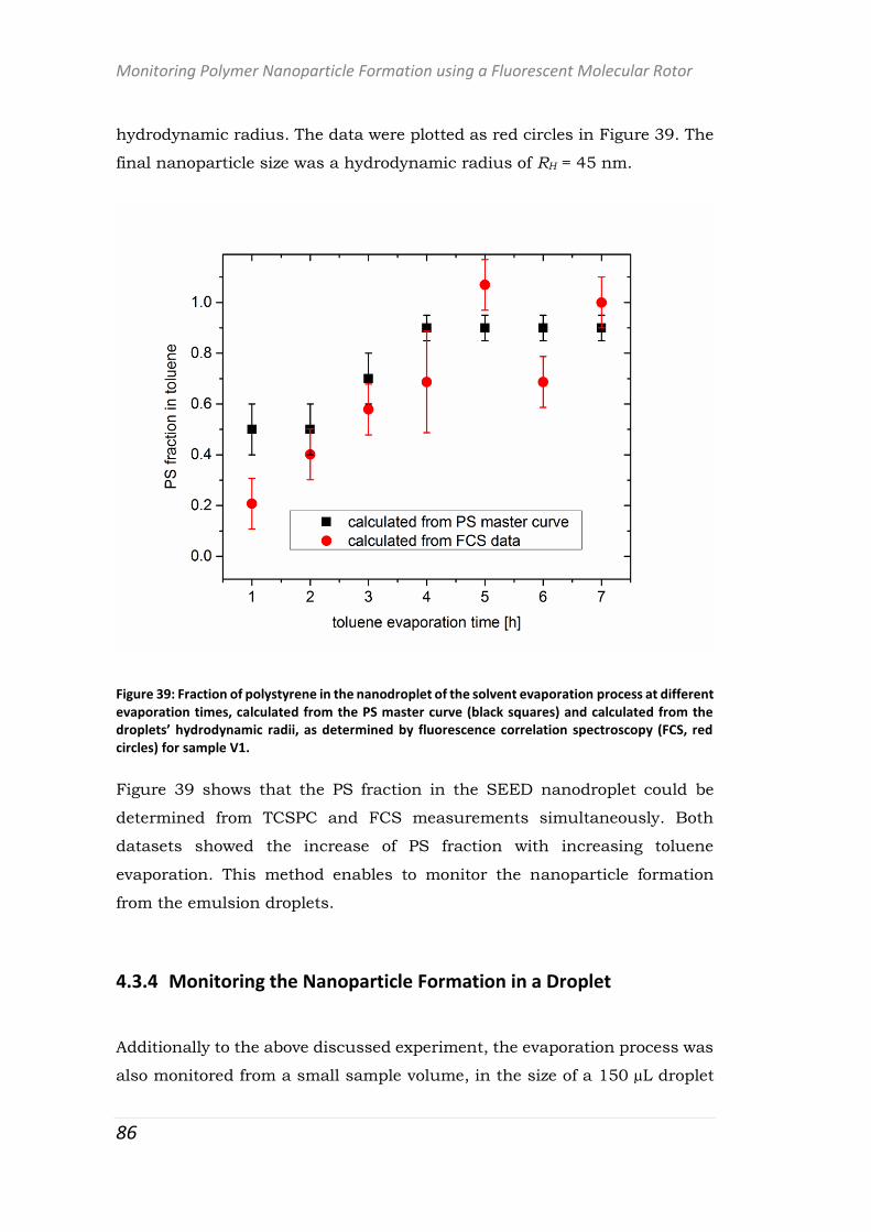
Monitoring Polymer Nanoparticle Formation using a Fluorescent Molecular Rotor
86
hydrodynamic radius. The data were plotted as red circles in Figure 39. The
final nanoparticle size was a hydrodynamic radius of RH = 45 nm.
Figure 39: Fraction of polystyrene in the nanodroplet of the solvent evaporation process at different evaporation times, calculated from the PS master curve (black squares) and calculated from the droplets’ hydrodynamic radii, as determined by fluorescence correlation spectroscopy (FCS, red circles) for sample V1.
Figure 39 shows that the PS fraction in the SEED nanodroplet could be
determined from TCSPC and FCS measurements simultaneously. Both
datasets showed the increase of PS fraction with increasing toluene
evaporation. This method enables to monitor the nanoparticle formation
from the emulsion droplets.
4.3.4 Monitoring the Nanoparticle Formation in a Droplet
Additionally to the above discussed experiment, the evaporation process was
also monitored from a small sample volume, in the size of a 150 µL droplet
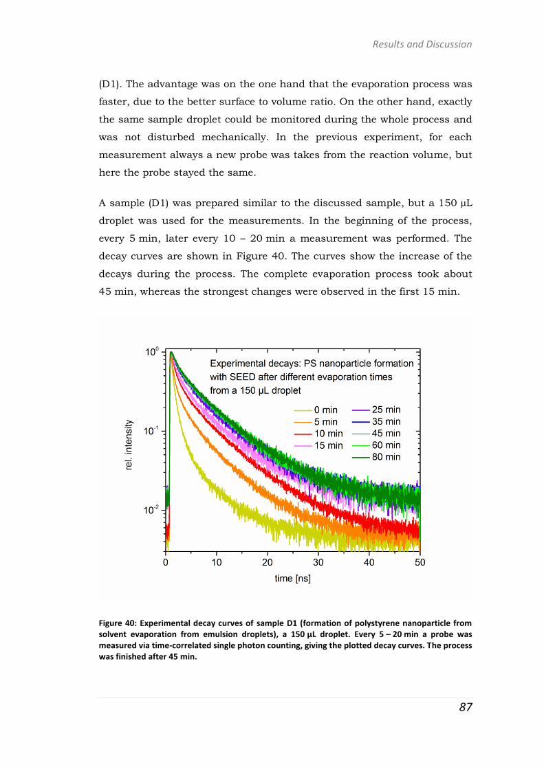
Results and Discussion
87
(D1). The advantage was on the one hand that the evaporation process was
faster, due to the better surface to volume ratio. On the other hand, exactly
the same sample droplet could be monitored during the whole process and
was not disturbed mechanically. In the previous experiment, for each
measurement always a new probe was takes from the reaction volume, but
here the probe stayed the same.
A sample (D1) was prepared similar to the discussed sample, but a 150 µL
droplet was used for the measurements. In the beginning of the process,
every 5 min, later every 10 – 20 min a measurement was performed. The
decay curves are shown in Figure 40. The curves show the increase of the
decays during the process. The complete evaporation process took about
45 min, whereas the strongest changes were observed in the first 15 min.
Figure 40: Experimental decay curves of sample D1 (formation of polystyrene nanoparticle from solvent evaporation from emulsion droplets), a 150 µL droplet. Every 5 – 20 min a probe was measured via time-correlated single photon counting, giving the plotted decay curves. The process was finished after 45 min.

Monitoring Polymer Nanoparticle Formation using a Fluorescent Molecular Rotor
88
From the decay curves the weighted average fluorescence lifetime were
calculated and plotted against the evaporation time. Figure 42 shows that
the obtained data were similar to the data from sample V1. The initial lifetime
was around 1 ns and increased to 5 ns in the final state of the evaporation
process. In a second experiment (D2) the findings were comparable to D1
and are shown in the appendix (Figure 52).
Figure 41: Weighted average fluorescence lifetimes at different toluene evaporation times from TCSPC measurements of sample D1.
To obtain information about the nanodroplets, the data points were
compared to the master curve and the PS fraction in the nanodroplet was
plotted against the toluene evaporation time. Again, the data showed that
the initial PS concentration in the droplet was around 50 %, as discussed for
sample V1. The increase of PS fraction during the evaporation process was
clearly observable. The final state of the process was again comparable to a
polystyrene fraction of 90 %. In this sample as well as in sample V1 the

Results and Discussion
89
fluorescence lifetime of the molecular rotor in pure polystyrene was not
reached.
Maybe it is just a question of the error of the measurements and calculations
or it might be possible that the complex SEED system influenced the
fluorescence lifetime. In case of the master curve, only the rotor dye, PS and
toluene were present. In the SEED samples, water and the surfactant SDS
were also present. It might be possible that their presence influenced the
rotors fluorescence lifetime. Sections 4.3.5, 4.3.6 and 4.3.7 focus on this
problem in more details.
Additional to the PS concentrations determined from the master curve the
obtained dataset were used for FCS autocorrelation to calculate the PS
concentration from the nanodroplet sizes.
Figure 42: Fraction of polystyrene in the nanodroplet of the solvent evaporation process at different evaporation times, calculated from the PS master curve (black squares) and calculated from the droplets’ hydrodynamic radii, as determined by fluorescence correlation spectroscopy (FCS, red circles) for sample D1.

Monitoring Polymer Nanoparticle Formation using a Fluorescent Molecular Rotor
90
The PS concentrations calculated from the master curve were in good
agreement with the PS concentrations calculated from the FCS data. The
final size of the nanoparticle was RH = 20 nm.
The presence of the molecular rotor LBX37 in the SEED process allowed
monitoring the shrinkage of the nanodroplets during the solvent evaporation
and therefore the formation of the nanoparticles. The actual evaporation
process started with a much lower solvent concentration as initially present
in the preparation process, which was most likely caused by the sonication
step. But the question why the final state of the process did not give a
fluorescence lifetime that is similar to the lifetime measured in pure PS was
still not clear.
4.3.5 Polystyrene Nanoparticles in Dry Environment
To exclude that the behavior of the fluorescent molecular rotor is different in
bulk PS compared to PS nanoparticles, the prepared nanoparticle
dispersions were dried and a thin film of solvent free PS nanoparticles was
measured. The obtained decay curve is depicted in Figure 43. The measured
data resulted in a fluorescence lifetime of τ = 5.4 ns. This value corresponded
to 100 % PS in the master curve.
Hence, it was clear, that the fluorescence lifetime of PS nanoparticles
prepared from solvent evaporation from emulsion droplets was not lower
than in bulk polystyrene. The experiment was repeated with four different
batches of polystyrene nanoparticles prepared from the SEED process. All
samples gave the same results.

Results and Discussion
91
Figure 43: Experimental decay curve (black) of the fluorescent molecular rotor LBX37 in PS nanoparticles prepared from SEED. The instrument response function (IRF) is shown in grey. The decay was fitted with a single exponential fit function (red), giving a fluorescence lifetime of τ = 5.4 ns. The lifetime is comparable to 100 PS in the master curve.
The nanoparticle formation by solvent evaporation can be monitored via
time-correlated single photon counting and fluorescence correlation
spectroscopy. The concentration change inside the nanodroplet as well as
the droplet shrinkage can be monitored. The experiment can either be
performed from a larger reaction volume or from a small droplet. Both
experiments show the same process behavior, but at different timescales.
4.3.6 Long Term Study of the Drying Process
Kinetic studies of the nanoparticle formation via solvent evaporation from
emulsion droplets showed a fluorescence lifetime of less than 5 ns. This
value was observed for studies from a large reaction volume as well as for
monitoring the process from a small reaction droplet. In comparison to the
master curve, the obtained fluorescence lifetime corresponded to a

Monitoring Polymer Nanoparticle Formation using a Fluorescent Molecular Rotor
92
polystyrene concentration of 90 %. But in the final state of the evaporation
process a PS nanoparticle and therefore 100 % PS were expected. From the
previous study of dried PS nanoparticle it was clear that the final SEED state
was different from the dry particles. So the question occurred whether the
SEED particles are really in their final state. The experiments showed that
the evaporation process was very slow in the last phase. To be sure that no
more toluene evaporateed after more than 24 h, one sample was measured
again after three months. The measurements gave exactly the same
fluorescence lifetimes values and amplitudes as obtained for the same
sample after 24 h of evaporation. Hence, the evaporation process was
completed in less than 24 h and no change was monitored after a longer time
interval.
So, the assumed short evaporation was not the reason for the final lifetime
in the SEED process that represented a PS concentration of 90 %.
4.3.7 Influence of SDS
As already mentioned it is possible that the presence of the surfactant SDS
played a role in the experiments. SDS was needed to stabilize the emulsion
and later the PS particle dispersion. The SDS molecules were present
everywhere in the aqueous solution. Mainly they were separating the PS
toluene emulsion droplets from the aqueous solution, but SDS could have
also been present in form of micelles. It could be possible that these micelles
encapsulated rotor molecules without polystyrene being present in the
micelles.
To investigate the hypothesis of the SDS influence, an experiment was
performed, in which a sample was prepared in the same way as it was done
for the SEED kinetic experiments, but without any polystyrene.
The aim was to monitor the behavior of the molecular rotor in SDS solutions.
After the evaporation of toluene (same procedure as done before), a decay
curve as shown in Figure 44 was obtained. The fluorescence lifetime was
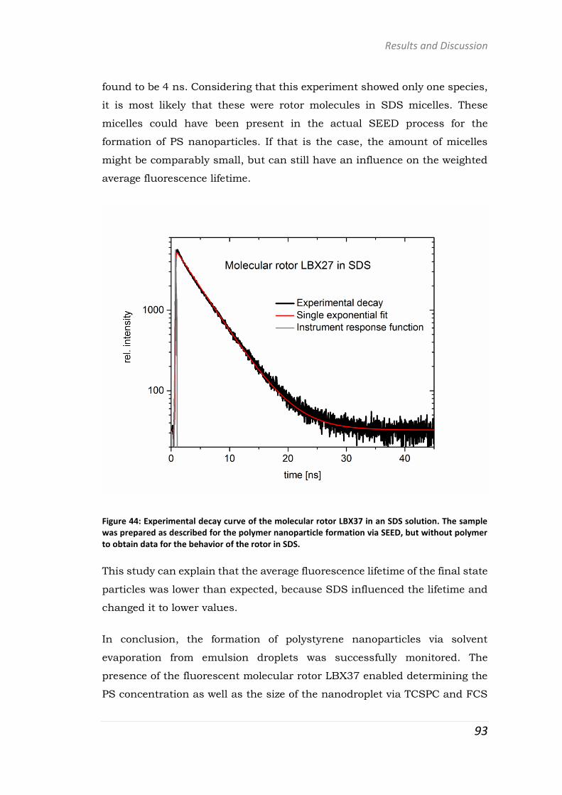
Results and Discussion
93
found to be 4 ns. Considering that this experiment showed only one species,
it is most likely that these were rotor molecules in SDS micelles. These
micelles could have been present in the actual SEED process for the
formation of PS nanoparticles. If that is the case, the amount of micelles
might be comparably small, but can still have an influence on the weighted
average fluorescence lifetime.
Figure 44: Experimental decay curve of the molecular rotor LBX37 in an SDS solution. The sample was prepared as described for the polymer nanoparticle formation via SEED, but without polymer to obtain data for the behavior of the rotor in SDS.
This study can explain that the average fluorescence lifetime of the final state
particles was lower than expected, because SDS influenced the lifetime and
changed it to lower values.
In conclusion, the formation of polystyrene nanoparticles via solvent
evaporation from emulsion droplets was successfully monitored. The
presence of the fluorescent molecular rotor LBX37 enabled determining the
PS concentration as well as the size of the nanodroplet via TCSPC and FCS

Monitoring Polymer Nanoparticle Formation using a Fluorescent Molecular Rotor
94
measurements. Both analysis techniques can be performed simultaneously,
giving comparable results. This method can be applied for samples from large
reactions volumes as well as for small volumes, such as single droplets. Since
the system is very complex, herein only the weighted average fluorescence
lifetimes were taken into account. But as the results show, the influence of
SDS, water or other factors can play a role. Therefore, the fluorescence
lifetimes need to be analyzed in more details to obtain even more information
about the drying process of the nanodroplet and the formation of the
nanoparticles. This analysis is very complex, but more than interesting as a
follow up project. Some initial studies are presented in the following.
4.3.8 A Closer Look Inside the Nanodroplets
In the previous experiments only the weighted average fluorescence lifetimes
of the samples were discussed. But, if the decay could not be fitted with a
single exponential fitting function, two or more fluorescence lifetimes were
present. These lifetimes as well as their fractions might give a closer look
inside the microenvironment and the nanoparticle formation process.
As an example, the short and long fluorescence lifetimes and amplitudes of
sample D1 are shown in Figure 45 and Figure 46. The values for the short
lifetimes increased from 0.6 ns to 2 ns with increasing toluene evaporation
time. These values were also found in the master curve for PS concentrations
up to 70 %. The long fluorescence lifetime increased from 4.3 ns up to 7.4 ns,
values that could not be found in the master curve. The weighted average
fluorescence lifetimes were suitable for comparisons to the master curve, but
the short and long lifetimes were not. Maybe the drying process influenced
the particle formation quite a lot.

Results and Discussion
95
Figure 45: Fluorescence lifetimes of sample D1. Blue triangles show the short fluorescence lifetime τ1 and orange stars resemble the long fluorescence lifetime τ2.
To get a better insight, a closer look to the amplitudes of both lifetimes can
be helpful. Figure 46 shows that the amplitudes of the short lifetime were
dominant in the first minutes of toluene evaporation, but the amplitudes for
the long lifetime increased and dominated the process in the final state.
Nevertheless, both lifetimes were present in the final state of the particle
formation. One hypothesis is that the particles were not homogeneous
particles, but they may have been dried in a capsule like shape. Maybe there
was an outer layer, or skin, that consisted of dry polystyrene, whereas inside
there was still a fraction of toluene present. Both microenvironments would
give different fluorescence lifetimes. Two different domains might also occur
for the molecular rotor from the interaction with PS and SDS molecules and
only with PS molecules.

Monitoring Polymer Nanoparticle Formation using a Fluorescent Molecular Rotor
96
Figure 46: Amplitudes of the fluorescence lifetimes of sample D1. Blue triangles show the amplitude A1 of the short fluorescence lifetime τ1 and orange stars resemble the amplitude A2 of the long fluorescence lifetime τ2.
4.3.9 Polystyrene Nanoparticles from SEED with Chloroform
Another interesting factor for investigating the nanodroplet drying behavior
is the solvent. Toluene as solvent for the nanoparticle formation was used
for several reasons, but mainly because it did not evaporate too fast at room
temperature, that measurements were possible in the time scale of the
evaporation process. But, to gain more information about the influence of
the solvent, the particle formation via SEED was also performed with
chloroform as solvent. Both ways, from a large reaction volume (CV1) and
from a single droplet (CD1) were tested. As an example the decay curves,
fluorescence lifetimes and amplitudes of the droplet sample CD1 are
presented and discussed in the following. Figure 47 presents the decay
curves for sample CD1 that shifted to longer times during the chloroform

Results and Discussion
97
evaporation. The behavior was similar to the samples made from toluene.
The data for the experiment from a large reaction volume CV1 are shown in
the appendix.
Figure 47: Experimental decay curves of sample CD1 (formation of polystyrene nanoparticle from solvent evaporation from emulsion droplets with chloroform as solvent), a 150 µL droplet. In appropriate time intervals a probe was measured via time-correlated single photon counting, giving the plotted decay curves. The process was finished after 44 min.
A closer look to the fluorescence lifetimes was made in Figure 48. The short,
long and weighted average fluorescence lifetimes were plotted against the
chloroform evaporation time. All three datasets showed a similar behavior.
In the first minutes of the evaporation process, the changes were small, but
within 15 min a strong change appeared. In this time range, the main
process has happened. After 44 min the complete process was in the final
state. If the lifetime values from Figure 48 were compared to the values
obtained from toluene samples, the datasets were similar and the
nanoparticle formation looked the same.

Monitoring Polymer Nanoparticle Formation using a Fluorescent Molecular Rotor
98
Figure 48: Fluorescence lifetimes of sample CD1. Blue triangles show the short fluorescence lifetime τ1, orange stars resemble the long fluorescence lifetime τ2 and black circles resemble the weighted average fluorescence lifetime τwa.
Looking at the amplitudes in Figure 49, the fast evaporation and the lifetime
change was observed, too. The short lifetime had a high amplitude in the
first minutes, but the fraction of the long lifetime increased drastically within
15 min, that showed the strong jump of the lifetimes. Herein, as well as in
the toluene samples, the final state of the nanoparticle formation showed a
long lifetime to short lifetime ratio of 6:4.

Results and Discussion
99
Figure 49: Amplitudes of the fluorescence lifetimes of sample CD1. Blue triangles show the amplitude A1 of the short fluorescence lifetime τ1 and orange stars resemble the amplitude A2 of the long fluorescence lifetime τ2.
In conclusion, the nanoparticle formation via solvent evaporation from
emulsion droplets can be monitored in the presence of different solvents,
such as toluene and chloroform and the obtained data show a similar
behavior of the fluorescence lifetimes and amplitudes of the molecular rotor.
Monitoring Polymer Nanoparticle Formation using a Fluorescent Molecular Rotor
100
4.4 Summary and Outlook
This project presents a different perspective in the field of polymer
nanoparticles, besides the preparation methods themselves or the possible
applications of the particles. Herein, the formation process of nanoparticles
was studied, to gain more information about the technique, in order to use
this process for the formation of nanoparticle drug delivery systems.
In this work, the nanoparticle formation of the SEED (solvent evaporation
from emulsion droplets) process was studied. With this method,
nanoparticles for drug delivery issues could be prepared. A deeper
understanding of the formation process, would enable easier formation of
new drug delivery systems. Polystyrene (PS) nanoparticles were prepared by
the evaporation of toluene from an emulsified system. This evaporation
process was monitored by adding a fluorescent molecular rotor to the
procedure. This rotor showed a fluorescence lifetime, which depends on the
microenvironment and mainly on the viscosity. Hence, the determination of
the lifetime, led to information about each stage in the process of
nanoparticle formation.
Experiments regarding the fluorescence lifetime of the rotor molecule in
different environments from pure toluene, various PS-toluene solutions and
pure PS, clearly showed the viscosity-dependent behavior. In a low viscosity
environment, as in toluene, the lifetime was 0.6 ns and increased with
increasing fraction of PS in the solutions until a fluorescence lifetime of
5.1 ns was reached in a pure PS film. The weighted average fluorescence
lifetimes of these samples formed the master curve for later determination of
the PS concentration.
To understand the particle formation during the evaporation process, the
weighted average fluorescence lifetimes were determined via TCSPC
measurements and with the help of the master curve the PS concentration

Summary and Outlook
101
in the nanodroplets was calculated. Hence, the method enabled the
determination of the stage of the particle formation process.
Additionally to the lifetime measurements, fluorescence correlation
spectroscopy (FCS) was used to investigate the size of the toluene-PS droplets
during the evaporation process. The hydrodynamic radius of the droplet was
calculated from the diffusion coefficients. FCS data showed a decreasing
droplet size from the beginning of the evaporation process until the final
particles size was reached. Furthermore, FCS data were used to determine
the PS concentrations in the nanodroplets, which were in good agreement to
the concentrations calculated from TCSPC experiments and the master
curve.
The presence of two fluorescence lifetimes in the particle formation process
has shown that the nanoparticles may form in an inhomogeneous way. It is
possible that a core-shell-like drying process was present in the SEED
nanoparticle formation procedure. Further investigations are necessary to
understand the process in more details.
Fluorescence molecular rotors are helpful molecules to monitor the
nanoparticle formation via SEED and give the possibility to understand the
evaporation process. Even though, this work gives just a first glance on what
is possible, further studies could be beneficial to understand the process
even more. An interesting aspect would be to investigate in much more
details, if the particles dry in a homogeneous way or if they end up more
heterogeneous, e.g. forming capsules. Therefore, the precise determination
of the fluorescence lifetimes from multi-exponential decays needs to be
improved further. Another interesting study could be to monitor the same
particle formation, but with another rotor molecule and compare the results.
Besides the SEED process for nanoparticle formation, there are many more
other ways. The investigation of these methods, such as miniemulsion
polymerization, would be beneficial to understand the ways to prepare
nanoparticles for drug delivery in a defined process.

Monitoring Polymer Nanoparticle Formation using a Fluorescent Molecular Rotor
102
4.5 Appendix – Additional Datasets
Additional data are presented in the figures and tables of this section.
Table 3: Fluorescence lifetimes, amplitudes and weighted average fluorescence lifetime data of the master curve (molecular rotor in different concentrations of polystyrene PS in toluene).
Fraction
PS in
toluene
Fluorescence
lifetime 1
τ1 in ns
Fluorescence
lifetime 2
τ2 in ns
Amplitude
of τ1
A1
Amplitude
of τ2
A2
Weighted
average fluorescence
lifetime
τwa in ns
0 0.60 - - - 0.60
0.1 0.60 3.0 0.997 0.003 0.61
0.2 0.62 3.5 0.995 0.006 0.63
0.3 0.69 3.3 0.982 0.018 0.74
0.4 0.75 3.6 0.973 0.028 0.83
0.5 0.93 3.5 0.923 0.077 1.11
0.6 1.20 3.7 0.84 0.16 1.60
0.63 1.13 3.4 0.85 0.15 1.64
0.65 1.50 4.0 0.70 0.30 2.25
0.7 1.58 4.3 0.68 0.32 2.42
0.73 1.91 4.9 0.27 0.73 3.36
0.8 2.03 4.5 0.45 0.55 3.07
0.85 2.20 5.0 0.25 0.75 4.30
0.89 3.20 5.6 0.28 0.72 4.93
0.9 3.00 5.2 0.20 0.80 4.76
1 - 5.1 - - 5.1

Appendix – Additional Datasets
103
Table 4: Fluorescence lifetimes, amplitudes and weighted average fluorescence lifetime data sample V1 (SEED of PS toluene nanodroplets – large reaction volume).
Toluene evapo-
ration
time
t in h
Fluorescence
lifetime 1
τ1 in ns
Fluorescence
lifetime 2
τ2 in ns
Amplitude
of τ1
A1
Amplitude
of τ2
A2
Weighted average
fluorescence
lifetime
τwa in ns
1 0.797 5.10 0.92 0.08 1.16
2 0.801 5.20 0.92 0.08 1.16
3 1.22 6.04 0.80 0.20 2.19
4 1.55 6.91 0.45 0.55 4.52
5 1.52 6.92 0.45 0.55 4.50
6 1.53 6.92 0.46 0.54 4.47
7 1.58 6.93 0.44 0.56 4.57
Figure 50: Sample V2 – SEED of polystyrene toluene nanodroplets. Left: Experimental decay curves measured via TCSPC at different time intervals of the evaporation process. Right: Weighted average fluorescence lifetimes, obtained from the experimental decays.
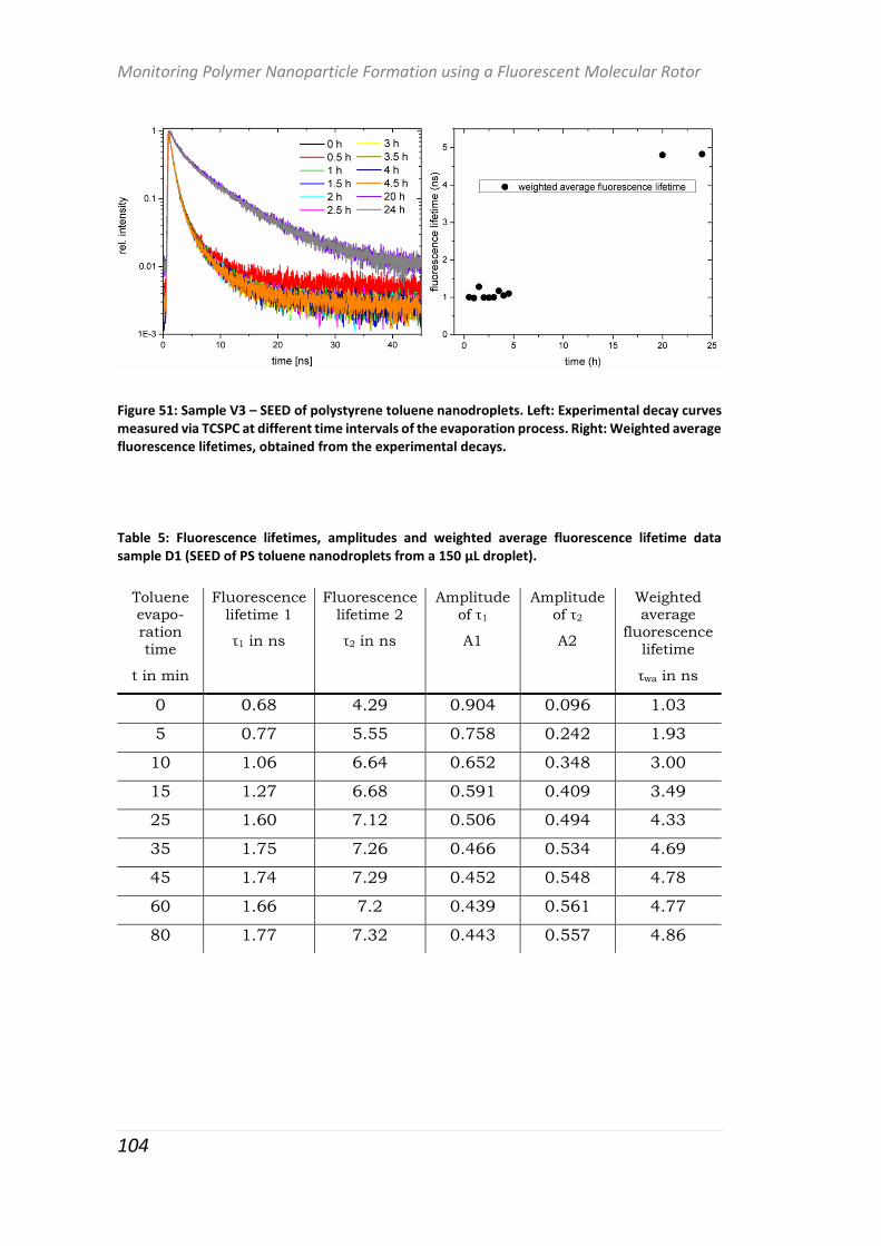
Monitoring Polymer Nanoparticle Formation using a Fluorescent Molecular Rotor
104
Figure 51: Sample V3 – SEED of polystyrene toluene nanodroplets. Left: Experimental decay curves measured via TCSPC at different time intervals of the evaporation process. Right: Weighted average fluorescence lifetimes, obtained from the experimental decays.
Table 5: Fluorescence lifetimes, amplitudes and weighted average fluorescence lifetime data sample D1 (SEED of PS toluene nanodroplets from a 150 µL droplet).
Toluene evapo-
ration
time
t in min
Fluorescence
lifetime 1
τ1 in ns
Fluorescence
lifetime 2
τ2 in ns
Amplitude
of τ1
A1
Amplitude
of τ2
A2
Weighted average
fluorescence
lifetime
τwa in ns
0 0.68 4.29 0.904 0.096 1.03
5 0.77 5.55 0.758 0.242 1.93
10 1.06 6.64 0.652 0.348 3.00
15 1.27 6.68 0.591 0.409 3.49
25 1.60 7.12 0.506 0.494 4.33
35 1.75 7.26 0.466 0.534 4.69
45 1.74 7.29 0.452 0.548 4.78
60 1.66 7.2 0.439 0.561 4.77
80 1.77 7.32 0.443 0.557 4.86
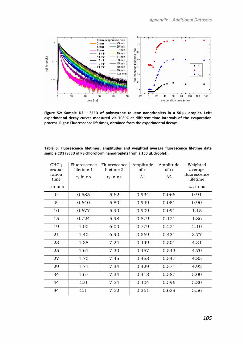
Appendix – Additional Datasets
105
Figure 52: Sample D2 – SEED of polystyrene toluene nanodroplets in a 50 µL droplet. Left: experimental decay curves measured via TCSPC at different time intervals of the evaporation process. Right: Fluorescence lifetimes, obtained from the experimental decays.
Table 6: Fluorescence lifetimes, amplitudes and weighted average fluorescence lifetime data sample CD1 (SEED of PS chloroform nanodroplets from a 150 µL droplet).
CHCl3 evapo-
ration
time
t in min
Fluorescence
lifetime 1
τ1 in ns
Fluorescence
lifetime 2
τ2 in ns
Amplitude
of τ1
A1
Amplitude
of τ2
A2
Weighted average
fluorescence
lifetime
τwa in ns
0 0.585 5.62 0.934 0.066 0.91
5 0.640 5.80 0.949 0.051 0.90
10 0.677 5.90 0.909 0.091 1.15
15 0.724 5.98 0.879 0.121 1.36
19 1.00 6.00 0.779 0.221 2.10
21 1.40 6.90 0.569 0.431 3.77
23 1.38 7.24 0.499 0.501 4.31
25 1.61 7.30 0.457 0.543 4.70
27 1.70 7.45 0.453 0.547 4.85
29 1.71 7.34 0.429 0.571 4.92
34 1.67 7.34 0.413 0.587 5.00
44 2.0 7.54 0.404 0.596 5.30
94 2.1 7.52 0.361 0.639 5.56

Monitoring Polymer Nanoparticle Formation using a Fluorescent Molecular Rotor
106
Figure 53: Sample CV1 – SEED of polystyrene chloroform nanodroplets from a large reaction volume. Left: Experimental decay curves measured via TCSPC at different time intervals of the evaporation process. Right: Fluorescence lifetimes, obtained from the experimental decays.

107
5 Concluding Remarks
In this thesis, two different methods which were dealing with drug delivery
systems were presented. The first method represents a newly developed
technique to prepare uniform and size-defined cell membrane models,
whereas the second method facilitates to monitor and understand the
preparation of nanoparticles. The main commonality of both methods
besides the application for drug delivery systems is the usage of fluorescent
molecules and fluorescence based methods.
A new method for the preparation of biological cell models was developed in
the first part of this work. The huge variety of different kinds of cell
membrane models that were already in use for many years was improved by
this new technique, which enables to form giant unilamellar vesicles as cell
models in a size-defined way. Three different diameters were presented in
this work, all of them in size dimensions of biological cells. The vesicle
formation was realized using a polymer hydrogel template that was micro-
patterned via photolithography. The very defined composition of the polymer
hydrogel, its cross-linking and swelling behavior were investigated and
resulted in an ideal template for growing hundreds of vesicles on one
template. The research on biological cells won’t stop in the near future,
because cells are our smallest living building units and researchers want to
understand their properties and functions, especially in the field of drug
delivery systems. New systems can overcome old and new diseases.
Hopefully, this method will help to understand the functions of biological
cells and cell membranes a bit more.
As just said, the field of drug delivery systems is huge and promising to fight
against certain diseases. The second part of this work focused on the
formation of nanoparticles which can be used as drug carriers. Polystyrene
as a cheap and well known polymer is often used in this regard, because it

Concluding Remarks
108
is biocompatible. The precise formation of the nanoparticles is essential for
the formation of very defined drug delivery systems. To understand the
formation of polystyrene nanoparticles, their preparation via solvent
evaporation from emulsion droplets was monitored. Even though, the here
presented method is still in the beginning of its development, it can be very
helpful to understand and tune the formation process depending on the
desired properties of the nanoparticles.
The whole work is based on polymer systems. Polymers are versatile and
have their use and applications in various disciplines and research fields.
Herein, two completely different polymer systems were studied. The first
system was based on a terpolymer, whose monomer units were statistically
distributed. It contained a special unit, which was activated by UV light and
cross-linked the polymer chains to a covalently bound network. Additionally
this network was able to absorb water, because it served as hydrogel. A
completely different polymer system – polymer nanoparticles – were studied
in the second project. Polymer nanoparticles are interesting systems,
because their properties differ from their bulk systems, due to their very
small sizes. And besides the two polymer systems that were investigated in
this thesis, many other types of polymer systems exist and are worth to
study. The manifoldness of polymers, their combinations, functionalities and
properties will provide the fundaments of polymer research for many more
decades.

109
6 FCS Analysis of Polymer-Based Systems - Cooperative Projects
Fluorescence correlation spectroscopy (FCS) is a unique tool, that is used in
many scientific disciplines. In this chapter, the manifold usage of FCS in
different collaborative projects, is shown. In cooperation with the
collaborative research center (CRC) 1066 – “Nanodimensional polymer
therapeutics for tumor therapy” – and as the work of the Q2 project
(Querschnittsprojekt – cross section project) – “Optical methods to study
endocytosis, intracellular trafficking and cargo release” – FCS was used to
determine the diffusion time and coefficient as well as the hydrodynamic
radius of different (mainly polymeric) species. Specific functionalizations,
conjugations and coatings were characterized and confirmed. Investigating
the formations of aggregates and determining the labeling efficiency are more
experiments, which can be performed using FCS.
A cooperative project with M. Schinnerer (JGU Mainz, manuscript in
preparation) focuses on a polymer brush based system for tumor immune
therapy. With FCS the size of the molecules was determined and the absence
of aggregates and free fluorescent dyes in the system was ensured.
Furthermore, the number of dyes per brush and the number of conjugated
antibodies per polymer brush was calculated from the fluorescence
brightness of the freely diffusing dye or antibody and the polymer brush.
Fluorescence cross-correlation spectroscopy (FCCS) was used in some of the
collaborative projects. The main difference to FCS is the usage of two
differently colored fluorescent molecules, instead of one. Both dyes have an
individual beam path, but an overlapping confocal volume. If both dye-
molecules are diffusing together, both intensity fluctuations correlate,
leading to a cross-correlation curve.

FCS Analysis of Polymer-Based Systems - Cooperative Projects
110
6.1 Fluorescence Correlation Spectroscopy (FCS) Characterizes Antibody-Polyplex-Conjugates for Cell Targeting
The chemical attachment of DEC205 antibodies to polyplexes was
investigated in this work. The DEC205 antibody is specific for targeting
dendritic immune cells (DCs) and thus interesting for cancer immune
therapy. Azide-containing block copolymers P(Lys)-b-P(HPMA) were used for
the complexation of plasmid-DNA (pDNA). The conjugation of the block
copolymer and the antibody was performed using strain-promoted alkyne-
azide cycloaddition (SPAAC). Dibenzocyclooctyne (DBCO) moieties were
incorporated site-specific to the DEC205 antibody. The chemical
accessibility of DBCO molecules within the antibody and the accessibility of
azide-functionalities on the surface of the polyplex were characterized by
fluorescence correlation spectroscopy.
Figure 54: Left: Experimental FCS autocorrelation curves for the azide-dye (CR-110-N3) and the DBCO-modified DEC205 antibody. The shift of the correlation curve indicated slower diffusion and confirmed that the azide-dye was covalently attached to the antibody. Right: Experimental autocorrelation curves of the DBCO-dye (AF647-DBCO) and the azide-functionalized polyplex. The shift towards longer diffusion times confirmed the addition of DBCO-dye to the azide-functionalized polyplex.
111
The experimental autocorrelation curves are shown in Figure 54: On the left,
the DBCO functionalization of the DEC205 antibody was confirmed by the
successful SPAAC of an azide-containing fluorescent dye. Furthermore, the
conjugation of a DBCO-dye to the azide-functionalized polyplex is shown on
the right side of Figure 54. The measurements show the general accessibility
of the azide functionalities on the polyplex’ surface. The reaction of DBCO-
functionalized DEC205 antibody with the azide functionalized polyplex was
also studied via FCS. The measurements showed the successful SPAAC
reaction, but a huge amount of non-conjugated antibody remained.
FCS was an ideal method to characterize SPAAC reactions of macromolecules
with small amounts of reactive groups by determining the size increase of
the fluorescent species resulting from the performed conjugation reaction.
This work presents the concept of the functionalization of nanoparticles with
antibodies with site-specific DBCO-modifications.
This work was published in Polymers (2018, 10, 141), entitled ”Site-Specific
DBCO Modification of DEC205 Antibody for Polymer Conjugation” as joint
project of the CRC1066 together with S. Beck, H.-J. Räder, R. Holm, M.
Schinnerer, M. Barz, K. Koynov and R. Zentel.

FCS Analysis of Polymer-Based Systems - Cooperative Projects
112
6.2 Fluorescence Correlation Spectroscopy Confirms Successful Coating of Dendritic Mesoporous Silica Nanoparticles (DMSN) with a pH-Responsive Block Copolymer for Drug Delivery
This project focused on a new drug delivery system for the tumor necrosis
factor-alpha (TNF-), a highly toxic drug used in cancer therapy. Herein,
dendritic mesoporous silica nanoparticles (DMSN) were coated with a pH-
responsive block copolymer gate system. The system combined charged
hyperbranched polyethylenimine (PEI) and nonionic hydrophilic
polyethylenglycol (PEG) to encapsulate and deliver TNF- into cancer and
dendritic cells. FCS was used to confirm that the nanoparticles were coated
with the pH-responsive block copolymer.
Figure 55: FCS autocorrelation curve of the free rhodamine B (black squares), RhB-labeled PEI-PEG (red circles), and the coated DMSN (blue triangles). The shift of the curves towards slower diffusion times and the resulting hydrodynamic radius Rh of 115 nm for the coated DMSN demonstrates successful functionalization with the gatekeeper.
Figure 55 shows the autocorrelation curves of freely diffusing rhodamine B
(RhB, black squares), rhodamine B labeled block copolymer PEI-PEG (red
113
circles) and the PEI-PEG coated DMSN (blue triangles). The shift towards
longer diffusion times indicated a significant change in the size of the
diffusing species. The shift of the autocorrelation curve for DMSN towards
longer diffusion times confirmed the successful coating with the polymer.
DMSN encapsulation with pH-sensitive PEI-PEG is a promising approach
drug delivery in cancer therapy.
This work was published in Advanced Healthcare Materials (2017, 1700012),
entitled ”Dendritic Mesoporous Silica Nanoparticles for pH-Stimuli-
Responsive Drug Delivery of TNF-Alpha” as joint project of the CRC1066
together with A. Kienzle, S. Kurch, J. Schlöder, C. Berges, R. Ose, J. Schupp,
A. Tuettenberg, H. Weiss, S. Winzen, M. Schinnerer, K. Koynov, M. Mezger,
N. K. Haass, W. Tremel and H. Jonuleit.
In a second cooperative project (manuscript in preparation), the dendritic
mesoporous silica nanoparticles (DMSNs) were coated with ferrocene-
carboxyaldehyde and fluorescence cross-correlation spectroscopy was used
to confirm the in situ coordination of a cyclodextrine sugar cap to the
ferrocene moiety on the DMSNs. The aim was to seal a small molecule for
drug delivery into the DMSN with the help of the sugar cap.

FCS Analysis of Polymer-Based Systems - Cooperative Projects
114
6.3 Fluorescence Cross-Correlation Spectroscopy (FCCS) Verifies the Functionalization of Dual Labeled Block Copolymers
This project introduced a new synthetic approach for trifunctional block
copolymers that enable site-specific conversion of the reactive entities in one
step. Herein, polysarcosine-block-poly(S-alkylsulfonyl)-L-cysteine (PSar-b-
PCys(SO2Et)) block copolymers self-assembled into core-shell
nanostructures. The hydrophilic moiety was labeled with a DBCO-CR110 dye
and the hydrophobic part with a Cy5-NHS dye to confirm the simultaneous
functionalization of the reactive groups. The dual labeled core-cross-linked
particles were analyze by fluorescence cross-correlation spectroscopy
(FCCS). The advantage of FCCS is that both fluorescent dyes are exited
simultaneously with two different lasers. Their diffusion is recorded as in
conventional FCS experiments and the autocorrelation curves of both dyes
are cross-correlated to confirm the joint diffusion of the dyes, when they are
attached to the same molecule.
Figure 56: Left: Polysarcosine-block-poly(S-alkylsulfonyl)-L-cysteine block copolymer was self-assembled to a micelle with Cy5-NHS dyes in the core and DBCO-CR110 dyes in the corona. Right: FCCS auto- and cross-correlation curves of the dual labeled particles show strong cross-correlation, confirming dual labeling.
The FCCS experiment confirmed the simultaneous functionalization of the
core and the corona of the polymer micelle. The amplitude of the cross-
115
correlation curve (black triangles) is comparable to the amplitudes of the
autocorrelation curves, implying that both dyes were attached to the core-
cross-linked micelle. The PSar-b-PCys(SO2Et) block copolymers showed
independently addressable and spatially separated functional groups,
enabling simultaneous functionalization of the core and the shell. In a single
step, active targets and fluorophores for detection can be introduced in the
block copolymer micelles.
This work was published in ACS Macro Letters (2017, 6, 1140−1145), entitled
”Combining Orthogonal Reactive Groups in Block Copolymers for Functional
Nanoparticle Synthesis in a Single Step” as joint project of the CRC1066
together with O. Schäfer, K. Klinker, L. Braun, D. Huesmann, K. Koynov and
M. Barz.
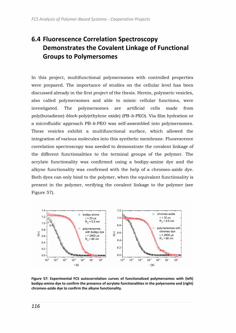
FCS Analysis of Polymer-Based Systems - Cooperative Projects
116
6.4 Fluorescence Correlation Spectroscopy Demonstrates the Covalent Linkage of Functional Groups to Polymersomes
In this project, multifunctional polymersomes with controlled properties
were prepared. The importance of studies on the cellular level has been
discussed already in the first project of the thesis. Herein, polymeric vesicles,
also called polymersomes and able to mimic cellular functions, were
investigated. The polymersomes are artificial cells made from
poly(butadiene)-block-poly(ethylene oxide) (PB-b-PEO). Via film hydration or
a microfluidic approach PB-b-PEO was self-assembled into polymersomes.
These vesicles exhibit a multifunctional surface, which allowed the
integration of various molecules into this synthetic membrane. Fluorescence
correlation spectroscopy was needed to demonstrate the covalent linkage of
the different functionalities to the terminal groups of the polymer. The
acrylate functionality was confirmed using a bodipy-amine dye and the
alkyne functionality was confirmed with the help of a chromeo-azide dye.
Both dyes can only bind to the polymer, when the equivalent functionality is
present in the polymer, verifying the covalent linkage to the polymer (see
Figure 57).
Figure 57: Experimental FCS autocorrelation curves of functionalized polymersomes with (left) bodipy-amine dye to confirm the presence of acrylate functionalities in the polyersome and (right) chromeo-azide dye to confirm the alkyne functionality.

117
For both dye labeled polymersomes the autocorrelation curves, generated
from FCS experiments, were delayed compared to the freely diffusing dyes,
confirming the attachment of the dyes to the larger species which diffuses
much slower. Fitting with a single component model function showed that
only one species was present and that the dye molecules were completely
attached to the polymer (no free dye was present in the polymer and
polymersomes). From the experiments the diffusion times and the
hydrodynamic radii were obtained.
This work was published in Soft Matter (2017, 14, 6, 894-900), entitled ”A
modular approach for multifunctional polymersomes with controlled
adhesive properties” as joint project together with J. Petit, L. Thomi, M.
Makowski, I. Negwer, K. Koynov, S. Herminghaus, F. Wurm, O.Bäumchen
and K. Landfester.

FCS Analysis of Polymer-Based Systems - Cooperative Projects
118
6.5 Fluorescence Correlation Spectroscopy Determines the Critical Micelle Concentration
Fluorescence correlation spectroscopy can be used in many different
research fields. Herein, FCS helps to investigate the dewetting dynamics of
surfactant solutions. To understand the correlation between the dewetting
dynamics and the surfactant properties, low and high molecular weight
surfactants were compared. As high molecular weight surfactant a PEO-
PPO-PEO triblock copolymer, also called Pluronic F-127, was used for this
work.
Figure 58: Left: Experimental FCS autocorrelation curves for rhodamine 6G in Pluronic F-127 sultions of different concentrations. Right: Hydrodynamic radii of rhodamine 6G at different surfactant concentrations. The hydrodynamic radius is the same as in water for surfactant concentrations up to 100 µM. The radius is larger at concentrations above CMC, because the dye molecules are encapsulated in surfactant micelles, which are larger and diffuse slower.
With FCS, the surfactant concentration was determined, at which the
surfactant forms aggregates. Therefore, the weakly hydrophobic fluorescent
dye rhodamine 6G was added to the Pluronic F-127 solution. The
hydrodynamic radius of the dye was measured at different surfactant
concentrations. The experimental autocorrelation curves and the
hydrodynamic radii are shown in Figure 58. At low surfactant concentrations
(0.1 – 100 µM) the hydrodynamic radius is identical to the one from
rhodamine 6G (RH = 0.55 nm). Above the critical micelle concentration,
resembled with the 2 mM sample, the fluorescent dye became incorporated

119
into the surfactant micelle and the hydrodynamic radius increased to the
size of a Pluronic F-127 micelle.
FCS was used to determine the behavior of the surfactant Pluronic F-127
below and above the critical micelle concentration to understand the
dewetting dynamics of the surfactant.
This work was published in Colloids and Surfaces A: Physicochemical and
Engineering Aspects (2017, 30–37), entitled ”Forced dewetting dynamics of
high molecular weight surfactant solutions” as joint project together with D.
Truszkowska, F. Henrich, K. Koynov, H. J. Räder, H.-J. Butt and G. K.
Auernhammer.

FCS Analysis of Polymer-Based Systems - Cooperative Projects
120
6.6 Fluorescence Correlation Spectroscopy Studies of Molecular Tracer Diffusion
The diffusion dynamics of molecular tracers in polymer networks was
studied by fluorescence correlation spectroscopy. To understand the polymer
tracer interactions, the tracer diffusion was measured at different molecular
weights, various polymer architectures and different polymer concentrations
for three polymers: polydimethylsiloxane (PDMS), polystyrene (PS) and
polybutadiene (PB). The diffusion slowdown of the tracer is expressed as
D(c)/D0 (D0 is the diffusion coefficient of the tracer) and plotted against the
concentration, see Figure 59. The experiments gave polymer-specific master
curves, which are independent of the molecular weight and independent of
the polymer architectures.
Figure 59: Normalized diffusion slowdown D(c)/D0 vs concentration of a molecular tracer. Linear PS at different molecular weights has black symbols. Black pentagons present PS combs. Linear PB is shown at two different molecular weights (PB 170 kg/mol: blue stars and PB 52 kg/mol: blue pentagons) and star PB at different molecular weights (PB 30 kg/mol: double-crossed blue symbols, PB 500 g/mol: blue triangles, PB 80 kg/mol: blue circles, PB 4.4 kg/mol: blue squares). The diffusion slowdown data for the tracer in linear PDMS (Mw = 60 kg/mol) are depicted by the grey squares. The solid black, blue and grey lines through the data represent the corresponding master curves.

121
Understanding the tracer diffusion in polymer systems helps to improve
applications, such as drug delivery, chromatography or hydrogel-based
sensors, in which tracers are needed.
This work was published in Macromolecules (2015, 48, 8907−8912), entitled
”Molecular Tracer Diffusion in Nondilute Polymer Solutions: Universal
Master Curve and Glass Transition Effects” as joint project together with A.
Vagias, M. Doroshenko, K. Koynov, H.-J. Butt, M. Gauthier, G. Fytas and D.
Vlassopoulos.


123
7 Bibliography
[1] Y. Zhang, H. F. Chan, K. W. Leong, Adv. Drug Deliv. Rev. 2013, 65,
104–120.
[2] C. S. P. Nikam A.P., Mukesh P., R., Int. J. Res. Dev.Pharm. L. Sci. 2014,
3, 1121–1127.
[3] V. Mohanraj, Y. Chen, M. & Chen, Trop. J. Pharm. Res. Trop J Pharm
Res 2006, 5, 561–573.
[4] S. Hasan, Res. J. Recent Sci. 2015, 4, 1–3.
[5] O. Salata, J. Nanobiotechnology 2004, 2, 3.
[6] R. Singh, J. W. Lillard, Exp. Mol. Pathol. 2009, 86, 215–223.
[7] A. H. Faraji, P. Wipf, Bioorganic Med. Chem. 2009, 17, 2950–2962.
[8] L. Nuhn, L. Braun, I. Overhoff, A. Kelsch, D. Schaeffel, K. Koynov, R.
Zentel, Macromol. Rapid Commun. 2014, 35, 2057–2064.
[9] L. Nuhn, M. Hirsch, B. Krieg, K. Koynov, K. Fischer, M. Schmidt, M.
Helm, R. Zentel, ACS Nano 2012, 6, 2198–2214.
[10] B. Mishra, B. B. Patel, S. Tiwari, Nanomedicine Nanotechnology, Biol.
Med. 2010, 6, 9–24.
[11] K. Tappertzhofen, M. Bednarczyk, K. Koynov, M. Bros, S. Grabbe, R.
Zentel, Macromol. Biosci. 2014, 14, 1444–1457.

Bibliography
124
[12] I. Tabujew, C. Freidel, B. Krieg, M. Helm, K. Koynov, K. Müllen, K.
Peneva, Macromol. Rapid Commun. 2014, 35, 1191–1197.
[13] T. Fritz, M. Voigt, M. Worm, I. Negwer, S. S. Müller, K. Kettenbach, T.
L. Ross, F. Roesch, K. Koynov, H. Frey, et al., Chem. - A Eur. J. 2016,
22, 11578–11582.
[14] M. A. Hood, U. Paiphansiri, D. Schaeffel, K. Koynov, M. Kappl, K.
Landfester, R. Muñoz-Espí, Chem. Mater. 2015, 27, 4311–4318.
[15] J. R. Lakowicz, Principles of Fluorescence Spectroscopy, Springer, New
York, 2006.
[16] W. Becker, Advanced Time-Correlated Single Photon Counting
Techniques, Springer, Berlin, Heidelberg, New York, 2005.
[17] Thermo Fisher Scientific, “Alexa Fluor Dyes—Across the Spectrum,”
can be found under:
https://www.thermofisher.com/de/de/home/brands/molecular-
probes/key-molecular-probes-products/alexa-fluor/alexa-fluor-dyes-
across-the-spectrum.html, 2018.
[18] W. L. Goh, M. Y. Lee, T. L. Joseph, S. T. Quah, C. J. Brown, C. Verma,
S. Brenner, F. J. Ghadessy, Y. N. Teo, J. Am. Chem. Soc. 2014, 136,
6159–6162.
[19] M. A. Haidekker, E. A. Theodorakis, J. Biol. Eng. 2010, 4, 11.
[20] M. A. Haidekker, M. Nipper, A. Mustafic, D. Lichlyter, M. Dakanali, E.
A. Theodorakis, Advanced Fluorescence Reporters in Chemistry and
Biology I: Fundamental and Molecular Design, Springer, Berlin
Heidelberg, 2010.
[21] M. A. Haidekker, T. P. Brady, D. Lichlyter, E. A. Theodorakis, Bioorg.
Chem. 2005, 33, 415–425.

125
[22] F. Zhou, J. Shao, Y. Yang, J. Zhao, H. Guo, X. Li, S. Ji, Z. Zhang,
European J. Org. Chem. 2011, 4773–4787.
[23] N. Amdursky, Y. Erez, D. Huppert, Acc. Chem. Res. 2012, 45, 1548–
1557.
[24] T. Atsbeha, A. M. Mohammed, M. Redi-Abshiro, J. Fluoresc. 2010, 20,
1241–1248.
[25] M. A. Haidekker, T. Ling, M. Anglo, H. Y. Stevens, J. A. Frangos, E. A.
Theodorakis, Chem. Biol. 2001, 8, 123–131.
[26] R. Ramadass, J. Bereiter-Hahn, J. Phys. Chem. B 2007, 111, 7681–
7690.
[27] G. Vaccaro, A. Bianchi, M. Mauri, S. Bonetti, F. Meinardi, A.
Sanguineti, R. Simonutti, L. Beverina, Chem. Commun. 2013, 49,
8474–8476.
[28] S. Sawada, T. Iio, Y. Hayashi, S. Takahashi, Anal. Biochem. 1992, 204,
110–117.
[29] M. Wahl, PicoQuant Tech. Note 2014, 1–14.
[30] PicoQuant GmbH, 8th European Short Course in “Time-Resolved
Microscopy and Correlation Spectroscopy,” Berlin, 2016.
[31] S. W. Paddock, Biotechniques 1999, 27, 992–1004.
[32] M. Minsky, Scanning 1988, 10, 128–138.
[33] R. H. Webb, Reports Prog. Phys. 1999, 59, 427–471.
[34] M. D. DB. Murphy, in Fundam. Light Microsc. Electron. Imaging, 2012,
pp. 265–305.
[35] O. Krichevsky, G. Bonnet, Rep. Prog. Phys 2002, 65, 251–297.

Bibliography
126
[36] P. Schwille, J. Bieschke, F. Oehlenschläger, Biophys. Chem. 1997, 66,
211–228.
[37] R. Rigler, E. S. Elson, Fluorescence Correlation Spectroscopy: Theory
and Applications, Springer, Berlin Heidelberg New Vork, 2011.
[38] D. Magde, E. L. Elson, W. W. Webb, Phys. Rev. Lett. 1972, 29, 705–
708.
[39] D. Magde, E. L. Elson, W. W. Webb, Biopolymers 1974, 13, 29–61.
[40] E. L. Elson, Biophys. J. 2011, 101, 2855–2870.
[41] E. L. Elson, D. Magde, Biopolymers 1974, 13, 1–27.
[42] P. Schwille, Cell Biochem. Biophys. 2001, 34, 383–408.
[43] P. Schwille, E. Haustein, Fluorescence Correlation Spectroscopy An
Introduction to Its Concepts and Applications, 2009.
[44] A. J. García-Sáez, P. Schwille, Methods 2008, 46, 116–122.
[45] S. Chiantia, J. Ries, P. Schwille, Biochim. Biophys. Acta - Biomembr.
2009, 1788, 225–233.
[46] K. Koynov, H.-J. Butt, Curr. Opin. Colloid Interface Sci. 2012, 17, 377–
387.
[47] E. Bianconi, A. Piovesan, F. Facchin, A. Beraudi, R. Casadei, F.
Frabetti, L. Vitale, M. C. Pelleri, S. Tassani, F. Piva, et al., Ann. Hum.
Biol. 2013, 40, 463–71.
[48] B. Alberts, A. Johnson, J. Lewis, M. Raff, K. Roberts, P. Walter, in Mol.
Biol. Cell, Garland Science, New York, 2002.
[49] P. Yeagle, The Membranes of Cells, Elsevier, 1993.
127
[50] Y.-H. M. Chan, S. G. Boxer, Curr. Opin. Chem. Biol. 2007, 11, 581–
587.
[51] A. D. Bangham, M. M. Standish, J. C. Watkins, J. Mol. Biol. 1965, 13,
238–252.
[52] S. F. Fenz, K. Sengupta, Integr. Biol. 2012, 4, 982–995.
[53] J. H. Fendler, Membrane Mimetic Chemistry, Wiley, New York, 1982.
[54] H. T. Tien, S. Carbone, E. A. Dawidowicz, Nature 1966, 212, 718–719.
[55] M. Winterhalter, Curr. Opin. Colloid Interface Sci. 2000, 5, 250–255.
[56] L. K. Tamm, H. M. McConnell, Biophys. J. 1985, 47, 105–113.
[57] P. Walde, K. Cosentino, H. Engel, P. Stano, ChemBioChem 2010, 11,
848–865.
[58] O. Wesołowska, K. Michalak, J. Maniewska, A. B. Hendrich, Acta
Biochim. Pol. 2009, 56, 33–39.
[59] A. Weinberger, F.-C. C. Tsai, G. H. H. Koenderink, T. F. F. Schmidt, R.
Itri, W. Meier, T. Schmatko, A. Schroder, C. Marques, A. Schröder, et
al., Biophys. J. 2013, 105, 154–164.
[60] A. Jesorka, M. Markstro, O. Orwar, Langmuir 2005, 21, 1230–1237.
[61] K. Karamdad, R. V. Law, J. M. Seddon, N. J. Brooks, O. Ces, Lab Chip
2015, 15, 557–562.
[62] E. B. Working, A. C. Andrews, Chem. Rev. 1941, 29, 245–256.
[63] J. Berg, J. Tymoczko, L. Stryer, in Biochemistry, W H Freeman, New
York, 2002.
[64] B. R. Lentz, Prog. Lipid Res. 2003, 42, 423–438.
Bibliography
128
[65] M. Mishkind, Trends Cell Biol. 2000, 10, 368.
[66] M. J. Hope, M. B. Bally, G. Webb, P. R. Cullis, BBA - Biomembr. 1985,
812, 55–65.
[67] B. Pépin-Donat, C. Campillo, F. Quemeneur, M. Rinaudo, C. Marques,
A. Schröder, G. Maret, Int. J. Nano Dimens. 2011, 2, 17–23.
[68] R. B. Lira, R. Dimova, K. a Riske, Biophys. J. 2014, 107, 1609–1619.
[69] S. I. M. Nomura, K. Tsumoto, T. Hamada, K. Akiyoshi, Y. Nakatani, K.
Yoshikawa, ChemBioChem 2003, 4, 1172–1175.
[70] K. Ishikawa, K. Sato, Y. Shima, I. Urabe, T. Yomo, FEBS Lett. 2004,
576, 387–390.
[71] F. M. Menger, M. I. Angelova, Acc. Chem. Res. 1998, 31, 789.
[72] J. P. Reeves, R. M. Dowben, J. Cell. Physiol. 1969, 73, 49–60.
[73] M. I. Angelova, D. S. Dimitrov, Faraday Discuss. Chem. SO 1986, 81,
303–311.
[74] R. Dimova, S. Aranda, N. Bezlyepkina, V. Nikolov, K. A. Riske, R.
Lipowsky, J. Phys. Condens. Matter 2006, 18, 1151–1176.
[75] T. Pott, H. Bouvrais, P. Méléard, Chem. Phys. Lipids 2008, 154, 115–
119.
[76] T. Shimanouchi, H. Umakoshi, R. Kuboi, Langmuir 2009, 25, 4835–
4840.
[77] F. Tao, P. Yang, Sci. Rep. 2015, 5, DOI 10.1038/srep09839.
[78] Y. P. Patil, S. Jadhav, Chem. Phys. Lipids 2014, 177, 8–18.
[79] D. Massenburg, B. R. Lentz, Biochemistry 1993, 32, 9172–9180.
129
[80] A. L. Bailey, P. R. Cullis, Biochemistry 1997, 36, 1628–1634.
[81] C. K. Haluska, K. A. Riske, V. Marchi-Artzner, J.-M. Lehn, R. Lipowsky,
R. Dimova, Proc. Natl. Acad. Sci. U. S. A. 2006, 103, 15841–6.
[82] N. Oku, R. C. Macdonald, BBA - Biomembr. 1983, 734, 54–61.
[83] K. S. Horger, D. J. Estes, R. Capone, M. Mayer, J. Am. Chem. Soc.
2009, 131, 1810–1819.
[84] T. Tanaka, Polymer (Guildf). 1979, 20, 1404–1412.
[85] A. Suzuki, T. Tanaka, Nature 1990, 346, 345–347.
[86] M. Heskins, J. E. Guillet, J. Macromol. Sci. Part A - Chem. 1968, 2,
1441–1455.
[87] H. G. Schild, Prog. Polym. Sci. 1992, 17, 163–249.
[88] R. Pelton, J. Colloid Interface Sci. 2010, 348, 673–674.
[89] G. Panambur, N. Davis, Aldrich Mater. Sci. 2016, 22–25.
[90] E. H. Specht, H. Valley, A. Neuman, N. Hills, H. T. Neher, Preparation
of Acrylamides, 1954.
[91] H.-G. Elias, Macromolecules - Industrial Polymers and Synthesis, 2007.
[92] J. M. Hoffman, P. S. Stayton, A. S. Hoffman, J. J. Lai, Bioconjug. Chem.
2015, 26, 29–38.
[93] M. Cetintas, J. de Grooth, A. H. Hofman, H. M. van der Kooij, K. Loos,
W. M. de Vos, M. Kamperman, Polym. Chem. 2017, 8, 2235–2243.
[94] H. Wei, X.-Z. Zhang, W.-Q. Chen, S.-X. Cheng, R.-X. Zhuo, J. Biomed.
Mater. Res. Part A 2006, 980–989.

Bibliography
130
[95] P. W. Beines, I. Klosterkamp, B. Menges, U. Jonas, W. Knoll, Langmuir
2007, 23, 2231–2238.
[96] A. Vagias, P. Košovan, C. Holm, H. Butt, K. Koynov, G. Fytas, Prog.
Colloid Polym. Sci. 2013, 140, 53–62.
[97] G. Dormán, G. D. Prestwich, Biochemistry 1994, 33, 5661–5673.
[98] O. Prucker, C. a. Naumann, J. Rühe, W. Knoll, C. W. Frank, J. Am.
Chem. Soc. 1999, 121, 8766–8770.
[99] N. A. Peppas, A. R. Khare, Adv. Drug Deliv. Rev. 1993, 11, 1–35.
[100] V. Carias, J. Wang, R. Toomey, Langmuir 2014, 4105–4110.
[101] E. Caló, V. V. Khutoryanskiy, Eur. Polym. J. 2015, 65, 252–267.
[102] K. Zubik, P. Singhsa, Y. Wang, H. Manuspiya, R. Narain, Polymers
(Basel). 2017, 9, 1–17.
[103] S. J. Buwalda, K. W. M. Boere, P. J. Dijkstra, J. Feijen, T. Vermonden,
W. E. Hennink, J. Control. Release 2014, 190, 254–273.
[104] M. Giannelli, P. W. Beines, R. F. Roskamp, K. Koynov, G. Fytas, W.
Knoll, J. Phys. Chem. C 2007, 111, 13205–13211.
[105] J. Fickert, M. Makowski, M. Kappl, K. Landfester, D. Crespy,
Macromolecules 2012, 45, 6324–6332.
[106] R. Raccis, R. Roskamp, I. Hopp, B. Menges, K. Koynov, U. Jonas, W.
Knoll, H.-J. J. Butt, G. Fytas, Soft Matter 2011, 7, 7042–7053.
[107] R. Macháň, M. Hof, Biochim. Biophys. Acta 2010, 1798, 1377–1391.
[108] W. S. Trimble, S. Grinstein, J. Cell Biol. 2015, 208, 259–271.
[109] S. J. Singer, G. L. Nicolson, Science 1972, 175, 720–731.

131
[110] G. Lindblom, in Encycl. Biophys. (Ed.: G.C.K. Roberts), Springer,
Berlin, Heidelberg, 2013.
[111] J. Kriegsmann, I. Gregor, I. Von Der Hocht, J. Klare, M. Engelhard, J.
Enderlein, J. Fitter, ChemBioChem 2009, 10, 1823–1829.
[112] F. A. Thomas, I. Visco, Z. Petrášek, F. Heinemann, P. Schwille, Data
Br. 2015, 5, 537–541.
[113] E. L. Crockett, J. Comp. Physiol. B Biochem. Syst. Environ. Physiol.
2008, 178, 795–809.
[114] B. N. Ames, M. K. Shigenaga, T. M. Hagen, Proc. Natl. Acad. Sci. U. S.
A. 1993, 90, 7915–7922.
[115] P. H. B. Aoki, L. F. C. Morato, F. J. Pavinatto, T. M. Nobre, C. J. L.
Constantino, O. N. Oliveira, Langmuir 2016, 32, 3766–3773.
[116] S. P. Stratton, D. C. Liebler, Biochemistry 1997, 36, 12911–12920.
[117] W. Caetano, P. S. Haddad, R. Itri, D. Severino, V. C. Vieira, M. S.
Baptista, A. P. Schröder, C. M. Marques, Langmuir 2007, 23, 1307–
1314.
[118] R. Sauer, A. Turshatov, S. Baluschev, K. Landfester, Macromolecules
2012, 45, 3787–3796.
[119] D. Schaeffel, R. H. Staff, H. J. Butt, K. Landfester, D. Crespy, K.
Koynov, Nano Lett. 2012, 12, 6012–6017.
[120] R. H. Staff, D. Schaeffel, A. Turshatov, D. Donadio, H.-J. Butt, K.
Landfester, K. Koynov, D. Crespy, Small 2013, 9, 3514–3522.
[121] J. Maul, B. G. Frushour, J. R. Kontoff, H. Eichenauer, K.-H. Ott, C.
Schade, Ullmann’s Encycl. Ind. Chem. 2012, 29, 475–521.
[122] A. W. Hui, A. E. Hamielec, J. Appl. Polym. Sci. 1972, 16, 749–769.
Bibliography
132
[123] K. S. Khuong, W. H. Jones, W. A. Pryor, K. N. Houk, J. Am. Chem. Soc.
2005, 127, 1265–1277.
[124] C. Loos, T. Syrovets, A. Musyanovych, V. Mailänder, K. Landfester, G.
U. Nienhaus, T. Simmet, Beilstein J. Nanotechnol 2014, 5, 2403–2412.
[125] A. K. Boal, F. Ilhan, J. E. Derouchey, T. Thurn-Albrecht, T. P. Russell,
V. M. Rotello, Nature 2000, 404, 746–748.
[126] O. D. Velev, E. W. Kaler, Langmuir 1999, 15, 3693–3698.
[127] J. P. Rao, K. E. Geckeler, Prog. Polym. Sci. 2011, 36, 887–913.
[128] ATTO-TEC GmbH, “Atto 425,” can be found under https://www.atto-
tec.com/attotecshop/product_info.php?language=en&info=p4_atto-
425.html&, 2018.
[129] J. M. Nölle, C. Jüngst, A. Zumbusch, D. Wöll, Polym. Chem. 2014, 5,
2700.

133
8 Abbreviations
AC Autocorrelation
AIBN Azobisisobutyronitrile
APD Avalanche photodiode
CLSM Confocal laser scanning microscopy
CMC Critical micelle concentration
CR110 Carboxyrhodamine 110, fluorescent dye
CRC Collaborative research center
Cy5-NHS Cyanine-5-monosuccinimidyl ester, fluorescent dye
DBCO Dibenzocyclooctyne
DC Dendritic immune cell
DCM Dichloromethane
DEC205 Specific antibody
DMSN Dendritic mesoporous silica nanoparticle
DNA Deoxyribonucleic acid
DOPC 1,2-dioleoyl-sn-glycero-3-phosphocholine
DOPE 1,2-dioleoyl-sn-glycero-3-phosphoethanolamine
DOPS 1,2-dioleoyl-sn-glycero-3-phosphoserine
FCCS Fluorescence cross-correlation spectroscopy
FCS Fluorescence correlation spectroscopy
FLIM Fluorescence lifetime imaging microscopy
FRET Förtst resonance energy transfer
GUAV Giant unilamellar anchored vesicle

Abbreviations
134
GUV Giant unilamellar vesicle
IRF Instrument response function
JGU Johannes Gutenberg University (Mainz)
LBX37 Fluorescent molecular rotor: 6-(5H-dibenzo[b,f]azepin-5-yl)-2-(2,6-diisopropylphenyl)-1H-benzo[de]isoquino-line-1,3(2H)-dione
LCST Lower critical solution temperature
LED Light-emitting diode
LUV Large unilamellar vesicle
MAA Methacrylic acid
MABP 4-Methacryloyloxybenzophenone
MEP Miniemulsion polymerization
MPI-P Max Planck-Institute for Polymer Research
NIPAAm N-isopropylacrylamide
NMR Nuclear magnetic resonance (spectroscopy)
PB Polybutadiene
PBS Phosphate buffered saline
PDI Polydispersity index
PDMS Polydimethylsiloxane
pDNA Plasmid deoxyribonucleic acid
PEG Polyethyleneglycol
PEI Polyethyleneimide
PEO Polyethyleneoxid
PET Polyethylenetherephtalate
P(Lys)-b-P(HPMA)
Polylysine-block-poly(N-(2-hydroxypropyl) methacrylamide
PMT Photomultiplier tube
PNIPAAm Poly(N-isopropylacrylamide)
135
PS Polystyrene
PSar-b-PCys(SO2Et)
Polysarcosine-block-poly(S-alkylsulfonyl)-L-cysteine
PVA Polyvinyl alcohol
RhB Rhodamine B
SDS Sodium dodecyl sulfate
SEED Solvent evaporation from emulsion droplets
SPAAC Strain-promoted alkyne-azide cycloaddition
SUV Small unilamellar vesicle or sonicated unilamellar vesicle
TCSPC Time-correlated single photon counting
TEA Triethylamine
TICT Twisted intramolecular charge transfer
TNF- Tumor necrosis factor alpha
UV Ultraviolet
V59 Initiator: 2,2'-Azobis(2-methylbutyronitrile)

137
9 Symbols
Ai Amplitude of the i-th fluorescence lifetime, e.g. A1, A2
c Concentration
D Diffusion coefficient
F(t) Fluorescence intensity at a time t
G(τ*) Normalized fluctuation autocorrelation function
hν Energy
hd Thickness of the dry polymer film
hdf Thickness of the dry patterned polymer film
hdh Thickness of the hole of the dry patterned polymer film
hs Thickness of the swollen polymer film
η Viscosity of the solution
I Intensity (Number of photons)
I0 Intensity at time 0
It Intensity at time t
φ Polymer volume fraction, φ = 1/Rs.
k Boltzmann constant, k = 1.38 · 10-23 J/K
λ Wavelength
Mn Number average molecular weight
Mw Weight avareage molceular weight
N Number of particle in the confocal observation volume
r0 Radial dimension of the observation volume
RH Hydrodynamic radius
Rs Swelling ratio, Rs = hs/hd

Symbols
138
S Structural parameter of the observation volume, S = z0/r0
S0 Electronic ground state
S1 First singlet electronic state
S2 Second singlet electronic state
t Time
T Temperature
T1 First triplet electronic state
τi i-th fluorescence lifetime, e.g. τ1, τ2
τD Diffusion time
τwa Weighted average fluorescence lifetime
τ* Delay time
ν Energy dose
Vobs Observation volume
z0 Axial dimension of the observation volume

139
Danksagung
[nicht in der Online-Version enthalten]
Das Gelingen dieser Arbeit wäre ohne die Unterstützung und Hilfe vieler
Menschen nicht möglich gewesen. Deswegen möchte ich DANKE sagen.
Vielen Dank an Prof. Dr. Hans-Jürgen Butt, dass er mir die Promotion in
seiner Gruppe ermöglicht hat und in unseren Diskussionen immer wieder
aus neuen Blickwinkeln auf die Forschungsergebnisse geschaut hat.
Besonderer Dank geht auch an meinen Projektleiter Dr. Kaloian Koynov.
Danke für die Betreuung in den letzten Jahren, vor allem aber danke für all
das, was ich dabei lernen durfte, sei es in wissenschaftlichen Diskussionen
oder auch persönlichen Gesprächen. Ein Dankeschön geht ebenfalls an
meinen Zweitgutachter Prof. Zentel, sowohl für die Begutachtung als auch
für die Möglichkeit, dass ich mich als Mitglied der Graduiertenschule des
Sonderforschungsbereichs 1066 bei Symposien, Sommerschulen und
Seminaren weiterbilden konnte.
Many thanks go to Carlos Marques for his expertise in GUVs, helpful
discussions and fruitful days together in the lab. Ganz vielen Dank an
Andreas Best für die Einweisungen in unsere Messgeräte und die Hilfe bei
den FCS-Messungen, danke für die Hilfe beim Aufbau des LED-Setups und
diversen anderen Aufbauten im Labor. Und vor allem danke dafür, dass du
jederzeit ein Ohr für Fragen und Problemchen hast und auch fast immer eine
Lösung parat hattest. Ein großes Dankeschön geht auch an Gunnar Kircher,
der mir besonders in den ersten Wochen immer eine helfende Hand bei den
chemischen Synthesen war und mir die Laborabläufe am MPIP näher
gebracht hat. Thanks to Dr. Shahed Behzadi for introducing me to the SEED

Danksagung
140
process. Für die Hilfe bei chemischen Fragen und Diskussionen, Fragen zu
Laborabläufen und das Zurverfügungstellen von Chemikalien, Glasgeräten
oder ganzen Abzügen danke ich Dr. Veronika Beer, Philipp Weis und Annika
Kretzschmann. Ohne Veronika und Franziska hätte ich mich in den ersten
Tagen im Institut wohl nicht nur verlaufen. Danke, dass ihr mir alles gezeigt
habt, was ich in den ersten Tagen und darüber hinaus über die Abläufe am
MPIP und im AK Butt wissen musste.
Danke auch für all die Unterstützung im Labor an meine wunderbaren Hiwis
Valentina Breising und Ephraim Prantl. Auch für die Hilfe bei diversen
technischen Problemchen möchte ich mich bei Andreas Best, Stefan Geiter,
Andreas Hanewald, Jürgen Thiel und besonders bei Laurent Gilson
bedanken. Für Kommentare und Korrekturen zu dieser Arbeit geht ein
herzliches Dankeschön an Kaloian Koynov, Daniel Crespy, Laurent Gilson,
Amy Stetten, Simone Beck, Philipp Benrath und an meine Eltern. Ebenfalls
bedanken möchte ich mich bei allen, mit denen ich eine tolle Zeit verbracht
habe, bei mal mehr und mal weniger wissenschaftlichen Diskussionen beim
Mittagessen, in den Kaffeepausen oder auch bei gemeinsamen
Unternehmungen. Danke an Vero, Franzi, Jing, Mahdis und Laurent für
viele lustige Büromomente. Danke für die offenen Ohren und das Teilen von
Freud und Leid an Vero, Franzi, Laurent, Inka, Jing, Philipp, Henning,
Annika, Ilka und Amelie. Danke an den gesamten AK Butt für all die
Unterstützung in der Zeit meiner Promotion.
Last but not least gilt ein besonderer Dank meiner Familie und meinen
Freunden, die alle Höhen und Tiefen miterlebt haben. Danke an Simone für
unsere gemeinsamen „Therapiestunden“ im Labor. Danke an Sandra und
Elly, die den Weg von Beginn an mit mir gegangen sind. Ein riesiges
Dankeschön an meine Famile, die immer für mich da war und ist. Ebenfalls
ein großes Dankeschön an Philipp für die immerwährende Unterstützung,
die Motivation, aber auch die Ruhe, die ich öfters mal gebraucht habe.
DANKESCHÖN!
141
Wissenschaftliche Beiträge
Artikel „PNIPAAm Gel-assisted Formation of Monodisperse
Giant Unilamellar Anchored Vesicles”
J. Schultze, A. Vagias, E. Prantl, V. Breising, A. Best,
H.-J. Butt, C. Marques, K. Koynov
In Bearbeitung zur Einreichung bei Nature
Communications.
Artikel „Site-Specific DBCO Modification of DEC205 Antibody
for Polymer Conjugation”
S. Beck, J. Schultze, H.-J. Räder, R. Holm, M.
Schinnerer, M. Barz, K. Koynov, R. Zentel
Polymers, 2018, 10, 141.
Artikel „A modular approach for multifunctional polymersomes
with controlled adhesive properties”
J. Petit, L. Thomi, J. Schultze, M. Makowski, I. Negwer,
K. Koynov, S. Herminghaus, F. Wurm, O. Bäumchen, K.
Landfester
Soft Matter 2017, 14, 6, 894-900.
Poster „Fluorescence correlation spectroscopy studies of
nanocarrier-based drug delivery systems”
J. Schultze, I. Negwer, H.-J. Butt, M. Helm, K. Koynov
Fluorescence Correlation Spectroscopy Workshop,
Garching, Oktober 2017.
Artikel „Combining Orthogonal Reactive Groups in Block
Copolymers for Functional Nanoparticle Synthesis in a
Single Step”
O. Schäfer, K. Klinker, L. Braun, D. Huesmann, J.
Schultze, K. Koynov, M. Barz
ACS Macro Lett. 2017, 6, 1140−1145.
Artikel „Dendritic Mesoporous Silica Nanoparticles for pH-
Stimuli-Responsive Drug Delivery of TNF-Alpha”
A. Kienzle, S. Kurch, J. Schlöder, C. Berges, R. Ose, J.
Schupp, A. Tuettenberg, H. Weiss, J. Schultze, S.
Winzen, M. Schinnerer, K. Koynov, M. Mezger, N. K.
Haass, W. Tremel, H. Jonuleit
Adv. Healthcare Mater. 2017, 1700012.

142
Artikel „Forced dewetting dynamics of high molecular weight
surfactant solutions”
D. Truszkowska, F. Henrich, J. Schultze, K. Koynov,
H.J. Räder, H.-J. Butt, G.K. Auernhammer
Colloids and Surfaces A: Physicochem. Eng. Aspects
2017, 30–37.
Vortrag „Structured PNIPAAm hydrogels as smart templates for
the preparation of monodisperse giant unilamellar
vesicles”
J. Schultze, H.-J. Butt, K. Koynov, C. Marques, A.
Vagias
Bratislava International Conference on Macromolecules,
Bratislava, Slowakei, September 2016.
Auszeichnung für den besten Konferenzvortrag
Poster „Preparation of monodisperse giant unilamellar vesicles
via gel-assisted formation”
J. Schultze, A. Vagias, C. Marques, K. Koynov, H.-J.
Butt
18. JCF-Frühjahrssymposium, Kiel, März 2016.
Artikel „Molecular Tracer Diffusion in Nondilute Polymer
Solutions: Universal Master Curve and Glass Transition
Effects”
A. Vagias, J. Schultze, M. Doroshenko, K. Koynov, H.-J.
Butt, M. Gauthier, G. Fytas, D. Vlassopoulos
Macromolecules 2015, 48, 8907−8912.

143
Curriculum Vitae
[nicht in der Online-Version enthalten]


![PowerPoint 프레젠테이션 · 1 DELIVERYõ . biz . uanl) [2018.12] 01. to [2018.11] B [2018.12] T CB 71 [2019.01] 01 DELIVERY . all E DELIVERY . DELIVERY . Title: PowerPoint 프레젠테이션](https://static.fdokument.com/doc/165x107/5f3950272fa95d3d354919d7/powerpoint-eoe-1-delivery-biz-uanl-201812-01-to-201811.jpg)