Praktikum Mobile und Verteilte Systeme WLAN Positioning · Prof. Dr. C. Linnhoff-Popien, P. Marcus,...

Prof. Dr. Claudia Linnhoff-Popien Philipp Marcus, Lorenz Schauer http://www.mobile.ifi.lmu.de Sommersemester 2015

Praktikum Mobile und Verteilte Systeme

WLAN Positioning

http://www.mobile.ifi.lmu.de/

Prof. Dr. C. Linnhoff-Popien, P. Marcus, M. Schönfeld- Praktikum Mobile und Verteilte Systeme Sommersemester 2015, Positioning: WLAN Positioning

WLAN Positioning

Today:

• Motivation

• Overview of different indoor positioning technologies/methods

• WLAN Positioning

• Sensor Fusion

2


Why Indoor Positioning?

• Developement of Location-based Services Value-added services that consider the position of a mobile target

– Navigation Systems

– Information Systems

– Emergency

– Advertising

– …

• Location-based Services require a positioning method

– GPS / Galileo

– GSM Cell-ID

– Indoor?

3


Indoor Positioning Systems

• Application examples

– Object & asset tracking

– Workflow optimization & maintenance

– Information services

– Healthcare & ambient living

– Security & safety

4

Ekahau (www.ekahau.com)

Cisco (www.cisco.com)


Positioning Fundamentals

5

• Positioning is determined by – one or several parameters observed by measurement methods

– a positioning method for position calculation

– a descriptive or spatial reference system

– an infrastructure

– protocols and messages for coordinating positioning

Positioning method Observable Measured by

Proximity sensing Cell-ID, coordinates Sensing for pilot signals

Lateration Range or Range difference

Traveling time of pilot signals Path loss of pilot signals Traveling time difference of pilot signals Path loss difference of pilot signals

Angulation Angle Antenna arrays

Dead reckoning Position and Direction of motion and Velocity and Distance

Any other positioning method Gyroscope Accelerometer Odometer

Pattern matching Visual images or Fingerprint

Camera Received signal strength


Fingerprinting

• Position is derived by the comparision of location dependent online measurements with previously recoded data:


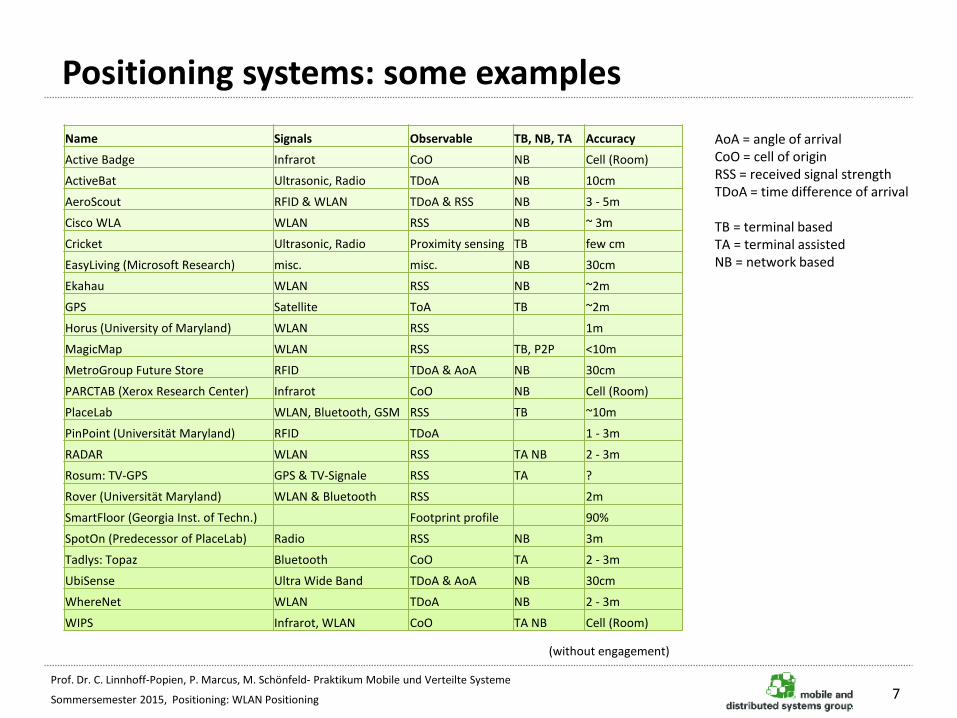
Positioning systems: some examples

Name Signals Observable TB, NB, TA Accuracy

Active Badge Infrarot CoO NB Cell (Room)

ActiveBat Ultrasonic, Radio TDoA NB 10cm

AeroScout RFID & WLAN TDoA & RSS NB 3 - 5m

Cisco WLA WLAN RSS NB ~ 3m

Cricket Ultrasonic, Radio Proximity sensing TB few cm

EasyLiving (Microsoft Research) misc. misc. NB 30cm

Ekahau WLAN RSS NB ~2m

GPS Satellite ToA TB ~2m

Horus (University of Maryland) WLAN RSS 1m

MagicMap WLAN RSS TB, P2P <10m

MetroGroup Future Store RFID TDoA & AoA NB 30cm

PARCTAB (Xerox Research Center) Infrarot CoO NB Cell (Room)

PlaceLab WLAN, Bluetooth, GSM RSS TB ~10m

PinPoint (Universität Maryland) RFID TDoA 1 - 3m

RADAR WLAN RSS TA NB 2 - 3m

Rosum: TV-GPS GPS & TV-Signale RSS TA ?

Rover (Universität Maryland) WLAN & Bluetooth RSS 2m

SmartFloor (Georgia Inst. of Techn.) Footprint profile 90%

SpotOn (Predecessor of PlaceLab) Radio RSS NB 3m

Tadlys: Topaz Bluetooth CoO TA 2 - 3m

UbiSense Ultra Wide Band TDoA & AoA NB 30cm

WhereNet WLAN TDoA NB 2 - 3m

WIPS Infrarot, WLAN CoO TA NB Cell (Room)

7

AoA = angle of arrival CoO = cell of origin RSS = received signal strength TDoA = time difference of arrival TB = terminal based TA = terminal assisted NB = network based

(without engagement)


WLAN Positioning

Why use IEEE 802.11 components for indoor positioning?

– Widely deployed infrastructure

– Available on many mobile platforms

– 2,4 GHz signal penetrates walls no line-of-sight necessary

– A standard WLAN access point deployment is often already sufficient to achieve room-level accuracy

– Active Scan:

• Sequentially iterate all WLAN bands. Probe Request -> Probe Response

– Passive Scan:

• Passive listening for beacons or probe responses

• Beacon: Small package with SSID name, transmission modes, encryption mode

8


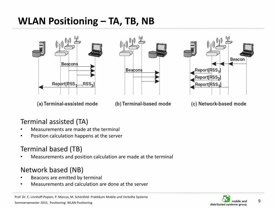
WLAN Positioning – TA, TB, NB

9

Terminal assisted (TA) • Measurements are made at the terminal • Position calculation happens at the server

Terminal based (TB) • Measurements and position calculation are made at the terminal

Network based (NB) • Beacons are emitted by terminal • Measurements and calculation are done at the server


WLAN Fingerprinting – Idea

10

WLAN Fingerprinting • Derive position from patterns of signals received from/at several WLAN access points • Observable: received signal strength (RSS) • Offline phase

– Record well-defined RSS patterns for well-defined reference positions and store them in a radio map

– Due to line-of-sight conditions on the spot, it might be necessary to observe RSS patterns from several directions for each position

• Online phase – RSS patterns related to the target are recorded and compared with the RSS fields of the entries

stored in the radio map – Position of the target is extracted from the reference position with the closest match

© 2006 ekahau.com


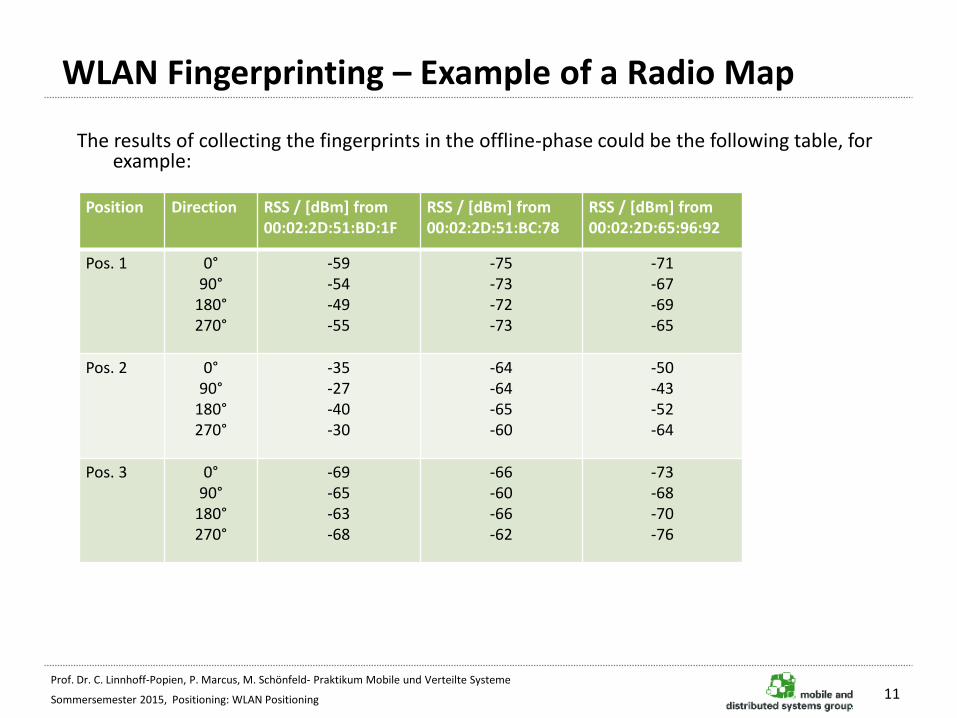
WLAN Fingerprinting – Example of a Radio Map

11

Position Direction RSS / [dBm] from 00:02:2D:51:BD:1F

RSS / [dBm] from 00:02:2D:51:BC:78

RSS / [dBm] from 00:02:2D:65:96:92

Pos. 1 0° 90°

180° 270°

-59 -54 -49 -55

-75 -73 -72 -73

-71 -67 -69 -65

Pos. 2 0° 90°

180° 270°

-35 -27 -40 -30

-64 -64 -65 -60

-50 -43 -52 -64

Pos. 3 0° 90°

180° 270°

-69 -65 -63 -68

-66 -60 -66 -62

-73 -68 -70 -76

The results of collecting the fingerprints in the offline-phase could be the following table, for example:


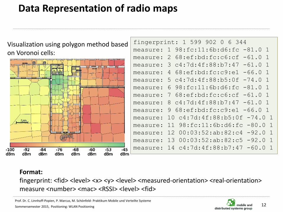
Data Representation of radio maps

12

fingerprint: 1 599 902 0 6 344

measure: 1 98:fc:11:6b:d6:fc -81.0 1

measure: 2 68:ef:bd:fc:c6:cf -61.0 1

measure: 3 c4:7d:4f:88:b7:47 -61.0 1

measure: 4 68:ef:bd:fc:c9:e1 -66.0 1

measure: 5 c4:7d:4f:88:b5:0f -74.0 1

measure: 6 98:fc:11:6b:d6:fc -81.0 1

measure: 7 68:ef:bd:fc:c6:cf -61.0 1

measure: 8 c4:7d:4f:88:b7:47 -61.0 1

measure: 9 68:ef:bd:fc:c9:e1 -66.0 1

measure: 10 c4:7d:4f:88:b5:0f -74.0 1

measure: 11 98:fc:11:6b:d6:fc -80.0 1

measure: 12 00:03:52:ab:82:c4 -92.0 1

measure: 13 00:03:52:ab:82:c5 -92.0 1

measure: 14 c4:7d:4f:88:b7:47 -60.0 1

Format: fingerprint: <fid> <level> <x> <y> <level> <measured-orientation> <real-orientation> measure <number> <mac> <RSSI> <level> <fid>

Visualization using polygon method based on Voronoi cells:


WLAN Fingerprinting – Empirical vs. Modeling Approach

Empirical approach

• Create radio maps from measurements

• Disadvantages

– Time consuming

– Measurements must be repeated whenever the configuration of access points changes

Modeling approach

• Create radio maps from a mathematical model

– Calculate the radio propagation conditions taking into account the positions of access points, transmitted signal strengths, free-space path loss, obstacles reflecting or scattering signals, …

• Disadvantages

– Complexity and accuracy of mathematical models

13


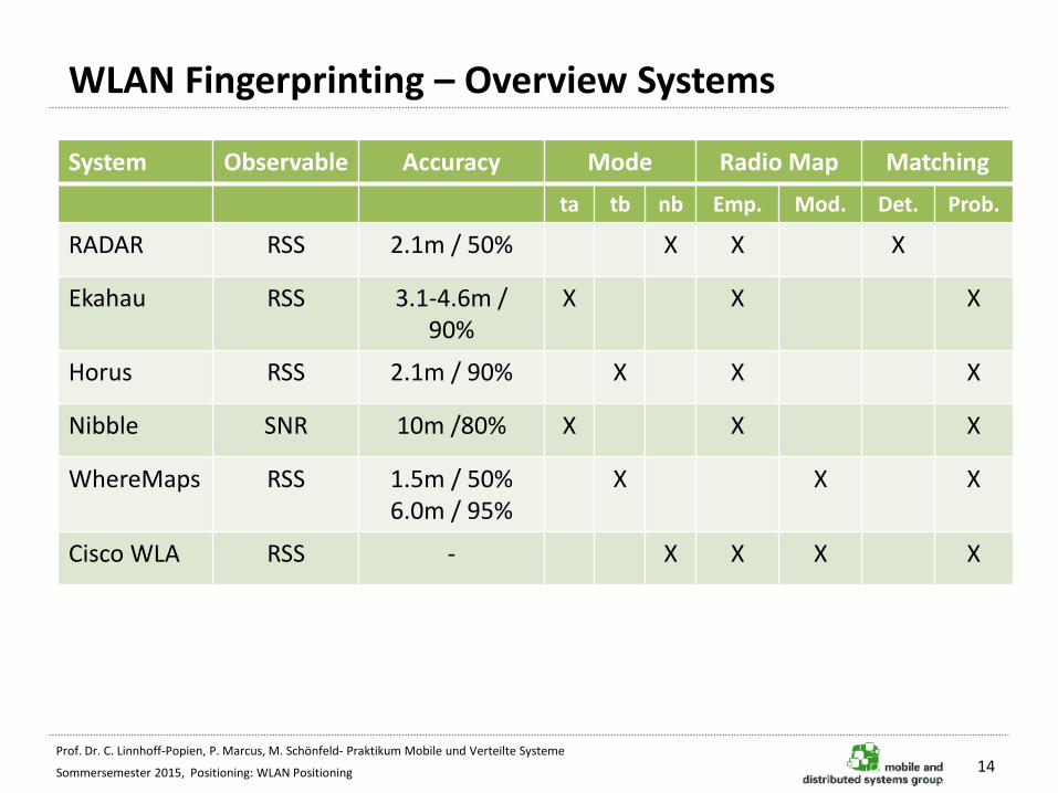
WLAN Fingerprinting – Overview Systems

14

System Observable Accuracy Mode Radio Map Matching

ta tb nb Emp. Mod. Det. Prob.

RADAR RSS 2.1m / 50% X X X

Ekahau RSS 3.1-4.6m / 90%

X X X

Horus RSS 2.1m / 90% X X X

Nibble SNR 10m /80% X X X

WhereMaps RSS 1.5m / 50% 6.0m / 95%

X X X

Cisco WLA RSS - X X X X


WLAN Fingerprinting – Deterministic vs. Probabilistic Approach

Deterministic Approach

• Record several RSS samples for each reference position and direction

• Create radio map from mean values of these samples

• Online phase: match observed and recorded sample according to Euclidian distance and adopt the reference position with the smallest distance as the current position of the terminal

Probabilistic Approach

• Describe variations of signal strengths experienced during the offline phase by probability distribution

• Probability distributions of various access points are applied to the observed RSS pattern to find the most probable position

• Accuracy can be significantly refined compared to the deterministic approach

15


WLAN Fingerprinting – Deterministic Positioning

• Position estimates are computed for terminal-based approaches as follows:

1. Perform a measurement of signal strengths on a given point

2. Search for the k-nearest-neighbors – the k recorded fingerprints with the minimal distance

k is a system parameter – often derived empirically for a given scenario

We will use a value of k=1

3. For each kNN-fingerprint lookup the location where it has been recorded

4. Compute the position estimate as the center of mass of these locations (coincides with the first fingerprint for 1NN)

16


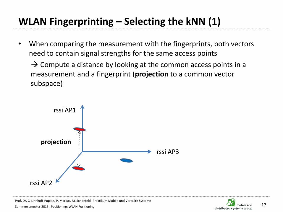
WLAN Fingerprinting – Selecting the kNN (1)

• When comparing the measurement with the fingerprints, both vectors need to contain signal strengths for the same access points

Compute a distance by looking at the common access points in a measurement and a fingerprint (projection to a common vector subspace)

17

projection

rssi AP1

rssi AP2

rssi AP3


WLAN Fingerprinting – Selecting the kNN (2)

• The selection of the kNN in Step 2. can be done in several ways

1. Euclidean distance in the largest common signal strength vector subspace:

2. Manhattan distance in the largest common signal strength vector subspace:

18

mit und

rssi AP2

rssi AP3

Manhattan distance

(euclidean) distance rssi AP2

rssi AP3


WLAN Fingerprinting – Computing the Position

• The position estimate can be computed from the set of kNN in different ways

1. Take the selected fingerprint if using 1NN

2. Compute the center of mass of kNN fingerprints: In this example, we have a vector r of fingerprints and each has a weight of mi=1:

3. Compute a weighted center of mass: The weights mi can be depend on the distance to the underlying measurement (penalty for very unsimilar fingerprints):

19

mi = 1/di

M = mi


WLAN Fingerprinting – Example

• Imagine the following example

– We collected a measurement

– We work on the radio map presented before

– The closest match is Pos. 3 with an orientation of 90°

– Simplified example for the given radio map:

20

=

71

57

65

m

Pos 1. Pos 2. Pos 3.

How can we estimate the error?


Estimating Positioning Errors

21

• Two categories of error estimations do exist:

– Prediction of expected errors in advance

a) Fingerprint Clustering

b) Leave Out Fingerprint

– Infer the expected position error from live measurements in the online phase

c) Best Candidate Set

d) Signal Strength Variance


Estimating Positioning Errors: Fingerprint Clustering (1)

22

Idea: As within given areas the fingerprints are nearly equal, a positioning system can‘t make an excact positioning assumption.

The real positition is expected to be anywhere in the area with a similar signal strength characteristic

Steps of the algorithm:

1. Compute Voronoi-Cells for the offline fingerprint database. Each fingerprint is now embedded in a Voronoi-Cell. Each collected fingerprint is represented by a collection of measured samples.

2. Randomly select a cluster and merge it with a random neighboring cluster iff the similarity is greater than a given threshold.

3. Repeat this step until no pair of neighboring clusters suffices the threshold.

4. Merge single-cell clusters with their most similar neighboring cluster.

5. The error is deduced from the size of the area the cluster covers



23

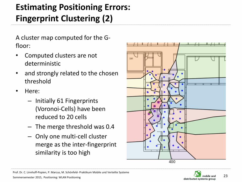
A cluster map computed for the G-floor:

• Computed clusters are not deterministic

• and strongly related to the chosen threshold

• Here:

– Initially 61 Fingerprints (Voronoi-Cells) have been reduced to 20 cells

– The merge threshold was 0.4

– Only one multi-cell cluster merge as the inter-fingerprint similarity is too high



24

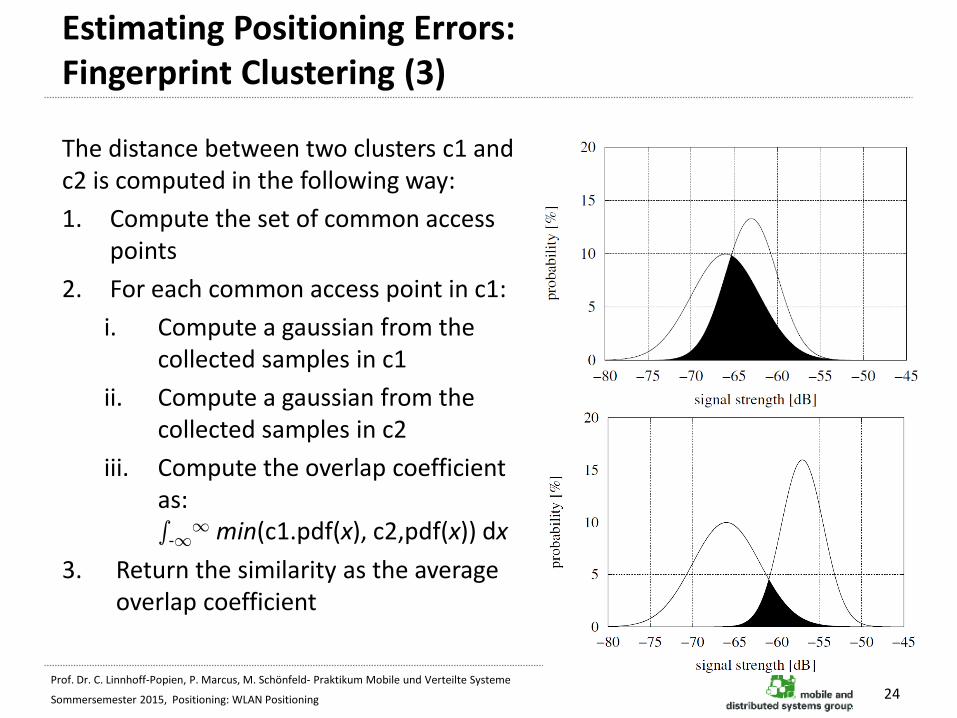
The distance between two clusters c1 and c2 is computed in the following way:

1. Compute the set of common access points

2. For each common access point in c1:

i. Compute a gaussian from the collected samples in c1

ii. Compute a gaussian from the collected samples in c2

iii. Compute the overlap coefficient as: s-1

1 min(c1.pdf(x), c2,pdf(x)) dx

3. Return the similarity as the average overlap coefficient


Estimating Positioning Errors: Leave Out Fingerprint

25

• Estimation of the error by performing an analysis on the radio map:

Assumption: For each given FP on a position p, the signal strength has been collected in m samples

1. Compute the distance in the signal strength vector space to all the (n-1) other fingerprints and select the nearest. Store the geographical distance.

2. The error is computed as the average of all the geographical distances + 2 times the standard deviation


Estimating Positioning Errors: Best Candidate Set

26

• Estimate the error by either computing:

– Computing the average geographical distance between the nearest and the k-1 nearest neighbors

– Computing the maximum geographical distance between the nearest neighbor and any of the remaining k-1 nearest neighbors

– Compute the maximum distance between any of the k nearest neighbors

• The latter two tend to highly overestimate the error when k is chosen large


Estimating Positioning Errors: Signal Strength Variance

27

• Small scale fading, multipath propagation etc. can lead to large changes in the measured signal strengths even for small movements

• If the variance of all samples in a FP is high, the probability that a FP far away might be selected is high too

1. For each AP in the samples of a FP, find the largest measured signal strength value (in dB)

2. Subtract this value from all the measured signal strength for this AP in all collected samples

3. Calculate the signal strength variance for each AP in this FP

4. Compute the average signal strength variance from the variances computed for each AP.


Comparing the Error Estimates

• The performance is measured by:

distance difference = estimated_error – real_error

• The performance of the algorithms depends on the setting:

28


Sensor Fusion

Idea:

• Refine the WLAN positioning with additional measurements from other sensor sources

– Accelerometer

– Gyroskope

– Compass

How to combine several sensors (Sensor Fusion):

• Probability distributions

– Kalman Filter

– Particle Filter

29


Sensor Fusion: WLAN Positionierung

Offline phase:

Recording of fingerprints (x, y, e, d, <MAC, RSSI>)

Online phase:

Distance computation between current signal strength measurment and fingerprints . One possibility:

Own position is estimated as the weighted average of k-Nearest-Neighbors (kNN) in signal space.

The reference positions of the neighbors allow for the etimation of variance:

Low variance High variance


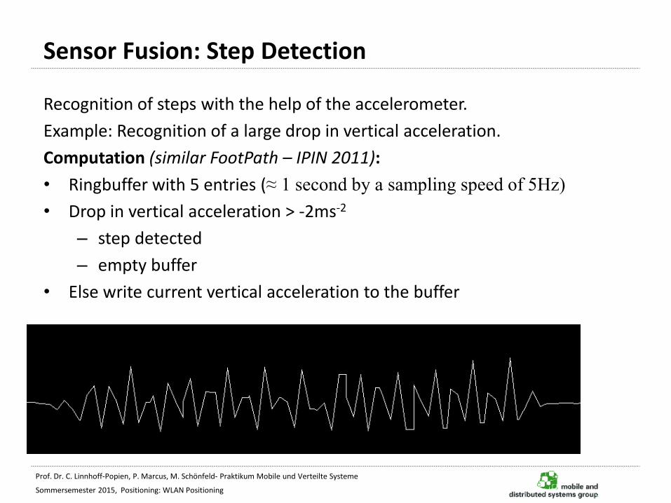
Sensor Fusion: Step Detection

Recognition of steps with the help of the accelerometer.

Example: Recognition of a large drop in vertical acceleration.

Computation (similar FootPath – IPIN 2011):

• Ringbuffer with 5 entries (≈ 1 second by a sampling speed of 5Hz)

• Drop in vertical acceleration > -2ms-2

– step detected

– empty buffer

• Else write current vertical acceleration to the buffer


Sensor Fusion: Particle Filter

„Recursive Bayesian filter for state etsimation of a dynamic system“

Assumptions:

• Current position is unknown but can be observed

• Observations are error-prone

• Position is modelled as probability distribution

• Discretisation of the distribution with a point cloud (particle)

Three phases:

• Initialisation

– creation of particles

• Prediction

– propagation of particles

• Update

– weighting of particles


Particle Filter: Initialisation

Different possibilities:

• Uniform distribution in building

• Point distribution at certain location

• Distribution according to initial measurement

– for example WLAN fingerprinting

– 2D Gaussian distribution

– variance according to kNN


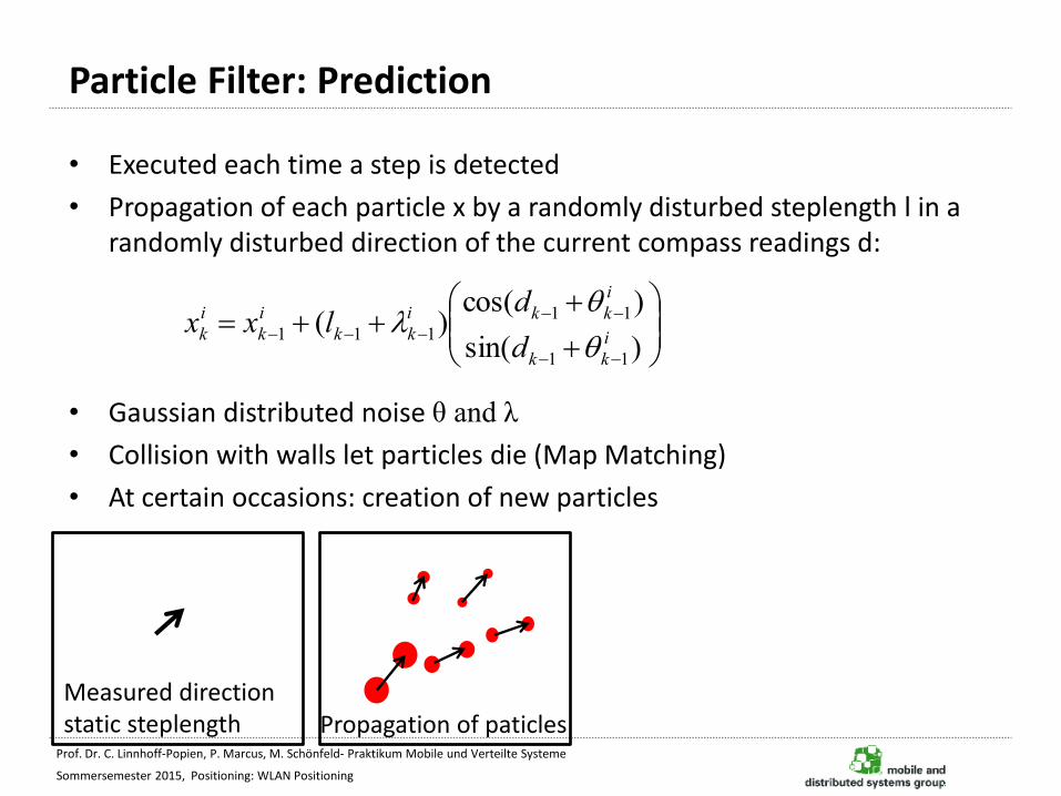
Particle Filter: Prediction

• Executed each time a step is detected

• Propagation of each particle x by a randomly disturbed steplength l in a randomly disturbed direction of the current compass readings d:

• Gaussian distributed noise θ and λ

• Collision with walls let particles die (Map Matching)

• At certain occasions: creation of new particles

=

)sin(

)cos()(

11

11

111 i

kk

i

kki

kk

i

k

i

kd

dlxx

Measured direction static steplength Propagation of paticles


Particle Filter: Update

• Execution each time a WLAN scan was successful

• Calculate probability distribution based on WLAN positioning (e.g., Gaussian distibution ~ Nμ,σ)

• Update the weight w of each particle x accordingly:

• Finlally normalise the weight:

i

kk

i

k

i

k wzxpw 1)|( =

)|( k

i

k zxp

=

i

i

k

i

ki

kw

ww


Links & Videos

• Multi-Sensor Pedestrian Indoor/Outdoor Navigation 2.5 D (DLR)

– http://www.youtube.com/watch?v=2NfSHNurOAc

• Pedestrian Inertial Navigation and Map-Matching (DLR)

– http://www.youtube.com/watch?v=4ZdBtZdNEzg

• Particle filters in action (University of Washington)

– http://www.cs.washington.edu/ai/Mobile_Robotics/mcl/

36

http://www.youtube.com/watch?v=2NfSHNurOAc

http://www.youtube.com/watch?v=4ZdBtZdNEzg

http://www.cs.washington.edu/ai/Mobile_Robotics/mcl/


Practical Course

• A simple WLAN positioning system

– Deterministic

– Empirical

• Android classes

– Broadcast Receiver

– WifiManager (active scanning)

– ScanResult

37

Praktikum Mobile und Verteilte Systeme WLAN Positioning · Prof. Dr. C. Linnhoff-Popien, P. Marcus,...

Documents

Transcript of Praktikum Mobile und Verteilte Systeme WLAN Positioning · Prof. Dr. C. Linnhoff-Popien, P. Marcus,...