
Recording, Processing and Use of Material-Specific Data in ... · Recording, Processing and Use of...
135
Recording, Processing and Use of Material-Specific Data in Pulse Electrochemical Machining Dissertation zur Erlangung des Grades des Doktors der Ingenieurwissenschaften der Naturwissenschaftlich-Technischen Fakultät II - Physik und Mechatronik - der Universität des Saarlandes von Andreas Rebschläger Saarbrücken 2015
Transcript of Recording, Processing and Use of Material-Specific Data in ... · Recording, Processing and Use of...
Recording, Processing and Use of Material-Specific Data in Pulse Electrochemical Machining
Dissertation
zur Erlangung des Grades des Doktors der Ingenieurwissenschaften
der Naturwissenschaftlich-Technischen Fakultät II - Physik und Mechatronik -
der Universität des Saarlandes
von
Andreas Rebschläger
Saarbrücken
2015

Tag des Kolloquiums: 28.06.2016 Dekan: Prof. Dr.-Ing. Georg Frey Berichterstatter: Prof. Dr.-Ing. Dirk Bähre
Prof. Dr.-Ing. Stefan Seelecke
Vorsitz: Prof. Dr. Andreas Schütze Akad. Mitarbeiter: Dr.-Ing. Frank Krämer

Abstract
The present work focuses on the manufacturing process based on pulsed
electrochemical dissolution. The quality of the Electrochemical Machining is
dependent on the properties and composition of the processed material, the process
parameters and the machine capability. Both, the reproduction accuracy and the
possible feed rates, resulting from the dissolution rates of the materials and
consequently also processing times differ, depending on the material and alloy
components. The basic machine-dependent, yet material-independent processes are
explained and presented in this work. Based on an experimental and simulation-
based evaluation, a method for the acquisition of machine-independent material data
under a number of influencing parameters is investigated. The focus of the
investigation lies on a widely used stainless steel and a powder metallurgically
produced high speed steel in different hardness conditions. The gathering of
material-specific data will be presented for the use in a process simulation and will be
validated against an in-process geometry measurement. For this purpose, an
experimental set-up was designed, built and tested, which allows the observation of
the dissolution process over a longer period of time under industrial process
conditions. A theoretical approach focusing on the inverse tool simulation based on
material data concludes the work.

Kurzzusammenfassung
Die vorliegende Arbeit beschäftigt sich mit dem gepulsten, elektrochemisch
abtragenden Fertigungsverfahren. Die Qualität der elektrochemischen Bearbeitung
ist abhängig von den Eigenschaften und der Zusammensetzung des zu bearbeiteten
Materials, den Prozessparametern und der Maschinenfähigkeit. Sowohl
Abbildgenauigkeit als auch mögliche Vorschübe, welche aus den Auflöseraten der
Materialien resultieren, und somit folglich auch Bearbeitungszeiten, unterscheiden
sich je nach Material und Legierungsbestandteilen. Die grundlegenden,
maschinenabhängigen jedoch materialunabhängigen Prozesse werden in dieser
Arbeit erläutert und vorgestellt. Darauf aufbauend werden experimentelle und
simulationsgestützte Auswerteverfahren zur Erfassung von maschinenunabhängigen
Materialdaten unter einer Vielzahl von Einflussparametern untersucht. Der Fokus
dieser Untersuchungen liegt hierbei auf einem weitverbreitet eingesetzten Edelstahl
und einem pulvermetallurgisch hergestellten Schnellarbeitsstahl in unterschiedlichen
Härtezuständen. Abschließend wird die Nutzung der erfassten werkstoffspezifischen
Daten zur Prozesssimulation vorgestellt und anhand einer in-Prozess
Geometrieerfassung validiert. Hierzu wurde eine Versuchsanordnung konzipiert,
gebaut und getestet, welche die Beobachtung des Formgebungsprozesses über
einen längeren Zeitraum unter industriellen Prozessbedingungen ermöglicht. Ein
theoretischer Ansatz zur inversen Werkzeugsimulation auf Basis von Materialdaten
bildet den Abschluss der Arbeit.
Vorwort
Im Laufe der Entstehung der vorliegenden Arbeit stand ich in Kontakt mit einer Vielzahl von Personen, welche mich teils richtungsweisend beeinflusst und unterstützt haben. Diesen Personen möchte ich an dieser Stelle persönlich danken.
Meinem Doktorvater Prof. Dr.-Ing. Dirk Bähre danke ich für die besondere Betreuung und kritischen Fragen, sowie den stets offenen, sachlichen als auch sehr persönlich geprägten Austausch an Informationen und Meinungen im Rahmen vieler Diskussionen und Treffen.
Prof. Dr.-Ing. Stefan Seelecke danke ich für Übernahme des Korreferates und die vielen interessanten Diskussionen und Fragen zur interdisziplinären Anwendung der jeweils gegenseitigen Technologien.
Meinen langjährigen Kollegen Olivier Weber und Philipp Steuer, die mich während der Ausarbeitung ertragen mussten Danke ich besonders! Neben der gegenseitigen Unterstützung in der Etablierung des Themengebietes, waren es vor allem die unzähligen und meist spätabendlichen, fachlichen Diskussionen, welche viele wertvolle Inhalte im Rahmen der Ausgestaltung der Arbeit lieferten.
Bernd Heitkamp für die vielen Diskussionen und Denkanstöße.
Ein Dank an meine wissenschaftlichen Hilfskräfte, Bachelor- sowie Masterarbeiter, welche durch die Anfertigung von Abschlussarbeiten und Unterstützung zu dieser Arbeit beigetragen haben.
Herrn Privatdozent Dr. Lohrengel, Herrn Dr. Hoogsteen und Frau Dr. Baumgärtner für die fachlichen Diskussionen und Hinweise im Rahmen der INSECT Konferenzen.
Den Mitarbeitern der Firma PEMTec: Herrn Brussee, Herrn Grützmacher, Herrn Otto, Herrn Vollmer und Herrn Kuhn für die langjährige Unterstützung in den Bereichen der Maschinentechnik, Konstruktion, Analyse elektrischer Daten und diversen Eingriffen in die Maschinensteuerung sowie Anpassungen der Software.
Den wissenschaftlichen und technischen Mitarbeitern am Lehrstuhl für Fertigungstechnik danke ich für die vielen fachlichen und persönlichen Unterredungen.
Herrn Simon Staudacher für die Unterstützung im Bereich der Metallographie, Herrn Moritz Stolpe für die Unterstützung bei der Härtemessung, Frau Anne Bauer für die Anfertigung von Vorrichtungen.
Ein großer Dank an alle Mitarbeiter der ZeMA gGmbH und den Mitarbeitern der im ZeMA ansässigen Lehrstühle für deren Kooperation, zudem dem Land Saarland und dem Europäischen Fonds für regionale Entwicklung (EFRE) für die Förderung der Forschungsaktivitäten im Projekt INTEGRATiF - ProQQuadrat.
Ganz speziell und von ganzem Herzen danke ich meiner Freundin für Ihre Geduld und allen voran meinen Eltern, welche mir den akademischen Weg überhaupt erst ermöglicht haben – DANKE!

CURRICULUM VITAE
Personal Information
Name Andreas Rebschläger
Date of birth and place: May 10th, 1984 in St. Ingbert, Germany
Professional Background
since 02/2015 Robert Bosch GmbH, Homburg/Saar, Germany
01/2013 – 12/2014 Group leader manufacturing processes and automation at
the ZeMA - Zentrum für Mechatronik und
Automatisierungstechnik gemeinnützige GmbH,
Saarbrücken, Germany
04/2010 – 12/2012 Scientific employee at the ZeMA - Zentrum für
Mechatronik und Automatisierungstechnik gemeinnützige
GmbH, Saarbrücken, Germany
Studies and Education
10/2004 – 03/2010 Dipl.-Ing. Mechatronik, Universität des Saarlandes,
Germany
2001 – 2003 Abitur, Leibniz-Gymnasium, St. Ingbert, Germany
2000 – 2001 US High School Diploma, Minneapolis High School (USD
239), Minneapolis, Kansas, USA
1994 – 2000 Leibniz-Gymnasium, St. Ingbert, Germany
1990 – 1994 Grundschule Oberwürzbach, St. Ingbert, Germany
Community Service
2003 – 2004 Community service (German: Zivildienst) German Red
Cross, including the training as paramedic (German:
Rettungssanitäter)
Parts of this work have been published as follows:
Publications
O. Weber, H. Natter, A. Rebschläger, D. Bähre: Surface quality and process
behaviour during Precise Electrochemical Machining of cast iron. International
Symposium on Electrochemical Machining INSECT2011, Editors: B. Mollay, M.M.
Lohrengel, pp.41-46, Vienna, 2011.
A. Rebschläger, O. Weber, D. Bähre: In-situ process measurements for industrial
size Pulse Electrochemical Machining. International Symposium on Electrochemical
Machining Technology INSECT2012, Editor: Maria Zybura-Skrabalak, pp.133-148,
Krakow, 2012.
O. Weber, H. Natter, A. Rebschläger, D. Bähre: Analytical characterization of the
dissolution behavior of cast iron by electrochemical methods. International
Symposium on Electrochemical Machining Technology INSECT2012, Editor: Maria
Zybura-Skrabalak, pp.41-55, Krakow, 2012.
D. Bähre, A. Rebschläger, O. Weber, P. Steuer: Reproducible, fast and adjustable
surface roughening of stainless steel using Pulse Electrochemical Machining.
Procedia CIRP 6, pp.385-390, 2013.
A. Rebschläger, O. Weber, B. Heitkamp: Benefits and Drawbacks Using Plastic
Materials Produced by Additive Manufacturing Technologies in the Electrochemical
Environement. International Symposium on Electrochemical Machining Technology
INSECT2013, Editors: A. Schubert, M. Hackert-Oschätzchen, pp.45-51, Chemnitz,
2013.
A. Rebschläger, R. Kollmannsperger, D. Bähre: Video based process observations of
the pulse electrochemical machining process at high current densities and small
gaps. Procedia CIRP 13 (2013), pp. 418-423, 2013.
M. Swat, A. Rebschläger, D. Bähre: Investigation of the energy consumption for the
pulse electrochemical machining (PECM) process. International Symposium on
Electrochemical Machining Technology INSECT2013, Editors: A. Schubert, M.
Hackert-Oschätzchen, pp.65-71, Chemnitz, 2013.
P. Steuer, A. Rebschläger, O. Weber, D. Bähre: The heat-affected zone in EDM and
its influence on a following PECM process. Procedia CIRP 13, pp.276-281, 2013.
O. Weber, D. Bähre, A. Rebschläger: Study of Pulse Electrochemical Machining
characteristics of spheroidal cast iron using sodium nitrate electrolyte. International
Conference on Competitive Manufacturing, COMA 13, pp.125-130 , South Africa,
2013.
O. Weber, A. Rebschläger, P. Steuer, D. Bähre: Modeling of the Material/Electrolyte
Interface and the Electrical Current Generated during the Pulse Electrochemical
Machining of Grey Cast Iron. Proceedings of the 2013 European COMSOL
Conference in Rotterdam, Rotterdam, 2013.
D. Bähre, O. Weber, A. Rebschläger: Study of Pulse Electrochemical Machining of
nickel-cobalt ferrous alloy. International Conference on Competitive Manufacturing,
COMA 13, pp.119-124 , South Africa, 2013.
D. Bähre, O. Weber, A. Rebschläger: Investigation on Pulse Electrochemical
Machining Characteristics of Lamellar Cast Iron using a Response Surface
Methodology-based Approach. Procedia CIRP 6, pp.363-368, 2013.
D. Bähre and A. Rebschläger (Editors): Proceedings International Symposium on
Electrochemical Machining Technology INSECT2014. ISBN 978-3-95735-010-7,
2014.
A. Rebschläger, K. U. Fink, T. Heib, D. Bähre: Geometric shaping analysis based on
PECM video process observations. International Symposium on Electrochemical
Machining Technology INSECT2014, Editors: D. Bähre, A. Rebschläger, pp.37-44,
Saarbrücken, 2014.
P. Steuer, A. Rebschläger, A. Ernst, D. Bähre: Process Design in Pulse
Electrochemical Machining Based on Material Specific Data – 1.4301 and Electrolytic
Copper as an Example. Key Engineering Materials Vols 651-653, pp. 732-737, 2015.
M. Swat, A. Rebschläger, K. Trapp, T. Stock, G. Seliger, D. Bähre: Investigating the
energy consumption of the PECM process for consideration in the selection of
manufacturing process chains. Procedia CIRP. 22nd CIRP conference on Life Cycle
Engineering (LCE), 2015.


TABLE OF CONTENTS I
TABLE OF CONTENTS
ABBREVIATIONS & SYMBOLS ................................................................................ II
LIST OF FIGURES ..................................................................................................... V
LIST OF TABLES ..................................................................................................... IX
1 INTRODUCTION ................................................................................................ 1
2 THE ELECTROCHEMICAL MACHINING PROCESS ....................................... 3
2.1 ELECTROCHEMICAL DISSOLUTION ............................................................................. 3
2.2 ELECTROCHEMICAL MACHINING – ECM .................................................................... 6
2.3 ELECTROLYTE ........................................................................................................14
2.4 PULSE ELECTROCHEMICAL MACHINING – PECM ......................................................18
3 SCIENTIFIC CONCEPT AND APPROACH ..................................................... 23
4 INVESTIGATED MATERIALS ......................................................................... 25
4.1 STAINLESS STEEL 1.4301 ........................................................................................25
4.2 POWDER METALLURGICAL STEEL S390 ....................................................................27
4.3 BASIC ELECTROCHEMICAL ANALYSIS .......................................................................29
5 INVESTIGATION METHODS ........................................................................... 33
5.1 FRONTAL GAP EXPERIMENTS ...................................................................................34
5.2 SIDE GAP EXPERIMENTS ..........................................................................................48
5.3 CONTINUOUS OBSERVATIONS ..................................................................................49
5.4 ELECTRICAL AND SURFACE MEASUREMENTS ............................................................56
6 SIMULATION CONCEPT ................................................................................. 59
6.1 STATIC SIMULATION ................................................................................................59
6.2 SIMULATION BASED ON MATERIAL-SPECIFIC DATA ......................................................62
6.3 TOOL SIMULATION BASED ON MATERIAL-SPECIFIC SIMULATION ...................................67
7 EXPERIMENTAL RESULTS, SIMULATION AND DISCUSSION .................... 69
7.1 MATERIAL-SPECIFIC DATA ........................................................................................69
7.1.1 Stainless steel 1.4301 .................................................................................................... 69
7.1.2 Powder metallurgical steel S390 .................................................................................... 77
7.2 EFFECTS FROM CONTINUOUS OBSERVATIONS ...........................................................86
7.3 SIMULATION BASED ON MATERIAL-SPECIFIC DATA ......................................................91
8 SUMMARY AND CONCLUSION ..................................................................... 97
REFERENCES ......................................................................................................... 99
APPENDIX A OLYPMUS ISPEED-TR ................................................................ 114
APPENDIX B MICROSCOPE CALIBRATION SLIDE ......................................... 115

II ABBREVIATIONS & SYMBOLS
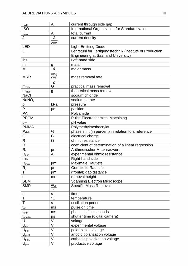
ABBREVIATIONS & SYMBOLS
Abbreviation or symbol
Unit Meaning
A cm² surface area
a 𝑚𝑔 ∙ 𝑐𝑚2
𝐶 ∙ 𝐴
constant
ai reference point on anode
AFM Abrasive Flow Machining
AISI American Iron and Steel Institute
b 1
𝑠
constant
C constant
C 𝑔
𝑙 electrolyte concentration
c constant
ci reference point in cathode
CAD computer-aided design
CV Cyclic Voltammetry
d 1
𝑠
constant
DIN Deutsches Institut für Normung
e constant
e- electron (negative charge)
ECM Electrochemical Machining
EDM Electrical Discharge Machining
EN European Committee for Standardization
F 𝐶
𝑚𝑜𝑙
Faraday constant (96,485.33289 C/mol)
f 𝑚𝑔
𝐶 constant
f Hz frequency
felectric Hz electrical frequency
FEM Finite element method
fmechanic Hz mechanical frequency
h mm removal height
HB hardness scale Brinell
HRC hardness scale Rockwell (C=150kgf, 120°diamond cone)
HV30 hardness scale Vickers (30 = load of 30kgf)
I A electrical current
ICP-OES Inductive Coupled Plasma - Optical Emission Spectrometry
Iexp A experimental amperage
IFEM A FEM simulated process current
Ifrontal A current through frontal gap
ilocal,i A local current between reference points ai and ci
Imax A maximum amperage
Ireal A real measured process current
ABBREVIATIONS & SYMBOLS III
Iside A current through side gap
ISO International Organization for Standardization
Itotal A total current
J 𝐴
𝑐𝑚²
current density
LED Light-Emitting Diode
LFT Lehrstuhl für Fertigungstechnik (Institute of Production Engineering at Saarland University)
lhs Left-hand side
m g mass
M 𝑔
𝑚𝑜𝑙 molar mass
MRR 𝑐𝑚³
𝐶
mass removal rate
mpract G practical mass removal
mtheor g theoretical mass removal
NaCl sodium chloride
NaNO3 sodium nitrate
p kPa pressure
P µm position
PA Polyamide
PECM Pulse Electrochemical Machining
pH pH value
PMMA Polymethylmethacrylat
Pshift % phase shift (in percent) in relation to a reference
Q C electrical charge
R Ω ohmic resistance
R² coefficient of determination of a linear regression
Ra µm Arithmetischer Mittenrauwert
Rexp A experimental ohmic resistance
rhs Right-hand side
Rmax µm Maximale Rautiefe
Rz µm Gemittelte Rautiefe
s µm (frontal) gap distance
s mm removal height
SEM Scanning Electron Microscope
SMR 𝑚𝑔
𝐶 Specific Mass Removal
t s time
T °C temperature
T s oscillation period
ton ms pulse on time
tshift ms phase shift in seconds
tshutter µs shutter time (digital camera)
U V voltage
Uexp V experimental voltage
Upol V polarization voltage
UpolA V anodic polarization voltage
UpolC V cathodic polarization voltage
Uprod V productive voltage

IV ABBREVIATIONS & SYMBOLS
US United States
Usim V simulated voltage
USSR Union of Soviet Socialist Republics
V cm³ Volume
v 𝑚𝑚
𝑚𝑖𝑛 velocity
v 𝑚𝑚
𝑚𝑖𝑛 feed rate
VDE Verband der Elektrotechnik und Elektronik
VDI Verein Deutscher Ingenieure
y0 µm initial gap
z valence
ZeMA Zentrum für Mechatronik und Automatisierungstechnik gemeinnützige GmbH
η % current efficiency
κ Ωcm specific resistance
ρ 𝑔
𝑐𝑚³ density
σ 𝑚𝑆
𝑐𝑚
conductivity
LIST OF FIGURES V
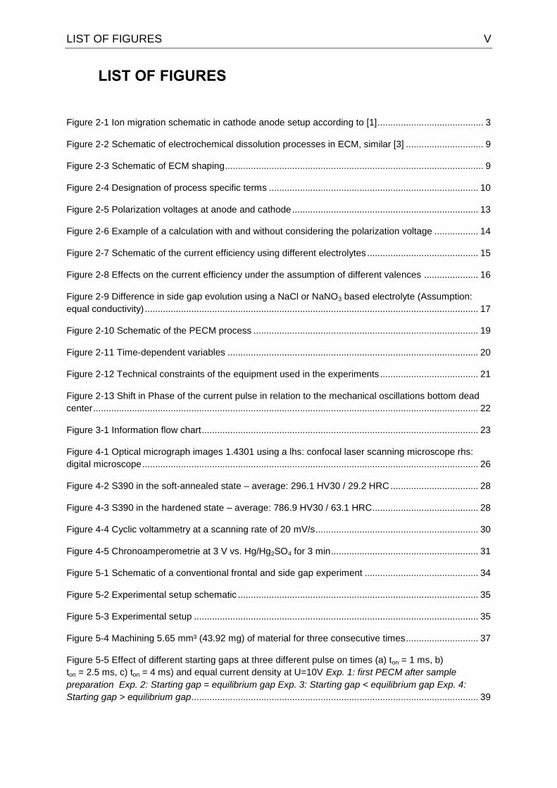
LIST OF FIGURES
Figure 2-1 Ion migration schematic in cathode anode setup according to [1] ......................................... 3
Figure 2-2 Schematic of electrochemical dissolution processes in ECM, similar [3] .............................. 9
Figure 2-3 Schematic of ECM shaping .................................................................................................... 9
Figure 2-4 Designation of process specific terms ................................................................................. 10
Figure 2-5 Polarization voltages at anode and cathode ........................................................................ 13
Figure 2-6 Example of a calculation with and without considering the polarization voltage ................. 14
Figure 2-7 Schematic of the current efficiency using different electrolytes ........................................... 15
Figure 2-8 Effects on the current efficiency under the assumption of different valences ..................... 16
Figure 2-9 Difference in side gap evolution using a NaCl or NaNO3 based electrolyte (Assumption:
equal conductivity) ................................................................................................................................. 17
Figure 2-10 Schematic of the PECM process ....................................................................................... 19
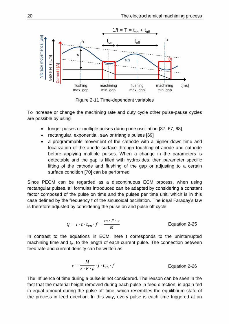
Figure 2-11 Time-dependent variables ................................................................................................. 20
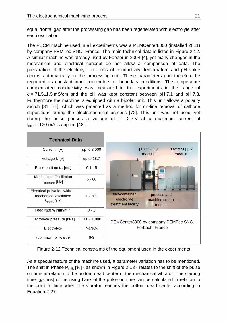
Figure 2-12 Technical constraints of the equipment used in the experiments ...................................... 21
Figure 2-13 Shift in Phase of the current pulse in relation to the mechanical oscillations bottom dead
center ..................................................................................................................................................... 22
Figure 3-1 Information flow chart ........................................................................................................... 23
Figure 4-1 Optical micrograph images 1.4301 using a lhs: confocal laser scanning microscope rhs:
digital microscope .................................................................................................................................. 26
Figure 4-2 S390 in the soft-annealed state – average: 296.1 HV30 / 29.2 HRC .................................. 28
Figure 4-3 S390 in the hardened state – average: 786.9 HV30 / 63.1 HRC ......................................... 28
Figure 4-4 Cyclic voltammetry at a scanning rate of 20 mV/s ............................................................... 30
Figure 4-5 Chronoamperometrie at 3 V vs. Hg/Hg2SO4 for 3 min ......................................................... 31
Figure 5-1 Schematic of a conventional frontal and side gap experiment ............................................ 34
Figure 5-2 Experimental setup schematic ............................................................................................. 35
Figure 5-3 Experimental setup .............................................................................................................. 35
Figure 5-4 Machining 5.65 mm³ (43.92 mg) of material for three consecutive times ............................ 37
Figure 5-5 Effect of different starting gaps at three different pulse on times (a) ton = 1 ms, b)
ton = 2.5 ms, c) ton = 4 ms) and equal current density at U=10V Exp. 1: first PECM after sample
preparation Exp. 2: Starting gap = equilibrium gap Exp. 3: Starting gap < equilibrium gap Exp. 4:
Starting gap > equilibrium gap ............................................................................................................... 39
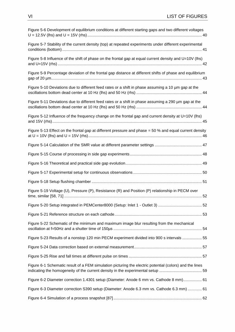
VI LIST OF FIGURES
Figure 5-6 Development of equilibrium conditions at different starting gaps and two different voltages
U = 12.5V (lhs) and U = 15V (rhs) ......................................................................................................... 40
Figure 5-7 Stability of the current density (top) at repeated experiments under different experimental
conditions (bottom) ................................................................................................................................ 41
Figure 5-8 Influence of the shift of phase on the frontal gap at equal current density and U=10V (lhs)
and U=15V (rhs) .................................................................................................................................... 42
Figure 5-9 Percentage deviation of the frontal gap distance at different shifts of phase and equilibrium
gap of 20 µm .......................................................................................................................................... 43
Figure 5-10 Deviations due to different feed rates or a shift in phase assuming a 10 µm gap at the
oscillations bottom dead center at 10 Hz (lhs) and 50 Hz (rhs) ............................................................ 44
Figure 5-11 Deviations due to different feed rates or a shift in phase assuming a 290 µm gap at the
oscillations bottom dead center at 10 Hz (lhs) and 50 Hz (rhs) ............................................................ 44
Figure 5-12 Influence of the frequency change on the frontal gap and current density at U=10V (lhs)
and 15V (rhs) ......................................................................................................................................... 45
Figure 5-13 Effect on the frontal gap at different pressure and phase = 50 % and equal current density
at U = 10V (lhs) and U = 15V (rhs) ........................................................................................................ 46
Figure 5-14 Calculation of the SMR value at different parameter settings ........................................... 47
Figure 5-15 Course of processing in side gap experiments .................................................................. 48
Figure 5-16 Theoretical and practical side gap evolution ...................................................................... 49
Figure 5-17 Experimental setup for continuous observations ............................................................... 50
Figure 5-18 Setup flushing chamber ..................................................................................................... 51
Figure 5-19 Voltage (U), Pressure (P), Resistance (R) and Position (P) relationship in PECM over
time, similar [58, 71] .............................................................................................................................. 52
Figure 5-20 Setup integrated in PEMCenter8000 (Setup: Inlet 1 - Outlet 3) ........................................ 52
Figure 5-21 Reference structure on each cathode ................................................................................ 53
Figure 5-22 Schematic of the minimum and maximum image blur resulting from the mechanical
oscillation at f=50Hz and a shutter time of 150µs ................................................................................. 54
Figure 5-23 Results of a nonstop 120 min PECM experiment divided into 900 s intervals .................. 55
Figure 5-24 Data correction based on external measurement .............................................................. 57
Figure 5-25 Rise and fall times at different pulse on times ................................................................... 57
Figure 6-1 Schematic result of a FEM simulation picturing the electric potential (colors) and the lines
indicating the homogeneity of the current density in the experimental setup ....................................... 59
Figure 6-2 Diameter correction 1.4301 setup (Diameter: Anode 6 mm vs. Cathode 8 mm) ................. 61
Figure 6-3 Diameter correction S390 setup (Diameter: Anode 6.3 mm vs. Cathode 6.3 mm) ............. 61
Figure 6-4 Simulation of a process snapshot [87] ................................................................................. 62
LIST OF FIGURES VII
Figure 6-5 Classification of materials, similar [41] ................................................................................. 63
Figure 6-6 Current efficiency in ECM and PECM, schematic similar [112] ........................................... 65
Figure 6-7 Scheme of the calculation steps implemented in Matlab ..................................................... 66
Figure 6-8 Sequence of a simulation with examples Inside loop: Simulation of the anode geometry
using a given cathode Outside loop: Iterative inverse simulation of the anode and cathode geometry
using a targeted anode geometry .......................................................................................................... 68
Figure 7-1 Current density [A/cm²] vs. feed rate [mm/min] ................................................................... 69
Figure 7-2 Current density [A/cm²] vs. SMR [mg/C] .............................................................................. 70
Figure 7-3 Current density [A/cm²] vs. frontal gap [µm] for all pulse times [ms] and voltages [V] ........ 70
Figure 7-4 Current density [A/cm²] vs. polarization voltage [V] ............................................................. 71
Figure 7-5 lhs: Current density [A/cm²] vs. feed rate [mm/min] rhs: Current density [A/cm²] vs. SMR
[mg/C] .................................................................................................................................................... 72
Figure 7-6 Time [min] vs. side gap [µm] development at an initial gap of 20 µm .................................. 73
Figure 7-7 Gap widening: Experiment, Theory and Simulation............................................................. 74
Figure 7-8 Optical images of the machined surface .............................................................................. 74
Figure 7-9 Surface roughness of 1.4301 at different current densities [A/cm²] ..................................... 75
Figure 7-10 SEM surface images of 1.4301 at different current densities ............................................ 76
Figure 7-11 Current density [A/cm²] vs. feed rate [mm/min] lhs: S390 soft-annealed / rhs: S390
hardened................................................................................................................................................ 77
Figure 7-12 Current density [A/cm²] vs. polarization voltage [V] lhs: S390 soft-annealed / rhs: S390
hardened................................................................................................................................................ 78
Figure 7-13 Current density [A/cm²] vs. frontal gap [µm] - including theoretical calculation following
Ohm’s law - lhs: S390 soft-annealed / rhs: S390 hardened .................................................................. 78
Figure 7-14 Current density [A/cm²] vs. SMR [mg/C] lhs: S390 soft-annealed / rhs: S390 hardened .. 79
Figure 7-15 Time [min] vs. side gap [µm] development at an initial gap of 20 µm lhs: S390 soft-
annealed / rhs: S390 hardened ............................................................................................................. 80
Figure 7-16 Optical image of a S390 surface (Ø6.3 mm) after machining at a current density below
20 A/cm² ................................................................................................................................................ 80
Figure 7-17 Optical micrograph images S390 in soft-annealed and hardened state ............................ 81
Figure 7-18 S390 SEM surface images at different current densities ................................................... 82
Figure 7-19 Current density [A/cm²] vs. surface roughness S390 soft-annealed ................................. 84
Figure 7-20 Current density [A/cm²] vs. surface roughness S390 hardened ........................................ 85
Figure 7-21 Electrode geometries for continuous dissolution and shaping observation ....................... 86
Figure 7-22 Verification of the feed rate used in the experiment and illustration of the oscillation and
equilibrium frontal gap based on the acquired data .............................................................................. 87

VIII LIST OF FIGURES
Figure 7-23 Direct extraction of material data from video data [88] ...................................................... 88
Figure 7-24 Side gap detection using software analysis ....................................................................... 89
Figure 7-25 Side gap evolution 0.4 mm below the initial anodic surface as function over time based on
video observation [88] ........................................................................................................................... 90
Figure 7-26 Experimental data for the validation of the introduced simulation ..................................... 91
Figure 7-27 Material data for 1.4301 (U=10V and ton=2.5ms) ............................................................... 92
Figure 7-28 Calculated shape compared to the experimental contour ................................................. 93
Figure 7-29 Inverse calculation of the cathode geometry ..................................................................... 94
LIST OF TABLES IX
LIST OF TABLES
Table 2.1 List of known properties and electrochemical valence values [3, 4] ....................................... 4
Table 2.2 Theoretical mass removal per Coulomb of iron ...................................................................... 5
Table 2.3 Short history of ECM [12, 13, 14, 15] ...................................................................................... 7
Table 4.1 Chemical composition of the austenitic steel 1.4301 ............................................................ 25
Table 4.2 Chemical composition of the powder metallurgical steel S390 [78] ...................................... 27
Table 5.1 Anode and cathode combinations in the experiments .......................................................... 35
Table 5.2 Optical resolution based on image acquisition using a microscope calibration slide ............ 53
Table 5.3 External, electric measuring equipment ................................................................................ 56
Table 6.1 Electrical data on the materials taken from their individual data sheets ............................... 60
Table 6.2 Classification of materials, similar [41] .................................................................................. 64
Table 7.1 S390 S - optical images of the machined surfaces and experimental data .......................... 83
Table 7.2 S390 S - experimental data ................................................................................................... 83
Table 7.3 S390 H - experimental data ................................................................................................... 84
Table 7.4 tanh-fit data under defined boundary conditions ................................................................... 92
Table 7.5 Calculation data ..................................................................................................................... 94

Introduction 1
1 Introduction
Electrochemical Machining as an unconventional production process, though already
commercially available around 1959 for the use in production, nowadays experiences
advanced applications through the modification of the mechanical as well as the
electrical components. While the principle of material dissolution based on
electrochemical processes remains unaltered, cost-driven mass production in
combination with high precision and reproducibility as well as micro-structuring are
pushing the development of the technology towards modified processing and
machine technologies.
One of these developments in processing and machine technology in recent years is
Pulse Electrochemical Machining. Electrical pulses in the millisecond range and
pulse overlaid mechanical tool vibration are the key deviations from the basic
Electrochemical Machining.
Based on personal experiences gathered from 2010 to 2015, mostly in discussions
and personal talks during the yearly International Symposium on ElectroChemical
Machining Technology (INSECT) and other topic specific conferences, the
application and decision for the invest into this process stands and falls with the
understanding of the basic principles thus the understanding of the possible use
cases the technology provides. Entrusted with the task to establish and supervise the
introduction of the then new technology at the Zentrum für Mechatronik und
Automatisierungstechnik gemeinnützige GmbH (ZeMA) and to transfer the results
towards application in cooperation with the Lehrstuhl für Fertigungstechnik (LFT) at
the Saarland University, this work is also meant to provide a cornerstone for future
generations at both institutes.
The aim of this work is therefore to present the basics and principles of
electrochemical dissolution, which enable their use in production, and from thereon to
investigate in depth the possibility to describe the information for the process and the
information in the process, based on these principles.
Instead of devoting a single chapter to the state of the art and available knowledge
from scientific literature, the topic specific information are incorporated into the
individual chapters.
By using and creating a standardized and mutually comparable representation of the
main process parameters and influences, the transferability towards use cases will
be enabled. Furthermore, the use and application of this material and machine-
specific knowledge will be transferred towards and validated against the application
using industrial equipment. With the concept of using the gathered information and to
simulate the process using software and thereby visualizing effects and relationships,
a method to improve the understanding and knowledge about this unconventional
process will be provided.

The electrochemical machining process 3
2 The electrochemical machining process
2.1 Electrochemical dissolution
The electrochemical (EC) process is the basic underlying process for the use of
electrochemical technology in production. The electrochemical dissolution describes
the dissolution process based on an electrical current over time taking place at the
interface between two connecting surfaces of different media. In this work, this
interface is between an electrolyte and a metal.
While the electrochemical reaction and its effects as well as consequences are well
known as corrosion, the electrochemical dissolution can be intentionally induced by
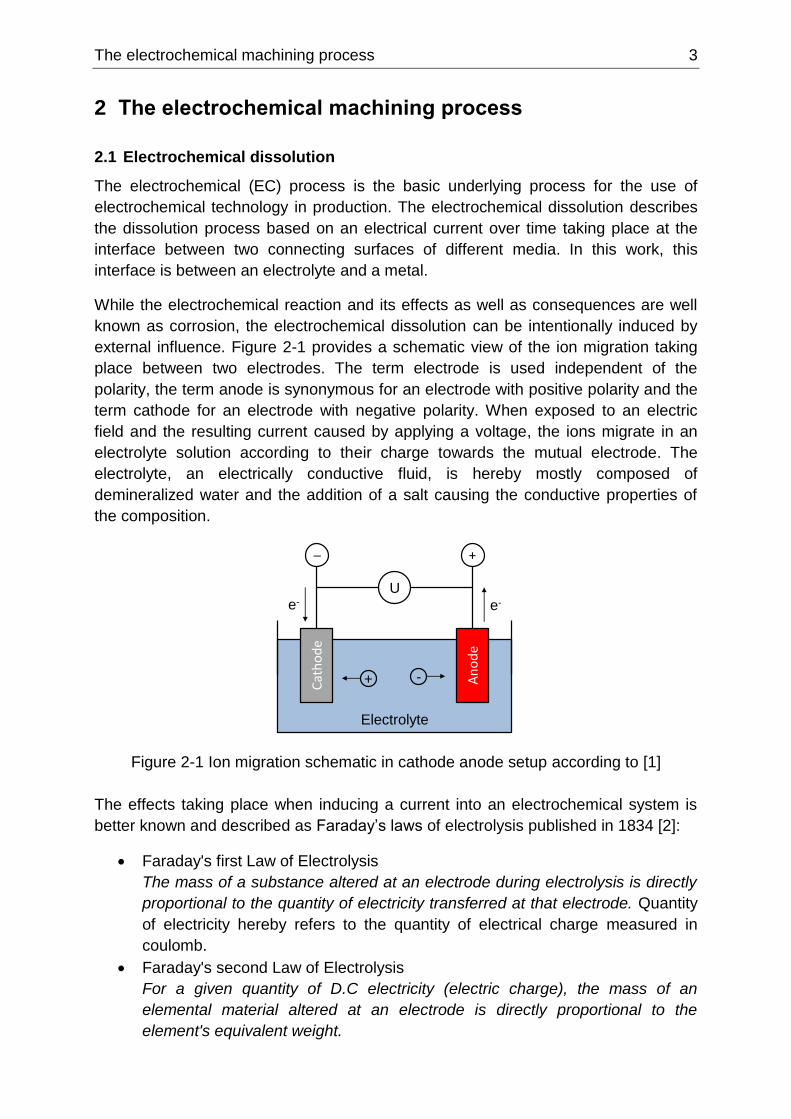
external influence. Figure 2-1 provides a schematic view of the ion migration taking
place between two electrodes. The term electrode is used independent of the
polarity, the term anode is synonymous for an electrode with positive polarity and the
term cathode for an electrode with negative polarity. When exposed to an electric
field and the resulting current caused by applying a voltage, the ions migrate in an
electrolyte solution according to their charge towards the mutual electrode. The
electrolyte, an electrically conductive fluid, is hereby mostly composed of
demineralized water and the addition of a salt causing the conductive properties of
the composition.
Figure 2-1 Ion migration schematic in cathode anode setup according to [1]
The effects taking place when inducing a current into an electrochemical system is
better known and described as Faraday’s laws of electrolysis published in 1834 [2]:
Faraday's first Law of Electrolysis
The mass of a substance altered at an electrode during electrolysis is directly
proportional to the quantity of electricity transferred at that electrode. Quantity
of electricity hereby refers to the quantity of electrical charge measured in
coulomb.
Faraday's second Law of Electrolysis
For a given quantity of D.C electricity (electric charge), the mass of an
elemental material altered at an electrode is directly proportional to the
element's equivalent weight.
Cat
ho
de
An
od
e
Ue- e-
-+
Electrolyte
_ +
4 The electrochemical machining process
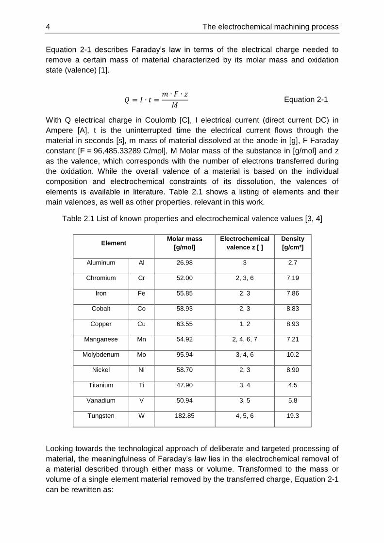
Equation 2-1 describes Faraday’s law in terms of the electrical charge needed to
remove a certain mass of material characterized by its molar mass and oxidation
state (valence) [1].
𝑄 = 𝐼 ∙ 𝑡 =𝑚 ∙ 𝐹 ∙ 𝑧
𝑀
Equation 2-1
With Q electrical charge in Coulomb [C], I electrical current (direct current DC) in
Ampere [A], t is the uninterrupted time the electrical current flows through the
material in seconds [s], m mass of material dissolved at the anode in [g], F Faraday
constant [F = 96,485.33289 C/mol], M Molar mass of the substance in [g/mol] and z
as the valence, which corresponds with the number of electrons transferred during
the oxidation. While the overall valence of a material is based on the individual
composition and electrochemical constraints of its dissolution, the valences of
elements is available in literature. Table 2.1 shows a listing of elements and their
main valences, as well as other properties, relevant in this work.
Table 2.1 List of known properties and electrochemical valence values [3, 4]
Element Molar mass
[g/mol]
Electrochemical
valence z [ ]
Density
[g/cm³]
Aluminum Al 26.98 3 2.7
Chromium Cr 52.00 2, 3, 6 7.19
Iron Fe 55.85 2, 3 7.86
Cobalt Co 58.93 2, 3 8.83
Copper Cu 63.55 1, 2 8.93
Manganese Mn 54.92 2, 4, 6, 7 7.21
Molybdenum Mo 95.94 3, 4, 6 10.2
Nickel Ni 58.70 2, 3 8.90
Titanium Ti 47.90 3, 4 4.5
Vanadium V 50.94 3, 5 5.8
Tungsten W 182.85 4, 5, 6 19.3
Looking towards the technological approach of deliberate and targeted processing of
material, the meaningfulness of Faraday’s law lies in the electrochemical removal of
a material described through either mass or volume. Transformed to the mass or
volume of a single element material removed by the transferred charge, Equation 2-1
can be rewritten as:
The electrochemical machining process 5
𝑚 =𝑀
𝑧 ∙ 𝐹∙ 𝐼 ∙ 𝑡
Equation 2-2
𝑚 = 𝑉 ∙ 𝜌 =𝑀
𝑧 ∙ 𝐹∙ 𝐼 ∙ 𝑡
Equation 2-3
𝑉 =𝑀
𝑧 ∙ 𝐹∙1
𝜌∙ 𝐼 ∙ 𝑡
Equation 2-4
V equals the volume of the material dissolved at the anode in [cm³] and ρ the density
of the material in [g/cm³].
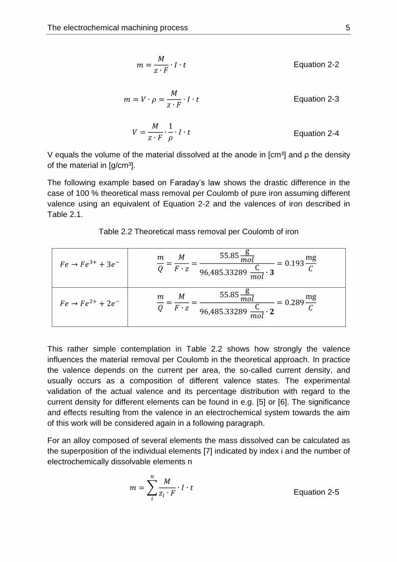
The following example based on Faraday’s law shows the drastic difference in the
case of 100 % theoretical mass removal per Coulomb of pure iron assuming different
valence using an equivalent of Equation 2-2 and the valences of iron described in
Table 2.1.
Table 2.2 Theoretical mass removal per Coulomb of iron
𝐹𝑒 → 𝐹𝑒3+ + 3𝑒− 𝑚
𝑄=
𝑀
𝐹 ∙ 𝑧=
55.85g
𝑚𝑜𝑙
96,485.33289 C
𝑚𝑜𝑙∙ 𝟑
= 0.193mg
𝐶
𝐹𝑒 → 𝐹𝑒2+ + 2𝑒− 𝑚
𝑄=
𝑀
𝐹 ∙ 𝑧=
55.85g
𝑚𝑜𝑙
96,485.33289 C
𝑚𝑜𝑙∙ 𝟐
= 0.289mg
𝐶
This rather simple contemplation in Table 2.2 shows how strongly the valence
influences the material removal per Coulomb in the theoretical approach. In practice
the valence depends on the current per area, the so-called current density, and
usually occurs as a composition of different valence states. The experimental
validation of the actual valence and its percentage distribution with regard to the
current density for different elements can be found in e.g. [5] or [6]. The significance
and effects resulting from the valence in an electrochemical system towards the aim
of this work will be considered again in a following paragraph.
For an alloy composed of several elements the mass dissolved can be calculated as
the superposition of the individual elements [7] indicated by index i and the number of
electrochemically dissolvable elements n
𝑚 = ∑𝑀
𝑧𝑖 ∙ 𝐹∙ 𝐼 ∙ 𝑡
𝑛
𝑖
Equation 2-5
6 The electrochemical machining process
𝑉 =1
𝜌𝑎𝑙𝑙𝑜𝑦∙ ∑
𝜌𝑖
100∙
𝑀
𝑧𝑖 ∙ 𝐹∙ 𝐼 ∙ 𝑡
𝑛
𝑖
Equation 2-6
As already presented in the rather simple example calculation, in the case of iron
assuming only two different valence values, this approach gets many times more
complex looking at an alloy. Yet, using Equation 2-6 the theoretical material removal
can be calculated for alloys with diverse and complex composition.
2.2 Electrochemical Machining – ECM
The technical use in production based on Faraday’s law is the Electrochemical
Machining, short ECM. These days ECM is mainly used in mass production e.g. by
companies like Philips [8] for the production of shaver caps, companies
manufacturing turbomachinery components [9], like LEISTRITZ TURBINENTECHNIK
GmbH or MTU Aero Engines AG, or in general the deburring of components. While
the underlying basics of the EC processes and mechanisms are the focus of
research in the field of physical chemistry, this broad knowledge is eventually finding
the way into the production, since many overlapping and interfering effects occur
during the practical use in production engineering.
Since its first practical application in 1928, see Table 2.3, Electrochemical Machining
became more and more interesting in industry. Arguments for the use of ECM are
stress free machining [3], the capability to process independent of the hardness state
of a metal, the theoretically infinite endurance of tools and the possibility of high
parallelization. To enable a user of this technology, high standards and requirements
have to be met concerning the power sources, machine robustness against the
corrosive environment, automation and coatings. These enablers are also main
obstacles to the technology. The process differs considerably from conventional
machining technologies like milling, turning and grinding, which makes it complicated
to become familiar with the theory quickly. Also monitoring and interpreting the
process during machining is complicated, since hardly any in-process investigations
or measurements at the electrode interfaces under process conditions are possible
due to high current densities. Furthermore, compared to other technologies the initial
acquisition costs are high. In this context Corbin [10] states:
“[…] Electrochemical machining is a last resort, not a step up. It is used when
there is no other practical way to machine a part, because it is very costly, slow
and difficult to make the hole precisely the right diameter and shape without
going to much higher expense than with traditional machining techniques. ECM
has its uses, one of which is to machine carbide materials that simply cannot be
cut any other way. There is nothing inherently more accurate about ECM. It
costs fortunes in equipment just to make it the same accuracy as lathe boring,
reaming, and diamond lapping. Using ECM makes sense when you can’t cut
the material in a more traditional way. People who sell ECM machines are the
first to tell you this. […] “
The electrochemical machining process 7
Despite the costs and complexity, ECM still is an important machining technology in
mass production and is gradually finding its way into smaller series. Selection criteria
indicating the use of ECM were already discussed in 1972 [11]. Due to advances in
power sources and processing, the focus in current research - personally judging
from the publications in recent years - has shifted towards the processes taking place
during material dissolution and more precise material models in general. This
knowledge then enables the reduction of iterations needed in tool-shaping, thus
making the process more competitive and cost efficient.
Table 2.3 Short history of ECM [12, 13, 14, 15]
around
1834
Michael Faraday (1791-1867) discovered the relationship
between electric charge and material conversion during
electrolysis.
1928 V.N. Gusev and L. Rozkov [13] (in Western literature often
found as W. Gussef) used the anodic dissolution with the aim
to properly dissolve metal - Electrochemical Machining (ECM).
1959 First commercial machine available in the US - Anocut
Engineering Company.
1960-1970s Serial use of ECM in the aerospace branch (industry) and in
tool manufacturing (forging dies) began in the USSR and in
Western Europe. Electrochemical technologies developed
during this period and companies like Philips, Hitachi,
Mitsubishi, AEG Elotherm, Amchem provided the equipment.
around
2000
Expansion of ECM technology with electrical and mechanical
pulses.
1998 - 2011 The complex of new bipolar microsecond ECM by vibrating
tool-electrode was introduced to market - Pulse
Electrochemical Machining (PECM).
starting
2000
Possibility to use the technology in the field of micro-
structuring, including the use of pulse length in the sub
microsecond range.
In DIN8580 [16] ECM is defined in the main group focusing on separating processes.
As part of the subgroup 3.4, ECM is further defined in DIN8590 [17] as imaging
electrochemical removal using an external power source at high current density,
caused by small distance between the tool electrode and the work piece at high flow
velocities of the electrolyte solution. Furthermore VDI3400 [18] and subsequent the
draft of VDI3401-Blatt 1 [19], based on VDI3401-Blatt 1 [20] and VDI3401-Blatt 3
[21], include definitions, a glossary and pictured use cases based on the
8 The electrochemical machining process
electrochemical dissolution. Most of these use cases can already be found in one of
the earliest books about ECM, the book of De Barr and Oliver [22] dating from 1968.
Here processes like electrolytic honing, electrochemical turning and milling as well as
electrochemical shaping, among others, are presented. In fact, the book ends with
chapter 13 “The future of electrochemical machining”, stating disadvantages of the
technology, which are partially still present today: Unfamiliarity with the techniques
involved, high capital costs, controlling the process and tool design for ECM.
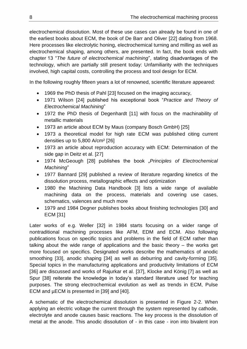
In the following roughly fifteen years a lot of renowned, scientific literature appeared:
1969 the PhD thesis of Pahl [23] focused on the imaging accuracy,
1971 Wilson [24] published his exceptional book “Practice and Theory of
Electrochemical Machining”
1972 the PhD thesis of Degenhardt [11] with focus on the machinability of
metallic materials
1973 an article about ECM by Maus (company Bosch GmbH) [25]
1973 a theoretical model for high rate ECM was published citing current
densities up to 5,800 A/cm² [26]
1973 an article about reproduction accuracy with ECM: Determination of the
side gap in Deitz et al. [27]
1974 McGeough [28] publishes the book „Principles of Electrochemical
Machining”
1977 Bannard [29] published a review of literature regarding kinetics of the
dissolution process, metallographic effects and optimization
1980 the Machining Data Handbook [3] lists a wide range of available
machining data on the process, materials and covering use cases,
schematics, valences and much more
1979 and 1984 Degner publishes books about finishing technologies [30] and
ECM [31]
Later works of e.g. Weller [32] in 1984 starts focusing on a wider range of
nontraditional machining processes like AFM, EDM and ECM. Also following
publications focus on specific topics and problems in the field of ECM rather than
talking about the wide range of applications and the basic theory – the works get
more focused on specifics. Designated works describe the mathematics of anodic
smoothing [33], anodic shaping [34] as well as deburring and cavity-forming [35].
Special topics in the manufacturing applications and productivity limitations of ECM
[36] are discussed and works of Rajurkar et al. [37], Klocke and König [7] as well as
Spur [38] reiterate the knowledge in today’s standard literature used for teaching
purposes. The strong electrochemical evolution as well as trends in ECM, Pulse
ECM and µECM is presented in [39] and [40].
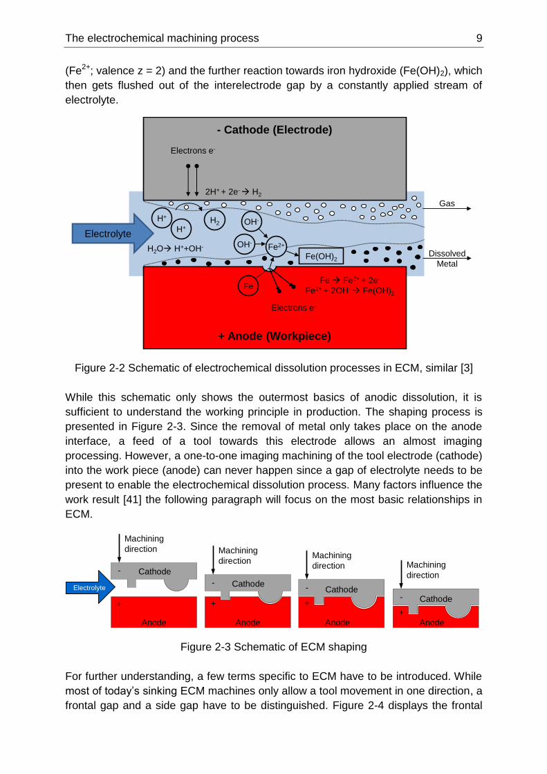
A schematic of the electrochemical dissolution is presented in Figure 2-2. When
applying an electric voltage the current through the system represented by cathode,
electrolyte and anode causes basic reactions. The key process is the dissolution of
metal at the anode. This anodic dissolution of - in this case - iron into bivalent iron
The electrochemical machining process 9
(Fe2+; valence z = 2) and the further reaction towards iron hydroxide (Fe(OH)2), which
then gets flushed out of the interelectrode gap by a constantly applied stream of
electrolyte.
Figure 2-2 Schematic of electrochemical dissolution processes in ECM, similar [3]
While this schematic only shows the outermost basics of anodic dissolution, it is
sufficient to understand the working principle in production. The shaping process is
presented in Figure 2-3. Since the removal of metal only takes place on the anode
interface, a feed of a tool towards this electrode allows an almost imaging
processing. However, a one-to-one imaging machining of the tool electrode (cathode)
into the work piece (anode) can never happen since a gap of electrolyte needs to be
present to enable the electrochemical dissolution process. Many factors influence the
work result [41] the following paragraph will focus on the most basic relationships in
ECM.
Figure 2-3 Schematic of ECM shaping
For further understanding, a few terms specific to ECM have to be introduced. While
most of today’s sinking ECM machines only allow a tool movement in one direction, a
frontal gap and a side gap have to be distinguished. Figure 2-4 displays the frontal
Electrons e-
- Cathode (Electrode)
+ Anode (Workpiece)
Dissolved
Metal
Electrolyte
H+
H+H2 OH-
OH-
Fe
Fe2+
Electrons e-
2H+ + 2e- H2
Fe Fe2+ + 2e-
Fe2+ + 2OH- Fe(OH)2
Fe(OH)2
Gas
H2O H++OH-
Machining
direction
Cathode-
+
Anode
ElectrolyteCathode-
+
Anode
Machining
direction
Cathode-
+
Anode
Machining
direction
Cathode-
+
Anode
Machining
direction
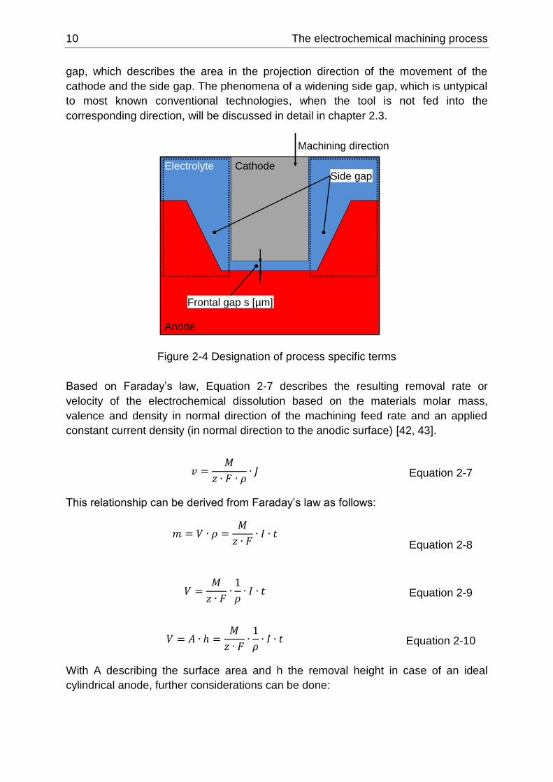
10 The electrochemical machining process
gap, which describes the area in the projection direction of the movement of the
cathode and the side gap. The phenomena of a widening side gap, which is untypical
to most known conventional technologies, when the tool is not fed into the
corresponding direction, will be discussed in detail in chapter 2.3.
Figure 2-4 Designation of process specific terms
Based on Faraday’s law, Equation 2-7 describes the resulting removal rate or
velocity of the electrochemical dissolution based on the materials molar mass,
valence and density in normal direction of the machining feed rate and an applied
constant current density (in normal direction to the anodic surface) [42, 43].
𝑣 =𝑀
𝑧 ∙ 𝐹 ∙ 𝜌∙ 𝐽
Equation 2-7
This relationship can be derived from Faraday’s law as follows:
𝑚 = 𝑉 ∙ 𝜌 =𝑀
𝑧 ∙ 𝐹∙ 𝐼 ∙ 𝑡
Equation 2-8
𝑉 =𝑀
𝑧 ∙ 𝐹∙1
𝜌∙ 𝐼 ∙ 𝑡
Equation 2-9
𝑉 = 𝐴 ∙ ℎ =𝑀
𝑧 ∙ 𝐹∙1
𝜌∙ 𝐼 ∙ 𝑡
Equation 2-10
With A describing the surface area and h the removal height in case of an ideal
cylindrical anode, further considerations can be done:
Electrolyte Cathode
Anode
Side gap
Frontal gap s [µm]
Machining direction
The electrochemical machining process 11
ℎ
𝑡=
𝑀
𝑧 ∙ 𝐹∙1
𝜌∙𝐼
𝐴
Equation 2-11
𝑤𝑖𝑡ℎ 𝑣 =ℎ
𝑡 (𝑎𝑠𝑠𝑢𝑚𝑖𝑛𝑔 𝑡 = 𝑐𝑜𝑛𝑠𝑡. ) 𝑎𝑛𝑑 𝐽 =
𝐼
𝐴
𝑣 =𝑀
𝑧 ∙ 𝐹∙1
𝜌∙ 𝐽
Equation 2-7
The current density J is usually used, either in A/cm² or in A/mm², since normalizing
to an area allows a comparison between experiments using different surface sizes,
and the current itself is one of the most important and modifiable parameters in
Faraday’s law when carrying out an experiment.
Also starting with Faraday’s law, the material-specific components, sometimes also
referred to as the electrochemical equivalent for a material, can be derived from
Equation 2-7.
𝑆𝑀𝑅 =𝑀
𝑧 ∙ 𝐹
Equation 2-12
𝑀𝑅𝑅 =𝑀
𝑧 ∙ 𝐹∙1
𝜌
Equation 2-13
The specific mass removal (SMR) in [mg/C] as well as the mass removal rate (MRR)
in [cm³/C] hereby represent material-specific coefficients. The relationship between
the two introduced removal rates can be written as:
𝑀𝑅𝑅 = 𝑆𝑀𝑅 ∙1
𝜌
Equation 2-14
Therefore Equation 2-7 becomes:
𝑣 = 𝑀𝑅𝑅 ∙ 𝐽 = 𝑆𝑀𝑅 ∙1
𝜌∙ 𝐽
Equation 2-15
It is obvious, that an essential factor for the use in production is still missing. While
the velocity or removal rate is often synonymous with the feed rate applied in ECM,
the factor allowing contemplations towards shaping accuracy comes from Ohm’s law
(Equation 2-16).
𝑈 = 𝑅 ∙ 𝐼 Equation 2-16
U potential in [V], R ohmic resistance in [Ω]
12 The electrochemical machining process
Ohm’s law provides the information about the relation between the current and
applied voltage in an electrically conductive medium. Since this conductive medium
is represented by an electrolyte, a liquid solution, Ohm’s law has to be adapted
towards the present geometric properties in accordance to the setup. Assuming two
parallel and equally sized opposing electrode surfaces at a distance s and a specific
resistance of the electrolyte κ the resistance in the enclosed volume can be written
as
𝑅 = 𝜅 ∙𝑠
𝐴
Equation 2-17
s distance between electrodes of a homogeneous conductor in [µm], A cross
sectional area in [cm²], κ specific resistance in [Ωcm]
By using the inverse relationship between resistance and conductivity
𝜅 =1
𝜎
Equation 2-18
the overall resistance can be written as
𝑅 =𝑠
𝜎 ∙ 𝐴
Equation 2-19
σ conductivity [mS/cm]
With the combination of the relationships stated above, Ohm’s law can be rewritten.
𝑈 = 𝑅 ∙ 𝐼 =𝑠
𝜎 ∙ 𝐴∙ 𝐼 =
𝑠
𝜎∙𝐼
𝐴
Equation 2-20
With J as the current density or current per surface area in [A/cm²]:
𝑈 =𝑠
𝜎∙ 𝐽 ↔ 𝑠 =
𝑈 ∙ 𝜎
𝐽 ↔ 𝐽 =
𝑈 ∙ 𝜎
𝑠
Equation 2-21
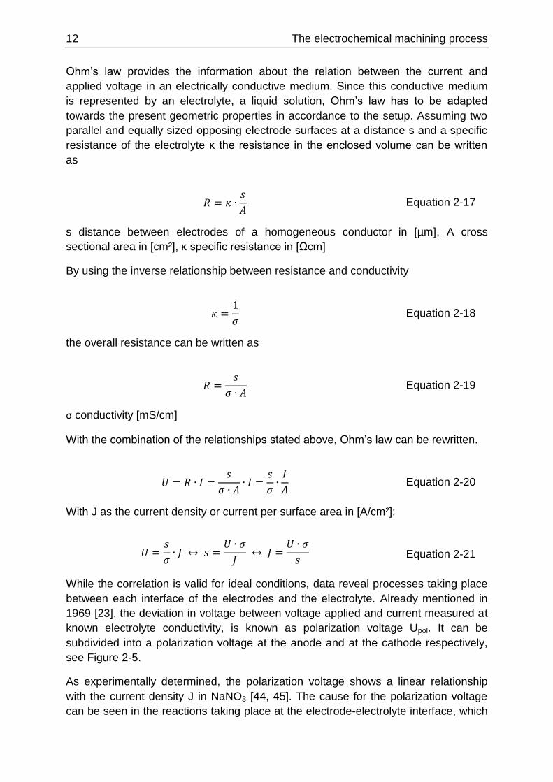
While the correlation is valid for ideal conditions, data reveal processes taking place
between each interface of the electrodes and the electrolyte. Already mentioned in
1969 [23], the deviation in voltage between voltage applied and current measured at
known electrolyte conductivity, is known as polarization voltage Upol. It can be
subdivided into a polarization voltage at the anode and at the cathode respectively,
see Figure 2-5.
As experimentally determined, the polarization voltage shows a linear relationship
with the current density J in NaNO3 [44, 45]. The cause for the polarization voltage
can be seen in the reactions taking place at the electrode-electrolyte interface, which
The electrochemical machining process 13
lead to oxide formations or layers and hence additional resistances. The stability,
reactivity and breakdown of such passive films [46], as well as the surface structure
[47] and mechanisms of the anodic dissolution [6] are still in the focus of research [5,
48]. Models were developed describing layers on an iron surface in NaNO3 [48], with
each of them showing different properties and resistances. Equally the same
investigations revealed differences in valence of Fe3+ und Fe2+ under different
electrical conditions [48, 49].
Figure 2-5 Polarization voltages at anode and cathode
Since the variable U is used for the voltage applied to the system overall, the variable
Uprod is introduced in Figure 2-5 to represent the productive voltage describing the
voltage in the ideal electrolyte system (Uprod = U in Equation 2-21 and previous
equations) which directly correlates with the current and conductivity.
𝑠 =(𝑈 − 𝑈𝑝𝑜𝑙) ∙ 𝜎
𝐽
Equation 2-22
Equation 2-22 shows the adapted form of Ohm’s law taking Upol into account. Since
the layer thicknesses, leading to Upol, are reported in the range of nm to some µm
[48], the gap distance is not reduced by these layer thicknesses. Similar to [44], the
polarization voltages, resulting from the cathode and anode material reactions will not
be further investigated, since the machine used in later experiments resembles a
two-electrode setup. Other than a three-electrode setup, used in [48] and developed
in [50], this two-electrode setup does not allow a reference measurement towards a
known potential. Therefore resulting effects from the electrode material (1.4301
conductivity 1.39x10⁷ mS/cm >> conductivity electrolyte ~70 mS/cm) cannot be
measured and the polarization voltage has to be evaluated experimentally.
UpolC
UpolA
Uprod
- Cathode (Electrode)
+ Anode (Workpiece)
Upol = UpolA + UpolCU = Upol + Uprod
sU
nm-µm
nm-µm
µm
14 The electrochemical machining process
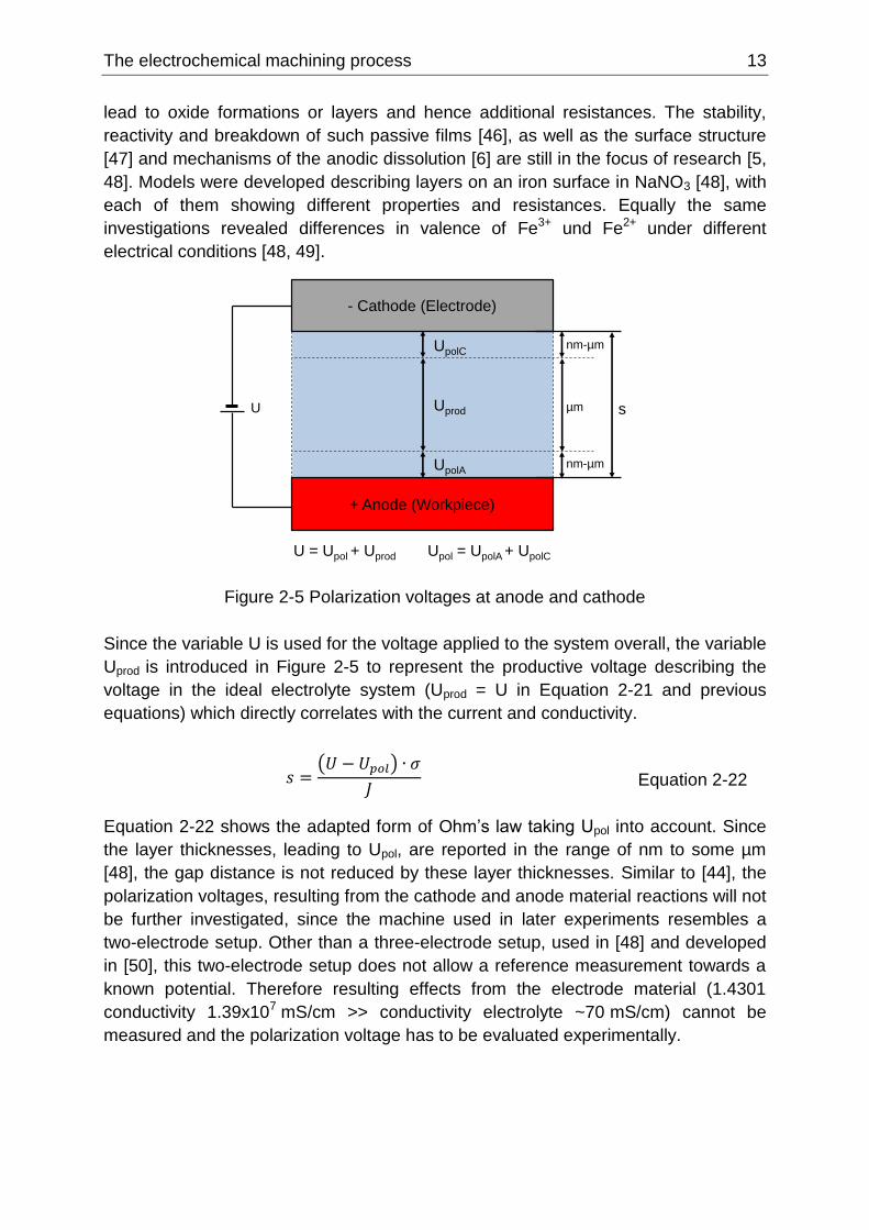
Figure 2-6 Example of a calculation with and without considering the polarization voltage
Figure 2-6 shows the application of Ohm’s law with and without considering the
polarization voltage at the example of experimental data. Only when considering Upol,
the experimentally determined relationship between current density and frontal gap
relationship can be described correctly.
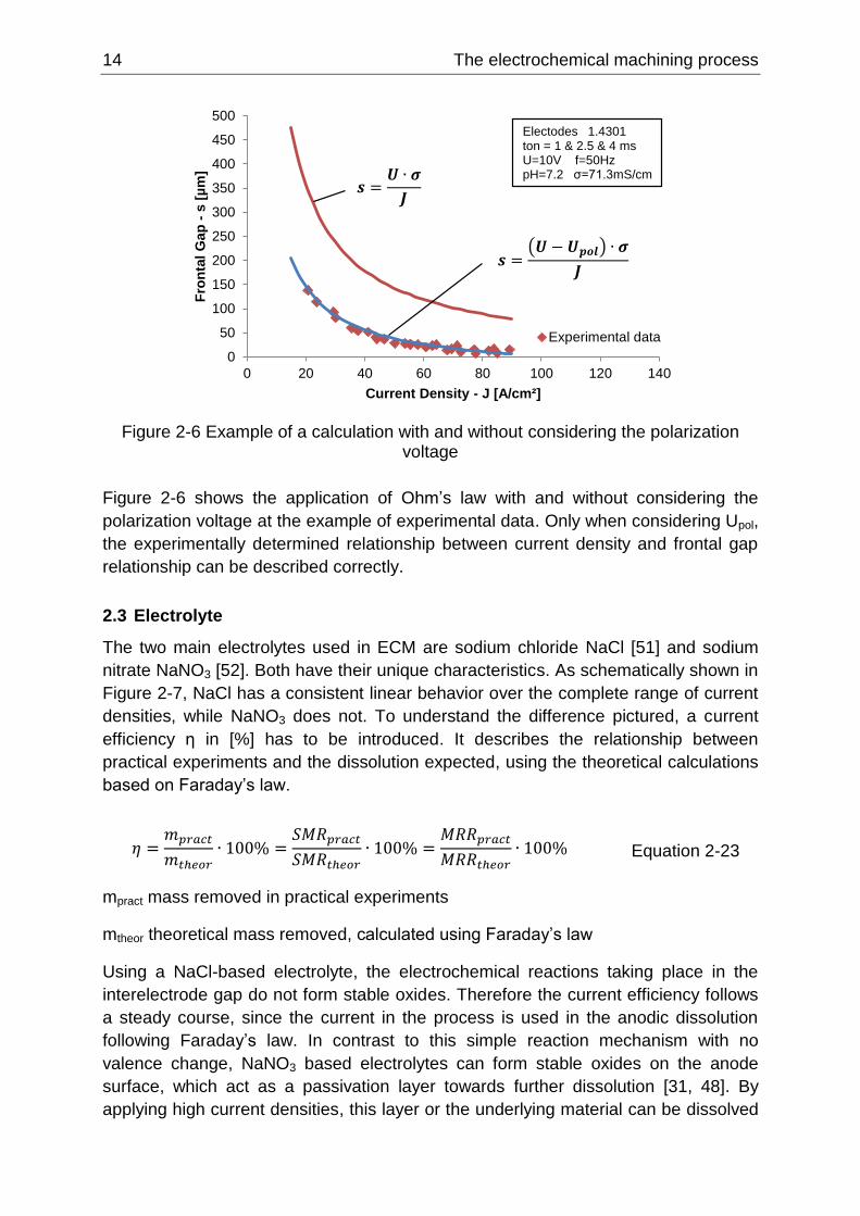
2.3 Electrolyte
The two main electrolytes used in ECM are sodium chloride NaCl [51] and sodium
nitrate NaNO3 [52]. Both have their unique characteristics. As schematically shown in
Figure 2-7, NaCl has a consistent linear behavior over the complete range of current
densities, while NaNO3 does not. To understand the difference pictured, a current
efficiency η in [%] has to be introduced. It describes the relationship between
practical experiments and the dissolution expected, using the theoretical calculations
based on Faraday’s law.
𝜂 =𝑚𝑝𝑟𝑎𝑐𝑡
𝑚𝑡ℎ𝑒𝑜𝑟∙ 100% =
𝑆𝑀𝑅𝑝𝑟𝑎𝑐𝑡
𝑆𝑀𝑅𝑡ℎ𝑒𝑜𝑟∙ 100% =
𝑀𝑅𝑅𝑝𝑟𝑎𝑐𝑡
𝑀𝑅𝑅𝑡ℎ𝑒𝑜𝑟∙ 100%
Equation 2-23
mpract mass removed in practical experiments
mtheor theoretical mass removed, calculated using Faraday’s law
Using a NaCl-based electrolyte, the electrochemical reactions taking place in the
interelectrode gap do not form stable oxides. Therefore the current efficiency follows
a steady course, since the current in the process is used in the anodic dissolution
following Faraday’s law. In contrast to this simple reaction mechanism with no
valence change, NaNO3 based electrolytes can form stable oxides on the anode
surface, which act as a passivation layer towards further dissolution [31, 48]. By
applying high current densities, this layer or the underlying material can be dissolved
0
50
100
150
200
250
300
350
400
450
500
0 20 40 60 80 100 120 140
Fro
nta
l G
ap
-s [
µm
]
Current Density - J [A/cm²]
Experimental data
Electodes 1.4301ton = 1 & 2.5 & 4 msU=10V f=50HzpH=7.2 σ=71.3mS/cm
The electrochemical machining process 15
and the dissolution process intensifies with increasing current density. The basics on
mass transport in high rate dissolution of iron in ECM electrolytes can be found for
chloride solutions in [53] and for nitrate solutions respectively in [54].
Figure 2-7 Schematic of the current efficiency using different electrolytes
In order to explain why this commonly used method to describe a material by its
current efficiency, is neither useful nor suitable for the aim of this work, a closer look
towards the valence in the theoretical part of Equation 2-23 is necessary.
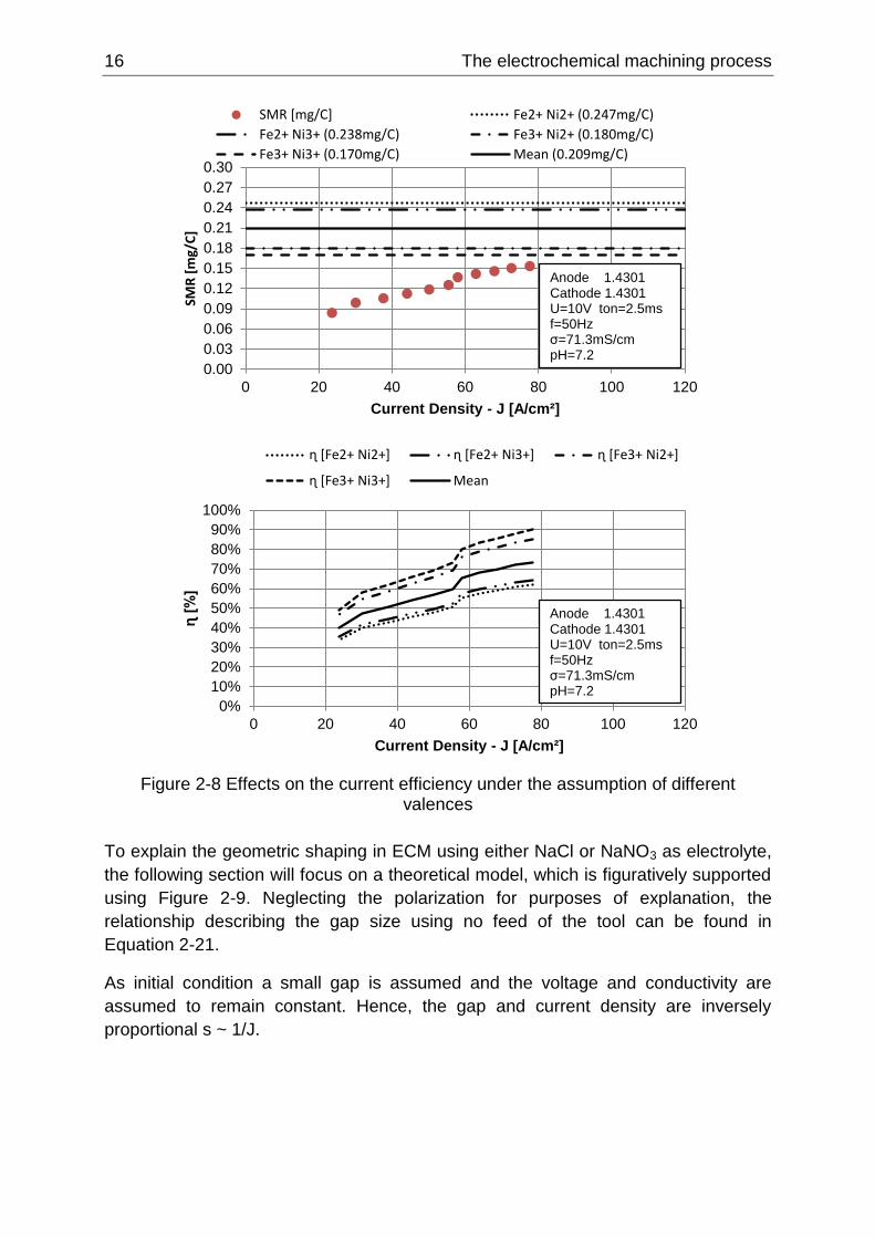
At the example of the material 1.4301, composed of roughly 69 % iron (Fe), 18 %
chromium (Cr) and 10 % nickel (Ni), the lack of quality in regard to the current
efficiency, without a clear understanding or sources in literature listing the valences,
is explained. The valence of chromium as machined in the underlying experiments is
6 (CrVI). Therefore the theoretical current efficiency will mainly be influenced by the
valence of Fe as 2 or 3 and the valence of Nickel as 2 or 3 (see Table 2.1). The four
combinations possible are pictured in Figure 2-8 and a value referred to as ‘Mean’ is
defined as the average towards the valence values of iron and nickel. The individual
values (red dots) indicate experimental results and the lines depict the theoretically
calculated SMR values based on the combinations as highlighted in the legend.
Looking at the calculated current efficiency values in the figure, the deviations are in
a range of up to 30% from the lowest to the highest values assuming variations of
valences. The method used cannot explain dissolution ineffective reactions, which
just result from a loss of mass of nonconductive material. However, the current
efficiency provides a quantitative assessment under known constraints. The
theoretical considerations can provide evidence when values of 100% and above are
calculated using faulty assumptions. Since the values can only be put in context,
when knowing the correct valences for each current density value, all material
dissolution results in this work will be based on measurable and comparable values
as SMR in [mg/C].
ɳ [%
]
Current density J [A/cm²]
NaCl
NaNO3
16 The electrochemical machining process
Figure 2-8 Effects on the current efficiency under the assumption of different valences
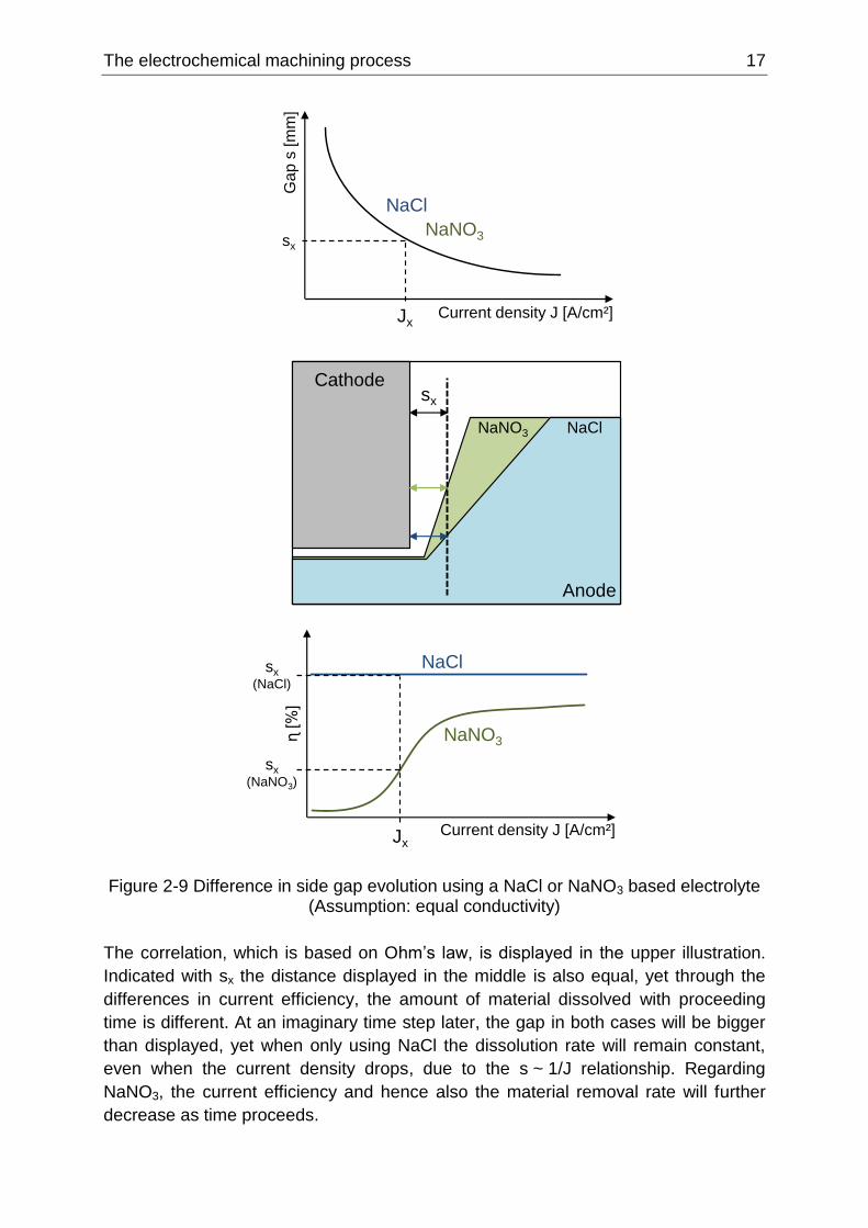
To explain the geometric shaping in ECM using either NaCl or NaNO3 as electrolyte,
the following section will focus on a theoretical model, which is figuratively supported
using Figure 2-9. Neglecting the polarization for purposes of explanation, the
relationship describing the gap size using no feed of the tool can be found in
Equation 2-21.
As initial condition a small gap is assumed and the voltage and conductivity are
assumed to remain constant. Hence, the gap and current density are inversely
proportional s ~ 1/J.
0.00
0.03
0.06
0.09
0.12
0.15
0.18
0.21
0.24
0.27
0.30
0 20 40 60 80 100 120
SMR
[m
g/C
]
Current Density - J [A/cm²]
SMR [mg/C] Fe2+ Ni2+ (0.247mg/C)
Fe2+ Ni3+ (0.238mg/C) Fe3+ Ni2+ (0.180mg/C)
Fe3+ Ni3+ (0.170mg/C) Mean (0.209mg/C)
Anode 1.4301Cathode 1.4301U=10V ton=2.5msf=50Hzσ=71.3mS/cmpH=7.2
0%
10%
20%
30%
40%
50%
60%
70%
80%
90%
100%
0 20 40 60 80 100 120
ɳ [
%]
Current Density - J [A/cm²]
ɳ [Fe2+ Ni2+] ɳ [Fe2+ Ni3+] ɳ [Fe3+ Ni2+]
ɳ [Fe3+ Ni3+] Mean
Anode 1.4301Cathode 1.4301U=10V ton=2.5msf=50Hzσ=71.3mS/cmpH=7.2
The electrochemical machining process 17
Figure 2-9 Difference in side gap evolution using a NaCl or NaNO3 based electrolyte (Assumption: equal conductivity)
The correlation, which is based on Ohm’s law, is displayed in the upper illustration.
Indicated with sx the distance displayed in the middle is also equal, yet through the
differences in current efficiency, the amount of material dissolved with proceeding
time is different. At an imaginary time step later, the gap in both cases will be bigger
than displayed, yet when only using NaCl the dissolution rate will remain constant,
even when the current density drops, due to the s ~ 1/J relationship. Regarding
NaNO3, the current efficiency and hence also the material removal rate will further
decrease as time proceeds.
ɳ [%
]
Current density J [A/cm²]
NaCl
NaNO3
sx
(NaNO3)
sx
(NaCl)
Jx
Cathode
NaNO3 NaCl
sx
Anode
Ga
p s
[m
m]
Current density J [A/cm²] Jx
sx
NaCl
NaNO3
18 The electrochemical machining process
In this work, only water-based technically pure NaNO3 by manufacturer Kirsch
Pharma GmbH [55] is used. The water is taken from a reverse osmosis process,
using an Aqua Medic Merlin II by company Aqua Medic. The measured conductivity
of the water going into the machine used in the experiments before adding the
NaNO3 was on an average measured at σ = 58 µS/cm. It is known, that the pH-value
and concentration of the electrolyte have an effect on the reaction products,
mechanisms and copying accuracy [56], yet considering the objective of this work
only experiments with a constant pH value and constant concentration in the inflow of
the process chamber are conducted.
The conductivity considerations in this work are carried out using published empirical
data [44]. Herein, the relation between conductivity, temperature and concentration of
NaNO3 dissolved in demineralized water was concluded as follows:
𝜎 = 𝑎 ∙ 𝐶2 + 𝑏 ∙ 𝐶 + (𝑐 ∙ 𝐶2 + 𝑑 ∙ 𝐶) ∙ 𝑇 Equation 2-24
with
σ = conductivity [mS/cm]
C = electrolyte concentration [g (NaNO3)/l] T = electrolyte temperature [°C]
and the constants derived as the following values: a = - 0.0000755 b = 0.0523 c = - 0.00000338 d = 0.00200
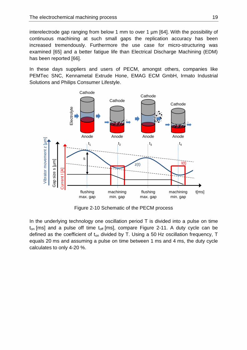
2.4 Pulse Electrochemical Machining – PECM
The Pulse Electrochemical Machining (PECM), schematically shown in Figure 2-10,
is a variation of the ECM process. During this process, the feed towards the work
piece is overlaid with a mechanical oscillation of the tool [57]. The oscillation
amplitude of the machine used is 200 μm, which results in two different process
phases. During the minimum gap size, a pulsed current with a pulse duration ranging
from 0.1-5 ms can be applied. The small gap size, achievable through the oscillation
of the cathode and short current pulses of up to 8,000 A, lead to an effective material
removal process resulting in good surface quality and precise copying accuracy [37].
The upward movement during the oscillation results in the phase of maximum gap
size, which enables enhanced flushing possibilities and consequently a better
removal of the processed material as compared to the conditions at minimum gap
size. While this process using just electrical pulses was already described by
Degenhardt in 1972 [11], a patent in 1979 [58] described the method and system
using a mechanical vibration overlaid with the electrical pulsation. It was not many
years later, that first results of experiments under pulsed current conditions were
published [59] and variations and use cases were reported [31, 60, 61]. Especially
the focus on new developments in ECM [37] and studies of ECM utilizing a vibrating
tool electrode [62, 63] gave an insight to the new possibilities this process opened. In
2009 the PECM application area was described with the potential of processing in an
The electrochemical machining process 19
interelectrode gap ranging from below 1 mm to over 1 µm [64]. With the possibility of
continuous machining at such small gaps the replication accuracy has been
increased tremendously. Furthermore the use case for micro-structuring was
examined [65] and a better fatigue life than Electrical Discharge Machining (EDM)
has been reported [66].
In these days suppliers and users of PECM, amongst others, companies like
PEMTec SNC, Kennametal Extrude Hone, EMAG ECM GmbH, Irmato Industrial
Solutions and Philips Consumer Lifestyle.
Figure 2-10 Schematic of the PECM process
In the underlying technology one oscillation period T is divided into a pulse on time
ton [ms] and a pulse off time toff [ms], compare Figure 2-11. A duty cycle can be
defined as the coefficient of ton divided by T. Using a 50 Hz oscillation frequency, T
equals 20 ms and assuming a pulse on time between 1 ms and 4 ms, the duty cycle
calculates to only 4-20 %.
z(t)
t[ms]flushing
max. gap
machining
min. gap
flushing
max. gap
machining
min. gap
t1 t2 t3 t4
s
Cathode
CathodeCathode
Cathode
Anode Anode Anode Anode
Ele
ctr
oly
te
I(t)
Cu
rre
nt
I [A
]
Ga
p s
ize
s [
µm
]
Vib
rato
r m
ove
me
ntz [
µm
]
20 The electrochemical machining process
Figure 2-11 Time-dependent variables
To increase or change the machining rate and duty cycle other pulse-pause cycles
are possible by using
longer pulses or multiple pulses during one oscillation [37, 67, 68]
rectangular, exponential, saw or triangle pulses [69]
a programmable movement of the cathode with a higher down time and
localization of the anode surface through touching of anode and cathode
before applying multiple pulses. When a change in the parameters is
detectable and the gap is filled with hydroxides, then parameter specific
lifting of the cathode and flushing of the gap or adjusting to a certain
surface condition [70] can be performed
Since PECM can be regarded as a discontinuous ECM process, when using
rectangular pulses, all formulas introduced can be adapted by considering a constant
factor composed of the pulse on time and the pulses per time unit, which is in this
case defined by the frequency f of the sinusoidal oscillation. The ideal Faraday’s law
is therefore adjusted by considering the pulse on and pulse off cycle
𝑄 = 𝐼 ∙ 𝑡 ∙ 𝑡𝑜𝑛 ∙ 𝑓 =𝑚 ∙ 𝐹 ∙ 𝑧
𝑀
Equation 2-25
In contrast to the equations in ECM, here t corresponds to the uninterrupted
machining time and ton to the length of each current pulse. The connection between
feed rate and current density can be written as
𝑣 =𝑀
𝑧 ∙ 𝐹 ∙ 𝜌∙ 𝐽 ∙ 𝑡𝑜𝑛 ∙ 𝑓
Equation 2-26
The influence of time during a pulse is not considered. The reason can be seen in the
fact that the material height removed during each pulse in feed direction, is again fed
in equal amount during the pulse off time, which resembles the equilibrium state of
the process in feed direction. In this way, every pulse is each time triggered at an
z(t)
t[ms]flushing
max. gap
machining
min. gap
flushing
max. gap
machining
min. gap
t1t4
sI(t)
Cu
rre
nt
I [A
]
Ga
p s
ize
s [
µm
]
Vib
rato
r m
ove
me
ntz [
µm
]ton toff
1/f = T = ton + toff
The electrochemical machining process 21
equal frontal gap after the processing gap has been regenerated with electrolyte after
each oscillation.
The PECM machine used in all experiments was a PEMCenter8000 (installed 2011)
by company PEMTec SNC, France. The main technical data is listed in Figure 2-12.
A similar machine was already used by Förster in 2004 [4], yet many changes in the
mechanical and electrical concept do not allow a comparison of data. The
preparation of the electrolyte in terms of conductivity, temperature and pH value
occurs automatically in the processing unit. These parameters can therefore be
regarded as constant input parameters or boundary conditions. The temperature
compensated conductivity was measured in the experiments in the range of
σ = 71.5±1.5 mS/cm and the pH was kept constant between pH 7.1 and pH 7.3.
Furthermore the machine is equipped with a bipolar unit. This unit allows a polarity
switch [31, 71], which was patented as a method for on-line removal of cathode
depositions during the electrochemical process [72]. This unit was not used, yet
during the pulse pauses a voltage of U = 2.7 V at a maximum current of
Imax = 120 mA is applied [48].
Technical Data
PEMCenter8000 by company PEMTec SNC,
Forbach, France
Current I [A] up to 8,000
Voltage U [V] up to 18.7
Pulse on time ton [ms] 0.1 - 5
Mechanical Oscillation
fmechanic [Hz] 5 - 60
Electrical pulsation without
mechanical oscilation
felectric [Hz]
1 - 200
Feed rate vf [mm/min] 0 - 2
Electrolyte pressure [kPa] 100 - 1,000
Electrolyte NaNO3
(common) pH-value 6-9
Figure 2-12 Technical constraints of the equipment used in the experiments
As a special feature of the machine used, a parameter variation has to be mentioned.
The shift in Phase Pshift [%] - as shown in Figure 2-13 - relates to the shift of the pulse
on time in relation to the bottom dead center of the mechanical vibrator. The starting
time tshift [ms] of the rising flank of the pulse on time can be calculated in relation to
the point in time when the vibrator reaches the bottom dead center according to
Equation 2-27.
process and
machine control
module
processing
module
self-contained
electrolyte
treatment facility
power supply
module
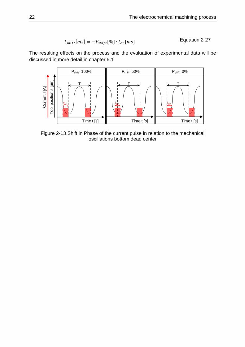
22 The electrochemical machining process
𝑡𝑠ℎ𝑖𝑓𝑡[𝑚𝑠] = −𝑃𝑠ℎ𝑖𝑓𝑡[%] ∙ 𝑡𝑜𝑛[𝑚𝑠]
Equation 2-27
The resulting effects on the process and the evaluation of experimental data will be
discussed in more detail in chapter 5.1
Figure 2-13 Shift in Phase of the current pulse in relation to the mechanical oscillations bottom dead center
Pshift=100% Pshift=50% Pshift=0%
To
ol po
sitio
n s
[µ
m]
Curr
en
t I [A
]
Time t [s]
T
ton
Time t [s] Time t [s]
T
ton
T
ton
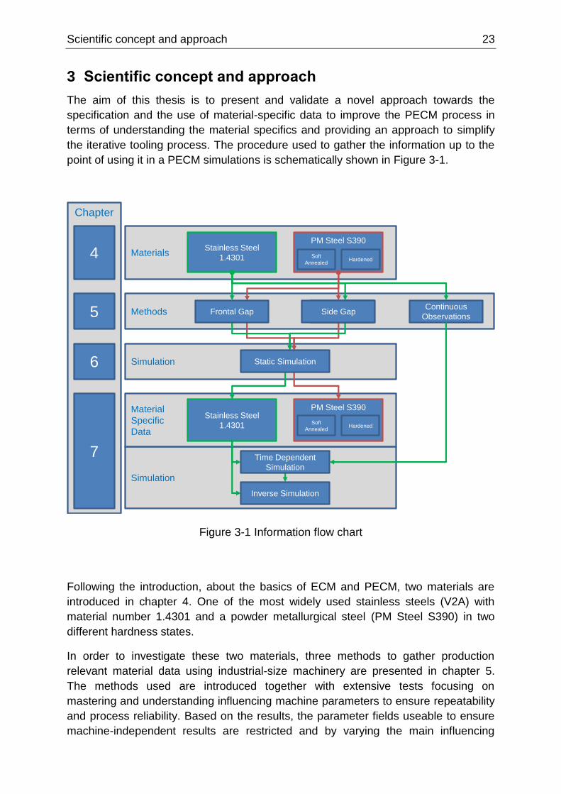
Scientific concept and approach 23
3 Scientific concept and approach
The aim of this thesis is to present and validate a novel approach towards the
specification and the use of material-specific data to improve the PECM process in
terms of understanding the material specifics and providing an approach to simplify
the iterative tooling process. The procedure used to gather the information up to the
point of using it in a PECM simulations is schematically shown in Figure 3-1.
Figure 3-1 Information flow chart
Following the introduction, about the basics of ECM and PECM, two materials are
introduced in chapter 4. One of the most widely used stainless steels (V2A) with
material number 1.4301 and a powder metallurgical steel (PM Steel S390) in two
different hardness states.
In order to investigate these two materials, three methods to gather production
relevant material data using industrial-size machinery are presented in chapter 5.
The methods used are introduced together with extensive tests focusing on
mastering and understanding influencing machine parameters to ensure repeatability
and process reliability. Based on the results, the parameter fields useable to ensure
machine-independent results are restricted and by varying the main influencing
Chapter
correction using
static simulation
Frontal gap
correction using
static simulation
Frontal gap
MaterialsStainless Steel
1.4301
PM Steel S390
Soft
AnnealedHardened
4
MethodsContinuous
Observations5
Simulation6
Simulation
7
Material
Specific
Data
Stainless Steel
1.4301
PM Steel S390
Soft
AnnealedHardened
Static Simulation
Frontal Gap
Time Dependent
Simulation
Inverse Simulation
Side gapSide gapSide Gap

24 Scientific concept and approach
parameters the materials are characterized individually. The data acquired includes
information about the dissolution rates, geometric precision and surface properties
achievable.
In chapter 6 simulation concepts are introduced. Aside from the Finite-Element-
Method (FEM) using commercially available software to validate and better
understand the electrical parameters in a complex three dimensional experiment, a
two dimensional simulation based on individual programming is presented.
With the possibility to validate experimental results and measurements using
simulation, the material-specific data recorded is evaluated and discussed in chapter
7. Based on the material data for the stainless steel, the simulation concept is tested
and validated towards experimental data recorded using the in-process observation
setup.
In each chapter, its main content is summarized to highlight the key content. Also the
topic specific information covering the state of the art and available knowledge from
scientific literature are incorporated and, if possible, additionally supported and
discussed using collected data and examples.
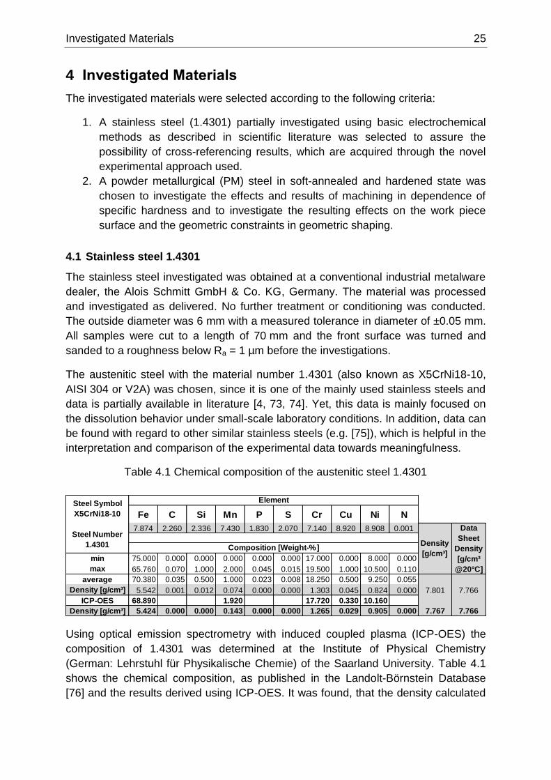
Investigated Materials 25
4 Investigated Materials
The investigated materials were selected according to the following criteria:
1. A stainless steel (1.4301) partially investigated using basic electrochemical
methods as described in scientific literature was selected to assure the
possibility of cross-referencing results, which are acquired through the novel
experimental approach used.
2. A powder metallurgical (PM) steel in soft-annealed and hardened state was
chosen to investigate the effects and results of machining in dependence of
specific hardness and to investigate the resulting effects on the work piece
surface and the geometric constraints in geometric shaping.
4.1 Stainless steel 1.4301
The stainless steel investigated was obtained at a conventional industrial metalware
dealer, the Alois Schmitt GmbH & Co. KG, Germany. The material was processed
and investigated as delivered. No further treatment or conditioning was conducted.
The outside diameter was 6 mm with a measured tolerance in diameter of ±0.05 mm.
All samples were cut to a length of 70 mm and the front surface was turned and
sanded to a roughness below Ra = 1 µm before the investigations.
The austenitic steel with the material number 1.4301 (also known as X5CrNi18-10,
AISI 304 or V2A) was chosen, since it is one of the mainly used stainless steels and
data is partially available in literature [4, 73, 74]. Yet, this data is mainly focused on
the dissolution behavior under small-scale laboratory conditions. In addition, data can
be found with regard to other similar stainless steels (e.g. [75]), which is helpful in the
interpretation and comparison of the experimental data towards meaningfulness.
Table 4.1 Chemical composition of the austenitic steel 1.4301
Using optical emission spectrometry with induced coupled plasma (ICP-OES) the
composition of 1.4301 was determined at the Institute of Physical Chemistry
(German: Lehrstuhl für Physikalische Chemie) of the Saarland University. Table 4.1
shows the chemical composition, as published in the Landolt-Börnstein Database
[76] and the results derived using ICP-OES. It was found, that the density calculated
Fe C Si Mn P S Cr Cu Ni N
7.874 2.260 2.336 7.430 1.830 2.070 7.140 8.920 8.908 0.001
min 75.000 0.000 0.000 0.000 0.000 0.000 17.000 0.000 8.000 0.000
max 65.760 0.070 1.000 2.000 0.045 0.015 19.500 1.000 10.500 0.110
average 70.380 0.035 0.500 1.000 0.023 0.008 18.250 0.500 9.250 0.055
Density [g/cm³] 5.542 0.001 0.012 0.074 0.000 0.000 1.303 0.045 0.824 0.000 7.801 7.766
ICP-OES 68.890 1.920 17.720 0.330 10.160
Density [g/cm³] 5.424 0.000 0.000 0.143 0.000 0.000 1.265 0.029 0.905 0.000 7.767 7.766
Data
Sheet
Density
[g/cm³
@20°C]
Density
[g/cm³]
Steel Symbol
X5CrNi18-10
Steel Number
1.4301
Element
Composition [Weight-%]
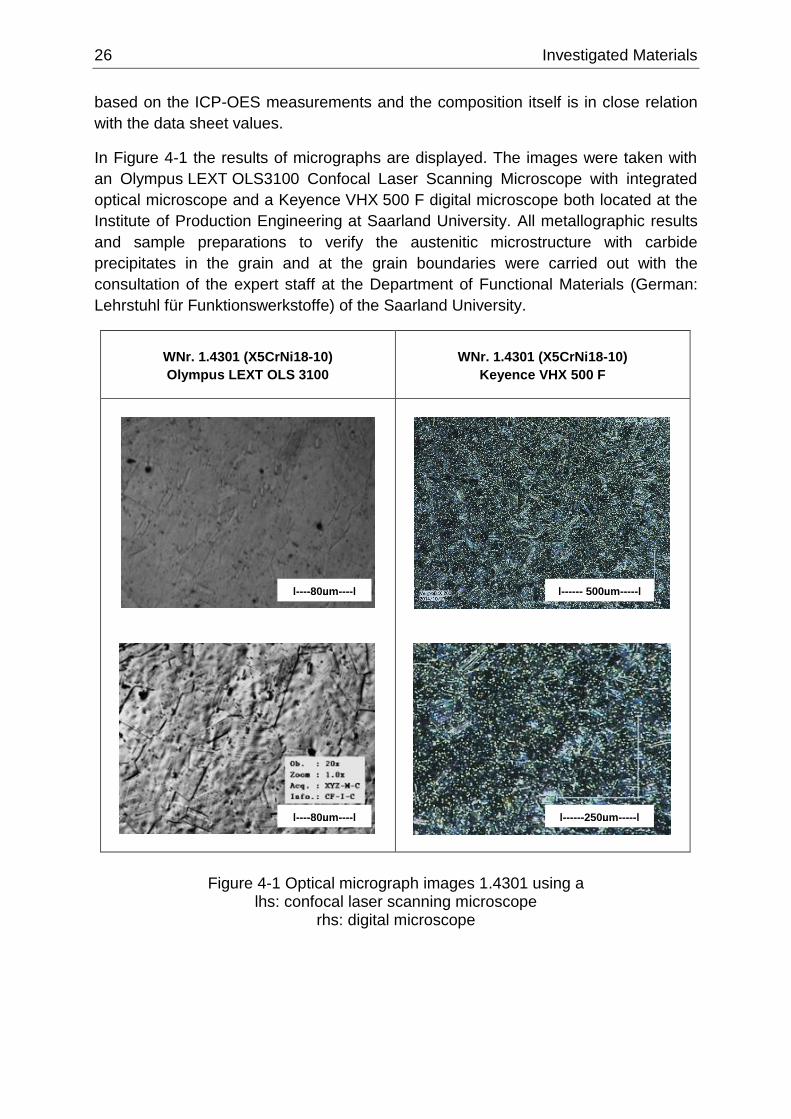
26 Investigated Materials
based on the ICP-OES measurements and the composition itself is in close relation
with the data sheet values.
In Figure 4-1 the results of micrographs are displayed. The images were taken with
an Olympus LEXT OLS3100 Confocal Laser Scanning Microscope with integrated
optical microscope and a Keyence VHX 500 F digital microscope both located at the
Institute of Production Engineering at Saarland University. All metallographic results
and sample preparations to verify the austenitic microstructure with carbide
precipitates in the grain and at the grain boundaries were carried out with the
consultation of the expert staff at the Department of Functional Materials (German:
Lehrstuhl für Funktionswerkstoffe) of the Saarland University.
Figure 4-1 Optical micrograph images 1.4301 using a lhs: confocal laser scanning microscope
rhs: digital microscope
WNr. 1.4301 (X5CrNi18-10)
Olympus LEXT OLS 3100
WNr. 1.4301 (X5CrNi18-10)
Keyence VHX 500 F
|----80µm----|
|----80µm----|
|------ 500µm-----|
|------250µm-----|
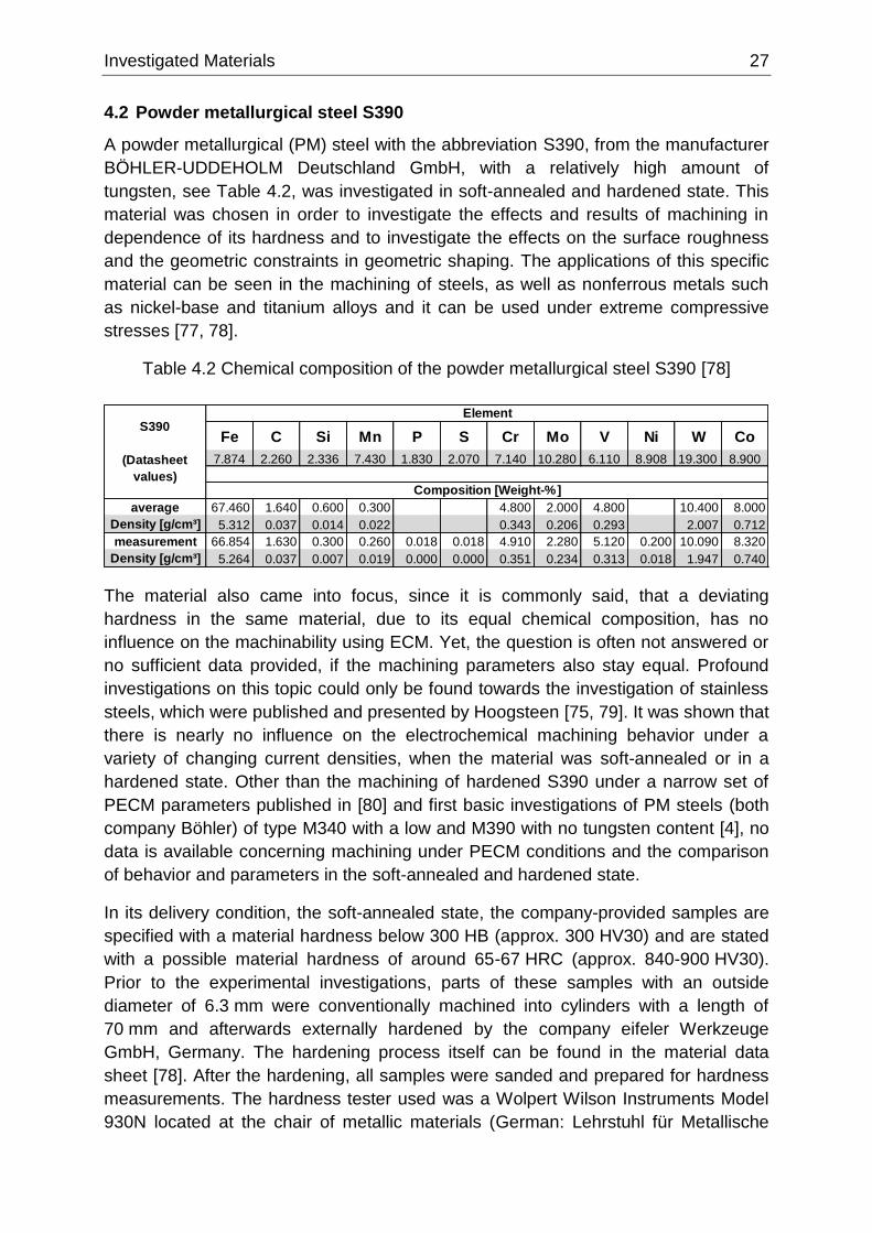
Investigated Materials 27
4.2 Powder metallurgical steel S390
A powder metallurgical (PM) steel with the abbreviation S390, from the manufacturer
BÖHLER-UDDEHOLM Deutschland GmbH, with a relatively high amount of
tungsten, see Table 4.2, was investigated in soft-annealed and hardened state. This
material was chosen in order to investigate the effects and results of machining in
dependence of its hardness and to investigate the effects on the surface roughness
and the geometric constraints in geometric shaping. The applications of this specific
material can be seen in the machining of steels, as well as nonferrous metals such
as nickel-base and titanium alloys and it can be used under extreme compressive
stresses [77, 78].
Table 4.2 Chemical composition of the powder metallurgical steel S390 [78]
The material also came into focus, since it is commonly said, that a deviating
hardness in the same material, due to its equal chemical composition, has no
influence on the machinability using ECM. Yet, the question is often not answered or
no sufficient data provided, if the machining parameters also stay equal. Profound
investigations on this topic could only be found towards the investigation of stainless
steels, which were published and presented by Hoogsteen [75, 79]. It was shown that
there is nearly no influence on the electrochemical machining behavior under a
variety of changing current densities, when the material was soft-annealed or in a
hardened state. Other than the machining of hardened S390 under a narrow set of
PECM parameters published in [80] and first basic investigations of PM steels (both
company Böhler) of type M340 with a low and M390 with no tungsten content [4], no
data is available concerning machining under PECM conditions and the comparison
of behavior and parameters in the soft-annealed and hardened state.
In its delivery condition, the soft-annealed state, the company-provided samples are
specified with a material hardness below 300 HB (approx. 300 HV30) and are stated
with a possible material hardness of around 65-67 HRC (approx. 840-900 HV30).
Prior to the experimental investigations, parts of these samples with an outside
diameter of 6.3 mm were conventionally machined into cylinders with a length of
70 mm and afterwards externally hardened by the company eifeler Werkzeuge
GmbH, Germany. The hardening process itself can be found in the material data
sheet [78]. After the hardening, all samples were sanded and prepared for hardness
measurements. The hardness tester used was a Wolpert Wilson Instruments Model
930N located at the chair of metallic materials (German: Lehrstuhl für Metallische
Fe C Si Mn P S Cr Mo V Ni W Co
7.874 2.260 2.336 7.430 1.830 2.070 7.140 10.280 6.110 8.908 19.300 8.900
average 67.460 1.640 0.600 0.300 4.800 2.000 4.800 10.400 8.000
Density [g/cm³] 5.312 0.037 0.014 0.022 0.343 0.206 0.293 2.007 0.712
measurement 66.854 1.630 0.300 0.260 0.018 0.018 4.910 2.280 5.120 0.200 10.090 8.320
Density [g/cm³] 5.264 0.037 0.007 0.019 0.000 0.000 0.351 0.234 0.313 0.018 1.947 0.740
S390
(Datasheet
values)
Element
Composition [Weight-%]
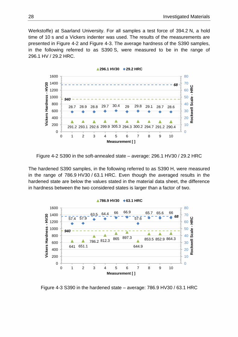
28 Investigated Materials
Werkstoffe) at Saarland University. For all samples a test force of 394.2 N, a hold
time of 10 s and a Vickers indenter was used. The results of the measurements are
presented in Figure 4-2 and Figure 4-3. The average hardness of the S390 samples,
in the following referred to as S390 S, were measured to be in the range of
296.1 HV / 29.2 HRC.
Figure 4-2 S390 in the soft-annealed state – average: 296.1 HV30 / 29.2 HRC
The hardened S390 samples, in the following referred to as S390 H, were measured
in the range of 786.9 HV30 / 63.1 HRC. Even though the averaged results in the
hardened state are below the values stated in the material data sheet, the difference
in hardness between the two considered states is larger than a factor of two.
Figure 4-3 S390 in the hardened state – average: 786.9 HV30 / 63.1 HRC
291.2 293.1 292.6 299.9 305.3 294.3 300.2 294.7 291.2 290.4
940
28.7 28.9 28.8 29.7 30.4 29 29.8 29.1 28.7 28.6
68
0
10
20
30
40
50
60
70
80
0
200
400
600
800
1000
1200
1400
1600
0 1 2 3 4 5 6 7 8 9 10
Measurement [ ]
Ro
ckw
ell S
cale
-H
RC
Vic
kers
Hard
ness -
HV
30
296.1 HV30 29.2 HRC
641 651.1
786.2 812.3865 897.3
644.9
853.5 852.9 864.3
940
57.4 57.963.5 64.4 66 66.9
57.6
65.7 65.6 6668
0
10
20
30
40
50
60
70
80
0
200
400
600
800
1000
1200
1400
1600
0 1 2 3 4 5 6 7 8 9 10
Ro
ckw
ell S
cale
-H
RC
Vic
ke
rs H
ard
ne
ss
-H
V3
0
Measurement [ ]
786.9 HV30 63.1 HRC
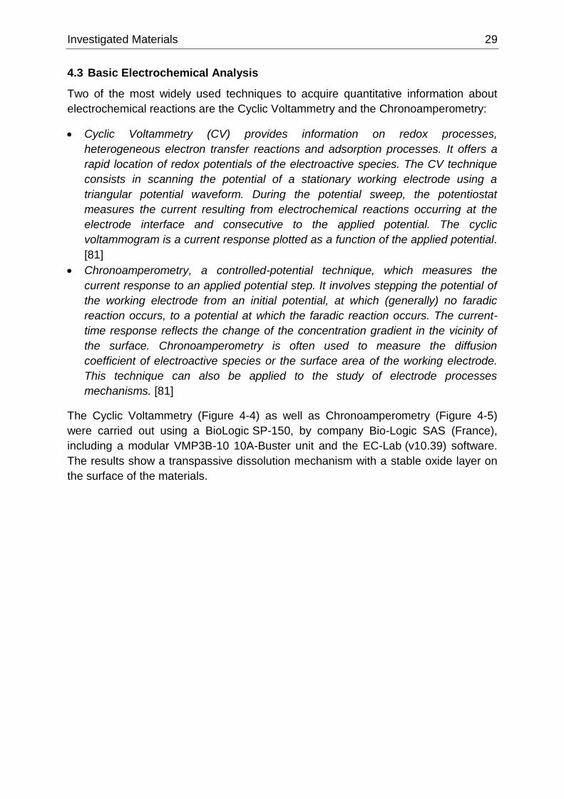
Investigated Materials 29
4.3 Basic Electrochemical Analysis
Two of the most widely used techniques to acquire quantitative information about
electrochemical reactions are the Cyclic Voltammetry and the Chronoamperometry:
Cyclic Voltammetry (CV) provides information on redox processes,
heterogeneous electron transfer reactions and adsorption processes. It offers a
rapid location of redox potentials of the electroactive species. The CV technique
consists in scanning the potential of a stationary working electrode using a
triangular potential waveform. During the potential sweep, the potentiostat
measures the current resulting from electrochemical reactions occurring at the
electrode interface and consecutive to the applied potential. The cyclic
voltammogram is a current response plotted as a function of the applied potential.
[81]
Chronoamperometry, a controlled-potential technique, which measures the
current response to an applied potential step. It involves stepping the potential of
the working electrode from an initial potential, at which (generally) no faradic
reaction occurs, to a potential at which the faradic reaction occurs. The current-
time response reflects the change of the concentration gradient in the vicinity of
the surface. Chronoamperometry is often used to measure the diffusion
coefficient of electroactive species or the surface area of the working electrode.
This technique can also be applied to the study of electrode processes
mechanisms. [81]
The Cyclic Voltammetry (Figure 4-4) as well as Chronoamperometry (Figure 4-5)
were carried out using a BioLogic SP-150, by company Bio-Logic SAS (France),
including a modular VMP3B-10 10A-Buster unit and the EC-Lab (v10.39) software.
The results show a transpassive dissolution mechanism with a stable oxide layer on
the surface of the materials.
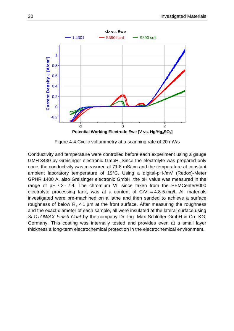
30 Investigated Materials
Figure 4-4 Cyclic voltammetry at a scanning rate of 20 mV/s
Conductivity and temperature were controlled before each experiment using a gauge
GMH 3430 by Greisinger electronic GmbH. Since the electrolyte was prepared only
once, the conductivity was measured at 71.8 mS/cm and the temperature at constant
ambient laboratory temperature of 19°C. Using a digital-pH-/mV (Redox)-Meter
GPHR 1400 A, also Greisinger electronic GmbH, the pH value was measured in the
range of pH 7.3 - 7.4. The chromium VI, since taken from the PEMCenter8000
electrolyte processing tank, was at a content of CrVI = 4.8-5 mg/l. All materials
investigated were pre-machined on a lathe and then sanded to achieve a surface
roughness of below Ra < 1 µm at the front surface. After measuring the roughness
and the exact diameter of each sample, all were insulated at the lateral surface using
SLOTOWAX Finish Coat by the company Dr.-Ing. Max Schlötter GmbH & Co. KG,
Germany. This coating was internally tested and provides even at a small layer
thickness a long-term electrochemical protection in the electrochemical environment.
Cyclic Voltammetry [ 20 mV/s ]
<I> vs. Ewe
1.4301.mpr # S390 hard.mpr S390 soft.mpr
Potential Working Electrode Ewe [V vs. Hg/HgSO4]20-2
Cu
rre
nt
De
ns
ity
J [
A/c
m²]
1
0,8
0,6
0,4
0,2
0
-0,2
Potential Working Electrode Ewe [V vs. Hg/Hg2SO4]
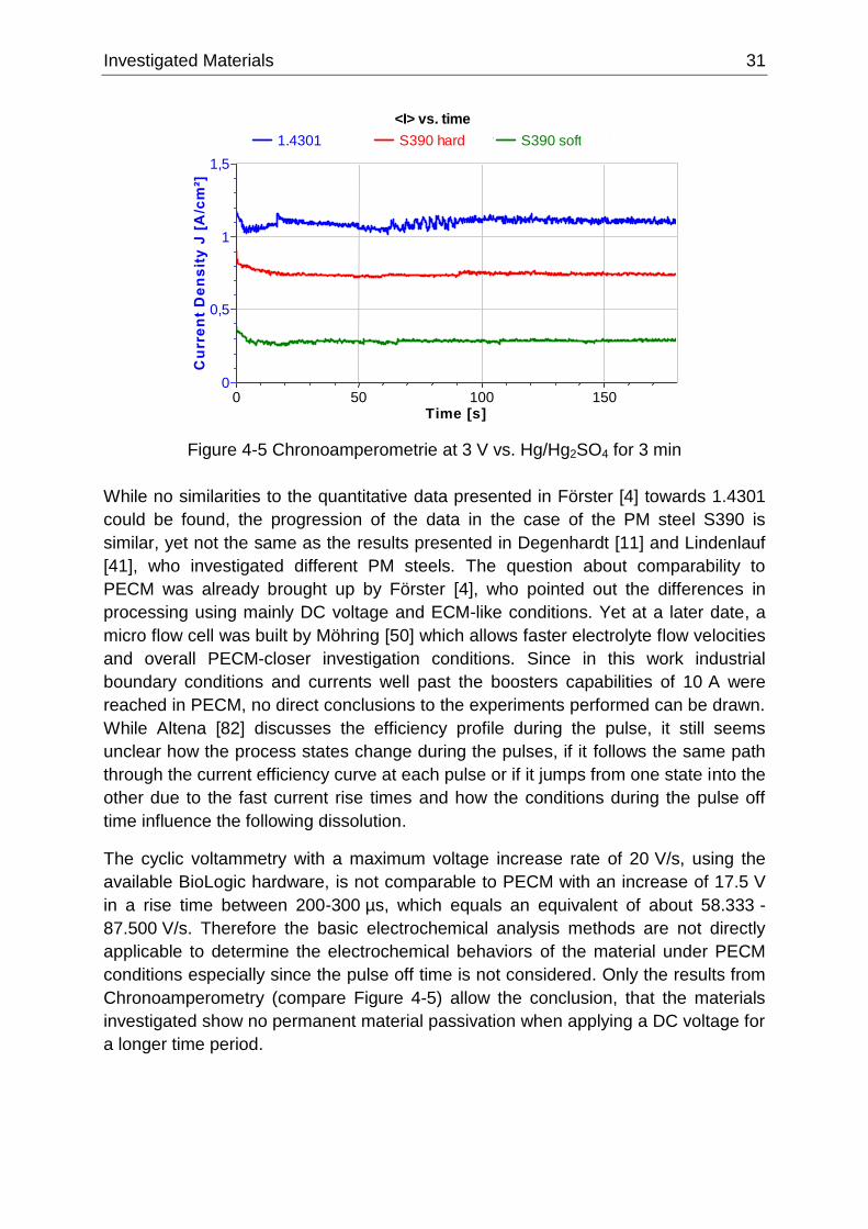
Investigated Materials 31
Figure 4-5 Chronoamperometrie at 3 V vs. Hg/Hg2SO4 for 3 min
While no similarities to the quantitative data presented in Förster [4] towards 1.4301
could be found, the progression of the data in the case of the PM steel S390 is
similar, yet not the same as the results presented in Degenhardt [11] and Lindenlauf
[41], who investigated different PM steels. The question about comparability to
PECM was already brought up by Förster [4], who pointed out the differences in
processing using mainly DC voltage and ECM-like conditions. Yet at a later date, a
micro flow cell was built by Möhring [50] which allows faster electrolyte flow velocities
and overall PECM-closer investigation conditions. Since in this work industrial
boundary conditions and currents well past the boosters capabilities of 10 A were
reached in PECM, no direct conclusions to the experiments performed can be drawn.
While Altena [82] discusses the efficiency profile during the pulse, it still seems
unclear how the process states change during the pulses, if it follows the same path
through the current efficiency curve at each pulse or if it jumps from one state into the
other due to the fast current rise times and how the conditions during the pulse off
time influence the following dissolution.
The cyclic voltammetry with a maximum voltage increase rate of 20 V/s, using the
available BioLogic hardware, is not comparable to PECM with an increase of 17.5 V
in a rise time between 200-300 µs, which equals an equivalent of about 58.333 -
87.500 V/s. Therefore the basic electrochemical analysis methods are not directly
applicable to determine the electrochemical behaviors of the material under PECM
conditions especially since the pulse off time is not considered. Only the results from
Chronoamperometry (compare Figure 4-5) allow the conclusion, that the materials
investigated show no permanent material passivation when applying a DC voltage for
a longer time period.
Chronoamperometrie [3V vs. Hg/HgSO4 for 3min]
<I> vs. time
1.4301.mpr # S390 hard.mpr S390 soft.mpr
Time [s]150100500
Cu
rre
nt
De
ns
ity
J [
A/c
m²]
1,5
1
0,5
0


Investigation Methods 33
5 Investigation Methods
In literature different methods are used to characterize materials using ECM or
PECM. To determine and evaluate material-specific parameters, most of the
experimental setups are based on laboratory conditions and have limited electric
boundary conditions [11, 41, 50, 65, 73, 83]. In most cases the current density is
limited well below 100 A/cm² (100 A/cm² = 1 A/mm²). Series production conditions
with either a focus on shaping or material behavior can only be found in recent
publications [44, 68, 84]. Since none of the laboratory scale setups offer the
possibility to upscale the components, a comparatively simple and cost-efficient test
setup was conceived to acquire material data. This setup for the collection and
comparison of material data is based on the idea to meet the three most important
measurable criteria in the PECM process, with the focus set on the field of production
engineering:
Material dissolution following Faraday’s law, as qualitative calculation for the
theoretical efficiency and the quantitative, practical machinability, using the
SMR value as indicator.
The frontal gap and side gap evolution as indicators for the size (precision)
and geometry achievable in PECM.
The resulting surface of the work piece under different current density
conditions.
To meet these three criteria a setup had to be realized, which allows an
understandable, reproducible and reliable collection of data under a wide range of
parameters. Since frontal gap and side gap evolution are concurrent processes, they
have to be investigated individually. For this purpose, two kinds of experimental
procedures are used:
One setup is used to investigate all of the above mentioned criteria with the
focus on
1. Faraday’s law
2. Frontal gap and side gap
3. Surface topology
Continuous observations (videos) are used to take into account the factor
time, since most of the experimental procedures mentioned above are rather
snapshots, or integral considerations of the process, and are rarely able to
reproduce interfering or concurrent processes in just one experiment.
These two setups, their calibration and limitations to certain parameter ranges are
discussed in this chapter. The evaluation of the work piece surface and topology is
primarily a standard follow-up process using meteorology well established in
production engineering and will be roughly discussed at the end of the chapter.
34 Investigation Methods
5.1 Frontal gap experiments
An experimental procedure focusing on shaping, presented in Figure 5-1, is
inadequate to differentiate between effects resulting from the partitioning of the total
current into the current through the frontal gap and the effects caused by the current
through the side gap. This is because the side gap increases continuously and
therefore also the surface area on the sides of the cathode increases. Hence, the
current density is inconsistent over the course of the experiment, since an increase in
side gap and surface leads to a further drop in the NaNO3 current density versus the
current efficiency curve.
Figure 5-1 Schematic of a conventional frontal and side gap experiment
Due to the stated reason, a novel and simple experimental setup was devised, which
does not completely reduce the effects of the side gap, yet results in a constant side
gap effect during the course of the experiments. This constant effect can then be
taken into account using appropriate measures, in this case FEM simulation. The
setup used is presented schematically in Figure 5-2 and Figure 5-3. The flushing
chamber pictured in Figure 5-3 is fed with the cathode towards the anode to assure
equal flushing conditions at all time. It is made from additive manufacturing and is
therefore electrically isolated. Similar to the schematic in Figure 5-2, it is constructed
to cover almost the complete lateral cathode and anode surfaces. By retracting the
cathode and connected flushing chamber, the cathode surface can be cleaned after
each experiment and the anode material can be changed using a quick-change
system from company EROWA, Switzerland, with a repeatability of 5 microns.
Electrolyte Cathode
Anode
Side gap
Frontal gap
Machining direction
I fro
nta
lI to
tal
I tota
l
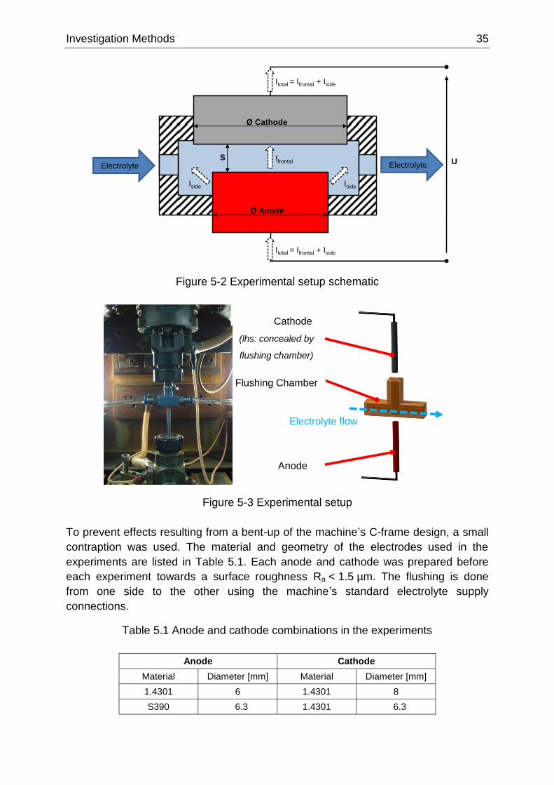
Investigation Methods 35
Figure 5-2 Experimental setup schematic
Figure 5-3 Experimental setup
To prevent effects resulting from a bent-up of the machine’s C-frame design, a small
contraption was used. The material and geometry of the electrodes used in the
experiments are listed in Table 5.1. Each anode and cathode was prepared before
each experiment towards a surface roughness Ra < 1.5 µm. The flushing is done
from one side to the other using the machine’s standard electrolyte supply
connections.
Table 5.1 Anode and cathode combinations in the experiments
Anode Cathode
Material Diameter [mm] Material Diameter [mm]
1.4301 6 1.4301 8
S390 6.3 1.4301 6.3
Ifrontal U
Ø Cathode
Ø Anode
Iside
SElectrolyte Electrolyte
Iside
Itotal = Ifrontal + Iside
Itotal = Ifrontal + Iside
Ø6mm Cathode
(lhs: concealed by
flushing chamber)
Ø6mm Anode
Flushing Chamber
Electrolyte flow
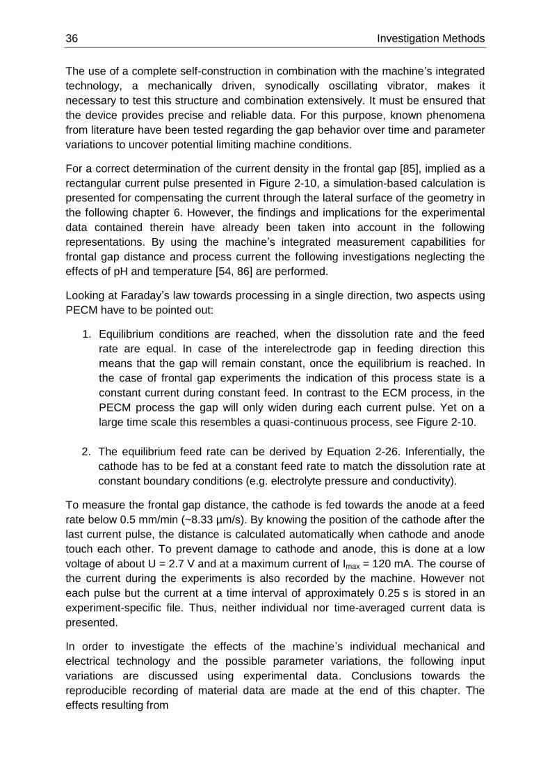
36 Investigation Methods
The use of a complete self-construction in combination with the machine’s integrated
technology, a mechanically driven, synodically oscillating vibrator, makes it
necessary to test this structure and combination extensively. It must be ensured that
the device provides precise and reliable data. For this purpose, known phenomena
from literature have been tested regarding the gap behavior over time and parameter
variations to uncover potential limiting machine conditions.
For a correct determination of the current density in the frontal gap [85], implied as a
rectangular current pulse presented in Figure 2-10, a simulation-based calculation is
presented for compensating the current through the lateral surface of the geometry in
the following chapter 6. However, the findings and implications for the experimental
data contained therein have already been taken into account in the following
representations. By using the machine’s integrated measurement capabilities for
frontal gap distance and process current the following investigations neglecting the
effects of pH and temperature [54, 86] are performed.
Looking at Faraday’s law towards processing in a single direction, two aspects using
PECM have to be pointed out:
1. Equilibrium conditions are reached, when the dissolution rate and the feed
rate are equal. In case of the interelectrode gap in feeding direction this
means that the gap will remain constant, once the equilibrium is reached. In
the case of frontal gap experiments the indication of this process state is a
constant current during constant feed. In contrast to the ECM process, in the
PECM process the gap will only widen during each current pulse. Yet on a
large time scale this resembles a quasi-continuous process, see Figure 2-10.
2. The equilibrium feed rate can be derived by Equation 2-26. Inferentially, the
cathode has to be fed at a constant feed rate to match the dissolution rate at
constant boundary conditions (e.g. electrolyte pressure and conductivity).
To measure the frontal gap distance, the cathode is fed towards the anode at a feed
rate below 0.5 mm/min (~8.33 µm/s). By knowing the position of the cathode after the
last current pulse, the distance is calculated automatically when cathode and anode
touch each other. To prevent damage to cathode and anode, this is done at a low
voltage of about U = 2.7 V and at a maximum current of Imax = 120 mA. The course of
the current during the experiments is also recorded by the machine. However not
each pulse but the current at a time interval of approximately 0.25 s is stored in an
experiment-specific file. Thus, neither individual nor time-averaged current data is
presented.
In order to investigate the effects of the machine’s individual mechanical and
electrical technology and the possible parameter variations, the following input
variations are discussed using experimental data. Conclusions towards the
reproducible recording of material data are made at the end of this chapter. The
effects resulting from
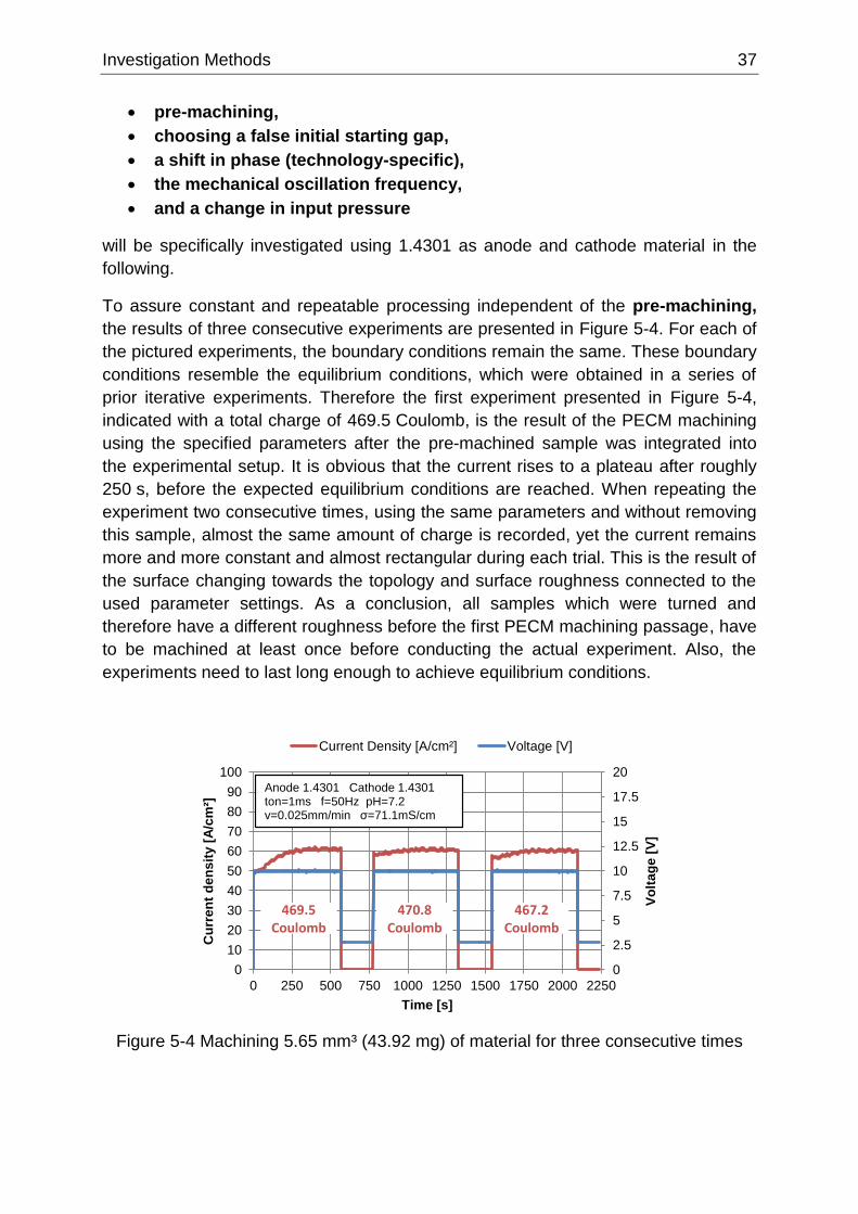
Investigation Methods 37
pre-machining,
choosing a false initial starting gap,
a shift in phase (technology-specific),
the mechanical oscillation frequency,
and a change in input pressure
will be specifically investigated using 1.4301 as anode and cathode material in the
following.
To assure constant and repeatable processing independent of the pre-machining,
the results of three consecutive experiments are presented in Figure 5-4. For each of
the pictured experiments, the boundary conditions remain the same. These boundary
conditions resemble the equilibrium conditions, which were obtained in a series of
prior iterative experiments. Therefore the first experiment presented in Figure 5-4,
indicated with a total charge of 469.5 Coulomb, is the result of the PECM machining
using the specified parameters after the pre-machined sample was integrated into
the experimental setup. It is obvious that the current rises to a plateau after roughly
250 s, before the expected equilibrium conditions are reached. When repeating the
experiment two consecutive times, using the same parameters and without removing
this sample, almost the same amount of charge is recorded, yet the current remains
more and more constant and almost rectangular during each trial. This is the result of
the surface changing towards the topology and surface roughness connected to the
used parameter settings. As a conclusion, all samples which were turned and
therefore have a different roughness before the first PECM machining passage, have
to be machined at least once before conducting the actual experiment. Also, the
experiments need to last long enough to achieve equilibrium conditions.
Figure 5-4 Machining 5.65 mm³ (43.92 mg) of material for three consecutive times
0
2.5
5
7.5
10
12.5
15
17.5
20
0
10
20
30
40
50
60
70
80
90
100
0 250 500 750 1000 1250 1500 1750 2000 2250
Vo
lta
ge
[V
]
Cu
rre
nt
de
ns
ity [
A/c
m²]
Time [s]
Current Density [A/cm²] Voltage [V]
469.5 Coulomb
470.8Coulomb
467.2Coulomb
Anode 1.4301 Cathode 1.4301 ton=1ms f=50Hz pH=7.2 v=0.025mm/min σ=71.1mS/cm
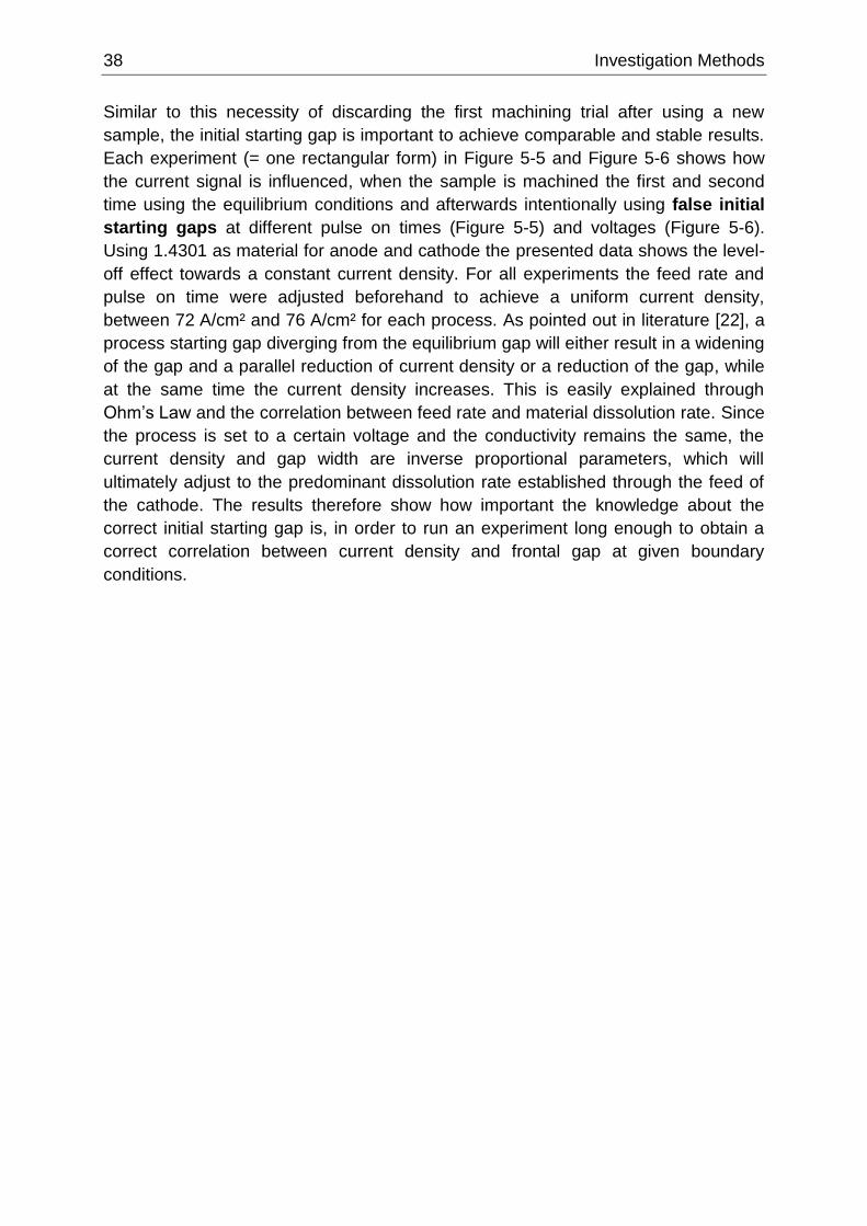
38 Investigation Methods
Similar to this necessity of discarding the first machining trial after using a new
sample, the initial starting gap is important to achieve comparable and stable results.
Each experiment (= one rectangular form) in Figure 5-5 and Figure 5-6 shows how
the current signal is influenced, when the sample is machined the first and second
time using the equilibrium conditions and afterwards intentionally using false initial
starting gaps at different pulse on times (Figure 5-5) and voltages (Figure 5-6).
Using 1.4301 as material for anode and cathode the presented data shows the level-
off effect towards a constant current density. For all experiments the feed rate and
pulse on time were adjusted beforehand to achieve a uniform current density,
between 72 A/cm² and 76 A/cm² for each process. As pointed out in literature [22], a
process starting gap diverging from the equilibrium gap will either result in a widening
of the gap and a parallel reduction of current density or a reduction of the gap, while
at the same time the current density increases. This is easily explained through
Ohm’s Law and the correlation between feed rate and material dissolution rate. Since
the process is set to a certain voltage and the conductivity remains the same, the
current density and gap width are inverse proportional parameters, which will
ultimately adjust to the predominant dissolution rate established through the feed of
the cathode. The results therefore show how important the knowledge about the
correct initial starting gap is, in order to run an experiment long enough to obtain a
correct correlation between current density and frontal gap at given boundary
conditions.
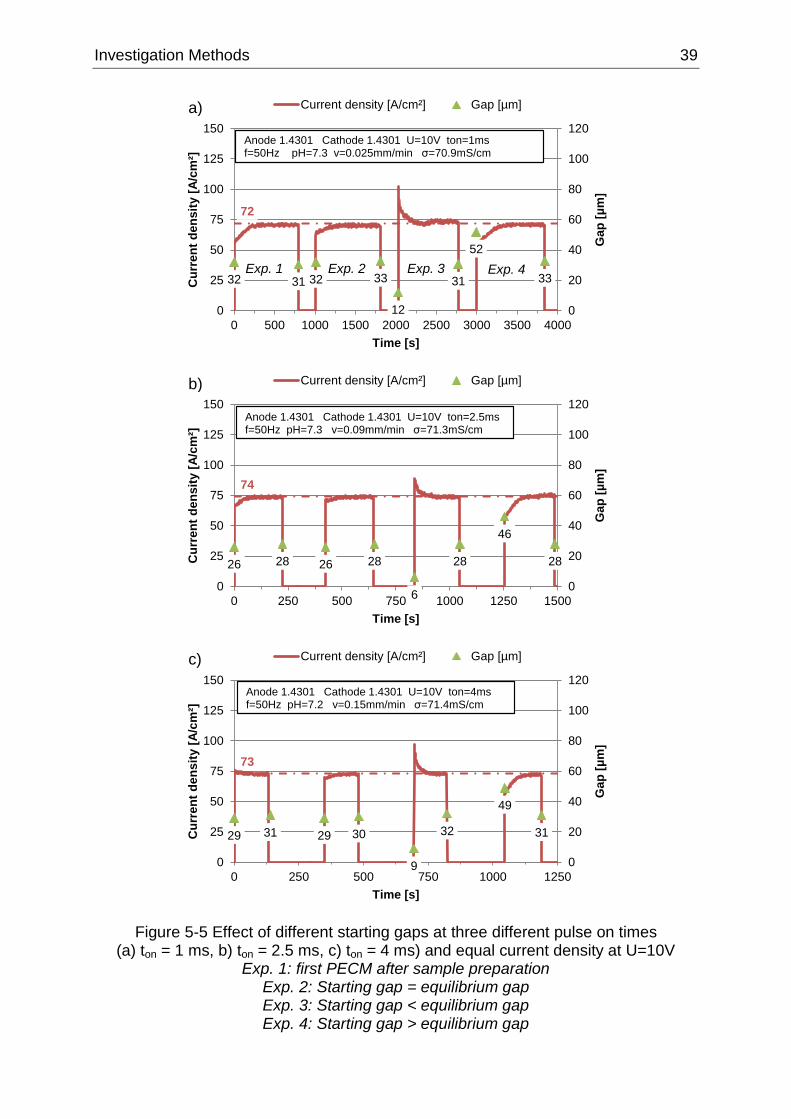
Investigation Methods 39
Figure 5-5 Effect of different starting gaps at three different pulse on times (a) ton = 1 ms, b) ton = 2.5 ms, c) ton = 4 ms) and equal current density at U=10V
Exp. 1: first PECM after sample preparation Exp. 2: Starting gap = equilibrium gap Exp. 3: Starting gap < equilibrium gap Exp. 4: Starting gap > equilibrium gap
72
32 31 32 33
12
31
52
33
0
20
40
60
80
100
120
0
25
50
75
100
125
150
0 500 1000 1500 2000 2500 3000 3500 4000
Gap
[µ
m]
Cu
rre
nt
de
ns
ity [
A/c
m²]
Time [s]
Current density [A/cm²] Gap [µm]
Anode 1.4301 Cathode 1.4301 U=10V ton=1ms f=50Hz pH=7.3 v=0.025mm/min σ=70.9mS/cm
74
26 28 26 28
6
28
46
28
0
20
40
60
80
100
120
0
25
50
75
100
125
150
0 250 500 750 1000 1250 1500G
ap
[µ
m]
Cu
rre
nt
de
ns
ity [
A/c
m²]
Time [s]
Current density [A/cm²] Gap [µm]
Anode 1.4301 Cathode 1.4301 U=10V ton=2.5ms f=50Hz pH=7.3 v=0.09mm/min σ=71.3mS/cm
73
29 31 29 30
9
32
49
31
0
20
40
60
80
100
120
0
25
50
75
100
125
150
0 250 500 750 1000 1250
Gap
[µ
m]
Cu
rre
nt
de
ns
ity [
A/c
m²]
Time [s]
Current density [A/cm²] Gap [µm]
Anode 1.4301 Cathode 1.4301 U=10V ton=4ms f=50Hz pH=7.2 v=0.15mm/min σ=71.4mS/cm
Exp. 1 Exp. 2 Exp. 3 Exp. 4
a)
b)
c)
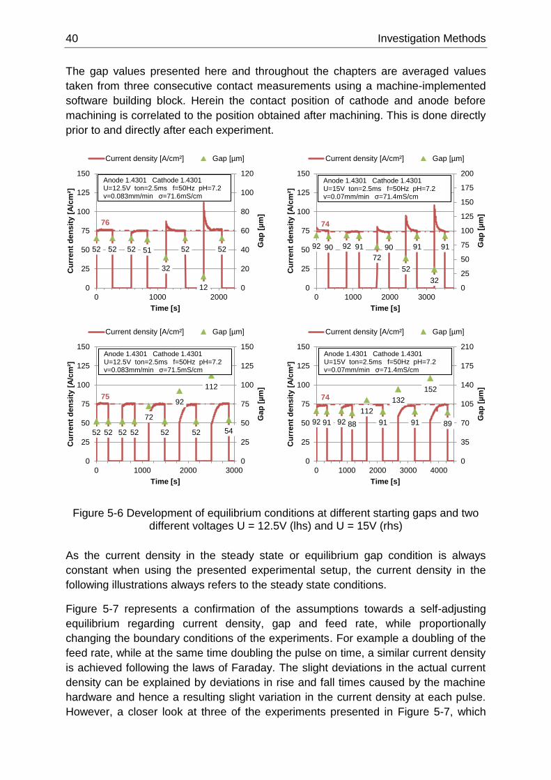
40 Investigation Methods
The gap values presented here and throughout the chapters are averaged values
taken from three consecutive contact measurements using a machine-implemented
software building block. Herein the contact position of cathode and anode before
machining is correlated to the position obtained after machining. This is done directly
prior to and directly after each experiment.
Figure 5-6 Development of equilibrium conditions at different starting gaps and two different voltages U = 12.5V (lhs) and U = 15V (rhs)
As the current density in the steady state or equilibrium gap condition is always
constant when using the presented experimental setup, the current density in the
following illustrations always refers to the steady state conditions.
Figure 5-7 represents a confirmation of the assumptions towards a self-adjusting
equilibrium regarding current density, gap and feed rate, while proportionally
changing the boundary conditions of the experiments. For example a doubling of the
feed rate, while at the same time doubling the pulse on time, a similar current density
is achieved following the laws of Faraday. The slight deviations in the actual current
density can be explained by deviations in rise and fall times caused by the machine
hardware and hence a resulting slight variation in the current density at each pulse.
However, a closer look at three of the experiments presented in Figure 5-7, which
76
52 52 52 51
32
52
12
52
0
20
40
60
80
100
120
0
25
50
75
100
125
150
0 1000 2000
Gap
[µ
m]
Cu
rren
t d
en
sit
y [
A/c
m²]
Time [s]
Current density [A/cm²] Gap [µm]
Anode 1.4301 Cathode 1.4301 U=12.5V ton=2.5ms f=50Hz pH=7.2 v=0.083mm/min σ=71.6mS/cm
75
52 52 52 52
72
52
92
52
112
54
0
25
50
75
100
125
150
0
25
50
75
100
125
150
0 1000 2000 3000
Gap
[µ
m]
Cu
rren
t d
en
sit
y [
A/c
m²]
Time [s]
Current density [A/cm²] Gap [µm]
Anode 1.4301 Cathode 1.4301 U=12.5V ton=2.5ms f=50Hz pH=7.2 v=0.083mm/min σ=71.5mS/cm
74
92 90 92 91
72
90
52
91
32
91
0
25
50
75
100
125
150
175
200
0
25
50
75
100
125
150
0 1000 2000 3000
Gap
[µ
m]
Cu
rren
t d
en
sit
y [
A/c
m²]
Time [s]
Current density [A/cm²] Gap [µm]
Anode 1.4301 Cathode 1.4301 U=15V ton=2.5ms f=50Hz pH=7.2 v=0.07mm/min σ=71.4mS/cm
74
92 91 92 88
112
91
132
91
152
89
0
35
70
105
140
175
210
0
25
50
75
100
125
150
0 1000 2000 3000 4000
Gap
[µ
m]
Cu
rren
t d
en
sit
y [
A/c
m²]
Time [s]
Current density [A/cm²] Gap [µm]
Anode 1.4301 Cathode 1.4301 U=15V ton=2.5ms f=50Hz pH=7.2 v=0.07mm/min σ=71.4mS/cm
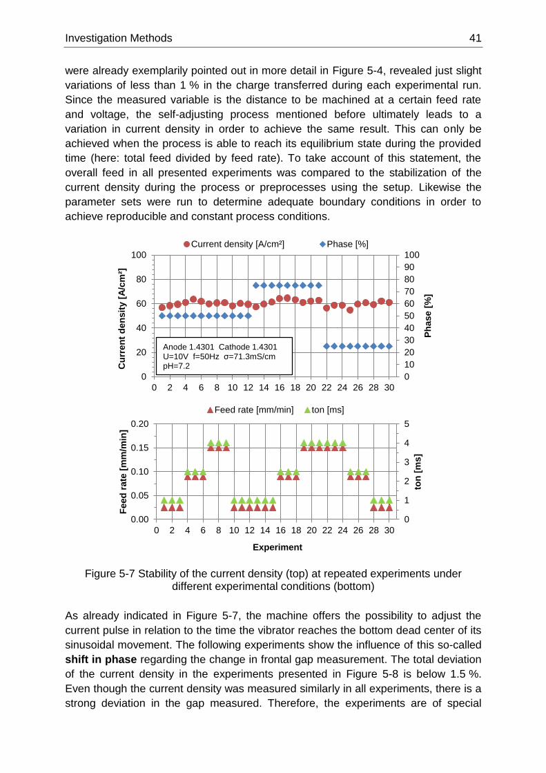
Investigation Methods 41
were already exemplarily pointed out in more detail in Figure 5-4, revealed just slight
variations of less than 1 % in the charge transferred during each experimental run.
Since the measured variable is the distance to be machined at a certain feed rate
and voltage, the self-adjusting process mentioned before ultimately leads to a
variation in current density in order to achieve the same result. This can only be
achieved when the process is able to reach its equilibrium state during the provided
time (here: total feed divided by feed rate). To take account of this statement, the
overall feed in all presented experiments was compared to the stabilization of the
current density during the process or preprocesses using the setup. Likewise the
parameter sets were run to determine adequate boundary conditions in order to
achieve reproducible and constant process conditions.
Figure 5-7 Stability of the current density (top) at repeated experiments under different experimental conditions (bottom)
As already indicated in Figure 5-7, the machine offers the possibility to adjust the
current pulse in relation to the time the vibrator reaches the bottom dead center of its
sinusoidal movement. The following experiments show the influence of this so-called
shift in phase regarding the change in frontal gap measurement. The total deviation
of the current density in the experiments presented in Figure 5-8 is below 1.5 %.
Even though the current density was measured similarly in all experiments, there is a
strong deviation in the gap measured. Therefore, the experiments are of special
0
10
20
30
40
50
60
70
80
90
100
0
20
40
60
80
100
0 2 4 6 8 10 12 14 16 18 20 22 24 26 28 30
Ph
ase [
%]
Cu
rren
t d
en
sit
y [
A/c
m²]
Experiment
Current density [A/cm²] Phase [%]
0
1
2
3
4
5
0.00
0.05
0.10
0.15
0.20
0 2 4 6 8 10 12 14 16 18 20 22 24 26 28 30
ton
[m
s]
Feed
rate
[m
m/m
in]
Experiment
Feed rate [mm/min] ton [ms]
Anode 1.4301 Cathode 1.4301U=10V f=50Hz σ=71.3mS/cm pH=7.2
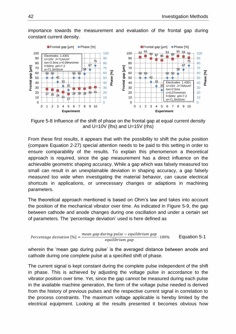
42 Investigation Methods
importance towards the measurement and evaluation of the frontal gap during
constant current density.
Figure 5-8 Influence of the shift of phase on the frontal gap at equal current density and U=10V (lhs) and U=15V (rhs)
From these first results, it appears that with the possibility to shift the pulse position
(compare Equation 2-27) special attention needs to be paid to this setting in order to
ensure comparability of the results. To explain this phenomenon a theoretical
approach is required, since the gap measurement has a direct influence on the
achievable geometric shaping accuracy. While a gap which was falsely measured too
small can result in an unexplainable deviation in shaping accuracy, a gap falsely
measured too wide when investigating the material behavior, can cause electrical
shortcuts in applications, or unnecessary changes or adaptions in machining
parameters.
The theoretical approach mentioned is based on Ohm’s law and takes into account
the position of the mechanical vibrator over time. As indicated in Figure 5-9, the gap
between cathode and anode changes during one oscillation and under a certain set
of parameters. The ‘percentage deviation’ used is here defined as
𝑃𝑒𝑟𝑐𝑒𝑛𝑡𝑎𝑔𝑒 𝑑𝑒𝑣𝑖𝑎𝑡𝑖𝑜𝑛 [%] =𝑚𝑒𝑎𝑛 𝑔𝑎𝑝 𝑑𝑢𝑟𝑖𝑛𝑔 𝑝𝑢𝑙𝑠𝑒 − 𝑒𝑞𝑢𝑖𝑙𝑖𝑏𝑟𝑖𝑢𝑚 𝑔𝑎𝑝
𝑒𝑞𝑢𝑖𝑙𝑖𝑏𝑟𝑖𝑢𝑚 𝑔𝑎𝑝∙ 100%
Equation 5-1
wherein the ‘mean gap during pulse’ is the averaged distance between anode and
cathode during one complete pulse at a specified shift of phase.
The current signal is kept constant during the complete pulse independent of the shift
in phase. This is achieved by adjusting the voltage pulse in accordance to the
vibrator position over time. Yet, since the gap cannot be measured during each pulse
in the available machine generation, the form of the voltage pulse needed is derived
from the history of previous pulses and the respective current signal in correlation to
the process constraints. The maximum voltage applicable is hereby limited by the
electrical equipment. Looking at the results presented it becomes obvious how
92 9590 87 86
9389
95 94 91
50 5042
33
25
50 5058
67
75
0
10
20
30
40
50
60
70
80
90
100
0
10
20
30
40
50
60
70
80
90
100
0 1 2 3 4 5 6 7 8 9 10
Ph
ase [
%]
Fro
nta
l g
ap
[µ
m]
Experiment
Frontal gap [µm] Phase [%]
Electrodes 1.4301U=15V J=70A/cm²ton=2.5msv=0.07mm/minf=50Hz pH=7.2σ=71.3mS/cm
28 28 28 30 3127 26 24 21
17
50 5058
67
75
50 5042
33
25
0
10
20
30
40
50
60
70
80
90
100
0
10
20
30
40
50
60
70
80
90
100
0 1 2 3 4 5 6 7 8 9 10
Ph
ase [
%]
Fro
nta
l g
ap
[µ
m]
Experiment
Frontal gap [µm] Phase [%]
Electrodes 1.4301U=10V J=71A/cm²ton=2.5ms v=0.09mm/minf=50Hz pH=7.2σ=71.3mS/cm
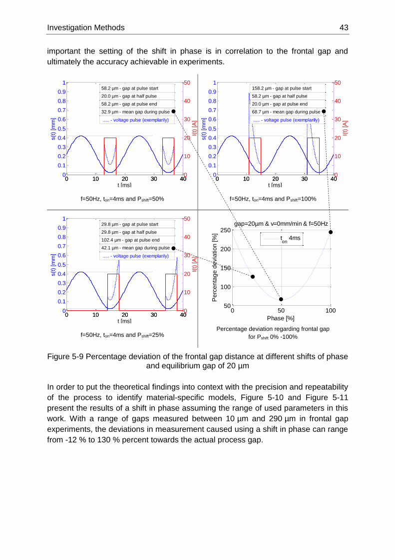
Investigation Methods 43
important the setting of the shift in phase is in correlation to the frontal gap and
ultimately the accuracy achievable in experiments.
f=50Hz, ton=4ms and Pshift=50%
f=50Hz, ton=4ms and Pshift=100%
f=50Hz, ton=4ms and Pshift=25%
Percentage deviation regarding frontal gap
for Pshift 0% -100%
Figure 5-9 Percentage deviation of the frontal gap distance at different shifts of phase and equilibrium gap of 20 µm
In order to put the theoretical findings into context with the precision and repeatability
of the process to identify material-specific models, Figure 5-10 and Figure 5-11
present the results of a shift in phase assuming the range of used parameters in this
work. With a range of gaps measured between 10 µm and 290 µm in frontal gap
experiments, the deviations in measurement caused using a shift in phase can range
from -12 % to 130 % percent towards the actual process gap.
0 10 20 30 400
0.1
0.2
0.3
0.4
0.5
0.6
0.7
0.8
0.9
1
s(t
) [m
m]
t [ms]0 10 20 30 40
0
10
20
30
40
50
I(t
) [A
]
58.2 µm - gap at pulse start
20.0 µm - gap at half pulse
58.2 µm - gap at pulse end
32.9 µm - mean gap during pulse
..... - voltage pulse (exemplarily)
0 10 20 30 400
0.1
0.2
0.3
0.4
0.5
0.6
0.7
0.8
0.9
1
s(t
) [m
m]
t [ms]0 10 20 30 40
0
10
20
30
40
50
I(t
) [A
]
158.2 µm - gap at pulse start
58.2 µm - gap at half pulse
20.0 µm - gap at pulse end
68.7 µm - mean gap during pulse
..... - voltage pulse (exemplarily)
0 10 20 30 400
0.1
0.2
0.3
0.4
0.5
0.6
0.7
0.8
0.9
1
s(t
) [m
m]
t [ms]0 10 20 30 40
0
10
20
30
40
50
I(t
) [A
]
29.8 µm - gap at pulse start
29.8 µm - gap at half pulse
102.4 µm - gap at pulse end
42.1 µm - mean gap during pulse
..... - voltage pulse (exemplarily)
0 50 10050
100
150
200
250gap=20µm & v=0mm/min & f=50Hz
Phase [%]
Pe
rce
nta
ge
de
via
tio
n [%
]
ton
4ms
0 0.5 10
20
40
60
80
Frontal gap percentage deviation [%]
at gap=290µm & Phase=50% & f=50Hz
vfeed
[mm/min]
Pe
rce
nta
ge
de
via
tio
n [%
]
ton
4ms
ton
2.5ms
ton
1ms
0 50 1000
2
4
6
8
10
12
Frontal gap percentage deviation [%]
at gap=290µm & vfeed
=0mm/min & f=10Hz
Phase [%]
Pe
rce
nta
ge
de
via
tio
n [%
]
ton
4ms
ton
2.5ms
ton
1ms
0 0.5 1-8
-6
-4
-2
0
2
4
Frontal gap percentage deviation [%]
at gap=290µm & Phase=50% & f=10Hz
vfeed
[mm/min]
Pe
rce
nta
ge
de
via
tio
n [%
]
ton
4ms
ton
2.5ms
ton
1ms
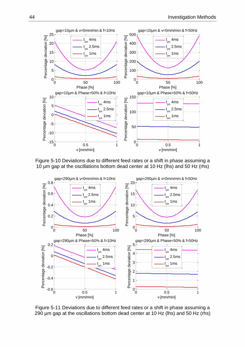
44 Investigation Methods
Figure 5-10 Deviations due to different feed rates or a shift in phase assuming a 10 µm gap at the oscillations bottom dead center at 10 Hz (lhs) and 50 Hz (rhs)
Figure 5-11 Deviations due to different feed rates or a shift in phase assuming a 290 µm gap at the oscillations bottom dead center at 10 Hz (lhs) and 50 Hz (rhs)
0 50 1000
100
200
300
400
500gap=10µm & v=0mm/min & f=50Hz
Phase [%]
Pe
rce
nta
ge
de
via
tio
n [%
]
ton
4ms
ton
2.5ms
ton
1ms
0 0.5 10
50
100
150gap=10µm & Phase=50% & f=50Hz
v [mm/min]
Pe
rce
nta
ge
de
via
tio
n [%
]
ton
4ms
ton
2.5ms
ton
1ms
0 50 1000
5
10
15
20
25gap=10µm & v=0mm/min & f=10Hz
Phase [%]
Pe
rce
nta
ge
de
via
tio
n [%
]
ton
4ms
ton
2.5ms
ton
1ms
0 0.5 1-15
-10
-5
0
5
10gap=10µm & Phase=50% & f=10Hz
v [mm/min]
Pe
rce
nta
ge
de
via
tio
n [%
]
ton
4ms
ton
2.5ms
ton
1ms
0 50 1000
5
10
15
20gap=290µm & v=0mm/min & f=50Hz
Phase [%]
Pe
rce
nta
ge
de
via
tio
n [%
]
ton
4ms
ton
2.5ms
ton
1ms
0 0.5 10
1
2
3
4
5gap=290µm & Phase=50% & f=50Hz
v [mm/min]
Pe
rce
nta
ge
de
via
tio
n [%
]
ton
4ms
ton
2.5ms
ton
1ms
0 50 1000
0.2
0.4
0.6
0.8gap=290µm & v=0mm/min & f=10Hz
Phase [%]
Pe
rce
nta
ge
de
via
tio
n [%
]
ton
4ms
ton
2.5ms
ton
1ms
0 0.5 1-0.6
-0.4
-0.2
0
0.2gap=290µm & Phase=50% & f=10Hz
v [mm/min]
Pe
rce
nta
ge
de
via
tio
n [%
]
ton
4ms
ton
2.5ms
ton
1ms
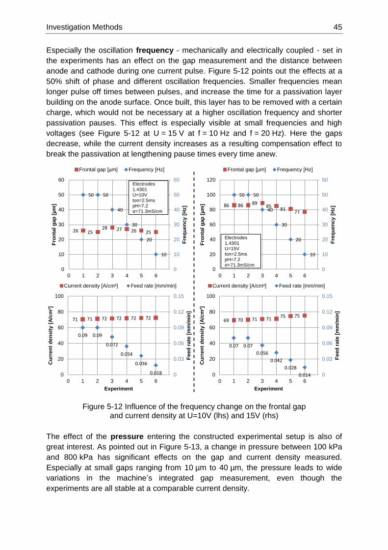
Investigation Methods 45
Especially the oscillation frequency - mechanically and electrically coupled - set in
the experiments has an effect on the gap measurement and the distance between
anode and cathode during one current pulse. Figure 5-12 points out the effects at a
50% shift of phase and different oscillation frequencies. Smaller frequencies mean
longer pulse off times between pulses, and increase the time for a passivation layer
building on the anode surface. Once built, this layer has to be removed with a certain
charge, which would not be necessary at a higher oscillation frequency and shorter
passivation pauses. This effect is especially visible at small frequencies and high
voltages (see Figure 5-12 at U = 15 V at f = 10 Hz and f = 20 Hz). Here the gaps
decrease, while the current density increases as a resulting compensation effect to
break the passivation at lengthening pause times every time anew.
Figure 5-12 Influence of the frequency change on the frontal gap and current density at U=10V (lhs) and 15V (rhs)
The effect of the pressure entering the constructed experimental setup is also of
great interest. As pointed out in Figure 5-13, a change in pressure between 100 kPa
and 800 kPa has significant effects on the gap and current density measured.
Especially at small gaps ranging from 10 µm to 40 µm, the pressure leads to wide
variations in the machine’s integrated gap measurement, even though the
experiments are all stable at a comparable current density.
86 86 8985
8177
50 50
40
30
20
10
0
10
20
30
40
50
60
0
20
40
60
80
100
120
0 1 2 3 4 5 6
Fre
qu
en
cy [
Hz]
Fro
nta
l g
ap
[µ
m]
Frontal gap [µm] Frequency [Hz]
Electrodes 1.4301U=15Vton=2.5mspH=7.2σ=71.3mS/cm
69 70 71 71 75 75
0.07 0.07
0.056
0.042
0.028
0.014 0
0.03
0.06
0.09
0.12
0.15
0
20
40
60
80
100
0 1 2 3 4 5 6
Feed
rate
[m
m/m
in]
Cu
rren
t d
en
sit
y [
A/c
m²]
Experiment
Current density [A/cm²] Feed rate [mm/min]
26 2528 27 26 25
50 50
40
30
20
10
0
10
20
30
40
50
60
0
10
20
30
40
50
60
0 1 2 3 4 5 6
Fre
qu
en
cy [
Hz]
Fro
nta
l g
ap
[µ
m]
Frontal gap [µm] Frequency [Hz]
Electrodes 1.4301U=10Vton=2.5mspH=7.2σ=71.3mS/cm
71 71 72 72 72 72
0.09 0.09
0.072
0.054
0.036
0.018 0
0.03
0.06
0.09
0.12
0.15
0
20
40
60
80
100
0 1 2 3 4 5 6
Feed
rate
[m
m/m
in]
Cu
rren
t d
en
sit
y [
A/c
m²]
Experiment
Current density [A/cm²] Feed rate [mm/min]
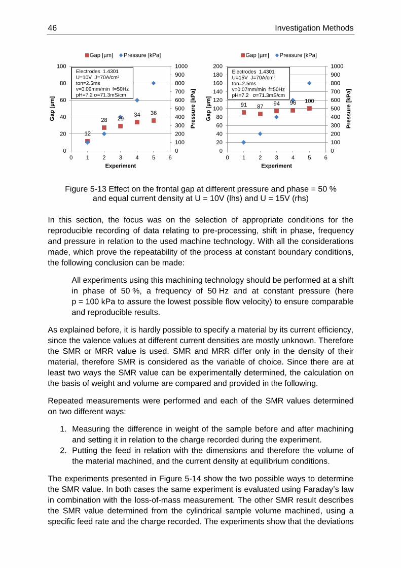
46 Investigation Methods
Figure 5-13 Effect on the frontal gap at different pressure and phase = 50 % and equal current density at U = 10V (lhs) and U = 15V (rhs)
In this section, the focus was on the selection of appropriate conditions for the
reproducible recording of data relating to pre-processing, shift in phase, frequency
and pressure in relation to the used machine technology. With all the considerations
made, which prove the repeatability of the process at constant boundary conditions,
the following conclusion can be made:
All experiments using this machining technology should be performed at a shift
in phase of 50 %, a frequency of 50 Hz and at constant pressure (here
p = 100 kPa to assure the lowest possible flow velocity) to ensure comparable
and reproducible results.
As explained before, it is hardly possible to specify a material by its current efficiency,
since the valence values at different current densities are mostly unknown. Therefore
the SMR or MRR value is used. SMR and MRR differ only in the density of their
material, therefore SMR is considered as the variable of choice. Since there are at
least two ways the SMR value can be experimentally determined, the calculation on
the basis of weight and volume are compared and provided in the following.
Repeated measurements were performed and each of the SMR values determined
on two different ways:
1. Measuring the difference in weight of the sample before and after machining
and setting it in relation to the charge recorded during the experiment.
2. Putting the feed in relation with the dimensions and therefore the volume of
the material machined, and the current density at equilibrium conditions.
The experiments presented in Figure 5-14 show the two possible ways to determine
the SMR value. In both cases the same experiment is evaluated using Faraday’s law
in combination with the loss-of-mass measurement. The other SMR result describes
the SMR value determined from the cylindrical sample volume machined, using a
specific feed rate and the charge recorded. The experiments show that the deviations
12
28 2934 36
0
100
200
300
400
500
600
700
800
900
1000
0
20
40
60
80
100
0 1 2 3 4 5 6
Pre
ss
ure
[k
Pa
]
Ga
p [
µm
]
Experiment
Gap [µm] Pressure [kPa]
Electrodes 1.4301U=10V J=70A/cm² ton=2.5msv=0.09mm/min f=50Hz pH=7.2 σ=71.3mS/cm
91 8794 96 100
0
100
200
300
400
500
600
700
800
900
1000
0
20
40
60
80
100
120
140
160
180
200
0 1 2 3 4 5 6
Pre
ss
ure
[k
Pa
]
Ga
p [
µm
]
Experiment
Gap [µm] Pressure [kPa]
Electrodes 1.4301U=15V J=70A/cm² ton=2.5msv=0.07mm/min f=50Hz pH=7.2 σ=71.3mS/cm
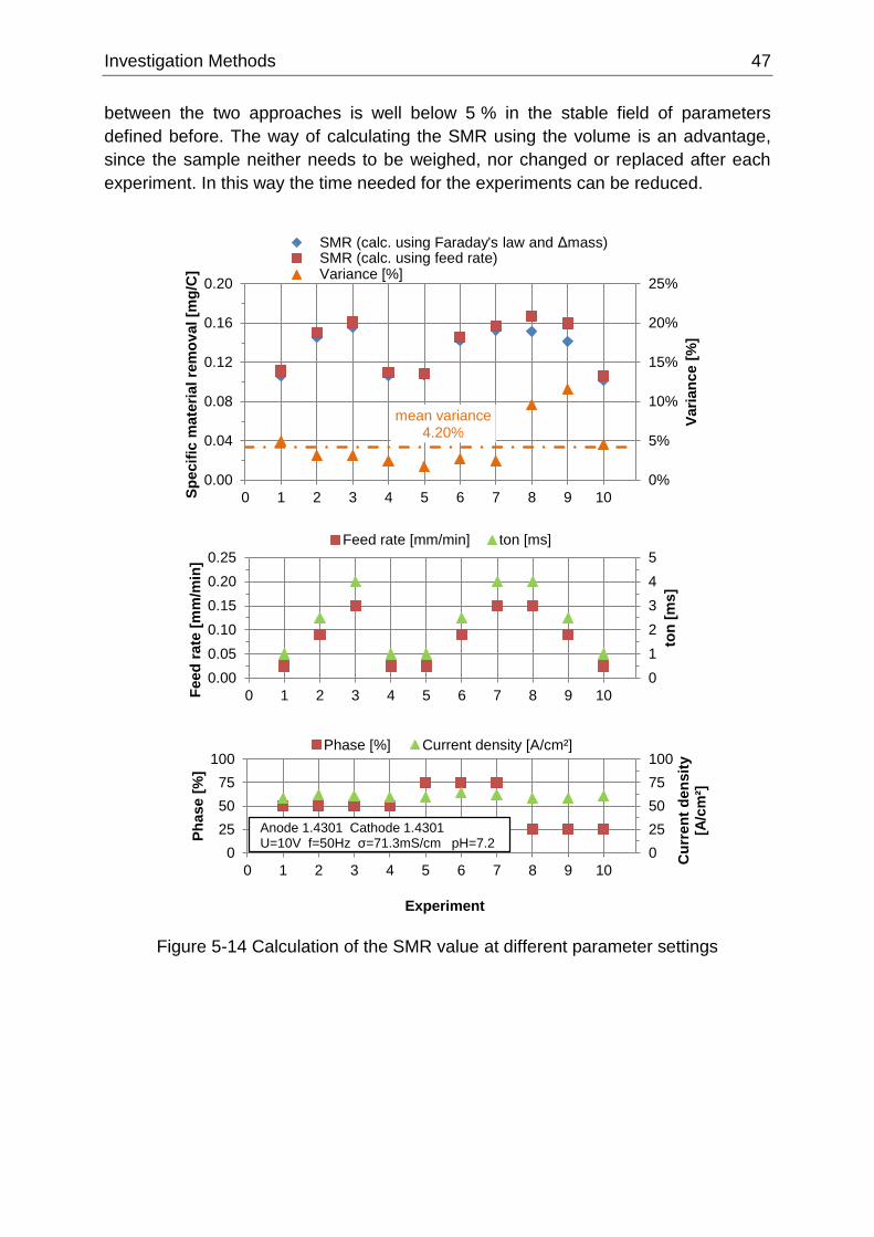
Investigation Methods 47
between the two approaches is well below 5 % in the stable field of parameters
defined before. The way of calculating the SMR using the volume is an advantage,
since the sample neither needs to be weighed, nor changed or replaced after each
experiment. In this way the time needed for the experiments can be reduced.
Figure 5-14 Calculation of the SMR value at different parameter settings
mean variance 4.20%
0%
5%
10%
15%
20%
25%
0.00
0.04
0.08
0.12
0.16
0.20
0 1 2 3 4 5 6 7 8 9 10
Va
ria
nc
e [
%]
Sp
ecif
ic m
ate
ria
l re
mo
va
l [m
g/C
]
Experiment
SMR (calc. using Faraday's law and Δmass)SMR (calc. using feed rate)Variance [%]
0
1
2
3
4
5
0.00
0.05
0.10
0.15
0.20
0.25
0 1 2 3 4 5 6 7 8 9 10
ton
[m
s]
Fe
ed
ra
te [
mm
/min
]
Feed rate [mm/min] ton [ms]
0
25
50
75
100
0
25
50
75
100
0 1 2 3 4 5 6 7 8 9 10
Cu
rre
nt
de
ns
ity
[A/c
m²]
Ph
ase
[%
]
Experiment
Phase [%] Current density [A/cm²]
Anode 1.4301 Cathode 1.4301U=10V f=50Hz σ=71.3mS/cm pH=7.2
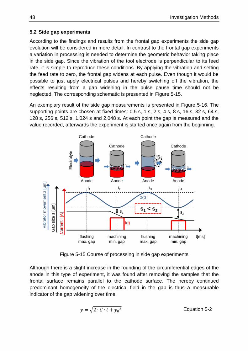
48 Investigation Methods
5.2 Side gap experiments
According to the findings and results from the frontal gap experiments the side gap
evolution will be considered in more detail. In contrast to the frontal gap experiments
a variation in processing is needed to determine the geometric behavior taking place
in the side gap. Since the vibration of the tool electrode is perpendicular to its feed
rate, it is simple to reproduce these conditions. By applying the vibration and setting
the feed rate to zero, the frontal gap widens at each pulse. Even though it would be
possible to just apply electrical pulses and hereby switching off the vibration, the
effects resulting from a gap widening in the pulse pause time should not be
neglected. The corresponding schematic is presented in Figure 5-15.
An exemplary result of the side gap measurements is presented in Figure 5-16. The
supporting points are chosen at fixed times: 0.5 s, 1 s, 2 s, 4 s, 8 s, 16 s, 32 s, 64 s,
128 s, 256 s, 512 s, 1,024 s and 2,048 s. At each point the gap is measured and the
value recorded, afterwards the experiment is started once again from the beginning.
Figure 5-15 Course of processing in side gap experiments
Although there is a slight increase in the rounding of the circumferential edges of the
anode in this type of experiment, it was found after removing the samples that the
frontal surface remains parallel to the cathode surface. The hereby continued
predominant homogeneity of the electrical field in the gap is thus a measurable
indicator of the gap widening over time.
𝑦 = √2 ∙ 𝐶 ∙ 𝑡 + 𝑦02 Equation 5-2
s1
z(t)
t[ms]flushing
max. gap
machining
min. gap
flushing
max. gap
machining
min. gap
t1 t2 t3 t4
Cathode
Cathode
Cathode
Cathode
Anode Anode Anode Anode
Ele
ctr
oly
te
I(t)
Cu
rrent
I [A
]
Ga
p s
ize
s [µ
m]
Vib
rato
r m
ovem
entz [
µm
]
s2
s1 < s2
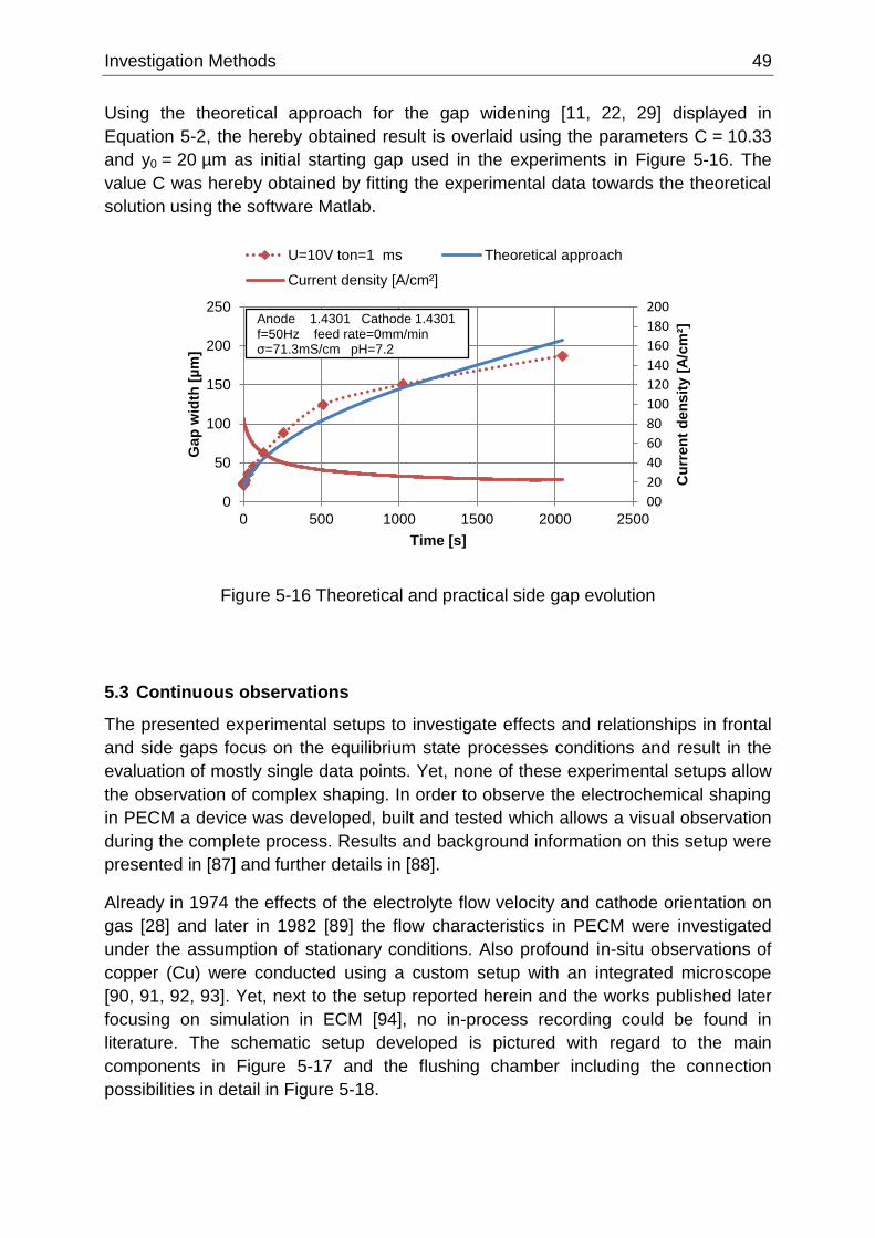
Investigation Methods 49
Using the theoretical approach for the gap widening [11, 22, 29] displayed in
Equation 5-2, the hereby obtained result is overlaid using the parameters C = 10.33
and y0 = 20 µm as initial starting gap used in the experiments in Figure 5-16. The
value C was hereby obtained by fitting the experimental data towards the theoretical
solution using the software Matlab.
Figure 5-16 Theoretical and practical side gap evolution
5.3 Continuous observations
The presented experimental setups to investigate effects and relationships in frontal
and side gaps focus on the equilibrium state processes conditions and result in the
evaluation of mostly single data points. Yet, none of these experimental setups allow
the observation of complex shaping. In order to observe the electrochemical shaping
in PECM a device was developed, built and tested which allows a visual observation
during the complete process. Results and background information on this setup were
presented in [87] and further details in [88].
Already in 1974 the effects of the electrolyte flow velocity and cathode orientation on
gas [28] and later in 1982 [89] the flow characteristics in PECM were investigated
under the assumption of stationary conditions. Also profound in-situ observations of
copper (Cu) were conducted using a custom setup with an integrated microscope
[90, 91, 92, 93]. Yet, next to the setup reported herein and the works published later
focusing on simulation in ECM [94], no in-process recording could be found in
literature. The schematic setup developed is pictured with regard to the main
components in Figure 5-17 and the flushing chamber including the connection
possibilities in detail in Figure 5-18.
00
20
40
60
80
100
120
140
160
180
200
0
50
100
150
200
250
0 500 1000 1500 2000 2500
Cu
rre
nt
de
ns
ity [
A/c
m²]
Ga
p w
idth
[µ
m]
Time [s]
U=10V ton=1 ms Theoretical approach
Current density [A/cm²]
Anode 1.4301 Cathode 1.4301f=50Hz feed rate=0mm/minσ=71.3mS/cm pH=7.2
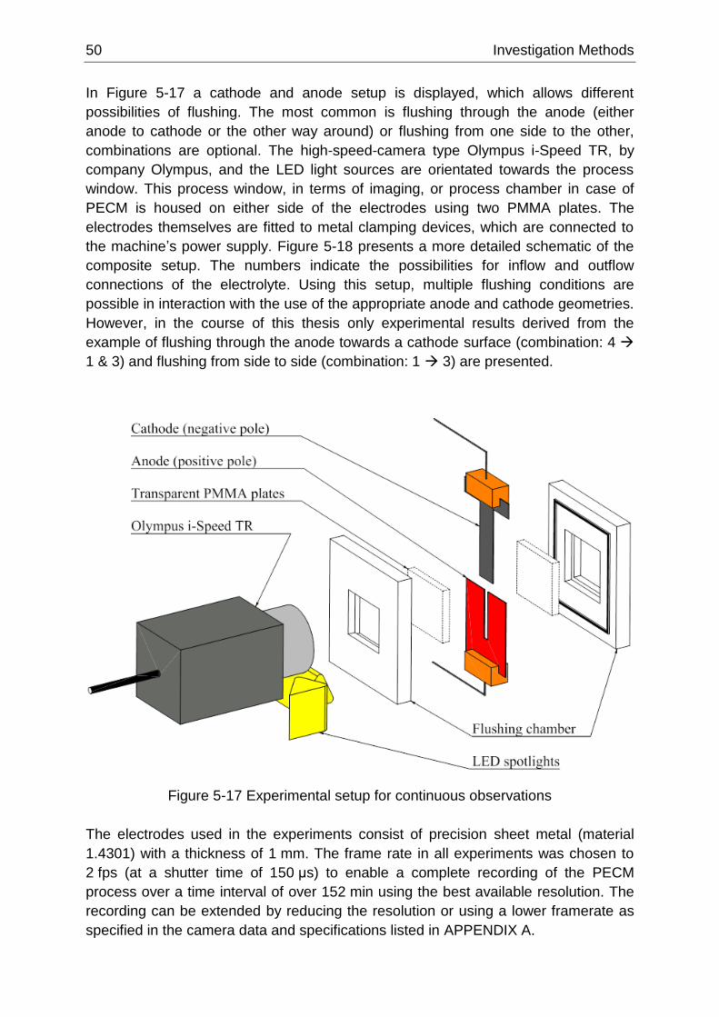
50 Investigation Methods
In Figure 5-17 a cathode and anode setup is displayed, which allows different
possibilities of flushing. The most common is flushing through the anode (either
anode to cathode or the other way around) or flushing from one side to the other,
combinations are optional. The high-speed-camera type Olympus i-Speed TR, by
company Olympus, and the LED light sources are orientated towards the process
window. This process window, in terms of imaging, or process chamber in case of
PECM is housed on either side of the electrodes using two PMMA plates. The
electrodes themselves are fitted to metal clamping devices, which are connected to
the machine’s power supply. Figure 5-18 presents a more detailed schematic of the
composite setup. The numbers indicate the possibilities for inflow and outflow
connections of the electrolyte. Using this setup, multiple flushing conditions are
possible in interaction with the use of the appropriate anode and cathode geometries.
However, in the course of this thesis only experimental results derived from the
example of flushing through the anode towards a cathode surface (combination: 4
1 & 3) and flushing from side to side (combination: 1 3) are presented.
Figure 5-17 Experimental setup for continuous observations
The electrodes used in the experiments consist of precision sheet metal (material
1.4301) with a thickness of 1 mm. The frame rate in all experiments was chosen to
2 fps (at a shutter time of 150 μs) to enable a complete recording of the PECM
process over a time interval of over 152 min using the best available resolution. The
recording can be extended by reducing the resolution or using a lower framerate as
specified in the camera data and specifications listed in APPENDIX A.
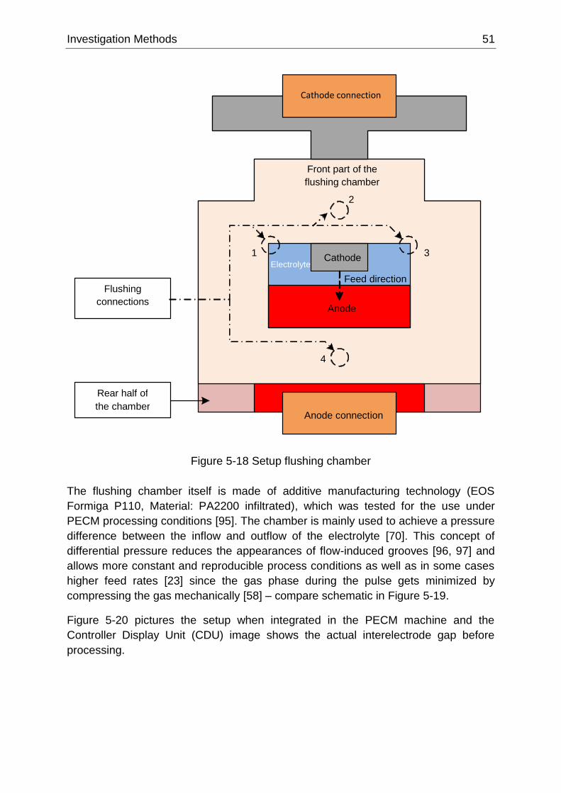
Investigation Methods 51
Figure 5-18 Setup flushing chamber
The flushing chamber itself is made of additive manufacturing technology (EOS
Formiga P110, Material: PA2200 infiltrated), which was tested for the use under
PECM processing conditions [95]. The chamber is mainly used to achieve a pressure
difference between the inflow and outflow of the electrolyte [70]. This concept of
differential pressure reduces the appearances of flow-induced grooves [96, 97] and
allows more constant and reproducible process conditions as well as in some cases
higher feed rates [23] since the gas phase during the pulse gets minimized by
compressing the gas mechanically [58] – compare schematic in Figure 5-19.
Figure 5-20 pictures the setup when integrated in the PECM machine and the
Controller Display Unit (CDU) image shows the actual interelectrode gap before
processing.
Cathode connection
Anode connect ion
Anode
Ca thode
Front part of t he flushing chamber
R ear half of t he chamber
Flushing connections
1 3
4
Feed d irection
2
Electrolyte
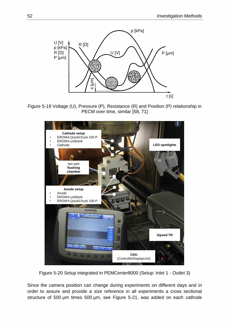
52 Investigation Methods
Figure 5-19 Voltage (U), Pressure (P), Resistance (R) and Position (P) relationship in PECM over time, similar [58, 71]
Figure 5-20 Setup integrated in PEMCenter8000 (Setup: Inlet 1 - Outlet 3)
Since the camera position can change during experiments on different days and in
order to assure and provide a size reference in all experiments a cross sectional
structure of 500 µm times 500 µm, see Figure 5-21, was added on each cathode
s [
µm
]
U [V]
p [kPa]
R [Ω]
P [µm]
t [s]
U [V]
p [kPa]
P [µm]
R [Ω]
iSpeed TR
LED spotlights
Cathode setup
• EROWA QuickChuck 100 P
• EROWA uniblank
• Cathode
CDU
(ControllerDisplayUnit)
two part
flushing
chamber
Anode setup
• Anode
• EROWA uniblank
• EROWA QuickChuck 100 P
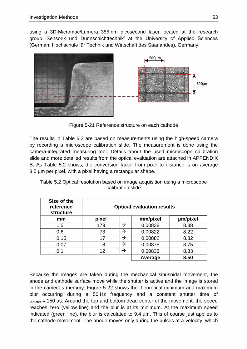
Investigation Methods 53
using a 3D-Micromac/Lumera 355 nm picosecond laser located at the research
group ‘Sensorik und Dünnschichttechnik’ at the University of Applied Sciences
(German: Hochschule für Technik und Wirtschaft des Saarlandes), Germany.
500µm
500µm
Figure 5-21 Reference structure on each cathode
The results in Table 5.2 are based on measurements using the high-speed camera
by recording a microscope calibration slide. The measurement is done using the
camera-integrated measuring tool. Details about the used microscope calibration
slide and more detailed results from the optical evaluation are attached in APPENDIX
B. As Table 5.2 shows, the conversion factor from pixel to distance is on average
8.5 µm per pixel, with a pixel having a rectangular shape.
Table 5.2 Optical resolution based on image acquisition using a microscope calibration slide
Size of the reference structure
Optical evaluation results
mm pixel mm/pixel µm/pixel
1.5 179 0.00838 8.38
0.6 73 0.00822 8.22
0.15 17 0.00882 8.82
0.07 8 0.00875 8.75
0.1 12 0.00833 8.33
Average 8.50
Because the images are taken during the mechanical sinusoidal movement, the
anode and cathode surface move while the shutter is active and the image is stored
in the camera’s memory. Figure 5-22 shows the theoretical minimum and maximum
blur occurring during a 50 Hz frequency and a constant shutter time of
tshutter = 150 µs. Around the top and bottom dead center of the movement, the speed
reaches zero (yellow line) and the blur is at its minimum. At the maximum speed
indicated (green line), the blur is calculated to 9.4 µm. This of course just applies to
the cathode movement. The anode moves only during the pulses at a velocity, which
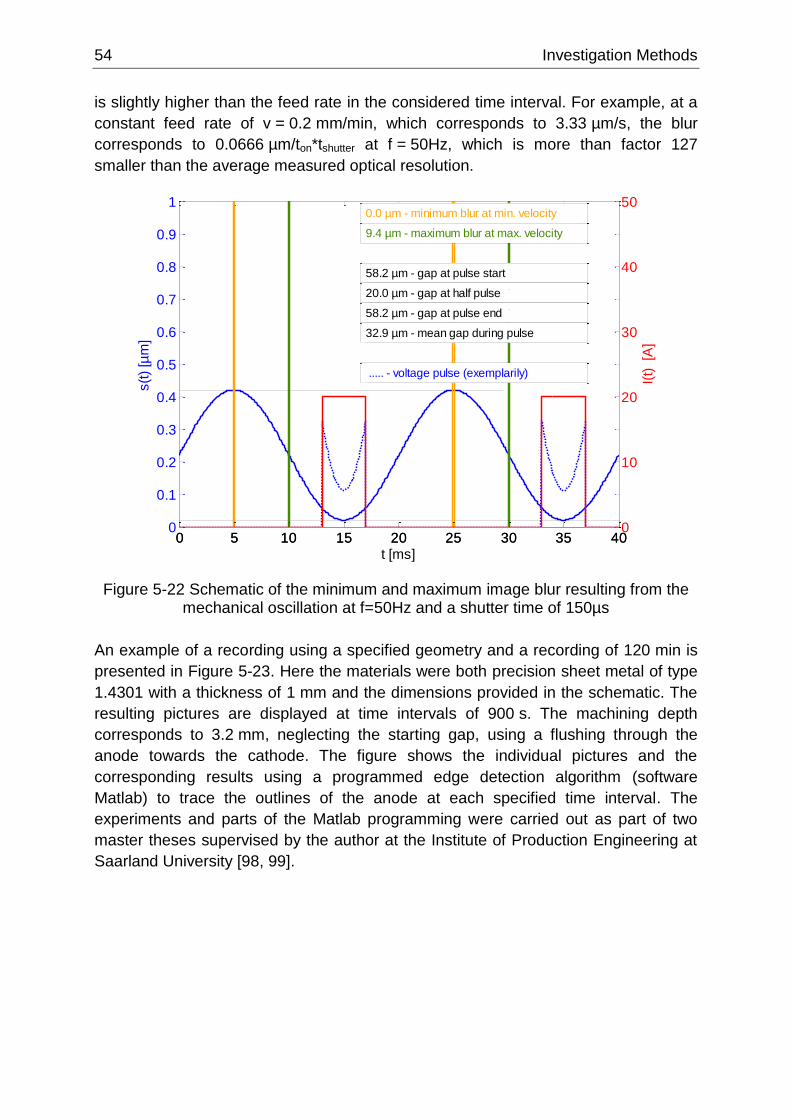
54 Investigation Methods
is slightly higher than the feed rate in the considered time interval. For example, at a
constant feed rate of v = 0.2 mm/min, which corresponds to 3.33 µm/s, the blur
corresponds to 0.0666 µm/ton*tshutter at f = 50Hz, which is more than factor 127
smaller than the average measured optical resolution.
Figure 5-22 Schematic of the minimum and maximum image blur resulting from the mechanical oscillation at f=50Hz and a shutter time of 150µs
An example of a recording using a specified geometry and a recording of 120 min is
presented in Figure 5-23. Here the materials were both precision sheet metal of type
1.4301 with a thickness of 1 mm and the dimensions provided in the schematic. The
resulting pictures are displayed at time intervals of 900 s. The machining depth
corresponds to 3.2 mm, neglecting the starting gap, using a flushing through the
anode towards the cathode. The figure shows the individual pictures and the
corresponding results using a programmed edge detection algorithm (software
Matlab) to trace the outlines of the anode at each specified time interval. The
experiments and parts of the Matlab programming were carried out as part of two
master theses supervised by the author at the Institute of Production Engineering at
Saarland University [98, 99].
0 5 10 15 20 25 30 35 400
0.1
0.2
0.3
0.4
0.5
0.6
0.7
0.8
0.9
1
s(t
) [µ
m]
t [ms]0 5 10 15 20 25 30 35 40
0
10
20
30
40
50
I(t
) [A
]
0.0 µm - minimum blur at min. velocity
9.4 µm - maximum blur at max. velocity
58.2 µm - gap at pulse start
20.0 µm - gap at half pulse
58.2 µm - gap at pulse end
32.9 µm - mean gap during pulse
..... - voltage pulse (exemplarily)
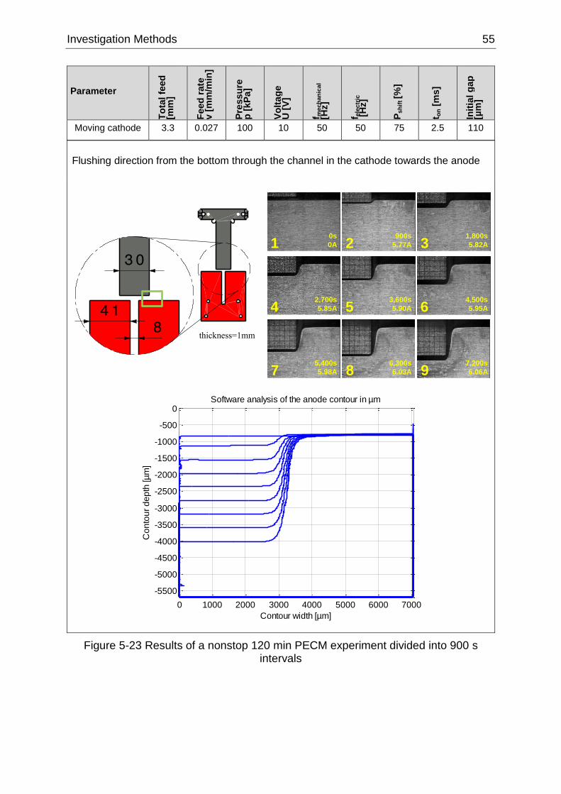
Investigation Methods 55
Parameter
To
tal fe
ed
[m
m]
Feed
rate
v [
mm
/min
]
Pre
ssu
re
p [
kP
a]
Vo
ltag
e
U [
V]
f mech
an
ical
[Hz]
f ele
ctr
ic
[H
z]
Psh
ift [%
]
t on [
ms]
Init
ial g
ap
[µ
m]
Moving cathode 3.3 0.027 100 10 50 50 75 2.5 110
Flushing direction from the bottom through the channel in the cathode towards the anode
Figure 5-23 Results of a nonstop 120 min PECM experiment divided into 900 s intervals
0s
0A
900s
5.77A
1,800s
5.82A
2,700s
5.85A
3,600s
5.90A
4,500s
5.95A
5,400s
5.98A
6,300s
6.03A
7,200s
6.06A
1 2 3
4 5 6
7 8 9
0 1000 2000 3000 4000 5000 6000 7000
-5500
-5000
-4500
-4000
-3500
-3000
-2500
-2000
-1500
-1000
-500
0
Contour width [µm]
Co
nto
ur
de
pth
[µ
m]
Software analysis of the anode contour in µm
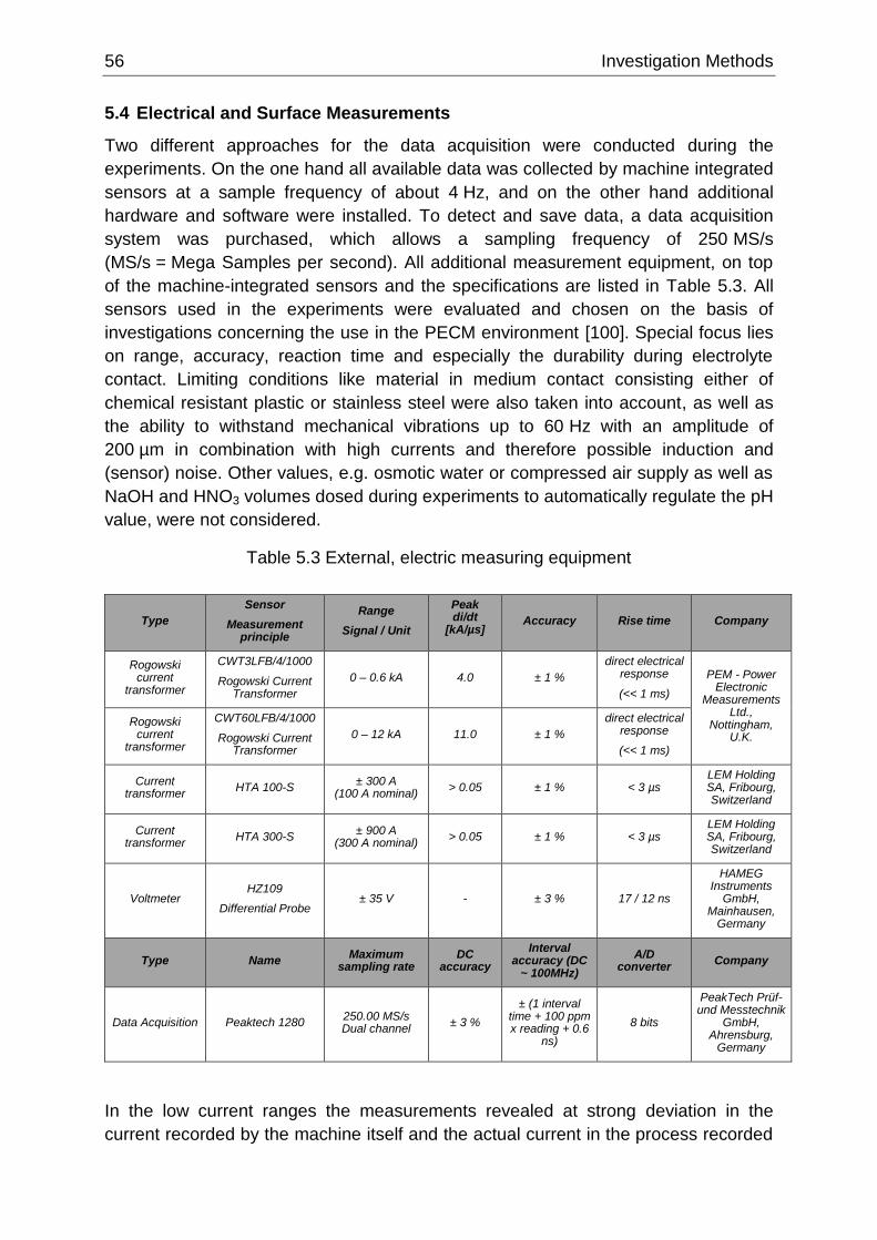
56 Investigation Methods
5.4 Electrical and Surface Measurements
Two different approaches for the data acquisition were conducted during the
experiments. On the one hand all available data was collected by machine integrated
sensors at a sample frequency of about 4 Hz, and on the other hand additional
hardware and software were installed. To detect and save data, a data acquisition
system was purchased, which allows a sampling frequency of 250 MS/s
(MS/s = Mega Samples per second). All additional measurement equipment, on top
of the machine-integrated sensors and the specifications are listed in Table 5.3. All
sensors used in the experiments were evaluated and chosen on the basis of
investigations concerning the use in the PECM environment [100]. Special focus lies
on range, accuracy, reaction time and especially the durability during electrolyte
contact. Limiting conditions like material in medium contact consisting either of
chemical resistant plastic or stainless steel were also taken into account, as well as
the ability to withstand mechanical vibrations up to 60 Hz with an amplitude of
200 µm in combination with high currents and therefore possible induction and
(sensor) noise. Other values, e.g. osmotic water or compressed air supply as well as
NaOH and HNO3 volumes dosed during experiments to automatically regulate the pH
value, were not considered.
Table 5.3 External, electric measuring equipment
Type
Sensor
Measurement principle
Range
Signal / Unit
Peak di/dt
[kA/µs] Accuracy Rise time Company
Rogowski current
transformer
CWT3LFB/4/1000
Rogowski Current Transformer
0 – 0.6 kA 4.0 ± 1 %
direct electrical response
(<< 1 ms)
PEM - Power Electronic
Measurements Ltd.,
Nottingham, U.K.
Rogowski current
transformer
CWT60LFB/4/1000
Rogowski Current Transformer
0 – 12 kA 11.0 ± 1 %
direct electrical response
(<< 1 ms)
Current transformer
HTA 100-S ± 300 A
(100 A nominal) > 0.05 ± 1 % < 3 µs
LEM Holding SA, Fribourg, Switzerland
Current transformer
HTA 300-S ± 900 A
(300 A nominal) > 0.05 ± 1 % < 3 µs
LEM Holding SA, Fribourg, Switzerland
Voltmeter HZ109
Differential Probe ± 35 V - ± 3 % 17 / 12 ns
HAMEG Instruments
GmbH, Mainhausen,
Germany
Type Name Maximum
sampling rate DC
accuracy
Interval accuracy (DC
~ 100MHz)
A/D converter
Company
Data Acquisition Peaktech 1280 250.00 MS/s Dual channel
± 3 %
± (1 interval time + 100 ppm x reading + 0.6
ns)
8 bits
PeakTech Prüf- und Messtechnik
GmbH, Ahrensburg,
Germany
In the low current ranges the measurements revealed at strong deviation in the
current recorded by the machine itself and the actual current in the process recorded
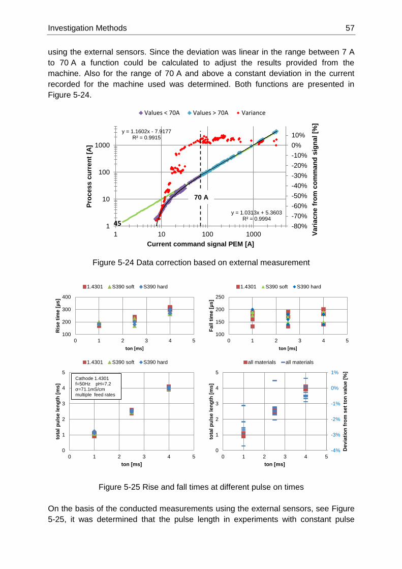
Investigation Methods 57
using the external sensors. Since the deviation was linear in the range between 7 A
to 70 A a function could be calculated to adjust the results provided from the
machine. Also for the range of 70 A and above a constant deviation in the current
recorded for the machine used was determined. Both functions are presented in
Figure 5-24.
Figure 5-24 Data correction based on external measurement
Figure 5-25 Rise and fall times at different pulse on times
On the basis of the conducted measurements using the external sensors, see Figure
5-25, it was determined that the pulse length in experiments with constant pulse
y = 1.1602x - 7.9177R² = 0.9915
y = 1.0313x + 5.3603R² = 0.9994
-80%
-70%
-60%
-50%
-40%
-30%
-20%
-10%
0%
10%
1
10
100
1000
1 10 100 1000 Vari
acn
e f
rom
co
mm
an
d s
ign
al
[%]
Pro
cess c
urr
en
t [A
]
Current command signal PEM [A]
Values < 70A Values > 70A Variance
70 A
45
-4%
-3%
-2%
-1%
0%
1%
0
1
2
3
4
5
0 1 2 3 4 5
De
via
tio
n f
rom
set
ton
va
lue
[%
]
tota
l p
uls
e l
en
gth
[m
s]
ton [ms]
all materials all materials
0
1
2
3
4
5
0 1 2 3 4 5
tota
l p
uls
e l
en
gth
[m
s]
ton [ms]
1.4301 S390 soft S390 hard
Cathode 1.4301f=50Hz pH=7.2σ=71.1mS/cmmultiple feed rates
100
200
300
400
0 1 2 3 4 5
Ris
e t
ime
[µ
s]
ton [ms]
1.4301 S390 soft S390 hard
100
150
200
250
0 1 2 3 4 5
Fa
ll t
ime
[µ
s]
ton [ms]
1.4301 S390 soft S390 hard
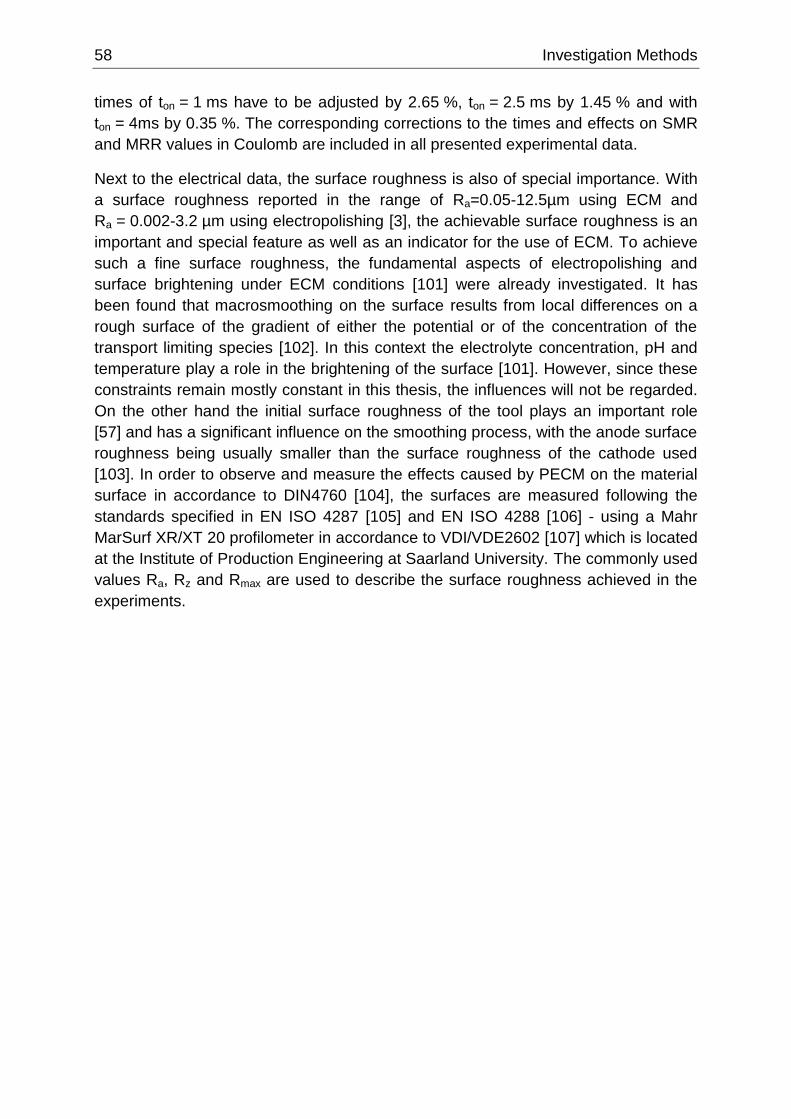
58 Investigation Methods
times of ton = 1 ms have to be adjusted by 2.65 %, ton = 2.5 ms by 1.45 % and with
ton = 4ms by 0.35 %. The corresponding corrections to the times and effects on SMR
and MRR values in Coulomb are included in all presented experimental data.
Next to the electrical data, the surface roughness is also of special importance. With
a surface roughness reported in the range of Ra=0.05-12.5µm using ECM and
Ra = 0.002-3.2 µm using electropolishing [3], the achievable surface roughness is an
important and special feature as well as an indicator for the use of ECM. To achieve
such a fine surface roughness, the fundamental aspects of electropolishing and
surface brightening under ECM conditions [101] were already investigated. It has
been found that macrosmoothing on the surface results from local differences on a
rough surface of the gradient of either the potential or of the concentration of the
transport limiting species [102]. In this context the electrolyte concentration, pH and
temperature play a role in the brightening of the surface [101]. However, since these
constraints remain mostly constant in this thesis, the influences will not be regarded.
On the other hand the initial surface roughness of the tool plays an important role
[57] and has a significant influence on the smoothing process, with the anode surface
roughness being usually smaller than the surface roughness of the cathode used
[103]. In order to observe and measure the effects caused by PECM on the material
surface in accordance to DIN4760 [104], the surfaces are measured following the
standards specified in EN ISO 4287 [105] and EN ISO 4288 [106] - using a Mahr
MarSurf XR/XT 20 profilometer in accordance to VDI/VDE2602 [107] which is located
at the Institute of Production Engineering at Saarland University. The commonly used
values Ra, Rz and Rmax are used to describe the surface roughness achieved in the
experiments.
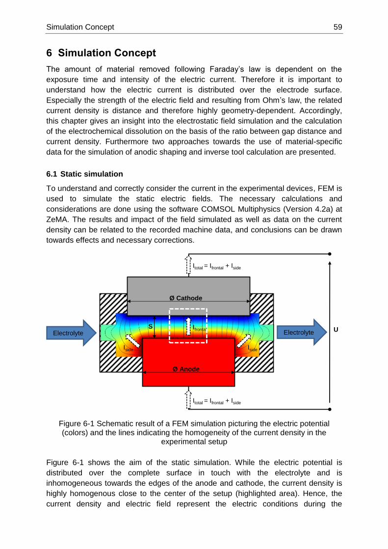
Simulation Concept 59
6 Simulation Concept
The amount of material removed following Faraday’s law is dependent on the
exposure time and intensity of the electric current. Therefore it is important to
understand how the electric current is distributed over the electrode surface.
Especially the strength of the electric field and resulting from Ohm’s law, the related
current density is distance and therefore highly geometry-dependent. Accordingly,
this chapter gives an insight into the electrostatic field simulation and the calculation
of the electrochemical dissolution on the basis of the ratio between gap distance and
current density. Furthermore two approaches towards the use of material-specific
data for the simulation of anodic shaping and inverse tool calculation are presented.
6.1 Static simulation
To understand and correctly consider the current in the experimental devices, FEM is
used to simulate the static electric fields. The necessary calculations and
considerations are done using the software COMSOL Multiphysics (Version 4.2a) at
ZeMA. The results and impact of the field simulated as well as data on the current
density can be related to the recorded machine data, and conclusions can be drawn
towards effects and necessary corrections.
Figure 6-1 Schematic result of a FEM simulation picturing the electric potential (colors) and the lines indicating the homogeneity of the current density in the
experimental setup
Figure 6-1 shows the aim of the static simulation. While the electric potential is
distributed over the complete surface in touch with the electrolyte and is
inhomogeneous towards the edges of the anode and cathode, the current density is
highly homogenous close to the center of the setup (highlighted area). Hence, the
current density and electric field represent the electric conditions during the
Ifrontal U
Ø Cathode
Ø Anode
Iside
SElectrolyte Electrolyte
Iside
Itotal = Ifrontal + Iside
Itotal = Ifrontal + Iside
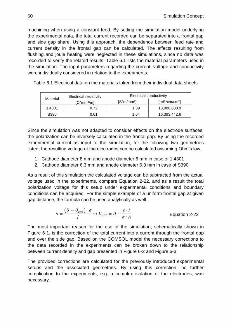
60 Simulation Concept
machining when using a constant feed. By setting the simulation model underlying
the experimental data, the total current recorded can be separated into a frontal gap
and side gap share. Using this approach, the dependence between feed rate and
current density in the frontal gap can be calculated. The effects resulting from
flushing and joule heating were neglected in these simulations, since no data was
recorded to verify the related results. Table 6.1 lists the material parameters used in
the simulation. The input parameters regarding the current, voltage and conductivity
were individually considered in relation to the experiments.
Table 6.1 Electrical data on the materials taken from their individual data sheets
Material Electrical resistivity Electrical conductivity
[Ω*mm²/m] [S*m/mm²] [mS*cm/cm²]
1.4301 0.72 1.39 13,888,888.9
S390 0.61 1.64 16,393,442.6
Since the simulation was not adapted to consider effects on the electrode surfaces,
the polarization can be inversely calculated in the frontal gap. By using the recorded
experimental current as input to the simulation, for the following two geometries
listed, the resulting voltage at the electrodes can be calculated assuming Ohm’s law.
1. Cathode diameter 8 mm and anode diameter 6 mm in case of 1.4301
2. Cathode diameter 6.3 mm and anode diameter 6.3 mm in case of S390
As a result of this simulation the calculated voltage can be subtracted from the actual
voltage used in the experiments, compare Equation 2-22, and as a result the total
polarization voltage for this setup under experimental conditions and boundary
conditions can be acquired. For the simple example of a uniform frontal gap at given
gap distance, the formula can be used analytically as well.
𝑠 =(𝑈 − 𝑈𝑝𝑜𝑙) ∙ 𝜎
𝐽↔ 𝑈𝑝𝑜𝑙 = 𝑈 −
𝑠 ∙ 𝐼
𝜎 ∙ 𝐴 Equation 2-22
The most important reason for the use of the simulation, schematically shown in
Figure 6-1, is the correction of the total current into a current through the frontal gap
and over the side gap. Based on the COMSOL model the necessary corrections to
the data recorded in the experiments can be broken down to the relationship
between current density and gap presented in Figure 6-2 and Figure 6-3.
The provided corrections are calculated for the previously introduced experimental
setups and the associated geometries. By using this correction, no further
complication to the experiments, e.g. a complex isolation of the electrodes, was
necessary.
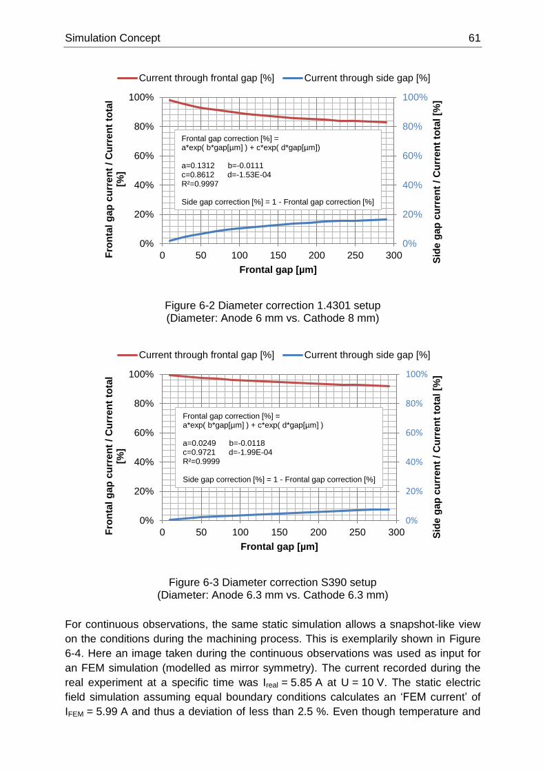
Simulation Concept 61
Figure 6-2 Diameter correction 1.4301 setup (Diameter: Anode 6 mm vs. Cathode 8 mm)
Figure 6-3 Diameter correction S390 setup (Diameter: Anode 6.3 mm vs. Cathode 6.3 mm)
For continuous observations, the same static simulation allows a snapshot-like view
on the conditions during the machining process. This is exemplarily shown in Figure
6-4. Here an image taken during the continuous observations was used as input for
an FEM simulation (modelled as mirror symmetry). The current recorded during the
real experiment at a specific time was Ireal = 5.85 A at U = 10 V. The static electric
field simulation assuming equal boundary conditions calculates an ‘FEM current’ of
IFEM = 5.99 A and thus a deviation of less than 2.5 %. Even though temperature and
0%
20%
40%
60%
80%
100%
0%
20%
40%
60%
80%
100%
0 50 100 150 200 250 300
Sid
e g
ap
cu
rren
t / C
urr
en
t to
tal [%
]
Fro
nta
l g
ap
cu
rre
nt
/ C
urr
en
t to
tal
[%]
Frontal gap [µm]
Current through frontal gap [%] Current through side gap [%]
Frontal gap correction [%] = a*exp( b*gap[µm] ) + c*exp( d*gap[µm])
a=0.1312 b=-0.0111c=0.8612 d=-1.53E-04R²=0.9997
Side gap correction [%] = 1 - Frontal gap correction [%]
0%
20%
40%
60%
80%
100%
0%
20%
40%
60%
80%
100%
0 50 100 150 200 250 300 Sid
e g
ap
cu
rren
t / C
urr
en
t to
tal [%
]
Fro
nta
l g
ap
cu
rre
nt
/ C
urr
en
t to
tal
[%]
Frontal gap [µm]
Current through frontal gap [%] Current through side gap [%]
Frontal gap correction [%] = a*exp( b*gap[µm] ) + c*exp( d*gap[µm] )
a=0.0249 b=-0.0118c=0.9721 d=-1.99E-04R²=0.9999
Side gap correction [%] = 1 - Frontal gap correction [%]
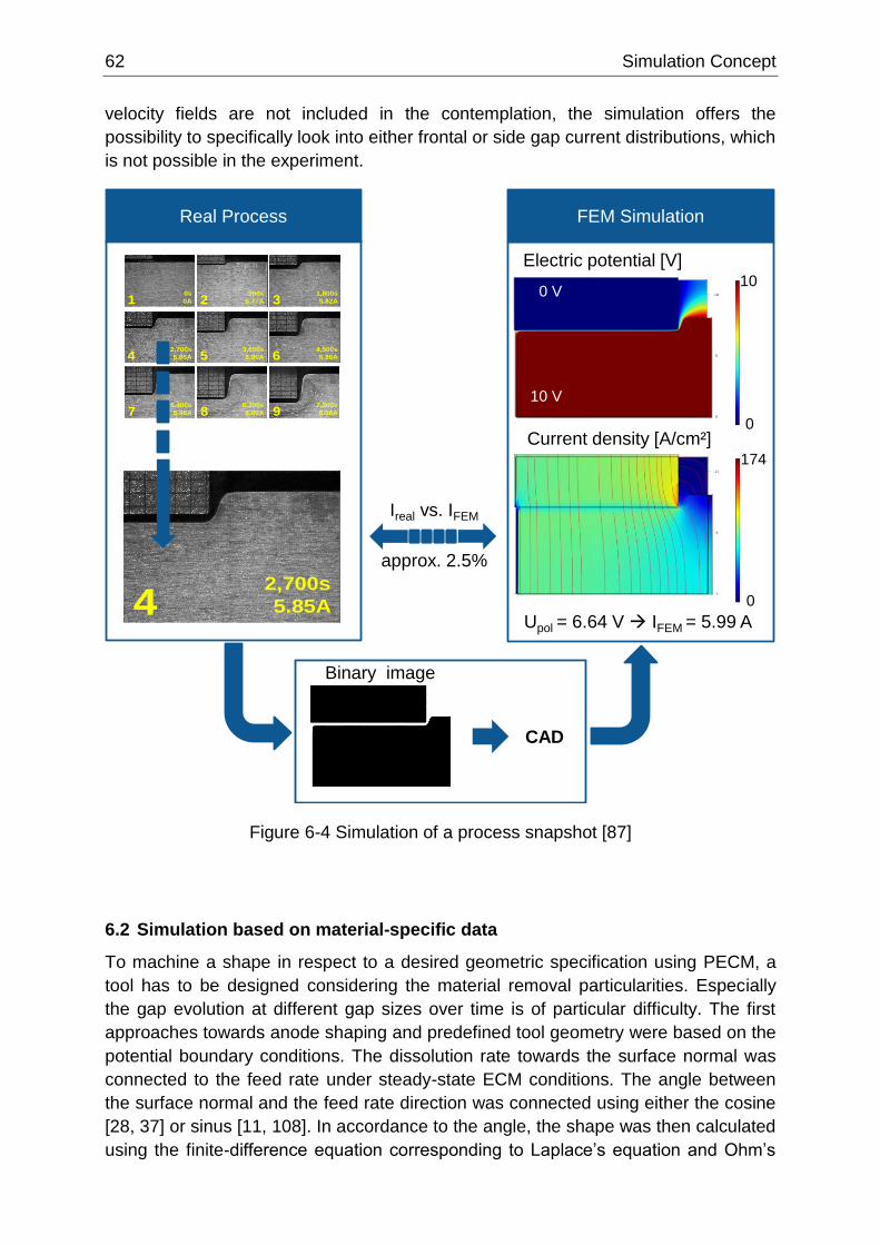
62 Simulation Concept
velocity fields are not included in the contemplation, the simulation offers the
possibility to specifically look into either frontal or side gap current distributions, which
is not possible in the experiment.
Figure 6-4 Simulation of a process snapshot [87]
6.2 Simulation based on material-specific data
To machine a shape in respect to a desired geometric specification using PECM, a
tool has to be designed considering the material removal particularities. Especially
the gap evolution at different gap sizes over time is of particular difficulty. The first
approaches towards anode shaping and predefined tool geometry were based on the
potential boundary conditions. The dissolution rate towards the surface normal was
connected to the feed rate under steady-state ECM conditions. The angle between
the surface normal and the feed rate direction was connected using either the cosine
[28, 37] or sinus [11, 108]. In accordance to the angle, the shape was then calculated
using the finite-difference equation corresponding to Laplace’s equation and Ohm’s
Ireal vs. IFEM
approx. 2.5%
Real Process FEM Simulation
CAD
0s
0A
900s
5.77A
1,800s
5.82A
2,700s
5.85A
3,600s
5.90A
4,500s
5.95A
5,400s
5.98A
6,300s
6.03A
7,200s
6.06A
1 2 3
4 5 6
7 8 9
Binary image
0s
0A
900s
5.77A
1,800s
5.82A
2,700s
5.85A
3,600s
5.90A
4,500s
5.95A
5,400s
5.98A
6,300s
6.03A
7,200s
6.06A
1 2 3
4 5 6
7 8 9
Electric potential [V]
10 V
10
0
0
174
Current density [A/cm²]
0 V
Upol = 6.64 V IFEM = 5.99 A
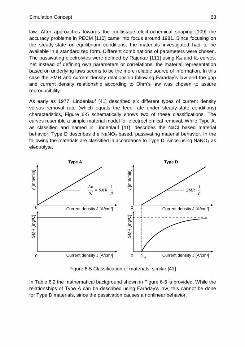
Simulation Concept 63
law. After approaches towards the multistage electrochemical shaping [109] the
accuracy problems in PECM [110] came into focus around 1981. Since focusing on
the steady-state or equilibrium conditions, the materials investigated had to be
available in a standardized form. Different combinations of parameters were chosen.
The passivating electrolytes were defined by Rajurkar [111] using Km and Kv curves.
Yet instead of defining own parameters or correlations, the material representation
based on underlying laws seems to be the more reliable source of information. In this
case the SMR and current density relationship following Faraday’s law and the gap
and current density relationship according to Ohm’s law was chosen to assure
reproducibility.
As early as 1977, Lindenlauf [41] described six different types of current density
versus removal rate (which equals the feed rate under steady-state conditions)
characteristics, Figure 6-5 schematically shows two of these classifications. The
curves resemble a simple material model for electrochemical removal. While Type A,
as classified and named in Lindenlauf [41], describes the NaCl based material
behavior, Type D describes the NaNO3 based, passivating material behavior. In the
following the materials are classified in accordance to Type D, since using NaNO3 as
electrolyte.
Figure 6-5 Classification of materials, similar [41]
In Table 6.2 the mathematical background shown in Figure 6-5 is provided. While the
relationships of Type A can be described using Faraday’s law, this cannot be done
for Type D materials, since the passivation causes a nonlinear behavior.
SM
R [
mg/C
]
Current density J [A/cm²]
SM
R [
mg/C
]
Current density J [A/cm²]
Type A
v[m
m/m
in]
Current density J [A/cm²]
v [
mm
/min
]
Current density J [A/cm²] 0
0
0
0
Type D
Jmin
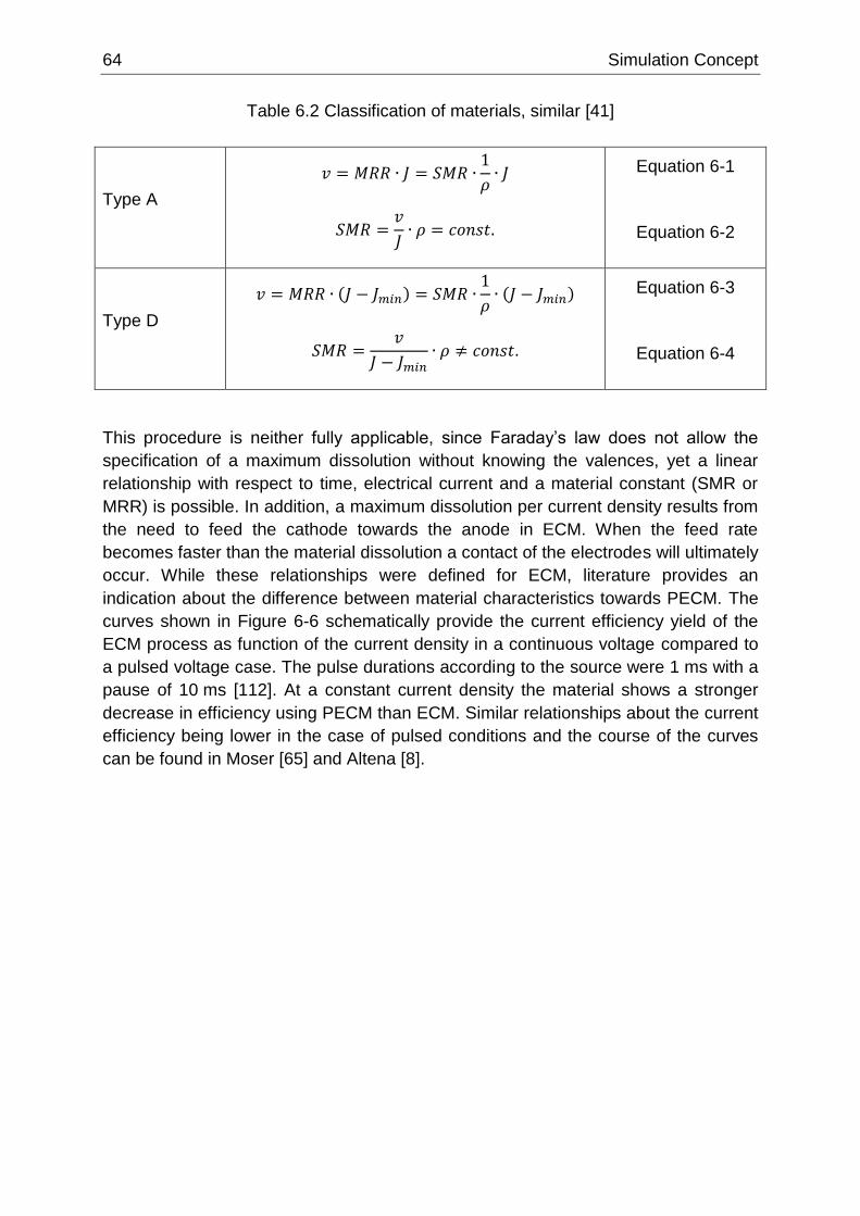
64 Simulation Concept
Table 6.2 Classification of materials, similar [41]
Type A
𝑣 = 𝑀𝑅𝑅 ∙ 𝐽 = 𝑆𝑀𝑅 ∙1
𝜌∙ 𝐽
𝑆𝑀𝑅 =𝑣
𝐽∙ 𝜌 = 𝑐𝑜𝑛𝑠𝑡.
Equation 6-1
Equation 6-2
Type D
𝑣 = 𝑀𝑅𝑅 ∙ (𝐽 − 𝐽𝑚𝑖𝑛) = 𝑆𝑀𝑅 ∙1
𝜌∙ (𝐽 − 𝐽𝑚𝑖𝑛)
𝑆𝑀𝑅 =𝑣
𝐽 − 𝐽𝑚𝑖𝑛∙ 𝜌 ≠ 𝑐𝑜𝑛𝑠𝑡.
Equation 6-3
Equation 6-4
This procedure is neither fully applicable, since Faraday’s law does not allow the
specification of a maximum dissolution without knowing the valences, yet a linear
relationship with respect to time, electrical current and a material constant (SMR or
MRR) is possible. In addition, a maximum dissolution per current density results from
the need to feed the cathode towards the anode in ECM. When the feed rate
becomes faster than the material dissolution a contact of the electrodes will ultimately
occur. While these relationships were defined for ECM, literature provides an
indication about the difference between material characteristics towards PECM. The
curves shown in Figure 6-6 schematically provide the current efficiency yield of the
ECM process as function of the current density in a continuous voltage compared to
a pulsed voltage case. The pulse durations according to the source were 1 ms with a
pause of 10 ms [112]. At a constant current density the material shows a stronger
decrease in efficiency using PECM than ECM. Similar relationships about the current
efficiency being lower in the case of pulsed conditions and the course of the curves
can be found in Moser [65] and Altena [8].
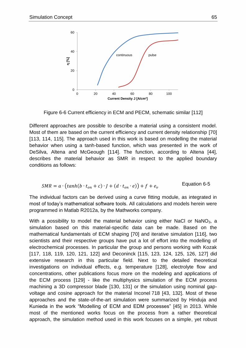
Simulation Concept 65
Figure 6-6 Current efficiency in ECM and PECM, schematic similar [112]
Different approaches are possible to describe a material using a consistent model.
Most of them are based on the current efficiency and current density relationship [70]
[113, 114, 115]. The approach used in this work is based on modelling the material
behavior when using a tanh-based function, which was presented in the work of
DeSilva, Altena and McGeough [114]. The function, according to Altena [44],
describes the material behavior as SMR in respect to the applied boundary
conditions as follows:
𝑆𝑀𝑅 = 𝑎 ∙ (𝑡𝑎𝑛ℎ(𝑏 ∙ 𝑡𝑜𝑛 + 𝑐) ∙ 𝐽 + (𝑑 ∙ 𝑡𝑜𝑛 ∙ 𝑒)) + 𝑓 + 𝑒𝑣
Equation 6-5
The individual factors can be derived using a curve fitting module, as integrated in
most of today’s mathematical software tools. All calculations and models herein were
programmed in Matlab R2012a, by the Mathworks company.
With a possibility to model the material behavior using either NaCl or NaNO3, a
simulation based on this material-specific data can be made. Based on the
mathematical fundamentals of ECM shaping [70] and iterative simulation [116], two
scientists and their respective groups have put a lot of effort into the modelling of
electrochemical processes. In particular the group and persons working with Kozak
[117, 118, 119, 120, 121, 122] and Deconinck [115, 123, 124, 125, 126, 127] did
extensive research in this particular field. Next to the detailed theoretical
investigations on individual effects, e.g. temperature [128], electrolyte flow and
concentrations, other publications focus more on the modeling and applications of
the ECM process [129] - like the multiphysics simulation of the ECM process
machining a 3D compressor blade [130, 131] or the simulation using nominal gap-
voltage and cosine approach for the material Inconel 718 [43, 132]. Most of these
approaches and the state-of-the-art simulation were summarized by Hinduja and
Kunieda in the work “Modelling of ECM and EDM processes” [45] in 2013. While
most of the mentioned works focus on the process from a rather theoretical
approach, the simulation method used in this work focuses on a simple, yet robust
0
20
40
60
0 20 40 60 80 100
ɳ [
%]
Current Density J [A/cm²]
continuous pulse
66 Simulation Concept
method based on experimental data similar to the approach used by the group
around Mount and Clifton [133, 134, 135]. The calculation steps implemented in
Matlab are presented in Figure 6-7.
Figure 6-7 Scheme of the calculation steps implemented in Matlab
Starting from the shape of a segmented cathode and anode, the closest distances
between points are determined. With the knowledge of the individual distances, the
current for a given potential can be calculated using Ohm’s law and then Faraday’s
law can be applied using the SMR values, which were determined experimentally.
The material removal (movement) at each individual point ( 𝑑ℎ𝑎𝑖 ) takes place in
normal direction towards the anodic surface. Based on the individually calculated
shortest distance and the voltage as boundary condition, the current density for each
point is calculated and then the point is moved in normal direction according to
Equation 6-6. The time-step can be chosen in accordance with the pulse on time ton
or as a multiple of it. Yet, the accuracy improves when using a time stepping equal to
the pulse on time, since a wider data range in the material model is used.
𝑑ℎ𝑎𝑖
𝑑𝑡
=
𝑀
𝑧 ∙ 𝐹 ∙ 𝜌∙ 𝑖𝑙𝑜𝑐𝑎𝑙,𝑖 ∙ �� ∙ 𝑡𝑜𝑛 ∙ 𝑓
Equation 6-6
ci
ai
ci+1
ci+x
ci-1
ci-2
ci-3
ci-4
ci-5
ci-y
ci+2
ai-1
ai-2
ai-3
ai+1
ai+2
ci-9
ci+3
ci-8
ci-7
ci-6
Move point ai
along its
normal vector
Tim
e s
tep
tj
Find shortest distances between
anode and cathode
in time step tj…
ai-3 ↔ ci-9
ai-2 ↔ ci-4
ai-1 ↔ ci-2
ai = (x1|y1) ↔ ci = (x2|y2)ai+1 ↔ ci+1
ai+2 ↔ ci+3
…
Calculate local gaps
Calculate local currents
based on voltage and conductivity
Use local current and known
material SMR values to calculate
local material removal
Move points along individual
normal vectors
Time step tj+1
…
REMESH
REMESH
σelectrolyte
Ilocal,i
U
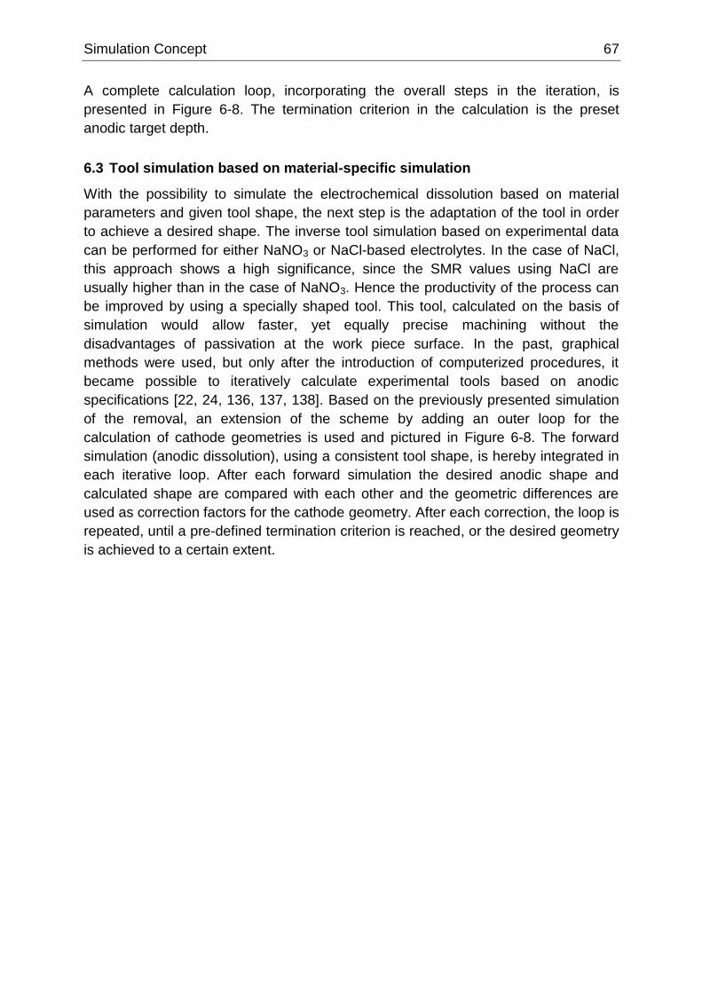
Simulation Concept 67
A complete calculation loop, incorporating the overall steps in the iteration, is
presented in Figure 6-8. The termination criterion in the calculation is the preset
anodic target depth.
6.3 Tool simulation based on material-specific simulation
With the possibility to simulate the electrochemical dissolution based on material
parameters and given tool shape, the next step is the adaptation of the tool in order
to achieve a desired shape. The inverse tool simulation based on experimental data
can be performed for either NaNO3 or NaCl-based electrolytes. In the case of NaCl,
this approach shows a high significance, since the SMR values using NaCl are
usually higher than in the case of NaNO3. Hence the productivity of the process can
be improved by using a specially shaped tool. This tool, calculated on the basis of
simulation would allow faster, yet equally precise machining without the
disadvantages of passivation at the work piece surface. In the past, graphical
methods were used, but only after the introduction of computerized procedures, it
became possible to iteratively calculate experimental tools based on anodic
specifications [22, 24, 136, 137, 138]. Based on the previously presented simulation
of the removal, an extension of the scheme by adding an outer loop for the
calculation of cathode geometries is used and pictured in Figure 6-8. The forward
simulation (anodic dissolution), using a consistent tool shape, is hereby integrated in
each iterative loop. After each forward simulation the desired anodic shape and
calculated shape are compared with each other and the geometric differences are
used as correction factors for the cathode geometry. After each correction, the loop is
repeated, until a pre-defined termination criterion is reached, or the desired geometry
is achieved to a certain extent.
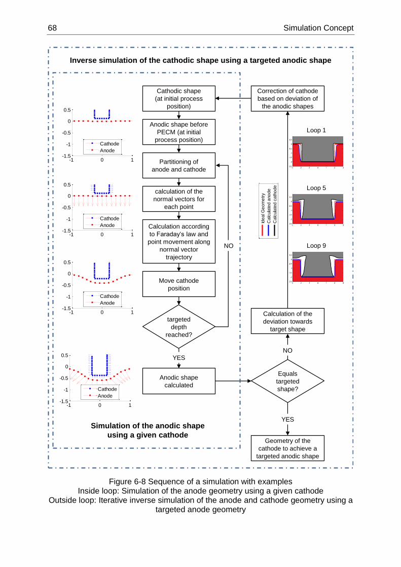
68 Simulation Concept
Figure 6-8 Sequence of a simulation with examples Inside loop: Simulation of the anode geometry using a given cathode
Outside loop: Iterative inverse simulation of the anode and cathode geometry using a targeted anode geometry
Cathodic shape
(at initial process
position)
Anodic shape before
PECM (at initial
process position)
Partitioning of
anode and cathode
calculation of the
normal vectors for
each point
Calculation according
to Faraday‘s law and
point movement along
normal vector
trajectory
Move cathode
position
targeted
depth
reached?
Anodic shape
calculated
Correction of cathode
based on deviation of
the anodic shapes
NO
Equals
targeted
shape?
Geometry of the
cathode to achieve a
targeted anodic shape
Calculation of the
deviation towards
target shape
NO
YES
YES
Simulation of the anodic shape
using a given cathode
Inverse simulation of the cathodic shape using a targeted anodic shape
-1 0 1-1.5
-1
-0.5
0
0.5
Cathode
Anode
-1 0 1-1.5
-1
-0.5
0
0.5
Cathode
Anode
-1 0 1-1.5
-1
-0.5
0
0.5
Cathode
Anode
-1 0 1-1.5
-1
-0.5
0
0.5
Cathode
Anode
-3-2
-10
12
3-2
.5-2
-1.5-1
-0.50
0.51
1.52
Ide
al G
eo
me
try
Ca
lcula
ted
ano
de
Ca
lcula
ted
ca
tho
de
-1 0 1-1.5
-1
-0.5
0
0.5
Cathode
Anode
-1 0 1-1.5
-1
-0.5
0
0.5
Cathode
Anode
-1 0 1-1.5
-1
-0.5
0
0.5
Cathode
Anode
-1 0 1-1.5
-1
-0.5
0
0.5
Cathode
Anode
-1 0 1-1.5
-1
-0.5
0
0.5
Cathode
Anode
-1 0 1-1.5
-1
-0.5
0
0.5
Cathode
Anode
-1 0 1-1.5
-1
-0.5
0
0.5
Cathode
Anode
-1 0 1-1.5
-1
-0.5
0
0.5
Cathode
Anode
-1 0 1-1.5
-1
-0.5
0
0.5
Cathode
Anode
-1 0 1-1.5
-1
-0.5
0
0.5
Cathode
Anode
-1 0 1-1.5
-1
-0.5
0
0.5
Cathode
Anode
-1 0 1-1.5
-1
-0.5
0
0.5
Cathode
Anode
Loop 1
Loop 5
Loop 9
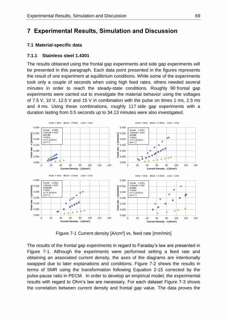
Experimental Results, Simulation and Discussion 69
7 Experimental Results, Simulation and Discussion
7.1 Material-specific data
7.1.1 Stainless steel 1.4301
The results obtained using the frontal gap experiments and side gap experiments will
be presented in this paragraph. Each data point presented in the figures represents
the result of one experiment at equilibrium conditions. While some of the experiments
took only a couple of seconds when using high feed rates, others needed several
minutes in order to reach the steady-state conditions. Roughly 90 frontal gap
experiments were carried out to investigate the material behavior using the voltages
of 7.5 V, 10 V, 12.5 V and 15 V in combination with the pulse on times 1 ms, 2.5 ms
and 4 ms. Using these combinations, roughly 117 side gap experiments with a
duration lasting from 0.5 seconds up to 34.13 minutes were also investigated.
Figure 7-1 Current density [A/cm²] vs. feed rate [mm/min]
The results of the frontal gap experiments in regard to Faraday’s law are presented in
Figure 7-1. Although the experiments were performed setting a feed rate and
obtaining an associated current density, the axes of the diagrams are intentionally
swapped due to later explanations and conditions. Figure 7-2 shows the results in
terms of SMR using the transformation following Equation 2-15 corrected by the
pulse-pause ratio in PECM. In order to develop an empirical model, the experimental
results with regard to Ohm’s law are necessary. For each dataset Figure 7-3 shows
the correlation between current density and frontal gap value. The data proves the
0.000
0.050
0.100
0.150
0.200
0.250
0.300
0 20 40 60 80 100 120 140
Feed
rate
-v
[m
m/m
in]
Current Density - J [A/cm²]
ton = 4ms ton = 2.5ms ton = 1ms
Anode 1.4301Cathode 1.4301U=7.5Vf=50Hzσ=71.3mS/cmpH=7.2
0.000
0.050
0.100
0.150
0.200
0.250
0.300
0 20 40 60 80 100 120 140
Feed
rate
-v
[m
m/m
in]
Current Density - J [A/cm²]
ton = 4ms ton = 2.5ms ton = 1ms
Anode 1.4301Cathode 1.4301U=15Vf=50Hzσ=71.3mS/cmpH=7.2
0.000
0.050
0.100
0.150
0.200
0.250
0.300
0 20 40 60 80 100 120 140
Feed
rate
-v
[m
m/m
in]
Current Density - J [A/cm²]
ton = 4ms ton = 2.5ms ton = 1ms
Anode 1.4301Cathode 1.4301U=10Vf=50Hzσ=71.3mS/cmpH=7.2
0.000
0.050
0.100
0.150
0.200
0.250
0.300
0 20 40 60 80 100 120 140
Feed
rate
-v
[m
m/m
in]
Current Density - J [A/cm²]
ton = 4ms ton = 2.5ms ton = 1ms
Anode 1.4301Cathode 1.4301U=12.5Vf=50Hzσ=71.3mS/cmpH=7.2
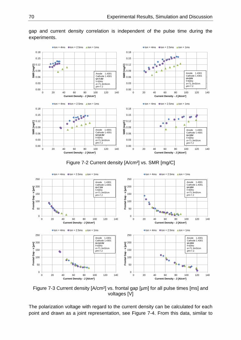
70 Experimental Results, Simulation and Discussion
gap and current density correlation is independent of the pulse time during the
experiments.
Figure 7-2 Current density [A/cm²] vs. SMR [mg/C]
Figure 7-3 Current density [A/cm²] vs. frontal gap [µm] for all pulse times [ms] and voltages [V]
The polarization voltage with regard to the current density can be calculated for each
point and drawn as a joint representation, see Figure 7-4. From this data, similar to
0.00
0.03
0.06
0.09
0.12
0.15
0.18
0 20 40 60 80 100 120 140
SM
R [
mg
/C]
Current Density - J [A/cm²]
ton = 4ms ton = 2.5ms ton = 1ms
Anode 1.4301Cathode 1.4301U=7.5Vf=50Hzσ=71.3mS/cmpH=7.2
0.00
0.03
0.06
0.09
0.12
0.15
0.18
0 20 40 60 80 100 120 140
SM
R [
mg
/C]
Current Density - J [A/cm²]
ton = 4ms ton = 2.5ms ton = 1ms
Anode 1.4301Cathode 1.4301U=12.5Vf=50Hzσ=71.3mS/cmpH=7.2
0.00
0.03
0.06
0.09
0.12
0.15
0.18
0 20 40 60 80 100 120 140
SM
R [
mg
/C]
Current Density - J [A/cm²]
ton = 4ms ton = 2.5ms ton = 1ms
Anode 1.4301Cathode 1.4301U=10Vf=50Hzσ=71.3mS/cmpH=7.2
0.00
0.03
0.06
0.09
0.12
0.15
0.18
0 20 40 60 80 100 120 140
SM
R [
mg
/C]
Current Density - J [A/cm²]
ton = 4ms ton = 2.5ms ton = 1ms
Anode 1.4301Cathode 1.4301U=15Vf=50Hzσ=71.3mS/cmpH=7.2
0
50
100
150
200
250
0 20 40 60 80 100 120 140
Fro
nta
l G
ap
-s [
µm
]
Current Density - J [A/cm²]
ton = 4ms ton = 2.5ms ton = 1ms
Anode 1.4301Cathode 1.4301U=7.5Vf=50Hzσ=71.3mS/cmpH=7.2
0
50
100
150
200
250
0 20 40 60 80 100 120 140
Fro
nta
l G
ap
-s [
µm
]
Current Density - J [A/cm²]
ton = 4ms ton = 2.5ms ton = 1ms
Anode 1.4301Cathode 1.4301U=10Vf=50Hzσ=71.3mS/cmpH=7.2
0
50
100
150
200
250
0 20 40 60 80 100 120 140
Fro
nta
l G
ap
-s [
µm
]
Current Density - J [A/cm²]
ton = 4ms ton = 2.5ms ton = 1ms
Anode 1.4301Cathode 1.4301U=12.5Vf=50Hzσ=71.3mS/cmpH=7.2
0
50
100
150
200
250
0 20 40 60 80 100 120 140
Fro
nta
l G
ap
-s [
µm
]
Current Density - J [A/cm²]
ton = 4ms ton = 2.5ms ton = 1ms
Anode 1.4301Cathode 1.4301U=15Vf=50Hzσ=71.3mS/cmpH=7.2
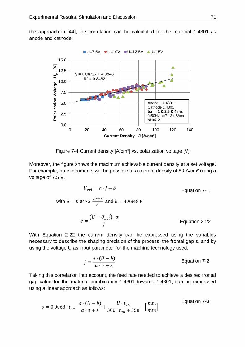
Experimental Results, Simulation and Discussion 71
the approach in [44], the correlation can be calculated for the material 1.4301 as
anode and cathode.
Figure 7-4 Current density [A/cm²] vs. polarization voltage [V]
Moreover, the figure shows the maximum achievable current density at a set voltage.
For example, no experiments will be possible at a current density of 80 A/cm² using a
voltage of 7.5 V.
𝑈𝑝𝑜𝑙 = 𝑎 ∙ 𝐽 + 𝑏
with 𝑎 = 0.0472 𝑉∙𝑐𝑚2
𝐴 and 𝑏 = 4.9848 𝑉
Equation 7-1
𝑠 =(𝑈 − 𝑈𝑝𝑜𝑙) ∙ 𝜎
𝐽
Equation 2-22
With Equation 2-22 the current density can be expressed using the variables
necessary to describe the shaping precision of the process, the frontal gap s, and by
using the voltage U as input parameter for the machine technology used.
𝐽 =𝜎 ∙ (𝑈 − 𝑏)
𝑎 ∙ 𝜎 + 𝑠 Equation 7-2
Taking this correlation into account, the feed rate needed to achieve a desired frontal
gap value for the material combination 1.4301 towards 1.4301, can be expressed
using a linear approach as follows:
𝑣 = 0.0068 ∙ 𝑡𝑜𝑛 ∙𝜎 ∙ (𝑈 − 𝑏)
𝑎 ∙ 𝜎 + 𝑠+
𝑈 ∙ 𝑡𝑜𝑛
300 ∙ 𝑡𝑜𝑛 + 350 [
𝑚𝑚
𝑚𝑖𝑛]
Equation 7-3
y = 0.0472x + 4.9848R² = 0.8482
0.0
2.5
5.0
7.5
10.0
12.5
15.0
0 20 40 60 80 100 120 140
Po
lari
za
tio
n V
olt
ag
e -
Up
ol[V
]
Current Density - J [A/cm²]
U=7.5V U=10V U=12.5V U=15V
Anode 1.4301Cathode 1.4301ton = 1 & 2.5 & 4 msf=50Hz σ=71.3mS/cmpH=7.2
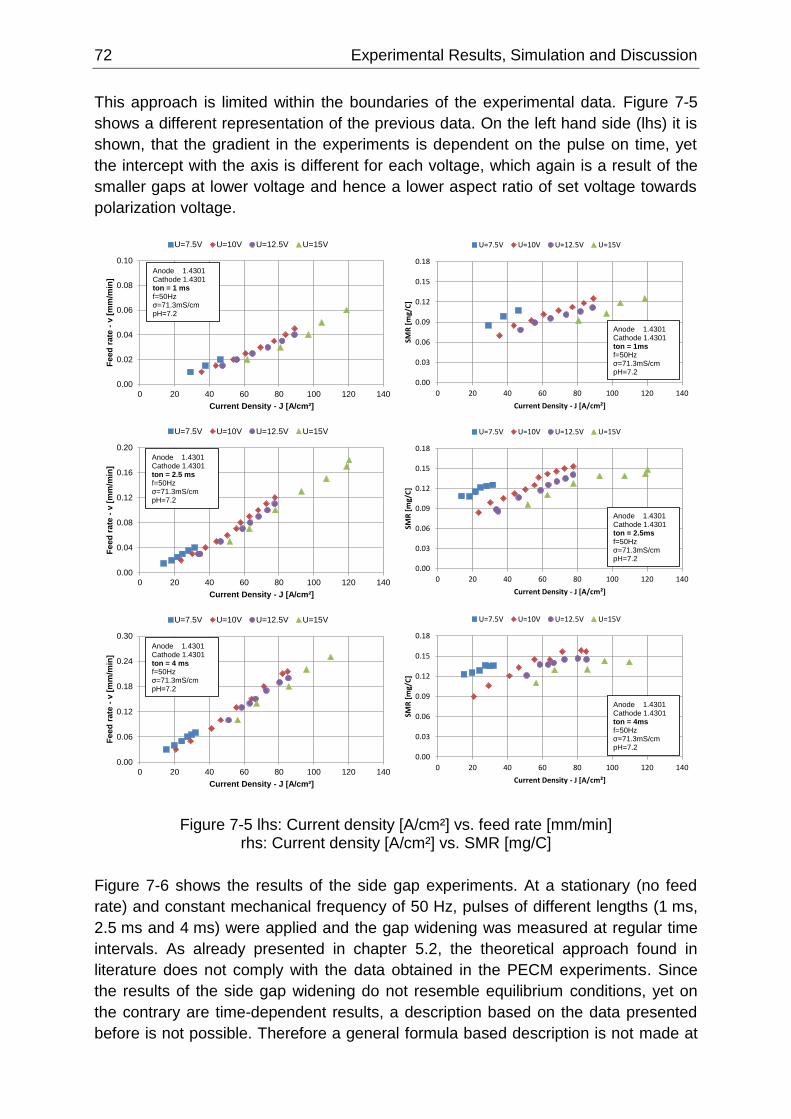
72 Experimental Results, Simulation and Discussion
This approach is limited within the boundaries of the experimental data. Figure 7-5
shows a different representation of the previous data. On the left hand side (lhs) it is
shown, that the gradient in the experiments is dependent on the pulse on time, yet
the intercept with the axis is different for each voltage, which again is a result of the
smaller gaps at lower voltage and hence a lower aspect ratio of set voltage towards
polarization voltage.
Figure 7-5 lhs: Current density [A/cm²] vs. feed rate [mm/min] rhs: Current density [A/cm²] vs. SMR [mg/C]
Figure 7-6 shows the results of the side gap experiments. At a stationary (no feed
rate) and constant mechanical frequency of 50 Hz, pulses of different lengths (1 ms,
2.5 ms and 4 ms) were applied and the gap widening was measured at regular time
intervals. As already presented in chapter 5.2, the theoretical approach found in
literature does not comply with the data obtained in the PECM experiments. Since
the results of the side gap widening do not resemble equilibrium conditions, yet on
the contrary are time-dependent results, a description based on the data presented
before is not possible. Therefore a general formula based description is not made at
0.00
0.02
0.04
0.06
0.08
0.10
0 20 40 60 80 100 120 140
Feed
rate
-v
[m
m/m
in]
Current Density - J [A/cm²]
U=7.5V U=10V U=12.5V U=15V
Anode 1.4301Cathode 1.4301ton = 1 msf=50Hzσ=71.3mS/cmpH=7.2
0.00
0.04
0.08
0.12
0.16
0.20
0 20 40 60 80 100 120 140
Feed
rate
-v
[m
m/m
in]
Current Density - J [A/cm²]
U=7.5V U=10V U=12.5V U=15V
Anode 1.4301Cathode 1.4301ton = 2.5 msf=50Hzσ=71.3mS/cmpH=7.2
0.00
0.06
0.12
0.18
0.24
0.30
0 20 40 60 80 100 120 140
Feed
rate
-v
[m
m/m
in]
Current Density - J [A/cm²]
U=7.5V U=10V U=12.5V U=15V
Anode 1.4301Cathode 1.4301ton = 4 msf=50Hzσ=71.3mS/cmpH=7.2
0.00
0.03
0.06
0.09
0.12
0.15
0.18
0 20 40 60 80 100 120 140
SMR
[m
g/C
]Current Density - J [A/cm²]
U=7.5V U=10V U=12.5V U=15V
Anode 1.4301Cathode 1.4301ton = 1msf=50Hzσ=71.3mS/cmpH=7.2
0.00
0.03
0.06
0.09
0.12
0.15
0.18
0 20 40 60 80 100 120 140
SMR
[m
g/C
]
Current Density - J [A/cm²]
U=7.5V U=10V U=12.5V U=15V
Anode 1.4301Cathode 1.4301ton = 2.5msf=50Hzσ=71.3mS/cmpH=7.2
0.00
0.03
0.06
0.09
0.12
0.15
0.18
0 20 40 60 80 100 120 140
SMR
[m
g/C
]
Current Density - J [A/cm²]
U=7.5V U=10V U=12.5V U=15V
Anode 1.4301Cathode 1.4301ton = 4msf=50Hzσ=71.3mS/cmpH=7.2
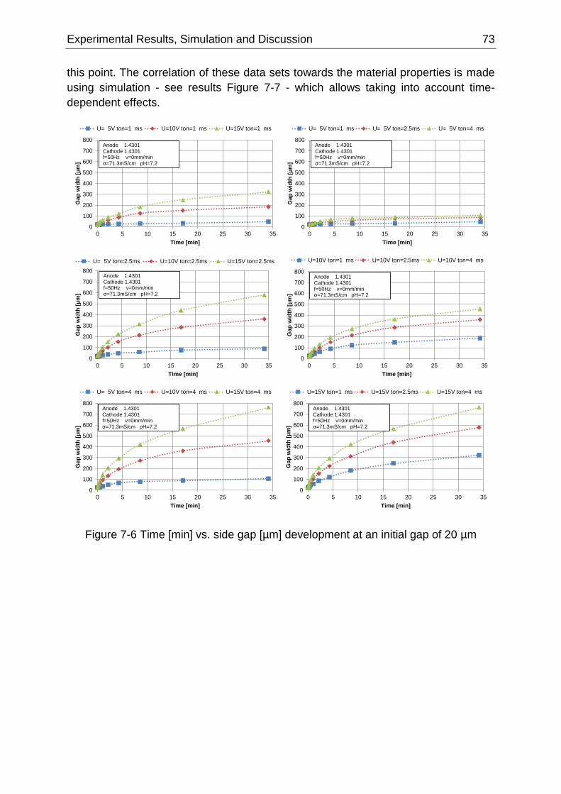
Experimental Results, Simulation and Discussion 73
this point. The correlation of these data sets towards the material properties is made
using simulation - see results Figure 7-7 - which allows taking into account time-
dependent effects.
Figure 7-6 Time [min] vs. side gap [µm] development at an initial gap of 20 µm
0
100
200
300
400
500
600
700
800
0 5 10 15 20 25 30 35
Gap
wid
th [
µm
]
Time [min]
U= 5V ton=1 ms U=10V ton=1 ms U=15V ton=1 ms
Anode 1.4301 Cathode 1.4301f=50Hz v=0mm/minσ=71.3mS/cm pH=7.2
0
100
200
300
400
500
600
700
800
0 5 10 15 20 25 30 35
Gap
wid
th [
µm
]
Time [min]
U= 5V ton=2.5ms U=10V ton=2.5ms U=15V ton=2.5ms
Anode 1.4301 Cathode 1.4301f=50Hz v=0mm/minσ=71.3mS/cm pH=7.2
0
100
200
300
400
500
600
700
800
0 5 10 15 20 25 30 35
Gap
wid
th [
µm
]
Time [min]
U= 5V ton=4 ms U=10V ton=4 ms U=15V ton=4 ms
Anode 1.4301 Cathode 1.4301f=50Hz v=0mm/minσ=71.3mS/cm pH=7.2
0
100
200
300
400
500
600
700
800
0 5 10 15 20 25 30 35
Gap
wid
th [
µm
]
Time [min]
U= 5V ton=1 ms U= 5V ton=2.5ms U= 5V ton=4 ms
Anode 1.4301 Cathode 1.4301f=50Hz v=0mm/minσ=71.3mS/cm pH=7.2
0
100
200
300
400
500
600
700
800
0 5 10 15 20 25 30 35
Gap
wid
th [
µm
]
Time [min]
U=10V ton=1 ms U=10V ton=2.5ms U=10V ton=4 ms
Anode 1.4301 Cathode 1.4301f=50Hz v=0mm/minσ=71.3mS/cm pH=7.2
0
100
200
300
400
500
600
700
800
0 5 10 15 20 25 30 35
Gap
wid
th [
µm
]
Time [min]
U=15V ton=1 ms U=15V ton=2.5ms U=15V ton=4 ms
Anode 1.4301 Cathode 1.4301f=50Hz v=0mm/minσ=71.3mS/cm pH=7.2
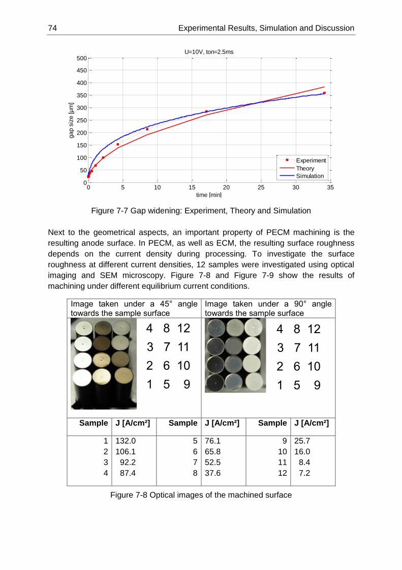
74 Experimental Results, Simulation and Discussion
Figure 7-7 Gap widening: Experiment, Theory and Simulation
Next to the geometrical aspects, an important property of PECM machining is the
resulting anode surface. In PECM, as well as ECM, the resulting surface roughness
depends on the current density during processing. To investigate the surface
roughness at different current densities, 12 samples were investigated using optical
imaging and SEM microscopy. Figure 7-8 and Figure 7-9 show the results of
machining under different equilibrium current conditions.
Image taken under a 45° angle towards the sample surface
Image taken under a 90° angle towards the sample surface
Sample J [A/cm²] Sample J [A/cm²] Sample J [A/cm²]
1
2
3
4
132.0
106.1
92.2
87.4
5
6
7
8
76.1
65.8
52.5
37.6
9
10
11
12
25.7
16.0
8.4
7.2
Figure 7-8 Optical images of the machined surface
0 5 10 15 20 25 30 350
50
100
150
200
250
300
350
400
450
500U=10V, ton=2.5ms
time [min]
ga
p s
ize
[µ
m]
Experiment
Theory
Simulation
4 8 12
3 7 11
2 6 10
1 5 9
4 8 12
3 7 11
2 6 10
1 5 9
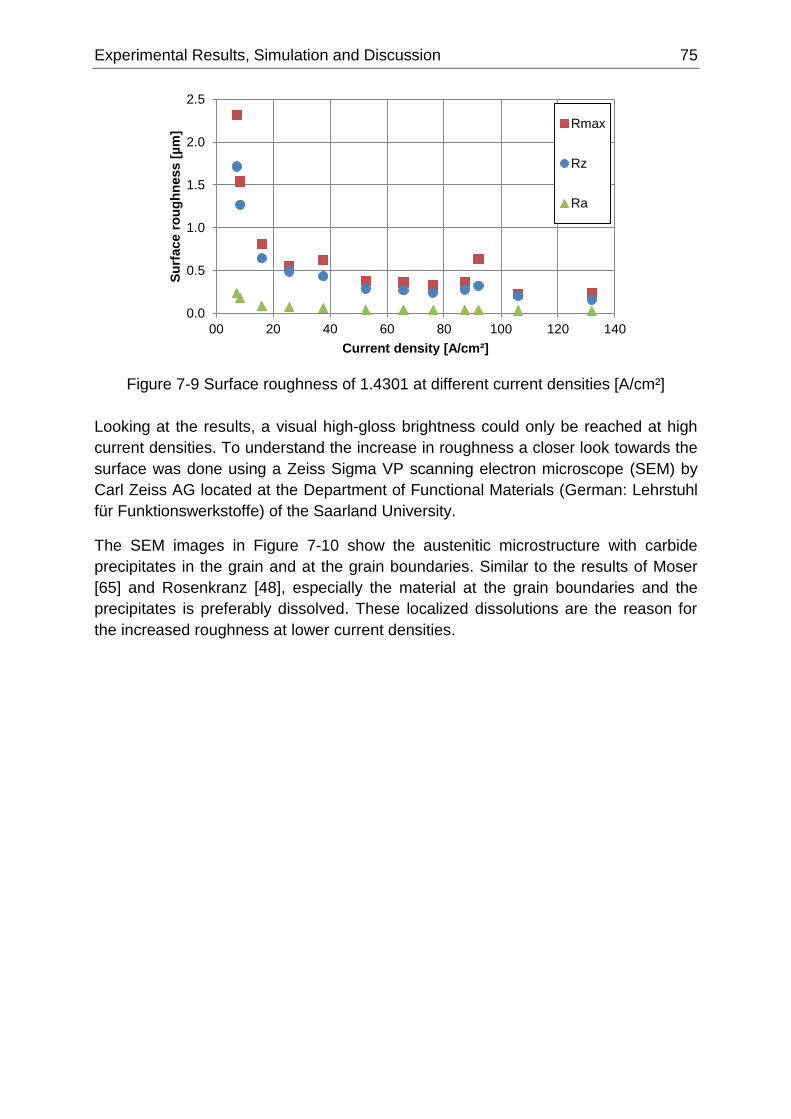
Experimental Results, Simulation and Discussion 75
Figure 7-9 Surface roughness of 1.4301 at different current densities [A/cm²]
Looking at the results, a visual high-gloss brightness could only be reached at high
current densities. To understand the increase in roughness a closer look towards the
surface was done using a Zeiss Sigma VP scanning electron microscope (SEM) by
Carl Zeiss AG located at the Department of Functional Materials (German: Lehrstuhl
für Funktionswerkstoffe) of the Saarland University.
The SEM images in Figure 7-10 show the austenitic microstructure with carbide
precipitates in the grain and at the grain boundaries. Similar to the results of Moser
[65] and Rosenkranz [48], especially the material at the grain boundaries and the
precipitates is preferably dissolved. These localized dissolutions are the reason for
the increased roughness at lower current densities.
0.0
0.5
1.0
1.5
2.0
2.5
00 20 40 60 80 100 120 140
Su
rfa
ce
ro
ug
hn
ess
[µ
m]
Current density [A/cm²]
1.4301
Rmax
Rz
Ra
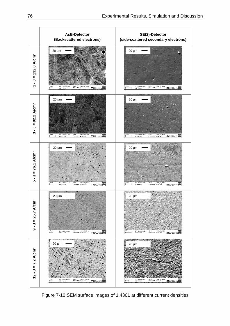
76 Experimental Results, Simulation and Discussion
Figure 7-10 SEM surface images of 1.4301 at different current densities
AsB-Detector
(Backscattered electrons)
SE(2)-Detector
(side-scattered secondary electrons)
1 -
J =
13
2.0
A/c
m²
3 -
J =
92
.2 A
/cm
²
5 -
J =
76
.1 A
/cm
²
9 -
J =
25
.7 A
/cm
²
12 -
J =
7.2
A/c
m²
20 µm 20 µm
20 µm 20 µm
20 µm 20 µm
20 µm 20 µm
20 µm 20 µm
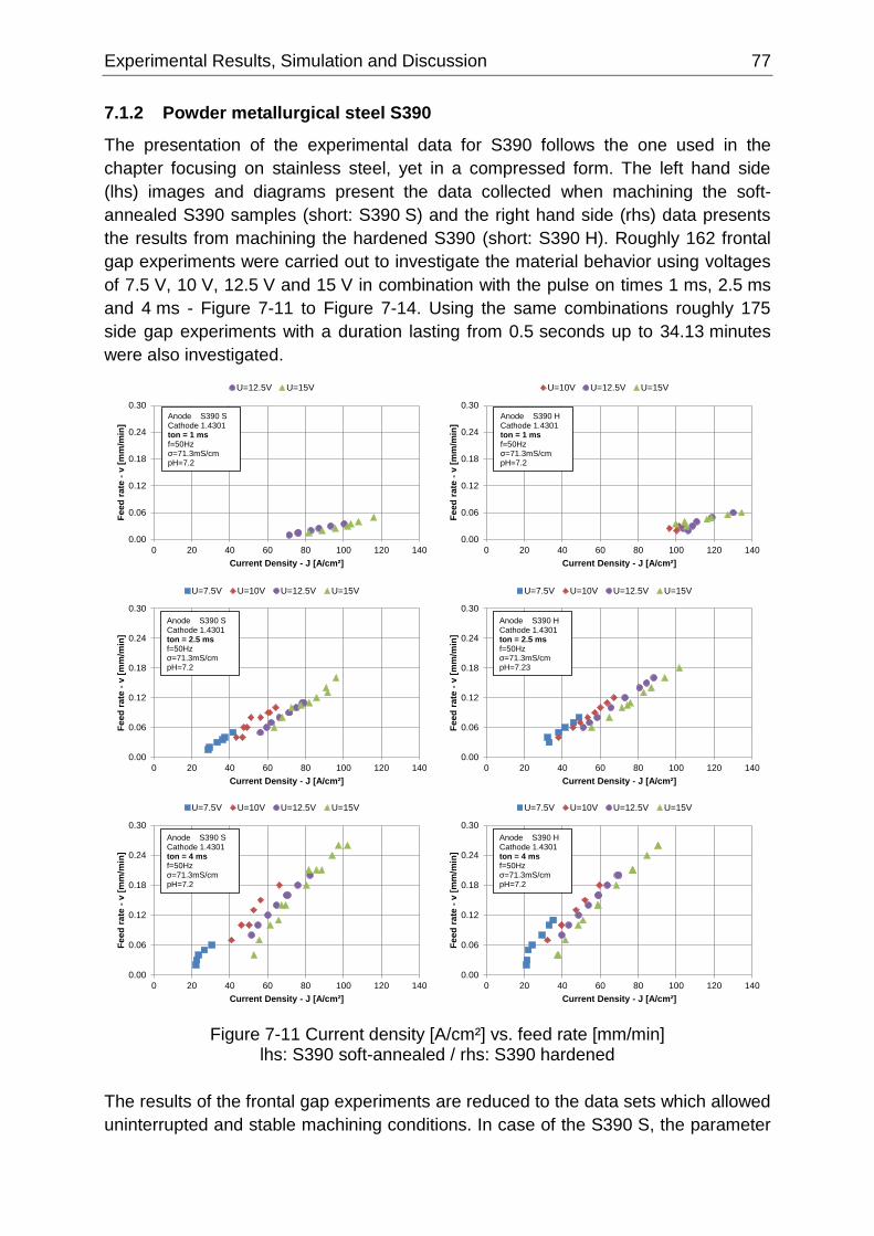
Experimental Results, Simulation and Discussion 77
7.1.2 Powder metallurgical steel S390
The presentation of the experimental data for S390 follows the one used in the
chapter focusing on stainless steel, yet in a compressed form. The left hand side
(lhs) images and diagrams present the data collected when machining the soft-
annealed S390 samples (short: S390 S) and the right hand side (rhs) data presents
the results from machining the hardened S390 (short: S390 H). Roughly 162 frontal
gap experiments were carried out to investigate the material behavior using voltages
of 7.5 V, 10 V, 12.5 V and 15 V in combination with the pulse on times 1 ms, 2.5 ms
and 4 ms - Figure 7-11 to Figure 7-14. Using the same combinations roughly 175
side gap experiments with a duration lasting from 0.5 seconds up to 34.13 minutes
were also investigated.
Figure 7-11 Current density [A/cm²] vs. feed rate [mm/min] lhs: S390 soft-annealed / rhs: S390 hardened
The results of the frontal gap experiments are reduced to the data sets which allowed
uninterrupted and stable machining conditions. In case of the S390 S, the parameter
0.00
0.06
0.12
0.18
0.24
0.30
0 20 40 60 80 100 120 140
Feed
rate
-v
[m
m/m
in]
Current Density - J [A/cm²]
U=12.5V U=15V
Anode S390 SCathode 1.4301ton = 1 msf=50Hzσ=71.3mS/cmpH=7.2
0.00
0.06
0.12
0.18
0.24
0.30
0 20 40 60 80 100 120 140
Feed
rate
-v
[m
m/m
in]
Current Density - J [A/cm²]
U=7.5V U=10V U=12.5V U=15V
Anode S390 SCathode 1.4301ton = 2.5 msf=50Hzσ=71.3mS/cmpH=7.2
0.00
0.06
0.12
0.18
0.24
0.30
0 20 40 60 80 100 120 140
Feed
rate
-v
[m
m/m
in]
Current Density - J [A/cm²]
U=7.5V U=10V U=12.5V U=15V
Anode S390 SCathode 1.4301ton = 4 msf=50Hzσ=71.3mS/cmpH=7.2
0.00
0.06
0.12
0.18
0.24
0.30
0 20 40 60 80 100 120 140
Feed
rate
-v
[m
m/m
in]
Current Density - J [A/cm²]
U=10V U=12.5V U=15V
Anode S390 H Cathode 1.4301ton = 1 msf=50Hzσ=71.3mS/cmpH=7.2
0.00
0.06
0.12
0.18
0.24
0.30
0 20 40 60 80 100 120 140
Feed
rate
-v
[m
m/m
in]
Current Density - J [A/cm²]
U=7.5V U=10V U=12.5V U=15V
Anode S390 H Cathode 1.4301ton = 2.5 msf=50Hzσ=71.3mS/cmpH=7.23
0.00
0.06
0.12
0.18
0.24
0.30
0 20 40 60 80 100 120 140
Feed
rate
-v
[m
m/m
in]
Current Density - J [A/cm²]
U=7.5V U=10V U=12.5V U=15V
Anode S390 H Cathode 1.4301ton = 4 msf=50Hzσ=71.3mS/cmpH=7.2
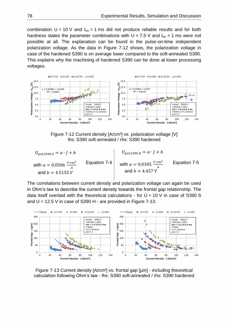
78 Experimental Results, Simulation and Discussion
combination U = 10 V and ton = 1 ms did not produce reliable results and for both
hardness states the parameter combinations with U = 7.5 V and ton = 1 ms were not
possible at all. The explanation can be found in the pulse-on-time independent
polarization voltage. As the data in Figure 7-12 shows, the polarization voltage in
case of the hardened S390 is on average lower compared to the soft-annealed S390.
This explains why the machining of hardened S390 can be done at lower processing
voltages.
Figure 7-12 Current density [A/cm²] vs. polarization voltage [V] lhs: S390 soft-annealed / rhs: S390 hardened
𝑈𝑝𝑜𝑙,𝑆390 𝑆 = 𝑎 ∙ 𝐽 + 𝑏
with 𝑎 = 0.0506 𝑉∙𝑐𝑚2
𝐴
and 𝑏 = 4.5155 𝑉
Equation 7-4
𝑈𝑝𝑜𝑙,𝑆390 𝐻 = 𝑎 ∙ 𝐽 + 𝑏
with 𝑎 = 0.0345 𝑉∙𝑐𝑚2
𝐴
and 𝑏 = 4.457 V
Equation 7-5
The correlations between current density and polarization voltage can again be used
in Ohm’s law to describe the current density towards the frontal gap relationship. The
data itself overlaid with the theoretical calculations - for U = 10 V in case of S390 S
and U = 12.5 V in case of S390 H - are provided in Figure 7-13.
Figure 7-13 Current density [A/cm²] vs. frontal gap [µm] - including theoretical calculation following Ohm’s law - lhs: S390 soft-annealed / rhs: S390 hardened
y = 0.0506x + 4.5155R² = 0.6562
0.0
2.5
5.0
7.5
10.0
12.5
15.0
0 20 40 60 80 100 120 140
Po
lari
zati
on
Vo
ltag
e -
Up
ol[V
]
Current Density - J [A/cm²]
U=7.5V U=10V U=12.5V U=15V
Anode S390 SCathode 1.4301ton = 1 & 2.5 & 4 msf=50Hz σ=71.3mS/cmpH=7.2
y = 0.0345x + 4.457R² = 0.6279
0.0
2.5
5.0
7.5
10.0
12.5
15.0
0 20 40 60 80 100 120 140P
ola
rizati
on
Vo
ltag
e -
Up
ol[V
]
Current Density - J [A/cm²]
U=7.5V U=10V U=12.5V U=15V
Anode S390 HCathode 1.4301ton = 1 & 2.5 & 4 msf=50Hz σ=71.3mS/cmpH=7.2
0
50
100
150
200
250
0 20 40 60 80 100 120 140
Fro
nta
l G
ap
-s
[µ
m]
Current Density - J [A/cm²]
Theory U=7.5V U=10V U=12.5V U=15V
Anode S390 SCathode 1.4301ton = 1 & 2.5 & 4 msf=50Hzσ=71.3mS/cmpH=7.2
0
50
100
150
200
250
0 20 40 60 80 100 120 140
Fro
nta
l G
ap
-s
[µ
m]
Current Density - J [A/cm²]
Theory U=7.5V U=10V U=12.5V U=15V
Anode S390 HCathode 1.4301ton = 1 & 2.5 & 4 msf=50Hzσ=71.3mS/cmpH=7.2
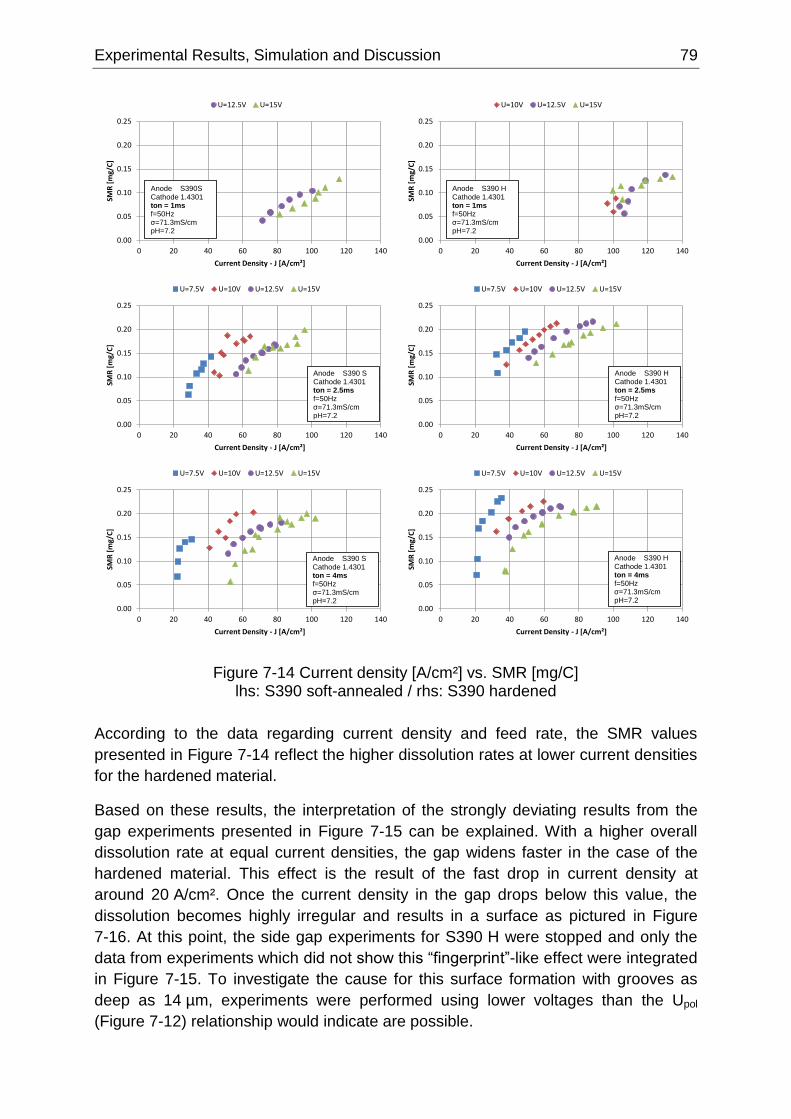
Experimental Results, Simulation and Discussion 79
Figure 7-14 Current density [A/cm²] vs. SMR [mg/C] lhs: S390 soft-annealed / rhs: S390 hardened
According to the data regarding current density and feed rate, the SMR values
presented in Figure 7-14 reflect the higher dissolution rates at lower current densities
for the hardened material.
Based on these results, the interpretation of the strongly deviating results from the
gap experiments presented in Figure 7-15 can be explained. With a higher overall
dissolution rate at equal current densities, the gap widens faster in the case of the
hardened material. This effect is the result of the fast drop in current density at
around 20 A/cm². Once the current density in the gap drops below this value, the
dissolution becomes highly irregular and results in a surface as pictured in Figure
7-16. At this point, the side gap experiments for S390 H were stopped and only the
data from experiments which did not show this “fingerprint”-like effect were integrated
in Figure 7-15. To investigate the cause for this surface formation with grooves as
deep as 14 µm, experiments were performed using lower voltages than the Upol
(Figure 7-12) relationship would indicate are possible.
0.00
0.05
0.10
0.15
0.20
0.25
0 20 40 60 80 100 120 140
SMR
[m
g/C
]
Current Density - J [A/cm²]
U=7.5V U=10V U=12.5V U=15V
Anode S390 SCathode 1.4301ton = 2.5msf=50Hzσ=71.3mS/cmpH=7.2
0.00
0.05
0.10
0.15
0.20
0.25
0 20 40 60 80 100 120 140
SMR
[m
g/C
]
Current Density - J [A/cm²]
U=12.5V U=15V
Anode S390S Cathode 1.4301ton = 1msf=50Hzσ=71.3mS/cmpH=7.2
0.00
0.05
0.10
0.15
0.20
0.25
0 20 40 60 80 100 120 140
SMR
[m
g/C
]
Current Density - J [A/cm²]
U=10V U=12.5V U=15V
Anode S390 HCathode 1.4301ton = 1msf=50Hzσ=71.3mS/cmpH=7.2
0.00
0.05
0.10
0.15
0.20
0.25
0 20 40 60 80 100 120 140
SMR
[m
g/C
]
Current Density - J [A/cm²]
U=7.5V U=10V U=12.5V U=15V
Anode S390 HCathode 1.4301ton = 2.5msf=50Hzσ=71.3mS/cmpH=7.2
0.00
0.05
0.10
0.15
0.20
0.25
0 20 40 60 80 100 120 140
SMR
[m
g/C
]
Current Density - J [A/cm²]
U=7.5V U=10V U=12.5V U=15V
Anode S390 SCathode 1.4301ton = 4msf=50Hzσ=71.3mS/cmpH=7.2
0.00
0.05
0.10
0.15
0.20
0.25
0 20 40 60 80 100 120 140
SMR
[m
g/C
]
Current Density - J [A/cm²]
U=7.5V U=10V U=12.5V U=15V
Anode S390 HCathode 1.4301ton = 4msf=50Hzσ=71.3mS/cmpH=7.2
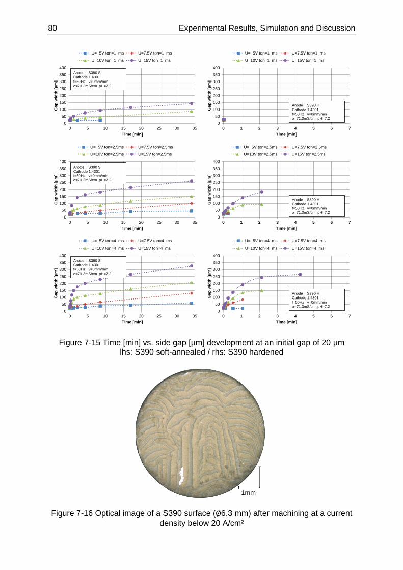
80 Experimental Results, Simulation and Discussion
Figure 7-15 Time [min] vs. side gap [µm] development at an initial gap of 20 µm lhs: S390 soft-annealed / rhs: S390 hardened
Figure 7-16 Optical image of a S390 surface (Ø6.3 mm) after machining at a current
density below 20 A/cm²
0
50
100
150
200
250
300
350
400
0 5 10 15 20 25 30 35
Gap
wid
th [
µm
]
Time [min]
U= 5V ton=1 ms U=7.5V ton=1 ms
U=10V ton=1 ms U=15V ton=1 ms
Anode S390 SCathode 1.4301f=50Hz v=0mm/minσ=71.3mS/cm pH=7.2
0
50
100
150
200
250
300
350
400
0 5 10 15 20 25 30 35
Gap
wid
th [
µm
]
Time [min]
U= 5V ton=2.5ms U=7.5V ton=2.5ms
U=10V ton=2.5ms U=15V ton=2.5ms
Anode S390 SCathode 1.4301f=50Hz v=0mm/minσ=71.3mS/cm pH=7.2
0
50
100
150
200
250
300
350
400
0 5 10 15 20 25 30 35
Gap
wid
th [
µm
]
Time [min]
U= 5V ton=4 ms U=7.5V ton=4 ms
U=10V ton=4 ms U=15V ton=4 ms
Anode S390 SCathode 1.4301f=50Hz v=0mm/minσ=71.3mS/cm pH=7.2
0
50
100
150
200
250
300
350
400
0 1 2 3 4 5 6 7
Gap
wid
th [
µm
]
Time [min]
U= 5V ton=1 ms U=7.5V ton=1 ms
U=10V ton=1 ms U=15V ton=1 ms
Anode S390 HCathode 1.4301f=50Hz v=0mm/minσ=71.3mS/cm pH=7.2
0
50
100
150
200
250
300
350
400
0 1 2 3 4 5 6 7
Gap
wid
th [
µm
]
Time [min]
U= 5V ton=2.5ms U=7.5V ton=2.5ms
U=10V ton=2.5ms U=15V ton=2.5ms
Anode S390 HCathode 1.4301f=50Hz v=0mm/minσ=71.3mS/cm pH=7.2
0
50
100
150
200
250
300
350
400
0 1 2 3 4 5 6 7
Gap
wid
th [
µm
]
Time [min]
U= 5V ton=4 ms U=7.5V ton=4 ms
U=10V ton=4 ms U=15V ton=4 ms
Anode S390 HCathode 1.4301f=50Hz v=0mm/minσ=71.3mS/cm pH=7.2
1mm
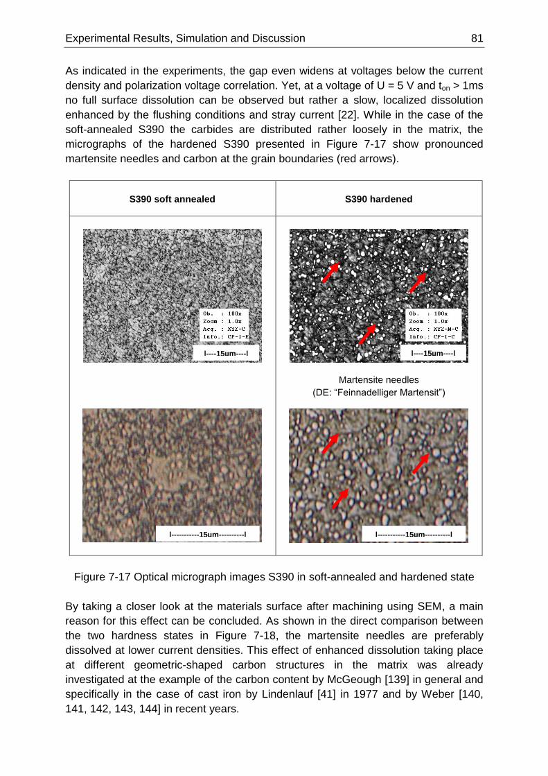
Experimental Results, Simulation and Discussion 81
As indicated in the experiments, the gap even widens at voltages below the current
density and polarization voltage correlation. Yet, at a voltage of U = 5 V and ton > 1ms
no full surface dissolution can be observed but rather a slow, localized dissolution
enhanced by the flushing conditions and stray current [22]. While in the case of the
soft-annealed S390 the carbides are distributed rather loosely in the matrix, the
micrographs of the hardened S390 presented in Figure 7-17 show pronounced
martensite needles and carbon at the grain boundaries (red arrows).
Figure 7-17 Optical micrograph images S390 in soft-annealed and hardened state
By taking a closer look at the materials surface after machining using SEM, a main
reason for this effect can be concluded. As shown in the direct comparison between
the two hardness states in Figure 7-18, the martensite needles are preferably
dissolved at lower current densities. This effect of enhanced dissolution taking place
at different geometric-shaped carbon structures in the matrix was already
investigated at the example of the carbon content by McGeough [139] in general and
specifically in the case of cast iron by Lindenlauf [41] in 1977 and by Weber [140,
141, 142, 143, 144] in recent years.
S390 soft annealed
S390 hardened
Martensite needles
(DE: “Feinnadelliger Martensit”)
|----15µm----| |----15µm----|
|-----------15µm----------| |-----------15µm----------|
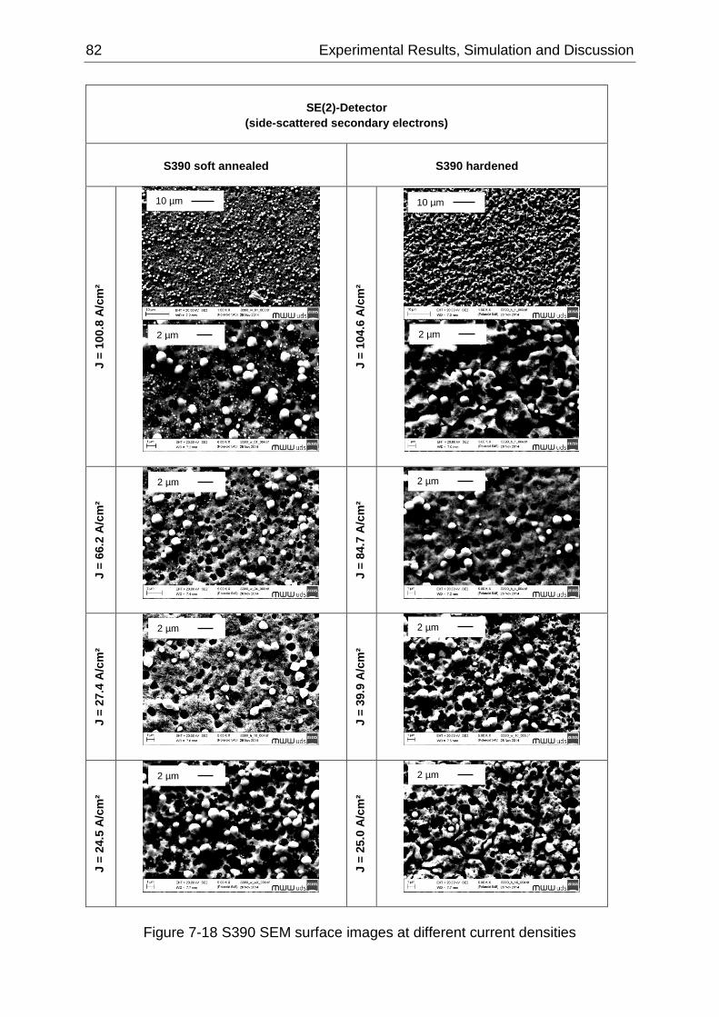
82 Experimental Results, Simulation and Discussion
Figure 7-18 S390 SEM surface images at different current densities
SE(2)-Detector
(side-scattered secondary electrons)
S390 soft annealed
S390 hardened
J =
100
.8 A
/cm
²
J =
104
.6 A
/cm
²
J =
66.2
A/c
m²
J =
84.7
A/c
m²
J =
27.4
A/c
m²
J =
39.9
A/c
m²
J =
24.5
A/c
m²
J =
25.0
A/c
m²
10 µm 10 µm
2 µm 2 µm
2 µm 2 µm
2 µm 2 µm
2 µm 2 µm
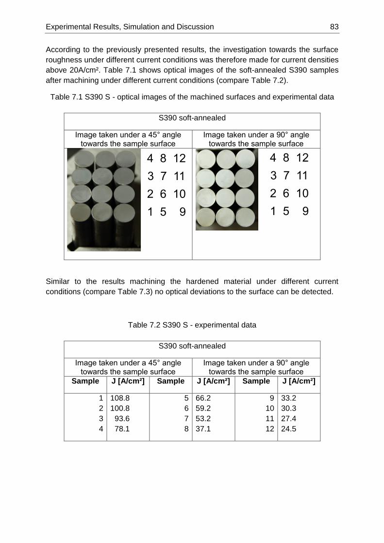
Experimental Results, Simulation and Discussion 83
According to the previously presented results, the investigation towards the surface
roughness under different current conditions was therefore made for current densities
above 20A/cm². Table 7.1 shows optical images of the soft-annealed S390 samples
after machining under different current conditions (compare Table 7.2).
Table 7.1 S390 S - optical images of the machined surfaces and experimental data
S390 soft-annealed
Image taken under a 45° angle towards the sample surface
Image taken under a 90° angle towards the sample surface
Similar to the results machining the hardened material under different current
conditions (compare Table 7.3) no optical deviations to the surface can be detected.
Table 7.2 S390 S - experimental data
S390 soft-annealed
Image taken under a 45° angle towards the sample surface
Image taken under a 90° angle towards the sample surface
Sample J [A/cm²] Sample J [A/cm²] Sample J [A/cm²]
1
2
3
4
108.8
100.8
93.6
78.1
5
6
7
8
66.2
59.2
53.2
37.1
9
10
11
12
33.2
30.3
27.4
24.5
4 8 12
3 7 11
2 6 10
1 5 9
4 8 12
3 7 11
2 6 10
1 5 9
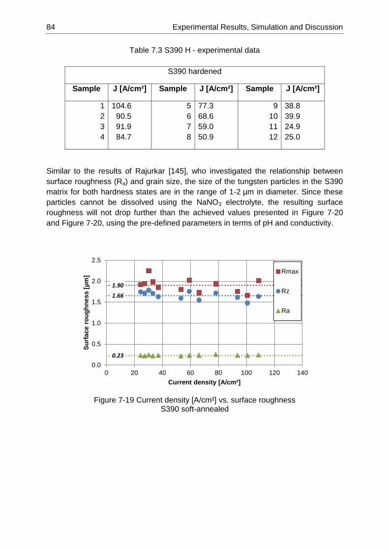
84 Experimental Results, Simulation and Discussion
Table 7.3 S390 H - experimental data
S390 hardened
Sample J [A/cm²] Sample J [A/cm²] Sample J [A/cm²]
1
2
3
4
104.6
90.5
91.9
84.7
5
6
7
8
77.3
68.6
59.0
50.9
9
10
11
12
38.8
39.9
24.9
25.0
Similar to the results of Rajurkar [145], who investigated the relationship between
surface roughness (Ra) and grain size, the size of the tungsten particles in the S390
matrix for both hardness states are in the range of 1-2 µm in diameter. Since these
particles cannot be dissolved using the NaNO3 electrolyte, the resulting surface
roughness will not drop further than the achieved values presented in Figure 7-20
and Figure 7-20, using the pre-defined parameters in terms of pH and conductivity.
Figure 7-19 Current density [A/cm²] vs. surface roughness S390 soft-annealed
0.23
1.66
1.90
0.0
0.5
1.0
1.5
2.0
2.5
0 20 40 60 80 100 120 140
Su
rfa
ce
ro
ug
hn
ess
[µ
m]
Current density [A/cm²]
S390 soft
Rmax
Rz
Ra
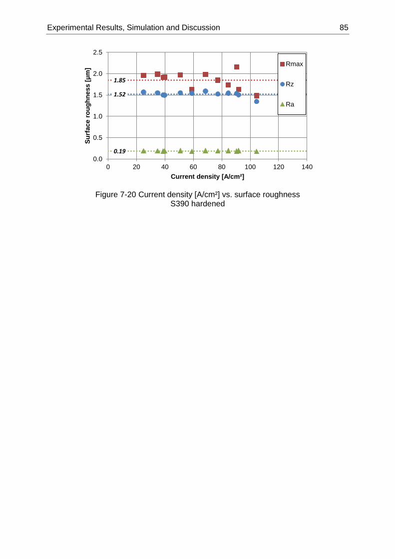
Experimental Results, Simulation and Discussion 85
Figure 7-20 Current density [A/cm²] vs. surface roughness S390 hardened
0.19
1.52
1.85
0.0
0.5
1.0
1.5
2.0
2.5
0 20 40 60 80 100 120 140
Su
rfa
ce
ro
ug
hn
ess
[µ
m]
Current density [A/cm²]
S390 hard
Rmax
Rz
Ra
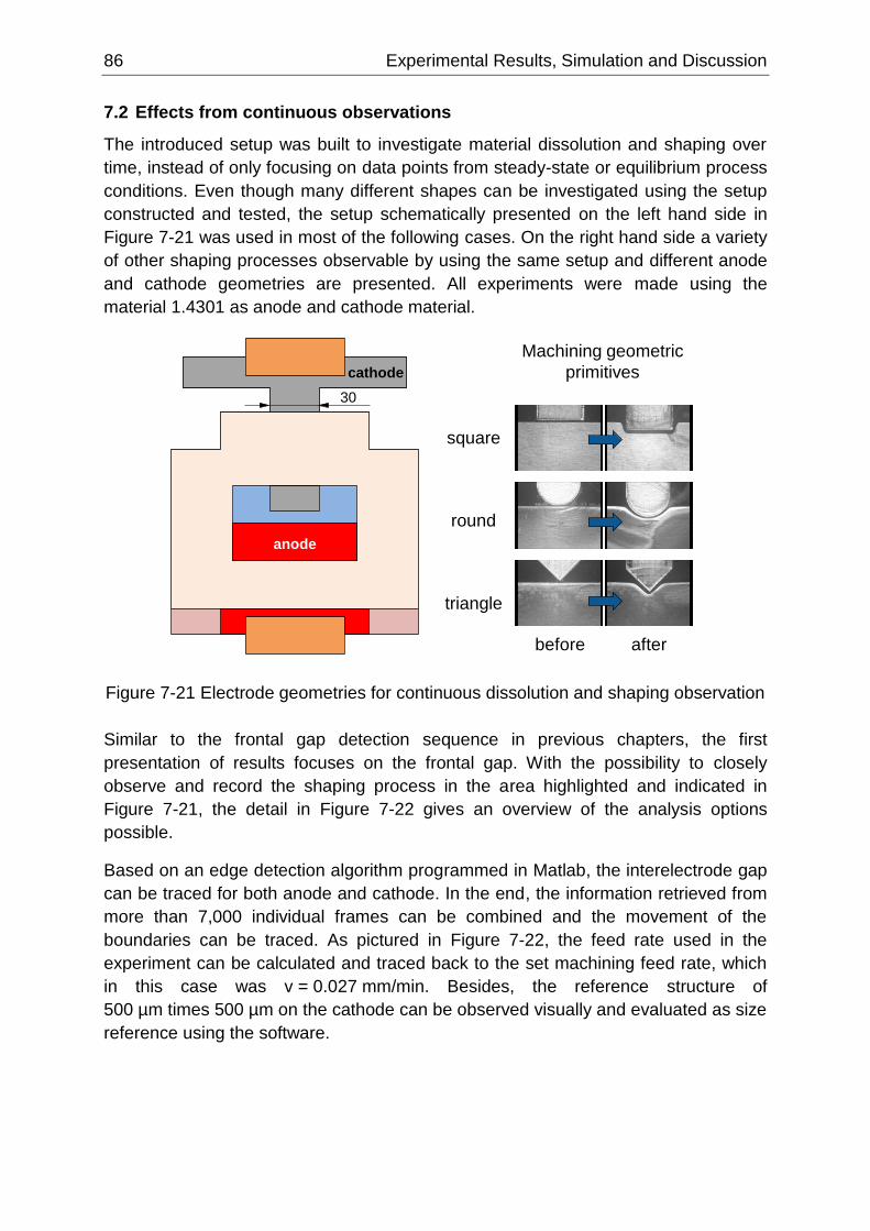
86 Experimental Results, Simulation and Discussion
7.2 Effects from continuous observations
The introduced setup was built to investigate material dissolution and shaping over
time, instead of only focusing on data points from steady-state or equilibrium process
conditions. Even though many different shapes can be investigated using the setup
constructed and tested, the setup schematically presented on the left hand side in
Figure 7-21 was used in most of the following cases. On the right hand side a variety
of other shaping processes observable by using the same setup and different anode
and cathode geometries are presented. All experiments were made using the
material 1.4301 as anode and cathode material.
Figure 7-21 Electrode geometries for continuous dissolution and shaping observation
Similar to the frontal gap detection sequence in previous chapters, the first
presentation of results focuses on the frontal gap. With the possibility to closely
observe and record the shaping process in the area highlighted and indicated in
Figure 7-21, the detail in Figure 7-22 gives an overview of the analysis options
possible.
Based on an edge detection algorithm programmed in Matlab, the interelectrode gap
can be traced for both anode and cathode. In the end, the information retrieved from
more than 7,000 individual frames can be combined and the movement of the
boundaries can be traced. As pictured in Figure 7-22, the feed rate used in the
experiment can be calculated and traced back to the set machining feed rate, which
in this case was v = 0.027 mm/min. Besides, the reference structure of
500 µm times 500 µm on the cathode can be observed visually and evaluated as size
reference using the software.
square
round
triangle
before after
Machining geometric
primitivescathode
anode
30
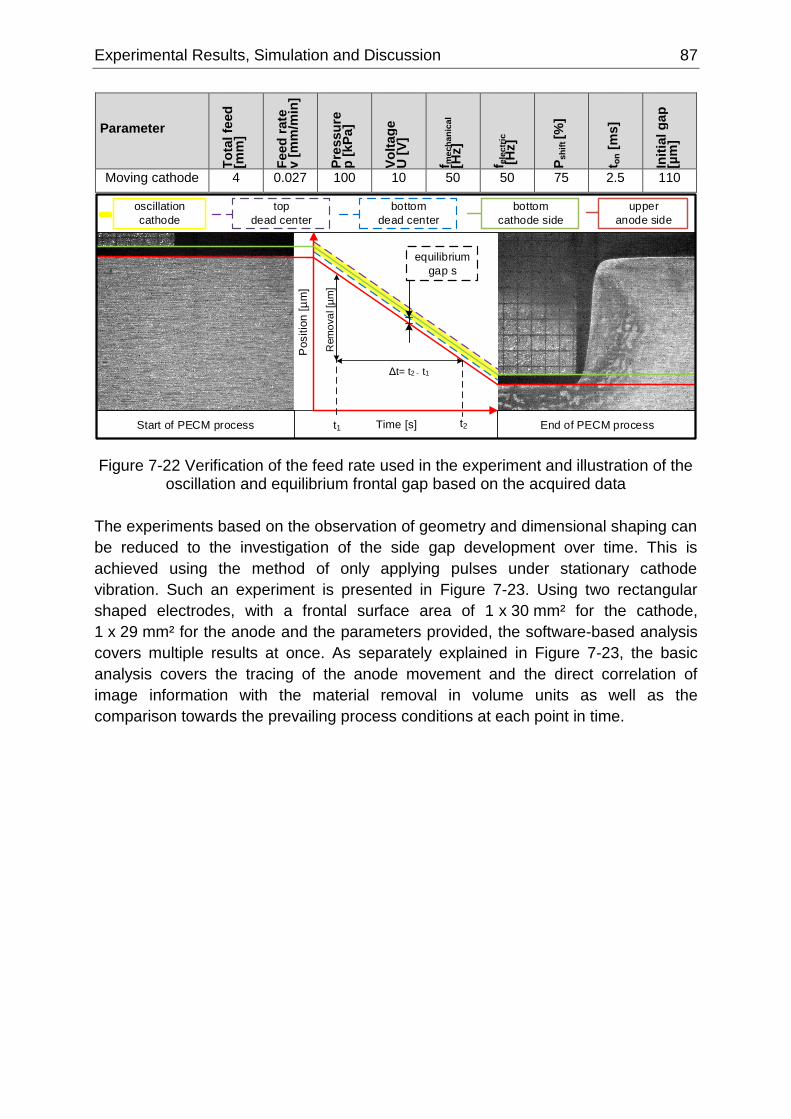
Experimental Results, Simulation and Discussion 87
Parameter
To
tal fe
ed
[m
m]
Feed
rate
v [
mm
/min
]
Pre
ssu
re
p [
kP
a]
Vo
ltag
e
U [
V]
f mech
an
ical
[Hz]
f ele
ctr
ic
[H
z]
Psh
ift [%
]
t on [
ms]
Init
ial g
ap
[µ
m]
Moving cathode 4 0.027 100 10 50 50 75 2.5 110
Figure 7-22 Verification of the feed rate used in the experiment and illustration of the oscillation and equilibrium frontal gap based on the acquired data
The experiments based on the observation of geometry and dimensional shaping can
be reduced to the investigation of the side gap development over time. This is
achieved using the method of only applying pulses under stationary cathode
vibration. Such an experiment is presented in Figure 7-23. Using two rectangular
shaped electrodes, with a frontal surface area of 1 x 30 mm² for the cathode,
1 x 29 mm² for the anode and the parameters provided, the software-based analysis
covers multiple results at once. As separately explained in Figure 7-23, the basic
analysis covers the tracing of the anode movement and the direct correlation of
image information with the material removal in volume units as well as the
comparison towards the prevailing process conditions at each point in time.
End of PECM processStart of PECM process
Positio
n [
µm
]
Time [s]
oscillation
cathode
top
dead center
bottom
dead center
bottom
cathode side
upper
anode side
equilibrium
gap s
Rem
ova
l [µ
m]
Δt= t2 - t1
t2 t1
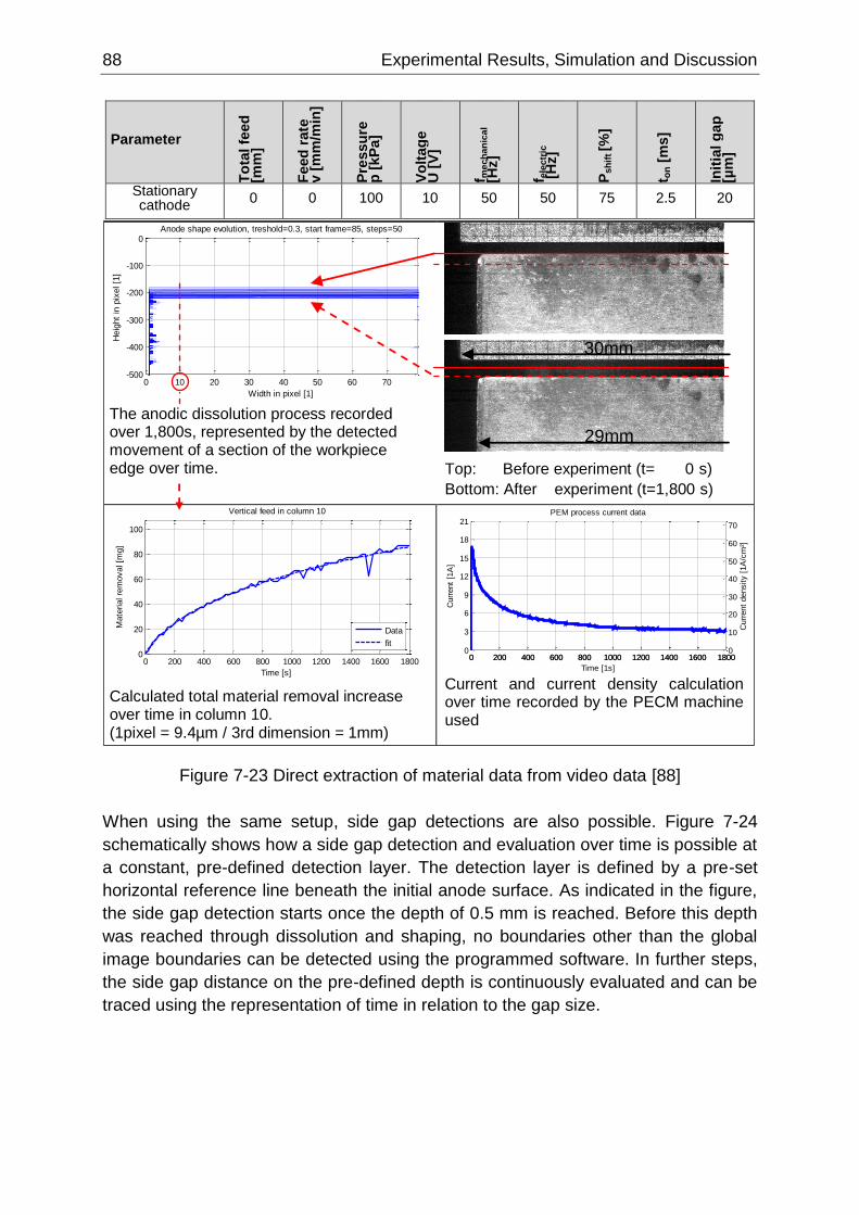
88 Experimental Results, Simulation and Discussion
Parameter
To
tal fe
ed
[m
m]
Feed
rate
v [
mm
/min
]
Pre
ssu
re
p [
kP
a]
Vo
ltag
e
U [
V]
f mech
an
ical
[Hz]
f ele
ctr
ic
[H
z]
Psh
ift [%
]
t on [
ms]
Init
ial g
ap
[µ
m]
Stationary cathode
0 0 100 10 50 50 75 2.5 20
Figure 7-23 Direct extraction of material data from video data [88]
When using the same setup, side gap detections are also possible. Figure 7-24
schematically shows how a side gap detection and evaluation over time is possible at
a constant, pre-defined detection layer. The detection layer is defined by a pre-set
horizontal reference line beneath the initial anode surface. As indicated in the figure,
the side gap detection starts once the depth of 0.5 mm is reached. Before this depth
was reached through dissolution and shaping, no boundaries other than the global
image boundaries can be detected using the programmed software. In further steps,
the side gap distance on the pre-defined depth is continuously evaluated and can be
traced using the representation of time in relation to the gap size.
0 10 20 30 40 50 60 70-500
-400
-300
-200
-100
0Anode shape evolution, treshold=0.3, start frame=85, steps=50
Width in pixel [1]
Heig
ht
in p
ixel [1
]
0 200 400 600 800 1000 1200 1400 1600 18000
3
6
9
12
15
18
21
24
27
PEM process current over time
Time [s]
Curr
ent
[A]
0 200 400 600 800 1000 1200 1400 1600 18000
0.1
0.2
0.3
0.4
0.5
0.6
0.7
0.8
0.9
1
Curr
ent
density [
A/c
m²]
0 200 400 600 800 1000 1200 1400 1600 18000
20
40
60
80
100
Vertical feed in column 10
Time [s]
Mate
rial re
moval [m
g]
Data
fit
The anodic dissolution process recorded over 1,800s, represented by the detected movement of a section of the workpiece edge over time.
Top: Before experiment (t= 0 s)
Bottom: After experiment (t=1,800 s)
0 10 20 30 40 50 60 70-500
-400
-300
-200
-100
0Anode shape evolution, treshold=0.3, start frame=85, steps=50
Width in pixel [1]
Heig
ht
in p
ixel [1
]
0 200 400 600 800 1000 1200 1400 1600 18000
3
6
9
12
15
18
21
24
27
PEM process current over time
Time [s]
Curr
ent
[A]
0 200 400 600 800 1000 1200 1400 1600 18000
0.1
0.2
0.3
0.4
0.5
0.6
0.7
0.8
0.9
1
Curr
ent
density [
A/c
m²]
0 200 400 600 800 1000 1200 1400 1600 18000
20
40
60
80
100
Vertical feed in column 10
Time [s]
Mate
rial re
moval [m
g]
Data
fit
Calculated total material removal increase over time in column 10. (1pixel = 9.4µm / 3rd dimension = 1mm)
0 10 20 30 40 50 60 70-500
-400
-300
-200
-100
0Anode shape evolution, treshold=0.3, start frame=85, steps=50
Width pixel [1]
Heig
ht
pix
el [1
]
0 200 400 600 800 1000 1200 1400 1600 18000
3
6
9
12
15
18
21
Time [1s]
PEM process current data
Curr
ent
[1A
]
0 20 40 60 80 1000
0.02
0.04
0.06
0.08
0.1
0.12Material removal
Current density [1A/cm²]
Specific
mass r
em
oval [1
mg/C
]
0 200 400 600 800 1000 1200 1400 1600 18000
10
20
30
40
50Vertical feed in column +10
Time [1s]
Vert
ical fe
ed p
ixel [1
]
0 200 400 600 800 1000 1200 1400 1600 18000
50
100
150
200
250
300
350
400
450
Vert
ical fe
ed [
1µ
m]
0 200 400 600 800 1000 1200 1400 1600 18000
500
1000
1500
2000
2500PEM process charge
Time [1s]
Charg
e [
1A
s]
0 200 400 600 800 1000 1200 1400 1600 18000
20
40
60
80
100
Vertical feed in column +10
Time [1s]
Mate
rial re
moval fit
[1m
g]
0 200 400 600 800 1000 1200 1400 1600 18000
0.005
0.01
0.015
0.02
0.025Vertical feedrate in column +10
Time [1s]
Vert
ical fe
edra
te [
1m
m/m
in]
0 200 400 600 800 1000 1200 1400 1600 18000
10
20
30
40
50
60
70
Curr
ent
density [
1A
/cm
²]
Current and current density calculation over time recorded by the PECM machine used
29mm
30mm
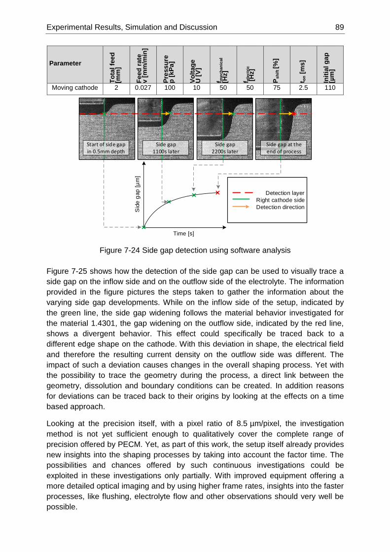
Experimental Results, Simulation and Discussion 89
Parameter
To
tal fe
ed
[m
m]
Feed
rate
v [
mm
/min
]
Pre
ssu
re
p [
kP
a]
Vo
ltag
e
U [
V]
f mech
an
ical
[Hz]
f ele
ctr
ic
[H
z]
Psh
ift [%
]
t on [
ms]
Init
ial g
ap
[µ
m]
Moving cathode 2 0.027 100 10 50 50 75 2.5 110
Figure 7-24 Side gap detection using software analysis
Figure 7-25 shows how the detection of the side gap can be used to visually trace a
side gap on the inflow side and on the outflow side of the electrolyte. The information
provided in the figure pictures the steps taken to gather the information about the
varying side gap developments. While on the inflow side of the setup, indicated by
the green line, the side gap widening follows the material behavior investigated for
the material 1.4301, the gap widening on the outflow side, indicated by the red line,
shows a divergent behavior. This effect could specifically be traced back to a
different edge shape on the cathode. With this deviation in shape, the electrical field
and therefore the resulting current density on the outflow side was different. The
impact of such a deviation causes changes in the overall shaping process. Yet with
the possibility to trace the geometry during the process, a direct link between the
geometry, dissolution and boundary conditions can be created. In addition reasons
for deviations can be traced back to their origins by looking at the effects on a time
based approach.
Looking at the precision itself, with a pixel ratio of 8.5 µm/pixel, the investigation
method is not yet sufficient enough to qualitatively cover the complete range of
precision offered by PECM. Yet, as part of this work, the setup itself already provides
new insights into the shaping processes by taking into account the factor time. The
possibilities and chances offered by such continuous investigations could be
exploited in these investigations only partially. With improved equipment offering a
more detailed optical imaging and by using higher frame rates, insights into the faster
processes, like flushing, electrolyte flow and other observations should very well be
possible.
Time [s]
Sid
e g
ap
[µ
m]
Side gap1100s later
Side gap2200s later
Side gap at theend of process
Detection layer
Right cathode side
Detection direction
Start of side gap in 0.5mm depth
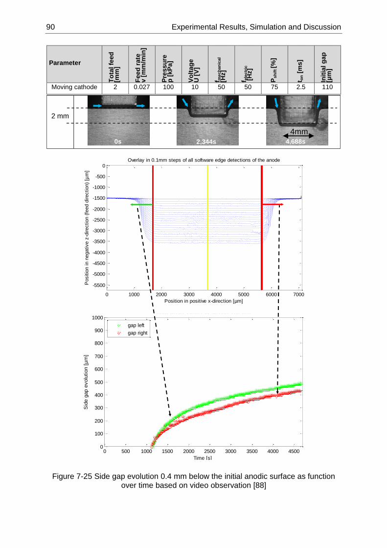
90 Experimental Results, Simulation and Discussion
Parameter
To
tal fe
ed
[m
m]
Feed
rate
v [
mm
/min
]
Pre
ssu
re
p [
kP
a]
Vo
ltag
e
U [
V]
f mech
an
ical
[Hz]
f ele
ctr
ic
[H
z]
Psh
ift [%
]
t on [
ms]
Init
ial g
ap
[µ
m]
Moving cathode 2 0.027 100 10 50 50 75 2.5 110
Figure 7-25 Side gap evolution 0.4 mm below the initial anodic surface as function over time based on video observation [88]
2 mm
time 0 s 2,344 s 4,688 s
4mm
0 1000 2000 3000 4000 5000 6000 7000
-5500
-5000
-4500
-4000
-3500
-3000
-2500
-2000
-1500
-1000
-500
0
Position in positive x-direction [µm]
Positio
n in n
egative z
-direction (
feed d
irection)
[µm
]
Overlay in 0.1mm steps of all software edge detections of the anode
0 500 1000 1500 2000 2500 3000 3500 4000 45000
100
200
300
400
500
600
700
800
900
1000
Side gap evolution 0.4mm below the
initial anodic surface as function over time
Time [s]
Sid
e g
ap e
volu
tion [
µm
]
gap left
gap right
0s 2,344s 4,688s
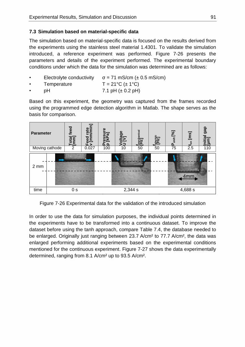
Experimental Results, Simulation and Discussion 91
7.3 Simulation based on material-specific data
The simulation based on material-specific data is focused on the results derived from
the experiments using the stainless steel material 1.4301. To validate the simulation
introduced, a reference experiment was performed. Figure 7-26 presents the
parameters and details of the experiment performed. The experimental boundary
conditions under which the data for the simulation was determined are as follows:
• Electrolyte conductivity σ = 71 mS/cm (± 0.5 mS/cm)
• Temperature T = 21°C (± 1°C)
• pH 7.1 pH (± 0.2 pH)
Based on this experiment, the geometry was captured from the frames recorded
using the programmed edge detection algorithm in Matlab. The shape serves as the
basis for comparison.
Parameter
To
tal fe
ed
[m
m]
Feed
rate
v [
mm
/min
]
Pre
ssu
re
p [
kP
a]
Vo
ltag
e
U [
V]
f mech
an
ical
[Hz]
f ele
ctr
ic
[H
z]
Psh
ift [%
]
t on [
ms]
Init
ial g
ap
[µ
m]
Moving cathode 2 0.027 100 10 50 50 75 2.5 110
Figure 7-26 Experimental data for the validation of the introduced simulation
In order to use the data for simulation purposes, the individual points determined in
the experiments have to be transformed into a continuous dataset. To improve the
dataset before using the tanh approach, compare Table 7.4, the database needed to
be enlarged. Originally just ranging between 23.7 A/cm² to 77.7 A/cm², the data was
enlarged performing additional experiments based on the experimental conditions
mentioned for the continuous experiment. Figure 7-27 shows the data experimentally
determined, ranging from 8.1 A/cm² up to 93.5 A/cm².
2 mm
time 0 s 2,344 s 4,688 s
4mm
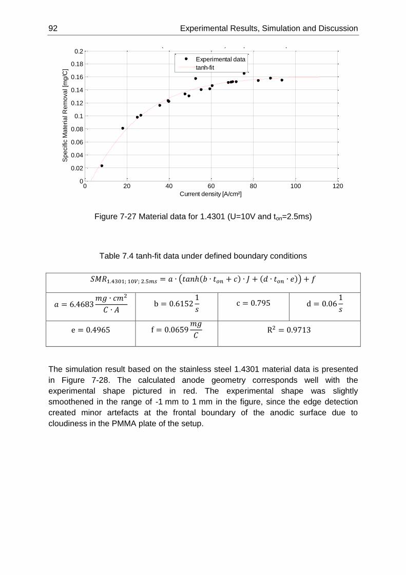
92 Experimental Results, Simulation and Discussion
Figure 7-27 Material data for 1.4301 (U=10V and ton=2.5ms)
Table 7.4 tanh-fit data under defined boundary conditions
𝑆𝑀𝑅1.4301; 10𝑉; 2.5𝑚𝑠 = 𝑎 ∙ (𝑡𝑎𝑛ℎ(𝑏 ∙ 𝑡𝑜𝑛 + 𝑐) ∙ 𝐽 + (𝑑 ∙ 𝑡𝑜𝑛 ∙ 𝑒)) + 𝑓
𝑎 = 6.4683𝑚𝑔 ∙ 𝑐𝑚2
𝐶 ∙ 𝐴 b = 0.6152
1
𝑠 c = 0.795 d = 0.06
1
𝑠
e = 0.4965 f = 0.0659𝑚𝑔
𝐶 R2 = 0.9713
The simulation result based on the stainless steel 1.4301 material data is presented
in Figure 7-28. The calculated anode geometry corresponds well with the
experimental shape pictured in red. The experimental shape was slightly
smoothened in the range of -1 mm to 1 mm in the figure, since the edge detection
created minor artefacts at the frontal boundary of the anodic surface due to
cloudiness in the PMMA plate of the setup.
-3 -2 -1 0 1 2 3-2.5
-2
-1.5
-1
-0.5
0Calculated vs. Experiment
horizontal dimension [mm]
ve
rtic
al d
ime
nsio
n [m
m]
-3 -2 -1 0 1 2 310
-2
10-1
100
101
102
103
Ab
so
lute
Pe
rce
nta
ge
Err
or
(y-A
xis
) [%
]Calculated
Experiment (Smoothened)
Absolute Percentage Error (y-Axis)
-3 -2 -1 0 1 2 3
-2
-1
0Calculated vs. Experiment
horizontal dimension [mm]
ve
rtic
al d
ime
nsio
n [m
m]
-3 -2 -1 0 1 2 30
50
100
150
200
Ab
so
lute
de
via
tio
n (
y-A
xis
) [ m
]
Calculated
Experiment (Smoothened)
Deviation
0 20 40 60 80 100 1200
0.02
0.04
0.06
0.08
0.1
0.12
0.14
0.16
0.18
0.2Material Data for 1.4301 (U=10V and ton=2.5ms) - interpolated from experimental data
Current density [A/cm²]
Sp
ecific
Ma
teri
al R
em
ova
l [m
g/C
]
Experimental data
tanh-fit
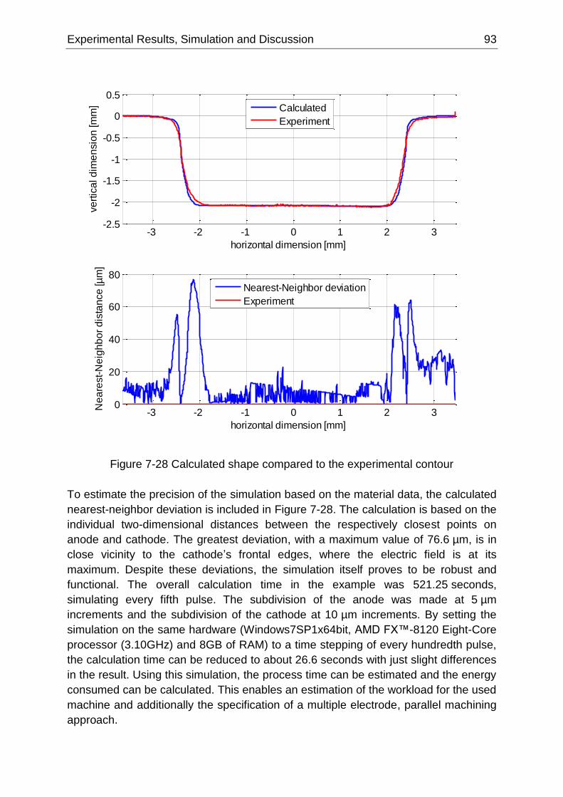
Experimental Results, Simulation and Discussion 93
Figure 7-28 Calculated shape compared to the experimental contour
To estimate the precision of the simulation based on the material data, the calculated
nearest-neighbor deviation is included in Figure 7-28. The calculation is based on the
individual two-dimensional distances between the respectively closest points on
anode and cathode. The greatest deviation, with a maximum value of 76.6 µm, is in
close vicinity to the cathode’s frontal edges, where the electric field is at its
maximum. Despite these deviations, the simulation itself proves to be robust and
functional. The overall calculation time in the example was 521.25 seconds,
simulating every fifth pulse. The subdivision of the anode was made at 5 µm
increments and the subdivision of the cathode at 10 µm increments. By setting the
simulation on the same hardware (Windows7SP1x64bit, AMD FX™-8120 Eight-Core
processor (3.10GHz) and 8GB of RAM) to a time stepping of every hundredth pulse,
the calculation time can be reduced to about 26.6 seconds with just slight differences
in the result. Using this simulation, the process time can be estimated and the energy
consumed can be calculated. This enables an estimation of the workload for the used
machine and additionally the specification of a multiple electrode, parallel machining
approach.
-3 -2 -1 0 1 2 3-2.5
-2
-1.5
-1
-0.5
0
0.5
horizontal dimension [mm]
ve
rtic
al d
ime
nsio
n [m
m]
Calculated
Experiment
-3 -2 -1 0 1 2 30
20
40
60
80
horizontal dimension [mm]
Ne
are
st-
Ne
igh
bo
r d
ista
nce
[µ
m]
Nearest-Neighbor deviation
Experiment
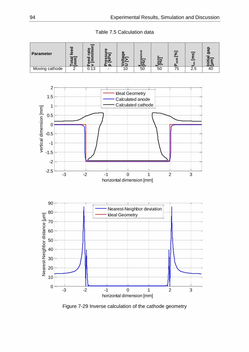
94 Experimental Results, Simulation and Discussion
Table 7.5 Calculation data
Parameter
To
tal fe
ed
[m
m]
Feed
rate
v [
mm
/min
]
Pre
ssu
re
p [
kP
a]
Vo
ltag
e
U [
V]
f mech
an
ical
[Hz]
f ele
ctr
ic
[H
z]
Psh
ift [%
]
t on [
ms]
Init
ial g
ap
[µ
m]
Moving cathode 2 0.13 - 10 50 50 75 2.5 40
Figure 7-29 Inverse calculation of the cathode geometry
-3 -2 -1 0 1 2 3-2.5
-2
-1.5
-1
-0.5
0
0.5
1
1.5
2
horizontal dimension [mm]
ve
rtic
al d
ime
nsio
n [m
m]
Ideal Geometry
Calculated anode
Calculated cathode
-3 -2 -1 0 1 2 30
10
20
30
40
50
60
70
80
90
horizontal dimension [mm]
Ne
are
st-
Ne
igh
bo
r d
ista
nce
[µ
m]
Nearest-Neighbor deviation
Ideal Geometry

Experimental Results, Simulation and Discussion 95
For the tool simulation, introduced in chapter 6.3, an ideal rectangular cavity was
assumed. With an electrode segmentation of 5 µm and simulating every tenth pulse,
using the parameters listed in Table 7.5, the simulation took 14 iterations and a total
time of 1,126.7 seconds to calculate the result pictured in Figure 7-29. The blue
outline shows the simulated anode geometry in contrast to the intended ideally
rectangular shape in red. The cathode theoretically needed to machine this cavity
with a depth of 2 mm is outlined in black. The nearest-neighbor deviation between
ideal anode and calculated anode calculates to a maximum deviation of 85.3 µm at
the transition edge from the initial surface into the gap. Even though this theoretical
approach could not be validated, it contains the opportunity for a scientific and
accelerated cathode design process based on material-specific dissolution data.

Summary and Conclusion 97
8 Summary and Conclusion
In the beginning of this work, the basics of the electrochemical dissolution and
processing of material using the ECM production process are presented. Based on
these principles and basic theory, the reference to the used PECM process and
machine technology is emphasized. By introducing and utilizing specifically designed,
yet easy-to-use experimental setups, the possibilities and necessary restrictions in
the experimentation using the available PECM machining technology is presented.
For the acquisition of material-specific data, three different experimental procedures
are introduced:
1. Frontal gap experiments (steady-state) are the key to derive material-specific
data under a wide range of boundary conditions. Yet in the focus of using
industrial process conditions, the necessity for e.g. identical pre-machining
before the actual experiment in order to eliminate the effects of preprocessing
using other machining technologies is emphasized. With this proceed frontal
gap and feed rate relationships, as well as surface roughness specifics from
combinations of pulse on times and different current densities can be
investigated.
2. Side gap experiments (steady-state) are useful to examine the relationship
between current density and passivation, through the widening of the gap over
time.
3. Continuous observations (dynamic over time) using a novel approach and
setup are introduced and tested. They allow a view into the overall geometric
shaping process while machining, and a variety of downstream data analysis
possibilities.
During the restriction of parameters and the introduction of machine-specific
boundary conditions for the gathering and recording of data, the theoretical aspects
of the technology are substantiated and discussed using experimental data. Also the
uncertainties are investigated and the individual limits towards the precision of each
mechanical, electrical and visual method are discussed.
The material-specific data at hand, the datasets are reworked and then presented
according to the basic principles of electrochemical dissolution. While the material
composition cannot be influenced, the data is adapted to show the effects on shape
and surface based on the process input parameters, which can be modified using the
machine technology to achieve a desired result.
The focus is set on the investigation of two different materials, a commonly used
stainless steel and a powder metallurgical steel. For a better understanding and
transparency, most experiments and validations are presented based on one
material, the stainless steel 1.4301, only. Here, the modelling and detailed
explanation of relationships and occurring effects as well as special features are
worked out. A standardized representation of material-specific data focused on
geometry and surface at both stationary and dynamic conditions is presented.
98 Summary and Conclusion
Furthermore, a commonly assumed fact regarding the independence of the
electrochemical process of the hardness of a material was substantiated with facts,
showing the possibility of machining, but also the drastic differences in the results at
the example of the powder metallurgical steel S390.
With the material data at hand, simulation possibilities derived from the process
basics are presented with the aim of validating the simulation in reference to actual
experimental data. The possibility to calculate and estimate geometries and shapes
as a way of visualizing the complex technological relationships is made available.
Using this mainly virtual tool (simulation) the development costs and process can be
decreased.
Based on this standardized proceed and simulation possibility to reduce the process
of iterative tool shaping, a machine control could be realized, which uses only the
targeted depth and desired surface roughness as input parameters. As basis of this
approach a material database or clusters of similar material compositions should be
made available similar to the approach in the plastics and metal processing industry,
where processing data is made available by the suppliers of the materials. The
clustering of materials could be achieved in accordance with the chemical
compositions as well with regard to the material’s microstructure. With this
knowledge at hand, the acceptance and use cases for the Electrochemical Machining
might further increase, yet at the same time be of benefit for the further improvement
of easy-to-use simulations as part of or additional packages for well-established CAD
software.
REFERENCES 99
REFERENCES
[1] C. Czeslik, H. Seemann and R. Winter: Basiswissen Physikalische Chemie. 4.,
aktualisierte Auflage, Vieweg+Teubner, Wiesbaden, 2010.
[2] "Wikipedia," Wikimedia Foundation Inc., 2015. [Online]. Available:
https://en.wikipedia.org/wiki/Faraday%27s_laws_of_electrolysis. [Accessed 11
July 2015].
[3] Metcut Research Associates Inc.: Machining Data Handbook 3rd edition,
Volume two. ISBN 0-936914-02-8, 1980.
[4] R. Förster: Untersuchung des Potentials elektrochemischer Senkbearbeitung
mit oszillierender Werkzeugelektrode für Strukturierungsaufgaben der
Mikrosystemtechnik. Dissertation, Albert-Ludwigs-Universität Freiburg im
Breisgau, Freiburg, 2004.
[5] K. P. Rataj: Elektrochemische Charakterisierung technisch relevanter
anodischer Oxidschichten bei niedrigen und höchsten Stromdichten.
Dissertation, Heinrich-Heine-Universität Düsseldorf, Düsseldorf, 2013.
[6] T. R. Münninghoff: Mechanismen der anodischen Auflösung von Metallen und
Legierungen bei extrem hohen Stromdichten. Dissertation, Heinrich-Heine-
Universität Düsseldorf, Düsseldorf, 2012.
[7] F. Klocke and W. König: Fertigungsverfahren 3 - Abtragen, Generieren,
Lasermaterialbearbeitung. 4.te, neu bearbeitete Auflage, Springer-Verlag Berlin
Heidelberg, 2007.
[8] H. S. J. Altena: EDM and ECM for mass production Philips DAP. Journal of
Materials Processing Technology 149 (2004), pp.18-21, 2004.
[9] F. Klocke, A. Klink, D. Veselovac, D. K. Aspinwall, S. L. Soo, M. Schmidt, J.
Schilp, G. Levy, J.-P. Kruth: Turbomachinery component manufacture by
application of electrochemical, electro-physical and photonic processes. CIRP
Annals - Manufacturing Technology 63 (2014), pp.703-726, 2014.
[10] D. R. Corbin: Corbin Handbook of Bullet Swaging No. 9. White City, OR 97503
USA: Corbin Manufacturing & Supply, Inc., 2012.
[11] H. Degenhardt: Elektrochemische Senkbarkeit metallischer Werkstoffe.
Dissertation, Rheinisch-Westfälische Technische Hochschule Aachen, Aachen,
1972.
100 REFERENCES
[12] M. Brussee: PECM History and Outlook. International Symposium on
Electrochemical Machining INSECT2011, Editors: B. Mollay, M.M. Lohrengel,
pp.8-9, Vienna, 2011.
[13] ECM, LLC: Short history of electrochemical machining (ECM) development.
http://www.indec-ecm.com/en/, online: 12.12.2014.
[14] W. Piersig: ECM - Elektrochemische Metallbearbeitung und EC-
Kombinationsverfahren. GRIN Verlag, ISBN 978-3-640-19833-7, 2008.
[15] K. P. Rajurkar, M. Sundaram, A. P. Malshe: Review of Electrochemical and
Electrodischarge Machining. Procedia CIRP 6 (2013), pp.13-26, 2013.
[16] DIN 8580: Fertigungsverfahren; Begriffe, Einteilung. DIN 8580:2003-09, Beuth
Verlag, Berlin, 2003.
[17] DIN 8590: Fertigungsverfahren Abtragen; Einordnung, Unterteilung, Begriffe.
DIN8590:2003-09, Beuth Verlag, Berlin, 2003.
[18] VDI 3400: Elektroerosive Bearbeitung; Begriffe, Verfahren, Anwendung. VDI-
Handbuch Betriebstechnik, 1975.
[19] VDI 3401 - Blatt 1 Entwurf: Elektrochemisches Abtragen; Formabtragen. VDI-
Handbuch Betriebstechnik, Teil 2: Fertigungsverfahren, Düsseldorf, 2009.
[20] VDI 3401 - Blatt 1: Elektrochemisches Abtragen; Formabtragen. VDI-Handbuch
Betriebstechnik, Teil 2, Düsseldorf, 1993.
[21] VDI 3401 - Blatt 3: Elektrochemisches Abtragen; Behandlung der
Elektrolytlösungen, Abwässer und Schlämme. VDI-Handbuch Betriebstechnik,
Teil 2, Düsseldorf, 1993.
[22] A. E. DeBarr and D. A. Oliver: Electrochemical Machining. MacDonald, London,
1968.
[23] D. Pahl: Über die Abbildungsgenauigkeit beim elektrochemischen Senken.
Dissertation, Rheinisch-Westfälische Technische Hochschule Aachen, Aachen,
1969.
[24] F. W. Wilson: Practice and Theory of Electrochemical Machining. John Wiley &
Sons Inc., 1971.
[25] W. Mauz: Technik der elektrochemischen Metallbearbeitung. Chemie-lng.-
Techn., Vol. 45 (1973), Nr. 4, pp.194-197, 1973.
[26] S. P. Loutrel, N. H. Cook: A Theorectical Model of High Rate Electrochemical
Machining. Journal of Engineering for Industry, Paper No.73-Prod-2, pp.1003-
REFERENCES 101
1008, 1973.
[27] H. Dietz, K. G. Günther, K. Otto: Reproduction Accuracy with Electrochemical
Machining: Determination of the Side Gap. Annals of CIRP, 22/1, pp.61-62,
1973.
[28] J. A. McGeough: Principles of Electrochemical Machining. Chapmann and Hall,
London, 1974.
[29] J. Bannard: Electrochemical machining. Journal of Applied Electrochemistry, 7,
pp.1-29, 1976.
[30] W. Degener: Handbuch Feinbearbeitung. VEB Verlag Technik, Berlin, 1979.
[31] W. Degner: Elektrochemische Metallbearbeitung. VEB Verlag Technik, Berlin,
1984.
[32] E. J. Weller and M. Haavisto: Nontraditional Machining Processes. Second
Edition, Society of Manufacturing Engineers, 1984.
[33] J. M. Fitz-Gerald, J. A. McGeough: Mathematical Theory of Electrochemical
Machining 1. Anodic Smoothing. J. Inst. Maths Applies (1969) 5, pp.387-408,
1969.
[34] J. M. Fitz-Gerald, J. A. McGeough, L. M. Marsh: Mathematical Theory of
Electrochemical Machining 2. Anodic Shaping. J. Inst. Maths Applies (1969) 5,
pp.409-421, 1969.
[35] J. M. Fitz-Gerald, J. A. McGeough: Mathematical Theory of Electrochemical
Machining 3. Deburring and Cavity-forming. J. Inst. Maths Applies (1970) 6,
pp.102-110, 1970.
[36] D. G. Risko, A. D. Davydov: Manufacturing applications and producitivity
limitations of electrochemical machining. Manufacturing Sience and
Engineering ASME 1993, PED-Vol. 64, pp.701-718, 1993.
[37] K. P. Rajurkar, D. Zhu, J. A. McGeough, J. Kozak, A. De Silva: New
Developments in Electro-Chemical Machining. Annals of CIRP, Vol. 48/2,
pp.567-579, 1999.
[38] W. König: Elektrochemisches Abtragen. In: G. Spur, T. Stöferle: Handbuch der
Fertigungsverfahren Band 4/1 Abtragen, Beschichten. München Wien: Carl
Hanser Verlag, 1987.
[39] J. Wijers: Sterke evolutie elektrochemisch. Mikroniek 2-2009, pp.36-42, 2009.
102 REFERENCES
[40] T. Masuzawa, T. Takawashi: Recent Trends in EDM/ECM Technologies in
Japan. VDI Berichte Nr. 1405, pp.1-15, 1998.
[41] H.-P. Lindenlauf: Werkstoff- und elektroytspezifische Einflüsse auf die
Elektrochemische Senkbarkeit ausgewählter Stähle und Nickellegierungen.
Dissertation, Rheinisch-Westfälische Technische Hochschule Aachen, Aachen,
1977.
[42] C. H. Hamann and W. Vielstich: Elektrochemie. 4., vollständig überarbeitete
und aktualisierte Auflage, Wiley-VCH, 2005.
[43] G. M. Alder, D. Clifton, F. Mill: A direct analytical solution to the tool design
problem in electrochemical machining under steady state conditions.
Proceedings of the Institution of Mechanical Engineers, Part B: Journal of
Engineering Manufacture, vol. 214, pp.745-750, 2000.
[44] H. S. J. Altena: Precision ECM by process characteristic modelling.
Dissertation, Glasgow Caledonian University, 2000.
[45] S. Hinduja, M. Kunieda: Modelling of ECM and EDM processes. CIRP Annals -
Manufacturing Technology , Vol. 62 (2013), pp.775–797, 2013.
[46] J. W. Schultze, M. M. Lohrengel: Stability, reactivity and breakdown of passive
films. Problems of recent and future research. Electrochimica Acta 45 (2000),
pp.2499-2513, 2000.
[47] C. Rosenkranz, M. M. Lohrengel, J. W. Schultze: The surface structure during
pulsed ECM of iron in NaNO3. Electrochimica Acta 50 (2005) , pp.2009-2016,
2005.
[48] C. Rosenkranz: Elektrochemische Prozesse an Eisenoberflächen bei extremen
anodische Stromdichten. Dissertation, Heinrich-Heine-Universität Düsseldorf,
Düsseldorf, 2005.
[49] M. M. Lohrengel, C. Rosenkranz: Microelectrochemical surface and product
investigations during electrochemical machining (ECM) in NaNO3. Corrosion
Science, 47, pp.785-794, 2005.
[50] A. Möhring: Entwicklung einer elektrochemischen Mikrodurchflusszelle zur
Untersuchung des Elektrochemischen Senkens (ECM, Electrochemical
Machining). Dissertation, Heinrich-Heine-Universität Düsseldorf, Düsseldorf,
2004.
[51] W. Pies, A. Weiss: a2215, I.2.1 Simple chlorides and their solid solutions.
SpringerMaterials - The Landolt-Börnstein Database
(http://www.springermaterials.com), DOI: 10.1007/10201462_30.
REFERENCES 103
[52] K. Gesi: 30A-2 KNO3 [F]. SpringerMaterials - The Landolt-Börnstein Database
(http://www.springermaterials.com), DOI: 10.1007/10635019_58.
[53] M. Datta, D. Landolt: On the role of mass transport in high rate dissolution of
iron ad nickel in ECM electrolytes - I. chloride solutions. Electrochimica Acta,
Vol. 25, pp.1255-1262, 1980.
[54] M. Datta, D. Landolt: On the role of mass transport in high rate dissolution of
iron ad nickel in ECM electrolytes - II. chlorate and nitrate solutions.
Electrochimica Acta, Vol. 25, pp.1263-1271, 1980.
[55] Kirsch Pharma GmbH: Sicherheitsdatenblatt nach 91/155/EWG -
Handelsname: Natriumnitrat, Material-Nr.: 10318. Ausgabedatum: 29.06.2007,
2007.
[56] A. K. M. De Silva, H. S. J. Altena, J. A. McGeough: Influence of Electrolyte
Concentration on Copying Accuracy of Precision-ECM. Annals of CIRP, 52/1,
pp.165-168, 2003.
[57] D. Bähre, A. Rebschläger, O. Weber, P. Steuer: Reproducible, fast and
adjustable surface roughening of stainless steel using Pulse Electrochemical
Machining. Procedia CIRP 6 (2013 ), pp.385-390, 2013.
[58] A. P. Semaschko, N. Z. Gimaev, I. V. Maksimov, S. V. Bezrukov, V. B.
Rabinovtisch: Verfahren und Anordnung zur elektrochemischen Bearbeitung.
Deutsches Patentamt, Offenlegungsschrift DE 29 03 873 A1, 1979.
[59] M. Datta, D. Landolt: Electrochemical Machining under pulsed current
conditions. Electrochimica Acta Band 26 (1981), pp.899-907, 1981.
[60] M. Datta, D. Landolt: Electrochemical saw using pulsating voltage. Journal of
Applied Electrochemical 13 (1983), pp.795-802, 1983.
[61] J. Kozak, K. P. Rajurkar, B. Wei: Analysis of electrochemical machining
process with short pulses. Materials Issues in Machining and the Physics of
Machining Processes, pp.131-146, 1992.
[62] J. Kozak, K. P. Rajurkar, Z. Gulbinowicz: Electrochemical machining with using
of vibrating tool electrode. International Symposium on Electrochemical
Machining INSECT2009, Editors: A. Michaelis, M. Schneider, pp. 31-36, 2009.
[63] J. Kozak, K. P. Rajurkar, S. Malicki: Study of electrochemical machining
utilizing a vibrating tool electrode. 16th International Conference on Computer-
aided Production Engineering CAPE 2000, IMechE Conference Transactions
2000-5, pp.173-181, 2000.
104 REFERENCES
[64] H.-P. Schulze: Problems of the processing accuracy for electro-erosion and
elctro-chemical machining processes. International Journal of Material Forming,
Vol. 2 Suppl. 1, pp.641-644, 2009.
[65] S. Moser: Mikrostrukturierung von Metallen durch elektrochemischen Abtrag mit
gepulstem Strom (PECM). Dissertation, Heinrich-Heine-Universität Düsseldorf,
Düsseldorf, 2004.
[66] B. Lilly, J. Brevick, C. S. Chen: The effect of pulsed electrochemical machining
on the fatigue life of H-13 steel. Transactions of NAMRI/SME, Volume XXV,
153-158, 1997.
[67] K. P. Rajurkar, J. Kozak, B. Wei: Study of Pulse Electrochemical Machining
Characteristics. Annals of CIRP, 41/1, pp.231-234, 1993.
[68] M. Burger: Präzise Elektrochemische Bearbeitung (PECM) komplexer
Strukturbauteile. Dissertation, Technische Universität München, München,
2010.
[69] J. Kozak: Thermal models of pulse electrochemical machining. Bulletin of the
polish academy of sciences, Technical Sciences Vol. 52, No. 4, pp.313-320,
2004.
[70] A. D. Davydov, V. M. Volgin, V. V. Lyubimov: Electrochemical Machining of
Metals: Fundamentals of Electrochemical Shaping. Russian Journal of
Electrochemistry, Vol. 40, No. 12, pp.1230-1265, 2004.
[71] A. Zaytsev, I. Agafonov, N. Gimaev, R. Moukhoutdinov, A. Belogorsky: Precise
pulse electrochemical machining by bipolar current Aspects of effective
technological application. Journal of Materials Processing Technology 149
(2004), pp.419-425, 2004.
[72] A. Zaitsev, N. Z. Gimaev, N. A. Amirchanova, A. L. Belogorsky, L. Markelova,
R. R. Muchutdinov, M. Brussee: METHOD FOR A REMOVAL OF CATHODE
DEPOSITIONS BY MEANS OF BIPOLAR PULSES. United States Patent,
Patent No.: US 6,620,307 B2, 2003.
[73] E. Rosset, M. Datta, D. Landolt: Electrochemical dissolution of stainless steels
in flow channel cells with and without photoresist masks. Journal of Applied
Electrochemical, 20 (1990), pp.69-76, 1990.
[74] G. Meichsner, L. Boenig, M. Hackert-Oschätzchen, M. P. T. Krönert, J.
Edelmann, A. Schubert: Determination of the gas generation during precise
electrochemical machining. International Symposium on Electrochemical
Machining Technology INSECT2014, Editors: D. Bähre, A. Rebschläger, pp.63-
75, Saarbrücken, 2014.
REFERENCES 105
[75] W. Hoogsteeen, T. P. Pajak: ECM Experiments on Stainless Steels.
International Symposium on Electrochemical Machining Technology
INSECT2010, Editors: J. Deconinck, D. De Wilde, pp.51-65, Brussels, 2010.
[76] M. Spittel, T. Spittel: Steel symbol/number: X5CrNi18–10/1.4301.
SpringerMaterials - The Landolt-Börnstein Database
(http://www.springermaterials.com), Springer-Verlag Berlin Heidelberg, DOI:
10.1007/978-3-540-44760-3_93, 2009.
[77] W. Schatt, K.-P. Wieters and B. Kieback: Pulvermetallurgie; Technologien und
Werkstoffe. 2., bearbeitete und erweiterte Auflage, Springer-Verlag, Berlin-
Heidelberg, 2007.
[78] Böhler Edelstahl GmbH: Böhler S390 microclean. Material Data Sheet:
http://www.bohler-edelstahl.com/english/files/S390DE.pdf (online 01/21/2015).
[79] W. Hoogsteen: The effect of the heat treatment of an ASTM A693 stainless
steel on the ECM behavior in NaNO3 and NaNO2 electrolyte. International
Symposium on Electrochemical Machining Technology INSECT2014, Editors:
D. Bähre, A. Rebschläger, pp.77-84, Saarbrücken, 2014.
[80] A. Schubert, G. Meichsner, M. Hackert-Oschätzchen, M. Zinecker, J.
Edelmann: Pusled Electrochemical Machining of Powder Metallurgy Steels.
International Symposium on Electrochemical Machining INSECT2011, Editors:
B. Mollay, M.M. Lohrengel, pp.68-75, Vienna, 2011.
[81] Bio-Logic Science Instruments SAS, EC-Lab Software User's Manual. Version
10.38, 2014.
[82] H. S. J. Altena: EDM and ECM for mass production Philips DAP. Journal of
Materials Processing Technology 149 (2004), pp.18-21, 2004.
[83] M. Hackert-Oschätzchen, M. Penzel, M. Kowalick, G. Meichsner, A. Schubert:
Transient Simulation of the Electrolyte Flow in a Closed Device for Precise
Electrochemical Machining. Proceedings of the 2014 COMSOL Conference in
Cambridge, Cambridge, 2014.
[84] A. Schubert, G. Meichsner, L. Boenig, M. Hacker-Oschätzchen, M. Krönert, J.
Edelmann: Resource-Efficient Design of Precise Electrochemical Machining.
International Symposium on Electrochemical Machining Technology
INSECT2013, Editors: A. Schubert, M. Hackert-Oschätzchen, pp.53-63,
Chemnitz, 2013.
[85] P. Steuer, A. Rebschläger, A. Ernst, D. Bähre: Process Design in Pulse
Electrochemical Machining Based on Material Specific Data – 1.4301 and
Electrolytic Copper as an Example. Key Engineering Materials Vols 651-653,
106 REFERENCES
pp. 732-737, 2015.
[86] C.-O. A. Olsson, D. Landolt: Passive films on stainless steels - chemistry,
structure and growth. Electrochimica Acta 48 (2003), pp.1093-1104, 2003.
[87] A. Rebschläger, R. Kollmannsperger, D. Bähre: Video based process
observations of the pulse electrochemical machining process at high current
densities and small gaps. Procedia CIRP 13 (2013), pp. 418-423, 2013.
[88] A. Rebschläger, K. U. Fink, T. Heib, D. Bähre: Geometric shaping analysis
based on PECM video process observations. International Symposium on
Electrochemical Machining Technology INSECT2014, Editors: D. Bähre, A.
Rebschläger, pp.37-44, Saarbrücken, 2014.
[89] C. Y. Yu, Y. H. Liu, Y. H. Huang, Y. C. Hsu: The Investigation of the Flow
Characteristics of the Gap in the Pulse Electrochemical Machining (PECM).
Annals of CIRP, 31/1, pp.119-123, 1982.
[90] M. Schneider, S. Schroth, N. Schubert, C. Lämmel, A. Michaelis: A novel
approach of in-situ investigation of the surface topography under near ECM-
conditions. International Symposium on Electrochemical Machining
INSECT2009, Editors: A. Michaelis, M. Schneider, pp.81-87, 2009.
[91] M. Schneider, S. Schroth, S. Richter, S. Höhn, N. Schubert, A. Michaelis: In-situ
investigation of the interplay between microstructure and anodic copper
dissolution under near-ECM conditions – Part 1: The active state.
Electrochimica Acta 56 (2011), pp.7628-7636, 2011.
[92] M. Schneider, S. Schroth, S. Richter, S. Höhn, N. Schubert, A. Michaelis: In-situ
investigation of the interplay between microstructure and anodic copper
dissolution under near-ECM conditions – Part 2: The transpassive state.
Electrochimica Acta 70 (2012), pp.76-83, 2012.
[93] S. Schroth: Optische In-situ-Beobachtung des anodischen
Auflösungsverhaltens von Kupfer unter ECM-nahen Bedingungen.
FRAUNHOFER VERLAG, Dresden, 2013.
[94] F. Klocke, M. Zeis, T. Herrig, S. Harst, A. Klink: Optical In Situ Measurements
and Interdisciplinary Modeling of the Electrochemical Sinking Process of
Inconel 718. Procedia CIRP 24 ( 2014 ), pp.114-119, 2014.
[95] A. Rebschläger, O. Weber, B. Heitkamp: Benefits and Drawbacks Using Plastic
Materials Produced by Additive Manufacturing Technologies in the
Electrochemical Environement. International Symposium on Electrochemical
Machining Technology INSECT2013, Editors: A. Schubert, M. Hackert-
Oschätzchen, pp.45-51, Chemnitz, 2013.
REFERENCES 107
[96] S. Agafonov, M. Brussee, J. Dorzweiler: The influence of pressure and flow on
the results of the PEM process.n.a..
[97] A. N. Zaytsev, V. P. Zhitnikov, T. V. Kosarev: Formation mechanism and
elimination of the workpiece surface macro-defects, aligned along the
electrolyte stream at electrochemical machining. Journal of Materials
Processing Technology 149 (2004), pp.439-444, 2004.
[98] K. Kollmannsperger, "Softwaregestütze Analyse des elektrochemischen
Materialverhaltens eines Edelstahls auf Basis experimentell erfasster Video-
und Bidldaten," Master Thesis, Saarland University, Saarbrücken, 2014.
[99] K. U. Fink, "Analyse der geometrischen Formgebung des gepulsten
elektrochemischen Abtragens auf Basis experimentell erfasster Video- und
Bilddaten," Master Thesis, Saarland University, Saarbrücken, 2014.
[100] A. Rebschläger, O. Weber, D. Bähre: In-situ process measurements for
industrial size Pulse Electrochemical Machining. International Symposium on
Electrochemical Machining Technology INSECT2012, Editor: Maria Zybura-
Skrabalak, pp.133-148, Krakow, 2012.
[101] M. Datta, D. Landolt: On the influence of electrolyte concentration, pH and
temperature on surface brightening of nickel under ECM conditions. Journal of
Applied Electrochemistry 7 (1977), pp.247-252, 1977.
[102] D. Landolt: Fundamental aspects of electropolishing. Electrochimia Acta, vol.
52 No. 1, pp.1-11, 1987.
[103] M. Zybura-Skrabalak, A. Ruszaij: The influence of electode surface geometrical
structure on electrochemical smoothing process. Journal of Materials
Processing Technology 107 (2000), pp. 288-292, 2000.
[104] DIN 4760: Gestaltabweichungen; Begriffe, Ordnungssystem. Beuth-Verlag,
Berlin, 1992.
[105] DIN EN ISO 4287: Geometrische Produktspezifikation (GPS) -
Oberflächenbeschaffenheit: Tastschnittverfahren - Benennungen, Definitionen
und Kenngrößen der Oberflächenbeschaffenheit. DIN EN ISO 4287:2010-07,
Beuth Verlag, Berlin, 2010.
[106] DIN EN ISO 4288: Geometrische Produktspezifikationen (GPS) -
Oberflächenbeschaffenheit: Tastschnittverfahren Regeln und Verfahren für die
Beurteilung der Oberflächenbeschaffenheit. EN ISO 4288 : 1997, Beuth Verlag,
Berlin, 1998.
[107] VDI/VDE 2602: Rauheitsmessung mit elektrischen Tastschnittgeräten.
108 REFERENCES
VDI/VDE-Handbuch Meßtechnik II, 1983.
[108] W. König, H.-J. Hümbs: Mathematical Model for the Calculation of the Contour
of the Anode in Electrochemical Machining. Annals of CIRP, 25/1, pp.83-87,
1977.
[109] V. M. Volgin, A. D. Davydov: Modeling of multistage electrochemical shaping.
Journal of Materials Processing Technology 149 (2004), pp.466-471, 2004.
[110] J. Kozak, K. Lubkowski, J. Peronczyk: Accuracy problems of the pulse
electrochemical machining. Proceedings of the International Machine Tool
Design and Research Conference, Issue of 1981, pp. 353-360, 1981.
[111] K. P. Rajurkar, D. Zhu, B. Wei: Minimization of Machining Allowance in
Electrochemical Machining. Annals of CIRP, 47/1, pp.165-168, 1998.
[112] C. Van Osenbruggen, I. C. De Regt: Elektrochemisch micro-bewerken.
Mikroniek 5-1988, Philips Technisch Tijdschrift 42-1984, 1984.
[113] B. Mollay, G. Schöllhammer, P. Raffelstetter: A modeling strategy for the
optimization of high-precision electrochemical machining processes.
International Symposium on Electrochemical Machining INSECT2009, Editors:
A. Michaelis, M. Schneider, pp.17-22, 2009.
[114] A. K. M. De Silva, H. S. J. Altena, J. A. McGeough: Precision ECM by Process
Characteristic Modelling. Annals of CIRP, 49/1, pp.151-155, 2000.
[115] S. Van Damme, G. Nelissen, B. Van Den Bossche, J. Deconinck: Numerical
model for predicting the efficiency behaviour during pulsed electrochemical
machining of steel in NaNO3. Journal of Applied Electrochemistry (2006) 36,
pp.1-10, 2006.
[116] H. Hocheng, Y. H. Sun, P. S. Kao: A material removal analysis of
electrochemical machining using flat-end cathode. Journal of Materials
Processing Technology 140 (2003), pp.264-268, 2003.
[117] J. Kozak: Mathematical models for computer simulation of electrochemical
machinig processes. Journal of Materials Processing Technology 76 (1998),
pp.170-175, 1998.
[118] J. Kozak, M. Chuchro, A. Ruszaj, K. Karbowski: The computer aided simulation
of electrochemical process with universal spherical electrodes when machining
sculptured surfaces. Journal of Materials Processing Technology 107 (2000),
pp.283-287, 2000.
[119] J. Kozak, L. Dabrowski, K. Lubkowski, M. Rozenek, R. Slawinski: CAE-ECM
REFERENCES 109
system for electrochemical technology of parts and tools. Journal of Materials
Processing Technology 107 (2000), pp.293-299, 2000.
[120] J. Kozak: Computer Simulation of Electrochemical Machining. Proceedings of
the World Congress on Engineering and Computer Science WCECS 2011 Vol.
II, ISBN: 978-988-19251-7-6, San Francisco, 2011.
[121] J. Kozak, D. Gulbinowicz, Z. Gulbinowicz: The Mathematical Modeling and
Computer Simulation of Pulse Electrochemical Micromachining. Engineering
Letter, 16:4, 2008.
[122] P. Domanowski, J. Kozak: Direct and inverse problems of shaping by
electrochemical generating machining. Journal of Materials Processing
Technology 107 (2000), pp.300-306, 2000.
[123] M. Purcar, L. Bortels, B. Van den Bossche, J. Deconinck: 3D electrochemical
machining computer simulations. Journal of Materials Processing Technology
149 (2004), pp.472-478, 2004.
[124] M. Purcar, A. Dorochenko, L. Bortels, J. Deconinck, B. Van den Bossche:
Advanced CAD integrated approach for 3D electrochemical machining
simulations. Journal of Materials Processing Technology 203 (2008), pp.58-71,
2008.
[125] L. Bortels, M. Purcar, B. Van den Bossche, J. Deconinck: A user-friendly
simulation software tool for 3D ECM. Journal of Materials Processing
Technology 149 (2004), pp.486-492, 2004.
[126] N. Smets, S. Van Damme, D. De Wilde, G. Weyns, J. Deconinck: Time
averaged temperature calculations in pulse electrochemical machining. Part I:
theoretical basis. Journal of Applied Electrochemistry (2007) 37, pp.1345-1355,
2007.
[127] N. Smets, S. Van Damme, D. De Wilde, G. Weyns, J. Deconinck: Time
averaged temperature calculations in pulse electrochemical machining, part II:
numerical simulation. Journal of Applied Electrochemistry (2008) 38, pp.551-
560, 2008.
[128] N. Smets, S. Van Damme, D. De Wilde, G. Weyns, J. Deconinck: Calculation of
temperature transients in pulse electrochemical machining (PECM). Journal of
Applied Electrochemistry (2007) 37, pp.315-324, 2007.
[129] R. Tsuboi, M. Yamamoto: Modeling and application of electrochemical
machining process. Proceedings of the ASME 2009 International Mechanical
Engineering Congress & Exposition IMECE 2009, IMECE2009-12552, pp.377-
384, Florida, 2009.
110 REFERENCES
[130] T. Fujisawa, L. Inaba, M. Yamamoto, D. Kato: Mulitphysics Simulation of
Electrochemical Machining Process for Three-Dimensional Compressor Blade.
Journal of Fluids Engineering, DOI: 10.1115/1.2956596, Volume 130 - Issue 8,
2008.
[131] F. Klocke, M. Zeis, S. Harst, A. Klink, D. Veselovac, M. Baumgärtner: Modeling
and Simulation of the Electrochemical Machining (ECM) Material Removal
Process for the Manufacture of Aero Engine Components. Procedia CIRP 8
(2013 ), pp.265-270, 2013.
[132] J. McClennan, G. Alder, A. Sherlock, F. Mill, D. Clifton: Two-dimensional tool
design for two-dimensional equilibrium electrochemical machining die-sinking
using a numerical method. Proceedings of the Institution of Mechanical
Engineers, Part B: Journal of Engineering Manufacture, vol. 220 no. 5, pp.637-
645 , 2006.
[133] D. Curry, A. Sherlock, A. Mount, R. Muir: Time-dependent simulation of
electrochemical machining under non-ideal conditions. WIT Transactions on
Engineering Sciences, Vol 48, pp.133-142, 2005.
[134] V. P. Zhitnikov, G. I. Fedorova, O. V. Zinatullina, A. V. Kamashev: Simulation of
non-stationary processes of electrochemical machining. Journal of Materials
Processing Technology 149 (2004), pp.398-403, 2004.
[135] A. R. Mount, D. Clifton, P. Howarth, A. Sherlock: An integrated strategy for
materials characterisation and process simulation in electrochemical machining.
Journal of Materials Processing Technology 138 (2003), pp.449-454, 2003.
[136] C. S. Chang, L. W. Hourng, C. T. Chung: Tool design in electrochemical
machining considering the effect of thermal-fluid properties. Journal of applied
electrochemistry, Vol. 29 (1999), pp.321-330, 1999.
[137] S. S. Patil, V. Yadava: Finite element prediction of tool shapes in electro-
chemical machining. International Journal Design Engineering, Vol. 1, No. 1,
pp.21-40, 2007.
[138] J. A. Westley, J. Atkinson, A. Duffield: Generic aspects of tool design for
electrochemical machining. Journal of Materials Processing Technology 149
(2004), pp.384-392, 2004.
[139] J. A. McGeough: Some effects of carbon content on the efficiency of
electrochemically machined carbon steels and cast iron. International Journal of
Production Research, Vol. 9, No. 2, 311-316, 1971.
[140] O. Weber, H. Natter, A. Rebschläger, D. Bähre: Surface quality and process
behaviour during Precise Electrochemical Machining of cast iron. International
REFERENCES 111
Symposium on Electrochemical Machining INSECT2011, Editors: B. Mollay,
M.M. Lohrengel, pp.41-46, Vienna, 2011.
[141] O. Weber, H. Natter, A. Rebschläger, D. Bähre: Analytical characterization of
the dissolution behavior of cast iron by electrochemical methods. International
Symposium on Electrochemical Machining Technology INSECT2012, Editor:
Maria Zybura-Skrabalak, pp.41-55, Krakow, 2012.
[142] O. Weber, D. Bähre, A. Rebschläger: Study of Pulse Electrochemical
Machining characteristics of spheroidal cast iron using sodium nitrate
electrolyte. International Conference on Competitive Manufacturing, COMA 13,
pp.125-130 , South Africa, 2013.
[143] O. Weber, A. Rebschläger, P. Steuer, D. Bähre: Modeling of the
Material/Electrolyte Interface and the Electrical Current Generated during the
Pulse Electrochemical Machining of Grey Cast Iron. Proceedings of the 2013
European COMSOL Conference in Rotterdam, Rotterdam, 2013.
[144] D. Bähre, O. Weber, A. Rebschläger: Investigation on Pulse Electrochemical
Machining Characteristics of Lamellar Cast Iron using a Response Surface
Methodology-based Approach. Procedia CIRP 6 (2013), pp.363-368, 2013.
[145] K. P. Rajurkar, C. L. Schnacker, R. P. Lindsay: Some Aspects of ECM
Performance and Control. Annals of CIRP, 37/1, pp.183-186, 1988.
[146] T. Wagner (geb. Haisch): High rate electrochemical dissolution of iron-based
alloys in NaCl and NaNO3 electrolytes. Dissertation, Universität Stuttgart,
Stuttgart, 2002.
[147] M. Swat, A. Rebschläger, D. Bähre: Investigation of the energy consumption for
the pulse electrochemical machining (PECM) process. International Symposium
on Electrochemical Machining Technology INSECT2013, Editors: A. Schubert,
M. Hackert-Oschätzchen, pp.65-71, Chemnitz, 2013.
[148] M. Swat, A. Rebschläger, K. Trapp, T. Stock, G. Seliger, D. Bähre: Investigating
the energy consumption of the PECM process for consideration in the selection
of manufacturing process chains. Procedia CIRP. 22nd CIRP conference on
Life Cycle Engineering (LCE), 2015.
[149] M. Spittel, T. Spittel: Steel symbol/number: X90CrMoV18/1.4112.
SpringerMaterials - The Landolt-Börnstein Database
(http://www.springermaterials.com), Springer-Verlag Berlin Heidelberg, DOI:
10.1007/978-3-540-44760-3_91, 2009.
[150] M. Spittel, T. Spittel: Steel symbol/number: X6CrNiMoTi17–12–2/1.4571.
SpringerMaterials - The Landolt-Börnstein Database
112 REFERENCES
(http://www.springermaterials.com), Springer-Verlag Berlin Heidelberg, DOI:
10.1007/978-3-540-44760-3_115, 2009.
[151] M. Spittel, T. Spittel: Steel symbol/number: X2CrNiMo17–12–2/1.4404.
SpringerMaterials - The Landolt-Börnstein Database
(http://www.springermaterials.com), Springer-Verlag Berlin Heidelberg, DOI:
10.1007/978-3-540-44760-3_100, 2009.
[152] M. Spittel, T. Spittel: Steel symbol/number: 100Cr6/1.3505. SpringerMaterials -
The Landolt-Börnstein Database (http://www.springermaterials.com), Springer-
Verlag Berlin Heidelberg, DOI: 10.1007/978-3-540-44760-3_83, 2009.
[153] N. Smets, S. Van Damme, D. De Wilde, G. Weyns, J. Deconinck: Time-
averaged concentration calculations in pulse electrochemical machining,
spectral approach. Journal of Applied Electrochemistry (2009) 39, pp.2481-
2488, 2009.
[154] N. Smets, S. Van Damme, D. De Wilde, G. Weyns, J. Deconinck: Time
averaged concentration calculations in pulse electrochemical machining,
spectral approach. Journal of Applied Electrochemistry (2009) 39, pp.791-798,
2009.
[155] N. Smets, S. Van Damme, D. De Wilde, G. Weyns, J. Deconinck: Time
averaged concentration calculations in pulse electrochemical machining.
Journal of Applied Electrochemistry (2008) 38, pp.1577-1582, 2008.
[156] N. Smets, S. Van Damme, D. De Wilde, G. Weyns, J. Deconinck: Time
averaged calculations in pulse electrochemical machining, using a strongly non-
linear model. Journal of Applied Electrochemistry (2010) 40, pp.1395-1405,
2010.
[157] R. N. Muir, D. R. Curry, F. Mill, A. Sherlock, A. R. Mount: Real-time
parameterization of electrochemical machining by ultrasound measurement of
the interelectrode gap. Proceedings of the Institution of Mechanical Engineers,
Part B: Journal of Engineering Manufacture, vol. 221, pp.551-558, 2007.
[158] A. R. Mount, P. S. Howarth, D. Clifton: The use of a segmented tool for the
analysis of electrochemical machining. Journal of Applied Electrochemistry 31,
pp.1213-1220, 2001.
[159] J. A. McGeough, M. C. Leu, K. P. Rajurkar, A. K. M. De Silva, Q. Liu:
Electroforming Process and Application to Micro/Macro Manufacturing. CIRP
Annals, Volume 50, Issue 2, pp.499–514, 2001.
[160] A. Lesch, G. Wittstock, C. Burger, J. Hackenberg, B. Walther: Two-way anodic
dissolution of low alloyed steel in chloride/nitrate mixed electrolytes.
REFERENCES 113
International Symposium on Electrochemical Machining INSECT2009, Editors:
A. Michaelis, M. Schneider, pp.89-94, 2009.
[161] D. Landolt, S. Mischler, M. Stemp: Electrochemical methods in tribocorrosion: a
critical appraisal. Electrochimica Acta 46 (2001), pp.3913-3929, 2001.
[162] J. Kozak: Computer simulation system for electrochemical shaping. Journal of
Materials Processing Technology 109 (2001), pp.354-359, 2001.
[163] F. Klocke, M. Zeis, A. Klink, D. Veselovac: Technological and economical
comparison of roughing strategies via milling, sinking-EDM, wire-EDM and
ECM for titanium- and nickel-based blisks. CIRP Journal of Manufacturing
Science and Technology 6 (2013), pp.198-203, 2013.
[164] T. Haisch, E. J. Mittemeijer: Electrochemical Machining: The Role of Steel
Microstructure in High-Rate Anodic Dissolution. JOM, Vol. 54, Issue 7, pp.38-
41, 2002.
[165] T. Haisch, E. Mittemeijer and J. W. Schultze: Electrochemical machining of the
steel 100Cr6 in aqueous NaCl and NaNO3 solutions: microstructure of surface
films formed by carbides. Electrochimica Acta 47 (2001), pp. 235–241, 2001.
[166] L. Dabrowski, T. Paczkowski: Computer Simulation of Two-dimensional
Electrolyte Flow in Electrochemical Machining. Russian Journal of
Electrochemistry, Vol. 41, No. 1, pp.91-98, 2005.
[167] D. Clifton, A. R. Mount, G. M. Alder, D. Jardine: Ultrasonic measurments of the
inter-electrode gap in electrochemical machining. International Journal of
Maching Tools & Manufacture, 42, pp.1259-1267, 2002.
[168] D. Clifton, A. R. Mount, F. Mill, P. Howarth: Characterization and representation
of non-ideal effects in electrochemical machining. Proceedings of the Institution
of Mechanical Engineers, Part B: Journal of Engineering Manufacture, vol. 217,
pp.373-385, 2003.
[169] M. Zybura, G. Skrabalak: Electrochemical Smoothing - Investigations of
Surafce Layer Properties depending on Various Electrochemical Machining
Ways. International Symposium on Electrochemical Machining Technology
INSECT2010, Editors: J. Deconinck, D. De Wilde, pp.9-15, Brussels, 2010.
[170] K. Weißhaar, M. Weinmann, A. Jung, O. Weber, H. Natter: Replication of
microstructured tools for electrochemical machining applications. The
International Journal of Advanced Manufacturing Technology, Springer London,
2015.
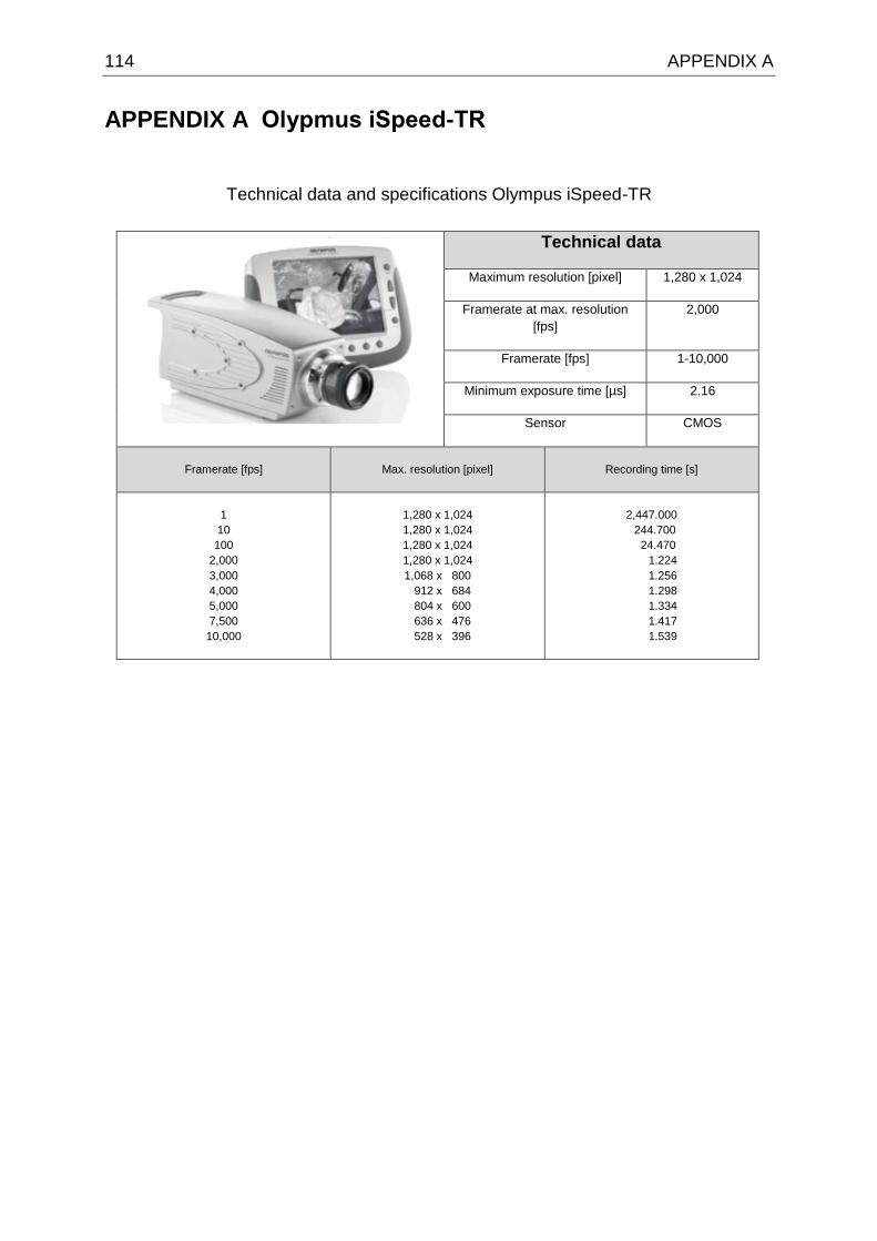
114 APPENDIX A
APPENDIX A Olypmus iSpeed-TR
Technical data and specifications Olympus iSpeed-TR
Technical data
Maximum resolution [pixel] 1,280 x 1,024
Framerate at max. resolution
[fps]
2,000
Framerate [fps] 1-10,000
Minimum exposure time [µs] 2.16
Sensor CMOS
Framerate [fps]
Max. resolution [pixel]
Recording time [s]
1
10
100
2,000
3,000
4,000
5,000
7,500
10,000
1,280 x 1,024
1,280 x 1,024
1,280 x 1,024
1,280 x 1,024
1,068 x 800
912 x 684
804 x 600
636 x 476
528 x 396
2,447.000
244.700
24.470
1.224
1.256
1.298
1.334
1.417
1.539
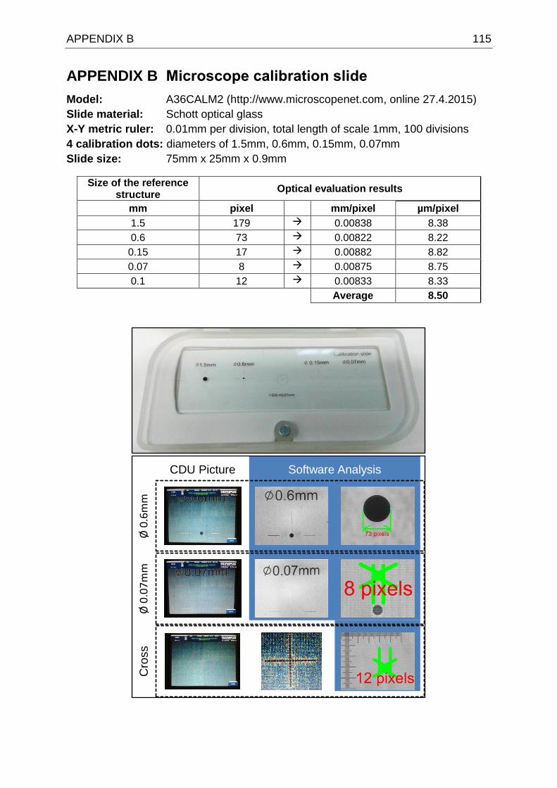
APPENDIX B 115
APPENDIX B Microscope calibration slide
Model: A36CALM2 (http://www.microscopenet.com, online 27.4.2015)
Slide material: Schott optical glass
X-Y metric ruler: 0.01mm per division, total length of scale 1mm, 100 divisions
4 calibration dots: diameters of 1.5mm, 0.6mm, 0.15mm, 0.07mm
Slide size: 75mm x 25mm x 0.9mm
Size of the reference structure
Optical evaluation results
mm pixel mm/pixel µm/pixel
1.5 179 0.00838 8.38
0.6 73 0.00822 8.22
0.15 17 0.00882 8.82
0.07 8 0.00875 8.75
0.1 12 0.00833 8.33
Average 8.50
CDU Picture Software Analysis
Cro
ss
Ø 0
.07
mm
Ø 0
.6m
m