Risk of Subsidence and Aquifer Contamination due to ... · Ali Zidane aus Libanon Basel, 2013 _____...
146
Risk of Subsidence and Aquifer Contamination due to Evaporite Dissolution: Modelization of Flow and Mass Transport in Porous and Free Flow Domains Inauguraldissertation zur Erlangung der Würde eines Doktors der Philosophie vorgelegt der Philosophisch-Naturwissenschaftlichen Fakultät der Universität Basel und der Université de Strasbourg Ecole Doctorale Science de la Terre, de l'Univers et de l'Environnement von Ali Zidane aus Libanon Basel, 2013
Transcript of Risk of Subsidence and Aquifer Contamination due to ... · Ali Zidane aus Libanon Basel, 2013 _____...

Risk of Subsidence and Aquifer Contamination due to Evaporite Dissolution: Modelization of Flow and Mass
Transport in Porous and Free Flow Domains
Inauguraldissertation
zur Erlangung der Würde eines Doktors der Philosophie
vorgelegt der Philosophisch-Naturwissenschaftlichen Fakultät
der Universität Basel
und der
Université de Strasbourg Ecole Doctorale Science de la Terre, de l'Univers et de l'Environnement
von
Ali Zidane aus Libanon
Basel, 2013

___________________________________________________________________________ Genehmigt von der Philosophisch-Naturwissenschaftlichen Fakultät der Universität Basel auf Antrag von
Prof. Dr. Peter Huggenberger Prof. Dr. Anis Younes Prof. Dr. Georg Kaufmann
Basel, 11 Dezember 2012 Prof. Dr. Jörg Schibler Dekan

Acknowledgements The work presented in this thesis was carried out in the Applied and Environmental Geology
Group (AUG), Institute of Geology and Paleontology, Department of Environmental Sciences
of the University of Basel. And in part within the “Laboratoire d’Hydrologie et de Géochimie
de Strasbourg (LHyGeS)”, in Strasbourg, France.
Many people have supported this project. First of all I wish to thank my supervisor in
Basel Prof. Peter Huggenberger for providing this chance to me and for his support and
encouragement during all this time. I also thank my supervisor in Strasbourg Prof. Anis
Younes for the knowledge, the advice and the great support he has passed on and the freedom
granted throughout my dissertation.
I am grateful to the jury members for their important critics, professors: Philippe Ackerer,
’’Directeur de recherches au LHyGeS’’, Georg Kaufmann ’’Head of a research unit at
Institut für geologische Wissenschaften Fachrichtung Geophysik Arbeitsgruppe Dynamik der
Erde’’, Brahim Amaziane ’’Maître de conférences au LMAP’’ and Eric Zechner
“Hydrogeologist Research Associate, Angewandte und Umweltgeologie, Dp.
Umweltwissenschaften‘‘
Lastly, I also wish to thank the members of the AUG and LHyGes for providing an
enjoyable and productive atmosphere and for their great support. In particular I thank Jannis
Epting, Stefan Scheidler, Rebecca Page, Stefan Wiesmeier, Silvia Leupin, Emanuel
Huber , Eva Vojtech, and Horst Dresmann. In Strasbourg I thank Fanilo Ramasomanana,
Noura Fajraoui, Salsabil Marzougi, Sana Ounaies and a very special thanks to Marwan Fahs.
Financial support for this project was provided by the Swiss National Science Foundation
(SNSF).

Table of contents
1
Table of contents
General introduction …………………………………...……………………..…5
Chapter 1…………………………………………………………………..… …. 10
Mathematical models for density driven flow in porous and free flow domains
1.1 The mathematical flow model ............................................................................ 11
1.1.1 The flow model in Porous media ................................................................. 11
Definition ..................................................................................................... 11
Governing equations .................................................................................... 12
Boundary conditions .................................................................................... 15
1.1.2 The free flow model ..................................................................................... 15
Definition ..................................................................................................... 15
Governing equations .................................................................................... 16
Boundary conditions .................................................................................... 16
1.2 The transport model ............................................................................................ 17
Definition ..................................................................................................... 17
Governing equations .................................................................................... 17
Boundary conditions .................................................................................... 19
1.3 Dissolution .......................................................................................................... 19
1.4 Coupling flow and transport models .................................................................. 19
Chapter 2…………………………………………………………………..… …. 21
Numerical models for density driven flow in porous and free flow domains
2.1 Flow discretization ............................................................................................. 22
2.1.1 Flow in porous media ................................................................................... 22
Introduction .................................................................................................. 22
The mixed finite element method ................................................................ 22
2.1.2 Discretization of free flow ........................................................................... 26
Introduction .................................................................................................. 26

Table of contents
2
The non-conforming Crouzeix-Raviart element .......................................... 27
2.2 Transport discretization ...................................................................................... 29
Introduction .................................................................................................. 29
The DG-MPFA discretization ...................................................................... 29
2.3 Dissolution.............................................................................................................. 32
Chapter 3…………………………………………………………………..… …. 33
Semi-analytical and numerical solutions for density driven flow in porous domains
3.1 Introduction ........................................................................................................ 35
3.2 Semianalytical method ....................................................................................... 36
3.3 New semianalytical strategy and numerical code .............................................. 37
3.3.1 Semianalytical strategy ...................................................................................... 37
3.3.2 Numerical code .................................................................................................. 37
3.4 Results and discussion ........................................................................................ 38
3.4.1 Case 1 ................................................................................................................ 38
3.4.2 Case 2 ................................................................................................................ 39
3.4.3 Case 3 ................................................................................................................ 40
3.4.4 Case 4 ................................................................................................................ 41
3.4.5 Case 5 ................................................................................................................ 42
3.4.6 Case 6a ............................................................................................................... 42
3.4.7 Case 6b .............................................................................................................. 43
3.5 Conclusion .......................................................................................................... 43
Appendix .................................................................................................................... 43
References .................................................................................................................. 44
Chapter 4…………………………………………………………………...……45
Semi-analytical and numerical solutions for density driven free flows
4.1. Introduction ........................................................................................................ 48

Table of contents
3
4.2. Mathematical Models ......................................................................................... 49
4.3. The semi-analytical solution ............................................................................... 50
4.4. The numerical solution ....................................................................................... 53
4.4.1 Stokes flow discretization…………………………………………………… 53
4.4.2 Mass transport discretization………………………………………………… 55
4.4.3 Coupling Stokes flow and mass transport……………….…………………... 57
4.5. Validation of the semi-analytical solution .......................................................... 57
4.5.1 Test case1: 0 008 0 1a . ;b . ………………………………………………... 57
4.5.2 Test case2: 0 006 0 05a . ;b . ……………………………………………….. 58
4.6. Conclusion .......................................................................................................... 58
Chapter 5…………………………………………………………………...……. 69
Salt dissolution process
5.1. Introduction ................................................................................................................ 72
5.2. Mathematical models .................................................................................................. 74
5.3.1. Discretization of the flow equation .................................................................... 75
5.3.2. Discretization of the transport equation ............................................................. 76
5.3.3. Dissolution model, moving boundary algorithm ................................................ 78
5.3. Time stepping procedure ............................................................................................ 79
5.4. Experimental set-up .................................................................................................... 80
5.5. Results and discussion ................................................................................................ 81
5.6. Conclusions ................................................................................................................ 81
Chapter 6…………………………………………………………………...……. 94
Evaporite dissolution and risk of subsidence
6.1. Introduction ........................................................................................................ 99

Table of contents
4
6.2. Model concept .................................................................................................. 101
6.3. Simulation of varying subsurface parameters .................................................. 103
6.4. Conclusions ...................................................................................................... 108
6.5. References......................................................................................................... 110
General conclusions and perspectives……………….…………………. .…....125
Bibliography…………………………………………………………………….128

Introduction
5
Introduction
Purpose
The importance of groundwater for the existence of human society cannot be overemphasized.
Indeed, groundwater is the major source of drinking water in both urban and rural areas.
Understanding the different mechanisms and phenomena that occur within the groundwater level
is essential for better management of a resource that has social and economic interests. On the
other hand the complexity and the cost to access the underground environment make it difficult
and sometimes impossible to study these mechanisms in-situ. Therefore, numerical modeling
appears as a useful tool to reproduce some observed phenomena and to predict others in order to
prevent as much as possible their negative effects on the environment.
A contribution to numerical methods has been made in this manuscript to simulate density driven
flow problems in porous and free flow domains. The validity of the numerical codes was proven
when compared against well-developed semi-analytical solutions for density driven flow in
porous media and in free flow media. When validated, the numerical models are used to study the
salt dissolution process. An adaptive mesh routine is developed and coupled to the density driven
flow code in free flow media in order to study the salt dissolution process in a fracture. Finally,
the density driven flow code in porous media is used to run a set of numerical simulations on a
2D cross section based on field measurements.
Regional subrosion
Groundwater circulation in evaporite bearing horizons and resulting dissolution (subrosion) of
salt frequently causes geomechanical problems such as land subsidence or collapses. Moreover,
the groundwater salt dissolution affects also the water quality, such as salinization and high
mineralization. A significant potential hazard arises if radioactive waste repositories are situated
in salt rock units. Salt deposits (e.g. rock salt), are largely widespread in a lot of continental
regions. The subrosion process is considered as a major concern in construction projects and
infrastructure planning (e.g. highways, railway connections). Moreover, the land subsidence
phenomenon can be detected in areas with densely populated residential wich causes important
infrastructural damages. The studied subrosion process studied in this thesis takes place in the
region of Muttenz-Pratteln area (Figure 1). The subrosion process within the study area was also
recorded in a 160 m of depth at the Adlertunnel, Basel, Switzerland which is part of a new
European North-South railway connection The study areas are located in the east of the city of

Introduction
6
Basel. These areas lie within the tectonic unit of the Tabular Jura, and they have been excessively
used for subsurface operations (e.g. groundwater pumping, water withdrawal for drinking water
supply, solution mining of halite). Further more, the studied areas are subdivided by a series of
NNE-SSW Horst and Graben structures.
Figure 1: Regional overview with working area
The Horst and Graben structure of the Tabular Jura in the area of Muttenz-Pratteln and the
Adlerhof-Anticline are explained in details in [Laubscher, 1982]. During an observation period of
78 days in 1997, land subsidence occurred in a section of the open-mined Adlertunnel at rates of
6 to 10 mm/month [Aegerter & Bosshardt, 1999].
Commonly the subrosion phenomenon is due to the extensive use of natural resources (e.g.
groundwater withdrawal for drinking water, solution mining of halite). Large scale groundwater
extraction and recharge may significantly increase the hydraulic gradients on large parts of the
aquifer which in turn would accelerate the karst evolution.
The first investigations on the relationship between solution mining and land subsidence were
made by [Trefzger 1925, 1950]. He compared subsidence and salt production rates for different
exploration wells in the Rheinfelden solution-mining district. And later the study continued with
[Hauber 1971] and recently with [Zechner et al. 2011].

Introduction
7
General overview
In order to develop and to validate the numerical codes required to simulate dissolution and
density driven transport, the thesis starts with the developed and the adopted mathematical and
numerical models (chapters 1-2).
In this work, we focus on the development of numerical models to simulate density flow in
porous and free flow free domains. The dissolution phenomenon and evolution of fractures over
time has been studied in this thesis as well. The developed models take into account the physical
processes (advection, dispersion, molecular diffusion) and chemical processes (dissolution) using
the equations of conservation of mass (PDEs) and the equation of dissolution. Efficient numerical
methods are used to solve these equations. The mixed finite element method (MFE) is used to
solve the flow in porous media and the nonconforming finite element method Crouzeix-Raviart
(CR) is used to solve the flow within fractures (non-porous media). The mass transport equation
is solved using the Multi-Point Flux Approximation method (MPFA) for the dispersion part and
the Discontinuous Galerkin method (DG) for the advection part. The simulation of the fractures
evolution is based on the development of a dynamic mesh method that adapts depending on the
amount of dissolved salt at the boundaries. The dissolution model is combined with the flow-
transport models in order to simulate density driven flow with fracture evolution.
In order to reach this goal, we needed first to validate the developed numerical codes. The first
part of the thesis addresses the validation of the numerical model to simulate density driven flow
in porous media. The simplified problem of saltwater intrusion in a coastal aquifer, known as the
Henry problem [Henry 1964], is widely used for the validation of numerical models. In fact, this
problem has a semi-analytical solution that was developed by Henry [Henry 1964] and corrected
by Ségol [1994]. However, this solution can only simulate saltwater intrusion with unrealistic
large amount of dispersion. The procedure developed by Henry is based on two steps: (i) an
approximation of the solution by using a Fourier series representation with a certain truncation
order of the coefficients and (ii) resolution of a strongly non-linear algebraic system to calculate
these coefficients. Since 1964 all the authors (Henry [1964] Ségol [1994], Simpson and Clement
[2004]) who worked on the Henry problem used the same iterative technique for solving the
obtained algebraic system. This iterative technique is based on a sequential resolution of
nonlinear systems of flow and mass transport. With this technique, convergence problems are
encountered when decreasing the value of molecular diffusion. In addition, the number of Fourier

Introduction
8
coefficients needed to calculate (and therefore the size of the nonlinear system to solve) increases
significantly when the diffusion decreases. To overcome these difficulties, a new procedure for
calculating the semi-analytical solution of the Henry problem is developed in this thesis. This
procedure consists of solving simultaneously the two systems of flow and transport by using the
Levenberg-Marquardt algorithm [Levenberg 1944, Marquardt 1963]. The use of this technique
allowed to develop, for the first time, semi-analytical solutions of saltwater intrusion in the case
of small diffusion and in the case of a large density contrast. These semi-analytical solutions were
compared to the numerical solutions and are therefore suited for density driven model validation
(chapter 3).
In the second part of this work, we studied the flow in fractured evaporitic rocks. The Stokes
equation that governs the flow is coupled to the advection dispersion equation via the state
equation relating the variation of the density to mass fraction. A numerical code was developed to
solve the nonlinear system using advanced numerical methods (MPFA-CR-DG). In order to
validate this new model a semi-analytical solution for a density Stokes flow is developed in this
thesis. This solution uses the same technique used for the Henry problem. Substituting Darcy's
equation by the Stokes equation in the Fourier-Galerkin method, we built a new nonlinear
algebraic system of equations. This system is more difficult to solve than the previous one
because of the high magnitude of the free flow velocities. Again, the Levenberg-Marquardt
algorithm is used to calculate the coefficients of the Fourier series of the semi-analytical solution.
This new semi-analytical solution could then be used to validate density driven flow for free
fluids (chapter 4).
The final part of this work is devoted to the transport problem with dissolution of rock salt.
In a first step of the dissolution study, we are interested in simulating salt dissolution within
fractures. The numerical model takes into account the density driven Stokes flow and the
dissolution of the fracture walls. A dynamic mesh algorithm is developed to track the evolution
of these walls over the time. A consistent dissolution profile is obtained when comparing the
numerical results with the experimental results for a simple fracture with reactive dissolution
walls (chapter 5).
Finally, and going to field scale, several observations and studies have been conducted on the salt
dissolution study and the rate of subsidence [Aegerter & Bosshardt, 1999, Laubscher, 1982
Spottke et al. 2005, Zechner et al. 2011]. The starting point was the results of Zechner et al.

Introduction
9
[2011] on a 2D cross section within the Muttenz-Pratteln area. These authors revealed that the
dissolution rate is very sensitive to the structure or dip of the halite formation. Therefore, more
concern was given in this thesis to the structure and tectonics of the aquifers and the fault zones
among other parameters to study their influence on the salt dissolution process and therefore on
the subsidence phenomenon. The boundary conditions used in these simulations are estimated
based on field measurements. The effect of several parameters was studied. The study showed,
however, that some parameters (well depth, hydraulic charge at the inlet of the aquifer) have
negligible effects on the dissolution. Other parameters (permeability, thickness of the lower
aquifer, fault geometry) have a considerable effect on the dissolution process (chapter 6).
Mathematical models for density driven flow in porous and free flow domains
10
Chapter 1
Mathematical models for density driven flow in porous and free flow
domains
Contents
1.1 The mathematical flow model ....................................................................................... 11
1.1.1 The flow model in Porous media ............................................................................ 11
Definition ................................................................................................................ 11
Governing equations ............................................................................................... 12
Boundary conditions ............................................................................................... 15
1.1.2 The free flow model ............................................................................................... 15
Definition ................................................................................................................ 15
Governing equations ............................................................................................... 16
Boundary conditions ............................................................................................... 16
1.2 The transport model ....................................................................................................... 17
Definition ................................................................................................................ 17
Governing equations ............................................................................................... 17
Boundary conditions ............................................................................................... 19
1.3 Dissolution ..................................................................................................................... 19
1.4 Coupling flow and transport models .............................................................................. 19
1. Chapter 1
Mathematical models for density driven flow in porous and free flow domains
11
1.1 The mathematical flow model
1.1.1 The flow model in Porous media
Definition
A porous medium is a solid containing void spaces (pores), connected or unconnected, dispersed
within it in either a regular or random manner. These so called pores may contain a variety of
fluids such as air, water, oil etc. If the pores represent a certain portion of the bulk volume, a
complex network can be formed which is able to carry fluids. Only these permeable and porous
media are taken into consideration in this volume.
Porosity
The porosity [-] of a material is determined by measuring the amount of void space inside, and
determining what percentage of the total volume of the material is made up of void space.
Porosity measurements can vary considerably, depending on the material. High or low
porosity will impact the way in which the material performs. For a material with a total volume tV
the porosity is given by:
p t s
t t
V V V
V V (1.1)
where
pV is the void volume (pore volume) and
sV is the volume of the solid material.
Permeability and intrinsic permeability
The intrinsic permeability k [L2] is the pertaining to the relative ease with which a porous
medium can transmit a liquid under a hydraulic or potential gradient. It is a property of the
porous medium and is independent of the nature of the liquid or the potential field.
The permeability K [L.T-1] is the rate at which liquids pass through a porous medium in a
specified direction. It is therefore the capacity for transmitting a fluid, measured by the rate at
which a fluid of standard viscosity can move a given distance through a given interval of
time. The permeability is a function of the intrinsic permeability k, the dynamic viscosity
[M.L-1.T-1] and the density of the circulating fluid [M.L-3]. The permeability K and the
Mathematical models for density driven flow in porous and free flow domains
12
intrinsic permeability k are scalar coefficients if the porous medium is isotropic, or if the flow
occurs only in one direction. Otherwise, the hydraulic conductivity matrix is given as follows:
xx xy xz
yx yy yz
zx zy zz
K K K
K K K
K K K
K (1.2)
with ijij
k gK
, where g [L.T-2] is the gravity acceleration.
Governing equations
The flow equation in a saturated porous media is described by a system of equations based on
Darcy’s law and the mass conservation equation or the continuity equation. In porous media,
Darcy’s law is considered as the analogous of the momentum conservation equation of the classic
fluid dynamics.
Darcy’s law
In 1856, Darcy established empirically that the flux of water Q [L3.T-1] through a permeable
formation with a section A [L2] and conductivity K [L.T-1] is proportional to the charge
difference 1 2H H H [L], and is inversely proportional to the distance L [L] separating two
points of charge 1 2H and H . Darcy’s law could be then written in the following form:
1 2H HQK
A L
(1.3)
Following [Bear 1979], the filtration velocity or Darcy’s velocity could be written in terms of
pressure gradient and gravity acceleration as follows:
p g z
k
q (1.4)
where
q : Darcy’s velocity [L.T-1];
k : The intrinsic permeability tensor of the medium [L2];
p : The pressure [M.L-1.T-2];
z : The depth [L].

Mathematical models for density driven flow in porous and free flow domains
13
The fluid velocity V [L.T-1] could be deduced from the Darcy’s velocity using the following
equation:
q
V (1.5)
The equivalent freshwater head h [L] is given in the following form:
0
ph z
g (1.6)
Using (1.6) and (1.4) the Darcy’s equation could be written in function of the freshwater head as
follows:
0
0
h z
q K (1.7)
where K [L.T-1] is the hydraulic conductivity tensor, and 0 [M.L-3] is the freshwater density.
If the density is considered as constant, equation (1.7) reduces to:
h q K (1.8)
Continuity equation
The continuity equation or the mass balance equation shows the principle of mass conservation of
the fluid. In a finite elementary volume (FEV), the amount of injected (or displaced) fluid should
be equal to the sum of the mass variation within an interval of time and the mass flux passing
through the volume. This could be given by the following equation [Bear 1979]:
. ps psf
t
q (1.9)
Assuming that the porosity is a function of the pressure, and the density is a function of the
pressure and the solute mass fraction (at a constant temperature), the first term in equation (1.9)
could be written in the following form:
p C
t t t p p t C t
(1.10)
Using the definitions of the porous matrix compressibility coefficient and the fluid
compressibility coefficient as given by Bear [Bear 1979]:
1 1
,1 p p
(1.11)
Equation (1.10) becomes:

Mathematical models for density driven flow in porous and free flow domains
14
p C
St t C t
(1.12)
with
psf [L3.T-1] is the sink/source term;
ps [M.L-3] is the sink/source density;
C [Mass solute/Mass fluid] is the solute mass fraction;
S [M-1.L.T2] is the specific pressure storativity for a rigid solid matrix and it’s given as follows:
(1 )S (1.13)
The continuity equation (1.9) could be then written in the following form:
. ps ps
p CS f
t C t
q (1.14)
Approximations
Referring to [Ackerer and Younes 2008], two approximations could be used with the mass
balance equation.
The Oberbeck–Boussinesq approximation: where density variations are neglected in the
fluid mass balance:
. psf
t
q
(1.15)
The density variation in the fluid flow direction is neglected, and the fluid mass
conservation equation (1.9) becomes:
. ps psft
q (1.16)
As stated by [Kolditz et al 1998, Johannsen et al 2002, Ackerer and Younes 2008] Boussinesq
assumption may introduce errors and should be avoided. The assumption stated by Bear [Bear
1979] consists in neglecting . q , which represents the density variations in the flow direction.
This approximation has been found efficient without particular loss of accuracy. Hence, the
continuity equation could be written in the following form:
. ps ps
p CS f
t C t
q (1.17)
Using (1.6) we get:

Mathematical models for density driven flow in porous and free flow domains
15
.s ps ps
h CS f
t C t
q (1.18)
where sS gS is the specific mass storativity related to head changes [L-1].
Boundary conditions
Three main types of boundary conditions are used when studying the fluid flow in porous media,
and they are stated as follows:
Dirichlet conditions
In this case the hydraulic charge is imposed at one or different sides of the domain.
, ,Dh x t h x t (1.19)
where ,Dh x t is a known function.
Neumann conditions
This type of boundary conditions consists of imposing a normal flux on one or different sides of
the domain.
. ,Nhq x t
q η K
η (1.20)
where η is the unit normal vector, and ,Nq x t is a known flux value.
Cauchy or Fourier conditions
These are mixed conditions of charge and flow. In certain cases, the flux is described as a
function of the charge, as follows:
. , ,F Fhg x t h f x t
q η K
η (1.21)
where ,Fg x t and ,Ff x t are known quantities.
1.1.2 The free flow model
Definition
Fluid flow through channels, cavities and fractures are referred to free fluid or free flow. Single-
phase steady incompressible flow through a free flow media is governed by the Navier-Stokes
equation:
Mathematical models for density driven flow in porous and free flow domains
16
2. p u u u g (1.22)
and the continuity equation:
0. u (1.23)
where u [L.T-1] is the velocity vector, and [M.L-1.T-1] is the dynamic viscosity.
Governing equations
In the treated cases within this thesis, we assume that the flow is sufficiently slow to consider the
inertial forces in the flow field (the first nonlinear term in equation (1.22)) negligibly small
compared with the viscous and pressure forces. Therefore, in this case, the free-flow is governed
by the following Stokes equations [Happel and Brenner 1965]:
2u gp (1.24)
0. u (1.25)
Boundary conditions
Referring to [Gresho and Sani 1987, Conca et al. 1994, 1995, Jäger and Mikelić 2001] three types
of boundary conditions are used in Stokes flow:
Imposed velocity
In this type, the vertical and/or the horizontal velocities are imposed at one or different sides of
the domain.
impu=u (1.26)
where impu is a known velocity vector.
Free boundary
Known as free outflow boundary condition, and is given by the following equation:
0p u η η
(1.27)
Imposed pressure
The pressure p is prescribed at the boundary. Note that in this case, we set also the velocity
components in the tangential direction to zero on the same boundary. This condition is named
Normal flow/Pressure or straight-out boundary condition.
Mathematical models for density driven flow in porous and free flow domains
17
0
imp
t
p p
.
u η
(1.28)
where tη is the unit tangential vector along the side where the pressure is imposed.
1.2 The transport model
Definition
When water flows, it could transport different kinds of species or solutes, in a dissolute form. At
this end, different physical and chemical phenomena could occur in the transport process of these
solutes. The physical mechanisms within the transport are the advection, the molecular diffusion
and the kinematic dispersion. For the moment, we consider that there’s no reaction in the
transport process, and therefore we show at first the transport equation with no chemical
reactions.
Governing equations
Advection
The advection (or convection) corresponds to the migration of solutes during displacement of
water. This is the phenomenon by which the contaminant moves with the movement of the water
which could be governed by Darcy or Stokes law. The average displacement of the contaminant
by advection is directly proportional to the average flow velocity of the water. When the solute
does not react with the environment, the transfer rate of the solute is that of the fluid that moves.
The advection is described by the following hyperbolic equation:
0C
. Ct
q
(1.29)
where
C [ML-3] is the solute concentration;
q [L.T-1] is the Darcy’s velocity.
In the case of free flows, the Darcy’s velocity is simply replaced by u , and the porosity by
one. This is also applicable for the rest of the transport equations within this section.
Molecular diffusion
The molecular diffusion is a phenomenon which is independent of the velocity of the fluid as it
occurs even in the absence of flow (velocity). It is related to the existence of a concentration

Mathematical models for density driven flow in porous and free flow domains
18
gradient in the fluid and is derived from the agitation of the molecules that tends to homogenize
the solute concentration within the medium (migration of molecules from high concentration
areas to those with low concentrations). The solute mass flow transported by molecular diffusion
is calculated according to Fick’s law:
0
C. C
t
mD (1.30)
where mD [L2.T-1] is the molecular diffusion diagonal tensor.
Dispersion
Dispersion is the transport phenomenon resulting from the combined action of these two
processes: Kinematic dispersion and molecular diffusion. The dispersion-diffusion transport
approaches a parabolic equation type and is given by:
0
C. C
t
D (1.31)
where
k mD D D is the dispersion tensor, given as follows :
, 2
i jM ij L T T ij
q qD D D D
q (1.32)
with
kD is the kinematic dispersion tensor;
LD the longitudinal dispersion coefficient, 0.52 2,L L i jD with q q q q ;
TD the transverse dispersion coefficient, T TD q ;
L the longitudinal dispersivity in the direction of flow;
T the transverse dispersivity normal to the direction of flow;
ij the Kronecker delta.
Advection-dispersion equation
The mathematical model that describes the transport of a solute with no interaction with the solid
matrix is given by the advection-dispersion equation as follows:
0
C. C . C
t
q D (1.33)

Mathematical models for density driven flow in porous and free flow domains
19
For free flows, the transport equation becomes:
0
C. C . D C
t
u (1.34)
where u is the flow velocity, and D is the diffusion coefficient.
Boundary conditions
The associated boundary conditions could be:
Dirichlet type (imposed concentration);
Neumann type (imposed concentration gradient);
Cauchy type (flux related to concentration).
1.3 Dissolution
In case of dissolution, the transport equation is written in the following form:
s
C. C . C Q
t
q D (1.35)
For free flows, the transport equation becomes:
s
C. C . D C Q
t
u (1.36)
where sQ is the dissolution flux, given as follows:
s satQ C C (1.37)
where [mol.L-2.T-1] is the mass transfer coefficient, and satC is the saturation concentration.
1.4 Coupling flow and transport models
Flow and transport equations are coupled by state equations linking density and viscosity to mass
fraction. We use a linear model for density and a power formulation for viscosity:
10 1 0 0
0
,
C
C and
(1.38)
where 1 and 1 are respectively the density and viscosity of the saturated (high density) fluid,
0 and 0 are the density and viscosity of the displaced (less dense) fluid. Note that different state
equations may be used for density and viscosity [Dierch and Kolditz 2002].

Mathematical models for density driven flow in porous and free flow domains
20
The following diagram shows the coupling between the transport and the flow equations:
0 0
0
. 0s
h CS
t C t
gh z
q
q k
2
0
p
.
u g
u
Flow in porous media Free flow Boundary conditions: imposed head or flux Boundary conditions: pressure or velocity Initial conditions : 0( )h t constant Initial conditions : 0( )h t constant
orq u , ,C
. . 0C
C Ct
q D
Boundary conditions : imposed concentration or dispersive flux Initial conditions : 0( )C t constant

Numerical models for density driven flow in porous and free flow domains
21
Chapter 2
Numerical models for density driven flow in porous and free flow
domains
Contents
2.1 Flow discretization ................................................................................................ 22
2.1.1 Flow in porous media ..................................................................................... 22
Introduction .................................................................................................... 22
The mixed finite element method .................................................................. 22
2.1.2 Discretization of free flow.............................................................................. 26
Introduction .................................................................................................... 26
The non-conforming Crouzeix-Raviart element ............................................ 27
2.2 Transport discretization ........................................................................................ 29
Introduction .................................................................................................... 29
The DG-MPFA discretization ........................................................................ 29
2.3 Dissolution ............................................................................................................ 32
2. Chapter 2

Numerical models for density driven flow in porous and free flow domains
22
2.1 Flow discretization
2.1.1 Flow in porous media
Introduction Different methods are used to solve the flow problem. Among them we cite the most used which
are: Finite Volumes (FV), Finite Differences (FD) and Finite Elements (FE). Detailed studies on
the application of conventional techniques for solving problems of hydrogeology are presented
by Remson et al. [1971] and Wang and Anderson [1982]. Each of these methods has its own
advantages and disadvantages. Since the flow equation should be coupled with the transport
equation (See Chapters 3, 4) the numerical flow model should provide accurate velocity field
with continuous fluxes between adjacent elements even for highly heterogeneous domains with
unstructured meshes.
The FD and FV Methods allow the calculation of an average head per element. They give an
exact mass balance at each element. The discretization of the flow equation with FDs is easy to
develop but it can only be applied on rectangular (2D) or cubic (3D) meshes. Similarly, the FV
method on triangular meshes requires triangles satisfying the Delaunay criterion (no point of a
triangle is inside the circumcircle of any other triangle of the domain). This criterion cannot be
easily applied on tetrahedrons. In addition, FV and FD approaches are not suitable for solving
problems where the hydraulic conductivity K is represented by a full discontinuous tensor.
Unlike FD and FV, the FE method allows the discretization of domains with complex geometry
and full parameter tensor. However, continuity of the normal component of the velocity between
adjacent elements in not guaranteed with the standard FE method. To overcome these difficulties,
we use the mixed finite element method for the discretization of flow in porous media.
The mixed finite element method The basic idea of the mixed finite element method is to approach simultaneously the hydraulic
head H and the flow velocity q . This approach has been used for the first time by Meissner
[1973], and later by Raviart and Thomass [1977]. The MFE method provides exact mass balance
for each element and preserves the same order of convergence for the hydraulic head H and the
flow velocity q . On the other side, it’s a well-adapted method for heterogeneous domains,
discretized with irregular meshes. In the following, we recall the main stages for the
discretization of the flow equation using the MFE method.

Numerical models for density driven flow in porous and free flow domains
23
The mixed finite element approach consists in writing the mass balance equation and Darcy’s
law separately in a variational form but with different basis functions. The mass balance
equation in (1.18) is discretized in a finite volume way and a fully implicit scheme which leads
to [Ackerer and Younes 2008, Younes et al. 2009]:
1
1 1n npsn
s i psi
h h CS E Q E f E
t C t
(2.1)
where E is the area of element E. With MFEs, the velocity inside each triangle E is
approximated with linear vectorial basis functions:
3
1
E Ej j
j
Q
q w (2.2)
where EjQ is the flux across the edge j of the element E and E
jw are the Raviart-Thomas basis
functions given by
1
2E ,iE
j
E ,i
x - x
E z - z
w (2.3)
and verify
1
0j
i j
E
if i j
if j i
w n (2.4)
where E ,ix and E ,iz are the coordinates of the vertex i of E (opposed to the edge i), jn is the unit
normal outwardly oriented vector and Ej the edge j of E .
Darcy’s law (1.7) could be written in the following form:
0-1 0
0
gh z
k q (2.5)
where k is the matrix of the intrinsic permeabilities with 2det( ) 0x z xzk k k k .
Equation (2.5) is written in a variational form which leads to:
1 00 0
0
0 0
1( ). . .
. .
i i i
E E E
Ei i
E EE E
g h g z
gh g z
k q w w w
w w
(2.6)

Numerical models for density driven flow in porous and free flow domains
24
Using Green’s formula and (2.4), we obtain,
1 0 0
0 0
( ). . .Ei i i E i i E
E EE E E E E
EE Ei E Ei
E E
gh h g z z
gh Th g z z
k q w w w n w w n
(2.7)
where Eh is the average head in element E, Ez the z-coordinate of the centre of E , EiTh the
average head on edge i of element E, Eiz the z-coordinate of the midpoint of edge i and E
represents the three element edges.
Combining (2.2) and (2.7) leads to the following matrix form:
3
0 00
1 0 0
E EE E E Eij j E E i i
j E
gB Q h z Th z
(2.8)
where:
1Tij i j
E
B w k w (2.9)
If we define ijr as the edge vector from node i toward node j , and ijl by :
1Tij ij ijl
r k r (2.10)
ijl verify the following properties:
12 Tij jk ik jk kil l l r k r , i, j ,k all different (2.11)
which leads to:
12 13 23 12 13 23 12 13 23
12 13 23 12 13 23 12 13 23
12 13 23 12 13 23 12 13 23
3 3 3 31
3 3 3 348
3 3 3 3
l l l l l l l l l
l l l l l l l l lE
l l l l l l l l l
B (2.12)
One notices that,
3
12 13 231
1
48ijj
B l l l LE
(2.13)
Despite the advantages of MFEs, the solution obtained is not unconditionally stable when using
small time steps. To overcome this problem, Younes et al. [2006] developed a mass lumping
procedure for the MFEs. The objective of this procedure is to avoid over and undershoots of the
standard MFE method when the time step is too small. Small time steps may be necessary to
Numerical models for density driven flow in porous and free flow domains
25
reach convergence for highly nonlinear problems. The main idea of the approach is to distribute
sink/source term and accumulation term for each element over its edges. Due to this re-
distribution, the new fluxes EiQ at the element level are defined by:
0Ei
i
Q (2.14)
Using (2.8) and 3
1
1
3E Ejj
z z
, leads to
3
1
1
3E Ejj
h Th
(2.15)
Inserting (2.15) into (2.8) the new flux through edge i is then:
0 0
0
E Ei ij j ij Ej
j jE
gQ N Th N z
(2.16)
with
T 1 T 1 T 123 23 23 31 23 12
T 1 T 1 T 131 23 31 31 31 12
T 1 T 1 T 112 23 12 31 12 12
det( )
E
r k r r k r r k rk
N r k r r k r r k r
r k r r k r r k r
(2.17)
The new flux EiQ corresponds to the actual flux under steady state conditions and without
sink/source terms. The second step in the mass lumping procedure consists in writing continuity
between elements E and E’ having common edge i. The continuity is written including the
‘equivalent steady state’ new fluxes EiQ , the storage and sink/source terms distributed over each
element edge, which leads to:
1
1
'
3
'0
3
n nps i i
i ps
E
n nps i i
i ps s
E
E Th ThCQ f S
C t t
E Th ThCQ f S
C t t
(2.18)
where the first and the second terms in (2.18) represent the characteristics restricted to element E
(resp. E’). The fluxes EiQ are estimated at time n+1, which leads to the following system
equation:

Numerical models for density driven flow in porous and free flow domains
26
110
110
0
0
1
3
1
3
3
3
i , j
nn ij s
j E
nn i
i , j j sj E'
nps i
i , j Ej ps sj E
nps i
i , j Ej ps sj E'
g ThN Th S E
t
g ThN Th S E'
t
E ThCg N z f S
C t t
Eg ThCN z f S
C t t
(2.19)
Equation (2.19) represents the discretized flow equations (1.7) and (1.18). Because the simplified
fluid mass balance (1.16) is used, the only time varying coefficients in the flow system matrix
are the viscosity and the time step length. If it can be assumed that the viscosity remains constant
and as long as the time step length is not modified, the system matrix does not change. In the
standard approach, the fluid mass balance equation (1.9) is used and the flow matrix has to be
built for each iteration. When the flow matrix is not re-build, direct solvers are very appropriate
and the system matrix has to be factorized once.
2.1.2 Discretization of free flow
Introduction Different methods can be used for the discretization of the Stokes equation [Langtangen and
Mardal 2002]. Boffi et al. [2008] detailed the properties of the finite elements used for the Stokes
problem, going from the cheapest element (Mini element, Me) to the most expensive one
(Taylor-Hood, TH). Some of the presented elements do not satisfy the mass conservation
properties. On the other side and due to stability conditions the system (1.24)-(1.25) cannot be
discretized with the same order for pressure and velocity approximations. Otherwise some sort of
stabilization is added to the mixed formulation [Li and Chen 2008]. To avoid these difficulties,
we use the non-conforming Crouzeix-Raviart (CR) elements for the velocity approximation in
combination with constant pressure per element, since they satisfy the Babuska-Brezzi condition
[Brezzi and Fortin 1991, Girault and Raviart 1986, Gresho and Sani 1998]. This condition is
central for ensuring that the final linear system to solve is non-singular [Langtangen 2002].
Moreover, the non-conforming Crouzeix-Raviart (CR) element has local mass conservation
properties [Bruman and Hansbo 2004] and leads to a relatively small number of unknowns due to
the low-order shape functions. The CR element is used in many problems such as the Darcy-

Numerical models for density driven flow in porous and free flow domains
27
Stokes problem [Bruman and Hansbo 2005], the Stokes problem [Crouzeix and Raviart 1973]
and the elasticity problem [Hansbo and Larson 2002, 2003]. The CR element gives a simple
stable optimal order approximation of the Stokes equations [Arnold 1993]. In the next section, we
recall the main stages for the discretization of the Stokes equation with the CR triangular
element.
The non-conforming Crouzeix-Raviart element
With the non-conforming finite element method, the degrees of freedom for the velocity vector u
are the two component i iu ,v of u at the midedge i facing the node i (Figure 2). Inside the
element E , we assume a linear variation of the velocity components E Eu ,v
E E E E E EE i i j j k k E i i j j k ku u u u , v v v v (2.20)
Figure 2: Crouziex-Raviart Finite element.
For an interior edge, the linear interpolation function i for the velocity is nonzero only on the
two adjacent elements E and E (see Figure 3) with
1 1
2Ei k j j k j k j i k i k j i j i kx z z y x x z x z x z x z x z x z x
E
(2.21)
where E is the area of the element E , ix and iz are the coordinates of the vertex i of E . The
interpolation function Ei equals 1 on the midedge i and zero on the midedges j and k of E
(Figure 3).
1
P
2
3
u3
v3
u1
v1
u2
v2

Numerical models for density driven flow in porous and free flow domains
28
Figure 3: the linear interpolation function for the velocity field.
The variational formulation of the Stokes equation (1.24) using the test function i over the
domain writes:
u Ι i i. p g z
(2.22)
where u is the gradient of the velocity vector u and Ι the 2 2 identity matrix.
Using Green’s formula, we get
u Ι η u Ιi i ip . p g z
(2.23)
The first integral contains boundary conditions. It vanishes in case of free-flow boundary or in
case of an interior edge i . In this last case, equation (2.23) becomes
u Ι u ΙE E' E EE E i E E i i i
E E E E
. p . p g z g z
(2.24)
Using (2.20) and (2.21), we obtain
3
1
3
1
u Ι
i j i jji
jEE E i Ei
i j i jEj
j
x x z z uz
. p PEx
x x z z v
(2.25)
and
i
Ei E i E i
E
zg z g z z
x
(2.26)
j
Eiϕ′
i
k Eiϕ
E’E
i

Numerical models for density driven flow in porous and free flow domains
29
where ij kx x x and i
k jz z z , Ez and iz are respectively the z-coordinate of the centre
of E and of the midpoint of edge i , E and Ep are respectively the mean density and pressure
over E . The finite volume formulation of the continuity equation (1.25) over the element E
writes:
0uE
. (2.27)
using (2.20), it becomes
3
1
0j jj j
j
z u x v
(2.28)
The final system to solve for the flow is obtained by writing equation (2.25) for each edge (two
equations per edge) and equation (2.28) for each element.
2.2 Transport discretization
Introduction For the transport equation, standard numerical methods, such as standard finite elements or finite
volumes, are known to generate solution with numerical diffusion and/or non-physical
oscillations when advection is dominant. These problems can be avoided with the discontinuous
Galerkin method (DG) [Siegel et al. 1997]. Indeed, DG leads to a high-resolution scheme for
advection that has been proven to be clearly superior to the already existing finite element
methods [Arnold et al. 2002].
In this manuscript, the explicit DG method, where fluxes are upwinded using a Riemann solver is
used to solve the advection equation and combined with the symmetric Multipoint Flux
Approximation (MPFA) method for the diffusion equation. In the next section we show the
discretization of the transport equation in free flow media. The discretization is quite the same in
porous media, with some minor modifications (Darcy’s velocity, porosity, dispersion tensor).
The DG-MPFA discretization The transport equation (1.35) with no sink/source terms is written in the following mixed form
[Younes et al. 2009, 2011]:
0u u
u
D
D
C. C .
tD C
(2.29)

Numerical models for density driven flow in porous and free flow domains
30
The dispersive flux uD is assumed to vary linearly inside the element E , therefore,
1
u ED D, Ei
i
. QE (2.30)
where u ηED, Ei D Ei
Ei
Q .
is the dispersive flux across the edge Ei of E .
We use the P1 DG method where the approximate solution ( , )hC tx is expressed with linear basis
functions Ei on each element E as follows:
3
1
, | E Eh E i i
i
C t C t
x x (2.31)
where EiC t are the three unknown coefficients corresponding to the degrees of freedom which
are the average value of the mass fraction defined at the triangle centroid E Ex ,z and its
deviations in each space direction [Cockburn et al. 1989] with the corresponding interpolation
functions:
1 2 3, 1, , , , . E E EE Ex z x z x x x z z z (2.32)
The variational formulation of (2.29) over the element E using Ei as test functions leads to:
*
,
. .
10
Ej E E E E E E E E
j i j j i j j ij j jE E E
E E Ei E D j i
EjE E
CC C
t
C QE
u u
u.η
(2.33)
This could be written in the following matrix form:
1
,
1 1 1302
2 2 21
3 3 33
0
0
E
ED jE E E
EjEE E E
E E EE
dCQdt C C C
dCA B C M C M C
dtC C C
dC
dt
(2.34)
with,
, ,
N0, ,
1
.
, 1 1,..,3
u
E
E E E Ei j j i i j j i
E E
E EE E E E E EE E
i j E i j i j E i j
E E
A B
Q QM M
E E

Numerical models for density driven flow in porous and free flow domains
31
where Ej is the adjacent element to E such that Ej is the common edge of E and Ej and
.EE Ej
E
Q
uη the water flux across Ej . The upwind parameter EE is defined by
1 . 0
0 . 0EjE
EjEj
if
if
uη
uη (2.35)
An explicit time discretization is used for the equation (2.34). An efficient geometric slope
limiter is used to avoid unphysical oscillations near sharp fronts [Younes et al. 2010b].
The dispersive fluxes ,ED jQ across edges are approximated using the MPFA method. The basic
idea of this method is to divide each triangle into 3 sub-cells as in Figure 4.
Inside the sub-cell 1 2O,F ,G,F formed by the corner O , the centre G and the midpoint edges
1F and 2F , we assume linear variation of the mass fraction between 1EC , 1TC and 2TC , the mass
fractions respectively at G and the two continuity points 1f and 2f . The symmetry of the MPFA
is achieved when the continuity points are localized at 1 2
1 2
2
3
Of Of
OF OF . In this case 1 2O, f ,G, f
is a parallelogram. Therefore, half-edge fluxes1 2
1 2andF F
O O
O O
Q D C Q D C
, taken
positive for outflow simplifies to [Younes and Fontaine 2008b]:
1
1 1 1 2 1 12
2 11 2 2 2
EO
E EO
OF .OF OF .OFQ TC C
Q TC COF .OF OF .OF
(2.36)
with 3E D E .
Figure 4: Triangle splitting into three sub-cells and linear concentration approximation on the sub-cell.
O
G 2f
1f
1OQ
2OQ
2F
1F
R
P
Numerical models for density driven flow in porous and free flow domains
32
This system is written for all sub-cells sharing the vertex O which create an interaction region.
Then by writing continuity of diffusive fluxes across half-edges and continuity of mass fraction at
continuity points, we obtain a local system A TC B C . This local system is solved to
obtain the mass fraction at the continuity points ( iTC ) as function of mass fraction at all elements
sharing the vertexO . The obtained relation is then substituted into (2.36) to obtain half-edge
fluxes explicitly as a weighted sum of the cell mass fraction of the interaction volume. Finally,
the summation of these fluxes is written using an implicit time discretization and substituted into
the equation (2.34).
2.3 Dissolution The DG method is also used for the discretization of the dissolution equation. Hence, multiplying
the dissolution equation (1.37) by the test function Ei defined in (2.32) we get:
1( ) (1 )E E n E n E
E i E i E i E i
E E E E
sat satC C C C C (2.37)
where nC and 1nC are the concentrations at the time step n and 1n respectively. We use a
time discretization where is such that:
0,
1,
for a full explicit scheme
for a full implicit scheme
(2.38)
The first right side term in (2.37) is treated as a constant quantity and is therefore added to the right hand side term of the global transport equation. The last two terms in (2.37) are added to equation (2.34).
Semi-analytical and numerical solutions for density driven flow in porous domains
33
Chapter 3
Semi-analytical and numerical solutions for density driven flow in
porous domains
Contents
3.1 Introduction ............................................................................................................. 35
3.2 Semianalytical method ............................................................................................ 36
3.3 New semianalytical strategy and numerical code ................................................... 37
3.3.1 Semianalytical strategy ...................................................................................... 37
3.3.2 Numerical code .................................................................................................. 37
3.4 Results and discussion ............................................................................................ 38
3.4.1 Case 1 ................................................................................................................ 38
3.4.2 Case 2 ................................................................................................................ 39
3.4.3 Case 3 ................................................................................................................ 40
3.4.4 Case 4 ................................................................................................................ 41
3.4.5 Case 5 ................................................................................................................ 42
3.4.6 Case 6a ............................................................................................................... 42
3.4.7 Case 6b .............................................................................................................. 43
3.5 Conclusion .............................................................................................................. 43
Appendix .................................................................................................................... 43
References .................................................................................................................. 44

Semi-analytical and numerical solutions for density driven flow in porous domains
34
Semi-analytical and numerical solutions for density driven flow in
porous domains
Paper published in water resources research journal
The Henry semianalytical solution for saltwater intrusion with reduced dispersion
Ali Zidane(1,2), Anis Younes(2) , Peter Huggenberger(1), Eric Zechner(1)
(1) Institute of Geology and Paleontology, Environmental Sciences Department, University of Basel, Bernouillistr. 32, 4056
Basel, Switzerland
(2) Laboratoire d’Hydrologie et de Geochimie de Strasbourg, University of Strasbourg, CNRS UMR 7517, Strasbourg,
France

The Henry semianalytical solution for saltwater intrusion withreduced dispersion
Ali Zidane,1,2 Anis Younes,1 Peter Huggenberger,2 and Eric Zechner2
Received 18 July 2011; revised 7 May 2012; accepted 11 May 2012; published 27 June 2012.
[1] The Henry semianalytical solution for salt water intrusion is widely used forbenchmarking density dependent flow codes. The method consists of replacing the streamfunction and the concentration by a double set of Fourier series. These series are truncatedat a given order and the remaining coefficients are calculated by solving a highly nonlinearsystem of algebraic equations. The solution of this system is often subject to substantialnumerical difficulties. Previous works succeeded to provide semianalytical solutions onlyfor saltwater intrusion problems with unrealistic large amount of dispersion. In this work,different truncations for the Fourier series are tested and the Levenberg-Marquardtalgorithm, which has a quadratic rate of convergence, is applied to calculate theircoefficients. The obtained results provide semianalytical solutions for the Henry problem inthe case of reduced dispersion coefficients and for two freshwater recharge values: theinitial value suggested by Henry (1964) and the reduced one suggested by Simpson andClement (2004). The developed semianalytical solutions are compared against numericalresults obtained by using the method of lines and advanced spatial discretization schemes.The obtained semianalytical solutions improve considerably the worthiness of the Henryproblem and therefore, they are more suitable for testing density dependent flow codes.
Citation: Zidane, A., A. Younes, P. Huggenberger, and E. Zechner (2012), The Henry semianalytical solution for saltwater intrusion
with reduced dispersion, Water Resour. Res., 48, W06533, doi:10.1029/2011WR011157.
1. Introduction[2] Saltwater intrusion into unconfined coastal aquifers
has been largely investigated using laboratory experiments[e.g., Goswami and Clement, 2007; Thorenz et al., 2002]and/or numerical simulations [e.g., Park and Aral, 2008].However, the existence of a semianalytical solution madethe synthetic Henry saltwater intrusion problem [Henry,1964] as one of the most widely tests used for verificationof density driven flow codes. The problem describes steadystate saltwater intrusion through an isotropic confined aqui-fer. Freshwater enters the idealized rectangular aquifer(Figure 1 ) with a constant flux rate from the inland (left)boundary. A hydrostatic pressure is prescribed along thecoast (right) boundary where the concentration correspondsto seawater concentration. The top and the bottom of the do-main are impermeable boundaries. The saltwater intrudesfrom the right until an equilibrium with the injected fresh-water is reached. The semianalytical solution of Henry[Henry, 1964] provides the steady state isochlors positionsby expanding the salt concentration and the stream function
in double Fourier series. Henry [1964] used only 78 termsin these series and calculated the coefficients using a Gausselimination procedure with full pivoting. Pinder andCooper [1970] were the first to simulate the Henry problemusing a transient numerical code with two different initialconditions to ensure convergence to the steady state solu-tion. The obtained results as well as those obtained later by[Segol et al., 1975; Frind, 1982; Huyakorn et al., 1987]were not in agreement with Henry’s solution. In 1987, Vossand Souza [1987] showed that the discrepancies in the pub-lished papers were due to the use of different dispersioncoefficients in numerical and semianalytical calculations.However, solving this problem did not lead to a satisfactorymatching. Many possible reasons for the discrepancies havebeen invoked in the literature: for Huyakorn et al. [1987],the discrepancies may be due to the discretization errorswithin the numerical codes and/or to the use of differentboundary conditions at the seaward side between semiana-lytical and numerical codes. Indeed, the sea boundary con-dition used in the work of Frind [1982], Huyakorn et al.[1987], and Voss and Souza [1987] was not consistent withthe original Henry problem. Croucher and O’Sullivan[1995] presented a grid convergence study to evaluate thetruncation error due to the spatial discretization. Kolditzet al. [1998] claimed that the discrepancies may be due tothe inaccuracy of the Boussinesq approximation assumedby Henry.
[3] The most important reason for discrepancies hasbeen invoked by Voss and Souza [1987] who claimed that,due to the lack of computing resources, Henry’s truncationmay not contain enough terms in the Fourier series to
1Laboratoire d’Hydrologie et de Geochimie de Strasbourg, CNRS,UMR 7517, University of Strasbourg, Strasbourg, France.
2Department of Environmental Sciences, Institute of Geology and Pale-ontology, University of Basel, Basel, Switzerland.
Corresponding author: A. Younes, Laboratoire d’Hydrologie et de Geo-chimie de Strasbourg, CNRS, UMR 7517, University of Strasbourg, 1 rueBlessig, 67084, Strasbourg Cedex, France. ([email protected])
©2012. American Geophysical Union. All Rights Reserved.0043-1397/12/2011WR011157
W06533 1 of 10
WATER RESOURCES RESEARCH, VOL. 48, W06533, doi:10.1029/2011WR011157, 2012

represent accurately the solution. In 1994, Segol [1994]revaluated the semianalytical solution of Henry by using anew truncation of the Fourier series with 138 terms instead ofthe 78 used by Henry. The revaluated solution shows a goodagreement with the numerical results [e.g., Oldenbourg andPrues, 1995; Herbert et al., 1988; Ackerer et al., 1999; Buesand Oltean, 2000; Abarca et al., 2007, Younes et al., 2009].
[4] In 2003, Simpson and Clement [2003] performed acoupled versus uncoupled analysis to show that the trueprofile in the Henry problem is largely determined byboundary forcing and much less by the density-dependenteffects. In the uncoupled flow, the solute transport acts as atracer and has no influence on the flow equation. Toimprove the worthiness of the Henry problem, they sug-gested a decreasing of the fresh water recharge by half[Simpson and Clement, 2004]. The semianalytical solutionis revaluated in this case by using 203 terms in the Fourierseries [Simpson and Clement, 2004].
[5] Henry [1964], Segol [1994], and Simpson andClement [2004] used the same iterative technique to calcu-late the coefficients of the Fourier series. They solved thenonlinear system as a system of linear equations where theexpansion coefficients are considered as unknowns. Thenonlinear right hand side is treated as a known quantity,updated iteratively until convergence. As stated by Segol[1994], this technique encountered substantial convergencedifficulties for small values of the dispersion coefficient.Note that all published works succeeded to develop semian-alytical solutions only when an unrealistically large amountof dispersion is introduced in the solution. This deficiencywas pointed out by Kolditz et al. [1998] and by Voss andSouza [1987, p. 1857], who stated that due to the largeamount of dispersion, ‘‘this test does not check whether amodel is consistent or whether it accurately represents den-sity driven flows, nor does it check whether a model can rep-resent field situation with relatively narrow transition zones.’’
[6] In this work, we calculate the coefficients of the Fou-rier series by using the Levenberg-Marquardt algorithm,which has a quadratic rate of convergence, to solve thenonlinear algebraic system of equations. Different trunca-tions of the infinite Fourier series are tested. Semianalyticalsolutions for the Henry problem are developed in the caseof reduced dispersion coefficients and for two freshwaterrecharge values: the initial value suggested by Henry andthe reduced one suggested by Simpson and Clement [2004].The semianalytical solutions are compared against numeri-cal results obtained using a robust numerical model basedon the method of lines and advanced spatial discretizationschemes [Younes et al., 2009].
2. Semianalytical Method[7] To obtain the semianalytical solution, Henry [1964]
used a constant dispersion coefficient and assumed theBoussinesq approximation valid which implies the exis-tence of stream function. Using these assumptions, thesteady state flow and transport can be written in the follow-ing nondimensional form [Henry, 1964, Segol, 1994]:
a@2
@x2þ @
2
@y2
� �¼ @C
@xþ 1
�; (1)
b@2C
@x2þ @
2C
@y2
� �¼ @ @y
@C
@x� @ @x
@C
@yþ 1
�
@
@yþ @C
@xþ 1
�; (2)
where is the dimensionless stream function, C is thedimensionless concentration, � ¼ L
d is the aspect ratio of thedomain with L and d, which are the length and the depth ofthe aquifer, respectively.
[8] The nondimensional parameters a and b in the previ-ous equations are given by
a ¼ Q
k1dand b ¼ D
Q; (3)
where Q [L2T�1] is the freshwater recharge, D [L2T�1] is
the coefficient of dispersion, k1 ¼ K �s��0
�0
� �with K [LT�1]
the saturated hydraulic conductivity, �0 [ML�3] and �s[ML�3] are the freshwater and saltwater densities,respectively.
[9] The solution technique, known as Galerkin or Fourier-Galerkin solution [Forbes, 1988], is obtained by replacingthe stream function and the salt concentration by doubleFourier series of the form:
¼X1m¼1
X1n¼0
Am;n sinðm�yÞ cos n�x
�
� �; (4)
C ¼X1r¼0
X1s¼1
Br;s cosðr�yÞ sin s�x
�
� �: (5)
[10] Substituting these relations into equations (1) and(2), multiplying equation (1) by 4 sinðg�yÞ cosðh� x
�Þ andequation (2) by 4 cosðg�yÞ sinðh� x
�Þ, and integrating overthe rectangular domain gives an infinite set of algebraicequations for Ag;h and Bg;h namely,
"2a�2Ag;hðg2 þ h2Þ� ¼X1r¼0
Br;hhNðg; rÞ þ 4
�Wðg; hÞ; (6)
"1b�2Bg;h g2 þ h2
�2
� �� ¼
X1n¼0
Ag;ngNðh; nÞ þ "1
X1s¼1
Bg;ssNðh; sÞ
þ Quad þ 4
�Wðh; gÞ:
(7)
[11] The functions "1; "2; N ; W and Quad are detailedin Appendix A.
Figure 1. Domain and boundary conditions for the Henrysaltwater intrusion problem.
W06533 ZIDANE ET AL.: HENRY SEMIANALYTICAL SOLUTION WITH REDUCED DISPERSION W06533
2 of 10

[12] Segol [1994, p. 272] wrote about how Henry [1964]described his solution of the set of algebraic equations (6)and (7): ‘‘An iterative solution of equation (6) was used inwhich the B0;h were computed by several sub iterations andvice versa. The subiterative cycle consisted of recomputingthe values of the quadratic terms (Quad) using the revisedvalues of Bg;h (g > 0) while continuing to hold the B0;h
constant and then using these values to recompute the Bg;h
(g > 0).’’[13] This procedure for computing the coefficients of the
Fourier series was also used by Segol [1994] and Simpsonand Clement [2004]. The convergence rate of the methoddepends upon the values of the parameters a and b. Toovercome the convergence difficulties, Segol [1994] andSimpson and Clement [2004] used the solution with the pa-rameters a ¼ 0:263 and b ¼ 0:2 as an initial guess for theother parameterizations. Then, the parameters a and b, arereduced with small stepwise changes until the desired solu-tion is obtained. Segol [1994] stated that the value b ¼ 0:1was the lower limit of the range for which a stable and con-vergent solution can be obtained.
3. New Semianalytical Strategy and NumericalCode
[14] In the first part of this section, we describe the newstrategy used for solving the nonlinear system of algebraicequations to calculate the Fourier series coefficients of thesemianalytical solution. In the second part, we briefly describethe numerical code used to compare numerical and semiana-lytical results.
3.1. Semianalytical Strategy
[15] The procedure used by Henry [1964], Segol [1994]and Simpson and Clement [2004] encounters substantialnumerical difficulties because of its low convergence ratewhen lowering the values of the parameters a and/or b.Indeed, Segol [1994] stated that when lowering the value ofb, more coefficients are required to obtain a stable solutionand the convergence of the scheme becomes difficult. Toobtain a stable solution, Segol [1994] decreased the valueof b by considering small stepwise changes and iterating atintermediate steps. The value b ¼ 0:1 was the lower limitof the range for which a stable and convergent solution canbe obtained.
[16] To avoid these difficulties, we use in this work the Lev-enberg-Marquardt algorithm [Levenberg, 1944; Marquardt,1963], which has a quadratic rate of convergence to solve theset of nonlinear algebraic equations [Yamashita and Fukush-ima, 2001]. The Levenberg-Marquardt method is consideredas one of the most efficient algorithms for solving systems ofnonlinear equations. The nonlinear algebraic system of equa-tions (6)–(7) is written in the form FðXÞ ¼ 0 where X is avector formed by the coefficients Ag;h and Bg;h. The algorithmattempts to minimize the sum of the squares of the function.The method is a combination of two minimization methods:the gradient descent method and the Gauss-Newton method.Far from the optimum, the Levenberg-Marquard methodbehaves like a gradient descent method, whereas, it acts likethe Gauss-Newton method nearby the optimum.
[17] The Levenberg-Marquardt iterates starting from aninitial solution X0. At each iteration k, the new solution
Xkþ1 ¼ Xk þ dk is obtained from the solution of the follow-ing linear system
�JðXkÞT JðXkÞ þ �kI
�dk ¼ �JðXkÞT FðXkÞ; (8)
where J is the Jacobian.[18] Small values of the parameter �k correspond to the
Gauss-Newton update while the large ones correspond tothe gradient descent update. When the solution approachesthe minimum, the parameter �k is decreased, what makesthe algorithm tends to the Gauss-Newton method.
[19] In this study the Jacobian J is approximated numeri-cally using finite differences and the Levenberg-Marquardtparameter is initially fixed to �0 ¼ 0:01. During iterations,if the new estimate is sufficiently better than the old one,the parameter � is reduced by ten. Otherwise it is increasedby a factor of two. The tolerance is fixed to 10�12 for thesum of the squares of the function.
3.2. Numerical Code
[20] The semianalytical results will be compared againstaccurate numerical results obtained using a combination ofthe method of lines and advanced spatial discretizationschemes.
[21] The flow system is written in terms of equivalentfresh water head [Huyakorn et al., 1987]:
�S@h
@tþ " @�
@C
@C
@tþ �r � q ¼ 0; (9)
q ¼ � �0g
�k rhþ �� �0
�0
rz
� �; (10)
where � is the fluid density [ML�3], S the specific massstorativity related to head changes [L�1], h the equivalentfreshwater head [L], t the time [T], " the porosity [-], C thesolute mass fraction [M. salt/M. fluid], q the Darcy’s veloc-ity [LT�1], �0 the density of the displaced fluid [ML�3], gthe gravity acceleration [LT�2], � the fluid dynamic viscos-ity [ML�1T�1], k the permeability tensor [L2] and z thedepth [L].
[22] The solute mass conservation is written in term ofmass fraction:
@ð"�CÞ@t
þr � ð�Cq� �DrCÞ ¼ 0: (11)
[23] For the Henry problem, the dispersion tensor isassumed constant D ¼ D�I (I is the identity matrix) and thedensity is assumed to vary linearly with respect to the massfraction. Due to the form of the governing equation used byHenry, the value of the dispersion coefficient D� used inthe numerical code is equal to the value used in the semian-alytical solution divided by porosity ðD� ¼ D="Þ.
[24] To achieve high accuracy for the spatial discretiza-tion, each equation within the flow-transport system (9)–(11)is modeled with a specific numerical method. The flow equa-tion is discretized with the locally mass conservative MixedFinite Element method (MFE), that produces accurate andconsistent velocity field [Ackerer and Younes, 2008; Youneset al., 2009; Younes et al., 2010]. The advection part of the
W06533 ZIDANE ET AL.: HENRY SEMIANALYTICAL SOLUTION WITH REDUCED DISPERSION W06533
3 of 10

transport equation is discretized with the DiscontinuousGalerkin (DG) method which produces accurate solutioneven for problems involving sharp fronts [Siegel et al.,1997]. Finally, the multi-point flux approximation (MPFA)is used to discretize the dispersion equation [Younes andAckerer, 2008] since it is locally conservative and can treatgeneral irregular grids on anisotropic heterogeneous domains[Aavatsmark, 2002; Younes and Fontaine, 2008a, 2008b].The combination of the three spatial discretization methodsMPFA, DG and MFE, has proven to be accurate and robustfor modeling density driven flow problems [Younes and Ack-erer, 2008; Konz et al., 2009: Zechner et al., 2011].
[25] The Differential Algebraic Solver with Precondi-tioned Krylov (DASPK) time solver is used to solve theMFE_DG_MPFA spatial discretization with the method oflines. DASPK is a mature and sophisticated time integra-tion package for large-scale Ordinary Differential Equa-tions (ODE) or Differential Algebraic Equations (DAE)systems. DASPK uses the Fixed Leading Coefficient Back-ward Difference Formulas (FLCBDF). The BDF approachworks well on stiff problems and has good stability proper-ties. DASPK solves systems of the general form:
Fðt; y; y0Þ ¼ 0: (12)
[26] Predictor and corrector polynomials are constructedin order to estimate the truncation error. The time steplength and choice of order of integration (up to fifth order)are adapted to minimize the computational effort whilekeeping the local temporal truncation error � i small,� i � "i ¼ "rjyij þ "a where the relative "r and absolute "a
local error tolerances are specified by the user.[27] In this study, the Henry problem is discretized with
a uniform triangular mesh of 3200 elements (same resultswere obtained with 5000 and 8000 elements).
4. Results and Discussion[28] As stated, by Abarca et al. [2007], the drawbacks of
the Henry problem arise from the high values of the param-eters a and b that Henry used to obtain the semianalyticalsolution. Indeed, Henry chose the dimensionless parame-ters � ¼ 2:0, a ¼ 0:263 and b ¼ 0:1. Segol [1994] statedthat the value b ¼ 0:1 was the lower limit of the range forwhich a stable and convergent solution can be obtained.Simpson and Clement [2004] proposed a semianalytical so-lution where the parameter a is reduced by half and the pa-rameter b is increased by a factor of 2 (� ¼ 2:0, a ¼ 0:1315and b ¼ 0:2). In this section, the semianalytical solution for
the Henry problem is calculated using the Levenberg-Marquardt algorithm and compared to the numerical solu-tion for different test cases. Table 1 provides the freshwaterflux, the saltwater density and the diffusion coefficients foreach test case. Two values for the parameter a are tested:the initial one and the halved one. The values of the param-eter b are reduced until b ¼ 0:02 (Table 1). Different trun-cations of the Fourier series are tested: the 78 coefficientsof Henry [1964], the 138 coefficients of Segol [1994] andthe 203 coefficients of Simpson and Clement [2004]. A newtruncation using 424 terms is introduced to calculate thesemianalytical solution in the case of small dispersion val-ues. Two domains are used for the calculation of the semi-analytical solution: the initial domain with an aspect ratio� ¼ L=d ¼ 2 and a larger domain with � ¼ 3 (Table 1).Three concentration isochlors (0.25, 0.5 and 0.75) are usedfor the comparison between the semianalytical and the nu-merical solutions. Table 2 provides the position of the threeisochlors for the new provided test cases. The transient nu-merical simulations are performed until a long time toensure a steady state solution. Figure 2 shows the temporalvariation of the concentration in the element correspondingto the intersection of the 0.25 isochlor with the base att ¼ 800 min for the studied test cases. The results show thatthe time required to reach a steady state depends on the pa-rameters a and b. For all test cases, 500 min of time seemsto be sufficient to obtain a steady position for the isochlors.
4.1. Case 1: The Standard Henry Problem Witha 5 0.263, b 5 0.1, and n 5 2.0
[29] This case is the standard test case solved by Henry[1964] on an IBM 650 digital computer using 38 coeffi-cients for the expansion of the stream function and 40 coef-ficients for the expansion of the concentration. Segol[1994] revaluated the semianalytical solution using anexpansion with 38 coefficients for the stream function and100 coefficients for the concentration. Simpson and Clem-ent [2004] calculated the solution using 103 and 100 coeffi-cients for the expansion of the stream function andconcentration, respectively. The same iteration procedure,including a number of subiterations, was used by all theauthors.
[30] We recalculate this standard test case with the Lev-enberg-Marquardt algorithm using the 78 coefficients ofHenry, the 138 coefficients of Segol and the 203 coeffi-cients of Simpson and Clement. Figure 3 compares the newcalculated isochlors and the semianalytical solution ofSegol [1994] to the numerical solution.
Table 1. Aspect Ratio, Freshwater Reacharge, Saltwater Density, Diffusion Coefficient and the Parameters ða; bÞ for the Different TestCases
� ¼ Ld Q ðm2 s�1Þ �s ðkg m�3Þ D ¼ "D� ðm2 s�1Þ a ¼ Q�0
Kð�s��0Þdb ¼ D
Q
Case 1 2 6:610�5 1025 6:610�6 0.263 0.1Case 2 2 3:310�5 1025 6:610�6 0.1315 0.2Case 3 2 3:310�5 1025 3:310�6 0.1315 0.1
2 6:610�5 1050 6:610�6 0.1315 0.1Case 4 2 6:610�5 1025 2:6410�6 0.263 0.04Case 5 2 6:610�5 1025 1:3210�6 0.263 0.02Case 6a 2 3:310�5 1025 1:3210�6 0.1315 0.04Case 6b 3 3:310�5 1025 1:3210�6 0.1315 0.04
W06533 ZIDANE ET AL.: HENRY SEMIANALYTICAL SOLUTION WITH REDUCED DISPERSION W06533
4 of 10

[31] The semianalytical solution obtained using theHenry truncation (78 terms) presents strong oscillationsalong the three isochlors (0.25, 0.5 and 0.75). This showsthat the Henry solution was in error not because the fullequilibrium solution was not reached, but rather because ofthe limited number of coefficients used in the Fourier se-ries. Note that Segol [1994] stated that the values obtainedby Henry are interpolated and ‘‘are drawn to eliminate localvariations that appear due to truncation of Fourier series’’.
[32] The Simpson and Clement truncation gives thesame semianalytical solution (not plotted in Figure 3) thanthe Segol truncation (138 terms). Contrarily to the solutionof Segol [1994], which is slightly shifted to the right (espe-cially the 0.75 isochlor), the calculated semianalytical solu-tion has an excellent agreement with the numerical solution(Figure 3).
4.2. Case 2: The Modified Henry Problem Witha 5 0.1315, b 5 0.2, and n 5 2.0
[33] Simpson and Clement [2004] discussed the worthi-ness of the Henry problem by comparing the isochlorsobtained with the coupled and uncoupled flow transportmodels. To increase the density-dependent effects com-pared to boundary forces, they proposed to decrease thefreshwater recharge by half. Compared to the previous testcase, the parameter a is reduced by 50% and the parameterb is increased by a factor of 2.
[34] The semianalytical solution is revaluated using ascheme of 203 terms. To facilitate the convergence, theyused the solution with the parameters a ¼ 0:263 andb ¼ 0:2 as an initial guess and then lowered the parametera using 10 nonuniform steps.
[35] The semianalytical solution calculated with the Lev-enberg-Marquardt algorithm in the case of Henry trunca-tion (78 terms) and the case of Segol truncation (138 terms)are shown in Figure 4. For both calculations, the initial so-lution for the Levenberg-Marquardt algorithm was set tozero.
[36] Figure 4 shows that the truncation of Henry (78terms) is not sufficient to obtain accurate results. The Simp-son truncation (203 terms) gives the same results (not plot-ted in Figure 4) than the Segol truncation (138 terms).Indeed, Simpson and Clement [2004] used the same expan-sion for the concentration (100 terms) than Segol [1994].This confirms the observation of Segol [1994] who statedthat the system is much less sensitive to the number ofcoefficients for the expansion of the stream function Agh
than the number of coefficients for the expansion of theconcentration Bgh. As in the previous case, the 38 coeffi-cients proposed by Henry and Segol for the expansion of thestream function are adequate. Comparison with numericalsolution shows a very good agreement with numericalresults. Note that the steady state position of the 0.25 isochlor
Table 2. Position of the 0.25, 0.5 and 0.75 Isochlors for the Test Cases 3, 4, 5 and 6b
z ¼
Case 3 (a ¼ 0:1315,b ¼ 0:1, � ¼ 2:0)
Case 4 (a ¼ 0:263,b ¼ 0:04, � ¼ 2:0)
Case 5 (a ¼ 0:263,b ¼ 0:02, � ¼ 2:0)
Case 6b (a ¼ 0:263,b ¼ 0:04, � ¼ 3:0)
(0.25) x ¼ (0.5) x ¼ (0.75) x ¼ (0.25) x ¼ (0.5) x ¼ (0.75) x ¼ (0.25) x ¼ (0.5) x ¼ (0.75) x ¼ (0.25) x ¼ (0.5) x ¼ (0.75) x ¼
0.000 0.540 0.824 1.167 1.043 1.184 1.375 0.951 1.048 1.200 1.217 1.458 1.8060.050 0.549 0.836 1.181 1.054 1.199 1.392 0.968 1.072 1.230 1.233 1.482 1.8320.100 0.570 0.867 1.216 1.079 1.233 1.432 1.006 1.125 1.291 1.272 1.538 1.8950.150 0.604 0.914 1.268 1.115 1.282 1.484 1.058 1.195 1.369 1.329 1.619 1.9830.200 0.649 0.974 1.331 1.161 1.341 1.543 1.123 1.274 1.447 1.402 1.716 2.0840.250 0.697 1.043 1.401 1.213 1.400 1.607 1.190 1.349 1.526 1.489 1.826 2.1910.300 0.761 1.121 1.475 1.272 1.464 1.666 1.265 1.433 1.604 1.587 1.941 2.2970.350 0.826 1.204 1.548 1.335 1.537 1.728 1.341 1.506 1.672 1.696 2.060 2.3990.400 0.904 1.291 1.619 1.402 1.602 1.781 1.422 1.582 1.739 1.812 2.178 2.4950.450 0.985 1.380 1.687 1.470 1.666 1.831 1.501 1.655 1.800 1.935 2.294 2.5850.500 1.081 1.468 1.750 1.540 1.730 1.876 1.571 1.725 1.854 2.060 2.405 2.6690.550 1.176 1.555 1.807 1.610 1.784 1.915 1.649 1.784 1.901 2.187 2.510 2.7450.600 1.279 1.638 1.857 1.680 1.842 1.943 1.719 1.842 1.938 2.313 2.610 2.8130.650 1.383 1.717 1.900 1.748 1.890 1.963 1.784 1.896 1.966 2.436 2.701 2.8720.700 1.487 1.791 1.930 1.813 1.929 1.977 1.848 1.938 1.985 2.556 2.784 2.9200.750 1.593 1.856 1.956 1.874 1.957 1.992 1.901 1.966 2.668 2.859 2.9570.800 1.700 1.907 1.975 1.923 1.974 1.946 1.991 2.773 2.918 2.9830.850 1.795 1.944 1.991 1.953 1.985 1.971 2.866 2.9620.900 1.882 1.967 1.970 1.996 2.938 2.9930.950 1.929 1.987 1.984 2.9781.000 1.946
Figure 2. Temporal variation of the concentration in theelement corresponding to the intersection of the 0.25 iso-chlor with the base at t ¼ 800 min for the studied test cases.
W06533 ZIDANE ET AL.: HENRY SEMIANALYTICAL SOLUTION WITH REDUCED DISPERSION W06533
5 of 10

is obtained after around 350 min whereas for the previouscase it was around 150 min (Figure 2).
[37] Figure 4 presents also the numerical results of theuncoupled flow model where the solute transport acts as atracer. In this case, the solute intrusion is due to boundaryforcing. Indeed, the right hand side boundary condition cor-responds to hydrostatic pressure with heavier saline water.This induces solute intrusion even in the case of uncoupledflow where the solute acts as a tracer inside the domain (formore details see Simpson and Clement [2004]).
4.3. Case 3: The Modified Henry Problem Witha 5 0.1315, b 5 0.1, and n 5 2.0
[38] This test case is obtained from the modified Henryproblem of Simpson and Clement [2004] and by lowering thedispersion coefficient by half (Table 1). This increases thedensity-dependent effects compared to boundary forcing.Figure 5 shows that the semianalytical isochlors move inland
significantly farther then the uncoupled numerical isochlors.Therefore, this case is more sensitive to density-dependenteffects than the Simpson and Clement [2004] test case. A verygood agreement is observed between semianalytical and nu-merical results, except the unphysical oscillations (local over-and undershoots) observed in the 0.25 semianalytical isochlorat the upper right corner of the domain (Figure 5). Note thatthese unphysical oscillations, due to truncation of the Fourierseries, remain in the solution with the Simpson and Clementtruncation of 203 terms. Therefore, a new truncation is per-formed by using 424 terms of the Fourier series with 214terms ðA1...7;0...30Þ for the expansion of the stream functionand 210 terms ðB0...6;1...30Þ for the expansion of the concen-tration. The results of this new truncation avoid the unphysi-cal oscillations at the right top corner of the domain, althoughthe position of the isochlors does not change. Note that thenew truncation requires significantly more computationaltime (around 5 days) than the Segol truncation (around 10 h).
Figure 3. Comparison of numerical and semianalytical results for the standard Henry problem witha ¼ 0:263, b ¼ 0:1, and � ¼ 2:0. The semianalytical solution is calculated using the Henry truncation(78 terms) and the Segol truncation (138 terms).
Figure 4. Comparison of numerical and semianalytical results for the modified Henry problem witha ¼ 0:1315, b ¼ 0:2, and � ¼ 2:0. The semianalytical solution is calculated using the Henry truncation(78 terms) and the Segol truncation (138 terms). The uncoupled numerical isochlors are also shown.
W06533 ZIDANE ET AL.: HENRY SEMIANALYTICAL SOLUTION WITH REDUCED DISPERSION W06533
6 of 10
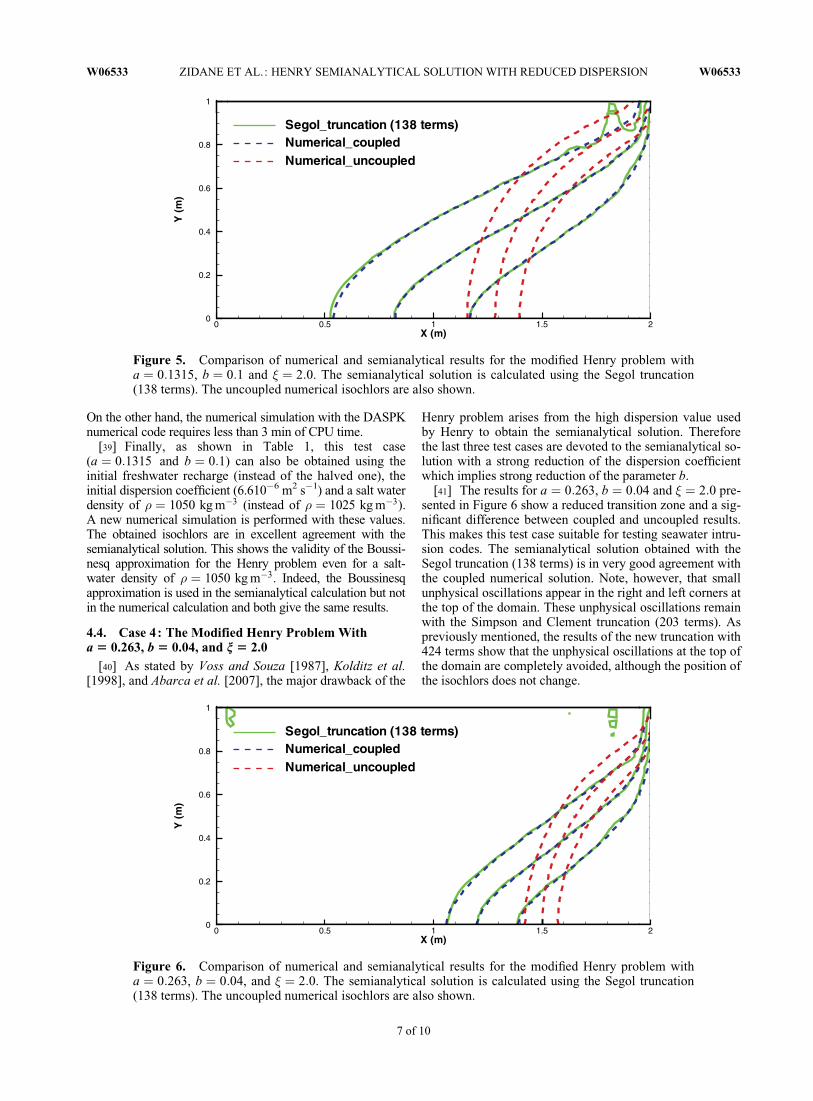
On the other hand, the numerical simulation with the DASPKnumerical code requires less than 3 min of CPU time.
[39] Finally, as shown in Table 1, this test case(a ¼ 0:1315 and b ¼ 0:1) can also be obtained using theinitial freshwater recharge (instead of the halved one), theinitial dispersion coefficient (6.610�6 m2 s�1) and a salt waterdensity of � ¼ 1050 kg m�3 (instead of � ¼ 1025 kg m�3).A new numerical simulation is performed with these values.The obtained isochlors are in excellent agreement with thesemianalytical solution. This shows the validity of the Boussi-nesq approximation for the Henry problem even for a salt-water density of � ¼ 1050 kg m�3. Indeed, the Boussinesqapproximation is used in the semianalytical calculation but notin the numerical calculation and both give the same results.
4.4. Case 4: The Modified Henry Problem Witha 5 0.263, b 5 0.04, and n 5 2.0
[40] As stated by Voss and Souza [1987], Kolditz et al.[1998], and Abarca et al. [2007], the major drawback of the
Henry problem arises from the high dispersion value usedby Henry to obtain the semianalytical solution. Thereforethe last three test cases are devoted to the semianalytical so-lution with a strong reduction of the dispersion coefficientwhich implies strong reduction of the parameter b.
[41] The results for a ¼ 0:263, b ¼ 0:04 and � ¼ 2:0 pre-sented in Figure 6 show a reduced transition zone and a sig-nificant difference between coupled and uncoupled results.This makes this test case suitable for testing seawater intru-sion codes. The semianalytical solution obtained with theSegol truncation (138 terms) is in very good agreement withthe coupled numerical solution. Note, however, that smallunphysical oscillations appear in the right and left corners atthe top of the domain. These unphysical oscillations remainwith the Simpson and Clement truncation (203 terms). Aspreviously mentioned, the results of the new truncation with424 terms show that the unphysical oscillations at the top ofthe domain are completely avoided, although the position ofthe isochlors does not change.
Figure 5. Comparison of numerical and semianalytical results for the modified Henry problem witha ¼ 0:1315, b ¼ 0:1 and � ¼ 2:0. The semianalytical solution is calculated using the Segol truncation(138 terms). The uncoupled numerical isochlors are also shown.
Figure 6. Comparison of numerical and semianalytical results for the modified Henry problem witha ¼ 0:263, b ¼ 0:04, and � ¼ 2:0. The semianalytical solution is calculated using the Segol truncation(138 terms). The uncoupled numerical isochlors are also shown.
W06533 ZIDANE ET AL.: HENRY SEMIANALYTICAL SOLUTION WITH REDUCED DISPERSION W06533
7 of 10

4.5. Case 5: The Modified Henry Problem Witha 5 0.263, b 5 0.02, and n 5 2.0
[42] In this test case, we lowered the dispersion by halfcompared to the previous case. The truncations proposedby Segol (138 terms) and Simpson and Clement (203terms) are not sufficient to obtain a stable solution in thiscase. Both truncations lead to significant unphysical oscil-lations not only in the top of the domain but also in the iso-chlors curves. The results of the new truncation (424 terms)are compared to the numerical solution in Figure 7. Despitethe unphysical oscillations observed at the top of the do-main, a good agreement is observed between the semiana-lytical and the numerical isochlors. These unphysicaloscillations could be avoided if one uses a truncation withmuch more coefficients. This requires very long computa-tional time (several weeks) and as previously this will haveno significant effects on the three isochlors positions. Theresults of Figure 7 show a very narrow transition zone due
the low dispersion coefficient, thus, saltwater invades morethe domain than the previous case. Coupled and uncouplednumerical results are significantly different (Figure 7)which reflects the importance of the density-dependenteffects compared to boundary forcing.
4.6. Case 6a: The Modified Henry Problem Witha 5 0.1315, b 5 0.04, and n 5 2.0
[43] This case has a small dispersion and a freshwaterrecharge reduced by half as suggested by Simpson andClement [2004]. As mentioned before, the solutionsobtained using the Segol (138 terms) and Simpson andClement (203 terms) truncations are not accurate and leadto significant unphysical oscillations not only at top of thedomain but also in the isochlor curves. Figure 8 shows thatthe new truncation (424 terms) gives a stable solutionwhich is in good agreement with the numerical resultsexcept in the lower left corner of the domain where the
Figure 7. Comparison of numerical and semianalytical results for the modified Henry problem witha ¼ 0:263, b ¼ 0:02, and � ¼ 2:0. The semianalytical solution is calculated using the new truncation(424 terms). The uncoupled numerical isochlors are also shown.
Figure 8. Comparison of numerical and semianalytical results for the modified Henry problem witha ¼ 0:1315, b ¼ 0:04, and � ¼ 2:0. The semianalytical solution is calculated using the new truncation(424 terms). The uncoupled numerical isochlors are also shown.
W06533 ZIDANE ET AL.: HENRY SEMIANALYTICAL SOLUTION WITH REDUCED DISPERSION W06533
8 of 10

semianalytical 0.25 isochlor is slightly more advanced thanthe numerical one. This discrepancy is observed becausethe semianalytical 0.25 isochlor is very close to the inlandboundary with zero concentration. Note that the 0.5 and0.75 isochlors are well reproduced by the numerical code.
4.7. Case 6b: The Modified Henry Problem Witha 5 0.1315, b 5 0.04, and n 5 3.0
[44] To reduce the influence of the zero-concentrationDirichlet left boundary condition on the 0.25 isochlor forthe previous case, a new semi analytical solution is per-formed on a larger rectangular domain with an aspect ration� ¼ L=d ¼ 3. The obtained semianalytical results are invery good agreement with the numerical solution as shownin Figure 9. Note that in this case, the steady state positionof the isochors is reached within 500 min. In Figure 9, thesaltwater intrudes much more in the domain than all previ-ous cases. Large differences can be observed betweencoupled and uncoupled results. Therefore, this test case isthe most sensitive one upon all the previous to density-de-pendent effects and should be preferred for benchmarkingdensity driven flow codes.
5. Conclusions[45] The Henry saltwater intrusion problem is considered
as one of the most popular test cases of density-dependentgroundwater flow models, since Henry [1964] provided asemianalytical solution of the problem by expanding thestream function and the salt concentration in double Fourierseries. These series are truncated at a given order and theremaining coefficients are calculated by solving a highlynonlinear system of algebraic equations. Henry [1964] useda truncation of 78 terms, Segol [1994] used a truncation of138 terms and Simpson and Clement [2004] used a trunca-tion of 203 terms. These authors solved the nonlinear sys-tem as a system of linear equations treating the nonlinearright hand side as a known quantity, updated iterativelyuntil convergence. This procedure encountered substantialconvergence difficulties especially for reduced dispersionvalues. Consequently, all published works succeeded todevelop semianalytical solutions only when an unrealisti-
cally large amount of dispersion is introduced in thesolution.
[46] In this work, this deficiency of the Henry problemwas avoided by using the Levenberg-Marquardt algorithm,which has a quadratic rate of convergence, to calculate thecoefficients of the Fourier series. Different truncations arestudied and a new truncation based on 424 terms is pro-posed to develop the semianalytical solutions of the Henryproblem with reduced dispersion coefficients.
[47] The obtained semianalytical solutions are in a verygood agreement with the numerical results obtained usingthe method of lines and advanced spatial discretizationschemes. These solutions improve the applicability of thesemianalytical solution of the Henry problem to saltwaterintrusion problems with reduced diffusion and are thereforemore suitable to benchmark density-driven flow codes.
Appendix A[48] The non linear algebraic equations are as follows:
"2a�2Ag;h g2 þ h2
�2
� �� ¼
X1r¼0
Br;hhNðg; rÞ þ 4
�Wðg; hÞ;
"1b�2Bg;h g2 þ h2
�2
� �� ¼
X1n¼0
Ag;ngNðh; nÞ þ "1
X1s¼1
Bg;sSNðh; sÞ
þ Quad þ 4
�Wðh; gÞ;
where
"1 ¼2; if : g ¼ 0
1; if : g 6¼ 0;
(
"2 ¼2; if : h ¼ 0
1; if : h 6¼ 0;
(
Nðh; nÞ ¼ ð�1Þhþn � 1
hþ nþ ð�1Þh�n � 1
h� n;
Figure 9. Comparison of numerical and semianalytical results for the modified Henry problem witha ¼ 0:1315, b ¼ 0:04, and � ¼ 3:0. The semianalytical solution is calculated using the new truncation(424 terms). The uncoupled numerical isochlors are also shown.
W06533 ZIDANE ET AL.: HENRY SEMIANALYTICAL SOLUTION WITH REDUCED DISPERSION W06533
9 of 10
Wðh; gÞ ¼ð�1Þh � 1
h; if : g ¼ 0
0; if : g 6¼ 0
;
8<:
Quad ¼ �4
X1m¼1
X1n¼0
X1r¼0
X1s¼1
Am;nBr;sðmsLR� nrFGÞ;
with
F ¼ �ðm�rÞ;g þ �ðr�mÞ;g � �ðmþrÞ;g;
L ¼ �ðm�rÞ;g þ �ðr�mÞ;g þ �ðmþrÞ;g;
G ¼ ð�1Þhþn�s � 1
hþ n� sþ ð�1Þh�nþs � 1
h� nþ s� ð�1Þhþnþs � 1
hþ nþ s
� ð�1Þh�n�s � 1
h� n� s;
R ¼ ð�1Þhþn�s � 1
hþ n� sþ ð�1Þh�nþs � 1
h� nþ sþ ð�1Þhþnþs � 1
hþ nþ s
þ ð�1Þh�n�s � 1
h� n� s;
and �i; j is the Kronecker delta such that
�i; j ¼1; if : i ¼ j
0; if : i 6¼ j:
(
[49] Acknowledgments. The authors would like to thank the anony-mous reviewers for their valuable comments and suggestions to improvethe quality of the paper. This study was partially supported by the GnRMoMaS (PACEN/CNRS ANDRA, BRGM CEA EDF IRSN) France. Andin part, was made possible by the support of SNF (Swiss National Founda-tion, grant 200020_125167), whose support is gratefully acknowledged.And a special thanks to Stefan Wiesmeier and Silvia Leupin for theirappreciated support.
ReferencesAavatsmark, I. (2002), An introduction to multipoint flux approximations
for quadrilateral grids, Comput. Geosci., 6, 404–432.Abarca, E., J. Carrera, X. Sanchez-Vila, and M. Dentz (2007), Anisotropic
dispersive Henry problem, Adv. Water Resour., 30(4), 913–926.Ackerer, P., and A. Younes (2008), Efficient approximations for the sim-
ulation of density driven flow in porous media, Adv. Water Resour.,31, 15–27.
Ackerer, P., A. Younes, and R. Mose (1999), Modeling variable densityflow and solute transport in porous medium: 1. Numerical model andverification, Transp. Porous Media, 35(3), 345–373.
Bues, M., and C. Oltean (2000), Numerical simulations for saltwater intru-sion by the mixed hybrid finite element method and discontinuous finiteelement method, Transp. Porous Med., 40(2), 171–200.
Croucher, A. E., and M. J. O’Sullivan (1995), The Henry problem for salt-water intrusion, Water Resour. Res., 31(7), 1809–1814.
Forbes, L. K. (1988), Surface waves of large amplitude beneath an elasticsheet, Part 2, Galerkin solution, J. Fluid Mech., 188, 491–508.
Frind, E. O. (1982), Simulation of long-term transient density-dependenttransport in groundwater, Adv. Water Resour., 5, 73–88.
Goswami, R. R., and T. P. Clement (2007), Laboratory-scale investigationof saltwater intrusion dynamics, Water Resour. Res., 43, W04418,doi:10.1029/2006WR005151.
Henry, H. R. (1964), Effects of dispersion on salt encroachment in coastalaquifers, in Sea Water in Coastal Aquifers, edited by H. H. Cooper, U.S.Geol. Surv. Supply Pap., 1613-C, C71–C84.
Herbert, A. W., C. P. Jackson, and D. A. Lever (1988), Coupled ground-water flow and solute transport with fluid density strongly dependentupon concentration, Water Resour Res., 24, 1781–1795.
Huyakorn, P. S., P. F. Andersen, J. W. Mercer, and H. O. White Jr. (1987),Saltwater intrusion in aquifers: Development and testing of a three-dimensional finite element model, Water Resour. Res., 23, 293–312.
Kolditz, O., R. Ratke, H. J. G. Diersch, and W. Zielke (1998), Coupledgroundwater flow and transport: 1. Verification of variable density flowand transport models, Adv. Water Res., 21, 27–46.
Konz, M., P. Ackerer, A. Younes, P. Huggenberger, and E. Zechner (2009),Two-dimensional stable-layered laboratory-scale experiments for testingdensity-coupled flow models, Water Resour. Res., 45, W02404, doi:10.1029/2008WR007118.
Levenberg, K. (1944), A method for the solution of certain nonlinear prob-lem in least squares, Quart. Appl. Math., 2, 164–168.
Marquardt, D. W. (1963), An algorithm for least-squares estimation of non-linear inequalities, SIAM J. Appl. Math., 11, 431–441.
Oldenburg, C. M., and K. Pruess (1995), Dispersive transport dynamics in astrongly coupled groundwater-brine flow system, Water Resour. Res.,31, 289–302.
Park, C. H., and M. M. Aral (2008), Saltwater intrusion hydrodynamics in atidal aquifer, J. Hydrol. Eng., 9, 863–872.
Pinder, G. F., and H. H. Cooper Jr. (1970), A numerical technique for calcu-lating the transient position of the saltwater front, Water Resour. Res.,6(3), 875–882.
Segol, G. (1994), Classic Groundwater Simulations Proving and ImprovingNumerical Models, Prentice-Hall, Old Tappan, N. J.
Segol, G., G. F. Pinder, and W. G. Gray (1975), A Galerkin-finite elementtechnique for calculating the transient position of the saltwater front,Water Resour. Res., 11(2), 343–347.
Siegel, P., R. Mose, P. Ackerer, and J. Jaffre (1997), Solution of the advec-tion diffusion equation using a combination of discontinuous and mixedfinite elements, Int. J. Numer. Methods Fluids, 24, 595–613.
Simpson, M. J., and T. P. Clement (2003), Theoretical analysis of the wor-thiness of the Henry and Elder problems as benchmarks of density-dependent groundwater flow models, Adv. Water Resour., 26, 17–31.
Simpson, M. J., and T. P. Clement (2004), Improving the worthiness of theHenry problem as a benchmark for density-dependent groundwater flowmodels, Water Resour. Res., 40, W01504, doi:10.1029/2003WR002199.
Thorenz, C., G. Kosakowski, O. Kolditz, and B. Berkowitz (2002), An ex-perimental and numerical investigation of saltwater movement incoupled saturated–partially saturated systems, Water Resour. Res., 38(6),1069, doi:10.1029/2001WR000364.
Voss, C. I., and W. R. Souza (1987), Variably density flow and solutetransport simulation of regional aquifers containing a narrow fresh-water-saltwater transition zone, Water Resour. Res., 23(10), 1851–1866.
Yamashita, N., and M. Fukushima (2001), On the rate of convergence ofthe Levenberg-Marquardt method, Computing, 15, 239–249.
Younes, A., and P. Ackerer (2008), Solving the advection-dispersion equationwith discontinuous Galerkin and multipoint flux approximation methodson unstructured meshes, Int. J. Numer. Methods Fluids, 58(6), 687–708.
Younes, A., and V. Fontaine (2008a), Hybrid and multi point formulationsof the lowest order mixed methods for Darcy’s flow on triangles, Int. J.Numer. Methods Fluids, 58, 1041–1062.
Younes, A., and V. Fontaine (2008b), Efficiency of mixed hybrid finiteelement and multi point flux approximation methods on quadrangular gridsand highly anisotropic media, Int. J. Numer. Methods Eng., 76(3), 314–336.
Younes, A., M. Fahs, and S. Ahmed (2009), Solving density flow problemswith efficient spatial discretizations and higher-order time integrationmethods, Adv. Water Resour., 32, 340–352.
Younes, A., P. Ackerer, and F. Delay (2010), Mixed finite element for solv-ing diffusion-type equations, Rev. Geophys., 48, RG1004, doi:10.1029/2008RG000277.
Zecheter, E., M. Konz, A. Younes, and P. Huggenberger (2011), Effects oftectonic structures, salt solution mining, and density-driven groundwaterhydraulics on evaporite dissolution, Hydrogeol. J., 19, 1323–1334,doi:10.1007/s10040-011-0759-5.
W06533 ZIDANE ET AL.: HENRY SEMIANALYTICAL SOLUTION WITH REDUCED DISPERSION W06533
10 of 10

Semi-analytical and numerical solutions for density driven free flows
45
Chapter 4
Semi-analytical and numerical solutions for density driven free flows
Contents
4.1. Introduction ................................................................................................................ 48
4.2. Mathematical Models ................................................................................................. 49
4.3. The semi-analytical solution ....................................................................................... 50
4.4. The numerical solution ............................................................................................... 53
4.4.1 Stokes flow discretization ..................................................................................... 53
4.4.2 Mass transport discretization ................................................................................. 55
4.4.3 Coupling Stokes flow and mass transport ............................................................. 57
4.5. Validation of the semi-analytical solution .................................................................. 57
4.5.1 Test case1: 0 008 0 1a . ;b . ................................................................................... 57
4.5.2 Test case2: 0 006 0 05a . ;b . ................................................................................. 58
4.6. Conclusion .................................................................................................................. 58

Semi-analytical and numerical solutions for density driven free flows
46
Paper Submitted to Advances in Water Resources Journal
A semi-analytical solution for density driven flow of free fluids
Anis Younes (1*), Ali Zidane(1,2), Peter Huggenberger(2) , Eric Zechner(2)
(1) Laboratoire d’Hydrologie de Geochimie de Strasbourg, University of Strasbourg, CNRS, UMR 7517 (2) Department of Environmental Sciences, University of Basel, Institute of Geology, Switzerland
* Corresponding author: Anis Younes
e-mail: [email protected]

Semi-analytical and numerical solutions for density driven free flows
47
Abstract
The Henry semi-analytical solution for salt water intrusion into costal aquifers is widely used for
benchmarking density driven flow in porous media. In this work, we develop a modified Henry
semi-analytical solution for density driven flow of free fluids. The new benchmark concerns
saltwater intrusion trough a channel where Stokes flow is coupled to mass transport via buoyancy
forces. The semi-analytical solution is calculated by replacing the stream function and the
concentration by a double set of Fourier series, truncated at a given order. The remaining
coefficients are calculated using the Levenberg-Marquardt algorithm to solve the obtained highly
nonlinear system of algebraic equations. The semi-analytical solution is validated against the
results of a transient numerical code based on the nonconforming Crouzeix-Raviart (CR) finite
element approximation for the Stokes flow and a combination of Discontinuous Galerkin (DG)
and Multi-Point Flux Approximation (MPFA) methods for the mass transport equation.
Keywords: Density driven flow, free fluids, Analytical solution, Crouzeix-Raviart,
Discontinuous Galerkin, MPFA

Semi-analytical and numerical solutions for density driven free flows
48
1. INTRODUCTION
The existence of semi-analytical solutions for nonlinear transport problems is well suited for the
validation of numerical codes before their use on real cases. In this sense, the synthetic Henry
saltwater intrusion problem [1] is one of the most widely used tests for the verification of density
driven flow codes in porous media. Indeed, the semi-analytical solution of Henry [1] provides the
steady state isochlors positions by expanding the salt concentration and the stream function in
double Fourier series. Henry [1] used 78 terms in these series and calculated the coefficients
using a Gauss elimination procedure. In 1994, Segol [2] revaluated the semi-analytical solution
by using a new truncation with 138 terms. A good agreement was generally observed between
this solution and numerical results [e.g. 3-8]. Effects of dispersion and anisotropy on the Henry
problem have been studied numerically in [9]. Recently, a new semi-analytical solution was
developed for the Henry problem in the case of small dispersion using a truncation based on 424
terms in the Fourier series [10].
In this work, we extend the Henry problem to free fluids domains and we develop a semi-
analytical solution for saltwater intrusion trough a channel (or a single fracture). To this aim, we
consider a synthetic problem describing the steady state saltwater intrusion through the channel.
Freshwater enters an idealized rectangular domain (Fig. 1) with a constant flux rate from the left
boundary. A hydrostatic pressure is prescribed along the right boundary with a denser salt-water
solution. The top and the bottom of the domain are impermeable boundaries. The saltwater
intrudes from the right until an equilibrium with the injected freshwater is reached. The free-flow
is governed by the Stokes equation [11-17] since the flow through the channel is considered
steady and laminar and the inertial forces in the flow field are assumed to be negligibly small
compared with the viscous and pressure forces. As with the standard Henry problem [1], we
develop the semi-analytical solution by expanding the concentration and the stream function in a
double set of Fourier series. Two test problems are studied corresponding to different density
contrasts. The Fourier series are evaluated using the truncation proposed in [10] based 424
coefficients. These coefficients are calculated by solving a highly nonlinear system of algebraic
equations with the Levenberg-Marquardt algorithm, which has a quadratic rate of convergence.
The semi-analytical solution is then compared against numerical results obtained using a robust
transient numerical code based on advanced numerical methods. Hence, the Stokes flow is
discretized using the Crouzeix-Raviart (CR) approximation, based on the nonconforming

Semi-analytical and numerical solutions for density driven free flows
49
piecewise linear finite elements for the velocity and the piecewise constant finite elements for the
pressure. This approximation provides locally mass conservative velocity which is an essential
property for mass transport to avoid artificial mass sources and sinks.
For the transport equation, the Discontinuous Galerkin (DG) method is used to discretize the
advection equation and combined with the symmetric Multipoint Flux Approximation (MPFA)
method for the discretization of the diffusion equation [18]. The DG method is a robust and
accurate numerical scheme for problems involving sharp fronts [19]. On the other hand, the
MPFA method is locally conservative and handles general irregular grids [20-22]. The MPFA
and the DG discretizations can be gathered into one system matrix without operator splitting [18].
To reduce the computational cost of simulations, flow and transport equations are solved
sequentially using a non-iterative scheme with proper time management based on local truncation
error control as in [23].
2. MATHEMATICAL MODELS
Single-phase steady incompressible flow is governed by the Navier-Stokes equation:
2u u u g. p (1)
and the continuity equation:
0u. (2)
where is the fluid density, u is the velocity vector, p is the pressure, g is gravity, and is
the dynamic viscosity.
In this work, we assume that the flow is sufficiently slow to consider the inertial forces in the
flow field (the first nonlinear term in equation (1)) negligibly small compared with the viscous
and pressure forces. Therefore, the free-flow simplifies to the following Stokes equations [24-
26]:
2u gp (3)
0u. (4)
Three kinds of boundary conditions are used with this system:
o The velocity u is prescribed on the boundary;
o Free outflow boundary condition 0u η ηp with η the outward normal vector to
the boundary;
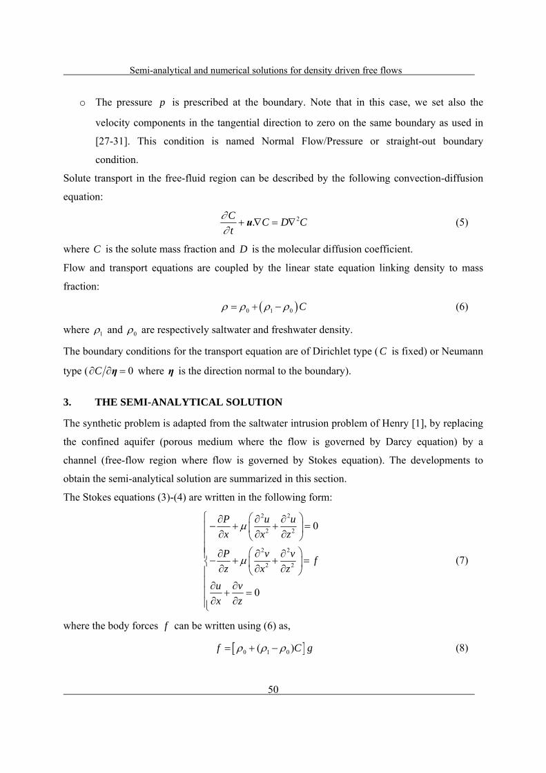
Semi-analytical and numerical solutions for density driven free flows
50
o The pressure p is prescribed at the boundary. Note that in this case, we set also the
velocity components in the tangential direction to zero on the same boundary as used in
[27-31]. This condition is named Normal Flow/Pressure or straight-out boundary
condition.
Solute transport in the free-fluid region can be described by the following convection-diffusion
equation:
2uC
. C D Ct
(5)
where C is the solute mass fraction and D is the molecular diffusion coefficient.
Flow and transport equations are coupled by the linear state equation linking density to mass
fraction:
0 1 0 C (6)
where 1 and 0 are respectively saltwater and freshwater density.
The boundary conditions for the transport equation are of Dirichlet type (C is fixed) or Neumann
type ( 0ηC where η is the direction normal to the boundary).
3. THE SEMI-ANALYTICAL SOLUTION
The synthetic problem is adapted from the saltwater intrusion problem of Henry [1], by replacing
the confined aquifer (porous medium where the flow is governed by Darcy equation) by a
channel (free-flow region where flow is governed by Stokes equation). The developments to
obtain the semi-analytical solution are summarized in this section.
The Stokes equations (3)-(4) are written in the following form:
2 2
2 2
2 2
2 2
0
0
P u u
x x z
P v vf
z x z
u v
x z
(7)
where the body forces f can be written using (6) as,
0 1 0( )f C g (8)

Semi-analytical and numerical solutions for density driven free flows
51
The last equation in (7) implies the existence of a stream function , such as:
uz
and vx
(9)
Inserting (9) into (7) leads to:
4 4 4
1 04 2 2 42 ( )
Cg
x x z z z
(10)
As in [1, 2], we define the following new variables:
x x d , z z d , u u d Q , v v d Q , u z , v x , z (11)
where x and z are non-dimensional coordinates, u and v are the non-dimensional velocities
and the non-dimensional stream function.
Using (11), eq (10) leads to:
4 4 4
4 2 2 4
12
Ca
x x z z x
(12)
with 3
1 0( )
Qa
gd
and L
d the aspect ratio of the domain, where L is the length and d is
the depth of the domain.
Similarly, the change of variables applied to the mass transport equation (5) (see [1, 2] for
details) leads to:
2 2
2 2
1 1C C C C Cb
x z z x x z z x
(13)
with D
bQ
and C is now the non-dimensional concentration.
The stream function and the concentration are represented by double Fourier series of the form:
,1 0
sin( ) cos( )m nm n
xA m z n
(14)
,0 1
cos( )sin( )r sr s
xC B r z s
(15)

Semi-analytical and numerical solutions for density driven free flows
52
Substituting these relations into equations (12) and (13), multiplying equation (12) by
4sin( ) cos( )x
g z h
and equation (13) by 4cos( )sin( )x
g z h
, and integrating over the
rectangular domain gives an infinite set of algebraic equations for ,g hA and ,g hB namely,
2
4 2 22 , ,2
0
4( ) ( , ) ( , )g h r h
r
ha A g B hN g r W g h
(16)
2
2 21 , , 1 ,2
0 1
4( ) ( , ) ( , ) ( , )g h g n g s
n s
hb B g A gN h n B SN h s Quad W h g
(17)
Details about the parameters 1 2, , , ,N W Quad , can be found in Appendix A.
The algebraic system of equations (16)-(17) has the same form than the system obtained by
Henry [1] and Segol [2] for the standard saltwater intrusion through a coastal aquifer. Note that
the flow equation (16) is different from the one obtained with the Darcy flow in [1].
Henry [1], Segol [2] and Simpson and Clement [32] used different truncations of the Fourier
series. They solved the nonlinear system as a system of linear equations where the expansion
coefficients are considered as unknowns. The nonlinear right hand side is treated as a known
quantity, updated iteratively until convergence. As stated by Segol [2], this technique
encountered substantial convergence difficulties for small values of the parameters a and b
which for the standard Henry problem correspond to
0
1 0Darcy
Qa
K d
( K is the hydraulic
conductivity of the porous medium) and Darcy
Db
Q .
To avoid convergence difficulties in the case of saltwater intrusion within a channel, we use in
this work the Levenberg-Marquardt algorithm [33, 34], which has a quadratic rate of
convergence, to solve the set of nonlinear algebraic equations (16) - (17) [35]. The method is
considered as one of the most efficient algorithm for solving systems of nonlinear equations. The
nonlinear algebraic system of equations (16)-(17) is written in the form 0F X where X is a
vector formed by the coefficients ,g hA and ,g hB to calculate. The Levenberg-Marquardt algorithm
includes two minimization methods: the gradient descent method and the Gauss-Newton method.
Far from the optimum, the Levenberg-Marquardt method behaves like a gradient descent method,

Semi-analytical and numerical solutions for density driven free flows
53
whereas, it acts like the Gauss Newton method nearby the optimum. The Jacobian J is
approximated numerically using finite differences.
Two test problems, corresponding to different density contrast, are studied in this work. The
Fourier series are truncated using 424 coefficients as in [10] with 214 terms 1..7,0..30A for the
expansion of the stream function and 210 terms 0..6,1..30B for the expansion of the concentration.
4. THE NUMERICAL SOLUTION
In this part, we summarize the numerical techniques used for the solution of the coupled stokes
flow and mass transport system.
4.1 STOKES FLOW DISCRETIZATION
The flow system (3)-(4) cannot be discretized with the same order for pressure and velocity
approximations due to stability conditions. Otherwise some sort of stabilization is added to the
mixed formulation [36]. To avoid these difficulties, we use the non-conforming Crouzeix-Raviart
(CR) elements for the velocity approximation in combination with constant pressure per element,
since they satisfy the Babuska-Brezzi condition [37-39]. This condition is central for ensuring
that the final linear system to solve is non-singular [40]. Moreover, the non-conforming
Crouzeix-Raviart (CR) finite element method has local mass conservation properties [41] and
leads to a relatively small number of unknowns due to the low-order shape functions. The CR
elements are used in many problems such as the Darcy-Stokes problem [42], the Stokes problem
[43] and the elasticity problem [44, 45]. The CR method gives a simple stable optimal order
approximation of the Stokes equations [46]. In the following, we recall the main stages for the
discretization of the Stokes equation with the CR triangular elements.
With the non-conforming finite elements method, the degrees of freedom for the velocity vector
u are the two component i iu ,v of u at the midedge i facing the node i . Inside the element E ,
we assume a linear variation of the velocity components E Eu ,v
E E E E E EE i i j j k k E i i j j k ku u u u , v v v v (18)
where the interpolation function Ei equals 1 on the midedge i and zero on the midedges j and
k of E (Fig. 2).
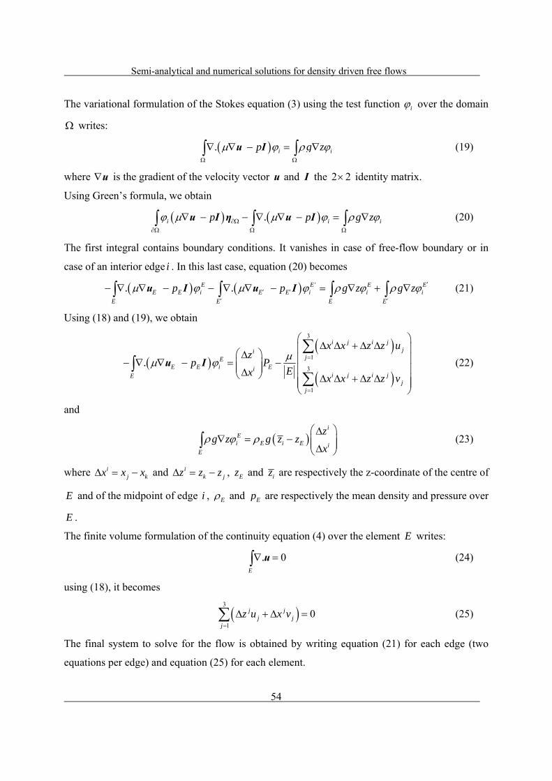
Semi-analytical and numerical solutions for density driven free flows
54
The variational formulation of the Stokes equation (3) using the test function i over the domain
writes:
u Ι i i. p g z
(19)
where u is the gradient of the velocity vector u and Ι the 2 2 identity matrix.
Using Green’s formula, we obtain
u Ι η u Ιi i ip . p g z
(20)
The first integral contains boundary conditions. It vanishes in case of free-flow boundary or in
case of an interior edge i . In this last case, equation (20) becomes
u Ι u ΙE E' E EE E i E E i i i
E E E E
. p . p g z g z
(21)
Using (18) and (19), we obtain
3
1
3
1
u Ι
i j i jji
jEE E i Ei
i j i jEj
j
x x z z uz
. p PEx
x x z z v
(22)
and
i
Ei E i E i
E
zg z g z z
x
(23)
where ij kx x x and i
k jz z z , Ez and iz are respectively the z-coordinate of the centre of
E and of the midpoint of edge i , E and Ep are respectively the mean density and pressure over
E .
The finite volume formulation of the continuity equation (4) over the element E writes:
0uE
. (24)
using (18), it becomes
3
1
0j jj j
j
z u x v
(25)
The final system to solve for the flow is obtained by writing equation (21) for each edge (two
equations per edge) and equation (25) for each element.

Semi-analytical and numerical solutions for density driven free flows
55
4.2 MASS TRANSPORT DISCRETIZATION
The DG leads to a high-resolution scheme for advection that has been proven to be clearly
superior to the already existing finite element methods [47]. In this work, the explicit DG
method, where fluxes are upwinded using a Riemann solver, is used to solve the advection
equation and combined with the symmetric Multipoint Flux Approximation (MPFA) method for
the diffusion equation.
The transport equation (5) is written in the following mixed form
0u u
u
D
D
C. C .
tD C
(26)
The dispersive flux uD is assumed to vary linearly inside the element E , therefore,
1
u ED D, Ei
i
. QE (27)
where u ηED, Ei D Ei
Ei
Q .
is the dispersive flux across the edge Ei of E .
We use the P1 DG method where the approximate solution ( , )hC tx is expressed with linear basis
functions Ei on each element E as follows:
3
1
, | E Eh E i i
i
C t C t
x x (28)
where EiC t are the three unknown coefficients corresponding to the degrees of freedom which
are the average value of the mass fraction defined at the triangle centroid E Ex ,z and its
deviations in each space direction [48] with the corresponding interpolation functions:
1 2 3, 1, , , , . E E EE Ex z x z x x x z z z (29)
The variational formulation of (26) over the element E using Ei as test functions leads to (see
[12] for details),

Semi-analytical and numerical solutions for density driven free flows
56
1
,
1 1 1302
2 2 21
3 3 33
0
0
E
ED jE E E
EjEE E E
E E EE
dCQdt C C C
dCA B C M C M C
dtC C C
dC
dt
(30)
with,
, ,
N0, ,
1
.
, 1 1,..,3
u
E
E E E Ei j j i i j j i
E E
E EE E E E E EE E
i j E i j i j E i j
E E
A B
Q QM M
E E
where Ej is the adjacent element to E such that Ej is the common edge of E and Ej and
.EE Ej
E
Q
uη the water flux across Ej . The upwind parameter EE is defined by
1 . 0
0 . 0EjE
EjEj
if
if
uη
uη (31)
An explicit time discretization is used for the equation (30). An efficient geometric slope limiter
is used to avoid unphysical oscillations near sharp fronts [49].
The dispersive fluxes ,ED jQ across edges are approximated using the MPFA method. The basic
idea of this method is to divide each triangle into 3 sub-cells as in Fig. 3. Inside the sub-cell
1 2O,F ,G,F formed by the corner O , the centre G and the midpoint edges 1F and 2F , we
assume linear variation of the mass fraction between 1EC , 1TC and 2TC , the mass fractions
respectively at G and the two continuity points 1f and 2f . The symmetry of the MPFA scheme
is achieved when the continuity points are localized at 1 2
1 2
2
3
Of Of
OF OF . In this case half-edge
fluxes 1 2
1 2andF F
O O
O O
Q D C Q D C
, taken positive for outflow write [50]:
1
1 1 1 2 1 12
2 11 2 2 2
EO
E EO
OF .OF OF .OFQ TC C
Q TC COF .OF OF .OF
(32)
with 3E D E .

Semi-analytical and numerical solutions for density driven free flows
57
This system is written for all sub-cells sharing the vertex O which create an interaction region.
Then by writing continuity of diffusive fluxes across half-edges and by assuming continuity of
mass fraction at continuity points, we obtain a local system A TC B C . This local system
is solved to obtain the mass fraction at the continuity points ( iTC ) as function of mass fraction at
all elements sharing the vertexO . The obtained relation is then substituted into (32) to obtain
half-edge fluxes explicitly as a weighted sum of the cell mass fraction of the interaction volume.
Finally, the summation of these fluxes is written using an implicit time discretization and
substituted into the equation (30).
4.3 COUPLING STOKES FLOW AND MASS TRANSPORT
Stokes flow equations (3)-(4) and the advection-diffusion mass transport equation (26) are
coupled by the state equation (6) linking density to mass fraction. Due to nonlinearities,
simulations can require an excessive computational time and/or heavy equipments. Adaptive
temporal discretization based on local truncation error control has been shown to be useful to
reduce the computational cost of the simulation [51-58]. In this work, we use the non-iterative
time stepping scheme based on local truncation error control developed in [23].
5. VALIDATION OF THE SEMI-ANALYTICAL SOLUTION
We consider a synthetic example 22 1 m where the domain is discretized with a regular
triangular mesh of 3200 elements. The flux at the left (inland) boundary is set to 2 10 92Q . m s .
To avoid very small values of the parameter a for which we cannot obtain a converged semi-
analytical solution, the viscosity is set to 1 Pa s in this synthetic problem.
5.1 TEST CASE 1: 0 008 0 1a . ;b .
In this test case, we set the freshwater density (at the left boundary) to 30 1000 kg m , the
saltwater density (at the right boundary) to 31 1011kg m and the diffusion coefficient to
2 10 092D . m s . The corresponding non-dimensional parameters a and b are:
3
1 0
0.008( )
Qa
gd
and 0.1D
bQ
.
Table 1 provides the position of the three principal isochlors (0.25, 0.5 and 0.75) obtained with
the semi-analytical solution using the truncation suggested in [10]. The transient numerical
Semi-analytical and numerical solutions for density driven free flows
58
simulation is performed until a long time to ensure a steady state solution. The three semi
analytical isochlors are then compared against the numerical solution in Fig. 4. A good agreement
can be observed between the semi-analytical and the numerical solutions (Fig. 4).
5.2 TEST CASE 2: 0 006 0 05a . ;b .
In this case, the saltwater density is increased to 31 1015kg m and the diffusion coefficient is
reduced to 2 10 046D . m s . The corresponding non-dimensional parameters a and b are then:
3
1 0
0.006( )
Qa
gd
and 0.05D
bQ
.
The same truncation based 424 coefficients of the Fourier series is used for the semi-analytical
solution. The positions of the three principal isochlors (0.25, 0.5, and 0.75) are listed in Table 1.
Fig. 5 shows the semi analytical and numerical isochlors. As previously, a good agreement can be
observed between the numerical and the semi-analytical solutions.
6. CONCLUSION
In this manuscript, we developed a semi analytical solution for the validation of density driven
flow of free fluids. The problem is adapted from the saltwater intrusion problem of Henry [1], by
replacing the confined aquifer by a channel. The semi-analytical solution is calculated by
replacing the stream function and the concentration by a double set of Fourier series. These series
are truncated using 424 terms as in [10]. The remaining coefficients are calculated by solving a
highly nonlinear system of algebraic equations using the Levenberg-Marquardt algorithm.
The semi analytical solution is validated using a synthetic problem of saltwater intrusion. Two
test cases including different density contrasts are studied. A transient numerical model is
developed for coupled Stokes flow and mass transport with large density variations. The model is
developed for a general triangular meshes and uses the CR finite elements for the flow
discretization, the DG method for advection and the symmetric MPFA method for diffusion. A
good agreement is observed between the semi-analytical and numerical solutions fro the two
studied test cases. The semi-analytical positions of the three principal isochlors are listed in Table
1 and can then be used for the validation of numerical codes.

Semi-analytical and numerical solutions for density driven free flows
59
ACKNOWLEDGMENTS
This study was supported by the SNF (Swiss National Foundation), whose support is gratefully
acknowledged.
Semi-analytical and numerical solutions for density driven free flows
60
Appendix A
24 2 2
2 , ,20
4( ) ( , ) ( , )g h r h
r
ha A g B hN g r W g h
2
2 21 , , 1 ,2
0 1
4( ) ( , ) ( , ) ( , )g h g n g s
n s
hb B g A gN h n B SN h s Quad W h g
Where
1
2, : 0
1, : 0
if g
if g
2
2, : 0
1, : 0
if h
if h
( 1) 1 ( 1) 1( , )
h n h n
N h nh n h n
( 1) 1, : 0
( , )
0, : 0
h
if gW h g h
if g
, ,1 0 0 1
( )4 m n r s
m n r s
Quad A B msLR nrFG
With
( ), ( ), ( ),m r g r m g m r gF
( ), ( ), ( ),m r g r m g m r gL
( 1) 1 ( 1) 1 ( 1) 1 ( 1) 1h n s h n s h n s h n s
Gh n s h n s h n s h n s
( 1) 1 ( 1) 1 ( 1) 1 ( 1) 1h n s h n s h n s h n s
Rh n s h n s h n s h n s
And ,i j is the Kronecker delta such that
,
1, :
0, :i j
if i j
if i j

Semi-analytical and numerical solutions for density driven free flows
61
References
[1] Henry HR. Effects of dispersion on salt encroachment in coastal aquifers, in Sea Water in Coastal Aquifers, U.S. Geol. Surv. Supply Pap., 1964,1613-C, 70 – 84.
[2] Segol G. Classic Groundwater Simulations Proving and Improving Numerical Models, Prentice-Hall, Old Tappan, N. J. 1994.
[3] Oldenburg CM, Pruess K. Dispersive transport dynamics in a strongly coupled groundwater-brine flow system. Water Resour Res 1995;31:289–302.
[4] Herbert AW, Jackson CP, Lever DA. Coupled groundwater flow and solute transport with fluid density strongly dependent upon concentration. Water Resour Res 1988;24:1781–95.
[5] Ackerer P, Younes A, and R. Mose. Modeling variable density flow and solute transport in porous medium: 1. Numerical model and verification, Transp. Porous Media, 1999, 35(3), 345–373.
[6] Buès M, Oltéan C. Numerical simulations for saltwater intrusion by the mixed hybrid finite element method and discontinuous finite element method, Transp. Porous Med., 2000 ,40(2), 171–200.
[7] Younes A, Fahs M, Ahmed S. Solving density flow problems with efficient spatial discretizations and higher-order time integration methods, Adv. Water Resour., 2009, 32, 340–352.
[8] Hinkelmann R, Sheta H, Class H and Helmig R. A Comparison of Different Model Concepts for Salt Water Intrusion Processes. In: Stauffer, F., Kinzelbach, W., Kovar, K. & E. Hoehn (eds.): ModelCARE 99: International Conference on Calibration and Reliability in Groundwater Modeling - Coping with uncertainty (20. - 23. September 1999, ETH Zurich, Switzerland). 265. IAHS Redbook, Zürich, Schweiz, 2000, 385-391.
[9] Abarca E, Carrera J, Sanchez-Vila X and Dentz M. Anisotropic dispersive Henry problem, Adv. Water Resour., 2007,30(4),pp.913–926.
[10] Zidane A, Younes A, Huggenberger P, Zechner E. The Henry semi-analytical solution for saltwater intrusion with reduced dispersion, Water Resou Res, 2012, VOL. 48, W06533, doi:10.1029/2011WR011157.
[11] Beavers G, Joseph D. Boundary conditions at a naturally permeable wall, J. Fluid Mech., 1967, 30:197.
[12] Saffman P. On the boundary condition at the surface of a porous medium, Studies Appl. Math. 1971, 50:93.
[13] Sanchez-Palencia E. Non-Homogeneous Media and Vibration Theory, volume 127 of Lecture Notes in Physics 1980, Spring-Verlag, Berlin.

Semi-analytical and numerical solutions for density driven free flows
62
[14] Kaviany M. Principles of Heat Transfer in Porous Media, Mechanical Engineering Series 1999, Springer-Verlag, New York.
[15] Jäger W, Mikelić A. On the interface boundary condition of Beavers, Joseph, and Saffman. SIAM J. Appl. Math 2000. 60:1111.
[16] Jäger W, Mikelić A. Asymptotic analysis of the laminar viscous flow over a porous bed. SIAM J. Sci. Comput., 2001a, 22:2006.
[17] Arbogast T, Lehr HL. Homogenization of a Darcy-Stokes system modeling vuggy porous media. Comput. Geosci. 2006, 10:291.
[18] Younes A, Ackerer P. Solving the advection-dispersion equation with Discontinuous Galerkin and Multipoint Flux Approximation methods on unstructured meshes. Int. J Numer Methods in Fluids. 2008; DOI: 10.1002/fld.1783.
[19] Shuangzhang T, Shahrouz A. A slope limiting procedure in Discontinuous Galerkin finite element method for gasdynamics applications. Int. J Numer Analy Modell 2005;2:163-178.
[20] Aavatsmark I. An introduction to multipoint flux approximations for quadrilateral grids. Comput Geosci, 2002;6:404–432.
[21] Aavatsmark I, Barkve T, Bøe Ø, Mannseth T. Discretization on non-orthogonal, quadrilateral grids for inhomogeneous, anisotropic media. J Comput Phys, 1996;127:2–14.
[22] Wheeler MF, Yotov I. A multipoint flux mixed finite element method. SIAM44 2006;5:2082-2106.
[23] Younes A, Ackerer P. Empirical versus time stepping with embedded error control for density-driven flow in porous media, Water Resour. Res., 2010, 46, W01504, doi:10.1029/2009WR008229
[24] Flekkøy EG, Rage T, Oxaal U, Feder J. Hydrodynamic Irreversibility in Creeping Flow, Phys. Rev,1996, PACS numbers: 47.15.Gf, 02.70.Bf, 02.70.Lq, 47.60.+I, VOLUME 77, NUMBER 20
[25] Happel J, Brenner H. Low Reynolds Number Hydrodynamics (Prentice Hall Inc., Englewood Cliffs, NJ,1965).
[26] Landau LD, Lifshitz EM. Fluid Mechanics (Pergamon Press, New York, 1987), 2nd ed.
[27] Conca C, Murat F, Pironneau O. The Stokes and Navier-Stokes equations with boundary conditions involving the pressure. Jpn J. Math.,1994,20, 263-318.
[28] Conca C, Parés C, Pironneau O, Thiriet M. Navier-Stokes equations with imposed pressure and velocity fluxes. Int. J. Numer. Methods Fluids, 1995, 20(4), 267-287.
[29] Gresho PM, Sani RL. On pressure boundary conditions for the incompressible Navier-Stokes equations. Int. J. Numer. Methods Fluids 7, 1987 ,1111-1145.

Semi-analytical and numerical solutions for density driven free flows
63
[30] Jäger W, Mikelić A. On the roughness-induced effective boundary conditions for an incompressible viscous flow, J. Differ. Equ. 2001b ,170, 96-122.
[31] Lukaszewicz G. On the Navier-Stokes equations in time dependent domains with boundary conditions involving the pressure. J. Math. Sci. Univ. Tokyo 4, 1997 ,529-550.
[32] Simpson MJ, Clement TP. Improving the worthiness of the Henry problem as a benchmark for density-dependent groundwater flow models, Water. Resour. Res., 2004 ,40, W01504, doi: 10.1029/2003WR002199
[33] Levenberg K. A method for the solution of certain nonlinear problem in least squares, Quart. Appl. Math., 1944,2 , 164-168.
[34] Marquardt DW. An algorithm for least-squares estimation of nonlinear inequalities, SIAM J. Appl. Math., 1963 ,11 , 431-441.
[35] Yamashita N, Fukushima M. On the rate of convergence of the Levenberg-Marquardt method. Computing 15, 2001, 239-249.
[36] Li J, Chen Z. A new local stabilized nonconforming finite element method for the Stokes equations, Computing, 2008, 82:157-170, doi 10.1007/s00607-008-0001-z
[37] Brezzi F, Fortin M. Mixed and hybrid finite element methods, Berlin: Springer 1991.
[38] Girault V, Raviart PA. Finite element methods for Navier-Stokes equations, Berlin: Springer 1986.
[39] Gresho PM, Sani RL. Incompressible flow and the finite element method, New York: Wiley; 1998.
[40] Langtangen HP, Mardal K, Winther R. Numerical methods for incompressible viscous flow. Adv. Water Res. 25, 2002, 1125-1146.
[41] Bruman E, Hansbo P. A stabilized nonconforming finite element method for incompressible flow, Comput. Methods App Mech. Eng., 2004 ,vol. 195, num. 23-24, p. 2881-99.
[42] Bruman E, Hansbo P. Stabilized Crouzeix-Raviart element for the Darcy-Stokes problem, Numerical Methods for Partial Differential Equation,2005 ,21(5), 986-997.
[43] Crouzeix M, Raviart P. Conforming and nonconforming finite element methods for solving the stationary Stokes equations. RAIRO Sér. Rouge, 1973 ,7(3), 33-75.
[44] Hansbo P, Larson MG. Discontinuous Galerkin and the Crouzeix-Raviart element: application to elasticity. ESAIM: Math. Model. Numer. Anal. 2003,37(1), 63-72.
[45] Hansbo P, Larson MG. Discontinuous Galerkin methods for incompressible and nearly incompressible elasticity by Nitshe’s method. Comput. Methods Appl. Mech. Engrg, 2002 ,191(17-18), 1895-1908.
[46] Arnold DN. On nonconforming linear-constant elements for some variants of the Stokes equations, presenta dal s.c. Franco Brezzi nella seduta del 24-6-93.

Semi-analytical and numerical solutions for density driven free flows
64
[47] Arnold DN, Brezzi F, Cockburn B, Marini LD. Unified analysis of discontinuous Galerkin methods for elliptic problems. SIAM J. Numer. Anal. 2002;5:1749-1779.
[48] Cockburn B, Hou S, Shu CW. TVB Runge Kutta local projection discontinuous Galerkin finite element method for conservative laws III: One dimensional systems, J. Compu.t Phys. 1989;84: 90-113.
[49] Younes A, Fahs M, Ackerer P. An efficient geometric approach to solve the slope limiting problem with the Discontinuous Galerkin method on unstructured triangles, Int. J. Numer. Meth. Biomed. Engng. 2010; 26:1824–1835.
[50] Younes A, Fontaine V. Efficiency of Mixed Hybrid Finite Element and Multi Point Flux Approximation methods on quadrangular grids and highly anisotropic media. Int J for Numer Meth in Engrg, 2008b;DOI: 10.1002/nme.2327.
[51] Diersch HJ. Finite element modelling of recirculation density driven saltwater intrusion processes in groundwater, Adv. Water Resour., 1988, 11, 25–43, doi:10.1016/0309-1708(88)90019-X.
[52] Diersch HJ, Kolditz O. Coupled groundwater flow and transport: 2. Thermohaline and 3D convection systems, Adv. Water Resour., 1998, 21, 401–425, doi:10.1016/S0309-1708(97)00003-1.
[53] Turek S. A comparative study of some time stepping techniques for the incompressible Navier-Stokes equations: From fully implicit nonlinear schemes to semi-implicit projection methods, Int. J. Numer. Methods Fluids, 1996, 22(10), 987–1011, doi:10.1002/(SICI)1097-0363 (19960530) 22:10<987::AID-FLD394>3.0.CO;2-7.
[54] Tocci MD, Kelley CT, Miller CT. Accurate and economical solution of the pressure�head form of Richards’ equation by the method of lines, Adv. Water Resour., 1997,20(1), 1–14, doi:10.1016/S0309-1708(96)00008-5
[55] Williams GA, Miller CT. An evaluation of temporally adaptive transformation approaches for solving Richards’ equation, Adv. Water Resour., 1999, 22(8), 831–840, doi:10.1016/S0309-1708(98)00048-7
[56] Kavetski D, Binning P, Sloan SW. Adaptive time stepping and error control in a mass conservative numerical solution of the mixed form of Richards equation, Adv. Water Resour., 2001,24(6), 595–605, doi:10.1016/S0309-1708(00)00076-2.
[57] Sloan SW, Abbo AJ. Biot consolidation analysis with automatic time stepping and error control. Part 1: Theory and implementation, Int. J. Numer. Anal. Methods Geomech., 1999, 23, 467–492, doi:10.1002/(SICI) 1096-9853(199905)23:6<467::AID-NAG949>3.0.CO;2-R.
[58] Saaltink MW, Carrera J, Olivella S. Mass balance errors when solving the convective form of the transport equation in transient flow problems, Water Resour. Res., 2004, 40, W05107, doi:10.1029/2003WR002866.
Semi-analytical and numerical solutions for density driven free flows
65
List of figures
Fig. 1: Boundary conditions for saltwater intrusion through a channel.
Fig. 2: The linear interpolation function for velocity field.
Fig. 3: Triangle splitting into three sub-cells and linear mass fraction approximation on the sub-cell. Fig. 4: Semi-analytical (dashed lines) and simulated concentration distribution for the first test case 0 008 0 1a . ;b . . The semi-analytical solution is calculated using a truncation based on
424 coefficients for the double Fourier series.
Fig. 5: Semi-analytical (dashed lines) and simulated concentration distribution for the second test
case 0 006 0 05a . ;b . . The semi-analytical solution is calculated using a truncation based on
424 coefficients for the double Fourier series.
List of tables
Table 1: Positions of the 0.25, 0.5 and 0.75 isochlors for the test cases 1 and 2.

Semi-analytical and numerical solutions for density driven free flows
66
Fig. 1
j
Eiϕ′
i
k Eiϕ
E’E
i
Fig. 2
O
G 2f
1f
1OQ
2OQ
2F
1F
R
P
Fig. 3
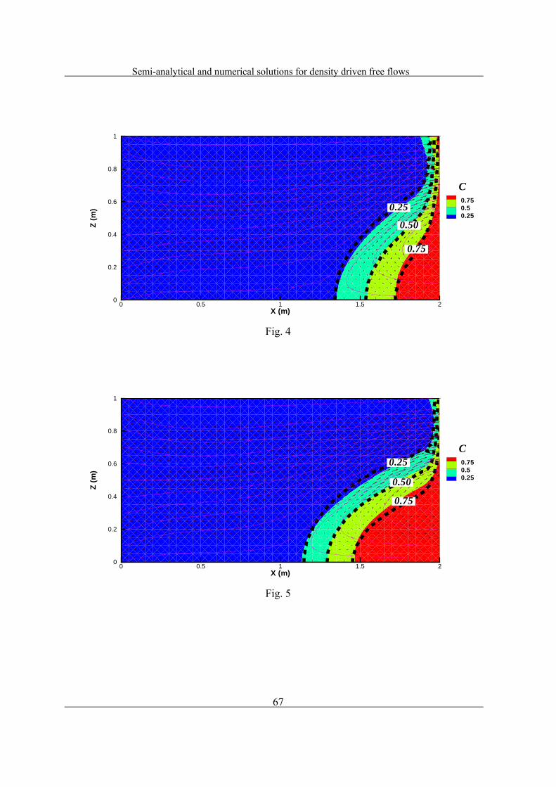
Semi-analytical and numerical solutions for density driven free flows
67
X (m)
Z(m
)
0 0.5 1 1.5 20
0.2
0.4
0.6
0.8
1
0.750.50.25
0.75
0.25
0.50
C
Fig. 4
X (m)
Z(m
)
0 0.5 1 1.5 20
0.2
0.4
0.6
0.8
1
0.750.50.25
0.75
0.25
0.50
C
Fig. 5

Semi-analytical and numerical solutions for density driven free flows
68
Case 1 ( 0.008a , 0.1b ) Case 2 ( 0.006a , 0.05b )
z = (0.25) x
=
(0.5) x
=
(0.75) x
= z =
(0.25) x
=
(0.5)x
=
(0.75) x
=
0.000 1.342 1.540 1.722 0.000 1.146 1.294 1.453
0.050 1.347 1.543 1.728 0.050 1.149 1.297 1.462
0.100 1.353 1.551 1.739 0.100 1.160 1.311 1.479
0.150 1.367 1.568 1.758 0.150 1.174 1.333 1.509
0.200 1.386 1.593 1.784 0.200 1.199 1.364 1.551
0.250 1.409 1.624 1.817 0.250 1.227 1.403 1.604
0.300 1.442 1.663 1.853 0.300 1.263 1.451 1.677
0.350 1.476 1.711 1.881 0.350 1.308 1.509 1.767
0.400 1.521 1.758 1.909 0.400 1.364 1.585 1.853
0.450 1.571 1.809 1.932 0.450 1.431 1.674 1.915
0.500 1.630 1.856 1.946 0.500 1.504 1.789 1.951
0.550 1.705 1.895 1.960 0.550 1.585 1.887 1.971
0.600 1.767 1.921 1.965 0.600 1.700 1.937 1.979
0.650 1.820 1.935 1.971 0.650 1.831 1.954 1.988
0.700 1.887 1.943 1.979 0.700 1.915 1.971 1.991
0.750 1.912 1.951 1.985 0.750 1.951 1.974 1.993
0.800 1.918 1.957 1.985 0.800 1.954 1.977
0.850 1.929 1.960 1.988 0.850 1.960 1.979
0.900 1.932 1.965 1.991 0.900 1.960 1.982
0.950 1.935 1.965 1.991 0.950 1.963 1.982
1.000 1.932 1.965 1.000 1.968 1.996
Table 1

Salt dissolution process
69
Chapter 5
Salt dissolution process
Contents
1. Introduction ..................................................................................................... 72
2. Mathematical models ....................................................................................... 73
3.1. Discretization of the flow equation ............................................................ 74
3.2. Discretization of the transport equation ..................................................... 76
3.3. Dissolution model, moving boundary algorithm ........................................ 77
3. Time stepping procedure ................................................................................. 78
4. Experimental set-up ......................................................................................... 79
5. Results and discussion ..................................................................................... 80
6. Conclusions ..................................................................................................... 81

Salt dissolution process
70
A moving boundary model for solid-liquid dissolution problems:
Application on density driven Stokes flow
Ali Zidane(1,2)*, Eric Zechner(2), Anis Younes (1), Constantin Oltéan(3) ,Peter Huggenberger(2)
(1) Laboratoire d’Hydrologie de Geochimie de Strasbourg, University of Strasbourg, CNRS, UMR 7517, France
(2) Department of Environmental Sciences, University of Basel, Institute of Geology, Switzerland (3) Laboratoire d’Environnement de Geochimie et Ouvrages, University of Nancy, France
Paper submitted to Theoretical and computational fluid dynamics journal
*Corresponding author: Ali Zidane
E-mail : [email protected]

Salt dissolution process
71
Abstract
Several models have been previously used to approximate moving boundary problems in numerical
simulations. In this paper, a simple and easily implemented model is described. The model is based on a
Dynamic Mesh Method (DMM) that adapts the size of the mesh with the moving boundary. The model is
applied to simulate a solid-liquid dissolution problem. A new combination of the Crouzeix-Raviart (CR),
Multipoint Flux Approximation (MPFA) and the Discontinuous Galerkin (DG) methods is presented in
this paper to solve the flow and the transport equations for free fluids. The CR element is used to solve the
laminar Stokes flow, and the MPFA-DG is used to solve the advection-dispersion transport equation. A
non-iterative time stepping scheme based on local truncation error is used which is the first to be applied
for such coupled problems. The developed numerical model with the moving boundary algorithm is tested
against a laboratory experiment of salt dissolution. The results show a good agreement between the
experimental and the numerical profiles which validate the developed numerical model with the moving
boundary method.
Keywords: Moving boundary, Dynamic mesh, CR, DG, MPFA, Salt dissolution.

Salt dissolution process
72
1. Introduction
Dissolution of highly soluble rocks such as evaporites has to be addressed in a variety of activities, e.g.in
the mining industry, with the construction of buildings or traffic lines, or during exploration of geothermal
energy. Dissolution cavities that occur within the subsurface salt deposits may lead to land subsidence or
catastrophic collapses [1, 55, 48, 26]. Moreover, salt dissolution affects also the water quality due to
salinization and high mineralization [39]. The first theoretical investigation of pore volume changes due to
dissolution was provided by [61]. Since then, a large number of studies were concerned by modelling the
pore volume change [66, 21, 53, 58, 13, 29, 71, 72]. In this manuscript we develop a numerical technique
to model the dissolution problem in a free flow media. The developed model has the advantage to be
simply applied in porous media and in free flow media. One of the key aspects for the description of the
dissolution phenomena is to track the movement and evolution of the boundary between solid and fluid.
Three types of problems arise with the numerical approach during simulation of moving boundaries [34]:
i) the discrete representation, ii) the evolution of the boundary in time and iii) how the boundary
conditions are imposed on the moving boundaries. There are two types of approaches that are typically
used with the numerical simulation of a moving boundary: the front tracking method and the front
capturing method. The most common front tracking method is the Arbitrary Lagrangien-Eulerian (ALE)
technique [23, 49]. With the ALE method the evolution of the mesh is considered by adopting a separate
grid and the computations are considered in both the absolute frame and the relative frame [23, 49]. With
the ALE method an averaging of the flow properties is required for all the fluid elements. This averaging
procedure represents the biggest drawback of the method [34]. Another type of the front tracking method
was developed by [59] in order to obtain the motion of the fluid-solid interface due to dissolution known
as the Random Walk Method (RWM). Another algorithm of the simulation of reactive flows in porous
media was recently developed by [70]. [70] combined the Marker Points Method (MPM) with the Lattice-
Boltzmann scheme. The latter consists of describing the boundary between the fluid and the solid phases
by a set of marker points. The positions of these marker points represent the interface solid-fluid. Within
the front capturing moving boundary algorithms the most popular methods are the Volume of Fluids
(VOF, [34]) and the Level-Set (LS, [52]) methods. Within both algorithms, the front tracking and the front
capturing are considered as sharp-front methods since the domain is divided into the two separate fluid or
solid phase. Another algorithm used to model the moving boundary problem is the Diffuse Interface
Method (DIM). As stated by [56], the idea of the DIM is dated back when Lord Rayleigh (1892) and van
der Waals (1893) considered the interface with a non-zero thickness, resulting in a diffuse interface. The
DIM was firstly used to model the interface between two fluids and later it was developed to a wide
variety of hydrodynamics applications [1, 47]. The idea behind the DIM consists of considering the solid-
liquid interface as a porous medium where the porosity goes from zero to one, and a phase indicator is

Salt dissolution process
73
used to set the fluid region to one and the solid region to zero.
Most of the discussed algorithms are able to represent the phenomena of moving boundaries during the
dissolution process adequately. However, they represent a high order of complexity, which results in large
computational storage requirements and/or numerical diffusion effects. Therefore, a new formulation of
the moving boundary condition is presented in the paper. The presented model is rather simple and can
easily be applied in for fluid flow both in porous media and in free flow media. The model is based on a
Dynamic Mesh Method (DMM) that adapts the size of the mesh with respect to the amount of
displacement at the moving boundary. The model is applied to simulate the dissolution problem in a free
flow media. To simulate the laminar density driven flow in a free flow media a new combination of the
Crouzeix-Raviart (CR), Multipoint flux Approximation (MPFA) and Discontinuous Galerkin (DG)
methods is presented in this paper. The CR based on the nonconforming piecewise linear finite elements
for the velocity and the piecewise constant finite elements for the pressure is used to solve the Stokes
equation, the DG-MPFA is used to solve the advection-dispersion transport equation. Non iterative time
stepping is used in this work. The scheme is based on local truncation error control as in [69]. It was able
to increase the numerical accuracy and to reduce the computational cost at the same time [69]. To
calculate the mass flux at the solid- fluid interface a reactive model is applied at the boundary by using a
constant reactive term.
In order to validate the developed numerical code, the model is tested against a laboratory salt fracture
dissolution experiment. A qualitative comparison between the numerical and the experimental results is
presented by comparing the dissolution profiles and the transient fracture aperture variations over three
different sections within the fracture height.
2. Mathematical models
In this manuscript the flow is considered steady and laminar and the inertial forces in the flow field are
assumed to be negligibly small compared with the viscous and pressure forces. Therefore, the free-flow is
governed by the Stokes equation [10, 57, 60, 40, 37, 38],
2u gp (1)
and the continuity equation:
0. u (2)
The solute obeys the local convection-diffusion transport equation in a free flow media [26, 33, 44, 4, 11,
22]:

Salt dissolution process
74
The solute mass conservation is written in term of mass fraction as follows:
0( C )
.( C D. C )t
u
(3)
State equations linking density and viscosity to mass fraction:
10 1 0 0
0
,
C
C and
(4)
The boundary conditions for the solute concentration at the moving boundary surface corresponds to the
first order reaction equation:
sat.( C D. C ) C C n u (5)
where is the fluid density [ML-3], t the time [T], C the solute mass fraction [M. salt/M. fluid], u the
velocity [LT-1], 0 the density of the injected fluid [ML-3], g the gravity acceleration [LT-2], the fluid
dynamic viscosity [ML-1T-1], is the mass transfer coefficient [ML-3T-1], D is the diffusion coefficient
[L2T-1], 1 and 1 are respectively, density and viscosity of the high density fluid (saltwater) and 0 the
viscosity of the injected fluid, satC is the saturation concentration [M. salt/M. fluid], and n is the unit
normal to the boundary surface.
3.1. DISCRETIZATION OF THE FLOW EQUATION
The system (1)-(2) cannot be discretized with the same order for pressure and velocity approximations due
to stability conditions. Otherwise some sort of stabilization is added to the mixed formulation [46]. To
avoid these difficulties, we use the non-conforming Crouzeix-Raviart (CR) elements for the velocity
approximation in combination with constant pressure per element, since they satisfy the Babuska-Brezzi
condition [14, 28, 30]. This condition is central for ensuring that the final linear system to solve is non-
singular [45]. Moreover, the non-conforming Crouzeix-Raviart (CR) element has local mass conservation
properties [15] and leads to a relatively small number of unknowns due to the low-order shape functions.
The CR element is used in many problems such as the Darcy-Stokes problem [16], the Stokes problem
[20] and the elasticity problem [31, 32]. The CR element gives a simple, stable and optimal order
approximation of the Stokes equations [8]. In the following, we recall the main stages for the
discretization of the Stokes equation with the CR triangular element.
With the non-conforming finite element method, the degrees of freedom for the velocity vector u are the
two components i iu ,v of u at the midedge i facing the node i (Fig. 1). Inside the element E , we
assume a linear variation of the velocity components E Eu ,v
E E E E E EE i i j j k k E i i j j k ku u u u , v v v v (6)
Salt dissolution process
75
Where the interpolation function Ei equals 1 on the midedge i and zero on the midedges j and k of
E .
The variational formulation of the Stokes equation (1) using the test function i over the domain
writes:
u Ι i i. p g z
(7)
where u is the gradient of the velocity vector u and Ι the 2 2 identity matrix.
Using Green’s formula,
u Ι η u Ιi i ip . p g z
(8)
The first integral contains boundary conditions. It vanishes in case of free-flow boundary or in case of an
interior edge i . In this last case, equation (8) becomes
u Ι u ΙE E' E EE E i E E i i i
E E E E
. p . p g z g z
(9)
Using (6) we obtain
3
1
3
1
u Ι
i j i jji
jEE E i Ei
i j i jEj
j
x x z z uz
. p PEx
x x z z v
(10)
and
i
Ei E i E i
E
zg z g z z
x
(11)
where ij kx x x and i
k jz z z , Ez and iz are respectively the z-coordinate of the centre of E
and of the midpoint of edge i , E and Ep are respectively the mean density and pressure over E .
The finite volume formulation of the continuity equation (2) over the element E writes:
0uE
. (12)
using (6), it becomes
3
1
0j jj j
j
z u x v
(13)
The final system to solve for the flow is obtained by writing equation (10) for each edge (two equations
per edge) and equation (13) for each element.

Salt dissolution process
76
3.2. DISCRETIZATION OF THE TRANSPORT EQUATION
Standard numerical methods, such as finite element (FE) or finite volume (FV), usually generate solutions
with numerical diffusion and/or non-physical oscillations when the advection part is dominant within the
transport equation. The DG allows us to avoid these oscillations [63] since it provides a high-resolution
scheme for advection. The local conservation of FV methods are maintained by the DG, in addition it
allows higher order approximations that could be used through a variational formulation in place of some
hybridised difference or functional reconstruction [41]. The method was used on diffusion-advection
problems in [10, 17, 35] and multiple strategies have been used to adapt the DG method to elliptic
problems [5, 9]. More details of DG methods can be found in [9, 17, 18].
Concerning the hyperbolic systems, the DG method has proven to be superior to the already existing FE
methods [9]. The DG method is used to solve the advection equation and combined with the Multipoint
Flux Approximation (MPFA) method for the dispersion equation.
The MPFA is locally conservative and handles general irregular grids on anisotropic heterogeneous
domains. The MPFA method can be combined with the DG method without the time splitting procedure
[68, 73]. Since the MPFA and the DG use the same type of unknowns (average value per element),
therefore both discretizations can be gathered into one system matrix.
The spatial discretization of the DG-MPFA is given as follows:
By substituting the mass conservation of the fluid in the transport equation [51] and referring to [4], the
transport equation (3) can then be written in the following mixed form:
D
D
CC . 0
tD C
u. u
u . (14)
the dispersive flux Du is assumed to vary linearly inside the element E , therefore,
, ,
1. . .E E
D D E D i D D ii iE E
dE n dl Q QE
u u u (15)
where ,ED iQ is the dispersive flux across the edge i.
We use the P1 DG method where the approximate solution ( , )hC tx is expressed with linear basis
functions Ei on each element E as follows:
3
1
, | E Eh E i i
i
C t C t
x x (16)
The three unknowns for each element are the average value of the mass fraction defined at the triangle
centroid E Ex , y and its deviations in each space direction [18] with the corresponding interpolation

Salt dissolution process
77
functions:
1 2 3, 1, , , , . E E EE Ex y x y x x x y y y (17)
The variational formulation of (14) over the element E using Ei as test functions gives (see [68]),
*
,
. .
10
Ej E E E E E E E E
j i j j i j j ij j jE E E
E E Ei E D j i
EjE E
CC C
t
C QE
u u
u.η
(18)
where E is the boundary edge of the element E, and *C the upstream mass fraction on E .
More details about the expression of each term in (18) could be found in [67].
3.3. DISSOLUTION MODEL, MOVING BOUNDARY ALGORITHM
In the presented model only the fluid phase is simulated and the effect of dissolution is considered by
increasing the size of the cells in the simulated domain with respect to the amount of dissolution that
occurs. The idea behind the model is quite simple and it’s based on the fact that the dissolved volume of
the solid should be filled by the fluid (Fig. 2). With the DMM there is no need to simulate the solid block
and no storage capacity is required for the boundary nodes.
In the studied case the moving boundary is applied on the dissolution problem. Therefore the variation of
the mesh size is directly related to the amount of dissolved salt that occurs at the solid-fluid interface. If
we consider a finite element E with area E , the dissolved mass within an interval of time dt is given as
follows:
( )satdm
Q C C Edt
(19)
where dm [M] is the amount of the dissolved mass within an interval of time dt , and Q is the dissolution
flux.
Knowing the density definition of a certain amount of solid that has been dissolved:
.s
dm
dA e (20)
where s is the solid density, .dA e is the volume of the dissolved solid, with dA the dissolved area and
e the dissolved thickness. In the case of 2D dissolution process the volume is then reduced to the area dA .
Using (20) in (19) we get:
( ).
s
satE C C dtdA
(21)
As shown in (Fig.3), the area of the dissolved solid could be approximated as follows:

Salt dissolution process
78
.dA dh dy (22)
where dh is the increment that should be added to the edge at the solid-fluid boundary, and dy is the
height of that edge. Since the coordinate variation is related to the nodes, then in case of multiple edges at
the salt boundary, the amount of dissolved area at each edge is divided on the two corresponding nodes. In
this case, the height dy used in (22) to deduce the amount of coordinate increment dh for each node, is
nothing but the sum of the halves of the two edges sharing the same node (Fig.4). Consequently, the
increment dh can be calculated for each node n at the solid-fluid interface at each time step as follows:
( ).( )
2. ( ). s
satE C C dtdh n
dy n
(23)
The calculated incrimination in (23) for each node at the interface is then added to the horizontal ordinate
of that node at each time step. To homogenize the domain, the size of the non-boundary elements is
increased in a proportional manner to their distance from the boundary. The developed DMM is simple
and easy to implement for moving boundary problems in both porous media and in free flow media.
3. Time stepping procedure
Numerical simulations of density driven problems require excessive computational time and/or heavy
equipments due to the strong nonlinearities between the flow and the transport equations. In order to
reduce the computational needs and maintaining accuracy at the same time, a non iterative time stepping
scheme based on local truncation error control is used as in [69]. The time stepping procedure is shown as
follows:
The local time truncation error of the concentration is evaluated using two approximations of adjacent
order of accuracy.
1
1 1 11
2
nn n n n n
n
tC C C C
t
e (24)
The time step is accepted if the absolute error criterion is verified,
1en (25)
If this criterion is met, the following time step is controlled by the temporal truncation error tolerance
using,
1
1min
en n
maxnt t s ,r
max
(26)
If the error criterion is not satisfied, the current time step is repeated using the latest error estimate

Salt dissolution process
79
1 11 1
maxe
n nj j minn
t t s ,rmax
(27)
where j indexes the recursive step size reduction, maxr and minr are used to limit multiplication and
reduction factors and often set equal to 2.0 and 0.1 respectively and 0 9s . a safety factor [64]. And the
temporal truncation error tolerance is set to 0 01. .
4. Experimental set-up
The fracture is constituted of two salt blocks dimensions 9.9 x 3.5 x 0.42 cm3 spaced about 0.4 cm apart
(Figs. 5, 6). The blocks were obtained by cutting from a compacted salt block used in cattle feed. The salt
blocks were inserted between two parallel transparent glass plates supported by a rigid metal structure.
During this operation, the fracture aperture can undergo a slight decrease estimated at about 0.025 – 0.075
mm. In order to ensure a good adhesion between the salt blocks and the glass plates, the former were
polished with very fine sandpaper. The impermeability of lateral boundaries is provided by rubber seals.
The cell is initially filled with a fully saturated saline NaCl solution (Csat = 357 g/L). After about 12 hours,
in order to induce dissolution of the rock matrix, distilled water is injected at a low flow rate (Qv = 1.0
mL/h) into the lower part of the cell through a plastic injection tip. The injection tip (1.5 mm inner
diameter) is centered between the two plates and located 2.0 mm above the lower cell edge. A peristaltic
pump ensures a quasi-constant flow rate. The mixing between the injected fluid and the dissolved part of
the rock matrix is removed through an exhaust nozzle disposed in the same way as the injection tip but in
the upper part of the cell. In order to better visualize the dissolution of the salt blocks, the injected fluid
was dyed by adding a few milligrams of fluorescein to the saline solution. Illuminated by a homogeneous
light source located behind the experimental model, the temporal and spatial evolution of the flow channel
between the salt blocks is followed using a numerical camera with a standard Charge Coupled Device
(CCD) detector consisting of 3888 x 2592 pixels. As the numerical camera is set in front of the
experimental model, the recorded images, caught at various intervals of time, are analyzed by image
processing software.
The experimental configuration is characterized by a more rapidly dissolution in the upper part compared
to the lower part. This behavior suggests that the fracture dissolution is the result of the free buoyant
convection. The less dense fluid will rise through the denser fluid resulting in different dissolution rates in
agreement with the fracture height. For relatively short times, i.e. at the beginning of the experiment (t <
10h), the dissolution rate increases approximately linearly with the fracture height while for relatively
large times (t > 20h ), the fracture dissolution is more rapid in the upper part compared to the lower part.

Salt dissolution process
80
However, the analysis of the experimental results highlighted the emergence and the development of the
gas bubbles arising from degassing during the dissolution of the rock matrix (small black spots located in
the flow channel). Despite the immersion of the salt blocks into a saturated solution for more than 12
hours followed by vacuum degassing or the injection of CO2, this degassing phenomenon was observed
for each carried out experiment. To verify the influence of this phenomenon on the spatial-temporal
fracture evolution, the experiment was repeated at least twice. A very good reproducibility was observed.
It not only shows a weak influence of the degassing phenomenon on the fracture dissolution but also a
relatively small impact of the heterogeneities within the salt blocks.
5. Results and discussion
The experimental results show that dissolution occurs mainly at the upper part of the fracture which
consequently leads to a remarkable change of the fracture walls shape (Fig.7). This is because the
dissolution of the fracture is due to the buoyant convection and that the reactive kinetics at the boundaries
is fast with respect to the reactant transport. To track the evolution of the reactive walls we took 4
snapshots of the fracture evolution after 10, 20, 30 and 40 hours, respectively. The final dissolution shapes
(Fig. 7) of the fracture walls prove the existing of two rotating eddies that circulate in a symmetrical
direction with respect to the vertical axis passing through the fracture median. The conducted laboratory
experiment was used to validate the developed numerical model. Due to the symmetrical profile of the
dissolution shapes, only half of the domain was simulated and compared against the experimental results.
Within the numerical model the left and the right sides are considered as impermeable and a free boundary
condition is applied at the top of the fracture (Table 1). A constant mass transfer coefficient is applied at
the reactive walls (20 mmol.cm-2.h-1) and the density difference is set to (25 kg.m-3) (Table 1). Results
show that dissolution rate increases with the fracture elevation (Fig. 8a-e). The concentration distribution
(Fig. 8e) shows that water is fully saturated at the bottom of the fracture and the concentration reduces
with the elevation to reach their minimal values at the top of the fracture. The concentration distribution
justifies the dissolution profiles since the dissolution flux at the interface is proportional to the
concentration gradient between the solid and the fluid. The numerical results show similar shapes
compared to the experimental results along the fracture body except the upper part (9 to 10 cm) where the
numerical results exceeds the experimental ones. The maximum deviation between the numerical and the
experimental results is observed above (9.8 cm) where the difference reaches up to (4mm) as shown in
(Fig. 9). In order to give an accurate comparison, three different sections are taken within the fracture at
elevations Z=1 cm, Z=5 cm, and Z=9 cm. The fracture aperture variations are recorded within these 3
cross sections during the experiment and during the numerical simulations. To illustrate the variations, the
recorded fracture aperture values are divided by the initial fracture width (i.e. 4mm for the experiment and

Salt dissolution process
81
2mm for the simulation), and the duration time at which the aperture is measured is divided by the final
duration of the experiment (i.e. 40h). A good match between the numerical and the experimental results is
observed over the 3 cross sections of the fracture aperture evolution (Fig. 10). The comparison shows that
over the first cross section, the final aperture width is about 3 times the original fracture width, where at
the middle it reaches up to 4 times the original fracture aperture and goes up to 8 times at the top of the
domain.
6. Conclusions
The paper explored numerical techniques to simulate density driven Stokes flow with a moving boundary
due to the dissolution process. A new combination of the CR_MPFA_DG is presented to model the Stokes
density driven flow. The Crouzeix-Raviart finite element is used to discretize the flow equation and the
DG-MPFA scheme is used to discretize the advection-dispersion transport equation. A first order reaction
model is applied at the moving boundary to simulate the dissolution process. To track the moving
boundary, an efficient algorithm for moving boundaries is developed in this paper.
To validate the developed numerical model, a set of laboratory experiment are conducted over a vertical
salt fracture. The transient and the final dissolution shapes of the salt fracture are compared against the
numerical results and a good agreement is observed. The developed numerical model is based on the
Stokes flow within the fracture and coupled to the advection-dispersion transport equation. To reduce the
computational time due to the coupling caused by buoyancy forces, we use a non-iterative time stepping
scheme where the time step length is controlled by the temporal truncation error. To model the fracture
enlargement we developed the DMM that adapts the size of the finite elements with respect to the amount
of dissolution that occurs at the moving boundary. The boundary is moved to the direction of the normal
vector to the solid-fluid interface. The developed DMM is a simple and easily implemented algorithm to
track the moving boundaries.
The validity of the newly developed numerical scheme CR_MPFA_DG to solve density driven flow for
free fluids is provided in this study. From the other side a new technique to track the moving boundary is
provided in this study which proved to be effective when compared against a laboratory experiment of salt
dissolution.
ACKNOWLEDGMENTS This study was partially supported by the SNF (Swiss National Foundation, Grant 200020_125167),
whose support is gratefully acknowledged.
Salt dissolution process
82
References
[1] Anderson, D.M., McFadden, G.B.: Diffuse-interface methods in fluid mechanics. Annu.
Rev. Fluid Mech. 30, 139–165 (1998)
[2] Aavatsmark, I.: An introduction to multipoint flux approximations for quadrilateral grids.
Computat Geoscien,6:404-432, (2002).
[3] Aavatsmark, I., Barkve, T., Bøe, Ø., Mannseth, T.: Discretization on non-orthogonal,
quadrilateral grids for inhomogeneous, anisotropic media. J Computat Physics;127:2-14,
(1996).
[4] Ackerer, P., Younes, A.: Efficient approximations for the simulation of density driven flow
in porous media. Adv Water Res;31:15-27, (2008).
[5] Aizinger, V., Dawson, C., Cockburn, B., Castillo, P.: The local discontinuous Galerkin
method for contaminant transport. Adv Water Res; 24:73-87, (2001).
[6] Anderson, R. Y., Kirkland, D. W.: Dissolution of salt deposits by brine density flow,
Geology, 8, 66−69, (1980).
[7] Arbogast, T., Lehr, HL.: Homogenization of a Darcy-Stokes system modeling vuggy porous media. Comput. Geosci., 10:291, (2006).
[8] Arnoldk, DN.: On nonconforming linear-constant elements for some variants of the Stokes equations, presenta dal s.c. Franco Brezzi nella seduta del 24-6-93.
[9] Arnold, DN., Brezzi, F., Cockburn, B., Marini, LD.: Unified analysis of discontinuousGalerkinmethods for elliptic problems. SIAM J. Numer. Anal.;5:1749-1779,(2002).
[10] Baumann, C.E, Oden, JT.: A discontinuous hp finite element method for convection–
diffusionproblems. Comput. Methods App Mech. Eng.;175:311–341,(1999).
[11] Bear, J.: Dynamics of Fluids in Porous Media ~Elsevier, New York, (1972).
[12] Beavers, G., Joseph, D.: Boundary conditions at a naturally permeable wall, J. Fluid Mech., 30:197, (1967).
[13] Bekri, S., Thovert, J.F., Adler, P.M.: Dissolution of porous media. Chem. Eng. Sci. 50, 2765–2791 (1995)
[14] Brezzi, F., Fortin, M.: Mixed and hybrid finite element methods, Berlin: Springer (1991).
[15] Bruman, E., Hansbo, P.: A stabilized nonconforming finite element method for incompressible flow, Comput. Methods App Mech. Eng.,vol. 195, num. 23-24, p. 2881-99, (2004).
Salt dissolution process
83
[16] Bruman, E., Hansbo, P.: Stabilized Crouzeix-Raviart element for the Darcy-Stokes problem, Numerical Methods for Partial Differential Equation,21(5), 986-997,(2005).
[17] Cockburn, B., Hou S., Shu, CW.: TVB Runge Kutta local projection discontinuous
Galerkin finite element method for conservative laws III: One dimensional systems. J
Comput Phys;84: 90-113,(1989).
[18] Cockburn, B., Shu, CW.: The Runge-Kutta Discontinuous Galerkin Method for
conservative laws V: Multidimentional Systems. J Comput Phys;141:199-224,(1998).
[19] Cockburn, B., Karniadakis, GE., Shu CW.(Eds.): Discontinuous Galerkin Methods: Theory,
Computation and Applications. Lecture Notes in Computational Science and
Engineering;11:Springer-Verlag,(2000).
[20] Crouzeix, M., Raviart, P.: Conforming and nonconforming finite element methods for solving the stationary Stokes equations. RAIRO Sér. Rouge,7(3), 33-75, (1973).
[21] Daccord, G. and Lemanczyk, R. Z., 1987, Acidizing physics, in Reservoir Stimulation (Edited by M. J. Economides and K. G. Nolte), Chap. 13. Schlumberger Educational Services,Houston, Texas.
[22] Diersch, H.J, Kolditz, O.: Coupled groundwater flow and transport: 2. Thermoline and 3D
convection systems, Adv Water Res;21:401-425,(1998).
[23] Donea, J., Giuliani, S., Halleux J.P.: An arbitrary Lagrangian–Eulerian finite element
method for transient dynamic fluid–structure interactions. Comput. Methods Appl. Mech.
Eng. 33, 689–723 (1982)
[24] Edwards, M.G., Rogers, C.F.: Finite volume discretization with imposed flux continuity for
the general tensor pressure equation. Computat Geoscien,2:259-290, (1998).
[25] Flekkøy, EG., Rage, T., Oxaal, U., Feder, J.: Hydrodynamic Irreversibility in Creeping Flow, Phys. Rev, PACS numbers: 47.15.Gf, 02.70.Bf, 02.70.Lq, 47.60.+I, VOLUME 77, NUMBER 20,(1996).
[26] Frumkin, A.: Speleogenesis in salt − the Mount Sedom area, Israel, in Speloegenesis −
evolution of karst aquifers, edited by A. B. Klimchouk, D. C. Ford, A. N. Palmer and W.
Dreybrodt, pp. 443−451, National Speleological Society, Huntsville, (2000).
[27] Frumkin, A., Raz, E..: Collapse and subsidence associated with salt karstification along the
Dead Sea, Carbonates Evaporates, 16(2), 117-130,(2001).
[28] Girault, V., Raviart, PA.: Finite element methods for Navier-Stokes equations, Berlin: Springer (1986).

Salt dissolution process
84
[29] Golfier, F., Zarcone, C., Bazin, B., Lenormand, R., Lasseux, D., Quintard, M.: On the ability of a Darcy-scale model to capture wormhole formation during the dissolution of a porous medium. J. Fluid Mech. 457, 213–254 (2002)
[30] Gresho, PM., Sani, RL.: Incompressible flow and the finite element method, New York: Wiley; (1998).
[31] Hansbo, P.: Larson MG. Discontinuous Galerkin and the Crouzeix-Raviart element: application to elasticity. ESAIM: Math. Model. Numer. Anal.,37(1), 63-72, (2003).
[32] Hansbo, P., Larson, MG.: Discontinuous Galerkin methods for incompressible and nearly incompressible elasticity by Nitshe’s method. Comput. Methods Appl. Mech. Engrg,191(17-18), 1895-1908, (2002) .
[33] Happel, J., Brenner, H.: Low Reynolds Number Hydrodynamics (Prentice Hall Inc., Englewood Cliffs, NJ,1965).
[34] Hirt, C.W., Nicolas, B.D.: Volume of fluid (VOF) method for the dynamics of free boundaries. J. Comput. Phys. 39, 201–225 (1981)
[35] Hughes, TJR., Masud, A., Wan, J.: A stabilized mixed discontinuous Galerkin method for
Darcy flow. Computat Meth Appl Mech Engrg;195(25-28):3347- 3381,(2006).
[36] Huyakorn, P., Anderson, P., Mercer, J., White, H.: Saltwater intrusion in aquifers:
development and testing of a three-dimensional finite element model. Water Resour
Res;23:293-312,( 1987).
[37] Jäger, W., Mikelić, A.: On the interface boundary condition of Beavers, Joseph, and Saffman. SIAM J. Appl. Math. 60:1111, (2000).
[38] Jäger, W., Mikelić, A.: Asymptotic analysis of the laminar viscous flow over a porous bed. SIAM J. Sci. Comput., 22:2006, (2001).
[39] Johnson, K. S: Dissolution of salt on the east flank of the Permian Basin in the
southwestern U.S.A., J. Hydrol., 54, 75−93, (1981).
[40] Kaviany, M.: Principles of Heat Transfer in Porous Media, Mechanical Engineering Series, Springer-Verlag, New York, (1999).
[41] Kirby, R.: A Posteriori Error Estimates and Local Time-Stepping for Flow and Transport
Problems in Porous Media, Ph.D thesis, University of Texas at Austin, (2000).
[42] Klausen, R.A, Russell T.F.: Relationships among some locally conservative discretization
methods which handle discontinuous coefficients. Journal Computat Geoscien,8(4):1-37,
(2004).
[43] Kozary, M.T., Dunlap, J. C. and Humphrey, W. E.: Incidence of saline deposits in geologic
time, Geol. Soc. Am. Spec. Pap., 88, 43−57, (1968).

Salt dissolution process
85
[44] Landau, LD., Lifshitz, EM.: Fluid Mechanics (Pergamon Press, New York, 1987), 2nd ed.
[45] Langtangen, HP., Mardal, K., Winther, R.: Numerical methods for incompressible viscous flow. Adv. Water Res. 25, 1125-1146, (2002).
[46] Li, J., Chen, Z.: A new local stabilized nonconforming finite element method for the Stokes equations, Computing, 82:157-170, doi 10.1007/s00607-008-0001-z, (2008).
[47] Luo, H., Quintard, M., Debenest, G., Laouafa, F.: Properties of a diffuse interface model based on a porous medium theory for solid–liquid dissolution problems, Comput Geosci, 16:913–932, DOI 10.1007/s10596-012-9295-1, (2012)
[48] Martinez, J. D., Johnson, K. S., Neal, J. T.: Sinkholes in evaporite rocks, Am. Sci., 86,
38−51. (1998).
[49] Maury, B.: Characteristics ale method for the unsteady 3d Navier–Stokes equations with a
free surface. Int. J. Comput. Fluid Dyn. 6, 175–188 (1996)
[50] McManus, K. M., Hanor, J. S.: Diagenetic evidence for massive evaporite dissolution, fluid
flow, and mass transfer in the Louisiana Gulf Coast. Geology, 21, 727?730, (1993).
[51] Oltean, C., Buès, M.A.: Coupled groundwater flow and transport in porous media. A
conservative or non-conservative form? Transport in Porous Media, 44 (2), 219-246,
(2001).
[52] S. Osher and J. A. Sethian, Fronts propagating with curvature dependent speed: Algorithms
based on Hamilton–Jacobi formulations, J. Comput. Phys. 79, 12 (1988).
[53] Piot, B. M. and Perthuis, H. G., 1987, Matrix acidizing of sandstones, in Reservoir
Stimulation (Edited by M. J. Economides and K. G. Nolte), Chap. 14. Schlumberger
Educational Services, Houston, Texas.
[54] Quinlan, J. F., Smith, R. A. and Johnson, K. S.: Gypsum karst and salt karst of the United
States of America, Le Grotte d'Italia, 4(XIII), 73?92, (1986).
[55] Reuter, F., Stoyan, D.: Sinkholes in carbonate, sulphate, and chloride karst regions:
Principles and problems of engineering geological investigations and predictions, with
comments for the destruction and mining industries, in Applied karst geology, edited by B.
F. Beck, pp. 3?25, A. A. Balkema, Rotterdam, Brookfield, (1993).
[56] Rowlinson JS,Widom B.: Molecular Theory of Capillarity. Oxford: Clarendon, (1989)
[57] Saffman, P.: On the boundary condition at the surface of a porous medium, Studies Appl.
Math., 50:93, (1971).

Salt dissolution process
86
[58] Sahimi, M., Galavas, G. R. and Tsotsis, T. T., 1990, Statistical and continuum models of
fluid-solid reactions in porous media. Chem. Engng Sci. 45, 1443-1502.
[59] Salles, J., Thovert, J. F. and Adler, P. M., 1993a, Deposition in porous media and clogging.
Chem. Engng Sci. 48, 2839-2858.
[60] Sanchez-Palencia, E.: Non-Homogeneous Media and Vibration Theory, volume 127 of Lecture Notes in Physics Spring-Verlag, Berlin (1980).
[61] Schechter, R. S. and Gidley, J. L. The change in pore size distribution from surface reaction in
porous media. A.I.Ch.E.J. 15, 339-350,(1969).
[62] Shuangzhang, T., Shahrouz, A.: A slope limiting procedure in Discontinuous Galerkin
finite element method for gasdynamics applications. Int. J Numer Analy Modell,2:163-178,
(2005).
[63] Siegel, P., Mosé, R., Ackerer, P., Jaffre, J.: Solution of the advection-diffusion equation
using a combination of discontinuous and mixed finite elements. Int J Numer Meth in
Fluids; 24(6): 595-613,(1997).
[64] Sloan, S.W., Abbo, A.J.: Biot consolidation analysis with automatic time stepping and error
control. Part 1: Theory and implementation", International journal for numerical and
analytical methods in geomechanics, Vol. 23, No. 6, pp. 467-492, (1999).
[65] Wheeler, M.F., Yotov, I.: A multipoint flux mixed finite element method. SIAM44;5:2082-
2106,(2006).
[66] Williams, B. B., Gidley, J. L. and Schechter, R. S.: Acidizing fundamentals. SPE
Monograph Series, Vol. 6, (1979).
[67] Younes, A., Fahs, M., Ahmed, S.: Solving density flow problems with efficient spatial
discretizations and higher-order time integration methods, Advances in Water Resources,
32, 340-352, (2009).
[68] Younes A., Ackerer P.: Solving the advection-dispersion equation with Discontinuous
Galerkin and Multipoint Flux Approximation methods on unstructured meshes. Int. J
Numer Methods in Fluids.DOI: 10.1002/fld.1783, (2008).

Salt dissolution process
87
[69] Younes, A., Ackerer, P.: Empirical versus time stepping with embedded error control for
density-driven flow in porous media", Water Resources Research, Vol. 46, No. 8, (2010).
[70] Yu, D., Ladd, A.J.C.: A numerical simulation method for dissolution in porous and
fractured media. J. Comput. Phys. 229, 6450–6465 (2010)
[71] Zhao, C., Hobbs, B.E., Ord, A.: Fundamentals of Computational Geoscience: Numerical
Methods and Algorithms. Springer, Berlin (2009)
[72] Zhao, C., Hobbs, B.E., Ord, A.: Theoretical analyses of nonaqueous phase liquid
dissolution-induced instability in twodimensional fluid-saturated porous media. Int. J.
Numer. Anal. Methods Geomech. 34, 1767–1796 (2010)
[73] Zidane, A., Younes, A., Huggenberger, P., Zechner, E.: The Henry semi-analytical solution
for saltater intrusion with reduced dispersion, Water Resou Res, VOL. 48, W06533,
doi:10.1029/2011WR011157, (2012).
List of Figures
Fig. 1: The linear interpolation functions for velocity field.
Fig.2: The numerical simulated domain.
Fig.3: Area of the dissolved salt for one finite element.
Fig.4: Relative height of the dissolved salt for each node at the boundary.
Fig.5: Domain and boundary condition of the experiment.
Fig.6: Schematic view of the experimental setup for the laboratory dissolution runs.
Fig.7: Photograph of the dissolution shape at different time steps of the experiment.
Fig.8: Dynamic mesh variation at different time interval, a)-10h, b)-20h, c)-30h,d)-40h, and e) the
normalized concentration distribution after 40h.
Fig.9: Comparison between the experimental and the simulated results, a)-with mesh, b) - without mesh.
normalized concentration distribution after 40h.
Fig.10: Comparison of the fracture aperture evolution for the experimental (black symbols) and the
numerical (white symbols) over the 3 sections perpendicular to the flow direction.
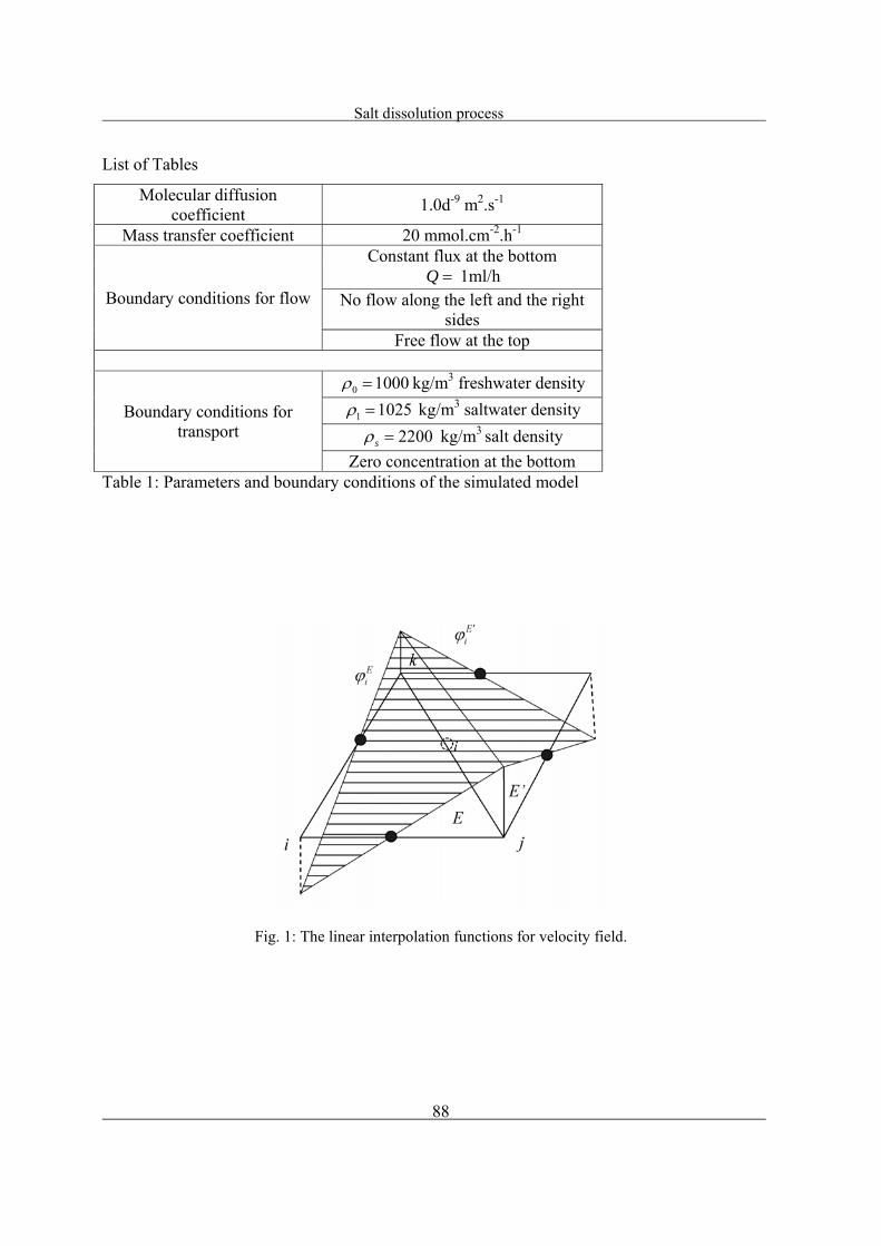
Salt dissolution process
88
List of Tables
Molecular diffusion coefficient
1.0d-9 m2.s-1
Mass transfer coefficient 20 mmol.cm-2.h-1
Boundary conditions for flow
Constant flux at the bottom Q 1ml/h
No flow along the left and the right sides
Free flow at the top
Boundary conditions for transport
0 1000 kg/m3 freshwater density
1 1025 kg/m3 saltwater density
2200s kg/m3 salt density
Zero concentration at the bottom Table 1: Parameters and boundary conditions of the simulated model
Fig. 1: The linear interpolation functions for velocity field.
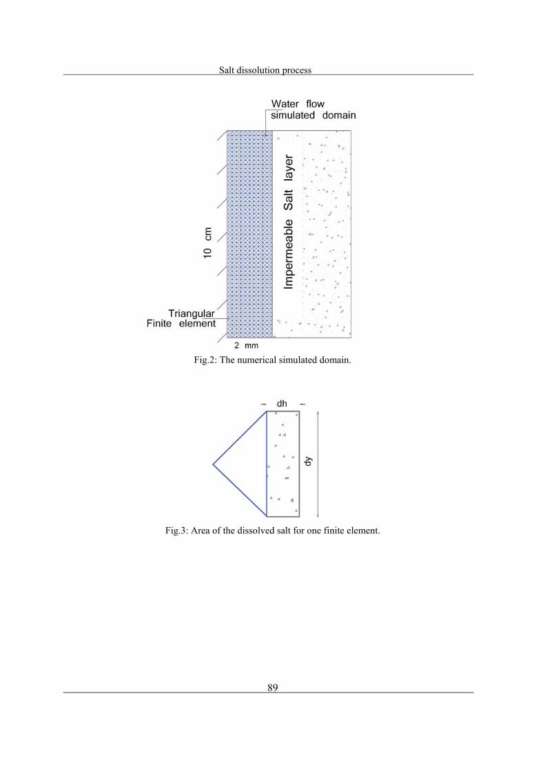
Salt dissolution process
89
Fig.2: The numerical simulated domain.
Fig.3: Area of the dissolved salt for one finite element.

Salt dissolution process
90
Fig.4: Relative height of the dissolved salt for each node at the boundary.

Salt dissolution process
91
Fig.5: Domain and boundary condition of the experiment.
Fig.6: Schematic view of the experimental setup for the laboratory dissolution runs.

Salt dissolution process
92
Fig.7: Photograph of the dissolution shape at different time steps of the experiment.
)a )b
)c )d
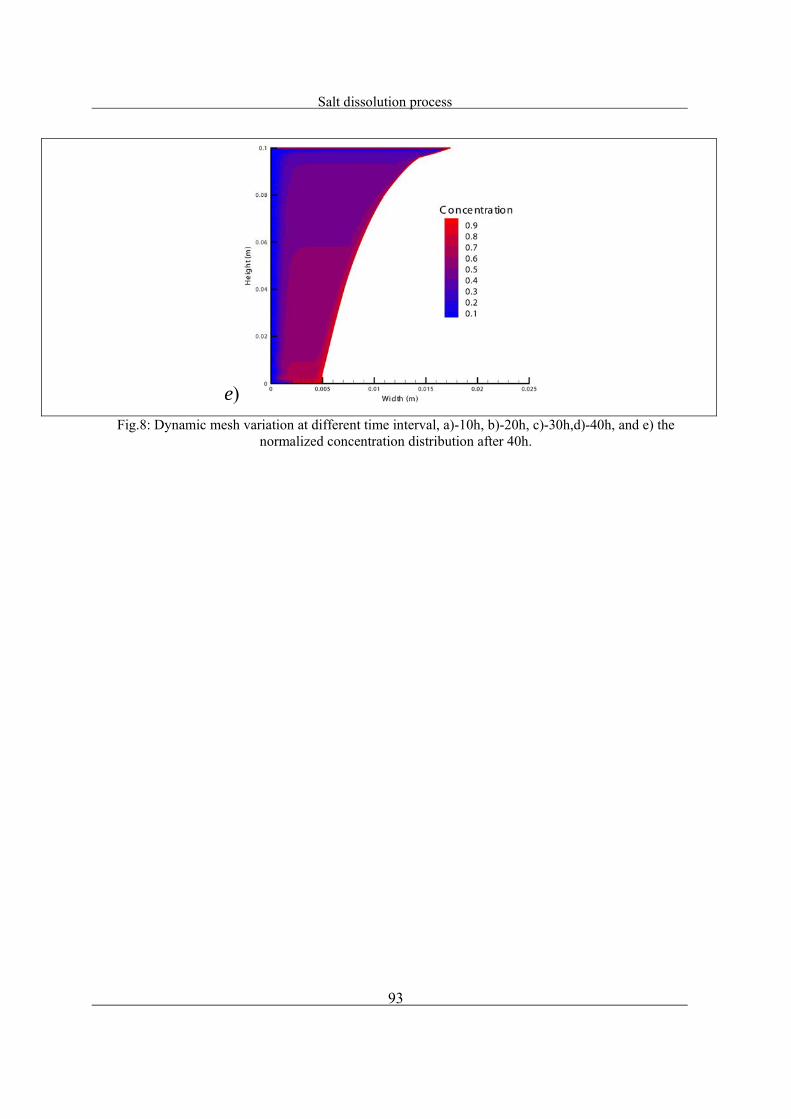
Salt dissolution process
93
)e
Fig.8: Dynamic mesh variation at different time interval, a)-10h, b)-20h, c)-30h,d)-40h, and e) the normalized concentration distribution after 40h.

Salt dissolution process
94
Fig.9: Comparison between the experimental and the simulated results, a)-with mesh, b) - without mesh.
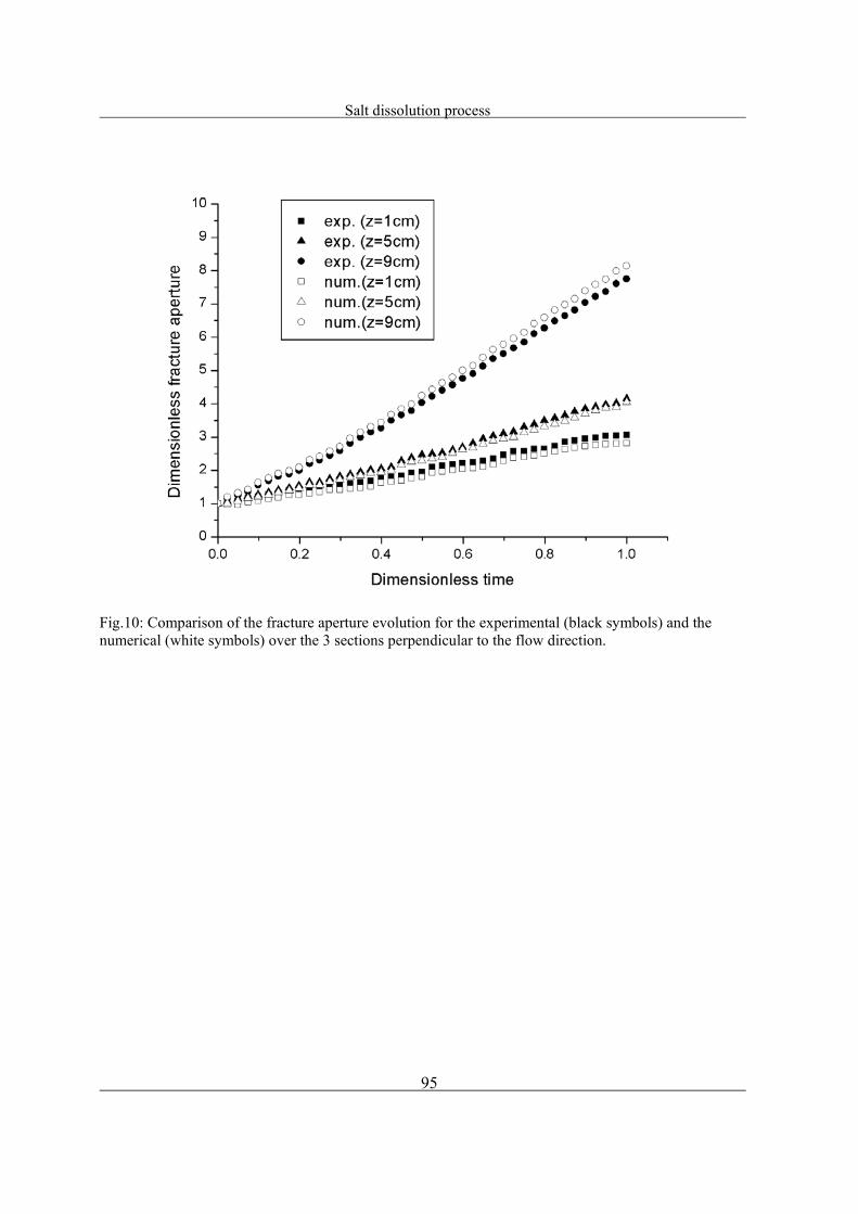
Salt dissolution process
95
Fig.10: Comparison of the fracture aperture evolution for the experimental (black symbols) and the numerical (white symbols) over the 3 sections perpendicular to the flow direction.
Evaporite dissolution and risk of subsidence
96
Chapter 6
Evaporite dissolution and risk of subsidence
Contents
6.1. Introduction ............................................................................................................. 99
6.2. Model concept ....................................................................................................... 101
6.3. Simulation of varying subsurface parameters ....................................................... 102
6.4. Conclusions ........................................................................................................... 108
6.5. References ............................................................................................................. 110

Evaporite dissolution and risk of subsidence
97
Paper submitted to journal of contaminant hydrology
On the effects of subsurface parameters on evaporite dissolution (Switzerland)
Ali Zidane*(1,2), Eric Zechner(1), Peter Huggenberger(1), Anis Younes(2)
(1) Institute of Geology and Paleontology, Environmental Sciences Department, University of Basel, Bernouillistr. 32, 4056
Basel, Switzerland
(2) Laboratoire d’Hydrologie et de Geochimie de Strasbourg, University of Strasbourg, CNRS UMR 7517, Strasbourg,
France
* Contact Person: Ali Zidane
Email: [email protected]

Evaporite dissolution and risk of subsidence
98
Abstract
Uncontrolled subsurface evaporite dissolution could lead to hazards such as land subsidence.
Observed subsidences in a study area of Northwestern Switzerland were mainly due to subsurface
dissolution (subrosion) of evaporites such as halite and gypsum. A set of 2D density driven flow
simulations were evaluated along 1,000 m long and 150 m deep 2D cross sections within the
study area that is characterized by tectonic horst and graben structures. The simulations were
conducted to study the effect of the different subsurface parameters that could affect the
dissolution process. Specific concern is given to the heterogeneity of normal fault zones and its
role for the dissolution of evaporites by considering several permeable faults that include non-
permeable areas. Results show that a large fault zone consisting of several smaller higher
conductive faults is the most important factor that affects the dissolution compared to the other
investigated parameters of thickness of the lower karstic aquifer above the halite, a dynamic
conductivity of the lower aquifer, and varying boundary conditions in the upper aquifer. The
mixed finite element method (MFE) is used to solve the flow equation, coupled with the
multipoint flux approximation (MPFA) and the discontinuous Galerkin method (DG) to solve the
diffusion and the advection parts of the transport equation.
Keywords: Density driven flow, Discontinuous finite elements, MPFA, Subrosion, Tectonics,
Switzerland.

Evaporite dissolution and risk of subsidence
99
1. Introduction
The importance of density driven flow arises due to its significant role in water resources
management and engineering (Oude Essink 2001, Paniconi et al. 2001, and Xue Y et al. 1995).
Simulation of saltwater transport models becomes a real need due to the large number of
environmental problems such as intrusion of saltwater in coastal aquifers, landfills leakage,
collapse of abandoned salt mines, radioactive waste disposal in salt rock formations and
subsurface dissolution of evaporites (Oude Essink 2001, Luo et al. 2012, Ludwig et al. 2001,
Magri et al. 2009). When carbonate rocks develop cavities over centuries, evaporite rocks can
form cavities within days. Therefore, gypsum or rock salt are seen as the most soluble common
rock formation (Martinez et al. 1998). Subsurface dissolution or subrosion occurs when non-
saturated groundwater gets in contact with evaporitic rock formations. The subsurface karst
development can create additional groundwater pathways. As a consequence, additional
mobilization of solutes can lead to widespread salinization of aquifers, and also land subsidence.
Even comparably small subsidence rates can have an important effect on sensitive urban
infrastructures (e.g. dams, buildings, traffic lines, power plants). The dissolution of salt is directly
related to the concentration gradient between salt and water. The basic principle was discussed by
(Johnson 1981, 2005) when he defined four requirements for dissolution of salt (NaCl) or
gypsum (CaSO4): (1) a deposit of salt or gypsum against which, or through which, water can
flow, (2) a supply of water subsaturated with Nacl/CaSO4, (3) an outlet where the resulting brine
can escape, and (4) energy provided from hydrostatic head differences and/or density gradients,
which causes groundwater flow through the system. Human activities can induce or influence any
of the four requirements. Zechner et al. (2011) studies three possible causes for the observed land
subsidence in northwestern Switzerland: (1) natural dissolution of the evaporites of the Middle
Muschelkalk (anhydrite and halite), which is related to the tectonic setting of the evaporitic
formations within a set of horst and graben structures, (2) salt solution mining, which has been
pursued at different locations over the last 150 years, (3) large scale extraction of groundwater in
an overlying fissured aquifer with hydrostatic connection to the underlying evaporites along fault
zones with increased hydraulic conductivity. The effects of increased hydrostatic gradient due to
both groundwater withdrawal and fluid density contrasts were evaluated in more details with a
series of 2D density-coupled solute transport simulations along an approximately 1000-m long,
and 150-m deep 2D cross section. Simulation results indicate that the upcoming process of saline

Evaporite dissolution and risk of subsidence
100
groundwater in to the main aquifer occurs under different distributions of subsurface parameters
and hydraulic boundary conditions. For the presented setup the simulations also revealed that the
most sensitive factor for the dissolution rate is the structure, or dip of the halite formation, which
leads to an increase of dissolution rates with increasing dips. However, the authors pointed out
that the assumption of a well-established homogenous karst with a constant thickness of 10 m on
top of the salt layer does not take into account the process of evaporitic karst evolution, which is
characterized by a dissolution process which is coupled to a dynamic development of subsurface
aquifer parts with increasing porosity and hydraulic conductivity.
Therefore, the presented work investigates the role of varying parameters such as aquifer
geometry and transient conductivity on the rate of salt dissolution. They include (1) variations of
thicknesses of the karst aquifer on top of the salt, or the thickness of the fault zones, (2) a
dynamic conductivity of the karst aquifer on top of the salt which is directly related to the amount
of the dissolved salt, and, in addition, (3) variations of the imposed hydraulic boundary
conditions such as the value of the constant head, or the depth of a well. The 2D simulations are
conducted using a numerical code that has been tested on a benchmark laboratory experiment in
Konz et al (2008, 2009a, b), Younes et al (2009, 2011) and field scale models (Zechner et al.
2011). In addition, the code has been recently tested against the Henry semianalytical solution for
salt water intrusion (Zidane et al. 2012). The karstified evaporites are represented as porous
aquifer. The opening porous space and fractures which are created during the dissolution process
and result in a transient hydraulic conductivity are simulated with a modified discrete fracture
approach (e.g. Kaufmann, 2002). The authors consider the approach valid on the simulated scale
due to the fact that no hydraulically relevant larger voids, or conduit network have been observed
in the dissolved halite or anhydrite/gypsum formations. Previous studies based on field
investigations and data evaluation, e.g. Ludwig et al. (2001), have shown the importance of
hydrological heterogeneities at various scales on density-driven transport. Luo et al. (2012)
presented a 2D and 3D modeling study to describe the impact of different engineering solutions
and appropriate remedial strategies for an abandoned, flooded deep salt mine in Stassfurt,
Germany. Luo et al. (2012) found that the hydrogeological structure in the study area played a
significant role in development of the subsurface concentration distribution. Due to the typical
lack of knowledge about the hydrogeological structure and properties in field studies, different
approaches to study the effect of heterogeneity within the simulations were used. Particularly,
Evaporite dissolution and risk of subsidence
101
more concern is given to the geometry of normal faults and their effect on the subrosion process.
To our knowledge, very few studies have investigated the hydraulic role of sub vertical fault
zones on the subrosion process. Magri et al. (2011) studied possible explanations for seawater
intrusion in the Seferihisar-Balcova Geothermal system in Turkey. They found, based on data
acquisitions and numerical simulations, that groundwater flow and coupled hydrochemical and
hydrothermal patterns are strongly controlled by fault tectonics. Therefore, specific concern in
the presented study is given to the structure of the normal fault zone and its role for the
dissolution of evaporites. In particular two approaches are studied, the variable width of the fault
and the heterogeneity. In the first approach the effect of different fault widths on the dissolution
process is studied, whereas in the second approach the single fault is replaced by several thin
faults separated by impermeable areas.
2. Model concept
The study site for the 2D simulations is located in northwestern Switzerland to the east of the
southeastern border of the Upper Rhine Graben and is part of the Tabular Jura (Fig. 1). Land
subsidence has been observed at six different locations, and monitored subsidence rates reached
more than 100 mm/year, affecting area ranges from 100 to 1500 m. The study area is underlain
by Triassic and Jurassic strata, which slightly dip to the southeast. The subsidence is mainly
caused by subsurface dissolution of halite (rock salt), and partly by dissolution of overlaying
anhydrite/gypsum formations of the Middle Muschelkalk. Fracture zones causing increased
permeability within the Jurassic and Triassic formations are supposed to favor vertical exchange
of groundwater also across aquitards. A 3D geological model consistent with the kinematic
evolution of the southeastern border of the Rhinegraben (Spottke et al. 2005) is used to map an
approximately 1,000-m-long and 150-m-deep 2D cross section. Regional hydrogeological
boundary conditions for the 2D density-coupled solute-transport simulations are derived from a
3D regional groundwater flow model with constant density (Fig. 1, 2). The simulated piezometric
head distribution within the Upper Muschelkalk Aquifer shows the effect of the large-scale
industrial pumping in the central part of the model (up to 1.5 m3/s), where the piezometric head is
lowered up to 5 m (Fig. 1).
In this study, the geometry and the boundary conditions for the 2D density-coupled models were
considered variable parameters. The initial geometry, boundary conditions and physical
parameters are similar to the previous models (Zechner et al. 2011), and were subsequently

Evaporite dissolution and risk of subsidence
102
varied according to the scenarios (Table 1-6). Depending on the simulated scenario, the
numerical model contains 29,000 to 35,000 non-regular triangular finite elements. Large
elements (5-10 m) are mainly located at the upper aquifer, and their size decreases within the
fault zones and the lower aquifer to reach less than 20 cm in some parts. According to the 3D
groundwater model, a constant head of 254.5m was initially imposed on the ESE boundary, but it
was modified in scenarios (S_Head_2-6) to test its effect on the salt dissolution process. A
pumping well located at the WNW end of the 2D cross section was simulated with different
lengths and with equally distributed flux on the vertical filter and fitted. The imposed pumping
rate of 0.15 m3/s corresponds to a simulated head of 251.0 m in the well as observed in 3D
simulation of regional groundwater hydraulics (Fig. 1). Similarly to the Hydrocoin test case
(OECD 1988), an impermeable boundary condition was applied at the lower part of the lower
aquifer, with a constant concentration and a density of 1200 kg/m3. As a consequence, salt can
enter the domain only via diffusion effects according to the approximation that salt dissolution is
instantaneous compared to the simulated time which is 30 years in all the simulated scenarios
(e.g. Alkattan et al. 1997). In all the simulations, the aquifer was initially filled with freshwater
(NaCl concentration equals 0) and initial piezometric head was set to 0.
The discrete fracture approach (Gureghian 1975, Huyakorn et al. 1983) is used to simulate
density-driven flow within the vertical cross section. Therefore, no additional exchange term
between matrix and fractures has to be taken into account in order to couple the matrix and
porous flow. Referring to (Ackerer and Younes 2008, Younes et al. 2009) the flow equation in a
porous media is given in the following form:
0
h CS
t C t
q
(1)
where is the fluid density [ML-3], S the specific mass storativity related to head changes [L-1],
h the equivalent freshwater head [L], t the time [T], the porosity [-], C the solute mass
fraction [M. salt/M. fluid], q the Darcy’s velocity [LT-1].
3. Effects of varying subsurface parameters
Modeling density driven flow problems requires a nonlinear coupling between flow and transport
equations. This nonlinearity is due to the density-viscosity linking between Darcy’s flow and the
advection dispersion transport equation. The strong nonlinearity between flow and transport can
typically lead to long CPU times. A spatial and temporal discretization with efficient advanced

Evaporite dissolution and risk of subsidence
103
approximations is developed to reduce the high computational need while maintaining accuracy
at the same time. The locally conservative method mixed finite element (MFE) is used to
discretize the flow, whereas the discontinuous Galerkin (DG) method is used to discretize the
advection combined with the multipoint flux approximation (MPFA) for the discretization of the
dispersion (Younes et al. 2009, Younes et al. 2011). The (MFE_DG_MPFA) has proven to be an
accurate and robust discretization when compared to experimental flow tank benchmark data in
Konz et al (2009a).
Firstly, the effect of a dynamic hydraulic conductivity of the lower aquifer were studied, and,
consequently, a dynamic porosity that is related proportionally to the variation of the
conductivity. Secondly, the effect of the different geometries of the 2D cross sections on the
dissolution process was investigated such as geometry and width of fault zones and thickness of
the lower aquifer). And finally, the effect of the boundary and initial conditions (value of the
hydraulic head, depth of the pumping well) were studied to test their effects on the salt
dissolution.
3.1. Hydraulic conductivity
Groundwater flow in karst aquifers is controlled by several processes. A crucial one is the
dissolution kinetics that results in karst void, or rapid fracture enlargement within an aquifer and
depends on the saturation level of NaCl. A large number of numerical experiments have been
conducted to study the evolution of karst aquifer. The studies start with one dimensional models
for single fracture enlargement (Dreybrodt 1990, Palmer 1991, Groves and Howard 1994a), and
continue to the evolution of two dimensional fracture networks with simple boundary conditions
(Groves and Howard 1994b, Howard and Groves 1995, Siemers and Dreybrodt 1998). All of the
above mentioned models, and also models that study the flow in a complex porous network
(Clemens et al. 1996, Kaufmann and Braun 1999, 2000), did not consider the effect of the
increasing conductivity of the fractures. A systematic parameter study for a karst aquifer has been
conducted by (Kaufmann 2002). The latter studied the effect of a time dependent conductivity
that takes the following form
3g [d(t)]
K(t)= 32v
(2)
where g is the acceleration of the gravity, and v is the kinematic viscosity of water. The term d(t)

Evaporite dissolution and risk of subsidence
104
is the time dependent fracture diameter, since the size of the fractures increases with the
dissolution process, and corresponds to the average fracture spacing. Following Kaufmann
(2002), modifications to the equation were introduced (2) in order to include the numerical
requirement that accounts for the amount of dissolved salt in the simulated scenarios. The MPFA
method allows us to calculate the mass of salt (in kg) that enters the domain through diffusion.
The amount of the dissolved mass is time dependent, since it depends on the flow velocity and
the saturation level of water. The density definition of the dissolved solid is:
s
m(t)=
V (3)
where s [kg/m3] is the salt density, m(t)[kg] is the mass of the dissolved salt block, and V [m3] is
the volume of the dissolved salt block. The latter could be expressed in function of the thickness,
width and length of the dissolved salt block (Fig. 3).
V=L.W.d(t) (4)
L, W and d(t)[m] are the length, width and thickness (or diameter), respectively, of the dissolved
salt. In a 2D model, the width term W is set to (W =1) in equation (4). Hence, replacing (3) and
(4) into equation (2) results in:
0
3
7 4 4 0
032
s
K( t ) K( t ) . E , if t
m( t )
LgK( t ) , if t
(5)
In the simulated scenarios is considered a constant that is updated iteratively at each time step,
and its initial value is simply deduced from the initial value of the conductivity for the lower
aquifer which is 0K(t )=7.4E-4 (Table 1). At the first time step ( 1t=t ), the amount of the
dissolved salt is calculated. Using equation (5), the first value of noted 0 is then deduced as
follows:
3
1
0032
s
m( t )Lg
K( t )
(6)
The updated value of K at the time step n is then deduced from both the dissolved mass at this
time step and the calculated value of at n-1. As a consequence, two simulations were ran

Evaporite dissolution and risk of subsidence
105
simultaneously: in the first one the value of the conductivity was kept constant with respect to the
dissolved salt, while in the second the hydraulic conductivity increases with respect to the amount
of dissolved salt as shown in equation (5). As expected, increasing the conductivity will increase
the dissolution rate. Since more freshwater can enter the lower aquifer, the concentration level
will be decrease within the lower aquifer, while the concentration gradient will increase. A
remarkable increment of the mass input is observed within the first variation of the conductivity
value. After this leap, the mass difference between the dynamic and the constant conductivity
tends to be constant, especially after t = 0.2 years. The steady state of both simulations is reached
in 0.5 years (Fig.4).
3.2. Aquifer geometry
The amount of salt that enters the system is controlled by the solute concentration gradient
between (saturated) boundary condition and the groundwater in the adjacent lower aquifer.
Therefore, the access of freshwater to the lower boundary is also affected by the geometry, or
thickness of the lower aquifer and the fault zones, which form a hydraulic connection to the
freshwater in the upper aquifer. Zechner et al. (2011) have assumed a uniform lower aquifer and
fault zone thickness of 10m. Due the uncertainty related to the thickness of the geometries,
different thicknesses ranging from 1 to 10m for the lower aquifer and 0.5 to 40 m for the fault
zones were tested to simulate the resulting amount of dissolved salt.
As expected, the x-axis flow velocity component increased when the thickness of the lower
aquifer decreased (Fig.5, Scenario S_Lower_1; Table 2). Observed velocities of 5 m/d show that
the convective part of the transport equation appears to have an important effect for dispersion of
the dissolved salt over the upper aquifer, especially in areas near the two fault zones (Fig.6,
Scenario S_Lower_1). The thinner lower aquifer forces the groundwater to flow faster, and
therefore accelerates the dissolution process (Fig.7). A considerable decrease of the mass input is
noticed when the lower aquifer thickness increases. Hence, an important variation of the mass
input is seen when the lower aquifer thickness goes from 8 to 10 m compared to recent variation
from 5 to 8m, and to old variation from 1 to 3m as shown in (Fig.7). The thickness of the lower
aquifer and the amount of dissolved salt has proved to be inversely correlated, which is due to the
velocity effect.
3.3. Faults geometry

Evaporite dissolution and risk of subsidence
106
It was expected that the thickness of the fault zones will have a similar influence on the salt
dissolution, because the fault width influences both flow rate and velocity. The following
simulations revealed a completely different effect for the different fault zones thicknesses. In fact,
different values for the fault zones thicknesses were simulated, going from 0.5 m, to 40 m width
(Table 3). The fault thickness could be related to flow velocity in the fault zones, where large
faults induce small velocities (Fig. 8, Scenario S_Fault_7) and, thus, less dissolution compared to
the other simulations (variable permeability, lower aquifer thickness, etc..). But if the fault zones
get wider, a large amount of freshwater will invade the lower aquifer and the concentration of
groundwater in the lower aquifer will be reduced. Hence, the concentration gradient between the
salt layer and the water within the lower aquifer increases, and, therefore, the dissolution process
with larger faults will increase (Figs. 9, 10). The results show (Fig. 10) that the mass input tends
to reach a steady state when the fault reaches the 40m thickness, since the last variation of the
mass input over the thickness variation from 25 to 40 m induces the smallest mass increase
among the different scenarios. Unfortunately, numerical limitations prevented us from simulating
values with fault thickness above 40m to find the fault thickness at which the steady state of mass
input is reached. The limitations are mainly due to the lack of memory when increasing the fault
thickness and maintaining the required mesh resolution in order to avoid numerical instability.
The velocity difference between the fault zone at the WNW boundary and the drawdown of the
pumping well induces turbulences within the faultzone which is basically due to the density
contrast between the upper and the lower aquifers (Fig. 8).
In the previous sections the effect of the faults thicknesses on the dissolution process was
demonstrated. With a 40 m thickness of fault, the dissolution rate has increased with about 125%
with respect to the original model (10 m of thickness). Another factor that could affect the salt
dissolution is the number of faults and their distribution. To study the impact of this factor on the
salt dissolution, different scenarios of largest (40 m) fault were applied. Major faults causing
significant displacement of sediments typically consist of sets of smaller faults, which can be
grouped into a fault zone. Groundwater models often describe fault zones as homogeneous zone
with increased hydraulic conductivity (e.g. Magri et al. 2011). In order to account for a more
realistic approach of heterogeneity within the fault zone, the 40 m width is decomposed into 2, 3
and 6 faults with different combinations of fault widths (Table 6).

Evaporite dissolution and risk of subsidence
107
Despite that the actual active width of the fault is reduced when the faults number is increased, a
substantial increase of mass input is observed when increasing the fault numbers (Figs. 11, 12).
The dissolved mass increased by an amount of 13% when the wide (40 m) fault is replaced by six
thin (2.5 m) faults (Fig. 12). This difference in mass input is due to the fact that steady state flow
conditions require more time to be established in the case of six thin faults compared to the one
single wide fault. To illustrate this difference, the time required for the lowest layer at the lower
aquifer to reach the saturation concentration was investigated. Therefore, average concentrations
for all the finite elements bordering the bottom of the lower aquifer were investigated for both
cases (one large and six thin faults). Results show that 1.9 years are required in order to reach
saturation within the lowest layer (i.e. no more dissolution) in the case of one wide fault, whereas
up to 2.75 years in the case of six thin faults (Fig. 13). An important variation of the horizontal
velocity component is observed in the lower aquifer in the case of 6 thin (2.5 m) faults (Fig. 14)
compared to the 1 large (40 m) fault (Fig. 8). The average velocity over the lower aquifer is 3.8
m/day in the case of six thin faults compared to 2.5 m/day in the case of one large fault. The
higher velocity in the lower aquifer extends the required time for steady state of flow to be
established and therefore increases the amount of dissolved salt.
3.4. Effect of boundary conditions
The simulated varying subsurface parameters proved to have an important effect on salt
dissolution. The observed variation reached up 125% (effect of fault thickness). Varying
boundary conditions, however, are also influencing flow velocities and have therefore the
potential to accelerate salt dissolution. Zechner et al. (2011) showed that the presence or absence
of a pumping well did not have a significant effect on the subrosion process in a well-established
karst. The authors did not test if the penetration depth of the pumping well would affect the
dissolution, neither did they observe how the dissolution could be influenced by a variation of
prescribed hydraulic heads at the recharging ESE boundary. In fact, increasing the hydraulic head
at the inlet boundary will certainly increase the flow velocity above the fault zone at the ESE
boundary. As a first approach, it could be expected that increasing the velocity above the ESE
fault zone would create a pressure decrease in the area. Thus, the velocity within the lower
aquifer could also be increased due to this decrease and, hence, potentially increase the
dissolution process. The results, however, do not confirm any effect on dissolution due to varying
hydraulic heads at the ESE boundary. Different values of the prescribed hydraulic boundary

Evaporite dissolution and risk of subsidence
108
heads were considered, going from 254 m to 300 m (Table 4). The effect of the simulated
scenarios for the hydraulic head appears somehow oscillatory (Fig. 16). Hydraulic heads of up to
300m at the ESE boundary lead to a significant increase in horizontal velocity parallel to the x-
axis of up to one magnitude in the upper aquifer. Its influence on both the horizontal velocity and
the resulting dissolution in lower aquifer, however, is negligible (Fig. 17, Scenario S_Head_6).
The difference between the minimum and the maximum values of the dissolved salt within the
different scenarios is less than 1 % (Fig. 16). Therefore, the value of the hydraulic head could be
considered as a negligible parameter on the dissolution process. The effect of the well depth,
however, confirms the results of Zechner et al (2011). Different lengths of the wells were
considered, going from 25m to 50 m (Table 5). As expected, the influence of the depth is also
negligible on the amount of the dissolved salt (Fig. 18).
4. Conclusions
Observed subsidences in the study area of Northwestern Switzerland were mainly due to
subsurface dissolution (subrosion) of evaporites (e.g. halite and gypsum). A set of 2D density
driven flow simulations were evaluated along 1,000 m long and 150 m deep 2D cross sections
within the study area. The simulations were conducted to study the effect of the different
parameters that could affect the dissolution process.
Modeling density effects with high contrasts requires a coupled flow-transport numerical model
for efficient computation due to the strong density-viscosity nonlinearity. A robust numerical
code with advanced spatial and temporal approximations is used to reduce the excessive
computational requirements and maintained the accuracy of the solution at the same time.
Numerical difficulties at the presented field scale were encountered with the simulation of
comparably thin structures such as fault thicknesses of less than 0.5 m and with lower aquifer
thicknesses of less than 1 m.
A reduction of the thickness of the lower aquifer to 1 m increases the dissolution rate by more
than 40%. Modeling the problem with a dynamic conductivity (varied relatively to the amount of
dissolved salt), proved to have an important effect on the rate of dissolution: a 25% increase of
the dissolution rate is observed when simulating the 2D model with a dynamic conductivity.
Steady state of flow, however, is reached in both cases (with constant and dynamic conductivity)
within 0.5 years. Among the studied parameters, two affecting the velocity field mostly in the
upper aquifer had a negligible effect on the dissolution rate: varying the value of the hydraulic
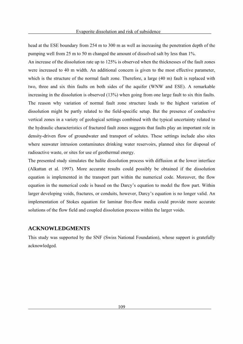
Evaporite dissolution and risk of subsidence
109
head at the ESE boundary from 254 m to 300 m as well as increasing the penetration depth of the
pumping well from 25 m to 50 m changed the amount of dissolved salt by less than 1%.
An increase of the dissolution rate up to 125% is observed when the thicknesses of the fault zones
were increased to 40 m width. An additional concern is given to the most effective parameter,
which is the structure of the normal fault zone. Therefore, a large (40 m) fault is replaced with
two, three and six thin faults on both sides of the aquifer (WNW and ESE). A remarkable
increasing in the dissolution is observed (13%) when going from one large fault to six thin faults.
The reason why variation of normal fault zone structure leads to the highest variation of
dissolution might be partly related to the field-specific setup. But the presence of conductive
vertical zones in a variety of geological settings combined with the typical uncertainty related to
the hydraulic characteristics of fractured fault zones suggests that faults play an important role in
density-driven flow of groundwater and transport of solutes. These settings include also sites
where seawater intrusion contaminates drinking water reservoirs, planned sites for disposal of
radioactive waste, or sites for use of geothermal energy.
The presented study simulates the halite dissolution process with diffusion at the lower interface
(Alkattan et al. 1997). More accurate results could possibly be obtained if the dissolution
equation is implemented in the transport part within the numerical code. Moreover, the flow
equation in the numerical code is based on the Darcy’s equation to model the flow part. Within
larger developing voids, fractures, or conduits, however, Darcy’s equation is no longer valid. An
implementation of Stokes equation for laminar free-flow media could provide more accurate
solutions of the flow field and coupled dissolution process within the larger voids.
ACKNOWLEDGMENTS
This study was supported by the SNF (Swiss National Foundation), whose support is gratefully
acknowledged.

Evaporite dissolution and risk of subsidence
110
References
Ackerer P, Younes A, 2008. Efficient approximations for the simulation of density driven flow in
porous media. Adv Water Res 31(1):15–27
Alkattan M, Oelkers EH, Dandurand JL, Schott J, 1997. Experimental studies of halite
dissolution kinetics: I. the effects of saturation state and the presence of trace metals. Chem Geol
137:201–220
Anderson RY, Kirkland DW, 1980. Dissolution of salt deposits by brine density flow. Geology
8:66–69
Clemens T, Hückinghaus D, Sauter M, Liedl R, Teutsch G ,1996. A combined continuum and
discrete network reactive transport model for the simulation of karst development, IAHS Publ.,
237, 309–318
Cooper AH , 2002. Halite karst geohazards (natural and man-made) in the United Kingdom.
Environ Geol 42:505–512
Dreybrodt W , 1990. The role of dissolution kinetics in the development of karst aquifers in
limestone: A model simulation of karst evolution, J. Geol., 98, 639– 655
GEODATA , 2010. Digital geological database for the city of Basel and northwestern
Switzerland. Geological Survey Basel-Landschaft and Basel-Stadt, University of Basel,
Switzerland
Groves CG, Howard AD, 1994a. Minimum hydrochemical conditions allowing limestone cave
development, Water Resour. Res., 30, 607– 615
Groves CG., Howard AD, 1994b. Early development of karst systems, 1, Preferential flow path
enlargement under laminar flow, Water Resour. Res., 30, 2837– 2846
Gutiérrez F, Desir G, Gutiérrez M, 2003. Causes of the catastrophic failure of an earth dam built
on gypsiferous alluvium and dispersive clays (Altorricón, Huesca Province, NE Spain). Environ
Geol 43:842–851
Gürler B, Hauber L, Schwander M, 1987. Die Geologie der Umgebung von Basel mit Hinweisen
über die Nutzungsmöglichkeiten der Erdwärme [The geology of the Basel region including
directions for the possibilities to use geothermal energy]. Beitrag zur Geologischen Karte der
Schweiz. Stämpfli & Cie, Bern, Switzerland

Evaporite dissolution and risk of subsidence
111
Guerrero J., Gutie´rrez F, Lucha P, 2003. Paleosubsidence and active subsidence due to evaporite
dissolution in the Zaragoza area (Huerva River valley, NE Spain): processes, spatial distribution
and protection measures for transport routes. Engineering Geology 72 (2004) 309–329
Hauber L, 1971. Zur Geologie des Salzfeldes von Schweizerhalle-Zinggibrunn (Kt.
Baselland)[On the geology of the salt mining field Schweizerhalle-Zinggibrunn (Canton
Baselland)]. Eclogae geol Helv 64(1):163–183
Gureghian, A. B., 1975 .A study by the finite element method of the influence of fractures in
confined aquifers, Soc. Pet. Eng. J., 15, 181 – 191.
Howard AD, Groves CG, 1995. Early development of karst systems, 2, Turbulent flow, Water
Resour. Res., 31, 19–26
Huyakorn, P. S., B. H. Lester, and J. W. Mercer, 1983. Finite element techniques for modeling
groundwater flow in fractured aquifers, Water Resour. Res., 19, 1019 – 1035.
James AN, Kirkpatrick IM, 1980. Design of foundations of dams containing soluble rocks and
soils. Quart J Eng Geol Hydrogeol 13(3):189–198.
Johnson KS, 1981. Dissolution of salt on the east flank of the Permian Basin in the southwestern
USA. J Hydrol 54:75–93
Johnson KS, 2005. Subsidence hazards due to evaporite dissolution in the United States. Environ
Geol 48:395–409
Kaufmann G, Braun J, 1999. Karst aquifer evolution in fractured rocks, Water Resour. Res., 35,
3223–3238
Kaufmann G, Braun J, 2000. Karst aquifer evolution in fractured, porous rocks, Water Resour.
Res., 36, 1381– 1392
Kaufmann G, 2002. Karst aquifer evolution in a changing water table environment. Water Resour
Res,38, NO. 6, 1090, 10.1029/2001WR000256
Konz M, Ackerer P, Meier E, Huggenberger P, Zechner E, Gechter D, 2008. On the measurement
of solute concentrations in 2-D flow tank experiments. Hydrol Earth Syst Sci 12:727–738
Konz M, Ackerer P, Younes A, Huggenberger P, Zechner E, 2009a. Two-dimensional stable-
layered laboratory-scale experiments for testing density-coupled flow models. Water Resour Res
45: W02404. doi:10.1029/2008WR007118

Evaporite dissolution and risk of subsidence
112
Konz M, Younes A, Ackerer P, Fahs M, Huggenberger P, Zechner E, 2009b. Variable-density
flow in heterogeneous porous media: laboratory experiments and numerical simulations. J Cont
Hydrol 108:168–175. doi:10.1016/j.jconhyd.2009.07.005
Lucha P, Cardona F, Gutierrez F, Guerrero J, 2007. Natural and human-induced dissolution and
subsidence processes in the salt outcrop of the Cardona Diapir (NE Spain). Environ Geol.
doi:10.1007/s00254-007-0729-3.
Ludwig R, Schelkes K, Vogel P, Wollrath J, 2001. Implications of large-scale heterogeneities for
hydraulic model studies at the potential site of a radioactive waste repository at Gorleben,
Germany. Eng Geol,61(2-3):119–30.
Luo J, Dierch H-JG, Monninkhoff L.M.M, 2012. 3D Modeling of saline groundwater flow and
transport in a flooded salt mine is Stassfurt, Germnay, Mine Water Environ 31:104-111, DOI
10.1007/s10230-012-0181-9.
Magri F, Akar T, Gemici U, Pekdeger A, 2011. Numerical investigations of fault-induced
seawater circulation in the Seferihisar-Balcova Geothermal system, western Turkey,
Hydrogeology journal DOI 10.1007/s10040-011-0797-z.
Martinez JD, Johnson KS, Neal JT, 1998. Sinkholes in evaporite rocks. Am Sci 86:38–51
OECD (ed), 1988. Hydrocoin Project. The International Hydrocoin Project, level 1: code
verification. OECD, Paris
Oude Essink GHP, 2001a. Improving fresh groundwater supply-problems and solutions. Ocean
Coastal Manage 44(5-6):429–49.
Oude Essink GHP, 2001b. Salt water intrusion in a three-dimensional groundwater system in The
Netherlands: a numerical study. Transport Porous Med 2001;43:137–58.
Palmer A. N, 1991. Origin and morphology of limestone caves, Geol. Soc. Am.Bull., 103, 1– 21
Paniconi C, Khlaifi I, Lecca G, Giacomelli A, Tarhouni J, 2001. A modeling study of seawater
intrusion in the korba coastal plain, Tunisia, Phys Chem Earth (B) 26(4):345–51.
Saladin M, 2004. Hydrogeologischer Zusammenhang von Tektonik und Grundwasserzirkulation
im Gebiet Muttenz-Pratteln [Hydrogeologic relationship between tectonics and groundwater
circulation in the Muttenz-Pratteln area]. Diplomarbeit, Universität Basel, Switzerland
Siemers J, Dreybrodt W, 1998. Early development of karst aquifers on percolation networks of
fractures in limestone, Water Resour. Res., 34, 409– 419.

Evaporite dissolution and risk of subsidence
113
Spottke I, Zechner E, Huggenberger P, 2005. The southeast border of the Upper Rhine graben: a
3D structural model of geology and its importance for groundwater flow. Int J Earth Sci 94:580–
593
Sroka A, Schober F, 1982. Die Berechnung der maximalen Bodenbewegungen über
kavernenartigen Hohlräumen unter Berücksichtigung der Hohlraumgeometrie [Calculation of the
maximum ground deformation considering the geometry of cavities]. Kali & Steinsalz, Berlin, pp
273–277
Wassmann TH, 1979. Mining subsidence in the East Netherlands. Proc Fifth Int Symp on Salt
1:463–475
Watson SJ, Barry DA, Scotting RJ, Hassanizadeh SM, 2002. Validation of classical density-
dependent theory for stable, high-concentration gradient brine displacements in coarse and
medium sand. Adv Water Resour 25:611–635
Xue Y, Xie C, Wu J, Lie P, Wang J, Jiang Q, 1995. A three-dimensional miscible transport
model for seawater intrusion in China. Water Resour Res 31(4):903–12.
Younes A, Fahs M, Ahmed S, 2009. Solving density driven flow problems with efficient spatial
discretizations and higher-order time integration methods. Adv Water Resour. doi:10.1016/j.
advwatres.2008.11.003
Younes A, Konz M, Fahs M, Zidane A, Huggenberger P, 2011. Modelling variable density flow
problems in heterogeneous porous media using the method of lines and advanced spatial
discretization methods. Mathematics and Computers in Simulation (81) 2346–2355
Zechner E, Konz M, Younes A, Huggenberger P, 2011. Effects of tectonic structures, salt
solution mining, and density-driven groundwater hydraulics on evaporite dissolution
(Switzerland). Hydrogeology journal DOI 10.1007/s10040-011-0759-5.
Zidane A, Younes A, Huggenberger P, Zechner E, 2012. The Henry semi-analytical solution for
saltwater intrusion with reduced dispersion, Water Resou Res, VOL. 48, W06533,
doi:10.1029/2011WR011157.

Evaporite dissolution and risk of subsidence
114
List of Figures
Figure 1: Study area map in Northwestern Switzerland, showing: location of subsidence areas,
normal faults, simulated piezometric head within the upper aquifer, and location of 2D cross
section for density-coupled transport model (modified after Zechner et al 2011).
Figure 2: 2D cross-section with hydrostratigraphic model for the simulation of density-coupled
flow and transport.
Figure 3: Volume of the removed salt block
Figure 4: Effect of variable conductivity on the amount of dissolved salt Figure 5: Simulated x-component of velocity with 1m thickness of the lower aquifer after 30
years
Figure 6: Simulated NaCl Concentration with 1m thickness of the lower aquifer after 30 years
Figure 7: Effect of lower aquifer thickness on the amount of dissolved salt (each point is a 30
years independent simulation)
Figure 8: Simulated x-component of velocity with 40m thickness of the fault zones after 30 years
Scenario (S_Fault_7)
Figure 9: Simulated NaCl Concentration with 40m thickness of the fault zones after 30 years
Scenario (S_Fault_7)
Figure 10: Effect of fault zone thickness on the amount of dissolved salt (each point is a 30 years
independent simulation).
Figure 11: Mass input with respect to the active width for the different fault number scenarios.
Figure 12: Active width for the different fault number scenarios.
Figure 13: Required time to reach the saturation in the lower aquifer.
Figure 14: Simulated x-component of velocity (with 6 thin faults) after 30 years.
Figure 15: Simulated NaCl Concentration (with 6 thin faults) after 30 years.
Figure 16: Effect of the hydraulic head on the amount of dissolved salt (each point is a 30 years
independent simulation).
Figure 17: Simulated x-component of velocity (300m) hydraulic head after 30 years
Scenario (S_Head_6)
Figure 18: Effect of the well depth on the amount of dissolved salt (each point is a 30 years
independent simulation)

Evaporite dissolution and risk of subsidence
115
List of tables
Table 1: Values of the physical and geometrical parameters for the set of scenarios concerning
the variation of the lower aquifer conductivity. ε is the porosity and K is the hydraulic
conductivity.
Table 2: Values of physical and geometrical parameters for the set of scenarios concerning the
variation of the lower aquifer thicknesses. ε is the porosity and K is the hydraulic conductivity.
Table 3: Values of physical and geometrical parameters for the set of scenarios concerning the
variation of the Fault zones thicknesses. ε is the porosity and K is the hydraulic conductivity.
Table 4: Values of physical and geometrical parameters for the set of scenarios concerning the
variation of the right side hydraulic head. ε is the porosity and K is the hydraulic conductivity.
Table 5: Values of physical and geometrical parameters for the set of scenarios concerning the
variation of the well depth. ε is the porosity and K is the hydraulic conductivity.

Evaporite dissolution and risk of subsidence
116
Fig. 1: Study area map in Northwestern Switzerland, showing: location of subsidence areas, normal faults, simulated piezometric head within the upper aquifer, and location of 2D cross section for density-coupled transport model (modified after Zechner et al 2011).
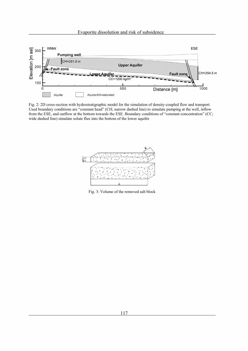
Evaporite dissolution and risk of subsidence
117
Fig. 2: 2D cross-section with hydrostratigraphic model for the simulation of density-coupled flow and transport. Used boundary conditions are “constant head” (CH; narrow dashed line) to simulate pumping at the well, inflow from the ESE, and outflow at the bottom towards the ESE. Boundary conditions of “constant concentration” (CC; wide dashed line) simulate solute flux into the bottom of the lower aquifer
Fig. 3: Volume of the removed salt block
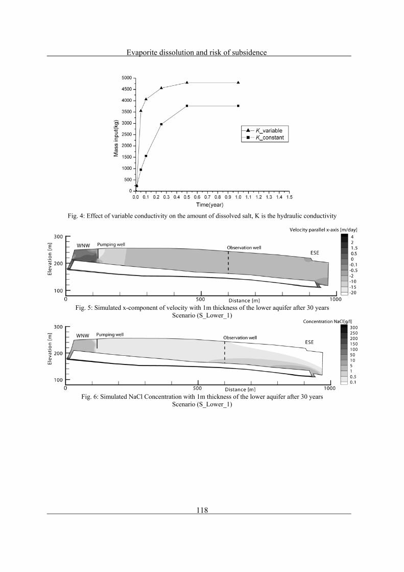
Evaporite dissolution and risk of subsidence
118
Fig. 4: Effect of variable conductivity on the amount of dissolved salt, K is the hydraulic conductivity
Fig. 5: Simulated x-component of velocity with 1m thickness of the lower aquifer after 30 years
Scenario (S_Lower_1)
Fig. 6: Simulated NaCl Concentration with 1m thickness of the lower aquifer after 30 years
Scenario (S_Lower_1)

Evaporite dissolution and risk of subsidence
119
Fig. 7: Effect of lower aquifer thickness on the amount of dissolved salt (each point is a 30 years
independent simulation).
Fig. 8: Simulated x-component of velocity with 40m thickness of the fault zones after 30 years
Scenario (S_Fault_7)
Fig. 9: Simulated NaCl Concentration with 40m thickness of the fault zones after 30 years
Scenario (S_Fault_7)

Evaporite dissolution and risk of subsidence
120
Fig. 10: Effect of fault zone thickness on the amount of dissolved salt (each point is a 30 years independent
simulation).
Fig. 11: Mass input with respect to the active width for the different fault number scenarios.
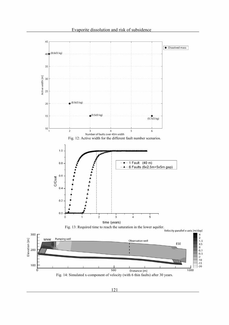
Evaporite dissolution and risk of subsidence
121
Fig. 12: Active width for the different fault number scenarios.
Fig. 13: Required time to reach the saturation in the lower aquifer.
Fig. 14: Simulated x-component of velocity (with 6 thin faults) after 30 years.

Evaporite dissolution and risk of subsidence
122
Fig. 15: Simulated NaCl Concentration (with 6 thin faults) after 30 years.
Fig. 16: Effect of the hydraulic head on the amount of dissolved salt (each point is a 30 years independent
simulation).
Fig. 17: Simulated x-component of velocity for the (300m) hydraulic head after 30 years
Scenario (S_Head_6)

Evaporite dissolution and risk of subsidence
123
Fig. 18: Effect of the well depth on the amount of dissolved salt (each point is a 30 years independent simulation)
Scenarios Parameters S_K_1 S_K_2
K Upper Aq. [m/s] 7.4E-4 7.4E-4 ε Upper Aq. [-] 3% 3% K Lower Aq.[m/s] 7.4E-4 Dynamic ε Lower Aq. [-] 1% Dynamic K Fault zones[m/s] 7.4E-4 7.4E-4 ε Fault Zones [-] 1% 1% Well depth [m] 25 25 Fault thickness[m] 10 10 Right side head[m] 254.5 254.5 Lower Aq. Slope[-] 6% 6% Lower Aq. Thickness [m] 10 10
Table 1: Values of physical and geometrical parameters for the set of scenarios concerning the variation of the lower
aquifer thicknesses. ε is the porosity and K is the hydraulic conductivity.
Scenarios Parameters S_Lower_1 S_Lower_2 S_Lower_3 S_Lower_4 S_Lower_5
K Upper Aq. [m/s] 7.4E-4 7.4E-4 7.4E-4 7.4E-4 7.4E-4 ε Upper Aq. [-] 3% 3% 3% 3% 3% K Lower Aq.[m/s] 7.4E-4 7.4E-4 7.4E-4 7.4E-4 7.4E-4 ε Lower Aq. [-] 1% 1% 1% 1% 1% K Fault zones[m/s] 7.4E-4 7.4E-4 7.4E-4 7.4E-4 7.4E-4 ε Fault Zones [-] 1% 1% 1% 1% 1% Well depth [m] 25 25 25 25 25 Fault thickness[m] 10 10 10 10 10 Right side head[m] 254.5 254.5 254.5 254.5 254.5 Lower Aq. Slope[-] 6% 6% 6% 6% 6% Lower Aq. Thickness [m] 1 3 5 8 10
Table 2: Values of physical and geometrical parameters for the set of scenarios concerning the variation of the lower
aquifer thicknesses. ε is the porosity and K is the hydraulic conductivity.
Scenarios Parameters S_Fault_1 S_ Fault _2 S_ Fault _3 S_ Fault _4 S_ Fault _5 S_ Fault _6 S_ Fault _7
K Upper Aq. [m/s] 7.4E-4 7.4E-4 7.4E-4 7.4E-4 7.4E-4 7.4E-4 7.4E-4 ε Upper Aq. [-] 3% 3% 3% 3% 3% 3% 3% K Lower Aq. [m/s] 7.4E-4 7.4E-4 7.4E-4 7.4E-4 7.4E-4 7.4E-4 7.4E-4 ε Lower Aq. [-] 1% 1% 1% 1% 1% 1% 1% K Fault zones [m/s] 7.4E-4 7.4E-4 7.4E-4 7.4E-4 7.4E-4 7.4E-4 7.4E-4

Evaporite dissolution and risk of subsidence
124
ε Fault Zones [-] 1% 1% 1% 1% 1% 1% 1% Well depth [m] 25 25 25 25 25 25 25 Fault thickness[m] 0.5 2 4 5 10 25 40 Right side head[m] 254.5 254.5 254.5 254.5 254.5 254.5 254.5 Lower Aq. Slope[-] 6% 6% 6% 6% 6% 6% 6% Lower Aq. Thickness [m] 10 10 10 10 10 10 10
Table 3: Values of physical and geometrical parameters for the set of scenarios concerning the variation of the Fault zones
thicknesses. ε is the porosity and K is the hydraulic conductivity.
Scenarios Parameters S_Head_1 S_Head_2 S_Head_3 S_Head_4 S_Head_5 S_Head_6
K Upper Aq. [m/s] 7.4E-4 7.4E-4 7.4E-4 7.4E-4 7.4E-4 7.4E-4 ε Upper Aq. [-] 3% 3% 3% 3% 3% 3% K Lower Aq.[m/s] 7.4E-4 7.4E-4 7.4E-4 7.4E-4 7.4E-4 7.4E-4 ε Lower Aq. [-] 1% 1% 1% 1% 1% 1% K Fault zones[m/s] 7.4E-4 7.4E-4 7.4E-4 7.4E-4 7.4E-4 7.4E-4 ε Fault Zones [-] 1% 1% 1% 1% 1% 1% Well depth [m] 25 25 25 25 25 25 Fault thickness[m] 10 10 10 1 10 10 Right side head[m] 254.5 260 270 280 290 300 Lower Aq. Slope[-] 6% 6% 6% 6% 6% 6% Lower Aq. Thickness [m] 10 10 10 10 10 10 Table 4: Values of physical and geometrical parameters for the set of scenarios concerning the variation of the right side hydraulic
head. ε is the porosity and K is the hydraulic conductivity. Scenarios Parameters S_well_1 S_well_2 S_well_3 S_well_4 S_well_5
K Upper Aq. [m/s] 7.4E-4 7.4E-4 7.4E-4 7.4E-4 7.4E-4 ε Upper Aq. [-] 3% 3% 3% 3% 3% K Lower Aq.[m/s] 7.4E-4 7.4E-4 7.4E-4 7.4E-4 7.4E-4 ε Lower Aq. [-] 1% 1% 1% 1% 1% K Fault zones[m/s] 7.4E-4 7.4E-4 7.4E-4 7.4E-4 7.4E-4 ε Fault Zones [-] 1% 1% 1% 1% 1% Well depth [m] 25 30 35 40 50 Fault thickness[m] 10 10 10 10 10 Right side head[m] 254.5 254.5 254.5 254.5 254.5 Lower Aq. Slope[-] 6% 6% 6% 6% 6% Lower Aq. Thickness [m] 10 10 10 10 10
Table 5: Values of physical and geometrical parameters for the set of scenarios concerning the variation of the well depth. ε is the porosity and K is the hydraulic conductivity.
Scenarios Parameters S_FN_1 S_FN_2 S_FN_3 S_FN_4
K Upper Aq. [m/s] 7.4E-4 7.4E-4 7.4E-4 7.4E-4 ε Upper Aq. [-] 3% 3% 3% 3% K Lower Aq.[m/s] 7.4E-4 7.4E-4 7.4E-4 7.4E-4 ε Lower Aq. [-] 1% 1% 1% 1% K Fault zones[m/s] 7.4E-4 7.4E-4 7.4E-4 7.4E-4 ε Fault Zones [-] 1% 1% 1% 1% Well depth [m] 25 25 25 25 Overall Fault thickness[m] 40 40 40 40 Right side head[m] 254.5 254.5 254.5 254.5 Lower Aq. Slope[-] 6% 6% 6% 6% Lower Aq. Thickness [m] 10 10 10 10 Faults number [-] 1 2 3 6 Active width [m] 40 2x10 3x5 6x2.5 Gap [m] 0 1x20 2x12.5 5x5
Table 6: Values of physical and geometrical parameters for the set of scenarios concerning the variation of faults number (FN). ε is the porosity and K is the hydraulic conductivity.

Conclusions
125
General conclusions and perspectives
The work presented in this thesis is divided into three main parts. Previous to the main parts,
general mathematical and numerical methods that could be used to solve the flow and the
transport problem in porous media and in free flow domains are introduced. Compared to
different solution methods (FD, FV, FE, TH), and taking into account that the flow equations
(Darcy and Stokes) should be coupled with density effects, the MFE method was used to solve
the flow in porous media and the CR finite element method was used to solve the flow in free
flow domains. Moreover, since the standards numerical methods (FV, FE) generate solution with
numerical diffusion and/or non-physical oscillations, the DG-MPFA method was used to solve
the advection-diffusion transport equation.
In the first part of this thesis, the developed MFE_DG_MPFA model was compared against a
well-developed semi-analytical solution. The semi-analytical method was already developed by
Henry [Henry 1964] in the saltwater intrusion problem. However, this solution can only simulate
saltwater intrusion with unrealistic large amount of dispersion. The solution procedure developed
by Henry is based on two steps: (i) an approximation of the solution by using a Fourier series
representation with a certain truncation order of the coefficients and (ii) resolution of a strongly
non-linear algebraic system to calculate these coefficients. This iterative technique is based on a
sequential resolution of nonlinear systems of flow and mass transport. With this technique,
convergence problems are encountered when decreasing the value of the molecular diffusion. To
overcome these difficulties, a new procedure to calculate the semi-analytical solution was
developed in this thesis. This procedure consists of solving simultaneously the flow and transport
algebraic equations by using the Levenberg-Marquardt algorithm [Levenberg 1944, Marquardt
1963]. The use of this technique allowed developing, for the first time, semi-analytical solutions
of saltwater intrusion in the case of small diffusion and in the case of a large density contrast.
A new semi-analytical solution was developed in the second part of this thesis. The semi-
analytical solution for density driven free flows was developed by following the steps of Henry
[Henry 1964], by using the Fourier-Galerkin method. Similar to the semi-analytical solution
algorithm adopted for density driven flow in porous media, the Levenberg-Marquadt algorithm
[Levenberg 1944, Marquardt 1963] was used to solve the nonlinear algebraic equations in free
flow domains. In order to validate the CR_DG_MPFA numerical model, the latter was compared
Conclusions
126
against the developed semi-analytical solution in a synthetic saltwater intrusion problem through
a fracture, where a good agreement was reproduced.
In the last part of this manuscript the focus was on the dissolution phenomenon. Within the
framework of the project, the study of salt dissolution in fractures was recently studied by
conducting a set of laboratory experiments for a salt block with cylindrical hole [Gechter et al.
2008]. As a continuation of this study, a numerical model was developed in this thesis to simulate
the salt dissolution within fractures. To simulate the salt dissolution process, a dynamic mesh
routine was also developed and coupled to the CR_DG_MPFA numerical model. This numerical
model with dynamic mesh adaptation was used to simulate a simple dissolution experiment for a
vertical fracture that has been recently conducted at Nancy University. The obtained numerical
dissolution profiles were in good agreement with the experimental result.
Finally, the density driven flow code in porous media was used to run a set of numerical
simulations on a 2D regional cross section from the Muttenz-Pratteln area. The aim of this study
was to reveal the most important parameters that have an influence on the salt dissolution process
that leads to the observed land subsidence within this area. The tectonic elements of faults were
found to be the most important parameters that affect the salt dissolution. By varying the
thickness and the repartition of faults the amount of the dissolved salt increased by more than one
magnitude. The thickness and the permeability variation within the lower aquifer were found to
have important effects on the salt dissolution. Effects of other parameters like the well depth and
the hydraulic head at the boundary were found to be negligible.
Among the mentioned points, we could summarize the following conclusions:
This deficiency encountered when solving the Henry problem was avoided by using the
Levenberg-Marquardt algorithm to calculate the coefficients of the Fourier series. The
adopted solution algorithm improve the applicability of the semianalytical solution of the
Henry problem to saltwater intrusion problems with reduced diffusion and with high
density contrast, and are therefore more suitable to benchmark density-driven flow codes.
The new developed semi-analytical solution for density drive flow in a free flow media is
considered as a useful tool to validate density driven Stokes flow codes.

Conclusions
127
The developed procedure by combining the numerical resolution of density driven free
flows with mesh adaptation is suitable to take into account evolution of fracture geometry
due to dissolution.
The geometry of the aquifer above the evaporite has a great influence on the subrosion
process, especially the fault thickness values. An increase of the dissolution rate up to
125% is observed when the thicknesses of the normal fault zones were increased to 40 m
width. A similar effect is observed when reducing the thickness of the aquifer to 1 m,
which increases the dissolution rate by more than 40%.
In the framework of this thesis we could point out some ideas for further investigations:
The results of this research thesis could be used as a basis for further experimental and
conceptual model developments on salt dissolution and solute transport by density-driven
groundwater flow. These may ultimately help provide predictions on land subsidence and
other risks.
The gained knowledge within this thesis could contribute to a 3D simulation of density
flow with field data and geological structures. This could help to improve the knowledge
on regional flow fields such as at the presented subsidence area in the region of Basel.
The reliability of the developed numerical tools has been proven against semi-analytical
and experimental results; therefore further numerical studies on field scale subrosion
processes could be conducted.
The studied dissolution case is of course an oversimplified representation of a natural
system; but the developed code with mesh adaptation could be used as a starting point to
study the dissolution phenomenon on real field applications, such as the development of
karstic voids in evaporites coupled with flow and transport within these voids.

Bibliography
128
Bibliography
Aavatsmark, I (2002), An introduction to multipoint flux approximations for quadrilateral
grids. Computat. Geoscien., 6:404-432.
Aavatsmark I, Barkve T., Bøe Ø., Mannseth T. (1996), Discretization on non-orthogonal,
quadrilateral grids for inhomogeneous, anisotropic media. J Comput Phys;127:2–14.
Abarca, E., J. Carrera, X. Sanchez-Vila and M. Dentz (2007), Anisotropic dispersive Henry
problem, Adv. Water Resour., 30(4),pp.913–926.
Ackerer, P, and A. Younes (2008) Efficient approximations for the simulation of density
driven flow in porous media. Adv Water Res, 31:15-27.
Aegerter, I. & Bosshardt, A.G. (1999): Technischer Bericht, Setzungsproblematik-
Massnahmen gegen Setzungen. Bericht im Auftrag der SBB, unpublished.
Aizinger, V., Dawson, C., Cockburn, B., Castillo, P.: The local discontinuous Galerkin
method for contaminant transport. Adv Water Res;24:73-87,(2001).
Alkattan M, Oelkers EH, Dandurand JL, Schott J (1997), Experimental studies of halite
dissolution kinetics: I. the effects of saturation state and the presence of trace metals.
Chem Geol 137:201–220
Anderson RY, Kirkland DW (1980) Dissolution of salt deposits by brine density flow.
Geology 8:66–69
Arbogast T. and Lehr H.L. (2006), Homogenization of a Darcy-Stokes system modeling
vuggy porous media. Comput. Geosci., 10:291.
Arnold D.N., On nonconforming linear-constant elements for some variants of the Stokes
equations, presenta dal s.c. Franco Brezzi nella seduta del 24-6-93.
Arnold DN, Brezzi F, Cockburn B., Marini LD. (2002), Unified analysis of discontinuous
Galerkin methods for elliptic problems. SIAM J. Numer. Anal.;5:1749-1779.
Baumann, C.E, Oden JT.: A discontinuous hp finite element method for convection–diffusion
problems. Computat Meth Appl Mech Engrg;175:311–341,(1999).
Beavers G. and Joseph D. (1967), Boundary conditions at a naturally permeable wall, J. Fluid
Mech., 30:197.
Bear, J.: Dynamics of Fluids in Porous Media ~Elsevier, New York, (1972).
Brezzi F., Fortin M., Mixed and hybrid finite element methods, Berlin: Springer (1991).

Bibliography
129
Boffi D, Brezzi F, Fortin M, Finite Elements for the Stokes problem, Lecture Notes in
Mathematics 1939, (2008), 45-100
Bruman E., Hansbo P. (2004), A stabilized nonconforming finite element method for
incompressible flow, Comput. Methods App0 Mech. Eng., vol. 195, num. 23-24,
p. 2881-99.
Bruman E., Hansbo P. (2005), Stabilized Crouzeix-Raviart element for the Darcy-Stokes
problem, Numerical Methods for Partial Differential Equation, 21(5), 986-997
Bues M., C. Oltean (2000), Numerical simulations for saltwater intrusion by the mixed hybrid
finite element method and discontinuous finite element method. Transport Porous Med
2000;40(2):171–200
Cardenas M, Slottke D., Ketcham R, Sharp Jr. (2007), Navier-Stokes flow and transport
simulations using real fractures shows heavy tailing due to eddies, Geophysical
Research Letters, Vol.34, L14404, doi:10.1029/2007GL030545,
Chavent, G., Roberts J.E.: A unified physical presentation of mixed, mixed-hybrid finite
elements and standard finite difference approximations for the determination of
velocities in waterflow problems. Adv Water Res;14:329-348,(1991).
Clemens T, Hückinghaus D, Sauter M, Liedl R, Teutsch G (1996) A combined continuum and
discrete network reactive transport model for the simulation of karst development, IAHS
Publ., 237, 309–318
Conca C., Murat F., Pironneau O. (1994), The Stokes and Navier-Stokes equations with
boundary conditions involving the pressure. Jpn J. Math. 20, 263-318
Conca C., Parés C., Pironneau O., Thiriet M. (1995), Navier-Stokes equations with imposed
pressure and velocity fluxes. Int. J. Numer. Methods Fluids 20(4), 267-287
Cockburn B., Hou S., Shu CW. (1989), TVB Runge Kutta local projection discontinuous
Galerkin finite element method for conservative laws III: One dimensional systems, J.
Compu.t Phys.;84: 90-113.
Cockburn, B., Shu, CW. (1998): The Runge-Kutta Discontinuous Galerkin Method for
conservative laws V: Multidimentional Systems. J Comput Phys;141:199-224.
Cockburn, B., Karniadakis, GE., Shu CW.(Eds.) (2000): Discontinuous Galerkin Methods:
Theory, Computation and Applications. Lecture Notes in Computational Science and
Engineering;11:Springer-Verlag.

Bibliography
130
Cooper AH (2002) Halite karst geohazards (natural and man-made) in the United Kingdom.
Environ Geol 42:505–512
Crouzeix M., Raviart P. (1973), Conforming and nonconforming finite element methods for
solving the stationary Stokes equations. RAIRO Sér. Rouge, 7(3), 33-75
Croucher, A.E., and M. J. O’Sullivan (1995), The Henry problem for saltwater intrusion,
Water Resour. Res., 31(7), 1809 – 1814.
Dalrymple G.B (1991), The importance of small science, EOS transactions AGU, 72(1),pp
1,4.
Diersch H.J. (1988), Finite element modelling of recirculation density driven saltwater
intrusion processes in groundwater, Adv. Water Resour., , 11, 25–43, doi:10.1016/0309-
1708(88)90019-X.
Diersch H.J., Kolditz O. (1998), Coupled groundwater flow and transport: 2. Thermohaline
and 3D convection systems, Adv. Water Resour., , 21, 401–425, doi:10.1016/S0309-
1708(97)00003-1.
Diersch, H.J. & Kolditz, O. (2002): Variable-density flow and transport in porous media:
approaches and challenges. Adv. Water Res., 25, 899–944.
Dreybrodt W (1990) The role of dissolution kinetics in the development of karst aquifers in
limestone: A model simulation of karst evolution, J. Geol., 98, 639– 655
Durlofsky, L.: Accuracy of mixed and control volume finite element approximations to Darcy
velocity and related quantities. Water Resour Res.;30:965-973, (1994).
Durie, R.W. & Jessen, F.W. (1964): Mechanism of the dissolution of salt in the formation
of underground cavities. Soc. Pet. Engn. J., 4, 2, 183-190.
Edwards, M.G., Rogers, C.F.: Finite volume discretization with imposed flux continuity for
the general tensor pressure equation. Computat Geoscien,2:259-290, (1998).
Flekkøy E.G., Rage T., Oxaal U., and Feder J. (1996), Hydrodynamic Irreversibility in
Creeping Flow, Phys. Rev, PACS numbers: 47.15.Gf, 02.70.Bf, 02.70.Lq, 47.60.+I,
VOLUME 77, NUMBER 20
Forbes L.K. (1988), Surface waves of large amplitude beneath an elastic sheet. Part 2.
Galerkin solution, J. Fluid Mechanics (188) 491-508.
Frind, E.O. (1982), Simulation of long-term transient density-dependent transport in
groundwater, Adv. Water Resour., 5, 73 – 88.
Frumkin, A. (1994): Morphology and development of salt caves. NSS Bulletin, 56, 82- 95.

Bibliography
131
Frumkin, A. (1998): Salt cave cross-sections and their paleoenvironmental implications.
Geomorphology, 23, 183-191.
Frumkin, A. (2000a): Dissolution of salt. In: Klimchouk, A. B., Ford, D. C., Palmer, A.
N. & Dreybrodt, W. (eds): Speleogenesis – evolution of karst aquifers, 169-170.
National Speleological Society, Huntsville.
Frumkin, A. (2000b): Speleogenesis in salt – the Mount Sedom area, Israel. In Klimchouk, A.
B., Ford, D. C., Palmer, A. N., Dreybrodt, W. (eds): Speloegenesis – evolution of karst
aquifers. National Speleological Society, Huntsville, 443-451.
Genuchten M.., (1991), Progress and opportunities o, hydrologic research, U.S. national
report 1987-1990, Twentieth general assembly, International union of geodesy and
geophysics, Vienna, Austria.
Gechter D, Huggenberger P., Ackerer, P and Waber H.N.,(2008), Genesis and shape of
natural solution cavities within salt deposits Water Resou Res, VOL. 44, W11409,
doi:10.1029/2007WR006753, 2008
GeoData (2010) Digital geological database for the city of Basel and northwestern
Switzerland. Geological Survey Basel-Landschaft and Basel-Stadt, University of Basel,
Switzerland
Girault V., Raviart PA., Finite element methods for Navier-Stokes equations, Berlin: Springer
1986
Gresho PM., Sani RL., Incompressible flow and the finite element method, New York: Wiley;
1998
Gresho PM, Sani R.L. (1987), On pressure boundary conditions for the incompressible
Navier-Stokes equations. Int. J. Numer. Methods Fluids 7, 1111-1145
Groves CG, Howard AD (1994a) Minimum hydrochemical conditions allowing limestone
cave development, Water Resour. Res., 30, 607– 615
Groves CG., Howard AD (1994b) Early development of karst systems, 1, Preferential flow
path enlargement under laminar flow, Water Resour. Res., 30, 2837– 2846
Gutiérrez F, Desir G, Gutiérrez M (2003) Causes of the catastrophic failure of an earth dam
built on gypsiferous alluvium and dispersive clays (Altorricón, Huesca Province, NE
Spain). Environ Geol 43:842–851
Gürler B, Hauber L, Schwander M (1987) Die Geologie der Umgebung von Basel mit
Hinweisen über die Nutzungsmöglichkeiten der Erdwärme [The geology of the Basel

Bibliography
132
region including directions for the possibilities to use geothermal energy]. Beitrag zur
Geologischen Karte der Schweiz. Stämpfli & Cie, Bern, Switzerland
Guerrero J., Gutie´rrez F, Lucha P (2003) Paleosubsidence and active subsidence due to
evaporite dissolution in the Zaragoza area (Huerva River valley, NE Spain): processes,
spatial distribution and protection measures for transport routes. Engineering Geology 72
(2004) 309–329
Gureghian, A. B., A study by the finite element method of the influence of fractures in
confined aquifers, Soc. Pet. Eng. J., 15, 181 – 191, 1975.
Goswami, R.R., and Clement, T.P., (2007), Laboratory-scale investigation of saltwater
intrusion dynamics: Water Resour. Res., 43, W04418, doi:10.1029/2006WR005151.
Hansbo P., Larson MG (2003), Discontinuous Galerkin and the Crouzeix-Raviart element:
application to elasticity. ESAIM: Math. Model. Numer. Anal. 37(1), 63-72
Hansbo P., Larson M.G. (2002), Discontinuous Galerkin methods for incompressible and
nearly incompressible elasticity by Nitshe’s method. Comput. Methods Appl. Mech.
Engrg, 191(17-18), 1895-1908
Happel, J., and Brenner,H.,(1965), Low Reynolds Number Hydrodynamics (Prentice Hall Inc.,
Englewood Cliffs, NJ).
Hauber L (1971) Zur Geologie des Salzfeldes von Schweizerhalle-Zinggibrunn (Kt.
Baselland)[On the geology of the salt mining field Schweizerhalle-Zinggibrunn (Canton
Baselland)]. Eclogae geol Helv 64(1):163–183
Henry, H. R. (1964), Effects of dispersion on salt encroachment in coastal aquifers, in Sea
Water in Coastal Aquifers, U.S. Geol. Surv. Supply Pap., 1613-C, 70 – 84.
Herbert AW, Jackson CP, Lever DA. (1988), Coupled groundwater flow and solute transport
with fluid density strongly dependent upon concentration. Water Resour Res; 24:1781–95.
Howard AD, Groves CG (1995) Early development of karst systems, 2, Turbulent flow,
Water Resour. Res., 31, 19–26
Huber, R., Helmig, R. ,(1999): Multiphase flow in heterogeneous porous media: a classical
finite element method versus an implicit pressure-explicit saturation-based mixed finite
element-finite volume approach. Int J Numer Meth in Fluids;29:899-920.
Hughes, TJR., Masud, A., Wan, J. ,(2006): A stabilized mixed discontinuous Galerkin method
for Darcy flow. Computat Meth Appl Mech Engrg;195(25-28):3347- 3381.
Bibliography
133
Huyakorn, P. S., P. F. Andersen, J. W. Mercer, and H. O. White Jr. (1987), Saltwater
intrusion in aquifers: Development and testing of a three-dimensional finite element
model, Water Resour. Res., 23, 293 – 312.
Huyakorn, P. S., B. H. Lester, and J. W. Mercer, Finite element techniques for modeling
groundwater flow in fractured aquifers, Water Resour. Res., 19, 1019 – 1035, 1983
Jäger W and Mikelić A. (2000), On the interface boundary condition of Beavers, Joseph, and
Saffman. SIAM J. Appl. Math. 60:1111.
Jäger W. and Mikelić A. (2001a), Asymptotic analysis of the laminar viscous flow over a
porous bed. SIAM J. Sci. Comput. 22:2006.
Jäger W. and Mikelić A. (2001b), On the roughness-induced effective boundary conditions
for an incompressible viscous flow, J. Differ. Equ. 170, 96-122
James AN, Kirkpatrick IM (1980) Design of foundations of dams containing soluble rocks
and soils. Quart J Eng Geol Hydrogeol 13(3):189–198
James, A. N. (1992): Soluble materials in civil engineering. Ellis Horwood, Chichester.
Johannsen, K., Kinzelbach, W., Oswald, S. & Wittum, G. (2002): The saltpool benchmark
problem – numerical simulation of saltwater upconing in a porous medium. Adv. Water
Res., 25, 335-348.
Johnson KS (1981) Dissolution of salt on the east flank of the Permian Basin in the
southwestern USA. J Hydrol 54:75–93
Johnson, K.S. (1992): Evaporite karst in the Permian Blaine Formation and associated
strata in Western Oklahoma, USA. Int. Contributions to Hydrogeology, 13, 405-420.
Johnson KS (2005) Subsidence hazards due to evaporite dissolution in the United States.
Environ Geol 48:395–409
Kaufmann G, Braun J (1999) Karst aquifer evolution in fractured rocks, Water Resour. Res.,
35, 3223–3238
Kaufmann G, Braun J (2000) Karst aquifer evolution in fractured, porous rocks, Water
Resour. Res., 36, 1381– 1392
Kaufmann G (2002) Karst aquifer evolution in a changing water table environment. Water
Resour Res,38, NO. 6, 1090, 10.1029/2001WR000256
Kaviany M. (1999), Principles of Heat Transfer in Porous Media, Mechanical Engineering
Series, Springer-Verlag, New York.
Bibliography
134
Kavetski D., Binning P., Sloan S.W. (2001), Adaptive time stepping and error control in a
mass conservative numerical solution of the mixed form of Richards equation, Adv. Water
Resour., ,24(6), 595–605, doi:10.1016/S0309-1708(00)00076-2.
Kirby, R.,(2000): A Posteriori Error Estimates and Local Time-Stepping for Flow and
Transport Problems in Porous Media, Ph.D thesis, University of Texas at Austin.
Klausen, R.A, Russell T.F.,(2004): Relationships among some locally conservative
discretization methods which handle discontinuous coefficients. Journal Computat
Geoscien,8(4):1-37.
Kolditz O, R. Ratke, H.-JG. Diersch, and W. Zielke (1998), Coupled groundwater flow and
transport: 1. Verification of variable density flow and transport models, Adv Water Res.
21, 27–46.
Konz, M., Ackerer P., Younes A., Huggenberger P., Zechner E. (2009), Two-dimensional
stable-layered laboratory-scale experiments for testing density-coupled flow models,
Water Resour. Res., 45: W02404, doi:10.1029/2008WR00711
Konz M, Ackerer P, Meier E, Huggenberger P, Zechner E, Gechter D (2008) On the
measurement of solute concentrations in 2-D flow tank experiments. Hydrol Earth Syst
Sci 12:727–738
Konz M, Younes A, Ackerer P, Fahs M, Huggenberger P, Zechner E(2009b) Variable-density
flow in heterogeneous porous media: laboratory experiments and numerical simulations. J
Cont Hydrol 108:168–175. doi:10.1016/j.jconhyd.2009.07.005
Kozary, M. T., Dunlap, J. C. and Humphrey, W. E.,(1968): Incidence of saline deposits in
geologic time, Geol. Soc. Am. Spec. Pap., 88, 43−57.
Levenberg, K. (1944), A method for the solution of certain nonlinear problem in least squares,
Quart. Appl. Math., 2 , 164-168.
Langtangen H.P., Mardal K., Winther R. (2002), Numerical methods for incompressible
viscous flow. Adv. Water Res. 25 1125-1146.
Landau L.D. and Lifshitz E.M., Fluid Mechanics (Pergamon Press, New York, 1987), 2nd ed.
Laubscher, H.P. (1982): Die Südostecke des Rheingrabens - ein kinematisches und
dynamisches Problem. Eclogae geol. Helv., 75, 1, 101-116.
Lucha P, Cardona F, Gutierrez F, Guerrero J (2007) Natural and human-induced dissolution
and subsidence processes in the salt outcrop of the Cardona Diapir (NE Spain). Environ
Geol. doi:10.1007/s00254-007-0729-3

Bibliography
135
Ludwig R, Schelkes K, Vogel P, Wollrath J (2001) Implications of large-scale heterogeneities
for hydraulic model studies at the potential site of a radioactive waste repository at
Gorleben, Germany. Eng Geol,61(2-3):119–30.
Lukaszewicz G. (1997), On the Navier-Stokes equations in time dependent domains with
boundary conditions involving the pressure. J. Math. Sci. Univ. Tokyo 4, 529-550
Li J., Chen Z. (2008), A new local stabilized nonconforming finite element method for the
Stokes equations, Computing, 82:157-170, doi 10.1007/s00607-008-0001-z
Marquardt, D. W. (1963), An algorithm for least-squares estimation of nonlinear
inequalities, SIAM J. Appl. Math., 11 , 431-441.
Martinez JD, Johnson KS, Neal JT (1998) Sinkholes in evaporite rocks. Am Sci 86:38–51
OECD (ed) (1988) Hydrocoin Project. The International Hydrocoin Project, level 1: code
verification. OECD, Paris
Meissner, U. (1973), A mixed finite element model for use in potential flow problem.
International Journal for Numerical Methods in Engineering, 6: 467-473.
McManus, K. M., Hanor, J. S.,(1993): Diagenetic evidence for massive evaporite dissolution,
fluid flow, and mass transfer in the Louisiana Gulf Coast. Geology, 21, 727?730.
Mosé, R., Siegel, P., Ackerer, P.: Application of the mixed hybrid finite element
approximation in a groundwater flow model: luxury or necessity? Water Resour Res;
30:3001-3012,(1994).
Oldenburg CM, Pruess K. (1995), Dispersive transport dynamics in a strongly coupled
groundwater-brine flow system. Water Resour Res 1995;31:289–302.
Oltean, C., Buès, M.A.,(2001): Coupled groundwater flow and transport in porous media. A
conservative or non-conservative form? Transport in Porous Media, 44 (2), 219-246.
Oude Essink GHP (2001a) Improving fresh groundwater supply-problems and solutions.
Ocean Coastal Manage 44(5-6):429–49.
Oude Essink GHP (2001b) Salt water intrusion in a three-dimensional groundwater system in
The Netherlands: a numerical study. Transport Porous Med 2001;43:137–58.
Oswald, S. & Kinzelbach, W. (2004): Three-dimensional physical benchmark
experiments to test variable-density flow models. J. Hydrol. 290, 22–42.
Quinlan, J. F., Smith, R. A. and Johnson, K. S.,(1986): Gypsum karst and salt karst of the
United States of America, Le Grotte d'Italia, 4(XIII), 73?92.

Bibliography
136
Palmer A. N (1991) Origin and morphology of limestone caves, Geol. Soc. Am.Bull., 103, 1–
21
Paniconi C, Khlaifi I, Lecca G, Giacomelli A, Tarhouni J (2001) A modeling study of
seawater intrusion in the korba coastal plain, Tunisia, Phys Chem Earth (B) 26(4):345–51.
Park, C. H., Aral, M. M. (2008), Saltwater Intrusion Hydrodynamics in a Tidal Aquifer,
Journal of Hydrologic Engineering, Vol 9, pp. 863-872.
Pinder, G. F., and H. H. Cooper Jr. (1970), A numerical technique for calculating the transient
position of the saltwater front, Water Resour. Res., 6(3), 875 – 882.
Remson, I., G. M. Hornberger, and F. J. Molz (1971). Numerical methods in subsurface
hydrology. Wiley, New-York.
Raviart, P. A., and J. M. Thomas (1977), A mixed hybrid finite element method for the
second order elliptic problem. Lectures Notes in Mathematics, 606: 292-315. Springer-
Verlag, New York.
Reuter, F., Stoyan, D.,(1993): Sinkholes in carbonate, sulphate, and chloride karst regions:
Principles and problems of engineering geological investigations and predictions, with
comments for the destruction and mining industries, in Applied karst geology, edited by
B. F. Beck, pp. 3?25, A. A. Balkema, Rotterdam, Brookfield,
Ritzel, A. (1911): Die Kristalltracht des Chlornatriums und ihrer Abhängigkeit vom
Lösungsmittel. Z. Kristallogr., 49, 152-192.
Saaltink M.W, Carrera J, Olivella S. (2004), Mass balance errors when solving the convective
form of the transport equation in transient flow problems, Water Resour. Res., , 40,
W05107, doi:10.1029/2003WR002866.
Saffman P. (1971), On the boundary condition at the surface of a porous medium, Studies
Appl. Math. 50:93.
Saladin M (2004) Hydrogeologischer Zusammenhang von Tektonik und
Grundwasserzirkulation im Gebiet Muttenz-Pratteln [Hydrogeologic relationship between
tectonics and groundwater circulation in the Muttenz-Pratteln area]. Diplomarbeit,
Universität Basel, Switzerland
Shuangzhang T., Shahrouz A. (2005), A slope limiting procedure in Discontinuous Galerkin
finite element method for gasdynamics applications. Int. J Numer Analy Modell;2:163-
178.

Bibliography
137
Segol, G. (1994), Classic Groundwater Simulations Proving and Improving Numerical
Models, Prentice-Hall, Old Tappan, N. J.
Segol, G., G. F. Pinder, and W. G. Gray (1975), A Galerkin-finite element technique for
calculating the transient position of the saltwater front, Water Resour. Res., 11(2), 343 –
347.
Siegel, P., R. Mose, P. Ackerer, and J. Jaffré (1997), Solution of the advection diffusion
equation using a combination of discontinuous and mixed finite elements, Int. J. Numer.
Methods In Fluids 24, 595–613.
Siemers J, Dreybrodt W (1998) Early development of karst aquifers on percolation networks
of fractures in limestone, Water Resour. Res., 34, 409– 419
Simpson, M. J., and T. P. Clement (2003), Theoretical analysis of the worthiness of the Henry
and Elder problems as benchmarks of density-dependent groundwater flow models, Adv.
Water Resour., 26, 17– 31.
Simpson, M. J., and T. P. Clement (2004), Improving the worthiness of the Henry problem as
a benchmark for density-dependent groundwater flow models, Water Resour. Res., 40,
W01504, doi:10.1029/2003WR002199.
Sloan S.W, Abbo A.J (1999), Biot consolidation analysis with automatic time stepping and
error control. Part 1: Theory and implementation, Int. J. Numer. Anal. Methods
Geomech., , 23, 467–492, doi:10.1002/(SICI) 1096-9853(199905)23:6<467::AID-
NAG949>3.0.CO;2-R.
Spottke I, Zechner E, Huggenberger P (2005) The southeast border of the Upper Rhine
graben: a 3D structural model of geology and its importance for groundwater flow. Int J
Earth Sci 94:580–593
Sroka A, Schober F (1982) Die Berechnung der maximalen Bodenbewegungen über
kavernenartigen Hohlräumen unter Berücksichtigung der Hohlraumgeometrie
[Calculation of the maximum ground deformation considering the geometry of cavities].
Kali & Steinsalz, Berlin, pp 273–277
Thorenz, C., G. Kosakowski, O. Kolditz, and B. Berkowitz (2002), An experimental and
numerical investigation of saltwater movement in coupled saturated–partially saturated
systems, Water Resour. Res., 38(6), 1069, doi:10.1029/2001WR000364.
Tocci M.D., Kelley C.T., Miller C.T. (1997), Accurate and economical solution of the
pressure-head form of Richards’ equation by the method of lines, Adv. Water Resour.,
,20(1), 1–14, doi:10.1016/S0309-1708(96)00008-5

Bibliography
138
Trefzger, E. (1925): Die Tektonik des westl. Dinkelbergs und des nördl. Tafeljuras bei
Basel. Ber. natf. Ges. Freiburg i.Br., 24, 1-63.
Trefzger, E. (1950): Die Steinsalzlagerstätte von Rheinfelden (Baden). Stratigraphie,
Solung und Senkung. Jber.u.Mitt.oberrh.geol.Ver., N.F. 32.
Turek S. (1996), A comparative study of some time-stepping techniques for the
incompressible Navier-Stokes equations: From fully implicit nonlinear schemes to semi-
implicit projection methods, Int. J. Numer. Methods Fluids, , 22(10), 987–1011,
doi:10.1002/(SICI)1097-0363 (19960530) 22:10<987::AID-FLD394>3.0.CO;2-7.
Voss, C. I., and W. R. Souza (1987), Variably density flow and solute transport simulation of
regional aquifers containing a narrow freshwater-saltwater transition zone, Water Resour.
Res., 23(10), 1851–1866.
Wagner, C. (1949): The dissolution rate of sodium chloride with diffusion and natural
convection as rate-determining factors. J. Phys. Colloid Chem., 53, 1030-1033.
Wang, J. F., and M. P. Anderson (1982). Introduction to groundwater modelling. Freeman,
San Francisco
Wassmann TH (1979) Mining subsidence in the East Netherlands. Proc Fifth Int Symp on
Salt 1:463–475
Watson SJ, Barry DA, Scotting RJ, Hassanizadeh SM (2002) Validation of classical density-
dependent theory for stable, high-concentration gradient brine displacements in coarse and
medium sand. Adv Water Resour 25:611–635
Wheeler MF, Yotov I.,(2006): A multipoint flux mixed finite element method.
SIAM44;5:2082-2106.
Williams G.A., Miller C.T. (1999), An evaluation of temporally adaptive transformation
approaches for solving Richards’ equation, Adv. Water Resour., , 22(8), 831–840,
doi:10.1016/S0309-1708(98)00048-7
Whitehead, A.N. (1889), "On the Motion of Viscous Incompressible Fluids: A method of
Approximation", Quart. J. of Pure and Appl. Math., 23, pp. 78-93; "Second
Approximation to Viscous Fluid Motion: A Sphere Moving Steadily in a Straight Line",
Ibid., pp. 143-152.
Xue Y, Xie C, Wu J, Lie P, Wang J, Jiang Q (1995) A three-dimensional miscible transport
model for seawater intrusion in China. Water Resour Res 31(4):903–12.
Yamashita, N., and M. Fukushima (2001), On the rate of convergence of the Levenberg-
Marquardt method. Computing 15, 239-249.

Bibliography
139
Younes, A., P. Ackerer, and F. Lehmann (2006), A new mass lumping scheme for the mixed
hybrid finite element method, International Journal for Numerical Methods in
Engineering, 67: 89–107.
Younes A, P. Ackerer (2008), Solving the advection-dispersion equation with Discontinuous
Galerkin and Multipoint Flux Approximation methods on unstructured meshes. Int. J
Numer Methods in Fluids, 58 (6), 687-708.
Younes, A., V. Fontaine (2008a), Hybrid and Multi Point Formulations of the Lowest Order
Mixed Methods for Darcy's Flow on Triangles, Int J Numer Meth in Fluids, 58 1041-
1062.
Younes A., V. Fontaine (2008b), Efficiency of Mixed Hybrid Finite Element and Multi Point
Flux Approximation methods on quadrangular grids and highly anisotropic media. Int. J.
Numer. Meth. in Eng., 76, 3, pp 314-336.
Younes, A., M. Fahs, and S. Ahmed (2009), Solving density flow problems with efficient
spatial discretizations and higher-order time integration methods, Advances in Water
Resources, 32, 340-352.
Younes A., P. Ackerer, and F. Delay (2010), Mixed finite element for solving diffusion-type
equations. Rev. Geophys., 48, RG1004, doi:10.1029/2008RG000277
Younes A. and Ackerer P. (2010), Empirical versus time stepping with embedded error control
for density-driven flow in porous media, Water Resour. Res., 46, W01504,
doi:10.1029/2009WR008229
Younes A., Fahs M., Ackerer P. (2010b), An efficient geometric approach to solve the slope
limiting problem with the Discontinuous Galerkin method on unstructured triangles, Int.
J. Numer. Meth. Biomed. Engng.; 26:1824–1835.
Younes A, Konz M, Fahs M, Zidane A, Huggenberger P (2011) Modelling variable density
flow problems in heterogeneous porous media using the method of lines and advanced
spatial discretization methods. Mathematics and Computers in Simulation (81) 2346–2355
Younes, A., Ackerer, P., Chavent, G.: From mixed finite elements to finite volumes for
elliptic PDEs in two and three dimensions. Int J Numer Meth in Engin.; 59: 365-388,(
2004).
Zechner E., Konz M., Younes A., Huggenberger P. (2011) Effects of tectonic structures, salt
solution mining, and density-driven groundwater hydraulics on evaporite dissolution.
Hydrogeology Journal, pp. 1-12. doi:10.1007/s10040-011-0759-5
Bibliography
140
Zidane, A., Younes, A., Huggenberger, P., Zechner, E.,(2012): The Henry semi-analytical
solution for saltater intrusion with reduced dispersion, Water Resou Res, VOL. 48,
W06533, doi:10.1029/2011WR011157.

List of figures
141
List of figures
Figure 1: Regional overview with working area [Spottke et al., 2005] _____________________6
Figure 2: Crouziex-Raviart Finite element __________________________________________28
Figure 3: The linear interpolation functions for velocity field ___________________________29
Figure 4: Triangle splitting into three sub-cells and linear concentration approximation on the
sub-cell _____________________________________________________________33
Ali Zidane Baumlihofstrasse 92, CH-4058 Basel
Tel. +41 78 861 23 43 E-Mail: [email protected]
Lebanese National (B-Permit holder), Single, Age: 27
1/2
EDUCATION
2009 – 2012 PhD in earth sciences (fluid mechanics), Basel University “Umweltgeologie, Geologisch-PaläontologischesInstitut” PhD topic: Modelling density driven flow in porous media and in free flow media; PhD supervisor: Prof.Dr. Peter Huggenberger
2008 – 2009 Master’s degree in Mechanics, Lebanese University, Beirut
Ranked number 1 in class (Grade: Very good) Recommended to do a PhD in Switzerland by the dean of the Faculty of Engineering in Lebanon Prof.Dr. Rafic Younes, Beirut, Lebanon
2003 – 2008 Mechanical engineer studies, Lebanese University, Beirut
Ranked number 2 in class (Grade: Very good)
PROFESSIONAL EXPERIENCE AND PROJECTS
07/2009 - 10/2009 Graduation project for Master’s Degree, Beirut, Lebanon Green roof building
Effect of a green roof on the energy consumption and HVAC load on a residential building
09/2008 - 08/2009 Mechanical Engineer (self employed), Beirut, Lebanon Design and Shops-drawing of a 27 floors residential building in Beirut including: Hvac Drainage and water supply Fire fighting
02/2008 - 07/2008 Final year project in Mechanical Engineering, Beirut, Lebanon Study and design of a new lavatory system Drainage system of water closet with suction pump to save water consumption; grey water system design
PUBLICATIONS (published and under review)
Zidane A., A. Younes, P. Huggenberger, E. Zechner (2012), The Henry semi- analytical solution for saltwater intrusion with reduced dispersion, WaterResour. Res, doi: 10.1029/2011WR011157, 2012. (Published)
Younes A, Konz M, Fahs M, Zidane A, Huggenberger P (2011) Modelling variable density flow problems in heterogeneous porous media using the method of lines and advanced spatial discretization methods. Mathematics and Computers in Simulation (81) 2346–2355. (Published)
Younes A., A. Zidane, P. Huggenberger, E. Zechner, A semi-analytical solution for density driven flow of free fluids. Advances in water resources journal
Zidane A., A. Younes, C. Oltean ,P. Huggenberger, E. Zechner . A moving boundary model for solid liquid dissolution problems, Theoretical and computational fluid dynamics journal.
Zidane A., E. Zechner , P. Huggenberger, A. Younes, On the effects of subsurface parameters on evaporite dissolution (Switzerland), Journal of contaminant hydrology.
Ali Zidane Baumlihofstrasse 92, CH-4058 Basel
Tel. +41 78 861 23 43 E-Mail: [email protected]
Lebanese National (B-Permit holder), Single, Age: 27
2/2
PUBLICATIONS (in preparation)
Huggenberger P, Gechter D, Zidane A, Zechner E, Epting J, Younes A. Evaluation of combined effects of salt dissolution, hydraulic processes and tectonic structures on intrastratal evaporite karstification
CONFERENCE PAPERS
Zidane A., A. Younes, P. Huggenberger, E. Zechner (2012), Analytical-numerical solution for density dependent flow in free flow media, Computational Methods in Water Resources 2012 (Conference in Urbana Champaign, IL, USA, 17-21 June 2012)
Zechner E., A. Zidane , A. Younes, P. Huggenberger, (2011), Simulation of high contrast density-driven transport at field scale, Geophysical Research Abstracts, 13, EGU11-11892
Zechner E., Zidane A., Konz M., Younes A., Huggenberger P. (2011): Subsurface dissolution of evaporitic rocks, Proceedings 9th Conference on Limestone Hydrogeology, Besançon.
BOOKS
Internal author in: Huggenberger, Peter; Epting, Jannis (Eds.): Urban Geology Process-Oriented Concepts for Adaptive and Integrated Resource Management 2011, XVI, 216 p., Springer IT SKILLS
Excellent knowledge in MS Word, Excel, PowerPoint, Adobe illustrator, Adobe Photoshop Proficient in Fortran, Matlab, Carrier Hap, AutoCad Broad experience with Numerical modelling LANGUAGE SKILLS
Arabic mother tongue, fluent in English and French, basic German skills HOBBIES
Football, movies REFERENCES
Dr. Anis Younes Chargé de recherche CR1, CNRS à L’HYGES 1 rue Blessig 67084 Strasbourg-Cedex, France Email: [email protected] Phone: +33 3 68 85 04 41
Dr. Philipe Ackerer Directeur de “Laboratoire d'Hydrologie et de Géochimie de Strasbourg” 1 rue Blessig, 67084 Strasbourg-Cedex, France Email: [email protected] Phone: +33 3 68 85 05 61
Prof. Dr. Rafic Younes Dean of the Faculty of Engineering Lebanese University Hadath, Beirut, Lebanon Email: [email protected] Phone: +961 5 463489
Prof.Dr. Peter Huggenberger Head of “Umweltgeologie, Geologisch-Paläontologisches Institut” Bernoullistrasse 32 4058 Basel, Switzerland Email: [email protected] Phone: +41 61 267 35 92


![oberberg-fussball.deoberberg-fussball.de › fileadmin › Spielzeiten › 2016-201… · Web view[Trainer: Zinedine Zidane] 0:1 Ronaldo (20.) 1:1 Mandzukic (27.) 1:2 Casemiro (61.)](https://static.fdokument.com/doc/165x107/5f0bb09a7e708231d431bcf0/oberberg-a-fileadmin-a-spielzeiten-a-2016-201-web-view-trainer-zinedine.jpg)