Schwarze LöCher Als Astronomische Objekte
146
Schwarze Löcher als Astronomische Objekte Zusammenfassung zur kumulativen Habilitation Jörn Wilms Institut für Astronomie und Astrophysik, Abteilung Astronomie 5. Mai 2002
Transcript of Schwarze LöCher Als Astronomische Objekte
8/12/2019 Schwarze LöCher Als Astronomische Objekte
http://slidepdf.com/reader/full/schwarze-lacher-als-astronomische-objekte 1/146
Schwarze Löcher als Astronomische Objekte
Zusammenfassung zur kumulativen Habilitation
Jörn WilmsInstitut für Astronomie und Astrophysik, Abteilung Astronomie
5. Mai 2002

8/12/2019 Schwarze LöCher Als Astronomische Objekte
http://slidepdf.com/reader/full/schwarze-lacher-als-astronomische-objekte 2/146
8/12/2019 Schwarze LöCher Als Astronomische Objekte
http://slidepdf.com/reader/full/schwarze-lacher-als-astronomische-objekte 3/146
Inhaltsverzeichnis
1 Einführung 51.1 Warum Schwarze Löcher? . . . . . . . . . . . . . . . . . . . . . . . . . . . . . . . . . . . 1.2 Auswahl der Veröffentlichungen . . . . . . . . . . . . . . . . . . . . . . . . . . . . . . . .
2 Sternentwicklung zum Schwarzen Loch 72.1 Entwicklung von Einzelsternen . . . . . . . . . . . . . . . . . . . . . . . . . . . . . . . . 2.2 Entwicklung von Doppelsternsystemen . . . . . . . . . . . . . . . . . . . . . . . . . . . . 2.3 Kompakte Objekte . . . . . . . . . . . . . . . . . . . . . . . . . . . . . . . . . . . . . . . 2.4 Massenbestimmung . . . . . . . . . . . . . . . . . . . . . . . . . . . . . . . . . . . . . .
3 Röntgenstrahlung stellarer Schwarzer Löcher 183.1 Astronomische Energieerzeugungsmechanismen . . . . . . . . . . . . . . . . . . . . . . . 3.2 Akkretion . . . . . . . . . . . . . . . . . . . . . . . . . . . . . . . . . . . . . . . . . . . . 3.3 Meßmethoden der Röntgenastronomie . . . . . . . . . . . . . . . . . . . . . . . . . . . . 3.4 Physik galaktischer Schwarzer Löcher . . . . . . . . . . . . . . . . . . . . . . . . . . . . .
3.4.1 Breitbandspektren im Röntgenbereich . . . . . . . . . . . . . . . . . . . . . . . . . 3.4.2 Hard State: Einzelbeobachtungen . . . . . . . . . . . . . . . . . . . . . . . . . . . 23.4.3 Zustandsänderungen und Soft State . . . . . . . . . . . . . . . . . . . . . . . . . .
4 Röntgenstrahlung supermassiver Schwarzer Löcher 334.1 Aktive Galaxien . . . . . . . . . . . . . . . . . . . . . . . . . . . . . . . . . . . . . . . . 4.2 Die Existenz Schwarzer Löcher in Aktiven Galaxien . . . . . . . . . . . . . . . . . . . . . 4.3 Röntgenbeobachtungen Aktiver Galaxien . . . . . . . . . . . . . . . . . . . . . . . . . . .
5 Zusammenfassung und Ausblick 40
A Wilms et al. (1999): Low-Luminosity States of the Black Hole Candidate GX 339 − 4.I. ASCA and Simultaneous RXTE/Radio Observations 45
B Nowak et al. (1999): Low-Luminosity States of the Black Hole Candidate GX 339 − 4.II. Timing Analysis 63
C Nowak et al. (2001): A Good Long Look at the Black Hole Candidates LMC X-1 and LMC X-3 77
D Wilms et al. (2001): Discovery of Recurring Soft to Hard State Transitions in LMC X-3 89
E Nowak & Wilms (1999): On the Enigmatic X-ray Source V1408 Aql (=4U 1957 + 11) 105
F Wilms, Allen, & McCray (2000): On the Absorption of X-rays in the Interstellar Medium 117
G Wilms, Speith, & Reynolds (1998): Broad Iron Lines in Active Galactic Nuclei 129
H Wilms et al. (2001): XMM-EPIC Observation of MCG − 6-30-15 141

8/12/2019 Schwarze LöCher Als Astronomische Objekte
http://slidepdf.com/reader/full/schwarze-lacher-als-astronomische-objekte 4/146
4 Inhaltsverzeichnis
8/12/2019 Schwarze LöCher Als Astronomische Objekte
http://slidepdf.com/reader/full/schwarze-lacher-als-astronomische-objekte 5/146
K APITEL 1
Einführung
1.1 Warum Schwarze Löcher?
Schwarze Löcher sind Körper, die so kompakt sind, daß ihre Entweichgeschwindigkeit größer als die Lgeschwindigkeit ist. Erste physikalische Überlegungen über die Existenz Schwarzer Löcher gehen überJahre zurück (Michell, 1784; Laplace, 1796), diese Überlegungen hatten jedoch rein hypothetischen Chter. Erst nachdem sich die Erkenntnis durchsetzte, daß Gravitation durch die Allgemeinen Relativitätsthbeschrieben werden muß, wurde erkannt, daß die Existenz Schwarzer Löcher eine direkte Vorhersage dTheorie ist (Schwarzschild, 1916).
Schwarze Löcher sind prinzipiell sehr einfache physikalische Objekte – sie sind durch die Angabe Masse, ihres Drehimpulses und ihrer Ladung vollständig charakterisiert. Im Fall nichtrotierender Schzer Löcher (“Schwarzschild Schwarz-Löcher”) ist der charakteristische Radius des Schwarzen LochesSchwarzschild Radius, R s, gegeben durch
R s = 2 GM
c2 = 3 km M
M(1.1)
Der Potentialtopf eines Schwarzen Lochs ist also sehr tief. Daher kann, wenn Material in diesen Potentiagebracht wird, eine sehr große Energiemenge freigesetzt werden. Dieser Prozeß der sogenannten Akkrspielt in der Astrophysik neben der Kernfusion eine herausragende Rolle als Energiequelle. SupermaSchwarze Löcher mit Massen M ∼ 106 ... 8 M in den Zentren Aktiver Galaxien stellen dann auch die stärk-sten dauerhaften Energiequellen in unserem Universum dar. Hier kann in einem Volumen, das dem unsSonnensystems entspricht, mehr Energie erzeugt werden, als in der restlichen Galaxie. Mit Temperatvon einigen Milliarden Kelvin ist die Umgebung Schwarzer Löcher auch einer der heißesten Orte im gaUniversum.
Diese nicht mehr mit normaler Intuition verständlichenn Phänomene machen die Untersuchung Schwa
Löcher und anderer kompakter Objekte wie der Neutronensterne zu einem sehr dankbaren wissenschaftlArbeitsfeld. Auch wenn Schwarze Löcher als astronomische Realität seit mehr als 30 Jahren bekannt sindadurch der prinzipielle Aufbau dieser astronomischen Objekte einigermaßen zugänglich ist, so sind dochviele der an ihnen beobachteten Phänomene immer noch nicht verstanden.
In dieser kumulativen Habilitationsarbeit soll versucht werden, einen Überblick über den momentaStand der Untersuchungen an galaktischen und extragalaktischen Schwarzen Löcher im Licht meinertersuchungen der letzten Jahre zu geben. Das einführende Kapitel 2 zeigt auf, wie aus normalen SterneRahmen unseres heutigen Verständnisses der Sternentwicklung stellare Schwarze Löcher entstehen könund bettet so das hier behandelte Forschungsgebiet in den größeren Rahmen der stellaren AstrophysikFerner werden in Kapitel 2 Methoden der optischen Astronomie dargestellt, mit denen festgestellt wekann, ob es sich bei einem beobachteten Objekt um ein Schwarzes Loch handelt. Ferner wird ein Ü
blick über die bekannten stellaren Schwarzen Löcher gegeben. In den folgenden Kapiteln 3 und 4 fassdann meine Untersuchungen an stellaren Schwarzen Löchern und Aktiven Galaxien zusammen. Ziel dUntersuchungen ist es insbesondere, mit Hilfe röntgenastronomischer Methoden Modelle für die Akkrvon Materie auf das kompakte Objekt zu überprüfen. Daher wird in Kapitel 3 zunächst ein Überblick
8/12/2019 Schwarze LöCher Als Astronomische Objekte
http://slidepdf.com/reader/full/schwarze-lacher-als-astronomische-objekte 6/146
6 Kapitel 1: Einführung
die heute diskutierten Akkretionsmechanismen gegeben. Ob und wie zwischen diesen Mechanismen unter-schieden werden kann, wird dann unter Zuhilfenahme der Veröffentlichungen im Anhang erläutert. Kapitel 4widmet sich dem Phänomen der breiten Eisenlinien, die in der Region starker Gravitation nahe supermassiverSchwarzer Löcher in Aktiven Galaxien entstehen. Mit derartigen Beobachtungen wird versucht, Vorhersa-gen der Allgemeinen Relativitätstheorie durch Messungen zu überprüfen. Im letzten Kapitel dieser Arbeitsoll schließlich versucht werden, einen Ausblick auf die Zukunft des Forschungsgebiets der astronomischenSchwarzen Löcher für die nächsten Jahre zu geben.
1.2 Auswahl der Veröffentlichungen
Der Anhang dieser Arbeit enthält eine Auswahl meiner Veröffentlichungen, mit deren Hilfe in den folgendenKapiteln gezeigt wird, mit welchen Beobachtungsmethoden und theoretischen Überlegungen versucht wird,die Beobachtungen galaktischer Schwarzer Löcher im Rahmen physikalischer Überlegungen zu interpretieren.Die Arbeiten im Anhang umfassen daher (referierte) Veröffentlichungen zum Thema galaktischer Schwarzer
Löcher sowie Untersuchungen zu supermassiven Schwarzen Löchern in Aktiven Galaxien. Ebenfalls Teildes Anhangs ist eine Veröffentlichung über die Absorption von Röntgenstrahlung im Interstellaren Mediumals Arbeit auf einem interessanten Forschungsgebiet, in dem Atomphysik, die Astrophysik des InterstellarenMediums und die Hochenergieastrophysik ineinander greifen.
Weitere Veröffentlichungen über Schwarze Löcher und insbesondere akkretierende Neutronensterne wur-den nicht in diese Arbeit selbst aufgenommen, um den Rahmen dieser Habilitationsschrift nicht zu spren-gen. Dennoch bitte ich, sie als Teil der Habilitationsleistungen zu zählen. Sie liegen daher dieser Arbeitals gesonderte Nachdrucke bei. Weitere, insbesondere nichtreferierte, Veröffentlichungen sind in der voll-ständigen Liste meiner wissenschaftlichen Veröffentlichungen enthalten, die ebenfalls beiliegt. Die über-wiegende Zahl meiner referierten und nichtreferierten Veröffentlichungen ist im World Wide Web unterhttp://astro.uni-tuebingen.de/~wilms/vita/ im Volltext einsehbar. Daher habe ich auf eine
Anlage der nichtreferierten Veröffentlichungen verzichtet.Wie es insbesondere in der beobachtenden Astronomie üblich ist, sind alle meine Arbeiten in Kollabo-ration mit anderen Wissenschaftlern und Wissenschaftlerinnen entstanden. Auf dem Gebiet der SchwarzenLöcher sind dies in Tübingen insbesondere Dipl. Phys. Katja Pottschmidt, Lic. math. Sara Benlloch und Prof.Dr. Rüdiger Staubert. International ist von überragender Bedeutung die Zusammenarbeit mit Dr. Michael A.Nowak (JILA und University of Colorado, Boulder, jetzt Massachusetts Institute of Technology), in der einüberwiegender Teil der im Anhang abgedruckten Arbeiten entstanden ist, sowie mit Dr. William A. Heindl(University of California at San Diego), Prof. Dr. James B. Dove (Metropolitan State College of Denver), Prof.Dr. Mitchell C. Begelman (JILA und University of Colorado, Boulder) und Prof. Dr. Christopher Reynolds(JILA, jetzt University of Maryland at College Park). Bei den Verweisen auf meine Veröffentlichungen habeich versucht, der Forderung der Habilitationsordnung der Fakultät für Physik Rechnung zu tragen und die
Schwerpunkte auf meinen konkreten Anteil an diesen Veröffentlichungen zu legen. Dies ist nicht immer ein-fach, da aufgrund der engen Kollaboration viele Ideen gemeinsamen Diskussionen entsprungen sind und nurnoch schwer zu rekonstruieren ist, wer der Urheber oder die Urheberin jeder bestimmten Idee war. Grundsätz-lich ist mein Anteil bei allen der im Anhang abgedruckten Veröffentlichungen mit50% anzusetzen, wobeidie Erst- oder Zweitautorenschaft im Normalfall keine Gewichtung dieses Anteils zuläßt.
8/12/2019 Schwarze LöCher Als Astronomische Objekte
http://slidepdf.com/reader/full/schwarze-lacher-als-astronomische-objekte 7/146
K APITEL 2
Sternentwicklung zum Schwarzen Loch
In diesem Kapitel soll ein Überblick über die verschiedenen Phasen der Sternentwicklung gegeben den, die zur Entstehung kompakter Objekte, also von weißen Zwergen, Neutronensternen oder SchwaLöchern führen. Abschnitt 2.1 führt in die Entwicklung von Einzelsternen ein, die dann in Abschnitt 2.Doppelsternsysteme erweitert wird. Abschnitt 2.3 faßt die physikalischen Eigenschaften kompakter Ob
zusammen. Es zeigt, daß aufgrund der Masse eine eindeutige Klassikation möglich ist. Daher wird imten Abschnitt dieses Kapitels, Abschnitt 2.4, die Methode der astronomischen Massenbestimmung mit der optischen Spektroskopie vorgestellt. Aus Platzgründen kann hier nur ein kurzer Abriß dieses Forschgebiets mit vielen Vereinfachungen gegeben werden, zur Vertiefung sei auf die sehr umfangreiche Literverwiesen (Kippenhahn & Weigert, 1990; Iben, 1991; Hansen & Kawaler, 1994; Verbunt & van den He1995; Wallerstein et al., 1997; Verbunt, 2001). Detaillierte neue Modellrechnungen für Sterne mit Ma< 9M nden sich zum Beispiel bei Dominguez et al. (1999), einen Überblick über noch massereichSterne geben Vanbeveren, de Loore & Van Rensbergen (1998).
2.1 Entwicklung von Einzelsternen
Sterne entstehen durch Kontraktion von Wolken im Interstellaren Medium, die hauptsächlich aus WasserHelium und einigen Gewichtsprozent schwererer Elemente (“Metalle” im astronomischen Sprachgebrabestehen. Wenn ein Teil dieser Wolke gravitativ instabil wird, das heißt, wenn der Gravitationsdruck nmehr durch thermischen Druck oder Magnetfelder ausgeglichen werden kann, dann zieht sich die Gaswzusammen, heizt sich auf und zerfällt in einzelne Fragmente. Wird die Temperatur im Inneren eines der wkontrahierenden Fragmente so heiß, daß Wasserstofffusion möglich wird, dann kann die Kontraktion geswerden und ein Stern entsteht. Die weitere Entwicklung des Sterns ist über weite Teile seines Lebens dadbestimmt, daß er sich im hydrostatischen Gleichgewicht bendet, das heißt in seinem Inneren herrschGleichgewicht zwischen dem nach innen gerichteten Druck aufgrund der Eigengravitation des Sternmatund dem diesem entgegengerichteten thermischen Gasdruck.
Die weitere Beschreibung der Sternentwicklung kann am besten anhand des sogenannten HertzsprRussell-Diagramms dargelegt werden. In diesem Diagramm, das nach seinen beiden Entdeckern benannwird die absolute Helligkeit eines Sterns über der Farbe des Sterns aufgetragen (Abb. 2.1). Hierbei isabsolute Helligkeit in der Astronomie deniert als die Helligkeit, in der ein Stern erscheinen würde, weaus einer Entfernung von 10 pc (∼32 Lichtjahre) beobachtet werden würde. Die Helligkeit wird dabei häugin der logarithmischen Intensitätsskala der sogenannten “Magnituden” angegeben, die deniert sind durc
m − m 0 = − 2.5log I I 0
(2.1)
Hier sind m die Magnitude des Sterns, I die gemessene Intensität, I 0 eine Referenzintensität und m 0 die die-ser Referenzintensität entsprechende Magnitude. Hellere Sterne haben eine kleinere Magnitude. Die S
hat eine scheinbare Helligkeit von ∼ −26 mag, Sirius als hellster Stern ∼ −1.8 mag. Die schwächsten mitbloßem Auge unter Normalbedingungen in Tübingen sichtbaren Sterne haben∼ 4 mag. Für die Beobachtungin einem bestimmten Wellenlängenbereich, der zum Beispiel durch einen Filter oder die spektrale Emplichkeitskurve der Meßapparatur deniert ist, gelten entsprechende Formeln, der Filter wird durch Anhä
8/12/2019 Schwarze LöCher Als Astronomische Objekte
http://slidepdf.com/reader/full/schwarze-lacher-als-astronomische-objekte 8/146
8 Kapitel 2: Sternentwicklung zum Schwarzen Loch
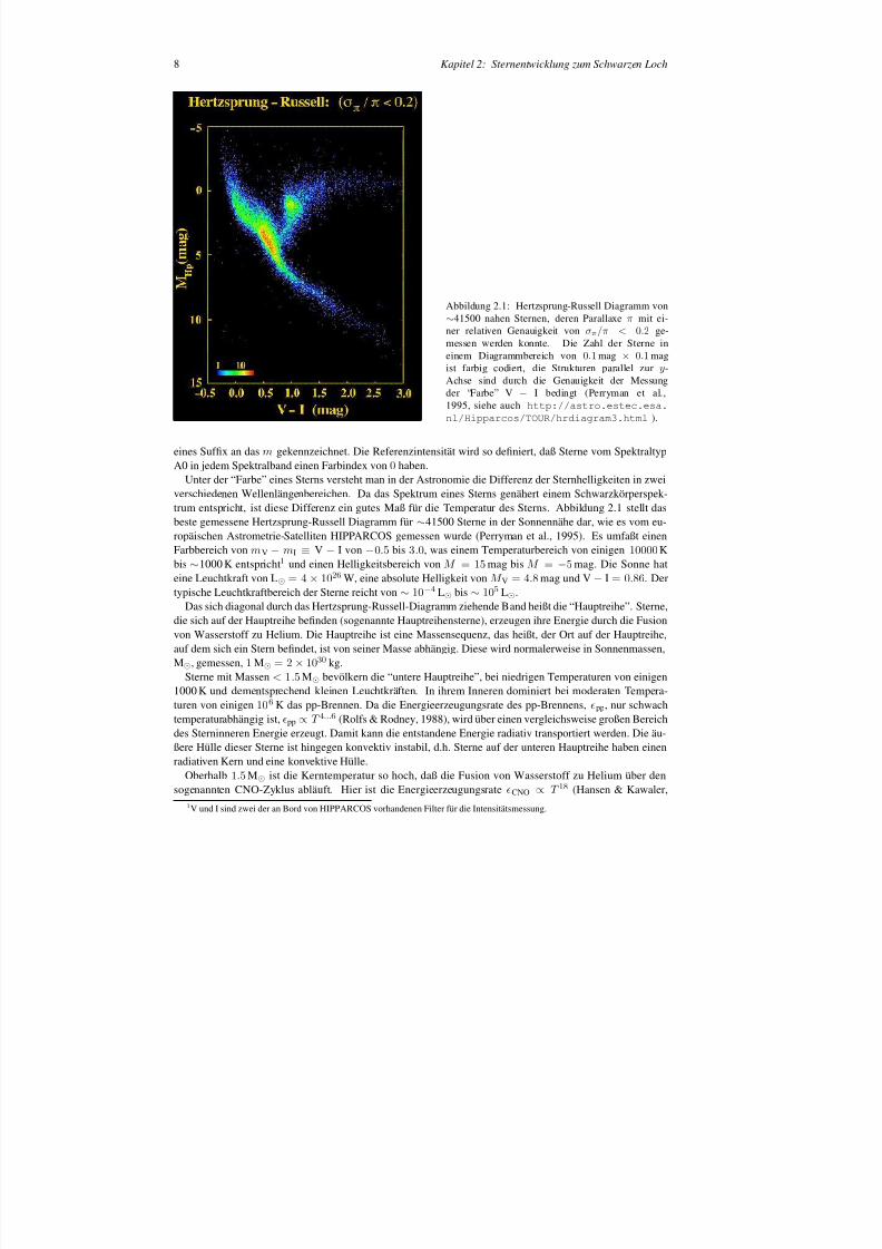
Abbildung 2.1: Hertzsprung-Russell Diagramm von∼41500 nahen Sternen, deren Parallaxe π mit ei-ner relativen Genauigkeit von σπ /π < 0 .2 ge-messen werden konnte. Die Zahl der Sterne ineinem Diagrammbereich von 0 .1 mag × 0 .1 magist farbig codiert, die Strukturen parallel zur y-Achse sind durch die Genauigkeit der Messungder “Farbe” V − I bedingt (Perryman et al.,1995, siehe auch http://astro.estec.esa.nl/Hipparcos/TOUR/hrdiagram3.html ).
eines Sufx an das m gekennzeichnet. Die Referenzintensität wird so deniert, daß Sterne vom SpektraltypA0 in jedem Spektralband einen Farbindex von 0 haben.
Unter der “Farbe” eines Sterns versteht man in der Astronomie die Differenz der Sternhelligkeiten in zweiverschiedenen Wellenlängenbereichen. Da das Spektrum eines Sterns genähert einem Schwarzkörperspek-trum entspricht, ist diese Differenz ein gutes Maß für die Temperatur des Sterns. Abbildung 2.1 stellt dasbeste gemessene Hertzsprung-Russell Diagramm für∼41500 Sterne in der Sonnennähe dar, wie es vom eu-ropäischen Astrometrie-Satelliten HIPPARCOS gemessen wurde (Perryman et al., 1995). Es umfaßt einenFarbbereich von m V − m I ≡ V− I von − 0.5 bis 3.0, was einem Temperaturbereich von einigen 10000Kbis ∼1000 K entspricht1 und einen Helligkeitsbereich von M = 15 mag bis M = − 5 mag. Die Sonne hateine Leuchtkraft von L = 4 × 1026 W, eine absolute Helligkeit von M V = 4 .8 mag und V− I = 0 .86. Dertypische Leuchtkraftbereich der Sterne reicht von∼ 10− 4 L bis∼ 105 L .
Das sich diagonal durch das Hertzsprung-Russell-Diagramm ziehende Band heißt die “Hauptreihe”. Sterne,die sich auf der Hauptreihe benden (sogenannte Hauptreihensterne), erzeugen ihre Energie durch die Fusionvon Wasserstoff zu Helium. Die Hauptreihe ist eine Massensequenz, das heißt, der Ort auf der Hauptreihe,auf dem sich ein Stern bendet, ist von seiner Masse abhängig. Diese wird normalerweise in Sonnenmassen,M , gemessen, 1 M = 2 × 1030 kg.
Sterne mit Massen < 1.5 M bevölkern die “untere Hauptreihe”, bei niedrigen Temperaturen von einigen1000 K und dementsprechend kleinen Leuchtkräften. In ihrem Inneren dominiert bei moderaten Tempera-turen von einigen 106 K das pp-Brennen. Da die Energieerzeugungsrate des pp-Brennens, pp , nur schwachtemperaturabhängig ist,pp ∝ T 4 ... 6 (Rolfs & Rodney, 1988), wird über einen vergleichsweise großen Bereichdes Sterninneren Energie erzeugt. Damit kann die entstandene Energie radiativ transportiert werden. Die äu-ßere Hülle dieser Sterne ist hingegen konvektiv instabil, d.h. Sterne auf der unteren Hauptreihe haben einenradiativen Kern und eine konvektive Hülle.
Oberhalb 1.5 M ist die Kerntemperatur so hoch, daß die Fusion von Wasserstoff zu Helium über densogenannten CNO-Zyklus abläuft. Hier ist die Energieerzeugungsrate CNO ∝ T 18 (Hansen & Kawaler,
1 V und I sind zwei der an Bord von HIPPARCOS vorhandenen Filter für die Intensitätsmessung.
8/12/2019 Schwarze LöCher Als Astronomische Objekte
http://slidepdf.com/reader/full/schwarze-lacher-als-astronomische-objekte 9/146
Kapitel 2.1: Entwicklung von Einzelsternen 9
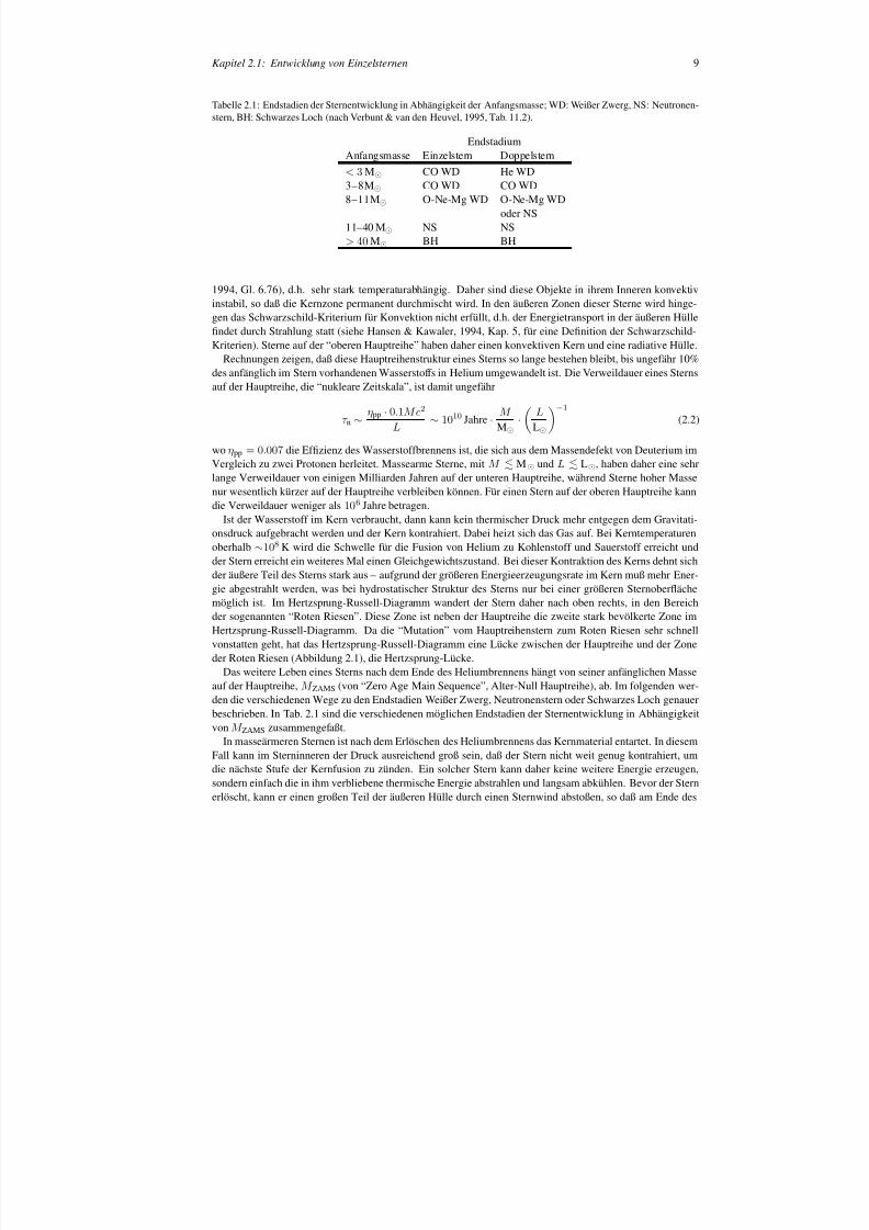
Tabelle 2.1: Endstadien der Sternentwicklung in Abhängigkeit der Anfangsmasse; WD: Weißer Zwerg, NS: Neutronen-stern, BH: Schwarzes Loch (nach Verbunt & van den Heuvel, 1995, Tab. 11.2).
EndstadiumAnfangsmasse Einzelstern Doppelstern< 3 M CO WD He WD3–8M CO WD CO WD8–11M O-Ne-Mg WD O-Ne-Mg WD
oder NS11–40 M NS NS> 40 M BH BH
1994, Gl. 6.76), d.h. sehr stark temperaturabhängig. Daher sind diese Objekte in ihrem Inneren konv
instabil, so daß die Kernzone permanent durchmischt wird. In den äußeren Zonen dieser Sterne wird hgen das Schwarzschild-Kriterium für Konvektion nicht erfüllt, d.h. der Energietransport in der äußeren Hndet durch Strahlung statt (siehe Hansen & Kawaler, 1994, Kap. 5, für eine Denition der SchwarzscKriterien). Sterne auf der “oberen Hauptreihe” haben daher einen konvektiven Kern und eine radiative H
Rechnungen zeigen, daß diese Hauptreihenstruktur eines Sterns so lange bestehen bleibt, bis ungefährdes anfänglich im Stern vorhandenen Wasserstoffs in Helium umgewandelt ist. Die Verweildauer eines Sauf der Hauptreihe, die “nukleare Zeitskala”, ist damit ungefähr
τ n ∼ ηpp · 0.1Mc2
L ∼ 1010 Jahre·
M M ·
LL
− 1
(2.2)
wo ηpp = 0 .007
die Efzienz des Wasserstoffbrennens ist, die sich aus dem Massendefekt von Deuterium Vergleich zu zwei Protonen herleitet. Massearme Sterne, mit M M und L L , haben daher eine sehrlange Verweildauer von einigen Milliarden Jahren auf der unteren Hauptreihe, während Sterne hoher Mnur wesentlich kürzer auf der Hauptreihe verbleiben können. Für einen Stern auf der oberen Hauptreihe die Verweildauer weniger als 106 Jahre betragen.
Ist der Wasserstoff im Kern verbraucht, dann kann kein thermischer Druck mehr entgegen dem Gravonsdruck aufgebracht werden und der Kern kontrahiert. Dabei heizt sich das Gas auf. Bei Kerntemperatoberhalb ∼108 K wird die Schwelle für die Fusion von Helium zu Kohlenstoff und Sauerstoff erreicht uder Stern erreicht ein weiteres Mal einen Gleichgewichtszustand. Bei dieser Kontraktion des Kerns dehnder äußere Teil des Sterns stark aus – aufgrund der größeren Energieerzeugungsrate im Kern muß mehr gie abgestrahlt werden, was bei hydrostatischer Struktur des Sterns nur bei einer größeren Sternober
möglich ist. Im Hertzsprung-Russell-Diagramm wandert der Stern daher nach oben rechts, in den Beder sogenannten “Roten Riesen”. Diese Zone ist neben der Hauptreihe die zweite stark bevölkerte ZonHertzsprung-Russell-Diagramm. Da die “Mutation” vom Hauptreihenstern zum Roten Riesen sehr scvonstatten geht, hat das Hertzsprung-Russell-Diagramm eine Lücke zwischen der Hauptreihe und der Zder Roten Riesen (Abbildung 2.1), die Hertzsprung-Lücke.
Das weitere Leben eines Sterns nach dem Ende des Heliumbrennens hängt von seiner anfänglichen Mauf der Hauptreihe, M ZAMS (von “Zero Age Main Sequence”, Alter-Null Hauptreihe), ab. Im folgenden weden die verschiedenen Wege zu den Endstadien Weißer Zwerg, Neutronenstern oder Schwarzes Loch genbeschrieben. In Tab. 2.1 sind die verschiedenen möglichen Endstadien der Sternentwicklung in Abhängvon M ZAMS zusammengefaßt.
In masseärmeren Sternen ist nach dem Erlöschen des Heliumbrennens das Kernmaterial entartet. In di
Fall kann im Sterninneren der Druck ausreichend groß sein, daß der Stern nicht weit genug kontrahierdie nächste Stufe der Kernfusion zu zünden. Ein solcher Stern kann daher keine weitere Energie erzeusondern einfach die in ihm verbliebene thermische Energie abstrahlen und langsam abkühlen. Bevor der erlöscht, kann er einen großen Teil der äußeren Hülle durch einen Sternwind abstoßen, so daß am Ende
8/12/2019 Schwarze LöCher Als Astronomische Objekte
http://slidepdf.com/reader/full/schwarze-lacher-als-astronomische-objekte 10/146
10 Kapitel 2: Sternentwicklung zum Schwarzen Loch
Lebens nur noch der Kern beobachtbar ist. Die Zusammensetzung dieses “weißen Zwergs” (white dwarf,WD) hängt von der Anfangsmasse des Sterns ab: Bei massenarmen Sternen (M ZAMS 3M ) erlischt dasKernbrennen schon nach dem Heliumbrennen, Sterne höherer Masse können noch bis zum Kohlenstoff odereventuell sogar bis zum Neon fusionieren.
Bei massereichen Sternen mit M ZAMS 10M setzen sich die Brennzyklen nach dem Heliumbrennenfort: Ist das Helium im Kern aufgebraucht, dann kann Kohlenstofffusion einsetzen, danach Sauerstoffbrennen,und so weiter, bis schließlich nach der Fusion von Eisen während des Siliziumbrennens durch Fusion keineweitere Energie mehr freigesetzt werden kann. Am Schluß hat der Stern einen “zwiebelschalenförmigen”Aufbau, mit einem Eisenkern, dann einer Siliziumschale, usw., bis zur Heliumschale und schließlich außeneiner Wasserstoffhülle. Da der relative Energiegewinn pro Kernbrennstufe immer geringer wird, während dieabgestrahlte Leuchtkraft des Sterns zunimmt, verringert sich nach Gl. (2.2) auch die nukleare Zeitskala immerweiter, bis sie beim Siliziumbrennen nur noch wenige Stunden bis Tage beträgt.
Ist auch diese Quelle erloschen, dann fällt der Stern in sich zusammen. Wie schon beim Beginn des He-liumbrennens verdichten sich dabei die inneren Regionen des Sterns stark und heizen sich stark auf. Dadurch Fusion keine weitere Energie aufgebracht werden kann, kann der Kollaps allerdings nicht weiter auf-gehalten werden. Das Sterninnere verdichtet auf Dichten im Bereich von 1010 ... 12 g cm− 3 (Arnett, 1996).Die Fermienergie der Elektronen ist hier so hoch, daß durch Elektroneneinfang die Atomkerne desintegrie-ren (“Neutronisierung”). In diesem Stadium wird der Druck im Sterninnern hauptsächlich durch relativisti-sche Elektronen und Neutrinos aufgebracht. Erst wenn Dichten vergleichbar der Kerndichte erreicht werden(ρ ∼ 1014 g cm− 3 ), kann der weitere Zusammenbruch des Sterns aufgehalten werden, da die Nukleonen sodicht zusammengepresst werden, daß die starke Wechselwirkung repulsiv wird (Arnett, 1996). Der hauptsäch-lich aus Neutronen bestehende Kern des Sterns hat zu diesem Zeitpunkt eine Masse von∼0.5M und einenRadius von∼10 km. Er bildet für die von außen mit Überschallgeschwindigkeit einfallende normale Materieeine quasi inkompressible Oberäche, von der das einfallende Material abprallt. Der Rückstoß dieses Mate-rials führt zur Bildung eines stehenden Schocks bei einer Höhe von ∼100 km oberhalb des Kerns (Bruenn,De Nisco & Mezzacappa, 2001). Material “regnet” durch diesen Schock auf die Oberäche des Neutronen-kerns. Wahrscheinlich aufgrund des Drucks der bei der Neutronisierung entstandenen Neutrinos, die nichtaus dem Stern entweichen können, da das akkretierende Material optisch dick für Neutrinos wird, wird dannnach einigen Millisekunden der Sternkollaps in eine Explosion umgewandelt, bei der der größte Teil der Hülledes Sterns abgestoßen wird. Der explodierende Stern wird als Supernova vom Typ Ib oder II sichtbar (sieheFilippenko, 1997, und die darin angegebene Literatur für Details zur Klassikation der Supernovae). Bei einersolchen Supernovaexplosion wird eine sehr große Energiemenge innerhalb kürzester Zeit freigesetzt: Super-novae haben typischerweise Helligkeiten im Bereich einiger 1010 L im optischen Spektralbereich, d.h. siesind heller als die Helligkeit einer typischen Spiralgalaxie wie unserer Milchstraße. Der innere, aus Neutronenbestehende Kern des Sterns bleibt nach dieser Explosion als “Neutronenstern” erhalten, er hat theoretischenRechnungen zufolge eine Masse von etwas über 1 M.
Am Ende einer Supernova muß allerdings nicht immer ein Neutronenstern entstanden sein. Beim Kol-laps der äußeren Hülle kann der Druck auf den Neutronenstern so groß sein, daß auch er nicht mehr stabilist. Da es sich bei Kernmaterie um das stabilste zur Zeit in der Physik bekannte Material handelt, geht mandavon aus, daß sich dieser Kollaps bis ins Unendliche fortsetzen wird. Es bildet sich ein Schwarzes Loch.Die genaue Massengrenze, oberhalb derer sich in Supernovae Schwarze Löcher bilden können, hängt starkvon der bislang noch nicht mit ausreichender Genauigkeit verstandenen Zustandsgleichung für Kernmaterialab. Ferner kann mit heute verfügbaren Computern auch die Supernovaexplosion nur unter sehr vereinfach-ten Annahmen (z.B. Rotationssymmetrie, keine Magnetfelder, vereinfachte Annahmen über die Rotation desSterns, vereinfachte Zustandsgleichung, Vernachlässigung relativistischer Effekte, . . . ) berechnet werden.Eine Zusammenfassung dieser Annahmen geben Bruenn, De Nisco & Mezzacappa (2001). Daher kann austheoretischen Berechnungen die genaue Grenze für M ZAMS , oberhalb derer bei Supernovae ein SchwarzesLoch entsteht, nicht erhalten werden.
Außer aus Supernovaberechnungen wird daher versucht, durch die Erklärung der Existenz beobachteterNeutronensterne die Grenzmasse für die Supernovaentstehung einzuengen. So folgern zum Beispiel Wellstein& Langer (1999) aus der Existenz eines Neutronensterns im System Wray 977/GX 301− 2 eine obere Grenze
8/12/2019 Schwarze LöCher Als Astronomische Objekte
http://slidepdf.com/reader/full/schwarze-lacher-als-astronomische-objekte 11/146
Kapitel 2.2: Entwicklung von Doppelsternsystemen 11
für die Entstehung eines Neutronensterns von M ZAMS = 13 . . . 21 M , während andere Autoren M ZAMS =20 . . . 50 M (Ergma & van den Heuvel, 1998) beziehungsweise M ZAMS 18M (Brown et al., 1999)angeben.
Die große Ungenauigkeit dieser Grenzmassen für die Schwarzlochentstehung ist nicht nur durch diegenauigkeit der Supernova-Simulationen bedingt, die in diese Abschätzungen nicht eingehen, sondern hsächlich durch die Ungenauigkeiten in unserem Verständnis der Sternentwicklung, hauptsächlich im Beder Modellierung des sehr starken Massenverlusts von Sternen mit M ZAMS 20M und im Bereich derModellierung der Durchmischungsprozesse in den konvektiven Zonen der Sterne.
Annahmen über den Sternwind sind wichtig, weil die Gesamtmasse eines Sterns die Entwicklungszkalen und sein Äußeres maßgeblich beeinußt. Sternwinde sind sehr dynamische Phänomene, die bis hnur grob verstanden sind. Die für die Schwarzlochentstehung so wichtigen massereiche Sterne haben so Leuchtkräfte, daß der Strahlungsdruck in den äußeren Zonen der Atmosphäre ausreicht, das Atmosphäreüber die Entweichgeschwindigkeit an der Sternoberäche zu beschleunigen. Zur Computersimulation soWinde müssen dreidimensionale strahlungshydrodynamische Rechnungen durchgeführt werden, für die weder die Computerleistung existiert, noch sind die für diese Rechnungen notwendigen Atomdaten honisierter Metalle bekannt. Daher gehen in die Sternentwicklungsrechnungen notwendigerweise Näheruein. Beispielsweise kann je nach angenommener Massenverlustrate ein Stern mit 60 M Hauptreihenmassevor seiner Supernovaexplosion eine Masse zwischen 4.5 M und 30 M haben (Woosley, Langer & Wea-ver, 1993), und damit in der Explosion entweder einen Neutronenstern oder ein schwarzes Loch erzeuge
Kentnisse über die Konvektion sind notwendig, weil die Konvektion verschiedene Zonen des Sterns dmischt und so zum Beispiel Wasserstoff aus Zonen, in denen vorher keine Fusion stattgefunden hat, in serstoffbrennende Zonen des Kerns transportieren kann. Dies verändert die chemische Struktur des Sund damit seine Entwicklung. Stellare Konvektion ist ebenfalls ein aktuelles astrophysikalisches Forschgebiet. Auch hier setzt wieder die Verfügbarkeit ausreichend guter Simulationsrechnungen mit dreidimsionaler Magnetohydrodynamik die Grenzen. Daher wird in Sternentwicklungsrechnungen üblicherweisverschiedenen “Mischungswegtheorien” gearbeitet, bei denen die Konvektion nur sehr genähert dargewird (Hansen & Kawaler, 1994, Kap. 5). In diesen Theorien setzt Konvektion “schlagartig” ein, sobaldSchwarzschild-Kriterium erfüllt wird. Genauso prompt wird das Sterninnere wieder als rein radiativ asehen, wenn das Schwarzschild-Kriterium nicht mehr erfüllt wird. Da das konvektive Material aus Imserhaltungsgründen nicht prompt gestoppt werden kann, wird es aber offensichtlich noch etwas in eine “überschießen”, die dem Schwarzschild-Kriterium nach eigentlich schon radiativ sein sollte. Theorien“convective overshoot” versuchen, diese Zone mit mehr oder weniger ad hoc Annahmen zu modellierenwirklich befriedigende Lösung ist hier aber auch noch nicht in Sicht (siehe Schröder, Pols & Eggleton und Young et al. 2001 für neuere Diskussionen zu diesem Thema). Daß eine solche wirklich notwendium die Entwicklung von einem Hauptreihenstern zu einem Weißen Zwerg, Neutronenstern oder SchwaLoch zu verstehen, sei daran illustriert, daß die Untergrenze für die Vorgängersterne von Neutronenstevon 8M auf 6M sinkt, wenn “overshoot” berücksichtigt wird (Verbunt & van den Heuvel, 1995).
Dennoch: Trotz all dieser Unsicherheiten der Sternentwicklung scheint es keinen Ausweg zu geben,eine gewisse Zahl an Sternen am Ende ihres Lebens ein Schwarzes Loch bildet. Ziel der UntersuchungSchwarzen Löchern ist es, die an ihnen beobachteten Phänomene zu verstehen. Dazu gehört insbesonauch, zu verstehen, wie die Schwarzen Löcher mit ihrer Umgebung wechselwirken und es gehört letztenauch dazu, zu verstehen, wie die Schwarzen Löcher entstanden sind.
2.2 Entwicklung von Doppelsternsystemen
Alle beobachteten Schwarzlochkandidaten in der Milchstraße sind Mitglieder von Doppelsternsystemen.ist teilweise ein Auswahleffekt, da Schwarze Löcher und Neutronensterne als Röntgendoppelsterne eine
Leuchtkraft haben und dadurch einfacher beobachtbar sind als alleinstehende Neutronensterne oder SchwLöcher (Kap. 3). Ferner sind ungefähr 50% aller Sterne Doppel- oder Mehrfachsysteme, so daß ein gewAnteil an Schwarzen Löchern in Doppelsternsystemen grundsätzlich zu erwarten ist. Je nach Massenvernis der Sterne verläuft die Entwicklung eines Doppelsternsystems stark unterschiedlich. Als Beispiel fü
8/12/2019 Schwarze LöCher Als Astronomische Objekte
http://slidepdf.com/reader/full/schwarze-lacher-als-astronomische-objekte 12/146
12 Kapitel 2: Sternentwicklung zum Schwarzen Loch
M1 M2CM L1
L2L3
L4
L5
10 R sun
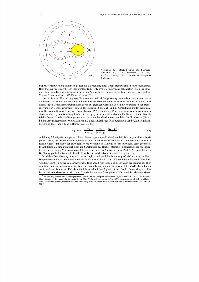
Abbildung 2.2: Roche-Potential mit Lagrange-Punkten L 1 , L 2 , . . . , L5 , für Massen M 1 = 18 Mund M 2 = 10 M . CM ist der Massenschwerpunktdes Systems.
Doppelsternentwicklung soll im Folgenden die Entwicklung eines Doppelsternsystems in einen sogenanntenHigh-Mass X-ray Binary beschrieben werden, da dieser Klasse einige der später behandelten Objekte angehö-ren. Für weitere Entwicklungswege siehe die am Anfang dieses Kapitels angegebene Literatur, insbesondereVerbunt & van den Heuvel (1995) und Verbunt (2001).
Unterschiede zur Entwicklung von Einzelsternen sind bei Doppelsternsystemen dann zu erwarten, wenndie beiden Sterne einander so nahe sind, daß ihre Gezeitenwechselwirkung einen Einuß bekommt. Beidiesen engen Doppelsternsystemen kann davon ausgegangen werden, daß sich die Rotationszeit der Sterneaufgrund von Gezeitenwechselwirkungen der Umlaufszeit angleicht und die Umlaufbahn um den gemeinsa-men Schwerpunkt kreisförmig wird (siehe Tassoul, 1978, Kapitel 2). Zur Berechnung von Bewegungen ineinem solchen System ist es angebracht, ein Bezugssystem zu wählen, das mit den Sternen rotiert. Das ef-fektive Potential in diesem Bezugssystem setzt sich aus den Gravitationspotentialen der Einzelsterne (die alsPunktmassen angenommen werden können) und einem zusätzlichen Term zusammen, der die Zentrifugalkraftbeschreibt: (z.B. Frank, King & Raine, 1992, Gl. 4.5)
ΦR( r ) = − GM 1| r − r 1 |
− GM 2| r − r 2 |
− (ωωω × r )2
2 (2.3)
Abbildung 2.2 zeigt die Äquipotentiallinien dieses sogenannten Roche-Potentials. Die ausgezeichnete Äqui-potentiallinie, die die Form einer Sanduhr hat und beide Punktmassen umläuft, deniert die sogenannteRoche-Fläche. Innerhalb der jeweiligen Roche-Volumina ist Material an den jeweiligen Stern gebunden.In Abbildung 2.2 sind zusätzlich noch die Sattelpunkte des Roche-Potentials eingezeichnet, die sogenann-ten Lagrange-Punkte. Von besonderem Interesse wird noch der “innere Lagrange-Punkt”, L 1 , sein, der beimBerührungspunkt der Roche-Flächen der Einzelsterne auf der Symmetrielinie des Systems liegt.
Bei vielen Doppelsternsystemen ist der anfängliche Abstand der Sterne so groß, daß sie während ihresHauptreihenstadiums wesentlich kleiner als ihre Roche-Volumina sind. Während dieser Phasen ist ihre Ent-wicklung identisch zu der von Einzelsternen. Dies ändert sich jedoch beim Verlassen der Hauptreihe. Hierdehnt ein Stern sein Volumen auf dem Weg zum Roten Riesen Stadium stark aus, so daß er dasRoche-Volumenerreichen kann. Ist dies der Fall, dann ießt Material auf den Begleiter über2 . Da die Entwicklungszeitska-len mit höherer Masse kürzer sind, wird Material immer vom Stern größerer Masse auf den kleinerer Masse
2 Der hier besprochene Fall ist der sogenannte “Case B”, der für die später behandelten Objekte relevant ist. Findet der Massen-überuß schon auf der Hauptreihe statt, so ist das ein “Case A”-Entwicklungsszenario. “Case C”ist dementsprechend die Entwicklungeines Doppelsternsystems, wenn der erste Massenübertrag erst nach dem Erreichen des Roten Riesen Stadiums statt ndet (Verbunt,2001).
8/12/2019 Schwarze LöCher Als Astronomische Objekte
http://slidepdf.com/reader/full/schwarze-lacher-als-astronomische-objekte 13/146
Kapitel 2.3: Kompakte Objekte 13
übergehen. Aufgrund der Drehimpulserhaltung wächst dabei der Abstand der beiden Sterne stark an.Ende dieser ersten Phase des Masseübertrags hat der ursprünglich massereichere Stern einen Großteil sMasse verloren. Der verbleibende Heliumkern dieses Sterns entwickelt sich weiter und explodiert schliein einer Supernova. Bei dieser Explosion kann das System auseinandergerissen werden. Ist dies nichFall, enthält das Doppelsternsystem nach der Explosion einen Neutronenstern oder ein Schwarzes Lochvon einem massereichen Hauptreihenstern umkreist wird. Im Laufe der weiteren Entwicklung des Syswird der ursprünglich masseärmere Stern sich ebenfalls ausdehnen. Füllt er sein Roche Lobe aus, dann Material über den inneren Lagrange-Punkt auf seinen kompakten Begleiter fallen und das System wirRöntgendoppelstern sichtbar (Kapitel 3).
Modikationen dieses Szenarios sind sehr wahrscheinlich. Wie in Abschnitt 2.1 dargestellt wurde, hmassereiche Sterne starke Sternwinde. Daher wird anstelle des oben vorgestellten konservativen Masseütrags im Doppelsternsystem, bei dem die Gesamtmasse des Systems und der Gesamtdrehimpuls erhaltenben, ein Teil der Masse und des Drehimpulses durch einen Sternwind das System verlassen. Ferner kanFall stärkerer Winde ein Masseübertrag auch dann stattnden, wenn ein Stern sein Roche-Volumen nochvollständig ausfüllt. In beiden Fällen verläuft die detaillierte Entwicklung eines Systems unterschiedlichder oben dargestellten. Tabelle 2.1 listet die wahrscheinlichen Endstadien für typische “Case B” Szenauf.
2.3 Kompakte Objekte
Trotz aller Unsicherheiten in der Sternentwicklung können den Erläuterungen in Abschnitt 2.1 zufolgEndstadium drei verschiedene Arten von Objekten entstehen: Weiße Zwerge, Neutronensterne und schwLöcher. Diese Objektarten werden häug unter dem Überbegriff “kompakte Objekte” zusammengefaßtheißt, sie sind Objekte stellarer Masse mit Radien, die klein sind im Vergleich zu normalen Sternen.
Kompakte Objekte können aus physikalischen Gründen nur innerhalb bestimmter Massengrenzen exi
ren, das heißt, daß sie häug durch eine Massenbestimmung klar identiziert werden können:Weiße Zwerge werden durch den Druck entarteter Elektronen stabilisiert. Mit mittleren Dichten von ρ ∼
105 ... 6 g cm− 3 haben sie typische Radien, die vergleichbar mit dem Erdradius sind. Oberhalb einGrenzmasse von 1.44 M, der Chandrasekhar-Grenze (Chandrasekhar, 1931), können weiße Zwergenicht existieren, da dann die Elektronen relativistisch entarten und kein Gleichgewicht mehr zwiscder Gravitation und dem Elektronendruck existiert.
Neutronensterne können oberhalb der Chandrasekhar-Grenze existieren, weil sie durch Wechselwirkungzwischen den Neutronen stabilisiert werden. Ihre typische Dichte liegt in der Nähe der von Kernterial, ρ ∼ 1013 . . . 1016 g cm− 3 , ihre Radien sind im Bereich von ∼10 km. Der Aufbau der Neutro-nensterne ist wenig verstanden, weil er stark von der Zustandsgleichung für Kernmaterie abhängtnoch nicht ausreichend gut bekannt ist (Shapiro & Teukolsky, 1983, Kapitel 8). Diese Unsichebedingt auch die obere Massengrenze für Neutronensterne, die je nach Zustandsgleichung zwisc∼2 M und∼ 3 M liegt. Die maximale Obergrenze für Neutronensterne wird für die steifste Zustandgleichung erreicht, die einem Kausalitätsargument von Oppenheimer & Volkoff (1939) folgend derreicht wird, wenn die Schallgeschwindigkeit im Neutronenstern gleich der LichtgeschwindigkeiDiese Oppenheimer-Volkoff Grenze liegt bei M OV = 3 .2 M (Rhoades & Rufni, 1974, unter derAnnahme einer “matching density” von ρ0 = 4 .6 × 1014 g cm− 3 , d.h. unter der Annahme, daß die Zu-standsgleichung von Kernmaterie bis zu einer Dichte von ρ 0 verstanden ist), neuere Untersuchungenvon Kalogera & Baym (1996) ergeben M OV = 2 .9 M (ρ0 = 5 .4 × 1014 g cm− 3 ) bzw. M OV = 2 .6 M(Olson, 2001, Mittelwert für verschiedene Zustandsgleichungen).
Schwarze Löcher sind damit alle die kompakten Objekte, die oberhalb der Oppenheimer-Volkoff-Grenbeobachtet werden3 . Ihre Größe kann durch den Schwarzschild-Radius, das heißt durch den Radius d3 Wiederholt sind sogenannte “exotische Sterne” als Alternativmodelle für Schwarze Löcher vorgeschlagen worden, Objekte, die
zum Beispiel als “Quarksterne” rein aus Quarks aufgebaut sind (siehe z.B. Drake et al., 2002).
8/12/2019 Schwarze LöCher Als Astronomische Objekte
http://slidepdf.com/reader/full/schwarze-lacher-als-astronomische-objekte 14/146
8/12/2019 Schwarze LöCher Als Astronomische Objekte
http://slidepdf.com/reader/full/schwarze-lacher-als-astronomische-objekte 15/146
Kapitel 2.4: Massenbestimmung 15
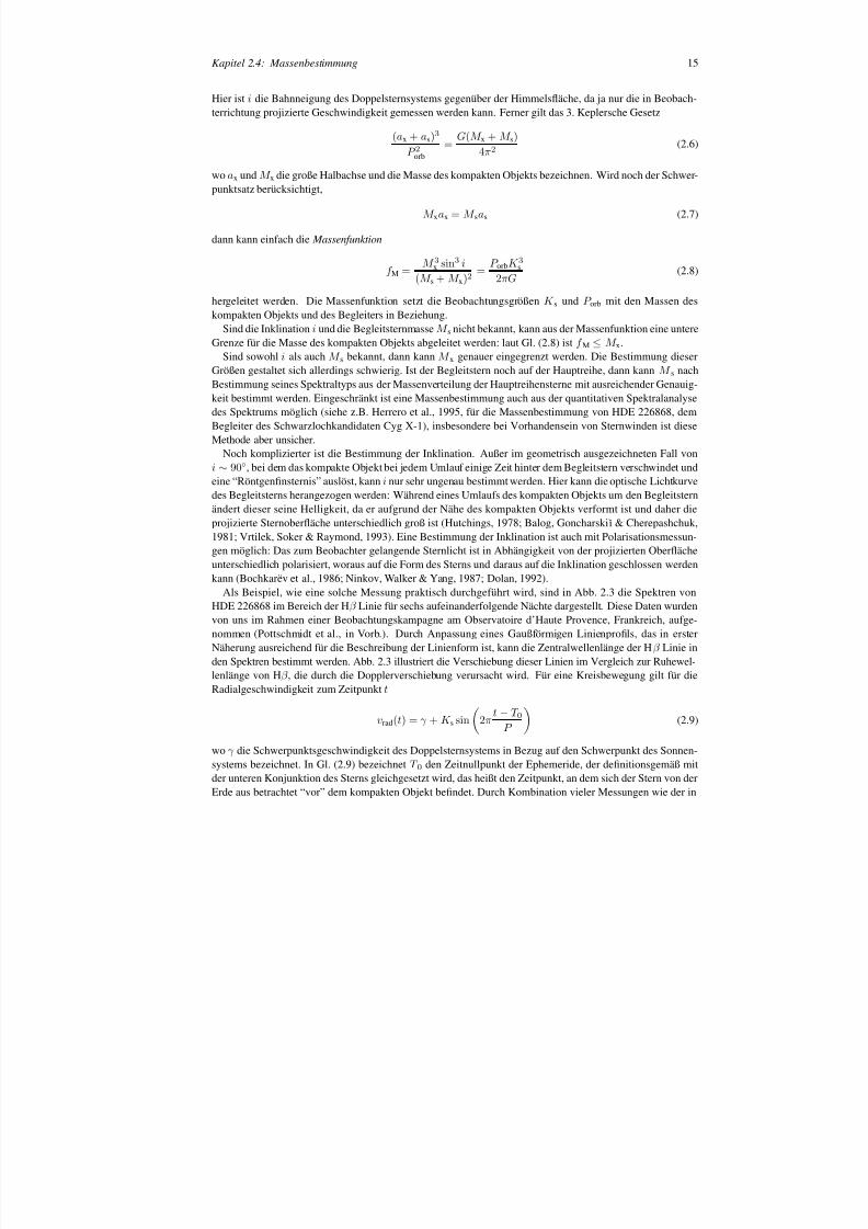
Hier ist i die Bahnneigung des Doppelsternsystems gegenüber der Himmelsäche, da ja nur die in Beobterrichtung projizierte Geschwindigkeit gemessen werden kann. Ferner gilt das 3. Keplersche Gesetz
(ax + a s)3
P 2orb
= G(M x + M s)
4π 2 (2.6)
woax undM x die große Halbachse und die Masse des kompakten Objekts bezeichnen. Wird noch der Schwpunktsatz berücksichtigt,
M xax = M sa s (2.7)
dann kann einfach die Massenfunktion
f M = M 3x sin3 i(M s + M x)2 =
P orb K 3s2πG
(2.8)
hergeleitet werden. Die Massenfunktion setzt die Beobachtungsgrößen K s und P orb mit den Massen deskompakten Objekts und des Begleiters in Beziehung.Sind die Inklination i und die Begleitsternmasse M s nicht bekannt, kann aus der Massenfunktion eine untere
Grenze für die Masse des kompakten Objekts abgeleitet werden: laut Gl. (2.8) ist f M ≤ M x.Sind sowohl i als auch M s bekannt, dann kann M x genauer eingegrenzt werden. Die Bestimmung dieser
Größen gestaltet sich allerdings schwierig. Ist der Begleitstern noch auf der Hauptreihe, dann kann M s nachBestimmung seines Spektraltyps aus der Massenverteilung der Hauptreihensterne mit ausreichender Genkeit bestimmt werden. Eingeschränkt ist eine Massenbestimmung auch aus der quantitativen Spektralandes Spektrums möglich (siehe z.B. Herrero et al., 1995, für die Massenbestimmung von HDE 226868,Begleiter des Schwarzlochkandidaten Cyg X-1), insbesondere bei Vorhandensein von Sternwinden ist dMethode aber unsicher.
Noch komplizierter ist die Bestimmung der Inklination. Außer im geometrisch ausgezeichneten Falli ∼ 90 , bei dem das kompakte Objekt bei jedem Umlauf einige Zeit hinter dem Begleitstern verschwindet eine “Röntgennsternis” auslöst, kanni nur sehr ungenau bestimmt werden. Hier kann die optische Lichtkurvedes Begleitsterns herangezogen werden: Während eines Umlaufs des kompakten Objekts um den Begleiändert dieser seine Helligkeit, da er aufgrund der Nähe des kompakten Objekts verformt ist und daheprojizierte Sternoberäche unterschiedlich groß ist (Hutchings, 1978; Balog, Goncharskiı & Cherepashchuk,1981; Vrtilek, Soker & Raymond, 1993). Eine Bestimmung der Inklination ist auch mit Polarisationsmegen möglich: Das zum Beobachter gelangende Sternlicht ist in Abhängigkeit von der projizierten Oberunterschiedlich polarisiert, woraus auf die Form des Sterns und daraus auf die Inklination geschlossen wkann (Bochkarëv et al., 1986; Ninkov, Walker & Yang, 1987; Dolan, 1992).
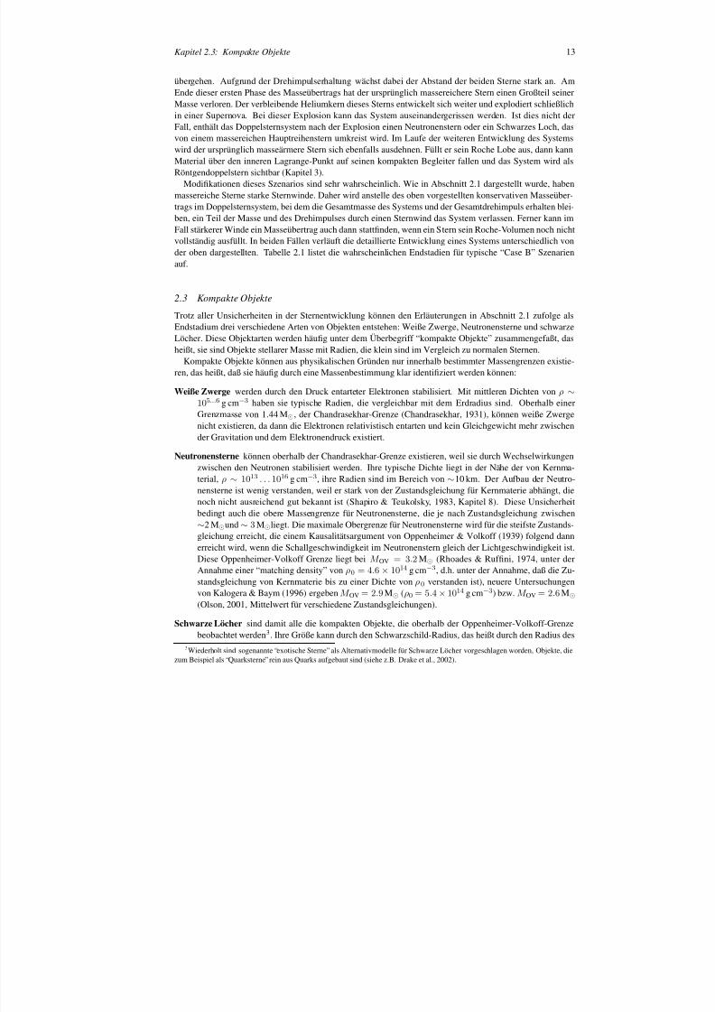
Als Beispiel, wie eine solche Messung praktisch durchgeführt wird, sind in Abb. 2.3 die Spektren
HDE 226868 im Bereich der Hβ Linie für sechs aufeinanderfolgende Nächte dargestellt. Diese Daten wurdevon uns im Rahmen einer Beobachtungskampagne am Observatoire d’Haute Provence, Frankreich, aunommen (Pottschmidt et al., in Vorb.). Durch Anpassung eines Gaußförmigen Linienprols, das in eNäherung ausreichend für die Beschreibung der Linienform ist, kann die Zentralwellenlänge der Hβ Linie inden Spektren bestimmt werden. Abb. 2.3 illustriert die Verschiebung dieser Linien im Vergleich zur Ruhelenlänge von Hβ , die durch die Dopplerverschiebung verursacht wird. Für eine Kreisbewegung gilt für Radialgeschwindigkeit zum Zeitpunkt t
vrad (t) = γ + K s sin 2πt − T 0
P (2.9)
wo γ die Schwerpunktsgeschwindigkeit des Doppelsternsystems in Bezug auf den Schwerpunkt des Sonsystems bezeichnet. In Gl. (2.9) bezeichnet T 0 den Zeitnullpunkt der Ephemeride, der denitionsgemäß mitder unteren Konjunktion des Sterns gleichgesetzt wird, das heißt den Zeitpunkt, an dem sich der Stern voErde aus betrachtet “vor” dem kompakten Objekt bendet. Durch Kombination vieler Messungen wie d
8/12/2019 Schwarze LöCher Als Astronomische Objekte
http://slidepdf.com/reader/full/schwarze-lacher-als-astronomische-objekte 16/146
16 Kapitel 2: Sternentwicklung zum Schwarzen Loch
0.0 0.2 0.4 0.6 0.8 1.0Orbital Phase
-150
-100
-50
0
50
100
R a
d i a l V e
l o c
i t y [ k m
/ s ]
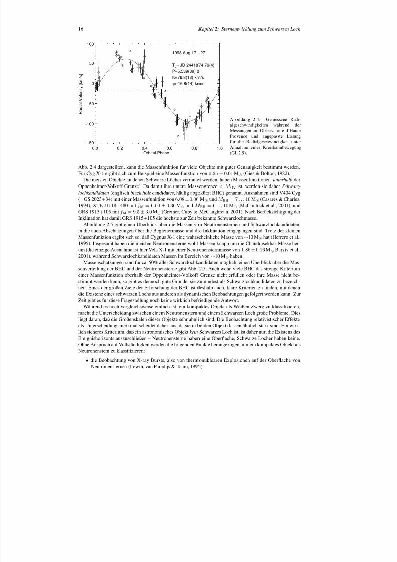
1998 Aug 17 - 27
T0= JD 2441874.79(4)P=5.539(39) dK=76.8(18) km/sγ =-16.8(14) km/s
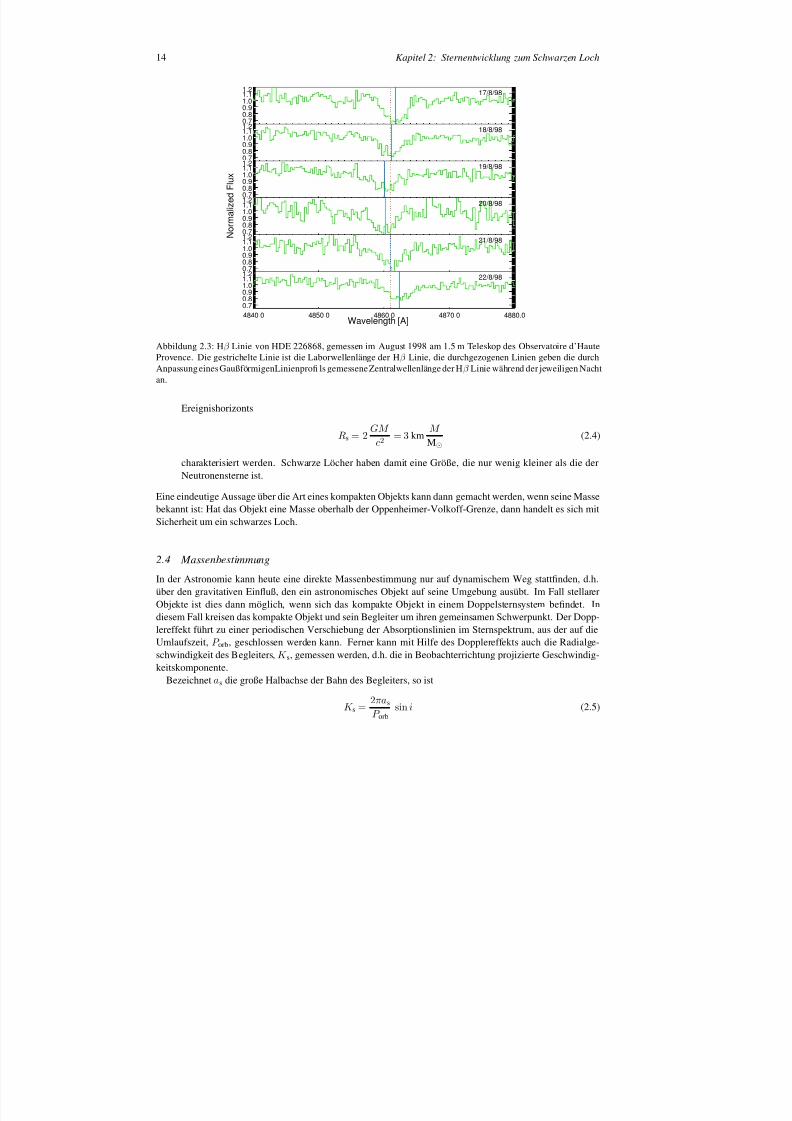
Abbildung 2.4: Gemessene Radi-algeschwindigkeiten während derMessungen am Observatoire d’HauteProvence und angepasste Lösungfür die Radialgeschwindigkeit unterAnnahme einer Kreisbahnbewegung(Gl. 2.9).
Abb. 2.4 dargestellten, kann die Massenfunktion für viele Objekte mit guter Genauigkeit bestimmt werden.Für Cyg X-1 ergibt sich zum Beispiel eine Massenfunktion von 0.25 ± 0.01 M (Gies & Bolton, 1982).
Die meisten Objekte, in denen Schwarze Löcher vermutet werden, haben Massenfunktionen unterhalb derOppenheimer-Volkoff Grenze! Da damit ihre untere Massengrenze < M OV ist, werden sie daher Schwarz-lochkandidaten (englisch black hole candidates , häug abgekürzt BHC) genannt. Ausnahmen sind V404 Cyg(= GS 2023+ 34) mit einer Massenfunktion von 6.08± 0.06 M und M BH = 7 . . . 10 M (Casares & Charles,1994), XTE J1118+ 480 mit f
M = 6 .00 ± 0.36 M und M
BH = 6 . . . 10 M (McClintock et al., 2001), und
GRS 1915+ 105 mit f M = 9 .5 ± 3.0 M (Greiner, Cuby & McCaughrean, 2001). Nach Berücksichtigung derInklination hat damit GRS 1915+ 105 die höchste zur Zeit bekannte Schwarzlochmasse.
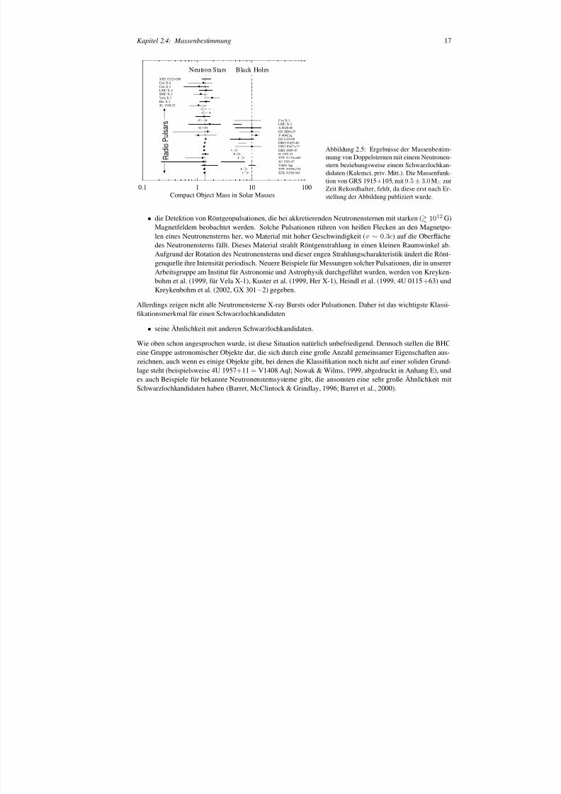
Abbildung 2.5 gibt einen Überblick über die Massen von Neutronensternen und Schwarzlochkandidaten,in die auch Abschätzungen über die Begleitermasse und die Inklination eingegangen sind. Trotz der kleinenMassenfunktion ergibt sich so, daß Cygnus X-1 eine wahrscheinliche Masse von∼10 M hat (Herrero et al.,1995). Insgesamt haben die meisten Neutronensterne wohl Massen knapp um die Chandrasekhar-Masse her-um (die einzige Ausnahme ist hier Vela X-1 mit einer Neutronensternmasse von 1.86 ± 0.16 M Barziv et al.,2001), während Schwarzlochkandidaten Massen im Bereich von∼10 M haben.
Massenschätzungen sind für ca. 50% aller Schwarzlochkandidaten möglich, einen Überblick über die Mas-senverteilung der BHC und der Neutronensterne gibt Abb. 2.5. Auch wenn viele BHC das strenge Kriteriumeiner Massenfunktion oberhalb der Oppenheimer-Volkoff Grenze nicht erfüllen oder ihre Masse nicht be-stimmt werden kann, so gibt es dennoch gute Gründe, sie zumindest als Schwarzlochkandidaten zu bezeich-nen. Eines der großen Ziele der Erforschung der BHC ist deshalb auch, klare Kriterien zu nden, mit denendie Existenz eines schwarzen Lochs aus anderen als dynamischen Beobachtungen gefolgert werden kann. ZurZeit gibt es für diese Fragestellung noch keine wirklich befriedigende Antwort.
Während es noch vergleichsweise einfach ist, ein kompaktes Objekt als Weißen Zwerg zu klassizieren,macht die Unterscheidung zwischen einem Neutronenstern und einem Schwarzen Loch große Probleme. Diesliegt daran, daß die Größenskalen dieser Objekte sehr ähnlich sind. Die Beobachtung relativistischer Effekteals Unterscheidungsmerkmal scheidet daher aus, da sie in beiden Objektklassen ähnlich stark sind. Ein wirk-lich sicheres Kriterium, daß ein astronomisches Objekt kein Schwarzes Loch ist, ist daher nur, die Existenz desEreignishorizonts auszuschließen – Neutronensterne haben eine Oberäche, Schwarze Löcher haben keine.
Ohne Anspruch auf Vollständigkeit werden die folgenden Punkte herangezogen, um ein kompaktes Objekt alsNeutronenstern zu klassizieren:
• die Beobachtung von X-ray Bursts, also von thermonuklearen Explosionen auf der Oberäche vonNeutronensternen (Lewin, van Paradijs & Taam, 1995).
8/12/2019 Schwarze LöCher Als Astronomische Objekte
http://slidepdf.com/reader/full/schwarze-lacher-als-astronomische-objekte 17/146
Kapitel 2.4: Massenbestimmung 17
0.1 1 10 100
Compact Object Mass in Solar Masses
4U 1538-52Her X-1Vela X-1
SMC X-1LMC X-4Cen X-3Cen X-4XTE J2123-058
XTE J1550-564XTE J1859+226V4641 Sgr4U 1543-47XTE J1118+480H 1705-25GRS 1009-45GRO J0422+32GRO J1655-40GS 1124-68V 404CygGS 2000+25A 0620-00LMC X-3Cyg X-1
Neutron Stars Black Holes
R a d i o P u l s a r s
Abbildung 2.5: Ergebnisse der Massenbestim-mung von Doppelsternen mit einem Neutronen-stern beziehungsweise einem Schwarzlochkan-didaten (Kalemci, priv. Mitt.). Die Massenfunk-tion von GRS 1915+ 105, mit 9 .5 ± 3 .0 M zurZeit Rekordhalter, fehlt, da diese erst nach Er-stellung der Abbildung publiziert wurde.
• die Detektion von Röntgenpulsationen, die bei akkretierenden Neutronensternen mit starken (1012 G)Magnetfeldern beobachtet werden. Solche Pulsationen rühren von heißen Flecken an den Magnelen eines Neutronensterns her, wo Material mit hoher Geschwindigkeit (v ∼ 0.3c) auf die Oberächedes Neutronensterns fällt. Dieses Material strahlt Röntgenstrahlung in einen kleinen RaumwinkelAufgrund der Rotation des Neutronensterns und dieser engen Strahlungscharakteristik ändert die Rgenquelle ihre Intensität periodisch. Neuere Beispiele für Messungen solcher Pulsationen, die in unArbeitsgruppe am Institut für Astronomie und Astrophysik durchgeführt wurden, werden von Kreybohm et al. (1999, für Vela X-1), Kuster et al. (1999, Her X-1), Heindl et al. (1999, 4U 0115+ 63) undKreykenbohm et al. (2002, GX 301− 2) gegeben.
Allerdings zeigen nicht alle Neutronensterne X-ray Bursts oder Pulsationen. Daher ist das wichtigste Kkationsmerkmal für einen Schwarzlochkandidaten
• seine Ähnlichkeit mit anderen Schwarzlochkandidaten.
Wie oben schon angesprochen wurde, ist diese Situation natürlich unbefriedigend. Dennoch stellen die eine Gruppe astronomischer Objekte dar, die sich durch eine große Anzahl gemeinsamer Eigenschaftenzeichnen, auch wenn es einige Objekte gibt, bei denen die Klassikation noch nicht auf einer soliden Glage steht (beispielsweise 4U 1957+ 11 = V1408 Aql; Nowak & Wilms, 1999, abgedruckt in Anhang E), undes auch Beispiele für bekannte Neutronensternsysteme gibt, die ansonsten eine sehr große ÄhnlichkeiSchwarzlochkandidaten haben (Barret, McClintock & Grindlay, 1996; Barret et al., 2000).
8/12/2019 Schwarze LöCher Als Astronomische Objekte
http://slidepdf.com/reader/full/schwarze-lacher-als-astronomische-objekte 18/146
K APITEL 3
Röntgenstrahlung stellarer Schwarzer Löcher
In diesem Kapitel werden meine Arbeiten der letzten Jahre auf dem Gebiet der Theorie der Strahlungs-erzeugung stellarer Schwarzer Löcher und ihrer Beobachtung zusammengefaßt. In Abschnitt 3.1 werdenzunächst die verschiedenen möglichen astronomischen Energieerzeugungsmechanismen verglichen. Es zeigtsich, daß die Energieerzeugung durch Akkretion von Material auf ein kompaktes Objekt efzienter ist als
die Energieerzeugung aus anderen Quellen wie zum Beispiel der Kernfusion. Abschnitt 3.2 ist dann einerBeschreibung der Standardtheorie der Akkretion gewidmet. Ein großer Teil der nahe des kompakten Objektsentstandenen Strahlung wird im Röntgenbereich emittiert, die zur Untersuchung benutzten Röntgensatellitenwerden in Abschnitt 3.3 vorgestellt. Abschnitt 3.4 bildet den Kern dieses Kapitels. Nach einer Einführungüber die verschiedenen beobachteten spektralen Zustände werden in diesem Abschnitt verschiedene Aspektezu meinen Beobachtungen an galaktischen Schwarzen Löchern dargestellt. Hierbei wird sowohl auf spek-trale Untersuchungen und Änderungen der Spektralzustände eingegangen, als auch auf Untersuchungen zumZeitverhalten dieser Quellen.
3.1 Astronomische Energieerzeugungsmechanismen
Schwarze Löcher zählen mit zu den leuchtkräftigsten bekannten astronomischen Quellen. Ein typischer stel-larer Schwarzlochkandidat kann leicht eine Leuchtkraft von 104 L bis 105 L besitzen, während aktive Gala-xien Leuchtkräfte von 1010 L und mehr erreichen können. Die Mechanismen zur Erzeugung dieser Energieund die Erklärung des beobachteten Photonenspektrums sind einer der großen Arbeitsschwerpunkte bei derErforschung astronomischer Schwarzer Löcher. Um solche Energiemengen unter Verwendung der vorhan-denen Materie erzeugen zu können, müssen sehr effektive Mechanismen benutzt werden. Daher kommeneigentlich nur zwei Mechanismen in Frage: Energieerzeugung aus Kernfusion und Energieerzeugung durchUmwandlung von potentieller Energie.
Wie in Kapitel 2 angesprochen wurde, ist Kernfusion über sehr lange Phasen im Leben der Sterne derenHauptenergiequelle. Beim wichtigsten Kernfusionsprozeß, der Fusion von Wasserstoff zu Helium, werdenknapp 1% der verfügbaren Ruhemasse der Protonen in Energie umgewandelt
∆ E nuc = 0 .007m pc2 (3.1)
Umgerechnet auf ein Kilogramm Material ergibt sich so bei Kernfusion eine Energieausbeute von ∼5 ×10¹⁴ J kg− 1 .
Der Energiegewinn einer Masse m, die aus der Unendlichkeit auf ein Objekt der Masse M und dem RadiusR fällt, beträgt dagegen
∆ E acc = GMm
R (3.2)
Für ein Schwarzes Loch mit M = 10 M und R = 30 km ergibt sich eine Energieausbeute von ∼3 ×10¹⁶ J kg− 1 . Damit ist die Akkretion von Material auf ein kompaktes Objekt, aufgrund des besonders tiefenPotentialtopfes, also fast 100× efzienter als die Kernfusion. Genauere Rechnungen unter Berücksichtigungrelativistischer Effekte zeigen, daß durch Akkretion im Idealfall knapp 40% der Ruhemasse in Energie um-gesetzt werden können (Akkretion auf ein maximal rotierendes Schwarzes Loch, siehe Frank, King & Raine
8/12/2019 Schwarze LöCher Als Astronomische Objekte
http://slidepdf.com/reader/full/schwarze-lacher-als-astronomische-objekte 19/146
Kapitel 3.2: Akkretion 19
1992, S. 191f.). Damit ist die Akkretion von Material der efzienteste Energieerzeugungsprozeß im Unsum – man könnte sagen, daß Newtons Apfel doch über E = mc 2 siegt . . .
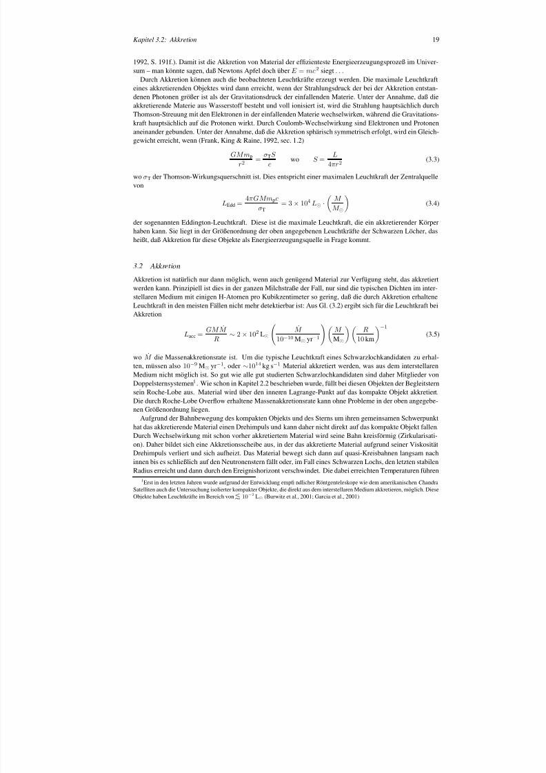
Durch Akkretion können auch die beobachteten Leuchtkräfte erzeugt werden. Die maximale Leuchtkeines akkretierenden Objektes wird dann erreicht, wenn der Strahlungsdruck der bei der Akkretion entdenen Photonen größer ist als der Gravitationsdruck der einfallenden Materie. Unter der Annahme, daakkretierende Materie aus Wasserstoff besteht und voll ionisiert ist, wird die Strahlung hauptsächlich dThomson-Streuung mit den Elektronen in der einfallenden Materie wechselwirken, während die Gravitatkraft hauptsächlich auf die Protonen wirkt. Durch Coulomb-Wechselwirkung sind Elektronen und Protaneinander gebunden. Unter der Annahme, daß die Akkretion sphärisch symmetrisch erfolgt, wird ein Ggewicht erreicht, wenn (Frank, King & Raine, 1992, sec. 1.2)
GMm p
r 2 = σTS
c wo S =
L4πr 2 (3.3)
wo σT der Thomson-Wirkungsquerschnitt ist. Dies entspricht einer maximalen Leuchtkraft der Zentralquvon
LEdd = 4πGMm pc
σT= 3 × 10⁴ L ·
M M
(3.4)
der sogenannten Eddington-Leuchtkraft. Diese ist die maximale Leuchtkraft, die ein akkretierender Köhaben kann. Sie liegt in der Größenordnung der oben angegebenen Leuchtkräfte der Schwarzen Löcherheißt, daß Akkretion für diese Objekte als Energieerzeugungsquelle in Frage kommt.
3.2 Akkretion
Akkretion ist natürlich nur dann möglich, wenn auch genügend Material zur Verfügung steht, das akkrwerden kann. Prinzipiell ist dies in der ganzen Milchstraße der Fall, nur sind die typischen Dichten im istellaren Medium mit einigen H-Atomen pro Kubikzentimeter so gering, daß die durch Akkretion erhaLeuchtkraft in den meisten Fällen nicht mehr detektierbar ist: Aus Gl. (3.2) ergibt sich für die LeuchtkraAkkretion
Lacc = GM M
R ∼ 2 × 10² L
M 10− 10 M yr− 1
M M
R10 km
− 1
(3.5)
wo M die Massenakkretionsrate ist. Um die typische Leuchtkraft eines Schwarzlochkandidaten zu erten, müssen also 10− 9 M yr− 1 , oder ∼1014 kg s− 1 Material akkretiert werden, was aus dem interstellarenMedium nicht möglich ist. So gut wie alle gut studierten Schwarzlochkandidaten sind daher MitgliedeDoppelsternsystemen1 . Wie schon in Kapitel 2.2 beschrieben wurde, füllt bei diesen Objekten der Begleitstesein Roche-Lobe aus. Material wird über den inneren Lagrange-Punkt auf das kompakte Objekt akkreDie durch Roche-Lobe Overow erhaltene Massenakkretionsrate kann ohne Probleme in der oben angegnen Größenordnung liegen.
Aufgrund der Bahnbewegung des kompakten Objekts und des Sterns um ihren gemeinsamen Schwerphat das akkretierende Material einen Drehimpuls und kann daher nicht direkt auf das kompakte Objekt fDurch Wechselwirkung mit schon vorher akkretiertem Material wird seine Bahn kreisförmig (Zirkularion). Daher bildet sich eine Akkretionsscheibe aus, in der das akkretierte Material aufgrund seiner ViskoDrehimpuls verliert und sich aufheizt. Das Material bewegt sich dann auf quasi-Kreisbahnen langsam innen bis es schließlich auf den Neutronenstern fällt oder, im Fall eines Schwarzen Lochs, den letzten staRadius erreicht und dann durch den Ereignishorizont verschwindet. Die dabei erreichten Temperaturen fü
1 Erst in den letzten Jahren wurde aufgrund der Entwicklung emp ndlicher Röntgenteleskope wie dem amerikanischen Chandra -Satelliten auch die Untersuchung isolierter kompakter Objekte, die direkt aus dem interstellaren Medium akkretieren, möglich. DieseObjekte haben Leuchtkräfte im Bereich von
10 − 2 L (Burwitz et al., 2001; Garcia et al., 2001).
8/12/2019 Schwarze LöCher Als Astronomische Objekte
http://slidepdf.com/reader/full/schwarze-lacher-als-astronomische-objekte 20/146
20 Kapitel 3: Röntgenstrahlung stellarer Schwarzer Löcher
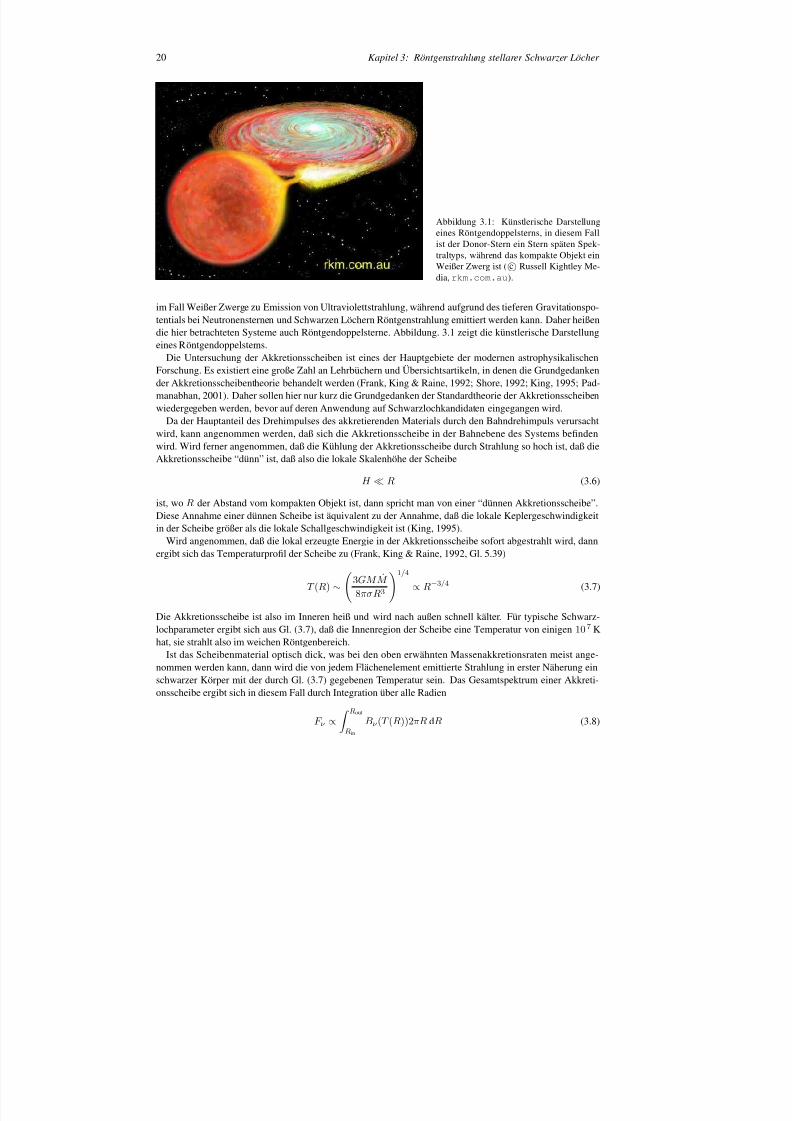
Abbildung 3.1: Künstlerische Darstellungeines Röntgendoppelsterns, in diesem Fallist der Donor-Stern ein Stern späten Spek-traltyps, während das kompakte Objekt einWeißer Zwerg ist ( c Russell Kightley Me-dia, rkm.com.au ).
im Fall Weißer Zwerge zu Emission von Ultraviolettstrahlung, während aufgrund des tieferen Gravitationspo-tentials bei Neutronensternen und Schwarzen Löchern Röntgenstrahlung emittiert werden kann. Daher heißendie hier betrachteten Systeme auch Röntgendoppelsterne. Abbildung. 3.1 zeigt die künstlerische Darstellungeines Röntgendoppelsterns.
Die Untersuchung der Akkretionsscheiben ist eines der Hauptgebiete der modernen astrophysikalischenForschung. Es existiert eine große Zahl an Lehrbüchern und Übersichtsartikeln, in denen die Grundgedankender Akkretionsscheibentheorie behandelt werden (Frank, King & Raine, 1992; Shore, 1992; King, 1995; Pad-manabhan, 2001). Daher sollen hier nur kurz die Grundgedanken der Standardtheorie der Akkretionsscheibenwiedergegeben werden, bevor auf deren Anwendung auf Schwarzlochkandidaten eingegangen wird.
Da der Hauptanteil des Drehimpulses des akkretierenden Materials durch den Bahndrehimpuls verursachtwird, kann angenommen werden, daß sich die Akkretionsscheibe in der Bahnebene des Systems bendenwird. Wird ferner angenommen, daß die Kühlung der Akkretionsscheibe durch Strahlung so hoch ist, daß dieAkkretionsscheibe “dünn” ist, daß also die lokale Skalenhöhe der Scheibe
H R (3.6)
ist, wo R der Abstand vom kompakten Objekt ist, dann spricht man von einer “dünnen Akkretionsscheibe”.Diese Annahme einer dünnen Scheibe ist äquivalent zu der Annahme, daß die lokale Keplergeschwindigkeitin der Scheibe größer als die lokale Schallgeschwindigkeit ist (King, 1995).
Wird angenommen, daß die lokal erzeugte Energie in der Akkretionsscheibe sofort abgestrahlt wird, dann
ergibt sich das Temperaturprol der Scheibe zu (Frank, King & Raine, 1992, Gl. 5.39)
T (R) ∼3GM M 8πσR 3
1 / 4
∝ R − 3 / 4 (3.7)
Die Akkretionsscheibe ist also im Inneren heiß und wird nach außen schnell kälter. Für typische Schwarz-lochparameter ergibt sich aus Gl. (3.7), daß die Innenregion der Scheibe eine Temperatur von einigen 107 Khat, sie strahlt also im weichen Röntgenbereich.
Ist das Scheibenmaterial optisch dick, was bei den oben erwähnten Massenakkretionsraten meist ange-nommen werden kann, dann wird die von jedem Flächenelement emittierte Strahlung in erster Näherung einschwarzer Körper mit der durch Gl. (3.7) gegebenen Temperatur sein. Das Gesamtspektrum einer Akkreti-
onsscheibe ergibt sich in diesem Fall durch Integration über alle Radien
F ν ∝ Rout
R in
Bν (T (R))2πR dR (3.8)
8/12/2019 Schwarze LöCher Als Astronomische Objekte
http://slidepdf.com/reader/full/schwarze-lacher-als-astronomische-objekte 21/146
Kapitel 3.3: Meßmethoden der Röntgenastronomie 21
10
l o g F
( b e l i e b i g e E i n h e i t e n )
1
ν
2
02
νlog(h /kT )out
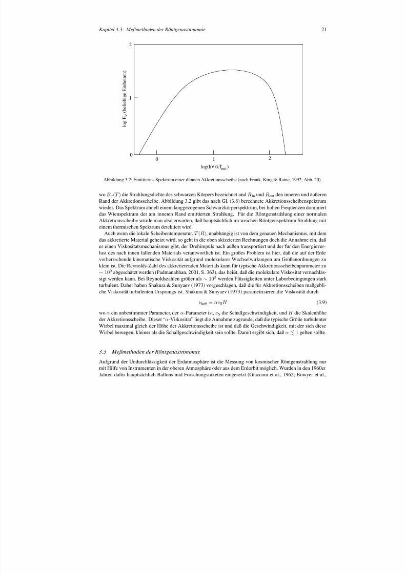
Abbildung 3.2: Emittiertes Spektrum einer dünnen Akkretionsscheibe (nach Frank, King & Raine, 1992, Abb. 20).
wo Bν (T ) die Strahlungsdichte des schwarzen Körpers bezeichnet und R in und Rout den inneren und äußerenRand der Akkretionsscheibe. Abbildung 3.2 gibt das nach Gl. (3.8) berechnete Akkretionsscheibenspekwieder. Das Spektrum ähnelt einem langgezogenen Schwarzkörperspektrum, bei hohen Frequenzen domdas Wienspektrum der am inneren Rand emittierten Strahlung. Für die Röntgenstrahlung einer normAkkretionsscheibe würde man also erwarten, daß hauptsächlich im weichen Röntgenspektrum Strahluneinem thermischen Spektrum detektiert wird.
Auch wenn die lokale Scheibentemperatur, T (R), unabhängig ist von dem genauen Mechanismus, mit demdas akkretierte Material geheizt wird, so geht in die oben skizzierten Rechnungen doch die Annahme eines einen Viskositätsmechanismus gibt, der Drehimpuls nach außen transportiert und der für den Energielust des nach innen fallenden Materials verantwortlich ist. Ein großes Problem ist hier, daß die auf der vorherrschende kinematische Viskosität aufgrund molekularer Wechselwirkungen um Größenordnungeklein ist. Die Reynolds-Zahl des akkretierenden Materials kann für typische Akkretionsscheibenparamet∼ 109 abgeschätzt werden (Padmanabhan, 2001, S. 363), das heißt, daß die molekulare Viskosität vernachsigt werden kann. Bei Reynoldszahlen größer als∼ 103 werden Flüssigkeiten unter Laborbedingungen starkturbulent. Daher haben Shakura & Sunyaev (1973) vorgeschlagen, daß die für Akkretionsscheiben maßgche Viskosität turbulenten Ursprungs ist. Shakura & Sunyaev (1973) parametrisieren die Viskosität durc
ν turb = αcSH (3.9)
wo α ein unbestimmter Parameter, der α-Parameter ist, cS die Schallgeschwindigkeit, und H die Skalenhöheder Akkretionsscheibe. Dieser “α-Viskosität” liegt die Annahme zugrunde, daß die typische Größe turbulenteWirbel maximal gleich der Höhe der Akkretionsscheibe ist und daß die Geschwindigkeit, mit der sich Wirbel bewegen, kleiner als die Schallgeschwindigkeit sein sollte. Damit ergibt sich, daß α 1 gelten sollte.
3.3 Meßmethoden der Röntgenastronomie
Aufgrund der Undurchlässigkeit der Erdatmosphäre ist die Messung von kosmischer Röntgenstrahlungmit Hilfe von Instrumenten in der oberen Atmosphäre oder aus dem Erdorbit möglich. Wurden in den 19Jahren dafür hauptsächlich Ballons und Forschungsraketen eingesetzt (Giacconi et al., 1962; Bowyer e
8/12/2019 Schwarze LöCher Als Astronomische Objekte
http://slidepdf.com/reader/full/schwarze-lacher-als-astronomische-objekte 22/146
22 Kapitel 3: Röntgenstrahlung stellarer Schwarzer Löcher
1965), die in den 1970er Jahren mit UHURU (Start Dezember 1970, Missionsende März 1973, eine Beschrei-bung des Satelliten ndet sich bei Giacconi et al., 1971), HEAO-1 (August 1977–Januar 1979; Peterson,1975; Rothschild et al., 1979), und dem Einstein -Satelliten (HEAO 2, November 1978–April 1981; Giacco-ni et al., 1979) durch Satelliten ergänzt wurden, werden seit den 1980er Jahren hauptsächlich Satelliten inder röntgenastronomischen Forschung eingesetzt und Ballons nur noch für Entwicklungszwecke oder spezi-elle Beobachtungsaufgaben genutzt. Der wissenschaftlich interessante Energiebereich ist dabei bei Energiengrößer als 0.1 keV, da unterhalb dieser Grenze die Absorption der Röntgenstrahlung im interstellaren Medi-um unserer Milchstraße die Beobachtungen sehr erschwert. Eine genaue Beschreibung der Modikation derRöntgenstrahlung im ISM ist in Anhang F dieser Arbeit zu nden (Wilms, Allen & McCray, 2000).
Für die Röntgenastronomie im Energiebereich10 keV sind hierbei der europäische EXOSAT (Mai 1983–April 1986; Turner, Smith & Zimmermann, 1981), das russisch-deutsche Mir-HEXE Experiment (Start imApril 1987, der Hauptteil der Mission endete 1990, die Instrumente waren vor dem Absturz der Mir imJanuar 2001 noch einsatzfähig; Reppin et al., 1983; Brinkman et al., 1983) und das amerikanische ComptonGamma-Ray Observatory (CGRO, April 1991–Juni 2000, siehe z.B. Schönfelder, 1995) zu nennen. Unterhalb∼10 keV ist neben Ginga (Februar 1987–November 1991; Turner et al., 1989) und ASCA (Februar 1993–März 2001; Makishima et al., 1996) insbesondere der deutsche Röntgensatellit ROSAT (Juni 1990–Februar1999; Briel & Pfeffermann, 1995; Zombeck et al., 1995) zu nennen, durch dessen “ROSAT All Sky Survey”die Zahl der bekannten Röntgenquellen von vorher knapp 1000 auf ∼150000 erhöht wurde. Ein sehr großerAnteil dieser Quellen sind Aktive Galaxien und enthalten damit Schwarze Löcher.
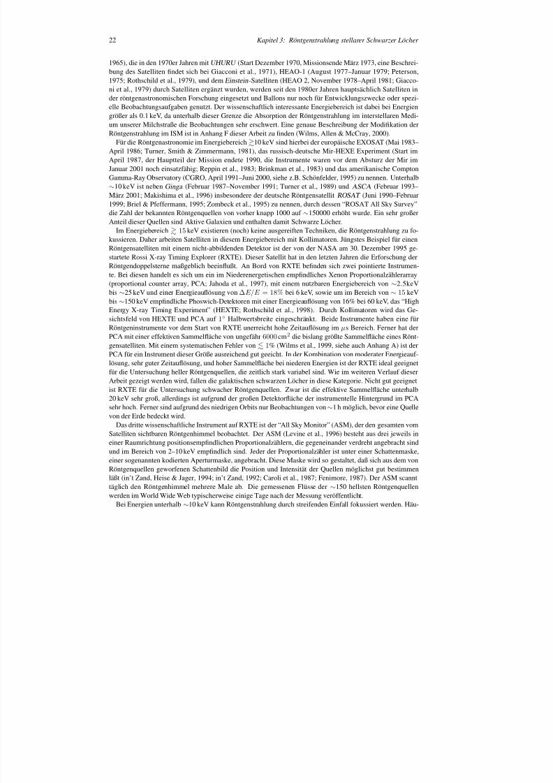
Im Energiebereich 15keV existieren (noch) keine ausgereiften Techniken, die Röntgenstrahlung zu fo-kussieren. Daher arbeiten Satelliten in diesem Energiebereich mit Kollimatoren. Jüngstes Beispiel für einenRöntgensatelliten mit einem nicht-abbildenden Detektor ist der von der NASA am 30. Dezember 1995 ge-startete Rossi X-ray Timing Explorer (RXTE). Dieser Satellit hat in den letzten Jahren die Erforschung derRöntgendoppelsterne maßgeblich beeinußt. An Bord von RXTE benden sich zwei pointierte Instrumen-te. Bei diesen handelt es sich um ein im Niederenergetischen empndliches Xenon Proportionalzählerarray(proportional counter array, PCA; Jahoda et al., 1997), mit einem nutzbaren Energiebereich von ∼2.5keVbis∼25 keV und einer Energieauösung von ∆ E/E = 18% bei 6 keV, sowie um im Bereich von∼ 15 keVbis∼150 keV empndliche Phoswich-Detektoren mit einer Energieauösung von 16% bei 60 keV, das “HighEnergy X-ray Timing Experiment” (HEXTE; Rothschild et al., 1998). Durch Kollimatoren wird das Ge-sichtsfeld von HEXTE und PCA auf 1 Halbwertsbreite eingeschränkt. Beide Instrumente haben eine fürRöntgeninstrumente vor dem Start von RXTE unerreicht hohe Zeitauösung im µs Bereich. Ferner hat derPCA mit einer effektiven Sammeläche von ungefähr 6000cm2 die bislang größte Sammeläche eines Rönt-gensatelliten. Mit einem systematischen Fehler von1% (Wilms et al., 1999, siehe auch Anhang A) ist derPCA für ein Instrument dieser Größe ausreichend gut geeicht. In der Kombination von moderater Energieauf-lösung, sehr guter Zeitauösung, und hoher Sammeläche bei niederen Energien ist der RXTE ideal geeignetfür die Untersuchung heller Röntgenquellen, die zeitlich stark variabel sind. Wie im weiteren Verlauf dieserArbeit gezeigt werden wird, fallen die galaktischen schwarzen Löcher in diese Kategorie. Nicht gut geeignetist RXTE für die Untersuchung schwacher Röntgenquellen. Zwar ist die effektive Sammeläche unterhalb20 keV sehr groß, allerdings ist aufgrund der großen Detektoräche der instrumentelle Hintergrund im PCAsehr hoch. Ferner sind aufgrund des niedrigen Orbits nur Beobachtungen von∼1 h möglich, bevor eine Quellevon der Erde bedeckt wird.
Das dritte wissenschaftliche Instrument auf RXTE ist der “All Sky Monitor” (ASM), der den gesamten vomSatelliten sichtbaren Röntgenhimmel beobachtet. Der ASM (Levine et al., 1996) besteht aus drei jeweils ineiner Raumrichtung positionsempndlichen Proportionalzählern, die gegeneinander verdreht angebracht sindund im Bereich von 2–10 keV empndlich sind. Jeder der Proportionalzähler ist unter einer Schattenmaske,einer sogenannten kodierten Aperturmaske, angebracht. Diese Maske wird so gestaltet, daß sich aus dem vonRöntgenquellen geworfenen Schattenbild die Position und Intensität der Quellen möglichst gut bestimmenläßt (in’t Zand, Heise & Jager, 1994; in’t Zand, 1992; Caroli et al., 1987; Fenimore, 1987). Der ASM scannttäglich den Röntgenhimmel mehrere Male ab. Die gemessenen Flüsse der ∼150 hellsten Röntgenquellenwerden im World Wide Web typischerweise einige Tage nach der Messung veröffentlicht.
Bei Energien unterhalb∼10 keV kann Röntgenstrahlung durch streifenden Einfall fokussiert werden. Häu-
8/12/2019 Schwarze LöCher Als Astronomische Objekte
http://slidepdf.com/reader/full/schwarze-lacher-als-astronomische-objekte 23/146
Kapitel 3.4: Physik galaktischer Schwarzer Löcher 23
g ist hier die Kombination eines Paraboloiden und eines Hyperboloiden, in Form eines sogenannten “WTeleskops”. Prominentestes Beispiel solcher Teleskope war der oben angesprochene ROSAT. Hier wurdpositionsempndlicher Proportionalzähler in der Brennebene des Wolter-Teleskops als Röntgendetektorwendet wurde, so daß das Instrument auch eine moderate Energieauösung besaß.
Mit der Entwicklung energiedispersiver “Charge coupled devices” (CCDs) wurde in der neuesten Genon astronomischer Röntgendetektoren eine wesentliche Steigerung der Energieauösung ermöglicht. Aufeuropäischen XMM-Newton Satelliten, der am 10. Dezember 1999 gestartet wurde, hat die europäische Rgenastronomie ein neues Großinstrument bekommen, das in den nächsten 10 Jahren noch viele Entdeckuverspricht. XMM-Newton hat drei parallel ausgerichtete Wolter-Teleskope mit einer räumlichen Auövon 6 FWHM. In der Fokalebene dieser Teleskope sitzen drei Detektorsysteme, die alle simultan Daaufnehmen. Hinter zwei der drei Teleskope ist zum einen ein Röntgen-Gitterspektrometer, das “ReeGrating Spectrometer” (RGS), installiert, das eine hohe Energieauösung (E/ ∆ E = 200 . . . 800) im Bereichvon 0.35 bis 2.5 keV besitzt (den Herder et al., 2001), zum anderen benden sich in der nullten Orddes RGS röntgenempndliche MOS-CCDs (Turner et al., 2001). In der Fokalebene des dritten Wolterskops bendet sich als Einzelinstrument die vom Max-Planck-Institut für Extraterrestrische Physik (MPGarching bei München und in Tübingen entwickelte pn-CCD (Strüder et al., 2001). Sowohl die MOSauch die pn-Kameras wurden im Rahmen des “European Photon Imaging Camera” (EPIC) Konsortiumsworfen und werden daher als EPIC-MOS und EPIC-pn Kamera bezeichnet. Mit einer EnergieauösungE/ ∆ E = 20 . . . 50 haben die EPIC Kameras eine wesentlich höhere Energieauösung als Proportionalzäler. Der nutzbare Energiebereich der EPIC-pn geht dabei von∼0.2keV bis zu∼10 keV, d.h. er überstreichtden Bereich des Röntgenspektrums, in dem Emissionslinien der astrophysikalisch relevanten Elementeobachtbar sind. Die gesamte Sammeläche der MOS- und pn-Kamera beträgt ∼ 3000cm2 , d.h. sie liegtin vergleichbarer Größenordnung mit RXTE. Da es sich bei den EPIC-Kameras um abbildende Instrumhandelt, ist ihr Volumen wesentlich kleiner als der der Proportionalzähler und damit ist auch der instrumtelle Hintergrund fast vernachlässigbar. Damit können mit XMM-Newton auch Quellen niedriger Intenin vernünftiger Zeit mit einem guten Signal zu Rausch-Verhältnis spektroskopiert werden. Im Rahmen dArbeit sind als schwache Quellen die Aktiven Galaxien zu nennen, die daher auch mit XMM untersuchtden (Benlloch et al., 2001; Wilms et al., 2001b, siehe auch Kapitel 4). Diese Untersuchungen protierendavon, daß sich XMM-Newton in einem exzentrischen 48 h Orbit bendet und daher lange Beobachtuohne störende Bedeckungen der Quellen durch die Erde möglich sind.
Komplementär zu XMM-Newton sind die Instrumente an Bord des amerikanischen Chandra -Satelliten, deram 23. Juli 1999 gestartet worden ist (Weisskopf et al., 2002). Hauptmerkmal von Chandra ist seine extremgute Röntgenoptik, die es mit< 1 FWHM Auösung erlaubt, im Röntgenbereich Bilder mit einer Qualität zuerstellen, die sonst nur im Optischen und Radiobereich möglich war. Dazu stehen als Instrumente wahlwdas ACIS, ein MOS-CCD Detektor, oder die “High Resolution Camera” (HRC), aus Mikrokanalplatten bhende Detektoren ohne Energieauösung, zur Verfügung. Mit Hilfe von Röntgen-Gitterspektrometern auch mit Chandra hochaufgelöste Spektroskopie (maximal E/ ∆ E = 2000) betrieben werden. Aufgrundvon Strahlenschäden an den ACIS-Detektoren ist deren ursprünglich mit den EPIC Detektoren auf XMNewton vergleichbare Energieauösung stark reduziert worden. Die lichtsammelnde Fläche von Chandra istmit 800cm2 bei 0.25 keV kleiner als bei XMM. Wie auch XMM bendet sich Chandra in einem Orbit langer Umlaufzeit (64 h).
3.4 Physik galaktischer Schwarzer Löcher
3.4.1 Breitbandspektren im Röntgenbereich
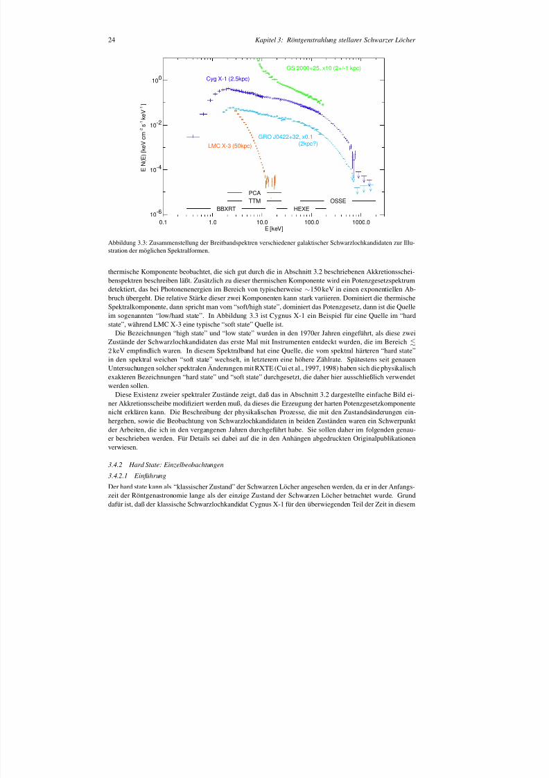
Zur Untersuchung der Physik galaktischer Schwarzer Löcher werden sowohl spektrale Informationen alsInformationen über deren Zeitverhalten auf allen Zeitskalen vom Millisekundenbereich bis hin zur Varlität über Jahrzehnte hinweg verwendet. Abbildung 3.3 gibt eine Zusammenstellung verschiedener typiSchwarzlochspektren. Sie zeigt, daß die Breitbandspektren im Röntgenbereich als die Summe zweier speler Komponenten dargestellt werden können: Bei niedrigen Energien, unterhalb ungefähr ∼2 keV, wird eine
8/12/2019 Schwarze LöCher Als Astronomische Objekte
http://slidepdf.com/reader/full/schwarze-lacher-als-astronomische-objekte 24/146
24 Kapitel 3: Röntgenstrahlung stellarer Schwarzer Löcher
0.1 1.0 10.0 100.0 1000.0E [keV]
10 -6
10 -4
10 -2
10 0
E N ( E ) [ k e
V c m
- 2 s - 1
k e
V - 1 ]
BBXRTTTM
HEXEOSSE
GS 2000+25, x10 (2+/-1 kpc)
PCA
Cyg X-1 (2.5kpc)
LMC X-3 (50kpc)
GRO J0422+32, x0.1(2kpc?)
Abbildung 3.3: Zusammenstellung der Breitbandspektren verschiedener galaktischer Schwarzlochkandidaten zur Illu-stration der möglichen Spektralformen.
thermische Komponente beobachtet, die sich gut durch die in Abschnitt 3.2 beschriebenen Akkretionsschei-benspektren beschreiben läßt. Zusätzlich zu dieser thermischen Komponente wird ein Potenzgesetzspektrumdetektiert, das bei Photonenenergien im Bereich von typischerweise ∼150 keV in einen exponentiellen Ab-bruch übergeht. Die relative Stärke dieser zwei Komponenten kann stark variieren. Dominiert die thermischeSpektralkomponente, dann spricht man vom “soft/high state”, dominiert das Potenzgesetz, dann ist die Quelleim sogenannten “low/hard state”. In Abbildung 3.3 ist Cygnus X-1 ein Beispiel für eine Quelle im “hardstate”, während LMC X-3 eine typische “soft state” Quelle ist.
Die Bezeichnungen “high state” und “low state” wurden in den 1970er Jahren eingeführt, als diese zweiZustände der Schwarzlochkandidaten das erste Mal mit Instrumenten entdeckt wurden, die im Bereich 2 keV empndlich waren. In diesem Spektralband hat eine Quelle, die vom spektral härteren “hard state”in den spektral weichen “soft state” wechselt, in letzterem eine höhere Zählrate. Spätestens seit genauenUntersuchungen solcher spektralen Änderungen mitRXTE (Cui et al., 1997, 1998) haben sich diephysikalischexakteren Bezeichnungen “hard state” und “soft state” durchgesetzt, die daher hier ausschließlich verwendetwerden sollen.
Diese Existenz zweier spektraler Zustände zeigt, daß das in Abschnitt 3.2 dargestellte einfache Bild ei-ner Akkretionsscheibe modiziert werden muß, da dieses die Erzeugung der harten Potenzgesetzkomponentenicht erklären kann. Die Beschreibung der physikalischen Prozesse, die mit den Zustandsänderungen ein-hergehen, sowie die Beobachtung von Schwarzlochkandidaten in beiden Zuständen waren ein Schwerpunktder Arbeiten, die ich in den vergangenen Jahren durchgeführt habe. Sie sollen daher im folgenden genau-er beschrieben werden. Für Details sei dabei auf die in den Anhängen abgedruckten Originalpublikationenverwiesen.
3.4.2 Hard State: Einzelbeobachtungen
3.4.2.1 Einführung
Der hard state kann als “klassischer Zustand” der Schwarzen Löcher angesehen werden, da er in der Anfangs-zeit der Röntgenastronomie lange als der einzige Zustand der Schwarzen Löcher betrachtet wurde. Grunddafür ist, daß der klassische Schwarzlochkandidat Cygnus X-1 für den überwiegenden Teil der Zeit in diesem
8/12/2019 Schwarze LöCher Als Astronomische Objekte
http://slidepdf.com/reader/full/schwarze-lacher-als-astronomische-objekte 25/146
Kapitel 3.4: Physik galaktischer Schwarzer Löcher 25
Zustand beobachtet wird (Liang & Nolan, 1984; Oda, 1977). Wie oben schon angesprochen wurde, ist dhard state beobachtete Potenzgesetzspektrum natürlich mit einem thermischen Akkretionsscheibenspeknicht erklärbar. Während frühe Arbeiten das beobachtete Röntgenspektrum noch durch thermische Brstrahlung zu erklären versuchten, konnten Sunyaev & Trümper (1979) überzeugend zeigen, daß das Spekdurch thermische Comptonisierug zustande kommt.
Die grundlegende Annahme dieses Modells ist, daß niederenergetische Photonen aus der Akkretionsschbeim Durchgang durch ein Elektronenplasma aufgrund von inversen Comptonstößen an hochenergetisElektronen von diesen Energie gewinnen. Der mittlere relative Energiegewinn eines Photons der Energ E pro Compton-Stoß an maxwellverteilten Elektronen der Temperatur T e ist (Rybicki & Lightman, 1979)
∆ E E
= 4kT e − E
m ec2 (3.10)
so daß ein Energiegewinn immer dann zu erwarten ist, wenn die Photonenenergie kleiner als die Temratur des Elektronenplasmas ist. Das Comptonisierungsspektrum ist ein Potenzgesetz mit einem durchMaxwell-Verteilung bedingten exponentiellen Abbruch. In frühen Modellen (z.B. Haardt & Maraschi, 1und die darin angegebene Literatur) wurde allgemein angenommen, daß das heiße Elektronenplasma“sandwichförmig” um die Akkretionsscheibe herum bendet. In Analogie an Modelle der Sonnenko(z.B. Burm, 1986), bei der ebenfalls ein heißes Gas nahe der kühlen Sonnenoberäche gefunden wird,das Elektronenplasma auch die “Akkretionsscheibenkorona” genannt. Mögliche physikalische Ursachedie Bildung der Korona sind wahrscheinlich magnetohydrodynamischen Ursprungs, beispielsweise durcBalbus-Hawley-Chandrasekhar Instabilität, bei der aufgrund der differentiellen Rotation der Akkretionssbe der magnetische Druck im Inneren der Akkretionsscheibe so stark ansteigt, daß magnetische Flußschläin der Scheibe aufsteigen. Auf der Scheibenoberäche kann dann durch magnetische Rekonnexion Enfreigesetzt werden, so daß das Material der Oberäche stark geheizt wird (Hawley & Balbus, 1991; BalbHawley, 1991; Stone et al., 1996; Hawley & Stone, 1998; Miller & Stone, 2000).
Die genaue analytische Berechnung des Comptonisierungsspektrums ist kompliziert, da dieses im allgenen von Annahmen über die Quellgeometrie, wie zum Beispiel der relativen Lage der Akkretionsscheikorona und der Quelle der weichen Photonen oder der Elektronendichteverteilung innerhalb der Akkretscheibenkorona abhängt. Die Rechnung basiert auf der Lösung der Kompaneets-Gleichung, einer quamechanisch modizierten Form der Fokker-Planck-Gleichung für den Photonentransport. HerleitungenFokker-Planck-Gleichung nden sich zum Beispiel in meiner Dissertation (Wilms, 1998) oder bei Ryb& Lightman (1979). Analytische Lösungen der Kompaneets-Gleichung sind unter anderem von SunyaTitarchuk (1980), Sunyaev & Titarchuk (1985), Poutanen (1994), Titarchuk (1994), Titarchuk & Lyuba(1995) und Hua & Titarchuk (1995) gegeben worden. Ein Problem all dieser Lösungen ist, daß sie nur füeinfache Quellgeometrien anwendbar sind. Der Vergleich dieser analytischen Comptonisierungsspektrenden Beobachtungen zeigt, daß die Spektren im hard state durch Comptonisierung erklärbar sind. Allerdsind vielfach die dabei erhaltenen Spektralparameter nicht selbstkonsistent. Für galaktische Schwarze Lndet sich beispielsweise häug, daß die beobachteten Spektren durch heiße (kT e ∼ 100keV) Akkretions-scheibenkoronen hoher optischer Tiefe, τ e 1, beschrieben werden. Dies ist aber physikalisch nicht erlaubt:hohe optische Tiefen führen dazu, daß die Comptonkorona sehr efzient von der eingestrahlten niederentischen Strahlung gekühlt wird (Haardt & Maraschi, 1993; Haardt, Maraschi & Ghisellini, 1994; Dove, W& Begelman, 1997; Dove et al., 1997).
Weitere Selbstkonsistenzprobleme der einfachen analytischen Comptonisierungsmodelle ergeben sichaus, daß ein Teil der von der Akkretionsscheibenkorona emittierten Strahlung wieder auf die Akkretionssbe eingestrahlt wird. Ein Teil dieser Strahlung wird durch Thomson-Streuung in der Akkretionsscheibektiert und führt zur Emission eines sogenannten “Compton-Reektionsbuckels” (Lightman & White, 1Ein weiterer Teil der eingestrahlten Strahlung wird in der Akkretionsscheibe absorbiert und dann in Form
Fluoreszenzstrahlung re-emittiert. Als stärkste Fluoreszenzlinie wird hier die Fe Kα Linie bei 6.4keV emit-tiert, die in den Röntgenspektren auch beobachtet wird (siehe auch Kapitel 4.1). Je nach Geometrie weschließlich bis zu 30% der eingestrahlten Energie in der Akkretionsscheibe selbst absorbiert, thermalisierals weiche Röntgenstrahlung wieder reemittiert. Es existiert daher eine starke Wechselwirkung zwischen
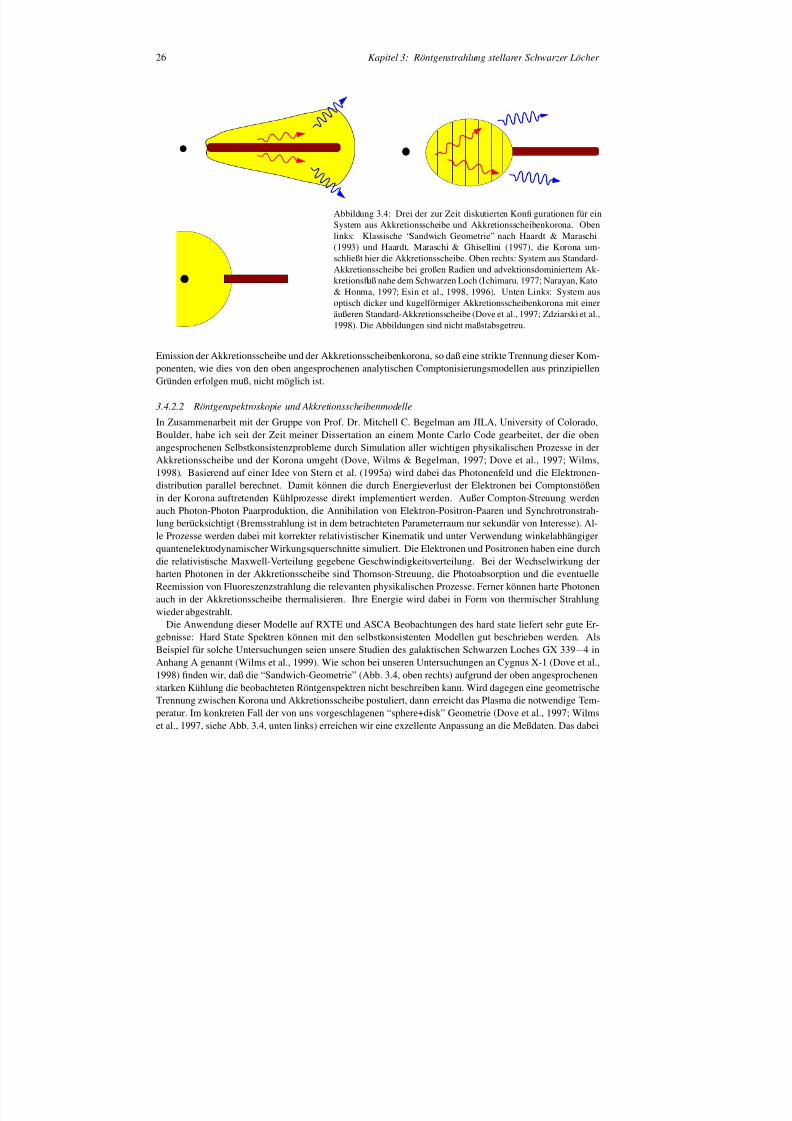
8/12/2019 Schwarze LöCher Als Astronomische Objekte
http://slidepdf.com/reader/full/schwarze-lacher-als-astronomische-objekte 26/146
26 Kapitel 3: Röntgenstrahlung stellarer Schwarzer Löcher
Abbildung 3.4: Drei der zur Zeit diskutierten Kon gurationen für einSystem aus Akkretionsscheibe und Akkretionsscheibenkorona. Obenlinks: Klassische “Sandwich Geometrie” nach Haardt & Maraschi(1993) und Haardt, Maraschi & Ghisellini (1997), die Korona um-schließt hier die Akkretionsscheibe. Oben rechts: System aus Standard-Akkretionsscheibe bei großen Radien und advektionsdominiertem Ak-kretionsuß nahe dem Schwarzen Loch (Ichimaru, 1977; Narayan, Kato& Honma, 1997; Esin et al., 1998, 1996). Unten Links: System ausoptisch dicker und kugelförmiger Akkretionsscheibenkorona mit eineräußeren Standard-Akkretionsscheibe (Dove et al., 1997; Zdziarski et al.,1998). Die Abbildungen sind nicht maßstabsgetreu.
Emission der Akkretionsscheibe und der Akkretionsscheibenkorona, so daß eine strikte Trennung dieser Kom-ponenten, wie dies von den oben angesprochenen analytischen Comptonisierungsmodellen aus prinzipiellenGründen erfolgen muß, nicht möglich ist.
3.4.2.2 Röntgenspektroskopie und Akkretionsscheibenmodelle
In Zusammenarbeit mit der Gruppe von Prof. Dr. Mitchell C. Begelman am JILA, University of Colorado,Boulder, habe ich seit der Zeit meiner Dissertation an einem Monte Carlo Code gearbeitet, der die obenangesprochenen Selbstkonsistenzprobleme durch Simulation aller wichtigen physikalischen Prozesse in derAkkretionsscheibe und der Korona umgeht (Dove, Wilms & Begelman, 1997; Dove et al., 1997; Wilms,1998). Basierend auf einer Idee von Stern et al. (1995a) wird dabei das Photonenfeld und die Elektronen-distribution parallel berechnet. Damit können die durch Energieverlust der Elektronen bei Comptonstößenin der Korona auftretenden Kühlprozesse direkt implementiert werden. Außer Compton-Streuung werdenauch Photon-Photon Paarproduktion, die Annihilation von Elektron-Positron-Paaren und Synchrotronstrah-lung berücksichtigt (Bremsstrahlung ist in dem betrachteten Parameterraum nur sekundär von Interesse). Al-le Prozesse werden dabei mit korrekter relativistischer Kinematik und unter Verwendung winkelabhängigerquantenelektrodynamischer Wirkungsquerschnitte simuliert. Die Elektronen und Positronen haben eine durchdie relativistische Maxwell-Verteilung gegebene Geschwindigkeitsverteilung. Bei der Wechselwirkung derharten Photonen in der Akkretionsscheibe sind Thomson-Streuung, die Photoabsorption und die eventuelleReemission von Fluoreszenzstrahlung die relevanten physikalischen Prozesse. Ferner können harte Photonenauch in der Akkretionsscheibe thermalisieren. Ihre Energie wird dabei in Form von thermischer Strahlungwieder abgestrahlt.
Die Anwendung dieser Modelle auf RXTE und ASCA Beobachtungen des hard state liefert sehr gute Er-gebnisse: Hard State Spektren können mit den selbstkonsistenten Modellen gut beschrieben werden. AlsBeispiel für solche Untersuchungen seien unsere Studien des galaktischen Schwarzen Loches GX 339− 4 inAnhang A genannt (Wilms et al., 1999). Wie schon bei unseren Untersuchungen an Cygnus X-1 (Dove et al.,1998) nden wir, daß die “Sandwich-Geometrie” (Abb. 3.4, oben rechts) aufgrund der oben angesprochenen
starken Kühlung die beobachteten Röntgenspektren nicht beschreiben kann. Wird dagegen eine geometrischeTrennung zwischen Korona und Akkretionsscheibe postuliert, dann erreicht das Plasma die notwendige Tem-peratur. Im konkreten Fall der von uns vorgeschlagenen “sphere+disk” Geometrie (Dove et al., 1997; Wilmset al., 1997, siehe Abb. 3.4, unten links) erreichen wir eine exzellente Anpassung an die Meßdaten. Das dabei
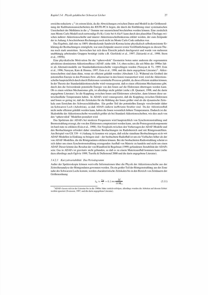
8/12/2019 Schwarze LöCher Als Astronomische Objekte
http://slidepdf.com/reader/full/schwarze-lacher-als-astronomische-objekte 27/146
Kapitel 3.4: Physik galaktischer Schwarzer Löcher 27
erreichte reduzierte χ 2 ist extrem klein, da die Abweichungen zwischen Daten und Modell in der Größenornung der Kalibrationsunsicherheiten des RXTE-PCA liegen, die durch die Einführung einer systematisUnsicherheit der Meßdaten in die χ 2 -Summe nur unzureichend beschrieben werden können. Eine zusätzlichzum Monte Carlo Modell noch notwendige Fe Kα Linie bei 6.4keV kann durch den plausiblen Überlapp zwi-schen äußerer Akkretionsscheibe und innerer Akkretionsscheibenkorona erklärt werden, der zum Zeitpder in Anhang A beschriebenen Rechnungen noch nicht im Monte Carlo Code enthalten war.
Das Ergebnis, daß eine zu 100% überdeckende Sandwich-Korona keine physikalisch selbstkonsistentklärung der Beobachtungen ermöglicht, war zum Zeitpunkt unserer ersten Veröffentlichungen zu diesemma noch stark umstritten. Inzwischen hat sich diese Einsicht jedoch durchgesetzt und wurde von mehunabhängig arbeitenden Gruppen bestätigt (siehe z.B. Gierlinski et al., 1997; Zdziarski et al., 1998; Sternet al., 1995b).
Eine physikalische Motivation für die “sphere+disk” Geometrie boten unter anderem die sogenanadvektions-dominierten Akkretionsüsse (ADAF; siehe Abb. 3.4, oben rechts), die seit Mitte der 1990erre als Alternativmodelle zur Standardakkretionsscheibe vorgeschlagen wurden (Narayan & Yi, 1995; et al., 1996; Narayan, Kato & Honma, 1997; Esin et al., 1998, und die darin angegebene Literatur)2 . Akkre-tionsscheiben sind dann dünn, wenn sie efzient gekühlt werden (Abschnitt 3.2). Während ein Großtepotentiellen Energie in den Protonen (bzw. allgemeiner in den Ionen) transportiert wird, wird die Akkretscheibe hauptsächlich durch durch Elektronen vermittelte Prozesse gekühlt, da diese efzient strahlen köIn der Theorie der Standardakkretionsscheibe wird vorausgesetzt, daß es einen efzienten Mechanismusdurch den die freiwerdende potentielle Energie von den Ionen auf die Elektronen übertragen werden kOb es einen solchen Mechanismus gibt, ist allerdings nicht geklärt (siehe z.B. Quataert, 1998, und die angegebene Literatur). Ist die Kopplung zwischen Ionen und Elektronen schwächer, dann können dieseterschiedliche Temperaturen haben. In ADAFs wird vorausgesetzt, daß die Kopplung zwischen Elektrund Ionen so gering ist, daß die Zeitskalen für die Kühlung der Ionen größer sind als die dynamische Zkala zum Erreichen des Schwarzschildradius. Ein großer Teil der potentiellen Energie verschwindet dim Schwarzen Loch (Advektion), so daß ADAFs äußerst inefziente Strahler sind. Da der Akkretionnicht mehr efzient gekühlt werden kann, haben die Ionen wesentlich höhere Temperaturen. Dadurch isSkalenhöhe der Akkretionsscheibe wesentlich größer als bei Standard-Akkretionsscheiben, wie dies auchden “sphere+disk” Modellen postuliert wird.
Das Spektrum der ADAFs bei niederen Frequenzen wird hauptsächlich von Synchrotronstrahlung Bremsstrahlung erzeugt, die von den Elektronen comptonisiert werden kann, um die Potenzgesetzkompoim hard state zu erklären (Esin et al., 1998). Ein Vergleich zwischen den Vorhersagen der ADAF-Modellden Beobachtungen erfordert daher simultane Beobachtungen im Radiobereich und mit RöntgensatellAm Beispiel von GX 339− 4 (Anhang A) konnten wir zeigen, daß solche simultane Beobachtungen nicht mitADAF-Modellen in Einklang zu bringen sind – der beobachtete Radiouß ist um ein Vielfaches höher avon ADAF-Modellen, die die Röntgendaten erklären können. Bei der beobachteten Radiostrahlung schesich daher um einen Synchrotronstrahlung erzeugenden Ausuß von Materie zu handeln und nicht um ADAF. Dieser könnte das Resultat der von Blandford & Begelman (1999) gefundenen Instabilität der ADsein: Gas in ADAFs ist gravitativ nicht gebunden, so daß es zu einem Materieausuß kommen kann (dazu allerdings auch Ogilvie 1999, Turolla & Dullemond 2000 und die darin angegebene Literatur).
3.4.2.3 Kurzzeitvariabilität: Das Periodogramm
Außer der Spektroskopie können wertvolle Informationen über die Physik der Akkretionsscheibe auZeitreihenanalyse der Röntgendaten gewonnen werden. Da ein großer Teil der Röntgenstrahlung aus der nahe des Schwarzen Lochs kommt, werden charakteristische Zeitskalen bis in den Bereich von ZeitdauerGrößenordnung
t lc ≈ rst
c = 0 .1 ms M 10 M (3.11)
2 ADAFs lassen sich in der Literatur bis in die 1960er Jahre zurückverfolgen, allerdings wurden die Arbeiten auf diesem Gebietweithin ignoriert (Svensson, 1997, und die darin angegebene Literatur).
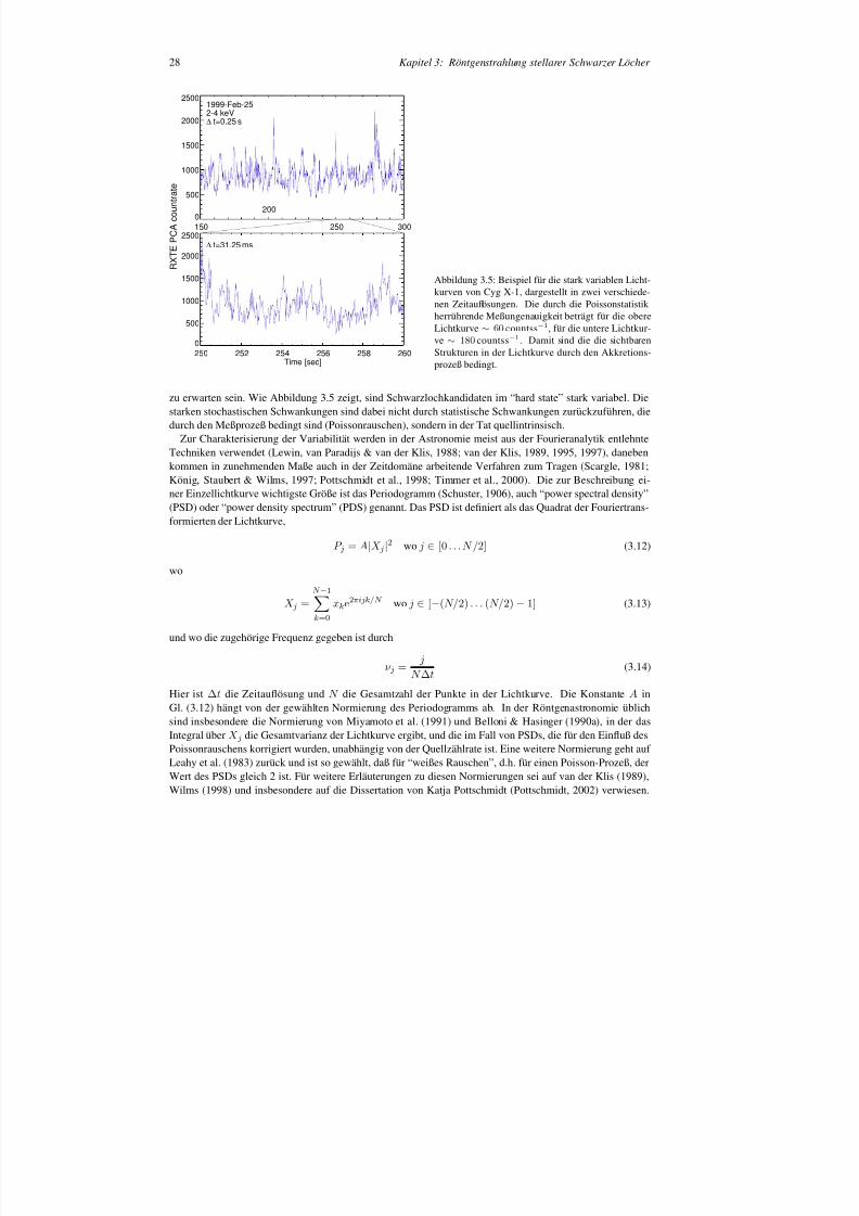
8/12/2019 Schwarze LöCher Als Astronomische Objekte
http://slidepdf.com/reader/full/schwarze-lacher-als-astronomische-objekte 28/146
28 Kapitel 3: Röntgenstrahlung stellarer Schwarzer Löcher
150 250 3000
500
1000
1500
2000
2500
200
250 252 254 256 258 260Time [sec]
0
500
1000
1500
2000
2500
R X T E P C A c o u n
t r a t e
1999-Feb-252-4 keV∆ t=0.25 s
∆ t=31.25 ms
Abbildung 3.5: Beispiel für die stark variablen Licht-kurven von Cyg X-1, dargestellt in zwei verschiede-nen Zeitauösungen. Die durch die Poissonstatistikherrührende Meßungenauigkeit beträgt für die obereLichtkurve∼ 60 countss− 1 , für die untere Lichtkur-ve ∼ 180 countss− 1 . Damit sind die die sichtbarenStrukturen in der Lichtkurve durch den Akkretions-prozeß bedingt.
zu erwarten sein. Wie Abbildung 3.5 zeigt, sind Schwarzlochkandidaten im “hard state” stark variabel. Diestarken stochastischen Schwankungen sind dabei nicht durch statistische Schwankungen zurückzuführen, diedurch den Meßprozeß bedingt sind (Poissonrauschen), sondern in der Tat quellintrinsisch.
Zur Charakterisierung der Variabilität werden in der Astronomie meist aus der Fourieranalytik entlehnteTechniken verwendet (Lewin, van Paradijs & van der Klis, 1988; van der Klis, 1989, 1995, 1997), danebenkommen in zunehmenden Maße auch in der Zeitdomäne arbeitende Verfahren zum Tragen (Scargle, 1981;König, Staubert & Wilms, 1997; Pottschmidt et al., 1998; Timmer et al., 2000). Die zur Beschreibung ei-ner Einzellichtkurve wichtigste Größe ist das Periodogramm (Schuster, 1906), auch “power spectral density”(PSD) oder “power density spectrum” (PDS) genannt. Das PSD ist deniert als das Quadrat der Fouriertrans-formierten der Lichtkurve,
P j = A|X j |2 wo j ∈[0. . . N / 2] (3.12)
wo
X j =N − 1
k=0xke2 πijk/N wo j ∈[− (N/ 2) . . . (N/ 2) − 1] (3.13)
und wo die zugehörige Frequenz gegeben ist durch
ν j = jN ∆ t
(3.14)
Hier ist ∆ t die Zeitauösung und N die Gesamtzahl der Punkte in der Lichtkurve. Die Konstante A inGl. (3.12) hängt von der gewählten Normierung des Periodogramms ab. In der Röntgenastronomie üblichsind insbesondere die Normierung von Miyamoto et al. (1991) und Belloni & Hasinger (1990a), in der dasIntegral über X j die Gesamtvarianz der Lichtkurve ergibt, und die im Fall von PSDs, die für den Einuß des
Poissonrauschens korrigiert wurden, unabhängig von der Quellzählrate ist. Eine weitere Normierung geht auf Leahy et al. (1983) zurück und ist so gewählt, daß für “weißes Rauschen”, d.h. für einen Poisson-Prozeß, derWert des PSDs gleich 2 ist. Für weitere Erläuterungen zu diesen Normierungen sei auf van der Klis (1989),Wilms (1998) und insbesondere auf die Dissertation von Katja Pottschmidt (Pottschmidt, 2002) verwiesen.
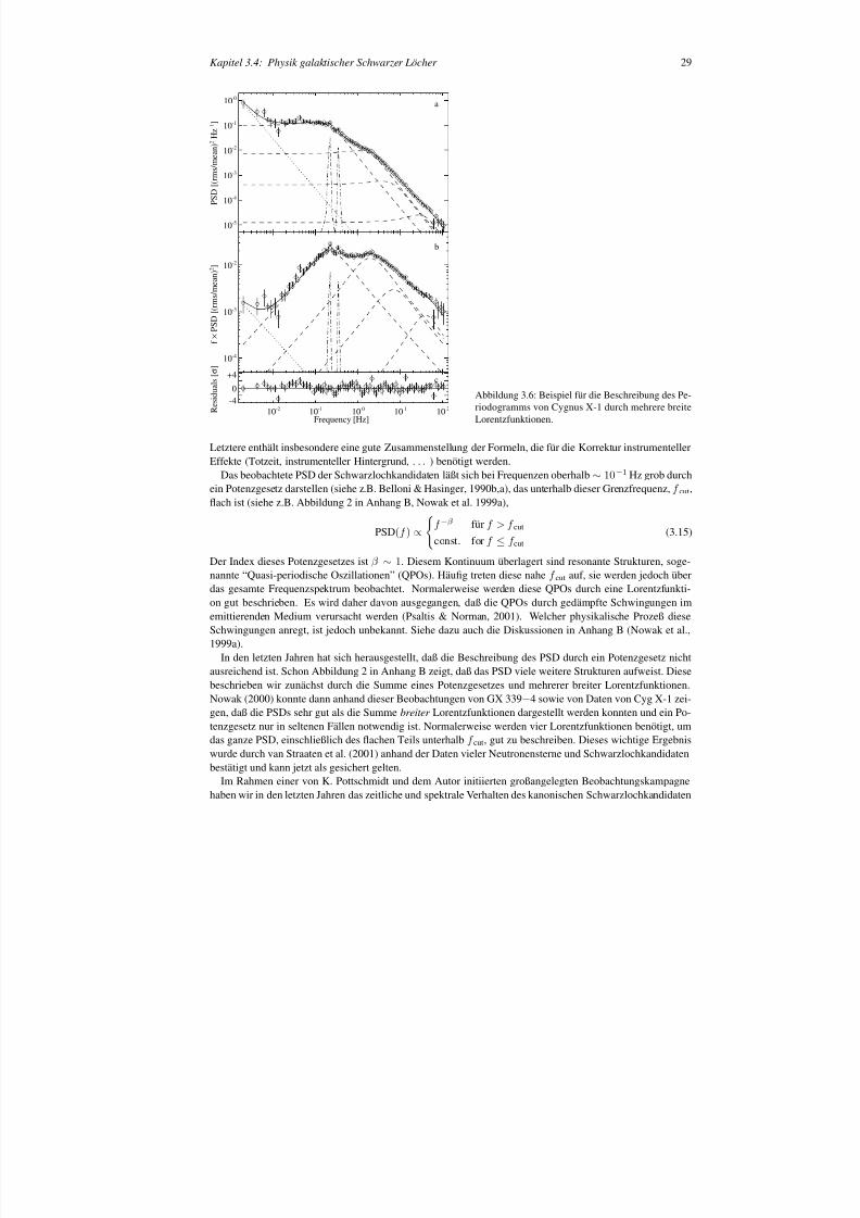
8/12/2019 Schwarze LöCher Als Astronomische Objekte
http://slidepdf.com/reader/full/schwarze-lacher-als-astronomische-objekte 29/146
Kapitel 3.4: Physik galaktischer Schwarzer Löcher 29
10 -5
10 -4
10 -3
10 -2
10 -1
10 0
P S D [ ( r m s / m e a n
) 2 H
z - 1 ]
a
10 -4
10 -3
10 -2
f × P S D [ ( r m s / m e a n ) 2
]
b
10 -2 10 -1 10 0 10 1 10 2-40
+4
R e s i d u a l s
[ σ ]
Frequency [Hz]
c
Abbildung 3.6: Beispiel für die Beschreibung des Pe-riodogramms von Cygnus X-1 durch mehrere breiteLorentzfunktionen.
Letztere enthält insbesondere eine gute Zusammenstellung der Formeln, die für die Korrektur instrumenEffekte (Totzeit, instrumenteller Hintergrund, . . . ) benötigt werden.Das beobachtete PSD der Schwarzlochkandidaten läßt sich bei Frequenzen oberhalb∼ 10− 1 Hz grob durch
ein Potenzgesetz darstellen (siehe z.B. Belloni & Hasinger, 1990b,a), das unterhalb dieser Grenzfrequenz f cut ,ach ist (siehe z.B. Abbildung 2 in Anhang B, Nowak et al. 1999a),
PSD(f ) ∝f − β für f > f cut
const. for f ≤ f cut(3.15)
Der Index dieses Potenzgesetzes ist β ∼ 1. Diesem Kontinuum überlagert sind resonante Strukturen, soge-nannte “Quasi-periodische Oszillationen” (QPOs). Häug treten diese nahe f cut auf, sie werden jedoch überdas gesamte Frequenzspektrum beobachtet. Normalerweise werden diese QPOs durch eine Lorentzfu
on gut beschrieben. Es wird daher davon ausgegangen, daß die QPOs durch gedämpfte Schwingungeemittierenden Medium verursacht werden (Psaltis & Norman, 2001). Welcher physikalische Prozeß dSchwingungen anregt, ist jedoch unbekannt. Siehe dazu auch die Diskussionen in Anhang B (Nowak e1999a).
In den letzten Jahren hat sich herausgestellt, daß die Beschreibung des PSD durch ein Potenzgesetz ausreichend ist. Schon Abbildung 2 in Anhang B zeigt, daß das PSD viele weitere Strukturen aufweist. beschrieben wir zunächst durch die Summe eines Potenzgesetzes und mehrerer breiter LorentzfunktioNowak (2000) konnte dann anhand dieser Beobachtungen von GX 339− 4 sowie von Daten von Cyg X-1 zei-gen, daß die PSDs sehr gut als die Summe breiter Lorentzfunktionen dargestellt werden konnten und ein Po-tenzgesetz nur in seltenen Fällen notwendig ist. Normalerweise werden vier Lorentzfunktionen benötigdas ganze PSD, einschließlich des achen Teils unterhalb f cut , gut zu beschreiben. Dieses wichtige Ergebniswurde durch van Straaten et al. (2001) anhand der Daten vieler Neutronensterne und Schwarzlochkandidbestätigt und kann jetzt als gesichert gelten.
Im Rahmen einer von K. Pottschmidt und dem Autor initiierten großangelegten Beobachtungskamphaben wir in den letzten Jahren das zeitliche und spektrale Verhalten des kanonischen Schwarzlochkandi
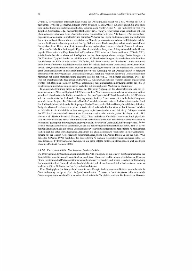
8/12/2019 Schwarze LöCher Als Astronomische Objekte
http://slidepdf.com/reader/full/schwarze-lacher-als-astronomische-objekte 30/146
30 Kapitel 3: Röntgenstrahlung stellarer Schwarzer Löcher
Cygnus X-1 systematisch untersucht. Dazu wurde das Objekt im Zeitabstand von 2 bis 3 Wochen mit RXTEbeobachtet. Typische Beobachtungsdauern waren zwischen 10 und 20 ksec, d.h. ausreichend, um gute spek-trale und zeitliche Informationen zu erhalten. Simultan dazu wurde Cygnus X-1 im Radiobereich vom RyleTeleskop, Cambridge, U.K., beobachtet (Beobachter: G.G. Pooley), ferner liegen quasi-simultane optischephotometrische Daten vom Krim-Observatorium vor (Beobachter: V. Lyutyi, A.E. Tarasov). Ziel dieser Kam-pagne ist es, Änderungen im spektralen und zeitlichen Verhalten der Quelle zu dokumentieren und im Rahmender in diesem Kapitel beschriebenen physikalischen Modelle zu interpretieren. Alleine im Röntgenbereich ha-ben wir die Gesamtbeobachtungszeit, mit der Cyg X-1 seit seiner Entdeckung beobachtet wurde, vervielfacht.Die Analyse dieser Daten ist noch nicht abgeschlossen, und wird noch mehrere Jahre in Anspruch nehmen.
Eine ausführliche Beschreibung der Ergebnisse der zeitlichen Analyse der Röntgendaten bildet die Grund-lage der Dissertation von Katja Pottschmidt (Pottschmidt 2002, siehe auch Pottschmidt et al. 2000a,b, 2002),auf die für die Details verwiesen sei. Im Gegensatz zu den oben angesprochenen wenigen Beobachtungen vonGX 339− 4 und Cyg X-1 handelt es sich hier um∼130 Einzelbeobachtungen, die es erlauben, sehr detailliertdas Verhalten des PSD zu untersuchen. Wir nden, daß dieses während des “hard state” immer durch vierbreite Lorentzfunktionen beschrieben werden kann. Da sich die Breite dieser Lorentzfunktionen kaum ändert,obwohl die Quellleuchtkraft variabel ist, kann davon ausgegangen werden, daß die physikalische Ursache fürdiese Lorentzfunktionen im hard state immer die selbe ist. Abhängig von der Quellleuchtkraft ist hingegendie charakteristische Frequenz der Lorentzfunktionen, das heißt, die Frequenz, bei der die Lorentzfunktion einMaximum hat. Diese charakteristische Frequenz liegt bei höherem L X bei höheren Frequenzen. Dieser Ef-fekt, daß charakteristische Frequenzen im PSD mitL X zunehmen, ist schon in früheren Studien angesprochenworden (z.B. Belloni & Hasinger, 1990b,a), aufgrund der neuen Interpretation der Komponenten des PSD istes jetzt jedoch möglich geworden, dieses Verhalten mit physikalischen Modellen zu überprüfen.
Eine mögliche Erklärung dieses Verhaltens des PSD ist in Änderungen der Massenakkretionsrate des Sy-stems zu suchen. Allen in Abschnitt 3.4.2.2 dargestellten Akkretionsscheibenmodellen ist zu eigen, daß siesich durch charakteristische Radien auszeichnen. Bei den “sphere+disk” Modellen oder den ADAFs ist einsolcher charakteristischer Radius der Übergang von der äußeren Akkretionsscheibe in die heiße Comptoni-sierende innere Region. Bei “Sandwich-Modellen” wird der charakteristische Radius beispielsweise durchden Radius deniert, bei dem die Bedingungen für das Einsetzen der Balbus-Hawley Instabilität erfüllt sind.Steigt die Massenakkretionsrate an, dann rückt der charakteristische Radius näher an das Schwarze Loch her-an. Modelle für die Variabilität im hard state gehen typischerweise davon aus, daß die f − 1 -Proportionalitätdes PSD durch stochastische Prozesse in der Akkretionsscheibe selbst entsteht (siehe z.B. Negoro et al., 1995;Nowak et al., 1999a,b; Psaltis & Norman, 2001). Diese intrinsische Variabilität wird dann durch physikali-sche Prozesse moduliert. Durch diese intrinsische Variabilität könnte zum Beispiel die Akkretionsscheibe zuresonanten, gedämpften Schwingungen angeregt werden, die den vier Lorentzfunktionen entsprechen. Ändertsich die Massenakkretionsrate adiabatisch, so daß die Scheibengeometrie selbstähnlich bleibt, dann ist es ver-nünftig anzunehmen, daß der für die Lorentzfunktion verantwortliche Resonator bei höherem M bei kleinerenRadien liegt. Da unter sehr allgemeinen Annahmen alle charakteristischen Frequenzen in einer Akkretions-scheibe mit der lokalen Keplerfrequenz zusammenhängen (siehe z.B. Psaltis, Belloni & van der Klis, 1999;di Matteo & Psaltis, 1999), heißt dies, daß bei größerem M auch die Resonatorfrequenz ansteigen sollte. Ge-naue (magneto-)hydrodynamische Rechnungen, die diese Effekte bestätigen, stehen jedoch noch aus (sieheallerdings Psaltis & Norman, 2001).
3.4.2.4 Kurzzeitvariabilität: Time Lags und Kohärenzfunktion
Die Untersuchung der Quellvariabilität mithilfe des PSD ermöglicht es nur schwer, die Zusammenhänge derVariabilität in verschiedenen Energiebändern zu erklären. Diese sind wichtig, da die physikalischen Ursachenfür die Entstehung des Röntgenspektrums wesentlich besser verstanden sind, als die Ursachen zur Entstehungder Variabilität selbst. Diese physikalischen Modelle sind jedoch nur dann wirklich selbstkonsistent, wenn sieauch das zeitliche Verhalten der Quelle beschreiben können.
Eine Abhängigkeit der Röntgenlichtkurven in zwei Energiebändern kann zum Beispiel durch thermischeComptonisierung erzeugt werden. Aufgrund verschiedener Prozesse in der Akkretionsscheibe werden dieCompton-gestreuten weichen Photonen eine charakteristische Variabilität besitzen. Da die weichen Photonen
8/12/2019 Schwarze LöCher Als Astronomische Objekte
http://slidepdf.com/reader/full/schwarze-lacher-als-astronomische-objekte 31/146
Kapitel 3.4: Physik galaktischer Schwarzer Löcher 31
in der Akkretionsscheibenkorona gestreut werden, sollte diese charakteristische Variabilität auch in der ctonisierten Strahlung beobachtbar sein, d.h. prinzipiell sollten eine bei niederen Photonenenergien undbei höheren Photonenenergien beobachtete Lichtkurve einander ähnlich sein. Das Maß dieser Ähnlicwird durch die Eigenschaften der Comptonkorona bestimmt. So ist leicht einsichtig, daß aufgrund des Sprozesses in der Korona die Weglänge, die Photonen zurücklegen, von der Endenergie der Photonen abhsein wird: Im Mittel haben Photonen, die aus der Korona bei höheren Photonenenergien entweichen, mCompton-Stöße erfahren und sind daher länger in der Korona geblieben. Daher ist zu erwarten, daß aufgder Comptonisierung die beobachtete Lichtkurve in einem härteren Energieband zwar die gleiche charristische Variabilität aufweist wie die Lichtkurve in einem niedrigeren Energieband, aber gegenüber letzverzögert ist. Ferner ist zu erwarten, daß aufgrund der Photonendiffusion durch die Korona die Variabbei hohen Frequenzen “ausgeschmiert” wird.
Mit Hilfe von Monte Carlo Rechnungen, insbesondere mit dem von mir entwickelten linearen Montelo Code, kann dieser Prozeß quantiziert werden. Dabei wird die Green’s Funktion für die DiffusionPhotonen durch die Compton-Korona berechnet, d.h. für ein vorgegebenes Anfangsspektrum, das zurt = 0 emittiert wird, wird berechnet, zu welchem Zeitpunkt Photonen in eine gewissen Energieband ausCompton-Korona austreten. Unter der Kenntnis der Green’s Funktion kann dann die in diesem Energieerwartete Variabilität berechnet werden, wenn ein bestimmtes Variabilitätsverhalten des Anfangsspektrvorausgesetzt wird.
Zum Testen solcher Vorhersagen wurden in unserer Gruppe in den letzten Jahren verschiedene Verfahentwickelt. Hier sind insbesondere die fourierfrequenzabhängigen “Time lags” zu nennen. In Schwarzlkandidaten wird beobachtet, daß eine in einem härteren Energiebereich beobachtete Lichtkurve der in eweicheren Energieband beobachteten sehr ähnelt, allerdings um einige 10− 3 bis 10− 2 Sekunden verzögertist. Quantitativ wird dieses Verhalten über die “Time Lags” beschrieben. Zur Berechnung des “Time wird die Phaseninformation der Fouriertransformierten der beiden Lichtkurven benutzt (Nowak & Vaug1996), während die “Ähnlichkeit” der Lichtkurven formaler mit Hilfe der Kohärenzfunktion beschrieben(Vaughan & Nowak, 1997).
Mit derartigen Rechnungen konnten wir zeigen, daß Comptonisierung nicht die Ursache für die oben be-schriebenen “Time Lags” in galaktischen BHC ist (Nowak et al., 1999b). Auch weitere von uns untersuUrsachen für die Variabilität scheinen auszuscheiden, so daß die Ursache der Variabilität noch als offen sehen ist.
3.4.3 Zustandsänderungen und Soft State
Im “soft state” ist die Akkretionsscheibe die klar dominierende spektrale Komponente. Die Untersuchunsoft state ist gegenüber der des hard state lange vernachlässigt worden. Dies liegt daran, daß die zwei Qudie immer im soft state beobachtet worden waren, LMC X-1 und LMC X-3, aufgrund ihrer Lage in der GMagellanischen Wolke und der damit verbundenen Entfernung von 50 kpc Quellen wesentlich kleineretensität sind, als die galaktischen hard state Quellen. Die von uns mit RXTE durchgeführten Beobachtudieser Quellen waren die ersten Untersuchungen, bei denen diese Objekte systematisch über längere Zeime (mehrere Jahre hinweg) beobachtet wurden3 . Eine ausführliche Darstellung unserer Beobachtungen wirdin den Anhängen C und D gegeben (Nowak et al., 2001; Wilms et al., 2001a).
Wie schon bei den Untersuchungen des hard state konnten wir auch hier durch den Vergleich vieler Bachtungen Fortschritte bei der Erklärung der beobachteten Phänomene gewinnen, die bei Einzelbeobachgen nur schwer verständlich sind. LMC X-1 und LMC X-3 sind recht ähnliche Objekte. In beiden Systsind die Donorsterne frühen Typs und auch die Leuchtkraft und die typischen spektralen Parameter der Rgenspektren dieser Quellen sind vergleichbar: Das Röntgenspektrum wird durch eine thermische Kompodominiert, die bei höheren Energien in ein weiches Potenzgesetzspektrum übergeht. Schon Ebisawa, Mi& Hanawa (1991) und Ebisawa et al. (1993) hatten jedoch bemerkt, daß LMC X-1 auf längeren Zeitsknur wenig variabel ist, während bei LMC X-3 Intensitätsänderungen über einen Faktor 4 und mehr erkbar waren. Diese sind auch gut in den RXTE-ASM Lichtkurven dieser Quellen zu erkennen (Abbildu
3 Frühere Studien, wie zum Beispiel die Ginga Analysen von Ebisawa, Mitsuda & Hanawa (1991) and Ebisawa et al. (1993), warenauf einige wenige Beobachtungen beschränkt.
8/12/2019 Schwarze LöCher Als Astronomische Objekte
http://slidepdf.com/reader/full/schwarze-lacher-als-astronomische-objekte 32/146
32 Kapitel 3: Röntgenstrahlung stellarer Schwarzer Löcher
in Anhang D). Die optische Variabilität von LMC X-3 ist jedoch gering. Wie wir in der Analyse photo-metrischer Daten des Begleitsterns von LMC X-3 zeigen konnten, ist diese nur schwach und nicht mit derLangzeitvariabilität im Röntgenbereich korreliert (Brocksopp, Groot & Wilms, 2001).
Wichtigstes Ergebnis unserer Monitoringkampagne war, daß wir diesen Unterschied in der Röntgenvaria-bilität erklären konnten: Im Gegensatz zu LMC X-1 zeigt LMC X-3 deutliche spektrale Änderungen, dietypisch sind für spektrale Zustandsänderungen vom soft state in den hard state. Besonders deutlich wurdedies im Jahr 1998, als zum ersten Mal in dieser Quelle ein reines Potenzgesetzspektrum beobachtet werdenkonnte (Abbildung 4 in Anhang D). In der Zwischenzeit wurde diese Entdeckung durch weitere Beobachtun-gen bestätigt (Boyd & Smale, 2000; Boyd et al., 2000; Wu et al., 2001; Soria et al., 2001). Damit ist LMC X-1der einzige Schwarzlochkandidat, der bisher keine Zustandsänderungen aufweist. Ähnliche Analysen vonspektralen Änderungen und der damit verbundenen physikalischen Parameter bei Zustandsänderungen habeich auch bei GX 339− 4 (Anhänge A und B) durchgeführt.
Als Ursache für Zustandsänderungen werden Änderungen in der Massenakkretionsrate angenommen. Diesist wahrscheinlich, da klare Änderungen von M mit Zustandsänderungen in den nicht-persistenten Schwarz-lochkandidaten einhergehen (Tanaka & Shibazaki, 1996; Wheeler, 1996). Physikalisch begründet werdenkann diese Annahme damit, daß alle vorgeschlagenen Mechanismen für die Entstehung von Akkretions-scheibenkoronen nur unterhalb einer kritischen Massenakkretionsrate funktionieren. Die Modulation von M kann im Fall von LMC X-3 im Akkretionsmechanismus selbst gesucht werden. Eine Zeitreihenanalyse vonLMC X-1 und LMC X-3 zeigt, daß LMC X-3 eher als Objekt, das über Roche-Lobe Overow akkretiert, zusehen ist, während bei LMC X-1 Windakkretion als wahrscheinlich erscheint (Nowak et al., 2001, abgedrucktin Anhang C). Damit ist die Akkretionsscheibe in LMC X-3 größer als die in LMC X-1, insbesondere kannder äußere Rand der Akkretionsscheibe durch die Röntgenstrahlung des zentralen Objekts aufgeheizt werden.Es kann gezeigt werden, daß diese Heizung ausreicht, M signikant zu ändern. Bei LMC X-1 ist die Akkre-tionsscheibe kleiner, so daß dieser Mechanismus hier nicht funktioniert. Ein solches Modell kann auch dieLangzeitvariation von LMC X-3 prinzipiell erklären (Anhang D), während wir bei V1408 Aql eher von einerpräzedierenden Akkretionsscheibe als Ursache für die Langzeitvariation ausgehen (Nowak & Wilms, 1999,abgedruckt in Anhang E). Siehe auch Pottschmidt et al. (2002) für Untersuchungen der Langzeitvariabilitätvon Cygnus X-1.
8/12/2019 Schwarze LöCher Als Astronomische Objekte
http://slidepdf.com/reader/full/schwarze-lacher-als-astronomische-objekte 33/146
K APITEL 4
Röntgenstrahlung supermassiver Schwarzer Löcher
Die zweite heute studierte Art Schwarzer Löcher sind die supermassiven Schwarzen Löcher in den ZeAktiver Galaxien (englisch active galactic nuclei , AGN). Obwohl diese mit Massen von 106 bis 108 Mwesentlich höhere Massen haben, als die im letzten Kapitel behandelten Schwarzlochkandidaten, sind Ain vielen Eigenschaften den galaktischen Schwarzlochkandidaten doch ähnlich – beispielsweise werden
Röntgenspektren ebenfalls durch Comptonisierung erzeugt.In diesem Kapitel werden verschiedene Aspekte meiner Untersuchungen zu Aktiven Galaxien zusammgefaßt. Abschnitt 4.1 führt in die benutzten Bezeichnungen, insbesondere die Klassikation der AGNAbschnitt 4.3 ist dann der Darstellung meiner Untersuchungen gewidmet, unter besonderer Berücksichtider Analyse der in diesen Objekten beobachteten Kα -Linie des Eisens.
4.1 Aktive Galaxien
Aktive Galaxien wurden in den frühen 1960er Jahren zunächst im Radiobereich als Objektklasse erkannDurchmusterungen des Himmels im Radiobereich wurden Radioquellen entdeckt, deren Winkelausdehmit den damals vorhandenen Radioteleskopen nicht meßbar war. Dies wurde als atypisch angesehen, dmeisten in dieser Zeit bekannten Radioquellen ausgedehnte Objekte waren; diese punktförmigen Radiolen bekamen den Namen “Radiosterne”. Das optische Spektrum dieser Objekte war durch Emissionslgekennzeichnet, was atypisch für Sterne ist, bei denen Spektrallinien typischerweise in Absorption beobtet werden. Ferner konnten diese Emissionslinien zunächst nicht identiziert werden, da sie bei Wellenlägefunden wurden, bei denen keine bekannten Spektrallinien existieren. Schmidt (1963) erkannte, daßEmissionslinien sehr wohl bekannten Elementen zugeordnet werden konnten, wenn man annahm, darotverschoben waren. Für den “Radiostern” 3C 273 wurde eine Rotverschiebung von z = 0 .158 ermittelt,wenig später fanden Greenstein & Matthews (1963) für 3C 48 die Rotverschiebung z = 0 .368. Gemeinhinwurde und wird angenommen, daß diese Rotverschiebung der Spektrallinien kosmologischen Ursprungdas heißt, diese großen Rotverschiebungen werden durch die Expansion des Universums verursacht unddurch eine Eigenbewegung des Strahlung emittierenden Objekts. “Radiosterne” sind daher keine stelObjekte, sondern stellen Quellen dar, die kosmologische Entfernungen von vielen Mpc und dementsprechohe Leuchtkräfte haben. Sie sind daher nur quasi-stellare Objekte, sogenannte Quasare . In der Folgezeitnach der Entdeckung der Quasare wurden Objekte mit ähnlichen Charakteristika auch bei niedriger Roschiebung entdeckt, bei denen außer dem Quasar auch noch eine Galaxie beobachtbar ist. Die Leuchtder Galaxie ist allerdings auch hier kleiner als die der Punktquelle, die sich im Zentrum der Galaxie beAlle Objekte dieser Art werden als “Aktive Galaxien” bezeichnet. Einen ausführlichen Überblick übeGeschichte der Aktiven Galaxien geben Kembhavi & Narlikar (1999).
Die wesentlichen Beobachtungseigenschaften von AGN sind ein sehr kleiner Winkeldurchmesser, Lekräfte im Bereich von Galaxienleuchtkräften, starke zeitliche Variabilität, häug ein aches (nichtthermisBreitbandspektrum vom radio oder Infrarotbereich bis in den MeV- oder sogar GeV-Bereich und starkesehr breite Emissionslinien im Optischen und Ultraviolet (Krolik, 1999). Ihrer Entdeckungsgeschichte Trotz ist nur ein kleiner Teil von AGN radiolaut, für die überwiegende Zahlder AGN trägt die Radioleuchtnur einen kleinen Teil zur bolometrischen Leuchtkraft bei (“radioleise AGN”). Im Folgenden soll hauptslich letzterer Typ der AGN angesprochen werden, da diese für meine Röntgenbeobachtungen von größe
8/12/2019 Schwarze LöCher Als Astronomische Objekte
http://slidepdf.com/reader/full/schwarze-lacher-als-astronomische-objekte 34/146
34 Kapitel 4: Röntgenstrahlung supermassiver Schwarzer Löcher
Interesse waren.Wie es oben schon angesprochen wurde, werden die optischen Spektren Aktiver Galaxien durch Emis-
sionslinien dominiert. Die Spektren sind dabei den planetarischen Nebeln in unserer Milchstraße ähnlich,insbesondere wird auch eine große Zahl an Linien aus verbotenen Übergängen beobachtet, wie zum Beispieldie [O II I ]λ5007Å und λ4959Å Linien, oder Linien von N II oder S II . Solche Linien sind typisch für Ga-se mit Teilchendichten von einigen 1000cm− 3 und Temperaturen im Bereich von ∼ 104 K. Die typischenLinienbreiten entsprechen Dopplerbreiten von einigen 100 km s− 1 . Im Gegensatz zu planetarischen Nebelnwerden in Aktiven Galaxien jedoch auch Linien von vergleichsweise hochionisierten Spezies beobachtet. DasLinienspektrum ist charakteristisch für das eines Gases, das von einem nichtthermischen Spektrum photoioni-siert wird. Außer den verbotenen Linien werden in den AGN Spektren auch erlaubte Linien, wie z.B. die Hαλ6563Å Linie oder weitere Linien von He I, He II , usw. beobachtet. Je nach beobachtetem AGN sind dieseLinien entweder von ähnlicher Breite wie die verbotenen Linien, oder aber sie werden mit Breiten von 1000bis 5000 kms− 1 beobachtet. Das Gas, das diese breiten Linien emittiert, hat Dichten im Bereich von einigen108 bis 1010 cm− 3 . Aufgrund thermischer Bewegung werden Geschwindigkeiten in der Größenordnung von
v = kT mp∼ 10 km s− 1 T
104 K
1/
2
(4.1)
erwartet, also Geschwindigkeiten, die wesentlich geringer sind, als die aus der beobachteten Linienverbreite-rung ermittelten. Daher ist davon auszugehen, daß das Gas, das die verbotenen bzw. erlaubten Linien aussen-det, relativ zur Galaxie in Bewegung ist. Aus der symmetrischen Linienform ist ferner davon auszugehen, daßdas emittierende Gas in der Form von Wolken auftritt, deren Geschwindigkeitsvektoren in erster Näherungisotrop verteilt sind. Für AGN, in denen sowohl breite erlaubte als auch dünne verbotene Linien auftreten, be-deutet dies, daß zwei kinematisch unterschiedliche Regionen existieren sollten, in denen die jeweiligen Linienentstehen.
Radioleise Aktive Galaxien, in denen breite erlaubte Linien und dünne verbotene Linien beobachtet werden,
werden als Seyfert 1 Galaxien bezeichnet (nach Carl Seyfert, der diese Objekte als erster beschrieben hat).Sind sowohl die erlaubten als auch die verbotenen Linien nur einige 100 km s− 1 breit, dann handelt es sichum eine Seyfert 2 Galaxie. Die Kontinuumsspektren von Seyfert 1 Galaxien sind zudem wesentlich stärker,als die von Seyfert 2 Galaxien. Weitere Unterschiede und Gemeinsamkeiten der Seyfert Galaxien und andererAktiver Galaxien, sowie der Klassikation dieser Objekte werden von Lawrence (1987) und Urry & Padovani(1995) diskutiert.
Entscheidend für das heutige Bild Aktiver Galaxien waren Messungen von Antonucci & Miller (1985),die das Spektrum der Seyfert 2 Galaxie NGC 1068 polarimetrisch untersuchten und feststellten, daß es sehrdem Spektrum einer Seyfert 1 Galaxie ähnelt. Solche und weitere Untersuchungen führten zu der Hypothese,daß es sich bei allen Aktiven Galaxien prinzipiell um die gleiche Art von astronomischen Objekt handeltund daß die Unterschiede zwischen den verschiedenen Aktiven Galaxien nur von unserem Blickwinkel auf
das Objekt herrühren. Auch wenn dieses “Vereinigungsmodell” (uni ed model ) der Aktiven Galaxien nochkeineswegs als gesichert gelten kann, so bietet es doch ein Paradigma, innerhalb dessen Beobachtungen vonAGN interpretiert werden können. Im folgenden sollen die Haupteigenschaften die Vereinigungsmodells kurzdargestellt werden, für die Details sei auf Urry & Padovani (1995), Krolik (1999), Antonucci (1993) und diedarin angegebene Literatur verwiesen.
Dem “Vereinigungsmodell” zufolge bendet sich im Zentrum eines AGN ein supermassives SchwarzesLoch mit einer Masse von 106 M bis 108 M , auf das∼ 3 M yr− 1 über eine Akkretionsscheibe akkretiertwerden. Um das Schwarze Loch und die Akkretionsscheibe herum benden sich in einer Zone mit einemDurchmesser von 1pc dichte Gaswolken, die durch die Strahlung des Schwarzen Lochs photoionisiertwerden. Diese dichten Wolken haben Geschwindigkeiten von einigen 1000km s− 1 und sind verantwortlichfür die beobachteten breiten Spektrallinien. Daher wird die Zone dieser Wolken als “Broad Line Region”(BLR) bezeichnet. Ob die Wolken der BLR sich um das Schwarze Loch bewegen, oder ob es zusätzlich zuroben angesprochenen statistischen Geschwindigkeitsverteilung auch noch einen Einfall der Wolken auf odereine Entfernung vom Schwarzen Loch gibt, ist noch nicht endgültig geklärt. Bei größeren Entfernungen vomSchwarzen Loch, das heißt bei Abständen von einigen 10 pc, existiert im “Vereinigungsmodell” eine zweite
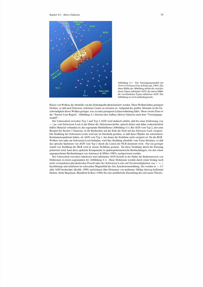
8/12/2019 Schwarze LöCher Als Astronomische Objekte
http://slidepdf.com/reader/full/schwarze-lacher-als-astronomische-objekte 35/146
Kapitel 4.1: Aktive Galaxien 35
Abbildung 4.1: Das Vereinigungsmodell derAktiven Galaxien (Urry & Padovani, 1995). Dieobere Hälfte der Abbildung erklärt die verschie-denen Typen radiolauter AGN, die untere Hälftedie verschiedenen Typen radioleiser AGN. DieAbbildung ist nicht maßstabsgerecht.
Klasse von Wolken, die ebenfalls von der Zentralquelle photoionisiert werden. Diese Wolken haben gerinDichten, so daß auch Emission verbotener Linien zu erwarten ist. Aufgrund des großen Abstands ist dischwindigkeit dieser Wolken geringer, was zu einer geringeren Linienverbreitung führt. Diese zweite Zodie “Narrow Line Region”. Abbildung 4.1 skizziert den Aufbau Aktiver Galaxien nach dem “Vereinigumodell”.
Der Unterschied zwischen Typ 1 und Typ 2 AGN wird dadurch erklärt, daß bei einer Entfernung ∼ 1pc vom Schwarzen Loch in der Ebene der Akkretionsscheibe, optisch dickes und daher wahrscheinkühles Material vorhanden ist, der sogenannte Molekültorus (Abbildung 4.1). Bei AGN vom Typ 2, alsoBeispiel bei Seyfert 2 Galaxien, ist für Beobachter auf der Erde die Sicht auf das Schwarze Loch verspDie Strahlung des Schwarzen Lochs wird nur im Streulicht gesehen, so daß diese Objekte ein schwächKontinuumsspektrum haben, als AGN vom Typ 1, bei denen die Sichtlinie nicht versperrt ist. Da die BWolken sich nahe am Schwarzen Loch benden, wird ihre Strahlung ebenfalls vom Torus blockiert, sodas optische Spektrum von AGN vom Typ 2 durch die Linien der NLR dominiert wird. Nur ein gerAnteil von Strahlung der BLR wird in unsere Sichtlinie gestreut. Da diese Strahlung durch die Strepolarisiert wird, kann diese spektrale Komponente in spektropolarimetrische Beobachtungen, wie den sangesprochenen Beobachtungen von Antonucci & Miller (1985), nachgewiesen werden.
Der Unterschied zwischen radioleisen und radiolauten AGN besteht in der Stärke der RadioemissionElektronen in einem sogenannten Jet (Abbildung 4.1). Diese Elektronen werden durch einen bislang nicht verstandenen physikalischen Prozeß nahe des Schwarzen Lochs auf Geschwindigkeiten von v ≈ cbeschleunigt und emittieren im schwachen Magnetfeld des Jets Synchrotronstrahlung. Jets werden in∼ 1%aller AGN beobachtet (Krolik, 1999) und können über Distanzen von mehreren 100 kpc hinweg kollibleiben. Siehe Begelman, Blandford & Rees (1984) für eine ausführliche Darstellung der relevanten The
8/12/2019 Schwarze LöCher Als Astronomische Objekte
http://slidepdf.com/reader/full/schwarze-lacher-als-astronomische-objekte 36/146
36 Kapitel 4: Röntgenstrahlung supermassiver Schwarzer Löcher
4.2 Die Existenz Schwarzer Löcher in Aktiven Galaxien
Außer der Existenz des Molekültorus ist die wesentliche Annahme des Vereinigungsmodells die ExistenzSchwarzer Löcher in den Zentren Aktiver Galaxien. Diese wurde primär aus der geringen Ausdehnung, hohen
Leuchtkraft und starken Zeitvariabilität gefolgert (Rees, 1984, und die darin angegebene Literatur), solcheFolgerungen sind jedoch noch kein Beweis für die Existenz der Schwarzen Löcher (Kormendy & Richstone,1995).
Zentrales Gebiet der Erforschung der Aktiven Galaxien in den letzten Jahren war daher insbesondere dieFrage, inwiefern die Existenz des zentralen Schwarzen Lochs auch durch direktere Messungen nachgewiesenwerden kann. Als direkte Methoden kommen hier insbesondere kinematische Verfahren in Frage, bei denenaus der Bewegung von Material nahe des Schwarzen Lochs Hinweise auf die vom Material eingeschlosseneMasse gezogen werden können (Ford et al., 1997, und die darin angegebene Literatur). Hierfür sind räum-lich aufgelöste spektroskopische Untersuchungen erforderlich, mit denen das Geschwindigkeitsfeld nahe desSchwarzen Lochs gemessen wird. Diese Daten liefern immer nur Informationen über die mittlere Bewegungder beobachteten Sterne, da schon die nächsten Aktiven Galaxien nicht mehr in Einzelsterne auösbar sind.
Die durch eine Punktmasse M verursachte Geschwindigkeitsdispersion σ ist näherungsweise gegeben durchσ2 =
GM R
(4.2)
wo R der Abstand von der Punktmasse ist. Der Einußbereich der Punktmasse ist bei einer intrinsischenGeschwindigkeitsdispersion der Sterne, σ0 , deniert durch den Bereich, in dem σ > σ 0 gilt, das heißt, dasSchwarze Loch hat einen Einuß auf die Sternbewegungen bis zu einem Radius
R ∼ GM
σ20
∼ 40 pc M 108 M σ2
0
100 km s− 1 (4.3)
(siehe zum Beispiel de Zeeuw, 2001). Im Virgohaufen (Entfernung: 20 Mpc) entspricht diese Entfernungeinem Winkelabstand von 0.2 , das heißt, daß solche Messungen mit weltraumbasierten Teleskopen wie demHubble Space Telescope durchgeführt werden müssen. Die dabei erhaltenen Massenkonzentrationen vonM ∼ 108 M sind verträglich mit den aus der AGN-Leuchtkraft abgeschätzten (Gebhardt et al., 2000), aller-dings ist diese Masse die Masse in einem Radius von R 40 pc, das heißt, daß sie noch keinen tatsächlichenBeweis für ein Schwarzes Loch liefern, da prinzipiell im beobachteten Volumen auch ein Sternhaufen hoherSterndichte verborgen sein könnte.
Aufgrund der höheren Auösung interferometrisch arbeitender Radioteleskope kann im Radiobereich einkleineres Volumen abgebildet werden. Die Entdeckung sehr dünner Emissionslinien eines Wasser-Masersin NGC 4258 (d = 6 .5 Mpc) durch Miyoshi et al. (1995) und Greenhill et al. (1995), die im Abstand von∼ 0.05 Millibogensekunden vom Zentrum dieser Seyfert-Galaxie gefunden wurden, ermöglichte die Mes-sung des Geschwindigkeitsfelds dieser Galaxie bei Abständen von 0.25 pc vom Zentralobjekt. Die VLBI-Beobachtungen von Greenhill et al. (1996), mit denen die Position der Wassermaser gemessen werden konnte,lassen sich gut durch Emission aus einer leicht verdrehten Akkretionsscheibe erklären. Die aus dem Ge-schwindigkeitsfeld gefolgerte Masse von∼ 4 × 10⁷ M innerhalb eines Volumen mit R 0.25 pc (Neufeld& Maloney, 1995) weist stark auf die Existenz eines Schwarzen Lochs hin. Allerdings besteht bei NGC 4258immer noch Uneinigkeit über den Modus der Akkretion, so könnte die Akkretion in NGC 4258 auch advekti-onsdominiert sein (Lasota et al., 1996; Lasota, 1999).
Die prinzipiell wohl direkteste Methode, die Existenz des zentralen Schwarzen Lochs nachzuweisen, rührt jedoch von der Beobachtung der Röntgenstrahlung Aktiver Galaxien her, da diese im Abstand von nur einigenSchwarzschildradien sehr nah am Schwarzen Loch entsteht.
4.3 Röntgenbeobachtungen Aktiver Galaxien
Die Röntgenspektren der Seyfert-Galaxien sind den in Kapitel 3 beschriebenen Röntgenspektren galaktischerSchwarzlochkandidaten sehr ähnlich. Auch die Röntgenspektren von Seyfert-Galaxien können in erster Nä-herung durch Potenzgesetze mit einem Photonenindex von Γ ∼ 1.7 und einem exponentiellen Abfall des
8/12/2019 Schwarze LöCher Als Astronomische Objekte
http://slidepdf.com/reader/full/schwarze-lacher-als-astronomische-objekte 37/146
Kapitel 4.3: Röntgenbeobachtungen Aktiver Galaxien 37
Spektrums bei einer charakteristischen Energie von ∼ 150keV beschrieben werden. Daher ist es auch hiersehr wahrscheinlich, daß das Röntgenspektrum durch Comptonisierung erzeugt wird.
Im Gegensatz zu galaktischen Schwarzlochkandidaten ist das Röntgenspektrum der Aktiven Galaxiedoch stärker von weiteren spektralen Features gekennzeichnet. Viele Aktive Galaxien zeigen im Niedergiespektrum bei ∼ 0.7 keV Strukturen, die als Absorptionskanten von O VI I oder O VIII gedeutet wurden(Nandra et al., 1993; Turner et al., 1993; Reynolds & Fabian, 1995). Diese Absorptionsstrukturen rüwahrscheinlich von einem heißen Gas her, dem “Warmen Absorber”, das sich ähnlich der Broad Line Rin der näheren Umgebung des Schwarzen Lochs bendet (Porquet & Dubau, 2000; Lee et al., 2001; Kom& Fink, 1997; Reynolds & Fabian, 1995, und die darin angegebene Literatur). Mit dem Aufkommen haufgelöster Instrumente ist diese Interpretation in jüngster Zeit kritisiert worden (Branduardi-Raymont e2001; Sako et al., 2002). Ich werde auf diese Kritik später noch einmal zurückkommen.
Bei höheren Energien, im Band zwischen 6 keV und 7 keV, wird ferner eine starke Kα Linie von Eisenbeobachtet, die Äquivalentbreiten von 150 eV und mehr erreichen kann. Wie auch bei galaktischen Schwlochkandidaten weicht das Röntgenspektrum oberhalb∼10 keV von der Potenzgesetzform ab und zeigt deutli-che Anzeichen für einen Compton-Reektionsbuckel (George & Fabian, 1991; Magdziarz & Zdziarski, 1Auch hier ist bei AGN wiederum die Stärke dieses Reektionsbuckels stärker als bei galaktischen Schwlochkandidaten.
Aufgrund der größeren Stärke der Eisenlinien und des Reektionsbuckels wird bei Aktiven Galaxien dausgegangen, daß die in Kapitel 3 für den Fall der galaktischen Schwarzlochkandidaten bereits diskut“Sandwich-Geometrie” die für AGN gültige Akkretionsgeometrie ist. Offen ist lediglich, inwiefern die ctonisierende Korona die Akkretionsscheibe vollständig oder teilweise bedeckt (siehe zum Beispiel ZdziLubinski & Smith, 1999; Stern et al., 1995b). Aufgrund der geometrischen Nähe von comptonisierenMedium und Akkretionsscheibe wird bis zu 50% der in der Korona erzeugten harten Strahlung auf diekretionsscheibe zurückgestrahlt und kann dort durch Fluoreszenz die Eisenlinie und durch Compton- bhungsweise Thomsonstreuung an den Elektronen in der Akkretionsscheibe den Reektionsbuckel erzeug
Da die beobachtete Strahlung nahe des Schwarzen Lochs entsteht, wird sie durch die physikalischen Ete in der Nähe des Schwarzen Lochs beeinußt. Typische Keplergeschwindigkeiten nahe des inneren Rder Akkretionsscheibe können bis zu 30% der Lichtgeschwindigkeit erreichen, so daß die von der Schemittierte Emissionslinie stark dopplerverbreitert sein kann, ferner wird eine geringe Rotverschiebung denienenergie aufgrund von Gravitationsrotverschiebung zu erwarten sein. Wichtig ist ferner das relativistBoosting, das zu stark asymetrischen Linienprolen führt. Eine genauere Beschreibung dieser Effekte sich in Anhang G (Wilms, Speith & Reynolds, 1998), einen ausführlicheren Überblick bieten Fabian (2000) und Fabian (1997). Solche relativistisch verbreiterten Linien werden tatsächlich beobachtet. Nder ersten Entdeckung einer solchen Linie in MCG− 6-30-15 mit ASCA (Tanaka et al., 1995) wurde in vie-len weiteren Objekten stark verbreiterte Fe Kα-Linien beobachtet (Fabian et al., 1995; Nandra et al., 1997;Reynolds, 1997). Diese Linien erwiesen sich alle als stark zeitlich variabel. Insbesondere wurde die Eisnie in MCG− 6-30-15 während einer Phase besonders niedriger Leuchtkraft als so breit beobachtet, daß iVerbreiterung nicht mehr durch Linienprole, wie sie von einem nichtrotierenden Schwarzen Loch ertet wurden, erklärt werden konnte. Linien aus der Akkretionsscheibe eines maximal rotierenden SchwaLochs konnten das beobachtete Linienprol jedoch erklären (Iwasawa et al., 1996). Bei rotierenden Schzen Löchern (Kerr-Schwarzlöcher) ist der innerste Orbit, auf dem Teilchen sich noch auf Kreisbahnendas Schwarze Loch bewegen können, näher am Ereignishorizont, als im Schwarzschild Fall. Gas am innRand einer Akkretionsscheibe um ein Kerr-Schwarzloch hat daher eine höhere Geschwindigkeit, so dabeobachteten Linien breiter sind. Alternativmodelle zu einer relativistischen Interpretation der Eisenlinieschwierig. Beispielsweise konnten wir zeigen, daß eine Linienverbreiterung aufgrund von Compton-Streuwie sie von Misra & Sutaria (1999) vorgeschlagen worden war, aus grundlegenden physikalischen Grünicht möglich ist.
Aufgrund der im Vergleich zu ASCA wesentlich höheren effektiven Fläche eignet sich XMM-Newtondiese früheren ASCA-Beobachtungen zu Überprüfen. Im Rahmen des “guaranteed time program” von XNewton hatten wir die Gelegenheit zu einer 100 ksec langen Beobachtung von MCG− 6-30-15. Erste Ergeb-nisse dieser Untersuchungen sind in Anhang H dargestellt (Wilms et al., 2001b). Während unserer X
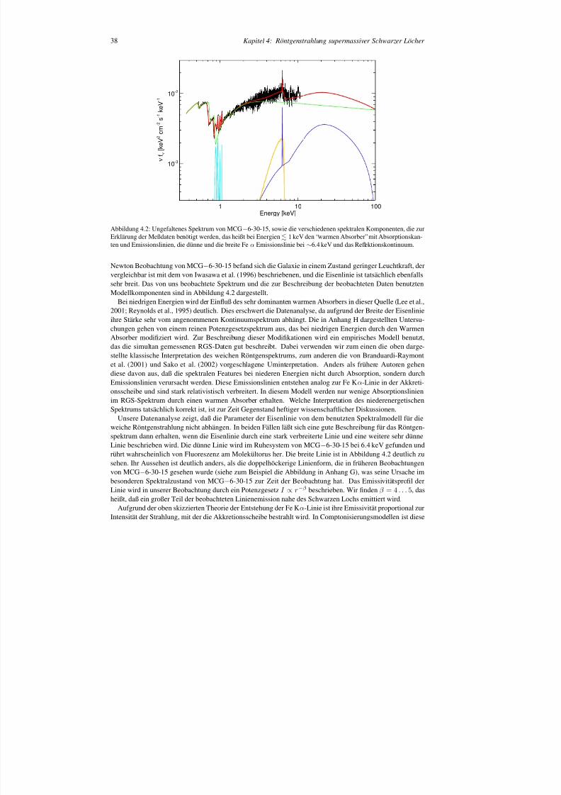
8/12/2019 Schwarze LöCher Als Astronomische Objekte
http://slidepdf.com/reader/full/schwarze-lacher-als-astronomische-objekte 38/146
38 Kapitel 4: Röntgenstrahlung supermassiver Schwarzer Löcher
1 10 100Energy [keV]
10 -3
10 -2
ν f ν [ k e
V 2
c m
- 2 s - 1 k
e V - 1
Abbildung 4.2: Ungefaltenes Spektrum von MCG− 6-30-15, sowie die verschiedenen spektralen Komponenten, die zurErklärung der Meßdaten benötigt werden, das heißt bei Energien1 keV den “warmen Absorber”mit Absorptionskan-ten und Emissionslinien, die dünne und die breite Fe α Emissionslinie bei∼6.4 keV und das Reektionskontinuum.
Newton Beobachtung von MCG− 6-30-15 befand sich die Galaxie in einem Zustand geringer Leuchtkraft, dervergleichbar ist mit dem von Iwasawa et al. (1996) beschriebenen, und die Eisenlinie ist tatsächlich ebenfallssehr breit. Das von uns beobachtete Spektrum und die zur Beschreibung der beobachteten Daten benutzten
Modellkomponenten sind in Abbildung 4.2 dargestellt.Bei niedrigen Energien wird der Einuß des sehr dominanten warmen Absorbers in dieser Quelle (Lee et al.,2001; Reynolds et al., 1995) deutlich. Dies erschwert die Datenanalyse, da aufgrund der Breite der Eisenlinieihre Stärke sehr vom angenommenen Kontinuumspektrum abhängt. Die in Anhang H dargestellten Untersu-chungen gehen von einem reinen Potenzgesetzspektrum aus, das bei niedrigen Energien durch den WarmenAbsorber modiziert wird. Zur Beschreibung dieser Modikationen wird ein empirisches Modell benutzt,das die simultan gemessenen RGS-Daten gut beschreibt. Dabei verwenden wir zum einen die oben darge-stellte klassische Interpretation des weichen Röntgenspektrums, zum anderen die von Branduardi-Raymontet al. (2001) und Sako et al. (2002) vorgeschlagene Uminterpretation. Anders als frühere Autoren gehendiese davon aus, daß die spektralen Features bei niederen Energien nicht durch Absorption, sondern durchEmissionslinien verursacht werden. Diese Emissionslinien entstehen analog zur Fe Kα -Linie in der Akkreti-
onsscheibe und sind stark relativistisch verbreitert. In diesem Modell werden nur wenige Absorptionslinienim RGS-Spektrum durch einen warmen Absorber erhalten. Welche Interpretation des niederenergetischenSpektrums tatsächlich korrekt ist, ist zur Zeit Gegenstand heftiger wissenschaftlicher Diskussionen.
Unsere Datenanalyse zeigt, daß die Parameter der Eisenlinie von dem benutzten Spektralmodell für dieweiche Röntgenstrahlung nicht abhängen. In beiden Fällen läßt sich eine gute Beschreibung für das Röntgen-spektrum dann erhalten, wenn die Eisenlinie durch eine stark verbreiterte Linie und eine weitere sehr dünneLinie beschrieben wird. Die dünne Linie wird im Ruhesystem von MCG− 6-30-15 bei 6.4 keV gefunden undrührt wahrscheinlich von Fluoreszenz am Molekültorus her. Die breite Linie ist in Abbildung 4.2 deutlich zusehen. Ihr Aussehen ist deutlich anders, als die doppelhöckerige Linienform, die in früheren Beobachtungenvon MCG− 6-30-15 gesehen wurde (siehe zum Beispiel die Abbildung in Anhang G), was seine Ursache imbesonderen Spektralzustand von MCG− 6-30-15 zur Zeit der Beobachtung hat. Das Emissivitätsprol der
Linie wird in unserer Beobachtung durch ein Potenzgesetz I ∝ r− β
beschrieben. Wir nden β = 4 . . . 5, dasheißt, daß ein großer Teil der beobachteten Linienemission nahe des Schwarzen Lochs emittiert wird.Aufgrund der oben skizzierten Theorie der Entstehung der Fe Kα -Linie ist ihre Emissivität proportional zur
Intensität der Strahlung, mit der die Akkretionsscheibe bestrahlt wird. In Comptonisierungsmodellen ist diese
8/12/2019 Schwarze LöCher Als Astronomische Objekte
http://slidepdf.com/reader/full/schwarze-lacher-als-astronomische-objekte 39/146
Kapitel 4.3: Röntgenbeobachtungen Aktiver Galaxien 39
Intensität jedoch wiederum proportional zur lokalen Emissivität der Akkretionsscheibe, das heißt, zur Endie in der Akkretionsscheibe freigesetzt wird. Damit scheinen unsere Beobachtungen zu implizieren, dalokale Energiefreisetzungsrate ∝ r − 4 ... − 5 ist. Dies ist im Rahmen der Theorie der Akkretionsscheiben nurschwer erklärbar, so daß weitere Energiequellen postuliert werden müssen. Wie in Anhang H ausgeführt ist eine mögliche Energiequelle die Extraktion von Energie aus dem rotierenden Schwarzen Loch (Bland& Znajek, 1977; Li, 2000; Agol & Krolik, 2000).
Bevor eine solche Interpretation der breiten Eisenlinie in MCG− 6-30-15 als gesichert gelten kann, sind jedoch noch weitere Beobachtungen notwendig. In einer 300 ksec langen XMM-Newton -Beobachtung vonMCG− 6-30-15, während derer die Quelle eine wesentlich höhere Röntgenleuchtkraft hatte als in der unsenden Fabian et al. (priv. Mitteilung) ebenfalls eine sehr breite Eisenlinie. Das aus dieser Beobachtunschlossene Emissionsprol ist ebenfalls ∝ r − 4 .5 am inneren Rand der Scheibe und geht dann in ein wenigersteiles r − 3 -Gesetz über (Vaughan, 2002, priv. Mitteilung). Allerdings benutzen diese Autoren andere Anahmen über das Kontinuumsspektrum, so daß diese Werte nicht einfach mit den unseren verglichen wekönnen, auch wenn dieses Prol tendenziell unsere Schlußfolgerungen bestätigt.
Dennoch ist eine genauere Analyse unserer Daten sicherlich notwendig. In einer gerade in Vorbereibendlichen Arbeit versuchen wir, durch verschiedene Kontinuumsmodelle zu überprüfen, inwiefern ure Annahme eines reinen Potenzgesetzkontinuums bestätigt werden kann. Durch die Analyse simulRXTE-Daten erweitern wir den zur Beschreibung des Spektrums benutzten Spektralbereich, um die Stdes Reektionskontinuums besser abschätzen zu können. Ferner wird mit Hilfe alternativer Modelle füLinienemission (Reynolds & Begelman, 1997; Young, Ross & Fabian, 1998; Martocchia, Matt & Karas, überprüft, inwiefern das von uns gefundene Linienprol tatsächlich eindeutig ist. Schließlich ist aufgrunVariabilität der Quelle und der Eisenlinie (Iwasawa et al., 1996) eine zeitlich aufgelöste UntersuchungQuellspektrums erforderlich.
8/12/2019 Schwarze LöCher Als Astronomische Objekte
http://slidepdf.com/reader/full/schwarze-lacher-als-astronomische-objekte 40/146
K APITEL 5
Zusammenfassung und Ausblick
In den letzten dreißig Jahren hat sich die Röntgenastronomie von einem von nur wenigen Personen be-triebenen exotischen Forschungsgebiet zu einem der Hauptzweige der modernen Astrophysik entwickelt.Hauptgrund für diese Entwicklung war, daß es dieses Forschungsgebiet erlaubt, Materie unter extremstenBedingungen zu untersuchen, die auf der Erde niemals erreichbar wären. Dazu gehören Magnetfelder mit
Stärken von 107
T genauso wie die hier behandelten Schwarzen Löcher.Im Rahmen meiner Forschungen der letzten Jahre habe ich versucht, theoretische Verfahren und Beobach-tungsmethoden zu entwickeln, mit denen die Strahlungsprozesse in der Umgebung Schwarzer Löcher unter-sucht werden können. Ergebnisse dieser Untersuchungen waren unter anderem, daß mit Hilfe systematischer,langjährig angelegter Untersuchungen ein tieferes Verständnis des Verhaltens galaktischer Schwarzer Löchererreicht wurde, das sowohl deren spektrale Entwicklung als auch die Entwicklung ihres zeitlichen Verhaltenseinschließt. Dieses Verhalten konnte mit Hilfe von Akkretionsmodellen interpretiert werden. Im Bereich dersupermassiven Schwarzen Löcher konnte mit Hilfe neuer Instrumente wie XMM-Newton aufgezeigt werden,daß Vorhersagen der Elektrodynamik Schwarzer Löcher möglicherweise beobachtbar sind.
In den nächsten Jahren sind von Chandra und XMM-Newton weitere überraschende Entdeckungen zuerwarten, mit denen der in dieser Arbeit dargestellte Stand der Forschung weiterentwickelt werden wird.
Aktuelle Forschungsgebiete sind hier zum Beispiel die Evolution der supermassiven Schwarzen Löcher, wiesie aufgrund der großen Sammeläche von XMM-Newton jetzt mit einem vernünftigen zeitlichen Aufwanddurchführbar sind oder die in Kapitel 4 angedeuteten Untersuchungen des heißen Gases in Aktiven Galaxienmit Hilfe hochaufgelöster Röntgenspektroskopie.
Die Untersuchungen an Röntgendoppelsternen werden von den zur Zeit geplanten Instrumenten, wie denvon NASA und ESA geplanten “All Sky Monitor”-Instrumenten auf der Internationalen Raumstation undinsbesondere den für die nächsten zehn Jahre geplanten Detektoren mit sehr großer Sammeläche, sehr pro-tieren. Instrumente wie das europäische XEUS-Projekt oder die Constellation-X Mission der NASA werdenes ermöglichen, mit bislang unerreichtem Signal zu Rausch Verhältnis die Strahlung von Neutronensternenund Schwarzen Löchern zu untersuchen. Eines der wichtigen Ziele ist hier zum Beispiel der Test der Zu-standsgleichung nuklearer Materie mit Hilfe zeitlich höchstaufgelöster Untersuchungen der Strahlung von
akkretierenden Neutronensterne oder die Untersuchung der Eisenlinien in Aktiven Galaxien im frühen Uni-versum. Es ist daher zu erwarten, daß die Hochenergieastrophysik auch noch in den nächsten dreißig Jahrenein interessantes und zukunftsweisendes Forschungsgebiet bleiben wird.
8/12/2019 Schwarze LöCher Als Astronomische Objekte
http://slidepdf.com/reader/full/schwarze-lacher-als-astronomische-objekte 41/146
Literaturverzeichnis
Agol, E. & Krolik, J. H. 2000, Astrophys. J., 528, 161Antonucci,R. 1993,Ann. Rev. Astron. Astrophys., 31, 473
Antonucci,R. R. J. & Miller, J. S. 1985, Astrophys. J., 297,621Arnett, D. 1996, Supernovae and Nucleosynthesis (Prince-
ton: Princeton Univ. Press)Balbus, S. A. & Hawley, J. F. 1991, Astrophys. J., 376, 214Balog, N. I., Goncharskiı, A. V., & Cherepashchuk, A. M.
1981, Sov. Astron. Lett., 7, 336Barret, D., McClintock, J. E., & Grindlay, J. E. 1996,
Astrophys. J., 473, 963Barret, D., Olive, J. F., Boirin, L., et al. 2000, Astrophys.
J., 533, 329Barziv, O., Kaper, L., van Kerkwijk, M. H., Telting, J. H.,
& van Paradijs, J. 2001, Astron. Astrophys., 377, 925Begelman, M. C., Blandford, R. D., & Rees, M. J. 1984,
Rev. Mod. Phys., 56, 255Belloni, T. & Hasinger, G. 1990a, Astron. Astrophys., 230,
103—. 1990b, Astron. Astrophys., 227, L33Benlloch, S., Wilms, J., Edelson, R. A., & Yaqoob, T.
2001, Astrophys. J., 562, L121Blandford, R. D. & Begelman, M. C. 1999, Mon. Not. R.
Astron. Soc., 303, L1Blandford, R. D. & Znajek, R. L. 1977, Mon. Not. R.
Astron. Soc., 179, 433Bochkarëv, N. G., Karitskaya, E. A., Luskutov, V. M., &
Sokolov, V. V. 1986, Sov. Astron., 30, 43Bowyer, S., Byram, E. T., Chubb, T. A., & Friedman, H.1965, Science, 147, 394
Boyd, P. & Smale, A. 2000, IAU Circ. 7424Boyd, P. T., Smale,A. P., Homan, J., et al.2000, Astrophys.
J., 542, L127Branduardi-Raymont, G., Sako, M., Kahn, S. M., et al.
2001, Astron. Astrophys., 365, L140Briel, U. G. & Pfeffermann, E. 1995, in EUV, X-Ray,
and Gamma-RayInstrumentation for Astronomy VI, ed.O. H. Siegmund & J. V. Vallerga, Proc. SPIE No. 2518(Bellingham, WA: SPIE), 120–131
Brinkman, A. C., Dam, J., Mels, W. A., Skinner, G. K., &Willmore, W. P. 1983, in Non-Thermal and Very HighTemperature Phenomena in X-Ray Astronomy, ed. G. C.Perola & M. Salvati (Roma: Istituto Astronomico, Uni-versità “La Sapienza”), 263
Brocksopp, C., Groot, P. J., & Wilms, J. 2001, Mon. Not.R. Astron. Soc., in press
Brown, G. E., Lee, C.-H., Wijers, R. A. M. J., & Bethe,H. A. 1999, Phys. Rep., 333-334, 471
Bruenn, S. W., De Nisco, K. R., & Mezzacappa, A. 2001,Astrophys. J., 560, 326
Burm, H. 1986, Astron. Astrophys., 165, 120Burwitz, V., Zavlin, V. E., Neuhäuser, R., et al. 2001,
Astron. Astrophys., 379, L35Caroli, E., Stephen, J. B., di Cocco, G., Natalucci, L., &Spizzichino, A. 1987, Space Sci. Rev., 45, 349
Casares, J. & Charles, P. A. 1994, Mon. Not. R. Astron.
Soc., 271, L5Chandrasekhar, S. 1931, Astrophys. J., 74, 81
Cui, W., Ebisawa, K., Dotani, T., & Kubota, A. 1998,Astrophys. J., 493, L75Cui, W., Heindl, W. A., Rothschild, R. E., et al. 1997,
Astrophys. J., 474, L57de Zeeuw, T. 2001, in ESO workshop on Black Holes in
Binaries and Galactic Nuclei, ed. L. Kaper, E. P. J. vanden Heuvel, & P. A. Woudt (Heidelberg: Springer), 78–87
den Herder, J. W., Brinkman, A. C., Kahn, S. M., et al.2001, Astron. Astrophys., 365, L7
di Matteo, T. & Psaltis, D. 1999, Astrophys. J., 526, L101Dolan, J. F. 1992, Astrophys. J., 384, 249Dominguez, I., Chief , A., Limongi, M., & Straniero, O.
1999, Astron. Astrophys., 524, 226Dove, J. B., Wilms, J., & Begelman, M. C. 1997, Astro-
phys. J., 487, 747Dove, J. B., Wilms, J., Maisack, M. G., & Begelman, M. C.
1997, Astrophys. J., 487, 759Dove, J. B., Wilms, J., Nowak, M. A., Vaughan, B., & Be-
gelman, M. C. 1998, Mon. Not. R. Astron. Soc., 289,729
Drake, J. J., Marshall, H. L., Dreizler, S., et al. 2002, Astro-phys. J., in press (astro-ph/0204159)
Ebisawa, K., Makino, F., Mitsuda, K., et al. 1993, Astro-phys. J., 403, 684
Ebisawa, K., Mitsuda, K., & Hanawa, T. 1991, Astrophys.J., 367, 213Ergma, E. & van den Heuvel, E. P. J. 1998, Astron. Astro-
phys., 331, L29Esin, A. A., Narayan, R., Cui, W., Grove, J. E., & Zhang,
S.-N. 1998, Astrophys. J., 505, 854Esin, A. A., Narayan, R., Ostriker, E. C., & Yi, I. 1996,
Astrophys. J., 465, 327Fabian, A. 1997, Astron. Geophys., 38, 10Fabian, A. C., Iwasawa, K., Reynolds, C. S., & Young,
A. J. 2000, Publ. Astron. Soc. Pac., 112, 1145Fabian, A. C., Nandra, K., Reynolds, C. S., et al. 1995,
Mon. Not. R. Astron. Soc., 277, L11Fenimore, E. E. 1987, Appl. Opt., 26, 2760Filippenko, A. V. 1997, Ann. Rev. Astron. Astrophys., 35,
309Ford, H. C., Zsvetanov, Z. I., Ferrarese, L., & Jaffe, W.
1997, in The Central Regions of the Galaxy and Gala-xies, IAU Symp. No. 184 (Dordrecht: Kluwer), in press
Frank, J., King, A., & Raine, D. 1992, Accretion Power inAstrophysics, 2nd edn. (Cambridge: Cambridge Univ.Press)
Garcia, M. R., McClintock, J. E., Narayan, R., et al. 2001,Astrophys. J., 553, L47
Gebhardt, K., Bender, R., Bower, G., et al. 2000, Astro-
phys. J., 539, L13, erratum: ApJ 555, L75George, I. M. & Fabian, A. C. 1991, Mon. Not. R. Astron.Soc., 249
Giacconi, R., Branduari, G., Briel, U., et al. 1979, Astro-
8/12/2019 Schwarze LöCher Als Astronomische Objekte
http://slidepdf.com/reader/full/schwarze-lacher-als-astronomische-objekte 42/146
42 Literaturverzeichnis
phys. J., 230, 540Giacconi, R., Gursky, H., Paolini, F. R., & Rossi, B. B.
1962, Phys. Rev. Lett., 9, 439Giacconi, R., Kellogg, E., Gorenstein, P., Gursky, H., &
Tananbaum, H. 1971, Astrophys. J., 165, L27Gierlinski, M., Zdziarski, A. A., Done, C., et al. 1997,Mon. Not. R. Astron. Soc., 288, 958
Gies, D. R. & Bolton, C. T. 1982, Astrophys. J., 260, 240Greenhill, L. J., Gwinn, C. R., Antonucci, R., & Barvainis,
R. 1996, Astrophys. J., 472, L21Greenhill, L. J., Jiang, D. R., Moran, J. M., et al. 1995,
Astrophys. J., 40, 619Greenstein, J. L. & Matthews, T. A. 1963, Astron. J., 68,
279Greiner, J., Cuby, J. G., & McCaughrean, M. J. 2001, Na-
ture, 414, 522Haardt, F. & Maraschi, L. 1993, Astrophys. J., 413, 507Haardt, F., Maraschi, L., & Ghisellini, G. 1994, Astrophys.
J., 432, L95—. 1997, Astrophys. J., 476, 620Hansen, C. J. & Kawaler, S. D. 1994, Stellar Interiors: Phy-
sical Principles, Structure, and Evolution (New York,Berlin, Heidelberg: Springer)
Hawley, J. F. & Balbus, S. A. 1991, Astrophys. J., 376, 223Hawley, J. F. & Stone, J. M. 1998, Astrophys. J., 501, 758Heindl, W. A., Coburn, W., Gruber, D. E., et al. 1999,
Astrophys. J., 521, L49Herrero, A., Kudritzki, R. P., Gabler, R., Vilchez, J. M., &
Gabler, A. 1995, Astron. Astrophys., 297, 556
Hua, X.-M. & Titarchuk, L. 1995, Astrophys. J., 449, 188Hutchings, J. B. 1978, Astrophys. J., 226, 264Iben, I. J. 1991, Astrophys. J., Suppl. Ser., 76, 55Ichimaru, S. 1977, Astrophys. J., 214, 840in’t Zand, J. J. M. 1992, PhD thesis, SRONin’t Zand, J. J. M., Heise, J., & Jager, R. 1994, Astron.
Astrophys., 288, 665Iwasawa, K., Fabian, A. C., Reynolds, C. S., et al. 1996,
Mon. Not. R. Astron. Soc., 282, 1038Jahoda, K., Swank, J. H., Giles, A. B., et al. 1997, in EUV,
X-Ray, and Gamma-Ray Instrumentation for Astrono-my VII, ed. O. H. Siegmund, Proc. SPIE No. 2808 (Bel-lingham, WA: SPIE), 59–70
Kalogera, V. & Baym, G. 1996, Astrophys. J., 470, L61Kaper, L., van den Heuvel, E. P. J., & Woudt, P. A., eds.
2001, ESO workshop on Black Holes in Binaries andGalactic Nuclei (Heidelberg: Springer)
Kembhavi, A. K. & Narlikar, J. V. 1999, Quasars and Acti-ve Galactic Nuclei (Cambridge: Cambridge Univ.Press)
King, A. 1995, in X-Ray Binaries, ed. W. H. G. Lewin,J. van Paradijs, & E. P. J. van den Heuvel, CambridgeAstrophysics Series No. 26 (Cambridge: CambridgeUniv. Press), 419–456
Kippenhahn, R. & Weigert, A. 1990, Stellar Structure andEvolution, 1 st edn. (Berlin, Heidelberg: Springer)
Komossa, S. & Fink, H. 1997, Astron. Astrophys., submit-tedKönig, M., Staubert, R., & Wilms, J. 1997, Astron. Astro-
phys., 326, L25
Kormendy, J. & Richstone, D. 1995, Ann. Rev. Astron.Astrophys., 33, 581
Kreykenbohm, I., Coburn, W., Wilms, J., et al. 2002,in New Visions of the X-Ray Universe in the XMM-
Newton and Chandra Era, ed. F. Jansen et al., ESA SP-488, ESA Publications, Noordwijk, in pressKreykenbohm, I., Kretschmar, P., Wilms, J., et al. 1999,
Astron. Astrophys., 341, 141Krolik, J. H. 1999, Active Galactic Nuclei, Princeton Se-
ries in Astrophysics (Princeton, N.J.: Princeton Univ.Press)
Kuster, M., Wilms, J., Blum, S., et al. 1999, Astrophys.Lett. Commun., 38, 161
Laplace, P. S. 1796, Le Système du Monde, Vol. II. DesMouvements Réels des Corps Célestes (Paris: Duprat)
Lasota, J.-P. 1999, Phys. Rep., in pressLasota, J.-P., Abramowicz, M. A., Chen, X., et al. 1996,
Astrophys. J., 462, 142Lawrence, A. 1987, Publ. Astron. Soc. Pac., 99, 309Leahy, D. A., Darbro, W., Elsner, R. F., et al. 1983, Astro-
phys. J., 266, 160Lee, J. C., Ogle, P. M., Canizares, C. R., et al. 2001, Astro-
phys. J., 554, L13Levine, A. M., Bradt, H., Cui, W., et al. 1996, Astrophys.
J., 469, L33Lewin, W. H. G., van Paradijs, J., & Taam, R. E. 1995, in
X-Ray Binaries, ed. W. H. G. Lewin, J. van Paradijs, &E. P. J. van den Heuvel, Cambridge Astrophysics SeriesNo. 26 (Cambridge: Cambridge Univ. Press), 175–232
Lewin, W. H. G., van Paradijs, J., & van den Heuvel, E.P. J., eds. 1995, X-Ray Binaries, Cambridge Astrophy-sics Series No. 26 (Cambridge: Cambridge Univ. Press)
Lewin, W. H. G., van Paradijs, J., & van der Klis, M. 1988,Space Sci. Rev., 46, 273
Li, L.-X. 2000, Astrophys. J., submitted (astro-ph/0012469)
Liang, E. P. & Nolan, P. L. 1984, Space Sci. Rev., 38, 353Lightman, A. P. & White, T. R. 1988, Astrophys. J., 335,
57Magdziarz, P. & Zdziarski, A. A. 1995, Mon. Not. R.
Astron. Soc., 273, 837Makishima, K., Tashiro, M., Ebisawa, K., et al. 1996, Publ.
Astron. Soc. Jpn., 48, 171Martocchia, A., Matt, G., & Karas, V. 2002, Astron. Astro-
phys., 383, L23McClintock, J. E., Garcia, M. R., Caldwell, N., et al. 2001,
Astrophys. J., 551, L147Michell, J. 1784, Philosophical Transactions of the Royal
Society of London, 74, 35, presented 1783 November27
Miller, K. A. & Stone, J. M. 2000, Astrophys. J., 534, 398Misra, R. & Sutaria, F. K. 1999, Astrophys. J., 517, 661Miyamoto,S., Kimura, K.,Kitamoto,S., Dotani, T., & Ebi-
sawa, K. 1991, Astrophys. J., 383, 784
Miyoshi, M., Moran, J., Herrnstein, J., et al. 1995, Nature,373, 127Nandra, K., Fabian, A. C., George, I. M., et al. 1993, Mon.
Not. R. Astron. Soc., 260, 504
8/12/2019 Schwarze LöCher Als Astronomische Objekte
http://slidepdf.com/reader/full/schwarze-lacher-als-astronomische-objekte 43/146
Literaturverzeichnis 43
Nandra, K., George, I. M., Mushotzky, R. F., Turner, T. J.,& Yaqoob, T. 1997, Astrophys. J., 477, 602
Narayan, R., Kato, S., & Honma, F. 1997, Astrophys. J.,476, 49
Narayan, R. & Yi, I. 1995, Astrophys. J., 452, 710Negoro, H., Kitamoto, S., Takeuchi, M., & Mineshige, S.1995, Astrophys. J., 452, L49
Neufeld, D. A. & Maloney, P. R. 1995, Astrophys. J., 447,L17
Ninkov, Z., Walker, G. A. H., & Yang, S. 1987, Astrophys.J., 321, 425
Nowak, M. A. 2000, Mon. Not. R. Astron. Soc., in press(astro
Nowak, M. A. & Vaughan, B. A. 1996, Mon. Not. R.Astron. Soc., 280, 227
Nowak, M. A., Vaughan, B. A., Wilms, J., Dove, J. B., &Begelman, M. C. 1999a, Astrophys. J., 510, 874
Nowak, M. A. & Wilms, J. 1999, Astrophys. J., 522, 476Nowak, M. A., Wilms, J., Heindl, W. A., et al. 2001, Mon.
Not. R. Astron. Soc., 320, 316Nowak, M. A., Wilms, J., Vaughan, B. A., Dove, J. B., &
Begelman, M. C. 1999b, Astrophys. J., 515, 726Oda, M. 1977, Space Sci. Rev., 20, 757Ogilvie, G. I. 1999, Mon. Not. R. Astron. Soc., 306, L9Olson, T. S. 2001, Phys. Rev. C, 63, 015802Oppenheimer, J. R. & Volkoff, G. M. 1939, Phys. Rep., 55,
374Padmanabhan, T. 2001, Theoretical Astrophysics. II. Stars
and Stellar Systems (Cambridge: Cambridge Univ.
Press)Perola, G. C. & Salvati, M., eds. 1983, Non-Thermal andVery High Temperature Phenomena in X-Ray Astrono-my (Roma: Istituto Astronomico, Università “La Sapi-enza”)
Perryman, M. A. C., Lindegren, L., Kovalevsky, J., et al.1995, Astron. Astrophys., 304, 69
Peterson, L. E. 1975, Ann. Rev. Astron. Astrophys., 13,423
Porquet, D. & Dubau, J. 2000, Rev. Mex. Astron. Astro-phys. (Serie de Conferencias), 9, 316
Pottschmidt, K. 2002, PhD thesis, Universität TübingenPottschmidt, K., König, M., Wilms, J., & Staubert, R.
1998, Astron. Astrophys., 334, 201Pottschmidt, K., Wilms, J., Nowak, M. A., et al. 2000a,
Astron. Astrophys., 357, L17—. 2002, Astron. Astrophys., submitted (astro-
ph/0202258)Pottschmidt, K., Wilms, J., Staubert, R., et al. 2000b, Adv.
Space Res., submitted (astro-ph/0008059)Poutanen, J. 1994, Academic dissertation, University of
Helsinki, HelsinkiPsaltis, D., Belloni, T., & van der Klis, M. 1999, Astro-
phys. J., 520, 262Psaltis, D. & Norman, C. 2001, Astrophys. J., submitted
(astro-ph/0001391)Quataert, E. 1998, Astrophys. J., 500, 978Rees, M. J. 1984, Ann. Rev. Astron. Astrophys., 22, 471Reppin, C., Pietsch, W., Trümper, J., Kendziorra, E., &
Staubert, R. 1983, in Non-Thermal and Very High Tem-perature Phenomenain X-Ray Astronomy,ed. G. C. Pe-rola & M. Salvati (Roma: Istituto Astronomico, Univer-sità “La Sapienza”), 279–282
Reynolds, C. S. 1997, Mon. Not. R. Astron. Soc., 286, 513Reynolds, C. S. & Begelman, M. C. 1997, Astrophys. J.,487, 109
Reynolds, C. S. & Fabian, A. C. 1995, Mon. Not. R.Astron. Soc., 274, 1167
Reynolds, C. S., Fabian, A. C., Nandra, K., et al. 1995,Mon. Not. R. Astron. Soc., 277, 901
Rhoades, C. E. & Ruf ni, R. 1974, Phys. Rev. Lett., 32,324
Rolfs, C. E. & Rodney, W. S. 1988, Cauldrons in the Cos-mos: Nuclear Astrophysics (Chicago, London: Univ.Chicago Press)
Rothschild, R., Boldt, E., Holt, S., et al. 1979, Space Sci.Inst., 4, 269
Rothschild, R. E., Blanco, P. R., Gruber, D. E., et al. 1998,Astrophys. J., 496, 538
Rybicki, G. B. & Lightman, A. P. 1979, Radiative Proces-ses in Astrophysics (New York: Wiley)
Sako, M., Kahn, S. M., Branduardi-Raymont, G., et al.2002, Astrophys. J., eingereicht (astro-ph/0112436)
Scargle, J. D. 1981, Astrophys. J., Suppl. Ser., 45, 1Schmidt, M. 1963, Nature, 197, 1040Schönfelder, V. 1995, Adv. Space Res., 15, 1Schröder, K., Pols, O. R., & Eggleton, P. P. 1997, Mon.
Not. R. Astron. Soc., 285, 696
Schuster, A. 1906, Astrophys. J., 23, 101Schwarzschild, K. 1916, Sitzber. Dtsch. Akad. Wiss. Ber-lin, Kl. Math. Phys. Tech., 189
Shakura, N. I. & Sunyaev,R. 1973, Astron.Astrophys., 24,337
Shapiro, S. L. & Teukolsky, S. A. 1983, Black Holes, Whi-te Dwarfs, and Neutron Stars (New York: Wiley)
Shore, S. N. 1992, An Introduction to Astrophysical Hy-drodynamics (San Diego: Academic Press)
Siegmund, O. H. & Vallerga, J. V., eds. 1995, EUV, X-Ray, and Gamma-Ray Instrumentation for AstronomyVI, Proc. SPIE No. 2518 (Bellingham, WA: SPIE)
Soria, R.,Wu, K.,Page,M. J., & Sakelliou, I. 2001, Astron.Astrophys., 365, L273
Stern, B. E., Begelman, M. C., Sikora, M., & Svensson, R.1995a, Mon. Not. R. Astron. Soc., 272, 291
Stern, B. E., Poutanen, J., Svensson, R., Sikora, M., & Be-gelman, M. C. 1995b, Astrophys. J., L13
Stone, J. M., Hawley, J. F., Gammie, C. F., & Balbus, S. A.1996, Astrophys. J., 463, 656
Strüder, L., Briel, U., Dennerl, K., et al. 2001, Astron.Astrophys., 365, L18
Sunyaev, R. A. & Titarchuk, L. G. 1980, Astron. Astro-phys., 86, 121
—. 1985, Astron. Astrophys., 143, 374
Sunyaev, R. A. & Trümper, J. 1979, Nature, 279, 506Svensson, R. 1997, iceland Conference on AccretionDisks, Reykjavik
Tanaka, Y., Nandra, K., Fabian, A. C., et al. 1995, Nature,
8/12/2019 Schwarze LöCher Als Astronomische Objekte
http://slidepdf.com/reader/full/schwarze-lacher-als-astronomische-objekte 44/146
44 Literaturverzeichnis
375, 659Tanaka, Y. & Shibazaki, N. 1996, Ann. Rev. Astron. Astro-
phys., 34, 607Tassoul, J.-L. 1978, Theory of Rotating Stars (Princeton:
Princeton Univ. Press)Timmer, J., Schwarz, U., Voss, H. U., et al. 2000, Phys.Rev. E, in press
Titarchuk, L. 1994, Astrophys. J., 434, 570Titarchuk, L. & Lyubarskij, Y. 1995, Astrophys. J., 450,
876Turner, M. J. L., Abbey, A., Arnaud, M., et al. 2001,
Astron. Astrophys., 365, L27Turner, M. J. L., Smith, A., & Zimmermann, H. U. 1981,
Space Sci. Rev., 30, 513Turner, M. J. L., Thomas, H. D., Patchett, B. E., et al. 1989,
Publ. Astron. Soc. Jpn., 41, 345Turner, T. J., Nandra, K., George, I. M., Fabian, A. C., &
Pounds, K. A. 1993, Astrophys. J., 419, 127Turolla, R. & Dullemond, C. P. 2000, Astrophys. J., 531,
L49Urry, C. M. & Padovani, P. 1995, Publ. Astron. Soc. Pac.,
107, 803van der Klis, M. 1989, in Timing Neutron Stars, ed.
H. Ögelman & E. P. J. van den Heuvel, NATO ASI No.C262 (Dordrecht: Kluwer), 27–69
van der Klis, M. 1995, in X-Ray Binaries, ed. W. H. G.Lewin, J. van Paradijs, & E. P. J. van den Heuvel, Cam-bridge Astrophysics Series No. 26 (Cambridge: Cam-bridge Univ. Press), 252–307
van der Klis, M. 1997, in Statistical Challenges in ModernAstronomy, II, ed. G. J. Babu & E. D. Feigelson (NewYork, Heidelberg: Springer), 321–331
van Straaten, S., van der Klis, M., di Salvo, T., Belloni,T., & Psaltis, D. 2001, Astrophys. J., in press (astro-ph/0107562)
Vanbeveren, D., deLoore,C., &Van Rensbergen, W. 1998,Astron. Astrophys. Rev., 9, 63
Vaughan, B. A. & Nowak, M. A. 1997, Astrophys. J., 474,L43
Verbunt, F. 2001, in ESO workshop on Black Holes in Bi-naries and Galactic Nuclei, ed. L. Kaper, E. P. J. van denHeuvel, & P. A. Woudt (Heidelberg: Springer), 279
Verbunt, F. & van den Heuvel, E. P. J. 1995, in X-Ray Bi-naries, ed. W. H. G. Lewin, J. van Paradijs, & E. P. J.van den Heuvel, Cambridge Astrophysics Series No. 26(Cambridge: Cambridge Univ. Press), 457–494
Vrtilek, S. D., Soker, N., & Raymond, J. C. 1993, Astro-phys. J., 404, 696
Wallerstein, G., Iben, Jr., I., Parker, P., et al. 1997, Rev.Mod. Phys., 69, 995
Weisskopf, M. C., Brinkman, B., Canizares, C., et al. 2002,Publ. Astron. Soc. Pac., 114, 1Wellstein, S. & Langer, N. 1999, Astron. Astrophys., 350,
148Wheeler, J. C. 1996, in Relativistic Astrophysics (Fest-
schrift I. Novikov), ed. B. J. T. Jones & D. Markovic(Cambridge: Cambridge Univ. Press)
Wilms, J. 1998, PhD thesis, Universität Tübingen, Tübin-gen
Wilms, J., Allen, A., & McCray, R. 2000, Astrophys. J.,542, 914
Wilms, J., Dove, J., Staubert, R., & Begelman, M. C.1997, in The TransparentUniverse, ed.C. Winkler, T. J.-L. Courvoisier, & P. Durouchoux, ESA SP No. 382(Noordwijk: ESA Publications Division), 233–236
Wilms, J., Nowak, M. A., Dove, J. B., Fender, R. P., & diMatteo, T. 1999, Astrophys. J., 522, 460
Wilms, J., Nowak, M. A., Pottschmidt, K., et al. 2001a,Mon. Not. R. Astron. Soc., 320, 327
Wilms, J., Reynolds, C. S., Begelman, M. C., et al. 2001b,Mon. Not. R. Astron. Soc., in press
Wilms, J., Speith, R., & Reynolds, C. S. 1998, in BlackHo-les: Theory and Observation, ed. F. W. Hehl, C. Kiefer,& R. Metzler, Lecture Notes in Physics No. 514 (Berlin,Heidelberg: Springer), 69–79
Woosley, S. E., Langer, N., & Weaver, T. A. 1993, Astro-phys. J., 411, 823Wu, K., Soria, R., Page, M. J., et al. 2001, Astron. Astro-
phys., 365, L267Young, A. J., Ross, R. R., & Fabian, A. C. 1998, Mon.Not.
R. Astron. Soc., 300, L11Young, P. A., Mamajek, E. E., Arnett, D., & Liebert, J.
2001, Astrophys. J., 556, 230Zdziarski, A. A., Lubinski, P., & Smith, D. A. 1999, Mon.
Not. R. Astron. Soc., 303, L11Zdziarski, A. A., Poutanen, J., Mikołajewska, J., et al.
1998, Mon. Not. R. Astron. Soc., 301, 435Zombeck, M. V., David, L. P., Harnden,F. R., & Kearns, K.
1995, in EUV, X-Ray, and Gamma-RayInstrumentationfor Astronomy VI, ed. O. H. Siegmund & J. V. Vallerga,Proc. SPIE No. 2518 (Bellingham, WA: SPIE), 304–321
8/12/2019 Schwarze LöCher Als Astronomische Objekte
http://slidepdf.com/reader/full/schwarze-lacher-als-astronomische-objekte 45/146
A NHANG A
Low-Luminosity States of the Black Hole Candidate GX 339 − 4I. ASCA and Simultaneous RXTE/Radio Observations
J. Wilms, M.A. Nowak, J.B. Dove, R.P. Fender, T. di Matteo
1999
Nachdruck aus
The Astrophysical Journal
Vol. 522, S. 460–475
45
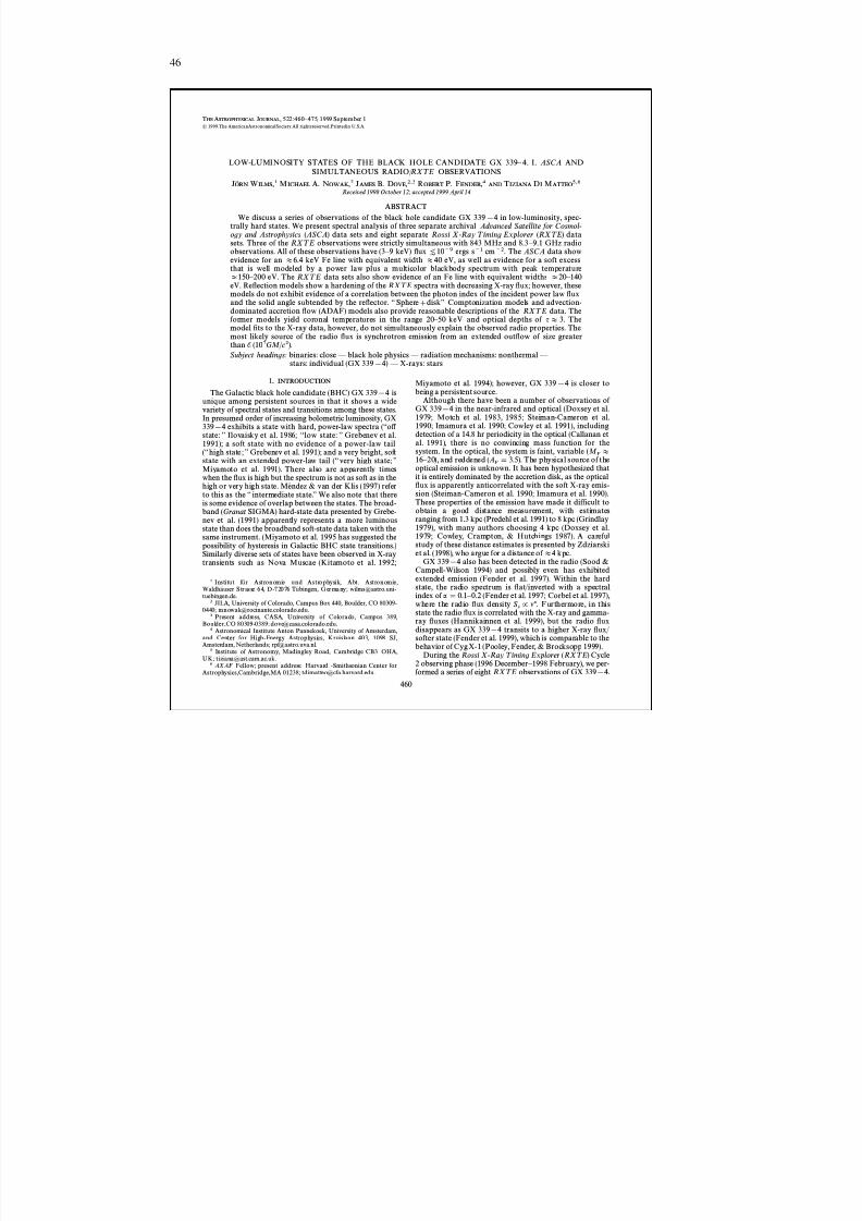
8/12/2019 Schwarze LöCher Als Astronomische Objekte
http://slidepdf.com/reader/full/schwarze-lacher-als-astronomische-objekte 46/146
46
THE ASTROPHYSICAL JOURNAL , 522:460 È 475, 1999 September 11999.The AmericanAstronomicalSociety.All rightsreserved.Printedin U.S.A.(
LOW-LUMINOSITY STATES OF THE BLACK HOLE CANDIDATE GX 339 [ 4. I. ASCA ANDSIMULTANEOUS RADIO/ RXT E OBSERVATIONS
JO RN W ILMS ,1 M ICHAEL A. N OWAK ,2 J AMES B. DOVE ,2,3 R OBERT P. F ENDER ,4 AND T IZIANA D I M ATTEO 5,6Received 1998 October 12; accepted 1999 April 14
ABSTRACTWe discuss a series of observations of the black hole candidate GX 339 [ 4 in low-luminosity, spec-
trally hard states. We present spectral analysis of three separate archival Advanced Satellite for Cosmol -ogy and Astrophysics (ASCA ) data sets and eight separate Rossi X -Ray T iming Explorer (RXT E ) datasets. Three of the RXT E observations were strictly simultaneous with 843 MHz and 8.3 È 9.1 GHz radioobservations. All of these observations have (3 È 9 keV) Ñux ergs s~1 cm ~2 . The ASCA data show[ 10~9evidence for an B 6.4 keV Fe line with equivalent width B 40 eV, as well as evidence for a soft excessthat is well modeled by a power law plus a multicolor blackbody spectrum with peak temperatureB 150 È 200 eV. The RXT E data sets also show evidence of an Fe line with equivalent widths B 20 È 140eV. ReÑection models show a hardening of the RXT E spectra with decreasing X-ray Ñux; however, thesemodels do not exhibit evidence of a correlation between the photon index of the incident power law Ñuxand the solid angle subtended by the reÑector. ““ Sphere ] diskÏÏ Comptonization models and advection-dominated accretion Ñow (ADAF) models also provide reasonable descriptions of the RXT E data. Theformer models yield coronal temperatures in the range 20 È 50 keV and optical depths of q B 3. Themodel Ðts to the X-ray data, however, do not simultaneously explain the observed radio properties. Themost likely source of the radio Ñux is synchrotron emission from an extended outÑow of size greaterthan O (107GM / c2).Subject headings: binaries: close È black hole physics È radiation mechanisms: nonthermal È
stars: individual (GX 339 [ 4) È X-rays: stars
1. INTRODUCTION
The Galactic black hole candidate (BHC) GX 339 [ 4 isunique among persistent sources in that it shows a widevariety of spectral states and transitions among these states.In presumed order of increasing bolometric luminosity, GX339[ 4 exhibits a state with hard, power-law spectra (““o† state: ÏÏ Ilovaisky et al. 1986; ““low state: ÏÏ Grebenev et al.1991); a soft state with no evidence of a power-law tail
(““ high state ; ÏÏ Grebenev et al. 1991); and a very bright, softstate with an extended power-law tail (““ very high state; ÏÏMiyamoto et al. 1991). There also are apparently timeswhen the Ñux is high but the spectrum is not as soft as in thehigh or very high state. & van der Klis (1997) referMe ndezto this as the ““ intermediate state.ÏÏ We also note that thereis some evidence of overlap between the states. The broad-band ( Granat SIGMA) hard-state data presented by Grebe-nev et al. (1991) apparently represents a more luminousstate than does the broadband soft-state data taken with thesame instrument. (Miyamoto et al. 1995 has suggested thepossibility of hysteresis in Galactic BHC state transitions.)Similarly diverse sets of states have been observed in X-raytransients such as Nova Muscae (Kitamoto et al. 1992;
1 Institut Astronomie und Astrophysik, Abt. Astronomie,fu rS trasse 64, D-72076 Germany;Waldha user Tu bingen, wilms = astro.uni-
tuebingen.de.
2 JILA, University of Colorado, Campus Box 440, Boulder, CO 80309-0440; mnowak = rocinante.colorado.edu.3 Present address, CASA, University of Colorado, Campus 389,
Boulder,CO 80309-0389; dove = casa.colorado.edu.4 Astronomical Institute Anton Pannekoek, University of Amsterdam,
and Center for High-Energy Astrophysics, Kruislaan 403, 1098 SJ,Amsterdam, Netherlands; rpf = astro.uva.nl.
5 Institute of Astronomy, Madingley Road, Cambridge CB3 OHA,UK; tiziana = ast.cam.ac.uk.
6 AXAF Fellow; present address: Harvard -Smithsonian Center forAstrophysics,Cambridge,MA 01238; tdimatteo = cfa.harvard.edu.
Miyamoto et al. 1994); however, GX 339 [ 4 is closer tobeing a persistent source.
Although there have been a number of observations of GX 339 [ 4 in the near-infrared and optical (Doxsey et al.1979; Motch et al. 1983, 1985; Steiman-Cameron et al.1990; Imamura et al. 1990; Cowley et al. 1991), includingdetection of a 14.8 hr periodicity in the optical (Callanan etal. 1991), there is no convincing mass function for the
system. In the optical, the system is faint, variable ( M V B
16 È 20), and reddened The physical source of the(AV \ 3.5).optical emission is unknown. It has been hypothesized thatit is entirely dominated by the accretion disk, as the opticalÑux is apparently anticorrelated with the soft X-ray emis-sion (Steiman-Cameron et al. 1990; Imamura et al. 1990).These properties of the emission have made it difficult toobtain a good distance measurement, with estimatesranging from 1.3 kpc (Predehl et al. 1991) to 8 kpc (Grindlay1979), with many authors choosing 4 kpc (Doxsey et al.1979; Cowley, Crampton, & Hutchings 1987). A carefulstudy of these distance estimates is presented by Zdziarskiet al. (1998), who argue for a distance of B 4 kpc.
GX 339 [ 4 also has been detected in the radio (Sood &Campell-Wilson 1994) and possibly even has exhibitedextended emission (Fender et al. 1997). Within the hardstate, the radio spectrum is Ñat/inverted with a spectralindex of a \ 0.1 È 0.2 (Fender et al. 1997; Corbel et al. 1997),where the radio Ñux density Furthermore, in thisSl P l a.state the radio Ñux is correlated with the X-ray and gamma-ray Ñuxes (Hannikainnen et al. 1999), but the radio Ñuxdisappears as GX 339 [ 4 transits to a higher X-ray Ñux/ softer state (Fender et al. 1999), which is comparable to thebehavior of Cyg X-1 (Pooley, Fender, & Brocksopp 1999).
During the Rossi X -Ray T iming Explorer (RXT E ) Cycle2 observing phase (1996 December È 1998 February), we per-formed a series of eight RXT E observations of GX 339 [ 4.
460
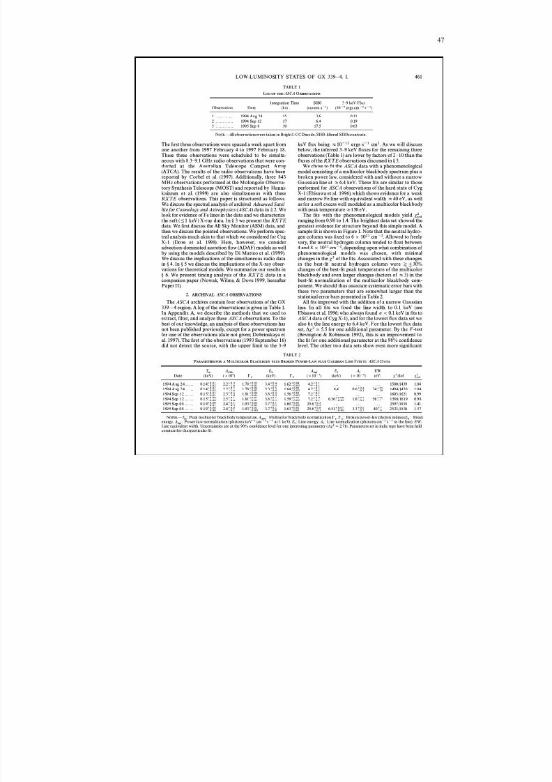
8/12/2019 Schwarze LöCher Als Astronomische Objekte
http://slidepdf.com/reader/full/schwarze-lacher-als-astronomische-objekte 47/146
47
LOW-LUMINOSITY STATES OF GX 339 [ 4. I. 461
TABLE 1
LOG OF THE ASCA O BSERVATIONS
Integration Time SIS0 3 È 9 keV FluxObservation Date (ks) (counts s ~1) (10~9 ergs cm ~2 s~1)
1 . . . . . . . . . . . . 1994 Aug 24 15 3.6 0.112 . . . . . . . . . . . . 1994 Sep 12 17 6.4 0.193 . . . . . . . . . . . . 1995 Sep 8 30 17.5 0.63
N OTE .ÈAllobservationswere taken in Bright1-CCDmode. SIS0: Ðltered SIS0countrate.
The Ðrst three observations were spaced a week apart fromone another from 1997 February 4 to 1997 February 18.These three observations were scheduled to be simulta-neous with 8.3 È 9.1 GHz radio observations that were con-ducted at the Australian Telescope Compact Array(ATCA). The results of the radio observations have beenreported by Corbel et al. (1997). Additionally, three 843MHz observations performed at the Molongolo Observa-tory Synthesis Telescope (MOST) and reported by Hanni-kainnen et al. (1999) are also simultaneous with theseRXT E observations. This paper is structured as follows.We discuss the spectral analysis of archival Advanced Satel -lite for Cosmology and Astrophysics (ASCA ) data in ° 2. Welook for evidence of Fe lines in the data and we characterizethe soft keV) X-ray data. In ° 3 we present the RXT E([ 1data. We Ðrst discuss the All Sky Monitor (ASM) data, andthen we discuss the pointed observations. We perform spec-tral analysis much akin to that which we considered for CygX-1 (Dove et al. 1998). Here, however, we consideradvection-dominated accretion Ñow (ADAF) models as wellby using the models described by Di Matteo et al. (1999).We discuss the implications of the simultaneous radio datain ° 4. In ° 5 we discuss the implications of the X-ray obser-vations for theoretical models. We summarize our results in° 6. We present timing analysis of the RXT E data in acompanion paper (Nowak, Wilms, & Dove 1999, hereafterPaper II).
2. ARCHIVAL ASCA OBSERVATIONS
The ASCA archives contain four observations of the GX339[ 4 region. A log of the observations is given in Table 1.In Appendix A, we describe the methods that we used toextract, Ðlter, and analyze these ASCA observations. To thebest of our knowledge, an analysis of these observations hasnot been published previously, except for a power spectrumfor one of the observations (date not given; Dobrinskaya etal. 1997). The Ðrst of the observations (1993 September 16)did not detect the source, with the upper limit to the 3 È 9
keV Ñux being B 10~12 ergs s~1 cm2. As we will discussbelow, the inferred 3 È 9 keV Ñuxes for the remaining threeobservations (Table 1) are lower by factors of 2 È 10 than theÑuxes of the RXT E observations discussed in ° 3.
We chose to Ðt the ASCA data with a phenomenologicalmodel consisting of a multicolor blackbody spectrum plus abroken power law, considered with and without a narrowGaussian line at B 6.4 keV. These Ðts are similar to thoseperformed for ASCA observations of the hard state of CygX-1 (Ebisawa et al. 1996), which shows evidence for a weakand narrow Fe line with equivalent width B 40 eV, as wellas for a soft excess well modeled as a multicolor blackbodywith peak temperature B 150 eV.
The Ðts with the phenomenological models yield sred2ranging from 0.98 to 1.4. The brightest data set showed thegreatest evidence for structure beyond this simple model. Asample Ðt is shown in Figure 1. Note that the neutral hydro-gen column was Ðxed to 6 ] 1021 cm~2 . Allowed to freelyvary, the neutral hydrogen column tended to Ñoat between4 and 8 ] 1021 cm~2 , depending upon what combination of phenomenological models was chosen, with minimalchanges in the s 2 of the Ðts. Associated with these changesin the best-Ðt neutral hydrogen column were Z ^ 30%changes of the best-Ðt peak temperature of the multicolorblackbody and even larger changes (factors of B 3) in thebest-Ðt normalization of the multicolor blackbody com-ponent. We should thus associate systematic error bars withthese two parameters that are somewhat larger than thestatistical error bars presented in Table 2.
All Ðts improved with the addition of a narrow Gaussianline. In all Ðts we Ðxed the line width to 0.1 keV (seeEbisawa et al. 1996; who always found p \ 0.1 keV in Ðts toASCA data of Cyg X-1), and for the lowest Ñux data set wealso Ðx the line energy to 6.4 keV. For the lowest Ñux dataset, *s 2 \ 5.5 for one additional parameter. By the F -test(Bevington & Robinson 1992), this is an improvement tothe Ðt for one additional parameter at the 98% conÐdencelevel. The other two data sets show even more signiÐcant
TABLE 2
P ARAMETERS FOR A M ULTICOLOR BLACKBODY PLUS BROKEN P OWER -L AW PLUS G AUSSIAN L INE F ITS TO ASCA D ATA
T in Adbb Eb Abpl El Al EWDate (keV) ( ] 104) ! 1 (keV) ! 2 (] 10~2) (keV) (] 10~4 ) (eV) s2 /dof s red2
1994 Aug 24 . . . . . . 0 .14~0.02
` 0.01 2.2~1.6
` 0.9 1.78~0.03
` 0.03 3.4~0.5
` 0.4 1.62~0.03
` 0.04 4.2~0.1
` 0.1 . . . . . . . . . 1500/1439 1.041994 Aug 24 . . . . . . 0 .14~0.02
` 0.01 2.2~1.6` 0.7 1.78~0.03
` 0.03 3.3~0.6` 0.5 1.64~0.03
` 0.03 4.2~0.1` 0.1 6.4 0.6~0.3
` 0.4 34~19` 25 1494/1438 1.04
1994 Sep 12 . . . . . . 0 .15~0.01` 0.01 2.5~1.0
` 0.6 1.81~0.01` 0.02 3.8~0.2
` 0.2 1.56~0.03` 0.03 7.2~0.1
` 0.1 . . . . . . . . . 1603/1621 0.991994 Sep 12 . . . . . . 0 .15~0.00
` 0.00 2.5~0.4` 0.1 1.81~0.01
` 0.01 3.8~0.1` 0.1 1.59~0.02
` 0.01 7.2~0.1` 0.0 6.36~0.09
` 0.08 1.6~0.2` 0.7 56~7
` 26 1580/1619 0.981995 Sep 08 . . . . . . 0 .19~0.01
` 0.00 2.4~0.3` 0.1 1.93~0.01
` 0.02 3.7~0.1` 0.1 1.60~0.02
` 0.01 25.6~0.3` 0.3 . . . . . . . . . 2597/1838 1.41
1995 Sep 08 . . . . . . 0 .19~0.00` 0.00 2.4~0.1
` 0.0 1.93~0.00` 0.01 3.7~0.0
` 0.1 1.63~0.01` 0.01 25.6~0.1
` 0.0 6.51~0.06` 0.07 3.3~0.5
` 0.6 40~6` 7 2523/1836 1.37
Peak multicolor blackbody temperature. Multicolor blackbody normalization. Broken power-law photon indexes. BreakN OTES .È T in: Adbb: ! 1, ! 2: Eb:energy. Power-law normalization (photons keV ~1 cm~2 s~1 at 1 keV). Line energy. Line normalization (photons cm ~2 s~1 in the line). EW:Abpl: El : Al :Line equivalent width. Uncertainties are at the 90% conÐdence level for one interesting parameter ( *s 2 \ 2.71). Parameters set in italic type have been heldconstantfor thatparticular Ðt.
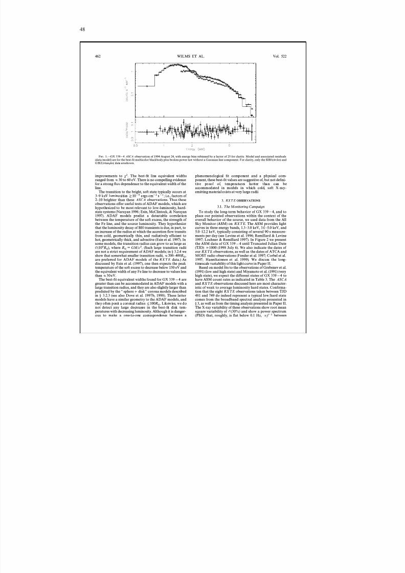
8/12/2019 Schwarze LöCher Als Astronomische Objekte
http://slidepdf.com/reader/full/schwarze-lacher-als-astronomische-objekte 48/146
48
462 WILMS ET AL. Vol. 522
F IG . 1.ÈGX 339 [ 4 ASCA observation of 1994 August 24, with energy bins rebinned by a factor of 25 for clarity. Model and associated residuals(data/model) are for the best-Ðt multicolor blackbody plus broken power law without a Gaussian line component. For clarity, only the SIS0 ( circles ) andGIS2( triangles ) data areshown.
improvements to s 2. The best-Ðt line equivalent widthsranged from B 30 to 60 eV. There is no compelling evidencefor a strong Ñux dependence to the equivalent width of theline.
The transition to the bright, soft state typically occurs at3 È 9 keV luminosities ergs cm ~2 s~1 ; i.e., factors of Z 10~92 È 10 brighter than these ASCA observations. Thus theseobservations o†er useful tests of ADAF models, which arehypothesized to be most relevant to low-luminosity, hard-
state systems (Narayan 1996 ; Esin, McClintock, & Narayan1997). ADAF models predict a detectable correlationbetween the temperature of the soft excess, the strength of the Fe line, and the source luminosity. They hypothesizethat the luminosity decay of BH transients is due, in part, toan increase of the radius at which the accretion Ñow transitsfrom cold, geometrically thin, and radiatively efficient tohot, geometrically thick, and advective (Esin et al. 1997). Insome models, the transition radius can grow to as large as
where (Such large transition radiiO (104RG ), RG 4 GM / c2.are not a strict requirement of ADAF models; in ° 3.2.4 weshow that somewhat smaller transition radii, B 200 È 400R G ,are preferred for ADAF models of the RXT E data.) Asdiscussed by Esin et al. (1997), one then expects the peaktemperature of the soft excess to decrease below 150 eV andthe equivalent width of any Fe line to decrease to values lessthan B 30 eV.
The best-Ðt equivalent widths found for GX 339 [ 4 aregreater than can be accommodated in ADAF models with alarge transition radius, and they are also slightly larger thanpredicted by the ““ sphere ] diskÏÏ corona models describedin ° 3.2.3 (see also Dove et al. 1997b, 1998). These lattermodels have a similar geometry to the ADAF models, andthey often posit a coronal radius Likewise, we do[ 100RG .not detect any large decreases in the best-Ðt disk tem-peratures with decreasing luminosity. Although it is danger-ous to make a one-to-one correspondence between a
phenomenological Ðt component and a physical com-ponent, these best-Ðt values are suggestive of, but not deÐni-t ive proof of, temperatures hotter than can beaccommodated in models in which cold, soft X-ray È emitting material exists at very large radii.
3. RXT E OBSERVATIONS
3.1. T he Monitoring Campaign
To study the long-term behavior of GX 339 [ 4, and toplace our pointed observations within the context of theoverall behavior of the source, we used data from the AllSky Monitor (ASM) on RXT E . The ASM provides lightcurves in three energy bands, 1.3 È 3.0 keV, 3.0 È 5.0 keV, and5.0 È 12.2 keV, typically consisting of several 90 s measure-ments per day (see Levine et al. 1996; Remillard & Levine1997; Lochner & Remillard 1997). In Figure 2 we presentthe ASM data of GX 339 [ 4 until Truncated Julian Date(TJD) B 1000 (1998 July 6). We also indicate the dates of our RXT E observations, as well as the dates of ATCA andMOST radio observations (Fender et al. 1997; Corbel et al.1997; Hannikainnen et al. 1999). We discuss the long-timescale variability of this light curve in Paper II.
Based on model Ðts to the observations of Grebenev et al.(1991) (low and high state) and Miyamoto et al. (1991) (veryhigh state), we expect the di†erent states of GX 339 [ 4 tohave ASM count rates as indicated in Table 3. The ASCAand RXT E observations discussed here are most character-istic of weak to average luminosity hard states. ConÐrma-tion that the eight RXT E observations taken between TJD481 and 749 do indeed represent a typical low/hard statecomes from the broadband spectral analysis presented in° 3, as well as from the timing analysis presented in Paper II.The X-ray variability of these observations show root meansquare variability of O (30%) and show a power spectrum(PSD) that, roughly, is Ñat below 0.1 Hz, P f ~1 between
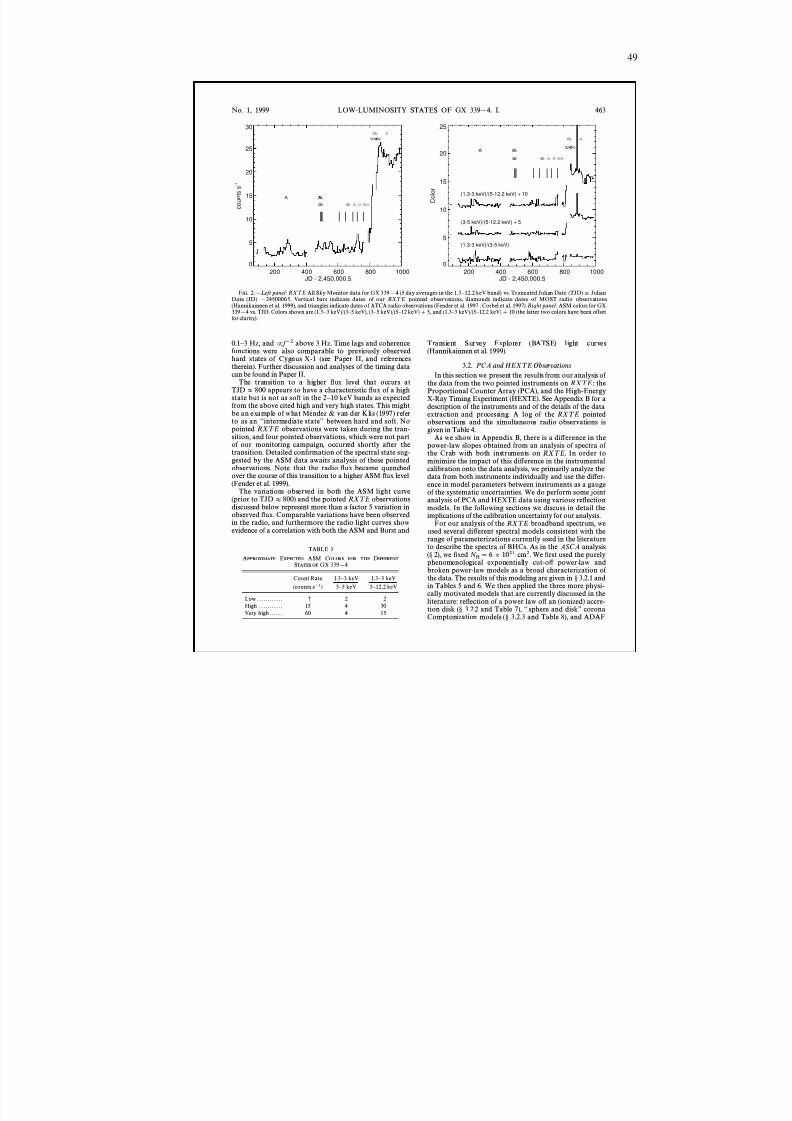
8/12/2019 Schwarze LöCher Als Astronomische Objekte
http://slidepdf.com/reader/full/schwarze-lacher-als-astronomische-objekte 49/146
49
200 400 600 800 1000JD - 2,450,000.5
0
5
10
15
20
25
30
c o u n
t s s
- 1
||| | | | | |
200 400 600 800 1000JD - 2,450,000.5
0
5
10
15
20
25
C o
l o r
(1.3-3 keV)/(3-5 keV)
(3-5 keV)/(5-12.2 keV) + 5
(1.3-3 keV)/(5-12.2 keV) + 10
||| | | | | |
No. 1, 1999 LOW-LUMINOSITY STATES OF GX 339 [ 4. I. 463
F IG . 2.È L eft panel: RXT E All Sky Monitor data for GX 339 [ 4 (5 day averages in the 1.3 È 12.2 keV band) vs. Truncated Julian Date (TJD) 4 JulianDate (JD) [ 2450000.5. Vertical bars indicate dates of our RXT E pointed observations, diamonds indicate dates of MOST radio observations(Hannikainnen et al. 1999), and triangles indicate dates o f ATCA radio observations (Fender et al. 1997 ; Corbel et al. 1997). Right panel: ASM colors for GX339[ 4 vs. TJD. Colors shown are (1.3 È 3 keV)/(3 È 5 keV), (3 È 5 keV)/(5 È 12 keV) ] 5, and (1.3 È 3 keV)/(5 È 12.2 keV) ] 10 (the latter two colors have been o†setfor clarity).
0.1 È 3 Hz, and P f ~2 above 3 Hz. Time lags and coherencefunctions were also comparable to previously observedhard states of Cygnus X-1 (see Paper II, and referencestherein). Further discussion and analyses of the timing datacan be found in Paper II.
The transition to a higher Ñux level that occurs atTJD B 800 appears to have a characteristic Ñux of a highstate but is not as soft in the 2 È 10 keV bands as expectedfrom the above cited high and very high states. This might
be an example of what & van der Klis (1997) referMe ndezto as an ““intermediate stateÏÏ between hard and soft. Nopointed RXT E observations were taken during the tran-sition, and four pointed observations, which were not partof our monitoring campaign, occurred shortly after thetransition. Detailed conÐrmation of the spectral state sug-gested by the ASM data awaits analysis of these pointedobservations. Note that the radio Ñux became quenchedover the course of this transition to a higher ASM Ñux level(Fender et al. 1999).
The variations observed in both the ASM light curve(prior to TJD B 800) and the pointed RXT E observationsdiscussed below represent more than a factor 5 variation inobserved Ñux. Comparable variations have been observedin the radio, and furthermore the radio light curves showevidence of a correlation with both the ASM and Burst and
TABLE 3
APPROXIMATE EXPECTED ASM C OLORS FOR THE D IFFERENT
STATES OF GX 339 [ 4
Count Rate(counts s ~1 )
1.3 È 3 keV3 È 5 keV
1.3 È 3 keV5 È 12.2 keV
Low . . . . . . . . . . . . 7 2 2High . . . . . . . . . . . 15 4 30Very high . . . . . . 60 4 15
Transient Survey Explorer (BATSE) light curves(Hannikainnen et al. 1999).
3.2. PCA and HEXT E ObservationsIn this section we present the results from our analysis of
the data from the two pointed instruments on RXT E : theProportional Counter Array (PCA), and the High-EnergyX-Ray Timing Experiment (HEXTE). See Appendix B for adescription of the instruments and of the details of the data
extraction and processing. A log of the RXT E pointedobservations and the simultaneous radio observations isgiven in Table 4.
As we show in Appendix B, there is a di†erence in thepower-law slopes obtained from an analysis of spectra of the Crab with both instruments on RXT E . In order tominimize the impact of this di†erence in the instrumentalcalibration onto the data analysis, we primarily analyze thedata from both instruments individually and use the di†er-ence in model parameters between instruments as a gaugeof the systematic uncertainties. We do perform some jointanalysis of PCA and HEXTE data using various reÑectionmodels. In the following sections we discuss in detail theimplications of the calibration uncertainty for our analysis.
For our analysis of the RXT E broadband spectrum, weused several di†erent spectral models consistent with therange of parameterizations currently used in the literatureto describe the spectra of BHCs. As in the ASCA analysis(° 2), we Ðxed cm2. We Ðrst used the purelyN H\ 6 ] 1021phenomenological exponentially cut-o† power-law andbroken power-law models as a broad characterization of the data. The results of this modeling are given in ° 3.2.1 andin Tables 5 and 6. We then applied the three more physi-cally motivated models that are currently discussed in theliterature: reÑection of a power law o† an (ionized) accre-tion disk ( ° 3.2.2 and Table 7), ““ sphere and diskÏÏ coronaComptonization models ( ° 3.2.3 and Table 8), and ADAF
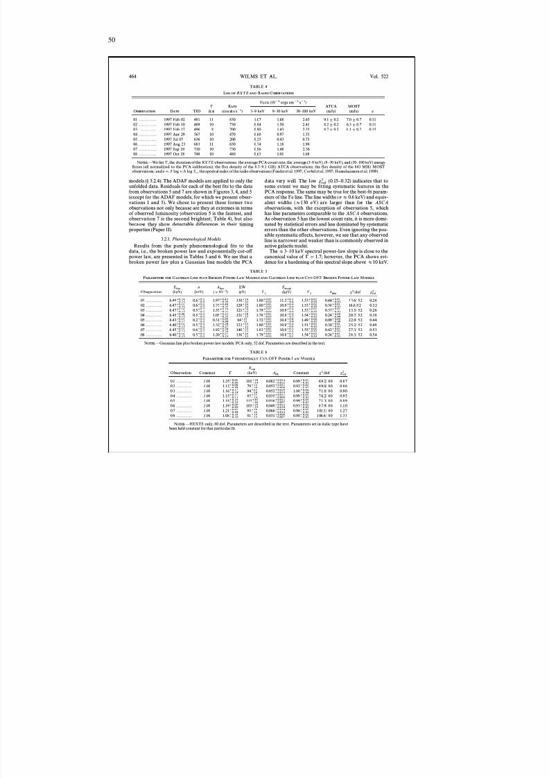
8/12/2019 Schwarze LöCher Als Astronomische Objekte
http://slidepdf.com/reader/full/schwarze-lacher-als-astronomische-objekte 50/146
50
464 WILMS ET AL. Vol. 522
TABLE 4
LOG OF RXT E AND R ADIO O BSERVATIONS
F LUX (10~9 ergs cm ~2 s~1)T RATE ATCA MOST
O BSERVATION DATE TJD (k s) (cou nt s s ~1) 3 È 9 keV 9 È 30 keV 30 È 100 keV (mJy) (mJy) a
01 . . . . . . . . . . . . 1997 Feb 02 481 11 830 1.07 1.68 2.65 9.1 ^ 0.2 7.0 ^ 0.7 0.1102 . . . . . . . . . . . . 1997 Feb 10 489 10 730 0.94 1.50 2.41 8.2 ^ 0.2 6.3 ^ 0.7 0.1103 . . . . . . . . . . . . 1997 Feb 17 496 8 700 0.90 1.43 2.35 8.7^ 0.2 6.1 ^ 0.7 0.1504 . . . . . . . . . . . . 1997 Apr 29 567 10 470 0.60 0.97 1.5505 . . . . . . . . . . . . 1997 Jul 07 636 10 200 0.25 0.43 0.7506 . . . . . . . . . . . . 1997 Aug 23 683 11 650 0.74 1.18 1.9807 . . . . . . . . . . . . 1997 Sep 19 710 10 730 0.96 1.48 2.3608 . . . . . . . . . . . . 1997 Oct 28 749 10 480 0.63 1.01 1.68
N OTES .ÈWe list T , the duration of the RXT E observations; the average PCA count rate; the average (3 È 9 keV), (9 È 30 keV), and (30 È 100 keV) energyÑuxes (all normalized to the PCA calibration); the Ñux density of the 8.3 È 9.1 GHz ATCA observations; the Ñux density of the 843 MHz MOSTobservations; and the spectral index of the radio observations (Fender et al. 1997; Corbel et al. 1997; Hannikainnen et al. 1999).a \ * log l / * log S
l,
models ( ° 3.2.4). The ADAF models are applied to only theunfolded data. Residuals for each of the best Ðts to the data
from observations 5 and 7 are shown in Figures 3, 4, and 5(except for the ADAF models, for which we present obser-vations 1 and 5). We chose to present these former twoobservations not only because are they at extremes in termsof observed luminosity (observation 5 is the faintest, andobservation 7 is the second brightest; Table 4), but alsobecause they show detectable di†erences in their timingproperties (Paper II).
3.2.1. Phenomenological Models
Results from the purely phenomenological Ðts to thedata, i.e., the broken power law and exponentially cut-o† power law, are presented in Tables 5 and 6. We see that abroken power law plus a Gaussian line models the PCA
data very well. The low (0.15 È 0.32) indicates that tos red2some extent we may be Ðtting systematic features in the
PCA response. The same may be true for the best-Ðt param-eters of the Fe line. The line widths ( p B 0.6 keV) and equiv-alent widths ( B 130 eV) are larger than for the ASCAobservations, with the exception of observation 5, whichhas line parameters comparable to the ASCA observations.As observation 5 has the lowest count rate, it is more domi-nated by statistical errors and less dominated by systematicerrors than the other observations. Even ignoring the pos-sible systematic e†ects, however, we see that any observedline is narrower and weaker than is commonly observed inactive galactic nuclei.
The B 3 È 10 keV spectral power-law slope is close to thecanonical value of ! \ 1.7; however, the PCA shows evi-dence for a hardening of this spectral slope above B 10 keV.
TABLE 5
P ARAMETERS FOR G AUSSIAN L INE PLUS BROKEN P OWER -L AW M ODELS AND G AUSSIAN L INE PLUS C UT -OFF B ROKEN P OWER -L AW M ODELS
E line p Aline EW EbreakObservation (keV) (keV) ( ] 10~3) (eV) ! 1 (keV) ! 2 Abkn s2 /dof s red2
01 . . . . . . . . . . . 6.48~0.15` 0.14 0.6~0.2
` 0.2 1.97~0.36` 0.42 130~22
` 24 1.80~0.01` 0.01 11.2~0.4
` 0.3 1.53~0.02` 0.02 0.44~0.01
` 0.01 13.6/ 52 0.2602 . . . . . . . . . . . 6.47~0.16
` 0.15 0.6~0.2` 0.2 1.73~0.35
` 0.40 129~24` 26 1.80~0.01
` 0.01 10.9~0.4` 0.4 1.53~0.02
` 0.02 0.38~0.01` 0.01 16 .6 /52 0 .32
03 . . . . . . . . . . . 6.47~0.15` 0.14 0.5~0.2
` 0.2 1.55~0.31` 0.29 121~23
` 24 1.79~0.01` 0.01 10.9~0.4
` 0.4 1.53~0.03` 0.02 0.37~0.01
` 0.01 13.5/ 52 0.2604 . . . . . . . . . . . 6.45~0.15
` 0.08 0.5~0.2` 0.2 1.05~0.22
` 0.25 121~23` 28 1.78~0.01
` 0.01 10.8~0.5` 0.4 1.54~0.03
` 0.03 0.24~0.00` 0.00 20.7/ 52 0.38
05 . . . . . . . . . . . 6.43~0.17` 0.15 0.2~0.2
` 0.3 0.31~0.08` 0.09 84~21
` 25 1.72~0.01` 0.01 10.8~0.8
` 0.8 1.49~0.05` 0.04 0.09~0.00
` 0.00 22.9/ 52 0.4406 . . . . . . . . . . . 6.40~0.15
` 0.14 0.5~0.2` 0.2 1.32~0.27
` 0.28 123~23` 23 1.80~0.01
` 0.01 10.9~0.4` 0.4 1.51~0.03
` 0.03 0.30~0.01` 0.01 25.2/ 52 0.48
07 . . . . . . . . . . . 6.45~0.13` 0.13 0.6~0.2
` 0.2 1.92~0.34` 0.38 140~23
` 23 1.83~0.01` 0.01 10.9~0.4
` 0.3 1.55~0.02` 0.02 0.42~0.01
` 0.01 27.3/ 52 0.5308 . . . . . . . . . . . 6.40~0.15
` 0.14 0.5~0.2` 0.2 1.20~0.23
` 0.27 130~23` 26 1.79~0.01
` 0.01 10.8~0.5` 0.5 1.54~0.03
` 0.03 0.26~0.01` 0.01 28.3/ 52 0.54
N OTES .ÈGaussian line plus broken power-law models: PCA only, 52 dof. Parameters are described in the text.
TABLE 6
P ARAMETERS FOR E XPONENTIALLY C UT -OFF P OWER -L AW M ODELS
EcutObservation Constant ! (keV) APL Constant s2 /dof s red
2
0 1 . . . . . . . . . . . 1.00 1.25~0.06
` 0.06 101~14
` 18 0.082~0.012
` 0.014 0.99~0.01
` 0.01 69.2/ 80 0 .870 2 . . . . . . . . . . . 1.00 1.12~0.08
` 0.08 79~10` 13 0.052~0.009
` 0.011 0.92~0.02` 0.02 69.0/ 80 0 .86
0 3 . . . . . . . . . . . 1.00 1.16~0.18` 0.17 94~28
` 63 0.052~0.019` 0.029 1.08~0.04
` 0.04 71.8/ 80 0 .900 4 . . . . . . . . . . . 1.00 1.15~0.11
` 0.11 85~16` 25 0.035~0.009
` 0.011 0.98~0.02` 0.02 76.2/ 80 0 .95
0 5 . . . . . . . . . . . 1.00 1.18~0.23` 0.19 115~46
` 85 0.016~0.007` 0.011 0.99~0.05
` 0.05 71.3/ 80 0 .890 6 . . . . . . . . . . . 1.00 1.19~0.09
` 0.09 103~19` 29 0.049~0.010
` 0.012 0.93~0.02` 0.02 87.9/ 80 1 .10
0 7 . . . . . . . . . . . 1.00 1.21~0.08` 0.07 95~14
` 20 0.066~0.012` 0.014 0.96~0.02
` 0.02 101.5/ 80 1.270 8 . . . . . . . . . . . 1.00 1.08~0.10
` 0.10 81~13` 19 0.031~0.007
` 0.009 0.98~0.02` 0.02 106.6/ 80 1.33
N OTES .ÈHEXTE only, 80 dof. Parameters are described in the text. Parameters set in italic type havebeen held constant for that particular Ðt.
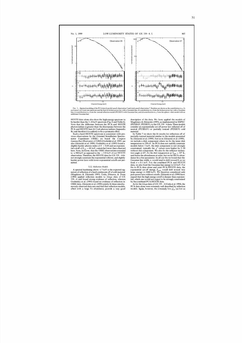
8/12/2019 Schwarze LöCher Als Astronomische Objekte
http://slidepdf.com/reader/full/schwarze-lacher-als-astronomische-objekte 51/146
51
1
10
n o r m a
l i z e d c o u n
t s / s e c / k e
V
Observation 05a)
-3-2-10123 b)
-3-2-10123 c)
-3-2-10123 d)
3 10 30Channel Energy [keV]
χ
10
100
n o r m a
l i z e d c o u n
t s / s e c / k e
V
Observation 07a)
-3-2-10123 b)
-3-2-10123 c)
-3-2-10123 d)
3 10 30Channel Energy [keV]
χ
No. 1, 1999 LOW-LUMINOSITY STATES OF GX 339 [ 4. I. 465
F IG . 3.ÈSpectral modeling of the PCA data from ( left panel ) observation 5 and ( right panel ) observation 7. Residues are shown as the contribution to s . Ineach panel: (a) Count rate spectrum and the best-Ðt broken power law with a Gaussian line, ( b) contribution to s from the broken power law with a Gaussianline, (c) contribution to s from the ionized reÑection model (PEXRIV) with Gaussian line, and ( d ) contribution to s from the sphere ] disk model with anadditional Gaussian line.
HEXTE data alone also show the high-energy spectrum tobe harder than the 3 È 10 keV spectrum (Fig. 4 and Table 6).Note that the di†erence between the PCA and HEXTE
photon indices is greater than the discrepancy between thePCA and HEXTE best-Ðt Crab photon indices (AppendixB), and therefore it is unlikely to be a systematic e†ect.
Such a hard HEXTE spectrum is consistent with pre-vious observations by the Oriented Scintillation Spectro-meter Experiment (OSSE) on board the ComptonGamma -Ray Observatory (CGRO ) (Grabelski et al. 1995; seealso Zdziarski et al. 1998). Grabelsky et al. (1995) found aslightly harder photon index of ! \ 0.88 and an exponen-tial cuto† of keV, somewhat lower than observedEcut
\ 68here. Note, however, that the OSSE observations extendedto B 500 keV as opposed to the D 110 keV of our HEXTEobservation. Therefore, the HEXTE data for GX 339 [ 4 donot strongly constrain the exponential rollover, and slightlyharder power laws with lower exponential cuto†s are per-mitted.
3.2.2. ReÑection Models
A spectral hardening above B 7 keV is the expected sig-nature of reÑection of a hard continuum o† of cold material(Magdziarz & Zdziarski 1995). Ueda, Ebisawa, & Done(1994) applied reÑection models to Ginga data of GX339[ 4 and found strong evidence of reÑection, whereasGrabelsky et al. (1995) found no evidence of reÑection inOSSE data. Zdziarski et al. (1998) jointly Ðt these simulta-neously observed data sets and Ðnd that reÑection models,albeit with a large Fe abundance, provide a very good
description of the data. We have applied the models of Magdziarz & Zdziarski (1995), as implemented in XSPEC(PEXRAV, PEXRIV), to the GX 339 [ 4 data. These models
consider an exponentially cut-o† power law reÑected o† of neutral (PEXRAV) or partially ionized (PEXRIV) coldmaterial.
In Table 7 we show the Ðt results for reÑection o† of partially ionized material similar to the models presentedby Zdziarski et al. (1998). Just as in Zdziarski et al. (1998),we include a disk component where we Ðx the inner disktemperature to 250 eV. As PCA does not usefully constrainmodels below 3 keV, the disk component is not stronglyconstrained; typically the s2 values were higher by 5 È 20without this component. We also Ðx the reÑector inclina-tion angle at 45¡, Ðx the disk temperature at K,T disk
\ 106and freeze the abundances at solar, but we let the Fe abun-dance be a free parameter. In all our Ðts we found that theGaussian line width, p , would tend to drift toward 0, so weÐxed p \ 0.1 keV. For the combined PCA and HEXTEdata, we also Ðxed the Gaussian line energy to 6.4 keV. ForÐts to PCA data alone and joint PCA/HEXTE data, theexponential cut-o† energy, would drift toward veryE fold,large energy ( ? 1000 keV). We therefore considered onlypure power laws without cuto†s. Zdziarski et al. (1998) haveargued that the high-energy cuto† is sharper than exponen-tial, which one would not expect to be strongly constrainedby the combined PCA/HEXTE data.
As for the Ginga data of GX 339 [ 4 (Ueda et al. 1994), thePCA data alone were extremely well described by reÑectionmodels. Again, however, the extremely low (as low ass red
2
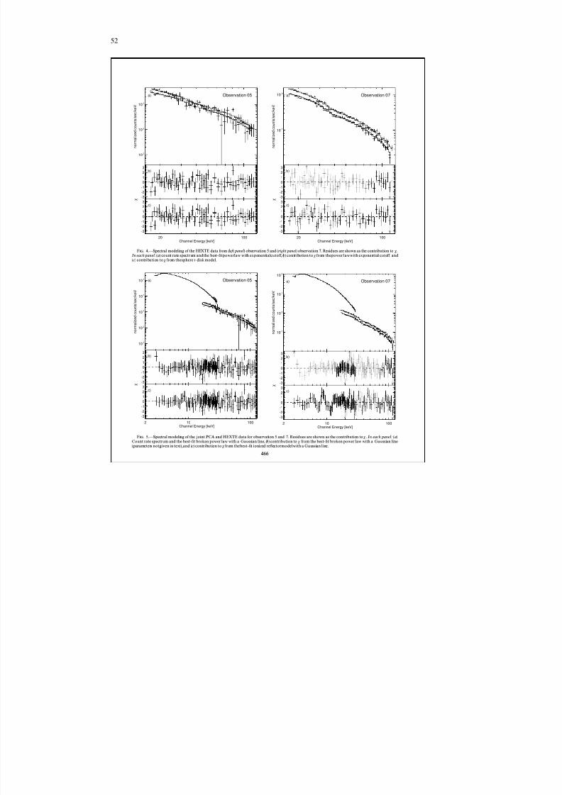
8/12/2019 Schwarze LöCher Als Astronomische Objekte
http://slidepdf.com/reader/full/schwarze-lacher-als-astronomische-objekte 52/146
52
10 -3
10 -2
10 -1
n o r m a
l i z e d c o u n
t s / s e c / k e
V
Observation 05a)
-3
-2-10123
b)
-3-2-10123
c)
20 100Channel Energy [keV]
χ
10 -1
10 0
n o r m a
l i z e d c o u n
t s / s e c / k e
V
Observation 07a)
-3
-2-10123
b)
-3-2-10123
c)
20 100Channel Energy [keV]
χ
10 -3
10 -2
10 -1
10 0
10 1
n o r m a
l i z e d c o u n
t s / s e c / k e
V
Observation 05a)
-3-2-10123
b)
-3-2-1012
3c)
2 10 100Channel Energy [keV]
χ
10 -1
10 0
10 1
10 2
n o r m a
l i z e d c o u n
t s / s e c / k e
V
Observation 07a)
-3-2-10123
b)
-3-2-1012
3c)
2 10 100Channel Energy [keV]
χ
F IG . 4.ÈSpectral modeling of the HEXTE data from ( left panel ) observation 5 and ( right panel ) observation 7. Residues are shown as the contribution to s .In each panel: (a) count rate spectrum andthe best-Ðtpowerlaw with exponentialcuto†, ( b) contribution to s from thepower lawwith exponential cuto†, and(c) contribution to s from thesphere ] disk model.
F IG . 5.ÈSpectral modeling of the joint PCA and HEXTE data for observation 5 and 7. Residues are shown as the contribution to s . In each panel: (a)Count rate spectrum and the best-Ðt broken power law with a Gaussian line, ( b) contribution to s from the best-Ðt broken power law with a Gaussian line(parameters notgiven in text),and ( c) contribution to s from thebest-Ðt ionized reÑectormodelwith a Gaussian line.
466
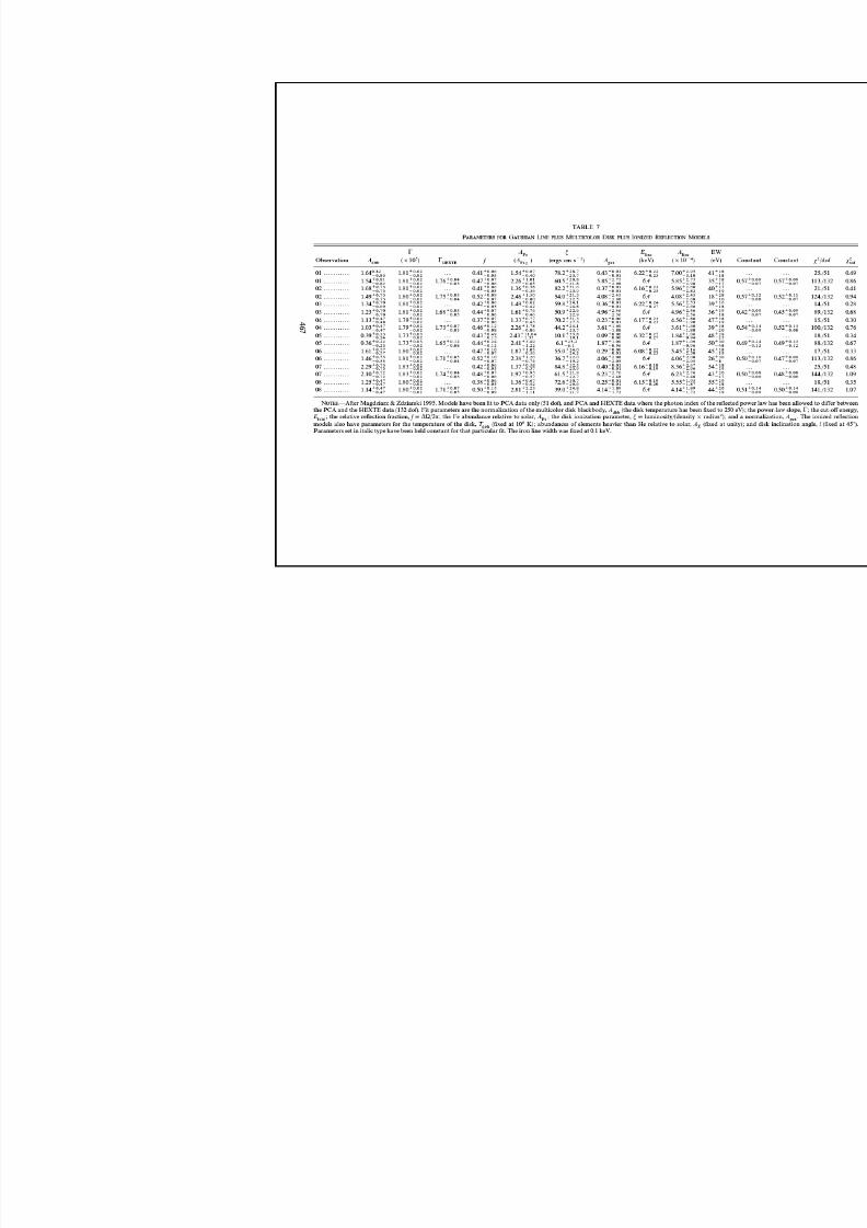
8/12/2019 Schwarze LöCher Als Astronomische Objekte
http://slidepdf.com/reader/full/schwarze-lacher-als-astronomische-objekte 53/146
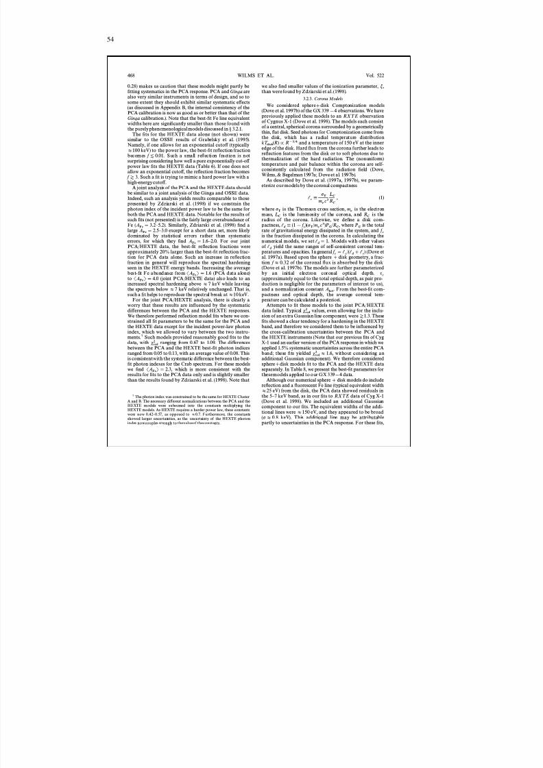
8/12/2019 Schwarze LöCher Als Astronomische Objekte
http://slidepdf.com/reader/full/schwarze-lacher-als-astronomische-objekte 54/146
54
468 WILMS ET AL. Vol. 522
0.28) makes us caution that these models might partly beÐtting systematics in the PCA response. PCA and Ginga arealso very similar instruments in terms of design, and so tosome extent they should exhibit similar systematic e†ects(as discussed in Appendix B, the internal consistency of thePCA calibration is now as good as or better than that of theGinga calibration.). Note that the best-Ðt Fe line equivalentwidths here are signiÐcantly smaller than those found withthe purely phenomenological models discussed in ° 3.2.1.
The Ðts for the HEXTE data alone (not shown) weresimilar to the OSSE results of Grabelsky et al. (1995).Namely, if one allows for an exponential cuto† (typicallyB 100 keV) to the power law, the best-Ðt reÑection fractionbecomes Such a small reÑection fraction is not f [ 0.01.surprising considering how well a pure exponentially cut-o† power law Ðts the HEXTE data (Table 6). If one does notallow an exponential cuto†, the reÑection fraction becomes
Such a Ðt is trying to mimic a hard power law with a f Z 3.high-energy cuto†.
A joint analysis of the PCA and the HEXTE data shouldbe similar to a joint analysis of the Ginga and OSSE data.Indeed, such an analysis yields results comparable to thosepresented by Zdziarski et al. (1998) if we constrain thephoton index of the incident power law to be the same forboth the PCA and HEXTE data. Notable for the results of such Ðts (not presented) is the fairly large overabundance of Fe Similarly, Zdziarski et al. (1998) Ðnd a(AFe
\ 3.2 È 5.2).large except for a short data set, more likelyAFe
\ 2.5 È 3.0dominated by statistical errors rather than systematicerrors, for which they Ðnd For our jointAFe
\ 1.6 È 2.0.PCA/HEXTE data, the best-Ðt reÑection fractions wereapproximately 20% larger than the best-Ðt reÑection frac-tion for PCA data alone. Such an increase in reÑectionfraction in general will reproduce the spectral hardeningseen in the HEXTE energy bands. Increasing the averagebest-Ðt Fe abundance from (PCA data alone)SAFeT \ 1.6to (joint PCA/HEXTE data) also leads to anSAFeT \ 4.0
increased spectral hardening above B 7 keV while leavingthe spectrum below B 7 keV relatively unchanged. That is,such a Ðt helps to reproduce the spectral break at B 10 keV.
For the joint PCA/HEXTE analysis, there is clearly aworry that these results are inÑuenced by the systematicdi†erences between the PCA and the HEXTE responses.We therefore performed reÑection model Ðts where we con-strained all Ðt parameters to be the same for the PCA andthe HEXTE data except for the incident power-law photonindex, which we allowed to vary between the two instru-ments. 7 Such models provided reasonably good Ðts to thedata, with ranging from 0.67 to 1.09. The di†erencess red
2between the PCA and the HEXTE best-Ðt photon indicesranged from 0.05 to 0.13, with an average value of 0.08. Thisis consistentwith the systematic di†erence between the best-Ðt photon indexes for the Crab spectrum. For these modelswe Ðnd which is more consistent with theSAFeT \ 2.3,results for Ðts to the PCA data only and is slightly smallerthan the results found by Zdziarski et al. (1998). Note that
7 The photon index was constrained to be the same for HEXTE ClusterA and B. The necessary di†erent normalizations between the PCA and theHEXTE models were subsumed into the constants multiplying theHEXTE models. As HEXTE requires a harder power law, these constantswere now 0.42 È 0.57, as opposed to B 0.7. Furthermore, the constantsshowed larger uncertainties, as the uncertainty of the HEXTE photonindex nowcouples strongly to thevalueof theconstants.
we also Ðnd smaller values of the ionization parameter, m,than were found by Zdziarski et al. (1998).
3.2.3. Corona Models
We considered sphere ] disk Comptonization models(Dove et al. 1997b) of the GX 339 [ 4 observations. We havepreviously applied these models to an RXT E observationof Cygnus X-1 (Dove et al. 1998). The models each consistof a central, spherical corona surrounded by a geometricallythin, Ñat disk. Seed photons for Comptonization come fromthe disk, which has a radial temperature distribution
and a temperature of 150 eV at the innerkT disk(R) P R~3@4edge of the disk. Hard Ñux from the corona further leads toreÑection features from the disk or to soft photons due tothermalization of the hard radiation. The (nonuniform)temperature and pair balance within the corona are self-consistently calculated from the radiation Ðeld (Dove,Wilms, & Begelman 1997a; Dove et al. 1997b).
As described by Dove et al. (1997a, 1997b), we param-eterize our models by the coronal compactness
l c 4pT
me c3L CR C
, (1)
where is the Thomson cross section, is the electronpT me
mass, is the luminosity of the corona, and is theL C RC
radius of the corona. Likewise, we deÐne a disk com-pactness, where is the totall d 4 (1 [ f c )(pT / me c3)P G / RC , P G
rate of gravitational energy dissipated in the system, and f cis the fraction dissipated in the corona. In calculating thenumerical models, we set Models with other valuesl d \ 1.of yield the same ranges of self-consistent coronal tem-l d
peratures and opac ities. In general (Dove et f c \ l c /(l d ] l c )al. 1997a). Based upon the sphere ] disk geometry, a frac-tion f B 0.32 of the coronal Ñux is absorbed by the disk(Dove et al. 1997b). The models are further parameterizedby an initial electron coronal optical depth, qc
(approximately equal to the total optical depth, as pair pro-
duction is negligible for the parameters of interest to us),and a normalization constant From the best-Ðt com-Akot.pactness and optical depth, the average coronal tem-perature can be calculated a posteriori.
Attempts to Ðt these models to the joint PCA/HEXTEdata failed. Typical values, even allowing for the inclu-s red
2sion of an extra Gaussian line component, were TheseZ 1.3.Ðts showed a clear tendency for a hardening in the HEXTEband, and therefore we considered them to be inÑuenced bythe cross-calibration uncertainties between the PCA andthe HEXTE instruments (Note that our previous Ðts of CygX-1 used an earlier version of the PCA response in which weapplied 1.5% systematic uncertainties across the entire PCAband; these Ðts yielded without considering ans red
2 B 1.6,additional Gaussian component). We therefore consideredsphere ] disk models Ðt to the PCA and the HEXTE dataseparately. In Table 8, we present the best-Ðt parameters forthesemodels applied to our GX 339 [ 4 data.
Although our numerical sphere ] disk models do includereÑection and a Ñuorescent Fe line (typical equivalent widthB 25 eV) from the disk, the PCA data showed residuals inthe 5 È 7 keV band, as in our Ðts to RXT E data of Cyg X-1(Dove et al. 1998). We included an additional Gaussiancomponent to our Ðts. The equivalent widths of the addi-tional lines were B 150 eV, and they appeared to be broad(p B 0.8 keV). This additional line may be attributablepartly to uncertainties in the PCA response. For these Ðts,
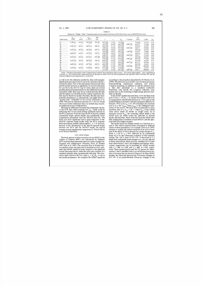
8/12/2019 Schwarze LöCher Als Astronomische Objekte
http://slidepdf.com/reader/full/schwarze-lacher-als-astronomische-objekte 55/146
55
No. 1, 1999 LOW-LUMINOSITY STATES OF GX 339 [ 4. I. 469
TABLE 8
M ODELS OF ““ SPHERE ] D ISK ÏÏ COMPTONIZATION PLUS G AUSSIAN L INE F ITS TO PCA D ATA O NLY AND TO HEXTE D ATA O NLY
ELine p ALine EW kT c
Observation (keV) (keV) ( ] 10~3 ) (eV) l c qc Akot Cons tant (keV) s2 /dof sred2
01 . . . . . . . . . . . 6.39~0.170.18 0.8~0.1
` 0.2 3.09~0.53` 0.60 197~30
` 30 0.62~0.04` 0.05 3.2~0.1
` 0.1 2.38~0.08` 0.06 . . . 28.6~0.4
` 0.4 19.2/53 0.3601 . . . . . . . . . . . . . . . . . . . . . . . 1.83~0.13
` 0.17 2.9~0.3` 0.5 0.91~0.09
` 0.09 0.99~0.01` 0.01 43.9~8
` 8 71.2/80 0.8902 . . . . . . . . . . . 6.36~0.19
` 0.19 0.8~0.1` 0.2 2.69~0.50
` 0.57 194~36` 41 0.63~0.05
` 0.06 3.3~0.1` 0.1 2.07~0.07
` 0.06 . . . 27.9~0.4` 0.4 15.7/53 0.30
02 . . . . . . . . . . . . . . . . . . . . . . . 1.96~0.12` 0.12 3.6~0.3
` 0.3 0.73~0.03` 0.04 0.92~0.02
` 0.02 34.0~2` 3 67.6/80 0.84
03 . . . . . . . . . . . 6.36~0.16` 0.21 0.8~0.2
` 0.2 2.42~0.49` 0.44 182~37
` 33 0.66~0.06` 0.06 3.4~0.1
` 0.1 1.95~0.06` 0.06 . . . 27.9~0.4
` 0.4 16.7/53 0.3103 . . . . . . . . . . . . . . . . . . . . . . . 2.21~0.34
` 0.48 3.4~1.1` 0.7 0.61~0.08
` 0.17 1.08~0.04` 0.04 37.4~7
` 26 72.4/80 0.9004 . . . . . . . . . . . 6.40~0.17
` 0.22 0.8~0.2` 0.2 1.53~0.34
` 0.32 174~39` 36 0.70~0.07
` 0.08 3.6~0.1` 0.1 1.27~0.05
` 0.05 . . . 26.6~0.4` 0.4 13.5/53 0.25
04 . . . . . . . . . . . . . . . . . . . . . . . 2.09~0.22` 0.19 3.4~0.5
` 0.6 0.46~0.04` 0.04 0.98~0.02
` 0.02 36.9~6` 9 78.1/80 0.98
05 . . . . . . . . . . . 6.28~0.97` 0.31 0.9~0.3
` 0.3 0.52~0.17` 0.73 138~100
` 100 0.68~0.08` 0.15 4.4~0.1
` 0.3 0.53~0.02` 0.02 . . . 20.6~0.4
` 0.4 20.5/53 0.3905 . . . . . . . . . . . . . . . . . . . . . . . 2.89~0.65
` 0.78 3.1~2.0` 1.1 0.16~0.03
` 0.03 0.99~0.05` 0.05 44.9~13
` 103 71.8/80 0.9006 . . . . . . . . . . . 6.26~0.22
` 0.24 0.9~0.2` 0.2 2.06~0.46
` 0.50 186~42` 45 0.66~0.05
` 0.07 3.6~0.1` 0.1 1.57~0.06
` 0.04 . . . 26.2~0.4` 0.4 16.5/53 0.31
06 . . . . . . . . . . . . . . . . . . . . . . . 2.33~0.18` 0.21 3.1~0.4
` 0.6 0.54~0.04` 0.08 0.93~0.02
` 0.02 42.3~8` 11 88.7/80 1.11
07 . . . . . . . . . . . 6.40~0.18` 0.19 0.8~0.2
` 0.2 2.67~0.49` 0.56 192~35
` 41 0.65~0.05` 0.06 3.3~0.1
` 0.1 2.06~0.07` 0.05 . . . 28.4~0.4
` 0.4 15.6/53 0.3007 . . . . . . . . . . . . . . . . . . . . . . . 1.99~0.16
` 0.13 3.1~0.4` 0.4 0.75~0.04
` 0.09 0.96~0.02` 0.02 40.7~6
` 10 102.9/80 1.2908 . . . . . . . . . . . 6.34~0.21
` 0.23 0.9~0.2` 0.2 1.74~0.40
` 0.40 189~43` 43 0.71~0.07
` 0.08 3.7~0.1` 0.1 1.30~0.05
` 0.05 . . . 25.9~0.4` 0.4 15.5/53 0.29
08 . . . . . . . . . . . . . . . . . . . . . . . 2.37~0.23
` 0.29 3.7~0.5
` 0.4 0.43~0.03
` 0.03 0.98~0.02
` 0.02 34.6~5
` 7 109.0/80 1.36
N OTES .ÈThe three Ðt parameters of the Comptonization model are the compactness of the corona, the coronal optical depth, and a normalizationl c , qc ,constant, The Gaussian line is parameterized as in the previous tables. From the best-Ðt parameters, the equivalent width of the line, EW, and theAkot.densityaveragedcoronal temperature, arederived.kT c ,
as well as for the reÑection model Ðts, lines with energiessigniÐcantly less than 6.4 keV can be Ðt, and this is likely asystematic e†ect. Part of the discrepancy between the dataand the model, however, is signiÐcant. As we have discussedfor our Ðts to the RXT E Cyg X-1 data, there are severalpossible physical interpretations for the additional requiredequivalent width: there may be an overlap between the diskand the sphere (our models invoke a sharp transition), thedisk may be Ñared (we model a Ñat disk), the disk may havenonsolar abundances, or, alternatively, one might invoke a““patchy diskÏÏ embedded in the corona (Zdziarski et al.1998). The best-Ðt reÑection fractions of f B 0.4 È 0.5 foundabove are further indication that our models may require
an additional source of reÑected Ñux.Allowing an additional Gaussian line component, the Ðtsto the PCA data yield extremely low which could besred
2 ,indicating that we are partly Ðtting systematic features inthe PCA response. Note also that the PCA data Ðts yieldedconsistently larger optical depths and consistently lowercompactness parameters than the HEXTE data Ðts. Thelatter was more signiÐcant and is again indicative of theHEXTE response being harder than the PCA response.Both instruments yielded optical depths however,qc B 3 È 4 ;because of the discrepancy in the best-Ðt spectral slopesbetween the PCA and the HEXTE bands, the best-Ðtaverage coronal temperatures range from 21 È 30 keV (PCA)to34 È 45 keV (HEXTE).
3.2.4. ADAF Models
The basic picture of mass accretion via an ADAF in thecontext of Galactic BHCs was introduced by Ichimaru(1977) and has been elaborated upon in a series of papers byNarayan and collaborators (Narayan, Kato, & Honma1997; Esin et al. 1997). The accretion Ñow is divided intotwo distinct zones: the inner part is modeled as a hot, opti-cally thin ADAF similar in some respects to the sphericalcorona discussed above, while the outer part consists of astandard optically thick, geometrically thin disk. The tran-sit ion radius between the two zones, is one of rtr
\ R tr / RG ,the model parameters. We compute the ADAF spectrum
according to the procedure described by Di Matteo et al.(1999). The electrons in an ADAF cool via three processes:bremsstrahlung, synchrotron radiation, and inverseCompton scattering. In addition we add the emission froma thin diskÈcalculated as a standard multicolorblackbodyÈand include the Compton reÑection com-ponent due to the scattering of high-energy photons inci-dent on the disk.
In the ADAF models discussed here, we Ðx the black holemass to be assume the magnetic Ðeld to bem 4 M / M _ \ 6,in equipartition with thermal pressure ( b \ 0.5), and set thestandard Shakura-Sunyaev viscosity parameter (Shakura &Sunyaev 1973) to be We normalize the accretionaSS
\ 0.3.
rate to where is the Eddington lumi-m 54 M 0 c2 / L Edd, L Eddnosity of the source. The hard state corresponds to massaccretion rates where is the criticalm 5 ¹ m 5crit
\ 10~2 , m 5critvalue above which an ADAF no longer exists. As m 5increases toward the scattering optical depth of them 5crit,ADAF goes up which causes the spectrum to becomeharder and smoother. Most of the Ñux from the ADAF plusdisk conÐguration is emitted around 100 keV, and the spec-trum falls o† at higher energies.
The model spectrum changes mainly as a function of r trand The various spectral states correspond to di†erentm 5 .values of these parameters. For example, Esin et al. (1997)attempt to explain the initial transition from soft to hardseen in the decay of Nova Muscae by a large change in rtr(from to followed by an exponentialrtrB 10 rtrB 104),decay in for the subsequent evolution of this transientm 5system. The ASCA data of GX 339 [ 4 discussed in ° 2imply that comparably large changes in are not relevantrtrto those observations. Here, however, unfolded RXT E datafrom observations 1 and 5, the brightest and faintest obser-vations, respectively, can be described by ADAF modelswith and respec-rtr
\ 200, m 5 \ 0.08 rtr \ 400, m 5 \ 0.05,tively. These model spectra and RXT E spectra for obser-vations 1 and 5 unfolded with a cut-o† broken power lawplus a Gaussian line are shown in Figure 6. In these ADAFmodels, the observed spectral and luminosity changes of GX 339 [ 4 are predominantly driven by changes in the
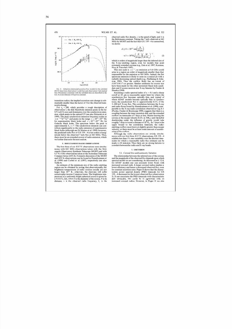
8/12/2019 Schwarze LöCher Als Astronomische Objekte
http://slidepdf.com/reader/full/schwarze-lacher-als-astronomische-objekte 56/146
56
470 WILMS ET AL. Vol. 522
F IG . 6.ÈAdvection-dominated accretion Ñow models for the unfoldedRXT E data from observation 1 ( solid line ) and observation 5 ( dot -dashed line). Parameters consistent with the unfolded data are described in thetext. A source distance of 4 kpcwas assumed.
transition radius; the implied accretion rate change is sub-stantially smaller than the factor of 5 for the observed lumi-nosity change.
For which provides a rough description of r trD 200,
observation 1, the disk blackbody emission peaks in the farUV/soft X-rays and dominates over the synchrotron emis-sion, which peaks in the optical/UV (see also Zdziarski et al.1998). The peak synchrotron emission frequency scales as
and peaks in the range l \ 1011 È 1012 HzP m~1@2m 5 1@2rtr5@4
for supermassive black holes and l\
1015
È 1016
Hz forGalactic black holes. The spectrum below the peak isapproximately The synchrotron emission can con-Sl
P l 2 .tribute signiÐcantly to the radio emission of supermassiveblack holes (although see Di Matteo et al. 1999); however,the predicted radio Ñux of GX 339 [ 4 is ten orders of mag-nitude below the observed 7 mJy Ñux at 843 MHz. Thus,there must be an extended source of radio emission, whichwe further discussin the next section.
4. SIMULTANEOUS RADIO OBSERVATIONS
The Ðrst three of our RXT E observations were simulta-neous with 843 MHz observations taken with the Mol-ongolo Observatory Synthesis Telescope (MOST) and with8.3 È 9.1 GHz observations taken at the Australian TelescopeCompact Array (ATCA). Extensive discussion of the MOSTand ATCA observations can be found in Hannikainnen etal. (1999) and Corbel et al. (1997), respectively (see alsoTable 4).
An estimate of the minimum size of the radio emittingregion can be obtained by noting that,observationally, thebrightness temperatures of radio sources usually are notlarger than 10 12 K ; otherwise, the electrons will su†ercatastrophic inverse Compton losses. The brightness tem-perature of a uniformly bright spherical source is given by
where d is the diameter of the source, D is its(cD / d l )2Sl /2nk,distance, l is the observed radio frequency, is theSl
observed radio Ñux density, c is the speed of light, and k isthe Boltzmann constant. Taking the 7 mJy observed at 843MHz by MOST and the fact that GX 339 [ 4 is unresolved,we derive
d Z 4 ] 1012 cmA D4 kpcB
B 3 ] 106R GA D4 kpcBA M
10 M _ B~1
, (2)
which is orders of magnitude larger than the inferred size of the X-ray È emitting region, even for models that positextremely extended coronae (e.g., Esin et al. 1997; Kazanas,Hua, & Titarchuk 1997).
This size scale is P l ~1 , so emission at 8.6 GHz couldarise in a region an order of magnitude smaller than thatresponsible for the emission at 843 MHz. Indeed, the Ñatspectrum emission is likely to arise in a conical jet with aradially decreasing optical depth (e.g., Hjellming & John-
ston 1988). Thus the outÑow likely has an extent of O (107GM / c2) or greater. Similar estimates for source sizehave been made for the other persistent black hole candi-date and Z-source neutron star X-ray binaries by Fender &Hendry (1999).
Assuming a radio spectral index of a \ 0.1 and a sharpcuto† at 10 km (a reasonable upper limit for where thesynchrotron Ñux becomes optically thin, and typical of where ADAF models become optically thin to synchro-tron), the synchrotron Ñux is approximately 0.1% of the3 È 100 keV X-ray Ñux. The correlation between the X-rayand radio Ñuxes found by Hannikainnen et al. (1999), com-parable to the X-ray/radio correlation observed in Cyg X-1(Pooley, Fender & Brocksopp 1999), suggests that there is acoupling between the inner accretion disk and the extendedoutÑow on timescales of 7 days or less. Matter leaving thecorona at the escape velocity (0.25 c at and thereafter30RG )decelerating under the inÑuence of gravity would takeroughly 7 days to travel a distance of As 7 days is the107RG .upper bound to the correlation timescale, the radio-emitting outÑow must leave at slightly greater than escapevelocity, or there must be at least some amount of acceler-ation of the outÑow.
Although the radio observations are strictly simulta-neous with our Ðrst three RXT E observations, GX 339 [ 4exhibits less than 1% rms variability over the shortest time-scales for which a reasonable radio Ñux estimate can bemade minutes). Thus there are no strong features to(Z 10correlate betweenthe radio and X-ray bands.
5. DISCUSSION
5.1. Coronal Size and L uminosity VariationThe relationship between the inferred size of the corona
and the magnitude of the observed Ñux depends upon whichspectral model we are considering. As discussed in ° 3.2.4,for ADAF models one can associate lower Ñuxes withincreased coronal radii. A larger coronal radius implies alower efficiency and hence a decreased observed Ñux, evenfor constant accretion rates. Paper II shows that the charac-teristic power spectral density (PSD) timescale for GX339 [ 4 decreases for the lowest observed Ñux (observation5). If one associates the PSD timescale with characteristicdisk timescales, this could be in agreement with anincreased coronal radius. However, in Paper II we also
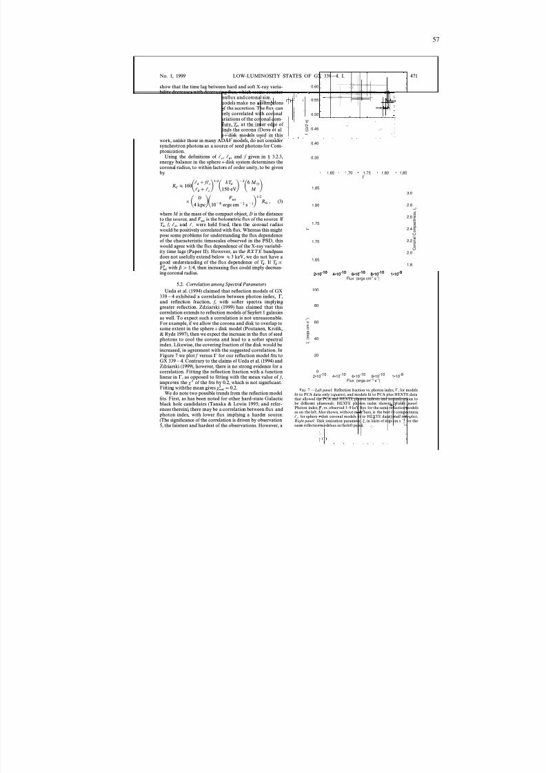
8/12/2019 Schwarze LöCher Als Astronomische Objekte
http://slidepdf.com/reader/full/schwarze-lacher-als-astronomische-objekte 57/146
57
1.65 1.70 1.75 1.80 1.85Γ
0.35
0.40
0.45
0.50
0.55
0.60
f ( Ω / 2
π )
2•10 -10 4•10 -10 6•10 -10 8•10 -10 1•10 -9
Flux (ergs cm -2 s -1)
1.65
1.70
1.75
1.80
1.85
Γ
2•10 -10 4•10 -10 6•10 -10 8•10 -10 1•10 -9
1.8
2.0
2.2
2.4
2.6
2.8
3.0
C o r o n a
l C o m p a c
t n e s s ,
l c
2•10 -10 4•10 -10 6•10 -10 8•10 -10 1•10 -9
Flux (ergs cm-2
s-1
)
0
20
40
60
80
100
ξ
( e r g s c m
s - 1 )
No. 1, 1999 LOW-LUMINOSITY STATES OF GX 339 [ 4. I. 471
show that the time lag between hard and soft X-ray varia-bility decreases with decreasing Ñux, which seems counterto a positive correlation betweenÑux and coronal size.
The sphere ] disk coronal models make no assumptionsabout the radiative efficiency of the accretion. The Ñux canbe either positively or negatively correlated with coronalradius, depending upon the variations of the coronal com-pactness, and the temperature, at the inner edge of l c , T d ,the accretion disk that surrounds the corona (Dove et al.1997b). Note that the sphere ] disk models used in thiswork, unlike those in many ADAF models, do not considersynchrotron photons as a source of seed photons for Com-ptonization.
Using the deÐnitions of and f given in ° 3.2.3,l c , l d ,energy balance in the sphere ] disk system determines thecoronal radius, to within factors of order unity, to be givenby
R C B 160
Al d ] f l c
ld
] lc
B1@2
A kT d
150 eVB~2
A6 M _
M B] A D4 kpcBA F tot
10~8 ergs cm ~2 s~1B1@2RG , (3)
where M is the mass of the compact object, D is the distanceto the source, and is the bolometric Ñux of the source. If F tot
f , and were held Ðxed, then the coronal radiusT d , l d , l c
would be positively correlated with Ñux. Whereas this mightpose some problems for understanding the Ñux dependenceof the characteristic timescales observed in the PSD, thiswould agree with the Ñux dependence of the X-ray variabil-ity time lags (Paper II). However, as the RXT E bandpassdoes not usefully extend below B 3 keV, we do not have agood understanding of the Ñux dependence of If T d . T d P
with b [ 1/4, then increasing Ñux could imply decreas-F totb
ing coronal radius.
5.2. Correlation among Spectral ParametersUeda et al. (1994) claimed that reÑection models of GX339[ 4 exhibited a correlation between photon index, ! ,and reÑection fraction, f , with softer spectra implyinggreater reÑection. Zdziarski (1999) has claimed that thiscorrelation extends to reÑection models of Seyfert 1 galaxiesas well. To expect such a correlation is not unreasonable.For example, if we allow the corona and disk to overlap tosome extent in the sphere ] disk model (Poutanen, Krolik,& Ryde 1997), then we expect the increase in the Ñux of seedphotons to cool the corona and lead to a softer spectralindex. Likewise, the covering fraction of the disk would beincreased, in agreement with the suggested correlation. InFigure 7 we plot f versus ! for our reÑection model Ðts toGX 339 [ 4. Contrary to the claims of Ueda et al. (1994) andZdziarski (1999), however, there is no strong evidence for acorrelation. Fitting the reÑection fraction with a functionlinear in ! , as opposed to Ðtting with the mean value of f ,improves the s 2 of the Ðts by 0.2, which is not signiÐcant.Fitting withthe mean gives s red
2 \ 0.2.We do note two possible trends from the reÑection model
Ðts. First, as has been noted for other hard-state Galacticblack hole candidates (Tanaka & Lewin 1995; and refer-ences therein), there may be a correlation between Ñux andphoton index, with lower Ñux implying a harder source.(The signiÐcance of the correlation is driven by observation5, the faintest and hardest of the observations. However, a
F IG . 7.È L eft panel: ReÑection fraction vs. photon index, ! , for modelsÐt to PCA data only ( squares ), and models Ðt to PCA plus HEXTE datathat allowed the PCA and HEXTE photon indexes and normalizations tobe di†erent ( diamonds ; HEXTE photon index shown). Middle panel:Photon index, ! , vs. observed 3 È 9 keV Ñux for the same reÑection modelsas on the left. Also shown, without error bars, is the best-Ðt compactness,
for sphere ] disk coronal models Ðt to HEXTE data ( small triangles ).l c ,Right panel: Disk ionization parameter, m, in units of ergs cm s ~1 for thesame reÑection modelsas in theleft panel.
8/12/2019 Schwarze LöCher Als Astronomische Objekte
http://slidepdf.com/reader/full/schwarze-lacher-als-astronomische-objekte 58/146
58
472 WILMS ET AL. Vol. 522
similar correlation is also present in color-intensity dia-grams.) Such a correlation is consistent with the expecta-tions of ADAF models, in which the radius increases withdecreasing Ñux (Fig. 6). Again, the sphere ] disk coronamodels do not predict a clear trend without knowledge of the Ñux dependences of other parameters such as T d .
Second, the ionization parameter, m, is positively corre-lated with Ñux. Such a correlation was noted by Z 0 ycki,Done, & Smith (1998) for Ginga observations of NovaMuscae. It is not unreasonable to expect the disk to becomeincreasingly ionized with increasing Ñux. We again cautionthat it is dangerous to make one-to-one correlationsbetween a model Ðt parameter and a true physical param-eter. Furthermore, the signiÐcance of the correlation isagain almost entirely determined by observation 5, thefaintest observation, which has m B0. However, if we takethe Ñux dependence of m as being real and interpret it physi-cally, it provides some constraints on the Ñux dependence of the coronal radius. The ionization parameter is P F tot /(oR2),
where o is the density of the disk. For a gas pressure È dominated Shakura-Sunyaev a disk, o P R~1.65 (Shakura& Sunyaev 1973). In order for m to be roughly linear in Ñux(the actual dependence is not strongly constrained by thedata), we require (For the sphere ] disk modelsF tot
P R 1.35.this would further require that approximately T d P R~1@3,depending upon the Ñux dependences of g, etc.)l d , l c ,Taken physically and in the context of a gas pressure È dominated Shakura-Sunyaev a model, the Ñux dependenceof m implies that the coronal radius increases with increas-ing Ñux.
6. SUMMARY
We have presented a series of observations of the blackhole candidate GX 339 [ 4 in low-luminosity, spectrallyhard states. These observations consisted of three separatearchival ASCA and eight separate RXT E data sets. All of these observations exhibited (3 È 9 keV) Ñux ergs s~1[ 10~9
cm~2 , and the observed Ñuxes spanned roughly a factor of 5in range for both the ASCA and RXT E data sets. Subject touncertainties in the cross calibration between ASCA andRXT E , the faintest ASCA observation was approximately afactor of 2 fainter than the faintest RXT E observation.
All of these observations showed evidence for an B 6.4keV Fe line with equivalent widths in the range of B 20 È 140eV. The ASCA observations further showed evidence for asoft excess that was well modeled by a power law plus amulticolor blackbody spectrum with peak temperatures inthe range B 150 È 200 eV. Both of these factors consideredtogether argue against sphere ] disk or ADAF type È geometry coronae with extremely large coronal radii of
(e.g., Esin et al. 1997).O (104R G )The RXT E data sets were well Ðt by sphere ] disk Com-
ptonization models with coronal temperatures in the range20 È 50 keV and optical depths near q B 3. These Ðtswere similar to our previous Ðts to RXT E data of CygX-1. Advection-dominated accretion Ñow models, whichposit a similar geometry, also provided reasonable descrip-tions of the unfolded RXT E data. The sphere ] disk andADAF models were not able, however, to also model the
observed radio Ñuxes. Thus, a static corona seems to beruled out by the observations. The ADAF models can implythat the coronal radius increases with decreasing Ñux. Thesphere ] disk corona models do not make a speciÐc predic-tion for the dependence of the coronal radius on the Ñux;however, they can be consistent with a positive correlationbetween coronal radius and Ñux. As described in Paper II, apositive correlation between Ñux and coronal radius is con-sistent with the observed Ñux dependence of the time lagsbetween hard and soft X-ray variability.
We also considered ““reÑection models ÏÏ of the RXT Edata. These models showed evidence of a hardening of theRXT E spectra with decreasing X-ray Ñux. They furthershowed evidence of a positive correlation between the best-Ðt ionization parameter, m, and the observed Ñux. Especiallythe latter of these correlations, however, was dominated bythe model Ðts of the faintest observation. The reÑectionmodels did not exhibit any evidence of a correlationbetween the photon index of the incident power-law Ñux
and the solid angle subtended by the reÑector.Three of the RXT E observations were strictly simulta-neous with 843 MHz and 8.3 È 9.1 GHz radio observations.The most likely source of the radio Ñux is synchrotron emis-sion from an extended outÑow with a size of O (107GM / c2).The correlation between radio and X-ray emission on time-scales of 7 days or less (Hannikainnen et al. 1999) implies astrong coupling of the inner disk accretion Ñow with thisspatially extended outÑow as is expected by recent theoreti-cal arguments (Blandford & Begelman 1999). Furthersimultaneous radio/X-ray observations, preferably with theaddition of IR/optical monitoring to constrain the locationof the synchrotron break and with the addition of soft X-raymonitoring to constrain the accretion disk parameters, arerequired to test such models in detail.
We would like to thank Christopher Reynolds for
keeping a sti† upper lip while explaining ASCA dataanalysis to us. We would also like to thank K. Mukai of theASCA GOF for useful advice. W. A. Heindl and D. Gruberkindly provided assistance with the HEXTE data extrac-tion, and S. Corbel provided assistance with the radio data.We are grateful to B. Stern for writing the original versionof KOTELP, and, more importantly, for Ðnally telling uswhat the name means (““ cauldron ÏÏ). We would also like toacknowledge useful conversations with B. Begelman, J.Chiang, B. A. Harmon, K. Pottschmidt, R. Staubert, C.Thompson, and A. Zdziarski. This work has been Ðnancedby NASA Grants NAG 5-4731 and NAG 5-3225 (M. A. N.,J. B. D.). M. N. was supported in part by the NationalScience Foundation under Grant Phy94-07194. J. W. wassupported by a travel grant from the Deutscher Akademis-cher Austauschdienst, R. P. F. was supported by an ECMarie Curie Fellowship (ERBFMBICT 972436), andT. D. M. thanks Trinity College and PPARC for Ðnancialsupport. This research has made use of data obtainedthrough the High Energy Astrophysics Science ArchiveResearch Center Online Service, provided by the NASA/ Goddard Space Flight Center.
8/12/2019 Schwarze LöCher Als Astronomische Objekte
http://slidepdf.com/reader/full/schwarze-lacher-als-astronomische-objekte 59/146
59
No. 1, 1999 LOW-LUMINOSITY STATES OF GX 339 [ 4. I. 473
APPENDIX A
ASCA DATA EXTRACTION
We extracted data from the two solid state detectors (SIS0, SIS1) and the two gas detectors (GIS2, GIS3) on board ASCA
by using the standard FTOOLS as described in the ASCA Data Reduction Guide (Day et al. 1998). The data extractionradius was limited by the fact that all the observations were in one-CCD mode and that the source was typically placed closeto the chip edge. We chose circular extraction regions with radii of B 4@ for SIS0, B 3@ for SIS1 (the maximum possibleextraction radii for these detectors), and B 6@ for GIS2 and GIS3. For observation 3 we excluded the central 40 A to avoid thepossibility of photon pileup. We used the SISCLEAN and GISCLEAN tools (with default values) to remove hot andÑickering pixels. We Ðltered the data with the strict cleaning criteria outlined in the ASCA Data Analysis Handbook;however, we took the larger value of 7 GeV/ c for the rigidity. We rebinned the spectral Ðles so that each energy bin containeda minimum of 20 photons. We retained SIS data in the 0.5 È 9 keV range and GIS data in the 1.5 È 9 keV range.
We accounted for the cross-calibration uncertainties of the three instruments by introducing a multiplicative constant foreach detector in all of our Ðts. Relative to SIS0, the SIS1 detector normalization was always found to be within 2%, the GIS2normalization was found to be within 9%, and the GIS3 normalization was found to be within 15%. For any givenobservation, the normalization constants varied by for di†erent spectral Ðts. The background was measured from[ ^ 1%rectangular regions on the two edges of the chip farthest from the source (SIS data), or from annuli with inner radii [ 6@ (GISdata). These data were cleaned and Ðltered in the same manner as the source Ðles.
The resulting data Ðles showed reasonable agreement between all four detectors. The most discrepant detector was SIS1,which also was the detector limited to the smallest extraction radius. This detector tended to show deviations from the otherdetectors for energies keV, and from the SIS0 detector for energies B 0.5 È 1 keV. The detectors were mostly in mutualZ 9agreement for the lowest Ñux observations. It is likely that the agreement could be further improved for observations locatedcloser to the center of the chips (thereby allowing larger extraction radii) and if low È Galactic latitude dark sky observations inone-CCD mode were available to use as background.
APPENDIX B
RXT E DATA EXTRACTION
In ° 3 we present data from both pointed instruments on RXT E , the Proportional Counter Array (PCA) and theHigh-Energy X-Ray Timing Experiment (HEXTE). As we showed in ° 3, the large e†ective area of these instruments results ina data analysis approach that is dominated by the calibration uncertainty of these detectors (especially the PCA). In thisappendix we summarize the major properties of both instruments and study their (inter-) calibration. All RXT E resultsobtained in this paper were obtained using the standard RXT E data analysis software, FTOOLS version 4.1 (including theRXT E patch 4.1.1 and the correct accounting of the time dependence of the PCA response; K. Jahoda 1998, privatecommunication). Spectral modeling was done using XSPEC, version 10.00s (Arnaud 1996).
The PCA consists of Ðve nearly identical coaligned Xenon proportional counter units (PCUs) with a total e†ective area of about 6500 cm 2. The instrument is sensitive in the energy range from 2 to D 60 keV (Jahoda et al. 1996). We used only data forwhich all Ðve PCUs were turned on. Background subtraction was done in the same manner as for our RXT E Cyg X-1observations (Dove et al. 1998). SpeciÐcally, a model using the rate of Very Large Events in the detector was used to estimatethe background Ñux. The major uncertainty of this estimated background is due to activation of radioactivity in the detectorsduring South Atlantic Anomaly passages. Since this background component is present for about 30 minutes after the passage,we ignored data measured during these intervals. Furthermore, data were not accumulated at times of high electron contami-nation. The electron contamination is measured by a certain ratio of veto rates in the detectors, the so-called electron ratio(Jahoda et al. 1999). As recommended by the RXT E Guest ObserverÏs Facility (GOF), we excluded times during which the““ electron ratio ÏÏ was larger than 0.1 in at least one of the detectors. Note that the observed count rates from GX 339 [ 4 aretoo high to allow the use of the newer background model made available by the RXT E GOF in 1998 June.
For spectral Ðtting, we limited the energy range of the PCA data from 3 to 30 keV and used version 2.2.1 of the PCAresponse matrices. These matrices are newer than those used by us previously (Dove et al. 1998), and they are primarilycharacterized by assuming a higher instrumental resolution (Jahoda et al. 1999). Because of the large PCA count rate of GX339[ 4 (D 800 counts s ~1 ) our observations are dominated by the remaining uncertainties in the detector calibration and notby Poisson errors. Therefore, a good understanding of these uncertainties is necessary.
Since the Crab spectrum is commonly assumed to be a featureless power law (Toor & Seward 1974), at least over narrowenergy ranges, the ratio between the Ðt to the Crab and the data can be used to deduce the systematic uncertainty associatedwith the detector calibration. We therefore extracted a public domain spectrum of the Crab nebula and pulsar measured withthe PCA on 1997 April 1. The Crab data were screened using the same criteria as those applied to our GX 339 [ 4 data, exceptfor that the ““ electron ratio ÏÏ check was not applied since the background contributes only 0.6% to the total number of photons detected for the Crab. Modeling the 3 to 30 keV Crab data with an absorbed power law resulted in a best-Ðt photonspectrum of the form
Nph\ 13.3E ~2.187 exp [ [ 2.54 ] 1021 cm ~2p
bf(E )] cm~2 s~1 keV ~1 , (B1)
where is the energy dependent bound-free absorption cross section for material of cosmic abundances as given bypbf(
E )Morrison & McCammon (1983), and where E is the photon energy measured in keV. For this Ðt to the Crab data,
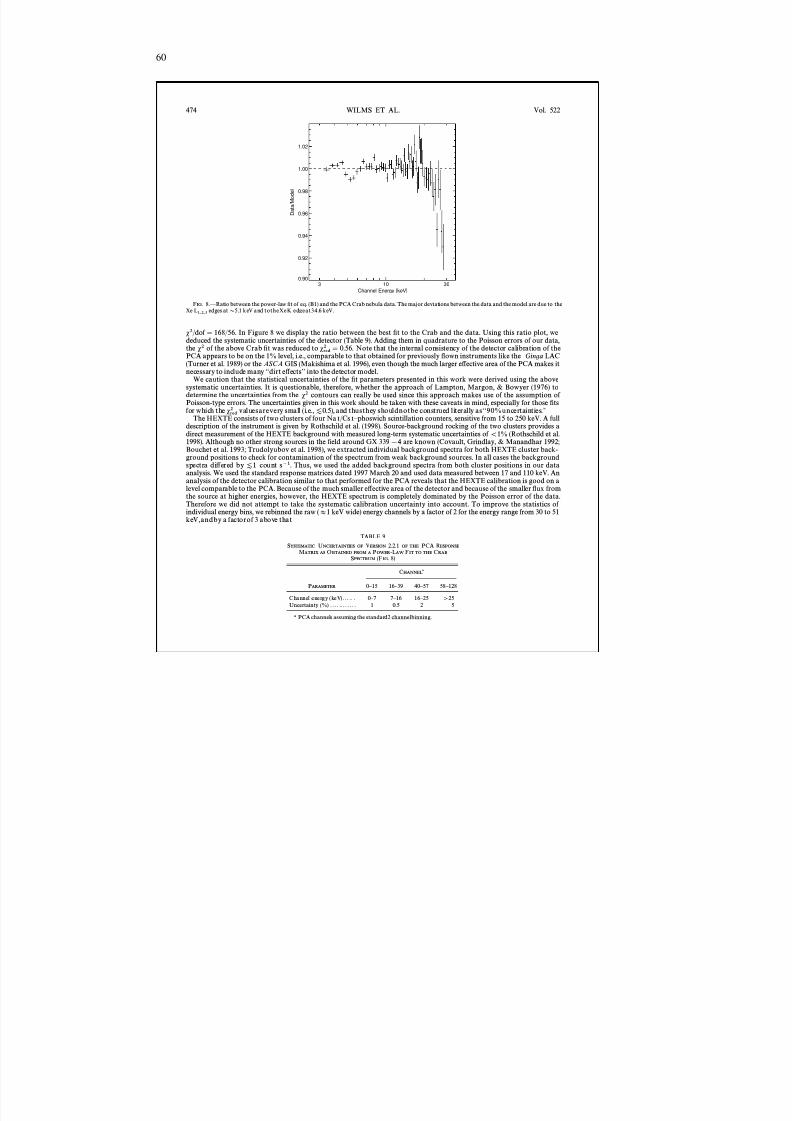
8/12/2019 Schwarze LöCher Als Astronomische Objekte
http://slidepdf.com/reader/full/schwarze-lacher-als-astronomische-objekte 60/146
60
Channel Energy [keV]
0.90
0.92
0.94
0.96
0.98
1.00
1.02
D a t a / M o d e l
3 10 30
474 WILMS ET AL. Vol. 522
F IG . 8.ÈRatio between the power-law Ðt of eq. (B1) and the PCA Crab nebula data. The major deviations between the data and the model are due to theXe edges at D 5.1 keV and totheXeK edgeat34.6 keV.L1,2,3
s 2 /dof \ 168/56. In Figure 8 we display the ratio between the best Ðt to the Crab and the data. Using this ratio plot, wededuced the systematic uncertainties of the detector (Table 9). Adding them in quadrature to the Poisson errors of our data,the s 2 of the above Crab Ðt was reduced to Note that the internal consistency of the detector calibration of thes red
2 \ 0.56.PCA appears to be on the 1% level, i.e., comparable to that obtained for previously Ñown instruments like the Ginga LAC(Turner et al. 1989) or the ASCA GIS (Makishima et al. 1996), even though the much larger e†ective area of the PCA makes itnecessary to include many ““dirt e†ectsÏÏ into the detector model.
We caution that the statistical uncertainties of the Ðt parameters presented in this work were derived using the abovesystematic uncertainties. It is questionable, therefore, whether the approach of Lampton, Margon, & Bowyer (1976) todetermine the uncertainties from the s 2 contours can really be used since this approach makes use of the assumption of Poisson-type errors. The uncertainties given in this work should be taken with these caveats in mind, especially for those Ðtsfor which the valuesarevery small (i.e., and thusthey shouldnotbe construed literally as““90%uncertainties.ÏÏs
red
2 [ 0.5),The HEXTE consists of two clusters of four Na I /Cs I È phoswich scintillation counters, sensitive from 15 to 250 keV. A full
description of the instrument is given by Rothschild et al. (1998). Source-background rocking of the two clusters provides adirect measurement of the HEXTE background with measured long-term systematic uncertainties of \ 1% (Rothschild et al.1998). Although no other strong sources in the Ðeld around GX 339 [ 4 are known (Covault, Grindlay, & Manandhar 1992;Bouchet et al. 1993; Trudolyubov et al. 1998), we extracted individual background spectra for both HEXTE cluster back-ground positions to check for contamination of the spectrum from weak background sources. In all cases the backgroundspectra di†ered by count s ~1 . Thus, we used the added background spectra from both cluster positions in our data[ 1analysis. We used the standard response matrices dated 1997 March 20 and used data measured between 17 and 110 keV. Ananalysis of the detector calibration similar to that performed for the PCA reveals that the HEXTE calibration is good on alevel comparable to the PCA. Because of the much smaller e†ective area of the detector and because of the smaller Ñux fromthe source at higher energies, however, the HEXTE spectrum is completely dominated by the Poisson error of the data.Therefore we did not attempt to take the systematic calibration uncertainty into account. To improve the statistics of individual energy bins, we rebinned the raw ( B 1 keV wide) energy channels by a factor of 2 for the energy range from 30 to 51keV,andby a factorof 3 above that.
TABLE 9
SYSTEMATIC UNCERTAINTIES OF V ERSION 2.2.1 OF THE PCA R ESPONSE
MATRIX AS
OBTAINED FROM A
POWER
-LAW
FIT TO THE
CRAB
SPECTRUM (F IG . 8)
C HANNEL a
P ARAMETER 0 È 15 16 È 39 40 È 57 58 È 128
Channel energy (keV). . . . . . 0 È 7 7 È 16 16 È 25 [ 25Uncertainty (%) . . . . .. . . .. . . 1 0.5 2 5
a PCA channels assuming the standard2 channelbinning.
8/12/2019 Schwarze LöCher Als Astronomische Objekte
http://slidepdf.com/reader/full/schwarze-lacher-als-astronomische-objekte 61/146
61
No. 1, 1999 LOW-LUMINOSITY STATES OF GX 339 [ 4. I. 475
When modeling the spectrum of GX 339 [ 4 from 3 to 110 keV as measured by the PCA and the HEXTE, the inter-calibration between the instruments is of some concern. Our experience with previous data and the response matrix describedby Dove et al. (1998) indicated that the Ñux calibration of the HEXTE with respect to the PCA was o† by about 25%; i.e., thederived HEXTE Ñuxes were D 75% of those found with the PCA. This deviation is mainly due to a slight misalignment of theHEXTE collimators, which has not yet been taken into account in the HEXTE response matrix (B. Heindl 1998, privatecommunication). Using the new PCA response, the Ñux ratio now appears to be larger and was found to be 62% È 69% in ourdata. Extracting spectra with internal software used by the HEXTE hardware team produced spectra identical to those foundusing our extraction procedure. Therefore we do not believe this change in the Ñux calibration to be due to errors in thedead-time correction. To take this o†set in the e†ective areas into account, we modeled the spectra using a multiplicativeconstant that was set to unity for the PCA, and that was a Ðt parameter for both HEXTE clusters. Thus, all Ñuxes given belowwere measured with respect to the PCA. The maximum deviation of the HEXTE clusters relative to each other was found tobe less than 8%.
Apart from the Ñux calibration, however, even more crucial for our analysis is the question of how well the inferred spectralshapes agree for the two instruments. Our Crab Ðts show that the PCA results in a photon index of ! \ 2.187 (eq. [B1]), whileour HEXTE Ðts gave ! \ 2.053. The generally accepted value for the Crab photon index in the 1 È 100 keV range is! \ 2.10 ^ 0.03. This value was adopted by Toor & Seward (1994) in their analysis of 28 di†erent rocket Ñight measurements.There are indications that the spectrum softens to ! D 2.5 above 150 keV (Jung 1989). Although the absolute uncertainty of the Crab Ñux in the 2 È 100 keV range has been estimated as large as 2%, and even larger below 2 keV et al.(NÔrgaard-Nielsen1994), the *! \ 0.134 deviation between the PCA and the HEXTE best-Ðt Crab photon index is still very worrisome, and it is
currently being studied by both the PCA and HEXTE instrument teams (K. Jahoda 1998, private communication).
REFERENCESArnaud, K. A. 1996, in ASP Conf. Ser. 101, Astronomical Data Analysis
Software and Systems V, ed. J. H. Jacoby & J. Barnes (San Francisco:ASP), 17
Bevington, P. R., & Robinson, D. K. 1992, Data Reduction and ErrorAnalysis for the Physical Sciences (2d ed.; New York: McGraw-Hill)
Blandford, R. D., & Begelman, M. C. 1999, MNRAS, 303, 1Bouchet, L., et al. 1993, ApJ, 407, 739Callanan, P. J., Charles, P. A., Honey, W. B., & Thorstensen, J. R. 1991,
MNRAS, 259, 395Corbel, S., Fender, R. P., Durouchoux, P., Sood, R. K., Tzioumis, A. K.,
Spencer, R. E., & Campbell-Wilson, D. 1997, in Proc. 4th ComptonSymposium, ed. C. D. Dermer, M. S. Strickman, & J. D. Kurfess,(Woodbury, NY: AIP), 937
Covault, C. E., Grindlay, J. E., & Manandhar, R. P. 1992, ApJ, 388, L65Cowley, A. P., Crampton, D., & Hutchings, J. B. 1987, AJ, 93, 195Cowley, A. P., Schmidtke, P. C., Crampton, D., Hutchings, J. B., & Bolte,
M. 1991, ApJ, 373, 228Day, C., Arnaud, K., Ebisawa, K., Gotthelf, E., Ingham, J., Mukai, K., &
White, N. 1998, The ASCA Data Reduction Guide, technical report,version 2.0 (Greenbelt, Md.: NASA GSFC)
Di Matteo, T., Fabian, A. C., Rees, M. J., Carilli, C. L., & Ivison, R. J. 1999,MNRAS, submittedDobrinskaya, J., Liang, E., Luo, C., Sheth, S., & Smith, I. 1997, in X-Ray
Imaging and Spectroscopy of Cosmic Hot Plasmas, ed. F. Makino &K. Mitsuda (Tokyo: Universial Academy), 481
Dove, J. B., Wilms, J., & Begelman, M. C. 1997a, ApJ, 487, 747Dove, J. B., Wilms, J., Maisack, M. G., & Begelman, M. C. 1997b, ApJ, 487,
759Dove, J. B., Wilms, J., Nowak, M. A., Vaughan, B. A., & Begelman, M. C.
1998, MNRAS, 298, 729Doxsey, R., Grindlay, J., Griffiths, R., Bradt, H., Johnston, M., Leach, R.,
Schwartz, D., & Scwartz, J. 1979, ApJ, 228, L67Ebisawa, K., Ueda, Y., Inoue, H., Tanaka, Y., & White, N. E. 1996, ApJ,
467, 419Esin, A. A., McClintock, J. E., & Narayan, R. 1997, ApJ, 489, 865Fender, R. P., & Hendry, M. A. 1999, MNRAS, in pressFender, R. P., Spencer, R. E., Newell, S. J., & Tzioumis, A. K. 1997,
MNRAS, 286, L29Fender, R. P., et al. 1999, ApJ, 519, L165Grabelsky, D. A., et al. 1995, ApJ, 441, 800Grebenev, S. A., Syunyaev, R., Pavlinsky, M. N., & Dekhanov, I. A. 1991,
Soviet Astron. Lett., 17, 413Grindlay, J. E. 1979, ApJ, 232, L33Hannikainnen, D. C., Hunstead, R. W., Campbell-Wilson, D., & Sood,
R. K. 1999, A&A, in pressHjellming, R. M., & Johnston, K. J. 1988, ApJ, 328, 600Ichimaru, S. 1977, ApJ, 214, 840Ilovaisky, S. A., Chevalier, C., Motch, C., & Chiappetti, L. 1986, A&A, 164,
671Imamura, J. N., Kristian, J., Middleditch, J., & Steiman-Cameron, T. Y.
1990, ApJ, 365, 312Jahoda, K., Swank, J. H., Giles, A. B., Stark, M. J., Strohmayer, T., Zhang,
W., & Morgan, E. H. 1996, in EUV, X-Ray, and Gamma-Ray Instru-mentation for Astronomy VII, ed. O. H. Siegmund (Bellingham, WA:SPIE), 59
Jahoda, K., et al. 1999, in preparationJung, G. V. 1989, ApJ, 338, 972
Kazanas, D., Hua, X.-M., & Titarchuk, L. 1997, ApJ, 480, 280Kitamoto, S., Tsunemi, H., Miyamoto, S., & Hayashida, K. 1992, ApJ, 394,
609Lampton, M., Margon, B., & Bowyer, S. 1976, ApJ, 208, 177Levine, A. M., Bradt, H., Cui, W., Jernigan, J. G., Morgan, E. H., Remil-
lard, R., Shirey, R. E., & Smith, D. A. 1996, ApJ, 469, L33Lochner, J., & Remillard, R. 1997, ASM Data Products Guide, version
dated 1997 August 27 8Magdziarz, P., & Zdziarski, A. A. 1995, MNRAS, 273, 837Makishima, K., et al. 1996, PASJ, 48, 171
M., & van der Klis, M. 1997, ApJ, 479, 926Me n dez,Miyamoto, S., Kimura, K., Kitamoto, S., Dotani, T., & Ebisawa, K. 1991,
ApJ, 383, 784Miyamoto, S., Kitamoto, S., Iga, S., Hayashida, K., & Egoshi, W. 1995,
ApJ, 442, L13Miyamoto, S., Kitamoto, S., Iga, S., Hayashida, K., & Terada, K. 1994,
ApJ, 435, 398Morrison, R., & McCammon, D. 1983, ApJ, 270, 119Motch, C., Ilovaisky, S. A., Chevalier, C., & Angebault, P. 1985, Space Sci.
Rev., 40, 219
Motch, C., Ricketts, M. J., Page, C. G., Ilovaisky, S. A., & Chevalier, C.1983, A&A, 119, 171Narayan, R. 1996, ApJ, 462, 136Narayan, R., Kato, S., & Honma, F. 1997, ApJ, 476, 49
H. U., C., Westergaard, N. J., &N Ôrgaard-Nielsen, Budtz-J Ôrgensen,Schnopper, H. W. 1994, A&A, 284, 705
Nowak, M. A., Wilms, J., & Dove, J. B. 1999, ApJ, 517, in press (Paper II)Pooley, G. G., Fender, R. P., & Brocksopp, C. 1999, MNRAS, 302, L1Poutanen, J., Krolik, J. H., & Ryde, F. 1997, MNRAS, 221, 21pPredehl, P., H., Burkert , W., & Schmitt , J . H. M. M. 1991,Bra uninger,
A&A, 246, L40Remillard, R. A., & Levine, A. M. 1997, in All-Sky X-Ray Observations in
the Next Decade, ed. N. Matsuoka & N. Kawai (Tokyo: Riken), 29Rothschild, R. E., et al. 1998, ApJ, 496, 538Shakura, N. I., & Sunyaev, R. 1973, A&A, 24, 337Sood, R., & Campell-Wilson, D. 1994, IAU Circ. 6006Steiman-Cameron, T. Y., Imamura, J. N., Middleditch, J., & Kristian, J.
1990, ApJ, 359, 197Tanaka, Y., & Lewin, W. H. G. 1995, in X-Ray Binaries, ed. W. H. G.
Lewin, J. van Paradijs, & E. P. J. van den Heuvel (Cambridge: Cam-bridge Univ. Press), 126
Toor, A., & Seward, F. D. 1974, AJ, 79, 995Trudolyubov, S., et al. 1998, A&A, 334, 895Turner, M. J. L., et al. 1989, PASJ, 41, 345Ueda, Y., Ebisawa, K., & Done, C. 1994, PASJ, 46, 107Zdziarski, A. 1999, in ASP Conf. Proc. 161, High-Energy Processes in
Accreting Black Holes: Observational and Theoretical Advances Due toOngoing Space Missions, ed. J. Poutanen & R. Svensson (San Fran-cisco: ASP), in press
Zdziarski, A. A., Poutanen, J., J., M., Ebisawa,Miko ¡ajewska, Gierlin ski,K., & Johnson, W. N. 1998, MNRAS, 301, 435
P. T., Done, C., & Smith, D. A. 1998, ApJ, 496, L25Z 0ycki,
8 The ASM Data Products Guide is available on the World Wide Webat http://heasarc.gsfc.nasa.gov/docs/xte/asm – products – guide.html.

8/12/2019 Schwarze LöCher Als Astronomische Objekte
http://slidepdf.com/reader/full/schwarze-lacher-als-astronomische-objekte 62/146
62
8/12/2019 Schwarze LöCher Als Astronomische Objekte
http://slidepdf.com/reader/full/schwarze-lacher-als-astronomische-objekte 63/146
A NHANG B
Low Luminosity States of the Black Hole Candidate GX 339 − 4II. Timing Analysis
1999
M.A. Nowak, J. Wilms, J.B. Dove
Nachdruck aus
The Astrophysical Journal
Vol. 517, S. 355–366
63
8/12/2019 Schwarze LöCher Als Astronomische Objekte
http://slidepdf.com/reader/full/schwarze-lacher-als-astronomische-objekte 64/146
64
THE ASTROPHYSICAL JOURNAL , 517:355 È 366, 1999 May 201999. The American Astronomical Society. All rights reserved. Printed in U.S.A.(
LOW-LUMINOSITY STATES OF THE BLACK HOLE CANDIDATE GX 339 [ 4. II. TIMING ANALYSIS
M ICHAEL A. N OWAK ,1 JO RN W ILMS ,2 AND JAMES B. DOVE 1,3
Received 1998 September 10; accepted 1998 November 4
ABSTRACTHere we present timing analysis of a set of eight Rossi X -Ray T iming Explorer (RXT E ) observations
of the black hole candidate GX 339 [ 4 that were taken during its hard/low state. On long timescales,the RXT E All Sky Monitor data reveal evidence of a 240 day periodicity, comparable to timescalesexpected from warped, precessing accretion disks. On short timescales all observations save one showevidence of a persistent Hz quasi-periodic oscillation. The broadband (10 ~3 to 10 2 Hz) power f QPO B 0.3appears to be dominated by two independent processes that can be modeled as very broad LorentzianÐts with The coherence function between soft and hard photon variability shows that if these areQ [ 1.truly independent processes, then they are individually coherent, but they are incoherent with oneanother. This is evidenced by the fact that the coherence function between the hard and soft variability isnear unity between 5 ] 10~3 to 10 Hz but shows evidence of a dip at f B 1 Hz. This is the region of overlap between the broad Lorentzian Ðts to the power spectral density. As in Cyg X-1, the coherencealso drops dramatically at frequencies Hz. Also as in Cyg X-1, the hard photon variability is seenZ 10to lag the soft photon variability with the lag time increasing with decreasing Fourier frequency. Themagnitude of this time lag appears to be positively correlated with the Ñux of GX 339 [ 4. We discuss allof these observations in light of current theoretical models of both black hole spectra and temporalvariability.Subject headings: accretion, accretion disks È black hole physics È binaries: general È X-rays: stars
1. INTRODUCTION
In a companion paper to this work (Wilms et al. 1999a,hereafter Paper I) we have presented spectral analysis of aseries of Advanced Satellite for Cosmology and Astrophysics(ASCA ) and simultaneous radio/ Rossi X -Ray T imingExplorer (RXT E ) observations of the black hole candidate(BHC) GX 339 [ 4. This source has exhibited both spec-trally soft states (see Grebenev et al. 1991; Miyamoto et al.1991) and spectrally hard states (see Grebenev et al. 1991;Miyamoto et al. 1992; Zdziarski et al. 1998). Both theASCA and RXT E observations presented in Paper Ishowed GX 339 [ 4 to be in spectrally hard and low-luminosity (3 È 9 keV Ñux ergs cm ~2 s~1 ) states. The[ 10~9
eight RXT E observations spanned roughly a factor of 5 interms of observed 3 È 9 keV Ñux.
In this work we shall consider the timing analysis of theeight RXT E observations. Timing analysis for GX 339 [ 4previously has been presented for the soft, bright ““ very highstateÏÏ (Miyamoto et al. 1991), the soft, fainter ““ high stateÏÏ(Grebenev et al. 1991), and the hard ““ low state ÏÏ (Grebenevet al. 1991; Miyamoto et al. 1992). In addition, timinganalysis has been presented for so-called ““intermediatestates,ÏÏ which are bright but spectrally harder than thetypical very high or high states & van der Klis(Me ndez1997). In general, the harder states exhibit more temporalvariability than the softer states (see van der Klis 1989).Timing analyses of the GX 339 [ 4 hard state have shownsimilar results to analyses of other hard-state BHCs(Miyamoto et al. 1992). SpeciÐcally, the GX 339 [ 4 tempo-
1 JILA, University of Colorado, Campus Box 440, Boulder, CO 80309-0440; mnowak = rocinante.colorado.edu, dove = rocinante.colorado.edu.
2 Institut Astronomie und Astrophysik, Abt. Astronomie,fu rS trasse 64, D-72076 Germany;Waldha user Tu bingen, wilms = astro.uni-
tuebingen.de.3 Also CASA, University of Colorado, Campus Box 389, Boulder, CO
80309-0389.
ral variability has been observed to be similar to that of Cygnus X-1 (Belloni & Hasinger 1990a, 1990b; Miyamotoet al. 1992 ; Nowak et al. 1999a, and references therein).
A discussion of Fourier techniques in speciÐc, and timinganalysis in general, has been presented by van der Klis 1989.Here we apply these Fourier analysis techniques in the samemanner as for our RXT E observations of Cyg X-1 (Nowaket al. 1999a). SpeciÐcally, we used the same techniques forestimating: deadtime corrections (Zhang et al. 1995; Zhang& Jahoda 1996); the error bars and Poisson noise levels of
the power spectral density (PSD) (Leahy et al. 1983; van derKlis 1989); the error bars and noise levels for the coherencefunction (Bendat & Piersol 1986; Vaughan & Nowak 1997) ;and the error bars and noise levels for the Fourierfrequency È dependent time lag between hard and softphoton variability (Bendat & Piersol 1986; Nowak et al.1999a). A self-contained discussion of these techniques asregards RXT E timing analysis is given by Nowak et al.(1999a).
This paper is organized as follows. First we consider evi-dence for long-term periodicities in the RXT E All SkyMonitor (ASM) data in ° 2. In ° 3 we consider the powerspectral density (PSD). In ° 4 we consider both the coher-ence function (see Vaughan & Nowak 1997) and theFourier frequency È dependent time lags between hard andsoft photon variability. We discuss the theoretical implica-tions of these observations in ° 5. We then summarize ourresults in ° 6.
2. ALL SKY MONITOR OBSERVATIONS OF LONG
““CHARACTERISTIC TIMESCALES ÏÏIN GX 339 [ 4
We used data from the All Sky Monitor (ASM) onRXT E to study the long-term behavior of GX 339 [ 4. TheASM is an array of three shadow cameras combined withposition-sensitive proportional counters that provides for aquasi-continuous coverage of the sky visible from RXT E .
355
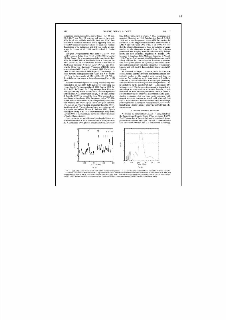
8/12/2019 Schwarze LöCher Als Astronomische Objekte
http://slidepdf.com/reader/full/schwarze-lacher-als-astronomische-objekte 65/146
65
200 400 600 800JD - 2,450,000.5
0
2
4
6
8
10
c o u n
t s s - 1
||| | | | | |
0 100 200 300 400 500Period (Days)
0
5
10
15
P o w e r
356 NOWAK, WILMS, & DOVE Vol. 517
In practice, light curves in three energy bandsÈ1.3 È 3.0 keV,3.0 È 5.0 keV, and 5.0 È 12.2 keVÈas well as over the wholeASM band are publicly available from the ASM dataarchives (Lochner & Remillard 1997). Typically there areseveral 90 s measurements available for each day. Furtherdescriptions of the instrument and Ðrst year results are pre-sented by Levine et al. (1996) and Remillard & Levine(1997).
In Figure 1 we present the ASM data of GX 339 [ 4 upuntil Truncated Julian Date (TJD) B 800 (1998 November15). See Paper I for a presentation of the complete to dateASM data of GX 339 [ 4. We also indicate in this Ðgure thedates of our RXT E observations, as well as the dates of Australian Telescope Compact Array (ATCA) and Mol-ongolo Observing Synthesis Telescope (MOST) radioobservations of GX339 [ 4 (Fender et al. 1997; Corbel et al.1998; Hannikainnen et al. 1999; Paper I). The average 1 perror bar for a point presented in Figure 1 is B 0.4 countss~1 . Note the three peaks (at TJD B 280, 480 È 580, 780) in
the ASM data that occur at intervals separated by B 250days.We determined the signiÐcance of any possible long-term
periodicities in the ASM light curves by computing theLomb-Scargle Periodogram (Lomb 1976; Scargle 1982) forthe 1.3 È 12.2 keV band for 5 day average data. Here weaverage data only where the best Ðt to the source positionand Ñux in an ASM observation has (see Lochners red
2 ¹ 1.5& Remillard 1997) in each of the three ASM energy chan-nels. We considered only ASM data taken before TJD 800,as GX 339 [ 4 underwent a state change shortly thereafter(see Paper I). The periodogram shown in Figure 1 revealsevidence of a 240 day period at greater than the 99.9%signiÐcance level. (The signiÐcance levels were estimated fol-lowing the methods of Horne & Baliunas 1986.) Epochfolding (see Leahy et al. 1983; Schwarzenberg-Czerny 1989;Davies 1990) of the ASM light curves also shows evidenceof this 240 day periodicity.
Long timescale periodicities and quasi periodicities arerelatively common in ASM observations of binary sources(R. A. Remillard 1997, private communication). Evidence
for a 294 day periodicity in Cygnus X-1 has been previouslyreported (Kemp et al. 1983; Priedhorsky, Terrell, & Holt1983) and is readily apparent in the ASM data during thehard state. A 198 day periodicity also has been observed inLMC X-3 (Cowley et al. 1991; Wilms et al. 1999b). We notethat the observed timescales of these periodicities are com-parable to the timescales expected from the radiationpressure È driven warping instability discovered by Pringle(1996; see also Maloney, Begelman & Pringle 1996;Maloney & Begelman 1997; Maloney, Begelman & Nowak1998). This is a fairly generic instability that causes a radi-atively efficient (i.e., non È advection dominated) accretiondisk to warp and precess on O (100 day) timescales. Such atimescale is consistent with the periodicities seen in manybinaries and with the 240 day periodicity that we see in GX339 [ 4.
As discussed in Paper I, however, both the Comptoncorona models and the advection-dominated accretion Ñow(ADAF) models of the spectral data suggest that the
observed Ñux variations are in large part attributable tovariations of the coronal radius. A pure warped, precessingdisk model would invoke only inclination angle e†ects. Thisis unlikely to be the case for GX 339 [ 4. As discussed byMaloney et al. (1996), however, the precession timescale andwarp shape are more sensitive to the outer boundary condi-tions than the inner boundary conditions. Perhaps then it ispossible that what we observe is a combination of a quasi-steadily precessing disk on large radii combined withcoronal structure changes on small radii. Although 240days is a characteristic timescale in both the Lomb-Scargleperiodogram and in the epoch folding analysis, it is obviousfrom Figure 1 that we are not observing a strictly periodicphenomenon.
3. POWER SPECTRAL DENSITIES
We studied the variability of GX 339 [ 4 using data fromthe Proportional Counter Array (PCA) on-board RXT E .
The PCA consists of Ðve nearly identical coaligned Xenonproportional counter units (PCUs) with a total e†ectivearea of about 6500 cm 2 , and it is sensitive in the energy
F IG . 1a F IG . 1b
F IG . 1.È( a ) RXT E All Sky Monitor data for GX 339 [ 4 (5 day averages in the 1.3 È 12.2 keV band) vs. Truncated Julian Date (TJD) 4 Julian Date (JD)[ 2,450,000.5. Dashes indicate dates of our RXT E pointed observations, diamonds indicate dates of MOST observations (Hannikainnen et al. 1999), andtriangles indicate dates of ATCA radio observations (Corbel et al. 1998). ( b ) A Lomb-Scargle Periodogram (see Lomb 1976; Scargle 1982) of the ASM dataforTJD \ 800. We have used600 periodsranging from 2 weeks to 500days.Linesare estimates of the99.9% and90% signiÐcance levels.
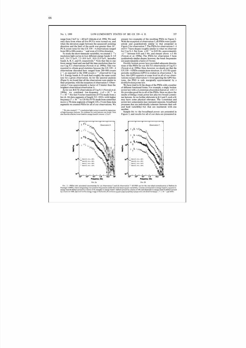
8/12/2019 Schwarze LöCher Als Astronomische Objekte
http://slidepdf.com/reader/full/schwarze-lacher-als-astronomische-objekte 66/146
66
Frequency (Hz)
10 -4
10 -2
10 0
10 2
R M S 2 / H z
10 -3 10 -2 10 -1 1.0 10.0 10 2
Observation 5
Band A, rms = 38%
Band B, rms = 39%
Band C, rms = 38%Band D, rms = 33%
Frequency (Hz)
10 -4
10 -2
10 0
10 2
R M S 2 / H z
10 -3 10 -2 10 -1 1.0 10.0 10 2
Frequency (Hz)
10 -4
10 -2
10 0
10 2
R M S 2 / H z
10 -3 10 -2 10 -1 1.0 10.0 10 2
Frequency (Hz)
10 -4
10 -2
10 0
10 2
R M S 2 / H z
10 -3 10 -2 10 -1 1.0 10.0 10 2
Frequency (Hz)
10 -4
10 -2
10 0
10 2
R M S 2 / H z
10 -3 10 -2 10 -1 1.0 10.0 10 2
Observation 7
Band A, rms = 36%
Band B, rms = 35%
Band C, rms = 34%Band D, rms = 29%
Frequency (Hz)
10 -4
10 -2
10 0
10 2
R M S 2 / H z
10 -3 10 -2 10 -1 1.0 10.0 10 2
Frequency (Hz)
10 -4
10 -2
10 0
10 2
R M S 2 / H z
10 -3 10 -2 10 -1 1.0 10.0 10 2
Frequency (Hz)
10 -4
10 -2
10 0
10 2
R M S 2 / H z
10 -3 10 -2 10 -1 1.0 10.0 10 2
No. 1, 1999 LOW-LUMINOSITY STATES OF BH GX 339 [ 4. II. 357
range from 2 keV to D 60 keV (Jahoda et al. 1996). We usedonly data from when all Ðve PCUs were turned on, andwhen the elevation angle between the spacecraft pointingdirection and the limb of the earth was greater than 10¡.PCA count rates for the GX 339 [ 4 observations rangedfrom 200 to 800 counts s ~1 and were of O (10 ks) duration.
To study the short-timescale variability, we created 2 ~8 sresolution light curves in four di†erent energy bands: 0 È 3.9keV, 3.9 È 7.5 keV, 7.5 È 10.8 keV, 10.8 È 21.9 keV, hereafterbands A, B, C, and D, respectively. 4 Note that this is onefewer energy band and one-half the time resolution than forour Cyg X-1 observations (Nowak et al. 1999a). This wasrequired to obtain good statistics because the GX 339 [ 4observations discussed here ranged from 200 È 800 countss~1 , as opposed to the 4500 counts s ~1 observed for CygX-1. Energy bands A È D each had roughly the same countrate for a given observation. As for the spectral analysis(Paper I), we found that all the observations were similar intheir properties, with the exception of observation 5. Obser-
vation 5 was approximately a factor of 5 fainter than thebrightest observation (observation 1).As for our RXT E observations of Cyg X-1 (Nowak et al.
1999a), we combined low-frequency ( B 8 ] 10~4 to7 ] 10~3 Hz) fast Fourier transforms (FFTs) made from afew (6 È 16) data segments of length 512 È 1024 s with higherfrequency (7 ] 10~3 to 128 Hz) FFTs made from somewhatmore data segments of length 128 s. From these data(Z 70)segments we created PSDs for all of our observations. We
4 We also created 2 ~13 s resolution light curves to search for signaturesof high-frequency features. No evidence for such features was found. Notealso thatthe e†ective lower limitfor energy bandA is more B 2 keV.
present two examples of the resulting PSDs in Figure 2.With the exception of observation 5, all PSDs were qualit-atively and quantitatively similar to that presented inFigure 2 for observation 7. The PSDs for observations 1 È 4and 6 È 7 have shapes roughly similar to what we observedfor Cyg X-1: Ñat from B 10~3 to 0.03 Hz, approximatelyP f ~1 between 0.03 and 3 Hz, and steeper above B 3 Hz(Nowak et al. 1999a). The PSDs for observation 5 havequalitatively similar shapes; however, the break frequenciesare approximately a factor of 3 lower.
Doubly broken power laws provided adequate descrip-tions of the PSDs for our RXT E observations of Cyg X-1(Nowak et al. 1999a). Here, however, we clearly see that theGX 339 [ 4 PSDs contain more structure. A B 0.3 Hz quasi-periodic oscillation (QPO) is evident in observation 7. Infact, this QPO appears at some level in all of our obser-vations except observation 5. Even ignoring the QPO fea-tures, the PSD is only marginally approximated by adoublybroken power law.
We have tried to Ðt the shape of the PSDs with a numberof di†erent functional forms. For example, a singly brokenpower law with a Lorentzian absorption feature at B 0.3 È 1Hz provides good Ðts to all of the PSDs. Here we show theresults of Ðtting a weak power law plus two broad Lorentz-ian features. As we further elaborate in °° 4 and 5, such a Ðtmay have some physical relevance. The Lorentzian andpower-law components may represent separate, broadbandprocesses that are individually coherent (between their softand hard variability) but that are incoherent with oneanother.
Sample Ðts to the broadband power are presented inFigure 3, and results for all of our data are presented in
F IG . 2a F IG . 2b
F IG . 2.ÈPSDs with associated uncertainties for ( a) observation 5 and ( b) observation 7. All PSD are for the one-sided normalization of Belloni &Hasinger (1990b), where integrating over positive frequencies yields the total mean square variability. Crosses correspond to energy band A, squares toenergy band B shifted upward by a factor of 10, triangles to energy band C shifted upward by a factor of 100, and diamonds to energy band D shifted upwardby a factorof 1000. (See text forthe energy range of thebands.) Rootmean square (rms)variabilityvalues were calculated between f \ 7 ] 10~3 and 40Hz.
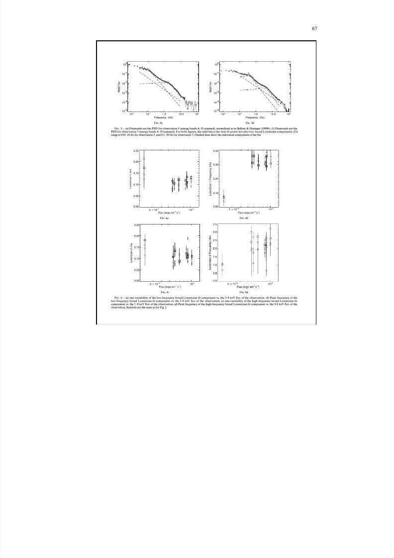
8/12/2019 Schwarze LöCher Als Astronomische Objekte
http://slidepdf.com/reader/full/schwarze-lacher-als-astronomische-objekte 67/146
67
Frequency (Hz)
10 -5
10 -4
10 -3
10 -2
10 -1
10 0
R M S
2 / H z
10 -2 10 -1 1.0 10.0 10 2
Frequency (Hz)
10 -5
10 -4
10 -3
10 -2
10 -1
10 0
R M S
2 / H z
10 -2 10 -1 1.0 10.0 10 2
Flux (ergs cm -2 s -1)
0.00
0.05
0.10
0.15
0.20
0.25
L o r e n
t z i a n
1 r m s
3. × 10 -10 10 -9 Flux (ergs cm -2 s -1)
0.00
0.10
0.20
0.30
0.40
L o r e n
t z i a n
1 F r e q u e n c y
( H z
)
3. × 10 -10 10 -9
Flux (ergs cm -2 s -1)
0.00
0.05
0.10
0.15
0.20
0.25
L o r e n
t z i a n
2 r m s
3. × 10 -10 10 -9
F IG . 3a F IG . 3b
F IG . 3.È( a ) Diamonds are the PSD for observation 5 (energy bands A È D summed), normalized as in Belloni & Hasinger (1990b). ( b ) Diamonds are thePSD for observation 7 (energy bands A È D summed). For both Ðgures, the solid line is the best-Ðt power law plus two broad Lorentzian components. (Fitrange is 0.03 È 10 Hz for observation 5, and 0.1 È 30 Hz for observaion 7.) Dashed lines show the individual components of the Ðts.
F IG . 4a F IG . 4b
F IG . 4c F IG . 4d
F IG . 4.È( a ) rms variability of the low-frequency broad Lorentzian Ðt component vs. the 3 È 9 keV Ñux of the observation. ( b ) Peak frequency of thelow-frequency broad Lorentzian Ðt component vs. the 3 È 9 keV Ñux of the observation. ( c) rms variability of the high-frequency broad Lorentzian Ðtcomponent vs. the 3 È 9 keV Ñux of the observation. ( d ) Peak frequency of the high-frequency broad Lorentzian Ðt component vs. the 3 È 9 keV Ñux of theobservation. Symbols are the same as for Fig. 2.
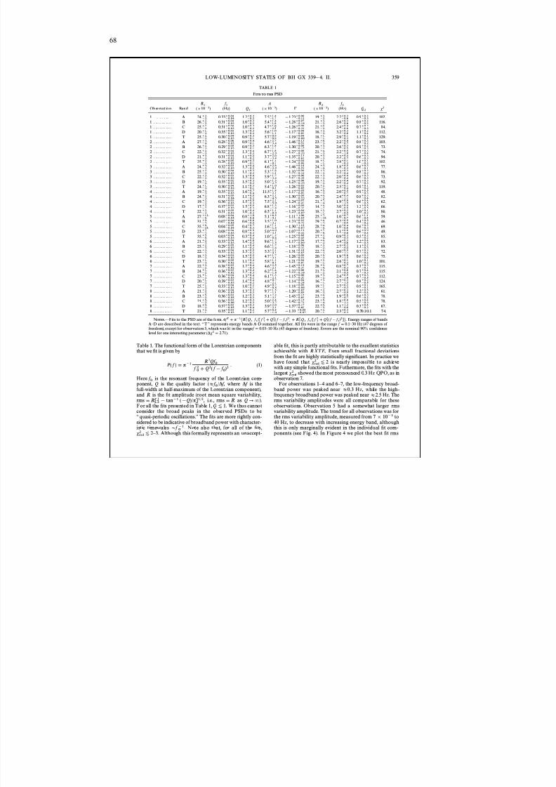
8/12/2019 Schwarze LöCher Als Astronomische Objekte
http://slidepdf.com/reader/full/schwarze-lacher-als-astronomische-objekte 68/146
68
LOW-LUMINOSITY STATES OF BH GX 339 [ 4. II. 359
TABLE 1
F ITS TO THE PSD
R1 f 1 A R2 f 2Ob se rvat io n Band ( ] 10~2 ) (Hz) Q1 (] 10~3 ) ! (] 10~2 ) (Hz) Q2 s2
1 . .. . . .. . .. . . A 24.~2.` 2. 0.33~0.04
` 0.04 1.2~0.2` 0.3 7.5~1.7
` 1.4 [ 1.23~0.11` 0.06 19.~2.
` 3. 2.2~0.6` 0.3 0.9~0.3
` 0.2 102.1 . .. . . .. . .. . . B 26.~2.
` 2. 0.31~0.03` 0.04 1.0~0.2
` 0.3 5.4~1.8` 1.4 [ 1.28~0.18
` 0.07 21.~2.` 3. 2.6~0.6
` 0.3 0.8~0.3` 0.2 116.
1 . .. . .. . . .. . . C 25.~2.` 2. 0.31~0.03
` 0.04 1.0~0.2` 0.3 4.7~2.5
` 1.6 [ 1.26~0.32` 0.08 21.~2.
` 4. 2.4~0.8` 0.4 0.7~0.3
` 0.2 84.1 . .. . .. . . .. . . D 20.~2.
` 1. 0.35~0.02` 0.03 1.3~0.2
` 0.3 5.6~1.1` 1.0 [ 1.17~0.09
` 0.04 16.~2.` 3. 3.2~0.6
` 0.3 1.1~0.4` 0.2 112.
1 . .. . .. . . .. . . T 25.~2.` 2. 0.30~0.03
` 0.04 0.9~0.1` 0.3 5.7~0.9
` 0.9 [ 1.19~0.06` 0.04 18.~1.
` 1. 2.9~0.3` 0.1 1.1~0.2
` 0.1 129.2 . .. . .. . . .. . . A 27.~4.
` 3. 0.28~0.03` 0.06 0.9~0.1
` 0.4 4.6~3.4` 2.7 [ 1.46~0.51
` 0.13 23.~3.` 4. 2.2~0.7
` 0.4 0.8~0.2` 0.3 103.
2 . .. . .. . . .. . . B 26.~3.` 2. 0.29~0.03
` 0.05 0.9~0.1` 0.3 6.3~1.7
` 1.8 [ 1.30~0.15` 0.08 20.~2.
` 3. 2.6~0.5` 0.3 0.9~0.3
` 0.2 73.2 . .. . .. . . .. . . C 22.~3.
` 2. 0.32~0.03` 0.04 1.3~0.2
` 0.4 6.7~2.9` 1.8 [ 1.27~0.23
` 0.08 21.~3.` 4. 2.2~1.0
` 0.5 0.7~0.4` 0.3 74.
2 . .. . .. . . .. . . D 21.~3.` 3. 0.31~0.03
` 0.04 1.1~0.2` 0.4 3.7~3.4
` 2.0 [ 1.35~0.62` 0.13 20.~3.
` 3. 2.2~0.7` 0.4 0.6~0.3
` 0.3 94.2 . .. . .. . . .. . . T 25.~3.
` 2. 0.28~0.03` 0.05 0.9~0.1
` 0.3 6.1~0.9` 1.1 [ 1.24~0.06
` 0.04 18.~1.` 1. 2.8~0.3
` 0.1 1.0~0.2` 0.1 102.
3 . .. . .. . . .. . . A 24.~3.` 3. 0.32~0.03
` 0.03 1.3~0.2` 0.4 4.6~2.9
` 2.8 [ 1.46~0.51` 0.16 24.~4.
` 3. 1.8~0.3` 0.5 0.6~0.1
` 0.3 77.3 . .. . .. . . .. . . B 25.~2.
` 2. 0.30~0.03` 0.04 1.1~0.2
` 0.3 5.3~1.6` 1.8 [ 1.32~0.16
` 0.09 22.~2.` 3. 2.2~0.4
` 0.3 0.8~0.2` 0.2 86.
3 . .. . .. . . .. . . C 22.~2.` 2. 0.32~0.02
` 0.03 1.3~0.2` 0.4 5.9~3.4
` 1.7 [ 1.27~0.38` 0.06 22.~2.
` 3. 2.0~0.4` 0.4 0.6~0.3
` 0.3 73.3 . .. . .. . . .. . . D 19.~2.
` 1. 0.35~0.02` 0.02 1.5~0.2
` 0.3 5.0~2.7` 1.3 [ 1.25~0.33
` 0.08 19.~2.` 3. 2.2~0.4
` 0.4 0.7~0.3` 0.3 92.
3 . .. . .. . . .. . . T 24.~3.` 1. 0.30~0.02
` 0.04 1.1~0.1` 0.3 5.4~0.8
` 1.0 [ 1.26~0.08` 0.03 20.~1.
` 2. 2.5~0.4` 0.1 0.9~0.2
` 0.1 119.4 . .. . .. . . .. . . A 19.
~3.` 2. 0.35
~0.03` 0.03 1.6
~0.4` 0.7 11.5
~2.1` 1.8 [ 1.17
~0.09` 0.05 16.
~3.` 5. 2.0
~0.7` 0.5 0.9
~0.3` 0.5 48.
4 . .. . .. . . .. . . B 24.~3.` 2. 0.31~0.04
` 0.05 1.1~0.2` 0.5 6.3~4.5
` 2.1 [ 1.30~0.53` 0.09 20.~3.
` 4. 2.4~1.1` 0.4 0.8~0.4
` 0.3 82.4 . .. . .. . . .. . . C 19.~2.
` 2. 0.36~0.03` 0.03 1.5~0.3
` 0.5 7.5~5.0` 2.1 [ 1.24~0.47
` 0.07 21.~4.` 7. 1.9~1.5
` 0.8 0.6~0.5` 0.4 62.
4 . . . . .. . . .. . . D 17.~2.` 2. 0.37~0.03
` 0.03 1.5~0.3` 0.5 6.8~1.4
` 1.3 [ 1.16~0.10` 0.05 14.~2.
` 4. 3.0~0.8` 0.4 1.2~0.5
` 0.5 66.4 . . . . .. . . .. . . T 22.~3.
` 2. 0.31~0.03` 0.05 1.0~0.2
` 0.4 6.5~0.9` 1.1 [ 1.23~0.07
` 0.04 18.~1.` 2. 2.7~0.5
` 0.2 1.0~0.2` 0.1 86.
5 . . . . .. . . .. . . A 27.~8.` 12. 0.08~0.05
` 0.04 0.8~0.6` 1.0 5.1~4.8
` 6.5 [ 1.11~0.85` 1.06 25.~10.
` 7. 1.0~0.7` 0.7 0.6~0.4
` 1.1 59.5 . . . . .. . . .. . . B 31.~7.
` 9. 0.07~0.05` 0.04 0.6~0.5
` 0.6 3.5~3.2` 5.0 [ 1.23~0.73
` 0.92 29.~7.` 4. 0.7~0.4
` 0.5 0.4~0.2` 0.5 46.
5 . . . . .. . . .. . . C 35.~10.` 8. 0.04~0.04
` 0.05 0.4~0.3` 0.7 1.6~1.4
` 5.1 [ 1.30~0.67` 1.10 28.~5.
` 4. 1.0~0.6` 0.4 0.6~0.3
` 0.3 69.5 . . . . .. . . .. . . D 23.~7.
` 7. 0.08~0.03` 0.04 0.8~0.3
` 0.8 5.0~3.8` 4.0 [ 1.07~0.41
` 0.19 20.~8.` 7. 1.1~0.6
` 0.6 0.6~0.4` 0.9 49.
5 . . . . .. . . .. . . T 35.~8.` 5. 0.03~0.03
` 0.04 0.3~0.2` 0.4 1.0~0.4
` 3.2 [ 1.25~0.45` 0.60 27.~4.
` 2. 0.9~0.3` 0.3 0.5~0.2
` 0.2 85.6 . . . . .. . . .. . . A 21.~3.
` 2. 0.33~0.03` 0.04 1.4~0.2
` 0.6 9.6~1.5` 1.7 [ 1.17~0.09
` 0.04 17.~2.` 4. 2.4~0.6
` 0.3 1.2~0.5` 0.4 83.
6 . . . . .. . . .. . . B 25.~3.` 2. 0.29~0.03
` 0.05 1.1~0.2` 0.4 6.6~1.4
` 1.7 [ 1.18~0.10` 0.06 18.~2.
` 3. 2.7~0.4` 0.2 1.1~0.3
` 0.2 89.6 . . . . .. . . .. . . C 22.~3.
` 3. 0.33~0.02` 0.04 1.3~0.2
` 0.5 5.3~4.1` 2.1 [ 1.31~0.65
` 0.10 22.~3.` 4. 2.0~1.1
` 0.5 0.7~0.4` 0.3 72.
6 . . . . .. . . .. . . D 18.~2.` 2. 0.34~0.02
` 0.03 1.5~0.2` 0.5 4.7~3.1
` 1.7 [ 1.26~0.51` 0.09 20.~3.
` 5. 1.9~1.5` 0.6 0.6~0.4
` 0.3 75.6 . . . . .. . . .. . . T 23.~3.
` 1. 0.30~0.02` 0.05 1.1~0.1
` 0.4 5.8~0.8` 1.1 [ 1.21~0.07
` 0.04 19.~1.` 2. 2.6~0.3
` 0.1 1.0~0.2` 0.1 101.
7 . . . . .. . . .. . . A 22.~2.` 2. 0.38~0.02
` 0.03 1.7~0.3` 0.4 4.6~2.8
` 2.5 [ 1.45~0.37` 0.18 28.~4.
` 2. 0.8~0.3` 0.7 0.3~0.1
` 0.3 115.7 . . . . .. . . .. . . B 24.~2.
` 1. 0.36~0.02` 0.03 1.3~0.3
` 0.4 6.2~1.8` 1.4 [ 1.22~0.16
` 0.06 21.~2.` 2. 2.1~0.5
` 0.6 0.7~0.3` 0.4 115.
7 . . . . .. . . .. . . C 23.~2.` 1. 0.36~0.03
` 0.04 1.3~0.2` 0.4 6.1~2.1
` 1.3 [ 1.15~0.20` 0.06 19.~2.
` 3. 2.4~1.6` 0.5 0.7~0.5
` 0.3 112.7 . . . . .. . . .. . . D 20.~2.
` 1. 0.39~0.03` 0.03 1.4~0.2
` 0.4 4.8~2.2` 0.7 [ 1.14~0.24
` 0.04 16.~1.` 3. 2.7~1.5
` 0.3 0.8~0.5` 0.2 124.
7 . . . . .. . . .. . . T 25.~2.` 1. 0.33~0.03
` 0.04 1.0~0.1` 0.2 4.9~0.8
` 0.7 [ 1.18~0.06` 0.05 19.~1.
` 1. 2.7~0.3` 0.2 0.9~0.1
` 0.1 165.
8 . . . . .. . . .. . . A 21.~2.` 2. 0.36~0.05` 0.04 1.3~0.3` 0.3 9.7~1.8` 1.5 [ 1.20~0.08` 0.05 16.~3.` 2. 2.7~0.5` 0.3 1.2~0.4` 0.5 61.8 . . . . .. . . .. . . B 23.~2.
` 5. 0.36~0.05` 0.03 1.2~0.3
` 0.3 5.1~3.9` 2.2 [ 1.45~0.69
` 0.15 23.~4.` 4. 1.9~0.7
` 0.6 0.6~0.2` 0.3 78.
8 . . . . .. . . .. . . C 21.~2.` 5. 0.36~0.06
` 0.03 1.2~0.3` 0.3 5.0~3.7
` 2.4 [ 1.42~0.71` 0.15 23.~4.
` 5. 1.8~1.1` 0.8 0.5~0.3
` 0.4 78.8 . . . . .. . .. . . . D 18.~2.
` 4. 0.37~0.05` 0.03 1.3~0.4
` 0.3 3.9~2.8` 2.0 [ 1.37~0.60
` 0.17 22.~5.` 4. 1.1~0.6
` 1.2 0.3~0.2` 0.4 67.
8 . . . . .. . .. . . . T 21.~1.` 2. 0.35~0.03
` 0.03 1.1~0.2` 0.2 5.7~1.0
` 0.8 [ 1.33 ~0.07` 0.05 20.~1.
` 2. 2.3~0.3` 0.3 0.70 .10.1 74.
N OTES .ÈFits to the PSD are of the form Energy ranges of bandsAf ! ] n~1 MR12 Q1 f 1 /[ f 1
2 ] Q12( f [ f 1)2] ] R2
2 Q2 f 2 /[ f 22 ] Q2
2( f [ f 2)2]N.A È D are described in the text. ““ T ÏÏ represents energy bands A È D summed together. All Ðts were in the range f \ 0.1 È 30 Hz (47 degrees of freedom), except for observation 5, which was Ðt in the range f \ 0.03 È 10 Hz (45 degrees of freedom). Errors are the nominal 90% conÐdencelevel for one interesting parameter ( *s 2 \ 2.71).
Table 1. The functional form of the Lorentzian componentsthat we Ðt is given by
P ( f ) \ n~1 R2Qf 0 f 0
2 ] Q2( f [ f 0)2 . (1)
Here is the resonant frequency of the Lorentzian com- f 0ponent, Q is the quality factor where * f is the(B f 0 / * f ,full-width at half-maximum of the Lorentzian component),and R is the Ðt amplitude (root mean square variability,
i.e., rms \ R as Q ] O ).rms \ R[ 12
[ tan ~1 ([ Q)/ n]1@2,For all the Ðts presented in Table 1, We thus cannotQ [ 1.consider the broad peaks in the observed PSDs to be““ quasi-periodic oscillations.ÏÏ The Ðts are more rightly con-sidered to be indicative of broadband power with character-istic timescales Note also that, for all of the Ðts,D f 0
~1 .Although this formally represents an unaccept-sred
2 [ 2 È 3.
able Ðt, this is partly attributable to the excellent statisticsachievable with RXT E . Even small fractional deviationsfrom the Ðt are highly statistically signiÐcant. In practice wehave found that is nearly impossible to achievesred
2 [ 2with any simple functional Ðts. Futhermore, the Ðts with thelargest showed the most pronounced 0.3 Hz QPO, as insred
2observation 7.
For observations 1 È 4 and 6 È 7, the low-frequency broad-band power was peaked near B 0.3 Hz, while the high-frequency broadband power was peaked near B 2.5 Hz. Therms variability amplitudes were all comparable for theseobservations. Observation 5 had a somewhat larger rmsvariability amplitude. The trend for all observations was forthe rms variability amplitude, measured from 7 ] 10~3 to40 Hz, to decrease with increasing energy band, althoughthis is only marginally evident in the individual Ðt com-ponents (see Fig. 4). In Figure 4 we plot the best Ðt rms
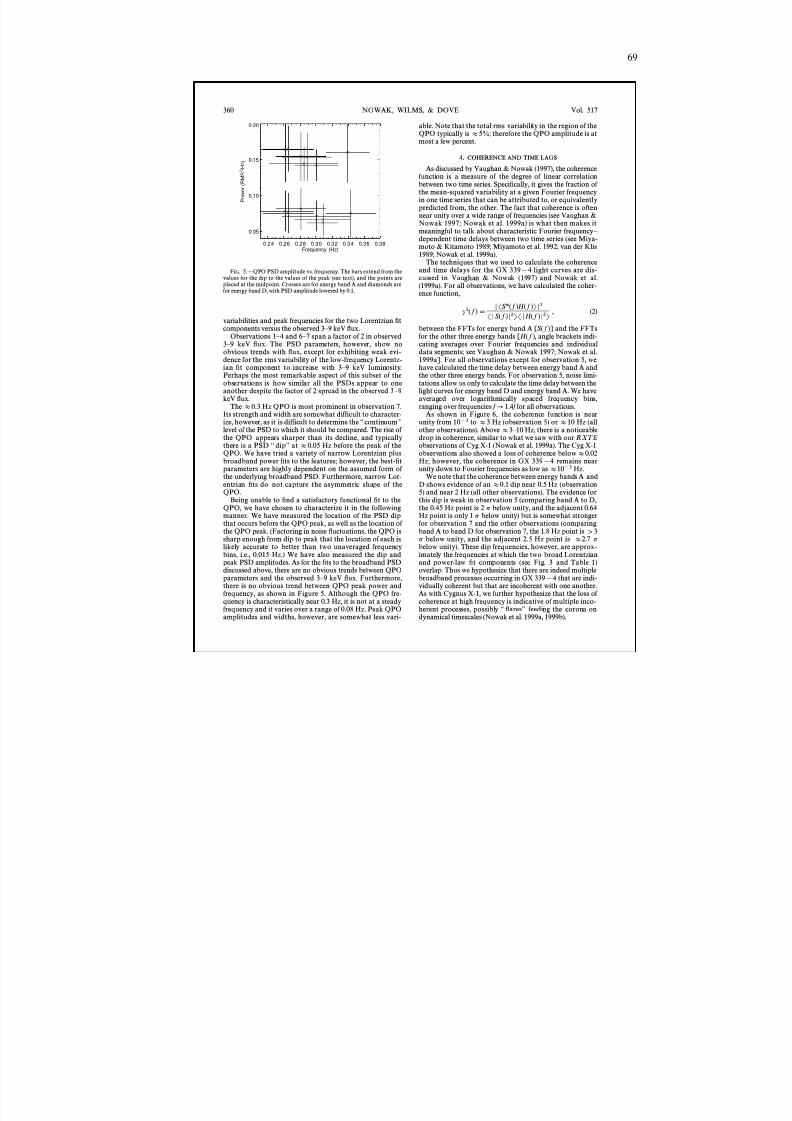
8/12/2019 Schwarze LöCher Als Astronomische Objekte
http://slidepdf.com/reader/full/schwarze-lacher-als-astronomische-objekte 69/146
69
0.24 0.26 0.28 0.30 0.32 0.34 0.36 0.38Frequency (Hz)
0.05
0.10
0.15
0.20
P o w e r
( R M S
2 / H z )
360 NOWAK, WILMS, & DOVE Vol. 517
F IG . 5.ÈQPO PSD amplitude vs. frequency. The bars extend from thevalues for the dip to the values of the peak (see text), and the points areplaced at the midpoint. Crosses are for energy band A and diamonds arefor energy band D, with PSD amplitude lowered by 0.1.
variabilities and peak frequencies for the two Lorentzian Ðtcomponents versus the observed 3 È 9 keV Ñux.
Observations 1 È 4 and 6 È 7 span a factor of 2 in observed3 È 9 keV Ñux. The PSD parameters, however, show noobvious trends with Ñux, except for exhibiting weak evi-dence for the rms variability of the low-frequency Lorentz-ian Ðt component to increase with 3 È 9 keV luminosity.Perhaps the most remarkable aspect of this subset of theobservations is how similar all the PSDs appear to oneanother despite the factor of 2 spread in the observed 3 È 9keV Ñux.
The B 0.3 Hz QPO is most prominent in observation 7.
Its strength and width are somewhat difficult to character-ize, however, as it is difficult to determine the ““ continuum ÏÏlevel of the PSD to which it should be compared. The rise of the QPO appears sharper than its decline, and typicallythere is a PSD ““ dipÏÏ at B 0.05 Hz before the peak of theQPO. We have tried a variety of narrow Lorentzian plusbroadband power Ðts to the features; however, the best-Ðtparameters are highly dependent on the assumed form of the underlying broadband PSD. Furthermore, narrow Lor-entzian Ðts do not capture the asymmetric shape of theQPO.
Being unable to Ðnd a satisfactory functional Ðt to theQPO, we have chosen to characterize it in the followingmanner. We have measured the location of the PSD dipthat occurs before the QPO peak, as well as the location of the QPO peak. (Factoring in noise Ñuctuations, the QPO issharp enough from dip to peak that the location of each islikely accurate to better than two unaveraged frequencybins, i.e., 0.015 Hz.) We have also measured the dip andpeak PSD amplitudes. As for the Ðts to the broadband PSDdiscussed above, there are no obvious trends between QPOparameters and the observed 3 È 9 keV Ñux. Furthermore,there is no obvious trend between QPO peak power andfrequency, as shown in Figure 5. Although the QPO fre-quency is characteristically near 0.3 Hz, it is not at a steadyfrequency and it varies over a range of 0.08 Hz. Peak QPOamplitudes and widths, however, are somewhat less vari-
able. Note that the total rms variability in the region of theQPO typically is B 5%; therefore the QPO amplitude is atmost a few percent.
4. COHERENCE AND TIME LAGS
As discussed by Vaughan & Nowak (1997), the coherencefunction is a measure of the degree of linear correlationbetween two time series. SpeciÐcally, it gives the fraction of the mean-squared variability at a given Fourier frequencyin one time series that can be attributed to, or equivalentlypredicted from, the other. The fact that coherence is oftennear unity over a wide range of frequencies (see Vaughan &Nowak 1997; Nowak et al. 1999a) is what then makes itmeaningful to talk about characteristic Fourier frequency È dependent time delays between two time series (see Miya-moto & Kitamoto 1989; Miyamoto et al. 1992; van der Klis1989; Nowak et al. 1999a).
The techniques that we used to calculate the coherenceand time delays for the GX 339 [ 4 light curves are dis-cussed in Vaughan & Nowak (1997) and Nowak et al.(1999a). For all observations, we have calculated the coher-ence function,
c2( f ) \ oSS*( f )H ( f )T o2
S oS( f )o2TS oH ( f )o2T , (2)
between the FFTs for energy band A [ S( f )] and the FFTsfor the other three energy bands [ H ( f ), angle brackets indi-cating averages over Fourier frequencies and individualdata segments; see Vaughan & Nowak 1997; Nowak et al.1999a]. For all observations except for observation 5, wehave calculated the time delay between energy band A andthe other three energy bands. For observation 5, noise limi-tations allow us only to calculate the time delay between thelight curves for energy band D and energy band A. We haveaveraged over logarithmically spaced frequency bins,ranging over frequencies f ] 1.4 f for all observations.
As shown in Figure 6, the coherence function is nearunity from 10 ~3 to B 3 Hz (observation 5) or B 10 Hz (allother observations). Above B 3 È 10 Hz, there is a noticeabledrop in coherence, similar to what we saw with our RXT Eobservations of Cyg X-1 (Nowak et al. 1999a). The Cyg X-1observations also showed a loss of coherence below B 0.02Hz; however, the coherence in GX 339 [ 4 remains nearunity down to Fourier frequencies as low as B 10~3 Hz.
We note that the coherence between energy bands A andD shows evidence of an B 0.1 dip near 0.5 Hz (observation5) and near 2 Hz (all other observations). The evidence forthis dip is weak in observation 5 (comparing band A to D,the 0.45 Hz point is 2 p below unity, and the adjacent 0.64Hz point is only 1 p below unity) but is somewhat strongerfor observation 7 and the other observations (comparingband A to band D for observation 7, the 1.8 Hz point is [ 3p below unity, and the adjacent 2.5 Hz point is B 2.7 pbelow unity). These dip frequencies, however, are approx-imately the frequencies at which the two broad Lorentzianand power-law Ðt components (see Fig. 3 and Table 1)overlap. Thus we hypothesize that there are indeed multiplebroadband processes occurring in GX 339 [ 4 that are indi-vidually coherent but that are incoherent with one another.As with Cygnus X-1, we further hypothesize that the loss of coherence at high frequency is indicative of multiple inco-herent processes, possibly ““ ÑaresÏÏ feeding the corona ondynamical timescales (Nowak et al. 1999a, 1999b).
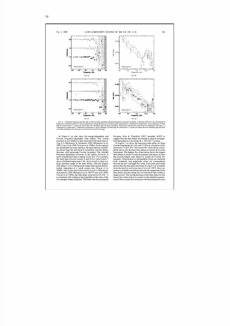
8/12/2019 Schwarze LöCher Als Astronomische Objekte
http://slidepdf.com/reader/full/schwarze-lacher-als-astronomische-objekte 70/146
70
Frequency (Hz)
0.5
1.0
1.5
2.0
C o
h e r e n c e
10 -3 10 -2 10 -1 1.0 10.0 10 2
Observation 5
Frequency (Hz)
0.5
1.0
1.5
2.0
C o
h e r e n c e
10 -3 10 -2 10 -1 1.0 10.0 10 2
Frequency (Hz)
0.5
1.0
1.5
2.0
C o
h e r e n c e
10 -3 10 -2 10 -1 1.0 10.0 10 2
Frequency (Hz)
0.001
0.010
0.100
L a g
( s e c . )
10 -2 10 -1 1.0 10.0 10 2
Observation 5
Frequency (Hz)
0.5
1.0
1.5
2.0
C o
h e r e n c e
10 -3 10 -2 10 -1 1.0 10.0 10 2
Observation 7
Frequency (Hz)
0.5
1.0
1.5
2.0
C o
h e r e n c e
10 -3 10 -2 10 -1 1.0 10.0 10 2
Frequency (Hz)
0.5
1.0
1.5
2.0
C o
h e r e n c e
10 -3 10 -2 10 -1 1.0 10.0 10 2
Frequency (Hz)
0.001
0.010
0.100
L a g
( s e c . )
10 -2 10 -1 1.0 10.0 10 2
Observation 7
Frequency (Hz)
0.001
0.010
0.100
L a g
( s e c . )
10 -2 10 -1 1.0 10.0 10 2 Frequency (Hz)
0.001
0.010
0.100
L a g
( s e c . )
10 -2 10 -1 1.0 10.0 10 2
No. 1, 1999 LOW-LUMINOSITY STATES OF BH GX 339 [ 4. II. 361
F IG . 6a F IG . 6b
F IG . 6c F IG . 6d
F IG . 6.ÈCoherence function and time lags of various energy channels (channel B [ squares ], channel C [ triangles ; coherence o†set by 0.5], and channel D[ diamonds ; coherence o†set by 1.0]) as compared to energy channel A. ( a) Coherence for observation 5. Solid lines correspond to unity coherence. ( b) Timelags for observation 5. Crosses are where the soft variability lags the hard variability. Solid line is the Poisson noise level for channel D time lags. ( c)Coherence for observation 7. Solid lines correspond to unity coherence. ( d ) Time lags for observation 7. Crosses are where the soft variability lags the hardvariability.Solidline isthe Poisson noise level forchannel D time lags.
In Figure 6 we also show the energy-dependent andFourier frequency È dependent time delays. The overallstructure is very similar to that observed in the hard state of Cyg X-1 (Miyamoto & Kitamoto 1989; Miyamoto et al.1992; Crary et al. 1999; Nowak et al. 1999a). In the regionsnot dominated by noise statistics, the hard photon variabil-ity always lags the soft photon variability, and the delaysdecrease with increasing Fourier frequency. The detailedfrequency-dependent structure of the delays, however, ismore complicated than a simple power law. For example,the time lags between bands A and D for observation 7show a Ñattened region near 1 Hz. As for Cyg X-1, there is alarge dynamic range in the time delays, with the longesttime delays ( B 0.1 s) being much longer than typical charac-teristic timescales of a small corona (see Nowak et al.1999b). Also as has been observed for Cyg X-1 (Miyamoto& Kitamoto 1989; Miyamoto et al. 1992; Crary et al. 1999;Nowak et al. 1999a), the time delay observed in GX 339 [ 4is consistent with scaling as the logarithm of the ratio of thetwo energies being compared. This latter fact has prompted
Kazanas, Hua & Titarchuk (1997, hereafter KHT) tosuggest that the time delays are related to photon propaga-tion timescales in a very large ( R B 105 GM / c2 ) corona.
In Figure 7 we show the measured time delay for threeFourier frequencies (0.1, 0.9, and 2.5 Hz) as a function of themeasured 3 È 9 keV Ñux. The lowest Ñux observation consis-tently shows the shortest time delays at nearly all Fourierfrequencies. The highest Ñux observation shows the longesttime delays at many Fourier frequencies and shows at leastthe second longest time delays at nearly all Fourier fre-quencies. Observations at intermediate Ñuxes are scatteredboth positively and negatively about an extrapolationbetween the low- and high-Ñux point. It has been previouslyshown that the time delay decreases in Cyg X-1 as it transitsfrom the hard to soft state (see Cui et al. 1997). Here wepresent a possible correlation between the magnitude of thetime delay and the energy Ñux for the hard state within asingle source. The strong decrease of the time delay for thelowest Ñux observation is counter to the simplest expecta-tions if the coronal size increases with decreasing Ñux (see,
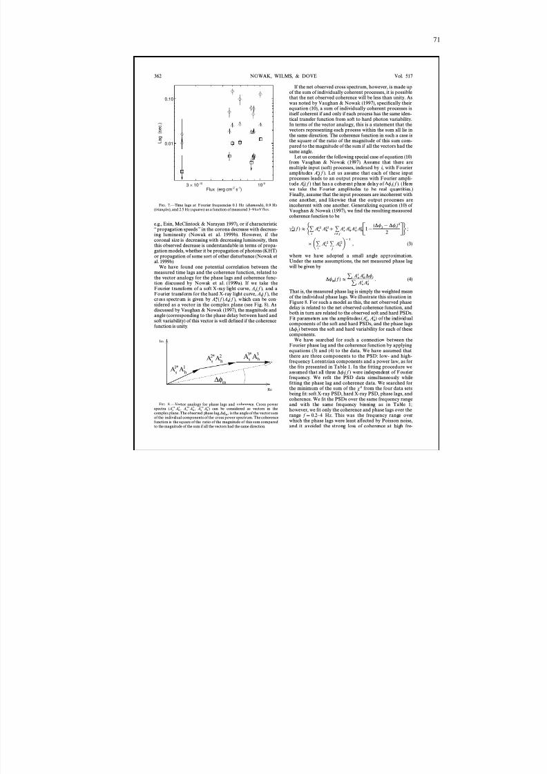
8/12/2019 Schwarze LöCher Als Astronomische Objekte
http://slidepdf.com/reader/full/schwarze-lacher-als-astronomische-objekte 71/146
71
Flux (erg cm-2
s-1
)
0.01
0.10
L a g
( s
e c
. )
3 × 10 -10 10 -9
A As h
1 1*
A As h
2*2
∆φ
A A
Re
s h3 3*
m
Im
362 NOWAK, WILMS, & DOVE Vol. 517
F IG . 7.ÈTime lags at Fourier frequencies 0.1 Hz ( diamonds ), 0.9 Hz(triangles ), and 2.5 Hz (squares ) as a function of measured 3 È 9 keV Ñux.
e.g., Esin, McClintock & Narayan 1997), or if characteristic““ propagation speeds ÏÏ in the corona decrease with decreas-ing luminosity (Nowak et al. 1999b). However, if thecoronal size is decreasing with decreasing luminosity, thenthis observed decrease is understandable in terms of propa-gation models, whether it be propagation of photons (KHT)or propagation of some sort of other disturbance (Nowak etal. 1999b).
We have found one potential correlation between themeasured time lags and the coherence function, related tothe vector analogy for the phase lags and coherence func-tion discussed by Nowak et al. (1999a). If we take theFourier transform of a soft X-ray light curve, and aAs( f ),Fourier transform for the hard X-ray light curve, theAh( f ),cross spectrum is given by which can be con-As*( f )Ah( f ),sidered as a vector in the complex plane (see Fig. 8). Asdiscussed by Vaughan & Nowak (1997), the magnitude andangle (corresponding to the phase delay between hard andsoft variability) of this vector is well deÐned if the coherencefunction is unity.
F IG . 8.ÈVector analogy for phase lags and coherence. Cross powerspectra can be considered as vectors in the(As1
R Ah1, As2R Ah2, As3
R Ah3)complex plane. The observed phase lag, is the angle of the vector sum* / m ,of the individual components of the cross power spectrum. The coherencefunction is the square of the ratio of the magnitude of this sum comparedto the magnitude of the sum if all the vectors had the same direction.
If the net observed cross spectrum, however, is made upof the sum of individually coherent processes, it is possiblethat the net observed coherence will be less than unity. Aswas noted by Vaughan & Nowak (1997), speciÐcally theirequation (10), a sum of individually coherent processes isitself coherent if and only if each process has the same iden-tical transfer function from soft to hard photon variability.In terms of the vector analogy, this is a statement that thevectors representing each process within the sum all lie inthe same direction. The coherence function in such a case isthe square of the ratio of the magnitude of this sum com-pared to the magnitude of the sum if all the vectors had thesame angle.
Let us consider the following special case of equation (10)from Vaughan & Nowak (1997). Assume that there aremultiple input (soft) processes, indexed by i, with Fourieramplitudes Let us assume that each of these inputAs
i ( f ).processes leads to an output process with Fourier ampli-tude that has a coherent phase delay of (HereAh
i ( f ) */ i( f ).
we take the Fourier amplitudes to be real quantities.)Finally, assume that the input processes are incoherent withone another, and likewise that the output processes areincoherent with one another. Generalizing equation (10) of Vaughan & Nowak (1997), we Ðnd the resulting measuredcoherence function to be
cm 2( f )B G;i
Asi2 Ah
i2] ;iE j
Asi Ah
i A sj Ah
j C1[ (* / j [ * / i)2
2 DH ;
] A;i
Asi2 ;
j Ah
i2B~1, (3)
where we have adopted a small angle approximation.Under the same assumptions, the net measured phase lagwill be given by
* / m ( f )B; i A s
i Ahi */ i
; i A si Ah
i . (4)
That is, the measured phase lag is simply the weighted meanof the individual phase lags. We illustrate this situation inFigure 8. For such a model as this, the net observed phasedelay is related to the net observed coherence function, andboth in turn are related to the observed soft and hard PSDs.Fit parameters are the amplitudes of the individual(As
i , Ahi )
components of the soft and hard PSDs, and the phase lagsbetween the soft and hard variability for each of these(* / i )
components.We have searched for such a connection between the
Fourier phase lag and the coherence function by applyingequations (3) and (4) to the data. We have assumed thatthere are three components to the PSD: low- and high-frequency Lorentzian components and a power law, as forthe Ðts presented in Table 1. In the Ðtting procedure weassumed that all three were independent of Fourier* / i( f )frequency. We reÐt the PSD data simultaneously whileÐtting the phase lag and coherence data. We searched forthe minimum of the sum of the s2 from the four data setsbeing Ðt: soft X-ray PSD, hard X-ray PSD, phase lags, andcoherence. We Ðt the PSDs over the same frequency rangeand with the same frequency binning as in Table 1;however, we Ðt only the coherence and phase lags over therange f \ 0.2 È 4 Hz. This was the frequency range overwhich the phase lags were least a†ected by Poisson noise,and it avoided the strong loss of coherence at high fre-
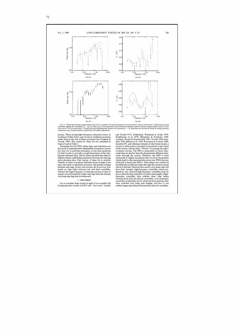
8/12/2019 Schwarze LöCher Als Astronomische Objekte
http://slidepdf.com/reader/full/schwarze-lacher-als-astronomische-objekte 72/146
72
0.01 0.10 1.00 10.00Frequency (Hz)
0.01
0.10
P h a s e
L a g
( r a
d )
0.01 0.10 1.00 10.00Frequency (Hz)
-0.05
0.00
0.05
0.10
0.15
0.20
[ 1 - γ
2 ( f ) ]
0.01 0.10 1.00 10.00Frequency (Hz)
0.01
0.10
P h a s e
L a g
( r a
d )
0.01 0.10 1.00 10.00Frequency (Hz)
0.00
0.02
0.04
0.06
0.08
[ 1 - γ
2 ( f ) ]
No. 1, 1999 LOW-LUMINOSITY STATES OF BH GX 339 [ 4. II. 363
F IG . 9a F IG . 9b
F IG . 9c F IG . 9d
F IG . 9.ÈPhase lags between energy bands A and D as a function of Fourier frequency for ( a) observation 5 and ( c) observation 7. (All points are hardvariability lagging soft variability.) where is the measured, noise-subtracted coherence function between energy bands A and D, for ( b)[1 [ c m
2 ( f )], cm 2 ( f )
observation 5 and ( d ) observation 7. All data has been logarithmically binned over frequencies f ] 1.4 f . Solid lines are the best-Ðt results for Ðtting equationsof theform of eqs. (2)and (3)(seetext andTable2 forfurther explanation).
quency. These strong high-frequency coherence losses, aswe discuss further below, may be due to nonlinear processesrather than to the sum of linear processes (see Vaughan &Nowak 1997). The results for these Ðts are presented inFigure 9 and in Table 2.
Assuming that the PSD, phase lags, and coherence arethe result of summing three independent processes (a powerlaw plus two Lorentzian processes), we see that equations(3) and (4) seem to provide a rough description of the timelag and coherence data. The Ðts make plausible that there isindeed a deeper underlying connection between the time lagand coherence data. One feature of these Ðts is notable.Namely, in order to produce coherence drops as large as areseen, one needs to add linear processes with greatly varyingintrinsic time lags. In fact, one process, the power law, hasnearly no time delay between soft and hard variability,whereas the high-frequency Lorentzian process is seen torequire even intrinsically longer time lags than the alreadyverylong time lags that are measured.
5. DISCUSSION
Let us consider these results in light of two models: theComptonization model of KHT and ““ shot noiseÏÏ models
(see Terrell 1972; Sutherland, Weisskopf & Kahn 1978;Priedhorsky et al. 1979; Miyamoto & Kitamoto 1989;Lochner, Swank & Szymkowiak 1991; Nowak 1994, here-after N94; Belloni et al. 1997; Poutanen & Fabian 1999,hereafter PF, and references therein). In the former model, asource of white noise is assumed to be present at the centerof the system, which is then ““ Ðltered ÏÏ by passage through aCompton corona. The PSD is attenuated on those time-scales that are shorter than the characteristic di†usion time-scales through the corona. Therefore, the PSD is moreattenuated at higher frequencies than at lower frequencies,which leads to the characteristic power-law PSDs that areobserved in hard-state BHCs. Time delays are created bythe di†erence in di†usion times through the corona for hardand soft photons. Photons that scatter over large radii willhave their intrinsic high-frequency variability wiped out ;therefore, any observed high-frequency variability must bedue to photons that scattered over short path lengths. High-frequency variability thus exhibits short time delaysbetween hard and soft photon variability. Low-frequencyvariability potentially can be observed from photons thathave scattered over large path lengths, and thus it canexhibit longer time delays between hard and soft variability.
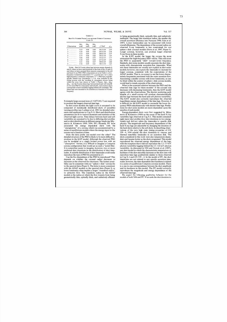
8/12/2019 Schwarze LöCher Als Astronomische Objekte
http://slidepdf.com/reader/full/schwarze-lacher-als-astronomische-objekte 73/146
73
364 NOWAK, WILMS, & DOVE Vol. 517
TABLE 2
B EST -F IT F OURIER P HASE L AGS BETWEEN ENERGY C HANNELS
A AND D
* / l1 * / pl * / l2Observa tion (rad) (rad) (rad) s2 /DoF sred
2
1 . . . .. . . .. . . . 0.13 0.06 0.49 301.5/119 2.532 . . . .. . . .. . . . 0.18 0.05 0.26 283.4/119 2.383 . . . .. . . .. . . . 0.13 0.04 0.28 269.9/119 2.274 . . . .. . . .. . . . 0.15 0.06 0.66 195.8/119 1.655 . . . .. . . .. . . . 0.06 0.04 0.25 132.4/113 1.176 . . . .. . . .. . . . 0.16 0.05 0.38 217.4/119 1.827 . . . .. . . .. . . . 0.11 0.04 0.27 309.9/119 2.608 . . . .. . . .. . . . 0.16 0.05 0.41 198.2/119 1.67
N OTES .ÈBest Ðt Fourier phase lags between energy channels Aand D, where we have used equations of the form of eqs. (2) and (3)and where we have assumed three separate components to the softand hard X-ray PSD. PSD components are as in Table 1: a low-frequency Lorentzian component (““ l 1 ÏÏ), a power law (““ pl ÏÏ), and ahigh-frequency Lorentzian component (““ l 2 ÏÏ). PSD data, logarith-mically binned over frequencies f ] 1.1 f , were included in theÐtting process with the resulting Ðt parameters always beingwithin the error bars shown in Table 1. PhasesÈ * / l1, * / pl,
the Fourier phase lags between hard and soft variabil-* / l2 Èareity for each PSD Ðt component individually, and positive phasecorresponds to hard variability lagging behind soft variability. Thephase lags were assumed to be constant as a function of Fourierfrequency.
Extremely large coronal sizes of O (105GM / c2) are requiredto produce the longest observed time lags.
In shot noise models the light curve is assumed to becomposed of statistically distributed shots of (possibly)varying proÐles (see Lochner et al. 1991 for detailed refer-ences and applications to Cyg X-1). Shot and distributionparameters are Ðt to various moments and statistics of theobserved light curves. Time delays between hard and soft
variability are assumed to be due to di†ering shot proÐlesand/or shot distributions in di†erent energy bands (see Miy -amoto & Kitamoto 1989; N94; PF). Recently, PF haveassociated the energy dependent shots with the““ energization ÏÏ of a corona, which was parameterized by aseries of equilibrium models where the energy input to thecorona was a function of time.
Does the data prefer one model over the other? Thedetailed structure of the PSD is likely to be more difficult toproduce in the KHT model. Although the observed PSDcan be modeled as a singly broken power law with an““ absorptionÏÏ feature, it is difficult to imagine a Comptoncorona conÐguration that would act as such a ““notch Ðlter.It is somewhat easier to imagine, however, two or morepreferred shot durations in the distribution of shot time-scales. A suitable distribution of shot timescales could easilyreproduce the type of PSD Ðts presented in ° 3.
Can the Ñux dependence of the PSD be reproduced? Thisdepends on whether the coronal radius decreases orincreases as the observed Ñux decreases. The former possi-bility can be consistent with our ““ sphere ] diskÏÏ corona Ðtsto the spectral data (Paper I). The latter is more consistentwith the ADAF models to the spectral data (Paper I), aslower luminosity often implies a larger ““ transition radiusÏÏto advective Ñow. The transition radius in the ADAFmodels is the radius at which the Ñow transits from beinggeometrically thin, optically thick, and radiatively efficient
to being geometrically thick, optically thin, and radiativelyinefficient. The larger this transition radius, the smaller theoverall accretion efficiency (see Narayan 1996; Esin et al.1997). Lower luminosities can be associated with loweroverall efficiencies. The dependence of the coronal radius onobserved X-ray luminosity is less constrained for oursphere ] disk coronal models (Dove et al. 1997; Paper I).Larger coronae, however, can produce larger observedX-ray Ñuxes in these models.
In the KHT model, the larger the corona the moreattenuated the high-frequency PSD will be. This will causethe PSD to apparently ““shiftÏÏ toward lower frequency.Similarly, shot noise models usually associate the shot time-scales with characteristic accretion-Ñow timescales. Whatsets these timescales are usually not explicit in shot noisemodels; however, one expects the timescales to increase forlarger coronae, consistent with the expectations of theADAF models. That is, we expect to see the lower charac-teristic frequencies associated with the outer accretion Ñow.
Associating a smaller corona with lower luminosity, as canbe Ðtted within the context of sphere ] disk corona models,would lead to trends opposite of the observations.
What is the expected relation between the PSD and theobserved time lags for these models? If the coronal sizedecreases with decreasing luminosity, then the KHT modelagrees with the observations. The shorter scattering pathlengths of a small corona will produce characteristicallyshorter lags between the hard and soft photon variability.The KHT model also correctly reproduces the observedlogarithmic energy dependence of the time lags. However, itis difficult for the KHT model to reconcile the lower fre-quency PSDs simultaneously with shorter time lags. Predic-tions for shot noise models are more dependent upon thespeciÐcs of each model.
Energy-dependent shots were Ðrst suggested by Miya-moto & Kitamoto (1989) as the cause of the hard X-rayvariability lags observed in Cyg X-1. This model contained
eight input shot proÐles (four shot durations in two energybands) and did not relate the timescales to speciÐc diskphysics. The magnitude and frequency dependence of thehard X-ray lags are adjustable by changing the duration of the hard shots relative to the soft shots. In describing obser-vations of the very high state timing properties of GX339[ 4, N94 related the shot durations to viscous andthermal instability timescales in an accretion disk. Theshots considered in this work were also temperature depen-dent and became hotter as the shots progressed. This modelreproduced the observed energy dependence of the lags,with the exception that it did not reproduce the 1.2 È 2.3 keVphoton variability lagging behind the 2.3 È 4.6 keV photonvariability. As discussed in N94 and Nowak et al. (1997),any shot model in which the characteristic temperature orhardness of the shot smoothly increases as the shot rises willreproduce time lags qualitatively similar to those observedin Cyg X-1 and GX 339 [ 4. In the model of PF, the shottimescales are not related to any speciÐc accretion time-scales; however, the time-dependent shot hardness is relatedto a series of equilibrium Compton coronae models. Thereis a one-to-one correspondence between the shot amplitudeand its hardness in this model. The PF model correctlyreproduces the magnitude and energy dependence of theobserved time lags.
We expect the following qualitative behavior for themodels of both N94 and PF. If we scale the shot duration to
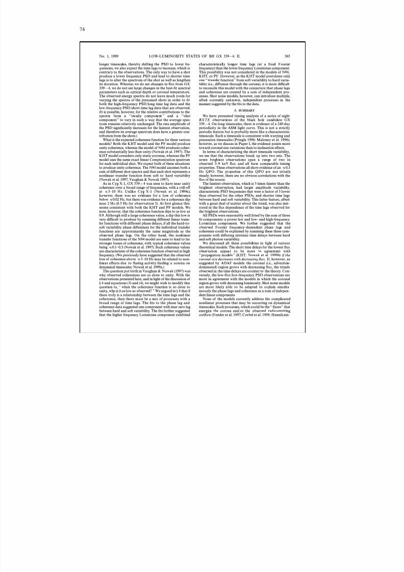
8/12/2019 Schwarze LöCher Als Astronomische Objekte
http://slidepdf.com/reader/full/schwarze-lacher-als-astronomische-objekte 74/146
74
No. 1, 1999 LOW-LUMINOSITY STATES OF BH GX 339 [ 4. II. 365
longer timescales, thereby shifting the PSD to lower fre-quencies, we also expect the time lags to increase, which iscontrary to the observations. The only way to have a shotproduce a lower frequency PSD and lead to shorter timelags is to alter the spectrum of the shot as well as lengthenits duration. Whereas we do see changes in Ñux from GX339[ 4, we do not see large changes in the best-Ðt spectralparameters such as optical depth or coronal temperature.The observed energy spectra do not leave much room forvarying the spectra of the presumed shots in order to Ðtboth the high-frequency PSD/long time lag data and thelow-frequency PSD/short time lag data that are observed.(It is possible, however, for the relative contributions to thespectra from a ““steady component ÏÏ and a ““shotcomponent ÏÏ to vary in such a way that the average spec-trum remains relatively unchanged. The rms amplitude of the PSD signiÐcantly increases for the faintest observation,and therefore its average spectrum does have a greater con-tribution from the shots.)
What is the expected coherence function for these variousmodels? Both the KHT model and the PF model produceunity coherence, whereas the model of N94 produces coher-ence substantially less than unity (Nowak et al. 1997). TheKHT model considers only static coronae, whereas the PFmodel uses the same exact linear Comptonization spectrumfor each individual shot. We expect both of these situationsto produce unity coherence. The N94 model assumes both asum of di†erent shot spectra and that each shot represents anonlinear transfer function from soft to hard variability(Nowak et al. 1997; Vaughan & Nowak 1997).
As in Cyg X-1, GX 339 [ 4 was seen to have near unitycoherence over a broad range of frequencies, with a roll-o† at B 3 È 10 Hz. Unlike Cyg X-1 (Nowak et al. 1999a),however, there was no evidence for a loss of coherencebelow B 0.02 Hz, but there was evidence for a coherence dipnear 2 Hz (0.5 Hz for observation 5). At Ðrst glance thisseems consistent with both the KHT and PF models. We
note, however, that the coherence function dips to as low as0.9. Although still a large coherence value, a dip this low isvery difficult to produce by summing di†erent linear trans-fer functions with di†erent phase delays, if all the hard-to-soft variability phase di†erences for the individual transferfunctions are approximately the same magnitude as theobserved phase lags. On the other hand, the nonlineartransfer functions of the N94 model are seen to lead to farstronger losses of coherence, with typical coherence valuesbeing B 0.1 È 0.3 (Nowak et al. 1997). Such coherence valuesare characteristic of the coherence function observed at highfrequency. (We previously have suggested that the observedloss of coherence above B 3 È 10 Hz may be related to non-linear e†ects due to Ñaring activity feeding a corona ondynamical timescales; Nowak et al. 1999a.)
The question put forth in Vaughan & Nowak (1997) waswhy observed coherences are so close to unity. With theobservations presented here, and in light of the discussion of ° 4 and equations (3) and (4), we might wish to modify thisquestion to, ““ when the coherence function is so close tounity, why is it as low as observed? ÏÏ We argued in ° 4 that if there truly is a relationship between the time lags and thecoherence, then there must be a mix of processes with abroad range of time lags. The Ðts to the phase lag andcoherence data suggested one component with near zero lagbetween hard and soft variability. The Ðts further suggestedthat the higher frequency Lorentzian component exhibited
characteristically longer time lags (at a Ðxed Fourierfrequency) than the lower frequency Lorentzian component.This possibility was not considered in the models of N94,KHT, or PF. However, as the KHT model postulates onlyone ““ transfer functionÏÏ from soft variability to hard varia-bility (i.e., di†usion through the corona), it is more difficultto reconcile this model with the conjecture that phase lagsand coherence are created by a sum of independent pro-cesses. Shot noise models, however, can introduce multiple,albeit currently unknown, independent processes in themanner suggested by the Ðts to the data.
6. SUMMARY
We have presented timing analysis of a series of eightRXT E observations of the black hole candidate GX339[ 4. On long timescales, there is evidence of a 240 dayperiodicity in the ASM light curve. This is not a strictlyperiodic feature but is probably more like a characteristictimescale. Such a timescale is consistent with warping and
precession timescales (Pringle 1996; Maloney et al. 1996);however, as we discuss in Paper I, the evidence points moretoward coronal size variations than to inclination e†ects.
In terms of characterizing the short timescale variability,we see that the observations break up into two sets. Theseven brightest observations span a range of two inobserved 3 È 9 keV Ñux and all have comparable timingproperties. These observations all show evidence of an B 0.3Hz QPO. The properties of this QPO are not strictlysteady; however, there are no obvious correlations with theÑux of the source.
The faintest observation, which is 5 times fainter than thebrightest observation, had larger amplitude variability,characteristic PSD frequencies that were a factor of 3 lowerthan observed for the other PSDs, and shorter time lagsbetween hard and soft variability. This latter feature, albeitwith a great deal of scatter about the trend, was also mir-rored in the Ñux dependence of the time lags observed for
the brightest observations.All PSDs were reasonably well Ðtted by the sum of threeÐt components: a power law and low- and high-frequencyLorentzian components. We further suggested that theobserved Fourier frequency È dependent phase lags andcoherence could be explained by summing these three com-ponents with di†ering intrinsic time delays between hardand soft photon variability.
We discussed all these possibilities in light of varioustheoretical models. The short time delays for the lowest Ñuxobservation appear to be more in agreement with““ propagation models ÏÏ (KHT; Nowak et al. 1999b) if thecoronal size decreases with decreasing Ñux . If, however, assuggested by ADAF models the coronal (i.e., advection-dominated) region grows with decreasing Ñux, the trendsobserved in the time delays are counter to the theory. Con-versely, the low-Ñux/low-frequency PSD observations aremore in agreement with the models in which the coronalregion grows with decreasing luminosity. Shot noise modelsare more likely able to be adapted to explain simulta-neously the phase lags and coherence as a sum of indepen-dent linear components.
None of the models currently address the complicatednonlinear processes that may be occurring on dynamicaltimescales. Such processes, which could be the ““ ÑaresÏÏ thatenergize the corona and/or the observed radio-emittingoutÑow (Fender et al. 1997; Corbel et al. 1998; Hannikain-
8/12/2019 Schwarze LöCher Als Astronomische Objekte
http://slidepdf.com/reader/full/schwarze-lacher-als-astronomische-objekte 75/146
75
366 NOWAK, WILMS, & DOVE
nen et al. 1999; Paper I), could be the cause of the strongloss of coherence seen at high frequency in both GX 339[ 4and Cyg X-1 (Nowak et al. 1999a), as well as the cause of the““ ÑatteningÏÏ with increasing photon energy observed at thehigh-frequency end of the Cyg X-1 PSD (Nowak et al.1999a).
We would like to acknowledge useful conversationswith T. Aldcroft, M. Begelman, R. Fender, P. Maloney,T. DiMatteo, K. Pottschmidt, R. Staubert, andB. Vaughan. This work has been Ðnanced by NASA GrantsNAG 5-3225, NAG 5-4731, and by a travel grant to J. W.from the DAAD.
REFERENCESBelloni, T., & Hasinger, G. 1990a, A&A, 227, L33 ÈÈÈ. 1990b, A&A, 230, 230Belloni, T., van der Klis, M., Lewin, W. H. G., van Paradijs, J., Dotani, T.,
Mitsuda, K., & Miyamoto, S. 1997, A&A, 322, 857Bendat, J., & Piersol, A. 1986, Random Data: Analysis and Measurement
Procedures (New York: Wiley)Corbel, S., Fender, R. P., Durouchoux, P., Sood, R. K., Tzioumis, A. K.,
Spencer, R. S., & Campbell-Wilson, D. 1998, in AIP Conf. Proc. 410,Fourth Compton Symposium, ed. C. D. Dermer, M. S. Strickman, &J. D. Kurfess (Woodbury, NY: AIP), 937
Cowley, A. P., et al. 1991, ApJ, 381, 526Crary, D. J., Finger, M. H., van der Hooft, C. K. F., van Paradijs, J., van
der Klis, M., & Lewin, W. H. G. 1999, ApJ, submittedCui, W., Zhang, S. N., Focke, W., & Swank, J. H. 1997, ApJ, 484, 383Davies, S. R. 1990, MNRAS, 244, 93Dove, J. B., Wilms, J., Maisack, M. G., & Begelman, M. C. 1997, ApJ, 487,
759Esin, A. A., McClintock, J. E., & Narayan, R. 1997, ApJ, 489, 865Fender, R. P., Spencer, R. E., Newell, S. J., & Tzioumis, A. K. 1997,
MNRAS, 286, L29Grebenev, S. A., Syunyaev, R., Pavlinsky, M. N., & Dekhanov, I. A. 1991,
Soviet Astron. Lett., 17, 413Hannikainnen, D. C., Hunstead, R. W., Campbell-Wilson, D., & Sood,
R. K. 1999, A&A, in pressHorne, J. H., & Baliunas, S. L. 1986, ApJ, 302, 757Jahoda, K., Swank, J. H., Giles, A. B., Stark, M. J., Strohmayer, T., Zhang,
W., & Morgan, E. H. 1996, in EUV, X-Ray, and Gamma-Ray Instru-mentation for Astronomy VII, ed. O. H. Siegmund (Bellingham, WA:SPIE), 59
Kazanas, D., Hua, X.-M., & Titarchuk, L. 1997, ApJ, 480, 280 (KHT)Kemp, J. C., et al. 1983, ApJ, 271, L65Leahy, D. A., Darbro, W., Elsner, R. F., Weisskopf, M. C., Sutherland,
P. G., Kahn, S., & Grindlay, J. 1983, ApJ, 266, 160Levine, A. M., Bradt, H., Cui, W., Jernigan, J. G., Morgan, E. H., Remil-
lard, R., Shirey, R. E., & Smith, D. A. 1996, ApJ, 469, L33Lochner, J., & Remillard, R. 1997, ASM Data Products Guide, Version
Dated August 27, 1997 (Greenbelt : NASA GSFC)5
Lochner, J. C., Swank, J. H., & Szymkowiak, A. E. 1991, ApJ, 376, 295Lomb, N. R. 1976, Ap&SS, 39, 447
5 The ASM Data Products Guide is available at http:// heasarc.gsfc.nasa.gov/docs/xte/asm – products – guide.html.
Maloney, P. R., & Begelman, M. C. 1997, ApJ, 491, L43Maloney, P. R., Begelman, M., & Nowak, M. A. 1998, ApJ, 504, 77Maloney, P. R., Begelman, M. C., & Pringle, J. E. 1996, ApJ, 472, 582
M., & van der Klis, M. 1997, ApJ, 479, 926Me ndez,Miyamoto, S., Kimura, K., Kitamoto, S., Dotani, T., & Ebisawa, K. 1991,
ApJ, 383, 784Miyamoto, S., & Kitamoto, S. 1989, Nature, 342, 773Miyamoto, S., Kitamoto, S., Iga, S., Negoro, H., & Terada, K. 1992, ApJ,
391, L21Narayan, R. 1996, ApJ, 462, 136Nowak, M. A. 1994, ApJ, 422, 688 (N94)Nowak, M. A., Vaughan, B. A., Dove, J., & Wilms, J. 1997, in ASP Conf.
Proc. 121, Accretion Phenomena and Related OutÑows, IAU Colloq.163, ed. D. Wickramasinghe, L. Ferrario, & G. V. Bicknell (San Fran-cisco: ASP), 366
Nowak, M. A., Vaughan, B. A., Wilms, J., Dove, J., & Begelman, M. C.1999a, ApJ, 510, 874
Nowak, M. A., Wilms, J., Vaughan, B. A., Dove, J., & Begelman, M. C.1999b, ApJ, in press
Poutanen, J., & Fabian, A. C. 1999, MNRAS, submitted (PF)Priedhorsky, W. C., Garmire, G. P., Rothschild, R., Boldt, E., Serlemitsos,
P., & Holt, S. 1979, ApJ, 233, 350Priedhorsky, W. C., Terrell, J., & Holt, S. S. 1983, ApJ, 270, 233Pringle, J. E. 1996, MNRAS, 281, 357Remillard, R. A., & Levine, A. M. 1997, in All-Sky X-Ray Observations in
the Next Decade, ed. N. Matsuoka, N. Kawai (Tokyo: Riken), 29Scargle, J. D. 1982, ApJ, 263, 835Schwarzenberg-Czerny, A. 1989, MNRAS, 241, 153Sutherland, P. G., Weisskopf, M. C., & Kahn, S. M. 1978, ApJ, 219, 1029Terrell, N. J. 1972, ApJ, 174, L35van der Klis, M. 1989, in Timing Neutron Stars, ed. H. & E. P. J.O gelman
van den Heuvel (Dordrecht: Kluwer), 27Vaughan, B. A., & Nowak, M. A. 1997, ApJ, 474, L43Wilms, J., Nowak, M. A., Dove, J. B., Fender, R. P., & Di Matteo, T. 1999a,
ApJ, submitted (Paper I)Wilms, J., Nowak, M. A., Dove, J. B., & Heindl, B. 1999b, ApJ, in prep-
arationZdziarski, A. A., Poutanen, J., J., M., Ebisawa,Miko¡ajewska, Gierlin ski,
K., & Johnson, W. N. 1998, MNRAS, 301, 435Zhang, W., & Jahoda, K. 1996, Deadtime E†ects in the PCA, Technical
Report, Version Dated 1996 September 26 (Greenbelt: NASA GSFC)Zhang, W., Jahoda, K., Swank, J. H., Morgan, E. H., & Giles, A. B. 1995,ApJ, 449, 930

8/12/2019 Schwarze LöCher Als Astronomische Objekte
http://slidepdf.com/reader/full/schwarze-lacher-als-astronomische-objekte 76/146
76
8/12/2019 Schwarze LöCher Als Astronomische Objekte
http://slidepdf.com/reader/full/schwarze-lacher-als-astronomische-objekte 77/146
A NHANG C
A Good Long Look at the Black Hole Candidates LMC X-1 and LMC X-3
M.A. Nowak, J. Wilms, W.A. Heindl, K. Pottschmidt, J.B. Dove, M.C. Begelman
2001
Nachdruck aus
Monthly Notices of the Royal Astronomical SocietyVol. 320, S. 316–326
77
8/12/2019 Schwarze LöCher Als Astronomische Objekte
http://slidepdf.com/reader/full/schwarze-lacher-als-astronomische-objekte 78/146
78
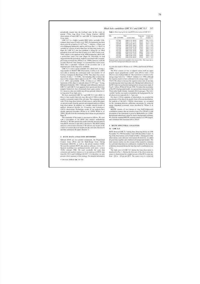
8/12/2019 Schwarze LöCher Als Astronomische Objekte
http://slidepdf.com/reader/full/schwarze-lacher-als-astronomische-objekte 79/146
79
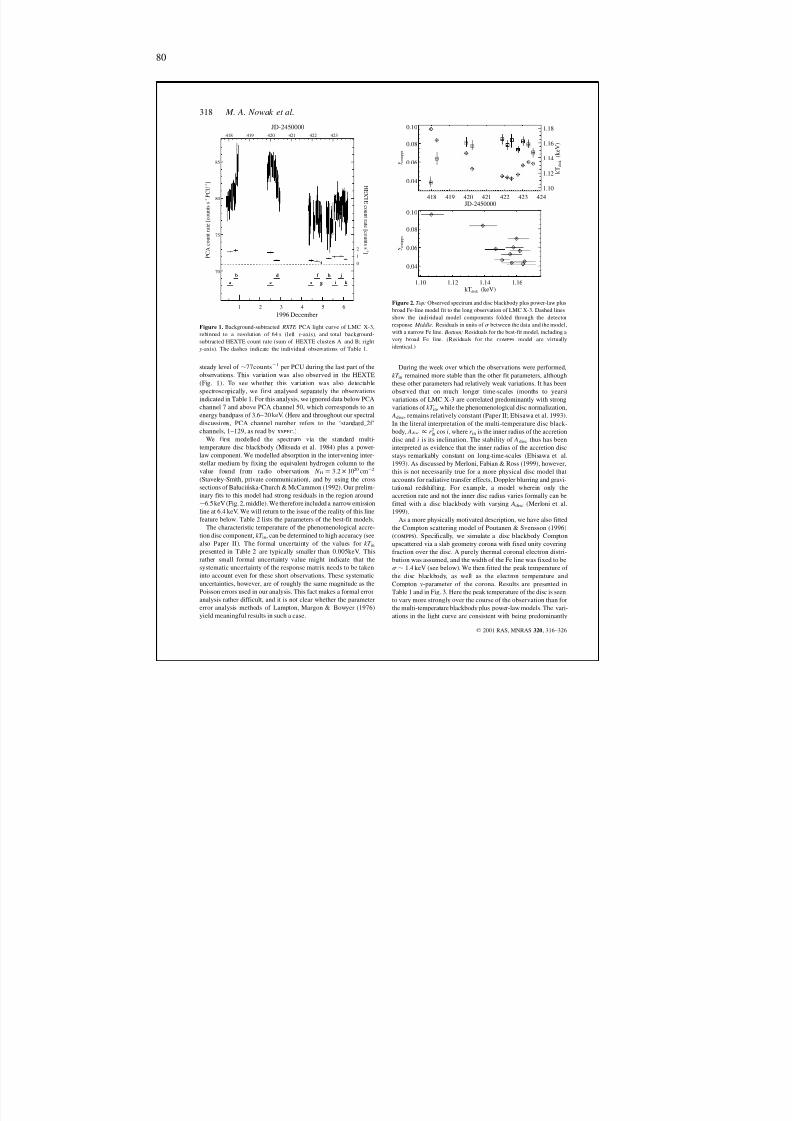
8/12/2019 Schwarze LöCher Als Astronomische Objekte
http://slidepdf.com/reader/full/schwarze-lacher-als-astronomische-objekte 80/146
80
70
75
80
85
P C A c o u n t r a t e
[ c o u n t s s - 1
P C U - 1 ]
HE XT E c o un t r a t e
[ c o un t s s -1 ]
418 419 420 421 422 423
JD-2450000
1 2 3 4 5 61996 December
0
1
2
aabb
ccdd
eef f
gghh
ii j j
k k
1.10 1.12 1.14 1.16kTdisk (keV)
0.04
0.06
0.08
0.10
c o m p p s
418 419 420 421 422 423 424JD-2450000
0.04
0.06
0.08
0.10
c o m p p s
1.10
1.12
1.14
1.16
1.18
k T
d i s k
( k e V )
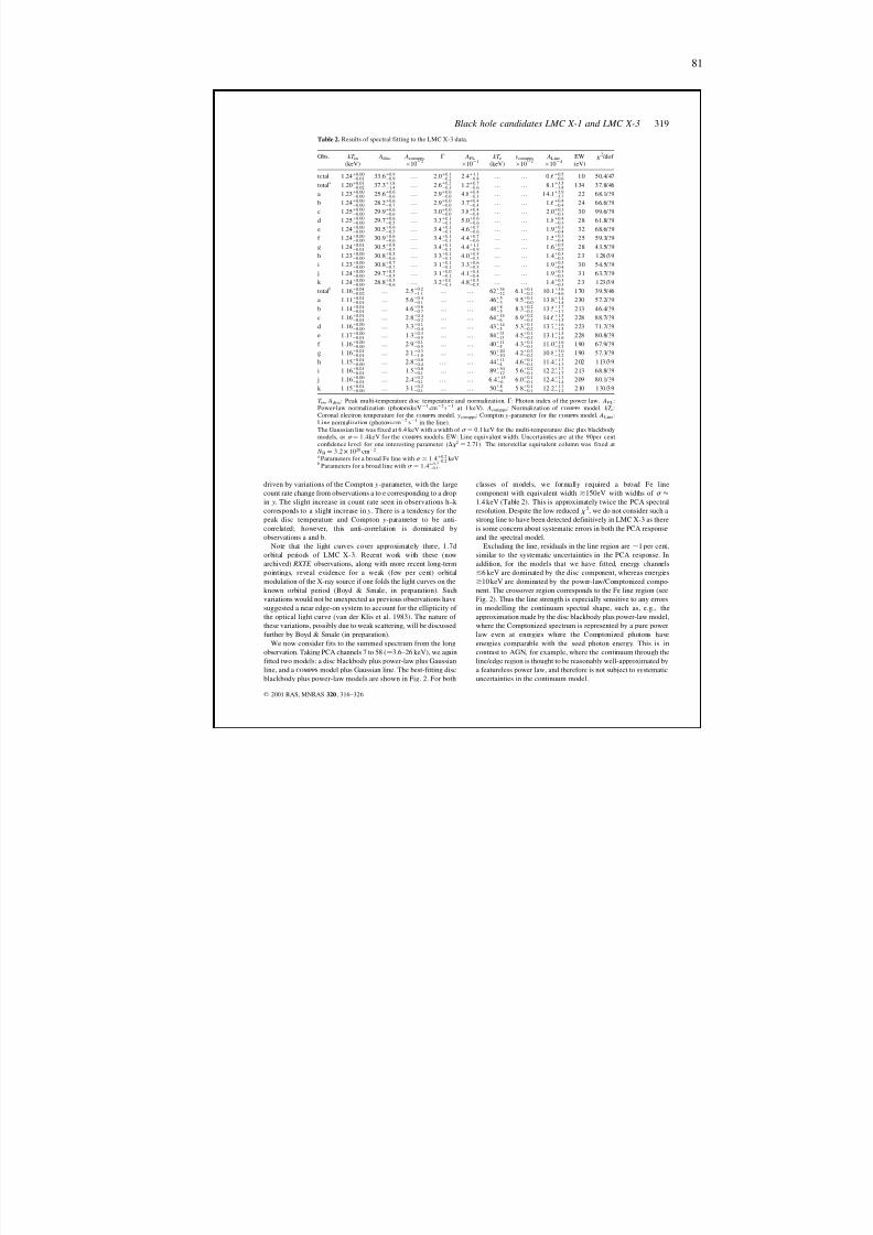
8/12/2019 Schwarze LöCher Als Astronomische Objekte
http://slidepdf.com/reader/full/schwarze-lacher-als-astronomische-objekte 81/146
81
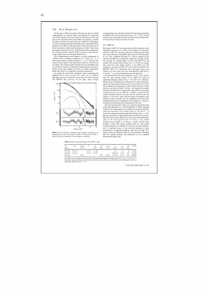
8/12/2019 Schwarze LöCher Als Astronomische Objekte
http://slidepdf.com/reader/full/schwarze-lacher-als-astronomische-objekte 82/146
82
0.1
1.0
10.0
100.0
C o u n t s s - 1 k e V - 1
-2-1012
∆ χ
Energy (keV)
-2-1012
∆ χ
3 10 20 30
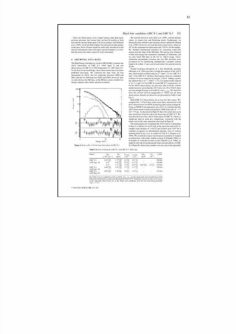
8/12/2019 Schwarze LöCher Als Astronomische Objekte
http://slidepdf.com/reader/full/schwarze-lacher-als-astronomische-objekte 83/146
83
0.1
1.0
10.0
100.0
C o u n t s s - 1 k e V - 1
-2-10
12
∆
χ
Energy (keV)
-2-1012
∆ χ
3 10 20
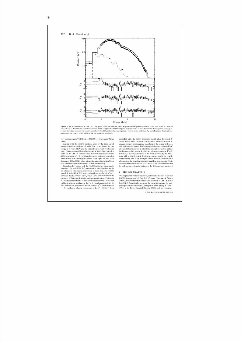
8/12/2019 Schwarze LöCher Als Astronomische Objekte
http://slidepdf.com/reader/full/schwarze-lacher-als-astronomische-objekte 84/146
84
0.1
1.0
.
C o u n t s s - 1 k e V - 1
∆ χ
4
0-4
∆ χ
4
0
-4
Energy (keV)
∆ χ
4
0
-4
0.5 1 3 10
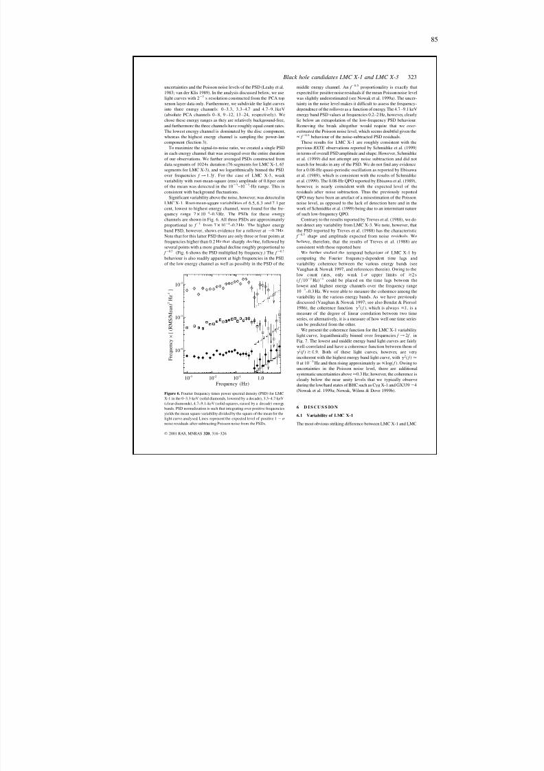
8/12/2019 Schwarze LöCher Als Astronomische Objekte
http://slidepdf.com/reader/full/schwarze-lacher-als-astronomische-objekte 85/146
85
Frequency (Hz)
F r e q u e n c y ×
[ ( R M S / M e a n ) 2 H z - 1 ]
10 -4
10 -3
10-2
10 -3 10 -2 10 -1 1.0
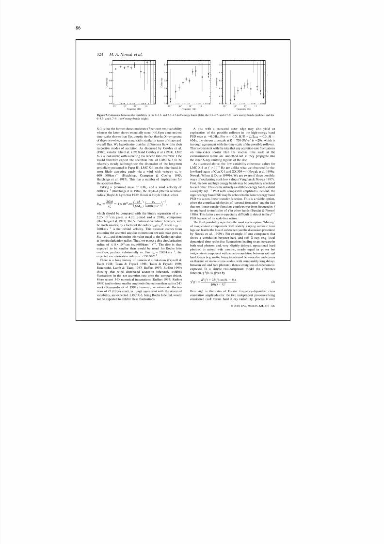
8/12/2019 Schwarze LöCher Als Astronomische Objekte
http://slidepdf.com/reader/full/schwarze-lacher-als-astronomische-objekte 86/146
86
Frequency (Hz)
0.0
0.2
0.4
0.6
0.8
1.0
C o
h e r e n c e
10 -3 10 -2 10 -1 1.0Frequency (Hz)
0.0
0.2
0.4
0.6
0.8
1.0
C o
h e r e n c e
10 -3 10 -2 10 -1 1.0Frequency (Hz)
0.0
0.2
0.4
0.6
0.8
1.0
C o
h e r e n c e
10 -3 10 -2 10 -1 1.0
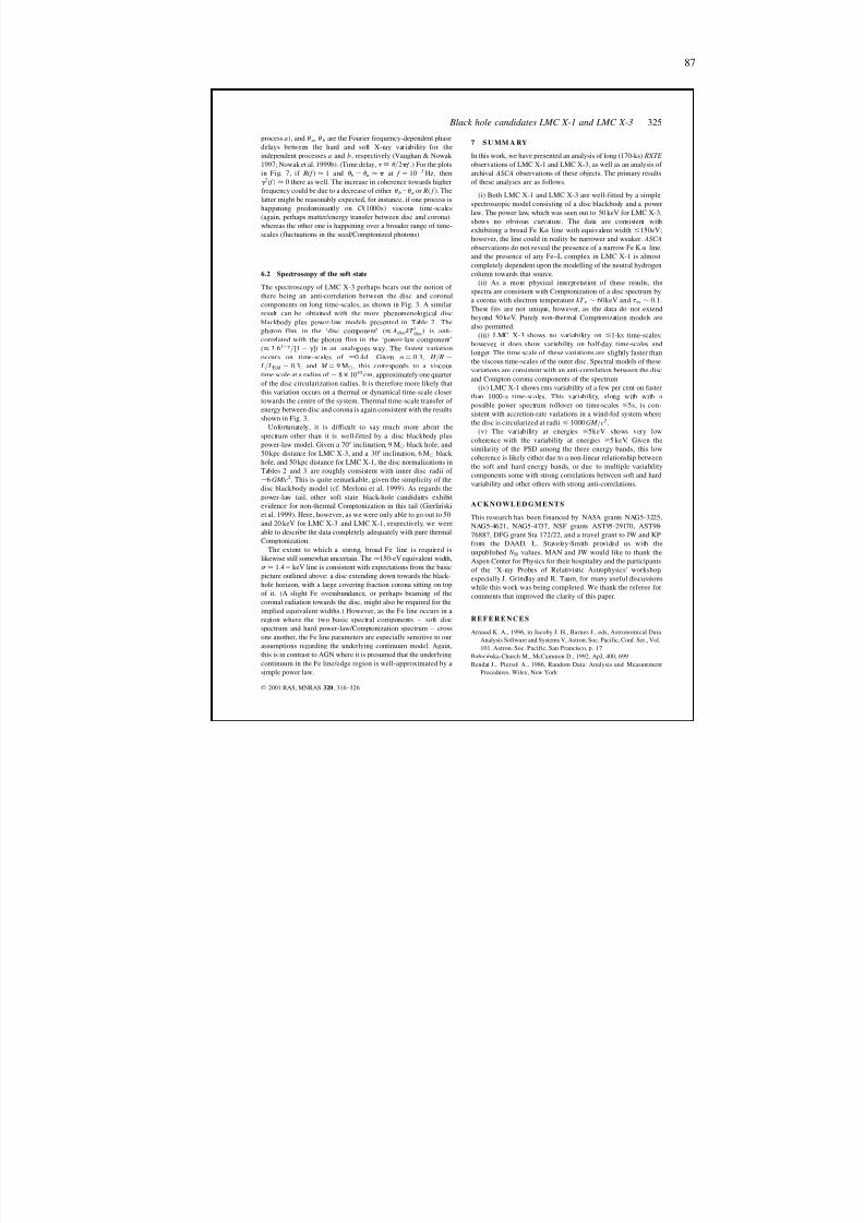
8/12/2019 Schwarze LöCher Als Astronomische Objekte
http://slidepdf.com/reader/full/schwarze-lacher-als-astronomische-objekte 87/146
87
8/12/2019 Schwarze LöCher Als Astronomische Objekte
http://slidepdf.com/reader/full/schwarze-lacher-als-astronomische-objekte 88/146
88
8/12/2019 Schwarze LöCher Als Astronomische Objekte
http://slidepdf.com/reader/full/schwarze-lacher-als-astronomische-objekte 89/146
A NHANG D
Discovery of Recurring Soft to Hard State Transitions in LMC X-3
J. Wilms, M.A. Nowak, K. Pottschmidt, W.A. Heindl, J.B. Dove, M.C. Begelman
2001
Nachdruck aus
Monthly Notices of the Royal Astronomical SocietyVol. 320, S. 327–340
89
8/12/2019 Schwarze LöCher Als Astronomische Objekte
http://slidepdf.com/reader/full/schwarze-lacher-als-astronomische-objekte 90/146
90
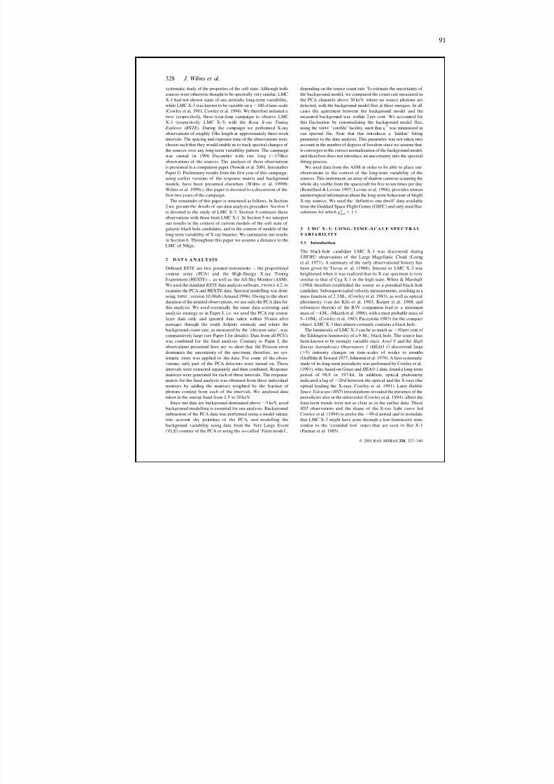
8/12/2019 Schwarze LöCher Als Astronomische Objekte
http://slidepdf.com/reader/full/schwarze-lacher-als-astronomische-objekte 91/146
91
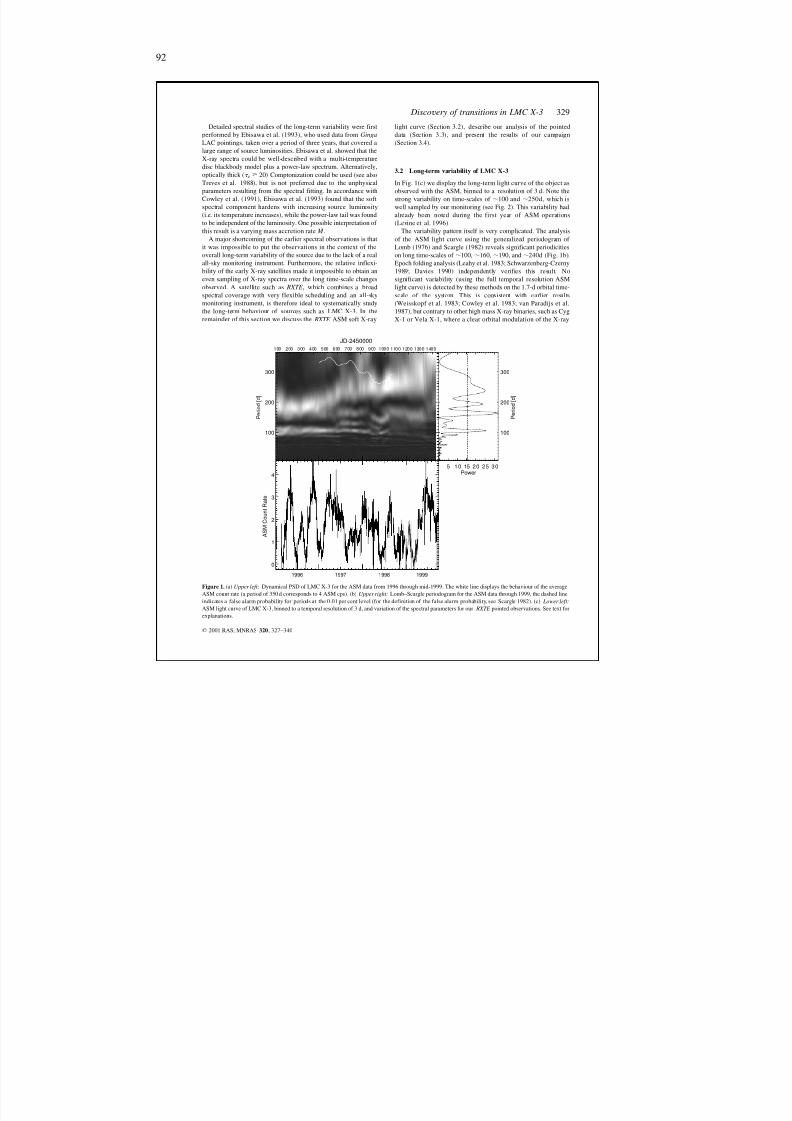
8/12/2019 Schwarze LöCher Als Astronomische Objekte
http://slidepdf.com/reader/full/schwarze-lacher-als-astronomische-objekte 92/146
92
100
200
300
P e r i o
d [ d ]
100 200 300 400 500 600 700 800 900 1000 1100 1200 1300 1400
JD-2450000
5 1 0 15 2 0 2 5 3 0Power
100
200
300
P e r i o
d [ d ]
0
1
2
3
4
A S M
C o u n
t R a
t e
1996 1997 1998 1999
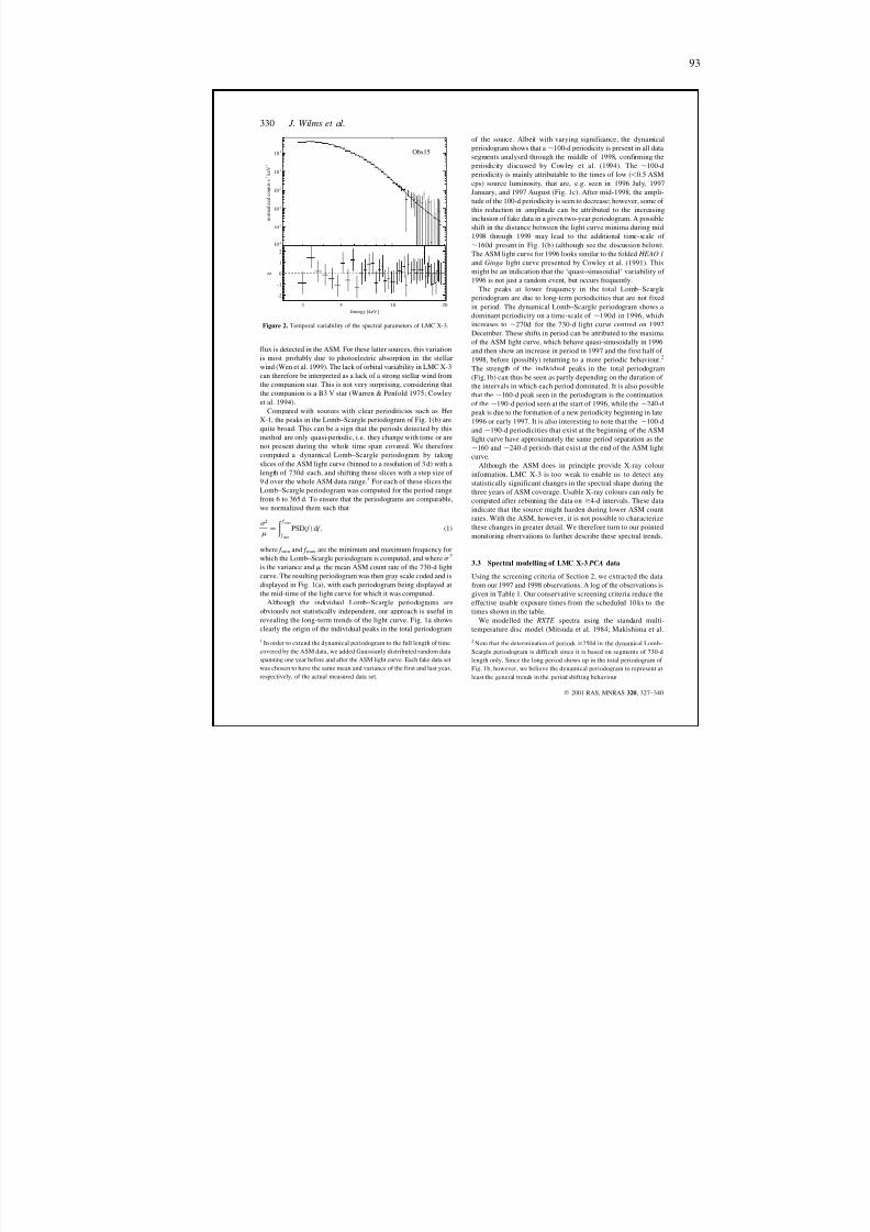
8/12/2019 Schwarze LöCher Als Astronomische Objekte
http://slidepdf.com/reader/full/schwarze-lacher-als-astronomische-objekte 93/146
93
10 -4
10 -3
10 -2
10 -1
10 0
10 1
n o r m a l i z e d c o u n t s s - 1
k e V - 1
Obs15
Energy [keV]
-2
-1
0
1
2
χ
3 5 10 20
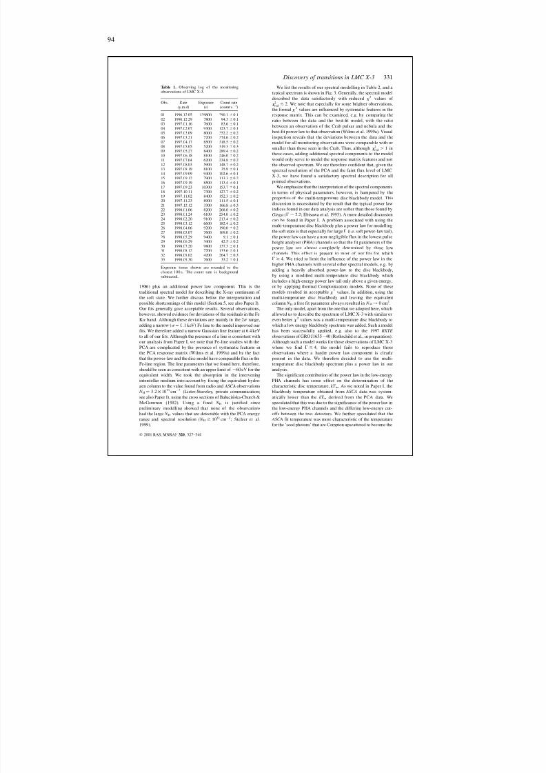
8/12/2019 Schwarze LöCher Als Astronomische Objekte
http://slidepdf.com/reader/full/schwarze-lacher-als-astronomische-objekte 94/146
94
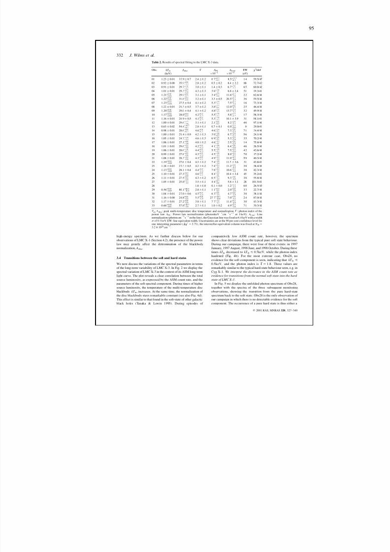
8/12/2019 Schwarze LöCher Als Astronomische Objekte
http://slidepdf.com/reader/full/schwarze-lacher-als-astronomische-objekte 95/146
95
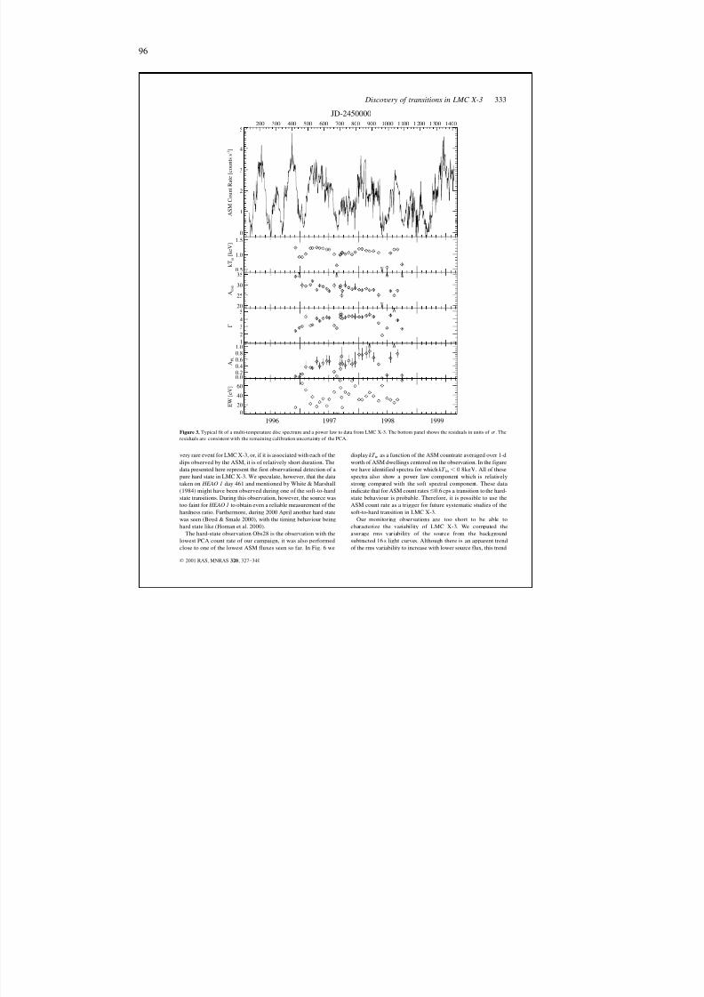
8/12/2019 Schwarze LöCher Als Astronomische Objekte
http://slidepdf.com/reader/full/schwarze-lacher-als-astronomische-objekte 96/146
96
0
1
2
3
4
5200 300 400 500 600 700 800 900 1000 1100 1 200 1 300 1400
JD-2450000
A S M C o u n t R a t e [ c o u n t s s - 1 ]
0.5
1.0
1.5
k T i n [ k e V ]
20
25
30
35
A d i s k
1
2
3
4
5
Γ
0.00.20.40.60.81.0
A P L
0
20
40
60
1996 1997 1998 1999
E W [ e V ]
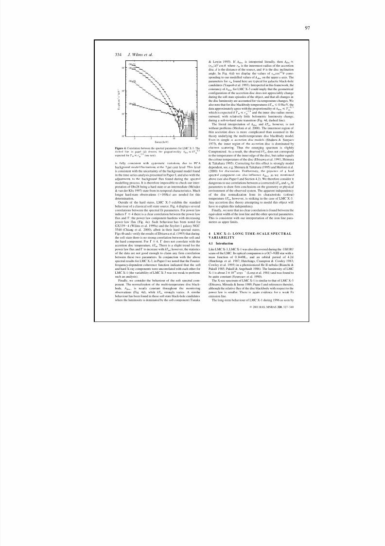
8/12/2019 Schwarze LöCher Als Astronomische Objekte
http://slidepdf.com/reader/full/schwarze-lacher-als-astronomische-objekte 97/146
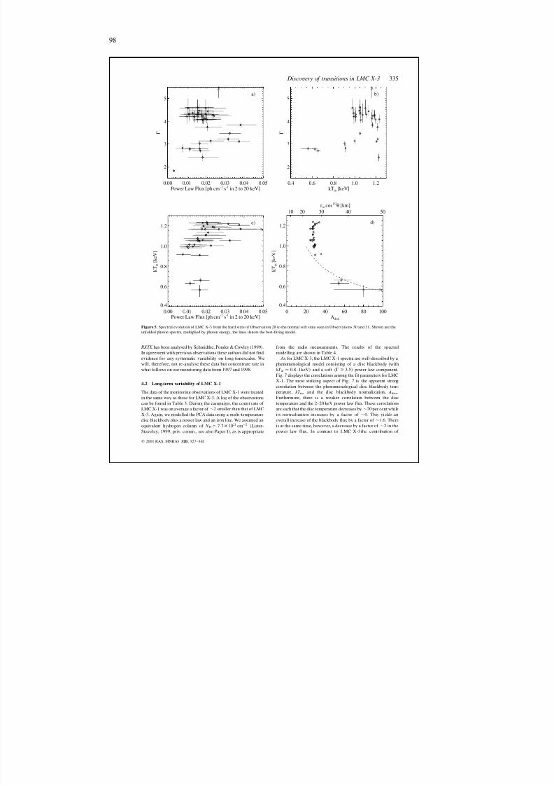
8/12/2019 Schwarze LöCher Als Astronomische Objekte
http://slidepdf.com/reader/full/schwarze-lacher-als-astronomische-objekte 98/146
98
0.00 0.01 0.02 0.03 0.04 0.05Power Law Flux [ph cm -2 s-1 in 2 to 20 keV]
2
3
4
5
Γ
a)
0.4 0.6 0.8 1.0 1.2kT in [keV]
2
3
4
5
Γ
b)
0.00 0.01 0.02 0.03 0.04 0.05Power Law Flux [ph cm -2 s-1 in 2 to 20 keV]
0.4
0.6
0.8
1.0
1.2
k T
i n [ k e V ]
c)
0.4
0.6
0.8
1.0
1.2
k T
i n [ k e V ]
0 20 40 60 80 100Adisk
10 20 30 40 50rin cos 1/2θ [km]
d)
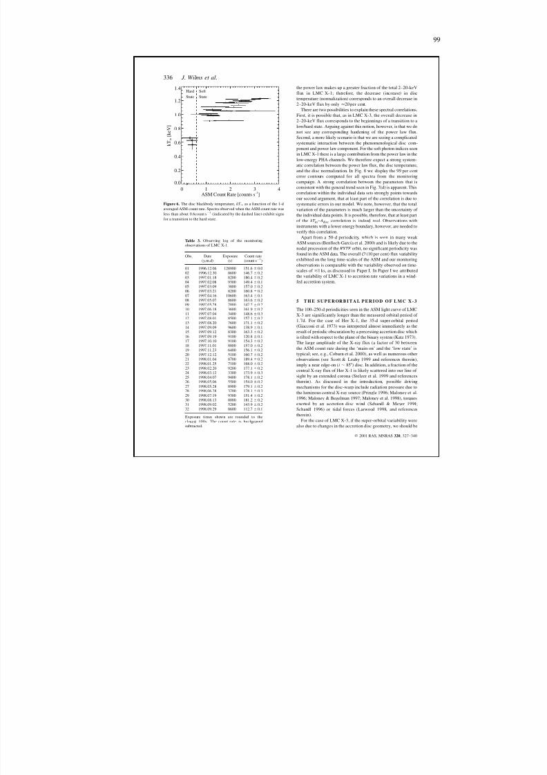
8/12/2019 Schwarze LöCher Als Astronomische Objekte
http://slidepdf.com/reader/full/schwarze-lacher-als-astronomische-objekte 99/146
99
0 1 2 3 4ASM Count Rate [counts s -1]
0.0
0.2
0.4
0.6
0.8
1.0
1.2
1.4
k T
i n [ k e V ]
Hard
State
Soft
State
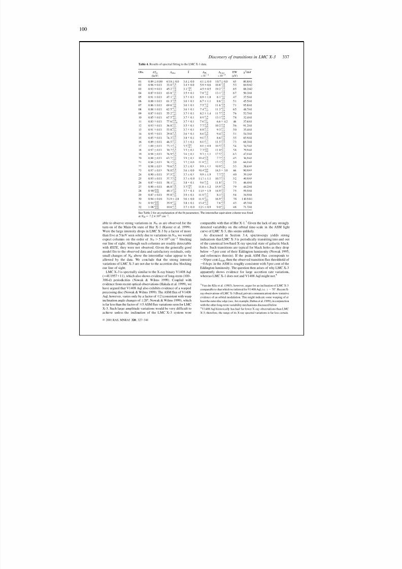
8/12/2019 Schwarze LöCher Als Astronomische Objekte
http://slidepdf.com/reader/full/schwarze-lacher-als-astronomische-objekte 100/146
100
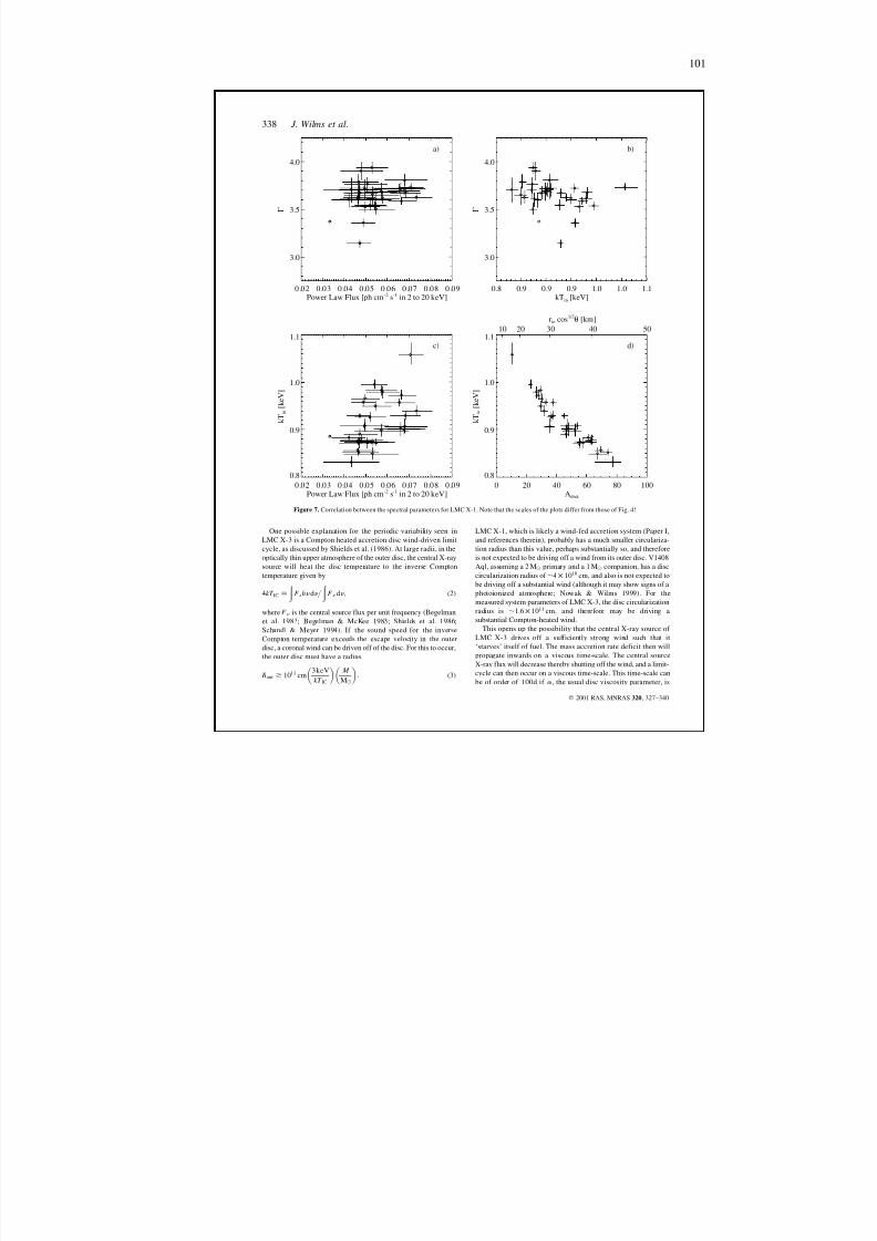
8/12/2019 Schwarze LöCher Als Astronomische Objekte
http://slidepdf.com/reader/full/schwarze-lacher-als-astronomische-objekte 101/146
101
0.02 0.03 0.04 0.05 0.06 0.07 0.08 0.09Power Law Flux [ph cm -2 s-1 in 2 to 20 keV]
3.0
3.5
4.0
Γ
a)
0.8 0.9 0.9 0.9 1.0 1.0 1.1kT in [keV]
3.0
3.5
4.0
Γ
b)
0.02 0.03 0.04 0.05 0.06 0.07 0.08 0.09Power Law Flux [ph cm -2 s-1 in 2 to 20 keV]
0.8
0.9
1.0
1.1
k T
i n [ k e V ]
c)
0.8
0.9
1.0
1.1
k T
i n [ k e V ]
0 20 40 60 80 100Adisk
10 20 30 40 50rin cos 1/2θ [km]
d)
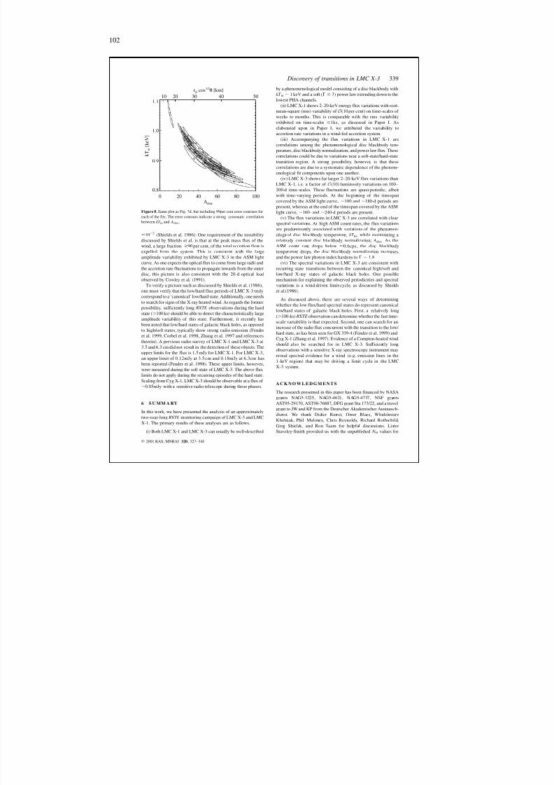
8/12/2019 Schwarze LöCher Als Astronomische Objekte
http://slidepdf.com/reader/full/schwarze-lacher-als-astronomische-objekte 102/146
102
0.8
0.9
1.0
1.1
k T
i n [ k e V ]
0 20 40 60 80 100A disk
10 20 30 40 50
rin cos 1/2 θ [km]
8/12/2019 Schwarze LöCher Als Astronomische Objekte
http://slidepdf.com/reader/full/schwarze-lacher-als-astronomische-objekte 103/146
103

8/12/2019 Schwarze LöCher Als Astronomische Objekte
http://slidepdf.com/reader/full/schwarze-lacher-als-astronomische-objekte 104/146
104
8/12/2019 Schwarze LöCher Als Astronomische Objekte
http://slidepdf.com/reader/full/schwarze-lacher-als-astronomische-objekte 105/146
A NHANG E
On the Enigmatic X-ray Source V1408 Aql (=4U 1957 + 11)
M.A. Nowak, J. Wilms
1999
Nachdruck aus
The Astrophysical JournalVol. 522, S. 476–486
105
8/12/2019 Schwarze LöCher Als Astronomische Objekte
http://slidepdf.com/reader/full/schwarze-lacher-als-astronomische-objekte 106/146
106
THE ASTROPHYSICAL JOURNAL , 522:476 È 486, 1999 September 11999.The AmericanAstronomicalSociety.All rightsreserved.Printedin U.S.A.(
ON THE ENIGMATIC X-RAY SOURCE V1408 AQUILAE ( \ 4U 1957 ] 11)
M ICHAEL A. NOWAK 1 AND JO RN W ILMS 2Received 1998 December 14; accepted 1999 April 14
ABSTRACTModels for the characteristically soft X-ray spectrum of the compact X-ray source V1408 Aql ( \ 4U
1957] 11) have ranged from optically thick Comptonization to multicolor accretion disk models. Wecritically examine the X-ray spectrum of V1408 Aql via archival Advanced Satellite for Cosmology and Astrophysics (ASCA ) data, archival data, and recent Rossi X -Ray T iming ExplorerRo ntgensatellit(RXT E ) data. Although we are able to Ðt a variety of X-ray spectral models to these data, we favor aninterpretation of the X-ray spectrum as being due to an accretion disk viewed at large inclination angles.Evidence for this hypothesis includes long-term (117, 235, 352 day) periodicities seen by the RXT E AllSky Monitor, which we interpret as being due to a warped precessing disk, and a 1 keV feature in theASCA data, which we interpret as being the blend of L Ñuorescence features from a disk atmosphere orwind. We also present a timing analysis of the RXT E data and Ðnd upper limits of 4% for the rmsvariability between f \ 10~3 and 16 Hz. The situation of whether the compact object is a black hole orneutron star is still ambiguous; however, it now seems more likely that an X-ray È emitting, warped accre-tion disk is an important component of this system.Subject headings: accretion, accretion disks È black hole physics È stars: individual (V1408 Aquilae) È
stars: neutron
1. INTRODUCTION
The low-mass X-ray binary (LMXB) V1408 Aql ( \ 4U1957] 11, 3U 1956 ] 11) was detected during scans of theAquila region by Uhuru in 1973 (Giacconi et al. 1974), and itwas subsequently identiÐed with an 18.7 mag star having astrong blue excess (Margon, Thornstensen, & Bowyer1978). The object is situated in a region of relatively smallextinction cm ~2 ; Dickey & Lockman(N HB 1.3 ] 10211990; Stark et al. 1992). measurements place the sourceAV
at a distance greater than 2.5 kpc, and comparisons of itsX-ray and optical luminosity to Sco X-1 place it at a dis-
tance of D 7 kpc (Margon et al. 1978).Little is known about the nature of the system. Opticalspectra of V1408 Aql reveal a power-law continuum withH a, Hb , and He II 4686 emission lines (Cowley, Hut-A chings, & Crampton 1988; Shahbaz et al. 1996), typical foran accretion disk È dominated system. Thorstensen (1987)reported a nearly perfectly sinusoidal V -band luminositymodulation with 10% amplitude and a 0.389 day ( \ 9.33 hr)period, which he interpreted as being due to X-ray heatingof the companion. In recent multicolor photometry a morecomplex light curve with 30% modulation amplitude wasobserved. Hakala, Muhli, & Dubus (1999) interpret thischange in the shape of the light curve as evidence for a diskwith a large outer rim, possibly because of a warped disk,seen close to edge-on (Hakala et al. 1999; see also ° 4). Thisinterpretation is also consistent with the shape of the infra-red spectrum (Smith, Beall, & Swain 1990). The shortorbital period is indicative of a late-type main-sequence star
of M D 1 as the donor star. The absence of X-rayM _eclipses and the assumption that the donor star Ðlls itsRoche lobe yield an upper limit on the orbital inclination of
1 JILA, University of Colorado, Campus Box 440, Boulder, CO 80309-0440; mnowak = rocinante.colorado.edu.
2 Institut Astronomie und Astrophysik, Abt. Astronomie,fu rS trasse 64, D-72076 Germany;Waldha user Tu bingen, wilms = astro.uni-
tuebingen.de.
i D 70¡ È 75¡, consistent with the models for the opticalvariability (Hakala et al.1999).
V1408 Aql is one of the less well studied possible blackhole candidates (BHCs). IdentiÐcation as either a BHC or aneutron star È low-mass X-ray binary (NS-LMXB) is usuallymade by analogy with the spectral and timing behavior of better observed sources. V1408 Aql has been a BHC since1984, when EXOSAT X-ray observations revealed thatV1408 Aql has a very soft X-ray spectrum, similar to thoseof other BHCs. In color-color diagrams, V1408 Aql lieshalfway between the BHC GX 339 [ 4 (in its high/soft state)and the neutron-star LMXBs Cyg X-2 and LMC X-2
(White & Marshall 1984; Schulz, Hasinger, & Tru mper1989). This color identiÐcation of V1408 Aql as a BHC,however, is not deÐnitive.
Previous narrowband observations have not character-ized the X-ray spectrum in a consistent manner. Theanalysis of 1983 and 1985 EXOSAT observations of V1408Aql led to contradictory results. While Singh, Apparao, &Kraft (1994) succeeded in Ðtting a Comptonization spec-trum to these data and interpreted this as an indication thatV1408 Aql is a BHC, Ricci, Israel, & Stella (1995) inter-preted the same data as being similar to that observed fromNS-LMXBs. Observations with Ginga , with its larger spec-tral range and e†ective area, have shed more light on thenature of V1408 Aql (Yaqoob, Ebisawa, & Mitsuda 1993).The values of the normalizations of multicolor disk models(MCDs) (Mitsuda et al. 1984), i.e., where is(rin / d )2 cos i, rinthe inner disk radius, d is the distance to the source, and i isthe inclination, have been used to distinguish betweenBHCs and NS-LMXBs (Tanaka & Lewin 1995). In the caseof V1408 Aql, km assuming d \ 7 kpc, whichrincos1@2 i B 2is more characteristic of sources containing neutron stars.Additionally, the Ginga observation showed evidence of ahard tail (1 È 18 keV) making up D 25% of the inferred Ñuxfor this system at that time. The best-Ðt power-law photonindices for the hard component ranged from ! B 2to3 .
The EXOSAT observations of Ricci et al. (1995) indicatethe presence of an iron Ñuorescence line with an equivalent
476
8/12/2019 Schwarze LöCher Als Astronomische Objekte
http://slidepdf.com/reader/full/schwarze-lacher-als-astronomische-objekte 107/146
107
V1408 AQL (4U 1957 ] 11) 477
width of 90 eV or smaller and a line energy of 7.06 keV (i.e.,highly ionized). Other values in the literature range fromnondetection (e.g., Yaqoob et al. 1993) to 200 eV (White &Marshall 1984), the uncertainty being mainly due to thedi†erence in the assumed spectral continua and the di†erentsensitivities of the instruments.
Except for one observation, which hints toward a weakred noise ( f ~ a) component between 10 ~4 and 10 ~3 Hz, allEXOSAT observations are consistent with the absence of any periodic features (Ricci et al. 1995). The Ginga obser-vations have yet to have their short timescale variabilityanalyzed; however, they do show evidence of signiÐcant Ñuxand color changes on long timescales s). The Vela 5B(Z 104satellite did not detect any long-term X-ray variability fromthis source (Priedhorsky & Terrell 1984); however, theupper limits to the variability were not particularly strong.
If the published spectral models are accepted at facevalue, then the relative energetics of the disk blackbody andpower-law components, as well as the slope of the high-
energy power law, are very similar to those seen in BHCssuch as LMC X-1 (Ebisawa, Mitsuda, & Inoue 1989; Wilmset al. 1998b), LMC X-3 (Treves et al. 1988; Wilms et al.1998b), and in the soft state of GX 339 [ 4 (Miyamoto et al.1991; Grebenev et al. 1991). However, at luminosities as lowas that of V1408 Aql, BHCs tend to show hard tails with noevidence of a disk or thermal component. On the otherhand, NS-LMXBs that exhibit soft disk spectra also tend toshow an additional D 2 keV blackbody component, whileshowing little hard Ñux (Miyamoto 1994 and referencestherein). Furthermore, low-luminosity NS-LMXBs alsotend to be dominated by hard emission.
Thus, there are good arguments that point toward V1408Aql being a neutron star and also toward it being a blackhole; however, none of the arguments are truly conclusive.In either case, V1408 Aql would still be a unique object,being either an unusually soft low-luminosity BHC, anunusually soft low-luminosity neutron star, or a soft
neutron star with an unusually energetic hard tail. With theadvent of X-ray detectors with much larger e†ective areasthan EXOSAT and Ginga , as well as with the availability of detectors of higher energy resolution, such as those on theAdvanced Satellite for Cosmology and Astrophysics (ASCA ),a critical reexamination of the X-ray spectrum of V1408 Aqlhas become possible. In this paper we present the resultsfrom our analysis of a 30 ks pointed observation with theRossi X -Ray T iming Explorer (RXT E ), as well as archivaldata from ASCA and the ( ROSAT ). In ° 2Ro ntgensatellitwe present the results from the spectral analysis. We discussthe timing analysis in ° 3 and the long-term variability of
the source in ° 4, and we discuss our results in ° 5. Thedetails of the data extraction are described in the Appendix.
2. SPECTRAL ANALYSIS
V1408 Aql was observed with RXT E in 1997 Novemberin three observing blocks for a total on-source time of 27 ks.A log of the observations is given in Table 1. Since thespectral shapes of the three observing blocks are identical,the data were analyzed together. Spectral and temporaldata were extracted using the methods outlined in theAppendix ° A1. Spectral analysis was performed withXSPEC, version 10.0s (Arnaud 1996).
The RXT E spectrum of V1408 Aql is very soft. The Pro-portional Counter Array (PCA) did not detect any Ñuxabove D 20 keV, and the High Energy X-ray TimingExperiment (HEXTE) count rates are consistent with zero :the background-subtracted count rates were 0.4 ^ 0.2 and0.0 ^ 0.2 counts s ~1 , for HEXTE clusters A and B, respec-tively. The residual Ñux in cluster A is most probably due to
a slight overestimation of the HEXTE background deadtime, as the spectrum seen is similar to the HEXTE back-ground. Therefore, we do not consider V1408 Aql to bedetected with HEXTE and will not further discuss thesedata.
To describe the PCA spectrum we use the spectral modelstraditionally applied to V1408 Aql: an exponentially cut o† power law, a multicolor disk blackbody (Mitsuda et al.1984), and a Comptonization model after Titarchuk (1994).Because of the low sensitivity of the PCA to the low absorb-ing column toward V1408 Aql (see Stelzer et al. 1999 for adiscussion of the sensitivity of the PCA to we ÐxedNH), NHto the Dickey & Lockman (1990) value of N H\ 1.3 ] 1021cm~2. The results of our spectral Ðts are given in Table 2,while the PCA spectrum and the residues are displayed inFigure 1. All three models roughly describe the obser-vational data. Note that we do not see any evidence for ahigh-energy power-law tail as that seen in previous obser-
vations. The 90% conÐdence level upper limit to the 3 È 20keV Ñux from a power law is 8 ] 10~12 ergs cm ~2 s~1,which is less than 2% of the observed 3 È 20 keV Ñux.
The best description of the PCA data is given by theComptonization model for 29 dof), while the(s red2 \ 0.82residues of the MCD model and the exponentially cut o† power law show structure in excess of that expected fromcalibration uncertainties of the PCA. These residues areespecially apparent in the low-energy channels of the PCA,below the characteristic feature of the Xe L-edge at D 5 keV(a region of very uncertain detector calibration; see the dis-cussion by Wilms et al. 1998a). Inspection of our best-Ðt
TABLE 1
O BSERVING L OG FOR V1408 AQL a
On-Source Time Count RateDate (ks) Instrument (counts s ~1)
1997 Nov 26.02 È 26.45 . . . . .. 21.2 RXT E -PCA 2301997 Nov 27.08 È 27.17 . .. .. . 4.7 RXT E -PCA 2291997 Nov 29.08 È 29.15 . .. .. . 1.5 RXT E -PCA 2331994 Oct 31.13 È 31.93 . . . . . . . 21.6 ASCA SIS0 9.8
ASCA SIS1 7.0ASCA GIS2 19.4ASCA GIS3 21.5
1992 May 08.39 È 11.14 .. .. . . 14.6 ROSAT PSPC 19.2
a Count rates given arebackgroundsubtracted.
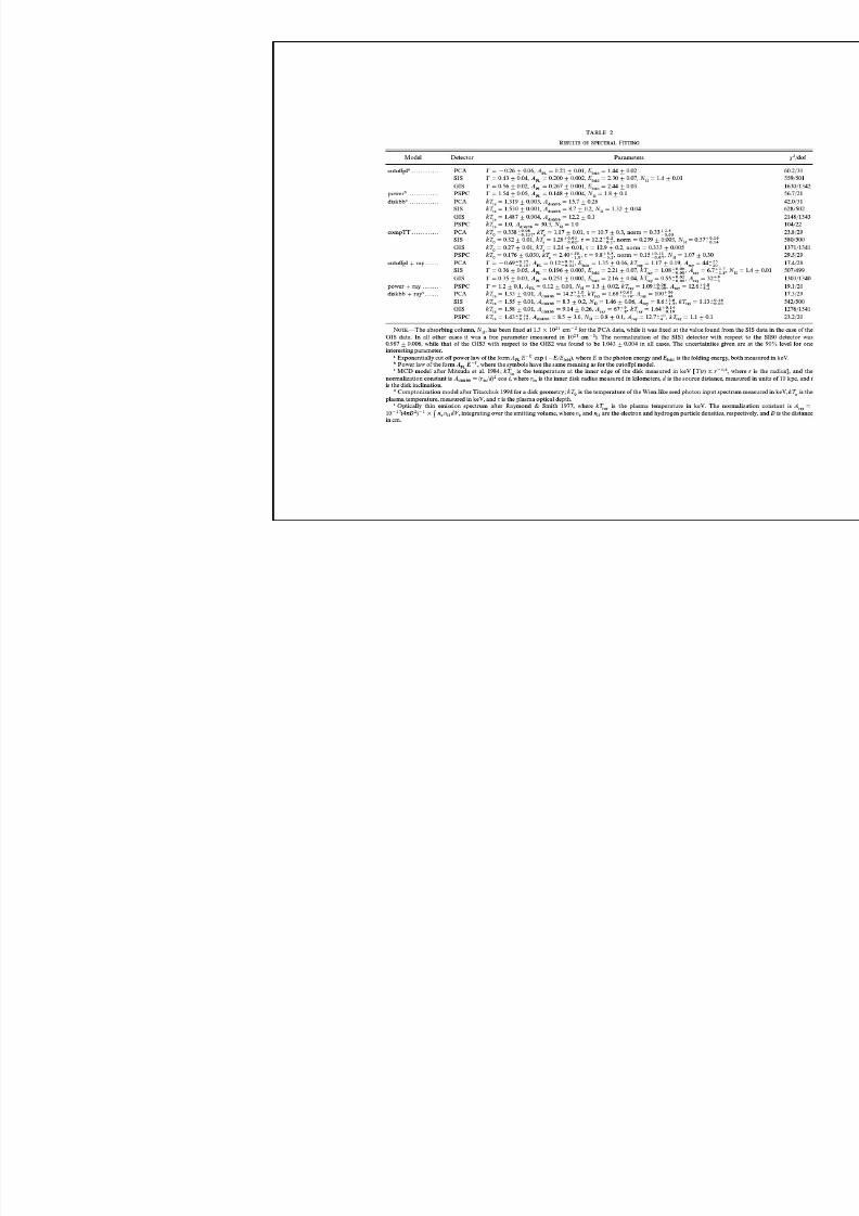
8/12/2019 Schwarze LöCher Als Astronomische Objekte
http://slidepdf.com/reader/full/schwarze-lacher-als-astronomische-objekte 108/146
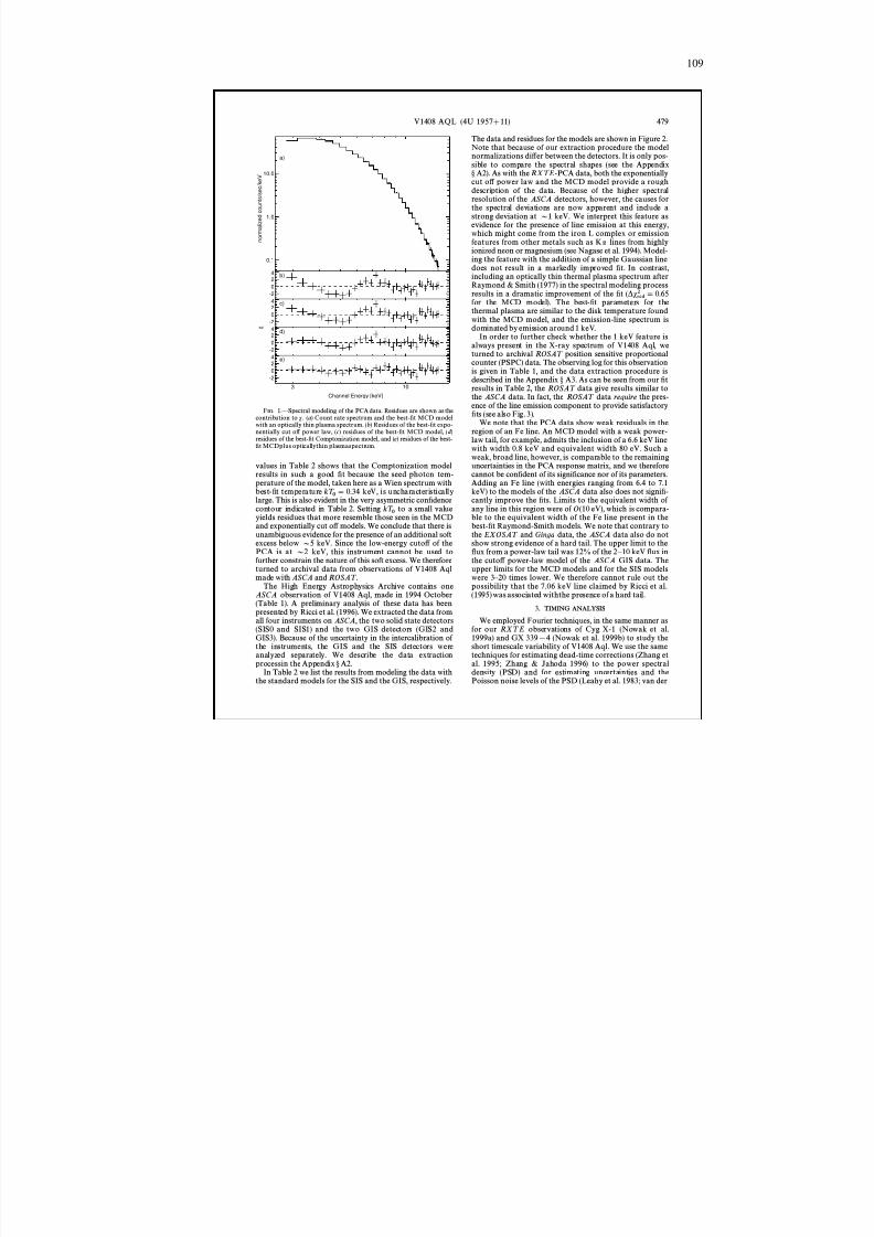
8/12/2019 Schwarze LöCher Als Astronomische Objekte
http://slidepdf.com/reader/full/schwarze-lacher-als-astronomische-objekte 109/146
109
0.1
1.0
10.0
n o r m a
l i z e d c o u n
t s / s e c / k e
V
a)
-2024 b)
-2024
c)
-2024 d)
-2024 e)
3 10
Channel Energy [keV]
χ
V1408 AQL (4U 1957 ] 11) 479
F IG . 1.ÈSpectral modeling of the PCA data. Residues are shown as thecontribution to s . (a) Count rate spectrum and the best-Ðt MCD modelwith an optically thin plasma spectrum. ( b) Residues of the best-Ðt expo-nentially cut o† power law, ( c) residues of the best-Ðt MCD model, ( d )residues of the best-Ðt Comptonization model, and ( e) residues of the best-Ðt MCDplus opticallythin plasmaspectrum.
values in Table 2 shows that the Comptonization modelresults in such a good Ðt because the seed photon tem-perature of the model, taken here as a Wien spectrum withbest-Ðt temperature keV, is uncharacteristicallykT 0
\ 0.34large. This is also evident in the very asymmetric conÐdencecontour indicated in Table 2. Setting to a small valuekT 0yields residues that more resemble those seen in the MCDand exponentially cut o† models. We conclude that there isunambiguous evidence for the presence of an additional softexcess below D 5 keV. Since the low-energy cuto† of thePCA is at D 2 keV, this instrument cannot be used tofurther constrain the nature of this soft excess. We thereforeturned to archival data from observations of V1408 Aqlmade with ASCA and ROSAT .
The High Energy Astrophysics Archive contains oneASCA observation of V1408 Aql, made in 1994 October(Table 1). A preliminary analysis of these data has beenpresented by Ricci et al. (1996). We extracted the data fromall four instruments on ASCA , the two solid state detectors(SIS0 and SIS1) and the two GIS detectors (GIS2 andGIS3). Because of the uncertainty in the intercalibration of the instruments, the GIS and the SIS detectors wereanalyzed separately. We describe the data extractionprocessin the Appendix ° A2.
In Table 2 we list the results from modeling the data withthe standard models for the SIS and the GIS, respectively.
The data and residues for the models are shown in Figure 2.Note that because of our extraction procedure the modelnormalizations di†er between the detectors. It is only pos-sible to compare the spectral shapes (see the Appendix° A2). As with the RXT E -PCA data, both the exponentiallycut o† power law and the MCD model provide a roughdescription of the data. Because of the higher spectralresolution of the ASCA detectors, however, the causes forthe spectral deviations are now apparent and include astrong deviation at D 1 keV. We interpret this feature asevidence for the presence of line emission at this energy,which might come from the iron L complex or emissionfeatures from other metals such as K a lines from highlyionized neon or magnesium (see Nagase et al. 1994). Model-ing the feature with the addition of a simple Gaussian linedoes not result in a markedly improved Ðt. In contrast,including an optically thin thermal plasma spectrum afterRaymond & Smith (1977) in the spectral modeling processresults in a dramatic improvement of the Ðt ( *s red
2 \ 0.65
for the MCD model). The best-Ðt parameters for thethermal plasma are similar to the disk temperature foundwith the MCD model, and the emission-line spectrum isdominated by emission around 1 keV.
In order to further check whether the 1 keV feature isalways present in the X-ray spectrum of V1408 Aql, weturned to archival ROSAT position sensitive proportionalcounter (PSPC) data. The observing log for this observationis given in Table 1, and the data extraction procedure isdescribed in the Appendix ° A3. As can be seen from our Ðtresults in Table 2, the ROSAT data give results similar tothe ASCA data. In fact, the ROSAT data require the pres-ence of the line emission component to provide satisfactoryÐts (see also Fig. 3).
We note that the PCA data show weak residuals in theregion of an Fe line. An MCD model with a weak power-law tail, for example, admits the inclusion of a 6.6 keV linewith width 0.8 keV and equivalent width 80 eV. Such a
weak, broad line, however, is comparable to the remaininguncertainties in the PCA response matrix, and we thereforecannot be conÐdent of its signiÐcance nor of its parameters.Adding an Fe line (with energies ranging from 6.4 to 7.1keV) to the models of the ASCA data also does not signiÐ-cantly improve the Ðts. Limits to the equivalent width of any line in this region were of O(10 eV), which is compara-ble to the equivalent width of the Fe line present in thebest-Ðt Raymond-Smith models. We note that contrary tothe EXOSAT and Ginga data, the ASCA data also do notshow strong evidence of a hard tail. The upper limit to theÑux from a power-law tail was 12% of the 2 È 10 keV Ñux inthe cuto† power-law model of the ASCA GIS data. Theupper limits for the MCD models and for the SIS modelswere 3 È 20 times lower. We therefore cannot rule out thepossibility that the 7.06 keV line claimed by Ricci et al.(1995) was associated withthe presence of a hard tail.
3. TIMING ANALYSIS
We employed Fourier techniques, in the same manner asfor our RXT E observations of Cyg X-1 (Nowak et al.1999a) and GX 339 [ 4 (Nowak et al. 1999b) to study theshort timescale variability of V1408 Aql. We use the sametechniques for estimating dead-time corrections (Zhang etal. 1995; Zhang & Jahoda 1996) to the power spectraldensity (PSD) and for estimating uncertainties and thePoisson noise levels of the PSD (Leahy et al. 1983; van der
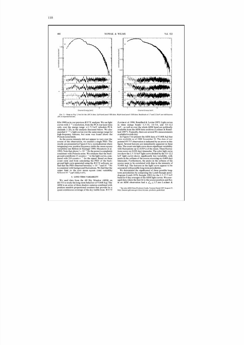
8/12/2019 Schwarze LöCher Als Astronomische Objekte
http://slidepdf.com/reader/full/schwarze-lacher-als-astronomische-objekte 110/146
110
0.01
0.10
1.00
n o r m a
l i z e d c o u n
t s / s e c / k e
V
a)
-2024 b)
-2024
c)
-2024 d)
-2024 e)
1 5 10Channel Energy [keV]
χ
0.01
0.10
1.00
n o r m a
l i z e d c o u n
t s / s e c / k e
V
a)
-2024 b)
-2024
c)
-2024 d)
-2024 e)
1 5 10Channel Energy [keV]
χ
480 NOWAK & WILMS Vol. 522
F IG . 2.ÈSame as Fig. 1, but for the ASCA data. L eft-hand panel: SIS data. Right -hand panel: GIS data. Residuals at 1.7 and 2.2 keV are well-knownASCA response features.
Klis 1989) as in our previous RXT E analyses. We use lightcurves with 2 ~5 s resolution, from the PCA top layer data
only, over the energy range B 1 È 7.2 keV (absolute PCAchannels 1 È 20), in the analysis discussed below. We alsosearched 2 ~11 s light curves over the same energy range forhigh-frequency features, but none was found above thePoisson noise limits.
As the source intensity did not appear to vary over thecourse of the observation, we created a single PSD. Theresults are presented in Figure 4 for a normalization whereintegrating over positive frequency yields the mean squarevariability (see Belloni & Hasinger 1990; Miyamoto et al.1992). Note that above f \ 10~2 Hz the power is completelyconsistent with Poisson noise. We estimate that the back-ground contributes 13 counts s ~1 to the light curves, com-pared with 210 counts s ~1 for the signal. Based on thesecount rates and from calculating the PSD of the back-ground light curve generated using the RXT E software, weÐnd that the PSD observed between f \ 10~3 and 10 ~2 Hzis consistent with background Ñuctuations. We Ðnd that the
upper limit to the root mean square (rms) variabilitybetween 10 ~3 and 16Hz is 4%.
4. LONG -TERM VARIABILITY
We used data from the All Sky Monitor (ASM) onRXT E to study the long-term behavior of V1408 Aql. TheASM is an array of three shadow cameras combined withposition sensitive proportional counters that provide for aquasi-continuous coverage of the sky visible from RXT E
(Levine et al. 1996; Remillard & Levine 1997). Light curvesin three energy bandsÈ1.3 È 3.0, 3.0 È 5.0, and 5.0 È 12.2
keVÈas well as over the whole ASM band are publicallyavailable from the ASM data archives (Lochner & Remil-lard 1997 3). Typically, there are several 90 s measurementsavailable for each day.
In Figure 5 we present the ASM data of V1408 Aql thatwere available as of 1998 November 20. The date of ourpointed RXT E observation is indicated by an arrow in thisÐgure. Several features are immediately apparent in thesedata. The count rate light curve shows signiÐcant variabilitywith Ñuctuations up to O(50%) of the mean. These Ñuctua-tions occur on O(100 day) timescales. The color light curve(we show the 1.3 È 3.0 keV light curve divided by the 5.0 È 12.2keV light curve) shows signiÐcantly less variability, withpeaks in the softness of the source occurring on O(400 day)timescales. Furthermore, the peaks in the softness of thesource seem to be correlated with dips in the intensity of V1408 Aql. The features in the light curve appear to beassociated with possible long-term periodicities.
We determined the signiÐcance of these possible long-term periodicities by computing the Lomb-Scargle perio-dogram (Lomb 1976; Scargle 1982) for the 1.3 È 12.2 keVband for 6 day averages of the ASM light curves. We aver-aged data where the best Ðt to the source position and Ñuxin an ASM observation had a (see Lochner &s red
2 ¹ 1.5
3 See also ASM Data Products Guide, Version Dated 1997 August 27,http://heasarc.gsfc.nasa.gov/docs/xte/asm – products – guide.html.
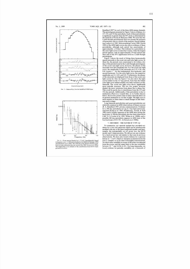
8/12/2019 Schwarze LöCher Als Astronomische Objekte
http://slidepdf.com/reader/full/schwarze-lacher-als-astronomische-objekte 111/146
111
10
n o r m a
l i z e d c o u n
t s / s e c / k e
V
a)
-2024 b)
-2024
c)
-2024 d)
-2024 e)
1 2
Channel Energy [keV]
χ
Frequency (Hz)
0.001
0.010
R M S
2 / H z
10 -3 10 -2 10 -1 1.0
No. 1, 1999 V1408 AQL (4U 1957 ] 11) 481
F IG . 3.ÈSame asFig. 1,but for the ROSAT PSPCdata
F IG . 4.ÈPower spectral density for 1 È 7.2 keV, logarithmically binnedin frequency over f ] 1.08 f and normalized as by Belloni & Hasinger (1990)and Miyamoto et al. (1992). The solid line is the e†ective Poisson noiselevel for noise-subtracted data (see van der Klis 1989; Nowak et al. 1999a).The dashed line is our estimate of the contribution from RXT E back-ground Ñuctuations.
Remillard 1997 3) in each of the three ASM energy channels.The periodogram presented in Figure 5 shows evidence of a117, 235, and 352 day periodicity. Each of these periodicitiesis signiÐcant at greater than the 95% level, as determined bythe methods of Horne & Baliunas (1986). We note that theLomb-Scargle periodogram does not assume the presenceof harmonics; this is a result of the analysis. Epoch folding(see Leahy et al. 1983; Schwarzenberg-Czerny 1989; Davies1990) of the ASM light curves also shows evidence of theseperiodicities, although each period has uncertainties of approximately ^ 10 days. The evidence for a periodicity inthe color light curve is somewhat weaker. Only the longestperiod appears, with an approximately 370 day period andthen only at the 50% signiÐcance level in a Lomb-Scargleperiodogram.
Figure 5 shows the result of Ðtting three harmonicallyspaced sinusoids to the count rate and color light curves. Inthese Ðts, the periods were constrained to be within a fewdays of the periods found in the Lomb-Scargle periodogram
of the count rate light curve; however, the phases of thesinusoids were left completely free. For the count rate lightcurve, the amplitudes of the sinusoids are 0.32, 0.26, and0.41 counts s ~1 for the fundamental, Ðrst harmonic, andsecond harmonic. For the color light curve, the respectiveamplitudes are 0.1, 0.05, and 0.01. Furthermore, the phasesof the sinusoids are displaced from those of the count ratelight curves by O(n ). In Figure 5 we also show the lightcurves folded on the 117 day period. Note that the foldedcolor light curve indeed exhibits very little variation on thistimescale. The count rate light curve shows signiÐcantlymore periodic structure. The low Ñux points, however,display the most variations from phase bin to phase bin.This could be partly due to interference from the 235 and352 day periods. Additionally, if this periodicity is due toinclination e†ects in a warped disk, as we further discussbelow, the low Ñux points come at times when the disk is atits greatest inclination to our line of sight. The light curve is
most sensitive at these times to small changes in disk thick-ness and/or shape.Long timescale periodicities and quasi periodicities are
relatively common in ASM observations of binary sources(R. A. Remillard 1997, private communication). Evidencefor a 294 day periodicity in Cyg X-1 has been previouslyreported (Kemp et al. 1983; Priedhorsky, Terrell, & Holt1983) and is readily apparent in the ASM data during thehard state. A 198 day periodicity also has been observed inLMC X-3 (Cowley et al. 1991; Wilms et al. 1998b), and apossible 240 day periodicity appears in ASM data of thelow/hard state of GX 339 [ 4 (Nowak et al. 1999b).
5. DISCUSSION È THE NATURE OF V 1408 A ql
To summarize, our spectral analysis has provided evi-dence for a very soft spectrum which can be satisfactorilymodeled with any of the three traditional models used here,namely, the exponentially cut o† power law, the MCDmodel, and Comptonization. We did not see any evidencefor a hard power-law tail similar to that seen in previousobservations. We have also found evidence for a spectralfeature at D 1 keV, which we interpret as emission from theiron L complex or as K a lines from highly ionized metals.No short-term variability in excess of the noise was detectedfrom the source, and the upper limit to the rms variabilitybetween 10 ~3 and 16 Hz is 4%. On long timescales, wefound evidence for periodic variability on a timescale of
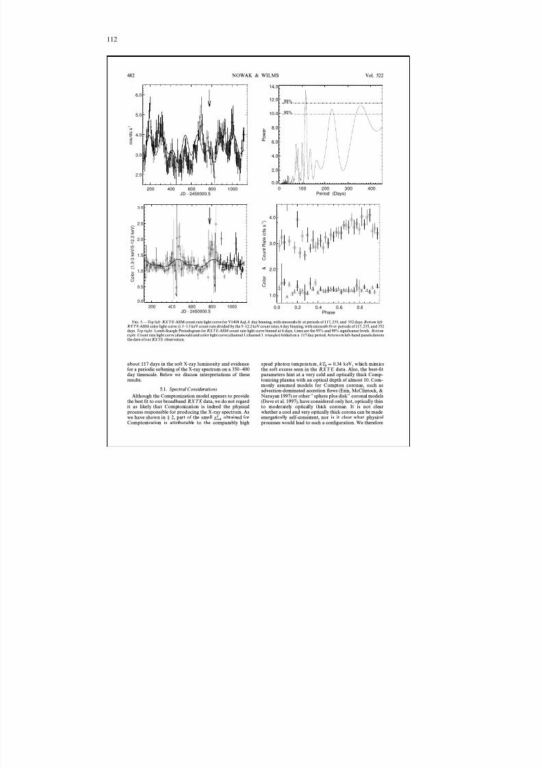
8/12/2019 Schwarze LöCher Als Astronomische Objekte
http://slidepdf.com/reader/full/schwarze-lacher-als-astronomische-objekte 112/146
112
200 400 600 800 1000JD - 2450000.5
2.0
3.0
4.0
5.0
6.0
c o u n
t s s - 1
0 100 200 300 400Period (Days)
0.0
2.0
4.0
6.0
8.0
10.0
12.0
14.0
P o w e r
99%
95%
200 400 600 800 1000JD - 2450000.5
0.0
0.5
1.0
1.5
2.0
2.5
3.0
C o
l o r
( 1 . 3
- 3 k e
V / 5 - 1
2 . 2
k e
V )
0.0 0.2 0.4 0.6 0.8Phase
1.0
2.0
3.0
4.0
C o
l o r
&
C o u n
t R a
t e ( c t s s - 1
)
482 NOWAK & WILMS Vol. 522
F IG . 5.È Top left: RXT E -ASM count rate light curve for V1408 Aql, 6 day binning, with sinusoids Ðt at periods of 117, 235, and 352 days. Bottom left:RXT E -ASM color light curve (1.3 È 3.3 keV count rate divided by the 5 È 12.2 keV count rate), 6 day binning, with sinusoids Ðt at periods of 117, 235, and 352days. Top right: Lomb-Scargle Periodogram for RXT E -ASM count rate light curve binned at 6 days. Lines are the 95% and 99% signiÐcance levels. Bottomright: Count rate light curve ( diamonds ) and color light curve (channel 1/channel 3; triangles ) folded on a 117 day period. Arrows in left-hand panels denotethe date of our RXT E observation.
about 117 days in the soft X-ray luminosity and evidencefor a periodic softening of the X-ray spectrum on a 350 È 400day timescale. Below we discuss interpretations of theseresults.
5.1. Spectral ConsiderationsAlthough the Comptonization model appears to provide
the best Ðt to our broadband RXT E data, we do not regardit as likely that Comptonization is indeed the physicalprocess responsible for producing the X-ray spectrum. Aswe have shown in ° 2, part of the small obtained fors red
2
Comptonization is attributable to the comparably high
speed photon temperature, keV, which mimicskT 0 \ 0.34the soft excess seen in the RXT E data. Also, the best-Ðtparameters hint at a very cold and optically thick Comp-tonizing plasma with an optical depth of almost 10. Com-monly assumed models for Compton coronae, such asadvection-dominated accretion Ñows (Esin, McClintock, &Narayan 1997) or other ““ sphere plus diskÏÏ coronal models(Dove et al. 1997), have considered only hot, optically thinto moderately optically thick coronae. It is not clearwhether a cool and very optically thick corona can be madeenergetically self-consistent, nor is it clear what physicalprocesses would lead to such a conÐguration. We therefore
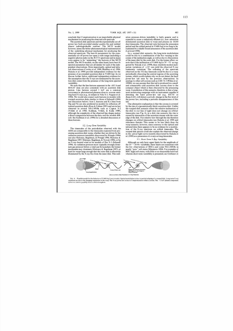
8/12/2019 Schwarze LöCher Als Astronomische Objekte
http://slidepdf.com/reader/full/schwarze-lacher-als-astronomische-objekte 113/146
113
No. 1, 1999 V1408 AQL (4U 1957 ] 11) 483
conclude that Comptonization is an improbable physicalmechanism for producing the observed soft spectrum.
The accretion disk spectrum and the exponentially cut o† power law both provided similar quality Ðts and yieldedalmost indistinguishable residues. The MCD model,however, seems the better phenomenological representationof the underlying physical mechanism for producing theobserved spectrum. The best-Ðt parameters for the expo-nentially cut o† power law span a wide range (including anegative photon index in the RXT E spectrum) and in manyways appear to be ““ mimicking ÏÏ the features of the MCDmodel. The MCD models, on the other hand, have best-Ðtspectral parameters that are all similar for each of the inde-pendent observations. More importantly, optical and infra-red observations (Cowley et al. 1988; Shahbaz et al. 1996;Hakala et al. 1999) provide independent evidence for thepresence of an extended accretion disk in V1408 Aql. As wediscuss further below, additional independent evidence forthe assumption that the X-rays are dominated by the accre-
tion disk comes from the presence of the long-term spectralvariability.We note that the line features apparent in the ASCA and
ROSAT data are also consistent with an accretion diskpicture. Line features around 1 keV are a commonoccurrence in photoionized plasmas close to sources emit-ting hard X-rays (e.g., in eclipse in Vela X-1; Nagase et al.1994). We would also expect such features in models withwarped accretion disks similar to those of Schandl (1996)(see discussion below). Iron L features and K a lines fromMg and Ne are also predicted in models for reÑection o† ionized accretion disks (Ross & Fabian 1993) and are in factobserved in several NS-LMXBs such as Cygnus X-2(Vrtilek et al. 1986; Kallman, Vrtilek, & Kahn 1989),although the complexity of the observed line shapes makesa direct comparison between the data and the models diffi-cult. See Kallman et al. (1996) for a detailed discussion of these features.
5.2. L ong-Term VariabilityThe timescales of the periodicities observed with the
ASM are comparable to the timescales expected from pre-cessing accretion disk warps, whether they are driven by theradiation pressure instability discovered by Pringle (1996)(see also Maloney, Begelman, & Pringle 1996; Maloney &Begelman 1997; Maloney, Begelman, & Nowak 1998), or byan X-ray È heated wind as for models of Her X-1 (Schandl1996). As radiation pressure must typically strongly domi-nate gas pressure before a wind can be launched, the formermechanism may dominate (Maloney & Begelman 1997), atleast for warps large enough that the outer disk is e†ectivelyilluminated by the X-ray Ñux from the inner disk. This radi-
ation pressure È driven instability is fairly generic and isexpected to cause a radiatively efficient (i.e., non È advectiondominated) accretion disk to warp and precess on O(100day) timescales. The observed ratio between the precessionperiod and the orbital period in V1408 Aql is too long to beexplained by a tidally forced precession of the accretion disk(Larwood 1998).
In a warped disk scenario, the long-term modulationscould be due to a combination of the Ñux varying as thecosine of the inclination angle, as well as due to obscurationof the inner disk by the outer disk. For the former e†ect, wenote that if the inclination of V1408 Aql is 70¡ È 75¡ as sug-gested by Hakala et al. (1999), then relatively modest incli-nation variations of ^ 10¡ can yield the observed X-rayluminosity variations. The softening of the spectrumobserved on the 352 day timescale could be due to a warpperiodically obscuring the central regions of the accretingsystem, which would explain why we do not detect the hardpower-law tail seen by the previous observations. In
analogy to other soft sources such as LMC X-3 (Wilms et al.1998b), we can assume that this tail is produced in a smalland comparably cold accretion disk corona close to thecompact object which is then obscured by the precessingwarp. A prediction of this scenario, therefore, is that a long-term monitoring campaign with an instrument capable of detecting the hard power-law tail (e.g., RXT E orBeppoSAX ), will detect a periodic change in the Ñux level of the power law, including a periodic disappearance of thistail.
One alternative explanation is that the corona is coveredby the rim of a (geometrically thick) accretion disk. Unlikethe warped disk scenario where the relative inclination of the disk to our line of sight does not change on orbitaltimescales (see Fig. 6), in a disk rim scenario the rim iscaused by interaction of the accretion stream with the outeredge of the disk. Our relative view through the rim thereforechanges on orbital timescales (see Hakala et al. 1999 and
references therein). This seems to be less likely than thewarp scenario, however, since contrary to the optical andinfrared data there appears to be no evidence for a modula-tion of the X-ray spectrum on orbital timescales. Thewarped disk picture could also explain the observed changein the optical light curve recently discovered by Hakala etal. (1999) as a precession of a warp on long timescales.
5.3. Short -Term X -Ray VariabilityAlthough we only have upper limits for the amplitude of
the 10 ~3 È 16 Hz variability, these limits are consistent withthe few observations of BHCs and some NS-LMXBs innearly ““ pure ÏÏ soft states (Miyamoto 1994). For examples of BHC high/soft states, with little or no discernible hard tailwherein short-term variability is presented, see Grebenev et
F IG . 6.ÈPossible model for the behavior of V1408 Aql (not to scale). Optical modulation is due to partial eclipsing of a warped disk. Long-term X-rayvariations are due to the changing orientation of the warp. The X-ray power law is due to Comptonization within a corona. The D 1 keV plasma componentisdue toa windor possibly dueto a diskatmosphere.
8/12/2019 Schwarze LöCher Als Astronomische Objekte
http://slidepdf.com/reader/full/schwarze-lacher-als-astronomische-objekte 114/146
114
484 NOWAK & WILMS Vol. 522
al. (1991) for an observation of GX 339 [ 4, Treves et al.(1988) for an observation of LMC X-3, Ebisawa et al. (1989)for an observation of LMC X-1, and Miyamoto et al. (1994)for observations of Nova Muscae. The PSD presented inthese works typically have a PSD level of (rms) 2 /Hz B 10~3at 0.01 Hz, which decreases as f ~0.7 for higher Fourierfrequencies and an rms variability of B 3% in the 10 ~2 È 30Hz range. This is slightly below the upper limits presentedin Figure 4.
The ““ normal branchÏÏ of the NS-LMXB GX 5 ] 1 alsohas a similar amplitude and shape PSD as described abovefor high/soft state BHC; however, its energy spectrum con-sists of both a 1 keV MCD component and a 2 keV black-body spectral component (Miyamoto 1994 and referencestherein). The high/soft state of Cir X-1 has been similarlymodeled (Miyamoto 1994 and references therein). If V1408Aql had weak 1 È 10 Hz variability comparable to that dis-cussed by Miyamoto (1994) for Cir X-1, our observationswould have detected it. Other soft neutron star sources with
luminosities of O(10%) Eddington (the approximate lumi-nosity of V1408 Aql, if it were a 1.4 neutron star givenM _
our hypothesis of a highly inclined disk), especially thebright atoll sources such as GX 13 ] 1, GX 3 ] 1, GX 9 ] 1,and GX 9 ] 9, can also exhibit ““ very low frequency noise ÏÏwith approximately 5% rms variability (Hasinger & van derKlis 1989). The 10 ~4 È 100 s low-amplitude variability in thelight curves of these sources has been interpreted as inter-mittent, slow nuclear burning on the surface of the neutronstar (Bildsten 1993, 1995). Low-frequency variability at sucha level is absent in V1408 Aql. Furthermore, bright atollsources often show a 0.1 È 10 Hz power spectrum in excess of the upper limits discussed here (Hasinger & van der Klis1989). The level of the 0.1 È 10 Hz PSD seen in GX 13 ] 1(Homan et al. 1998), for example, also would have beeneasily detected in the PSD of V1408 Aql, yet it was not.
5.4. Black Hole or Neutron Star?
The nature of the compact object as of now is not clear.The general picture outlined above is similar to that seen inneutron star X-ray binaries such as Sco X-1, Cyg X-2, andothers. Yaqoob et al. (1993) pointed out that the normal-ization of the best-Ðt MCD model appears to indicate thatthe compact object is a neutron star. This argument,however, strongly relies on the assumed distance to V1408Aql, for which no compelling measurement exists (a lowerlimit of 2.5 kpc comes from the fact that ASCA - andROSAT -measured are consistent with the fullN H-valuesGalactic column) and also relies on the assumption that theaccretion disk is seen closer to face-on. The recent opticaland soft X-ray variability measurements, however, make alarge inclination more probable.
Taking these points into account and assuming for thesake of argument a source distance of 7 kpc, then the overallÑux of V1408 Aql is comparable to that of the high state of the BHC GX 339 [ 4, which is a very plausible BHC. Theupper limits to the high-frequency variability discussedabove are consistent with previously observed BHC powerspectra in high/soft states. If transitions from the hard stateto the soft state occur at 5% È 10% of the Eddington lumi-nosity (see Nowak 1995), then the compact object in V1408Aql is consistent with being a 2 È 3 black hole. Thus,M _
although there is no compelling evidence that V1408 Aqlcontains a black hole, there also is no compelling evidencethat V1408 Aql is a neutron star.
5.5. Conclusions
X-ray spectroscopy and the study of both the long-termand the short-term variability of V1408 Aql make a systemgeometry as that depicted in Figure 6 seem likely. A low-mass main-sequence star serves, via Roche lobe overÑow, asthe donor for a compact object which is surrounded by alarge accretion disk which in turn dominates the system atall wavelength ranges. The accretion disk is surrounded byan optically thin plasma, in the form of either an accretiondisk wind or a stationary accretion disk photosphere, whichemits the observed X-ray line radiation. A small hot coronadirectly surrounding the compact object produces the hardX-ray power law. The whole accretion disk precesses on atimescale of about 117 days, obscuring the central regionand causing the power-law tail to periodically disappearand reappear. Also on these long timescales, the changingview of the warp causes the orbital modulation of theoptical light curve (because of partial obscuration of theouter accretion disk) to vary from sinusoidal (Thorstensen
1987) to a more complex pattern (Hakala et al. 1999).The nature of the compact object in V1408 Aql is stillambiguous. We have put forth a hypothesis, however, thatmight explain the observed phenomenology and makes pre-dictions that are observationally testable. X-ray monitoringover the 117 day period with an instrument like RXT E orBeppoSAX should reveal whether the X-ray power-law tailreally does periodically disappear and reappear as predictedby our model. Furthermore, if the source is at 10% andL Eddcontains a neutron star, then about one ““ Type I ÏÏ micro-burst per day might be expected (Bildsten 1995). Thisshould be easily observable during such a campaign. Onemight also hope to Ðnd ““ kilohertz QPOs ÏÏ (van der Klis1998), as are often associated with atoll sources. For theselatter two possibilities, however, we note that some of thebrighter atoll sources such as GX 13 ] 1 have yet to exhibitkilohertz QPOs (Homan et al. 1998 and references therein)and rarely exhibit Type I bursts (see, for example, Matsubaet al. 1984 and references therein). Finally, high spectralresolution observations as will be provided by the upcom-ing new generation of X-ray instruments, such as the grat-ings on the Advanced X -Ray Astronomy Facility and theX -Ray Multiple Mirror Mission , will provide the spectralresolution necessary for resolving and studying the Fe Lcomplex. This will allow the application of plasma spectro-scopic diagnostics (e.g., Liedahl et al. 1992) to the study of this fascinating source.
We thank Neil Brandt and Christopher Reynolds forvaluable advice concerning the ASCA data analysis. Wewould also like to acknowledge useful correspondence withLars Bildsten and Rob Fender. Ingo Kreykenbohm madesome literature references available to us. We thank ErikKuulkers for pointing out to us additional references. RudyWijnands provided invaluable advice concerning the timinganalysis. This work has been Ðnanced by NASA grantsNAG 5-3225, NAG 5-4737, and NAG 5-7024. J. W. wasalso supported by a travel grant from the Deutscher Akade-mischer Austauschdienst. This research has made use of data obtained through the High Energy AstrophysicsScience Archive Research Center Online Service, providedby the NASA Goddard Space Flight Center, and theROSAT archive at the Max-Planck-Institut Extra-fu rterrestrische Physik in Garching bei Mu nchen.
8/12/2019 Schwarze LöCher Als Astronomische Objekte
http://slidepdf.com/reader/full/schwarze-lacher-als-astronomische-objekte 115/146
115
No. 1, 1999 V1408 AQL (4U 1957 ] 11) 485
APPENDIX A
DATA ANALYSIS METHODOLOGY
A1. RXT E DATA ANALYSIS
Our RXT E data were analyzed using the same procedure as that for our analysis of the spectrum of GX 339 [ 4 (Wilms etal. 1998a). The screening criteria for the selection of good on-source data were that the source elevation be larger than 10¡ anddata measured within 30 minutes of passages of the South Atlantic Anomaly or during times of high particle background (asexpressed by the ““ electron ratio ÏÏ being greater than 0.1) were ignored. Using these selection criteria, a total exposure time of 27 ks was obtained. To increase the signal-to-noise level of the data, we restricted the analysis to the Ðrst anode layer of theproportional counter units (PCUs) where most source photons are detected (the particle background is almost independent of the anode layer), and we combined the data from all Ðve PCUs.
To take into account the calibration uncertainty of the PCA we applied the channel-dependent systematic uncertaintiesdescribed by Wilms et al. (1998a). These uncertainties were determined from a power-law Ðt to an observation of the CrabNebula and pulsar taking into account all anode chains; however, they also do provide a good estimate for the Ðrst anodelayer only since most of the photons are detected in this layer.
Since V1408 Aql has a comparably small count rate we are able to use the new background model for the PCA that wasmade available by the RXT E Guest Observers Facility in 1998 June. The quality of this model was checked by looking athigh detector channels which are completely background dominated. Although the measured count rate of V1408 Aql was atthe high end of the applicability of the new background model, the agreement between the model and the measuredbackground was good. This is in part due to the fact that V1408 Aql is a very soft source which allows greater latitude in usingthe background model for faint sources. Remaining background residuals were minimized by using the XSPEC CORFILEfacility which renormalizes the background Ñux to decrease the best-Ðt The corrections applied to the background Ñuxs red
2 .were on the order of indicating that at least for this source the background model provides a good background[ 1.5%,estimate. Since the spectrum is completely background dominated above 20 keV, and because of the calibration uncertaintybelow 3 keV, we restricted the spectral analysis to the range from 3 to 20 keV.
For the timing analysis we generated light curves from the GoodXenon data. Note that although there are short data gapsof 1 È 4 s duration that are Ñagged by commensurate jumps in the value of the time coordinate from one data bin to the next,there are occasional data gaps where the extraction software generates a continuous series of time bins despite the data losses.These data gaps do not appear in light curves generated from the STANDARD2F data (which is processed by a di†erent eventanalyzer on-board RXT E ). These gaps can be recognized, however, in the high time resolution data by searching for anysequence, 1 s or greater in length, of time bins with zero count rate. Four such unÑagged sequences, with 16 s duration each,were found in our data. (Aside from these four 16 s sequences, there were a few instances where two 1/32 s time bins in a rowwould have zero detected counts. The lack of counts in these bins was consistent with counting statistics, and we did notconsider these to be data gaps.) The power spectra that we presented in Figure 4 were made from continous data segmentswithout internal data gaps. If we include data segments with the unÑagged data gaps in the calculation of the PSD, we obtaina low-amplitude (5% rms) PSD that is Ñat from 10 ~3 to 10 ~2 Hz and is exponentially cut o† at higher Fourier frequencies. Infact, the presence of unÑagged data gaps can be deduced from such a characteristic PSD shape (R. Wijnands 1999, privatecommunication).
A2. ASCA DATA ANALYSIS
We extracted data from the two solid state detectors (SIS0, SIS1) and the two gas detectors (GIS2, GIS3) on board ASCA
by using the standard FTOOLS as described in the ASCA Data Reduction Guide (Day et al. 1998). The data extractionregions were limited by the fact that all the observations were in 1-CCD mode and that the source was placed close to the chipedge. To maximize the extraction regions, we chose rectangular regions of 6 @] 8@ and 6 @] 7@ for SIS0 and SIS1, respectively.Choosing a rectangular region does not a†ect the shape of the extracted spectrum; however, the ASCAARF ancillaryresponse matrix generator assumes a circular region, so the Ñux normalization is slightly o† (hence the B 30% normalizationdi†erences between the SIS and GIS detectors in Table 2). For the GIS detectors we chose circular regions centered on thesource each with a radius of 13 @.
The SIS count rate for V1408 Aql is large enough that the central regions of the CCD su†er from pileup (i.e., two or moreevents being registered as a single event). Estimates of the amount of this pileup can be found in the appendix presented byEbisawa et al. (1996). Based on our measured spectrum and these estimates, we chose to exclude from analysis centralrectangular regions with dimensions of 4 @] 3@ and 3 @] 3@ for SIS0 and SIS1, respectively. With these exclusions, we estimatethat pileup will contribute less than 1% of the counts at 10 keV.
We used the SISCLEAN and GISCLEAN tools (Day et al. 1998), with the default values, to remove hot and Ñickeringpixels. As the spectrum of V1408 Aql is very similar to the low Ñux level of Cir X-1 described by Brandt et al. (1996), we Ðlteredthe data with the same cleaning criteria outlined in that work; however, we took the slightly larger values of 10¡ for theminimum elevation angle and 7 GeV/ c for the rigidity. Also, similar to the work of Brandt et al. (1996), we formed backgroundestimates by extracting a circular region of radius 5 @ near the edge of the detector for the GIS observations. For the SISobservations, we chose L-shaped regions near the corner of the chip opposite from the source. Background, however,contributes relatively little to the observations.
We rebinned the spectral Ðles so that each energy bin contained a minimum of 20 photons. We retained SIS data in the0.6 È 10 keV range and GIS data in the 1 È 10 keV range. The cross-calibration uncertainties among the instruments were
8/12/2019 Schwarze LöCher Als Astronomische Objekte
http://slidepdf.com/reader/full/schwarze-lacher-als-astronomische-objekte 116/146
116
486 NOWAK & WILMS
accounted for by introducing a multiplicative constant for each detector in all of our Ðts. As discussed above, the resultingdata Ðles showed reasonable agreement betweenall four detectors.
A3. ROSAT DATA ANALYSIS
The extraction of the ROSAT spectrum was performed using the standard ROSAT PSPC data analysis package, theExtended X-Ray ScientiÐc Analysis System (Zimmermann et al. 1998), following the procedures described by Brunner et al.(1997). Source counts were extracted from a circular region centered on the position of V1408 Aql with a radius of 2@, while thebackground was extracted from an annulus centered on the source from which source counts from detected backgroundsources were removed. A correction for the telescope vignetting was applied to the standard ROSAT response matrix. Thespectrum was then rebinned into 26 channels of D 10,000 counts each to ensure an even signal-to-noise ratio over the wholeROSAT energy band. As forRXT E and ASCA , the spectral analysis of the extracted data was then performed with XSPEC,ignoring data measured below 0.5 keV and above 2.5 keV.
REFERENCESArnaud, K. A. 1996, in ASP Conf. Ser. 101, Astronomical Data Analysis
Software and Systems V, ed. J. H. Jacoby & J. Barnes (San Francisco:ASP), 17
Belloni, T.,& Hasinger,G. 1990, A&A, 230, 230Bildsten,L. 1993, ApJ, 418, L21 ÈÈÈ. 1995, ApJ, 438, 852Brandt, W. N., Fabian, A. C., Dotani, T., Nagase, F., Inoue, H., Kotani, T.,
& Segawa, Y. 1996, MNRAS, 283, 1071Brunner, H., C., Friedrich, P., T., Staubert, R., & Ri†ert, H.Mu ller, Do rrer,1997, A&A, 326, 885
Cowley, A.P., Hutchings, J. B.,& Crampton,D. 1988, ApJ, 333, 906Cowley, A.P., et al.1991,ApJ,381, 526Davies, S.R. 1990, MNRAS,244,93Day, C., Arnaud, K., Ebisawa, K., Gotthelf, E., Ingham, J., Mukai, K., &
White, N. 1998, The ASCA Data Reduction Guide, Tech. Rep.,(Greenbelt: NASAGSFC),v.2.0
Dickey, J. M.,& Lockman,F. J. 1990, ARA&A, 28,215Dove, J. B., Wilms, J., Maisack, M. G., & Begelman, M. C. 1997, ApJ, 487,
759Ebisawa, K.,Mitsuda,K., & Inoue,H. 1989, PASJ,41, 519Ebisawa, K., Ueda, Y., Inoue, H., Tanaka, Y., & White, N. E. 1996, ApJ,
467, 419Esin, A.A., McClintock, J. E.,& Narayan,R. 1997, ApJ, 489, 865Giacconi, R., Murray, S., Gursky, H., Kellogg, E., Schreier, E., Matilsky, T.,
Koch,D., & Tananbaum, H. 1974, ApJS, 27,37Grebenev, S. A., Sunyaev, R., Pavlinsky, M. N., & Dekhanov, I. A. 1991,
SovietAstron.Lett.,17, 413Hakala, P. J.,Muhli, P.,& Dubus,G. 1999, MNRAS,submittedHasinger,G., & vander Klis, M.1989,A&A, 225, 79Homan, J., Klis, M. V., Wijnands, R., Vaughan, B., & Kuulkers, E. 1998,
ApJ, 499, L41Horne,J. H.,& Baliunas,S. L.1986, ApJ, 302, 757Kallman, T. R., Liedahl, D., Osterheld, A., Goldstein, W., & Kahn, S. 1996,
ApJ, 465, 994Kallman, T. R.,Vrtilek, S.D., & Kahn,S. M.1989, ApJ, 345,498Kemp, J.C.,et al. 1983, ApJ,271,L65Larwood,J. 1998, MNRAS,299,L32Leahy, D. A., Darbro, W., Elsner, R. F., Weisskopf, M. C., Sutherland,
P. G.,Kahn,S., & Grindlay,J. 1983, ApJ, 266, 160Levine, A. M., Bradt, H., Cui, W., Jernigan, J. G., Morgan, E. H., Remil-
lard,R., Shirey, R.E., & Smith,D. A.1996,ApJ, 469, L33Liedahl, D. A., Kahn, S. M., Osterheld, A. L., & Goldstein, W. H. 1992,
ApJ, 391, 306Lomb, N. R.1976,Ap&SS, 39,447Maloney, P. R.,& Begelman,M. C.1997,ApJ, 491, L43Maloney, P. R., Begelman, M. C., & Nowak, M. A. 1998, ApJ, 504, 77, in
pressMaloney, P. R.,Begelman, M.C., & Pringle, J. E. 1996, ApJ, 472, 582Margon, B.,Thornstensen,J. R.,& Bowyer, S. 1978, ApJ, 221, 907Matsuba, E., Dotani, T., Mitsuda, K., Asai, K., Lewin, W. H. G., van
Paradijs,J., & vander Klis, M.1995, PASJ, 47,575Mitsuda, K.,et al.1984,PASJ, 36,741Miyamoto, S. 1994, Time-Variation from X-Ray Stars, Tech. Rep. RN 548
(Tokyo: ISAS)Miyamoto, S., Kimura, K., Kitamoto, S., Dotani, T., & Ebisawa, K. 1991,
ApJ, 383, 784Miyamoto, S., Kitamoto, S., Iga, S., Hayashida, K., & Terada, K. 1994,ApJ, 435, 398
Miyamoto, S., Kitamoto, S., Iga, S., Negoro, H., & Terada, K. 1992, ApJ,391, L21
Nagase, F., Zylstra, G., Sonobe, T., Kotani, T., Inoue, H., & Woo, J. 1994,ApJ, 436, L1
Nowak,M. A. 1995, PASP, 107, 1207Nowak, M. A. Vaughan, B. A., Wilms, J., Dove, J., & Begelman, M. C.
1999a,ApJ,510, 874Nowak,M. A.,Wilms, J.,& Dove, J. B. 1999b,ApJ,517, 355Priedhorsky,W. C.,& Terrell, J. 1984, ApJ, 280, 661Priedhorsky,W. C.,Terrell,J., & Holt, S.S. 1983, ApJ, 270, 233Pringle, J. E. 1996, MNRAS, 281, 357Raymond, J. C.,& Smith,B. W.1977,ApJS,35, 419Remillard, R. A., & Levine, A. M. 1997, in All-Sky X-Ray Observations in
theNext Decade, ed.N. Matsuoka& N. Kawai (Tokyo: Riken), 29Ricci, D., Asai, K., Israel, G. L., Mereghetti, S., Mitsuda, K., Parmar, A. N.,
& Stella, L. 1996, Mem. Soc. Astron. Italiana,67, 1039Ricci,D., Israel, G. L.,& Stella, L. 1995, A&A, 299, 731Ross,R. R.,& Fabian, A. C.1993,MNRAS, 261, 74Scargle, J. D. 1982, ApJ, 263, 835Schandl, S.1996, A&A, 307, 95Schulz, N.S., Hasinger, G., & J.1989, A&A,225,48Tru mper,Schwarzenberg-Czerny,A. 1989,MNRAS, 241, 153Shahbaz, T., Smale, A. P., Naylor, T., Charles, P. A., van Paradijs, J.,
Hassall, B. J. M.,& Callanan,P. 1996, MNRAS, 282, 1437Singh,K. P., Apparao,K. M.V.,& Kraft,R. P.1994, ApJ,421,753Smith,H. A., Beall,J. H., & Swain,M. R.1990, AJ, 99, 273Stark, A. A., Gammie, C. F., Wilson, R. W., Bally, J., Linke, R. A., Heiles,
C.,& Hurwitz,M. 1992, ApJS, 79,77Stelzer, B., Wilms, J., Staubert, R., Gruber, D., & Rothschild, R. 1999,
A&A, inpressTanaka, Y., & Lewin, W. H. G. 1995, in X-Ray Binaries, ed. W. H. G.
Lewin, J. van Paradijs, & E. P. J. van den Heuvel (Cambridge: Cam-bridge Univ. Press), 126
Thorstensen,J. R.1987,ApJ, 312, 739Titarchuk, L. 1994, ApJ, 434, 570Treves, A., Belloni, T., Chiapetti, L., Maraschi, L., Stella, L., Tanzi, E. G., &
vander Klis, M.1988,ApJ, 325, 119van der Klis, M. 1989, in Timing Neutron Stars, ed. H. & E. P. J.O gelman
vanden Heuvel(Dordrecht: Kluwer), 27 ÈÈÈ. 1998, in Proc. Third William Fairbank Meeting, in press (astro-
ph/9812395)Vrtilek, S. D., Kahn, S. M., Grindlay, J. E., Seward, F. D., & Helfand, D. J.
1986, ApJ, 307,698White,N. E.,& Marshall,F. E. 1984, ApJ, 281, 354Wilms, J., Nowak, M. A., Dove, J. B., Fender, R. P., & di Matteo, T. 1998a,
ApJ, inpressWilms, J., Nowak, M. A., Dove, J. B., Pottschmidt, K., Heindl, W. A.,
Begelman, M. C., & Staubert, R. 1998b, in Highlights in X-RayAstronomy, ed.B. Aschenbach & M. Freyberg,in press
Yaqoob, T.,Ebisawa,K., & Mitsuda,K. 1993, MNRAS, 264, 411Zhang, W., & Jahoda, K. 1996, Deadtime E†ects in the PCA, Tech. Rep.
(Greenbelt: NASAGSFC)Zhang, W., Jahoda, K., Swank, J. H., Morgan, E. H., & Giles, A. B. 1995,
ApJ, 449, 930Zimmermann, U., Boese, G., Becker, W., Belloni, T., S., Izzo,Do bereiner,
C., Kahabka, P., & Schwentker, O. 1998, EXSAS UserÏs Guide, 5th ed.,Tech. Rep. (Garching: Max-Planck-Institut Extraterrestrischefu rPhysik)
8/12/2019 Schwarze LöCher Als Astronomische Objekte
http://slidepdf.com/reader/full/schwarze-lacher-als-astronomische-objekte 117/146
8/12/2019 Schwarze LöCher Als Astronomische Objekte
http://slidepdf.com/reader/full/schwarze-lacher-als-astronomische-objekte 118/146
118
THE ASTROPHYSICAL JOURNAL , 542:914 È 924, 2000 October 202000. The American Astronomical Society. All rights reserved. Printed in U.S.A.(
ON THE ABSORPTION OF X-RAYS IN THE INTERSTELLAR MEDIUM
J. W ILMS
Institut Astronomie und Astrophysik, Abteilung Astronomie, Strasse 64, D-72076 Germany;fu r Waldha user Tu bingen, wilms = astro.uni-tuebingen.de
AND
A. ALLEN AND R. MC CRAY
JILA, University of Colorado, Campus Box 440, Boulder, CO 80309-0440; allenu = super.colorado.edu, dick = jila.colorado.eduReceived 1999 July 13; accepted 2000 May 23
ABSTRACTWe present an improved model for the absorption of X-rays in the interstellar medium (ISM) intended
for use with data from future X-ray missions with larger e†ective areas and increased energy resolutionsuch as Chandra and the X -Ray Multiple Mirror mission, in the energy range eV. Compared withZ 100previous work, our formalism includes recent updates to the photoionization cross section and revisedabundances of the interstellar medium, as well as a treatment of interstellar grains and the molecule.H 2We review the theoretical and observational motivations behind these updates and provide a subroutinefor the X-ray spectral analysis program XSPEC that incorporates our model.Subject headings: atomic data È dust, extinction È ISM: abundances È X-rays: ISM
1. INTRODUCTION
Precise knowledge of the modiÐcation of X-ray radiationin the interstellar medium (ISM) is of crucial importance forthe understanding of X-ray spectra from cosmic sourcessince the observed X-ray spectra have to be corrected forthis modiÐcation before interpreting the observed data. Thecurrent state of the art in the computation of the energy-dependent photoionization cross section of the ISM, pISM,has been summarized by & McCam-Ba ¡ucin ska-Churchmon (1992, hereafter BM92). These authors greatlyimproved 1 the precision in the computation of com-pISMpared with previous implementations (Strom & Strom1961; Brown & Gould 1970; Fireman 1974; Ride & Walker1977; Morrison & McCammon 1983, hereafter MM83) byallowing the assumed abundances of the ISM to be adjustedand by using polynomial Ðts to the photoionization crosssections of Henke et al. (1982).
Although the BM92 model provides sufficient precisionfor data analysis with current instruments, the advent of X-ray missions with instruments of high energy resolutionand large e†ective areas, such as Chandra or the NewtonX -ray Multiple Mirror mission (XMM -Newton ), will resultin large improvements in the precision of X-ray astronomi-cal measurements. It is therefore necessary to have tools athand that reÑect the current understanding of the physics of the interaction of X-rays with the ISM at the percent level.
In this paper we improve on the models of BM92 byincorporating recent improvements in the photoionizationcross sections and by taking into account the physics of theinterstellar dust and the molecular phase of the interstellarmedium. Section 2 describes the formalism employed tocompute We describe the atomic physics data ( ° 2.2)pISM.
and explain our choices of elemental and molecular abun-dances ( ° 2.3) as well as dust grain parameters ( ° 2.4). Wesummarize the model, compare it with previous models,and point out its remaining shortcomings in ° 3. In the
1 When referring to the cross sections of BM92 we use their subroutinesas implemented as the ““ phabsÏÏ model in XSPEC, version 10.0z (Arnaud1996). This implementation contains improvements compared to the orig-inal publication. Starting with XSPEC, version 11.0, other cross sectionsare used in the computation of this model (see ° 2.2 below).
appendices, we derive the inÑuence of dust on pISM(Appendix A) and describe the implementation of ourmodel into XSPEC (Appendix B).
The intended readership of this paper consists of users of the new missions, many of whom do not intend to becomespecialists on the ISM. We have therefore attempted toinclude sufficient information to make this paper self-contained and have chosen a review-like style.
2. MODELING THE X -RAY ABSORPTION IN THE ISM
2.1. X-Ray Absorptivity in the ISMThe total photoionization cross section of the ISM, pISM,
is obtained by summing over the contributions of the astro-physically relevant elements. Taking into account the
phases of the ISM, can be written aspISMpISM
\ pgas ] pmolecules
] pgrains . (1)
As is common for X-ray applications, we normalize topISMthe total hydrogen number density (i.e., in molecular,neutral, or ionized form), so that the observed X-rayN H,spectrum of a source, is given byIobs,
Iobs(E) \ e~ pISM(E )N HI source(E) , (2)
where is measured in atoms cm ~2 and is theN H Isource(E)X-ray spectrum as emitted by the X-ray source. We dropthe explicit energy dependence of for the rest of thepISMpaper.
The contribution of the gaseous, nonmolecular cold andwarm phases of the ISM to is obtained by summing thepISMphotoionization cross sections of the individual atoms andions in these phases, weighting their contributions by theabundances. Hence,
pgas \ ;
Z , iAZ ] aZ , i ] (1 [ bZ , i ) ] pbf(Z , i) , (3)
where we use the notation pioneered by Ride & Walker(1977), in which is the abundance inAZ \ N (Z )/ N (H)number of element Z with respect to hydrogen, aZ , i \N (Z , i)/ N (Z ) is the fraction of ions of element Z that are inionization stage i, and is the total photoionizationpbf(Z , i)cross section of element Z in ionization stage i. The deple-
914
8/12/2019 Schwarze LöCher Als Astronomische Objekte
http://slidepdf.com/reader/full/schwarze-lacher-als-astronomische-objekte 119/146
119
X-RAY ABSORPTION IN THE ISM 915
tion of the elements into grains is taken into accountthrough the ““ depletion factor ÏÏ 1 [ bZ
, i .
For the molecular phase of the ISM, only molecularhydrogen needs to be taken into account because of its largeabundance ( D 20% of the hydrogen might be molecular, see° 2.3). Therefore,
pmolecules \ AH2
pbf(H2) . (4)
For material in the grain phase of the ISM, several com-plications arise. Since the X-ray optical depth of a largegrain can be much greater than 1 (see Fig. 2), most of theX-ray absorption will occur on its surface. Consequently,the contribution of material ““within ÏÏ the grain to isp ISMsmall. Thus, the net e†ect of this shielding is that the pres-ence of grains reduces the e†ective absorptivity of the ISMrelative to the absorptivity of a completely gaseous medium.As we show in Appendix A, the total optical depth forgrains with a size distribution is given bydngr(a)/ da
qgrains \ pgrains N H
\ N H mg P 0
= dngr(a)da
pgeom
] [1 [ exp ([ SpTS N T)]da . (5)
In the derivation of equation (5) we assume that the grainsare of chemically homogeneous composition with anaverage photoabsorption cross section SpT and can beapproximated as spheres with radius a and average columndensity SN T (measured in atoms cm ~2 ). Since the grains arepartly transparent to X-rays, their absorption cross sectionis smaller than the grain geometrical cross section, pgeom
\
na2 . Finally, the number of grains per hydrogen atom alongthe line of sight is We discuss the validity of thesemg .assumptions in ° 2.4 and give explicit formulae for all pa-rameters of equation (5) in Appendix A.
In the following sections we describe the data used forevaluating equations (1) and (5) in greater detail.
2.2. Atomic PhysicsDespite decades of e†ort, the knowledge of elemental
photoionization cross sections in the X-ray regime is stilluncertain. In many cases, therefore, one has to rely on eithertheoretical work or interpolation along the isoelectronicsequence to obtain usable cross sections and then use com-pilations of experimental data to gauge the precision of these theoretical computations. In what follows we willdescribe the basis of the photoionization cross sections usedhere, focusing on the region eV. The emphasis is onE Z 100the choice of cross sections that are good for instrumentswith a resolution comparable to the CCDs on Chandra orXMM -Newton . Therefore, we will not make an attempt toinclude the resonances that are important close to theabsorption edges that might well be important for thegrating instruments aboard these satellites.
For the computation of the photoionization cross sectionof H, we use the Ðtting formula of Band et al. (1990), whichprovides a very good approximation of the exact, analyticcross section but is much faster to evaluate. The maximumdeviation between the Band et al. (1990) formula and theanalytical cross section (e.g., Bethe & Salpeter 1957,eq. [71.7], divided by 2) is D 1.5% at energies below 2 keV.
The cross section for helium is taken from the recenttheoretical evaluation of Yan, Sadeghpour, & Dalgarno
(1998). Autoionization resonances occur at energies lessthan 0.08 keV, and the four strongest resonances areincluded here (as in BM92), using values from Oza (1986)and Fernley, Taylor, & Seaton (1987). For energies between0.1 and 1 keV, the helium cross section is smaller by a factorof D 0.9 È D 0.6 than that assumed in the subroutine used byBM92, which is based on theoretical work of Chen, Cooper,& Brion (1991) and on experimental data by Marr & West(1976). The Yan et al. (1998) cross section, however, agreeswith other more recent theoretical computations (e.g., thoseof Verner & Yakovlev 1995) and is in agreement with morerecent experimental data (Yan et al. 1998, and referencestherein). It also has the correct E~3.5 asymptote required bynonrelativistic quantum theory (Bethe & Salpeter 1957).For implications of this smaller He cross section on studiesof the ISM, see, e.g., Arabadjis & Bregman (1999).
For all other elements we use the photoionization crosssections as originally published by Verner et al. (1993) andlater updated by Verner & Yakovlev (1995) and which are
used in XSPEC version 11.0. These authors Ðtted the resultsfrom Hartree-Dirac-Slater computations of for individ-pbfual subshells to a semiempirical Ðtting formula. The majoradvantage of this semiempirical Ðtting formula over pre-vious Ðtting formulae (such as, e.g., polynomial Ðts) is that itrequires only a small number of Ðtting parameters toexpress to high accuracy while preserving the correctpbfasymptotical properties. A comparison between the experi-mental data and these cross sections is presented by Verner& Yakovlev (1995), who focus on the overall agreementthroughout the electromagnetic spectrum. In addition, wecompared the total photoionization cross sections com-puted from the Ðtting formula with the compilation of datapresented by Henke, Gullikson, & Davis (1993) for therange from 0.1 to 10 keV. Except for energies close to the Kand L shell edges, our comparisons indicate maximum rela-tive deviations between these cross sections on the order of 5% above 1 keV.
In their determination of close to the K and L shellpbfedges, Henke et al. (1993) used a linear interpolationthrough the resonances to the edge energy. Since this edgeenergy was obtained from experimental data, it includes thee†ects of energy shifts in the solid state and thus is notrepresentative of the true edge energy for the gaseous stateof the materials. Indeed, the di†erence in edge energybetween the solid and the gaseous states can be up toseveral tens of eV (see, e.g., Nicolosi, Jannitti, & Tondello1991, for an illustrative experimental example). In manycases, Henke et al. also do not consider the di†erent sub-shell threshold energies. On the other hand, the Verner &Yakovlev (1995) cross sections are based on quantummechanical computations that include the resonances, andthe edge energy is una†ected by solid-state e†ects. We havechecked the precision of the Verner & Yakovlev edge ener-gies by comparing them with the computations of Gould &Jung (1991), which are more appropriate for our work thanthe Henke et al. (1982, 1993) values since they assume theelements to be in the gas phase. For Z [ 8 the edge energiesof Verner & Yakovlev (1995) agree on the 10 eV level withthose of Gould & Jung (1991). For C, N, and O, the edgeenergies adopted by Verner & Yakovlev (1995) are betweenthose of Henke et al. (1993) and Gould & Jung (1991). Wetherefore decided to adopt the Verner & Yakovlev edgeenergies for this work. Note, however, that these di†erencesin the edge energy are relevant only for instruments with
8/12/2019 Schwarze LöCher Als Astronomische Objekte
http://slidepdf.com/reader/full/schwarze-lacher-als-astronomische-objekte 120/146
120
916 WILMS, ALLEN, & M CCRAY Vol. 542
extremely high resolution and are irrelevant for most otherwork.
For molecular hydrogen we adopt the cross sectionsreported by Yan et al. (1998) for energies above 85 eV.These cross sections are claimed to be accurate to about 5%and have the correct E ~3.5 asymptotics. Albeit outside of our formal energy range eV), we note that the Ðt(E Z 100formula given by equation (18) of Yan et al. (1998) for ener-gies below 85 eV has signiÐcant deviations with respect tothe tabulated cross sections of Samson & Haddad (1994),on which the Yan et al. values are based. Furthermore, theÐt formula is noncontinuous at 85 eV. For energies between30 and 85 eV we Ðnd that the cross section can be represent-ed by
pbf,H2(x ) \ ;
i /0
5a i x ~ i , (6)
where x \ E /15.4 eV and where is given in megabarnspbf(\ 10~18 cm2). The Ðt coefficients are given in Table 1.a i
The maximum deviation between the Ðt and the tabulateddata is less than 1%. We note that the photoabsorption
TABLE 1
F IT COEFFICIENTS TO EQUATION (6) FOR THEa i H2P HOTOABSORPTION CROSS S ECTION
a0
a1
a2
a3
a4
a5
0.664 [ 11.768 78.118 [ 231.339 368.053 [ 189.953
cross section of is which results in an increaseH2 D 2.85pH,
over previous estimates of for regions where molecularpISMhydrogen is an important contributor to the total absorpti-
vity (i.e., below D 1 keV). Molecular e†ects were notincluded in the earlier models, so essentially these modelsassumed pbf,H2
\ 2pbf,H.
2.3. Abundances
Naturally, the assumed elemental abundances are of crucial importance for the computation of While manypISM.measurements of gas-phase abundances have been made,measurement of the total gas plus dust abundance of theISM is very difficult. As a result, solar abundances, i.e.,abundances determined from analysis of the solar photo-sphere or (carbonaceous) meteorites, have generally beenused as the reference abundance for the ISM (Anders &Ebihara 1982; Grevesse & Anders 1989; Anders & Grevesse1989; Shull 1993, and references therein). For reference, welist in Table 2 what we consider to be the best estimates of
these ““localÏÏ ISM abundances. We list the logarithmicabundances by number, normalized to a hydrogen abun-dance of based on the meteoritic abundanceslog A
H\ 12,of Anders & Grevesse (1989). We updated the abundancesof C and N using the results of Grevesse et al. (1991) andGrevesse & Noels (1993), respectively. The solar abundanceof iron has been the subject of several discussions in recentyears (Raassen & Uylings 1998; Kostik, Shchukina, &Rutten 1996; et al. 1991, and references therein).Bie montWe adopted as recently determinedlog A
Fe\ 7.50 ^ 0.05
TABLE 2
M OLECULAR W EIGHT , K EDGE E NERGIES , ABUNDANCES , AND D EPLETION F ACTORS FOR1 [ bZ
THE ABUNDANT ELEMENTS
12 ] log A Z 1 [ bZ ekZ E
Kb
Element (amu) (keV) Solar c ISM d This Paper MM83 Ride77
1 H . . . . . . . . . 1 . . . 12.00 12.00 1.0 1.0 1.02 He . . . . . . . . 4 . . . 10.99 10.99 1.0 1.0 1.06 C . . . . . . . . . 12 0.29 8.60 8.38 0.5 0.0 0.27 N . . . . . . . . . 14 0.41 7.97 7.88 1.0 0.0 0.58 O . . . . . . . . . 16 0.54 8.93 8.69 0.6 0.75 0.510 Ne . . . . . . 20 0.87 8.09 7.94 1.0 1.0 1.011 Na . . . . . . 23 1.08 6.31 6.16 0.25 0.0 . . .12 Mg . . . . . . 24 1.31 7.59 7.40 0.2 0.0 0.213 Al . . . . . . . 27 1.57 6.48 6.33 0.02 0.0 . . .14 Si . . . . . . . . 28 1.85 7.55 7.27 0.1 0.0 0.515 P . . . . . . . . 31 2.15 5.57 5.42 0.6 . . . . . .16 S . . . . . . . . 32 2.48 7.27 7.09 0.6 0.0 0.717 Cl . . . . . . . 35 2.83 5.27 5.12 0.5 0.0 . . .18 Ar . . . . . . . 40 3.20 6.56 6.41 1.0 1.0 0.520 Ca . . . . . . 40 4.04 6.34 6.20 0.003 0.0 . . .22 Ti . . . . . . . 48 4.97 4.93 4.81 0.002 . . . . . .24 Cr . . . . . . . 52 5.97 5.68 5.51 0.03 0.0 . . .25 Mn . . . . . . 55 6.55 5.53 5.34 0.07 . . . . . .26 Fe . . . . . . . 56 7.12 7.50 7.43 0.3 0.0 0.227 Co . . . . . . 59 7.73 4.92 4.92 0.05 . . . . . .
28 Ni . . . . . . . 59 8.35 6.25 6.05 0.04 0.0 . . .
a Molecular weight.b K edge energy (rounded after Verner & Yakovlev 1995).c Solar abundance (see also ° 2.3; Anders & Grevesse 1989; Grevesse et al. 1991; Grevesse &
Noels 1993).d Adopted abundance of the ISM based on Snow & Witt 1996, Cardelli et al. 1996, and
Meyer et al. 1997, 1998; see ° 2.3.e Ratio of gas abundance to total ISM abundance, using our adopted abundances1 [ bZ ,
(° 2.4) and, for comparison, the older values of Morrison & McCammon 1983 (MM83) andRide & Walker 1977 (Ride77).
8/12/2019 Schwarze LöCher Als Astronomische Objekte
http://slidepdf.com/reader/full/schwarze-lacher-als-astronomische-objekte 121/146
121
No. 2, 2000 X-RAY ABSORPTION IN THE ISM 917
by Grevesse & Sauval (1999) in a critical reevaluation of theavailable data on Fe I lines. The uncertainty of the solarabundances in Table 2 is D 0.06 dex or smaller with theexception of and for which the uncertaintylog A Ne log A Ar ,is 0.1 dex.
As more abundance measurements have been madeoutside our solar system, it has become apparent that thetotal gas plus dust ISM abundances are actually lower thanthe solar abundances (SoÐa, Cardelli, & Savage 1994;Savage & Sembach 1996, and references therein). Studies of the carbon abundance reviewed by Snow & Witt (1995)strongly indicate a subsolar abundance of carbon in theISM, with a probable value of D 70% solar. Similarreductions of 20% È 30% with respect to solar abundancesare also indicated for the other metals (Snow & Witt 1996;Savage & Sembach 1996). This trend is consistent with newmeasurements of the gas-phase abundance of O, C, and Nobtained with the Goddard High Resolution Spectrograph(GHRS) on the Hubble Space Telescope (Meyer, Jura, &
Cardelli 1998; Meyer, Cardelli, & SoÐa 1997; Cardelli et al.1996).Possible di†erences between solar and ISM abundances
had been noted already at the time of publication of pre-vious models for and the previous computations of p ISM,
closely reÑect the historical changes in the understand-p ISMing of these local abundances. Ride & Walker (1977), forinstance, used abundances that were greater than solarabundances in order to better represent abundance valuesin an ISM assumed to be chemically enriched by Galacticevolution, and the model of BM92 was speciÐcally designedto allow adjustments to the assumed abundances. 2 Nowthat a consistent picture of lower ISM abundance seems tohave emerged, the cosmic abundance needs to be revised inmodels of To that end we adopt default recommendedp ISM.abundances for the ISM. These abundance values are listedin Table 2 and refer to the total abundance of the elementsin either the gaseous or grain phase of the ISM. For C, N,
and O, we use the values of Cardelli et al. (1996) and Meyeret al. (1997, 1998), respectively, while for all other elementswe use the abundances given by Snow & Witt (1996; Mg, Si,S, Ca, Ti, Cr, Fe, Ni), or, where no value was recommendedby these authors, we assume an abundance of 70% withrespect to our adopted solar abundances.
We are aware that these abundances are still very muchuncertain; the uncertainties in the general ISM abundancesare still on the order of 0.1 dex or higher and also stronglydepend on the line of sight. However, we feel that it has beenadequately established that solar abundances are enrichedwith respect to the ISM and that for most astronomicalwork using the ISM abundances in Table 2 is preferable.Since one may anticipate the need for further revision of theinterstellar abundances, we have also included an option tochange these default abundances in the XSPEC implemen-tation of our model (AppendixB), as BM92 did.
Because of the appreciable di†erence in the X-ray crosssections for molecular and neutral hydrogen ( ° 2.2), it isnecessary to include the contribution of molecular hydro-gen. About one-half of the hydrogen in the Galaxy as awhole is molecular; however, it is not uniformly distributed
2 The abundances available in XSPEC are those of Anders & Grevesse(1989), Feldman (1992), and Anders & Ebihara (1982); in addition, user-speciÐed abundances are possible. The BM92 model allows the user tovarythe abundances withrespect to these defaultabundances.
(Shull & Beckwith 1982). Surveys of low Galactic latitudesindicate that the ratio between and H I is stronglyH
2dependent on the radial distance from the Galactic center(Brinks 1990; Bronfman et al. 1988). UV observations of H 2absorption lines with Copernicus and with the orbiting andretrievable far- and extreme-ultraviolet spectrometer(ORFEUS II ) echelle spectrograph indicate that about20% È 25% of the hydrogen is in in the local ISMH 2(Savage et al. 1977; W. Gringel et al. 2000, in preparation).These results are very line-of-sight dependent, though, withsome lines of sight being completely free of Because of H 2 .these large Ñuctuations in the I ratio, it is thus difficultH 2 /Hto choose a ““ typical value.ÏÏ In order to include the e†ect of molecular hydrogen on we therefore choose to use thep ISMvalue of 20% as the default value. To more accuratelyaccount for the opacity of molecular hydrogen, however, westrongly recommend that this ratio be set to that corre-sponding to the line of sight to the source. The abundancesof other molecules are much smaller, so their inclusion is
necessary only for work along lines of sight with very highand hence not within the scope of this paper.N H
2.4. Grain PhysicsEvidence for the presence of dust grains in the ISM comes
from the observed interstellar extinction (Fitzpatrick 1999;Mathis 1990), as well as from the fact that the observedabundances of the elements in the ISM are generally lessthan the abundances assumed for the ISM (Savage &Sembach 1996). The ratio between the observed and theassumed abundances is called the ““depletion,ÏÏ of theb Z ,elements. It is generally assumed that the depletion indi-cates the presence of dust in the ISM, especially since themost depleted elements, C, O, and Si, are thought to begood candidates for the formation of solids in the ISM(SoÐa et al. 1994; Snow & Witt 1995; Mathis 1996, andreferences therein).
We have adopted a simpliÐed grain model that assumesspherical grains in a Mathis, Rumpl, & Nordsieck (MRN)size distribution (Mathis, Rumpl, & Nordsieck 1977),
dngr(a)da
P a~3.5 , where amin ¹ a ¹ amax , (7)
where typically grain size ranges from 0.025 to 0.25 km(Draine & Lee 1984). While the grain composition andstructure is still a matter of debate (Mathis 1996; Dwek1997; Smith & Dwek 1998; Wol†, Clayton, & Gibson1998), here, we assume composite (““ Ñu†yÏÏ) grains, consist-ing of vacuum inclusions in solids. Thus, the grain density inour model ( o \ 1 g cm~3 ) is less than the o \ 2 g cm~3 usedin previous models (Fireman 1974; Ride & Walker 1977;MM83).
We assume chemically homogeneous grains consisting of silicates, graphites, and oxides. We list the adopted chemicalcomposition of the grains in Table 2 in terms of the““depletion factorÏÏ the ratio between the gas abun-1 [ b Z ,dance and the total interstellar abundance of the elements.Table 2 is based on the compilation of measurements givenby Shull (1993), which is in general agreement with laterGHRS measurements (Savage & Sembach 1996). Contraryto Shull, we do not assume N to be depleted into grains as issuggested by the observational evidence (Savage &Sembach 1996; Meyer et al. 1997). As recommended bySoÐa et al. (1994), we also assume a larger abundance of Fe
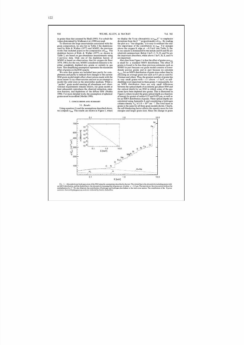
8/12/2019 Schwarze LöCher Als Astronomische Objekte
http://slidepdf.com/reader/full/schwarze-lacher-als-astronomische-objekte 122/146
122
0.1 1.0 10.0E [keV]
100
200
300
400
C N
O
NeMgAl
SiS Ar Ca
Cr
Fe-L
HH+He
H2
0.1 1.0 10.0
700
600
σ E
3 k e V
[ 1 0 - 2
4 c m
2 ]
Fe
Ni
0.1 1.0 10.0E [keV]
10 -610 -510 -410 -310 -210
-1
σ [ M
b a r n
/ H ]
918 WILMS, ALLEN, & M C CRAY Vol. 542
in grains than that assumed by Shull (1993). For cobalt thevalues determined by Mullman et al. (1998) are used.
To illustrate the large uncertainties associated with thegrain composition, we also list in Table 2 the depletionsused by Ride & Walker (1977) and MM83, the previousworks that included grains in the computation of Thep ISM.depletion factors of Ride & Walker (1977), as shown inTable 2, are based on gas-abundance measurements usingCopernicus data. Only one of the depletion factors of MM83 is based on observation, that for oxygen (de Boer1979, 1981); for the rest, MM83 considered elements to beeither completely depleted into grains or entirely in gasform. This simplifying assumption represents the maximume†ect of grains on theISM opacity.
We note that grains are included here partly for com-pleteness and partly to indicate how changes to the currentISM grain model might a†ect observations made with themore recent X-ray observatories and not as an attempt tomodel the solid state in the interstellar medium. While a
““ perfect ÏÏ grain model meeting all abundance and obser-vational requirements remains elusive, our grain model atleast adequately reproduces the observed extinction, emis-sion features, and depletions of the di†use ISM (Mathis1996). For more detailed work, the assumption of sphericalgrains must be modiÐed (Mathis 1990).
3. CONCLUSIONS AND SUMMARY
3.1. ResultsUsing equation (1) and the assumptions described above,
we compute The results are shown in Figure 1, wherep ISM.
we display the X-ray absorptivity as to emphasizep ISME 3
deviations from the E ~3 proportionality of By readingpbf
.the plot as a ““bar diagram,ÏÏ it is easy to estimate the rela-tive importance of the contributors to For energiesp ISM.above the oxygen K edge at D 0.5 keV (see Table 2), theX-ray opacity is dominated by the metals and H and He arerelatively unimportant. Below 1 keV, C, N, O, and Ne arethe important absorbers, while above 1 keV, Si, S, and Feare important.
Also clear from Figure 1 is that the e†ect of grains on p ISMis small for a standard MRN distribution. The e†ect of grains is found to be less than previous estimates such asMM83 in part because our grain model consists of lowerdensity porous grains and in part because we calculate
for an MRN distribution of grain sizes rather than byp grainschoosing an average grain size such as 0.3 k m as used byFireman and others. Thus, the greatest number of grains liesin very small grains with q > 1 above D 1 keV, so self-shielding is not important in these grains. Consequently, for
an MRN distribution there are only small di†erencesbetween the optical depth of an entirely gas-phase ISM andthe optical depth for an ISM in which some of the gasatoms have been depleted into grains. This is illustrated inFigure 2, where we plot the grain optical depth as a functionof energy for grains of radius 0.25 and 0.025 k m, as well asfor an MRN distribution of grains. These optical depths arecalculated using Appendix A and considering a hydrogencolumn density of 1.0 ] 1020 cm ~2 . The total mass inN Hgrains is the same for all three grain models shown. Clearly,the self-blanketing factor a†ects the opacity more for lowenergies and larger grain sizes. Since the change in grain
F IG . 1.ÈAbsorptivity per hydrogen atom of the ISM using the assumptions described in the text. The dotted line is the absorptivity including grains withan MRN distribution, and the dashed line is the absorptivity assuming that all grains are of radius a \ 0.3 k m. The inset shows the cross section without themultiplication by E3 . We also illustrate the contribution of hydrogen and hydrogen plus helium to the total cross section. The contribution of the cross H 2sectionto thetotal hydrogencross sectionis indicated by thedot-dashedline.
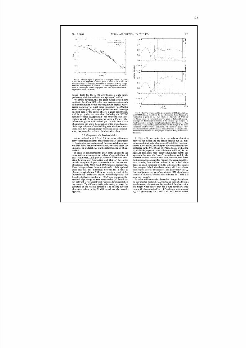
8/12/2019 Schwarze LöCher Als Astronomische Objekte
http://slidepdf.com/reader/full/schwarze-lacher-als-astronomische-objekte 123/146
123
-0.10
-0.05
0.00
0.05
0.10
0.15
0.20a
r e l a t i v
e d
e v
i a t i o
n
0.1 1.0 10.0E [keV]
-0.10
-0.05
0.00
0.05
0.10
0.15
0.20b
No. 2, 2000 X-RAY ABSORPTION IN THE ISM 919
F IG . 2.ÈOptical depth of grains for a hydrogen column NH\ 1.0
] 1020 cm~2 (see Appendix A) and for grains of radius a \ 0.25 k m (dot -dashed line ) and a \ 0.025 k m (dashed line ) as a function of X-ray energy.
The total mass in grains is constant. The shielding reduces the opticaldepth at low energies and for large grain sizes. The labels denote the Kedges of theelements indicated.
optical depth for the MRN distribution is quite small,grains only slightly modifythe absorptivity of the ISM.
We stress, however, that the grain model as used hereapplies to the di†use ISM rather than to dense regions suchas inner molecular clouds or young stellar objects, wheregrains might play a much more important role (Mathis1990). By changing the range of grain sizes from the rangeadopted here for the di†use ISM to a grain distributionwith larger grains, our formalism (including the XSPECroutine described in Appendix B) can be used to treat theseregions as well. As an example, we show in Figure 1 theinÑuence of grains with a \ 0.3 km. In this case, X-rayobservations will allow the detection of the grains becauseof the large inÑuence of self-shielding, even with instruments
that do not have the high energy resolution to see the solid-state resonancee†ects close to theabsorption edges.
3.2. Comparison with Previous ModelsAs we outlined in °° 2.2 and 2.3, the major di†erences
between this model and the previous models are the updatesto the atomic cross sections and the assumed abundances.With the use of simulated observations, we can examine theimpact of an updated on the interpretation of obser-p ISMvations.
In order to demonstrate the e†ect of the updates to thecross sections, we compare our values of with those of p ISMMM83 and BM92. In Figure 3 a we show the relative devi-ation between our formulation and that of the earliermodels, using our adopted cross sections and the assumedabundances of the MM83 and BM92 models, respectively.Thus, the Ðgure shows the cumulative e†ect of the updatedcross sections. The di†erences between the models atphoton energies below 0.3 keV are mainly a result of theuncertainty in the He cross section. Additional peaks at theK and L shell edges are due to D 10 eV discrepancies in theassumed edge energy between these models ( ° 2.2) and arenot relevant for practical work with moderate-resolutioninstruments. The di†erence in the values of produces thepbfcurvature of the relative deviation. The missing subshellabsorption edges in the MM83 model are also readilyapparent.
F IG . 3.ÈRelative deviation of the cross sections of BM92 ( solid lines )and MM83 ( dashed lines ) from the model described here. The relativecomputation is given as where value of BM92 or(p i
[ p )/ p , pi\ the
MM83 and where p is our formulation. The spikes at the K and L absorp-tion edges are due to slight di†erences in the assumed edge energies. ( a)Relative deviation computed using the abundances of BM92 and MM83,respectively. This panel highlights the e†ect of the change in the crosssections. ( b) Relative deviation from our model, computed using the solar
abundances of Table 2, illustrating the cumulative e†ect of using di†erentdefault solar abundances and changing cross sections. See ° 2.2 for furtherdiscussion.
In Figure 3 b, we again show the relative deviationbetween our model and the earlier models but this timeusing our default solar abundance (Table 2) for the abun-dances in our model, including the additional elements notcontained in the MM83 and BM92 models, as well as the
molecule (important especially below D 300 eV). In thisH 2Ðgure, all models are with ““ solarÏÏ abundances, but the dis-agreement between the ““ solarÏÏ abundances used by thedi†erent authors results in 10% of the di†erence betweenthe three models compared in Figure 3. However, the di†er-ence resulting from di†erent values of the ““ solarÏÏ abun-dance is small compared with the di†erence that resultsfrom using our default abundance values, which are reducedwith respect to solar abundances. The discrepancy in p ISM
that results from the use of our default ISM abundancesinstead of the solar abundances indicated in Table 2 isshown in Figure4.
In order to illustrate the observable changes introducedby our updated model of we studied these e†ects usingp ISM,simulations of observations. We simulated the observationof a bright X-ray source that has a pure power-law spec-trum with photon index ! \ [ 1.7 and a normalization of
photons cm ~2 s~1 keV~1 at 1 keV. Such a sourceAPL\ 2
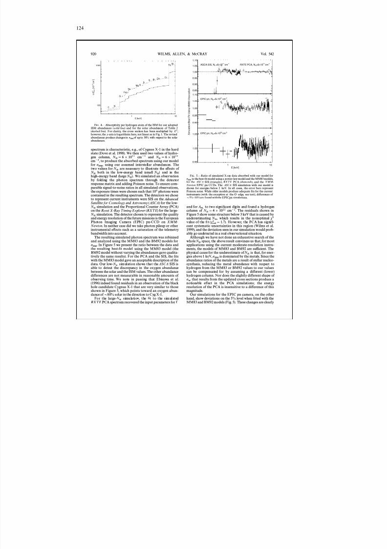
8/12/2019 Schwarze LöCher Als Astronomische Objekte
http://slidepdf.com/reader/full/schwarze-lacher-als-astronomische-objekte 124/146
8/12/2019 Schwarze LöCher Als Astronomische Objekte
http://slidepdf.com/reader/full/schwarze-lacher-als-astronomische-objekte 125/146
125
No. 2, 2000 X-RAY ABSORPTION IN THE ISM 921
due to the update of the abundances and cross sections. It isfor instruments such as the EPIC pn camera that we recom-mend that our model be used. The EPIC observation simu-lated here is quite short (the raw EPIC pn count rate of Cygnus X-1 will be D 2400 counts s ~1 , so the spectrum usedfor modeling here has an exposure time of only 4 ks, shorterthan the minimum XMM -Newton observing time of 5 ks),and the ratio plots in Figure 5 already show the character-istic curvature due to the deviation in the shape of the crosssection assumed in the MM83 models. We note that asimilar behavior is also present when Ðtting the simulatedspectrum with the BM92 data. When using the BM92 crosssections, however, it is possible to obtain a good descriptionof the overall absorption by treating the abundances as freeparameters. In this case the ““ wavyÏÏ residual structure stillremains, although the relative abundances found for theelements do come close to the abundances that we assumedin our modeling of As a result, we recommend usingp ISM .our model whenever high-precision work on the 1% È 2%
level is necessary, as well as in cases when the absorbingcolumn resulting from the spectral Ðtting process is to bephysically interpreted (i.e., when comparing X-ray N H
values with radio data or when modeling an observed X-rayspectrum for which the value is known by other means).N H
3.3. CaveatsWhile we feel that the model for as presented in thep ISM
previous sections is well suited for most X-ray astronomicalwork, several astronomical or physical issues had to beneglected in the modeling process. In particular, our modeldoes not include the e†ects of the warm phase or of theionized phase of the ISM. In addition, we ignore Thomsonscattering, which becomes important at moderate to highThomson optical depths and keV. These e†ects haveE Z 4not been included largely because they are negligible formost situations in which our model is likely to be used.Furthermore, the model assumes that there is no variation
of the abundances along the line of sight. Finally, we notethat energy-dependent scattering by dust grains has notbeen considered here since an XSPEC routine (““dustÏÏ)already exists to treat it.
The warm and ionized phases of the ISM have beenneglected here for a number of reasons. Large parts of theISM are assumed to be (moderately) ionized, and a goodmodel for should in principle include the ionized phase.p ISM
However, there is even less agreement on the ionizationstate of the ISM as a whole than there is on the grain phase,which was discussed in ° 2.4. The major reason for thisdisagreement is a good one: the ionization of the ISMdepends strongly on the line of sight, so any general modelfor the ionization structure of the Galaxy is prone to fail. Itappears, however, that most of the warm phase of the ISMis only moderately ionized, so our model will still be appli-cable except for photon energies close to the K edges. Foroxygen, e.g., the K edge energy increases from 0.54 keV forO I to 0.61 keV for O IV , and the photoionization crosssection is also dependent on the ionization stage. It shouldbe noted, though, that the ionization of hydrogen willstrongly inÑuence for energies below 0.1 keV. Forp ISM
instance, in their study of soft X-ray emission from othergalaxies, Cui et al. (1996) assumed the ratio between H I andH II to be 1. Using the code presented in Appendix B, thise†ect may be taken into account by changing the relativeabundances of He and the metals with respect to hydrogen.
Similar line-of-sight e†ects also hold true for the abun-dances. In the Galaxy, measurement of abundances in H II
regions and planetary nebulae has suggested the existenceof a radial abundance gradient, particularly at small Galac-tic radii (Rana 1991; Kaufer et al. 1994, and referencestherein). When one computes the absorption of any back-ground object through such a medium with varying abun-dances, the abundances measured in the X-rays will be theaverage of the abundance variations along the line of sight.Since the abundances in our model are allowed to vary, it ispossible to take this e†ect into account. Obviously, in sucha case the assumed abundance set with respect to which therelative abundances are measured is a matter of taste, andusing the solar abundances of Table 2 as a baseline insteadof the ISMabundances might be a better choice.
Our model also ignores the inÑuence of Thomson scat-tering because for many observations it will not make asubstantial contribution. This is not to say that it is alwaysnegligible; Thomson scattering is the dominant physical
process for the attenuation of X-rays aboveD
10 keV. As arough guideline, Thomson scattering should always beincluded in the modeling process when cm ~2N H Z 1022
(see, e.g., Stelzer et al. 1999). Detailed instructions based onMonte Carlo modeling of Thomson scattering in moder-ately optically thick media are given by Yaqoob (1997).Note, however, that Yaqoob assumes the electrons to befree. When the electrons are bound, it is more appropriateto consider incoherent scattering, i.e., Compton scattering,o† the bound electrons. The cross sections for incoherentscattering and the Klein-Nishina cross section are slightlydi†erent (on the percent level), which should be taken intoaccount. Analytical estimates for this e†ect have been givenby Gorshkov, Mikhailov, & Sherman (1973) for the Hatom; for other elements tables are available (Hubbell et al.1975; Henke et al. 1993). For most work, however, thesecorrections are negligible.
Finally, we also stress that our model, like its prede-
cessors MM83 and BM92, is not well suited for extremelyhigh precision work, e.g., high signal-to-noise ratio spectrawith the grating spectrometers on XMM -Newton andChandra . The energy resolution of these very highresolution instruments is so high that the X-ray absorptionÐne structure (XAFS) within grains and molecules mightbecome relevant, as well as resonance e†ects close to theabsorption edges in the absorption cross section itself. Forthe inclusion of the resonances much higher resolutioncross sections than those available here are required. XAFSe†ects become noticeable especially in regions of large N H
where grains are an important ingredient. For these studies,dedicated modeling codes are being devised, which shouldbe used instead. See Forrey, Woo, & Cho (1998), Woo,Forrey, & Cho (1997), Woo (1995), and the referencestherein for further details.
3.4. Summary and Outlook
We have presented an improved model for the X-rayabsorption in the interstellar medium valid above D 100 eVby updating the relevant photoionization cross sections andby including the e†ect of the molecule and a revised setH 2
of recommended elemental abundances for the interstellarmedium. Since the abundances of the metals are smallerthan previously estimated, our values of are generallyp ISM
smaller than those used previously. We have shown thatthese updates will be relevant for instruments to be avail-
8/12/2019 Schwarze LöCher Als Astronomische Objekte
http://slidepdf.com/reader/full/schwarze-lacher-als-astronomische-objekte 126/146
126
922 WILMS, ALLEN, & M C CRAY Vol. 542
able as this paper goes into print. We have also reconsi-dered the e†ect of grains in the ISM by improving the grainmodel and the calculation of taking into accountqgrains ,recent studies of the physical properties of interstellar dustgrains. Our results show that the change in opacity due tograins on for realistic grain models and realistic chemi-pISMcal composition of the grains is small. As described inAppendix B, our calculation of is available as a sub-pISMroutine that can be used with X-ray data analysis packagessuch as XSPEC.
This work highlights the point made by Shull (1993) andothers: that great uncertainties remain in much of theatomic physics data needed to interpret X-ray astronomicalobservations. The e†ective areas and energy resolutions of instruments recently launched will be more sensitive thanthe available atomic data for the X-ray energy range canaccommodate, and the situation is even worse for possiblefuture instruments such as Constellation -X or the X-RayEvolving Universe Spectroscopy Mission (XEUS ). Thedi†er-
ences between the currently available cross sections dis-cussed in ° 2.2 are still at the 5% level. We hope that the
advent of the new instruments will also initiate newattempts to more accurately determine the atomic data onwhich X-ray astronomy can rely. We will therefore continueover the next years to update the database of the computa-tions presented here and periodically release new versionsof the code presented in Appendix B that will incorporatethe improvements in the abundances or the atomicphysics.
This work has been partially Ðnanced by NASA grantsNGT 5-80, NAG5-7339, and NAG5-7340 and by a Nation-al Physical Science Consortium Fellowship grant (to A. A.).J. W. acknowledges the hospitality of the high-energy astro-physics groups at JILA and at the University of Californiaat San Diego, where part of this work was done. We thankthe referee Dan McCammon for his comments, whichgreatly improved the presentation of this paper, and forproviding the code for the helium autoionization reso-nances. We also thank Laurie Kovalenko, Phil Maloney,
Katja Pottschmidt, Richard Rothschild, Staubert,Ru digerKlaus Werner, and Svet Zhekov for useful comments.
APPENDIX A
SELF-SHIELDING IN THE GRAINS
To derive the optical depth of the grains (eq. [5]), we consider a population of grains of homogeneous chemical composi-tion with size a , geometrical cross section column density SN T, and average photoionization cross section SpT (perpgeom,atom). For grains of realistic shape, SN T is a complicated function of a. Since the inÑuence of grains on is small, however,pISMfor simplicity we canassumethat the grains arespheres with radius a so that
SNT\ 4oa3k
\ 4na3
, (A1)
where o is the mass density of the grain, n the number density of the grain, and k the mean molecular weight of the grainÏs
constituents. Using thenotation of ° 2.1, k is given by
k \ ;Z
AZ ] bZ ] kZN;Z
AZ ] bZ . (A2)
Here, is the molecular weight of element Z (Table 2). For the default abundances and depletions of Table 2, k \ 18.2kZ
amu \ 3.0 ] 10~23 g atom ~1 . Assuming o \ 1 g cm~3 , the grain number density is n \ 3.3 ] 1022 atoms cm ~3 . Ignoringsolid-state e†ects, the photoionization cross section of thegrain material is given by
SpT\ ;Z
AZ ] bZ ] pbf(Z )N;Z
AZ ] bZ . (A3)
For a column density of grains of a single size along the line of sight, the optical depth for photoabsorption of theN grainsgrains is the product between the geometrical optical depth of the grains, and the fraction of photons thatN grains pgeom,encounter the grain and are absorbed:
qgrains \ N grains pgeom[1 [ exp ([ SpTSN T)] . (A4)
In computing for grains of a single size it is sometimes convenient to express in terms of the optical depth thatpISM qgrainswould beobserved ifthe constituentsofthegrain wereinthe gaseous phase, Hence,q
grains
\ fNgas
SpT.
f \N grains pgeom
N gasSpT [1 [ exp ([ SpTSNT)] \ 1 [ exp ([ SpTSNT)
SpTSNT , (A5)
since the columndensityof the grain is Thisfactor iscalled the self-blanketing factor(Fireman 1974).N gas /(N grains pgeom).For the general case that the grains have a size distribution wheredngr(a)/ da ,
P 0
= dngrda
da \ 1 , (A6)
8/12/2019 Schwarze LöCher Als Astronomische Objekte
http://slidepdf.com/reader/full/schwarze-lacher-als-astronomische-objekte 127/146
127
No. 2, 2000 X-RAY ABSORPTION IN THE ISM 923
a similar derivation shows that
qgrains\ N Hmg P 0
= dngr(a)da
pgeom[1 [ exp ([ SpTSN T)]da , (A7)
where is the number of grains per hydrogen atom along the line of sight. For spherical grains,mg
mg \ ; A Z ] bZ
] kZNP dngrda
] o ]43 na3 ] da . (A8)
For a power-law size distribution, where we can express in terms of special functions.dngr(a)/ da \ ka ~ p , amin¹ a ¹ amax, qgrainsInserting into equation (A7) and performing a partial integration, we obtain for p \ 4pgeom
\ na2
qgrains\ N Hmg
nk p [ 3 G 1
aminp ~3 (1 [ e~4 WpXna min@3) [ 1
amaxp ~3 (1 [ e~4 WpXna max@3)
] (4SpTn /3)p ~3 [c(4 [ p, 4SpTnamax /3) [ c(4 [ p, 4SpTnamin /3)]H , (A9)
where the incomplete gamma function is given by ( ° 6.5 of Abramowitz & Stegun 1964)
c(a, x ) \ P 0
x
e~t
ta~1 dt (A10)
and can be evaluated using algorithms presented by ° 6.2 of Press et al. (1992).
APPENDIX B
IMPLEMENTATION INTO XSPEC
Using the formalism and data described in ° 2, we have written subroutines that can be used in conjunction with thepopular X-ray data analysis package XSPEC (Arnaud 1996). 3
Given the uncertainty of many of the parameters entering the model, there are several interfaces to the subroutine. Themain spectral model, ““ tbabs,ÏÏ is intended as a replacement for the earlier ““ wabsÏÏ and ““ phabsÏÏ models, as well as theirredshifted versions. This model assumes the abundances and depletion factors of Table 2. A subroutine ““ztbabs ÏÏ for modelingredshifted absorption is also available. The latter subroutine does not account for the dust component, as X-ray observationswith a measurable dust inÑuence will most probably include only observations of Galactic objects, at least within the nextdecade.
In addition, the XSPEC model ““ tbvarabs ÏÏ provides a full interface to the X-ray absorption model presented in ° 2 andallows the user to change all abundances, depletion factors, and grain properties. We stress that this model is very powerfuland therefore prone to misuse. Caution is required when Ðtting data with too many free parameters.
REFERENCESAbramowitz, M., & Stegun, I. A. 1964, Handbook of Mathematical Func-
tions (Washington: U.S. Government Printing Office)Anders, E., & Ebihara, M. 1982, Geochim. Cosmochim. Acta, 46, 2363Anders, E., & Grevesse, N. 1989, Geochim. Cosmochim. Acta, 53, 197Arabadjis, J. S., & Bregman, J. N. 1999, ApJ, 510, 806Arnaud, K. A. 1996, in Astronomical Data Analysis Software and Systems
V, ed. J. H. Jacoby & J. Barnes (San Francisco: ASP), 17M., & McCammon, D. 1992, ApJ, 400, 699 (BM92)Ba ¡ucin ska-Church,
Band, I. M., Trzhaskovskaya, M. B., Verner, D. A., & Yakovlev, D. G.1990, A&A, 237, 267
Bethe, H. A., & Salpeter, E. E. 1957, Quantum Mechanics of One- andTwo-Electron Atoms (Berlin : Springer)
E., Baudoux, M., Kurucz, R. L., Ansbacher, W., & Pinnington,Bie mont,E. H. 1991, A&A, 249, 539
Brinks, E. 1990, in The Interstellar Medium in Galaxies, ed. H. A. Thron-son & J. M. Shull (Dordrecht: Kluwer), 39
Bronfman, L., Cohen, R. S., Alvarez, H., & Thaddeus, P. 1988, ApJ, 324,248Brown, R. L., & Gould, R. J. 1970, Phys. Rev. D, 1, 2252Cardelli, J. A., Meyer, D. M., Jura, M., & Savage, B. D. 1996, ApJ, 467, 334Chen, W. F., Cooper, G., & Brion, C. E. 1991, Phys. Rev. A, 44, 186Cui, W., Sanders, W. T., McCammon, D., Snowden, S. L., & Womble, D. S.
1996, ApJ, 468, 102de Boer, K. S. 1979, ApJ, 229, 132 ÈÈÈ. 1981, ApJ, 244, 848
Dove, J. B., Wilms, J., Nowak, M. A., Vaughan, B., & Begelman, M. C.1998, MNRAS, 289, 729
Draine, B. T., & Lee, H. M. 1984, ApJ, 285, 89Dwek, E. 1997, ApJ, 484, 779Ebisawa, K., Ueda, Y., Inoue, H., Tanaka, Y., & White, N. E. 1996, ApJ,
467, 419Feldman, U. 1992, Phys. Scr., 46, 202Fernley, J. A., Taylor, K. T., & Seaton, M. J. 1987, J. Phys. B, 20, 6457Fireman, E. L. 1974, ApJ, 187, 57Fitzpatrick, E. L. 1999, PASP, 111, 63Fogel, M. E., & Leung, C. M. 1998, ApJ, 501, 175Forrey, R. C., Woo, J. W., & Cho, K. 1998, ApJ, 505, 236Gorshkov, V. G., Mikhailov, A. I., & Sherman, S. G. 1973, Zh. Eksp. Teor.
Fiz., 64, 1128 (Sov. Phys. È JETP, 37, 572)Gould, R. J., & Jung, Y.-D. 1991, ApJ, 373, 271Grevesse, N., & Anders, E. 1989, in AIP Conf. Proc. 183, Cosmic Abun-
dances of Matter, ed. C. Waddington (New York: AIP), 1Grevesse, N., Lambert, D. L., Sauval, A. J., van Dishoeck, E. F., Farmer,C. B., & Norton, R. H. 1991, A&A, 242, 488
Grevesse, N., & Noels, A. 1993, in Origin and Evolution of the Elements,ed. N. Prantzos, E. Vangioni-Flam, & M. Casse (Cambridge: CambridgeUniv. Press), 15
Grevesse, N., & Sauval, A. J. 1999, A&A, 347, 348Henke, B. L., Gullikson, E. M., & Davis, J. C. 1993, At. Data Nucl. Data
Tables, 54, 181 (http ://cindy.lbl.gov/optical – constants/)
3 These subroutines are available at http://astro.uni-tuebingen.de/nh/.

8/12/2019 Schwarze LöCher Als Astronomische Objekte
http://slidepdf.com/reader/full/schwarze-lacher-als-astronomische-objekte 128/146
8/12/2019 Schwarze LöCher Als Astronomische Objekte
http://slidepdf.com/reader/full/schwarze-lacher-als-astronomische-objekte 129/146
A NHANG G
Broad Iron Lines in Active Galactic Nuclei:A Possible Test of the Kerr Metric?
J. Wilms, R. Speith, C.S. Reynolds
1998
Nachdruck aus
Black holes: theory and observation
Hrsg. F.W. Hehl, R.J.K. Metzler, C. KieferLecture Notes in Physics
Vol 514, S. 69–79Berlin, Heidelberg, New York: Springer Verlag
129
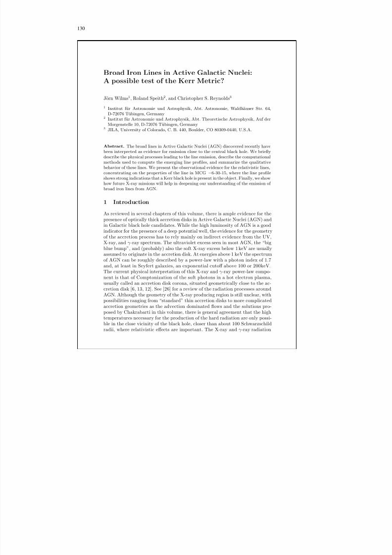
8/12/2019 Schwarze LöCher Als Astronomische Objekte
http://slidepdf.com/reader/full/schwarze-lacher-als-astronomische-objekte 130/146
130
Broad Iron Lines in Active Galactic Nuclei:A possible test of the Kerr Metric?
J orn Wilms 1 , Roland Speith 2 , and Christopher S. Reynolds 3
1 Institut f¨ ur Astronomie und Astrophysik, Abt. Astronomie, Waldh¨ auser Str. 64,D-72076 T ubingen, Germany
2 Institut f¨ ur Astronomie und Astrophysik, Abt. Theoretische Astrophysik, Auf derMorgenstelle 10, D-72076 T¨ ubingen, Germany
3 JILA, University of Colorado, C. B. 440, Boulder, CO 80309-0440, U.S.A.
Abstract. The broad lines in Active Galactic Nuclei (AGN) discovered recently havebeen interpreted as evidence for emission close to the central black hole. We brieydescribe the physical processes leading to the line emission, describe the computationalmethods used to compute the emerging line proles, and summarize the qualitativebehavior of these lines. We present the observational evidence for the relativistic lines,concentrating on the properties of the line in MCG − 6-30-15, where the line proleshows strong indications that a Kerr black hole is present in the object. Finally, we showhow future X-ray missions will help in deepening our understanding of the emission of broad iron lines from AGN.
1 Introduction
As reviewed in several chapters of this volume, there is ample evidence for thepresence of optically thick accretion disks in Active Galactic Nuclei (AGN) andin Galactic black hole candidates. While the high luminosity of AGN is a goodindicator for the presence of a deep potential well, the evidence for the geometryof the accretion process has to rely mainly on indirect evidence from the UV,X-ray, and γ -ray spectrum. The ultraviolet excess seen in most AGN, the “bigblue bump”, and (probably) also the soft X-ray excess below 1 keV are usuallyassumed to originate in the accretion disk. At energies above 1 keV the spectrumof AGN can be roughly described by a power-law with a photon index of 1.7and, at least in Seyfert galaxies, an exponential cutoff above 100 or 200keV.The current physical interpretation of this X-ray and γ -ray power-law compo-nent is that of Comptonization of the soft photons in a hot electron plasma,usually called an accretion disk corona, situated geometrically close to the ac-cretion disk [6, 13, 12]. See [26] for a review of the radiation processes aroundAGN. Although the geometry of the X-ray producing region is still unclear, withpossibilities ranging from “standard” thin accretion disks to more complicatedaccretion geometries as the advection dominated ows and the solutions pro-posed by Chakrabarti in this volume, there is general agreement that the hightemperatures necessary for the production of the hard radiation are only possi-ble in the close vicinity of the black hole, closer than about 100 Schwarzschildradii, where relativistic effects are important. The X-ray and γ -ray radiation
8/12/2019 Schwarze LöCher Als Astronomische Objekte
http://slidepdf.com/reader/full/schwarze-lacher-als-astronomische-objekte 131/146
131
70 Jorn Wilms, Roland Speith, Christopher S. Reynolds
from Seyfert galaxies, therefore, should exhibit signatures that allow us to di-rectly probe this region and perhaps even to nd physical processes enablingus to directly measure parameters of the black hole as its mass or its angularmomentum.
The availability of high sensitivity X-ray and γ -ray satellites in the past tenyears has allowed the observational study of the broad band spectrum of AGN tosearch for such processes. Recently, extremely broad Iron uorescence lines havebeen observed in several Seyfert galaxies. The most convincing interpretation forthese lines is that they are produced in a geometrically thin accretion disk closeto the central black hole. If this interpretation is correct, the line proles are thebest evidence for the existence of black holes known so far. In this review, we give
a brief introduction to the eld. In §2 we describe the physical processes leadingto line emission close to the black hole, i.e. Compton reection and uorescentline emission (§2.1), followed by a description of the computational methods usedto calculate the emerging line proles ( §2.2), and a summary of the qualitativebehavior of the emitted lines ( §2.3). In §3, we describe the observational evidencefor the relativistic lines and give a summary of possible future observations.A recommended review of the subject stressing the observational material hasrecently been published by Fabian [7].
2 Line Emission Close to the Black Hole
2.1 Compton Reection and ReprocessingOne direct consequence of the Accretion Disk Corona model is that it requiresthe presence of a hot electron plasma with a temperature of a few 100 keV inthe close vicinity of the cold accretion disk, which has a temperature of lessthan 10 6 K (∼ 0.1 keV). Due to the proximity of the cold material, hard X-raysemitted from the corona interact with the cold material, leading to observablespectral features. In a gas with kT <
∼ 0.2 keV, only Hydrogen and Helium arefully ionized. Most metals, i.e. elements with a nuclear charge number Z > 2,are only moderately ionized [24]. Since the cross-section for photo-absorption isσbf ∝ E − 3 , most of the irradiating soft X-rays (i.e.photons with E <∼ 10keV) getphoto-absorbed within the accretion disk. On the other hand, the cross-section
for Compton scattering is almost equal to the Thomson cross section σ T (a con-stant), so that photons with high energies predominantly Compton scatter off the electrons in the disk. The threshold energy above which Compton scatter-ing dominates is about 15 keV. Since the electrons in the accretion disk havelow thermal velocities, Compton scattered X-ray photons with E 15 keV loseenergy. The result of these two processes, photoabsorption and Compton scat-tering, is a “hump” of radiation in the spectrum emerging from the disk, peakingat about 30 keV(Fig. 1; see also [18, 10, 19] and references therein]. Such humpshave indeed been found in many Seyfert galaxies, proving the presence of coldmatter in these objects [21].
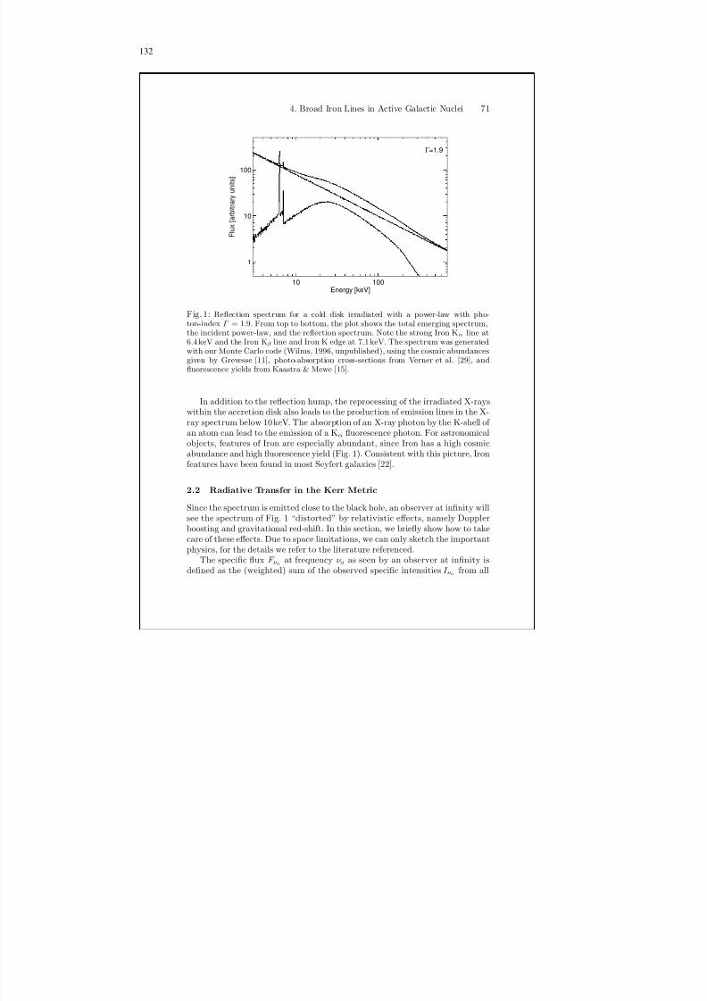
8/12/2019 Schwarze LöCher Als Astronomische Objekte
http://slidepdf.com/reader/full/schwarze-lacher-als-astronomische-objekte 132/146
132
4. Broad Iron Lines in Active Galactic Nuclei 71
10 100Energy [keV]
1
10
100
F l u x
[ a r b
i t r a r y u n
i t s ]
Γ =1.9
Fig. 1: Reection spectrum for a cold disk irradiated with a power-law with pho-ton-index Γ = 1 .9. From top to bottom, the plot shows the total emerging spectrum,the incident power-law, and the reection spectrum. Note the strong Iron K α line at6.4 keV and the Iron K β line and Iron K edge at 7.1 keV. The spectrum was generatedwith our Monte Carlo code (Wilms, 1996, unpublished), using the cosmic abundancesgiven by Grevesse [11], photo-absorption cross-sections from Verner et al. [29], and
uorescence yields from Kaastra & Mewe [15].
In addition to the reection hump, the reprocessing of the irradiated X-rayswithin the accretion disk also leads to the production of emission lines in the X-ray spectrum below 10keV. The absorption of an X-ray photon by the K-shell of an atom can lead to the emission of a K α uorescence photon. For astronomicalobjects, features of Iron are especially abundant, since Iron has a high cosmicabundance and high uorescence yield (Fig. 1). Consistent with this picture, Ironfeatures have been found in most Seyfert galaxies [22].
2.2 Radiative Transfer in the Kerr Metric
Since the spectrum is emitted close to the black hole, an observer at innity willsee the spectrum of Fig. 1 “distorted” by relativistic effects, namely Dopplerboosting and gravitational red-shift. In this section, we briey show how to takecare of these effects. Due to space limitations, we can only sketch the importantphysics, for the details we refer to the literature referenced.
The specic ux F ν o at frequency ν o as seen by an observer at innity isdened as the (weighted) sum of the observed specic intensities I ν o from all
8/12/2019 Schwarze LöCher Als Astronomische Objekte
http://slidepdf.com/reader/full/schwarze-lacher-als-astronomische-objekte 133/146
133
72 Jorn Wilms, Roland Speith, Christopher S. Reynolds
parts of the accretion-disk,
F ν o = Ω
I ν o cos θ dΩ, (1)
where Ω is the solid angle subtended by the accretion disk as seen from theobserver and θ is the angle between the direction to the disk and the directionof the observed photon. Since the black hole (=AGN) is assumed to be very faraway from the observer (=us), we can safely set cos θ = 1. Thus, we “only” haveto compute the specic intensity I ν o at innity from the spectrum emitted onthe surface of the accretion disk, I ν e . In an axisymmetric accretion disk, I ν e is afunction of the radial distance of the point of emission from the black hole, r e ,and of the inclination angle, ie , of the emitted photon, measured with respectto the normal of the accretion disk.
Due to Doppler boosting and gravitational red-shift, the observed frequencyν o is related to the emitted frequency ν e by
g = ν oν e
= 11 + z
, (2)
where z is the red-shift of the photon. According to Liouville’s theorem, thephase-space density of photons, proportional to I /ν 3 , is constant along the pathof propagation of the photon (the null-geodesic). It is therefore possible to expresseq. (1) in terms of the emitted specic ux on the accretion disk:
F ν o = Ω
I ν o
ν 3oν 3o dΩ =
Ω
I ν e
ν 3eν 3o dΩ =
Ωg3 I ν e (r e , i e ) dΩ. (3)
In other words, the computation of the emerging spectrum breaks down to thecomputation of the “red-shift” g. In the weak eld limit, when r/M 3 ingeometric units, and in the Schwarzschild metric, g and therefore the line proleemitted by the accretion disk, can be evaluated analytically. Proles computedthis way have been presented, e.g., by Fabian et al. [9] for the Schwarzschildcase, and by Chen & Halpern [4] in the weak eld limit. In most cases, however,the computation has to be done in the Kerr metric since the accreting black holewill be sped up by the accreted material [28].
The “brute force” approach to the computation of g in the Kerr metric isthe direct integration of the trajectory of the photon in the Kerr metric [3, 16].This approach allows the computation of exact line proles even in the case of very complicated geometries, like thick accretion disks, but is very expensive:The computation of one line prole takes several hours on a typical workstation,and several tens of minutes on a supercomputer (Bromley, Chen & Miller [3]quote a computation time of 15 minutes on a Cray T3D with 128 nodes forthe computation of one line prole). It is clear, therefore, that ray-tracing isnot suitable for the analysis of X-ray observations, where a direct comparisonbetween the measured data and the theory is to be made using a χ 2 minimizationmethod.
8/12/2019 Schwarze LöCher Als Astronomische Objekte
http://slidepdf.com/reader/full/schwarze-lacher-als-astronomische-objekte 134/146
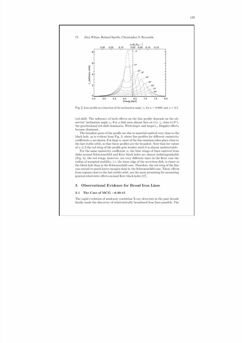
8/12/2019 Schwarze LöCher Als Astronomische Objekte
http://slidepdf.com/reader/full/schwarze-lacher-als-astronomische-objekte 135/146
135
74 Jorn Wilms, Roland Speith, Christopher S. Reynolds
0
2
4
6
8
I ν o
[ a r b
i t r a r y u n
i t s ]
4.5 5.0 5.5 6.0 6.5 7.0 7.5 8.0Energy [keV]
-0.15-0.05 -0.100.000.100.200.30z=(E e /E o) - 1
5 o
10 o
20 o
30 o
40 o
50 o
60 o
70 o
80 o
Fig. 2: Line prole as a function of the inclination angle i o for a = 0 . 9981 and α = 0 . 5.
red-shift. The inuence of both effects on the line prole depends on the ob-servers’ inclination angle i o : For a disk seen almost face on (i.e. i o close to 0 ),
the gravitational red-shift dominates. With larger and larger i
o , Doppler effectsbecome dominant.The broadest parts of the prole are due to material emitted very close to the
black hole, as is evident from Fig. 3, where line proles for different emissivitycoefficients α are shown. For large α , most of the line emission takes place close tothe last stable orbit, so that these proles are the broadest. Note that for valuesof α >
∼ 2 the red wing of the prole gets weaker until it is almost undetectable.For the same emissivity coefficient α , the blue wings of lines emitted from
disks around Schwarzschild and Kerr black holes are almost indistinguishable(Fig. 4), the red wings, however, are very different since in the Kerr case theradius of marginal stability, i.e. the inner edge of the accretion disk, is closer tothe black hole than in the Schwarzschild case. Therefore, the red wing of the line
can extend to much lower energies than in the Schwarzschild case. These effectsfrom regions close to the last stable orbit, are the most promising for measuringgeneral relativistic effects around Kerr black holes [17].
3 Observational Evidence for Broad Iron Lines
3.1 The Case of MCG − 6-30-15
The rapid evolution of moderate resolution X-ray detectors in the past decadenally made the discovery of relativistically broadened Iron lines possible. The
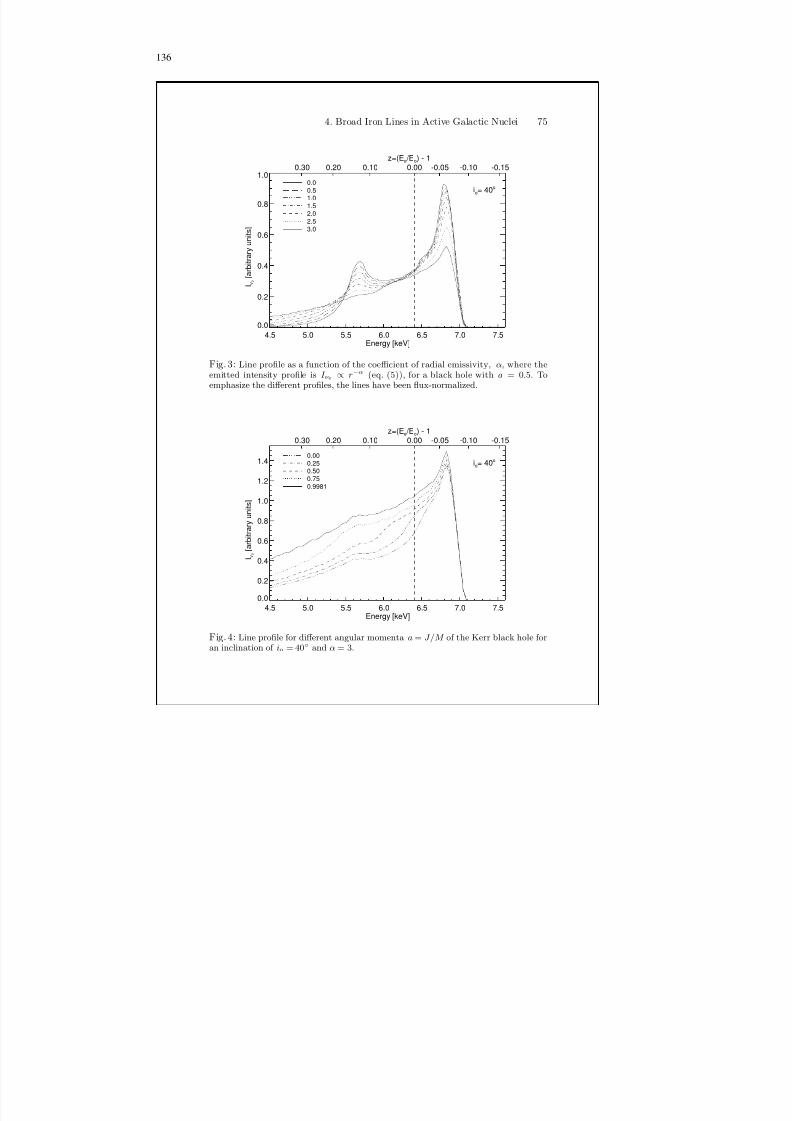
8/12/2019 Schwarze LöCher Als Astronomische Objekte
http://slidepdf.com/reader/full/schwarze-lacher-als-astronomische-objekte 136/146
136
4. Broad Iron Lines in Active Galactic Nuclei 75
0.0
0.2
0.4
0.6
0.8
1.0
I ν o [
a r b
i t r a r y u n
i t s ]
4.5 5.0 5.5 6.0 6.5 7.0 7.5Energy [keV]
-0.15-0.05 -0.100.000.100.200.30z=(E e /E o) - 1
0.0 0.5 1.0 1.5 2.0 2.5 3.0
io= 40 o
Fig. 3: Line prole as a function of the coefficient of radial emissivity, α, where theemitted intensity prole is I ν e
∝ r − α (eq. (5)), for a black hole with a = 0 .5. Toemphasize the different proles, the lines have been ux-normalized.
0.0
0.2
0.4
0.6
0.8
1.0
1.2
1.4
I ν o
[ a r b
i t r a r y u n
i t s ]
4.5 5.0 5.5 6.0 6.5 7.0 7.5Energy [keV]
-0.15-0.05 -0.100.000.100.200.30z=(E e /E o) - 1
0.00 0.25 0.50 0.75 0.9981
io= 40 o
Fig. 4: Line prole for different angular momenta a = J/M of the Kerr black hole foran inclination of io = 40 and α = 3.
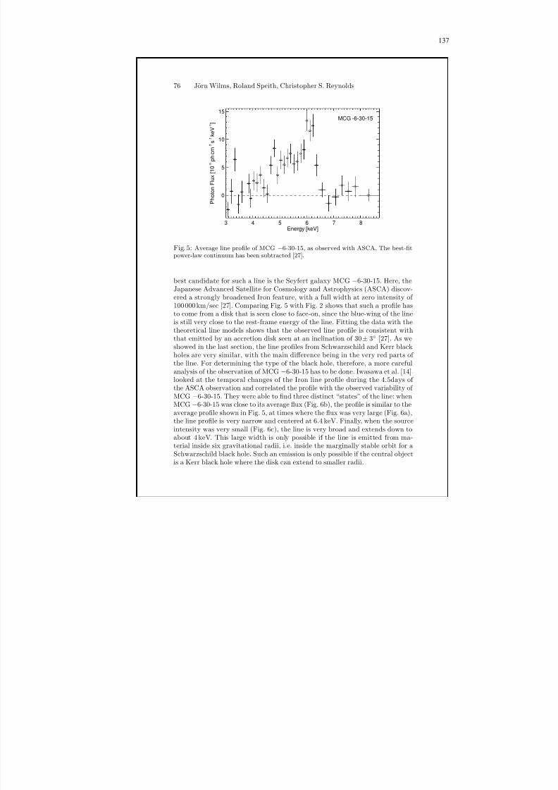
8/12/2019 Schwarze LöCher Als Astronomische Objekte
http://slidepdf.com/reader/full/schwarze-lacher-als-astronomische-objekte 137/146
137
76 Jorn Wilms, Roland Speith, Christopher S. Reynolds
3 4 5 6 7 8Energy [keV]
0
5
10
15
P h o t o n
F l u x
[ 1 0 - 5
p h c m
- 2 s - 1
k e V - 1 ]
MCG -6-30-15
Fig. 5: Average line prole of MCG − 6-30-15, as observed with ASCA. The best-tpower-law continuum has been subtracted [27].
best candidate for such a line is the Seyfert galaxy MCG − 6-30-15. Here, theJapanese Advanced Satellite for Cosmology and Astrophysics (ASCA) discov-ered a strongly broadened Iron feature, with a full width at zero intensity of 100000km/sec [27]. Comparing Fig. 5 with Fig. 2 shows that such a prole hasto come from a disk that is seen close to face-on, since the blue-wing of the lineis still very close to the rest-frame energy of the line. Fitting the data with thetheoretical line models shows that the observed line prole is consistent withthat emitted by an accretion disk seen at an inclination of 30 ± 3 [27]. As weshowed in the last section, the line proles from Schwarzschild and Kerr blackholes are very similar, with the main difference being in the very red parts of the line. For determining the type of the black hole, therefore, a more carefulanalysis of the observation of MCG − 6-30-15 has to be done. Iwasawa et al. [14]looked at the temporal changes of the Iron line prole during the 4.5days of
the ASCA observation and correlated the prole with the observed variability of MCG − 6-30-15. They were able to nd three distinct “states” of the line: whenMCG − 6-30-15 was close to its average ux (Fig. 6b), the prole is similar to theaverage prole shown in Fig. 5, at times where the ux was very large (Fig. 6a),the line prole is very narrow and centered at 6.4 keV. Finally, when the sourceintensity was very small (Fig. 6c), the line is very broad and extends down toabout 4 keV. This large width is only possible if the line is emitted from ma-terial inside six gravitational radii, i.e. inside the marginally stable orbit for aSchwarzschild black hole. Such an emission is only possible if the central objectis a Kerr black hole where the disk can extend to smaller radii.
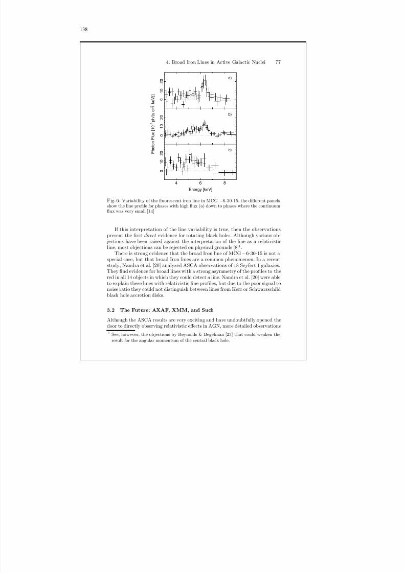
8/12/2019 Schwarze LöCher Als Astronomische Objekte
http://slidepdf.com/reader/full/schwarze-lacher-als-astronomische-objekte 138/146
138
4. Broad Iron Lines in Active Galactic Nuclei 77
1 0
Energy [keV]
- 5
2 0
1 0
0
2 0 a)
b)
c)
2
2 0
P h o
t o n F l u x
[ 1 0
p h / ( s c m
k e
V ) ]
1 0
4
0
0
6 8
Fig. 6: Variability of the uorescent iron line in MCG − 6-30-15, the different panelsshow the line prole for phases with high ux (a) down to phases where the continuum
ux was very small [14]
If this interpretation of the line variability is true, then the observationspresent the rst direct evidence for rotating black holes. Although various ob- jections have been raised against the interpretation of the line as a relativisticline, most objections can be rejected on physical grounds [8] 1 .
There is strong evidence that the broad Iron line of MCG − 6-30-15 is not aspecial case, but that broad Iron lines are a common phenomenon. In a recentstudy, Nandra et al. [20] analyzed ASCA observations of 18 Seyfert 1 galaxies.They nd evidence for broad lines with a strong asymmetry of the proles to thered in all 14 objects in which they could detect a line. Nandra et al. [20] were able
to explain these lines with relativistic line proles, but due to the poor signal tonoise ratio they could not distinguish between lines from Kerr or Schwarzschildblack hole accretion disks.
3.2 The Future: AXAF, XMM, and Such
Although the ASCA results are very exciting and have undoubtfully opened thedoor to directly observing relativistic effects in AGN, more detailed observations1 See, however, the objections by Reynolds & Begelman [23] that could weaken the
result for the angular momentum of the central black hole.
8/12/2019 Schwarze LöCher Als Astronomische Objekte
http://slidepdf.com/reader/full/schwarze-lacher-als-astronomische-objekte 139/146
139
78 Jorn Wilms, Roland Speith, Christopher S. Reynolds
are needed.With the currently planned next generation X-ray missions, the American
Advanced X-ray Astrophysics Facility (AXAF; launch 1998), the Russian Spec-trum-X/ γ (SXG, launch 1998), the European X-ray Multiple Mirror mission(XMM; launch 1999), and the US-Japanese Astro E (launch 2000), we will beable to use X-ray instruments with a much higher energy resolution and largereffective areas than presently available. The huge effective area of XMM will al-low us to probe for temporal variability in the line on much smaller time-scalesthan presently possible: With XMM we might be able to study the time-delaybetween uctuations in the continuum and the reaction of the line to these uc-tuations, allowing us to directly probe the geometry of the accretion ow. The
large energy resolution of AXAF and Astro E will enable us to measure lineproles with a much higher resolution than ever before, which should help us todistinguish without doubt between the current relativistic models for the broadline emission. In the framework of the European EPIC consortium for XMM,two of us (J.W. and C.S.R.) have proposed an uninterrupted 100ksec observa-tion of MCG − 6-30-15. The signal to noise ratio of such an observation will bemuch higher than that of Fig. 6, making the study of the line variability on shorttime-scales possible. Our future ability to observe relativistic effects happeningon a large scale close to 10 8 M black holes look very positive indeed.
Acknowledgments J.W. thanks Prof. N. Straumann for his enthusiastic sugges-tion to write this review and to Prof. F. W. Hehl for his invitation to include the
review in these proceedings. We thank J. Dove, I. Kreykenbohm, K. Pottschmidt,T. Rauch, and R. Staubert for helpful discussions.
Bibliography
[1] Arnaud, K. A., 1996, in Astronomical Data Analysis Software and SystemsV, ed. J. H. Jacoby, J. Barnes, (San Francisco: Astron. Soc. Pacic), 17
[2] Bao, G., Hadravana, P., Østgaard, E., 1994, ApJ, 435, 55
[3] Bromley, B. C., Chen, K., Miller, W. A., 1997, ApJ, 475, 57
[4] Chen, K., Halpern, J. P., 1989, ApJ, 344, 115
[5] Cunningham, C. T., 1975, ApJ, 202, 788
[6] Dove, J. B., Wilms, J., Begelman, M. C., 1997, ApJ, 487, 747
[7] Fabian, A., 1997, Astron. Geophys., 38, 10
[8] Fabian, A. C., et al., 1995, MNRAS, 277, L11
[9] Fabian, A. C., et al., 1989, MNRAS, 238, 729
[10] George, I. M., Fabian, A. C., 1991, MNRAS, 249
8/12/2019 Schwarze LöCher Als Astronomische Objekte
http://slidepdf.com/reader/full/schwarze-lacher-als-astronomische-objekte 140/146
140
4. Broad Iron Lines in Active Galactic Nuclei 79
[11] Grevesse, N., Anders, E., 1989, in Cosmic abundances of matter, ed. C.Waddington, (New York: AIP Conf. Proc.), 1
[12] Haardt, F., Maraschi, L., Ghisellini, G., 1994, ApJ, 432, L95
[13] Hua, X.-M., Titarchuk, L., 1995, ApJ, 449, 188
[14] Iwasawa, K., et al., 1996, MNRAS, 282, 1038
[15] Kaastra, J. S., Mewe, R., 1993, A&AS, 97, 443
[16] Karas, V., Vokrouhlick´y, D., Polnarev, A. G., 1992, MNRAS, 259, 569
[17] Laor, A., 1991, ApJ, 376, 90[18] Lightman, A. P., White, T. R., 1988, ApJ, 335, 57
[19] Magdziarz, P., Zdziarski, A. A., 1995, MNRAS, 273, 837
[20] Nandra, K., et al., 1997, ApJ, 477, 602
[21] Nandra, K., Pounds, K. A., 1994, MNRAS, 268, 405
[22] Pounds, K. A., et al., 1989, MNRAS, 240, 769
[23] Reynolds, C. S., Begelman, M. C., 1997, ApJ, 488, 109
[24] Shull, J. M., Van Steenburg, M., 1982, ApJS, 48, 95[25] Speith, R., Riffert, H., Ruder, H., 1995, Comput. Phys. Commun., 88, 109
[26] Svensson, R., 1996, A&AS, 120, C475
[27] Tanaka, Y., et al., 1995, Nature, 375, 659
[28] Thorne, K. S., 1974, ApJ, 191, 507
[29] Verner, D. A., et al. , 1993, Atomic Data Nucl. Data Tables, 55, 233
8/12/2019 Schwarze LöCher Als Astronomische Objekte
http://slidepdf.com/reader/full/schwarze-lacher-als-astronomische-objekte 141/146
A NHANG H
XMM -EPIC observation of MCG − 6-30-15: direct evidence for the extraction of energy from aspinning black hole?
J. Wilms, C.S. Reynolds, M.C. Begelman, J. Reeves, S. Molendi, R. Staubert, E. Kendziorra
2001
Nachdruck aus
Monthly Notices of the Royal Astronomical Society
Vol. 542, 328, S. L27–L31
141
8/12/2019 Schwarze LöCher Als Astronomische Objekte
http://slidepdf.com/reader/full/schwarze-lacher-als-astronomische-objekte 142/146
142
XMM -EPIC observation of MCG–6-30-15: direct evidence for theextraction of energy from a spinning black hole?
Jorn Wilms, 1 PChristopher S. Reynolds, 2,3 † Mitchell C. Begelman, 3,4 James Reeves, 5
Silvano Molendi, 6 Rudiger Staubert 1 and Eckhard Kendziorra 1
1 Institut fu r Astronomie und Astrophysik, Abt. Astronomie, Universita ¨ t Tu bingen, Sand 1, D-72076 Tu ¨ bingen, Germany2 Department of Ast ronomy, University of Maryland, College Park, MD 20742, USA3 JILA, Campus Box 440, University of Colorado, Boulder, CO 80309, USA4 Department of Ast rophysical and Planetary Sciences, University of Colorado, Boulder, CO 80309, USA5 X-Ray As tronomy Group, Department of Physi cs and Astronomy, Leicester University, Leiceste r LE1 7RH 6 Istituto di Fisica Cosmica, CNR, via Bass ini 15, I-20133 Milano, Italy
Accepted 2001 October 22. Received 2001 October 22; in original form 2001 August 24
A B S T R A C T
We present XMM-Newton European Photon Imaging Camera (EPIC) observations of thebright Seyfert 1 galaxy MCG–6-30-15, focusing on the broad Fe K a line at , 6 keVand theassociated reection continuum, which is believed to originate from the inner accretion disc.We nd these reection features to be extremely broad and redshifted, indicating an origin inthe very central regions of the accretion disc. It seems likely that we have caught this source inthe ‘deep minimum’ state rst observed by Iwasawa et al. The implied central concentrationof X-ray illumination is difcult to understand in any pure accretion disc model. We suggestthat we are witnessing the extraction and dissipation of rotational energy from a spinningblack hole by magnetic elds connecting the black hole or plunging region to the disc.
Key words: accretion, accretion discs – black hole physics – galaxies: individual:MCG– 6-30-15 – galaxies: Seyfert – X-rays: galaxies.
1 I N T R OD U C T I ON
X-ray spectra of Seyfert 1 galaxies commonly show an iron K a
emission line at , 6 keV. The line is often extremely broad, with avelocity width of . 70000kms
2 1. Furthermore, the asymmetriesin the line proles are well explained by relativistic effects. Both of these facts suggest that the line is emitted from the surface layers of the accretion disc within a few gravitational radii r g ¼ GM = c 2 of the black hole (BH) itself. It is now widely believed that thisspectral feature is a relatively clean probe of the immediateenvironments of supermassive BHs (see Fabian et al. 2000, andreferences therein).
One of the best-studied broad iron line sources is the nearbybright Seyfert 1 galaxy MCG–6-30-15 ð z ¼ 0:008 Þ. This was therst active galactic nucleus (AGN) for which a relativistic iron linedisc prole was measured. In their Advanced Satellite for Cosmology and Astrophysics ( ASCA) observations, Tanaka et al.(1995) found that the iron line prole could be explained byemission from an accretion disc around a non-rotating (Schwarz-schild) BH. In a detailed reanalysis, however, Iwasawa et al. (1996)found a much broader line during a period of low continuum X-rayux, the so-called ‘deep minimum state’. The line becomes so
broad that disc models require emission from within 6 r g,suggesting either a rotating (Kerr) BH, with its marginally stableorbit at r ms , 6r g (Iwasawa et al. 1996; Dabrowski et al. 1997), oriron uorescence from material spiralling into the BH at , r ms
(Reynolds & Begelman 1997). Such a broad line was laterconrmed, e.g. by Guainazzi et al. (1999) and Lee et al. (1999).
Using the new generation of X-ray satellites such as XMM- Newton with their improved collecting area and X-ray CCDspectral resolution, the Fe line of Seyferts can be studied in greaterdetail than was possible before. In this Letter, we present data froma 100ks XMM-Newton observation of MCG–6-30-15.
2 I N S T R U M E N TAT I O N A N D D ATAR E D U C T I O N
Our observation covered most of orbit 108 of XMM-Newton , on2000 June 11/12, and was simultaneous with the Rossi X-rayTiming Explorer ( RXTE ). Here, we report on data from theEuropean Photon Imaging Cameras (EPIC) on board XMM- Newton (Stru der et al. 2001; Turner et al. 2001). To prevent photonpile-up, the EPIC-pn camera was operated in its small-windowmode (using the medium thick lter to prevent optical lightcontamination), and the EPIC MOS-1 camera was operated inits timing mode. The MOS-2 camera was operated in full-frame† Hubble Fellow while at the University of Colorado.
PE-mail: [email protected]
Mon. Not. R. Astron. Soc. 328, L27–L31 (2001)
q 2001 RAS
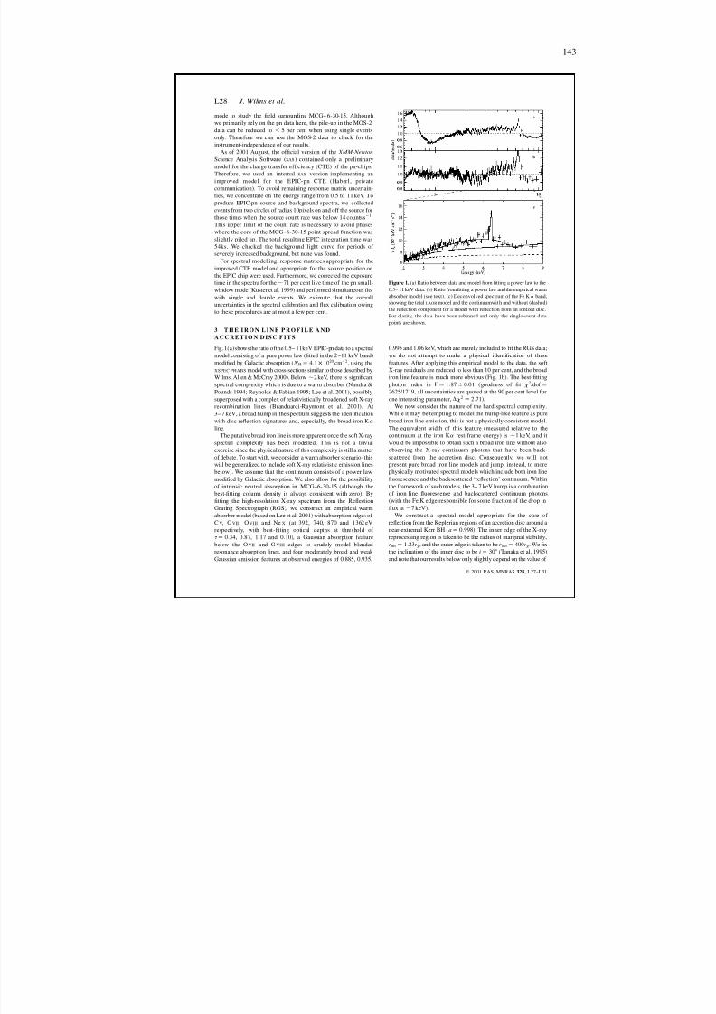
8/12/2019 Schwarze LöCher Als Astronomische Objekte
http://slidepdf.com/reader/full/schwarze-lacher-als-astronomische-objekte 143/146
143
mode to study the eld surrounding MCG– 6-30-15. Although
we primarily rely on the pn data here, the pile-up in the MOS-2data can be reduced to , 5 per cent when using single eventsonly. Therefore we can use the MOS-2 data to check for theinstrument-independence of our results.
As of 2001 August, the ofcial version of the XMM-Newton
Science Analysis Software ( SAS ) contained only a preliminarymodel for the charge transfer efciency (CTE) of the pn-chips.Therefore, we used an internal SAS version implementing animproved model for the EPIC-pn CTE (Haberl, privatecommunication). To avoid remaining response matrix uncertain-ties, we concentrate on the energy range from 0.5 to 11 keV. Toproduce EPIC-pn source and background spectra, we collectedevents from two circles of radius 10pixels on and off the source forthose times when the source count rate was below 14 counts s
2 1 .This upper limit of the count rate is necessary to avoid phaseswhere the core of the MCG–6-30-15 point spread function wasslightly piled up. The total resulting EPIC integration time was54ks. We checked the background light curve for periods of severely increased background, but none was found.
For spectral modelling, response matrices appropriate for theimproved CTE model and appropriate for the source position onthe EPIC chip were used. Furthermore, we corrected the exposuretime in the spectra for the , 71 per cent live time of the pn small-window mode (Kuster et al. 1999) and performed simultaneous tswith single and double events. We estimate that the overalluncertainties in the spectral calibration and ux calibration owingto these procedures are at most a few per cent.
3 T H E I R O N L I N E P R O F I L E A N DA C C R E T I O N D I S C F I T S
Fig.1(a)showsthe ratio ofthe 0 :5– 11keV EPIC-pn data to a spectralmodel consisting of a pure power law (tted in the 2 –11 keV band)modied by Galactic absorption ð N H ¼ 4:1 £ 1020 cm 2 2 , using theXSPEC PHABS model with cross-sections similar to those described byWilms, Allen & McCray 2000). Below , 2 keV, there is signicantspectral complexity which is due to a warm absorber (Nandra &Pounds 1994; Reynolds & Fabian 1995; Lee et al. 2001), possiblysuperposed with a complex of relativistically broadened soft X-rayrecombination lines (Branduardi-Raymont et al. 2001). At3– 7 keV, a broad hump in the spectrum suggests the identicationwith disc reection signatures and, especially, the broad iron K a
line.The putative broad iron line is more apparent once the soft X-ray
spectral complexity has been modelled. This is not a trivialexercise since the physical nature of this complexity is still a matterof debate. To start with, we consider a warm absorber scenario (thiswill be generalized to include soft X-ray relativistic emission linesbelow). We assume that the continuum consists of a power lawmodied by Galactic absorption. We also allow for the possibilityof intrinsic neutral absorption in MCG–6-30-15 (although thebest-tting column density is always consistent with zero). By
tting the high-resolution X-ray spectrum from the ReectionGrating Spectrograph (RGS), we construct an empirical warmabsorber model (based on Lee et al. 2001) with absorption edges of C V, O VII , O VIII and Ne X (at 392, 740, 870 and 1362 eV,respectively, with best-tting optical depths at threshold of t ¼ 0:34, 0.87, 1.17 and 0.10), a Gaussian absorption featurebelow the O VII and O VIII edges to crudely model blendedresonance absorption lines, and four moderately broad and weak Gaussian emission features at observed energies of 0.885, 0.935,
0.995 and 1.06 keV, which are merely included to t the RGS data;we do not attempt to make a physical identication of thesefeatures. After applying this empirical model to the data, the softX-ray residuals are reduced to less than 10 per cent, and the broadiron line feature is much more obvious (Fig. 1b). The best-ttingphoton index is G ¼ 1:87 ^ 0:01 (goodness of t x 2 = dof ¼2625 = 1719, all uncertainties are quoted at the 90 per cent level forone interesting parameter, D x
2 ¼ 2:71Þ.We now consider the nature of the hard spectral complexity.
While it may be tempting to model the hump-like feature as purebroad iron line emission, this is not a physically consistent model.The equivalent width of this feature (measured relative to thecontinuum at the iron K a rest-frame energy) is , 1 keV, and itwould be impossible to obtain such a broad iron line without alsoobserving the X-ray continuum photons that have been back-scattered from the accretion disc. Consequently, we will notpresent pure broad iron line models and jump, instead, to morephysically motivated spectral models which include both iron lineuorescence and the backscattered ‘reection’ continuum. Withinthe framework of such models, the 3– 7 keV hump is a combinationof iron line uorescence and backscattered continuum photons
(with the Fe K edge responsible for some fraction of the drop inux at , 7 keV).
We construct a spectral model appropriate for the case of reection from the Keplerian regions of an accretion disc around anear-extremal Kerr BH ða ¼ 0:998 Þ. The inner edge of the X-rayreprocessing region is taken to be the radius of marginal stability,r ms ¼ 1:23 r g , and the outer edge is taken to be r out ¼ 400 r g . We xthe inclination of the inner disc to be i ¼ 308 (Tanaka et al. 1995)and note that our results below only slightly depend on the value of
Figure 1. (a) Ratio between data and model from tting a power law to the0:5– 11 keV data. (b) Ratio from tting a power law and the empirical warmabsorber model (see text). (c) Deconvolved spectrum of the Fe K a band,showing the total LAOR model and the continuumwit h and without (dashed)the reection component for a model with reection from an ionized disc.For clarity, the data have been rebinned and only the single-event datapoints are shown.
L28 J. Wilms et al.
q 2001 RAS, MNRAS 328, L27–L31
8/12/2019 Schwarze LöCher Als Astronomische Objekte
http://slidepdf.com/reader/full/schwarze-lacher-als-astronomische-objekte 144/146
144
i chosen. We assume that the reected emission has an emissivity
prole e / r 2 b
and leave b as a free parameter. The reectioncontinuum is described using the PEXRIV model of XSPEC andnormalized to the case where the accretion disc intercepts half of the X-ray power-law continuum photons (i.e. R ¼ 1Þ. Both the ironline prole and the reection continuum are then relativisticallysmeared [using the model of Laor (1991) as the kernel]. Here, andthroughout the rest of the spectral modelling discussed in thispaper, we also include a narrow (unresolved) Gaussian line at6.4 keV with equivalent width W K a ,N to model the obvious narrow-line core. This component presumably originates from distantmaterial such as the putative molecular torus of Seyfert unicationschemes, and has recently be seen in several other AGN [e.g. inNGC 5548 (Yaqoob et al. 2001) or in Mrk 205 (Reeves et al.2001)].
First, we consider the case of a fairly cold accretion disc (rest-frame iron line energy of 6.4 keV, disc ionization parameter j ¼ 1,and R ¼ 1Þ. The resulting best-tting parameters are G ¼2:09 ^ 0:01, b ¼ 3:6 ^ 0:1, W K a ;N ¼ 38eV and W K a ;B ¼ 805eVðx 2 = dof ¼ 2383 = 1717 Þ. However, this model fails to explain thedata as well as possessing an unphysically large broad-lineequivalent width. Signicant residuals (up to , 20 per cent)remain in the 3– 11 keV band. The pattern of residuals suggeststhat the model is failing to produce the red wing of the 3 –7 keVhump, and is underestimating the ux in the blueward edge of thisfeature. A hard tail above 8 keV suggests that we are alsounderestimating the strength of the high-energy reectioncontinuum. If we allow the relative normalization of the reectioncontinuum, R, to be a free parameter, the t converges to a verylarge value of R ð R ¼ 7:6þ 1:8
2 1:3 , also G ¼ 2:35 ^ 0:05 and b ¼4:4 ^ 0:2, x 2 = dof ¼ 2055 = 1716 Þ. Despite the slightly better x 2 ,large residuals around , 7 keV remain.
Ionization of the accretion disc surface is another way of increasing the amount of reection continuum. To model this (withthe relative normalization of the reection continuum xed to R ¼ 1Þ, we allow the ionization parameter of the disc j , the tem-perature of the disc T and the energy of the iron line E tobe free parameters ( E is constrained to lie in the range of allowableFe K a energies: 6.40 to 6.97keV). The resulting best t has G ¼2:00 ^ 0:02 ; b ¼ 3:29þ 0:12
2 0:11 , E ¼ 6:40 þ 0:052 0 keV, j ¼ 1380 þ 570
2 190 ;T . 6:0 £ 105 K, W K a ;N ¼ 41eV and W K a ;B ¼ 235eV ðx 2 = dof ¼2051 = 1714 Þ. This leads to a signicantly better t with the higheriron edge/line energies explaining the residual at , 7 keV.However, signicant residuals still exist in the 3– 5 keV range(suggesting that we are still under-predicting the ux in the redwing of the reection feature) and above 8 keV.
Detailed examination of this last spectral model shows thatfeatures in the soft X-ray band below 1.5 keV determine the best-tting ionization parameter and temperature. Consequently, suchts must be viewed with suspicion – there are a number of physicalprocesses that are not included in this reection model but whichmay well contribute to the soft X-ray spectrum (most notably, therecombination line and edge emission from C, N, O and Ne). It
would also not be surprising if our empirical warm absorber modelleft small soft X-ray residuals which may then be mistakenly ttedby ionized reection models.
First, we can consider the ionized reection ts ignoring alldata below 1.5 keV. Retting the ionized disc model (includingthe empirical warm absorber) to the 1 :5– 11keV band results ina good t with no clear residuals. The best-tting parameters areG ¼ 1:94 ^ 0:02, b ¼ 4:6 ^ 0:3, E ¼ 6:95þ 0
2 0:15 keV, W K a ;N ¼51eV and W K a ;B ¼ 582eV ðx 2 = dof ¼ 1506 = 1312 Þ. T and j are
unconstrained by the data, while the relative normalization of
the reection continuum is constrained to be R,
4:7. During thetting R is anti-correlated with W K a ,B . These quantities arephysically consistent with each other (i.e. the iron line has theappropriate strength for that value of R and j ) when R , 1:5–2(corresponding to W K a ;B
, 300–400eV Þ.This spectral modelling suggests that the accretion disc may be
ionized. Consequently, the K a line need not be intrinsically narrowas we have assumed so far, but might be Compton-broadened in thehot skin of the accretion disc [note that Compton broadening alonecannot explain the large line width (Reynolds & Wilms 2000)]. Weexamine this possibility by relaxing our assumption of a narrowintrinsic line and, instead, model the intrinsic iron line with aGaussian prole of width s . Using the 1 :5– 11 keV data, the best-tting value is s ¼ 0 (with other parameters as above). Even if weforce the line to be very broad (e.g. s ¼ 1 keV, at the expense of reducing the goodness of t by Dx 2 ¼ 13Þ, the data still requireb . 3:9.
The second approach for handling the soft X-ray spectrum is tomodel explicitly the recombination K lines of C, N, O and Ne.Qualitatively, this model is the same as the mixed emission-linemodel of Branduardi-Raymont et al. (2001) with the presence of additional warm absorption. The best-tting parameters are G ¼1:96 ^ 0:01 ; b ¼ 4:70þ 0:25
2 0:27 , E ¼ 6:97 þ 02 0:10 keV, W K a ;N ¼ 53eV,
j . 130 and W K a ;B ¼ 546eV ðx 2 = dof ¼ 1907 = 1704 Þ. Again, therelative reection normalization is poorly constrained by thesedata, but self-consistency is achieved for R , 1:5–2 andW K a ;B
, 300– 400eV. We conclude that the parametrization of the soft energy spectrum does not qualitatively change the resultsfor the broadened Fe K a line.
We note that the PEXRIV reection model employed here is alsoincomplete because of the neglect of Compton smearing of theabsorption edges. We do not expect this to seriously compromiseour results since the observed smearing is much greater than thatexpected from Compton effects. However, we will examine theseeffects using improved models (Ballantyne, Iwasawa & Fabian2001; Nayakshin & Kallman 2001) in a future publication.Preliminary investigations show our current conclusions to berobust. Finally, to check the dependence of these result on possibleremaining calibration uncertainties, we used the data from theMOS-2 camera. The best-tting parameters that we nd areconsistent to within the error bars, with slight deviations at the Siedge which are a known calibration issue. We conclude that ourresults are independent of any remaining calibration issues with theEPIC instruments.
To summarize, our physically motivated best-tting modelconsists of reection from an ionized accretion disc that emitsH-like iron K a uorescence with a relative reection fractionof R < 1:5–2 and a broad iron line equivalent with of W K a ;B
< 300–400eV. The 2–10keV ux of F 22 10 ¼ 2:3 £
10 2 11 erg s 2 1 cm 2 2 is comparable with the ‘deep minimum state’found by Iwasawa et al. (1996, F 22 10 ¼ 2:0 £ 10 2 11 erg s 2 1 cm 2 2Þ.The most interesting feature of these spectral models is that a very
steep emissivity prole b ¼ 4:3– 5 :0 for the iron-line/reection features is required . We address the implications of this result inthe next section.
Finally, we note that if r in is allowed to vary, the data requirer in , 2:1r g in order to model the red wing of the 3 –8 keV hump.We explicitly note that the data cannot be adequately described byany reection model with an inner radius of r in ¼ 6r g , the radius of marginal stability around a Schwarzschild BH. Thus models inwhich the X-ray reection occurs in the Keplerian part of accretion
XMM-EPIC observation of MCG–6-30-15 L29
q 2001 RAS, MNRAS 328, L27–L31
8/12/2019 Schwarze LöCher Als Astronomische Objekte
http://slidepdf.com/reader/full/schwarze-lacher-als-astronomische-objekte 145/146
145
discs around a non-rotating BH cannot explain these data. In
principle, there can be X-ray reection inside the radius of marginal stability (Reynolds & Begelman 1997). However, asdiscussed below, the extremely steep emissivity index b requiredby our data is very hard to understand in the context of Schwarzschild geometry.
4 D I SC U S SI O N
Very steep emission proles are required in all of our good ts tothe Fe K a line and reection continuum. Here, we explore theimplications of this result, assuming that the reected ux(including the iron line) from a local patch of the disc isproportional to the X-ray continuum ux (at the iron K-shelledge) irradiating that patch. We will assume that a xed fraction f of the energy released locally in the body of the accretiondisc is transported into an accretion disc corona and then radiatedin the X-ray band. Studies of such coronae suggest that f , 1 inorder to produce the observed continua (Haardt & Maraschi 1993;Dove et al. 1997). Thus, while our assumption may not be true indetail, it must be approximately true across a wide range of discradii.
4.1 Accretion disc models
Can standard BH accretion disc models (Novikov & Thorne 1973;Riffert & Herold 1995) explain the observed emissivity proles?With the assumptions described above, this question reduces to anexamination of the radial distribution of energy dissipation in suchdisc models. For a disc around an a ¼ 0:998BH, the ux emittedfrom the disc per unit proper area of the disc, E (r ), peaks atr , 1:6r g and then gradually steepens to approach E ðr Þ / r 2 3 . Atno point does E (r ) become as steep as r
2 4.5, as required by our iron
line observations. This is true for any assumed BH spin. Also, asnoted above, the emissivity prole is steeper than accretion discmodels even if one accounts for intrinsic broadening of the ironline via Comptonization.
We note that there are two complications that may be relevant toreal discs, even though they go beyond the realm of standard discmodels. First, magnetic elds might couple material within r ¼ r ms
to the rest of the disc, thereby permitting continued energyextraction from this material (Gammie 1999; Krolik 1999; Agol &Krolik 2000, hereafter AK00). Non-relativistic accretion discsimulations employing pseudo-Newtonian potentials suggest thatthe stresses and presumably the dissipation remain fairly at withinthis region (Hawley & Krolik 2001; Armitage, Reynolds & Chiang2001). Hence it would seem that the required emissivities aredifcult to achieve through such effects for discs aroundSchwarzschild holes. Secondly, X-rays produced away from theequatorial plane might be gravitationally focused into the centralregions of the disc. However, using the method of Petrucci & Henri
(1997), we nd that such effects cannot produce the observedemissivity prole unless the X-ray source is already situated in thevery central regions of the disc.
We conclude that the disc has to be irradiated in a more centrallyconcentrated manner than predicted by current pure accretion discmodels. In other words, we require some additional X-ray sourcethat is both powerful and very centrally concentrated. There is oneobvious candidate: X-rays that are associated with the magneticextraction of BH spin energy.
4.2 Magnetic extraction of BH spin energy
Here, we explore the suggestion that the central X-ray source isassociated with the extraction of BH spin energy, focusing onscenarios in which the BH spin is extracted via magnetic elds thatpierce the (stretched) event horizon (Blandford & Znajek 1977).An alternative class of models in which the magnetic elds do notpierce the horizon will be addressed below. In order to produce therequired steep irradiation prole, the X-ray production must occurclose to the disc itself with a production rate that is a steeplydeclining function of radius. Thus we are led to consider models inwhich the magnetic eld lines connect the rotating event horizon tothe accretion disc and/or disc corona. For deniteness, we willconsider the canonical near-extremal Kerr BH.
In models in which the magnetic eld lines are strongly coupledto the body of the accretion disc, the magnetic eld transmits aretarding couple to the BH if the BH rotates faster than themagnetically connected region of the disc where the extractedrotational energy will be deposited. In order to power the observedX-ray source, the eld strength close to the BH needs to be B ,
104 Gð M = 107 M ( Þ2 1 (Blandford & Znajek 1977). This is not animpossibly high eld; the corresponding magnetic pressure is stillsubstantially below the ram pressure of the accretion ow withinr ms and so can be conned to the BH region.
If a ring within the disc of width d r is connected to the eventhorizon with magnetic ux d C , then the power dumped into thering is (setting GM BH ¼ c ¼ 1Þ
d P ¼ðd C Þ2V D ðV H 2 V D Þ
4p 2d r ð2 d Z BH = dr Þ; ð1Þ
where V D ðr Þ ¼ ðr 3 = 2 þ aÞ2 1 is the angular velocity of the accretiondisc, and the angular velocity of the event horizon is V H ¼ 0:479(Li 2000). The BH resistance, Z BH , is a function of disc radius, r ,dened by a map from the BH horizon to the accretion disc alongthe magnetic eld lines. Viscous forces then transport this energyoutwards by some distance before it is dissipated and radiated.AK00 and Li (2000) examine this process in detail and compute theradial dependence of the energy dissipation when the magneticeld connects to the accretion disc at one particular radius. We canuse the formulae of AK00 (also see Li 2000) as the Green’sfunction for computing the more general case.
It is beyond the scope of this Letter to address the detaileddistribution of the hole-threading magnetic eld across the discsurface, B(r ), or the nature of Z BH (r ). If all of the extracted spinenergy is dumped into a ring at r ¼ r ms , the emissivity is very steepðb . 6Þ within r , 1:8r g and gradually attens to E / r 2 3:5 atlarge radius (Li 2000). More generally, the spin energy will bedeposited into a range of radii, attening this prole. We willassume d Z BH = dr / r 2 n and d C = dr / r 2 m ðm ¼ 2 corresponds to adipole eld for r @ 1Þ. For n ¼ 1 and m ¼ 2, E / r 2 3 at r ¼ 2r gand is atter inside that radius. To produce emission proles asextreme as those required by our data (i.e. b , 4:5 at r , 1:5r g Þ,
eld congurations must be as concentrated as m,
3–4 (withsome dependence on n ). Such conditions could be achieved, forexample, if the eld were ‘pinned’ on to the BH by the rampressure of the accretion ow.
We note that the models addressed by AK00 do not employ theBlandford–Znajek effect but, instead, magnetically torque the discvia coupling to matter deep within the plunging region. Forparameters relevant to our discussion, the extra energy source isprovided by the BH spinvia the Penrose effect occurring within the
L30 J. Wilms et al.
q 2001 RAS, MNRAS 328, L27–L31
8/12/2019 Schwarze LöCher Als Astronomische Objekte
http://slidepdf.com/reader/full/schwarze-lacher-als-astronomische-objekte 146/146
146
radius of marginal stability (but outside the stretched horizon). In
this case, all of the extra torque is provided at the inner edge of thedisc (rather than across a range of radii as addressed above) and soa steep emissivity prole is a natural outcome.
Finally, we note that the large self-consistent value of R ,
1:5– 2 may have its origin in general relativity. Some fraction f ret , 0:5 of the upwardly directed disc emission will be bent bythe strong gravity and strike the disc again (‘returning radiation’:Cunningham 1975; Speith, Riffert & Ruder 1995; AK00), furtherenhancing W K a ,B . This can enhance the relative amount of reection by up to a factor of 2. Further computations are requiredto assess the effect of returning radiation on the emissivity prolein a self-consistent manner.
5 C O N CL U S I ON S
We have presented XMM-Newton -EPIC observations of MCG–6-30-15 containing a spectral feature that is best describedas an extremely broad and redshifted X-ray reection feature. Onthe basis of both the extreme spectrum and the source ux, it seemslikely that we have caught MCG–6-30-15 in the peculiar ‘deepminumum’ state rst noted by ASCA (Iwasawa et al. 1996). Theextreme nature of the line prole leads us to conclude that itoriginates from the most central parts of the accretion disc.Standard accretion disc models cannot produce an emissivityprole that is centrally concentrated enough to produce theobserved feature. It also seems unlikely that gravitational focusingof the continuum X-rays or magnetic coupling of the plungingregion to the rest of the disc can ameliorate this conclusion.Therefore we suggest that, during the deep minimum state, X-raysassociated with the magnetic extraction of the spin energy of theblack hole are dominating the emission, producing a sufcientlycompact source to explain our observations. Our results thusconrm the suggestion of Iwasawa et al. (1996) and Dabrowskiet al. (1997) that MCG–6-30-15 possesses a rapidly rotating black hole.
In a forthcoming paper, we will present a more detailed analysisof our observation, including simultaneous ts with the RXTE
MCB). This work is based on observations obtained with XMM-
Newton , an ESA science mission with instruments andcontributions directly funded by ESA Member States and theUSA (NASA).
R E F E R E N C E S
Agol E., Krolik J. H., 2000, ApJ, 528, 161, (AK00)Armitage P. J., Reynolds C. S., Chiang J., 2001, ApJ, 548, 868Ballantyne D. R., Iwasawa K., Fabian A. C., 2001, MNRAS, 323, 506Blandford R. D., Znajek R. L., 1977, MNRAS, 179, 433Branduardi-Raymont G., Sako M., Kahn S. M., Brinkman A. C.,
Kaastra J. S., Page M. J., 2001, A&A, 365, L140Cunningham C. T., 1975, ApJ, 202, 788Dabrowski Y., Fabian A. C., Iwasawa K., Lasenby A. N., Reynolds C. S.,
1997, MNRAS, 288, L11Dove J. B., Wilms J., Maisack M. G., Begelman M. C., 1997, ApJ, 487, 759Fabian A. C., Iwasawa K., Reynolds C. S., Young A. J., 2000, PASP, 112,
1145Gammie C. F., 1999, ApJ, 522, L57Guainazzi M. et al., 1999, A&A, 341, L27Haardt F., Maraschi L., 1993, ApJ, 413, 507Hawley J. F., Krolik J. H., 2001, ApJ, 548, 348Iwasawa K. et al., 1996, MNRAS, 282, 1038Krolik J. H., 1999, ApJ, 515, L73Kuster M., Benlloch S., Kendziorra E., Briel U. G., 1999, in Siegmund
O. H., Flanagan K. A., eds, EUV, X-ray and Gamma-RayInstrumentation for Astronomy X. SPIE, Bellingham, WA, p. 673
Laor A., 1991, ApJ, 376, 90Lee J. C., Fabian A. C., Brandt W. N., Reynolds C. S., Iwasawa K., 1999,
MNRAS, 310, 973LeeJ. C.,OgleP.M., Canizares C. R.,MarshallH. L., Schulz N.S., Morales
R., Fabian A. C., Iwasawa K., 2001, ApJ, 554, L13Li L.-X., ApJ,2000, submitted (astro-ph/0012469)Nandra K., Pounds K. A., 1994, MNRAS, 268, 405Nayakshin S., Kallman T. R., 2001, ApJ, 546, 406Novikov I. D., Thorne K. S., 1973, in DeWitt C., DeWitt B., eds, Black
Holes – Les Astres Occlus. Gordon and Breach, New York, p. 345Petrucci P. O., Henri G., 1997, A&A, 326, 99Reeves J. N. et al., 2001, A&A, 365, L134Reynolds C. S., Begelman M. C., 1997, ApJ, 487, 109
XMM-EPIC observation of MCG–6-30-15 L31


![[jura.esel.to] eBook Skripte-Lehrbücher - Hemmer - Basics - Zivilrecht](https://static.fdokument.com/doc/165x107/5571f90f49795991698eb268/juraeselto-ebook-skripte-lehrbacher-hemmer-basics-zivilrecht.jpg)