USDOT Region V Regional University Transportation Center Final Report

IL IN

WI

MN

MI

OH

NEXTRANS Project No. 107PUY2.1

Developing Operational and Policy Insights into Next Generation Vehicle Needs Based on an Integrated Understanding of the

Transportation and Energy System of Systems

By

Shubham Agrawal Ph.D. student, School of Civil Engineering

Purdue University shubham@purdue.edu

and

Xiaohui Liu

Ph.D. student, School of Chemical Engineering Purdue University

liu668@purdue.edu

and

Joseph F. Pekny Professor of Chemical Engineering

Purdue University pekny@purdue.edu

and

Srinivas Peeta

Professor of Civil Engineering Purdue University

peeta@purdue.edu

and

J. Eric Dietz Professor of Computer and Information Technology

Purdue University jedietz@purdue.edu

and

Mohammad Miralinaghi

Ph.D. student, School of Civil Engineering Purdue University

smiralin@purdue.edu

DISCLAIMER

Funding for this research was provided by the NEXTRANS Center, Purdue University under Grant No. DTRT12-G-UTC05 of the U.S. Department of Transportation, Office of the Assistant Secretary for Research and Technology (OST-R), University Transportation Centers Program. The contents of this report reflect the views of the authors, who are responsible for the facts and the accuracy of the information presented herein. This document is disseminated under the sponsorship of the Department of Transportation, University Transportation Centers Program, in the interest of information exchange. The U.S. Government assumes no liability for the contents or use thereof.

USDOT Region V Regional University Transportation Center Final Report

TECHNICAL SUMMARY

NEXTRANS Project No 019PY01Technical Summary - Page 1

IL IN

WI

MN

MI

OH

NEXTRANS Project No. 107PUY2.1 Final Report, 31st July 2016

Title Developing Operational and Policy Insights into Next Generation Vehicle Needs Based on an Integrated Understanding of the Transportation and Energy System of Systems

Introduction Electric vehicles (EVs) have received considerable attention in the recent past with the promise of achieving reduced petroleum dependency, enhanced energy efficiency, and improved environmental sustainability. EVs, especially battery electric vehicles (BEVs), have different characteristics and concerns as compared to internal combustion engine vehicles (ICEVs) such as range limitation, range anxiety, long battery recharging time, lower fuel efficient speed, and recuperation of energy lost during the deceleration phase if equipped with regenerative braking system (RBS). Hence, it is expected that BEV and ICEV drivers will have different travel behaviors, e.g. route choice. With increasing the market penetration of BEVs, this difference in travel behavior will have implications on the network performance, especially in terms of system travel time and overall energy consumption. This study develops a multi-class dynamic user equilibrium (MCDUE) model to evaluate the traffic network performance under equilibrium conditions for mixed traffic flow with BEVs and ICEVs by accounting for the difference in their route choice behavior.

Further, the driving range of an EV decreases due to battery degradation with use and time. This can make EVs less attractive for consumers as battery replacement is expensive. This study develops a multi-paradigm modeling framework integrating microscopic traffic simulation model, EV energy consumption model, battery circuit model, and semi-empirical battery degradation model to study the impacts of EV travel patterns on battery lifespan.

Findings The results from MCDUE model provide useful insights related to the BEV route choice behavior and its impact on network performance. As the battery state-of-charge consumption of BEVs is lower at slower speeds, BEVs tend to select routes with lower speeds to reduce electricity costs and avoid range anxiety. Moreover, the electricity regeneration during braking due to RBS makes it economical for BEVs to select routes with stop-and-go traffic conditions. Such potential unconventional route choice behavior of BEVs can reduce congestion on routes with higher speeds, e.g. freeways, while increasing congestion on routes with lower speeds, e.g. arterial routes. This can potentially lead to improvement in network performance and move the traffic network towards system optimal conditions in terms of travel time. The results also

NEXTRANS Project No 019PY01Technical Summary - Page 2

indicate that with increase in traffic congestion, the route choice behavior of EVs become similar to ICEVs as the difference in speed between freeways and arterial routes decreases.

This study quantifies the impacts of temperature, vehicle travel patterns, and driving behavior on battery lifespan for a large EV population. The results illustrate that at lower temperatures, the variation in battery lifespans of a large population of EVs is higher due to differences in vehicle travel patterns and driving behavior. The battery lifespan decreases as the average daily distance traveled increases. The results also indicate that the battery lifespan is lower for the drivers with high speed variation during driving. The variation in battery lifespan decreases with increase in temperature.

Recommendations The research insights of this project can be leveraged by traffic operators, energy operators, vehicle owners, policymakers and vehicle manufacturers. First, traffic operators need to incorporate the difference in route choice behavior of BEVs and ICEVs in devising control strategies to enhance the traffic network performance without exclusively using just monetary instruments like tolling or congestion pricing, at least under mixed traffic environments. Second, the insights related to energy consumption can aid energy operators to plan for infrastructure investments to support the increasing market penetration of electric vehicles. Third, vehicle owners should assess the lifetime cost of EV ownership including maintenance cost, insurance cost and battery resale value, based on their travel needs and geographic location. Finally, policymakers and vehicle manufacturers should factor regional temperature conditions in designing strategies, e.g. tax credits and battery warranty, to promote EV adoption. Since the impacts of vehicle travel patterns and driving behavior are considerable at lower temperatures, these need to be factored by vehicle manufacturers in designing of warranty strategies for colder regions.

i

ACKNOWLEDGEMENT

The authors would like to thank the NEXTRANS Center, the USDOT Region V

Regional University Transportation Center at Purdue University, for supporting this

research.

ii

TABLE OF CONTENTS

LIST OF FIGURES ........................................................................................................... iv

LIST OF TABLES .............................................................................................................. v

CHAPTER 1. INTRODUCTION .................................................................................... 6

1.1 Background and motivation ............................................................................... 6

1.2 Research objectives ............................................................................................ 7

1.3 Organization of the research .............................................................................. 7

CHAPTER 2. CONCEPTUAL FOUNDATION AND LITERATURE REVIEW ......... 8

2.1 Electric vehicle characteristics ........................................................................... 8

2.2 Electric vehicle energy consumption models ..................................................... 9

2.3 Electric vehicle energy-efficient routing .......................................................... 10

2.4 Electric vehicle traffic assignment models ...................................................... 10

2.5 Charging station facility location problem ....................................................... 12

2.6 Electric vehicle battery degradation and life estimation models ..................... 12

CHAPTER 3. ROUTING ASPECTS OF ELECTRIC VEHICLE DRIVERS AND

THEIR EFFECTS ON NETWORK PERFORMANCE ................................................... 14

3.1 Multi-Class Dynamic User Equilibrium Model (MCDUE) ............................. 16

3.1.1 Problem statement ................................................................................... 16

3.1.2 MCDUE formulation .............................................................................. 17

3.2 Solution procedure ........................................................................................... 23

3.2.1 Solution procedure .................................................................................. 23

3.2.2 Role of microscopic simulation .............................................................. 25

3.2.3 Electric vehicle energy consumption model ........................................... 25

3.2.4 Time-Dependent Least Cost Path (TDLCP) algorithm .......................... 27

3.2.5 Path flow update process ........................................................................ 30

3.3 Numerical experiments .................................................................................... 32

3.3.1 Experiment setup .................................................................................... 32

iii

3.3.2 Effect of BEV market penetration .......................................................... 34

3.3.3 Effect of electricity cost .......................................................................... 37

3.3.4 Effect of range anxiety ............................................................................ 39

3.3.5 Effect of congestion level ....................................................................... 40

3.3.6 Insights from numerical experiments ..................................................... 42

CHAPTER 4. QUANTIFYING THE IMPACTS OF ELECTRIC VEHICLE TRAVEL

PATTERNS ON BATTERY LIFESPAN ........................................................................ 44

4.1 Methodology .................................................................................................... 45

4.1.1 Household vehicle travel patterns ........................................................... 45

4.1.2 Electric vehicle energy consumption model ........................................... 49

4.1.3 Battery model .......................................................................................... 49

4.1.4 Battery degradation model ...................................................................... 50

4.1.5 Assumptions and simulation ................................................................... 52

4.2 Results and discussion ..................................................................................... 54

CHAPTER 5. CONCLUSIONS AND FUTURE WORK ............................................. 59

5.1 Summary .......................................................................................................... 59

5.2 Major findings .................................................................................................. 60

5.3 Future research directions ................................................................................ 61

REFERENCES ................................................................................................................. 62

iv

LIST OF FIGURES

Figure 1 Tesla Roadster Energy Consumption (Haaren, 2011) ........................................ 11

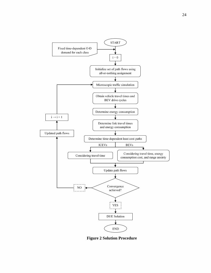
Figure 2 Solution Procedure ............................................................................................. 24

Figure 3 Study Network .................................................................................................... 33

Figure 4 Temporal Distribution of Demand Factors......................................................... 33

Figure 5 Effect of BEV Market Penetration on Average Travel Time ............................. 35

Figure 6 Effect of BEV Market Penetration on Freeway Flows ....................................... 36

Figure 7 Effect of BEV Market Penetration on Battery SOC Consumption .................... 36

Figure 8 Effect of Electricity Cost on Average Travel Time ............................................ 38

Figure 9 Effect of Electricity Cost on Freeway Flow ....................................................... 38

Figure 10 Effect of Electricity Cost on Battery SOC Consumption ................................. 39

Figure 11 Effect of Range Anxiety on Travel Time Distribution ..................................... 40

Figure 12 Effect of Congestion Level on Freeway Flow .................................................. 41

Figure 13 Effect of Congestion Level on Battery SOC Consumption.............................. 42

Figure 14 Conceptual flowchart........................................................................................ 46

Figure 15 Indianapolis road network ................................................................................ 47

Figure 16 Speed profile of a sample vehicle and its corresponding battery power profile

and current profile ............................................................................................................. 48

Figure 17 Indianapolis monthly average temperature ...................................................... 53

Figure 18 Battery lifespan distribution at: (a) constant temperatures; (b) Indianapolis

temperature; (c) cumulative frequency curves for all scenarios ....................................... 55

Figure 19 Impact of vehicle travel patterns on battery lifespan at: (a) constant temperatures;

(b) Indianapolis temperature. ............................................................................................ 57

Figure 20 Impact of driving behavior on cycle aging for Indianapolis. ........................... 58

v

LIST OF TABLES

Table 1 Parameters of the energy consumption model (Haaren, 2011) ............................ 27

Table 2 Base Demand for the Time Horizon .................................................................... 33

Table 3 Parameter definitions for equivalent-circuit battery model ................................. 50

Table 4 Coefficient values and units of the battery degradation model ........................... 52

Table 5 The percentile of battery lifespan and total travel distances for different

temperature scenarios........................................................................................................ 56

6

CHAPTER 1. INTRODUCTION

1.1 Background and motivation

The transportation sector is an important component of energy consumption. It

accounts for about 70% of the total oil consumption in the U.S. (U.S. EIA, 2012; U.S. EPA,

2015). Internal combustion engine vehicles (ICEVs) use liquid fossil fuels as their energy

sources, and have become the largest contributors to urban air pollution (Funk and Rabl,

1999). In 2013, greenhouse gas emissions from transportation sector accounted for about

27% of total U.S. greenhouse gas emissions, making it the second largest contributor of

greenhouse gas emissions in the U.S. after the electricity sector (U.S. EPA, 2015). Electric

vehicles have received considerable attention in the recent past with the promise of

achieving reduced petroleum dependency, enhanced energy efficiency, and improved

environmental sustainability. An electric vehicle (EV) uses a battery-powered electric

motor for propulsion unlike an ICEV which is powered by burning gasoline or diesel.

Although the environmental sustainability of EVs is debated for the source of electricity

generated for recharging the EV’s battery, they have a clear advantage over ICEVs due to

their energy efficiency. Since electricity can be generated from renewable energy, EVs

have the potential to significantly reduce emissions from transportation sectors as the

electricity fuel mix evolves (EPRI, 2007; Wang, 1999; Weiller, 2011). According to the

U.S. Department of Energy (USDOE, 2014), it is estimated that only about 17–21% of the

energy stored in the gas tank of an ICEV is converted to power at the wheels because for

example, the combustion engine alone loses 62.4% of the energy from fuel as heat. By

contrast, EVs convert about 59–62% of the electrical energy from the grid to power at the

wheels. EVs can be equipped with regenerative braking system that can further enhance

overall fuel efficiency and reduce emissions (Clarke et al., 2010).

However, the greater adoption of EV still faces several substantial challenges.

These include range anxiety (that is, the fear of running out of battery charge before

completing the trip) (Tate et al., 2008), long battery recharging time (Morrow et al., 2008),

7

scarce availability of charging infrastructure (Lin and Greene, 2011; Miralinaghi et al.,

2017, 2016; Pearre et al., 2011), the potential impact on power grid stability (Kang and

Recker, 2009), higher vehicle prices (Rezvani et al., 2015), and concerns about battery such

as reduction in lifespan due to degradation and resale value for second use (Neubauer et

al., 2012; Saxena et al., 2015). Thus, a realistic framework to analyze the impacts of EVs

based on an integrated understanding of the transportation and energy system of systems

is essential for developing operational and policy insights.

1.2 Research objectivess

The research objectives are the following:

• Develop a multi-class dynamic user equilibrium (MCDUE) model to evaluate the

network performance under equilibrium conditions for mixed traffic flow with EVs

and ICEVs by accounting for the difference in their route choice behavior.

• Develop a multi-paradigm modeling framework to quantify EV battery lifespan for

a large population of EVs by integrating microscopic traffic simulation model, EV

energy consumption model, battery circuit model, and semi-empirical battery

degradation model.

1.3 Organization of the research

The remainder of the report is organized as follows. CHAPTER 2 presents the

conceptual foundation for the proposed study and reviews related literature. CHAPTER 3

presents a framework to study the routing aspects of EV drivers and their effects on the

network performance. CHAPTER 4 presents a multi-paradigm modeling framework to

quantify the impacts of EV travel patterns on battery lifespan. CHAPTER 5 summarizes

the research findings and insights, and discusses future research directions.

8

CHAPTER 2. CONCEPTUAL FOUNDATION AND LITERATURE REVIEW

This chapter introduces the conceptual foundation of the study and literature review

on existing tools for quantifying the impacts of EVs on transportation network

performance, and the impacts of EV travel patterns on battery lifespan.

2.1 Electric vehicle characteristics

There are two main types of EVs in the market: plug-in hybrid electric vehicle

(PHEV) and battery electric vehicle (BEV). PHEVs are equipped with both internal

combustion engine and electric motor, and BEVs are equipped with only the electric motor.

As a PHEV uses two drive-trains, typically its operating cost is higher than that of a BEV

which uses single drive-train. There are unique characteristics currently associated with

BEVs, including limited battery capacity and long recharging time that can be limiting for

travel compared to ICEVs. Given the current battery technologies, a BEV typically has a

driving range of around 80 – 100 miles with a full charge, depending on the vehicle type

and battery size. Some premium BEVs, such Tesla Model S, have a higher range of about

250 – 350 miles with the advancement of battery technology which is expected to improve

further; however, they are significantly more expensive compared to typical EVs. The

limited driving range of BEVs imposes an issue, known as the range anxiety, that is, the

driver concerns that the vehicle will run out of battery power before reaching the

destination (Tate et al., 2008). This issue is especially limiting for long trips where the

travel distance is close to or beyond the driving range (Mock et al., 2010; Yu et al., 2011).

This study focuses on BEVs rather than PHEVs as the purpose of this study is to capture

range anxiety which is not applicable to PHEVs. A PHEV is similar to a BEV when

operating on battery (if range anxiety is not a concern) and an ICEV when operating on

gasoline or diesel.

Typically, a BEV spends 6-8 hours (slow charging) to get fully charged, depending

on the electrical charging equipment, charging schemes, and battery capacity (Botsford and

9

Szczepanek, 2009). Fast charging technology is available, with 10 minutes charging for a

range up to 100 miles. However, it requires special equipment in the power connector and

is sparsely deployed in the public infrastructure. Even the “quick charge” facility available

at public charging stations can take around 30 minutes to charge the battery up to 80%

(USDOE, 2016). Furthermore, fast charging, including quick charging, can deteriorate the

battery health and is not advisable on a regular basis (Rezvanizaniani et al., 2014). Another

alternative to en route charging for long distance travel is battery swapping stations (BSS)

where a depleted battery pack is quickly swapped with a recharged one. The success of

BSS requires car manufacturers to follow certain battery standards, and even then can entail

battery stock problem, especially in urban areas. These technological and logistical

challenges make BSS impractical to implement (Senart et al., 2010). Therefore, BEV

drivers currently, and in the near future, are expected to charge their vehicles through

home-based overnight charging or workplace-based charging mechanisms most of the

time.

2.2 Electric vehicle energy consumption models

In the context of EV energy consumption computation, electrochemical theory

based models require battery-level data like voltage and current while the models using

driving parameters such as speed and acceleration generally use basic principles of physics

to estimate power consumption. Chan (2000) provides an overview of various

electrochemical process based methods. Plett (2004) proposes an extended Kalman-

Filtering based method for the battery management system of Lithium-Lead based hybrid

EV battery packs. While these methods are essential for battery SOC estimation, it is not

practical to use them for the traffic-related perspective here due to their battery data

requirements. Battery SOC per unit time can be computed by ADVISOR, a tool developed

by the National Renewable Energy Laboratory (NREL) to analyze vehicle performance

and fuel economy (Johnson, 2002; Wipke et al., 1999). It uses basic physics and model

component performance to replicate the vehicle drivetrain process (NREL, 2013). Maia et

al. (2011) use a simulator called Simulation of Urban Mobility (SUMO) to simulate the

10

energy consumption of EVs. Wu et al. (2015) use test vehicles installed with an in-vehicle

data collection system to measure and analyze EV energy consumption. Tanaka et al.

(2008) perform a similar study to determine EV power consumption under different speed

profiles. Yao et al. (2013) propose a SOC estimation method based on dynamometer test

data. Van Haaren (2012) analytically compute energy power consumption for EVs and

estimate the parameters through curve-fitting based on the Tesla Roadster data published

by Straubel (2008). This study uses the battery model proposed by Van Haaren (2012) due

to its computational efficiency and capability to capture battery recuperation.

2.3 Electric vehicle energy-efficient routing

Related to energy-efficient routing, Sachenbacher et al. (2011) introduces the

problem of finding the most energy-efficient path for EVs with recuperation in a graph-

theoretical context. Artmeier et al. (2010) and Storandt (2012) propose revised shortest-

path algorithms to address energy-optimal routing. They formulate energy-efficient routing

in the presence of rechargeable batteries as a special case of the constrained shortest path

problem and propose adaptations of existing shortest path algorithms. Ichimori et al. (1983)

and Adler et al. (2014) address the EV shortest-walk problem to determine the route from

an origin to a destination with minimum detouring; this route may include cycles for

detouring to recharge batteries. Adler and Mirchandani (2014) further study the online

routing and scheduling of EVs that involve wait time as well as a reservation scheme to

have a fully-charged battery in place due to limited capacity at a battery swap station.

Schneider et al. (2014) investigate the EV routing problem with custom time windows and

battery-charging stations in a dynamic context. However, they consider the travel time to

be independent of flow in the routing model.

2.4 Electric vehicle traffic assignment models

In the context of EV traffic assignment, Jiang et al. (2012) formulate a multi-class

path constrained traffic assignment model for mixed traffic flow with BEVs and ICEVs. In

their model, BEV is a vehicle class with trip length no more than the driving range of full

11

battery capacity, and thus BEVs’ equilibrium routes are restricted to the set of distance-

constrained paths. However, they do not consider energy recuperation using RBS. Later,

Jiang and Xie (2014) extend their model to the combined mode choice and assignment

framework by assuming different travel cost functions for BEVs and ICEVs. He et al.

(2014) study the network equilibrium of BEVs with recharging capabilities. They propose

to minimize the traditional user equilibrium term plus the recharging time. The energy

consumption is used to compute the set of usable paths. However, they consider travel time

(including recharging time) minimization as the single decision criterion for route choice,

and neglect the energy consumption factor in the cost function. In addition, their models

focus on static traffic equilibrium rather than dynamic user equilibrium (DUE). Most traffic

assignment related studies assume that the electricity consumption is simply a linear

function of the distance traveled and the route travel time (He et al., 2014; Jiang and Xie,

2014). However, energy consumption is closely related to travel speed, terrain, battery

SOC, temperature, etc. For example, Figure 1 shows the energy consumption rate versus

speed for the Tesla Roadster as presented by Van Haaren (2012).

Figure 1 Tesla Roadster Energy Consumption (Van Haaren, 2012)

12

2.5 Charging station facility location problem

Several studies have investigated the facility location problem of charging stations

(Chen et al., 2013; He et al., 2013; Hess et al., 2012; Xi et al., 2013) and battery-swapping

stations (Mak et al., 2013) where depleted batteries can be recharged or exchanged en route

on long trips. Nie and Ghamami (2013) analyze the selection of battery size and charging

capacity to meet a given level of service such that social cost is minimized. He et al. (2013)

investigate the charging station location problem for PHEVs. The assumption is that

PHEVs are always charged at trip destinations, and that travelers jointly select routes and

destinations based upon charging prices at destinations. Note that range limitation is not an

issue just for BEVs, but also applies to vehicles with alternative fuels which need to find

refueling facilities to successfully complete the trip. Several studies have addressed

refueling facility location for alternative fuel based trips (Kuby and Lim, 2005; Upchurch

et al., 2009; Wang and Lin, 2009).

2.6 Electric vehicle battery degradation and life estimation models

Two types of battery degradation/aging mechanisms are significant: during storage

(calendar aging) and during use (cycle aging). Calendar aging is due to side reactions

resulting from thermodynamic instability of active materials, while cycle aging results

from kinetic effects, such as structural disordering, or concentration gradients. In past

work, the total aging effect is considered as the summation of calendar aging and cycle

aging, but interactions may occur (Broussely et al., 2005, 2001; Wright et al., 2002).

Battery aging mainly happens at the two electrodes: anode (e.g. graphite) and cathode (e.g.

lithium metal oxide). Aging mechanisms occurring at anodes and cathodes are significantly

different. Most researchers believe that changes to the Solid Electrolyte Interphase (SEI)

due to reactions of the anode with the electrolyte are the major source for aging at the anode

(Aurbach et al., 2002; Vetter et al., 2005). Unlike the anode, the cathode can be made using

different types of metal oxide materials. Different materials have quite different effects on

battery life, and the mechanisms of capacity fade at the cathode are not completely

13

understood. Moreover, battery aging is induced by various processes and their interactions,

and most of them cannot be studied independently (Morrow et al., 2008). Due to the

complexity of the Li-ion battery system, some researchers have created semi-empirical

battery life models for specific Li-ion battery chemistries based on experimental data (Lee

et al., 2015; Purewal et al., 2014; Wang et al., 2014, 2011). Thomas et al. (2008) built a

degradation model and an error model using a statistical method based on experimental

data.

Using the aforementioned battery life estimation models, some researchers have

studied the battery lifespan for EVs/PHEVs (plug-in hybrid electric vehicles). For example,

Guenther et al. (2013) studied the EV battery lifespan for different charging behaviors and

three speed profiles. Similarly, other studies (Marano et al., 2009) applied speed profiles

from standard driving cycles, such as Urban Dynamometer Driving Schedule (UDDS), by

either repetition or combination. However, the impacts of realistic vehicle travel patterns

with detailed speed profiles on battery lifespans for a large population of EVs have not

been studied. As shown in our study results, vehicle travel patterns and driving behavior

can have significant impacts on battery lifespan. Using speed profiles from standard driving

cycles may be useful under a variety of considerations, but they fail to represent the

variation in driving behavior and traffic conditions. Hence, using realistic speed profiles

that can capture the effects of traffic conditions will enhance the estimation of EV battery

lifespan.

14

CHAPTER 3. ROUTING ASPECTS OF ELECTRIC VEHICLE DRIVERS AND THEIR EFFECTS ON NETWORK PERFORMANCE

The market share of EVs has increased significantly in recent years (Mock and

Yang, 2014) and is likely to increase further in future, due to multiple incentives such as

government subsidies, advancement in battery technology and public acceptance of EVs.

Shepherd et al. (2012) investigate the effect of multiple factors such as subsidy, average

vehicle life and emission rates on the market penetration of BEVs. Becker et al. (2009)

predict that EVs, including both PHEVs and BEVs, could comprise 24% of the light-

vehicle fleet in USA by 2030. The increase in the market penetration of EVs, especially

BEVs, will impact the traffic stream, which may imply new driving and route choice

imperatives. BEVs are typically equipped with regenerative braking system (RBS) that can

recuperate a part of the kinetic energy lost during the deceleration phase to recharge the

battery. This is where braking energy that would otherwise be dissipated as heat is captured

and restored in the battery. This can increase the driving range of a BEV. Studies show that

in typical urban areas, the recuperation could increase range by about 20%, and often more

in hilly areas (Artmeier et al., 2010). Due to the long battery recharging time, en route

recharging is usually not an attractive option for BEVs currently, and thus energy-efficient

driving and energy recuperation are important factors for BEV drivers. There are two

important factors that can encourage a BEV driver to select an energy-efficient route rather

than the traditional least travel time route: (i) reduce the operating cost, and (ii) improve

the driving range. A BEV driver needs to pay for electricity to charge the battery. In

addition, with every charge-discharge cycle, battery life degrades. Therefore, a BEV driver

may prefer a route with extra travel time but with reduced energy consumption to decrease

operating cost. Because the initial state-of-charge (SOC) of electric battery may not always

be full before starting a trip, or the travel distance may be close to the driving range, some

BEV drivers may face the dilemma of range anxiety because of the fear of running out of

battery charge before completing the trip. In such a situation, a BEV driver may select a

15

route with higher level of congestion to recuperate a part of kinetic energy lost to recharge

the battery so as to improve the range. In addition, for BEVs, energy consumed per unit

distance traveled is lower at moderate speed than at higher speed. This can further

incentivize BEV drivers to select more congested routes under range anxiety. The presence

of BEVs in the traffic stream with the above characteristics of route choice raises two

interesting questions: (i) whether the incentives in terms of energy savings and range

improvement, and the range anxiety factor, can lead to different route selection by BEV

drivers as compared to the ICEV drivers, and (ii) whether this difference in route choice

behavior can affect network performance in terms of system travel time. These two

questions form the motivation for this study.

This study evaluates the network performance under equilibrium conditions for

mixed traffic flow with BEVs and ICEVs by accounting for the difference in their route

choice behavior. A multi-class dynamic user equilibrium (MCDUE) model is proposed to

investigate the equilibrium of traffic network. The BEVs’ route choice behavior is modeled

by considering the tradeoff between travel time and energy consumption, and the range

anxiety. A microscopic simulation-based solution procedure is proposed to enable accurate

computation of energy consumption by using a detailed speed profile rather than a simple

function of distance. The effect of battery recuperation is also factored in estimating energy

consumption. Thus, the effect of traffic conditions on energy consumption, and

subsequently the route choice of BEVs, is captured in a realistic manner. BEV range

anxiety is modeled as a step function that triggers when the remaining battery SOC is less

than a pre-specified threshold percentage. This introduces nonlinearity in the travel cost

function. As part of the solution procedure, a time-dependent least cost path problem for

BEVs is developed as a mixed integer linear model by considering a nonlinear travel cost

function.

The study experiments show that ICEVs prefer to choose routes with least travel

time while BEVs desire routes with slower speeds to save energy and/or improve range.

Based on the current and near future prospects of technology, BEVs will have maximum

fuel-efficiency at lower speeds (~15mph) while ICEVs are fuel-efficient in moderate speed

16

range (~45mph). Due to the need for energy-efficiency and range improvement in the route

selection for BEVs, the network performance in terms of average travel time and average

battery SOC consumption (energy consumption as a percentage of battery capacity) is also

analyzed.

This study has contributions for both theory and practice. In a theoretical context,

it provides an analytical treatment where the congestion and energy imperatives of ICEVs

and BEVs, respectively, are synergistically traded off. This potentially has the synergistic

implication that the traffic system performance can be enhanced beyond that of a traffic

stream with only ICEVs. This study also extends the current literature related to BEV

routing by incorporating the effect of range anxiety in route choice behavior realistically

by considering accurate battery SOC consumption based on detailed speed profile rather

than a simple function of distance. From a practical perspective, this result provides

insights to decision-makers on analyzing BEV route choice to manage network-wide traffic

conditions towards system optimum without exclusively using just monetary instruments

like tolling or congestion pricing, at least under mixed traffic environments.

3.1 Multi-Class Dynamic User Equilibrium Model (MCDUE)

3.1.1 Problem statement

We consider a mixed traffic scenario consisting of BEV and ICEV drivers whose

route choices are based on the DUE principle with respect to the generalized cost. That is,

they seek the individual least time-dependent generalized cost in their route selection. The

generalized cost for BEVs includes three components: (1) route travel time, (2) energy

consumption, and (3) cost reflecting range anxiety when the remaining SOC level is below

a certain threshold. The generalized cost for ICEVs includes only the route travel time.

Different from the more extensively studied analytical single user class DUE (Peeta and

Ziliaskopoulos, 2001), the problem is modeled as a multiple user class DUE formulation

with two vehicle classes (BEVs and ICEVs). This study extends the single user class DUE

formulation proposed by Ban et al. (2008) as a complementarity problem to multiple user

classes.

17

3.1.2 MCDUE formulation

The notations used are as follows:

Sets: 𝐺𝐺 Network, 𝐺𝐺 ≡ (𝑁𝑁,𝐴𝐴); 𝑁𝑁 Set of nodes; 𝐴𝐴 Set of links; 𝑇𝑇 Time horizon; 𝑅𝑅 Set of origins; 𝑆𝑆 Set of destinations; ℳ Set of vehicle classes, ℳ ≡ (𝐸𝐸, 𝐼𝐼); 𝐸𝐸 BEV class; 𝐼𝐼 ICEV class;

𝐴𝐴(𝑖𝑖) Set of outbound links of node 𝑖𝑖 ∈ 𝑁𝑁; 𝐵𝐵(𝑖𝑖) Set of inbound links of node 𝑖𝑖 ∈ 𝑁𝑁; 𝐾𝐾𝑟𝑟𝑟𝑟 Set of simple paths from origin 𝑟𝑟 ∈ 𝑅𝑅 to destination 𝑠𝑠 ∈ 𝑆𝑆; 𝐿𝐿𝑘𝑘 Sequence of links in path 𝑘𝑘 ∈ 𝐾𝐾𝑟𝑟𝑟𝑟.

Indices: 𝑡𝑡 Time period, 𝑡𝑡 ∈ 𝑇𝑇; 𝑡𝑡𝑑𝑑 Departure time period, 𝑡𝑡𝑑𝑑 ∈ 𝑇𝑇; 𝑖𝑖 Node, 𝑖𝑖 ∈ 𝑁𝑁; 𝑎𝑎 Link, 𝑎𝑎 ∈ 𝐴𝐴; 𝑟𝑟 Origin node, 𝑟𝑟 ∈ 𝑅𝑅; 𝑠𝑠 Destination node, 𝑠𝑠 ∈ 𝑆𝑆; 𝑚𝑚 Vehicle class, 𝑚𝑚 ∈ ℳ; ℎ𝑎𝑎 Head node of link 𝑎𝑎; 𝑙𝑙𝑎𝑎 Tail node of link 𝑎𝑎; 𝑘𝑘 Path, 𝑘𝑘 ∈ 𝐾𝐾𝑟𝑟𝑟𝑟.

Parameters:

𝑑𝑑𝑖𝑖𝑟𝑟𝑚𝑚(𝑡𝑡) Time-dependent travel demand from node 𝑖𝑖 ∈ 𝑁𝑁 to destination 𝑠𝑠 ∈ 𝑆𝑆 for each vehicle class 𝑚𝑚 in time period 𝑡𝑡 ∈ 𝑇𝑇

𝜗𝜗 Value of time; 𝛼𝛼 Coefficient of energy cost for BEV class; 𝛾𝛾 Coefficient of range anxiety cost for BEV class; 𝜔𝜔 Range anxiety threshold percentage; 𝒦𝒦 Battery capacity.

18

Variables: 𝜏𝜏𝑎𝑎(𝑡𝑡) Travel time on link 𝑎𝑎 in time period 𝑡𝑡; 𝒮𝒮𝑎𝑎(𝑡𝑡) Energy consumed on link 𝑎𝑎 in time period 𝑡𝑡; 𝐶𝐶𝑎𝑎𝑚𝑚(𝑡𝑡) Generalized travel cost for vehicle class 𝑚𝑚 on link 𝑎𝑎 in time period 𝑡𝑡;

𝜋𝜋𝑖𝑖𝑟𝑟𝑚𝑚(𝑡𝑡) Minimum generalized travel cost from node 𝑖𝑖 to destination 𝑠𝑠 for vehicle class 𝑚𝑚 in time period 𝑡𝑡;

𝜏𝜏𝑎𝑎(𝑡𝑡) Travel time on link 𝑎𝑎 in time period 𝑡𝑡;

𝑢𝑢𝑎𝑎𝑟𝑟𝑚𝑚 (𝑡𝑡) Inflow rate into link 𝑎𝑎 bound for destination 𝑠𝑠 for vehicle class 𝑚𝑚 in time period 𝑡𝑡;

𝑣𝑣𝑎𝑎𝑟𝑟𝑚𝑚(𝑡𝑡) Exit flow rate from link 𝑎𝑎 bound for destination 𝑠𝑠 for vehicle class 𝑚𝑚 in time period 𝑡𝑡;

𝑥𝑥𝑎𝑎𝑟𝑟𝑚𝑚(𝑡𝑡) Flow on link 𝑎𝑎 bound for destination 𝑠𝑠 for vehicle class 𝑚𝑚 in time period 𝑡𝑡; 𝑢𝑢𝑎𝑎𝑚𝑚(𝑡𝑡) Inflow rate into link 𝑎𝑎 for vehicle class 𝑚𝑚 in time period 𝑡𝑡; 𝑣𝑣𝑎𝑎𝑚𝑚(𝑡𝑡) Exit flow rate from link 𝑎𝑎 for vehicle class 𝑚𝑚 in time period 𝑡𝑡;

𝑓𝑓𝑟𝑟𝑟𝑟,𝑘𝑘𝐸𝐸 (𝑡𝑡𝑑𝑑)

Flow on path 𝑘𝑘 from origin 𝑟𝑟 to destination 𝑠𝑠 departing in time period 𝑡𝑡𝑑𝑑 for BEV class;

𝒮𝒮𝑇𝑇 Total energy consumption;

𝛽𝛽 Variable associated with range anxiety cost; 0 if the total energy consumption (𝒮𝒮𝑇𝑇) is less than or equal to range anxiety threshold 𝜔𝜔 ∗ 𝒦𝒦, 𝛾𝛾 otherwise.

Under DUE, the generalized travel costs of all utilized time-dependent routes for

the same departure time are equal and less than or equal to those of unutilized routes. For

the MCDUE, this principle holds for each vehicle class. The MCDUE can be formulated

as a complementarity problem using Equation (1). The mathematical operator 𝑝𝑝 ⊥ 𝑞𝑞

denotes that 𝑝𝑝 is perpendicular to q, that is, 𝑝𝑝𝑇𝑇𝑞𝑞 = 0. Equation (1) implies that for each

vehicle class 𝑚𝑚 ∈ ℳ, the inflow rate 𝑢𝑢𝑎𝑎𝑟𝑟𝑚𝑚 (𝑡𝑡) into link 𝑎𝑎 bound for destination 𝑠𝑠 in time

period 𝑡𝑡 can be non-zero only if the generalized travel cost 𝐶𝐶𝑎𝑎𝑚𝑚(𝑡𝑡) on link 𝑎𝑎 in time period

𝑡𝑡 is equal to the difference between the minimum generalized travel cost 𝜋𝜋𝑙𝑙𝑎𝑎𝑟𝑟𝑚𝑚 (𝑡𝑡) from tail

node 𝑙𝑙𝑎𝑎 of link 𝑎𝑎 to destination 𝑠𝑠 in time period 𝑡𝑡 and the minimum generalized travel cost

𝜋𝜋ℎ𝑎𝑎𝑟𝑟𝑚𝑚 �𝑡𝑡 + 𝜏𝜏𝑎𝑎(𝑡𝑡)� from head node ℎ𝑎𝑎 of link 𝑎𝑎 to destination 𝑠𝑠 in time period 𝑡𝑡 + 𝜏𝜏𝑎𝑎(𝑡𝑡),

where 𝜏𝜏𝑎𝑎(𝑡𝑡) is the travel time on link 𝑎𝑎 in time period 𝑡𝑡.

19

0 ≤ 𝑢𝑢𝑎𝑎𝑟𝑟𝑚𝑚 (𝑡𝑡) ⊥ �𝐶𝐶𝑎𝑎𝑚𝑚(𝑡𝑡) + 𝜋𝜋ℎ𝑎𝑎𝑟𝑟𝑚𝑚 �𝑡𝑡 + 𝜏𝜏𝑎𝑎(𝑡𝑡)� − 𝜋𝜋𝑙𝑙𝑎𝑎𝑟𝑟

𝑚𝑚 (𝑡𝑡)� ≥ 0 ∀𝑚𝑚,𝑎𝑎, 𝑠𝑠, 𝑡𝑡 (1)

Generalized cost functions

As discussed earlier, the generalized travel cost functions are different for the two

vehicle classes. For ICEVs, the generalized cost includes travel time only; for BEVs it

includes travel time, energy related costs and range anxiety if the remaining battery SOC

level is below a threshold. The BEV and ICEV drivers select the least cost routes based on

the generalized travel cost. The energy related costs account for both monetary (electricity

consumption cost) and non-monetary (such as long-recharging time, battery degradation,

etc.) costs related to energy consumption. To incorporate range anxiety behavior, when the

remaining SOC is less than a pre-specified threshold percentage (𝜔𝜔) of the battery capacity

(𝒦𝒦), a cost associated with range anxiety (𝛽𝛽 = 𝛾𝛾) is imposed for the BEV. Otherwise, it is

assumed that there is no range anxiety issue for the BEV driver, that is, the range anxiety

cost is zero (𝛽𝛽 = 0). Also, while the range anxiety threshold can vary across drivers, we

assume it to be homogeneous across BEV drivers in both the study formulation and

experiments to focus on understanding the network effects of range anxiety by using the

notion of low anxiety and high anxiety drivers. Further, the heterogeneity in range anxiety

threshold can be seamlessly incorporated by extending the study formulation through the

use of multiple BEV classes in the proposed MCDUE.

The generalized travel cost functions for BEVs (𝐶𝐶𝑎𝑎𝐸𝐸(𝑡𝑡)) and ICEVs (𝐶𝐶𝑎𝑎𝐼𝐼(𝑡𝑡)) on link

𝑎𝑎 in time period 𝑡𝑡 are defined using Equations (2) and (3). These cost functions involve

two variables, 𝜏𝜏𝑎𝑎(𝑡𝑡) and 𝒮𝒮𝑎𝑎(𝑡𝑡), representing travel time and energy consumption on link 𝑎𝑎

in time period 𝑡𝑡 respectively. The parameters 𝜗𝜗, 𝛼𝛼 and 𝛾𝛾 refer to value of time, coefficient

of energy related costs and cost associated with range anxiety, respectively.

𝐶𝐶𝑎𝑎𝐸𝐸(𝑡𝑡) = 𝜗𝜗 ∙ 𝜏𝜏𝑎𝑎(𝑡𝑡) + 𝛼𝛼 ∙ 𝒮𝒮𝑎𝑎(𝑡𝑡) + 𝛽𝛽 ∙ 𝒮𝒮𝑎𝑎(𝑡𝑡) ∀𝑎𝑎, 𝑡𝑡 (2)

𝐶𝐶𝑎𝑎𝐼𝐼(𝑡𝑡) = 𝜗𝜗 ∙ 𝜏𝜏𝑎𝑎(𝑡𝑡) ∀𝑎𝑎, 𝑡𝑡 (3)

20

𝛽𝛽 = �γ 𝑖𝑖𝑓𝑓 𝒮𝒮𝑇𝑇 ≥ 𝜔𝜔 ∗𝒦𝒦0 𝑜𝑜𝑡𝑡ℎ𝑒𝑒𝑟𝑟𝑒𝑒𝑖𝑖𝑠𝑠𝑒𝑒

�

Mass balance constraints

The mass balance constraints ensure that the flow for each vehicle class 𝑚𝑚 bound

for destination 𝑠𝑠 is conserved for every link 𝑎𝑎 ∈ 𝐴𝐴 in each time period 𝑡𝑡 ∈ 𝑇𝑇, that is, the

rate of change of link flow 𝑥𝑥𝑎𝑎𝑟𝑟𝑚𝑚 (𝑡𝑡) is the difference between inflow rate 𝑢𝑢𝑎𝑎𝑟𝑟𝑚𝑚 (𝑡𝑡) and exit

flow rate 𝑣𝑣𝑎𝑎𝑟𝑟𝑚𝑚(𝑡𝑡). This constraint is expressed in Equation (4).

𝑑𝑑𝑥𝑥𝑎𝑎𝑟𝑟𝑚𝑚(𝑡𝑡)𝑑𝑑𝑡𝑡

= 𝑢𝑢𝑎𝑎𝑟𝑟𝑚𝑚 (𝑡𝑡) − 𝑣𝑣𝑎𝑎𝑟𝑟𝑚𝑚(𝑡𝑡) ∀𝑚𝑚,𝑎𝑎, s, 𝑡𝑡 (4)

Flow conservation constraints

These constraints ensure that the flow for each vehicle class 𝑚𝑚 bound for

destination 𝑠𝑠 is conserved at every node 𝑖𝑖 ∈ 𝑁𝑁 in each time period 𝑡𝑡 ∈ 𝑇𝑇 ; the total

outbound flow from a node is equal to the demand originating at that node (𝑑𝑑𝑖𝑖𝑟𝑟𝑚𝑚(𝑡𝑡)) plus

the total inbound flow at that node. This constraint is expressed as:

� 𝑢𝑢𝑎𝑎𝑟𝑟𝑚𝑚 (𝑡𝑡)𝑎𝑎∈𝐴𝐴(𝑖𝑖)

= 𝑑𝑑𝑖𝑖𝑟𝑟𝑚𝑚(𝑡𝑡) + � 𝑣𝑣𝑎𝑎𝑟𝑟𝑚𝑚(𝑡𝑡)𝑎𝑎∈𝐵𝐵(𝑖𝑖)

∀𝑚𝑚, 𝑖𝑖, 𝑠𝑠, 𝑡𝑡 (5)

FIFO constraints

The first-in first-out (FIFO) principle states that vehicles departing later cannot, on

average, exit a link earlier; that is, vehicles must exit the link later than the vehicles that

entered earlier than them. While FIFO may not always hold in reality as vehicles can

overtake others, for aggregated flow this constraint is satisfied. FIFO constraints can be

represented as:

𝑡𝑡1 + 𝜏𝜏𝑎𝑎(𝑡𝑡1) ≤ 𝑡𝑡2 + 𝜏𝜏𝑎𝑎(𝑡𝑡2) ∀ 𝑡𝑡1 < 𝑡𝑡2 (6)

Flow propagation constraints

The flow propagation constraints describe the spatial and temporal traffic flow

dynamics at the macroscopic level (Astarita, 1996) as shown in Equation (7). In particular,

21

these constraints depict the relationship between combined inflow rate in time period 𝑡𝑡 and

combined exit flow in time period 𝑡𝑡 + 𝜏𝜏𝑎𝑎(𝑡𝑡) of all vehicle classes with change in travel

time 𝜏𝜏𝑎𝑎(𝑡𝑡) of link 𝑎𝑎 in time period 𝑡𝑡 . These constraints are synergistic with the FIFO

principle. They are based on the assumption that driving characteristics, such as maximum

speed and acceleration, of all vehicle classes are similar.

� 𝑣𝑣𝑎𝑎𝑟𝑟𝑚𝑚�𝑡𝑡 + 𝜏𝜏𝑎𝑎(𝑡𝑡)�𝑚𝑚∈ℳ

=∑ 𝑢𝑢𝑎𝑎𝑟𝑟𝑚𝑚 (𝑡𝑡)𝑚𝑚∈ℳ

1 + 𝑑𝑑𝜏𝜏𝑎𝑎(𝑡𝑡)𝑑𝑑𝑡𝑡�

∀𝑎𝑎, 𝑠𝑠, 𝑡𝑡 (7)

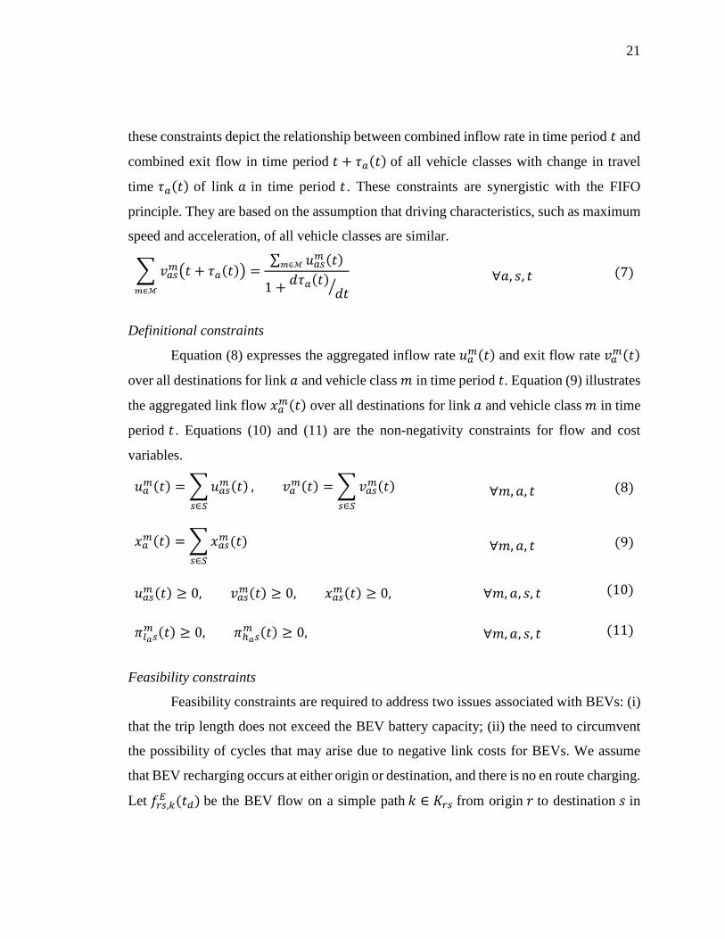
Definitional constraints

Equation (8) expresses the aggregated inflow rate 𝑢𝑢𝑎𝑎𝑚𝑚(𝑡𝑡) and exit flow rate 𝑣𝑣𝑎𝑎𝑚𝑚(𝑡𝑡)

over all destinations for link 𝑎𝑎 and vehicle class 𝑚𝑚 in time period 𝑡𝑡. Equation (9) illustrates

the aggregated link flow 𝑥𝑥𝑎𝑎𝑚𝑚(𝑡𝑡) over all destinations for link 𝑎𝑎 and vehicle class 𝑚𝑚 in time

period 𝑡𝑡 . Equations (10) and (11) are the non-negativity constraints for flow and cost

variables.

𝑢𝑢𝑎𝑎𝑚𝑚(𝑡𝑡) = �𝑢𝑢𝑎𝑎𝑟𝑟𝑚𝑚 (𝑡𝑡)𝑟𝑟∈𝑆𝑆

, 𝑣𝑣𝑎𝑎𝑚𝑚(𝑡𝑡) = �𝑣𝑣𝑎𝑎𝑟𝑟𝑚𝑚(𝑡𝑡)𝑟𝑟∈𝑆𝑆

∀𝑚𝑚,𝑎𝑎, 𝑡𝑡 (8)

𝑥𝑥𝑎𝑎𝑚𝑚(𝑡𝑡) = �𝑥𝑥𝑎𝑎𝑟𝑟𝑚𝑚(𝑡𝑡)𝑟𝑟∈𝑆𝑆

∀𝑚𝑚,𝑎𝑎, 𝑡𝑡 (9)

𝑢𝑢𝑎𝑎𝑟𝑟𝑚𝑚 (𝑡𝑡) ≥ 0, 𝑣𝑣𝑎𝑎𝑟𝑟𝑚𝑚(𝑡𝑡) ≥ 0, 𝑥𝑥𝑎𝑎𝑟𝑟𝑚𝑚(𝑡𝑡) ≥ 0, ∀𝑚𝑚,𝑎𝑎, 𝑠𝑠, 𝑡𝑡 (10)

𝜋𝜋𝑙𝑙𝑎𝑎𝑟𝑟𝑚𝑚 (𝑡𝑡) ≥ 0, 𝜋𝜋ℎ𝑎𝑎𝑟𝑟

𝑚𝑚 (𝑡𝑡) ≥ 0, ∀𝑚𝑚,𝑎𝑎, 𝑠𝑠, 𝑡𝑡 (11)

Feasibility constraints

Feasibility constraints are required to address two issues associated with BEVs: (i)

that the trip length does not exceed the BEV battery capacity; (ii) the need to circumvent

the possibility of cycles that may arise due to negative link costs for BEVs. We assume

that BEV recharging occurs at either origin or destination, and there is no en route charging.

Let 𝑓𝑓𝑟𝑟𝑟𝑟,𝑘𝑘𝐸𝐸 (𝑡𝑡𝑑𝑑) be the BEV flow on a simple path 𝑘𝑘 ∈ 𝐾𝐾𝑟𝑟𝑟𝑟 from origin 𝑟𝑟 to destination 𝑠𝑠 in

22

departure time period 𝑡𝑡𝑑𝑑. Equation (12) illustrates that the inflow rate 𝑢𝑢𝑎𝑎𝑟𝑟𝐸𝐸 (𝑡𝑡) of BEVs on

link 𝑎𝑎 bound for destination 𝑠𝑠 in time period 𝑡𝑡 is the sum of flows from all origins 𝑟𝑟 ∈ 𝑅𝑅

bound for destination 𝑠𝑠 departing in any time period 𝑡𝑡𝑑𝑑 ∈ 𝑇𝑇 such that these flows reach

link 𝑎𝑎 in time period 𝑡𝑡. Equation (13) defines an indicator variable 𝐼𝐼𝑎𝑎,𝑡𝑡𝑘𝑘 (𝑡𝑡𝑑𝑑) with value

equal to 1 if link 𝑎𝑎 is in the sequence of links 𝐿𝐿𝑘𝑘 for path 𝑘𝑘 and the flow departing from

origin 𝑟𝑟 to destination 𝑠𝑠 in time period 𝑡𝑡𝑑𝑑 enters link a in time period 𝑡𝑡, and 0 otherwise.

Equations (14) and (15) define a function 𝜙𝜙𝐿𝐿𝑘𝑘[𝑗𝑗](𝑡𝑡𝑑𝑑) to represent the time period in which

the flow departing in time period 𝑡𝑡𝑑𝑑 reaches the 𝑗𝑗𝑡𝑡ℎ link in the sequence of links 𝐿𝐿𝑘𝑘 for path

𝑘𝑘. Note that as variable 𝜏𝜏𝑎𝑎(𝑡𝑡) is strictly positive, Equation (15) eliminates the possibility

of any cycle in the path. Equation (16) restricts the set of paths 𝐾𝐾𝑟𝑟𝑟𝑟 to contain paths with

minimum generalized cost for every O-D pair 𝑟𝑟𝑠𝑠 for every departure time period 𝑡𝑡𝑑𝑑 ∈ 𝑇𝑇

for BEVs. Equation (17) satisfies the battery capacity constraint for BEVs, that is, the total

battery consumption for BEVs on path 𝑘𝑘 from origin 𝑟𝑟 to destination 𝑠𝑠 departing in time

period 𝑡𝑡𝑑𝑑 cannot exceed the maximum battery capacity 𝒦𝒦.

𝑢𝑢𝑎𝑎𝑟𝑟𝐸𝐸 (𝑡𝑡) = � � � 𝑓𝑓𝑟𝑟𝑟𝑟,𝑘𝑘𝐸𝐸 (𝑡𝑡𝑑𝑑)𝐼𝐼𝑎𝑎,𝑡𝑡

𝑘𝑘

𝑘𝑘∈𝐾𝐾𝑟𝑟𝑟𝑟

(𝑡𝑡𝑑𝑑) 𝑟𝑟∈𝑅𝑅𝑡𝑡𝑑𝑑∈𝑇𝑇,

𝑡𝑡𝑑𝑑≤𝑡𝑡

∀𝑎𝑎, 𝑠𝑠, 𝑡𝑡 (12)

𝐼𝐼𝑎𝑎,𝑡𝑡𝑘𝑘 (𝑡𝑡𝑑𝑑) = �1 𝑖𝑖𝑓𝑓 𝐿𝐿𝑘𝑘[𝑗𝑗] = 𝑎𝑎,𝜙𝜙𝐿𝐿𝑘𝑘[𝑗𝑗](𝑡𝑡𝑑𝑑) = 𝑡𝑡

0 𝑜𝑜𝑡𝑡ℎ𝑒𝑒𝑟𝑟𝑒𝑒𝑖𝑖𝑠𝑠𝑒𝑒� ∀𝑗𝑗 ∈ 𝐼𝐼+, 𝑗𝑗 ≤ |𝐿𝐿𝑘𝑘| (13)

𝜙𝜙𝐿𝐿𝑘𝑘[1](𝑡𝑡𝑑𝑑) = 𝑡𝑡𝑑𝑑 (14)

𝜙𝜙𝐿𝐿𝑘𝑘[𝑗𝑗+1](𝑡𝑡𝑑𝑑) = 𝜙𝜙𝐿𝐿𝑘𝑘[𝑗𝑗](𝑡𝑡𝑑𝑑) + 𝜏𝜏𝐿𝐿𝑘𝑘[𝑗𝑗] �𝜙𝜙𝐿𝐿𝑘𝑘[𝑗𝑗](𝑡𝑡𝑑𝑑)� (15)

�𝐶𝐶𝑗𝑗𝐸𝐸 �𝜙𝜙𝐿𝐿𝑘𝑘[𝑗𝑗](𝑡𝑡𝑑𝑑)�|𝐿𝐿𝑘𝑘|

𝑗𝑗=1

= 𝜋𝜋𝑟𝑟𝑟𝑟𝐸𝐸 (𝑡𝑡𝑑𝑑) ∀𝑟𝑟, 𝑠𝑠,𝑘𝑘, 𝑡𝑡𝑑𝑑 (16)

�𝑆𝑆𝑎𝑎 �𝜙𝜙𝐿𝐿𝑘𝑘[𝑗𝑗](𝑡𝑡𝑑𝑑)�|𝐿𝐿𝑘𝑘|

𝑗𝑗=1

≤ 𝒦𝒦 ∀𝑟𝑟, 𝑠𝑠, 𝑘𝑘 (17)

23

Equations (1) – (17) constitute the complementarity based MCDUE model. The

next section presents a solution procedure for it.

3.2 Solution procedure

This section illustrates the solution procedure and summarizes its various

components. Analytical methods have been proposed in the literature to solve the

complementarity problem (Ban et al., 2008). The complexity of the MCDUE model is

similar to that of the DUE formulation proposed by Ban et al. (2008), and hence a similar

solution strategy can be used to solve it analytically.

As discussed earlier, the generalized travel cost function of BEVs consists of travel

time, energy consumption, and range anxiety if the SOC level is below a threshold. The

energy consumed and its regeneration due to RBS depend on the microscopic speed profile,

particularly the speed and acceleration profiles. These microscopic details of speed

profiles, and hence the percentage of battery charge consumed and its regeneration, are

difficult to express in an analytical closed form, precluding the use of an analytical solution

approach. Therefore, an iterative solution procedure is adopted to solve the MCDUE

model. The solution procedure uses a microscopic traffic simulator, an energy consumption

model, a time-dependent least cost path algorithm, and a path-flow update mechanism in

each iteration.

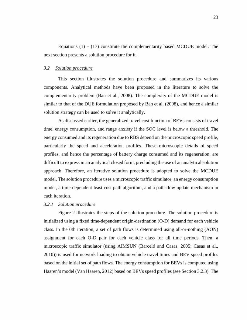
3.2.1 Solution procedure

Figure 2 illustrates the steps of the solution procedure. The solution procedure is

initialized using a fixed time-dependent origin-destination (O-D) demand for each vehicle

class. In the 0th iteration, a set of path flows is determined using all-or-nothing (AON)

assignment for each O-D pair for each vehicle class for all time periods. Then, a

microscopic traffic simulator (using AIMSUN (Barceló and Casas, 2005; Casas et al.,

2010)) is used for network loading to obtain vehicle travel times and BEV speed profiles

based on the initial set of path flows. The energy consumption for BEVs is computed using

Haaren’s model (Van Haaren, 2012) based on BEVs speed profiles (see Section 3.2.3). The

24

Figure 2 Solution Procedure

25

energy consumption and travel time for each link in each time period are determined by

taking the average of energy consumed and travel time experienced on that link,

respectively, for all vehicles entering the link in corresponding time period. Next, the time-

dependent least (generalized) cost paths (TDLCPs) are determined for both ICEVs and

BEVs. For ICEVs, the time, energy related costs and range anxiety. The computed

TDLCPs are appended to their corresponding path set if they are already not in that set.

The path flows for each O-D pair for each vehicle class for all time periods are updated

simultaneously using a modified version of a flow update mechanism proposed by Smith

(Smith, 1984). The iteration counter is updated by 1. The updated path flows are simulated

using AIMSUN to generate the vehicle travel times and BEV speed profiles. This process

is continued until convergence is achieved, which occurs when the average of the

difference between the generalized path travel cost of each path of each O-D pair and the

lowest generalized path travel cost for that O-D pair is less than 5% of the lowest

generalized path travel cost.

3.2.2 Role of microscopic simulation

The generalized link travel cost for a BEV includes the battery SOC which requires the

vehicle’s speed profile as input to compute energy consumption. Microscopic traffic

simulation software AIMSUN is used to obtain link travel times and BEV speed profiles.

In zeroth iteration, the simulation is performed using path flows based on AON assignment.

In future iterations, the generated TDLCPs and the corresponding flows obtained using the

modified Smith's mechanism for both vehicle classes for each O-D pair for all time periods

are provided as input to AIMSUN. Hence, the role of microscopic traffic simulation in this

study is to generate BEV speed profiles and vehicle travel times.

3.2.3 Electric vehicle energy consumption model

The model proposed by (Van Haaren, 2012) is used to compute battery energy

consumption. It considers power losses at constant speed (𝑉𝑉) and variable speed

separately. The power loss at constant speed (𝑃𝑃𝑐𝑐𝑐𝑐𝑐𝑐𝑟𝑟) is the sum of the losses due to

aerodynamics (𝑃𝑃𝑎𝑎𝑎𝑎𝑟𝑟), drive-train (𝑃𝑃𝑑𝑑𝑟𝑟), rolling resistance (𝑃𝑃𝑟𝑟𝑟𝑟) and ancillary losses (𝑃𝑃𝑎𝑎𝑐𝑐𝑐𝑐)

26

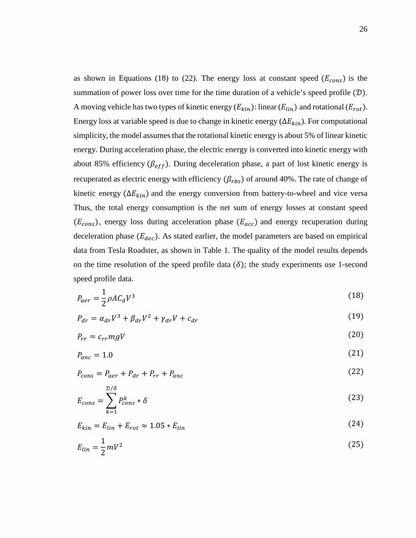
as shown in Equations (18) to (22). The energy loss at constant speed (𝐸𝐸𝑐𝑐𝑐𝑐𝑐𝑐𝑟𝑟) is the

summation of power loss over time for the time duration of a vehicle’s speed profile (𝒟𝒟).

A moving vehicle has two types of kinetic energy (𝐸𝐸𝑘𝑘𝑖𝑖𝑐𝑐): linear (𝐸𝐸𝑙𝑙𝑖𝑖𝑐𝑐) and rotational (𝐸𝐸𝑟𝑟𝑐𝑐𝑡𝑡).

Energy loss at variable speed is due to change in kinetic energy (Δ𝐸𝐸𝑘𝑘𝑖𝑖𝑐𝑐). For computational

simplicity, the model assumes that the rotational kinetic energy is about 5% of linear kinetic

energy. During acceleration phase, the electric energy is converted into kinetic energy with

about 85% efficiency (𝛽𝛽𝑎𝑎𝑒𝑒𝑒𝑒). During deceleration phase, a part of lost kinetic energy is

recuperated as electric energy with efficiency (𝛽𝛽𝑟𝑟𝑟𝑟𝑟𝑟) of around 40%. The rate of change of

kinetic energy (Δ𝐸𝐸𝑘𝑘𝑖𝑖𝑐𝑐) and the energy conversion from battery-to-wheel and vice versa

Thus, the total energy consumption is the net sum of energy losses at constant speed

(𝐸𝐸𝑐𝑐𝑐𝑐𝑐𝑐𝑟𝑟) , energy loss during acceleration phase (𝐸𝐸𝑎𝑎𝑐𝑐𝑐𝑐) and energy recuperation during

deceleration phase (𝐸𝐸𝑑𝑑𝑎𝑎𝑐𝑐). As stated earlier, the model parameters are based on empirical

data from Tesla Roadster, as shown in Table 1. The quality of the model results depends

on the time resolution of the speed profile data (𝛿𝛿); the study experiments use 1-second

speed profile data.

𝑃𝑃𝑎𝑎𝑎𝑎𝑟𝑟 =12𝜌𝜌𝐴𝐴𝐶𝐶𝑑𝑑𝑉𝑉3 (18)

𝑃𝑃𝑑𝑑𝑟𝑟 = 𝛼𝛼𝑑𝑑𝑟𝑟𝑉𝑉3 + 𝛽𝛽𝑑𝑑𝑟𝑟𝑉𝑉2 + 𝛾𝛾𝑑𝑑𝑟𝑟𝑉𝑉 + 𝑐𝑐𝑑𝑑𝑟𝑟 (19)

𝑃𝑃𝑟𝑟𝑟𝑟 = 𝑐𝑐𝑟𝑟𝑟𝑟𝑚𝑚𝑚𝑚𝑉𝑉 (20)

𝑃𝑃𝑎𝑎𝑐𝑐𝑐𝑐 = 1.0 (21)

𝑃𝑃𝑐𝑐𝑐𝑐𝑐𝑐𝑟𝑟 = 𝑃𝑃𝑎𝑎𝑎𝑎𝑟𝑟 + 𝑃𝑃𝑑𝑑𝑟𝑟 + 𝑃𝑃𝑟𝑟𝑟𝑟 + 𝑃𝑃𝑎𝑎𝑐𝑐𝑐𝑐 (22)

𝐸𝐸𝑐𝑐𝑐𝑐𝑐𝑐𝑟𝑟 = �𝑃𝑃𝑐𝑐𝑐𝑐𝑐𝑐𝑟𝑟𝑘𝑘 ∗ 𝛿𝛿𝒟𝒟 𝛿𝛿⁄

𝑘𝑘=1

(23)

𝐸𝐸𝑘𝑘𝑖𝑖𝑐𝑐 = 𝐸𝐸𝑙𝑙𝑖𝑖𝑐𝑐 + 𝐸𝐸𝑟𝑟𝑐𝑐𝑡𝑡 ≈ 1.05 ∗ 𝐸𝐸𝑙𝑙𝑖𝑖𝑐𝑐 (24)

𝐸𝐸𝑙𝑙𝑖𝑖𝑐𝑐 =12𝑚𝑚𝑉𝑉2 (25)

27

𝐸𝐸𝑎𝑎𝑐𝑐𝑐𝑐 =∆𝐸𝐸𝑘𝑘𝑖𝑖𝑐𝑐𝛽𝛽𝑎𝑎𝑒𝑒𝑒𝑒

(26)

𝐸𝐸𝑑𝑑𝑎𝑎𝑐𝑐 = 𝛽𝛽𝑟𝑟𝑟𝑟𝑟𝑟 ∗ ∆𝐾𝐾𝐸𝐸 (27)

Table 1 Parameters of the energy consumption model (Van Haaren, 2012) Parameter Definition Value 𝐶𝐶𝑑𝑑 Drag coefficient 0.29 ρ Air density (kg/m3) 1.2 𝐴𝐴 Vehicle front area (m2) 2.27 𝛼𝛼𝑑𝑑𝑟𝑟 Drivetrain coefficient 1 4*10-6 𝛽𝛽𝑑𝑑𝑟𝑟 Drivetrain coefficient 2 5*10-4 𝛾𝛾𝑑𝑑𝑟𝑟 Drivetrain coefficient 3 0.0293 𝑐𝑐𝑑𝑑𝑟𝑟 Drivetrain coefficient 4 0.375 𝑐𝑐𝑟𝑟𝑟𝑟 Rolling resistance coefficient 0.0075 𝑚𝑚 Vehicle mass (kg) 1520 𝑚𝑚 Gravity (m/s2) 9.81 𝛽𝛽𝑎𝑎𝑒𝑒𝑒𝑒 Battery to motor efficiency 0.85 𝛽𝛽𝑟𝑟𝑟𝑟𝑟𝑟 Regeneration efficiency 0.4

3.2.4 Time-Dependent Least Cost Path (TDLCP) algorithm

As illustrated in Figure 1, in each iteration the TDLCP algorithm identifies a TDLCP for

each vehicle class in each time period for each O-D pair. This path is appended to the

corresponding path set if it is not already in it. Flows are shifted from paths with higher

generalized costs to those with lower generalized costs (see Section 3.2.5 for the flow

update process).

TDLCPs for BEVs

For BEVs, the generalized cost consists of travel time, energy related costs and the cost

associated with range anxiety. The travel time and SOC on each link in each time period

are obtained from AIMSUN. To solve the TDLCP problem, we construct a time-expanded

network 𝐺𝐺𝑡𝑡(𝑁𝑁𝑡𝑡,𝐴𝐴𝑡𝑡) from the original network 𝐺𝐺(𝑁𝑁,𝐴𝐴) as follows. For each time period 𝑡𝑡,

a copy of nodes 𝑁𝑁 is created. For each link 𝑎𝑎 ∈ 𝐴𝐴, if its travel time in time period 𝑡𝑡 is 𝜏𝜏𝑎𝑎(𝑡𝑡),

a link 𝑏𝑏 ∈ 𝐴𝐴𝑡𝑡 in time-expanded network connecting from node 𝑙𝑙𝑎𝑎 in time period 𝑡𝑡 to node

ℎ𝑎𝑎 in time period 𝑡𝑡 + 𝜏𝜏𝑎𝑎(𝑡𝑡) is constructed. Thus, the travel time of the newly constructed

28

link (𝜏𝜏𝑟𝑟) is equal to 𝜏𝜏𝑎𝑎(𝑡𝑡), and the energy consumed on the newly constructed link (𝒮𝒮𝑟𝑟) is

equal to 𝒮𝒮𝑎𝑎(𝑡𝑡). The TDLCP for BEVs is to find the least generalized cost path in 𝐺𝐺𝑡𝑡 by

solving the following mathematical formulation.

The notations used are as follows:

Sets: 𝐺𝐺𝑡𝑡 Time-expanded network; 𝑁𝑁𝑡𝑡 Set of nodes in 𝐺𝐺𝑡𝑡; 𝐴𝐴𝑡𝑡 Set of links in 𝐺𝐺𝑡𝑡; 𝑟𝑟𝑡𝑡 Origin node in 𝐺𝐺𝑡𝑡; 𝑠𝑠𝑡𝑡 Destination node in 𝐺𝐺𝑡𝑡;

Indices: 𝑏𝑏 Link, 𝑏𝑏 ∈ 𝐴𝐴𝑡𝑡;

Parameters: 𝜏𝜏𝑟𝑟 Travel time on link 𝑏𝑏 ∈ 𝐴𝐴𝑡𝑡; 𝒮𝒮𝑟𝑟 Energy consumed on link 𝑏𝑏 ∈ 𝐴𝐴𝑡𝑡; 𝑀𝑀 Sufficiently large positive number;

Variables:

𝑓𝑓𝑖𝑖𝑗𝑗 Decision variable, 𝑓𝑓𝑖𝑖𝑗𝑗 ∈ {0,1}, 𝑓𝑓𝑖𝑖𝑗𝑗 = 1 if link (𝑖𝑖, 𝑗𝑗) ∈ 𝐴𝐴𝑡𝑡 is selected, 0 otherwise;

𝑦𝑦 Auxiliary variable, 𝑦𝑦 ∈ {0,1}.

The objective function (28) minimizes the generalized cost that includes three

terms: path travel time, energy related costs, and cost associated with range anxiety.

Equation (29) is the flow conservation constraint, implying that one unit of flow is sent

from source 𝑟𝑟𝑡𝑡 to sink 𝑠𝑠𝑡𝑡 in 𝐺𝐺𝑡𝑡. Constraint (30) specifies that the energy consumed along

the path is bounded by the BEV’s battery capacity 𝒦𝒦, that is, a BEV cannot run out of

battery charge en route. Equations (31) – (34) state that if ∑ 𝒮𝒮𝑟𝑟𝑟𝑟∈𝐴𝐴𝑡𝑡 ∙ 𝑓𝑓𝑟𝑟 ≥ 𝜔𝜔 ∙ 𝒦𝒦, then 𝑦𝑦 =

1 and 𝛽𝛽 = 𝛾𝛾, otherwise 𝑦𝑦 = 0 and 𝛽𝛽 = 0. This implies that the cost associated with range

anxiety is triggered only if the battery SOC consumed is more than the specific threshold

percentage of battery (𝜔𝜔). If the SOC is below the threshold percentage of battery charge,

there is no range anxiety issue for the BEV driver and 𝛽𝛽 = 0. The parameter 𝑀𝑀, also known

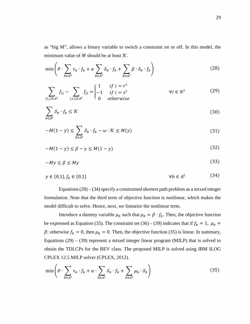
29

as “big M”, allows a binary variable to switch a constraint on or off. In this model, the

minimum value of 𝑀𝑀 should be at least 𝒦𝒦.

min�𝜗𝜗 ∙ � 𝜏𝜏𝑟𝑟𝑟𝑟∈𝐴𝐴𝑡𝑡

∙ 𝑓𝑓𝑟𝑟 + 𝛼𝛼 � 𝒮𝒮𝑟𝑟 ∙ 𝑓𝑓𝑟𝑟𝑟𝑟∈𝐴𝐴𝑡𝑡

+ � 𝛽𝛽 ∙ 𝒮𝒮𝑟𝑟𝑟𝑟∈𝐴𝐴𝑡𝑡

∙ 𝑓𝑓𝑟𝑟� (28)

� 𝑓𝑓𝑖𝑖𝑗𝑗 − � 𝑓𝑓𝑗𝑗𝑖𝑖 =(𝑗𝑗,𝑖𝑖)∈𝐴𝐴𝑡𝑡(𝑖𝑖,𝑗𝑗)∈𝐴𝐴𝑡𝑡

�1 𝑖𝑖𝑓𝑓 𝑖𝑖 = 𝑟𝑟𝑡𝑡

−1 𝑖𝑖𝑓𝑓 𝑖𝑖 = 𝑠𝑠𝑡𝑡0 𝑜𝑜𝑡𝑡ℎ𝑒𝑒𝑟𝑟𝑒𝑒𝑖𝑖𝑠𝑠𝑒𝑒

∀𝑖𝑖 ∈ 𝑁𝑁𝑡𝑡 (29)

� 𝒮𝒮𝑟𝑟𝑟𝑟∈𝐴𝐴𝑡𝑡

∙ 𝑓𝑓𝑟𝑟 ≤ 𝒦𝒦 (30)

−𝑀𝑀(1 − 𝑦𝑦) ≤ � 𝒮𝒮𝑟𝑟𝑟𝑟∈𝐴𝐴𝑡𝑡

∙ 𝑓𝑓𝑟𝑟 − 𝜔𝜔 ∙ 𝒦𝒦 ≤ 𝑀𝑀(𝑦𝑦) (31)

−𝑀𝑀(1 − 𝑦𝑦) ≤ 𝛽𝛽 − 𝛾𝛾 ≤ 𝑀𝑀(1 − 𝑦𝑦) (32)

−𝑀𝑀𝑦𝑦 ≤ 𝛽𝛽 ≤ 𝑀𝑀𝑦𝑦 (33)

𝑦𝑦 ∈ {0,1},𝑓𝑓𝑟𝑟 ∈ {0,1} ∀𝑏𝑏 ∈ 𝐴𝐴𝑡𝑡 (34)

Equations (28) – (34) specify a constrained shortest path problem as a mixed integer

formulation. Note that the third term of objective function is nonlinear, which makes the

model difficult to solve. Hence, next, we linearize the nonlinear term.

Introduce a dummy variable 𝜇𝜇𝑟𝑟 such that 𝜇𝜇𝑟𝑟 = 𝛽𝛽 ∙ 𝑓𝑓𝑟𝑟. Then, the objective function

be expressed as Equation (35). The constraint set (36) – (39) indicates that if 𝑓𝑓𝑟𝑟 = 1, 𝜇𝜇𝑟𝑟 =

𝛽𝛽; otherwise 𝑓𝑓𝑟𝑟 = 0, then 𝜇𝜇𝑟𝑟 = 0. Then, the objective function (35) is linear. In summary,

Equations (29) – (39) represent a mixed integer linear program (MILP) that is solved to

obtain the TDLCPs for the BEV class. The proposed MILP is solved using IBM ILOG

CPLEX 12.5 MILP solver (CPLEX, 2012).

min�𝜗𝜗 ∙ � 𝜏𝜏𝑟𝑟𝑟𝑟∈𝐴𝐴𝑡𝑡

∙ 𝑓𝑓𝑟𝑟 + 𝛼𝛼 ∙ � 𝒮𝒮𝑟𝑟 ∙ 𝑓𝑓𝑟𝑟𝑟𝑟∈𝐴𝐴𝑡𝑡

+ � 𝜇𝜇𝑟𝑟 ∙ 𝒮𝒮𝑟𝑟𝑟𝑟∈𝐴𝐴𝑡𝑡

� (35)

30

𝜇𝜇𝑟𝑟 ≤ 𝛽𝛽 ∀𝑏𝑏 ∈ 𝐴𝐴𝑡𝑡 (36)

𝜇𝜇𝑟𝑟 ≥ 𝛽𝛽 −𝑀𝑀(1 − 𝑓𝑓𝑟𝑟) ∀𝑏𝑏 ∈ 𝐴𝐴𝑡𝑡 (37)

𝜇𝜇𝑟𝑟 ≥ 0 ∀𝑏𝑏 ∈ 𝐴𝐴𝑡𝑡 (38)

𝜇𝜇𝑟𝑟 ≤ 𝑀𝑀 ∙ 𝑓𝑓𝑟𝑟 ∀𝑏𝑏 ∈ 𝐴𝐴𝑡𝑡 (39)

TDLCPs for ICEVs

For ICEVs, the generalized travel cost consists of travel time only. The travel time

on each link in each time period is obtained from AIMSUN. Then, the decreasing order of

time (DOT) algorithm (Chabini, 1998) is implemented to compute the time-dependent

shortest paths. These paths are used to update the path set for ICEVs in each time period

for each O-D pair.

3.2.5 Path flow update process

After the TDLCPs are computed in an iteration, they are appended to their

corresponding path set and path costs are updated for all paths in the set. The path sets for

both vehicle classes for all O-D pairs for each time period are updated simultaneously using

the modified Smith’s mechanism (Smith, 1984).

Modified Smith’s mechanism

The notations are used as follows:

Sets: 𝑊𝑊 Set of origin-destination (O-D) pairs; 𝑃𝑃𝑤𝑤𝑡𝑡𝑚𝑚 Set of paths for vehicle class 𝑚𝑚 and O-D pair 𝑒𝑒 in time period 𝑡𝑡

Indices: 𝑒𝑒 O-D pair, 𝑒𝑒 ∈ 𝑊𝑊; 𝑖𝑖, 𝑗𝑗 Indices for paths, 𝑖𝑖, 𝑗𝑗 ∈ 𝑃𝑃𝑤𝑤𝑡𝑡𝑚𝑚 ;

Variables:

𝐶𝐶𝑤𝑤𝑡𝑡𝑚𝑚 (𝑖𝑖) Generalized travel cost for vehicle class 𝑚𝑚 and O-D pair 𝑒𝑒 on path 𝑖𝑖 in time period 𝑡𝑡;

∆𝐶𝐶𝑤𝑤𝑡𝑡𝑚𝑚 (𝑖𝑖, 𝑗𝑗) Generalized travel cost difference between path 𝑖𝑖 and path 𝑗𝑗 for vehicle

31

class 𝑚𝑚 and O-D pair 𝑒𝑒 in time period 𝑡𝑡;

∆�̂�𝐶𝑤𝑤𝑡𝑡𝑚𝑚 (𝑖𝑖, 𝑗𝑗) Normalized cost difference between path 𝑖𝑖 and path 𝑗𝑗 for vehicle class 𝑚𝑚 and O-D pair 𝑒𝑒 in time period 𝑡𝑡;

𝑓𝑓𝑤𝑤𝑡𝑡𝑚𝑚(i) Flow on path 𝑖𝑖 for vehicle class 𝑚𝑚 and O-D pair 𝑒𝑒 in time period 𝑡𝑡;

∆𝑓𝑓𝑤𝑤𝑡𝑡𝑚𝑚(i) Change in flow on path 𝑖𝑖 for vehicle class 𝑚𝑚 and O-D pair 𝑒𝑒 in time period 𝑡𝑡;

𝑓𝑓∗𝑤𝑤𝑡𝑡𝑚𝑚 (i) Updated flow on path 𝑖𝑖 for vehicle class 𝑚𝑚 and O-D pair 𝑒𝑒 in time period

𝑡𝑡;

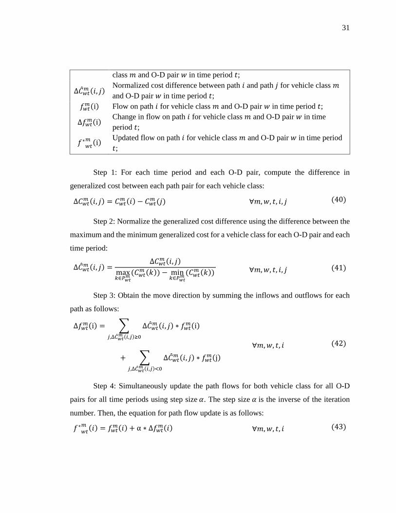
Step 1: For each time period and each O-D pair, compute the difference in

generalized cost between each path pair for each vehicle class:

∆𝐶𝐶𝑤𝑤𝑡𝑡𝑚𝑚 (𝑖𝑖, 𝑗𝑗) = 𝐶𝐶𝑤𝑤𝑡𝑡𝑚𝑚 (𝑖𝑖) − 𝐶𝐶𝑤𝑤𝑡𝑡𝑚𝑚 (𝑗𝑗) ∀𝑚𝑚,𝑒𝑒, 𝑡𝑡, 𝑖𝑖, 𝑗𝑗 (40)

Step 2: Normalize the generalized cost difference using the difference between the

maximum and the minimum generalized cost for a vehicle class for each O-D pair and each

time period:

∆�̂�𝐶𝑤𝑤𝑡𝑡𝑚𝑚 (𝑖𝑖, 𝑗𝑗) =∆𝐶𝐶𝑤𝑤𝑡𝑡𝑚𝑚 (𝑖𝑖, 𝑗𝑗)

max𝑘𝑘∈𝑃𝑃𝑤𝑤𝑡𝑡

𝑚𝑚 (𝐶𝐶𝑤𝑤𝑡𝑡𝑚𝑚 (𝑘𝑘)) − min𝑘𝑘∈𝑃𝑃𝑤𝑤𝑡𝑡

𝑚𝑚 (𝐶𝐶𝑤𝑤𝑡𝑡𝑚𝑚 (𝑘𝑘)) ∀𝑚𝑚,𝑒𝑒, 𝑡𝑡, 𝑖𝑖, 𝑗𝑗 (41)

Step 3: Obtain the move direction by summing the inflows and outflows for each

path as follows:

∆𝑓𝑓𝑤𝑤𝑡𝑡𝑚𝑚(i) = � ∆�̂�𝐶𝑤𝑤𝑡𝑡𝑚𝑚 (𝑖𝑖, 𝑗𝑗) ∗ 𝑓𝑓𝑤𝑤𝑡𝑡𝑚𝑚(i)𝑗𝑗,∆�̂�𝐶𝑤𝑤𝑡𝑡

𝑚𝑚 (𝑖𝑖,𝑗𝑗)≥0

+ � ∆�̂�𝐶𝑤𝑤𝑡𝑡𝑚𝑚 (𝑖𝑖, 𝑗𝑗) ∗ 𝑓𝑓𝑤𝑤𝑡𝑡𝑚𝑚(j)𝑗𝑗,∆�̂�𝐶𝑤𝑤𝑡𝑡

𝑚𝑚 (𝑖𝑖,𝑗𝑗)<0

∀𝑚𝑚,𝑒𝑒, 𝑡𝑡, 𝑖𝑖 (42)

Step 4: Simultaneously update the path flows for both vehicle class for all O-D

pairs for all time periods using step size 𝛼𝛼. The step size 𝛼𝛼 is the inverse of the iteration

number. Then, the equation for path flow update is as follows:

𝑓𝑓∗𝑤𝑤𝑡𝑡𝑚𝑚 (𝑖𝑖) = 𝑓𝑓𝑤𝑤𝑡𝑡𝑚𝑚(𝑖𝑖) + α ∗ ∆𝑓𝑓𝑤𝑤𝑡𝑡𝑚𝑚(𝑖𝑖) ∀𝑚𝑚,𝑒𝑒, 𝑡𝑡, 𝑖𝑖 (43)

32

The flow update mechanism presented heretofore is obtained through three

important modifications to Smith’s flow update mechanism. First, it uses multiple vehicle

classes and the temporal dimension to reflect flow propagation of BEVs and ICEVs along

various links, unlike the static context of Smith’s mechanism where a path flow is

considered to be present on all links of that path simultaneously. Second, it normalizes the

cost difference (see Equation (41)) before determining the move direction of the flow

update process, leading to improved convergence. Third, it updates the path flow vectors

for both vehicle classes for all time periods for all O-D pairs simultaneously to eliminate

order bias in the flow update process.

3.3 Numerical experiments

3.3.1 Experiment setup

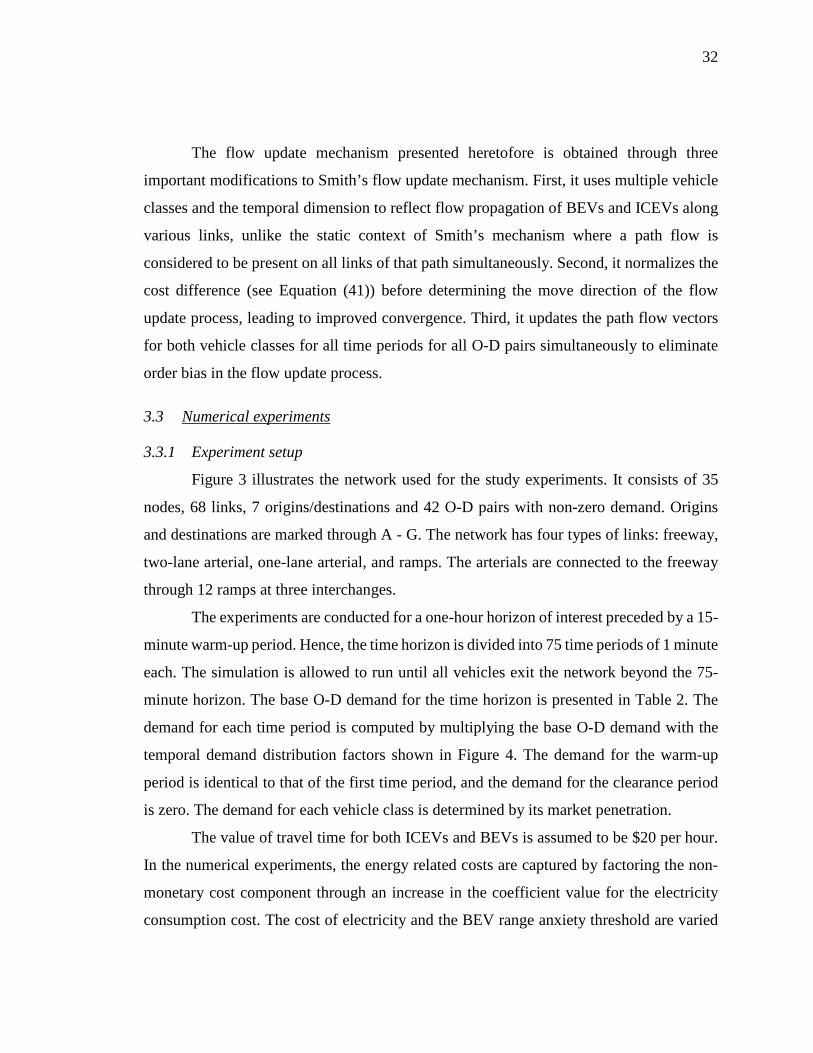
Figure 3 illustrates the network used for the study experiments. It consists of 35

nodes, 68 links, 7 origins/destinations and 42 O-D pairs with non-zero demand. Origins

and destinations are marked through A - G. The network has four types of links: freeway,

two-lane arterial, one-lane arterial, and ramps. The arterials are connected to the freeway

through 12 ramps at three interchanges.

The experiments are conducted for a one-hour horizon of interest preceded by a 15-

minute warm-up period. Hence, the time horizon is divided into 75 time periods of 1 minute

each. The simulation is allowed to run until all vehicles exit the network beyond the 75-

minute horizon. The base O-D demand for the time horizon is presented in Table 2. The

demand for each time period is computed by multiplying the base O-D demand with the

temporal demand distribution factors shown in Figure 4. The demand for the warm-up

period is identical to that of the first time period, and the demand for the clearance period

is zero. The demand for each vehicle class is determined by its market penetration.

The value of travel time for both ICEVs and BEVs is assumed to be $20 per hour.

In the numerical experiments, the energy related costs are captured by factoring the non-

monetary cost component through an increase in the coefficient value for the electricity

consumption cost. The cost of electricity and the BEV range anxiety threshold are varied

33

to perform sensitivity analysis. The effect of the BEV market penetration on network

performance is also analyzed.

Figure 3 Study Network

Figure 4 Temporal Distribution of Demand Factors

Table 2 Base Demand for the Time Horizon O/D A B C D E F G

A 0 3000 160 250 70 70 100 B 3000 0 375 100 125 50 300 C 75 100 0 100 40 35 75 D 75 50 100 0 50 25 100 E 75 100 40 50 0 50 40 F 75 40 40 25 40 0 40 G 125 150 75 100 100 50 0

34

3.3.2 Effect of BEV market penetration

Sensitivity analysis is performed for BEV market penetration under the scenario

with no range anxiety. The electricity cost is assumed to be 50 cents/kWh as the fee to

recharge a BEV at a commercial level 2 charging station may range between 30 cents/kWh

to 80 cents/kWh (Blink, 2015). Figure 5 illustrates the effect of the BEV market penetration

on the travel time distribution of BEVs and ICEVs. The average travel time of ICEVs is

less than that of BEVs, implying that BEVs trade off their travel time for savings in energy

consumption while ICEVs prefer routes with least travel time. Further, the system

performance in terms of the total system travel time (TSTT) improves as the market

penetration of BEVs increases. This is because as the BEV market penetration increases,

more BEVs shift from freeway to arterials, thereby enhancing the performance of freeway

as illustrated by Figure 6. Since freeway flows are typically larger than arterial flows, this

shift tends to have a positive impact on overall network performance with the BEV market

penetration increase. Hence, the preference of some BEVs to choose paths with higher

travel time to save battery SOC consumption or recuperate battery charge moves the

network towards system optimality in terms of TSTT. Though the total number of vehicles

on freeway decreases with increase in BEV market penetration, the number of BEVs on

freeway increases leading to the general trend of reduction in BEV average travel time.

While it is expected that an increase in market penetration of BEVs should increase

the average travel time of BEVs, the opposite trend is observed in Figure 5. This

phenomenon can be explained as follows. As the total travel demand is fixed, an increase

in market penetration implies that more BEVs from all O-D pairs shift to arterial routes

except for the O-D pairs A-B and B-A (refer Figure 3) for which the freeway still remains

the optimal route. Therefore, with an increase in market penetration of BEVs, the overall

traffic volume on the freeway decreases. Thus, the average travel time of ICEVs decreases

as most of them use the freeway route and its travel time decreases due to the decrease in

volume. The average travel times of BEVs for O-D pairs A-B and B-A also decreases as

most of them use the freeway route. Since, the travel demand for these two O-D pairs is

significantly larger than for the other O-D pairs (refer Table 2), the weighted decrease in

35

travel time of BEVs of these O-D pairs outweighs the weighted increase in travel times of

all other O-D pairs. Therefore, an overall decrease in system level average travel time is

observed.

The effect of market penetration on the average BEV battery SOC consumption is

illustrated in Figure 7. The average battery SOC consumption increases with the increase

in market penetration of BEVs because the number of ICEVs decreases, and hence more

number of BEVs are present on freeway (see Figure 6). Due to the relatively higher speed

on freeway compared to arterials coupled with the fact that higher speed increases energy

consumption (see Section 3.2.3), the average battery SOC consumption increases as the

number of BEVs on freeway increases with market penetration.

Figure 5 Effect of BEV Market Penetration on Average Travel Time

36

Figure 6 Effect of BEV Market Penetration on Freeway Flows

Figure 7 Effect of BEV Market Penetration on Battery SOC Consumption

37

3.3.3 Effect of electricity cost

The effect of electricity cost on network performance is analyzed for the case with

no range anxiety and equal market penetration of BEVs and ICEVs. Figure 8 shows the

relationship between average travel time and electricity cost. The average travel time

reduces for ICEVs with an increase in electricity cost, but has an overall negative effect on

BEVs. At low electricity costs, the magnitude of positive effect for ICEVs is slightly higher

than that for BEVs leading to an overall positive effect for the system. Akin to the

discussion in Section 3.3.2, the increase in average travel time for BEVs and decrease for

ICEVs can be explained by the shift in the flow of BEVs from freeway to arterials, as

illustrated in Figure 9. At higher electricity costs, more BEVs shift from freeway to arterials

as they have more incentive to save on energy consumption though these routes are longer

in terms of travel time. This initially leads to a decrease in freeway travel time, thereby

causing a decrease in average travel time for both BEVs and ICEVs. At the higher range

of electricity costs, a large fraction of BEVs shift to arterials leading to high congestion.

While this large shift by BEVs leads to further decrease in average travel time for ICEVs

on freeway, the increase in travel time of BEVs on arterials more than negates benefits on

freeway and causes system level increases in average travel time. As a result, average travel

time of the system increases beyond a certain electricity cost.

The effect of electricity cost on the average battery SOC consumption for BEVs is

illustrated in Figure 10, which indicates that the average battery SOC consumption

decreases with electricity cost increase. As the electricity cost increases, BEVs have more

incentive to shift to routes with lesser battery SOC consumption, and hence more BEVs

shift from freeway to arterials (as shown in Figure 9). Due to the relatively lower speed on

arterials compared to freeway, the battery SOC consumption decreases (see Section 3.2.3).

38

Figure 8 Effect of Electricity Cost on Average Travel Time

Figure 9 Effect of Electricity Cost on Freeway Flow

39

Figure 10 Effect of Electricity Cost on Battery SOC Consumption

3.3.4 Effect of range anxiety

To analyze the effect of range anxiety, it is classified into low range anxiety and

high range anxiety. A driver with high range anxiety is more reluctant towards consuming

battery SOC and feels anxious at a relatively higher level of remaining battery capacity

compared to a driver with low range anxiety. The typical percentage of battery SOC

consumption on the freeway route in the study network is around 75-80%. Hence, high

range anxiety is assumed to be triggered when a BEV consumes 70% of the battery capacity

(that is, 30% battery is remaining) and low range anxiety is assumed to be triggered when

90% of the battery capacity (that is, 10% battery is remaining) is consumed. Figure 11

illustrates the effect of range anxiety on travel time distribution of BEVs and ICEVs for an

electricity cost of 50 cents/kWh and equal market penetration of ICEVs and BEVs. It

indicates that high range anxiety has a negative impact on the network performance as

BEVs experience higher travel times under high range anxiety compared to the case of low

range anxiety. Vehicles with travel time of around 20 minutes in the network are typically

40

those for which destinations are relatively closer to their origins and mostly use arterial

routes (see Figure 3). At high range anxiety, a significant number of BEVs use routes with

higher travel time to reduce battery SOC consumption and hence shift from freeway to

arterial routes. This causes severe congestion on the arterial routes and has a negative

impact on the travel time of the vehicles on arterial routes, including vehicles whose trips

partly involve arterial travel. Hence, all vehicles including ICEVs experience relatively

higher travel times under high range anxiety, with BEVs performing slightly worse than

ICEVs, on average.

Figure 11 Effect of Range Anxiety on Travel Time Distribution

3.3.5 Effect of congestion level

The effect of congestion level on route selection by BEVs is analyzed for the case

of equal market penetration, an electricity cost of 50 cents/kWh and without range anxiety.

Congestion levels are classified as free flow, mild congestion, moderate congestion and

high congestion based on average network speeds of about 50 mph, 31 mph, 21 mph and

15 mph, respectively. Figure 12 shows the ratio of freeway flow to total flow for BEVs and

ICEVs. The freeway flow for both ICEVs and BEVs decreases with increase in congestion

41

and the difference between freeway flow of ICEVs and BEVs decreases as well. With

increase in congestion, the travel time on freeway route increases, and hence vehicles tend

to move to alternative routes. Under free flow, BEVs save on electricity cost by selecting

arterial routes as they have slower speeds. As congestion increases, the average speeds on

both freeway and arterials decrease, reducing the incentive for BEVs to select arterial

routes. Hence, as congestion increases, BEV behavior is closer to that of ICEVs in terms

of route selection.

Figure 12 Effect of Congestion Level on Freeway Flow

Figure 13 shows the effect of traffic congestion on average battery SOC

consumption. The average battery SOC consumption decreases up to the moderate

congestion level and then increases slightly for the high traffic congestion level. This can

be explained using the relationship between speed and energy consumption per mile for

BEVs in Figure 1. The energy-efficiency for BEVs is lowest under free flow as the vehicles

consistently drive at high speeds. As congestion increases, the speed decreases, and up to

a certain point the average battery SOC consumption also decreases. Under high

congestion, though the average network speed is about 15 mph, a good proportion of BEVs

42

travel at very low speeds (less than 10mph) for a major portion of their trip with low

energy-efficiency, increasing their average battery SOC consumption.

Figure 13 Effect of Congestion Level on Battery SOC Consumption

3.3.6 Insights from numerical experiments

The numerical experiments illustrate that, based on the generalized travel cost, BEV

drivers in general tend to shift from the route with lower travel time (freeways) to routes

with higher travel times (arterials) to reduce electricity costs and avoid range anxiety. This

route choice aspect of some BEVs reduces freeway congestion and benefits other vehicles

using the freeway, but consequently increases congestion on arterial routes. The overall

network performance is the net effect of these contrasting phenomena. In a network such

as the one considered for the study experiments, where freeway flow is significantly higher

than that of arterials, BEVs will have a positive impact on the overall network performance.

The route choice behavior tends to have a positive impact on overall system

performance under both an increase in BEV market penetration and electricity cost.

However, under very high BEV market penetration or at very high electricity cost,

increased congestion on arterials more than negates the freeway benefits, leading to

43

reduced system performance. The average battery SOC consumption of BEVs increases

with their market penetration as more BEVs are on freeway, while it decreases with

increase in electricity cost as they have more incentive to shift to arterial routes.

As traffic congestion increases, average network speed decreases, thereby reducing

incentive for BEVs to select alternative routes to save on energy consumption. This

increases the relative importance of travel time in the BEV route choice behavior, reducing

the difference in route choice behavior of BEVs and ICEVs. The average battery SOC

consumption decreases with increase in congestion until the moderate traffic congestion

level. Under the high congestion level, the average battery SOC consumption increases as

the vehicles travel a major portion of their trip at very low speeds (less than 10 mph) which

is not energy-efficient for BEVs.

In summary, BEV route choice imperatives can synergistically lead to improved

network performance under mixed traffic conditions for traffic networks with high levels

of freeway flow and the availability route alternatives involving arterials.

44

CHAPTER 4. QUANTIFYING THE IMPACTS OF ELECTRIC VEHICLE TRAVEL PATTERNS ON BATTERY LIFESPAN

The majority of EVs in the market use a Li-ion battery pack with an energy capacity

of around 20 kWh. For example, the battery pack energy capacity for the Nissan leaf is 24

kWh, Honda Fit EV is 20 kWh, Ford Focus Electric is 23 kWh, and Smart EV is 17.6 kWh.

The energy capacity of a battery pack degrades with time and usage (Broussely et al., 2005;

Guenther et al., 2013; Purewal et al., 2014; Vetter et al., 2005; Wang et al., 2014, 2011).

As the energy capacity decreases, the vehicle range drops. An oft-stated common criterion

is that the battery should be retired from the vehicle application if its capacity has depleted

to 70-80% of its original capacity (Broussely et al., 2005; Saxena et al., 2015; Vetter et al.,

2005). The replacement of a battery pack poses significant cost to vehicle owners, though

batteries can be resold and utilized for other applications such as renewable energy storage

(Huang et al., 2012; Neubauer and Pesaran, 2011; Wood et al., 2011). Under this common

battery replacement criteria, well-designed battery warranty strategies will play a crucial

role in widespread EV adoption. However, among the current commercialized EVs

available in the market, only Nissan Leaf has a battery capacity warranty against

degradation from regular use. Under this warranty, Nissan will repair or replace a Leaf's

battery within five years or 60,000 miles if it loses more than 30 percent of its energy

capacity (DeMuro, 2013). Therefore, quantifying EV battery lifespan for a large

population of EVs is important for vehicle manufacturers, car owners, and battery

researchers seeking to support practical applications.

This study quantifies EV battery lifespan for a large population of EVs through a

semi-empirical battery aging model and a microscopic traffic simulation model. Realistic

speed profiles are generated using microscopic traffic simulation model for the

Indianapolis road transportation network. Five different temperature scenarios are

examined. The results illustrate the impacts of temperature, total distance traveled, average

speed and speed deviation on battery lifespan. This will provide insights for policymakers,

45

vehicle manufacturers and researchers to improve battery technology, and design regional

strategies to promote EV adoption.

4.1 Methodology

A multi-paradigm modeling approach provides the flexibility to study the lifespan

characteristics of a population of EVs. It enables different systems to be simulated with the

most suitable modeling methods. Population behavior for a transportation network is

addressed using building blocks, each of which represents a relevant set of phenomena. By

building up theses blocks together, the whole system can be simulated and investigated in

a holistic manner. This paper considers four different building blocks: a microscopic traffic

network simulation model which provides realistic speed profiles of vehicles, an EV energy

consumption model which provides power demand results for different speed profiles, a

battery circuit model which converts power demands to current flows, and a semi-empirical

battery degradation model which simulates battery lifespan based on current flows and

temperature.

Using the microscopic traffic network simulation model, vehicle trips from the

National Household Travel Survey (NHTS) of 2009 data are matched with simulated speed

profiles that reflect traffic conditions. The speed profile data is then fed into the EV energy

consumption model to compute power profiles. The power profiles are used as inputs to

the battery circuit model to obtain battery current data. In the end, the battery current data

is fed into the battery aging model to simulate EV battery life. Figure 14 shows a simplified

flowchart of the methodology framework.

4.1.1 Household vehicle travel patterns

For EVs, travel distance, travel speed, and vehicle acceleration and deceleration all

impact battery lifespan. In this study, real-world household vehicle travel information is

extracted from the NHTS data. The NHTS data provides daily trip profiles of 150,147

random households across the United States (Federal Highway Administration, 2010).

Among the 150,147 households, 4,350 are from the state of Indiana. This study extracts all

of the 2,832 samples which are from Indianapolis urban and suburban areas to represent

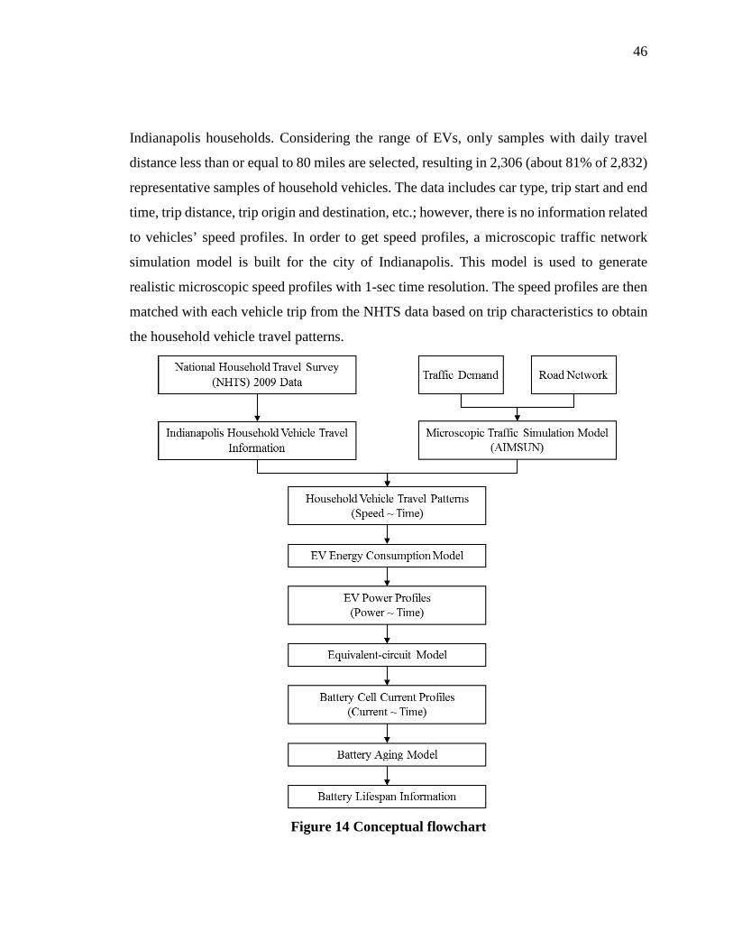
46

Indianapolis households. Considering the range of EVs, only samples with daily travel

distance less than or equal to 80 miles are selected, resulting in 2,306 (about 81% of 2,832)

representative samples of household vehicles. The data includes car type, trip start and end

time, trip distance, trip origin and destination, etc.; however, there is no information related

to vehicles’ speed profiles. In order to get speed profiles, a microscopic traffic network

simulation model is built for the city of Indianapolis. This model is used to generate

realistic microscopic speed profiles with 1-sec time resolution. The speed profiles are then

matched with each vehicle trip from the NHTS data based on trip characteristics to obtain

the household vehicle travel patterns.

Figure 14 Conceptual flowchart

47

Traffic simulation techniques are commonly used to capture the interactions

between vehicles as well as between vehicles and infrastructure at a microscopic level. A

microscopic simulation model employs various models such as car-following, lane-

changing, route choice, etc. to mimic real-world conditions. In this study, detailed speed

profiles of vehicles are required to compute the battery lifespan of EVs. The traffic network

simulation software AIMSUN is used to generate realistic drive-cycles of the vehicles at

the microscopic level (Barceló and Casas, 2005; Casas et al., 2010). A detailed road

network of Indianapolis is built in AIMSUN. The network contains all the freeways, most

of the urban roads and some minor roads as shown in Figure 15. The traffic is simulated

for a 24-hour period with discrete 15-minute interval origin-destination (O-D) demand

matrices. The traffic demand level is calibrated based on the NHTS data for the state of

Indiana.

Figure 15 Indianapolis road network

48

In AIMSUN, vehicles are assigned to specific routes based on distance and road-

type. The trip data for each vehicle from the 2306 samples is obtained by matching to a

specific trip in the network based on the trip departure time, trip distance, trip purpose, and

freeway route indicator. The trip departure time and trip distance are the primary

parameters used for matching. From these, the trip end time will be determined

automatically as the speed profile is generated by the network. The trip purpose is used to

assign route towards the downtown area or the sub-urban area, and the freeway route

indicator is used to check whether the trip uses the freeway. The drive-cycle data from

AIMSUN is gathered for specific vehicles that match the trip profiles from NHTS data

based on the above criteria. The first plot in Figure 16 shows an example of the vehicle

speed profile information.

Figure 16 Speed profile of a sample vehicle and its corresponding battery power

profile and current profile

49

4.1.2 Electric vehicle energy consumption model

EV energy consumption depends significantly on the microscopic speed profile

data. There are several models and simulation tools available that can simulate EV energy

consumptions based on the speed profile data. For example, ADVISOR (Markel et al.,

2002; NREL, 2013) and Autonomie (Argonne National Laboratory, 2016) can simulate an

EV’s power profile, MPGe (mile per gasoline equivalent), state of charge (SOC) profile,

etc. for any given speed profile. These tools simulate the detailed performance of the power

train/propulsion systems, and hence are computationally expensive. This study uses the

model proposed by Van Haaren (2012) as presented in Section 3.2.3.

4.1.3 Battery model

Battery degradation rate is different at different C-rates, so the current profile is

needed to simulate battery life. The C-rate is a measure of the rate at which a battery is

being discharged. It is defined as the discharge current divided by the theoretical current

draw under which the battery would deliver its nominal rated capacity in one hour. A 1C

discharge rate would deliver the battery's rated capacity in 1 hour. A 2C discharge rate

implies that it will discharge twice as fast (30 minutes). Thus, battery current profile is

required to compute battery degradation. In this study, an equivalent-circuit model for Li-

ion battery is implemented as a Simulink block diagram to extract cell current profile using

the power profile. The internal resistance and open-circuit voltage of the cell are

implemented as 1-D lookup tables based on instantaneous battery state-of-charge. The

equivalent-circuit model can be represented by equations (44)-(48). The definition of the

parameters used are shown in Table 3.

𝑉𝑉𝑐𝑐𝑎𝑎𝑙𝑙𝑙𝑙 (𝑡𝑡) = 𝑉𝑉𝑂𝑂𝐶𝐶 (𝑡𝑡) − 𝐼𝐼𝑐𝑐𝑎𝑎𝑙𝑙𝑙𝑙 (𝑡𝑡) ∗ 𝑅𝑅𝑖𝑖𝑐𝑐𝑡𝑡 (𝑡𝑡) (44)

𝑃𝑃𝑐𝑐𝑎𝑎𝑙𝑙𝑙𝑙(𝑡𝑡) = 𝑃𝑃𝑟𝑟𝑎𝑎𝑡𝑡𝑡𝑡(𝑡𝑡)𝑁𝑁𝑐𝑐𝑎𝑎𝑙𝑙𝑙𝑙

= 𝑉𝑉𝑐𝑐𝑎𝑎𝑙𝑙𝑙𝑙(𝑡𝑡) ∗ 𝐼𝐼𝑐𝑐𝑎𝑎𝑙𝑙𝑙𝑙(𝑡𝑡) (45)

𝑉𝑉𝑂𝑂𝐶𝐶(𝑡𝑡) = 𝑓𝑓�𝐸𝐸𝑆𝑆𝑂𝑂𝐶𝐶(𝑡𝑡)� (46)

50

𝑅𝑅𝑖𝑖𝑐𝑐𝑡𝑡(𝑡𝑡) = 𝑚𝑚�𝐸𝐸𝑆𝑆𝑂𝑂𝐶𝐶(𝑡𝑡)� (47)

𝐸𝐸𝑆𝑆𝑂𝑂𝐶𝐶(𝑡𝑡) = 𝐸𝐸𝑆𝑆𝑂𝑂𝐶𝐶(0) + 1

𝐵𝐵𝐴𝐴ℎ𝐶𝐶𝑎𝑎𝐶𝐶∗ �

𝐼𝐼𝑐𝑐𝑎𝑎𝑙𝑙𝑙𝑙(𝑡𝑡)3600

𝑡𝑡

0𝑑𝑑𝑡𝑡 (48)

Table 3 Parameter definitions for equivalent-circuit battery model Parameter Definition

𝑽𝑽𝒄𝒄𝒄𝒄𝒄𝒄𝒄𝒄(𝒕𝒕) Cell terminal voltage at time 𝒕𝒕 𝑽𝑽𝑶𝑶𝑶𝑶(𝒕𝒕) Cell open-circuit voltage at time 𝒕𝒕 𝑰𝑰𝒄𝒄𝒄𝒄𝒄𝒄𝒄𝒄(𝒕𝒕) Cell current at time 𝒕𝒕 𝑹𝑹𝒊𝒊𝒊𝒊𝒕𝒕(𝒕𝒕) Cell internal resistance at time 𝒕𝒕 𝑷𝑷𝒄𝒄𝒄𝒄𝒄𝒄𝒄𝒄(𝒕𝒕) Electrical power out of the cell at time 𝒕𝒕 𝑷𝑷𝒃𝒃𝒃𝒃𝒕𝒕𝒕𝒕(𝒕𝒕) Electrical power out of the battery pack 𝑵𝑵𝒄𝒄𝒄𝒄𝒄𝒄𝒄𝒄 Number of cells in the battery pack 𝑬𝑬𝑺𝑺𝑶𝑶𝑶𝑶(𝒕𝒕) State-of-charge at time 𝒕𝒕 𝒇𝒇�𝐄𝐄𝑺𝑺𝑶𝑶𝑶𝑶(𝒕𝒕)�,𝒈𝒈�𝑬𝑬𝑺𝑺𝑶𝑶𝑶𝑶(𝒕𝒕)� 1-D lookup tables as function of state-of-charge at time 𝒕𝒕 𝑩𝑩𝑨𝑨𝑨𝑨𝑶𝑶𝒃𝒃𝑨𝑨 Nominal ampere-hour capacity of the cell

4.1.4 Battery degradation model

Battery degradation causes capacity loss and impedance growth during operation

and is also a result of storage. Operational degradation is called cycle aging, and storage

degradation is called calendar aging. Calendar aging happens regardless of whether the

battery is operated or not. It is mainly caused by the Li-ion loss during SEI formation at

the graphite anode, and is strongly affected by two parameters: time and temperature

(Wang et al., 2014). Cycle aging only happens when the battery is operating and there is

current flow. The total battery energy capacity loss is the summation of these two effects.

This study uses a semi-empirical model developed by Wang et al. (2014) that

includes three important experimental parameters: time, temperature, and discharge rate .

They performed experiments for 1.5 Ah, 18650 cylindrical cells and created a test matrix

to measure each cell. The cell has a LiMn1/3Ni1/3Co1/3 + LiMn2O4 (NCM+LMO) cathode

and a graphite anode. They modeled both calendar aging and cycle aging using substantial

experimental data. The cycle aging model is for a given constant C-rate. In reality, it is not

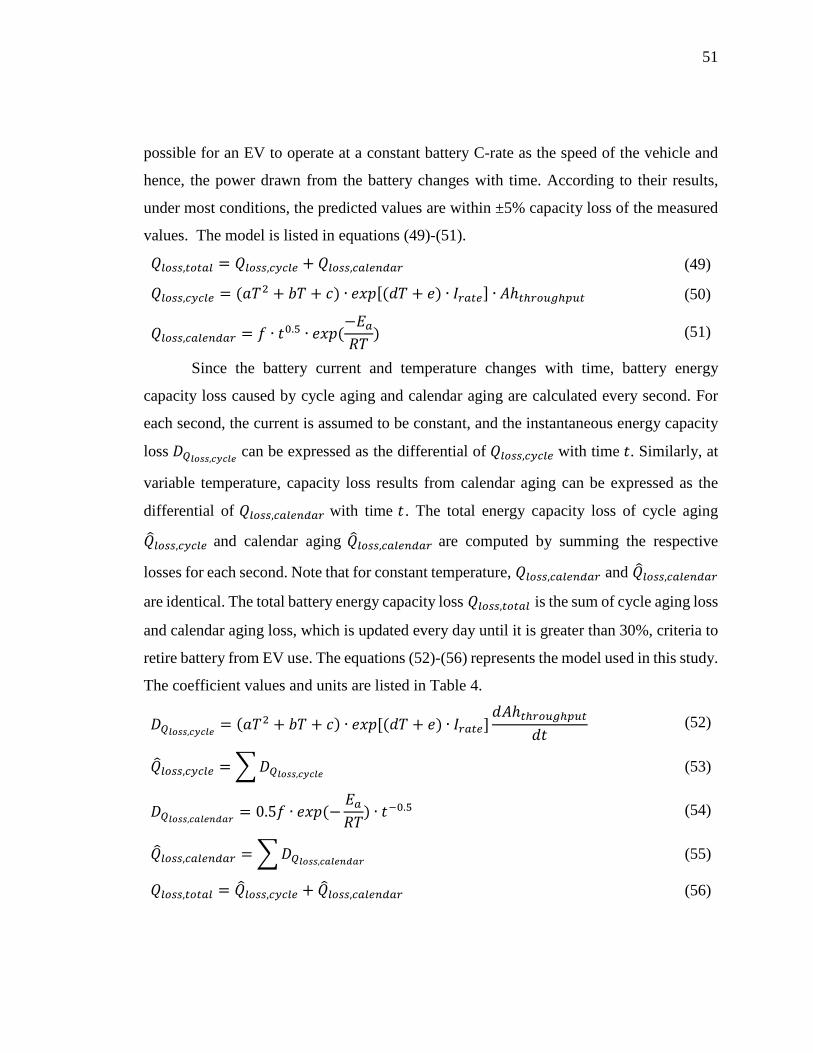
51

possible for an EV to operate at a constant battery C-rate as the speed of the vehicle and

hence, the power drawn from the battery changes with time. According to their results,

under most conditions, the predicted values are within ±5% capacity loss of the measured

values. The model is listed in equations (49)-(51).

𝑄𝑄𝑙𝑙𝑐𝑐𝑟𝑟𝑟𝑟,𝑡𝑡𝑐𝑐𝑡𝑡𝑎𝑎𝑙𝑙 = 𝑄𝑄𝑙𝑙𝑐𝑐𝑟𝑟𝑟𝑟,𝑐𝑐𝑐𝑐𝑐𝑐𝑙𝑙𝑎𝑎 + 𝑄𝑄𝑙𝑙𝑐𝑐𝑟𝑟𝑟𝑟,𝑐𝑐𝑎𝑎𝑙𝑙𝑎𝑎𝑐𝑐𝑑𝑑𝑎𝑎𝑟𝑟 (49)

𝑄𝑄𝑙𝑙𝑐𝑐𝑟𝑟𝑟𝑟,𝑐𝑐𝑐𝑐𝑐𝑐𝑙𝑙𝑎𝑎 = (𝑎𝑎𝑇𝑇2 + 𝑏𝑏𝑇𝑇 + 𝑐𝑐) ∙ 𝑒𝑒𝑥𝑥𝑝𝑝 [(𝑑𝑑𝑇𝑇 + 𝑒𝑒) ∙ 𝐼𝐼𝑟𝑟𝑎𝑎𝑡𝑡𝑎𝑎] ∙ 𝐴𝐴ℎ𝑡𝑡ℎ𝑟𝑟𝑐𝑐𝑟𝑟𝑟𝑟ℎ𝐶𝐶𝑟𝑟𝑡𝑡 (50)

𝑄𝑄𝑙𝑙𝑐𝑐𝑟𝑟𝑟𝑟,𝑐𝑐𝑎𝑎𝑙𝑙𝑎𝑎𝑐𝑐𝑑𝑑𝑎𝑎𝑟𝑟 = 𝑓𝑓 ∙ 𝑡𝑡0.5 ∙ 𝑒𝑒𝑥𝑥𝑝𝑝 (−𝐸𝐸𝑎𝑎𝑅𝑅𝑇𝑇

) (51)

Since the battery current and temperature changes with time, battery energy

capacity loss caused by cycle aging and calendar aging are calculated every second. For

each second, the current is assumed to be constant, and the instantaneous energy capacity

loss 𝐷𝐷𝑄𝑄𝑙𝑙𝑙𝑙𝑟𝑟𝑟𝑟,𝑐𝑐𝑐𝑐𝑐𝑐𝑙𝑙𝑐𝑐 can be expressed as the differential of 𝑄𝑄𝑙𝑙𝑐𝑐𝑟𝑟𝑟𝑟,𝑐𝑐𝑐𝑐𝑐𝑐𝑙𝑙𝑎𝑎 with time 𝑡𝑡. Similarly, at

variable temperature, capacity loss results from calendar aging can be expressed as the

differential of 𝑄𝑄𝑙𝑙𝑐𝑐𝑟𝑟𝑟𝑟,𝑐𝑐𝑎𝑎𝑙𝑙𝑎𝑎𝑐𝑐𝑑𝑑𝑎𝑎𝑟𝑟 with time 𝑡𝑡 . The total energy capacity loss of cycle aging

𝑄𝑄�𝑙𝑙𝑐𝑐𝑟𝑟𝑟𝑟,𝑐𝑐𝑐𝑐𝑐𝑐𝑙𝑙𝑎𝑎 and calendar aging 𝑄𝑄�𝑙𝑙𝑐𝑐𝑟𝑟𝑟𝑟,𝑐𝑐𝑎𝑎𝑙𝑙𝑎𝑎𝑐𝑐𝑑𝑑𝑎𝑎𝑟𝑟 are computed by summing the respective

losses for each second. Note that for constant temperature, 𝑄𝑄𝑙𝑙𝑐𝑐𝑟𝑟𝑟𝑟,𝑐𝑐𝑎𝑎𝑙𝑙𝑎𝑎𝑐𝑐𝑑𝑑𝑎𝑎𝑟𝑟 and 𝑄𝑄�𝑙𝑙𝑐𝑐𝑟𝑟𝑟𝑟,𝑐𝑐𝑎𝑎𝑙𝑙𝑎𝑎𝑐𝑐𝑑𝑑𝑎𝑎𝑟𝑟

are identical. The total battery energy capacity loss 𝑄𝑄𝑙𝑙𝑐𝑐𝑟𝑟𝑟𝑟,𝑡𝑡𝑐𝑐𝑡𝑡𝑎𝑎𝑙𝑙 is the sum of cycle aging loss

and calendar aging loss, which is updated every day until it is greater than 30%, criteria to

retire battery from EV use. The equations (52)-(56) represents the model used in this study.

The coefficient values and units are listed in Table 4.

𝐷𝐷𝑄𝑄𝑙𝑙𝑙𝑙𝑟𝑟𝑟𝑟,𝑐𝑐𝑐𝑐𝑐𝑐𝑙𝑙𝑐𝑐 = (𝑎𝑎𝑇𝑇2 + 𝑏𝑏𝑇𝑇 + 𝑐𝑐) ∙ 𝑒𝑒𝑥𝑥𝑝𝑝 [(𝑑𝑑𝑇𝑇 + 𝑒𝑒) ∙ 𝐼𝐼𝑟𝑟𝑎𝑎𝑡𝑡𝑎𝑎]𝑑𝑑𝐴𝐴ℎ𝑡𝑡ℎ𝑟𝑟𝑐𝑐𝑟𝑟𝑟𝑟ℎ𝐶𝐶𝑟𝑟𝑡𝑡

𝑑𝑑𝑡𝑡 (52)

𝑄𝑄�𝑙𝑙𝑐𝑐𝑟𝑟𝑟𝑟,𝑐𝑐𝑐𝑐𝑐𝑐𝑙𝑙𝑎𝑎 = �𝐷𝐷𝑄𝑄𝑙𝑙𝑙𝑙𝑟𝑟𝑟𝑟,𝑐𝑐𝑐𝑐𝑐𝑐𝑙𝑙𝑐𝑐 (53)

𝐷𝐷𝑄𝑄𝑙𝑙𝑙𝑙𝑟𝑟𝑟𝑟,𝑐𝑐𝑎𝑎𝑙𝑙𝑐𝑐𝑐𝑐𝑑𝑑𝑎𝑎𝑟𝑟 = 0.5𝑓𝑓 ∙ 𝑒𝑒𝑥𝑥𝑝𝑝 (−𝐸𝐸𝑎𝑎𝑅𝑅𝑇𝑇

) ∙ 𝑡𝑡−0.5 (54)

𝑄𝑄�𝑙𝑙𝑐𝑐𝑟𝑟𝑟𝑟,𝑐𝑐𝑎𝑎𝑙𝑙𝑎𝑎𝑐𝑐𝑑𝑑𝑎𝑎𝑟𝑟 = �𝐷𝐷𝑄𝑄𝑙𝑙𝑙𝑙𝑟𝑟𝑟𝑟,𝑐𝑐𝑎𝑎𝑙𝑙𝑐𝑐𝑐𝑐𝑑𝑑𝑎𝑎𝑟𝑟 (55)

𝑄𝑄𝑙𝑙𝑐𝑐𝑟𝑟𝑟𝑟,𝑡𝑡𝑐𝑐𝑡𝑡𝑎𝑎𝑙𝑙 = 𝑄𝑄�𝑙𝑙𝑐𝑐𝑟𝑟𝑟𝑟,𝑐𝑐𝑐𝑐𝑐𝑐𝑙𝑙𝑎𝑎 + 𝑄𝑄�𝑙𝑙𝑐𝑐𝑟𝑟𝑟𝑟,𝑐𝑐𝑎𝑎𝑙𝑙𝑎𝑎𝑐𝑐𝑑𝑑𝑎𝑎𝑟𝑟 (56)

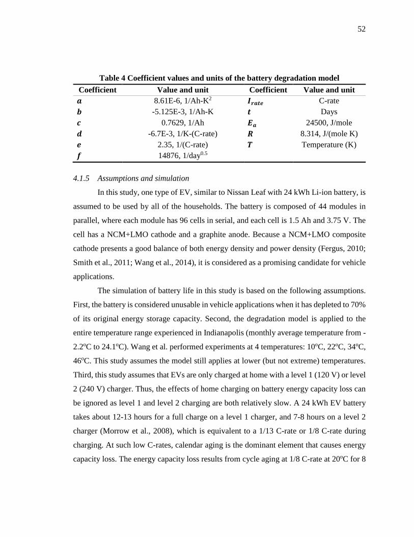
52

Table 4 Coefficient values and units of the battery degradation model Coefficient Value and unit Coefficient Value and unit 𝒃𝒃 8.61E-6, 1/Ah-K2 𝑰𝑰𝒓𝒓𝒃𝒃𝒕𝒕𝒄𝒄 C-rate 𝒃𝒃 -5.125E-3, 1/Ah-K 𝒕𝒕 Days 𝒄𝒄 0.7629, 1/Ah 𝑬𝑬𝒃𝒃 24500, J/mole 𝒅𝒅 -6.7E-3, 1/K-(C-rate) 𝑹𝑹 8.314, J/(mole K) 𝒄𝒄 2.35, 1/(C-rate) 𝑻𝑻 Temperature (K) 𝒇𝒇 14876, 1/day0.5

4.1.5 Assumptions and simulation

In this study, one type of EV, similar to Nissan Leaf with 24 kWh Li-ion battery, is

assumed to be used by all of the households. The battery is composed of 44 modules in

parallel, where each module has 96 cells in serial, and each cell is 1.5 Ah and 3.75 V. The

cell has a NCM+LMO cathode and a graphite anode. Because a NCM+LMO composite

cathode presents a good balance of both energy density and power density (Fergus, 2010;

Smith et al., 2011; Wang et al., 2014), it is considered as a promising candidate for vehicle

applications.

The simulation of battery life in this study is based on the following assumptions.

First, the battery is considered unusable in vehicle applications when it has depleted to 70%

of its original energy storage capacity. Second, the degradation model is applied to the

entire temperature range experienced in Indianapolis (monthly average temperature from -

2.2oC to 24.1oC). Wang et al. performed experiments at 4 temperatures: 10oC, 22oC, 34oC,

46oC. This study assumes the model still applies at lower (but not extreme) temperatures.

Third, this study assumes that EVs are only charged at home with a level 1 (120 V) or level

2 (240 V) charger. Thus, the effects of home charging on battery energy capacity loss can

be ignored as level 1 and level 2 charging are both relatively slow. A 24 kWh EV battery

takes about 12-13 hours for a full charge on a level 1 charger, and 7-8 hours on a level 2

charger (Morrow et al., 2008), which is equivalent to a 1/13 C-rate or 1/8 C-rate during

charging. At such low C-rates, calendar aging is the dominant element that causes energy

capacity loss. The energy capacity loss results from cycle aging at 1/8 C-rate at 20oC for 8

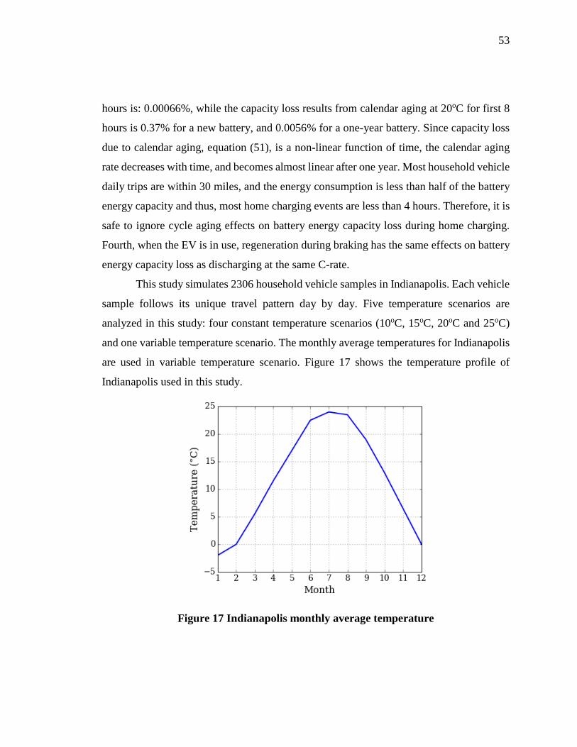
53

hours is: 0.00066%, while the capacity loss results from calendar aging at 20oC for first 8

hours is 0.37% for a new battery, and 0.0056% for a one-year battery. Since capacity loss

due to calendar aging, equation (51), is a non-linear function of time, the calendar aging

rate decreases with time, and becomes almost linear after one year. Most household vehicle

daily trips are within 30 miles, and the energy consumption is less than half of the battery

energy capacity and thus, most home charging events are less than 4 hours. Therefore, it is

safe to ignore cycle aging effects on battery energy capacity loss during home charging.

Fourth, when the EV is in use, regeneration during braking has the same effects on battery

energy capacity loss as discharging at the same C-rate.

This study simulates 2306 household vehicle samples in Indianapolis. Each vehicle

sample follows its unique travel pattern day by day. Five temperature scenarios are

analyzed in this study: four constant temperature scenarios (10oC, 15oC, 20oC and 25oC)

and one variable temperature scenario. The monthly average temperatures for Indianapolis

are used in variable temperature scenario. Figure 17 shows the temperature profile of

Indianapolis used in this study.

Figure 17 Indianapolis monthly average temperature

54

4.2 Results and discussion

The simulation results of EV battery lifespan for different temperature scenarios

are presented and discussed in the following paragraphs. Each EV follows its unique speed

profile every day. Some EVs may have up to 6 trips every day, while others may have only

one trip per day. The impacts of temperature, vehicle travel patterns, and driving behavior

are illustrated on battery life distribution to provide a holistic picture of battery lifespan for

a large population of EVs.

Temperature affects both calendar aging and cycle aging. Figure 18(a) shows the

simulated battery life histogram at four constant temperatures. The results indicate that the

EV battery lifespan is (8.58±1.80) years at 10oC, (7.33±0.73) years at 15oC, (5.73±0.19)

years at 20oC, and (4.20±0.06) years at 25oC. The EV battery life decreases as temperature

increases. At higher temperatures, the battery degrades faster than at lower temperatures.

The variation of EV battery life also decreases as temperature increases. This is because at

higher temperatures, calendar aging dominates cycle aging as all EVs are at the same

environmental temperature, and hence, the effects of vehicle travel patterns and driving

behavior diminishes. In reality, temperature will not be constant all year long. The average

monthly temperature profile in Indianapolis is used to simulate the EV battery lifespan in

the city of Indianapolis. The annual average temperature in Indianapolis is 11.7oC. The

simulated EV battery lifespan is (7.54±1.68) years. Figure 18(b) shows the distribution of

battery life in Indianapolis. Although the temperature profile of Indianapolis varies

between -2.2oC to 24.1oC, the simulated result is similar to the scenario of 10oC, and lies

between the 10oC and 15oC scenarios (refer Figure 18(c)). Therefore, considering

consistent vehicle travel patterns throughout the year, the average annual temperature is

reasonable to use as an estimate in computing degradation due to temperature effects. Table

5 shows detailed percentile of battery lifespan and EV total travel distance for the five

temperature scenarios.

55

Figure 18 Battery lifespan distribution at: (a) constant temperatures; (b)

Indianapolis temperature; (c) cumulative frequency curves for all scenarios

56

Table 5 The percentile of battery lifespan and total travel distances for different temperature scenarios

Indianapolis 10oC 15oC 20oC 25oC

Value (years)

Value (miles)

Value (years)

Value (miles)

Value (years)

Value (miles)

Value (years)

Value (miles)

Value (years)

Value (miles)

0 0.30 1653 1.42 1845 3.01 1346 4.38 967 3.88 693 5 4.88 7612 5.62 8557 5.98 6128 5.34 4368 4.08 3126

10 5.15 14080 6.05 15937 6.23 11960 5.42 8676 4.11 6232 15 5.67 20522 6.52 23167 6.49 17738 5.51 12966 4.13 9336 20 5.96 24057 6.86 27517 6.66 21846 5.56 16210 4.15 11722 25 6.24 28160 7.20 32299 6.83 26037 5.61 19341 4.17 13968 30 6.57 33104 7.52 37529 6.98 29413 5.65 21909 4.18 15884 35 6.84 37303 7.79 42370 7.09 34320 5.68 25692 4.19 18600 40 7.03 41468 8.05 47277 7.21 39438 5.71 29845 4.20 21658 45 7.33 45874 8.34 52302 7.32 44586 5.74 34051 4.21 24739 50 7.57 50940 8.62 58141 7.44 49936 5.77 38548 4.22 28198 55 7.83 55766 8.89 63756 7.54 55476 5.79 43793 4.22 32193 60 8.04 59556 9.15 68126 7.63 60685 5.82 48672 4.23 35902 65 8.39 63527 9.51 72704 7.75 66484 5.84 53664 4.24 39676 70 8.57 68782 9.71 78730 7.82 72842 5.86 58531 4.24 43029 75 8.88 74111 10.04 85170 7.93 80160 5.88 65792 4.25 48768 80 9.23 79197 10.37 91204 8.03 88416 5.91 73454 4.26 54756 85 9.44 85882 10.64 98854 8.11 97524 5.92 81784 4.26 60833 90 9.65 94144 10.90 108763 8.18 111200 5.94 96430 4.27 73250 95 10.29 107729 11.49 124828 8.34 131553 5.97 116933 4.28 89239

100 10.68 146400 12.00 169360 8.46 177280 6.00 156720 4.28 119280

In order to gain insights into the relationship between vehicle travel patterns and

battery lifespan, the simulated battery life is plotted against the total travel distance before

the battery is depleted to 70% of its original capacity. Figure 19(a) shows battery lifespan

versus total travel distance at four constant temperatures. The results illustrate that, at lower

temperatures the effect of total travel distance is greater than that at higher temperatures. It

means that at higher temperatures, battery lifespan is less sensitive to total travel distance.

The negative slope indicates that as the EV travels longer, the battery life becomes shorter.

The width of the strip shows the variation of battery life resulting from driving behavior

such as average speed and speed deviation. As temperature increases, the strip starts

57

Figure 19 Impact of vehicle travel patterns on battery lifespan at: (a) constant

temperatures; (b) Indianapolis temperature.

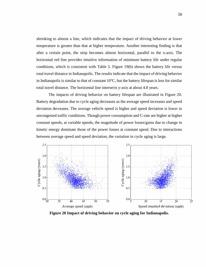
58

shrinking to almost a line, which indicates that the impact of driving behavior at lower

temperature is greater than that at higher temperature. Another interesting finding is that

after a certain point, the strip becomes almost horizontal, parallel to the x-axis. The

horizontal red line provides intuitive information of minimum battery life under regular

conditions, which is consistent with Table 5. Figure 19(b) shows the battery life versus

total travel distance in Indianapolis. The results indicate that the impact of driving behavior

in Indianapolis is similar to that of constant 10oC, but the battery lifespan is less for similar

total travel distance. The horizontal line intersects y-axis at about 4.8 years.

The impacts of driving behavior on battery lifespan are illustrated in Figure 20.

Battery degradation due to cycle aging decreases as the average speed increases and speed

deviation decreases. The average vehicle speed is higher and speed deviation is lower in

uncongested traffic conditions. Though power consumption and C-rate are higher at higher

constant speeds, at variable speeds, the magnitude of power losses/gains due to change in

kinetic energy dominate those of the power losses at constant speed. Due to interactions

between average speed and speed deviation, the variation in cycle aging is large.

Figure 20 Impact of driving behavior on cycle aging for Indianapolis.

59

CHAPTER 5. CONCLUSIONS AND FUTURE WORK

This chapter summarizes the research, highlights its findings, and proposes

directions for future research.

5.1 Summary

This study proposes two frameworks integrating modeling approaches used in

transportation and energy sectors. First, the differences between the route choice behaviors

of BEVs and ICEVs in a mixed traffic context with the potential for BEV range anxiety

are analyzed, and their implications for traffic network performance under equilibrium

conditions are examined. A multi-class DUE model is formulated and a microscopic

simulation-based solution procedure is proposed. The use of microscopic simulation as part

of the solution procedure enhance the accuracy of BEV energy consumption computation.

Consequently, it aids in realistically capturing the effect of traffic congestion on BEV route

selection. The traffic network performance, in terms of travel time and energy

consumption, is analyzed with respect to the network characteristics (such as market

penetration and traffic congestion) and factors that affect BEV route choice (such as

electricity cost and range anxiety threshold). Second, the impacts of temperature, vehicle

travel patterns, and driving behavior on EV battery lifespan are investigated. A multi-

paradigm modeling framework integrated with microscopic traffic simulation model, EV

energy consumption model, battery circuit model, and semi-empirical battery degradation

model is developed. Realistic vehicle travel patterns are generated using real-world vehicle

trips data from NHTS 2009 data, and simulated speed profiles for each trip using a

microscopic traffic simulation model built for Indianapolis road network that reflect traffic

conditions. An analytical EV energy consumption model and a semi-empirical battery

degradation model are then employed to compute the battery lifespan under different

temperature scenarios.

60

5.2 Major findings

First, the numerical analysis presented in CHAPTER 3 provides useful insights

related to BEV route choice behavior and its impact on network performance. As battery

SOC consumption for BEVs is lower at slower speeds, they can reduce their energy

consumption by traveling on routes with slower speeds. Moreover, the RBS system

equipped in BEVs reduces the rate of energy dissipation in stop-and-go traffic conditions

and makes it more economical for them in terms of battery SOC consumption. The results

from the numerical experiments indicate that BEVs choose routes with slower speeds,

typically arterial routes, to reduce their battery SOC consumption and avoid range anxiety.

Such potential unconventional route choice behavior by BEVs based on the generalized

travel cost can decrease traffic congestion on routes with higher free flow speeds while

increasing traffic congestion on routes with lower free flow speeds. This can lead to the

improvement of traffic network performance and move the traffic network towards system

optimal conditions in terms of travel time. Furthermore, with an increase in traffic

congestion, BEV route choice behavior becomes similar to that of ICEVs as speeds in the

network decrease, thereby reducing BEV incentive to switch routes to save on energy

consumption. These insights can aid traffic operators to devise control strategies in the

emerging mixed traffic stream, and policymakers to determine an optimal trajectory for

promoting electric vehicles. Further, the insights related to energy consumption can aid

energy operators to plan for infrastructure investments to support the increasing market

penetration of electric vehicles.

Second, the multi-paradigm modeling framework presented in CHAPTER 4 is used

to quantify the impacts of temperature, vehicle travel patterns, and driving behavior on EV

battery lifespan that provide useful information for vehicle owners, policymakers and

vehicle manufacturers. The results indicate that temperature has a substantial impact on

battery lifespan, and can overshadow the impacts of vehicle travel patterns and driving

behavior at high temperatures. The study insights aid vehicle owners to assess the lifetime

cost of EV ownership, including maintenance cost, insurance cost and battery resale value,

61

based on their travel needs and geographic location. Since temperature has a significant

impact on battery degradation, policymakers and vehicle manufacturers should consider

regional temperature conditions while designing strategies like tax credits, battery

warranty, etc., to promote EV adoption. Since the impacts of vehicle travel patterns and

driving behavior are considerable at lower temperatures, these need to be factored in

warranty strategies for colder regions. Vehicle manufacturers should factor the

environmental conditions in which the battery will be used, as also vehicle travel patterns

and consumer driving behaviors.

5.3 Future research directions

Future research should focus on developing optimal control strategies to enhance

the network performance using the microscopic simulation-based solution procedure for

the MCDUE model presented in this study. Also, statistical models based on real-world

survey data should be developed to better understand the route choice preferences of EV

drivers. Furthermore, the data presented in this study provides a realistic foundation for

future work to study the dynamics of EV battery market, and provides insights for battery

studies that will impact real-world battery lifespan. Future research should also target

improving battery lifespan, and considering regional temperature profiles, vehicle travel

patterns and EV driving behaviors.

62

REFERENCES

Adler, J.D., Mirchandani, P.B., 2014. Online routing and battery reservations for electric

vehicles with swappable batteries. Transportation Research Part B: Methodological

70, 285–302.

Adler, J.D., Mirchandani, P.B., Xue, G., Xia, M., 2014. The electric vehicle shortest-walk

problem with battery exchanges. Networks and Spatial Economics 1–19.

Argonne National Laboratory, 2016. Autonomie [WWW Document]. URL

http://www.autonomie.net (accessed 1.30.16).

Artmeier, A., Haselmayr, J., Leucker, M., Sachenbacher, M., 2010. The shortest path

problem revisited: Optimal routing for electric vehicles, in: KI 2010: Advances in

Artificial Intelligence. Springer, pp. 309–316.

Astarita, V., 1996. A continuous time link model for dynamic network loading based on

travel time function, in: Lesort, J.-B. (Ed.), Proceedings of the 13th International

Symposium on Transportation and Traffic Theory. Pergamori, Oxford, pp. 79–102.

Aurbach, D., Zinigrad, E., Cohen, Y., Teller, H., 2002. A short review of failure

mechanisms of lithium metal and lithiated graphite anodes in liquid electrolyte

solutions. Solid State Ionics 148, 405–416. doi:10.1016/S0167-2738(02)00080-2

Ban, X.J., Liu, H.X., Ferris, M.C., Ran, B., 2008. A link-node complementarity model and

solution algorithm for dynamic user equilibria with exact flow propagations.

Transportation Research Part B: Methodological 42, 823–842.

Barceló, J., Casas, J., 2005. Dynamic network simulation with AIMSUN, in: Simulation

Approaches in Transportation Analysis. Springer, pp. 57–98.

Becker, T.A., Sidhu, I., Tenderich, B., 2009. Electric vehicles in the United States: a new

model with forecasts to 2030. Center for Entrepreneurship & Technology (CET).

Technical Brief.

Blink, 2015. Car Charging Group, Inc. [ONLINE] Available at:

http://www.blinknetwork.com.

63

Botsford, C., Szczepanek, A., 2009. Fast charging vs. slow charging: Pros and cons for the

new age of electric vehicles, in: EVS24 International Battery, Hybrid Fuel Cell

Electric Vehicle Symposium.

Broussely, M., Biensan, P., Bonhomme, F., Blanchard, P., Herreyre, S., Nechev, K.,

Staniewicz, R.J., 2005. Main aging mechanisms in Li ion batteries. Journal of Power

Sources 146, 90–96. doi:10.1016/j.jpowsour.2005.03.172

Broussely, M., Herreyre, S., Biensan, P., Kasztejna, P., Nechev, K., Staniewicz, R.J., 2001.

Aging mechanism in Li ion cells and calendar life predictions. Journal of Power

Sources 97–98, 13–21. doi:10.1016/S0378-7753(01)00722-4

Casas, J., Ferrer, J.L., Garcia, D., Perarnau, J., Torday, A., 2010. Traffic simulation with

aimsun, in: Fundamentals of Traffic Simulation. Springer, pp. 173–232.

Chabini, I., 1998. Discrete dynamic shortest path problems in transportation applications:

Complexity and algorithms with optimal run time. Transportation Research Record:

Journal of the Transportation Research Board 170–175.

Chan, H.L., 2000. A new battery model for use with battery energy storage systems and

electric vehicles power systems, in: Power Engineering Society Winter Meeting,

2000. IEEE. pp. 470–475.

Chen, T.D., Kockelman, K.M., Khan, M., others, 2013. The electric vehicle charging

station location problem: a parking-based assignment method for Seattle, in:

Transportation Research Board 92nd Annual Meeting. pp. 13–1254.

Clarke, P., Muneer, T., Cullinane, K., 2010. Cutting vehicle emissions with regenerative

braking. Transportation Research Part D: Transport and Environment 15, 160–167.

doi:10.1016/j.trd.2009.11.002

CPLEX, I.I., 2012. V12. 5: User’s manual for CPLEX.

DeMuro, D., 2013. 2013 Nissan Leaf gets new battery warranty [WWW Document].

Autotrader. URL http://www.autotrader.com/car-news/2013-nissan-leaf-gets-new-

battery-warranty-201645 (accessed 7.12.14).

EPRI, 2007. Environmental assessment of plug-in hybrid electric vehicles. Technical

Report 1015325, Electric Power Research Institute 1, 1–38.

64

Federal Highway Administration, 2010. National Household Travel Survey of 2009,

[ONLINE] Available at: http://nhts.ornl.gov.

Fergus, J.W., 2010. Recent developments in cathode materials for lithium ion batteries.

Journal of Power Sources 195, 939–954. doi:10.1016/j.jpowsour.2009.08.089

Funk, K., Rabl, A., 1999. Electric versus conventional vehicles: social costs and benefits

in France. Transportation Research Part D: Transport and Environment 4, 397–411.

Guenther, C., Schott, B., Hennings, W., Waldowski, P., Danzer, M.A., 2013. Model-based

investigation of electric vehicle battery aging by means of vehicle-to-grid scenario

simulations. Journal of Power Sources 239, 604–610.

doi:10.1016/j.jpowsour.2013.02.041

He, F., Wu, D., Yin, Y., Guan, Y., 2013. Optimal deployment of public charging stations

for plug-in hybrid electric vehicles. Transportation Research Part B: Methodological

47, 87–101.

He, F., Yin, Y., Lawphongpanich, S., 2014. Network equilibrium models with battery

electric vehicles. Transportation Research Part B: Methodological 67, 306–319.

Hess, A., Malandrino, F., Reinhardt, M.B., Casetti, C., Hummel, K.A., Barceló-Ordinas,

J.M., 2012. Optimal deployment of charging stations for electric vehicular networks,

in: Proceedings of the First Workshop on Urban Networking. pp. 1–6.

Huang, S., Safiullah, H., Xiao, J., Hodge, B.M.S., Hoffman, R., Soller, J., Jones, D.,

Dininger, D., Tyner, W.E., Liu, A., Pekny, J.F., 2012. The effects of electric vehicles

on residential households in the city of Indianapolis. Energy Policy 49, 442–455.

doi:10.1016/j.enpol.2012.06.039

Ichimori, T., Ishii, H., Nishida, T., 1983. Two routing problems with the limitation of fuel.

Discrete Applied Mathematics 6, 85–89.

Jiang, N., Xie, C., 2014. Computing and analyzing mixed equilibrium network flows with

gasoline and electric vehicles. Computer-Aided Civil and Infrastructure Engineering

29, 626–641.

Jiang, N., Xie, C., Waller, S., 2012. Path-constrained traffic assignment: model and

algorithm. Transportation Research Record: Journal of the Transportation Research

65

Board 25–33.

Johnson, V.H., 2002. Battery performance models in ADVISOR. Journal of power sources

110, 321–329.

Kang, J.E., Recker, W.W., 2009. An activity-based assessment of the potential impacts of

plug-in hybrid electric vehicles on energy and emissions using 1-day travel data.

Transportation Research Part D: Transport and Environment 14, 541–556.

doi:10.1016/j.trd.2009.07.012

Kuby, M., Lim, S., 2005. The flow-refueling location problem for alternative-fuel vehicles.

Socio-Economic Planning Sciences 39, 125–145.

Lee, Y.J., Choi, H.Y., Ha, C.W., Yu, J.H., Hwang, M.J., Doh, C.H., Choi, J.H., 2015. Cycle

life modeling and the capacity fading mechanisms in a

graphite/LiNi<inf>0.6</inf>Co<inf>0.2</inf>Mn<inf>0.2</inf>O<inf>2</inf> cell.

Journal of Applied Electrochemistry 45, 419–426. doi:10.1007/s10800-015-0811-6

Lin, Z., Greene, D., 2011. Promoting the market for plug-in hybrid and battery electric

vehicles. Transportation Research Record: Journal of the Transportation Research

Board 2252, 49–56. doi:10.3141/2252-07

Maia, R., Silva, M., Araújo, R., Nunes, U., 2011. Electric vehicle simulator for energy

consumption studies in electric mobility systems, in: Integrated and Sustainable

Transportation System (FISTS), 2011 IEEE Forum on. pp. 227–232.

Mak, H.-Y., Rong, Y., Shen, Z.-J.M., 2013. Infrastructure planning for electric vehicles

with battery swapping. Management Science 59, 1557–1575.

Marano, V., Onori, S., Guezennec, Y., Rizzoni, G., Madella, N., 2009. Lithium-ion

batteries life estimation for plug-in hybrid electric vehicles. Vehicle Power and

Propulsion Conference, 2009. VPPC ’09. IEEE 536–543.

doi:10.1109/VPPC.2009.5289803

Markel, T., Brooker, A., Hendricks, T., Johnson, V., Kelly, K., Kramer, B., O’Keefe, M.,

Sprik, S., Wipke, K., 2002. ADVISOR: A systems analysis tool for advanced vehicle

modeling. Journal of Power Sources 110, 255–266. doi:10.1016/S0378-

7753(02)00189-1

66

Miralinaghi, M., Keskin, B.B., Lou, Y., Roshandeh, A.M., 2016. Capacitated Refueling

Station Location Problem with Traffic Deviations Over Multiple Time Periods.

Networks and Spatial Economics 1–23. doi:10.1007/s11067-016-9320-3

Miralinaghi, M., Lou, Y., Keskin, B.B., Zarrinmehr, A., Shabanpour, R., 2017. Refueling

Station Location Problem with Traffic Deviation Considering Route Choice and

Demand Uncertainty. International Journal of Hydrogen Energy 42, 3335–3351.

doi:10.1016/j.ijhydene.2016.12.137

Mock, P., Schmid, S.A., Friedrich, H.E., 2010. Market prospects of electric passenger

vehicles. Electric and Hybrid Vehicles: Power Sources, Models, Sustainability,

Infrastructure and the Market. Elsevier.

Mock, P., Yang, Z., 2014. Driving electrification: A global comparison of fiscal incentive

policy for electric vehicles. The International Council on Clean Transportation

(ICCT) 22, 2014.

Morrow, K., Karner, D., Francfort, J., 2008. Plug-in hybrid electric vehicle charging

infrastructure review. US Department of Energy-Vehicle Technologies Program 34.

doi:10.2172/946853

Neubauer, J., Brooker, A., Wood, E., 2012. Sensitivity of battery electric vehicle

economics to drive patterns, vehicle range, and charge strategies. Journal of Power

Sources 209, 269–277. doi:10.1016/j.jpowsour.2012.02.107

Neubauer, J., Pesaran, A., 2011. The ability of battery second use strategies to impact plug-

in electric vehicle prices and serve utility energy storage applications. Journal of

Power Sources 196, 10351–10358. doi:10.1016/j.jpowsour.2011.06.053

Nie, Y.M., Ghamami, M., 2013. A corridor-centric approach to planning electric vehicle

charging infrastructure. Transportation Research Part B: Methodological 57, 172–

190.

NREL, 2013. ADVISOR Advanced Vehicle Simulator. [ONLINE] Available at:

http://adv-vehicle-sim.sourceforge.net.

Pearre, N.S., Kempton, W., Guensler, R.L., Elango, V. V., 2011. Electric vehicles: How

much range is required for a day’s driving? Transportation Research Part C: Emerging

67

Technologies 19, 1171–1184. doi:10.1016/j.trc.2010.12.010

Peeta, S., Ziliaskopoulos, A.K., 2001. Foundations of Dynamic Traffic Assignment: The

Past, the Present and the Future. Networks and Spatial Economics 1, 233–265.

doi:10.1023/A:1012827724856

Plett, G.L., 2004. Extended Kalman filtering for battery management systems of LiPB-

based HEV battery packs: Part 3. State and parameter estimation. Journal of power

sources 134, 277–292.

Purewal, J., Wang, J., Graetz, J., Soukiazian, S., Tataria, H., Verbrugge, M.W., 2014.

Degradation of lithium ion batteries employing graphite negatives and nickel-cobalt-

manganese oxide + spinel manganese oxide positives: Part 2, chemical-mechanical

degradation model. Journal of Power Sources 272, 1154–1161.

doi:10.1016/j.jpowsour.2014.07.028

Rezvani, Z., Jansson, J., Bodin, J., 2015. Advances in consumer electric vehicle adoption

research: A review and research agenda. Transportation Research Part D: Transport

and Environment 34, 122–136. doi:10.1016/j.trd.2014.10.010

Rezvanizaniani, S.M., Liu, Z., Chen, Y., Lee, J., 2014. Review and recent advances in

battery health monitoring and prognostics technologies for electric vehicle (EV)

safety and mobility. Journal of Power Sources 256, 110–124.

Sachenbacher, M., Leucker, M., Artmeier, A., Haselmayr, J., 2011. Efficient energy-

optimal routing for electric vehicles, in: AAAI.

Saxena, S., Le Floch, C., Macdonald, J., Moura, S., 2015. Quantifying EV battery end-of-

life through analysis of travel needs with vehicle powertrain models. Journal of Power

Sources 282, 265–276. doi:10.1016/j.jpowsour.2015.01.072

Schneider, M., Stenger, A., Goeke, D., 2014. The electric vehicle-routing problem with

time windows and recharging stations. Transportation Science 48, 500–520.

Senart, A., Kurth, S., Le Roux, G., 2010. Assessment framework of plug-in electric

vehicles strategies, in: Smart Grid Communications (SmartGridComm), 2010 First

IEEE International Conference on. pp. 155–160.

Shepherd, S., Bonsall, P., Harrison, G., 2012. Factors affecting future demand for electric

68

vehicles: A model based study. Transport Policy 20, 62–74.

Smith, a. J., Burns, J.C., Xiong, D., Dahn, J.R., 2011. Interpreting high precision

coulometry results on Li-ion cells. Journal of The Electrochemical Society 158,

A1136. doi:10.1149/1.3625232

Smith, M.J., 1984. The stability of a dynamic model of traffic assignment-an application

of a method of Lyapunov. Transportation Science 18, 245–252.

Storandt, S., 2012. Quick and energy-efficient routes: computing constrained shortest paths

for electric vehicles, in: Proceedings of the 5th ACM SIGSPATIAL International

Workshop on Computational Transportation Science. pp. 20–25.

Straubel, J.B., 2008. Roadster efficiency and range [WWW Document]. Tesla Motors.

URL https://www.teslamotors.com/blog/roadster-efficiency-and-range (accessed

7.12.14).

Tanaka, D., Ashida, T., Minami, S., 2008. An analytical method of EV velocity profile

determination from the power consumption of electric vehicles, in: Vehicle Power and

Propulsion Conference, 2008. VPPC’08. IEEE. pp. 1–3.

Tate, E.D., Harpster, M.O., Savagian, P.J., 2008. The electrification of the automobile:

from conventional hybrid, to plug-in hybrids, to extended-range electric vehicles.

SAE international journal of passenger cars-electronic and electrical systems 1, 156–

166.

Thomas, E. V., Bloom, I., Christophersen, J.P., Battaglia, V.S., 2008. Statistical

methodology for predicting the life of lithium-ion cells via accelerated degradation

testing. Journal of Power Sources 184, 312–317. doi:10.1016/j.jpowsour.2008.06.017

U.S. EIA, 2012. Annual Energy Review 2011, U.S. Energy Information Administration.

doi:/EIA-1384(2011)

U.S. EPA, 2015. Inventory of U.S. greenhouse gas emissions and sinks: 1990-2013. U.S.

Environmental Protection Agency 564. doi:EPA 430-R-13-001

Upchurch, C., Kuby, M., Lim, S., 2009. A model for location of capacitated alternative-

fuel stations. Geographical Analysis 41, 85–106.

USDOE, 2016. All-electric vehicles. [ONLINE] Available at:

69

http://www.fueleconomy.gov/feg/evtech.shtml.

USDOE, 2014. Benefits and considerations of electricity as a vehicle fuel. [ONLINE]

Available at: http://www.afdc.energy.gov/fuels/electricity_benefits.html.

Van Haaren, R., 2012. Assessment of electric cars ’ range requirements and usage patterns

based on driving behavior recorded in the National Household Travel Survey of 2009,

Earth and Environmental Engineering Department, Columbia University, Fu

Foundation School of Engineering and Applied Science, New York.

Vetter, J., Novak, P., Wagner, M.R., Veit, C., Moller, K.C., Besenhard, J.O., Winter, M.,

Wohlfahrt-Mehrens, M., Vogler, C., Hammouche, A., 2005. Ageing mechanisms in

lithium-ion batteries. Journal of Power Sources 147, 269–281.

doi:10.1016/j.jpowsour.2005.01.006

Wang, J., Liu, P., Hicks-Garner, J., Sherman, E., Soukiazian, S., Verbrugge, M., Tataria,

H., Musser, J., Finamore, P., 2011. Cycle-life model for graphite-LiFePO4 cells.

Journal of Power Sources 196, 3942–3948. doi:10.1016/j.jpowsour.2010.11.134

Wang, J., Purewal, J., Liu, P., Hicks-Garner, J., Soukazian, S., Sherman, E., Sorenson, A.,

Vu, L., Tataria, H., Verbrugge, M.W., 2014. Degradation of lithium ion batteries

employing graphite negatives and nickel-cobalt-manganese oxide + spinel manganese

oxide positives: Part 1, aging mechanisms and life estimation. Journal of Power

Sources 269, 937–948.

Wang, M., 1999. Fuel-cycle greenhouse gas emissions impacts of alternative transportation

fuels and advanced vehicle technologies. Transportation Research Record 1664, 9.

doi:10.3141/1664-02

Wang, Y.-W., Lin, C.-C., 2009. Locating road-vehicle refueling stations. Transportation

Research Part E: Logistics and Transportation Review 45, 821–829.

Weiller, C., 2011. Plug-in hybrid electric vehicle impacts on hourly electricity demand in

the United States. Energy Policy 39, 3766–3778. doi:10.1016/j.enpol.2011.04.005

Wipke, K.B., Cuddy, M.R., Burch, S.D., 1999. ADVISOR 2.1: A user-friendly advanced

powertrain simulation using a combined backward/forward approach. Vehicular

Technology, IEEE Transactions on 48, 1751–1761.

70

Wood, E., Alexander, M., Bradley, T.H., 2011. Investigation of battery end-of-life

conditions for plug-in hybrid electric vehicles. Journal of Power Sources 196, 5147–

5154. doi:10.1016/j.jpowsour.2011.02.025

Wright, R.B., Motloch, C.G., Belt, J.R., Christophersen, J.P., Ho, C.D., Richardson, R.A.,

Bloom, I., Jones, S.A., Battaglia, V.S., Henriksen, G.L., Unkelhaeuser, T., Ingersoll,

D., Case, H.L., Rogers, S.A., Sutula, R.A., 2002. Calendar- and cycle-life studies of

advanced technology development program generation 1 lithium-ion batteries.

Journal of Power Sources 110, 445–470. doi:10.1016/S0378-7753(02)00210-0

Wu, X., Freese, D., Cabrera, A., Kitch, W.A., 2015. Electric vehicles’ energy consumption

measurement and estimation. Transportation Research Part D: Transport and

Environment 34, 52–67.

Xi, X., Sioshansi, R., Marano, V., 2013. Simulation-optimization model for location of a

public electric vehicle charging infrastructure. Transportation Research Part D:

Transport and Environment 22, 60–69. doi:10.1016/j.trd.2013.02.014

Yao, E., Wang, M., Song, Y., Yang, Y., 2013. State of charge estimation based on

microscopic driving parameters for electric vehicle’s battery. Mathematical Problems

in Engineering 2013.

Yu, A.S.O., Silva, L.L.C., Chu, C.L., Nascimento, P.T.S., Camargo Jr, A.S., 2011. Electric

vehicles: struggles in creating a market, in: Technology Management in the Energy

Smart World (PICMET), 2011 Proceedings of PICMET’11: pp. 1–13.

Contacts For more information:

Srinivas Peeta Principal Investigator Professor of Civil Engineering & Director NEXTRANS Center, Purdue University Ph: (765) 496 9726 Fax: (765) 807 3123 peeta@purdue.edu https://engineering.purdue.edu/~peeta/

NEXTRANS Center Purdue University - Discovery Park 3000 Kent Ave. West Lafayette, IN 47906 nextrans@purdue.edu (765) 496-9724 www.purdue.edu/dp/nextrans