Sur la convergence locale de la méthode des projections ...
81
Sur la convergence locale de la méthode des projections alternées Dominikus Noll
Transcript of Sur la convergence locale de la méthode des projections ...
Sur la convergence locale de la méthodedes projections alternées
Dominikus Noll
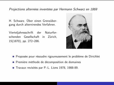
Projections alternées inventées par Hermann Schwarz en 1869
H. Schwarz. Über einen Grenzüber-gang durch alternirendes Verfahren.
Vierteljahresschrift der Naturfor-schenden Gesellschaft in Zürich,15(1870), pp. 272–286.
Proposée pour résoudre rigoureusement le problème de Dirichlet
Première méthode de décomposition de domaines
Travaux revisités par P.-L. Lions 1978, 1988-89.

Projections alternées dans le cas convexe
Schwarz, Sobolev, v. Neumann : sous-spaces affines
W. Cheney, A. Goldstein : Convergence pour ensembles convexesfermés dans Rn. 1959
L.M. Bregman : Convergence faible pour convexes fermés dansl’espace de Hilbert. 1965
H.H. Bauschke : Cas convexe essentiellement résolu en 1995.
H. Hundal. Echec de la convergence forte, 2002.
ba1
bb1
ba2
bb2
b a3
A
B
b
B
ba1
bb1
ba2
bb2
ba3
A
b
b

ba1
bb1
ba2
bb2
ba3
A
B
b
b ba1
bb1
ba2
bb
b b
A
B
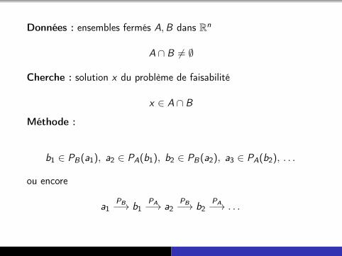
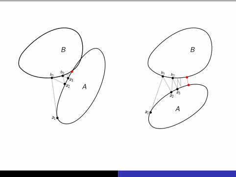
Données : ensembles fermés A,B dans Rn
A ∩ B 6= ∅
Cherche : solution x du problème de faisabilité
x ∈ A ∩ B
Méthode :
b1 ∈ PB(a1), a2 ∈ PA(b1), b2 ∈ PB(a2), a3 ∈ PA(b2), . . .
ou encore
a1PB−→ b1
PA−→ a2PB−→ b2
PA−→ . . .

Projections alternées dans le cas non-convexe :
Existe-t-il des applications ?
Conditions assurant la convergence locale ?
Echec de convergence possible ?

Echec de convergence

Théorème(Combettes, Trussell 1990). Soient A,B des fermés dans Rn.Supposons que la suite alternée ak , bk est bornée et vérifieak − bk → 0. Alors l’ensemble des points d’accumulation de ak , bkest ou un singleton, ou un compact continu.
Théorème(Bauschke, Noll 2013). Le cas d’un compact continu non-singletonpeut se produire.
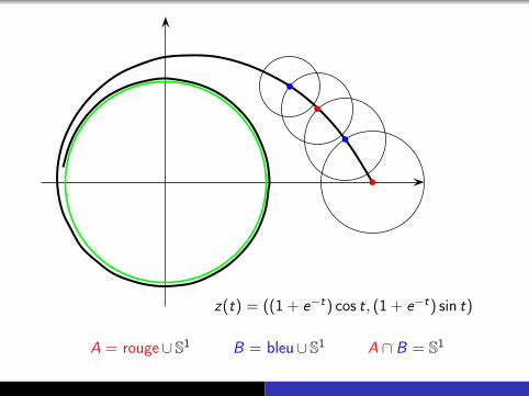
z(t) = ((1 + e−t) cos t, (1 + e−t) sin t)
A = rouge∪ S1 B = bleu∪ S
1 A ∩ B = S1

A = (cos t, sin t, s) : 0 ≤ s ≤ 1, 0 ≤ t ≤ 2πB = ((1 + e−t) cos t, (1 + e−t) sin t, e−t/2) : 0 ≤ t ≤ ∞
Bauschke, Noll (2014, Archiv der Math.)
Existe-t-il des applications ?

Applications des projections alternées non-convexes :
Démosaïquage de couleurs
Débruitage de séries chronologiques (algorithme de Cadzow)
Tomographie
Placement de pôles (en contrôle)
Synthèse de lois de commande en feedback (contrôle)
Ebauche de tracements de routes (Road profile design)
Restitution de blocks d’images JPEG et MPEG perdus
Faisabilité affine creuse (correction de fautes dans des codeslinéaires)
Empilements denses dans des variétés Grassmanniennes(télécommunication)
Algorithme EM pour les lois normales
Problème de phase (interférométrie, cristallographie, . . . )

Convergence locale

Théorème(A.S. Lewis, J. Malick 2008). Soient A,B des sous-variétés declasse C 2 de Rn, dont l’intersection est transversale en x∗ ∈ A ∩ B.Alors il exist un voisinage U de x∗ tel que toute suite alternéeak , bk qui rentre dans U converge vers un a∗ ∈ A ∩ B avec vitesseR-linéaire.
b x∗
A
B
Transversalité
TA(x∗) + TB(x
∗) = Rn
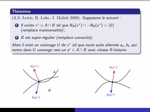
Théorème(A.S. Lewis, R. Luke, J. Malick 2009). Supposons le suivant :
1 Il existe x∗ ∈ A ∩ B tel que NA(x∗) ∩ −NB(x∗) = 0(remplace transversalité) ;
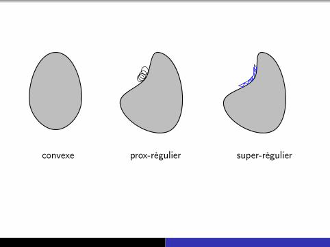
2 B est super-régulier (remplace convexité).
Alors il exist un voisinage U de x∗ tel que toute suite alternée ak , bk quirentre dans U converge vers un a∗ ∈ A ∩ B avec vitesse R-linéaire.
A
B
NB(x∗)
NA(x∗)
b
NB(x∗)
NA(x∗)
b
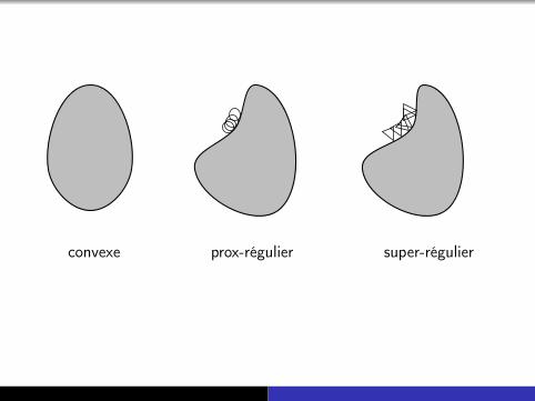
convexe prox-régulier super-régulier

convexe prox-régulier super-régulier
convexe prox-régulier super-régulier

H.H. Bauschke, D.R. Luke, H.M. Phan, X. Wang (2013). Restrictednormal cones and the method of alternating projections.Set-valued Var. Anal.
A
B
NB(x∗)
NA(x∗)
NA(x∗) ∩ −NB(x
∗)
b
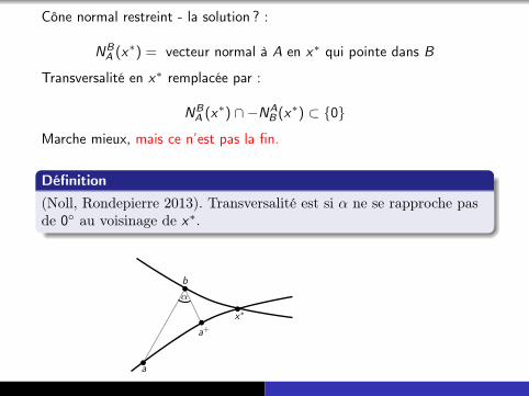
Cône normal restreint - la solution ? :
NBA (x∗) = vecteur normal à A en x∗ qui pointe dans B
Transversalité en x∗ remplacée par :
NBA (x∗) ∩ −NA
B (x∗) ⊂ 0
Marche mieux, mais ce n’est pas la fin.
Définition(Noll, Rondepierre 2013). Transversalité est si α ne se rapproche pasde 0 au voisinage de x∗.
b
b
b
b
α
b
a
a+
x∗

Que se passe-t-il si l’intersection est tangentielle ?
• L’échec de convergence, est-il dû à un manque de régularité ?
• ou parce que l’intersection est (trop) tangentielle ?
.
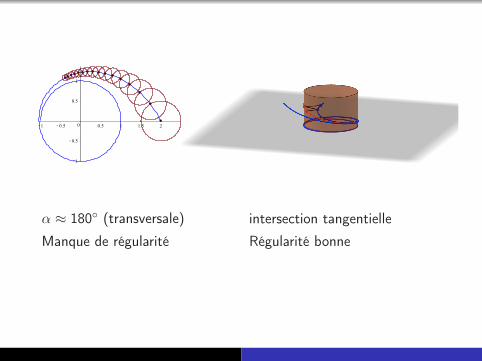
α ≈ 180 (transversale) intersection tangentielle
Manque de régularité Régularité bonne

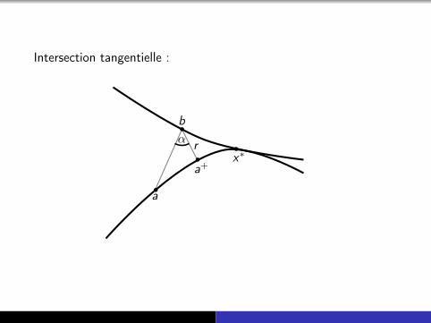
Intersection tangentielle :
α
b
a
a+
x∗
r
Intersection tangentielle :
α
b
a
a+x∗
r

Intersection tangentielle :
α
b
aa+
x∗r

Intersection tangentielle :
α
b
aa+
x∗r
α = ∠(a − b, a+ − b) et r = ‖b − a+‖tendent tous les deux vers 0 quand a, b, a+ → x∗

Définition(Noll, Rondepierre 2013). Les fermés A,B vérifient la conditiond’angle en x∗ ∈ A ∩ B s’il existe γ > 0, ω ∈ [0, 2) et un voisinage U dex∗ tel que pour tout block a PB−→ b PA−→ a+ dans U on a
1− cosαrω
≥ γ
Intersection tangentielle signifie α et r tendent vers 0.
Condition d’angle signifie qu’il y a un lien entre les deux. L’angle nes’annule pas trop vite.
ω = 0 transversalité (α 6→ 0, r → 0).

Théorème(Noll, Rondepierre 2013). Supposons qu’il existent x∗ ∈ A ∩ B etω ∈ (0, 2) tels que
1 la condition d’angle pour ce ω est vérifiée en x∗ ∈ A ∩ B.
2 B est régulier en x∗ au sens de Hölder par rapport à A avec ω/2.
Alors il existe un voisinage U de x∗ tel que toute suite alternée ak , bk quirentre dans U converge vers un a∗ ∈ A ∩ B avec vitesse
‖ak − a∗‖ = O(k−
2−ω2ω
), ‖bk − a∗‖ = O
(k−
2−ω2ω
)
Cas ω = 0 donne convergence R-linéaire comme avant

Théorème(Noll, Rondepierre 2013). Soient A,B des fermés sous-analytiques. Alorsen tout x∗ ∈ A ∩ B la condition d’angle est vérifiée pour un certainω ∈ [0, 2).
Ensemble semi-analytique :
A =N⋃
i=1
M⋂j=1
x ∈ Rn : φij(x) = 0, ψij(x) > 0
avec φij , ψij réel-analytiques.
A sous-analytique ⇐⇒ ∀a ∈ A ∃r > 0 ∃A semi-analytique bornéA ∩ B(a, r) = x : (x , y) ∈ A

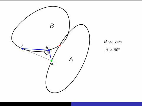
Que signifie la Hölder régularité ?

A
B
b
a+
b+
B convexe
A
B
b
a+
b+
β
B convexe
β ≥ 90
A
B
b
a+
b+
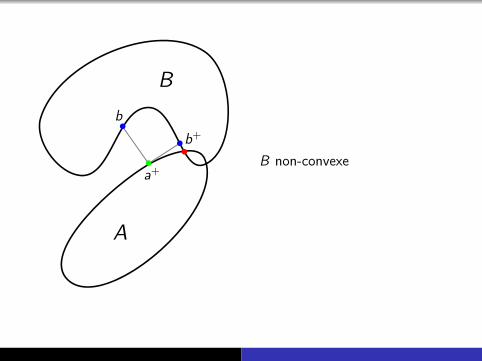
B non-convexe
β < 90 possible

β
A
B
b
a+
b+
B non-convexe
β < 90 possible

β
A
B
b
a+
b+
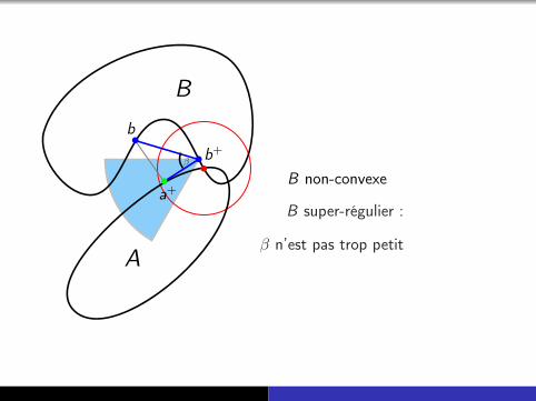
B non-convexe
β < 90 possiblesi B super-régulier :
β n’est pas trop petit
A
B
b
a+
b+
B non-convexe
β < 90 possibleB super-régulier :
β n’est pas trop petit
β


échec de super-régularité

r (1+
c)r
B
A
β=
arccos√ cr
σ

r
B
A
β=
arccos√ cr
σ

B
A
β=
arccos√ cr
σ

B
A
β=
arccos√ cr
σ

Conséquence : notre régularité Hölderienne s’avère plus flexible.Toujours valable pour packman.

Corollaire(Noll, Rondepierre 2013). Soient A,B sous-analytiques, B Hölderrégulier par rapport à A. Soit ak , bk une suite alternée bornée avecak − bk → 0. Alors il existe ω ∈ [0, 2) tel que la suite converge versun a∗ ∈ A ∩ B avec vitesse
‖ak − a∗‖ = O(k−
2−ω2ω
), ‖bk − a∗‖ = O
(k−
2−ω2ω
)

Problème de phase (Phase retrieval)

Problème de phase (en anglais: phase retrieval)
Reconstruire un signal x(t), t = 0, . . . ,N − 1 inconnu, à partir deson amplitude de Fourier a(f ) = |x(f )|, f = 0, . . . ,N − 1 connue.
Faut donc reconstruire la phase de Fourier x(f )/|x(f )|.
Sous-déterminé : Besoin d’ajouter de l’information.
=⇒ Mesures additionnelles dans un deuxième plan deFourier (Gerchberg-Saxton 1972).
=⇒ supp(x) au domaine temporel connu :x(t) = 0 pour t 6∈ S (atomicity constraint).
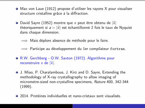
Max von Laue (1912) propose d’utiliser les rayons X pour visualiserstructure cristalline grâce à la diffraction.
David Sayre (1952) montre que x peut être obtenu de |x |théoriquement si a = |x | est échantillonné 2 fois le taux de Nyquistdans chaque dimension.
=⇒ Mais déplore absence de méthode pour le faire.
=⇒ Participe au développement du 1er compilateur fortran.
R.W. Gerchberg - O.W. Saxton (1972). Algorithme pourreconstruire x de |x |.
J. Miao, P. Charalambous, J. Kirz and D. Sayre, Extending themethodology of X-ray crystallography to allow imaging ofmicrometre-sized non-crystalline specimens, Nature 400, 342-344(1999).
2014. Protéines individuelles et nano-cristaux sont visualisés.

David Sayre(1924–2012)
Crystallographer who pioneered methods of X-ray imaging and modern computing.
David Sayre, who died on 23 February, was a pioneer in crystallography and diffraction imaging, a visionary in
X-ray microscopy and an architect of modern computing. A superb scientist, deep thinker and wonderful mentor, he could have built a scientific empire. But that was not his style. He was driven by the desire to do pure and original science.
Sayre was born on 2 March 1924 in New York. His father was an organic chemist whose ancestors helped to found the town of Southampton, New York, in the sixteenth century. His mother was the daughter of Jewish immigrants. Sayre was edu-cated at Yale University in New Haven, Connecticut, graduating in 1943 at the age of 19 with a bachelor’s degree in physics. The Second World War was at its height, so Sayre worked on radar at the Radiation Laboratory at the Massachusetts Institute of Technology in Cambridge.
In 1946, guessing biology would be the next exciting field, Sayre became a graduate student in biology at the Uni-versity of Pennsylvania in Philadelphia and then at Harvard University in Cambridge. He was not initially inter-ested in what he was learning, but in 1947 Sayre came across an article about X-ray crystallography that changed his life. He joined Raymond Pepinsky’s crystallography laboratory at Auburn University in Alabama, where he used a mathematical operation known as the Fourier transform to analyse the structures of crystals probed with X-ray beams.
That year, Sayre married Anne Colquhoun, a fiction writer. She took a teaching position at the Tuskegee Institute, but her involvement in the school, which enrolled black students, was controversial in the Deep South at that time, and the Sayres soon left. They moved to Oxford, UK, where Sayre completed his PhD in the lab of Dorothy Hodgkin in 1951.
Sayre produced his most profound papers during this period, solving the ‘phase problem’ in crystallography — the loss of phase information in the measurement of diffraction intensity. In 1952, he proposed atomicity — the fact that atoms are small and discrete points relative to the space between them — as a constraint for determining the phases of crystals of small molecules, giving
rise to what is now called Sayre’s equation. Atomicity is the key concept behind the direct methods used for crystallography today, although Sayre did not share the 1985 chemistry Nobel prize awarded for
it. In 1952, Sayre also realized that, even in the absence of regular crystal structure, information could be gleaned from the fine sampling of diffraction patterns.
Sayre saw early on that solving complex crystal structures would require substantial computational resources. In 1956 he joined IBM’s Watson Research Center in New York, and eventually became assistant manager of the team that wrote the original FORTRAN compiler. He became corporate director of programming, and later head of the IBM programming research group. In 1969, he and his team proved the efficiency of virtual memory in computing.
In 1972–73, Sayre took a sabbatical, returning to Hodgkin’s lab and to crystal-lography. It was during this time that one of us (J.K.) met the Sayres, forming a lasting friendship and collaboration. Anne Sayre also wrote the influential book Rosalind
Franklin and DNA, about the outstanding crystallographer and Sayre family friend who had died of cancer at an early age.
After returning to IBM, Sayre became interested in X-ray microscopy. His 1971 idea
of how to fabricate Fresnel zone plates for focusing X-rays became a reality through the use of IBM’s nanofabrica-tion technology and with the advent of synchrotron radiation sources such as the National Synchrotron Light Source at Brookhaven National Labo-ratory in Upton, New York. X-ray microscopy based on zone plates is now used in synchrotron-radiation facilities worldwide.
Around 1990, Anne developed scleroderma, a debilitating disease, and David retired from work to care for her. But he continued working to real-ize his 1952 dream: the reconstruction of molecular structures without the use of crystals. The idea came to fruition almost 50 years later, with the publica-tion in 1999 of the first reconstruction of a non-crystalline model object from its diffraction pattern (which was J.M.’s PhD project). This paper established coherent diffraction imaging (CDI), also called lensless imaging or diffrac-tion microscopy, as the most promising form of high-resolution X-ray imaging. CDI is now one of the fastest-growing fields in X-ray science.
Anne died in 1998, and in the last decade of his life David suffered from
Parkinson’s disease. But he continued to participate in research and to offer advice. A researcher with exceptional intuition, David lived for science. His passing is a huge loss for all of us.
Janos Kirz is distinguished professor emeritus at Stony Brook University, New York, and scientific adviser for the Advanced Light Source, Lawrence Berkeley National Laboratory, Berkeley, California 94720, USA. He was a collaborator and friend of David for nearly 40 years. Jianwei Miao is a professor in the Department of Physics and Astronomy and the California NanoSystems Institute, University of California, Los Angeles, California 90095, USA. He worked with David on coherent diffraction imaging beginning in 1996, first as a student, then as a collaborator and friend. e-mail: [email protected]
IBM
AR
CH
IVES
OBITUARYCOMMENT
3 8 | N A T U R E | V O L 4 8 4 | 5 A P R I L 2 0 1 2 | C O R R E C T E D 1 2 J U L Y 2 0 1 2© 2012 Macmillan Publishers Limited. All rights reserved
Max von Laue(photo 1929)
David Sayre(photo 1972)
W. O. Saxton(photo 2012)

Gerchberg-Saxton error reduction (1972)1 Etant donné l’estimation actuelle x , calculer x et «corriger»
l’amplitude de Fourier y(f ) := a(f )x(f )
|x(f )|.
2 Calculer transformé de Fourier inverse y de y , et «corriger»
le domaine x+(t) =
y(t) pour t ∈ S0 pour t 6∈ S
.
3 Remplacer x par x+ et boucler.
=⇒ Optique, astronomie, cristallographie, nanomatériaux, ...=⇒ Aucune preuve de convergence depuis 1972.
Nous en fournissons la première.

Théorème(Noll, Rondepierre 2013). Supposons que le problème de reconstructionde phase a une solution x∗ ∈ A ∩ B. Si la contrainte du domain temporelest représentée par un ensemble B sous-analytique, alors l’algorithme deGerchberg-Saxton converge au voisinage de x∗ vers une solution duproblème de phase avec vitesse de convergence O
(k−
2−ω2ω
)pour un
certain ω ∈ [0, 2).
Preuve. Une instance des projections alternées non-convexes :
A = x ∈ CN : |x(f )| = a(f ) pour tout f
A est prox-régulier et non-convexe
B = y ∈ CN : y(t) = 0 pour tout t 6∈ S
PA(x) = (ax/|x |) PB(y) = y · 1S

100 200 300 400 500 600 700 800
50
100
150
200
250
300
350
400
450
500
550
100 200 300 400 500 600 700 800
50
100
150
200
250
300
350
400
450
500
550
x = rteiφt y = rge iφg
rteiφg rge iφt
100 200 300 400 500 600 700 800
50
100
150
200
250
300
350
400
450
500
550
100 200 300 400 500 600 700 800
50
100
150
200
250
300
350
400
450
500
550
100 200 300 400 500 600 700 800
50
100
150
200
250
300
350
400
450
500
550
100 200 300 400 500 600 700 800
50
100
150
200
250
300
350
400
450
500
550
x = rteiφt y = rge iφg
rteiφg rgeφt
100 200 300 400 500 600 700 800
50
100
150
200
250
300
350
400
450
500
550
100 200 300 400 500 600 700 800
50
100
150
200
250
300
350
400
450
500
550

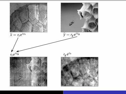
Conséquences :
Phase de Fourier x/|x | donne l’information essentielle sur x .Amplitude de Fourier a = |x | ne permet pas de localiserl’image x .Exemple : translater dans le domaine temporel change la phasede Fourier, mais non l’amplitude.Reconstruction de la phase donc difficile !
100 200 300 400 500 600 700 800 900 1000
100
200
300
400
500
600
700
800
900
1000100 200 300 400 500 600 700 800 900 1000
100
200
300
400
500
600
700
800
900
1000
original élargi (inconnu) phase de Fourier (inconnue)
100 200 300 400 500 600 700 800 900 1000
100
200
300
400
500
600
700
800
900
1000100 200 300 400 500 600 700 800 900 1000
100
200
300
400
500
600
700
800
900
1000
amplitude de Fourier (connue) support estimé (connu a priori)

100 200 300 400 500 600 700 800 900 1000
100
200
300
400
500
600
700
800
900
1000100 200 300 400 500 600 700 800 900 1000
100
200
300
400
500
600
700
800
900
1000
100 200 300 400 500 600 700 800 900 1000
100
200
300
400
500
600
700
800
900
1000100 200 300 400 500 600 700 800 900 1000
100
200
300
400
500
600
700
800
900
1000
. guess map1 map6 map15
100 200 300 400 500 600 700 800 900 1000
100
200
300
400
500
600
700
800
900
1000100 200 300 400 500 600 700 800 900 1000
100
200
300
400
500
600
700
800
900
1000100 200 300 400 500 600 700 800 900 1000
100
200
300
400
500
600
700
800
900
1000
100 200 300 400 500 600 700 800 900 1000
100
200
300
400
500
600
700
800
900
1000
. map38 map80 map100 map200
100 200 300 400 500 600 700 800 900 1000
100
200
300
400
500
600
700
800
900
1000100 200 300 400 500 600 700 800 900 1000
100
200
300
400
500
600
700
800
900
1000100 200 300 400 500 600 700 800 900 1000
100
200
300
400
500
600
700
800
900
1000
100 200 300 400 500 600 700 800 900 1000
100
200
300
400
500
600
700
800
900
1000
. guess dr1 dr2 dr3
100 200 300 400 500 600 700 800 900 1000
100
200
300
400
500
600
700
800
900
1000100 200 300 400 500 600 700 800 900 1000
100
200
300
400
500
600
700
800
900
1000100 200 300 400 500 600 700 800 900 1000
100
200
300
400
500
600
700
800
900
1000
100 200 300 400 500 600 700 800 900 1000
100
200
300
400
500
600
700
800
900
1000
. dr7 dr20 dr36 dr60

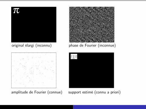
Image idéale x0 =PI élargie à 1024× 1024 par rajout de zéros(an anglais : 0-padding).0=noir, 256=blanc.Estimation initiale est version flouée, bruitée et tournée de 90
de Pi.Amplitude de Fourier a = |x0| connue.A = x ∈ C1024×1024 : |x(f )| = a(f ) pour toute fréquence f .B = y ∈ C1024×1024 : y(t) = 0 ∀ pixel t hors masque.Masque = la zone grise autour du PI. Hypothèse a priori :masque connu.PA ne réussit pas complètement dans le temps donné.Douglas-Rachford reconstruit phase assez complètement.

J. Douglas, H.H. Rachford. On the numerical solution of heat conductionproblems in two and three dimensions. TAMS 82 (1956), 421 – 439.
P.-L. Lions, B. Mercier. Splitting algorithms for the sum of two nonlinearoperators. SIAM J.Num. Anal. 16 (1979), 946–979.
J.R. Fienup. Phase retrieval algorithms : a comparison. Applied Optics,1982. HIO = Hybrid-Input-Output
A B
x
a
y
b
x+
a ∈ PA(x)
y = 2a − x ∈ RA(x)
b ∈ PB(y)
x+ = x + b − a
reflect-reflect-averageb
b
b
bb
b
Convergence pour les projections alternées :
A.S. Lewis, J. Malick (2008). Alternating projections on manifolds.Math. Oper. Res. 33, 216–234.
A.S. Lewis, R. Luke, J. Malick (2009). Local linear convergence foralternating and averaged non-convex projections.Foundations Comp. Math. 9, 485–513.
H.H. Bauschke, D.R. Luke, H.M. Phan, X. Wang (2013). Restrictednormal cones and the method of alternating projections.Set-valued Var. Anal. 31, 431–501.
D. Noll, A. Rondepierre (2013). On local convergence of the method ofalternating projections. Foundations of Computational Mathematics,2015.

Lien avec l’inégalité de Kurdyka-Łojasiewicz :
H. Attouch, J. Bolte, P. Redont, A. Soubeyran (2010). Proximalalternating minimization and projection methods for nonconvex problems.An approach based on the Kurdyka-Łojasiewicz inequality. JMOR35(2) :2010,438-457.
H. Attouch, J. Bolte, B.F. Svaiter (2013). Convergence of descentmethods for semi-algebraic and tame problems : proximal algorithms,forward-backward splitting, and regularized Gauss-Seidel methods. Math.Programming 137(1-2) :2013,91-129.
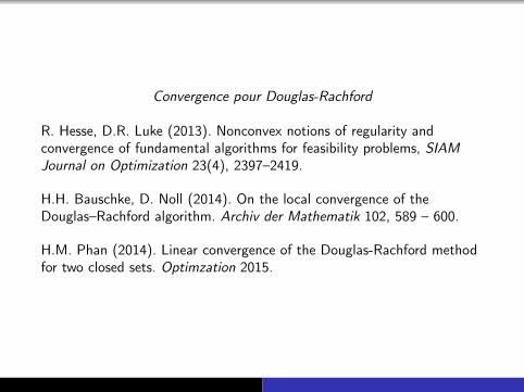
Convergence pour Douglas-Rachford
R. Hesse, D.R. Luke (2013). Nonconvex notions of regularity andconvergence of fundamental algorithms for feasibility problems, SIAMJournal on Optimization 23(4), 2397–2419.
H.H. Bauschke, D. Noll (2014). On the local convergence of theDouglas–Rachford algorithm. Archiv der Mathematik 102, 589 – 600.
H.M. Phan (2014). Linear convergence of the Douglas-Rachford methodfor two closed sets. Optimzation 2015.
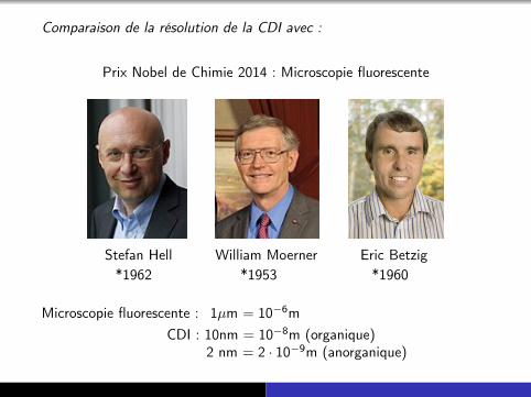
Comparaison de la résolution de la CDI avec :
Prix Nobel de Chimie 2014 : Microscopie fluorescente
Stefan Hell William Moerner Eric Betzig*1962 *1953 *1960
Microscopie fluorescente : 1µm = 10−6mCDI : 10nm = 10−8m (organique)
2 nm = 2 · 10−9m (anorganique)

Merci pour votre attention !

Ω
−∆u = f sur Ω u = 0 sur ∂Ω

Ω Ω1 Ω2
−∆u2k+1 = f sur Ω1 u2k+1 = u2k sur ∂Ω1
−∆u2k = f sur Ω2 u2k = u2k−1 sur ∂Ω2
u0 ∈ H10 (Ω)

〈u, v〉 =
∫Ω∇u · ∇v dx , u, v ∈ H1
0 (Ω)
〈u2k+1 − u, v1〉 = 0 ∀v1 ∈ H10 (Ω1), u2k+1 − u2k ∈ H1
0 (Ω1)
〈u2k − u, v2〉 = 0, ∀v2 ∈ H10 (Ω2), u2k − u2k−1 ∈ H1
0 (Ω2)
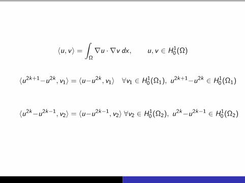
〈u, v〉 =
∫Ω∇u · ∇v dx , u, v ∈ H1
0 (Ω)
〈u2k+1−u2k , v1〉 = 〈u−u2k , v1〉 ∀v1 ∈ H10 (Ω1), u2k+1−u2k ∈ H1
0 (Ω1)
〈u2k−u2k−1, v2〉 = 〈u−u2k−1, v2〉 ∀v2 ∈ H10 (Ω2), u2k−u2k−1 ∈ H1
0 (Ω2)

〈u, v〉 =
∫Ω∇u · ∇v dx , u, v ∈ H1
0 (Ω)
u2k+1 − u2k = PH10 (Ω1)(u − u2k)
u2k − u2k−1 = PH10 (Ω2)(u − u2k−1)

u − u2k+1 = PH10 (Ω1)⊥(u − u2k)
u − u2k = PH10 (Ω2)⊥(u − u2k−1)
Corollaire
Si Ω = Ω1 ∪ Ω2, alors la suite des projections alternées u − u2k+1,u − u2k converge vers 0 en norme H1
0 (Ω).
Preuve. Il suffit de montrer que H10 (Ω1) + H1
0 (Ω2) est dense dansH1
0 (Ω). Pour cela il suffit de montrer que tout φ ∈ D(Ω) peut êtreécrit comme φ = φ1 + φ2 avec φi ∈ D(Ωi ).

Application : Algorithme EM
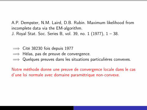
A.P. Dempster, N.M. Laird, D.B. Rubin. Maximum likelihood fromincomplete data via the EM-algorithm.J. Royal Stat. Soc. Series B, vol. 39, no. 1 (1977), 1 – 38.
=⇒ Cité 38230 fois depuis 1977=⇒ Hélas, pas de preuve de convergence.=⇒ Quelques preuves dans les situations particulières convexes.
Notre méthode donne une preuve de convergence locale dans le casd’une loi normale avec domaine paramétrique non-convexe.

Structured low-rank matrix approximation

Given a structured matrix x ∈ S, solve the problem
(P)minimize ‖x ′ − x‖Fsubject to x ′ ∈ S
rank(x ′) ≤ r
S = Hankel matrices (denoising of time series)
S = Toeplitz matrices (spectral estimation problems)
S = positive semidefinite matrices
S = stable matrices
Use non-convex alternating projections :
A = x : x ∈ S PA = easy ? ? ?
B = x : rank(x) ≤ r PB = truncated SVD
Can now prove local convergence to x∗ ∈ x : rank(x) ≤ r , x ∈ S. Neednot be solution of (P)

Sparse affine feasibility

minimize ‖x‖0 = number of non-zero entries in xsubject to Ax = b
x ∈ Rn
Use non-convex alternating projections :
A = x ∈ Rn : ‖x‖0 ≤ k =⋃
card(I )≤k
spanei : i ∈ I︸ ︷︷ ︸=:AI
PA(x) =⋃
I active
PAI (x)
B = x ∈ Rn : Ax = b PB(x) = x − A†(Ax − b)

Packings in Grassmannian manifolds
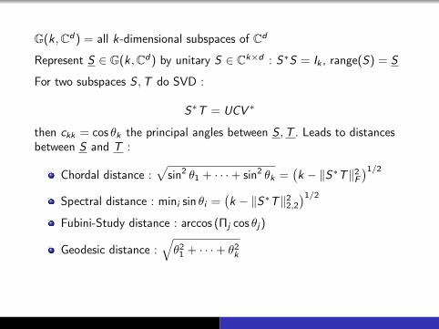
G(k,Cd) = all k-dimensional subspaces of Cd
Represent S ∈ G(k,Cd) by unitary S ∈ Ck×d : S∗S = Ik , range(S) = S
For two subspaces S ,T do SVD :
S∗T = UCV ∗
then ckk = cos θk the principal angles between S ,T . Leads to distancesbetween S and T :
Chordal distance :√
sin2 θ1 + · · ·+ sin2 θk =(k − ‖S∗T‖2F
)1/2Spectral distance : mini sin θi =
(k − ‖S∗T‖22,2
)1/2Fubini-Study distance : arccos (Πj cos θj)
Geodesic distance :√θ21 + · · ·+ θ2
k

Packing for the chordal distance :
pack(S1, . . . , SN) := minm 6=n
dchord(Sm, Sn) = minm 6=n
(k − ‖S∗mSn‖2F
)1/2True problem : max
S1,...,SNpackchord(S1, . . . , SN)
Instead feasibility problem : Given ρ > 0, want S1, . . . , SN suchthat packchord(S1, . . . , SN) ≥ ρ
minm 6=n
(k − ‖S∗mSn‖2F
)1/2 ≥ ρ ≡ maxm 6=n‖S∗mSn‖F ≤ µ :=
√k − ρ2

Put S := [S1S2 . . . SN ]
Gramian G = S∗S ∈ CkN×kN 0, Gmn = S∗mSn
1 G is Hermitian2 Each diagonal block of G is identity Ik3 G 04 rank(G ) ≤ d5 trace(G ) = kN
Conversely, any G with these properties can be factored G = S∗Sand S = [S1 . . . SN ] gives then rise to a configuration of Nsubspaces in the Grassmannian G(k ,Cd ).

Now alternating projections :
Structural constraint (convex) :
A = H ∈ CkN×kN : H = H∗,Hnn = Ik , ‖Hmn‖F ≤ µ
Spectral constraint (non-convex) :
B = G ∈ CkN×kN : G 0, rank(G ) ≤ d , trace(G ) = kN
Any solution G ∈ A ∩ B gives a packing of size N of the Grassmannianwith chordal distance packing index ≥ ρ.
Compute projection on A (easy) :
H = PA(G ) : Hmn =
Gmn ‖Gmn‖F ≤ µµGmn/‖Gmn‖F else
Compute projection on B (more involved but possible) :
Let H =kN∑j=1
λjuju∗j be spectral decomposition, where
λ1 ≥ λ2 ≥ · · · ≥ λkN . Then
G =d∑
j=1
(λj − γ)+ uju∗j ∈ PB(H)
provided γ is chosen such thatd∑
j=1
(λj − γ)+ = kN.