Symbolic Methods for Factoring Linear Differential Operators - RISC
112
JOHANNES KEPLER UNIVERSIT ¨ AT LINZ Netzwerk f¨ ur Forschung, Lehre und Praxis Symbolic Methods for Factoring Linear Differential Operators Dissertation zur Erlangung des akademischen Grades Doktor der Technischen Wissenschaften Angefertigt am Institut f¨ ur Symbolisches Rechnen Betreuung: O. Univ.Prof. Dipl.-Ing. Dr. Franz Winkler Mitbetreuung: Dr. G¨ unter Landsmann Begutachtung: Erster Begutachter: O. Univ.Prof. Dipl.-Ing. Dr. Franz Winkler Zweiter Begutachter: O. Univ.Prof Dipl.-Math. Dr. Jochen Pfalzgraf Eingereicht von: Glauco Alfredo L´opez D´ ıaz, M.Sc.-Math. Linz, Februar 2006 Johannes Kepler Universit¨ at A-4040 Linz · Altenbergerstraße 69 · Internet: http://www.uni-linz.ac.at · DVR 0093696
Transcript of Symbolic Methods for Factoring Linear Differential Operators - RISC
JOH AN N E S K E P L E R
U N IVE R S IT AT L IN Z
N e t z w e r k f u r F o r s c h u n g , L e h r e u n d P r a x i s
Symbolic Methods for Factoring Linear Differential
Operators
Dissertation
zur Erlangung des akademischen Grades
Doktor der Technischen Wissenschaften
Angefertigt am Institut fur Symbolisches Rechnen
Betreuung:
O. Univ.Prof. Dipl.-Ing. Dr. Franz Winkler
Mitbetreuung:
Dr. Gunter Landsmann
Begutachtung:
Erster Begutachter: O. Univ.Prof. Dipl.-Ing. Dr. Franz Winkler
Zweiter Begutachter: O. Univ.Prof Dipl.-Math. Dr. Jochen Pfalzgraf
Eingereicht von:
Glauco Alfredo Lopez Dıaz, M.Sc.-Math.
Linz, Februar 2006
Johannes Kepler Universitat
A-4040 Linz · Altenbergerstraße 69 · Internet: http://www.uni-linz.ac.at · DVR 0093696
Eidesstattliche Erklarung
Ich erklare an Eides statt, dass ich die vorliegende Dissertation selbststandig und ohne fremdeHilfe verfasst, andere als die angegebenen Quellen und Hilfsmittel nicht benutzt bzw. die wortlich odersinngemaß entnommenen Stellen als solche kenntlich gemacht habe.
Glauco Alfredo Lopez DıazHagenberg, 1. februar 2006
Abstract
A survey of symbolic methods for factoring linear differential operators is given. Starting from basicnotions – ring of operators, differential Galois theory – methods for finding rational and exponentialsolutions that can provide first order right-hand factors are considered. Subsequently several knownalgorithms for factorization are presented. These include Singer’s eigenring factorization algorithm,factorization via Newton polygons, van Hoeij’s methods for local factorization, and an adapted versionof Pade approximation.
In addition a procedure based on pure algebraic methods for factoring second order linear partialdifferential operators is developed. Splitting an operator of this kind reduces to solving a system oflinear algebraic equations. Those solutions which satisfy a certain differential condition, immediatelyproduce linear factors of the operator. The method applies also to operators of third order, therebyresulting in a more complicated system of equations. In contrast to the second order case, differentialequations must also be solved, which, in particular cases, are simplified with the aid of characteristicsets.
Finally, complete decomposition into linear factors of ordinary differential operators of arbitraryorder is discussed. A splitting formula is developed, provided that a linear basis of solutions is available.This theoretical representation is valuable in understanding the nature of the classical Beke algorithmand its variants like the algorithm LODEF by Schwarz and the Beke-Bronstein algorithm.
Zusammenfassung
Es wird ein Uberblick uber symbolische Methoden zur Faktorisierung linearer Differentialoperatorengegeben. Beginnend mit grundlegenden Begriffen wie Operatorring oder differentielle Galoistheorie,diskutiert der Autor Methoden zum Auffinden rationaler wie auch exponentieller Losungen, mit derenHilfe rechte Faktoren von Operatoren gefunden werden konnen. Im Folgenden werden verschiedeneFaktorisierungsalgorithmen vorgestellt, darunter Singers Eigenring-Faktorisierungsalgorithmus, Fak-torisierung mit Hilfe von Newton Polygonen, van Hoeijs Methode zur lokale Faktorisierung und eineadaptierte Version der Pade Approximation.
Daruberhinaus entwickelt der Autor eine rein algebraische Methode zur Faktorisierung von linearenpartiellen Differentialoperatoren. Das Zerlegen so eines Operators reduziert sich auf das Auffindender Losungen eines linearen algebraischen Gleichungssystems. Diejenigen Losungen dieses Systems,welche eine bestimmte differentielle Bedingung erfullen, erzeugen direkt lineare Faktoren des Opera-tors. Dieselbe Methode ist auch auf Operatoren dritter Ordnung anwendbar, wobei ein komplexeresGleichungssystem auftritt. Im Gegensatz zum Fall 2. Ordnung mussen hier auch Differentialgleichungengelost werden, welche sich manchmal mit Hilfe charakteristischer Mengen vereinfachen lassen.
Zuletzt wird die vollstandige Zerlegung gewohnlicher Differentialoperatoren von beliebiger Ord-nung in lineare Faktoren behandelt. Unter Zugrundelegung einer linearen Basis des Losungsraumswird eine Zerlegungsformel entwickelt. Diese theoretische Darstellung erweist sich als hilfreich zumVerstandnis des klassischen Beke-Algorithmus und seiner Varianten - wie Beke-Bronstein-Algorithmusoder Schwarz’ LODEF-Algorithmus.
Acknowledgements
In first place I would like to thank “God” almighty for every think good in my life, and also toallow me to make my dreams true.
In second place RISC-Linz Institute which formed me as a researcher in applied mathematics.
In third place the following people:
My Parents Felix Jesus y Elisa Amelia for all their love, moral support and encouragement.
My brothers Juan Alejandro y Juan Miguel, who are like my sons.
My University in Merida, Venezuela, “Universidad de Los Andes”, for allow me to study in Austria,my academic permission and scholarship.
My friends and colleagues in Venezuela Prof. Gisela de Zarrasin, Prof. Dr. Jesus Rodrıguez Millan,Prof. Jose Gımenez Ph.D., Prof. Miguel Narvaez, Prof. Hugo Leiva Ph.D., who helped and supportedme all the time.
Univ.-Prof. Dr.phil. DDr.h.c. Bruno Buchberger, O. Uni.Prof. Dipl.-Ing. Dr. Franz Winkler andDr. Gunter Landsmann for all the knowledge that they gave me during their courses, lectures andseminars.
The RISC System administrators: Dipl.-Ing. Karoly Erdei and M.Sc. Werner Danielczyk-Landerl,the people who have solved my problems with the system.
The RISC’s secretaries: Mrs. Betina Curtis and Mrs. Ramona Pochinger, the people who havesolved my problems with formalities.
My advisor Prof. Franz Winkler, who taught Computer Algebra, who introduced me in the businessof Symbolic Differential Computation, and who guided me to do research in applied mathematics.
My intermediate supervisor Dr. Gunter Landsmann. His patient guidance and helpful suggestionshave played a significant role in the fact this work has resulted in a Ph.D. thesis. I am very grateful tohim, because he has revised and improved my written English style.
The Post-Doc at RISC: Dr. Karoly Bosa, Dr. Teimuraz Kutsia, Dr. Carsten Schneider, for all theirhelp at anytime I needed.
My colleagues and friends at RISC: Dipl.-Ing. Camelia Rosenkranz, Dr. Rahul Ramesh Athale,M.Sc. Burkhard Zimmermann, M.Sc. Rebhi Baraka, Lic. Jose Manuel Garcia Vallinas, Dipl.-Ing.Alexander Zapletal and Cornelius Nevrinceanu Ph.D..
My Austrian family Franz and Anni Hackl, who adopted me like a son, their children Sabine,Martin and Michaela, and also Rudy and Jutta Fasching and their son Rudiger.
My German teacher Dipl.-Pad. Monika Ginthor and family, best friends and the best languageteacher I ever had.
Dr. Elena Kartashova, Prof. Serguei P. Tsarev and very special to the late Prof. Manuel Bronsteinfor their stimulating conversations about some topics developed in this thesis.
My girlfriend Margit Macsodi, for all her love, compression, support, patience and help.
My friends at the distance, but always friends, Robert Lorenzo, Orlando Pichardo and PedroEcheverria Ph.D..
The work on the thesis was supported by the project det, Fonds zur Forderung der wiss. Forschung,P16357-N04.
To all of you “Thank You”.
1. INTRODUCTION
1.1 Historical Motivation
Let (k, δ) be a differential field of characteristic 0 with algebraically closed field of constants C. Wewill write y(n) instead of δn(y) and y′, y′′, . . . for δ(y), δ2(y), . . .. Let D = k[∂] be the ring of lineardifferential operators over k, that is, the non-commutative polynomial ring in the variable ∂, where
∂a = a∂ + a′ for all a ∈ k.
Any linear differential operator L ∈ k[∂] of the form
L = ∂n + an−1∂n−1 + · · · + a1∂ + a0∂
0
defines an order n linear homogeneous scalar differential equation L(y) = 0 by
y(n) + an−1yn−1 + · · · + a1y
′ + a0y = 0.
Factorizing a linear differential operator L into a product L = QR, simplifies the computation ofsolutions as a solution of R(y) = 0 is a solution of L(y) = 0 as well. Moreover, we can find linearlyindependent solutions. As an example consider the following linear ordinary differential operator:
∂2 + (x− 1)∂ − x
whose factorization is(∂ + x)(∂ − 1).
Its scalar equation can be written as
y′′ + (x− 1)y′ − xy =
(d
dx+ x
)(y′ − y) = 0
which has linearly independent solutions
y1 = ex and y2 = ex
∫e−
x2
2 −xdx.
In particular, an operator L is said to be reducible if there exists operators L1 and L2 of lowerorder such that L = L2L1, in this case we say that L1 is a right factor and L2 is a left factor of L. Ifan operator is not reducible then it is called irreducible.
From Landau [1902], we know that any two decomposition of an operator L into irreducible com-ponents have the same number of factors and their orders are the same up to permutations. As anexample consider the derivative δ = d/dx in the field k then the following linear differential operator
∂2 = ∂∂ =
(∂ +
1
x− c
)(∂ − 1
x− c
),
with c ∈ C has essentially two different factorizations.
Even when the intention of the this part of the thesis is to study the existent algorithms for factoringlinear ordinary differential operators, in section 2.3 we will discuss rational and exponential solutionsof linear ordinary homogeneous differential equations. However, we would like to mention that thereare several algorithms for solving linear differential equation in particular we give a short survey aboutthem:
1. Introduction 3
1. Rational solutions:
Rational solutions are elements of k. To decompose the operators of this class, Liouville [1833a,b]already gave an algorithm, but only when k is a rational function field over the constants. Moregeneral versions have been presented by Singer [1991] and Bronstein [1992a]. To solve scalarequations, there are implementations by Abramov and Bronstein in Maple and in the Bernina
package. To solve matrix equations, there is an implementation by M. Barkatou in the Isolde
package. Both cases are restricted to the field Q(x) of rational functions in x with coefficients inthe algebraic closure of Q.
2. Algebraic solutions:
Algebraic solutions are solutions lying in an algebraic extension of k; i.e., they satisfy an irre-ducible polynomial over k. An example for this class is 3
√1 −√
x.
Many renowned mathematicians like Pepin [1881], Fuchs [1875, 1878], Klein and Jordan [1878]were searching for an algorithm for algebraic solutions. Today there exists an algorithm by Singer[1979] with some improvements in Singer and Ulmer [1993], but it is far from being satisfactorybecause it is very expensive; in this case one needs to substitute a minimal polynomial decom-posed into invariants in the differential equation. Another method from Fakler [1997] combinesLiouvillian solutions with the algebraic case of Risch’s algorithm (see Bronstein [1997]), it hasnot been implemented.
3. Liouvillian solutions:
Liouvillian solutions are solutions generated by repeatedly adjoining algebraic numbers, integralsor exponentials of integrals. An example of such a generation is
x√
x−−→√x
eR
−→ exp
[∫ √x
].
In Singer [1981] it was shown that given a homogeneous linear differential equation L(y) = 0with coefficients in F , a finite algebraic extension of Q(x), one can find in a finite number ofsteps, a basis for the vector space of Liouvillian solutions of L(y) = 0.
For order two equations the method is given by Kovacic [1986], with small improvements by Weil[1994]. For order three, the methods are given by Singer and Ulmer [1993].
Although the problem of finding all the Liouvillian solutions of a homogeneous linear differentialequation is decidable in theory for any order Singer [1991], the published decision procedure isnot consider a practical algorithm and has not been implemented.
4. Exponential solutions:
An exponential solution of the equation L(y) = 0 is a solution whose logarithmic derivative y′
ylies in k.
Exponential functions form the most important subclass of Liouvillian functions. Proceduresproviding algorithms that produce exponential solutions lie at the basis of all known algorithmsfor finding Liouvillian solutions. Fortunately, there are algorithms for exponential solutions. Thevery first one is from Beke [1894]. For the formal case, van Hoeij [1997a] has implemented classicalmethods. Factorization over Q(z) is based on the formal case.
Dividing functions into one of these classes is not always unique; e.g., for the function y =√x,
it is possible to attach it either to the algebraic functions or to the exponential, since y′
y = 12x ,
and 12x ∈ k. Furthermore, it can be hard to decide for a given function whether it is Liouvillian
and how one could find the simplest construction. A combination of the above methods is usedin the implementation by van Hoeij in the Maple computer algebra system.
For factorization of linear differential operators which constitutes the main subject of this thesis,we have the following known methods:
1. Introduction 4
1. Beke’s method: In 1894 Beke gave a method for factorization of linear differential operators inthe ring Q(x)[∂]. Previous implementations for factorization in k(x)[∂] are based on his method.For example, the factorizer in the Kovacic algorithm (Kovacic [1986]) is based on Beke’s method.To find a factor via Beke’s method one must first compute another operator (the second exterior
power) and then compute a first order right-hand factor. Construct an auxiliary operator L whoseassociated Riccati equations have among their solutions all possible coefficients bi of factors
M = ∂m + bm−1∂m−1 + · · · + b1∂ + b0∂
0
of L. From L one can bound the degrees of the numerators and denominators of these coefficients.
An implementation of Beke’s method has been accomplished by Bronstein [1992b] in the Ax-
iom system. Schwarz [1989] has implemented the full algorithm for equations of small order inScratchpad II. Simplifications of the the Beke algorithm as well as a detailed complexity anal-ysis can be found in Grigoriev [1990a]. There is an algorithm for determining the reducibilityof a differential system in Grigoriev [1990b]. A method to enumerate all factors of a differentialoperator is given in Tsarev [1996].
2. The eigenring method: The eigenring of a differential equation L(y) = 0 is the finite dimensionalC-algebra of all the endomorphisms of the equation, where C is the subfield of constants of k.This eigenring is the set of all rational solutions of other differential equations associated to L.If this eigenring is not too trivial, then some factorizations of L can be deduced from it. Themethod was introduced by Singer [1996] and has been improved by van Hoeij [1997b].
3. Van Hoiej’s methods for factoring differential operators are not based on Beke’s algorithm. Heuses algorithms to find local factorizations (i.e., factors with coefficients in k(x)) and applies anadapted version of Pade approximation to produce a global factorization.
In order to do this, one should make a good choice of a singular point of the operator L anda formal local right-hand factor of degree 1 at this point. After a translation of the variable(x 7→ x + p or x 7→ x−1) and a shift ∂ 7→ ∂ + e with e ∈ k(x), the operator L has a right-hand
factor of the form ∂− y′
y with an explicit y ∈ k[[x]]. Now one tries to find out whether y′
y belongs
to k(x). Equivalently, one tries to find a linear relation between y and y′ over k[x]. This is carriedout by a Pade approximation. The method extends to finding right-hand factors of higher degreeand yields in that case a generalization of the Pade approximation.
This local-to-global approach has been implemented in Maple V.5 computer algebra system.
4. Full factorizations: The structure of all possible factorizations of an ordinary differential operatoris known due to a fundamental theorem of Loewy [1906]: An ordinary operator has uniquefactorization into completely reducible factors, i.e., in operators that have enough right factors.Recent work of Tsarev [1996] combined the local formal factorization of the previous case withthe classical work of Beke [1894].
In general, the main disadvantage of all factorization algorithms is their tremendous complexity,especially if the order if the given operator is higher than two.
Much less is known about factorization of linear partial differential operators. In the 19th century, avast interest in finding solutions of non-linear partial differential equations resulted in the developmentof the methods of Lagrange, Monge, Boole, and Ampere. In particular, Darboux [1870] generalizedthe method of Monge (known as the method of intermediate integrals) to obtain the most powerfulmethod in those days for explicitly integrating partial differential equations.
In Anderson and Kamran [1997], Juras [1995], and Zhiber, Sokolov, and Startsev [1995], the Dar-boux method was put in a more precise and efficient (although not completely algorithmic) form. Forthe case of a single second order non-linear partial differential equation of the form
uxy = f(x, y, u, ux, uy) (1.1.1)
1. Introduction 5
the idea was to linearize it. Using the substitution
u(x, y) → u(x, y) + ǫv(x, y)
and canceling the terms proportional to ǫn, n > 1, we obtain the linear partial differential equation
vxy = Avx +Bvy + Cv (1.1.2)
with coefficients A,B, and C depending on x, y, u, ux, uy. Studying equations of type (1.1.2), Laplaceinvented a method for their transformation that is sometimes called the Laplace cascade method. First,the corresponding linear partial differential operator satisfies the condition
L = ∂x∂y −A∂x −B∂y − C =
(∂x −B)(∂y −D) +H = (∂y −A)(∂x −B) +K,(1.1.3)
whereH = ∂xA−AB − C and K = ∂yB −AB − C
are the Laplace invariants of Equation (1.1.2). Therefore, if either H = 0 or K = 0, the second orderlinear partial differential operator L is factorable, and the solutions of Equation (1.1.2) can be foundthrough quadratures. If both H and K vanish, L is a left least common multiple of the two first orderlinear partial differential operators. If both H and K are nonzero, the two Laplace transformationsL→ L1 and L→ L−1 can be applied using the substitutions
v1 = (∂y −A)v, v−1 = (∂y −B)v. (1.1.4)
These (invertible) transformations result in two new second order linear partial differential operatorsL1 and L−1 of the same form as (1.1.2) with different coefficients if and only if H 6= 0 and K 6= 0. Inthe general case, we obtain the two infinite sequences
L→ L1 → L2 → · · ·
L→ L−1 → L−2 → · · ·If one of these sequences is finite (i.e., the corresponding Laplace invariant vanishes at some step,
and the Laplace transformation cannot be applied further), then the final linear partial differentialoperator Li is trivially factorable.
We can consider initial Equation (1.1.1) and calculate all Laplace invariants and Laplace trans-formations (which means that we express all the mixed derivatives of u in terms of x, y, u, and thenon-mixed derivatives ux...x and uy,...,y).
Theorem 1. A second order scalar hyperbolic partial differential equation of the form (1.1.1) is Dar-boux integrable if and only if both its Laplace sequences are finite.
In Juras [1995] and Anderson and Kamran [1997], this method was also generalized to the case ofa general second order non-linear hyperbolic partial differential equation
F (x, y, u, ux, uy, uxx, uxy, uyy) = 0.
The original “Darboux method” (as Darboux stated in Darboux [1870]) is extendable in principleto equations of all orders in an arbitrary number of variables, even to systems of equations; however, inDarboux [1870] and subsequent papers by Goursat, Gau, Gosse, Vessiot, et al., the detailed calculationswere performed only for a single second order equation with one dependent and two independentvariables.
On the other hand, Blumberg [1912] and Miller [1932] have discussed the necessity of a suitablegeneralization of the concept of completely reducible operators to partial operators, and they haveillustrated this problem with few typical examples. In particular, in Blumberg [1912] is given anexample of a third-order operator which has two different factorizations into completely reducible
1. Introduction 6
factors. With this it is shown that the result of Loewy about the uniqueness of the factorization intocompletely reducible factors, is not true for partial differential operators.
Nowadays, due to the growing interest in Computer Algebra and the use of the Computer AlgebraSystems, one tendency is treat factoring as finding superideals of a left ideal in the ring of linearpartial differential operators rather than factoring a single linear differential partial operator, as doneby Tsarev [2000] and Li, Schwarz, and Tsarev [2003]. In Tsarev [2000] a concept of factorization isdeveloped which makes some characteristic factors to be uniquely defined similar to the case of ordinaryoperators. In Li et al. [2003] the factorization of systems of linear partial differential operators with afinite-dimensional (over the subring of constants) space of solution is studied, then the linear differentialsubvarieties are viewed as the factors of the input systems.
Another tendency is to try to imitate the procedures and use the techniques for factoring poly-nomials, as done by Grigoriev and Schwarz [2004] with their algorithm “Hensel Decent” for factoringlineal partial differential operators of arbitrary order. They have named it in that way because it isclose in nature to the well-known Hensel lifting.
Grigoriev and Schwarz consider the homogeneous part of a differential operator, they define thesymbol of an operator as the homogeneous polynomial with the same coefficients as the homogeneouspart and the same powers as the corresponding derivatives. They define an operator to be separableif its symbol is separable, i.e., if all the roots of the symbol are distinct in an algebraically closed fieldextension of the field of coefficients. If the operator is separable then to find its possible factorizationsreduces to polynomial factorization in the field of coefficients, rational operations in that field andtaking derivatives.
We present a naive approach for factoring second order linear differential operators into linearfactors in the ring k(x, y)[∂x, ∂y], the ring of linear partial differential operators in the indeterminates∂x, ∂y, with coefficients in the field of rational functions over the field k of characteristic zero, i.e., anoperator of the form
L := ∂2x + E∂x∂y +D∂2
y + C∂x +B∂y +A
with coefficients A,B,C,D,E ∈ k(x, y).
In the very general case we do not need to solve any differential equation, we only need to find asquare root and solving a system of linear equations plus a test equation (a first order linear partialdifferential equation), if we are lucky and there exists the square root, the system has a unique solutionand afterwards if the test equation is satisfied, we can get a factorization in linear factors.
Our result improves the theorem 3.1 (Miller [1932]) of Grigoriev and Schwarz [2004], because wedo not only propose a possible right factor of a partial differential operator of second order, but ratherwe find the factorization at once when it exists, with this we avoid the division in each particular case;moreover, we do not make case distinction.
1.2 Outline of the Thesis
The thesis is organized in the following way:
• Chapter 2 is the motivation for the study of the symbolic treatment for the factorization oflinear differential operators. In Section 2.1 we present the basic definitions related with lineardifferential operators. In Section 2.2 we introduce the main contribution of the thesis, a naiveapproach for factoring second order linear partial differential operators in the ring k(x, y)[∂x, ∂y],the algorithm gl1 derived from it and one example of the procedure.
In Section 2.3 we extend the procedure to linear partial differential operators of third order. Wepropose answers for the two possible factorizations, reducing the problem to solving a systemof algebraic and differential equations, which can be triangularized by characteristic sets. InSection 2.4 we give an outline of the recent algorithm called “Hensel Decent” due to Grigorievand Schwarz [2004].
1. Introduction 7
• In Chapter 3 we start the study of the factorization algorithms for linear ordinary differentialoperators. Section 3.1 contains the basic facts about Galois theory of linear differential equations,starting with differential field extensions and a factorization formula in the settings of the ringof linear differential operators, provided available a fundamental set of solutions.
Section 3.2 deals with the generalization of the Frobenius method for solving second order ordi-nary differential equations, using the natural embedding k(x) → k((x)), partial fraction decom-position and indicial equations.
Section 3.3 is devoted to finding exponential solutions of linear homogeneous differential equationsin a particular case, i.e to finding rational solutions of the Riccati equation associated to the givenlinear equation with rational function coefficients and solutions of the same kind. We study theRiccatiRational algorithm due to Schwarz [1994], which searches for bounds on the coefficientsof a possible solution and reduces to solving a linear system. If this system is feasible we obtaina rational solution of the associated Riccati equation and at once a right-hand factor of theoperator corresponding to the original equation.
In Section 3.4, the core of the thesis, we study Beke’s algorithms for finding right-hand factors oflinear differential operators. The main idea of Beke’s algorithm is to decide in finitely many stepsif a differential operator is reducible or not, and - in the first case - to construct a non-trivialright-hand factor. For this one must first compute another operator, the second exterior power.The main obstacle for using this approach is its tremendous complexity.
In Section 3.5 we present the algorithm LODEF of Schwarz [1989], which is implemented inScratchpat II. In LODEF, which is the first algorithm that appeared after Beke’s algorithm,Schwarz modifies Beke’s algorithm making it recursively reducing the order of possible rightfactors. He estimates degree bounds for the coefficients of right factors and computes the size ofrational solutions of certain differential equations. Later Schwarz developed the RiccatiRationalalgorithm thereby specifying the last step of the Beke algorithm.
In Section 3.6 we introduce the efficient algorithm due to Bronstein [1994], for computing theassociated equations appearing in Beke’s method.
• Chapter 4 gives an outline of more advanced methods beyond Beke’s approach. Section 4.1 dealswith Singer’s eigenring factorization algorithm, an adaptation of the Berlekamp algorithm to thering of operators. Section 4.2 is devoted to a geometric factorization method using a generalizationof Newton polygons. Section 4.3 contains van Hoeij’s techniques for local factorization in k((x))[∂](i.e., the ring of linear differential operators with coefficients in the field of formal Laurent series inthe indeterminate x over k) using new notions of Newton polynomials and coprime factorization.
Finally, in Section 4.4, we present van Hoeij’s method for local factorization over k(x) using ageneralization of Pade approximation.
Part I
FACTORIZATION OF LINEAR PARTIAL DIFFERENTIAL
OPERATORS
2. FACTORIZATION OF LINEAR PARTIAL DIFFERENTIAL OPERATORS
In this chapter we motivate the study of symbolic factorization of linear differential operators. We givea naive approach for factoring second order linear differential operators from k(x, y)[∂x, ∂y] into linearfactors. Inspired by the fact that the Laplacian is reducible in C,
∇2 = ∂xx + ∂yy = (∂x − ∂yi)(∂x + ∂yi).
we propose an answer in the way of a undetermined coefficients procedure. The problem of factorizationreduces to finding a square root and solving a system of linear equations plus a test equation (a firstorder linear partial differential equation). If the square root exists, the linear system has a uniquesolution. If in addition the test equation is satisfied, we otain a factorization into linear factors.
In this approach we only need to:
• compute a square root;
• solve a system of two linear equations in two unknowns; and
• evaluate the linear system’s solution in a linear partial differential equation.
Our approach provides an algorithmic solution to the problem of factoring second order linearpartial differential operators. It is based on naive algebraic methods, and it is general in the sense thatit produces the same known results for second order linear ordinary differential operators. In contrastto the ordinary case, for the partial case we need not consider any Riccati equation.
Comparing our approach with other known ones, we have found that we not only propose a possibleright factor but rather we find the factorization when it exists, without appealing to the necessity todefine new structures or to extend the original domain in which we are working.
We have tried to generalize our approach for higher order operators, however we have found thatthe situation is rather different. In order to get a possible factorization in a product of lower orderoperators one needs to solve a system of algebraic and differential equations. But the main difficulty isin fact that the number of algebraic equations is always less than the number of differential equations.In some cases we can plug in the solutions of an overdeterminated algebraic system into the differentialequations, however we still have to solve some differential equations.
The chapter is organized in the following way:
• In Section 2.1 we present the basic definitions and the necessary algebraic machinery.
• Section 2.2 presents our approach, which is our main result, a theorem that establishes the basesfor factoring second order linear partial differential operators in k(x, y)[∂x, ∂y].
• In Section 2.3 we extend our approach to the case of third order linear differential operators.
• In Section 2.4 we present the recent algorithm “Hensel Decent” for factoring lineal partial dif-ferential operators, which reduces to polynomial factorization (over k), rational operations in kand taking derivatives.
2. Factorization of Linear Partial Differential Operators 10
2.1 Definitions
In this section we present the algebraic machinery in which the factorization algorithms of linear dif-ferential operators can be presented and proved to be correct. The main idea is to define the notion ofderivation in a pure algebraic setting (i.e., without using the notions of “function”, “limit”, and “tan-gent line” from analysis). This way, we can later translate a factorization problem of linear differentialoperators to a factorization problem of polynomials in some algebraic structure, which can be doneusing algebraic algorithms.
Let R be a commutative ring (resp. field). A derivation on R is a map δ : R → R such that
δ(a+ b) = δ(a) + δ(b), and δ(ab) = δ(a)b+ aδ(b).
for all a, b ∈ R. The pair (R, δ) is called a differential ring (resp. field). The set
Constδ(R) = {c ∈ R such that δ(c) = 0}
is called the subring (resp. subfield) of constants of R w.r.t. δ.
A subset S ⊆ R is called a differential subring (resp. subfield) of R if S is a subring (resp.subfield) of R and δ(S) ⊆ S.
The following are examples of differential rings:
• Any ring R with trivial derivation, i.e., δ = 0, is a differential ring.
• The ring of real C∞-functions on an open subset U ⊆ R with ordinary derivation ddx .
• The ring of real C∞-functions on an open subset U ⊆ Rn with partial derivation ∂∂xi
( 1 ≤ i ≤ n).
• the ring of analytic functions on an open set of C with complex differentiation.
For a commutative ring R we also have
• The polynomial ring R[t] with formal derivation ddt .
• R[t1, . . . , tn] with formal partial derivation ∂∂ti
.
The following are examples of differential fields. Let C denote a field.
• C(z), with derivation f 7→ f ′ = dfdz .
• The field of formal Laurent series C((z)), with derivation f 7→ f ′ = dfdz .
• The field of convergent Laurent series C({z}), with derivation f 7→ f ′ = dfdz .
• The field of all meromorphic functions on any open connected subset of the extended complexplane C ∪ {∞}, with derivation f 7→ f ′ = df
dz .
• C (z, ez), with derivation f 7→ f ′ = dfdz .
Let R be a differential ring with derivation a 7→ a′. The ring of differential polynomials iny1, . . . , yn over R, denoted by
R{{y1, . . . , yn}},is defined in the following way. For each i = 1, . . . , n let
y(j)i , j ∈ N
2. Factorization of Linear Partial Differential Operators 11
be an infinite set of distinct indeterminates. For convenience we will write yi for y(0)i , y′i for y
(1)i and
y′′i for y(2)i . We define
R{{y1, . . . , yn}},to be the polynomial ring
R[y1, y′1, y
′′1 , . . . , y2, y
′2, y
′′2 , . . . , yn, y
′n, y
′′n, . . .].
We extend the derivation of R to a derivation on
R{{y1, . . . , yn}},
by setting(y(j)i
)′= y
(j+1)i .
A ∆-ring is a commutative ring R with identity 1R equipped with a set of derivations
∆ = {δ1, . . . , δr},
such thatδiδj = δjδi, for all i, j = 1, . . . , r.
A ∆-field k is a field that is a ∆-ring. If R is a ∆-ring, the set
{c ∈ R | δi(c) = 0 for all i = 1, . . . , r}
is called the constants of R. This can be seen to be a ring and, if R is a field, then this set will be afield as well.
The following are examples of ∆-fields.
• Let C be a field and t1, . . . , tr indeterminates. The field C(t1, . . . , tr) with derivations δi, i =1, . . . , r defined by
δi(c) = 0, for all c ∈ C and
δi(tj) =
1 if i = j
0 if i 6= j
is a ∆-field.
• The field of fractions C((t1, . . . , tr)) of the ring of formal power series in r variables is a ∆-fieldwith the derivations defined above.
• For C = C, the complex numbers, the field of fractions
C({t1, . . . , tr})
of the ring of convergent power series in r variables with ∆ defined as above is again a ∆-field.
Let R and S be ∆-rings, and let φ : R → S be a ring homomorphism. If φ commutes with eachδ ∈ ∆, then φ is called a differential homomorphism (or ∆-homomorphism).
Let k be a ∆-field with derivations ∆ = {∂1, . . . , ∂r}. The ring of linear partial differentialoperators k[∂1, . . . , ∂r] with coefficients in k is the non-commutative polynomial ring in the variables∂i, where the ∂i satisfy
∂ia = a∂i + ∂i(a) for all a ∈ k.
where ∂i(a) ∈ k is the derivative of a with respect to ∂i.
The following are examples of rings of differential operators.
2. Factorization of Linear Partial Differential Operators 12
• Let (k, ′ ) be a differential field such that its subfield of constants C is different from k and hascharacteristic 0. When r = 1 we obtain the skew ring (i.e., non-commutative ring) D := k[∂],called the ring of linear ordinary differential operators with coefficients in k, which consistsof all expressions
L := an∂n + · · · + a1∂ + a0
with n ∈ Z, n ≥ 0, and ai ∈ k for i = 0, . . . , n.
The degree of L above, denoted by deg L, is m if am 6= 0 and ai = 0 if i > m. In the case L = 0we define the degree to be ∞. The addition in D is obvious and the multiplication is completelydetermined by the prescribed rule:
∂a = a∂ + a′.
Since there exists an element a ∈ k with a′ 6= 0, the ring D is not commutative. A differentialoperator
L = an∂n + · · · + a1∂ + a0
acts on k with the interpretation∂(y) := y′.
Thus the equation L(y) = 0 has the same meaning as the scalar differential equation
any(n) + · · · + a1y
′ + a0y = 0.
In connection with this one sometimes uses the expression “order of L” and writes ord(L), insteadof the degree of L.
• Let k be a field. The ring k(x, y)[∂x, ∂y] of linear differential operators in the variables ∂x, ∂y withcoefficients in k(x, y), the field of the rational functions in the indeterminates x, y over k.
2.2 Naive Approach
Let k be an algebraically closed field of characteristic zero. k(x, y)[∂x, ∂y], the ring of linear differentialoperators in the variables ∂x, ∂y.
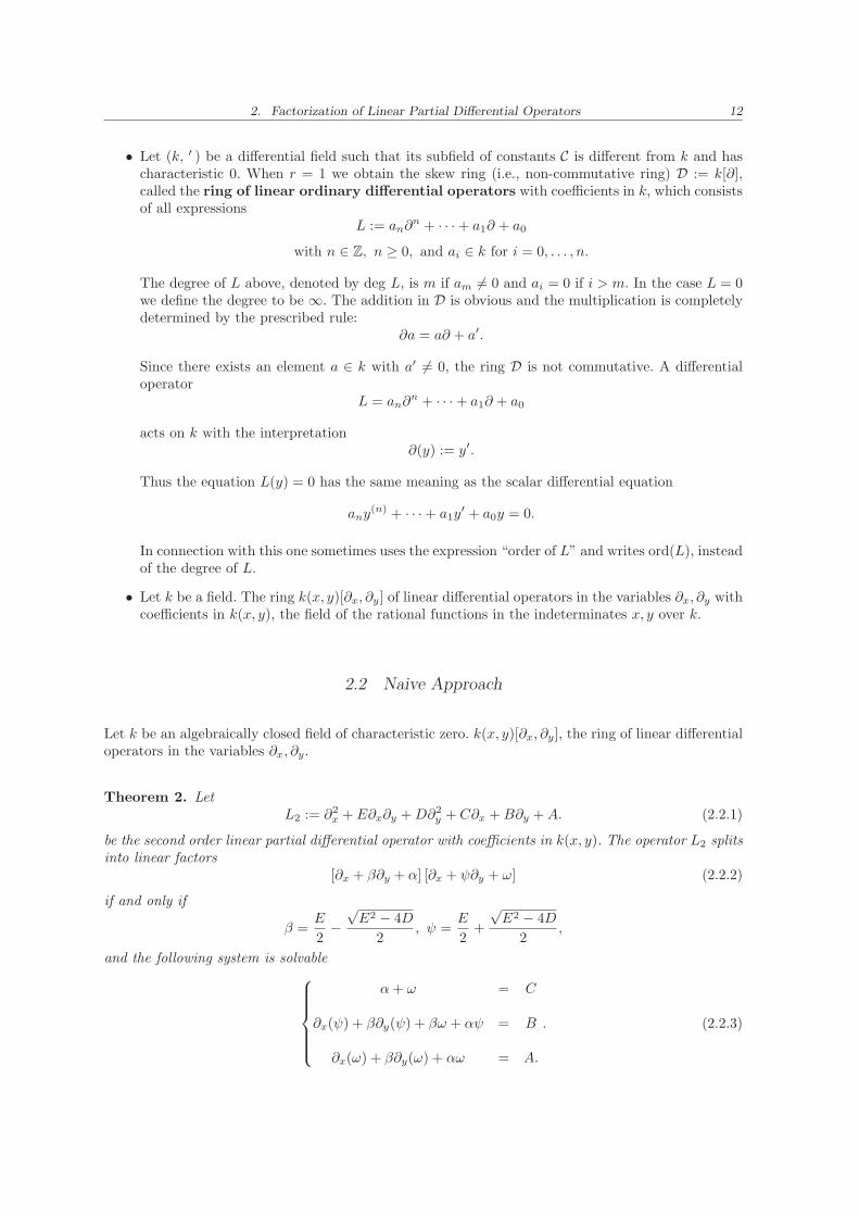
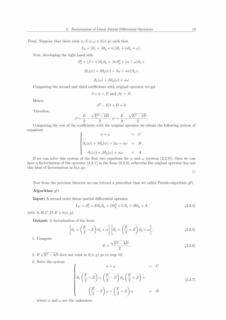
Theorem 2. LetL2 := ∂2
x + E∂x∂y +D∂2y + C∂x +B∂y +A. (2.2.1)
be the second order linear partial differential operator with coefficients in k(x, y). The operator L2 splitsinto linear factors
[∂x + β∂y + α] [∂x + ψ∂y + ω] (2.2.2)
if and only if
β =E
2−
√E2 − 4D
2, ψ =
E
2+
√E2 − 4D
2,
and the following system is solvable
α+ ω = C
∂x(ψ) + β∂y(ψ) + βω + αψ = B
∂x(ω) + β∂y(ω) + αω = A.
. (2.2.3)
2. Factorization of Linear Partial Differential Operators 13
Proof. Suppose that there exist α, β, ψ, ω ∈ k(x, y) such that
L2 = [∂x + β∂y + α] [∂x + ψ∂y + ω] .
Now, developing the right hand side
∂2x + (β + ψ)∂x∂y + βψ∂2
y + (α+ ω)∂x+
[∂x(ψ) + β∂y(ψ) + βω + αψ] ∂y+
∂x(ω) + β∂y(ω) + αω
Comparing the second and third coefficients with original operator we get
β + ψ = E and βψ = D.
Hence,β2 − Eβ +D = 0
Therefore,
β =E
2−
√E2 − 4D
2, ψ =
E
2+
√E2 − 4D
2,
Comparing the rest of the coefficients with the original operator we obtain the following system ofequations
α+ ω = C
∂x(ψ) + β∂y(ψ) + βω + αψ = B
∂x(ω) + β∂y(ω) + αω = A
.
If we can solve this system of the first two equations for α and ω (system (2.2.3)), then we canhave a factorization of the operator (2.2.1) in the form (2.2.2), otherwise the original operator has notthis kind of factorization in k(x, y).
Now from the previous theorem we can extract a procedure that we called Pseudo-algorithm gl1.
Algorithm gl1
Input: A second order linear partial differential operator
L2 := ∂2x +E∂x∂y +D∂2
y + C∂x +B∂y +A (2.2.4)
with A,B,C,D,E ∈ k(x, y).
Output: A factorization of the form:[∂x +
(E
2− Z
)∂y + α
] [∂x +
(E
2+ Z
)∂y + ω
]. (2.2.5)
1. Compute
Z =
√E2 − 4D
2. (2.2.6)
2. If√E2 − 4D does not exist in k(x, y) go to step 10.
3. Solve the system
α+ ω = C
∂x
(E
2+ Z
)+
(E
2− Z
)∂y
(E
2+ Z
)+
(E
2− Z
)ω +
(E
2+ Z
)α = B
(2.2.7)
where α and ω are the unknowns.
2. Factorization of Linear Partial Differential Operators 14
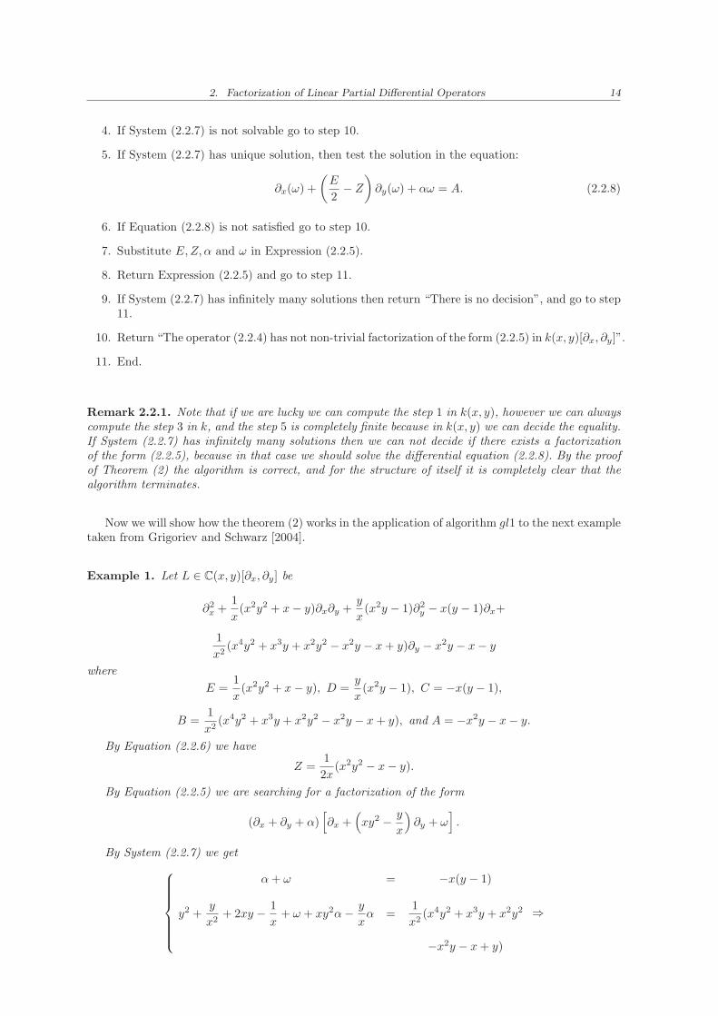
4. If System (2.2.7) is not solvable go to step 10.
5. If System (2.2.7) has unique solution, then test the solution in the equation:
∂x(ω) +
(E
2− Z
)∂y(ω) + αω = A. (2.2.8)
6. If Equation (2.2.8) is not satisfied go to step 10.
7. Substitute E,Z, α and ω in Expression (2.2.5).
8. Return Expression (2.2.5) and go to step 11.
9. If System (2.2.7) has infinitely many solutions then return “There is no decision”, and go to step11.
10. Return “The operator (2.2.4) has not non-trivial factorization of the form (2.2.5) in k(x, y)[∂x, ∂y]”.
11. End.
Remark 2.2.1. Note that if we are lucky we can compute the step 1 in k(x, y), however we can alwayscompute the step 3 in k, and the step 5 is completely finite because in k(x, y) we can decide the equality.If System (2.2.7) has infinitely many solutions then we can not decide if there exists a factorizationof the form (2.2.5), because in that case we should solve the differential equation (2.2.8). By the proofof Theorem (2) the algorithm is correct, and for the structure of itself it is completely clear that thealgorithm terminates.
Now we will show how the theorem (2) works in the application of algorithm gl1 to the next exampletaken from Grigoriev and Schwarz [2004].
Example 1. Let L ∈ C(x, y)[∂x, ∂y] be
∂2x +
1
x(x2y2 + x− y)∂x∂y +
y
x(x2y − 1)∂2
y − x(y − 1)∂x+
1
x2(x4y2 + x3y + x2y2 − x2y − x+ y)∂y − x2y − x− y
where
E =1
x(x2y2 + x− y), D =
y
x(x2y − 1), C = −x(y − 1),
B =1
x2(x4y2 + x3y + x2y2 − x2y − x+ y), and A = −x2y − x− y.
By Equation (2.2.6) we have
Z =1
2x(x2y2 − x− y).
By Equation (2.2.5) we are searching for a factorization of the form
(∂x + ∂y + α)[∂x +
(xy2 − y
x
)∂y + ω
].
By System (2.2.7) we get
α+ ω = −x(y − 1)
y2 +y
x2+ 2xy − 1
x+ ω + xy2α− y
xα =
1
x2(x4y2 + x3y + x2y2
−x2y − x+ y)
⇒
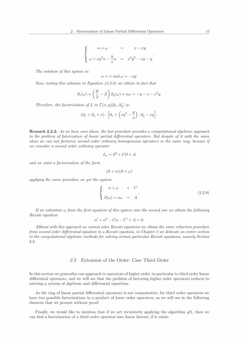
2. Factorization of Linear Partial Differential Operators 15
α+ ω = x− xy
ω + xy2α− y
xα = x2y2 − xy − y
.
The solution of this system is:α = x and ω = −xy.
Now, testing this solution in Equation (2.2.8) we obtain in fact that
∂x(ω) +
(E
2− Z
)∂y(ω) + αω = −y − x− x2y.
Therefore, the factorization of L in C(x, y)[∂x, ∂y] is:
(∂x + ∂y + x) ·[∂x +
(xy2 − y
x
)· ∂y − xy
].
Remark 2.2.2. As we have seen above, the last procedure provides a computational algebraic approachto the problem of fatorization of linear partial differential operators. But despite of it with the sameideas we can not factorize second order ordinary homogeneous operators in the same way, because ifwe consider a second order ordinary operator
Lo = ∂2 + C∂ +A
and we want a factorization of the form
(∂ + α)(∂ + ω)
applying the same procedure we get the system
α+ ω = C
∂(ω) + αω = A. (2.2.9)
If we substitute ω from the first equation of this system into the second one we obtain the followingRiccati equation
α′ + α2 − Cα− C ′ +A = 0.
Althout with this approach we cannot solve Riccati equations we obtain the same reduction procedurefrom second order differential equation to a Riccati equation, in Chapter 2 we dedicate an entire sectionto the computational algebraic methods for solving certain particular Riccati equations, namely Section3.3.
2.3 Extension of the Order: Case Third Order
In this section we generalize our approach to operators of higher order, in particular to third order lineardifferential operators, and we will see that the problem of factoring higher order operators reduces tosolveing a system of algebraic and differential equations.
As the ring of linear partial differential operators is not commutative, for third order operators wehave two possible factorizations in a product of lower order operators, as we will see in the followingtheorem that we present without proof.
Finally, we would like to mention that if we act recursively applying the algorithm gl1, then wecan find a factorization of a third order operator into linear factors, if it exists.
2. Factorization of Linear Partial Differential Operators 16
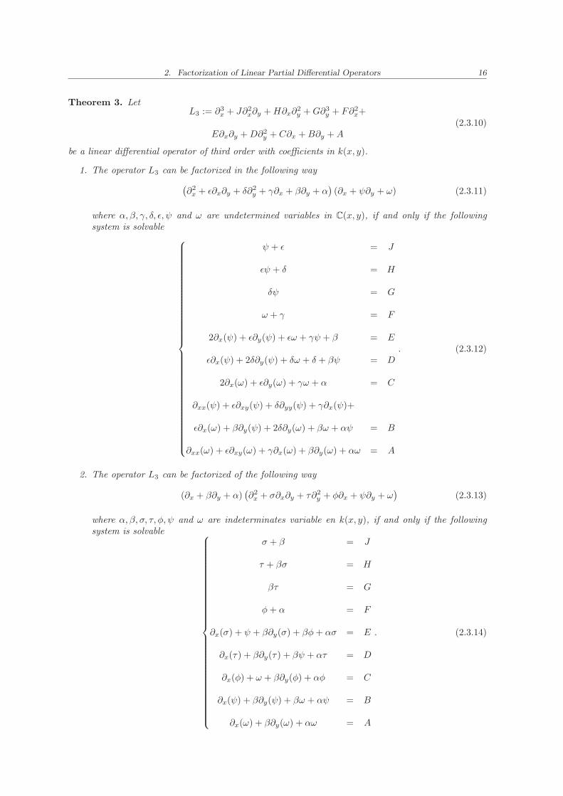
Theorem 3. LetL3 := ∂3
x + J∂2x∂y +H∂x∂
2y +G∂3
y + F∂2x+
E∂x∂y +D∂2y + C∂x +B∂y +A
(2.3.10)
be a linear differential operator of third order with coefficients in k(x, y).
1. The operator L3 can be factorized in the following way
(∂2
x + ǫ∂x∂y + δ∂2y + γ∂x + β∂y + α
)(∂x + ψ∂y + ω) (2.3.11)
where α, β, γ, δ, ǫ, ψ and ω are undetermined variables in C(x, y), if and only if the followingsystem is solvable
ψ + ǫ = J
ǫψ + δ = H
δψ = G
ω + γ = F
2∂x(ψ) + ǫ∂y(ψ) + ǫω + γψ + β = E
ǫ∂x(ψ) + 2δ∂y(ψ) + δω + δ + βψ = D
2∂x(ω) + ǫ∂y(ω) + γω + α = C
∂xx(ψ) + ǫ∂xy(ψ) + δ∂yy(ψ) + γ∂x(ψ)+
ǫ∂x(ω) + β∂y(ψ) + 2δ∂y(ω) + βω + αψ = B
∂xx(ω) + ǫ∂xy(ω) + γ∂x(ω) + β∂y(ω) + αω = A
. (2.3.12)
2. The operator L3 can be factorized of the following way
(∂x + β∂y + α)(∂2
x + σ∂x∂y + τ∂2y + φ∂x + ψ∂y + ω
)(2.3.13)
where α, β, σ, τ, φ, ψ and ω are indeterminates variable en k(x, y), if and only if the followingsystem is solvable
σ + β = J
τ + βσ = H
βτ = G
φ+ α = F
∂x(σ) + ψ + β∂y(σ) + βφ+ ασ = E
∂x(τ) + β∂y(τ) + βψ + ατ = D
∂x(φ) + ω + β∂y(φ) + αφ = C
∂x(ψ) + β∂y(ψ) + βω + αψ = B
∂x(ω) + β∂y(ω) + αω = A
. (2.3.14)
2. Factorization of Linear Partial Differential Operators 17
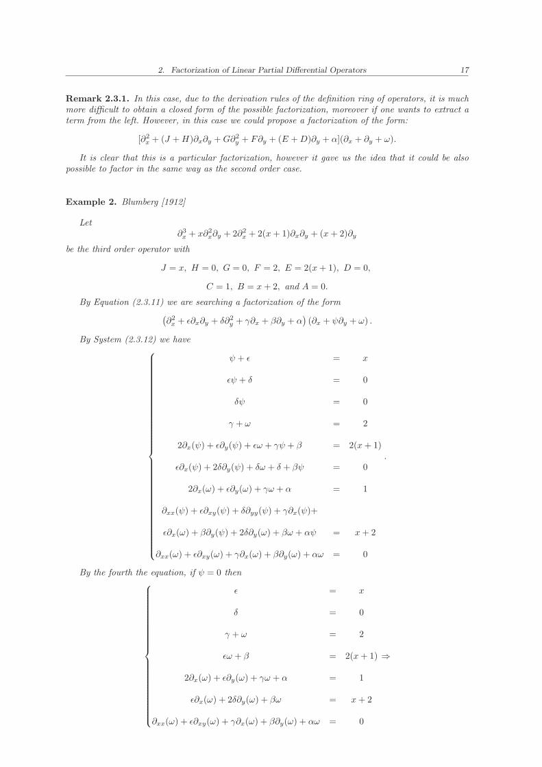
Remark 2.3.1. In this case, due to the derivation rules of the definition ring of operators, it is muchmore difficult to obtain a closed form of the possible factorization, moreover if one wants to extract aterm from the left. However, in this case we could propose a factorization of the form:
[∂2x + (J +H)∂x∂y +G∂2
y + F∂y + (E +D)∂y + α](∂x + ∂y + ω).
It is clear that this is a particular factorization, however it gave us the idea that it could be alsopossible to factor in the same way as the second order case.
Example 2. Blumberg [1912]
Let∂3
x + x∂2x∂y + 2∂2
x + 2(x+ 1)∂x∂y + (x+ 2)∂y
be the third order operator with
J = x, H = 0, G = 0, F = 2, E = 2(x+ 1), D = 0,
C = 1, B = x+ 2, and A = 0.
By Equation (2.3.11) we are searching a factorization of the form(∂2
x + ǫ∂x∂y + δ∂2y + γ∂x + β∂y + α
)(∂x + ψ∂y + ω) .
By System (2.3.12) we have
ψ + ǫ = x
ǫψ + δ = 0
δψ = 0
γ + ω = 2
2∂x(ψ) + ǫ∂y(ψ) + ǫω + γψ + β = 2(x+ 1)
ǫ∂x(ψ) + 2δ∂y(ψ) + δω + δ + βψ = 0
2∂x(ω) + ǫ∂y(ω) + γω + α = 1
∂xx(ψ) + ǫ∂xy(ψ) + δ∂yy(ψ) + γ∂x(ψ)+
ǫ∂x(ω) + β∂y(ψ) + 2δ∂y(ω) + βω + αψ = x+ 2
∂xx(ω) + ǫ∂xy(ω) + γ∂x(ω) + β∂y(ω) + αω = 0
.
By the fourth the equation, if ψ = 0 then
ǫ = x
δ = 0
γ + ω = 2
ǫω + β = 2(x+ 1)
2∂x(ω) + ǫ∂y(ω) + γω + α = 1
ǫ∂x(ω) + 2δ∂y(ω) + βω = x+ 2
∂xx(ω) + ǫ∂xy(ω) + γ∂x(ω) + β∂y(ω) + αω = 0
⇒
2. Factorization of Linear Partial Differential Operators 18
γ = 2 − ω
xω + β = 2(x+ 1)
2∂x(ω) + x∂y(ω) + γω + α = 1
x∂x(ω) + βω = x+ 2
∂xx(ω) + x∂xy(ω) + γ∂x(ω) + β∂y(ω) + αω = 0
⇒
γ = 2 − ω
xω + β = 2(x+ 1)
2∂x(ω) + x∂y(ω) + 2ω − ω2 + α = 1
x∂x(ω) + βω = x+ 2
∂xx(ω) + x∂xy(ω) + (2 − ω)∂x(ω) + β∂y(ω) + αω = 0
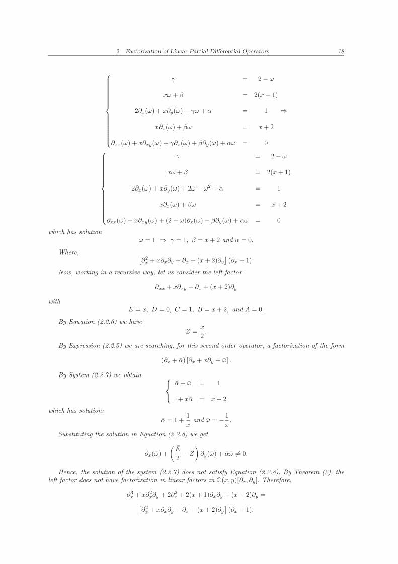
which has solutionω = 1 ⇒ γ = 1, β = x+ 2 and α = 0.
Where, [∂2
x + x∂x∂y + ∂x + (x+ 2)∂y
](∂x + 1).
Now, working in a recursive way, let us consider the left factor
∂xx + x∂xy + ∂x + (x+ 2)∂y
withE = x, D = 0, C = 1, B = x+ 2, and A = 0.
By Equation (2.2.6) we have
Z =x
2.
By Expression (2.2.5) we are searching, for this second order operator, a factorization of the form
(∂x + α) [∂x + x∂y + ω] .
By System (2.2.7) we obtain
α+ ω = 1
1 + xα = x+ 2
which has solution:
α = 1 +1
xand ω = − 1
x.
Substituting the solution in Equation (2.2.8) we get
∂x(ω) +
(E
2− Z
)∂y(ω) + αω 6= 0.
Hence, the solution of the system (2.2.7) does not satisfy Equation (2.2.8). By Theorem (2), theleft factor does not have factorization in linear factors in C(x, y)[∂x, ∂y]. Therefore,
∂3x + x∂2
x∂y + 2∂2x + 2(x+ 1)∂x∂y + (x+ 2)∂y =
[∂2
x + x∂x∂y + ∂x + (x+ 2)∂y
](∂x + 1).
2. Factorization of Linear Partial Differential Operators 19
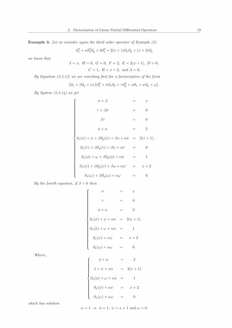
Example 3. Let us consider again the third order operator of Example (2)
∂3x + x∂2
x∂y + 2∂2x + 2(x+ 1)∂x∂y + (x+ 2)∂y
we know thatJ = x, H = 0, G = 0, F = 2, E = 2(x+ 1), D = 0,
C = 1, B = x+ 2, and A = 0.
By Equation (2.3.13) we are searching first for a factorization of the form
(∂x + β∂y + α)(∂2
x + σ∂x∂y + τ∂2y + φ∂x + ψ∂y + ω
).
By System (2.3.14) we get
σ + β = x
τ + βσ = 0
βτ = 0
φ+ α = 2
∂x(σ) + ψ + β∂y(σ) + βφ+ ασ = 2(x+ 1)
∂x(τ) + β∂y(τ) + βψ + ατ = 0
∂x(φ) + ω + β∂y(φ) + αφ = 1
∂x(ψ) + β∂y(ψ) + βω + αψ = x+ 2
∂x(ω) + β∂y(ω) + αω = 0
.
By the fourth equation, if β = 0 then
σ = x
τ = 0
φ+ α = 2
∂x(σ) + ψ + ασ = 2(x+ 1)
∂x(φ) + ω + αφ = 1
∂x(ψ) + αψ = x+ 2
∂x(ω) + αω = 0
.
Where,
φ+ α = 2
1 + ψ + xα = 2(x+ 1)
∂x(φ) + ω + αφ = 1
∂x(ψ) + αψ = x+ 2
∂x(ω) + αω = 0
which has solutionα = 1 ⇒ φ = 1, ψ = x+ 1 and ω = 0.
2. Factorization of Linear Partial Differential Operators 20
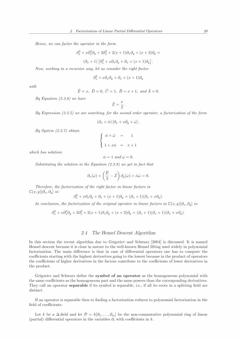
Hence, we can factor the operator in the form
∂3x + x∂2
x∂y + 2∂2x + 2(x+ 1)∂x∂y + (x+ 2)∂y =
(∂x + 1)[∂2
x + x∂x∂y + ∂x + (x+ 1)∂y
].
Now, working in a recursive way, let us consider the right factor
∂2x + x∂x∂y + ∂x + (x+ 1)∂y
withE = x, D = 0, C = 1, B = x+ 1, and A = 0.
By Equation (2.2.6) we have
Z =x
2.
By Expression (2.2.5) we are searching, for the second order operator, a factorization of the form
(∂x + α) [∂x + x∂y + ω] .
By System (2.2.7) obtain
α+ ω = 1
1 + xα = x+ 1
which has solution:α = 1 and ω = 0.
Substituting the solution in the Equation (2.2.8) we get in fact that
∂x(ω) +
(E
2− Z
)∂y(ω) + αω = 0.
Therefore, the factorization of the right factor in linear factors inC(x, y)[∂x, ∂y] is:
∂2x + x∂x∂y + ∂x + (x+ 1)∂y = (∂x + 1)(∂x + x∂y).
In conclusion, the factorization of the original operator in linear factors in C(x, y)[∂x, ∂y] is:
∂3x + x∂2
x∂y + 2∂2x + 2(x+ 1)∂x∂y + (x+ 2)∂y = (∂x + 1)(∂x + 1)(∂x + x∂y).
2.4 The Hensel Descent Algorithm
In this section the recent algorithm due to Grigoriev and Schwarz [2004] is discussed. It is namedHensel descent because it is close in nature to the well-known Hensel lifting used widely in polynomialfactorization. The main difference is that in case of differential operators one has to compute thecoefficients starting with the highest derivatives going to the lowest because in the product of operatorsthe coefficients of higher derivatives in the factors contribute to the coefficients of lower derivatives inthe product.
Grigoriev and Schwarz define the symbol of an operator as the homogeneous polynomial withthe same coefficients as the homogeneous part and the same powers than the corresponding derivatives.They call an operator separable if its symbol is separable, i.e., if all its roots in a splitting field aredistinct.
If an operator is separable then to finding a factorization reduces to polynomial factorization in thefield of coefficients.
Let k be a ∆-field and let D = k[∂1, . . . , ∂m] be the non-commutative polynomial ring of linear(partial) differential operators in the variables ∂i with coefficients in k.
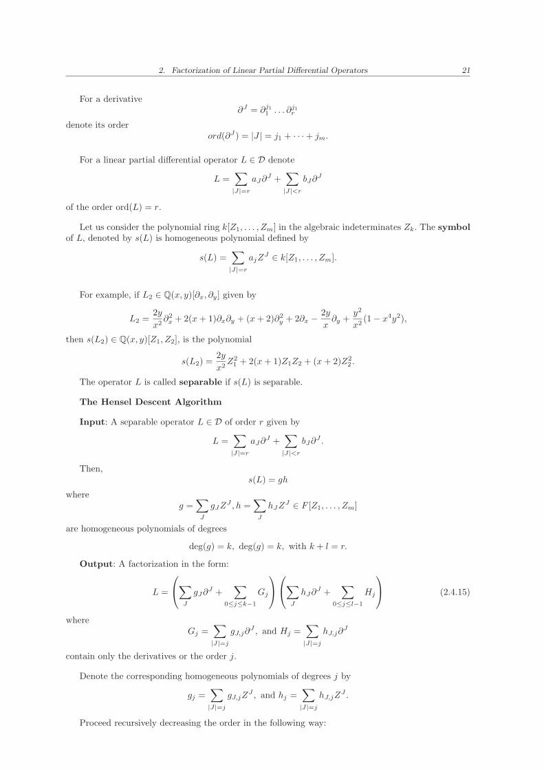
2. Factorization of Linear Partial Differential Operators 21
For a derivative∂J = ∂j1
1 . . . ∂j1r
denote its orderord(∂J ) = |J | = j1 + · · · + jm.
For a linear partial differential operator L ∈ D denote
L =∑
|J|=r
aJ∂J +
∑
|J|<r
bJ∂J
of the order ord(L) = r.
Let us consider the polynomial ring k[Z1, . . . , Zm] in the algebraic indeterminates Zk. The symbolof L, denoted by s(L) is homogeneous polynomial defined by
s(L) =∑
|J|=r
ajZJ ∈ k[Z1, . . . , Zm].
For example, if L2 ∈ Q(x, y)[∂x, ∂y] given by
L2 =2y
x2∂2
x + 2(x+ 1)∂x∂y + (x+ 2)∂2y + 2∂x − 2y
x∂y +
y2
x2(1 − x4y2),
then s(L2) ∈ Q(x, y)[Z1, Z2], is the polynomial
s(L2) =2y
x2Z2
1 + 2(x+ 1)Z1Z2 + (x+ 2)Z22 .
The operator L is called separable if s(L) is separable.
The Hensel Descent Algorithm
Input: A separable operator L ∈ D of order r given by
L =∑
|J|=r
aJ∂J +
∑
|J|<r
bJ∂J .
Then,s(L) = gh
whereg =
∑
J
gJZJ , h =
∑
J
hJZJ ∈ F [Z1, . . . , Zm]
are homogeneous polynomials of degrees
deg(g) = k, deg(g) = k, with k + l = r.
Output: A factorization in the form:
L =
∑
J
gJ∂J +
∑
0≤j≤k−1
Gj
∑
J
hJ∂J +
∑
0≤j≤l−1
Hj
(2.4.15)
whereGj =
∑
|J|=j
gJ,j∂J , and Hj =
∑
|J|=j
hJ,j∂J
contain only the derivatives or the order j.
Denote the corresponding homogeneous polynomials of degrees j by
gj =∑
|J|=j
gJ,jZJ , and hj =
∑
|J|=j
hJ,jZJ .
Proceed recursively decreasing the order in the following way:
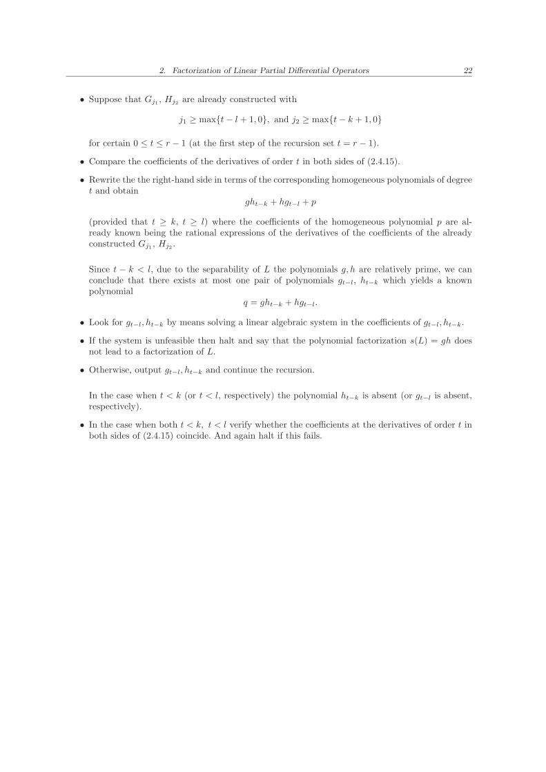
2. Factorization of Linear Partial Differential Operators 22
• Suppose that Gj1 , Hj2 are already constructed with
j1 ≥ max{t− l + 1, 0}, and j2 ≥ max{t− k + 1, 0}
for certain 0 ≤ t ≤ r − 1 (at the first step of the recursion set t = r − 1).
• Compare the coefficients of the derivatives of order t in both sides of (2.4.15).
• Rewrite the the right-hand side in terms of the corresponding homogeneous polynomials of degreet and obtain
ght−k + hgt−l + p
(provided that t ≥ k, t ≥ l) where the coefficients of the homogeneous polynomial p are al-ready known being the rational expressions of the derivatives of the coefficients of the alreadyconstructed Gj1 , Hj2 .
Since t − k < l, due to the separability of L the polynomials g, h are relatively prime, we canconclude that there exists at most one pair of polynomials gt−l, ht−k which yields a knownpolynomial
q = ght−k + hgt−l.
• Look for gt−l, ht−k by means solving a linear algebraic system in the coefficients of gt−l, ht−k.
• If the system is unfeasible then halt and say that the polynomial factorization s(L) = gh doesnot lead to a factorization of L.
• Otherwise, output gt−l, ht−k and continue the recursion.
In the case when t < k (or t < l, respectively) the polynomial ht−k is absent (or gt−l is absent,respectively).
• In the case when both t < k, t < l verify whether the coefficients at the derivatives of order t inboth sides of (2.4.15) coincide. And again halt if this fails.
Part II
FACTORIZATION OF LINEAR ORDINARY DIFFERENTIAL
OPERATORS
3. THE BEKE ALGORITHM
In 1894 Beke gave a method for factoring linear differential operators in the ring Q(x)[∂], and afteralmost one hundred years it has been improved and extended to the ring k(x)[∂] where k is an arbitrarydifferential field of characteristic 0. It has also been implemented in Computer Algebra Systems bySchwarz [1989], Schwarz [1994], Bronstein [1994], Bronstein and Petkovsek [1996].
Schwarz analyses the costs of factoring linear homogeneous differential equations with rationalcoefficients and he describes the algorithm of Beke in a different way by recursively reducing the orderof possible right factors. Moreover, he estimates bounds for the degree of their coefficients and hecomputes the size of rational solutions of certain differential equations. Finally, he describes how thealgorithm LODEF is implemented in the computer algebra system Scratchpat II.
The first section of this chapter is devoted to some basic preliminaries about differential Galoistheory of linear homogeneous differential equations. Subsequently, Sections 3.2 and 3.3 are developedto study the methods for finding rational and exponential solutions of linear homogeneous differentialequations. In section 3.4 we will present the Beke’s algorithm. In section 3.5 and 3.6 we present somevariants of the Beke’s algorithm, namely the Schwarz’s LODEF algorithm and the Beke-Bronsteinalgorithm, respectively.
3.1 Preliminaries
In ordinary Galois theory of algebraic equations, questions about solvability of equations are translatedinto questions about fields and finite groups. For differential equations, the proper setting is differentialfields and algebraic groups.
The goal of Differential Galois Theory is a Fundamental Theorem which sets up a bijective cor-respondence between the intermediate differential subfields of an extension of differential fields andcertain subgroups of the group of differential automorphisms of the field extension (the differentialGalois group).
Let (k, δ) be a differential field. We also write y(n) instead of δn(y) and y′, y′′, . . . for δ(y), δ2(y), . . ..The field of constants
Constδ(k) = {c ∈ k | c′ = 0}is denoted by C. A differential field extension of (k, δ) is a differential field (K,∆) such that K isa field extension of k and ∆ is an extension of the derivation of k to the derivation on K. An order nlinear scalar differential equation over k is an equation of the form
y(n) + an−1y(n−1) + · · · + a1y
′ + a0y = b (3.1.1)
where ai, b ∈ k. The equation is called homogeneous if b = 0, and inhomogeneous otherwise. Asolution of (3.1.1) in a differential extension K ⊇ k is an element f ∈ K such that
f (n) + an−1f(n−1) + · · · + a1f
′ + a0f = b.
A differential field extension (K,∆) of (k, δ) is called a Liouvillian extension if there is a towerof fields
k = K0 ⊂ K1 ⊂ · · · ⊂ Km = K
where Ki+1 is a simple field extension Ki(ηi) of Ki, such that one of the following holds:
3. The Beke Algorithm 25
• ηi is algebraic over Ki, or
• η′i ∈ Ki (extension by an integral), or
• η′i/ηi ∈ Ki (extension by the exponential of an integral).
A solution of L(y) = 0 which is contained in
• k, the coefficient field, will be called a rational solution,
• an algebraic extension of k will be called an algebraic solution,
• a Liouvillian extension of k will be called a Liouvillian solution.
A solution z of L(y) = 0 is called exponential if z′/z is in the coefficient field k.
Let A ∈ kn×n be an n×n matrix with entries in the field k. A linear system is a vector equationof the form
y′ = Ay. (3.1.2)
A solution of (3.1.2) in a differential extension K ⊇ k is an element v ∈ Kn such that v′ = Av.
The solution set of a linear system (3.1.2) in a given extension K ⊇ k is a vector space over C.The same is true for homogeneous linear scalar equations. Practically, both concepts describe the samesituation.
The companion matrix of a homogeneous scalar linear differential equation
L(y) = y(n) + an−1y(n−1) + · · · + a1y
′ + a0y = 0
is the matrix
AL =
0 1 0 . . . 00 0 1 . . . 0...
......
. . ....
0 0 0 . . . 1−a0 −a1 −a2 . . . an−1
.
In the following lemma we will see the relation between scalar equations and linear systems.
Lemma 1. Let j : k −→ kn be the map
f 7→ ( f, f ′, f (2), . . . , f (n−1) )T .
For any scalar equation L(y) = 0, the map j induces a C-linear isomorphism
{ f ∈ k |L(f) = 0 } ∼= { v ∈ kn | v′ = ALv }.
Proof. Let us write L in the form
L = y(n) + an−1y(n−1) + · · · + a1y
′ + a0y
If L(f) = 0 thenj(f)′ = AL · j(f).
Conversely, if v′ = ALv then
v2 = v′1, v3 = v(2)1 , . . . , vn = v
(n−1)1 and v′n = −a0v1 − a1v2 − · · · − an−1vn,
whence L(v1) = 0 and j(v1) = v.
3. The Beke Algorithm 26
Therefore, any homogeneous linear differential equation can be considered as a linear system. Thefollowing lemma describes the relation between linear dependency over the ground field k and itssubfield of constants C.
Lemma 2. Let A ∈ kn×n and consider solutions v1, v2, . . . , vr ∈ kn of the system y′ = Ay. If{v1, . . . , vr} is linearly dependent over k then also over C.
Proof. By induction over r. For r = 1 the statement is true, so let r > 1 and assume that v1, . . . , vr
are linearly dependent over k. Then
r∑
i=1
λivi = 0, λi ∈ k, not all λi = 0.
If a proper subset of {v1, . . . , vr} is linearly dependent over k then by induction hypothesis it islinearly dependent over C. So assume that all proper subsets are linearly independent. This impliesthat
λi 6= 0, for all i = 1, . . . , r,
and so
v1 =
r∑
i=2
− λi
λ1vi.
Writing αi = − λi
λ1we get
0 = v′1 −Av1 =
r∑
i=2
(α′ivi + αiv
′i) −Av1 =
r∑
i=2
α′ivi +A
r∑
i=2
αivi −Av1 =
r∑
i=2
α′ivi
and thus α′2 = · · · = α′
r = 0, which means that α2, . . . , αr ∈ Ck. Therefore,
v1 − α2v2 − · · · − αrvr = 0
shows that v1, . . . , vr are linearly dependent over Ck.
Corollary 4. A ∈ kn×n, K ⊇ k with const(K) = C. Then
dimC{x ∈ Kn |x′ = Ax } ≤ n.
Consider a matrix A ∈ kn×n, and assume for a moment, that the system y′ = Ay admits n C-linearly independent solutions v1, . . . , vn ∈ kn. Then the matrix F = (v1, . . . , vn) is non-singular andF ′ = AF .
Let K ⊇ k be a differential extension with Const(K) = C, A ∈ kn×n. A matrix F ∈ GLn(K) iscalled a fundamental matrix of the system y′ = Ay if F ′ = AF .
The Wronskian matrix of y1, . . . , yn ∈ k is the n× n matrix:
W (y1, . . . , yn) =
y1 y2 . . . yn
y′1 y′2 . . . y′n...
......
...
y(n−1)1 y
(n−1)2 . . . y
(n−1)n
.
The Wronskian, w(y1, . . . , yn) of y1, . . . , yn is det (W (y1, . . . , yn)).
3. The Beke Algorithm 27
Theorem 5. Let k be a differential field with field of constants C. Then n elements of k are linearlydependent over C if and only if their Wronskian vanishes.
Proof. Suppose y1, . . . , yn are linearly dependent over C, then there exist ci ∈ C for i = 1, . . . , n not allzero such that
c1y1 + . . .+ cnyn = 0.
On differentiating this equation n−1 times we get the n linear homogeneous equations for c1, . . . , cn:
c1y′1 + . . .+ cny
′n = 0
...
c1y(n−1)1 + . . .+ cny
(n−1)n = 0.
There are thus n equations to determine the constants c1, . . . , cn. Since the ci are not all 0, thedeterminant must vanish.
Conversely, suppose that the Wronskian of y1, . . . , yn vanishes. By induction we can construct amonic scalar differential equation L(y) = 0 of order n over k such that
L(yi) = 0 for i = 1, . . . , n.
For n = 1, put
L1(y) = y′ − y′1y1y,
where the termy′1y1
is interpreted as 0 if y1 = 0. Suppose, by induction hypothesis, that Lm(y) for
m ≥ 1, has been constructed such that
Lm(yi) = 0 for i = 1, . . . ,m.
Define now
Lm+1(y) = Lm(y)′ − Lm(ym+1)′
Lm(ym+1)Lm(y)
where the termLm(ym+1)
′
Lm(ym+1)is interpreted as 0 if Lm(ym+1) = 0. Whence,
Lm+1(yi) = 0 for i = 1, . . . ,m+ 1.
Then L = Ln has the required property. The columns of the Wronskian matrix are solutions of theassociated companion matrix differential equation y′ = ALy. By Lemma (2), y1, . . . , yn are linearlydependent over C.
A set of n solutions {y1, . . . , yn} of an order n equation L(y) = 0, linearly independent over theconstants C, is a fundamental set or fundamental system 1 of solutions of L(y) = 0.
Let k ⊂ K1 and k ⊂ K2 be extensions of differential fields. A field isomorphism σ : K1 → K2 is adifferential k-isomorphism if
(σ(a))′ = σ(a′), for all a ∈ K1 and
σ(a) = a for all a ∈ k.
The differential Galois group of a differential extension K of k, denoted by G(K/k), is the setof all k-automorphisms of K.
A differential extension field K of k is called a Picard-Vessiot extension of k for the equationL(y) = 0 if:
1 The term fundamental system is due to Fuchs, J. fur Math. 66 (1866), p. 126 [Ges. Math. Werke 1, p.165]
3. The Beke Algorithm 28
1. K is generates over k as a differential field by a fundamental set of solutions {y1, . . . , yn} ofL(y) = 0, i.e., K = k < y1, . . . , yn >;
2. K has the same field of constants as k, i.e., const(K) = C.
In other words, a Picard-Vessiot extension fieldK is the smallest differential field extension of k suchthat the equation has solution space dimension n over C. The Picard-Vessiot extension is the equivalentof the splitting field for an algebraic equation. If C is is algebraically closed and of characteristic 0,then there is always a Picard-Vessiot extension, unique up to differential isomorphisms. See Kaplansky[1957], p. 21 or Kolchin [1948], p. 412.
Proposition 1. Let k be a differential field of characteristic 0 with algebraically closed subfield ofconstants C. Let L(y) = 0 be a linear differential equation over k. Then,
1. there exists a Picard-Vessiot extension for the equation,
2. any two Picard-Vessiot extensions for the equation are isomorphic.
Let k be a differential field of characteristic 0 with algebraically closed subfield of constants C.Let L(y) = 0 be a linear differential equation over k. Let K be the Picard-Vessiot extension of k forL(x) = 0, and write
V (L) = {f ∈ K |L(f) = 0}for the space of solutions. V (L) is generated as C-vector space by n C-linearly independent solutionsy1, . . . , yn. The Galois group of L(y) = 0, denoted by Gal(K/k), is the differential Galois groupG(K/k) of the Picard-Vessiot extension K . A computational representation of Gal(K/k) is obtainedas follows:
Assume that f ∈ V (L), then for any automorphism σ ∈ Gal(K/k) we have
L (σ(f)) = σ (L(f)) = 0.
In other words, each automorphism moves a solution of L(y) = 0 to another solution. Consequently,σ(f) is a linear C-combination of the yi’s. This yields a matrix representation of Gal(K/k).
Thus Gal(K/k) acts faithfully on the vector space V (L), and so Gal(K/k) can be viewed asa subgroup of GL(V (L)); more precisely, it is a linear algebraic group over C. There is a Galoiscorrespondence between algebraic subgroups of G and differential subfields of K. The fixed field ofGal(K/k) under this correspondence is k.
A linear differential equation L(y) = 0 defined over k is said to be solvable in terms of lineardifferential equations of lower order if the associated Picard-Vessiot extension K of k lies in atower of fields
k = k0 ⊂ k1 ⊂ · · · ⊂ kn,
where ki = ki−1(ti), and ti is algebraic over ki−1, or ti satisfies a linear differential equation of lowerorder defined over ki−1, for each i.
It has been shown in Singer [1989] that L(y) = 0 is solvable in terms of Liouvillian solutions (i.e., itsPicard-Vessiot extension lies in a Liouvillian extension of k) if and only if its Galois group Gal(K/k)contains a solvable (in the algebraic sense) subgroup of finite index. However, finding Liouvilliansolutions is still hard and one attempt is to find these solutions by effectively searching over a boundedspace (see Singer [1981]).
3. The Beke Algorithm 29
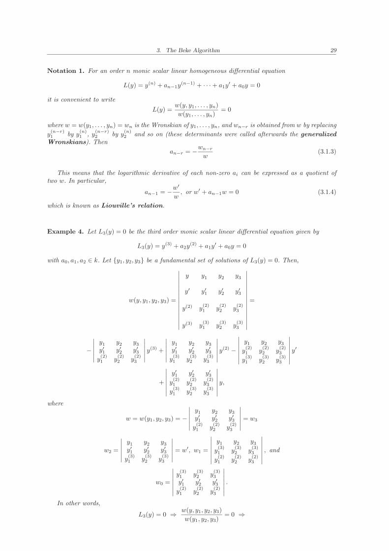
Notation 1. For an order n monic scalar linear homogeneous differential equation
L(y) = y(n) + an−1y(n−1) + · · · + a1y
′ + a0y = 0
it is convenient to write
L(y) =w(y, y1, . . . , yn)
w(y1, . . . , yn)= 0
where w = w(y1, . . . , yn) = wn is the Wronskian of y1, . . . , yn, and wn−r is obtained from w by replacing
y(n−r)1 by y
(n)1 , y
(n−r)2 by y
(n)2 and so on (these determinants were called afterwards the generalized
Wronskians). Then
an−r = −wn−r
w(3.1.3)
This means that the logarithmic derivative of each non-zero ai can be expressed as a quotient oftwo w. In particular,
an−1 = −w′
w, or w′ + an−1w = 0 (3.1.4)
which is known as Liouville’s relation.
Example 4. Let L3(y) = 0 be the third order monic scalar linear differential equation given by
L3(y) = y(3) + a2y(2) + a1y
′ + a0y = 0
with a0, a1, a2 ∈ k. Let {y1, y2, y3} be a fundamental set of solutions of L3(y) = 0. Then,
w(y, y1, y2, y3) =
∣∣∣∣∣∣∣∣∣∣∣∣∣∣∣
y y1 y2 y3
y′ y′1 y′2 y′3
y(2) y(2)1 y
(2)2 y
(2)3
y(3) y(3)1 y
(3)2 y
(3)3
∣∣∣∣∣∣∣∣∣∣∣∣∣∣∣
=
−
∣∣∣∣∣∣
y1 y2 y3y′1 y′2 y′3y(2)1 y
(2)2 y
(2)3
∣∣∣∣∣∣y(3) +
∣∣∣∣∣∣
y1 y2 y3y′1 y′2 y′3y(3)1 y
(3)2 y
(3)3
∣∣∣∣∣∣y(2) −
∣∣∣∣∣∣∣
y1 y2 y3y(2)1 y
(2)2 y
(2)3
y(3)1 y
(3)2 y
(3)3
∣∣∣∣∣∣∣y′
+
∣∣∣∣∣∣∣
y′1 y′2 y′3y(2)1 y
(2)2 y
(2)3
y(3)1 y
(3)2 y
(3)3
∣∣∣∣∣∣∣y,
where
w = w(y1, y2, y3) = −
∣∣∣∣∣∣
y1 y2 y3y′1 y′2 y′3y(2)1 y
(2)2 y
(2)3
∣∣∣∣∣∣= w3
w2 =
∣∣∣∣∣∣
y1 y2 y3y′1 y′2 y′3y(3)1 y
(3)2 y
(3)3
∣∣∣∣∣∣= w′, w1 =
∣∣∣∣∣∣∣
y1 y2 y3y(3)1 y
(3)2 y
(3)3
y(2)1 y
(2)2 y
(2)3
∣∣∣∣∣∣∣, and
w0 =
∣∣∣∣∣∣∣
y(3)1 y
(3)2 y
(3)3
y′1 y′2 y′3y(2)1 y
(2)2 y
(2)3
∣∣∣∣∣∣∣.
In other words,
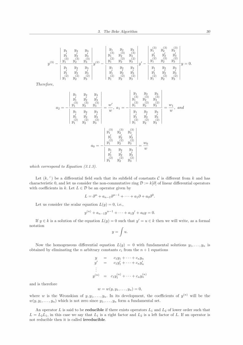
L3(y) = 0 ⇒ w(y, y1, y2, y3)
w(y1, y2, y3)= 0 ⇒
3. The Beke Algorithm 30
y(3) −
∣∣∣∣∣∣
y1 y2 y3y′1 y′2 y′3y(3)1 y
(3)2 y
(3)3
∣∣∣∣∣∣∣∣∣∣∣∣
y1 y2 y3y′1 y′2 y′3y(2)1 y
(2)2 y
(2)3
∣∣∣∣∣∣
y(2) −
∣∣∣∣∣∣∣
y1 y2 y3y(3)1 y
(3)2 y
(3)3
y(2)1 y
(2)2 y
(2)3
∣∣∣∣∣∣∣∣∣∣∣∣∣
y1 y2 y3y′1 y′2 y′3y(2)1 y
(2)2 y
(2)3
∣∣∣∣∣∣
y′ −
∣∣∣∣∣∣∣
y(3)1 y
(3)2 y
(3)3
y′1 y′2 y′3y(2)1 y
(2)2 y
(2)3
∣∣∣∣∣∣∣∣∣∣∣∣∣
y1 y2 y3y′1 y′2 y′3y(2)1 y
(2)2 y
(2)3
∣∣∣∣∣∣
y = 0.
Therefore,
a2 = −
∣∣∣∣∣∣
y1 y2 y3y′1 y′2 y′3y(3)1 y
(3)2 y
(3)3
∣∣∣∣∣∣∣∣∣∣∣∣
y1 y2 y3y′1 y′2 y′3y(2)1 y
(2)2 y
(2)3
∣∣∣∣∣∣
=w′
w, a1 = −
∣∣∣∣∣∣∣
y1 y2 y3y(3)1 y
(3)2 y
(3)3
y(2)1 y
(2)2 y
(2)3
∣∣∣∣∣∣∣∣∣∣∣∣∣
y1 y2 y3y′1 y′2 y′3y(2)1 y
(2)2 y
(2)3
∣∣∣∣∣∣
=w1
w, and
a0 = −
∣∣∣∣∣∣∣
y(3)1 y
(3)2 y
(3)3
y′1 y′2 y′3y(2)1 y
(2)2 y
(2)3
∣∣∣∣∣∣∣∣∣∣∣∣∣
y1 y2 y3y′1 y′2 y′3y(2)1 y
(2)2 y
(2)3
∣∣∣∣∣∣
=w0
w
which correspond to Equation (3.1.3).
Let (k, ′ ) be a differential field such that its subfield of constants C is different from k and hascharacteristic 0, and let us consider the non-commutative ring D := k[∂] of linear differential operatorswith coefficients in k. Let L ∈ D be an operator given by
L = ∂n + an−1∂n−1 + · · · + a1∂ + a0∂
0.
Let us consider the scalar equation L(y) = 0, i.e.,
y(n) + an−1yn−1 + · · · + a1y
′ + a0y = 0.
If y ∈ k is a solution of the equation L(y) = 0 such that y′ = u ∈ k then we will write, as a formalnotation
y =
∫u.
Now the homogeneous differential equation L(y) = 0 with fundamental solutions y1, . . . , yn isobtained by eliminating the n arbitrary constants ci from the n+ 1 equations
y = c1y1 + · · · + cnyn
y′ = c1y′1 + · · · + cny
′n
...
y(n) = c1y(n)1 + · · · + cny
(n)n
and is thereforew = w(y, y1, . . . , yn) = 0,
where w is the Wronskian of y, y1, . . . , yn. In its development, the coefficients of y(n) will be thew(y, y1, . . . , yn) which is not zero since y1, . . . , yn form a fundamental set.
An operator L is said to be reducible if there exists operators L1 and L2 of lower order such thatL = L2L1, in this case we say that L1 is a right factor and L2 is a left factor of L. If an operator isnot reducible then it is called irreducible.
3. The Beke Algorithm 31
Remark 3.1.1. If we interpret this definition in terms of the scalar equation we can say, in the oldfashion way, that:
“A linear homogeneous differential equation is called irreducible when it is has no common solu-tions with any other linear homogeneous differential equation of inferior order with the same kind ofcoefficients.”
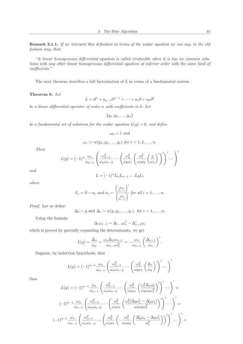
The next theorem describes a full factorization of L in terms of a fundamental system.
Theorem 6. LetL = ∂n + an−1∂
n−1 + · · · + a1∂ + a0∂0
be a linear differential operator of order n with coefficients in k. Let
{y1, y2, . . . , yn}
be a fundamental set of solutions for the scalar equation L(y) = 0, and define
ω0 = 1 and
ωr := w(y1, y2, . . . , yr) for r = 1, 2, . . . , n.
Then
L(y) = (−1)n ωn
ωn−1
ω2
n−1
ωnωn−2· · ·(
ω22
ω3ω1
(ω2
1
ω2ω0
(y
ω1
)′)′)′
· · ·
′
andL = (−1)nLnLn−1 . . . L2L1
where
Li = ∂ − αi and αi =
(ωi
ωi−1
)′
(ωi
ωi−1
) for all i = 1, . . . , n.
Proof. Let us define∆0 = y and ∆r = w(y, y1, . . . , yr), for r = 1, . . . , n.
Using the formula∆rωr−1 = ∆r−1ω
′r − ∆′
r−1ωr
which is proved by partially expanding the determinants, we get
L(y) =∆n
ωn=ωn∆nωn−1
ωn−1ω2n
= − ωn
ωn−1
(∆n−1
ωn
)′.
Suppose, by induction hypothesis, that
L(y) = (−1)n−1 ωn
ωn−1
(ω2
n−1
ωnωn−2· · ·(
ω22
ω3ω1
(∆1
ω2
)′)′
· · ·)′
then
L(y) = (−1)n−1 ωn
ωn−1
(ω2
n−1
ωnωn−2· · ·(
ω22
ω3ω1
(ω2
1∆1ω0
ω2ω0ω21
)′)′
· · ·)′
=
(−1)n−1 ωn
ωn−1
(ω2
n−1
ωnωn−2· · ·(
ω22
ω3ω1
(ω2
1(∆0ω′1 − ∆′
0ω1)
ω2ω0ω21
)′)′
· · ·)′
=
(−1)n−1 ωn
ωn−1
(ω2
n−1
ωnωn−2· · ·(
ω22
ω3ω1
(− ω2
1
ω2ω0
(∆′
0ω1 − ∆0ω′1
ω21
))′)′
· · ·)′
=
3. The Beke Algorithm 32
(−1)n ωn
ωn−1
ω2
n−1
ωnωn−2· · ·(
ω22
ω3ω1
(ω2
1
ω2ω0
(∆0
ω1
)′)′)′
· · ·
′
.
Therefore,
L(y) = (−1)n ωn
ωn−1
ω2
n−1
ωnωn−2· · ·(
ω22
ω3ω1
(ω2
1
ω2ω0
(y
ω1
)′)′)′
· · ·
′
and using the fact that ω0 = 1 by definition, we obtain
L(y) = (−1)n ωn
ωn−1
ωn−1
ωn
ωn−1
ωn−2· · ·(ω2
ω3
ω2
ω1
(ω1
ω2ω1
(y
ω1
)′)′)′
· · ·
′
.
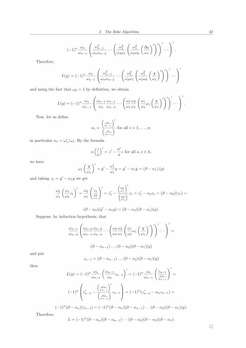
Now, let us define
αi =
(ωi
ωi−1
)′
(ωi
ωi−1
) for all i = 1, . . . , n;
in particular α1 = ω′1/ω1. By the formula
a(za
)′= z′ − a′
az for all a, z ∈ k,
we have
ω1
(y
ω1
)′= y′ − ω′
1
ω1y = y′ − α1y = (∂ − α1) (y)
and taking z1 = y′ − α1y we get
ω2
ω1
(ω1
ω2z1
)′=ω2
ω1
(z1ω2
ω1
)′
= z′1 −
(ω2
ω1
)′
(ω2
ω1
) z1 = z′1 − α2z1 = (∂ − α2)(z1) =
(∂ − α2)(y′ − α1y) = (∂ − α2)(∂ − α1)(y).
Suppose, by induction hypothesis, that
ωn−1
ωn−2
ωn−2
ωn−1
ωn−2
ωn−3· · ·(ω2
ω3
ω2
ω1
(ω1
ω2ω1
(y
ω1
)′)′)′
· · ·
′
=
(∂ − αn−1) . . . (∂ − α2)(∂ − α1)(y)
and putzn−1 = (∂ − αn−1) . . . (∂ − α2)(∂ − α1)(y)
then
L(y) = (−1)n ωn
ωn−1
(ωn−1
ωnzn−1
)′= (−1)n ωn
ωn−1
(zn−1
ωn
ωn−1
)′
=
(−1)n
z′n−1 −
(ωn
ωn−1
)′
(ωn
ωn−1
) zn−1
= (−1)n(z′n−1 − αnzn−1) =
(−1)n(∂ − αn)(zn−1) = (−1)n(∂ − αn)(∂ − αn−1) . . . (∂ − α2)(∂ − α1)(y).
Therefore,L = (−1)n(∂ − αn)(∂ − αn−1) · · · (∂ − α3)(∂ − α2)(∂ − α1).
3. The Beke Algorithm 33
Remark 3.1.2. Note that the order of the factors (∂ − αi) must in general be preserved, for it is nottrue for any two suffixes i and j
(∂ − αi)(∂ − αj) = (∂ − αj)(∂ − αi).
In other words, the factors of the differential operator are in general not permutable (Landau [1902]).
3.2 Rational Solutions of Linear Differential Equations
In this section we present a method for finding rational solutions of linear differential equations withcoefficients in k(x) in case char(k) = 0 and ordinary derivative d/dx. This method generalizes the wellknown Frobenius method for solving second-order ordinary differential equations relative to a singularpoint, like e.g. the Euler equation, the hypergeometric equation or equations of Fuchsian type. See forinstance Ince [1964]), Cohen, Cuypers, and Sterk [1999] (for equations of third order) and van der Putand Singer [2003]. It will appear again later in connection with finding exponential solutions of lineardifferential equations. Although the coefficients of the linear differential equations that we considerhere are in k(x), we will work in the field k((x)) of formal Laurent series. In the sequel we denote thealgebraic closure of an arbitrary field K by K.
Let k be a field of characteristic 0 and k[[x]] the ring of formal power series. A typical element ofk[[x]] is
∞∑
i=0
aixi, where ai ∈ k.
The quotient field of k[[x]], denoted by k((x)), is the field of formal Laurent series. k((x)) is containedin the algebraically closed field of formal Puiseux series
⋃
n∈N
k((x1/n)),
A typical non-zero element a ∈ k((x)) can be written as
a = xm∑
j≥0
ajxj where a0 6= 0 and m ∈ Z.
The order ord(a) of a is the exponent m of the first non-vanishing term of a. By definition ord(0) =∞. In Chapter 4 we present more details on Puiseux series.
We consider k(x) and k((x)) as differential fields equipped with derivation ∂ = d/dx.
Let L ∈ k(x)[∂] be the operator
L = ∂n + an−1∂n−1 + · · · + a1∂ + a0∂
0.
We write the coefficients of L as partial fractions
ai =
di∑
j=0
pi,jxj +
s∑
σ=1
−1∑
j=dσi
qσi,j(x− xσ)j +
t∑
τ=1
eτi∑
j=1
Bτi,j(x)
Aτ (x)j, for all i.
An element a ∈ k((x)) is said to have a pole of order n at x = x0, if in the Laurent series, am = 0for m < −n and an 6= 0, i.e.,
a =∑
i≥n
ai(x− x0)i.
a is said to have a pole of order n at ∞, if the Laurent series of a ∈ k((x−1)) at 0 has onlyfinitely many negative degree terms, starting with −n.
3. The Beke Algorithm 34
Proposition 2. A solution f of the equation
y(n) + an−1y(n−1) + · · · + a1y
(1) + a0y = 0
can only have a pole at α if at least one of the ai has a pole at α. Also, ∞ is a possible pole of f .Hence the location of the possible poles of f is known.
Proof. Suppose that f has a pole at 0 of order s. Then the expansion of f at 0 is
xs + ls+1xs+1 + · · · with s < 0.
If ai(0) 6= 0 for all i, then the lowest power of x in the equation
y(n) + an−1y(n−1) + · · · + a1y
′ + a0y = 0
is s − n and it would appear in only one member, namely the first one y(n) and as a consequence itmust have 0 as a coefficient, i.e.,
s(s− 1)(s− 2) . . . (s− n+ 1) = 0.
Then, s = 0, s = 1, ... , s = n− 1. In any case, s ≥ 0 which is a contradiction.
If it exists, a rational solution of the scalar equation L(y) = 0 has the form
f =M∑
j=0
pjxj +
s∑
σ=1
−1∑
j=Mσ
qσj (x− xσ)j +
t∑
τ=1
Nτ∑
j=1
Bτj (x)
Aτ (x)j+
N∑
i=1
γi
x− ci.
Let p ∈ k((x)) be given by
p = xm∑
i≥0
pixi, where p0 6= 0 and m ∈ Z.
The indicial polynomial Ip(m) in m (seen as variable) of degree ≤ n, for the linear differentialequation
y(n) + an−1y(n−1) + · · · + a1y
(1) + a0y = 0
at 0 is the coefficient of the term of lowest degree of x after substituting p in the differential equation.It is obvious that Ip(m) will be independent of the coefficients a1, a2, . . . , and will involve a0 as amultiplicative factor. The roots of Ip(m) (in an algebraic closure of k) are called local exponents of theequation at 0. The equation Ip(m) = 0 is called the indicial equation.
Now we are ready to present the algorithm.
Algorithm:
Let us consider the equation
y(n) + an−1y(n−1) + · · · + a0y = 0 (3.2.5)
where some ai ∈ k(x) has a pole at 0. Suppose that the expansion of f in the Laurent series at 0 is
f =u
v= xs + ls+1x
s+1 + · · · with s ∈ Z and s < 0.
The expansion of the ai in Laurent series at 0 is written as
ai =∑
j≥ni
ai,jxj for all i,
3. The Beke Algorithm 35
where ai,ni∈ k∗ and ni ∈ Z. If ai = 0 we put ni = ∞ and ai,ni
has no meaning. Then the lowestpower of x in Equation (3.2.5) are
s(s− 1)(s− 2) . . . (s− n+ 1)xs−n,
s(s− 1)(s− 2) . . . (s− n+ 1)(s− n+ 2)an−1,nn−1xs−n+1+nn−1 ,
...
sa1,n1xs−1+n1 , and
a0,n0xs+n0 .
Let m denote the minimum of {−n,−n+ 1 + nn−1, . . . ,−1 + n1, n0}. The coefficient I(s) of xs+m
can be written as
ǫ1s(s− 1)(s− 2) . . . (s− n+ 1)+
+ǫ2s(s− 1)(s− 2) . . . (s− n+ 1)(s− n+ 2)an−1,nn−1+ · · ·+
ǫ1sa1,n1+ ǫ0a0,n0
,
where ǫi = 1 if the corresponding element in
{−n,−n+ 1 + nn−1, . . . ,−1 + n1, n0}
is minimal and ǫi = 0 otherwise.
The expression for I is a non-zero polynomial in s (seen as a variable) of degree ≤ n, this is preciselythe indicial polynomial for Equation (3.2.5) at 0.
Since f satisfies Equation (3.2.5) the coefficient I(s) of xs+m must be 0. Thus s is a solution of theequation
I(s) = 0
which is exactly the indicial equation for Equation (3.2.5) at 0. We have three possibilities, namely
1. If there is no s with I(s) = 0 then we can stop the calculations since in that case there is norational solution f 6= 0 of the equation.
2. If there is no negative integer s with I(s) = 0 but there is an integer r ≥ 0 then we define s0 = 0.
3. If there is a negative integer solution of I(s) = 0 then s0 < 0 denotes the smallest one.
In other words, the possible values s for the exact power xs are the negative integers s with I(s) = 0.
Now we perform a similar calculation at ∞. Let ords(f) denote the order of the function f at thepoint s.
Let αi denote the poles of ai. For every i, the method above yields an integer si ≤ 0 such that, forany rational solution f 6= 0, one has ordαi
(f) ≥ si, or there are no rational solutions.
This means that (working in the Laurent series field k((x−1))) we can write
f =T
N∈ k(x)∗
with knownN =
∏
i
(x− αi)−si and with some polynomial T.
3. The Beke Algorithm 36
In order to estimate the degree of T let us consider the expansions in Laurent series of f and the ai
at ∞ (i.e., we make a calculation in the differential field k((x−1))). Suppose that the expansions havethe form
f = xt + gt+1xt+1 + · · · and
ai =∑
j≥mi
bi,jxj for all i.
If ai 6= 0, then bi,mi∈ k∗ and mi ∈ Z. If ai = 0 then we put mi = −∞ and bi,mi
has no meaning.Then, the possible highest power of x in Equation (3.2.5) are
t(t+ 1)(t+ 2) . . . (t+ n+ 1)xt−n,
t(t+ 1)(t+ 2) . . . (t+ n+ 1)(t+ n+ 2)bn−1,mn−1xt−n+1+mn−1 ,
...
tb1,m1xt−1+m1 , and
b0,m0xt+m0 .
Let M denote the maximum of {−n,−n+ 1 +mn−1, . . . ,−1 +m1,m0}. Let J(t) be the expression
ǫ1t(t+ 1)(t+ 2) . . . (t+ n+ 1)+
ǫ2t(t+ 1)(t+ 2) . . . (t+ n+ 1)(t+ n+ 2)bn−1,mn−1+ · · ·+
ǫ1tb1,m1+ ǫ0b0,m0
,
where ǫi = 1 if the corresponding term is equal to M and ǫi = 0 otherwise.
Then J(t) is a non-zero polynomial of degree ≤ n in t (seen as a variable). This is the indicialpolynomial of Equation (3.2.5) at ∞.
If there is no integer t with J(t) = 0 then we stop the procedure. In other case, let s∞ denote thelargest integer that is a zero in J . Then we find that t ≤ s∞.
Expanding f =T
Nat ∞ leads to the inequality
deg(T ) ≤ s∞ + deg(N).
Let d be the bound for the degree of T and write
T = tdxd + · · · + t0.
The equation satisfied by f provides an order n equation for T . This leads to a set of linear equationsfor the coefficients ti. With linear algebra one can find all solutions. This ends the algorithm.
Example 5. Consider the equation
y(3) − 8x2 − 63x− 27
(24x+ 27)xy(2) +
448x2 + 1080x+ 1080
3(8x+ 9)2xy(1) − 24
(8x+ 9)2xy = 0
with coefficients in partial fraction decomposition
a2 = −1
3+
16
8x+ 9+
1
x, a1 = − 152
9(8x+ 9)− 128
(8x+ 9)2+
40
9x, and
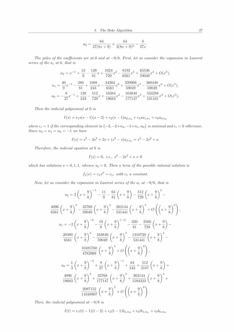
3. The Beke Algorithm 37
a0 =64
27(8x+ 9)+
64
3(8x+ 9)2− 8
27x.
The poles of the coefficients are at 0 and at −9/8. First, let us consider the expansion in Laurentseries of the ai at 0, that is
a2 = x−1 +13
9− 128
81x+
1024
729x2 − 8192
6561x3 +
65536
59049x4 +O(x5),
a1 =40
9x−1 − 280
81+
1088
243x− 34304
6561x2 +
339968
59049x3 − 360448
59049x4 +O(x5),
a0 = − 8
27x−1 +
128
243− 512
729x+
16384
19683x2 − 163840
177147x3 +
524288
531441x4 +O(x5).
Then the indicial polynomial at 0 is
I(s) = ǫ1s(s− 1)(s− 2) + ǫ2(s− 1)a2,n2+ ǫ3sa1,n1
+ ǫ0a0,n0
where ǫi = 1 if the corresponding element in {−3,−2+n2,−1+n1, n0} is minimal and ǫi = 0 otherwise.Since n2 = n1 = n0 = −1 we have
I(s) = s3 − 3s2 + 2s+ (s2 − s)a2,n2= s3 − 2s2 + s.
Therefore, the indicial equation at 0 is
I(s) = 0, i.e., s3 − 2s2 + s = 0
which has solutions s = 0, 1, 1, whence s0 = 0. Then a term of the possible rational solution is
f1(x) = c1x0 = c1, with c1 a constant.
Now, let us consider the expansion in Laurent series of the ai at −9/8, that is
a2 = 2
(x+
9
8
)−1
− 11
9− 64
81
(x+
9
8
)− 512
729
(x+
9
8
)2
−
4096
6561
(x+
9
8
)3
− 32768
59049
(x+
9
8
)4
− 262144
531441
(x+
9
8
)5
+O
((x+
9
8
)6),
a1 = −2
(x+
9
8
)−2
− 19
9
(x+
9
8
)(−1)
− 320
81− 2560
729
(x+
9
8
)−
20480
6561
(x+
9
8
)2
− 163840
59049
(x+
9
8
)3
− 1310720
531441
(x+
9
8
)4
−
10485760
4782969
(x+
9
8
)5
+O
((x+
9
8
)6),
a0 =1
3
(x+
9
8
)−2
+8
27
(x+
9
8
)−1
+64
243+
512
2187
(x+
9
8
)+
4096
19683
(x+
9
8
)2
+32768
177147
(x+
9
8
)3
+262144
1594323
(x+
9
8
)4
+
2097152
14348907
(x+
9
8
)5
+O
((x+
9
8
)6).
Then, the indicial polynomial at −9/8 is
I(t) = ǫ1t(t− 1)(t− 2) + ǫ2(t− 1)b2,m2+ ǫ3tb1,m1
+ ǫ0b0,m0
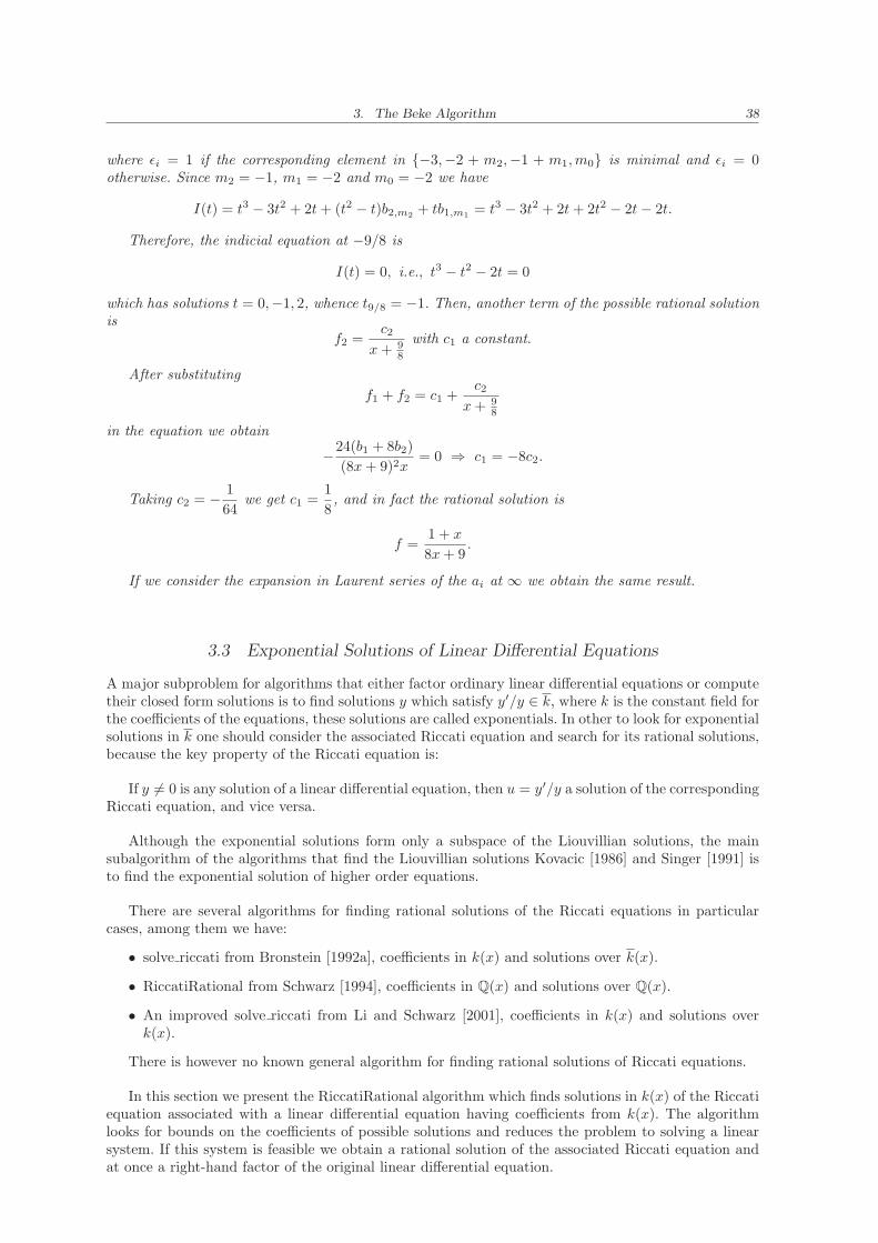
3. The Beke Algorithm 38
where ǫi = 1 if the corresponding element in {−3,−2 + m2,−1 + m1,m0} is minimal and ǫi = 0otherwise. Since m2 = −1, m1 = −2 and m0 = −2 we have
I(t) = t3 − 3t2 + 2t+ (t2 − t)b2,m2+ tb1,m1
= t3 − 3t2 + 2t+ 2t2 − 2t− 2t.
Therefore, the indicial equation at −9/8 is
I(t) = 0, i.e., t3 − t2 − 2t = 0
which has solutions t = 0,−1, 2, whence t9/8 = −1. Then, another term of the possible rational solutionis
f2 =c2
x+ 98
with c1 a constant.
After substituting
f1 + f2 = c1 +c2
x+ 98
in the equation we obtain
−24(b1 + 8b2)
(8x+ 9)2x= 0 ⇒ c1 = −8c2.
Taking c2 = − 1
64we get c1 =
1
8, and in fact the rational solution is
f =1 + x
8x+ 9.
If we consider the expansion in Laurent series of the ai at ∞ we obtain the same result.
3.3 Exponential Solutions of Linear Differential Equations
A major subproblem for algorithms that either factor ordinary linear differential equations or computetheir closed form solutions is to find solutions y which satisfy y′/y ∈ k, where k is the constant field forthe coefficients of the equations, these solutions are called exponentials. In other to look for exponentialsolutions in k one should consider the associated Riccati equation and search for its rational solutions,because the key property of the Riccati equation is:
If y 6= 0 is any solution of a linear differential equation, then u = y′/y a solution of the correspondingRiccati equation, and vice versa.
Although the exponential solutions form only a subspace of the Liouvillian solutions, the mainsubalgorithm of the algorithms that find the Liouvillian solutions Kovacic [1986] and Singer [1991] isto find the exponential solution of higher order equations.
There are several algorithms for finding rational solutions of the Riccati equations in particularcases, among them we have:
• solve riccati from Bronstein [1992a], coefficients in k(x) and solutions over k(x).
• RiccatiRational from Schwarz [1994], coefficients in Q(x) and solutions over Q(x).
• An improved solve riccati from Li and Schwarz [2001], coefficients in k(x) and solutions overk(x).
There is however no known general algorithm for finding rational solutions of Riccati equations.
In this section we present the RiccatiRational algorithm which finds solutions in k(x) of the Riccatiequation associated with a linear differential equation having coefficients from k(x). The algorithmlooks for bounds on the coefficients of possible solutions and reduces the problem to solving a linearsystem. If this system is feasible we obtain a rational solution of the associated Riccati equation andat once a right-hand factor of the original linear differential equation.
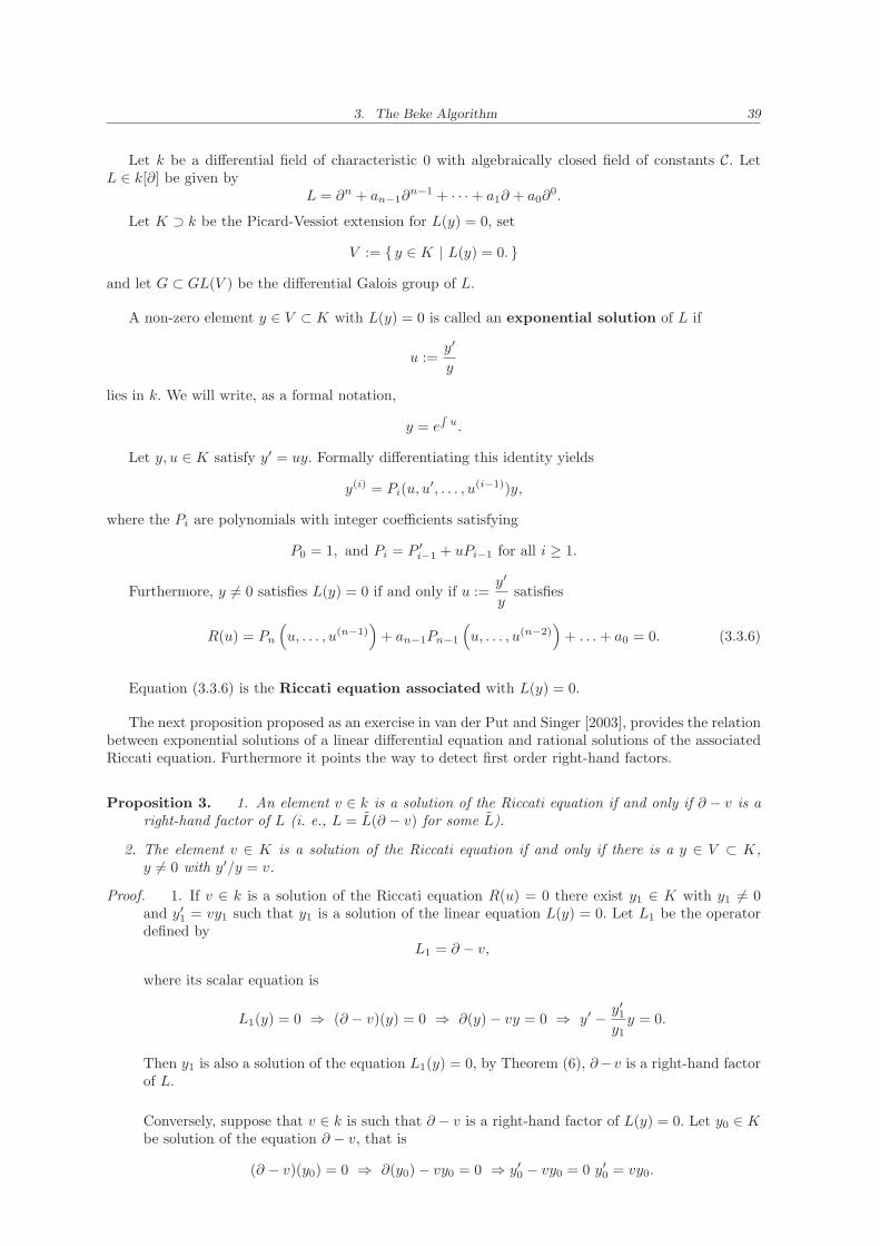
3. The Beke Algorithm 39
Let k be a differential field of characteristic 0 with algebraically closed field of constants C. LetL ∈ k[∂] be given by
L = ∂n + an−1∂n−1 + · · · + a1∂ + a0∂
0.
Let K ⊃ k be the Picard-Vessiot extension for L(y) = 0, set
V := { y ∈ K | L(y) = 0. }
and let G ⊂ GL(V ) be the differential Galois group of L.
A non-zero element y ∈ V ⊂ K with L(y) = 0 is called an exponential solution of L if
u :=y′
y
lies in k. We will write, as a formal notation,
y = eR
u.
Let y, u ∈ K satisfy y′ = uy. Formally differentiating this identity yields
y(i) = Pi(u, u′, . . . , u(i−1))y,
where the Pi are polynomials with integer coefficients satisfying
P0 = 1, and Pi = P ′i−1 + uPi−1 for all i ≥ 1.
Furthermore, y 6= 0 satisfies L(y) = 0 if and only if u :=y′
ysatisfies
R(u) = Pn
(u, . . . , u(n−1)
)+ an−1Pn−1
(u, . . . , u(n−2)
)+ . . .+ a0 = 0. (3.3.6)
Equation (3.3.6) is the Riccati equation associated with L(y) = 0.
The next proposition proposed as an exercise in van der Put and Singer [2003], provides the relationbetween exponential solutions of a linear differential equation and rational solutions of the associatedRiccati equation. Furthermore it points the way to detect first order right-hand factors.
Proposition 3. 1. An element v ∈ k is a solution of the Riccati equation if and only if ∂ − v is aright-hand factor of L (i. e., L = L(∂ − v) for some L).
2. The element v ∈ K is a solution of the Riccati equation if and only if there is a y ∈ V ⊂ K,y 6= 0 with y′/y = v.
Proof. 1. If v ∈ k is a solution of the Riccati equation R(u) = 0 there exist y1 ∈ K with y1 6= 0and y′1 = vy1 such that y1 is a solution of the linear equation L(y) = 0. Let L1 be the operatordefined by
L1 = ∂ − v,
where its scalar equation is
L1(y) = 0 ⇒ (∂ − v)(y) = 0 ⇒ ∂(y) − vy = 0 ⇒ y′ − y′1y1y = 0.
Then y1 is also a solution of the equation L1(y) = 0, by Theorem (6), ∂−v is a right-hand factorof L.
Conversely, suppose that v ∈ k is such that ∂ − v is a right-hand factor of L(y) = 0. Let y0 ∈ Kbe solution of the equation ∂ − v, that is
(∂ − v)(y0) = 0 ⇒ ∂(y0) − vy0 = 0 ⇒ y′0 − vy0 = 0 y′0 = vy0.
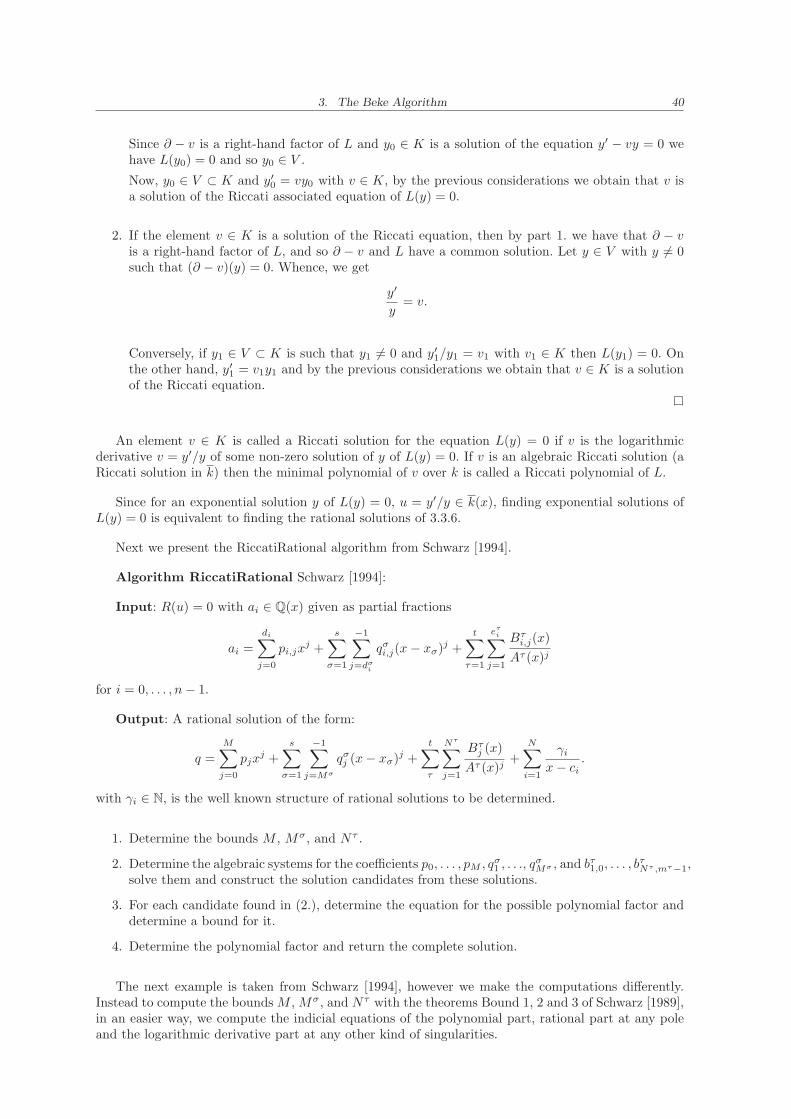
3. The Beke Algorithm 40
Since ∂ − v is a right-hand factor of L and y0 ∈ K is a solution of the equation y′ − vy = 0 wehave L(y0) = 0 and so y0 ∈ V .
Now, y0 ∈ V ⊂ K and y′0 = vy0 with v ∈ K, by the previous considerations we obtain that v isa solution of the Riccati associated equation of L(y) = 0.
2. If the element v ∈ K is a solution of the Riccati equation, then by part 1. we have that ∂ − vis a right-hand factor of L, and so ∂ − v and L have a common solution. Let y ∈ V with y 6= 0such that (∂ − v)(y) = 0. Whence, we get
y′
y= v.
Conversely, if y1 ∈ V ⊂ K is such that y1 6= 0 and y′1/y1 = v1 with v1 ∈ K then L(y1) = 0. Onthe other hand, y′1 = v1y1 and by the previous considerations we obtain that v ∈ K is a solutionof the Riccati equation.
An element v ∈ K is called a Riccati solution for the equation L(y) = 0 if v is the logarithmicderivative v = y′/y of some non-zero solution of y of L(y) = 0. If v is an algebraic Riccati solution (aRiccati solution in k) then the minimal polynomial of v over k is called a Riccati polynomial of L.
Since for an exponential solution y of L(y) = 0, u = y′/y ∈ k(x), finding exponential solutions ofL(y) = 0 is equivalent to finding the rational solutions of 3.3.6.
Next we present the RiccatiRational algorithm from Schwarz [1994].
Algorithm RiccatiRational Schwarz [1994]:
Input: R(u) = 0 with ai ∈ Q(x) given as partial fractions
ai =
di∑
j=0
pi,jxj +
s∑
σ=1
−1∑
j=dσi
qσi,j(x− xσ)j +
t∑
τ=1
eτi∑
j=1
Bτi,j(x)
Aτ (x)j
for i = 0, . . . , n− 1.
Output: A rational solution of the form:
q =M∑
j=0
pjxj +
s∑
σ=1
−1∑
j=Mσ
qσj (x− xσ)j +
t∑
τ
Nτ∑
j=1
Bτj (x)
Aτ (x)j+
N∑
i=1
γi
x− ci.
with γi ∈ N, is the well known structure of rational solutions to be determined.
1. Determine the bounds M , Mσ, and Nτ .
2. Determine the algebraic systems for the coefficients p0, . . . , pM , qσ1 , . . ., q
σMσ , and bτ1,0, . . . , b
τNτ ,mτ−1,
solve them and construct the solution candidates from these solutions.
3. For each candidate found in (2.), determine the equation for the possible polynomial factor anddetermine a bound for it.
4. Determine the polynomial factor and return the complete solution.
The next example is taken from Schwarz [1994], however we make the computations differently.Instead to compute the bounds M , Mσ, and Nτ with the theorems Bound 1, 2 and 3 of Schwarz [1989],in an easier way, we compute the indicial equations of the polynomial part, rational part at any poleand the logarithmic derivative part at any other kind of singularities.
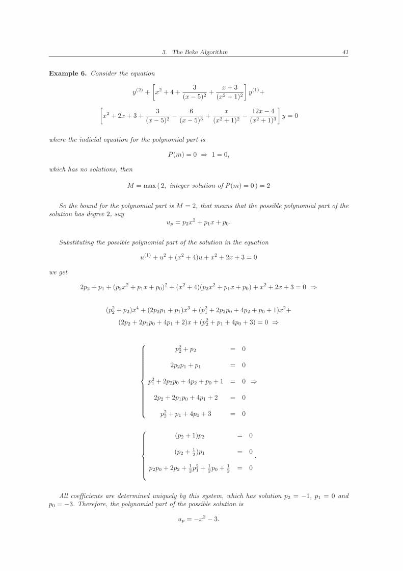
3. The Beke Algorithm 41
Example 6. Consider the equation
y(2) +
[x2 + 4 +
3
(x− 5)2+
x+ 3
(x2 + 1)2
]y(1)+
[x2 + 2x+ 3 +
3
(x− 5)2− 6
(x− 5)3+
x
(x2 + 1)2− 12x− 4
(x2 + 1)3
]y = 0
where the indicial equation for the polynomial part is
P (m) = 0 ⇒ 1 = 0,
which has no solutions, then
M = max ( 2, integer solution of P (m) = 0 ) = 2
So the bound for the polynomial part is M = 2, that means that the possible polynomial part of thesolution has degree 2, say
up = p2x2 + p1x+ p0.
Substituting the possible polynomial part of the solution in the equation
u(1) + u2 + (x2 + 4)u+ x2 + 2x+ 3 = 0
we get
2p2 + p1 + (p2x2 + p1x+ p0)
2 + (x2 + 4)(p2x2 + p1x+ p0) + x2 + 2x+ 3 = 0 ⇒
(p22 + p2)x
4 + (2p2p1 + p1)x3 + (p2
1 + 2p2p0 + 4p2 + p0 + 1)x2+
(2p2 + 2p1p0 + 4p1 + 2)x+ (p22 + p1 + 4p0 + 3) = 0 ⇒
p22 + p2 = 0
2p2p1 + p1 = 0
p21 + 2p2p0 + 4p2 + p0 + 1 = 0
2p2 + 2p1p0 + 4p1 + 2 = 0
p22 + p1 + 4p0 + 3 = 0
⇒
(p2 + 1)p2 = 0
(p2 + 12 )p1 = 0
p2p0 + 2p2 + 12p
21 + 1
2p0 + 12 = 0
.
All coefficients are determined uniquely by this system, which has solution p2 = −1, p1 = 0 andp0 = −3. Therefore, the polynomial part of the possible solution is
up = −x2 − 3.
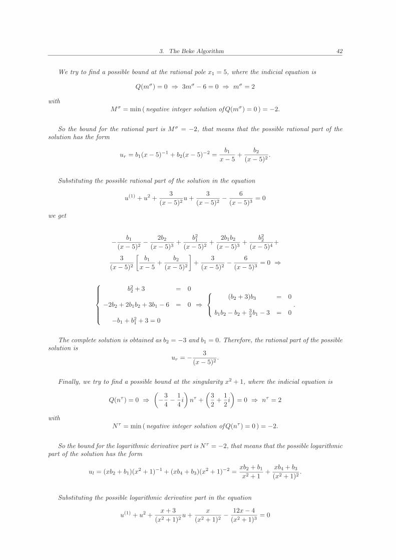
3. The Beke Algorithm 42
We try to find a possible bound at the rational pole x1 = 5, where the indicial equation is
Q(mσ) = 0 ⇒ 3mσ − 6 = 0 ⇒ mσ = 2
withMσ = min (negative integer solution ofQ(mσ) = 0 ) = −2.
So the bound for the rational part is Mσ = −2, that means that the possible rational part of thesolution has the form
ur = b1(x− 5)−1 + b2(x− 5)−2 =b1
x− 5+
b2(x− 5)2
.
Substituting the possible rational part of the solution in the equation
u(1) + u2 +3
(x− 5)2u+
3
(x− 5)2− 6
(x− 5)3= 0
we get
− b1(x− 5)2
− 2b2(x− 5)3
+b21
(x− 5)2+
2b1b2(x− 5)3
+b22
(x− 5)4+
3
(x− 5)2
[b1
x− 5+
b2(x− 5)2
]+
3
(x− 5)2− 6
(x− 5)3= 0 ⇒
b22 + 3 = 0
−2b2 + 2b1b2 + 3b1 − 6 = 0
−b1 + b21 + 3 = 0
⇒
(b2 + 3)b3 = 0
b1b2 − b2 + 32b1 − 3 = 0
.
The complete solution is obtained as b2 = −3 and b1 = 0. Therefore, the rational part of the possiblesolution is
ur = − 3
(x− 5)2.
Finally, we try to find a possible bound at the singularity x2 + 1, where the indicial equation is
Q(nτ ) = 0 ⇒(−3
4− 1
4i
)nτ +
(3
2+
1
2i
)= 0 ⇒ nτ = 2
withNτ = min (negative integer solution ofQ(nτ ) = 0 ) = −2.
So the bound for the logarithmic derivative part is Nτ = −2, that means that the possible logarithmicpart of the solution has the form
ul = (xb2 + b1)(x2 + 1)−1 + (xb4 + b3)(x
2 + 1)−2 =xb2 + b1x2 + 1
+xb4 + b3(x2 + 1)2
.
Substituting the possible logarithmic derivative part in the equation
u(1) + u2 +x+ 3
(x2 + 1)2u+
x
(x2 + 1)2− 12x− 4
(x2 + 1)3= 0

3. The Beke Algorithm 43
we get
−b2x4 + 2b1x
3 + 3b4x2 + 4b3x+ 2b1x− b4 − b2
(x2 − 1)3+
u2 +x+ 3
(x2 + 1)2u+
x
(x2 + 1)2− 12x− 4
(x2 + 1)3= 0 ⇒
b22 − b2 = 0
2b1b2 − 2b1 + 1 = 0
2b2b4 − 3b4 + b21 + 2b22 = 0
2b1b4 + 2b2b3 + 4b1b2 + 3b2 − 3b1 − 10 − 4b3 = 0
2b1b3 + 2b2b4 + 4 + 2b2 + 3b1 − b4 + 2b21 + b22 + b24 = 0
2b1b4 + 2b3b4 + 2b2b3 + 2b1b2 + 3b2 + 3b4 − 11 − b1 − 3b3 = 0
4 + 3b1 + b2 + 3b3 + b4 + b21 + 2b1b3 + b23 = 0
⇒
b1b4 + b2b3 + 12b1 + 3
2b2 − 2b3 − 6 = 0
b24 + 2b1b3 − 2b2b4 + 5b4 − b2 + 3b1 + 4 = 0
b24 + b4 − b23 − 3b3 = 0
b3b4 + 34b4 + 1
2b3 = 0
.
The non-linear system comprising the highest equation for b3 and b4 has to be transformed into aGrobner bases. Due to factorization two non-trivial alternatives are obtained:
b3 + 3 = 0
b4 + 1 = 0or
b24 + 3b3 + 5 = 0
b23 + 3b3 + 52 = 0
.
From the first alternative we get b4 = −1 and b3 = −3. Substituting them in the remaining equations,the linear system
b2 + 23b1 = 0
b2 − 3b1 = 0⇒
b2 = 0
b1 = 0⇒
is obtained with the solution b1 = b2 = 0.Therefore, the logarithmic derivative part of the possiblesolution is
ul = − x+ 3
(x2 + 1)2.
Combining these results yields the solution candidate
u = up + ur + ul = −x2 − 3 − 3
(x− 5)2− x+ 3
(x2 + 1)2.
It turns out that this is already a genuine solution of the Riccati equation. It generates the factor-ization
(∂ + 1)
[∂ + x2 + 3 +
3
(x− 5)2+
x+ 3
(x2 + 1)2
].
The other two alternatives lead to complex expressions which do not turn into solutions of theRiccati equation.
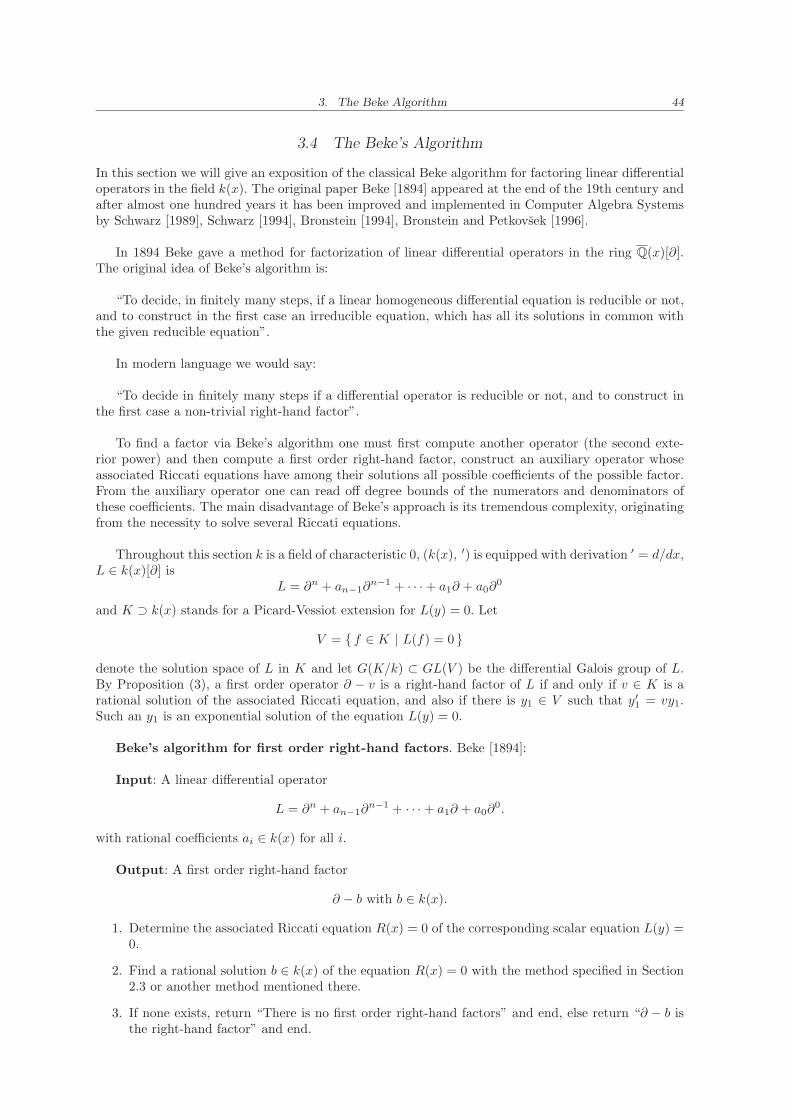
3. The Beke Algorithm 44
3.4 The Beke’s Algorithm
In this section we will give an exposition of the classical Beke algorithm for factoring linear differentialoperators in the field k(x). The original paper Beke [1894] appeared at the end of the 19th century andafter almost one hundred years it has been improved and implemented in Computer Algebra Systemsby Schwarz [1989], Schwarz [1994], Bronstein [1994], Bronstein and Petkovsek [1996].
In 1894 Beke gave a method for factorization of linear differential operators in the ring Q(x)[∂].The original idea of Beke’s algorithm is:
“To decide, in finitely many steps, if a linear homogeneous differential equation is reducible or not,and to construct in the first case an irreducible equation, which has all its solutions in common withthe given reducible equation”.
In modern language we would say:
“To decide in finitely many steps if a differential operator is reducible or not, and to construct inthe first case a non-trivial right-hand factor”.
To find a factor via Beke’s algorithm one must first compute another operator (the second exte-rior power) and then compute a first order right-hand factor, construct an auxiliary operator whoseassociated Riccati equations have among their solutions all possible coefficients of the possible factor.From the auxiliary operator one can read off degree bounds of the numerators and denominators ofthese coefficients. The main disadvantage of Beke’s approach is its tremendous complexity, originatingfrom the necessity to solve several Riccati equations.
Throughout this section k is a field of characteristic 0, (k(x), ′) is equipped with derivation ′ = d/dx,L ∈ k(x)[∂] is
L = ∂n + an−1∂n−1 + · · · + a1∂ + a0∂
0
and K ⊃ k(x) stands for a Picard-Vessiot extension for L(y) = 0. Let
V = { f ∈ K | L(f) = 0 }
denote the solution space of L in K and let G(K/k) ⊂ GL(V ) be the differential Galois group of L.By Proposition (3), a first order operator ∂ − v is a right-hand factor of L if and only if v ∈ K is arational solution of the associated Riccati equation, and also if there is y1 ∈ V such that y′1 = vy1.Such an y1 is an exponential solution of the equation L(y) = 0.
Beke’s algorithm for first order right-hand factors. Beke [1894]:
Input: A linear differential operator
L = ∂n + an−1∂n−1 + · · · + a1∂ + a0∂
0.
with rational coefficients ai ∈ k(x) for all i.
Output: A first order right-hand factor
∂ − b with b ∈ k(x).
1. Determine the associated Riccati equation R(x) = 0 of the corresponding scalar equation L(y) =0.
2. Find a rational solution b ∈ k(x) of the equation R(x) = 0 with the method specified in Section2.3 or another method mentioned there.
3. If none exists, return “There is no first order right-hand factors” and end, else return “∂ − b isthe right-hand factor” and end.
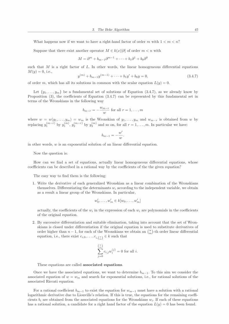
3. The Beke Algorithm 45
What happens now if we want to have a right-hand factor of order m with 1 < m < n?
Suppose that there exist another operator M ∈ k(x)[∂] of order m < n with
M = ∂m + bm−1∂m−1 + · · · + b1∂
1 + b0∂0
such that M is a right factor of L. In other words, the linear homogeneous differential equationsM(y) = 0, i.e.,
y(m) + bm−1y(m−1) + · · · + b1y
′ + b0y = 0, (3.4.7)
of order m, which has all its solutions in common with the scalar equation L(y) = 0.
Let {y1, . . . , ym} be a fundamental set of solutions of Equation (3.4.7), as we already know byProposition (3), the coefficients of Equation (3.4.7) can be represented by this fundamental set interms of the Wronskians in the following way
bm−r = −wm−r
wfor all r = 1, . . . ,m
where w = w(y1, . . . , ym) = wm is the Wronskian of y1, . . . , ym and wm−r is obtained from w by
replacing y(m−r)1 by y
(m)1 , y
(m−r)2 by y
(m)2 and so on, for all r = 1, . . . ,m. In particular we have:
bm−1 = −w′
w.
in other words, w is an exponential solution of an linear differential equation.
Now the question is:
How can we find a set of equations, actually linear homogeneous differential equations, whosecoefficients can be described in a rational way by the coefficients of the the given equation?
The easy way to find them is the following:
1. Write the derivative of each generalized Wronskian as a linear combination of the Wronskiansthemselves. Differentiating the determinants wi according to the independent variable, we obtainas a result a linear group of the Wronskians. In particular,
w′0, . . . , w
′m ∈ k[w0, . . . , w
′m]
actually, the coefficients of the wi in the expression of each wi are polynomials in the coefficientsof the original equation.
2. By successive differentiation and suitable elimination, taking into account that the set of Wron-skians is closed under differentiation if the original equation is used to substitute derivatives oforder higher than n− 1, for each of the Wronskians we obtain an
(nm
)-th order linear differential
equation, i.e., there exist ci,0, . . . , ci,(n
m) ∈ k such that
(n
m)∑
j=0
ci,jw(j)i = 0 for all i.
These equations are called associated equations.
Once we have the associated equations, we want to determine bm−1. To this aim we consider theassociated equation of w = wm and search for exponential solutions, i.e., for rational solutions of theassociated Riccati equation.
For a rational coefficient bm−1 to exist the equation for wm−1 must have a solution with a rationallogarithmic derivative due to Liouville’s relation. If this is true, the equations for the remaining coeffi-cients bi are obtained from the associated equations for the Wronskians wi. If each of these equationshas a rational solution, a candidate for a right hand factor of the equation L(y) = 0 has been found.
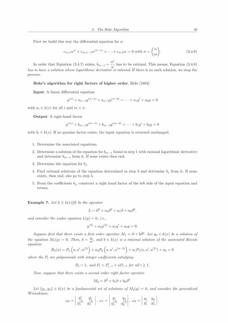
3. The Beke Algorithm 46
First we build this way the differential equation for w
cm,σwσ + cm,σ−1w
(σ−1) + · · · + cm,0w = 0 with σ =
(n
m
). (3.4.8)
In order that Equation (3.4.7) exists, bm−1 =w′
whas to be rational. This means, Equation (3.4.8)
has to have a solution whose logarithmic derivative is rational. If there is no such solution, we stop theprocess.
Beke’s algorithm for right factors of higher order. Beke [1894]:
Input: A linear differential equation
y(n) + an−1y(n−1) + an−2y
(n−2) + · · · + a1y′ + a0y = 0
with ai ∈ k(x) for all i and m < n.
Output: A right-hand factor
y(m) + bm−1y(m−1) + bm−2y
(m−2) + · · · + b1y′ + b0y = 0
with bi ∈ k(x). If no genuine factor exists, the input equation is returned unchanged.
1. Determine the associated equations.
2. Determine a solution of the equation for bm−1 found in step 1 with rational logarithmic derivativeand determine bm−1 from it. If none exists then end.
3. Determine the equation for bj .
4. Find rational solutions of the equation determined in step 3 and determine bj from it. If noneexists, then end, else go to step 5.
5. From the coefficients bj , construct a right hand factor of the left side of the input equation andreturn.
Example 7. Let L ∈ k(x)[∂] be the operator
L = ∂3 + a2∂2 + a1∂ + a0∂
0,
and consider the scalar equation L(y) = 0, i.e.,
y(3) + a2y(2) + a1y
′ + a0y = 0.
Suppose first that there exists a first order operator M1 = ∂ + b∂0. Let y0 ∈ k(x) be a solution of
the equation M1(y) = 0. Then, b =y′
0
y0, and b ∈ k(x) is a rational solution of the associated Riccati
equation
R3(u) = P3
(u, u′, u(2)
)+ a2P2
(u, u′, u(n−2)
)+ a1P1(u, u
′, u(2)) + a0 = 0
where the Pi are polynomials with integer coefficients satisfying
P0 = 1, and Pi = P ′i−1 + uPi−1 for all i ≥ 1.
Now, suppose that there exists a second order right factor operator
M2 = ∂2 + b1∂ + b0∂0.
Let {y1, y2} ∈ k(x) be a fundamental set of solutions of M2(y) = 0, and consider the generalizedWronskians:
ω0 =
∣∣∣∣y′1 y′2y(2)1 y
(2)2
∣∣∣∣ , ω1 =
∣∣∣∣∣y1 y2y(2)1 y
(2)2
∣∣∣∣∣ , ω2 =
∣∣∣∣y1 y2y′1 y′2
∣∣∣∣ .
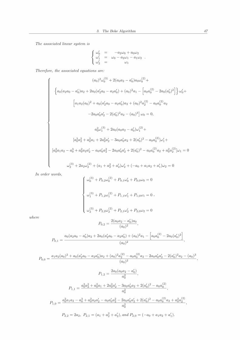
3. The Beke Algorithm 47
The associated linear system is
ω′0 = −a2ω0 + a0ω2
ω′1 = ω0 − a2ω1 − a1ω2
ω′2 = ω1
.
Therefore, the associated equations are:
(a0)2ω
(3)0 + 2(a0a2 − a′0)a0ω
(2)0 +
{a0(a2a0 − a′0)a2 + 2a0(a
′2a0 − a2a
′0) + (a0)
2a1 −[a0a
(2)0 − 2a0(a
′0)
2]}
ω′0+
[a1a2(a0)
2 + a0(a′2a0 − a2a
′0)a2 + (a0)
2a(2)2 − a0a
(2)0 a2
−2a0a′0a
′2 − 2(a′0)
2a2 − (a0)3]ω0 = 0,
a20ω
(3)1 + 2a0(a0a2 − a′0)ω
(2)1 +
[a20a
22 + a2
0a1 + 2a20a
′2 − 3a0a
′0a2 + 2(a′0)
2 − a0a(2)0 ]ω′
1+
[a20a1a2 − a3
0 + a20a2a
′2 − a0a
′0a
22 − 2a0a
′0a
′2 + 2(a′0)
2 − a0a(2)0 a2 + a2
0a(2)2 ]ω1 = 0
ω(3)2 + 2a2ω
(2)2 + (a1 + a2
2 + a′2)ω′2 + (−a0 + a1a2 + a′1)ω2 = 0
In order words,
ω(3)0 + P0,2ω
(2)0 + P0,1ω
′0 + P0,0ω0 = 0
ω(3)1 + P1,2ω
(2)1 + P1,1ω
′1 + P1,0ω1 = 0
ω(3)2 + P2,2ω
(2)2 + P2,1ω
′2 + P2,0ω2 = 0
,
where
P0,2 =2(a0a2 − a′0)a0
(a0)2,
P0,1 =a0(a2a0 − a′0)a2 + 2a0(a
′2a0 − a2a
′0) + (a0)
2a1 −[a0a
(2)0 − 2a0(a
′0)
2]
(a0)2,
P0,0 =a1a2(a0)
2 + a0(a′2a0 − a2a
′0)a2 + (a0)
2a(2)2 − a0a
(2)0 a2 − 2a0a
′0a
′2 − 2(a′0)
2a2 − (a0)3
(a0)2,
P1,2 =2a0(a0a2 − a′0)
a20
,
P1,1 =a20a
22 + a2
0a1 + 2a20a
′2 − 3a0a
′0a2 + 2(a′0)
2 − a0a(2)0
a20
,
P1,0 =a20a1a2 − a3
0 + a20a2a
′2 − a0a
′0a
22 − 2a0a
′0a
′2 + 2(a′0)
2 − a0a(2)0 a2 + a2
0a(2)2
a20
,
P2,2 = 2a2, P2,1 = (a1 + a22 + a′2), and P2,0 = (−a0 + a1a2 + a′1).
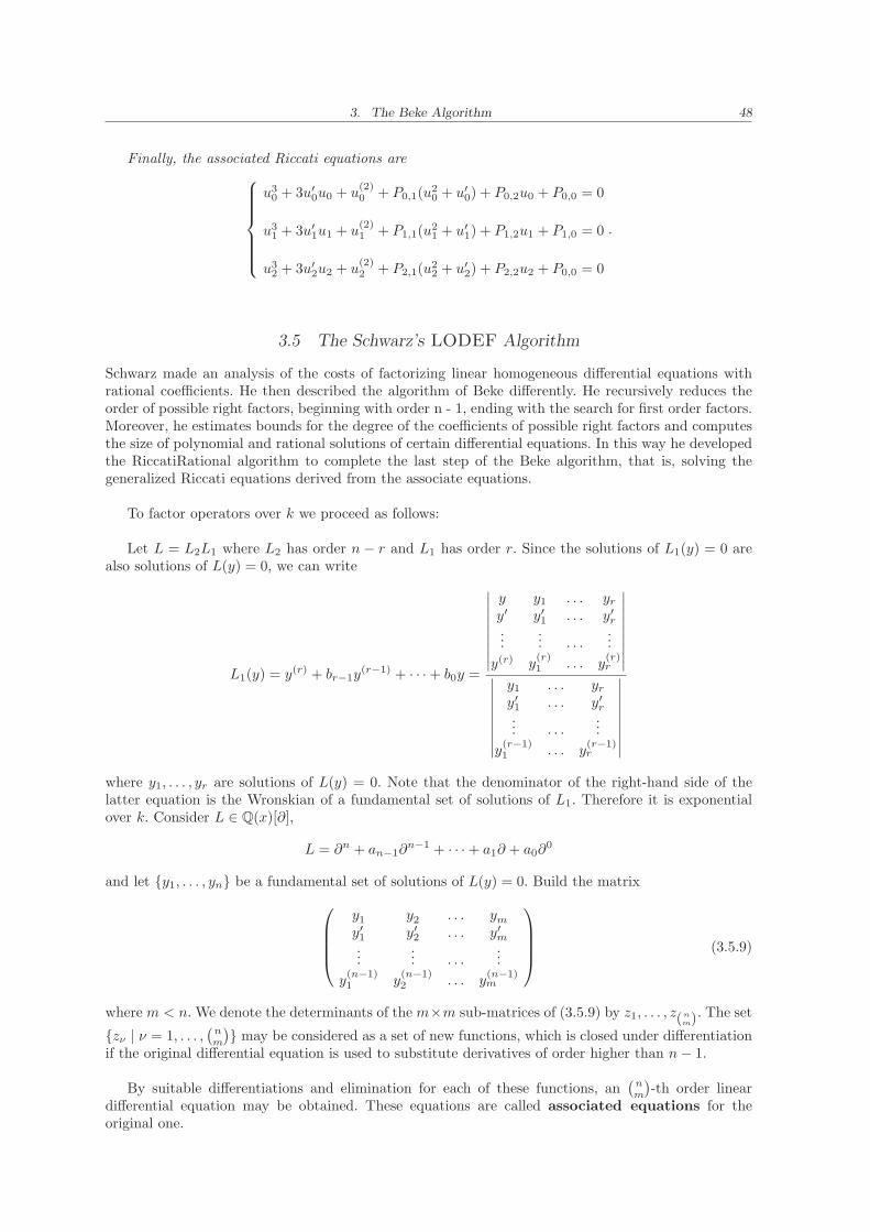
3. The Beke Algorithm 48
Finally, the associated Riccati equations are
u30 + 3u′0u0 + u
(2)0 + P0,1(u
20 + u′0) + P0,2u0 + P0,0 = 0
u31 + 3u′1u1 + u
(2)1 + P1,1(u
21 + u′1) + P1,2u1 + P1,0 = 0
u32 + 3u′2u2 + u
(2)2 + P2,1(u
22 + u′2) + P2,2u2 + P0,0 = 0
.
3.5 The Schwarz’s LODEF Algorithm
Schwarz made an analysis of the costs of factorizing linear homogeneous differential equations withrational coefficients. He then described the algorithm of Beke differently. He recursively reduces theorder of possible right factors, beginning with order n - 1, ending with the search for first order factors.Moreover, he estimates bounds for the degree of the coefficients of possible right factors and computesthe size of polynomial and rational solutions of certain differential equations. In this way he developedthe RiccatiRational algorithm to complete the last step of the Beke algorithm, that is, solving thegeneralized Riccati equations derived from the associate equations.
To factor operators over k we proceed as follows:
Let L = L2L1 where L2 has order n − r and L1 has order r. Since the solutions of L1(y) = 0 arealso solutions of L(y) = 0, we can write
L1(y) = y(r) + br−1y(r−1) + · · · + b0y =
∣∣∣∣∣∣∣∣∣
y y1 . . . yr
y′ y′1 . . . y′r...
... . . ....
y(r) y(r)1 . . . y
(r)r
∣∣∣∣∣∣∣∣∣∣∣∣∣∣∣∣∣∣
y1 . . . yr
y′1 . . . y′r... . . .
...
y(r−1)1 . . . y
(r−1)r
∣∣∣∣∣∣∣∣∣
where y1, . . . , yr are solutions of L(y) = 0. Note that the denominator of the right-hand side of thelatter equation is the Wronskian of a fundamental set of solutions of L1. Therefore it is exponentialover k. Consider L ∈ Q(x)[∂],
L = ∂n + an−1∂n−1 + · · · + a1∂ + a0∂
0
and let {y1, . . . , yn} be a fundamental set of solutions of L(y) = 0. Build the matrix
y1 y2 . . . ym
y′1 y′2 . . . y′m...
... . . ....
y(n−1)1 y
(n−1)2 . . . y
(n−1)m
(3.5.9)
where m < n. We denote the determinants of the m×m sub-matrices of (3.5.9) by z1, . . . , z(n
m). The set
{zν | ν = 1, . . . ,(
nm
)} may be considered as a set of new functions, which is closed under differentiation
if the original differential equation is used to substitute derivatives of order higher than n− 1.
By suitable differentiations and elimination for each of these functions, an(
nm
)-th order linear
differential equation may be obtained. These equations are called associated equations for theoriginal one.
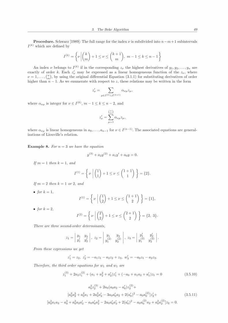
3. The Beke Algorithm 49
Procedure. Schwarz [1989]: The full range for the index ν is subdivided into n−m+1 subintervalsI(k) which are defined by
I(k) =
{ν
∣∣∣∣(k
m
)+ 1 ≤ ν ≤
(k + 1
m
), m− 1 ≤ k ≤ n− 1
}
An index ν belongs to I(k) if in the corresponding zν the highest derivatives of y1, y2, . . . , yn areexactly of order k. Each z′ν may be expressed as a linear homogeneous function of the zν , whereν = 1, . . . ,
(nm
), by using the original differential Equation (3.1.1) for substituting derivatives of order
higher than n− 1. As we enumerate with respect to z, these relations may be written in the form
z′ν =∑
µ∈I(k)∪I(k+1)
ανµzµ,
where ανµ is integer for ν ∈ I(k), m− 1 ≤ k ≤ n− 2, and
z′ν =
(n
m)∑
µ=1
ανµzµ,
where ανµ is linear homogeneous in a0, . . . , an−1 for ν ∈ I(n−1). The associated equations are general-izations of Liouville’s relation.
Example 8. For n = 3 we have the equation
y(3) + a2y(2) + a1y
′ + a0y = 0.
If m = 1 then k = 1, and
I(1) =
{ν
∣∣∣∣(
1
1
)+ 1 ≤ ν ≤
(1 + 1
1
) }= {2}.
If m = 2 then k = 1 or 2, and
• for k = 1,
I(1) =
{ν
∣∣∣∣(
1
2
)+ 1 ≤ ν ≤
(1 + 1
2
) }= {1},
• for k = 2,
I(2) =
{ν
∣∣∣∣(
2
2
)+ 1 ≤ ν ≤
(2 + 1
2
) }= {2, 3}.
There are three second-order determinants,
z1 =
∣∣∣∣y1 y2y′1 y′2
∣∣∣∣ , z2 =
∣∣∣∣∣y1 y2y(2)1 y
(2)2
∣∣∣∣∣ , z3 =
∣∣∣∣y′1 y′2y(2)1 y
(2)2
∣∣∣∣ .
From these expressions we get
z′1 = z2, z′2 = −a1z1 − a2z2 + z3, w
′3 = −a0z1 − a2z3.
Therefore, the third order equations for w1 and w1 are
z(3)1 + 2a2z
(2)1 + (a1 + a2
2 + a′2)z′1 + (−a0 + a1a2 + a′1)z1 = 0 (3.5.10)
a20z
(3)2 + 2a0(a0a2 − a′0)z
(2)2 +
[a20a
22 + a2
0a1 + 2a20a
′2 − 3a0a
′0a2 + 2(a′0)
2 − a0a(2)0 ]z′2+ (3.5.11)
[a20a1a2 − a3
0 + a20a2a
′2 − a0a
′0a
22 − 2a0a
′0a
′2 + 2(a′0)
2 − a0a(2)0 a2 + a2
0a(2)2 ]z2 = 0.
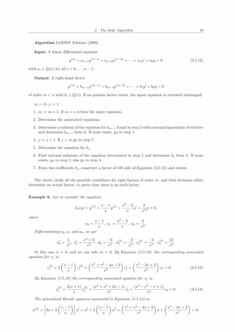
3. The Beke Algorithm 50
Algorithm LODEF Schwarz [1989]:
Input: A linear differential equation
y(n) + an−1y(n−1) + an−2y
(n−2) + · · · + a1y′ + a0y = 0 (3.5.12)
with ai ∈ Q(x) for all i = 0, . . . , n− 1.
Output: A right-hand factor
y(m) + bm−1y(m−1) + bm−2y
(m−2) + · · · + b1y′ + b0y = 0
of order m < n with bi ∈ Q(x). If no genuine factor exists, the input equation is returned unchanged.
m := 0, j := 1
1. m := m+ 1. If m = n return the input equation.
2. Determine the associated equations.
3. Determine a solution of the equation for bm−1 found in step 2 with rational logarithmic derivativeand determine bm−1 from it. If none exists, go to step 1.
4. j := j + 1. If j > m go to step 7.
5. Determine the equation for bj .
6. Find rational solutions of the equation determined in step 5 and determine bj from it. If noneexists, go to step 1, else go to step 4.
7. From the coefficients bj , construct a factor of left side of Equation (3.5.12) and return.
The above yields all the possible candidates for right factors of order m, and trial divisions eitherdetermine an actual factor, or prove that there is no such factor.
Example 9. Let us consider the equation
L2(y) = y(3) +x− 1
xy(2) +
x2 − 2
xy′ +
2
x2y = 0,
where
a2 =x− 1
x, a1 =
x2 − 2
x, a0 =
2
x2.
Differentiating a2, a1 and a0, we get
a′2 =1
x2, a′1 =
x2 + 2
x2, a′0 =
−4
x3, a
(2)2 =
−2
x3, a
(2)1 =
−4
x3, a
(2)0 =
12
x4.
In this case n = 3, and we can take m = 2. By Equation (3.5.10), the corresponding associatedequation for z1 is:
z(3)1 + 2
(x− 1
x
)z(2)1 +
(x3 + x2 − 4x+ 2
x2
)z′1 +
(x3 − 2x+ 2
x2
)z1 = 0. (3.5.13)
By Equation (3.5.10) the corresponding associated equation for z2 is:
z(3)2 +
2(x+ 1)
xz(2)2 +
(x3 + x2 + 2x− 1)
x2z′2 +
(x4 − x3 − x+ 1)
x3z2 = 0. (3.5.14)
The generalized Riccati equation associated to Equation (3.5.13) is:
u(2) +
[3u+ 2
(x− 1
x
)]u′ + u3 + 2
(x− 1
x
)u2 +
(x3 + x2 − 4x+ 2
x2
)u+
(x3 − 2x+ 2
x2
)= 0,
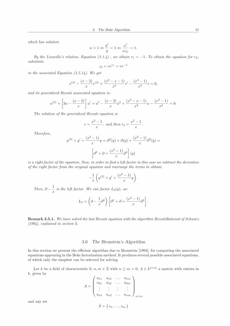
3. The Beke Algorithm 51
which has solution
u = 1 ⇔ y′
y= 1 ⇔ ω′
ωS3
= 1.
By the Liouville’s relation, Equation (3.1.4) , we obtain r1 = −1. To obtain the equation for r2,substitute
z2 = ver1 = ve−1
in the associated Equation (3.5.14). We get
v(3) − (x− 2)
xv(2) +
(x3 − x− 1)
x2v′ − (x3 − 1)
x3v = 0,
and its generalized Riccati associated equation is:
u(2) +
[3u− (x− 2)
x
]u′ + u3 − (x− 2)
xu2 +
(x3 − x− 1)
x2u− (x3 − 1)
x3= 0.
The solution of the generalized Riccati equation is
v =x2 − 1
x, and then r2 =
x2 − 1
x.
Therefore,
y(2) + y′ +(x2 − 1)
xy = ∂2(y) + ∂(y) +
(x2 − 1)
x∂0(y) =
[∂2 + ∂ +
(x2 − 1)
x∂0
](y)
is a right factor of the equation. Now, in order to find a left factor in this case we subtract the derivativeof the right factor from the original equation and rearrange the terms to obtain:
− 1
x
(y(2) + y′ +
(x2 − 1)
xy
).
Then, ∂ − 1
xis the left factor. We can factor L2(y), as:
L2 =
(∂ − 1
x∂0
)[∂2 + ∂ +
(x2 − 1)
x∂0
].
Remark 3.5.1. We have solved the last Riccati equation with the algorithm RiccatiRational of Schwarz[1994], explained in section 3.
3.6 The Bronstein’s Algorithm
In this section we present the efficient algorithm due to Bronstein [1994], for computing the associatedequations appearing in the Beke factorization method. It produces several possible associated equations,of which only the simplest can be selected for solving.
Let k be a field of characteristic 0, n,m ∈ Z with n ≥ m > 0, A ∈ kn×m a matrix with entries ink, given by
A =
a11 a12 . . . a1m
a21 a22 . . . a2m
......
......
an1 an2 . . . anm
n×m
and any setS = { s1, . . . , sm }
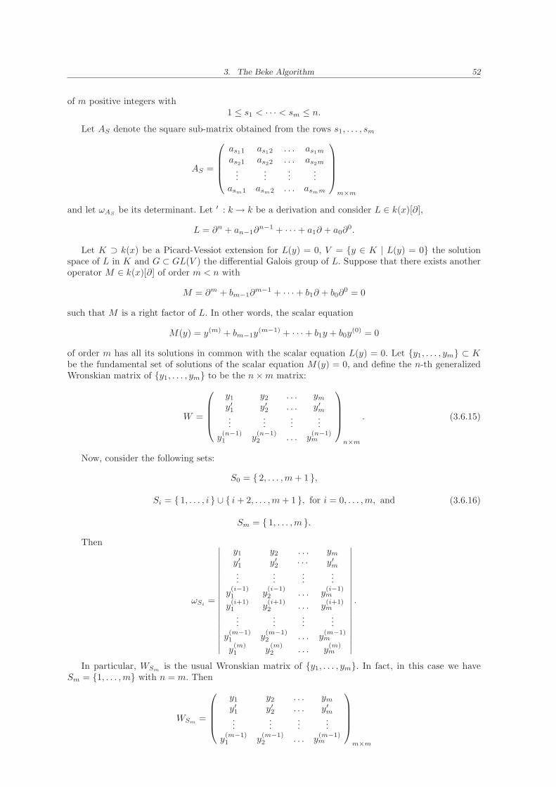
3. The Beke Algorithm 52
of m positive integers with1 ≤ s1 < · · · < sm ≤ n.
Let AS denote the square sub-matrix obtained from the rows s1, . . . , sm
AS =
as11 as12 . . . as1m
as21 as22 . . . as2m
......
......
asm1 asm2 . . . asmm
m×m
and let ωASbe its determinant. Let ′ : k → k be a derivation and consider L ∈ k(x)[∂],
L = ∂n + an−1∂n−1 + · · · + a1∂ + a0∂
0.
Let K ⊃ k(x) be a Picard-Vessiot extension for L(y) = 0, V = {y ∈ K | L(y) = 0} the solutionspace of L in K and G ⊂ GL(V ) the differential Galois group of L. Suppose that there exists anotheroperator M ∈ k(x)[∂] of order m < n with
M = ∂m + bm−1∂m−1 + · · · + b1∂ + b0∂
0 = 0
such that M is a right factor of L. In other words, the scalar equation
M(y) = y(m) + bm−1y(m−1) + · · · + b1y + b0y
(0) = 0
of order m has all its solutions in common with the scalar equation L(y) = 0. Let {y1, . . . , ym} ⊂ Kbe the fundamental set of solutions of the scalar equation M(y) = 0, and define the n-th generalizedWronskian matrix of {y1, . . . , ym} to be the n×m matrix:
W =
y1 y2 . . . ym
y′1 y′2 . . . y′m...
......
...
y(n−1)1 y
(n−1)2 . . . y
(n−1)m
n×m
. (3.6.15)
Now, consider the following sets:
S0 = { 2, . . . ,m+ 1 },
Si = { 1, . . . , i } ∪ { i+ 2, . . . ,m+ 1 }, for i = 0, . . . ,m, and
Sm = { 1, . . . ,m }.
(3.6.16)
Then
ωSi=
∣∣∣∣∣∣∣∣∣∣∣∣∣∣∣∣∣∣∣
y1 y2 . . . ym
y′1 y′2 · · · y′m...
......
...
y(i−1)1 y
(i−1)2 . . . y
(i−1)m
y(i+1)1 y
(i+1)2 . . . y
(i+1)m
......
......
y(m−1)1 y
(m−1)2 . . . y
(m−1)m
y(m)1 y
(m)2 . . . y
(m)m
∣∣∣∣∣∣∣∣∣∣∣∣∣∣∣∣∣∣∣
.
In particular, WSmis the usual Wronskian matrix of {y1, . . . , ym}. In fact, in this case we have
Sm = {1, . . . ,m} with n = m. Then
WSm=
y1 y2 . . . ym
y′1 y′2 . . . y′m...
......
...
y(m−1)1 y
(m−1)2 . . . y
(m−1)m
m×m
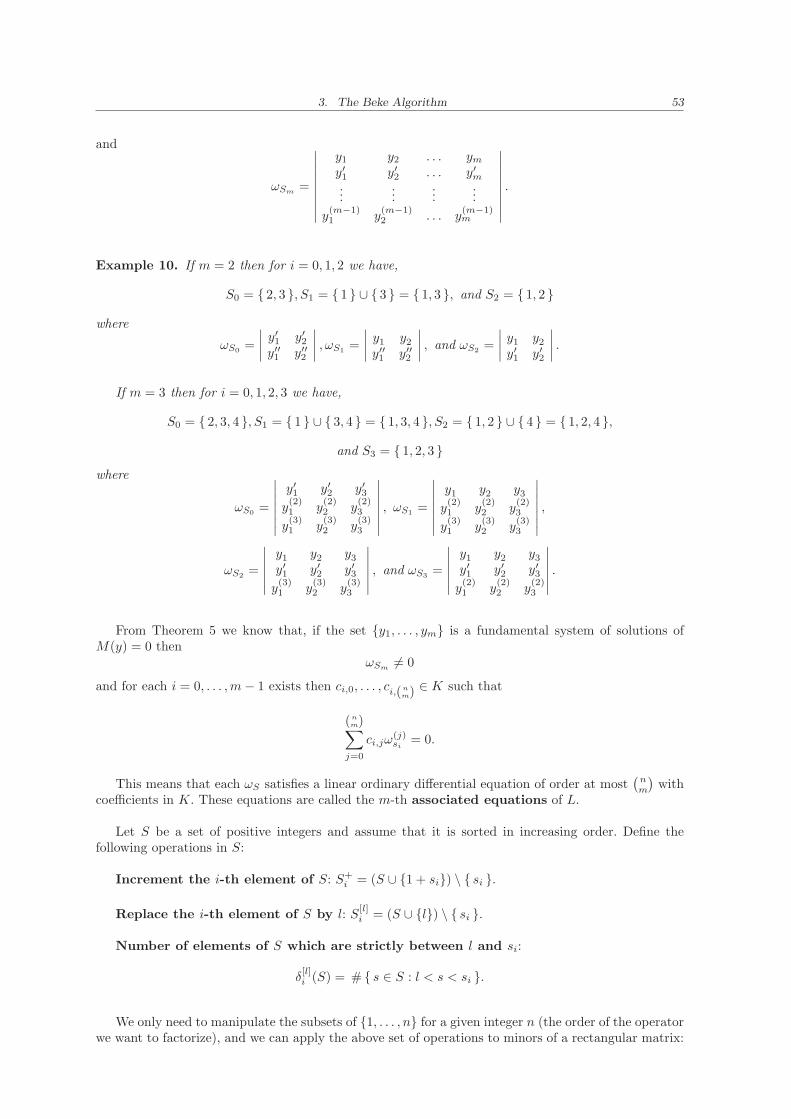
3. The Beke Algorithm 53
and
ωSm=
∣∣∣∣∣∣∣∣∣
y1 y2 . . . ym
y′1 y′2 . . . y′m...
......
...
y(m−1)1 y
(m−1)2 . . . y
(m−1)m
∣∣∣∣∣∣∣∣∣
.
Example 10. If m = 2 then for i = 0, 1, 2 we have,
S0 = { 2, 3 }, S1 = { 1 } ∪ { 3 } = { 1, 3 }, and S2 = { 1, 2 }
where
ωS0=
∣∣∣∣y′1 y′2y′′1 y′′2
∣∣∣∣ , ωS1=
∣∣∣∣y1 y2y′′1 y′′2
∣∣∣∣ , and ωS2=
∣∣∣∣y1 y2y′1 y′2
∣∣∣∣ .
If m = 3 then for i = 0, 1, 2, 3 we have,
S0 = { 2, 3, 4 }, S1 = { 1 } ∪ { 3, 4 } = { 1, 3, 4 }, S2 = { 1, 2 } ∪ { 4 } = { 1, 2, 4 },
and S3 = { 1, 2, 3 }where
ωS0=
∣∣∣∣∣∣∣
y′1 y′2 y′3y(2)1 y
(2)2 y
(2)3
y(3)1 y
(3)2 y
(3)3
∣∣∣∣∣∣∣, ωS1
=
∣∣∣∣∣∣∣
y1 y2 y3y(2)1 y
(2)2 y
(2)3
y(3)1 y
(3)2 y
(3)3
∣∣∣∣∣∣∣,
ωS2=
∣∣∣∣∣∣
y1 y2 y3y′1 y′2 y′3y(3)1 y
(3)2 y
(3)3
∣∣∣∣∣∣, and ωS3
=
∣∣∣∣∣∣
y1 y2 y3y′1 y′2 y′3y(2)1 y
(2)2 y
(2)3
∣∣∣∣∣∣.
From Theorem 5 we know that, if the set {y1, . . . , ym} is a fundamental system of solutions ofM(y) = 0 then
ωSm6= 0
and for each i = 0, . . . ,m− 1 exists then ci,0, . . . , ci,(n
m) ∈ K such that
(n
m)∑
j=0
ci,jω(j)si
= 0.
This means that each ωS satisfies a linear ordinary differential equation of order at most(
nm
)with
coefficients in K. These equations are called the m-th associated equations of L.
Let S be a set of positive integers and assume that it is sorted in increasing order. Define thefollowing operations in S:
Increment the i-th element of S: S+i = (S ∪ {1 + si}) \ { si }.
Replace the i-th element of S by l: S[l]i = (S ∪ {l}) \ { si }.
Number of elements of S which are strictly between l and si:
δ[l]i (S) = # { s ∈ S : l < s < si }.
We only need to manipulate the subsets of {1, . . . , n} for a given integer n (the order of the operatorwe want to factorize), and we can apply the above set of operations to minors of a rectangular matrix:
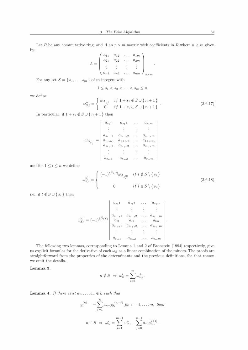
3. The Beke Algorithm 54
Let R be any commutative ring, and A an n×m matrix with coefficients in R where n ≥ m givenby:
A =
a11 a12 . . . a1m
a21 a22 . . . a2m
......
......
an1 an2 . . . anm
n×m
.
For any set S = { s1, . . . , sm } of m integers with
1 ≤ s1 < s2 < · · · < sm ≤ n
we define
ω+S,i =
{ωA
S+i
if 1 + si /∈ S ∪ {n+ 1 }0 if 1 + si ∈ S ∪ {n+ 1 }
. (3.6.17)
In particular, if 1 + si /∈ S ∪ {n+ 1 } then
ωAS+i
=
∣∣∣∣∣∣∣∣∣∣∣∣∣∣∣∣
as11 as12 . . . as1m
......
......
asi−11 asi−12 . . . asi−1m
a1+si1 a1+si2 . . . a1+sim
asi+11 asi+12 . . . asi+1m
......
......
asm1 asm2 . . . asmm
∣∣∣∣∣∣∣∣∣∣∣∣∣∣∣∣
,
and for 1 ≤ l ≤ n we define
ω[l]S,i =
(−1)δ[l]i
(S)ωAS[l]i
if l /∈ S \ { si }
0 if l ∈ S \ { si }(3.6.18)
i.e., if l /∈ S ∪ { si } then
ω[l]S,i = (−1)δ
[l]i
(S)
∣∣∣∣∣∣∣∣∣∣∣∣∣∣∣∣
as11 as12 . . . as1m
......
......
asi−11 asi−12 . . . asi−1m
al1 al2 . . . alm
asi+11 asi+12 . . . asi+1m
......
......
asm1 asm2 . . . asmm
∣∣∣∣∣∣∣∣∣∣∣∣∣∣∣∣
.
The following two lemmas, corresponding to Lemma 1 and 2 of Bronstein [1994] respectively, giveus explicit formulas for the derivative of each ωS as a linear combination of the minors. The proofs arestraightforward from the properties of the determinants and the previous definitions, for that reasonwe omit the details.
Lemma 3.
n /∈ S ⇒ ω′S =
m∑
i=1
ω+S,i.
Lemma 4. If there exist a1, . . . , an ∈ k such that
y(n)i = −
n∑
j=1
an−jy(n−j)i for i = 1, . . . ,m, then
n ∈ S ⇒ ω′S =
m−1∑
i=1
ω+S,i −
n−1∑
j=0
ajω[j+1]S,m .
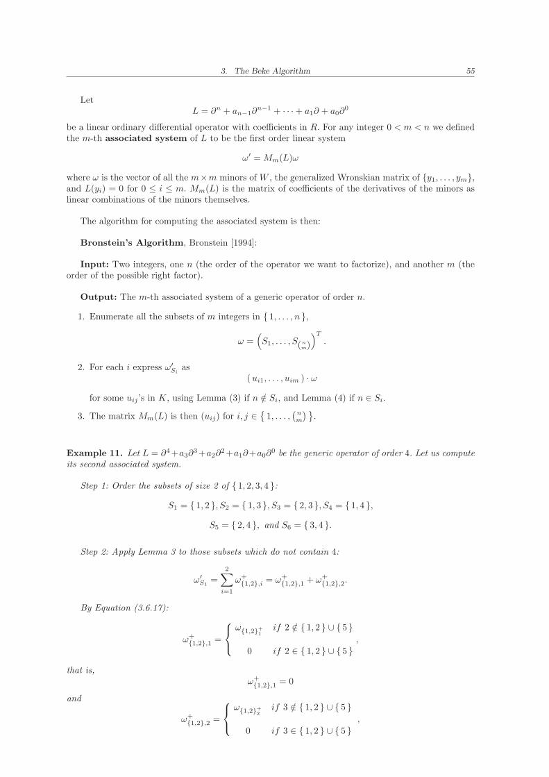
3. The Beke Algorithm 55
LetL = ∂n + an−1∂
n−1 + · · · + a1∂ + a0∂0
be a linear ordinary differential operator with coefficients in R. For any integer 0 < m < n we definedthe m-th associated system of L to be the first order linear system
ω′ = Mm(L)ω
where ω is the vector of all the m×m minors of W , the generalized Wronskian matrix of {y1, . . . , ym},and L(yi) = 0 for 0 ≤ i ≤ m. Mm(L) is the matrix of coefficients of the derivatives of the minors aslinear combinations of the minors themselves.
The algorithm for computing the associated system is then:
Bronstein’s Algorithm, Bronstein [1994]:
Input: Two integers, one n (the order of the operator we want to factorize), and another m (theorder of the possible right factor).
Output: The m-th associated system of a generic operator of order n.
1. Enumerate all the subsets of m integers in { 1, . . . , n },
ω =(S1, . . . , S(n
m)
)T
.
2. For each i express ω′Si
as(ui1, . . . , uim ) · ω
for some uij ’s in K, using Lemma (3) if n /∈ Si, and Lemma (4) if n ∈ Si.
3. The matrix Mm(L) is then (uij) for i, j ∈{
1, . . . ,(
nm
) }.
Example 11. Let L = ∂4+a3∂3+a2∂
2+a1∂+a0∂0 be the generic operator of order 4. Let us compute
its second associated system.
Step 1: Order the subsets of size 2 of { 1, 2, 3, 4 }:
S1 = { 1, 2 }, S2 = { 1, 3 }, S3 = { 2, 3 }, S4 = { 1, 4 },
S5 = { 2, 4 }, and S6 = { 3, 4 }.
Step 2: Apply Lemma 3 to those subsets which do not contain 4:
ω′S1
=
2∑
i=1
ω+{1,2},i = ω+
{1,2},1 + ω+{1,2},2.
By Equation (3.6.17):
ω+{1,2},1 =
ω{1,2}+1
if 2 /∈ { 1, 2 } ∪ { 5 }
0 if 2 ∈ { 1, 2 } ∪ { 5 },
that is,ω+{1,2},1 = 0
and
ω+{1,2},2 =
ω{1,2}+2
if 3 /∈ { 1, 2 } ∪ { 5 }
0 if 3 ∈ { 1, 2 } ∪ { 5 },
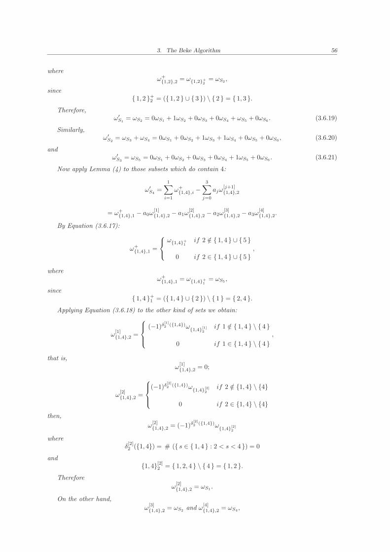
3. The Beke Algorithm 56
whereω+{1,2},2 = ω{1,2}+
2= ωS2
,
since{ 1, 2 }+
2 = ({ 1, 2 } ∪ { 3 }) \ { 2 } = { 1, 3 }.Therefore,
ω′S1
= ωS2= 0ωS1
+ 1ωS2+ 0ωS3
+ 0ωS4+ ωS5
+ 0ωS6. (3.6.19)
Similarly,ω′
S2= ωS3
+ ωS4= 0ωS1
+ 0ωS2+ 1ωS3
+ 1ωS4+ 0ωS5
+ 0ωS6, (3.6.20)
andω′
S3= ωS5
= 0ωS1+ 0ωS2
+ 0ωS3+ 0ωS4
+ 1ωS5+ 0ωS6
. (3.6.21)
Now apply Lemma (4) to those subsets which do contain 4:
ω′S4
=
1∑
i=1
ω+{1,4},i −
3∑
j=0
ajω[j+1]{1,4},2
= ω+{1,4},1 − a0ω
[1]{1,4},2 − a1ω
[2]{1,4},2 − a2ω
[3]{1,4},2 − a3ω
[4]{1,4},2.
By Equation (3.6.17):
ω+{1,4},1 =
ω{1,4}+1
if 2 /∈ { 1, 4 } ∪ { 5 }
0 if 2 ∈ { 1, 4 } ∪ { 5 },
whereω+{1,4},1 = ω{1,4}+
1= ωS5
,
since{ 1, 4 }+
1 = ({ 1, 4 } ∪ { 2 }) \ { 1 } = { 2, 4 }.Applying Equation (3.6.18) to the other kind of sets we obtain:
ω[1]{1,4},2 =
(−1)δ[1]2 ({1,4})ω{1,4}[1]
2if 1 /∈ { 1, 4 } \ { 4 }
0 if 1 ∈ { 1, 4 } \ { 4 },
that is,
ω[1]{1,4},2 = 0;
ω[2]{1,4},2 =
(−1)δ[2]2 ({1,4})ω{1,4}[2]
2if 2 /∈ {1, 4} \ {4}
0 if 2 ∈ {1, 4} \ {4}then,
ω[2]{1,4},2 = (−1)δ
[2]2 ({1,4})ω{1,4}[2]
2
whereδ[2]2 ({1, 4}) = # ({ s ∈ { 1, 4 } : 2 < s < 4 }) = 0
and{1, 4}[2]
2 = { 1, 2, 4 } \ { 4 } = { 1, 2 }.Therefore
ω[2]{1,4},2 = ωS1
.
On the other hand,
ω[3]{1,4},2 = ωS2
and ω[4]{1,4},2 = ωS4
,
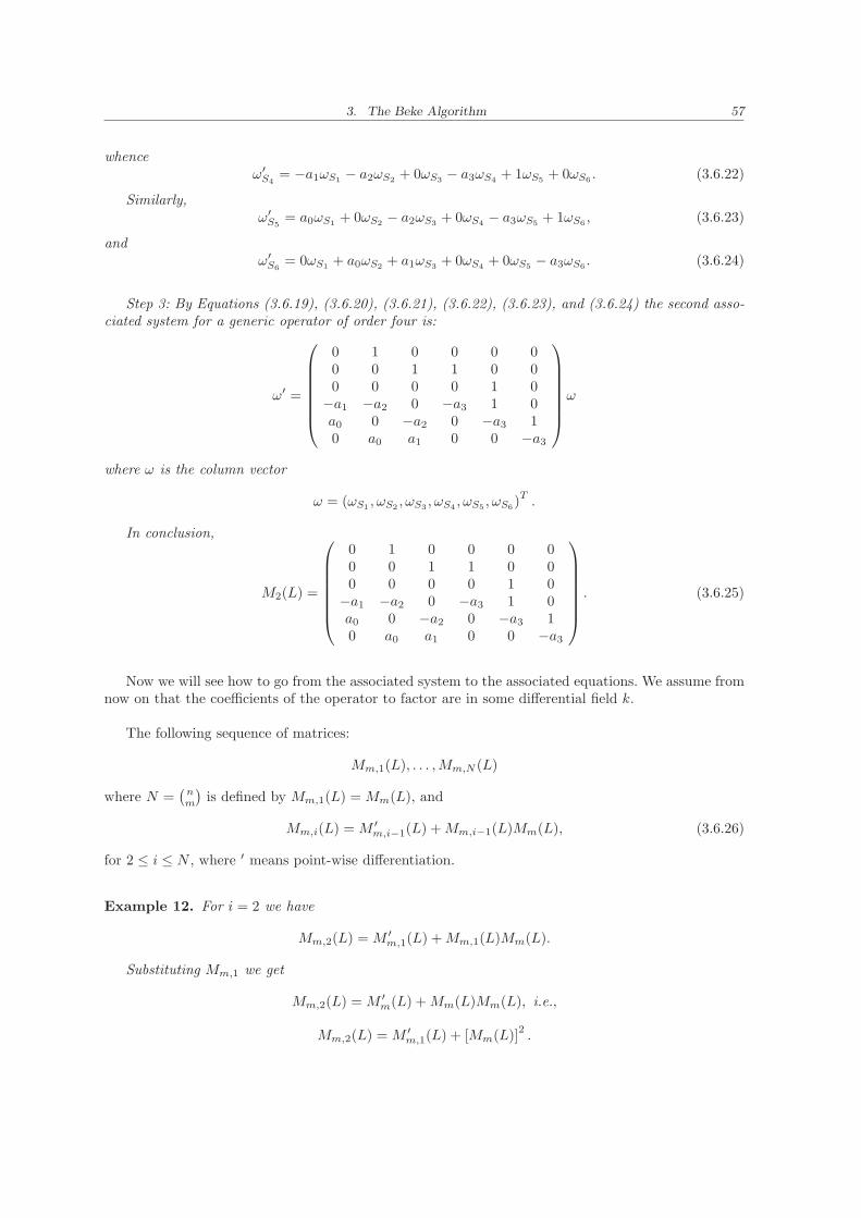
3. The Beke Algorithm 57
whenceω′
S4= −a1ωS1
− a2ωS2+ 0ωS3
− a3ωS4+ 1ωS5
+ 0ωS6. (3.6.22)
Similarly,ω′
S5= a0ωS1
+ 0ωS2− a2ωS3
+ 0ωS4− a3ωS5
+ 1ωS6, (3.6.23)
andω′
S6= 0ωS1
+ a0ωS2+ a1ωS3
+ 0ωS4+ 0ωS5
− a3ωS6. (3.6.24)
Step 3: By Equations (3.6.19), (3.6.20), (3.6.21), (3.6.22), (3.6.23), and (3.6.24) the second asso-ciated system for a generic operator of order four is:
ω′ =
0 1 0 0 0 00 0 1 1 0 00 0 0 0 1 0
−a1 −a2 0 −a3 1 0a0 0 −a2 0 −a3 10 a0 a1 0 0 −a3
ω
where ω is the column vector
ω = (ωS1, ωS2
, ωS3, ωS4
, ωS5, ωS6
)T.
In conclusion,
M2(L) =
0 1 0 0 0 00 0 1 1 0 00 0 0 0 1 0
−a1 −a2 0 −a3 1 0a0 0 −a2 0 −a3 10 a0 a1 0 0 −a3
. (3.6.25)
Now we will see how to go from the associated system to the associated equations. We assume fromnow on that the coefficients of the operator to factor are in some differential field k.
The following sequence of matrices:
Mm,1(L), . . . ,Mm,N (L)
where N =(
nm
)is defined by Mm,1(L) = Mm(L), and
Mm,i(L) = M ′m,i−1(L) +Mm,i−1(L)Mm(L), (3.6.26)
for 2 ≤ i ≤ N , where ′ means point-wise differentiation.
Example 12. For i = 2 we have
Mm,2(L) = M ′m,1(L) +Mm,1(L)Mm(L).
Substituting Mm,1 we get
Mm,2(L) = M ′m(L) +Mm(L)Mm(L), i.e.,
Mm,2(L) = M ′m,1(L) + [Mm(L)]
2.
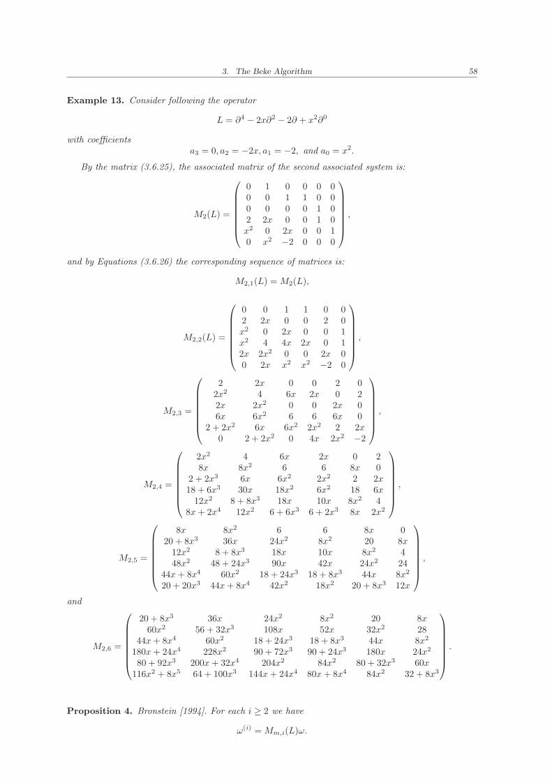
3. The Beke Algorithm 58
Example 13. Consider following the operator
L = ∂4 − 2x∂2 − 2∂ + x2∂0
with coefficientsa3 = 0, a2 = −2x, a1 = −2, and a0 = x2.
By the matrix (3.6.25), the associated matrix of the second associated system is:
M2(L) =
0 1 0 0 0 00 0 1 1 0 00 0 0 0 1 02 2x 0 0 1 0x2 0 2x 0 0 10 x2 −2 0 0 0
,
and by Equations (3.6.26) the corresponding sequence of matrices is:
M2,1(L) = M2(L),
M2,2(L) =
0 0 1 1 0 02 2x 0 0 2 0x2 0 2x 0 0 1x2 4 4x 2x 0 12x 2x2 0 0 2x 00 2x x2 x2 −2 0
,
M2,3 =
2 2x 0 0 2 02x2 4 6x 2x 0 22x 2x2 0 0 2x 06x 6x2 6 6 6x 0
2 + 2x2 6x 6x2 2x2 2 2x0 2 + 2x2 0 4x 2x2 −2
,
M2,4 =
2x2 4 6x 2x 0 28x 8x2 6 6 8x 0
2 + 2x3 6x 6x2 2x2 2 2x18 + 6x3 30x 18x2 6x2 18 6x
12x2 8 + 8x3 18x 10x 8x2 48x+ 2x4 12x2 6 + 6x3 6 + 2x3 8x 2x2
,
M2,5 =
8x 8x2 6 6 8x 020 + 8x3 36x 24x2 8x2 20 8x
12x2 8 + 8x3 18x 10x 8x2 448x2 48 + 24x3 90x 42x 24x2 24
44x+ 8x4 60x2 18 + 24x3 18 + 8x3 44x 8x2
20 + 20x3 44x+ 8x4 42x2 18x2 20 + 8x3 12x
,
and
M2,6 =
20 + 8x3 36x 24x2 8x2 20 8x60x2 56 + 32x3 108x 52x 32x2 28
44x+ 8x4 60x2 18 + 24x3 18 + 8x3 44x 8x2
180x+ 24x4 228x2 90 + 72x3 90 + 24x3 180x 24x2
80 + 92x3 200x+ 32x4 204x2 84x2 80 + 32x3 60x116x2 + 8x5 64 + 100x3 144x+ 24x4 80x+ 8x4 84x2 32 + 8x3
.
Proposition 4. Bronstein [1994]. For each i ≥ 2 we have
ω(i) = Mm,i(L)ω.
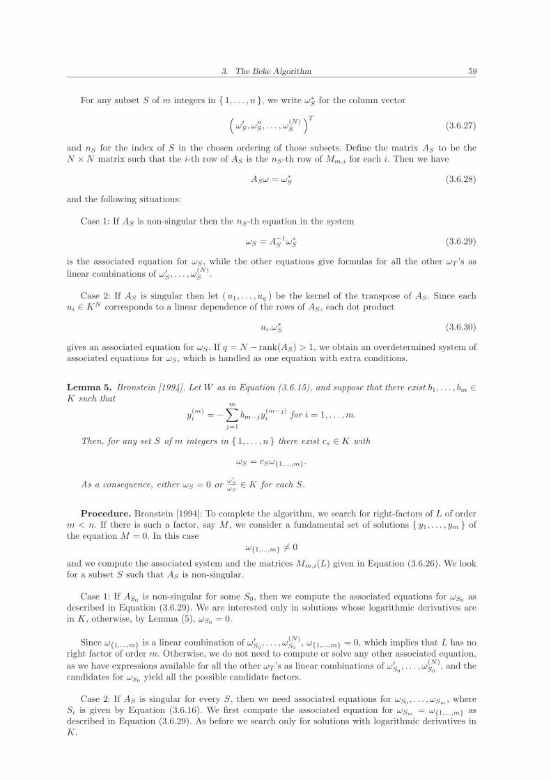
3. The Beke Algorithm 59
For any subset S of m integers in { 1, . . . , n }, we write ω∗S for the column vector
(ω′
S , ω′′S , . . . , ω
(N)S
)T
(3.6.27)
and nS for the index of S in the chosen ordering of those subsets. Define the matrix AS to be theN ×N matrix such that the i-th row of AS is the nS-th row of Mm,i for each i. Then we have
ASω = ω∗S (3.6.28)
and the following situations:
Case 1: If AS is non-singular then the nS-th equation in the system
ωS = A−1S ω∗
S (3.6.29)
is the associated equation for ωS , while the other equations give formulas for all the other ωT ’s as
linear combinations of ω′S , . . . , ω
(N)S .
Case 2: If AS is singular then let (u1, . . . , uq ) be the kernel of the transpose of AS . Since eachui ∈ KN corresponds to a linear dependence of the rows of AS , each dot product
ui.ω∗S (3.6.30)
gives an associated equation for ωS . If q = N − rank(AS) > 1, we obtain an overdetermined system ofassociated equations for ωS , which is handled as one equation with extra conditions.
Lemma 5. Bronstein [1994]. Let W as in Equation (3.6.15), and suppose that there exist b1, . . . , bm ∈K such that
y(m)i = −
m∑
j=1
bm−jy(m−j)i for i = 1, . . . ,m.
Then, for any set S of m integers in { 1, . . . , n } there exist cs ∈ K with
ωS = cSω{1,...,m}.
As a consequence, either ωS = 0 orω′
S
ωS∈ K for each S.
Procedure. Bronstein [1994]: To complete the algorithm, we search for right-factors of L of orderm < n. If there is such a factor, say M , we consider a fundamental set of solutions { y1, . . . , ym } ofthe equation M = 0. In this case
ω{1,...,m} 6= 0
and we compute the associated system and the matrices Mm,i(L) given in Equation (3.6.26). We lookfor a subset S such that AS is non-singular.
Case 1: If AS0is non-singular for some S0, then we compute the associated equations for ωS0
asdescribed in Equation (3.6.29). We are interested only in solutions whose logarithmic derivatives arein K, otherwise, by Lemma (5), ωS0
= 0.
Since ω{1,...,m} is a linear combination of ω′S0, . . . , ω
(N)S0
, ω{1,...,m} = 0, which implies that L has noright factor of order m. Otherwise, we do not need to compute or solve any other associated equation,
as we have expressions available for all the other ωT ’s as linear combinations of ω′S0, . . . , ω
(N)S0
, and thecandidates for ωS0
yield all the possible candidate factors.
Case 2: If AS is singular for every S, then we need associated equations for ωS0, . . . , ωSm
, whereSi is given by Equation (3.6.16). We first compute the associated equation for ωSm
= ω{1,...,m} asdescribed in Equation (3.6.29). As before we search only for solutions with logarithmic derivatives inK.
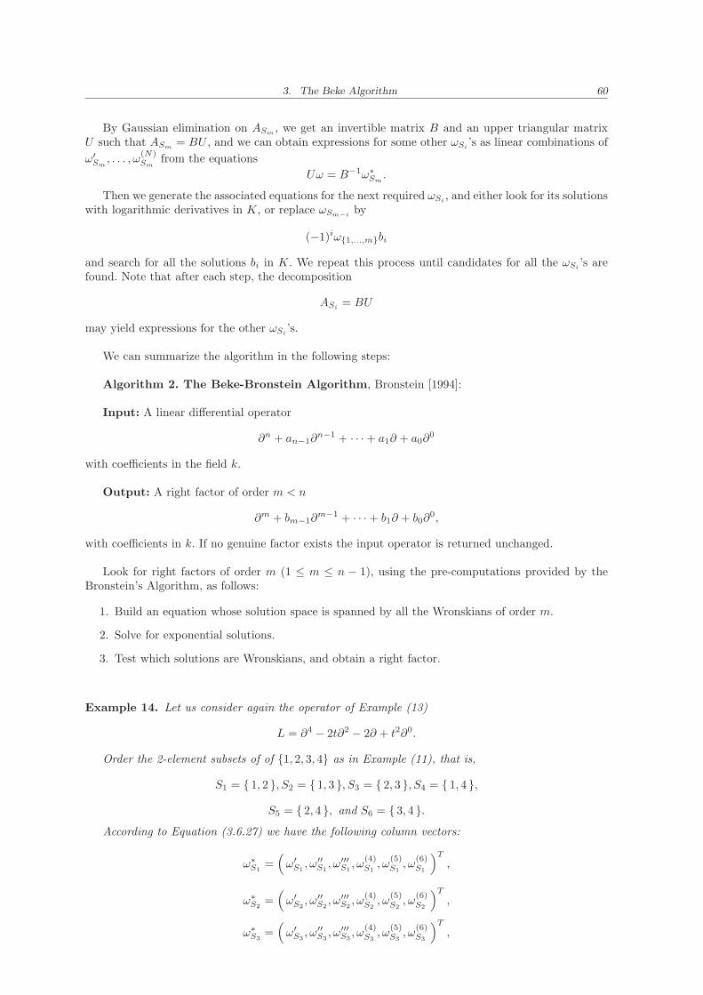
3. The Beke Algorithm 60
By Gaussian elimination on ASm, we get an invertible matrix B and an upper triangular matrix
U such that ASm= BU , and we can obtain expressions for some other ωSi
’s as linear combinations of
ω′Sm, . . . , ω
(N)Sm
from the equations
Uω = B−1ω∗Sm.
Then we generate the associated equations for the next required ωSi, and either look for its solutions
with logarithmic derivatives in K, or replace ωSm−iby
(−1)iω{1,...,m}bi
and search for all the solutions bi in K. We repeat this process until candidates for all the ωSi’s are
found. Note that after each step, the decomposition
ASi= BU
may yield expressions for the other ωSi’s.
We can summarize the algorithm in the following steps:
Algorithm 2. The Beke-Bronstein Algorithm, Bronstein [1994]:
Input: A linear differential operator
∂n + an−1∂n−1 + · · · + a1∂ + a0∂
0
with coefficients in the field k.
Output: A right factor of order m < n
∂m + bm−1∂m−1 + · · · + b1∂ + b0∂
0,
with coefficients in k. If no genuine factor exists the input operator is returned unchanged.
Look for right factors of order m (1 ≤ m ≤ n − 1), using the pre-computations provided by theBronstein’s Algorithm, as follows:
1. Build an equation whose solution space is spanned by all the Wronskians of order m.
2. Solve for exponential solutions.
3. Test which solutions are Wronskians, and obtain a right factor.
Example 14. Let us consider again the operator of Example (13)
L = ∂4 − 2t∂2 − 2∂ + t2∂0.
Order the 2-element subsets of of {1, 2, 3, 4} as in Example (11), that is,
S1 = { 1, 2 }, S2 = { 1, 3 }, S3 = { 2, 3 }, S4 = { 1, 4 },
S5 = { 2, 4 }, and S6 = { 3, 4 }.According to Equation (3.6.27) we have the following column vectors:
ω∗S1
=(ω′
S1, ω′′
S1, ω′′′
S1, ω
(4)S1, ω
(5)S1, ω
(6)S1
)T
,
ω∗S2
=(ω′
S2, ω′′
S2, ω′′′
S2, ω
(4)S2, ω
(5)S2, ω
(6)S2
)T
,
ω∗S3
=(ω′
S3, ω′′
S3, ω′′′
S3, ω
(4)S3, ω
(5)S3, ω
(6)S3
)T
,
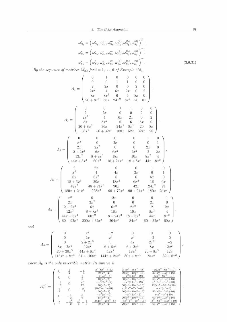
3. The Beke Algorithm 61
ω∗S4
=(ω′
S4, ω′′
S4, ω′′′
S4, ω
(4)S4, ω
(5)S4, ω
(6)S4
)T
,
ω∗S5
=(ω′
S5, ω′′
S5, ω′′′
S5, ω
(4)S5, ω
(5)S5, ω
(6)S5
)T
,
ω∗S6
=(ω′
S6, ω′′
S6, ω′′′
S6, ω
(4)S6, ω
(5)S6, ω
(6)S6
)T
. (3.6.31)
By the sequence of matrices M2,i for i = 1, . . . , 6 of Example (12),
A1 =
0 1 0 0 0 00 0 1 1 0 02 2x 0 0 2 0
2x2 4 6x 2x 0 28x 8x2 6 6 8x 0
20 + 8x3 36x 24x2 8x2 20 8x
,
A2 =
0 0 1 1 0 02 2x 0 0 2 0
2x2 4 6x 2x 0 28x 8x2 6 6 8x 0
20 + 8x3 36x 24x2 8x2 20 8x60x2 56 + 32x3 108x 52x 32x2 28
,
A3 =
0 0 0 0 1 0x2 0 2x 0 0 12x 2x2 0 0 2x 0
2 + 2x3 6x 6x2 2x2 2 2x12x2 8 + 8x3 18x 10x 8x2 4
44x+ 8x4 60x2 18 + 24x3 18 + 8x3 44x 8x2
,
A4 =
2 2x 0 0 1 0x2 4 4x 2x 0 16x 6x2 6 6 6x 0
18 + 6x3 30x 18x2 6x2 18 6x48x2 48 + 24x3 90x 42x 24x2 24
180x+ 24x4 228x2 90 + 72x3 90 + 24x3 180x 24x2
,
A5 =
x2 0 2x 0 0 12x 2x2 0 0 2x 0
2 + 2x3 6x 6x2 2x2 2 2x12x2 8 + 8x3 18x 10x 8x2 4
44x+ 8x4 60x2 18 + 24x3 18 + 8x3 44x 8x2
80 + 92x3 200x+ 32x4 204x2 84x2 80 + 32x3 60x
,
and
A6 =
0 x2 −2 0 0 00 2x x2 x2 −2 00 2 + 2x3 0 4x 2x2 −2
8x+ 2x4 12 t2 6 + 6x3 6 + 2x3 8x 2x2
20 + 20x3 44x+ 8x4 42x2 18x2 20 + 8x3 12x116x2 + 8x5 64 + 100x3 144x+ 24x4 80x+ 8x4 84x2 32 + 8x3
,
where A6 is the only invertible matrix. Its inverse is
A−16 =
0 12 −x
3x2(8x3−31)2
30(x3−2)(31x6−56x3+48)60(x6−10x3+16)
−x(2x6−6x3+19)30(x6−10x3+16)
0 0 16
−x(2x3−5)10(x3−2)
−x2(11x3−19)30(x6−10x3+16)
(3x6−8x3+10)60(x6−10x3+16)
− 12 0 x2
12−x3(2x3−5)20(x3−2)
−x4(11x3−19)60(x6−10x3+16)
x2(3x6−8x3+10)120(x6−10x3+16)
12 0 −x2
12(6x6+x3−20)
60(x3−2)x(11x6+7x3−64)60(x6−10x3+16)
−x2(x6−6)40(x6−10x3+16)
0 − 12
x6
−x2(x3−5)15(x3−2)
−x3(3x3−2)20(x6−10x3+16)
x(x6−x3+10)60(x6−10x3+16)
t −x2
2x3
6 − 13
−x(2x6−20x3+5)30(x3−2)
−3x2(x6−4x3+10)20(x6−10x3+16)
(x9−6x6+30x3+10)60(x6−10x3+16)
.
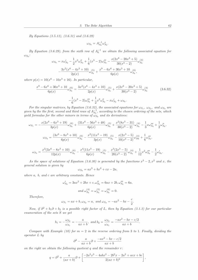
3. The Beke Algorithm 62
By Equations (3.5.13), (3.6.31) and (3.6.29)
ωS6= A−1
S6ω∗
S6.
By Equation (3.6.29), from the sixth row of A−16 we obtain the following associated equation for
ωS6:
ωS6= xω′
S6− 1
2x2ω′′
S6+
1
6(x3 − 2)ω′′′
S6− x(2x6 − 20x3 + 5)
30(x3 − 2)ω
(4)S6
−3x2(x6 − 4x3 + 10)
2p(x)ω
(5)S6
+x9 − 6x6 + 30x3 + 10
6p(x)ω
(6)S6,
where p(x) = 10(x6 − 10x3 + 16). In particular,
x9 − 6x6 + 30x3 + 10
6p(x)ω
(6)S6
=3x2(x6 − 4x3 + 10)
2p(x)ω
(5)S6
+x(2x6 − 20x3 + 5)
30(x3 − 2)ω
(4)S6
(3.6.32)
−1
6(x3 − 2)ω′′′
S6+
1
2x2ω′′
S6− xω′
S6+ ωS6
.
For the singular matrices, by Equation (3.6.32), the associated equations for ωS1, ωS2
, and ωS3are
given by the the first, second and third rows of A−1S6
, according to the chosen ordering of the sets, whichyield formulas for the other minors in terms of ωS6
and its derivatives:
ωS1= −x(2x
6 − 6x3 + 19)
3p(x)ω
(6)S6
+(31x6 − 56x3 + 48)
6p(x)ω
(5)S6
+x2(8x3 − 31)
30(x3 − 2)ω
(4)S6
− 1
3xω′′′
S6+
1
2ω′′
S6,
ωS2=
(3x6 − 8x3 + 10)
6p(x)ω
(6)S6
− x2(11x3 − 19)
3p(x)ω
(5)S6
− x(2x3 − 5)
10(x3 − 2)ω
(4)S6 +
1
6ω′′′
S6,
ωS3=x2(3x6 − 8x3 + 10)
12p(x)ω
(6)S6
− x4(11x3 − 19)
6p(x)ω
(5)S6
− x3(2x3 − 5)
20(x3 − 2)ω
(4)S6
+1
12x2ω′′′
S6− 1
2ω′
S6.
As the space of solutions of Equation (3.6.30) is generated by the functions x3 − 2, x2 and x, thegeneral solution is given by
ωS6= ax3 + bx2 + cx− 2a,
where a, b, and c are arbitrary constants. Hence
ω′S6
= 3ax2 + 2bx+ c, ω′′S6
= 6ax+ 2b, ω′′′S6
= 6a,
and ω(4)S6
= ω(5)S6
= ω(6)S6
= 0.
Therefore,
ωS1= ax+ b, ωS2
= a, and ωS3= −ax2 − bx− c
2.
Now, if ∂2 + b1∂ + b2 is a possible right factor of L, then by Equation (3.1.3) for our particularenumeration of the sets S we get
b1 = −ωS2
ωS1
= − a
ax+ b, and b2 =
ωS3
ωS1
=−ax2 − bx− c/2
ax+ b.
Compare with Example (10) for m = 2 in the reverse ordering from 3 to 1. Finally, dividing theoperator L by
∂2 − a
ax+ b∂ +
−ax2 − bx− c/2
ax+ b
on the right we obtain the following quotient q and the remainder r:
q = ∂2 +a
(ax+ b)∂ +
[−2a2x3 − 4abx2 − 2b2x− 2a2 + acx+ bc
2(ax+ b)2
],
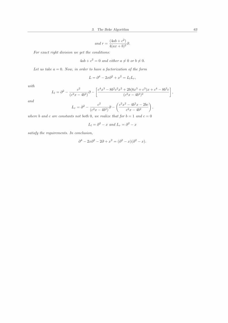
3. The Beke Algorithm 63
and r =(4ab+ c2)
4(ax+ b)2∂.
For exact right division we get the conditions:
4ab+ c2 = 0 and either a 6= 0 or b 6= 0.
Let us take a = 0. Now, in order to have a factorization of the form
L = ∂4 − 2x∂2 + x2 = LlLr,
with
Ll = ∂2 − c2
(c2x− 4b2)∂ −
[c4x3 − 8b2c2x2 + 2b(8x3 + c3)x+ c4 − 8b3c
(c2x− 4b2)2
],
and
Lr = ∂2 − c2
(c2x− 4b2)∂ −
(c2x2 − 4b2x− 2bc
c2x− 4b2
),
where b and c are constants not both 0, we realize that for b = 1 and c = 0
Ll = ∂2 − x and Lr = ∂2 − x
satisfy the requirements. In conclusion,
∂4 − 2x∂2 − 2∂ + x2 = (∂2 − x)(∂2 − x).
4. ADVANCED METHODS
In this chapter we will present methods for factoring linear differential operators which are not basedon Beke’s algorithm. We discuss Singer’s eigenring factorization method, introduced in Singer [1996],Newton polygons introduced in Malgrange [1979], and van Hoeij’s factorization methods introducedin van Hoeij [1997a] and in van Hoeij [1997b].
Let Kp denote the field with p elements. The core of Berlekamp’s algorithm for factoring a squarefreepolynomial f ∈ Kp[x] is the structure of the quotient
A = Kp[x]/Kp[x] · f.
In particular, if f = f1 · · · fm where the fi are pairwise relatively prime irreducible polynomials ofdegree di, then A is the direct sum of fields,
A = Kpd1 ⊕ · · · ⊕ Kpdm .
If Φ is the map Φ : x 7→ xp − x, then dimKp(ker Φ) = m. Therefore, computing the kernel of the
map Φ gives a quick way of determining the number of factors of f and, in particular, irreducibility.
Singer tried to generalize this idea to non-commutative polynomial rings and faced various problems.For example, let k be a field and σ a non-trivial automorphism of k and consider the ring k[x;σ] ofpolynomials in x over k with the usual addition and multiplication defined by
x · a = σ(a) · x for all a ∈ k.
Let f ∈ k[x;σ] and consider the left ideal k[x;σ] · f . The quotient
M = k[x;σ]/k[x;σ] · f
is a left k[x;σ]-module without a cononical ring structure. Singer replaces M with the ring E(M) ofk[x;σ]-endomorphisms of M , called the eigenring of k[x;σ] · f . In Griesbrecht [1992] it is shown thatf is irreducible if and only if E(M) has no zero divisors (and in fact is a field).
Considering the ring D = k[∂] one can start to proceed as with the ring k[x;σ]. In contrast to k[x;σ],D has in general a poor supply of two sided ideals. Furthermore, one cannot completely rely on theserings to determine irreducibility. Singer therefore looked beyond purely ring theoretic properties to findcriteria for irreducibility. The key fact is that to each linear operator L ∈ D one can associate a linearalgebraic group Gal(K/k), the Galois group of L(y) = 0, where K is its Picard-Vessiot extension, andthat L’s factorization properties are intimately related with the structure and representation theoryof Gal(K/k).
There are distinguished two cases:
1. Gal(K/k) is a reductive group, and
2. Gal(K/k) is a non-reductive group.
When Gal(K/k) is a reductive group, properties of EndD(D/D · L) determine if L is reducible.
Recall that a linear algebraic group is a subgroup or the group of invertible n×n matrices (undermatrix multiplication) that is defined by polynomial equations. An algebraic group is a group that
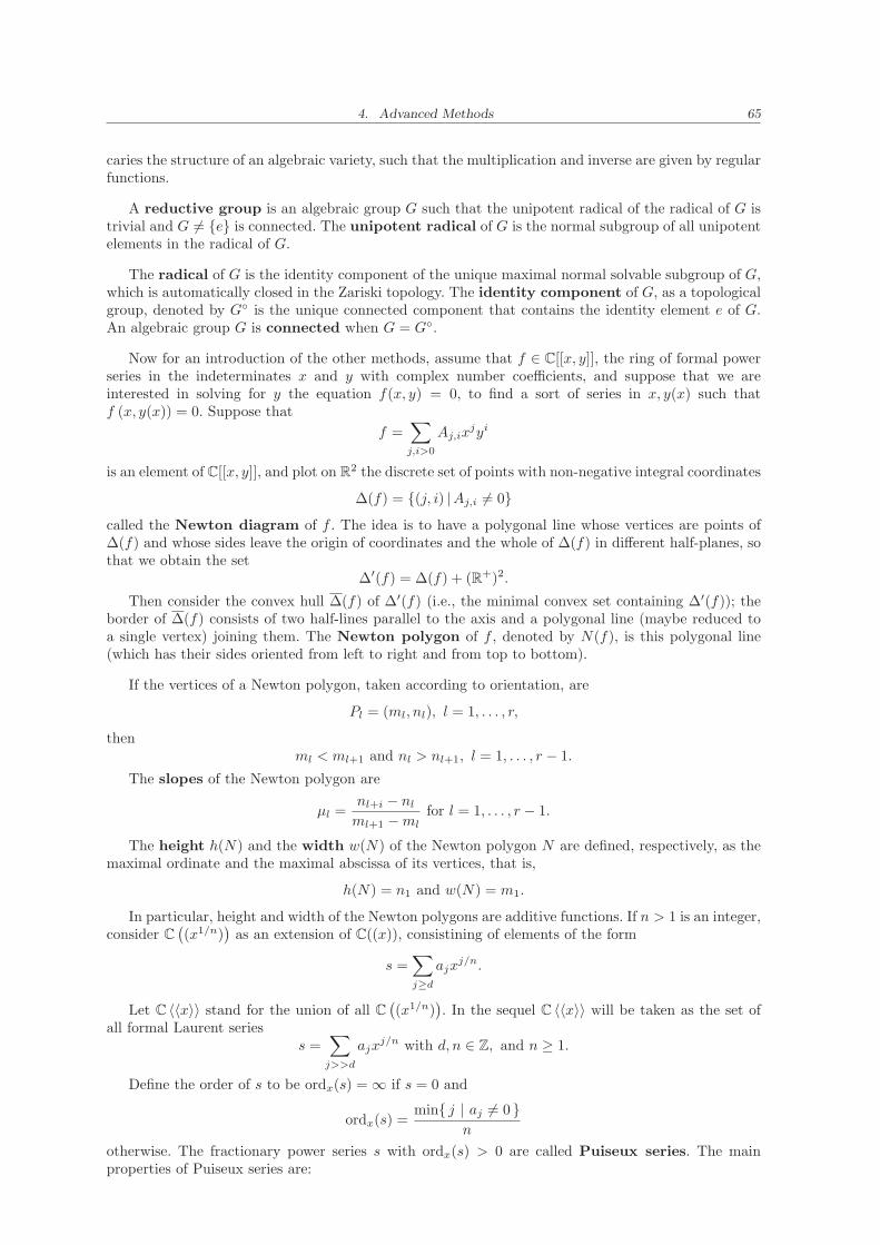
4. Advanced Methods 65
caries the structure of an algebraic variety, such that the multiplication and inverse are given by regularfunctions.
A reductive group is an algebraic group G such that the unipotent radical of the radical of G istrivial and G 6= {e} is connected. The unipotent radical of G is the normal subgroup of all unipotentelements in the radical of G.
The radical of G is the identity component of the unique maximal normal solvable subgroup of G,which is automatically closed in the Zariski topology. The identity component of G, as a topologicalgroup, denoted by G◦ is the unique connected component that contains the identity element e of G.An algebraic group G is connected when G = G◦.
Now for an introduction of the other methods, assume that f ∈ C[[x, y]], the ring of formal powerseries in the indeterminates x and y with complex number coefficients, and suppose that we areinterested in solving for y the equation f(x, y) = 0, to find a sort of series in x, y(x) such thatf (x, y(x)) = 0. Suppose that
f =∑
j,i>0
Aj,ixjyi
is an element of C[[x, y]], and plot on R2 the discrete set of points with non-negative integral coordinates
∆(f) = {(j, i) |Aj,i 6= 0}called the Newton diagram of f . The idea is to have a polygonal line whose vertices are points of∆(f) and whose sides leave the origin of coordinates and the whole of ∆(f) in different half-planes, sothat we obtain the set
∆′(f) = ∆(f) + (R+)2.
Then consider the convex hull ∆(f) of ∆′(f) (i.e., the minimal convex set containing ∆′(f)); theborder of ∆(f) consists of two half-lines parallel to the axis and a polygonal line (maybe reduced toa single vertex) joining them. The Newton polygon of f , denoted by N(f), is this polygonal line(which has their sides oriented from left to right and from top to bottom).
If the vertices of a Newton polygon, taken according to orientation, are
Pl = (ml, nl), l = 1, . . . , r,
thenml < ml+1 and nl > nl+1, l = 1, . . . , r − 1.
The slopes of the Newton polygon are
µl =nl+i − nl
ml+1 −mlfor l = 1, . . . , r − 1.
The height h(N) and the width w(N) of the Newton polygon N are defined, respectively, as themaximal ordinate and the maximal abscissa of its vertices, that is,
h(N) = n1 and w(N) = m1.
In particular, height and width of the Newton polygons are additive functions. If n > 1 is an integer,consider C
((x1/n)
)as an extension of C((x)), consistining of elements of the form
s =∑
j≥d
ajxj/n.
Let C 〈〈x〉〉 stand for the union of all C((x1/n)
). In the sequel C 〈〈x〉〉 will be taken as the set of
all formal Laurent seriess =
∑
j>>d
ajxj/n with d, n ∈ Z, and n ≥ 1.
Define the order of s to be ordx(s) = ∞ if s = 0 and
ordx(s) =min{ j | aj 6= 0 }
n
otherwise. The fractionary power series s with ordx(s) > 0 are called Puiseux series. The mainproperties of Puiseux series are:
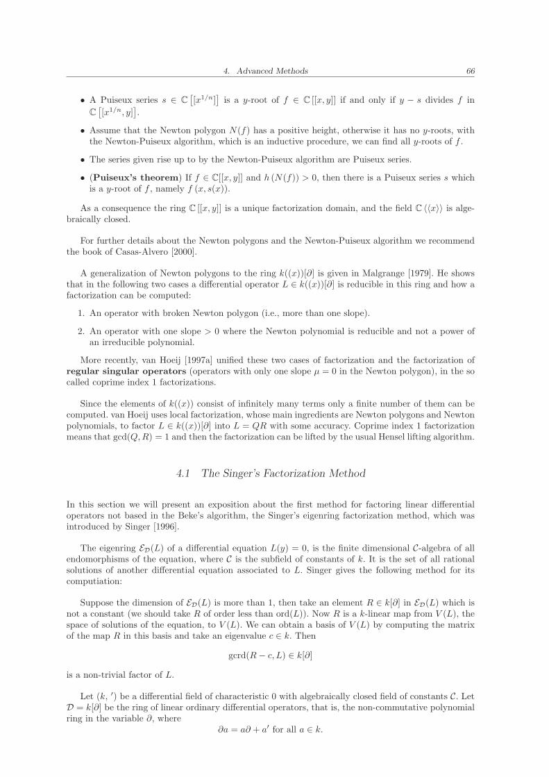
4. Advanced Methods 66
• A Puiseux series s ∈ C[[x1/n]
]is a y-root of f ∈ C [[x, y]] if and only if y − s divides f in
C[[x1/n, y]
].
• Assume that the Newton polygon N(f) has a positive height, otherwise it has no y-roots, withthe Newton-Puiseux algorithm, which is an inductive procedure, we can find all y-roots of f .
• The series given rise up to by the Newton-Puiseux algorithm are Puiseux series.
• (Puiseux’s theorem) If f ∈ C[[x, y]] and h (N(f)) > 0, then there is a Puiseux series s whichis a y-root of f , namely f (x, s(x)).
As a consequence the ring C [[x, y]] is a unique factorization domain, and the field C 〈〈x〉〉 is alge-braically closed.
For further details about the Newton polygons and the Newton-Puiseux algorithm we recommendthe book of Casas-Alvero [2000].
A generalization of Newton polygons to the ring k((x))[∂] is given in Malgrange [1979]. He showsthat in the following two cases a differential operator L ∈ k((x))[∂] is reducible in this ring and how afactorization can be computed:
1. An operator with broken Newton polygon (i.e., more than one slope).
2. An operator with one slope > 0 where the Newton polynomial is reducible and not a power ofan irreducible polynomial.
More recently, van Hoeij [1997a] unified these two cases of factorization and the factorization ofregular singular operators (operators with only one slope µ = 0 in the Newton polygon), in the socalled coprime index 1 factorizations.
Since the elements of k((x)) consist of infinitely many terms only a finite number of them can becomputed. van Hoeij uses local factorization, whose main ingredients are Newton polygons and Newtonpolynomials, to factor L ∈ k((x))[∂] into L = QR with some accuracy. Coprime index 1 factorizationmeans that gcd(Q,R) = 1 and then the factorization can be lifted by the usual Hensel lifting algorithm.
4.1 The Singer’s Factorization Method
In this section we will present an exposition about the first method for factoring linear differentialoperators not based in the Beke’s algorithm, the Singer’s eigenring factorization method, which wasintroduced by Singer [1996].
The eigenring ED(L) of a differential equation L(y) = 0, is the finite dimensional C-algebra of allendomorphisms of the equation, where C is the subfield of constants of k. It is the set of all rationalsolutions of another differential equation associated to L. Singer gives the following method for itscomputiation:
Suppose the dimension of ED(L) is more than 1, then take an element R ∈ k[∂] in ED(L) which isnot a constant (we should take R of order less than ord(L)). Now R is a k-linear map from V (L), thespace of solutions of the equation, to V (L). We can obtain a basis of V (L) by computing the matrixof the map R in this basis and take an eigenvalue c ∈ k. Then
gcrd(R− c, L) ∈ k[∂]
is a non-trivial factor of L.
Let (k, ′) be a differential field of characteristic 0 with algebraically closed field of constants C. LetD = k[∂] be the ring of linear ordinary differential operators, that is, the non-commutative polynomialring in the variable ∂, where
∂a = a∂ + a′ for all a ∈ k.
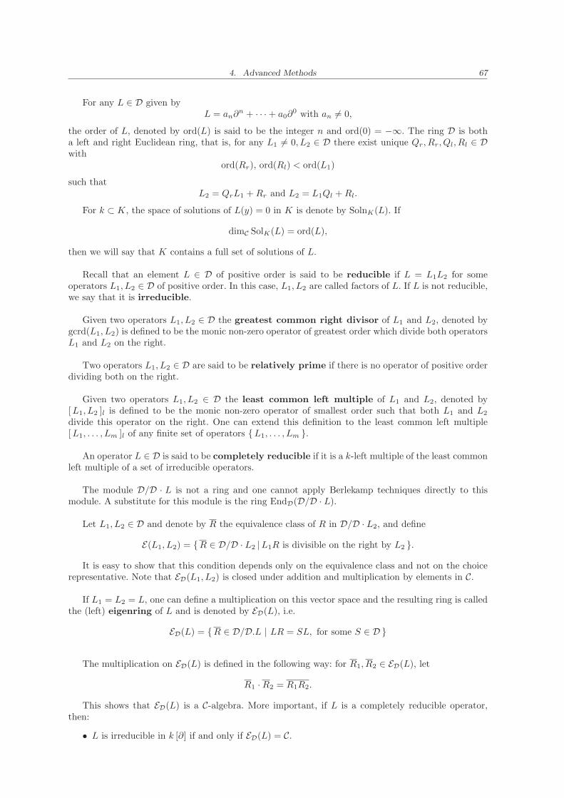
4. Advanced Methods 67
For any L ∈ D given byL = an∂
n + · · · + a0∂0 with an 6= 0,
the order of L, denoted by ord(L) is said to be the integer n and ord(0) = −∞. The ring D is botha left and right Euclidean ring, that is, for any L1 6= 0, L2 ∈ D there exist unique Qr, Rr, Ql, Rl ∈ Dwith
ord(Rr), ord(Rl) < ord(L1)
such thatL2 = QrL1 +Rr and L2 = L1Ql +Rl.
For k ⊂ K, the space of solutions of L(y) = 0 in K is denote by SolnK(L). If
dimC SolK(L) = ord(L),
then we will say that K contains a full set of solutions of L.
Recall that an element L ∈ D of positive order is said to be reducible if L = L1L2 for someoperators L1, L2 ∈ D of positive order. In this case, L1, L2 are called factors of L. If L is not reducible,we say that it is irreducible.
Given two operators L1, L2 ∈ D the greatest common right divisor of L1 and L2, denoted bygcrd(L1, L2) is defined to be the monic non-zero operator of greatest order which divide both operatorsL1 and L2 on the right.
Two operators L1, L2 ∈ D are said to be relatively prime if there is no operator of positive orderdividing both on the right.
Given two operators L1, L2 ∈ D the least common left multiple of L1 and L2, denoted by[L1, L2 ]l is defined to be the monic non-zero operator of smallest order such that both L1 and L2
divide this operator on the right. One can extend this definition to the least common left multiple[L1, . . . , Lm ]l of any finite set of operators {L1, . . . , Lm }.
An operator L ∈ D is said to be completely reducible if it is a k-left multiple of the least commonleft multiple of a set of irreducible operators.
The module D/D · L is not a ring and one cannot apply Berlekamp techniques directly to thismodule. A substitute for this module is the ring EndD(D/D · L).
Let L1, L2 ∈ D and denote by R the equivalence class of R in D/D · L2, and define
E(L1, L2) = {R ∈ D/D · L2 |L1R is divisible on the right by L2 }.
It is easy to show that this condition depends only on the equivalence class and not on the choicerepresentative. Note that ED(L1, L2) is closed under addition and multiplication by elements in C.
If L1 = L2 = L, one can define a multiplication on this vector space and the resulting ring is calledthe (left) eigenring of L and is denoted by ED(L), i.e.
ED(L) = {R ∈ D/D.L | LR = SL, for some S ∈ D }
The multiplication on ED(L) is defined in the following way: for R1, R2 ∈ ED(L), let
R1 ·R2 = R1R2.
This shows that ED(L) is a C-algebra. More important, if L is a completely reducible operator,then:
• L is irreducible in k [∂] if and only if ED(L) = C.
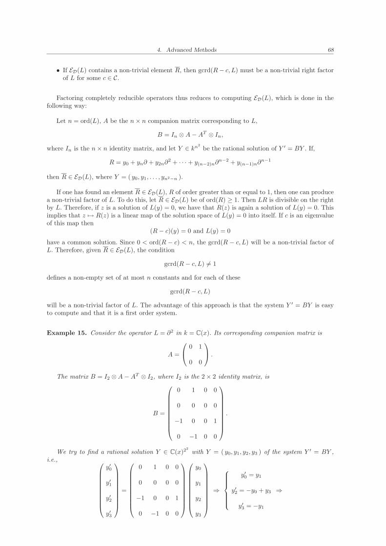
4. Advanced Methods 68
• If ED(L) contains a non-trivial element R, then gcrd(R− c, L) must be a non-trivial right factorof L for some c ∈ C.
Factoring completely reducible operators thus reduces to computing ED(L), which is done in thefollowing way:
Let n = ord(L), A be the n× n companion matrix corresponding to L,
B = In ⊗A−AT ⊗ In,
where In is the n× n identity matrix, and let Y ∈ kn2
be the rational solution of Y ′ = BY . If,
R = y0 + yn∂ + y2n∂2 + · · · + y(n−2)n∂
n−2 + y(n−1)n∂n−1
then R ∈ ED(L), where Y = ( y0, y1, . . . , yn2−n ).
If one has found an element R ∈ ED(L), R of order greater than or equal to 1, then one can producea non-trivial factor of L. To do this, let R ∈ ED(L) be of ord(R) ≥ 1. Then LR is divisible on the rightby L. Therefore, if z is a solution of L(y) = 0, we have that R(z) is again a solution of L(y) = 0. Thisimplies that z 7→ R(z) is a linear map of the solution space of L(y) = 0 into itself. If c is an eigenvalueof this map then
(R− c)(y) = 0 and L(y) = 0
have a common solution. Since 0 < ord(R − c) < n, the gcrd(R − c, L) will be a non-trivial factor ofL. Therefore, given R ∈ ED(L), the condition
gcrd(R− c, L) 6= 1
defines a non-empty set of at most n constants and for each of these
gcrd(R− c, L)
will be a non-trivial factor of L. The advantage of this approach is that the system Y ′ = BY is easyto compute and that it is a first order system.
Example 15. Consider the operator L = ∂2 in k = C(x). Its corresponding companion matrix is
A =
0 1
0 0
.
The matrix B = I2 ⊗A−AT ⊗ I2, where I2 is the 2 × 2 identity matrix, is
B =
0 1 0 0
0 0 0 0
−1 0 0 1
0 −1 0 0
.
We try to find a rational solution Y ∈ C(x)22
with Y = ( y0, y1, y2, y3 ) of the system Y ′ = BY ,i.e.,
y′0
y′1
y′2
y′3
=
0 1 0 0
0 0 0 0
−1 0 0 1
0 −1 0 0
y0
y1
y2
y3
⇒
y′0 = y1
y′2 = −y0 + y3
y′3 = −y1
⇒
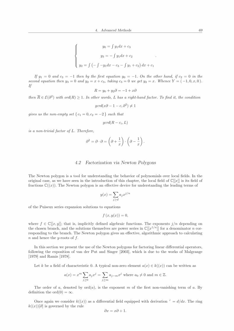
4. Advanced Methods 69
y0 =∫y1dx+ c3
y3 = −∫y1dx+ c2
y2 =∫ (
−∫−y1dx− c3 −
∫y1 + c2
)dx+ c1
.
If y1 = 0 and c3 = −1 then by the first equation y0 = −1. On the other hand, if c2 = 0 in thesecond equation then y3 = 0 and y2 = x+ c3, taking c3 = 0 we get y2 = x. Whence Y = (−1, 0, x, 0 ).If
R = y0 + y2∂ = −1 + x∂
then R ∈ E(∂2) with ord(R) ≥ 1. In other words, L has a right-hand factor. To find it, the condition
gcrd(x∂ − 1 − c, ∂2) 6= 1
gives us the non-empty set { c1 = 0, c2 = −2 } such that
gcrd(R− ci, L)
is a non-trivial factor of L. Therefore,
∂2 = ∂ · ∂ =
(∂ +
1
x
)·(∂ − 1
x
).
4.2 Factorization via Newton Polygons
The Newton polygon is a tool for understanding the behavior of polynomials over local fields. In theoriginal case, as we have seen in the introduction of this chapter, the local field of C[[x]] is its field offractions C((x)). The Newton polygon is an effective device for understanding the leading terms of
y(x) =∑
j≥d
ajxj/n
of the Puiseux series expansion solutions to equations
f (x, y(x)) = 0,
where f ∈ C[[x, y]]; that is, implicitly defined algebraic functions. The exponents j/n depending onthe chosen branch, and the solutions themselves are power series in C[[x1/n]] for a denominator n cor-responding to the branch. The Newton polygon gives an effective, algorithmic approach to calculatingn and hence the y-roots of f .
In this section we present the use of the Newton polygons for factoring linear differential operators,following the exposition of van der Put and Singer [2003], which is due to the works of Malgrange[1979] and Ramis [1978].
Let k be a field of characteristic 0. A typical non-zero element a(x) ∈ k((x)) can be written as
a(x) = xm∑
j≥0
ajxj =
∑
j≥m
aj−mxj where a0 6= 0 and m ∈ Z.
The order of a, denoted by ord(a), is the exponent m of the first non-vanishing term of a. Bydefinition the ord(0) = ∞.
Once again we consider k((x)) as a differential field equipped with derivation ′ = d/dx. The ringk((x))[∂] is governed by the rule
∂x = x∂ + 1.
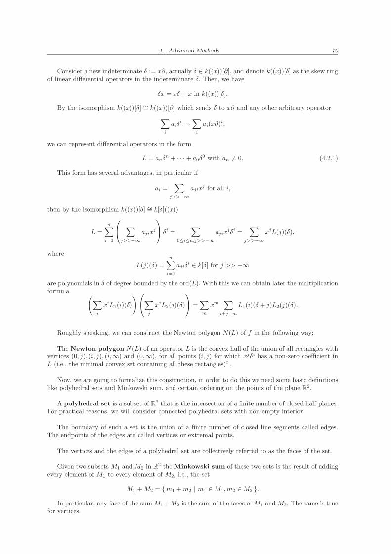
4. Advanced Methods 70
Consider a new indeterminate δ := x∂, actually δ ∈ k((x))[∂], and denote k((x))[δ] as the skew ringof linear differential operators in the indeterminate δ. Then, we have
δx = xδ + x in k((x))[δ].
By the isomorphism k((x))[δ] ∼= k((x))[∂] which sends δ to x∂ and any other arbitrary operator
∑
i
aiδi 7→
∑
i
ai(x∂)i,
we can represent differential operators in the form
L = anδn + · · · + a0δ
0 with an 6= 0. (4.2.1)
This form has several advantages, in particular if
ai =∑
j>>−∞ajix
j for all i,
then by the isomorphism k((x))[δ] ∼= k[δ]((x))
L =
n∑
i=0
∑
j>>−∞ajix
j
δi =
∑
0≤i≤n,j>>−∞ajix
jδi =∑
j>>−∞xjL(j)(δ).
where
L(j)(δ) =
n∑
i=0
ajiδi ∈ k[δ] for j >> −∞
are polynomials in δ of degree bounded by the ord(L). With this we can obtain later the multiplicationformula (
∑
i
xiL1(i)(δ)
)∑
j
xjL2(j)(δ)
=
∑
m
xm∑
i+j=m
L1(i)(δ + j)L2(j)(δ).
Roughly speaking, we can construct the Newton polygon N(L) of f in the following way:
The Newton polygon N(L) of an operator L is the convex hull of the union of all rectangles withvertices (0, j), (i, j), (i,∞) and (0,∞), for all points (i, j) for which xjδi has a non-zero coefficient inL (i.e., the minimal convex set containing all these rectangles)”.
Now, we are going to formalize this construction, in order to do this we need some basic definitionslike polyhedral sets and Minkowski sum, and certain ordering on the points of the plane R2.
A polyhedral set is a subset of R2 that is the intersection of a finite number of closed half-planes.For practical reasons, we will consider connected polyhedral sets with non-empty interior.
The boundary of such a set is the union of a finite number of closed line segments called edges.The endpoints of the edges are called vertices or extremal points.
The vertices and the edges of a polyhedral set are collectively referred to as the faces of the set.
Given two subsets M1 and M2 in R2 the Minkowski sum of these two sets is the result of addingevery element of M1 to every element of M2, i.e., the set
M1 +M2 = {m1 +m2 | m1 ∈M1,m2 ∈M2 }.
In particular, any face of the sum M1 +M2 is the sum of the faces of M1 and M2. The same is truefor vertices.
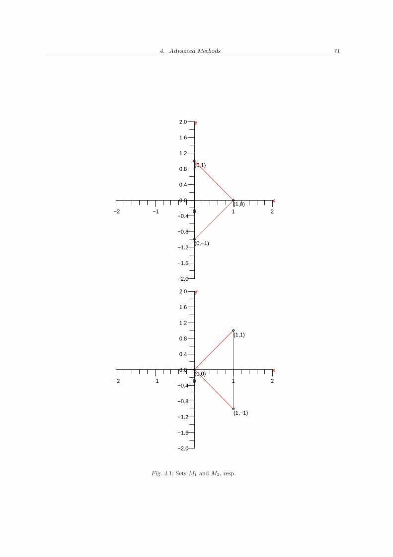
4. Advanced Methods 71
x
y
(0,−1)
(0,1)
(1,0)
1.2
0.4
−1.2
−2.0
2.0
1.6
0.8
0.0
−0.4
−0.8
−1.6
210−1−2
x
y
(1,−1)
(1,1)
(0,0)
1.2
0.4
−1.2
−2.0
2.0
1.6
0.8
0.0
−0.4
−0.8
−1.6
210−1−2
Fig. 4.1: Sets M1 and M2, resp.
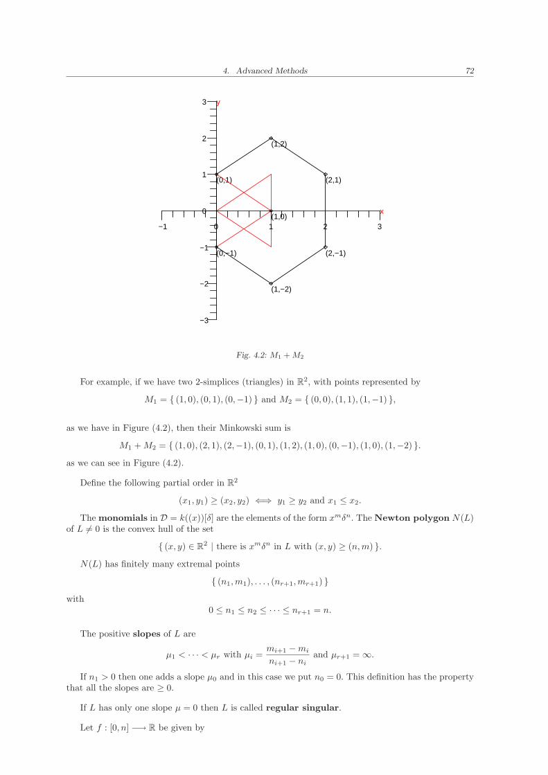
4. Advanced Methods 72
(1,−2)
(0,−1)
(1,2)
(0,1)
(2,−1)
(2,1)
(1,0)x
y
1
−3
3
2
0
−1
−2
3210−1
Fig. 4.2: M1 + M2
For example, if we have two 2-simplices (triangles) in R2, with points represented by
M1 = { (1, 0), (0, 1), (0,−1) } and M2 = { (0, 0), (1, 1), (1,−1) },
as we have in Figure (4.2), then their Minkowski sum is
M1 +M2 = { (1, 0), (2, 1), (2,−1), (0, 1), (1, 2), (1, 0), (0,−1), (1, 0), (1,−2) }.
as we can see in Figure (4.2).
Define the following partial order in R2
(x1, y1) ≥ (x2, y2) ⇐⇒ y1 ≥ y2 and x1 ≤ x2.
The monomials in D = k((x))[δ] are the elements of the form xmδn. The Newton polygon N(L)of L 6= 0 is the convex hull of the set
{ (x, y) ∈ R2 | there is xmδn in L with (x, y) ≥ (n,m) }.
N(L) has finitely many extremal points
{ (n1,m1), . . . , (nr+1,mr+1) }
with0 ≤ n1 ≤ n2 ≤ · · · ≤ nr+1 = n.
The positive slopes of L are
µ1 < · · · < µr with µi =mi+1 −mi
ni+1 − niand µr+1 = ∞.
If n1 > 0 then one adds a slope µ0 and in this case we put n0 = 0. This definition has the propertythat all the slopes are ≥ 0.
If L has only one slope µ = 0 then L is called regular singular.
Let f : [0, n] −→ R be given by
4. Advanced Methods 73
1. f(n0) = f(n1) = m1.
2. f(ni) = mi for all i.
3. f is (affine) linear on each segment [ni, ni+1] .
The slopes are the slopes of the graph. The length of the slope ki is ni+1 −ni. We reserve the termspecial polygon for a convex set that is the Newton polygon of some differential operator.
Let b(L) denote the graph of f . The boundary part B(L) of L is
B(L) =∑
(n,m)∈b(L)
an,mzmδn.
WriteL = B(L) +R(L).
We say that L1 > L2 if the points of b(L1) either lie in the interior of N(L2) or on the vertical ray
{ (nr+1, y) | y > mr+1 }.
Clearly R(L) > B(L) and R(L) > L. We note that the product of two monomials
M1 := xm1δn1 and M2 := xm2δn2
with m1,m2 ∈ Z and n1, n2 ∈ N is not a monomial. In fact, the product is
xm1+m2(δ +m2)n1δn2 . (4.2.2)
However,B(M1M2) = xm1+m2δn1+n2 .
As consequence of Formula (4.2.2) we have the formula
x−iL(j)(δ)xi = L(j)(δ + i) for all i ≥ 0 and j >> −∞. (4.2.3)
Form (4.2.1) has several advantages, because if L1, L2 ∈ D where
L1 =∑
i>>−∞xiL1(i)(δ) and L2 =
∑
j>>−∞xjL2(j)(δ),
by Formula (4.2.3) we get the multiplication formula
(∑
i>>−∞xiL1(i)(δ)
)
∑
j>>−∞xjL2(j)(δ)
=
∑
m>>−∞xm
∑
i+j=m
L1(i)(δ + j)L2(j)(δ).
(4.2.4)
The main properties of the Newton polygons are
• N(L1L2) = N(L1) +N(L2),
• the set of slopes of L1L2 is the union of the sets of slopes of L1 and L2,
• the length of the slope of L1L2 is the sum of length of the same slope for L1 and L2,
for all L1, L2 ∈ k((x))[δ].
The next theorem will provide us a way to factor linear differential operators using Newton polygons.For a proof we refer to van der Put and Singer [2003], pp. 88.
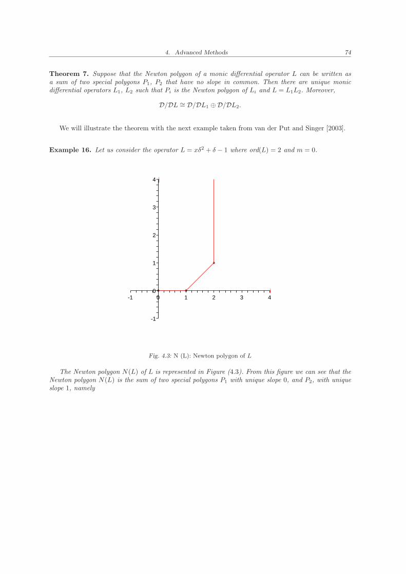
4. Advanced Methods 74
Theorem 7. Suppose that the Newton polygon of a monic differential operator L can be written asa sum of two special polygons P1, P2 that have no slope in common. Then there are unique monicdifferential operators L1, L2 such that Pi is the Newton polygon of Li and L = L1L2. Moreover,
D/DL ∼= D/DL1 ⊕D/DL2.
We will illustrate the theorem with the next example taken from van der Put and Singer [2003].
Example 16. Let us consider the operator L = xδ2 + δ − 1 where ord(L) = 2 and m = 0.
1
20
-1
10-1i
j4
4
3
3
2
Fig. 4.3: N (L): Newton polygon of L
The Newton polygon N(L) of L is represented in Figure (4.3). From this figure we can see that theNewton polygon N(L) is the sum of two special polygons P1 with unique slope 0, and P2, with uniqueslope 1, namely
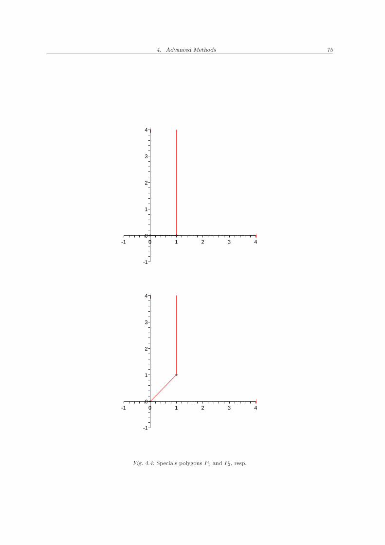
4. Advanced Methods 75
1
20
-1
10-1i
j4
4
3
3
2
1
20
-1
10-1i
j4
4
3
3
2
Fig. 4.4: Specials polygons P1 and P2, resp.
4. Advanced Methods 76
By Theorem (7) we want to find L1, L2 ∈ k((x))[δ] such that Pi is the Newton polygon of Li andL = L1L2. Suppose that
L1 = L1(0)(δ) + xL1(1)(δ) + · · · ,
L2 = L2(0)(δ) + xL2(1)(δ) + · · · .Since n1 = 1 (i.e. the abscissa of the extremal point (1, 0)) and ord(L) we have L1(0)(δ) is monic
polynomial of degree 1 and the L1(i)(δ) have degree 0 for i > 0.
On the other hand, P2 has no slope equal to 0, this means that L2(0)(δ) is a constant. In factL2(0)(δ) = 1, because (0, 0) is an extremal point of P2. Comparing the coefficients of x0 in L = L1L2
we getL1(0)(δ)L2(0)(δ) = L(0)(δ) =⇒ L1(0)(δ) = δ − 1.
Comparing the coefficients of x1 we have
L1(0)(δ + 1)L2(1)(δ) + L1(0)(δ)L2(0)(δ) = L(1)(δ) ⇒
δL2(1)(δ) + L1(1)(δ) = δ2.
This implies that L2(1)(δ) = δ and L1(1)(δ) = 0. It can be shown by induction that
L1(i)(δ) = L2(i)(δ) = 0 for i ≥ 2.
Therefore, the operator L factors as L = L1L2 where
L1 = δ − 1 and L2 = xδ + 1.
4.3 Factorization via Newton Polynomials and Coprime Index 1
From Malgrange [1979] we know that an element of k((x))[∂] which has only one slope in the Newtonpolygon and which has an irreducible Newton polynomial is irreducible in k((x))[∂]. He shows thatin the following two cases a differential operator L ∈ k((x))[∂] is reducible in this ring and how afactorization can be computed:
1. An operator with broken Newton polygon (i.e. more than one slope).
2. An operator with one slope > 0 where the Newton polynomial is reducible and not a power ofan irreducible polynomial.
In van Hoeij [1997a] these two cases of factorization and the factorization of regular singular oper-ators are unified in the so called coprime index 1 factorization.
Since the elements of k((x)) consist of infinitely many terms, only a finite number of them can becomputed. This means that a factorization can only be determinated up to some finite accuracy.
We start this section with some basic definitions like filtered ring, filtration and associated gradedring. These important concepts will become very useful, since often information can be obtained bypassing from a ring with a “natural” filtration to the associated graded ring, and then translating theresult back to the original ring. In particular, this is useful if the ring is filtered by (additive) subgroups,such that the associated graded ring is commutative.
A filtration of a ring D is a chain of additive subgroups Di of D, such that
1 ∈ D0, · · · ⊃ Di−1 ⊃ Di ⊃ Di+1 ⊃ · · · , i ∈ Z,with
DiDj ⊂ Di+j for all i, j ∈ Z, and D =⋃
i∈Z
Di.

4. Advanced Methods 77
A ring equipped with a filtration is called a filtered ring.
A grading {Di}i∈Z of the ring D is a sequence of additive subgroups Di of D such that
D =⊕
i∈Z
Di and DiDj ⊆ Di+j for all i, j ∈ Z.
A ring with a grading {Di} is called graded. The elements of Di are called homogeneous ofdegree i. A homogeneous element of R is simply an element of one of the groups Di. If f ∈ D, thereis a unique expression for f of the form
f = f0 + f1 + · · · with fi ∈ Di and fj = 0 for j >> 0,
the fi are called the homogeneous components of f . In particular, the component D0 is a subringof D containing 1D.
Let D be a filtered ring with a filtration {Di}i∈Z. The associated graded ring, denoted by gr(D)is defined as
gr(D) =⊕
i∈Z
Di/Di+1 (as additive groups),
equipped with the obvious addition and multiplication given by
(r +Di+1)(s+Dj+1) = (rs+Di+j+1), for r ∈ Di, s ∈ Dj .
The symbol map σ : D → gr(D) is defined as:
σ(0) = 0, and σ(f) = f +Di+1 if f ∈ Di\Di+1.
Let D be a ring, a discrete valuation on the ring D is a map v : D → Z ∪ {∞} such that
• v(fg) = v(f) + v(g),
• v(f + g) ≥ min (v(f), v(g)), and
• v(0) = ∞,
for all f, g ∈ D. As a consequence of the first two properties we have
v(f + g) = min (v(f), v(g)) if v(f) 6= v(g).
A valuation v defines a filtration on a ring D as follows
Di = { f ∈ D | v(f) ≥ i }.
For a positive integer a the set D0/Da has the structure of a ring.
For a ring D with a valuation v we define a truncation σa with accuracy a for non-zero elementsf ∈ D and a positive integer a as follows
σa(f) = f +Dv(f)+a ∈ Dv(f)/Dv(f)+a.
Let k be a field of characteristic 0 and consider the ring D = k((x))[δ], where δ = x∂ ∈ k((x))[∂].Let L ∈ D be a differential operator given by
L =∑
j,i
ajixjδi.
Let s ∈ Q be a rational number with s ≥ 0, write s = u/d with u, d ∈ Z, gcd(u, d) = 1 and d > 0.Then the function vs : D → Z ∪ {∞} given by
vs
∑
j,i
ajixjδi
= inf{jd− iu : aji 6= 0},
4. Advanced Methods 78
defines a discrete valuation on D. We take infimum instead of minimum for formal reasons with respectto the zero operator. As mentioned above, the valuation vs gives a filtration (Di)i∈Z
Di = {L ∈ D|vs(L) ≥ i}
and a truncation σa,s with accuracy a
σa,s(L) = L+Dvs(L)+a ∈ Dvs(L)/Dvs(L)+a.
To σ1,s for L ∈ D corresponds the so-called Newton polynomial Ns(L) of L for slope s (whichdoes not correspond to the usual definition of the Newton polynomial), and roughly speaking we cancompute it in the following way:
“The length l(s) of a slope s in the Newton polygon N(L) is defined as the length of the projectionof this slope onto the x-axis. The Newton polynomial Ns(L) is a polynomial in a new indeterminateT of degree
l(s)
d,
and its monomials can be computed from the points which lie exactly on the slope s and the leadingcoefficients of the corresponding aji”.
In particular, σ1,s(L) is an element of
D =⋃
i∈Z
Di/Di+1.
A multiplication is defined for elements of D, and an addition is only defined for f, g ∈ D whichare elements of the same Di/Di+1. There is a k-linear bijection N ′
s : D0/D1 → k[T ] which is also aring isomorphism if i = 0. If i = 0 then N ′
0 is defined by
xuδd 7−→ T.
For every i ∈ Z there is a unique pair of integers ui, di with
0 ≤ di < d and vs(xuiδdi) = i
such that the map φi : D0/D1 → Di/Di+1 defined by
φi(a) = xuiδdia
is a bijection. Now, for s > 0 let N ′s : Di/Di+1 → k[T ] be defined by
N ′s(a) = N ′
s
(φ−1
i (a))
as we see in the next diagram
D0/D1 k[T ]
Di/Di+1
................................................................................................................................................................... ............N ′
s
.............................................................................................................................
φi
...........................................................................................................................
N ′s
.
N ′s is also defined for non-zero elements of L ∈ D asN ′
s (σ1,s(L)). For slope s = 0 define the Newtonpolynomial N0(L) as N ′
0(L). By Formula (4.2.4) the following property follows for Q,R ∈ D
N0(QR) = ST=T+v0(R)(N0(Q))N0(R).
Here ST=T+v0(R)(N0(Q)) means N0(Q) with T replaced by T + v0(R). For slope s > 0 we have thefollowing property for Q,R ∈ D
N ′s(QR) = T pN ′
s(Q)N ′s(R).
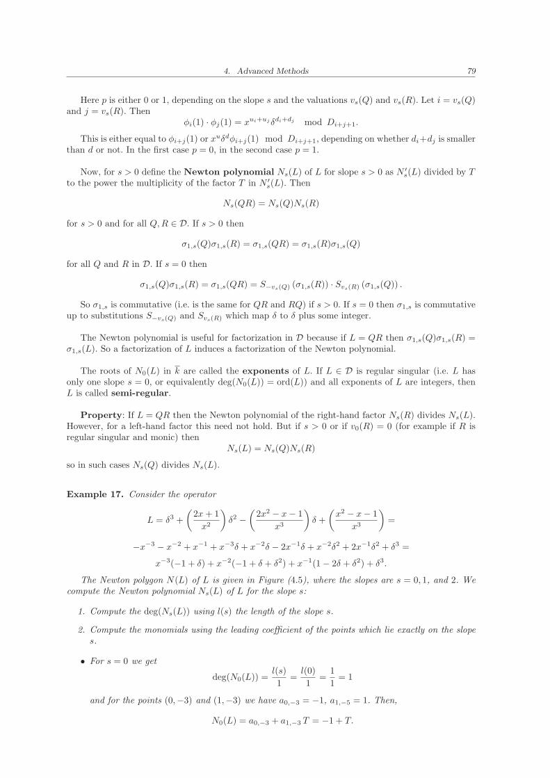
4. Advanced Methods 79
Here p is either 0 or 1, depending on the slope s and the valuations vs(Q) and vs(R). Let i = vs(Q)and j = vs(R). Then
φi(1) · φj(1) = xui+ujδdi+dj mod Di+j+1.
This is either equal to φi+j(1) or xuδdφi+j(1) mod Di+j+1, depending on whether di+dj is smallerthan d or not. In the first case p = 0, in the second case p = 1.
Now, for s > 0 define the Newton polynomial Ns(L) of L for slope s > 0 as N ′s(L) divided by T
to the power the multiplicity of the factor T in N ′s(L). Then
Ns(QR) = Ns(Q)Ns(R)
for s > 0 and for all Q,R ∈ D. If s > 0 then
σ1,s(Q)σ1,s(R) = σ1,s(QR) = σ1,s(R)σ1,s(Q)
for all Q and R in D. If s = 0 then
σ1,s(Q)σ1,s(R) = σ1,s(QR) = S−vs(Q) (σ1,s(R)) · Svs(R) (σ1,s(Q)) .
So σ1,s is commutative (i.e. is the same for QR and RQ) if s > 0. If s = 0 then σ1,s is commutativeup to substitutions S−vs(Q) and Svs(R) which map δ to δ plus some integer.
The Newton polynomial is useful for factorization in D because if L = QR then σ1,s(Q)σ1,s(R) =σ1,s(L). So a factorization of L induces a factorization of the Newton polynomial.
The roots of N0(L) in k are called the exponents of L. If L ∈ D is regular singular (i.e. L hasonly one slope s = 0, or equivalently deg(N0(L)) = ord(L)) and all exponents of L are integers, thenL is called semi-regular.
Property: If L = QR then the Newton polynomial of the right-hand factor Ns(R) divides Ns(L).However, for a left-hand factor this need not hold. But if s > 0 or if v0(R) = 0 (for example if R isregular singular and monic) then
Ns(L) = Ns(Q)Ns(R)
so in such cases Ns(Q) divides Ns(L).
Example 17. Consider the operator
L = δ3 +
(2x+ 1
x2
)δ2 −
(2x2 − x− 1
x3
)δ +
(x2 − x− 1
x3
)=
−x−3 − x−2 + x−1 + x−3δ + x−2δ − 2x−1δ + x−2δ2 + 2x−1δ2 + δ3 =
x−3(−1 + δ) + x−2(−1 + δ + δ2) + x−1(1 − 2δ + δ2) + δ3.
The Newton polygon N(L) of L is given in Figure (4.5), where the slopes are s = 0, 1, and 2. Wecompute the Newton polynomial Ns(L) of L for the slope s:
1. Compute the deg(Ns(L)) using l(s) the length of the slope s.
2. Compute the monomials using the leading coefficient of the points which lie exactly on the slopes.
• For s = 0 we get
deg(N0(L)) =l(s)
1=l(0)
1=
1
1= 1
and for the points (0,−3) and (1,−3) we have a0,−3 = −1, a1,−5 = 1. Then,
N0(L) = a0,−3 + a1,−3 T = −1 + T.
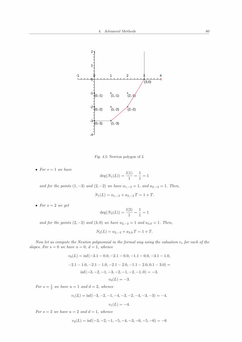
4. Advanced Methods 80
2i
j
1
(3,0)
(2,-1)
0
(2,-2)
(1,-1)
-1
(1,-2)
(1,-3)
(0,-1)
(0,-2)
(0,-3)
2
1
0
-1
-2
-3
4
-4
3
Fig. 4.5: Newton polygon of L
• For s = 1 we have
deg(N1(L)) =l(1)
1=
1
1= 1
and for the points (1,−3) and (2,−2) we have a1,−3 = 1, and a2,−2 = 1. Then,
N1(L) = a1,−3 + a2,−2 T = 1 + T.
• For s = 2 we get
deg(N2(L)) =l(2)
1=
1
1= 1
and for the points (2,−2) and (3, 0) we have a2,−2 = 1 and a3,0 = 1. Then,
N2(L) = a2,−2 + a3,0 T = 1 + T.
Now let us compute the Newton polynomial in the formal way using the valuation vs for each of theslopes. For s = 0 we have u = 0, d = 1, whence
v0(L) = inf(−3.1 − 0.0,−2.1 − 0.0,−1.1 − 0.0,−3.1 − 1.0,
−2.1 − 1.0,−2.1 − 1.0,−2.1 − 2.0,−1.1 − 2.0, 0.1 − 3.0) =
inf(−3,−2,−1,−3,−2,−1,−2,−1, 0) = −3.
v0(L) = −3.
For s = 12 we have u = 1 and d = 2, whence
v1(L) = inf(−3,−2,−1,−4,−3,−2,−4,−3,−3) = −4.
v1(L) = −4.
For s = 2 we have u = 2 and d = 1, whence
v2(L) = inf(−3,−2,−1,−5,−4,−3,−6,−5,−6) = −6
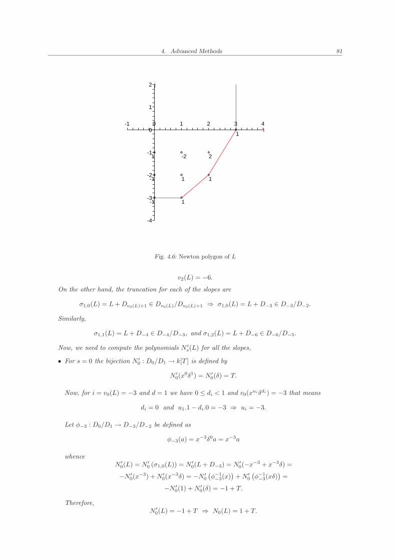
4. Advanced Methods 81
2i
j
1
1
2
0
1
-2
-1
1
1
1
-1
-1
2
1
0
-1
-2
-3
4
-4
3
Fig. 4.6: Newton polygon of L
v2(L) = −6.
On the other hand, the truncation for each of the slopes are
σ1,0(L) = L+Dv0(L)+1 ∈ Dv0(L)/Dv0(L)+1 ⇒ σ1,0(L) = L+D−3 ∈ D−3/D−2.
Similarly,
σ1,1(L) = L+D−4 ∈ D−4/D−3, and σ1,2(L) = L+D−6 ∈ D−6/D−5.
Now, we need to compute the polynomials N ′s(L) for all the slopes,
• For s = 0 the bijection N ′0 : D0/D1 → k[T ] is defined by
N ′0(x
0δ1) = N ′0(δ) = T.
Now, for i = v0(L) = −3 and d = 1 we have 0 ≤ di < 1 and v0(xuiδdi) = −3 that means
di = 0 and u1.1 − di.0 = −3 ⇒ ui = −3.
Let φ−3 : D0/D1 → D−3/D−2 be defined as
φ−3(a) = x−3δ0a = x−3a
whenceN ′
0(L) = N ′0 (σ1,0(L)) = N ′
0(L+D−3) = N ′0(−x−3 + x−3δ) =
−N ′0(x
−3) +N ′0(x
−3δ) = −N ′0
(φ−1−3(x)
)+N ′
0
(φ−1−3(xδ)
)=
−N ′0(1) +N ′
0(δ) = −1 + T.
Therefore,N ′
0(L) = −1 + T ⇒ N0(L) = 1 + T.
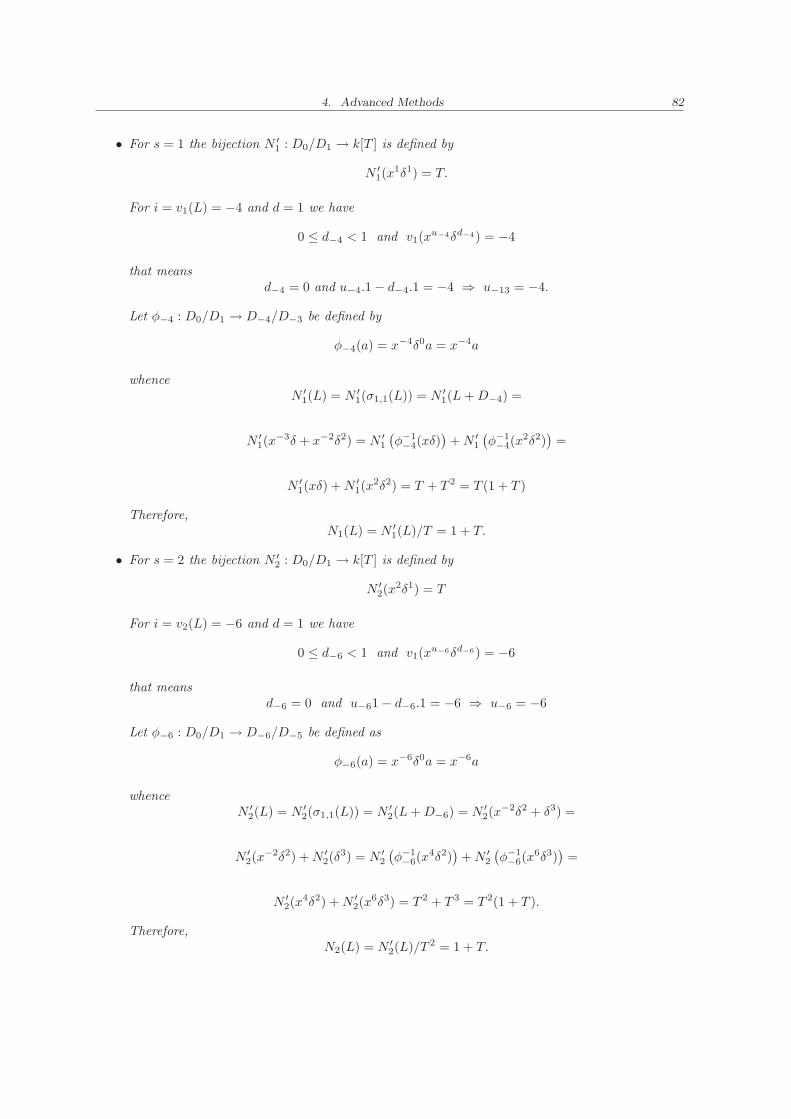
4. Advanced Methods 82
• For s = 1 the bijection N ′1 : D0/D1 → k[T ] is defined by
N ′1(x
1δ1) = T.
For i = v1(L) = −4 and d = 1 we have
0 ≤ d−4 < 1 and v1(xu−4δd−4) = −4
that meansd−4 = 0 and u−4.1 − d−4.1 = −4 ⇒ u−13 = −4.
Let φ−4 : D0/D1 → D−4/D−3 be defined by
φ−4(a) = x−4δ0a = x−4a
whenceN ′
1(L) = N ′1(σ1,1(L)) = N ′
1(L+D−4) =
N ′1(x
−3δ + x−2δ2) = N ′1
(φ−1−4(xδ)
)+N ′
1
(φ−1−4(x
2δ2))
=
N ′1(xδ) +N ′
1(x2δ2) = T + T 2 = T (1 + T )
Therefore,N1(L) = N ′
1(L)/T = 1 + T.
• For s = 2 the bijection N ′2 : D0/D1 → k[T ] is defined by
N ′2(x
2δ1) = T
For i = v2(L) = −6 and d = 1 we have
0 ≤ d−6 < 1 and v1(xu−6δd−6) = −6
that meansd−6 = 0 and u−61 − d−6.1 = −6 ⇒ u−6 = −6
Let φ−6 : D0/D1 → D−6/D−5 be defined as
φ−6(a) = x−6δ0a = x−6a
whenceN ′
2(L) = N ′2(σ1,1(L)) = N ′
2(L+D−6) = N ′2(x
−2δ2 + δ3) =
N ′2(x
−2δ2) +N ′2(δ
3) = N ′2
(φ−1−6(x
4δ2))
+N ′2
(φ−1−6(x
6δ3))
=
N ′2(x
4δ2) +N ′2(x
6δ3) = T 2 + T 3 = T 2(1 + T ).
Therefore,N2(L) = N ′
2(L)/T 2 = 1 + T.
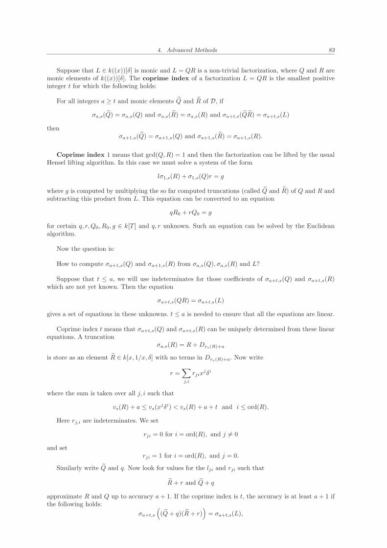
4. Advanced Methods 83
Suppose that L ∈ k((x))[δ] is monic and L = QR is a non-trivial factorization, where Q and R aremonic elements of k((x))[δ]. The coprime index of a factorization L = QR is the smallest positiveinteger t for which the following holds:
For all integers a ≥ t and monic elements Q and R of D, if
σa,s(Q) = σa,s(Q) and σa,s(R) = σa,s(R) and σa+t,s(QR) = σa+t,s(L)
thenσa+1,s(Q) = σa+1,s(Q) and σa+1,s(R) = σa+1,s(R).
Coprime index 1 means that gcd(Q,R) = 1 and then the factorization can be lifted by the usualHensel lifting algorithm. In this case we must solve a system of the form
lσ1,s(R) + σ1,s(Q)r = g
where g is computed by multiplying the so far computed truncations (called Q and R) of Q and R andsubtracting this product from L. This equation can be converted to an equation
qR0 + rQ0 = g
for certain q, r,Q0, R0, g ∈ k[T ] and q, r unknown. Such an equation can be solved by the Euclideanalgorithm.
Now the question is:
How to compute σa+1,s(Q) and σa+1,s(R) from σa,s(Q), σa,s(R) and L?
Suppose that t ≤ a, we will use indeterminates for those coefficients of σa+t,s(Q) and σa+t,s(R)which are not yet known. Then the equation
σa+t,s(QR) = σa+t,s(L)
gives a set of equations in these unknowns. t ≤ a is needed to ensure that all the equations are linear.
Coprime index t means that σa+t,s(Q) and σa+t,s(R) can be uniquely determined from these linearequations. A truncation
σa,s(R) = R+Dvs(R)+a
is store as an element R ∈ k[x, 1/x, δ] with no terms in Dvs(R)+a. Now write
r =∑
j,i
rjixjδi
where the sum is taken over all j, i such that
vs(R) + a ≤ vs(xjδi) < vs(R) + a+ t and i ≤ ord(R).
Here rj,i are indeterminates. We set
rji = 0 for i = ord(R), and j 6= 0
and setrji = 1 for i = ord(R), and j = 0.
Similarly write Q and q. Now look for values for the lji and rji such that
R+ r and Q+ q
approximate R and Q up to accuracy a+ 1. If the coprime index is t, the accuracy is at least a+ 1 ifthe following holds:
σa+t,s
((Q+ q)(R+ r)
)= σa+t,s(L),
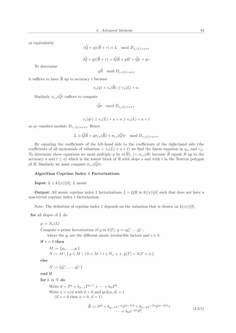
4. Advanced Methods 84
or equivalently(Q+ q)(R+ r) ≡ L mod Dvs(L)+a+t
(Q+ q)(R+ r) = QR+ qR′ + Qr + qr.
To determineqR mod Dvs(L)+a+t
it suffices to have R up to accuracy t because
vs(q) + vs(R) ≥ vs(L) + a.
Similarly vt,s(Q) suffices to compute
Qr mod Dvs(L)+a+t.
vs(qr) ≥ vs(L) + a+ a ≥ vs(L) + a+ t
so qr vanishes modulo Dvs(L)+a+t. Hence
L ≡ QR+ qσt,s(R) + σt,s(Q)r mod Dvs(L)+a+t.
By equating the coefficients of the left-hand side to the coefficients of the right-hand side (thecoefficients of all monomials of valuation < vs(L) + a + t) we find the linear equation in qji and rji.
To determine these equations we must multiply q by σ(R), (= σt,s(R) because R equals R up to theaccuracy a and t ≤ a) which is the lowest block of R with slope s and with t in the Newton polygon
of R. Similarly we must compute σt,s(Q)r.
Algorithm Coprime Index 1 Factorizations
Input: L ∈ k((x))[δ], L monic
Output: All monic coprime index 1 factorizations L = QR in k((x))[δ] such that does not have anon-trivial coprime index 1 factorization.
Note: The definition of coprime index 1 depends on the valuation that is chosen on k((x))[δ].
for all slopes of L do
g := Ns(L)
Compute a prime factorization of g in k[T ], g = cge11 . . . ger
r ,
where the gi are the different monic irreducible factors and c ∈ k.
if s = 0 then
M := {g1, . . . , gr}N := M \ { g ∈M | ∃h ∈M ∧ i ∈ N+ s. t. g(T ) = h(T + i) }
else
N := {ge11 , . . . , g
err }
end if
for h in N do
Write h = T p + hp−1Tp−1 + · · · + h0T
0.
Write s = u/d with d > 0 and gcd(u, d) = 1(if s = 0 then u = 0, d = 1)
R := δpd + hp−1x−nδ(p−1)d + hp−2x
−2nδ(p−2)d+· · · + h0x
−pnδ0.(4.3.5)
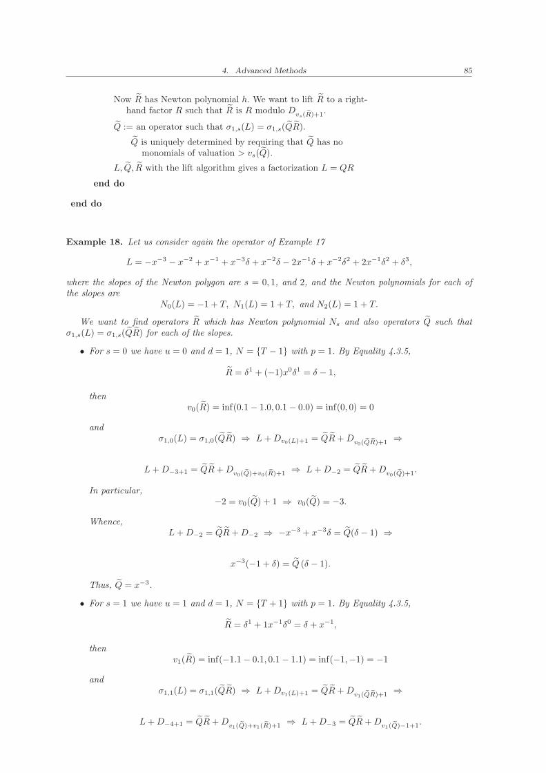
4. Advanced Methods 85
Now R has Newton polynomial h. We want to lift R to a right-hand factor R such that R is R modulo Dvs( eR)+1.
Q := an operator such that σ1,s(L) = σ1,s(QR).
Q is uniquely determined by requiring that Q has nomonomials of valuation > vs(Q).
L, Q, R with the lift algorithm gives a factorization L = QR
end do
end do
Example 18. Let us consider again the operator of Example 17
L = −x−3 − x−2 + x−1 + x−3δ + x−2δ − 2x−1δ + x−2δ2 + 2x−1δ2 + δ3,
where the slopes of the Newton polygon are s = 0, 1, and 2, and the Newton polynomials for each ofthe slopes are
N0(L) = −1 + T, N1(L) = 1 + T, and N2(L) = 1 + T.
We want to find operators R which has Newton polynomial Ns and also operators Q such thatσ1,s(L) = σ1,s(QR) for each of the slopes.
• For s = 0 we have u = 0 and d = 1, N = {T − 1} with p = 1. By Equality 4.3.5,
R = δ1 + (−1)x0δ1 = δ − 1,
thenv0(R) = inf(0.1 − 1.0, 0.1 − 0.0) = inf(0, 0) = 0
andσ1,0(L) = σ1,0(QR) ⇒ L+Dv0(L)+1 = QR+Dv0( eQ eR)+1 ⇒
L+D−3+1 = QR+Dv0( eQ)+v0( eR)+1 ⇒ L+D−2 = QR+Dv0( eQ)+1.
In particular,−2 = v0(Q) + 1 ⇒ v0(Q) = −3.
Whence,L+D−2 = QR+D−2 ⇒ −x−3 + x−3δ = Q(δ − 1) ⇒
x−3(−1 + δ) = Q (δ − 1).
Thus, Q = x−3.
• For s = 1 we have u = 1 and d = 1, N = {T + 1} with p = 1. By Equality 4.3.5,
R = δ1 + 1x−1δ0 = δ + x−1,
thenv1(R) = inf(−1.1 − 0.1, 0.1 − 1.1) = inf(−1,−1) = −1
andσ1,1(L) = σ1,1(QR) ⇒ L+Dv1(L)+1 = QR+Dv1( eQ eR)+1 ⇒
L+D−4+1 = QR+Dv1( eQ)+v1( eR)+1 ⇒ L+D−3 = QR+Dv1( eQ)−1+1.
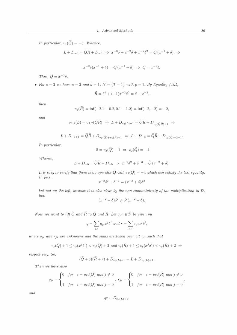
4. Advanced Methods 86
In particular, v1(Q) = −3. Whence,
L+D−3 = QR+D−3 ⇒ x−3δ + x−2δ + x−2δ2 = Q (x−1 + δ) ⇒
x−2δ(x−1 + δ) = Q (x−1 + δ) ⇒ Q = x−2δ.
Thus, Q = x−2δ.
• For s = 2 we have u = 2 and d = 1, N = {T − 1} with p = 1. By Equality 4.3.5,
R = δ1 + (−1)x−2δ0 = δ + x−2,
thenv2(R) = inf(−2.1 − 0.2, 0.1 − 1.2) = inf(−2,−2) = −2,
andσ1,2(L) = σ1,2(QR) ⇒ L+Dv2(L)+1 = QR+Dv2( eQ eR)+1 ⇒
L+D−6+1 = QR+Dv2( eQ)+v2( eR)+1 ⇒ L+D−5 = QR+Dv2( eQ)−2+1.
In particular,−5 = v2(Q) − 1 ⇒ v2(Q) = −4.
Whence,L+D−5 = QR+D−5 ⇒ x−2δ2 + δ−3 = Q (x−2 + δ).
It is easy to verify that there is no operator Q with v2(Q) = −4 which can satisfy the last equality.In fact,
x−2δ2 + δ−3 = (x−2 + δ)δ2
but not on the left, because it is also clear by the non-commutativity of the multiplication in D,that
(x−2 + δ)δ2 6= δ2(x−2 + δ).
Now, we want to lift Q and R to Q and R. Let q, r ∈ D be given by
q =∑
j,i
qjixjδi and r =
∑
j,i
rjixjδi,
where qji and rji are unknowns and the sums are taken over all j, i such that
vs(Q) + 1 ≤ vs(xjδi) < vs(Q) + 2 and vs(R) + 1 ≤ vs(x
jδi) < vs(R) + 2 ⇒
respectively. So,(Q+ q)(R+ r) +Dvs(L)+1 = L+Dvs(L)+1.
Then we have also
qji =
0 for i = ord(Q) and j 6= 0
1 for i = ord(Q) and j = 0
, rji =
0 for i = ord(R) and j 6= 0
1 for i = ord(R) and j = 0
,
andqr ∈ Dvs(L)+1.
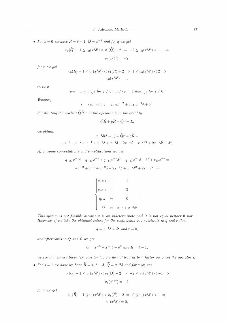
4. Advanced Methods 87
• For s = 0 we have R = δ − 1, Q = x−3 and for q we get
v0(Q) + 1 ≤ v0(xjδi) < v0(Q) + 2 ⇒ −2 ≤ v0(x
jδi) < −1 ⇒
v0(xjδi) = −2,
for r we getv0(R) + 1 ≤ v1(x
jδi) < v1(R) + 2 ⇒ 1 ≤ v0(xjδi) < 2 ⇒
v0(xjδi) = 1,
in turnq02 = 1 and qj2 for j 6= 0, and r01 = 1 and rj1 for j 6= 0.
Whence,r = r10x and q = q−20x
−2 + q−11x−1δ + δ2.
Substituting the product QR and the operator L in the equality
QR+ qR+ Qr = L,
we obtain,x−3δ(δ − 1) + Qr + qR =
−x−3 − x−2 + x−1 + x−3δ + x−2δ − 2x−1δ + x−2δ2 + 2x−1δ2 + δ3.
After some computations and simplifications we get
q−20x−2δ − q−20x
−2 + q−11x−1δ2 − q−11x
−1δ − δ2 + r10x−4 =
−x−2 + x−1 + x−2δ − 2x−1δ + x−2δ2 + 2x−1δ2 ⇒
q−2,0 = 1
q−1,1 = 2
q1,0 = 0
−δ2 = x−1 + x−2δ2
.
This system is not feasible because x is an indeterminate and it is not equal neither 0 nor 1.However, if we take the obtained values for the coefficients and substitute in q and r then
q = x−1δ + δ2 and r = 0,
and afterwards in Q and R we get
Q = x−3 + x−1δ + δ2 and R = δ − 1,
we see that indeed these two possible factors do not lead us to a factorization of the operator L.
• For s = 1 we have we have R = x−1 + δ, Q = x−2δ and for q we get
v1(Q) + 1 ≤ v1(xjδi) < v1(Q) + 2 ⇒ −2 ≤ v1(x
jδi) < −1 ⇒
v1(xjδi) = −2,
for r we getv1(R) + 1 ≤ v1(x
jδi) < v1(R) + 2 ⇒ 0 ≤ v1(xjδi) < 1 ⇒
v1(xjδi) = 0,
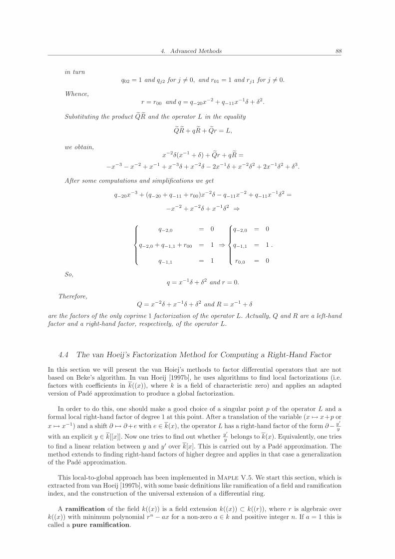
4. Advanced Methods 88
in turnq02 = 1 and qj2 for j 6= 0, and r01 = 1 and rj1 for j 6= 0.
Whence,r = r00 and q = q−20x
−2 + q−11x−1δ + δ2.
Substituting the product QR and the operator L in the equality
QR+ qR+ Qr = L,
we obtain,x−2δ(x−1 + δ) + Qr + qR =
−x−3 − x−2 + x−1 + x−3δ + x−2δ − 2x−1δ + x−2δ2 + 2x−1δ2 + δ3.
After some computations and simplifications we get
q−20x−3 + (q−20 + q−11 + r00)x
−2δ − q−11x−2 + q−11x
−1δ2 =
−x−2 + x−2δ + x−1δ2 ⇒
q−2,0 = 0
q−2,0 + q−1,1 + r00 = 1
q−1,1 = 1
⇒
q−2,0 = 0
q−1,1 = 1
r0,0 = 0
.
So,q = x−1δ + δ2 and r = 0.
Therefore,Q = x−2δ + x−1δ + δ2 and R = x−1 + δ
are the factors of the only coprime 1 factorization of the operator L. Actually, Q and R are a left-handfactor and a right-hand factor, respectively, of the operator L.
4.4 The van Hoeij’s Factorization Method for Computing a Right-Hand Factor
In this section we will present the van Hoiej’s methods to factor differential operators that are notbased on Beke’s algorithm. In van Hoeij [1997b], he uses algorithms to find local factorizations (i.e.factors with coefficients in k((x)), where k is a field of characteristic zero) and applies an adaptedversion of Pade approximation to produce a global factorization.
In order to do this, one should make a good choice of a singular point p of the operator L and aformal local right-hand factor of degree 1 at this point. After a translation of the variable (x 7→ x+p or
x 7→ x−1) and a shift ∂ 7→ ∂+e with e ∈ k(x), the operator L has a right-hand factor of the form ∂− y′
y
with an explicit y ∈ k[[x]]. Now one tries to find out whether y′
y belongs to k(x). Equivalently, one tries
to find a linear relation between y and y′ over k[x]. This is carried out by a Pade approximation. Themethod extends to finding right-hand factors of higher degree and applies in that case a generalizationof the Pade approximation.
This local-to-global approach has been implemented in Maple V.5. We start this section, which isextracted from van Hoeij [1997b], with some basic definitions like ramification of a field and ramificationindex, and the construction of the universal extension of a differential ring.
A ramification of the field k((x)) is a field extension k((x)) ⊂ k((r)), where r is algebraic overk((x)) with minimum polynomial rn − ax for a non-zero a ∈ k and positive integer n. If a = 1 this iscalled a pure ramification.
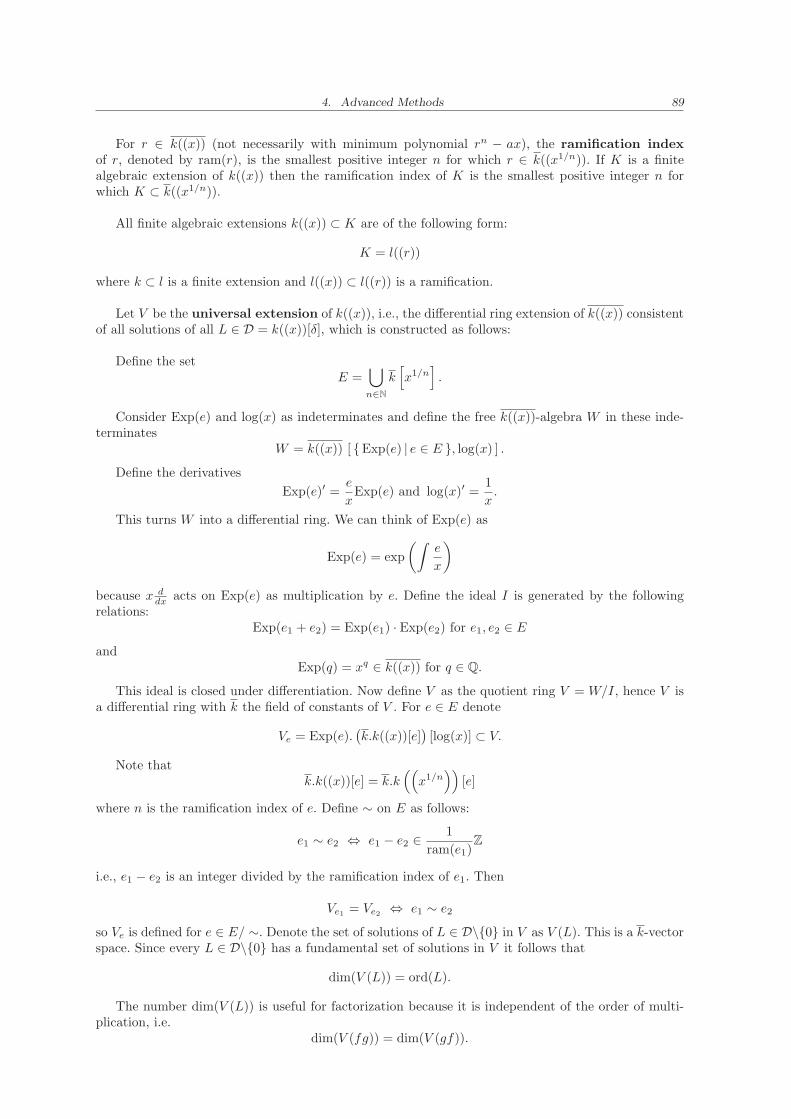
4. Advanced Methods 89
For r ∈ k((x)) (not necessarily with minimum polynomial rn − ax), the ramification indexof r, denoted by ram(r), is the smallest positive integer n for which r ∈ k((x1/n)). If K is a finitealgebraic extension of k((x)) then the ramification index of K is the smallest positive integer n forwhich K ⊂ k((x1/n)).
All finite algebraic extensions k((x)) ⊂ K are of the following form:
K = l((r))
where k ⊂ l is a finite extension and l((x)) ⊂ l((r)) is a ramification.
Let V be the universal extension of k((x)), i.e., the differential ring extension of k((x)) consistentof all solutions of all L ∈ D = k((x))[δ], which is constructed as follows:
Define the setE =
⋃
n∈N
k[x1/n
].
Consider Exp(e) and log(x) as indeterminates and define the free k((x))-algebra W in these inde-terminates
W = k((x)) [ {Exp(e) | e ∈ E }, log(x) ] .
Define the derivatives
Exp(e)′ =e
xExp(e) and log(x)′ =
1
x.
This turns W into a differential ring. We can think of Exp(e) as
Exp(e) = exp
(∫e
x
)
because x ddx acts on Exp(e) as multiplication by e. Define the ideal I is generated by the following
relations:Exp(e1 + e2) = Exp(e1) · Exp(e2) for e1, e2 ∈ E
andExp(q) = xq ∈ k((x)) for q ∈ Q.
This ideal is closed under differentiation. Now define V as the quotient ring V = W/I, hence V isa differential ring with k the field of constants of V . For e ∈ E denote
Ve = Exp(e).(k.k((x))[e]
)[log(x)] ⊂ V.
Note thatk.k((x))[e] = k.k
((x1/n
))[e]
where n is the ramification index of e. Define ∼ on E as follows:
e1 ∼ e2 ⇔ e1 − e2 ∈ 1
ram(e1)Z
i.e., e1 − e2 is an integer divided by the ramification index of e1. Then
Ve1= Ve2
⇔ e1 ∼ e2
so Ve is defined for e ∈ E/ ∼. Denote the set of solutions of L ∈ D\{0} in V as V (L). This is a k-vectorspace. Since every L ∈ D\{0} has a fundamental set of solutions in V it follows that
dim(V (L)) = ord(L).
The number dim(V (L)) is useful for factorization because it is independent of the order of multi-plication, i.e.
dim(V (fg)) = dim(V (gf)).
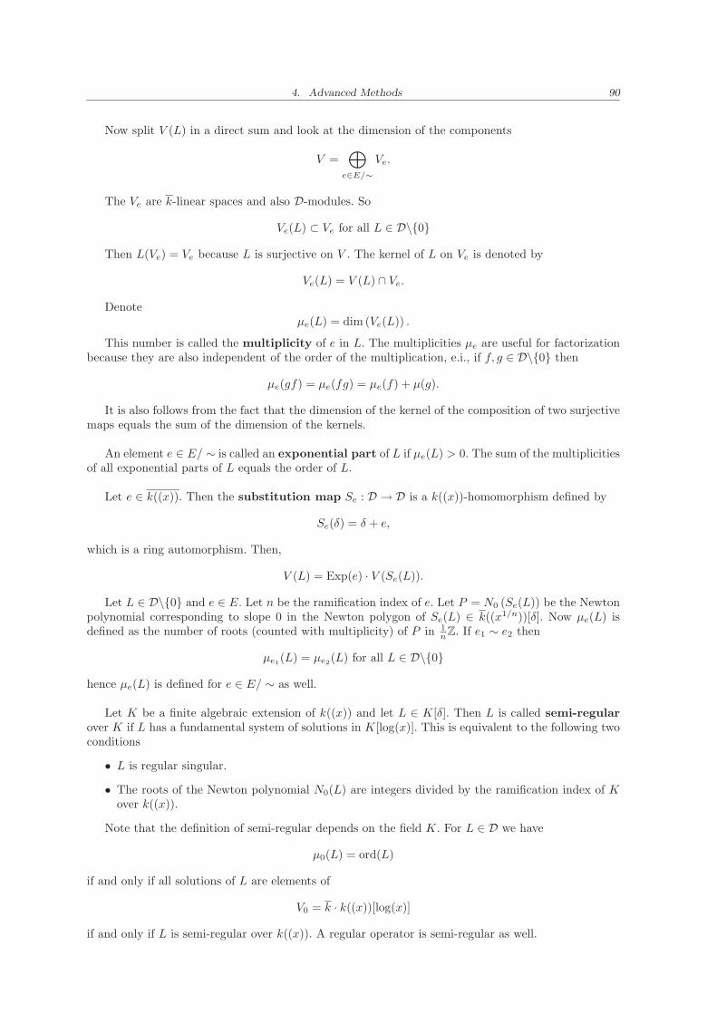
4. Advanced Methods 90
Now split V (L) in a direct sum and look at the dimension of the components
V =⊕
e∈E/∼Ve.
The Ve are k-linear spaces and also D-modules. So
Ve(L) ⊂ Ve for all L ∈ D\{0}
Then L(Ve) = Ve because L is surjective on V . The kernel of L on Ve is denoted by
Ve(L) = V (L) ∩ Ve.
Denoteµe(L) = dim (Ve(L)) .
This number is called the multiplicity of e in L. The multiplicities µe are useful for factorizationbecause they are also independent of the order of the multiplication, e.i., if f, g ∈ D\{0} then
µe(gf) = µe(fg) = µe(f) + µ(g).
It is also follows from the fact that the dimension of the kernel of the composition of two surjectivemaps equals the sum of the dimension of the kernels.
An element e ∈ E/ ∼ is called an exponential part of L if µe(L) > 0. The sum of the multiplicitiesof all exponential parts of L equals the order of L.
Let e ∈ k((x)). Then the substitution map Se : D → D is a k((x))-homomorphism defined by
Se(δ) = δ + e,
which is a ring automorphism. Then,
V (L) = Exp(e) · V (Se(L)).
Let L ∈ D\{0} and e ∈ E. Let n be the ramification index of e. Let P = N0 (Se(L)) be the Newtonpolynomial corresponding to slope 0 in the Newton polygon of Se(L) ∈ k((x1/n))[δ]. Now µe(L) isdefined as the number of roots (counted with multiplicity) of P in 1
nZ. If e1 ∼ e2 then
µe1(L) = µe2
(L) for all L ∈ D\{0}
hence µe(L) is defined for e ∈ E/ ∼ as well.
Let K be a finite algebraic extension of k((x)) and let L ∈ K[δ]. Then L is called semi-regularover K if L has a fundamental system of solutions in K[log(x)]. This is equivalent to the following twoconditions
• L is regular singular.
• The roots of the Newton polynomial N0(L) are integers divided by the ramification index of Kover k((x)).
Note that the definition of semi-regular depends on the field K. For L ∈ D we have
µ0(L) = ord(L)
if and only if all solutions of L are elements of
V0 = k · k((x))[log(x)]
if and only if L is semi-regular over k((x)). A regular operator is semi-regular as well.
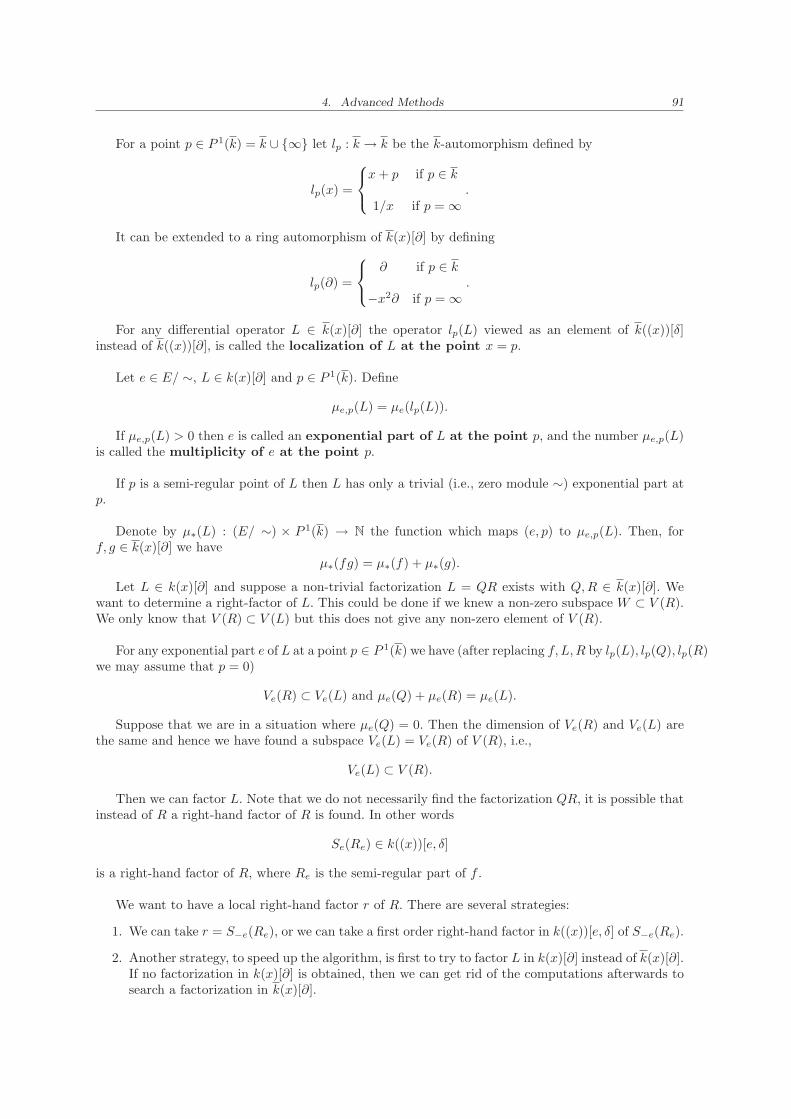
4. Advanced Methods 91
For a point p ∈ P 1(k) = k ∪ {∞} let lp : k → k be the k-automorphism defined by
lp(x) =
x+ p if p ∈ k
1/x if p = ∞.
It can be extended to a ring automorphism of k(x)[∂] by defining
lp(∂) =
∂ if p ∈ k
−x2∂ if p = ∞.
For any differential operator L ∈ k(x)[∂] the operator lp(L) viewed as an element of k((x))[δ]instead of k((x))[∂], is called the localization of L at the point x = p.
Let e ∈ E/ ∼, L ∈ k(x)[∂] and p ∈ P 1(k). Define
µe,p(L) = µe(lp(L)).
If µe,p(L) > 0 then e is called an exponential part of L at the point p, and the number µe,p(L)is called the multiplicity of e at the point p.
If p is a semi-regular point of L then L has only a trivial (i.e., zero module ∼) exponential part atp.
Denote by µ∗(L) : (E/ ∼) × P 1(k) → N the function which maps (e, p) to µe,p(L). Then, forf, g ∈ k(x)[∂] we have
µ∗(fg) = µ∗(f) + µ∗(g).
Let L ∈ k(x)[∂] and suppose a non-trivial factorization L = QR exists with Q,R ∈ k(x)[∂]. Wewant to determine a right-factor of L. This could be done if we knew a non-zero subspace W ⊂ V (R).We only know that V (R) ⊂ V (L) but this does not give any non-zero element of V (R).
For any exponential part e of L at a point p ∈ P 1(k) we have (after replacing f, L,R by lp(L), lp(Q), lp(R)we may assume that p = 0)
Ve(R) ⊂ Ve(L) and µe(Q) + µe(R) = µe(L).
Suppose that we are in a situation where µe(Q) = 0. Then the dimension of Ve(R) and Ve(L) arethe same and hence we have found a subspace Ve(L) = Ve(R) of V (R), i.e.,
Ve(L) ⊂ V (R).
Then we can factor L. Note that we do not necessarily find the factorization QR, it is possible thatinstead of R a right-hand factor of R is found. In other words
Se(Re) ∈ k((x))[e, δ]
is a right-hand factor of R, where Re is the semi-regular part of f .
We want to have a local right-hand factor r of R. There are several strategies:
1. We can take r = S−e(Re), or we can take a first order right-hand factor in k((x))[e, δ] of S−e(Re).
2. Another strategy, to speed up the algorithm, is first to try to factor L in k(x)[∂] instead of k(x)[∂].If no factorization in k(x)[∂] is obtained, then we can get rid of the computations afterwards tosearch a factorization in k(x)[∂].
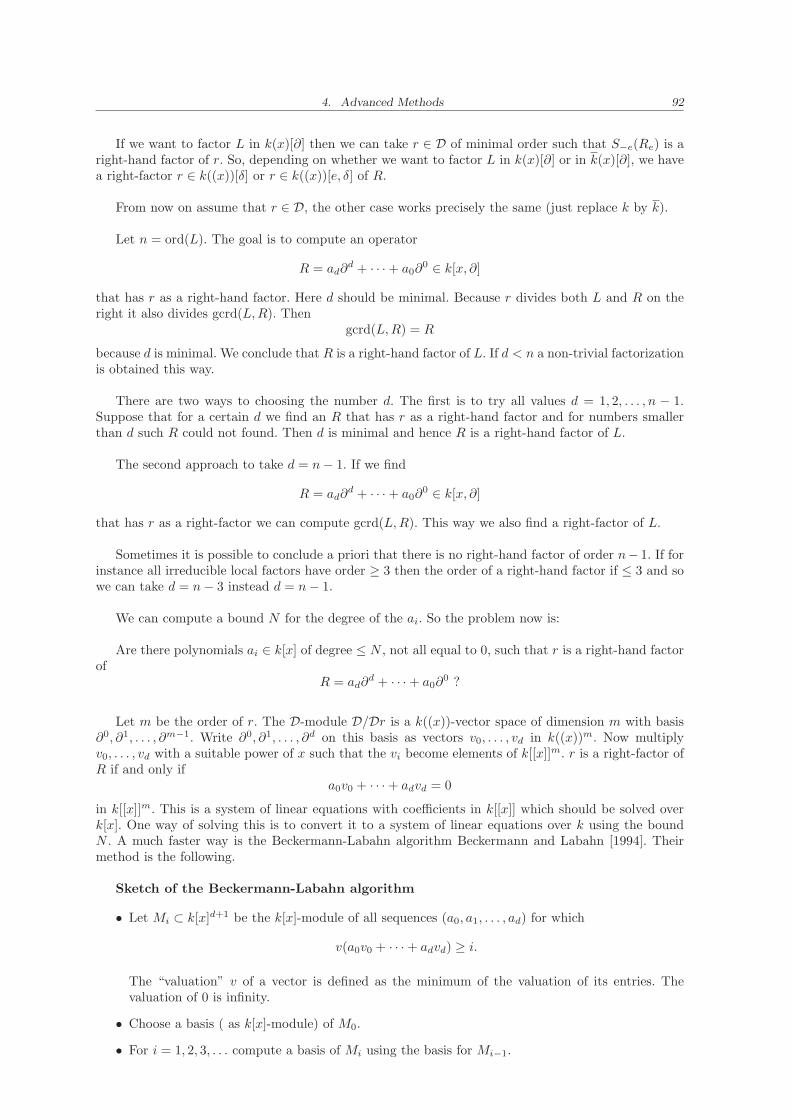
4. Advanced Methods 92
If we want to factor L in k(x)[∂] then we can take r ∈ D of minimal order such that S−e(Re) is aright-hand factor of r. So, depending on whether we want to factor L in k(x)[∂] or in k(x)[∂], we havea right-factor r ∈ k((x))[δ] or r ∈ k((x))[e, δ] of R.
From now on assume that r ∈ D, the other case works precisely the same (just replace k by k).
Let n = ord(L). The goal is to compute an operator
R = ad∂d + · · · + a0∂
0 ∈ k[x, ∂]
that has r as a right-hand factor. Here d should be minimal. Because r divides both L and R on theright it also divides gcrd(L,R). Then
gcrd(L,R) = R
because d is minimal. We conclude that R is a right-hand factor of L. If d < n a non-trivial factorizationis obtained this way.
There are two ways to choosing the number d. The first is to try all values d = 1, 2, . . . , n − 1.Suppose that for a certain d we find an R that has r as a right-hand factor and for numbers smallerthan d such R could not found. Then d is minimal and hence R is a right-hand factor of L.
The second approach to take d = n− 1. If we find
R = ad∂d + · · · + a0∂
0 ∈ k[x, ∂]
that has r as a right-factor we can compute gcrd(L,R). This way we also find a right-factor of L.
Sometimes it is possible to conclude a priori that there is no right-hand factor of order n− 1. If forinstance all irreducible local factors have order ≥ 3 then the order of a right-hand factor if ≤ 3 and sowe can take d = n− 3 instead d = n− 1.
We can compute a bound N for the degree of the ai. So the problem now is:
Are there polynomials ai ∈ k[x] of degree ≤ N , not all equal to 0, such that r is a right-hand factorof
R = ad∂d + · · · + a0∂
0 ?
Let m be the order of r. The D-module D/Dr is a k((x))-vector space of dimension m with basis∂0, ∂1, . . . , ∂m−1. Write ∂0, ∂1, . . . , ∂d on this basis as vectors v0, . . . , vd in k((x))m. Now multiplyv0, . . . , vd with a suitable power of x such that the vi become elements of k[[x]]m. r is a right-factor ofR if and only if
a0v0 + · · · + advd = 0
in k[[x]]m. This is a system of linear equations with coefficients in k[[x]] which should be solved overk[x]. One way of solving this is to convert it to a system of linear equations over k using the boundN . A much faster way is the Beckermann-Labahn algorithm Beckermann and Labahn [1994]. Theirmethod is the following.
Sketch of the Beckermann-Labahn algorithm
• Let Mi ⊂ k[x]d+1 be the k[x]-module of all sequences (a0, a1, . . . , ad) for which
v(a0v0 + · · · + advd) ≥ i.
The “valuation” v of a vector is defined as the minimum of the valuation of its entries. Thevaluation of 0 is infinity.
• Choose a basis ( as k[x]-module) of M0.
• For i = 1, 2, 3, . . . compute a basis of Mi using the basis for Mi−1.
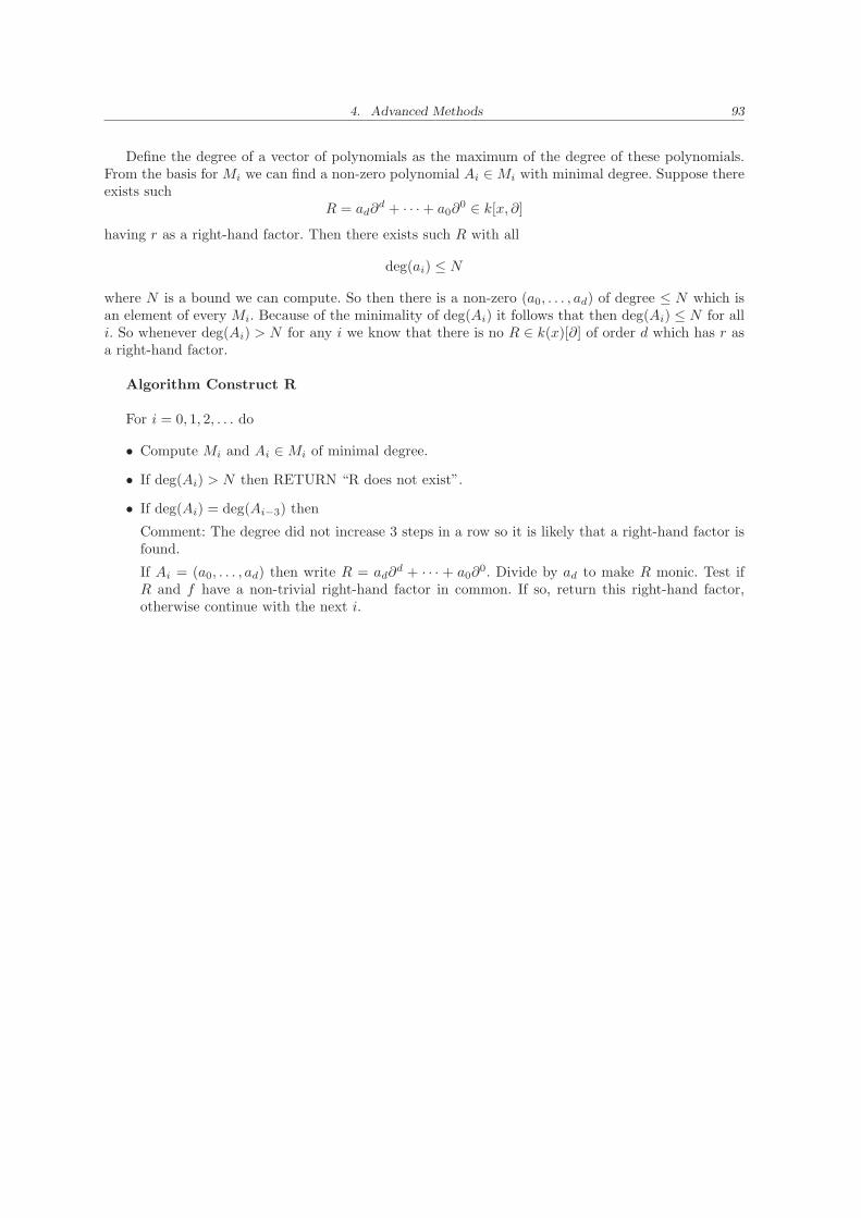
4. Advanced Methods 93
Define the degree of a vector of polynomials as the maximum of the degree of these polynomials.From the basis for Mi we can find a non-zero polynomial Ai ∈Mi with minimal degree. Suppose thereexists such
R = ad∂d + · · · + a0∂
0 ∈ k[x, ∂]
having r as a right-hand factor. Then there exists such R with all
deg(ai) ≤ N
where N is a bound we can compute. So then there is a non-zero (a0, . . . , ad) of degree ≤ N which isan element of every Mi. Because of the minimality of deg(Ai) it follows that then deg(Ai) ≤ N for alli. So whenever deg(Ai) > N for any i we know that there is no R ∈ k(x)[∂] of order d which has r asa right-hand factor.
Algorithm Construct R
For i = 0, 1, 2, . . . do
• Compute Mi and Ai ∈Mi of minimal degree.
• If deg(Ai) > N then RETURN “R does not exist”.
• If deg(Ai) = deg(Ai−3) then
Comment: The degree did not increase 3 steps in a row so it is likely that a right-hand factor isfound.
If Ai = (a0, . . . , ad) then write R = ad∂d + · · · + a0∂
0. Divide by ad to make R monic. Test ifR and f have a non-trivial right-hand factor in common. If so, return this right-hand factor,otherwise continue with the next i.
5. CONCLUSIONS
In this thesis, starting from an overview of symbolic factorization of linear differential operators, a newresult – a procedure for factoring second order partial differential operators – was presented. Beginningwith the ring of linear differential operators the research took us – through differential Galois theoryand the body of methods for finding rational and exponential solutions of linear differential equations –to the state of the art: Singer’s eigenring factorization algorithm, factorization via Newton’s polygons,and the van Hoeij’s methods for local factorization.
In Chapter 1, we presented an algorithmic solution of the problem of factoring second order linearpartial differential operators. Based on purely algebraic methods and by using techniques of differentialalgebra, we solved the problem in its original settings.
In contrast with the case of ordinary differential operators, the advantage of this approach is that,in the most general case, it is not necessary to solve a Riccati equation for partial differential operators.
Comparing our method with other known ones, we have found that:
• Compared with (Miller [1932]), our work is characterized by the following.
– We do not only propose a possible right factor but rather we find the factorization when itexists, without appealing to the necessity to define new structures or to extend the originaldomain in which we are working.
– While Miller found only a possible right-hand factor, we devise a complete factorization ofthe operator, and, in each case, we avoid dividing the operator by the right-hand factor.
– We do not make a case distinction, since we propose to find a square root and to solve asystem of two linear equations in two unknowns plus one first order linear partial differentialequation.
– If the square root exists and if the system of algebraic equations which we obtain has aunique solution, we consider the extra linear partial differential equation. The extra partialdifferential equation is used as a test equation, rather than been used as an additionalcondition.
• Comparing our approach with the Hensel descent of Grigoriev and Schwarz [2004], for secondorder linear differential operators we have found following.
– We need neither to define new objects nor to work in another algebraic structure, because wefind the factorization at once in the domain of definition of the linear differential operators.
– Instead of solving the problem by reformulating it in a commutative ring, we solve it in theoriginal non-commutative setting.
– We do not need to apply undetermined coefficients, after applying polynomial factorizationin each particular case. This reduces the complexity of our approach.
We would like to mention also that:
• The structure of Theorem (2) proposes an algorithmic method, algorithm gl1, whose proof ofcorrectness is given by the proof of Theorem (2). This method can be easily implemented in anycomputer algebra system;
5. Conclusions 95
• The method above has been generalized to operators of third order, but this results in a morecomplicated system of equations. In contrast to the second order case, we must solve certaindifferential equations, which, in particular cases, are simplified with the aid of characteristic sets.
In Chapter 2 we have introduced a formula for the complete factorization of a given element of thering of linear differential operators. This factorization is always possible when a fundamental set ofsolutions of a differential equation is available. With the formula above we have explained, in a directway, the classical Beke algorithm (Beke [1894]) and its variants, as well as the algorithm LODEF bySchwarz [1989], and the Beke-Bronstein algorithm Bronstein [1994].
We can summarize Beke’s algorithm in the following way:
• For first order right-hand factors, the idea is to find a rational solution of the Riccati equationassociated with the linear scalar equation defined by the linear differential operator. If this Riccatiequation has a rational solution, then it is also at once an exponential solution of the linear scalarequation. This exponential solution yields a first order right-hand factor.
• For searching right-hand factors of higher order, the idea is to determine the coefficients of thepossible right-hand factor of order m, where m < n and n is the order of the given operator. Afterhaving chosen m we have to express the associated equations for it (i.e., the differential equationsin the generalized Wronskians, of a subset of m elements, of a fundamental set of solutions of thescalar equation); solve the equations for rational solutions; and construct a right-hand factor. Ifone of the associated equations has not rational solution, then stop the process by saying thatthere is not a right-hand factor of order m. Then try another m, and so on.
After almost one hundred years, Schwarz [1989] automated Beke’s algorithm, extending it to searchrecursively from possible right-hand factors of order n− 1, until possible right-hand factors of order 1.He described also a different way to find the associated equations, and implemented this procedure –the algorithm LODEF – in the Scrachpad II computer algebra system. He then analysised the cost offactorization of linear differential operators with rational function coefficients, estimating bounds forthe size of the polynomials in the numerator of the rational function solutions. With these ideas, hedeveloped the RiccatiRational algorithm, to complete the last step of the Beke algorithm, namely tosolve the generalized Riccati equations derived from the associated equations.
A faster approach – the Beke-Bronstein algorithm, Bronstein [1994] – is an efficient procedurefor computing the associated equations, based on elementary operations on sets of positive integers.It produces many possible choices of the associated equation. The algorithm is designed to select thesimplest equations for solving. These ideas were formalized, Two years later in Bronstein and Petkovsek[1996], in the so called “Pseudo-Linear Algebra”. The resulting theory was formulated afterwards asoperations in differential modules (Chapter 2 of van der Put and Singer [2003]).
There are several algorithms for finding rational solutions of linear differential equations, some ofthem depending on the coefficient field and others on the order of the equation. For our explanationof how to find rational solutions of linear differential equations, we have chosen an algorithm forfinding solutions of differential equations with rational function coefficients. The procedure dependson a theorem which says that a solution can only have a pole at either α or ∞, if at least one of thecoefficients has pole either at α or ∞. After identifying the poles of the coefficients, we expand themin Laurent series at each of the poles, we use indicial equations to find bounds on the numerator of thecoefficients of the solution, and with linear algebra we can find the numerators and hence the solution.
In contrast to the case of rational solutions of linear differential equations, there are few algorithmsfor finding either exponential solutions of linear differential equation or rational solutions of the asso-ciated Riccati equation, only for particular cases. We have discussed the RiccatiRational algorithm –Schwarz [1994] – for finding rational solutions in the coefficient field of the Riccati equation associatedwith a given linear differential equation. The algorithm searches for bounds on the coefficients of thepossible solution and is ultimately reduced to solving a system of linear equations. If the system isfeasible, we obtain a rational solution of the associated Riccati equation and at once a right-handfactor of the original linear differential equation. In our example, we have simplified the application of
5. Conclusions 96
the algorithm, namely the computation of the bounds given in Schwarz [1989], using the techniquescommonly applied only to rational solutions in the general case.
Recently Cluzeau and van Hoeij [2004] presented a new algorithm, based on local and modularcomputation, for finding exponential solutions of differential equations with rational function coeffi-cients. The approach reduces the number of possibilities in the combinatorial part of the algorithm.The authors have also showed how unnecessary extensions of the constants can be avoided. Their ideais to use information mod p in several ways, in order to speed up the computations the exponen-tial solutions in characteristic 0. They also devised a recursive algorithm – Algorithm FindASol – forconstructing a field extension over which an exponential solution, if one exists, can be found.
We concluded this work, in Chapter 3, by presenting the known algorithms for commutative poly-nomials with a view to adaptation, generalization, and reformulation of their analogues for lineardifferential operators, as follows
• Berlekamp algorithm for the Singer’s eigenring algorithm (Singer [1996]),
• Newton polygons for geometric factorization and module decomposition (van der Put and Singer[2003]),
• Puiseux series and local parametrization of curves for factorization via Newton polygons and thecoprime index 1 (van Hoeij [1997a]),
• Pade approximation for the van Hoeij’s algorithm for finding right-hand factors (van Hoeij[1997b]).
In conclusion, this work presents the results of our studies in differential Galois theory, as appliedto symbolic factorization of differential operators. Starting from the clarification and systematiza-tion of the theoretical foundations relevant to factorization, we have evolved original ideas about thefactorization of partial diffential operators and provided the thoretical foundations and algorithmicspecifications for second order linear operators. Furthemore, we have complemented the theoreticalwork with a number of concrete examples chosen from relevant application areas.
This work can be extended in a number of ways. On the theoretical side, we feel that interestingfuture work could be in the area of differential elimination, where our results may be instrumentalin solving linear differential equations by operators. On the applications side, the our results cancomplement a computer-algebra system, by proving tools for solving a class of partial differentialequations, by factorization.
6. LIST OF NOTATION
• Chapter 2
– R ring, k field, 10
– δ : R → R derivation on the ring R, 10
– (R, δ) (reps. (k, δ)) differential ring (reps. field), 10
– Constδ(R) subring of constants of R with respect to δ, 10
– S differential subring (resp. subfield) of R, 10
– R{{y1, . . . , yn}} ring of differential polynomials in the inderminates y1, . . . , yn over R, 10
– k[∂1, . . . , ∂r] ring of partial differential operators with coefficients in k, 11
– D := k[∂] ring of linear ordinary differential operators with coefficients in k, 12
– L linear differential operator, 12
– deg(L) = ord(L) degree or order of L, 12
– s(L) symbol of L, 21
• Chapter 3
– AL companion matrix of L, 25
– W (y1, y2, . . . , yn) Wronskian matrix of y1, y2, . . . , yn ∈ k, 26
– w(y1, y2, . . . , yn) Wronskian of y1, y2, . . . , yn ∈ k, 26
– G(K/k) differential Galois group of the extension K of k, 27
– Gal(K/k) Galois group of a differential equation L(y) = 0 with coefficients in k and Picard-Vessiot extension K, 28
– K algebraic closure of a field K, 33
– k(x) field of rational functions over k, 33
– k[[x]] ring of formal power series in the indeterminate x with coefficients in k, 33
– k((x)) field of formal Laurent series in the x with finite pole order and coefficients in k, 33
– ord(a) order of a ∈ k((x)), 33
– Ip(m) indicial polynomial of p ∈ k((x)), 34
– ords(f) order of f ∈ k((x)) at s, 35
– S = {si|1 ≤ s1 < · · · < sm ≤ n}, 51
– AS square submatrix of A ∈ kn×m, 52
– S+i increment the i-th element of S, 53
– S[l]i replace the i-th element of S by l, 53
– δ[l]i (S) number of elements of S which are strictly between l and si, 53
• Chapter 4
– ED(L) eigenring of L, 64, 66, 67
– gcrd(L1, L2) greatest common right divisor of L1 and L2, 67
– [L1, L2]l least common left multiple of L1 and L2, 67
– N(L) Newton polygon of L, 70
6. List of Notation 98
– gr(D) associated graded ring of the ring D, 77
– v : D → Z ∪ {∞} discrete valuation on the ring D, 77
– (Di)i∈Z, with Di = {f ∈ D | v(f) ≥ i}, filtration w.r.t. v, 77
– σa truncation with accuracy a, 77
– Ns(L) Newton polynomial of L for the slope s, 78
– T indeterminate for expressing the Newton polynomial, 78
– ram(r) ramification index of an element r ∈ k((x)), 89
– E =⋃
n∈Nk[x1/n
]⊂ k((x)), 89
– Exp(e) = exp(∫
ex
)∈ V for e ∈ E, 89
– V Universal extension (as a ring) of k((x)), 89
– Ve = Exp(e) ·(k · k((x))[e]
)[log(x)], 89
– e1 ∼ e2 ⇔ e1 − e2 ∈ 1
ram(e1)Z, 89
– V (L) solution space of L in V , 89
– Ve(L) = V (L) ∩ Ve kernel of L on Ve, 90
– µe(L) = dim (Ve(L)) multiplicity of e in L, 90
– Se(δ) = δ + e substitution map for an element e ∈ E, 90
– lp(L) localization of L at the point p, 91
7. LIST OF ALGORITHMS
• Chapter 1
– Algorithm gl1, 13
– Hensel Descent, 21
• Chapter 2
– Algorithm for finding rational solutions of linear differential equations, 34
– Algorithm RiccatiRational, 40
– Beke’s algorithm for first order right-hand factors, 44
– Beke’s algorithm for right-hand factors of higher order, 46
– Algorithm LODEF, 50
– Bronstein’s Algorithm, 55
– The Beke-Bronstein Algorithm, 60
• Chapter 3
– Algorithm Coprime Index 1 Factorizations, 84
– Beckermann-Labahn algorithm, 92
– Algorithm Construct R, 93
8. LIST OF FIGURES
• Figure 4.1 Graphics of the sets M1 and M2, resp., 71
• Figure 4.2 Minkowski sum of the sets M1 and M2, 72
• Figure 4.3 Newton polygon N(L) of L, 74
• Figure 4.4 Special polygons P1 and P2, resp., 75
• Figure 4.5 Newton polygon of L, 80
• Figure 4.6 Newton polygon of L with coefficients, 81
INDEX
∆field, 11homomorphism, 11ring, 11
algebraicgroup, 64solution, 25
associatedequations, 45, 48, 53graded ring, 77system, 55
companion matrix, 25completely reducible operator, 67connected group, 65constants of a ∆-ring, 11coprime index
1 factorization, 83of a factorization, 83
derivation, 10differential
k-isomorphism, 27field, 10
extension, 24Galois group, 27ring, 10subring (resp. subfield), 10
discrete valuation, 77
eigenring, 64, 67exponential
solution, 25, 39exponential part of a differential
operator, 90, 91exponents of a differential operator, 79
filtered ring, 77filtration, 76fundamental
matrix, 26set (system) of solutions, 27
Galois group of a differential equation, 28generalized Wronskians, 29graded ring, 77grading, 77greatest common right divisor, 67
height of a Newton polygon, 65homogeneous
components, 77differential equation, 24
identity component, 65indicial
equation, 34polynomial, 34
inhomogeneous differentialequation, 24
irreducibility, 30, 67
least common left multiple, 67linear
algebraic group, 64scalar differential equation, 24system, 25
Liouville’s relation, 29Liouvillian
extension, 24solution, 25
localization of an operator at apoint, 91
Minkowski sum, 70multiplicity of an element, 90, 91
Newtondiagram, 65polygon of
a differential equation, 70, 72an algebraic equation, 65
polynomial, 78, 79
Picard-Vessiot extension, 27pole at
∞, 33a point, 33
polyhedral set, 70Puiseux
’s theorem, 66series, 33
pure ramification, 88
radical of an algebraic group, 65ramification, 88
index, 89rational solution, 25reducibility, 30, 67reductive group, 65regular singular operator, 66, 72relatively prime operators, 67Riccati equation associated, 39
101
Index 102
ring of differential polynomials, 10ring of linear
ordinary differential operators, 12partial differential opera-
tors, 11
semi-regular operator, 79, 90separable operator, 21slopes of a Newton polygon, 65, 72solution of a
differential equation, 24linear system, 25
solvability, 28sub-matrix, 52subring (subfield) of constants, 10substitution map, 90symbol of an operator, 20, 21
truncation, 77
unipotent radical of an algebraicgroup, 65
universal extension, 89
width of a Newton polygon, 65Wronskian, 26
matrix, 26
BIBLIOGRAPHY
Ian M. Anderson and Niky Kamran. The variational bicomplex for hyperbolic second-order scalarpartial differential equations in the plane. Duke Mathematical Journal, 87(2):265–319, 1997.
B. Beckermann and G. Labahn. A uniform approach for the fast computation of Matrix-type Padeapproximants. SIAM J. Matrix Analysis and Applications, 16:804–823, 1994.
Emanuel Beke. Die Irreducibilitat der homogenen linearen Differentialgleichungen. MathematischeAnnalen, 45:185–195, 1894.
Henry Blumberg. Uber algebraishe Eigenschaften von linearen homogenen Differentialausdrucken. PhDthesis, Gottingen, 1912. Inaugural-Dissertation.
Manuel Bronstein. Symbolic Integration I - Trascendental Functions, volume 1 of Algorithms andComputation in Mathematics. Springer, Berlin, Heidelberg, New York, Barcelona, Budapest, HongKong, London, Milan, Paris, Santa Clara, Singapore, Tokio, 1997.
Manuel Bronstein. Linear differential equations: Breaking through the order 2 barrier. In Paul S. Wang,editor, Proceedings of the 1992 International Symposium on Symbolic and Algebraic ComputationISSAC’92, Berkeley, California, USA, pages 42–48. ACM Press, 1992a. Available online at the URLhttp://www-sop.inria.fr/cafe/Manuel.Bronstein/publications/mb papers.html.
Manuel Bronstein. On solutions of linear differential equations in their coefficient field. Jour-nal of Symbolic Computation, 13:413–439, 1992b. Available online at the URL http://www-sop.inria.fr/cafe/Manuel.Bronstein/publications/mb papers.html.
Manuel Bronstein. An improved algorithm for factoring linear ordinary differential operators. InJoachim von zur Gathen, editor, Proceedings of the 1994 International Symposium on Symbolic andAlgebraic Computation ISSAC’94, Oxford, England, United Kingdom, pages 336–340. ACM Press,1994.
Manuel Bronstein and Marko Petkovsek. An introduction to pseudo-linear alge-bra. Theoretical Computer Science, 157(1):3–33, 1996. Available online at theURL http://www-sop.inria.fr/cafe/Manuel.Bronstein/publications/mb papers.html, andhttp://citeseer.nj.nec.com/bronstein96introduction.html.
Eduardo Casas-Alvero. Singularities of Plane Curves. Number 276 in London Mathematical SocietyLecture Note Series. Cambridge University Press, 2000.
Thomas Cluzeau and Mark van Hoeij. A modular algorithm for computing the exponential solutionsof a linear differential operator. Journal Symbolic Computation, 38(3):1043–1076, 2004.
Arjeh M. Cohen, Hans Cuypers, and Hans Sterk, editors. Some Tapas in Computer Algebra, volume 4of Algorithms and Computation in Mathematics. Springer, Berlin, Heidelberg, New York, Barcelona,Hong Kong, London, Milan, Paris, Singapore, Tokyo, 1999.
Jean Gaston Darboux. Ann. Ecole Normale Superieure, 7:163–173, 1870.
Winfried Fakler. On second order homogeneous linear differential equations with Liouvillian so-lutions. Theoretical Computer Science, 187(1-2):27–48, 1997. Available online at the URLhttp://www.citeseer.nj.ne.com/fakler97second.html.
L. Fuchs. Uber die linearen Differentialgleichungen zweiter Ordnung, welche algebraische Integralebesitzen, und eine neue Anwendung der Invariantentheory. Journal fur die reine und angewandteMathematik, 81, 1875.
BIBLIOGRAPHY 104
L. Fuchs. Uber die linearen Differentialgleichungen zweiter Ordnung, welche algebraische Integralebesitzen, zweite Abhandlung. Journal fur die reine und angewandte Mathematik, 85, 1878.
M. Griesbrecht. Factoring in skew-polynomial rings. Preprint, 1992. Department of Computer Science,University of Toronto.
D. Yu Grigoriev. Complexity of factoring and calculating the gcd of linear ordinary differential oper-ators. Journal of Symbolic Computation, 10:7–37, 1990a.
D. Yu Grigoriev. Complexity of irreducibility testing for a system of linear ordinary differential equa-tions. In Shunro Watanabe and Morio Nagata, editors, Proceedings of the 1990 International Sympo-sium on Symbolic and Algebraic Computation ISSAC’90, Tokyo, Japan, pages 225–230. ACM Press,1990b.
Dima Grigoriev and Fritz Schwarz. Factoring and solving linear partial differential equations. Com-puting, 73:179–197, 2004.
E. L. Ince. Ordinary Differential Equations. Dover Publications, Inc., New York, 1964.
C. Jordan. Memorie sur les equations differentielles lineaires a integrale algebrique. Journal fur diereine und angewandte Mathematik, 84, 1878.
M. Juras. Generalized Laplace invariants and classical integration methods for second-order scalarhyperbolic partial differential equations in the plane. In J. Janyske, editor, Proceedings of the 6thInternational Conference on “Differential Geometry and Applications”, Masaryk Univ., Brno, CzechRepublik, August 28 - September 1, pages 275–284, 1995.
Irving Kaplansky. Introduction to Differential Algebra. Actualites Scientifiques et Industrielles 1251.Publications de L’Institut de Mathematique de L’Universite de Nancago. Hermann, 6, Rue de laSorbonne, Paris V, 1957.
E. R. Kolchin. Algebraic matrix groups and the Picard-Vessiot theory of homogeneous linear ordinarydifferential equations. Annals of Mathematics, 49, 1948.
Jerald J. Kovacic. An algorithm for solving second order linear homogeneous differential equations.Journal of Symbolic Computation, 2:3–43, 1986.
Edmund Landau. Ein satz uber die zerlegung homogener linearer Differentialausdrucke in irreducibleFactoren. Journal fu die reine und angewandte Mathematik, 124:115–120, 1902.
Ziming Li and Fritz Schwarz. Rational solutions of riccati-like partial differential equations. Journalof Symbolic Computation, 31:691–716, 2001.
Ziming Li, Fritz Schwarz, and Serguei P. Tsarev. Factoring systems of linear pdes with finite-dimensional solution spaces. Journal of Symbolic Computation, 36:443–471, 2003.
Joseph Liouville. Premier memoire sur la determination des integrales dont la valeur est algebrique.Journal de l’Ecole polytechnique, 14:124–148, 1833a.
Joseph Liouville. Second memoire sur la determination des integrales dont la valeur est algebrique.Journal de l’Ecole polytechnique, 14:149–193, 1833b.
A. Loewy. Uberber vollstandig reduzible lineare homogene Differentialgleichungen. MathematischeAnnalen, 62:89–117, 1906.
B. Malgrange. Sur la reduction formelle des equations differentielles a singularites irregulieres, 1979.Manuscript.
F. H. Miller. Reducible and irreducible linear differential operators. PhD thesis, Columbia University,1932.
P. Th. Pepin. Methode pour obtenir les integrales algebriques des equationes differentielles lineairesdu second ordre. ATTi dell’ Accad. Pont. de Nuovi Lincei, XXXIV:243–388, 1881.
J.-T. Ramis. Devissage gevrey. Asterisque, 59/60:173–204, 1978.
BIBLIOGRAPHY 105
Fritz Schwarz. A factorization algorithm for linear ordinary differential equations. In Gaston H.Gonnet, editor, Proceedings of the ACM-SIGSAM 1989 International Symposium on Symbolic andAlgebraic Computation ISSAC’89, Portland, Oregon, USA, pages 17–25. ACM Press, 1989.
Fritz Schwarz. Efficient factorization of linear ode’s. A Quartely Publication of the SIGSAM Bolletin.Special Interest Group on Symbolic and Algebraic Manipulation, 28(1):9–17, 1994.
Michael F. Singer. Algebraic solutions of linear differential equations. In Proceedings of the Queen’sUniversity 1979 Conference on Number Theory, volume 62(2), pages 379–420, 1979.
Michael F. Singer. Liouvillian solutions of nth homogeneous linear differential equations. AmericanJournal of Mathematics, 103(4):661–682, 1981.
Michael F. Singer. An outline of differential Galois theory. In E. Tournier, editor, Computer Algebraand Differential Equations, pages 3–58, London, San Diego, New York, Berkeley, Boston, Sydney,Tokyo, Toronto, 1989. Academic Press.
Michael F. Singer. Liouvillian solutions of linear differential equations with Liouvillian coefficients.Journal of Symbolic Computation, 11(3):251–274, 1991.
Michael F. Singer. Testing reducibility of linear differential operators: A group theory perspective.Applicable Algebra in Engineering, Communication and Computing, 7(2):77–104, 1996. Avalaible online at the URL http://www4.ncsu.edu/ singer/ms papers.html.
Michael F. Singer and Felix Ulmer. Liouvillian and algebraic solutions of second and third order linearhomogeneous differential equations. Journal of Symbolic Computation, 16:37–73, 1993. Availableonline at the URL http://www4.ncsu.edu/ singer/ms papers.html.
S. P. Tsarev. An algorithm for complete enumeration of all factorizations of a linear ordinary differentialoperator. In Y. N. Lakshman, editor, Proceedings of the 1996 International Symposium on Symbolicand Algebraic Computation ISSAC’96, Zurich, Switzerland, pages 226–231. ACM Press, 1996.
S. P. Tsarev. Factoring linear partial differential operators and the Darboux method for integratingnonlinear partial differential equations. Theoretical and Mathematical Physics, 122(1):121–133, 2000.
Marius van der Put and Michael F. Singer. Galois Theory of Linear Differential Equations, volume 328of Grundlehren der Mathematischen Wissenschaften [Fundamental Principles of Mathematical Sci-ences], A Series of Comprehensive Studies in Mathematics. Springer-Verlag, Berlin, 2003. Availableonline at the URL http://www4.ncsu.edu/ singer/ms papers.html.
Mark van Hoeij. Formal solutions and factorization of differential operators with power seriescoefficients. Journal of Symbolic Computation, 24:1–30, 1997a. Available online at the URLhttp://www.math.fsu.edu/ hoeij/papers.html.
Mark van Hoeij. Factorization of differential operators with rational functions coeffi-cients. Journal of Symbolic Computation, 24:537–561, 1997b. Available online at the URLhttp://www.math.fsu.edu/ hoeij/papers.html.
Jacques-Arthur Weil. The use of the special semi-group for solving differential equations. In Joachimvon zur Gathen, editor, Proceedings of the 1994 International Symposium on Symbolic and AlgebraicComputation ISSAC’94, Oxford, England, United Kingdom, pages 341–347. ACM Press, 1994.
A. V. Zhiber, V. V. Sokolov, and S. Ya Startsev. On nonlinear Darboux-integrable hyperbolic equations.Doklady RAN, 343(6):746–748, 1995. In Russian.
CURRICULUM VITAE
Glauco Alfredo Lopez Dıaz
Research Institute for Symbolic Computation (RISC)Johannes Kepler University, Linz, Austria
Tel: +43 (0)732 2468 9955 Fax: +43 (0)732 2468 9930E-mail: [email protected]
Homepage: http://www.risc.uni-linz.ac.at/people/gdiaz
Personal Data
Family name: Lopez DıazFirst name: Glauco AlfredoDate of birth: 4th June, 1963Place of birth: Caracas, D.F. VenezuelaCitizenship: VenezuelanPrivate address: Sankt Peter Straße 31, A-4240 Freistadt, Austria
Education
2001 – : Currently, I am a Ph.D. Student of Technical Sciences.Research Institute for Symbolic Computation (RISC-Linz),Johannes Kepler University, Linz, Austria.Research topic: Symbolic Differential Computation.
1991 – 1998: M.Sc. in Mathematics.“Univeridad de Los Andes” (University of The Andes), ULA-Merida,Merida, Venezuela.Master Thesis: Bernoulli Polynomials and Bernoulli Numbers.Supervisor: Prof. Francisco Rivero Ph.D..
1982 – 1989: Bachelor in Mathematics.“Universidad Central de Venezuela” (Central University of Venezuela), UCV,Caracas, Venezuela.Bachelor Thesis: On the set of the non-wandering points over a compacttwo-dimensional manifold.Supervisor: Prof. Pedro Echeverria Ph.D..Winner of a Special Graduation Award.
1976 – 1981: High School “Colegio Fe y Alegrıa”, La Rinconada, Caracas, Venezuela.
Research Interests
• Symbolic Computation
• Computer Algebra
• Differential Galois Theory
• Differential Elimination
• Symbolic Differential Computation
Technical Reports
Rahul Ramesh Athale, Glauco Alfredo Lopez Dıaz.Explaining Schwarz’s lodef algorithm with examplesTechnical report no. 03-11 in RISC-Linz Report Series, RISC-Linz, Johannes Kepler University,Linz, Austria, November 2003.
Curriculum Vitae 108
Glauco Alfredo Lopez Dıaz.Una nueva formula de recurrencia para los numeros de BernoulliTechnical report no. 213 in Notas de Matematicas, Departamento de Matematicas, Facultad deCiencias, Universidad de Los Andes, Merida, Venezuela, 2001.
Glauco Alfredo Lopez Dıaz.Propiedades importantes de los numeros de BernoulliTechnical report no. 212 in Notas de Matematicas, Departamento de Matematicas, Facultad deCiencias, Universidad de Los Andes, Merida, Venezuela, 2001.
Glauco Alfredo Lopez Dıaz.Polinomios de Bernoulli y numeros de BernoulliTechnical report no. 211 in Notas de Matematicas, Departamento de Matematicas, Facultad deCiencias, Universidad de Los Andes, Merida, Venezuela, 2001.
Professional Experience
Since September 2004, I am employed by the project det, Fonds zur Forderung der wiss.Forschung, P16357-N04, at the Research Institute for Symbolic Computation (RISC-Linz),Johannes Kepler University, Linz, Austria.Supervisor : O. Uni.Prof. Dipl.-Ing. Dr. Franz Winkler.
September 2003 - March 2004, I was employed by the project det, Fonds zur Forderung derwiss. Forschung, P16357-N04, at the Research Institute for Symbolic Computation (RISC-Linz),Johannes Kepler University, Linz, Austria.Supervisor : O. Uni.Prof. Dipl.-Ing. Dr. Franz Winkler.
Since October 2001, I am a Ph.D. student at RISC-Linz in Austria.
Since January 1999: Assistant Professor of the Department of Mathematics, College of Sci-ence, University of The Andes, Merida, Venezuela.
Since February 1993: Ordinarious Member of the Department of Mathematics, College of Sci-ence, University of The Andes, Merida, Venezuela.
May 1991 - December 1998: Instructor of the Department of Mathematics, College of Science,University of The Andes, Merida, Venezuela.
March 1990 - April 1991: Lecturer at the College of Engineering, “Universidad Jose MariaVargas” (Jose Maria Vargas University), Caracas, Venezuela.Topics: Mathematics I, Mathematics II, Mathematics IV, Analitic Geometry.
March 1989 - March 1990: Lecturer at the “Instituto Universitario de Tecnologia RodolfoLoero Arismendi” (Lodolfo Loero Arismendi University Institute of Technology), I.U.T.I.R.L.A.,Caracas, Venezuela.Topics: Mathematics I, Logic, Statistics II.
January 1989 - April 1991: Lecturer at the College of Engineering, “Instutito Universitariode Nuevas Profesiones” (New Professions University Institute), Caracas, Venezuela.Topics: Mathematics I, Mathematics II, Mathematics III, Numerical Analysis.
Curriculum Vitae 109
Other Experiences
January - August 1988: Operator at the Service of Trains, “Metro de Caracas C.A.”, Caracas,Venezuela.
March 1986 - April 1987: Trainer II for the practice lectures at the College of Science, CentralUniversity of Venezuela, Caracas, Venezuela.Topics: Mathematics III, Mathematics IV.
October 1984 - March 1986: Trainer I for the practice lectures at the College of Science,Central Univeristy of Venezuela, Caracas, Venezuela.Topics: Mathematics IV, Mathematics II, Mathematics III.
Special Courses and Workshops
September 1995: VII Venezuelan School of Mathematics, University of The Andes, Merida,Venezuela. Course: Eliptic Curves in Criptography.
March - April 1993: VI Workshop in Mathematics, “Universidad Simon Bolivar” (SimonBolivar University), Caracas, Venezuela.
September 1992: V Venezuelan School of Mathematics, University of The Andes, Merida,Venezuela. Course: Computational Methods in the Theory of Operators over Hilbert Spaces.
January 1992: International Research Workshop on Banach Space Theory, University of TheAndes, College of Scince, Department de Matematicas, Merida, Venezuela.
September 1991: IV Venezuelan School of Mathematics, University of The Andes, Merida,Venezuela. Course: Multilinear Algebra and Free Finite Resolutions.
September 1987 - January 1988: Course for Operators at the Service of Trains, “Metro deCaracas C.A.”, Caracas, Venezuela.
March 1986: First Workshop on Analysis, University of The Andes, College of Science, Depart-ment of Mathematics, Merida, Venezuela.
August 1985: Summer School at the “Instituto Venezolano de Investigaciones Cientifıcas”(Venezuelan Institute for Scientific Research), IVIC, Caracas, Venezuela.
Scholarships
April 2004 - August 2004: Scholarship from the Research Institute for Symbolic Computation(RISC-Linz), Johannes Kepler University, Linz, Austria.
March 2003 - August 2003: Scholarship from the Research Institute for Symbolic Computa-tion (RISC-Linz), Johannes Kepler University, Linz, Austria.
Since Ocotber 2001: Scholarship from the University of The Andes, Merida, Venezuela.
September 1974 - June 1987: Scholarship from the Ministery of Education of the VenezuelanRepublic.
Languages
Spanich: Native.English: Proficient.German: Fair.