TAG: Statistisches Parsing mit TAG - coli-saar.github.io · lation from (Lavelli and Satta, 1991)....
37
TAG: Statistisches Parsing mit TAG Vorlesung “Grammatikformalismen” Alexander Koller 3. Mai 2019
Transcript of TAG: Statistisches Parsing mit TAG - coli-saar.github.io · lation from (Lavelli and Satta, 1991)....
TAG:Statistisches Parsing mit TAG
Vorlesung “Grammatikformalismen” Alexander Koller
3. Mai 2019

Statistisches Parsing
• Letztes Mal: Parsingalgorithmus für TAG, Laufzeit O(n6).
• Problem: Grammatiken mit hoher Abdeckung sind sehr ambig — wie finden wir den besten Parse? ‣ Ansatz: Probabilistische Grammatiken.
• Problem: Woher kriegen wir eine Grammatik mit hoher Abdeckung? ‣ handgeschriebene für einzelne Sprachen: EN, DE, FR
‣ Ansatz: Aus Baumbank lernen.

AmbiguitätenWir wollen disambiguieren, d.h. “korrekten” Parse für ambigen Satz berechnen.
S
NP VP
VP
I
V NP
anshot
PP
P
in
Det N
elephant
NP
my
PRP$ N
pyjamas
S
NP VP
I
VNP
anshot
PP
P
in
Det
N
elephant
NP
my
PRP$ N
pyjamas
N
Woran erkennen wir den “korrekten” Baum?
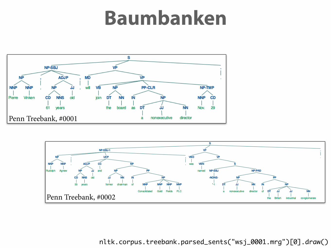
Baumbanken
Penn Treebank, #0001
Penn Treebank, #0002
nltk.corpus.treebank.parsed_sents("wsj_0001.mrg")[0].draw()

Probabilistische kfGen
• Eine probabilistische kontextfreie Grammatik (PCFG)ist eine kfG, in der ‣ jede Produktionsregel A → w hat eine W. P(A → w | A):
wenn wir A expandieren, wie w. ist Regel A → w?
‣ für jedes Nichtterminal A müssen W. zu eins summieren:
‣ wir schreiben abgekürzt P(A → w) für P(A → w | A)
X
w
P (A ! w | A) = 1
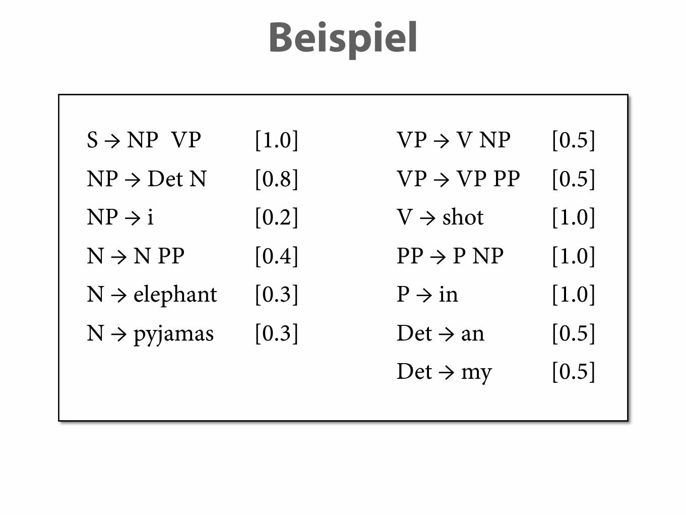
Beispiel
S → NP VP [1.0] VP → V NP [0.5]
NP → Det N [0.8] VP → VP PP [0.5]NP → i [0.2] V → shot [1.0]
N → N PP [0.4] PP → P NP [1.0]N → elephant [0.3] P → in [1.0]
N → pyjamas [0.3] Det → an [0.5]Det → my [0.5]

Generativer Prozess
• PCFG erzeugt zufällige Ableitung der kfG. ‣ Ereignis = Expansion von NT durch Produktionsregel
‣ alle statistisch unabhängig voneinander
S⇒ NP VP ⇒ i VP ⇒ i VP PP⇒* i shot an elephant in my pyjamas
1.0 0.2 0.5
0.00072
S⇒ NP VP ⇒ i VP ⇒* i V Det N⇒* i shot … pyjamas
1.0 0.2 0.4
0.4⇒ i V Det N PP
0.00057
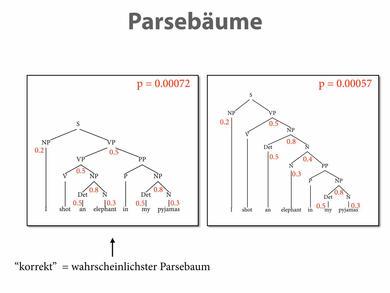
Parsebäume
S
NP VP
I
VNP
anshot
PP
P
in
Det
N
elephant
NP
my
Det N
pyjamas
N
S
NP VP
VP
I
V NP
anshot
PP
P
in
Det N
elephant
NP
my
Det N
pyjamas
p = 0.00072 p = 0.00057
“korrekt” = wahrscheinlichster Parsebaum
0.2 0.5
0.5
0.8
0.5 0.3
0.8
0.5 0.3
0.2 0.5
0.8
0.5
0.8
0.5 0.3
0.4
0.3

Algorithmen für PCFGs
• Erweitere CKY-Parser um Viterbi-Algorithmus:berechnet besten Parsebaum aus der Chart.
• Lies aus Baumbank (z.B. Penn Treebank) einekfG mit hoher Abdeckung ab.
• Schätze mit Maximum Likelihood Estimation (MLE) die Regelw. als relative Häufigkeiten:
P (A � w) =C(A � w)
C(A � •) =C(A � w)Pw0 C(A � w0)
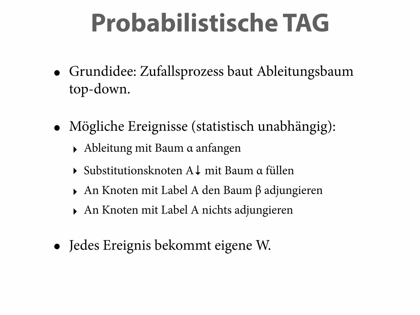
Probabilistische TAG
• Grundidee: Zufallsprozess baut Ableitungsbaum top-down.
• Mögliche Ereignisse (statistisch unabhängig): ‣ Ableitung mit Baum α anfangen
‣ Substitutionsknoten A↓ mit Baum α füllen
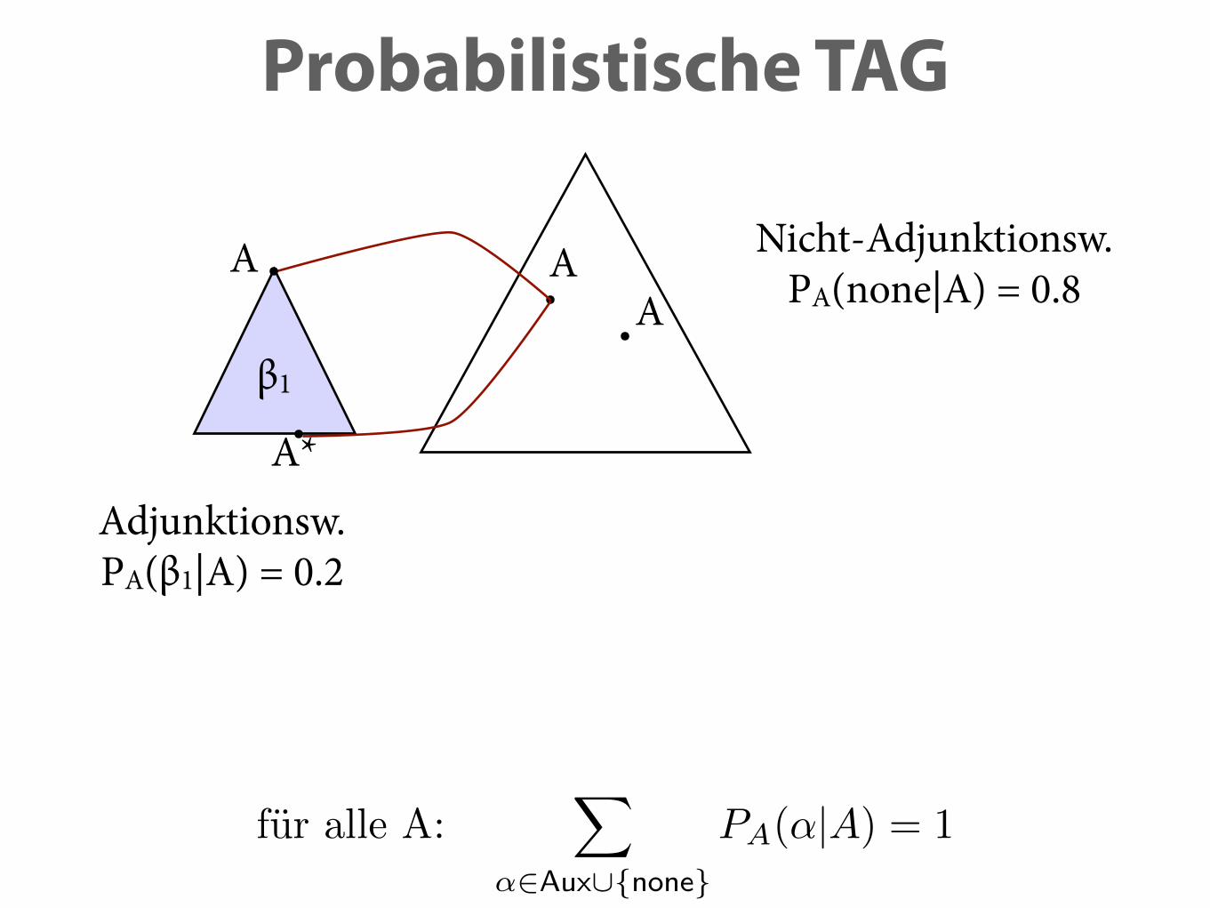
‣ An Knoten mit Label A den Baum β adjungieren
‣ An Knoten mit Label A nichts adjungieren
• Jedes Ereignis bekommt eigene W.

Probabilistische TSGS
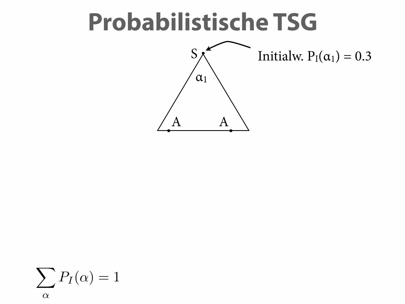
Probabilistische TSG
α1
A A
Initialw. PI(α1) = 0.3
X
↵
PI(↵) = 1
S

Probabilistische TSG
α1
A A
Initialw. PI(α1) = 0.3
Substitutionsw. PS(α2 | A) = 0.4
X
↵
PI(↵) = 1
α2
fur alle A:X
↵
PS(↵|A) = 1
S
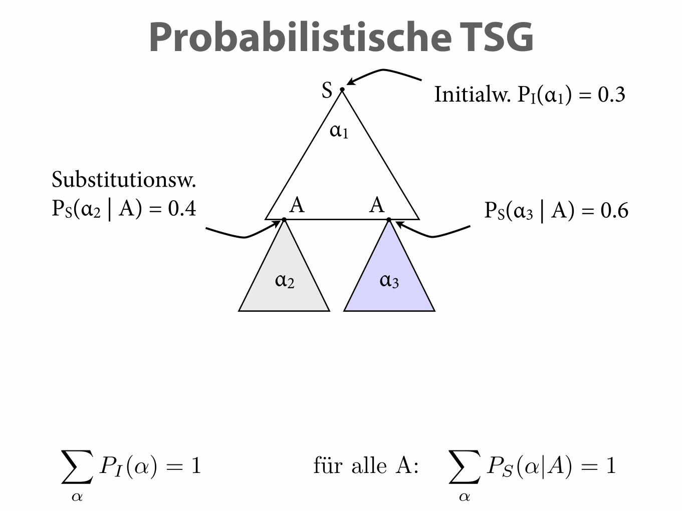
Probabilistische TSG
α1
A A
Initialw. PI(α1) = 0.3
Substitutionsw. PS(α2 | A) = 0.4 PS(α3 | A) = 0.6
X
↵
PI(↵) = 1
α2 α3
fur alle A:X
↵
PS(↵|A) = 1
S

Probabilistische TSG
α1
A A
Initialw. PI(α1) = 0.3
Substitutionsw. PS(α2 | A) = 0.4 PS(α3 | A) = 0.6
X
↵
PI(↵) = 1
P (↵1(↵2,↵3)) = PI(↵1) · PS(↵2|A) · PS(↵3|A) = 0.072
α2 α3
fur alle A:X
↵
PS(↵|A) = 1
S
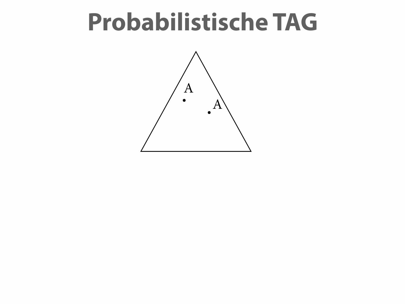
Probabilistische TAG
AA

Probabilistische TAG
AA
β1
A
A*Adjunktionsw. PA(β1|A) = 0.2
fur alle A:X
↵2Aux[{none}
PA(↵|A) = 1
Probabilistische TAG
AA
β1
A
A*Adjunktionsw. PA(β1|A) = 0.2
Nicht-Adjunktionsw. PA(none|A) = 0.8
fur alle A:X
↵2Aux[{none}
PA(↵|A) = 1

Probabilistische TAG
AA
β1
A
A*Adjunktionsw. PA(β1|A) = 0.2
Nicht-Adjunktionsw. PA(none|A) = 0.8
P (↵1(�1)) = PI(↵1) · PA(�1|A) · PA(none|A) = 0.048
fur alle A:X
↵2Aux[{none}
PA(↵|A) = 1
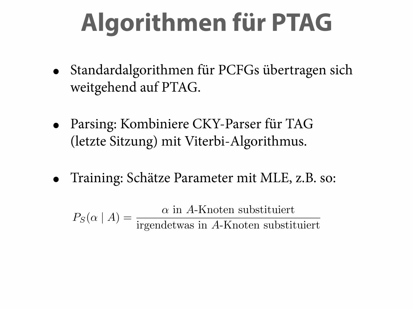
Algorithmen für PTAG
• Standardalgorithmen für PCFGs übertragen sich weitgehend auf PTAG.
• Parsing: Kombiniere CKY-Parser für TAG (letzte Sitzung) mit Viterbi-Algorithmus.
• Training: Schätze Parameter mit MLE, z.B. so:
PS(↵ | A) =
↵ in A-Knoten substituiert
irgendetwas in A-Knoten substituiert

Algorithmen für PTAG
• Standardalgorithmen für PCFGs übertragen sich weitgehend auf PTAG.
• Parsing: Kombiniere CKY-Parser für TAG (letzte Sitzung) mit Viterbi-Algorithmus.
• Training: Schätze Parameter mit MLE, z.B. so:
PS(↵ | A) =
↵ in A-Knoten substituiert
irgendetwas in A-Knoten substituiert
erfordert Baumbankmit TAG-Annotationen
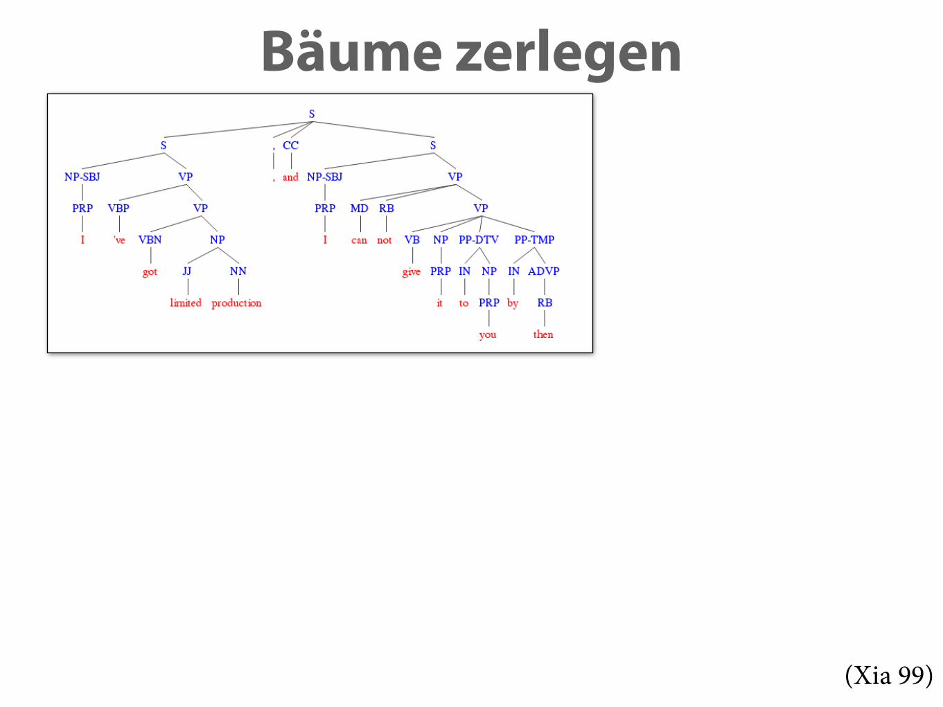
Bäume zerlegen
(Xia 99)

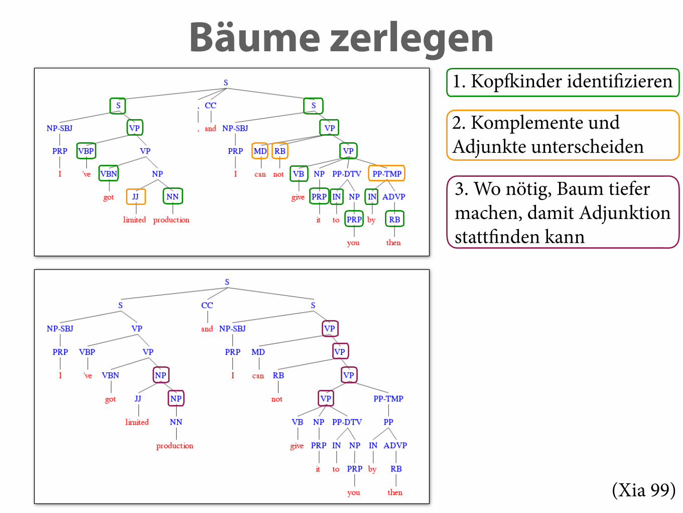
Bäume zerlegen1. Kopfkinder identifizieren
(Xia 99)

Bäume zerlegen1. Kopfkinder identifizieren
2. Komplemente undAdjunkte unterscheiden
(Xia 99)
Bäume zerlegen1. Kopfkinder identifizieren
2. Komplemente undAdjunkte unterscheiden
3. Wo nötig, Baum tiefermachen, damit Adjunktion stattfinden kann
(Xia 99)

Bäume zerlegen1. Kopfkinder identifizieren
2. Komplemente undAdjunkte unterscheiden
3. Wo nötig, Baum tiefermachen, damit Adjunktion stattfinden kann
4. Elementarbäumeablesen
(Xia 99)

Ergebnis
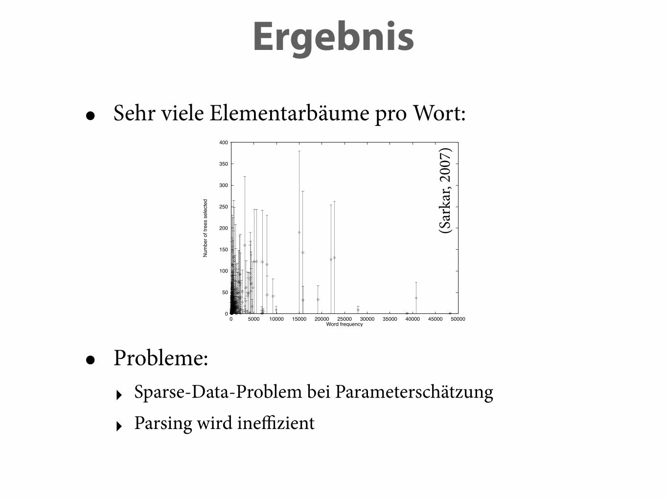
• Sehr viele Elementarbäume pro Wort:
0
50
100
150
200
250
300
350
400
0 5000 10000 15000 20000 25000 30000 35000 40000 45000 50000
Num
ber o
f tre
es s
elec
ted
Word frequency
Figure 3: Number of trees selected plotted against words with a particular fre-quency. (x-axis: words of frequency x; y-axis: number of trees selected, error barsindicate least and most ambiguous word of a particular frequency x)
4 Experimental Setup
4.1 Parsing Algorithm
The parser used in this paper implements a chart-based head-corner algorithm. Theuse of head-driven prediction to enchance efficiency was first suggested by (Kay,1989) for CF parsing (see (Sikkel, 1997) for a more detailed survey). (Lavelliand Satta, 1991) provided the first head-driven algorithm for LTAGs which was achart-based algorithm but it lacked any top-down prediction. (van Noord, 1994) de-scribes a Prolog implementation of a head-corner parser for LTAGs which includestop-down prediction. Significantly, (van Noord, 1994) uses a different closure re-lation from (Lavelli and Satta, 1991). The head-corner traversal for auxiliary treesstarts from the footnode rather than from the anchor.
The parsing algorithm we use is a chart-based variant of the (van Noord, 1994)algorithm. We use the same head-corner closure as proposed there. We do not givea complete description of our parser here since the basic idea behind the algorithmcan be grasped by reading (van Noord, 1994). Our parser differs from the algorithmin (van Noord, 1994) in some important respects: our implementation is chart-based and explicitly tracks goal and item states and does not perform any implicit
8
(Sar
kar,
2007
)
Ergebnis
• Sehr viele Elementarbäume pro Wort:
0
50
100
150
200
250
300
350
400
0 5000 10000 15000 20000 25000 30000 35000 40000 45000 50000
Num
ber o
f tre
es s
elec
ted
Word frequency
Figure 3: Number of trees selected plotted against words with a particular fre-quency. (x-axis: words of frequency x; y-axis: number of trees selected, error barsindicate least and most ambiguous word of a particular frequency x)
4 Experimental Setup
4.1 Parsing Algorithm
The parser used in this paper implements a chart-based head-corner algorithm. Theuse of head-driven prediction to enchance efficiency was first suggested by (Kay,1989) for CF parsing (see (Sikkel, 1997) for a more detailed survey). (Lavelliand Satta, 1991) provided the first head-driven algorithm for LTAGs which was achart-based algorithm but it lacked any top-down prediction. (van Noord, 1994) de-scribes a Prolog implementation of a head-corner parser for LTAGs which includestop-down prediction. Significantly, (van Noord, 1994) uses a different closure re-lation from (Lavelli and Satta, 1991). The head-corner traversal for auxiliary treesstarts from the footnode rather than from the anchor.
The parsing algorithm we use is a chart-based variant of the (van Noord, 1994)algorithm. We use the same head-corner closure as proposed there. We do not givea complete description of our parser here since the basic idea behind the algorithmcan be grasped by reading (van Noord, 1994). Our parser differs from the algorithmin (van Noord, 1994) in some important respects: our implementation is chart-based and explicitly tracks goal and item states and does not perform any implicit
8
(Sar
kar,
2007
)
• Probleme: ‣ Sparse-Data-Problem bei Parameterschätzung
‣ Parsing wird ineffizient

Lexikalisierung: Segen und Fluch
• Modellierung von bilexikalischen Abhängigkeiten: ‣ PS(α1, w1 | α2, w2, η2) für Substitution an Knoten η2
‣ erfasst z.B. Selektionspräferenzen
‣ ähnliche Modelle ermöglichen sehr akkuratesParsing für PCFGs (z.B. Collins-Parser)
• Modell hat sehr viele Parameter: ‣ ca. 100.000 lexikalisierte Elementarbäume in Section 02-21
‣ nicht annähernd genug Daten, um für jedes Paar von lexikalisierten Bäumen Wahrscheinlichkeiten zu lernen

Backoff-Modelle
• Zerlege Parameter in zwei Teile:
• Interpoliere PS aus diesen beiden Teilen: ‣ für häufige Wortpaare lexikalisiertes Modell hoch gewichten
‣ für seltenere auf unlexikalisiertes zurückfallen
unlexikalisiert lexikalisiert
PS(↵1, w1 | ↵2, w2, ⌘2) = P (u)S (↵1 | ↵2, w2, ⌘2) · P (`)
S (w1 | ↵1,↵2, w2, ⌘2)
⇡ P (u)S (↵1 | ↵2, ⌘2) · P (`)
S (w1 | ↵1,↵2, w2, ⌘2)

Akkuratheit
40 words 100 wordsLR LP CB 0 CB 2 CB LR LP CB 0 CB 2 CB
(Magerman, 1995) 84.6 84.9 1.26 56.6 81.4 84.0 84.3 1.46 54.0 78.8(Collins, 1996) 85.8 86.3 1.14 59.9 83.6 85.3 85.7 1.32 57.2 80.8present model 86.9 86.6 1.09 63.2 84.3 86.2 85.8 1.29 60.4 81.8(Collins, 1997) 88.1 88.6 0.91 66.5 86.9 87.5 88.1 1.07 63.9 84.6(Charniak, 2000) 90.1 90.1 0.74 70.1 89.6 89.6 89.5 0.88 67.6 87.7
Figure 6: Parsing results. LR = labeled recall, LP = labeled precision; CB = average crossingbrackets, 0 CB = no crossing brackets, 2 CB = two or fewer crossing brackets. All figuresexcept CB are percentages.
improvements in smoothing and cleaner han-dling of punctuation and coordination, per-haps these results can be brought more up-to-date.
6 Conclusion: related and future
work
(Neumann, 1998) describes an experimentsimilar to ours, although the grammar he ex-tracts only arrives at a complete parse for 10%of unseen sentences. (Xia, 1999) describes agrammar extraction process similar to ours,and describes some techniques for automati-cally filtering out invalid elementary trees.
Our work has a great deal in commonwith independent work by Chen and Vijay-Shanker (2000). They present a more detaileddiscussion of various grammar extraction pro-cesses and the performance of supertaggingmodels (B. Srinivas, 1997) based on the ex-tracted grammars. They do not report parsingresults, though their intention is to evaluatehow the various grammars a↵ect parsing ac-curacy and how k-best supertagging a↵fectsparsing speed.
Srinivas’s work on supertags (B. Srinivas,1997) also uses TAG for statistical parsing,but with a rather di↵erent strategy: tree tem-plates are thought of as extended parts-of-speech, and these are assigned to words basedon local (e.g., n-gram) context.
As for future work, there are still possibili-ties made available by TAG which remain tobe explored. One, also suggested by (Chenand Vijay-Shanker, 2000), is to group elemen-tary trees into families and relate the trees ofa family by transformations. For example, onewould imagine that the distribution of active
verbs and their subjects would be similar tothe distribution of passive verbs and their no-tional subjects, yet they are treated as inde-pendent in the current model. If the two con-figurations could be related, then the sparse-ness of verb-argument dependencies would bereduced.
Another possibility is the use of multiply-anchored trees. Nothing about PTAG requiresthat elementary trees have only a single an-chor (or any anchor at all), so multiply-anchored trees could be used to make, forexample, the attachment of a PP dependentnot only on the preposition (as in the cur-rent model) but the lexical head of the prepo-sitional object as well, or the attachment ofa relative clause dependent on the embed-ded verb as well as the relative pronoun. Thesmoothing method described above wouldhave to be modified to account for multipleanchors.
In summary, we have argued that TAG pro-vides a cleaner way of looking at statisti-cal parsing than lexicalized PCFG does, anddemonstrated that in practice it performs inthe same range. Moreover, the greater flex-ibility of TAG suggests some potential im-provements which would be cumbersome toimplement using a lexicalized CFG. Furtherresearch will show whether these advantagesturn out to be significant in practice.
Acknowledgements
This research is supported in part by AROgrant DAAG55971-0228 and NSF grant SBR-89-20230-15. Thanks to Mike Collins, AravindJoshi, and the anonymous reviewers for theirvaluable help. S. D. G.
(Chiang, 2000)
Parsingeffizienz
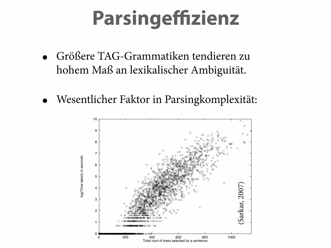
• Größere TAG-Grammatiken tendieren zuhohem Maß an lexikalischer Ambiguität.
• Wesentlicher Faktor in Parsingkomplexität:
0
1
2
3
4
5
6
7
8
9
10
0 200 400 600 800 1000
log(
Tim
e ta
ken)
in s
econ
ds
Total num of trees selected by a sentence
Figure 7: The impact of syntactic lexical ambiguity on parsing times. Log of thetime taken to parse a sentence plotted against the total number of trees selected bythe sentence. Coefficient of determination: R2 = 0.82. (x-axis: Total number oftrees selected by a sentence; y-axis: log(time) in seconds).
time complexity. We tested this hypothesis by plotting the number of derivationsreported for each sentence plotted against the time taken to produce them (shown inFigure 8). The figure shows that the final number of derivations reported is clearlynot a valid predictor of parsing time complexity.
6 Sentence Complexity
There are many ways of describing sentence complexity6, which are not necessar-ily independent of each other. In the context of lexicalized tree-adjoining grammar(and in other lexical frameworks, perhaps with some modifications) the complexityof syntactic and semantic processing is related to the number of predicate-argumentstructures being computed for a given sentence.
In this section, we explore the possibility of characterizing sentence complexityin terms of the number of clauses which is used as an approximation to the numberof predicate-argument structures to be found in a sentence.
6This section is based on some joint work with Fei Xia and Aravind Joshi, previously publishedas a workshop paper (Sarkar, Xia, and Joshi, 2000).
13
(Sar
kar,
2007
)

Supertagging
• Idee: Wenn man wüsste, welcher Elementarbaum der jeweils richtige für jedes Wort wäre, wäre Parsing viel einfacher. ‣ Sarkar 07: 548K sec (≈ eine Woche) → 30 sec für 2250 Sätze
• Können wir richtige Elementarbäume raten, bevor wir mit Parsing anfangen? → Supertagging (Bangalore & Joshi 02)

Supertagging
• Ursprünglicher Ansatz: Supertagging ≈ POS-Tagging, nur mit mehr Klassen.
• Verwende z.B. Hidden Markov Models:
• Heute nimmt man neuronale Netze, mit sehr hoher Akkuratheit.
α1 α2 α3 α4
w1 w2 w3 w4

Tagging-Accuracy
(Bangalore & Joshi 02)
Parsingeffizienz
0
1
2
3
4
5
6
7
8
9
10
2 4 6 8 10 12 14 16 18 20
log(
time)
in s
econ
ds
Sentence length
Figure 4: Parse times plotted against sentence length. Coefficient of determination:R2 = 0.65. (x-axis: Sentence length; y-axis: log(time in seconds))
time complexity analyses reported for parsing algorithms assume that the only rel-evant factor is the length of the sentence. In this paper, we will explore whethersentence length is the only relevant factor.4
Figure 5 shows the median of time taken for each sentence length. This figureshows that for some sentences the time taken by the parser deviates by a largemagnitude from the median case for the same sentence length. Next we consideredeach set of sentences of the same length to be a sample, and computed the standarddeviation for each sample. This number ignores the outliers and gives us a betterestimate of parser performance in the most common case. Figure 6 shows the plotof the standard deviation points against parsing time. The figure also shows thatthese points can be described by a linear function.
4A useful analogy to consider is the run-time analysis of quicksort. For this particular sortingalgorithm, it was detemined the distribution of the order of the numbers in the input array to be sortedwas an extremely important factor to guarantee sorting in time ⇥(nlogn). An array of numbers thatis already completely sorted has time complexity ⇥(n2).
10
-6
-4
-2
0
2
4
6
8
0 5 10 15 20 25
log(
Tim
e in
sec
s)
Sentence length
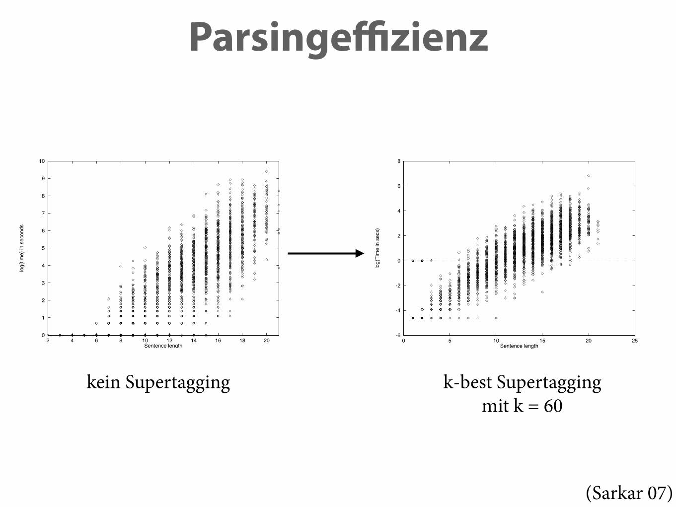
Figure 14: Time taken by the parser after n-best Supertagging (n = 60). Total timewas reduced from 548K seconds to 21K seconds. (x-axis: Sentence length; y-axis:log(time) in seconds)
another tree in the derivation until all the trees in the LTAG derivation tree aregenerated. This is analogous to the probability distribution over parse trees definedin a probabilistic context-free grammar.
A key issue is how to estimate all of the above probability distributions. Thesupervised learning solution is to estimate these probability distributions usingmaximum likelihood estimation from hand annotated data: the correct Supertagsequence for each sentence in training data to estimate probabilities for the Su-pertagger, and the correct LTAG derivation for each sentence in the training datato estimate probabilities for the LTAG statistical parser. There are standard heuris-tic methods to convert the Treebank parse trees into LTAG derivations (Xia, 1999;Chiang, 2000; Chen and Vijay-Shanker, 2000) and also see Section 3. Trainingin the supervised setting simply amounts to relative frequency counts which arenormalized to provide the probabilities needed9.
Instead of supervised learning, we consider here the setting of a model trainedon small amount of seed labeled data combined with a model trained on largeramounts of unlabeled or raw data, where the correct annotations are not provided.
9There are issues about smoothing these distributions which we do not cover here as they are notpertinent to our discussion here.
20
kein Supertagging k-best Supertagging mit k = 60
(Sarkar 07)

Zusammenfassung
• W.modell von PCFG überträgt sich recht einfachauf PTAG.
• Herausforderungen: ‣ Parameterschätzung erfordert TAG-annotiertes Korpus→ Korpus automatisch konvertieren
‣ Lexikalisierung macht Trainingsdaten sparse→ Smoothing
‣ Hohes Maß an lexikalischer Ambiguität→ Supertagging