Technische Universit¨at Braunschweig
49
Technische Universit¨ at Braunschweig Embedding Force Control in a Robot Control System TorstenKr¨oger Studienarbeit Betreuer: Dipl.-Ing. Bernd Finkemeyer 18. M¨ arz 2002 Institut f¨ ur elektrische Messtechnik und Grundlagen der Elektrotechnik Prof. Dr.-Ing. J.-Uwe Varchmin
Transcript of Technische Universit¨at Braunschweig
Technische Universitat Braunschweig
Embedding Force Control in a Robot Control System
Torsten Kroger
Studienarbeit
Betreuer: Dipl.-Ing. Bernd Finkemeyer
18. Marz 2002
Institut fur elektrische Messtechnik und
Grundlagen der Elektrotechnik
Prof. Dr.-Ing. J.-Uwe Varchmin

Erklarung
Hiermit erklare ich, dass die vorliegende Arbeit selbstandig nur unter Verwendung deraufgefuhrten Hilfsmittel von mir erstellt wurde.
Braunschweig, den 18. Marz 2002
Unterschrift
Kurzfassung
Das vorliegende Manuskript ist die Dokumentation einer Studienarbeit an der Techni-schen Universitat Braunschweig. Zielsetzung ist es, einen Kraftregler in einer vorhandenenRobotersteuerung zu implementieren. Diese Steuerung, der Treiber fur einen Kraft-/Momentensensor sowie der Treiber einer Space Mouse werden einleitend beschrieben.Nach der Vorstellung moglicher Kraftregelkonzepte folgt die Beschreibung des implemen-tierten Reglers, und abschließend wird eine Anwendung des Reglers dokumentiert, dessenZiel das kraftgeregelte Absetzen eines windschiefen Klotzes auf eine Ablage ist.
Abstract
This document is the report of a student research project at the ’Technische UniversitatBraunschweig’. Its aim is to embed a force controller into an existing robot control ar-chitecture. Introductory, this architecture, the driver for a force-torque sensor as wellthe driver for a Space Mouse are described. After the presentation of several force con-trol approaches, the implemented force controller is detailed. An application, the forcecontrolled placing a warped block, is documented finally.

Acknowledgements
During this student research project, I have interacted with many people. Each hashad some influence on the final version of this document. I greatly appreciate all thehelpful chats with Niels Otten during the time in the robot laboratory. My roommate,Christian Meiners, proofread this report and proposed some very good improvements inexpression as well as in spelling. Lastly, I would like to thank my lovely parents for theirunbelievable support during my years of study.
Torsten Kroger
Contents
1 Introduction 11.1 Software . . . . . . . . . . . . . . . . . . . . . . . . . . . . . . . . . . . . 1
1.1.1 The Object Server . . . . . . . . . . . . . . . . . . . . . . . . . . 11.1.2 The Position Controller . . . . . . . . . . . . . . . . . . . . . . . 2
1.2 Hardware . . . . . . . . . . . . . . . . . . . . . . . . . . . . . . . . . . . 31.2.1 The Space Mouse . . . . . . . . . . . . . . . . . . . . . . . . . . . 31.2.2 The JR3 Force-Torque Sensor . . . . . . . . . . . . . . . . . . . . 81.2.3 Robot and PC . . . . . . . . . . . . . . . . . . . . . . . . . . . . . 13
2 Force Control 152.1 Introduction . . . . . . . . . . . . . . . . . . . . . . . . . . . . . . . . . . 152.2 Hybrid Control Concepts . . . . . . . . . . . . . . . . . . . . . . . . . . . 16
2.2.1 Implicit Hybrid Force-Position Controller . . . . . . . . . . . . . . 162.2.2 Parallel Force-Position Control . . . . . . . . . . . . . . . . . . . 172.2.3 Add-On Force Controller . . . . . . . . . . . . . . . . . . . . . . . 18
2.3 Summary . . . . . . . . . . . . . . . . . . . . . . . . . . . . . . . . . . . 18
3 Conceptional Formulation 20
4 The Add-On Force Controller 214.1 Program Structure . . . . . . . . . . . . . . . . . . . . . . . . . . . . . . 224.2 Control Algorithm . . . . . . . . . . . . . . . . . . . . . . . . . . . . . . 244.3 Messages . . . . . . . . . . . . . . . . . . . . . . . . . . . . . . . . . . . . 264.4 Setting up the Force Control Parameters . . . . . . . . . . . . . . . . . . 28
5 Force Controlled Placing of a Block 325.1 Presuppositions . . . . . . . . . . . . . . . . . . . . . . . . . . . . . . . . 325.2 Strategy and Algorithm . . . . . . . . . . . . . . . . . . . . . . . . . . . 335.3 Detailed Overview . . . . . . . . . . . . . . . . . . . . . . . . . . . . . . 34
6 Summary 38
A Contents of the Enclosed CD 39
List of Tables 40
List of Figures 42
Bibliography 43
1 Introduction 1
1 Introduction
This document is the report of a student research project at the ’Technische Universitat
Braunschweig’. The emphasis is on force controlled robots, i.e. manutec r2 robots, which
are used for an approach for a PC based robot control system at the ’Institut fur Robotik
und Prozessinformatik’ (iRP).
1.1 Software
The heart of the robot control system is an object server, which was implemented by
Michael Borchard [1]. To comply with real time requirements, the operating system QNX
was chosen, while a Windows-NT c© PC is used to program in a convenient environment.
Both PCs are connected via a fast-ethernet connection.
1.1.1 The Object Server
Hardware QNX PC WinNTc©
PC
PC Interface
PowerElectronics
Robot
Sensors
HardwareDriver
PositionController
Space MouseApplication
HardwareDriver forSensors
MiRPAObject Server
TCP/IPInterface
ForceController
...
TCP/IPInterface
GUI
ProgramEditor
Teach Box
...
��
��
��
��
��
��
��
��
��
��
� �
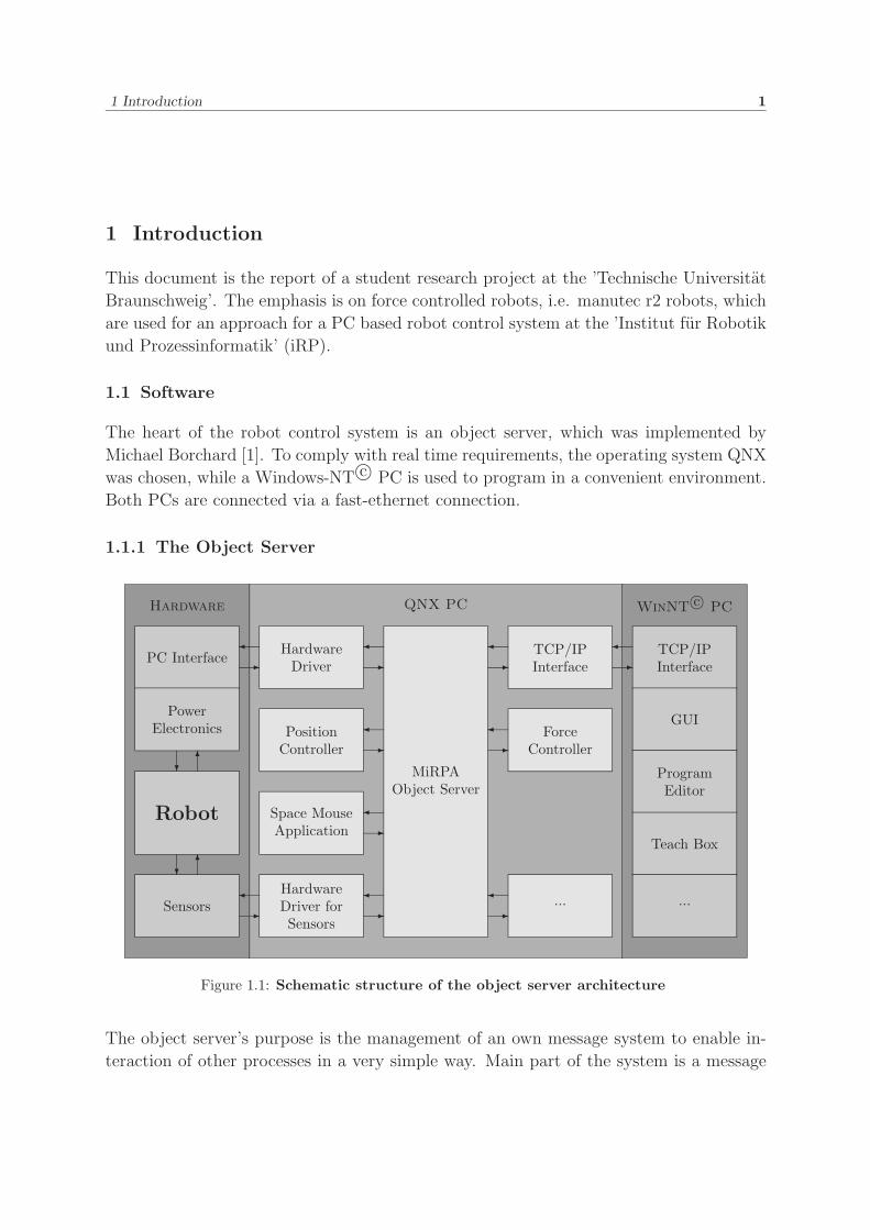
� �
Figure 1.1: Schematic structure of the object server architecture
The object server’s purpose is the management of an own message system to enable in-
teraction of other processes in a very simple way. Main part of the system is a message
1 Introduction 2
list containing all message names, the server understands. Any process can send a mes-
sage, e.g. named ’SetPos’, with optional parameters to the object server. Depending on
the entries in the message list, the object server knows all processes that understand the
message ’SetPos’ and forwards it to all these processes. To let the object server know
that a process understands a specific message, the process has to register the message
with a COMOBJECT message. In this example, the position controller is able to understand
the message ’SetPos’, and another application sends this message with a joint position as
parameter to the object server. Since the position control process has registered ’SetPos’,
it receives the message and interprets it as a new desired position value. Applications
are also able to set a client limitation, i.e. in this case only one process is allowed to
send ’SetPos’, to avoid getting new position values from different processes. Every sent
message needs to be answered with a reply message to acknowledge the sender that the
message was received correctly. In general, there are three different message types for
sending data: GENERAL, REQUEST and ANSWER. GENERAL is just a message to send informa-
tion to any receiver that understands the respective message. Just a short reply message
is necessary. Every REQUEST message has to be replied and another message to be sent
as ANSWER message. Besides all mentioned message types, the object server understands
some CONTROL messages, too. E.g. processes are able to start other processes or to get
the message list from the object server. For more information about functionalities of
this system please refer to [1].
The existing object server system is shown in figure 1.1. The power electronics of the r2
robot (see chapter 1.2.3 on page 13) are controlled via an interface card from Vigilant,
which is driven by a hardware driver implemented by Jorg Hanna [3]. For a good dynamic
behavior, a position controller is connected to the object server, which receives desired
position values from another process, e.g. the Space Mouse application (see chapter 1.2.1
on page 5), a Zero++ program or the add-on force controller (chapter 4 on page 21. To
enable remote robot control, a TCP/IP interface is available for communication with any
other connected computer. Each process has got an individual process priority (1...29) in
the QNX system. In this case, the position controller is the most important part of the
system, followed by the add-on force controller and the object server.
1.1.2 The Position Controller
1 400 4 1002 666.67 5 1603 186.67 6 120
Table 1.1: Increments per degree for each joint
Another relevant software part is the position controller from Jorg Hanna (for detailed
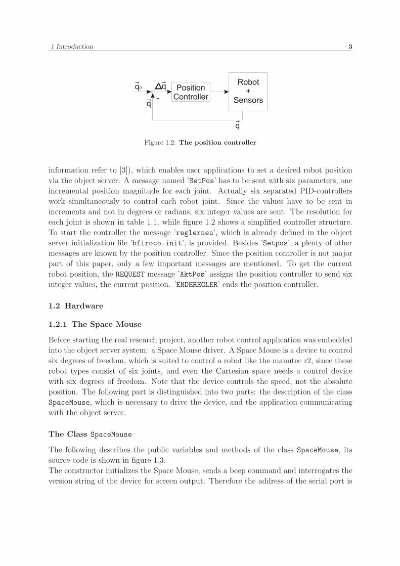
1 Introduction 3
Figure 1.2: The position controller
information refer to [3]), which enables user applications to set a desired robot position
via the object server. A message named ’SetPos’ has to be sent with six parameters, one
incremental position magnitude for each joint. Actually six separated PID-controllers
work simultaneously to control each robot joint. Since the values have to be sent in
increments and not in degrees or radians, six integer values are sent. The resolution for
each joint is shown in table 1.1, while figure 1.2 shows a simplified controller structure.
To start the controller the message ’reglerneu’, which is already defined in the object
server initialization file ’bfiroco.init’, is provided. Besides ’Setpos’, a plenty of other
messages are known by the position controller. Since the position controller is not major
part of this paper, only a few important messages are mentioned. To get the current
robot position, the REQUEST message ’AktPos’ assigns the position controller to send six
integer values, the current position. ’ENDEREGLER’ ends the position controller.
1.2 Hardware
1.2.1 The Space Mouse
Before starting the real research project, another robot control application was embedded
into the object server system: a Space Mouse driver. A Space Mouse is a device to control
six degrees of freedom, which is suited to control a robot like the manutec r2, since these
robot types consist of six joints, and even the Cartesian space needs a control device
with six degrees of freedom. Note that the device controls the speed, not the absolute
position. The following part is distinguished into two parts: the description of the class
SpaceMouse, which is necessary to drive the device, and the application communicating
with the object server.
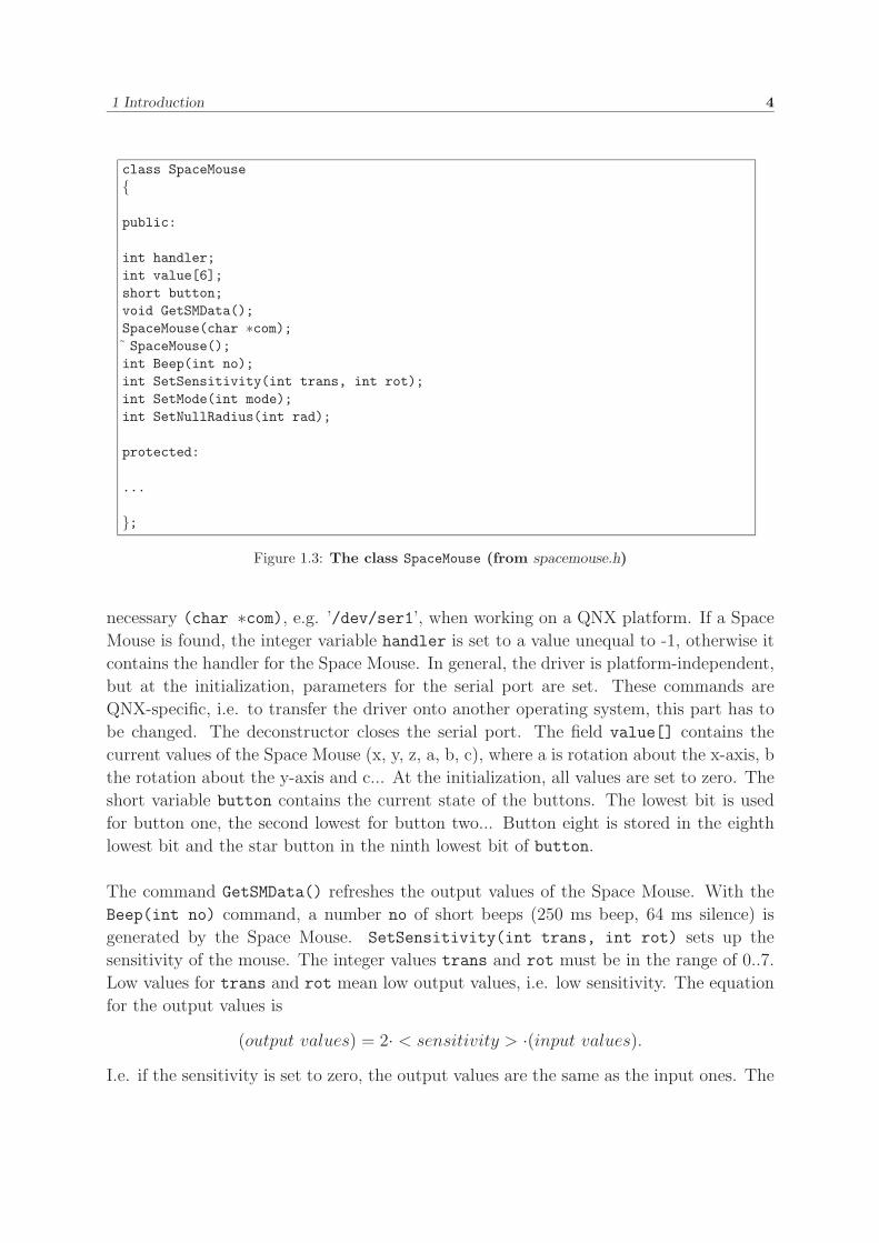
The Class SpaceMouse
The following describes the public variables and methods of the class SpaceMouse, its
source code is shown in figure 1.3.
The constructor initializes the Space Mouse, sends a beep command and interrogates the
version string of the device for screen output. Therefore the address of the serial port is
1 Introduction 4
class SpaceMouse{
public:
int handler;int value[6];short button;void GetSMData();SpaceMouse(char ∗com);˜ SpaceMouse();int Beep(int no);int SetSensitivity(int trans, int rot);int SetMode(int mode);int SetNullRadius(int rad);
protected:
...
};
Figure 1.3: The class SpaceMouse (from spacemouse.h)
necessary (char ∗com), e.g. ’/dev/ser1’, when working on a QNX platform. If a Space
Mouse is found, the integer variable handler is set to a value unequal to -1, otherwise it
contains the handler for the Space Mouse. In general, the driver is platform-independent,
but at the initialization, parameters for the serial port are set. These commands are
QNX-specific, i.e. to transfer the driver onto another operating system, this part has to
be changed. The deconstructor closes the serial port. The field value[] contains the
current values of the Space Mouse (x, y, z, a, b, c), where a is rotation about the x-axis, b
the rotation about the y-axis and c... At the initialization, all values are set to zero. The
short variable button contains the current state of the buttons. The lowest bit is used
for button one, the second lowest for button two... Button eight is stored in the eighth
lowest bit and the star button in the ninth lowest bit of button.
The command GetSMData() refreshes the output values of the Space Mouse. With the
Beep(int no) command, a number no of short beeps (250 ms beep, 64 ms silence) is
generated by the Space Mouse. SetSensitivity(int trans, int rot) sets up the
sensitivity of the mouse. The integer values trans and rot must be in the range of 0..7.
Low values for trans and rot mean low output values, i.e. low sensitivity. The equation
for the output values is
(output values) = 2· < sensitivity > ·(input values).
I.e. if the sensitivity is set to zero, the output values are the same as the input ones. The
1 Introduction 5
original values cover a range of approximately -360 to 360. To get uniform values, the
range delivered by the class SpaceMouse is set to -1000..1000. The range does not get
larger, if the sensitivity increases. The default is set to zero. Usually, it is not necessary
to change the value for sensitivity, because an own conversion has to be achieved anyway.
In general, the Space Mouse behaves very sensitive, even if its sensitivity is set to zero.
To get a real zero position and to avoid value changes by a very slight motion, the null
radius can be set with the function SetNullRadius(int rad). I.e. with a null radius of
zero, every motion around the zero point causes new values. With a larger null radius,
there is a virtual sphere, in which a movement is not recognized (actually two spheres,
one for the translatory and one for the rotatory degrees of freedom). With a value of
eight, movements within two percent of the whole range do not change the output values.
Default is 13.
Mode Dominant Translatory Rotatory
0 off off off1 off off on2 off on off3 off on on4 on off off5 on off on6 on on off7 on on on
Table 1.2: Space Mouse control modes
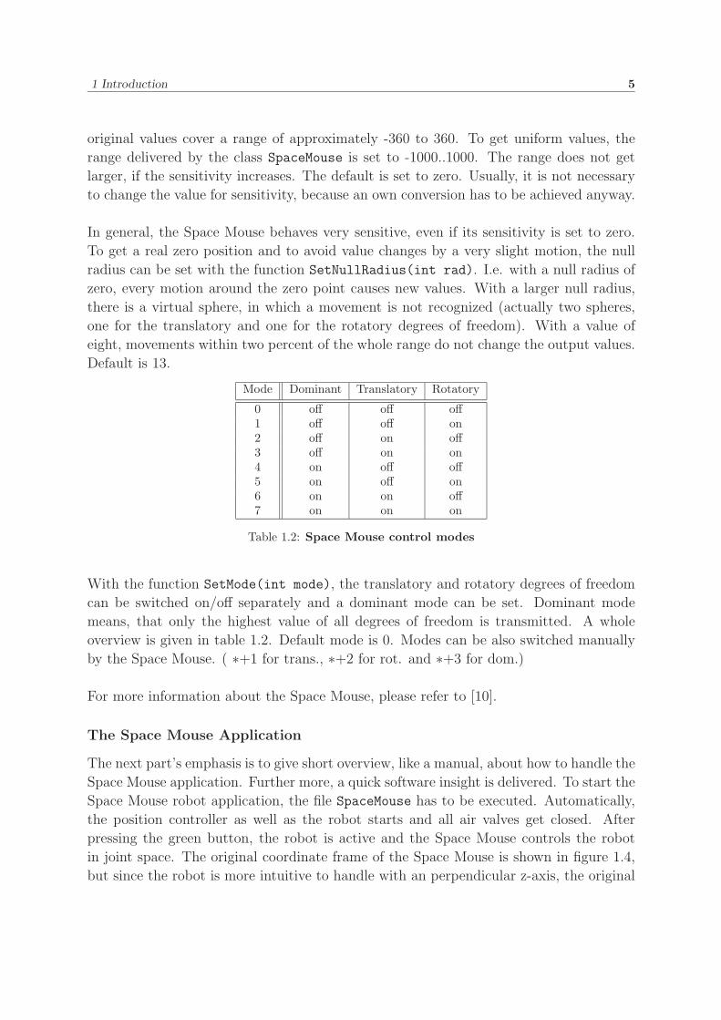
With the function SetMode(int mode), the translatory and rotatory degrees of freedom
can be switched on/off separately and a dominant mode can be set. Dominant mode
means, that only the highest value of all degrees of freedom is transmitted. A whole
overview is given in table 1.2. Default mode is 0. Modes can be also switched manually
by the Space Mouse. ( ∗+1 for trans., ∗+2 for rot. and ∗+3 for dom.)
For more information about the Space Mouse, please refer to [10].
The Space Mouse Application
The next part’s emphasis is to give short overview, like a manual, about how to handle the
Space Mouse application. Further more, a quick software insight is delivered. To start the
Space Mouse robot application, the file SpaceMouse has to be executed. Automatically,
the position controller as well as the robot starts and all air valves get closed. After
pressing the green button, the robot is active and the Space Mouse controls the robot
in joint space. The original coordinate frame of the Space Mouse is shown in figure 1.4,
but since the robot is more intuitive to handle with an perpendicular z-axis, the original
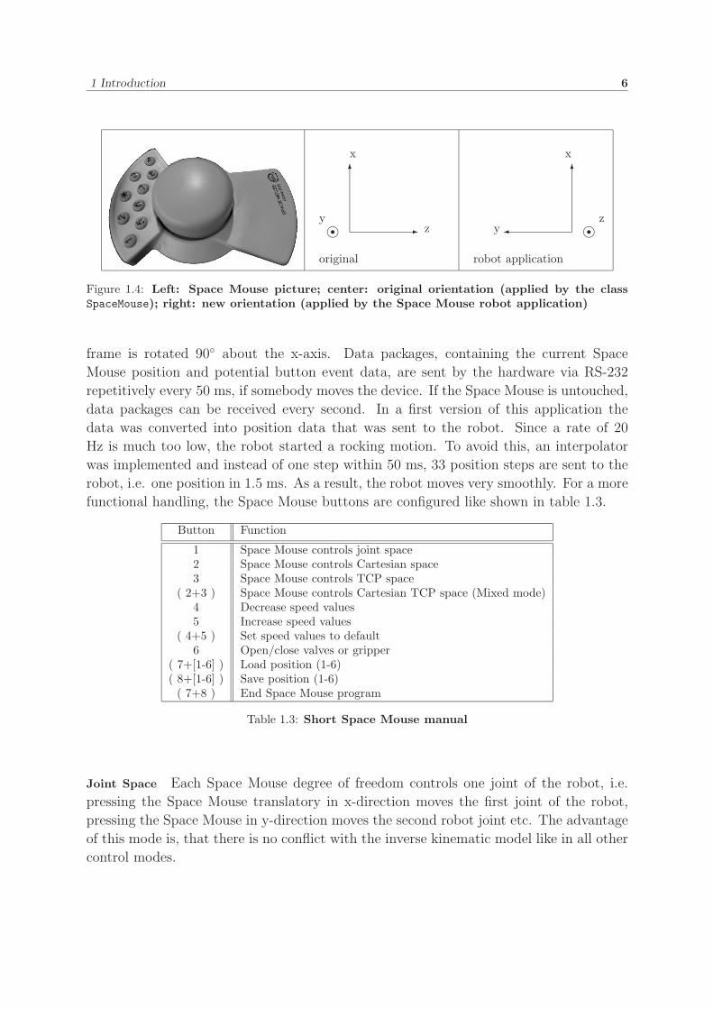
1 Introduction 6
�
� z
x
��y
original
�
�y
x
��z
robot application
Figure 1.4: Left: Space Mouse picture; center: original orientation (applied by the classSpaceMouse); right: new orientation (applied by the Space Mouse robot application)
frame is rotated 90◦ about the x-axis. Data packages, containing the current Space
Mouse position and potential button event data, are sent by the hardware via RS-232
repetitively every 50 ms, if somebody moves the device. If the Space Mouse is untouched,
data packages can be received every second. In a first version of this application the
data was converted into position data that was sent to the robot. Since a rate of 20
Hz is much too low, the robot started a rocking motion. To avoid this, an interpolator
was implemented and instead of one step within 50 ms, 33 position steps are sent to the
robot, i.e. one position in 1.5 ms. As a result, the robot moves very smoothly. For a more
functional handling, the Space Mouse buttons are configured like shown in table 1.3.
Button Function
1 Space Mouse controls joint space2 Space Mouse controls Cartesian space3 Space Mouse controls TCP space
( 2+3 ) Space Mouse controls Cartesian TCP space (Mixed mode)4 Decrease speed values5 Increase speed values
( 4+5 ) Set speed values to default6 Open/close valves or gripper
( 7+[1-6] ) Load position (1-6)( 8+[1-6] ) Save position (1-6)
( 7+8 ) End Space Mouse program
Table 1.3: Short Space Mouse manual
Joint Space Each Space Mouse degree of freedom controls one joint of the robot, i.e.
pressing the Space Mouse translatory in x-direction moves the first joint of the robot,
pressing the Space Mouse in y-direction moves the second robot joint etc. The advantage
of this mode is, that there is no conflict with the inverse kinematic model like in all other
control modes.
1 Introduction 7
Cartesian Space Button two switches to Cartesian control mode, i.e. the following trans-
formation is applied:
RTnew = TRotRPYSM · TTrans
SM · RTold
Where TRotRPYSM is a rotation frame containing the rotatory Space Mouse values, TTrans
SM
a translation frame that contains the translatory values and RTnew is the robot’s new
position w.r.t. the robot base frame, which is the reference frame. As a result the
absolute speed value for translatory movements is constant, but for rotatory movements
it depends on the distance to the corresponding rotation axis. To keep the absolute
velocity of the manipulator constant, a compensation factor, which contains the distance
to the respective axis, was integrated.
TCP Space Pressing button three puts the reference frame into the task frame, i.e. if
there is no tool, the task frame equals the tool center point frame (TCP), otherwise, there
is an offset frame TCPTTask that transforms the TCP frame to the task frame.
RTnew = RTold · TCPTTask · TTransSM · TRotRPY
SM · TCPTTask−1
Cartesian TCP Space (Mixed Mode) This control mode offers the most intuitive robot
control. Translatory movements are executed w.r.t. the robot base frame like in Cartesian
mode, but for rotatory movements the robot base frame is translatory shifted into the task
frame. As the separation of rotatory and translatory degrees of freedom are separated,
the transformation is more complex:
RTnew = RTTransold · TTrans
SM · RTRotRPYold · TCPTTrans
Task
· RTRotRPYold
−1 · TRotRPYSM · RTRotRPY
old · TCPTTransTask
−1
The syntax RTTransold means a translation frame, which contains only the old manipula-
tor position, but not its orientation. RTRotRPYold is the respective rotation frame of the
old manipulator position. This syntax is considered to rule for all other transformation
frames in the equation above. To comprehend the transformation completely a figure is
necessary, but since this document’s part is not the main one such an explanation was
abandoned.
1 Introduction 8
Several Other Functions The buttons four and five are responsible for the speed set
point, which can range from 1 to 100, default is 20. Pressing button four decreases the
speed by one integer, button five increases the speed. While pressing one of these buttons,
robot control is disabled. To accelerate speed setup, the Space Mouse’s head needs to
be touched and button four or five to be pressed. Attention: if the buttons are released
before the head of the Space Mouse, the robot may move unintentional. The default
speed value is set, when both buttons, four and five, are pressed simultaneously.
To open or close a gripper or to activate/deactivate a sucker, button six has to be hit.
To store a position, button eight and a number between one and six have to be pressed
simultaneously. To load a stored position, button seven and one of the numbers have
to be used. This way, the user is able to store six positions, which are available even
after ending the program, since they are stored in a file named ’pos.dat’. Hitting button
seven and eight simultaneously moves the robot to its default position, ends the position
controller and with it the robot and closes all valves.
Since there are still problems with the inverse kinematics, the user has to press the
∗-key when the robot needs to reconfigure itself. This way, the user is not appalled, if the
robot takes a new configuration. To disable this feature, the Space Mouse application
has to be started with the -e option.
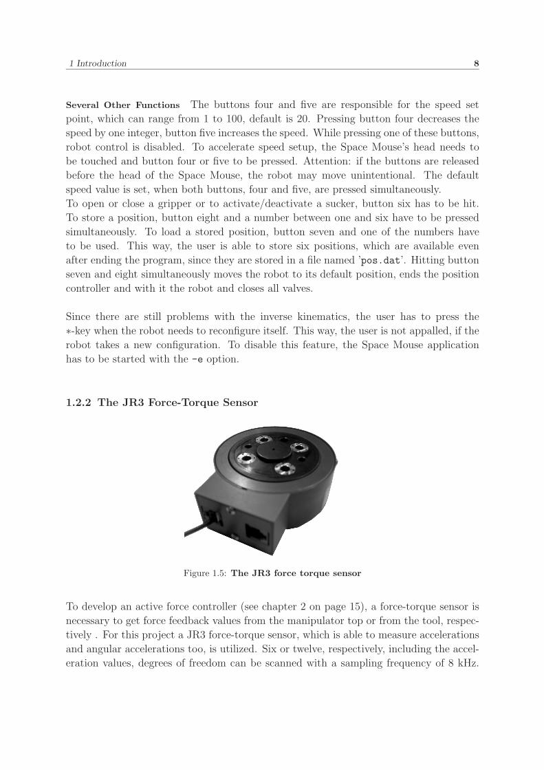
1.2.2 The JR3 Force-Torque Sensor
Figure 1.5: The JR3 force torque sensor
To develop an active force controller (see chapter 2 on page 15), a force-torque sensor is
necessary to get force feedback values from the manipulator top or from the tool, respec-
tively . For this project a JR3 force-torque sensor, which is able to measure accelerations
and angular accelerations too, is utilized. Six or twelve, respectively, including the accel-
eration values, degrees of freedom can be scanned with a sampling frequency of 8 kHz.
1 Introduction 9
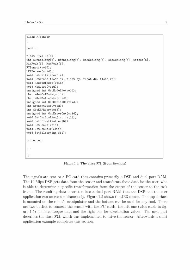
class FTSensor{
public:
float FTValue[6];int CurScaling[6], MinScaling[6], MaxScaling[6], DefScaling[6], Offset[6],MinPeak[6], MaxPeak[6];FTSensor(void);˜ FTSensor(void);void SetUnits(short e);void SetTrans(float dx, float dy, float dz, float rz);void ResetOffset(void);void Measure(void);unsigned int GetModelNo(void);char ∗GetCalDate(void);char ∗GetSoftwDate(void);unsigned int GetSerialNo(void);int GetSoftwVer(void);int GetEEPRVer(void);unsigned int GetErrorCnt(void);void SetCurScaling(int cs[6]);void SetOffset(int os[6]);void GetPeaks(void);void GetPeaks R(void);void SetFilter(int fil);
protected:
...
};
Figure 1.6: The class FTS (from ftsenso.h)
The signals are sent to a PC card that contains primarily a DSP and dual port RAM.
The 10 Mips DSP gets data from the sensor and transforms these data for the user, who
is able to determine a specific transformation from the center of the sensor to the task
frame. The resulting data is written into a dual port RAM that the DSP and the user
application can access simultaneously. Figure 1.5 shows the JR3 sensor. The top surface
is mounted on the robot’s manipulator and the bottom can be used for any tool. There
are two outlets to connect the sensor with the PC cards, the left one (with cable in fig-
ure 1.5) for force-torque data and the right one for acceleration values. The next part
describes the class FTS, which was implemented to drive the sensor. Afterwards a short
application example completes this section.
1 Introduction 10
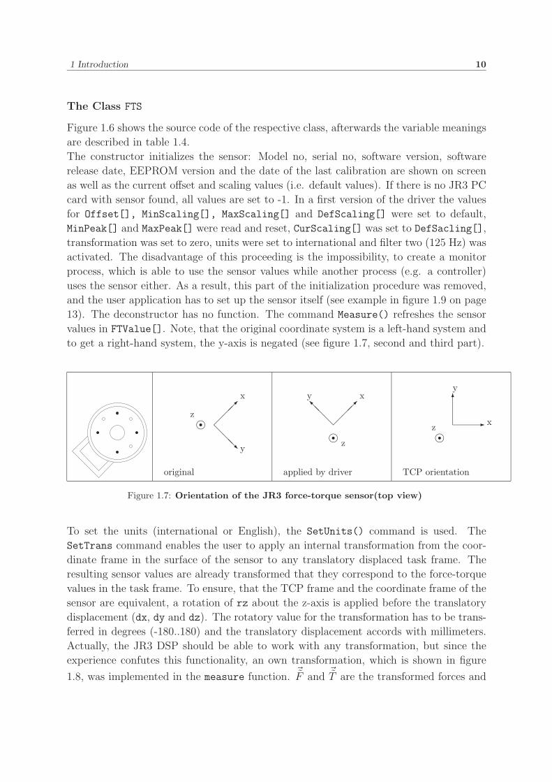
The Class FTS
Figure 1.6 shows the source code of the respective class, afterwards the variable meanings
are described in table 1.4.
The constructor initializes the sensor: Model no, serial no, software version, software
release date, EEPROM version and the date of the last calibration are shown on screen
as well as the current offset and scaling values (i.e. default values). If there is no JR3 PC
card with sensor found, all values are set to -1. In a first version of the driver the values
for Offset[], MinScaling[], MaxScaling[] and DefScaling[] were set to default,
MinPeak[] and MaxPeak[] were read and reset, CurScaling[] was set to DefSacling[],
transformation was set to zero, units were set to international and filter two (125 Hz) was
activated. The disadvantage of this proceeding is the impossibility, to create a monitor
process, which is able to use the sensor values while another process (e.g. a controller)
uses the sensor either. As a result, this part of the initialization procedure was removed,
and the user application has to set up the sensor itself (see example in figure 1.9 on page
13). The deconstructor has no function. The command Measure() refreshes the sensor
values in FTValue[]. Note, that the original coordinate system is a left-hand system and
to get a right-hand system, the y-axis is negated (see figure 1.7, second and third part).
����
����
x
y
��z
original
����
���
xy
��z
applied by driver
�
�y
x��
z
TCP orientation
Figure 1.7: Orientation of the JR3 force-torque sensor(top view)
To set the units (international or English), the SetUnits() command is used. The
SetTrans command enables the user to apply an internal transformation from the coor-
dinate frame in the surface of the sensor to any translatory displaced task frame. The
resulting sensor values are already transformed that they correspond to the force-torque
values in the task frame. To ensure, that the TCP frame and the coordinate frame of the
sensor are equivalent, a rotation of rz about the z-axis is applied before the translatory
displacement (dx, dy and dz). The rotatory value for the transformation has to be trans-
ferred in degrees (-180..180) and the translatory displacement accords with millimeters.
Actually, the JR3 DSP should be able to work with any transformation, but since the
experience confutes this functionality, an own transformation, which is shown in figure
1.8, was implemented in the measure function. �F and �T are the transformed forces and
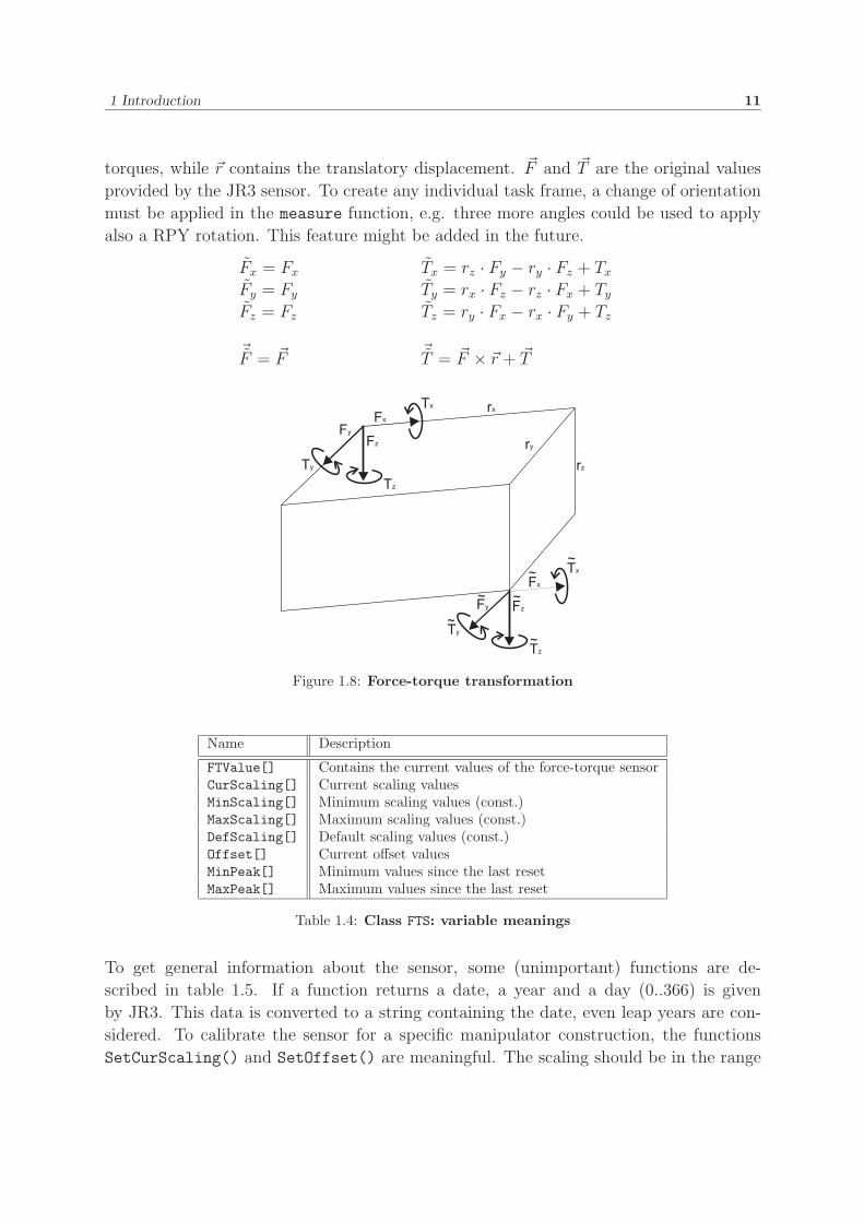
1 Introduction 11
torques, while �r contains the translatory displacement. �F and �T are the original values
provided by the JR3 sensor. To create any individual task frame, a change of orientation
must be applied in the measure function, e.g. three more angles could be used to apply
also a RPY rotation. This feature might be added in the future.
Fx = Fx Tx = rz · Fy − ry · Fz + Tx
Fy = Fy Ty = rx · Fz − rz · Fx + Ty
Fz = Fz Tz = ry · Fx − rx · Fy + Tz
�F = �F �T = �F × �r + �T
Figure 1.8: Force-torque transformation
Name Description
FTValue[] Contains the current values of the force-torque sensorCurScaling[] Current scaling valuesMinScaling[] Minimum scaling values (const.)MaxScaling[] Maximum scaling values (const.)DefScaling[] Default scaling values (const.)Offset[] Current offset valuesMinPeak[] Minimum values since the last resetMaxPeak[] Maximum values since the last reset
Table 1.4: Class FTS: variable meanings
To get general information about the sensor, some (unimportant) functions are de-
scribed in table 1.5. If a function returns a date, a year and a day (0..366) is given
by JR3. This data is converted to a string containing the date, even leap years are con-
sidered. To calibrate the sensor for a specific manipulator construction, the functions
SetCurScaling() and SetOffset() are meaningful. The scaling should be in the range
1 Introduction 12
Name Description
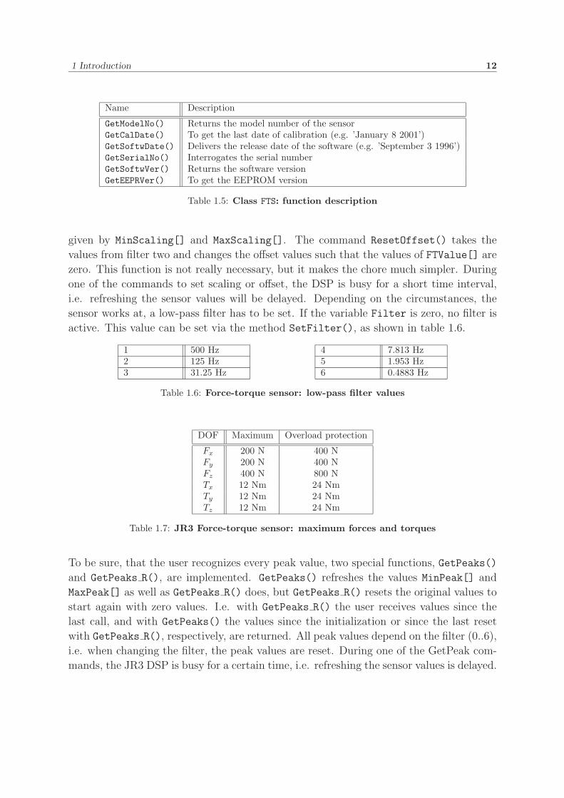
GetModelNo() Returns the model number of the sensorGetCalDate() To get the last date of calibration (e.g. ’January 8 2001’)GetSoftwDate() Delivers the release date of the software (e.g. ’September 3 1996’)GetSerialNo() Interrogates the serial numberGetSoftwVer() Returns the software versionGetEEPRVer() To get the EEPROM version
Table 1.5: Class FTS: function description
given by MinScaling[] and MaxScaling[]. The command ResetOffset() takes the
values from filter two and changes the offset values such that the values of FTValue[] are
zero. This function is not really necessary, but it makes the chore much simpler. During
one of the commands to set scaling or offset, the DSP is busy for a short time interval,
i.e. refreshing the sensor values will be delayed. Depending on the circumstances, the
sensor works at, a low-pass filter has to be set. If the variable Filter is zero, no filter is
active. This value can be set via the method SetFilter(), as shown in table 1.6.
1 500 Hz 4 7.813 Hz2 125 Hz 5 1.953 Hz3 31.25 Hz 6 0.4883 Hz
Table 1.6: Force-torque sensor: low-pass filter values
DOF Maximum Overload protection
Fx 200 N 400 NFy 200 N 400 NFz 400 N 800 NTx 12 Nm 24 NmTy 12 Nm 24 NmTz 12 Nm 24 Nm
Table 1.7: JR3 Force-torque sensor: maximum forces and torques
To be sure, that the user recognizes every peak value, two special functions, GetPeaks()
and GetPeaks R(), are implemented. GetPeaks() refreshes the values MinPeak[] and
MaxPeak[] as well as GetPeaks R() does, but GetPeaks R() resets the original values to
start again with zero values. I.e. with GetPeaks R() the user receives values since the
last call, and with GetPeaks() the values since the initialization or since the last reset
with GetPeaks R(), respectively, are returned. All peak values depend on the filter (0..6),
i.e. when changing the filter, the peak values are reset. During one of the GetPeak com-
mands, the JR3 DSP is busy for a certain time, i.e. refreshing the sensor values is delayed.
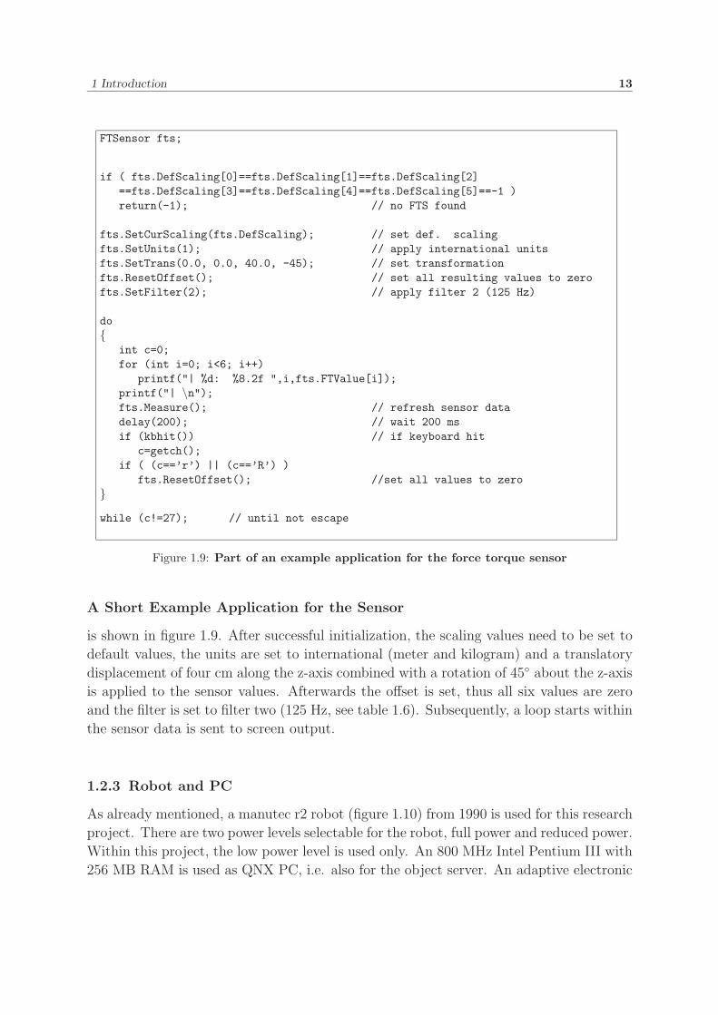
1 Introduction 13
FTSensor fts;
if ( fts.DefScaling[0]==fts.DefScaling[1]==fts.DefScaling[2]==fts.DefScaling[3]==fts.DefScaling[4]==fts.DefScaling[5]==-1 )return(-1); // no FTS found
fts.SetCurScaling(fts.DefScaling); // set def. scalingfts.SetUnits(1); // apply international unitsfts.SetTrans(0.0, 0.0, 40.0, -45); // set transformationfts.ResetOffset(); // set all resulting values to zerofts.SetFilter(2); // apply filter 2 (125 Hz)
do{
int c=0;for (int i=0; i<6; i++)
printf("| %d: %8.2f ",i,fts.FTValue[i]);printf("| \n");fts.Measure(); // refresh sensor datadelay(200); // wait 200 msif (kbhit()) // if keyboard hit
c=getch();if ( (c==’r’) || (c==’R’) )
fts.ResetOffset(); //set all values to zero}while (c!=27); // until not escape
Figure 1.9: Part of an example application for the force torque sensor
A Short Example Application for the Sensor
is shown in figure 1.9. After successful initialization, the scaling values need to be set to
default values, the units are set to international (meter and kilogram) and a translatory
displacement of four cm along the z-axis combined with a rotation of 45◦ about the z-axis
is applied to the sensor values. Afterwards the offset is set, thus all six values are zero
and the filter is set to filter two (125 Hz, see table 1.6). Subsequently, a loop starts within
the sensor data is sent to screen output.
1.2.3 Robot and PC
As already mentioned, a manutec r2 robot (figure 1.10) from 1990 is used for this research
project. There are two power levels selectable for the robot, full power and reduced power.
Within this project, the low power level is used only. An 800 MHz Intel Pentium III with
256 MB RAM is used as QNX PC, i.e. also for the object server. An adaptive electronic
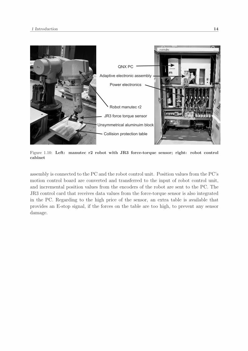
1 Introduction 14
Figure 1.10: Left: manutec r2 robot with JR3 force-torque sensor; right: robot controlcabinet
assembly is connected to the PC and the robot control unit. Position values from the PC’s
motion control board are converted and transferred to the input of robot control unit,
and incremental position values from the encoders of the robot are sent to the PC. The
JR3 control card that receives data values from the force-torque sensor is also integrated
in the PC. Regarding to the high price of the sensor, an extra table is available that
provides an E-stop signal, if the forces on the table are too high, to prevent any sensor
damage.
2 Force Control 15
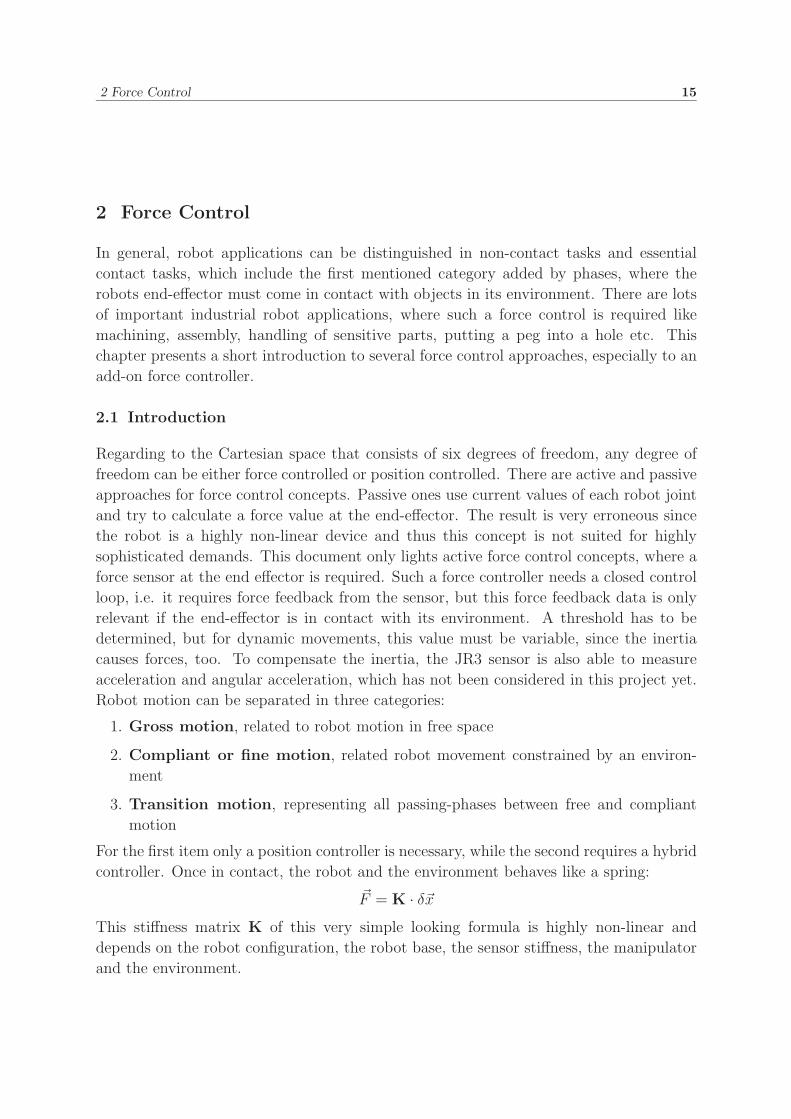
2 Force Control
In general, robot applications can be distinguished in non-contact tasks and essential
contact tasks, which include the first mentioned category added by phases, where the
robots end-effector must come in contact with objects in its environment. There are lots
of important industrial robot applications, where such a force control is required like
machining, assembly, handling of sensitive parts, putting a peg into a hole etc. This
chapter presents a short introduction to several force control approaches, especially to an
add-on force controller.
2.1 Introduction
Regarding to the Cartesian space that consists of six degrees of freedom, any degree of
freedom can be either force controlled or position controlled. There are active and passive
approaches for force control concepts. Passive ones use current values of each robot joint
and try to calculate a force value at the end-effector. The result is very erroneous since
the robot is a highly non-linear device and thus this concept is not suited for highly
sophisticated demands. This document only lights active force control concepts, where a
force sensor at the end effector is required. Such a force controller needs a closed control
loop, i.e. it requires force feedback from the sensor, but this force feedback data is only
relevant if the end-effector is in contact with its environment. A threshold has to be
determined, but for dynamic movements, this value must be variable, since the inertia
causes forces, too. To compensate the inertia, the JR3 sensor is also able to measure
acceleration and angular acceleration, which has not been considered in this project yet.
Robot motion can be separated in three categories:
1. Gross motion, related to robot motion in free space
2. Compliant or fine motion, related robot movement constrained by an environ-
ment
3. Transition motion, representing all passing-phases between free and compliant
motion
For the first item only a position controller is necessary, while the second requires a hybrid
controller. Once in contact, the robot and the environment behaves like a spring:
�F = K · δ�xThis stiffness matrix K of this very simple looking formula is highly non-linear and
depends on the robot configuration, the robot base, the sensor stiffness, the manipulator
and the environment.
2 Force Control 16
The third item, the transition motion, is an enormous research problem and part of this
approach. The development of such a robust controller is not that trivial, since there are
too many factors ruling: the robot position, the robot’s manipulator, its surface and the
material of the handled object as well as the one of the environment change the stiffness,
whose calculation is highly sophisticated, perhaps impossible. For this kind of highly non-
linear systems, an adaptive control concept must be applied, i.e. the control parameter
vary depending on the behavior of the system. For the transition problem, a fuzzy control
concept might be a successful solution. The long-term aim of this research project is to
develop a robust hybrid force-position controller. In several technical literatures lots
of concepts are presented, but since the system architecture of all available commercial
robot systems is much too slow for convenient force control (they are designed for position
control), a new system was developed as part of this research project: the object server
as middleware (see chapter 1.1.1 on page 1). For more information about force control,
refer to [9]. Note: in this chapter the word ’force’ means forces and torques.
2.2 Hybrid Control Concepts
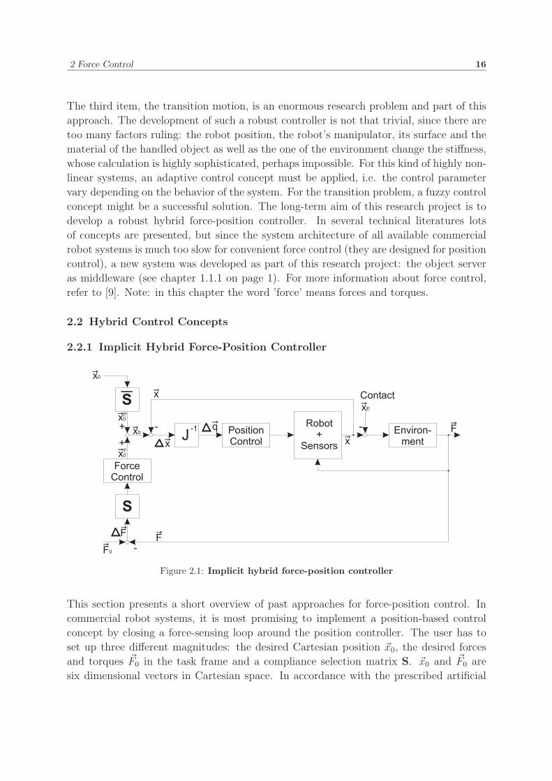
2.2.1 Implicit Hybrid Force-Position Controller
Figure 2.1: Implicit hybrid force-position controller
This section presents a short overview of past approaches for force-position control. In
commercial robot systems, it is most promising to implement a position-based control
concept by closing a force-sensing loop around the position controller. The user has to
set up three different magnitudes: the desired Cartesian position �x0, the desired forces
and torques �F0 in the task frame and a compliance selection matrix S. �x0 and �F0 are
six dimensional vectors in Cartesian space. In accordance with the prescribed artificial
2 Force Control 17
constraints, the i-th diagonal element of the matrix S has the value 1, if the i-th DOF with
respect to the task frame is force controlled, and the value 0, if it is position controlled.
An implicit hybrid force-position controller is shown in figure 2.1. The force controller’s
input is the difference between the selected desired force values and the respective current
contact force in the task frame. Its output is an equivalent position �xF0 in force controlled
directions, which is superimposed to the orthogonal vector �xP0 , which contains the nominal
position in orthogonal position controlled directions that are selected by S. S is defined as
E−S, where E is the identity matrix. The Cartesian position difference ∆�x is transformed
into the joint difference vector ∆�q via the inverse Jacobian. The robot is actually only
controlled by the position controller, whose input is ∆�q.
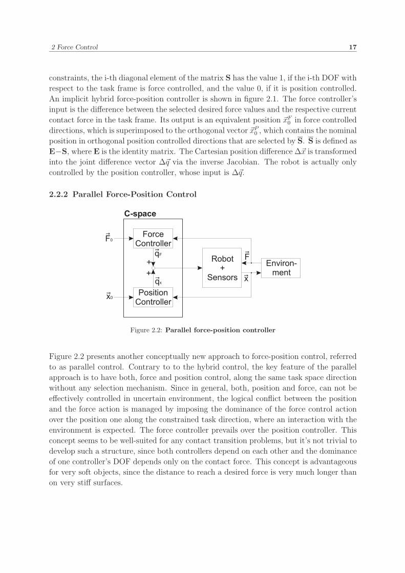
2.2.2 Parallel Force-Position Control
Figure 2.2: Parallel force-position controller
Figure 2.2 presents another conceptually new approach to force-position control, referred
to as parallel control. Contrary to to the hybrid control, the key feature of the parallel
approach is to have both, force and position control, along the same task space direction
without any selection mechanism. Since in general, both, position and force, can not be
effectively controlled in uncertain environment, the logical conflict between the position
and the force action is managed by imposing the dominance of the force control action
over the position one along the constrained task direction, where an interaction with the
environment is expected. The force controller prevails over the position controller. This
concept seems to be well-suited for any contact transition problems, but it’s not trivial to
develop such a structure, since both controllers depend on each other and the dominance
of one controller’s DOF depends only on the contact force. This concept is advantageous
for very soft objects, since the distance to reach a desired force is very much longer than
on very stiff surfaces.
2 Force Control 18
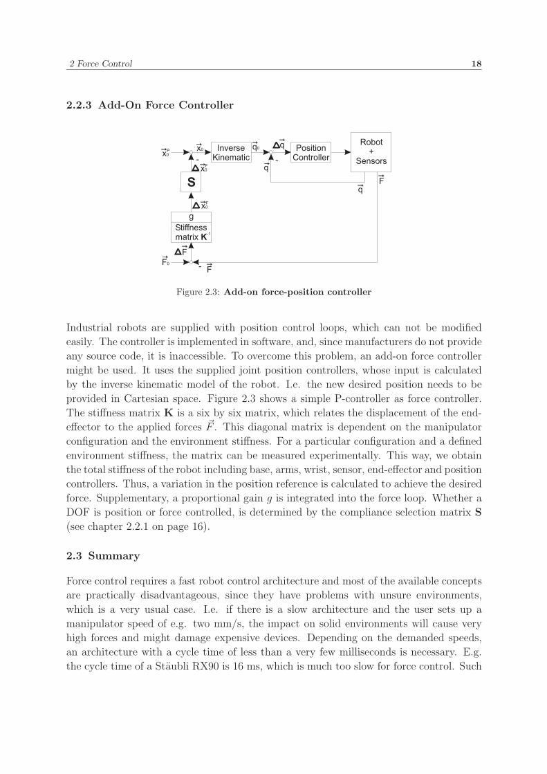
2.2.3 Add-On Force Controller
Figure 2.3: Add-on force-position controller
Industrial robots are supplied with position control loops, which can not be modified
easily. The controller is implemented in software, and, since manufacturers do not provide
any source code, it is inaccessible. To overcome this problem, an add-on force controller
might be used. It uses the supplied joint position controllers, whose input is calculated
by the inverse kinematic model of the robot. I.e. the new desired position needs to be
provided in Cartesian space. Figure 2.3 shows a simple P-controller as force controller.
The stiffness matrix K is a six by six matrix, which relates the displacement of the end-
effector to the applied forces �F . This diagonal matrix is dependent on the manipulator
configuration and the environment stiffness. For a particular configuration and a defined
environment stiffness, the matrix can be measured experimentally. This way, we obtain
the total stiffness of the robot including base, arms, wrist, sensor, end-effector and position
controllers. Thus, a variation in the position reference is calculated to achieve the desired
force. Supplementary, a proportional gain g is integrated into the force loop. Whether a
DOF is position or force controlled, is determined by the compliance selection matrix S
(see chapter 2.2.1 on page 16).
2.3 Summary
Force control requires a fast robot control architecture and most of the available concepts
are practically disadvantageous, since they have problems with unsure environments,
which is a very usual case. I.e. if there is a slow architecture and the user sets up a
manipulator speed of e.g. two mm/s, the impact on solid environments will cause very
high forces and might damage expensive devices. Depending on the demanded speeds,
an architecture with a cycle time of less than a very few milliseconds is necessary. E.g.
the cycle time of a Staubli RX90 is 16 ms, which is much too slow for force control. Such
2 Force Control 19
a robot architecture can only be used for very slow speeds to prevent heavy impacts on
a solid environment. The next problem occurs, when handling dynamic objects with a
defined force, where a fast force controller is definitely necessary. A lower cycle time
enables faster movements and much better behavior at contact transitions. Such fast
robot control architectures are not available on the market yet.
3 Conceptional Formulation 20
3 Conceptional Formulation
This chapter contains the conceptional formulation of this student research project and
describes the given architecture. The long-term aim of this research project is to develop
a hybrid force-position control architecture, like shown in chapter 2.2.1 on page 16. With
such a controller users are able to split a complex assembly procedure into primitive ac-
tions, like the displacement of a not ideally gripped block that needs only four different
setpoints.
As already mentioned, in chapter 1.1.1 on page 1, the object server is used for inter-
process communication. The position controller, introduced in chapter 1.1.2 on page 2,
receives desired position values via the object server. To get first impressions for the
realization of a hybrid force-position controller, the implementation of a simpler add-on
force-torque controller was chosen. The existing architecture has to be expanded by a
force control loop, comparable to figure 2.3 (page 18). The described add-on control con-
cept is disadvantageous, since the stiffness matrix K behaves like a simple P-controller
and is only ideal for a special robot configuration and known environment. Since the user
does not know any exact deviations of the environment, another concept has to be created.
But first of all, the implementation of a driver for the JR3 force-torque sensor is re-
quired. Afterwards, the force-torque controller needs to be developed and dimensioned
for the r2 robot, which is a presupposition to program the corresponding primitive ac-
tions. To get a real application for such a force-torque controller, an example program
has to be styled. A not ideally gripped block is simulated by a ’cuboid’ with non parallel
planes, to enable negligence of any displacement within the gripper. The user applica-
tion does not know any deviations of the block, and its purpose is to place the block on
the ground ideally, i.e. the forces must not exceed a limit and the deviations must be
calculated. If one corner has ground contact, it must not be displaced in any direction,
only rotatory movements around this contact point are allowed, until one whole edge is in
contact with the ground plane. Lastly, only a rotation around this edge is allowed until
the whole bottom plane is down. This trivial seeming task is more sophisticated than an
unskilled person might think at the first time.
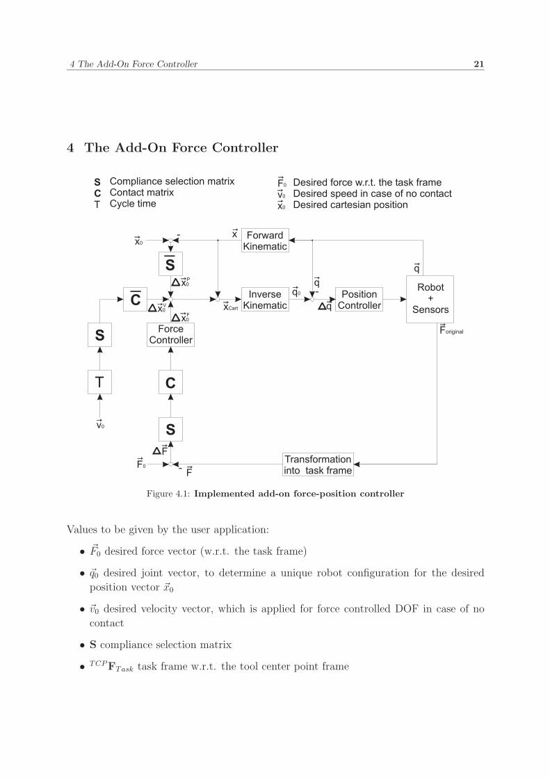
4 The Add-On Force Controller 21
4 The Add-On Force Controller
Figure 4.1: Implemented add-on force-position controller
Values to be given by the user application:
• �F0 desired force vector (w.r.t. the task frame)
• �q0 desired joint vector, to determine a unique robot configuration for the desired
position vector �x0
• �v0 desired velocity vector, which is applied for force controlled DOF in case of no
contact
• S compliance selection matrix
• TCPFTask task frame w.r.t. the tool center point frame
4 The Add-On Force Controller 22
Due to the basics introduced in chapter 2.2.3 (page 18), the mentioned add-on force
controller is not powerful enough. The concept was extended like shown in figure 4.1 by a
PID controller instead of the inverse stiffness matrix K−1 and a contact matrix C, which
is similar to the compliance selection matrix S (see chapter 2.2.1 on page 16). If the
absolute magnitude of the force or the torque, respectively, in one DOF is larger than a
defined threshold, the i-th diagonal element of C is 1 otherwise 0. The vector �F0 is given
w.r.t. the task frame, which can be set up by the user. By default, the task frame equals
the TCP frame, i.e. the center of the force-torque sensor surface. For the case that one
DOF is force controlled and there is no environment contact, i.e. the respective element
of the S matrix is 1 and the equivalent C element is 0, the force control loop is not closed.
To get contact by moving the manipulator in a particular direction, a six dimensional
velocity vector �v0 is applied to each DOF, which is force controlled, but there is no contact
in its direction. The vector given in mm/s (◦/s) is multiplied by the cycle time to get
the desired movement ∆�xV0 for one cycle. After exceeding the contact threshold value,
the PID force-torque controller is applied to calculate new position difference values ∆�xF0
for the directions, which are force controlled and in contact. Figure 4.1 is simplified
and shows a block diagram of the controller. To get a unique robot configuration for a
desired position, the position values are given in joint values. On the basis of a frame
calculated by the kinematic robot model, a vector �x0 can be determined. �x0 contains
the new position values for the DOF that are position controlled, while ∆�xP0 consists of
new position difference values. All prementioned vectors �x0, �F0 and �v0 contain values
for x, y and z direction and rotatory values about the x, the y and the z-axis. The
corresponding differences ∆�xF0 , ∆�xP
0 and ∆�xV0 are added to the current position �x, and
the new respective joint values �q0 are determined by the inverse kinematic model of the
robot and are send via ’SetPos’ to the object server, which transfers the values to the
position controller. Lastly some words about the ’actio equals reactio’ problem. If the
desired force or torque, respectively, of one DOF is positive, the robot is supposed to
move in the positive direction of the task frame coordinate system, which is a right hand
system, of course. The same principle rules for the velocity vector �v0. The JR3 sensor
values behave in the same manner. I.e. if there is contact in the corresponding DOF, the
JR3 values are negative, while the desired force acts in the right direction, but is signed
positive. To get correct feedback values, the sensor values have to be negated, therewith
the controller acts as shown in figure 4.1 and is supposed to keep the force difference near
zero.
4.1 Program Structure
This section describes the general program structure of the force controller, whose pro-
gram flow chart is shown in figure 4.2. Of course, not every detail is mentioned, since
it would be too voluminous. The command ’ic’ starts the program by default, the op-
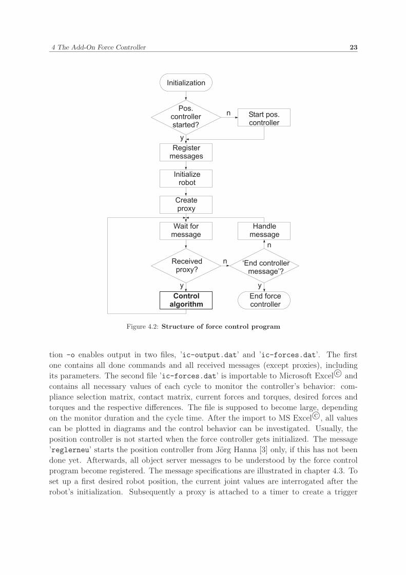
4 The Add-On Force Controller 23
Figure 4.2: Structure of force control program
tion -o enables output in two files, ’ic-output.dat’ and ’ic-forces.dat’. The first
one contains all done commands and all received messages (except proxies), including
its parameters. The second file ’ic-forces.dat’ is importable to Microsoft Excel c© and
contains all necessary values of each cycle to monitor the controller’s behavior: com-
pliance selection matrix, contact matrix, current forces and torques, desired forces and
torques and the respective differences. The file is supposed to become large, depending
on the monitor duration and the cycle time. After the import to MS Excel c©, all values
can be plotted in diagrams and the control behavior can be investigated. Usually, the
position controller is not started when the force controller gets initialized. The message
’reglerneu’ starts the position controller from Jorg Hanna [3] only, if this has not been
done yet. Afterwards, all object server messages to be understood by the force control
program become registered. The message specifications are illustrated in chapter 4.3. To
set up a first desired robot position, the current joint values are interrogated after the
robot’s initialization. Subsequently a proxy is attached to a timer to create a trigger
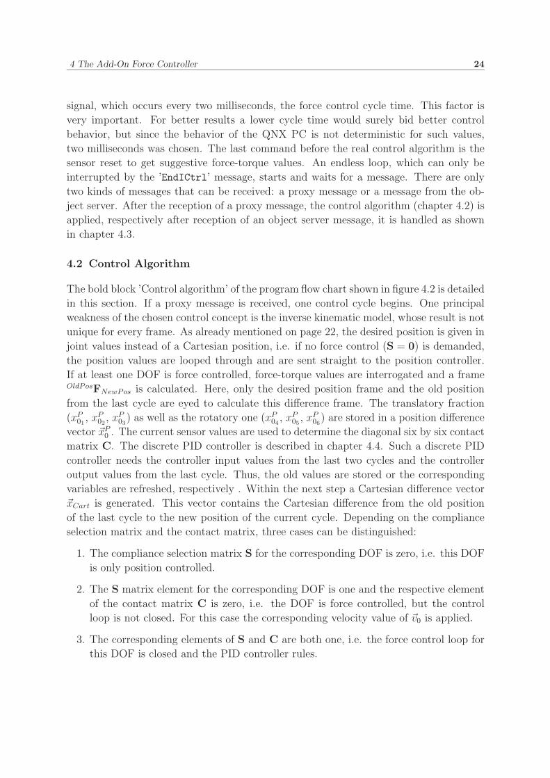
4 The Add-On Force Controller 24
signal, which occurs every two milliseconds, the force control cycle time. This factor is
very important. For better results a lower cycle time would surely bid better control
behavior, but since the behavior of the QNX PC is not deterministic for such values,
two milliseconds was chosen. The last command before the real control algorithm is the
sensor reset to get suggestive force-torque values. An endless loop, which can only be
interrupted by the ’EndICtrl’ message, starts and waits for a message. There are only
two kinds of messages that can be received: a proxy message or a message from the ob-
ject server. After the reception of a proxy message, the control algorithm (chapter 4.2) is
applied, respectively after reception of an object server message, it is handled as shown
in chapter 4.3.
4.2 Control Algorithm
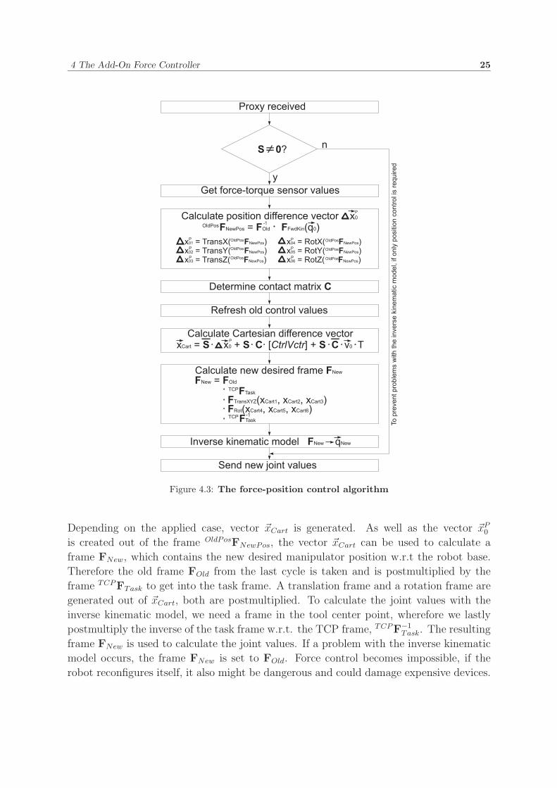
The bold block ’Control algorithm’ of the program flow chart shown in figure 4.2 is detailed
in this section. If a proxy message is received, one control cycle begins. One principal
weakness of the chosen control concept is the inverse kinematic model, whose result is not
unique for every frame. As already mentioned on page 22, the desired position is given in
joint values instead of a Cartesian position, i.e. if no force control (S = 0) is demanded,
the position values are looped through and are sent straight to the position controller.
If at least one DOF is force controlled, force-torque values are interrogated and a frameOldPosFNewPos is calculated. Here, only the desired position frame and the old position
from the last cycle are eyed to calculate this difference frame. The translatory fraction
(xP01
, xP02
, xP03
) as well as the rotatory one (xP04
, xP05
, xP06
) are stored in a position difference
vector �xP0 . The current sensor values are used to determine the diagonal six by six contact
matrix C. The discrete PID controller is described in chapter 4.4. Such a discrete PID
controller needs the controller input values from the last two cycles and the controller
output values from the last cycle. Thus, the old values are stored or the corresponding
variables are refreshed, respectively . Within the next step a Cartesian difference vector
�xCart is generated. This vector contains the Cartesian difference from the old position
of the last cycle to the new position of the current cycle. Depending on the compliance
selection matrix and the contact matrix, three cases can be distinguished:
1. The compliance selection matrix S for the corresponding DOF is zero, i.e. this DOF
is only position controlled.
2. The S matrix element for the corresponding DOF is one and the respective element
of the contact matrix C is zero, i.e. the DOF is force controlled, but the control
loop is not closed. For this case the corresponding velocity value of �v0 is applied.
3. The corresponding elements of S and C are both one, i.e. the force control loop for
this DOF is closed and the PID controller rules.
4 The Add-On Force Controller 25
Figure 4.3: The force-position control algorithm
Depending on the applied case, vector �xCart is generated. As well as the vector �xP0
is created out of the frame OldPosFNewPos, the vector �xCart can be used to calculate a
frame FNew, which contains the new desired manipulator position w.r.t the robot base.
Therefore the old frame FOld from the last cycle is taken and is postmultiplied by the
frame TCPFTask to get into the task frame. A translation frame and a rotation frame are
generated out of �xCart, both are postmultiplied. To calculate the joint values with the
inverse kinematic model, we need a frame in the tool center point, wherefore we lastly
postmultiply the inverse of the task frame w.r.t. the TCP frame, TCPF−1Task. The resulting
frame FNew is used to calculate the joint values. If a problem with the inverse kinematic
model occurs, the frame FNew is set to FOld. Force control becomes impossible, if the
robot reconfigures itself, it also might be dangerous and could damage expensive devices.
4 The Add-On Force Controller 26
Usually the inverse kinematic model is unique, and thus, the obtained joint values are
sent to the position controller.
4.3 Messages
Only the described control algorithm is insufficient for the user application, since more
control commands are necessary for a convenient user application. Besides a message
that contains the new desired set point (position, force, velocity in case of no contact and
compliance selection matrix), ’SetFPV’ (set force position value), some more messages
are necessary, e.g. to end the force controller, to setup the task frame and to get current
force-torque values. The fact, that the robot is an object of the r2 class and that the user
application program as well as the force control program needs access to the robot, is a
problem. There are two solutions: either a pointer to the r2 object is transmitted from the
force controller to the user application (or vice versa) or all required commands need to
be implemented. The second solution was chosen and three extra messages provide robot
commands: ’RobotMove’, ’SetRobotConf’ and ’GetCurPos’. A survey of all messages is
presented below.
EndICtrl
This simple GENERAL message ends the force-position controller, i.e. the force control
program ends the position controller, logs off from the object server and ends itself.
SetFPV
This is one of the most important messages, its type is also GENERAL, since no answer
is required. ’SetFPV’ is similar to the ’SetPos’ message (set position) for the position
controller, but instead of one parameter, four parameters are attached:
1. Six integer elements containing the desired joint values (i.e. the position) in incre-
ments.
2. A six-dimensional field of floating-point numbers, which contains the desired force
values in N for each DOF w.r.t. the task frame.
3. A single integer value, whose bits represent the diagonal elements of the compliance
selection matrix S. The least significant bit represents the first element of S etc.
4. Lastly, a vector that contains six velocities for the case of force control without
contact. These six floating-point values must be given in mm/s.
4 The Add-On Force Controller 27
SetTCPOffset
For a translatory displacement of the task frame w.r.t the tool center point frame, the
GENERAL message ’SetTCPOffset’ is used. Note: only a translatory displacement can be
applied, for another orientation, this command has to be expanded by RPY angles for
example, but this feature is supposed to be implemented in future time. A field of three
floating-point values has to be attached to this message. Each value represents the trans-
latory displacement in millimeters. On the basis of these magnitudes, a transformation
frame TCPFTask is generated and the sensor values are transformed into the task frame.
Desired forces are controlled in this frame.
If another program monitors the sensor values, this transformation is not applied, since
it is executed by the measure function of the FTS class and not by the JR3 DSP. For
correct monitor values, a pointer to the corresponding FTS object has to be sent to the
monitor program, which just has to interrogate the variable FTValue.
SetRotZ
If the coordinate systems are twisted by 45◦, it has to be compensated by this function,
that both, the manipulator frame and the force-torque sensor frame, are orientated in
the same manner. I.e. to obtain a force-torque sensor frame, which is coincident with the
tool center point frame, a rotation about the z-axis is applied. The angle in degrees about
the z-axis is attached to this message as integer value. In comparison to ’SetTCPOffset’
the transformation of this GENERAL message is executed by the JR3 DSP, i.e. a monitor
programm can eye the same values. Actually a rotation about the z-axis does not hit
every case, but for the r2 robot this simple transformation is enough. For any future
upgrades with more parameters, remember, that the JR3 DSP has problems with complex
transformations (see chapter 1.2.2 on page 8). Of course, this transformation is applied
before the transformation initialized by the ’SetTCPOffset’ message.
RobotMove
The original Move command of the r2 class needs to be replaced to enable the user
application smooth robot movements to a defined position. To acknowledge the user
application, when the movement is complete, the ’RobotMove’ message is a REQUEST
message. After reception of this message, the timer, which is attached to a proxy, is
disarmed and the Move command is executed. Its parameters are transferred with the
’RobotMove’ message as joint values, i.e. six floating-point magnitudes in radians. After
the complete movement, an ANSWER message with the current position is sent to the object
server and the timer is rearmed.
4 The Add-On Force Controller 28
SetRobotConf
Before the inverse kinematic model can be applied, the Denavit-Hartenbeg parameters
as well as acceleration and deceleration parameters need to be transmitted to the force
controller. All parameters are sent via this GENERAL message.
GetFTSValues
To provide the force feedback values to the user application, the REQUEST message ’GetFTSValues’
is applied. The ANSWER message is attended by a six-tuple of floating-point values con-
taining the current forces and torques that are measured in the respective task frame.
FTSReset
Another GENERAL message is ’FTSReset’, which zeroizes the force-torque values from the
sensor to get useful values for force control. This command should be achieved right
before force control is enabled.
GetCurPos
Actually, this REQUEST message equals the ’AktPos’ message provided by the position
controller. The user application sends this message, and the attachment of the ANSWER
contains six joint values in increments.
SetCtrlPara
During the setup of the control parameters (see chapter 4.4), the parameters themselves
had to be varied. Thus, a dynamic change of these parameters is necessary and is enabled
by this GENERAL message. A six-tuple of floating-point values, which contains the P-values,
the I-times and the D-times of the force as well as of the torque controller is attached as
parameter. Matching parameters are applied by default, i.e. it is not recommended to
change the respective magnitudes, which are shown in table 4.1.
P I D Conversion (�F ⇒ �x)Force controller 0.5 4 ms 200 ms 0.0001Torque controller 2.9 10 ms 80 ms 0.002
Table 4.1: Final PID control values
4.4 Setting up the Force Control Parameters
One of the most significant parts of this project is to setup matching force and torque
control parameters. Figure 4.4 shows the setup that was used to find the corresponding
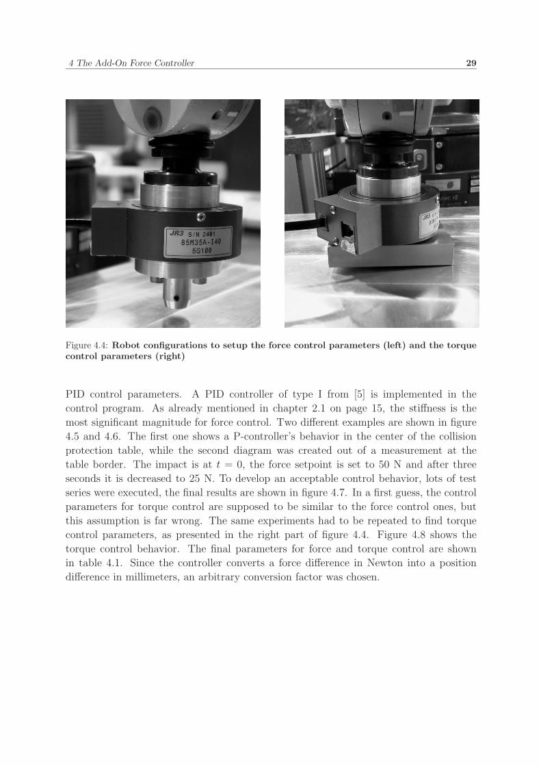
4 The Add-On Force Controller 29
Figure 4.4: Robot configurations to setup the force control parameters (left) and the torquecontrol parameters (right)
PID control parameters. A PID controller of type I from [5] is implemented in the
control program. As already mentioned in chapter 2.1 on page 15, the stiffness is the
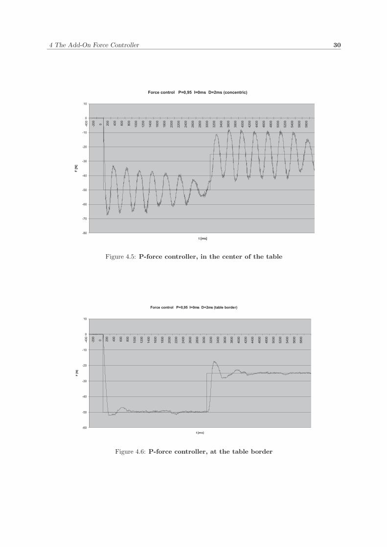
most significant magnitude for force control. Two different examples are shown in figure
4.5 and 4.6. The first one shows a P-controller’s behavior in the center of the collision
protection table, while the second diagram was created out of a measurement at the
table border. The impact is at t = 0, the force setpoint is set to 50 N and after three
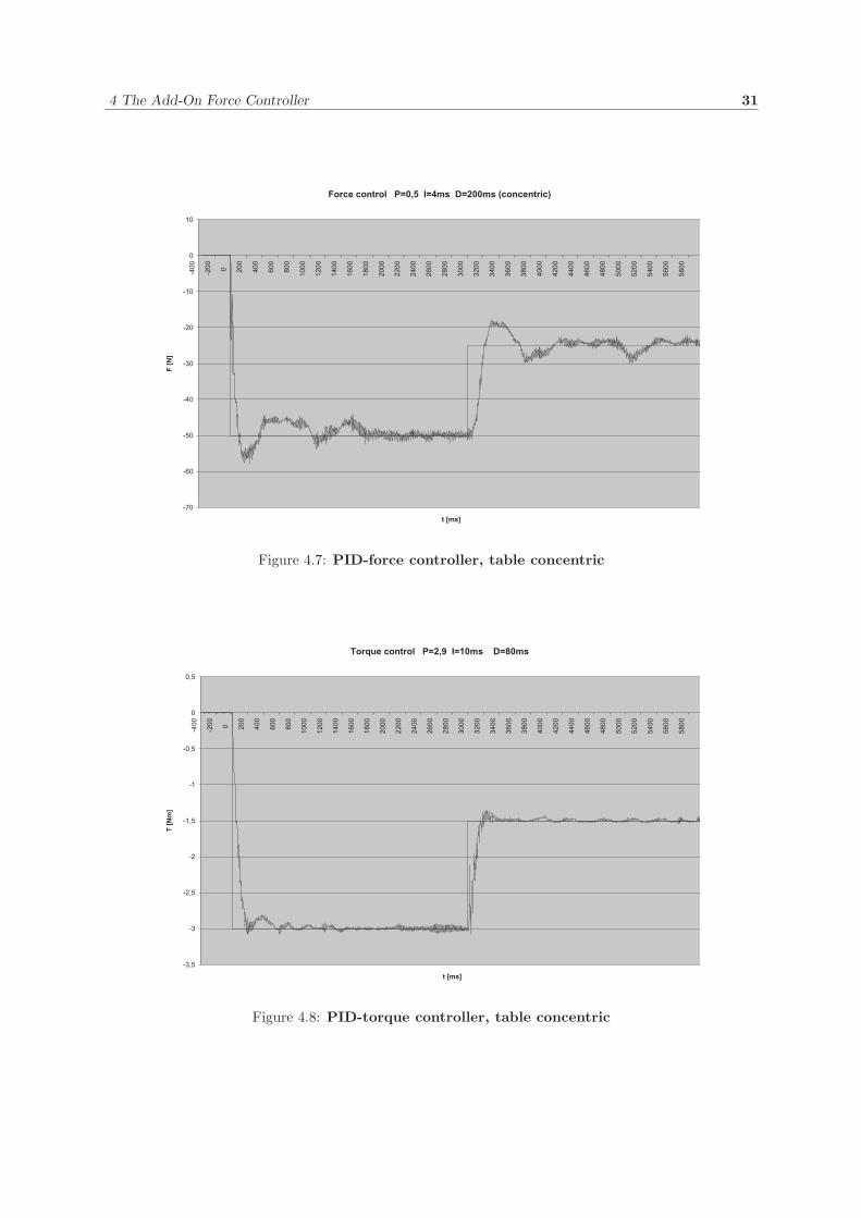
seconds it is decreased to 25 N. To develop an acceptable control behavior, lots of test
series were executed, the final results are shown in figure 4.7. In a first guess, the control
parameters for torque control are supposed to be similar to the force control ones, but
this assumption is far wrong. The same experiments had to be repeated to find torque
control parameters, as presented in the right part of figure 4.4. Figure 4.8 shows the
torque control behavior. The final parameters for force and torque control are shown
in table 4.1. Since the controller converts a force difference in Newton into a position
difference in millimeters, an arbitrary conversion factor was chosen.
4 The Add-On Force Controller 30
Figure 4.5: P-force controller, in the center of the table
Figure 4.6: P-force controller, at the table border
4 The Add-On Force Controller 31
Figure 4.7: PID-force controller, table concentric
Figure 4.8: PID-torque controller, table concentric
5 Force Controlled Placing of a Block 32
5 Force Controlled Placing of a Block
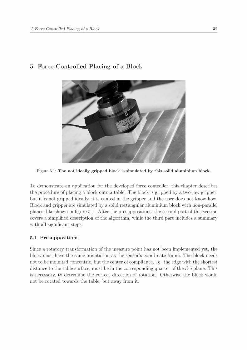
Figure 5.1: The not ideally gripped block is simulated by this solid aluminium block.
To demonstrate an application for the developed force controller, this chapter describes
the procedure of placing a block onto a table. The block is gripped by a two-jaw gripper,
but it is not gripped ideally, it is canted in the gripper and the user does not know how.
Block and gripper are simulated by a solid rectangular aluminium block with non-parallel
planes, like shown in figure 5.1. After the presuppositions, the second part of this section
covers a simplified description of the algorithm, while the third part includes a summary
with all significant steps.
5.1 Presuppositions
Since a rotatory transformation of the measure point has not been implemented yet, the
block must have the same orientation as the sensor’s coordinate frame. The block needs
not to be mounted concentric, but the center of compliance, i.e. the edge with the shortest
distance to the table surface, must be in the corresponding quarter of the �n-�o plane. This
is necessary, to determine the correct direction of rotation. Otherwise the block would
not be rotated towards the table, but away from it.
5 Force Controlled Placing of a Block 33
�F0 =
00
20N000
S =
0 0 0 0 0 00 0 0 0 0 00 0 1 0 0 00 0 0 0 0 00 0 0 0 0 00 0 0 0 0 0
�v0 =
00
4mm/s000
�x0 = current pos.
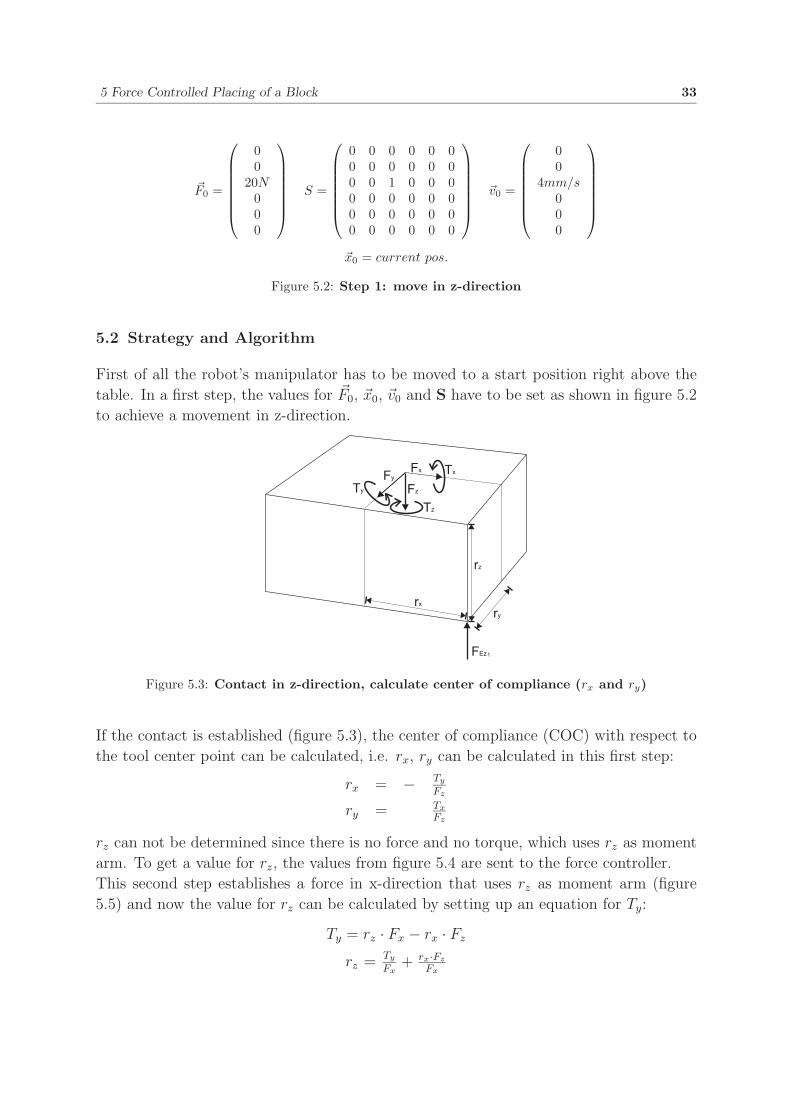
Figure 5.2: Step 1: move in z-direction
5.2 Strategy and Algorithm
First of all the robot’s manipulator has to be moved to a start position right above the
table. In a first step, the values for �F0, �x0, �v0 and S have to be set as shown in figure 5.2
to achieve a movement in z-direction.
Figure 5.3: Contact in z-direction, calculate center of compliance (rx and ry)
If the contact is established (figure 5.3), the center of compliance (COC) with respect to
the tool center point can be calculated, i.e. rx, ry can be calculated in this first step:
rx = − Ty
Fz
ry = Tx
Fz
rz can not be determined since there is no force and no torque, which uses rz as moment
arm. To get a value for rz, the values from figure 5.4 are sent to the force controller.
This second step establishes a force in x-direction that uses rz as moment arm (figure
5.5) and now the value for rz can be calculated by setting up an equation for Ty:
Ty = rz · Fx − rx · Fz
rz = Ty
Fx+ rx·Fz
Fx
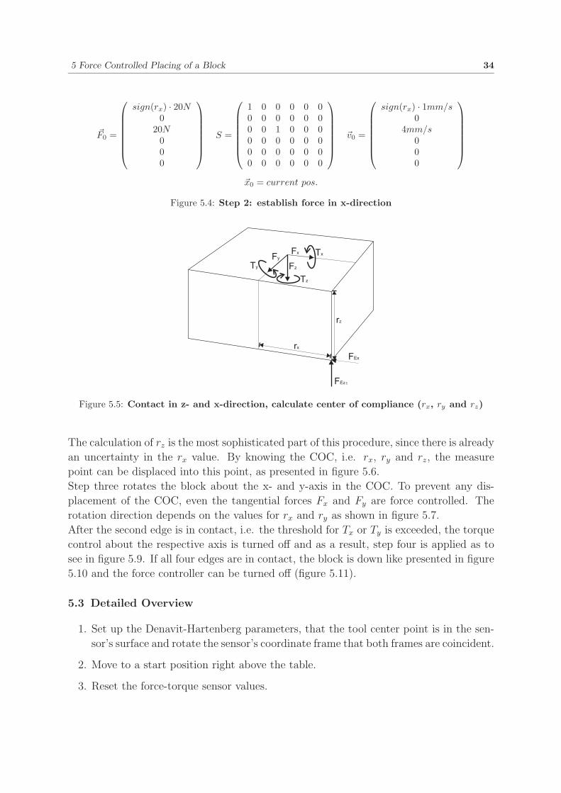
5 Force Controlled Placing of a Block 34
�F0 =
sign(rx) · 20N0
20N000
S =
1 0 0 0 0 00 0 0 0 0 00 0 1 0 0 00 0 0 0 0 00 0 0 0 0 00 0 0 0 0 0
�v0 =
sign(rx) · 1mm/s0
4mm/s000
�x0 = current pos.
Figure 5.4: Step 2: establish force in x-direction
Figure 5.5: Contact in z- and x-direction, calculate center of compliance (rx, ry and rz)
The calculation of rz is the most sophisticated part of this procedure, since there is already
an uncertainty in the rx value. By knowing the COC, i.e. rx, ry and rz, the measure
point can be displaced into this point, as presented in figure 5.6.
Step three rotates the block about the x- and y-axis in the COC. To prevent any dis-
placement of the COC, even the tangential forces Fx and Fy are force controlled. The
rotation direction depends on the values for rx and ry as shown in figure 5.7.
After the second edge is in contact, i.e. the threshold for Tx or Ty is exceeded, the torque
control about the respective axis is turned off and as a result, step four is applied as to
see in figure 5.9. If all four edges are in contact, the block is down like presented in figure
5.10 and the force controller can be turned off (figure 5.11).
5.3 Detailed Overview
1. Set up the Denavit-Hartenberg parameters, that the tool center point is in the sen-
sor’s surface and rotate the sensor’s coordinate frame that both frames are coincident.
2. Move to a start position right above the table.
3. Reset the force-torque sensor values.
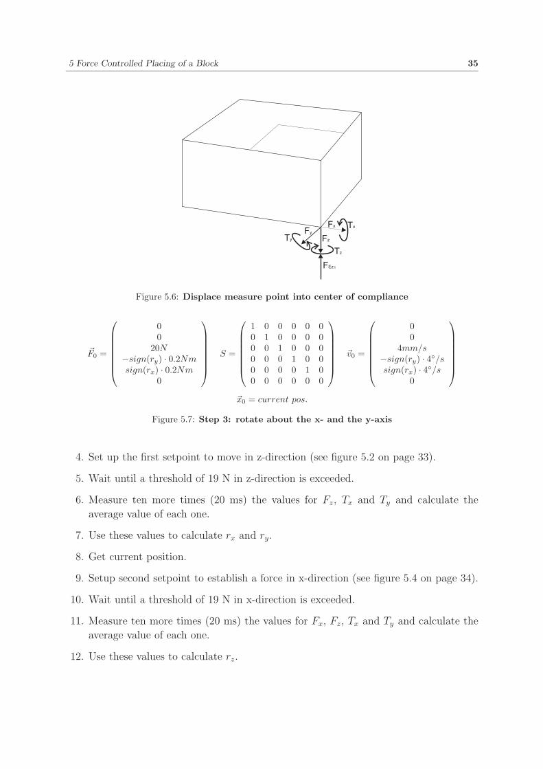
5 Force Controlled Placing of a Block 35
Figure 5.6: Displace measure point into center of compliance
�F0 =
00
20N−sign(ry) · 0.2Nmsign(rx) · 0.2Nm
0
S =
1 0 0 0 0 00 1 0 0 0 00 0 1 0 0 00 0 0 1 0 00 0 0 0 1 00 0 0 0 0 0
�v0 =
00
4mm/s−sign(ry) · 4◦/ssign(rx) · 4◦/s
0
�x0 = current pos.
Figure 5.7: Step 3: rotate about the x- and the y-axis
4. Set up the first setpoint to move in z-direction (see figure 5.2 on page 33).
5. Wait until a threshold of 19 N in z-direction is exceeded.
6. Measure ten more times (20 ms) the values for Fz, Tx and Ty and calculate the
average value of each one.
7. Use these values to calculate rx and ry.
8. Get current position.
9. Setup second setpoint to establish a force in x-direction (see figure 5.4 on page 34).
10. Wait until a threshold of 19 N in x-direction is exceeded.
11. Measure ten more times (20 ms) the values for Fx, Fz, Tx and Ty and calculate the
average value of each one.
12. Use these values to calculate rz.
5 Force Controlled Placing of a Block 36
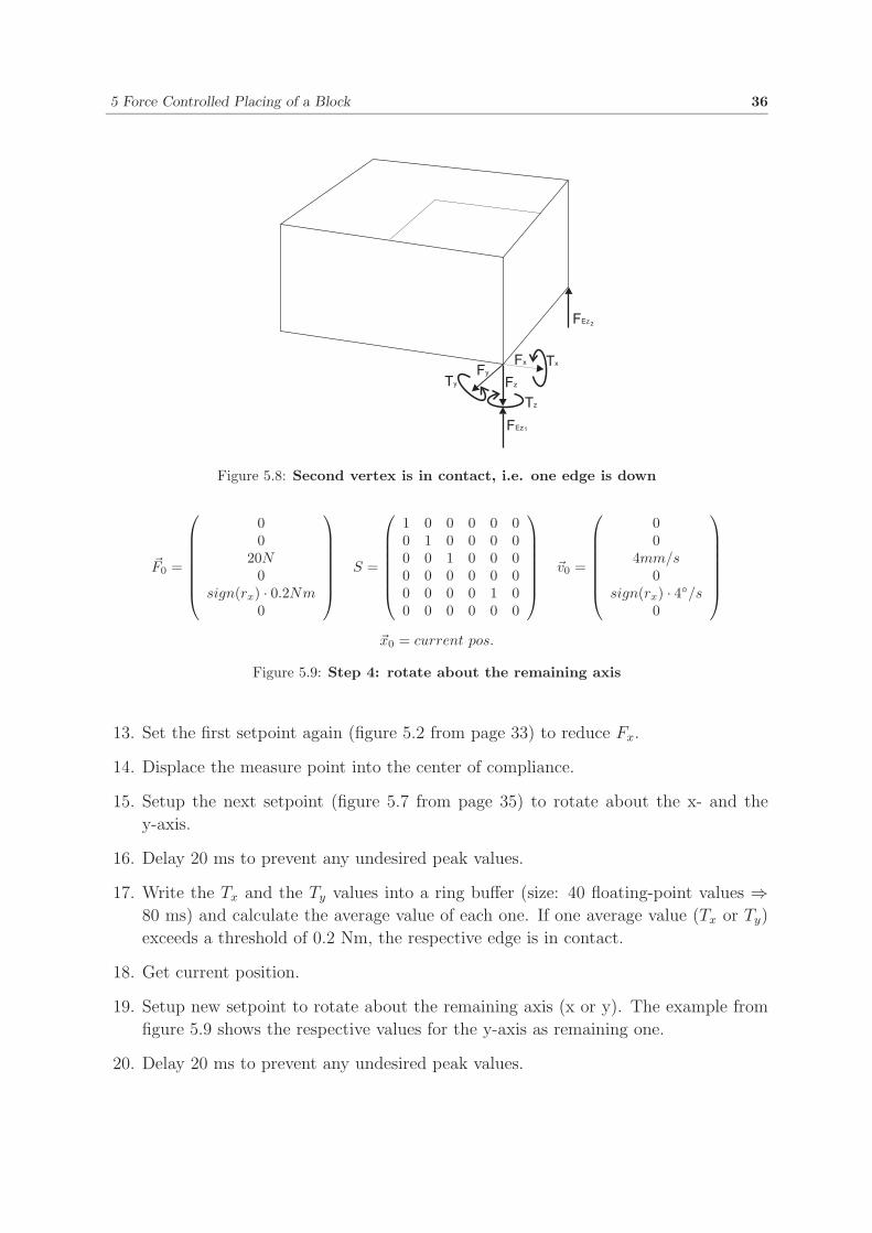
Figure 5.8: Second vertex is in contact, i.e. one edge is down
�F0 =
00
20N0
sign(rx) · 0.2Nm0
S =
1 0 0 0 0 00 1 0 0 0 00 0 1 0 0 00 0 0 0 0 00 0 0 0 1 00 0 0 0 0 0
�v0 =
00
4mm/s0
sign(rx) · 4◦/s0
�x0 = current pos.
Figure 5.9: Step 4: rotate about the remaining axis
13. Set the first setpoint again (figure 5.2 from page 33) to reduce Fx.
14. Displace the measure point into the center of compliance.
15. Setup the next setpoint (figure 5.7 from page 35) to rotate about the x- and the
y-axis.
16. Delay 20 ms to prevent any undesired peak values.
17. Write the Tx and the Ty values into a ring buffer (size: 40 floating-point values ⇒80 ms) and calculate the average value of each one. If one average value (Tx or Ty)
exceeds a threshold of 0.2 Nm, the respective edge is in contact.
18. Get current position.
19. Setup new setpoint to rotate about the remaining axis (x or y). The example from
figure 5.9 shows the respective values for the y-axis as remaining one.
20. Delay 20 ms to prevent any undesired peak values.
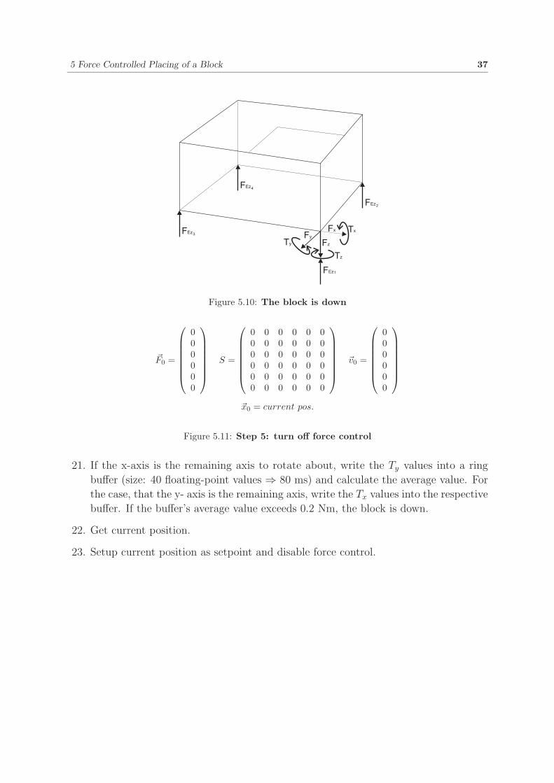
5 Force Controlled Placing of a Block 37
Figure 5.10: The block is down
�F0 =
000000
S =
0 0 0 0 0 00 0 0 0 0 00 0 0 0 0 00 0 0 0 0 00 0 0 0 0 00 0 0 0 0 0
�v0 =
000000
�x0 = current pos.
Figure 5.11: Step 5: turn off force control
21. If the x-axis is the remaining axis to rotate about, write the Ty values into a ring
buffer (size: 40 floating-point values ⇒ 80 ms) and calculate the average value. For
the case, that the y- axis is the remaining axis, write the Tx values into the respective
buffer. If the buffer’s average value exceeds 0.2 Nm, the block is down.
22. Get current position.
23. Setup current position as setpoint and disable force control.
6 Summary 38
6 Summary
Regarding to the nature of interaction between a robot and its environment, robot ap-
plications can be categorized in two classes. The first one covers non-contact tasks, like
simple pick-and-place operations, spray painting, gluing, welding etc. In contrast to these
tasks, many advanced robot applications require the manipulator to get in contact with
its environment and to produce certain forces. These tasks are referred to as essential
contact tasks, which require a force controlled robot. One of the most important facts for
force control is, that a fast robot control architecture is necessary. This enables the force
controller to react quickly. While moving the manipulator towards a solid surface with
a too low sampling rate, the occurring forces are very high and might damage expensive
devices. The object server as basis for communication is fast, flexible and easy to under-
stand, i.e. a very good presupposition for force control. The hardware drivers as well as a
position controller have been implemented already. Several force control concepts would
be possible as solution, but the easiest way to expand the existing system by a force
controller is to develop an add-on force controller, whose control loop surrounds the po-
sition control loop. One of the most significant weak points of this concept is the inverse
kinematic model: if there is no unique solution for the corresponding robot configuration,
this concept does not work. Another very important part of the development of such a
controller is to find the right control parameters. Actually, these parameters depend on
many factors: the robot configuration, the environment stiffness, the force-torque sensor,
the tool surface, the environment surface etc. Particularly the P-factor of the controller
has to be adapted for different stiffnesses, i.e. a high stiffness requires a low P-value and
vice versa. Here, the parameters have been found experimentally. The user application
sends a setpoint to the force controller, which contains the desired force �F0, the desired
position �x0, the compliance selection matrix S and a desired speed �v0 for the case of an
open force control loop.
As an application, the force controlled placing of a not ideally gripped block was chosen.
A canted block in a two-jaw gripper was simulated by a solid rectangular aluminium block
with non-parallel planes and had to be placed onto a collision protection table. Only four
different setpoints are necessary to place the block smoothly on the table (see chapter
5.2 on page 33). This concept is attended by some more calculations, but the block is
placed on basis of the four mentioned steps. With the implemented control concept, many
different force controlled assembly and machining applications can be achieved.
A Contents of the Enclosed CD 39
A Contents of the Enclosed CD
Notice: important folders contain a readme file with further information
LIST OF TABLES 40
List of Tables
1.1 Increments per degree for each joint . . . . . . . . . . . . . . . . . 2
1.2 Space Mouse control modes . . . . . . . . . . . . . . . . . . . . . . . 5
1.3 Short Space Mouse manual . . . . . . . . . . . . . . . . . . . . . . . 6
1.4 Class FTS: variable meanings . . . . . . . . . . . . . . . . . . . . . . . 11
1.5 Class FTS: function description . . . . . . . . . . . . . . . . . . . . . 12
1.6 Force-torque sensor: low-pass filter values . . . . . . . . . . . . . . 12
1.7 JR3 Force-torque sensor: maximum forces and torques . . . . . . 12
4.1 Final PID control values . . . . . . . . . . . . . . . . . . . . . . . . . 28
LIST OF FIGURES 41
List of Figures
1.1 Schematic structure of the object server architecture . . . . . . 1
1.2 The position controller . . . . . . . . . . . . . . . . . . . . . . . . . . 3
1.3 The class SpaceMouse (from spacemouse.h) . . . . . . . . . . . . . . . 4
1.4 The Space Mouse . . . . . . . . . . . . . . . . . . . . . . . . . . . . . 6
1.5 The JR3 force torque sensor . . . . . . . . . . . . . . . . . . . . . . . 8
1.6 The class FTS (from ftsenso.h) . . . . . . . . . . . . . . . . . . . . . . 9
1.7 Orientation of the JR3 force-torque sensor(top view) . . . . . . 10
1.8 Force-torque transformation . . . . . . . . . . . . . . . . . . . . . . . 11
1.9 Part of an example application for the force torque sensor . . . . 13
1.10 r2 robot and control cabinet . . . . . . . . . . . . . . . . . . . . . . . 14
2.1 Implicit hybrid force-position controller . . . . . . . . . . . . . . . 16
2.2 Parallel force-position controller . . . . . . . . . . . . . . . . . . . . 17
2.3 Add-on force-position controller . . . . . . . . . . . . . . . . . . . . 18
4.1 Implemented add-on force-position controller . . . . . . . . . . . . 21
4.2 Structure of force control program . . . . . . . . . . . . . . . . . . . 23
4.3 The force-position control algorithm . . . . . . . . . . . . . . . . . 25
4.4 Robot configurations to setup the force-torque controller . . . . 29
4.5 P-force controller, in the center of the table . . . . . . . . . . . . . 30
4.6 P-force controller, at the table border . . . . . . . . . . . . . . . . 30
4.7 PID-force controller, table concentric . . . . . . . . . . . . . . . . . 31
4.8 PID-torque controller, table concentric . . . . . . . . . . . . . . . . 31
5.1 The not ideally gripped block is simulated by this solid alu-
minium block. . . . . . . . . . . . . . . . . . . . . . . . . . . . . . . . . 32
5.2 Step 1: move in z-direction . . . . . . . . . . . . . . . . . . . . . . . 33
5.3 Contact in z-direction, calculate center of compliance (rx and ry) 33
5.4 Step 2: establish force in x-direction . . . . . . . . . . . . . . . . . 34
5.5 Contact in z- and x-direction, calculate center of compliance (rx,
ry and rz) . . . . . . . . . . . . . . . . . . . . . . . . . . . . . . . . . . . 34
5.6 Displace measure point into center of compliance . . . . . . . . . 35
5.7 Step 3: rotate about the x- and the y-axis . . . . . . . . . . . . . . 35
5.8 Second vertex is in contact, i.e. one edge is down . . . . . . . . . 36
5.9 Step 4: rotate about the remaining axis . . . . . . . . . . . . . . . 36
5.10 The block is down (sketch) . . . . . . . . . . . . . . . . . . . . . . . 37
LIST OF FIGURES 42
5.11 Step 5: turn off force control . . . . . . . . . . . . . . . . . . . . . . 37
BIBLIOGRAPHY 43
Bibliography
[1] Borchard, Michael: Kommunikationsmodell einer PC-basierten Roboters-
teuerung. Institut fur Robotik und Prozessinformatik, TU Braunschweig, 2001
[2] Breymann, Ulrich: C++ Eine Einfuhrung. Carl Hanser Verlag, 1996
[3] Hanna, Jorg: Entwicklung der Betriebssoftware und Regelung einer PC-basierten
Robotersteuerung. Institut fur Robotik und Prozessinformatik, TU Braunschweig,
2001
[4] Kernighan, Brian W. and Ritchie, Dennis M.: Programmieren in C, Carl
Hanser Verlag, 1990
[5] Lutz, Holger and Wendt, Wolfgang: Taschenbuch der Regelungstechnik.
Verlag Harri Deutsch, 1995
[6] McKerrow, Phillip John: Introduction to Robotics. Addison Wesley, 1991
[7] Ratke, Holger Entwicklung der WindowsNT-Benutzeroberflche einer PC-
basierten Robotersteuerung. Institut fur Robotik und Prozessinformatik, TU Braun-
schweig, 2000
[8] Watcom Software Systems Ltd.: C Library Reference, QNX software systems,
1996
[9] Vukobratovic, M. and Surdilovic, D.: Control of Robotic Systems in Contact
tasks: An Overview
[10] 3Dconnexion Inc., http://www.logicad3d.com (November 2001)