econstor www.econstor.eu

Der Open-Access-Publikationsserver der ZBW – Leibniz-Informationszentrum WirtschaftThe Open Access Publication Server of the ZBW – Leibniz Information Centre for Economics

Standard-Nutzungsbedingungen:

Die Dokumente auf EconStor dürfen zu eigenen wissenschaftlichenZwecken und zum Privatgebrauch gespeichert und kopiert werden.

Sie dürfen die Dokumente nicht für öffentliche oder kommerzielleZwecke vervielfältigen, öffentlich ausstellen, öffentlich zugänglichmachen, vertreiben oder anderweitig nutzen.

Sofern die Verfasser die Dokumente unter Open-Content-Lizenzen(insbesondere CC-Lizenzen) zur Verfügung gestellt haben sollten,gelten abweichend von diesen Nutzungsbedingungen die in der dortgenannten Lizenz gewährten Nutzungsrechte.

Terms of use:

Documents in EconStor may be saved and copied for yourpersonal and scholarly purposes.

You are not to copy documents for public or commercialpurposes, to exhibit the documents publicly, to make thempublicly available on the internet, or to distribute or otherwiseuse the documents in public.

If the documents have been made available under an OpenContent Licence (especially Creative Commons Licences), youmay exercise further usage rights as specified in the indicatedlicence.

zbw Leibniz-Informationszentrum WirtschaftLeibniz Information Centre for Economics

Cesa-Bianchi, Ambrogio; Pesaran, M. Hashem; Rebucci, Alessandro

Working Paper

Uncertainty and Economic Activity: A GlobalPerspective

CESifo Working Paper, No. 4736

Provided in Cooperation with:Ifo Institute – Leibniz Institute for Economic Research at the University ofMunich

Suggested Citation: Cesa-Bianchi, Ambrogio; Pesaran, M. Hashem; Rebucci, Alessandro(2014) : Uncertainty and Economic Activity: A Global Perspective, CESifo Working Paper, No.4736

This Version is available at:http://hdl.handle.net/10419/96879

Uncertainty and Economic Activity: A Global Perspective

Ambrogio Cesa-Bianchi M. Hashem Pesaran Alessandro Rebucci

CESIFO WORKING PAPER NO. 4736 CATEGORY 12: EMPIRICAL AND THEORETICAL METHODS

APRIL 2014

An electronic version of the paper may be downloaded • from the SSRN website: www.SSRN.com • from the RePEc website: www.RePEc.org

• from the CESifo website: Twww.CESifo-group.org/wp T

CESifo Working Paper No. 4736

Uncertainty and Economic Activity: A Global Perspective

Abstract

The 2007-2008 global financial crisis and the subsequent anemic recovery have rekindled academic interest in quantifying the impact of uncertainty on macroeconomic dynamics based on the premise that uncertainty causes economic activity to slow down and contract. In this paper, we study the interrelation between financial markets volatility and economic activity assuming that both variables are driven by the same set of unobserved common factors. We further assume that these common factors affect volatility and economic activity with a time lag of at least a quarter. Under these assumptions, we show analytically that volatility is forward looking and that the output equation of a typical VAR estimated in the literature is mis-specified as least squares estimates of this equation are inconsistent. Empirically, we document a statistically significant and economically sizable impact of future output growth on current volatility, and no effect of volatility shocks on business cycles, over and above those driven by the common factors. We interpret this evidence as suggesting that volatility is a symptom rather than a cause of economic instability.

JEL-Code: E440, F440, G150.

Keywords: uncertainty, realized volatility, GVAR, great recession, identification, business cycle, common factors.

Ambrogio Cesa-Bianchi Bank of England

London / United Kingdom ambrogio.cesa-

bianchi@bankofengland.co.uk

M. Hashem Pesaran Department of Economics

University of Southern California USA - 90089-0253 Los Angeles CA

pesaran@dornsife.usc.edu

Alessandro Rebucci Johns Hopkins University

Carey Business School & IDB Baltimore / Maryland / USA

arebucci@jhu.edu

March 27, 2014 We would like to thank Rudiger Bachmann, Alex Chudik, Stephane Dees, Jean Imbs, Roberto Rigobon, Lucio Sarno, Ron Smith, and Vanessa Smith for helpful comments and suggestions. Gang Zhang provided excellent research assistance. The views expressed in this paper are solely those of the authors and should not be taken to represent those of the Bank of England or the Inter-American Development Bank.

1 Introduction

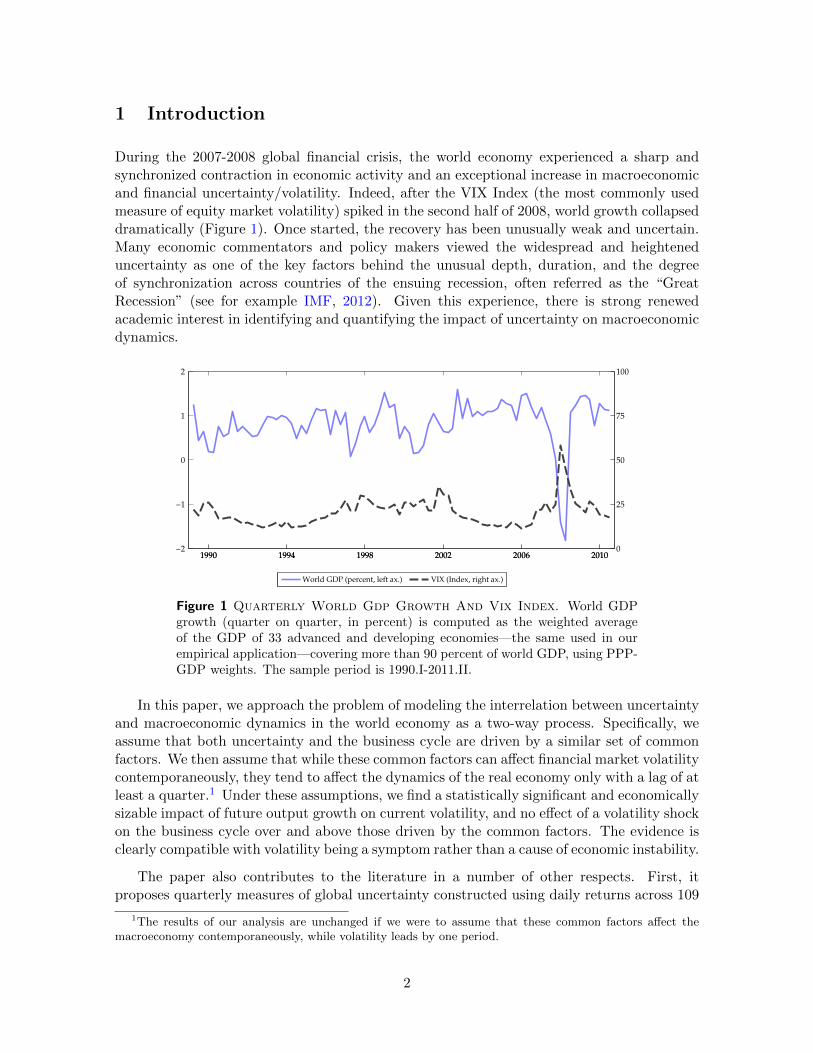
During the 2007-2008 global financial crisis, the world economy experienced a sharp andsynchronized contraction in economic activity and an exceptional increase in macroeconomicand financial uncertainty/volatility. Indeed, after the VIX Index (the most commonly usedmeasure of equity market volatility) spiked in the second half of 2008, world growth collapseddramatically (Figure 1). Once started, the recovery has been unusually weak and uncertain.Many economic commentators and policy makers viewed the widespread and heighteneduncertainty as one of the key factors behind the unusual depth, duration, and the degreeof synchronization across countries of the ensuing recession, often referred as the “GreatRecession” (see for example IMF, 2012). Given this experience, there is strong renewedacademic interest in identifying and quantifying the impact of uncertainty on macroeconomicdynamics.

1990 1994 1998 2002 2006 2010−2

−1

0

1

2

1990 1994 1998 2002 2006 20100

25

50

75

100

World GDP (percent, left ax.) VIX (Index, right ax.)

Figure 1 Quarterly World Gdp Growth And Vix Index. World GDPgrowth (quarter on quarter, in percent) is computed as the weighted averageof the GDP of 33 advanced and developing economies—the same used in ourempirical application—covering more than 90 percent of world GDP, using PPP-GDP weights. The sample period is 1990.I-2011.II.

In this paper, we approach the problem of modeling the interrelation between uncertaintyand macroeconomic dynamics in the world economy as a two-way process. Specifically, weassume that both uncertainty and the business cycle are driven by a similar set of commonfactors. We then assume that while these common factors can affect financial market volatilitycontemporaneously, they tend to affect the dynamics of the real economy only with a lag of atleast a quarter.1 Under these assumptions, we find a statistically significant and economicallysizable impact of future output growth on current volatility, and no effect of a volatility shockon the business cycle over and above those driven by the common factors. The evidence isclearly compatible with volatility being a symptom rather than a cause of economic instability.

The paper also contributes to the literature in a number of other respects. First, itproposes quarterly measures of global uncertainty constructed using daily returns across 109

1The results of our analysis are unchanged if we were to assume that these common factors affect themacroeconomy contemporaneously, while volatility leads by one period.

2

asset prices worldwide. We shall consider four asset classes, namely equity prices, exchangerates, bond prices, and commodity prices. Second, it builds an empirical model of volatilityand the business cycle for 33 countries representing over 90 percent of the world economythat takes the following stylized facts into account: (i) shocks are transmitted in financialmarkets faster than in markets for goods and services; (ii) while volatility is well representedby a stationary process, macroeconomic time series are typically found to follow (or beingwell approximated by) unit root processes; and (iii) neither volatility nor the business cyclecan be reduced to a single common component (i.e., they are driven by both common andidiosyncratic factors). Third and finally, using the global model and a number of differentrealized volatility measures, the paper investigates the interaction between volatility and thebusiness cycle in an interconnected world economy.

To measure economic uncertainty, we build on the contributions of Andersen, Bollerslev,Diebold, and Labys (2001, 2003) and Barndorff-Nielsen and Shephard (2002, 2004), and wecompute realized volatility for a given quarter using daily returns on 92 asset prices (in 33advanced and emerging economies) and 17 commodity indices. Then we study the time seriesproperties of these volatility measures as well as the extent to which they are driven by globalor asset-specific factors.

To study the interconnection between volatility and the business cycle, we use the GlobalVector Autoregressive (GVAR) methodology, originally proposed by Pesaran, Schuermann,and Weiner (2004) and further developed in Dees, di Mauro, Pesaran, and Smith (2007) andDees, Pesaran, Smith, and Smith (2014). The GVAR methodology is a relatively novel ap-proach to global macroeconomic modeling that combines time series, panel data, and factoranalysis techniques to address the curse of dimensionality problem in modelling the intercon-nections in the world economy.2 Augmenting the GVAR framework with a volatility modulealso allows us to treat the volatility measures we consider as endogenous in a parsimoniousyet disaggregated model of the world economy. In this way, we can identify and illustrate thedifferent linkages that might exist between volatility and the idiosyncratic and global com-ponents of economic activity. We refer to this combined model as the GVAR-VOL model.

To identify the effects of a volatility shock, we assume that both volatility and real eco-nomic activity are affected by the same set of unobserved common factors. These factorscould capture general political and economic events that are difficult to measure, but never-theless have important impacts on volatility and economic activity.3 We further assume thatthese common factors affect volatility contemporaneously but have an impact on macroe-conomic dynamics with a delay: an assumption that rests on the observation that shocksare typically transmitted in financial markets faster than in markets for goods and services.Finally, assuming weak cross-sectional dependence of country-specific idiosyncratic shocks,we can identify global volatility shocks that are not driven by the common factors.

Our main findings are as follows: from a theoretical view point we show that volatility isforward looking and that the output equation of a typical VAR estimated in the literature ismis-specified as least squares estimates of this equation are inconsistent. This implies that,if our assumptions are plausible, typical impulse response functions of measures of economic

2For a recent review of the methodology and a number of applications of the GVAR see di Mauro andPesaran (2013).

3Note that while these factors are common across all markets, countries, and variables, they can havedifferential effects on variables within and across different countries.

3

activity to volatility shocks are biased regardless of the structural VAR identification schemeemployed.

Empirically, we provide three main sets of results. First, our (unconditional) descriptiveanalysis shows that volatility is persistent, but is well approximated by a stationary processat business cycle frequency. It behaves countercyclically—consistently with the commonwisdom in the literature—and it can significantly lead the business cycle. We also find thatrealized volatility co-moves significantly within asset classes, but is not as highly correlatedacross asset classes (especially for commodities).

Second, by using a small open economy assumption and the law of large numbers appliedto cross-sectionally weakly correlated processes, our multi-country analysis allows us to con-sistently estimate the effects of future, contemporaneous, and lagged values of the changesin global (aggregate) activity on volatility. Our results show that there is a strong negativestatistical association between future output growth and current volatility.

Third and finally, we find that exogenous changes to volatility have no statistically signif-icant impact on economic activity over and above that of its common component. In otherwords, we find that volatility shocks have little or no direct effect on real GDP once we con-dition on a small set of country-specific and global macro-financial factors in the GVAR-VOLmodel. We do not interpret this evidence as saying that volatility has no effect on economicactivity. Instead, we suggest that most of its effect (often found in the literature) may becoming from the fact that volatility itself is driven by the same common factors that affectthe business cycle. In other words, volatility seems to be more of a symptom rather than acause of economic instability.

The above result differs from the ones in literature that typically find volatility to have astatistically significant negative effect on economic activity. This finding primarily emanatesfrom the identifying assumption made in the literature that rules out the existence of acontemporaneous effect from activity on volatility. As a robustness check, we also estimatedthe GVAR-VOL model excluding future and contemporaneous activity variables from thevolatility module. Under these identifying assumptions, and in line with the literature, we dofind that volatility has some direct impact on real GDP and a strong association with equityprice and exchange rates, which in turn can affect economic activity indirectly via balancesheet and wealth effects. We see our contribution as providing an alternative identifyingassumption which allows volatility and activity to be inter-related through a third set offactors.

The rest of the paper is organized as follows. The next section briefly surveys the the-oretical and empirical literature on the interconnection between volatility and the businesscycle. In Section 3 we sets out a simple factor model for volatility and economic activity.Building on this theoretical framework, Section 4 describes the model that we use for theempirical analysis on the relation between volatility and business cycle. Section 5 gives thedetails of how we construct our proxy measures of economic uncertainty and the data we use,and Section 6 documents their main time-series properties and comovement with economicactivity. Section 7 discusses the specification and estimation of the model. Section 8 reportsand comments on the empirical results of the analysis. Section 9 relates our empirical find-ings to those of the existing literature. Several appendices provide details on the data set weused and some descriptive statistics on individual volatility series, as well as other technical

4

details and supplemental results.

2 Theory and related empirical literature

Standard macroeconomic theory suggests that an increase in uncertainty may cause a tem-porary fall in economic activity. From the viewpoint of the firm, irreversible investmentprovides the traditional mechanism through which changes in uncertainty affect economicactivity (see Bernanke (1983), Dixit and Pindyck (1994) and, more recently, Bloom (2009)).In this framework, exogenous changes in volatility lead to the postponement of irreversibleinvestment and hence a fall in the current level of economic activity.4 But as uncertainty isresolved, investment plans are brought forward and the level of economic activity begins torecover. On the households’ side, Leland (1968) and Kimball (1990) show how, under certainassumptions, increased uncertainty regarding the future stream of labour income and divi-dends induces households to increase their precautionary savings by reducing consumption,and hence demand. But again, as uncertainty recedes, consumption recovers. Financial fric-tions provide an additional mechanism through which uncertainty may affect the economy,generally via an increase in the risk premium (see Christiano, Motto, and Rostagno, 2014,Gilchrist, Sim, and Zakrajsek, 2013, Arellano, Bai, and Kehoe, 2012).5

Based on the above theoretical reasoning, a first strand of the empirical literature revisitedthe relation between uncertainty and the business cycle, mainly focusing on the U.S. econ-omy.6 Bloom (2009) in particular examines the relationship between volatility and outputgrowth using Hodrick-Prescott filtered data in a recursively identified VAR, where the volatil-ity measure is ordered before economic activity. He shows that in a such a set up, increasesin volatility generate a quick drop and rebound in industrial production. Bloom, Floetotto,Jaimovich, Saporta-Eksten, and Terry (2012) show that this result holds using different prox-ies for uncertainty computed from micro data, such as the cross-sectional dispersion of firmstotal factor productivity (TFP) and output growth. Baker and Bloom (2013) attempt toidentify the causal link between uncertainty and economic activity using an instrumentalvariable approach.

The available evidence for other countries is consistent with the one for the United States.Carriere-Swallow and Cespedes (2013) estimate a battery of small open economy VARs for20 advanced and 20 emerging market economies in which the VIX index is assumed to bedetermined exogenously. Their results show that emerging market economies suffer deeper

4Favero, Pesaran, and Sharma (1994) provide an empirical investigation of this effect in the case of thedevelopment of oil fields in the North Sea.

5From a theoretical perspective, the impact of uncertainty on economic activity could also be positive.For example Mirman (1971) shows that, if there is a precautionary motive for savings, then higher volatilityshould lead to higher savings rate, and hence a higher investment rate. Also, Oi (1961), Hartman (1976) andAbel (1983) show that, if labor can be freely adjusted, the marginal revenue product of capital is convex inprice; in this case, uncertainty may increase the level of the capital stock and, therefore, investment.

6The countercyclical behavior of the U.S. stock market volatility is a well known stylized fact. See, forexample, Schwert (1989a) and Schwert (1989b). On the volatility of firm-level stock returns see Campbell,Lettau, Malkiel, and Xu (2001), Bloom, Bond, and Reenen (2007) and Gilchrist, Sim, and Zakrajsek (2013); onthe volatility of plant, firm, industry and aggregate output and productivity see Bloom, Floetotto, Jaimovich,Saporta-Eksten, and Terry (2012) and Bachmann and Bayer (2013); on the behavior of expectations’ disagree-ment see Popescu and Smets (2010) and Bachmann, Elstner, and Sims (2013).

5

and more prolonged impacts from uncertainty shocks, and that a substantial portion of suchlarger impact can be explained by the presence of credit constraints in the case of emergingmarket economies, which is in accordance with the recent work of Christiano, Motto, andRostagno (2014), Gilchrist, Sim, and Zakrajsek (2013) and Arellano, Bai, and Kehoe (2012).Using an unbalanced panel of 60 countries, Baker and Bloom (2013) also provide evidenceof the counter-cyclicality of different proxies for uncertainty, such as stock market volatility,sovereign bond yields volatility, exchange rate volatility and GDP forecast disagreement.Finally, Hirata, Kose, Otrok, and Terrones (2012) use a factor-augmented VAR (FAVAR),with factors computed based on data for 18 advanced economies and a recursive identificationscheme in which the volatility variable is ordered first in the VAR. They find that, in responseto an uncertainty (volatility) shock, GDP falls and then rebounds consistent with Bloom(2009), although the impact is smaller.

The analysis of the interrelation between volatility and economic activity is challengingfor a number of reasons. First, and most importantly, the direction of causality betweenuncertainty and economic activity is difficult to establish empirically and likely runs in bothways. Theoretically, for instance, some papers provide examples of how spikes in uncer-tainty may be the result of adverse economic conditions rather than being a driving forceof economic downturns (see, for example, Van Nieuwerburgh and Veldkamp, 2006, Fosteland Geanakoplos, 2012, Bachmann and Moscarini, 2011, Tian, 2012, Decker, D’Erasmo, andMoscoso Boedo, 2014). While the existing literature typically assumes from the outset of theempirical analysis that uncertainty causes activity to slow and contract, we assume that bothuncertainty and activity are driven by the same set of common factors. This is a possibilitythat is supported by available empirical evidence and that, as we shall see in the next sectionof the paper, gives rise to estimation issues that can be dealt with only in a the context of amulti-country empirical model like the one we use.

Gilchrist, Sim, and Zakrajsek (2013), for instance, estimate a VAR for the United Stateswith both an aggregate uncertainty measure (computed from firm-level equity returns withthe Fama-factor approach) and the 10 years BBB-Treasury credit spread. They find thatan increase in uncertainty as measured by stock market volatility leads to an economicallyand statistically significant drop in detrended GDP (with some mean-reversion but no over-shooting). However, once shocks to uncertainty are orthogonalized with respect to the con-temporaneous information from the corporate bond market (i.e., the stock market volatilityordered after credit spread in their recursive identification) uncertainty shocks do not haveany statistically significant effect on detrended GDP. This evidence suggests that indeed fi-nancial factors (i.e., financial shocks or frictions) could drive both volatility and the businesscycle.

Using data from business surveys, Bachmann, Elstner, and Sims (2013) show that positiveinnovations to business uncertainty (measured as either sectorial business forecasts disagree-ment or ex post forecast errors) have protracted negative effects on the level of economicactivity, without any evidence of the drop–and–rebound dynamics documented in the studiesmentioned above. The authors suggest as possible explanation for this result that “uncer-tainty is driven by some kind of first moment shock that has long-lived effects on production.”This would imply that uncertainty itself is not the ultimate cause of the long-lasting esti-mated negative impact found in the data. Again, this evidence is consistent with the ideathat uncertainty may simply be a by-product of “bad” economic times and may be caused

6

by expectations of long-lasting economic downturns.

A second challenge in the analysis of uncertainty and economic activity lies in the fact thatstandard theory requires a persistent increase in volatility to explain a persistent downturnin activity. In fact in standard theoretical models activity rebounds when uncertainty isresolved. But as we see in Figure 1, and unlike typical macroeconomic variables like realGDP or inflation, volatility is not very persistent. For example, during the recent greatrecession, uncertainty quickly reverted back to normal levels after spiking in 2008, whileworld output growth continued to be depressed several years after the onset of the subprimecrisis in the United States in early 2007. Partly because of this reason, researcher’s attentionshifted to a distinct source of uncertainty that is much more persistent, namely measuresof “macroeconomic policy uncertainty” (see, for instance Baker, Bloom, and Davis, 2013,Kose and Terrones, 2012, Mumtaz and Surico, 2013). We address this issue specifying anempirical model that takes the different degree of persistence of volatility and macro variablesinto explicit account and we do not relay on filtering procedures to isolate the business cyclefrequencies of economic activity.

Finally, note that both volatility and the business cycle have idiosyncratic (to countries,asset classes, and regions) as well as common components. A separate strand of empiricalliterature argues that the international business cycle is better characterized by a combinationof global and regional cycles rather than a single world business cycle (see, for instance Kose,Otrok, and Whiteman, 2003, Hirata, Kose, and Otrok, 2013). Similar findings extend tofinancial cycles (see Kose, Otrok, and Prasad, 2013). We take this into account by consideringthe joint behavior of economic activity in many countries and by allowing for the possibilityof multiple sources of global financial volatility.

3 A simple factor model of volatility and macroeconomic dy-namics

We begin with a simple model and assume that a small set of common factors characterizethe evolution of the world economy. Moreover, given the possible bidirectional relationshipbetween volatility and growth, we allow these factors to drive both asset price volatility andmacroeconomic variables. Finally, we assume that these factors affect financial markets fasterthan they can affect macroeconomic dynamics: while affecting financial market volatilitycontemporaneously, they can affect macroeconomic dynamics only with a lag of at leastone quarter. Note, however, that our basic assumption is the time difference between theway common factors affect volatility and the real economy. For example, the results of ouranalysis remain qualitatively unchanged if we were to assume that common factors affect themacroeconomy contemporaneously, but with volatility leading the factors by one quarter.

Suppose that there are N + 1 countries in the global economy, indexed by i = 0, 1, ..., N ,where country 0 serves as the numeraire. Denote by vt a (m× 1) vector of global volatilitiesand by yit a (kyi × 1) vector of country-specific macroeconomic aggregates that include, forinstance, GDP and inflation. Both macroeconomic variables and volatilities are affected byone or more common latent factors, represented by the (s × 1) vector, nt. We assume thatyit is a unit root process, or I(1), and vt is stationary, or I(0): assumptions that, as we shall

7

see, are supported by the data. We also assume that m and s are fixed and do not increasewith N and/or T .

We shall begin by re-examining the relationship between vt and ∆yit, assuming that thesevariables are related indirectly through a set of common latent factors, nt. In particular, weconsider the following dynamic specification (suppressing the deterministic components suchas intercepts and higher order lags to simplify the exposition):

vt = Φ1vvt−1 + Λnt + ξt, (1)

∆yit = Φ1i∆yi,t−1 + Γint−1 + ζit, for i = 0, 1, ..., N.

According to (1), the common factors nt affect volatility first, as it realizes contemporaneously,before impacting macroeconomic variables. The same process nt also affects macroeconomicvariables in country i with a lag of one quarter. Note here that the process nt represents aglobal factor and it is therefore common across all countries and markets, but it can affect eachcountry in the global economy differently via different country-specific loadings, as definedby the elements of Γi.

The common factors could arise either as a result of the internal dynamics of the globaleconomy or could be the result of political or other external factors such as wars, naturaldisasters or could even reflect rumors and noisy information. In this paper we do not takespecific position regarding the nature of such common factors. But we believe that it is rea-sonable to suppose that financial markets and their volatility are more immediately affectedby such news or events as compared to the real economy where employment and investmentdecisions are subject to inertia and government regulations, which prevents production firmsand households to adapt to news and political events as promptly as it is done by financialfirms.

We make the following statistical assumptions:

A. |λ(Φ1i)| < 1 − ε, for some strictly positive constant ε > 0, where λ(Φ1i)denotes the eigenvalue of Φ1i;

B. the country-specific coefficients, Φ1i and Γi are random draws from commondistributions with finite moments;

C. the average factor loading matrix Γ = (N + 1)−1∑N

i=0 Γi, and Λ are fullcolumn rank matrices such that Γ′Γ and Λ′Λ are non-singular. Specifically,we assume that kyi ≥ s, and m ≥ s, namely that there are at least as manymacro variables and volatility measures as common factors;

D. the idiosyncratic errors, ζit and ξt are serially uncorrelated, with ξt be-ing independently distributed of the factors. Specifically, E(ζitζit′) = 0,E(ξtξt′) = 0, and E(ntξ

′t′) = 0, for all i, t, and t′ 6= t.

E. ζit are cross-sectionally weakly correlated (in the sense defined by Chudik,Pesaran, and Tosetti, 2011) so that ζt = (N+1)−1

∑Ni=0 ζit = Op

[(N + 1)−1/2

].

Since nt is unobserved, a direct relationship between ∆yit and vt can be established if nt iseliminated from the above system of equations. Under assumption C, it is possible to obtain∆yit in terms of vt, and vice versa. However, due to the presence of the idiosyncratic errors

8

ζit and ξt, it is not possible to identify the common factors from the observables, unless—aswe shall see—N is sufficiently large and assumptions A and E hold.

Let’s first solve for the volatility variables. Assume for simplicity that the dynamics ofthe macro equations are homogenous, i.e., Φ1i = Φ1, for all i. Averaging the macro equationsacross i, we have:

∆yt = Φ1∆yt−1 + Γnt−1 + ζt,

where Γ and ζt are defined above, and yt = (N + 1)−1∑N

i=0 yit.7 Under Assumption C,

solving for nt, we have:

nt = (Γ′Γ)−1

Γ′ (

∆yt+1 −Φ1∆yt − ζt+1

),

which if used in (1) yields:

vt = Φ1vvt−1 + Ψ1,v∆yt+1 + Ψ0,v∆yt −Ψ1,vζt+1 + ξt, (2)

whereΨ1,v = Λ(Γ′Γ)

−1Γ′, and Ψ0,v = −Λ(Γ′Γ)

−1Γ′Φ1.

Therefore, under the above set up, volatility is led by macroeconomic dynamics and respondsto expected changes in economic activity. For example, during the recent global crisis, onecould argue that a few factors were responsible for the evolution of the world economy andthose factors affected volatility directly within a given quarter, but were impacting on growthand inflation with a lag of at least one quarter. This means, for instance, that when LehmanBrothers went bankrupt in September 2008, volatility increased within the same quarter whilegrowth and inflation were affected by this shock only in the subsequent quarters.8

Equation (2) also raises an important estimation issue. If the number of countries, N +1,is fixed, there is an endogeneity problem. Specifically, ∆yt+1 and ζt+1 are correlated and,therefore, consistent estimation of the parameters would require the use of instrumentalvariables, which in the present context are difficult to find. This endogeneity problem wouldarise in the case of any volatility-growth regression for an individual country. An examplewould be the typical bivariate VAR model for the United States estimated in the literaturewith a measure of volatility and output growth. Under our assumptions, however, for Nsufficiently large we have that ζt+1 →p 0, as N → ∞. In other words, by using a smallopen economy assumption and the law of large numbers applied to cross-sectionally weaklycorrelated processes, we can address the endogeneity problem of equation (2). Hence, theparameters of (2) can be consistently estimated by least squares regressions of vt on vt−1,∆yt+1, and ∆yt. This clearly highlights the value added of taking a multi-country approachto the analysis of the interrelation between volatility and the business cycle.

Note that using a large number of countries permits consistent estimation of (2) even if themacro dynamics are heterogeneous across countries (namely Φi differ across i). In this case,the derivation of the expression for nt is more complicated and now involves lags of ∆yt. But

7One could also use weighted cross sectional averages so long as the weights are granular, in the sense thatthey are all of order (N + 1)−1.

8As we noted above, an equivalent assumption is that volatility started to rise in the run up to the Lehman’scollapse while growth and inflation were affected during the same quarter in which Lehman collapsed. Whatmatters is to assume that these factors affect financial markets faster than they can affect macroeconomicdynamics.

9

Chudik and Pesaran (2013) show that, even with dynamic heterogeneity, under assumptionA and E, nt can be approximated by an infinite distributed lag function of ∆yt+1, ∆yt,and their lagged values. The coefficients of such distributed lag function decay exponentiallyand can therefore be suitably truncated for estimation. In this heterogeneous setting, thevolatility regression equation (2) can be written as:

vt = Φ1vvt−1 +

pT∑j=0

Ψ1−j,v∆yt+1−j + ξt +Op

[(N + 1)−1/2

], (3)

where pT = O(T 1/3). In practice, Chudik and Pesaran (2013) show that one can set pT =T 1/3.

We now solve for the macro variables. For each country i we have:

∆yit = Φ1i∆yi,t−1 + Ξi1vt−1 −Ξi2vt−2 + uit, (4)

where:Ξi1 = Γi(Λ

′Λ)−1Λ′, Ξi2 = Γi(Λ′Λ)−1Λ′Φ1v,

and:uit = ζit −Ξi1ξt−1. (5)

The expression (4) for ∆yit has the familiar appearance of the reduced-form equation of abivariate VAR for ∆yit and vt, as it is typically estimated in the literature. However, due tothe dependence of vt−1 on ξt−1, we have that:

E(uitv′t−1) = −Γi(Λ

′Λ)−1Λ′E(ξt−1ξ

′t−1)6= 0,

and, therefore, the parameters of (4) can not be consistently estimated by ordinary leastsquares. This implies that, under the assumption that the factor model (1) is true, anybivariate VAR containing an equation like (4) would produce an inconsistent impulse responseof ∆yit for shocks to vt, regardless of the identification assumption made. The analysistherefore shows that, if the factor model (1) holds, we cannot estimate the impact of volatilityand growth in a model in which vt−1 enters directly in the equation for ∆yit, even if we wereto take a global perspective, focusing only on global volatility and global activity. Note,moreover, that this result does not depend on the timing assumption that we made at thebeginning of this section: the mis-specification of (4) also follows when we assume that thecommon factors affect contemporaneously both volatility and economic activity.

4 The GVAR-VOL model

Modelling global volatility and world growth is problematic for two more reasons other thanthe estimation issues discussed in the previous section. First, the stochastic process of mostmacroeconomic times series, such as real output or the level of nominal variables, has a unitroot or has roots that are very close to unity (namely they are best approximated as I(1)processes). In contrast, as we will see later, although persistent, volatility measures are clearlystationary at quarterly frequency and best represented as I(0) variables. Using the HP filter,as often done in some empirical analysis in the literature, may change the business cycle

10

component of economic activity, or may affect its permanent component when the shocksare large and persistent. Moreover, the use of the HP filter may not be appropriate in caseswhere the model contains a mixture of I(0)/I(1) variables (see Harvey and Jaeger, 1993, forexample).

Second, while the bivariate representation (3) and (4) is appealing for its simplicity,in practice there are many sources of volatility and many countries in the world economy.Neither volatility nor the international business cycle can be satisfactorily modelled by asingle factor.9 For this reason a more general framework where yit (where i = 0, 1, ..., N) andvt are modelled jointly is better suited for this type of analysis. We also need to deal withthe high dimensional nature of the problem since—as suggested in the previous section—Nmust be sufficiently large for the effects of future changes in global output on volatility to becorrectly estimated.

In what follows we avoid the curse of dimensionality by adopting the global vector autore-gressive (GVAR) methodology, where a joint model for yit (where i = 0, 1, ..., N) is developedby estimating separate country-specific models conditional on the global and country specificfactors. As shown in Dees, di Mauro, Pesaran, and Smith (2007), Dees, Pesaran, Smith, andSmith (2014), in the GVAR model the unobserved factors are proxied by country-specific for-eign variables, and to the extent that such common factors are also the drivers of the volatilityvariables, vt, then conditional country-specific models can be estimated consistently withoutthe need to include the volatility variables, vt. The part of vt that can not be explained bythe common factors are then absorbed in the residuals of the country-specific models. Byconstruction, these innovations will be weakly cross-sectionally correlated and do not poseany problem for the consistent estimation of the GVAR model. This aspect of the GVARis particularly convenient since it avoids the estimation pitfalls—discussed in the previoussection—that arise if vt or its lagged values are included in the individual models for yit, fori = 0, 1, ..., N .

Having developed the GVAR model for yit for i = 0, 1, ..., N , the GVAR can then be aug-mented with a set of volatility equations of the type defined by (3). We label this augmentedmodel the GVAR-VOL model. More specifically, to build the GVAR-VOL model we proceedas follows. First, we estimate a stationary autoregressive distributed lag (ARDL) model forvolatility in which we include the future, contemporaneous, and lagged values of the changesin a set of macroeconomic variables for which the assumptions made in the previous sectionare valid. These variables are I(0) by construction and hence conform with the I(0) nature ofthe volatility variables. So this system is balanced. We label this ARDL model the “volatilitymodule.” Next, we specify and estimate a standard GVAR model in yit for i = 0, 1, ..., N ,without vt. Finally, the standard GVAR and the volatility module are combined and solvedsimultaneously for simulation purposes. We now describe in more detail each of the two com-ponents of the GVAR-VOL model and how they are combined, but first we have to establishsome notation.

9See for instance Kose, Otrok, and Whiteman (2003) on the international business cycle and Kose, Otrok,and Prasad (2013) on the international financial cycle.

11

4.1 Notations

Consider a vector vt of (m× 1) global volatility measures and assume that they are I(0), anassumption that, as we shall see, is supported by the data.

Next, define a (ki× 1) vector xit = (y′it,χ′it)′ of country-specific domestic macroeconomic

and financial variables. The (kyi × 1) vector yit includes the macroeconomic variables forwhich the assumptions made above are likely to hold (such as GDP and inflation), while the(kχi × 1) vector χit includes typical financial variables for which our assumptions may nothold. Financial variables (such as equity prices, exchange rates, and interest rates) are likelyto be affected by the set of common factors (nt) with the same speed with which they affectvolatility.

Now define a (K×1) vector xt of all country-specific domestic macroeconomic and finan-cial variables as:

xt = (x′0t,x′1t, ...,x

′Nt)′, (6)

with K = ΣN0 ki. Note here that not all countries need to have the same set of variables, and

we can also re-write xit as follows:xit = Sixt, (7)

where Si is an appropriate (ki × K) selection matrix. Then define a (k × 1) vector x∗it ofcountry-specific foreign macroeconomic and financial variables, with k = maxi(ki):

x∗it = Wixt. (8)

where Wi is an appropriate (k × K) weighting matrix of predetermined weights, typicallyconstructed using trade or financial weights specific to country i.10 Finally, also define a(ky × 1) vector y∗t of global macroeconomic variables as:

y∗t = Pxt, (9)

where P is a (ky ×K) weighting and selection matrix, typically made up of zeros and PPP-GDP weights, so as to select only the macroeconomic variables yit and not the financialvariables χit.

11

We assume that xit, x∗it, and y∗t all follow I(1) processes.

4.2 Volatility module

Consistently with (3), we estimate a separate ARDL model for the level of the volatilitymeasures (vt) augmented with the future, contemporaneous, and the lagged values of thechanges in the global macroeconomic variables (∆y∗t ). As noted above, we include only they∗t (and not the χ∗t ) since the assumptions under which we derived the volatility module (3)are likely to hold only for slow moving variables such as GDP and inflation. The volatilitymodule is therefore specified as:

vt = Φvvt−1 + Ψ1,v∆y∗t+1 + Ψ0,v∆y∗t + Ψ−1,v∆y∗t−1 + ξt, (10)

10These weights can be fixed or time-varying. But to keep the notations simple here we assume they aretime-invariant in the construction of x∗it.

11Like in the case of the Wi matrix, the P matrix could also be time-varying.

12

where Φv is a (m ×m) matrix and Ψ1,v,Ψ0,vΨ−1,v are (m × ky) matrices of constant coef-ficients.12 By using the definition of y∗t in (9), and noting that P is a (ky × K) matrix ofknown and time invariant weights, the model in (10) can now be re-written as:

vt = Φvvt−1 + Ψ1,vP∆xt+1 + Ψ0,vP∆xt + Ψ−1,vP∆xt−1 + ξt. (11)

Three remarks are in order here. First, note that the volatility module in (10) is fullyconsistent with the factor model (1). In fact, in the volatility module, we condition only onthose global macroeconomic variables for which our assumptions are likely to hold (i.e., weexclude asset prices and interest rates). Second, the residuals ξt are volatility innovationsthat are orthogonal to future, current and past changes in global macroeconomic variablesby construction, and can be interpreted as exogenous volatility changes with respect to thosevariables.13 Third and finally, under the assumptions A–E above, for N sufficiently large,the parameters of (11) can be consistently estimated by OLS despite the presence of ∆y∗t+1

in the volatility equation, (10).

4.3 The GVAR methodology

There are two stages in specifying and building a standard GVAR model.14 In the first stage,country-specific vector-autoregression models that relate the domestic variables, xit, to theirown lagged values and to the country-specific foreign variables, x∗it, are specified. Theseaugmented vector autoregressive models are labelled VARX∗ models. Consistent estimationof the VARX∗ models is achieved by treating the x∗it variables as weakly exogenous, an as-sumption which is expected to hold on a priori grounds assuming countries can be viewedas small open economies, and tend to hold when subjected to econometric testing as in ourapplication.15 In the second stage, individual country models are combined using link matri-ces that relate foreign variables to country-specific variables. The link matrices are definedin terms of trade weights, or other suitable international transaction flows data. This yieldsa high-dimensional VAR without any exogenous variables, which can be used for forecastingand impulse response analysis, controlling for a large set of global and country-specific fac-tors. Note that, with the GVAR modelling approach, we do not filter macroeconomic seriesto obtain their cyclical component, thus avoiding the perils of contaminating the data withspurious components resulting from filtering procedures.

Formally, for each country i, consider the following country-specific VARX∗(1,1) model(with no constants and no time trends for simplicity):

xit = Φ1ixi,t−1 + Ψ0ix∗it + Ψ1ix

∗i,t−1 + εit, for i = 0, 1, ..., N, (12)

12Note that additional lags of vt and ∆y∗t can be included in (10) so as to ensure that the volatilityinnovations become approximately serially uncorrelated.

13This is a notion of a volatility shock close to the one by Bernanke (1983), Dixit and Pindyck (1994), andBloom (2009) papers (i.e., volatility shock which is not associated with first moment shocks).

14See Pesaran, Schuermann, and Weiner (2004), Dees, di Mauro, Pesaran, and Smith (2007), and di Mauroand Pesaran (2013) for more details on the theory and application of the GVAR methodology.

15Weak exogeneity of the x∗it variables for the estimation of the reduced form parameters of the VARX∗

models does not imply any statement on the economic causal relation between x∗it and xit. It simply statesthat the parameters of the VARX∗ model can be estimated consistently conditional on x∗it without needing tospecify or estimate the marginal models for x∗it. See Engle, Hendry, and Richard (1983) for a formal definition.

13

where Φ1i is (ki × ki), Ψ0i and Ψ1i are (ki × k) matrices. The (ki × 1) vector of error terms,εit, are assumed serially uncorrelated as well as cross-sectionally weakly correlated. Usingthe identities in (7) and (8) we have:

Sixt = Φ1iSixt−1 + Ψ0iWixt + Ψ1iWixt−1 + εit, (13)

which yields:Gixt = Hixt−1 + εit, (14)

with:Gi = (Si −Ψ0iWi) , Hi = (Φ1iSi + Ψ1iWi) ,

where Gi and Hi are (ki ×K) matrices, where as before K = ΣNi=0ki.

Stacking all country-specific models, we can now write the above system more compactlyas:

Gxt = Hxt−1 + εt, (15)

with:

G = (G′0,G′1, ...,G

′N )′, H = (H′0,H

′1, ...,H

′N )′, εt = (ε′0t, ε

′1t, ..., ε

′Nt)′,

where G and H are (K ×K) matrices. Finally, assuming that G is non-singular we have:

xt = Fxt−1 + ut, (16)

where F = G−1H and the residuals of the reduced-form GVAR are given by:

ut = G−1εt, (17)

where ut = (u′0t,u′1t, ...,u

′Nt)′. Note that uit refers to the reduced form innovations to the

variables xit, which can be further partitioned as xit = (y′it,χ′it)′, where as before yit refers

to the macroeconomic variables of country i, and χit, the financial variables of country i.This partitioning is important for our identification scheme, since in the underlying factormodel (1) we only maintain that latent factors affect the macro variables (yit) with a delayand not the financial variables (χit). Specifically, for each country i, we select the elementsof ut associated with the equations of the macroeconomic variables yit in the (kyi × 1) vectoruyit; and the elements of ut associated with the equations of the financial variables (χit) inthe (kχi × 1) vector uχit, such that

uyit = Syiut, and uχit = Sχi ut, (18)

where Syi and Sχi are appropriate (kyi ×k) and (kχi ×k) selection matrices, respectively. Finallywe define

uyt = (u′y0t,u′y1t, ...,u

′yNt)′, and uχt =

(u′χ0t,u

′χ1t, ...,u

′χNt

)′. (19)

Two remarks are in order here. First, we note that, the GVAR module in (16) is alsoconsistent with the factor model (1).16 This is because, as Chudik and Pesaran (2011, 2013)show, the GVAR model can be derived as an approximation to an infinite dimensional VAR(in which all global macro and financial factors are included) that converges to a global

16Note that while (16) is specified in levels, the factor model (1) is specified in first differences.

14

unobserved common factor model in which x∗it (and hence y∗it) are proxies for the latentglobal factors. Importantly, however, as long as the x∗it variables are weakly exogenous, it ispossible to estimate the VARX∗ models by OLS because we have not included the volatilityvariables, vt, directly in the GVAR, unlike the bivariate or panel VARs typically used in theliterature in which volatility and activity variables are included jointly.

Second, the vector of all country-specific innovations εt defined by equation (15) are cross-sectionally weakly correlated (see Pesaran, Schuermann, and Weiner, 2004, Dees, di Mauro,Pesaran, and Smith, 2007, Dees, Pesaran, Smith, and Smith, 2014). Therefore, no commonfactor (such as a global volatility shock) could drive them. Differently, the vector of reduced-form residuals ut = G−1εt defined by equation (17) could share a common component. This isbecause the G matrix includes all contemporaneous interdependencies in the global economyin the form of a mix between estimated parameters and pre-determined weights in the linkmatrices, Wi. As a result, a global volatility shock could affect ut: a possibility that we nowdiscuss in more detail and that we will explore empirically in our application in the last partof the paper.

4.4 Combining the volatility module and the GVAR

The combined GVAR-VOL model is derived in Appendix by stacking the GVAR module(16) and the volatility module (11) in matrix format, yielding a VAR in vt and xt+1. Sincevolatility does not enter directly into the activity equations of the GVAR model, the onlyway a global volatility innovation ξt can have an impact on activity is via its correlationwith the reduced-form residuals of the GVAR defined in (17). In other words, under ouridentification assumptions, for the volatility innovations, ξt, to affect economic activity, overand above that of the unobserved common factors that drive both volatility and the businesscycle, they must significant statistical correlations with the elements of ut.

The factor model (1) provides guidance as to how ξt and ut can be related under ouridentifying assumptions. Recall that the factor model (1) assumes that the latent factors, nt,can affect financial market volatility contemporaneously, but they tend to affect the dynamicsof the real economy (yit) only with a lag of at least a quarter. This assumption has twoimportant implications. First, as we noted already, the timing assumption is less likelyto hold for financial variables (such as equity prices or interest rates). Therefore, withinour theoretical framework only the relationship (if any) between the GVAR reduced forminnovations associated with the macroeconomic variables, namely uyt defined by (19), and ξtcan be strictly interpreted in terms of causation, while the relation between uχt and ξt hasto be viewed as simple statistical association. Second, equation (5) shows that the volatilityinnovations ξt affect the ut residuals only with a lag. With these considerations in mind,in the last part of the paper we will explore empirically the relation between volatility andeconomic activity by regressing the elements of both uyt and uχt on ξt−1.

15

5 Realized quarterly measures of volatility

This section describes how we construct the variables that we use to measure economicuncertainty at quarterly frequency and the data set we have assembled to compute them.

5.1 Background

We measure economic uncertainty with the “volatility” of asset prices. Asset price volatilityhas been used extensively in the theoretical and empirical literature to measure uncertainty,and implicitly assumes that uncertainty can be characterized in terms of probability distribu-tions. It therefore abstracts from the Knightian notion of uncertainty that claims that sometypes of uncertainty can not be as such characterized.

Even if we confine our attention to “volatility,” this is not directly observable and likemany other economic concepts, such as expectations, demand and supply, it is usually treatedas a latent variable and measured indirectly using a number of different proxies. Initially,volatility was measured by standard deviations of output or asset price changes computedover time, typically using a rolling window. But then it was realized that such a historicalmeasure tends to underestimate sudden changes in volatility and is only suitable when theunderlying volatility is relatively stable.

To allow for time variations in volatility, Engle (1982) developed the autoregressive con-ditional heteroskedastic (ARCH) model that relates the (unobserved) volatility to squaresof past innovations in price changes. Such a model-based approach only partly overcomesthe deficiency of the historical measure and continues to respond very slowly when volatilityundergoes rapid changes, as it has been the case during the recent financial crisis (see, forexample, Hansen, Huang, and Shek, 2012). The use of ARCH or its various generalizations(GARCHs) in macro-econometric modelling is further complicated by temporal aggregationissues of daily GARCH models for use with quarterly data.

In the finance literature, the focus of the volatility measurement has now shifted tomarket-based implied volatility obtained from option prices, and realized measures based onthe summation of intra-period higher-frequency squared returns (see, for example, Andersen,Bollerslev, Diebold, and Labys (2001, 2003), Barndorff-Nielsen and Shephard (2002, 2004)).The use of implied volatility from option prices in macro-econometric models has thus farbeen limited both by data availability and the fact that we still need to aggregate dailyvolatilities to a quarterly frequency. This explains the popularity of the VIX Index, which isan average of the daily option price implied volatility of the S&P 500 index (see Figure 1).

In contrast, the idea of realized volatility can be easily adapted for use in macro-econometricmodels by summing squares of daily returns within a given quarter to construct a quarterlymeasure of market volatility. The approach can be extended to include intra-daily returnobservations when available, but this could contaminate the quarterly realized volatility mea-sures with measurement errors of intra-daily returns due to market micro-structure and jumpsin intra-daily returns. In addition intra-daily returns are not available for all markets thatwe want to consider and, when available, tend to cover a relatively short time period ascompared to our data period that begins in 1979.

16

Note that if we consider a panel of asset prices, a different measure of volatility canbe computed as the cross-sectional dispersion of asset prices. As we show in Appendix B,however, given a panel data of asset prices, realized volatility and cross-sectional dispersionare closely related. Indeed, in our application, we obtain similar results when we use thecross-sectional dispersion measures (the results are not reported for sake of brevity).

Realized volatility and cross-sectional dispersion encompass most measures of uncertaintyproposed in the macroeconomic literature. For example Schwert (1989b), Ramey and Ramey(1995), Bloom (2009), Fernandez-Villaverde, Guerron-Quintana, Rubio-Ramirez, and Uribe(2011) use aggregate time series volatility (summary measures of dispersion over time ofoutput growth, stock market returns, or interest rates); Leahy and Whited (1996), Camp-bell, Lettau, Malkiel, and Xu (2001), Bloom, Bond, and Reenen (2007) and Gilchrist, Sim,and Zakrajsek (2013) use dispersion measures of firm-level stock market returns; Bloom,Floetotto, Jaimovich, Saporta-Eksten, and Terry (2012) use cross-sectional dispersion ofplant/firm/industry profits, stocks, or total factor productivity.17

In the rest of this section, therefore, we provide precise definitions of the realized volatilitymeasures that we use and briefly describe the data set we assembled to compute them.

5.2 Three types of volatility measures

We construct three types of volatility measures: at the level of individual markets (eithercountry equity markets, foreign exchange markets, country bond markets, or individual com-modity markets), at the level of an asset class (i.e., aggregating across individual marketswithin a given asset class), and at the global level (i.e., aggregating across all asset mar-kets).18 For exposition purposes, we shall label realized volatility at the level of individualmarkets, at the level of a whole asset class, and at the global level as Market-Specific Volatility,Asset-Specific Volatility, and Global Volatility, respectively.

5.2.1 Market-specific realized volatility

To construct quarterly measures of realized volatility at the level of individual assets, webegin with the daily price of asset of type κ, in country i, measured on close of day τ inquarter t and we denote it by Pκit(τ). We label the quarterly realized volatility for quarter tat daily rate (RVκit) as “market-specific realized volatility,” or market volatility for brevity.

17The literature has also used uncertainty measures based on expectation dispersion: while summarizing therange of disagreement among individual forecasters at a point in time, they do not give information about theuncertainty surrounding the individual’s forecast. See, for instance, Zarnowitz and Lambros (1987), Popescuand Smets (2010), and Bachmann, Elstner, and Sims (2013).

18One could also consider all asset prices for a given country to construct a country specific measure ofvolatility. In our application, however, we consider only a small number of asset classes (equities, bonds,exchange rates and commodity prices), and large number of countries for each asset class as well as allcommodities for which data are available. This approach is therefore less attractive in our global study withmany countries and would be better suited for a country specific study with many different asset classes.

17

We compute market volatility as:

RVκit =

√√√√D−1t

Dt∑τ=1

(rκit(τ)− rκit)2 (20)

where rκit(τ) = ∆ lnPκit(τ) and rκit = D−1t∑Dt

τ=1 rκit(τ) is the average daily price changesover the quarter t, and Dt is the number of trading days in quarter t. For most timeperiods, Dt = 3 × 22 = 66, which is larger than the number of data points typically usedin the construction of daily realized market volatility in finance.19 The same market-specificvolatility measures can also be computed for real asset prices, with Pκit(τ) in the aboveexpression replaced by Pκit(τ)/Pit, where Pit is the general price level in country i for quartert, but they yield very similar results and in our application they are not reported.20

5.2.2 Asset-specific realized volatility

Market-specific realized volatility—as defined in (20)—can be aggregated across countries fora given asset class such as equity, long term bond, or exchange rate, or across all commoditiesto construct asset-specific realized volatility measures. This aggregation can be carried outby taking averages using equal weights or PPP-GDP weights or other weighting schemes. Letwit be the weight attached to market (country) i in quarter t, then the realized volatility forasset type κ, in quarter t, denoted by RVκt, is given by:

RVκt =

Nt∑i=1

witRVκit, (21)

where Nt is the number of markets (countries) in quarter t with price data on asset typeκ. In this way, we construct measures of realized volatility by different asset classes whichwe label “asset-specific realized volatility,” or asset volatility for brevity. Also, a log-linearaggregate defined by:

RVLκt =

Nt∑i=1

wit ln(RVκit),

could be used.

5.2.3 Global volatility

Finally, a “global realized volatility” measure can be computed by aggregating across differentasset classes, namely:

RVt =1

M

M∑κ=1

Nt∑i=1

witRVκit, (22)

19In the case of intra-day observations prices are usually sampled at 10-minutes interval which yields around48 intra-daily returns in an 8 hour-long trading day.

20We measure Pit by the consumer price index (CPIit) when dealing with equity and bond prices andexchange rates, and use the U.S. producer price index (PPIUS,t) when measuring realized volatility of realcommodity prices. The realized volatility measures of real asset prices are almost identical to the ones com-puted in equation (20) and are available from the authors on request.

18

where M is the number of assets that we consider. Alternatively, using a log-specification,we could have:

RVLt =1

M

M∑κ=1

Nt∑i=1

wit ln(RVκit).

5.3 Data

To construct quarterly measures of market-specific realized volatilities, we first collect dailyprices of stock market equity indices, exchange rates, long-term government bonds (wheneveravailable) for 33 advanced and emerging economies, and daily prices of most internationallytraded commodities. The data set spans 109 asset prices and, for each asset price, up to 8479daily observations from 1979 to 2011 (depending on data availability).

After computing the market-specific realized volatility measures as in (20), we re-scalethem so as to express them at quarterly rates. We do that by multiplying RVκit by

√Dt:

in this way we obtain realized volatility measures that are consistent with the remainingmacroeconomic time series that we shall use in our empirical analysis (which are at quarterlyfrequency, too). Therefore all results, charts, and tables presented hereinafter shall refer tothe realized volatility measures expressed at quarterly rates.

The sources of the data and their sampling information are reported in Appendix C, whilea plot of all series—computed as in equation (20)—is reported in Appendix D. Figure 2 plotsthe quarterly realized volatility of equity prices in the United States and compares it withthe quarterly average of the VIX index (already plotted in Figure 1), often considered as abenchmark measure of uncertainty. As Figure 2 shows, the realized volatility of U.S. equityprices co-moves very closely with the VIX Index, with a correlation coefficient of 0.84 and0.86 in levels and first differences, respectively.

1990 1995 2000 2005 20100.00

0.10

0.20

0.30

0.40

1990 1995 2000 2005 20100

25

50

75

100

RV US Equity (left ax.) VIX Index (right ax.)

Figure 2 Quarterly U.S. Equity Realized Volatility And The VixIndex. The VIX Index is the quarterly average of the daily Chicago BoardOptions Exchange Market Volatility Index from Bloomberg. The sample periodis 1990.I-2011.II.

19

6 Properties of realized volatilities at business cycle frequency

In this section we consider some of the key time series properties of the realized volatility mea-sures. These time series properties are of interest themselves but also potentially importantfor the empirical analysis of the relationship between volatility and the macroeconomy setout in Section 3. First, we focus on market-specific volatility. Then we consider asset-specificvolatilities, reporting key time series properties as well as the extent to which individualvolatility measures co-move within and between asset classes. Finally, we investigate the(unconditional) relation between realized volatility and economic activity at quarterly fre-quency.

6.1 Market-specific realized volatility

Individual realized volatility series are positively skewed, fat–tailed, and persistent, eventhough not persistent enough to be described as I(1) processes. Summary statistics for all109 market specific realized volatility series are reported in Appendix D, and Table 1 reportsthe summary statistics of RVκit—computed as in equation (20)—for a few selected advancedeconomies (United States, Canada, Japan, Germany, U.K., France, Australia, Switzerland,and Norway) and emerging market economies (Thailand, Indonesia, South Korea, China,Brazil, and India).

Considering the summary statistics in Table 1, we see that there is a high degree ofsimilarity across countries and asset classes. But by comparing advanced economies withemerging market economies as a group we can also see important differences: for all threeasset classes, standard deviations of realized volatilities for the emerging market economiesare larger and their persistence is smaller than in advanced economies.

6.1.1 Persistence

In contrast to the typical macroeconomic variable, market-specific volatility appears station-ary. As we noted earlier, the persistence and the stationarity (or lack thereof) of volatilityis a crucial property for the purpose of modelling the interaction between volatility and themacroeconomy. An Augmented Dickey-Fuller test on individual equity price volatility with aconstant and 4 and 8 lags—labelled ADF (4) and ADF (8) in the Table 1—rejects the null of aunit root for all countries, with the exception of South Korea and Indonesia. This conclusionlargely holds for the other two asset classes considered. The only cases in which both theADF (4) and ADF (8) cannot reject the null hypothesis of unit root are: Canada (exchangerate and bond volatility), UK (bond volatility), Germany (bond volatility), Switzerland (bondvolatility), and Brazil (bond volatility). Nonetheless, given that these tests have weak powertoward rejecting the null hypothesis, this is quite strong evidence in favor of our stationarityassumption.

20

Table 1 Summary Statistics Of Quarterly Realized Volatility For Selected Countries

United States Canada Japan

EQ FX LB EQ FX LB EQ FX LB

Obs 130 – 130 130 130 100 130 130 114Mean 0.08 – 0.09 0.07 0.03 0.08 0.09 0.05 0.13StDev 0.04 – 0.05 0.04 0.02 0.03 0.04 0.02 0.08AutoCorr 0.55 – 0.80 0.62 0.78 0.65 0.50 0.44 0.73Skew 3.32 – 2.02 2.87 2.39 1.62 2.09 1.23 1.72Kurt 18.25 – 8.55 15.42 11.84 7.37 12.02 5.97 7.00ADF(4) -3.44 – -2.65 -3.39 -1.87∗ -2.53∗ -3.85 -3.69 -3.45ADF(8) -3.32 – -2.01∗ -2.68 -2.06∗ -1.45∗ -2.84 -3.84 -2.39∗

Germany UK France

EQ FX LB EQ FX LB EQ FX LB

Obs 130 130 130 130 130 100 130 130 101Mean 0.09 0.05 0.06 0.08 0.05 0.07 0.09 0.05 0.07StDev 0.04 0.01 0.03 0.04 0.02 0.03 0.04 0.01 0.02AutoCorr 0.46 0.51 0.78 0.47 0.62 0.74 0.48 0.49 0.57Skew 2.64 0.73 1.30 2.46 1.31 2.00 2.05 0.60 0.90Kurt 16.14 4.09 4.95 11.27 5.09 10.00 8.67 3.73 3.81ADF(4) -3.78 -4.98 -1.78∗ -3.63 -3.93 -2.48∗ -3.45 -5.22 -3.36ADF(8) -3.60 -4.03 -1.27∗ -3.32 -3.07 -2.10∗ -3.32 -4.00 -2.22∗

Australia Switzerland Norway

EQ FX LB EQ FX LB EQ FX LB

Obs 130 130 129 130 130 69 125 130 74Mean 0.08 0.05 0.08 0.07 0.06 0.10 0.11 0.05 0.07StDev 0.04 0.03 0.03 0.04 0.01 0.04 0.05 0.02 0.06AutoCorr 0.34 0.54 0.57 0.51 0.44 0.75 0.47 0.60 0.07Skew 4.01 2.82 0.69 2.13 0.47 1.16 2.96 1.84 4.72Kurt 26.18 19.58 4.69 9.07 2.87 4.43 15.66 9.79 32.99ADF(4) -3.65 -3.10 -3.45 -3.36 -5.03 -1.73∗ -3.70 -3.62 -4.43ADF(8) -3.31 -3.07 -3.58 -3.18 -4.07 -1.48∗ -3.04 -2.76 -2.30∗

Thailand Indonesia Korea

EQ FX LB EQ FX LB EQ FX LB

Obs 97 121 43 94 78 31 130 130 42Mean 0.13 0.03 0.12 0.14 0.07 0.09 0.12 0.03 0.09StDev 0.06 0.04 0.06 0.08 0.10 0.06 0.06 0.05 0.04AutoCorr 0.50 0.59 0.42 0.41 0.80 0.19 0.69 0.53 0.38Skew 1.23 3.46 0.68 2.37 3.59 2.89 1.43 4.67 1.05Kurt 3.97 16.15 2.34 11.09 18.46 12.95 5.49 29.42 4.07ADF(4) -3.04 -4.37 -2.77 -2.38∗ -2.67 -2.62 -2.41∗ -3.58 -3.18ADF(8) -2.91 -3.15 -1.89∗ -2.30∗ -2.33∗ – -2.24∗ -2.65 -2.57∗

China Brazil India

EQ FX LB EQ FX LB EQ FX LB

Obs 74 121 24 86 77 17 97 130 –Mean 0.15 0.01 0.06 0.25 0.07 0.03 0.12 0.03 –StDev 0.07 0.05 0.04 0.26 0.05 0.04 0.05 0.02 –AutoCorr 0.58 -0.01 -0.12 0.81 0.52 0.69 0.48 0.37 –Skew 1.38 6.45 1.11 3.84 1.71 0.88 1.16 2.54 –Kurt 5.49 50.24 3.57 20.00 6.62 2.83 3.75 14.21 –ADF(4) -2.72 -4.36 -2.20∗ -3.57 -2.58∗ – -3.16 -4.22 –ADF(8) -2.72 -3.26 – -2.81 -2.24∗ – -3.13 -2.97 –

Note. These summary statistics refer to the realized volatility measures RVκit at quarterly rates, computedover the 1979.I-2011.II period (subject to data availability). The labels EQ, FX, and LB stand for equityvolatility, exchange rate volatility and long-term government bond volatility, respectively. ADF(4) and ADF(8)are the ADF t-statistics computed with 4 and 8 lags, respectively. The asterisk indicates the cases where thetest cannot reject the null hypothesis of I(1) with a confidence level lower than 90 percent.

21

6.1.2 Synchronization

The degree of synchronization is higher than among typical macroeconomic variables, butvaries substantially across asset classes. We measure synchronization by the contemporaneouscorrelation among market-specific volatilities within each asset class. In order to gauge towhat extent our volatility measures co-move across countries we conduct both a standardprincipal component analysis and pair-wise correlation analysis.

The average pairwise correlation of a volatility seriesRVκit is computed over i = 0, 1, ..., N(number of countries), and κ = 1, 2, ...,M (number of assets). The average is computed forall pairs of countries and all pairs of assets. This is done for a given asset as well as for agiven country. An overall average can also be computed across country pairs and asset pairs.The average pairwise correlation can be interpreted as an average measure of the degree ofsynchronization of volatilities across markets and asset types. Using principle component(PC) analysis, the degree of synchronization can be measured by the importance of thefirst PC of volatilities of assets under consideration. In the case of balanced panels bothapproaches can be used and provide different measures of synchronization. But in the caseof unbalanced panels, which is the type of panels we are considering, the average pairwisecorrelation has the advantage that it can be applied to a larger number of assets/countries.

We start with equity price volatility. In our data set, equity price volatility series coveringthe full sample period 1979.I-2011.II are available for only 16 countries.21 The first principalcomponent on these 16 series explains 63 percent of the total variation in the level of equityprice volatilities, and 65 percent of the total variation in the first difference of equity pricevolatilities. The corresponding figures for exchange rates (21 series) are 62 percent and 59percent, and for commodities (8 series) are 47 percent and 36 percent. Finally, in the case ofgovernment bonds, the number of volatility series covering the full sample period are only 3.The application of the PC to bond market volatilities is therefore unlikely to produce reliableestimates. By comparison, the first PC of real GDP explains 97 percent (for log levels) and18 percent (for log first differences) on 33 available series, and the first principal componentof CPI inflation explains 66 and 47 percent of the variations of level and first differences ofthe inflation rate, respectively, again applied to 33 available series.

The pairwise correlation analysis—which instead uses all the available sample information—yields similar results for real GDP, but somewhat different results for inflation and volatilities.The average pairwise correlations of our volatility measures are: 0.47 and 0.46 for equity prices(in levels and first differences, respectively); 0.23 and 0.21, for exchange rates; 0.42 and 0.33for long-term government bonds; and 0.24 and 0.16 for commodity prices.22 By comparison,the average pairwise correlation of real GDP is 0.95 and 0.15 (in levels and first differences,respectively) and the average pairwise correlation of inflation is 0.28 and 0.07, for level andfirst differences, respectively.

In sum, the comovement of market-specific realized volatilities within asset classes islarger than standard macroeconomic variables (such as real GDP growth and CPI inflation).However, the actual degree of synchronization varies with the specific asset class we consider

21Since principal component analysis can be computed only on balanced panels, we compute the firstprincipal component only on the series with available data covering the full sample period.

22All individual–specific average pairwise correlations are reported in Table E.1 in Appendix.

22

and the measure of synchronization we use. Moreover, as we shall see in the next subsection,asset-specific volatility is not highly correlated across asset classes. In view of this evidence,for the analysis of the relation between uncertainty and macroeconomic activity we will useboth asset-specific realized volatility and global volatility (that aggregates all four asset classesin a single measure of global volatility) rather than using highly disaggregated market–specificrealized volatilities.

6.2 Asset-specific and global realized volatility

In this subsection, we report and discuss the properties of the asset-specific volatility measures(RVκt) computed as in equation (21) for the four asset classes that we consider in ourapplication. Moreover, we also consider the global volatility measure (RVt) computed asin equation (22), i.e. the simple average of our asset–specific volatility measures (with equalweighting). As we already noted, while the aggregation into asset–specific volatility measurescan be accomplished in many different ways, for transparency, in the rest of the paper wecomputed them using equal weights. It is important to note here that aggregating ourmeasures using either PPP-GDP weights, logarithms based series, or principal componenttechniques give essentially the same results.

6.2.1 Summary statistics

Table 2 reports the summary statistics for asset-specific volatility measures. The resultsshow that asset-specific volatilities, although persistent, tend to be mean reverting. Also, notsurprisingly, there are significant departures from normality.

Table 2 Summary Statistics of Asset–specific RealizedVolatility Measures

Equity Exch. Rate Bond Commodity

Mean 0.10 0.05 0.07 0.13Median 0.10 0.04 0.07 0.12Max 0.31 0.12 0.17 0.29Min 0.06 0.02 0.03 0.08St. Dev. 0.04 0.01 0.02 0.03Auto Corr. 0.61 0.58 0.71 0.62Skew. 2.01 1.49 0.99 2.24Kurt. 9.44 7.48 4.64 11.10ADF(4) -3.55 -4.32 -3.22 -5.12ADF(8) -2.91 -3.93 -2.40∗ -3.82Frac. Int. 0.43 0.46 0.42 0.41

Note. Summary statistics are computed over the 1979.I–2011.II period(subject to data availability). ADF(4) and ADF(8) are the ADF t-statisticscomputed with 4 and 8 lags, respectively. The asterisk indicates the caseswhere the test cannot reject the null hypothesis of I(1) with a confidencelevel lower than 90 percent. Frac. Int. refers to the the coefficient offractional integration term in ARFIMA(0,d,0) estimation.

23

Spikes in asset-specific volatility are rare events. The strong positive skewness indicatesthat the tail on the right side of the distribution is longer than the left side, and the bulkof the density lies to the left of the mean. Moreover, the positive excess kurtosis suggeststhat a high share of the variance is due to infrequent extreme jumps in asset returns. This isparticularly the case for equity and commodity price volatilities. Indeed, Table 2 also showsthat equity prices and commodity prices tend to be more volatile than exchange rates andbond prices. The average volatility of equity and commodity prices are 10 and 13 percent perquarter, respectively, almost twice as large as the volatilities of exchange rates and long-termgovernment bonds.23

Asset-specific realized volatility is persistent, but it is mean reverting. As reported in Ta-ble 2, the four series display a similar degree of persistence, with a first order auto-correlationcoefficient of about 0.6 for equity, exchange rates and commodity volatility, and about 0.7for bond volatility. Figure 3 shows that autocorrelation function decays quite rapidly to zerofor the four series. Indeed, standard ADF tests reject the null hypothesis that the volatil-ity variables have a unit root. And when we test for fractional integration, for comparisonwith the finance literature, we find that all four series are indeed stationary.24 In contrast,macroeconomic variables are typically modeled as unit root processes.

0 1 2 3 4 5 6−0.2

0

0.2

0.4

0.6

Equity Prices

0 1 2 3 4 5 6−0.2

0

0.2

0.4

0.6

Exchange Rates

0 1 2 3 4 5 6−0.2

0

0.2

0.4

0.6

Long−term Bonds

0 1 2 3 4 5 6−0.2

0

0.2

0.4

0.6

Commodity Prices

Figure 3 Auto-correlation of asset–specific realized volatility mea-sures. Auto–correlation coefficients are computed over the 1979.I–2011.II pe-riod.

This I(0)/I(1) mismatch poses a challenge for modelling the interaction between volatilityand the macroeconomy. For instance, while the “Great Recession” has been very protracted,global volatility subsided in all asset classes. The statistical property of our realized volatilitymeasures is taken into account by augmenting the GVAR with a separate I(0) volatility

23This may reflect the fact that some countries manage the nominal exchange rate and that the sample ofbond prices is limited to the most advanced and financially developed economies in the world.

24In the finance literature, volatility at higher frequencies has been found to be highly persistent, withthe longer-run dependencies well described by a fractionally integrated process (see, e.g., Ding, Granger, andEngle, 1993, Baillie, Bollerslev, and Mikkelsen, 1996, Andersen and Bollerslev, 1997, Comte and Renault,1998).

24

module.

6.2.2 Volatility synchronization

Measures of asset-specific realized volatility do not always move together, as we can see inFigure 4 which compares their behavior to that of global volatility. Specifically, Figure 4plots the asset-specific volatility measures (RVκt) computed as in equation (21) togetherwith the global measure of volatility (RVt) computed as in equation (22). For instance,the biggest spike in commodity price volatility in the sample coincides with the 1979 energycrisis, without a matching movement in other asset-specific volatilities. Equity price volatilityincreased sharply in 1987 when stock markets around the world crashed, without increasesin bond or commodity price volatility. Bond and exchange rate volatility were relatively highat the end of the 1990s after the Asian financial crisis in 1997, the default in Russia, andthe near default of a large US Hedge Fund (LTCM) in 1998. Only during the 2008-09 globalfinancial crisis all asset-specific volatility series moved together.

1979 1984 1989 1994 1999 2004 20090

0.1

0.2

0.3

0.4

Equity Prices

1979 1984 1989 1994 1999 2004 20090.05

0.1

0.15

0.2

0.25

1979 1984 1989 1994 1999 2004 20090

0.05

0.1

0.15

Exchange Rates

1979 1984 1989 1994 1999 2004 20090

0.1

0.2

0.3

1979 1984 1989 1994 1999 2004 20090

0.05

0.1

0.15

0.2

Long−term Bonds

1979 1984 1989 1994 1999 2004 20090.05

0.1

0.15

0.2

0.25

1979 1984 1989 1994 1999 2004 20090

0.1

0.2

0.3

Commodity Prices

1979 1984 1989 1994 1999 2004 20090

0.1

0.2

0.3

Asset specific Realized Volatility − RVκ

(left ax.) Global Realized Volatility − RV (right ax.)

Figure 4 Asset-specific Aggregate Realized Volatility Measure. RVκ is thesimple average of the volatility measures across countries/commodities computed as inequation (21) over the 1979.I-2011.II period. RV is the simple average of the RVκ com-puted as in equation (22) over the same sample period.

Table 3 shows that the sample correlation between our asset–specific volatility measures(RVκt) is positive and significant for equity prices, exchange rates, and bonds (between 0.3and 0.5). However, it is relatively low for commodities, (between 0.15 and 0.25). Thisevidence suggests that, although global volatility is a useful concept, it is important to look

25

also at asset-specific volatilities. More generally, this evidence is consistent with the notionthat market-specific realized volatility is not necessarily well represented by a single globalfactor. In view of this finding, in our empirical analysis we shall consider all our asset-specificvolatility measures and we shall jointly model them with a VAR model.

Table 3 Correlation Between Asset–specific RealizedVolatility Measures

Equity Exch. Rate Bond Commodity

Equity 1.00 – – –Exch. Rate 0.52 1.00 – –Bond 0.49 0.32 1.00 –Commodity 0.16 0.14 0.24 1.00

Note. The correlations are computed over the 1979.I–2011.II period.

6.2.3 Output growth and volatility correlations

One robust stylized fact from the U.S. business cycle literature is that most uncertaintymeasures are strongly countercyclical, rising in recessions and falling during booms. Doesthis property holds for all the proxies of uncertainty that we constructed, as well as for othercountries? How are our asset-price volatility measures related to the business cycle?

We investigate this issue by examining the comovement between asset-price volatility andthe quarterly growth rate of real GDP.25 In particular, we compute the cross-correlationbetween the growth rates of real GDP and all volatility series in our data set as:

Rκi(±n) = COR(∆yit,RVκi,t±n) n = 0, 1, ..., 4,

where ∆yit is the quarterly growth rate of real GDP in country i, RVκi,t±n is the level ofthe volatility of asset κ in country i, and n stands for the lead/lag of the generic variableRVκi,t±n for which the correlation coefficient is computed. Figure 5 displays the results. Thecountry-specific cross-correlations are averaged over all countries in our data set (dark dots),and the heterogeneity within each group is taken into account by computing confidence bands(light shaded areas) as in Pesaran, Smith, and Im (1996).26

All volatility variables display a negative correlation with the growth rate of real GDP.This is consistent with the empirical evidence on the countercyclicality of stock market volatil-ity documented for the United States, but also puts forth some new evidence concerning thecyclicality of realized volatility of other asset classes. In fact, exchange rate and long-termgovernment bond volatility are as negatively correlated with real GDP growth as stock mar-ket volatility, while the correlation between commodity price volatility and growth is slightlylower. On average, over the whole sample, the contemporaneous correlation between all

25We find similar results (not reported but available on request from the authors) when we compute thesecorrelations detrending real GDP with a deterministic quadratic trend or the HP filter.

26The variance of the cross-section can be calculated by taking the variance across countries and dividingit by (N − 1), where N is the number of countries. As Pesaran, Smith, and Im (1996) prove, this adjustmentyields a consistent estimate of the true cross-section variance.

26

−4 −3 −2 −1 0 +1 +2 +3 +4−0.5

−0.25

0

0.25

Equity Volatility

−4 −3 −2 −1 0 +1 +2 +3 +4−0.5

−0.25

0

0.25

−4 −3 −2 −1 0 +1 +2 +3 +4−0.5

−0.25

0

0.25

Exch. Rate Volatility

−4 −3 −2 −1 0 +1 +2 +3 +4−0.5

−0.25

0

0.25

−4 −3 −2 −1 0 +1 +2 +3 +4−0.5

−0.25

0

0.25

Long−Term Bond Volatility

−4 −3 −2 −1 0 +1 +2 +3 +4−0.5

−0.25

0

0.25

−4 −3 −2 −1 0 +1 +2 +3 +4−0.5

−0.25

0

0.25

Commodity Volatility

−4 −3 −2 −1 0 +1 +2 +3 +4−0.5

−0.25

0

0.25

Figure 5 Lead/Lag correlation with quarterly GDP Growth. Thecorrelation coefficients are computed over the 1979.I–2011.II period (subject todata availability). Each dot graphs the cross-country average of the correlationcoefficient. The shaded areas graph the cross-country two standard deviationsconfidence bands.

volatility measures and GDP quarterly growth is between −0.2 and −0.3. Moreover, therelation between global volatility and GDP growth is very similar across countries, given thenarrow error bands.

Concluding, the lead/lag pattern of volatility and GDP growth shows that—for the fourasset classes that we consider—volatility can significantly lead the business cycle. This isparticularly true for equity price volatility, for which we obtain the largest correlation coef-ficient for RVt−1. It is however to bear in mind that these are simple correlations and nocausal relation can be inferred.

7 Specifying and estimating the GVAR-VOL model

In this section we briefly describe the specification and estimation of the GVAR-VOL modelin our application.

7.1 The standard component of the GVAR model

The GVAR that we use in our application has 26 country-specific VARX* models, includ-ing all major advanced and emerging economies in the world and accounting for about 90percent of world GDP. Core advanced economies are: United States, UK, Japan, Australia,

27

Canada, New Zealand, Norway, Sweden, Switzerland and the euro area. The latter is madeup of its eight largest economies: Austria, Belgium, Finland, France, Germany, Italy, Nether-lands, Spain. Emerging markets economies include China, India, and an emerging Asia blockexcluding China and India (Indonesia, South Korea, Malaysia, Philippines, Singapore, andThailand), a Latin America block (Argentina, Brazil, Chile, Mexico, and Peru).27 Thus,the version of the GVAR model that we specify uses data for 33 countries. The models areestimated over the 1979.II–2011.II period.

Table 4 Variables Specification of the Country-specific VARX∗ Models

Non-US models US modelDomestic Foreign Domestic Foreign

yit y∗it yUS y∗USπit π∗

it πUS π∗US

qit q∗it qUSρSit ρS∗it ρSUS ρS∗USρLit ρL∗it ρLUS -

eit − pit - - e∗US − p∗US- pot pot -

Note. In the non-US models the inclusion of the listed variables depends on data availability.

For the specification of the country-specific models we follow Dees, di Mauro, Pesaran, andSmith (2007). All country-specific VARX∗ models, with the exception of the United States,include the same set of variables (subject to data availability) as summarized in Table 4.28

The variables included in each country model are log real GDP (yit), the rate of inflation(πit = pit−pi,t−1), the real exchange rate defined as (eit−pit), and, when available, real equityprices (qit), a short rate (ρSit) and a long rate of interest (ρLit), with: yit = ln(GDPit/CPIit),pit = ln(CPIit), qit = ln(EQit/CPIit), eit = ln(Eit), ρ

Sit = 0.25 · ln(1 + RSit/100), ρLit =

0.25 · ln(1 +RLit/100). Here, GDPit is nominal Gross Domestic Product of country i at timet (in domestic currency); CPIit is the Consumer Price Index in country i at time t (equal to100 in year 2000); EQit is a nominal Equity Price Index; Eit is the nominal exchange rate ofcountry i at time t in terms of U.S. dollars; RSit is the short rate of interest in percent per year(typically a three-month rate); RLit is a long rate of interest in percent per year (typically a10-year rate).

All country models (except the U.S.) also include the log of nominal oil prices (pot ) asa weakly exogenous foreign variable. The oil price is determined in the U.S. model as anendogenous variable, but is included in the remaining country-specific VARX models as aweakly exogenous regressor.

The U.S. model is specified differently. First, as we mentioned, the oil price is includedas an endogenous variable. In addition, given the importance of the U.S. financial variablesin the global economy, the U.S. specific foreign financial variables, q∗US,t, and ρ∗LUS,t, are notincluded in the U.S. model. Indeed, when tested, these variables fail to pass weak exogeneity

27The time series data for the euro area are constructed as weighted averages using Purchasing Power ParityGDP weights, averaged over the 2009-2011 period (Source: World Bank). Emerging Latin American and Asiancountries enter the model individually.

28While the most important details are reported below, the full specification is available from the authorsunder request.

28

tests. Note, however, that the real value of the U.S. dollar, by construction, is determinedoutside the U.S. model, and the U.S. specific real exchange rate (defined as e∗US,t − p∗US,t) isincluded in the U.S. model as a weakly exogenous foreign variable.

The GVAR model hinges on the assumption that the variables included in the country-specific models are integrated of order one (or I(1)). We test this assumption by performingthe weighted symmetric test for unit root introduced by Fuller and Park (1995). The testlargely supports the unit root hypothesis with only a few exceptions, as discussed by Cesa-Bianchi, Pesaran, Rebucci, and Xu (2012) who use the same GVAR specification and data.

Table 5 Lag Specification of the Country-specific VARX* Models and Numberof Cointegrating Relations

p q CR p q CR

ARGENTINA 2 2 3 NORWAY 2 1 3AUSTRALIA 1 1 3 NEW ZEALAND 2 2 2BRAZIL 2 2 2 PERU 2 2 2CANADA 2 2 3 PHILIPPINES 2 1 2CHINA 2 2 2 SOUTH AFRICA 2 2 2CHILE 2 2 3 SAUDI ARABIA 2 1 1EURO 2 2 3 SINGAPORE 2 1 3INDIA 2 2 2 SWEDEN 2 1 3INDONESIA 2 2 3 SWITZERLAND 2 1 4JAPAN 2 2 3 THAILAND 2 1 2KOREA 2 2 3 TURKEY 2 2 1MALAYSIA 1 1 1 UNITED KINGDOM 1 1 3MEXICO 2 2 2 UNITED STATES 2 1 2

Note. For each country p is the lag order of the domestic variables, q is the lag order of theforeign variables, and CR is the number of the cointegrating relations.

The lag order of the individual country VARX*(pi,qi) models is selected according tothe Akaike information criterion under the constraints imposed by data limitations. Therank of the cointegrating space for each country was tested using Johansen’s trace and max-imal eigenvalue statistics, as set out in Pesaran, Shin, and Smith (2000) for models withweakly exogenous I(1) regressors, in the case where unrestricted constants and restrictedtrend coefficients are included in the individual country error correction models. Finally,the country-specific models were estimated subject to reduced rank restrictions (Johansen,1992). The order of the VARX* models, as well as the number of cointegration relations, arepresented in Table 5.

The weak exogeneity test results suggest that most of the weak exogeneity assumptionsare not rejected by the data. To test for weak exogeneity we follow Johansen (1992) andHarbo, Johansen, Nielsen, and Rahbek (1998), who proposed a test on the joint significanceof the estimated error correction terms in auxiliary equations for the country-specific foreignvariables (x∗it). Specifically, the test fails to reject the null of weak exogeneity only in 11 outof 153 cases.

Other than the unit roots, the two largest eigenvalues of the GVAR (in modulus) are 0.91and 0.86, implying a satisfactory rate of convergence of the model to its long-run equilibrium.

29

Moreover, the persistence profiles—the time profiles of the effects of variable specific shockson the cointegration relations in the GVAR model—return to equilibrium after about 10quarters for all cointegration relations, providing additional evidence on the stability of thesystem.

7.2 The volatility module

In this section we present estimates of the volatility module in (10) using our asset-specificvolatility measures—labelled RVκt and defined as in equation (21)—as a proxy for vt. Specif-ically, we use realized volatility measures for four asset classes: equity prices, exchange rates,long-term government bonds, and commodity prices. As a result vt is a (4 × 1) vector ofrealized volatilities.

We model the vector vt as a VAR model that includes its own lagged values (where thenumber of lags has been determined with Akaike criterion), and augmented with the lead,contemporaneous, and the first order lag of global output growth (∆y∗t±1) and global inflation(∆π∗t±1). Table 6 reports the OLS estimates and the associated t-ratios in square brackets.

Table 6 Volatility Module

vEQ,t vFX,t vLB,t vCOM,t

c 0.09 0.05 0.04 0.08[3.91] [5.25] [2.97] [5.50]

vEQ,t−1 0.53 -0.08 -0.03 -0.09[5.86] [-2.16] [-0.55] [-1.52]

vFX,t−1 0.08 0.55 0.00 0.00[0.36] [6.54] [-0.01] [0.02]

vLB,t−1 -0.01 -0.03 0.71 0.11[-0.06] [-0.64] [9.37] [1.37]

vCOM,t−1 -0.14 -0.01 -0.03 0.48[-1.12] [-0.19] [-0.37] [6.02]

∆y∗t+1 -3.37 -0.98 -1.21 -0.99[-5.41] [-4.04] [-3.17] [-2.50]

∆π∗t+1 0.60 0.17 0.07 -0.50

[1.57] [1.14] [0.28] [-2.03]∆y∗t 0.63 -0.50 -0.21 -0.71

[0.85] [-1.73] [-0.46] [-1.52]∆π∗

t -0.07 0.23 0.11 0.23[-0.17] [1.50] [0.44] [0.94]

∆y∗t−1 -0.01 -0.08 -0.11 0.11[-0.02] [-0.32] [-0.27] [0.27]

∆π∗t−1 -0.23 -0.07 0.11 -0.06

[-0.61] [-0.48] [0.48] [-0.25]

Note. t-Statistics are in brackets. The lag order is determined with Akaike criterion with amaximum of 4 lags. The labels EQ, FX, LB, and COM stand for equity volatility, exchange ratevolatility, long-term government bond volatility, and commodity volatility respectively. The modelis estimated over the 1979.II–2011.II period.

For each volatility variable the coefficient on its own first order lag is positive and statisti-

30

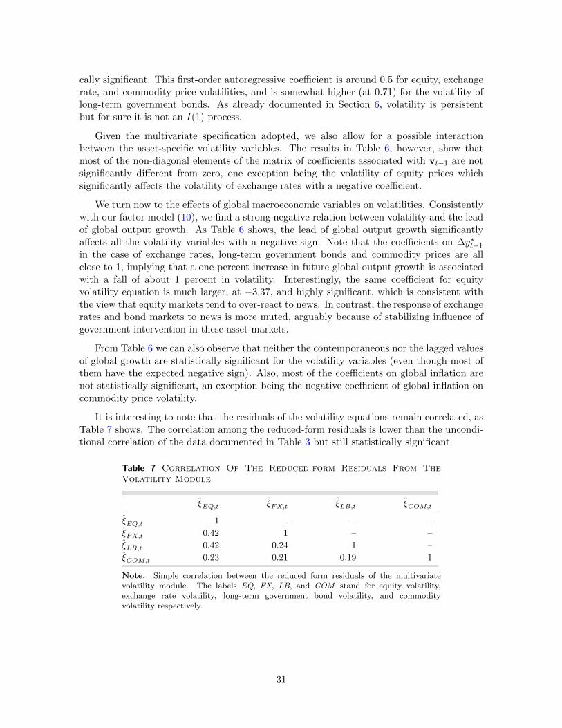
cally significant. This first-order autoregressive coefficient is around 0.5 for equity, exchangerate, and commodity price volatilities, and is somewhat higher (at 0.71) for the volatility oflong-term government bonds. As already documented in Section 6, volatility is persistentbut for sure it is not an I(1) process.

Given the multivariate specification adopted, we also allow for a possible interactionbetween the asset-specific volatility variables. The results in Table 6, however, show thatmost of the non-diagonal elements of the matrix of coefficients associated with vt−1 are notsignificantly different from zero, one exception being the volatility of equity prices whichsignificantly affects the volatility of exchange rates with a negative coefficient.

We turn now to the effects of global macroeconomic variables on volatilities. Consistentlywith our factor model (10), we find a strong negative relation between volatility and the leadof global output growth. As Table 6 shows, the lead of global output growth significantlyaffects all the volatility variables with a negative sign. Note that the coefficients on ∆y∗t+1

in the case of exchange rates, long-term government bonds and commodity prices are allclose to 1, implying that a one percent increase in future global output growth is associatedwith a fall of about 1 percent in volatility. Interestingly, the same coefficient for equityvolatility equation is much larger, at −3.37, and highly significant, which is consistent withthe view that equity markets tend to over-react to news. In contrast, the response of exchangerates and bond markets to news is more muted, arguably because of stabilizing influence ofgovernment intervention in these asset markets.

From Table 6 we can also observe that neither the contemporaneous nor the lagged valuesof global growth are statistically significant for the volatility variables (even though most ofthem have the expected negative sign). Also, most of the coefficients on global inflation arenot statistically significant, an exception being the negative coefficient of global inflation oncommodity price volatility.

It is interesting to note that the residuals of the volatility equations remain correlated, asTable 7 shows. The correlation among the reduced-form residuals is lower than the uncondi-tional correlation of the data documented in Table 3 but still statistically significant.

Table 7 Correlation Of The Reduced-form Residuals From TheVolatility Module

ξEQ,t ξFX,t ξLB,t ξCOM,t

ξEQ,t 1 – – –

ξFX,t 0.42 1 – –

ξLB,t 0.42 0.24 1 –

ξCOM,t 0.23 0.21 0.19 1

Note. Simple correlation between the reduced form residuals of the multivariatevolatility module. The labels EQ, FX, LB, and COM stand for equity volatility,exchange rate volatility, long-term government bond volatility, and commodityvolatility respectively.

31

8 The macroeconomic impact of volatility innovations

Equipped with the estimates of the two components of our GVAR-VOL model, we are readyto look at the impact of volatility innovations on the macroeconomic dynamics. We firstexamine whether the volatility innovations have an impact on the reduced-form residuals ofthe GVAR. This permits us to see the extent to which volatility changes that are not drivenby the common factors nt have the potential for explaining movements in macroeconomicvariables once the effects of common and country-specific factors (embedded in the GVARmodel) are filtered out. If the answer is positive, we then could illustrate and quantify thesesecond round effects by simulating the full GVAR-VOL model. If the answer is negative, wewould conclude that this component of volatility cannot drive macroeconomic dynamics.

To analyze how volatility innovations impact on the GVAR residuals we estimate thefollowing country-specific, variable-specific equations:

ui`t = αi`ξt−1 + ζi`t, (23)

where ui`t is selected from the vector of the GVAR reduced-form residuals ut defined byequation (17) so as to pick the residuals of variable ` = 1, ..., ki in country i = 0, 1, ..., N . Theterm ξt is instead constructed as:

ξt =1

M

M∑κ=1

ξκt, (24)

where ξκt are the residuals of the volatility module and M = 4. We label the simple average ofthe reduced-form residuals (ξt) a global volatility shock. Note here that the lagged specificationin the relationship between ui`t and ξt−1 is in line with our discussion of Section 3 that showsthat—under our assumptions—the volatility innovations affect the GVAR residuals with alag.

An alternative approach would have been to aggregate the asset-specific volatility vari-ables to construct a global volatility measure—as in equation (22)—and then estimate aunivariate ARDL model in global volatility augmented with macro variables. However, theheterogeneity of the coefficients on global output growth across asset types (see Table 6) sug-gests that an aggregated approach could result in biased estimates. But as we shall see below,qualitatively similar results are obtained even if we adopt an aggregate volatility model, withthe difference that the coefficient of the global output growth in the aggregate volatility modelis more difficult to interpret.

Table 8 reports the regression results for output growth and inflation, as well as for equityprices and exchange rates. To evaluate these results, recall that under our identificationassumptions, spelled out in Section 3, nt affects financial market volatility contemporaneouslyand macroeconomic variables with a lag. While this assumption seems reasonable for slow-moving variables such as GDP and inflation, it is less likely to hold for fast moving financialvariables such as equity prices and exchange rates. Therefore, only the relation betweenξt and uyt (i.e., the residuals of GDP and inflation) can be strictly interpreted in termsof causation, while the relation between ξt and uχt (i.e., the residuals of equity prices andexchange rates) has to be interpreted as simple statistical association.

We describe first the estimation of (23) for GDP and inflation. Starting from the GVAR

32

Table

8GVAR-V

OL

Model:GlobalVolatilityIn

novationsAnd

Reduced-form

GVAR

Residuals

GD

PIn

flati

on

Equ

ity

Pri

ceE

xch

an

ge

Rate

αi,y

t-S

tat

R2

αi,π

t-S

tat

R2

αi,eq

t-S

tat

R2

αi,ep

t-S

tat

R2

AR

GE

NT

INA

0.10

0.88

0.0

1-0

.06

-0.0

80.0

04.1

92.3

30.0

4-1

.70

-1.9

70.0

3A

US

TR

AL

IA0.

040.

710.

00

0.0

10.1

70.0

00.1

80.3

10.0

0-0

.33

-0.8

60.0

1B

RA

ZIL

0.04

0.34

0.00

-0.3

3-0

.45

0.0

0–

––

-0.1

6-0

.29

0.0

0C

AN

AD

A0.

030.

960.0

10.0

00.0

80.0

00.6

91.3

60.0

2-0

.38

-1.8

00.0

3C

HIN

A0.

070.

890.

01

0.1

01.3

80.0

2–

––

0.1

20.4

00.0

0C

HIL

E0.

070.

690.

00

-0.0

5-0

.47

0.0

01.0

81.6

50.0

2-0

.44

-1.3

60.0

1E

UR

O0.

041.

350.

01

0.0

31.6

30.0

20.9

71.7

90.0

3-0

.17

-0.5

10.0

0IN

DIA

0.09

1.27

0.01

0.0

50.7

10.0

00.4

40.4

60.0

0-0

.25

-1.2

80.0

1IN

DO

NE

SIA

0.04

0.36

0.00

-0.1

4-0

.99

0.0

1–

––

-0.5

4-0

.83

0.0

1JA

PA

N0.

000.

030.0

00.0

41.5

70.0

21.5

42.6

60.0

6-0

.81

-2.3

50.0

4K

OR

EA

0.24

2.90

0.07

0.0

71.3

30.0

12.1

12.3

70.0

4-0

.18

-0.5

00.0

0M

AL

AY

SIA

-0.0

4-0

.39

0.0

00.0

61.1

60.0

12.0

81.8

80.0

30.1

00.4

20.0

0M

EX

ICO

0.05

0.63

0.0

00.0

60.3

60.0

0–

––

-1.2

6-2

.71

0.0

6N

OR

WA

Y-0

.07

-0.9

80.0

1-0

.02

-0.4

60.0

01.2

61.3

80.0

2-0

.38

-1.1

40.0

1N

EW

ZE

AL

AN

D0.

00-0

.02

0.0

0-0

.06

-1.1

20.0

1-0

.15

-0.2

80.0

0-0

.35

-0.9

90.0

1P

ER

U-0

.06

-0.3

30.

00

-0.0

4-0

.06

0.0

0–

––

0.7

11.1

80.0

1P

HIL

IPP

INE

S0.

090.

930.

01

-0.0

7-0

.59

0.0

00.9

90.8

70.0

1-0

.42

-1.4

10.0

2S

OU

TH

AF

RIC

A0.

051.

090.

01

0.0

20.4

00.0

00.6

40.9

40.0

1-0

.65

-1.3

60.0

2S

AU

DI

AR

AB

IA0.

383.

050.0

70.0

20.3

40.0

0–

––

-0.0

1-0

.15

0.0

0S

ING

AP

OR

E-0

.06

-0.4

90.

00

0.0

00.1

00.0

01.6

71.8

80.0

3-0

.15

-0.9

70.0

1S

WE

DE

N0.

141.

880.0

30.0

0-0

.01

0.0

01.5

01.8

70.0

3-0

.22

-0.6

00.0

0S

WIT

ZE

RL

AN

D0.

133.

530.0

90.0

20.7

40.0

00.6

71.3

20.0

1-0

.13

-0.3

50.0

0T

HA

ILA

ND

0.07

0.75

0.00

0.1

22.0

90.0

42.0

92.0

30.0

3-0

.35

-1.2

90.0

1T

UR

KE

Y0.

030.

190.

00

0.0

80.3

70.0

0–

––

-0.2

6-0

.59

0.0

0U

NIT

ED

KIN

GD

OM

0.05

1.25

0.0

10.0

20.8

00.0

10.3

30.6

30.0

0-0

.62

-2.1

00.0

4U

SA

0.10

2.32

0.04

0.0

41.0

40.0

10.5

41.1

40.0

1–

––

Note

.R

esult

sof

the

regre

ssio

nui`t

=αi`ξ t−1

+ζi`t

as

ineq

uati

on

(23).

The

coeffi

cien

tsαi,y,αi,π,αi,eq,αi,ep

rep

ort

the

impact

of

the

glo

bal

vola

tility

innov

ati

ons

(ξt−

1)

on

the

GV

AR

reduce

d-f

orm

resi

duals

(ui`t)

ass

oci

ate

dw

ith

each

countr

y’s

GD

P,

inflati

on,

equit

ypri

ce,

and

exch

ange

rate

equati

ons,

resp

ecti

vel

y.

33

residuals of the GDP equations, Table 8 shows that almost all coefficients (αi,y) are notstatistically significant at the 95 percent level. The only exceptions are Korea, Saudi Arabia,Sweden, Switzerland and the United States, for which the estimates are statistically significantbut have a positive sign—which is not consistent with standard theory.

We further checked the significance of the estimates by using a multiple testing proce-dure due to Holm (1979), which controls for the overall size of the tests, taking account ofpossible dependence across the 33 t-tests carried out for each of the four variables in Table 8.Application of the Holm procedure yields only one statistically significant coefficient for theGDP growth innovations, namely for Switzerland. Together with the fact that the R2 of theregressions is very small (averaging 0.01 across all countries) these results suggest that thereis virtually no direct effect of a volatility innovation on GDP over and above that of nt thatare taken into account under the GVAR methodology through the use of country-specific for-eign variables. Similar results also hold for the residuals of the GVAR’s inflation equations:as Table 8 shows, the impact of the volatility innovations on the inflation residuals (αi,π) islargely insignificant, the only exception being Thailand.

These results suggest that there is limited scope for volatility to explain macro dynamicsdirectly after we condition on the set of global and country-specific macroeconomic fac-tors included in the GVAR model. Volatility, however, could be affecting economic activityindirectly via its impact on the level of asset prices and the associated wealth effects onconsumption and investment. So we now turn to this indirect channel.

As we noted, it is possible that a volatility innovation is associated with the residual ofthe equity price equations, the exchange rate equations, or the interest rate equations—thatwe collected in the vector uχt defined in (19). If volatility shocks were to be statisticallyassociated with the residuals of the financial variables in the GVAR, they would have achannel to affect, indirectly, also GDP and inflation. However, the timing assumption in ourfactor model is less likely to hold for financial variables. Therefore, the relation between theelements of uχt and the (lagged) volatility innovations, ξt−1, cannot be strictly interpreted interms of causation but has instead to be interpreted as simple statistical association.

We report the estimation of equation (23) for the residuals of the equity price and theexchange rate equations (the results for the interest rates equations are very similar andtherefore are not reported here for sake of brevity). The results show that almost all coeffi-cients are statistically insignificant. In the case of equity prices, the exceptions are Argentina,Japan, Korea, and Thailand with a (counter-intuitive) positive coefficient; in the case of ex-change rates the exceptions are Japan, Mexico and the United Kingdom. Note, however,that none of these coefficients are statistically significant when using Holm multiple testingprocedure.

In summary, we find that a global volatility shock, identified by assuming that commonfactors drive both volatility and the macroeconomic dynamics of individual countries butaffect them with a lag of at least a quarter, has no direct or indirect effect on real GDPonce we condition on a small set of country-specific and global macro-financial factors in theGVAR-VOL model. We interpret this evidence as suggesting that most of the effects thatvolatility has on economic activity documented in the existing literature come from the factthat volatility and the business cycle may share the same set of common factors. In this sense,volatility appears more of a symptom rather a cause of economic stagnation and instability

34

during and after the recent global crisis.

9 Reconciling our findings with the literature

In this section we relate our empirical results to those in the existing empirical literatureon uncertainty and the business cycle, according to which volatility is often found to have asignificant negative effect on economic activity.

As explained in Section 3, in our simple factor model (1), the aggregate volatility andmacro shocks are identified through a timing assumption on the relative speed with whichthe common factors, nt, impact the volatility and macroeconomic variables, and the smallopen economy assumption that allows us to eliminate the effects of country specific shocks onvolatility. In contrast, with a few notable exceptions, in the literature identification is typi-cally achieved through a recursive ordering of variables in a VAR framework (or, equivalently,through a Cholesky decomposition of the variance-covariance matrix of the reduced-formresiduals in a VAR), with GDP ordered after volatility.29

In our factor model, these identification assumptions are equivalent to assuming that:

I. the factors nt affect both volatility and macroeconomic variables contempo-raneously;

II. the macroeconomic variables (∆yit) are not allowed to affect volatility (vt)contemporaneously.

According to assumption I, the factor model (1) can be re-written as:

vt = Φ1vvt−1 + Λnt + ξ0t , (25)

∆yit = Φ1i∆yi,t−1 + Γint + ζ0it, for i = 0, 1, ..., N,

where we note that the common factors nt now enter contemporaneously in both equations.It is important to stress here that, in the absence of any additional assumption, the systemin (25) is not identified. After substituting nt from the activity equation into the volatilityequation, and taking averages over i, we obtain:

vt = Φ1vvt−1 + Ψ0v∆yt + Ψ1v∆yt−1 − Ψ0vζ0it︸ ︷︷ ︸

Op((N+1)−1/2)

+ ξ0t . (26)

Equation (26) is a modified volatility module in the lags of volatility and the lags andcontemporaneous values of changes in macroeconomic variables that resembles the volatilityequation of a typical bivariate VAR in volatility and economic activity considered in theliterature. In order to achieve identification, the literature generally assumes that ∆yit cannot

29See the papers by Gilchrist, Sim, and Zakrajsek (2013), Bachmann, Elstner, and Sims (2013), and Caldara,Fuentes-Albero, Gilchrist, and Zakrajsek (2013). Also, see Baker and Bloom (2013) who try to deal with thecontemporaneous determination of volatility and economic activity by using a panel of indicators for naturaldisasters, terrorist attacks and political shocks as instruments.

35

affect vt contemporaneously (assumption II), which in the case of the above specificationrequires that Ψ0v = 0.

But as noted already in Section 3, the activity equation features the same estimationissues as in our baseline specification: since volatility is correlated with the error terms, OLSwould produce inconsistent estimates of the effect of volatility on economic activity.30 Thisimplies that the mis-specification of the activity equation—one of our main results—does notdepend on the timing assumption but requires only the assumption that the same commonfactors drive both activity and volatility.

We can now quantify empirically the impact of volatility and economic activity under thisalternative set of assumptions. Note that, since we do not include volatility directly into theGVAR, our approach does not suffer from the inconsistency bias described above. Similarlyto what we did in the previous section, we therefore regress the residuals from the modifiedvolatility module (26) on the reduced-form residuals of the GVAR.

For the purpose of implementing the analysis in manner that is as close as possibleto the approach taken in the literature, we re-estimate the volatility module using globalvolatility—labelled RVt and defined as the average of the asset-specific volatility variablesas in equation (22)—as a proxy for vt. As a result, and differently from our baseline wherevt is a (4 × 1) vector of realized volatilities, the volatility module has now a univariaterepresentation. According to (26), the specification of the modified volatility module includeslagged global volatility (vt−1), and the first lag of global output growth (∆y∗t−1) and globalinflation (∆π∗t−1).

31 Note that we also consider two additional versions of the volatilitymodule: a specification with the future, contemporaneous, and lagged changes in the globalvariables and a specification with the contemporaneous and lagged changes in the globalvariables only. Table 9 reports the OLS estimates of these three specifications and theassociated t-ratios in square brackets.

The baseline specification (s1), is presented in the first column of Table 9. Interestingly,the coefficient on lagged global growth is negative but is not statistically significant. Inspecification (s2), which includes both contemporaneous and lagged global variables, the co-efficient on contemporaneous global growth is negative as in the baseline specification, but itis now statistically significant. Finally, consistently with the results in our baseline volatil-ity model in Table 6, specification (s3) shows a strong negative and statistically significantrelation between volatility and the future global output growth.

An important consideration is in order here. According to the modified factor model (25),the relation between the volatility innovations and the GVAR innovations is now contempo-raneous, whereby the volatility innovations are assumed to be exogenous by virtue of therecursive identification assumption made. We therefore estimate the following regression:

ui`t = βi`ξ0t + ζ0i`t, (27)

where ξ0t are the volatility innovations from the baseline specification of the modified volatilitymodule—i.e., the residuals from specification (s1) in Table 9.

30The activity equation can be obtained by substituting nt from the volatility equation into the activityequation, but is not derived here for sake of brevity.

31The number of lags of global volatility has been determined with Akaike criterion.

36

Table 9 Modified Volatility Module

(s1) (s2) (s3)

vt vt vt

c 0.04 0.06 0.06[4.64] [5.57] [6.54]

vt−1 0.54 0.44 0.48[6.37] [4.97] [5.99]

∆y∗t+1 -1.56[-5.54]

∆π∗t+1 0.06

[0.36]∆y∗t -1.01 -0.15

[-3.02] [-0.44]∆π∗

t 0.04 0.11[0.20] [0.64]

∆y∗t−1 -0.42 -0.03 -0.04[-1.33] [-0.10] [-0.14]

∆π∗t−1 -0.20 -0.13 -0.07

[-1.04] [-0.70] [-0.38]

Note. t-Statistics are in brackets. The lag order is determined with Akaikecriterion with a maximum of 4 lags. The model is estimated over the1979.II–2011.II period.

Table 10 reports the estimation results. As in the previous section, for each countryi = 0, 1, ..., N we consider the GVAR reduced-form residuals from different equations, namelyGDP, inflation, equity prices and exchange rates. Starting with the GDP residuals, Table 10shows that 8 out of 26 coefficients (βi,y) are now statistically significant at the 95 percent level;and the statistically significant coefficients have a negative sign, implying that an increase involatility would negatively affect GDP. Similar results are obtained for the inflation residuals:6 out of 26 coefficients (βi,π) have a statistically significant coefficient, in most cases with anegative sign. Note, however, that according to Holm multiple testing procedure only onecoefficient (namely, Brazil GDP) is statistically significant; and the R2 of the regressions arestill small, averaging 0.03 for the GDP regression and 0.02 for the inflation regressions.

We now analyze the association between volatility and asset price residuals. All thecoefficients on the equity price residuals (βi,eq) are negative and statistically significant atthe 95 percent level, with only two exception: Korea and the Philippines. Interestingly,this result is robust to the Holm multiple testing procedure: 13 out 19 coefficients are stillstatistically significant. Moreover, the size of the coefficients is large, with a cross-countryaverage for βi,eq of −2.23; and the explanatory power of the volatility innovations is large aswell, with a cross-country average of the R2 of 0.13. Similar (but less clear-cut) results holdfor the exchange rate residuals (βi,ep), for which an increase in volatility generally implies asignificant depreciation of currencies vis-a-vis the U.S. dollar, which is indicative of “flightto safety” often observed during times of increased economic uncertainty.

This evidence suggests that, when we assume (as it is commonly done in the literature)that activity cannot affect volatility contemporaneously, global volatility has some direct

37

Table

10Modified

GVAR-V

OL

Model:GlobalVolatilityIn

novationsAnd

Reduced-form

GVAR

Residuals

GD

PIn

flati

on

Equ

ity

Pri

ceE

xch

an

ge

Rate

βi,y

t-S

tat

R2

βi,π

t-S

tat

R2

βi,eq

t-S

tat

R2

βi,ep

t-S

tat

R2

AR

GE

NT

INA

-0.2

1-2

.23

0.04

0.1

80.3

10.0

0-4

.10

-2.7

40.0

60.7

91.0

80.0

1A

US

TR

AL

IA-0

.03

-0.8

20.

01

-0.0

4-0

.97

0.0

1-2

.05

-4.6

50.1

51.2

13.9

50.1

1B

RA

ZIL

-0.2

9-3

.41

0.09

0.8

31.3

70.0

2–

––

1.3

93.0

10.0

7C

AN

AD

A-0

.03

-1.0

90.0

1-0

.06

-2.2

40.0

4-2

.21

-5.8

30.2

20.8

24.9

90.1

7C

HIN

A0.

020.

230.

00

-0.0

6-0

.95

0.0

1–

––

0.1

20.4

70.0

0C

HIL

E-0

.17

-1.8

90.

03

0.0

00.0

10.0

0-1

.58

-2.9

40.0

70.8

33.1

20.0

7E

UR

O-0

.04

-1.8

80.0

3-0

.03

-1.7

20.0

2-2

.42

-5.9

40.2

30.0

80.2

90.0

0IN

DIA

0.06

0.90

0.01

0.0

71.0

10.0

1-2

.54

-3.2

50.0

80.2

41.4

70.0

2IN

DO

NE

SIA

-0.1

6-1

.60

0.02

0.0

60.4

70.0

0–

––

1.3

22.4

40.0

5JA

PA

N-0

.14

-2.8

30.

06

-0.0

4-1

.91

0.0

3-2

.23

-4.8

90.1

6-0

.86

-3.0

20.0

7K

OR

EA

-0.2

1-3

.00

0.0

7-0

.01

-0.1

90.0

0-1

.38

-1.8

20.0

31.2

34.5

00.1

4M

AL

AY

SIA

-0.2

4-2

.67

0.0

6-0

.11

-2.7

80.0

6-2

.73

-3.0

00.0

70.4

42.2

20.0

4M

EX

ICO

-0.0

1-0

.15

0.0

00.1

91.3

70.0

2–

––

1.2

73.2

90.0

8N

OR

WA

Y0.

00-0

.06

0.00

0.0

30.7

90.0

1-4

.07

-6.0

00.2

30.6

82.4

70.0

5N

EW

ZE

AL

AN

D-0

.05

-0.8

80.0

1-0

.06

-1.3

20.0

1-1

.89

-4.5

90.1

50.8

02.7

00.0

6P

ER

U0.

060.

380.

00

-0.3

6-0

.66

0.0

0–

––

0.1

70.3

30.0

0P

HIL

IPP

INE

S-0

.06

-0.6

90.0

0-0

.23

-2.3

90.0

5-1

.17

-1.2

30.0

10.6

12.4

80.0

5S

OU

TH

AF

RIC

A-0

.04

-1.0

20.0

10.0

71.9

00.0

3-1

.94

-3.5

30.0

90.7

91.9

80.0

3S

AU

DI

AR

AB

IA0.

040.

330.0

00.0

20.4

40.0

0–

––

-0.0

1-0

.17

0.0

0S

ING

AP

OR

E-0

.10

-0.9

30.

01

0.0

72.0

40.0

3-3

.68

-5.4

20.2

00.2

92.3

50.0

4S

WE

DE

N-0

.14

-2.1

40.

04

-0.0

1-0

.27

0.0

0-2

.20

-3.3

80.0

90.6

52.1

50.0

4S

WIT

ZE

RL

AN

D-0

.03

-1.0

30.0

1-0

.01

-0.4

90.0

0-2

.19

-5.7

00.2

1-0

.15

-0.4

70.0

0T

HA

ILA

ND

-0.2

2-2

.93

0.07

-0.1

7-3

.66

0.1

0-2

.15

-2.5

10.0

50.2

91.2

70.0

1T

UR

KE

Y-0

.20

-1.4

20.

02

0.1

00.5

70.0

0–

––

1.2

13.4

20.0

9U

NIT

ED

KIN

GD

OM

-0.0

7-1

.93

0.03

-0.0

3-1

.09

0.0

1-2

.19

-5.6

50.2

10.4

31.7

40.0

2U

NIT

ED

ST

AT

ES

-0.1

0-2

.97

0.0

7-0

.07

-2.3

00.0

4-2

.01

-5.7

00.2

1–

––

Note

.R

esult

sof

the

regre

ssio

nui`t

=βi`ξ0 t

+ζ0 i`t

as

ineq

uati

on

(27).

The

coeffi

cien

tsβi,y,βi,π,βi,eq,

andβi,ep

rep

ort

the

impact

of

the

vola

tility

innov

ati

ons

(ξ0 t)

on

the

GV

AR

reduce

d-f

orm

resi

duals

(ui`t)

ass

oci

ate

dw

ith

each

countr

y’s

GD

P,

inflati

on,

equit

ypri

ce,

and

exch

ange

rate

equati

ons,

resp

ecti

vel

y.

38

impact on real GDP and has a strong association with equity price and exchange rates,which in turn can affect economic activity indirectly via balance sheet and wealth effects.

10 Conclusions

The recent global financial crisis has spurred renewed academic interest on quantifying thecausal impact of uncertainty on macroeconomic dynamics. In this paper, we study theinterrelation between volatility and macroeconomic dynamics in the world economy underthe assumption that both uncertainty and business cycle are driven by the same set of commonfactors. We further assume that while these common factors affect financial market volatilitycontemporaneously, they can affect macroeconomic dynamics only with a lag of at least onequarter. Under these assumptions, we show analytically that volatility is forward looking andthat the output equation of the typical VARs estimated in the literature is mis-specified asleast squares estimates of this equation are inconsistent. This implies that, if our identificationassumption is plausible, typical impulse response functions of measures of economic activity tovolatility shocks are biased regardless of the structural VAR identification scheme employed.

We then construct global measures of uncertainty by using realized volatility at quarterlyfrequency for 109 asset prices. Empirically, we provide three main sets of results. First, our(unconditional) descriptive analysis shows that volatility is persistent, but is well approxi-mated by a stationary process at business cycle frequency. It behaves countercyclically—consistently with the common wisdom in the literature—and it can significantly lead thebusiness cycle. We also find that realized volatility co-moves significantly within asset classes(equities, bonds, exchange rates and commodities), but it is not as highly correlated acrossasset classes.

Second, our multi-country analysis allows us to consistently estimate the relation betweenGDP growth and volatility. Our results show that there is a strong negative and statisticallysignificant association between future output growth and current volatility.

Third, we find that volatility shocks have no statistically significant impact on economicactivity over and above that of its common component. In other words, we find that a shockto global volatility has little or no direct effect on real GDP once we condition on a small setof country-specific and global macro-financial factors in the GVAR-VOL model.

We do not interpret this evidence meaning that volatility has no effect on economicactivity. We argue that most of its effect (often found in the literature) may be coming fromthe fact that volatility itself is driven by the same common factors that affect the businesscycle. In other words, volatility is likely to be more of a symptom rather than a cause ofeconomic instability.

39

References

Abel, A. B. (1983): “Optimal Investment under Uncertainty,” American Economic Review, 73(1),228–33.

Andersen, T. G., and T. Bollerslev (1997): “Heterogeneous Information Arrivals and ReturnVolatility Dynamics: Uncovering the Long-Run in High Frequency Returns,” Journal of Finance,52(3), 975–1005.

Andersen, T. G., T. Bollerslev, F. X. Diebold, and P. Labys (2001): “The Distribution ofRealized Exchange Rate Volatility,” Journal of the American Statistical Association, 96, 42–55.

(2003): “Modeling and Forecasting Realized Volatility,” Econometrica, 71(2), 579–625.

Arellano, C., Y. Bai, and P. Kehoe (2012): “Financial Markets and Fluctuations in Uncer-tainty,” unpublished manuscript.

Bachmann, R., and C. Bayer (2013): “’Wait-and-See’ business cycles?,” Journal of MonetaryEconomics, 60(6), 704–719.

Bachmann, R., S. Elstner, and E. R. Sims (2013): “Uncertainty and Economic Activity: Evi-dence from Business Survey Data,” American Economic Journal: Macroeconomics, 5(2), 217–249.

Bachmann, R., and G. Moscarini (2011): “Business Cycles and Endogenous Uncertainty,” 2011Meeting Papers 36, Society for Economic Dynamics.

Bailey, N., G. Kapetanios, and M. H. Pesaran (2012): “Exponent of Cross-sectional De-pendence: Estimation and Inference,” Cambridge Working Papers in Economics 1206, Faculty ofEconomics, University of Cambridge, Revised version.

Baillie, R. T., T. Bollerslev, and H. O. Mikkelsen (1996): “Fractionally integrated general-ized autoregressive conditional heteroskedasticity,” Journal of Econometrics, 74(1), 3–30.

Baker, S. R., and N. Bloom (2013): “Does Uncertainty Reduce Growth? Using Disasters asNatural Experiments,” NBER Working Papers 19475, National Bureau of Economic Research, Inc.

Baker, S. R., N. Bloom, and S. J. Davis (2013): “Measuring Economic Policy Uncertainty,”unpublished manuscript, Stanford University.

Barndorff-Nielsen, O. E., and N. Shephard (2002): “Estimating quadratic variation usingrealized variance,” Journal of Applied Econometrics, 17(5), 457–477.

(2004): “Econometric Analysis of Realized Covariation: High Frequency Based Covariance,Regression, and Correlation in Financial Economics,” Econometrica, 72(3), 885–925.

Bernanke, B. S. (1983): “Irreversibility, Uncertainty, and Cyclical Investment,” The QuarterlyJournal of Economics, 98(1), 85–106.

Bloom, N. (2009): “The Impact of Uncertainty Shocks,” Econometrica, 77(3), 623–685.

Bloom, N., S. Bond, and J. V. Reenen (2007): “Uncertainty and Investment Dynamics,” Reviewof Economic Studies, 74(2), 391–415.

Bloom, N., M. Floetotto, N. Jaimovich, I. Saporta-Eksten, and S. J. Terry (2012):“Really Uncertain Business Cycles,” NBER Working Papers 18245, National Bureau of EconomicResearch, Inc.

40

Caldara, D., C. Fuentes-Albero, S. Gilchrist, and E. Zakrajsek (2013): “The Macroeco-nomic Implications of Financial and Uncertainty Shocks,” unpublished manuscript.

Campbell, J. Y., M. Lettau, B. G. Malkiel, and Y. Xu (2001): “Have Individual StocksBecome More Volatile? An Empirical Exploration of Idiosyncratic Risk,” Journal of Finance,56(1), 1–43.

Carriere-Swallow, Y., and L. F. Cespedes (2013): “The impact of uncertainty shocks in emerg-ing economies,” forthcoming Journal of international Economics.

Cesa-Bianchi, A., M. H. Pesaran, A. Rebucci, and T. Xu (2012): “On The Transmissionof Global Shocks to Latin America Before and After China’s Emergence in the World Economy,”Economia, 12(2)(Spring), 1–75.

Christiano, L., R. Motto, and M. Rostagno (2014): “Risk Shocks,” American Economic Re-view, 104(1), 27–65.

Chudik, A., and M. H. Pesaran (2011): “Infinite-dimensional VARs and factor models,” Journalof Econometrics, 163(1), 4–22.

(2013): “Econometric Analysis of High Dimensional VARs Featuring a Dominant Unit,”Econometric Reviews, 32(5-6), 592–649.

Chudik, A., M. H. Pesaran, and E. Tosetti (2011): “Weak and strong crosssection dependenceand estimation of large panels,” Econometrics Journal, 14(1), C45–C90.

Comte, F., and E. Renault (1998): “Long memory in continuous-time stochastic volatility mod-els,” Mathematical Finance, 8(4), 291–323.

Decker, R., P. D’Erasmo, and H. Moscoso Boedo (2014): “Market Exposure and EndogenousFirm Volatility over the Business Cycle,” unpublished manuscript.

Dees, S., F. di Mauro, M. H. Pesaran, and L. V. Smith (2007): “Exploring the internationallinkages of the euro area: a global VAR analysis,” Journal of Applied Econometrics, 22(1), 1–38.

Dees, S., M. H. Pesaran, V. L. Smith, and R. P. Smith (2014): “Constructing Multi-CountryRational Expectations Models,” forthcoming Oxford Bulletin of Economics and Statistics.

di Mauro, F., and M. H. Pesaran (eds.) (2013): The GVAR Handbook: Structure and Applica-tions of a Macro Model of the Global Economy. Oxford University Press, Oxford.

Ding, Z., C. W. J. Granger, and R. F. Engle (1993): “A long memory property of stock marketreturns and a new model,” Journal of Empirical Finance, 1(1), 83–106.

Dixit, A. K., and R. S. Pindyck (1994): Investment under Uncertainty. Princeton UniversityPress.

Engle, R. F. (1982): “Autoregressive Conditional Heteroscedasticity with Estimates of the Varianceof United Kingdom Inflation,” Econometrica, 50(4), 987–1007.

Engle, R. F., D. F. Hendry, and J.-F. Richard (1983): “Exogeneity,” Econometrica, 51(2),277–304.

Favero, C., M. H. Pesaran, and S. Sharma (1994): “A Duration Model of Irreversible OilInvestment: Theory and Empirical Evidence,” Journal of Applied Econometrics, 9, S95–S112.

41

Fernandez-Villaverde, J., P. Guerron-Quintana, J. F. Rubio-Ramirez, and M. Uribe(2011): “Risk Matters: The Real Effects of Volatility Shocks,” American Economic Review, 101(6),2530–61.

Fostel, A., and J. Geanakoplos (2012): “Why Does Bad News Increase Volatility and DecreaseLeverage?,” Journal of Economic Theory, 147(2), 501–525.

Fuller, W., and H. Park (1995): “Alternative Estimators and Unit Root Tests for the Autore-gressive Process,” Journal of Time Series Analysis, 16, 415–429.

Gilchrist, S., J. Sim, and E. Zakrajsek (2013): “Uncertainty, Financial Frictions, and Irre-versible Investment,” unpublished manuscript.

Hansen, P. R., Z. Huang, and H. H. Shek (2012): “Realized GARCH: a joint model for returnsand realized measures of volatility,” Journal of Applied Econometrics, 27(6), 877–906.

Harbo, I., S. Johansen, B. Nielsen, and A. Rahbek (1998): “Asymptotic Inference on Cointe-grating Rank in Partial Systems,” Journal of Business & Economic Statistics, 16(4), 388–99.

Hartman, R. (1976): “Factor Demand with Output Price Uncertainty,” American Economic Review,66(4), 675–81.

Harvey, A. C., and A. Jaeger (1993): “Detrending, Stylized Facts and the Business Cycle,”Journal of Applied Econometrics, 8(3), 231–47.

Hirata, H., M. A. Kose, and C. Otrok (2013): “Regionalization vs. Globalization,” IMF WorkingPapers 13/19, International Monetary Fund.

Hirata, H., M. A. Kose, C. Otrok, and M. E. Terrones (2012): “Global House Price Fluctu-ations: Synchronization and Determinants,” in NBER International Seminar on Macroeconomics2012, NBER Chapters. National Bureau of Economic Research, Inc.

Holm, S. (1979): “A simple sequentially rejective multiple test procedure,” Scandinavian Journal ofStatistics, 6, 65–70.

IMF (2012): “How Does Uncertainty Affect Economic Performance?,” in World Economic Outlook,October 2012, world economic outlook 4, pp. 49–53. Washington: International Monetary Fund.

Johansen, S. (1992): “Cointegration in partial systems and the efficiency of single-equation analysis,”Journal of Econometrics, 52(3), 389–402.

Kimball, M. S. (1990): “Precautionary Saving in the Small and in the Large,” Econometrica, 58(1),53–73.

Kose, A., C. Otrok, and E. Prasad (2013): “International Spillovers: Real and Financial Chan-nels,” unpublished manuscript.

Kose, M. A., C. Otrok, and C. H. Whiteman (2003): “International Business Cycles: World,Region, and Country-Specific Factors,” American Economic Review, 93(4), 1216–1239.

Kose, M. A., and M. E. Terrones (2012): “Uncertainty weighing on the global recovery,”VoxEU.org.

Leahy, J. V., and T. M. Whited (1996): “The Effect of Uncertainty on Investment: Some StylizedFacts,” Journal of Money, Credit and Banking, 28(1), 64–83.

Leland, H. (1968): “Saving and Uncertainty: The Precautionary Demand for Saving,” The QuarterlyJournal of Economics, 82, 465–473.

42

Lintner, J. (1965): “The Valuation of Risk Assets and the Selection of Risky Investments in StockPortfolios and Capital Budgets,” The Review of Economics and Statistics, 47(1), 13–37.

Mirman, L. J. (1971): “Uncertainty and Optimal Consumption Decisions,” Econometrica, 39(1),179–85.

Mumtaz, H., and P. Surico (2013): “Policy Uncertainty and Aggregate Fluctuations,” WorkingPapers 708, Queen Mary, University of London, School of Economics and Finance.

Oi, W. (1961): “The desirability of price stability under perfect competition,” Econometrica, 29(1),58–64.

Pesaran, M. H., T. Schuermann, and S. M. Weiner (2004): “Modeling Regional Interdependen-cies Using a Global Error-Correcting Macroeconometric Model,” Journal of Business & EconomicStatistics, 22, 129–162.

Pesaran, M. H., Y. Shin, and R. J. Smith (2000): “Structural analysis of vector error correctionmodels with exogenous I(1) variables,” Journal of Econometrics, 97(2), 293–343.

Pesaran, M. H., R. Smith, and K. Im (1996): “Dynamic Linear Models for Heterogenous Panels,”in The Econometrics of Panel Data, ed. by L. Mtys, and P. Sevestre, chap. 8, pp. 145–195. KluwerAcademic Publishers, Dordrecht, The Netherlands.

Popescu, A., and F. R. Smets (2010): “Uncertainty, Risk-taking, and the Business Cycle inGermany,” CESifo Economic Studies, 56(4), 596–626.

Ramey, G., and V. A. Ramey (1995): “Cross-Country Evidence on the Link between Volatilityand Growth,” American Economic Review, 85(5), 1138–51.

Ross, S. A. (1976): “The arbitrage theory of capital asset pricing,” Journal of Economic Theory,13(3), 341–360.

Schwert, G. W. (1989a): “Business cycles, financial crises, and stock volatility,” Carnegie-RochesterConference Series on Public Policy, 31(1), 83–125.

Schwert, G. W. (1989b): “Why Does Stock Market Volatility Change over Time?,” Journal ofFinance, 44(5), 1115–53.

Sharpe, W. F. (1964): “Capital Asset Prices: A Theory of Market Equilibrium under Conditions ofRisk,” Journal of Finance, 19:3, 425–442.

Tian, C. (2012): “Riskiness Choice and Endogenous Productivity Dispersion over the Business Cy-cle,” PIER Working Paper Archive 12-025, Penn Institute for Economic Research, Department ofEconomics, University of Pennsylvania.

Van Nieuwerburgh, S., and L. Veldkamp (2006): “Learning asymmetries in real business cycles,”Journal of Monetary Economics, 53(4), 753–772.

Zarnowitz, V., and L. A. Lambros (1987): “Consensus and Uncertainty in Economic Prediction,”Journal of Political Economy, 95(3), 591–621.

43

Appendix to

“Uncertainty and Economic Activity: A Global Perspective”

by A. Cesa-Bianchi, M.H. Pesaran, and A. Rebucci

March 27, 2014

A The combined GVAR-VOL model

The combined GVAR-VOL model can be obtained by stacking the system of equations forthe GVAR model (16) with those of the volatility module, (11). We have:[

Im Ψ1,vP0 IK

] [vt

xt+1

]=

[Φv (Ψ0,v −Ψ1,v)P0 F

] [vt−1xt

]+ ... (28)[

0 (Ψ−1,v −Ψ0,v)P0 0

] [vt−2xt−1

]+ ...[

0 −Ψ−1,vP0 0

] [vt−3xt−2

]+

[ξt

ut+1

],

or, more compactly:[vt

xt+1

]= Ξ−10 Ξ1

[vt−1xt

]+ Ξ−10 Ξ2

[vt−2xt−1

]+ Ξ−10 Ξ3

[vt−3xt−2

]+ Ξ−10

[ξt

ut+1

], (29)

where:

Ξ0 =

[Im Ψ1,vP0 IK

], Ξ1 =

[Φv (Ψ0,v −Ψ1,v)P0 F

],

Ξ2 =

[0 (Ψ−1,v −Ψ0,v)P0 0

], Ξ2 =

[0 −Ψ−1,vP0 0

].

B Cross-sectional measures of dispersion

B.I Definition

As noted in the body of the paper, uncertainty can also be measured by the cross-sectionaldispersion of returns at any given point in time and for each asset class. We label thequarterly cross-sectional dispersion of asset κ, for quarter t, at daily rates (CDκt) as “asset-specific cross-sectional dispersion.” We compute asset-specific cross-sectional dispersion as:

CDκt =

√√√√D−1t

Dt∑τ=1

Nt∑i=1

wit (rκit(τ)− rκt(τ))2 (30)

where rκit(τ) = ∆ lnPκit(τ) and rκit = D−1t∑Dt

τ=1 rκit(τ) is the average daily price changesover the quarter t, and Dt is the number of trading days in quarter t; and wit are weightsattached to country i in quarter t.

44

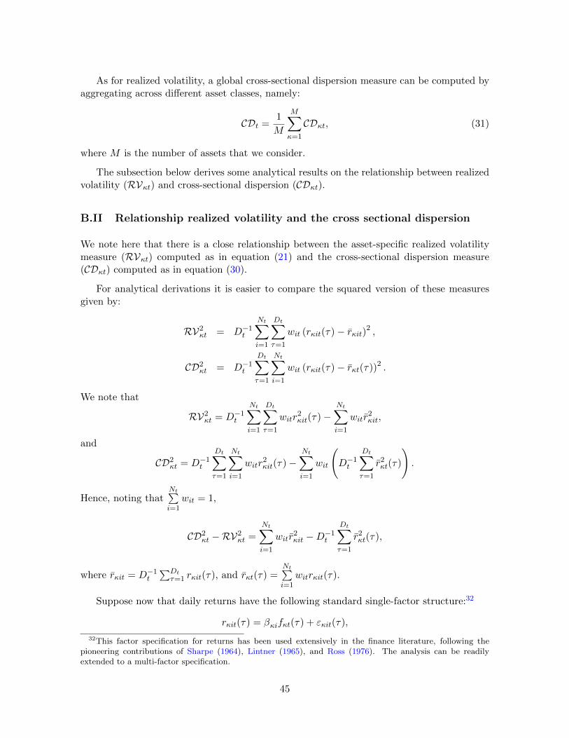
As for realized volatility, a global cross-sectional dispersion measure can be computed byaggregating across different asset classes, namely:

CDt =1

M

M∑κ=1

CDκt, (31)

where M is the number of assets that we consider.

The subsection below derives some analytical results on the relationship between realizedvolatility (RVκt) and cross-sectional dispersion (CDκt).

B.II Relationship realized volatility and the cross sectional dispersion

We note here that there is a close relationship between the asset-specific realized volatilitymeasure (RVκt) computed as in equation (21) and the cross-sectional dispersion measure(CDκt) computed as in equation (30).

For analytical derivations it is easier to compare the squared version of these measuresgiven by:

RV2κt = D−1t

Nt∑i=1

Dt∑τ=1

wit (rκit(τ)− rκit)2 ,

CD2κt = D−1t

Dt∑τ=1

Nt∑i=1

wit (rκit(τ)− rκt(τ))2 .

We note that

RV2κt = D−1t

Nt∑i=1

Dt∑τ=1

witr2κit(τ)−

Nt∑i=1

witr2κit,

and

CD2κt = D−1t

Dt∑τ=1

Nt∑i=1

witr2κit(τ)−

Nt∑i=1

wit

(D−1t

Dt∑τ=1

r2κt(τ)

).

Hence, noting thatNt∑i=1

wit = 1,

CD2κt −RV2κt =

Nt∑i=1

witr2κit −D−1t

Dt∑τ=1

r2κt(τ),

where rκit = D−1t∑Dt

τ=1 rκit(τ), and rκt(τ) =Nt∑i=1

witrκit(τ).

Suppose now that daily returns have the following standard single-factor structure:32

rκit(τ) = βκifκt(τ) + εκit(τ),

32This factor specification for returns has been used extensively in the finance literature, following thepioneering contributions of Sharpe (1964), Lintner (1965), and Ross (1976). The analysis can be readilyextended to a multi-factor specification.

45

where the factor is strong in the sense that (see Bailey, Kapetanios, and Pesaran, 2012):

limNt→∞

Nt∑i=1

witβκi = βκt 6= 0,

limNt→∞

Nt∑i=1

witβ2κi = σ2κβt + β

2κt 6= 0.

The idiosyncratic components, εκit(τ), are assumed to be independently distributed fromβκifκt(τ), cross-sectionally weakly correlated, and serially uncorrelated with zero means andfinite variances. Also let:

limDt→∞

D−1t

Dt∑τ=1

f2κt(τ) = h2κft.

We now note that

Nt∑i=1

witr2κit =

(Nt∑i=1

witβ2κi

)f2κt +

(Nt∑i=1

witε2κit

)+ 2

(Nt∑i=1

witβκiεκit

)fκt

=(σ2κβt + β

2κt

)f2κt +Op

(D−1/2t

)+Op

(N−1/2t

),

where fκt = D−1t∑Dt

τ=1 fκt(τ), and εκit = D−1t∑Dt

τ=1 εκit(τ). Also

D−1t

Dt∑τ=1

r2κt(τ) = D−1t

Dt∑τ=1

[βκtfκt(τ) + εκt(τ)

]2= β

2κt

[D−1t

Dt∑τ=1

f2κt(τ)

]+D−1t

Dt∑τ=1

ε2κt(τ) + 2D−1t

Dt∑τ=1

βκtεκt(τ)fκt(τ)

= β2κth

2κft +Op

(N−1/2t

)+Op

(D−1/2t

).

Hence

CD2κt −RV2κt =

(σ2κβt + β

2κt

)f2κt − β

2κth

2κft +Op

(N−1/2t

)+Op

(D−1/2t

)= σ2κβtf

2κt − β

2κtσ

2κft +Op

(N−1/2t

)+Op

(D−1/2t

).

where σ2κft =(h2κft − f2κt

)≥ 0, is the variance of the common factor for asset type κ.

This expression shows that, under fairly general assumptions and for Nt and Dt suffi-ciently large, we would expect the cross-sectional dispersion measure to be closely relatedto asset-specific measures of realized volatility when the factor loadings, βκi, are not toodispersed across countries. The results also show that the relative magnitudes of the crosssection dispersion and realized volatility measures depend on the relative values of σ2κβtf

2κt

and β2κtσ

2κft.

Figure B.1 displays a comparison between realized volatility and cross-sectional dispersionusing our data set. For this comparison we removed the countries that experienced episodesof high inflation during the sample over which RV and CD were computed: Argentina,

46

Global

1979 1984 1989 1994 1999 2004 20090.05

0.1

0.15

0.2

0.25

Equity Prices

1979 1984 1989 1994 1999 2004 20090

0.1

0.2

0.3

0.4

Exchange Rates

1979 1984 1989 1994 1999 2004 20090.02

0.04

0.06

0.08

0.1

0.12

Long−term Bonds

1979 1984 1989 1994 1999 2004 20090

0.05

0.1

0.15

0.2

Commodity Prices

1979 1984 1989 1994 1999 2004 20090

0.1

0.2

0.3

0.4

Realized Volatility − RV Cross−sectional Dispersion − CD

Figure B.1 A Comparison Between Realized Volatility and Cross-sectional Dispersion.The upper panel compares global realized volatility (RVt, light thick line) and global cross-sectionaldispersion (CDt, dark thin line), computed as in equations (22) and (31) respectively. The lowerpanels display the same comparison for the asset-specific measures. Specifically, RVκt is computedas in equation (21) and CDκt is computed as in equation (30). All measures are expressed at quarterlyrates and computed over the 1990.I-2011.II period. High/hyperinflation countries are discarded (asexplained in the text).

Brazil, Chile, Mexico, and Turkey.33 This is because the CD measure—given the way it iscomputed—is more affected than the RV measure by the presence of large outliers, thereforedriving a wedge between the two measures. Note, however, that this wedge is not discernible

33Note that Peru—who also experienced periods of consumer price inflation—is not removed form the samplesince daily asset price data is available only after the hyperinflation period.

47

when we use all countries but perform the cross-country aggregation using PPP-GDP weightsinstead of equal weights (as it is done above).

The upper panel compares global realized volatility (RVt, light thick line) and globalcross-sectional dispersion (CDt, dark thin line), computed as in equations (22) and (31),respectively. Their sample correlation over the 1979.I to 2011.II period is 0.92. The lowerpanels display the asset-specific realized volatility measure (RVκt) computed as in equation(21) with equal weights and compare it with the cross-sectional dispersion measure (CDκt)computed as in equation (30) with equal weights. Both series are then re-scaled by the factor√Dt so as to be expressed at quarterly rates. Figure B.1 suggests that the two measures are

very closely related, consistently with the evidence provided by Bloom, Floetotto, Jaimovich,Saporta-Eksten, and Terry (2012). The simple correlation between the asset-specific measuresis 0.92 for equity prices, 0.85 for exchange rates, 0.95 for government bonds, and 0.93 forcommodity prices.

C Data

This appendix provides additional information on the sources of the data we used to constructthe realized volatility measures.34

Equity. For equity prices we use the MSCI Index in local currency. The data source forthe daily equity price indices is Bloomberg. The countries included in the sample are thefollowing: Argentina, Australia, Austria, Belgium, Brazil, Canada, Chile, China, Finland,France, Germany, India, Indonesia, Italy, Japan, Korea, Malaysia, Mexico, Netherlands,Norway, New Zealand, Peru, Philippines, Saudi Arabia, South Africa, Singapore, Spain,Sweden, Switzerland, Thailand, Turkey, United Kingdom, and United States. 35

Bonds. We used 10 years government bonds from Bloomberg. The countries includedin the sample are: Australia, Austria, Belgium, Brazil, Canada, China, Finland, France,Germany, India, Indonesia, Italy, Japan, Korea, Malaysia, Mexico, Netherlands, Norway,New Zealand, Peru, Philippines, South Africa, Singapore, Spain, Sweden, Switzerland, Thai-land,United Kingdom, and United States. 36

Exchange rates. Daily exchange rates, measured in terms of the US dollar are obtainedfrom Bloomberg. The countries included in the sample are the following: Argentina, Aus-tralia, Austria, Belgium, Brazil, Canada, Chile, China, Finland, France, Germany, India,Indonesia, Italy, Japan, Korea, Malaysia, Mexico, Netherlands, Norway, New Zealand, Peru,Philippines, Saudi Arabia, South Africa, Singapore, Spain, Sweden, Switzerland, Thailand,

34A description of the macroeconomic data used for the estimation of the GVAR model can be found at thefollowing web page: https://sites.google.com/site/gvarmodelling/.

35The list of Bloomberg tickers is as follows: MSELTAG, MSDLAS, MSDLAT, MSDLBE, MSELTBR, MS-DLCA, MSELTCF, MSELTCH, MSDLFI, MSDLFR, MSDLGR, MSELTIA, MSELTINF, MSDLIT, MSDLJN,MSELTKO, MXMY, MSELTMXF , MSDLNE, MSDLNO, MSDLNZ, MSELTPR, MSELTPHF, MSELTSA,MGCLSA, MSDLSG, MSDLSP, MSDLSW, MSDLSZ, MSELTTHF, MSELTTK, MSDLUK, MSDLUS.

36The list of Bloomberg tickers is as follows: GACGB10; GAGB10YR; GBGB10YR; GEBR10Y;GCAN10YR; GCNY10YR BGNC; GFIN10YR; GFRN10; GDBR10; GIDN10YR; GBTPGR10; GJGB10;GVSK10YR; MGIY10Y; GMXN10YR; GNTH10YR; GNOR10YR; GNZGB10; GRPE10Y; PDSF10YR;GSAB10YR; MASB10Y; GSPG10YR; GSGB10YR; GSWISS10; GVTL10YR; GUKG10; USGG10YR.

48

Turkey, and United Kingdom.37

Commodities. The data source for the daily commodity price indices is Bloomberg. Therealized volatility measures are computed for the following commodities: Corn, Soybean,Wheat, Coffee, Rice, Sugar, Cocoa, Gold, Silver, Copper, Natural gas, Coal, Oil(CO1),Livestock, Meat and livestock, CRB Commodity Excess Return Index, Linseed oil.38

D Realized volatility charts and summary statistics

This appendix reports a plot of the realized volatility measures and a full set of country-specific and commodity-specific summary statistics over the period 1979-2011.

1979 1985 1992 1998 2005 20110

0.2

0.4

0.6

0.8

1ARGENTINA − Equity Prices

1979 1985 1992 1998 2005 20110

0.1

0.2

0.3

0.4AUSTRALIA − Equity Prices

1979 1985 1992 1998 2005 20110

0.1

0.2

0.3

0.4AUSTRIA − Equity Prices

1979 1985 1992 1998 2005 20110

0.05

0.1

0.15

0.2

0.25BELGIUM − Equity Prices

1979 1985 1992 1998 2005 20110

0.5

1

1.5

2BRAZIL − Equity Prices

1979 1985 1992 1998 2005 20110

0.1

0.2

0.3

0.4CANADA − Equity Prices

37The list of Bloomberg tickers is as follows: USDARS; USDAUD CMPN; USDATS; USDBEF; USDBRL;USDCAD; USDCNY; USDCLP; USDFIM; USDFRF; USDDEM; USDINR; USDIDR; USDITL; USDJPY; US-DKRW; USDMYR; USDMXN; USDNLG; USDNOK; USDNZD; USDPEN; USDPHP; USDZAR; USDSAR;USDSGD; USDESP; USDSEK; USDCHF; USDTHB; USDTRY ; USDGBP.

38The list of Bloomberg tickers is as follows: C1; S1; W1; KC1; RR1; Sb1; CC1; GOLDS; SILV; HG1; NGA;QZ1; CO1; CRB LIVS; EYCI; CRY; COMDLINO.

49

1979 1985 1992 1998 2005 20110

0.1

0.2

0.3

0.4

0.5CHINA − Equity Prices

1979 1985 1992 1998 2005 20110

0.05

0.1

0.15

0.2

0.25CHILE − Equity Prices

1979 1985 1992 1998 2005 20110

0.2

0.4

0.6

0.8FINLAND − Equity Prices

1979 1985 1992 1998 2005 20110

0.1

0.2

0.3

0.4FRANCE − Equity Prices

1979 1985 1992 1998 2005 20110

0.1

0.2

0.3

0.4GERMANY − Equity Prices

1979 1985 1992 1998 2005 20110.05

0.1

0.15

0.2

0.25

0.3INDIA − Equity Prices

1979 1985 1992 1998 2005 20110

0.2

0.4

0.6

0.8INDONESIA − Equity Prices

1979 1985 1992 1998 2005 20110

0.1

0.2

0.3

0.4ITALY − Equity Prices

1979 1985 1992 1998 2005 20110

0.1

0.2

0.3

0.4JAPAN − Equity Prices

1979 1985 1992 1998 2005 20110

0.1

0.2

0.3

0.4KOREA − Equity Prices

50

1979 1985 1992 1998 2005 20110

0.1

0.2

0.3

0.4

0.5MALAYSIA − Equity Prices

1979 1985 1992 1998 2005 20110.05

0.1

0.15

0.2

0.25

0.3MEXICO − Equity Prices

1979 1985 1992 1998 2005 20110

0.1

0.2

0.3

0.4NETHERLANDS − Equity Prices

1979 1985 1992 1998 2005 20110

0.1

0.2

0.3

0.4NORWAY − Equity Prices

1979 1985 1992 1998 2005 20110

0.05

0.1

0.15

0.2

0.25NEW ZEALAND − Equity Prices

1979 1985 1992 1998 2005 20110

0.1

0.2

0.3

0.4

0.5PERU − Equity Prices

1979 1985 1992 1998 2005 20110

0.1

0.2

0.3

0.4

0.5PHILIPPINES − Equity Prices

1979 1985 1992 1998 2005 20110

0.1

0.2

0.3

0.4

0.5SOUTH AFRICA − Equity Prices

1979 1985 1992 1998 2005 20110

0.1

0.2

0.3

0.4SAUDI ARABIA − Equity Prices

1979 1985 1992 1998 2005 20110

0.1

0.2

0.3

0.4SINGAPORE − Equity Prices

51

1979 1985 1992 1998 2005 20110

0.1

0.2

0.3

0.4SPAIN − Equity Prices

1979 1985 1992 1998 2005 20110

0.1

0.2

0.3

0.4SWEDEN − Equity Prices

1979 1985 1992 1998 2005 20110

0.05

0.1

0.15

0.2

0.25SWITZERLAND − Equity Prices

1979 1985 1992 1998 2005 20110

0.1

0.2

0.3

0.4THAILAND − Equity Prices

1979 1985 1992 1998 2005 20110

0.1

0.2

0.3

0.4

0.5TURKEY − Equity Prices

1979 1985 1992 1998 2005 20110

0.1

0.2

0.3

0.4UK − Equity Prices

1979 1985 1992 1998 2005 20110

0.1

0.2

0.3

0.4USA − Equity Prices

1979 1985 1992 1998 2005 20110

0.2

0.4

0.6

0.8

1ARGENTINA − Exchange Rates

1979 1985 1992 1998 2005 20110

0.05

0.1

0.15

0.2

0.25AUSTRALIA − Exchange Rates

1979 1985 1992 1998 2005 20110.02

0.04

0.06

0.08

0.1

0.12AUSTRIA − Exchange Rates

52

1979 1985 1992 1998 2005 20110.02

0.04

0.06

0.08

0.1

0.12BELGIUM − Exchange Rates

1979 1985 1992 1998 2005 20110

0.1

0.2

0.3

0.4BRAZIL − Exchange Rates

1979 1985 1992 1998 2005 20110

0.05

0.1

0.15

0.2CANADA − Exchange Rates

1979 1985 1992 1998 2005 20110

0.1

0.2

0.3

0.4

0.5CHINA − Exchange Rates

1979 1985 1992 1998 2005 20110

0.2

0.4

0.6

0.8

1CHILE − Exchange Rates

1979 1985 1992 1998 2005 20110

0.05

0.1

0.15

0.2FINLAND − Exchange Rates

1979 1985 1992 1998 2005 20110.02

0.04

0.06

0.08

0.1

0.12FRANCE − Exchange Rates

1979 1985 1992 1998 2005 20110.02

0.04

0.06

0.08

0.1

0.12GERMANY − Exchange Rates

1979 1985 1992 1998 2005 20110

0.05

0.1

0.15

0.2INDIA − Exchange Rates

1979 1985 1992 1998 2005 20110

0.2

0.4

0.6

0.8INDONESIA − Exchange Rates

53

1979 1985 1992 1998 2005 20110.02

0.04

0.06

0.08

0.1

0.12ITALY − Exchange Rates

1979 1985 1992 1998 2005 20110.02

0.04

0.06

0.08

0.1

0.12

0.14JAPAN − Exchange Rates

1979 1985 1992 1998 2005 20110

0.1

0.2

0.3

0.4KOREA − Exchange Rates

1979 1985 1992 1998 2005 20110

0.05

0.1

0.15

0.2

0.25MALAYSIA − Exchange Rates

1979 1985 1992 1998 2005 20110

0.5

1

1.5MEXICO − Exchange Rates

1979 1985 1992 1998 2005 20110.02

0.04

0.06

0.08

0.1

0.12NETHERLANDS − Exchange Rates

1979 1985 1992 1998 2005 20110

0.05

0.1

0.15

0.2NORWAY − Exchange Rates

1979 1985 1992 1998 2005 20110

0.05

0.1

0.15

0.2

0.25NEW ZEALAND − Exchange Rates

1979 1985 1992 1998 2005 20110

0.05

0.1

0.15

0.2PERU − Exchange Rates

1979 1985 1992 1998 2005 20110

0.05

0.1

0.15

0.2

0.25PHILIPPINES − Exchange Rates

54

1979 1985 1992 1998 2005 20110

0.1

0.2

0.3

0.4SOUTH AFRICA − Exchange Rates

1979 1985 1992 1998 2005 20110

0.005

0.01

0.015

0.02

0.025

0.03SAUDI ARABIA − Exchange Rates

1979 1985 1992 1998 2005 20110

0.02

0.04

0.06

0.08

0.1SINGAPORE − Exchange Rates

1979 1985 1992 1998 2005 20110

0.05

0.1

0.15

0.2SPAIN − Exchange Rates

1979 1985 1992 1998 2005 20110

0.05

0.1

0.15

0.2SWEDEN − Exchange Rates

1979 1985 1992 1998 2005 20110.02

0.04

0.06

0.08

0.1SWITZERLAND − Exchange Rates

1979 1985 1992 1998 2005 20110

0.05

0.1

0.15

0.2

0.25THAILAND − Exchange Rates

1979 1985 1992 1998 2005 20110

0.2

0.4

0.6

0.8TURKEY − Exchange Rates

1979 1985 1992 1998 2005 20110.02

0.04

0.06

0.08

0.1

0.12UK − Exchange Rates

1979 1985 1992 1998 2005 20110

0.05

0.1

0.15

0.2AUSTRALIA − Long−term Bonds

55

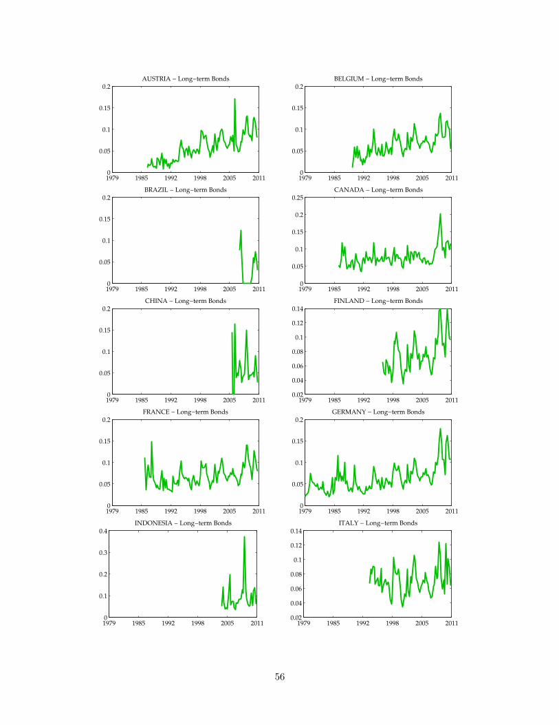
1979 1985 1992 1998 2005 20110

0.05

0.1

0.15

0.2AUSTRIA − Long−term Bonds

1979 1985 1992 1998 2005 20110

0.05

0.1

0.15

0.2BELGIUM − Long−term Bonds

1979 1985 1992 1998 2005 20110

0.05

0.1

0.15

0.2BRAZIL − Long−term Bonds

1979 1985 1992 1998 2005 20110

0.05

0.1

0.15

0.2

0.25CANADA − Long−term Bonds

1979 1985 1992 1998 2005 20110

0.05

0.1

0.15

0.2CHINA − Long−term Bonds

1979 1985 1992 1998 2005 20110.02

0.04

0.06

0.08

0.1

0.12

0.14FINLAND − Long−term Bonds

1979 1985 1992 1998 2005 20110

0.05

0.1

0.15

0.2FRANCE − Long−term Bonds

1979 1985 1992 1998 2005 20110

0.05

0.1

0.15

0.2GERMANY − Long−term Bonds

1979 1985 1992 1998 2005 20110

0.1

0.2

0.3

0.4INDONESIA − Long−term Bonds

1979 1985 1992 1998 2005 20110.02

0.04

0.06

0.08

0.1

0.12

0.14ITALY − Long−term Bonds

56

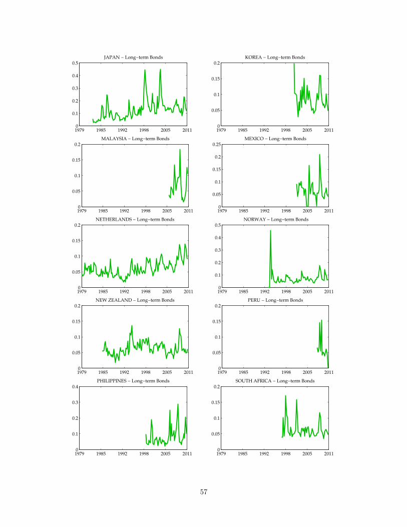
1979 1985 1992 1998 2005 20110

0.1

0.2

0.3

0.4

0.5JAPAN − Long−term Bonds

1979 1985 1992 1998 2005 20110

0.05

0.1

0.15

0.2KOREA − Long−term Bonds

1979 1985 1992 1998 2005 20110

0.05

0.1

0.15

0.2MALAYSIA − Long−term Bonds

1979 1985 1992 1998 2005 20110

0.05

0.1

0.15

0.2

0.25MEXICO − Long−term Bonds

1979 1985 1992 1998 2005 20110

0.05

0.1

0.15

0.2NETHERLANDS − Long−term Bonds

1979 1985 1992 1998 2005 20110

0.1

0.2

0.3

0.4

0.5NORWAY − Long−term Bonds

1979 1985 1992 1998 2005 20110

0.05

0.1

0.15

0.2NEW ZEALAND − Long−term Bonds

1979 1985 1992 1998 2005 20110

0.05

0.1

0.15

0.2PERU − Long−term Bonds

1979 1985 1992 1998 2005 20110

0.1

0.2

0.3

0.4PHILIPPINES − Long−term Bonds

1979 1985 1992 1998 2005 20110

0.05

0.1

0.15

0.2SOUTH AFRICA − Long−term Bonds

57

1979 1985 1992 1998 2005 20110

0.05

0.1

0.15

0.2

0.25SINGAPORE − Long−term Bonds

1979 1985 1992 1998 2005 20110

0.05

0.1

0.15

0.2SPAIN − Long−term Bonds

1979 1985 1992 1998 2005 20110

0.05

0.1

0.15

0.2

0.25SWEDEN − Long−term Bonds

1979 1985 1992 1998 2005 20110

0.05

0.1

0.15

0.2

0.25SWITZERLAND − Long−term Bonds

1979 1985 1992 1998 2005 20110

0.1

0.2

0.3

0.4THAILAND − Long−term Bonds

1979 1985 1992 1998 2005 20110

0.05

0.1

0.15

0.2

0.25UK − Long−term Bonds

1979 1985 1992 1998 2005 20110

0.1

0.2

0.3

0.4USA − Long−term Bonds

1979 1985 1992 1998 2005 20110

0.1

0.2

0.3

0.4CORN − Commodity Prices

1979 1985 1992 1998 2005 20110

0.05

0.1

0.15

0.2

0.25SOYBEAN − Commodity Prices

1979 1985 1992 1998 2005 20110

0.1

0.2

0.3

0.4WHEAT − Commodity Prices

58

1979 1985 1992 1998 2005 20110

0.1

0.2

0.3

0.4

0.5COFFEE − Commodity Prices

1979 1985 1992 1998 2005 20110

0.1

0.2

0.3

0.4RICE − Commodity Prices

1979 1985 1992 1998 2005 20110

0.2

0.4

0.6

0.8SUGAR − Commodity Prices

1979 1985 1992 1998 2005 20110.05

0.1

0.15

0.2

0.25COCOA − Commodity Prices

1979 1985 1992 1998 2005 20110

0.1

0.2

0.3

0.4

0.5GOLD − Commodity Prices

1979 1985 1992 1998 2005 20110

0.2

0.4

0.6

0.8SILVER − Commodity Prices

1979 1985 1992 1998 2005 20110

0.1

0.2

0.3

0.4COPPER − Commodity Prices

1979 1985 1992 1998 2005 20110.04

0.06

0.08

0.1

0.12NATURAL GAS − Commodity Prices

1979 1985 1992 1998 2005 20110

0.1

0.2

0.3

0.4COAL − Commodity Prices

1979 1985 1992 1998 2005 20110

0.2

0.4

0.6

0.8OIL (CO1) − Commodity Prices

59

1979 1985 1992 1998 2005 20110

0.05

0.1

0.15

0.2LIVESTOCK − Commodity Prices

1979 1985 1992 1998 2005 20110.02

0.04

0.06

0.08

0.1

0.12

0.14MEAT & LIVESTOCK − Commodity Prices

60

Table D.1 Realized Volatility of Equity Prices

Obs Mean Median Max Min St. Dev. Auto Corr. Skew. Kurt.

ARGENTINA 94 0.21 0.16 1.00 0.08 0.14 0.57 2.89 14.16AUSTRALIA 130 0.08 0.07 0.34 0.03 0.04 0.34 4.01 26.18AUSTRIA 130 0.07 0.06 0.31 0.01 0.05 0.76 2.02 8.29BELGIUM 130 0.07 0.06 0.24 0.03 0.04 0.62 2.13 8.28BRAZIL 86 0.25 0.16 1.83 0.07 0.26 0.81 3.84 20.00CANADA 130 0.07 0.06 0.34 0.03 0.04 0.62 2.87 15.42CHINA 74 0.15 0.13 0.42 0.07 0.07 0.58 1.38 5.49CHILE 94 0.08 0.07 0.24 0.04 0.03 0.39 1.82 7.42FINLAND 94 0.15 0.11 0.77 0.04 0.10 0.54 3.03 18.06FRANCE 130 0.09 0.07 0.28 0.04 0.04 0.48 2.05 8.67GERMANY 130 0.09 0.08 0.34 0.04 0.04 0.46 2.64 16.14INDIA 97 0.12 0.10 0.29 0.05 0.05 0.48 1.16 3.75INDONESIA 94 0.14 0.12 0.57 0.04 0.08 0.41 2.37 11.09ITALY 130 0.10 0.09 0.28 0.04 0.04 0.55 1.55 6.19JAPAN 130 0.09 0.09 0.34 0.03 0.04 0.50 2.09 12.02KOREA 130 0.12 0.10 0.34 0.03 0.06 0.69 1.43 5.49MALAYSIA 125 0.09 0.08 0.47 0.03 0.06 0.44 3.09 15.99MEXICO 94 0.12 0.11 0.30 0.05 0.05 0.47 1.68 7.02NETHERLANDS 130 0.08 0.07 0.30 0.03 0.04 0.59 2.32 9.92NORWAY 125 0.11 0.10 0.39 0.05 0.05 0.47 2.96 15.66NEW ZEALAND 94 0.09 0.08 0.24 0.04 0.04 0.49 1.55 6.27PERU 74 0.13 0.13 0.45 0.06 0.06 0.57 2.10 10.70PHILIPPINES 101 0.12 0.10 0.44 0.04 0.06 0.51 2.35 11.69SOUTH AFRICA 130 0.12 0.11 0.41 0.04 0.05 0.35 2.12 10.14SAUDI ARABIA 24 0.15 0.14 0.34 0.07 0.07 0.19 1.07 3.63SINGAPORE 130 0.09 0.08 0.39 0.04 0.05 0.42 2.63 13.89SPAIN 130 0.08 0.07 0.29 0.03 0.04 0.58 1.75 7.60SWEDEN 117 0.10 0.08 0.30 0.04 0.05 0.55 1.54 5.58SWITZERLAND 130 0.07 0.06 0.25 0.02 0.04 0.51 2.13 9.07THAILAND 97 0.13 0.11 0.30 0.06 0.06 0.50 1.23 3.97TURKEY 94 0.21 0.20 0.42 0.07 0.07 0.57 0.73 3.07UK 130 0.08 0.07 0.29 0.03 0.04 0.47 2.46 11.27USA 130 0.08 0.07 0.34 0.03 0.04 0.55 3.32 18.25

61

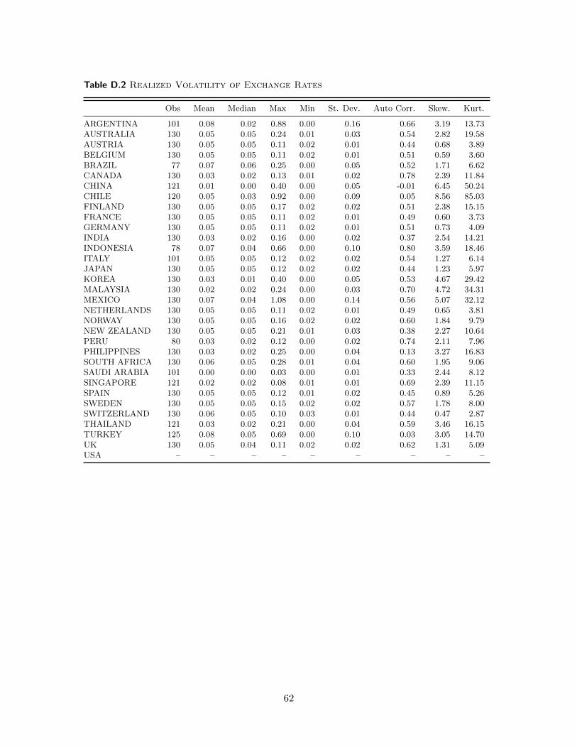
Table D.2 Realized Volatility of Exchange Rates

Obs Mean Median Max Min St. Dev. Auto Corr. Skew. Kurt.

ARGENTINA 101 0.08 0.02 0.88 0.00 0.16 0.66 3.19 13.73AUSTRALIA 130 0.05 0.05 0.24 0.01 0.03 0.54 2.82 19.58AUSTRIA 130 0.05 0.05 0.11 0.02 0.01 0.44 0.68 3.89BELGIUM 130 0.05 0.05 0.11 0.02 0.01 0.51 0.59 3.60BRAZIL 77 0.07 0.06 0.25 0.00 0.05 0.52 1.71 6.62CANADA 130 0.03 0.02 0.13 0.01 0.02 0.78 2.39 11.84CHINA 121 0.01 0.00 0.40 0.00 0.05 -0.01 6.45 50.24CHILE 120 0.05 0.03 0.92 0.00 0.09 0.05 8.56 85.03FINLAND 130 0.05 0.05 0.17 0.02 0.02 0.51 2.38 15.15FRANCE 130 0.05 0.05 0.11 0.02 0.01 0.49 0.60 3.73GERMANY 130 0.05 0.05 0.11 0.02 0.01 0.51 0.73 4.09INDIA 130 0.03 0.02 0.16 0.00 0.02 0.37 2.54 14.21INDONESIA 78 0.07 0.04 0.66 0.00 0.10 0.80 3.59 18.46ITALY 101 0.05 0.05 0.12 0.02 0.02 0.54 1.27 6.14JAPAN 130 0.05 0.05 0.12 0.02 0.02 0.44 1.23 5.97KOREA 130 0.03 0.01 0.40 0.00 0.05 0.53 4.67 29.42MALAYSIA 130 0.02 0.02 0.24 0.00 0.03 0.70 4.72 34.31MEXICO 130 0.07 0.04 1.08 0.00 0.14 0.56 5.07 32.12NETHERLANDS 130 0.05 0.05 0.11 0.02 0.01 0.49 0.65 3.81NORWAY 130 0.05 0.05 0.16 0.02 0.02 0.60 1.84 9.79NEW ZEALAND 130 0.05 0.05 0.21 0.01 0.03 0.38 2.27 10.64PERU 80 0.03 0.02 0.12 0.00 0.02 0.74 2.11 7.96PHILIPPINES 130 0.03 0.02 0.25 0.00 0.04 0.13 3.27 16.83SOUTH AFRICA 130 0.06 0.05 0.28 0.01 0.04 0.60 1.95 9.06SAUDI ARABIA 101 0.00 0.00 0.03 0.00 0.01 0.33 2.44 8.12SINGAPORE 121 0.02 0.02 0.08 0.01 0.01 0.69 2.39 11.15SPAIN 130 0.05 0.05 0.12 0.01 0.02 0.45 0.89 5.26SWEDEN 130 0.05 0.05 0.15 0.02 0.02 0.57 1.78 8.00SWITZERLAND 130 0.06 0.05 0.10 0.03 0.01 0.44 0.47 2.87THAILAND 121 0.03 0.02 0.21 0.00 0.04 0.59 3.46 16.15TURKEY 125 0.08 0.05 0.69 0.00 0.10 0.03 3.05 14.70UK 130 0.05 0.04 0.11 0.02 0.02 0.62 1.31 5.09USA – – – – – – – – –

62

Table D.3 Realized Volatility of Long-term Bonds

Obs Mean Median Max Min St. Dev. Auto Corr. Skew. Kurt.

ARGENTINA – – – – – – – – –AUSTRALIA 129 0.08 0.07 0.19 0.00 0.03 0.57 0.69 4.69AUSTRIA 99 0.06 0.05 0.17 0.01 0.03 0.73 0.70 3.56BELGIUM 88 0.06 0.06 0.14 0.01 0.03 0.72 0.46 3.05BRAZIL 17 0.03 0.01 0.12 0.00 0.04 0.69 0.88 2.83CANADA 100 0.08 0.07 0.20 0.03 0.03 0.65 1.62 7.37CHINA 24 0.06 0.05 0.16 0.00 0.04 -0.12 1.11 3.57CHILE – – – – – – – – –FINLAND 61 0.08 0.07 0.14 0.04 0.02 0.74 0.70 3.11FRANCE 101 0.07 0.07 0.15 0.03 0.02 0.57 0.90 3.81GERMANY 130 0.06 0.06 0.18 0.02 0.03 0.78 1.30 4.95INDIA – – – – – – – – –INDONESIA 31 0.09 0.07 0.37 0.04 0.06 0.19 2.89 12.95ITALY 72 0.07 0.07 0.12 0.03 0.02 0.40 0.62 3.41JAPAN 114 0.13 0.12 0.45 0.02 0.08 0.73 1.72 7.00KOREA 42 0.09 0.08 0.20 0.03 0.04 0.38 1.05 4.07MALAYSIA 24 0.07 0.05 0.18 0.01 0.04 0.42 1.10 3.83MEXICO 39 0.06 0.06 0.21 0.00 0.04 0.25 1.33 6.40NETHERLANDS 130 0.06 0.06 0.14 0.02 0.02 0.75 0.85 3.61NORWAY 74 0.07 0.06 0.46 0.00 0.06 0.07 4.72 32.99NEW ZEALAND 105 0.06 0.06 0.14 0.02 0.02 0.63 0.84 3.93PERU 14 0.06 0.05 0.15 0.00 0.04 -0.05 1.28 4.15PHILIPPINES 50 0.08 0.06 0.29 0.02 0.06 0.33 1.80 5.92SOUTH AFRICA 57 0.06 0.06 0.17 0.03 0.03 0.44 2.10 7.51SAUDI ARABIA – – – – – – – – –SINGAPORE 52 0.12 0.10 0.25 0.04 0.06 0.58 0.68 2.49SPAIN 73 0.08 0.07 0.17 0.03 0.02 0.50 1.31 6.44SWEDEN 83 0.08 0.07 0.21 0.04 0.03 0.59 1.90 8.13SWITZERLAND 69 0.10 0.09 0.23 0.03 0.04 0.75 1.16 4.43THAILAND 43 0.12 0.10 0.27 0.05 0.06 0.42 0.68 2.34TURKEY – – – – – – – – –UK 100 0.07 0.07 0.24 0.03 0.03 0.74 2.00 10.00USA 130 0.09 0.08 0.31 0.03 0.05 0.80 2.02 8.55

63

Table D.4 Realized Volatility of Commodity Prices

Obs Mean Median Max Min St. Dev. Auto Corr. Skew. Kurt.

CORN 130 0.12 0.10 0.28 0.04 0.05 0.50 1.04 4.00SOYBEAN 130 0.11 0.10 0.24 0.04 0.04 0.45 1.10 4.03WHEAT 130 0.13 0.12 0.30 0.05 0.04 0.59 1.17 4.57COFFEE 130 0.17 0.16 0.43 0.06 0.06 0.48 1.29 6.01RICE 90 0.13 0.12 0.30 0.05 0.05 0.39 1.09 4.91SUGAR 130 0.20 0.18 0.52 0.08 0.07 0.57 1.11 4.94COCOA 130 0.15 0.15 0.25 0.08 0.04 0.53 0.21 2.33GOLD 130 0.09 0.08 0.42 0.02 0.05 0.67 2.81 16.87SILVER 130 0.15 0.13 0.75 0.04 0.09 0.61 3.01 16.32COPPER 90 0.13 0.12 0.38 0.06 0.05 0.60 2.06 9.82NATURAL GAS 18 0.08 0.09 0.12 0.04 0.02 0.43 -0.27 2.33COAL 39 0.12 0.10 0.34 0.06 0.06 0.55 1.95 7.08OIL (CO1) 117 0.16 0.14 0.55 0.03 0.08 0.63 1.85 8.49LIVESTOCK 120 0.06 0.06 0.17 0.03 0.03 0.57 1.75 6.70MEAT & LIVEST. 59 0.05 0.05 0.13 0.02 0.02 0.23 1.51 5.20CRB INDEX 69 0.08 0.08 0.23 0.04 0.03 0.76 2.58 13.15LINSEED OIL 19 0.08 0.08 0.15 0.04 0.03 0.05 0.68 2.65

64

E Realized volatility pairwise correlations

In this appendix we report a full set of pairwise correlations. The average pairwise correlationof a volatility series RVκit (where i = 1, 2, ..., N is the number of countries and κ = 1, 2, ...,Mis the number of assets) is the cross-sectional average of the correlation between each pairthat these series for all i. Hence, the average pairwise correlation can be interpreted as anaverage measure of synchronization of the volatility measures for a given asset class.

Table E.1 Average Pairwise Correlation Across Countries

Equity Exch. Rate Bond

Level First Diff. Level First Diff. Level First Diff.ARGENTINA 0.22 0.29 -0.03 0.07 – –AUSTRALIA 0.54 0.56 0.33 0.30 0.47 0.38AUSTRIA 0.43 0.48 0.39 0.38 0.50 0.37BELGIUM 0.53 0.50 0.40 0.38 0.57 0.46BRAZIL 0.16 0.15 0.24 0.23 -0.29 0.08CANADA 0.55 0.58 0.23 0.32 0.52 0.33CHINA 0.61 0.51 -0.03 -0.05 0.32 0.27CHILE 0.42 0.45 0.03 -0.02 – –FINLAND 0.34 0.19 0.35 0.30 0.57 0.48FRANCE 0.56 0.57 0.42 0.39 0.57 0.46GERMANY 0.60 0.58 0.42 0.41 0.54 0.44INDIA 0.37 0.28 0.17 0.12 – –INDONESIA 0.38 0.25 0.15 0.23 0.49 0.29ITALY 0.47 0.46 0.42 0.41 0.50 0.43JAPAN 0.52 0.48 0.25 0.27 0.31 0.23KOREA 0.46 0.39 0.19 0.11 0.32 0.28MALAYSIA 0.38 0.39 0.14 0.12 0.30 0.15MEXICO 0.51 0.52 0.06 0.04 0.40 0.30NETHERLANDS 0.54 0.56 0.41 0.41 0.56 0.47NORWAY 0.55 0.59 0.41 0.37 0.36 0.18NEW ZEALAND 0.49 0.39 0.26 0.24 0.40 0.34PERU 0.44 0.58 0.17 -0.09 0.40 0.16PHILIPPINES 0.43 0.33 0.07 -0.02 0.21 0.15SOUTH AFRICA 0.49 0.53 0.23 0.26 0.29 0.31SAUDI ARABIA 0.46 0.48 0.10 0.08 – –SINGAPORE 0.58 0.52 0.28 0.27 0.49 0.41SPAIN 0.54 0.55 0.38 0.34 0.49 0.40SWEDEN 0.57 0.56 0.36 0.31 0.56 0.46SWITZERLAND 0.56 0.57 0.37 0.36 0.54 0.47THAILAND 0.46 0.40 0.09 0.07 0.38 0.26TURKEY 0.36 0.37 0.04 0.04 – –UK 0.56 0.57 0.37 0.35 0.52 0.35USA 0.59 0.58 – – 0.55 0.42

Note. Level indicates that the pairwise correlations have been computed on the level of thevolatility variables as in equation 20; First difference indicates that the pairwise correlations havebeen computed on the first difference of the volatility variables.

65