THE DERIVE - NEWSLETTER #81 - austromath.at · An International Scientific Journal of Sapientia...
52
THE DERIVE - NEWSLETTER #81 ISSN 1990-7079 THE BULLETIN OF THE USER GROUP C o n t e n t s: 1 Letter of the Editor 2 Editorial - Preview 3 Recommended Websites Duncan E. McDougall 5 Diophantine Polynomials (1) Piotr Trebisz 22 Ein mathematisches Modell für Schneckenhäuser A Mathematical Model for Snail Shells 38 User Forum Robert Setif & Josef Böhm 44 Request: Calculation Time and “π in slices”? March 2011
Transcript of THE DERIVE - NEWSLETTER #81 - austromath.at · An International Scientific Journal of Sapientia...
THE DERIVE - NEWSLETTER #81 ISSN 1990-7079
T H E B U L L E T I N O F T H E
U S E R G R O U P C o n t e n t s: 1 Letter of the Editor 2 Editorial - Preview 3 Recommended Websites Duncan E. McDougall 5 Diophantine Polynomials (1) Piotr Trebisz 22 Ein mathematisches Modell für Schneckenhäuser A Mathematical Model for Snail Shells 38 User Forum Robert Setif & Josef Böhm 44 Request: Calculation Time and “π in slices”?
March 2011

D-N-L#81
B o o k - s h e l f & I n f o r m a t i o n D-N-L#81
This is a great website: Images of Mathematicians on postage stamps
http://jeff560.tripod.com/stamps.html with not only the images but much information about mathematicians from all over the world
Download two Computer Algebra Systems free of charge: Octave and Xoctave: http://www.gnu.org/software/octave/ XCAS: Of Aide for free software XCAS , aid written by Renée de GRAEVE Université J Fourier GRENOBLE FRANCE. This AIDE is enormous. I have not the courage for translate it for you. You may find it on the site
www-fourier.ujf-grenoble.fr/~parisse/giac_fr.html
Thanks to Robert Setif for this information
A wonderful book about Strange Attractors can be downloaded free of charge (together with programs) from
http://sprott.physics.wisc.edu/sa.htm
http://sprott.physics.wisc.edu/fractals.htm
I plan an extended DNL-paper on this fascinating topic. “Create your own Strange Attractor!” (See two graphs on page 43.)
This is a website on Curves (in German) http://www.blaesius-anne.de/arbeit_kurven/kurvenG1a.html
SOME RELATED PUBLICATIONS FROM PREVIOUS FORMATEX ACTIVITIES -Book: “Research, Reflections and Innovations in Integrating ICT in Education”:
http://www.formatex.org/micte2009/volume1.htm
http://www.formatex.org/micte2009/volume2.htm
http://www.formatex.org/micte2009/volume3.htm
Zwei sehr schöne Bücher: Rainer Müller, Klassische Mechanik, De Gruyter 2010, ISBN 978 3 11 025002 2 Georg Glaeser, Wie aus der Zahl ein Zebra wurde, ein mathematisches
Fotoshooting, Spektrum 2010, ISBN 978 3 8274 2502 7
For TI-Nspire novices:
Steve Oullette, TI-Nspire for Dummies, Wiley Publishing 2009, ISBN 978 0 470 37934 9
Written by a math teacher, TI-Nspire For Dummies helps students and educators alike take full advantage of this outstanding tool for teaching and learning math.

D-N-L#81
L E T T E R O F T H E E D I T O R p 1
Liebe DUG-Mitglieder, und wieder war ich nicht rechtzeitig mit dem DNL! Wir haben in den 50 Seiten zwar „nur“ drei längere Artikel, aber diese haben in einem regen und langen Aus-tausch von emails eine bemerkenswerte Eigendyamik entwickelt. Viele Fragen, Ideen, Änderungen und Verbesserungs-vorschläge gingen hin und her. Wir hoffen, dass sich die Bemühungen für die Leser der Beiträge lohnen. Duncan Mc Dougall zeigt interessante Zusammenhänge in Polynomen mit ganzen Koeffizienten und rationalen Extremwer-ten. Piotr Trebisz nutzt die ganze „power“ eines CAS für die Berechnung und Dar-stellung von Schneckenhäusern. Robert Setif stellte mir ein nettes Problem, das ich dann doch in seinem Sinn gelöst haben dürfte. Dietmar Oertel hat zwei inhaltsschwere Papiere geschickt, die demnächst im DNL zu finden sein werden. Roger Folsom stellt im User Forum eine Frage an die DERIVE User, ein langer Brief von ihm steht für das nächste User Forum bereit. Auch mit David Sjöstrand hat es einen ausgedehn-ten – möglicherweise noch nicht beende-ten – Briefwechsel bezüglich des „Bewei-ses“ aus dem DNL#80 gegeben (Seite 40). Ich möchte Euch besonders auf die In-ternet Links hinweisen. Zwei mächtige CAS sind frei verfügbar. Das Buch von Julien C. Sprott über „Strange Attrac-tors“ ist eine Schatzkiste für “Frakta-listen”. Die deutschen Bücher auf der Info-seite sind ein wahrer Genuss für Auge und Hirn. Leider gibt es dieses Mal nur wenig zum TI-Nspire. Version 3 kann beeits von der TI-homepage bezogen werden. Die neuen Möglichkeiten wollen wir im nächsten DNL besprechen. Ich wünsche Euch eine schöne Zeit und verbleibe mit den besten Grüßen
Dear DUG Members, and again I was not in time with the DNL! We have 50 pages and „only“ three more extended articles. But these developped a remarkable momentum from an intense exchange of emails. Many questions, ideas, changes and proposals for improvements went to and fro. We hope that our ef-forts will be appreciated by the readers. Duncan Mc Dougall shows interesting rela-tionships in polynomials with integer coef-ficients and rational turning points. Piotr Trebisz uses the full „power“ of a CAS for the calculation and presentation of snail shells. Robert Setif presents a nice problem, which I could solve in his sense. Dietmar Oertel sent two very contentful papers which can be found in the next newsletters. Roger Folsom presents a request in the User Forum, a long letter is ready for publication in the next User Forum. I had an extended – possibly not yet finished – email exchange with David Sjöstrand concerning the „Proof“ from DNL#80 (page 40). I’d like to point especially to the internet links. Two powerful CAS can be downloaded free of charge. Julien C. Sprott’s book about “Strange Attractors“ is a treasure box for “fractalists“. The German books presented on the info page are a true pleasure for eyes and brain. Unfortunately we have little stuff for the TI-Nspire this time. Version 3 can be downloaded from the TI-website. We will talk about the new features in the next DNL. I wish you a good time and remain with my best regards,
Download all DNL-DERIVE- and TI-files from http://www.austromath.at/dug/

p 2
E D I T O R I A L
D-N-L#81
The DERIVE-NEWSLETTER is the Bulle-tin of the DERIVE & CAS-TI User Group. It is published at least four times a year with a contents of 40 pages minimum. The goals of the DNL are to enable the ex-change of experiences made with DERIVE, TI-CAS and other CAS as well to create a group to discuss the possibilities of new methodical and didactical manners in teaching mathematics.
Editor: Mag. Josef Böhm D´Lust 1, A-3042 Würmla Austria Phone: ++43-(0)660 3136365 e-mail: [email protected]
Contributions: Please send all contributions to the Editor. Non-English speakers are encouraged to write their contributions in English to rein-force the international touch of the DNL. It must be said, though, that non-English articles will be warmly welcomed nonethe-less. Your contributions will be edited but not assessed. By submitting articles the author gives his consent for reprinting it in the DNL. The more contributions you will send, the more lively and richer in contents the DERIVE & CAS-TI Newsletter will be. Next issue: June 2011
Preview: Contributions waiting to be published Some simulations of Random Experiments, J. Böhm, AUT, Lorenz Kopp, GER Wonderful World of Pedal Curves, J. Böhm Tools for 3D-Problems, P. Lüke-Rosendahl, GER Financial Mathematics 4, M. R. Phillips Hill-Encription, J. Böhm Simulating a Graphing Calculator in DERIVE, J. Böhm Henon & Co, J. Böhm Do you know this? Cabri & CAS on PC and Handheld, W. Wegscheider, AUT An Interesting Problem with a Triangle, Steiner Point, P. Lüke-Rosendahl, GER Overcoming Branch & Bound by Simulation, J. Böhm, AUT Graphics World, Currency Change, P. Charland, CAN Cubics, Quartics – Interesting features, T. Koller & J. Böhm Logos of Companies as an Inspiration for Math Teaching Exciting Surfaces in the FAZ / Pierre Charland´s Graphics Gallery BooleanPlots.mth, P. Schofield, UK Old traditional examples for a CAS – what´s new? J. Böhm, AUT Truth Tables on the TI, M. R. Phillips Where oh Where is It? (GPS with CAS), C. & P. Leinbach, USA Embroidery Patterns, H. Ludwig, GER Mandelbrot and Newton with DERIVE, Roman Hašek, CZ & Rob Gough, UK A Conics-Explorer, J. Böhm, AUT Tutorials for the NSpireCAS, G. Herweyers, BEL Some Projects with Students, R. Schröder, GER Dirac Algebra, Clifford Algebra, D. R. Lunsford, USA Treating Differential Equations (M. Beaudin, G. Piccard, Ch. Trottier) Structured Combinatorics, D. Oertel, GER A new approach to Taylor Series, D. Oertel, GER Statistics with TI-Nspire, G. Herweyers, BEL Cesar Multiplication, G. Schödl, AUT Find your very own Strange Attractor, J. Böhm, AUT and others
Impressum: Medieninhaber: DERIVE User Group, A-3042 Würmla, D´Lust 1, AUSTRIA Richtung: Fachzeitschrift Herausgeber: Mag.Josef Böhm

D-N-L#81
R e c o m m e n d e d W e b s i t e s p 3
I invite you browsing in higher mathematics journals. “emis” opens a spectacular view to the work of many mathematicians free of charge. You can find a rich collection of websites hosting mathematics journals from universities and mathematical societies from all over the world.
The Electronic Library of Mathematics
http://www.emis.de/elibm/journals/index.html
Acta Mathematica Academiae Paedagogicae Nyíregháziensis
Acta Mathematica Universitatis Comeniana,
Acta Universitatis Apulensis, Alba Julia, Romania
An International Scientific Journal of Sapientia University of Transylania, Romania
Analele Stiintifice ale Universitatii Ovidius Constanta, Romania
Annales Academiæ Scientiarum Fennicæ, Helsinki
Annales Mathematicae et Informaticae, Esterházy Károly College Eger
Applied Mathematics E-Notes, Taiwan
Archivum Mathematicum, Faculty of Science of Masaryk University Brno
Advances in Geometry
Algebra Montpellier Announcements
Algebraic and Geometric Topology (see also: http://msp.warwick.ac.uk/gtp/)
Balkan Journal of Geometry and Its Applications (Balkan Society of Geometers)
Beiträge zur Algebra und Geometrie / Contributions to Algebra and Geometry
Bulletin of the Venezuelan Mathematical Association
Sociedad de Estadística e Investigación Operativa
Bulletin of the Belgian Mathematical Society Simon Stevin
Bulletin of the Malaysian Mathematical Sciences Society
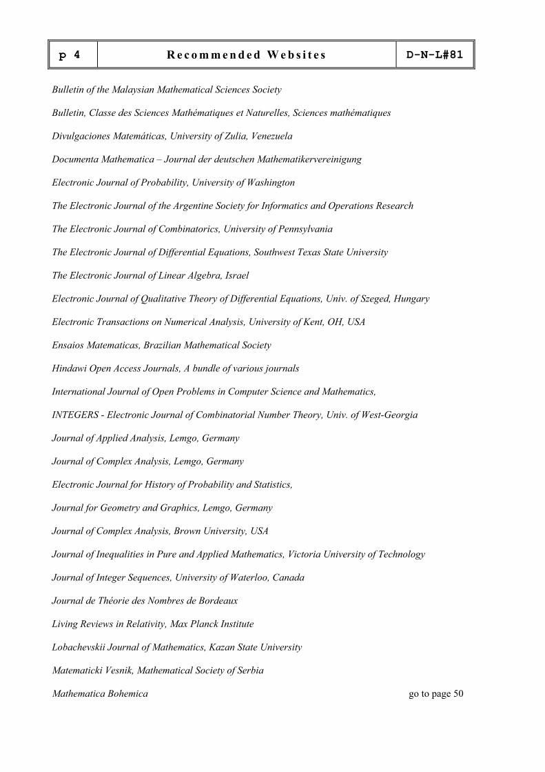
p 4
R e c o m m e n d e d W e b s i t e s D-N-L#81
Bulletin of the Malaysian Mathematical Sciences Society
Bulletin, Classe des Sciences Mathématiques et Naturelles, Sciences mathématiques
Divulgaciones Matemáticas, University of Zulia, Venezuela
Documenta Mathematica – Journal der deutschen Mathematikervereinigung
Electronic Journal of Probability, University of Washington
The Electronic Journal of the Argentine Society for Informatics and Operations Research
The Electronic Journal of Combinatorics, University of Pennsylvania
The Electronic Journal of Differential Equations, Southwest Texas State University
The Electronic Journal of Linear Algebra, Israel
Electronic Journal of Qualitative Theory of Differential Equations, Univ. of Szeged, Hungary
Electronic Transactions on Numerical Analysis, University of Kent, OH, USA
Ensaios Matematicas, Brazilian Mathematical Society
Hindawi Open Access Journals, A bundle of various journals
International Journal of Open Problems in Computer Science and Mathematics,
INTEGERS - Electronic Journal of Combinatorial Number Theory, Univ. of West-Georgia
Journal of Applied Analysis, Lemgo, Germany
Journal of Complex Analysis, Lemgo, Germany
Electronic Journal for History of Probability and Statistics,
Journal for Geometry and Graphics, Lemgo, Germany
Journal of Complex Analysis, Brown University, USA
Journal of Inequalities in Pure and Applied Mathematics, Victoria University of Technology
Journal of Integer Sequences, University of Waterloo, Canada
Journal de Théorie des Nombres de Bordeaux
Living Reviews in Relativity, Max Planck Institute
Lobachevskii Journal of Mathematics, Kazan State University
Matematicki Vesnik, Mathematical Society of Serbia
Mathematica Bohemica go to page 50
D-N-L#81
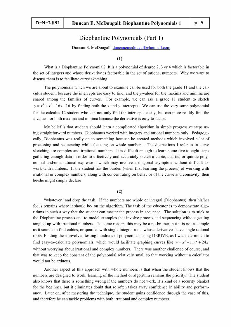
Duncan E. McDougall: Diophantine Polynomials 1 p 5
Diophantine Polynomials (Part 1)
Duncan E. McDougall, [email protected] (1)
What is a Diophantine Polynomial? It is a polynomial of degree 2, 3 or 4 which is factorable in the set of integers and whose derivative is factorable in the set of rational numbers. Why we want to discuss them is to facilitate curve sketching.
The polynomials which we are about to examine can be used for both the grade 11 and the cal-
culus student, because the intercepts are easy to find, and the y-values for the maxima and minima are shared among the families of curves. For example, we can ask a grade 11 student to sketch
3 2 16 16y x x x= + − − by finding both the x and y intercepts. We can use the very same polynomial for the calculus 12 student who can not only find the intercepts easily, but can more readily find the x-values for both maxima and minima because the derivative is easy to factor.
My belief is that students should learn a complicated algorithm in simple progressive steps us-
ing straightforward numbers. Diophantus worked with integers and rational numbers only. Pedagogi-cally, Diophantus was really on to something because he created methods which involved a lot of processing and sequencing while focusing on whole numbers. The distractions I refer to in curve sketching are complex and irrational numbers. It is difficult enough to learn some five to eight steps gathering enough data in order to effectively and accurately sketch a cubic, quartic, or quintic poly-nomial and/or a rational expression which may involve a diagonal asymptote without difficult-to-work-with numbers. If the student has the burden (when first learning the process) of working with irrational or complex numbers, along with concentrating on behavior of the curve and concavity, then he/she might simply declare
(2)
“whatever” and drop the task. If the numbers are whole or integral (Diophantus), then his/her focus remains where it should be- on the algorithm. The task of the educator is to demonstrate algo-rithms in such a way that the student can master the process in sequence. The solution is to stick to the Diophantine process and to model examples that involve process and sequencing without getting tangled up with irrational numbers. To some readers this may be a no-brainer, but it is not as simple as it sounds to find cubics, or quartics with single integral roots whose derivatives have single rational roots. Finding these involved testing hundreds of polynomials using DERIVE, as I was determined to find easy-to-calculate polynomials, which would facilitate graphing curves like 3 211 24y x x x= + + without worrying about irrational and complex numbers. There was another challenge of course, and that was to keep the constant of the polynomial relatively small so that working without a calculator would not be arduous.
Another aspect of this approach with whole numbers is that when the student knows that the
numbers are designed to work, learning of the method or algorithm remains the priority. The student also knows that there is something wrong if the numbers do not work. It’s kind of a security blanket for the beginner, but it eliminates doubt that so often takes away confidence in ability and perform-ance. Later on, after mastering the technique, the student gains confidence through the ease of this, and therefore he can tackle problems with both irrational and complex numbers.

p 6
Duncan E. McDougall: Diophantine Polynomials 1 D-N-L#81
It is my objective to propose families of cubics and quartics which are factorable in the integers
and whose derivatives are factorable in the set of rational numbers. I will also
(3)
propose methods using DERIVE by which you can construct your own polynomials. We’ll start with the very basic table of linear and quadratic polynomials then lead up to the cubics and quartics. I will end the paper with a brief discussion of the quintic, which should have worked but didn’t.
The following diagram (Table 1) contains all the various linear and quadratic forms along with
the general set of cubics. Using Table I
For example, take a cubic of the form ( )( )( )2 22x a x ab x b+ + + whose derivative has ra-
tional roots. Choosing any integers 1a = and 3b = for example, our new polynomial is
( )( )( )1 6 9x x x+ + + with roots 1, 6, and 9.− − − The differential form is 23 32 69x x+ + whose
roots are -3 and 233
− .
(4)
Table I
Family Function Roots Derivative Roots
Conditions on coefficients and constants to have integral roots
a none 0 none not applicable a x x = 0 a none not applicable
a x + b bx
a−
= a none not applicable
2( )x a+ x a= − 2 (x + a) x a= − none
x2 + a x 0,x a= − 2x + a 2ax = − a must be even
2 ( )( )( )
x x a b abx a x b+ + + =
= + + ,x a b= − − 2x + a + b
2a bx − −
= a and b are both odd or both even
2 ( )( )( )
acx x ad bc bdax b cx d+ + + =
= + + ,b dx
a c= − − 2acx ad bc+ +
2ad bcx
ac− −
=
a ≠ 0, c ≠ 0 ad + bc must either equal ac or be an even multiple of it
3( )x a+ x a= − 3(x + a)2 x a= − none

D-N-L#81
Duncan E. McDougall: Diophantine Polynomials 1 p 7
Family Function Roots Derivative Roots
Conditions on coeffs & consts to have integral roots
2( ) ( )x a x b+ + ,x a= −
b− 2(x + a) (3x +2b + a) 2,
3b ax a − −
= − 2b a+ is a multiple of 3
( )( )x x a x b+ + 0,x = ,a b− −
23 2 ( )x x a b ab+ + + 2 2( )
3
a b a ab bx
− + ± − +=
a2 – ab + b2 equals zero or a perfect square
2 2( )( 2 )( )x a x ab x b+ + + 2 ,x a= −
22 ,ab b− −
2
2 2
2 2
3(2 4 2 )(2 2 )
xx a ab bab a ab b
++ + + ++ + +
2 2
,
2 23
x ab
a ab b
= −
− − − 2a2 – ab + 2b2 must be a multiple of 3
( 1)( )( )x x a x a+ − + 1,x = − ,a a−
2 23 2x x a− − 21 1 3
3ax ± +
=
4+3a2 must be a perfect square (a = =0,1,4,15,...)
(5)
The polynomials in Table II consist of the particular numerical families with single roots. These are the ones that are ready to use in your classroom today.
As we observe the families in Table II (page 9), it is hard not to notice the pattern 8, 15, 21, 30, 35, and 36. It is a quadratic arithmetic sequence, whose elements (except for a couple) all work as families of curves.
In terms of methods for single roots let us begin by entering the form ( )( )x x a x b+ + into
DERIVE. This guarantees a factorable form. Press C for Calculus and differentiate. The resulting form is put in function form as DECLARE. Now we can either guess values and hope that our quad-ratic is factorable, or fix a value for “a”, and then guess values for “b” until the quadratic is factor-able. The question is, do we have anything to guide our guessing? In fact, we do. Visually, the val-ues of “x” for maxima and minima will occur between the first and last x-intercepts. Hence, if we were to choose 0 and 8 as two of our first and last roots, we would know that the third one must come between them. It’s just a question of leaving enough room between the roots so that the critical points can occur as integers and/or rational numbers. Algebraically, we enter ( )( )8x x a x− − into DERIVE,
and then differentiate giving ( )23 2 8 8 .x x a a+ − + Since
(6)
we have a quadratic; the discriminant 2 4B AC− must equal a perfect square in order to be factorable.
Using the command DECLARE, we set ( ) ( )2 24 32 256 4 8 64f a a a a a= − + = − + and evaluate (or
use the TI83 where second function gives “TABLE” and we search it for perfect squares). Both 3 and 5 come up quickly implying both ( )( )3 8x x x− − and ( )( )5 8x x x− − have derivatives whose roots
are rational.

p 8
Duncan E. McDougall: Diophantine Polynomials 1 D-N-L#81
You may like to continue working in DERIVE; then use the TABLE-command in connection with SELECT in order to find (more) values for a leading to a perfect square, Josef:
I don’t pretend to have all the families necessarily, but applying translations to any given family will yield many polynomials. The following is a small sample arrived at by adding a constant to all the terms: given family ( )( )3 8x x x− −
add 1 ( )( )( )1 2 7x x x+ − −
add 2 ( )( )( )2 1 6x x x+ − −
add 3 ( ) ( )3 5x x x+ −
add 4 ( )( )( )4 1 4x x x+ + −
add 5 ( )( )( )5 2 3x x x+ + −
add 6 ( )( )( )6 3 2x x x+ + −
add 7 ( )( )( )7 4 1x x x+ + −
add 8 ( )( )( )8 5x x x+ + , etc.

D-N-L#81
Duncan E. McDougall: Diophantine Polynomials 1 p 9
Interestingly enough, the entire above (all members of the famly) shares a maximum height of
400 5 4 20 ,27 3 3 3
= ⋅ ⋅ , and minimum low of 36− , and the difference between their corresponding
x-coordinates is exactly 143
. (The students can prove this, Josef)
A linear relationship exists between these values and those found in the quartics. We shall ex-plore this after exploring quartic family of curves.
(7)
Table II
Family Function Roots Derivative Roots Transformation
3 2
( 3)( 8)11 24
x x xx x x
+ +
+ + 0, -3, -8 2
(3 4)( 6)3 22 24
x xx x+ +
+ + 4 , 6
3− − ( )( 3 )( 8 )x k x a k x a k± ± ± ± ±
3 2
( 5)( 8)13 40
x x xx x x
+ +
+ + 0, -5, -8 2
(3 20)( 2)3 26 40
x xx x+ +
+ + 20 , 2
3− − ( )( 5 )( 8 )x k x a k x a k± ± ± ± ±
3 2
( 7)( 15)22 105
x x xx x x
+ +
+ + 0, -7,
-15 2
(3 35)( 3)3 44 105
x xx x+ +
+ + 35 , 3
3− − ( )( 7 )( 15 )x k x a k x a k± ± ± ± ±
3 2
( 8)( 15)23 120
x x xx x x
+ +
+ + 0, -8,
-15 2
(3 10)( 12)3 46 120
x xx x+ +
+ +
10 , 123
− −
( )( 8 )( 15 )x k x a k x a k± ± ± ± ±
3 2
( 5)( 21)26 105
x x xx x x
+ +
+ + 0, -5,
-21 2
(3 7)( 15)3 52 105
x xx x+ +
+ + 7 , 15
3− − ( )( 5 )( 21 )x k x a k x a k± ± ± ± ±
3 2
( 16)( 21)37 336
x x xx x x
+ +
+ + 0, -16,
-21 2
(3 56)( 6)3 74 336
x xx x+ +
+ + 56 , 6
3− − ( )( 16 )( 21 )x k x a k x a k± ± ± ± ±
( 26 )( 26)x x a x+ − + 3 2 (52 ) 26 (26 )x x a x a+ − + −
0, a - 26, - 26
2 23 52 26x x a a+ + − not rational
3 2
( 14)( 30)44 420
x x xx x x
+ +
+ + 0, -14,
-30 2
(3 70)( 6)3 88 420
x xx x+ +
+ + 70 , 6
3− − ( )( 14 )( 30 )x k x a k x a k± ± ± ± ±
3 2
( 16)( 30)46 480
x x xx x x
+ +
+ + 0, -16,
-30 2
(3 20)( 24)3 92 480
x xx x+ +
+ +
20 , 243
− −
( )( 16 )( 30 )x k x a k x a k± ± ± ± ±
( 33 )( 33)x x a x+ − + 3 2 (66 ) 33 (33 )x x a x a+ − + −
0, a - 33, -33
23 2 (66 )
1089 33
x x a
a
+ − +
+ − not rational
3 2
( 11)( 35)46 385
x x xx x x
+ +
+ + 0, -11,
-35 2
(3 77)( 5)3 92 385
x xx x+ +
+ + , 5
773
− − ( )( 11 )( 35 )x k x a k x a k± ± ± ± ±
3 2
( 24)( 35)59 840
x x xx x x
+ +
+ + 0, -24,
-35 2
(3 28)( 30)3 118 840
x xx x+ +
+ + 28
, 303
− − ( )( 24 )( 35 )x k x a k x a k± ± ± ± ±
( 36 )( 36)x x a x+ − + 3 2 (72 ) 36 (36 )x x a x a+ − + −
0, a - 36, -36
23 2 (72 )
1296 36
x x a
a
+ − +
+ − not rational

p 10
Duncan E. McDougall: Diophantine Polynomials 1 D-N-L#81
(8)
Having fully explored the cubic, the quartic family of curves presented quite a challenge be-cause there would be three roots, (other than zero), to find. Visually, I opted for a span of 7, (one less than the 8 for cubics) entered ( )( )( )7x x a x b x− − − into DERIVE, fixed 3a = (only because it had
worked with the cubic), took the derivative and evaluated “b” from 1 to 7 hoping some value “b” would work. The derived form was ( ) ( )3 24 3 30 20 42 21x x b x b b+ − − + + − and by declaring “f” as the
function I simply tested values for “b” and systematically factored (pressing F). To my great delight 4b = worked, giving ( )( )( )2 6 1 2 7x x x− − − . Observing 3 and 4 together, I acted on a hunch that
Pythagorean Triples might work. So following in the footsteps of Diophantus, I tried triplets begin-ning with odd numbers and even numbers, and they worked beautifully. An added bonus were those triplets with consecutive legs such as 20 - 21 - 29 and 119 - 120 - 169, etc., which also worked won-derfully. The patterns appear in Table III.
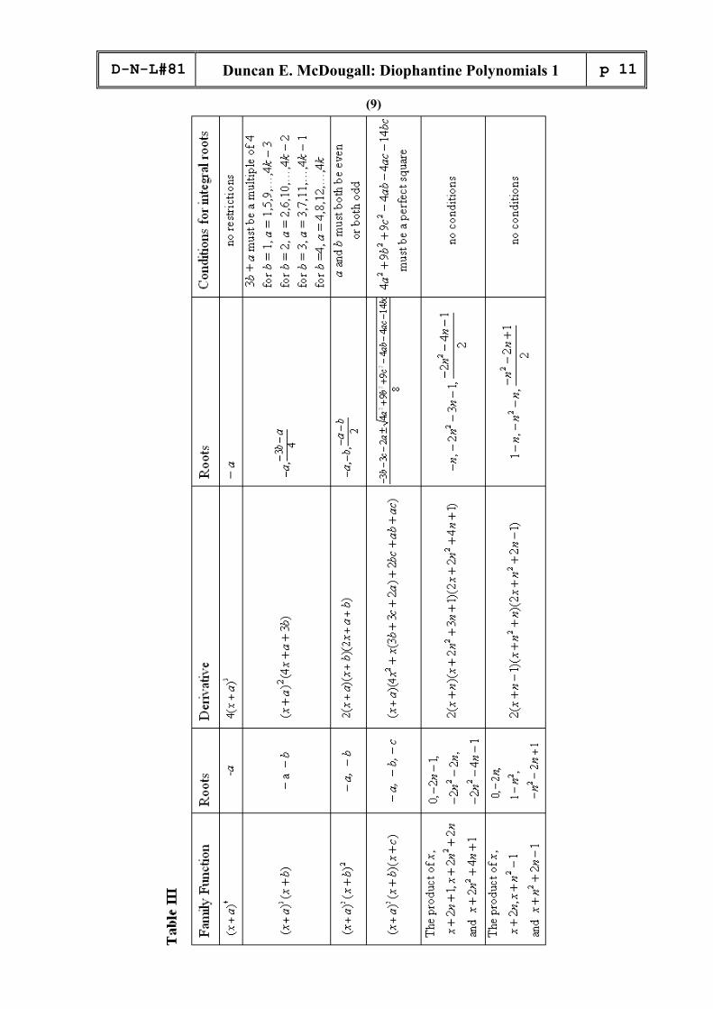
The numerical families of the form ( )( )( )x x a x b x c+ + + appear in Table IV. The numerical
families for the form ( )( )2x x a x b+ + appear in Table V.
Editor’s comment: How to use Table II for obtaining a bundle of cubics giving extremal values with rational x-coordinates:
D-N-L#81
Duncan E. McDougall: Diophantine Polynomials 1 p 11
(9)

p 12
Duncan E. McDougall: Diophantine Polynomials 1 D-N-L#81
(10)

D-N-L#81 Duncan E. McDougall: Diophantine Polynomials 1 p 13
(11)
Table V
Family Function Roots Derivative Roots Transformation 2 ( 5)( 7)x x x+ − 0, -5, 7 2 ( 5)(2 7)x x x− + 7,
20,5 − 2( ) ( 5 )( 7 )x k x a k x a k± + ± − ±
2 ( 5)( 2)x x x+ + 0, -5, -2, ( 5)(4 5)x x x+ + 5,4
0, 4 −− 2( ) ( 5 )( 2 )x k x a k x a k± + ± + ±
2 ( 5)( 9)x x x+ + 0, -5, -9 2 ( 3)(2 15)x x x+ + 15,2
0, 3 −− 2( ) ( 5 )( 9 )x k x a k x a k± + ± + ±
2 ( 7)( 10)x x x+ + 0, -7, -10 ( 4)(4 35)x x x+ + 35,4
0, 4 −− 2( ) ( 7 )( 10 )x k x a k x a k± + ± + ±
2 ( 9)( 14)x x x+ + 0, -9, -14 ( 12)(4 21)x x x+ + 21,4
0, 12 −− 2( ) ( 9 )( 14 )x k x a k x a k± + ± + ±
(12) The Quintic
In terms of multiple roots the quintic lends itself nicely to easy-to-work-with numbers which are small in quantity. However, for quintics of the form ( )( )( )( )x x a x b x c x d− − − − , the derivative
has no rational roots primarily because of Fermat’s Last Theorem whereby there are no integral values
for which 4 4 4x y z+ = . Having run the computer through thousands of number combinations (just to be sure), no derivative with rational roots could be found. Our Table VI contains multiple roots only.
Table VII contains the numerical families for the forms ( )( )3x x a x b+ + and ( ) ( )22x x a x b+ + .
With all the patterns that do work, it was too tempting not to try to make a linear link among the
cubic, quartic, and quintic forms. Let us examine the following facts:
I. Cubic Form x(x – 5)(x – 8)
Derivative (3x – 20)(x – 2)
Smallest Root 0
2
Largest Root 8
203
Range 8
143
Sum of Roots 13
26 5203 60=
II. Quartic Form x(x – 3)(x – 4) (x – 7)
Derivative 2(x – 1)(2x – 7) (x - 6)
Smallest Root 0
1
Largest Root 7
6
Range 7
5
Sum of Roots 14
21 6302 60=
III. Quintic Form x(x – 2)(x – 3)(x – 4)(x – 6)
Derivative 4 3 25 60 240 360 144x x x x− + − +
Smallest Root 0
0.616036…
Largest Root 6
5.383963…
Range 6
4.767926
Sum of Roots 15
12

p 14
Duncan E. McDougall: Diophantine Polynomials 1 D-N-L#81
(13)
D-N-L#81
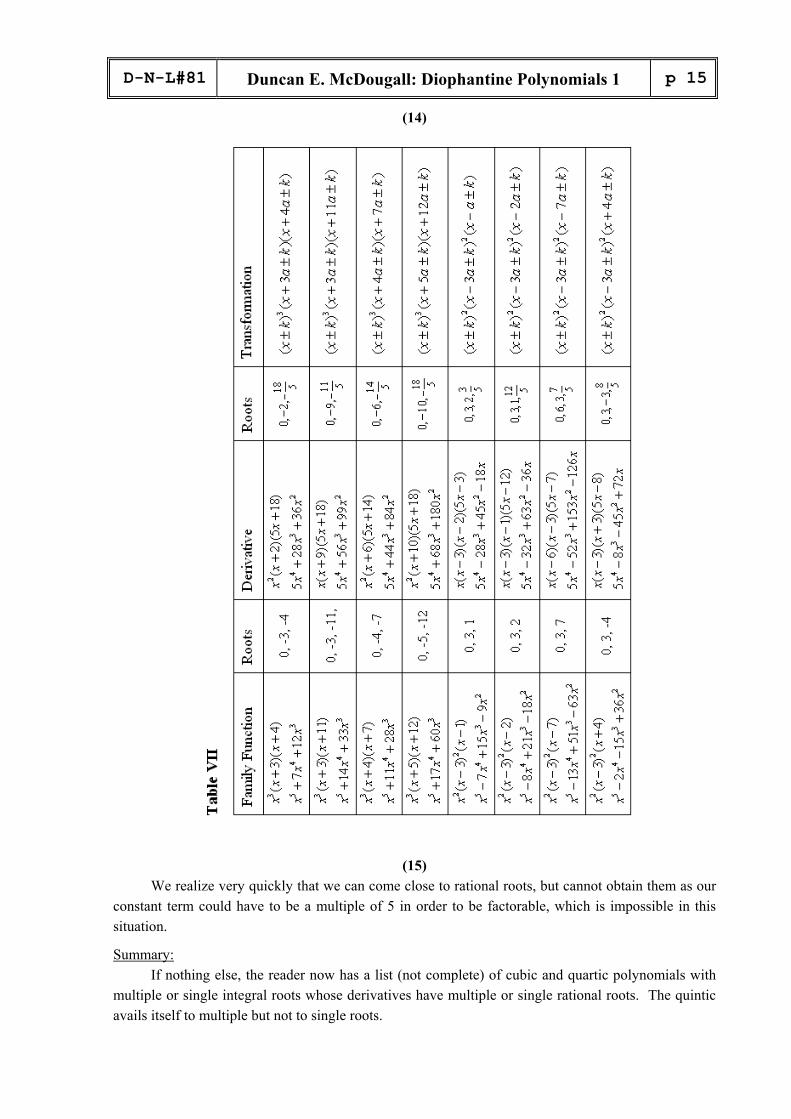
Duncan E. McDougall: Diophantine Polynomials 1 p 15
(14)
(15) We realize very quickly that we can come close to rational roots, but cannot obtain them as our
constant term could have to be a multiple of 5 in order to be factorable, which is impossible in this situation.
Summary: If nothing else, the reader now has a list (not complete) of cubic and quartic polynomials with
multiple or single integral roots whose derivatives have multiple or single rational roots. The quintic avails itself to multiple but not to single roots.

p 16
Duncan E. McDougall: Diophantine Polynomials 1 D-N-L#81
I would never have attempted all this work without the user-friendly program DERIVE, as I was
able to test many polynomials in seconds and quickly find derivative and corresponding factored forms. It goes without saying that the same Diophantine process can be applied to rational forms, making life a little easier for the curve sketcher.
Part 2 of the Diophantine Polynomials will follow.
Additional Editor’s Comments I enjoyed this contribution very much. As you might know from earlier articles I liked to use the computer as a training partner for the students providing random generated problems from various fields of the curriculum. Duncan mentioned that he used the TABLE function of the TI-83 for discovering certain ex-pressions as perfect squares. I felt inspired to use the TI-Nspire for producing random gen-erated polynomial functions. Take the quartics presented in Table IV (the Pythagorean Trip-lets). First of all we can – preferable together with the students – derive the condition(s) for having rational roots of the first derivative. (These are the first three lines in the Calculator Applica-tion of NspireCAS below.) Then let’s discuss how to produce Pythagorean Triplets – and finally use the spread sheet application to create random Pythagorean Triplets.
2 2 2 2
2 2 2
, 2 ,x m n y mn z m nx y z
= − = = +
+ =
ifthen
This is shown in the next screen shot.
In columns A and B are defined random generated integer numbers between -10 and +10 (without 0). Cell A1 and B1 contain the same formula which must be copied down – say 20 times. In columns C, D and E are the values for the constants a, b, and a + b of the polynomial g. As you can see we obtain pretty much nice triplets of numbers.

D-N-L#81
Duncan E. McDougall: Diophantine Polynomials 1 p 17
The next three lines of the calculator present a test, if the roots of the first derivative are really rational numbers. I took the values of rows 1, 5, and 16. Let the students confirm the calculation by plotting one or more function graphs and investi-gating the turning points:
p 18
Duncan E. McDougall: Diophantine Polynomials 1 D-N-L#81
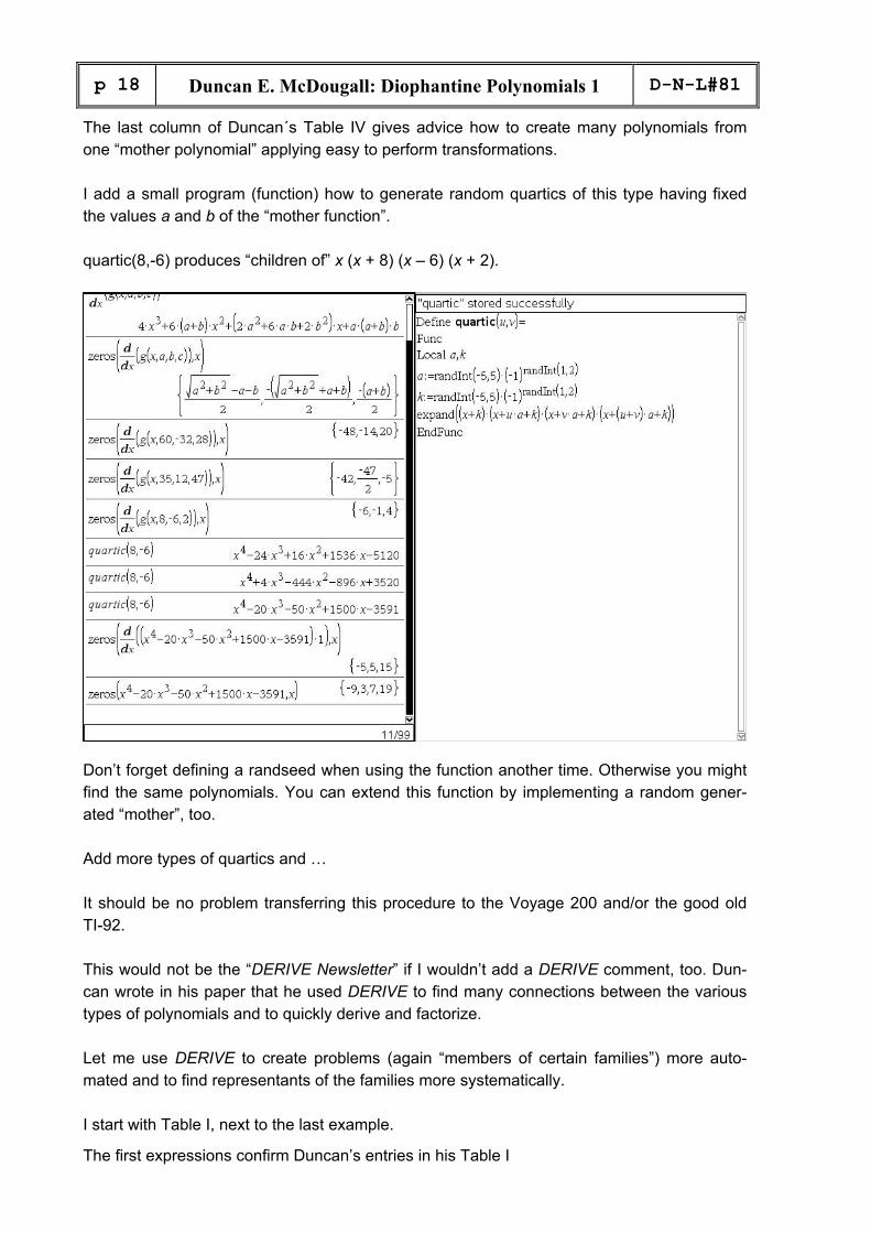
The last column of Duncan´s Table IV gives advice how to create many polynomials from one “mother polynomial” applying easy to perform transformations. I add a small program (function) how to generate random quartics of this type having fixed the values a and b of the “mother function”. quartic(8,-6) produces “children of” x (x + 8) (x – 6) (x + 2).
Don’t forget defining a randseed when using the function another time. Otherwise you might find the same polynomials. You can extend this function by implementing a random gener-ated “mother”, too. Add more types of quartics and … It should be no problem transferring this procedure to the Voyage 200 and/or the good old TI-92. This would not be the “DERIVE Newsletter” if I wouldn’t add a DERIVE comment, too. Dun-can wrote in his paper that he used DERIVE to find many connections between the various types of polynomials and to quickly derive and factorize. Let me use DERIVE to create problems (again “members of certain families”) more auto-mated and to find representants of the families more systematically. I start with Table I, next to the last example.
The first expressions confirm Duncan’s entries in his Table I
D-N-L#81
Duncan E. McDougall: Diophantine Polynomials 1 p 19
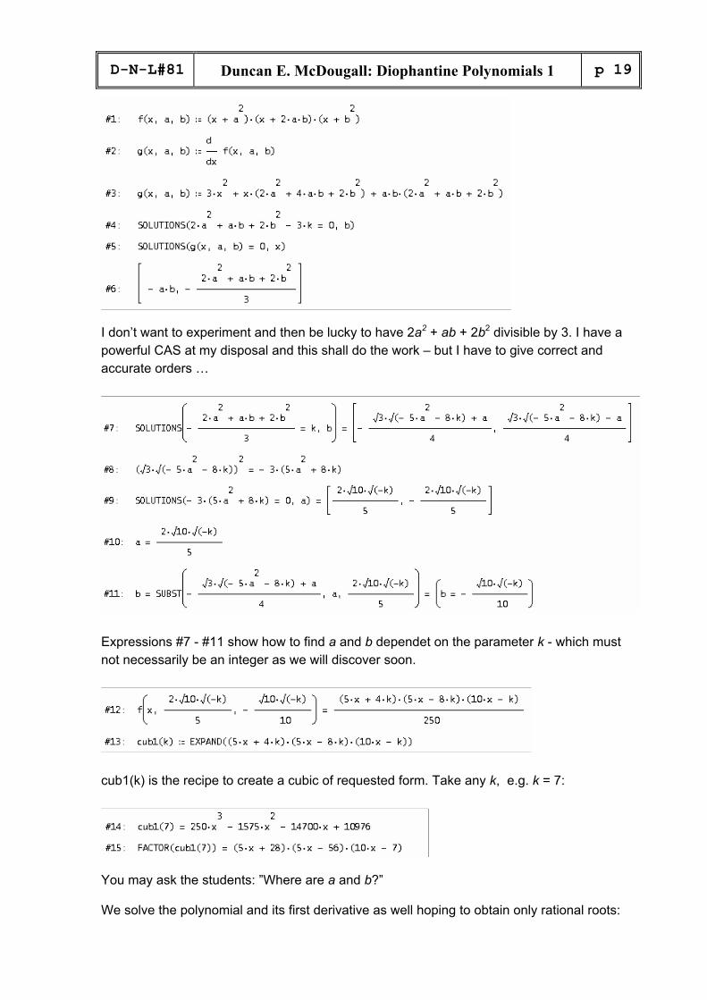
I don’t want to experiment and then be lucky to have 2a2 + ab + 2b2 divisible by 3. I have a powerful CAS at my disposal and this shall do the work – but I have to give correct and accurate orders …
Expressions #7 - #11 show how to find a and b dependet on the parameter k - which must not necessarily be an integer as we will discover soon.
cub1(k) is the recipe to create a cubic of requested form. Take any k, e.g. k = 7:
You may ask the students: ”Where are a and b?” We solve the polynomial and its first derivative as well hoping to obtain only rational roots:
p 20
Duncan E. McDougall: Diophantine Polynomials 1 D-N-L#81
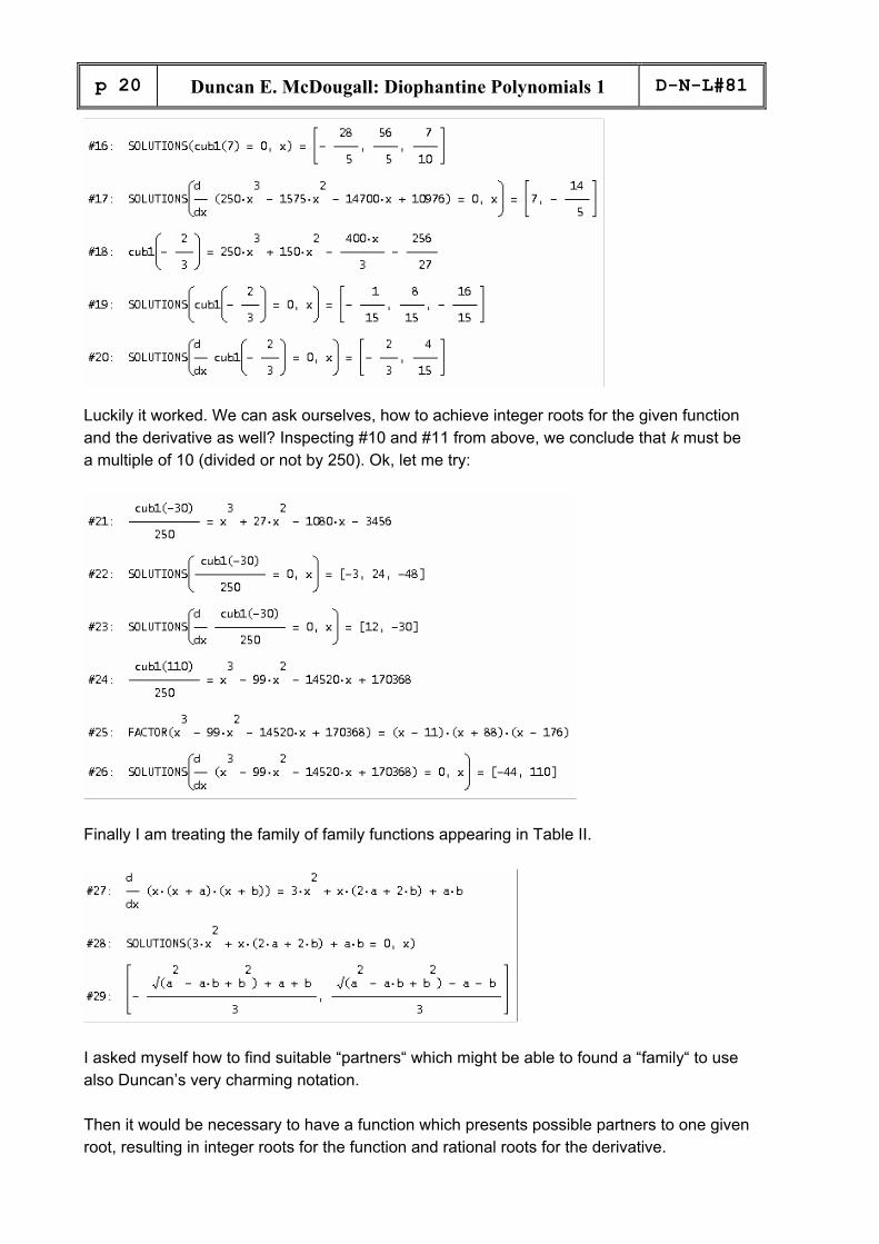
Luckily it worked. We can ask ourselves, how to achieve integer roots for the given function and the derivative as well? Inspecting #10 and #11 from above, we conclude that k must be a multiple of 10 (divided or not by 250). Ok, let me try:
Finally I am treating the family of family functions appearing in Table II.
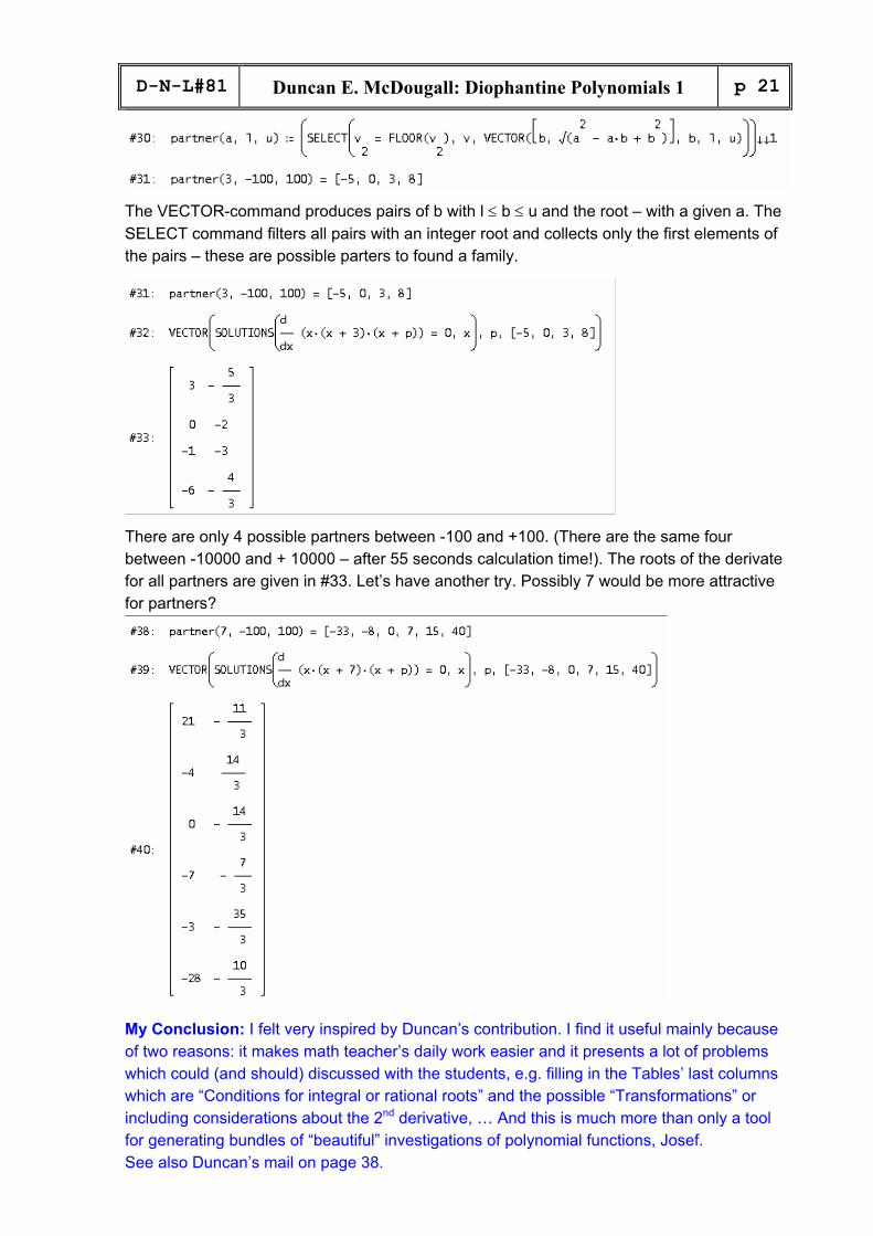
I asked myself how to find suitable “partners“ which might be able to found a “family“ to use also Duncan’s very charming notation. Then it would be necessary to have a function which presents possible partners to one given root, resulting in integer roots for the function and rational roots for the derivative.
D-N-L#81
Duncan E. McDougall: Diophantine Polynomials 1 p 21
The VECTOR-command produces pairs of b with l ≤ b ≤ u and the root – with a given a. The SELECT command filters all pairs with an integer root and collects only the first elements of the pairs – these are possible parters to found a family.
There are only 4 possible partners between -100 and +100. (There are the same four between -10000 and + 10000 – after 55 seconds calculation time!). The roots of the derivate for all partners are given in #33. Let’s have another try. Possibly 7 would be more attractive for partners?
My Conclusion: I felt very inspired by Duncan’s contribution. I find it useful mainly because of two reasons: it makes math teacher’s daily work easier and it presents a lot of problems which could (and should) discussed with the students, e.g. filling in the Tables’ last columns which are “Conditions for integral or rational roots” and the possible “Transformations” or including considerations about the 2nd derivative, … And this is much more than only a tool for generating bundles of “beautiful” investigations of polynomial functions, Josef. See also Duncan’s mail on page 38.

p 22
Piotr Trebisz: A Mathematical Model for Snail Shells D-N-L#81
Ein Mathematisches Modell für Schneckenhäuser
A Mathematical Model for Snail Shells
von Piotr Trebisz [email protected]
Wahrscheinlich ist schon jedem DERIVE-Nutzer der spiralförmige Torus aufgefallen der auf der Ver-packung von Derive abgebildet ist. Dieses geometrische Objekt hat mich dazu inspiriert, einen Beitrag über Schneckenhäuser zu schreiben, die auf logarithmischen Spiralen basieren.
Schneckenhäuser sind ein sehr schönes Beispiel dafür, dass logarithmische Spiralen ein häufig wie-derkehrendes Muster in der Natur sind. Logarithmische Spiralen sind selbstähnlich, das heißt, dass eine kleine Spirale genauso aussieht wie eine große Spirale. Das ermöglicht Schnecken ihre Häuser kontinuierlich weiterzubauen, ohne dass sich deren Geometrie ändert.
Ich werde im Laufe der folgenden Artikelreihe ein mathematisches Modell für solche Schneckenhäu-ser vorstellen. Da die von mir vorgestellten Schneckenhäuser einige besondere Eigenschaften haben, die so in der Literatur noch nirgendwo beschrieben wurden, nehme ich mir die Freiheit heraus, sie nach mir zu benennen: Die Trebisz-Spiralen.
Beginnen wir bei der Konstruktion unserer Schneckenhäuser mit einer einfachen Variante, bei der uns als Basis eine planare logarithmische Spirale dient, ähnlich wie bei einer Nautilus-Schale. Ich nenne sie „Trebisz-Spirale – Typ 1“
It is very likely that all DERIVE users have noticed the spiral formed torus on the package and the manual. This geometric object inspired me to write a paper on logarithmic based snail shells.
Snail shells are a very beautiful example for the fact that logarithmic spirals are a frequently recurring pattern in nature. Logarithmic spirals are self similar, i.e. a small spiral looks like a large one. And this enables snails building their shells continuously without changing their geometry.

D-N-L#81
Piotr Trebisz: A Mathematical Model for Snail Shells p 23
Over the following series of contributions I will introduce a mathematic model for such snail shells. As these snail shells will show some special properties, which I didn’t find elsewhere in literature, I take the freedom to call them Trebisz Spirals.
We will start constructing our snail shells with an easy model, taking a plane logarithmic spi-ral as base, very similar to a shell of a nautilus. I call it “Trebisz-Spiral – Type 1”.
Als Gerüst für das Schneckenhaus dient eine planare logarithmische Spirale die nach ihrem Radius bzw. ihrer Länge parametrisiert ist. Der Parameter „t“ steht hierbei für den Radius bzw. die Länge der Spirale, während „b“ die Basis des Logarithmus ist.
A plane logarithmic spiral which is parameterized according its radius and its length, respec-tively is serving as the shell’s scaffold. Parameter “t“ is standing for the radius and the length of the spiral, respectively, and “b“ is the base of the logarithm.
Example: SNAIL(e, t) SUB [2,3] with
0 ≤ t ≤ 1
The frequent reader of the DNL knows my devotion to sliders. We can ani-mate the base spirals in the 3D-plot window:
See the respective plot parameters to for presenting 5 rotations:
Josef

p 24
Piotr Trebisz: A Mathematical Model for Snail Shells D-N-L#81
Dass diese Spirale nach ihrem Radius parametrisiert ist, lässt sich leicht überprüfen, indem man sich anschaut, wie weit ein Punkt auf dieser Spirale vom Zentrum entfernt ist in Abhängigkeit von „t“.
It is easy to check that the radius is the parameter of this spiral by inspecting the distance of a point on the spiral to the centre dependent on “t“.
Dass die Spirale auch nach Ihrer Länge parametrisiert ist, lässt sich dadurch zeigen, dass die Tangente an jedem Punkt der Spirale eine konstante Länge hat
The fact that this spiral has also its length as parameter can be shown by demonstrating that the tangent on each spiral point has constant length.
Wie man sieht, ist die Spirale auch nach der Länge parametrisiert, aber multipliziert mit einem kon-stanten Maßstabs-Faktor.
Um den Mantel des Schneckenhauses zu konstruieren benötigen wir ein lokales mitdrehendes Koordi-natensystem aus 2 Vektoren die senkrecht zueinander und zur Tangente der Spirale stehen.
Dies gelingt uns, indem wir die 2. Ableitung der Spirale nach „t“ bestimmen. Dabei machen wir uns zu Nutze, dass die 2. Ableitung einer Kurve, die nach ihrer Länge parametrisiert ist, einen Vektor er-gibt, der in der Krümmungsebene der Kurve liegt und der senkrecht zu ihrer Tangente steht.
As one can see the spiral is also parameterized wrt its length multiplied by a constant scaling factor.
For constructing the surface of the snail shell we need a local co-rotating system of coordi-nates consisting of two vectors which are perpendicular to each other and perpendicular wrt the tangent of the spiral.
The 2nd derivative of the spiral wrt “t” can help. With its length as parameter the 2nd derivative of the curve results in a vector lying in the osculation plane of the curve perpendicular to its tangent.
Das Kreuzprodukt aus Tangente und 2. Ableitung liefert uns einen weiteren Vektor der senkrecht zur Tangente und zur 2. Ableitung steht. Dieser Vektor soll unsere lokale mitdrehende X-Achse sein. Und die lokale Y-Achse können wir direkt aus der 2. Ableitung nach „t“ bestimmen. Die lokale mitdrehen-de Z-Achse entspricht der Tangente der Spirale.
The cross product from tangent and 2nd derivative delivers another vector which is perpen-dicular to both tangent and 2nd derivative. This vector shall form our local co-rotating X-axis. The local Y-axis is given directly by the 2nd derivative wrt “t”. the local co-rotating Z-axis is the spiral tangent.
D-N-L#81
Piotr Trebisz: A Mathematical Model for Snail Shells p 25
Es lässt sich zeigen dass dieses lokale mitdrehende Koordinatensystem die selbe Händigkeit besitzt wie das globale Koordinatensystem, in dem die Spirale definiert ist.
We can show that this local co-rotating system of coordinates has the same direction as the global system where the spiral is defined.
Die Mantelfläche soll einfachheitshalber einen kreisförmigen Querschnitt haben. Der Radius der Man-telfläche soll linear mit dem Radius bzw. mit der Länge der Spirale wachsen, „m“ ist der Linearfaktor.
To make it easy we will have a circle as cross section of the surface. The radius of the sur-face shall increase linearly according to the radius – and the length – of the spiral with "m" as linear-factor.
Und schon ist das Schneckenhaus fertig. Es ist die Summe aus Spirale und Mantel.
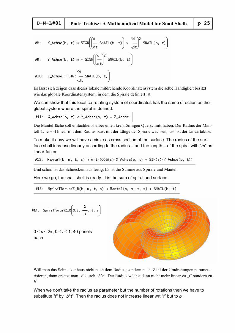
Here we go, the snail shell is ready. It is the sum of spiral and surface.
0 ≤ s ≤ 2π, 0 ≤ t ≤ 1; 40 panels each
Will man das Schneckenhaus nicht nach dem Radius, sondern nach Zahl der Umdrehungen paramet-risieren, dann ersetzt man „t“ durch „b^t“. Der Radius wächst dann nicht mehr linear zu „t“ sondern zu bt.
When we don’t take the radius as parameter but the number of rotations then we have to substitute "t" by "b^t". Then the radius does not increase linear wrt “t” but to bt.
p 26
Piotr Trebisz: A Mathematical Model for Snail Shells D-N-L#81
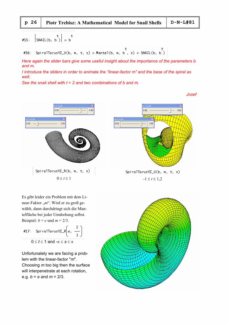
Here again the slider bars give some useful insight about the importance of the parameters b and m. I introduce the sliders in order to animate the “linear-factor m” and the base of the spiral as well. See the snail shell with t = 2 and two combinations of b and m.
Josef
0 ≤ t ≤ 1
-1 ≤ t ≤ 1,2
Es gibt leider ein Problem mit dem Li-near-Faktor „m“. Wird er zu groß ge-wählt, dann durchdringt sich die Man-telfläche bei jeder Umdrehung selbst. Beispiel: b = e und m = 2/3.
0 ≤ t ≤ 1 and -π ≤ s ≤ π Unfortunately we are facing a prob-lem with the linear-factor "m". Choosing m too big then the surface will interpenetrate at each rotation, e.g. b = e and m = 2/3.

D-N-L#81
Piotr Trebisz: A Mathematical Model for Snail Shells p 27
Wird „m“ zu klein gewählt, dann klafft bei jeder Umdrehung eine hässliche Lücke zwischen der Mantelfläche. Bei-spiel b = e und m = 1/4.
Choosing "m" too small, then we have an ugly gap between the sur-face, e.g. b = e and m = 1/4 Wie kann man zur Basis „b“ das richtige „m“ so bestimmen dass sich die Mantelfläche nach jeder Umdrehung exakt berührt, ohne sich selbst zu durchdringen? b = e und m = 0.4593761774.
How to determine the right “m“ for given base “b“ that the surface is osculating exactly after each full rotation without interpenetrating? b = e and m = 0.4593761774.
Dazu müssen wir uns den Schnitt des Schneckenhauses durch die XY-Ebene anschauen. Die Z-Koor-dinate von #16 (vereinfacht) muss also 0 sein. Wir lösen die entsprechende Gleichung nach „t“ auf:
We have to investigate the section of the snail shell with the XY-plane. Hence the Z-coordinate of simplified #16 must equal zero. We solve the respective equation for "t":
Wir können die gefundene Lösung verallgemeinern, denn das Schneckenhaus schneidet die XY-Ebene nicht nur einmal, sondern bei jeder halben Umdrehung. Wenn wir also zu der Lösung ein beliebiges ganzzahlige Vielfaches von 1/2 dazu addieren, dann erhalten wir wieder eine gültige Lösung. „k“ ist eine beliebige ganze Zahl.
We can generalize the found solution because the snail shell does not intersect the XY-plane only once but at every half rotation. We obtain another valid solution by adding any integer multiple of ½. ”k” is an arbitrary integer.
p 28
Piotr Trebisz: A Model for Snail Shells D-N-L#81
Für die Lösung des Selbstdurchdringungsprolems können wir aber nur jene Lösungen für „t“ gebrau-chen, die sich in einer ganzen Umdrehung unterscheiden, deshalb schränken wir die Lösungen für „t“ wie folgt ein:
For solving the interpenetrating problem we can use only such solutions for “t” which differ in a full rotation. We set a constraint for „t“ as follows:
Setzt man diese Lösung für „t“ in die Schneckenhaus-Formel ein, wird die Z-Koordinate 0 und man erhält den XY-Schnitt der Fläche, wo man sehen kann, ob sie sich selbst durchdringt oder nicht. Schauen wir uns mal ein paar Schnittkurven für k = 0 an:
Substituting this solution for "t" in in the formula for the snail house the Z-coordinate will be-come 0 and one obtains the XY-intersection of the surface. This section shows whether the surface is interpenetrating or not. We will look at some intersection curves for k = 0:
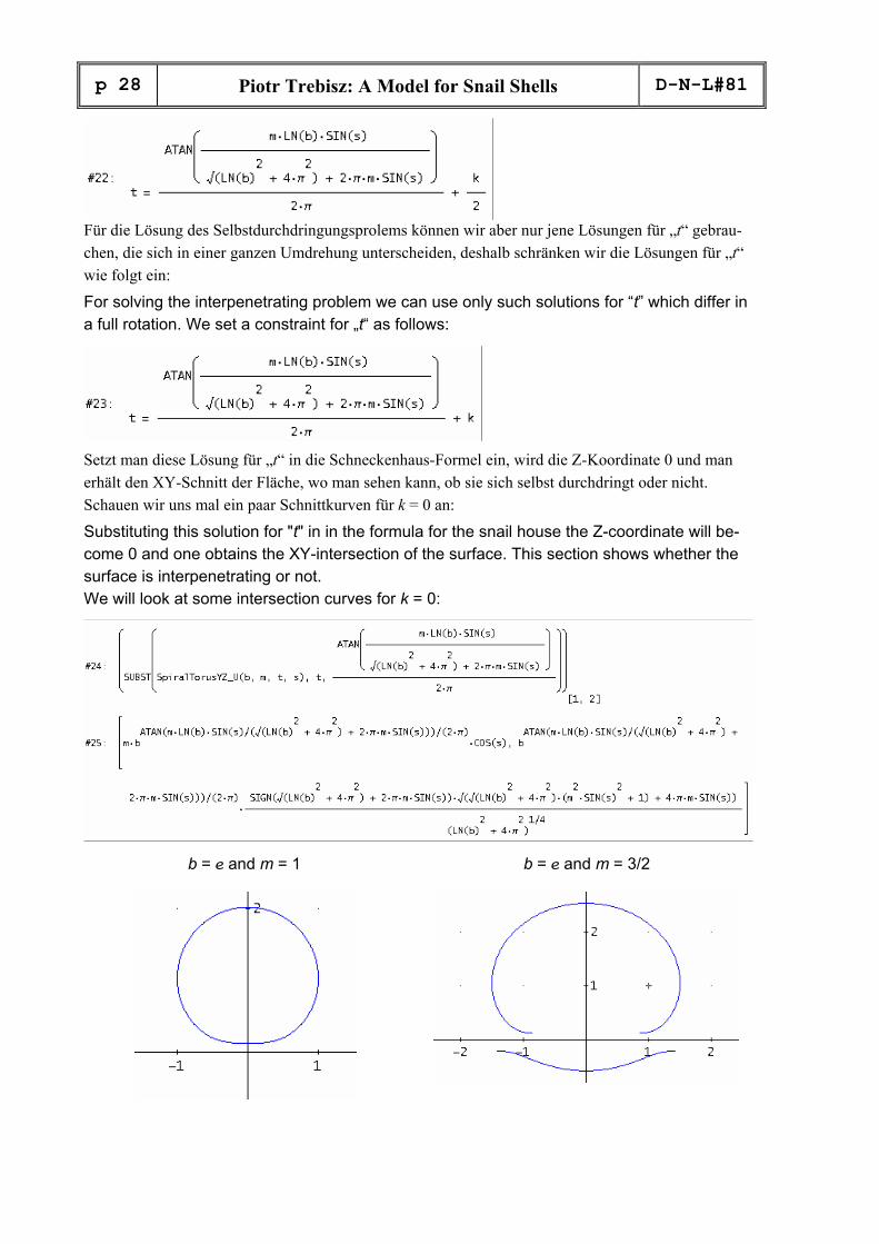
b = e and m = 1
b = e and m = 3/2
D-N-L#81
Piotr Trebisz: A Mathematical Model for Snail Shells p 29
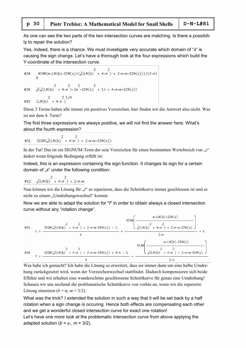
Hoppla!!! Warum ist denn im 2. Beispiel die Schnittkurve unterbrochen? Der Grund dafür liegt in der Lösung, die wir für „t“ bestimmt haben. Formal gesehen ist die Lösung vollkommen in Ordnung. Wenn man sie zur Probe in die Z-Koordinate des Schneckenhauses einsetzt, dann wird diese 0.
Nur hat die Lösung einen gravierenden Schönheitsfehler! Bei bestimmten Kombinationen von „b“ und „m“ zerfällt die Schnittkurve in zwei Teile, die zwar genau zusammenpassen, sich aber auch in genau einer halben Umdrehung unterscheiden! Das erkennt man daran, dass sich das zweite Stück der Schnittkurve auf der anderen Seite der X-Achse befindet. Dieses Kurvenstück gehört zum Schnitt des Schneckenhauses mit der XY-Ebene nach der nächsten halben Umdrehung!
Offensichtlich gibt es einen bestimmen Wertebereich von „s“, wo es in der Y-Koordinate zu einem Vorzeichenwechsel kommt. Und das wiederum führt zu einem „Umdrehungswechsel“ in der Schnitt-kurve! Dieser „Umdrehungswechsel“ zeigt sich sehr schön, wenn man sich die Schnittkurven für zwei Lösungen anschaut, die sich in einer halben Umdrehung unterscheiden.
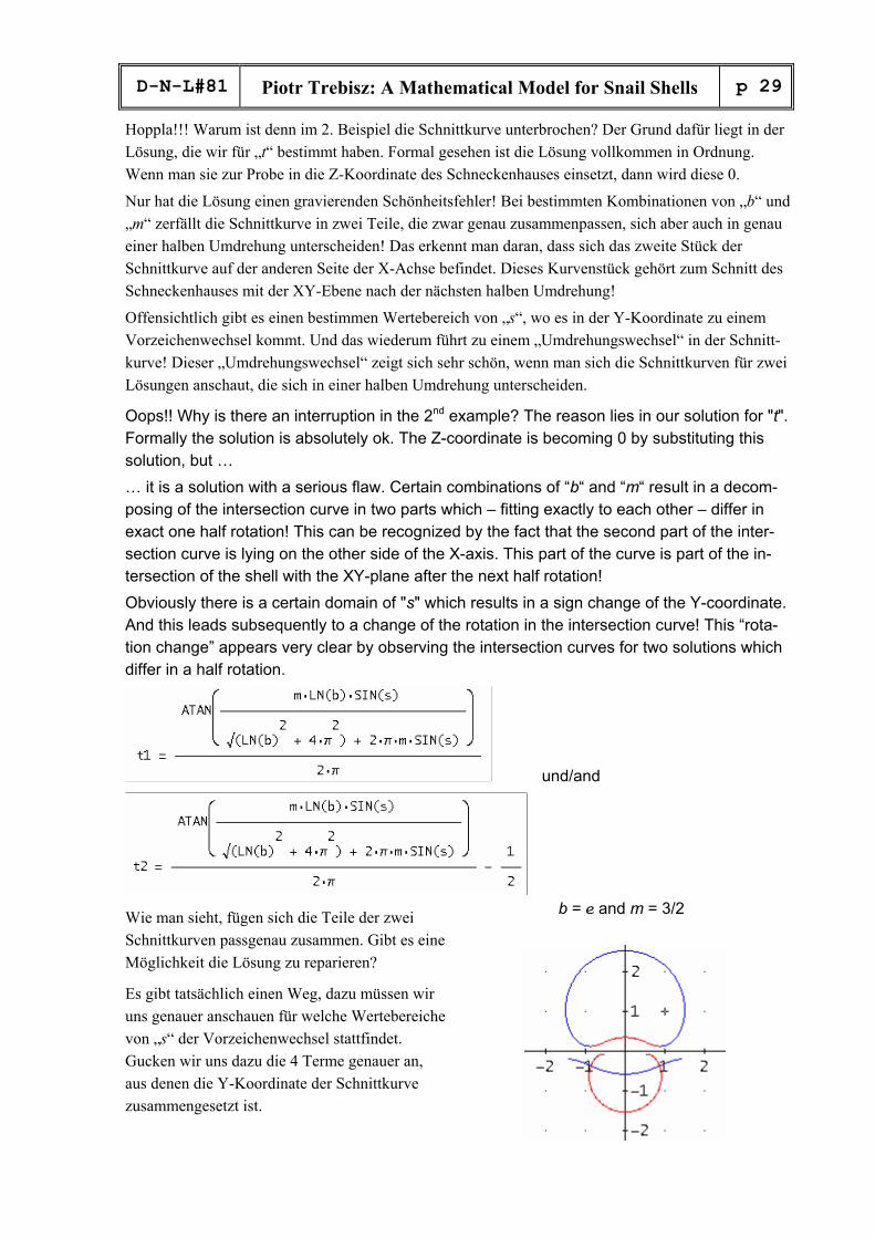
Oops!! Why is there an interruption in the 2nd example? The reason lies in our solution for "t". Formally the solution is absolutely ok. The Z-coordinate is becoming 0 by substituting this solution, but … … it is a solution with a serious flaw. Certain combinations of “b“ and “m“ result in a decom-posing of the intersection curve in two parts which – fitting exactly to each other – differ in exact one half rotation! This can be recognized by the fact that the second part of the inter-section curve is lying on the other side of the X-axis. This part of the curve is part of the in-tersection of the shell with the XY-plane after the next half rotation! Obviously there is a certain domain of "s" which results in a sign change of the Y-coordinate. And this leads subsequently to a change of the rotation in the intersection curve! This “rota-tion change” appears very clear by observing the intersection curves for two solutions which differ in a half rotation.
und/and
Wie man sieht, fügen sich die Teile der zwei Schnittkurven passgenau zusammen. Gibt es eine Möglichkeit die Lösung zu reparieren?
Es gibt tatsächlich einen Weg, dazu müssen wir uns genauer anschauen für welche Wertebereiche von „s“ der Vorzeichenwechsel stattfindet. Gucken wir uns dazu die 4 Terme genauer an, aus denen die Y-Koordinate der Schnittkurve zusammengesetzt ist.
b = e and m = 3/2
p 30
Piotr Trebisz: A Mathematical Model for Snail Shells D-N-L#81
As one can see the two parts of the two intersection curves are matching. Is there a possibili-ty to repair the solution? Yes, indeed, there is a chance. We must investigate very accurate which domain of “s“ is causing the sign change. Let’s have a thorough look at the four expressions which build the Y-coordinate of the intersection curve.
Diese 3 Terme haben alle immer ein positives Vorzeichen, hier finden wir die Antwort also nicht. Was ist mit dem 4. Term?
The first three expressions are always positive, we will not find the answer here. What’s about the fourth expression?
In der Tat! Das ist ein SIGNUM-Term der sein Vorzeichen für einen bestimmten Wertebreich von „s“ ändert wenn folgende Bedingung erfüllt ist:
Indeed, this is an expression containing the sign-function. It changes its sign for a certain domain of „s” under the following condition:
Nun können wir die Lösung für „t“ so reparieren, dass die Schnittkurve immer geschlossen ist und es nicht zu einem „Umdrehungswechsel“ kommt.
Now we are able to adapt the solution for "t" in order to obtain always a closed intersection curve without any “rotation change“.
Was habe ich gemacht? Ich habe die Lösung so erweitert, dass sie immer dann um eine halbe Umdre-hung zurückgesetzt wird, wenn der Vorzeichenwechsel stattfindet. Dadurch kompensieren sich beide Effekte und wir erhalten eine wunderschöne geschlossene Schnittkurve für genau eine Umdrehung! Schauen wir uns nochmal die problematische Schnittkurve von vorhin an, wenn wir die reparierte Lösung einsetzen (b = e, m = 3/2).
What was the trick? I extended the solution in such a way that it will be set back by a half rotation when a sign change is occuring. Hence both effects are compensating each other and we get a wonderful closed intersection curve for exact one rotation! Let’s have one more look at the problematic intersection curve from above applying the adapted solution (b = e, m = 3/2).
D-N-L#81
Piotr Trebisz: A Mathematical Model for Snail Shells p 31
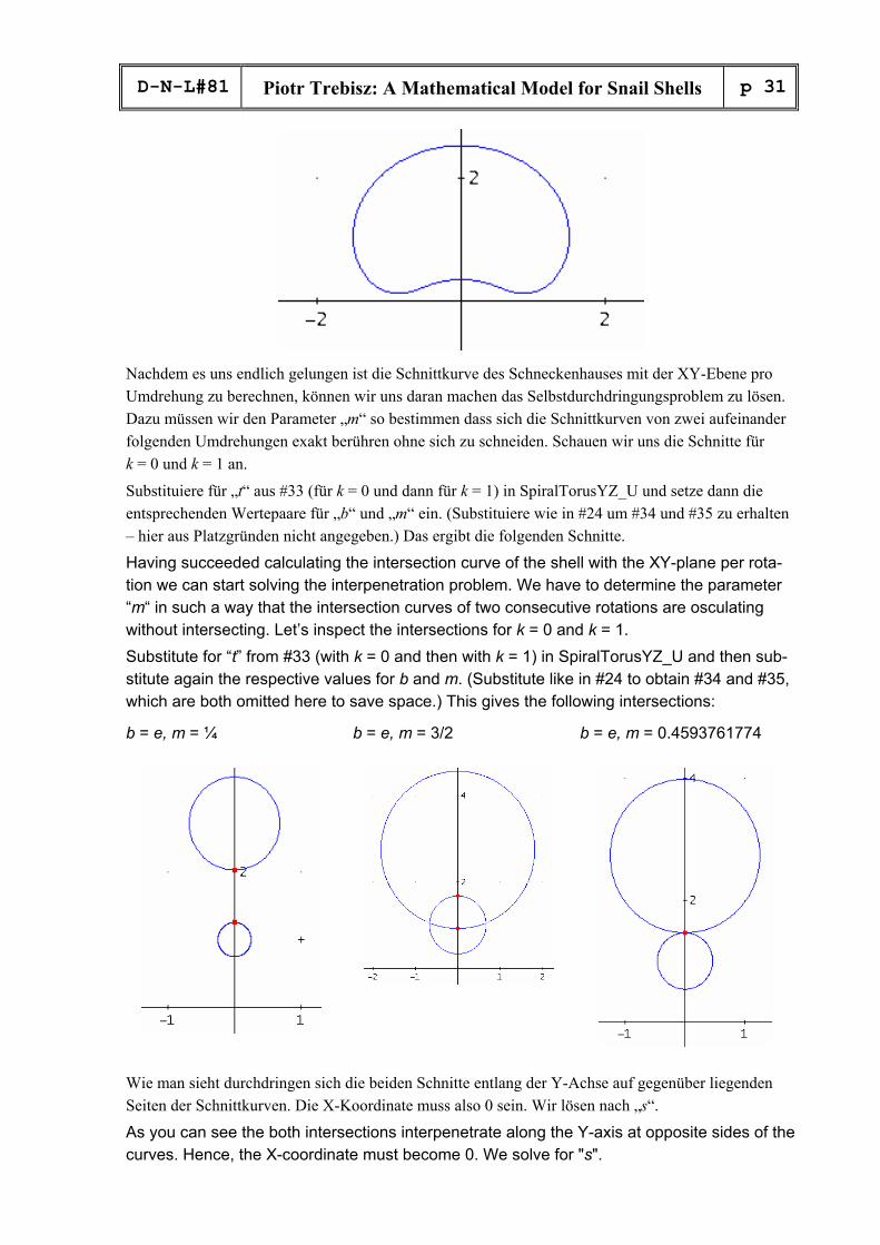
Nachdem es uns endlich gelungen ist die Schnittkurve des Schneckenhauses mit der XY-Ebene pro Umdrehung zu berechnen, können wir uns daran machen das Selbstdurchdringungsproblem zu lösen. Dazu müssen wir den Parameter „m“ so bestimmen dass sich die Schnittkurven von zwei aufeinander folgenden Umdrehungen exakt berühren ohne sich zu schneiden. Schauen wir uns die Schnitte für k = 0 und k = 1 an.
Substituiere für „t“ aus #33 (für k = 0 und dann für k = 1) in SpiralTorusYZ_U und setze dann die entsprechenden Wertepaare für „b“ und „m“ ein. (Substituiere wie in #24 um #34 und #35 zu erhalten – hier aus Platzgründen nicht angegeben.) Das ergibt die folgenden Schnitte.
Having succeeded calculating the intersection curve of the shell with the XY-plane per rota-tion we can start solving the interpenetration problem. We have to determine the parameter “m“ in such a way that the intersection curves of two consecutive rotations are osculating without intersecting. Let’s inspect the intersections for k = 0 and k = 1. Substitute for “t” from #33 (with k = 0 and then with k = 1) in SpiralTorusYZ_U and then sub-stitute again the respective values for b and m. (Substitute like in #24 to obtain #34 and #35, which are both omitted here to save space.) This gives the following intersections: b = e, m = ¼
b = e, m = 3/2
b = e, m = 0.4593761774
Wie man sieht durchdringen sich die beiden Schnitte entlang der Y-Achse auf gegenüber liegenden Seiten der Schnittkurven. Die X-Koordinate muss also 0 sein. Wir lösen nach „s“.
As you can see the both intersections interpenetrate along the Y-axis at opposite sides of the curves. Hence, the X-coordinate must become 0. We solve for "s".
p 32
Piotr Trebisz: A Mathematical Model for Snail Shells D-N-L#81
Die Lösungen für s sind: / The solutions for s are:
and
Die beiden Lösungen werden eingesetzt (in #35 und #36). Both solutions are substituted (in #35 and #36).
Wenn sich die Mantelfläche nur berühren, aber nicht durchdringen soll, müssen beide Y-Koordinaten gleich sein. Folgende Gleichung muss also nach „m“ gelöst werden:
zweite Komponenten von #39 = zweite. Komponente von #40.
If the surface shall only osculate (and not interpenetrate) then both Y-coordinates must be equal. So we have to solve the following equation for “m“: second component of #39 = second component of #40.

D-N-L#81
Piotr Trebisz: A Mathematical Model for Snail Shells p 33
Nebenbei kann man aus dieser Gleichung ablesen, welcher Umdrehungszahl eine Windung "w" ent-spricht, also der Umdrehungszahl nach der sich die Mantelfläche selber berührt. Additionally one can read off from this equation the rotation number which is corresponding to one coil "w" i.e. the rotation number when the surface is osculating itself.
Damit erhalten wir eine 3. Art von Schneckenhaus, das nach der Anzahl der Windungen parametrisiert ist.
Doing so we obtain another kind of snail shell which is parameterized according to the num-ber of coils.
Die Gleichung (#41) kann vereinfacht werden
Equation (#41) can be simplified.
Die Gleichung ist leider höchst nichtlinear und läßt sich nicht analytisch nach „m“ lösen, deshalb müs-sen wir das Newton-Verfahren anwenden.
This equation is not linear at all and cannot be solved for “m“ analytically. So we have to ap-ply the Newton-Raphson method.

p 34
Piotr Trebisz: A Mathematical Model for Snail Shells D-N-L#81
Gesucht ist ein Wert für „m“ für den gilt f(b,m) = 0. Für das Newton-Verfahren wird die 1. Ableitung von f(b,m) nach „m“ benötigt. g(b,m) ist die 1. Ableitung von f(b,m).
We would like to find a value for "m" with f(b,m) = 0. For the Newton-algorithm we need the first derivative of f(b,m) wrt "m". g(b,m) is the first derivative of f(b,m).
Leider ist DERIVE nicht selbstständig in der Lage die 1. Ableitung von f(b,m) nach „m“ zu bestim-men. Jeder Versuch führt zu einer Fehlermeldung wegen zu wenig Speicher.
Wenn wir aber DERIVE exakt vorgeben wie es die 1. Ableitung bestimmen soll, ist die Software doch dazu in der Lage. Dazu zerlegen wir f(b,m) in 4 Teilfunktionen …
Unfortunately DERIVE is unable to find this first derivative. Each attempt leads to an error message: Memory Exhausted. If we give some hints how to find the first derivative then the software is able to differentiate f(b,m). We decompose f(b,m) into 4 partial functions … (I omit printing this – from the didactical point of view – interesting part of Piotr´s file in order to save space. I invite you to follow his steps in expressions #47 - #55 of his dfw-file. #55 is the final result for g(m,b). See also my comment at the end of this article, Josef)
Den Newton-Algorithmus kann man als kleines DERIVE-Programm realisieren.
The Newton-Raphson algorithm is realised in form of a short DERIVE program.

D-N-L#81
Piotr Trebisz: A Mathematical Model for Snail Shells p 35
M_YZ(b, n) berechnet das passende "m" zur Basis "b" auf "n" Stellen genau. Und da wir auch die Windungszahl berechnet haben, können wir nun das Schneckenhaus auch nach der Windungszahl parametrisieren. Das findet sich in SpiralFlaecheYZ_W.
M_YZ(b, n) calculates the matching "m" fort he base "b" accurate to "n" decimal places. And as we have calculated the coil number, too, we are able to parameterize the snail house ac-cording to this number, giving SpiralFlaecheYZ_W. Now we can find the answer for my question on page 23:
“How to obtain this very special m?”
Here I came across a strange - bug? Preparing the publication of this article I reproduced all calculation steps and I failed simplifying (and approximating as well) expression #63. I asked Piotr and he answered that he is aware of this fact, but there will occur nor problems in the respective mth-file. So I stored his dfw-file as an mth-file - loosing all graphs and comments – and surprisingly enough, now it worked – as you can see above.
What happened here? I switched back to the dfw-file and opened the function g(m,b) via Author > Function Definition. I saw the function for a moment and then there was in place of the function the message “Memory Full” in the Edit Window!! I tried calculating the first derivative of f(m,b) – no success, Memory Exhausted.
When I did the same in the mth-file, the same message appeared in the Function Definition Window, but when simplifying M_YZ which is based on f(m,b) and the predefined g(m,b) DERIVE continues cooperating with the user … These are expressions #63 and #64 above. Don’t ask my why. Hopefully Albert Rich is reading this remark and maybe that he will provide some explanation for this strange behaviour.
If one of our members knows the reason or if he has some conjectures then please let us know, Josef (and Piotr, of course) I continue with Piotr’s closing lines. Ich bevorzuge es immer auf n + 2 Stellen genau zu rechnen. Eine Extra Vor-Komma-Stelle und eine Extra Nach-Komma-Stelle für den Rundungsfehler I prefer calculating for n + 2 decimal places. One extra digit in front of the decimal point and one extra digit at the end of the number to consider a possible rounding error.
p 36
Piotr Trebisz: A Mathematical Model for Snail Shells D-N-L#81
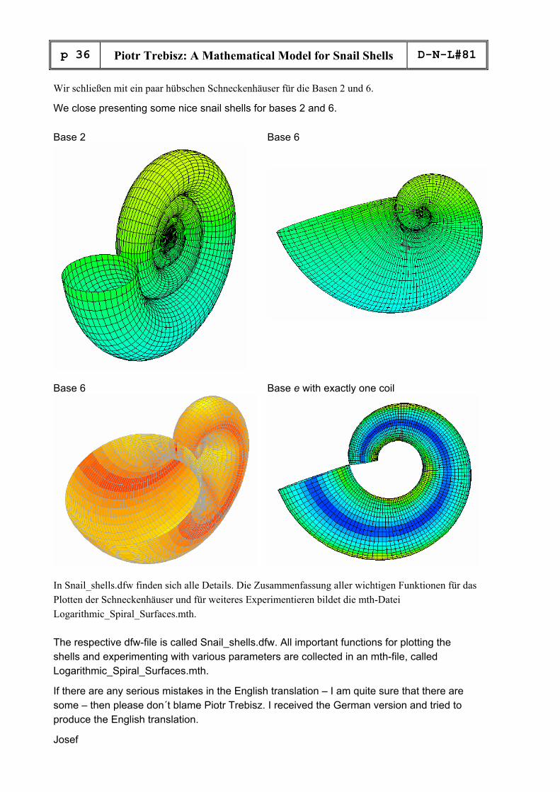
Wir schließen mit ein paar hübschen Schneckenhäuser für die Basen 2 und 6.
We close presenting some nice snail shells for bases 2 and 6. Base 2
Base 6
Base 6
Base e with exactly one coil
In Snail_shells.dfw finden sich alle Details. Die Zusammenfassung aller wichtigen Funktionen für das Plotten der Schneckenhäuser und für weiteres Experimentieren bildet die mth-Datei Logarithmic_Spiral_Surfaces.mth. The respective dfw-file is called Snail_shells.dfw. All important functions for plotting the shells and experimenting with various parameters are collected in an mth-file, called Logarithmic_Spiral_Surfaces.mth. If there are any serious mistakes in the English translation – I am quite sure that there are some – then please don´t blame Piotr Trebisz. I received the German version and tried to produce the English translation. Josef

D-N-L#81
Piotr Trebisz: A Mathematical Model for Snail Shells p 37
As you can see in the following screen shots, MuPad and MATHEMATICA can both derive function f(b,m). The derivative is much bulkier than Piotr’s result. I plotted f(e,m) and g(e,m) in MuPad and compared with the DERIVE plot. It looks pretty the same, so the results should be identical?
MuPad above and MATHEMATICA below

p 38
D E R I V E - a n d CAS-TI - U s e r F o r u m D-N-L#81
Exchange of mails connected with Duncan McDougal´s “Diophantine Polynomials”
Mail from Duncan McDougal as answer on my request concerning the table in (12) on page 13. Dun-can had 740/60 as sum of the roots in the last row … In an earlier mail he had asked: “Just out of curiosity (if I may ask), what are your intentions with this article?” This was my answer: I have two intentions: (1) Finding and exploring patterns is very important in mathematics education and in
mathematics in general. Your paper is an excellent example for discovering – and using – patterns.
(2) The second reason is given in my final comments (page 21). Hi Josef,
You are correct, the sum is 12 and should remain 12. However, the pattern becomes 520, 630, and 740 as an arithmetic sequence and 740/60 reduces to 37/3, a wee bit more than 12. I am still secretly hoping that someone sees a pattern I don't see and will come up with a brilliant discovery on the Quintic. Thus, I am suggesting that although 12 is the prob-able answer, maybe 37/3 is what it could be??? I acknowledge that I've proven that there is no monic quintic for which the first derivative contains integral and/or rational roots, but the pattern is hard to resist or ignore.
I am still very much interested in this topic and will entertain questions or comments from any interested party. I've only just begun the process for non-monic polynomials and already the quartics look daunting.
Anyway, I am flattered that you like my work enough to use it because that is what it was meant for. I remain Yours truly, Duncan McDougall Danny Ross Lunsford (22 01 2011)
Hello Derivers, the routines provided in the LinearAlgebra.mth file leave something to be desired in practice - has anyone resolutely attacked the problem of diagonalization and determination of eigen-spaces of large matrices? For my application large = 8x8. I need a robust and fast diagonalization scheme. (DNL#80). Hi Derivers, (19 02 2011) In implementing the Johnson Trotter algorithm one comes to a point where the direction of a mobile integer must be changed. My working area is an (N+2) x 2 matrix with the working permutations in the 1st column and the directions in the 2nd (directions are + or - 1). Eventually one has to change directions for all integers larger than the largest mobile integer - so I have a statement to run over the array
MAP(IF(P SUB i SUB 1 > Largest, P SUB i SUB 2 := -P SUB i SUB 2), i, [2,..,N+1]) However the sub-array assignment never takes place, even though the statement is executed. What exactly is going on? I know sub-array assignments must be simplified, but that should be happening here. Thanks in advance! -drl

D-N-L#81
D E R I V E - a n d CAS-TI - U s e r F o r u m p 39
Hi Derivers, (19 02 2011) OK see attached - I changed the map statement a bit but still no joy. The SHAPE function is one I made that creates arrays, don't worry about it, the size of the array created is (N+2) x 2. The output is included and you can see that the sign changes are never executed. (20 02 2011) It doesn't work - see attached - a function to generate all permutations of 1 to N by accretion was given in Derive Newsletter 41. It creates two nested loops, the inner one with k going from m to 1 in steps of -1, the outer with m going from 2 to N in steps of 1. All the variables are local to the PERMS function. We can make the inner loop into a MAP statement but the syntactically identical function works when the accretion variable t is global, but fails when you make it local to the function - I'm completely baffled
p 40
D E R I V E - a n d CAS-TI - U s e r F o r u m D-N-L#81
Danny Ross promised an article on Clifford Algebra and Dirac matrices some time ago. I asked him whether his request is in connection with this intended paper for the DNL and he answered. 20 02 2011 Yes, will work out solution to hydrogen fine structure as an example application. See attached for teaser on the algebraic environment. Derive makes it very easy to keep track of the rather complex algebraic operations in the Clifford algebra of Dirac matrices. On page 48 in DNL#80 I published the email communication with Albert Rich. Unfortunately I did not include the respective website where you can find many details about his fascinating current research. Albert wrote: Hello Josef, Yes, feel free to include my 2 January 2011 email in the next DNL. Also please include the website address http://www.apmaths.uwo.ca/RuleBasedMathematics As far as my current research, I recommend the following ongoing discussion on the Usenet group sci.math.symbolic http://groups.google.com/group/sci.math.symbolic/browse_thread/thread/90b4f2e39ee5ad9d?hl=en in which I am collaborating with Martin to develop powerful new rules for integrating trigono-metric expressions. In particular for your next DNL, you might find of interest my last post in which I outline how recurrence equations are transformed into integration rules. Martin is certainly one of the world's most active and knowledgeable Derive users. Appar-ently he lives in Germany and is a member of DUG. Do you know his last name? Aloha, Albert Does anybody know, who “Martin” is. I found an email-address which could have been Mar-tin’s one: ([email protected]). It would be great if we could find out who is the „secret“ DERIVE user? (The email address is not valid any more!)
David Sjöstrand from Sweden wrote:
Dear Josef, after only having had a short glance at your and Carl´s paper in DNL #80 I couldn´t resist investigating some more sequences with Excel. (I shouldn´t have done this. I have so many things I must do.) It seems that the sequence P(n)=m*P(n-3) + (1-m)*P(n-2) is convergent for all m and all ini-tial conditions. I attach josef_carl.xls. David sent a proof for DNL#80, page 22 in his next mail and we started an exciting exchange of mails. The results of this correspondence will form an article in DNL#82, Josef
D-N-L#81
D E R I V E - a n d CAS-TI - U s e r F o r u m p 41
Notes by R.N. (Roger) Folsom Monterey, California, USA [email protected].
As you will see below, I am trying to formally prove the circumstances under which a particu-lar inequality is true --- and Derive's Simplify or Solve command actually says that it is true. (For now, all I need is sufficient conditions.) But I have not been able to figure out the Derive6.1 command or commands that will do that. My sources are Bernhard Kutzler and Vlasta Kolol-Voljc's "Introduction to Derive 6, Ad-vanced Mathematics for Your PC" (hereafter Derive6); and Albert and Joan Rich, Theresa Shelby, and David Stoutemeyer's "Derive User Manual Version 6" (hereafter Derive3). Derive6's equation solver (page 57), when used to determine whether a relationship is True or False, doesn't apply to what I am trying to do because it doesn't allow conditions to be imposed on the equation's (or, in my case, the inequality's) variables. Derive6's discussion of the IF tool (on pages 166 and 227) didn't help because I didn't un-derstand page 166 (I don't know any Analytic Geometry), and although I think that I did un-derstand page 227 I couldn't figure out how to apply it to my problem. Derive3's discussion of the IF tool (pages 309-310), made sense, but again I couldn't figure out how to apply it to my problem. My understanding is that the IF tool has four fields: a test condition, a "then" clause of re-sults if the test condition is satisfied, an "else" clause of results if the test condition is NOT satisfied, and an "unknown" clause. Derive3's opening IF example (page 309) is a payroll problem: IF(h <= 40, 10h, 400 + 15(h-40)) where h is hours worked and 10h and 15(h-40) are worker payment amounts. Unfortu-nately, the problem does not include the unknown clause, which if not included but is needed turns out to be the entire IF(...) tool. An example that does include an unknown clause would have been helpful. What I want is a tool, or set of tools, that let me state restrictions on my inequality's variables, then state the inequality itself, and returns either "true" or "false", or ? (or the same object) if the restrictions are too weak to determine whether the inequality is true or false. ---------------------------------------------------------------- The r↓n variables below are annual (or some other time period) rates of growth, such as in-terest rates, inflation and deflation rates, real output growth or decline rates, etc. Rates of growth r↓n can be either positive, zero, or negative. The number N is the number of time periods being considered. Sometimes "total" rates of growth over N time periods are calculated by summing the N periodic rates of change r↓n (n = 1,2,...,N), which is less accurate than multiplying the N corresponding (1+r↓n) factors. Summing the r↓n can give results that are either larger or smaller than the more accurate multiplication of the (1 + r↓n).

p 42
D E R I V E - a n d CAS-TI - U s e r F o r u m D-N-L#81
However, a common situation is that over N time periods, more rates of growth r↓n are posi-tive than negative. If that difference is sufficiently large, summing the N periodic rates of change r↓n gives a lower total rate of growth over N periods than does multiplyng the corre-sponding (1 + r↓n) numbers, so that summation understates the true total rate of change over N periods. Mathematically, that "common situation" inequality can be written in three basic ways. See statements #2, #3, and #4, below. SATISFYING THE "COMMON SITUATION" INEQUALITY; A SUFFICIENT CONDITION: All r↓n ≥ 0 If ALL of the r↓n are positive or zero (r↓n ≥ 0), the "common situation" inequality holds, be-cause the left side's terms are smaller than the right side's factors. For an example, let N = 3, and see statements #5, #6, #7, and #8. Note that in #7 --- a rearrangement of #2 with N = 3 --- the left side is -1, and ALL of the variables on the right side are positive. Therefore, a SUFFICIENT condition for the "usual condition" inequality is simply that all all r↓n >= 0.
Statement #5 can be written as
In statement #6, multiplying out the (r↓n + 1) factors would eliminate the -1 - (r↓3 + r↓2 + r↓1) expression. Doing that (by using Derive's Simplify-Factor command) gives statement #7.
or
Note: I have done the same calculations above using N = 5.
D-N-L#81
D E R I V E - a n d CAS-TI - U s e r F o r u m p 43
Given the sufficient condition that all r↓n ≥ 0, statements #7 and #8 are obviously true be-cause the left side is negative, and every term on the right side is positive. And since statements #7 and #8 are merely a rearrangement of #5, which is an example of statements #4, #3, and #2, statement #7 demonstrates that if all r↓n ≥ 0, the "usual situation" inequality holds, so that summing N periodic rates of change r↓n (instead of multiplying cor-responding 1 + r↓n numbers) understates the true total rate of change over N periods. HOWEVER, I need to learn how to persuade Derive6.1 to do a formal proof (results either true, false, or unknown) of the preceding paragraph's results, because my next step is to experiment with less restrictive conditions, such as all r↓n >= -1. ================================================================ TO DO: Figure out a formal proof --- for any statement #5 through #8 --- that when #10 (be-low) holds, comes up with "true" rather than the wrong answer of "false." For example, Simplify-Basic of either IF(#10, #7) or IF(#7, #10) returns the same (written out) IF statement, presumably meaning that Simplify could not determine whether the inequality was true or false, despite the "all r↓n >= 0" variable conditions. But Solve-Expression of either IF(#10, #7) or IF(#7, #10) concludes that the constrained ine-quality is false, when I know that it is true (from the analysis that follows #8). I clearly am not using IF properly. It may not be intended for what I am trying to do. In that case, I need to know what else to do.
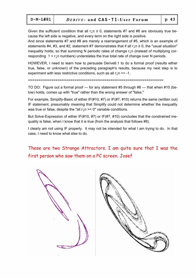
These are two Strange Attractors. I am quite sure that I was the first person who saw them on a PC screen. Josef

p 44
Robert Setif & Josef Böhm: π in Slices D-N-L#81
I received a mail from Robert Setif, a DUG Member from the very first times of its existence: Dear Josef, (in bad English) I am always alive and I spend my time to program often deranged counting with different mathemati-cal softwares (Derive, Mathematica, Maple, Mupad, Xcas, python, pari-gp). Regarding these soft-wares, do you know others, free preferably? I send you 3 files which calculate decimals of PI. You can make what you want.of them.I I am unable to ameliorate them on billing(displaying, printing ). In fact, the billing of long integers or floats with a lot of decimales by edges(slices) of 3 or 5 or 10 digits.It would be more practical for checking. Could you fix me on this subject? I should like if there is a function that for instance "time_elapsed(pi_machin(10001)) for calculating the time for that calcul.Thank you very much. I congratulate you for your work. Best regards. (in good French) Je suis toujours en vie et je passe mon temps à programmer des calculs souvent délirants avec diffé-rents logiciels mathématiques (Derive, Mathematica, Maple, Mupad, Maxima, Xcas, python, pari-gp). A propos de ces logiciels, en connaissez-vous d'autres, gratuits de préférence? Je vous envoie 3 fichiers qui calculent des décimales de PI. Vous pouvez en faire ce que vous voulez. Je suis incapable de les améliorer sur l'affichage. En effet, l'affichage de longs entiers ou de flottants avec beaucoup de décimales par tranches de 3 ou 5 ou 10 chiffres serait plus pratique pour la vérifica-tion. Pourriez-vous me dépanner à ce sujet? J'aimerais aussi une fonction comme par exemple "time_elapsed(pi_machin(10001)) qui donnerait le temps nécessaire pour ce calcul. Merci infiniment. Je vous félicite pour votre travail.Bravo ! These are Robert’s files which were attached to his mail :

D-N-L#81
Robert Setif & Josef Böhm: π in Slices p 45
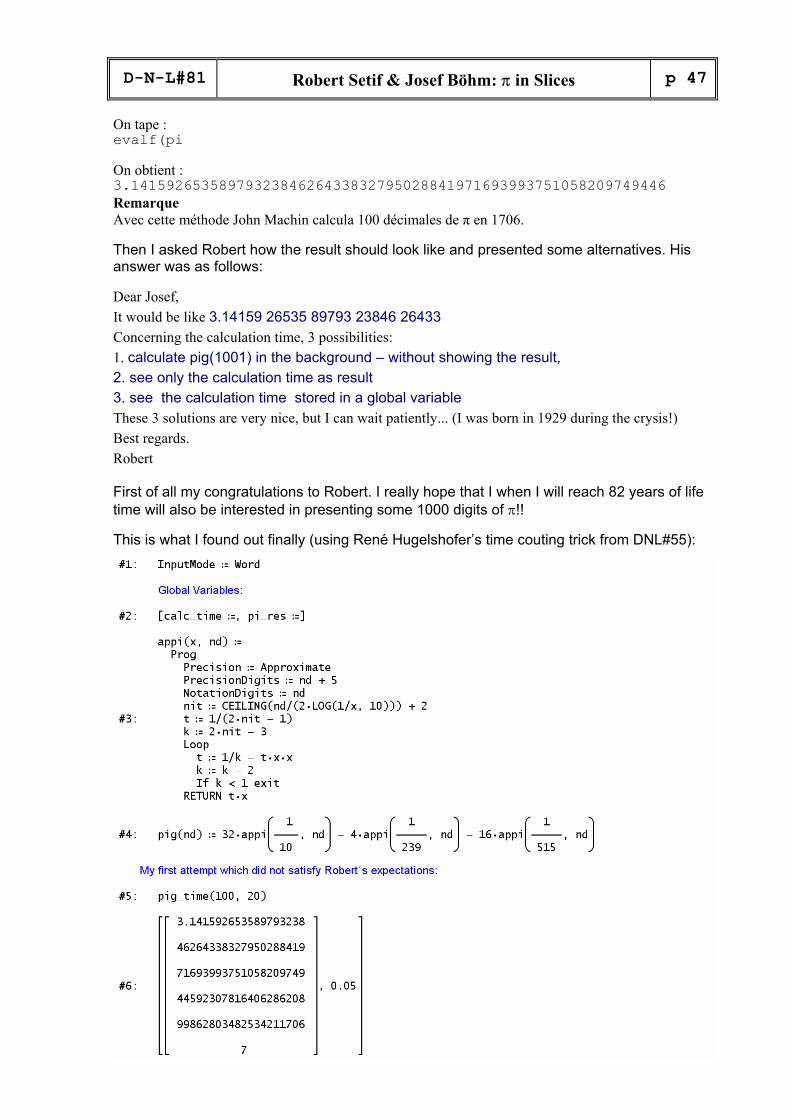
The second file was pig.dfw which was pretty the same as pig1.mth above including a com-ment that Robert had calculated π up to 5000 decimal places and needed approximatey 12 minutes. I wrote back and asked for some information about this algorithm – and I had some ideas how to answer his request applying string manipulations and the time counter which was presented by René Hugelshofer some time ago. Using the DNL-index I found out that this was in DNL#55. But read first Robert’s information about this algorithm for calculating π with arbitrary accu-racy:
p 46
Robert Setif & Josef Böhm: π in Slices D-N-L#81
Dear Josef, Explications about functions appin et appi of my approx of PI. Of Aide for free software XCAS , aid written by Renée de GRAEVE Université J Fourier GRENOBLE FRANCE. This AIDE is enormous. I have not the courage for translate it for you. You may find it on the site
www-fourier.ujf-grenoble.fr/~parisse/giac_fr.html
Bernard Parisse author of XCAS Université J Fourier GRENOBLE FRANCE Please excuse that shambles of French-English. Atan(x)=x-x^3/3+x^5/5… PI/4=4 atan(1/5) – atan(1/239) Pour calculer la somme de n termes de la série on va utiliser la méthode de Hörner pour faire le moins possibles de multiplications, on a :
arctan(x)=x(1−x2(1/3−x2(1/5−x2(....−x2(1/2n−1)))))
L’utilisateur doit rentrer la valeur a de x et le nombre n de termes de la série.
gregory(a,n):={ local t,k; t:=1/(2*n-1); for (k:=2*n-3;k>0;k:=k-2) { t:=1/k-a^2*t; } return (a*t); };
On tape : 16*gregory(1/5,18)-4*gregory(1/239,6) On obtient : 3.14159265359
On tape : evalf(16*gregory(1/5,42)-4*gregory(1/239,20))
On obtient avec DIGITS :=60 3.14159265358979323846264338327950288419716939937510582097494
Soit Rn(x) le reste de la série ∑k=1∞(−1)k+1x2k−1/2k−1 : Rn(x)=∑k=n+1
∞(−1)k+1x2k−1/2k−1. On sait que |Rn(x)|<|x|2n+1/2n+1 Pour avoir |Rn(1/5)|=|Rn(0.2)|<10−61 il faut que :22n+1<(2n+1)102n−60 et comme 210≃ 103 cela donne si on suppose 2n+1>10 :
10(6n+3)/10<102n−59 soit 593<14n soit n≃ 42 On vérifie pour n=42 on a (1/5)85/85<2.56e−62 On peut aussi écrire si on suppose que 2n+1>10 : |x|2n+1/2n+1<x2n+1/10<10−61 donc on va choisir x2n+1<10−60 soit (2n+1)log10(x)<−60 ou encore n>((−60)/log10(x)−1)/2 Pour x=1/5 on a n>42.4202967422 et comme 2n+1>40 on peut améliorer la majoration |x|2n+1/2n+1<x2n+1/40<10−61 ce qui donne n>((−60+log10(4))/log10(1/5)−1)/2=41.9896201841 donc on prend n=42 pour x=1/239 on a n>11.66 donc on prend n=12 et on vérifie : (1/239)25/25=1.38711499837e−61.
On choisit 62 Chiffres pour DIGITS et on tape :
evalf(16*gregory(1/5,42)-4*gregory(1/239,12))
On obtient : 3.1415926535897932384626433832795028841971693993751058209749446
D-N-L#81
Robert Setif & Josef Böhm: π in Slices p 47
On tape : evalf(pi
On obtient : 3.1415926535897932384626433832795028841971693993751058209749446 Remarque Avec cette méthode John Machin calcula 100 décimales de π en 1706.
Then I asked Robert how the result should look like and presented some alternatives. His answer was as follows:
Dear Josef, It would be like 3.14159 26535 89793 23846 26433 Concerning the calculation time, 3 possibilities: 1. calculate pig(1001) in the background – without showing the result, 2. see only the calculation time as result 3. see the calculation time stored in a global variable These 3 solutions are very nice, but I can wait patiently... (I was born in 1929 during the crysis!) Best regards. Robert
First of all my congratulations to Robert. I really hope that I when I will reach 82 years of life time will also be interested in presenting some 1000 digits of π!!
This is what I found out finally (using René Hugelshofer’s time couting trick from DNL#55):

p 48
Robert Setif & Josef Böhm: π in Slices D-N-L#81

D-N-L#81
Robert Setif & Josef Böhm: π in Slices p 49
Robert’s answer: Thank you very much for your work. It is great (magnifique en français).

p 50
R e c o m m e n d e d W e b S i t e s D-N-L#81
Mathematical Physics Electronic Journal, University of Barcelona
Probability Surveys
Publications de l'Institut Mathématique, Mathematical Institute of the Serbian Academy of Arts and Sciences
Rendiconti, University of Torino
Revista Colombiana de Estadística (Colombian Journal of Statistics)
Revista Colombiana de Matemáticas, University of Bogota
Séminaires & Congrès, proceedings of mathematical meetings
Séminaire Lotharingien de Combinatoire, Universities of Bayreuth, Erlangen and Strasbourg
Siberian Electronic Mathematical Reports, Sobolev Institute of Mathematics
Surveys in Mathematics and its Applications, University Constantin Brâncuşi of Târgu-Jiu
Symmetry, Integrability and Geometry: Methods and Applications (SIGMA), Ukraine
The Journal of Nonlinear Science and its Applications, Iran
Theory and Applications of Categories, Sackville, Canada
TICMI, Tbilisi International Centre of Mathematics and Informatics
Universitatis Iagellonicae Acta Mathematica, University of Krakóv, Poland
Journal of Analysis and its Applications, Lemgo, Germany
Mathematical Proceedings of the Royal Irish Academy
Memoirs on Differential Equations and Mathematical Physics, Tbilisi
The New York Journal of Mathematics
Novi Sad Journal of Mathematics The EMIS-website http://www.emis.de/elibm/ is hosting also a rich collection of • Conference Proceedings
• Monographs and Lecture Notes
• Classical Works, Selecta and Opera Omnia (among others Riemann and Hamilton)
• Software and Other Special Electronic Resources (among others: Mathematical English
Usage – A Dictionary)