
ALEMANIAact on the Protection of Trade Marks and Other Symbols Trade Mark Act
Trade in Services and Market Structure
Inaugural-Dissertation zur Erlangung des akademischen Grades eines Doktors
der Wirtschafts- und Sozialwissenschaften der Christian-Albrechts-Universität zu Kiel
Vorgelegt von Aidan Islyami
[Master of Arts in Economics (KIMEP)] aus Almaty, Kasachstan.
Kiel, 2012

Gedruckt mit Genehmigung der Wirtschafts- und Sozialwissenschaftlichen Fakultät
der Christian-Albrechts-Universität zu Kiel
Dekan: Prof.Dr. Roman Liesenfeld
Erstberichterstattender: Prof.Dr. Johannes Bröcker
Zweitberichterstattender:
Prof. Dr. Rolf Langhammer
Tag der Abgabe der Arbeit: 13 Februar, 2012 Tag der mündlichen Prüfung: 30 Mai, 2012
iii
Contents Contents .....................................................................................................................................iii Acknowledgements .................................................................................................................... v List of abbreviations .................................................................................................................. vi Introduction
Short Bibliography ................................................................................................................. 3 Chapter One: Trade in Intermediate Producer Services under Imperfect Competition ............... 4
1.1. Introduction .................................................................................................................... 4 1.2 Model setting .................................................................................................................. 6 1.3. Partial derivatives of markup........................................................................................... 9 1.4. Data in benchmark and model calibration...................................................................... 11 1.5. Results of the numerical experiments ............................................................................ 12
1.5.1. Results of the base scenario .................................................................................... 12 1.5.2. Stability of the initial equilibrium ........................................................................... 14 1.5.3. Numeraire problem ................................................................................................ 17 1.5.4. Other specifications of the model ........................................................................... 19
1.6. Concluding remarks ...................................................................................................... 22 Bibliography ......................................................................................................................... 23 Appendices ........................................................................................................................... 25
Chapter Two: On Equilibrium Stability in the CGE models with Monopolistic Competition ... 34
2.1. Introduction .................................................................................................................. 34 2.2. Model structure ............................................................................................................. 36
2.2.1. Base model setting ................................................................................................. 36 2.2.2. Equations of the model in the mixed complementarity problem format ................... 38 2.2.3. Data and calibration ............................................................................................... 39
2.3. Results from the base model and equilibrium stability ................................................... 40 2.3.1. Interpretation of the results ..................................................................................... 40 2.3.2. Equilibrium stability and uniqueness ...................................................................... 45
2.4. Alternative perspective on stability ............................................................................... 48 2.5. Analytical expression of stability conditions ................................................................. 54
2.5.1. Alternative model formulation ................................................................................ 54 2.5.2. Conditions of full specialization in the IRS sector .................................................. 59
2.6. Conclusion .................................................................................................................... 59 Bibliography ......................................................................................................................... 60 Appendices ........................................................................................................................... 61
Chapter Three: FDI in Distribution Services and Trade versus Investment Trade-Off ............. 67
3.1. Introduction .................................................................................................................. 67
iv
3.2. Model setting ................................................................................................................ 70 3.2.1. Case 1: No investments .......................................................................................... 71 3.2.2. Case 2: FDI in manufacturing ................................................................................. 72 3.2.3. Case 3: FDI in distribution services ........................................................................ 72 3.2.4. Case 4: FDI in both manufacturing and distribution services .................................. 73
3.3. Analytical results .......................................................................................................... 74 3.3.1. Determinants of FDI in distribution ........................................................................ 74 3.3.2. Determinants of FDI in manufacturing ................................................................... 79
3.4. Numerical results .......................................................................................................... 81 3.4.1. Selecting parameter values ..................................................................................... 81 3.4.2. A non-monotonic relationship between trade costs and FDI in distribution ............. 89
3.5. Concluding remarks ...................................................................................................... 93 Bibliography ......................................................................................................................... 93
Appendices .................................................................................................................................95 Conclusion …………………………………………………………………………………… 106 Affirmation …………………………………………………………………………………… 109

v
Acknowledgements This research has been supported by the Germany Academic Exchange Service (DAAD), Open Society Institute (OSI) and the University of Kiel. I am grateful to Prof. Bröcker and Prof. Langhammer for research supervision. I appreciate all the comments and suggestions I received at the conferences in Vienna, Aix-en-Provence and Rome. I am also grateful to my family, friends and colleagues in Kiel and Almaty.

vi
List of abbreviations CRS Constant returns to scale CES Constant elasticity of substitution CGE Computable general equilibrium model DS Dixit Stiglitz ERP Effective rate of protection FDI Foreign Direct Investments GAMS Generalized Algebraic Modeling System GATS General agreement on trade in services GDP Gross domestic product IRS Increasing returns to scale MOAP Marshallian output adjustment process MCM Micro consistency matrix MCP Mixed complementarity problem NEG New Economic Geography SAM Social accounting matrix UNCTAD United Nations Conference on Trade and Development VA Value Added WTO World Trade Organization
vii
List of Tables Table 1.1. Results of services trade liberalization in percentages ............................................ 12 Table 1.2. Results of services trade liberalization in percentages for higher markup ............... 15 Table 1.3. Results of services trade liberalization in percentages ............................................ 16 Table 1.4. Results of services trade liberalization in percentages for different
numeraire values .................................................................................................. 18 Table 1.5. Results of services trade liberalization in percentages ............................................ 20 Table 1.1C. Results of services trade liberalization in levels ..................................................... 27 Table 1.1D. Micro-consistency matrix (MCM) ......................................................................... 29 Table 2.1. Micro-consistency matrix ...................................................................................... 40 Table 2.2. Percentage change from the benchmark after a tax cut (t = 0) ................................ 43 Table 2.3. Percentage change from the benchmark after a tax cut for the closed
version of the model (t = 0) .................................................................................. 45 Table 2.4. Percentage change from the benchmark after a tax cut and different
benchmark value of the IRS sector output............................................................. 47 Table 2.1A. Percentage change from the benchmark after tax cut (t = 0) .................................. 61 Table 2.2A. Micro-consistency matrix of the modified M62 model .......................................... 62 Table 3.1. The ratio of exports from the home to host country of the multinational
with and without FDI in distribution for different values of DK , a and b .............. 85 Table 3.2. The value of the distribution threshold for different parameter values .................... 92
viii
List of Figures Figure 1.1. The impact of the elasticity of substitution between varieties on markup
depending on the values of conjectural elasticity and the number of firms ............ 10 Figure 1.2. The share of the outputs of final goods for different values of the price
share (An unstable initial equilibrium case) .......................................................... 15 Figure 1.3. The share of the outputs of final goods for different values of the price
share (A stable initial equilibrium case) ................................................................ 17 Figure 1.1A.The production structure of the Y industry ............................................................ 25 Figure 2.1. Model stability ...................................................................................................... 47 Figure 2.2. Model stability from NEG perspective: Inital scenario .......................................... 50 Figure 2.3. Model stability from NEG perspective: 045 .............................................. 50 Figure 2.4. Model stability from NEG perspective: 0 00.65 ............................. 51 Figure 2.5. Model stability from NEG perspective: 0 00.1 ................................ 51 Figure 2.6. Model stability from NEG perspective: The case with import tariffs on
both goods ............................................................................................................ 52 Figure 2.7. Dynamic time path of the relative output of good X .............................................. 53 Figure 2.8. Dynamic time path of the relative wage of skilled labor in X sector ...................... 54 Figure 2.1B.Dynamic path of the output of good X ................................................................... 62 Figure 2.2B.Dynamic path of the output of good Z ................................................................... 62 Figure 2.3B.Dynamic path of the number of firms .................................................................... 63 Figure 2.4B.Dynamic path of welfare ....................................................................................... 63 Figure 2.5B.Dynamic path of ............................................................................................... 63 Figure 2.6B.Dynamic path of the unskilled labor wage ............................................................. 63 Figure 2.7B.Dynamic path of the consumer expenditure ........................................................... 64 Figure 2.8B.Dynamic path of the firm level price in industry X ................................................ 64 Figure 3.1. Investment decisions of the multinational firm for different values of fixed
costs of FDI in manufacturing (FM) and fixed costs of FDI in distribution (FDS) ................................................................................................................... 86
Figure 3.2. (FDS = 0.6) Investment decisions of the multinational firm for different values of fixed costs of FDI in manufacturing (FM) and bilateral tariff rate (t) ......................................................................................................................... 87
Figure 3.3. (FDS = 0.4) Investment decisions of the multinational firm for different values of fixed costs of FDI in manufacturing (FM) and southern tariff rate (tS) ........................................................................................................................ 88
Figure 3.4.A (FM = 0.3) and Figure 3.4.B (FM = 0.35) Investment decisions of the multinational firm for different values of fixed costs of FDI in distribution (FDS) and southern tariff rate (tS) ......................................................................... 89
Figure 3.5 (FDS = 0.457) The investment decisions of the multinational firm for different values of fixed costs of FDI in manufacturing (FM) and southern tariff rate (tS) ........................................................................................................ 90
Figure 3.6 The derivative of the difference in profits between modes 3 and 1 for different values of the southern tariff rate (tS) ....................................................... 91
Figure 3.1A. Strategies of the multinational firm ...................................................................... 95
1
Introduction The service sector represents a substantial and rising share of output, employment and FDI in many countries. This makes it crucial for future growth and development prospects. It is observed that the share of services in value added and employment is increasing with the level of development: starting from 35% of GDP in the lowest income countries and up to over 70% in developed countries (Hoekman, 2006). At the same time, trade in services constitutes only one fifth of the total world trade (Hoekman, 2006). This could be explained by the intangible nature of many services, by trade barriers, and in particular by the fact that the service trade with its four different modes of supply ( cross-border trade, consumption abroad, foreign affiliates trade in services through commercial presence, and temporary movement of persons) is highly insufficiently recorded. Recorded trade is basically cross-border trade. It is this trade which has grown faster than trade in goods as a result of the advancement of information technology. Due to high relatively to goods trade barriers, it is expected that global welfare gains to be achieved after services trade liberalization could be substantial. In particular, the services trade is expected to bring significant benefits to developing countries, where barriers are the highest. The objective of the dissertation is to contribute to the existing knowledge in the field of the services trade and its impact on developing countries. It is also to investigate the implications for trade policy analysis of enhanced ways of modeling of the inherent features attributable to the services sector such as imperfectly competitive market structure. The most straightforward indications of the imperfectly competitive market structure in services are the intrinsic heterogeneity of services and the presence of increasing returns to scale. The dissertation concentrates on two types of services: producer and distribution services. Both sectors play a key role in determining the quality and price of goods. In particular, producer services as intermediate services are an important input in the goods production that influences productivity of manufacturing goods. On the other hand, the distribution services constitute an important link between producers and final consumers. Consequently, this dissertation concentrates on studying the role of both types of services and their impact on the economy within the vertical production structure. The first chapter of the dissertation entitled “Trade in Intermediate Producer Services under Imperfect Competition” builds upon the general equilibrium models in Markusen et al. (2005) and Konan and Assche (2007) to analyze the impact of services trade liberalization under oligopoly competition. It aims to study the impact of trade in producer services on the welfare, downstream industry output, prices of the factors of production and the pattern of trade. Oligopoly market structure with firms that make conjectures about the production of their domestic and foreign rival firms is developed. Models with constant elasticity of substitution production functions capture special features attributable to services such as heterogeneity and preference for variety. It is found that large differences in markups between the domestic and foreign firms could lead to a negative welfare effect. The second chapter is entitled “On Equilibrium Stability in the CGE models with Monopolistic Competition”. A simplified model is constructed to study the effects that lead to the emergence of an unstable equilibrium and counterintuitive comparative statics result. The
2
Global Correspondence Principle and the dynamics underlying the initially static model are applied to study the model stability. We assume that there are two sectors of the economy: increasing returns to scale sector (IRS) and constant returns to scale sector (CRS). It is analytically demonstrated that the elasticity of substitution between varieties and the difference in the skill intensities of the two sectors of the economy will increase the stability of the initial equilibrium. Moreover, it could be proved that an ad valorem tax cut will have the same impact on the direction of change of the key endogenous variables of the model irrespective of the underlying data as given in the social accounting matrix (SAM). The dynamic time paths of the endogenous variables from unstable to stable equilibrium are also presented. Even though the model presented in chapter 2 is just a reduced version of the model presented in chapter 1, it is important for explaining the results of the model with oligopoly competition. In other words, it is impossible to give a complete interpretation of the results in chapter 1 and make a judgment about the stability of the initial equilibrium without analyzing the simplified version of that model presented in chapter 2. Similarly, the simplified model allows us to single out the effects that determine the results of the model and the role of the market structure. Moreover, no comprehensive analytical results could be presented for the model in chapter 1 as it could be for the model in chapter 2. Finally, the third chapter entitled “FDI in Distribution Services and Trade versus Investment Trade-off” studies the determinants of FDI in distribution using a partial equilibrium model. Foreign Direct Investments represent a form of mode 3 of services trade. This is an important channel of services trade especially for the distribution sector which mainly comprises retail and wholesale trade. Differently from franchising those two types of distribution services could only be supplied by FDI. The model represents an extension of the standard proximity/concentration tradeoff and is motivated by evidence in Hanson et al. (2001) according to which foreign direct investment could be differentiated as production oriented and distribution oriented. Consequently, a model in which a vertically integrated multinational firm has several options of foreign market penetration such as exporting, FDI in manufacturing and FDI in distribution is developed. There is a market seeking motive to invest in distribution services and there is a cost-oriented motive to invest in manufacturing. It is found that market size in the host country, productivities of producing differentiated goods, substitutability and the host country distribution margin increase incentive for FDI in distribution. On the other hand, transportation cost and wage rates in both the host and the home country of the multinational weaken the incentive of a multinational to invest in distribution services. Similarly, market size in the south and in the north, substitutability, wage in the home country, productivity of producing outsourced good in the south and the host country tariff will increase incentive to invest in manufacturing. Moreover, it was found numerically that there is a non-monotonic relationship between trade costs and FDI in distribution. The results of the dissertation could have some implications for economic policy making. In particular, it is always important for host country governments to decide not only whether foreign services providers should be taxed or not but also which instruments should be used to achieve greater welfare gains. In the first chapter of the dissertation there are two policy tools at the disposal of the host country government: per unit of output tariff or lump sum entry tax. It was found that both are inappropriate and free trade in producer services brings higher welfare.
3
Many developing countries use special policies to attract FDI. There are different policy instruments at the disposal of a host country government such as fiscal incentives in terms of indirect subsidies, tax relieve and so on, financial incentives in the form of government grants or credits at subsidized rates and all other ways of preferential treatment (Navaretti and Venables, 2004). The reasons to attract FDI could be based either on welfare improving considerations or they could be motivated by political economy processes. Irrespective of the reasons, knowing the determinants of FDI in the specific services sector such as distribution could facilitate the implementation of host country policies. In the third chapter of the dissertation such determinants are presented. Due to the vast empirical and theoretical literature on the relationship between FDI and trade, trade policies could also have an implicit impact on incentives for FDI. This is already acknowledged by policymakers. In this dissertation we are trying to study how incentives to invest in distribution are affected by the presence or absence of FDI in manufacturing. Short Bibliography Hanson, G.H., Mataloni, R.J., Slaughter M.J., (2001) “Expansion Strategies of US
Multinational Firms” Brookings Trade Forum, pp.245-294. Hoekman, Bernard. (2006). ‘Liberalization of Trade in Services: A Survey’, World Bank
working paper. Konan, D., Assche, A., (2007). “Regulation, Market Structure and Service Trade
Liberalization”, Economic Modeling 24 (2007), pp. 895-923. Markusen, J., Rutherford, T., and Tarr, D., (2005) “Trade and direct investment in producer
services and the domestic market for expertise”, Canadian Journal of Economics 38 (2005), pp. 758–777.
Navaretti, G., and Venables, A., (2004) “Multinational Firms in the World Economy”, Princeton and Oxford: Princeton University Press.
4
Chapter 1
Trade in Intermediate Producer Services under Imperfect Competition In this chapter a stylized CGE model is constructed to study the impact of liberalization of barriers for foreign providers of intermediate producer services under imperfect competition on welfare, downstream industry output, prices of factors of production and the pattern of trade. An attempt is made at incorporating oligopoly market structure into the services sector within a general equilibrium model. Consequently, a model with firms making output conjectures about domestic and foreign rivals is adopted. The case of a small developing country with a less efficient services sector relative to foreign firms is assumed. In this framework, interaction and the relative significance of mechanisms resulting from a preference for variety, pro competitive and efficiency effects is analyzed. It is found that the liberalization of trade in services might be negative in terms of welfare only if there is a significant difference in the relative economies of scale and diversification between domestic and foreign firms. On the other hand, underlying market structure is found to have little impact on results. 1.1. Introduction
There are many studies that emphasize the potential global gains from services trade liberalization. Those gains are expected to be higher than the gains from trade in goods (Hoekman, 2006). In particular, the services trade is expected to bring significant benefits to the developing countries where barriers are the highest. The outcomes could be improvements in household welfare (Rutherford et al., 2006), long run growth performance (Mattoo et al., 2006) and domestic industry productivity (Markusen et al., 2005). On the other hand, numerous quantitative models show that the effects are uneven and some countries may even lose due to various reasons: rents accruing to foreign investors, terms of trade deterioration, etc. It is also observed that the gains from FDI flows which could be classified as liberalization in terms of GATS (General Agreement on Trade in Services) Mode 3 commercial presence and ownership restrictions are large and more variable compared to the gains coming from the cross border trade mode of supply (Hoeckman, 2006). Similarly, the impact on the specific factor such as skilled labor could be more pronounced. The types of services under consideration are typically producer services such as business, transportation, telecommunications, and so on that are used as intermediate inputs and subject to different barriers such as entry barriers and taxes per unit of provided services. Markusen et al. (2005) use a model with monopolistic competition to show that foreign producer services could actually provide substantial benefits to rival domestic firms. In particular, rival firms benefit from the expansion of the services industry as a whole. This is because the domestic downstream industry purchases higher quality business services and expands as more foreign firms enter the domestic market. Hence, the optimal tariff is found to be a subsidy. In other words, services trade liberalization is found to have a positive impact not only on domestic consumers but also on rival firms and downstream consumers.

Chapter 1. Trade in Intermediate Producer Services under Imperfect Competition
5
However, particularly in developing countries many backbone services such as telecommunications, finance and insurance are characterized by oligopoly markets. Hoekman (2006), Mattoo and Sauve (2003) and others stress the importance of market structure and regulation for the outcome of services trade liberalization. Furthermore, even though there are many trade models that incorporate market power, there are few that address special issues related to services (Copeland, 2002). In contrast to standard models with prefect competition, models of imperfect competition could produce unexpected results. It is sufficient to consider the case of a simple Cournot duopoly with different marginal costs to obtain the counterintuitive effects on welfare. In particular, let us assume that marginal costs are constant and the marginal cost of the first firm is higher than the marginal cost of the second firm. Then, under certain parameters, the decreasing of the marginal cost of the first firm so that it still remains higher than the marginal cost of the second firm brings a negative welfare effect. This happens because of the inefficiency associated with the increase in the share of the less efficient firm. On the other hand, in our model, foreign firms are subject to higher fixed costs compared to domestic firms and will consequently tend to form more concentrated market structure. In addition to discriminatory national treatment limitations such as specific licensing, foreign firms could be expected to have higher fixed costs than domestic firms due to adaptation costs to operate in a new business environment, language barriers, etc. However, it is also plausible to assume that foreign firms are more efficient per unit of service compared to local firms in developing countries. Even though the productivity difference in services should be smaller than in manufacturing because of their less tradable nature, the counterintuitive effects with higher markups in the foreign sector compared to the domestic will be invalid. In other words, there will be no similar Cournot effect with fixed costs as there is with marginal costs. It could be demonstrated that a possible negative welfare effect in such case occurs rather because of the unstable initial equilibrium. However, there is another source of inefficiency associated with the misallocation of monopoly markups between different sectors of the economy. In particular, Epifani and Gancia (2011) find that trade liberalization that only applies to certain industries could lead to a negative impact on welfare when it raises markup heterogeneity. A similar argument could be applied to our model since foreign and domestic services are imperfect substitutes and could be thought of as different sectors. Consequently, in order to verify if a similar case is possible in our model, we would need to have smaller fixed cost in the foreign industry relative to the domestic industry because higher markups are translated into higher fixed costs. This could take place if the foreign firms possess significantly greater economies of scale and market expertise compared to domestic firms. Having entry tax and the tax per unit of service output would not only enable us to model the actual type of barriers that foreign firms face in developing markets, but also to differentiate between the impact from different efficiency of foreign firms in both variable and fixed costs. The purpose of this chapter is therefore to build upon the approach in Markusen et al. (2005) and construct an oligopoly model with conjectural output variations in producer services in order to study the impact of services trade liberalization on consumer welfare and domestic service providers. Those will depend on the impact on foreign firms and the downstream industry that uses producer services as inputs. In particular, the impact of services trade liberalization on domestic services will depend on the difference in efficiency, economies of scale and fixed costs between foreign and domestic service firms. Factors of production are supplied inelastically. Hence, changes in production of industries will define the impact on the

Chapter 1. Trade in Intermediate Producer Services under Imperfect Competition
6
prices of factors of production. In particular, impact on skilled labor will be driven by the relative change in producer services which use it more intensively than other sectors. On the other hand, the impact on unskilled labor would be defined by the change in the more unskilled labor intensive perfectly competitive sector. In order to study the impact of services trade liberalization we will need to disentangle the relative importance and interactions between such causal mechanisms and effects as market crowding, preference for variety, pro competitive effect and so on. The stylized quantitative model is succinct and specifically designed to address the given problem. The impact on the welfare of the host country would depend on the magnitude of those effects and could among other things be negative even when all the profits of the foreign firms accrue to the domestic representative agent. On the other hand, services trade liberalization is expected to bring higher gains in the oligopoly models compared to the monopolistic competition models due to the pro-competitive effect. The chapter is structured as follows: section 2 presents a detailed formulation of the model. The impacts of some of the parameters of the model on the markup are presented in section 3. Section 4 describes considerations of the data and the calibration strategy used to obtain a benchmark replication of the model. Section 5 represents the numerical results of services trade liberalization, discusses alternative model specifications and a numeraire problem. Section 6 concludes. The derivation of the markup equation and the program code are given in Appendix. 1.2 Model setting We assume that there are two sectors in the economy: Y denotes the sector that uses producer services as an intermediate input and Z is a perfectly competitive sector, which could also indicate all the other sectors of the economy. The consumers demand only final goods and consumer utility is a Cobb Douglas composite of them:
1 (1.2.1)U Z Y The Y sector is a CES (Constant elasticity of substitution) composite of producer services and value added:
1 11( ) (1.2.2)VA PSY Q Q
Here PSQ denotes quantity of producer services and VAQ denotes the value added, θ>0 is a corresponding elasticity of substitution. Analogous to Konan and Assche (2007) producer services are modeled so that they positively affect the value added productivity when used as an intermediate good. The production structure of the Y sector is presented in Appendix A. Producer services, in turn, constitute an Armington type CES function of domestic and foreign services:
1 11( (1 ) ) (1.2.3)PSQ XD XF
σ is an Armington elasticity for services. While there are no barriers to trade in final goods, trade in services is subject to barriers and could only be provided through commercial presence.

Chapter 1. Trade in Intermediate Producer Services under Imperfect Competition
7
Domestic (XD) and foreign (XF) services are aggregates of several varieties. Each firm produces only one good (variety) and competes in quantities with both domestic and foreign firms:
11
1( ) (1.2.4)
d ddd d
n
ii
XD xd
1
1
1
( ) (1.2.5)f f
ff f
n
jj
XF xf
Corresponding dual price indexes would then be: 1
(1 ) 1
1( ) (1.2.4 ')
dd d
n
ii
PD pd
1
1 1
1( ) (1.2.5 ')
ff f
n
jj
PF pf
Here nd , nf are the number of domestic and foreign firms correspondingly. The production of each variety is subject to scale economies due to fixed costs. It also employs domestic primary factors of production: S denotes skilled labor and L denotes unskilled labor or all the other factors of production:
1 1, (1.2.6)d di i i dxd S L i n 1 1, (1.2.7)f f
j j j fxf S L j n
Similarly, the value added of the Y sector and the perfectly competitive sector are the Cobb Douglas composites of the primary factors of production:
1 (1.2.8)VA VAVAQ S L 1 (1.2.9)Z S L
I assume that the producer services sector is more skilled labor intensive than the value added and perfectly competitive sector and that foreign producer services are less skilled labor intensive compared to domestic services. In other words, it is assumed that:
, (1.2.10)d f d f VA
In addition, I assume that foreign firms are more efficient relative to domestic firms. There are few if no empirical studies of comparative efficiency between domestic and foreign service providers in developing countries (Whalley, 2004). The markup charged by producer services firms will depend on the substitution elasticities at different stages of production and the output conjectures of rival firms. In Appendix B, the perceived price elasticity of demand is derived under the assumptions that 1) domestic firms make the same conjectures about the behavior of foreign firms as they do about the behavior of rival domestic firms, 2) there is symmetry in-between domestic firms and 3) all firms conjecture a constant value addedi:
1 1 1 1 1 1 1 1(1 ) (1 ) / (1.2.11)d d d d dPS i i i i i dd
i d d
SH S n
The markup for foreign firms could be obtained analogously:
1 1 1 1 1 1 1 1(1 ) (1 ) / (1.2.11 )f f f f fPS i i i i i ff
i f f
SH S n
Here ln( )
ln( )
d ki
i
d xd
d xd is the conjectural elasticity of firm’s output, /d
i d dS s n is a share of
the domestic firm in the total producer services industry and ln( )ln( )Y
d Yd P
is the price
elasticity of demand in the downstream industry.
i This assumption follows from the model structure.

Chapter 1. Trade in Intermediate Producer Services under Imperfect Competition
8
Then, the markup is obtained from the Lerner formula:
( ) 11
11 1 (1.2.12)
d i i ii i i i
i ii i
i i
d di i i id
i
pd xd pdMR pd xd pd xd pdxd xdpd xd
pd pd MC
We could see that the markup of firm i ( di ) is an inverse of the price elasticity of demand.
The markup equation for foreign firms is calculated in the same way. Then, the Cournot competition will be a particular case of this setting with 0d
i and 0fi . Another
specification would be a cartel with di dn and f
i fn . The adopted modeling approach assumes economies of scale at the firm level based on fixed costs. Domestic and foreign firms are modeled as representative agents that receive markup revenues and pay fixed costs. In other words, a zero profit condition at the domestic variety level will look as follows:
11* (1 ) (1.2.13)d d d
dPXD n MC
Here 1d ddMC w v , w is a skilled wage and v is an unskilled wage. The price per variety ipd , is determined as follows:
11* d
i dpd PXD n i
Hence, the price at the industry level is increasing in the elasticity of substitution between varieties and decreasing in the number of firms. The total cost for the domestic industry, under zero profit condition, could then be written in the following way:
1
1 * * (1.2.14)dd d ddTC MC n XD PXD XD ii
Similarly, we could write the zero profit condition for the foreign industry: 1
1 (1 ) (1.2.15)f f ffn PXF TFX MC
If we put it into words, the foreign services providers are subject to discriminatory treatment in the form of per unit of output of services tax (TFX) imposed only on foreign firms. I assume that costs are fixed in quantities at the variety level (FC) and the second term on the left hand side of (1.2.14) represents the total markup revenue of the domestic industry. The latter is also the total fixed cost in values at the industry level:
* * * * (1.2.16)d
dd FC dPXD XD FC P n
It will not be quite fixed as it changes in terms of the price of the fixed cost (dFCP ) and the
number of firms. This is a very useful modeling approach that enables us to have a market power at the firm level and zero profits at the industry level at the same time. Moreover, I assume that
d
dFCP MC and
f
fFCP MC .
The equivalent of the equation (1.2.16) for the foreign sector would look as follows: ii The economies of scope could also be incorporated into the setting by adding a fixed cost at an industry level.

Chapter 1. Trade in Intermediate Producer Services under Imperfect Competition
9
* * * * * (1.2.17)f ff f fPXF XF FC MC n LST n
Here LST denotes a lump sum or entry tax on foreign firms. It could be thought of as a license fee that each foreign firm needs to pay in order to access the domestic market. All the taxes are collected by the domestic representative consumer. A market clearing condition for domestic services at an industry level would be:
( , ) (1.2.18)PSC PXD PXFXD Q
PXD
The left hand side represents a demand for a domestic industry good by Shepard’s lemma and the right hand side is the quantity supplied. Any condition could be transferred to the variety level if we take into account that:
1 (1.2.19)dxd n XD
In this way, analogous to Markusen (2002), Markusen et al. (2005), the symmetry between varieties enables one to express the whole system at the industry level only. Finally, the market clearing condition for example for skilled labor could be written as follows in accordance to the structure of the model:
( ) ( ) (1.2.20)f d
f dVAVA f d
QPZ MC MCS Z Q n xf FC n xd FCw w w w
1.3. Partial derivatives of markup Evaluating partial derivatives of the markup equation with respect to parameters could already give us some insights about the economic reasoning engraved into the model behavior. In particular, the partial derivatives with respect to price elasticity of demand in downstream industry and the elasticity of substitution between producer services and value added are negative under condition (1.3.1):
(1.3.1)d di
d d
ss n
iii
2 (1 ) 0 (1.3.2)d
d d di PSi i i
SH S
The higher price elasticity of demand in downstream industry will translate into a higher responsiveness of the latter to the changes in input prices and consequently less market power in domestic producer services:
2
1(1 ) 0 (1.3.3)
dd d di PSi i i
SH S
Similarly, the market power of producer services will decline as the downstream industry gets more flexible in substituting between its primary factors and services inputs. The sign of the partial derivative with respect to the Armington type elasticity will depend on the value of conjectural elasticity of firm output:
2
0 11 ( 1)(1 ) / (1.3.4)0 1
ddidi
d i d di
ifs n
if
iii Even if 0i the left hand side should be negative in most of the cases so that inequality holds.
Chapter 1. Trade in Intermediate Producer Services under Imperfect Competition
10
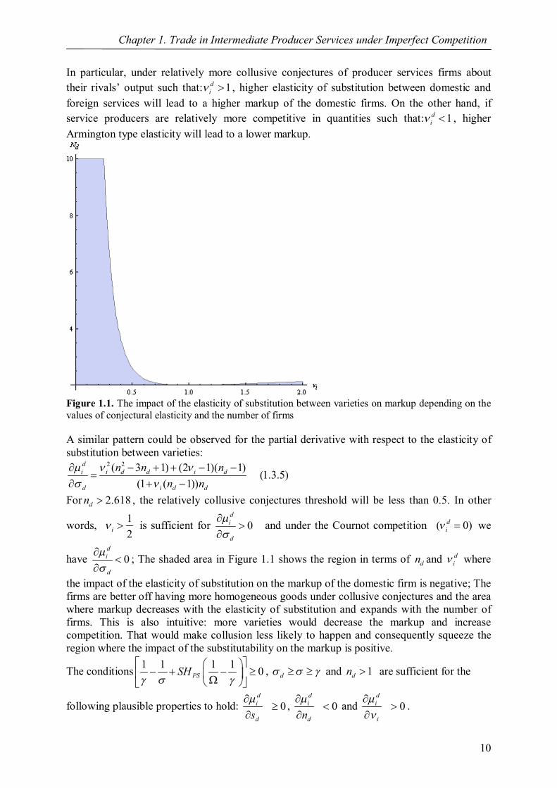
In particular, under relatively more collusive conjectures of producer services firms about their rivals’ output such that: 1d
i , higher elasticity of substitution between domestic and foreign services will lead to a higher markup of the domestic firms. On the other hand, if service producers are relatively more competitive in quantities such that: 1d
i , higher Armington type elasticity will lead to a lower markup.
Figure 1.1. The impact of the elasticity of substitution between varieties on markup depending on the values of conjectural elasticity and the number of firms A similar pattern could be observed for the partial derivative with respect to the elasticity of substitution between varieties:
2 2( 3 1) (2 1)( 1)(1.3.5)
(1 ( 1))
di i d d i d
d i d d
n n nn n
For 2.618dn , the relatively collusive conjectures threshold will be less than 0.5. In other
words, 12i is sufficient for 0
di
d
and under the Cournot competition ( 0)di we
have 0di
d
; The shaded area in Figure 1.1 shows the region in terms of dn and di where
the impact of the elasticity of substitution on the markup of the domestic firm is negative; The firms are better off having more homogeneous goods under collusive conjectures and the area where markup decreases with the elasticity of substitution and expands with the number of firms. This is also intuitive: more varieties would decrease the markup and increase competition. That would make collusion less likely to happen and consequently squeeze the region where the impact of the substitutability on the markup is positive.
The conditions 1 1 1 1 0PSSH
, d and 1dn are sufficient for the
following plausible properties to hold: 0di
ds
, 0di
dn
and 0di
i
.
Chapter 1. Trade in Intermediate Producer Services under Imperfect Competition
11
Namely, the markups of the domestic firms increase with the domestic share and more collusive conjectures about the behavior of rival firms and drops in the number of domestic firms. 1.4. Data in benchmark and model calibration
The data was structured so that the parameters fall into reasonable ranges based on empirical estimates and also reflect the assumptions made with respect to the structure of the model. The micro-consistency matrix (MCM) used for the benchmark calibration could be found in Appendix D. The data from the note by the UNCTAD Secretatiat UNCTAD (2003) reports that the share of producer services in GDP is 20% on average for developed countries and about 5% for least developed countries. It is in the range of 7.5%-10% in developing countries. It could be inferred from the MCM that the share of producer services of our model is taken to be 10% of GDP. The number of firms is set to be the same in foreign and domestic sectors and equals 10. In the base scenario, I assume that the share of domestic industry is equal to the share of foreign industry. The foreign firms are subject to two types of discriminatory barriers: per unit output tax and lump sum entry tax which are taken to be equal to each other in value terms. The final goods are traded so that the good from the sector with imperfect competition is imported and the good from the perfectly competitive sector is exported in the benchmark scenario. I assume Cournot competition and increasing substitution elasticities from the top level to the bottom in the production structure of the model: ,d f .
There are several ways in which a CGE model with imperfect competition could be calibrated. I extraneously set the number of firms and the benchmark level of the markups and calibrate the bottom level elasticity of substitution ,d f residually (Gasiorek et. al (1992); Haaland and Norman (1992); Willenbockel (1994, 2004)). I use the value of 1.38 for foreign and 1.33 for domestic price to marginal cost ratio. Those values could then easily be
transformed into the markup value: 11 0.275, 0.25f d
fPXF
MC . It should be
even higher under increasing returns to scale (Christopoulou and Vermeulen, 2008). In particular, the average price to marginal cost ratios are estimated to be 1.56 for the Euro area and 1.38 for the US with more variety across different sectors. However, taking higher markup would result in lower calibrated elasticity and unstable initial equilibrium. Therefore the choice of the parameter values is in part determined by stability considerations as it will be further elaborated in the next section. Since there is no consistent information on the cost structure, the fixed cost ratio is obtained residually from markup estimates. The model is calibrated so that in the benchmark as many variables are equal to one as possible. Under the assumption of small open economy, the price elasticity of demand in downstream industry should be equal to infinity: . There are no precise estimates for the substitution elasticities used in the model. For example, there are many estimates of the Armington substitution elasticity between domestic and imported goods (McDaniel and Baristreri, 2003). It is found that studies with higher sectoral disaggregation obtain higher Armiangton elasticities. Consequently, statistically significant elasticities are found to be in the range of 0.14-5.3. However, elasticities vary across sectors and it is rational to expect that elasticities of substitution between services are less than elasticities between goods. The
Chapter 1. Trade in Intermediate Producer Services under Imperfect Competition
12
following values of elasticities of substitution are assumed under the base scenario: 0.5, 2 . Consequently, the calibrated bottom level elasticities are 5.14d
and 4.5f . The factor intensities are assumed to be in accordance with assumptions made on their values: 0.3, 0.8, 0.75, 0.625, 0.725d f VA .
Further considerations on the stability of the initial equilibrium would lead to a recalibration of the parameters. If not specified differently, the exchange rate is taken as a numeraire. The code of the CGE model is written in the GAMS syntax. 1.5. Results of the numerical experiments
1.5.1. Results of the base scenario
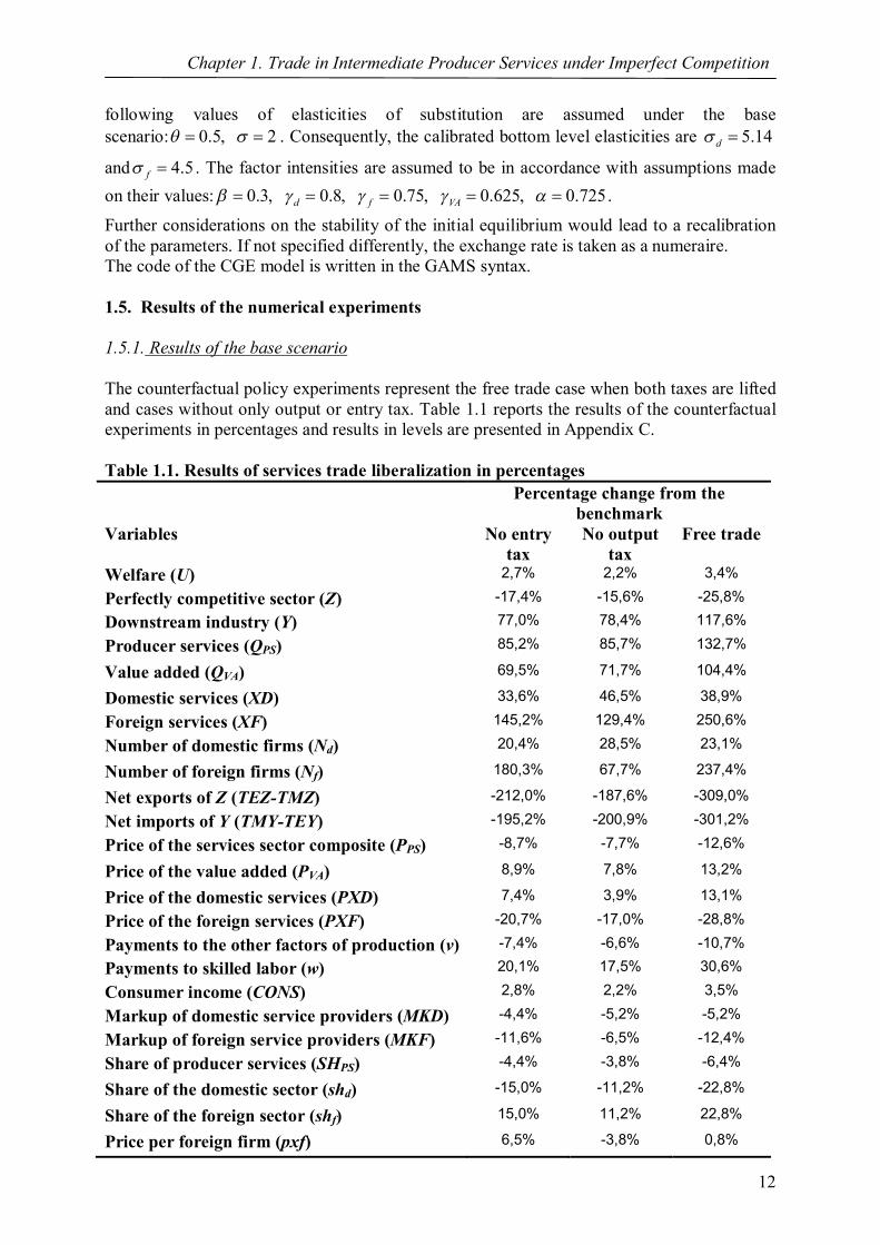
The counterfactual policy experiments represent the free trade case when both taxes are lifted and cases without only output or entry tax. Table 1.1 reports the results of the counterfactual experiments in percentages and results in levels are presented in Appendix C. Table 1.1. Results of services trade liberalization in percentages
Percentage change from the benchmark
Variables No entry tax
No output tax
Free trade
Welfare (U) 2,7% 2,2% 3,4%
Perfectly competitive sector (Z) -17,4% -15,6% -25,8%
Downstream industry (Y) 77,0% 78,4% 117,6%
Producer services (QPS) 85,2% 85,7% 132,7%
Value added (QVA) 69,5% 71,7% 104,4%
Domestic services (XD) 33,6% 46,5% 38,9%
Foreign services (XF) 145,2% 129,4% 250,6%
Number of domestic firms (Nd) 20,4% 28,5% 23,1%
Number of foreign firms (Nf) 180,3% 67,7% 237,4%
Net exports of Z (TEZ-TMZ) -212,0% -187,6% -309,0%
Net imports of Y (TMY-TEY) -195,2% -200,9% -301,2%
Price of the services sector composite (PPS) -8,7% -7,7% -12,6%
Price of the value added (PVA) 8,9% 7,8% 13,2%
Price of the domestic services (PXD) 7,4% 3,9% 13,1%
Price of the foreign services (PXF) -20,7% -17,0% -28,8%
Payments to the other factors of production (v) -7,4% -6,6% -10,7%
Payments to skilled labor (w) 20,1% 17,5% 30,6%
Consumer income (CONS) 2,8% 2,2% 3,5%
Markup of domestic service providers (MKD) -4,4% -5,2% -5,2%
Markup of foreign service providers (MKF) -11,6% -6,5% -12,4%
Share of producer services (SHPS) -4,4% -3,8% -6,4%
Share of the domestic sector (shd) -15,0% -11,2% -22,8%
Share of the foreign sector (shf) 15,0% 11,2% 22,8%
Price per foreign firm (pxf) 6,5% -3,8% 0,8%
Chapter 1. Trade in Intermediate Producer Services under Imperfect Competition
13
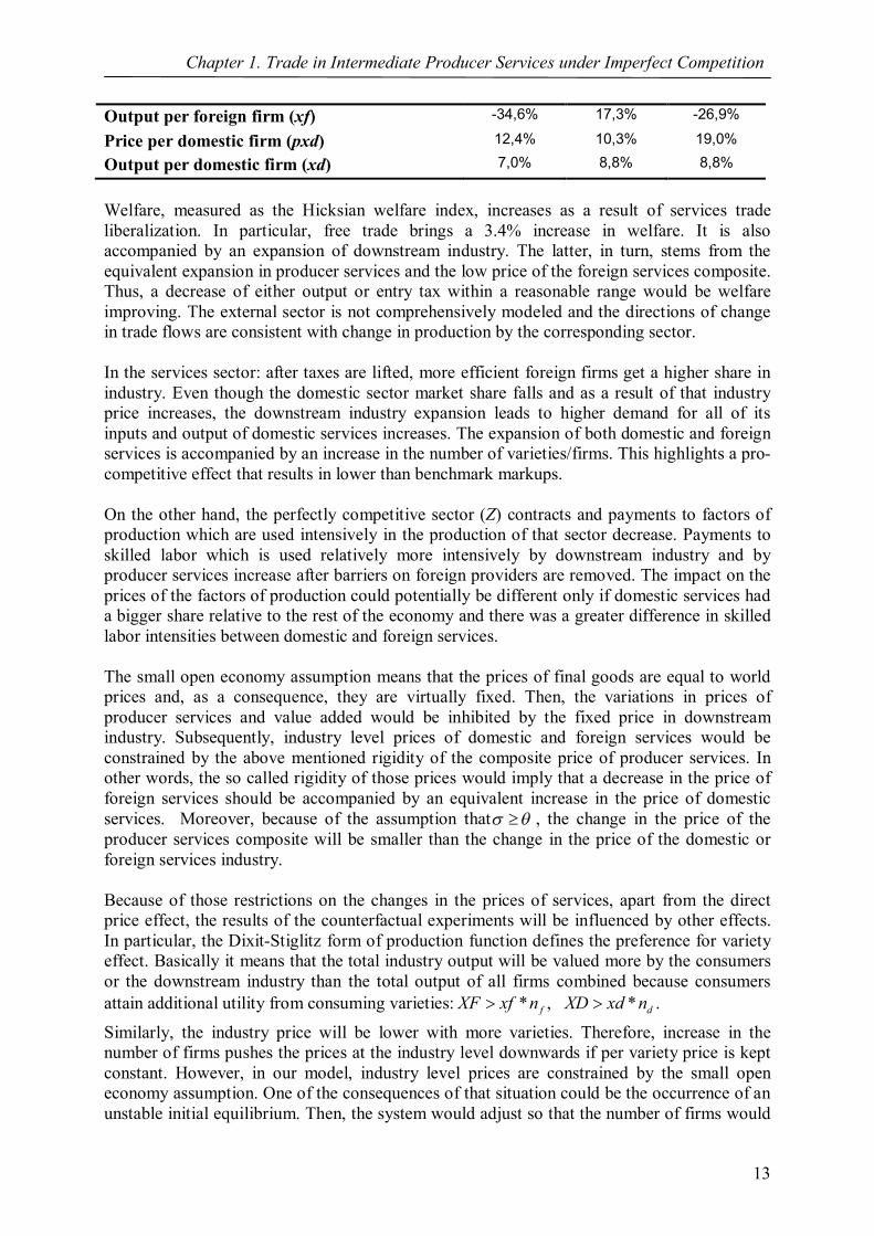
Output per foreign firm (xf) -34,6% 17,3% -26,9%
Price per domestic firm (pxd) 12,4% 10,3% 19,0%
Output per domestic firm (xd) 7,0% 8,8% 8,8%
Welfare, measured as the Hicksian welfare index, increases as a result of services trade liberalization. In particular, free trade brings a 3.4% increase in welfare. It is also accompanied by an expansion of downstream industry. The latter, in turn, stems from the equivalent expansion in producer services and the low price of the foreign services composite. Thus, a decrease of either output or entry tax within a reasonable range would be welfare improving. The external sector is not comprehensively modeled and the directions of change in trade flows are consistent with change in production by the corresponding sector. In the services sector: after taxes are lifted, more efficient foreign firms get a higher share in industry. Even though the domestic sector market share falls and as a result of that industry price increases, the downstream industry expansion leads to higher demand for all of its inputs and output of domestic services increases. The expansion of both domestic and foreign services is accompanied by an increase in the number of varieties/firms. This highlights a pro-competitive effect that results in lower than benchmark markups. On the other hand, the perfectly competitive sector (Z) contracts and payments to factors of production which are used intensively in the production of that sector decrease. Payments to skilled labor which is used relatively more intensively by downstream industry and by producer services increase after barriers on foreign providers are removed. The impact on the prices of the factors of production could potentially be different only if domestic services had a bigger share relative to the rest of the economy and there was a greater difference in skilled labor intensities between domestic and foreign services. The small open economy assumption means that the prices of final goods are equal to world prices and, as a consequence, they are virtually fixed. Then, the variations in prices of producer services and value added would be inhibited by the fixed price in downstream industry. Subsequently, industry level prices of domestic and foreign services would be constrained by the above mentioned rigidity of the composite price of producer services. In other words, the so called rigidity of those prices would imply that a decrease in the price of foreign services should be accompanied by an equivalent increase in the price of domestic services. Moreover, because of the assumption that , the change in the price of the producer services composite will be smaller than the change in the price of the domestic or foreign services industry. Because of those restrictions on the changes in the prices of services, apart from the direct price effect, the results of the counterfactual experiments will be influenced by other effects. In particular, the Dixit-Stiglitz form of production function defines the preference for variety effect. Basically it means that the total industry output will be valued more by the consumers or the downstream industry than the total output of all firms combined because consumers attain additional utility from consuming varieties: * , *f dXF xf n XD xd n .
Similarly, the industry price will be lower with more varieties. Therefore, increase in the number of firms pushes the prices at the industry level downwards if per variety price is kept constant. However, in our model, industry level prices are constrained by the small open economy assumption. One of the consequences of that situation could be the occurrence of an unstable initial equilibrium. Then, the system would adjust so that the number of firms would
Chapter 1. Trade in Intermediate Producer Services under Imperfect Competition
14
fall rather than increase after services trade liberalization. It could also happen that the price per variety increases while the industry price falls. This is exemplified in the difference of the impacts of two barriers for trade in services. The results of the corresponding counterfactual experiments are given in columns 1 and 2 of Table 1.1. The barriers could be understood as a tax per firm or variety (LST) and a tax per unit of output of the firm (TFX). Consequently, a decrease in the tax per firm facilitates the entry of more foreign firms into the market. Apparently the love-of-variety effect dominates over the constrained direct effect. It could be seen from the increasing rather than decreasing price per foreign firm. The rise in industry production is fully explained by the increase in the number of firms and the output per firm even falls. On the other hand, smaller barriers per unit of output of each firm would also lead to an increase in the number of varieties. Even though more varieties would pressure the price per foreign firm to increase, the direct price effect dominates and it falls. In this case, the preference for varieties effect constrains the expansion of foreign services as the increase in the number of firms also constitutes a burden of higher fixed costs. Consequently, there is more expansion in foreign services as a result of the increase in production of each individual firm rather than as a result of the rise in the number of firms. The relative significance of the two instruments of services trade liberalization depends on the value of fixed costs, the elasticities of substitution between varieties and skilled labor intensities. In particular, removal of the entry tax compared to removal of the output tax has resulted in greater increase in the output of foreign services and consequently greater share of producer services output. Therefore, both the share of the domestic sector and its production are smaller under no entry tax. That leads to less distortion in the proportion of inputs of the downstream industry which explains a somewhat higher increase in the production of producer services under no output tax. On the other hand, the consumer welfare is higher with no entry tax because the representative consumer receives more per unit of output tax revenues from the expanding foreign services sector. 1.5.2. Stability of the initial equilibrium It has been mentioned that markups could be expected to have higher values than assumed in the benchmark. Let us take a somewhat higher value of foreign markup:
0.375, 0.25f d . That would correspond to a price to marginal cost ratio of 1.6 and
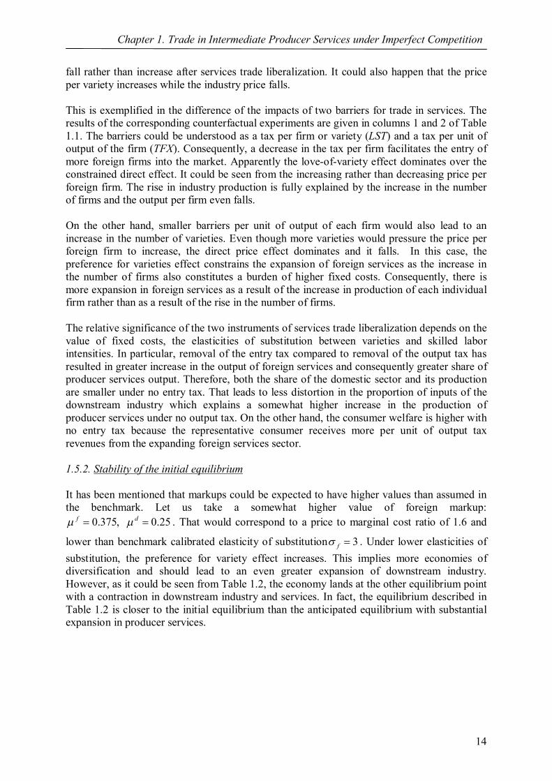
lower than benchmark calibrated elasticity of substitution 3f . Under lower elasticities of substitution, the preference for variety effect increases. This implies more economies of diversification and should lead to an even greater expansion of downstream industry. However, as it could be seen from Table 1.2, the economy lands at the other equilibrium point with a contraction in downstream industry and services. In fact, the equilibrium described in Table 1.2 is closer to the initial equilibrium than the anticipated equilibrium with substantial expansion in producer services.
Chapter 1. Trade in Intermediate Producer Services under Imperfect Competition
15
Table 1.2. Results of services trade liberalization in percentages for higher markup Percentage change from the
benchmark Variables No entry
tax No output
tax Free trade
Welfare (U) -1,7% -1,5% -2,2%
Perfectly competitive sector (Z) 9,5% 7,3% 12,4%
Downstream industry (Y) -48,2% -35,5% -61,3%
Producer services (QPS) -49,3% -36,6% -62,4%
Domestic services (XD) -53,4% -37,5% -68,9%
Foreign services (XF) -45,1% -35,7% -55,4%
Number of domestic firms (Nd) -38,5% -26,1% -51,8%
Number of foreign firms (Nf) -10,5% -28,8% -26,1%
Payments to the other factors of production (v) 4,4% 3,4% 5,8%
Payments to skilled labor (w) -9,6% -7,4% -12,4%
Share of the foreign sector (shf) 4,2% 0,8% 9,0%
Price per foreign firm (pxf) -4,9% -13,2% -16,3%
Output per foreign firm (xf) -34,4% 6,3% -31,3%
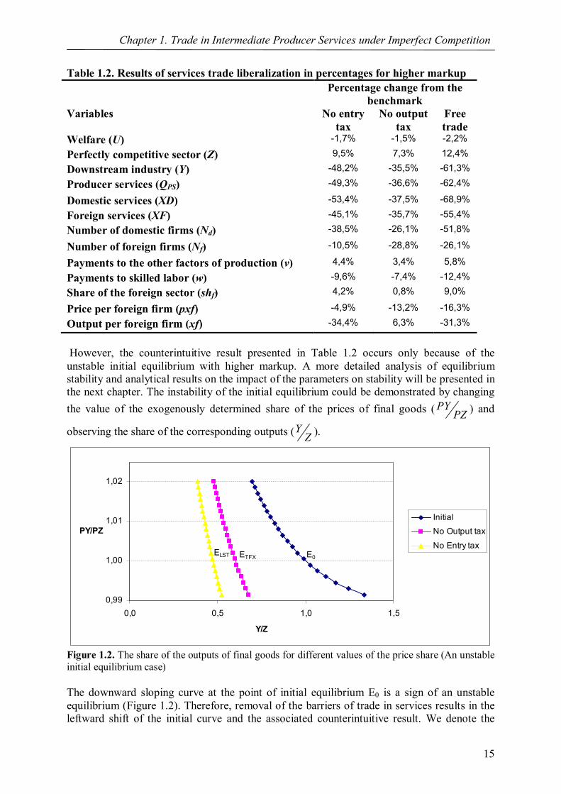
However, the counterintuitive result presented in Table 1.2 occurs only because of the unstable initial equilibrium with higher markup. A more detailed analysis of equilibrium stability and analytical results on the impact of the parameters on stability will be presented in the next chapter. The instability of the initial equilibrium could be demonstrated by changing the value of the exogenously determined share of the prices of final goods ( PY
PZ ) and
observing the share of the corresponding outputs (YZ ).
0,99
1,00
1,01
1,02
0,0 0,5 1,0 1,5
Y/Z
PY/PZInitialNo Output tax
No Entry taxE0ETFX
ELST
Figure 1.2. The share of the outputs of final goods for different values of the price share (An unstable initial equilibrium case) The downward sloping curve at the point of initial equilibrium E0 is a sign of an unstable equilibrium (Figure 1.2). Therefore, removal of the barriers of trade in services results in the leftward shift of the initial curve and the associated counterintuitive result. We denote the
Chapter 1. Trade in Intermediate Producer Services under Imperfect Competition
16
share of the world prices of two goods as *
**
PYPPZ
and the relative supply price of the two
goods obtained from the production structure of the model as the function of taxes and the
ratio of outputs: ( , )SYP tZ
. Then, the Marshallian output adjustment stability conditioniv could
be written as follows:
0 1 0* 1( , ) * 0 (1.5.1)S
Y Y YP P tZ Z Z
Here 0 { , }t TFX LST and 0Y
Z
are the values of the barriers and the output ratio in the
benchmark. In other words, the following should hold: 0
* 0( , ) 0 (1.5.2)SYP P tZ
1t and 1Y
Z
are the corresponding values after one of the two barriers for the services trade are
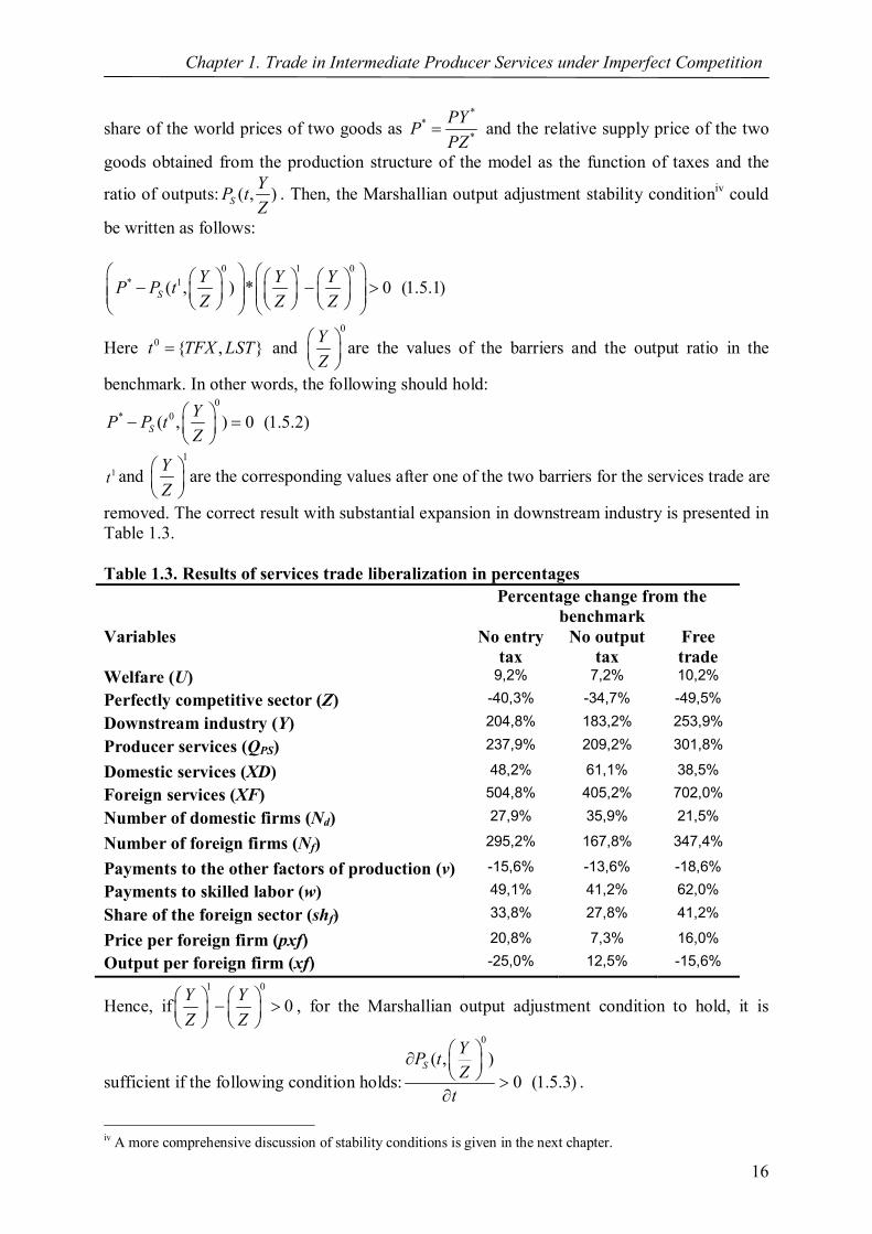
removed. The correct result with substantial expansion in downstream industry is presented in Table 1.3. Table 1.3. Results of services trade liberalization in percentages Percentage change from the
benchmark Variables No entry
tax No output
tax Free trade
Welfare (U) 9,2% 7,2% 10,2%
Perfectly competitive sector (Z) -40,3% -34,7% -49,5%
Downstream industry (Y) 204,8% 183,2% 253,9%
Producer services (QPS) 237,9% 209,2% 301,8%
Domestic services (XD) 48,2% 61,1% 38,5%
Foreign services (XF) 504,8% 405,2% 702,0%
Number of domestic firms (Nd) 27,9% 35,9% 21,5%
Number of foreign firms (Nf) 295,2% 167,8% 347,4%
Payments to the other factors of production (v) -15,6% -13,6% -18,6%
Payments to skilled labor (w) 49,1% 41,2% 62,0%
Share of the foreign sector (shf) 33,8% 27,8% 41,2%
Price per foreign firm (pxf) 20,8% 7,3% 16,0%
Output per foreign firm (xf) -25,0% 12,5% -15,6%
Hence, if1 0
0Y YZ Z
, for the Marshallian output adjustment condition to hold, it is
sufficient if the following condition holds:
0
( , )0 (1.5.3)
SYP tZ
t
.
iv A more comprehensive discussion of stability conditions is given in the next chapter.
Chapter 1. Trade in Intermediate Producer Services under Imperfect Competition
17
Moreover, if we take into account that dual to (1.2.2)1 1
1( )VA PSPY P P
, dual to (1.2.8) 1VA VA
VAP w v and dual to (1.2.9) 1PZ w v , the impact of taxes on the relative supply price will be mainly determined by the impact on the composite price of producer services:
0
( , )0 (1.5.4)
PSYP tZ
t
Since production of final goods is assumed to be at the benchmark, the impact of the barriers on producer services will be defined only by the direct impact on foreign producers. Consequently, equations (1.2.15) and (1.2.17) could be written in the following way under the benchmark:
0
10 01
(1.5.5)(1 )f
f
ff
TFX MCPXFn
and
0 0 0
0 0
* * *(1.5.6)
ff f f
f
FC MC n LST nPXF
XF
Then, from (1.5.5) and (1.5.6) it follows that: 0 0
( , ) ( , )0 (1.5.7), 0 (1.5.8)
Y YPXF TFX PXF LSTZ Z
TFX LST
Those inequalities mean that the fall in relative output of the downstream industry:
The situation with 1 0
0Y YZ Z
could only occur when the LST and TFX tax barriers are
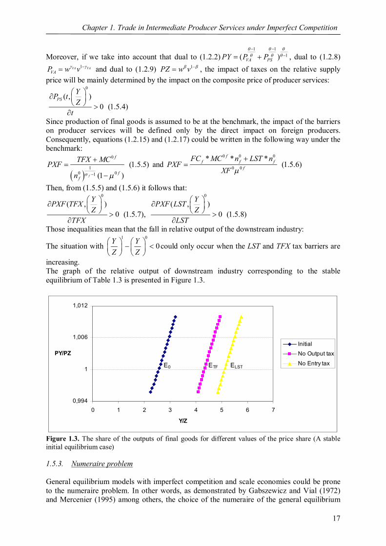
increasing. The graph of the relative output of downstream industry corresponding to the stable equilibrium of Table 1.3 is presented in Figure 1.3.
0,994
1
1,006
1,012
0 1 2 3 4 5 6 7
Y/Z
PY/PZInitialNo Output tax
No Entry taxELSTE0 ETF
Figure 1.3. The share of the outputs of final goods for different values of the price share (A stable initial equilibrium case) 1.5.3. Numeraire problem
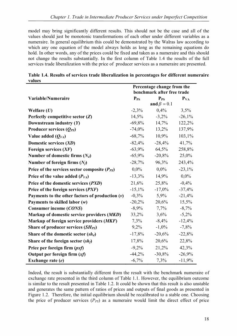
General equilibrium models with imperfect competition and scale economies could be prone to the numeraire problem. In other words, as demonstrated by Gabszewicz and Vial (1972) and Mercenier (1995) among others, the choice of the numeraire of the general equilibrium
Chapter 1. Trade in Intermediate Producer Services under Imperfect Competition
18
model may bring significantly different results. This should not be the case and all of the values should just be monotonic transformations of each other under different variables as a numeraire. In general equilibrium this could be demonstrated by the Walras law according to which any one equation of the model always holds as long as the remaining equations do hold. In other words, any of the prices could be fixed and taken as a numeraire and this should not change the results substantially. In the first column of Table 1.4 the results of the full services trade liberalization with the price of producer services as a numeraire are presented. Table 1.4. Results of services trade liberalization in percentages for different numeraire values Percentage change from the
benchmark after free trade Variable/Numeraire PPS PPS
and 0.1 PVA
Welfare (U) -2,3% 0,4% 3,5% Perfectly competitive sector (Z) 14,5% -3,2% -26,1% Downstream industry (Y) -69,8% 14,7% 122,2% Producer services (QPS) -74,0% 13,2% 137,9% Value added (QVA) -68,7% 10,9% 103,1% Domestic services (XD) -82,4% -28,4% 41,7% Foreign services (XF) -63,9% 64,5% 258,8% Number of domestic firms (Nd) -65,9% -20,8% 25,0% Number of foreign firms (Nf) -28,7% 96,3% 243,4% Price of the services sector composite (PPS) 0,0% 0,0% -23,1% Price of the value added (PVA) -13,3% 14,9% 0,0% Price of the domestic services (PXD) 21,6% 25,8% -0,4% Price of the foreign services (PXF) -15,1% -17,0% -37,4% Payments to the other factors of production (v) -0,3% 5,9% -21,4% Payments to skilled labor (w) -20,2% 20,6% 15,5% Consumer income (CONS) -8,9% 7,7% -8,7% Markup of domestic service providers (MKD) 33,2% 3,6% -5,2% Markup of foreign service providers (MKF) 7,3% -8,4% -12,4% Share of producer services (SHPS) 9,2% -1,0% -7,8% Share of the domestic sector (shd) -17,8% -20,6% -22,8% Share of the foreign sector (shf) 17,8% 20,6% 22,8% Price per foreign firm (pxf) -9,2% 21,2% 42,3% Output per foreign firm (xf) -44,2% -30,8% -26,9% Exchange rate (e) -6,7% 7,3% -11,9% Indeed, the result is substantially different from the result with the benchmark numeraire of exchange rate presented in the third column of Table 1.1. However, the equilibrium outcome is similar to the result presented in Table 1.2. It could be shown that this result is also unstable and generates the same pattern of ratios of prices and outputs of final goods as presented in Figure 1.2. Therefore, the initial equilibrium should be recalibrated to a stable one. Choosing the price of producer services (PPS) as a numeraire would limit the direct effect of price
Chapter 1. Trade in Intermediate Producer Services under Imperfect Competition
19
adjustment even more than the assumption of a small open economy. This is because the latter only fixes the prices of final goods. One of the mechanisms that could improve the stability of the initial equilibrium is the market crowding in skilled labor effect. This effect will be stronger the higher is the difference between , ,d f VA and and the lower is the value of d f . v In particular, the second column of Table 1.4 presents the same result but with a new value of unskilled labor intensity: 0.1 . This time, the result follows the pattern of Tables 1.1 and 1.3 and the equilibrium outcome is stable with the same slope as in Figure 1.3. The impact is just a monotonic transformation of the initial result. Consequently, in this model, the numeraire problem could only occur because of the instability of the resultant initial equilibrium. Similarly to the price of producer services, taking PXF and PXD as a numeraire also undermines the direct effect even more and produces the same result in terms of the directions of change of the variables as the first column of Table 1.4. Taking the price of unskilled labor as a numeraire also leads to the same result as with PXF, PXD and PPS. However, it undermines the market crowding effect. All of those cases could be recalibrated to a stable result equivalent to column two of Table 1.4 by taking 0.1 . On the other hand, taking the price of the value added of the downstream industry (PVA) or the price of the skilled labor as a numeraire represent just the monotonic transformations of the initial result as it could be seen from the results presented in the third column of Table 1.4. Skilled labor represents a small share of the total value added and therefore taking the price of skilled labor as a numeraire is insufficient to obtain an unstable result. There is another aspect associated with the numeraire problem in the general equilibrium models with oligopoly and monopoly market structure. Namely, if the monopoly or oligopoly firm is large relative to the market size of the given economy, its pricing strategy could have repercussions on the prices of other goods and consumer income. Consequently, if such feedback effects are taken into account by the respective oligopoly/monopoly firm, the choice of the numeraire would be important in determining outcomes. However, if the share of the oligopoly firm is small relative to the rest of the economy, which should be the case for most of the economies and firms, the results obtained under full cognition of the feedback effects and without them would not be much different from each other. This problem has been studied numerically using a prototype model in Willenbockel (2005). It was found that if the share of the firm is less than 10% of the economy, the results with and without the full cognition of the feedback effects will be approximately the same. In our model, the share of the whole producer services industry is equal to 10% of the GDP. Therefore, this type of the problem is not relevant to our model and there is no need to calculate oligopoly profits with full cognition of the feedback effects. 1.5.4. Other specifications of the model Let us introduce some other changes to the benchmark setting. In order to study the impact of market structure on model behavior, we could change the conjectures of the firms about the production strategy of their rivals. In particular, let us assume perfect collusion such that:
di dn and f
i fn . The elasticity of substitution between producer services and the value added and the elasticity of substitution between foreign varieties should be recalibrated in
v A more detailed discussion of the market crowding effect as well as the analytical derivation of the parameters that could strengthen it will be given in the next chapter.
Chapter 1. Trade in Intermediate Producer Services under Imperfect Competition
20
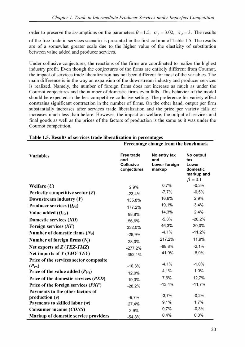
order to preserve the assumptions on the parameters: 1.5, 3.02, 3f d . The results
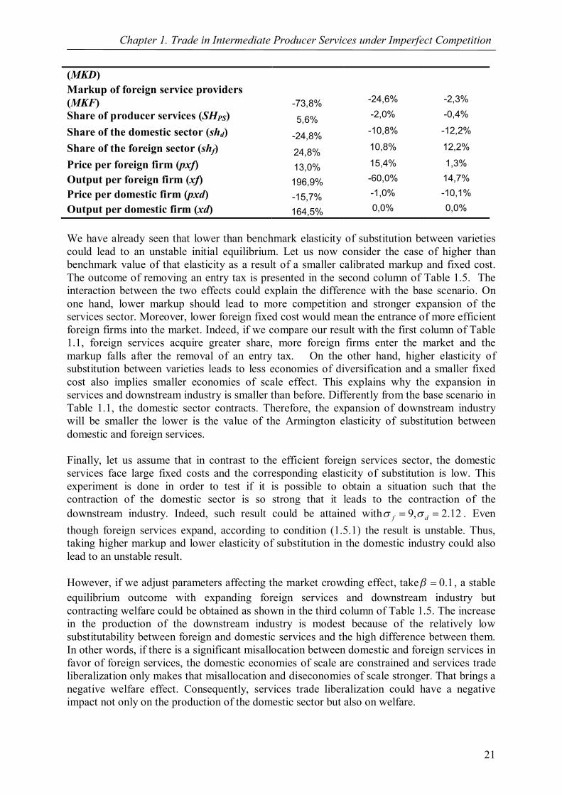
of the free trade in services scenario is presented in the first column of Table 1.5. The results are of a somewhat greater scale due to the higher value of the elasticity of substitution between value added and producer services. Under collusive conjectures, the reactions of the firms are coordinated to realize the highest industry profit. Even though the conjectures of the firms are entirely different from Cournot, the impact of services trade liberalization has not been different for most of the variables. The main difference is in the way an expansion of the downstream industry and producer services is realized. Namely, the number of foreign firms does not increase as much as under the Cournot conjectures and the number of domestic firms even falls. This behavior of the model should be expected in the less competitive collusive setting. The preference for variety effect constrains significant contraction in the number of firms. On the other hand, output per firm substantially increases after services trade liberalization and the price per variety falls or increases much less than before. However, the impact on welfare, the output of services and final goods as well as the prices of the factors of production is the same as it was under the Cournot competition. Table 1.5. Results of services trade liberalization in percentages Percentage change from the benchmark
Variables Free trade and Collusive conjectures
No entry tax and Lower foreign markup
No output tax Lower domestic markup and
0.1 Welfare (U) 2,9% 0,7% -0,3%
Perfectly competitive sector (Z) -23,4% -7,7% -0,5%
Downstream industry (Y) 135,8% 16,6% 2,9%
Producer services (QPS) 177,2% 19,1% 3,4%
Value added (QVA) 98,8% 14,3% 2,4%
Domestic services (XD) 56,6% -5,3% -20,2%
Foreign services (XF) 332,0% 46,3% 30,0%
Number of domestic firms (Nd) -28,9% -4,1% -11,2%
Number of foreign firms (Nf) 28,0% 217,2% 11,9%
Net exports of Z (TEZ-TMZ) -277,2% -88,8% -2,1%
Net imports of Y (TMY-TEY) -352,1% -41,9% -8,9%
Price of the services sector composite (PPS) -10,3%
-4,1%
-1,0%
Price of the value added (PVA) 12,0% 4,1% 1,0%
Price of the domestic services (PXD) 19,3% 7,6% 12,7%
Price of the foreign services (PXF) -28,2% -13,4% -11,7%
Payments to the other factors of production (v) -9,7%
-3,7%
-0,2%
Payments to skilled labor (w) 27,4% 9,1% 1,7%
Consumer income (CONS) 2,9% 0,7% -0,3%
Markup of domestic service providers -54,8% 0,4% 0,0%
Chapter 1. Trade in Intermediate Producer Services under Imperfect Competition
21
(MKD) Markup of foreign service providers (MKF) -73,8%
-24,6%
-2,3%
Share of producer services (SHPS) 5,6% -2,0% -0,4%
Share of the domestic sector (shd) -24,8% -10,8% -12,2%
Share of the foreign sector (shf) 24,8% 10,8% 12,2%
Price per foreign firm (pxf) 13,0% 15,4% 1,3%
Output per foreign firm (xf) 196,9% -60,0% 14,7%
Price per domestic firm (pxd) -15,7% -1,0% -10,1%
Output per domestic firm (xd) 164,5% 0,0% 0,0%
We have already seen that lower than benchmark elasticity of substitution between varieties could lead to an unstable initial equilibrium. Let us now consider the case of higher than benchmark value of that elasticity as a result of a smaller calibrated markup and fixed cost. The outcome of removing an entry tax is presented in the second column of Table 1.5. The interaction between the two effects could explain the difference with the base scenario. On one hand, lower markup should lead to more competition and stronger expansion of the services sector. Moreover, lower foreign fixed cost would mean the entrance of more efficient foreign firms into the market. Indeed, if we compare our result with the first column of Table 1.1, foreign services acquire greater share, more foreign firms enter the market and the markup falls after the removal of an entry tax. On the other hand, higher elasticity of substitution between varieties leads to less economies of diversification and a smaller fixed cost also implies smaller economies of scale effect. This explains why the expansion in services and downstream industry is smaller than before. Differently from the base scenario in Table 1.1, the domestic sector contracts. Therefore, the expansion of downstream industry will be smaller the lower is the value of the Armington elasticity of substitution between domestic and foreign services. Finally, let us assume that in contrast to the efficient foreign services sector, the domestic services face large fixed costs and the corresponding elasticity of substitution is low. This experiment is done in order to test if it is possible to obtain a situation such that the contraction of the domestic sector is so strong that it leads to the contraction of the downstream industry. Indeed, such result could be attained with 9, 2.12f d . Even though foreign services expand, according to condition (1.5.1) the result is unstable. Thus, taking higher markup and lower elasticity of substitution in the domestic industry could also lead to an unstable result. However, if we adjust parameters affecting the market crowding effect, take 0.1 , a stable equilibrium outcome with expanding foreign services and downstream industry but contracting welfare could be obtained as shown in the third column of Table 1.5. The increase in the production of the downstream industry is modest because of the relatively low substitutability between foreign and domestic services and the high difference between them. In other words, if there is a significant misallocation between domestic and foreign services in favor of foreign services, the domestic economies of scale are constrained and services trade liberalization only makes that misallocation and diseconomies of scale stronger. That brings a negative welfare effect. Consequently, services trade liberalization could have a negative impact not only on the production of the domestic sector but also on welfare.
Chapter 1. Trade in Intermediate Producer Services under Imperfect Competition
22
This outcome could be expected to occur for example in telecommunications or the transportation services sectors. The domestic incumbents may have property rights over infrastructure and there could be some local characteristics that cannot be easily acquired or local legislation that cannot be easily adjusted to by foreign firms. That should lead to a relatively small estimate of the elasticity of substitution between domestic and foreign services and relatively higher economies of scale in the domestic industry. Those are the reasons that lead to the result presented in Table 1.5. On the other hand, in the financial and business services there should be less of those kinds of barriers and therefore the estimate of the Armington substitution elasticity could be expected to be higher. Moreover, the differences in productivity and the entry costs could be smoothed by relative spillover effects. This could lead to an expansion of domestic services as well as foreign services and follow the base scenario of our model. 1.6. Concluding remarks
The model constructed in this chapter has demonstrated several key results important for policy analysis and further empirical studies. In particular, it has been found that:
Trade liberalization in producer services leads to an expansion of downstream industry that uses them as inputs.
A very high level of markup in both domestic and foreign services could lead to an
unstable equilibrium. In other words, considerations about the instability of the initial equilibrium could impose additional constraints on the value of the model parameters.
The conjectures of firms about the production strategy of their rivals have little impact
on model results. On the other hand, changes in the elasticities of substitution could have more profound effects on the model results compared to conjectures of the firms.
High difference in markups between domestic and foreign firms could lead to an
insignificant expansion in downstream industry and a negative welfare effect. Moreover, it was found that the two common types of barriers on the operations of foreign firms would have a similar impact on the direction of change of the key variables of the model. However, they define two different patterns of expansion of the foreign services industry. The analytical results of the relationships between parameter values and the markup have also been presented. The expansion of downstream industry as a result of the liberalization of trade in producer services could also be explained as follows: If trade protection of intermediates including service intermediates is higher than trade protection of downstream industry, the effective rate of protection (ERP) in downstream industry is negative. That means that downstream industry value added is effectively taxed not protected. Therefore, cutting trade barriers on producer services turns ERP for downstream industry to be positive and that leads to an expansion of the latter. It should be added that the magnitudes of the numerical results should be accepted with due caution because of the stylized nature of the underlying model. In other words, it is rather narrowly focused and emphasizes particular mechanisms only. On the other hand, a stylized quantitative model could serve as a useful tool to disentangle the various effects present in the more complicated applied models. Those latter models are frequently viewed as black boxes
Chapter 1. Trade in Intermediate Producer Services under Imperfect Competition
23
because it could be difficult to explain which mechanisms and effects are responsible for the results (Devarajan, Robinson, 2005). Both applied and stylized models should be combined to be used effectively in policy analysis. Improvements in the data on services could significantly enhance the power of the analysis. In the model setting presented in this chapter, individual firm efficiency and fixed cost share depend positively on each other. The differences in fixed cost share between foreign and domestic firms appear to be critical for the negative welfare effect obtained from the policy experiments in the numerical model. However, there is a lack of data on the comparative efficiency of foreign versus domestic firms in services. Bibliography Christopoulou, R., Vermeulen, P., (2008) "Markups in the euro area and the US over the
period 1981-2004 - a comparison of 50 sectors" Working Paper Series 856, European Central Bank.
Copeland, B., (2002) “Benefits and costs of trade and investment liberalization in services: Implications from trade theory” in Curtis, J. M. and D. C. Ciuriak, eds. Trade Policy Research 2002. Department of Foreign Affairs and International Trade, Canada, pp. 107–218.
Devarajan, S., Robinson, S., (2005) “The Influence of Computable General Equilibrium Model on Policy” in Kehoe. T, Srinivasan, T. N. and Whalley, John (eds) Frontiers in Applied General Equilibrium Modelling. Cambridge University Press, pp. 402-428.
Epifani, P., Gancia, G., (2011) “Trade, markup heterogeneity and misallocations”, Journal of International Economics (83), pp. 1-13.
Gabszewicz, J.J., and Vial, J.-P., (1972) “Oligopoly “A la Cournot” in a General Equilibrium Analysis”, Journal of Economic Theory (4), pp. 381-400.
Gasiorek, M., Smith, A., Venables, A., (2002) “The accession of the UK to the EC: a welfare analysis”. J. Common Mark. Stud. 40, pp. 425–447.
Haaland, J., Norman, V., (1992) “Global production effects of European integration” In: Winters, L.A. (eds), Trade Flows and Trade Policy after 1992, Cambridge University Press, Cambridge, pp. 67-91.
Hoekman, Bernard. (2006). ‘Liberalization of Trade in Services: A Survey’, World Bank working paper.
Konan, D., Assche, A., (2007). “Regulation, Market Structure and Service Trade Liberalization”, Economic Modeling 24 (2007), pp. 895-923.
Markusen, J., (1989) “Trade in Producer Services and in Other Specialized Intermediate Inputs”, American Economic Review (79), pp. 85-95.
Markusen, J., (2002) “General Equilibrium Modeling using GAMS and MPS/GE”. Boulder. www.gams.de/b/courses/dublin/tutorial.pdf.
Markusen, J., Rutherford, T., and Tarr, D., (2005) “Trade and direct investment in producer services and the domestic market for expertise”, Canadian Journal of Economics 38 (2005), pp. 758–777.
Mattoo, A., Rathindran, R., and Subramanian, A., (2006) “Measuring Services Trade liberalization and its Impacts on Economic Growth: An Illustration”, Journal of Economic Integration 21 (2006), pp. 64-98.
Mattoo, A., Sauve, P., (2003) “Domestic Regulation and Services Trade Liberalization”, Oxford University Press: Washington, D.C.
McDaniel, C., and Balistreri, E., (2003) “A Review of Armington Trade Substitution Elasticities”, Économie Internationale, 94-95, pp. 301-314.
Chapter 1. Trade in Intermediate Producer Services under Imperfect Competition
24
Mercenier, J., (1995) “Nonuniqueness of Solutions in Applied General Equilibrium Models with Scale Economies and Imperfect Competition”, Economic Theory (6), pp. 161-77.
Rutherford, T., Tarr, D., and Shepotylo, O., (2006) “The Impact of WTO Accession and the DDA: The Importance of Liberalization of Barriers Against FDI in Services for Growth and Poverty Reduction,” in Thomas Hertel and L. Alan Winters (eds.), Poverty and the WTO (Palgrave and World Bank), pp.467-96.
de Santis, R., (2002) “A computable general equilibrium model for open economies with imperfect competition and product differentiation”. J. Econ. Integration (17), pp. 311– 338.
UNCTAD (2003). “Assessment of Trade in Services and Development Gains”, Handbook of Statistics. Draft note by the UNCTAD secretariat.
Whalley, J., (2004) “Assessing the Benefits to Developing Countries of Liberalization in Services Trade” , The World Economy 27(8), pp.1223-53.
Willenbockel, D., (1994) “Applied General Equilibrium Modelling: Imperfect Competition and European Integration” John Wiley, Chichester.
Willenbockel, D., (2004) “Specification Choice and Robustness in CGE Trade Policy Analysis with Imperfect Competition”, Economic Modeling (21), pp.1065-99.
Willenbockel, D., (2005) “The Price Normalization Problem in General Equilibrium Models with Oligopoly Power: An Attempt at Perspective”, Middlesex University Business School Discussion Paper Series: Economics.
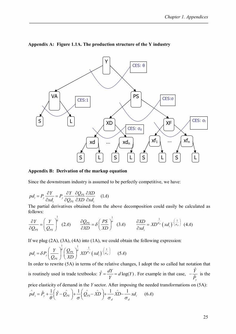
Chapter 1. Appendices
25
Appendix A: Figure 1.1A. The production structure of the Y industry
Appendix B: Derivation of the markup equation Since the downstream industry is assumed to be perfectly competitive, we have:
(1 )PSi y y
i PS i
QY Y XDpd P P Axd Q XD xd
The partial derivatives obtained from the above decomposition could easily be calculated as follows:
1
(2 )PS PS
Y Y AQ Q
1
(3 )PSQ PS AXD XD
1 1
(4 )ddi
i
XD XD xd Axd
If we plug (2A), (3A), (4A) into (1A), we could obtain the following expression:
1 1 1 1
(5 )dd
PSi y i
PS
QYpd P XD xd AQ XD
In order to rewrite (5A) in terms of the relative changes, I adopt the so called hat notation that
is routinely used in trade textbooks: ˆ log( )dYY d YY
. For example in that case, ˆˆ
y
YP
is the
price elasticity of demand in the Y sector. After imposing the needed transformations on (5A): 1 1 1 1ˆ ˆ (6 )y PS PS ii
d d
pd P Y Q Q XD XD xd A
Y
VA PS
CES: θ
XD XF
CES:σ
xd
… xf1 xfn
xdn
…
CES: σf
CES: σd
S L
S S S S L L L L
CES:1
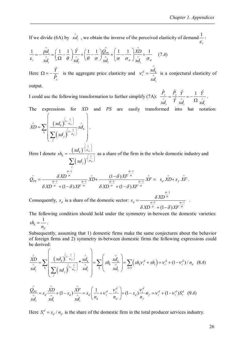
Chapter 1. Appendices
26
If we divide (6A) by ixd
, we obtain the inverse of the perceived elasticity of demand 1
i:
ˆ1 1 1 1 1 1 1 1 (7 )i PS
i d di i i i
pd QY XD Axd xd xd xd
Here ˆ
y
YP
is the aggregate price elasticity and d ki
i
xd
xd
is a conjectural elasticity of
output.
I could use the following transformation to further simplify (7A): ˆ ˆ ˆ ˆ1
ˆy y
i i i
P P Y YYxd xd xd
.
The expressions for XD and PS are easily transformed into hat notation:
11
11
d
d
kk
kj
j
xdXD xd
xd
.
Here I denote
1
1
d
d
kk
jj
xdsh
xd
as a share of the firm in the whole domestic industry and
1 1
1 1 1 1(1 )
(1 ) (1 )PS d f
XD XFQ XD XF s XD s XFXD XF XD XF
.
Consequently, ds is a share of the domestic sector:
1
1 1
(1 )d
XDsXD XF
.
The following condition should hold under the symmetry in-between the domestic varieties: 1
kd
shn
.
Subsequently, assuming that 1) domestic firms make the same conjectures about the behavior of foreign firms and 2) symmetry in-between domestic firms the following expressions could be derived:
11
11* (1 ) / (8 )
d
d
k d d dk kk k i i i i d
k k k ii i ij
j
xd xd xdXD sh sh sh n Axd xd xdxd
1(1 ) (1 ) (1 ) (9 )d d
d d d dPS i id d d i d f i i i
d d fi i i
Q XD XFs s s s n S An n nxd xd xd
Here /d
i d dS s n is the share of the domestic firm in the total producer services industry.
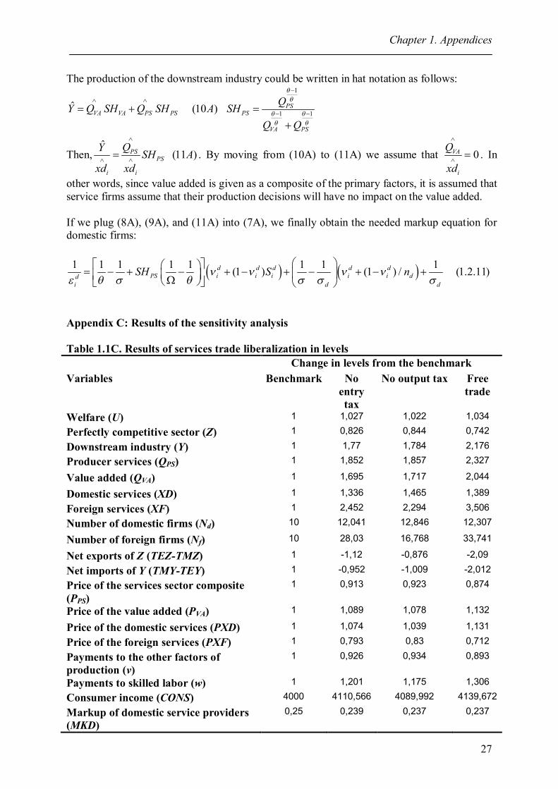
Chapter 1. Appendices
27
The production of the downstream industry could be written in hat notation as follows:
ˆ (10 )VA VA PS PSY Q SH Q SH A
1
1 1PS
PS
VA PS
QSHQ Q
Then,ˆ
(11 )PSPS
i i
QY SH Axd xd
. By moving from (10A) to (11A) we assume that 0VA
i
Q
xd
. In
other words, since value added is given as a composite of the primary factors, it is assumed that service firms assume that their production decisions will have no impact on the value added. If we plug (8A), (9A), and (11A) into (7A), we finally obtain the needed markup equation for domestic firms:
1 1 1 1 1 1 1 1(1 ) (1 ) / (1.2.11)d d d d dPS i i i i i dd
i d d
SH S n
Appendix C: Results of the sensitivity analysis Table 1.1C. Results of services trade liberalization in levels Change in levels from the benchmark Variables Benchmark No
entry tax
No output tax Free trade
Welfare (U) 1 1,027 1,022 1,034
Perfectly competitive sector (Z) 1 0,826 0,844 0,742
Downstream industry (Y) 1 1,77 1,784 2,176
Producer services (QPS) 1 1,852 1,857 2,327
Value added (QVA) 1 1,695 1,717 2,044
Domestic services (XD) 1 1,336 1,465 1,389
Foreign services (XF) 1 2,452 2,294 3,506
Number of domestic firms (Nd) 10 12,041 12,846 12,307
Number of foreign firms (Nf) 10 28,03 16,768 33,741
Net exports of Z (TEZ-TMZ) 1 -1,12 -0,876 -2,09
Net imports of Y (TMY-TEY) 1 -0,952 -1,009 -2,012
Price of the services sector composite (PPS)
1 0,913 0,923 0,874
Price of the value added (PVA) 1 1,089 1,078 1,132
Price of the domestic services (PXD) 1 1,074 1,039 1,131
Price of the foreign services (PXF) 1 0,793 0,83 0,712
Payments to the other factors of production (v)
1 0,926 0,934 0,893
Payments to skilled labor (w) 1 1,201 1,175 1,306
Consumer income (CONS) 4000 4110,566 4089,992 4139,672
Markup of domestic service providers (MKD)
0,25 0,239 0,237 0,237
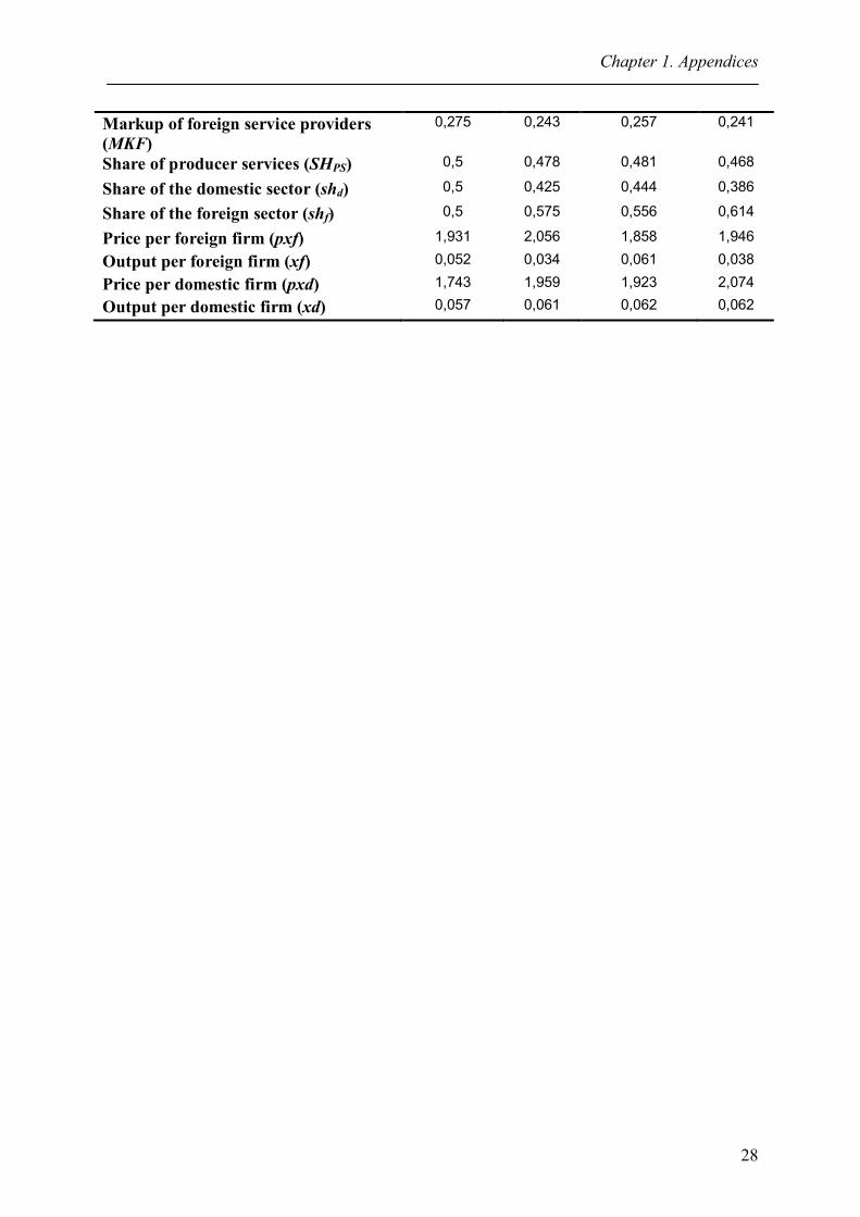
Chapter 1. Appendices
28
Markup of foreign service providers (MKF)
0,275 0,243 0,257 0,241
Share of producer services (SHPS) 0,5 0,478 0,481 0,468
Share of the domestic sector (shd) 0,5 0,425 0,444 0,386
Share of the foreign sector (shf) 0,5 0,575 0,556 0,614
Price per foreign firm (pxf) 1,931 2,056 1,858 1,946
Output per foreign firm (xf) 0,052 0,034 0,061 0,038
Price per domestic firm (pxd) 1,743 1,959 1,923 2,074
Output per domestic firm (xd) 0,057 0,061 0,062 0,062
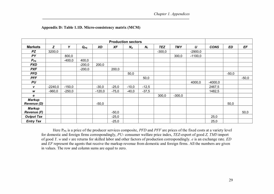
Chapter 1. Appendices
29
Appendix D: Table 1.1D. Micro-consistency matrix (MCM)
Production sectors Markets Z Y QPS XD XF Nd Nf TEZ TMY U CONS ED EF
PZ 3200,0 -300,0 -2900,0 PY 800,0 300,0 -1100,0 PPS -400,0 400,0 PXD -200,0 200,0 PXF -200,0 200,0 PFD 50,0 -50,0 PFF 50,0 -50,0 PU 4000,0 -4000,0 v -2240,0 -150,0 -30,0 -25,0 -10,0 -12,5 2467,5 w -960,0 -250,0 -120,0 -75,0 -40,0 -37,5 1482,5 e 300,0 -300,0
Markup Revenue (D) -50,0 50,0
Markup Revenue (F) -50,0 50,0 Output Tax -25,0 25,0 Entry Tax -25,0 25,0
Here PPS is a price of the producer services composite, PFD and PFF are prices of the fixed costs at a variety level
for domestic and foreign firms correspondingly, PU- consumer welfare price index, TEZ-export of good Z, TMY-import of good Y. w and v are returns for skilled labor and other factors of production correspondingly. e is an exchange rate. ED and EF represent the agents that receive the markup revenue from domestic and foreign firms. All the numbers are given in values. The row and column sums are equal to zero.
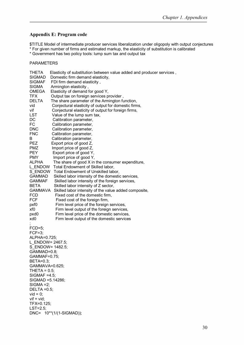
Chapter 1. Appendices
30
Appendix E: Program code
$TITLE Model of intermediate producer services liberalization under oligopoly with output conjectures * For given number of firms and estimated markup, the elasticity of substitution is calibrated * Government has two policy tools: lump sum tax and output tax
PARAMETERS THETA Elasticity of substitution between value added and producer services , SIGMAD Domestic firm demand elasticity, SIGMAF FDI firm demand elasticity , SIGMA Armington elasticity , OMEGA Elasticity of demand for good Y, TFX Output tax on foreign services provider , DELTA The share parameter of the Armington function, vid Conjectural elasticity of output for domestic firms, vif Conjectural elasticity of output for foreign firms, LST Value of the lump sum tax, DC Calibration parameter, FC Calibration parameter, DNC Calibration parameter, FNC Calibration parameter, B Calibration parameter, PEZ Export price of good Z, PMZ Import price of good Z, PEY Export price of good Y, PMY Import price of good Y, ALPHA The share of good X in the consumer expenditure, L_ENDOW Total Endowment of Skilled labor, S_ENDOW Total Endowment of Unskilled labor, GAMMAD Skilled labor intensity of the domestic services, GAMMAF Skilled labor intensity of the foreign services, BETA Skilled labor intensity of Z sector, GAMMAVA Skilled labor intensity of the value added composite, FCD Fixed cost of the domestic firm, FCF Fixed cost of the foreign firm, pxf0 Firm level price of the foreign services, xf0 Firm level output of the foreign services, pxd0 Firm level price of the domestic services, xd0 Firm level output of the domestic services ; FCD=5; FCF=3; ALPHA=0.725; L_ENDOW= 2467.5; S_ENDOW= 1482.5; GAMMAD=0.8; GAMMAF=0.75; BETA=0.3; GAMMAVA=0.625; THETA = 0.5; SIGMAF =4.5; SIGMAD =5.14286; SIGMA =2; DELTA =0.5; vid = 0; vif = vid; TFX=0.125; LST=2.5; DNC= 10**(1/(1-SIGMAD));

Chapter 1. Appendices
31
FNC= 10**(1/(1-SIGMAF)); PEZ=1; PMZ= 1000/999; PEY=999/1000; PMY=1; B= 2**(1/(THETA-1)); POSITIVE VARIABLES W ! Consumption (static welfare) level Z ! Activity level for sector Z Y ! Activity level for sector Y PS ! Intermediate producer services VA ! Value added XD ! Activity level for sector XD domestic services XF ! Activity level for sector XF foreign (MNE) services ND ! Number of domestic service firms NF ! Number of foreign (MNE) service firms TMZ ! Activity level for imports of Z TEZ ! Activity level for exports of Z TMY ! Activity level for imports of Y TEY ! Activity level for imports of Y PW ! Price index for consumption PZ ! Price index for commodity Z PY ! Price index for commodity Y PPS ! Price index for producer services PVA ! Price index for the value added PXD ! Price index for domestic commodity PFD ! Price of fixed costs for domestic services PXF ! Price index for commodity Z MNE PFF ! Price of fixed costs for MNE services RL ! Return to unskilled labor L (composite) RS ! Return to skilled labor S (skilled labor) PFX ! Price index for foreign exchange CONS ! Income level for consumer CONS ENTRED ! Dummy agent for domestic services (receives markups) ENTREF ! Dummy agent for foreign services (receives markups) MKD ! Markup by domestic firms MKF ! Markup by foreign firms SHPS ! Share of the producer services shd ! Share of the domestic industry in the producer services shf ! Share of the foreign firms in the producer services ; EQUATIONS PriceW Zero profit condition for welfare PriceZ Zero profit condition for Z PriceY Zero profit condition for Y PriceVA Zero profit condition for VA PricePS Zero profit condition for Producer Services PriceXD MR=MC condition for domestic firms PriceXF MR=MC condition for foreign firms PricePFD Zero profit condition for domestic fixed costs PricePFF Zero profit condition for foreign fixed costs E_TEY Zero profit condition for exports of Y E_TMZ Zero profit condition for imports of Z E_TEZ Zero profit condition for exports of Z E_TMY Zero profit condition for imports of Y DW Demand for W DZ Demand for Z DY Demand for Y
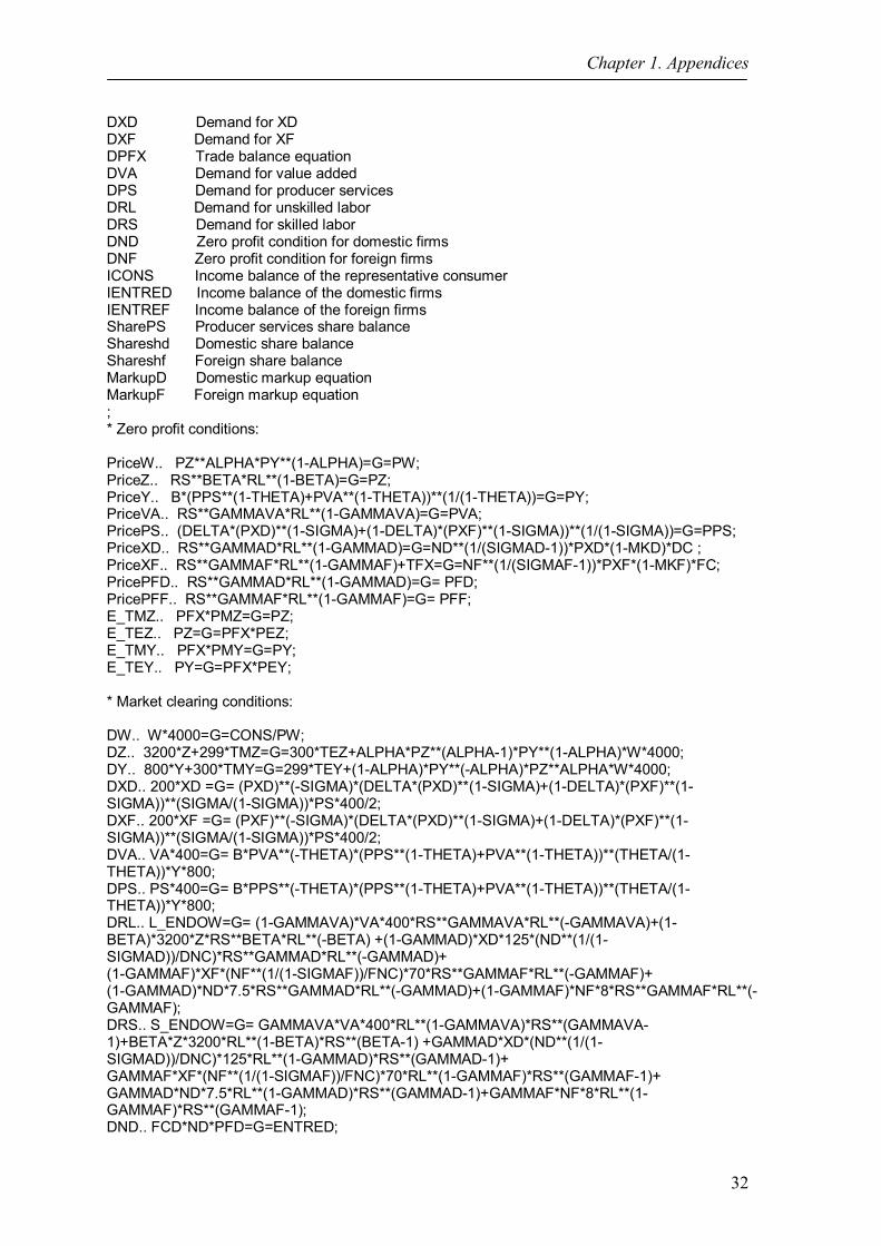
Chapter 1. Appendices
32
DXD Demand for XD DXF Demand for XF DPFX Trade balance equation DVA Demand for value added DPS Demand for producer services DRL Demand for unskilled labor DRS Demand for skilled labor DND Zero profit condition for domestic firms DNF Zero profit condition for foreign firms ICONS Income balance of the representative consumer IENTRED Income balance of the domestic firms IENTREF Income balance of the foreign firms SharePS Producer services share balance Shareshd Domestic share balance Shareshf Foreign share balance MarkupD Domestic markup equation MarkupF Foreign markup equation ; * Zero profit conditions: PriceW.. PZ**ALPHA*PY**(1-ALPHA)=G=PW; PriceZ.. RS**BETA*RL**(1-BETA)=G=PZ; PriceY.. B*(PPS**(1-THETA)+PVA**(1-THETA))**(1/(1-THETA))=G=PY; PriceVA.. RS**GAMMAVA*RL**(1-GAMMAVA)=G=PVA; PricePS.. (DELTA*(PXD)**(1-SIGMA)+(1-DELTA)*(PXF)**(1-SIGMA))**(1/(1-SIGMA))=G=PPS; PriceXD.. RS**GAMMAD*RL**(1-GAMMAD)=G=ND**(1/(SIGMAD-1))*PXD*(1-MKD)*DC ; PriceXF.. RS**GAMMAF*RL**(1-GAMMAF)+TFX=G=NF**(1/(SIGMAF-1))*PXF*(1-MKF)*FC; PricePFD.. RS**GAMMAD*RL**(1-GAMMAD)=G= PFD; PricePFF.. RS**GAMMAF*RL**(1-GAMMAF)=G= PFF; E_TMZ.. PFX*PMZ=G=PZ; E_TEZ.. PZ=G=PFX*PEZ; E_TMY.. PFX*PMY=G=PY; E_TEY.. PY=G=PFX*PEY; * Market clearing conditions: DW.. W*4000=G=CONS/PW; DZ.. 3200*Z+299*TMZ=G=300*TEZ+ALPHA*PZ**(ALPHA-1)*PY**(1-ALPHA)*W*4000; DY.. 800*Y+300*TMY=G=299*TEY+(1-ALPHA)*PY**(-ALPHA)*PZ**ALPHA*W*4000; DXD.. 200*XD =G= (PXD)**(-SIGMA)*(DELTA*(PXD)**(1-SIGMA)+(1-DELTA)*(PXF)**(1-SIGMA))**(SIGMA/(1-SIGMA))*PS*400/2; DXF.. 200*XF =G= (PXF)**(-SIGMA)*(DELTA*(PXD)**(1-SIGMA)+(1-DELTA)*(PXF)**(1-SIGMA))**(SIGMA/(1-SIGMA))*PS*400/2; DVA.. VA*400=G= B*PVA**(-THETA)*(PPS**(1-THETA)+PVA**(1-THETA))**(THETA/(1-THETA))*Y*800; DPS.. PS*400=G= B*PPS**(-THETA)*(PPS**(1-THETA)+PVA**(1-THETA))**(THETA/(1-THETA))*Y*800; DRL.. L_ENDOW=G= (1-GAMMAVA)*VA*400*RS**GAMMAVA*RL**(-GAMMAVA)+(1-BETA)*3200*Z*RS**BETA*RL**(-BETA) +(1-GAMMAD)*XD*125*(ND**(1/(1-SIGMAD))/DNC)*RS**GAMMAD*RL**(-GAMMAD)+ (1-GAMMAF)*XF*(NF**(1/(1-SIGMAF))/FNC)*70*RS**GAMMAF*RL**(-GAMMAF)+ (1-GAMMAD)*ND*7.5*RS**GAMMAD*RL**(-GAMMAD)+(1-GAMMAF)*NF*8*RS**GAMMAF*RL**(-GAMMAF); DRS.. S_ENDOW=G= GAMMAVA*VA*400*RL**(1-GAMMAVA)*RS**(GAMMAVA-1)+BETA*Z*3200*RL**(1-BETA)*RS**(BETA-1) +GAMMAD*XD*(ND**(1/(1-SIGMAD))/DNC)*125*RL**(1-GAMMAD)*RS**(GAMMAD-1)+ GAMMAF*XF*(NF**(1/(1-SIGMAF))/FNC)*70*RL**(1-GAMMAF)*RS**(GAMMAF-1)+ GAMMAD*ND*7.5*RL**(1-GAMMAD)*RS**(GAMMAD-1)+GAMMAF*NF*8*RL**(1-GAMMAF)*RS**(GAMMAF-1); DND.. FCD*ND*PFD=G=ENTRED;
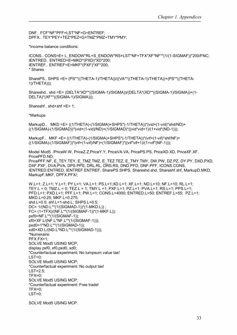
Chapter 1. Appendices
33
DNF.. FCF*NF*PFF+LST*NF=G=ENTREF; DPFX.. TEY*PEY+TEZ*PEZ=G=TMZ*PMZ+TMY*PMY; *Income balance conditions: ICONS.. CONS=E= L_ENDOW*RL+S_ENDOW*RS+LST*NF+TFX*XF*NF**(1/(1-SIGMAF))*200/FNC; IENTRED.. ENTRED=E=MKD*(PXD)*XD*200; IENTREF.. ENTREF=E=MKF*(PXF)*XF*200; * Shares SharePS.. SHPS =E= (PS**((THETA-1)/THETA))/((VA**((THETA-1)/THETA))+(PS**((THETA-1)/THETA))); Shareshd.. shd =E= (DELTA*XD**((SIGMA-1)/SIGMA))/(DELTA*(XD**((SIGMA-1)/SIGMA))+(1-DELTA)*(XF**((SIGMA-1)/SIGMA))); Shareshf.. shd+shf =E= 1; *Markups MarkupD.. MKD =E= ((1/THETA)-(1/SIGMA)+SHPS*(-1/THETA))*(vid+(1-vid)*shd/ND)+ ((1/SIGMA)-(1/SIGMAD))*(vid+(1-vid)/ND)+(1/SIGMAD)*((vid*vid+1)/(1+vid*(ND-1))); MarkupF.. MKF =E= ((1/THETA)-(1/SIGMA)+SHPS*(-1/THETA))*(vif+(1-vif)*shf/NF)+ ((1/SIGMA)-(1/SIGMAF))*(vif+(1-vif)/NF)+(1/SIGMAF)*((vif*vif+1)/(1+vif*(NF-1))); Model Mod5 /PriceW.W, PriceZ.Z,PriceY.Y, PriceVA.VA, PricePS.PS, PriceXD.XD, PriceXF.XF, PricePFD.ND, PricePFF.NF, E_TEY.TEY, E_TMZ.TMZ, E_TEZ.TEZ, E_TMY.TMY, DW.PW, DZ.PZ, DY.PY, DXD.PXD, DXF.PXF, DVA.PVA, DPS.PPS, DRL.RL, DRS.RS, DND.PFD, DNF.PFF, ICONS.CONS, IENTRED.ENTRED, IENTREF.ENTREF, SharePS.SHPS, Shareshd.shd, Shareshf.shf, MarkupD.MKD, MarkupF.MKF, DPFX.PFX/; W.L=1; Z.L=1; Y.L=1; PY.L=1; VA.L=1; PS.L=1;XD.L=1; XF.L=1; ND.L=10; NF.L=10; RL.L=1; TEY.L = 0; TMZ.L = 0; TEZ.L = 1; TMY.L =1; PXF.L=1; PZ.L=1; PVA.L=1; RS.L=1; PPS.L=1; PFD.L=1; PXD.L=1; PFF.L=1; PW.L=1; CONS.L=4000; ENTRED.L=50; ENTREF.L=55; PZ.L=1; MKD.L=0.25; MKF.L=0.275; shd.L=0.5; shf.L=1-shd.L; SHPS.L=0.5; DC= 1/(ND.L**(1/(SIGMAD-1))*(1-MKD.L)) ; FC= (1+TFX)/(NF.L**(1/(SIGMAF-1))*(1-MKF.L)); pxf0=NF.L**(1/(SIGMAF-1)); xf0=XF.L/(NF.L*NF.L**(1/(SIGMAF-1))); pxd0=1*ND.L**(1/(SIGMAD-1)); xd0=XD.L/(ND.L*ND.L**(1/(SIGMAD-1))); *Numeraire: PFX.FX=1; SOLVE Mod5 USING MCP; display pxf0, xf0,pxd0, xd0; *Counterfactual experiment: No lumpsum value tax! LST=0; SOLVE Mod5 USING MCP; *Counterfactual experiment: No output tax! LST=2.5; TFX=0; SOLVE Mod5 USING MCP; *Counterfactual experiment: Free trade! TFX=0; LST=0; SOLVE Mod5 USING MCP.

34
Chapter 2 On Equilibrium Stability in the CGE models with Monopolistic Competition A simple general equilibrium model with monopolistic competition is constructed to study the conditions of equilibrium stability. The effects leading to unstable equilibrium and the subsequent counterintuitive comparative statics result are identified. Moreover, the impacts of the parameters of the model on the stability of the benchmark equilibrium are presented by developing dynamic extensions underlying the initially static model. In particular, it is shown that the elasticity of substitution between the Dixit-Stiglitz varieties, difference in the skilled labor intensities of two sectors of the economy and the relative size of the increasing returns to scale sector increase the stability of the benchmark equilibrium. The dynamic time paths of the endogenous variables from unstable to stable equilibrium are presented. It is also found that the results of an ad valorem tax cut would have the same effect in terms of directions of change on most of the endogenous variables of the model irrespective of data. 2.1. Introduction This chapter constructs a simple general equilibrium model with two factors of production and two sectors of the economy: the increasing returns to scale sector with monopolistic competition market structure and the perfectly competitive constant returns to scale sector. It then studies the impact of a tax cut in the increasing returns to scale sector on the output of the industries and factor returns. It is found that under the small open economy assumption, it is possible to classify the results into two categories in terms of the direction of change of the endogenous variables. However, small open economy assumption also eliminates the price effect which makes the result dependent on indirect effects. This makes it possible for a counterintuitive result to occur. We identify indirect effects and study the parameters of the system that influence them. In recent literature on international trade, the increasing returns to scale sector with monopolistically competitive market structure is assumed to describe the services sector (Markusen et al., 2005). This is plausible because there are many varieties of services and a higher number of them makes it more likely that consumer specific services are available. Therefore, the availability of more varieties of services increases consumer utility (love of variety effect). It would also be reasonable to assume that skilled labor is used more intensively by services compared to other industries. The convention to give some special name to factors of production or sectors of the economy depends on the problem being considered. In particular, in the core-periphery model of Krugman (1991), the increasing returns to scale sector is assumed to be manufacturing and the perfectly competitive sector is agriculture. Consequently, the manufacturing sector is assumed to employ workers and the agricultural sector is assumed to employ peasants. Therefore, without a loss of generality let us assign skilled labor to be the factor that is intensively used in the monopolistically competitive or services industry. It could also be the manufacturing industry which is likely to be subject to imperfect competition as well.

Chapter 2. On Equilibrium Stability in the CGE models with Monopolistic Competition
35
Already in Samuelson (1947) it was stated that the comparative static outcomes are intimately tied to the stability of the equilibrium. Consequently, the stability of the benchmark equilibrium needs to be studied in order to determine if the counterintuitive result is stable or not. There are two stability concepts depending on the market adjustment mechanisms: Marshallian and Walrasian stability. In Walrasian equilibrium, market adjustment is defined in terms of endogenously changing prices and in Marshallian equilibrium it is defined in terms of quantities. Each concept is chosen depending on the nature of the economic setting. Even though the Walrasian stability concept is often implied by default in many studies while checking for equilibrium stability, it is not suitable for our model because we have fixed prices of final goods. Furthermore, the Marshallian stability concept is associated with the theory of production and it is more appropriate to the setting with small open economy assumption and correspondingly with no adjustments in the prices of traded goods. There are several approaches to determine the stability of the equilibrium by studying alternative specifications of the dynamic extensions of the static model. Given that we have already established that the Marshallian stability concept is appropriate to our model setting, the most straightforward way is to check it by looking at whether the condition of Marshallian output adjustment process holds (Ide and Takayama, 1990). Another way is to resort to the methods used in the new economic geography theory (Krugman, 1991). In that case, the dynamics of the labor movement between sectors is studied in analogy with the interregional labor movement of new economic geography models. In these models, skilled labor is assumed to be immobile between regions in the short run. On the other hand, unskilled labor is assumed to be always immobile. This enables us to uncover new insights of model behavior and detect agglomeration type effects. It also provides us with the framework for introducing the dynamic evolution of variables by distinguishing between short run equilibrium where skilled labor is immobile between the sectors and long run equilibrium where it is mobile between the sectors. Finally, the specification with the dynamics in the number of varieties of the increasing returns to scale sector that also appears to trigger the counterintuitive effect is studied. It enables us to obtain an analytical representation of the parameter impacts on stability. The results with respect to the impact of the structural parameters of the model on stability are found to be identical and the counterintuitive result is unstable in all specifications. The instability of the equilibrium obtained from the benchmark data makes us conclude that the counterintuitive effect cannot be given any reasonable interpretation. Nevertheless, a proper comparative statics could be achieved subject to specific assumptions even under an unstable initial equilibrium according to the global correspondence principle of Samuelson. In particular, Samuelson (1971) demonstrated that the impact of the international transfer is independent of the size of the transfer and the stability or instability of the initial equilibrium. Bhagwati et al. (1987) generalize the global correspondence principle by extending it to the shifts in any parameter of the system and not only international transfers. In other words, in an economy with two goods, the comparative statics of a shift in any parameter of the model does not depend on the stability or instability of the initial equilibrium or on the magnitude of the shift if some certain conditions hold. These conditions are less restrictive than the requirement of Walrasian stability. It should be noted that Walrasian stability ensures the applicability of the standard differential calculus methods. That is to say, if equilibrium is unstable, the impact of the parameter shift given by the implicit function theorem will be

Chapter 2. On Equilibrium Stability in the CGE models with Monopolistic Competition
36
misleading. Consequently, one of the conditions guarantees the existence of a positive equilibrium price and another is a dynamic price adjustment mechanism or Walrasian tâtonnement. It postulates that the relative price of a good (remember that we have only two goods) should increase (decrease) when excess demand corresponding to that good is positive (negative). Hence, more general criteria than the Walrasian equilibrium stability could be obtained so that it is possible to have valid comparative statics results even in the case when initial equilibrium is unstable. Ide and Takayama (1990) derive the same conditions in the case with increasing returns to scale and fixed world prices. In that case, Marshallian stability should be ensured. It is justified to be equivalent to the stability of the long run equilibrium. Furthermore, Ide and Takayama (1990) state that many comparative static paradoxes associated with variable returns to scale disappear when Marshallian stability is assumed. Similarly to the case of Walrasian stability, less restrictive assumptions required for valid comparative statics results could be formulated. Consequently, the assumption equivalent to the Walrasian tâtonnement would be a Marshallian output adjustment process. This allows us to demonstrate the appropriate comparative statics outcome of an ad valorem tax cut from the unstable benchmark equilibrium point of our model. The rest of the chapter is organized as follows: section 2 presents the setting of the base model with all of the equations in the mixed complementarity format. It also describes data and the calibration procedure. Section 3 presents the results of the model and derives a proposition that classifies the results into two categories depending on changes in the industries of the economy. It further investigates the stability of the equilibrium and demonstrates proper comparative statics outcome. Section 4 draws on analogies with new economic geography literature. Section 5 derives the analytical conditions of stability and full specialization by selecting the core equations responsible for the model behavior and Section 6 concludes. In Appendix A, we reproduce both the counterintuitive result and the impact of the parameters under a different dataset by transforming a standard textbook CGE model. Appendix B represents the dynamic time paths of the endogenous variables and Appendix C contains the code of the model written in the GAMS syntax. 2.2 . Model structure 2.2.1 Base model setting There are two goods, denoted by Z and X, produced in the small open economy. The consumer utility index is a Cobb Douglas composite of those goods and it is given by:
1 (2.2.1)U Z X The X industry, henceforth an IRS (increasing returns to scale) industry is a CES composite (constant elasticity of substitution) of several varieties given by:
11
1( ) (2.2.2)
n
jj
X x
Here is the elasticity of substitution between varieties: 1 . Each variety is, in turn, a Cobb Douglas composite of skilled and unskilled labor:
1 1, (2.2.3)i i ix S L i n

Chapter 2. On Equilibrium Stability in the CGE models with Monopolistic Competition
37
Here ,i iS L are the quantities of skilled and unskilled labor correspondingly, used in the production of variety i. Subsequently, the dual price index will be a composite of factor prices: 1c w v . Here w and v are the wages of skilled and unskilled labor. The industry is subject to an ad valorem tax t. Then, PX(1-t) is an after tax price faced by an IRS producer. Each firm in the IRS sector produces one variety only and a monopolistic competition market structure is assumed. Hence, the markup charged by firms will be constant and given by:
1markup
The value of the industry fixed cost is taken to equal the net markup revenue: 1* * * *(1 ) (2.2.4)FC c n PX X t
Here FC is a quantity of the fixed cost per firm and c is a marginal cost composite of factor prices;vi The production of good Z is subject to constant returns to scale, henceforth CRS industry, and perfect competition. In this case, the production function is given as:
1 (2.2.5)Z S L I assume that the production of an IRS industry is more skilled labor intensive than the production of a CRS industry: . The prices of both final goods PZ and PX would practically be fixed under the assumption of a small open economy and free trade in final goods. As it could be seen from the expressions below, the prices of the goods could only move together with the value of the exchange rate:
* * (2.2.6)PX ePX and PZ ePZ Here e denotes an exchange rate and * *,PX PZ are the world prices of both goods.vii In other words, export and import prices of both goods will be fixed implying fixed prices of the final goods. Under the symmetry assumption, (2.2.2) would transfer into:
11 1* * * (2.2.7)X x n x n n
It means that the total industry output will be higher than the output of all of the varieties: *X x n ; This is explained by the love of variety effect. Let me denote the
corresponding multiplier as: 1
1n n . Then, the industry price PX would be different from the variety price px:
(2.2.8)pxPXn
The price of an individual variety will depend on the IRS industry price and love of variety multiplier ( n ). According to the small open economy assumption, the industry price is fixed and the love of variety multiplier depends positively on the number of varieties and negatively on the elasticity of substitution.
vi Assuming the same factor price composite for fixed and variable costs, makes our model more tractable. vii In the mixed complementarity form of model equations, in order to have a possibility for both goods to be either exported or imported, I distinguish between export world price and import world price. Therefore, initially inactive equations are added to the code.

Chapter 2. On Equilibrium Stability in the CGE models with Monopolistic Competition
38
2.2.2 Equations of the model in the mixed complementarity problem format The equations of the model are written in the mixed complementarity problem (MCP) format which is used to express different types of economic models. Thus, the model equations could be divided as zero profit conditions, market clearing conditions and income balance conditions in the standard way. Under the assumption of symmetry between varieties, all of the equations are given at the industry level.viii Zero profit conditions: In general, the following condition should be satisfied for every sector: total cost total revenue, output 0,(total cost - total revenue) output = 0
The profits in the IRS sector would also be zero after we account for taxes and markup. Output is a complementarity variable associated with every zero profit condition.
1 1 1: (1 ) (1 ) (1 )(1 ) (2.2.9)For X c w v PX t n px t
1: (2.2.10)For Z w v PZ 1: (2.2.11)For W PZ PX PW
I assume that the good Z is exported and the good X is imported in the equilibrium. The exports of Z are denoted TEZ and the imports of X are denoted TMX:
: (2.2.12)For TEZ PZ ePEZ
: (2.2.13)For TMX ePMX PX The world export price of Z (PEZ) and the world import price of X (PMX) are fixed. The equations corresponding to the imports of good Z and exports of good X are also added. They are calibrated to be inactive in the benchmark equilibrium by taking the prices PEX and PMZ slightly different from PMX and PEZ:
: (2.2.14)For TEX PX ePEX
: (2.2.15)For TMZ ePMZ PZ Market clearing conditions: The general form is: supply demand, price 0,(supply - demand) price = 0
The price of the commodity is an associated variable here. We should, therefore, consider each existing commodity in turn.
: * (2.2.16)For PW W PW CONS
viii They could also be given at the variety level as we do in the other version of the same model. It is important to ensure that if the right hand side of the equation is given in quantities or values at the industry level, then the same should be true for the left hand side of the equation. All those equations with exception of calibration multipliers are present in the program code.

Chapter 2. On Equilibrium Stability in the CGE models with Monopolistic Competition
39
Here PW is a utility price index. It could also be thought of as an expenditure function; CONS is an income of the representative consumer.
: (2.2.17)PWFor PZ Z TMZ TEZ WPZ
According to the Shepard’s lemma, PWPZ
represents the demand for good Z by the
representative consumer per unit of utility. Similarly for X:
: (2.2.18)PWFor PX X TMX TEX WPX
Let us denote the endowments of skilled and unskilled labor in the economy as S and L . Then the market clearing conditions for the factors of production could be given as follows:
: (2.2.19)Z XPZ c X cFor v L L L Z FC nv v vn
: (2.2.20)Z XPZ c X cFor w S S S Z FC nw w wn
The primary factors are demanded by both sectors and ,i iS L are the amounts of skilled and unskilled labor demanded by sector i. The FC is given at the quantity level and the latter term of equations (2.2.19) and (2.2.20) denotes the amounts of the factors of production needed for the fixed cost. I assume that the factors of production are required in the same proportions to cover fixed cost as for the production of the individual firm. It should be
remembered that: *X x nn ;
: * * * * (2.2.21)For e TEX PEX TEZ PEZ TMX PMX TMZ PMZ The equation (2.2.21) is a balance of trade with the exchange rate as an associated variable. Income balance condition: A general form of the income balance condition is:
, 0income endowment tax revenue income ; In our model, only the income of the representative agent is considered:
: * (2.2.22)For CONS CONS Sw Lv tPX X The last expression equates the total fixed cost to the markup revenue and has n as an associated variable:
: * * * *(1 )* (2.2.23) (2.2.4)For n FC c n PX t X ix 2.2.3. Data and calibration The micro-consistency matrix looks as follows:
ix The zero profits in the X industry are attained by changes in the number of firms. Therefore, to be more precise, the last equation could also be thought of as the actual zero profit condition for X. The former zero profit condition would then be classified as a profit maximization condition equating marginal cost to marginal revenue.
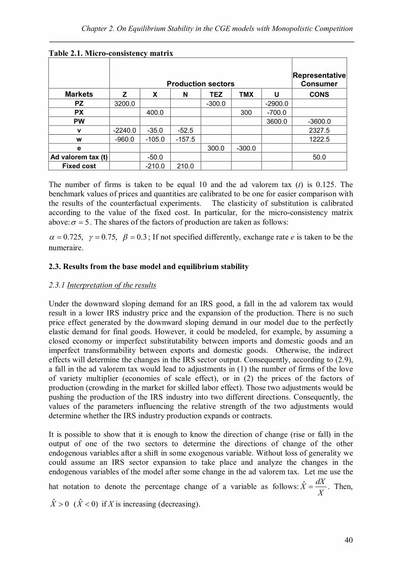
Chapter 2. On Equilibrium Stability in the CGE models with Monopolistic Competition
40
Table 2.1. Micro-consistency matrix
Production sectors Representative
Consumer Markets Z X N TEZ TMX U CONS
PZ 3200.0 -300.0 -2900.0 PX 400.0 300 -700.0 PW 3600.0 -3600.0 v -2240.0 -35.0 -52.5 2327.5 w -960.0 -105.0 -157.5 1222.5 e 300.0 -300.0
Ad valorem tax (t) -50.0 50.0 Fixed cost -210.0 210.0
The number of firms is taken to be equal 10 and the ad valorem tax (t) is 0.125. The benchmark values of prices and quantities are calibrated to be one for easier comparison with the results of the counterfactual experiments. The elasticity of substitution is calibrated according to the value of the fixed cost. In particular, for the micro-consistency matrix above: 5 . The shares of the factors of production are taken as follows:
0.725, 0.75, 0.3 ; If not specified differently, exchange rate e is taken to be the numeraire. 2.3. Results from the base model and equilibrium stability 2.3.1 Interpretation of the results Under the downward sloping demand for an IRS good, a fall in the ad valorem tax would result in a lower IRS industry price and the expansion of the production. There is no such price effect generated by the downward sloping demand in our model due to the perfectly elastic demand for final goods. However, it could be modeled, for example, by assuming a closed economy or imperfect substitutability between imports and domestic goods and an imperfect transformability between exports and domestic goods. Otherwise, the indirect effects will determine the changes in the IRS sector output. Consequently, according to (2.9), a fall in the ad valorem tax would lead to adjustments in (1) the number of firms of the love of variety multiplier (economies of scale effect), or in (2) the prices of the factors of production (crowding in the market for skilled labor effect). Those two adjustments would be pushing the production of the IRS industry into two different directions. Consequently, the values of the parameters influencing the relative strength of the two adjustments would determine whether the IRS industry production expands or contracts. It is possible to show that it is enough to know the direction of change (rise or fall) in the output of one of the two sectors to determine the directions of change of the other endogenous variables after a shift in some exogenous variable. Without loss of generality we could assume an IRS sector expansion to take place and analyze the changes in the endogenous variables of the model after some change in the ad valorem tax. Let me use the
hat notation to denote the percentage change of a variable as follows: ˆ dXXX
. Then,
ˆ ˆ0 ( 0)X X if X is increasing (decreasing).

Chapter 2. On Equilibrium Stability in the CGE models with Monopolistic Competition
41
It could be shown that after any change in an IRS industry output, the firm (variety) level output will be unchanged: ˆ 0x . If we plug c from (2.2.9) into (2.2.4), we could obtain the following expression:
1 1(1 ) (1 ) (1 ) (2.2.4)PX t n nFC PX t X
or
( 1) (2.4)X FCnn ( 1)x FC ˆ 0x . Therefore, higher elasticity of substitution would make it more likely that every firm would produce more output because there is less need to produce more varieties of goods for the given level of industry output when varieties are more substitutable between each other. Similarly, a higher fixed cost makes it more optimal to produce fewer varieties to cut the total value of fixed cost and correspondingly more of each variety for a given value of industry output.
Apparently from (2.2.7) it follows that: ˆ ˆˆ ˆ( 0 0)1
X n X n
. Similarly, 0px
follows from (2.2.8) and 0PX PZ
should hold under a small open economy assumption. Let us make some further transformations to the model equations in order to have an easier interpretation of the effects. The market clearing conditions for both factors of production can be transformed as follows:
1 1( * ) ( * ) *PZ c X c w v w v XS Z FCn Z FC n
w w w w wn n
(2.3.1)PZ c XZ FCnw w n
Now, if I plug c from equation (2.2.9) into (2.3.1) and multiply it by w, we could derive the following:
1 ( 1) ( 1)* (1 ) (1 ) * (1 )
( 1)* (1 ) * (1 )
X XwS PZ Z PX t n FCn PZ Z PX t FCnnn
X XPZ Z PX t PZ Z PX t X
* (1 ) (2.3.2)wS PZ Z PX t X Similarly for v:
(1 ) * (1 ) (1 ) (2.3.3)vL PZ Z PX t X In the hat notation, it will look as follows:
ˆ ˆˆ 1 (1 1) (2.3.4)w shx X shx Z , ˆ ˆˆ 2 (1 2) (2.3.5)v shx X shx Z
where (1 )1* (1 )
PX t XshxPZ Z PX t X
, (1 ) (1 )2
(1 ) * (1 ) (1 )PX t Xshx
PZ Z PX t X
.
Moreover, a zero profit condition for CRS sector (2.2.10) could be written as: ˆ ˆ(1 ) 0w v or ˆ ˆ(1 ) (2.3.6)w v .
In other words, skilled and unskilled wages would be changing in different directions. As a result, when the skilled labor intensive IRS sector expands the unskilled labor intensive CRS sector contracts: ˆ ˆ0 0X Z .It could be proved by contradiction: if ˆ 0Z , then from (2.3.4) and (2.3.5) we obtain ˆ 0w and ˆ 0v which contradicts (2.3.6).
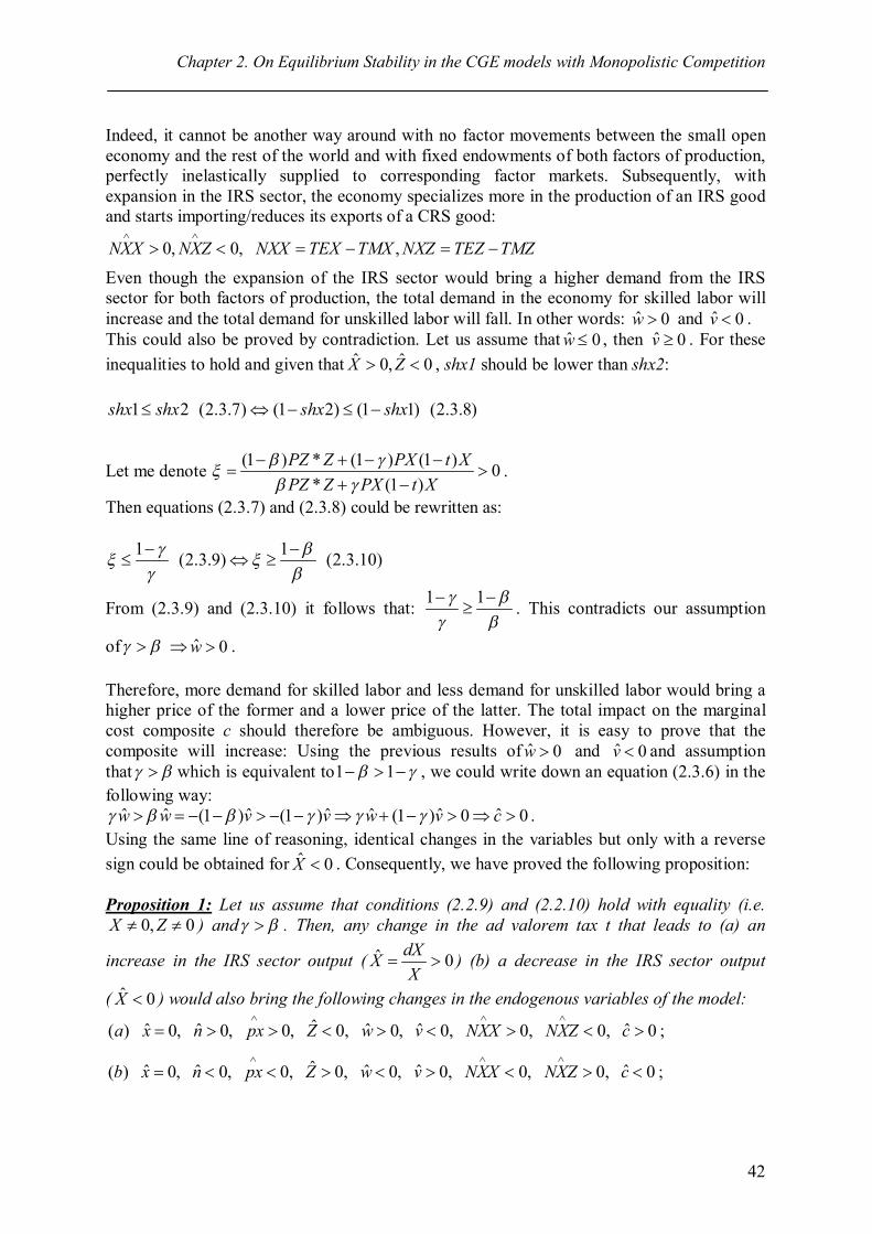
Chapter 2. On Equilibrium Stability in the CGE models with Monopolistic Competition
42
Indeed, it cannot be another way around with no factor movements between the small open economy and the rest of the world and with fixed endowments of both factors of production, perfectly inelastically supplied to corresponding factor markets. Subsequently, with expansion in the IRS sector, the economy specializes more in the production of an IRS good and starts importing/reduces its exports of a CRS good:
0, 0, ,NXX NXZ NXX TEX TMX NXZ TEZ TMZ
Even though the expansion of the IRS sector would bring a higher demand from the IRS sector for both factors of production, the total demand in the economy for skilled labor will increase and the total demand for unskilled labor will fall. In other words: ˆ 0w and ˆ 0v . This could also be proved by contradiction. Let us assume that ˆ 0w , then ˆ 0v . For these inequalities to hold and given that ˆ ˆ0, 0X Z , shx1 should be lower than shx2:
1 2 (2.3.7) (1 2) (1 1) (2.3.8)shx shx shx shx
Let me denote (1 ) * (1 ) (1 ) 0* (1 )
PZ Z PX t XPZ Z PX t X
.
Then equations (2.3.7) and (2.3.8) could be rewritten as:
1 1(2.3.9) (2.3.10)
From (2.3.9) and (2.3.10) it follows that: 1 1
. This contradicts our assumption
of ˆ 0w . Therefore, more demand for skilled labor and less demand for unskilled labor would bring a higher price of the former and a lower price of the latter. The total impact on the marginal cost composite c should therefore be ambiguous. However, it is easy to prove that the composite will increase: Using the previous results of ˆ 0w and ˆ 0v and assumption that which is equivalent to1 1 , we could write down an equation (2.3.6) in the following way:
ˆ ˆ ˆ ˆ ˆ ˆ ˆ(1 ) (1 ) (1 ) 0 0w w v v w v c . Using the same line of reasoning, identical changes in the variables but only with a reverse sign could be obtained for ˆ 0X . Consequently, we have proved the following proposition: Proposition 1: Let us assume that conditions (2.2.9) and (2.2.10) hold with equality (i.e.
0, 0X Z ) and . Then, any change in the ad valorem tax t that leads to (a) an
increase in the IRS sector output ( ˆ 0dXXX
) (b) a decrease in the IRS sector output
( ˆ 0X ) would also bring the following changes in the endogenous variables of the model: ˆˆ ˆ ˆ ˆ ˆ( ) 0, 0, 0, 0, 0, 0, 0, 0, 0a x n px Z w v NXX NXZ c
;
ˆˆ ˆ ˆ ˆ ˆ( ) 0, 0, 0, 0, 0, 0, 0, 0, 0b x n px Z w v NXX NXZ c
;
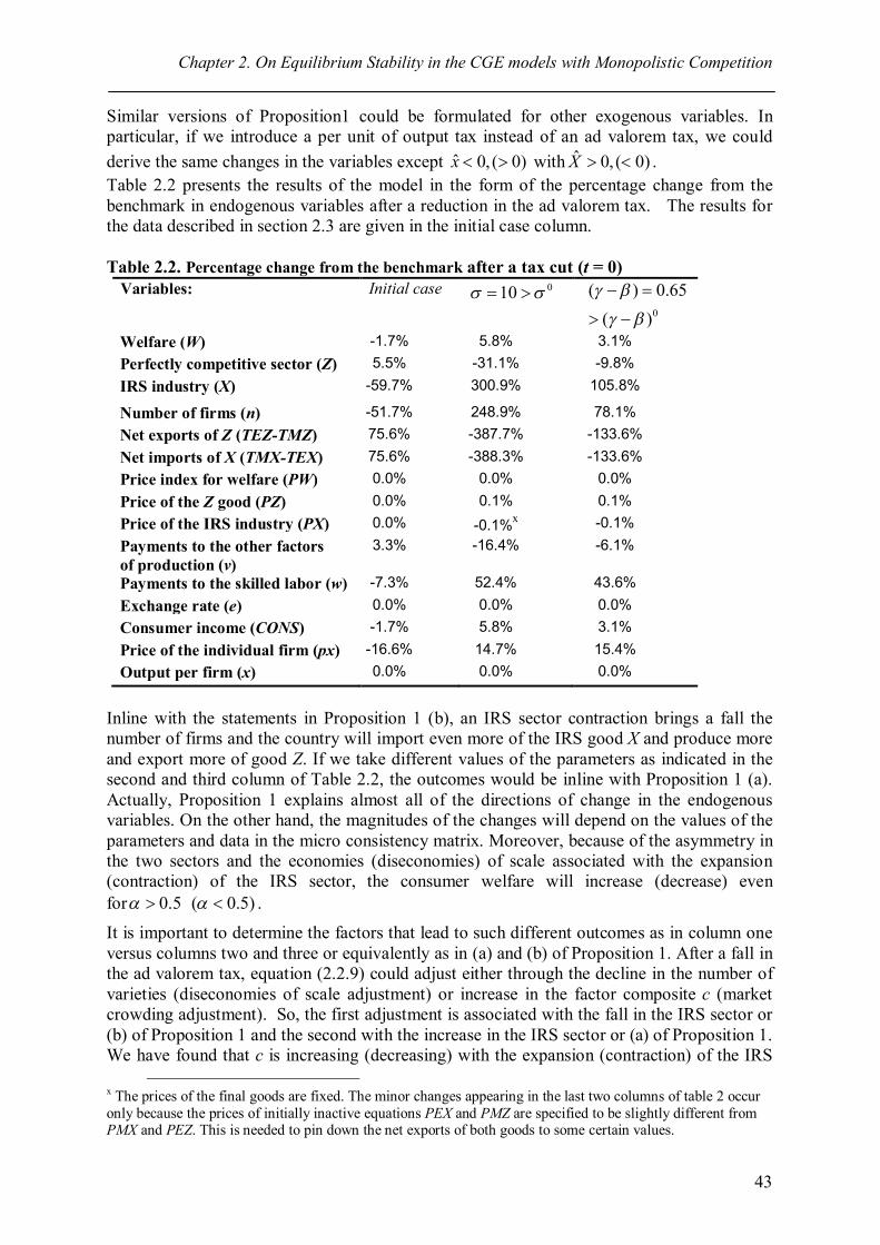
Chapter 2. On Equilibrium Stability in the CGE models with Monopolistic Competition
43
Similar versions of Proposition1 could be formulated for other exogenous variables. In particular, if we introduce a per unit of output tax instead of an ad valorem tax, we could derive the same changes in the variables except ˆ 0, ( 0)x with ˆ 0, ( 0)X . Table 2.2 presents the results of the model in the form of the percentage change from the benchmark in endogenous variables after a reduction in the ad valorem tax. The results for the data described in section 2.3 are given in the initial case column.
Table 2.2. Percentage change from the benchmark after a tax cut (t = 0)
Variables: Initial case 010 0
( ) 0.65( )
Welfare (W) -1.7% 5.8% 3.1% Perfectly competitive sector (Z) 5.5% -31.1% -9.8% IRS industry (X) -59.7% 300.9% 105.8%
Number of firms (n) -51.7% 248.9% 78.1% Net exports of Z (TEZ-TMZ) 75.6% -387.7% -133.6% Net imports of X (TMX-TEX) 75.6% -388.3% -133.6% Price index for welfare (PW) 0.0% 0.0% 0.0% Price of the Z good (PZ) 0.0% 0.1% 0.1% Price of the IRS industry (PX) 0.0% -0.1%x -0.1% Payments to the other factors of production (v)
3.3% -16.4% -6.1%
Payments to the skilled labor (w) -7.3% 52.4% 43.6% Exchange rate (e) 0.0% 0.0% 0.0% Consumer income (CONS) -1.7% 5.8% 3.1% Price of the individual firm (px) -16.6% 14.7% 15.4% Output per firm (x) 0.0% 0.0% 0.0%
Inline with the statements in Proposition 1 (b), an IRS sector contraction brings a fall the number of firms and the country will import even more of the IRS good X and produce more and export more of good Z. If we take different values of the parameters as indicated in the second and third column of Table 2.2, the outcomes would be inline with Proposition 1 (a). Actually, Proposition 1 explains almost all of the directions of change in the endogenous variables. On the other hand, the magnitudes of the changes will depend on the values of the parameters and data in the micro consistency matrix. Moreover, because of the asymmetry in the two sectors and the economies (diseconomies) of scale associated with the expansion (contraction) of the IRS sector, the consumer welfare will increase (decrease) even for 0.5 ( 0.5) .
It is important to determine the factors that lead to such different outcomes as in column one versus columns two and three or equivalently as in (a) and (b) of Proposition 1. After a fall in the ad valorem tax, equation (2.2.9) could adjust either through the decline in the number of varieties (diseconomies of scale adjustment) or increase in the factor composite c (market crowding adjustment). So, the first adjustment is associated with the fall in the IRS sector or (b) of Proposition 1 and the second with the increase in the IRS sector or (a) of Proposition 1. We have found that c is increasing (decreasing) with the expansion (contraction) of the IRS
x The prices of the final goods are fixed. The minor changes appearing in the last two columns of table 2 occur only because the prices of initially inactive equations PEX and PMZ are specified to be slightly different from PMX and PEZ. This is needed to pin down the net exports of both goods to some certain values.

Chapter 2. On Equilibrium Stability in the CGE models with Monopolistic Competition
44
sector. Consequently, both effects will be opposite to each other in either scenario. Before testing the stability of the obtained counterintuitive result, let us study the mechanisms that lead to its appearance. The parameters that influence market crowding adjustment are skilled labor intensities of production or the cost shares of skilled labor in both industries. In particular, the higher cost share of skilled labor in the IRS sector () will strengthen the adjustment. On the other hand, since the expansion of one industry leads to the contraction of the other due to the fixed values of factor endowments, higher cost share of skilled labor in the CRS sector ( ) will weaken this adjustment. In other words, higher value of brings it closer to given that . This means that the impact of any change in the production mix of goods X and Z is less significant on the prices of the factors of production. This implies weaker market crowding adjustment. However, the results of the benchmark calibration clearly demonstrate the dominance of adjustments in the number of firms (1). A fall in the number of firms would bring a fall in the production of the IRS sector and the so called contraction effect observed for benchmark data. In this case, a fall in the ad valorem tax would lead to the reshuffle in the IRS industry. We could think of it as a situation in which some firms would exit the market because lower prices would not bring a positive price effect that normally results from higher demand. In other words, under lower per output production costs and fixed price of final good, it would be more efficient for the IRS industry to produce fewer individual varieties. This would result in the contraction of the IRS industry given the assumption of a fixed industry level price. This adjustment is more likely to occur with higher values of the love of variety multiplier and therefore with lower elasticity of substitution between varieties ( ). Returning to the results in Table 2.2, we observe that the overall decrease in the factor composite is smaller than the fall in the love of variety multiplier in the initial case. The situation could be reversed by either increasing the elasticity of substitution which would diminish the love of variety multiplier or increasing the difference in the skilled labor intensities of two sectors ( ) which would strengthen the factor market crowding effect. This is exactly what we do in the two last columns of Table 2.2. Both changes lead to the IRS sector expansion and to a reverse in the pattern of trade in final goods. This is inline with the standard price effect and market crowding effect dominates the diseconomies of scale effect. The outcomes of the adjustment in equation (2.2.9) working through the change in the price of skilled labor will be inline with the results in Markusen et al. (2005). In particular, the service trade liberalization brings higher wages for skilled workers due to the expansion in the services industry. Despite the rise in the number of firms, the rise in the factor prices composite is greater than the rise in the love of variety multiplier. All indirect effects should have much less significance in the presence of price effect. However, they could still explain some changes in the variables. In order to study the impact of a tax cut with the price effect, we could, for example, consider a closed version of the model. A closed version of our model would only imply the absence of the external sector. All the other parameters and functional forms are the same as in the initial case. The results of a closed model with different numeraire values are presented in Table 2.3.

Chapter 2. On Equilibrium Stability in the CGE models with Monopolistic Competition
45
Table 2.3. Percentage change from the benchmark after a tax cut for the closed version of the model (t = 0)
Variables/Numeraire PZ PX PW v w Welfare (W) 2.9% 2.9% 2.9% 2.9% 2.9% Perfectly competitive sector (Z) -1.3% -1.3% -1.3% -1.3% -1.3% Downstream industry (X) 14.7% 14.7% 14.7% 14.7% 14.7%
Number of foreign firms (n) 11.6% 11.6% 11.6% 11.6% 11.6% Price index for welfare (PW) -4.0% 11.5% 0.0% -3.3% -5.7%
Price of the Z good (PZ) 0.0% 16.2% 4.2% 0.7% -1.7% Price of the downstream industry (PX)
-13.9% 0.0% -10.3% -13.3% -15.4%
Payments to the other factors of production (v)
-0.7% 15.3% 3.4% 0.0% -2.5%
Payments to the skilled labor (w) 1.8% 18.2% 6.0% 2.5% 0.0% Consumer income (CONS) -1.3% 14.7% 2.9% -0.5% -3.0%
Price of the individual firm (px) -11.5% 2.8% -7.8% -10.9% -13.0%
As a result of the price effect, the impact of a tax cut on the real variables of the model is the same under any numeraire value. Apparently, the direct price effect dominates over all the other effects and sets the direction of change in all the real variables. Consequently, an IRS sector expands, a CRS sector contracts and the representative consumer attains a higher utility level due to the economies of scale in the IRS production. Even though the model became smaller, it now comprises changes in the prices of goods. Therefore, the prices of the factors of production would not always be changing in the different directions as we had in Proposition 1 under a small open economy assumption. On the other hand, changes in prices are relative and depend on the numeraire. In particular, even though the price charged by an individual firm in the IRS sector is decreasing after a tax cut, it will be slightly increasing relative to the price of good X. The case with the price of good X as a numeraire is special because it is changing more in its magnitude than any other price variable. Hence, the changes in prices could switch to be positive or significantly increase when expressed in terms of the PX. This is only a matter of the numeraire choice and has no impact on the model behavior.
2.3.2 Equilibrium stability and uniqueness The counterintuitive result obtained under diseconomies of scale might be unstable according to the global correspondence principle of Samuelson. As we have already discussed in the introduction and according to Ide and Takayama (1990), the Marshallian output adjustment mechanism should hold for any comparative statics outcome. Consequently, let us adopt the
following notation: (1 )PX tPPZ
is a relative after tax world price of good X and SP is a
relative supply price or price at which producers break even. It could be derived from equations (2.2.9) and (2.2.10):
(2.3.11)( 1)S
wPv n
The relative output of the IRS sector will depend on the supply price. We could invert this
relationship and assume that the supply price depends on the relative output: SXPZ
.
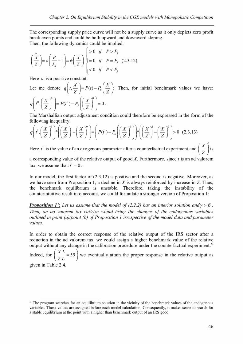
Chapter 2. On Equilibrium Stability in the CGE models with Monopolistic Competition
46
The corresponding supply price curve will not be a supply curve as it only depicts zero profit break even points and could be both upward and downward sloping. Then, the following dynamics could be implied:
0
1 0 (2.3.12)
0
S
SS
S
if P PX P Xa if P PZ P Z
if P P
Here a is a positive constant.
Let me denote , ( ) ;SX Xq t P t PZ Z
Then, for initial benchmark values we have:
0 00 0, ( ) 0S
X Xq t P t PZ Z
.
The Marshallian output adjustment condition could therefore be expressed in the form of the following inequality:
0 1 0 0 1 01 1, * ( ) * 0 (2.3.13)S
X X X X X Xq t P t PZ Z Z Z Z Z
Here 1t is the value of an exogenous parameter after a counterfactual experiment and 1X
Z
is
a corresponding value of the relative output of good X. Furthermore, since t is an ad valorem tax, we assume that: 1 0t . In our model, the first factor of (2.3.12) is positive and the second is negative. Moreover, as we have seen from Proposition 1, a decline in X is always reinforced by increase in Z. Thus, the benchmark equilibrium is unstable. Therefore, taking the instability of the counterintuitive result into account, we could formulate a stronger version of Proposition 1: Proposition 1’: Let us assume that the model of (2.2.2) has an interior solution and . Then, an ad valorem tax cut/rise would bring the changes of the endogenous variables outlined in point (a)/point (b) of Proposition 1 irrespective of the model data and parameter values. In order to obtain the correct response of the relative output of the IRS sector after a reduction in the ad valorem tax, we could assign a higher benchmark value of the relative output without any change in the calibration procedure under the counterfactual experiment.xi
Indeed, for . 55.
X LZ L
we eventually attain the proper response in the relative output as
given in Table 2.4.
xi The program searches for an equilibrium solution in the vicinity of the benchmark values of the endogenous variables. Those values are assigned before each model calculation. Consequently, it makes sense to search for a stable equilibrium at the point with a higher than benchmark output of an IRS good.
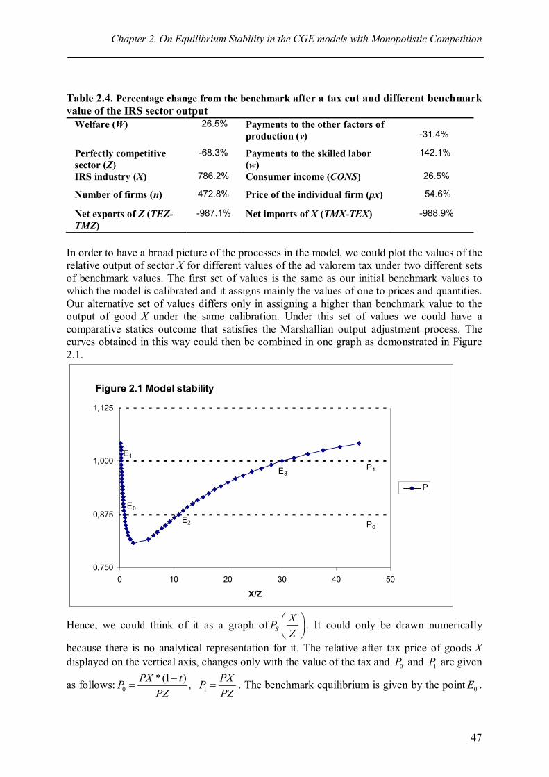
Chapter 2. On Equilibrium Stability in the CGE models with Monopolistic Competition
47
Table 2.4. Percentage change from the benchmark after a tax cut and different benchmark value of the IRS sector output
Welfare (W) 26.5% Payments to the other factors of production (v)
-31.4%
Perfectly competitive sector (Z)
-68.3% Payments to the skilled labor (w)
142.1%
IRS industry (X) 786.2% Consumer income (CONS) 26.5%
Number of firms (n) 472.8% Price of the individual firm (px) 54.6%
Net exports of Z (TEZ-TMZ)
-987.1% Net imports of X (TMX-TEX) -988.9%
In order to have a broad picture of the processes in the model, we could plot the values of the relative output of sector X for different values of the ad valorem tax under two different sets of benchmark values. The first set of values is the same as our initial benchmark values to which the model is calibrated and it assigns mainly the values of one to prices and quantities. Our alternative set of values differs only in assigning a higher than benchmark value to the output of good X under the same calibration. Under this set of values we could have a comparative statics outcome that satisfies the Marshallian output adjustment process. The curves obtained in this way could then be combined in one graph as demonstrated in Figure 2.1.
Figure 2.1 Model stability
0,750
0,875
1,000
1,125
0 10 20 30 40 50
X/Z
P
E0
E1
E2
E3P1
P0
Hence, we could think of it as a graph of SXPZ
. It could only be drawn numerically
because there is no analytical representation for it. The relative after tax price of goods X displayed on the vertical axis, changes only with the value of the tax and 0P and 1P are given
as follows: 0 1*(1 ) ,PX t PXP PPZ PZ
. The benchmark equilibrium is given by the point 0E .
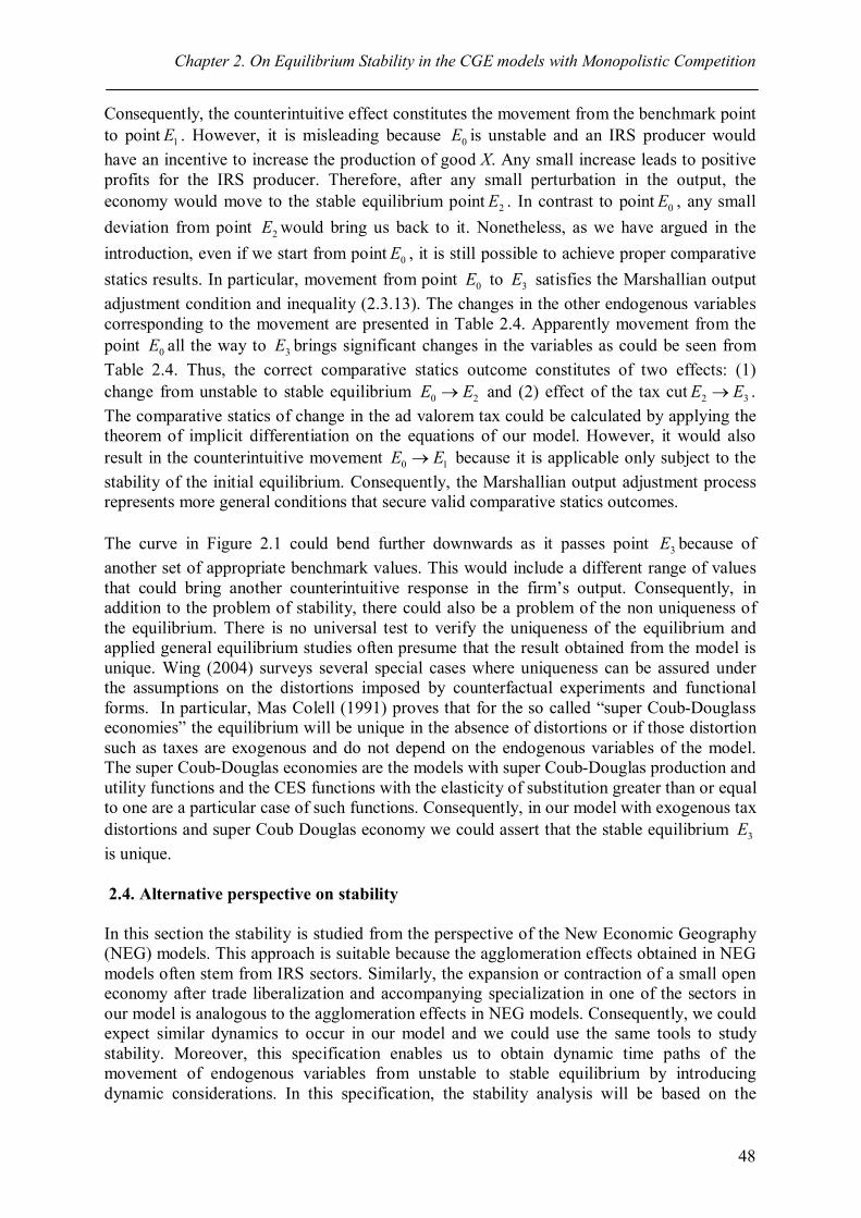
Chapter 2. On Equilibrium Stability in the CGE models with Monopolistic Competition
48
Consequently, the counterintuitive effect constitutes the movement from the benchmark point to point 1E . However, it is misleading because 0E is unstable and an IRS producer would have an incentive to increase the production of good X. Any small increase leads to positive profits for the IRS producer. Therefore, after any small perturbation in the output, the economy would move to the stable equilibrium point 2E . In contrast to point 0E , any small deviation from point 2E would bring us back to it. Nonetheless, as we have argued in the introduction, even if we start from point 0E , it is still possible to achieve proper comparative statics results. In particular, movement from point 0E to 3E satisfies the Marshallian output adjustment condition and inequality (2.3.13). The changes in the other endogenous variables corresponding to the movement are presented in Table 2.4. Apparently movement from the point 0E all the way to 3E brings significant changes in the variables as could be seen from Table 2.4. Thus, the correct comparative statics outcome constitutes of two effects: (1) change from unstable to stable equilibrium 0 2E E and (2) effect of the tax cut 2 3E E . The comparative statics of change in the ad valorem tax could be calculated by applying the theorem of implicit differentiation on the equations of our model. However, it would also result in the counterintuitive movement 0 1E E because it is applicable only subject to the stability of the initial equilibrium. Consequently, the Marshallian output adjustment process represents more general conditions that secure valid comparative statics outcomes. The curve in Figure 2.1 could bend further downwards as it passes point 3E because of another set of appropriate benchmark values. This would include a different range of values that could bring another counterintuitive response in the firm’s output. Consequently, in addition to the problem of stability, there could also be a problem of the non uniqueness of the equilibrium. There is no universal test to verify the uniqueness of the equilibrium and applied general equilibrium studies often presume that the result obtained from the model is unique. Wing (2004) surveys several special cases where uniqueness can be assured under the assumptions on the distortions imposed by counterfactual experiments and functional forms. In particular, Mas Colell (1991) proves that for the so called “super Coub-Douglass economies” the equilibrium will be unique in the absence of distortions or if those distortion such as taxes are exogenous and do not depend on the endogenous variables of the model. The super Coub-Douglas economies are the models with super Coub-Douglas production and utility functions and the CES functions with the elasticity of substitution greater than or equal to one are a particular case of such functions. Consequently, in our model with exogenous tax distortions and super Coub Douglas economy we could assert that the stable equilibrium 3E is unique. 2.4. Alternative perspective on stability In this section the stability is studied from the perspective of the New Economic Geography (NEG) models. This approach is suitable because the agglomeration effects obtained in NEG models often stem from IRS sectors. Similarly, the expansion or contraction of a small open economy after trade liberalization and accompanying specialization in one of the sectors in our model is analogous to the agglomeration effects in NEG models. Consequently, we could expect similar dynamics to occur in our model and we could use the same tools to study stability. Moreover, this specification enables us to obtain dynamic time paths of the movement of endogenous variables from unstable to stable equilibrium by introducing dynamic considerations. In this specification, the stability analysis will be based on the

Chapter 2. On Equilibrium Stability in the CGE models with Monopolistic Competition
49
incentives of high skilled workers to move to a sector (region) with a higher relative wage. Therefore, in order to derive the result interpretation which is equivalent to the NEG model results, we will need to introduce some transformations to our model. In the seminal paper of Krugman (1991), the Dixit-Stiglitz based New Economic Geography model has been developed. The model features 2 regions and 2 sectors, such that, similarly to our model, one sector (agriculture) is governed by constant returns to scale and another sector (manufacturing) is subject to increasing returns to scale production and is a Dixit-Stiglitz composite of varieties. However, the factors of production are assumed to be sector specific which makes it different in terms of effects leading to agglomeration and also analytically more tractable than our model. Currently this model is also known as a Core-Periphery model (Fujita et al., 1999) where a two region economy could have equilibrium with a manufacturing core and agricultural periphery or one where the production of two sectors is equally divided between regions. The core-periphery concentration outcome occurs due to the presence of backward and forward linkages which underpin centripetal forces. In particular, a higher variety of goods produced in one region lowers the price index and strengthens the incentive to move more manufacturing into that region (forward linkage). On the other hand, higher incomes in one region would lead to higher wages bringing more workers there (backward linkage). There will be no such effects in our model because the supply of labor in the given country is fixed and not mobile with the rest of the world. Besides, the IRS industry price index is fixed and that precludes the price effect. While real wages matter in the Krugman model, in our model it is sufficient to study nominal wages. The downward pressure on the IRS price index from an increase in the number of varieties is neutralized by an increase in the price charged for each variety. Therefore, the agglomeration effects of our model occur as a result of the concentration in one sector of the economy and the corresponding movement of both types of labor into that sector. Consequently, let us assume two different sector specific types of skilled labor. This assumption is intuitively reasonable and enables us to analyze stability from the perspective of the NEG models. The following changes will be introduced to the model equations: Firstly, sector specific skilled labor would now have different wages:
12 (2.4.1)c w v
Therefore zero profit conditions for both sectors would be as follows: 1 1: 2 (1 ) (1 ) (2.4.2)For X w v PX t n
1: 1 (2.4.3)For Z w v PZ Secondly, there will be two market clearing conditions for skilled labor corresponding to the two sectors of the economy:
1: (1 ) (2.4.4)1
PZFor w S Zw
2 : (2.4.5)2 2
c X cFor w S FCnw wn
Here is a share of the total endowment of skilled labor which is specific to the IRS sector. The benchmark value of ( 0 0.2147 ) is calculated from the share of skilled labor in the
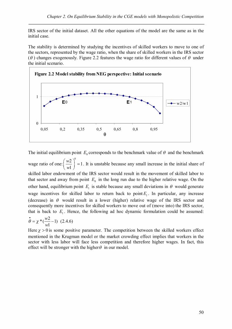
Chapter 2. On Equilibrium Stability in the CGE models with Monopolistic Competition
50
IRS sector of the initial dataset. All the other equations of the model are the same as in the initial case. The stability is determined by studying the incentives of skilled workers to move to one of the sectors, represented by the wage ratio, when the share of skilled workers in the IRS sector ( ) changes exogenously. Figure 2.2 features the wage ratio for different values of under the initial scenario.
0
1
0,05 0,2 0,35 0,5 0,65 0,8 0,95
w2/w1E0 E1
q
Figure 2.2 Model stability from NEG perspective: Initial scenario
The initial equilibrium point 0E corresponds to the benchmark value of and the benchmark
wage ratio of one:02 1
1ww
. It is unstable because any small increase in the initial share of
skilled labor endowment of the IRS sector would result in the movement of skilled labor to that sector and away from point 0E in the long run due to the higher relative wage. On the other hand, equilibrium point 1E is stable because any small deviations in would generate wage incentives for skilled labor to return back to point 1E . In particular, any increase (decrease) in would result in a lower (higher) relative wage of the IRS sector and consequently more incentives for skilled workers to move out of (move into) the IRS sector, that is back to 1E . Hence, the following ad hoc dynamic formulation could be assumed:
2*( 1) (2.4.6)1
ww
Here 0 is some positive parameter. The competition between the skilled workers effect mentioned in the Krugman model or the market crowding effect implies that workers in the sector with less labor will face less competition and therefore higher wages. In fact, this effect will be stronger with the higher in our model.
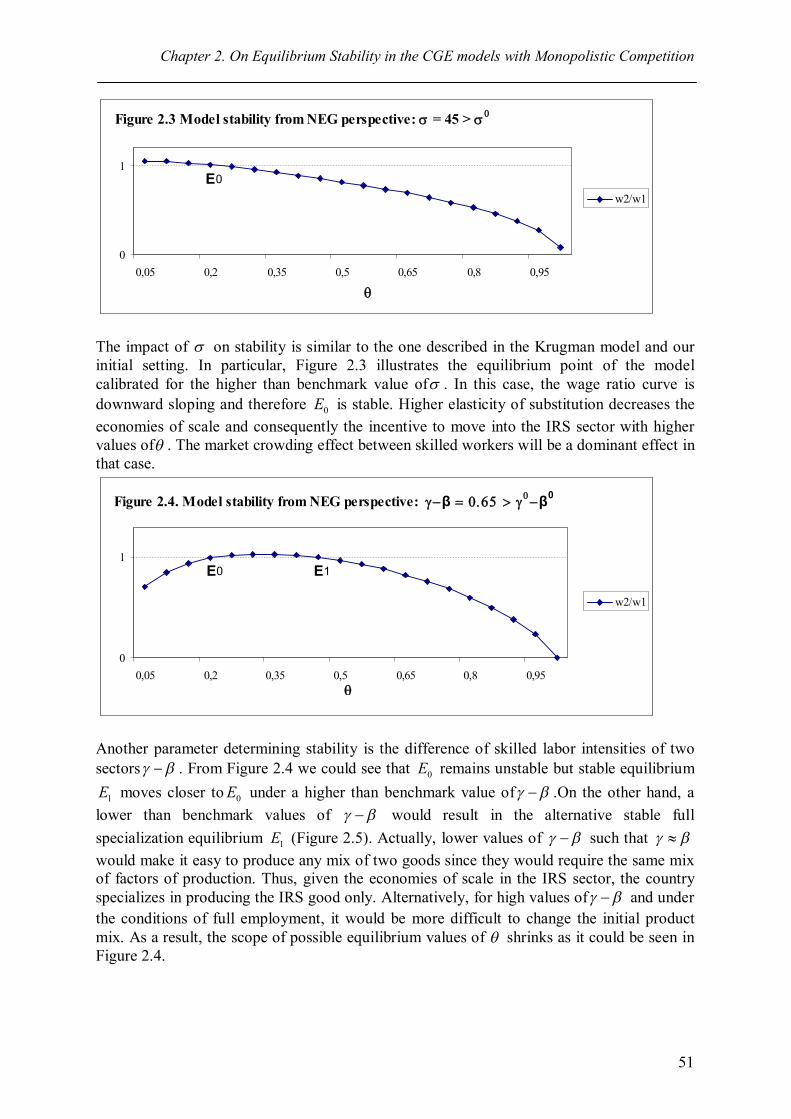
Chapter 2. On Equilibrium Stability in the CGE models with Monopolistic Competition
51
0
1
0,05 0,2 0,35 0,5 0,65 0,8 0,95
w2/w1E0
Figure 2.3 Model stability from NEG perspective: s = 45 > s0
q
The impact of on stability is similar to the one described in the Krugman model and our initial setting. In particular, Figure 2.3 illustrates the equilibrium point of the model calibrated for the higher than benchmark value of . In this case, the wage ratio curve is downward sloping and therefore 0E is stable. Higher elasticity of substitution decreases the economies of scale and consequently the incentive to move into the IRS sector with higher values of . The market crowding effect between skilled workers will be a dominant effect in that case.
0
1
0,05 0,2 0,35 0,5 0,65 0,8 0,95
w2/w1
E0 E1
Figure 2.4. Model stability from NEG perspective: g-β = 0.65 > g0-β0
q
Another parameter determining stability is the difference of skilled labor intensities of two sectors . From Figure 2.4 we could see that 0E remains unstable but stable equilibrium
1E moves closer to 0E under a higher than benchmark value of .On the other hand, a lower than benchmark values of would result in the alternative stable full specialization equilibrium 1E (Figure 2.5). Actually, lower values of such that would make it easy to produce any mix of two goods since they would require the same mix of factors of production. Thus, given the economies of scale in the IRS sector, the country specializes in producing the IRS good only. Alternatively, for high values of and under the conditions of full employment, it would be more difficult to change the initial product mix. As a result, the scope of possible equilibrium values of shrinks as it could be seen in Figure 2.4.
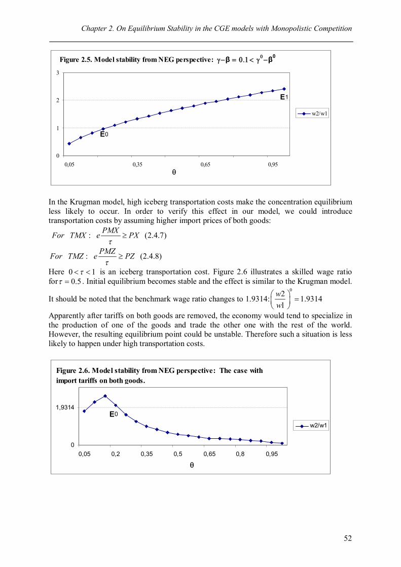
Chapter 2. On Equilibrium Stability in the CGE models with Monopolistic Competition
52
0
1
2
3
0,05 0,35 0,65 0,95
w2/w1
E0
E1
Figure 2.5. Model stability from NEG perspective: g-β = 0.1< g0-β0
q
In the Krugman model, high iceberg transportation costs make the concentration equilibrium less likely to occur. In order to verify this effect in our model, we could introduce transportation costs by assuming higher import prices of both goods:
: (2.4.7)PMXFor TMX e PX
: (2.4.8)PMZFor TMZ e PZ
Here 0 1 is an iceberg transportation cost. Figure 2.6 illustrates a skilled wage ratio for 0.5 . Initial equilibrium becomes stable and the effect is similar to the Krugman model.
It should be noted that the benchmark wage ratio changes to 1.9314:02 1.9314
1ww
Apparently after tariffs on both goods are removed, the economy would tend to specialize in the production of one of the goods and trade the other one with the rest of the world. However, the resulting equilibrium point could be unstable. Therefore such a situation is less likely to happen under high transportation costs.
0
1,9314
0,05 0,2 0,35 0,5 0,65 0,8 0,95
w2/w1
Figure 2.6. Model stability from NEG perspective: The case with import tariffs on both goods.
E0
q
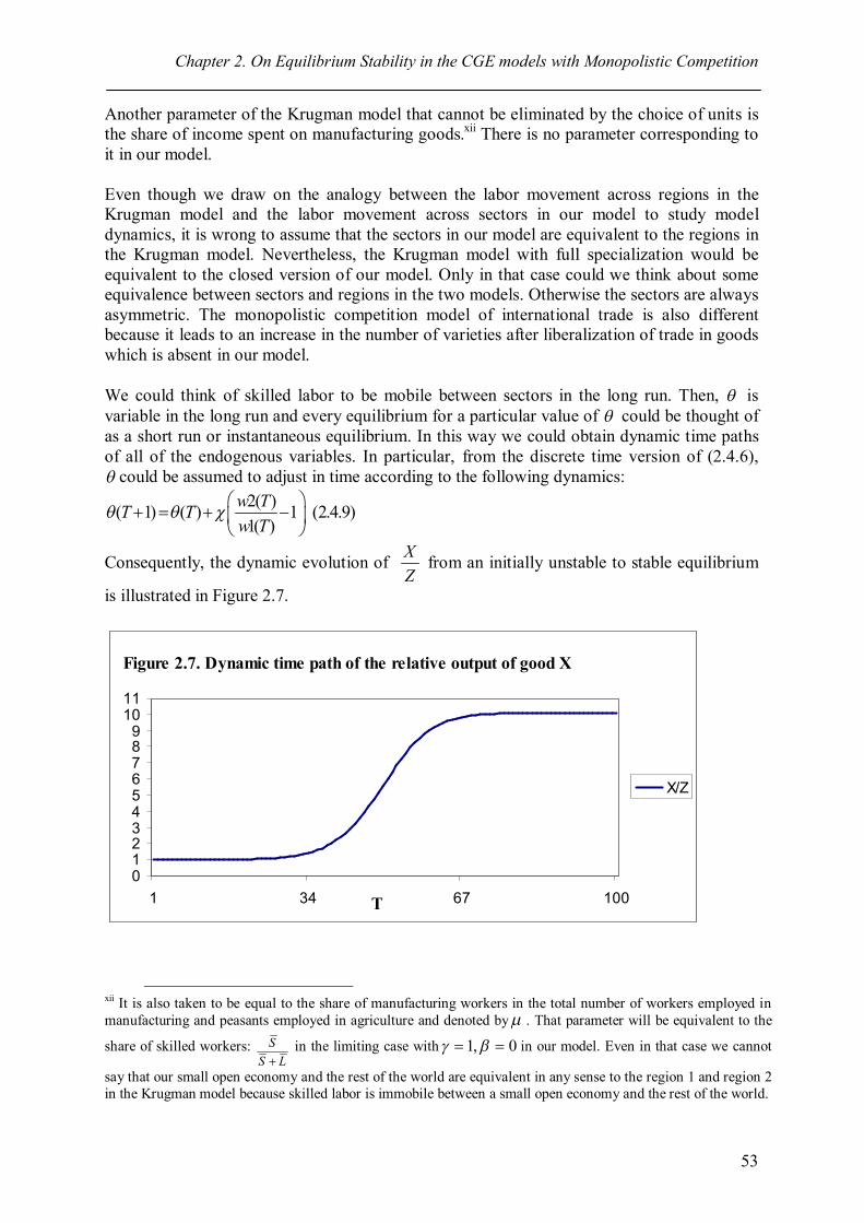
Chapter 2. On Equilibrium Stability in the CGE models with Monopolistic Competition
53
Another parameter of the Krugman model that cannot be eliminated by the choice of units is the share of income spent on manufacturing goods.xii There is no parameter corresponding to it in our model. Even though we draw on the analogy between the labor movement across regions in the Krugman model and the labor movement across sectors in our model to study model dynamics, it is wrong to assume that the sectors in our model are equivalent to the regions in the Krugman model. Nevertheless, the Krugman model with full specialization would be equivalent to the closed version of our model. Only in that case could we think about some equivalence between sectors and regions in the two models. Otherwise the sectors are always asymmetric. The monopolistic competition model of international trade is also different because it leads to an increase in the number of varieties after liberalization of trade in goods which is absent in our model. We could think of skilled labor to be mobile between sectors in the long run. Then, is variable in the long run and every equilibrium for a particular value of could be thought of as a short run or instantaneous equilibrium. In this way we could obtain dynamic time paths of all of the endogenous variables. In particular, from the discrete time version of (2.4.6), could be assumed to adjust in time according to the following dynamics:
2( )( 1) ( ) 1 (2.4.9)1( )
w TT Tw T
Consequently, the dynamic evolution of XZ
from an initially unstable to stable equilibrium
is illustrated in Figure 2.7.
0123456789
1011
1 34 67 100
X/Z
T
Figure 2.7. Dynamic time path of the relative output of good X
xii It is also taken to be equal to the share of manufacturing workers in the total number of workers employed in manufacturing and peasants employed in agriculture and denoted by . That parameter will be equivalent to the
share of skilled workers: SS L
in the limiting case with 1, 0 in our model. Even in that case we cannot
say that our small open economy and the rest of the world are equivalent in any sense to the region 1 and region 2 in the Krugman model because skilled labor is immobile between a small open economy and the rest of the world.
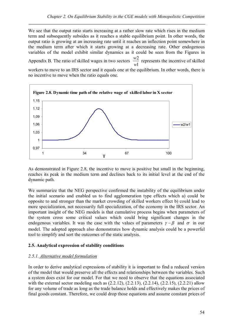
Chapter 2. On Equilibrium Stability in the CGE models with Monopolistic Competition
54
We see that the output ratio starts increasing at a rather slow rate which rises in the medium term and subsequently subsides as it reaches a stable equilibrium point. In other words, the output ratio is growing at an increasing rate until it reaches an inflection point somewhere in the medium term after which it starts growing at a decreasing rate. Other endogenous variables of the model exhibit similar dynamics as it could be seen from the Figures in
Appendix B. The ratio of skilled wages in two sectors 21
ww
represents the incentive of skilled
workers to move to an IRS sector and it equals one at the equilibrium. In other words, there is no incentive to move when the ratio equals one.
0,97
1
1,03
1,06
1,09
1,12
1,15
1 34 67 100
w2/w1
T
Figure 2.8. Dynamic time path of the relative wage of skilled labor in X sector
As demonstrated in Figure 2.8, the incentive to move is positive but small in the beginning, reaches its peak in the medium term and declines back to its initial level at the end of the dynamic path. We summarize that the NEG perspective confirmed the instability of the equilibrium under the initial scenario and enabled us to find agglomeration type effects which a) could be opposite to and stronger than the market crowding of skilled workers effect b) could lead to more specialization, not necessarily full specialization, of the economy in the IRS sector. An important insight of the NEG models is that cumulative process begins when parameters of the system cross some critical values which could bring significant changes in the endogenous variables. It was the case with the values of parameters and in our model. The adopted approach also demonstrates how dynamic analysis could be a powerful tool to simplify and sort the outcomes of the static analysis. 2.5. Analytical expression of stability conditions 2.5.1. Alternative model formulation In order to derive analytical expressions of stability it is important to find a reduced version of the model that would preserve all the effects and relationships between the variables. Such a system does exist for our model. For that we need to observe that the equations associated with the external sector modeling such as (2.2.12), (2.2.13), (2.2.14), (2.2.15), (2.2.21) allow for any volume of trade as long as the trade balance holds and effectively makes the prices of final goods constant. Therefore, we could drop those equations and assume constant prices of
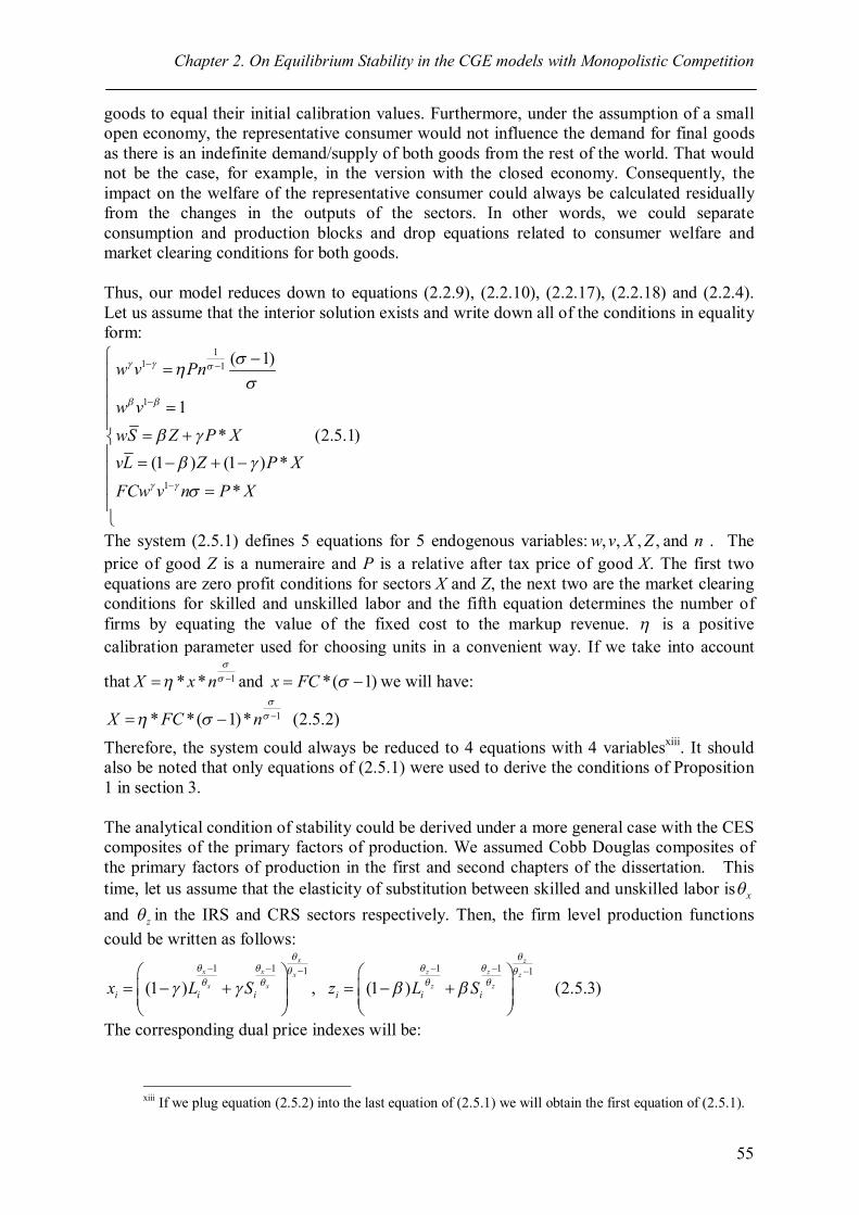
Chapter 2. On Equilibrium Stability in the CGE models with Monopolistic Competition
55
goods to equal their initial calibration values. Furthermore, under the assumption of a small open economy, the representative consumer would not influence the demand for final goods as there is an indefinite demand/supply of both goods from the rest of the world. That would not be the case, for example, in the version with the closed economy. Consequently, the impact on the welfare of the representative consumer could always be calculated residually from the changes in the outputs of the sectors. In other words, we could separate consumption and production blocks and drop equations related to consumer welfare and market clearing conditions for both goods. Thus, our model reduces down to equations (2.2.9), (2.2.10), (2.2.17), (2.2.18) and (2.2.4). Let us assume that the interior solution exists and write down all of the conditions in equality form:
11 1
1
1
( 1)
1* (2.5.1)
(1 ) (1 ) **
w v Pn
w vwS Z P XvL Z P XFCw v n P X
The system (2.5.1) defines 5 equations for 5 endogenous variables: , , , ,w v X Z and n . The price of good Z is a numeraire and P is a relative after tax price of good X. The first two equations are zero profit conditions for sectors X and Z, the next two are the market clearing conditions for skilled and unskilled labor and the fifth equation determines the number of firms by equating the value of the fixed cost to the markup revenue. is a positive calibration parameter used for choosing units in a convenient way. If we take into account
that 1* *X x n and *( 1)x FC we will have:
1* *( 1)* (2.5.2)X FC n
Therefore, the system could always be reduced to 4 equations with 4 variablesxiii. It should also be noted that only equations of (2.5.1) were used to derive the conditions of Proposition 1 in section 3. The analytical condition of stability could be derived under a more general case with the CES composites of the primary factors of production. We assumed Cobb Douglas composites of the primary factors of production in the first and second chapters of the dissertation. This time, let us assume that the elasticity of substitution between skilled and unskilled labor is x and z in the IRS and CRS sectors respectively. Then, the firm level production functions could be written as follows:
1 1 1 11 1
(1 ) , (1 ) (2.5.3)
x zx x z zx z
x x z zi i i i i ix L S z L S
The corresponding dual price indexes will be:
xiii If we plug equation (2.5.2) into the last equation of (2.5.1) we will obtain the first equation of (2.5.1).

Chapter 2. On Equilibrium Stability in the CGE models with Monopolistic Competition
56
1 1
1 1 1 11 1(1 ) , (1 ) (2.5.4)x x z zx zx zc w v c w v
This would transform the factor market clearing conditions of (2.2.19) and (2.2.20):
: (1 ) (1 ) * (2.5.5)xz
xz cc XFor v L Z FC nv v n
: * (2.5.6)z x
z xc c XFor w S Z FC nw w n
Consequently, the main equations of the model will be transformed as follows: 1
1
1
1
( 1)
1
* (2.5.7)
(1 ) (1 ) *
*
z x
x
z x
x
x
z
xzZ X
xzZ X
x
c Pn
c
ccS S S Z P Xw w
ccL L L Z P Xv v
FCc n P X
The values of X and Z could be derived from the third and fourth equations of (2.5.7):
1
(1 ) (1 ), (2.5.8)( (1 ) (1 ) ) ( (1 ) (1 ) )
x xz z
x z x z x x z x zzx z
w S v L v L w SX ZPc w v c v w
Apparently from the first equation of (2.5.1), the calibration parameter could be chosen in such a way that 0 0w v . Moreover, from the second equation of (2.5.7) we could infer that 0 0 0 0 1w v w v . Then, Z and X from (2.5.8) could be written as follows:
(1 ) (1 ), (2.5.9)( ) ( )
S L L SX ZP
Since 0 , the numerators in (2.5.9) should also be positive: (1 ) 0, (1 ) 0 (2.5.10)S L L S
Those conditions represent the constraints on factor endowments to be in the diversification cone defined by the technological parameters of the model. The conditions of (2.5.10) could be combined into the following constraint on factor endowments:
(2.5.11)SS L
The quantities of skilled and unskilled labor could be compared when 0 0w v . Hence, condition (2.5.11) states that the ratio of skilled labor to the sum of skilled and unskilled labor should not exceed the skilled labor intensity of the IRS sector . Otherwise it will be
impossible to have full employment of skilled workers and the endowment point ( , )S L

Chapter 2. On Equilibrium Stability in the CGE models with Monopolistic Competition
57
would be out of the diversification cone. Similarly, the ratio of skilled labor to the sum of skilled and unskilled labor should not be less than the skilled labor intensity in the CRS sector because there will be no full employment of unskilled workers otherwise. In order to derive the stability condition, let us introduce the following variables: -unit cost ratio of the IRS good over CRS good, r- the ratio of skilled to unskilled labor
wage: wrv
, ik - factor input ratio for two sectors: ,x zx z
x z
S Sk kL L
and - the ratio of labor
used in the IRS industry to total labor: xLL
.
Then, could be determined from the first and second equations of (2.5.7):
1
1 1
( 1) (2.5.12)x
z
c P n
c
We could use the hat notation ( ˆ d
) and the corresponding rules to present (2.5.12) in
the following form: ˆˆ ˆ ˆ (2.5.13)
1x znc c
If we assume that 1
1 1(1 )
x
x x
ww v
and1
1 1(1 )
z
z z
ww v
, which also holds
for 0 0w v , the equation (2.5.13) could be written as follows:
ˆˆ ˆ( ) (2.5.14)1
nr
Using the fourth equation of (2.5.7) and inserting the value of P*X from the fifth equation of (2.5.7), we could obtain the expression for as follows:
1 1
(1 ) * (1 )(1 ) (2.5.15)
x x
xx x
x
x xxx x
c cP X FCc n cL FCv v nvL L L L
This could be transformed into hat notation: ˆ ˆ ˆ ˆ( ) (2.5.16)x xn c v
Furthermore, if we use the expression for xc from (2.5.4) and apply the hat transformation we will obtain the following expression for : ˆ ˆ ˆ ˆ ˆ ˆ ˆ ˆ ˆ ˆ( (1 ) ) ( ) (2.5.17)x x xn w v v n w v n r
Let us write the expression for the ratio of skilled to unskilled labor endowment using (2.5.7):

Chapter 2. On Equilibrium Stability in the CGE models with Monopolistic Competition
58
(1 ) (2.5.18)x zx z x zx z
x z
S S S S L S L k kL L L L L L
The factor input ratios could also be calculated from (2.5.7):
1
1
*, (2.5.19)
(1 ) (1 ) (1 )(1 ) *
x
xx
x z
x
x
xx
x zx x
c P XS wwk r k rc vL P Xv
Subsequently, the total differential of (2.5.18) could be written as follows:
0 (2.5.20)x x z z zk d dk dk k d dk
The values of the derivatives of xk and zk could be found from (2.5.19):
1 ˆ ˆ, (2.5.21)(1 )
xxx x x z z zdk r dr k r dk k r
If we plug expressions from (2.5.21) into (2.5.20), we will obtain the following expression:
ˆ( ) ( (1 ) ) 0 (2.5.22)x z x x z zk k d k k r
Let us now solve (2.5.22) for : ˆ ˆ (2.5.23)x x z z
x z
k k rk k
Here 1
. Consequently, r and are monotonically related. The initial equilibrium
should be stable if an increase in the relative wage of skilled labor (r) brings an expansion of the industry that uses skilled labor intensively. The equilibrium is thus stable if and only if ˆ
0r . In order to obtain an expression for
ˆr in terms of the parameters of our model, we
could insert the value of from (2.5.23) into (2.5.17) and then the obtained value of n into (2.5.14):
ˆ ˆx x z zx
x z
k kn rk k
and therefore
ˆˆ ˆ( ) (2.5.24)1
x x z zx
x z
k k rrk k
After inserting the values of xk and zk from (2.5.19) and under 0 0w v , (2.5.24) is transformed into the following stability condition: ˆ 1( ) 0 (2.5.25)ˆ 1
x z
r
Consequently, condition (2.5.25) could be used to prove the following proposition:
Chapter 2. On Equilibrium Stability in the CGE models with Monopolistic Competition
59
Proposition 2: Let us assume that the model formulated in section 2.2 has interior solutions. The initial equilibrium of the model is stable if and only if
2
( )(1 )1 (2.5.26)( )
x z
Hence, the initial equilibrium will be stable for relatively high values of and and for relatively small values of . The last variable is small when the share of labor in the IRS sector is high. Therefore, unstable equilibrium is more likely to occur when the IRS industry is small. The condition (2.5.26) holds for any CRS production functions and , and s are allowed to be functions of r. The Cobb-Douglas composites of the primary factors that we assumed in our model formulation presented in section 2.2 is just a particular case of condition (2.5.26) with constant , and 1x z :
2( )(1 )1 (2.5.27)
( )
2.5.2 Conditions of full specialization in the IRS sector In Proposition 2, the impact of the parameters on the equilibrium stability has been proved. We have also found that when the initial equilibrium is unstable, it indicates that the model will deviate from it so that the output of the IRS sector will increase relative to the output of the CRS sector. As a result of that the model reaches a new stable equilibrium point. Since it is not always easy to find that new equilibrium, we may suspect that the point at which the economy specializes in the production of the IRS sector is the new stable equilibrium. It is important to find out whether the full specialization in the production of the IRS good is equilibrium because it enables our small economy to realize the maximum economies of scale. That, in turn, could bring the highest utility to the representative consumer as we have seen in section 3. If full specialization in the production of an IRS good is an equilibrium, the revenue obtained from selling only the IRS good subject to the resource constraints should be enough to pay the factors of production at their initial price. In other words, producers will have an incentive to produce the IRS good only if it brings higher profits. In terms of equations in (2.5.1), the total expenditure on the factors of production under initial prices 0 0 1w v is S L . The last equation of (2.5.1) gives the value of total revenue of the IRS good: 0* * *P X FC n . Consequently, we find that full specialization outcome is not equilibrium after inserting the benchmark values and comparing the two numbers: 0* * * 8*10*5 400 3550 1222.5 2327.5P X FC n S L . 2.6. Conclusion How do we proceed in the applied general equilibrium models if the initial equilibrium is found to be unstable? Then, the equilibrium should be recalibrated by changing the values of the structural parameters. There are always parameter estimates which are taken only within some certain range of values such as elasticities and factor intensities. Moreover, in our model, it is possible to identify the relationship between the parameter values and stability of the initial equilibrium. Consequently, it is possible to implement the proper recalibration procedure. It consists of increasing the value of or the share of the IRS industry ( ) from (2.5.26) and /or increasing the value of .

Chapter 2. On Equilibrium Stability in the CGE models with Monopolistic Competition
60
The counterintuitive unstable outcome is more likely to occur when the diseconomies of scale effect is stronger than the factor market crowding effect in the absence of the direct price effect. It also appears that the lower value of is increasing the possibility of having a full specialization in the IRS sector as an equilibrium under sufficient economies of scale. The model presents a good example of how dynamic analysis could be used to determine the validity of the results and uncover new effects in the static model. Moreover, we have seen that even with an unstable equilibrium it is still possible to obtain valid comparative statics. However, it will not be meaningful for policy analysis due to the inappropriately large changes in the endogenous variables. In that case, the changes in the endogenous variables could be substantial because they incorporate both the movement from unstable to stable equilibrium and the impact from the change in the exogenous variable.
Bibliography Bhagwati, J., Brecher, R., and Hatta, T., (1987) “The global correspondence principle: A
Generalization”, American Economic Review 77, pp.124-132. Ide, T., and Takayama, A., (1990) “Variable Returns to Scale and the Global Correspondence
Principle in the Theory of International Trade”, Economic Letters 33. pp.301-308. Fujita, M., Krugman, P., Venables, A.J. (1999) “The Spatial Economy” Cambridge, MA:
MIT Press. Krugman, P., (1991) “Increasing returns and economic geography, Journal of Political
Economy”, 99: pp.483-499. Markusen, J., (2002) “General Equilibrium Modeling using GAMS and MPSGE”,
Boulder.http://spot.colorado.edu/~markusen/teaching.htmMarkusen, J., Rutherford, T., and Tarr, D., (2005) “Trade and direct investment in producer services and the domestic market for expertise”, Canadian Journal of Economics 38 (2005), pp. 758–777.
Mas-Colell, A., (1991) “On the uniqueness of equilibrium once again”, in W.A. Barnett et al (eds.), Equilibrium Theory and Applications: Proceedings of the Sixth International Symposium in Economic Theory and Econometrics, New York: Cambridge University Press, pp. 275-296.
Samuelson, P., (1947) “Foundations of Economics Analysis”, Cambridge: Harvard University Press; enlarged ed., (1983).
Samuelson, P., (1971) “On the trail of conventional beliefs about the transfer problem” in J. Bhagwati et al., eds., Trade Balance of Payments and Growth: Papers in International Economics in Honor of Charles P. Kindleberger, Amsterdam: North- Holland, pp. 327-351.
Wing, I., (2004) “Computable General Equilibrium Models and Their Use in Economy-Wide Policy Analysis”. MIT Joint Program on the Science and Policy of Global Change. Technical Note 6.
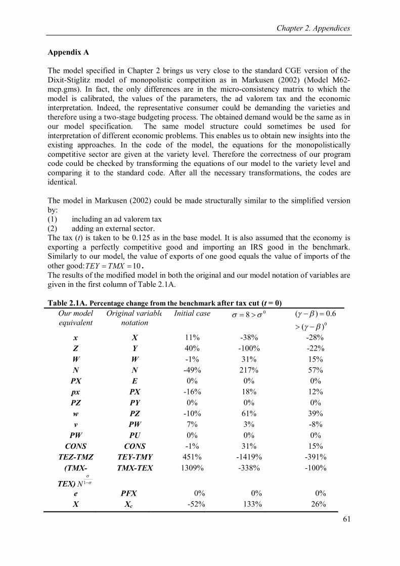
Chapter 2. Appendices
61
Appendix A The model specified in Chapter 2 brings us very close to the standard CGE version of the Dixit-Stiglitz model of monopolistic competition as in Markusen (2002) (Model M62-mcp.gms). In fact, the only differences are in the micro-consistency matrix to which the model is calibrated, the values of the parameters, the ad valorem tax and the economic interpretation. Indeed, the representative consumer could be demanding the varieties and therefore using a two-stage budgeting process. The obtained demand would be the same as in our model specification. The same model structure could sometimes be used for interpretation of different economic problems. This enables us to obtain new insights into the existing approaches. In the code of the model, the equations for the monopolistically competitive sector are given at the variety level. Therefore the correctness of our program code could be checked by transforming the equations of our model to the variety level and comparing it to the standard code. After all the necessary transformations, the codes are identical. The model in Markusen (2002) could be made structurally similar to the simplified version by: (1) including an ad valorem tax (2) adding an external sector. The tax (t) is taken to be 0.125 as in the base model. It is also assumed that the economy is exporting a perfectly competitive good and importing an IRS good in the benchmark. Similarly to our model, the value of exports of one good equals the value of imports of the other good: 10TEY TMX . The results of the modified model in both the original and our model notation of variables are given in the first column of Table 2.1A. Table 2.1A. Percentage change from the benchmark after tax cut (t = 0)
Our model equivalent
Original variable notation
Initial case 08 0
( ) 0.6( )
x X 11% -38% -28% Z Y 40% -100% -22% W W -1% 31% 15% N N -49% 217% 57%
PX E 0% 0% 0% px PX -16% 18% 12% PZ PY 0% 0% 0% w PZ -10% 61% 39% v PW 7% 3% -8%
PW PU 0% 0% 0% CONS CONS -1% 31% 15%
TEZ-TMZ TEY-TMY 451% -1419% -391% (TMX-
TEX) 1N
TMX-TEX 1309% -338% -100%
e PFX 0% 0% 0% X Xc -52% 133% 26%
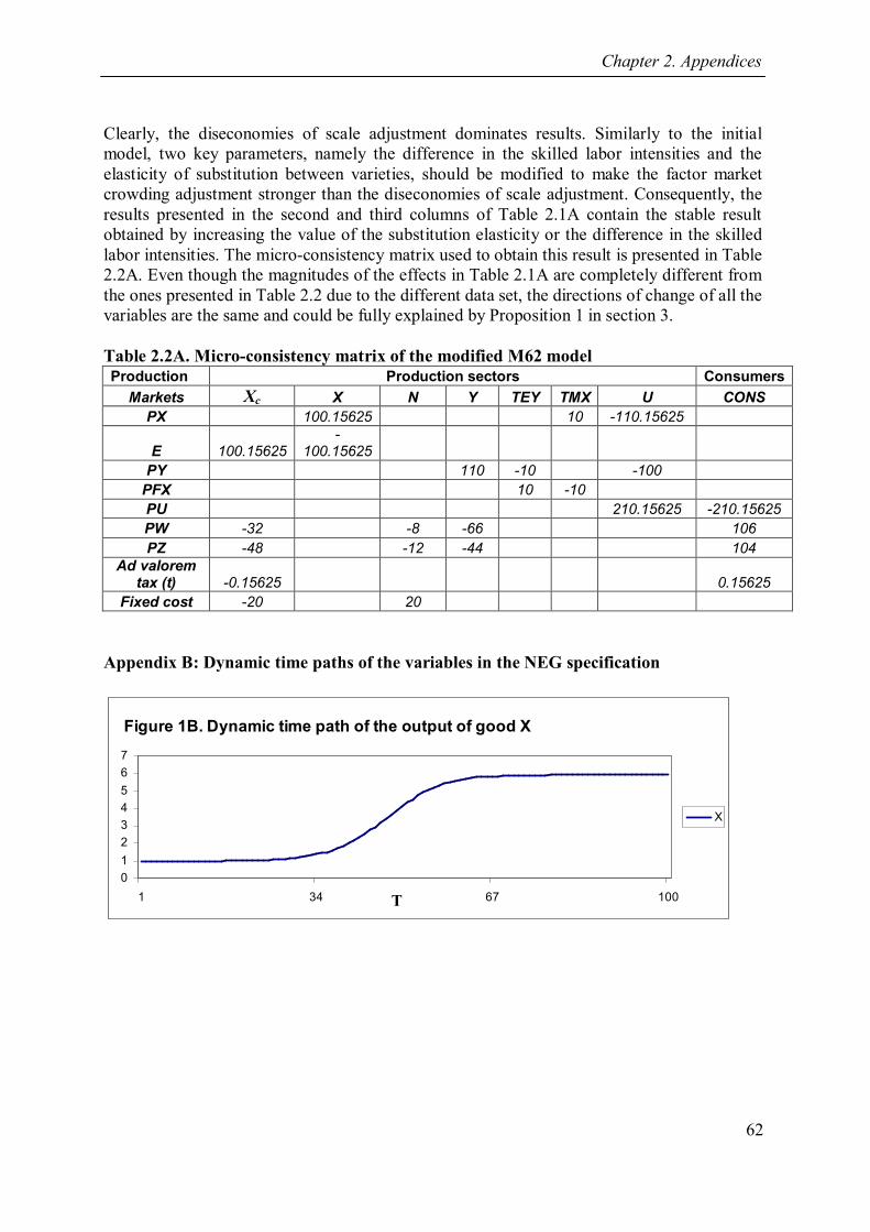
Chapter 2. Appendices
62
Clearly, the diseconomies of scale adjustment dominates results. Similarly to the initial model, two key parameters, namely the difference in the skilled labor intensities and the elasticity of substitution between varieties, should be modified to make the factor market crowding adjustment stronger than the diseconomies of scale adjustment. Consequently, the results presented in the second and third columns of Table 2.1A contain the stable result obtained by increasing the value of the substitution elasticity or the difference in the skilled labor intensities. The micro-consistency matrix used to obtain this result is presented in Table 2.2A. Even though the magnitudes of the effects in Table 2.1A are completely different from the ones presented in Table 2.2 due to the different data set, the directions of change of all the variables are the same and could be fully explained by Proposition 1 in section 3. Table 2.2A. Micro-consistency matrix of the modified M62 model Production Production sectors Consumers
Markets Xc X N Y TEY TMX U CONS PX 100.15625 10 -110.15625
E 100.15625 -
100.15625 PY 110 -10 -100
PFX 10 -10 PU 210.15625 -210.15625 PW -32 -8 -66 106 PZ -48 -12 -44 104
Ad valorem tax (t) -0.15625 0.15625
Fixed cost -20 20 Appendix B: Dynamic time paths of the variables in the NEG specification
01234567
1 34 67 100
X
Figure 1B. Dynamic time path of the output of good X
T
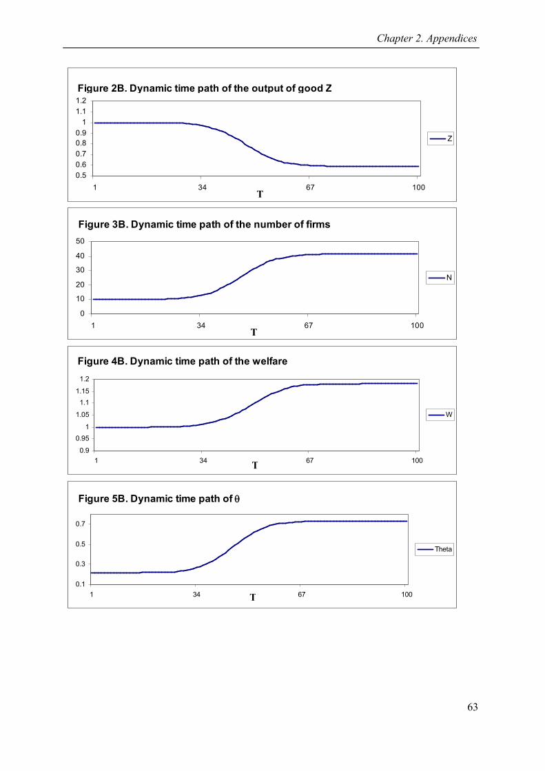
Chapter 2. Appendices
63
0.50.60.70.80.9
11.11.2
1 34 67 100
Z
T
Figure 2B. Dynamic time path of the output of good Z
0
10
20
30
40
50
1 34 67 100
N
T
Figure 3B. Dynamic time path of the number of firms
0.9
0.951
1.05
1.11.15
1.2
1 34 67 100
W
Figure 4B. Dynamic time path of the welfare
T
0.1
0.3
0.5
0.7
1 34 67 100
Theta
T
Figure 5B. Dynamic time path of q
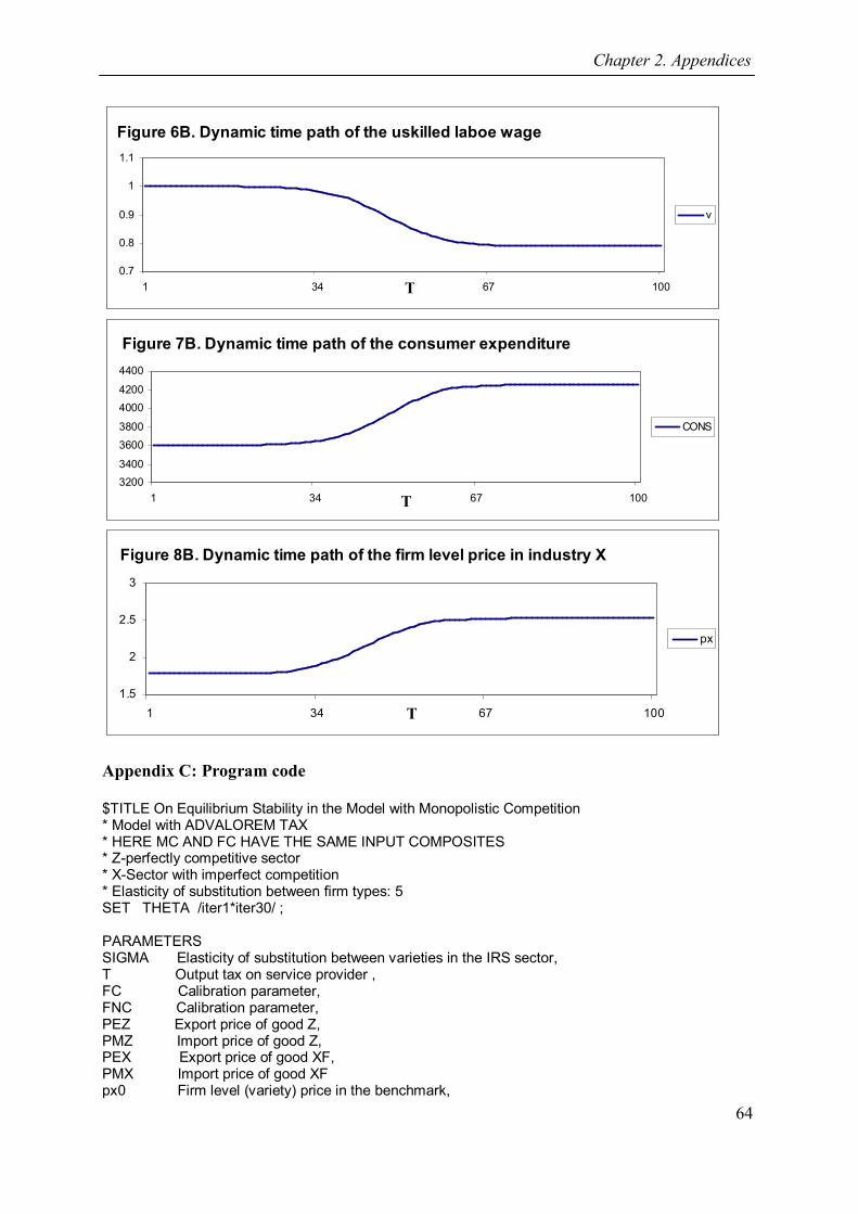
Chapter 2. Appendices
64
0.7
0.8
0.9
1
1.1
1 34 67 100
v
T
Figure 6B. Dynamic time path of the uskilled laboe wage
32003400
36003800
40004200
4400
1 34 67 100
CONS
T
Figure 7B. Dynamic time path of the consumer expenditure
1.5
2
2.5
3
1 34 67 100
px
T
Figure 8B. Dynamic time path of the firm level price in industry X
Appendix C: Program code $TITLE On Equilibrium Stability in the Model with Monopolistic Competition * Model with ADVALOREM TAX * HERE MC AND FC HAVE THE SAME INPUT COMPOSITES * Z-perfectly competitive sector * X-Sector with imperfect competition * Elasticity of substitution between firm types: 5 SET THETA /iter1*iter30/ ; PARAMETERS SIGMA Elasticity of substitution between varieties in the IRS sector, T Output tax on service provider , FC Calibration parameter, FNC Calibration parameter, PEZ Export price of good Z, PMZ Import price of good Z, PEX Export price of good XF, PMX Import price of good XF px0 Firm level (variety) price in the benchmark,

Chapter 2. Appendices
65
x0 Firm level (variety) output in the benchmark, pxOT Firm level (variety) price after tax, xOT Firm level (variety) output after tax, ALPHA The share of good X in the consumer expenditure, BETA Skill intensity of the CRS sector, GAMMA Skill intensity of the IRS sector, P Relative world after tax price of good X, S_ENDOW Total Endowment of Skilled Labor , L_ENDOW Total Endowment of Unskilled Labor , Q(THETA) Relative output of good X; SIGMA =5; T=0.125; ALPHA=0.725; GAMMA=0.75; BETA=0.3; FNC= 10**(1/(1-SIGMA)); S_ENDOW=1222.5; L_ENDOW=2327.5; PEZ=1; PMZ= 1000/999; PEX=999/1000; PMX=1; POSITIVE VARIABLES W ! Consumption (static welfare) level Z ! Activity level for sector Z X ! Activity level for sector X N ! Number of service firms TMZ ! Activity level for imports of Z TEZ ! Activity level for exports of Z TMX ! Activity level for imports of Y TEX ! Activity level for imports of Y PW ! Price index for consumption PZ ! Price index for commodity Z PX ! Price index for commodity Z RL ! Return to unskilled labor L (all other factors composite) RS ! Return to skilled labor S (skilled labor) E ! Price index for foreign exchange CONS ! Income level for consumer CONS; EQUATIONS PriceW Zero profit condition for welfare PriceZ Zero profit condition for Z sector PriceX Zero profit condition for X E_TEX Zero profit condition for exports of X E_TMZ Zero profit condition for imports of Z E_TEZ Zero profit condition for exports of Z E_TMX Zero profit condition for imports of X DW Market clearing condition for W DZ Market clearing condition for Z DX Market clearing condition for X DPFX Trade balance equation DRL Market clearing condition for L (all other factors composite) DRS Market clearing condition for S (skilled labor) DN An equation to detrmine N ICONS Income balance for representative consumer; * Zero profit conditions: PriceX.. RS**GAMMA*RL**(1-GAMMA)=G=N**(1/(SIGMA-1))*PX*(1-T)*(1-(1/SIGMA))*FC; PriceZ.. RS**BETA*RL**(1-BETA)=G=PZ; PriceW.. PZ**ALPHA*PX**(1-ALPHA)=G=PW;
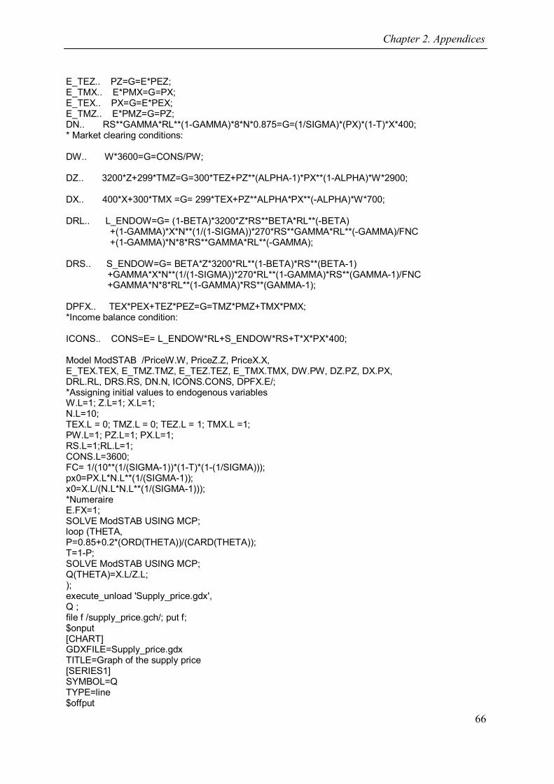
Chapter 2. Appendices
66
E_TEZ.. PZ=G=E*PEZ; E_TMX.. E*PMX=G=PX; E_TEX.. PX=G=E*PEX; E_TMZ.. E*PMZ=G=PZ; DN.. RS**GAMMA*RL**(1-GAMMA)*8*N*0.875=G=(1/SIGMA)*(PX)*(1-T)*X*400; * Market clearing conditions: DW.. W*3600=G=CONS/PW; DZ.. 3200*Z+299*TMZ=G=300*TEZ+PZ**(ALPHA-1)*PX**(1-ALPHA)*W*2900; DX.. 400*X+300*TMX =G= 299*TEX+PZ**ALPHA*PX**(-ALPHA)*W*700; DRL.. L_ENDOW=G= (1-BETA)*3200*Z*RS**BETA*RL**(-BETA) +(1-GAMMA)*X*N**(1/(1-SIGMA))*270*RS**GAMMA*RL**(-GAMMA)/FNC +(1-GAMMA)*N*8*RS**GAMMA*RL**(-GAMMA); DRS.. S_ENDOW=G= BETA*Z*3200*RL**(1-BETA)*RS**(BETA-1) +GAMMA*X*N**(1/(1-SIGMA))*270*RL**(1-GAMMA)*RS**(GAMMA-1)/FNC +GAMMA*N*8*RL**(1-GAMMA)*RS**(GAMMA-1); DPFX.. TEX*PEX+TEZ*PEZ=G=TMZ*PMZ+TMX*PMX; *Income balance condition: ICONS.. CONS=E= L_ENDOW*RL+S_ENDOW*RS+T*X*PX*400; Model ModSTAB /PriceW.W, PriceZ.Z, PriceX.X, E_TEX.TEX, E_TMZ.TMZ, E_TEZ.TEZ, E_TMX.TMX, DW.PW, DZ.PZ, DX.PX, DRL.RL, DRS.RS, DN.N, ICONS.CONS, DPFX.E/; *Assigning initial values to endogenous variables W.L=1; Z.L=1; X.L=1; N.L=10; TEX.L = 0; TMZ.L = 0; TEZ.L = 1; TMX.L =1; PW.L=1; PZ.L=1; PX.L=1; RS.L=1;RL.L=1; CONS.L=3600; FC= 1/(10**(1/(SIGMA-1))*(1-T)*(1-(1/SIGMA))); px0=PX.L*N.L**(1/(SIGMA-1)); x0=X.L/(N.L*N.L**(1/(SIGMA-1))); *Numeraire E.FX=1; SOLVE ModSTAB USING MCP; loop (THETA, P=0.85+0.2*(ORD(THETA))/(CARD(THETA)); T=1-P; SOLVE ModSTAB USING MCP; Q(THETA)=X.L/Z.L; ); execute_unload 'Supply_price.gdx', Q ; file f /supply_price.gch/; put f; $onput [CHART] GDXFILE=Supply_price.gdx TITLE=Graph of the supply price [SERIES1] SYMBOL=Q TYPE=line $offput
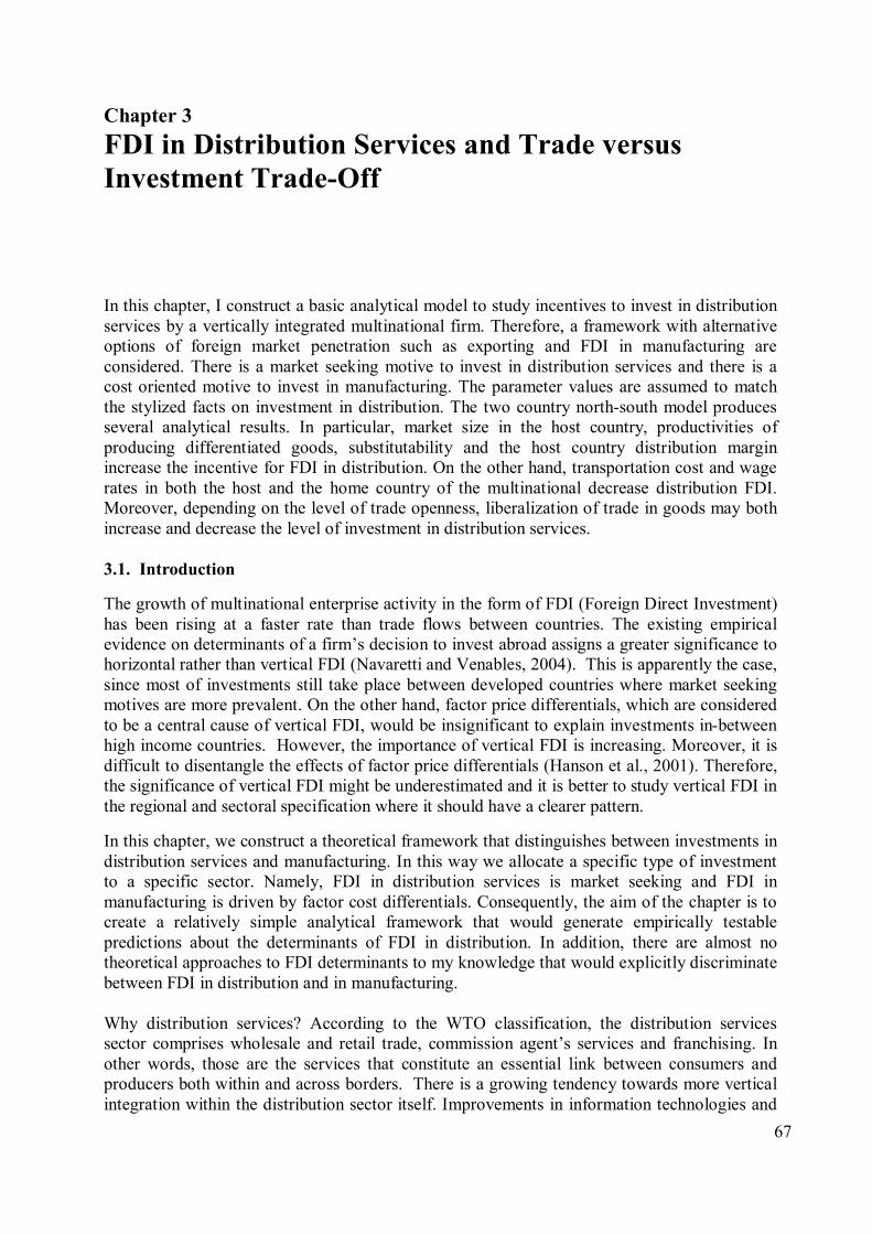
67
Chapter 3 FDI in Distribution Services and Trade versus Investment Trade-Off In this chapter, I construct a basic analytical model to study incentives to invest in distribution services by a vertically integrated multinational firm. Therefore, a framework with alternative options of foreign market penetration such as exporting and FDI in manufacturing are considered. There is a market seeking motive to invest in distribution services and there is a cost oriented motive to invest in manufacturing. The parameter values are assumed to match the stylized facts on investment in distribution. The two country north-south model produces several analytical results. In particular, market size in the host country, productivities of producing differentiated goods, substitutability and the host country distribution margin increase the incentive for FDI in distribution. On the other hand, transportation cost and wage rates in both the host and the home country of the multinational decrease distribution FDI. Moreover, depending on the level of trade openness, liberalization of trade in goods may both increase and decrease the level of investment in distribution services. 3.1. Introduction
The growth of multinational enterprise activity in the form of FDI (Foreign Direct Investment) has been rising at a faster rate than trade flows between countries. The existing empirical evidence on determinants of a firm’s decision to invest abroad assigns a greater significance to horizontal rather than vertical FDI (Navaretti and Venables, 2004). This is apparently the case, since most of investments still take place between developed countries where market seeking motives are more prevalent. On the other hand, factor price differentials, which are considered to be a central cause of vertical FDI, would be insignificant to explain investments in-between high income countries. However, the importance of vertical FDI is increasing. Moreover, it is difficult to disentangle the effects of factor price differentials (Hanson et al., 2001). Therefore, the significance of vertical FDI might be underestimated and it is better to study vertical FDI in the regional and sectoral specification where it should have a clearer pattern.
In this chapter, we construct a theoretical framework that distinguishes between investments in distribution services and manufacturing. In this way we allocate a specific type of investment to a specific sector. Namely, FDI in distribution services is market seeking and FDI in manufacturing is driven by factor cost differentials. Consequently, the aim of the chapter is to create a relatively simple analytical framework that would generate empirically testable predictions about the determinants of FDI in distribution. In addition, there are almost no theoretical approaches to FDI determinants to my knowledge that would explicitly discriminate between FDI in distribution and in manufacturing. Why distribution services? According to the WTO classification, the distribution services sector comprises wholesale and retail trade, commission agent’s services and franchising. In other words, those are the services that constitute an essential link between consumers and producers both within and across borders. There is a growing tendency towards more vertical integration within the distribution sector itself. Improvements in information technologies and
Chapter 3. FDI in Distribution Services and Trade versus Investment Trade-Off
68
logistic services made it possible for large retailers to integrate wholesale functions as well. Thus, this chapter focuses on the distribution sector in general. The sector accounts for up to 50% of the price paid by consumers (Pilat, 1997). Trade in two major components of distribution services: international wholesale and retail trade occurs mainly through commercial presence or mode 3 of GATS (General Agreement on Trade in Services). Moreover, in sectoral terms, the composition of FDI in general has shifted towards services. The distribution sector is connected to manufacturing in several ways. The retail industry, for example, sets product standards, shares information on product promotion and consumer preferences with the manufacturing industry. Moreover, the profit of the manufacturing sector depends on promotional services provided by retailers such as pre-sale information, advertising, credits, free delivery and so on (Tirole, 1988). That establishes potential benefits from vertical integration with the retail sector. Furthermore, many manufacturing firms have either their own distribution chains (see cars or luxury goods) or have binding contracts with wholesale traders to control the marketing of their products. A rational question that the reader may have at this point is: Is there any evidence for multinational firms to view the two types of investments as alternatives? Hanson et al. (2001) study the data on primary and secondary industries of the foreign affiliates of US based multinational firms whose parent primary industry is manufacturing. They find that the second major industry of the foreign affiliate sales of those firms is wholesale trade. Moreover, controlling for the size of the firm they find that most of the firms chose to invest in either manufacturing or wholesale trade and rarely in bothxiv. Consequently, the authors argue that FDI should be differentiated as production oriented and distribution oriented. The subsequent feature of the model that allows investments in manufacturing and/or in distribution by the firm which is vertically integrated across both of those sectors domestically is motivated by this empirical pattern. At the same time, there is a lot of literature on substitutability and complementarity between FDI and trade in general. On the theoretical front, theories on horizontal FDI predict a negative relationship between FDI and tradexv and theories on vertical FDI predict a positive relationship. However, empirical evidence indicates that it is more complex than that. Pontes (2004) criticizes the standard theories of FDI for assuming a monotonic relationship between FDI and trade. He then obtains a non-monotonic relationship, in a model with vertically related intermediate and final stages of production. There is also a growing body of empirical research on substitutability/complementarity between FDI and trade. Most of it supports the complementarity relationship. For example, Swensson (2004) finds that complementarity is prevalent at the high levels of data aggregation. However, at the lower levels of aggregation corresponding to the product lines substitutability is observed. This provides an explanation on the discrepancy between theoretical models that usually assume substitutability and existing empirical evidence. Head and Ries (2001) study the relationship between exports and distribution FDI. They find significant evidence supporting the assumption of their theoretical model and, as many other empirical studies, the complementarity relationship between FDI in manufacturing and exports.
xiv Here controlling for the size of the firm means that the effect does not appear only because foreign affiliates of relatively smaller firms tend to specialize in one sector. xv Also taking into account subsequent trade with intermediates.
Chapter 3. FDI in Distribution Services and Trade versus Investment Trade-Off
69
Moreover, the positive relationship between FDI in distribution and exports was found to be stronger than the one for manufacturing, as it was expected. On the other hand, Nordas et al. (2007) find that FDI in the distribution services sector would raise imports from the host to the home country of the multinational firm. In terms of the policy relevance of the given issue, it should be noted that there is a widespread view in developing countries that FDI in distribution services yields little development impact and it is not crucial for growth (Palmade et al., 2004). At the same time, developing countries make a lot of effort to attract FDI in manufacturing that could be brought by efficiency seeking multinational firms. As a matter of fact, in terms of the level of FDI, manufacturing still remains to be the politically most preferred sector in developing economies. It is also feared that more investments in distribution could create urban sprawl and push smaller and less efficient retailers out of the market, which in turn could potentially bring more unemployment. As a matter of fact, there is an ongoing debate whether to allow FDI in the retail sector or not in several developing countries like India and Indonesia. On the other hand, the restrictions on distribution could hinder the efficiency of the upstream industries and consequently bring higher business costs. Restrictions could also lead to rent-creation by incumbent firms. Indeed, Kalirajan (2000) finds that restrictions are primarily cost-creating. Market structure of the distribution sector varies from country to country. However, there is a general trend for higher market concentration. For example in the retail sector, this could be efficiency improving due to the significant economies of scale (Nordas et al., 2007). In addition to that, retailing is characterized by a decline in the total number of outlets and at the same time by an increase in the number of large megastores. The impact of the market structure in distribution on the profit of the vertically integrated firm and on the upstream firm is considered in the last section. Another stylized fact about retailing is that the number of offered varieties of products has increased over time (Eckel, 2009). Apparently, those changes are the result of increasing globalization and freer trade. The above mentioned stylized facts are incorporated in the model constructed in this chapter when trade openness brings more FDI in distribution. There are several studies related to the interaction between trade in distribution services, market concentration and trade in goods. In particular, Francois and Wooton (2007) find that a rising concentration in distribution services could be an effective barrier for trade in goods. As for the goods trade, Ishikawa (2008) shows that trade liberalization in goods, if not accompanied by FDI in distribution services, could hurt domestic consumers and lead to the an overall welfare fall. The rest of the chapter is organized as follows: the next section presents an outline of the theoretical model. In the third section we present the parameter assumptions and the corresponding analytical results. The fourth section presents numerical results and the non-monotonic relationship between trade costs and FDI in distribution and the fifth section concludes.
Chapter 3. FDI in Distribution Services and Trade versus Investment Trade-Off
70
3.2. Model setting
A two country model is considered. It is a stylized fact that FDIs originate predominantly from developed countries (Navaretti and Venables, 2004). Therefore, I assume that the multinational firm is located in a developed country and is denoted by north. Similarly, a developing country receives FDI and is denoted by south. It is assumed that each economy is composed of a monopolistic sector of two differentiated tradable goods and a competitive numeraire sector. Initially, only one of the differentiated goods could be produced in each country. The vertically integrated monopolist maximizes profits by serving two segmented markets. In other words, in addition to the local market it could serve the foreign market through investments or trade. We assume a quadratic utility function:
2 2( , , ) ( 2 ) / 2 (3.2.1)x y x yU x y z z x y x xy y Here z is a numeraire good and x, y are two differentiated goods traded by a multinational firm. The functional form of the utility function enables us to conduct a partial equilibrium analysis of the differentiated goods only. This is because markets for numeraire and non-numeraire goods are separated which leads to no income effects on those goods. Consequently, the derived demand functions will be linear and will look as follows, for example, for the developed country:
(3.2.2)c c
N xN xN yN xN xN
c cN yN yN xN yN yN
x a b P c P
y a b P c P
Here 2 2 2; ; ; , , { , }i j j iiN iN xN yN
i j i j i j
a b c c i j i j x y
Let us assume a symmetric case with :xN yN Na a a and :xN yN Nb b b . Moreover, let us
assume that 1xN yNc c . This is not a loss of generality because units can be chosen so that both coefficients equal one. Then, (3.2.2) will simplify to:
(3.2.3)c c
N N xN N yN
c cN N yN N xN
x a P b P
y a P b P
This form enables us to give meaning to the remaining parameters: 0Na is the market size in the north and [0,1]Nb represents the substitutability between the two goods. Similarly for the developing country:
(3.2.4)c c
S S xS S yS
c cS S yS S xS
x a P b P
y a P b P
The Y-good is produced in the south and the X-good is produced in the north. We could also think of those goods to be composites of the foreign and domestic goods of a multinational
Chapter 3. FDI in Distribution Services and Trade versus Investment Trade-Off
71
firm. There is only one factor of production. Thus, the production function in the manufacturing industry Y in the south, for instance, could be represented asxvi:
(3.2.5)Sy L Here denotes productivity. Similarly in the north:
(3.2.6)N Nx L The multinational could also shift the production of its good to the developing country:
(3.2.7)S Sx L In contrast to producer services, where skilled labor intensity is an important distinguishing factor, distribution services employ many low skilled workers. Differently from FDI in manufacturing, FDI in distribution is expected to bring little impact on employment in the host country. On the contrary, it may actually decrease labor demand. Therefore, the corresponding variable labor costs may both increase or decrease after FDI in distribution. Consequently, in this setting, we neglect variable costs of distribution. They could also be thought of to be partially included in variable production costs. The marginal costs of production will be later chosen to set the units of measurement in the reference equilibrium. On the other hand, there will be distinct fixed costs of FDI in distribution. Since no portfolio investments are considered in this model, the words FDI and investment are used interchangeably. There will be four scenarios depending on the decision of the multinational firm to serve the foreign market through exports, to invest in manufacturing, to invest in distribution services or to invest in both. In what follows, I would like to consider all four cases or modes of supplying the southern market separately. 3.2.1. Case 1: No investments In this case the developed country exports the local good, imports the foreign good and no investments take place. The multinational firm will maximize its profit at home and abroad by optimally choosing the prices it charges for both goods. In particular, the domestic profit is given as follows:
1 ( ) ( ) (3.2.8)c p c pN yN yN N xN xN NP P y P P x
The producers’ prices are obtained routinely from corresponding maximization conditions:
(3.2.9) (3.2.10)1
pyN pS N
xNN N
P w wPt
Here ,N Sw w denote wages in the north and south correspondingly, is a transportation cost and Nt is an ad valorem sales tax imposed by the north on the importing firm. The multinational firm which has a full monopoly over good X will also export it to the south and maximize the profit by charging producer price p
xP :xvii
1 ( ) (3.2.11)1
pxS N
S SS N
P w xt
xvi I could have chosen a form with plant-level economies of scale. However, in the setting where production takes place either in two countries or in the south only, that would be equivalent to adding an additional incentive for FDI in manufacturing. The effect will be consistent with theoretical and empirical predictions of plant-level economies of scale on FDI in manufacturing. It won’t bring any significant changes to the main outcomes of the model. xvii The upper index is used to indicate whether we use producer’s price (p) or consumer’s price (c).
Chapter 3. FDI in Distribution Services and Trade versus Investment Trade-Off
72
Here St is an ad valorem tariff imposed by the south. I assume that there are many small distribution outlets in the south and the distribution margin is fixed at the level KD. Hence, consumer prices will be determined as follows:
(3.2.12) (3.2.13)c c pSyS D xS xS D
wP K P P K
On the other hand, monopoly in the distribution sector would result in a problem of double marginalization with very high prices and very small outputs of goods. Then, the combined profit of the distribution and manufacturing sectors will be smaller than the vertically integrated profit and consumers will be worse off. 3.2.2. Case 2: FDI in manufacturing In this case, the multinational firm shifts the production of the northern country good to the south. Accordingly, both goods will be produced in the south and incur transportation costs and taxes. In this case, no goods will be produced in the north and the labor of the northern country could be thought to move to headquarter activities even though it is not explicitly modeled. This assumption is rather strong and it constrains labor endowment of the south to be large relative to the labor endowment of the north in order to produce feasible values. The production function is represented by (3.2.7), with higher productivity in the north:
N S .However, it would also be intuitive to have S N
S N
w w
. In other words, even though it is
more efficient to produce good X in the north, the unit cost of producing X is lower in the south. That incorporates the vertical motive to invest in the south. Additionally, there will also be an implicit horizontal motive since the multinational firm supplies to the host market as well. As in the case before, multinational firm will maximize its profits by charging consumer prices for both goods domestically and the producer price for the X-good in the south:
2 ( ) ( ) ( (1 ) )
( (1 ) ) (3.2.14)
c p c p c SN yN yN N xN xN N yN N N
c SxN N N
S
wP P y P P x P t y
wP t x
2 ( ) (3.2.15)p SS xS S
S
wP x FM
Here FM is a fixed cost of FDI in manufacturing. Labor is assumed to be immobile between countries. Therefore, only the resources of the southern country will be used in the final production. 3.2.3. Case 3: FDI in distribution services In this case, the multinational firm invests only in distribution services. I assume that it takes over the less efficient distribution sector of the south and becomes the only distributor in the south just as it is already in the north. This effect is justified by the cost-predation considerations discussed below. The multinational firm incurs no distribution costs. The profits in both markets are determined as follows:
Chapter 3. FDI in Distribution Services and Trade versus Investment Trade-Off
73
3 1
3
( (1 ) ) ( ) (3.2.16)
( ) ( ) ( )
( (1 ) ) (3.2.17)
c cS NN yN N N xN N N
N
c p c p c SS yS yS S xS xS S yS S
c NxS S S
N
w wP t y P x
wP P y P P x FDS P y
wP t x FDS
Here FDS is a fixed cost of FDI in distribution services. It consists partially of the cost of acquisition of the southern distribution sector and the cost of erecting no entry barriers as well as the fixed costs of operating in a foreign market. The distributor sources the Y-good locally and the X-good from its own home country. Apparently, there is a horizontal motive to invest in distribution services. 3.2.4. Case 4: FDI in both manufacturing and distribution services The profits in the north and in the south will be given as follows:
4 2 (3.2.18)N N 4 ( ) ( ) ( ) ( )
( ) ( ) (3.2.19)
c p c p c SS yS yS S xS xS S yS S
c SxS S
S
wP P y P P x FM FDS P y
wP x FM FDS
Here 1 is a measure of complementarity between two types of investments. Thus, profits in the north change only with investments in manufacturing. The schematic representation of the strategies of the multinational firm is given in Appendix A. Existing industrial organization literature, in most cases similar to the assumptions of the model, supports the concept of full forward vertical integration by a monopolist firm and the corresponding takeover of downstream industry. In other words, in the case without economies of scale and with fixed-proportion downstream production technology, the upstream monopolist would be able to eject the competing downstream firms (fringe firms). This effect occurs due to the strategic cost-predation considerations when a dominant monopolist drives competitors out of the downstream market by strategically increasing prices of the inputs it supplies. Bonroy and Larue (2007) find a partial forward integration in the model with decreasing returns to scale in the downstream industry and increasing returns to scale in the upstream industry. In the present model, one unit of manufacturing input is required to produce one unit of output in distribution. That represents a fixed-proportion technology. The upstream firm supplies only one good, the price of which, under average values of substitutability, could significantly increase the costs of potential fringe firms. Therefore, in the given model setting, the assumption of full forward vertical integration after FDI in distribution is justified. Returning to the model setting, the total profit that the multinational firm will obtain in each mode is just the sum of the profits in the north and in the south. The profit functions depending on the parameters of the model could be obtained after solving the corresponding profit maximization problems:
Chapter 3. FDI in Distribution Services and Trade versus Investment Trade-Off
74
1 1 1
, ,
2 2 2
, ,
3 3 3
, , ,
4
( , , , , , , , , ) max ( )
( , , , , , , , ) max ( )
( , , , , , , , , ) max ( )
( , , , , , , , , ) max
pc cxN yN xS
pc cxN yN xS
c c c cxN yN xS yS
cxN
N S N S N D N SP P P
N S S D N SP P P
N S N S N N SP P P P
N S SP
t t w w K b
t w K b FM
t t w w b FDS
t w b FM FDS
4 4
, , ,
(3.2.20)
( )c c cyN xS yS
N SP P P
The optimization problem could be simplified if we note that
,, ,
, , , , ,
max ( ) max max 1, 2(3.2.21)
max ( ) max max 3, 4
p p c cc cxN yNxN yN xS xS
c c c c c c c cxN yN xS yS xS yS xN yN
i i i iN S S N
P PP P P P
i i i iN S S N
P P P P P P P P
for i
for i
Any stationary points obtained from optimization will always be a maximum because of the concavity of profits in (3.2.21). For the profits in (3.2.21) to be concave, the corresponding Hessian matrix should be negative semi-definite at the stationary point. The sign definiteness of the Hessian matrix is equivalent to the sign definiteness of the corresponding quadratic form at the stationary point. The negative definiteness of the quadratic form could be demonstrated as follows:
2
2
2 0, 1, 21
iSP
xS S
for iP t
22 2 2 2 2
22 2 2 2 22 0, 4(1 ) 0, 3, 4
i i i i iS S S S Sc c c c c c
xS yS xS yS xS yS
b for iP P P P P P
22 2 2 2 2
22 2 2 2 22 0, 4(1 ) 0 1, 2,3,4
i i i i iN N N N Nc c c c c c
xN yN xN yN xN yN
b for iP P P P P P
Let iD in (3.2.22) denote the feasible set of the parameters of mode i . In other words, in that set, prices, quantities and profits are greater or equal than zero.
* * * *
* * * * *
{ | ( ) 0, ( ) 0, ( ) 0, ( ) 0,
0, 0, 0, 0, ( ) 0} (3.2.22)
i S i N i S i N i
ixNi yNi xSi ySi i
D parameters x P x P y P y P
P P P P P
The number of the parameters defined in iD will change in different specifications. We define D as the feasible set of parameter values of our model to be an intersection of the feasible sets of each mode: 1 2 3 4D D D D D . 3.3. Analytical results
3.3.1. Determinants of FDI in distribution
In this subsection we restrict our analysis to incentives to invest in distribution both with and without FDI in manufacturing. Since profits in the north are the same in modes 1 and 3 as well
Chapter 3. FDI in Distribution Services and Trade versus Investment Trade-Off
75
as in modes 2 and 4, we could restrict our analysis only to profits in the south. However, northern profits will already need to be taken into account in the next subsection.
In order to study the impact of the parameters on the decision to invest in distribution, we define the following functions:
3 1 4 20 , (3.3.1)D DM Hence, the derivatives of those functions will provide us with an underlying intuition of the impact of the parameters. In particular, a positive value of the derivative means more distribution FDI. The incentive to invest in distribution is studied both under a prohibitively high cost of manufacturing (D0) and in the case when manufacturing investment has already taken place (DM). According to the envelope theorem, the impact of the changes in parameter values would incorporate the impact from the changes in maximizer variables and therefore a partial derivative of the profit function would exactly reflect the change in the optimally chosen value function. Moreover, the profit differences in (3.3.1) could be reduced to:
3 1 4 20 ,S S S SD DM This is because profits in the north are the same for modes 1 and 3 as well as for modes 2 and 4 as could be seen from (3.2.21). Therefore country specific indexes for the market size and sustainability could be dropped: ,S S Na a b b b . Let me denote the feasibility sets corresponding to D0 and DM as D0F and DMF:
1 30D F D D ; 2 4DMF D D ; Hence, the following proposition could be proved: Proposition 1: Let us assume the case where FDI in manufacturing takes place, all of the parameters belong to the feasibility set DMF and distribution markups are nonnegative. Then, the market size in the south (a), fixed cost of manufacturing (FM), productivities of producing both differentiated goods in the south ( , )S , southern market inefficiency in distribution ( )DK would increase the incentive to invest in distribution and the southern wage ( )Sw and a fixed cost of distribution (FDS) would decrease it. Moreover, if
(3.3.2)1
SD
wa Kb
substitutability (b) stimulates FDI in distribution. However if
1S
Dwa K
b
, then (3.3.3)Sb is a sufficient condition for a positive impact of
substitutability on incentive to invest in distribution. The last condition considers the case where market size in the south is sufficiently small for the markup that the multinational firm earns on the Y good to be less than the domestic distribution
margin: 01
SD
wa Kb
. Then, the productivity of the locally produced good should not
be much less than the productivity of the good produced by the multinational in the south, taking into account the substitutability between the two goods. Otherwise, an increase in the substitutability between the differentiated goods may not lead to FDI in distribution. A similar proposition could be formulated for the case under a prohibitively high fixed cost of manufacturing.
Chapter 3. FDI in Distribution Services and Trade versus Investment Trade-Off
76
Proposition 2: Let us assume the case with no FDI in manufacturing, all parameters belonging to the feasibility set D0F and nonnegative distribution markups. Then, the market size in the south (a), productivities of producing differentiated goods ( , )N , southern market inefficiency in distribution ( )DK would increase the incentive to invest in distribution and fixed cost of distribution (FDS), transportation cost ( ) , southern wage ( )Sw and northern
wage ( )Nw would decrease it. Moreover, if 1(1 ) (3.3.4)1
S SD
S
w wa b Kt
substitutability (b) has a positive impact on incentive to invest in distribution. In order to prove propositions 1 and 2 we need to show that the following conditions hold
0, 0, 0, 0, 0, 0, 0 0
;1 1
S D S
S SD D S
DM DM DM DM DM DM DM DManda FM K w FDS b
w wa afor K K bb b
for Proposition 1 and the following conditions hold 0 0 0 0 0 0 0 0 00, 0, 0, 0, 0, 0, 0, 0 0
(3.3.4) ;N D S N
D D D D D D D D Danda K FDS w w b
if holds
for Proposition 2. The proofs of both propositions are given in Appendices B and C. Many parameters in Propositions 1 and 2 directly influence the quantities of goods. Furthermore, it is possible to show that the quantity of the good that the multinational sources from the home country (X good) will be larger with FDI in distribution than without it under both specifications:
* * * *0 3 3 1 1
1( , ) ( , ) (1 )2
1 1(1 ) (1 ) (1 ) 0 (3.3.5)2 2
S NS x y S x y S
N
S ND S D S
N
w wx x P P x P P a b t
bw wa b K t b K t
* * * *4 4 2 2
1 1( , ) ( , ) (1 )2 2
(1 ) 0 (3.3.6)2
S S S SM S x y S x y D
S S
D
w w bw wx x P P x P P a b a b K
b K
The impact on the output of the locally produced good (Y-good) is less obvious. However, we could demonstrate that the price of that good will be larger or smaller with FDI in distribution than without depending on whether the monopoly markup is higher or smaller than the local distribution margin DK :
* * * *0 3 1 4 2
1 1 (3.3.7)2 1 2 1
S S Sy y y yM y y D D
monopoly markup
w w wa aP P P P P P K Kb b
Chapter 3. FDI in Distribution Services and Trade versus Investment Trade-Off
77
In the case when the distribution markup of the multinational firm is smaller than DK , the price of the Y-good decreases after FDI in distribution ( 0 0, 0y yMP P ) and it could be shown using (3.2.4) that the price of the X good also decreases after FDI in distribution:
0 0 0 0x yP b P x or 0xM yM MP b P x . On the other hand, if the distribution markup is higher than DK , and the price of the Y-good is larger with FDI in distribution than without it ( 0 0, 0y yMP P ), it could be shown that the output of that good is smaller with FDI in distribution than without: 0 0, 0My y . This could be proved by using the difference form of (3.2.4) and considering both cases with increasing and decreasing price of the X-good after FDI in distribution: if
0 0xP then 0 0 000
0y xy P b P
.
If 0 0xP then 0 0 0 0 0 000
( ) 0y x y xy P b P b P P x
. So in either case 0 0.y
Similarly it could be shown that: 0My . In other words, the following proposition has been proved: Proposition 3: Let us assume that all the parameters belong to the feasibility set and distribution markups are nonnegative. Then, the output of the good that the multinational firm sources from its home country is higher with FDI in distribution than without. Moreover, if the distribution markup of the locally sourced good (Y) is lower than the local distribution cost ( DK ), denoted as case (I), the final prices of both goods sold by the multinational firm will decline after FDI in distribution. On the other hand, if the distribution markup of the locally sourced good is higher than the local distribution cost, denoted as case (II), the final price of the local good will increase and the quantity of it will decline after FDI in distribution:
0 01( ) 0 0, 0, 0, 0;2 (1 )
SD y yM x xM
waI K P P P Pb
0 01( ) 0 0, 0, 0, 0;2 (1 )
SD y yM M
waII K P P y yb
This proposition is independent of the fixed cost of manufacturing and will help us interpret the results from Propositions 1 and 2:
1) Market size (a): A higher market size in the south would result in higher demand from the south and consequently more potential profit after investment in distribution.
2) Productivities ( , , )S N : A higher productivity of producing either good both in the north and in the south would make production and trade less costly. That would stimulate FDI in distribution.
3) Transportation cost ( ) : Obviously, in the case where all production takes place in the south, transportation costs are incurred only to the north and as a result do not matter. Otherwise, the multinational firm chooses the mode with fewer exports to the south and the correspondingly smaller per unit cost of transporting it.
4) Southern distribution margin ( )DK : Higher southern market inefficiency in distribution would widen the gap between the level of exports to the south with and without FDI in
Chapter 3. FDI in Distribution Services and Trade versus Investment Trade-Off
78
distribution. Therefore, the amount of potential rent that the monopolist could extract after investing in distribution rises with DK . This leads to the positive sign with respect to DK .
5) Southern wage ( )Sw : Higher costs of production in the south would result in lower monopoly rent after distribution FDI. Although the negative effect is unambiguous in modes 2 and 4, in the case without manufacturing FDI there will also be a smaller counter effect. Namely, the higher cost of production in the south would raise the price of the Y-good and consequently increase the demand for the X-good. This should stimulate distribution FDI since it brings more exports of the X-good.
6) Northern wage ( )Nw : Here, as the cost of producing the X-good and accordingly its price increase, the distribution markup will shrink, the mode with no FDI in distribution and less exports will be chosen. Even though labor is not employed in distribution in this model, higher wages in both the host and the home country of the multinational firm would result in less FDI in distribution.
7) Substitutability (b): More substitutability, also entailing higher consumer flexibility in choosing between the two goods, would restrict monopoly power in the modes where the multinational supplies only one good to the southern market. This should stimulate FDI in distribution. One of the incentives for FDI in distribution is eliminating the inefficiency associated with underconsumption of the X-good produced by the monopoly relative to the competitively produced Y-good. However, this effect could be small or even reverse when the productivity of the Y-good is small relative to the productivity of X-good for a given value of the substitutability between the goods. Then, consumers would have less incentive to substitute the X-good for the more expensive Y-good. Consequently, when the market size in the south is so small that condition (3.3.2) does not hold, the positive impact of FDI in distribution is also small. In that case, for the positive impact of the substitutability on the incentive to invest in distribution it is sufficient if the ratio of corresponding productivities satisfies condition (3.3.3).
In the case where only modes with and without distribution are compared, the segmented markets are independent of each other. Therefore, the northern market size as well as the tariff imposed by the north would have no impact on the incentive to invest in distribution. The impacts of the fixed costs are trivial. The obtained results could be contrasted with existing empirical studies. In particular, Hanson et al. (2001) find that the share of FDI in the wholesale trade sector in the total of wholesale and manufacturing FDI is decreasing in the host country GDP. This result is inconsistent with the horizontal theories of FDI, especially when applied to distribution services. Boatman (2007) uses agency theory considerations to study the determinants of FDI in distribution. In that study, firms choose between supplying the foreign market by investing in distribution services or by exporting. Both Hanson et al. (2001) and Boatman (2007) find a positive and significant relationship between per capita GDP in the host country and FDI in distribution. We could draw parallels to our study because per capita GDP could be used as an alternative measure of market size.
Chapter 3. FDI in Distribution Services and Trade versus Investment Trade-Off
79
3.3.2. Determinants of FDI in manufacturing
The model has not been constructed to provide a comprehensive framework to find all of the determinants of FDI in manufacturing. However, the impact of some parameters could also be shown analytically and additional assumptions on the values of the parameters could be derived. Those assumptions would be useful in the numerical analysis. Similarly to the case for distribution, let us define the following functions:
2 1 4 32 , (3.3.8)D DDS Then, the following Proposition on the determinants of FDI in manufacturing could be proved: Proposition 4: Let us assume that all parameters belong to the feasibility set D, distribution
markups are nonnegative and the following condition holds: (1 ) (3.3.9)N Sn
N S
w w t
Then, the market size in the south ( Sa ) and in the north ( )Na ,substitutability (b),the northern wage ( )Nw , productivity of producing an outsourced good in the south ( )S , and southern tariff ( )St would increase the incentive to invest in manufacturing. On the other hand, southern market inefficiency in distribution ( )DK , productivity of producing an outsourced good in the north ( )N , productivity of producing a local good in the south ( ) would decrease the incentive to invest in manufacturing. Moreover, if 2 (3.3.10)Sb , the southern
wage ( )Sw and the northern tariff ( )Nt would also decrease the incentive to invest in manufacturing. The proof of Proposition 4 is given in Appendix D. Proposition 4 holds in both scenarios with and without FDI in distribution. Furthermore, the difference in profits in the north ( N ) is the same irrespective of FDI in distribution and could be written as follows:
* * * *1 1 2 2
2 1 4 3
( , ) 0 ( , ) 0
1 (1 ) (1 ) (1 ) *4
* (1 ) 0
N xN yN N xN yN
NN N N N
N S S SN n N n n
N S
x P P x P P
NN S Nn
N S
w w w wa b t a t b t
w w wt
(1 )Sn
N S
w t
If condition (3.3.9) does not hold, the profits of the multinational firm in the north will be smaller with FDI in manufacturing than without it. Therefore, for FDI in manufacturing to take place, a fall in the northern profit after FDI in manufacturing should be compensated by an increase in profits from supplying the southern market. This situation could happen when diseconomies of scale are high enough for the multinational firm to split production between the two countries and it would require an additional constraint linking the market size variables. In other words, market size in the south should be sufficiently high relative to market size in the north for the market seeking effect of FDI in manufacturing to be stronger than the negative factor cost differentials effect. Consequently, condition (3.3.9) should hold for the positive vertical motive of FDI in manufacturing to exist.

Chapter 3. FDI in Distribution Services and Trade versus Investment Trade-Off
80
The following economic interpretation could be given to the results of Proposition 4:
1) Market size ( , )S Na a : Higher demand from the south would apparently bring more investments in manufacturing which basically means fewer expenses per unit of the supplied good. The impact of the market size in the north will depend on the presence or absence of the vertical motive to invest in manufacturing. We have a vertical motive in our model by assuming (3.3.9) and therefore the impact is positive.
2) Substitutability (b): More substitutability increases profits in both cases as it practically creates bigger markets for the multinational. Thus, the mode with more quantities sold will be chosen.
3) Southern distribution margin ( DK ): Similarly to the previous argument but only relative to the south, the inefficiency cost is higher under the mode with more quantities sold in the south.
4) Northern wage ( )Nw : A higher northern wage means higher cost for the multinational firm. Apparently, in order to avoid paying a higher cost at home, the multinational will have an incentive to invest in manufacturing.
5) Productivities ( , , )S N : The productivity in the north is the inverse of the northern wage and the productivity of producing an exported good in the south increases the incentive to invest. On the other hand, higher productivity in producing a local good in the south would squeeze the market for the exported good and make investing in manufacturing less profitable.
6) Southern tariff ( )St : No tariffs need to be paid after the FDI in manufacturing. Therefore the positive impact represents a tariff jumping effect.
7) Southern wage ( )Sw : Even though a higher southern wage increases profits under no investments in the south by increasing its market share, its impact on profits after FDI in manufacturing is ambiguous. This is because in addition to the indirect effect of getting higher market share there is a direct effect of paying more for the production of the previously exported good. Hence, if the productivity of producing the local good is sufficiently high so that it satisfies (3.3.10), the direct effect will be stronger than the indirect effect and the total effect on profits under the FDI in manufacturing will be negative. Similar considerations to the impact of the northern tariff presented below could explain the negative impact of the southern wage on the profit in the north.
8) Northern tariff ( )Nt : The impact of the northern tariff is restricted only to the north. Even though both profits with the FDI in manufacturing and without will fall under the higher tariff, for the given wage rate the cost of production will be determined by productivities. Higher productivity means smaller cost or smaller producer price for the retailer. In other words, if the productivity of producing the local good is high enough and satisfies (3.3.10), the producer price of that good is small enough relative to the producer price of the exported good. That makes the impact of the tariff hike stronger on the exported good and therefore the profits with the FDI in manufacturing would contract more than the profits with no FDI in manufacturing.
Chapter 3. FDI in Distribution Services and Trade versus Investment Trade-Off
81
9) Transportation cost ( ) : The impact of the transportation cost is ambiguous. In contrast to the northern tariff discussed above, transportation cost does not depend on the producer price and applies per unit of output. On the one hand, investment in manufacturing reduces the transportation cost of supplying the south. On the other hand, the transportation cost of supplying the north increases. The total effect will depend on the relative quantities supplied by the multinational to the north and the south which, in turn, depends on the values of the market size in the two countries.xviii In other words, a large market size in the north relative to the south would lead to a negative impact on FDI in manufacturing and a large market size in the south relative to the north would lead to a positive impact. Either case could happen in practice.
3.4. Numerical results
3.4.1. Selecting parameter values
The analytical results of the parameter impact have been obtained so far by using the constraints of the feasibility set and some intuitive assumptions but without assigning any particular values to the parameters. However, it is possible to obtain more insights into our analysis by assigning values to the parameters within the range implied by the empirical evidence and by choosing units of measurement. In particular, we will be able to see the impact of the FDI in distribution on the volume of trade, exports and imports. Furthermore, numerical analysis will enable us to study the impact of the southern tariff on the incentive to invest in distribution. This effect is found to be ambiguous and will be dealt with in the next subsection. Let us first choose the reference equilibrium to be mode 4 in the south when both types of investments take place. The two degrees of freedom corresponding to the choice of units of measurement of the two commodities are used in such a way that:
*4 1xP and *
4 1 (3.4.1)yP
As a consequence of (3.4.1) we will have S . Then, we could define the wage per unit of productivity in the south as follows:
(3.4.2)S S
S
w w w
Since the northern wage per unit of productivity always appears in the form of N
N
w
, without
assigning any value to the northern productivity parameter N , we assume that NN
N
w w w
.
Productivities are chosen to define units of measurement. Despite higher productivity in the north, the difference in the nominal north south wage should be stronger. Moreover, in the previous section, for the derivation of the analytical results it was assumed that:
(1 ) (3.3.9)N Sn
N S
w w t
.
Consequently, we assume that 2Nw in the benchmark. Without a loss of generality, we could express all of the variables as multiples of the wage per unit of productivity. Thus, the parameters are assigned the following values initially:
xviii The expression for the impact of the transportation cost is given at the end of Appendix D.
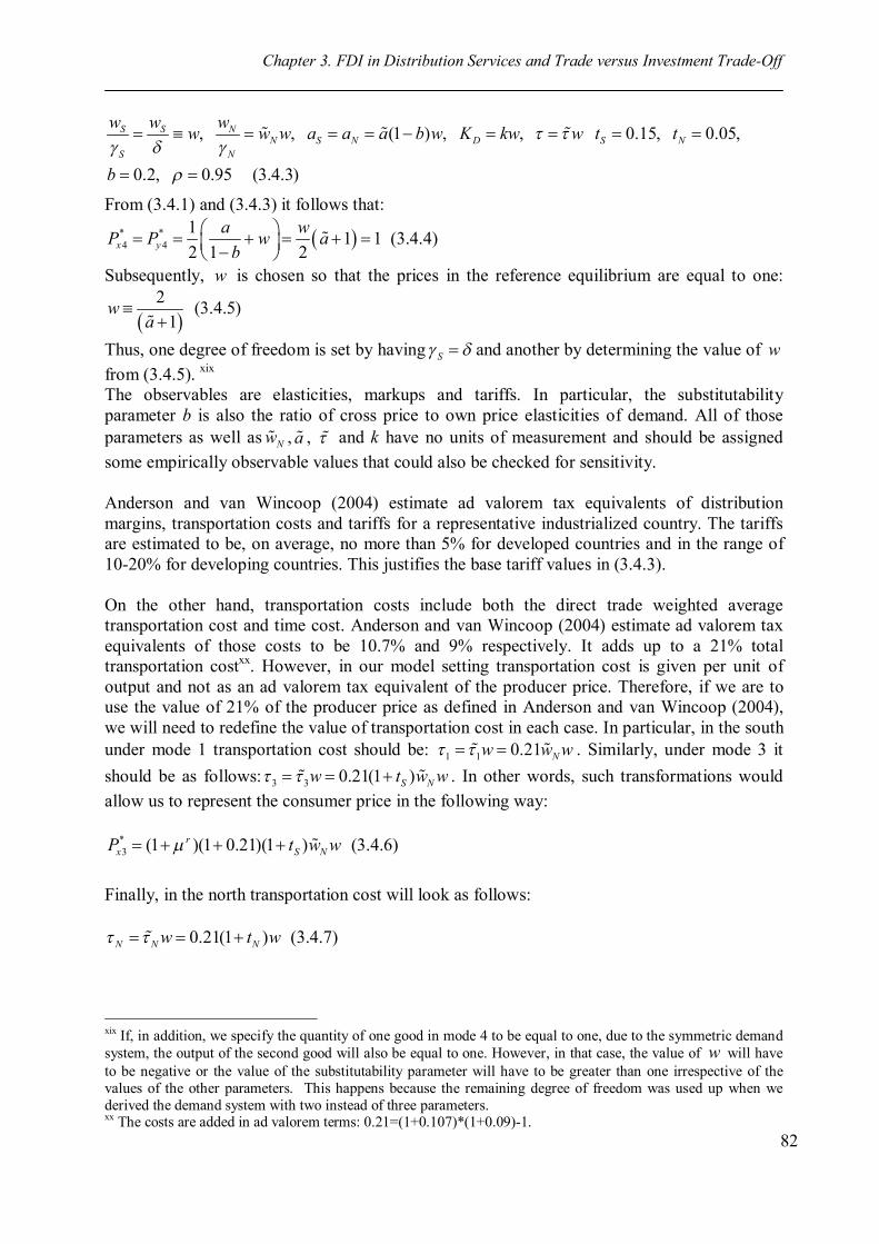
Chapter 3. FDI in Distribution Services and Trade versus Investment Trade-Off
82
, , (1 ) , , 0.15, 0.05,
0.2, 0.95 (3.4.3)
S S NN S N D S N
S N
w w ww w w a a a b w K kw w t t
b
From (3.4.1) and (3.4.3) it follows that:
* *4 4
1 1 1 (3.4.4)2 1 2x y
a wP P w ab
Subsequently, w is chosen so that the prices in the reference equilibrium are equal to one:
2 (3.4.5)
1w
a
Thus, one degree of freedom is set by having S and another by determining the value of w from (3.4.5). xix The observables are elasticities, markups and tariffs. In particular, the substitutability parameter b is also the ratio of cross price to own price elasticities of demand. All of those parameters as well as Nw , a , and k have no units of measurement and should be assigned some empirically observable values that could also be checked for sensitivity. Anderson and van Wincoop (2004) estimate ad valorem tax equivalents of distribution margins, transportation costs and tariffs for a representative industrialized country. The tariffs are estimated to be, on average, no more than 5% for developed countries and in the range of 10-20% for developing countries. This justifies the base tariff values in (3.4.3). On the other hand, transportation costs include both the direct trade weighted average transportation cost and time cost. Anderson and van Wincoop (2004) estimate ad valorem tax equivalents of those costs to be 10.7% and 9% respectively. It adds up to a 21% total transportation costxx. However, in our model setting transportation cost is given per unit of output and not as an ad valorem tax equivalent of the producer price. Therefore, if we are to use the value of 21% of the producer price as defined in Anderson and van Wincoop (2004), we will need to redefine the value of transportation cost in each case. In particular, in the south under mode 1 transportation cost should be: 1 1 0.21 Nw w w . Similarly, under mode 3 it should be as follows: 3 3 0.21(1 )S Nw t w w . In other words, such transformations would allow us to represent the consumer price in the following way:
*3 (1 )(1 0.21)(1 ) (3.4.6)r
x S NP t w w
Finally, in the north transportation cost will look as follows:
0.21(1 ) (3.4.7)N N Nw t w
xix If, in addition, we specify the quantity of one good in mode 4 to be equal to one, due to the symmetric demand system, the output of the second good will also be equal to one. However, in that case, the value of w will have to be negative or the value of the substitutability parameter will have to be greater than one irrespective of the values of the other parameters. This happens because the remaining degree of freedom was used up when we derived the demand system with two instead of three parameters. xx The costs are added in ad valorem terms: 0.21=(1+0.107)*(1+0.09)-1.
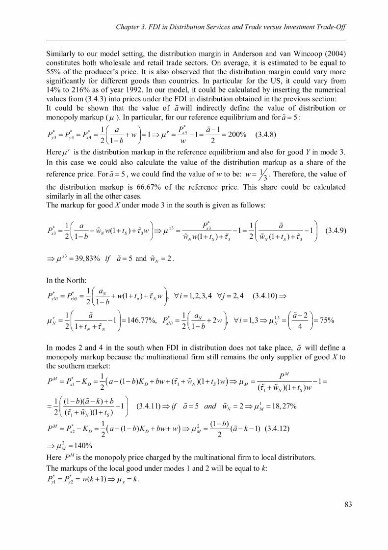
Chapter 3. FDI in Distribution Services and Trade versus Investment Trade-Off
83
Similarly to our model setting, the distribution margin in Anderson and van Wincoop (2004) constitutes both wholesale and retail trade sectors. On average, it is estimated to be equal to 55% of the producer’s price. It is also observed that the distribution margin could vary more significantly for different goods than countries. In particular for the US, it could vary from 14% to 216% as of year 1992. In our model, it could be calculated by inserting the numerical values from (3.4.3) into prices under the FDI in distribution obtained in the previous section: It could be shown that the value of awill indirectly define the value of distribution or monopoly markup ( ). In particular, for our reference equilibrium and for 5a :
** * * 43 4 4
1 11 1 200% (3.4.8)2 1 2
r xy y x
Pa aP P P wb w
Here r is the distribution markup in the reference equilibrium and also for good Y in mode 3. In this case we could also calculate the value of the distribution markup as a share of the reference price. For 5a , we could find the value of w to be: 1
3w . Therefore, the value of
the distribution markup is 66.67% of the reference price. This share could be calculated similarly in all the other cases. The markup for good X under mode 3 in the south is given as follows:
** 3 33 3
3 3
1 1(1 ) 1 1 (3.4.9)2 1 (1 ) 2 (1 )
x xx N S
N S N S
Pa aP w w t wb w w t w t
3 39,83% 5x if a and 2Nw .
In the North:
* *
* 1,3
1 (1 ) , 1, 2,3, 4 2, 4 (3.4.10)2 1
1 1 21 146.77%, 2 , 1,3 75%2 1 2 1 4
NyNi xNj n N
r NN xNi N
N N
aP P w t w i jb
aa aP w it b
In modes 2 and 4 in the south when FDI in distribution does not take place, a will define a monopoly markup because the multinational firm still remains the only supplier of good X to the southern market:
* 11 1
1
1
1
1 (1 ) ( )(1 ) 12 ( )(1 )
1 (1 )( ) 1 (3.4.11) 5 2 18, 27%2 ( )(1 )
MM
x D D N S MN S
N MN S
PP P K a b K bw w t ww t w
b a k b if a and ww t
* 22
2
1 (1 )(1 ) ( 1) (3.4.12)2 2
140%
Mx D D M
M
bP P K a b K bw w a k
Here MP is the monopoly price charged by the multinational firm to local distributors. The markups of the local good under modes 1 and 2 will be equal to k:
* *1 2 ( 1) .y y yP P w k k
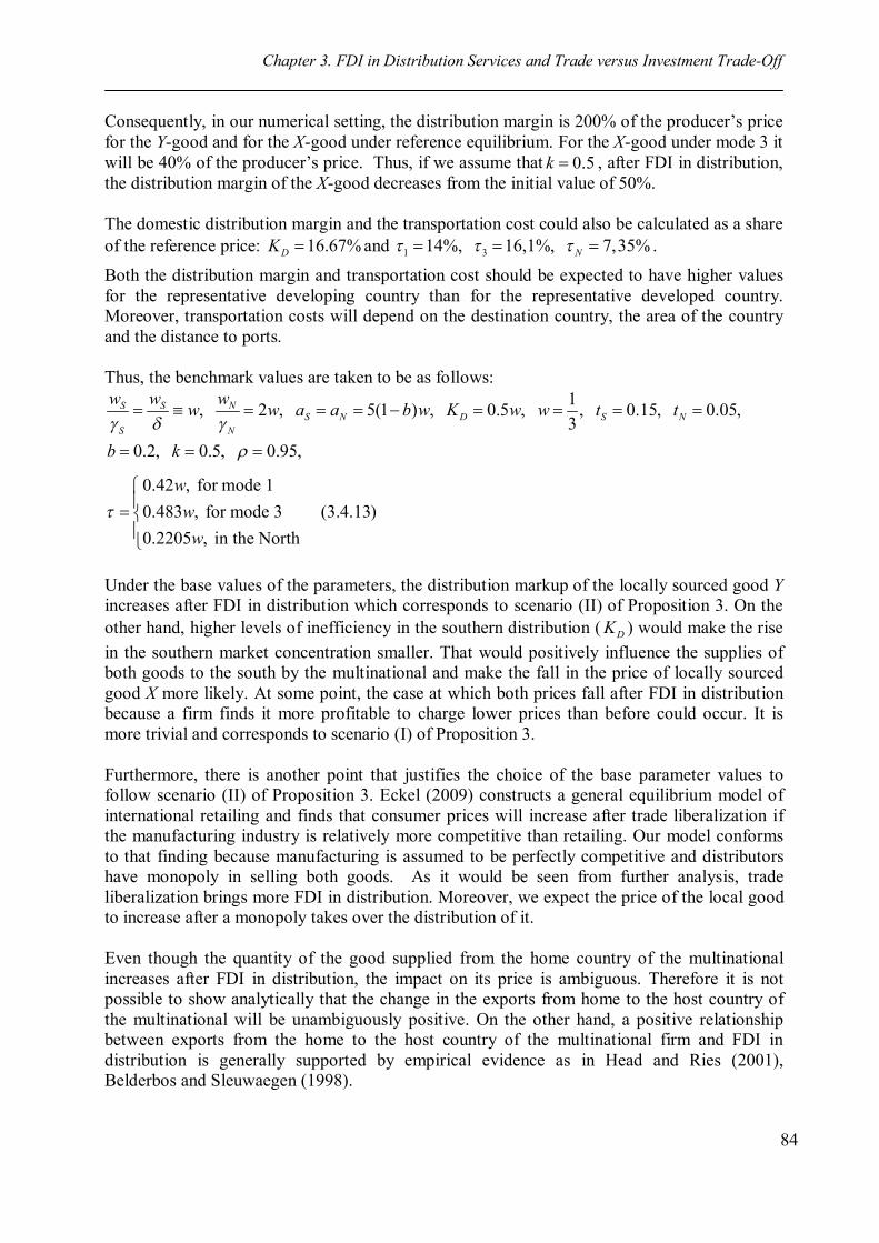
Chapter 3. FDI in Distribution Services and Trade versus Investment Trade-Off
84
Consequently, in our numerical setting, the distribution margin is 200% of the producer’s price for the Y-good and for the X-good under reference equilibrium. For the X-good under mode 3 it will be 40% of the producer’s price. Thus, if we assume that 0.5k , after FDI in distribution, the distribution margin of the X-good decreases from the initial value of 50%. The domestic distribution margin and the transportation cost could also be calculated as a share of the reference price: 16.67%DK and 1 314%, 16,1%, 7,35%N .
Both the distribution margin and transportation cost should be expected to have higher values for the representative developing country than for the representative developed country. Moreover, transportation costs will depend on the destination country, the area of the country and the distance to ports. Thus, the benchmark values are taken to be as follows:
1, 2 , 5(1 ) , 0.5 , , 0.15, 0.05,3
0.2, 0.5, 0.95,
0.42 , for mode 10.483 , for mode 3 (3.4.13)0.2205 , in the North
S S NS N D S N
S N
w w ww w a a b w K w w t t
b k
www
Under the base values of the parameters, the distribution markup of the locally sourced good Y increases after FDI in distribution which corresponds to scenario (II) of Proposition 3. On the other hand, higher levels of inefficiency in the southern distribution ( DK ) would make the rise in the southern market concentration smaller. That would positively influence the supplies of both goods to the south by the multinational and make the fall in the price of locally sourced good X more likely. At some point, the case at which both prices fall after FDI in distribution because a firm finds it more profitable to charge lower prices than before could occur. It is more trivial and corresponds to scenario (I) of Proposition 3. Furthermore, there is another point that justifies the choice of the base parameter values to follow scenario (II) of Proposition 3. Eckel (2009) constructs a general equilibrium model of international retailing and finds that consumer prices will increase after trade liberalization if the manufacturing industry is relatively more competitive than retailing. Our model conforms to that finding because manufacturing is assumed to be perfectly competitive and distributors have monopoly in selling both goods. As it would be seen from further analysis, trade liberalization brings more FDI in distribution. Moreover, we expect the price of the local good to increase after a monopoly takes over the distribution of it. Even though the quantity of the good supplied from the home country of the multinational increases after FDI in distribution, the impact on its price is ambiguous. Therefore it is not possible to show analytically that the change in the exports from home to the host country of the multinational will be unambiguously positive. On the other hand, a positive relationship between exports from the home to the host country of the multinational firm and FDI in distribution is generally supported by empirical evidence as in Head and Ries (2001), Belderbos and Sleuwaegen (1998).
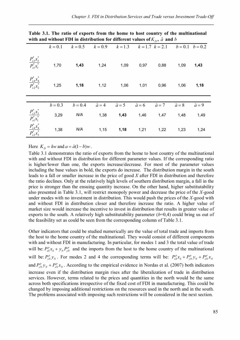
Chapter 3. FDI in Distribution Services and Trade versus Investment Trade-Off
85
Table 3.1. The ratio of exports from the home to host country of the multinational with and without FDI in distribution for different values of DK , a and b 0.1k
0.5k
0.9k
1.3k
1.7k
2.1k
0.1b
0.2b
* *3 3* *1 1
x
x
P xP x
1,70 1,43 1,24 1,09 0,97 0,88 1,09 1,43
* *4 4
* *2 2
x
x
P xP x
1,25 1,18 1,12 1,06 1,01 0,96 1,06 1,18
0.3b 0.4b 4a 5a 6a 7a 8a 9a
* *3 3* *1 1
x
x
P xP x
3,29
N/A 1,38 1,43 1,46 1,47 1,48 1,49
* *4 4
* *2 2
x
x
P xP x
1,38
N/A 1,15 1,18 1,21 1,22 1,23 1,24
Here DK kw and (1 )a a b w . Table 3.1 demonstrates the ratio of exports from the home to host country of the multinational with and without FDI in distribution for different parameter values. If the corresponding ratio is higher/lower than one, the exports increase/decrease. For most of the parameter values including the base values in bold, the exports do increase. The distribution margin in the south leads to a fall or smaller increase in the price of good X after FDI in distribution and therefore the ratio declines. Only at the relatively high levels of southern distribution margin, a fall in the price is stronger than the ensuing quantity increase. On the other hand, higher substitutability also presented in Table 3.1, will restrict monopoly power and decrease the price of the X-good under modes with no investment in distribution. This would push the prices of the X-good with and without FDI in distribution closer and therefore increase the ratio. A higher value of market size would increase the incentive to invest in distribution that results in greater value of exports to the south. A relatively high substitutability parameter (b=0,4) could bring us out of the feasibility set as could be seen from the corresponding column of Table 3.1. Other indicators that could be studied numerically are the value of total trade and imports from the host to the home country of the multinational. They would consist of different components with and without FDI in manufacturing. In particular, for modes 1 and 3 the total value of trade will be: p p
xS S N yNP x y P and the imports from the host to the home country of the multinational
will be: pyN NP y . For modes 2 and 4 the corresponding terms will be: p p p
xS S yN N xN NP x P y P x
and p pyN N xN NP y P x . According to the empirical evidence in Nordas et al. (2007) both indicators
increase even if the distribution margin rises after the liberalization of trade in distribution services. However, terms related to the prices and quantities in the north would be the same across both specifications irrespective of the fixed cost of FDI in manufacturing. This could be changed by imposing additional restrictions on the resources used in the north and in the south. The problems associated with imposing such restrictions will be considered in the next section.
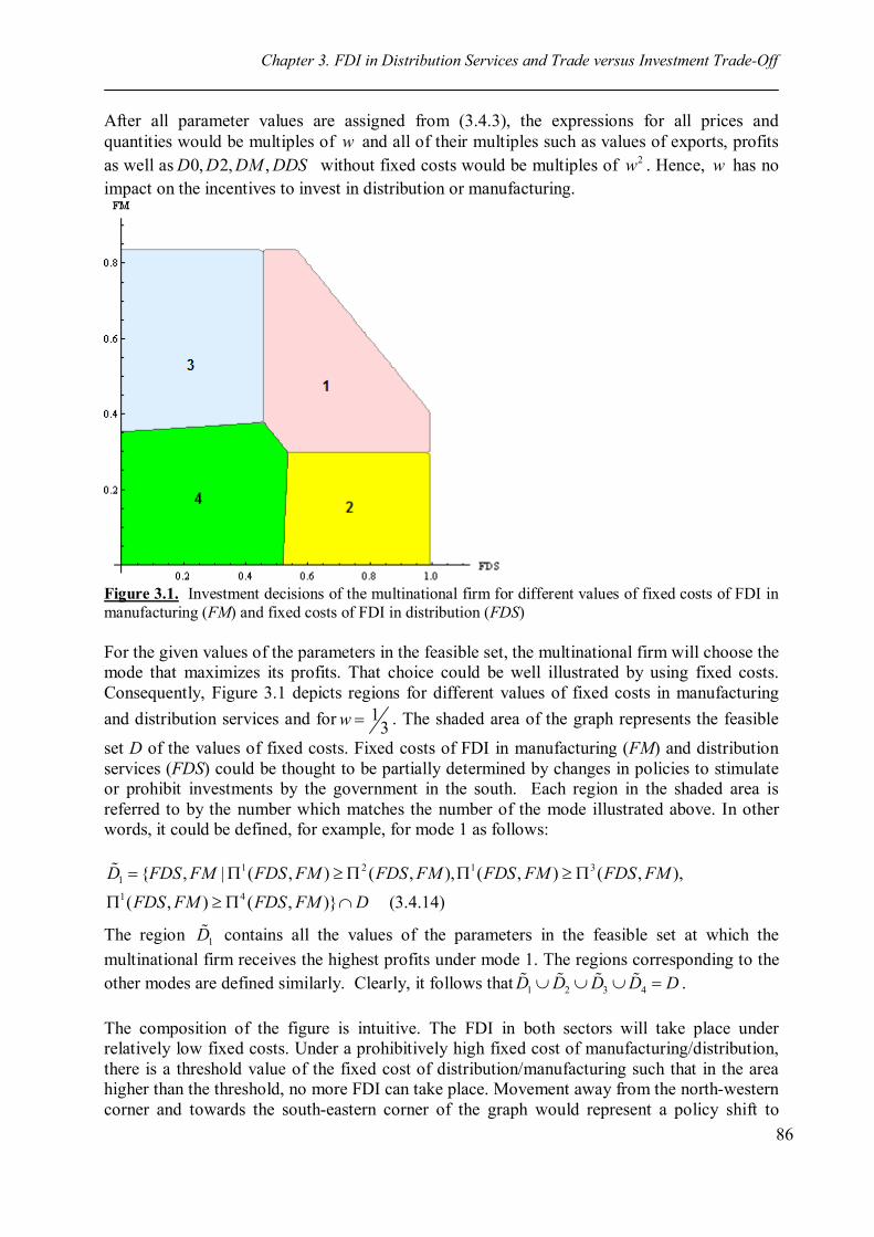
Chapter 3. FDI in Distribution Services and Trade versus Investment Trade-Off
86
After all parameter values are assigned from (3.4.3), the expressions for all prices and quantities would be multiples of w and all of their multiples such as values of exports, profits as well as 0, 2, ,D D DM DDS without fixed costs would be multiples of 2w . Hence, w has no impact on the incentives to invest in distribution or manufacturing.
Figure 3.1. Investment decisions of the multinational firm for different values of fixed costs of FDI in manufacturing (FM) and fixed costs of FDI in distribution (FDS) For the given values of the parameters in the feasible set, the multinational firm will choose the mode that maximizes its profits. That choice could be well illustrated by using fixed costs. Consequently, Figure 3.1 depicts regions for different values of fixed costs in manufacturing and distribution services and for 1
3w . The shaded area of the graph represents the feasible
set D of the values of fixed costs. Fixed costs of FDI in manufacturing (FM) and distribution services (FDS) could be thought to be partially determined by changes in policies to stimulate or prohibit investments by the government in the south. Each region in the shaded area is referred to by the number which matches the number of the mode illustrated above. In other words, it could be defined, for example, for mode 1 as follows:
1 2 1 311 4
{ , | ( , ) ( , ), ( , ) ( , ),( , ) ( , )} (3.4.14)
D FDS FM FDS FM FDS FM FDS FM FDS FMFDS FM FDS FM D
The region 1D contains all the values of the parameters in the feasible set at which the multinational firm receives the highest profits under mode 1. The regions corresponding to the other modes are defined similarly. Clearly, it follows that 1 2 3 4D D D D D . The composition of the figure is intuitive. The FDI in both sectors will take place under relatively low fixed costs. Under a prohibitively high fixed cost of manufacturing/distribution, there is a threshold value of the fixed cost of distribution/manufacturing such that in the area higher than the threshold, no more FDI can take place. Movement away from the north-western corner and towards the south-eastern corner of the graph would represent a policy shift to
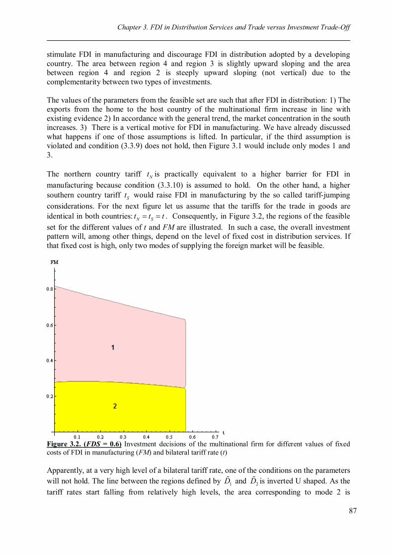
Chapter 3. FDI in Distribution Services and Trade versus Investment Trade-Off
87
stimulate FDI in manufacturing and discourage FDI in distribution adopted by a developing country. The area between region 4 and region 3 is slightly upward sloping and the area between region 4 and region 2 is steeply upward sloping (not vertical) due to the complementarity between two types of investments. The values of the parameters from the feasible set are such that after FDI in distribution: 1) The exports from the home to the host country of the multinational firm increase in line with existing evidence 2) In accordance with the general trend, the market concentration in the south increases. 3) There is a vertical motive for FDI in manufacturing. We have already discussed what happens if one of those assumptions is lifted. In particular, if the third assumption is violated and condition (3.3.9) does not hold, then Figure 3.1 would include only modes 1 and 3. The northern country tariff Nt is practically equivalent to a higher barrier for FDI in manufacturing because condition (3.3.10) is assumed to hold. On the other hand, a higher southern country tariff St would raise FDI in manufacturing by the so called tariff-jumping considerations. For the next figure let us assume that the tariffs for the trade in goods are identical in both countries: N St t t . Consequently, in Figure 3.2, the regions of the feasible set for the different values of t and FM are illustrated. In such a case, the overall investment pattern will, among other things, depend on the level of fixed cost in distribution services. If that fixed cost is high, only two modes of supplying the foreign market will be feasible.
Figure 3.2. (FDS = 0.6) Investment decisions of the multinational firm for different values of fixed costs of FDI in manufacturing (FM) and bilateral tariff rate (t) Apparently, at a very high level of a bilateral tariff rate, one of the conditions on the parameters will not hold. The line between the regions defined by 1D and 2D is inverted U shaped. As the tariff rates start falling from relatively high levels, the area corresponding to mode 2 is
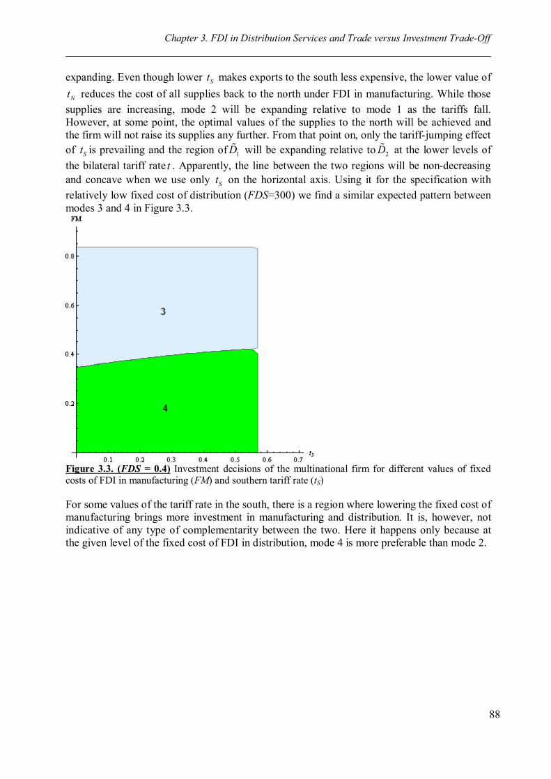
Chapter 3. FDI in Distribution Services and Trade versus Investment Trade-Off
88
expanding. Even though lower St makes exports to the south less expensive, the lower value of
Nt reduces the cost of all supplies back to the north under FDI in manufacturing. While those supplies are increasing, mode 2 will be expanding relative to mode 1 as the tariffs fall. However, at some point, the optimal values of the supplies to the north will be achieved and the firm will not raise its supplies any further. From that point on, only the tariff-jumping effect of St is prevailing and the region of 1D will be expanding relative to 2D at the lower levels of the bilateral tariff rate t . Apparently, the line between the two regions will be non-decreasing and concave when we use only St on the horizontal axis. Using it for the specification with relatively low fixed cost of distribution (FDS=300) we find a similar expected pattern between modes 3 and 4 in Figure 3.3.
Figure 3.3. (FDS = 0.4) Investment decisions of the multinational firm for different values of fixed costs of FDI in manufacturing (FM) and southern tariff rate (tS) For some values of the tariff rate in the south, there is a region where lowering the fixed cost of manufacturing brings more investment in manufacturing and distribution. It is, however, not indicative of any type of complementarity between the two. Here it happens only because at the given level of the fixed cost of FDI in distribution, mode 4 is more preferable than mode 2.
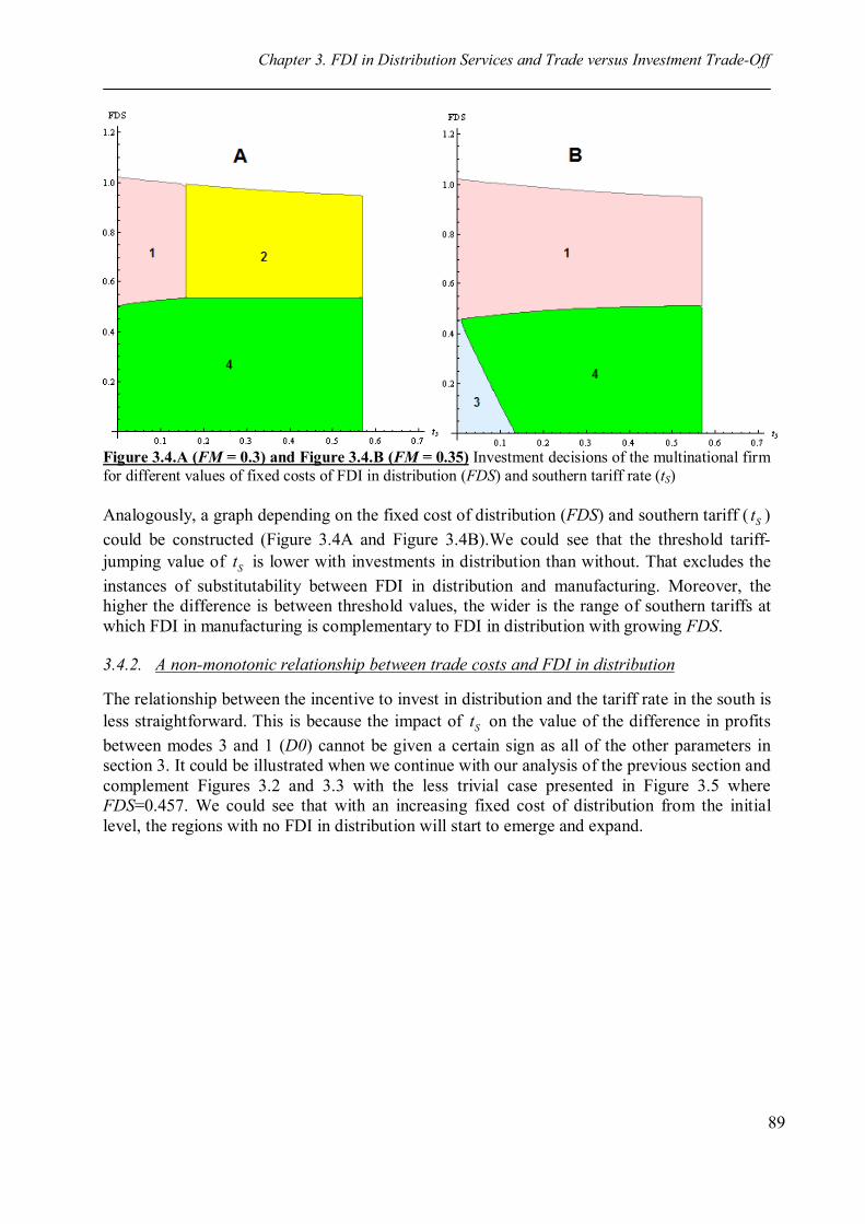
Chapter 3. FDI in Distribution Services and Trade versus Investment Trade-Off
89
Figure 3.4.A (FM = 0.3) and Figure 3.4.B (FM = 0.35) Investment decisions of the multinational firm for different values of fixed costs of FDI in distribution (FDS) and southern tariff rate (tS) Analogously, a graph depending on the fixed cost of distribution (FDS) and southern tariff ( St ) could be constructed (Figure 3.4A and Figure 3.4B).We could see that the threshold tariff-jumping value of St is lower with investments in distribution than without. That excludes the instances of substitutability between FDI in distribution and manufacturing. Moreover, the higher the difference is between threshold values, the wider is the range of southern tariffs at which FDI in manufacturing is complementary to FDI in distribution with growing FDS. 3.4.2. A non-monotonic relationship between trade costs and FDI in distribution
The relationship between the incentive to invest in distribution and the tariff rate in the south is less straightforward. This is because the impact of St on the value of the difference in profits between modes 3 and 1 (D0) cannot be given a certain sign as all of the other parameters in section 3. It could be illustrated when we continue with our analysis of the previous section and complement Figures 3.2 and 3.3 with the less trivial case presented in Figure 3.5 where FDS=0.457. We could see that with an increasing fixed cost of distribution from the initial level, the regions with no FDI in distribution will start to emerge and expand.
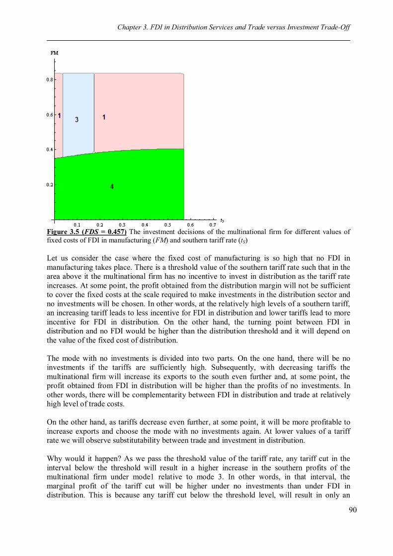
Chapter 3. FDI in Distribution Services and Trade versus Investment Trade-Off
90
Figure 3.5 (FDS = 0.457) The investment decisions of the multinational firm for different values of fixed costs of FDI in manufacturing (FM) and southern tariff rate (tS) Let us consider the case where the fixed cost of manufacturing is so high that no FDI in manufacturing takes place. There is a threshold value of the southern tariff rate such that in the area above it the multinational firm has no incentive to invest in distribution as the tariff rate increases. At some point, the profit obtained from the distribution margin will not be sufficient to cover the fixed costs at the scale required to make investments in the distribution sector and no investments will be chosen. In other words, at the relatively high levels of a southern tariff, an increasing tariff leads to less incentive for FDI in distribution and lower tariffs lead to more incentive for FDI in distribution. On the other hand, the turning point between FDI in distribution and no FDI would be higher than the distribution threshold and it will depend on the value of the fixed cost of distribution. The mode with no investments is divided into two parts. On the one hand, there will be no investments if the tariffs are sufficiently high. Subsequently, with decreasing tariffs the multinational firm will increase its exports to the south even further and, at some point, the profit obtained from FDI in distribution will be higher than the profits of no investments. In other words, there will be complementarity between FDI in distribution and trade at relatively high level of trade costs. On the other hand, as tariffs decrease even further, at some point, it will be more profitable to increase exports and choose the mode with no investments again. At lower values of a tariff rate we will observe substitutability between trade and investment in distribution. Why would it happen? As we pass the threshold value of the tariff rate, any tariff cut in the interval below the threshold will result in a higher increase in the southern profits of the multinational firm under mode1 relative to mode 3. In other words, in that interval, the marginal profit of the tariff cut will be higher under no investments than under FDI in distribution. This is because any tariff cut below the threshold level, will result in only an
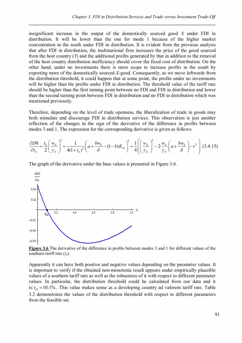
Chapter 3. FDI in Distribution Services and Trade versus Investment Trade-Off
91
insignificant increase in the output of the domestically sourced good X under FDI in distribution. It will be lower than the one for mode 1 because of the higher market concentration in the south under FDI in distribution. It is evident from the previous analysis that after FDI in distribution, the multinational firm increases the price of the good sourced from the host country (Y) and the additional profits generated by that in addition to the removal of the host country distribution inefficiency should cover the fixed cost of distribution. On the other hand, under no investments there is more scope to increase profits in the south by exporting more of the domestically sourced X-good. Consequently, as we move leftwards from the distribution threshold, it could happen that at some point, the profits under no investments will be higher than the profits under FDI in distribution. The threshold value of the tariff rate should be higher than the first turning point between no FDI and FDI in distribution and lower than the second turning point between FDI in distribution and no FDI in distribution which was mentioned previously. Therefore, depending on the level of trade openness, the liberalization of trade in goods may both stimulate and discourage FDI in distribution services. This observation is just another reflection of the changes in the sign of the derivative of the difference in profits between modes 3 and 1. The expression for the corresponding derivative is given as follows:
2 222
2
0 1 1(1 ) 2 (3.4.15)2 4(1 ) 4S N S N N S
DS N S N N
t w bw w w bwD a b K at t
The graph of the derivative under the base values is presented in Figure 3.6.
Figure 3.6 The derivative of the difference in profits between modes 3 and 1 for different values of the southern tariff rate (tS) Apparently it can have both positive and negative values depending on the parameter values. It is important to verify if the obtained non-monotonic result appears under empirically plausible values of a southern tariff rate as well as the robustness of it with respect to different parameter values. In particular, the distribution threshold could be calculated from our data and it is: 10.1%Slt . This value makes sense as a developing country ad valorem tariff rate. Table 3.2 demonstrates the values of the distribution threshold with respect to different parameters from the feasible set.
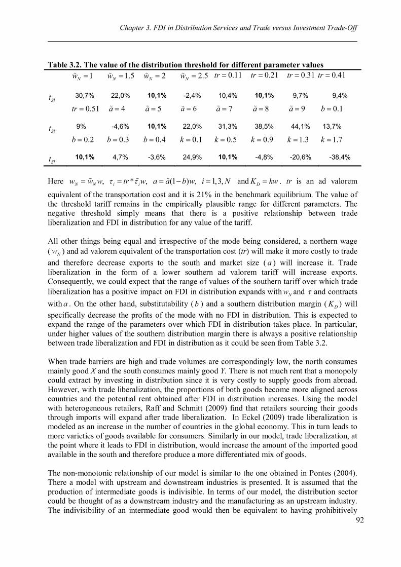
Chapter 3. FDI in Distribution Services and Trade versus Investment Trade-Off
92
Table 3.2. The value of the distribution threshold for different parameter values 1Nw
1.5Nw
2Nw
2.5Nw
0.11tr
0.21tr
0.31tr
0.41tr
Slt 30,7% 22,0% 10,1% -2,4% 10,4% 10,1% 9,7% 9,4%
0.51tr
4a 5a 6a 7a 8a 9a 0.1b
Slt 9% -4,6% 10,1% 22,0% 31,3% 38,5% 44,1% 13,7%
0.2b
0.3b
0.4b
0.1k
0.5k
0.9k
1.3k
1.7k
Slt 10,1% 4,7% -3,6% 24,9% 10,1% -4,8% -20,6% -38,4%
Here , * , (1 ) , 1,3,N N i iw w w tr w a a b w i N and DK kw . tr is an ad valorem
equivalent of the transportation cost and it is 21% in the benchmark equilibrium. The value of the threshold tariff remains in the empirically plausible range for different parameters. The negative threshold simply means that there is a positive relationship between trade liberalization and FDI in distribution for any value of the tariff. All other things being equal and irrespective of the mode being considered, a northern wage ( Nw ) and ad valorem equivalent of the transportation cost (tr) will make it more costly to trade and therefore decrease exports to the south and market size ( a ) will increase it. Trade liberalization in the form of a lower southern ad valorem tariff will increase exports. Consequently, we could expect that the range of values of the southern tariff over which trade liberalization has a positive impact on FDI in distribution expands with Nw and and contracts with a . On the other hand, substitutability ( b ) and a southern distribution margin ( DK ) will specifically decrease the profits of the mode with no FDI in distribution. This is expected to expand the range of the parameters over which FDI in distribution takes place. In particular, under higher values of the southern distribution margin there is always a positive relationship between trade liberalization and FDI in distribution as it could be seen from Table 3.2. When trade barriers are high and trade volumes are correspondingly low, the north consumes mainly good X and the south consumes mainly good Y. There is not much rent that a monopoly could extract by investing in distribution since it is very costly to supply goods from abroad. However, with trade liberalization, the proportions of both goods become more aligned across countries and the potential rent obtained after FDI in distribution increases. Using the model with heterogeneous retailers, Raff and Schmitt (2009) find that retailers sourcing their goods through imports will expand after trade liberalization. In Eckel (2009) trade liberalization is modeled as an increase in the number of countries in the global economy. This in turn leads to more varieties of goods available for consumers. Similarly in our model, trade liberalization, at the point where it leads to FDI in distribution, would increase the amount of the imported good available in the south and therefore produce a more differentiated mix of goods. The non-monotonic relationship of our model is similar to the one obtained in Pontes (2004). There a model with upstream and downstream industries is presented. It is assumed that the production of intermediate goods is indivisible. In terms of our model, the distribution sector could be thought of as a downstream industry and the manufacturing as an upstream industry. The indivisibility of an intermediate good would then be equivalent to having prohibitively
Chapter 3. FDI in Distribution Services and Trade versus Investment Trade-Off
93
high fixed costs of manufacturing. The pattern remains unchanged when I use only the tariff imposed by the south as a trade cost and keep the level of the northern country tariff constant, in line with theoretical specifications that focus on trade barriers in the host country only. The relationship between FDI in distribution and trade costs is usually assumed to be negative. The data disaggregation argument as in Swensson (2004) would make less sense in this case. Intuitively it would rather strengthen the complementarity relationship. Therefore I argue that the relationship is non-monotonic and that it is more specific and incontrovertible than the standard relationship between FDI and trade costs. 3.5. Concluding remarks
In this chapter of the dissertation, a model that studies the determinants of FDI in distribution has been constructed. The structure of the model is motivated by existing links between manufacturing and distribution as well as by the data pattern of production oriented and distribution oriented FDI as presented in Hanson et al. (2001). The following features of the model signify the distinctive attributes of the distribution sector:
Full forward vertical integration after FDI in distribution.
Distribution services could only be supplied by investments to the other country.
After FDI in distribution, the multinational firm starts selling a more balanced combination of goods.
One of the important aspects that could be used to evaluate the performance of the analytical model is its ability to capture existing stylized facts. The model constructed in this chapter, captures several intuitive results and paves the way for empirical specification. In particular, our model generates several determinants of FDI in distribution with and without FDI in manufacturing. It also generates the determinants of FDI in manufacturing. Furthermore, we find that there is a non-monotonic relationship between trade costs and FDI in distribution services. Afterwards, we conduct a sensitivity check by taking different parameter values and find the non-monotonic result to be robust with respect to them. However, the obtained results should be accepted with due caution subject to the structure of the model. The market structure of the distribution sector could be modeled more comprehensively to make comparisons with empirical literature on the interaction between market structure in distribution services and trade in goods more solid. It is also important to be aware of the scope of relevance of the model. Namely, it is constructed to study the incentives of the multinational firm to invest given the assumptions about directions of change in the parameters and endogenous variables. However, it is inadequate to study the welfare implications of the investments to host and home countries and to analyze the magnitudes of change in prices and quantities. Namely, due to the partial equilibrium nature of the model, it is not specified how the monopoly rent is redistributed and the wages remain unchanged in both countries after either type of investment. Therefore, no judgments could be made with respect to the impact of FDI in distribution on the real income of consumers. Bibliography Anderson, J., and van Wincoop, E., (2004) “Trade costs” Journal of Economic Literature, Vol.
42, pp. 691-751.
Chapter 3. FDI in Distribution Services and Trade versus Investment Trade-Off
94
Caillaud, B., and Rey, P., (1986) “A Note on Vertical Restraints with the Provision of Distribution Services”. Mimeo, INSEE and MIT.
Church, J., and Ware, R., (2000) “Industrial Organization: A Strategic Approach”, Toronto: Irwin-McGraw-Hill.
Belderbos, R., and Sleuwaegen, L., (1998) “Tariff Jumping FDI and Export Substitution: Japanese Electronics Firms in Europe”, International Journal of Industrial Organization, Vol. 16, pp. 601-638.
Boatman, K., (2007) “What Determines Distribution FDI?” Journal of Business and Public Affairs, 1(1).
Bonroy, O., and Larue, B., (2007) “Forward Vertical Integration: The Fixed-Proportion Case Revisited” Economics Bulletin, Vol.12, No.24, pp.1-9.
Eckel, C., (2009) “International Trade and Retailing” CESifo working paper No.2597. Francois, J and Wooton, I., (2007) “Market Structure and Market Access”, World Bank Policy
Research Paper 4151. Hanson, G.H., Mataloni, R.J., Slaughter M.J., (2001) “Expansion Strategies of US
Multinational Firms” Brookings Trade Forum, pp.245-294. Head, K., and Ries, J., (2001) “Overseas Investment and Firm Exports” Review of
International Economics, 9(1), pp.108-122. Head, K., and Ries, J., (2004) “Exporting and FDI as Alternative Strategies” Oxford Review of
Economic Policy, 20(3), pp.409-423. Ishikawa, J., Morita, H., and Mukunoki, H., (2008) “FDI in Post-Production Services and
Product Market Competition” mimeo. Kalirajan, K., (2000) “Restrictions on Trade in Distribution Services”, Staff Research Paper,
Australian Productivity Commission, Ausinfo, Canberra. Kolstad, I., and Villanger, E., (2004) “Determinants of Foreign Direct Investment in Services”,
CMI Working Papers WP 2004:2, CMI, Bergen. Markusen, J., and Horstman, I., (1992) “Endogenous Market Structures in International
Trade”, Journal of International Economics, 32: pp 109-129. Markusen, J., (2002) “Multinational Firms and the Theory of International Trade”, Cambridge:
MIT. Navaretti, G., and Venables, A., (2004) “Multinational Firms in the World Economy”,
Princeton and Oxford: Princeton University Press. Nordas, H., Pinali, E., and Geloso-Grosso, M., (2007) “Market Structure in the Distribution
Sector and Merchandise Trade”, OECD Trade Policy Working Paper No.68, Paris. Palmade, V., and Anayiotas, A., (2004) “FDI trends” Public Policy for the Private Sector 273,
World Bank, Washington, DC. Pilat, D., (1997) “Regulation and Performance in the Distribution Sector”, OECD Economics
Department Working Papers No. 180, OECD, Paris. Pontes, J.P., (2007) “A non-monotonic relationship between FDI and trade” Economic Letters
95, pp. 369-373. Raff, H., Schmitt, N., (2009) “Imports, Pass-Through, and the Structure of Retail Markets”,
mimeo. Swensson, D.L, (2004) “Foreign Investment and the Mediation of Trade Flows”, Review of
International Economics 12(4), pp.609-629. Tirole, J., (1988) “The Theory of Industrial Organization”, Cambridge, MA: MIT Press. Varian, H., (1992) “Microeconomic Analysis”, Third Edition, Norton: New York.
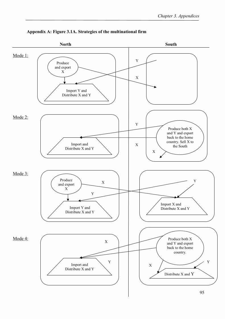
Chapter 3. Appendices
95
Appendix A: Figure 3.1A. Strategies of the multinational firm
Import and Distribute X and Y
Produce both X and Y and export back to the home country. Sell X to
the South X
X
Y
Produce
and export X
Import Y and Distribute X and Y
Import X and Distribute X and Y
Y
Y
X
Import and Distribute X and Y
Produce both X and Y and export back to the home
country.
X Y
Distribute X and Y
X
Y
Produce
and export X
Import Y and Distribute X and Y
X
Y
North
Mode 1:
South
Mode 2:
Mode 3:
Mode 4:

Chapter 3. Appendices
96
Appendix B: Proof of Proposition 1 After optimization, all the prices and quantities could be expressed as functions of the parameters:
* *2 2
1( , ) (1 ) 0 (1 )2
S SS x y D
S
bw wx P P a b K B
2* *2 2
(1 )( , ) 1 1 1 0 (2 )2 2 2 2
SS x y D
S
wb b b b by P P a K B
* *2 2
1 (1 ) 0 (3 ), 0 (4 )2
S S Sx D y D
S
bw w wP a b K B P K B
22 * *
2 21( , ) (1 ) 0 (5 )4
S Sx y D
S
w wP P a b K b FM B
Then, the conditions defined by the feasibility set for mode 2 could be written as:
2 { | (1 ),(2 ),(3 ),(4 ),(5 )}D parameters B B B B B Similarly, the optimal values of prices, quantities, profits and feasible set could be defined for mode 4:
* * * *4 4 4 4
1 1( , ) 0 (6 ), ( , ) 0 (7 )2 2
S S S SS x y S x y
S S
w w w wx P P a b B y P P a b B
* *4 4
1 10 (8 ), (9 )2 (1 ) 2 (1 )
S Sx y
S
w wa aP B P Bb b
2 224 * *
4 4 2 2
1 1 1 1 1( , ) ( ) 0 (10 )2 (1 ) 2
S Sx y S
S S S
bw waP P aw FM FDS Bb
4 { | (6 ),(7 ),(8 ),(9 ),(10 )}D parameters B B B B B and 2 4DMF D D . The expression for DM is obtained from the difference in the profit functions:
2 22
2 2
2
1 1 1 1 12 (1 ) 2
1 (1 ) (1 )4
S SS
S S S
S S SD
S
bw waDM awb
bw bw wa b K FM FDS
In addition to that, the distribution markups for both goods should be nonnegative:
0 (11 ) 0 (12 )(1 ) (1 )
S S
S
w wa aB Bb b
.
For mode 2, this condition is equivalent to (3B). Those inequalities would help us determine the sign of derivatives of the difference in profits (DM).
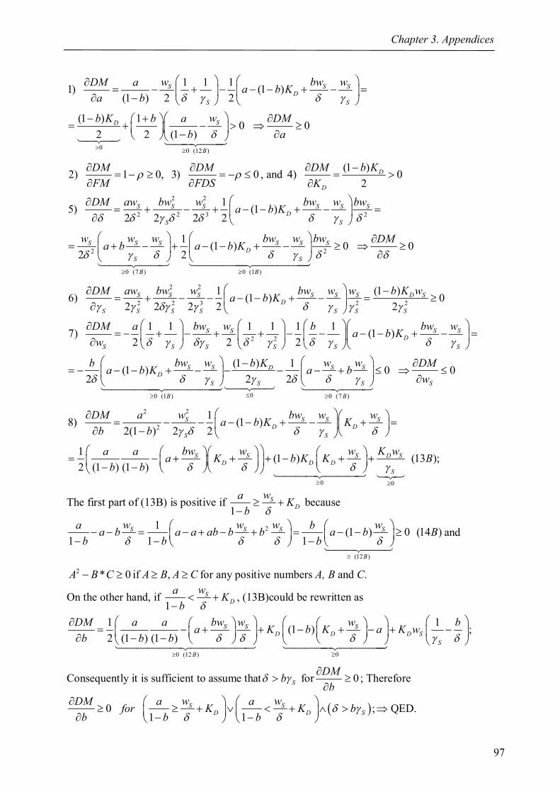
Chapter 3. Appendices
97
0 0 (12 )
1 1 11) (1 )(1 ) 2 2
(1 ) 1 0 02 2 (1 )
S S SD
S S
SD
B
w bw wDM a a b Ka b
wb K b a DMb a
2) 1 0, 3) 0DM DMFM FDS
, and (1 )4) 0
2D
D
b KDMK
2 2
2 2 3 2
2 2
0 (7 ) 0 (1 )
15) (1 )2 2 2 2
1 (1 ) 0 02 2
S S S S S SD
S S
S S S S S SD
S S
B B
aw bw w bw w bwDM a b K
w w w bw w bw DMa b a b K
2 2
2 2 3 2 2
(1 )16) (1 ) 02 2 2 2 2
S S S S S S D SD
S S S S S S S
aw bw w bw w w b K wDM a b K
2 2
00 (1 ) 0 (7 )
1 1 1 1 1 17) (1 )2 2 2
(1 ) 1(1 ) 02 2 2
S S S SD
S S S S S S
S S S SDD
S S S S
B B
bw w bw wDM a b a b Kw
bw w w wb Kb DMa b K a bw
0
22
2
0 0
18) (1 )2(1 ) 2 2
1 (1 ) (13 );2 (1 ) (1 )
S S S SD D
S S
S S S D SD D D
S
w bw w wDM a a b K Kb b
bw w w K wa a a K b K K Bb b
The first part of (13B) is positive if 1
SD
wa Kb
because
2
(12 )
1 (1 ) 0 (14 )1 1 1
S S S S
B
w w w wa ba b a a ab b b a b Bb b b
and
2 * 0A B C if ,A B A C for any positive numbers A, B and C.
On the other hand, if 1
SD
wa Kb
, (13B)could be rewritten as
00 (12 )
1 1(1 ) ;2 (1 ) (1 )
S S SD D D S
S
B
bw w wDM a a ba K b K a K wb b b
Consequently it is sufficient to assume that Sb for 0DMb
; Therefore
0 ;1 1
S SD D S
w wDM a afor K K bb b b
QED.

Chapter 3. Appendices
98
Appendix C: Proof of Proposition 2 The optimal values for prices and quantities profit for modes 1 are given as follows:
* *1 1
1 (1 ) 0 (1 ) 0 (2 )2
S N Sx D D S y D
N
w w wP a b K K t C P K C
* *1 1
1( , ) (1 ) (1 ) 0 (3 )2
S NS x y D S
N
bw wx P P a b K t C
2* *1 1( , ) 1 (1 ) (1 ) 1 (1 ) 0 (4 )
2 2 2 2S N
S x y D SN
w wb b b by P P a K b t C
2
1 * *1 1
1( , ) (1 ) (1 ) 0 (5 )4(1 )
S Nx y D S
S N
bw wP P a b K t Ct
The inequalities (2C) and (5C) hold trivially for positive values of the parameters and are therefore excluded from the feasibility set:
1 { | (1 ), (3 ),(4 )}D parameters C C C Similarly for mode 3:
* *3 3
1 10 (6 ) (1 ) 0 (7 )2 1 2 1
S Ny x S
N
w wa aP C P t Cb b
* *3 3
* *3 3
1( , ) (1 ) 0 (8 )2
1( , ) (1 ) 0 (9 )2
S NS x y S
N
S NS x y S
N
w wx P P a b t C
w wy P P a b t C
2223 * *
3 31 1 1( , ) (1 ) (1 )2 1 4 4 2
(1 ) 0 (10 )2
S N S Nx y S S
N N
S NS
N
w w w wa aP P t tb
bw w t FDS C
3 { | (8 ),(9 ),(10 )}D parameters C C C and 1 30DM D D . Similarly to the proof of Proposition 1, the expression for D0 is just a difference of the two profit functions:
222
2
1 20 (1 ) 2 (1 ) 2 (1 )4 1
1 (1 ) (1 )4(1 )
S N S N S NS S S
N N N
S ND S
S N
w w w w bw waD t a t tb
bw wa b K t FDSt
The monopoly markup for mode 1 would only apply to the X good and would be given by (3C). For mode 3, distribution markups would be as follows: 1 1(1 ) 0 (11 ) 0 (12 )2 (1 ) 2 (1 )
N SS
N
w wa at C Cb b
Now we could determine the signs of the derivatives of D0 with respect to the parameters:

Chapter 3. Appendices
99
0 0 (8 ) 0 (9 )
0 1 11) (1 ) (1 ) (1 )(1 ) 2 2(1 )
(1 ) (1 ) (1 )2(1 ) 2(1 )(1 )
S N S NS D S
N S N
S S N S NDS S
S S N N
C C
w w bw wD a t a b K ta b t
t w w w wb K a b t a b tt t b
0 (12 ) 0
(1 )1 0(1 ) 0 02(1 )(1 ) 2(1 )(1 )
S S
S S
C
w t bb Da bt b t b a
2
3 2 2 2
2 2
0 (9 )
02) (1 ) (1 ) (1 )2 2 2 2(1 )
(1 ) (1 )2 2(1 )
S S S N S S NS D S
N S N
S S N S S NS D
N S N
C
w aw bw w bw bw wD t a b K tt
w w w bw bw wa b t a b Kt
0 (3 )
(1 ) 0
0 0
S
C
t
D
03) 0N
D
follows from 0 0
N
Dw
because N
N
w
appears in the form of a ratio in all of the
expressions for profits.
(1 )0 04) 0, 5) 1 02(1 )
D
D S
b KD DK t FDS
0 1 16) (1 ) (1 ) (1 ) (1 )2 2(1 )
1 0(1 ) 0 02
N S S NS D S S
N S N
S D
w w bw wD t a b a b K t tt
Dt b K
2
0 (9 )
0 17) (1 ) (1 ) (1 )2 2 (1 )
1 (1 ) (1 ) (1 )2 2 (1 )
S N S NS D S
S N S N
S N S NS D S
N S N
C
w w bw wD a b bt a b K tw t
w w bw wba b t a b K tt
0 (3 )
0
0 0
C
S
Dw
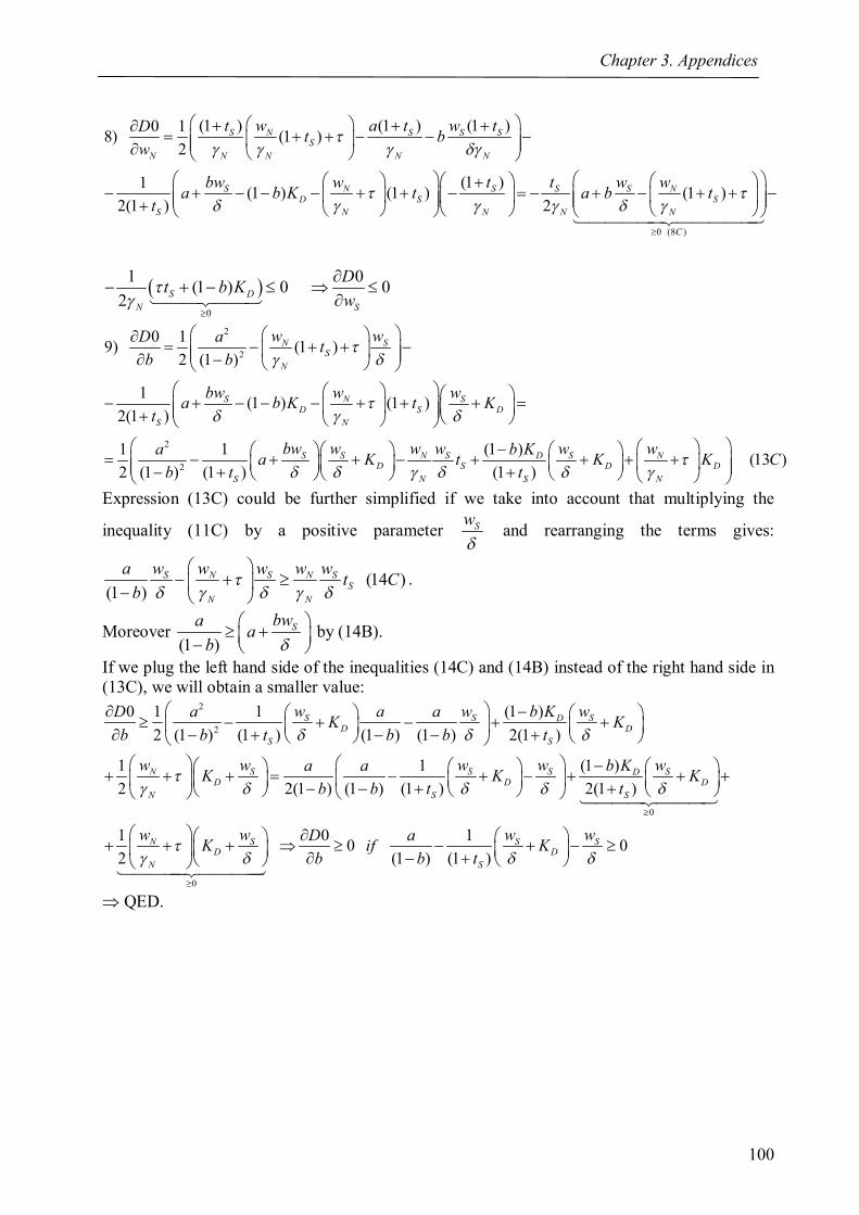
Chapter 3. Appendices
100
0 (8 )
(1 ) (1 ) (1 )0 18) (1 )2
(1 )1 (1 ) (1 ) (1 )2(1 ) 2
S N S S SS
N N N N N
S N S S S ND S S
S N N N N
C
t w a t w tD t bw
bw w t t w wa b K t a b tt
0
1 0(1 ) 0 02 S D
N S
Dt b Kw
2
2
2
2
0 19) (1 )2 (1 )
1 (1 ) (1 )2(1 )
(1 )1 12 (1 ) (1 ) (1 )
N SS
N
S N SD S D
S N
S S N S S NDD S D
S N S N
w wD a tb b
bw w wa b K t Kt
bw w w w w wb Ka a K t Kb t t
(13 )DK C
Expression (13C) could be further simplified if we take into account that multiplying the
inequality (11C) by a positive parameter Sw
and rearranging the terms gives:
(14 )(1 )
S N S N SS
N N
w w w w wa t Cb
.
Moreover (1 )
Sbwa ab
by (14B).
If we plug the left hand side of the inequalities (14C) and (14B) instead of the right hand side in (13C), we will obtain a smaller value:
2
2
0
(1 )0 1 12 (1 ) (1 ) (1 ) (1 ) 2(1 )
(1 )1 12 2(1 ) (1 ) (1 ) 2(1 )
12
S S SDD D
S S
N S S S SDD D D
N S S
N
w w wb KD a a aK Kb b t b b t
w w w w wb Ka aK K Kb b t t
w
0
0 10 0(1 ) (1 )
S S SD D
N S
w w wD aK if Kb b t
QED.

Chapter 3. Appendices
101
Appendix D: Proof of Proposition 4 The differences in profits are given as follows:
221 12 (1 ) (1 ) (1 ) ;4 4(1 )
1 1(1 ) (1 ) (1 ) ; (1 )2 2
NS S S NS D S D S
S S N
N S N S N SN n n n
N S N S
bw w bw wD a b K a b K t FMt
w w w w wHere a b t t t D
1 1 (1 ) (1 ) (1 ) (2 )2 2
NS N S N SS S S
N S N S
w w w w wDDS a b t t FM FDS D
Consequently we need to show that:
2 2 2 20, 0, 0, 0, 0, 0, 0, 0,
2 2 2 2 20, 0, 0, 0, 0, 0, 0, 0, 0,
2 22 0, 0, 0,
S S N N N N
S S S S D N N
SS S n
D DDS D DDS D DDS D DDSa a a a b b w wD DDS D DDS D D DDS D DDS
t t KD DDS D DDSif bw w t t
0.n
The quantities and prices in the south are the same as given in the proof of Propositions 1 and 2. The prices and quantities in the north are given as follows:
* *
*
1 1(1 ) , 1, 2,3, 4 , 1,32 1 2 1
1 (1 ) , 2, 42 1
N S N NyNi n xNi
N
N SxNi n
S
a w a wP t i P ib b
a wP t ib
* *
* *
* *
*
1( , ) (1 ) 0 1,3 (3 )2
1( , ) (1 ) (1 ) 0 2,4 (4 )2
1( , ) (1 ) 0 1,3 (5 )2
( ,
N SN xNi yNi N n
N
S SN xNi yNi N n n
S
N SN xNi yNi N n
N
N xNi
w wy P P a b t i D
w wy P P a b t t i D
w wx P P a b t i D
x P P
* 1) (1 ) (1 ) 0 2, 4 (6 )2
S SyNi N n n
S
w wa t b t i D
(1 ) (7 ) (3.3.9)N Sn
N S
w w t D
Corresponding markups will be: 1 1 1(1 ) 0 (8 ), 0 (9 ), (1 ) 0 (10 )2 1 2 1 2 1
N S N N N Sn n
N S
a w a w a wt D D t Db b b
In order to prove proposition 4, we need to show that:
Chapter 3. Appendices
102
0 (1 )
2 1 11) (1 ) (1 ) (1 )2 2(1 )
1 1 1(1 ) (1 )2 1 2 2 1
S S S NS D S D S
S S S N
S S N S S S SS D S D
S N S S S
B
bw w bw wD a b K a b K ta t
bw t w w bw w ta b K a b Kt t
0 (7 ) 0 (7 )
1 2 1(1 ) 0 0, (1 ) 0 0.2 2
N S N Sn S
N S S S N S S
D D
w w w wD DDS DDSt ta a a
0 (7 )
2 1 22) (1 ) 0 0, 02
NN S
nN N N N S N N
D
w wD DDS D DDSta a a a a
2 (1 ) (1 )3) (1 ) (1 ) (1 )2 2(1 )
S S S NS D S D S
D S S N
bw w bw wD b ba b K a b K tK t
0 (1 ) 0 (7 )
(1 ) (1 ) 2(1 ) (1 ) 0 02 1 2
S S S N SS D n
S S N S D
B D
bw w t w wb b Da b K tt K
0 (1 )
2 14) (1 ) (1 )2
1 1(1 ) (1 ) (1 )2 (1 )
1 (1 )2
S N Sn n
N S
S S S S ND S D S D S
S S N
S S SD S D
S
B
w w wD t tb
w bw w bw wK a b K a b K tt
w bw wK a b K
0 (7 )
1
1 2(1 ) (1 ) 0 02
S
S
S S N SD n n
N S
D
tt
w w w w DK t tb
0 (7 )
(1 ) 0 02
S N SS
N S
D
w w wDDS DDStb b
0 (5 )
1 1 1(1 ) (1 ) (1 )4 2 2
1 (1 ) 0; (11 )2
NN S S N S
n N n nN N N S N N S
S NN n
N N
D
w w w w wt a b t tw
w wa b t D
Chapter 3. Appendices
103
0 (11 )0 (3 )
2 1 2 25) (1 ) (1 ) 0 0 02
NS N
S D SN N N N N N
DC
bw wD D Da b K tw w w
0 (11 )0 (8 )
(1 ) (1 ) 1(1 ) (1 )4 2 2
(1 ) (1 ) 0 0 02
NS N S S S N S
S S SN N N S N N S N
NS S N
S SN N N N N
DC
t w w t w w wDDS t a b tw w
t w w DDS DDSa b tw w
2
0 (7 )
2
0 (5 ),(6 )
(1 ) (1 )4
(1 ) 1(1 ) (1 ) 02 2
NS n N S
nS S N S
D
S n S N SN n n
S N S
D D
w t w w t
w t w w wa b t t
(12D)
2
0 (12 )
2 26) (1 ) 0 02
NS S S
S DS S S S S
D
w bw wD Da b K
2 2
0 (12 )0 (7 )0 (6 ),(8 )
1 (1 ) (1 ) 02 2 4
0
NS S N S S N S
S S SS S N S S N S S
DDB C
S
w w w w w w wDDS a b t t
DDS
2 2
27) (1 ) (1 ) (1 )2 2 (1 )
S S S S S NS D S D S
S S N
bw bw w bw bw wD a b K a b K tt
2 2 2
2 2
0 (1 )
(1 ) (1 ) (1 )2 2 (1 ) 2
(1 ) (1 ) (1 )2 2 (1 )
S N S S S S S N Sn n S D
N S S N S
S N S S S S Sn n S D
N S S S
B
S
bw w w bw t bw bw w wt t a b Kt
bw w w bw t bw wt t a b Kt
bw
2
0 (7 )
2(2 ) (1 ) 0 0;2
N Sn n
N S
D
w w Dt t
2 2
0 (7 ) 0 (7 )
(1 ) (1 ) (1 ) 0 0;2 2
S N S S N SS n n
N S N S
D D
bw w w bw w wDDS DDSt t t
Chapter 3. Appendices
104
2
2
2 18) (1 ) (1 )4(1 )
1 2(1 ) (1 ) 0 02(1 )
S NS D S
S S N
N S NS D S
S N N S
bw wD a b K tt t
w bw w Da b K tt t
0 (8 )
1 1 1(1 ) (1 )4 2 2
1 (1 ) 0 02
N N S N S N SS S S
S N N S N N S
N S NS S
N N S
C
w w w w w w wDDS t a b tt
w w w DDSa b tt
0 (1 )
0 (7 )0 (3 )
2 1 19) (1 )2
(1 ) 1(1 ) (1 ) (1 )2 (1 ) 2 2
S SS D
S S S
B
S N n N SS D S n
S N S N S
DC
bw wD ba b Kw
bw w t w wb ba b K t tt
0 (5 ),(6 )
(1 ) 1 2(1 ) (1 ) 2 0.2 2
n S N SN n n S
S N S S
D D
t w w w Da b t t if bw
0 (7 ) 0 (6 ),(8 )
0 (7 )
1 1 1 1(1 ) (1 )2 2 2 2
(1 ) (11 (1 )2 2
N S S N SS S S
S S N S S N S
D B C
n N Sn
S N S
D
w w w w wDDS b t a b tw
t w w tb t
0 (5 ),(6 )
) 1(1 ) (1 )2 2
2 0.
n S N SN n n
S N S
D D
SS
w w wa b t t
DDSif bw
0 (7 )
0 (5 ),(6 )
2 110) * (1 )2 2
1 2(1 ) (1 ) 2 0.2
NS N S
nn n n S N S
D
S S N SN n n S
S N S n n
D D
w w wD DDS b tt t t
w w w w D DDSa b t t if bt t
QED.
Chapter 3. Appendices
105
2 111) (1 ) (1 ) (1 )2 2
1 (1 ) (1 ) ;2
S N N SS D S n
N N S
S SN n n
S
bw w w wD ba b K t t
w wa b t t
1 1 1(1 ) (1 )4 2 2
1 1 1 1* (1 ) (1 ) (1 )2 2 2 2
1 (1 )2
N S S N SS S S
N S N S
N S S N Sn N n n
N S N S
S NS S
N
w w w w wDDS t a b t
w w w w wb t a b t t
w wa b t
1 1(1 ) (1 ) (1 ) ;2 2
N S S Sn N n n
N S S
w w w wb t a b t t
106
Conclusion In the conclusion, the possibilities of improving and extending the obtained results as well as possible empirical implementations are considered. One of the ways of improving the results of the model on producer services is to obtain analytical results similar to the results of chapter 2 that do not depend on the data. In particular, it could be demonstrated that if the output of the downstream industry and both foreign and domestic services is increasing, the output of the perfectly competitive sector would fall, the price of skilled labor would increase and the price of unskilled labor would fall. The proof of that statement will be similar to the proof of Proposition 1 in chapter 2. From the results of chapter 1 and the stability conditions it could be concluded that after services trade liberalization, either in terms of the removal of barriers per unit of firm or per unit of output, the output of foreign services and the downstream industry increase. However, the output of domestic services may both increase and decrease depending on the difference in the elasticities of substitution between the varieties in domestic and foreign services. If the domestic services contract, the impact of the services trade liberalization on the factor prices and the output of the perfectly competitive sector will be ambiguous. On the other hand, if we assume that in addition to the decrease in domestic services, the output of the perfectly competitive sector increases, the price of skilled labor will decline and the price of unskilled labor will increase. However, such a case could only occur under a disproportionately big domestic producer services industry which is practically implausible. Consequently, even though the results of chapter 1 are robust for different datasets, no comprehensive analytical results can be presented. It would make little sense to aggregate the social accounting matrix of a particular country to the form presented in chapter 1. In particular, consumers would also consume services and there will be several manufacturing industries that could have the same structure of production as the Y sector of the model in chapter 1. Consequently, the main information that could influence the performance of the model and that could be inferred from the SAM of a particular country would be the elasticities of substitution and the share of producer services in the total economy. On the other hand, the structure of downstream industry and producer services as well as the effects of the model could be used to explain the results of the applied general equilibrium models of a small open economy. The vertical control theory of Industrial Organization literature studies different options for the upstream monopoly to maximize its profit (Tirole, 1988) and it could broaden our analysis of chapter 3. In particular, an upstream monopoly or manufacturer may realize higher profit under a more competitive downstream industry or distribution industry if compared to the notation in our model. It is known that a monopoly in the downstream industry would result not only in smaller profit for the upstream monopoly but in socially suboptimal output and price if compared to the vertically integrated outcome. This happens because the downstream monopoly does not take the incremental profit of the upstream firm into account which leads to suboptimally low output. On the other hand, vertical integration internalizes the externality of the downstream industry on the upstream monopoly. However, the upstream monopoly could incur additional costs or face
107
constraints in achieving vertical integration. For example, in the context of our model, a monopoly has to pay the fixed cost of investing in distribution (FDS). There will be no double marginalization problem under modes with no FDI in distribution in our model because the downstream industry is assumed to be competitive. Despite the absence of the above mentioned externality, the profits of the multinational firm will be affected by inefficiency in the southern distribution services. Moreover, under the modes with no FDI in distribution, the downstream industry would substitute towards a cheaper domestic good produced under perfect competition. This externality would also diminish the profit of the upstream monopolist. In order to solve those problems, an instrument called a tie-in or bundling could be used by the upstream monopolist (Tirole, 1988). Basically it means signing contracts with the downstream firms according to which they have to buy the domestically produced good from the upstream monopolist. If such contracts are not costly and legal to be established, our problem will reduce to a simple proximity/concentration tradeoff. In other words, a southern market distribution margin could then be thought of as a per unit tariff of selling goods in the south which could be avoided by FDI in distribution. Consequently, in the settings where southern market distribution margin is low and the tie-ins or similar arrangements are legal, FDI in distribution is less likely to occur. Another vertical restraint that could be used by the multinational is a franchise fee or a two-part tariff. It represents a payment of a lump sum amount of the franchise fee in addition to the per unit price that the upstream monopolist charges the downstream industry. However, this instrument could be an alternative to FDI in distribution when the distribution sector is a monopoly. In the case of a competitive distribution sector, the franchise fee should be equal to zero. An upstream monopolist may prefer a retail monopoly because of the negative externalities between retail and upstream industry and between retailers themselves. In particular, Caillaud and Rey (1986) find that competitive retailers may provide less promotional services that stimulate demand and increase the profit of the upstream monopolist than retail monopoly. Another negative externality is that retailers may free ride on the promotional services provided by other retailers. This leads to a suboptimal level of such services and lower profits for the upstream firm. Consequently, depending on the availability of vertical instruments, the market structure of the distribution sector could lead to both higher and lower incentives for FDI in distribution. On the other hand, existing low levels of FDI in distribution could be explained by the presence of the different types of vertical arrangements. The empirical implementation of the model in the third chapter would require detailed firm level data. The model does not specify any structure from which the equation to be estimated could be derived. Therefore a system of regression equations with total exports, affiliates sales of the distribution affiliates and the affiliate sales of the manufacturing affiliates on the left hand side and the set of the determinants as well as industry and country specific effects on the right hand side should be specified. The non-monotonic result of the analytical model could be tested by including both the level and the square of the average ad valorem tariff rate variable in the regression model. Other variables which could be important in the determination of the choice between FDI in distribution or manufacturing are indexes for the investment climate and intellectual property rights protection. In particular, the latter may influence the diversion of investments from

108
manufacturing to distribution. Firm level data seems to be more preferable for empirical analysis as a theoretical model determines the decisions of firms. Moreover, at the country level panel or cross section data, it is more probable to observe investments in both manufacturing and distribution not all one or all the other. Empirical analysis should be expected to confirm most of the results of the theoretical model and replicate some of the gravity type regression models.

Affirmation I hereby affirm that I have completed my doctoral thesis entitled “Trade in Services and Market Structure” entirely on my own and unassisted, and that I have specially marked all of the quotes I have used from other authors as well as those passages in my work that are extremely close to the thoughts presented by other authors, and listed the sources in accordance with the regulations I have been given. 02.02.2012, Almaty (Aidan Islyami)

Aidan Islyami
Samal-1, h-4, apt-31 050051 Almaty, Kazakhstan Cell phone: +7701758804E-mail: [email protected]; [email protected] Date and place of birth: June 1, 1981 in Almaty, Kazakhstan Nationality: Kazakhstan
Educational experience: 10/2006-06/2012 03/2007-05/2009 06/2004-07/ 2004 08/2002-11/2004 09/1998-06/2002
PhD in Quantitative Economics program at the University of Kiel Thesis: “Trade in services and market structure” Advanced Studies Program in International Economic Policy Research at the Kiel Institute for the World Economy Kiel University Summer School, Kiel, Germany. Kazakhstan Institute of Management, Economics and Strategic Research (KIMEP), MA program in Economics, specialization in finance, GPA: 4.19 Kazakh National University (KAZNU), Faculty of Mechanics and Mathematics. (Diploma with honors); major: Applied Mathematics; Specialization: Mathematical Modeling
Academic employment:
07/2011-present
Kazakh-British Technical University, International School of Economics (ISE) Position: Senior-Lecturer Courses: AP Microeconomics, AP Macroeconomics, AP Calculus AB.
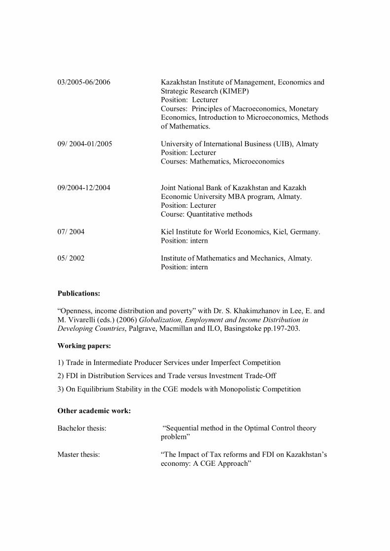
03/2005-06/2006 09/ 2004-01/2005
Kazakhstan Institute of Management, Economics and Strategic Research (KIMEP) Position: Lecturer Courses: Principles of Macroeconomics, Monetary Economics, Introduction to Microeconomics, Methods of Mathematics. University of International Business (UIB), Almaty Position: Lecturer Courses: Mathematics, Microeconomics
09/2004-12/2004 07/ 2004 05/ 2002
Joint National Bank of Kazakhstan and Kazakh Economic University MBA program, Almaty. Position: Lecturer Course: Quantitative methods Kiel Institute for World Economics, Kiel, Germany. Position: intern Institute of Mathematics and Mechanics, Almaty. Position: intern
Publications: “Openness, income distribution and poverty” with Dr. S. Khakimzhanov in Lee, E. and M. Vivarelli (eds.) (2006) Globalization, Employment and Income Distribution in Developing Countries, Palgrave, Macmillan and ILO, Basingstoke pp.197-203. Working papers: 1) Trade in Intermediate Producer Services under Imperfect Competition
2) FDI in Distribution Services and Trade versus Investment Trade-Off
3) On Equilibrium Stability in the CGE models with Monopolistic Competition
Other academic work: Bachelor thesis: Master thesis:
“Sequential method in the Optimal Control theory problem” “The Impact of Tax reforms and FDI on Kazakhstan’s economy: A CGE Approach”

Conference presentations:
2nd FIW Research Conference on "International Economics", Vienna, December 2008.
IXth Doctoral Meeting in International Trade and International Finance, Aix- en-Provence, April 2009.
Eleventh Annual Conference of European Trade Study Group (ETSG), Rome, September 2009. Academic awards:
HESP OSI Scholarship for studies at KIMEP. University of Kiel scholarship for summer courses in Kiel, Germany. DAAD/OSI scholarship for doctoral studies.
Language skills: Kazakh (native), Russian (fluent), English (fluent), German (upper-intermediate, CEFR: B2). Computer skills: Microsoft Office, Mathematica, E-views, GAMS/MPSGE, SPSS, Delphi (basics). References: available upon request.