
UniVerMeC A Framework for Development, Assessment and ... · heterogenen Algebra formalisiert und...
223
UniVerMeC – A Framework for Development, Assessment and Interoperable Use of Verified Techniques Von der Fakultät für Ingenieurwissenschaften, Abteilung Informatik und Angewandte Kognitionswissenschaft der Universität Duisburg-Essen zur Erlangung des akademischen Grades Doktor der Naturwissenschaften genehmigte Dissertation von Stefan Kiel aus Frankenberg (Eder) 1. Gutachter: Prof. Dr. Wolfram Luther 2. Gutachter: Prof. Dr. Jürgen Wolff von Gudenberg Tag der mündlichen Prüfung: 27.01.2014
Transcript of UniVerMeC A Framework for Development, Assessment and ... · heterogenen Algebra formalisiert und...
UniVerMeC – A Framework for Development,Assessment and Interoperable Use of Verified
Techniques
Von der Fakultät für Ingenieurwissenschaften,Abteilung Informatik und Angewandte
Kognitionswissenschaftder Universität Duisburg-Essen
zur Erlangung des akademischen Grades
Doktor der Naturwissenschaften
genehmigte Dissertation
von
Stefan Kielaus
Frankenberg (Eder)
1. Gutachter: Prof. Dr. Wolfram Luther2. Gutachter: Prof. Dr. Jürgen Wolff von GudenbergTag der mündlichen Prüfung: 27.01.2014


U N I V E R M E C – A F R A M E W O R K F O R D E V E L O P M E N T,A S S E S S M E N T A N D I N T E R O P E R A B L E U S E O F V E R I F I E D
T E C H N I Q U E S
stefan kiel
With Applications in Distance Computation, Global Optimization, and ComparisonSystematics

Stefan Kiel: UniVerMeC – A Framework for Development, Assessment andInteroperable Use of Verified Techniques, With Applications in DistanceComputation, Global Optimization, and Comparison Systematics

A B S T R A C T
Verified algorithms play an important role in the context of different applicationsfrom various areas of science. An open question is the interoperability between dif-ferent verified range arithmetics and their numerical comparability. In this thesis, atheoretical framework is provided for interoperable handling of the arithmetics with-out altering their verification features. For this purpose, we formalize the arithmeticsusing a heterogeneous algebra. Based on this algebra, we introduce the concept offunction representation objects. They characterize a mathematical function by inclu-sion functions in different arithmetics and allow for representing particular featuresof the function (e.g., differentiability). The representation objects allow us to describeproblems by functional and relational dependencies so that different verified meth-ods can be used interchangeably. On this basis, we develop a new verified distancecomputation algorithm which can handle non-convex objects. Furthermore, a veri-fied global optimization algorithm is adapted so that it can use the different methodsmade accessible by the function representation objects. Moreover, we formalize andimprove interval-based hierarchical structures which are used by both algorithms.To evaluate our approach, we provide a prototypical implementation and performfair numerical comparisons between the different arithmetics. Finally, we apply theframework to relevant application cases from biomechanics and modeling, simula-tion and control of fuel cells. We demonstrate that our implementation supportsparallel computations on the CPU and GPU and show that it can be extended byinterfacing additional external IVP solver libraries.
Z U S A M M E N FA S S U N G
Verifizierte numerische Verfahren spielen in zahlreichen Anwendungskontexten einewichtige Rolle. Hierbei ist die Interoperabilität zwischen den verschiedenen verwen-deten Wertebereichsarithmetiken sowie ihre numerische Vergleichbarkeit eine offeneFrage. In dieser Arbeit wird ein theoretisches Rahmenwerk zur Verfügung gestellt,welches die Interoperabilität zwischen den Arithmetiken unter Beibehaltung der Ve-rifikationseigenschaften sicherstellt. Hierzu werden die Arithmetiken mittels einerheterogenen Algebra formalisiert und darauf aufbauend das Konzept der “Funk-tionsrepräsentationsobjekte” eingeführt. Damit können mathematische Funktionenmittels Inklusionsfunktionen in unterschiedlichen Arithmetiken charakterisiert undihre Eigenschaften (z.B. Differenzierbarkeit) dargestellt werden. Mit Hilfe der Reprä-sentationsobjekte ist es möglich Problemstellungen, die mittels funktionaler und rela-tionaler Beziehungen repräsentierbar sind, derart zu beschreiben, dass unterschied-liche verifizierte Methoden eingesetzt werden können. Aufbauend hierauf wird einneuer Algorithmus zur verifizierten Abstandsberechnung zwischen nicht konvexenKörpern entwickelt. Weiterhin wird ein verifizierter globaler Optimierungsalgorith-mus derart angepasst, dass er die durch Funktionsrepräsentationsobjekte zugänglichgemachten, unterschiedlichen Methoden flexibel nutzen kann. Beide Algorithmengreifen auf in das Rahmenwerk integrierte Hilfsdatenstrukturen zur intervallbasier-ten hierarchischen Zerlegung zurück, die im Kontext dieser Arbeit formalisiert undverbessert werden. Zur Evaluation wird der Gesamtansatz prototypisch implemen-tiert. Hierbei werden nicht nur numerische Vergleiche zwischen den unterschiedli-chen Arithmetiken durchgeführt, sondern auch relevante Anwendungsfälle aus derBiomechanik und der Simulation von Brennstoffzellen behandelt. Weiterhin wird de-monstriert, dass die vorliegende Implementierung parallele Berechnungen auf derCPU und GPU unterstützt und durch die Anbindung weiterer externer AWP Löser-bibliotheken flexibel erweiterbar ist.
v


P U B L I C AT I O N S
Most ideas, figures and algorithms appeared previously in the follow-ing publications:
• R. Cuypers, S. Kiel, and W. Luther. “Automatic Femur Decom-position, Reconstruction, and Refinement Using SuperquadricShapes.” In: Proceedings of the IASTED International Conference.Vol. 663. 2009, p. 59
• E. Auer, R. Cuypers, E. Dyllong, S. Kiel, and W. Luther. “Veri-fication and Validation for Femur Prosthesis Surgery.” In: Com-puter-assisted proofs - tools, methods and applications. Ed. by B. M.Brown, E. Kaltofen, S. Oishi, and S. M. Rump. Dagstuhl Sem-inar Proceedings 09471. Schloss Dagstuhl, 2010. url: http:
//drops.dagstuhl.de/opus/volltexte/2010/2513
• E. Dyllong and S. Kiel. “Verified Distance Computation Be-tween Convex Hulls of Octrees Using Interval OptimizationTechniques.” In: PAMM 10.1 (2010), pp. 651–652. issn: 1617-7061
• E. Auer, A. Chuev, R. Cuypers, S. Kiel, and W. Luther. “Rele-vance of Accurate and Verified Numerical Algorithms for Veri-fication and Validation in Biomechanics.” In: EUROMECH Col-loquium 511. Ponta Delgada, Azores, Portugal, 2011
• S. Kiel. “Verified Spatial Subdivision of Implicit Objects UsingImplicit Linear Interval Estimations.” In: Curves and Surfaces.Ed. by J.-D. Boissonnat, P. Chenin, A. Cohen, C. Gout, T. Lyche,M.-L. Mazure, and L. Schumaker. Vol. 6920. Lecture Notes inComputer Science. Springer, 2012, pp. 402–415
• E. Dyllong and S. Kiel. “A Comparison of verified distance com-putation between implicit objects using different arithmetics forrange enclosure.” In: Computing 94 (2 2012), pp. 281–296. issn:0010-485X
• S. Kiel. “YalAA: Yet Another Library for Affine Arithmetic.” In:Reliable Computing 16 (2012), pp. 114–129
• E. Auer, S. Kiel, and A. Rauh. “Verified Parameter Identificationfor Solid Oxide Fuel Cells.” In: Proceedings of the 5th InternationalConference on Reliable Engineering Computing. 2012
• S. Kiel, W. Luther, and E. Dyllong. “Verified distance com-putation between non-convex superquadrics using hierarchical
vii
space decomposition structures.” In: Soft Computing 17.8 (2013),pp. 1367–1378. issn: 1432-7643
• S. Kiel, E. Auer, and A. Rauh. “Use of GPU Powered IntervalOptimization for Parameter Identification in the Context of SOFuel Cells.” In: Proceedings of NOLCOS 2013 - 9th IFAC Sympo-sium on Nonlinear Control Systems. 2013. doi: 10.3182/20130904-3-FR-2041.00169
• S. Kiel, E. Auer, and A. Rauh. “An Environment for Testing,Verification and Validation of Dynamical Models in the Contextof Solid Oxide Fuel Cells.” In: Reliable Computing 19.3 (2014),pp. 302–317
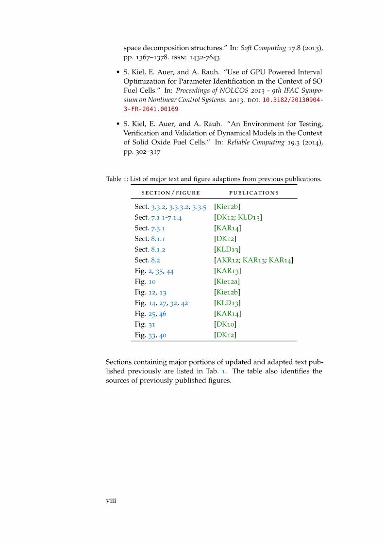
Table 1: List of major text and figure adaptions from previous publications.
section/figure publications
Sect. 3.3.2, 3.3.3.2, 3.3.5 [Kie12b]Sect. 7.1.1-7.1.4 [DK12; KLD13]Sect. 7.3.1 [KAR14]Sect. 8.1.1 [DK12]Sect. 8.1.2 [KLD13]Sect. 8.2 [AKR12; KAR13; KAR14]Fig. 2, 35, 44 [KAR13]Fig. 10 [Kie12a]Fig. 12, 13 [Kie12b]Fig. 14, 27, 32, 42 [KLD13]Fig. 25, 46 [KAR14]Fig. 31 [DK10]Fig. 33, 40 [DK12]
Sections containing major portions of updated and adapted text pub-lished previously are listed in Tab. 1. The table also identifies thesources of previously published figures.
viii
D A N K S A G U N G
Die Erstellung dieser Arbeit erfolgte zu wesentlichen Teilen im Rah-men des durch die Deutsche Forschungsgemeinschaft gefördertenProjekts “Intervallbasierte Verfahren für adaptive hierarchische Mo-delle in Modellierungs- und Simulationssystemen”. An erster Stelledanke ich Frau Dr. Eva Dyllong und Herrn Prof. Dr. Wolfram Luther,die als Projektleiterin beziehungsweise Lehrstuhlinhaber die Durch-führung des Forschungsvorhabens ermöglichten und unterstützten.Herzlichen Dank auch an Herrn Prof. Dr. Jürgen Wolff von Guden-berg für die Übernahme des Korreferats. Mein besonderer Dank anFrau Dr. Ekaterina Auer, die mich nicht nur als Kollegin stets unter-stützte, sondern auch die Anwendung der entwickelten Methoden imKontext von Festoxidbrennstoffzellen anregte und im Rahmen einerKooperation ermöglichte. In diesem Zusammenhang danke ich auchHerrn Dr. Andreas Rauh für die zur Verfügung gestellten Festoxid-brennstoffzellenmodelle. Mein herzlicher Dank geht an die Mitarbei-ter des Lehrstuhls für Computergrafik und Wissenschaftliches Rech-nen für die stets kollegiale Atmosphäre und das freundliche Arbeits-umfeld. Und nicht zuletzt ein großes Dankeschön an meine Elternund Familie, die mich immer in jeglicher Hinsicht unterstützten.
ix

C O N T E N T S
1 introduction 1
1.1 Problem Motivation 2
1.2 Objectives 3
1.3 Related Work 5
1.4 Structure 6
2 univermec software 9
2.1 Requirements 9
2.1.1 Verification Requirements 10
2.1.2 Standard Requirements 12
2.1.3 Interoperability Requirements 13
2.1.4 Expandability Requirements 13
2.2 Software Architecture 14
2.3 Use-Cases 17
2.4 User Input and Output 19
2.5 Conclusions 21
3 arithmetics 23
3.1 Floating-Point Arithmetic 24
3.2 Interval Arithmetic 25
3.2.1 Basic Arithmetic 26
3.2.2 Natural Interval Extension 28
3.2.3 P1788 - Interval Standard 29
3.2.4 Implementations 31
3.2.5 Overestimation 32
3.3 Affine Arithmetic 33
3.3.1 Basic Model 33
3.3.2 Extended Models 35
3.3.3 Implementation of Elementary Functions 35
3.3.4 Implementations 40
3.3.5 Architecture of YalAA 41
3.4 Taylor Models 44
3.4.1 Basic Model 45
3.4.2 Implementations 46
3.5 Abstract Algebra and Hierarchy 46
3.5.1 Universal Inclusion Representation 46
3.5.2 Heterogeneous Algebra 48
3.5.3 Arithmetic Hierarchy and Conversions 52
3.6 Implementation of the Arithmetic Layer 54
3.7 GPU-Powered Computations 58
3.8 Conclusions 61
xi

xii contents
4 functions in univermec 63
4.1 Algorithmic Differentiation 64
4.2 Verified Function Enclosures 67
4.2.1 Mean-Value Forms 67
4.2.2 Other Enclosure Techniques 68
4.3 Interval Contractors 69
4.3.1 One-dimensional Interval Newton Contractor 70
4.3.2 Multidimensional Interval Newton Contractor 72
4.3.3 Consistency Techniques 73
4.3.4 Implicit Linear Interval Estimations 74
4.4 Function Layer 76
4.4.1 Formal Definition 76
4.4.2 Interfaces of the Function Layer 78
4.4.3 Implementation of the Function Layer 83
4.5 Conclusions 90
5 modeling layer 93
5.1 Geometric Models 93
5.2 Initial Value Problems 96
5.3 Optimization Problems 97
5.4 Further Problem Types 98
6 hierarchical space decomposition 99
6.1 Interval Trees 100
6.1.1 Formal Definition and Standard Trees 100
6.1.2 Contracting Trees 103
6.1.3 Parametric Tree 108
6.1.4 Realization in UniVerMeC 109
6.2 General Multisection 110
6.3 Conclusions 113
7 algorithms 115
7.1 Distance Computation 116
7.1.1 A Basic Distance Computation Algorithm forInterval Trees 118
7.1.2 Using Normals for Distance Computation 124
7.1.3 Improvements of ε-Distance Algorithm UsingFloating-Point Methods 125
7.1.4 Further Improvements 126
7.2 Global Optimization 127
7.2.1 Basic Algorithm 129
7.2.2 A Configurable Algorithm 133
7.2.3 Parallelization of the Algorithm 138
7.2.4 Provided Strategy Elements and Possible En-hancements 141
7.3 Interfacing of External Solvers 143
7.3.1 ValEncIA-IVP 145

contents xiii
7.3.2 VNODE-LP 149
7.3.3 Other Solvers 150
7.4 Conclusions 151
8 applications 153
8.1 TreeVis 154
8.1.1 Comparisons Between Range Arithmetics 156
8.1.2 Verification of Distances for Total Hip Replace-ment 164
8.2 VeriCell 168
8.3 Conclusions 178
9 conclusions 181
references 185

L I S T O F F I G U R E S
Figure 1 Validation and verification assessment cycle 11
Figure 2 Relaxed layered structure of UniVerMeC. 15
Figure 3 Hierarchy of facades in the objects layer. 17
Figure 4 User input and corresponding ouput at the dif-ferent abstraction levels of UniVerMeC. 20
Figure 5 User interfaces of integrated problem solvingenvironments built upon UniVerMeC. 21
Figure 6 Overview of the requirements. 22
Figure 7 Geometric representation of a two dimensionalinterval vector. 27
Figure 8 The layers of IEEE P1788 . 29
Figure 9 The wrapping effect. 32
Figure 10 The joint range of two partially dependent affineforms. 33
Figure 11 Affine approximations for ex over [0, 1]. 36
Figure 12 Basic architecture of YalAA 43
Figure 13 Interaction of YalAA’s policy classes 44
Figure 14 Arithmetic hierarchy in UniVerMeC. 53
Figure 15 The arithmetic layer of UniVerMeC and its semi-automatic generation. 58
Figure 16 The stream processing model. 59
Figure 17 Implicit linear estimations 75
Figure 18 Interfaces IVFunction and IFunction for rep-resentation of functions. 79
Figure 19 Interface IDerivative for accessing derivatives. 80
Figure 20 Interfaces IGPUEval and IGPUFuture<T> for func-tion evaluation on the GPU. 81
Figure 21 The IContractor interface. 82
Figure 22 Simplified struture of the uniform function rep-resentation layer and its implementation in Uni-VerMeC. 85
Figure 23 Interaction of the host program with the GPU
kernel implementation. 89
Figure 24 The geometric model representation layer. 95
Figure 25 IVP problem type considered in UniVerMeC. 97
Figure 26 Decomposition of a sphere using a binary tree. 103
Figure 27 Illustration of a white inversion node. 104
Figure 28 Overview of tree decomposition layer. 109
Figure 29 Multisection schemes 111
Figure 30 Multisection layer of UniVerMeC 113
xiv

Figure 31 Test cases for distance computation with an in-terval optimization algorithm 117
Figure 32 Graphical representation of case selectors fordistance computation. 120
Figure 33 List sorting criteria used in ε-distance 121
Figure 34 Strategy element interface 135
Figure 35 Integration of GPU strategy elements into theinterval global optimization algorithm. 140
Figure 36 Integration of ValEncIA-IVP 146
Figure 37 Integration of VNODE-LP 148
Figure 38 Managing a geometric scene with TreeVis. 154
Figure 39 TreeVis GUI 155
Figure 40 Plot of the surfaces from Tab. 19 158
Figure 41 Average CPU time for the ε-distance algorithm 163
Figure 42 Visualization of the test cases from Tab. 24. 167
Figure 43 Maximum deviation of Euler’s method 171
Figure 44 CPU and GPU evaluation benchmark for the ob-jective function 172
Figure 45 Procedure for identifying consistent states 173
Figure 46 SOFC simulation results with VNODE-LP 177
Figure 47 Width of output intervals with respect to theinput width 178
L I S T O F TA B L E S
Table 1 List of major text and figure adaptions fromprevious publications. viii
Table 2 IEEE 754-2008 formats 25
Table 3 Decorations in IEEE P1788 . 31
Table 4 Overview over affine arithmetic libraries. 42
Table 5 Arithmetics in the inclusion representation frame-work. 47
Table 6 Basic operations and elementary functions con-sidered in the heterogeneous algebra. 49
Table 7 Additional functions for the floating-point al-gebra. 51
Table 8 Mapping of arithmetics and their implement-ing types. 54
Table 9 Conditions that the m4 macro package takesfor granted for the underlying types at eachlevel in the hierarchy. 55
Table 10 Evaluation trace of a function. 66
Table 11 Extended interval division 71
xv
Table 12 Interfaces from the function layer and their for-mal concepts. 78
Table 13 Implemented contractors and enclosures. 90
Table 14 The tree decomposition structures implementedin UniVerMeC and their theoretical basis. 109
Table 15 Rules for weights of coordinate directions 112
Table 16 Handling of variables in the parallel versionof the interval global optimization algorithmwith regard to thread synchronization. 139
Table 17 Strategy elements used in the default strategyof the global optimization algorithm. 141
Table 18 External solvers interfaced with UniVerMeC 150
Table 19 Implicit surfaces used for comparing range-bound-ing methods. 157
Table 20 Geometric configurations for comparing dif-ferent range-bounding methods 158
Table 21 Results of the test cases from Tab. 20 withoutnormal vectors 160
Table 22 Results for the test cases from Tab. 20 with thenormal cone test 161
Table 23 Parameters of the SQ model and their ranges. 165
Table 24 Geometric configurations for the THR test cases 166
Table 25 Test results for the scenarios from Tab. 24 166
Table 26 Parameter identification results for the one-di-mensional model 174
Table 27 Parameter identification results for the three-dimensional model 176
L I S T I N G S
Listing 1 Excerpt from the m4 macros to register an in-terval type using C-XSC as the underlying li-brary. 56
Listing 2 Excerpt from the m4 macros to register an in-terval type using PROFIL/BIAS as the under-lying library. 57
Listing 3 A functor for defining a function in UniVer-MeC. The concrete functor is the right-handside of the Brusselator. 84
Listing 4 Excerpt from the opt_worker_state_t structurepassed to strategy elements. 134
xvi
Listing 5 Excerpt from the phase_config_t structure re-sponsible for configuring the optimization al-gorithm. 136
Listing 6 Strategy element for prunig a box by formallysolving (60) using an ILIE. 142
Listing 7 Python script using an extension module ofUniVerMeC to read a resource graph file. 159
A L G O R I T H M S
1 Split operation for a standard interval tree node. . . . . 103
2 Splitting operation for a contracting tree node. . . . . . 106
3 Conversion of a white inversion node to a set of stan-dard white nodes. . . . . . . . . . . . . . . . . . . . . . . 107
4 Split operation for a parametric tree node. . . . . . . . . 108
5 Calculation of a distance enclosure between two intervaltrees . . . . . . . . . . . . . . . . . . . . . . . . . . . . . . 123
6 Abstract pattern for branch and bound algorithms basedon [Kea96]. . . . . . . . . . . . . . . . . . . . . . . . . . . 130
7 Sequential version of the configurable interval global op-timization algorithm in UniVerMeC. . . . . . . . . . . . 137
A C R O N Y M S
AA affine arithmetic
AD algorithmic differentiation
API application programming interface
CPU central processing unit
CSG computer solid geometry
DAG directed acyclic graph
ED elemental differentiability
FIFO first in, first out
xvii

FP floating-point
FPA floating-point arithmetic
FRO function representation object
GPU graphics processing unit
GPGPU general purpose computations on the GPU
GUI graphical user interface
IA interval arithmetic
ILIE implicit linear interval estimation
IVP initial value problem
KKT Karush-Kuhn-Tucker
LDB linear dominated bounder
LIFO last in, first out
MPI message-passing interface
ODE ordinary differential equation
PDE partial differential equation
QFB quadratic fast bounder
SFINAE substitution failure is not an error
SIMD single instruction multiple data
SIMT single instruction multiple threads
SISD single instruction single data
SOFC solid oxide fuel cell
SQ superquadric
THR total hip replacement
TM Taylor model
N O TAT I O N
Generally, the notation used in this these follows the standardizedinterval notation introduced in [Kea+02]. We denote scalars and vec-tors by lower case letters (i.e., x,y) and matrices by upper case ones(i.e., M, T ). Interval quantities are bold-faced (i.e., x,y); affine forms
xviii

notation xix
are marked by a hat (i.e., (x, y)); and Taylor models by a breve (i.e.,x, y). Additionally, we use calligraphic letters (i.e., M, S) for sets andfractured letter (i.e., T,N) for tuples. Individual entries of a tupleT = (E1, . . . ,En) can be accessed by the shorthand notation T.Ei (forthe i-th element).


1I N T R O D U C T I O N
Today, numerical computations are normally carried out on a digital Numericalcomputations on acomputer
computer using floating-point arithmetic (FPA). Despite the fact thatthe results are not exact and that this finite number system is notflawless, a direct floating-point (FP) implementation of an algorithmbased on the real-number system can yield satisfactory results. How-ever, such a behavior is by no means guaranteed and the producedresults might turn out to be fatally wrong. Thus, it is usually neces-sary to adapt the algorithms carefully to the FP number system. Evenso, the result is only an approximation of the true one.
The need for guaranteed results arose in many application areas Verified methods
very early on. This led, for example, to the use of interval arith-metic (IA) (developed by Moore [Moo66] and others) as a calculus forautomatically bounding the approximation or rounding errors. Theapproach produces bounds that are guaranteed to enclose the realnumber result. A method that handles rounding errors, does not in-troduce approximation errors, and does not neglect solutions is calledverified because it guarantees the correctness of results obtained on acomputer.
Aside from the above-mentioned numerical errors, we have to cope Error sources
with additional error sources in practical applications. The two mostimportant ones are modeling errors and uncertain (input) parameters.Modeling errors arise because the formal model on which our com-putations are based usually does not correspond to the real worldexactly. Additionally, model parameters are not known exactly ingeneral. On the one hand the values of these parameters mightbe known only up to a certain degree of accuracy, for example, ifthey come from measurements; on the other hand, the parametersmight be given in form of stochastic distributions (which in turn, canhave uncertain characteristics). Handling and propagating both un-certainty and numerical errors through complex computations canbecome quite complicated if only FPA is used. IA or range arithmeticsin general can handle both directly.
Even though IA is employed in many different application areas Sophisticatedverified arithmeticsnowadays, its naive application often produces correct but, due to
wide bounds, useless results from the practical point of view. Overthe time, several more sophisticated verified arithmetics and tech-niques were proposed to supplement or replace IA, for example, cen-tered forms [Neu90], affine arithmetic (AA) [CS90], ellipsoid arith-metic [Neu93], generalized IA [Han75], Taylor models (TMs) [Ber95b]or consistency techniques which try to exploit domain knowledge to
1

2 introduction
tighten bounds. Often, improved tightness of enclosures is achievedat the cost of a higher computational effort per operation.
1.1 problem motivation
Branch and bound algorithms are a common problem solving strat-Branch and boundalgorithms egy in the scope of interval computations, for example, for distance
computation [DG07c], global optimization [HW04] or path planning[Jau01]. Their basic principle is the subdivision of the search regioninto box-shaped subregions. Besides this basic principle, additionaltechniques are applied, such as heuristics for box selection or subdivi-sion directions, more sophisticated enclosure techniques, or intervalcontractors. Without these accelerating devices, the performance ofbranch and bound algorithms might be poor due to their exponentialcomplexity.
For good results it is necessary to choose the kind of an acceleratorSelection ofaccelerators depending on the problem at hand. However, even experienced users
might have difficulties selecting them in a satisfactory way. That is,they have problems finding the method delivering bounds in a rea-sonable computational time and at acceptable memory cost that arealso sharp enough to be useful. From a theoretical point of view, thisquestion was investigated only for few range bounding techniquesover sufficiently small intervals1. In practice, where intervals can-not become arbitrarily small during subdivision due to memory andruntime constraints, such theoretical considerations are merely guide-lines despite having applications in special cases.
Matters are further complicated by the fact that the actual speedInteroperabilityproblems of a numerical method on a computer is determined not only by its
theoretical properties but also by its actual implementation. Whilea lot of implementations are freely available for verified techniques,they are usually not interoperable with each other. Thus, employingtechniques provided by different libraries requires substantial efforton the users’ part. They do not only need to cope with differentinterfaces, but also to develop a problem definition and a solvingstrategy abstract enough to be used with these.
Due to these difficulties in employing and combining different tech-Consequences ofinteroperability
problemsniques, a single one is usually used throughout the entire application.This voluntary restriction might lead to inferior results. Worse, theproblems with interoperability of existing software packages mightprevent a practice-oriented user, who is mainly interested in the re-sults, from employing verified computations entirely even if theywould suit his needs. Additionally, there is a lack of practical ex-perience as to which method performs well for a specific problem be-
1 Neumaier [Neu03] gives an overview of the different definitions for the approxima-tion orders of range enclosure techniques. He also notes that obtaining analogousresults for wide intervals is difficult.
1.2 objectives 3
cause there are next to no comparisons between the techniques. Thetask becomes more complicated if modern hardware architectures aretaken into account: Depending on the actual problem structure, it canbe favorable to tackle the problem or its parts with graphics process-ing units (GPUs) instead of employing the standard central process-ing unit (CPU). These highly parallel many-core processors can oftenimprove the problem solving time. However, they require a specialtreatment. Implementations well suited for the CPU may not performwell on a GPU. Usually, problems are not solved entirely on the GPU.In case of a hybrid CPU/GPU approach additional interoperability ef-forts are necessary to cope with the different hardware architectures.For example, libraries employed for IA on the CPU are not necessarilyinteroperable with GPU interval libraries. To summarize, there is noframework that would allow for selection of adequate verified algo-rithms and for handling interoperability problems between existingsoftware on the CPU, and even less those arising in a hybrid CPU/GPU
computation environment.
1.2 objectives
The first main objective of this thesis is to provide the theoretical Theoreticalfoundationfoundations for a software framework that tackles the interoperabil-
ity problems. This is done by carefully analyzing common techniquesemployed in existing interval algorithms and by deriving appropri-ate interfaces that allow for using these techniques as interchange-able and interoperable software components in different algorithms.The framework should take care of the interoperability between dif-ferent verified techniques automatically and employ well-tested soft-ware packages as its basis. Thus, users would be able to specify aproblem once and then employ various techniques interchangeablyto solve the problem. Additionally, they should get a fair comparisonof the performance in the respective problem domains. Furthermore,it should be possible to combine the available techniques to improvesolutions for a problem. Here, we also aim to provide a theoreticalfoundation for conditions under which techniques are allowed to in-teract with each other (i.e., in such a way as still to produce verifiedresults). While the use of the GPU is not in the main focus of this the-sis, we will also discuss some strategies to enable the use of verifiedinterval techniques in a mixed CPU/GPU environment.
The theoretical foundations are then practically applied to develop Extensible softwareframeworkthe proof of concept software framework UniVerMeC that tackles the
interoperability problem as the second objective. Since it is only aproof of concept, we limit the implementation to a set of selectedcommon techniques. However, the framework should be extensiblewhich necessitates application of modern software engineering tech-niques. That is, we implement an open platform to which new tech-

4 introduction
niques can be added. As more and more users provide reference im-plementations of their new techniques (algorithms, contractors, rangearithmetics, etc.) inside the framework, the task of fair comparisonsbetween new developments becomes less difficult. Currently, authorsof a new development are often forced to make their own implemen-tation of the techniques they want to compare with, because, for ex-ample, a reference implementation is not available publicly or cannotbe employed easily in the software system of the authors. This resultsin comparisons with easy-to-implement techniques or with inferiorimplemented references. A uniform framework, where both the newtechnique and the reference implementation of existing techniquesare available, would help authors and end users in equal measure.The tedious task of providing comparisons would be simplified forsoftware developers. End users would benefit from the better resultsand at the same time from getting the reference implementations in-side a uniform framework.
The final main objective is to evaluate the approach and its practi-Evaluation of theapproach cal realization by applying the developed tool to several real world ex-
amples. We focus on geometric computations since the combinationof continuous and discrete data makes them especially susceptibleto rounding and other computational errors [Yap97]. In this scope,we discuss improvements in interval-based hierarchical space decom-position structures for geometric objects and show how they canbe used for uniformly handling different geometric modeling tech-niques. Furthermore, we present a novel algorithm for computinga verified bound on the distance between non-convex objects that ap-plies the developed hierarchical space decomposition structures. Thisapplication also demonstrates that the encapsulation provided by theframework allows users to employ the same algorithm with severaltechniques for range enclosures. This makes it possible to comparethem fairly and, thus, give users a better overall database for choosingthe “right” technique. At least to our knowledge, such comparisonsbased on the same problem and algorithm implementation were notavailable until now.
As another application of the distance computation algorithm, wehighlight verification of important subprocesses in an automatic sup-port tool for total hip replacement (THR). In this scope, we apply ouralgorithm to derive the distances between the femur bone and thefemur shaft. They are modeled using non-convex superquadrics (SQs)or non-convex polyhedrons, that is, smooth and non-smooth models.
The second large use-case area is modeling, simulation and controlof solid oxide fuel cells (SOFCs). We show how thermal SOFC mod-els can be realized in the unified notations of the framework. Afterthat, we demonstrate how to identify model parameters by using amodular variant of the global optimization algorithm by Hansen andWalster [HW04]. Besides this, we show how to speed up the process
1.3 related work 5
using the GPU. Moreover, we interface different external libraries orsolvers with UniVerMeC, and use them for parameter identificationor for simulating the SOFCs.
1.3 related work
Since this thesis covers a rather broad field, the complete discussionof related work would be too lengthy. Therefore, more specific as-pects will be discussed in the subsequent chapters. Here, we touchupon the general topics of combination and comparison of differenttechniques.
The question of how different techniques for verified computations Contractorprogrammingcan be combined or compared has recieved some attention lately. For
example, Chabert and Jaulin [CJ09] proposed, under the name con-tractor programming, a framework for the flexible and easy reconfig-uration of constraint programming solvers. Their idea is to split aclassical interval-based solver into components: a paver and one orseveral contractors. The paver handles the bisection, manages inter-val boxes and calls the contractors. Users can alter the behavior of thesolver by altering the list of contractors of the paver. Contractors areaccelerating devices for branch and bound algorithms as explained inthe previous section (e.g. interval Newton, hull consistency). The au-thors claim that it is possible to implement much more flexible solversthan existing ones. The IBEX library and the Quimper language [Cha]are implementations of their ideas.
Another environment that allows for flexible configuration of the GlobtLab
solving process and user configuration of different techniques is theGloptLab software developed by Domes [Dom09]. It is a MATLABprogram for solving quadratic constraint satisfaction problems. Userscan configure the solving process of GloptLab by providing an user-defined strategy. This strategy combines the already implementedsolving techniques (accelerating devices) inside the branch and boundalgorithm and can be adapted to the current problem. Users can ex-tend the tool by adding their own accelerating devices.
Again in the context of constraint programming, Vu, Sam-Haroud, Inclusionrepresentationframework
and Faltings [VSHF09] propose a theoretical framework called inclu-sion representation. This framework can be used to unify differentrange arithmetics (e.g. IA or AA). Their formalism allows us to de-rive common definitions for inclusion functions or natural extensionsfor all arithmetics. The authors use it to demonstrate how constraintprogramming can benefit from more sophisticated range arithmetics.
Auer and Rauh [AR12] developed an online platform called VERI- VERICOMP
COMP. On the one hand, the platform allows for comparing differentverified initial value problem (IVP) solvers using a common set of testproblems or a user-defined problem. On the other hand, the platform

6 introduction
tries to recommend solver settings for custom problems automaticallyon the basis of data that was collected on similar problems.
Domes, Fuchs, and Schichl [DFS11] developed an environment forEnvironment forcomparing global
optimization codestesting global optimization codes. It provides interfaces to differentsolvers. The solvers can be called with a selection of test problemsmanaged by the environment. Furthermore, it can be used to evalu-ate the results of the solvers almost automatically. A graphical userinterface allows for handling of the environment.
While all of the above mentioned software systems overlap withRelation withUniVerMeC UniVerMeC at one point or another, they all are more specialized
towards specific problems (e.g., building a constraint solver or com-paring solvers). In their specific domains, they provide additionalfeatures that are not offered by UniVerMeC. However, the idea andstructure of our tool is more general. It provides problem-dependentmodeling layers (Sect. 5) that allow for applying the framework indifferent domains. In this way, UniVerMeC can be the basis for in-tegrated environments in those domains. For example, both TreeVis
(Sect. 8.1) and VeriCell (Sect. 8.2) use the framework as a commoncode base but target different problem domains. Moreover, tools forcomparisons such as VERICOMP can be implemented on top of Uni-VerMeC to reduce the amount of necessary work to develop them2.In conclusion, UniVerMeC fills a conceptual gap because, on the onehand, it can be used to compare existing techniques in a fair man-ner, and, on the other hand, the framework can be employed as thebasis for creating domain dependent verified problem solving envi-ronments much more easily.
1.4 structure
The thesis is structured as follows. In Chap. 2, the conceptual basisRequirements
for this thesis is provided. Here, requirements for the software, theoverall software architecture, possible use-cases, and the organizationof user input and output are discussed.
The following five chapters are organized using the software struc-Arithmetics
ture as a guideline: Each of them discusses one layer of the software.In Chap. 3, an overview of the theory and existing implementationsof the arithmetics considered inside the framework is given. Further-more, we analyze how to unify different arithmetics to allow for aninterchangeable use while still preserving the property of verification.As a use-case, we describe YalAA, an AA library developed in thescope of the thesis, which already implements some of the guidelineson the arithmetic library level. Besides this, we discuss the automaticgeneration of adapters and cast operators for the arithmetics as wellas the extension of the arithmetic layer to GPU computations.
2 For example, uniform function representation or interfaces to different solvers arealready available in UniVerMeC.

1.4 structure 7
Problems solved within the developed framework are usually de- Functionrepresentation inUniVerMeC
scribed by functional and relational dependencies. Chap. 4 is con-cerned with the data type independent, homogeneous representationand implementation of functions in the mathematical sense insideUniVerMeC. Furthermore, the notion of interval contractors is intro-duced and the contractor techniques implemented in the frameworkare explained.
In Chap. 5, the problem dependent layers in the middle of the Modeling layer
framework structure are described. In particular, we give details onthe layer devoted to different geometric modeling types supportedby the framework, the layer for IVPs and the layer for optimizationproblems.
Chapter 6 discusses common utility data structures used in interval- Hierarchicaldecompositionsbranch-and-bound algorithms. We describe uniform interfaces for in-
terval trees used in the scope of geometric problems. Furthermore,we introduce the enhanced variants developed in the scope of thethesis, for example, trees for parametric surfaces or trees with inte-grated contractors. As for non-geometric algorithms, we discuss uni-form interfaces and implementations for multisection schemes andbox management data structures.
Now we are ready to move to algorithms, which use the tools de- Algorithms
scribed in the previous chapters. In Chap. 7, the algorithms currentlysupplied with the framework are outlined. In particular, the novelverified distance computation algorithm between geometric objects inour uniform representation and the modular verified global optimiza-tion algorithm for inequality constrained problems. Furthermore, wediscuss how to interface existing solvers, for example, Ipopt [WB06]for optimization or VNODE-LP [Ned06] for IVPs, so that they workon the uniform problem description.
In Chap. 8, we apply the newly developed and implemented al- Practicalapplicationsgorithms for different purposes. First, we compare different verified
techniques in the scope of distance computation. After that, we dis-cuss applications of the framework in the areas of hip replacementsurgery and parameter identification and simulation of SOFCs. Finally,a summary of the main results and possible future research directionsare given in Chap. 9.


2U N I V E R M E C S O F T WA R E
This chapter gives an overview of the software framework developed Chapter structure
in the scope of this thesis. First, it discusses and specifies require-ments for the framework with a focus on verification, interoperabil-ity, and extensibility. After that, an overview on the architecture ofthe framework is given. Then, we discuss use-cases for which Uni-VerMeC can be applied. Finally, we illustrate the input and outputparadigm with an example.
2.1 requirements
UniVerMeC (Unified Framework for Verified GeoMetric Computa- UniVerMeCframeworktions) is intended to be an integrated platform for providing various
verified techniques, for example, IA, AA, TMs, or interval contractors.The goal is to make them available in a uniform environment. Fur-thermore, the framework should offer uniform abstractions for thesupplied different verified techniques, so that it is possible to imple-ment algorithms in the framework that do not depend on a concretetechnique but only on its abstraction. The resulting algorithms arehighly configurable and flexible. Moreover, the framework shouldallow users to combine different techniques and to configure interac-tively1 the algorithms to adapt them to the their problem domains. Inthis way, users are encouraged to try out different techniques and tochoose the one that fits best.
An important aspect is the fact that each user wants to solve his/her Optimization goalsof usersproblem with different optimization goals in mind. For example,
the following objectives might be of interest: the tightness of the re-sult enclosure, minimization of the CPU time or the memory usage,employment of software in real time environments, or exploitationof computational power of special hardware co-processors, such asGPUs. UniVerMeC should feature a modular architecture to allowusers to configure algorithms according to their needs. Note that wedo not support real time computations in UniVerMeC. In an inher-ently modular and object-oriented environment, where subsystemscan be transparently replaced, it is hardly possible to meet real timerequirements without restricting the flexibility. Thus, UniVerMeConly supports offline computations. Flexibility is the main require-ment of UniVerMeC. It is met through the use of abstraction at dif-ferent levels as shown in Sect. 2.2. However, flexibility comes at theprice of a runtime and memory overhead. Less general solutions tai-
1 at runtime
9
10 univermec software
lored towards a specific scenario might have a higher efficiency intheir problem domain.
Another requirement for UniVerMeC is to allow fair comparisonsFair comparisons
of different techniques. To make a comparison fair and meaningful,it is important to fix basic conditions. For example, the test hardware,the problem description, the measures, and the algorithms have to bethe same except for the techniques to be compared. Especially in thecontext of numerical comparisons, comparisons are often made use-less by the fact that their result depends on the employed implemen-tation. If a new technique is developed, it is as often as not comparedto an own implementation instead of an optimized implementationavailable somewhere else. Another frequently encountered mistakeis to compare to a basic method and not to the best one available. Forexample, a new range enclosure method is only compared to naiveinterval evaluation and not to more sophisticated ones such as cen-tered forms or AA. Sometimes comparisons focus on one artificialbenchmark criterion but not on performance in more complex andmore realistic scenarios. Such comparisons can be considered unfairand are not very useful. As a uniform platform, UniVerMeC alreadyprovides fixed basic conditions for the test. To allow fair compar-isons between sophisticated well-tested implementations of the tech-niques, UniVerMeC should not reimplement them but allow usersto interface existing libraries with it and to exchange these librariestransparently. Therefore, an important requirement is to provide in-teroperability between techniques supplied by third party libraries.
To summarize, the framework should fulfill the following require-Summary ofrequirements ments:
• Verification inside the framework
• Support for standards
• Integration and interoperable use of different verified techniques
• Expandability and flexible combination of techniques
• Configurable algorithms to support different optimization goals
• Applicable in different problem domains
These requirements are described in detail below.
2.1.1 Verification Requirements
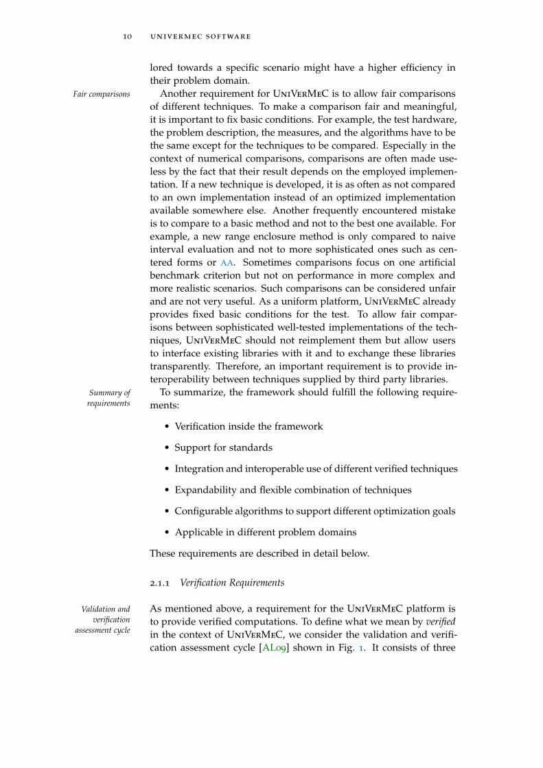
As mentioned above, a requirement for the UniVerMeC platform isValidation andverification
assessment cycleto provide verified computations. To define what we mean by verifiedin the context of UniVerMeC, we consider the validation and verifi-cation assessment cycle [AL09] shown in Fig. 1. It consists of three

2.1 requirements 11
Computer model
Real world
Validation
Formal model
Design
Verification
Figure 1: The validation and verification assessment cycle [AL09]. UniVer-MeC only performs numerical result verification, which is of useduring the transformation of the formal model into a computer-ized one.
main components: the real world, the formal model, and the com-puter model. Usually, the real world is analyzed with respect to theapplication domain in the design step to create the formal model. Inthis phase, the aspects relevant to the current application domain areidentified to integrate them into the formal model. In the second step,the formal model itself is transformed into a computer-based model.This usually means implementing a concrete computer program. Atthis step, verification can be performed. There are several verifica-tion kinds, for example, “code verification”, “formal verification”, or“result verification”. In the third step, the computer model is thenvalidated, that is, the resemblance between the model and the realworld is checked.
By using UniVerMeC, we are able to cover the verification step Basis of verifiedsoftwareand take care of some aspects of validation. The primary goal is,
however, to provide numerical algorithms with automatic result ver-ification. They can be characterized by the following “design princi-ple” [Rum10]:
“Mathematical theorems are formulated whose assump-tions are verified with the aid of a computer.”
One way to achieve this is to use numerical algorithms in conjunc-tion with rigorous arithmetics and fixed point theorems to accountfor rounding errors and to obtain verified results. Often, it is notsufficient just to replace the standard FPA by a rigorous one. In ad-dition, we have to account for the approximation errors of the algo-rithms. Verification techniques provided by UniVerMeC cope withnumerical errors introduced by the use of finite arithmetics and withapproximation errors inside the algorithms. Although, we do not han-dle modeling errors, it is possible to account for modeling errors in

12 univermec software
parameters inside the framework by introducing interval uncertain-ties into model descriptions. Most methods supplied by UniVerMeCcan cope with interval uncertainties in principle, owing to the use ofrange arithmetics.
To classify software tools further, Auer and Luther [AL09] intro-Taxonomy fornumerical
verificationduced a taxonomy for numerical verification with four classes. Thedegree of verification in each class increases from the fourth to thefirst class. Basically, no guarantees about the result are given if an ap-plication belongs to the fourth class, whereas the first one demandsfull numerical or analytical verification, employment of code verifi-cation, and appropriate handling of uncertainties. The two classesin-between require the use of IEEE 754 arithmetic and a guarantee ofstability, for example, by sensitivity analysis (the third class). Addi-tionally, “relevant subsystems” should be “implemented using toolswith result verification” (the second class). Complete definitions areto be found in [AL09]. According to this taxonomy, UniVerMeC ful-fills at least the requirements for Class 2. In fact, it can be classifiedsomewhere between Class 1 and 2 because it provides full result veri-fication, and model uncertainties can be handled by range arithmetics.However, no code verification for its implementation is provided.
2.1.2 Standard Requirements
The trustworthiness of the results produced by a system with or with-Standard compliance
out result verification depends not only on the used methods but alsoon whether employed hardware or software libraries deliver reliableresults with sufficient guarantees. Therefore, the above mentionedtaxonomy for numerical verification requires highest verification classsoftware and hardware to conform to the IEEE 754 standard and toan upcoming interval standard, which is currently being developedunder the name IEEE P1788.
UniVerMeC complies with these requirements by employing IEEENon-standardizedarithmetics
754-2008 double precision arithmetic. Furthermore, the uniform in-terface defined for all arithmetics is oriented towards the upcominginterval standard IEEE P1788. However, UniVerMeC does not pro-vide its own arithmetic implementation but uses already existingones. Therefore, the extent to which the IA in the framework con-forms to the standard depends on the chosen external implementa-tion. Because other range arithmetics such as affine forms or TMs,have no standard currently, the overall standardization in UniVer-MeC is more complicated. Still, if implementations orient themselvesto the upcoming interval standard, employment in an environmentsuch as UniVerMeC is much easier. An example is our own libraryYalAA [Kie12b] for AA, which tries to emulate the interface of IEEEP1788 as much as possible.

2.1 requirements 13
2.1.3 Interoperability Requirements
Because of the limited standard support in the external tools, Uni- Interoperability atdifferent levelsVerMeC has to ensure the interoperable use of different techniques
by itself. According to ISO/IEC 2382-1:1993, interoperability is de-fined as:
Definition 1 (Interoperability [Isob]) “The capability to communicate,execute programs, or transfer data among various functional units in a man-ner that requires the user to have little or no knowledge of the unique char-acteristics of those units.”
In the scope of UniVerMeC, we are concerned with interoperabilityat different levels. The first interoperability problems appear directlyif we do not want to implement all techniques by ourselves but usealready developed libraries. To reach our goal of interoperability wehave to overcome the problem that libraries usually do not share thesame interfaces even if they implement the same technique or method,that is, we cannot use them interchangeably in a straightforward way.Furthermore, we want to allow users to employ various techniques orcombinations of them. Therefore, we have to ensure interoperabilitybetween different techniques without loosing the current degree ofverification. To conform to the above definition, UniVerMeC shouldhandle interoperability automatically and transparently for the end-user as much as possible. Above we discussed the interoperabilitywith respect to software. However, very similar problems appear ifmodern many-core-architectures, for example, GPUs, are applied to ac-celerate computations. Because these platforms currently have a stillvery limited tool support compared to the CPU, the automatic andtransparent handling is not as far-reaching as in the CPU case. How-ever, such problems as transferring CPU intervals (independent of theapplied CPU library) to the GPU and back are handled by UniVerMeCautomatically, if requested by the user.
The foundation for fulfilling the interoperability requirements will Importance of IEEEP1788be the use of IEEE 754-2008 FP arithmetic. It is the basic building
block for almost all verified techniques employed in UniVerMeC andis used to transfer data between the different libraries. Furthermore,the IEEE 754-2008 data types are available not only on the CPU butalso on modern GPUs [WFF11] and can therefore be used for trans-ferring data between host and GPU without loss of information. Thecommon basis for using different techniques will be further discussedin Sect. 3.5 and the integration of the GPUin Sect. 3.7.
2.1.4 Expandability Requirements
As already mentioned in the introduction of this thesis, our goal is not Integration of newtechniquesto provide a complete framework but a proof of concept. That is, on the

14 univermec software
one hand UniVerMeC should provide a number of techniques thatare available to users readily and that allow us to assess whether theapproach can be used to solve practical problems in different appli-cation areas. On the other hand, that means that UniVerMeC shouldact as a skeletal structure that users can extend with new techniquesto fulfill their needs. Therefore, an important requirement for the de-veloped software is to provide abstract interfaces that can be used todescribe a wide class of techniques. Users should be able to imple-ment and integrate new techniques in the framework with the inter-faces. This would automatically allow for interaction with the rest ofUniVerMeC.
Prior to actual implementation, it is necessary to provide a theoret-Formal framework
ically motivated set of formalizations and definitions for the basicbuilding blocks such as arithmetics, contractors or types of enclo-sures employed in verified computations. This theoretical work en-sures that the provided abstract interfaces can cover a large numberof techniques and should result in a set of well-founded interfaces inthe actual software.
2.2 software architecture
UniVerMeC uses modern software engineering techniques to fulfillDesign patterns
the requirements outlined above. To decouple parts of the system,we rely mainly on the object-oriented paradigm during the frame-work’s design, but also use other techniques from generative pro-gramming [CE00], for example, template metaprogramming or semi-automatical program code generation. During the design of complexsoftware projects, developers often face the same kind of problemsindependent of the actual project content. For such a problem, a“well-proven generic scheme for its solution” [Bus+96, p. 8] is calleda design-pattern, a technique which was popularized by Gamma etal. [Gam+95]. If possible, UniVerMeC tries to make use of existingdesign-patterns.
Design-patterns can be applied to implement concepts at differentRelaxed layeredstructure levels of abstraction. If they are applied at the highest level, where
they “express a fundamental structural organization schema for soft-ware systems” [Bus+96, p. 12], they are also called architectural pattern.A well-known example for an architectural pattern is a layered struc-ture [Bus+96, pp. 31-51]. It decomposes a system into a set of layers,where each layer represents a certain level of abstraction. For de-coupling the layers, it also imposes certain restrictions which layerscan communicate to each other and defines how communication isperformed. Usually, in a strict layered architecture, only adjacent lay-ers can communicate. In this case, lower layers are not aware of thehigher ones, and a higher level layer only knows the direct adjacentlower level one. An example of the layered structure pattern in action
2.2 software architecture 15
core
Uniform interfaces for arithmetics
functions
Uniform function representation
ivp
Uniform
IVP
representation
objects
Uniform
geometric object
representation
opt
Uniform
opt. problem
representation
section
Multisection schemes
and box management
trees
Uniform interval
tree representation
algorithms
Algorithms built upon the framework
Real/interval/affine arithmeticTaylor models
Matrices and vectors
Functions Rn → Rm
DerivativesContractors
IVP
Inequality constrained problems
Implicit objectsPolyhedrons/parametric objectsDeformations/transformations
Naive/Ratz multisectionCoordinate direction weights
Standard interval treesContracting trees
Global optimizationDistance Computation
Interfaces to external solvers
Applications
Framework
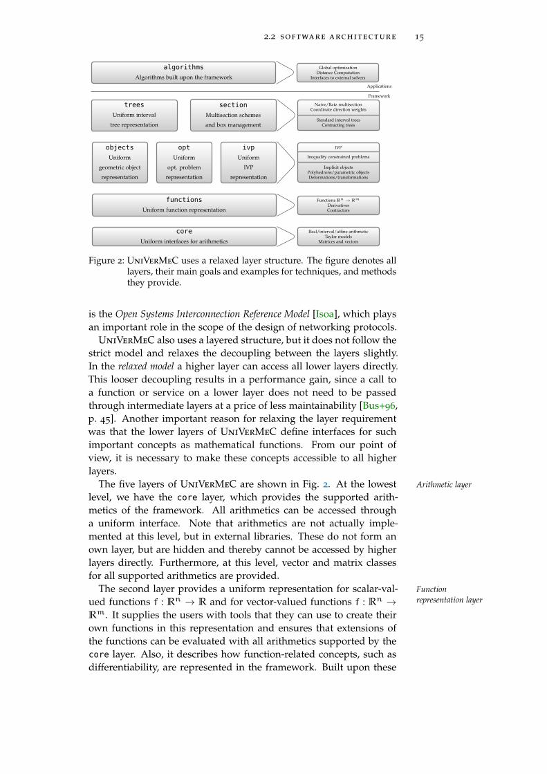
Figure 2: UniVerMeC uses a relaxed layer structure. The figure denotes alllayers, their main goals and examples for techniques, and methodsthey provide.
is the Open Systems Interconnection Reference Model [Isoa], which playsan important role in the scope of the design of networking protocols.
UniVerMeC also uses a layered structure, but it does not follow thestrict model and relaxes the decoupling between the layers slightly.In the relaxed model a higher layer can access all lower layers directly.This looser decoupling results in a performance gain, since a call toa function or service on a lower layer does not need to be passedthrough intermediate layers at a price of less maintainability [Bus+96,p. 45]. Another important reason for relaxing the layer requirementwas that the lower layers of UniVerMeC define interfaces for suchimportant concepts as mathematical functions. From our point ofview, it is necessary to make these concepts accessible to all higherlayers.
The five layers of UniVerMeC are shown in Fig. 2. At the lowest Arithmetic layer
level, we have the core layer, which provides the supported arith-metics of the framework. All arithmetics can be accessed througha uniform interface. Note that arithmetics are not actually imple-mented at this level, but in external libraries. These do not form anown layer, but are hidden and thereby cannot be accessed by higherlayers directly. Furthermore, at this level, vector and matrix classesfor all supported arithmetics are provided.
The second layer provides a uniform representation for scalar-val- Functionrepresentation layerued functions f : Rn → R and for vector-valued functions f : Rn →
Rm. It supplies the users with tools that they can use to create theirown functions in this representation and ensures that extensions ofthe functions can be evaluated with all arithmetics supported by thecore layer. Also, it describes how function-related concepts, such asdifferentiability, are represented in the framework. Built upon these
16 univermec software
functionalities, the layer provides a uniform representation of intervalcontractors and enclosures.
The modeling layer lies in the middle of the framework. It is di-Modeling layer
vided into three independent layers: the objects layer, which repre-sents geometric objects, the opt layer for optimization problems, andthe ivp layer for IVPs. The sublayers depend on the problem domain.The objects layer maps discrete geometric structures, such as poly-hedrons and smooth structures (e.g., implicit objects) on a uniformdescription. The layer describes objects independently of their un-derlying modeling type. Furthermore, it provides deformations ortransformations to alter objects. In general, an optimization problemconsists of an objective function, inequality constraints, and boundson the variables. They are assembled in the opt sublayer to providea uniform representation. The ivp sublayer combines the functiondescribing the problem’s right-hand side with the related data, forexample, initial values or possibly time dependent parameters, intoan abstract IVP description. It can be solved by IVP solvers interfacedto the framework.
Basically, the fourth layer consists of two separated layers. On theDecomposition layer
one hand, we have the trees part, which defines and supplies hierar-chical space decomposition structures working on the geometric ob-jects descriptions generated by the objects layer. On the other hand,we have the section layer, which provides multisection schemes. Theydo not work on objects but only on box-shaped regions in a user-defined space. Note that both layers basically provide utility datastructures for the algorithms. Consequently, the structures of thetrees layer are not considered to be geometric objects.
Algorithms making use of the services and methods provided byAlgorithm layer
UniVerMeC are implemented at the topmost layer. Currently, a veri-fied global optimization method and an algorithm for computing anenclosure of the distance between possibly non-convex objects areavailable. Furthermore, interfaces to solvers for optimization andIVPs are provided on this level. They make use of the problemdescription capability of UniVerMeC. Algorithms within the frame-work can employ them, for example, to speed up the computationalprocess.
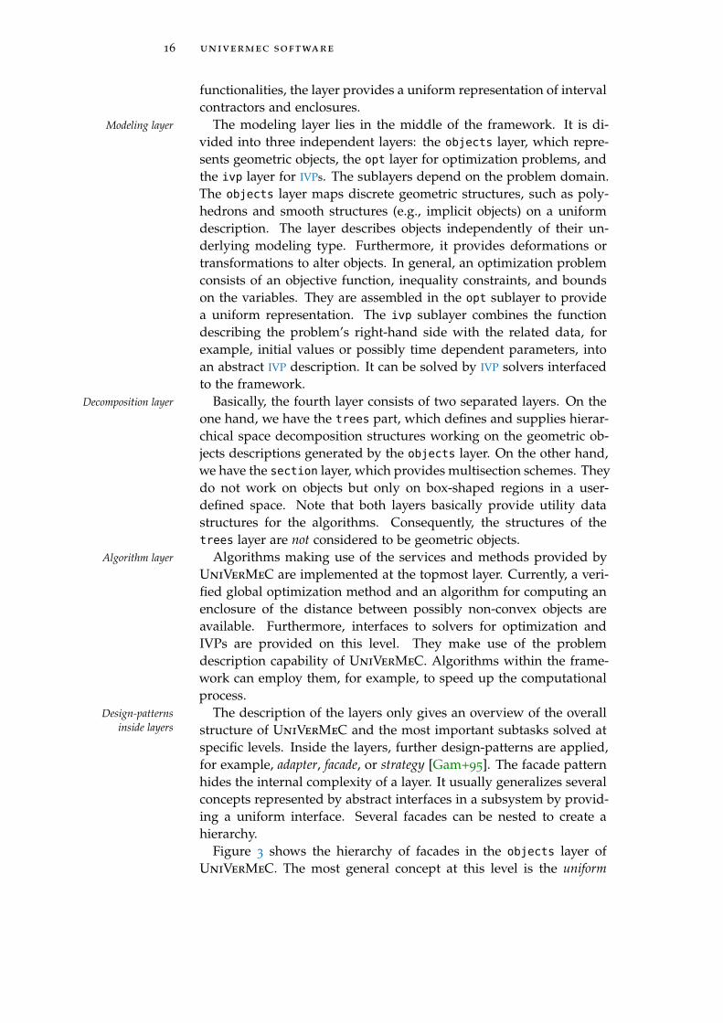
The description of the layers only gives an overview of the overallDesign-patternsinside layers structure of UniVerMeC and the most important subtasks solved at
specific levels. Inside the layers, further design-patterns are applied,for example, adapter, facade, or strategy [Gam+95]. The facade patternhides the internal complexity of a layer. It usually generalizes severalconcepts represented by abstract interfaces in a subsystem by provid-ing a uniform interface. Several facades can be nested to create ahierarchy.
Figure 3 shows the hierarchy of facades in the objects layer ofUniVerMeC. The most general concept at this level is the uniform

2.3 use-cases 17
IGeoObj
ICSGNode
ICSGLeaf ICSGTransform
IParamSurface
IParamTrans
IPoly
IConvexPoly
objects
Figure 3: Abstract interfaces forming a hierarchy of facades in the objectslayer. Interfaces at the bottom of the hierarchy represent morespecialized concepts.
object representation provided by the abstract IGeoObj interface. It de-scribes an object by an in/out function, that is, a function that returnswhether a point or a region belongs to the object (lies inside it) or not.Closed objects can be defined by such a function, independently ofwhether they are constructed by a single implicit function, by sev-eral computer solid geometry (CSG) operations, by a (deformed ornon-deformed) parametric function or by a polyhedron. If a methodon a higher level is only capable of handling some specific modelingtype, for example, an algorithm for simplifying a CSG tree, it can re-quest a more specialized interface as input. Note that even the mostspecialized interfaces still hide many implementation details. For ex-ample, CSG operations can be implemented by different branches ofR-functions [Sha91]. The information about what branch is actuallyused is never propagated to a higher level, but is always hidden as theimplementation detail. Since only abstract interfaces pass over layerboundaries, the implementations can be exchanged. More details onthe design of the individual layers and the methods they provide aregiven in the respective chapters later on.
2.3 use-cases
We evaluate our approach during this thesis using several use-cases, Used algorithms
which are outlined in this section. The evaluation is mainly based ontwo algorithms. They are implemented on the top of UniVerMeC:distance computation (Sect. 7.1) and global optimization (Sect. 7.2).The former computes verified bounds on the distance between twoobjects of which both can be non-convex. It works solely on the treerepresentation of the objects and thus is completely decoupled fromthe underlying modeling type (e.g., polyhedron, implicit object, para-metric object). Therefore, the algorithm can compute the distancebetween objects described by two different modeling types (e.g., be-tween polyhedrons and parametric objects). The global optimizationalgorithm does not work with tree decompositions but uses the sec-
18 univermec software
tion layer for space decomposition. It solves classical inequality con-strained optimization problems.
The first use-case is the comparison and evaluation of different ver-Comparison ofrange-enclosure
methodsified techniques for range enclosure in the scope of distance compu-tation. Classical IA overestimates the range of a function in general(Sect. 3.2.5). Sometimes the overestimation is so large that the ob-tained results are useless. For example, a branch and bound algo-rithm can be forced into massive recursion due to clustering effectsoccurring near (local) minimums [DK94] because of overestimation.Several more sophisticated enclosure methods, for example, AA orTMs were, proposed to overcome these problems. However, a faircomparison between these new techniques is still lacking. Using Uni-VerMeC, we compared how long it takes to compute an enclosureof the distance between two smooth objects up to a user-specifiedenclosure width. The framework allows us to use the same imple-mentation of the algorithm for all considered techniques and ensuresthat the overall overhead inside the framework is always the same,thus producing fair comparison results.
In the second use-case, we consider a system for automatic surgeryTotal hipreplacement planning for THR [Cuy11], which was developed in the recent project
PROREOP [Pro]. It uses possibly non-convex multi-component SQ
[Bar81] models or polyhedral models. To ensure that the automat-ically selected implant fits, several distance computations betweentwo SQs or between an SQ and a polyhedron are carried out. UsingUniVerMeC, it is possible to derive verified bounds on the distanceseven in the non-convex cases and to ensure that the selected implantsfit with certainty. Because SQs can be described both parametricallyand implicitly, we are also going to compare distance computationbetween parametrically and implicitly described objects.
The third use-case for the framework is concerned with the param-Parameteridentification of
SOFCseter identification for a thermal SOFC model [AKR12] emerging fromthe research project VerIPC-SOFC. Parameters of a model are usu-ally identified by solving an optimization problem with a quadraticerror measure as the objective function to minimize. It is based onthe deviation of the simulated values for a considered set of param-eters from the measured ones. The goal is to parametrize the modelso that it resembles the real SOFC stack as closely as possible. Sincethe model function is complex2, it is hard to find a global solutionto the problem in general. Furthermore, it is also very expensive toevaluate the function. Therefore, we will also present results that useGPU acceleration.
As a fourth use-case we highlight the possibility to input problemsCombination ofdifferent solvers and then solve them using different solvers that have interfaces to
UniVerMeC. As an example, we show how different verified and
2 It depends on the sum of differences to over 19000 measurements and the simulatedtemperatures can be derived only by solving an IVP numerically.

2.4 user input and output 19
non-verified IVP solvers perform in the simulation of a SOFC modeldescribed by the ivp layer of UniVerMeC, as well as how we canapply FP optimization algorithms for parameter identification of theSOFCs and then validate their results using verified IVP solvers.
2.4 user input and output
Usually, solving a problem starts with creating an appropriate model Model specificationin UniVerMeCby analyzing the real world and identifying aspects relevant to the
current problem, as represented by the verification and validation as-sessment cycle in Fig. 1. A model is a simplified and idealized viewon the world. Typically it introduces some modeling error. Modelsin UniVerMeC are represented using one of the model descriptionlayers of: objects, opt, or ivp. They are problem dependent. That is,if users want to work on a model type not currently supported, theyhave to add an additional model description layer. As seen in Fig. 2,all model description layers are placed at the same level in the middleof the framework above the function and below the decompositionlayer. This positioning is not arbitrary. It enables the model descrip-tion layers to employ concepts defined at lower levels for describingmodels. In particular, it is possible to use intervals, vectors, matrices,and mathematical functions to specify a model.
Now consider a user who wants to input an already existing model Organization ofmodel inputinto the framework. Often, such a model is composed of entities pro-
vided at lower layers of the framework. Because the input in Uni-VerMeC is organized for each layer separately, it is not possible toinput it directly but first to input the parts of the model described atthe lower layers. Then all parts are assembled together to form thecomplete model. In general, we can say that users have to performthe necessary steps to input a model in the reversed data flow orderof the framework, that is, they have to start in Fig. 2 at the bottomand proceed to the top. This is a direct result of the use of a relaxedlayered architecture because it allows (and forces) us to use concepts3
defined at lower layers to describe more abstract concepts at higherlayers.
To illustrate this approach consider the application of UniVerMeC Example
in the scope of the PROREOP project as outlined in Sect. 2.3. The goalis to calculate a bound on the distance between an implant and thefemur-shaft which are both modeled by a multi-component SQ model.If we apply UniVerMeC to the problem, we get the input and outputsas depicted in Fig. 4. In the first step, users can configure options atthe arithmetic level, for example, the bounder for converting a TM toan interval, if they are not satisfied with the standard settings. On the
3 Their use is forced because higher level layers do not provide any tools to describeentities which were defined at lowers levels.

20 univermec software
core functions objects trees algorithms
TM orderTM bounder
SQ parametersImplicit or parametric?
CSG-operationsTrans. parameters
Tree configuration(determines arithmetic
and contractors)
Max. CPU timeDesired tightness
Uniform functionrepresentation
Uniform objectrepresentation
Uniform treerepresentation
ResultsStatus information
Figure 4: User input and corresponding ouput at the different abstractionlevels of UniVerMeC for the distance computation use-case.
next layer, users can input the SQ’s parameters4 and choose betweenan implicit or parametric description. The returned uniform functionrepresentation is used at the next level to define implicit or parametricsurfaces or to apply CSG operations, deformations (e.g. tapering andbending), and affine transformations. The result is a uniform objectrepresentation. It describes the multi-component SQ model. At thenext layer, users can configure the hierarchical space decompositionstructures. The tree configuration done here determines what arith-metic to use for a function range enclosure and if contractors or othersophisticated techniques are applied to improve the decomposition’squality. Basically, the trees are just utility data structures for the ac-tual algorithm to calculate the distance. This enables us to decouplethe algorithm from the object representation, range bounders and soon. At the top level, users set the algorithm’s options, for example,the desired tightness of the bound.
While the framework gives an output at every layer, most usersUse of GUIs
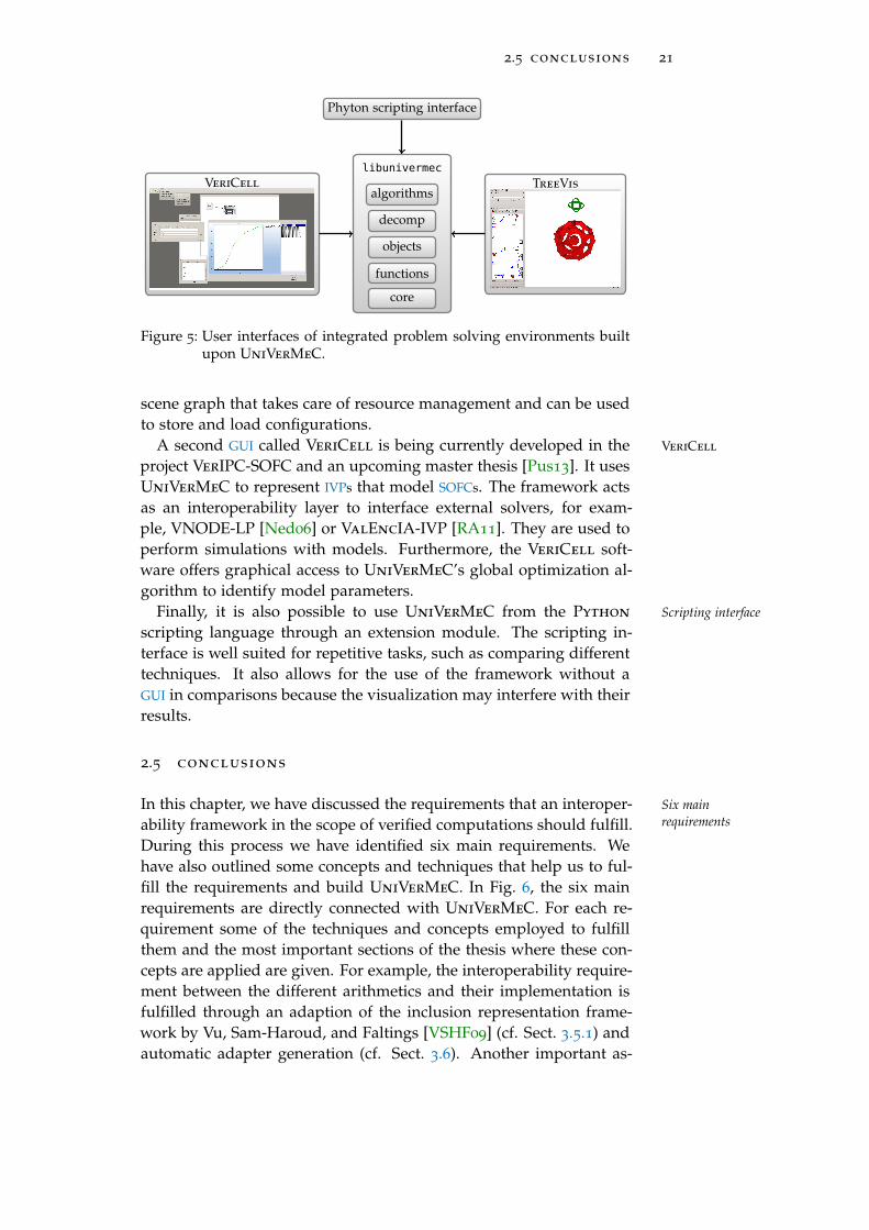
will only be interested in the values returned by the algorithms onthe topmost layer. Therefore, these parts of the framework are linkedinto a dynamic library called libunivermec, which is then utilized bygraphical user interface (GUI) programs as depicted in Fig. 5. Theyhide the intermediate steps outlined in this section.
The program TreeVis was developed in the scope of project Tell-TreeVis
Him&S. It provides access to the geometric part of UniVerMeC, thatis, the geometric objects layer, the distance computation algorithm,and the hierarchical decomposition structures. It allows users to de-fine implicit or parametric objects based on smooth functions easilyby entering the formulas directly or by choosing predefined ones. Fur-thermore, it can load polyhedrons into the framework. The trees areconfigured through the user interface graphically and then the dis-tance computation can be run on them. It can visualize the trees anddistances using OpenGL. All these steps are carried out on a special
4 Strictly speaking, the SQ parameters, for example, roundness or scaling are FP num-bers or intervals and belong to the core layer and have to be entered there. We omitthis details for clarity reasons.
2.5 conclusions 21
libunivermec
algorithms
decomp
objects
functions
core
TreeVisVeriCell
Phyton scripting interface
Figure 5: User interfaces of integrated problem solving environments builtupon UniVerMeC.
scene graph that takes care of resource management and can be usedto store and load configurations.
A second GUI called VeriCell is being currently developed in the VeriCell
project VerIPC-SOFC and an upcoming master thesis [Pus13]. It usesUniVerMeC to represent IVPs that model SOFCs. The framework actsas an interoperability layer to interface external solvers, for exam-ple, VNODE-LP [Ned06] or ValEncIA-IVP [RA11]. They are used toperform simulations with models. Furthermore, the VeriCell soft-ware offers graphical access to UniVerMeC’s global optimization al-gorithm to identify model parameters.
Finally, it is also possible to use UniVerMeC from the Python Scripting interface
scripting language through an extension module. The scripting in-terface is well suited for repetitive tasks, such as comparing differenttechniques. It also allows for the use of the framework without aGUI in comparisons because the visualization may interfere with theirresults.
2.5 conclusions
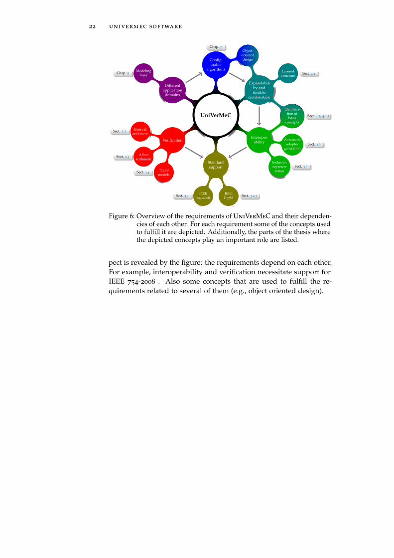
In this chapter, we have discussed the requirements that an interoper- Six mainrequirementsability framework in the scope of verified computations should fulfill.
During this process we have identified six main requirements. Wehave also outlined some concepts and techniques that help us to ful-fill the requirements and build UniVerMeC. In Fig. 6, the six mainrequirements are directly connected with UniVerMeC. For each re-quirement some of the techniques and concepts employed to fulfillthem and the most important sections of the thesis where these con-cepts are applied are given. For example, the interoperability require-ment between the different arithmetics and their implementation isfulfilled through an adaption of the inclusion representation frame-work by Vu, Sam-Haroud, and Faltings [VSHF09] (cf. Sect. 3.5.1) andautomatic adapter generation (cf. Sect. 3.6). Another important as-
22 univermec software
UniVerMeC
Verification
Intervalarithmetic
Affinearithmetic
Taylormodels
Standardsupport
IEEE754-2008
IEEEP1788
Interoper-ability
Inclusionrepresen-
tation
Automaticadapter
generation
Expandabil-ity andflexible
combination
Layeredstructure
Config-urable
algorithms
Differentapplication
domains
Modelinglayer
Object-orienteddesign
Identifica-tion ofbasis
concepts
Sect. 3.5
Sect. 3.6
Sect. 3.2
Sect. 3.3
Sect. 3.4
Sect. 3.1 Sect. 3.2.3
Chap. 5
Chap. 7
Sect. 4.3, 4.4.1
Sect. 2.2
Figure 6: Overview of the requirements of UniVerMeC and their dependen-cies of each other. For each requirement some of the concepts usedto fulfill it are depicted. Additionally, the parts of the thesis wherethe depicted concepts play an important role are listed.
pect is revealed by the figure: the requirements depend on each other.For example, interoperability and verification necessitate support forIEEE 754-2008 . Also some concepts that are used to fulfill the re-quirements related to several of them (e.g., object oriented design).

3A R I T H M E T I C S
The purpose of this chapter is twofold: the first four sections give an Rigorous arithmetics
introduction into the basic arithmetics for verified computations ona digital computer, and the remaining sections discuss the interoper-ability of the mentioned arithmetics. Arithmetics are the crucial basicbuilding blocks for verified computations. Therefore, different arith-metics and even more variants of them have been proposed duringthe last 50 years. The chapter introduces the most commonly usedrigorous range arithmetics: interval arithmetic, affine arithmetic, andTaylor models. The discussion highlights not only their theoretical as-pects but also their different implementations. We will show throughthe example of AA how to develop a generic library which fits wellinto existing interval environment and handles numerous variants ofAA by employing policy-based design.
It is well-known that, besides special cases, rigorous range arith- Improvingrange-boundsmetics, such as IA or AA only return a rough outer bound, that is, an
over-approximating bound on the range of an expression. Usually,we can improve the bounds by subdividing the considered range thatleads to the classic branch and bound algorithms, which are applied,for example, in global optimization. However, their brute force subdi-vision of the search space leads to an exponential runtime. Anotherway to obtain sharper bounds is to use different methods for rangebounding, because, depending on the expression, either interval oraffine arithmetic might provide better bounds for its range. It is evenpossible to intersect the bounds computed by different methods inorder to improve them. This is, for example, offered by libaa [Sto]library for IA and AA .
Recently, Vu, Sam-Haroud, and Faltings [VSHF09] proposed a gen- Inclusionrepresentationeral formal framework for using different rigorous range arithmetics
simultaneously in the scope of constraint programming. They intro-duce the notion of a so-called inclusion representation and derive on itsbasis formalizations for inclusion functions and natural extensionsindependent of the actual arithmetic. Furthermore, they show thattheir inclusion representation can be applied to IA and different vari-ants of AA. However, they do not discuss the practical consequencesof providing an environment that supports different arithmetics andpossibly different libraries for each of them. One goal of this chap-ter is to build a theoretical basis and an implementation that solvespractical problems while combining different arithmetics.
The chapter starts with a brief discussion of FPA in Sect. 3.1. It Chapter structure
is followed by Sect. 3.2, which introduces IA, the upcoming IEEE
23

24 arithmetics
P1788, and possible implementations. AA, its variants, and our ownimplementation YalAA are discussed throughout in Sect. 3.3. TMs arethe last of our four supported arithmetics, and described in Sect. 3.4.Based on the work by Vu, Sam-Haroud, and Faltings, which we out-line in Sect. 3.5, we build the theoretical foundation for the arithmeticlayer of our software. Moreover, we extend their work by present-ing an inclusion representation for TMs. As a preparation for thepractical implementation based on the inclusion representation, weformulate a heterogeneous algebra for all arithmetics, which definesa common set of operations, elementary functions and the possibilityof operations between different arithmetics. As a foundation for ourset of functions, we chose the upcoming IEEE P1788 interval standard.After that, we present possible conversions between the arithmetics,also based on the inclusion representations. Finally, in Sect. 3.6 wecombine our theoretical considerations to provide a generator frame-work for adapters. The adapters should tackle the practical challengesevolving from the use of different arithmetics and libraries providedby different vendors. Finally, Sect. 3.7 discusses interoperability chal-lenges that come into play if we work in a heterogeneous CPU/GPU
environment.
3.1 floating-point arithmetic
By default, even a modern computer does not perform arithmeticFloating-pointsystem operations on the real numbers exactly in hardware. Instead, the
operands are usually converted to machine number (e.g., FP num-bers). With these, operations are performed that only approximatetheir exact counterpart in general. Modern computers usually con-tain a FP unit that conforms with the IEEE 754-2008 [Iee] standard.Following Muller et al. [Mul+10, pp. 13-20], we define a FP system asan integer 4-tuple (β,p, emin, emax) with the base β > 2, the precisionp > 2, and the minimum and maximum exponents emin, emax. A num-ber x belongs to the FP system if it can be represented by a 3-tuple(s,m, e):
x = (−1)s ·m ·βe
where s ∈ {0, 1} is the sign, e the integer exponent with emin 6 e 6emax and m = |M| ·β1−p the significand. It holds 0 6 m < β and theintegral significand M satisfies |M| 6 βp−1. A normalized represen-tation has to comply with 1 6 |m| < β.
IEEE 754-2008 specifies several FP formats. However, the singleIEEE 754-2008standard and double precision formats (cf. Tab. 2) are the most widely used.
In the rest of this work, we denote the set of double precision FP num-bers excluding ±∞ and NaN by F. The extended set of FP numbersF ∪ {−∞,∞, NaN} is denoted by F. Accordingly, R denotes the set ofextended real numbers R ∪ {−∞,∞}. In general, we will call mem-

3.2 interval arithmetic 25
Table 2: IEEE 754-2008 single and double precision formats
format p emin emax
Single 24 -126 127
Double 53 -1022 1023
bers of F that are not in F special forms. The operators F(D) and F(D ′)return the set of all (extended) FP numbers contained in D ⊆ R andD ′ ⊆ R respectively. The set of FP numbers is finite. Thus, in general,a number x ∈ R has to be approximated by a FP number x ∈ F. Theapproximated number is derived by a mapping fl : R → F, which iscalled a rounding [Rum10, p. 302], [Mul+10, pp. 20-25]. The IEEE 754-2008 provides several definitions for a rounding. The standard moderound to nearest chooses the FP number with the minimum deviationfrom the real result
|fl(x) − x| = minf∈F
|f− x| .
If the result lies exactly between two FP numbers, the even number ischosen. The two directed rounding modes round to ±∞ are of specialinterest for our work. The rounding fl+∞(x) returns the smallest FP
number greater than x, whereas fl−∞(x) returns the largest FP numberless than x.
Unfortunately, the IEEE 754-2008 standard only defines the four Correctly rounded
basic arithmetic operations {+,−, ·, /} and square root. They can bedefined using a rounding [Rum10, p. 302], [Mul+10, pp. 20-25] by
x ◦y := fl(x ◦ y) ,
where x,y ∈ F, ◦ ∈ {+,−, ·, /} is the real- and ◦ the correspondingFP operation. We call these operations correctly rounded because theirresult is identical to the result of the exact operation rounded to thenext FP number under the current rounding. The results obtained forother elementary functions, such as exponential, logarithm or trigono-metric functions provided by modern processors and programmingenvironments are often not correctly rounded. In specific, the IEEE754-2008 does not make any guarantees for them.
3.2 interval arithmetic
While interval analysis is older than digital computer systems, the Interval analysis
modern use of it in verified numerics on computers is widely at-tributed to Ramon E. Moore, who published his book Interval Analysisin 1966 [Moo66]. IA is capable of deriving rigorous lower and upperbounds on an exact result even in the presence of rounding errors. It

26 arithmetics
can compute (rigorous) bounds on a function’s codomain over someaxis-aligned box. Our discussion of the basic properties of intervalarithmetic follows [AH83].
3.2.1 Basic Arithmetic
A compact real intervalCompact realinterval
x = [x, x] ={x∣∣ x 6 x 6 x}
consists of two endpoints x, x ∈ R, which we call lower and upperbound respectively. We denote the set of all compact and non-emptyreal intervals with IR. Furthermore, we define the midpoint of aninterval
mid (x) :=x+ x
2, (1)
its width
wid (x) := x− x , (2)
its radius
rad (x) :=x− x
2, (3)
and the midpoint-radius1 form
< mid x, rad x >:={x∣∣ mid x− rad x 6 x 6 mid x+ rad x
}= x .
An interval is empty if x > x and unbounded if at least one end-point is ±∞. The extended set of intervals IR includes empty andunbounded intervals. As for the FP numbers, we call members ofIR those that are not in IR special forms. Furthermore, the IR(D)
operator returns the set of all real intervals over D ⊂ R.A basic arithmetic operation ◦ ∈ {+,−, ·, /} is defined for two inter-Basic operations
vals x,y ∈ IR as:
x ◦y ={x ◦ y
∣∣ x ∈ x,y ∈ y}
. (4)
1 All intervals in this work are considered to be in endpoint form if not specifiedotherwise.

3.2 interval arithmetic 27
x1
x2
Figure 7: The rectangle represented by the two dimensional interval vector([2, 3], [1, 4]).
The division is only defined if 0 6∈ y holds. Explicit endpoint formu-las can be derived for all operations:
x+y =[x+ y, x+ y
]x−y =
[x− y, x− y
]x ·y =
[min
(xy, xy, xy, xy
), max
(xy, xy, xy, xy
)]1/x =
[1
x,1
x
], for 0 /∈ x .
(5)
The result of all operations (5) is again an interval. Therefore, IR
is closed under the basic arithmetic operations. We call a functionF : IRn ⊃ D→ IRm an inclusion function for f : Rn ⊃ D→ Rm overan interval box x ∈ IRn if the inclusion property
F(x) ⊇{f(x)
∣∣ x ∈ x} (6)
holds. An interval vector x ∈ IRn is an axis-aligned n-dimensionalcuboid, which we will also call a box. Geometrically it is a rectanglein two dimensions (cf. Fig. 7).
On a computer, we work with machine intervals, the endpoints Machine intervals
of which are FP numbers. We denote the set of all bounded andnon-empty machine intervals with IF. If we include empty and un-bounded intervals, we obtain IF. The IF(D) and IF(D ′) operatorsreturn the set of all machine intervals over D ⊆ R,D ′ ⊆ R. For ma-chine intervals, the basic operations also obey the inclusion property,that is, x ◦ y ⊆ x� y holds for the real operations ◦ ∈ {+,−, ·, /} andthe respective machine operation �. The more strict definition givenin (4) does not hold in general. Usually, this is achieved by usingdirected roundings for the formulas (5). That is, the result of a realoperation is rounded towards −∞ and +∞ for the lower and upperbound respectively. Note that (4) can yield a member of IF in generaleven if all operands are members of IF.

28 arithmetics
Usually, not only the basic operations (5) but also elementary func-Elementaryfunctions tions, such as sine, cosine, logarithm, or exponential, are needed in a
practical computation. Interval extensions of these satisfying (6) canbe constructed, for example, through polynomial series expansionsor by considering their monotonicity features. Ready to use func-tions are provided by interval libraries, for example, C-XSC [HK04]or filib++ [Ler+06]. One problem with these implementations is thatthey do not necessarily provide the same set of functions or the do-main on which the interval extension is defined. These incompatibil-ities are tackled by the upcoming interval standard IEEE P1788 (cf.Sect. 3.2.3), where a set of elementary standard functions, includingtheir domains, has been defined. While to our knowledge no libraryyet fully supports the functions required by IEEE P1788, we can as-sume in the remainder of this work that usable interval extensions ofthe common elementary functions are available.
3.2.2 Natural Interval Extension
An easy way to construct a function satisfying the inclusion prop-Natural extension
erty (6) is the natural interval extension.
Definition 2 (Natural interval extension) Let an inductively describedfunction2 f : Rn ⊃ D → Rm be given. If we replace all quantities in f bytheir respective interval counterparts, we obtain an inclusion function F forf, which we call the natural interval extension of f.
The natural interval extension F is inclusion monotonicProperties of thenatural extension
x ⊂ y =⇒ F(x) ⊂ F(y) (7)
and thin
F(x) = f(x) (8)
for x = [x, x]. Furthermore, if every variable appears only once in theexpression describing f, and if all used operations and elementaryfunctions are continuous, then F is minimal. This means that for agiven y ∈ IRn
¬∃x ∈ IR : F(y) \ x 6= ∅∧ ∀y ∈ y : f(y) ∈ x , (9)
that is, F computes the smallest box satisfying the inclusion prop-erty (6) [Jau+01, Theorem 2.2].
2 That is, the function is given by a finite composition of the basic operations {+,−, ·, /},elementary functions, variables and constants.

3.2 interval arithmetic 29
Encoding
Representation
encodes
Interval datum
represents
Mathematical model
identityinterval hull
Figure 8: The layers of IEEE P1788 as defined in [P17, pp. 13-14].
3.2.3 P1788 - Interval Standard
Currently, a standardization process for IA takes place in the IEEE IEEE P1788
P1788 working group with the goal to create an interval standard sim-ilar to IEEE 754-2008 for FP arithmetic. Because a final version is notavailable at the moment, the following paragraph outlines only partsimportant for UniVerMeC. It is based on the draft version 8.4 [P17].
In Fig. 8 the four layers (or levels) of IEEE P1788 are shown. They IEEE P1788 layers
are similar to the layers in the IEEE 754-2008 standard. The bottomlayer defines the mathematical theory on which the standard is based,that is, the real interval IR system over real numbers system R andcorresponding arithmetic operations3. At the second layer, the intervaldatums are introduced approximating the mathematical objects fromthe first layer by a finite set. Every interval datum is a real interval,but a real interval can be in general only represented with the helpof the interval hull operation on the interval datum layer. The thirdlayer describes the representation of an interval datum, for example,by two FP numbers. Finally, intervals are encoded as bit strings onthe uppermost layer, with no further requirements.
In the scope of UniVerMeC, the set of standard operations and Set of elementaryfunctionselementary functions required by IEEE P1788 [P17; WK09] is of a
special importance4. The text of the standard specifies not only a setof elementary functions but also their definition domains and ranges.This is important for functions, for example, the power function, forwhich different definitions and thus different definition domains andfunction ranges make sense depending on the concrete applicationcontext5. The heterogeneous algebra concept from Sect. 3.5 is based
3 The IEEE P1788 standard draft allows for certain flavors of intervals [P17, pp. 17-18]. We restrict our discussion to the set–based flavor [P17, pp. 27-68] which is usedthroughout this work.
4 This part of the text of the standard has already passed the voting in the IEEE P1788
group.5 See [HNW13] for a discussion of possible variants of the interval power function.

30 arithmetics
on the specifications of the IEEE P1788 standard. This concept isused to provide a uniform set of elementary functions for all rangearithmetics supported by UniVerMeC and to ensure interoperabilitybetween them.
An important aspect discussed in the scope of IEEE P1788 is theMidpoint and radius
representation of intervals in the midpoint-radius form instead of theendpoint-form. The motion [VH12] included into the current stan-dard draft [P17, p. 60], defines the midpoint and the radius of aninterval to ensure that a verified conversion to the midpoint-radiusform is easily possible. While we limit our discussion to the end-point representation of intervals in the scope of this thesis, we usethe definitions from IEEE P1788 for the midpoint and the radius inthe remainder of this work:
Definition 3 (Midpoint [P17; VH12]) For an interval x ∈ IF, mid (x)
is the mathematical midpoint x+x2 rounded to nearest, ties to even. Themidpoints of (−∞,∞), (−∞,a], and [a,∞] for a ∈ F are defined as 0, thesmallest representable FP number, and the biggest representable FP numberrespectively.
Definition 4 (Radius [P17; VH12]) For an interval x ∈ IF the radiusrad (x) is the smallest number in F so that x is contained in[mid (x) − rad (x), mid (x) + rad (x)].
Another interesting concept in IEEE P1788 is the exception han-Decorations
dling realized by decorated intervals. A decorated interval consistsof an interval and a decoration. The decoration is mainly intendedfor tracking properties of inductively defined functions through theircomputational graphs. Formally, a decoration in the context of theset-based flavor6 describes the properties of a pair (f, x) where f :
Rn ⊃ D → R and x ∈ IRn [P17, p. 40]. For the set–based fla-
vor considered in this thesis, the decorations in Tab. 3 are supported.The ordering of the decorations is quality based. Following IEEEP1788 we can say that “decorations above trv are ‘good’ and thosebelow are ‘bad’ ” [P17, p. 40]. Note that the com decoration impliesfor machine arithmetic7 that no overflow happened [P17, p. 44]. Animportant advantage over global flags used in IEEE 754-2008 is thata decoration is directly attached to a datum. However, decorationsrequire more memory and are computationally more expensive. Toreduce these penalties, IEEE P1788 offers an optional computationmode with compressed intervals with less recorded information [P17,pp. 45-46]. To our knowledge, no IA library besides JInterval [NZ14]implements the decoration concept of IEEE P1788 currently. However,
6 Every IEEE P1788 conforming interval flavor has its own set of decorations andpropagation rules. These must comply with the basic principles of the decorationsystem given in [P17, pp. 21-23]. Our discussion is limited to the decoration systemof the set-based flavor [P17, pp. 40-46].
7 the second level in IEEE P1788
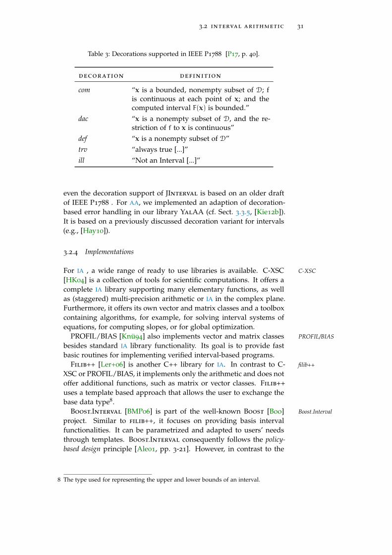
3.2 interval arithmetic 31
Table 3: Decorations supported in IEEE P1788 [P17, p. 40].
decoration definition
com “x is a bounded, nonempty subset of D; fis continuous at each point of x; and thecomputed interval F(x) is bounded.”
dac “x is a nonempty subset of D, and the re-striction of f to x is continuous”
def “x is a nonempty subset of D”trv “always true [...]”ill “Not an Interval [...]”
even the decoration support of JInterval is based on an older draftof IEEE P1788 . For AA, we implemented an adaption of decoration-based error handling in our library YalAA (cf. Sect. 3.3.5, [Kie12b]).It is based on a previously discussed decoration variant for intervals(e.g., [Hay10]).
3.2.4 Implementations
For IA , a wide range of ready to use libraries is available. C-XSC C-XSC
[HK04] is a collection of tools for scientific computations. It offers acomplete IA library supporting many elementary functions, as wellas (staggered) multi-precision arithmetic or IA in the complex plane.Furthermore, it offers its own vector and matrix classes and a toolboxcontaining algorithms, for example, for solving interval systems ofequations, for computing slopes, or for global optimization.
PROFIL/BIAS [Knü94] also implements vector and matrix classes PROFIL/BIAS
besides standard IA library functionality. Its goal is to provide fastbasic routines for implementing verified interval-based programs.
Filib++ [Ler+06] is another C++ library for IA. In contrast to C- filib++
XSC or PROFIL/BIAS, it implements only the arithmetic and does notoffer additional functions, such as matrix or vector classes. Filib++uses a template based approach that allows the user to exchange thebase data type8.
Boost.Interval [BMP06] is part of the well-known Boost [Boo] Boost.Interval
project. Similar to filib++, it focuses on providing basis intervalfunctionalities. It can be parametrized and adapted to users’ needsthrough templates. Boost.Interval consequently follows the policy-based design principle [Ale01, pp. 3-21]. However, in contrast to the
8 The type used for representing the upper and lower bounds of an interval.
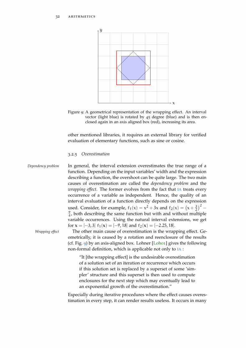
32 arithmetics
x
y
Figure 9: A geometrical representation of the wrapping effect. An intervalvector (light blue) is rotated by 45 degree (blue) and is then en-closed again in an axis aligned box (red), increasing its area.
other mentioned libraries, it requires an external library for verifiedevaluation of elementary functions, such as sine or cosine.
3.2.5 Overestimation
In general, the interval extension overestimates the true range of aDependency problem
function. Depending on the input variables’ width and the expressiondescribing a function, the overshoot can be quite large. The two maincauses of overestimation are called the dependency problem and thewrapping effect. The former evolves from the fact that IA treats everyoccurrence of a variable as independent. Hence, the quality of aninterval evaluation of a function directly depends on the expressionused. Consider, for example, f1(x) = x2 + 3x and f2(x) =
(x+ 3
2
)2−
94 , both describing the same function but with and without multiplevariable occurrences. Using the natural interval extensions, we getfor x = [−3, 3] f1(x) = [−9, 18] and f2(x) = [−2.25, 18].
The other main cause of overestimation is the wrapping effect. Ge-Wrapping effect
ometrically, it is caused by a rotation and reenclosure of the results(cf. Fig. 9) by an axis-aligned box. Lohner [Loh01] gives the followingnon-formal definition, which is applicable not only to IA :
“It [the wrapping effect] is the undesirable overestimationof a solution set of an iteration or recurrence which occursif this solution set is replaced by a superset of some ’sim-pler’ structure and this superset is then used to computeenclosures for the next step which may eventually lead toan exponential growth of the overestimation.”
Especially during iterative procedures where the effect causes overes-timation in every step, it can render results useless. It occurs in many
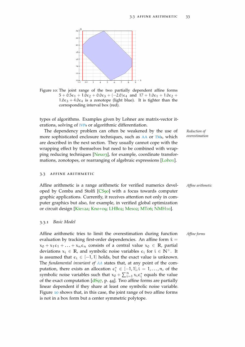
3.3 affine arithmetic 33
x
y
1.0 2.0 3 4 5 6 7 8 9
10
12
14
16
18
20
22
24
Figure 10: The joint range of the two partially dependent affine forms5 + 0.5ε1 + 1.0ε2 + 0.0ε3 + (−2.0)ε4 and 17 + 1.0ε1 + 1.0ε2 +1.0ε3 + 4.0ε4 is a zonotope (light blue). It is tighter than thecorresponding interval box (red).
types of algorithms. Examples given by Lohner are matrix-vector it-erations, solving of IVPs or algorithmic differentiation.
The dependency problem can often be weakened by the use of Reduction ofoverestimationmore sophisticated enclosure techniques, such as AA or TMs, which
are described in the next section. They usually cannot cope with thewrapping effect by themselves but need to be combined with wrap-ping reducing techniques [Neu03], for example, coordinate transfor-mations, zonotopes, or rearranging of algebraic expressions [Loh01].
3.3 affine arithmetic
Affine arithmetic is a range arithmetic for verified numerics devel- Affine arithmetic
oped by Comba and Stolfi [CS90] with a focus towards computergraphic applications. Currently, it receives attention not only in com-puter graphics but also, for example, in verified global optimizationor circuit design [Kie12a; Kno+09; LHB02; Mes02; MT06; NMH10].
3.3.1 Basic Model
Affine arithmetic tries to limit the overestimation during function Affine forms
evaluation by tracking first-order dependencies. An affine form x =
x0 + x1ε1 + . . . + xnεn consists of a central value x0 ∈ R, partialdeviations xi ∈ R, and symbolic noise variables εi for i ∈ N+. Itis assumed that εi ∈ [−1, 1] holds, but the exact value is unknown.The fundamental invariant of AA states that, at any point of the com-putation, there exists an allocation ε∗i ∈ [−1, 1], i = 1, . . . ,n, of thesymbolic noise variables such that x0 +
∑ni=1 xiε
∗i equals the value
of the exact computation [dS97, p. 44]. Two affine forms are partiallylinear dependent if they share at least one symbolic noise variable.Figure 10 shows that, in this case, the joint range of two affine formsis not in a box form but a center symmetric polytope.
34 arithmetics
In the following, we denote the set of all affine forms over the realOperations
numbers by AR. For two affine forms x, y ∈ AR and a scalar α ∈ R,Comba and Stolfi define the basic affine operations addition, scaling,and translation straightforwardly:
x+ y = (x0 + y0) + (x1 + y1)ε1 + . . .+ (xn + yn)εn ,
αx = αx0 +αx1ε1 + . . .+αxnεn ,
α+ x = (x0 +α) + x1ε1 + . . .+ xnεn .
(10)
In case of nonlinear operations, such as division or multiplication, aswell as for elementary functions, such as square root, sine, cosine, itis not possible to carry out affine computations directly. The basicidea for evaluating a nonlinear function f in the affine computationalmodel is to split it into its affine and non-affine parts. Usually, this isdone by providing an affine approximation fa. Afterwards, the non-linear part is enclosed and a new error term xn+1εn+1 with the newindependent noise variable εn+1 is appended to the affine form. Wewill discuss the implementation of nonlinear elementary functions inAA in Sect. 3.3.3 in more detail.
Formally an interval containing the range of an affine form x =Conversions to andfrom IA x0 +
∑ni=0 xiεi can be obtained by replacing all symbolic noise vari-
ables εi by their interval domain [−1, 1]:
x = x0 +
n∑i=0
xi · [−1, 1] . (11)
Furthermore, we can derive an affine form x enclosing an interval xby
x = mid (x) + rad (x)εn+1 (12)
where εn+1 is a symbolic noise variable that was not used before.In practice, we work with FP numbers instead of real numbers toAA with FPA
represent the partial deviations in an affine form. In the following, wedenote the set of all affine forms over the FP numbers with AF. Here,the affine operations (10) are no longer exact but incur a roundingerror, which we have to determine. De Figueiredo and Stolfi [dS97,pp. 51-53] propose to perform the operations three times (with roundto nearest and to plus/minus infinity respectively) in order to obtainthe exact rounding error. After that, they add it as a new indepen-dent error term to the affine form. It is also important to note that,in (12) the midpoint and radius, Def. 3, 4 have to be used to ensureproper inclusions. Due to the use of FP numbers, overflows can oc-cur. Most implementations of affine arithmetic allow us to detectoverflows during the computation by providing a special form. Forexample, two special forms are introduced in the error handling ap-proach proposed in [dS97, p. 46]: The empty affine form and a form

3.3 affine arithmetic 35
covering the whole real line. The extended set of affine forms overthe FP numbers AF contains these special forms in addition to allmembers of the set AF. It depends on the actual implementationused if and what special forms are available.
3.3.2 Extended Models
Several authors [Bil08; Kol07; Mes02; MT06; NM11] proposed im- Classification ofimprovementsprovements to the basic AA model. Most of them can be classified
into three groups: better implementation techniques, changes in themodel without the necessity to add higher-order noise symbols, andthese with higher order noise symbols.
An example for the first category is the a posteriori error correc- Betterimplementationtechniques
tion approach [NM11]. Its goal is to reduce the number of roundingmode switches at the expense of precision, which usually results ina faster computation. Another example is the improved multiplica-tion routine described in [Kol07]. These kind of improvements can beintegrated into an implementation without too much effort.
The second category consists of improvements that alter the compu- Altered computationmodeltation model itself but still retain an affine model. Commonly known
examples are the AF1 and AF2 forms introduced by Messine [Mes02].In both models, the number of independent noise symbols is limitedto the number of independent input variables, thus preventing thegrowth of affine forms during a lengthy computation process. Theyalso add special terms for coping with round off or approximationerrors.
Finally, there are extended models that also track nonlinear depen- Higher-order noisesymbolsdencies in the computational graph up to a certain degree. Messine
introduces in [MT06] an affine computation model with quadraticnoise symbols xiε2i . Bilotta [Bil08] considers the general case wherenoise symbols up to a chosen order n are used.
3.3.3 Implementation of Elementary Functions
The overall usability of an AA library heavily depends on the number Referenceimplementationof provided elementary functions and their quality. At the moment,
most publicly available libraries orient themselves on the implementa-tion guidelines given by de Figueiredo and Stolfi [dS97]. The authorsalso provide a free reference implementation [Sto].
3.3.3.1 Convex and Concave Functions
In [dS97, pp. 55ff.;64ff.] de Figueiredo and Stolfi propose two methods Implementingnon-affine functionsfor implementing a non-affine function: the best affine approximation
and the min-range approximation. To simplify matters, they only con-sider one-dimensional affine approximations f(x) = αx+ζ± δ, where

36 arithmetics
x
f(x)
1.01.0
e exex
u = ln(e− 1)
p∗1(x)
(a) Best approximation p∗1(x)
x
f(x)
1.01.0
1.00.0
e ex
p◦1(x)
(b) Min-range po1(x)
Figure 11: Affine approximations for ex over [0, 1].
δ is the approximation error. However, the affine form x is a first-order polynomial in its n symbolic noise symbols ε1, · · · , εn. That is,the authors ignore that x itself depends on n independent variables.De Figueiredo and Stolfi that this does not impose a limitation forone-dimensional elementary functions, but they do not give a proofof this.
The best polynomial approximation p∗n(x) of degree n to a func-Best polynomialapproximation tion f(x) ∈ C0[a,b] is uniquely defined by the equioscillation prop-
erty [MH03, Theorem 3.4]. It follows from the property that theapproximation error is maximal in (at least) n + 2 points where itattains the absolute value of ||f(x) − pn(x)||∞. In general, p∗n(x) can-not be determined analytically but with iterative procedures, such asthe Remez algorithm [Mul06, pp. 41-46]. However, a polynomial ofdegree one is sufficient for AA . De Figueiredo and Stolfi developed aprocedure for directly determining p∗1(x).
Theorem 1 (Best affine approximation [dS97]) Let f(x) ∈ C2[a,b] bea bounded and convex or concave function. Then p∗1(x) = αx+ ζ is the bestdegree one polynomial approximation over [a,b] with
α :=f(b) − f(a)
b− a,
ζ :=f(u) + f(a) −α(a+ u)
2,
δ :=
∣∣∣∣f(u) − f(a) −α(u− a)
2
∣∣∣∣ ,
where u is defined through f ′(u) = α and δ > ||f(x) − p∗1(x)||∞.

3.3 affine arithmetic 37
The best-affine approximation minimizes the error term δ and thuspreserves as much affine dependencies as possible. Geometrically,it can be visualized as the parallelogram with the minimum area(cf. Fig. 11a). The width on the x-axis is fixed by wid [a,b] and thewidth on the y-axis is minimized as it is determined by δ.
Despite its good properties in preserving affine dependencies, p∗1(x) Min-rangeapproximationoverestimates the range. This is visible in Fig. 11a where p∗1(x) for
the exponential function ex over the domain [0, 1] is shown. The min-imum value of ex is y = 1.0 at x = 0. However, the minimum valuecovered by the parallelogram is y ≈ 0.788133. To reduce the over-estimation, de Figueiredo and Stolfi propose another approximationmethod, which they call min-range affine approximation.
Theorem 2 (Min-range affine approximation [dS97]) Let a convex andbounded function f(x) ∈ C2[a,b] be given. Then p◦1(x) = αx+ ζ is themin-range approximation over [a,b] with
α := f ′(a) ,
ζ :=f(b) + f(a) −α(a− b)
2,
δ :=
∣∣∣∣f(b) +α(a− b) − f(a)2
∣∣∣∣ ,
where δ is the approximation error. The min-range approximation for aconcave function is derived by swapping a and b in the formulas.
As shown in Fig. 11b, the min-range approximation yields a tighterrange, in fact the exact range, for the example at the expense of pre-serving fewer affine dependencies. This results in an increased error.
De Figueiredo and Stolfi also discuss the FP implementation of both FP implementation
techniques. Since p∗1(x) cannot be determined exactly in finite arith-metic, and, thus, the equioscillation property does not hold, it turnsout that the min-range approach needs fewer evaluations of the func-tion to be approximated. This is an important advantage, becausethe evaluation usually needs to be carried out using computationallyexpensive IA 9. In the asymptotic case, both approaches have thequadratic approximation property.
3.3.3.2 Non-Convex and Non-Concave Functions
The restriction to strictly convex or concave functions prevents im- Approximatingnon-convexfunctions
plementation of several important standard functions. Consequently,the reference implementation of AA libaa [Sto] does not contain func-tions, such as the sine or the cosine. Libaffa [GCH] provides them,but the implementation is not fully verified. Because all arithmetics
9 IEEE 754-2008 does not specify the accuracy of elementary functions (aside from thesquare root). Usually, neither the results delivered by standard math libraries arecorrectly rounded, nor rounding modes are respected.

38 arithmetics
supported in UniVerMeC should offer a common set of verified ele-mentary standard functions, we developed the new AA library YalAA(Yet Another Library for Affine Arithmetic) [Kie12b] to overcomethese shortcomings. It offers verified support for non-convex/concavestandard functions through the use of Chebyshev interpolation. Itcan be shown [MH03, Sect. 6.5] that the polynomial approximationobtained in this way is near-best. Therefore, the geometry is similar tothe best-approximation p∗1 in Fig. 11a.
The Chebyshev nodes xk are defined asChebyshevinterpolation
xk = cos(π(2k+ 1)
2n+ 2
), k = 0, . . . ,n ,
and are the roots of the Chebyshev polynomials
Ti(x) = cos iθ , if x = cos θ ,
see [MH03]. A function f : [−1, 1] → R can be approximated usingthe n-th degree Chebyshev interpolant
pcn(x) =c02
+
n∑k=1
ckTk(x)
with the Chebyshev coefficients10
ci =2
n+ 1
n∑k=0
f(xk)Ti(xk) .
For approximating a function on a general finite interval [a,b], a lin-ear transformation to [−1, 1] is necessary. The new Chebyshev nodesare obtained through the inverse transformation as
x ′k =1
2((b− a)xk + a+ b)
so that the coefficients are equal to
c ′i =2
n+ 1
n∑k=0
f(x ′k)Ti(xk) .
The new interpolant is given as
pcn(x) =c02
+
n∑k=0
c ′kTk(x)
10 Using the Chebyshev nodes as interpolation points ensures under mild assumptions(Dini-Lipschitz condition) uniform convergence of the series (see [MH03, Sect. 6.1]for details).
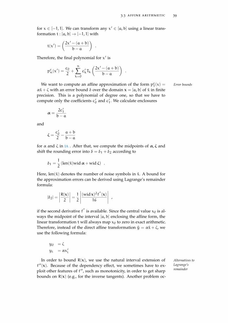
3.3 affine arithmetic 39
for x ∈ [−1, 1]. We can transform any x ′ ∈ [a,b] using a linear trans-formation t : [a,b]→ [−1, 1] with
t(x ′) =(2x ′ − (a+ b)
b− a
).
Therefore, the final polynomial for x ′ is
pcn(x′) =
c02
+
n∑k=0
c ′kTk
(2x ′ − (a+ b)
b− a
).
We want to compute an affine approximation of the form pc1(x) = Error bounds
αx+ ζ with an error bound δ over the domain x = [a,b] of x in finiteprecision. This is a polynomial of degree one, so that we have tocompute only the coefficients c ′0 and c ′1. We calculate enclosures
α =2c ′1b− a
and
ζ =c ′02
−a+ b
b− a
for α and ζ in IA . After that, we compute the midpoints of α, ζ andshift the rounding error into δ = δ1 + δ2 according to
δ1 =1
2(len(x)widα+ wid ζ) .
Here, len(x) denotes the number of noise symbols in x. A bound forthe approximation errors can be derived using Lagrange’s remainderformula:
|δ2| =
∣∣∣∣R(x)2∣∣∣∣ = 1
2
∣∣∣∣∣(wid x)2f′′(x)
16
∣∣∣∣∣ ,
if the second derivative f′′
is available. Since the central value x0 is al-ways the midpoint of the interval [a,b] enclosing the affine form, thelinear transformation t will always map x0 to zero in exact arithmetic.Therefore, instead of the direct affine transformation y = αx+ ζ, weuse the following formula:
y0 = ζ
yi = αx ′i
In order to bound R(x), we use the natural interval extension of Alternatives toLagrange’sremainder
f ′′(x). Because of the dependency effect, we sometimes have to ex-ploit other features of f ′′, such as monotonicity, in order to get sharpbounds on R(x) (e.g., for the inverse tangents). Another problem oc-

40 arithmetics
curs if a function is not two times differentiable over its domain. Inthis case, we cannot use the Lagrange remainder formula. In YalAA,this is only the case for the inverse sine and cosine functions. Bothfunctions have the domain [−1, 1], and their respective second deriva-tives ± x
(1−x2)3/2 are undefined at the endpoints. For both functions,
we calculate
e(x) = ‖f(x) − p1(x)‖∞ ,
that is, the exact error of our approximation. The maximum error canoccur either at the endpoints of [a,b] or at a local maximum. Thelocal maximum is x∗ such that f ′(x∗) − p ′1(x
∗) = 0. If we solve thisequation, we get x1|2 = ±
√1− 1
c21as candidates for the maximum.
We have to evaluate e(x) at all 4 points a,b, x1, x2 with IA in order toderive a verified upper bound. This technique is much more expen-sive than the ordinary Lagrange remainder, hence we only apply itnear the endpoints, where the derivatives behave poorly.
3.3.4 Implementations
Several libraries for AA are publicly available. Examples are the refer-Publicly availableimplementations ence implementation libaa [Sto] (written in pure C) or libaffa [GCH],
aaflib [Han] and, YalAA [Kie12b] (C++ object-oriented implementa-tions). YalAA was developed in the scope of this thesis.
Libaa covers only the standard affine model and provides a purelyLibaa
C application programming interface (API), which is not well suitedfor integration into an object-oriented C++ environment. Since itis exclusively based on the implementation guidelines given by deFigueiredo and Stolfi [dS97], it is limited to strictly convex or concaveelementary functions, which excludes important standard functionssuch as sine or cosine. For elementary functions, the implementa-tion is not always fully verified, as it uses fesetround to set directedrounding modes for evaluating them through the standard FP envi-ronment. However, the rounding modes are not considered by theimplementations of standard functions in general11.
Both libaffa and its fork aaflib are written in C++ and provideLibaffa and aaflib
object-oriented interfaces. In contrast to libaa, they not only offerconvex and concave standard functions but also provide implemen-tations for functions, such as sine or cosine. However, both librariesdo not always deliver fully verified results12. The libraries implementthe standard affine computation model.
To overcome these shortcoming of currently available implementa-YalAA
11 Actually, the behavior is implementation-defined according to the C11 stan-dard [C11a, §F.10].
12 For example, libaffa does not perform any rounding modes changes or a posteriorierror correction for the exponentiation function.

3.3 affine arithmetic 41
tions, we developed YalAA. It offers a verified common set of ele-mentary functions oriented with IEEE P1788 as a general guideline.The implementation recommendations of de Figueiredo and Stolfiwere used where possible. Otherwise, we applied our the Chebyshevinterpolation approach. A further goal was to create a sufficientlyflexible library allowing for support of extended affine computationmodels. Section 3.3.5 describes the design of YalAA in more detail.
Currently, UniVerMeC offers a support for libaffa, which could Support inUniVerMeCbe used as a reference for integrating aaflib in a straightforward way.
However, neither of them provide completely verified results. Libaa
is not supported because the non-object-oriented approach is difficultto incorporate in a purely object-oriented environment. Additionally,UniVerMeC supports YalAA. This library will be used in the restof this work because of the above mentioned limitations of the otherlibraries (cf. also Tab. 4).
3.3.5 Architecture of YalAA
YalAA makes heavy use of template metaprogramming techniques, Policy-based design
for example, of policy and trait classes [Ale01; Mye95]. They allowfor flexible adaption of the library to changing requirements. A traitclass is a class template offering type definitions, constants, and staticmethods. Usually, it needs to be specialized for different data typesand offers, in this way, a uniform interface for them. In YalAA, it ismainly used as a compile-time replacement for the adapter pattern.A policy class encapsulates a part of the functionality of a systemand makes it available through a uniform interface. It can be inter-preted as a static compile-time variant of the well-known strategy pat-tern. As the functionalities chosen are normally orthogonal to eachother, it is possible to use arbitrary combinations of policy classes.Thus, providing a wide range of functionality in a library without im-plementing each feature combination separately. This policy-baseddesign technique can be seen as a generator in the sense of gener-ative programming and, thus, weakens the library scaling problem,which describes the increased amount of work necessary if every pos-sible combination of features has to be implemented manually [CE00,p. 333].
The architecture of YalAA is shown in Fig. 12. The library is Architecture ofYalAAstructured around the template class AffineForm, which represents
an affine form, and offers the public interface to the user. This classtemplate is parametrized by four policy classes and, additionally, bythe base type T and the interval type IV. IV should represent intervalsin the endpoint form of the base type T. While T is the type for partialdeviations (usually double, but other types like exact rational num-bers are possible), the latter determines the underlying interval type.Since YalAA uses a trait class to access it, any existing interval library

42 arithmetics
Table 4: Overview over AA libraries. The listed elementary functions areoriented on IEEE P1788 .
libaa libaffa aaflib yalaa
Prog. Language C C++ C++ C++Affine Models AF0 AF0 AF0 AF0, AF1,
AF2
Verified X × × X
Supported Functions
sqr X X X X
pown × X X X
pow × X X X
sqrt X X X X
exp X X X X
log × X X X
sin × X X X
cos × X X X
tan × X X X
asin × × × X
acos × × × X
atan × × X X
atan2 × × × ×sinh × X × X
cosh × X × X
tanh × X X X
asinh × X × X
acosh × X × X
atanh × X × X
abs X X × X
min X × × ×max X × × ×

3.3 affine arithmetic 43
AffineForm+operator+=(af: const self_t&): self_t&+operator-=(af: const self_t&): self_t&+operator*=(af: const self_t&): self_t&+operator/=(af: const self_t&): self_t&. . .
T: BasetypeET: ErrorTermAC: AffineCombinationAK: ArithmeticKernelAP: AffinePolicyEP: ErrorPolicyIV: Intervaltype
BasetypeIntervaltype«concept»
ErrorTerm
T
«concept»
AffinePolicy
TETAC
«concept»
ErrorPolicy
TIV
«concept»
AffineCombination
TET
«concept»
ArithmeticKernel
TETAC
Figure 12: Basic architecture of YalAA
can be integrated seamlessly. Furthermore, users can perform mixedcomputations between affine forms and types T and IV in the basicoperations. This is important because AA is often employed insideexisting IA environments.
The policy class ErrorTerm represents an error term x · ε. It pro- ErrorTerm
vides an ordering on the error terms and is responsible for generatingnew noise variables. The latter operation has to be thread-safe if thelibrary is used in a multi-threaded environment. Furthermore, theclass stores the unique identifier for noise symbols and so limits theirmaximum number. Such operations are possibly performance critical.Therefore, users can adapt them to their current needs by changingthe policy.
The AffineCombination policy class is responsible for storing an AffineCombination
affine combination consisting of the central value and the error terms.Further, it provides the affine operations addition, scaling and transla-tion. Any operation performed in YalAA is broken down into these.Note that no rounding control, error correction, or handling is nec-essary at this particular level because those are only the plain basicoperations.
The core component of YalAA is the ArithmeticKernel policy. ArithmeticKernel
It provides an implementation of all supported operations and ele-mentary functions and performs the affine part of them. Further-more, it calculates bounds on the approximation and rounding er-ror and tracks exceptional situations occurring during the compu-tation, for example, domain violations or overflows. This informa-tion is propagated through the ArithmeticError class, which acts asa uniform interface between possibly different implementations ofArithmeticKernel and the rest of YalAA. Since the verified imple-mentation of an operation depends heavily on the underlying type,ArithmeticKernel has to be specialized for each base type T.
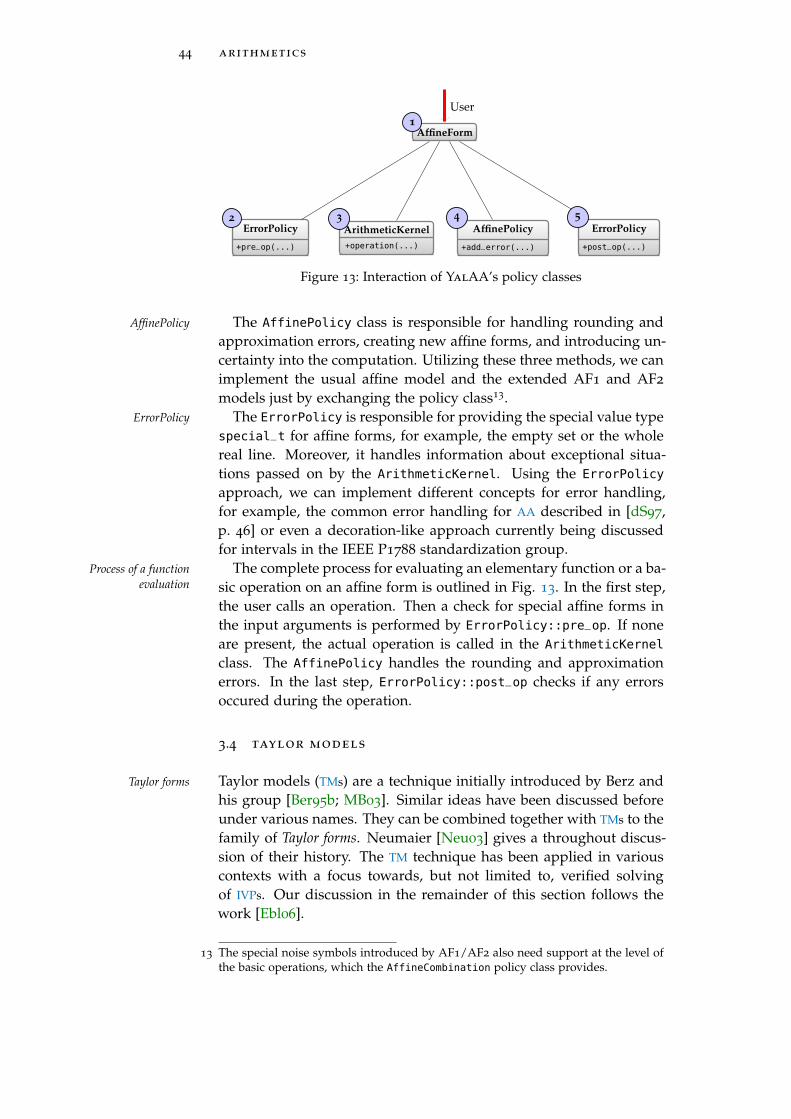
44 arithmetics
ErrorPolicy
+pre_op(...)
ArithmeticKernel+operation(...)
AffinePolicy
+add_error(...)
ErrorPolicy
+post_op(...)
AffineForm
User1
2 3 4 5
Figure 13: Interaction of YalAA’s policy classes
The AffinePolicy class is responsible for handling rounding andAffinePolicy
approximation errors, creating new affine forms, and introducing un-certainty into the computation. Utilizing these three methods, we canimplement the usual affine model and the extended AF1 and AF2
models just by exchanging the policy class13.The ErrorPolicy is responsible for providing the special value typeErrorPolicy
special_t for affine forms, for example, the empty set or the wholereal line. Moreover, it handles information about exceptional situa-tions passed on by the ArithmeticKernel. Using the ErrorPolicy
approach, we can implement different concepts for error handling,for example, the common error handling for AA described in [dS97,p. 46] or even a decoration-like approach currently being discussedfor intervals in the IEEE P1788 standardization group.
The complete process for evaluating an elementary function or a ba-Process of a functionevaluation sic operation on an affine form is outlined in Fig. 13. In the first step,
the user calls an operation. Then a check for special affine forms inthe input arguments is performed by ErrorPolicy::pre_op. If noneare present, the actual operation is called in the ArithmeticKernel
class. The AffinePolicy handles the rounding and approximationerrors. In the last step, ErrorPolicy::post_op checks if any errorsoccured during the operation.
3.4 taylor models
Taylor models (TMs) are a technique initially introduced by Berz andTaylor forms
his group [Ber95b; MB03]. Similar ideas have been discussed beforeunder various names. They can be combined together with TMs to thefamily of Taylor forms. Neumaier [Neu03] gives a throughout discus-sion of their history. The TM technique has been applied in variouscontexts with a focus towards, but not limited to, verified solvingof IVPs. Our discussion in the remainder of this section follows thework [Ebl06].
13 The special noise symbols introduced by AF1/AF2 also need support at the level ofthe basic operations, which the AffineCombination policy class provides.

3.4 taylor models 45
3.4.1 Basic Model
The idea behind TMs is to compute the range of a function by exploit- Taylor model
ing Taylor’s theorem. Based on it, a polynomial approximation andan interval bound on the error are constructed.
Definition 5 (Taylor model) Let Pf,n be the n-th order Taylor polynomialof a function f ∈ Cn+1(D),D ⊂ Rm and x ∈ IRm with x ⊂ D. Aninterval i(f,n) is a n-th order remainder bound if ∀x ∈ x : f(x) − Pf,n(x) ∈i(f,n) holds. The pair
(Pf,n, i(f,n)
)is called a Taylor model and x is called
its domain.
In the remainder of this thesis, we denote the set of TMs over the realnumbers by TR. The operator TR(D) returns all TMs over D ⊂ R.
An arithmetic for this model has been developed by Berz’s group. Basic operations
For two TMs x1 =(Pf1,n, i(f1,n)
), and x2 =
(Pf2,n, i(f2,n)
)we can
define the addition using
x1 + x2 =(Pf1+f2,n, i(f1+f2,n)
), with Pf1+f2,n = Pf1,n + Pf2,n ,
and i(f1+f2,n) = i(f1,n) + i(f2,n).
Multiplication of two polynomials of degree n results in a polynomialof the degree 2n at most, which is split into two parts with degrees6 n and > n, respectively:
Pf1,n · Pf2,n = Pf1f2,6n + Pf1f2,>n
The resulting TM consists of the polynomial Pf1f2,6n and a remainderbound that also encloses the codomain W(Pf1f2,>n) of Pf1f2,>n:
x1 · x2 =(Pf1f2,n, i(f1f2,n)
), with Pf1f2,n = Pf1f2,6n ,
and if1f2,n = W(Pf1f2,>n)+
W(Pf1,n)i(f2,n)+
W(Pf2,n)i(f1,n)+
i(f1,n)i(f2,n)
Definitions for division and elementary functions can be found in[Mak98]. An important advantage of the Taylor basis is that, for anoperation ◦ or elementary function e, the polynomial part P ′ of x1 ◦ x2or e(x1) equals the truncated Taylor series expansion for this opera-tion or elementary function.
An interval x ∈ IR can be converted to a TM by Conversions fromand to intervals
x =(mid (x), rad (x)) . (13)
To determine the result of a computation in a practically comprehen-sive form, it is necessary to compute an interval bounding the range

46 arithmetics
of a TM. Here, the main challenge is to bound the range of the poly-nomial part. Different approaches are available. They range fromsimple interval evaluation or the use of the Horner scheme to tech-niques developed especially for TMs, for example, the linear dominatedbounder (LDB) or the quadratic fast bounder (QFB) [MB05b] algorithms.
Analogous to IA and AA , the set of all TMs over the FP numbers isFP implementation
denoted as TF and the extended set of all TMs TF. Rigorous enclo-sures in the case of FPA and rounding errors are described, for exam-ple, in [Ebl06, pp. 80-87 104-111]. In finite arithmetic, the midpointand radius operations in (13) have to comply with Def. 3 and 4.
3.4.2 Implementations
The reference implementation for TMs is COSY [BM06], which wasCOSY
developed by Berz and his group. It is written in FORTRAN but of-fers an interface for access from C/C++ programs. A posteriori errorcorrection approach described in [RMB05] ensures that COSY is rel-atively fast despite the high number of basic FP operations that theTaylor arithmetic requires. The COSY implementation requires a spe-cial license. COSY uses its own memory management system, whichmakes employment in an environment like UniVerMeC difficult.
Riot is a C++ object-oriented implementation of the TM approach.Riot
In contrast to COSY, it is available as free software and offers a mem-ory management that can be employed in a more straightforward wayin object-oriented environments. However, Riot is slower comparedto COSY and does not provide newer algorithms such as the QFB. Thenumber of independent TMs in a computation is limited to eight.
3.5 abstract algebra and hierarchy
An important goal for UniVerMeC is to provide interoperable accessBuilding blocks forfunctions to (at least) the arithmetics described above. That is, it should support
a uniform way of specifying functions, so that they can be evaluatedwith every available arithmetic. The most functions we consider canbe described by a finite composition of certain building blocks, forexample, basic operations and elementary functions. This sectionspecifies these building blocks more formally as an algebra for allarithmetics. Furthermore, the interoperability between the supportedarithmetics is discussed.
3.5.1 Universal Inclusion Representation
In general, the use of various inclusion arithmetics simultaneously toCombination ofdifferent arithmetics improve the tightness of enclosures of functions is not new. For exam-
ple, de Figueiredo and Stolfi [dS97, pp. 75f.] propose combined useof interval and affine arithmetic. Consequently, their reference imple-

3.5 abstract algebra and hierarchy 47
Table 5: Representation of arithmetics supported by UniVerMeC in theframework of Vu, Sam-Haroud, and Faltings [VSHF09].
T VT DT fT (VT )
Reals (x) (x) [x , x] id(x)
IA (a , b) (x) [a , b] id(x)
AA (x0 , x1 , . . . , xn ) (ε1 , . . . , εn ) [−1 , 1]n x0 +∑ni=1 xiεi
TMs (a1 , . . . , an , e1 , e2 ) (x , e) [−1 , 1]n e +n∑i=1
aixi
mentation of AA supports a hybrid computation mode that performsevery operation twice with interval and affine arithmetic and allowsfor intersecting the results.
More recently, Vu, Sam-Haroud, and Faltings [VSHF09] proposed Inclusionrepresentationthe use of different inclusions techniques in the scope of numerical
constraint propagation. For this purpose, they introduce the abstractnotion of an inclusion representation.
Definition 6 (Inclusion representation [VSHF09]) Let µ : R → 2A bea function and R a non-empty set. The pair (R,µ) is an inclusion represen-tation for a set A if there exists a function ζ : 2A → R so that
(i) µ(ζ(∅)) = ∅(ii) ∀S ⊆ A : S ⊆ µ(ζ(S))
holds.
This rather abstract definition is specialized by the authors for theclass of real representations. In this case, R contains tuples of realnumbers and for ∀T ∈ R
µ(T) = {fT (VT )|VT ∈ DT [VT ]}
holds. VT is a sequence of variables, DT the sequence of associateddomains, and fT : DT → R a function. It is shown by the authorshow to represent various inclusion techniques in their framework; seeTab. 5. Although they give no advice on how to integrate TMs intotheir framework, they can be represented as shown in the table for adegree n TM of one variable over the canonical interval14 [−1, 1] withthe remainder bound e. The representation could be easily extendedto involve m variables. All considered arithmetics in UniVerMeC arerepresented according to this inclusion framework.
Based on this formal definition, the authors derive a generalized Inclusion functions
notion for an inclusion function (which is characterized e.g. in theinterval case by (6)).
14 Most existing software for TMs uses a linear transformation to ensure that the poly-nomial part of the model lies inside this interval.

48 arithmetics
Definition 7 (Inclusion function [VSHF09]) A function F : RX → RY
is called an inclusion function for f : X→ Y if
(S ⊆ µX(T))⇒ ({f(x)|x ∈ S} ⊆ µY (F(T)))
holds for all S ⊆ X and ∀T ∈ RX. Here, (RX,µX), (RY,µY) are inclusionrepresentations for X and Y.
Among the considered arithmetics the above definition cannot beused for computations in finite-precision without range-arithmetics.For simplicity, we will nevertheless use the term inclusion functionwith regard to all base sets (including F, F). Based on the generalnotion of an inclusion function, it is now possible to derive straight-forward generalizations of the natural interval extension (Def. 2) forall supported arithmetics.
Definition 8 (Generalized natural extension [VSHF09]) A functionF : D ⊆ Rn → Rm is called the natural extension of f : D ⊆ Rn → Rm
in the inclusion representation (R,µ), if it is constructed by replacing allvariables, basic operations, constants, and elementary functions in f by theirrespective counterparts in (R,µ).
In the above definition it is assumed that the counterparts of the ele-mentary functions themselves comply to Def. 7. Although this frame-work supplies formal definitions for inclusion representations andfunctions, a definition of the basic building blocks, that is, the set ofoperations and elementary functions, is still missing. They are de-fined in the following.
3.5.2 Heterogeneous Algebra
The goal of this section is to specify a set of operations and elemen-Base set of functions
tary functions that is available for every supported arithmetic. Fur-thermore, it defines what functions and operations are allowed for acertain kind of arithmetic as well as what combinations between dif-ferent arithmetics are possible. The upcoming standard IEEE P1788
acts as a basis for the set of standard functions, their definitions, anddomains. Following the interval standard, we first define a set ofpoint functions and then extend them to the different arithmeticsthat UniVerMeC supports using the notation of generalized inclu-sion functions according to Def. 7.
Formally, we define the set of basic operations and elementaryHeteregenous realalgebra functions by specifying a heterogeneous algebra. We use the algebra
notion of Birkhoff and Lipson [BL70], who define it as a 2-tuple (S,F)where “S is a family of non-void sets Si of different types of ele-ments” and “F = {fα} is a set of finitary operations”. In our case, thefamily S consists of the arithmetic base sets mentioned earlier, thatis, S := {R, IR, AR, TR}. Our algebra supports the basic operations

3.5 abstract algebra and hierarchy 49
Table 6: Basic operations and elementary functions considered in the het-erogeneous algebra in UniVerMeC. The set of functions and theirdomains are taken from the IEEE P1788 standard [P17, p. 24].
operation / func . e definition domain D(e)
x ◦ y with ◦ ∈ {+ , − , ·} R × R
x/y R × R \ {0}
abs(x) R
acos(x) [−1 , 1]
acosh(x) [1 ,∞)
asin(x) [−1 , 1]
asinh(x) R
atan(x) R
atanh(x) R
cos(x) R
cosh(x) R
exp(x) ex R
log(x) log10 (x) R+ \ {0}
neg(x) −x R
pown(x , p) xp R × Z+ ∪ R \ {0} × Z−
pow(x , y)
ey ln(x) if x > 0
0 if x = 0
(R+ \ {0} × R
)∪(
{0} × R+ \ {0})
sin(x) R
sinh(x) R
sqr(x) x2 R
sqrt(x)√x R+
tan(x) R \{(k + 0 .5)π
∣∣ k ∈ Z}
tanh(x) R
inf(x) x IR
sup(x) x IR
mid (x) (1) IR
wid (x) (2) IR
rad (x) widx2 IR
to_iv(x) (11) AR
to_iv(x) TM→ IA conversionTR
Sect. 3.4 (LDB, QFB, . . .)

50 arithmetics
FC := {+,−, ·, /}, unary elementary functions FE := {acos, acosh, asin,asinh, atan, atanh, cos, cosh, exp, log, neg, sin, sinh, sqr, sqrt, tan,tanh}, and binary elementary functions FB := {pown, pow}. In Tab. 6,the natural domain D(e) associated with each individual function eis given (i.e., e : D(e) → R for e ∈ FC ∪FE ∪FB). The first part of theset F of basic operations is formally defined as
F(1) :={eM : M
(D(e)
)→M
∣∣ e ∈ FC ∪FE, M ∈ S}∪{
powM : M(D
(pow)1
)×M
(D
(pow)2
)→M
∣∣ M ∈ S}∪{
pownM : M(D
(pown)1
)×D2 →M
∣∣ M ∈ S}
where eM, powM, pownM are inclusion functions in the sense of Def. 7;for e, pow, pown in the respective arithmetic and D
(p)i is the i-th com-
ponent of the natural domain for p ∈ {pow, pown} for i = 1, 2. Fur-thermore, we want to allow the use of basic operations with mixedoperand types if this does not incur any information loss. There-fore, we define the second part of the set of operations as F(2) :=
F(2) ′ ∪F(2 ′′) with
F(2 ′) :=
{◦ : M1
(D
(◦)1
)×M2
(D
(◦)2
)→M1
∣∣◦ ∈ {+,−, ·, /}, M1 ∈ S, M2 ∈ {R, IR }, M1 6= M2
},
and
F(2 ′′) :=
{◦ : M1
(D
(◦)1
)×M2
(D
(◦)2
)→M2
∣∣◦ ∈ {+,−, ·, /}, M2 ∈ S, M1 ∈ {R, IR }, M1 6= M2
}where ◦ is an inclusion function in the sense of Def. 7; for ◦ ∈{+,−, ·, /} and D
(◦)1 ,D(◦)
2 are the first and second component of thenatural domain of the operation according to Tab. 6. The implemen-tation is straightforward if we apply type conversion. Each r ∈ R
can be treated as the point-interval [r, r], and each interval x can betreated as an affine form or a TM, by applying the conversion formu-las (11) or (13) respectively. In practice we sometimes need operationsthat are defined for some of the arithmetics. Therefore, in addition toFC, FE and, FB we consider a further set FI := {inf, sup, rad , wid , mid }
exclusively for intervals and introduce
F(3) :={e : D(e) → R
∣∣ e ∈ FI
}

3.5 abstract algebra and hierarchy 51
Table 7: Additional functions for the FP algebra to handle the special forms.All functions map into the set B = {true, false}.
function e definition domain De
is_special(x) true iff x ∈ F \ F F
is_empty(x) true iff x is NaN F
is_unbounded(x) true iff x = ±∞ F
is_special(x) true iff x ∈ IF \ IF IF
is_empty(x) true iff x > x IF
is_unbounded(x) true iff x = −∞∨ x =∞ IF
is_special(x) true iff x ∈AF \ AF AF
is_empty(x) optional, implementation dependent AF
is_unbounded(x) optional, implementation dependent AF
is_special(x) true iff x ∈ TF \ TF IF
is_empty(x) optional, implementation dependent TF
is_unbounded(x) optional, implementation dependent TF
into our algebra. Furthermore, we consider an outer function to_iv(cf. Tab. 6) that maps an affine form or a TM to an interval
F(4) :={
to_iv : D(to_iv) → IR}
.
This leads to the final definition of our heterogeneous algebra EA forreal computations as:
EA :=
S,⋃
16i64
F(i)
. (14)
The real algebra can be assigned a corresponding FP algebra which Corresponding FPalgebrais used for the actual computations. To obtain it, we have to perform
two steps: First we replace the real domain sets of all mappings bytheir respective FP counterparts, that is, R by F, IR by IF and so on.Then we replace the range sets of the mappings by their respectiveextended FP counterparts, that is, R by F, IR by IF and so on. This iscrucial to be able to handle overflows that might occur during com-putations in finite precision. Note that rounding issues have to behandled carefully during the actual implementation. UniVerMeC re-lies here solely on the concrete implementation of the arithmetic thatis employed. To make it easier for users to handle the extended setsF, IF, AF, and TF, we extend the algebra EA by the set of func-tions specified in Tab. 7. The function is_special allows users to checkwhether something went wrong during the computation. This func-tion is mandatory for all arithmetics because, if a library introducesspecial forms to handle overflows, domain violation, and similar er-

52 arithmetics
rors, there probably exists a function to tell these forms apart fromthe “normal” forms. The more specialized functions is_empty andis_unbounded can be used to check whether the result is empty or un-bounded (which is possibly caused by an overflow) respectively. Uni-VerMeC guarantees the existence of the three functions and, if possi-ble maps them to the respective routines provided by the underlyingarithmetic library. However, the actual semantics can be different inconcrete implementations since they are not standardized in general.Because we do not make any assumptions about the behavior of theunderlying library, it might choose, for example, to call the exit func-tion or to throw an exception if an overflows occurs. In UniVerMeC,we can guarantee only that users can rely on the uniform functionsin the framework if a library provides special forms. Formally, wedefine the set of operations
F(5) :={e : M→ B
∣∣ e ∈ FF, M ∈ {F, IF, AF, TF}}
where FF := {is_special, is_empty, is_unbounded} is defined accord-ing to Tab. 7 and B := {true, false}. That is, the FP algebra FA for thefinite arithmetics is defined as:
FA := {S∪ {B},F ∪F(5)} . (15)
Note that there are no assumptions about the behavior of functionsin FA if their natural domain is violated, for example, if x ∈ IF \ IF isused as input15. In this case, the outcome is implementation-defined,that is, undefined in the general case. The algebra specification givenhere is well founded in the upcoming IEEE P1788 standard and mostexisting arithmetic implementations conform to this algebra specifi-cation in general. More details on practical considerations along withrespective implementations are given in Sect. 3.6.
3.5.3 Arithmetic Hierarchy and Conversions
The algebras above implicitly define a hierarchy between the differentConversionoperators arithmetics. It determines what guarantees we can make for conver-
sions between them. Figure 14 shows two types of conversions insidethe hierarchy for which we can make guarantees: lossless (solid lines)and enclosure preserving (dotted lines) conversions. A lossless con-version means that no information about the solution area is lost.
Definition 9 (Lossless conversion between real algebras) Let M1,M2 be two support sets of the (exact) real algebra with their respective
15 The domains of all functions are restricted to the non-extended sets F, IF, AF andTF.

3.5 abstract algebra and hierarchy 53
Floating-point arithmetic
Interval arithmetic
Affine arithmetic Taylor models
Figure 14: Arithmetic hierarchy in UniVerMeC. Lossless conversions arerepresented by solid lines and enclosure preserving conversionsby dotted lines.
real inclusion representations (M1,µM1) and (M2,µM2
). A mapping ϕ :
M1 →M2 is called lossless conversion if
µM1(x) = µM2
(ϕ(x))
holds for ∀x ∈M1.
The possibility for the lossless conversions shown in Fig. 14 follows di-rectly from the algebra definitions and (12), (13). Applying these for-mulas on a computer using FPA can result in rounding errors widen-ing the enclosed area. Therefore, we use the following definition inthe case of the FP algebras.
Definition 10 (Lossless conversion between FP algebras) Let M1, M2
be two support sets of the finite FP algebras. A mapping ϕ : M1 → M2
is called lossless if its corresponding mapping in the respective (exact) realalgebra is lossless.
In the case of enclosure preserving conversions, the requirement isless strict. We only require that no covered area is lost.
Definition 11 (Enclosure preserving conversion) Let M1, M2 be twosupport sets of either of the exact or the finite algebra with their respectivereal inclusion representations (M1,µM1
) and (M2,µM2). A mapping ϕ :
M1 →M2 is called enclosure preserving conversion if
µM1(x) ⊆ µM2
(ϕ(x))
holds for ∀x ∈M1.
In some cases it might be necessary to perform a cast between arith-metic types even if this incurs an information loss. For these cases, aforced conversion is supported:
Definition 12 (Forced conversion) Let M1, M2 be two support sets ofeither the exact or the finite algebra. A mapping ϕ : M1 → M2 is calledforced conversion if and only if it
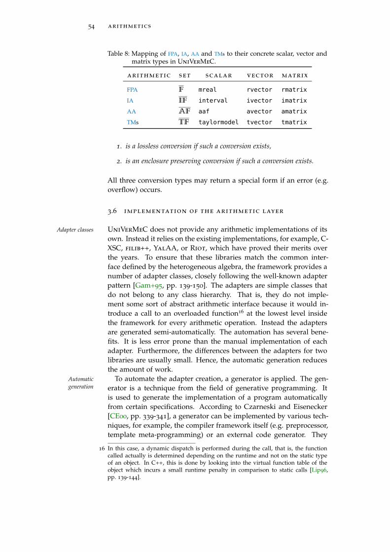
54 arithmetics
Table 8: Mapping of FPA, IA, AA and TMs to their concrete scalar, vector andmatrix types in UniVerMeC.
arithmetic set scalar vector matrix
FPA F mreal rvector rmatrix
IA IF interval ivector imatrix
AA AF aaf avector amatrix
TMs TF taylormodel tvector tmatrix
1. is a lossless conversion if such a conversion exists,
2. is an enclosure preserving conversion if such a conversion exists.
All three conversion types may return a special form if an error (e.g.overflow) occurs.
3.6 implementation of the arithmetic layer
UniVerMeC does not provide any arithmetic implementations of itsAdapter classes
own. Instead it relies on the existing implementations, for example, C-XSC, filib++, YalAA, or Riot, which have proved their merits overthe years. To ensure that these libraries match the common inter-face defined by the heterogeneous algebra, the framework provides anumber of adapter classes, closely following the well-known adapterpattern [Gam+95, pp. 139-150]. The adapters are simple classes thatdo not belong to any class hierarchy. That is, they do not imple-ment some sort of abstract arithmetic interface because it would in-troduce a call to an overloaded function16 at the lowest level insidethe framework for every arithmetic operation. Instead the adaptersare generated semi-automatically. The automation has several bene-fits. It is less error prone than the manual implementation of eachadapter. Furthermore, the differences between the adapters for twolibraries are usually small. Hence, the automatic generation reducesthe amount of work.
To automate the adapter creation, a generator is applied. The gen-Automaticgeneration erator is a technique from the field of generative programming. It
is used to generate the implementation of a program automaticallyfrom certain specifications. According to Czarneski and Eisenecker[CE00, pp. 339-341], a generator can be implemented by various tech-niques, for example, the compiler framework itself (e.g. preprocessor,template meta-programming) or an external code generator. They
16 In this case, a dynamic dispatch is performed during the call, that is, the functioncalled actually is determined depending on the runtime and not on the static typeof an object. In C++, this is done by looking into the virtual function table of theobject which incurs a small runtime penalty in comparison to static calls [Lip96,pp. 139-144].
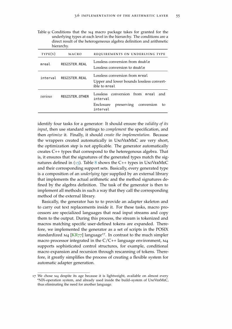
3.6 implementation of the arithmetic layer 55
Table 9: Conditions that the m4 macro package takes for granted for theunderlying types at each level in the hierarchy. The conditions are adirect result of the heterogeneous algebra definition and arithmetichierarchy.
type(s) macro requirements on underlying type
mreal REGISTER_REALLossless conversion from double
Lossless conversion to double
interval REGISTER_REALLossless conversion from mreal
Upper and lower bounds lossless convert-ible to mreal
various REGISTER_OTHERLossless conversion from mreal andinterval
Enclosure preserving conversion tointerval
identify four tasks for a generator: It should ensure the validity of itsinput, then use standard settings to complement the specification, andthen optimize it. Finally, it should create the implementation. Becausethe wrappers created automatically in UniVerMeC are very short,the optimization step is not applicable. The generator automaticallycreates C++ types that correspond to the heteregenous algebra. Thatis, it ensures that the signatures of the generated types match the sig-natures defined in (15). Table 8 shows the C++ types in UniVerMeCand their corresponding support sets. Basically, every generated typeis a composition of an underlying type supplied by an external librarythat implements the actual arithmetic and the method signatures de-fined by the algebra definition. The task of the generator is then toimplement all methods in such a way that they call the correspondingmethod of the external library.
Basically, the generator has to to provide an adapter skeleton andto carry out text replacements inside it. For these tasks, macro pro-cessors are specialized languages that read input streams and copythem to the output. During this process, the stream is tokenized andmacros matching specific user-defined tokens are expanded. There-fore, we implemented the generator as a set of scripts in the POSIXstandardized m4 [KR77] language17. In contrast to the much simplermacro processor integrated in the C/C++ language environment, m4
supports sophisticated control structures, for example, conditionalmacro expansion and recursion through rescanning of tokens. There-fore, it greatly simplifies the process of creating a flexible system forautomatic adapter generation.
17 We chose m4 despite its age because it is lightweight, available on almost every*NIX-operation system, and already used inside the build–system of UniVerMeC,thus eliminating the need for another language.

56 arithmetics
dnl L i s t o f f u n c t i o n names in t h e * e x t e r n a l * l i b r a r ydef ine ( ‘UNARY_STANDARD_FUNCTIONS_interval ’ , ‘ ‘ abs ’ , ‘ acos ’ ,
‘ acosh ’ , ‘ as in ’ , ‘ asinh ’ , ‘ atan ’ , ‘ atanh ’ , ‘ cos ’ , ‘ cosh ’ ,‘ exp ’ , ‘ log10 ’ , ‘ s i n ’ , ‘ s inh ’ , ‘ sqr ’ , ‘ s q r t ’ , ‘ tan ’ ,‘ tanh ’ , ‘ I n f ’ , ‘ Sup ’ , ‘mid ’ ’ )
dnl Code b l o c k f o r p e r f o r m i n g i n f / supdef ine ( B_PERFORM_UNARY_FUN_inf_interval , ‘ re turn
mreal ( _double ( I n f ( args . m_adapt ) ) ) ; ’ )def ine ( B_PERFORM_UNARY_FUN_sup_interval , ‘ re turn
mreal ( _double ( Sup ( args . m_adapt ) ) ) ; ’ )
dnl Code b l o c k f o r t h e i n t e g e r power f u n c t i o ndef ine ( ‘B_PERFORM_BINARY_FUN_pown_interval ’ , ‘ arg . m_adapt =
power ( arg . m_adapt , e ) ; re turn arg ; ’ )
dnl R e g i s t e r s t h e i n t e r v a l t y p eREGISTER_INTERVAL( ‘ cxsc : : i n t e r v a l ’ , ‘ ’ , ‘// C−XSC Headers# include < i n t e r v a l . hpp># include <imath . hpp>’ ) �Listing 1: Excerpt from the m4 macros to register an interval type using C-
XSC as the underlying library.
The design of the macro package is based on the arithmetic hierar-Design of adaptermacros chy (see Fig. 15). For every hierarchy level, it provides a macro that
creates the types on this level: REGISTER_REAL, REGISTER_INTERVAL,and REGISTER_OTHER. The reason for this division is that the under-lying type has to fulfill different requirements depending on its posi-tion in the arithmetic hierarchy. The requirements are listed in Tab. 9.The package ensures that exactly one adapter for FP numbers andone adapter for intervals is registered. At the top level, it allowsthe registration of an arbitrary number of adapters. Currently, weonly consider affine forms and TMs. Moreover, the common macroREGISTER_OTHER allows for easy addition of new types, which can beeither a new kind of arithmetic, for example, Chebyshev models18,or variants of an existing arithmetic, for example, the AF1 or AF2
forms for AA. Therefore, it ensures the extensibility of the frameworkat this level. Note that adding a new arithmetic might also requirethat users extend the theoretical basis (e.g. the inclusion representa-tions and algebra) to ensure that the framework still produces correctresults.
Listing 1 shows an excerpt19 of the m4 macros a user has to write tointroduce the C-XSC interval type into UniVerMeC. Listing 2 shows
18 Currently, several researchers seek to provide an alternative to the classical TMs byusing the Chebyshev basis [Dze12; Jol11]. Chebyshev models might offer betterenclosures due to better properties of Chebyshev polynomials. When the work isfinished, the corresponding implementations could be included in our frameworkeasily.
19 A few minor parts were left out for clarity.

3.6 implementation of the arithmetic layer 57
def ine ( ‘UNARY_STANDARD_FUNCTIONS_interval ’ , ‘ ‘Abs ’ , ‘ ArcCos ’ ,‘ ArCosh ’ , ‘ ArcSin ’ , ‘ ArSinh ’ , ‘ ArcTan ’ , ‘ ArTanh ’ , ‘ Cos ’ ,‘ Cosh ’ , ‘Exp ’ , ‘ Log10 ’ , ‘ Sin ’ , ‘ Sinh ’ , ‘ Sqr ’ , ‘ Sqr t ’ ,‘ Tan ’ , ‘ Tanh ’ , ‘ I n f ’ , ‘ Sup ’ , ‘Mid ’ , ‘Diam ’ , ‘ rad ’ ’ )
dnl Code b l o c k f o r t h e i n t e g e r power f u n c t i o ndef ine ( ‘B_PERFORM_BINARY_FUN_pown_interval ’ , ‘ arg . m_adapt =
Power ( arg . m_adapt , e ) ; re turn arg ; ’ )
dnl Hull O p e r a t o rdef ine ( ‘B_PERFORM_OP_| _ i n t e r v a l _ i n t e r v a l ’ , ‘ m_adapt =
Hull ( m_adapt , other . m_adapt ) ; ’ )dnl I n t e r s e c t i o n o p e r a t o rdef ine ( ‘B_PERFORM_OP_&_ i n t e r v a l _ i n t e r v a l ’ ,
‘ i f ( ! I n t e r s e c t i o n ( m_adapt , m_adapt , other . m_adapt ) )m_adapt = INTERVAL( 1 , −1) ; ’ )
dnl R e g i s t e r s t h e i n t e r v a l t y p eREGISTER_INTERVAL( ‘INTERVAL ’ , ‘ ’ , ‘// PROFIL/BIAS Headers# include < I n t e r v a l . h># include <Functions . h>’ ) �Listing 2: Excerpt from the m4 macros to register an interval type using
PROFIL/BIAS as the underlying library.
the macros necessary for the PROFIL/BIAS library. The first definespecifies the names of standard functions as used by the library. Theyare employed to automatically create calls to the corresponding li-brary functions in the function bodies of the adapter. The bodies ofthese functions are generated by expanding macros of the form B_-
PERFORM_UNARY_FUN_<function name>_<type> for functions and B_-
PERFORM_OP_<operation name>_<type left>_<type right> for oper-ators. Normally, these macros are created automatically based on thefunction names list provided by the user and the assumption that theexternal library provides operator overloading for its data type. If theautomatic generation is not suitable, users can suppress it by specify-ing these macros manually. This has to be done, for example, for theinf, sup, mid functions in case of the C-XSC library, because it doesnot return double (which we can cast to our mreal type) but its owntype (cxsc::real) that encapsulates a double. After providing themanual macro overloads, the REGISTER_INTERVAL function is calledto register the new type in the adapter generator framework. Thecall takes as arguments the underlying type and the library headersto be included. The information in the adapter generator frameworkis not only utilized to generate the adapters but also to create addi-tional support classes in the framework automatically. This ensuresthat the framework can be extended with new arithmetic types eas-ily. The process is depicted in Fig. 15. The trait classes generatedautomatically provide operations for casting between the arithmetic

58 arithmetics
GNU autotools
Buildsystem
User inputRequested li-braries
configure
m4
Adapter generationcxscadapt.m4
yalaaadapt.m4...
basetemplate.m4
UniVerMeCArithmetic layer
Type Casts
Arithmetic traits Adapters Fadbadtraits
3rd party libs Matrix
Template Lib.
libaffa
YalAA...
C-XSCfilib++
...
RiOt...
FADBAD
callsAuxiliary files
generates
definetypes
Figure 15: The arithmetic layer of UniVerMeC and its semi-automatic gener-ation with the help of the build system and the m4 macro proces-sor. Automatically generated parts are drawn in red and externallibraries in green.
types according to the hierarchy in Fig. 14. These are used by the ac-tual cast operators lossless_cast, enclosure_cast and forced_cast
based on Def. 10, 11, or 12 respectively. Type definitions for the cor-responding vector and matrix types of the framework are also con-tained in trait classes. UniVerMeC uses the Matrix Template Li-brary 4 [GL], which allows for a uniform handling of vectors andmatrices of different base types and ensures common interfaces forall vector and matrix classes. In the last step, the m4 generationlayer creates suitable FADBAD++ [Sta97] trait classes for all gener-ated adapters. FADBAD++ is a free library for algorithmic differen-tiation (AD), (cf. Sect. 4.1) including the computation of Taylor coeffi-cients. It can be applied to arbitrary arithmetic types.
3.7 gpu-powered computations
So far we did not discuss interoperability problems that occur if theGPU computations
computation is not carried out on the same hardware architecture,that is, a IEEE 754-2008 compliant CPU. Recently, the use of highlyparallel many-core architectures has attracted much attention sincethey are now available at a relative low cost in form of modernGPUs. Historically, GPUs were highly specialized hardware for ren-dering. In the early days, they used merely a non-programmable

3.7 gpu-powered computations 59
Kernel
.. .. .. .. ..d1 dn
Figure 16: In the stream processing model the same kernel is applied to alldata elements d1, . . . ,dn. The order in which the data elementsare processed is not defined.
fixed-function pipeline. As computer graphics became more sophis-ticated, the need for more flexible GPUs arose. This lead to the intro-duction of the domain specific shader languages. First, their expres-siveness was limited and tailored to computer graphics. Over time,the languages were extended and many of their restrictions disap-peared. Owing to this, the field of general purpose computations onthe GPU (GPGPU) appeared. While the first GPGPU programs werewritten using the computer graphics specific shader languages, spe-cial languages like OpenCL (Open Computing Language) [Ope] orCUDA (Compute Unified Device Architecture) [NVI12] were devel-oped later. The former is a vendor independent standard maintainedby the Khronos group. The latter was developed as a specific lan-guage for NVIDIA cards originally. We use CUDA in the remainderof this thesis because, in our opinion, it still has a better overall toolsupport. However, the CUDA and OpenCL programming modelsare so similar in general that porting our implementation to OpenCLshould not be too difficult.
Both languages are based on the so-called stream processing model, Stream processingmodelwhich is shown in Fig. 16. It consists of a stream that is composed of
many data elements and a kernel. The kernel is applied to all elementsof the stream in parallel. This model imposes several restrictions onthe tasks for which it can be efficiently applied. First, the task needsto be parallelizable, that is, the kernel should be able to process themembers of the stream independently. Furthermore, the model isefficient only if the stream is large enough. Another restriction is im-posed by the fact that, currently, the stream processing is done on anextra device such as the GPU with its own memory. Because we haveto transfer the stream first from the main memory to the GPU, it is im-portant that the kernel is computationally expensive. Otherwise, thegain in time from using the parallel architecture will be negated bythe input/output time needed to transfer the stream and the resultsfrom the main memory to the GPU and back.
A GPU consists of stream multiprocessors and can run hundreds ofthreads simultaneously. Compared to CPU threads, the GPU threadsare much more lightweight. In contrast to common CPU single in-

60 arithmetics
struction single data (SISD) architectures20, GPUs employ a single in-struction multiple data (SIMD) model. In the scope of NVIDIA CUDA[NVI12, p. 61], it is also referred to as single instruction multiplethreads (SIMT) so as to emphasize that the architecture applies tothreads and that programmers do not need to cope with divergingbranches manually, as is the case in some traditional SIMD architec-tures. The divergences occur if a branching condition, for example,an if statement, is evaluated differently by two threads. It is prob-lematic because the execution of diverging branches can lead to a se-rialized execution21 on a GPU. This prevents the utilization of a greatpart of the computational power of a GPU which depends mainly onparallelization. Therefore, problems that inhabit a large amount ofbranching are not well suited for GPU computations in general.
In connection with computer graphics applications, interval andRange computationson the GPU affine arithmetic received some attention from the point of view of
GPU parallelization [BN13; FPC10; Hij+10; Kno+09]. However, mostof these publications focus on real-time ray-tracing and not on deriv-ing verified results on the GPU. Currently, the adaption of interval-based algorithms for the GPU is obstructed by the lack of appropriatesoftware libraries on the GPU. The Boost.Interval GPU [Hwu11] li-brary is an exception. However, it is outdated and does not make useof the recent improvements in the IEEE 754-2008 support for mod-ern GPUs [WFF11]. An improved version of the library is currentlysupplied with the CUDA toolkit. Like its predecessor, it is limitedto the basic operations, which means that only rational functions canbe evaluated with it. To our knowledge, there is no verified GPU AA
or TM library publicly available. A goal of an ongoing master the-sis at the university of Duisburg-Essen is to provide a GPU poweredimplementation of YalAA [Gö13].
For these reasons, we limit our support for elementary functions inGPU algebra
the algebra with regard to the GPU to the basic operations (includingsquare root), and FP and IA . That also implies that the GPU supportdoes not fit well into our general arithmetic based on the heteroge-neous algebra and has to be handled separately. We denote the set ofIEEE 754-2008 (extended) double numbers and intervals on the GPU
by F ′ (F ′) and IF ′ (IF′) respectively. Because the formal derivation
of the GPU algebra GA is analog the CPU FP algebra (15), we omit itand only state its definition:
GA :=({F′, IF
′}, {sqrt, pown,+,−, ·, /}
). (16)
20 Note that a modern CPU often has more than one core and thus can process multiplethreads in parallel. Extensions such as MMX, 3DNow! or SSE add SIMD instructionsto the CPU, which we do not consider at first.
21 Whether the execution has to be serialized depends on implementation details. Forcurrent NVIDIA cards, it depends on whether the threads are in the same group ofthreads (a so-called wrap), which share certain resources on the card.
3.8 conclusions 61
Similar to the CPU algebra, the supported basic operations and el-ementary functions (cf. Tab. 6) of GA are required to be inclusionfunctions according to Def. 7. Note that both CPU and GPU algebrasultimately use the IEEE 754-2008 double type as base type. That is,we can use this type to transfer data from the CPU to the GPU andback safely. These transfers do not incur any rounding or loss ofinformation. Thus, they are suitable for rigorous computations.
We do not maintain a complex framework of automatically gener-ated adapter classes for the GPU but use a slightly enhanced versionof the interval type supplied with the CUDA framework that fits ouralgebra definition. The reasons are the following:
1. The GPU library support is still very limited, and we are notaware of any third party libraries that we could support.
2. In contrast to the CPU arithmetic framework, we consider onlyFPA and IA.
3. We do not provide support for libraries like fadbad++ or MTL4
on the GPU and thus do not need additional adapter classes.
4. GPU development is moving very fast. Therefore, it seems tooearly to provide a fixed framework similar to that on the CPU.
In fact, we do not provide extensive support tools for GPU program-ming on the arithmetic layer because GPU routines are still imple-mented on a low level. Therefore, GPU programs are often tailoredtowards a specific problem. Other aspects of the GPU support in Uni-VerMeC are discussed in the next chapter. They concern the auto-matic transfer of large data sets (streams) to the GPU so that it canprocess them effectively.
3.8 conclusions
In this chapter, we have presented an approach for handling different Heterogeneousalgebrarigorous range-arithmetics in a uniform environment. It is based on
the theoretical framework of inclusion representations by Vu, Sam-Haroud, and Faltings, which allows for performing mixed compu-tations with different arithmetics to improve inclusions in the scopeof contraint propagation. We extended this framework to cover abroader range of theoretical problems. However, the larger part ofour contribution in this chapter was devoted to solving the practi-cal problems of using different arithmetics simultaneously. For thispurpose, we presented a heterogeneous algebra that defines commonsets of compositions and elementary functions and is supported inthe upcoming IEEE P1788 standard. The approach helps to over-come two shortcomings of existing software: First, arithmetics cannow be used interchangeably to evaluate functions. Second, the al-gebra formalize and restrict the ways two different arithmetic types
62 arithmetics
can interact with each other in the same computation. The concept ofusing more than one arithmetic type is refined by arranging them ina hierarchy and deriving formal conditions for lossless and enclosurepreserving conversions. While the actually applied conversion algo-rithms are well-known, the formalized conditions for the conversiontypes based on the inclusion representations are new. An importantadvantage is that our approach can be extended to a new arithmeticby merely providing an inclusion representation for it. The hetero-geneous algebra can be extended for a new arithmetic in most casesstraightforwardly.
The second part of this chapter was devoted to the practical con-Practicalimplementation siderations that have to be taken into account if different range arith-
metics are applied in a rigorous computation environment. Our goalwas to provide a software that implements the theoretical frameworkby employing existing libraries instead of developing a conformingimplementation for each arithmetic. We reached the goal by apply-ing methods from generative programming to provide an adaptergenerator framework. Compared to traditional approaches, whichuse a fixed set of libraries, our new technique is much more flexible.The approach is vendor independent, that is, we support the use ofdifferent arithmetics provided by different libraries. Another advan-tage of the automatic generation is that additional libraries can beincorporated without too much effort on the users’ side, if these li-braries follow interface conventions used by most arithmetic types inC++. Furthermore, similar to its theoretical foundation, the practicaladapter generation framework can be extended easily if necessary.

4F U N C T I O N S I N U N I V E R M E C
This chapter discusses functions in the context of UniVerMeC. Func- Functionrepresentationtion is understood in a mathematical sense, that is, as a mapping
Rn → Rm. An important feature of our framework is the capabilityto encapsulate such functions into objects that can be passed insidethe framework. By using these objects, it is possible to evaluate inclu-sion functions for all supported arithmetics. As mentioned in Chap. 2,one of our design goals was to allow users as much freedom as pos-sible in entering functions into the system and high flexibility withrespect to their internal representation. For example, it should bepossible to enter functions into the framework as closed form ana-lytical expressions (e.g. f(x,y, z) = x2 + y2 + z2 − 1) or as C++ codeblocks, which are allowed to contain constructs such as while or if
directives depending on the function variables.Such flexibility of our approach comes at a price. For example, Feature system
we cannot assume that all functions are differentiable. To be able toexploit such special characteristics of functions, we introduce a fea-ture system: a set of orthogonal functionalities1 that are associatedwith a concrete function. Our software features are realized by in-terfaces providing access to them. While UniVerMeC supplies stan-dard implementations for the feature interfaces, users are always freeto implement these interfaces themselves. For example, derivativescan be obtained through UniVerMeC’s standard implementation byalgorithmic differentiation, but users can also choose to provide thederivatives manually. Both custom implementations by users and ourstandard implementations have to obey the formal definitions for theinterfaces that we derive in Sect. 4.4.1.
This generic approach makes the framework more complex. Ad- Limitations
ditionally, it becomes more difficult to optimize algorithms becausenothing is known about the internal representation of functions. Theimplementation of techniques that depend on specific internal func-tion representations, and which cannot work with the black boxesthat UniVerMeC provides, becomes very complicated. Dependingon the intended application domain and solving techniques, othermore specific implementations may be better suited. An example isthe IBEX library [Cha], which provides functionality that partiallyoverlaps with UniVerMeC (cf. Sect. 1.3). It implements ideas fromcontractor programming [CJ09] and allows users to adapt algorithmsby combining one or several contractors with a bisection scheme in
1 That is, the functionalities do not interact and arbitrary combinations of them arepossible. [Ale01, pp. 19-20]
63

64 functions in univermec
the scope of constraint programming or global optimization. In IBEX,a function is defined as an expression which is in turn representedas a directed acyclic graph (DAG). Evaluations of the function and itsderivatives are carried out on the DAG and are restricted to IA.
In this respect, the IBEX approach to function representation isComparison withIBEX more limited than that of UniVerMeC. Both approaches have advan-
tages and disadvantages. On the one hand, contractors can be opti-mized towards the function representation with DAGs, which mightlead to faster algorithms. This is not possible for the function repre-sentation in UniVerMeC because nothing is known about its internalstructure. Another positive argument in favor of IBEX is that, con-tracting techniques that require forward/backward propagation suchas HC4 [Ben+99] can work on a DAG basis automatically. On the otherhand, certain functions cannot be represented by DAGs easily, whereasUniVerMeC can handle them in a straightforward way. Examples arethe in/out function for polyhedrons realized with ray intersection (cf.Sect. 5.1) or the objective functions for the parameter identificationoptimization problem for SOFCs (cf. Sect. 8.2). Moreover, it is pos-sible to extend UniVerMeC so that it provides a DAG structure forfunctions (where it is reasonable) through its feature system.
This chapter consists of two parts: In the first part, we review well-Chapter structure
known basic techniques for AD, range-enclosures, and box contrac-tion, which we apply later in the scope of hierarchical space decom-positions (cf. Sect. 6.1) and the algorithms (cf. Chap. 7). After that,details are given on one possible realization of a universal functionrepresentation in software in the second part.
Section 4.1 contains a brief overview on AD. In Sect. 4.2, we dis-cuss several basic enclosure techniques, including mean-value forms.The first part of the chapter ends with Sect. 4.3 in which we describeinterval contractors. We begin the second part of the chapter by deter-mining a theoretical basis for representing functions. After that, weshow how the theoretical basis can be realized in software by provid-ing a set of appropriate interfaces. We conclude with a brief overviewof standard implementations for the interfaces supplied by UniVer-MeC.
4.1 algorithmic differentiation
Derivatives are required by any algorithms in the context of verifiedAlgorithmicdifferentiation computations. Consider a function f described by a code sequence.
Differentiating it by hand or using a computer algebra system re-quires an analytical expression. Such an expression is sometimes dif-ficult to obtain. Algorithmic differentiation is a well-known technique(cf. [Gri00; Nau12; Ral81]2) for details) that allows us to obtain the nu-merical values for derivatives at points also without explicit analytic
2 We base our further discussion on [Gri00] mainly.

4.1 algorithmic differentiation 65
expressions. Because AD is based on the chain rule, the method issimilar to classic symbolic differentiation. In contrast to numericalmethods such as divided differences, it does not introduce additionaltruncation errors into the computation [Gri00, p. 2].
To apply AD to a function described by a code sequence, we restrict Evaluationprocedureour discussion to functions f : Rn ⊃ D → Rm over an open set D,
which can be expressed as a finite composition of the basic binaryoperations {+,−, ·, /} and differentiable elementary functions, such asthe sine as defined in the algebra (14) of the arithmetic layer. Notethat this restriction excludes conditions from the code sequence thatdepend directly or indirectly on the variables of f. The code sequencedefining the function f with n inputs and m outputs can be evaluatedby the following procedure [Gri00, p. 19]:
vi−n = xi , i = 1 . . . n ,
vi = ϕi(vj)j≺i , i = 1 . . . l , (17)
ym−i = vl−i , i = m− 1 . . . 0 ,
where xi are the input variables, ym−i are the outputs, and ϕi areelementary operations as defined above. The relation ≺ denotes adirect dependence of vi on vj.
Generally, in an AD environment it is assumed that all ϕi ∈ Cd(Di). ElementaldifferentiabilityThis assumption is called elemental differentiability (ED) [Gri00, p. 24].
With its help, Griewank formulates and proves the following theorem:
Theorem 3 (Chain Rule) “Under Assumption ED the set D of points x ∈D for which the function y = f(x) is well defined by the evaluation procedure[(17)] forms an open subset of Rn and f ∈ Cd(D), 0 6 d 6∞.”
The theorem states that if all elementary functions are continuous orcontinuously differentiable, the function f built of them inherits therespective feature in a certain domain.
To obtain derivatives through AD, two main methods are distin- Forwarddifferentiationguished: forward and backward differentiation. We restrict our discus-
sion to the basics of the former. If a function f : Rn ⊃ D → Rm
is evaluated with the procedure (17), the variables vi can be seen asnodes in a computational graph. They store the intermediate resultsfrom which the function values are computed. In forward mode, eachnode additionally stores the intermediate values for the directionalderivatives. Using the procedure [Gri00, p. 39]
v ′i−n = x ′i , i = 1 . . . n ,
v ′i =∑j≺i
∂
∂vjϕi(ui)v
′j , i = 1 . . . l , (18)
y ′l−i = v′l−1 , m > i > 0 ,

66 functions in univermec
Table 10: Evaluation trace of the implicit equation of an SQ and its directionalderivative of x1.
evaluation (17) forward differentiation (18)
v−2 = x1 v ′−2 = 1
v−1 = x2 v ′−1 = 0
v0 = x3 v ′0 = 0
v1 = v−2/a1 v ′1 = v ′−2/a1v2 = v
2/ε21 v ′2 = v
′2/ε2−11
2ε2
v3 = v−1/a2 v ′3 = v ′−1/a2v4 = v
2/ε23 v ′4 = v
′2/ε2−13
2ε2
v5 = v2 + v4 v ′5 = v ′2 + v′4
v6 = vε2/ε15 v ′6 = v
′ε2/ε1−15
ε2ε1
v7 = v0/a3 v ′7 = v ′0/a3v8 = v
2/ε17 v ′8 = v
′2/ε1−17
2ε1
v9 = v5 + v8 v ′9 = v ′5 + v′8
v10 = v9 − 1 v ′10 = v ′9
y1 = v10 y ′1 = v ′10
where ui = (vj)j≺i ∈ Rni denotes the arguments on which ϕi de-pends, a directional derivative can be computed.
As an example, consider a superquadric [Bar81] described by anExample
implicit function:
f(x1, x2, x3) =
((x1a1
) 2ε2
+
(x2a2
) 2ε2
)ε2ε1
+
(x3a3
) 2ε1
− 1 , (19)
where a1,a2,a3, ε1, ε2 ∈ R are model parameters. Table 10 showshow we can evaluate f using (17) while simultaneously computingthe directional derivative with respect to x1.
In the case of a vector-valued function f(x) = (f1(x), . . . , fm(x)) , x ∈Forward vs.backward
differentiationRn, the forward differentiation returns the directional derivative withrespect to xi for all member functions f1, . . . , fm in one run. In contrast,the backward differentiation which roughly speaking works by firstevaluating a function f, storing some information during the eval-uation and then calculating the derivatives through propagation ofso-called adjoints beginning from the function values of f backwardsreturns all directional derivatives for one function fi at a time. To sum-marize, it is advisable to use the forward differentiation if the deriva-tives of many dependent variables with respect to a few independentvariables are required and to use the backward method in the oppo-site case. Both methods can be implemented through operator over-

4.2 verified function enclosures 67
loading or source code transformation, whereas operator overloadingseems to be more widely used at least in C++ programs.
4.2 verified function enclosures
As mentioned in Sect. 3.2.5, the evaluation of a function with IA us-ing the natural extension can lead to considerable overestimationof the true range. Often, the natural extension with more sophisti-cated arithmetics, such as AA or TMs, produces better enclosures. Be-sides the enhanced arithmetics, using enclosure techniques other thanthe natural extension can deliver considerably better bounds for therange. In this chapter, we will discuss for them examples briefly, suchas the mean-value form and its variants. Details on the implementa-tions available in our framework are given at the end of Sect. 4.4.3.
4.2.1 Mean-Value Forms
Let f : Rn ⊃ D → R, f ∈ C1(D), be given. Based on the mean- Mean-value form
value theorem, an inclusion function Fm for f over x ⊂ D can bederived [AH83, pp. 28-29] as
Fm(x) := f(mid x) +∇F(x) · (x− mid x) , (20)
where ∇F is an inclusion function for the gradient of f. Fm is calledthe mean-value form. If Fm is implemented for machine arithmetic,it is sufficient to choose the point mid x such that mid x ∈ x holds.Usually, the mean-value form provides better enclosures for narrowintervals than the natural interval extension because of the quadraticapproximation property it possesses. The use of progressive gradi-ents [HW04, pp. 126-128] can improve the enclosure quality evenmore. The idea is to replace certain components of x by real num-bers:
Fm(x) := f(mid x) +n∑i=1
∂
∂xiF(x1, . . . , xi, mid xi+1,, . . . , mid xn)
· (xi − mid xi) .
(21)
Another way to improve the enclosure is to replace mid x by an- Bicentered form
other point c ∈ x. Such form Fc is called the centered form. Actually,the theorem of Baumann [Neu90, Theorem 2.3.6] allows us to derivevalues c+, c− ∈ x for centered forms leading to the best upper andlower bounds respectively. The intersection
Fc+(x)∩ Fc−(x)

68 functions in univermec
is called the bicentered form. It is twice as expensive as a normal cen-tered form, but it returns the exact range if f is monotone as shownin [Neu90, p. 59].
To improve the results further, the derivative ∇f can be replaced bySlopes
a slope [Neu90, pp. 56-57]. The function sf : D×D → Rn is called aslope for f if the relation
f(x) = f(c) + sf(c, x) · (x− c) (22)
holds for certain x, c ∈ D. The slope is uniquely defined only if n = 1.In the multivariate case, slopes are not unique. They can be calculatedautomatically by slope arithmetic [BHK03], which is similar to AD.An inclusion function for f can be obtained with slopes as follows:
Fs(x) := f(mid x) + Sf(mid x, x) · (x− mid x) , (23)
where Sf is an interval inclusion function for sf.
4.2.2 Other Enclosure Techniques
Because bounding the range of a function is a crucial part of intervalTaylor inclusionfunction computations, many more techniques were proposed aside from the
ones discussed in the previous section. For example, a second orderTaylor inclusion function of f is defined as [Jau+01, p. 35]:
FT (x) := f(c) +∇f(c) · (x− c) +1
2(x− c) · ∇2F(x) · (x− c) , (24)
where f : Rn ⊃ D → R, f ∈ C2(D), c ∈ x, x ∈ D, and ∇f,∇2f arethe gradient and Hessian matrix of f. The enclosure can be improvedfurther if the progressive gradient technique is applied to both thegradient and the Hessian matrix. In this case, the Hessian matrix is nolonger symmetric and all n2 entries have to be computed. Therefore,it is advisable to use a replacement scheme that retains at least partsof the symmetry [HW04, pp. 128-129].
If a function has certain features, specialized procedures for rangeExploitingmonotonicity bounding might be applicable. For example, if a function f : R ⊃
D → R increases monotonically over an interval x ∈ D, a rangeenclosure can be computed by
FM(x) := [f(x), f(x)]
or by
FM(x) := [f(x), f(x)]
if f decreases monotonically. This approach can be extended to themultidimensional case even if f is monotonic only in some of its vari-

4.3 interval contractors 69
ables [HW04, pp. 37-38]. For univariate functions, the linear boundaryvalue form [Neu90, pp. 59-60] is of special interest if 0 ∈ f ′(x). Special-ized procedures are also available for polynomials (cf. [Sta95] for acomparison).
4.3 interval contractors
In the previous section, we discussed how to get a narrow bound on Solving an equation
the range of a function. In this section, the task is to check whetherx is a solution to the equation f(x) = c with f : Rn ⊃ D → R and acertain constant c ∈ R. Such a check is not easy to perform rigorouslyon a computer where we work with finite arithmetic3. It is not suffi-cient to replace both quantities x, c by intervals x, c containing themand then to ascertain whether the implication F(x) = c holds. Moregenerally,
F(x)∩ c 6= ∅ =⇒ ∃x ∈ x, c ∈ c : f(x) = c
does not hold for x ∈ IRn, c ∈ IR even in exact arithmetic because theintersection could be non-empty owing to overestimation. To provethat x contains a solution, we have to apply computational fixed-pointtheorems (cf. [FL05; FLS04; Moo77]). However, the opposite conclu-sion is true, that is,
F(x)∩ c = ∅ =⇒ ¬∃x ∈ x, c ∈ c : f(x) = c . (25)
This fact helps us to decide whether a box x can be discarded withoutloosing a part of the solution. Because even the smallest intersectioninterval caused by overestimation forces us to treat the whole x asa potential solution, algorithms solely relying on the possibility todiscard a box according to (25) often do not perform very well.
To make better use of the available information, we can try to shrink Contractors
the box x by removing its parts that do not solve the equation f(x) =c. Following, Jaulin et al. [Jau+01, p. 66], we call such shrinkingtechniques contractors. We use our definition from [KLD13] to definea contractor formally:
Definition 13 (Interval contractor) Let x, c ∈ IR and f : Rn ⊃ D→ R
be given. A contractor C is an algorithm taking the function f and theintervals x and c as parameters, and returning an interval x(1) such thatx(1) ⊆ x and ∀x ∈ x \ x(1) : ¬∃c ∈ c : f(x) = c. That is, it removes partsfrom x that do not solve the equality f(x) = c.
We use the term interval contractor because its output x(1) is an in-terval vector. Therefore, the maximum possible contraction that can
3 Even checking such a relation non-rigorously in FPA is not trivial. At the very least,it requires rewriting the equation as an inclusion f(x) ∈ [c− ε, c+ ε] for some ε > 0determined by the programmer.

70 functions in univermec
be achieved by it is restricted to the smallest interval hull of the ac-tual solution set. A contractor complying to Def. 13 possesses twoof the three properties of a constraint narrowing operator identified byBenhamou in [Ben96]: contractance (x(1) does not grow during thecontraction) and correctness (no solution is lost). In contrast to the def-inition in [Ben96], we do not require monotonicity. That is, it does notfollow from Def. 13 that x(1) ⊆ x ′(1) for solution sets of a contractorC if it is applied to the same relation f(x) = y over different domainsx, x ′ such that x ⊆ x ′. However, most implemented techniques willhave this property in practice, because it is important for proving theconvergence of branch and bound algorithms.
Note that most methods discussed in the remainder of this chapterCoping withinequalities solve the equation g(x) = 0. We can still consider them as contractors
in the sense of our definition by setting
f(x) := g(x) − c . (26)
To fit inequalities into our framework, we use half-open intervals asright-hand sides. That is, we rewrite f(x) 6 c in f(x) = (−∞, c]. Inthe following subsections, we will give a short outline of the basicsof several techniques that can be used to realize a contractor thatconforms to Def. 13. The section focuses on techniques implementedin UniVerMeC and on improvements that can be provided in ourframework relatively easily (for the actual techniques available in theframework, see Sect. 4.4.3).
4.3.1 One-dimensional Interval Newton Contractor
A well-known technique for determining the roots of f : R ⊃ D→ R,Newton iteration
which is an at least onetime continuously differentiable function, isthe Newton iteration4
x(k+1) := x(k) −f(x(k)
)f ′(x(k)
)where x(k) is a value sufficiently close to a root of f. The used nota-tion and further discussion of the one-dimensional interval Newtonoperator
N(x(k), x(k)
):= x(k) −
f(x(k)
)F ′(x(k)
) (27)
with x(k) ∈ IR and x(k) ∈ x(k) is based on [HW04, pp. 169-173]. Theexpansion point x(k) ∈ x(k) can be chosen arbitrarily, with a common
4 See [Ueb95, pp. 319ff.] for a derivation and details.

4.3 interval contractors 71
Table 11: Results of the extended interval division of x and y 3 0 where 0lies on one of the boundaries according to [Kul09].
y = [0, 0] y < y = 0 0 = y < y
x = 0 = x ∅ [0, 0] [0, 0]x < 0 > y ∅ [ xy ,+∞) (−∞, xy ]
x < 0 < x ∅ (−∞,+∞) (−∞,+∞)
x > 0 < x ∅ (−∞, xy ] [ xy ,+∞)
choice being the midpoint mid x(k). The interval Newton iteration isobtained by intersecting with the original box
x(k+1) := N(x(k), x(k)
)∩ x(k) . (28)
The most important property of the interval Newton operation is thatno solution is lost. That is, if x∗ ∈ x is a root of f, then x∗ ∈ N (x, x).Consequently, if (28) results in an empty interval, this is proof thatf contains no root in x [Ham+95, Theorem 6.1]. Note that, for FP
intervals, the theorems hold only if we ensure proper inclusions, forexample, by using directed rounding modes. In particular, the evalu-ations of f and its derivative f ′ have to be performed with inclusionfunctions:
N(x(k), x(k)
)= x(k) −
F([x(k), x(k)
])F ′(x(k)
)with x(k) ∈ IF, x(k) ∈ x(k).
The interval division in the Newton operator (27) is defined only Extended intervaldivisionif 0 /∈ F ′
(x(k)
). However, if f has multiple roots in the interval x(k),
this is not the case. To handle this, we can apply extended intervaldivision. For this operation, many different definitions were proposedby various researchers. A thorough discussion of the different ap-proaches can be found in [Che11]. In this thesis, we use the definitionby Kulisch [Kul09] that is used in the upcoming IEEE P1788 standard.To compute the result of xy for x,y ∈ IR, Kulisch basically suggeststo remove zero from y if it is present. Therefore, the division resultis
x
y=
{x
y
∣∣∣∣ x ∈ x,y ∈ y \ {0}
}. (29)
Detailed rules for obtaining the bounds for the set (29) are given inTab. 11. It is assumed that the zero lies on the boundary of y. If it liesin the interior, y can be split into two intervals, [y, 0] and [0,y], andthe extended division can be performed with these parts indepen-dently. The procedure results in two different intervals, which can

72 functions in univermec
either be processed separately or transformed in one proper intervalby taking the convex hull. In this case, the information about thegap can be stored5. Note that the intersection in the interval Newtoniteration (28) produces bounded interval(s) again in both cases.
Another important feature of the interval Newton operator is theExistence proof
ability to prove that a box contains a simple root. This is the case if
N(x, x) ⊂ x
holds. This is also true if the function f depends on an interval param-eter p6. In this case, x contains a simple zero for each p ∈ p [HW04,Theorems 9.6.8/9.6.9].
4.3.2 Multidimensional Interval Newton Contractor
Let f : Rn ⊃ D → Rn, f ∈ C1(D) and x ∈ IRn be given. To findRewriting as linearsystems of equations all solutions to the nonlinear system of equations f(x) = (0, . . . , 0)T
for x ∈ x, we can use the multidimensional interval Newton opera-tor. Our discussion and notation are based on [HW04, pp. 238-241].Usually, the one-dimensional relation (27) is rewritten in the multidi-mensional case as a linear system of equations because the derivativeof f is now the Jacobian matrix. The necessity to invert it would re-strict the applicability of the Newton operator to cases with a regularJacobian matrix. For the interval-valued Jacobian matrix Jf(x), thismeans that every real matrix M ∈ Jf(x) has to be regular. Therefore,to find all solutions x∗ in the multidimensional case, the followinglinear system of equations is usually solved
f(x) + Jf(x)(x∗ − x) = 0 ,
where x ∈ x is an expansion point.A common approach to find an enclosure for x∗ is to use the itera-Gauss-Seidel method
tive Gauss-Seidel method. Usually, the method is applied to systempreconditioned with a matrix B ∈ Rn×n in such a way as to obtain adiagonally dominant matrix and to decrease its spectral radius, whichis important for the convergence of the method. The approximate in-verse of mid Jf(x) is commonly chosen [MKC09, p. 96] for B and canbe computed with FPA cheaply. Thus, we actually solve the system7
B · Jf(x)︸ ︷︷ ︸:=M
(x∗ − x) = −B · f(x)︸ ︷︷ ︸:=r
(30)
5 See, for example, the discussion in [Bee06, pp. 46-47] about the handling of gaps inthe recent solver SONIC.
6 In particular, this case occurs if the rewriting rule (26) is applied.7 If we compute with FPA we have to evaluate F([x, x]) instead of f(x). Then the right-
hand side is an interval r.

4.3 interval contractors 73
By solving, we mean that we determine an interval box that containsthe solution set of the system. Generally, this is not the smallest boxbut just an outer approximation. Finally, through the interval Gauss-Seidel iteration
N(x(k), x(k)
)i:= x
(k)i +
1
M(k)ii
(r(k)i −
∑i−1
j=1M
(k)ij
(x(k+1)j − x
(k)j
)−∑n
j=i+1M
(k)ij
(x(k)j − x
(k)j
)), (31)
x(k+1)i := N
(x(k), x(k)i
)∩ x(k)i ,
the i-th line of the multidimensional interval Newton operator anditeration is obtained. Analogously to the one-dimensional case, theextended interval division (29) is used if 0 ∈M(k)
ii . Arising gaps arehandled similarly to the one-dimensional case. Similarly to the one-dimensional interval Newton method, no solutions are lost duringthe iteration process in the multidimensional variant. Consequently,we can also use N(x, x) to prove that x does not contain a solution orthat x contains a unique root [Ham+95, Theorem 13.1]
To improve the bounds, (31) can be altered so that the lines i with Hansen-Senguptamethod0 /∈Mii are computed first. This optimized method is together with
the optimization already included in (31) referred to as Hansen-Sen-gupta method [HW04, pp. 96-99] and used commonly.
In [Kea96, pp. 120-143], Kearfott studies other choices for the pre- Optimalpreconditionersconditioning matrix B. He introduces two classes that conform with
certain optimality conditions he defines: C-preconditioners suitablefor contracting a box during the Newton step and E-preconditionersfor optimizing gaps appearing during extended interval division. Fur-thermore, he suggests various optimality criteria for each class of pre-conditioners, for example, width-optimality of the resulting box. Theactual computation of the preconditioning matrices is carried out bysolving a linear optimization problem of a special structure. Kearfottadvises using the width-optimality preconditioner if the matrix M isdense and small, because its computation is not much more expen-sive than the inverse of the midpoint matrix.
Besides the Gauss-Seidel method, the solution set of (30) can be, for Alternativeproceduresexample, bounded with Gaussian elimination or Krawczyk’s method.
Neumaier gives a thorough discussion of these methods in [Neu90,pp. 124-131 152-166]. However, he proves that the bounds of theGauss-Seidel iteration are never worse than the Krawczyk’s ones forthe same preconditioning matrix B [Neu90, Theorem 4.3.5].
4.3.3 Consistency Techniques
Various other techniques that can act as contractors appeared in the Consistencytechniquesfield of constraint programming and are sometimes denoted as con-

74 functions in univermec
sistency techniques. In the scope of the thesis, we restrict our discus-sion to box consistency as described by Hansen and Walster [HW04,pp. 196-203]. An overview of other consistency techniques is to befound in [BG06].
Let f : Rn ⊃ D→ R, f ∈ C1(D), x ∈ IRn and y ∈ IR be given. TheBox consistency
box consistency algorithm aims at removing parts of x that do notfulfill f(x) = y for x ∈ x and is thus a contractor according to Def. 13.It is based on an one-dimensional interval Newton step. First, it hasto map the function f to n one-dimensional interval functions
fi(xi) := f(x1, . . . , xi−1, xi, xi+1, . . . , xn) −y for i = 1, . . . ,n
suitable for this kind of operator. From the inclusion property of in-terval arithmetic, it is clear that any zero of f in x is also containedin fi. To increase the efficiency of the procedure, Hansen and Walsterchoose a subinterval xL =
[xi, c
]⊆ xi with xi < c 6 xi. The lower
bound on xi is improved by applying the interval Newton operatorN(xL, xL
)defined in (27) on fi. With an appropriately chosen inter-
val xU, the upper bound can be improved. The procedure is repeatedfor each component xi. In [HW04, pp. 201-202], detailed algorithmsare given along with an explanation about how to choose the valuesfor c.
4.3.4 Implicit Linear Interval Estimations
Bühler [Büh02] developed implicit linear interval estimations (ILIEs)Thick hyperplanes
in the scope of computer graphics to render implicit objects reliably.The boundary of an implicit object is described by the solution setLS =
{x∣∣ f(x) = 0, x ∈ D
}of the equation f(x) = 0 with an implicit
function f : Rn ⊃ D → R. In this context LS is referred to as thelevel set of f. ILIEs can be used to tighten the level set and thus act ascontractors. Bühler calls a thick hyperplane
h(x) =
n∑i=1
pixi + j (32)
with pi ∈ R and j ∈ IR implicit linear interval estimation for f over thebox x ∈ Rn if and only if
x ∈ LS =⇒ 0 ∈ h(x)
for all x ∈ x. Thus, the thick hyperplane is by definition a verifiedlinearization of f over x with respect to the level set. A graphicalrepresentation of an ILIE is shown in Fig. 17a.
To tighten the solution set for the equation f(x) = c over the box x ∈Contraction
IRn with f : Rn ⊃ D → R and c ∈ Rn, the ILIE h is constructed for
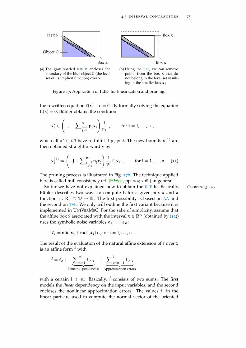
4.3 interval contractors 75
Object O
Box x
ILIE h
(a) The gray shaded ILIE h encloses theboundary of the blue object O (the levelset of its implicit function) over x.
Box x
Box x1
(b) Using the ILIE, we can removepoints from the box x that donot belong to the level set result-ing in the smaller box x1.
Figure 17: Application of ILIEs for linearization and pruning.
the rewritten equation f(x) − c = 0. By formally solving the equationh(x) = 0, Bühler obtains the condition
x∗i ∈(−j−
∑n
j=1j6=i
pjxj
)1
pi, for i = 1, . . . ,n ,
which all x∗ ∈ LS have to fulfill if pi 6= 0. The new bounds x(1) arethen obtained straightforwardly by
x(1)i :=
(−j−
∑n
j=1j6=i
pjxj
)1
pi∩ xi , for i = 1, . . . ,n . (33)
The pruning process is illustrated in Fig. 17b. The technique appliedhere is called hull consistency (cf. [HW04, pp. 203-208]) in general.
So far we have not explained how to obtain the ILIE h. Basically, Constructing ILIEs
Bühler describes two ways to compute h for a given box x and afunction f : Rn ⊃ D → R. The first possibility is based on AA andthe second on TMs. We only will outline the first variant because it isimplemented in UniVerMeC. For the sake of simplicity, assume thatthe affine box x associated with the interval x ∈ Rn (obtained by (12))uses the symbolic noise variables ε1, . . . , εn:
xi := mid xi + rad (xi) εi for i = 1, . . . ,n .
The result of the evaluation of the natural affine extension of f over xis an affine form f with
f = f0 +∑n
i=1fiεi︸ ︷︷ ︸
Linear dependencies
+∑l
i=n+1fiεi︸ ︷︷ ︸
Approximation errors
with a certain l > n. Basically, f consists of two sums: The firstmodels the linear dependency on the input variables, and the secondencloses the nonlinear approximation errors. The values fi in thelinear part are used to compute the normal vector of the oriented

76 functions in univermec
hyperplane L and the distance d of the hyperplane to the origin. Thecentral value f0 also contributes to d. The thickness is determined bythe nonlinear noise part of f and contributes together with d to theinterval quantity j in (32). For a detailed algorithm, see [Büh02].
4.4 function layer
This section explains the actual realization of the representation ofSection’s structure
mathematical functions inside UniVerMeC. We begin the discussionby providing formal definitions for the representations. After that,we show how to transfer this formal framework to abstract interfacesin our software. Finally, the section concludes with the description ofa flexible default implementation of these interfaces.
4.4.1 Formal Definition
UniVerMeC is not restricted to functions f given in a specific wayFunctionrepresentation
objects(e.g., as an analytical expression). Instead, f is characterized by atleast one inclusion function for each arithmetic supported by theframework. Formally, f is described by a function representation ob-ject (FRO):
Definition 14 (Function representation object) Let f : Rn ⊃ D →Rm be given. A function representation object of f is a tuple Of,n,m =
(I,F) where
1. I = {F(1), . . . , F(q)} is the set of inclusion functions where q is thenumber of arithmetics supported in the framework. This set containsone inclusion function F(i) (Def. 7) for each (finite) arithmetic.
2. F ⊆ {E(1)f , . . . ,E(r)
f } is a subset of the set of features where r is thenumber of supported features in the framework. Each E
(i)f is a tuple
of certain form (cf. Def. 15).
The definition guarantees that each FRO can be evaluated at least withall supported arithmetics8 using an appropriate inclusion function.Furthermore, a set of features can be provided that supplies additionalfunctionalities associated with f. Possible features are, for example,further range-enclosure possibilities or contractors specialized for thegiven f.
Based on our discussion and our previous work, we identify thePredefined features
following set of features, which are important in our opinion andwhich we will need later (this set can be extended if necessary):
8 at the moment: FP , IA , AA and TMs
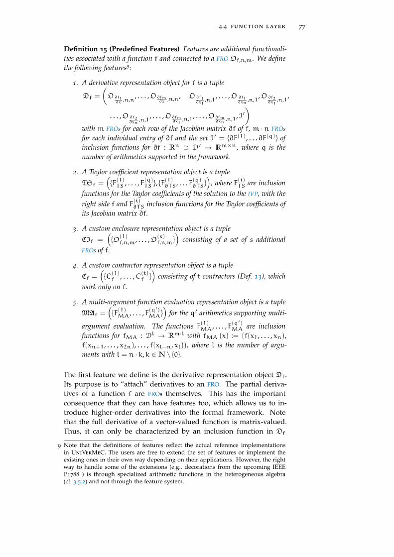
4.4 function layer 77
Definition 15 (Predefined Features) Features are additional functionali-ties associated with a function f and connected to a FRO Of,n,m. We definethe following features9:
1. A derivative representation object for f is a tuple
Df =
(O∂f1
∂x ,n,n, . . . ,O∂fm
∂x ,n,n, O ∂f1∂x1
,n,1, . . . ,O ∂f1
∂xn,n,1
,O ∂f2∂x1
,n,1,
. . . ,O ∂f2∂xn
,n,1, . . . ,O∂fm
∂x1,n,1, . . . ,O∂fm
∂xn,n,1, I ′
)with m FROs for each row of the Jacobian matrix ∂f of f, m · n FROs
for each individual entry of ∂f and the set I ′ = {∂F(1), . . . ∂F(q)} ofinclusion functions for ∂f : Rn ⊃ D ′ → Rm×n, where q is thenumber of arithmetics supported in the framework.
2. A Taylor coefficient representation object is a tupleTSf =
({F
(1)TS , . . . , F(q)TS }, {F
(1)∂TS, . . . F(q)∂TS}
), where F(i)TS are inclusion
functions for the Taylor coefficients of the solution to the IVP, with theright side f and F(i)∂TS inclusion functions for the Taylor coefficients ofits Jacobian matrix ∂f.
3. A custom enclosure representation object is a tupleCIf =
({O
(1)f,n,m, . . . ,O(s)
f,n,m})
consisting of a set of s additionalFROs of f.
4. A custom contractor representation object is a tupleCf =
({C
(1)f , . . . ,C(t)
f })
consisting of t contractors (Def. 13), whichwork only on f.
5. A multi-argument function evaluation representation object is a tupleMAf =
({F
(1)MA, . . . , F(q
′)MA}
)for the q ′ arithmetics supporting multi-
argument evaluation. The functions F(1)MA, . . . , F(q′)
MA are inclusionfunctions for fMA : Dl → Rm·l with fMA (x) := (f(x1, . . . , xn),f(xn+1, . . . , x2n), . . . , f(xl−n, xl)), where l is the number of argu-ments with l = n · k,k ∈N \ {0}.
The first feature we define is the derivative representation object Df.Its purpose is to “attach” derivatives to an FRO. The partial deriva-tives of a function f are FROs themselves. This has the importantconsequence that they can have features too, which allows us to in-troduce higher-order derivatives into the formal framework. Notethat the full derivative of a vector-valued function is matrix-valued.Thus, it can only be characterized by an inclusion function in Df
9 Note that the definitions of features reflect the actual reference implementationsin UniVerMeC. The users are free to extend the set of features or implement theexisting ones in their own way depending on their applications. However, the rightway to handle some of the extensions (e.g., decorations from the upcoming IEEEP1788 ) is through specialized arithmetic functions in the heterogeneous algebra(cf. 3.5.2) and not through the feature system.

78 functions in univermec
Table 12: The most important interfaces of the function layer and the formalconcepts that they realize.
interface description concept
IVFunctionfunction representation Def. 14
IFunction
IDerivative derivatives of a function
Def. 15
ITaylorCoeff Taylor coefficient’s of a functionICustomCon custom contractors for a functionICustomEncl custom enclosures for a functionIGPUEval multi-argument evaluation
IContractor contractor representation Def. 13
because FROs are limited to vector-valued functions within the frame-work. The Taylor coefficient representation object TSf is only of in-terest in the context of IVPs with the right-hand side f. Many IVP
solvers (e.g., VNODE-LP in our case) need Taylor coefficients of a so-lution to compute its enclosure. With the third feature, the customenclosure representation object, it is possible to provide additionalinclusion functions for f. They might be of interest if f belongs to aclass of functions (e.g., polynomials) for which different specializedtechniques for constructing inclusion functions exist (e.g., applicationof the Horner scheme for polynomials). Similarly to the third feature,the custom contractor representation object is merely a set of contrac-tors that exploit special knowledge about the inner structure of thegiven function. The multi-argument function evaluation representa-tion object is the last feature we define. It allows us to evaluate thefunction for different arguments simultaneously.
4.4.2 Interfaces of the Function Layer
In this subsection, we discuss the software interfaces giving accessConnection to thetheoretical basis to basic concepts defined previously. In Tab. 12, the most important
interfaces we will discuss are shown. Each interface has a formalcounterpart. We discuss how the implementation maps to the formalfoundation and what requirements are induced on the actual classesimplementing our interfaces.
Function InterfacesThe two interfaces IVFunction and IFunction shown in Fig. 18 areFROs in software
the key interfaces of the function layer. IFunction is merely a con-venience interface for scalar-valued functions. It is derived from
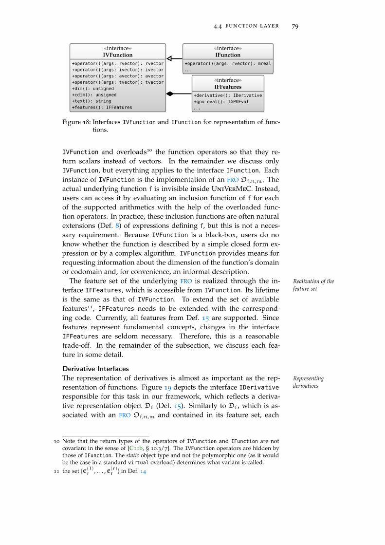
4.4 function layer 79
«interface»IVFunction
+operator()(args: rvector): rvector+operator()(args: ivector): ivector+operator()(args: avector): avector+operator()(args: tvector): tvector+dim(): unsigned+cdim(): unsigned+text(): string+features(): IFFeatures
«interface»IFunction
+operator()(args: rvector): mreal. . .
«interface»IFFeatures
+derivative(): IDerivative+gpu_eval(): IGPUEval. . .
Figure 18: Interfaces IVFunction and IFunction for representation of func-tions.
IVFunction and overloads10 the function operators so that they re-turn scalars instead of vectors. In the remainder we discuss onlyIVFunction, but everything applies to the interface IFunction. Eachinstance of IVFunction is the implementation of an FRO Of,n,m. Theactual underlying function f is invisible inside UniVerMeC. Instead,users can access it by evaluating an inclusion function of f for eachof the supported arithmetics with the help of the overloaded func-tion operators. In practice, these inclusion functions are often naturalextensions (Def. 8) of expressions defining f, but this is not a neces-sary requirement. Because IVFunction is a black-box, users do noknow whether the function is described by a simple closed form ex-pression or by a complex algorithm. IVFunction provides means forrequesting information about the dimension of the function’s domainor codomain and, for convenience, an informal description.
The feature set of the underlying FRO is realized through the in- Realization of thefeature setterface IFFeatures, which is accessible from IVFunction. Its lifetime
is the same as that of IVFunction. To extend the set of availablefeatures11, IFFeatures needs to be extended with the correspond-ing code. Currently, all features from Def. 15 are supported. Sincefeatures represent fundamental concepts, changes in the interfaceIFFeatures are seldom necessary. Therefore, this is a reasonabletrade-off. In the remainder of the subsection, we discuss each fea-ture in some detail.
Derivative InterfacesThe representation of derivatives is almost as important as the rep- Representing
derivativesresentation of functions. Figure 19 depicts the interface IDerivative
responsible for this task in our framework, which reflects a deriva-tive representation object Df (Def. 15). Similarly to Df, which is as-sociated with an FRO Of,n,m and contained in its feature set, each
10 Note that the return types of the operators of IVFunction and IFunction are notcovariant in the sense of [C11b, § 10.3/7]. The IVFunction operators are hidden bythose of IFunction. The static object type and not the polymorphic one (as it wouldbe the case in a standard virtual overload) determines what variant is called.
11 the set {E(1)f , . . . ,E(r)
f } in Def. 14
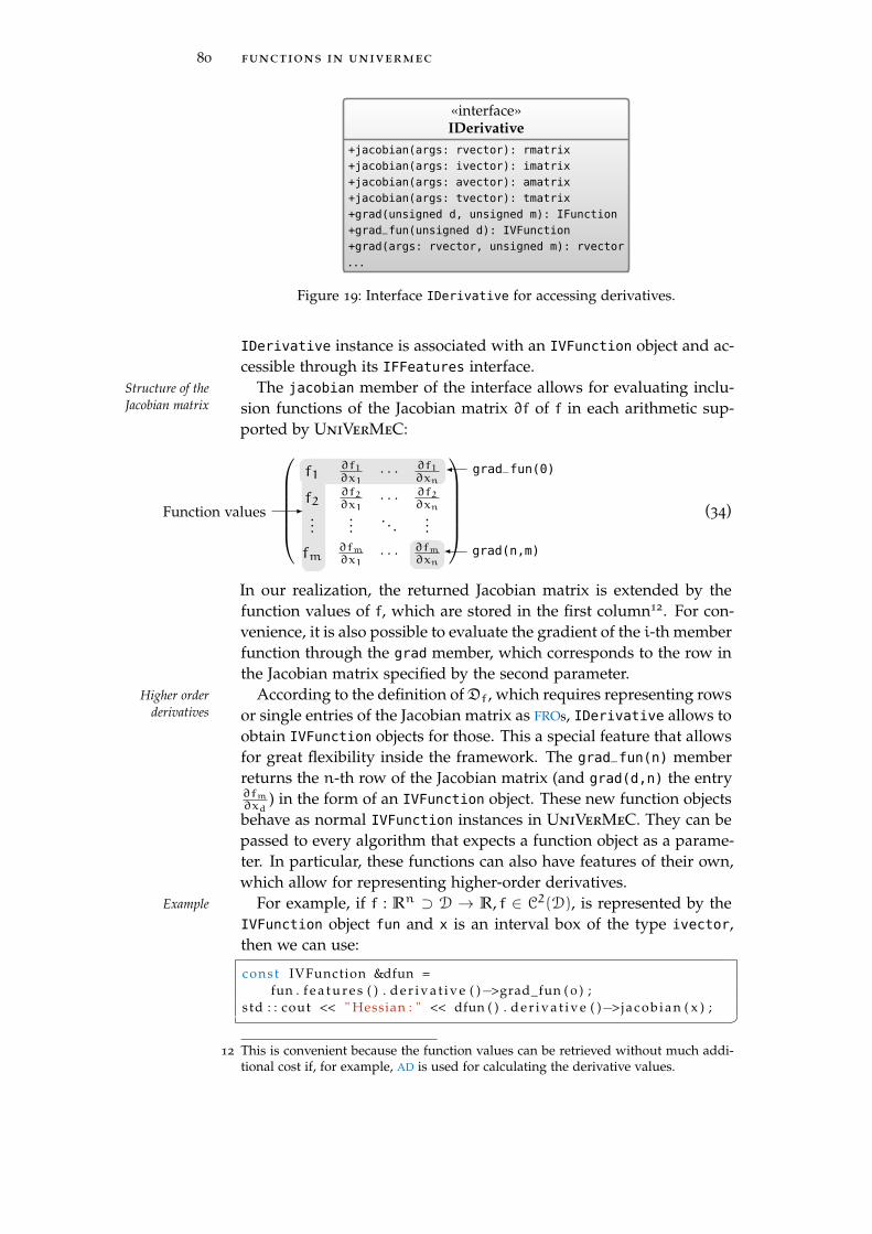
80 functions in univermec
«interface»IDerivative
+jacobian(args: rvector): rmatrix+jacobian(args: ivector): imatrix+jacobian(args: avector): amatrix+jacobian(args: tvector): tmatrix+grad(unsigned d, unsigned m): IFunction+grad_fun(unsigned d): IVFunction+grad(args: rvector, unsigned m): rvector. . .
Figure 19: Interface IDerivative for accessing derivatives.
IDerivative instance is associated with an IVFunction object and ac-cessible through its IFFeatures interface.
The jacobian member of the interface allows for evaluating inclu-Structure of theJacobian matrix sion functions of the Jacobian matrix ∂f of f in each arithmetic sup-
ported by UniVerMeC:f1
∂f1∂x1
· · · ∂f1∂xn
f2∂f2∂x1
· · · ∂f2∂xn
......
. . ....
fm∂fm∂x1
· · · ∂fm∂xn
(34)Function values
grad_fun(0)
grad(n,m)
In our realization, the returned Jacobian matrix is extended by thefunction values of f, which are stored in the first column12. For con-venience, it is also possible to evaluate the gradient of the i-th memberfunction through the grad member, which corresponds to the row inthe Jacobian matrix specified by the second parameter.
According to the definition of Df, which requires representing rowsHigher orderderivatives or single entries of the Jacobian matrix as FROs, IDerivative allows to
obtain IVFunction objects for those. This a special feature that allowsfor great flexibility inside the framework. The grad_fun(n) memberreturns the n-th row of the Jacobian matrix (and grad(d,n) the entry∂fm∂xd
) in the form of an IVFunction object. These new function objectsbehave as normal IVFunction instances in UniVerMeC. They can bepassed to every algorithm that expects a function object as a parame-ter. In particular, these functions can also have features of their own,which allow for representing higher-order derivatives.
For example, if f : Rn ⊃ D → R, f ∈ C2(D), is represented by theExample
IVFunction object fun and x is an interval box of the type ivector,then we can use:
const IVFunction &dfun =fun . f e a t u r e s ( ) . d e r i v a t i v e ( )−>grad_fun ( 0 ) ;
s td : : cout << " Hessian : " << dfun ( ) . d e r i v a t i v e ( )−>j a c o b i a n ( x ) ; �12 This is convenient because the function values can be retrieved without much addi-
tional cost if, for example, AD is used for calculating the derivative values.

4.4 function layer 81
«interface»IGPUEval
+open_device(): void+close_device(): void+IGPUFuture<ivector> comp(args: vector<ivector>)+IGPUFuture<rvector> comp(args: vector<rvector>)
«interface»IGPUFuture<T>
+ready(): bool+valid(): bool+results(): vector<T>
T: Base Type
Figure 20: Interfaces IGPUEval and IGPUFuture<T> for function evaluationon the GPU.
to represent its gradient by a new IVFunction object dfun. Calling thejacobian member of dfun would return an interval-based enclosureof the Hessian matrix of f over x. The lifetime of the new object dfunis determined by that of the IVFunction instance fun from which theyoriginated.
GPU Evaluation InterfaceAs already mentioned in Sect. 3.7, UniVerMeC supports computa- GPU evaluation
interfacetions on the GPU. This is realized at the function layer by providingthe interface IGPUEval, which corresponds in our formal basis with amulti-argument evaluation representation object MAf (Def. 15). There-fore, each IGPUEval object is associated to an IVFunction instanceand accessible through its feature interface. Figure 20 depicts theIGPUEval interface with its four member functions. The open_device
and close_device members should be called prior to the first andafter the last GPU function evaluation. They have no counterpart inMAf. Their purpose is, for example, to allocate static data (e.g., modelparameters) on the GPU before starting the computation.
Following the definitions of MAf, IGPUEval provides inclusion func- Asynchronism
tions for f for all supported arithmetics on the GPU (cf. Sect. 3.7). Wecan evaluate them through the overloaded comp functions. Currently,they take either a list of interval vectors or real vectors and return afuture object for the list of the corresponding inclusion function val-ues. A future object is a kind of handle that refers to values thathave not been computed at the time of returning it. It is commonlyused in parallel computing (e.g., [HS08, pp. 369-375]). Therefore, acall to comp is non-blocking. For GPU computations, UniVerMeCsupplies the IGPUFuture<T> interface. It has a template parameterT that is chosen depending on whether an interval computation orFP computation is desired. This ensures type safety13 and extendabil-ity with further types (e.g., affine forms) if necessary. With the helpof IGPUFuture<T>, users can check whether the results have been al-ready computed (the ready() member) or whether the future is valid.The results() member returns the list of function values and blocksuntil the computation is finished. Using the future mechanism, it ispossible to interleave one or several computations on the GPU, whichallows for better utilization of the GPU’s resources.
13 The result type is statically determined by the overloaded function call of IGPUEval.
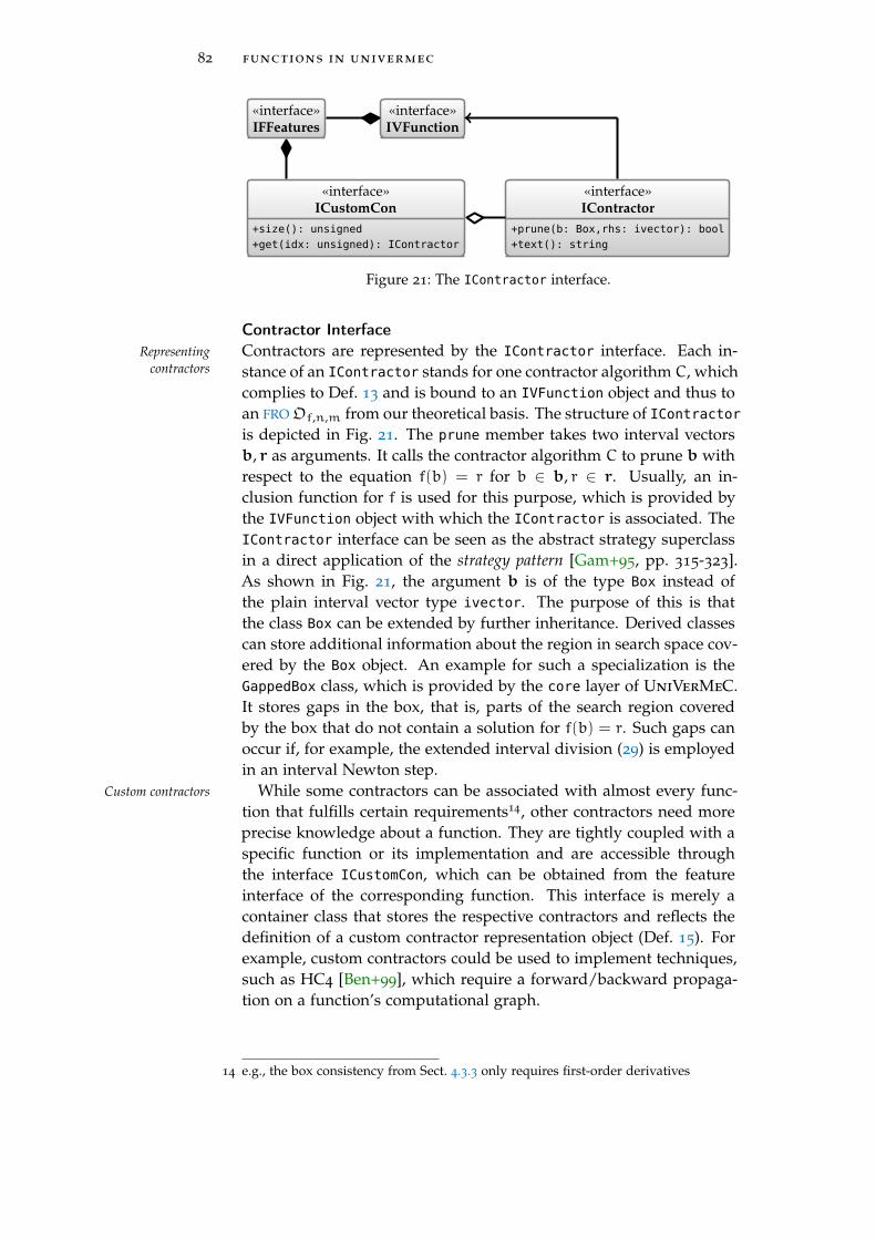
82 functions in univermec
«interface»IContractor
+prune(b: Box,rhs: ivector): bool+text(): string
«interface»ICustomCon
+size(): unsigned+get(idx: unsigned): IContractor
«interface»IFFeatures
«interface»IVFunction
Figure 21: The IContractor interface.
Contractor InterfaceContractors are represented by the IContractor interface. Each in-Representing
contractors stance of an IContractor stands for one contractor algorithm C, whichcomplies to Def. 13 and is bound to an IVFunction object and thus toan FRO Of,n,m from our theoretical basis. The structure of IContractoris depicted in Fig. 21. The prune member takes two interval vectorsb, r as arguments. It calls the contractor algorithm C to prune b withrespect to the equation f(b) = r for b ∈ b, r ∈ r. Usually, an in-clusion function for f is used for this purpose, which is provided bythe IVFunction object with which the IContractor is associated. TheIContractor interface can be seen as the abstract strategy superclassin a direct application of the strategy pattern [Gam+95, pp. 315-323].As shown in Fig. 21, the argument b is of the type Box instead ofthe plain interval vector type ivector. The purpose of this is thatthe class Box can be extended by further inheritance. Derived classescan store additional information about the region in search space cov-ered by the Box object. An example for such a specialization is theGappedBox class, which is provided by the core layer of UniVerMeC.It stores gaps in the box, that is, parts of the search region coveredby the box that do not contain a solution for f(b) = r. Such gaps canoccur if, for example, the extended interval division (29) is employedin an interval Newton step.
While some contractors can be associated with almost every func-Custom contractors
tion that fulfills certain requirements14, other contractors need moreprecise knowledge about a function. They are tightly coupled with aspecific function or its implementation and are accessible throughthe interface ICustomCon, which can be obtained from the featureinterface of the corresponding function. This interface is merely acontainer class that stores the respective contractors and reflects thedefinition of a custom contractor representation object (Def. 15). Forexample, custom contractors could be used to implement techniques,such as HC4 [Ben+99], which require a forward/backward propaga-tion on a function’s computational graph.
14 e.g., the box consistency from Sect. 4.3.3 only requires first-order derivatives

4.4 function layer 83
Function EnclosuresAnother important aspect is special enclosure functions for f such Handling of
function enclosuresas mean-value forms (cf. Sect. 4.2). In our theoretical basis, enclo-sures are not explicitly modeled, because we can treat them as FROs
Of,n,m with a different set I of inclusion functions. Therefore, theyare realized in UniVerMeC by providing a new IVFunction instancethat wraps the original one and performs the enclosure technique forfunction evaluation.
We illustrate this behavior using the example of the mean-value Example ofconstructionforms introduced in Sect. 4.2.1. Let f : Rn ⊃ D → R, f ∈ C1(D),
be defined by an expression, and Of,n,m an FRO for f, the inclusionfunctions of which are obtained by natural extension. Let further funbe an IVFunction instance that realizes Of,n,m. A mean-value formenclosure in the framework is a new IVFunction object that carriesout the following three steps for its inclusion functions evaluated withany of the supported arithmetics:
1. Perform an enclosure_cast (Def. 11) to intervals on the argu-ments, if necessary.
2. Apply (20) using the interval inclusion function of fun.
3. Perform a forced_cast (Def. 12) to the original argument type,which is, actually, a lossless_cast (Def. 10) for all arithmeticsexcept FPA in which the range is obviously lost.
Clearly, the new IVFunction is the realization of another FRO for f.Analogously to the ICustomCon interface, an ICustomEncl interface Custom enclosures
exists and can be accessed through features of an IVFunction. Itcorresponds to the custom inclusion function representation objectfrom Def. 15 and is just a container that holds the set of additionalinclusion functions.
Other Interfaces and Possible ExtensionsIn addition to the above mentioned interfaces, UniVerMeC provides Taylor coefficients
the ITaylorCoeff interface. It is the computer realization of the Tay-lor coefficient representation object defined in Def. 15.
Interesting candidates for the extension of the feature interface are, Possible extensions
for example, objects for calculating slopes of a function or for its rep-resentation by a DAG that would allow for a generic implementationof techniques such as hull consistency. If these additional functional-ities are to be integrated into the framework, it is necessary to alterthe interface IFFeatures accordingly
4.4.3 Implementation of the Function Layer
To make integration of functions into the framework easier, UniVer- Functors forrepresentingfunctions
MeC supplies standard implementations for all interfaces. These stan-dard implementations can be applied if users provide their functions

84 functions in univermec
s t r u c t b r u s s e l a t o r _ t{
3 b r u s s e l a t o r _ t ( const core : : a r i t h : : mreal &a ,const core : : a r i t h : : mreal &b )
: m_a( b ) , m_b( b ) { }
template <typename T>8 T operator ( ) ( const T& args ) const
{T re s ( 2 ) ;r es [ 0 ] = m_a + args [ 0 ] * ( args [ 0 ] * args [ 1 ] − m_b − 1 ) ;r es [ 1 ] = args [ 0 ] * ( m_b−args [ 0 ] * args [ 1 ] ) ;
13 re turn r es ;}
s td : : s t r i n g t e x t ( ) const{
18 re turn " B r u s s e l a t o r " ;}
unsigned cdim ( ) const{
23 re turn 2 ;}
unsigned dim ( ) const{
28 re turn 2 ;}
p r i v a t e :core : : a r i t h : : mreal m_a ;
33 core : : a r i t h : : mreal m_b ;} ; �Listing 3: A functor for defining a function in UniVerMeC. The concrete
functor is the right-hand side of the Brusselator.
in form of a functor. A functor is a well-known concept in C++: It isa structure with an overloaded function operator(). In contrast toplain function pointers, it also stores context information as membervariables.
An Introductory ExampleAs an example consider that the right-hand side of the BrusselatorExploiting templates
ordinary differential equation (ODE) [Sta97, p.70]
x = a+ x(xy− b− 1)
y = x(b− xy)(35)
has to be represented in our framework. In this example, a and b areparameters. A possible implementation as a functor is given in list-ing 3. The most important member of the structure is the operator(),which is realized as a template function in this example. This is

4.4 function layer 85
«interface»IVFunction
«interface»IFunction
«interface»IDerivative
«interface»IGPUEval
«interface»ICustomCon
«interface»ITaylorCoeff
FVBase
FDeriv
FTaylorCoeff
FGPUEval
FCustomCon
«interface»FMaster
+get_f(): T. . .
FJoin
inhe
rita
nce
depe
nds
onch
osen
feat
ure
setF1
,...
,Fn
T : FunctorF1: FeatureF2: Feature. . .
T: Functor
T: Functor
T: Functor
T: Functor
T: Functor
T: Functor
inhe
rite
din
terf
ace
chos
ende
pend
ing
onfu
ncto
rT
«interface»IFFeatures
Figure 22: Simplified struture of the uniform function representation layerand its implementation in UniVerMeC.
the recommended way because it allows for evaluation with all sup-ported arithmetics and to provide derivatives by AD. A further recom-mendation is for users to restrict operation and function calls insideof the template to the set defined by the algebra (15), because naturalinclusion functions for all arithmetics are constructed automaticallyby template instantiation in this case. This is possible only becausethe arithmetic layer provides a common set of functions with uni-form names. It demonstrates the importance of generating uniformadapters at the arithmetic level automatically. The other members ofthe structure in listing 3 are just auxiliary functions that return di-mension of the function’s (co-)domain and a textual description forthe functor.
With this functor available, an IVFunction instance can be gener- Creating anIVFunction
instanceated straightforwardly to evaluate (35). As shown in Fig. 22, theimplemention class corresponding to IVFunction is the FVBase tem-plate. To create an IVFunction object, it is sufficient to generate abrusselator_t functor with the desired parameter values for a,band then to instantiate FVBase with brusselator_t as the templateparameter:
IVFunction * b r u s s e l a t o r = new FVBase< b r u s s e l a t o r _ t >(new b r u s s e l a t o r _ t ( 1 . 0 , 1 . 0 ) ) ; �
The resulting IVFunction object could then, for example, be employedto define an IVP, which can be solved with an ODE software, such as

86 functions in univermec
VODE [BBH89], interfaced to our framework (cf. Sect. 7.3). Note thatthe actual implementation (the functor) is hidden at this point.
The function object we have instantiated so far has an empty fea-Adding features
ture set, that is, there are no means for calculating derivatives. How-ever, if the functor uses a template for the operator() and the under-lying mathematical function is differentiable, support for the IDeriva-
tive interface can be added easily:
IVFunction * b r u s s e l a t o r = new FJoin < b r u s s e l a t o r _ t ,FDeriv < b r u s s e l a t o r _ t > , FTaylorCoeff < b r u s s e l a t o r _ t > >
(new b r u s s e l a t o r _ t ( 1 . 0 , 1 . 0 ) ) ; �In this case, we join FVBase (which is inherited by FJoin), FDeriv
and FTaylorCoeff. Consequently, the resulting IVFunction instance’sfeature set contains the IDerivative and ITaylorCoeff interfaces.An IVP using this more sophisticated IVFunction object for its right-hand side could be solved, for example, with ValEncIA-IVP [RA11],which requires first-order derivatives or VNODE-LP [Ned06], whichrequires Taylor coefficients. Both are interfaced with out framework(cf. Sect. 7.3).
Internal Structure of the Function Layer ImplementationAn important aspect of the feature system and its interfaces is thatAllowing arbitrary
feature combinations arbitrary combinations of features are possible. In our default im-plementation, this is achieved basically by associating an individualimplemention class with each interface and the ability to combinethese classes through multiple inheritance. As shown in Fig. 22, thisapproach is implemented by the FJoin class template. FJoin inheritsfrom FVBase, which in turn inherits from IVFunction or IFunction15.Furthermore, FJoin inherits from each selected feature class. If a fea-ture is requested through the IFFeatures interface, the appropriatelytype-casted this pointer of the FJoin instance is returned.
The feature is automatically enabled or disabled during compiletime using the substitution failure is not an error (SFINAE) principlebased on the static type of the FJoin template. SFINAE means thatif a type substitution of a template parameter is invalid, this is nottreated as an error that stops the compilation process. This can beexploited, for example, to activate or disable functions based on con-ditions checked on compile time (e.g. through the std::enable_if
template provided by the standard library in the new C++11 stan-dard [C11b, § 20.9.7.6]). Another feature of our function layer defaultimplementation is that all classes implementing features are decou-pled not only from each other but also from FVBase and vice versa.That allows us to use another implementation for a feature interfacetogether with the existing default ones. It would be even possible to
15 This decision is made automatically during compile time depending on whetherthe functor is scalar. A functor is treated as scalar if a function with the signatureinterval operator()(const ivector &args) const exists.
4.4 function layer 87
replace the FVBase basic class and still use the default feature imple-mentations, if necessary.
The decoupling is achieved by the FMaster template that is in- Cross delegation
herited by FVBase and all feature classes16. FMaster is an interfacethat provides access to an instance of the underlying functor usingthe get_f() member. This interface is only implemented by FVBase,which stores the actual instance of the functor. If any other featureclass, for example, FDeriv, requests the functor using its inheritedget_f() member, the call is forwarded to the only implementation(provided by FVBase) inside the final inheritance formed by FJoin.This pattern is sometimes referred to as “cross delegation” [Cli], be-cause neither FDeriv nor FVBase know about each other. The call iscross delegated transparently to another branch of the (multiple) inher-itance graph.
Note that we work on functor instances instead of functor types. Work- Instances vs. types
ing only on types requires default constructors in every functor inorder for each feature class to create its own instance. Alternatively,we could declare all methods static. However, these approacheswould result in functors the behavior of which is determined at com-pile time by their static type, without the possibility to parametrizethem further at runtime. As an illustration, consider the Brussela-tor example in listing 3 and its instantiation again. The static type isFJoin<brusselator_t, FDeriv<brusselator_t>, FTaylorCoeff<bru-
sselator_t> >. It is determined at compile time. However, if we useinstances instead of types, we are free to alter the parameters a,bin (35) at runtime freely.
The idea can be extended further by providing a functor that acts Function parser
as a parser capable of handling closed form expressions. In thiscase, such expressions can be entered at runtime and result in validIVFunction objects. Internally, the function parser of UniVerMeCis based on FVBase and uses Boost.Spirit [GK] to parse the expres-sion and to evaluate the resulting abstract syntax tree recursively. Us-ing FDeriv, the resulting function provides derivatives up to a user-defined order17 automatically. For example, an IFunction object forthe function f(x,y, z) = x2 + y2 + z2 − 1 can be generated using thefunction parser as follows:
IFunct ion * sphere =parser : : p a r s e _ s t r i n g ( " sqr ( x0 ) +sqr ( x1 ) +sqr ( x2 )−1" ) ; �
FDerivAs mentioned above, the FDeriv template is an implementation of Generation of
derivative inclusionfunctions
the IDerivative interface. It provides derivatives for a function f :
Rn ⊃ D → Rm, f ∈ Cd(D), defined by a templated functor and
16 Technically, we have to use virtual inheritance [C11b, § 10.1] to avoid storing mul-tiple FMaster instances inside one FJoin instance.
17 see below
88 functions in univermec
makes them available through the interface. In this process, AD isused the principles of which we reviewed in Sect. 4.1 briefly. As theconcrete AD implementation, we use FADBAD++ [SB] developed byStauning and Bendtsen. It is a C++ template library, implemented bythe means of operator overloading and working with arbitrary arith-metic types through trait classes. FADBAD++ provides computationof derivatives (by forward or backward differentiation) and Taylor co-efficients. Because appropriate FADBAD++ trait classes for all arith-metics supported by our framework are automatically generated onthe arithmetic layer (cf. Sect. 3.6), inclusion functions for derivativescan be computed for all of them. As an example consider the implicitfunction of the unit sphere defined by the template
template <typename T>typename T : : value_type operator ( ) ( const T& args ){
re turn sqr ( args [ 0 ] ) +sqr ( args [ 1 ] ) +sqr ( args [ 2 ] ) − 1 ;} �To compute the values of derivatives with forward differentiationwith FADBAD++ and IA, we have to wrap our arguments into thefadbad::F template, that is, to instantiate the operator() templatewith mtl::dense_vector<fadbad::F<interval> > as T. Backward dif-ferentiation can be performed by using fadbad::B as a replacementfor fadbad::F.
A distinctive feature of FADBAD++ is the ability to compute higherGeneration ofhigher-order
derivativesorder derivatives by template nesting. For example, fadbad::F<-
fadbad::F<interval> > is used to obtain the second order deriva-tive. Even mixed nesting of the forward and backward types is sup-ported. However, the derivative order has to be decided upon atcompile time because it depends on the static type18 of the templatearguments. With the help of the FDeriv class, users can choose themaximum derivative order at compile time for each function individ-ually19. The necessary type nesting and instantiations of the templateoperator() for higher-order derivatives as well as the generation ofthe new IVFunction objects for the grad(d,m) and grad_fun(d) (seeFig. 19) are handled automatically by FDeriv itself. We recommendchoosing a not too high maximum order because the automaticallyperformed template nesting can increase the compilation time signif-icantly. The default order, which is also used for functions gener-ated through the parser, is set to 3. In our opinion, this is a reason-able setting because higher order derivatives are seldomly used inthe verified context aside from Taylor coefficients, which are, how-ever, handled by the ITaylorCoeff interface and its implementationFTaylorCoeff respectively.
18 which changes depending on the number of template nestings19 This is realized using third template parameter.

4.4 function layer 89
«interface»IGPUEval FGPUEval
«interface»IGPUDeviceEval
+comp_iv(double* a,int s):IGPUDeviceFuture
+comp_rv(double* a,int s):IGPUDeviceFuture
«interface»IGPUFuture
GPUFutureImpl «interface»IGPUDeviceFuture
,«instantiate»
Host code Host⇔ CUDA
CU
DA
Code
T : Functor
T : Base typeT : Base type
Figure 23: Interaction of the host program with the GPU kernel implementa-tion.
FGPUEvalThe GPU integration at the functions layer of UniVerMeC consists of Memory transfer to
the GPUthree parts as shown in Fig. 23. The left part, to which we refer ashost code, provides implementations for the interfaces of the functionlayer. In the middle, we have glue code, which basically consists oftwo interfaces imitating the interfaces of the host part with one im-portant difference: They do not take a list of ivectors or rvectorsto process but an array of doubles, the type we identified in Sect. 3.7as suitable for communication between CPU and GPU. It is importantto note that the comp_iv and comp_rv functions of IGPUDeviceEval
have to fulfill the same requirements as for the comp members ofIGPUEval defined in Sect. 4.4.2. This procedure also decouples theGPU code from the CPU code and makes it independent from librariesemployed on the CPU. Some of them, for example, the Matrix Tem-plate Library [GL], can be problematic to parse with the CUDA Ccompiler. The conversion to the double array is done by the FGPUEval
class automatically, and the memory layout is configurable. For exam-ple, a list of a(1), . . . ,a(m) d-dimensional mreal vectors is convertedto
a(1)1 , . . . ,a(n)1 ,a(1)2 , . . . ,a(n)2 ,a(1)3 , . . . ,a(n)d ,
a(n+1)1 , . . . ,a(2n)1 ,a(n+1)2 , . . . ,a(2n)d , . . . ,a(m)
d
where n ∈ N. If n = 1 the list is simply flattened, that is, all compo-nents of a vector are stored in a row. More interesting is to choose nequal to the blocksize of the CUDA kernel doing the actual computa-tion. In this case, coalesced global memory access is possible, whichreduces the number of overall memory requests [Cud, pp. 70-72]. Be-cause we do not make any assumptions about it, the actual kernelcode is not shown in Fig. 23. The only requirement we pose is for itto implement the IGPUDeviceEval and IGPUDeviceFuture interfaces.However, we recommend restricting the arithmetic functions on the

90 functions in univermec
Table 13: Implemented contractors and enclosures in UniVerMeC.
name type description
BCContractor Contractor Box consistency (Sect. 4.3.3)ILIEEncl Both ILIE (Sect. 4.3.4)MeanValueForm Enclosure Mean value form (20)
GPU to the sets described in Sect. 3.7. Non-blocking GPU computa-tions for the IGPUDeviceFuture support can be implemented usingCUDA streams [NVI12, pp. 31-34].
Example Implementations at the Function LayerWe omit the implementation details of the further classes of the func-Supplied example
implementations tion layer and give a short overview of the implemented contrac-tors and enclosures in UniVerMeC. The available techniques listedin Tab. 13 have been explained already earlier in this chapter. Onlythe classification of ILIEEncl as enclosure and contractor might needsome clarification. If we construct an ILIE as described in Sect. 4.3.4,we automatically get an inclusion function20 (the thick hyperplaneitself). Users can access the pruning procedure (33) by a custom con-tractor. This allows us to utilize both enclosure and contraction fea-tures without much overhead induced by the encapsulation.
4.5 conclusions
In this chapter, we described our approach to representing mathemat-Foundations
ical functions in our framework for verified computations. We startedby giving a short introduction to AD and interval enclosures that werely on later. In the third section of the chapter, we defined contrac-tors formally and discussed how this contractor notion relates to thewell-established definition of a constraint narrowing operator by Ben-hamou [Ben96]. Moreover, we described several further well-knowntechniques, for example, interval Newton or box consistency that weuse as a contractor.
The final section of the chapter was devoted to the handling ofData-typeindependent
functionrepresentation
functions (seen as black boxes) in our framework. We started by de-scribing the theoretical basis of our approach. First, we introducedthe notion of FROs and extended their functionalities by defining sev-eral representation objects for features. After that, we showed howto implement this theoretical basis. We arrived at a generic data-type independent21 representation of a function f by an interface
20 The range of the inclusion function is equivalent to the inclusion function obtainedby AA widely with the exception of rounding errors that occur during the ILIE calcu-lation.
21 with respect to the arithmetic
4.5 conclusions 91
(IVFunction), which characterized f by inclusion functions. In thisway, we were able to hide the internal representation completely with-out restricting the ways of actual implementation of functions. Thestrategy corresponds to the practices in modern software design thatpropose the wide use of encapsulation. As a second corner stoneof our function representation layer, we discussed how to enrich theIVFunction interface with additional functionalities by feature repre-sentation objects. They are realized as a set of interfaces connected toIVFunction. Each of them represents and allows access to a certainfunctionality coupled with the underlying function f. In this scope,we discussed features for derivatives, GPU evaluations and contrac-tors tailored for specific functions. This approach is made even moreflexible by handling enclosure functions and derivatives as standardIVFunction objects. These have their own feature sets again and can-not be distinguished from “normal” IVFunction instances. There-fore, an algorithm, for example, box consistency, which works on anIVFunction instance of f, can be applied to derivatives of f withoutany extra effort. Additionally, algorithms can dynamically activateaccelerating devices (if a function provides a corresponding feature)without additional work on the user’s part.
In this chapter, we also discussed how to integrate standalone con- Comparison withIBEXtractors in our framework. The provided interface (IContractor) al-
lows us to mimic techniques of contractor programming [CJ09] insideUniVerMeC. However, our approach for function representation ismore flexible than current implementations of contractor program-ming, such as IBEX [Cha]. IBEX can be used only with IA. Besides,functions inside IBEX have to be represented DAGs. Both are limita-tions from which our framework does not suffer. However, it is im-portant to note that the focus of IBEX lies on constraint propagationand that many techniques in this area benefit from the DAG represen-tation. Moreover, note that techniques based on forward/backwardpropagation (e.g. through operator overloading) cannot be applied toour black-box function representation. However, DAGs or contractorsbased on them can use the feature system of UniVerMeC.
Providing support for all interfaces necessary for a full integration Supplied standardimplementationsof a function into UniVerMeC leads to a considerable amount of
work. Therefore, we supply a standard implementation for all ourinterfaces discussed in the last part of this chapter. Users who wantto employ the standard implementation need to provide only theirfunction f in form of a functor with a templated22 function opera-tor. This template is instantiated with every arithmetic type, whichgenerates a natural inclusion function for all arithmetics supportedby the core layer automatically. Furthermore, it can be used to cal-culate derivative values by AD. Such level of automatization is only
22 The concept of entering user-specific functions through templates is well establishedin the verified numerical software, for example, in the packages VNODE-LP [Ned06]or FADBAD++ [SB].
92 functions in univermec
possible owing to the standardization of the set of available elemen-tary functions for all arithmetics (cf. Sect. 3.5) and the automaticallygenerated adapters (cf. Sect. 3.6). An interesting direction for the fu-ture research would be to make the contractors from IBEX availablein UniVerMeC. This is easily possible for functions in UniVerMeC,which are generated in the way outlined above.

5M O D E L I N G L AY E R
The purpose of the modeling layer is to express application domain Purpose
dependent notions in terms of the basic concepts (e.g. real/inter-val quantities and functions) defined earlier. Therefore, UniVerMeCdoes not have a single but many independent modeling layers — onefor each application domain. In this chapter, we demonstrate the useof the modeling layer in the scope of three case studies: the represen-tation of geometric objects, initial value problems, and optimizationproblems. All three case studies emerged from the need to apply ourframework to a certain close-to-life problem (cf. Chap. 8). Users arefree to alter the supplied model representation to fit their problems.Alternatively, they can introduce new model types to open new ap-plication domains.
To begin we start with a discussion of geometric models in Uni- Structure
VerMeC. After that, we describe the IVP representation supplied withthe framework and possibilities to integrate optimization problemsinto the modeling layer. Finally, we give a short outlook on potentialextensions with further modeling types.
5.1 geometric models
Geometric objects are important in many real-life applications. Thus, Geometric objects
various notions to describe them exist. For an extensive overview ofthe different geometric modeling types, see [Ago05a, pp. 156-225]. Inour applications, we need support for (non-convex) implicit objectsand polyhedrons. Furthermore, we employ parametric descriptionsof the implicit objects, if they are available. Limiting our understand-ing of geometric objects to the above ones, we can define them asbelow:
Definition 16 (Geometric object) We call a bounded set O ⊂ Rn geo-metric object if it is regular. That is, O is equivalent to the closure of itsinterior [Ago05a, p. 158]. Further, O is described either by
1. An implicit function f : Rn ⊃ D→ R withO =
{x∣∣ x ∈ D∧ f(x) 6 0
}. Then O is called an implicit object.
2. A parametric function p : Rn−1 ⊃ D→ Rn with∂O =
{p(x)
∣∣ x ∈ D}
. Then O is called a parametric object.
3. “The intersection of a finite number of halfplanes1” [Ago05b, p. 31].Then O is called a convex polyhedron.
1 With the help of a hyperplane h(x) in Hesse normal form, we define a halfplane as{x∣∣ h(x) 6 0} [Ago05b, p. 20].
93
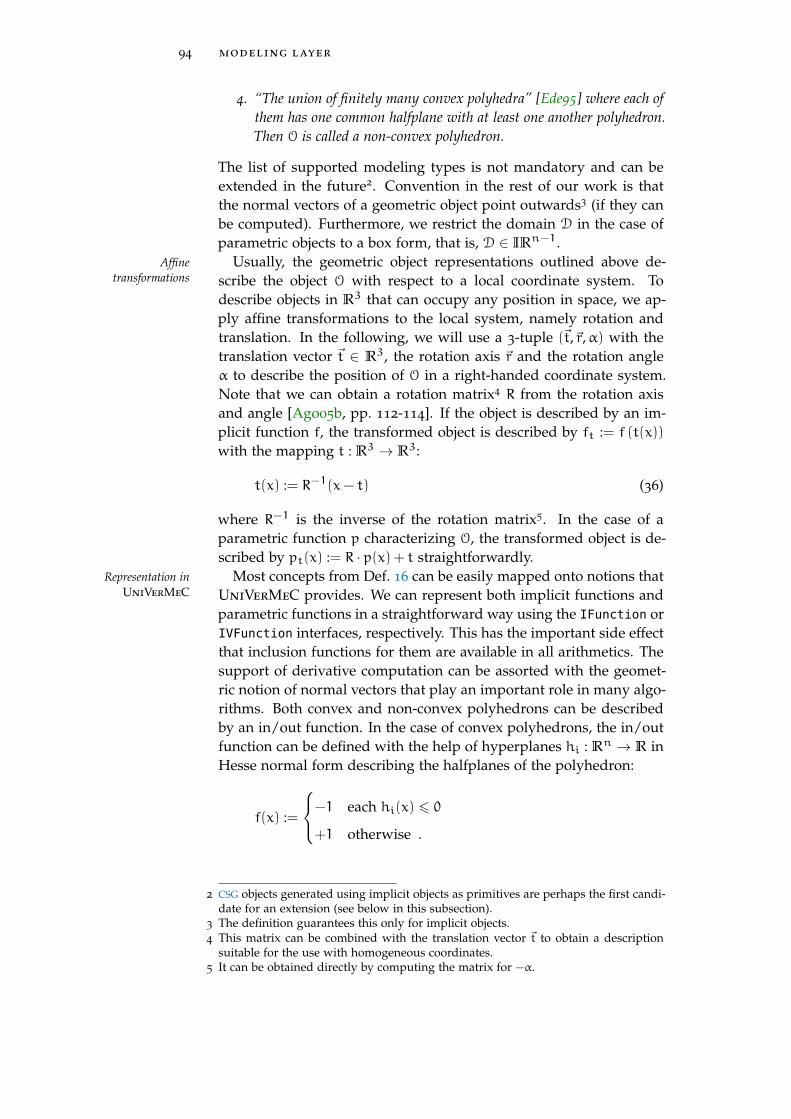
94 modeling layer
4. “The union of finitely many convex polyhedra” [Ede95] where each ofthem has one common halfplane with at least one another polyhedron.Then O is called a non-convex polyhedron.
The list of supported modeling types is not mandatory and can beextended in the future2. Convention in the rest of our work is thatthe normal vectors of a geometric object point outwards3 (if they canbe computed). Furthermore, we restrict the domain D in the case ofparametric objects to a box form, that is, D ∈ IRn−1.
Usually, the geometric object representations outlined above de-Affinetransformations scribe the object O with respect to a local coordinate system. To
describe objects in R3 that can occupy any position in space, we ap-ply affine transformations to the local system, namely rotation andtranslation. In the following, we will use a 3-tuple (~t,~r,α) with thetranslation vector ~t ∈ R3, the rotation axis ~r and the rotation angleα to describe the position of O in a right-handed coordinate system.Note that we can obtain a rotation matrix4 R from the rotation axisand angle [Ago05b, pp. 112-114]. If the object is described by an im-plicit function f, the transformed object is described by ft := f (t(x))
with the mapping t : R3 → R3:
t(x) := R−1(x− t) (36)
where R−1 is the inverse of the rotation matrix5. In the case of aparametric function p characterizing O, the transformed object is de-scribed by pt(x) := R · p(x) + t straightforwardly.
Most concepts from Def. 16 can be easily mapped onto notions thatRepresentation inUniVerMeC UniVerMeC provides. We can represent both implicit functions and
parametric functions in a straightforward way using the IFunction orIVFunction interfaces, respectively. This has the important side effectthat inclusion functions for them are available in all arithmetics. Thesupport of derivative computation can be assorted with the geomet-ric notion of normal vectors that play an important role in many algo-rithms. Both convex and non-convex polyhedrons can be describedby an in/out function. In the case of convex polyhedrons, the in/outfunction can be defined with the help of hyperplanes hi : Rn → R inHesse normal form describing the halfplanes of the polyhedron:
f(x) :=
−1 each hi(x) 6 0
+1 otherwise .
2 CSG objects generated using implicit objects as primitives are perhaps the first candi-date for an extension (see below in this subsection).
3 The definition guarantees this only for implicit objects.4 This matrix can be combined with the translation vector ~t to obtain a description
suitable for the use with homogeneous coordinates.5 It can be obtained directly by computing the matrix for −α.

5.1 geometric models 95
«interface»IGeoObj
+cf(): IFunction+normals(): IVFunction. . .
«interface»IParamSurface
+p_fun(): IVFunction+p_normals(): IVFunction. . .
«interface»ICSGNode
+operator[](unsigned i): ICSGNode+parent(): ICSGNode. . .
«interface»IPoly
«interface»ICSGTransform
«interface»ICSGLeaf
«interface»IParamTrans
Figure 24: Structure of the geometric model representation layer (simpli-fied).
In case of non-convex polyhedra, more complex algorithms such asray intersection or algebraic decomposition [Ede95] are necessary.
The geometric modeling layer of UniVerMeC is shown in Fig. 24. IGeoObj
The main interface IGeoObj is implemented by all geometric objectsin the framework. It describes a geometric object by the means of anin/out function:
Definition 17 (In/out function) Let a geometric object O ⊂ Rn (Def. 16)be given. We call finout : Rn → R an in/out function for O if
x ∈ O ⇐⇒ finout(x) 6 0
holds.
An IFunction instance representing an FRO for an in/out functionfor the geometric object represented by an IGeoObj can be retrievedthrough the cf() member. As usual, it provides inclusion functionsfor all supported arithmetics. The reasoning behind using this repre-sentation as the basis for geometric objects was that this descriptionwas available for implicit objects and polyhedrons in a straightfor-ward way. Furthermore, all parametric objects we considered in ourapplications can be described as closed-form implicit expressions. Forother object types such an expression can be obtained sometimes bymeans of implicitization [BJ05]. The IGeoObj interface also providesdirect support for accessing normal vectors, if they are available. Thisis realized with the help of an IVFunction instance representing afunction fnormal : Rn → Rn+1, where the first member function v1is equal to finout and v2, . . . , vn+1 calculate the n components of thenormal vector. Similar to the function returned by the cf() member,the normals can be evaluated with every supported arithmetic.
Besides this basic interface, specialized ones are available for each Specializedinterfacessupported modeling type. They allow users to access description spe-

96 modeling layer
cific features, for example, the parametric function p for a parametricobject in IParamSurface, or to enumerate the faces of a polyhedron inIPoly. Both parametric surfaces and implicit objects can act as leavesof a tree. The purpose is to associate affine transformations (e.g. ro-tation and translation) with an object. Additionally, the tapering andbending transformations from [JLS00, pp. 41-49] are supported.
An interesting topic for our future work would be to extend theCSG operations andR-functions framework with respect to CSG operations for implicit primitives. As
indicated by the interface names (e.g. ICSGNode), the layer is pre-pared for such an extension. However, providing CSG operations foreach supported arithmetic is not an easy task. The implementationof union and intersection using the min and max functions is well-known and straightforward in the interval case (e.g. [Duf92]). How-ever, the use of differentiable functions would be preferable for AA
and TMs. A possibility is the representation of the set-theoretical op-erations intersection and union by R-functions [Sha07; Sha91], whichare differentiable nearly everywhere. Fryazinov, Pasko, and Comni-nos [FPC10] provide a non-verified realization of CSG operations inAA using R-functions and the min-range approximation. In a recentmaster thesis [Rot12], we investigated how this approach can be inte-grated into UniVerMeC in a verified manner. Since several questionscould not be answered in this scope, for example, how to reduce over-estimation in case of the C2 branch of the R-functions that suffer fromthe dependency problem, or how to provide similar approximationsfor TMs, no support for CSG operations is currently provided.
5.2 initial value problems
ODEs and IVPs are important means of describing physical processes.IVPs
In this thesis, we limit our discussion to the representation of the IVP
type, which is needed later on for the modeling of the temperatureof SOFCs (cf. Sect. 8.2). An IVP in our framework has to conform withthe following definition
Definition 18 (Initial value problem) An IVP for an ODE
x = f(x,p,u(t)) (37)
with f : R|s|+|p|+|u| ⊃ D→ R|s| ∈ C(D), x ∈ R|s|, p ∈ R|p| and possiblya piecewise constant u : R→ R|u| is a tuple I = (f,p,u, x0,u0, t0), wherex0 ∈ R|s|,u0 ∈ R|u|, t0 ∈ R are the initial values. We call f right-handside of the problem, p parameters and u(t) control input. Additionally, weassume that u(t) if present is constant in each integration time-step so thatwe can treat u(t) as parameter and (37) as autonomous.
The resulting abstract IVP representation corresponding to the abovedefined tuple is depicted in Fig. 25. In UniVerMeC, it is realizedin the form of the IIVP interface. Each IIVP instance is associated

5.3 optimization problems 97
IVP
f : R|s|+|p|+|u| → R|s|
p
t
u(t)
u0 x0 t0
x(t)
Figure 25: IVP problem type considered in UniVerMeC.
with an underlying IVP I. It stores and provides access to all val-ues of I. The ivector class is used to store parameters and initialvalues. In this way, uncertainty can be represented if necessary6.Both f(x,p,u(t)) and u(t) are realized as an IVFunction. This al-lows for evaluating them with verified and non-verified arithmeticsand thus interface different solver types. Using the feature system ofthe function, it is also possible to represent derivatives and Taylor co-efficients, of the right-hand side, which is important for solvers, suchas VNODE-LP [Ned06] and ValEncIA-IVP [RA11], used later on.
5.3 optimization problems
The third type of problem we consider here as an example of real- Optimizationproblemsworld applications of our framework are from the area of optimiza-
tion. They play an important role in many fields of applied scienceand are used, for example, to determine the best (or at least a good7)set of parameters for a complex system. Usually the goal of solvingan optimization problem is to determine such an x∗ ∈ Rn that a func-tion ϕ : Rn → R attains its minimum. Often x∗ has to fulfill certainconstraints. More formally, we define an optimization problem by:
Definition 19 (Optimization problem) An optimization problem
minx∈D
ϕ(x)
gi(x) 6 0 for i = 1, . . . ,m(38)
consists of a scalar objective function ϕ : Rn ⊃ D → R and j constraintsgi : Rn ⊃ D→ R.
The above definition is limited to a special class of optimization prob-lems called inequality constrained problems. Our definition and repre-sentation scheme can be extended to the more general class of equalityconstrained problems by supplying k equality constraints hi(x) = 0
with i = j+ 1, . . . ,k. In both cases, the integration of the problem de-scription into our framework is straightforward. The objective func-tions and the constraints are represented using IFunction. This not
6 Otherwise, point intervals can be employed.7 Depending on whether local or global optimization is performed.

98 modeling layer
only ensures access to various arithmetics (e.g., for verified and non-verified solvers) but also allows for computing derivatives of the firstand the second order that are often required in the scope of optimiza-tion (e.g. for Karush-Kuhn-Tucker (KKT) conditions [BV09, pp. 243-246]).
5.4 further problem types
The previous sections of this chapter outlined how different problemIntegration of newtypes types can be integrated into our framework. While the discussed
types cover a large range of problem domains, they are not exhaus-tive. In general, problems that can be described using functions8 andrelational dependencies are well-suited for integration in the mod-eling layer. It might be more complicated to integrate new modelsif they work on functions in a way that interferes with the blackbox nature of our function representation IVFunction. For exam-ple, the ICSGTransform class realizes affine transformations on im-plicit objects by providing a new IVFunction instance which usesformula (36). While in this case the implementation of the inclusionfunctions is straightforward, special care needs to be taken of features,such as derivatives. If the original function is differentiable and thederivatives are obtained by the means of AD, using AD is not possiblefor the new wrapping IVFunction instance, because the inner detailsof the original function are hidden in a black box. Instead, the chainrule has to applied manually to provide derivatives, as it is done al-ready in the FLinChainRule class supplied by the framework for thelinear cases.
Another interesting extension of the framework is to combine al-Combination ofexisting types ready integrated modeling types. Parameter identification (cf. Sect.
8.2) that can be treated as an optimization problem is an exampleapplication in which such a combination is useful. Often the sys-tem for which the parameters need to be identified is described bymeans of differential equations. In this case, each evaluation of theobjective function of the parameter identification problem requiressolving an IVP. This combination of different modeling types posesadditional challenges. For example, optimization algorithms performbetter if derivatives are available. In case of the scenario outlinedabove, where the objective function depends on the solution to an IVP,derivatives can be obtained by solving a sensitivity problem [Kie+11].A sensitivity problem is in turn an IVP that depends on the deriva-tives of the right-hand side of the original problem. Because UniVer-MeC is capable of handling higher-order derivatives, the extensionof the IVP modeling layer with sensitivity problems can be done in astraightforward way.
8 For which meaningful inclusion functions in the supported arithmetics are available.
6H I E R A R C H I C A L S PA C E D E C O M P O S I T I O N
The goal of this chapter is first to give an overview on hierarchical Goals
space decomposition structures and to describe the novel intervaltrees developed in the scope of this thesis. Such structures are oftenemployed as utility data types in the context of branch and boundalgorithms. This chapter consists of two sections: In the first section,we discuss n-trees and in the second section general multisections. Inthis thesis we denote by n-trees a special data structure that is boundto a geometric object in contrast to general multisections. N-treesclassify1 a box-shaped region of space with respect to this object.
Hierarchical space decomposition structures are well-known in the Interval trees
context of geometric computations. Quadtrees and octrees [Sam06;Sam90] are the most common ones for two- or three-dimensional datarespectively. They are special cases of n-trees. We use a verified ex-tension of them which we call interval trees. The variant in this thesisis a refinement of the work by Dyllong and Grimm [DG07d; DG08].Interval trees are associated with a geometric object O and subdividerecursively the user-defined starting box into subboxes with respectto O. Each subbox has a color assigned to it, which indicates whetherit belongs to O (black), is disjoint with O (white), or could not beclassified at the current subdivision level (gray). In contrast to thework by Dyllong and Grimm, the focus of this work lies not on theadaptive handling of CSG models but on the handling of differentmodeling types. Additionally, we provide several extensions, such asthe integration of contractors into the trees.
Jaulin et al. [Jau+01, pp. 48-51] introduced a technique similar to Subpavings
n-trees under the name subpaving. Its purpose is also the coveringof a certain set S by a non-overlapping collection of interval boxes.Jaulin et al. distinguish between inner and outer approximations, thatis, the set S is approximated by two subpavings P1,P2 of S whereP1 ⊆ S ⊆ P2. Because the set S can be related to the geometric objectO associated to an n-tree, P1 corresponds to the union of all blackcolored boxes, and P2 to the union of all boxes associated with blackand gray leaf nodes of the tree. Because of this, subpavings and n-trees can be treated as largely equivalent. Especially it is possible tostore subpavings using binary trees [Jau+01, pp. 51-52]. The maindifference is that the inner and outer approximations are separateentities while n-trees generate both implicitly in one data structure.
The second part of the chapter discusses schemes for multisection Generalmultisectionsand memory management for storing the generated subboxes. In
1 Classify, in this sense means to determine whether a box belongs to the object.
99

100 hierarchical space decomposition
contrast to the n-trees, no hierarchical structure that covers the wholesearch space is created in this case. Instead, heuristically sorted listsstore the relevant parts of the search space. Usually, these lists aregenerated by a multisection scheme that depends on a heuristic forchoosing relevant coordinate directions and subdividing points. Be-cause the multisection layer is currently used only by the global op-timization algorithm, we limit our discussion of schemes to severalwell-known techniques from global optimization at this point. Be-sides, we provide a generic basis that can be extended with furtherschemes in the future if necessary.
6.1 interval trees
In this section, we introduce our notion of n-trees. While the formaldefinition we give in the first subsection includes the classic quad-and octrees, the actual trees with which we work later on are binarytrees. Using binary trees makes the integration of certain improve-ments, such as inversion nodes, easier. We explain the details of theimproved structures in Sect. 6.1.2. Our way of handling parametricsurfaces with interval trees is introduced in Sect. 6.1.3. Finally, thesection is concluded with a short discussion of our actual softwareimplementation in Sect. 6.1.4.
6.1.1 Formal Definition and Standard Trees
As already described an interval tree subdivides the space recursivelyTrees
into colored subboxes. To formalize this notion, we give a definitionof a tree first:
Definition 20 (Tree [Knu97, p. 308]) A tree is a “finite set T of one ormore nodes such that
1. there is one specially designated node called the root of the tree, root(T);and
2. the remaining nodes (excluding the root) are partitioned into m > 0disjoint sets T1, . . . ,Tm, and each of these sets in turn is a tree. Thetrees T1, . . . ,Tm are called subtrees of the root.”
Following Knuth [Knu97, p. 311], we call “each root [...] to be theparent of the roots of its subtrees and the latter [...] are children oftheir parent”. If a subtree Ti has zero children, we call root(Ti) a leafnode. Otherwise, it is called an inner node. The set of subtrees of treeTi is denoted with ch(Ti). Furthermore, we abbreviate the root noderoot(Ti) of a subtree Ti with Ti.
As mentioned previously, our interval trees resemble those ideasInterval trees
introduced by Dyllong and Grimm [DG07d; DG08]. Here, we first
6.1 interval trees 101
provide a formal basis covering the ideas from their paper. This def-inition can be used to describe new tree types introduced later on:
Definition 21 (Tree type) A n ′-tree2 type TT is a 4-tuple (C,ψ, split,M)
where
1. C = (C1, . . . ,Cq) is a set of colors
2. ψ : TTT →W ⊂ Rn is an interpretation mapping
3. split : TTT → Tn′
TT is a splitting function
4. M is the set of all possible meta-information (stored in the tree nodes)
and TTT is the set of all n ′-trees of type TT.
The purpose of the tree type is to provide a uniform mechanism forsupporting an extended set of node colors. Additionally, the interpre-tation mapping can be used to associate regions that do not have boxform with a tree node. Each interval tree has a unique tree type thatallows for interpreting the date stored in the tree:
Definition 22 (Interval tree) An interval tree IT is a tuple(T,O,Of,n,1,TT) where T is a tree (cf. Def. 20), O ⊂ Rn is a geometricobject (cf. Def. 16), Of,n,1 is an FRO (cf. Def. 14) for the in/out function (cf.Def. 17) f of O, and TT is the tree type of I. Each of the subtrees T1, . . . ,Tmmust have either zero or n ′ children. Each node of the interval tree is a5-tuple (x,C,P,N,M). Here, x ∈ IRn is an interval vector, C ∈ TT.C isthe color of the node, P is the parent of this node, N contains the n ′ childrenof the node or is empty and M ∈ TT.M the meta-information of the node. IfTT.M is the empty set no meta-information is stored.
The area associated with a node is determined by the interpretationmapping ψ of the tree type TT. It depends on the actual interpreta-tion mapping whether we call a tree regular:
Definition 23 (Regular interval tree) We call an interval tree regular ifthe following conditions are fulfilled:
1. ψ (Ti) =⋃
Tj∈ch(Ti)ψ(Tj)
;
2.◦ψ(Tj)∩◦ψ (Tk) = ∅ for all Tj,Tk ∈ ch(Ti), j 6= k where
◦ψ (T) the
interior of ψ (T) ;
3. ψ(Tj)
is a compact set for ∀Tj ∈ ch(Ti) .
Now, we are ready to define the type TTdef of standard interval Standard intervaltreestrees (which are similar to the commonly used quad- and octrees)
2 Beginning from here, we use n ′-tree instead of n-tree, because the identifier n isused for the dimension of geometric objects in this context.

102 hierarchical space decomposition
and their interval tree extensions, by Dyllong and Grimm [DG07d;DG08]. The main difference between their and our trees is that wedo not split each component of a box at every level. Instead, simi-larly to subpavings by Jaulin et al. [Jau+01, pp. 48-51], we only useone bisection per level. We define the default interpretation mappingψdef : Tdef → S ⊂ Rn for our standard trees as:
ψdef(Ti) := Ti.x . (39)
This means that the area associated with an interval tree node is thebox x stored inside this node. Furthermore, the default color set isCdef := {black, gray, white}. Initially, any node in the tree is coloredgray, that is, we have no knowledge about how the area associatedwith a node and the object O are related. The meaning of black andwhite node colors are defined below:
Definition 24 (Standard node colors) Let N be a tree node of the tree T.Then setting the color of N to
white implies that T.TT.ψ(N)∩T.O = ∅ ;
black implies that T.TT.ψ(N) ⊆ T.O ;
gray has no implication.
That is, the area associated with a white node has no intersection withO. The area associated with a black node is a subset of O. One way tocheck whether a node with the associated area x can be colored blackor white is to use the interval inclusion function F for the in/outfunction f of the geometric object O provided by the FRO Of,n,1:
color(x) :=
black , if F(x) 6 0 ,
white , if F(x) > 0 ,
gray , otherwise .
(40)
Owing to overestimation during evaluation of F, the color functioncould label nodes gray even if they are in reality black or white. Thisdoes not introduce wrong information into the tree structure, but en-larges uncertain areas where a decision needs to be made at a deepersubdivision level. Next, we define the default split operation, whichcorresponds to the simple bisection algorithm shown in Alg. 1. It sub-divides x in the middle of its widest component into two parts andreturns a set of nodes covering both parts. To obtain the color of thenew nodes, the function (40) is used. To conclude, we define the typeof standard interval trees as TTdef :=
(Cdef,ψdef, splitdef, ∅
)where
splitdef is given by Alg. 1 and the set of meta-information is empty.In the above defined standard interval trees, we used IA to boundOther standard trees
the range of the in/out function of the underlying geometric object

6.1 interval trees 103
Algorithm 1: Split operation for a standard interval tree node.Data: Tree IT, Interval tree node N = (x,C,P,N) of ITResult: Set of nodes R
x := N.x; Determine the widest component i of x;x(0) := (x1, . . . , [xi, mid xi], . . . , xn);x(1) := (x1, . . . , [mid xi, xi], . . . , xn);R :=
{(x(0), color(x(0)),N, ∅
)∪(x(1), color(x(0)),N, ∅
)};
N.N := R; return R;
Figure 26: Decomposition of a sphere using a binary tree. The uncertainarea is shown by the grid boxes.
in the color function (40). Sometimes the use of more sophisticatedrange bounding techniques, such as AA, might improve the qualityof the decomposition, that is, reduce the number of gray leaf nodes.We use AA straightforwardly in our trees by first converting the boxx associated with the current node to an affine form using (11). Then,the node color can be obtained by using an affine inclusion functionof the in/out function instead of an interval inclusion function. Thisaffine extension of the function is readily available because the func-tion is represented by an FRO. We call this tree type standard affine tree.Similarly, the standard Taylor model tree and the standard mean-valueform tree can be obtained. All standard trees conform with Def. 23.
6.1.2 Contracting Trees
As explained previously, an interval tree T with the associated geo- Uncertain area
metric object O ⊂ Rn can be interpreted both as its inner and outerapproximation P1 ⊆ O ⊆ P2. In theory, it is possible to approxi-mate O arbitrarily precisely [Jau+01, p. 50] using axis-aligned boxes.However, in practice, the set G := P2 \ P1 is not infinitesimally smallbecause we cannot use arbitrarily small boxes for approximation dueto memory and runtime constraints (cf. Fig. 26). G is the union ofthe areas associated with the gray leaf nodes of T. We call it uncertainarea, because we cannot decide which parts of it actually belong to O.
There are several further sources of uncertainty aside from the use Overestimation
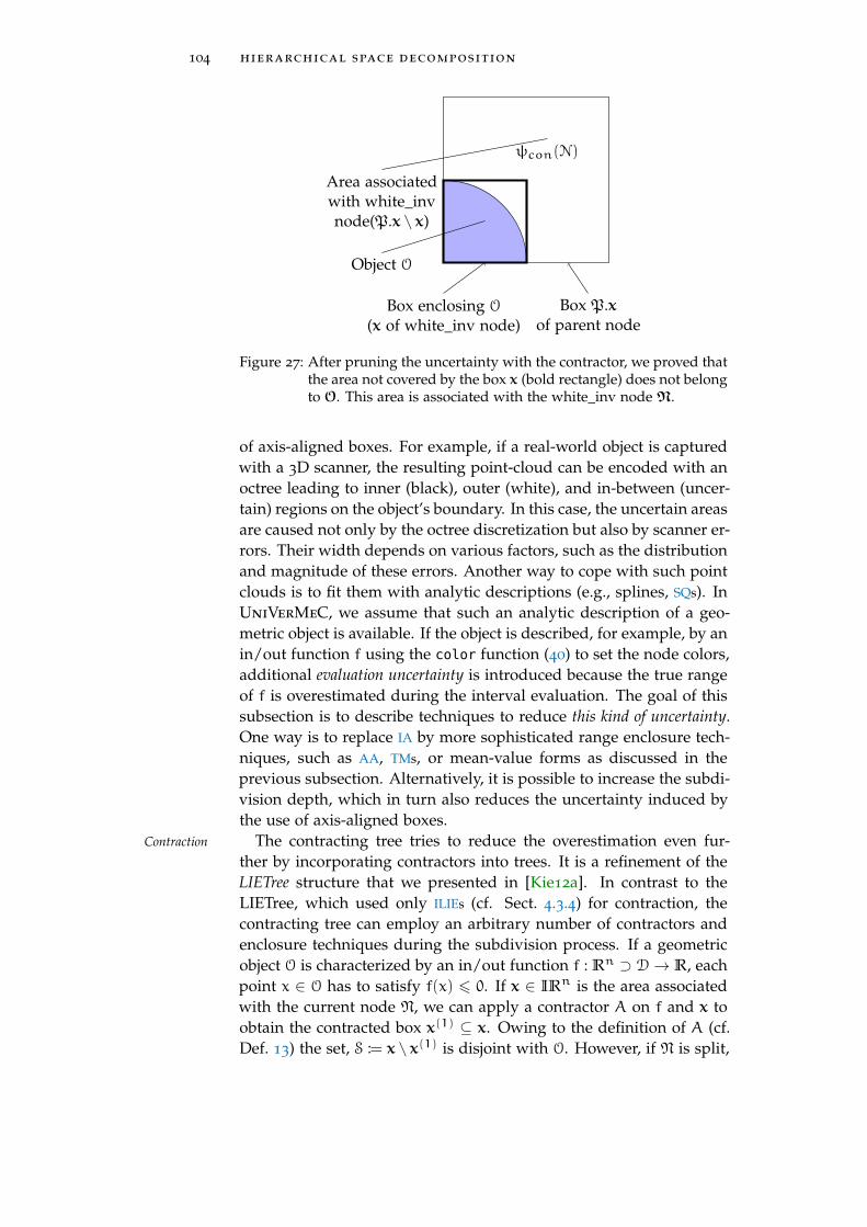
104 hierarchical space decomposition
Box enclosing O
(x of white_inv node)Box P.x
of parent node
Object O
ψcon(N)
Area associatedwith white_invnode(P.x \ x)
Figure 27: After pruning the uncertainty with the contractor, we proved thatthe area not covered by the box x (bold rectangle) does not belongto O. This area is associated with the white_inv node N.
of axis-aligned boxes. For example, if a real-world object is capturedwith a 3D scanner, the resulting point-cloud can be encoded with anoctree leading to inner (black), outer (white), and in-between (uncer-tain) regions on the object’s boundary. In this case, the uncertain areasare caused not only by the octree discretization but also by scanner er-rors. Their width depends on various factors, such as the distributionand magnitude of these errors. Another way to cope with such pointclouds is to fit them with analytic descriptions (e.g., splines, SQs). InUniVerMeC, we assume that such an analytic description of a geo-metric object is available. If the object is described, for example, by anin/out function f using the color function (40) to set the node colors,additional evaluation uncertainty is introduced because the true rangeof f is overestimated during the interval evaluation. The goal of thissubsection is to describe techniques to reduce this kind of uncertainty.One way is to replace IA by more sophisticated range enclosure tech-niques, such as AA, TMs, or mean-value forms as discussed in theprevious subsection. Alternatively, it is possible to increase the subdi-vision depth, which in turn also reduces the uncertainty induced bythe use of axis-aligned boxes.
The contracting tree tries to reduce the overestimation even fur-Contraction
ther by incorporating contractors into trees. It is a refinement of theLIETree structure that we presented in [Kie12a]. In contrast to theLIETree, which used only ILIEs (cf. Sect. 4.3.4) for contraction, thecontracting tree can employ an arbitrary number of contractors andenclosure techniques during the subdivision process. If a geometricobject O is characterized by an in/out function f : Rn ⊃ D→ R, eachpoint x ∈ O has to satisfy f(x) 6 0. If x ∈ IRn is the area associatedwith the current node N, we can apply a contractor A on f and x toobtain the contracted box x(1) ⊆ x. Owing to the definition of A (cf.Def. 13) the set, S := x \ x(1) is disjoint with O. However, if N is split,
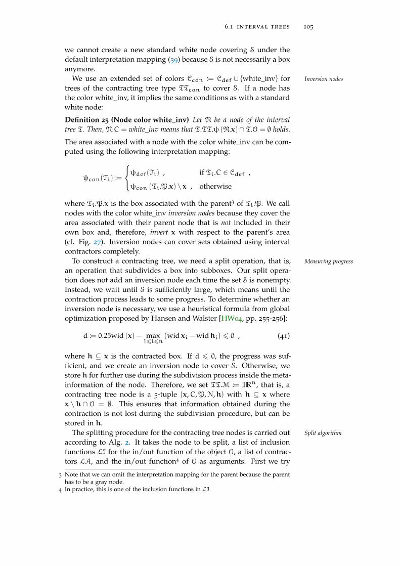
6.1 interval trees 105
we cannot create a new standard white node covering S under thedefault interpretation mapping (39) because S is not necessarily a boxanymore.
We use an extended set of colors Ccon := Cdef ∪ {white_inv} for Inversion nodes
trees of the contracting tree type TTcon to cover S. If a node hasthe color white_inv, it implies the same conditions as with a standardwhite node:
Definition 25 (Node color white_inv) Let N be a node of the intervaltree T. Then, N.C = white_inv means that T.TT.ψ (N.x)∩T.O = ∅ holds.
The area associated with a node with the color white_inv can be com-puted using the following interpretation mapping:
ψcon(Ti) :=
ψdef(Ti) , if Ti.C ∈ Cdef ,
ψcon (Ti.P.x) \ x , otherwise
where Ti.P.x is the box associated with the parent3 of Ti.P. We callnodes with the color white_inv inversion nodes because they cover thearea associated with their parent node that is not included in theirown box and, therefore, invert x with respect to the parent’s area(cf. Fig. 27). Inversion nodes can cover sets obtained using intervalcontractors completely.
To construct a contracting tree, we need a split operation, that is, Measuring progress
an operation that subdivides a box into subboxes. Our split opera-tion does not add an inversion node each time the set S is nonempty.Instead, we wait until S is sufficiently large, which means until thecontraction process leads to some progress. To determine whether aninversion node is necessary, we use a heuristical formula from globaloptimization proposed by Hansen and Walster [HW04, pp. 255-256]:
d := 0.25wid (x) − max16i6n
(wid xi − widhi) 6 0 , (41)
where h ⊆ x is the contracted box. If d 6 0, the progress was suf-ficient, and we create an inversion node to cover S. Otherwise, westore h for further use during the subdivision process inside the meta-information of the node. Therefore, we set TT.M := IRn, that is, acontracting tree node is a 5-tuple (x,C,P,N,h) with h ⊆ x wherex \ h ∩ O = ∅. This ensures that information obtained during thecontraction is not lost during the subdivision procedure, but can bestored in h.
The splitting procedure for the contracting tree nodes is carried out Split algorithm
according to Alg. 2. It takes the node to be split, a list of inclusionfunctions LI for the in/out function of the object O, a list of contrac-tors LA, and the in/out function4 of O as arguments. First we try
3 Note that we can omit the interpretation mapping for the parent because the parenthas to be a gray node.
4 In practice, this is one of the inclusion functions in LI.

106 hierarchical space decomposition
Algorithm 2: Splitting operation for a contracting tree node.Data: Node N = (x,C,P,N,h), List of contractors LA, List of
inclusion functions LI, in/out function f of OResult: Set of nodes R
R = ∅; e := (−∞,∞);2 forall the e ∈ LI do
e := e(N.h)∩ e;4 if e > 0 then N.C := white;5 else if e 6 0 then
if N.x == N.h then N.C := black;else
R := {(N.h, white_inv,N, ∅,N.h)} ;R := R∪ {(N.h, black,N, ∅,N.h)} ;
if N.C 6= gray ∨R 6= ∅ then N.N := R; return R;forall the A ∈ LA do
12 Apply A on f and N.h to obtain h(c); N.h := h(c);13 if N.h == ∅ then N.C := white;
elseCalculate d using (41);
16 if d 6 0 thenR := {(N.h, white_inv,N, ∅,N.h)};R := R∪ {(N.h, gray,N, ∅,N.h)} ;
if N.C 6= gray ∨R 6= ∅ then N.N := R; return R;20 Determine the widest component i of N.h;
Bisect N.x using the component i and midhi into x(0), x(1);Bisect N.h using the component i and midhi into h(0),h(1);
R := R∪{(x(0), gray,N, ∅,h(0)
),(x(1), gray,N, ∅,h(1)
)};
N.N := R; return R;
to determine the node color of the node to be split by using each ofthe inclusion functions in LI in a loop (line 2). If a node color otherthan gray can be determined, it is assigned to N and the algorithmterminates (lines 4; 5). Otherwise, each contractor in LA is applied toshrink h (line 12). If the resulting h is empty, the whole node N is dis-joint with O and can be colored white (line 13). If this is not the case,we check the criterion (41) to determine whether the progress was suf-ficient. In this case, a new inversion node is created (line 16). Finally,if no contractor leads to sufficient progress, a normal bisection is per-formed (line 20). To summarize, the tree type of a contracting treeis TTcon :=
(Ccon,ψcon, splitcon, IRn
)where splitcon is defined by
Alg. 2. Trees of type TTcon are regular.The outlined splitting procedure can be improved in some ways.Improvements
For example, in our implementation, it is possible to assign priori-ties to the used enclosures and contractors. Another way to improvethe contracting tree is to extend the idea of white inversion nodes to
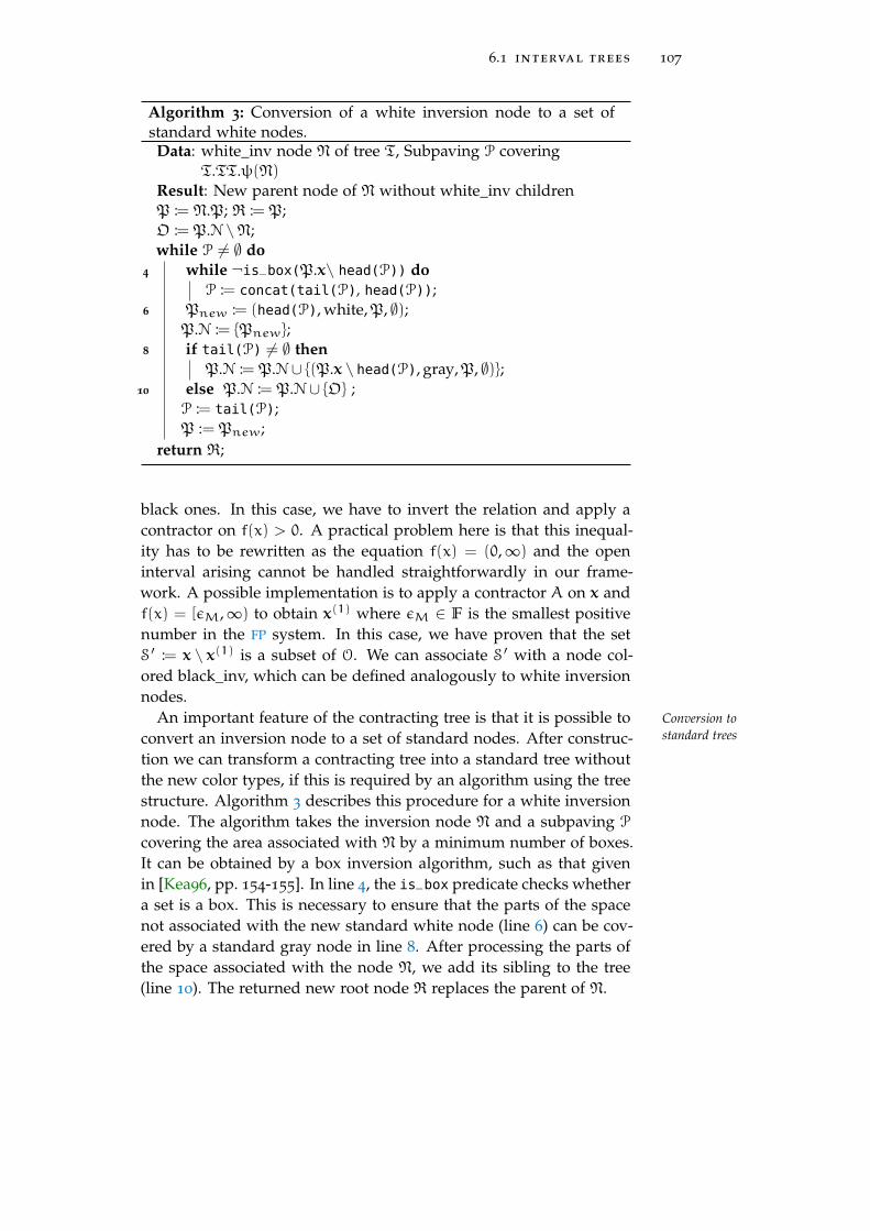
6.1 interval trees 107
Algorithm 3: Conversion of a white inversion node to a set ofstandard white nodes.Data: white_inv node N of tree T, Subpaving P covering
T.TT.ψ(N)Result: New parent node of N without white_inv childrenP := N.P; R := P;O := P.N \N;while P 6= ∅ do
4 while ¬is_box(P.x\ head(P)) doP := concat(tail(P), head(P));
6 Pnew := (head(P), white,P, ∅);P.N := {Pnew};
8 if tail(P) 6= ∅ thenP.N := P.N ∪ {(P.x \ head(P), gray,P, ∅)};
10 else P.N := P.N ∪ {O} ;P := tail(P);P := Pnew;
return R;
black ones. In this case, we have to invert the relation and apply acontractor on f(x) > 0. A practical problem here is that this inequal-ity has to be rewritten as the equation f(x) = (0,∞) and the openinterval arising cannot be handled straightforwardly in our frame-work. A possible implementation is to apply a contractor A on x andf(x) = [εM,∞) to obtain x(1) where εM ∈ F is the smallest positivenumber in the FP system. In this case, we have proven that the setS ′ := x \ x(1) is a subset of O. We can associate S ′ with a node col-ored black_inv, which can be defined analogously to white inversionnodes.
An important feature of the contracting tree is that it is possible to Conversion tostandard treesconvert an inversion node to a set of standard nodes. After construc-
tion we can transform a contracting tree into a standard tree withoutthe new color types, if this is required by an algorithm using the treestructure. Algorithm 3 describes this procedure for a white inversionnode. The algorithm takes the inversion node N and a subpaving P
covering the area associated with N by a minimum number of boxes.It can be obtained by a box inversion algorithm, such as that givenin [Kea96, pp. 154-155]. In line 4, the is_box predicate checks whethera set is a box. This is necessary to ensure that the parts of the spacenot associated with the new standard white node (line 6) can be cov-ered by a standard gray node in line 8. After processing the parts ofthe space associated with the node N, we add its sibling to the tree(line 10). The returned new root node R replaces the parent of N.

108 hierarchical space decomposition
Algorithm 4: Split operation for a parametric tree node.Data: Parametric tree node N = (x,C,P,N,u), Inclusion function
P of p : Rn−1 → Rn
Result: Set of nodes R
u := N.u; Determine longest axis i of u;u(1) := (u1, . . . , [ui, midui], . . . ,un−1);u(2) := (u1, . . . , [midui,ui], . . . ,un−1);R :=
{(P(u(1)), not_white,N, ∅,u(1)
)};
R := R∪{(P(u(2)), not_white,N, ∅,u(2)
)};
N.N := R; return R;
6.1.3 Parametric Tree
Both standard trees and contracting trees discussed previously em-Parametric surfaces
ployed an in/out function for the geometric object. From the geo-metric objects that the framework supports (cf. Def. 16), these treesare suited best for implicit objects because they are described by anin/out function. Especially for parametric objects, the use of in/outfunctions for characterization is not optimal. Therefore, we introducethe parametric tree, which is capable of handling parametric objectsdirectly. Moreover, this tree type is non-regular.
A parametric tree T has an associated parametric object O. Let O :=Parametric tree {(p1(u), . . . ,pn(u))
∣∣ u ∈ u(0)}⊂ Rn be described by the parametric
function p : Rn−1 ⊃ u(0) → Rn over its parametric domain u(0) ∈IRn−1. Each parametric tree node is a 5-tuple (x,C,P,N,u) wherethe meta-information entry is from the set IRn−1 and stores the partof the parametric domain that is associated with the current node. Foreach parametric tree node, x ⊇
{p(u)
∣∣ u ∈ u} has to hold. Therefore,the associated area x has a non-empty intersection with the geometricobject O for each node N. To take into account this knowledge, weintroduce a new node color:
Definition 26 (Node color not_white) A node N of an interval tree T
can be classified as not_white if T.TT.ψ(N.x)∩T.O 6= ∅ holds.
Because we can classify each node in a parametric tree as not_white,the set of colors is Cpar := {not_white}. Furthermore, the paramet-ric tree uses the standard interpretation mapping ψdef. The splittingoperation is similar to that of the standard trees from Sect. 6.1.1: abisection at the midpoint. In contrast to the standard trees, the para-metric tree performs the bisection on the parametric domain u andnot on x (cf. Alg. 4). This is also the reason why the parametric treeis non-regular. To summarize, the tree type of a parametric tree isTTpar :=
(Cpar,ψdef, splitpar, IRn−1
)where splitpar is defined by
Alg. 4.

6.1 interval trees 109
«interface»ITree
+root(): ITreeNode. . .
«interface»ITreeNode
+tree(): ITree+parent(): ITreeNode+operator[](unsigned c): ITreeNode+split(): void. . .
«interface»IIVTree
+obj(): IGeoObj. . .
«interface»IIVTreeNode
+normal(): ivector+color(): tree_color_t. . .
SIVTreeNode
CIVTreeNode
SParamTreeNode
PolyIVTreeNode
SIVTree
CIVTree
SParamTree
PolyIVTree
T: Arithmetic Type
Box+X(): ivector. . .
Figure 28: Overview of tree decomposition layer in UniVerMeC (simpli-fied).
6.1.4 Realization in UniVerMeC
The basic structure of the tree decomposition layer in UniVerMeC is Implementation
shown in Fig. 28. A tree is represented by an ITree interface and, fol-lowing Def. 20, by a collection of ITreeNode instances. Interval trees(cf. Def. 22) are integrated into the overall structure by the IIVTree
interface and interval tree nodes correspond to IIVTreeNode. Intervaltrees allow us to access the uniform representation of the associatedgeometric object provided by the IGeoObj interface (cf. Sect. 5.1). Us-ing the IIVTreeNode interface, the members of the tuple defining aninterval tree node can be retrieved. As an additional feature, the in-
Table 14: The tree decomposition structures implemented in UniVerMeCand their theoretical basis.
Colors Mapping Arithmetic Regular Type
BinIVTree Cdef ψdef IA X TTdef
BinAATree Cdef ψdef AA X TTdef
BinAATree Cdef ψdef TM X TTdef
CIVTree Ccon ψcon various X TTcon
SParamIVTree Cpar ψdef IA × TTpar
PolyIVTree Cdef ψdef IA X TTdef

110 hierarchical space decomposition
terface can compute the normal vectors of the geometric object over abox, if normals are available. Each of the tree types discussed aboveis provided as a separate class implementing the IIVTree interface.An overview of the classes and their connections with the theoreticalbasis discussed in the previous parts of this section is given in Tab. 14.The standard trees BinIVTree, BinAATree, and BinTMTree are realizedas instatiations of the class template SIVTree<T> that provides a uni-form basis for them. The PolyIVTree is a standard tree, which isoptimized for polyhedral objects O.
From the software perspective, the tree decomposition layer hasPurpose from thesoftware perspective two main purposes: First, it provides an implementation of the inter-
val tree concept, which is reusable from different algorithms. Second,it pursues the encapsulation and abstraction ideas from the earlier lay-ers. The tree decomposition layer allows us to hide which of the tech-niques defined earlier is actually used inside a tree. An algorithmworking with the IIVTree interface does not need to know whichmodeling type or range enclosure technique is employed or whethercontractors are incorporated in the tree. Instead, it only needs to beable to interpret the colors of the tree nodes. Algorithms built ontop of UniVerMeC working solely on the tree decompositions can beimplemented in a uniform manner without taking the different char-acteristics of range-enclosure techniques or contractors into account.In this way, UniVerMeC not only enables fair comparisons betweenthe employed techniques but makes the algorithms easily extendable.
6.2 general multisection
As already mentioned in the introduction, algorithms with automaticBasic branch andbound principle result verification (e.g., for global optimization) often employ an inter-
val branch and bound pattern. Usually, this class of algorithms storesparts of the search space in a sorted working list L :=
(x(1), . . . , x(q)
)in the form of interval boxes x(i). The basic principle of these algo-rithms is to take the first box from L, process it, and eventually createnew boxes by multisection5. Good criteria for sorting L and for themultisection are crucial for improving the runtime of a branch andbound algorithm, which has an exponential worst-case complexity.These criteria have an inherently heuristical nature.
This fact stipulated much research on developing and evaluatingSorting L
heuristics. Berner [Ber95a, pp. 29-34] examined the three strategiescommonly used for sorting L: oldest-first, depth-first, and best-first.The first two resemble the well-known first in, first out (FIFO) andlast in, first out (LIFO) principles that can be implemented easily byusing a queue or a stack for L. The best-first strategy in global op-timization sorts the list in such a way that Φ
(x(i)
)6 Φ
(x(j)
)holds
for all 1 6 i, j 6 q, i < j and an inclusion function Φ of the objec-
5 We consider the bisection a special case of multisection.

6.2 general multisection 111
(a) The naive multisectionschemes generates 2n newboxes.
(b) The Ratz multisectionscheme generates n + 1
new boxes.
Figure 29: Multisection schemes for subdividing the box x ∈ IRn (bold rect-angle) in each coordinate.
tive function ϕ. Berner [Ber95a, Satz 2.2] proves that the best-firststrategy does not behave worse in the normal case, compared to theother two strategies in the best case6. A problem of the best-first strat-egy is that its quality depends on the quality of the range enclosureobtained for ϕ over x. Therefore, other criteria for sorting L wereproposed. An interesting idea that has been studied recently is thereject-index [Cse01; Mar+06], [Kah05, pp. 34-38]. In its basic version,it tries to measure the difference between the currently known lowerbound on the global minimum ϕ∗ and Φ(x) scaled by wid x.
It is important to choose not only a good order for storing boxes Multisectionstrategiesin L but also a good generation scheme for them. Such schemes
are denoted as multisection, which means that an axis-aligned boxx ∈ IRn is subdivided into j > 2 disjoint subboxes. Because the re-sulting boxes have to be axis-aligned again, the subdivision is alwaysperformed in parallel to a coordinate axis. Two possible schemes sub-dividing x along every coordinate axis are depicted in Fig. 29 for thetwo dimensional case. The naive scheme (cf. Fig. 29a) suffers froman exponential growth of boxes in each step, which is not suitableeven for moderate values of n. An alternative schema was proposedby Ratz [Rat92, pp. 60-62] in the scope of the interval Gauss-Seidelmethod. The number of boxes grows linearly if this scheme is used(cf. Fig. 29b). Here, only the most important coordinate is bisected,whereas the subdivision in the other directions is performed for onlyone of the boxes created during this bisection. In the naive scheme,too, the growth can be limited if instead only the most importantcoordinates are considered for bisection.
Determining the importance of a coordinate direction is another Coordinate weights
crucial topic in this scope. In [RC95], Ratz and Csendes comparedthe commonly used rules (cf. Tab. 15). The maximum width rule
6 The best case is that the global minimum ϕ∗ is known apriori and can be used toapply the midpoint test (53) (cf. Sect. 7.2.1).
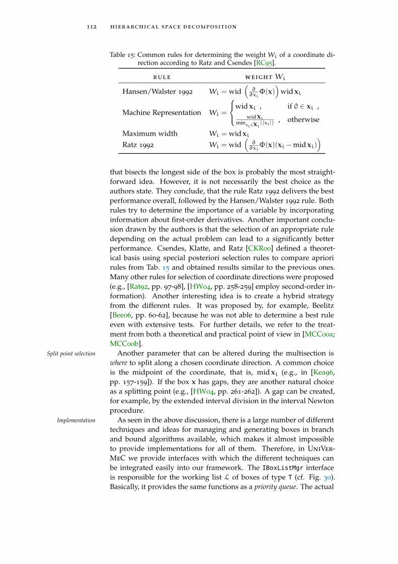
112 hierarchical space decomposition
Table 15: Common rules for determining the weight Wi of a coordinate di-rection according to Ratz and Csendes [RC95].
rule weight Wi
Hansen/Walster 1992 Wi = wid(∂∂xiΦ(x)
)wid xi
Machine Representation Wi =
wid xi , if 0 ∈ xi ,widxi
minxi∈xi(|xi|), otherwise
Maximum width Wi = wid xiRatz 1992 Wi = wid
(∂∂xiΦ(x)(xi − mid xi)
)
that bisects the longest side of the box is probably the most straight-forward idea. However, it is not necessarily the best choice as theauthors state. They conclude, that the rule Ratz 1992 delivers the bestperformance overall, followed by the Hansen/Walster 1992 rule. Bothrules try to determine the importance of a variable by incorporatinginformation about first-order derivatives. Another important conclu-sion drawn by the authors is that the selection of an appropriate ruledepending on the actual problem can lead to a significantly betterperformance. Csendes, Klatte, and Ratz [CKR00] defined a theoret-ical basis using special posteriori selection rules to compare apriorirules from Tab. 15 and obtained results similar to the previous ones.Many other rules for selection of coordinate directions were proposed(e.g., [Rat92, pp. 97-98], [HW04, pp. 258-259] employ second-order in-formation). Another interesting idea is to create a hybrid strategyfrom the different rules. It was proposed by, for example, Beelitz[Bee06, pp. 60-62], because he was not able to determine a best ruleeven with extensive tests. For further details, we refer to the treat-ment from both a theoretical and practical point of view in [MCC00a;MCC00b].
Another parameter that can be altered during the multisection isSplit point selection
where to split along a chosen coordinate direction. A common choiceis the midpoint of the coordinate, that is, mid xi (e.g., in [Kea96,pp. 157-159]). If the box x has gaps, they are another natural choiceas a splitting point (e.g., [HW04, pp. 261-262]). A gap can be created,for example, by the extended interval division in the interval Newtonprocedure.
As seen in the above discussion, there is a large number of differentImplementation
techniques and ideas for managing and generating boxes in branchand bound algorithms available, which makes it almost impossibleto provide implementations for all of them. Therefore, in UniVer-MeC we provide interfaces with which the different techniques canbe integrated easily into our framework. The IBoxListMgr interfaceis responsible for the working list L of boxes of type T (cf. Fig. 30).Basically, it provides the same functions as a priority queue. The actual

6.3 conclusions 113
«interface»IBoxListMgr
+add(T* box): void+add(box_lst_t lst): void+select(): T*+empty(): bool. . .
«interface»IMultiSection
+section(T box): box_lst_t
«interface»IDirWeight
+weight(T box): split_lst_t
«interface»IPointChooser
+pchoose(T box, split_lst_tlst, int sects): void
Box management SectionT: Box T: Box
T: Box
T: Box
Figure 30: Interfaces of the multisection layer of UniVerMeC.
multisection part in UniVerMeC is split up onto three interfaces thatcorrespond to three parameters of a multisection strategy, which havebeen identified above: IMultiSection (basic scheme), IDirWeight (co-ordinate weights), IPointChooser (split point selection). The actualmultisection is performed by an IMultiSection instance. A concreterealization of a multisection scheme through IMultiSection can beparametrized with the other two interfaces, so that it can employ dif-ferent coordinate weights and split point selection easily. Currently,we provide the Ratz section scheme, the coordinate weight rules max-imum width, and Ratz 1992.
6.3 conclusions
In this chapter, we presented our refinements for the interval tree ap- Formal framework
proach by Dyllong and Grimm, and we discussed how our techniquerelates to the subpavings introduced by Jaulin et al. An importantnew aspect of our work is that we presented our trees in scope of aformal framework, which is also able to cover the standard intervaltrees and the CSG trees introduced in [DG07d; DG08].
Our standard IA, AA and TM trees are a direct application of the al- Standard trees
ready known interval tree idea. Their uniform implementation can becarried out in a flexible framework, such as UniVerMeC, in a straight-forward manner. The use of more sophisticated arithmetics inside thetrees cannot only improve the range-enclosure quality but also clearthe way for a comprehensive and fair comparison of the differentarithmetics in the scope of geometric computations. This is even more

114 hierarchical space decomposition
important as, in contrast to the work of Dyllong and Grimm, the fo-cus of our work does not lie on CSG objects, with quadric primitives,but on more complex implicit objects which often are described bymuch more complicated expressions. Therefore, they are plagued toan increased degree by overestimation problems, such as the depen-dency problem, which sometimes can be reduced by applying moresophisticated arithmetics.
A novel structure we presented in this chapter was the contract-Contracting tree
ing tree. It combines the well-known concepts of contractors andinterval trees while retaining the important regularity notion. Usingcontractors during the subdivision can lead to a significant reductionof the uncertain areas and, thus, increase the quality of the decom-position. Additionally, the contracting tree fits very well into thesoftware framework that we provide because it employs the differ-ent arithmetics, range-enclosure techniques, and contractors offeredby UniVerMeC in a uniform manner. Furthermore, we showed thatit can be converted losslessly to the standard tree types, which meansthat algorithms do not need any extra adaption to the tree.
The second novel tree structure closes a conceptual gap with re-Parametric tree
spect to supporting different geometric modeling types. All othertree types discussed in the thesis are best used in conjunction withimplicit objects. With the parametric tree, we provide a new treetype optimized for objects described parametrically. This extends thescope of where our tree structures can be applied practically and canbe seen mainly as a software addition. It is important for the decou-pling purpose of the decomposition layer from a software engineeringperspective.
The second section of the chapter gave an overview of techniquesMultisectionstrategies for multisection strategies and sorting working lists. This discussion
led to a breakdown of a multisection strategy into three distinct com-ponents: multisection scheme, coordinate weights, and split point.We explained how the identified components are mapped onto soft-ware interfaces, which allow users to integrate new multisection tech-niques discussed in the literature more easily. Furthermore, the uni-form components can be reused from different algorithms.
7A L G O R I T H M S
The purpose of this chapter is to describe algorithms that can be im- Categories foralgorithms inUniVerMeC
plemented in or made accessible by our framework. In general, if agiven task should be solved by an algorithm, we can distinguish threedifferent cases:
• A new algorithm was designed for this task and a completeimplementation is necessary.
• An existing algorithm is suitable but a reimplementation is nec-essary.
• An existing algorithm provided by a third party can be used. Itneeds to be interfaced to the existing problem descriptions.
In this chapter, we give examples for the categories and show howthe use of UniVerMeC can facilitate each of these tasks. For eachcategory a different depth of knowledge is necessary. While the firstcategory requires a deep understanding and the second category stilla good amount of knowledge of the topic, the third category onlydemands using the third party library’s specific interface. The levelof detail in which we discuss the different algorithms in this chapteris adjusted to these needs.
As an example of a new algorithm, we give an in-depth discussion Algorithms availablein UniVerMeCof ε-distance. Developed in scope of the thesis, this approach com-
putes verified bounds on the distance between two geometric objects.The implementation of the algorithm is made much easier by theuse of the framework, because techniques that ε-distance employs,namely those for describing geometric objects (cf. Sect. 5.1) and fortheir hierarchical decompositions (cf. Sect. 6.1) are already available.
Global optimization is our example for the second category. Wegive an overview of important parts of the theory of interval globaloptimization and show how state-of-art algorithms from the area canbe adapted and implemented in our framework in a straightforwardmanner. Moreover, we demonstrate how the implementation bene-fits from the already existing support for different range-arithmetics(cf. Chap. 3), functions, derivatives, contractors (cf. Chap. 4), andmultisections (cf. Sect. 6.2).
As an example of the last category, we interface already existing thirdparty libraries for solving IVPs. Because we treat these libraries as blackboxes, we completely omit a theory discussion in this section. Al-though, the existing libraries themselves do not benefit from UniVer-MeC in this case, users can take advantage of the uniform model de-scriptions and the ability to combine different algorithms or solvers.
115

116 algorithms
The chapter is structured as follows. The new distance computa-Chapterorganization tion algorithm is described in Sect. 7.1, followed by the global opti-
mization algorithm in Sect. 7.2. After that we describe the interfacingof ValEncIA-IVP and VNODE-LP (two verified solvers for IVPs) be-fore finally summarizing the material in Sect. 7.4.
7.1 distance computation
Distance computation plays an important role in many applicationStandard algorithms
domains (e.g., robotics or biomechanics). For convex polyhedral mod-els, standard algorithms, such as GJK [GJK88] or V-clip [Mir98], arereadily available. Whereas the latter uses the Voronoi regions of fea-tures to compute the distance, the former is an iterative approachthat calculates the Minkowski difference, between two polyhedrons1,constructs a simplex inside the difference and computes the distancebetween the simplex and the origin. In each iteration, the simplex ismodified to reduce the distance. A more complete overview for non-verified state-of-the-art procedures can be found in [Koc+09; LG98].
The distance computation between modeling types other than poly-Handling othermodeling types hedral objects has attracted some attention in recent work (e.g., [LS02;
UY07]). A very interesting class of objects are SQs, which can be de-scribed both by an implicit equation or parametrically. They wereintroduced by Barr [Bar81] in the context of computer graphics. Be-cause the model depends only on 5 parameters, SQs are widely ap-plied for surface reconstruction [JLS00]. Recent research showed thatthey can be used in biomechanics for bone modeling [Cuy11]. Anapproximation of the distance between SQs can be obtained usinggeneral purpose optimization methods as shown in [Cha+08; PSD09].However, rigorous bounds are of great interest in biomechanics. Inhis recent master thesis [Chu11], the main results of which were pub-lished in [Aue+11], Chuev investigated how to obtain such boundsfor convex SQs. He developed an a posteriori verification methodbased on an FP approximation (e.g., from GJK or interior point gen-eral purpose optimization). Compared to verified a apriori methodsfor convex objects, such as the interval GJK variant [DL04b] presentedby Dyllong and Luther, which could be adapted to convex SQs as well,the approach of Chuev has the advantage that well-tested and fast FP
implementations can be used to obtain the approximate distance. Theuse of the rather slow IA is limited to the verification step. However,in contrast to purely interval methods, his approach cannot handlemodel uncertainty in a straightforward way.
From the few algorithms available for verified distance computa-A posterioriverification tion, we outline the approach of Chuev [Chu11] because it has im-
1 The applicability of the GJK algorithm is not limited to polyhedral objects. It issuitable for convex objects in general if a so-called support mapping [Ber04, pp. 130-131] is available.

7.1 distance computation 117
(a) Two cubes with parallelsides.
(b) Two rotated cubes. (c) Two objects describedby over 700 hyper-planes.
Figure 31: Three test scenarios for which the interval global optimization ap-proach required many iterations before delivering a narrow dis-tance enclosure.
portant usage in scope of the biomechanical application discussed inSect. 8.1.2 and is different compared to the interval tree methods de-scribed in detail later. It computes a rigorous bound on the distancebetween two convex SQs or a convex SQ and a point. For simplicityreasons, we will outline the method for the latter case only. Let aconvex SQ O be given by its implicit function f : R3 → R and a pointp ∈ R3. The FP solver returns an approximate solution point q ∈ R3
for the minimum distance between the SQ and p. The a posteriori ver-ification of the approximation is performed in two separate steps. Inthe first step, we compute a point q− on the line l(s) = p+ s · (q− p),so that f(q−) 6 0 holds. A rigorous upper bound on the minimumdistance between p and O is obtained by ‖p− q−‖. Assuming thatq is a good approximation, the quality of the rigorous upper boundincreases if q− approaches q. The second step starts by searching apoint q+ on the line l(s), so that, f(q+) > 0. Then the interval hyper-plane h(x) = ∇F (�(q−,q+)) · (x−�(q−,q+)) is constructed where∇F is an inclusion function for the gradient of f and � the intervalhull operator. Because h(x) contains a support plane of O, which issimultaneously a separating plane between O and p, calculating theminimum distance between h(x) and p yields a rigorous lower boundon the distance between O and p. The algorithm can be implementedon a computer easily because all operations can be carried out withstandard IA.
A disadvantage of this a posteriori verification approach is that it is Using generalpurposeoptimization
applicable only for convex objects. This is also true for criteria fromgeneral purpose optimization. For example, the KKT conditions arenecessary and sufficient for the global optimum in the case of con-vex optimization problems [BV09, p. 244]. For non-convex problems,it is more difficult to find criteria for verifying a given approximatesolution a posteriori. However, non-convex geometric objects arisenaturally in modeling real-world scenarios (e.g., bent SQs for bonemodeling in total hip replacement cf. Sect. 8.1.2). One way to com-pute the distance is to apply a general-purpose interval global op-timization algorithm (e.g., [Bee06; HW04; Kea96]), which can copewith both convex and non-convex problems. Consider two geomet-

118 algorithms
ric objects O1,O2 ⊂ Rn described by the in/out functions f1, f2 withfi : Rn → R. To compute the minimum distance between them, thefollowing optimization problem can be solved:
minx∈R2n
∥∥∥x(1) − x(2)∥∥∥2 ,
f1(x(1)) 6 0 , (42)
f2(x(2)) 6 0 .
where x =(x(1), x(2)
)Twith x(i) ∈ Rn. We tested this approach
in [DK10] only for convex polyhedra, which can be described byunions of halfspaces. These unions translate directly into inequalityconstraints for an optimization problem. The tests were carried outusing an implementation of the state-of-art interval global optimiza-tion algorithm for inequality constrained problems by Hansen andWalster [HW04, pp. 343-379] (cf. Sect. 7.2). We performed only slightadaptions of the general purpose approach; in particular, we em-ployed parallelization to improve the runtime. While it was possibleto derive the distances in this way (cf. [DK10] for details), the solvingprocess was slow, especially in some geometric degenerated scenar-ios (cf. Fig. 31). For our purposes, a more important problem is that,while in theory these kinds of algorithms work without derivatives,the actucal implementations usually expect a differentiable problem.This is not guaranteed if the objects Oi are non-smooth (e.g., non-convex polyhedra) or CSG objects where special treatment of the set-theoretic operations (e.g., with R-functions [Sha07; Sha91]) would benecessary to ensure differentiability (cf. Sect. 5.1). Also, the exploita-tion of parametric descriptions is difficult with standard global opti-mization methods.
7.1.1 A Basic Distance Computation Algorithm for Interval Trees
Another approach to calculate the distance between the two non-Distancecomputation
between treesconvex objects O1,O2 is to construct their hierarchical decompositions(e.g., as an octree) and carry out the distance computation betweenthem. The algorithm for rigorous distance computation proposed inthis thesis follows this approach and derives a rigorous bound thatalso holds for the original objects based on the trees. Our algorithmis a refinement of the algorithm in [BDL04] (Dist. 1), [DL04a] (Dist. 2),and [DG07a; DG07b] (Dist. 3/4). The algorithm Dist. 1 computesthe distance between two objects encoded in one octree. Thus, bothobjects share a common coordinate system. The algorithm Dist. 2
is developed for the case of two objects encoded by octrees that arerepresented in different coordinate systems. Both algorithms workon octrees with a fixed subdivision depth. These algorithms do notconsider the underlying objects and are limited by the maximum sub-

7.1 distance computation 119
division depth of the octrees which they take as input. The last al-gorithms Dist. 3/4 assume again that the trees are not representedin a common coordinate system. Additionally, they offer a dynamicsplitting behavior. To achieve this, an analytic model is assumed tolie behind the octree data structure. Thus, the subdivision depth ofa node can be dynamically increased if necessary. However, bothalgorithms return only a lower bound on the distance.
Our own algorithm ε-distance [DK12; KLD13] can be seen as a hy- ε - distancealgorithmbrid version of the above algorithms. It assumes that the interval trees
decomposing O1,O2 share a common coordinate system. Therefore,the algorithm uses an improved version of the node-node distancecomputation mechanism from [BDL04]. Because our interval trees arealways connected with an analytic model of the underlying geometricobject (cf. Def. 22), the algorithm can make use of an adaptive mecha-nism for increasing the subdivision depth if necessary. In contrast tothe Dist. 3/4 approach, we compute a fully rigorous enclosure Υ onthe distance between O1,O2, so that, υ = minx∈O1,y∈O2 ‖x− y‖ ∈ Υholds with widΥ 6 ε where ε > 0 is the user-defined accuracy. Wewill restrict the basic discussion of the algorithm to the tree typeswith color sets C ⊆ {black, gray, white, not_white}. Inversion nodescan be converted to these colors if necessary (cf. Alg. 3).
The input of the algorithm are the trees IT1 and IT2 associated Used data structures
with the geometric objects O1 and O2, respectively. Additionally, it isassumed that ITi.TT.ψ(N) maps into IRn for all N ∈ TITi.TT, i =1, 2. Throughout the rest of this section, we denote the interval box(e.g., ITi.TT.ψ(N)) associated with a node (e.g., N) by a bold letter (n)to simplify the notation. The algorithm ε-distance uses a working listL with candidate tuples (X,Y,d). Here X and Y denote nodes fromthe first and second subdivision tree, whereas d is an enclosure ofthe square of the Euclidean distance ‖x−y‖2 between them. Furthervariables of the algorithm are the enclosure Υ of the minimum dis-tance υ between O1 and O2 and the final list Lfinal. A user-providedthreshold ε is employed as a termination criterion, that is, the algo-rithm stops if widΥ 6 ε.
The basic idea of ε-distance is as follows. The algorithm takes the Case selector fordistance queriesbetween interval treenodes
first tuple (X,Y,d) from L and splits the node associated intervalvector of which has the smaller width. If we assume that X wassplit and denote the resulting set of child nodes by N, the ε-distancegenerates a new tuple (N,Y,d(N,Y)) for each node N ∈ N that is notwhite. We can discard tuples with white2 nodes because they do notbelong to the object. The function d(N,Y) returns an enclosure of thesquare of the Euclidean distance between the object parts of O1 andO2 contained in the area covered by the nodes N,Y. The enclosure
2 or white inversion

120 algorithms
x1
x2
√c1
√c2
(a) Two black nodes
x1
x2
maxmin
min
max
√c ′1
√c ′2
(b) A black and a gray node
Figure 32: Graphical representation of case selectors. The lines visualize thedistances between the two depicted areas associated with nodes.On the axes, the
√ci (
√c ′i) are shown. They represent (or en-
close) the projection of distance between these axis-aligned boxeson each axis.
d is computed by the function d(X,Y) defined in (43), which uses aslightly extended version (45) of the case selector (44) from [BDL04]:
d(X,Y)2 :=
∑ni=1 ci , X.C = Y.C = black ,∑ni=1 c
′i , X.C = black 6= Y.C ,
‖x−y‖2 , otherwise ;
(43)
ci :=
(yi − xi)
2 , yi > xi ,
(xi − yi)2 , xi > yi ,
0 , otherwise ;
(44)
c ′i :=
(yi − xi)
2 , yi > xi ,
(xi −yi)2 , xi > yi ,
[0, max(h ′i,h′′i )] , otherwise ;
(45)
h ′i :=
(yi − xi)2 , yi > xi ,
0 , otherwise ;
h ′′i :=
(yi − xi)2 , yi > xi ,
0 , otherwise .

7.1 distance computation 121
Uncertainty
Difference Best first
Upper bound
Lower bound
(a) Start situation: The width of the dis-tance enclosure is dominated by theuncertain area’s width.
Uncertainty
Upper bound
Lower bound
Difference Best first
(b) Situation after applying the criteria:The width of the uncertain area hasbeen reduced. Thus, producing abetter distance enclosure.
Figure 33: The algorithm switches between two criteria for list sorting: dif-ference and best-first. The former tries to produce black nodes andthe latter white nodes. After applying both criteria we should beable to reduce the uncertain region from both sides.
The new selector c ′i provides tighter bounds if only one node is black3.Both selectors, the old and the improved one, are depicted in Fig. 32.If N and Y are both black, we discard them and update Υ as follows:Since d(N,Y) establishes an upper bound for the actual distance be-tween the objects, Υ chosen as the minimum between its current valueand d(N,Y):
Υ := min(Υ,d(N,Y)
). (46)
The lower bound Υ is updated by min(Υ,d(N,Y)
).
If at least one node is gray, we have an uncertain area (cf. Fig. 33a) Handling gray andnot_white nodeswhere it is unknown if a part of the object lies there. However,
d(N,Y) is a verified lower bound for the minimum distance betweenN.x and y for all points they possibly contain. The tuple can be dis-carded if
d(N,Y) > Υ . (47)
This criterion is equivalent to the well-known midpoint test in intervalglobal optimization. Because we stop if widΥ 6 ε, we do not needto process a tuple further if d(N,Y)−Υ 6 ε holds, that is, the tuplefulfills the termination criterion. In this case, Υ is updated with Υ =
min(Υ,d(N,Y)
)and the tuple is discarded, otherwise it is inserted
into L for further processing. Nodes with the color not_white canbe handled similarly to gray nodes. The main difference is that ifboth nodes are not white, we know that the upper bound on theirdistance establishes a rigorous upper bound the distance betweenO1,O2. Therefore, we apply (46) to update Υ in this case.
Similarly to interval global optimization, the sorting of L has a Sorting L
3 Likewise, if Y is black and X is gray, the second case of (43) applies.
122 algorithms
great impact on the algorithm’s performance. The sorting criteriaare mostly of heuristic nature. The intuitive idea is to use a best-firstcriterion that puts tuples with small lower bounds first. That is, if
d1 < d2 (best-first) (48)
holds for two tuples with the associated distance enclosures d1,d2,the tuple with the enclosure d1 should be processed first. This strat-egy usually leads to a faster subdivision of the gray leaf nodes border-ing on white nodes. Another possibility is to sort the list accordingto the minimum difference of the tuple’s associated distance and thecurrent verified upper bound on the minimum distance:
d1 −Υ < d2 −Υ (difference) . (49)
This criterion is similar to the reject-index [Cse01] (cf. Sect. 6.2) with-out scaling and often leads to a heavier subdivision of the gray leafnodes bordering on black nodes. Our algorithm alternates both crite-ria reducing the uncertain area from both sides (cf. Fig. 33b).
Our procedure to compute a verified enclosure between the dis-Algorithm
tance of two geometric objects O1,O2 is given in Alg. 5. As input,the algorithm takes the accuracy threshold ε and two interval treesIT1, IT2 representing the objects. Therefore, the implementation isindependent of the actual underlying geometric modeling type. Asmentioned above, we assume that the range of ITi.TT.ψ is a box forevery node in TITi.TT, i = 1, 2. We allow the use of nodes with thecolor white_inv as an exception from this rule, because the algorithmdoes not need to consider the area associated with nodes that do notintersect with the geometric objects. To allow for easy extension withfurther colors several predicates are used to check whether a nodeof a tree for the geometric object O has certain properties instead ofchecking for concrete colors. In the following list, the predicates, theirconditions and the corresponding node colors are given:
is_solid The node cannot be subdivided further (black, white, white-_inv).
is_divis The node can be subdivided further (gray, not_white).
has_point The associated area of the node intersects O (black, not-_white).
is_empty The associated area of the node does not intersect O (white,white_inv).
After beginning, the algorithm initializes its working list L with thetwo root nodes of the trees in line 2. Here, we assume that is_emptyevaluates to false for both root nodes. After that, the threshold ε2 is
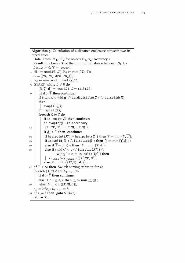
7.1 distance computation 123
Algorithm 5: Calculation of a distance enclosure between two in-terval treesData: Trees IT1, IT2 for objects O1,O2; Accuracy εResult: Enclosure Υ of the minimum distance between O1,O2Lfinal := ∅; Υ := [∞,∞];
2 R1 := root(IT1.T);R2 := root(IT2.T);L := {(R1,R2,d(R1,R2))};
4 ε2 ← max(wid r1, wid r2)/2;5 START: while L 6= ∅ do
(X,Y,d) := head(L); L:= tail(L);7 if d > Υ then continue;
if ((wid x < widy) ∧ is_divisible(Y)) ∨ is_solid(X)then
swap(X, Y);C := split(X);foreach C in C do
if is_empty(C) then continue;// swap(C,Y) if necessary
13 (X ′,Y ′,d ′) := (C,Y,d(C,Y));if d ′ > Υ then continue;
15 if has_point(X ′) ∧ has_point(Y ′) then Υ := min(Υ,d ′
);
16 if is_solid(X ′) ∧ is_solid(Y ′) then Υ := min (Υ,d ′) ;17 else if Υ− d ′ 6 ε then Υ := min (Υ,d ′) ;18 else if (wid x ′ < ε2∨ is_solid(X ′)) ∧
(widy ′ < ε2∨ is_solid(Y ′)) thenLfinal := Lfinal ∪ {(X ′,Y ′,d ′)};
else L := L∪{(X ′,Y ′,d ′)
};
22 if Υ <∞ then Switch sorting criterion for L;foreach (X,Y,d) in Lfinal do
if d > Υ then continue;else if Υ− d 6 ε then Υ := min (Υ,d) ;
26 else L := L∪ {(X,Y,d)};ε2 := 0.9ε2; Lfinal := ∅;
28 if L 6= ∅ then goto START;return Υ;

124 algorithms
initialized in line 4. If the area x associated with a node X falls underthe threshold ε2, that is, if
wid x 6 ε2 ,
it is temporarily suspended from the subdivision process. If bothnodes of a tuple fall below the threshold, the tuple is moved to anintermediate list Lfinal. Basically, this approach combines the oldest-first sorting strategy (cf. Sect. 6.2) with the best-first and differencecriteria, which are used for sorting L. This ensures that the searcharea is subdivided more uniformly, while still preferring parts thatare likely to contain the desired minimum distance. Another advan-tage is that the oldest-first strategy often reduces the number of el-ements in L [Kah05, p. 34]. However, whether this also is the caseif the oldest-first strategy is combined with other strategies needs amore thorough experimental analysis. After entering the main loop(line 5), the algorithm takes the first tuple from L and tries to discardit (line 7) using (47). If this is not possible, the node with the largerassociated area is split. After that, we iterate over its children. Newtuples are generated (line 13) using the created child nodes if theyare not proven to have an empty intersection with O. Further, if thehas_point predicate evaluates true for both nodes, we can update theupper bound Υ (line 15). If both nodes are black, the minimum Υ
is updated and the tuple is discarded (line 16). The same steps arecarried out if a tuple delivers the desired accuracy (line 17). As ex-plained above, a tuple falling under the threshold ε2 is temporarilymoved to Lfinal and ignored (line 18). If L is empty, we exchange thesorting criterion if possible4 (line 22), move all elements from Lfinalto L so that Lfinal is empty (line 26), decrease ε2, and finally restartthe main loop (line 28). The above algorithm does not use higher or-der information, such as offered by normals, in order to be applicableto a wide range of models.
7.1.2 Using Normals for Distance Computation
Depending on the geometric configuration, the basic algorithm de-Clustering effects
scribed in the previous subsection might suffer from massive cluster-ing effects, which can be reduced sometimes by incorporating higherorder information into the computation process [DK94]. Therefore,our algorithm can optionally make use of information provided bynormals.
Denote enclosures of the normal vectors of O1,O2 over x,y for aNon-collinearity test
tuple (X,Y,d) by nx and ny. The tuple can be safely discarded if
0 6∈ nx ×ny . (50)
4 The algorithm starts with the best-first criterion because the difference criterion isonly suitable if a meaningful Υ is known.

7.1 distance computation 125
The criterion is based on the observation that the two normal vectorshave to be collinear to each other at a point of minimum distancebetween two objects. It has been used by Snyder et al. [Sny+93] in arigorous algorithm for collision detection.
Another test is to check whether the vectors y− x and x− y lie in Normal cone test
the normal cones with the generating vectors nx and ny, respectively.We can discard a tuple if at least one of the intersections
y− x
‖y− x‖ ∩nx‖nx‖
∩− ny
‖ny‖,x−y
‖x−y‖ ∩ny
‖ny‖∩− nx‖nx‖
(51)
is empty. As a rule, this condition serves its purpose only if no inter-val vector contains the zero.
In case of an analytic model description (e.g., implicit functions) Aquiring normals inUniVerMeCnormal vectors can be acquired by differentiation of the correspond-
ing expressions. In UniVerMeC, derivatives are available through theIDerivative interface (cf. Sect. 4.4.2). The information is gathered in-side the interval trees decomposing the geometric object and madeaccessible through the normal() member function in IIVTreeNode (cf.Sect. 6.1.4). Because ε-distance relies solely on this function to ob-tain normals, the algorithm can use them independently of the actualgeometric modeling types describing O1,O2.
7.1.3 Improvements of ε-Distance Algorithm Using Floating-Point Meth-ods
The runtime of the algorithm depends heavily on its ability to prune Initialize Υ
parts of the search space quickly. Therefore, we can accelerate it byproviding a good initial value for Υ. It can be derived by the meansof FP methods not necessarily returning the best but still a good valuefor Υ. Such a value can be obtained using, for example, FP optimiza-tion algorithms.
Let f1, f2 : Rn → R the in/out functions describing O1,O2 ⊂ Rn Using approximatesolutionsand x∗
′= (x(1)∗
′, x(2)∗
′)T ∈ R2n, x(i)∗
′ ∈ Rn be the approximatesolution point of (42) returned by an FP solver. In order to initializethe interval algorithm with these values, we have to make sure thatthe points are feasible by checking f1
(x(1)∗
′)6 0 and f2
(x(2)∗
′)6 0.
In finite arithmetic, we can use, for example, IA to perform this checkin a rigorous manner. If both points are feasible, we can initialize Υby
Υ :=∥∥∥x(1)∗ ′ − x(2)∗ ′∥∥∥2 .
If the point is not feasible or its feasibility cannot be proved withstandard IA, we can try to move it inside the feasible region along theobject’s negative normal vector. Alternatively, we can apply an a pos-teriori verification technique, for example, ε-inflation in combinationwith a fixed-point theorem (cf. for details [Ham+97, p. 299]).
126 algorithms
To obtain an approximate solution, any FP solver interfaced to Uni-Obtainingapproximate
solutionsVerMeC can be used. Because our solver interfaces work on thesame uniform function representation as that used by the geomet-ric layer (cf. Sect. 5.1) for the in/out functions, it can be applied in astraightforward manner to (42). Currently, an interface to the interiorpoint optimization algorithm provided by the IpOpt library [WB06](cf. Sect. 7.3.3) is part of the framework. Note that, in the case of in-terior point algorithms, we can ensure that the returned approximatesolution x∗
′is feasible by modifying the termination criterion, so that
the approximate solution lies slightly in the interior of the object andits feasibility can be proven with naive IA in most cases directly. Weused this approach in [DK10].
7.1.4 Further Improvements
The distance computation algorithm described in the previous sectionExploiting hullconsistency allows us to compute the distance between geometric objects repre-
sented by interval trees. As such, its performance depends not onlyon the geometric configuration and the accuracy ε requested by theuser but also on the quality of the hierarchical decompositions. Be-cause the algorithm works with our very general interval tree notion(cf. Def. 22), it can make use of more sophisticated structures, forexample, the contracting tree (cf. Sect. 6.1.2), to improve the decom-position quality. However, a tree IT remains associated to a geomet-ric object O in every case, that is, the node colors reflect knowledgeabout O. This makes the introduction of contractors that prune theareas associated with tree nodes complicated if these contractors ex-ploit domain knowledge of the algorithm (e.g., Υ). To allow the useof such contractors, the interval trees can be extended with the pos-sibility to store temporary nodes that are removed after the mainalgorithm finishes. As an example of such an exploitation, considerthe replacement of the simple midpoint test (47) by hull consistency5
(cf. Sect. 4.3.3). If Υ is the upper bound on the minimum distanceand x,y are two boxes, then
‖x∗ − y∗‖2 6 Υ
holds for all candidates x∗,y∗ ∈ Rn for the minimum distance, wherex∗ ∈ x,y∗ ∈ y. If we solve this inequality formally for the i-th com-ponent of x, we obtain the following condition:
x∗i ∈ yi ±
√√√√√√√[0,Υ]− n∑
j=1j6=i
(xj −yj)2
∩ [0,∞) .
5 Replacing the midpoint-test by hull consistency is also employed in modern algo-rithms for global optimization (e.g. [HW04, pp. 293-294])
7.2 global optimization 127
That is, x∗ is a candidate for the minimum distance between the boxesx and y only if this condition holds for each of its coordinates i =1 . . . n.
Another interesting approach for improving the algorithm is to Extended proximityqueriesuse more sophisticated distance computation primitives in addition
to (43). For example, it might be possible to construct an ILIE (cf.Sect. 4.3.4), which encloses the boundary of the geometric object overa box x and then to use this hyperplane to compute the distance.Moreover, it would be interesting to identify convex subregions ofthe geometric objects. Special techniques (e.g., interior point optimiz-ers, GJK) can be used to find local solutions in these convex areasmuch faster than using our general-purpose method. A further ap-proach was proposed by Dyllong and Grimm [DG07c] for proximityqueries between CSG models. The authors use a special interval oc-tree structure [DG07d] that simplifies the CSG tree by employing atechnique from Duff [Duf92]: If a box associated with a node con-tains only a single CSG primitive, it is not subdivided further andthe node is tagged non-terminal gray. Special distance procedures arethen implemented for all primitives (e.g., box-sphere, sphere-sphere).This method is only suitable if the number of primitives is limitedand they are simple enough so that explicit techniques for them exist.Therefore, Dyllong and Grimm only considered quadric primitives.
7.2 global optimization
The second algorithm which is implemented directly in the UniVer-MeC framework is an interval-based global optimization method. Usu-ally, modern global optimization algorithms resemble the historicalalgorithms6, such as the Moore-Skelboe [Ske74] or Ichijda-Fujii [IF79]method, with a basic branch and bound pattern. The improvementsare techniques, such as new heuristics for multisection (cf. Sect. 6.2)or new accelerating devices. Modern global optimization algorithmsare described, for example, in [Bee06; HW04; Kea03]. Because theeffectiveness of the new techniques depends to a significant degreeon the actual optimization problem and most algorithms for globaloptimization are structured in a rather monolithic way, the need formore flexible approaches arose and lead to the development of suchtechniques as contractor programming [CJ09].
In this chapter the flexible interval global optimization algorithm Design goals
supplied with the UniVerMeC framework is described. The algo-rithm itself is based on the state-of-art method described by Hansenand Walster [HW04]. This implementation is an adapted version[AKR12; KAR13] of the original one discussed in [DK10]. Three mainobjectives guided the development and the adaption of the algorithm:First, it should fit well into the existing UniVerMeC environment and
6 cf. [RR88] for a thorough treatment of these

128 algorithms
allow us to reuse techniques and methods provided by previous lay-ers in the framework. Second, similarly to contracting programming,the set of accelerating devices should be configurable. Third, the algo-rithm should allow the use of modern techniques for parallelizationon the CPU and the GPU, which can lead to a significant speed up onmodern hardware.
The first objective can be fulfilled in a straightforward manner byEmployingUniVerMeC carefully considering the design concepts on which UniVerMeC is
based and using them in the new algorithm where necessary. A cor-ner stone of our approach is to describe objective and constraint func-tions using the homogeneous data-type independent function rep-resentation (cf. Sect. 5.3). This automatically allows us to employmore sophisticated arithmetics for bounding the range of a functionor to take advantage of information on derivatives. Moreover, contrac-tors provided with the framework in form of IContractor instances(cf. Sect. 4.4.2) can be easily integrated in the algorithm using thisfunction representation. This meets our second objective. To fulfillthe third objective parallelization, we employ OpenMP [DM98] forshared-memory CPU parallelization. Currently, GPU parallelizationcan be applied only in form of multiple parallel evaluations of the ob-jective function, if the IFunction instance realizing the FRO supportsthe IGPUEval feature.
As already mentioned above, our algorithm is based on the algo-Related work
rithm for inequality constrained problems by Hansen and Walster[HW04, pp. 343-378]. In our variant, the original algorithm is subdi-vided into several phases which can be configured by different strate-gies depending on the actual problem. This flexible structure allowsfor application of our software to cases where monolithic general-purpose implementations run into difficulties (cf. Sect. 8.2). This con-figurability makes our algorithm resemble the contractor program-ming approach by Chabert and Jaulin [CJ09]. However, current im-plementations (e.g. IBEX) of this approach exhibit certain limitations.For example, they are restricted to the use of IA whereas UniVerMeCcan employ more sophisticated techniques, such as TMs. While theuse of TMs is in itself not new in global optimization (e.g., [MB05a]),the interoperable and interchangeable employment of different arith-metics and their combinations requires a solid software foundation,which is provided by UniVerMeC on the arithmetic (cf. Chap. 3) andfunction (cf. Chap. 4) levels. For a more detailed comparison betweenIBEX and UniVerMeC, see Sect. 1.3 and Sect. 4.
The parallelization of interval global optimization has been consid-Previousparallelization
approachesered by several authors. For example, Berner [Ber95a] investigatedhow such an algorithm can be run on a computer cluster with dis-tributed memory. She laid special emphasis on how to distribute thework among the different processor nodes. A similar approach is cho-sen by Beelitz [Bee06] in his thesis in the scope of the recent solver
7.2 global optimization 129
SONIC. The author considered two means of parallelization: Asidefrom the use of the message-passing interface (MPI) [Mpi] for systemswith distributed memory, he also investigated how the multiple coresof modern processors can be utilized with the help of shared-memoryparallelization in OpenMP.
The CPU parallelization in UniVerMeC is also realized in OpenMP.The approach is therefore similar to that approach of Beelitz. In con-trast to his software, the algorithm in UniVerMeC does not supportthe use of MPI for distributed memory parallelization. Instead, weemploy the GPU to perform multiple evaluations of the objective func-tion in parallel in combination with the shared-memory paralleliza-tion. Compared to the distributed-memory parallelization, the GPU
approach is currently more limited because computationally expen-sive steps, such as interval Newton, can not be carried out using theGPU. However, recent progress in interval computations on the GPU
makes it likely that more and more steps from the optimization algo-rithm can be transferred to the GPU. For example, Beck and Nehmeier[BN13] investigated how an interval Newton algorithm can be imple-mented on the GPU and Kozikowski and Kubica [KK13] consideredthe application of IA and AD in conjunction with OpenCL. Both pub-lications are important building blocks which could be used in thefuture for transferring further parts of interval global optimization tothe GPU.
The rest of this section is structured as follows. After describing Section structure
the basic branch and bound pattern for global optimization and com-monly used accelerating devices in Sect. 7.2.1, we discuss our ownconfigurable algorithm in Sect. 7.2.2. Details on the parallelizationare given in Sect. 7.2.3. Finally, a brief description of the implemen-tation of accelerating devices and possible future improvements aregiven in Sect. 7.2.4.
7.2.1 Basic Algorithm
The interval global optimization algorithm computes an enclosure Abstract branch andbound patternϕ∗ for the global minimum ϕ∗ of the optimization problem (38) with
the objective function ϕ : Rn ⊃ D → R and inequality constraintsgi(x) 6 0, i = 1, . . . ,m. Similarly to other interval global optimiza-tion algorithms, our approach can be described by an abstract branchand bound pattern (e.g., [Kea96, p. 171]). In Alg. 6, we adapt thispattern formally for our concrete algorithm. The input is the ini-tial search region x(0) ∈ IRn and the problem (38). If ϕ∗ ∈ x(0),the output list of boxes Lfinal contains at least one box x(i) withϕ∗ ∈
{ϕ(x(i))
∣∣ x(i) ∈ x(i)}. Some authors extend the above pat-tern slightly. For example, the original version of Kearfott uses anadditional list with boxes guaranteed to contain unique minimizers.

130 algorithms
Algorithm 6: Abstract pattern for branch and bound algorithmsbased on [Kea96].
Data: Search space x(0), Optimization problem (38)Result: List of boxes containing candidates for global optimizersL := {x(0)}; Lfinal := ∅;while L 6= ∅ dox := head(L); L := tail(L);
4 Try to discard x;5 Try to contract x;6 if x fulfills the termination criterion then
Lfinal := Lfinal ∪ {x};else
Perform multisection on x and add resulting boxes to L;return Lfinal;
Such a proof can be carried out with the interval Newton operator (cf.Sect. 4.3.1, 4.3.2) or other existence tests.
To create an actually useful algorithm, the rather abstract pattern inFeasbility
Alg. 6 needs to be refined. Basically, we have to replace the lines 4-6 byconcrete techniques. However, before outlining the methods for this,we need to discuss under which circumstances a box or parts of it canbe discarded safely due to the constraints. Safely means that we donot want to loose the guarantee that the computed global minimumis rigorous. In a constrained minimization problem such as (38), wecan discard a point x from the solution set if it is infeasible, that is,gi(x) > 0 for at least one i ∈ {1, . . . ,m}. Using range arithmetics(e.g., IA), we can test the feasibility of whole boxes. A box x is calledinfeasible if Gi(x) > 0 for at least one i ∈ {1, . . . ,m} and feasible ifGi(x) 6 0 for i = 1, . . . ,m. Here, Gi has to be an inclusion functionof gi. Additionally, we define the feasible region F of (38) by
F :={x ∈ D
∣∣ gi(x) 6 0 for i = 1, . . . ,m}
and the strictly feasible region FS by
FS :={x ∈ D
∣∣ gi(x) < 0 for i = 1, . . . ,m}
.
Furthermore, we assume that
◦x(0) ⊇ FS (52)
holds, that is, FS lies in the interior of the starting box. This conditioncan be always fulfilled by adding additional inequality constraints tothe problem if necessary.
Besides these basic means to discard a box, modern optimizationMidpoint,monotonicity and
non-convexity testsalgorithms use several further techniques. The midpoint test is used

7.2 global optimization 131
in most interval global optimization algorithms and was proposed byIchida and Fujii [IF79]. A box x is discarded if
Φ(x) > ϕ∗ (53)
where ϕ∗ is the currently known best upper bound on ϕ∗. We canupdate ϕ∗ by
ϕ∗ := min(ϕ∗,ϕ(mid x)
), (54)
if a box x is feasible. Additionally, most modern algorithms em-ploy higher-order information to discard boxes. Two commonly usedtests are the monotonicity and the non-convexity (e.g., [Rat92, pp. 43-53],[Wie97, pp. 72-73][Kah05, pp. 50-51]). The monotonicity test ex-ploits the fact that a (local) minimum can only occur either at theboundary of F or at a stationary point of ϕ. If we assume thatϕ ∈ C1(D), IA can be used to discard a box x ∈ IRn, x ⊆ FS, if
0 /∈ (∇Φ)i(x) , i = 1, . . . ,n (55)
holds, where (∇Φ)i is an inclusion function for the i-th component ofthe gradient of ϕ. In this case, ϕ is monotone for at least one coordi-nate direction, and, thus, x cannot contain a stationary point. For thenon-convexity test second-order information is required. Therefore,we assume here that ϕ ∈ C2(D). The test exploits the fact that a nec-essary condition for a (local) minimum ϕ∗
′inside FS is, that ϕ∗
′has
a neighborhood where ϕ is (locally) convex. Denote by ∇2Φ an in-clusion function for the Hessian matrix of ϕ. A box x ∈ IRn, x ⊆ FScan be discarded if
(∇2Φ)ii(x) < 0 , (56)
because then the Hessian matrix cannot be semi-positive definite overx. This implies that ϕ is non-convex in this box.
Another important part of modern interval global optimization Fritz Johnconditionsalgorithms is the employment of the interval Newton method (cf.
Sect. 4.3.1, 4.3.2). Usually, the Newton step is performed to check theKKT or the closely related Fritz-John conditions (e.g., [Kea96, pp. 195-198], [Bee06, pp. 104-106]). In both cases, we have to assume thatϕ,gi ∈ C2(D), i = 1, . . . ,m. Following Hansen and Walster [HW04,pp. 347-348], we use the Fritz-John conditions in our algorithm:
λ0∇ϕ(x) +m∑i=1
λi∇gi(x) = 0 ,
λigi = 0 , for i = 1, . . . ,m ,
λi > 0 , for i = 0, . . . ,m .
(57)

132 algorithms
In contrast to the KKT conditions, (57) introduces an additional La-grange multiplier7 λ0. This leads to m + n + 1 variables but onlym + n equations. Therefore, Hansen and Walster [HW04, pp. 326-330] introduce a normalization equation
m∑i=0
λi − 1 = 0 (58)
for the case of an inequality constrained problem. Additionally, thenormalization allows for deriving initial bounds on the Lagrange mul-tiplier:
λi ∈ [0, 1] , for i = 0, . . . ,m .
These bounds allow us to carry out the multidimensional intervalNewton step using the Gauss-Seidel iteration (cf. Sect. 4.3.2) to solvethe nonlinear system of equations consisting of (57) and (58).
The last ingredients required to complete Alg. 6 are the multisec-Terminationcriterion tion procedure, the sorting for L, and a termination criterion. Any
of multisection strategies and sorting criteria discussed in Sect. 6.2is a viable choice. As for the termination criteria one simple possi-bility is to use a single threshold εx > 0 for the multisection, andmove a box x to Lfinal if wid x 6 εx. In more sophisticated methods,a box x has to fulfill more conditions. For example, three thresh-olds εx, εϕ, εg > 0 are used in the algorithm of Hansen and Walster[HW04, pp. 369-371]:
wid x 6 εx , (59a)
widΦ(x) 6 εϕ , (59b)
Gi(x) 6 εg , for i = 1, . . . ,m . (59c)
The first criterion (59a) ensures that boxes in Lfinal are not too large,whereas the second (59b) tries to limit the width of the objective func-tion enclosure for possible solution candidates. This is likely to im-prove the final bound on the global minimum. While theoretically,we have to require Gi(x) 6 0, we cannot prove this in every case be-cause of overestimation. If a (nearly) optimal value occurs close toor on the boundary of F, we often cannot discard it (e.g., with (53)).The third criterion (59c) guarantees that the algorithm terminates inthis case nonetheless, without altering the correctness of the returnedenclosure of the global minimum.
Finally, after termination of Alg. 6, we need to determine an enclo-Determining ϕ∗
sure ϕ∗ for the global minimum ϕ∗. This is done by processing all
7 Because the Lagrange multipliers are the variables in the dual problem to (38), they aresometimes called dual variables. The dual problem can be used to find a lower boundon ϕ∗ of (38). A thorough treatment of duality can be found in [BV09, pp. 215-272].

7.2 global optimization 133
boxes on the solution list Lfinal ={x(1), . . . , x(l)
}in the following
way:
ϕ∗ :=[
mini=1,...,l
Φ(x(i)), min(ϕ∗, max
i=1,...,lΦ(x(i)
))].
Note that we can improve the upper bound of ϕ∗ by taking into ac-count the already known bound ϕ∗ obtained by the midpoint test.Furthermore, the returned result is a rigorous bound on ϕ∗ even ifthe criterion (59c) lead to the acceptance of boxes x(i) with x(i) \F 6= ∅.Based on the contents of the list Lfinal, we can determine if the prob-lem is feasible. If we found at least one feasible box for (54), we knowthat the problem is feasible. If Lfinal is empty after termination, it isinfeasible. Otherwise, the feasibility is unknown.
The algorithm of Hansen and Walster, on which our own imple- Furtherimprovementsmentation is based, uses the techniques described above but in a more
sophisticated manner. For example, the tests (53)-(56) are replaced byhull and box consistency (cf. Sect. 4.3.3). Additionally, several furthertechniques that we do not implement are suggested. Examples are aline search method [HW04, pp. 349-352] or methods that perform afirst or second order Taylor expansion of ϕ [HW04, pp. 296-299] andformally solve the inequality
Φ(x) 6 ϕ∗ (60)
in order to prune a box x.
7.2.2 A Configurable Algorithm
After presenting the general techniques of interval global optimiza- Algorithm phases
tion, we describe the flexible algorithm that is available in UniVer-MeC. Careful analysis of the basic algorithm showed that we have todistinguish three kinds of boxes8: Feasible boxes x ⊆ F where (54)can be updated, strictly feasible boxes x ⊆ FS where techniques fromunconstrained optimization such as (55) or (56) can be applied, andboxes with unknown feasibility. In the last case, techniques such ashull or box consistency (cf. Sect. 4.3.3) can be applied to the con-straints gi(x) to discard infeasible parts. Our algorithm accounts forthese different kinds of treatment by supplying corresponding strat-egy sets, which are only called with the appropriate boxes:
strat_pos_infeas Applied to boxes with unknown feasibility
strat_feas Applied to feasible boxes x ⊆ F
strat_strict_feas Applied to strictly feasible boxes x ⊆ FS
strat_split Applied to new boxes generated during multisection
8 which are treated differently inside the algorithm

134 algorithms
s t r u c t opt_worker_s ta te_t{
/ / Upper boundalgorithm : : u t i l s : : UpperBound ubound ;/ / Current boxOptBox * cbox ;/ / O b j e c t i v e f u n c t i o nconst f u n c t i o n s : : IFunct ion &org_obj ;/ / I n e q u a l i t y c o n s t r a i n t sconst FLst o r g _ i n e q _ c o n s t r a i n t s ;/ / E n c l o s u r e o f o b j e c t i v e f u n c t i o nconst f u n c t i o n s : : IFunct ion * ob j ;/ / E n c l o s u r e o f i n e q u a l i t y c o n s t r a i n t sconst FLst * i n e q _ c o n s t r a i n t s ;/ / S t a t i s t i c a l i n f o r m a t i o nstd : : map<std : : s t r i n g , unsigned > discards ;
} ; �Listing 4: Excerpt from the opt_worker_state_t structure passed to strategy
elements.
strat_final Applied to all boxes before termination
strat_{a ,b ,c ,d} Called in between for all boxes
Additionally, strat_tmp is supplied, which is called during configu-ration changes on all boxes. The strat_split phase is, for example,used to compute bounds on the objective function, which are, depend-ing on the actual criterion, necessary for sorting L. strat_final canbe used to improve the bounds on ϕ∗ during the termination (e.g., byapplying hull consistency on (60)). The strategy sets strat_{a ,b ,c ,d}can be used for strategy elements that need to be called in between.A configuration change means that the strategies are altered duringruntime.
Currently, a configuration change can be triggered by reaching ei-Configurationchange ther a specific number of iterations or a specific minimal box width
(for all boxes). Denote the latter threshold by εt > 0. If wid x 6 εtholds for a box x, it is no longer subdivided but stored in a temporarylist Ltmp. When a configuration change occurs, the strategies fromstrat_tmp are applied to all boxes of Ltmp. After that, all boxesfrom Ltmp are moved back into L and εt is decreased. This kind ofbehavior is similar to our sub-routine in the ε-distance algorithm (cf.Sect. 7.1.1). We introduce LIFO-like elements into the sorting of L alsoin this case
Up to this point, we did not explain the components of which strat-Strategy elements
egy sets consisted. Each set can either be empty or consist of one ormore strategy elements. When our solver processes a phase, it calls thestrategy elements in the order preconfigured by the user. A strategyelement works on the local worker state of the solver. The relevant
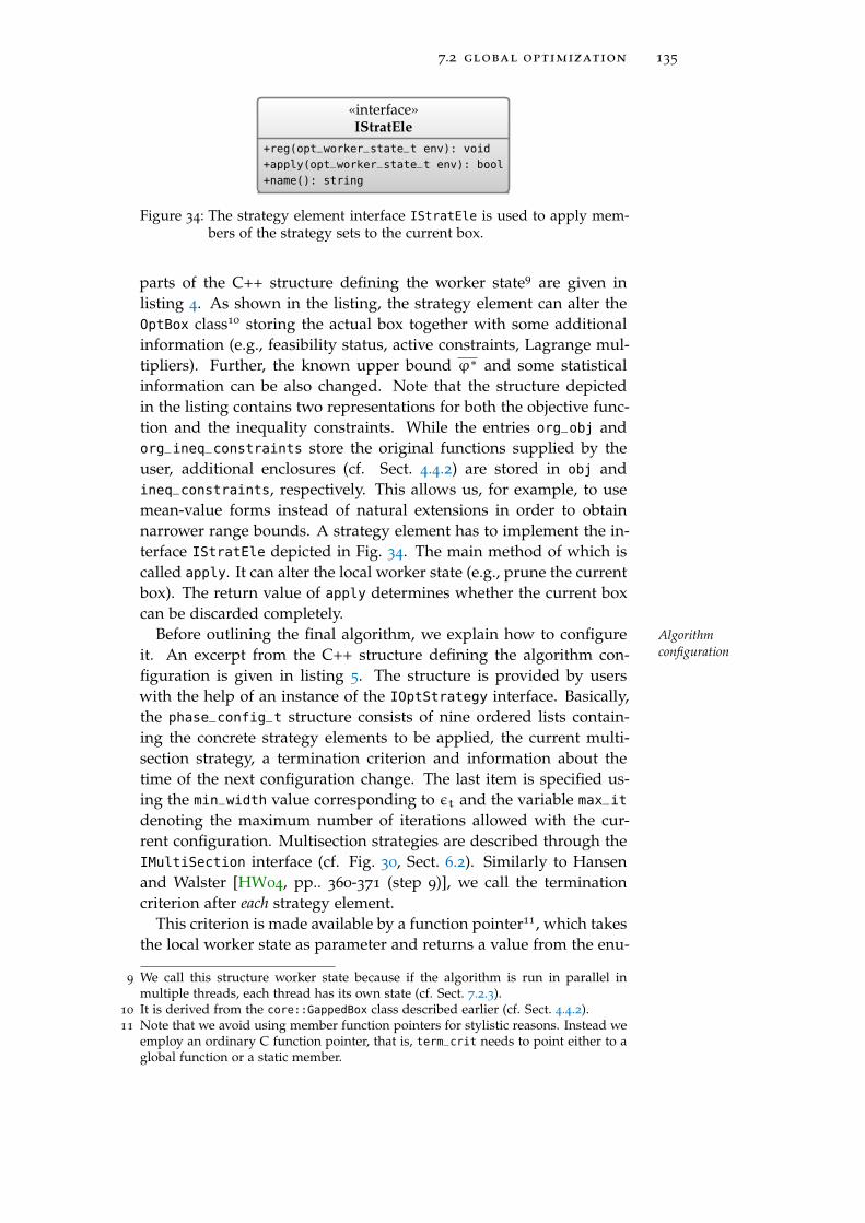
7.2 global optimization 135
«interface»IStratEle
+reg(opt_worker_state_t env): void+apply(opt_worker_state_t env): bool+name(): string
Figure 34: The strategy element interface IStratEle is used to apply mem-bers of the strategy sets to the current box.
parts of the C++ structure defining the worker state9 are given inlisting 4. As shown in the listing, the strategy element can alter theOptBox class10 storing the actual box together with some additionalinformation (e.g., feasibility status, active constraints, Lagrange mul-tipliers). Further, the known upper bound ϕ∗ and some statisticalinformation can be also changed. Note that the structure depictedin the listing contains two representations for both the objective func-tion and the inequality constraints. While the entries org_obj andorg_ineq_constraints store the original functions supplied by theuser, additional enclosures (cf. Sect. 4.4.2) are stored in obj andineq_constraints, respectively. This allows us, for example, to usemean-value forms instead of natural extensions in order to obtainnarrower range bounds. A strategy element has to implement the in-terface IStratEle depicted in Fig. 34. The main method of which iscalled apply. It can alter the local worker state (e.g., prune the currentbox). The return value of apply determines whether the current boxcan be discarded completely.
Before outlining the final algorithm, we explain how to configure Algorithmconfigurationit. An excerpt from the C++ structure defining the algorithm con-
figuration is given in listing 5. The structure is provided by userswith the help of an instance of the IOptStrategy interface. Basically,the phase_config_t structure consists of nine ordered lists contain-ing the concrete strategy elements to be applied, the current multi-section strategy, a termination criterion and information about thetime of the next configuration change. The last item is specified us-ing the min_width value corresponding to εt and the variable max_it
denoting the maximum number of iterations allowed with the cur-rent configuration. Multisection strategies are described through theIMultiSection interface (cf. Fig. 30, Sect. 6.2). Similarly to Hansenand Walster [HW04, pp.. 360-371 (step 9)], we call the terminationcriterion after each strategy element.
This criterion is made available by a function pointer11, which takesthe local worker state as parameter and returns a value from the enu-
9 We call this structure worker state because if the algorithm is run in parallel inmultiple threads, each thread has its own state (cf. Sect. 7.2.3).
10 It is derived from the core::GappedBox class described earlier (cf. Sect. 4.4.2).11 Note that we avoid using member function pointers for stylistic reasons. Instead we
employ an ordinary C function pointer, that is, term_crit needs to point either to aglobal function or a static member.

136 algorithms
enum TERM_RESULT { NONE, SOLUTION, REDUCED, TMP_REMOVED } ;typedef TERM_RESULT ( * f_ term_t ) ( const
opt_worker_s ta te_t &) ;s t r u c t phase_conf ig_t{
/ / s t r a t e g i e s f o r t h e s p l i t t i n g s t e ps t r a t _ e l e _ l s t _ t p s p l i t ;/ / s t r a t e g i e s f o r PHASE_As t r a t _ e l e _ l s t _ t pa ;/ / s t r a t e g y e l e m e n t s f o r PHASE_POS_INFEASs t r a t _ e l e _ l s t _ t p in feas ;/ / . . ./ / s t r a t e g y e l e m e n t s f o r PHASE_FINALs t r a t _ e l e _ l s t _ t s o l _ s t r a t s ;/ / GPU s t r a t e g y e l e m e n t sg p u _ s t r a t _ e l e _ l s t _ t gpu_pspl i t ;/ / m u l t i s e c t i o n s t r a t e g ydecomp : : IMul t iSec t ion <OptBox>* s e c t i o n ;/ / p o i n t e r t o t e r m i n a t i o n c r i t e r i o nf_ term_t t e r m _ c r i t ;/ / minimum width f o r s u b d i v i s i o n in t h i s p h a s ecore : : a r i t h : : mreal min_width ;/ / maximum number o f i t e r a t i o n s in t h i s p h a s eunsigned max_it ;
} ; �Listing 5: Excerpt from the phase_config_t structure responsible for
configuring the optimization algorithm.
meration TERM_RESULT. This returned value determines further courseof action taken by the main algorithm in the following way:
• none : No action needed.
• solution : Box is moved to Lfinal.
• tmp_removed : Box is moved to Ltmp.
• reduced : Box is moved back into L.
In the last three cases, the main loop of the algorithm is restarted.Our supplied standard strategy uses (59) to check whether a finalsolution has already been found. In addition, it uses the εt thresh-old to decide whether the box should be moved to Ltmp. The lastreturn value reduced indicates whether the strategy elements ap-plied upto the current point led to sufficient progress. If this the case,the (reduced) box is added to L without a multisection and the mainloop is restarted. The advantage of this approach is that we applycomputationally cheap strategy elements first, and if they lead to asufficient progress, we can reapply them on the reduced box andavoid expensive steps until they are really required. To check suffi-cient progress, Hansen and Walster proposed the criterion (41) thatwe already used in the scope of contracting trees (cf. Sect. 6.1.2).

7.2 global optimization 137
Algorithm 7: Sequential version of the configurable interval globaloptimization algorithm in UniVerMeC.
Input: Search region x(0), Optimization problem (38), Strategyconfiguration
Output: Enclosure ϕ∗ of minimum ϕ∗, List of candidate boxesGet initial configuration;
2 L := {x(0)};Ltmp := ∅;S := RUNNING;
5 ϕ∗ :=∞;6 while S == RUNNING do7 if L = ∅ then
Get configuration for next phase;forall the x ′ in Ltmp do
apply_strat_eles(STRAT_TMP, x ′);L := L∪ {x ′};
12 Ltmp := ∅;13 if L = ∅ then S := FINISHED; continue; ;14 x := head(L); L := tail(L);
apply_strat_eles(STRAT_A, x);if ¬feasible(x) then
apply_strat_eles(STRAT_POS_INFEAS, x);apply_strat_eles(STRAT_B, x);if feasible(x) then apply_strat_eles(STRAT_FEAS, x) ;apply_strat_eles(STRAT_C, x);if strictly_feasible(x) then
apply_strat_eles(STRAT_STRICT_FEAS, x);23 apply_strat_eles(STRAT_D, x);24 Lsplit := split(x);
forall the x ′ in Lsplit doapply_strat_eles(STRAT_SPLIT, x ′);
27 L := L∪ {x ′};28 forall the x ′ in Lfinal do
apply_strat_eles(STRAT_FINAL, x ′);ϕ∗ := min
x∈LfinalΦ(x);
ϕ∗ := min(ϕ∗, maxx∈Lfinal
Φ(x));
32 return (ϕ∗,Lfinal)
138 algorithms
In Alg. 7, the sequential version of our approach is shown. It re-Algorithmdescription quires the search region x(0), the optimization problem (38), and the
strategy configuration12 as input. The algorithm returns an enclosureϕ∗ of the global minimum ϕ∗ and a list of candidate global mini-mizers. For checking whether a box can be guaranteed to be feasibleor strictly feasible, the predicates13 feasible and strictly_feasible
are used. The main parts of the algorithm are encapsulated into theapply_strat_eles function. This function takes the current strategyset and the current box as arguments. Every strategy element fromthe set is applied to the current box. After each application of a strat-egy element, a user-defined termination criterion is used to determinewhether the box can be discarded, moved to Ltmp or Lfinal, or suffi-cient progress was made. If any of these is the case, the appropriateaction is taken, and the current loop is restarted.
The algorithm starts with initializing L, Ltmp, ϕ∗ and the sta-tus variable S in lines 2-5. The status variable can take the valuesRUNNING or FINISHED which indicate whether the algorithm isstill working in the main loop or finished its work there. The mainloop is entered in line 6. If there is no box in L the configurationis changed, the strategy for the boxes in Ltmp is carried out, andthe boxes are moved back into L (lines 7-12). If L is still empty, thealgorithm leaves the main loop, applies the strategies for the finalphase, and returns the global minimum (lines 28-32) before terminat-ing. Otherwise, the algorithm takes the first box x from L and appliesthe strategy elements depending on the feasibility of x (lines 14-23).After that, the multisection is performed and the new boxes are at-tached to L (lines 24-27).
7.2.3 Parallelization of the Algorithm
The basic techniques discussed in Sect. 7.2.1 can be carried out in par-Reentrancy
allel on different subdivision boxes. For example, two interval New-ton steps to solve (57), (58) for the boxes x(i), x(j), x(i) 6= x(j) do nothave any data dependency. Therefore, our parallelization approachbasically consists in launching multiple threads that execute the mainloop of Alg. 7 independently of each other. This approach is only suit-able if the strategy elements called through the apply_strat_eles
function are reentrant, that is, it is safe to call them from multiplethreads in parallel on different opt_worker_state_t instances.
The implementation of reentrant strategy elements is encouragedby the architecture of UniVerMeC. Note that the apply method in theIStratEle interface (cf. Fig. 34) is declared const in our implemen-tation. This ensures that a call to this method can not modifiy any
12 In the implementation, this is an instance of the IOptStrategy interface.13 Note that if the predicates return false, this does not imply that a box is not (strictly)
feasible but only that the (strict) feasibility could not be proven.

7.2 global optimization 139
Table 16: Handling of variables in the parallel version of the interval globaloptimization algorithm with regard to thread synchronization.
var . shared/copy sync . method sync . time
L shared critical sectionLtmp private copy critical section config. changeLfinal private copy critical section finalization phaseϕ∗ private copy critical section each iterationIT shared atomic instr.S shared atomic instr.
data stored in the IStratEle instance14. In general, we assume that amethod declared const performs only read operations on shared data,and is, therefore, reentrant from multiple threads. Thus, a strategy el-ement should modify only the passed opt_worker_state_t structure.To allow the straightforward and easy implementation of const cor-rect functions most methods in interfaces provided by UniVerMeCare also declared to be const15. In the rest of our work, we assumethat all strategy elements used are reentrant.
While we can safely postulate that the strategy elements called by Shared variables
different threads share no data, certain other data structures used inAlg. 7 need to be shared. Usually, the required wall clock time to solvea problem decreases with additional processors16 (i.e., parallelizationyields good results), if each of these processors performs a meaningfultask and the synchronization overhead is not too high [Ber95a, p. 74]. Of-ten both conditions are in conflict with each other if it is not possibleto subdivide the main task a priori into equal subtasks that can be as-signed to each processor and require no or very little communicationwith each other.
In global optimization, we do not know at the beginning of the al-gorithm how the work is distributed inside the search region x(0)17.Therefore, an a priori subdivision of the search region might lead tothe case in which one processor has to carry out all the work, sup-pressing any potential speed up through parallelization. To avoidthis, we have to perform a dynamical work sharing during runtime.While this is a non-trivial task in the case of parallelization with dis-tributed memory (e.g., [Bee06, pp. 125-139]), it is possible to share L
between all threads in our case. The advantage is that each thread
14 If we assume that keywords such as mutable are avoided during the implementa-tion of the actual instances of these interfaces. The use of such keywords mightundermine the guarantees made by declaring a member function const.
15 For example, all methods provided by the interfaces IVFunction, and IContractor.16 In the optimal case, the decrease is linear. However, the maximum gain depends
according to Amdahl’s law on how much of the program needs to be carried outsequentially [CJP08, pp. 33-34].
17 This depends, for example, on where global or local optimizers are situated in x(0).
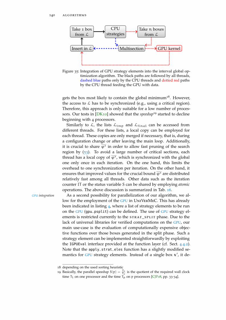
140 algorithms
Take 1 boxfrom L
CPUstrategies
Take n boxesfrom L
Multisection GPU kernelInsert in L
Figure 35: Integration of GPU strategy elements into the interval global op-timization algorithm. The black paths are followed by all threads,dashed blue paths only by the CPU threads and dotted red pathsby the CPU thread feeding the GPU with data.
gets the box most likely to contain the global minimum18. However,the access to L has to be synchronized (e.g., using a critical region).Therefore, this approach is only suitable for a low number of proces-sors. Our tests in [DK10] showed that the speedup19 started to declinebeginning with 4 processors.
Similarly to L, the lists Ltmp and Lfinal can be accessed fromdifferent threads. For these lists, a local copy can be employed foreach thread. These copies are only merged if necessary, that is, duringa configuration change or after leaving the main loop. Additionally,it is crucial to share ϕ∗ in order to allow fast pruning of the searchregion by (53). To avoid a large number of critical sections, eachthread has a local copy of ϕ∗, which is synchronized with the globalone only once in each iteration. On the one hand, this limits theoverhead to one synchronization per iteration. On the other hand, itensures that improved values for the crucial bound ϕ∗ are distributedrelatively fast among all threads. Other data such as the iterationcounter IT or the status variable S can be shared by employing atomicoperations. The above discussion is summarized in Tab. 16.
As a second possibility for parallelization of our algorithm, we al-GPU integration
low for the employment of the GPU in UniVerMeC. This has alreadybeen indicated in listing 4, where a list of strategy elements to be runon the GPU (gpu_psplit) can be defined. The use of GPU strategy el-ements is restricted currently to the strat_split phase. Due to thelack of universal libraries for verified computations on the GPU, ourmain use-case is the evaluation of computationally expensive objec-tive functions over those boxes generated in the split phase. Such astrategy element can be implemented straightforwardly by exploitingthe IGPUEval interface provided at the function layer (cf. Sect. 4.4.2).Note that the apply_strat_eles function has a slightly modified se-mantics for GPU strategy elements. Instead of a single box x ′, it de-
18 depending on the used sorting heuristic19 Basically, the parallel speedup S(p) = T1
Tpis the quotient of the required wall clock
time T1 on one processor and the time Tp on p processors [CJP08, pp. 33-34].

7.2 global optimization 141
Table 17: Strategy elements used in the default strategy of the global opti-mization algorithm.
name description
bounder_t Bound on the objective function using IA
midpoint_t Midpoint test (53)feas_t Feasibility test based on IA
ilie_cbounder_t Feasibility update and pruning of infeasibleparts using an ILIE
bc_const_t Pruning infeasible parts using box consistencyu_ubound_t Updating ϕ∗ with the help of (54)ilie_bounder_t Updating the bound on the objective function
and pruning of the box using (60) with an ILIE
bc_ubound_t Prune box using (60) with box consistencybc_grad_t Apply box consistency on gradient check-
ing (55)
livers multiple boxes at once. In fact, additional multisections areperformed before starting the GPU computation in the current imple-mentation. This ensures that the GPU’s computational resources areutilized better. The integration of the GPU steps into the parallel CPU
version is shown in Fig. 35. One CPU thread is responsible for trans-ferring data from and to the GPU. Its execution path is denoted bythe dotted red line. Notice that this thread also performs the nor-mal activities of the other CPU threads. If non-blocking operations20
are used by GPU strategy elements, a better overall utilization of theavailable computational resources is achieved.
7.2.4 Provided Strategy Elements and Possible Enhancements
As a usage example for the algorithm, we provide a default strategy Implementingstrategy elements(DefaultStrategy) implementing the strategy interface IOptStrate-
gy and a number of strategy elements (cf. Tab. 17). They make useof the techniques provided by the framework to implement variantsof the interval global optimization methods described in Sect. 7.2.1.These predefined strategy elements rely heavily on the already exist-ing infrastructure of UniVerMeC. Thus, they are comparatively easyto implement.
Consider, for example, the implementation of ilie_bounder_t givenin listing 6. This strategy element tries to prune the current box byformally solving the equation (60) using an ILIE. The advantages ofusing a uniform framework for implementation are clearly visible inthe listing: To construct an ILIE, we need to evaluate ϕ over x using
20 For example, the IGPUFuture approach described in Sect. 4.4.2.

142 algorithms
s t r u c t i l i e _ b o u n d e r _ t : publ ic I S t r a t E l e{
v i r t u a l bool apply ( opt_worker_s ta te_t &env ) const{
using namespace core : : a r i t h ;f u n c t i o n s : : enc l : : ILIEEncl enc l ( * env . ob j ) ;s td : : unique_ptr <f u n c t i o n s : : IFunction >
l o b j ( enc l . enc l ( env . cbox−>ref_X ( ) ) ) ;i f ( l o b j ) {
i n t e r v a l bound ( ( * l o b j ) ( env . cbox−>ref_X ( ) ) ) ;env . cbox−>bound ( ) &= bound ;i f ( ! i s _ i n f i n i t y ( env . ubound ( ) ) )
re turn l o b j −>f e a t u r e s ( ) . custom_consistency ( )−>get ( 0 ) . prune ( * env . cbox ,
i n t e r v a l (− i n f i n i t y ( ) , env . ubound ( ) ) ) ;}re turn f a l s e ;
}
v i r t u a l s td : : s t r i n g name ( ) const{
re turn " ILIE Bounder " ;}
} ; �Listing 6: Strategy element for prunig a box by formally solving (60) using
an ILIE.
AA. In the listing, this step is performed implicitly by constructing anenclosure object that returns a new function representation. It deliv-ers new bounds on ϕ over x in AA. Additionally, this new functionobject provides a custom contractor that formally solves (60) to prunex. Basically, all enclosure and contractor techniques supplied insideUniVerMeC can be used in a similar manner without too much effort,allowing for the maximum flexibility of the actual algorithm configu-ration used in global optimization.
The algorithm we consider in this section is not intended to be aRelationship tostate-of-the-art
solverscomplete replacement for state-of-the-art solvers such as COCONUT[Sch04], GlobSol [Kea03] or SONIC [Bee+04]. Instead, it can servewell as a platform for testing different techniques in an easy way.Here, UniVerMeC ensures flexibility with respect to employed tech-niques thanks to its uniform treatment of different range arithmetics.This feature is not provided by the other solvers. Additionally, thereare several special cases in which choosing UniVerMeC over theother solvers is advantageous. For example, the GPU parallelizationis currently supported only by UniVerMeC. Another possibility isfor situations where other algorithms available within UniVerMeCshould be applied on the same model description. Such a situationis discussed in Sect. 8.2. Here, the optimization algorithm is com-bined with external IVP solvers to validate the solution. An examplefor an even deeper integration is investigated in an ongoing master

7.3 interfacing of external solvers 143
thesis [Pus13], where the value of the objective function is calculatedusing verified IVP solvers, and, thus, the IVP solvers are called fromwithin the optimization algorithm. Note that no modification of ouralgorithm is necessary because our function representation allows usto treat even such cases as black boxes.
Since our implementation is not intended to be a replacement for Futureenhancementsstate-of-the-art-solvers (asides from special cases) but a test environ-
ment for different and new techniques, further improvements we dis-cuss in the following concentrate on points relevant for this goal. Theextension of the GPU support is very interesting because it is currentlyan outstanding feature. Using the GPU throughout major parts of thealgorithm might allow us to solve complicated problems, which canbe dealt with currently only by using expensive computer clusters21,even with state-of-the-art solvers, on much less expensive systems.Furthermore, making better use of the more sophisticated arithmeticsmight improve the algorithm results significantly.
However, it is difficult to give general directions about when touse a certain arithmetic or range-enclosure technique to obtain betterresults. For example, Kearfott and Arazyan [KA00] conclude their ex-amination of TMs in the scope of global optimization by stating thattheir usage “is sometimes helpful and sometimes not helpful”. Kear-fott and Walster [KW02] highlight several cases where TMs lead tobetter results in interval global optimization and investigate whetherthere is a good heuristic to determine when to use them. One in-vestigated heuristic consists in randomly choosing some boxes andevaluating them with the help of both IA and TMs to judge whetherthe increased computational effort of using TMs is worthwhile. Im-plementing such a sampling procedure during the strategy phasechanges of our global optimization algorithm might be an interest-ing extension for the future. Additionally, the use of techniques de-veloped especially for arithmetics other than IA (e.g., ILIEs or affinereformulation [NMH10]) should be investigated further. Combiningdifferent possibilities might provide insight into which techniques re-sult in improvements and are, as such, interesting for incorporationinto the state-of-the-art solvers.
7.3 interfacing of external solvers
Besides acting as platform for the direct implementation of algorithms Relation betweenUniVerMeC andexternal solvers
as shown in the two previous sections, UniVerMeC makes it possibleto access already existing external solvers. In this case, the goal isto allow third party solvers to work on UniVerMeC’s internal modeland problem descriptions discussed in Chap. 5. Therefore, an exter-nal solver interfaced to the framework does not employ the whole
21 See, for example, the description of the computer systems employed to solve somerealistic test problems with SONIC [Bee06, p. 146].

144 algorithms
infrastructure but as a rule, uses only the components contained inthe problem description.
The main task while implementing an interface to an external solverDifficulty factors foremploying external
solversis centered on software analysis. It is necessary to examine the prob-lem input format required by the external library to be interfacedand make a connection between those components and their coun-terparts in UniVerMeC. An often employed design pattern in thisscope is the adapter pattern [Gam+95, pp. 139-150]. In our experience,the difficulty of implementing such an interface for numerical solversdepends mostly on two factors22:
1. Whether the external solver is supplied with a well-defined in-terface that can be utilized by UniVerMeC to provide the prob-lem description.
2. The availability of an appropriate (in the best case standardized)format for exchanging numerical quantities.
In general, the first point is the responsibility of the developer ofthird party software. An important aspect that should have been con-sidered during the design process of the external software is, fromour point of view, the reduction of external dependencies in the soft-ware interface. For example, quantities such as matrices and vectorsshould be represented by built-in types of the chosen programminglanguage (e.g., by std::vector in C++ or C-style arrays). The reasonis that using special class libraries (e.g., MTL [GL]) in the public in-terface would break encapsulation and put the additional burden onthe user of learning them and possibly dealing with incompatibilitiesbetween different class libraries in order to use the third party library.
This aspect is connected with the second factor mentioned above.Custom approaches to representing numerical quantities should beabandoned in favor of the standardized ways. For example, built-in types for the standardized IEEE 754-2008 FP representations areavailable in many of modern programming languages. These shouldbe used wherever possible. A serious problem in the case of a verifiedsolver employing range arithmetics is that a standardized format forexchanging verified data is not available at the moment. At least forIA, the adoption of the upcoming standard IEEE P1788 would makethings easier in this regard. Until then, exchanging intervals by theirendpoints using IEEE 754-2008 types is an alternative.
In general, the interfacing or combination of different tools does notRelated work
seem to receive much attention in the verified context. An exceptionis the environment VERICOMP [AR12] (cf. Sect. 1.3), which allowsusers to compare different verified IVP solvers. One reason for thelack of interoperable tools might be that “[...] solvers have disparateinterfaces, which makes developing a unified comparison platform a
22 There are also other factors leading to difficulties. For example, if a program can becompiled only with outdated compilers, written in an obscure language, and so on.

7.3 interfacing of external solvers 145
challenge” as stated in [AR12]. VERICOMP is used to run the inte-grated IVP solvers either with a set of predefined problems or withproblems provided by the user. In the second case, VERICOMP triesto recommend optimal settings based on the already solved prob-lems under certain optimatility conditions derived by the authors.As already explained in Sect. 1.3, UniVerMeC follows a more gen-eral approach and, thus, can be used to implement applications suchas VERICOMP with less effort. Other examples interfacing differentverified solvers are is the comparison platform for global optimiza-tion tools described in [DFS11] (cf. Sect. 1.3). Furthermore, the CO-CONUT environment [Sch04] is capable of calling external solvers.Similarly to VERICOMP both follow a more specific approach com-pared to UniVerMeC.
In contrast to the integration of different verified solvers, the com-bination of rigorous solvers with non-rigorous implementations re-ceived more attention. For example, several FP solvers are applied inscope of the global optimization package GlobSol to find points thatlie near global or local solutions, and can later be verified in a rigorousmanner with interval methods [Kea+04]. In UniVerMeC, we want tosupport the employment of both rigorous and non-rigorous externalsolvers. However, in contrast to existing software packages, we wantto supply building blocks that can be combined to solve specific prob-lems. Examples for such combinations are given in Sect. 7.1.3, whereFP solvers are used to accelerate the distance computation algorithmor in Sect. 8.2 where parameters of mathematical models are identi-fied using an external FP solver and then validated with the help ofan external rigorous IVP solver. In the latter case as well, the intervalglobal optimization method from Sect. 7.2 can be applied to identifythe parameters, which are validated then once again by an externalIVP solver.
7.3.1 ValEncIA-IVP
ValEncIA-IVP [RA11] is a verified solver for obtaining verified en- Required input
closures on the solution of IVPs such as the ones defined in Sect. 5.2(cf. Def. 18). It computes an enclosure of the exact solution to an IVP
over a certain time interval by an algorithm derived from the Picarditeration. Basically, it relies only on enclosures of the range of theright-hand side of the problem at points of time computed using aconstant step size and over intervals between them. Additionally, itrequires bounds on the Jacobian matrix of the right side over the samepoints. The Hessian matrix is needed only for the sensitivity analysis,which we do not support currently. All three types of informationcan be provided using the function layer (cf. Sect. 4.4).
ValEncIA-IVP was designed to work as a standalone application Interfacing astandalone solverand not as a library which can be accessed from external programs.

146 algorithms
ValEncIA-IVP
PROFIL/BIASAPI
FADBAD++API
system
Global C function
for right-hand side
system
Overload for
FADBAD++ types
«interface»IIVP
+rhs(): IVFunction+u(): IVFunction+p(): ivector. . .
«interface»IVFunction
«interface»IDerivative
providesright hand side
provides
right-hand side
prov
idesx(0
),...
Figure 36: ValEncIA-IVP is intended for standalone usage. The green com-pability layer was added which mapped the functions used bythe solver to their UniVerMeC counterparts. Furthermore, thespecification of an IVP through the IIVP interface is mapped toValEncIA-IVP’s internal representation.
Users have to specify their problem by adjusting global functions rep-resenting the right-hand side of the problem and by setting the initialvalues and parameters in the main function. Besides, the solver ispermanently coupled with the libraries PROFIL/BIAS [Knü94] forIA and Fadbad++ [SB] for AD. This makes altering the code of thesolver inevitable if we are to employ it in the context of UniVerMeC,a dynamic environment where problems to solve can be exchangedat runtime.
A full decoupling of ValEncIA-IVP from its underlying librariesCompatibility layers
would result in a reimplementation of major code portions. To avoidthis and to enable the easy integration of new versions, we implementa compability layer which maps the APIs used by ValEncIA-IVP tothose provided by UniVerMeC. As shown in Fig. 36, the compabil-ity layer consists of four components. The PROFIL/BIAS and FAD-BAD++ components provide the parts of the API of the respectivepackages used by ValEncIA-IVP. In case of PROFIL/BIAS, it is suf-ficient to write small wrappers which map its functions and types totheir respective counterparts of the core layer of UniVerMeC. Theactual library used to carry out interval computations is then the oneemployed by UniVerMeC. In turn, the FADBAD++ emulation con-sists only of a fadbad::F type which allows us to store values for thederivatives and to return them through the usual FADBAD++ API.
In the original implementation, the right-hand side of the IVP to beSpecifying theright-hand side solved by ValEncIA-IVP is specified by the global templated function
system. It is called either with FP, PROFIL/BIAS IA, or FADBAD++types to evaluate the right-hand side or its Jacobian matrix. Our layer
7.3 interfacing of external solvers 147
provides two overloads for these functions, which return either thevalue of the right-hand side or our fadbad::F types containing thevalues of the derivatives. The actual computations of the values arecarried out by the IVFunction instance representing the right-handside of the IVP. In contrast to the original implementation, the ad-justed solver can now work with IVPs, the derivatives of the rightsides of which are either described analytically by a closed-form ex-pression or derived by AD. Furthermore, the IVP can be changed atruntime and need not be specified at compile time.
Up to this point it was not necessary to change the ValEncIA-IVP Changes toValEncIA-IVPcode itself. Still the following slight alterations of the code are un-
avoidable:
1. Header references to the original PROFIL/BIAS and FADBAD++headers are removed and the new headers for the compatibilityAPI are added.
2. The initialization functions for the initial state values, parame-ters and so on are moved from the main method to an externalone, the functions are altered in such a way, that they read thesevalues from the current IIVP instance.
3. The main method is renamed.
Fortunately, none of these requires major changes in ValEncIA-IVPitself. Thus, there is a high probability that a new version of the solvercan be added to UniVerMeC in a straightforward manner.
After adding the compatibility layer, we can solve an IVP encoded Usage
by the IIVP instance problem by calling the function:
e x t r a s : : i n t e r f a c e s : : so lv e_ i vp _v a le nc ia ( problem , stop_time ,s tep_s ize , f i lename ) ; �
The values stop_time and step_size determine the integration inter-val and the step size of the solver. Results are written by ValEncIA-IVP in the file specified by filename.
Note that there is room for improvements in our way of incorpo- Furtherimprovementsrating ValEncIA-IVP. It might be an interesting idea for the future
to make the state enclosure at stop_time and, if possible, the enclo-sures of the intermediate integration steps accessible directly insidethe framework without needing to read them from the file. How-ever, this would require a more thorough adaption of the solver’scode base. Another possibility for improvements lies in the fact thatneither our interface nor ValEncIA-IVP itself are thread safe at themoment since several global variables have to be used. To be able touse them in a multithreaded mode, it is necessary to revise the wholecode thoroughly.

148 algorithms
«interface»AD_ODE
+compTerms(): void+sumTerms(. . .): void. . .
«interface»AD_VAR
compTerms(): voidsumTerms(. . .): void. . .
«interface»AD
VNODE+VNODE(AD var)+integrate(. . .): void. . .
ADODEWrapper DFODEWrapper
MyAD
«interface»IIVP
«interface»IVFunction
«interface»ITaylorCoeff
Providesdata
Figure 37: The red interfaces are used by VNODE-LP to access the actualIVP. To use VNODE-LP inside UniVerMeC we provide the greenclasses implementing these interfaces. The necessary informationis obtained by them from the underlying IVP represented by theIIVP interface.
7.3 interfacing of external solvers 149
7.3.2 VNODE-LP
VNODE-LP [Ned06] is a verified solver for obtaining rigorous bounds Literateprogrammingon the solutions to IVPs. A distinctive feature of VNODE-LP is that it
was developed using the literate programming approach [Knu84]. Thisapproach allows to combine code and documentation. In the caseof a verified numerical program, this has the advantage that there isa clear correspondence between the underlying mathematical theoryand its actual code. In this way, finding of errors in the implementa-tion is facilitated.
VNODE-LP is based on the Taylor expansion principle and com- Providing Taylorcoefficientsputes the Taylor coefficients of the solution from the right-hand side
of the IVP. Therefore, the solver requires these coefficients togetherwith those of the corresponding variational equation23. As shown inFig. 37, two abstract interfaces are used by VNODE-LP to accessthe IVP to be solved. The first, AD_ODE, provides the Taylor coeffi-cients of the solution, and the second AD_VAR, those of the variationalequation. Both interfaces provide these data using VNODE-LP’s in-ternal interval type24. These design principles of VNODE-LP allowfor its use as an external library in UniVerMeC. Basically, we onlyhave to provide implementations for the interfaces AD_ODE and AD_VAR.These implementations obtain the necessary coefficients through theITaylorCoeff interface from the function layer (cf. Sect. 4.4.2) andconvert the data from UniVerMeC’s internal interval type to VNODE-LP’s one. A lossless conversion between the types is possible sinceboth represent intervals by their double endpoints. In the same way,the initial values, the starting time, and so on can be communicatedthrough the solver’s public interface.
VNODE-LP can be called from inside UniVerMeC by the following Usage
function:
core : : a r i t h : : i v e c t o r solve_ivp_vnodelp ( const ivp : : IIVP&ivp , const core : : a r i t h : : mreal &stop ,std : : vector <core : : a r i t h : : i v e c t o r > &s r e s u l t s ,s td : : ostream &os = std : : cout , core : : a r i t h : : mrealsub_step = −1 .0 , const i v p _ c a l l b a c k _ t * cb = 0 , boolcparams = f a l s e ) ; �
The first three parameters specify the problem in the form of an IIVP
instance, the integration end time and a vector to store (intermediate)results. For convenience, a fourth argument is an ostream instancewhich is used to display intermediate results and the solution (e.g.,for plotting with GNUPlot). The sub_step (sstep) variable is used tosubdivide the integration interval [t0, tend] into subintervals [t0 + i ·sstep, t0 + (i+ 1) · sstep], i = 0, . . . ,k where t0 + (k+ 1) · sstep = tendfor which intermediate results are generated. Furthermore, users can
23 Basically, these are the coefficients of the derivative (Jacobian matrix) of the right-hand side.
24 The interval type is provided by an external library used by VNODE-LP.

150 algorithms
Table 18: Overview of the external solvers interfaced with UniVerMeC andof information required by them. The rigorous solvers are givenin the first part of the table and the non-rigorous in the second.
solver type required information
ValEncIA-IVP IVP Initial values, FP and interval boundsof the right-hand side and its Jaco-bian matrix
VNODE-LP IVP Initial values, interval Taylor coeffi-cients of the solution and the varia-tional equation
ODE IVP Initial values, FP values of the right-hand side (and optionally its Jacobianmatrix)
VODE IVP Initial values, FP values of the right-hand side (and optionally its Jacobianmatrix)
IpOpt Opti. (38) Starting point, FP values for the ob-jective function and constraints/theirderivatives, FP values for Hessian ma-trix of Lagrangian
specify a callback function cb, which is called after the integrationover each subinterval is completed. It can be used to manipulate in-termediate results, parameters, or solver settings. The last parametercparams indicates whether parameters of the IVP to be solved changeduring the integration. In particular, this is the case, if the functionu(t) is piecewise constant. Note that a parameter change is only al-lowed in between subintervals specified by sub_step. Furthermore,a small value for sub_step may lead to a slowdown of VNODE-LP’sintegration process because its automatic stepsize control is only ap-plicable inside the subintervals. Our side of the VNODE-LP imple-mentation is thread safe.
7.3.3 Other Solvers
Besides ValEncIA-IVP and VNODE-LP, several further solvers wereInterfacing FPsolvers interfaced with UniVerMeC. A complete overview of the available
solvers is given in Tab. 18. Among these are the two non-rigorousIVP solvers ODE [SG75] and VODE [BBH89]. Additionally, the inte-rior point optimization algorithm IpOpt [WB06] is supported. Here,we do not describe the interfacing of non-rigorous solvers in detailbecause this process is straightforward in most aspects (cf. [KAR14]for details on the VODE interface). The reason is that a commonly ac-knowledged standardized format for data exchange is available with
7.4 conclusions 151
IEEE 754-2008 and that, additionally, less information was needed bythe examined non-rigorous IVP solvers compared to the rigorous ones.The examined packages required only values for the right-hand side(and optionally the Jacobian matrix).
7.4 conclusions
In this chapter, we discussed how algorithms can be implemented Ways of addingalgorithmsinside of UniVerMeC and how UniVerMeC can be used to employ
algorithms implemented by third party developers. In the formercase, the newly implemented algorithm can be tightly connected tothe underlying framework to benefit from already implemented data-structures and methods. In the latter case, the third party library islikely to make use only of the uniform model description providedby the framework through adapters. Each way has its advantagesdepending on the users’ goals. If the goal is to analyze a problemdescribed using UniVerMeC’s modeling layer by combining differentsolver libraries, it is sufficient to provide the corresponding interfacesto them. Alternatively, the framework can be used to implement newalgorithms for verified computations. In this case, the building blocksprovided at the different layers of the framework can be reused inorder to speed up implementation of new algorithms. We providedexamples for both use-cases in this chapter.
The first discussed algorithm was ε-distance (cf. Sect. 7.1). This Distancecomputationis a novel distance computation approach for deriving a rigorous en-
closure on the distance between two possibly non-convex geometricobjects. It was developed in scope of this thesis and its implemen-tation makes heavy use of techniques supplied by UniVerMeC. Be-sides using the modeling layer (cf. Sect. 5.1) to describe the geomet-ric objects, the algorithm works on hierarchical space decompositionsconstructed by the techniques outlined in Sect. 6.1. To speed up thecomputations, the algorithm can make use of normals or FP solvers.Both are provided inside the integrated environment of UniVerMeC,making the implementation fairly straightforward.
In Sect. 7.2, an interval global optimization algorithm was discussed Interval globaloptimizationas the second example. This algorithm benefits greatly from our ho-
mogeneous data type independent function representation (cf. Sect.4.4). Moreover, it can employ such techniques as contractors, whichare readily available inside the framework. Besides showing howstandard methods from global optimization can be implemented us-ing the already existing UniVerMeC building blocks, we discussedhow the monolithic global optimization approach of Hansen and Wal-ster [HW04] can be modified to fit into the dynamic and modularenvironment. Additionally, we explained how the support for GPU
computations in UniVerMeC can be exploited inside this algorithm.The final Sect. 7.3 discussed ways to interface third party imple- Third party solvers

152 algorithms
mentations of solvers. Interfaced solvers do not make use of majorportions of the framework. Usually, they employ only the uniformmodel description (cf. Sect. 5), which is accessed with the help ofan adapter to be provided by the users. The main focus of presen-tation was on verified solvers because they play an important rolein our actual applications in the next chapter, and their integrationwas much more complicated than non-rigorous ones. The reason isthat there is currently no standardized data exchange format such asIEEE 754-2008 for non-rigorous solvers. Usually, a certain interval li-brary is employed by each verified solver. These libraries are oftennot interoperable, which makes interfacing the solvers harder. Ad-ditionally, verified IVP solvers tend to need more information thantheir FP counterparts. We discussed the interfacing of the verified IVP
solvers ValEncIA-IVP and VNODE-LP and concluded the sectionwith a brief overview of interfaced FP solvers.
In the future, the framework can be extended by interfacing fur-Extension withfurther solvers ther solvers. Possible interesting candidates are, on the one hand,
verified solvers for optimization problems such as GlobSol [Kea03]and, on the other hand, non-rigorous optimizers. Here, specializedsolvers for linear optimization problems are important additions, be-cause they are necessary not only for computing optimal precondi-tioners for the interval Newton procedure (cf. Sect. 4.3.2) but also forsolving linear relaxed problems (e.g., obtained using affine reformu-lations [NMH10]).
Aside from third party solvers, new algorithms can be implementedExtension withfurther algorithms inside UniVerMeC directly. One algorithm class not represented cur-
rently is verified path planning for which an approach was presentedby Jaulin [Jau01]. In a master thesis [Sch11], it was investigated howthis algorithm can be implemented inside UniVerMeC. A more so-phisticated and possibly faster approach for verified path planningbased on rapidly exploring random trees [LaV06, pp. 228-237] waspresented in [Gri08]. An interesting future goal would be to imple-ment this approach to investigate whether the verified feasibility testsused in [Gri08] can be improved by employing more sophisticatedarithmetics . A further interesting point here would be to study howthe algorithm behaves inside scenes described by complex modelsprovided by the modeling layer of UniVerMeC.
8A P P L I C AT I O N S
In the previous chapter, we presented several algorithms that make Applicationexamplesuse of various features of UniVerMeC. In particular, we use its uni-
form handling of different verified techniques. In this chapter, we de-scribe applications in which these algorithms and UniVerMeC weresuccessfully used. Additionally, we give numerical results for them.We consider two different areas in order to demonstrate that ourframework is universally applicable: distance computation betweengeometric models and parameter identification for SOFC models.
In the scope of distance computation, we show that the ε-distancealgorithm introduced in Sect. 7.1.1 derives rigorous bounds on thedistance between geometric objects given by various modeling types.These modeling types and forms appear in the scope of an automaticassistance system for THR surgery [Cuy11], where distance computa-tion plays an important role. Our results can be seen as a steppingstone towards the full verification of the medical process. As a secondexample from the same area, we consider the comparison of differentrange bounding techniques using the ε-distance algorithm. This ex-ample shows that UniVerMeC can act as a fair comparison platform,which was one of our design goals (cf. Sect. 2.1).
In the second application area (the parameter identification of SOFC
models), our focus lies not only on the interval optimization algo-rithm with GPU acceleration described in Sect. 7.2 but also on thecapability of UniVerMeC to apply internal and external interfacedsolvers to the same problem description. Additionally, this last ex-ample demonstrates how the results of non-verified algorithms canbe validated using verified solvers if a process cannot be carried outcompletely in a rigorous way. Here, we have to cope with both IVPs
(cf. Sect. 5.2) and optimization problems (cf. Sect. 5.3) because theobjective function of the parameter identification problem dependson the SOFC models, which are described by the means of IVPs.
This chapter is structured as follows: We start in Sect. 8.1 with a Chapter structure
short introduction into the TreeVis program, which is a GUI for the ge-ometric part of UniVerMeC. After that, we present the test cases forthe comparison of the different arithmetics along with the obtainedresults in Sect. 8.1.1 and consider the distance computation in scopeof the THR assistance system in Sect. 8.1.2. In Sect. 8.2, we discuss theusage of UniVerMeC in the context of SOFCs. We present results ofparameter identification and validate the obtained sets using a rigor-ous IVP solver. Conclusions are in Sect. 8.3.
153

154 applications
(a) An implicit sur-face can be spec-ified by choosinga predefined oneor through a for-mula.
(b) SQs can be config-ured using a dia-log frame.
(c) Hierarchicaldecompositionsare configuredand attached to amodel with thehelp of a dialogwindow. (d) All surfaces, transfor-
mations, etc. arestored and managedin a resource graph.
Figure 38: TreeVis allows users to manage a geometric scene in an interac-tive manner.
8.1 treevis
TreeVis is an interactive GUI supplied with UniVerMeC. It providesInteractive sceneconfiguration an easy access to the geometric modeling layer (cf. Sect. 5.1), the in-
terval tree decompositions (cf. Sect. 6.1) and the ε-distance algorithm(cf. Sect. 7.1.1). With TreeVis, users can create a geometric scene,which consists of one or several geometric objects. These objects canbe added to or removed from the scene interactively. Implicit objectsare defined either by entering the formula for the implicit functiondirectly or by choosing a predefined surface (cf. Fig. 38a). Polyhe-dra are loaded from ASCII files describing them (e.g., in the objectfile format [Off]). SQs are configured through a specialized dialog(cf. Fig. 38b), which allows for altering the model parameters. In thisway, both implicit and parametric descriptions of an SQ are generated.Additionally, TreeVis allows users to apply transformations such asrotation1 or bending, to a geometric object. These transformations arerealized inside UniVerMeC by arranging them and the associated ge-ometric objects in a tree (similar to CSG trees, cf. Sect. 5.1). Afterusers finished configuring the transformation tree, they instantiate itand create what we call a TreeVis model. Finally, users can add inter-
1 In its current implementation, TreeVis always uses FP matrices to represent rotations.This is a GUI limitation. In the underlying framework UniVerMeC both FP andinterval matrices can be applied.
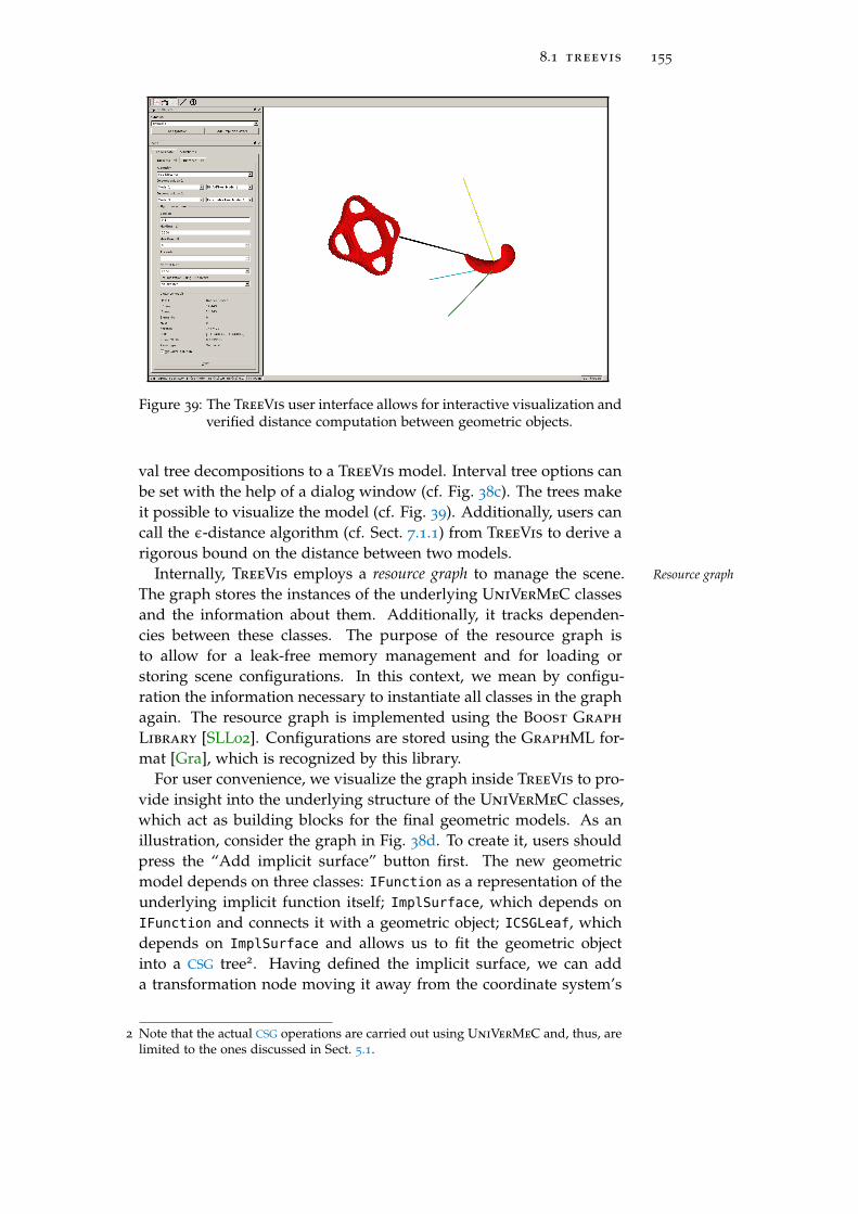
8.1 treevis 155
Figure 39: The TreeVis user interface allows for interactive visualization andverified distance computation between geometric objects.
val tree decompositions to a TreeVis model. Interval tree options canbe set with the help of a dialog window (cf. Fig. 38c). The trees makeit possible to visualize the model (cf. Fig. 39). Additionally, users cancall the ε-distance algorithm (cf. Sect. 7.1.1) from TreeVis to derive arigorous bound on the distance between two models.
Internally, TreeVis employs a resource graph to manage the scene. Resource graph
The graph stores the instances of the underlying UniVerMeC classesand the information about them. Additionally, it tracks dependen-cies between these classes. The purpose of the resource graph isto allow for a leak-free memory management and for loading orstoring scene configurations. In this context, we mean by configu-ration the information necessary to instantiate all classes in the graphagain. The resource graph is implemented using the Boost Graph
Library [SLL02]. Configurations are stored using the GraphML for-mat [Gra], which is recognized by this library.
For user convenience, we visualize the graph inside TreeVis to pro-vide insight into the underlying structure of the UniVerMeC classes,which act as building blocks for the final geometric models. As anillustration, consider the graph in Fig. 38d. To create it, users shouldpress the “Add implicit surface” button first. The new geometricmodel depends on three classes: IFunction as a representation of theunderlying implicit function itself; ImplSurface, which depends onIFunction and connects it with a geometric object; ICSGLeaf, whichdepends on ImplSurface and allows us to fit the geometric objectinto a CSG tree2. Having defined the implicit surface, we can adda transformation node moving it away from the coordinate system’s
2 Note that the actual CSG operations are carried out using UniVerMeC and, thus, arelimited to the ones discussed in Sect. 5.1.

156 applications
origin. Finally, the terminal model instance can be created. A treedecomposing the model can be associated with this instance.
8.1.1 Comparisons Between Range Arithmetics
The first practical application of UniVerMeC is the comparison of dif-Considered objecttypes ferent range arithmetics in the scope of verified distance computation.
For this purpose, we use the ε-distance algorithm to obtain rigorousenclosures of the distances between various implicit surfaces. There-fore, this comparison also serves as a practical test for our distancecomputation approach. We focus on models described by implicitfunctions because they are represented analytically, which allows usto compare the range arithmetics from the point of view of their im-pact on the algorithm’s performance. Polyhedral objects would notbe well suited for this task because their description by simple half-planes would diminish the impact of the used range arithmetic. Para-metric descriptions would be also suited for such a comparison. Wedid not employ them because the only class of surfaces describedparametrically inside UniVerMeC were SQs.
Distinctive features of the ε-distance algorithm are that it computesQuality of rangebounds vs.
computation timesdistances up to a user-specified accuracy and performs an adaptivesubdivision on the hierarchical structures decomposing the geometricmodels. In our comparison, we measure the time that the algorithmrequires to obtain a rigorous distance bound up to the required toler-ance with a specific arithmetic. This criterion is more realistic than,for example, studying only the quality of the range bounds. To under-stand this point, consider a test function for which AA always returnstighter bounds than IA. However, we cannot guarantee that using AA
leads to a better algorithm performance because, in general, opera-tions on affine forms are more expensive than those on intervals. Thatis, it might be faster to subdivide the trees deeper and perform cheapinterval operations instead of using a smaller subdivision depth andcarrying out fewer expensive AA operations. In our study, we avoidthis pitfall by considering only the time that is required to obtain thefinal result. We think that, in practice, users are also likely to be in-terested only in the end result. Aside from the runtime, the requiredmemory usage3 is also of interest. In general, the correlation betweentechniques computing tight range bounds and the overall requiredmemory is more obvious: cheaper techniques lead to a more exten-sive subdivision and, in this way, generate more nodes, which in turnincreases the memory use.
3 In [AR10], several further comparison criteria for set-based IVPs are given. Based onthem, the authors define a recommender system (cf. Sect. 1.3, [AR12]) for verifiedIVP solvers. The criterion used in our comparison can be seen as a variant of the C5criterion from this paper (“user CPU time wrt. resulting interval width”). Since thecriteria from [AR10] are designed specifically for IVPs, not all of them are applicablein our context.

8.1 treevis 157
Table 19: Implicit surfaces used for comparing range-bounding methods.
object formula
Bretzel 2 (x2(1− x2) − y2)2 + 0.5y2 − 0.025(1+ (x2 + y2 + z2))
Citrus x2 + z2 − 4y3(1− 0.5y)3
Cylinder x2 + y2 − 1
Dedocube ((x2 + y2 − 0.64)2 + (z2 − 1)2)((y2 + z2 − 0.64)2 + (x2 −1)2)((x2 + z2 − 0.64)2 + (y2 − 1)2)0.02
Dodeca 2 − cos(x + αy) + cos(x − αy) + cos(y + αz) + cos(y − αz) +cos(z+αx) + cos(z−αx) with α = 1.61803
Ellipsoid 0.5x2 + 0.25y2 + z2 − 1
Heart (x2 + 2.25y2 + z2)3 − x2z3 − 0.1125y2z3
Klein’s bottle (x2 + y2 + z2 + 2y − 1)((x2 + y2 + z2 − 2y − 1)2 − 8z2) +16xz(x2 + y2 + z2 − 2y− 1)
Plop x2 + (z+ y2)3
Pseudocube x500 + y500 + z500 − 1
Sphere x2 + y2 + z2 − r2
Sphere hole (y− x2 − y2 + 1)4 + (x2 + y2 + z2)4 − 1
Stretched sphere x2 + y2 + z4 − 1
Tetrahedral (x2 + y2 + z2)2 + 8xyz− 10(x2 + y2 + z2) + 25
Trigo (1− x2 + y2)2 + sin(z)3 − 0.125
Besides its methodological adequacy, the implementation of ε-dis- Adequacy ofε-distancetance inside UniVerMeC ensures that the comparison is fair. The
reason is that the implementation of ε-distance itself neither needsnor has any knowledge of the arithmetic used to bound the rangeof the expression describing the implicit function. That is, the imple-mentation of the algorithm is the same regardless of the employedarithmetic. Furthermore, the homogeneous data type independentFRO provided by the IFunction interface (cf. Sect. 4.4.2) and the us-age of a function parser to create the implicit functions ensure, incombination with the arithmetic layer (cf. Sect. 3.6), that the over-head for using different arithmetics inside the framework is alwaysthe same. Finally, the affine transformations (e.g., rotation) are carriedout uniformly inside the geometric modeling layer (cf. Sect. 5.1). Theonly component we exchange is the interval tree which uses specificmethods for range bounding to determine the node colors.
To compare the different range-bounding methods, we use 16 dif- Test cases
ferent test cases, which are based on 15 well-known (e.g., [Kno+09])implicit surfaces (cf. Tab. 19). A test case consists of the two implicitobjects for which we want to derive a distance bound and, possibly,affine transformations describing their position in space. Affine trans-formations are applied according to equation (36) where the rotationmatrix and translation vector are converted to the used arithmetic be-forehand. Test cases for which the expressions describing the implicitsurfaces do not suffer from the dependency problem are called sim-ple (non-simple otherwise). Further, we make a distinction between

158 applications
Figure 40: Plot of all implicit surfaces produced by an interval tree. Thesubdivision process was stopped if the volume of a node was lessthan 10−4. In the first line Bretzel 2 to Kleins bottle and in thesecond line Plop to Trigo, ordered according to Tab. 19.
Table 20: Configurations for the 16 test cases. The surfaces are given inTab. 19. Rotation is described by the axis and the angle in degrees.The starting box is used for the root nodes of the tree structures forthe hierarchical decomposition. In the last column, the intersectionof all derived enclosures is given.
scene object translation rotation start box minimum enclosure
1
Trigo (0, 0, 1) ([−4, 4], [−4, 4], [−4, 4])[0.338, 0.340]
Sphere (r = 0.5) ([−1, 1], [−1, 1], [−1, 1])
2
Sphere ([−1, 1], [−1, 1], [−1, 1])[1.000, 1.001]
Pseudocube (−3, 1, 0) ([−4,−2], [0, 2], [−1, 1])
3
Ellipsoid ([−2, 2], [−2, 2], [−2, 2])[0.999, 1.001]
Plop (0, 0,−2) ([−1, 1], [−1, 1], [−3,−1])
4
Cylinder ([−1, 1], [−1, 1], [−1, 1])[1.162, 1.163]
Stret. Sphere (3, 1, 0) ([2, 4], [0, 2], [−1, 1])
5
Sphere ~r = ex,α = 45 ([−1, 1], [−1, 1], [−1, 1])[0.999, 1.001]
Pseudocube (3, 0, 0) ([2, 4], [−1, 1], [−1, 1])
6
Cylinder ([−1, 1], [−1, 1], [−1, 1])[1.111, 1.112]
Stret. Sphere (3, 1, 0) ~r = ex,α = 45 ([2, 4], [0, 2], [−1, 1])
7
Trigo ~r = ey,α = 90 ([−4, 4], [−4, 4], [−4, 4])[0.400, 0.401]
Sphere (1.6, 0, 0) ([0.6, 2.6], [−1, 1], [−1, 1])
8
Ellipsoid ~r = ex,α = −70 ([−2, 2], [−2, 2], [−2, 2])[0.000, 0.000]
Plop (0, 0.7,−1.5) ([−1, 1]3 + Trans.)
9
Klein’s bottle (4, 4, 4) ([1, 8], [1, 8], [1, 8])[0.316, 0.318]
Dodeca ([−4.5, 4.5]3)
10
Heart (0.5, 0, 2) ([−0.5, 1.5], [−1, 1], [1, 3])[0.811, 0.813]
Bretzel 2 ([−1, 1], [−1, 1], [−1, 1])
11
Sphere hole (0, 3, 0) ([−2, 2], [1, 5], [−2, 2])[0.0000, 0.012]
Citrus (0, 3, 0) ([−1, 1], [2, 4], [−1, 1])
12
Tetrahedral ([−3, 3], [−3, 3], [−3, 3])[0.281, 0.283]
Dedocube ([−1, 1], [−1, 1], [−1, 1])
13
Klein’s bottle (4, 4, 4) ~r = ez,α = 45 ([1, 8], [1, 8], [1, 8])[0.131, 0.134]
Dodeca ([−4.5, 4.5]3)
14
Bretzel 2 ([−1, 1], [−1, 1], [−1, 1])[0.086, 0.088]
Heart (0, 1.5, 0) ~r = ex,α = −90 ([−2, 2], [−0.5, 3.5], [−2, 2])
15
Tetrhedral ([−3, 3], [−3, 3], [−3, 3])[0.217, 0.220]
Dedocube ~r = ey,α = 45 ([−2, 2], [−2, 2], [−2, 2])
16
Sphere hole ~r = ex,α = 270 ([−1, 1], [−1, 1], [−1, 1])[0.156, 0.159]
Citrus (0,−3, 0) ([−2, 2], [−5, 1], [−2, 2])

8.1 treevis 159
# ! / usr / b in / python
import univermecextimport sys
scene = univermecext . SceneGraph ( )stream = univermecext . open_stream ( sys . argv [ 1 ] )scene . load_scene ( stream )f o r h in scene . handles ( ) :
t = scene . property ( h ) . type ( )i f t == univermecext . vertex_prop_t .MODEL:
p r i n t " Found model root : " + s t r ( scene . model_name ( h ) ) �Listing 7: Python script using an extension module of UniVerMeC to read
a resource graph file.
rotated and non-rotated cases. In this way, we obtain four groups oftest cases (cf. Tab. 20): simple (1-4), simple rotated (5-8), non-simple(9-12), non-simple rotated (13-16). We have already used the samegroups in [DK12] to compare the different arithmetics. However, ournew results are not directly comparable to the ones in [DK12] becausewe use newer versions of the libraries for range enclosures. Moreover,we exchanged the non-verified AA library libaffa against YalAA.Additionally, the results were computed with a newer version of theε-distance algorithm, which employs the improved case selector (44),whereas the original version of the case-selector from [BDL04] wasused in [DK12]. This test rerun revealed several bugs in the origi-nal implementation from [DK12] that led to erroneous results for theminimum enclosures. The corrected4 versions are given in Tab. 20.
To compare the techniques, we tried to compute enclosures for the Test method
distance for each scenario with the accuracies ε ∈ {0.1, 0.01, 0.001} andmeasured the required CPU time with and without the normal conetest (51). The maximum allowed CPU time was set to 1200 seconds.Every scenario was tested with the standard trees using IA, AA andTMs for range enclosure. Additionally, we used the contracting tree intwo configurations: In the first, we employed the mean-value form forthe range enclosure and no contraction so that the tree behaved likea standard one. In the second configuration, AA was used for rangebounding and box consistency (cf. Sect. 4.3.3) for contraction. Theunderlying libraries were C-XSC [HK04] (v. 2.5.2), YalAA [Kie12b](v. 0.91), Riot [Ebl06] and FADBAD++ [SB] (v. 2.1). Our test systemconsisted of an Intel Xeon CPU E5-2680 with 8 cores and 64 GB RAM.All tests were carried out under Linux. UniVerMeC was compiledusing the gcc compiler (v. 4.7.2) with -O3 optimizations. To minimizethe impact of measurement errors, each test was performed threetimes, and the average of the required time was taken.
4 The table also corrects minor typing errors for the given geometric configurations.

160 applications
Table 21: Results for the test cases from Tab. 20 for different accuracies andtree structures without the use normal vectors. For each test case,the CPU time (t) in seconds, the number of iterations (i) in tenthousands and the number of tree nodes (n) in thousands are given.The best result for each category is marked in green and if a testcase could not be solved in the preset time of 1200s it is markedwith a dash (–). Additionally, the averages for each group (∅1)and the averages over all test cases (∅2) are shown.BinIVTree BinAATree BinTMTree CIVTree CIVTree
(IA) (AA) (TMs) (mean-value form (20)) (AA; box consistency)ε 0.1 0.01 0.001 0.1 0.01 0.001 0.1 0.01 0.001 0.1 0.01 0.001 0.1 0.01 0.001
1
t 0.31 0.79 101.13 0.71 1.46 108.02 2.86 4.53 135.22 1.20 4.63 107.11 0.84 1.55 12.73
i 32.72 82.59 5602.15 43.96 97.62 5638.82 43.84 95.22 5615.23 96.84 342.40 5792.83 7.01 22.76 509.46
n 18.68 30.86 311.13 23.51 35.90 316.98 23.13 35.39 315.70 32.74 78.86 329.92 8.37 18.01 79.35
2
t 0.59 11.25 1045.95 0.01 0.05 0.41 5.31 31.47 – 0.78 12.29 1067.38 0.05 0.27 1.89
i 57.14 761.08 48533.36 0.04 0.30 2.25 57.37 762.18 – 60.56 775.74 49099.88 0.04 0.27 1.83
n 13.10 51.75 398.66 0.87 5.90 44.09 13.15 51.82 – 13.83 53.04 402.61 0.82 4.98 33.68
3
t 90.32 – – 352.24 – – 338.37 – – 518.74 – – 145.16 – –i 4971.02 – – 16816.67 – – 15274.49 – – 24747.24 – – 899.49 – –n 189.63 – – 327.12 – – 305.57 – – 414.64 – – 96.98 – –
4
t 0.86 57.53 – 1.20 60.35 – 2.57 74.17 – 1.20 61.56 – 1.07 40.56 –i 89.10 3413.81 – 90.87 3421.80 – 89.35 3414.40 – 101.15 3538.45 – 36.86 1736.02 –n 22.85 190.51 – 23.13 191.02 – 22.93 190.60 – 24.56 195.74 – 14.90 121.93 –
∅1t 23.02 23.19 573.54 88.54 20.62 54.21 87.28 36.72 135.22 130.48 26.16 587.24 36.78 14.12 7.31
i 1287.49 1419.16 27067.76 4237.89 1173.24 2820.54 3866.26 1423.93 5615.23 6251.45 1552.19 27446.36 235.85 586.35 255.65
n 61.06 91.04 354.89 93.66 77.60 180.54 91.19 92.60 315.70 121.44 109.21 366.26 30.27 48.31 56.51
5
t 1.41 25.58 – 0.02 0.13 0.96 9.42 58.17 – 1.69 26.51 – 0.04 0.26 1.76
i 121.62 1581.85 – 0.05 0.33 2.39 113.74 1518.67 – 124.38 1563.53 – 0.05 0.36 2.56
n 23.28 92.90 – 1.00 6.52 47.71 22.09 89.70 – 23.70 92.56 – 0.93 6.53 46.85
6
t 0.19 15.13 – 0.26 11.45 848.97 0.95 17.13 913.02 0.29 11.69 851.55 0.64 11.61 875.28
i 19.81 1018.39 – 16.08 749.93 40141.16 15.59 744.83 40117.81 21.72 787.65 40453.46 18.40 567.50 30913.57
n 8.89 72.08 – 7.93 59.60 466.32 7.81 59.22 465.82 9.34 62.73 470.08 9.05 55.95 390.87
7
t 0.29 1.61 154.59 1.16 3.41 166.02 6.85 13.24 215.01 2.41 5.02 166.60 0.59 1.46 22.59
i 29.50 161.19 8334.47 61.78 209.21 8427.92 66.29 206.40 8384.54 165.92 360.81 8730.41 11.09 35.76 1047.16
n 18.23 60.64 406.06 30.03 74.64 421.41 30.67 74.09 419.79 55.54 104.87 454.80 9.12 22.62 110.65
8
t 0.02 0.03 0.03 0.15 0.19 0.18 0.51 0.54 0.55 0.31 0.38 0.38 4.00 4.47 6.23
i 2.29 3.08 3.11 7.61 9.88 10.10 6.13 7.17 7.24 31.03 36.51 37.01 2.93 3.48 3.83
n 1.28 2.55 2.55 4.56 5.57 5.63 4.00 4.33 4.35 6.93 9.35 9.47 2.33 2.55 3.00
∅1t 0.48 10.59 77.31 0.40 3.80 254.03 4.43 22.27 376.19 1.18 10.90 339.51 1.32 4.45 226.47
i 43.30 691.13 4168.79 21.38 242.34 12145.39 50.44 619.27 16169.87 85.76 687.13 16406.96 8.12 151.77 7991.78
n 12.92 57.04 204.31 10.88 36.58 235.27 16.14 56.84 296.65 23.88 67.37 311.45 5.36 21.91 137.84
9
t 77.77 – – 3.70 4.86 116.74 8.80 16.31 197.36 31.98 39.08 153.39 4.95 7.58 86.81
i 4266.56 – – 258.58 299.71 5115.12 96.01 144.92 4933.42 1961.16 2362.96 7710.40 242.11 300.93 3254.29
n 237.12 – – 19.89 34.98 207.89 18.41 35.47 205.61 65.06 109.71 263.54 19.35 38.92 175.47
10
t 0.79 4.45 95.23 2.43 9.25 107.32 8.29 28.98 324.66 12.10 21.45 74.08 2.72 7.75 38.54
i 78.59 344.16 4378.33 167.13 432.04 2624.42 151.86 387.19 2530.37 759.20 1239.60 3022.19 50.77 120.67 283.94
n 24.73 158.56 2901.05 25.84 143.87 1761.48 28.83 138.96 1752.79 106.60 189.86 1293.81 20.14 66.02 349.13
11
t 0.11 0.49 2.26 0.25 0.43 0.53 2.24 3.48 4.35 0.99 1.70 1.98 3.78 3.92 4.72
i 9.89 41.64 169.32 8.21 17.39 19.07 6.65 11.54 13.43 65.96 121.50 136.21 5.90 8.82 10.75
n 5.92 23.37 90.38 6.48 9.85 12.74 5.92 9.37 12.69 21.82 31.86 39.91 7.90 8.52 11.27
12
t 176.20 183.47 – 6.77 11.78 148.46 13.28 47.23 327.64 11.41 29.36 694.38 7.36 28.05 239.53
i 8878.33 10004.04 – 279.57 460.38 5536.01 88.82 325.64 4227.08 713.94 1615.26 27552.03 147.33 407.24 4086.06
n 1949.55 1561.80 – 141.67 204.84 1329.13 44.18 179.86 1158.10 85.04 344.28 3848.62 44.02 193.04 1335.38
∅1t 63.72 62.80 48.74 3.29 6.58 93.26 8.15 24.00 213.50 14.12 22.90 230.96 4.70 11.82 92.40
i 3308.34 3463.28 2273.82 178.37 302.38 3323.65 85.83 217.32 2926.08 875.06 1334.83 9605.21 111.53 209.42 1908.76
n 554.33 581.24 1495.72 48.47 98.39 827.81 24.34 90.91 782.30 69.63 168.93 1361.47 22.85 76.62 467.81
13
t 223.40 – – 3.82 4.60 11.84 8.99 14.06 49.95 46.69 47.72 70.19 4.92 6.69 17.92
i 10711.36 – – 262.77 277.54 616.49 96.41 109.72 496.66 2658.49 2711.29 3805.67 250.67 266.94 604.16
n 386.34 – – 17.55 30.42 90.63 17.58 27.88 92.80 70.68 83.71 204.42 17.14 31.04 90.27
14
t 0.23 0.32 1.26 3.41 4.52 19.03 7.98 12.42 24.81 7.60 10.53 20.08 32.01 40.06 70.20
i 23.96 33.62 110.14 225.65 291.17 865.60 185.62 241.62 396.80 496.97 692.31 1232.31 86.53 109.15 362.95
n 10.58 17.45 97.00 27.79 41.72 231.54 16.87 34.17 99.44 45.93 65.99 183.68 19.09 27.22 190.56
15
t 90.40 158.27 – 33.75 51.04 434.67 76.52 152.91 805.67 – – – 53.24 95.16 324.23
i 5286.66 8950.85 – 1407.15 2126.73 18680.19 922.07 1571.90 17068.31 – – – 1983.32 2988.31 9895.31
n 273.01 715.85 – 205.51 314.42 1134.47 103.16 253.62 1050.39 – – – 141.85 366.44 912.75
16
t 0.14 0.31 1.38 0.39 2.57 100.52 2.38 28.61 785.37 1.28 2.77 – 0.36 0.61 3.00
i 15.72 32.43 117.97 23.13 91.96 3187.48 13.85 74.98 3076.38 113.32 224.52 – 4.08 7.72 34.48
n 5.29 14.73 72.99 7.74 60.57 1393.89 6.88 56.74 1388.70 19.24 54.18 – 3.16 6.48 31.96
∅1t 78.54 52.96 1.32 10.34 15.68 141.52 23.97 52.00 416.45 18.52 20.34 45.13 22.63 35.63 103.84
i 4009.42 3005.63 114.06 479.67 696.85 5837.44 304.49 499.56 5259.54 1089.59 1209.38 2518.99 581.15 843.03 2724.23
n 168.80 249.34 84.99 64.65 111.78 712.63 36.12 93.10 657.83 45.28 67.96 194.05 45.31 107.80 306.38
∅2t 41.44 35.32 175.23 25.64 11.07 147.40 30.96 33.55 315.30 42.58 19.62 291.56 16.36 16.67 121.82
i 2162.14 2032.98 8406.11 1229.33 565.73 6490.50 1076.76 641.09 7238.94 2141.19 1169.47 13415.67 234.16 438.39 3643.60
n 199.28 230.23 534.98 54.41 81.32 533.14 41.95 82.75 580.51 66.38 105.48 681.89 25.95 64.68 268.65
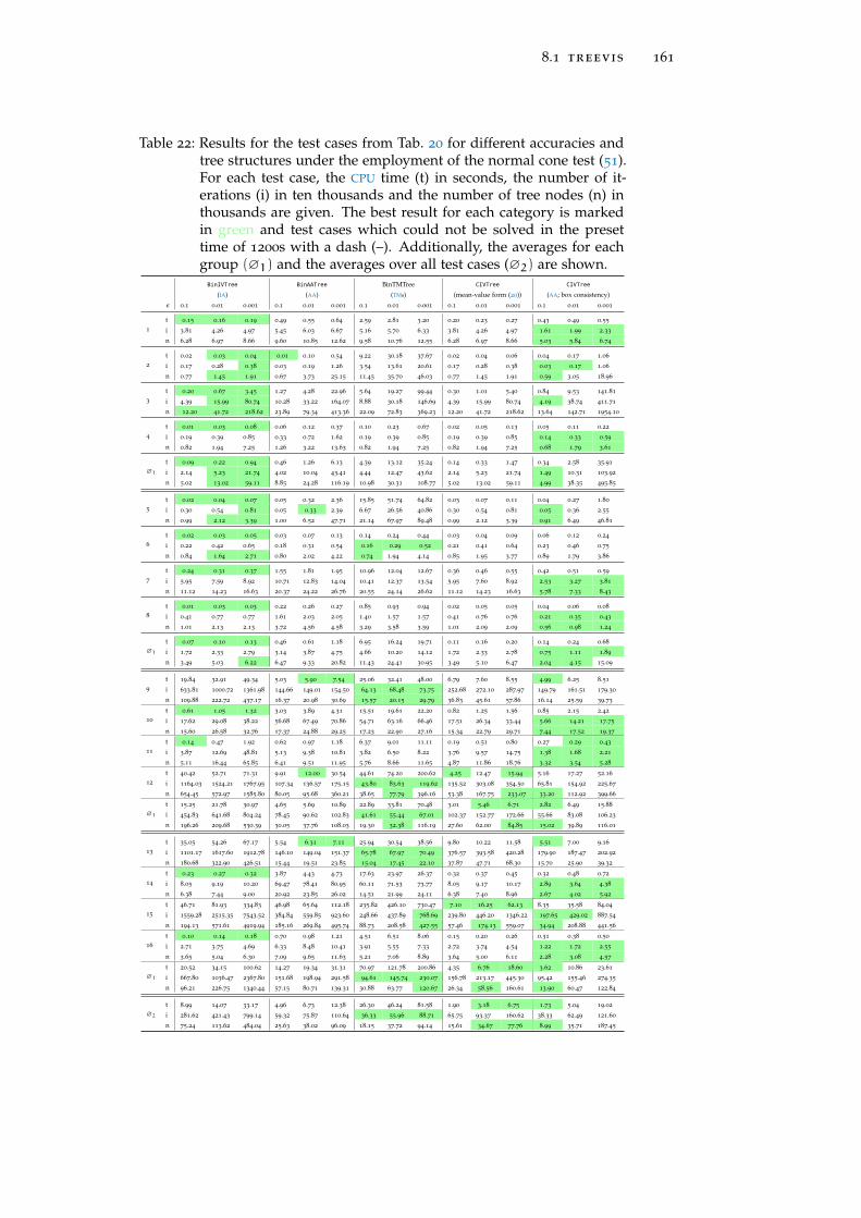
8.1 treevis 161
Table 22: Results for the test cases from Tab. 20 for different accuracies andtree structures under the employment of the normal cone test (51).For each test case, the CPU time (t) in seconds, the number of it-erations (i) in ten thousands and the number of tree nodes (n) inthousands are given. The best result for each category is markedin green and test cases which could not be solved in the presettime of 1200s with a dash (–). Additionally, the averages for eachgroup (∅1) and the averages over all test cases (∅2) are shown.
BinIVTree BinAATree BinTMTree CIVTree CIVTree
(IA) (AA) (TMs) (mean-value form (20)) (AA; box consistency)
ε 0.1 0.01 0.001 0.1 0.01 0.001 0.1 0.01 0.001 0.1 0.01 0.001 0.1 0.01 0.001
1
t 0.15 0.16 0.19 0.49 0.55 0.64 2.59 2.81 3.20 0.20 0.23 0.27 0.43 0.49 0.55
i 3.81 4.26 4.97 5.45 6.03 6.67 5.16 5.70 6.33 3.81 4.26 4.97 1.61 1.99 2.33
n 6.28 6.97 8.66 9.60 10.85 12.62 9.58 10.76 12.55 6.28 6.97 8.66 5.03 5.84 6.74
2
t 0.02 0.03 0.04 0.01 0.10 0.54 9.22 30.18 37.67 0.02 0.04 0.06 0.04 0.17 1.06
i 0.17 0.28 0.38 0.03 0.19 1.26 3.54 13.61 20.61 0.17 0.28 0.38 0.03 0.17 1.06
n 0.77 1.45 1.91 0.67 3.73 25.15 11.45 35.70 46.03 0.77 1.45 1.91 0.59 3.05 18.96
3
t 0.20 0.67 3.45 1.27 4.28 22.96 5.64 19.27 99.44 0.30 1.01 5.40 0.84 9.53 141.81
i 4.39 15.99 80.74 10.28 33.22 164.07 8.88 30.18 146.69 4.39 15.99 80.74 4.19 38.74 411.71
n 12.20 41.72 218.62 23.89 79.34 413.36 22.09 72.83 369.23 12.20 41.72 218.62 13.64 142.71 1954.10
4
t 0.01 0.03 0.08 0.06 0.12 0.37 0.10 0.23 0.67 0.02 0.05 0.13 0.05 0.11 0.22
i 0.19 0.39 0.85 0.33 0.72 1.62 0.19 0.39 0.85 0.19 0.39 0.85 0.14 0.33 0.59
n 0.82 1.94 7.25 1.26 3.22 13.63 0.82 1.94 7.25 0.82 1.94 7.25 0.68 1.79 3.61
∅1t 0.09 0.22 0.94 0.46 1.26 6.13 4.39 13.12 35.24 0.14 0.33 1.47 0.34 2.58 35.91
i 2.14 5.23 21.74 4.02 10.04 43.41 4.44 12.47 43.62 2.14 5.23 21.74 1.49 10.31 103.92
n 5.02 13.02 59.11 8.85 24.28 116.19 10.98 30.31 108.77 5.02 13.02 59.11 4.99 38.35 495.85
5
t 0.02 0.04 0.07 0.05 0.32 2.36 15.85 51.74 64.82 0.03 0.07 0.11 0.04 0.27 1.80
i 0.30 0.54 0.81 0.05 0.33 2.39 6.67 26.56 40.86 0.30 0.54 0.81 0.05 0.36 2.55
n 0.99 2.12 3.39 1.00 6.52 47.71 21.14 67.97 89.48 0.99 2.12 3.39 0.91 6.49 46.81
6
t 0.02 0.03 0.05 0.03 0.07 0.13 0.14 0.24 0.44 0.03 0.04 0.09 0.06 0.12 0.24
i 0.22 0.42 0.65 0.18 0.31 0.54 0.16 0.29 0.52 0.21 0.41 0.64 0.23 0.46 0.75
n 0.84 1.64 2.71 0.80 2.02 4.22 0.74 1.94 4.14 0.85 1.95 3.77 0.89 1.79 3.86
7
t 0.24 0.31 0.37 1.55 1.81 1.95 10.96 12.04 12.67 0.36 0.46 0.55 0.42 0.51 0.59
i 5.95 7.59 8.92 10.71 12.83 14.04 10.41 12.37 13.54 5.95 7.60 8.92 2.53 3.27 3.81
n 11.12 14.23 16.63 20.37 24.22 26.76 20.55 24.14 26.62 11.12 14.23 16.63 5.78 7.33 8.43
8
t 0.01 0.03 0.03 0.22 0.26 0.27 0.85 0.93 0.94 0.02 0.05 0.05 0.04 0.06 0.08
i 0.41 0.77 0.77 1.61 2.03 2.05 1.40 1.57 1.57 0.41 0.76 0.76 0.21 0.35 0.43
n 1.01 2.13 2.13 3.72 4.56 4.58 3.29 3.58 3.59 1.01 2.09 2.09 0.56 0.98 1.24
∅1t 0.07 0.10 0.13 0.46 0.61 1.18 6.95 16.24 19.71 0.11 0.16 0.20 0.14 0.24 0.68
i 1.72 2.33 2.79 3.14 3.87 4.75 4.66 10.20 14.12 1.72 2.33 2.78 0.75 1.11 1.89
n 3.49 5.03 6.22 6.47 9.33 20.82 11.43 24.41 30.95 3.49 5.10 6.47 2.04 4.15 15.09
9
t 19.84 32.91 49.34 5.03 5.90 7.54 25.06 32.41 48.00 6.79 7.60 8.55 4.99 6.25 8.51
i 633.81 1000.72 1361.98 144.66 149.01 154.50 64.13 68.48 73.75 252.68 272.10 287.97 149.79 161.51 179.30
n 109.88 222.72 437.17 16.37 20.98 30.69 15.57 20.15 29.79 36.83 45.61 57.86 16.14 25.59 39.73
10
t 0.61 1.05 1.32 3.03 3.89 4.31 15.51 19.61 22.20 0.82 1.25 1.56 0.85 2.15 2.42
i 17.62 29.08 38.22 56.68 67.49 70.86 54.71 63.16 66.46 17.51 26.34 33.44 5.66 14.21 17.75
n 15.60 26.58 32.76 17.37 24.88 29.25 17.23 22.90 27.16 15.34 22.79 29.71 7.44 17.52 19.37
11
t 0.14 0.47 1.92 0.62 0.97 1.18 6.37 9.01 11.11 0.19 0.51 0.80 0.27 0.29 0.43
i 3.87 12.69 48.81 5.13 9.38 10.81 3.82 6.50 8.22 3.76 9.57 14.75 1.38 1.68 2.21
n 5.11 16.44 65.85 6.41 9.51 11.95 5.76 8.66 11.65 4.87 11.86 18.76 3.32 3.54 5.28
12
t 40.42 52.71 71.31 9.91 12.00 30.54 44.61 74.20 200.62 4.25 12.47 15.94 5.16 17.27 52.16
i 1164.03 1524.21 1767.95 107.34 136.57 175.15 43.80 83.63 119.62 135.52 303.08 354.50 65.81 154.92 225.67
n 654.45 572.97 1585.80 80.05 95.68 360.21 38.65 77.79 396.16 53.38 167.75 233.07 33.20 112.92 399.66
∅1t 15.25 21.78 30.97 4.65 5.69 10.89 22.89 33.81 70.48 3.01 5.46 6.71 2.82 6.49 15.88
i 454.83 641.68 804.24 78.45 90.62 102.83 41.61 55.44 67.01 102.37 152.77 172.66 55.66 83.08 106.23
n 196.26 209.68 530.39 30.05 37.76 108.03 19.30 32.38 116.19 27.60 62.00 84.85 15.02 39.89 116.01
13
t 35.05 54.26 67.17 5.54 6.31 7.11 25.94 30.54 38.56 9.80 10.22 11.58 5.51 7.00 9.16
i 1101.17 1617.60 1912.78 146.10 149.04 151.37 65.78 67.97 70.49 376.57 393.58 420.28 179.90 187.47 202.92
n 180.68 322.90 426.51 15.44 19.51 23.85 15.04 17.45 22.10 37.87 47.71 68.30 15.70 25.90 39.32
14
t 0.23 0.27 0.32 3.87 4.43 4.73 17.63 23.97 26.37 0.32 0.37 0.45 0.32 0.48 0.72
i 8.05 9.19 10.20 69.47 78.41 80.95 60.11 71.53 73.77 8.05 9.17 10.17 2.89 3.64 4.38
n 6.38 7.44 9.00 20.92 23.85 26.02 14.51 21.99 24.11 6.38 7.40 8.96 2.67 4.02 5.92
15
t 46.71 81.93 334.83 46.98 65.64 112.18 235.82 426.10 730.47 7.10 16.25 62.13 8.35 35.58 84.04
i 1559.28 2515.35 7543.52 384.84 559.85 923.60 248.66 437.89 768.69 239.80 446.20 1346.22 197.65 429.02 887.54
n 194.13 571.61 4919.94 185.16 269.84 495.74 88.73 208.58 427.55 57.46 174.13 559.07 34.94 208.88 441.56
16
t 0.10 0.14 0.18 0.70 0.98 1.21 4.51 6.51 8.06 0.15 0.20 0.26 0.31 0.38 0.50
i 2.71 3.75 4.69 6.33 8.48 10.41 3.91 5.55 7.33 2.72 3.74 4.54 1.22 1.72 2.55
n 3.65 5.04 6.30 7.09 9.65 11.63 5.21 7.06 8.89 3.64 5.00 6.11 2.28 3.08 4.57
∅1t 20.52 34.15 100.62 14.27 19.34 31.31 70.97 121.78 200.86 4.35 6.76 18.60 3.62 10.86 23.61
i 667.80 1036.47 2367.80 151.68 198.94 291.58 94.61 145.74 230.07 156.78 213.17 445.30 95.42 155.46 274.35
n 96.21 226.75 1340.44 57.15 80.71 139.31 30.88 63.77 120.67 26.34 58.56 160.61 13.90 60.47 122.84
∅2t 8.99 14.07 33.17 4.96 6.73 12.38 26.30 46.24 81.58 1.90 3.18 6.75 1.73 5.04 19.02
i 281.62 421.43 799.14 59.32 75.87 110.64 36.33 55.96 88.71 65.75 93.37 160.62 38.33 62.49 121.60
n 75.24 113.62 484.04 25.63 38.02 96.09 18.15 37.72 94.14 15.61 34.67 77.76 8.99 35.71 187.45

162 applications
We did not perform the tests using the graphical TreeVis programbecause the visualization could distort the results. Instead, we optedfor automatic processing of all tests with the help of the Python inter-face offered by UniVerMeC. The necessary extension module for thePython scripting language is generated with the help of SWIG5 [Swi].Using this module, we can read the resource graph file format of Tree-Vis. For example, the program in listing 7 reads the resource graphfile passed as an argument and prints the names of all model rootsdefined there. In this way, TreeVis is used to graphically configurethe scene and the actual tedious test runs are handled automaticallyby a script, which additionally minimizes input/output errors.
The obtained results without the normal cone test are given inTest results
Tab. 21. In the table, the required CPU time (t), total number of al-gorithm iterations (i) and the number of used tree nodes (n) for eachaccuracy, scenario and tree are listed. Additionally, the averages foreach subgroup are given. Besides the CPU time, the total numberof tree nodes might be of interest because the memory required tocomplete a scenario is directly proportional to this number. For thestandard trees, the numbers confirm our result from [DK12] whichindicates that AA is a good overall choice. For the simple scenarios,standard IA performs comparatively well. However, it fails for twoscenarios in the highest accuracy, whereas AA is successful for them.The tight range enclosures obtained with TMs seem not to make upfor their high computational cost. However, better enclosure widthsachieved using TMs make the algorithm employ fewer tree nodes inseveral scenarios compared to the other techniques. Besides the stan-dard trees, we also tested our contracting tree (column 6). It deliveredthe best performance overall in respect both to computational timeand number of tree nodes.
In Tab. 22, the results for the test series using normal vectors aregiven. In general, the normal cone test improves the performance forall tree structures and allows us to carry out the scenarios with thehighest accuracy without premature termination. Especially for thesimple test cases not suffering from the dependency problem, stan-dard IA delivered the best overall performance (cf. Fig. 41) if theadditional information provided by normal vectors is used. If themore complex scenarios 9-16 are taken into account, the mean-valueform performs best with respect to the CPU time. The use of the con-tracting tree keeps the number of tree nodes low in some scenariosbut fails to do so in others. Its performance with respect to the CPU
time is average6. It might be an interesting topic for future researchto test the contracting tree with ILIEs because we obtained promisingresults for them in the context of the LIETree in [Kie12a]. Addition-
5 Small Interface and Wrapper Generator6 Here, one reason might be an implementation detail of the CIVTree class that en-
forces additional function evaluations in order to obtain the enclosure for the normalvectors.
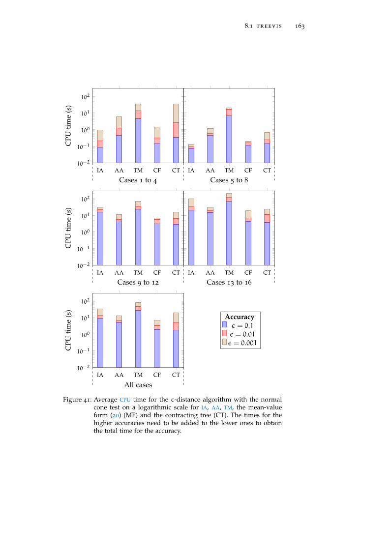
8.1 treevis 163
IA AA TM CF CT10−2
10−1
100
101
102
Cases 1 to 4
CPU
tim
e(s
)
IA AA TM CF CT
Cases 5 to 8
IA AA TM CF CT10−2
10−1
100
101
102
Cases 9 to 12
CPU
tim
e(s
)
IA AA TM CF CT
Cases 13 to 16
IA AA TM CF CT10−2
10−1
100
101
102
All cases
CPU
tim
e(s
)
Accuracyε = 0.1ε = 0.01ε = 0.001
Figure 41: Average CPU time for the ε-distance algorithm with the normalcone test on a logarithmic scale for IA, AA, TM, the mean-valueform (20) (MF) and the contracting tree (CT). The times for thehigher accuracies need to be added to the lower ones to obtainthe total time for the accuracy.

164 applications
ally, the extension of the contracting tree with black inversion nodes(cf. Sect. 6.1.2, which is currently not implemented) might improvethe overall performance of this tree structure. While still good AA
is not the best choice in this test series. TMs suffer from their highcomputational cost7.
8.1.2 Verification of Distances for Total Hip Replacement
In the last subsection, we showed how the ε-distance algoritm canAutomatic systemfor THR be used to compare different range-bounding methods and to derive
rigorous enclosure of distances for the test cases. We focus on thisbecause verified distance computation plays a major role in severalapplication areas where obtaining rigorous bounds is of high impor-tance. As an example for such an area, we consider a system devel-oped by Cuypers for automated selection of a hip implant [Cuy11] ina THR surgery, which appeared in the course of the project PROREOP[Pro]. The system takes the CT image of a rooted femoral shaft asinput and constructs an SQ model from it. Furthermore, it uses SQs todescribe the potential implants. For the automatic selection of an ap-propriate implant, the THR assistance system simulates the insertionprocess of the implant into the femoral shaft, which requires severaldistance computations, in particular, between two SQs and an SQ anda polyhedron. All these geometric models can be non-convex.
The original system of Cuypers was validated in the study [Cuy11,Numericalverification and
validationpp. 124-141] against the state of the art technique of manual implantselection. However, questions regarding the numerical verificationand validation were not considered in this original work. In [ALC13],the whole system was considered from the numerical point of view.The authors examined important subprocesses with regard to the nu-merical verification taxonomy introduced in [AL09] (cf. Sect. 2.1.1).Additionally, a fully verified approach for the distance computationsubprocess was presented in [Aue+11; Chu11] for the case of con-vex SQs modeling the bones. In this thesis, we describe our resultsfrom [KLD13], where we considered the computation of rigorousbounds between non-convex SQs and between a non-convex SQ and anon-convex polyhedron using UniVerMeC.
As mentioned previously, an SQ [Bar81] can be described by theSQ models
implicit function (19). The model depends on five parameters, wherea1,a2,a3 determine the scaling at the coordinate axes and ε1, ε2 de-
7 It would be interesting to test whether this high computational costs appear becauseof using Riot [Ebl06] and whether TMs perform better if the reference implementa-tion COSY [BM06] is employed
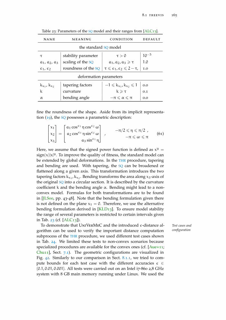
8.1 treevis 165
Table 23: Parameters of the SQ model and their ranges from [ALC13].
name meaning condition default
the standard SQ model
τ stability parameter τ > 0 10−5
a1, a2, a3 scaling of the SQ a1,a2,a3 > τ 1.0ε1, ε2 roundness of the SQ τ 6 ε1, ε2 6 2− τ, 1.0
deformation parameters
kx1 , kx2 tapering factors −1 6 kx1 ,kx2 6 1 0.0k curvature k > τ 0.1α bending angle −π 6 α 6 π 0.0
fine the roundness of the shape. Aside from its implicit representa-tion (19), the SQ possesses a parametric description: x1x2
x3
=
a1 cosε1 η cosε2 ω
a2 cosε1 η sinε2 ω
a3 sinε1 η
,−π/2 6 η 6 π/2 ,
−π 6 ω 6 π(61)
Here, we assume that the signed power function is defined as xy =
sign(x)|x|y. To improve the quality of fitness, the standard model canbe extended by global deformations. In the THR procedure, taperingand bending are used. With tapering, the SQ can be broadened orflattened along a given axis. This transformation introduces the twotapering factors kx1 ,kx2 . Bending transforms the area along x3-axis ofthe original SQ into a circular section. It is described by the curvaturecoefficient k and the bending angle α. Bending might lead to a non-convex model. Formulas for both transformations are to be foundin [JLS00, pp. 43-48]. Note that the bending formulation given thereis not defined on the plane x1 = 0. Therefore, we use the alternativebending formulation derived in [KLD13]. To ensure model stabilitythe range of several parameters is restricted to certain intervals givenin Tab. 23 (cf. [ALC13]).
To demonstrate that UniVerMeC and the introduced ε-distance al- Test cases andconfigurationgorithm can be used to verify the important distance computation
subprocess of the THR procedure, we used different test cases shownin Tab. 24. We limited these tests to non-convex scenarios becausespecialized procedures are available for the convex ones (cf. [Aue+11;Chu11], Sect. 7.1). The geometric configurations are visualized inFig. 42. Similarly to our comparison in Sect. 8.1.1, we tried to com-pute bounds for each test case with the different accuracies ε ∈{0.1, 0.01, 0.001}. All tests were carried out on an Intel i7-860 2,8 GHzsystem with 8 GB main memory running under Linux. We used the

166 applications
Table2
4:Configurations
ofthe
fourtest
cases.TheSQ
parameters
areprovided
inthe
order(a1 ,a
2 ,a2 ,ε
1 ,ε2 ,k,α
,kx1 ,k
x2 ).The
lastcolumn
containsthe
transformation
ofthe
secondSQ
inthe
form(tx1 ,tx2 ,tx3 ,rx1 ,rx2 ,rx3 ,α
r )w
heretx1 ,tx2 ,tx3
isthe
translation,rx1 ,rx2 ,rx3
therotation
axisand
αr
therotation
angle.
sc
en
es
q1
sq
2t
ra
ns
fo
rm
at
io
ns
q2
1(0.2
5,0.75,0.2
5,5037 ,103 ,0,0,0,0
)(0.2
5,0.75,0.2
5,5037 ,103 ,0,0,0,0
)(4,4,0,1,0,0,7
0)
2(0.5
0,0.25,2,
1918 ,1925 ,0.9,4
5,0,0)
(0.25,0.2
5,3,1,1,0.5,70,0,0
)(0,2.5,−
0.75,1,0,0,9
0)
3Polyhedron
(1,1,4,185 ,1,0,3,3
0,0,0)
(−2,4,−
1.5,0,0.7,−0.3,9
0)
4(0.2
5,1,4,1,1,0.3,120,1.5,2.7
)(0.3
5,0.75,0.9,
32 ,1,0,0,1.8,0.4)
(4,0,0,1,0,0,0)
Table2
5:Testresults
forthe
scenariosfrom
Tab.2
4w
ithand
without
thenorm
alcone
test(5
1).The
treeconfiguration
column
indicatesw
hichtree
type(standard
intervaltreeor
parametric
tree)w
asused.
Thequalifier
FPinit
indicatesthat
thealgorithm
was
initializedusing
resultsfrom
anFP
solver.T
hetotal
CPU
time
inseconds
isgiven.
Adash
indicatesthat
thescenario
couldnot
befinished
inthe
predefinedtim
e.A
crossshow
sthat
theconfiguration
isnot
supportedby
oursystem
.
tr
ee
co
nf
ig
ur
at
io
n
wit
ho
ut
no
rm
al
sw
it
hn
or
ma
ls
re
su
lt
0.1
0.01
0.001
0.1
0.01
0.001
1
SParamIVTree
/SParamIVTree
10.
335.
2235.
010.
535.
1231.
7
[4.935,4.9
37]
BinIVTree
/BinIVTree
––
––
––
2
SParamIVTree
/SParamIVTree
27.
8295.
5–
24.
3153.
9–
[0.368,0.3
75]
SParamIVTree
/SParamIVTree
(FPinit)
18.
0283.
1–
13.
9148.
4–
3SParamIVTree
/PolyIVTree
266.
3376.
9-
××
×[0.4
10,0.4
22]
4SParamIVTree
/SParamIVTree
104.
0-
-25.
2353.
5–
[2.670,2.6
71]

8.1 treevis 167
Figure 42: The test cases 1-4 from Tab. 24 (from left to right).
gcc (v. 4.6) compiler, -O3 optimizations with C-XSC [HK04] as theunderlying interval library and FADBAD++ for AD. The maximumCPU time was limited to 600 seconds.
As mentioned above, SQs can be described both by an implicit func- Numerical results
tion or by an explicit parametrization. Because UniVerMeC supportsboth possibilities for geometric modeling (cf. Sect. 5.1) and ε-distanceis capable of deriving rigorous bounds on the distance regardless ofthe modeling type, we tried to solve the first scenario with both mod-eling kinds using parametric trees (cf. Sect. 6.1.3) and standard in-terval trees (cf. Sect. 6.1.1). For the implicit case, it was not possibleto complete the scenario in time and after 600 seconds a distance en-closure with the width ≈ 0.35 was obtained for ε = 0.1. Because itturned out that the parametric representation is much better suitedfor distance computation, we used it in the subsequent cases 2-4. Itssuitability might originate from the fact that the parametric tree sub-divides the parametric domain, which is one dimension lower thanthe object space subdivided in the implicit model. It is interestingthat the use of normals did not make a difference in this test case.
In scenario 2, we considered two non-convex nearly intersectingbent SQs. The use of normal vectors decreased the runtime for ε =
0.01 by almost 50 percent. However, even with the normal support, itwas not possible to reach a result for ε = 0.001 in time.
The third test case consisted of a bent SQ and a non-convex poly-hedron. We used the PolyIVTree for subdividing the polyhedron (cf.Sect. 6.1.4), which employs a ray intersection test to determine thenode colors. This tree structure does not support normals at the mo-ment. So that, the test could be run only without them. Despite theselimitations, an enclosure with the width of ε = 0.01 could be obtainedin the predefined time.

168 applications
The fourth test case consisted of a bent/tapered SQ and a taperedSQ. Using normal vectors, it was possible to improve the distanceenclosure by a large margin and to obtain results for ε = 0.01 in time.
As discussed in Sect. 7.1.3, an FP solver can be used to acceleratethe ε-distance algorithm. This is demonstrated in the second testcase where we used the interior point optimizer IpOpt [WB06] whichis interfaced to UniVerMeC8 (cf. Sect. 7.3.3). Note that this optimizerexpects the problem in the form (42) (for implicit functions). Thus,the overall procedure benefits from the fact that both implicit andparametric descriptions are supported by UniVerMeC. The implicitdescription is used for obtaining the initial value using the FP solverwhereas the ε-distance algorithm works with the parametric one.
The results of this section show that we can provide a full numericalSummary
verification of an important subprocess of the automatic THR surgeryassistant system developed by Cuypers [Cuy11] with the help of Uni-VerMeC. In this scope, we benefit from the fact that UniVerMeCcan employ both implicit and parametric descriptions. The obtainedbounds on the distance are at least one magnitude smaller than themodeling errors. That is, numerical errors are not the dominatingones. Although our approach is rather slow, it can work also withnon-convex objects. It can be carried out offline because the implantselection is performed before the surgery. Currently, the integrationof our verified subprocedure into the software program developed byCuypers [Cuy11] is a future task. During the implementation, the con-siderations with regard to the other subprocesses made in [ALC13]need to be taken into account additionally.
8.2 vericell
In this section, we describe the usage of UniVerMeC inside the pro-VeriCell
environment gram VeriCell which was developed by Auer and Pusch [KAR14;Pus13]. VeriCell is a graphical interface for handling SOFC mod-els. An SOFC is a device that converts chemical energy into electricityand is currently being developed as an important building block fordecentralized energy supplies. One challenge is robust and reliablecontrol of such devices. To develop such control strategies simplified,but accurate mathematical models for SOFCs are required [Dö+13].The goal of the VeriCell program is to provide a flexible environ-ment that can be used to work with and test different control-orientedSOFC models. Important tasks to be performed with SOFC models areparameter identification, validation of parameters, and simulation.
Currently, VeriCell considers only the thermal behavior of SOFCs,Employment ofUniVerMeC which can be described by a system of partial differential equations
8 We have to choose a feasible starting point manually in such a way that IpOpt doesnot converge to the origin (in the local coordinate system) of an SQ because thederivatives required by this solver are not defined there.

8.2 vericell 169
(PDEs). Using a spatial semi-discretization, it is possible to derivea set of nonlinear ODEs [Dö+13]. VeriCell works exclusively withthese ODEs. The uniform function representation of UniVerMeC (cf.Sect. 4.4) is used for the right-hand sides of the ODEs. Furthermore,the modeling layer (cf. Sect. 5.2) is employed for the IVPs for the ODEs
if a cell is simulated. Additionally, the optimization problem for theparameter identification of the SOFC models can be defined with thehelp of UniVerMeC. The simulation of SOFCs is then performed byone of the IVP solvers (cf. Sect. 7.3) interfaced to UniVerMeC, whichcan be graphically configured and called from within the VeriCell
environment. Besides, VeriCell allows for using the integrated inter-val global optimization algorithm of UniVerMeC (cf. Sect. 7.2) or theinterior point solver IpOpt interfaced to the framework (cf. Sect. 7.3.3)for parameter identification.
In the rest of this section, we present the results for parameter iden- SOFC models
tification and simulation of SOFC models that were obtained usingUniVerMeC and the interfaced solvers. We work with the control-ori-ented SOFC models derived in the joint project VerIPC-SOFC betweenthe universities of Rostock and Duisburg-Essen [Dö+13]. Dependingon the resolution of the semi-discretization grid, which was used toderive the ODEs, these models have one (1× 1× 1), three (1× 3× 1)or nine states (3× 3× 1). In the following, we consider the first twoof these basic models. The first one gives no information about thetemperature inside the cell stack, which is partially provided by thesecond one. The 1× 3× 1 models consists of more complex expres-sions and is more complicated from the numerical point of view. Theadditional temperature values inside the stack simulate states thatcannot be measured.
The simple 1× 1× 1 model can be described by
θFC = mH2 ·(p∆H,2 · θ2FC + p∆H,1 · θFC + p∆H,0
)+ 6 · pA · (θA − θFC) + (θAG − θFC)
·(mH2 · (pH2,2 · θ2FC + pH2,1 · θFC + pH2,0)
+ mH2O · (pH2O,2 · θ2FC + pH2O,1 · θFC + pH2O,0)
+ mN2 · (pN2,A,2 · θ2FC + pN2,A,1 · θFC + pN2,A,0))
+ IFC · pel − mA · (θFC − θCG) ·(77 · pN2,C,0/100
+ 11 · pO2,0/50+ 77 · pN2,C,1 · θFC/100+ 11 · pO2,1 · θFC/50+ 77 · pN2,C,2 · θ2FC/100+ 11 · pO2,2 · θ2FC/50
)
(62)
where θFC is the state-variable and θFC(0) = 299.7053 K the initialcondition. The model depends on 20 parameters, for example, on thecoefficients of second-order polynomials that approximate the heatcapacities of hydrogen (pH2,i), nitrogen (pN2,A,i) or air (pO2,i) and,additionally, on 8 time dependent control-input variables. In our IVP
representation (cf. Def. 18), these time-dependent parameters are de-

170 applications
scribed by a piecewise-constant control input function u : R → R8.A detailed description of the parameters and their initializations canbe found in [AKR12]. The initial values were obtained by the FP opti-mizer fminsearch, which is part of the MATLAB package and is animplementation of the Nelder-Mead simplex method [NM65].
The identification of the parameter values of the SOFC models isProblem statement
an important task because good choices of the parameters enableus to adapt the model closely to the existing real system. Usually,the parameter identification is performed by solving a least-squaresoptimization problem. In our case, the objective function ϕ of theoptimization problem (38) is given by
ϕ(p) :=
l∑i=1
s∑j=1
(yj(ti,p) − yj,meas(ti)
)2 (63)
where p ∈ Rn is the vector containing the parameters to be iden-tified9, y(ti,p) the simulated temperature at time ti, ymeas(ti) themeasured temperature, s the number of measurable states, and l thenumber of measurements. In our case, there are l = 19964 equidistantmeasurements (every second) and one (1× 1× 1) or two (1× 3× 1)measurable states. We assume without loss of generality in the for-mula (63) that states with numbers 1 through s are measurable. Thelarge number of measurements does not only make evaluating ϕ ex-pensive computationally but also increases the overestimation due tothe dependency problem if evaluated with IA. Additionally, least-square problems such as (63) often suffer from cancellation effects ingeneral, which increases the overestimation even more [Kie+11].
In our case, we have no analytical solution for (62) (and for theSolving the IVP
higher-dimensional 1× 3× 1 model). Therefore, to obtain fully rigor-ous results on the minimum of ϕ, we have to solve the IVP numeri-cally using a verified solver such as VNODE-LP [Ned06]. Althoughsolving this problem with VNODE-LP is possible in UniVerMeC, thistime-consuming process slows down the global optimization algo-rithm. Therefore, we followed the approach of Rauh et al. [Rau+12]and used Euler’s method to approximate the IVP:
y(k) := y(k−1) + h · f(y(k−1),p) . (64)
Here, f is the right-hand side of (62), y(k−1) is the value obtained atthe previous time step and h is the step size. Note that we can obtaina verified approximation by a simple interval extension of (64). Thisverified approximation accounts for the rounding errors but neglectsthe discretization ones. In Fig. 43, the maximum absolute deviationbetween the results of (64) and those obtained using the fully verifiedsolver VNODE-LP are shown. For a step size of h = 1s, which is also
9 Note that we do not necessarily try to identify all parameters but select a subset ofthem for identification.

8.2 vericell 171
0 0.5 1 1.5 2
·104
0
2
4
Time (s)
Max
imum
absolute
error(K
)
h = 1h = 15h = 30h = 45h = 60
Figure 43: The maximum absolute deviation of the verified enclosure ob-tained by VNODE-LP and different step sizes h for Euler’smethod for the 1× 1× 1 model.
the sampling rate of the measurements, this deviation is less than0.25K at each time step. This is acceptable considering that a worst-case measurement error can reach ±15K. The reason for this rathergood performance of Euler’s method is our small step size in thiscontext [Dö+13]. However, Fig. 43 also shows that we cannot increasethe step size to decrease our computational effort because this mightlead to a much greater error. Thus, we stick to h = 1s in the rest ofour discussion.
Using Euler’s method, we can derive an explicit expression for the Advantages ofEuler’s methodobjective function ϕ:
ϕ(p) :=
l∑i=1
s∑j=1
(y(i−1)j (p) + f(y
(i−1)j (p),p) − yj,meas(ti)
)2. (65)
With this explicit expression, it is possible to compute the derivativesof ϕ straightforwardly by AD. Note that if we apply a numericalsolver to find the solution to the IVP, computing proper enclosuresof the solution derivatives require solving an additional system ofODEs for the sensitivities of the original problem [Kie+11]. Obviously,this process is very expensive computationally. Using the verifiedapproximation approach, we can speed up the function evaluations ofϕ additionally by employing the GPU. The reason is that the objectivefunction (65) requires only operations which are present in our GPU
algebra (16).To enable model evaluation on the GPU, the CPU implementation Model evaluation on
the GPUof (65) in UniVerMeC is accompanied by a corresponding CUDAkernel, which by using allows the function to be evaluated with bothFPA and IA. The kernel is accessed through the interface IGPUEval (cf.

172 applications
0 0.2 0.4 0.6 0.8 1
·106
10−2
10−1
100
101
102
103
Number of boxes
Wal
ltim
e(s
)
GPU 1× 1× 1CPU 1× 1× 1CPU 1× 3× 1GPU 1× 3× 1
Figure 44: Benchmarks for the evaluation of the objective function on theGPU and the CPU. The given time is the wall time on a logarithmicscale. For the GPU, it includes the necessary memory transfers.
Sect. 4.4.2) at the function layer and, thus, can be integrated straight-forwardly into our global optimization algorithm (cf. Sect. 7.2.3).
Benchmark results for evaluations of the objective function (65)for both models are shown in Fig. 44. The simulations were per-formed on an Intel Xeon CPU E5-2680 with 8 cores, 64 GB RAM anda GeForce GTX 580 with 512 CUDA cores and CUDA [NVI12] (V.4.2) (cf. Sect. 8.1.1 for further details on the computer configuration).The benchmarks start with n = 1 boxes. In every step, we increasen by 8192 until n > 1048576. For the simple 1× 1× 1 model, theGPU implementation has a speedup of approximately 19 comparedto the parallel CPU one. In the 1× 3× 1 case, the achieved speedupis 30. Note that the GPU kernel is not optimized heavily. Our com-parison between an optimized GPU kernel of the nine-dimensionalmodel and the non-optimized variant in [KAR13] indicated only aminor speedup. This might be due to the high arithmetic densityof (65) compared to the relatively small amount of data that is re-quired during the evaluation. In fact, the kernel requires only theinput parameters selected for identification, the fixed set of constantparameters, the time-dependent control variables, and the measure-ments for each time step. Note that the latter three sets of data canbe shared between all threads on the GPU.
To classify parameters, Rauh et al. [Rau+12] introduced the notionConsistency ofparameter sets of a consistent parameter set. A parameter set p is called consistent if
the condition
yj(ti,p) ∈(yj,meas(ti) + δ
)(66)
is fulfilled for each time step i = 1, . . . , l and each measurable statej = 1, . . . , s, where δ = [−15, 15] is the worst-case measurement error.

8.2 vericell 173
Initial parameter values
IVP “solver”(Euler’s formula)
Selection ofsearch space
Objective function ϕInterval
optimizationalgorithm
IpOpt
Optimalitymeasure Validation
withVNODE-LP
1 candidate 1 candidate
qcandidates
Figure 45: Overview of the procedure for identifying consistent parametersets for SOFC models in UniVerMeC. Steps that are verified areshown in green boxes and non-verified steps in red boxes.
In case of verified interval evaluations, yj(ti,p) needs to be a subsetof yj,meas(ti) +δ. Analogously, a parameter set is called inconsistentif yj(ti,p) 6∈
(yj,meas(ti) + δ
)or, in the interval case,
yj(ti,p)∩(yj,meas(ti) + δ
)= ∅ (67)
holds at least for one time step i ∈ {1, . . . , l} and measurable state j ∈{1, . . . , s}. In UniVerMeC, it is possible to validate that a parameterset is consistent with respect to (66).
The complete procedure for identifying a consistent parameter set Obtainingconsistent statesusing UniVerMeC is shown in Fig. 45. Currently, UniVerMeC offers
two distinct ways to find such a parameter set. Either the integratedinterval optimization algorithm (cf. Sect. 7.2.2) or the external FP
solver IpOpt (cf. Sect. 7.3.3) can be used. In both cases the procedurestarts with providing an initial guess for the parameter values. Suchguesses can be obtained, for example, from an external source (e.g.,MATLAB’s fminsearch in [Rau+12] or setting all parameters to zero)or from a previous run of our framework. Note that using arbitraryinitial values (e.g., setting all parameters to zero) is supported only

174 applications
Table 26: Results of the parameter identification for the 1× 1× 1 model. Thefirst column identifies the used solver. If the initial value for thesolver is known, it is given in the second column. The errors mea-sure is given in the third column. In the fourth column, the walltime is specified. The last column indicates whether the identifiedparameter set fulfills (66).
solver pinit e time consistent?
IpOpt (0 , . . . , 0) 2.39 K 555.5 s X
fminsearch ? 8.24 K ≈ 21600 s ×Interval opt. fminsearch 7.84 K 4130.86 s ×
if IpOpt is used in the next step of the procedure. The reason isthat IpOpt can optimize with respect to the complete parameter set.In contrast, our interval solver considers only 6 parameters10 at themoment and tries to improve a local solution found by another solverusing mainly the test for consistent parameter sets. A search spaceconsisting of all parameters is too large because of the branch andbound nature of the interval method. Therefore, we restrict the searchspace to
x(0) = pinit + [−1, 1]6 (68)
where pinit ∈ R6 is the initial guess for the selected parameters. Theremaining parameters are replaced by their FP values. Note that thealgorithm itself (restricted to the search space) and the interval eval-uation of ϕ on the CPU and the GPU are verified11. At termination,the interval optimization algorithm returns a list containing q can-didate interval vectors for the parameter set. Following Rauh et al.[Rau+12], we identify each parameter candidate interval vector withits midpoint and calculate the following measure:
e =
√∑li=1
∑sj=1
(yj(ti, midp) − yj,meas(ti)
)2l
.
For the further processing we select the candidate with the smallestvalue of e. This step is not necessary if IpOpt is used because thissolver returns only one solution. In the last step, we check whetherthe parameter set is consistent. This step is again fully verified be-cause we employ the rigorous IVP solver VNODE-LP to calculate stateenclosures for each time step ti, i = 1, . . . , l and check for each tiwhether the interval equivalent of (66) holds.
In both considered cases (1× 1× 1 and 1× 3× 1models), the resultsSolver configuration:IpOpt
10 These parameters are selected based on their importance for the process [AKR12].11 Euler’s method employed inside ϕ to solve the IVP is not verified and if IpOpt eval-
uates ϕ FPA is used instead of IA.

8.2 vericell 175
for IpOpt were obtained with the test configuration described above.Other parameter sets were obtained at a test system of the Universityof Rostock and are described in [Dö+13; Rau+12]. In any case, thevalidation with VNODE-LP was carried out within UniVerMeC. Onedifficulty during the usage of IpOpt is to obtain the derivative valuesof (65). Although the explicit expression for ϕ obtained by Euler’sformula allowed us to employ AD, the large number of measurementsand the nesting caused by the recursive nature of (64) slowed theused FADBAD++ library down significantly. Therefore, we opted notto provide the second order derivatives usually required by IpOpt
but used an option of the solver that automatically approximates therequired values based on the first-order information that we supply.
The interval global optimization algorithm was configured with the Solver configuration:Intervaloptimization
following strategy:
strat_split Bounding the objective function with IA and testing (67)
strat_a Testing feasibility of the box
strat_pos_infeas Applying box consistency on the constraints
strat_tmp Trying to find an upper bound ϕ∗ and using the mid-point test (53).
Additionally, the maximum subdivision depth was set to 10−2 andthe maximum number of iterations to 200000. The starting box x(0)
was obtained using (68). Based on the starting box, we added boundconstraints to the problem to ensure that the condition (52) held forour problem. Note that the only test for discarding boxes besides themidpoint test (53) is the inconsistency condition (67). In particular,we refrain from the use of derivatives for two reasons: First, AD is notsupported on the GPU at the moment in UniVerMeC12 and obtain-ing analytical closed form expressions of the derivatives for manualimplementation on the GPU is not suitable in this case. Second, weuse the criterion (67) not only to check for inconsistent states butalso for limiting the overestimation during the evaluation of ϕ. Thismakes (65) non-differentiable due to the intersection operator. Ourmethod is largely similar to the algorithm used in [Rau+12]; however,we use the Ratz section scheme (cf. Sect. 6.2) as opposed to the stan-dard bisection used there. Moreover, our implementation is fastersince we employed CPU and GPU parallelization.
The numerical results for the 1× 1× 1 model are given in Tab. 26. 1× 1× 1 results
Bearing in mind that the wall times are not completely comparable, itseems fair to state that IpOpt clearly outperforms fminsearch in thiscase. Using IpOpt, we were even able to obtain a consistent parameterset where fminsearch failed to provide one. We used the interval
12 Refer to Sect. 3.7 for general information on limitations of GPU computations inUniVerMeC and to [KK13] for information on AD with IA on the GPU which mightbe used to extend the framework in the future.

176 applications
Table 27: Results of the parameter identification for the 1× 3× 1 model. Thefirst column identifies the used solver. If the initial value for thesolver is known, it is given in the second column. The errors mea-sure is given in the third column. In the fourth column, the walltime is specified. The last column indicates whether the identifiedparameter set fulfills (66).
solver pinit e time consistent?
IpOpt (0 , . . . , 0) 430.55 K 2817.23 s ×fminsearch ? 37.57 K ? ×IpOpt fminsearch 26.59 K 235.565 s ×Interval opt. fminsearch 57.31 K 5021.06 s ×
optimization routine only with the results of fminsearch becauseIpOpt delivered an already consistent parameter set. Compared tothe original FP results, the use of the interval routine led to a decreaseof the error measure. However, the returned set is still not consistent.The GPU accelerated search routine required a little more than an hourto obtain the results. This is much faster than the pure CPU methoddescribed in [Rau+12] which needed ≈ 10 hours13
The results for the higher dimensional 1× 3× 1 model are given1× 3× 1 results
in Tab. 27. In this case, IpOpt failed to provide acceptable boundswhen initialized with zero for all parameters. The reason might bethe numerical problems originating from the approximation of thesecond-order information. Therefore, we used the results obtainedin Rostock with the fminsearch method to initialize IpOpt. In thiscase, the solver terminated after 139 iterations due to errors in theevaluation (63) or its derivatives. The results given in the table arefor a maximum of 130 iterations, which led to a slight improvementover the initial fminsearch results. Note that the comparatively lowwall time is caused by the facts that the solver obtained a good initialbound and performed relatively few iterations as well as that theevaluation of derivatives is multi-threaded14 inside UniVerMeC.
We also tried to improve the results of fminsearch using intervalmethods in this case. Here, the GPU interval optimization had notany advantage but led to a worse parameter set. One reason forthe bad interval results might be that the more complex 1 × 3 × 1model contains non-measurable states for which we cannot use thecondition (67) to limit the overestimation.
During the validation step (cf. Fig. 45), the SOFCs are simulatedValidation results
using the rigorous solver VNODE-LP. In Fig. 46, the simulation re-
13 Note that the computations were carried out on different systems and slightly differ-ent versions of the SOFC models.
14 The derivatives have to be obtained by forward differentiation because FADBAD++cannot handle the large computational graph of (65) with backward differentiation.The total CPU time required by IpOpt was 2791.14s.

8.2 vericell 177
0 0.5 1 1.5 2
·104
400
600
800
1,000
Time (s)
Tem
perature
(K)
Measurement
1 × 1 × 1 (IpOpt)
1 × 3 × 1 (fminsearch)
1 × 3 × 1 (IpOpt)
Figure 46: Simulation results for the parameter sets from Tab. 26, 27 ob-tained with VNODE-LP. In the plot, the rigorous upper boundon the simulated temperature and the consistent area are shown.
sults for the parameter set for the 1× 1× 1 model obtained by IpOpt
and the two parameter sets for the 1× 3× 1 model are shown. Fora complete simulation run with one test parameter set, VNODE-LPrequired approximately 1700 seconds of CPU time on our test system.In the plot, we show only the upper bound on the simulated tempera-ture and the state θ315 of the three dimensional model. The parameterset for the 1× 1× 1 model clearly lies inside the gray tolerance rangefor the measurements. The 1× 3× 1 parameter set obtained by IpOpt
violates this area. For the other considered parameter set that wasobtained by fminsearch, the violation of the consistency conditionsis less noticeable. However, it is also inconsistent and has a largerdeviation for the measurable state θ0 not shown in the plot.
The usage of UniVerMeC allowed us to combine different veri- Futureimprovementsfied and non-verified solvers to obtain a parameter set for the one-
dimensional model and to rigorously prove that these parametersare indeed consistent. Furthermore, the objective function evaluationbenchmark (cf. Fig. 44) and the comparison of the runtimes of ourGPU accelerated interval global optimization method to the methoddescribed in [Rau+12] showed that the employment of GPGPU canlead to a significant speed-up in interval computations.
However, it was not possible in general to improve the parame-ter sets obtained by the FP solvers by the interval algorithm. Whileone reason is certainly that the interval optimization algorithm onlyperforms a local search in our configuration due to memory and run-time restrictions, another reason might be that we employ standard IA
without techniques to reduce the wrapping effect or the dependencyproblem apart from the condition (67), which in turn makes (65) non-
15 θ3 corresponds to θ in the one-dimensional model.
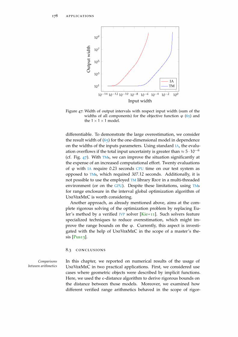
178 applications
10−14 10−12 10−10 10−8 10−6 10−4 10−2 100
101
103
105
107
109
Input width
Out
put
wid
th
IATM
Figure 47: Width of output intervals with respect input width (sum of thewidths of all components) for the objective function ϕ (65) andthe 1× 1× 1 model.
differentiable. To demonstrate the large overestimation, we considerthe result width of (65) for the one-dimensional model in dependenceon the widths of the inputs parameters. Using standard IA, the evalu-ation overflows if the total input uncertainty is greater than ≈ 5 · 10−6(cf. Fig. 47). With TMs, we can improve the situation significantly atthe expense of an increased computational effort. Twenty evaluationsof ϕ with IA require 0.23 seconds CPU time on our test system asopposed to TMs, which required 307.12 seconds. Additionally, it isnot possible to use the employed TM library Riot in a multi-threadedenvironment (or on the GPU). Despite these limitations, using TMs
for range enclosure in the interval global optimization algorithm ofUniVerMeC is worth considering.
Another approach, as already mentioned above, aims at the com-plete rigorous solving of the optimization problem by replacing Eu-ler’s method by a verified IVP solver [Kie+11]. Such solvers featurespecialized techniques to reduce overestimation, which might im-prove the range bounds on the ϕ. Currently, this aspect is investi-gated with the help of UniVerMeC in the scope of a master’s the-sis [Pus13].
8.3 conclusions
In this chapter, we reported on numerical results of the usage ofComparisonsbetween arithmetics UniVerMeC in two practical applications. First, we considered use
cases where geometric objects were described by implicit functions.Here, we used the ε-distance algorithm to derive rigorous bounds onthe distance between those models. Moreover, we examined howdifferent verified range arithmetics behaved in the scope of rigor-

8.3 conclusions 179
ous distance computation. For this purpose, we constructed severaltest cases, grouped them according to the complexity of the expres-sions describing the geometric objects, and derived bounds on thedistance between them using different arithmetics for enclosing thecorresponding ranges. The use of UniVerMeC ensured that the over-all overhead was the same for all arithmetics and, thus, the compar-ison was fair. Here, we confirmed our previous results from [DK12]and found that using AA was a good overall choice without the infor-mation provided by the normal cone test (51). If (51) was used thetest results indicated that the mean-value form (20) was the favorablechoice for the range enclosure. Additionally, the test confirmed theusefulness of our contracting tree structure introduced in Sect. 6.1.2,of the ε-distance algorithm itself (cf. Sect. 7.1.1) and of its extensionwith normals (cf. Sect. 7.1.2).
Our second practical use case was from the area of distance com- Application in THRassistanceputation again. We considered an automatic assistance system for
THR surgery where various distance queries between possibly non-convex SQs and polyhedra were carried out. We demonstrated thatUniVerMeC could handle these kinds of distance queries in a rigor-ous manner. This use case confirmed not only that the verification ofthis important subprocess of the THR assistance system was possiblebut also that UniVerMeC could carry out distance queries betweendifferent modeling types even if one modeling type was non-smooth(e.g, a polyhedron). Additionally, we showed that the method for im-proving the runtime of the ε-distance algorithm using an FP optimizeractually had the desired effect.
Our last use case was the parameter identification for control-orien- Application inparameteridentification andsimulation of SOFCs
ted SOFC models. Here, we demonstrated how different rigorous andnon-rigorous solvers could work together sharing the same problemdescription. Although we could not derive fully rigorous bounds onthe optimal parameters, it was possible to find a parameter set usingan FP solver that had a much smaller error measure than the setsidentified previously. Using UniVerMeC, it was possible to integratethis solver seamlessly into a procedure that proved with the help of averified IVP solver that the enclosures of simulated states of the SOFC
model with this new parameter set were inside the tolerance rangedefined by measurements on a real SOFC for every time step. Finally,we demonstrated that the evaluation of the objective function of anoptimization problem on the GPU could lead to a significant speed upof our interval global optimization algorithm.


9C O N C L U S I O N S
In this thesis, we presented the theoretical foundations of interoper-able handling of verified techniques supplemented by a prototypicalimplementation UniVerMeC. A goal of our approach was to makecombination of existing methods or their interchangeable use possi-ble. The interchangeability of techniques allowed us to achieve ournext goal: It ensured fair comparisons between the techniques be-cause, using our approach, it was possible to exchange a single tech-nique (e.g., the used range arithmetic) while keeping the environmentconstant (e.g., same algorithm implementation, same test scenarios).This level of abstraction during the assessment process is new in thearea. In addition to providing fair comparisons, it allowed for a fasterdevelopment of new methods in the geometrical context in this thesissince basic building blocks could be reused and exchanged easily. Be-sides this, our approach facilitated application of verified techniquesto real life problems as demonstrated in this thesis for the areas oftotal hip replacement and SOFC control.
The structure of this thesis followed roughly the layered hierarchy Arithmetics
principle employed as the basic architectural pattern of our proto-type implementation. First, we discussed and specified the necessarygeneral requirements for a framework implementing the goals above.After that, we introduced rigorous range arithmetics, which are themost basic building blocks of verified numerical computations. Inthis scope, we presented a new flexible library for AA called YalAA. Ithandles different affine computation models and features in contrastto existing AA implementations, verified affine extensions of elemen-tary functions that are neither convex nor concave. On the level ofarithmetics, we introduced a heterogeneous algebra that defines com-mon sets of operations for FPA, IA, AA and TMs. These sets are orientedon the upcoming IEEE P1788 standard. This algebra is extended byhierarchically arranged safe conversions between the different arith-metic types. Based on those theoretical considerations, we designedand realized a generator for semi-automatic creation of adapters sothat different libraries implementing the basic arithmetic types canbe easily integrated in the overall system. Additionally, we specifieda refinement of this algebra for the GPU. The set of operations andsupported arithmetics for the GPU is smaller as a consequence of thecurrently limited state of GPU support in verified computations.
The second layer we discussed concerned important auxiliary meth- Functions
ods such as AD, function enclosures, and interval contractors, whichare necessary for the algorithms we consider later. Our main con-
181

182 conclusions
tribution at this level is the introduction of FROs that are theoreticalconstructs for characterizing a real function by a number of inclusionfunctions. Other important characteristics, for example, derivatives,contractors, or Taylor coefficients, can be represented and attachedto an FRO. This concept is embedded into our universal framework.This theoretical basis allowed us to derive a software realization ofa homogeneous function type that is independent of the actual arith-metic. In this scope, we also described the integration of functionevaluations on the GPU into our implementation.
Arithmetics and functions are the most important basic buildingProblem modeling
blocks for model descriptions in many application areas. Therefore,after introducing uniform concepts for both, we investigated how dif-ferent modeling and problem types could be described with theirhelp inside UniVerMeC. Our examples were from the areas of geo-metric models, IVPs and optimization.
Having described our modeling types, we introduced hierarchicalHierarchicaldecompositions decompositions that played an important role in the algorithms we
were interested in. The main contributions at this level are the fol-lowing: first, we introduced a flexible theoretical foundation for de-scribing various interval trees. Second, we presented two new treetypes. The first was the contracting tree, which made use of inter-val contractors to reduce uncertain regions during the decomposi-tions. Moreover, it featured special inversion nodes for better han-dling of regions produced by these contractors. The other tree struc-ture was introduced for dealing with parametric surfaces. Aside fromdemonstrating how those tree types could be implemented in Uni-VerMeC, we discussed the integration of various well-known multi-section schemes from global optimization.
The usefulness of providing uniform access to various verified meth-Algorithms
ods was further demonstrated by different algorithms supported in-side the framework. In this scope, we presented a new algorithmfor obtaining rigorous enclosures on the minimum distance betweennon-convex objects described by different geometric modeling types.The implementation of the algorithm ensured flexible access to andeasy reuse of various verified methods. As a second example, wediscussed the implementation of a state-of-the-art interval global op-timization algorithm inside the framework. The focus of the discus-sion was how UniVerMeC facilitated the implementation of a highlyconfigurable algorithm. Furthermore, we explained how the capa-bility to evaluate certain functions on the GPU could be integratedinto the optimization method. Finally, we demonstrated how variousthird party solvers could be interfaced with the framework. In thisway, they worked with the uniform modeling descriptions providedby UniVerMeC and could be integrated into general computationscenarios if necessary.
To demonstrate the practicability of our approach, we consideredPractical testscenarios

conclusions 183
three real life motivated test scenarios. In the first one, we computedrigorous distance enclosures for 16 different test cases that were de-scribed by implicit functions and grouped according to the complex-ity of their expressions. We solved each test case with the help ofdifferent techniques for range bounding and compared the requiredCPU times. The obtained results demonstrated not only that the newdistance algorithm was capable of solving all test cases but also thatUniVerMeC was suitable for easy and fair comparison between dif-ferent arithmetics. Moreover, our new tree structures turned out tobe an improvement compared to standard trees for certain test cases.
As a second scenario, we considered the verification of an impor-tant subprocess of a system for automatic selection of an appropriateimplant in the context of THR surgery. The considered subprocess con-sisted of several distance queries between two possibly non-convexSQs, or a non-convex SQ and a non-convex polyhedron. Using ournew distance algorithm, it was possible to derive verified enclosuresfor all those scenarios. This result demonstrates that our algorithmcan derive distances between objects described by different geomet-ric modeling types. More generally, it shows that verification of thisimportant subprocess in the overall THR assistance system is possible.
Our last scenario concerned parameter identification of control-oriented SOFC models. To identify an optimized set of parameters fordifferent SOFC models, we applied our global optimization methodand interfaced third party optimizers. In addition, we demonstratedhow function evaluation on the GPU can accelerate the identificationprocess. The computed parameter sets were examined with respect totheir compliance with measurements taken using a real SOFC testrig.The consistency check was performed by means of a rigorous IVP
solver interfaced to UniVerMeC. We were able to prove that a con-sistent set of parameters was identified. In general, this test scenariodemonstrated how the framework allowed us to use different tech-niques provided by internal and external solvers and to combinethem in one process to tackle complex practical problems.
An important aspect for further improvements is the full incorpo- Future research
ration of the upcoming IEEE P1788 interval standard. Wide accep-tance of IEEE P1788 throughout the interval community would makecertain tasks easier performed by UniVerMeC (e.g., interfacing ofthird party libraries for verified computation). However to realizethis point, we have to wait until IA libraries (e.g., C-XSC) and thethird party libraries implementing the solvers conform to the stan-dard. Another important goal for the whole framework would be tounify the CPU algebra (15) and the GPU algebra (16) as soon as thecorresponding lower-level libraries provide the necessary support. Afull unification could be expected only if the other arithmetics asidefrom IA were to support the GPU computations. At least for AA, pre-liminary work has been done in the non-rigorous case [Kno+09].

184 conclusions
Aside from these general improvements at the basic level of theframework, more specific ones are possible at the higher layers. Forexample, further enclosure methods or contractors at the functionlayer would be a valuable addition for the algorithms working inUniVerMeC. The modeling layer can be extended by further prob-lem types if users from further application areas feel the need to doso. At the decomposition layer, it would be interesting to test whetherthe black inversion nodes outlined in Sect. 6.1.2 improve the perfor-mance of contracting trees. A further candidate for improvementat this layer is the handling of polyhedra by special data structures(e.g., extended octrees [BN90]). The ε-distance algorithm can be im-proved, on the one hand, by replacing the case selector (43) with morecase-specific procedures. On the other hand, the ε-distance algorithmwould benefit greatly from parallelization. Our global optimizationmethod could be improved by providing further state-of-the-art tech-niques (see [Neu04] for an overview). Furthermore, the GPU inte-gration should be improved as soon as the library support becomesadequate. To extend the scope of UniVerMeC with respect to applica-tion areas, it would be interesting to add further algorithms (e.g., thepath planning approach from [Jau01]) or interface more solvers (e.g.,GlobSol [Kea03]). To further facilitate the usage of UniVerMeC weplan to make it available as open-source software in the near future.
The results for the test scenarios used to evaluate UniVerMeC weresatisfactory in general. Especially for the distance computations inthe THR procedure, it would be interesting to find ways to speed upthe process. In our experience, the evaluation of powers in SQ expres-sions is one of the main difficulties in this special scenario. Therefore,aside from the techniques outlined above (e.g., parallelization), usingfaster implementations1 for the power function might lead to a de-crease in computation times. However, such steps should carried outby the developers of low-level IA libraries directly.
Finally, we see the parameter identification procedure as a furthercandidate for improvements. For example, it might be interesting totest how other FP solvers that do not require the Hessian matrix ofthe objective function (65) perform with the considered optimizationproblem because IpOpt seemed to suffer from the Hessian matrixapproximation technique that we used to achieve acceptable compu-tation times. The complete verification of the identification processis, currently, being investigated in the scope of UniVerMeC in anongoing master’s thesis [Pus13].
1 Refer to [HNW13] for a discussion of the general interval power function.
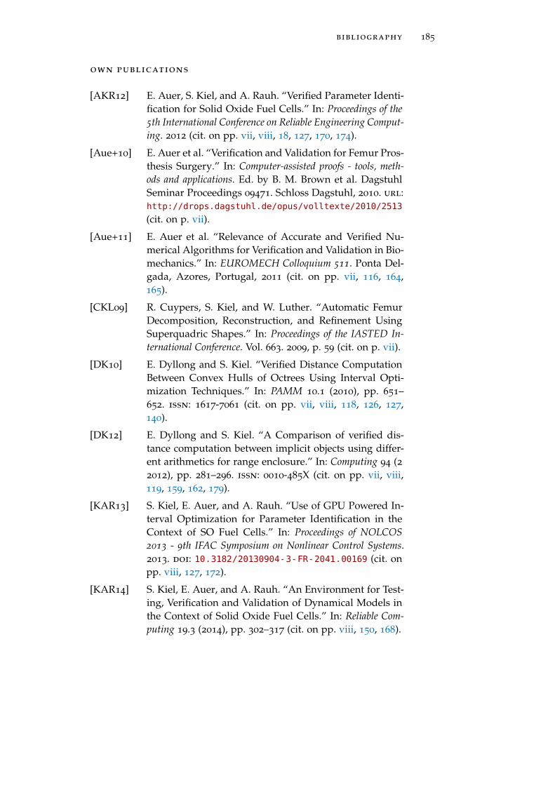
bibliography 185
own publications
[AKR12] E. Auer, S. Kiel, and A. Rauh. “Verified Parameter Identi-fication for Solid Oxide Fuel Cells.” In: Proceedings of the5th International Conference on Reliable Engineering Comput-ing. 2012 (cit. on pp. vii, viii, 18, 127, 170, 174).
[Aue+10] E. Auer et al. “Verification and Validation for Femur Pros-thesis Surgery.” In: Computer-assisted proofs - tools, meth-ods and applications. Ed. by B. M. Brown et al. DagstuhlSeminar Proceedings 09471. Schloss Dagstuhl, 2010. url:http://drops.dagstuhl.de/opus/volltexte/2010/2513
(cit. on p. vii).
[Aue+11] E. Auer et al. “Relevance of Accurate and Verified Nu-merical Algorithms for Verification and Validation in Bio-mechanics.” In: EUROMECH Colloquium 511. Ponta Del-gada, Azores, Portugal, 2011 (cit. on pp. vii, 116, 164,165).
[CKL09] R. Cuypers, S. Kiel, and W. Luther. “Automatic FemurDecomposition, Reconstruction, and Refinement UsingSuperquadric Shapes.” In: Proceedings of the IASTED In-ternational Conference. Vol. 663. 2009, p. 59 (cit. on p. vii).
[DK10] E. Dyllong and S. Kiel. “Verified Distance ComputationBetween Convex Hulls of Octrees Using Interval Opti-mization Techniques.” In: PAMM 10.1 (2010), pp. 651–652. issn: 1617-7061 (cit. on pp. vii, viii, 118, 126, 127,140).
[DK12] E. Dyllong and S. Kiel. “A Comparison of verified dis-tance computation between implicit objects using differ-ent arithmetics for range enclosure.” In: Computing 94 (22012), pp. 281–296. issn: 0010-485X (cit. on pp. vii, viii,119, 159, 162, 179).
[KAR13] S. Kiel, E. Auer, and A. Rauh. “Use of GPU Powered In-terval Optimization for Parameter Identification in theContext of SO Fuel Cells.” In: Proceedings of NOLCOS2013 - 9th IFAC Symposium on Nonlinear Control Systems.2013. doi: 10.3182/20130904-3-FR-2041.00169 (cit. onpp. viii, 127, 172).
[KAR14] S. Kiel, E. Auer, and A. Rauh. “An Environment for Test-ing, Verification and Validation of Dynamical Models inthe Context of Solid Oxide Fuel Cells.” In: Reliable Com-puting 19.3 (2014), pp. 302–317 (cit. on pp. viii, 150, 168).
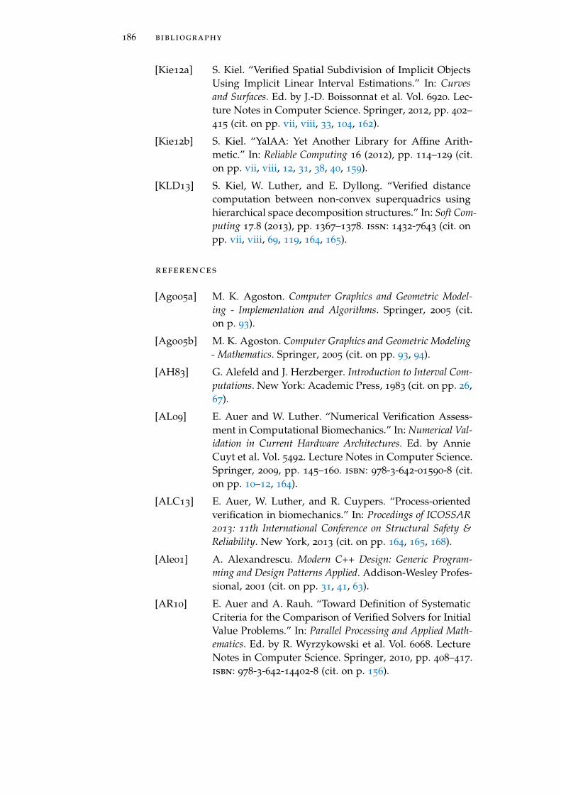
186 bibliography
[Kie12a] S. Kiel. “Verified Spatial Subdivision of Implicit ObjectsUsing Implicit Linear Interval Estimations.” In: Curvesand Surfaces. Ed. by J.-D. Boissonnat et al. Vol. 6920. Lec-ture Notes in Computer Science. Springer, 2012, pp. 402–415 (cit. on pp. vii, viii, 33, 104, 162).
[Kie12b] S. Kiel. “YalAA: Yet Another Library for Affine Arith-metic.” In: Reliable Computing 16 (2012), pp. 114–129 (cit.on pp. vii, viii, 12, 31, 38, 40, 159).
[KLD13] S. Kiel, W. Luther, and E. Dyllong. “Verified distancecomputation between non-convex superquadrics usinghierarchical space decomposition structures.” In: Soft Com-puting 17.8 (2013), pp. 1367–1378. issn: 1432-7643 (cit. onpp. vii, viii, 69, 119, 164, 165).
references
[Ago05a] M. K. Agoston. Computer Graphics and Geometric Model-ing - Implementation and Algorithms. Springer, 2005 (cit.on p. 93).
[Ago05b] M. K. Agoston. Computer Graphics and Geometric Modeling- Mathematics. Springer, 2005 (cit. on pp. 93, 94).
[AH83] G. Alefeld and J. Herzberger. Introduction to Interval Com-putations. New York: Academic Press, 1983 (cit. on pp. 26,67).
[AL09] E. Auer and W. Luther. “Numerical Verification Assess-ment in Computational Biomechanics.” In: Numerical Val-idation in Current Hardware Architectures. Ed. by AnnieCuyt et al. Vol. 5492. Lecture Notes in Computer Science.Springer, 2009, pp. 145–160. isbn: 978-3-642-01590-8 (cit.on pp. 10–12, 164).
[ALC13] E. Auer, W. Luther, and R. Cuypers. “Process-orientedverification in biomechanics.” In: Procedings of ICOSSAR2013: 11th International Conference on Structural Safety &Reliability. New York, 2013 (cit. on pp. 164, 165, 168).
[Ale01] A. Alexandrescu. Modern C++ Design: Generic Program-ming and Design Patterns Applied. Addison-Wesley Profes-sional, 2001 (cit. on pp. 31, 41, 63).
[AR10] E. Auer and A. Rauh. “Toward Definition of SystematicCriteria for the Comparison of Verified Solvers for InitialValue Problems.” In: Parallel Processing and Applied Math-ematics. Ed. by R. Wyrzykowski et al. Vol. 6068. LectureNotes in Computer Science. Springer, 2010, pp. 408–417.isbn: 978-3-642-14402-8 (cit. on p. 156).

References 187
[AR12] E. Auer and A. Rauh. “VERICOMP: a system to compareand assess verified IVP solvers.” English. In: Computing94 (2-4 2012), pp. 163–172. issn: 0010-485X (cit. on pp. 5,144, 145, 156).
[Bar81] A. H. Barr. “Superquadrics and Angle-Preserving Trans-formations.” In: Computer Graphics and Applications, IEEE1.1 (1981), pp. 11 –23. issn: 0272-1716 (cit. on pp. 18, 66,116, 164).
[BBH89] P. Brown, G. Byrne, and A. Hindmarsh. “VODE: A Vari-able-Coefficient ODE Solver.” In: SIAM Journal on Scien-tific and Statistical Computing 10.5 (1989), pp. 1038–1051
(cit. on pp. 86, 150).
[BDL04] K. Bühler, E. Dyllong, and W. Luther. “Reliable Distanceand Intersection Computation Using Finite Precision Ge-ometry.” In: Numerical Software with Result Verification. Ed.by R. Alt et al. Vol. 2991. Lecture Notes in Computer Sci-ence. Springer, 2004, pp. 579–600. isbn: 978-3-540-21260-7(cit. on pp. 118–120, 159).
[Bee+04] T. Beelitz et al. SONIC — A Framework for the RigorousSolution of Nonlinear Problems. Tech. rep. Online accessedon 03.06.2013 http://www-ai.math.uni-wuppertal.de/
SciComp/preprints/SC0407.ps.gz. Bergische Univer-sität Wuppertal, 2004 (cit. on p. 142).
[Bee06] T. Beelitz. “Effiziente Methoden zum Verifizierten Lösenvon Optimierungsaufgaben und Nichtlinearen Gleichun-gssystemen.” PhD thesis. Bergische Universität Wupper-tal, 2006 (cit. on pp. 72, 112, 117, 127–129, 131, 139, 143).
[Ben+99] F. Benhamou et al. “Revising hull and box consistency.”In: Logic Programming - Proceedings of the 1999 Interna-tional Conference on Logic Programming. Ed. by D. de Schr-eye. Massachusetts Institute of Technology, 1999, pp. 230
–245 (cit. on pp. 64, 82).
[Ben96] F. Benhamou. “Heterogeneous constraint solving.” In: Al-gebraic and Logic Programming. Ed. by M. Hanus and M.Rodríguez-Artalejo. Vol. 1139. Lecture Notes in ComputerScience. Springer, 1996, pp. 62–76. isbn: 978-3-540-61735-8 (cit. on pp. 70, 90).
[Ber04] G. van den Bergen. Collision Detection in Interactive 3D En-vironments. Morgan Kaufmann Publishers, 2004 (cit. onp. 116).
[Ber95a] S. Berner. Ein paralleles Verfahren zur verifizierten globalenOptimierung. Shaker, 1995 (cit. on pp. 110, 111, 128, 139).

188 bibliography
[Ber95b] M. Berz. “Modern Map Methods for Charged ParticleOptics.” In: Nuclear Instruments and Methods A363 (1995),pp. 100–104 (cit. on pp. 1, 44).
[BG06] F. Benhamou and L. Granvilliers. “Chapter 16 - Continu-ous and Interval Constraints.” In: Handbook of ConstraintProgramming. Ed. by F. Rossi, P. van Beek, and T. Walsh.Vol. 2. Foundations of Artificial Intelligence. Elsevier, 2006,pp. 571 –603 (cit. on p. 74).
[BHK03] M. Bräuer, W. Hofschuster, and W. Krämer. Steigungsarith-metiken in C-XSC. Tech. rep. Online accessed on 17.8.2012
http://www2.math.uni-wuppertal.de/~xsc/preprints/
prep _ 01 _ 3 . pdf. Bergische Unversität GH Wuppertal,2003 (cit. on p. 68).
[Bil08] G. Bilotta. “Self-verified extension of affine arithmetic toarbitrary order.” In: Le Matematiche 63.1 (2008), pp. 15–30
(cit. on p. 35).
[BJ05] B. Bastl and F. Jezek. “Comparison of Implicitization Me-thods.” In: Journal for Geometry and Graphics 9.1 (2005),pp. 11–29 (cit. on p. 95).
[BL70] G. Birkhoff and J. D. Lipson. “Heterogeneous algebras.”In: Journal of Combinatorial Theory 8.1 (1970), pp. 115 –133.issn: 0021-9800 (cit. on p. 48).
[BM06] M. Berz and K. Makino. COSY INFINITY 9.0. Tech. rep.MSUHEP 060803. Michigan State University, 2006 (cit. onpp. 46, 164).
[BMP06] H. Bronnimann, G. Melquiond, and S. Pion. “The designof the Boost interval arithmetic library.” In: Theoreticalcomputer science 351.1 (2006), pp. 111–118 (cit. on p. 31).
[BN13] P.-D. Beck and M. Nehmeier. “Parallel Interval NewtonMethod on CUDA.” In: Applied Parallel and Scientific Com-puting. Ed. by Pekka Manninen and Per Öster. Vol. 7782.Lecture Notes in Computer Science. Springer, 2013, pp. 454–464. isbn: 978-3-642-36802-8 (cit. on pp. 60, 129).
[BN90] P. Brunet and I. Navazo. “Solid representation and op-eration using extended octrees.” In: ACM Transactions onGraphics (TOG) 9.2 (1990), pp. 170–197 (cit. on p. 184).
[Boo] Boost C++ Libraries. Online accessed on 19.06.2012 http:
//www.boost.org (cit. on p. 31).
[Bus+96] F. Buschmann et al. Pattern-Oriented Software Architecture- A System of Patterns. Wiley, 1996 (cit. on pp. 14, 15).
References 189
[BV09] S. Boyd and L. Vandenberghe. Convex Optimization. On-line accessed on 15.05.2013 http://www.stanford.edu/
~boyd/cvxbook/bv_cvxbook.pdf. Cambridge UniversityPress, 2009 (cit. on pp. 98, 117, 132).
[Büh02] K. Bühler. “Implicit linear interval estimations.” In: Pro-ceedings of the 18th spring conference on Computer graphics.ACM. 2002, p. 132 (cit. on pp. 74–76).
[C11a] C Programing Language – ISO/IEC 9899:2011. Geneva, Swi-tzerland, 2011 (cit. on p. 40).
[C11b] Information technology – Programming languages – C++ ISO/-IEC 14882:2011. Geneva, Switzerland, 2011 (cit. on pp. 79,86, 87).
[CE00] K. Czarneski and U. W. Eisenecker. Generative Program-ming - Methods, Tools, and Applications. Addison-Wesley,2000 (cit. on pp. 14, 41, 54).
[Cha] G. Chabert. IBEX Homepage. Online accessed on 07.2.2013
http://www.emn.fr/z-info/ibex/ (cit. on pp. 5, 63, 91).
[Cha+08] N. Chakraborty et al. “Proximity Queries Between Con-vex Objects: An Interior Point Approach for Implicit Sur-faces.” In: IEEE Transactions on Robotics 24.1 (2008), pp. 211–220 (cit. on p. 116).
[Che11] C.-Y. Chen. “Extended interval Newton method basedon the precise quotient set.” In: Computing 92 (4 2011),pp. 297–315. issn: 0010-485X (cit. on p. 71).
[Chu11] A. Chuev. “Akkurate Abstandsberechungen zwischen 3DObjekten dargestellt als Superquadriken.” MA thesis. Uni-versität Duisburg-Essen, 2011 (cit. on pp. 116, 164, 165).
[CJ09] G. Chabert and L. Jaulin. “Contractor programming.” In:Artificial Intelligence 173.11 (2009), pp. 1079 –1100. issn:0004-3702 (cit. on pp. 5, 63, 91, 127, 128).
[CJP08] B. Chapman, G. Jost, and R. Van der Pas. Using OpenMP:portable shared memory parallel programming. MIT press,2008 (cit. on pp. 139, 140).
[CKR00] T. Csendes, R. Klatte, and D. Ratz. “A Posteriori Direc-tion Selection Rules for Interval Optimization Methods.”In: CEJOR 8 (2000), pp. 225–236 (cit. on p. 112).
[Cli] M. Cline. C++ FAQ 25.10 – What does it mean to "delegateto a sister class" via virtual inheritance? Online accessedon 29.05.2014 http://www.parashift.com/c++- faq-
lite/mi-delegate-to-sister.html (cit. on p. 87).

190 bibliography
[CS90] J.L.D. Comba and J. Stolfi. “Affine arithmetic and its ap-plications to computer graphics.” In: Proceedings of VISIBGRAPI (Brazilian Symposium on Computer Graphics andImage Processing). Citeseer. 1990, pp. 9–18 (cit. on pp. 1,33, 34).
[Cse01] T. Csendes. “New Subinterval Selection Criteria for In-terval Global Optimization.” In: Journal of Global Opti-mization 19.3 (2001), pp. 307–327. issn: 0925-5001 (cit. onpp. 111, 122).
[Cud] NVIDIA CUDA C Programming Guide. 4.2. NVIDIA. 2012
(cit. on p. 89).
[Cuy11] R. Cuypers. Geometrische Modellierung mit Superquadrikenzur Optimierung skelettaler Diagnosesysteme. Logos, 2011
(cit. on pp. 18, 116, 153, 164, 168).
[DFS11] F. Domes, M. Fuchs, and H. Schichl. The Optimization TestEnvironment. Online accessed on 06.08.2013 http://www.
mat.univie.ac.at/~dferi/testenv.html. 2011 (cit. onpp. 6, 145).
[DG07a] E. Dyllong and C. Grimm. “A Modified Reliable DistanceAlgorithm for Octree-encoded Objects.” In: PAMM 7.1(2007), pp. 4010015–4010016 (cit. on p. 118).
[DG07b] E. Dyllong and C. Grimm. “An Efficient Distance Al-gorithm for Interval-Based Octree-Encoded CSG Objectswith Time-Space Coherence Utilization.” In: PAMM 7.1(2007), pp. 1023007–1023008 (cit. on p. 118).
[DG07c] E. Dyllong and C. Grimm. “Proximity Queries betweenInterval-Based CSG Octrees.” In: AIP Conference Proceed-ings 936.1 (2007). Ed. by Theodore E. Simos, George Psi-hoyios, and Ch. Tsitouras, pp. 162–165 (cit. on pp. 2, 127).
[DG07d] E. Dyllong and C. Grimm. “Verified Adaptive OctreeRepresentations of Constructive Solid Geometry Objects.”In: Simulation und Visualisierung. Citeseer. 2007, pp. 223–235 (cit. on pp. 99, 100, 102, 113, 114, 127).
[DG08] E. Dyllong and C. Grimm. “A Reliable Extended OctreeRepresentation of CSG Objects with an Adaptive Subdi-vision Depth.” In: Parallel Processing and Applied Mathe-matics. Ed. by R. Wyrzykowski et al. Vol. 4967. LectureNotes in Computer Science. Springer, 2008, pp. 1341–1350 (cit. on pp. 99, 100, 102, 113).
[DK94] K. Du and R. B. Kearfott. “The cluster problem in mul-tivariate global optimization.” In: Journal of Global Opti-mization 5 (3 1994), pp. 253–265. issn: 0925-5001 (cit. onpp. 18, 124).
References 191
[DL04a] E. Dyllong and W. Luther. “An Accurate Distance Algo-rithm for Octree-Encoded Objects.” In: PAMM 4.1 (2004),pp. 562–563. issn: 1617-7061 (cit. on p. 118).
[DL04b] E. Dyllong and W. Luther. “The GJK distance algorithm:an interval version for incremental motions.” In: Numer-ical Algorithms 37.1 (2004), pp. 127–136. issn: 1017-1398
(cit. on p. 116).
[DM98] L. Dagum and R. Menon. “OpenMP: an industry stan-dard API for shared-memory programming.” In: Compu-tational Science Engineering, IEEE 5.1 (1998), pp. 46 –55.issn: 1070-9924. doi: 10.1109/99.660313 (cit. on p. 128).
[Dom09] F. Domes. “GloptLab - A configurable framework for therigorous global solution of quadratic constraint satisfac-tion problems.” In: Optimization Methods and Software (4-52009), pp. 727 –747 (cit. on p. 5).
[dS97] L. H. de Figueiredo and J. Stolfi. Self-Validated NumericalMethods and Applications. Rio de Janeiro: IMPA, 1997 (cit.on pp. 33–37, 40, 41, 44, 46).
[Duf92] T. Duff. “Interval arithmetic recursive subdivision for im-plicit functions and constructive solid geometry.” In: Pro-ceedings of the 19th annual conference on Computer graphicsand interactive techniques. SIGGRAPH ’92. New York, NY,USA: ACM, 1992, pp. 131–138. isbn: 0-89791-479-1 (cit.on pp. 96, 127).
[Dze12] T. Dzetkulic. Rigorous Computation with Function Enclo-sures in Chebyshev Basis. 2012 (cit. on p. 56).
[Dö+13] T. Dötschel et al. “Thermal behavior of high-temperaturefuel cells: reliable parameter identification and interval-based sliding mode control.” In: Soft Computing (2013),pp. 1–15. issn: 1432-7643 (cit. on pp. 168, 169, 171, 175).
[Ebl06] I. Eble. “Über Taylormodelle.” PhD thesis. UniversitätKarlsruhe, 2006 (cit. on pp. 44, 46, 159, 164).
[Ede95] H. Edelsbrunner. “Algebraic decomposition of non-con-vex polyhedra.” In: Proceedings. 36th Annual Symposiumon Foundations of Computer Science. 1995, pp. 248–257 (cit.on pp. 94, 95).
[FL05] A. Frommer and B. Lang. “Existence Tests for Solutionsof Nonlinear Equations Using Borsuk’s Theorem.” In:SIAM Journal on Numerical Analysis 43.3 (2005), pp. 1348–1361 (cit. on p. 69).
[FLS04] A. Frommer, B. Lang, and M. Schnurr. “A Comparison ofthe Moore and Miranda Existence Tests.” In: Computing72.3-4 (2004), pp. 349–354. issn: 0010-485X (cit. on p. 69).

192 bibliography
[FPC10] O. Fryazinov, A. Pasko, and P. Comninos. “Fast reliableinterrogation of procedurally defined implicit surfacesusing extended revised affine arithmetic.” In: Computers& Graphics 34.6 (2010), pp. 708 –718. issn: 0097-8493 (cit.on pp. 60, 96).
[Gam+95] E. Gamma et al. Design Patterns Elements of Reusable Object-Oriented Software. Addison-Wesley, 1995 (cit. on pp. 14,16, 54, 82, 144).
[GCH] O. Gay, D. Coeurjolly, and N.J. Hurst. libaffa. Online ac-cessed on 15.11.2010 http://www.nongnu.org/libaffa/
(cit. on pp. 37, 40).
[GJK88] E. G. Gilbert, D. W. Johnson, and S. S. Keerthi. “A fastprocedure for computing the distance between complexobjects in three-dimensional space.” In: IEEE Journal ofRobotics and Automation 4.2 (Apr. 1988), pp. 193 –203. issn:0882-4967 (cit. on p. 116).
[GK] J. Guzman and H. Kaiser. Boost.Spirit Homepage. Onlineaccessed on 28.02.2013 http://http://boost-spirit.
com/ (cit. on p. 87).
[GL] P. Gottschling and A. Lumsdaine. The Matrix Template Li-brary 4. Online accessed on 18.06.2012 http://www.osl.
iu.edu/research/mtl/mtl4/ (cit. on pp. 58, 89, 144).
[Gra] GraphML Specification. Online accessed on 10.06.2013 http:
/ / graphml . graphdrawing . org / specification . html.2003 (cit. on p. 155).
[Gri00] A Griewank. Evaluating Derivatives - Principles and Tech-niques of Algorithmic Differentiation. SIAM, 2000 (cit. onpp. 64, 65).
[Gri08] C. Grimm. “Result Verification of RRT-based Single-Que-ry Path Planning through Interval Analysis.” In: PAMM8.1 (2008), pp. 10971–10972. issn: 1617-7061 (cit. on p. 152).
[Gö13] D. Göttner. “Entwurf und Implementierung einer GPU-basierten Bibliothek für eine erweiterte Intervallarithmetikzur Visualisierung impliziter Objekte mit realistischenBeleuchtungsmodellen.” Ongoing. MA thesis. UniversitätDuisburg-Essen, 2013 (cit. on p. 60).
[Ham+95] R. Hammer et al. C++ Toolbox for Verified Computing. Spri-ngerVerlag, 1995 (cit. on pp. 71, 73).
[Ham+97] R. Hammer et al. C++ Toolbox for Verified Scientific Com-puting I: Basic Numerical Problems. Secaucus, NJ, USA:Springer, 1997. isbn: 3540591109 (cit. on p. 125).

References 193
[Han] Institute of Microelectronic Systems in Hannover. aaflib.Online accessed on http://sourceforge.net/projects/
aaflib/ (cit. on p. 40).
[Han75] E. Hansen. “A generalized interval arithmetic.” In: In-terval Mathematics. Ed. by Karl Nickel. Vol. 29. LectureNotes in Computer Science. Springer, 1975, pp. 7–18 (cit.on p. 1).
[Hay10] N. T. Hayes. Trits to Tretris. P1788, Motion 18. 2010 (cit. onp. 31).
[Hij+10] Y. Hijazi et al. “CSG Operations of Arbitrary Primitiveswith Interval Arithmetic and Real-Time Ray Casting.” In:Scientific Visualization: Advanced Concepts. Ed. by H. Ha-gen. Vol. 1. Schloss Dagstuhl–Leibniz-Zentrum für Infor-matik, 2010, pp. 78–89. isbn: 978-3-939897-19-4 (cit. onp. 60).
[HK04] W. Hofschuster and W. Krämer. “C-XSC 2.0 – A C++Library for Extended Scientific Computing.” In: Numer-ical Software with Result Verification. Ed. by R. Alt et al.Vol. 2991. Lecture Notes in Computer Science. Springer,2004, pp. 259–276 (cit. on pp. 28, 31, 159, 167).
[HNW13] O. Heimlich, M. Nehmeier, and J. Wolff von Gudenberg.“Variants of the general interval power function.” In: SoftComputing 17.8 (2013), pp. 1357–1366. issn: 1432-7643 (cit.on pp. 29, 184).
[HS08] M. Herlihy and N. Shavit. The Art of Multiprocessor Pro-gramming. Elsevier, 2008 (cit. on p. 81).
[HW04] E. Hansen and G. W. Walster. Global Optimization UsingInterval Analysis. New York: Marcel Dekker, 2004 (cit. onpp. 2, 4, 67–70, 72–75, 105, 112, 117, 118, 126–128, 131–133, 135, 136, 151).
[Hwu11] “GPU Computing Gems Jade Edition.” In: ed. by W. W.Hwu. Morgan Kaufmann, 2011. Chap. Interval Arithmeticin CUDA (cit. on p. 60).
[Iee] IEEE Standard for Floating-Point Arithmetic - IEEE Std 754-2008 (Revision of IEEE Std 754-1985). 2008 (cit. on p. 24).
[IF79] K. Ichida and Y. Fujii. “An interval arithmetic method forglobal optimization.” In: Computing 23.1 (1979), pp. 85–97. issn: 0010-485X (cit. on pp. 127, 131).
[Isoa] Information technology - Open Systems Interconnection - Ba-sic Reference Model: The Basic Model ISO/IEC 7498-1:1994(E).Geneva, Switzerland, 1996 (cit. on p. 15).
[Isob] Information technology - Vocabulary ISO/IEC 2382-1:1993.Geneva, Switzerland, 1993 (cit. on p. 13).

194 bibliography
[Jau+01] L. Jaulin et al. Applied Interval Analysis. Springer, 2001
(cit. on pp. 28, 68, 69, 99, 102, 103, 113).
[Jau01] L. Jaulin. “Path Planning Using Intervals and Graphs.”In: Reliable Computing 7.1 (2001), pp. 1–15 (cit. on pp. 2,152, 184).
[JLS00] A. Jaklic, A. Leonardis, and F. Solina. Segmentation andrecovery of superquadrics. Vol. 20. Springer, 2000 (cit. onpp. 96, 116, 165).
[Jol11] M. Joldes. “Approximations polynomiales rigoureuses etapplications.” Online accessed on 12.12.2012, http : / /
perso.ens-lyon.fr/mioara.joldes/these/theseJoldes.
pdf. PhD thesis. École Normale Supérieure de Lyon, 2011
(cit. on p. 56).
[KA00] R. B. Kearfott and A. Arazyan. “Taylor Series Models inDeterministic Global Optimization.” In: Proceedings of Au-tomatic Differentiation 2000: From Simulation to Optimiza-tion. 2000 (cit. on p. 143).
[Kah05] J. H. T. Kahou. “Some new Acceleration Mechanismsin Verified Global Optimization.” PhD thesis. BergischeUniversität Wuppertal, 2005 (cit. on pp. 111, 124, 131).
[Kea+02] R. B. Kearfott et al. Standardized notation in interval anal-ysis. Online accessed on 06.11.2012 http://radon.mat.
univie.ac.at/~neum/ms/notation.pdf. 2002 (cit. onp. xviii).
[Kea+04] R. B. Kearfott et al. “Libraries, Tools, and Interactive Sys-tems for Verified Computations: Four Case Studies.” In:Numerical Software with Result Verification. Ed. by R. Altet al. Vol. 2991. LNCS. Springer, 2004, pp. 36–63 (cit. onp. 145).
[Kea03] R. B. Kearfott. “GlobSol: History, Composition, and Ad-vice on Use.” In: Global Optimization and Constraint Sat-isfaction. Ed. by C. Bliek, C. Jermann, and A. Neumaier.Vol. 2861. Lecture Notes in Computer Science. Springer,2003, pp. 17–31. isbn: 978-3-540-20463-3 (cit. on pp. 127,142, 152, 184).
[Kea96] R. B. Kearfott. Rigorous Global Search: Continuous Problems.Kluwer Academic Publishers, 1996 (cit. on pp. xvii, 73,107, 112, 117, 129–131).
[Kie+11] M. Kieffer et al. “Verified Global Optimization for Esti-mating the Parameters of Nonlinear Models.” In: ed. byA. Rauh and E. Auer. Springer, 2011 (cit. on pp. 98, 170,171, 178).
References 195
[KK13] G. Kozikowski and B. J. Kubica. “Interval Arithmetic andAutomatic Differentiation on GPU Using OpenCL.” In:Applied Parallel and Scientific Computing. Ed. by P. Man-ninen and P. Öster. Vol. 7782. Lecture Notes in Com-puter Science. Springer, 2013, pp. 489–503. isbn: 978-3-642-36802-8 (cit. on pp. 129, 175).
[Kno+09] A. Knoll et al. “Fast Ray Tracing of Arbitrary Implicit Sur-faces with Interval and Affine Arithmetic.” In: ComputerGraphics Forum 28.1 (2009), pp. 26–40. issn: 1467-8659 (cit.on pp. 33, 60, 157, 183).
[Knu84] D. E. Knuth. “Literate Programming.” In: The ComputerJournal 27.2 (1984), pp. 97–111 (cit. on p. 149).
[Knu97] D. E. Knuth. The Art of Computer Programming - Funda-mental Algorithms. Vol. 1. Addison Wesly, 1997 (cit. onp. 100).
[Knü94] O. Knüppel. “PROFIL/BIAS—a fast interval library.” In:Computing 53.3 (1994), pp. 277–287 (cit. on pp. 31, 146).
[Koc+09] S. Kockara et al. “Contact Detection Algorithms.” In: Jour-nal of Computers 4.10 (2009), p. 1053. issn: 1796-203X (cit.on p. 116).
[Kol07] V. L. Kolev. “Optimal Multiplication of G-intervals.” In:Reliable Computing 13 (5 2007), pp. 399–408. issn: 1385-3139 (cit. on p. 35).
[KR77] B.W. Kernighan and D.M. Ritchie. The M4 macro processor.Tech. rep. 1977 (cit. on p. 55).
[Kul09] U. Kulisch. Arithmetic operations for floating-point intervals.Motion 05.2 of IEEE P1788, Online accessed on 28.11.2012
http://grouper.ieee.org/groups/1788/PositionPapers/
ArithOp2.pdf. 2009 (cit. on p. 71).
[KW02] R. B. Kearfott and G. W. Walster. “Symbolic Precondi-tioning with Taylor Models: Some Examples.” In: ReliableComputing 8.6 (2002), pp. 453–468. issn: 1385-3139 (cit. onp. 143).
[LaV06] M. S. LaValle. Planning Algorithms. Online accessed on06.06.2013 http://planning.cs.uiuc.edu/bookbig.pdf.Cambridge University Press, 2006 (cit. on p. 152).
[Ler+06] M. Lerch et al. “FILIB++, a fast interval library support-ing containment computations.” In: ACM Transactions onMathematical Software (TOMS) 32.2 (2006), pp. 299–324
(cit. on pp. 28, 31).
[LG98] M. Lin and S. Gottschalk. “Collision Detection betweenGeometric Models: A Survey.” In: Proceedings of IMA Con-ference on Mathematics of Surfaces. 1998 (cit. on p. 116).
196 bibliography
[LHB02] A. Lemke, L. Hedrich, and E. Barke. “Analog circuit siz-ing based on formal methods using affine arithmetic.” In:Proceedings of the 2002 IEEE/ACM international conferenceon Computer-aided design. ACM. 2002, pp. 486–489 (cit. onp. 33).
[Lip96] S. B. Lippman. Inside the C++ Object Model. Addison Wes-ley, 1996 (cit. on p. 54).
[Loh01] R. J. Lohner. “On the Ubiquity of the Wrapping Effectin the Computation of Error Bounds.” In: Perspectives onEnclosure Methods. Ed. by U. Kulisch, R. Lohner, and A.Facius. Springer, 2001, pp. 201–217 (cit. on pp. 32, 33).
[LS02] C. Lennerz and E. Schomer. “Efficient distance compu-tation for quadratic curves and surfaces.” In: GeometricModeling and Processing, 2002. Proceedings. 2002, pp. 60 –69 (cit. on p. 116).
[Mak98] K. Makino. “Rigorous Analysis of Nonlinear Motion inParticle Accelerators.” PhD thesis. Michigan State Uni-versity, 1998 (cit. on p. 45).
[Mar+06] M. C. Markót et al. “New interval methods for constrain-ed global optimization.” In: Mathematical Programming106.2 (2006), pp. 287–318. issn: 0025-5610 (cit. on p. 111).
[MB03] K. Makino and M. Berz. “Taylor models and other vali-dated functional inclusion methods.” In: International Jour-nal of Pure and Applied Mathematics 4.4 (2003), pp. 379–456
(cit. on p. 44).
[MB05a] K. Makino and M. Berz. “Verified Global Optimizationwith Taylor Model based Range Bounders.” In: Transac-tions on Computers 4.11 (2005) (cit. on p. 128).
[MB05b] K. Makino and M. Berz. “Verified global optimizationwith Taylor model-based range bounders.” In: Transac-tions on Computers 11.1 (2005), pp. 1611–1618 (cit. on p. 46).
[MCC00a] M. S. Markót, T. Csendes, and A. E. Csallner. “Multisec-tion in Interval Branch-and-Bound Methods for GlobalOptimization II. Numerical Tests.” In: Journal of GlobalOptimization 16.3 (2000), pp. 219–228. issn: 0925-5001 (cit.on p. 112).
[MCC00b] M. S. Markót, T. Csendes, and A. E. Csallner. “Multisec-tion in Interval Branch-and-Bound Methods for GlobalOptimization – I. Theoretical Results.” In: Journal of GlobalOptimization 16.4 (2000), pp. 371–392. issn: 0925-5001 (cit.on p. 112).

References 197
[Mes02] F. Messine. “Extentions of Affine Arithmetic: Applica-tion to Unconstrained Global Optimization.” In: Journalof Universal Computer Science 8.11 (2002), pp. 992–1015 (cit.on pp. 33, 35).
[MH03] J. C. Mason and D. C. Handscomb. Chebyshev Polynomials.CRC Press, 2003 (cit. on pp. 36, 38).
[Mir98] B. Mirtich. “V-Clip: Fast and robust polyhedral collisiondetection.” In: ACM Trans. Graph. 17 (3 1998), pp. 177–208. issn: 0730-0301 (cit. on p. 116).
[MKC09] R. E. Moore, R. B. Kearfott, and M. J. Cloud. Introductionto Interval Analysis. SIAM, 2009 (cit. on p. 72).
[Moo66] R. E. Moore. Interval Analysis. Prentice-Hall, 1966 (cit. onpp. 1, 25).
[Moo77] R. Moore. “A Test for Existence of Solutions to Nonlin-ear Systems.” In: SIAM Journal on Numerical Analysis 14.4(1977), pp. 611–615 (cit. on p. 69).
[Mpi] MPI: A Message-Passing Interface Standard Version 3.0. 2012
(cit. on p. 129).
[MT06] F. Messine and A. Touhami. “A General Reliable Quadra-tic Form: An Extension of Affine Arithmetic.” In: ReliableComputing 12 (3 2006), pp. 171–192. issn: 1385-3139 (cit.on pp. 33, 35).
[Mul+10] J.-M. Muller et al. Handbook of Floating-Point Arithmetic.Birkhäuser, 2010 (cit. on pp. 24, 25).
[Mul06] J.-M. Muller. Elementary Functions Algorithms and Imple-mentations. Second edition. Birkhäser, 2006 (cit. on p. 36).
[Mye95] N. C. Myers. “Traits: a new and useful template tech-nique.” In: C++ Report (1995). http://www.cantrip.org/traits.html Last access on 19.06.2012 (cit. on p. 41).
[Nau12] U. Naumann. The Art of Differentiating Computer Programs:An Introduction to Algorithmic Differentiation. SIAM, 2012
(cit. on p. 64).
[Ned06] N.S. Nedialkov. VNODE-LP A Validated Solver for InitialValue Problems in Ordinary Differential Equations. Tech. rep.CAS-06-06-NN. McMaster University, 2006 (cit. on pp. 7,21, 86, 91, 97, 149, 170).
[Neu03] A. Neumaier. “Taylor forms use and limits.” In: ReliableComputing 9.1 (2003), pp. 43–79 (cit. on pp. 2, 33, 44).
[Neu04] A. Neumaier. “Complete search in continuous global op-timization and constraint satisfaction.” In: Acta Numer-ica 13 (Apr. 2004), pp. 271–369. issn: 1474-0508 (cit. onp. 184).

198 bibliography
[Neu90] A. Neumaier. Interval methods for systems of equations. Cam-bridge University Press, 1990 (cit. on pp. 1, 67–69, 73).
[Neu93] A. Neumaier. “The wrapping effect, ellipsoid arithmetic,stability and confidence regions.” In: Computing (Suppl.)9 (1993), pp. 175–190 (cit. on p. 1).
[NM11] J. Ninin and F. Messine. Reliable Affine Arithmetic. Inter-national Symposium on Scientific Computing, ComputerArithmetic, and Validated Numerics (SCAN 2010). 2011
(cit. on p. 35).
[NM65] J. A. Nelder and R. Mead. “A Simplex Method for Func-tion Minimization.” In: The Computer Journal 7.4 (1965),pp. 308–313 (cit. on p. 170).
[NMH10] J. Ninin, F. Messine, and P. Hansen. A Reliable Affine Re-laxation Method for Global Optimization. Tech. rep. Onlineaccssed on 03.06.2013 ftp://ftp.irit.fr/IRIT/APO/RT-
APO-10-05.pdf. IRIT and Cahiers du GERAD, 2010 (cit.on pp. 33, 143, 152).
[NVI12] NVIDIA. NVIDIA CUDA C Programming Guide 4.2. 2012
(cit. on pp. 59, 60, 90, 172).
[NZ14] D. Y. Nadezhin and I. Zhilin S. “JInterval Library: Prin-ciples, Development, and Perspectives.” In: Reliable Com-puting 19.3 (2014), pp. 229–247 (cit. on p. 30).
[Off] Object File Format (cit. on p. 154).
[Ope] The OpenCL Specification - Version 1.2 - Rev. 15. 2011 (cit.on p. 59).
[P17] “P1788/D8.4: Draft Standard for Interval Arithmetic” (cit.on pp. 29–31, 49).
[Pro] PROREOP Website. http://www.uni-due.de/proreop/,Last accessed: 15.02.2013 (cit. on pp. 18, 164).
[PSD09] R. F. Portal, L. G. Sousa, and J. P. Dias. “Contact detec-tion of convex superquadrics using optimization tech-niques with graphical user interface.” In: Proceedings ofthe 7th EUROMECH Solid Mechanics Conference. 2009 (cit.on p. 116).
[Pus13] T. Pusch. “Umsetzung einer verifizierten Parameteriden-tifikation mit GUI Realisierung für Festoxidbrennstoffzel-len.” Ongoing. MA thesis. Universität Duisburg-Essen,2013 (cit. on pp. 21, 143, 168, 178, 184).
[RA11] A. Rauh and E. Auer. “Verified Simulation of ODEs andDAEs in ValEncIA-IVP.” In: Reliable Computing 5.4 (2011),pp. 370–381 (cit. on pp. 21, 86, 97, 145).
[Ral81] L. B. Rall, ed. Automatic Differentiation: Techniques and Ap-plications. Springer, 1981 (cit. on p. 64).

References 199
[Rat92] D. Ratz. “Automatische Ergebnisverifikation bei globalenOptimierungsproblemen.” Online accessed on 12.04.2013
http://digbib.ubka.uni- karlsruhe.de/volltexte/
41092. PhD thesis. Universität Karlsruhe (TH), 1992 (cit.on pp. 111, 112, 131).
[Rau+12] A. Rauh et al. “Interval Methods for Control-OrientedModeling of the Thermal Behavior of High-TemperatureFuel Cell Stacks.” In: In Proc. of SysID 2012. Accepted.2012 (cit. on pp. 170, 172–177).
[RC95] D. Ratz and T. Csendes. “On the selection of subdivi-sion directions in interval branch-and-bound methodsfor global optimization.” In: Journal of Global Optimization7.2 (1995), pp. 183–207 (cit. on pp. 111, 112).
[RMB05] N. Revol, K. Makino, and M. Berz. “Taylor models andfloating-point arithmetic: proof that arithmetic operationsare validated in COSY.” In: Journal of Logic and AlgebraicProgramming 64.1 (2005), pp. 135–154 (cit. on p. 46).
[Rot12] W. Rotzsche. “Mengentheoretische Operationen mit R-Funktionen auf CSG-Bäumen unter Nutzung von Inter-vallbibliotheken.” MA thesis. Universität Duisburg-Essen,2012 (cit. on p. 96).
[RR88] H. Ratschek and J. Rokne. New Computer Methods for Glob-al Optimization. Online version, access on 13.05.2013 http:
//pages.cpsc.ucalgary.ca/~rokne/global_book.pdf.Ellis Horwood Ltd, 1988 (cit. on p. 127).
[Rum10] S. M. Rump. “Verification methods: Rigorous results us-ing floating-point arithmetic.” In: Acta Numerica 19 (2010),pp. 287–449 (cit. on pp. 11, 25).
[Sam06] H Samet. Foundations of Multidimensional and Metric DataStructures. San Francisco: Morgan Kaufmann, 2006 (cit.on p. 99).
[Sam90] H. Samet. The Design and analysis of spatial data-structures.Addison-Wesly Publishling, 1990 (cit. on p. 99).
[SB] O. Stauning and C. Bendtsen. fadbad++ web page. Onlineaccessed on 18.01.2010 http://www.fadbad.com/ (cit. onpp. 88, 91, 146, 159).
[Sch04] H. Schichl. “Global Optimization in the COCONUT Pro-ject.” In: Numerical Software with Result Verification. Ed. byR. Alt et al. Vol. 2991. Lecture Notes in Computer Science.Springer, 2004, pp. 243–249. isbn: 978-3-540-21260-7 (cit.on pp. 142, 145).

200 bibliography
[Sch11] A. Schamberger. “Verifizierte Pfadplanung unter Verwen-dung einer einheitlichen Objektrepräsentation mit Visu-alisierung.” MA thesis. Universität Duisburg-Essen, 2011
(cit. on p. 152).
[SG75] L. Shampine and M. Gordon, eds. Computer Solution ofOrdinary Differential Equations: The Initial Value Problem.Freeman, 1975 (cit. on p. 150).
[Sha07] V. Shapiro. “Semi-analytic geometry with R-functions.”In: ACTA numerica 16 (2007) (cit. on pp. 96, 118).
[Sha91] V. Shapiro. Theory of R-functions and applications: A primer.1991 (cit. on pp. 17, 96, 118).
[Ske74] S. Skelboe. “Computation of rational interval functions.”In: BIT Numerical Mathematics 14.1 (1974), pp. 87–95. issn:0006-3835 (cit. on p. 127).
[SLL02] J. G. Siek, L. Lee, and A. Lumsdaine. The Boost GraphLibrary. User Guide and Reference Manual. Addison-WesleyLongman, 2002 (cit. on p. 155).
[Sny+93] J. M. Snyder et al. “Interval methods for multi-point colli-sions between time-dependent curved surfaces.” In: Pro-ceedings of the 20th annual conference on Computer graph-ics and interactive techniques. SIGGRAPH ’93. ACM, 1993,pp. 321–334. isbn: 0-89791-601-8 (cit. on p. 125).
[Sta95] V. Stahl. “Interval Methods for Bounding the Range ofPolynomials and Solving Systems of Nonlinear Equati-ons.” PhD thesis. Johannes Kepler Universität Linz, 1995
(cit. on p. 69).
[Sta97] O. Stauning. “Automatic Validation of Numerical Solu-tions.” PhD thesis. Technical University of Denmark, 1997
(cit. on pp. 58, 84).
[Sto] J. Stolfi. libaa. Online accessed on 08.06.2011 http://www.
ic.unicamp.br/~stolfi/ (cit. on pp. 23, 35, 37, 40).
[Swi] SWIG web page. Online accessed on 21.06.2013 http://
www.swig.org (cit. on p. 162).
[Ueb95] C. Ueberhuber. Computernumerik 2. Springer, 1995 (cit. onp. 70).
[UY07] A. Uteshev and M. Yashina. “Distance Computation froman Ellipsoid to a Linear or a Quadric Surface in Rn.” In:Computer Algebra in Scientific Computing. Ed. by V. Ganzha,E. Mayr, and E. Vorozhtsov. Vol. 4770. Lecture Notes inComputer Science. Springer, 2007, pp. 392–401 (cit. onp. 116).
[VH12] Kreinovich V. and N. Hayes. midprad. P1788 Motion 37.2012 (cit. on p. 30).
References 201
[VSHF09] X.-H. Vu, D. Sam-Haroud, and B. Faltings. “Enhancingnumerical constraint propagation using multiple inclu-sion representations.” In: Annals of Mathematics and Arti-ficial Intelligence 55 (3 2009), pp. 295–354. issn: 1012-2443
(cit. on pp. 5, 21, 23, 24, 47, 48, 61).
[WB06] A. Wächter and L. T. Biegler. “On the implementationof an interior-point filter line-search algorithm for large-scale nonlinear programming.” In: Math. Program. 106.1(2006), pp. 25–57. issn: 0025-5610 (cit. on pp. 7, 126, 150,168).
[WFF11] N. Whitehead and A. Fit-Florea. Precision & Performance:Floating Point and IEEE 754 Compliance for NVIDIA GPUs.Tech. rep. NVIDIA, 2011 (cit. on pp. 13, 60).
[Wie97] A. Wiethoff. “Verifizierte globale Optimierung auf Par-allelrechnern.” Online accessed on 15.05.2013 http://
digbib . ubka . uni - karlsruhe . de / volltexte / 118497.PhD thesis. Universität Karlsruhe, 1997 (cit. on p. 131).
[WK09] J. Wolff von Gudenberg and V. Kreinovich. ElementaryFunctions. IEEE P1788 – Motion 10.02. 2009 (cit. on p. 29).
[Yap97] C.-K. Yap. “Towards exact geometric computation.” In:Computational Geometry 7.1-2 (1997), pp. 3 –23. issn: 0925-7721 (cit. on p. 4).


colophon
This document was typeset using TEX and KOMA-Script. It usesthe typographical look-and-feel classicthesis developed by AndréMiede. The figures were created using TikZ and PGFPlots.