
Université de Liège - bictel.ulg.ac.be
295
Université de Liège Faculté des Sciences Appliquées Département de Chimie Appliquée Laboratoire d’Analyse et de Synthèse des Systèmes Chimiques Optimal synthesis of sensor networks Carine Gerkens Thèse présentée en vue de l’obtention du grade de Docteur en Sciences de l’Ingénieur Mai 2009
Transcript of Université de Liège - bictel.ulg.ac.be

Université de Liège
Faculté des Sciences Appliquées
Département de Chimie Appliquée
Laboratoire d’Analyse et deSynthèse des Systèmes Chimiques
Optimal synthesis of sensor networks
Carine Gerkens
Thèse présentée en vue de l’obtention du grade de
Docteur en Sciences de l’Ingénieur
Mai 2009


To Marie, Emmanuel and Pierre


Cherchons comme cherchentceux qui doivent trouver
et trouvons comme trouventceux qui doivent chercher encore.
Car il est écrit :celui qui est arrivé au termene fait que commencer.
Saint Augustin

Summary
To allow monitoring and control of chemical processes, a sensor network has to be installed.It must allow the estimation of all important variables of the process. However, all mea-surements are erroneous, it is not possible to measure every variable and some types ofsensors are expensive.Data reconciliation allows to correct the measurements, to estimate the values of unmea-sured variables and to compute a posteriori uncertainties of all variables. However, aposteriori standard deviations are function of the number, the location and the precisionof the measurement tools that are installed.A general method to design the cheapest sensor network able to estimate all process keyvariables within a prescribed accuracy in the case of steady-state processes has been devel-oped. That method uses a posteriori variances estimation method based on the analysisof the sensitivity matrix. The goal function of the optimization problem depends on theannualized cost of the sensor network and on the accuracies that can be reached for thekey variables. The problem is solved by means of a genetic algorithm.To reduce the computing time, two parallelization techniques using the message passinginterface have been examined: the global parallelization and the distributed genetic algo-rithms. Both methods have been tested on several examples.To extend the method to dynamic processes, a dynamic data reconciliation method al-lowing to estimate a posteriori variances was necessary. Kalman filtering approach andorthogonal collocation-based moving horizon method have been compared. A posteriorivariances computing has been developed using a similar method than the one used for thesteady-state case. The method has been reconciled on several small examples.On the basis of the variances estimation an observability criterion has been defined fordynamic systems so that the sensor network design algorithm could be modified for thedynamic case.Another problem that sensor networks have to allow to solve is process faults detectionand localisation. The method has been adapted to generate sensor networks that allow todetect and locate process faults among a list of faults in the case of steady-state processes.
i
ii SUMMARY
Thesis organisationThe thesis begins with an introductive chapter followed by a chapter devoted to the stateof the art.
The first part of the thesis is devoted to the design of sensor networks for steady-stateprocesses. It is organized this way:
∙ The third chapter is devoted to non linear steady-state data reconciliation. After apresentation of the necessity of data reconciliation, the problem is formulated. Theconstrained optimization problem is transformed into an unconstrained one usingLagrange method. One obtains the sensitivity matrix of the problem. By writingthe necessary conditions for optimality, it allows the computation of the reconciledprocess variables and their a posteriori variances.
∙ In the fourth chapter, the optimization strategy used to solve the sensor networkdesign problem is described. That problem being combinatorial and generally mul-timodal, it is solved by means of genetic algorithm.
∙ The five steps of the sensor network design algorithm are described in the fifth chap-ter.
∙ The sixth chapter is devoted to the algorithm parallelization. It begins with a descrip-tion of some parallelization notions and routines. Then two parallelization techniquesare described: global parallelization and distributed genetic algorithms.
∙ In the seventh chapter, four examples are presented: an ammonia synthesis loop,a combined cycle power plant, a ketene cracker and a naphta reformer. For allthose processes, the sensor network design is carried out and the two parallelizationtechniques are compared. The parameters of the distributed genetic algorithms arestudied for the ammonia synthesis loop.
∙ The design of sensor networks allowing the detection and the localisation of processfaults occurring in steady-state processes is studied in chapter 8. The first part of thechapter consists of the description of the fault detection method that is used. Thenthe sensor network design algorithm is explained. Finally, the program is applied ontwo water networks.
∙ Chapter 9 is devoted to the conclusions of this first part.
In the second part of the thesis, dynamic data reconciliation and estimation of a posteriorivariances are approached. It is divided into six chapters:
∙ In chapter 10, the dynamic data reconciliation problem is formulated.
∙ Chapter 11 is devoted to filtering methods. After a general introduction to thosetechniques, the extended Kalman filter is described.

iii
∙ Moving-horizon estimation is approached in chapter 12. The chapter begins by thedescription of a moving window. Two methods are studied in this chapter. In thefirst method, the dynamic model is integrated by means of the fourth order Runge-Kutta method while in the second one differential equations are discretized by meansof orthogonal collocations. In both approaches, a successive quadratic algorithm isused to perform optimization. In the second method, the optimization of collocationsvariables and process variables can be carried out sequentially or simultaneously.
∙ Chapter 13 is devoted to the theoretical development of a posteriori variances inthe case of dynamic processes. This development is similar to the one used for thesteady-state case.
∙ Three examples are studied in chapter 14: one tank, a network of five tanks and astirred tank reactor with heat exchange. For each cases, the profiles on the entirehorizon are given, a priori and a posteriori standard deviations are compared anderror distributions are drawn.
∙ Chapter 15 is devoted to the conclusions of this second part.
The last part of the thesis has for subject the sensor network design for dynamic processes.
∙ In chapter 16, the sensor network design algorithm developed for steady-state pro-cesses is adapted to dynamic processes. The frequency of measurement is taken intoaccount. The program is based on an observability criterion obtained thanks to aposteriori variances development.
∙ In chapter 17, sensor networks are designed for the three examples studied in chapter14.
∙ Chapter 18 is devoted to the conclusions of this last part.
General conclusions and future works are presented in chapter 19.

Résumé
Afin de permettre le suivi et le contrôle des procédés chimiques, un réseau de capteurs doitêtre installé. Il doit permettre l’estimation de toutes les variables importantes du procédé.Cependant, toutes les mesures sont entachées d’erreurs, toutes les variables ne peuvent pasêtre mesurées et certains types de capteurs sont onéreux.La réconciliation de données permet de corriger les mesures, d’estimer les valeurs desvariables non mesurées et de calculer les incertitudes a posteriori de toutes les variables.Cependant, les écarts-types a posteriori sont fonction du nombre, de la position et de laprécision des instruments de mesure qui sont installés.Une méthode générale pour réaliser le design du réseau de capteur le moins onéreux capabled’estimer toutes les variables clés avec une précision déterminée dans le cas des procédésstationnaires a été développée. Cette méthode utilise une technique d’estimation des vari-ances a posteriori basée sur l’analyse de la matrice de sensibilité. La fonction objectif duproblème d’optimisation dépend du coût annualisé du réseau de capteurs et des précisionsqui peuvent être obtenues pour les variables clés. Le problème est résolu au moyen d’unalgorithme génétique.Afin de réduire le temps de calcul, deux techniques de parallélisation utilisant une inter-face de passage de messages (MPI) ont été examinées: la parallélisation globale et lesalgorithmes génétiques distribués. Les deux méthodes ont été testées sur plusieurs exem-ples.Afin d’étendre la méthode aux procédés fonctionnant de manière dynamique, une méthodede réconciliation dynamique des données permettant le calcul des variances a posterioriest nécessaire. La méthode des filtres de Kalman et une technique de fenêtre mobile baséesur les collocations orthogonales ont été comparées. Le calcul des variances a posteriori aété développé grâce à une méthode similaire à celle utilisée dans le cas stationnaire. Laméthode a été validée sur plusieurs petits exemples.Grâce à la méthode d’estimation des variances a posteriori, un critère d’observabilité aété défini pour les systèmes dynamiques de sorte que l’algorithme de design de réseaux decapteurs a pu être adapté aux systèmes dynamiques.Un autre problème que les réseaux de capteurs doivent permettre de résoudre est la détec-tion et la localisation des erreurs de procédé. La méthode a été adaptée afin de générerdes réseaux de capteurs permettant de détecter et de localiser les erreurs de procédé parmiune liste d’erreurs dans le cas des procédés fonctionnant de manière stationnaire.
v
vi RÉSUMÉ
Organisation de la thèseLa thèse commence par un chapitre introductif suivi d’un chapitre consacré à l’état del’art.
La première partie de la thèse est consacrée au design de réseaux de capteurs pour lesprocédés stationnaires. Elle est organisée de cette façon :
∙ Le troisième chapitre est consacré à la réconciliation de données non linéaire dans lecas des procédés stationnaires. Après une présentation de la nécessité de la récon-ciliation des données, le problème est formulé. Le problème d’optimisation contraintest transformé en un problème non contraint grâce à la méthode de Lagrange. Onobtient la matrice de sensibilité du problème. En écrivant les conditions nécessairesd’optimalité, elle permet le calcul des variables réconciliées et de leur variances aposteriori.
∙ Dans le quatrième chapitre, la stratégie d’optimisation utilisée pour résoudre le prob-lème de design de réseaux de capteurs est décrite. Ce problème étant combinatoireet généralement multimodal, il est résolu au moyen d’algorithmes génétiques.
∙ Les cinq étapes de l’algorithme de design des réseaux de capteurs sont décrites auchapitre 5.
∙ Le sixième chapitre est consacré à la parallélisation de l’algorithme. Il débute parla description de certaines notions et routines de parallélisation. Ensuite, deux tech-niques de parallélisation sont décrites : la parallélisation globale et les algorithmesgénétiques distribués.
∙ Quatre exemples sont présentés au chapitre 7 : une boucle de synthèse d’ammoniac,une centrale turbine-gaz-vapeur, une unité de crackage de cétènes et une unité dereforming de naphta. Pour tous ces procédés, le design du meilleure réseaux decapteurs a été réalisé et les deux techniques de parallélisation sont comparées. Lesparamètres des algorithmes génétiques distribués sont étudiés dans le cas de la bouclede synthèse d’ammoniac.
∙ Le design de réseaux de capteurs permettant la détection et la localisation de fautesde procédés dans les procédés fonctionnant de manière stationnaire est étudié auchapitre 8. La première partie de ce chapitre consiste en la description de la méthodede détection de pannes qui est utilisée. Ensuite, la méthode de design de réseaux decapteurs est expliquée. Finalement , l’algorithme est appliqués pour deux réseaux dedistribution d’eau.
∙ Le chapitre 9 est consacré aux conclusions de cette première partie.
Dans la seconde partie de la thèse, la réconciliation de données dynamique et l’estimationdes variances a posteriori sont abordées. Elle est divisée en six chapitres :

vii
∙ Au chapitre 10, le problème de réconciliation de données dynamique est formulé.
∙ Le chapitre 11 est consacré aux méthodes de filtrage. Après une introduction généraleaux techniques de filtrage, le filtre de Kalman étendu est décrit.
∙ Les techniques de fenêtre de temps mobile sont abordées au chapitres 12. Le chapitredébute par un description d’une fenêtre de temps mobile. Deux méthodes sontétudiées dans ce chapitre. Dans la première technique, le modèle dynamique estintégré au moyen de la méthode de Rune-Kutta du quatrième ordre tandis que dansla seconde méthode les équations différentielles sont discrétisées au moyen de col-locations orthogonales. Dans les deux approches, un algorithme de programmationséquentielle quadratique est utilisé pour réaliser l’optimisation. Dans la secondeméthode, l’optimisation des variables de collocation et des variables du procédé peutêtre réalisée de manière séquentielle ou simultanée.
∙ Le chapitre 13 est consacré au développement théorique des variances a posterioridans le cas des procédés dynamiques. Ce développement est similaire a celui utilisédans le cas stationnaire.
∙ Trois exemples sont étudiés au chapitre 14 : une cuve, un réseau de cinq cuves et unréacteur à cuve parfaitement mélangée avec échange de chaleur. Pour chaque cas, lesprofiles des variables sont donnés pour l’ensemble de l’horizon de temps, les variancesa priori et a posteriori sont comparées et les distributions des erreurs sont dessinées.
∙ Le chapitre 15 est consacré aux conclusions de la seconde partie.
La dernière partie de la thèse a pour sujet le design de réseaux de capteurs pour les procédésfonctionnant de manière dynamique.
∙ Au chapitre 16, l’algorithme de design de réseaux de capteurs développé pour le casstationnaire est adapté aux procédés dynamiques. La fréquence des mesures est priseen compte. Le programme se base sur un critère d’observabilité obtenu grâce audéveloppement de la méthode d’estimation des variances a posteriori.
∙ Au chapitre 17, le design de réseaux de capteurs est réalisé pour les trois exemplesétudiés au chapitre 14.
∙ Le chapitre 18 est dédié aux conclusions de cette dernière partie.
Les conclusions générales et des pistes de travaux futures sont présentés au chapitre 19.


Acknowledgements
I would like to take the opportunity that is given to me to sincerely express my gratitude toeveryone who close or by far has collaborated to the realization of this thesis.
I want to sincerely thank Professor Georges Heyen for the confidence he accorded me, bygiving me the opportunity to carry out a Ph.D. within his staff, as well as for the preciousadvices he gave me.
I also would like to thank all the members of my thesis committee, particularly the exteriormembers, who accepted to participate to this Ph.D.
I am grateful to the Walloon Region and the European Social Funds who funded this researchby way of the convention First-Europe OPTIMES. I also want to thank you Professor Mar-quardt for allowing me to realize an internship as part of the OPTIMES research project.
I want to thank you Professor Boris Kalitventzeff and Belsim s.a. who accepted to be theindustrial partner of this project. I am grateful to Christophe Pirnay who helped me creat-ing the interface of the program.
I thank you the members of the LASSC for the working atmosphere. I am particularlygrateful to Christophe Ullrich for the memorable discussions we had about the dynamicdata reconciliation. I also thank him for his writing advices.
Finally I would like to warmly thank my family, especially, my husband Mickaël and mychildren Marie, Emmanuel and Pierre for their support and their patience during all thoseyears of research.
ix


Contents
Summary i
Résumé v
Acknowledgements ix
Table of contents xiv
List of figures xviii
List of tables xx
Nomenclature xxvi
1 Introduction 11.1 Problem position . . . . . . . . . . . . . . . . . . . . . . . . . . . . . . . . 11.2 Objectives . . . . . . . . . . . . . . . . . . . . . . . . . . . . . . . . . . . . 21.3 Summary . . . . . . . . . . . . . . . . . . . . . . . . . . . . . . . . . . . . 2
2 State of the art 5
I Network design for steady-state processes 15
3 Steady-state data reconciliation 173.1 Formulation for non linear steady-state systems . . . . . . . . . . . . . . . 19
4 Algorithm description 234.1 Formulation of the reconciliation model and model linearisation . . . . . . 244.2 Files of requirements . . . . . . . . . . . . . . . . . . . . . . . . . . . . . . 25
4.2.1 Sensor database . . . . . . . . . . . . . . . . . . . . . . . . . . . . . 254.2.2 Precision requirements . . . . . . . . . . . . . . . . . . . . . . . . . 264.2.3 Sensor requirements . . . . . . . . . . . . . . . . . . . . . . . . . . 27
4.3 Verification of the problem feasibility . . . . . . . . . . . . . . . . . . . . . 274.4 Optimization of the sensor network . . . . . . . . . . . . . . . . . . . . . . 28
xi
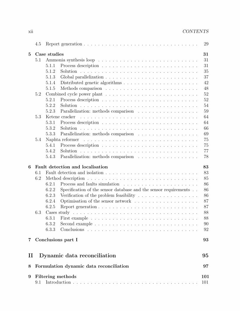
xii CONTENTS
4.5 Report generation . . . . . . . . . . . . . . . . . . . . . . . . . . . . . . . . 29
5 Case studies 315.1 Ammonia synthesis loop . . . . . . . . . . . . . . . . . . . . . . . . . . . . 31
5.1.1 Process description . . . . . . . . . . . . . . . . . . . . . . . . . . . 315.1.2 Solution . . . . . . . . . . . . . . . . . . . . . . . . . . . . . . . . . 355.1.3 Global parallelization . . . . . . . . . . . . . . . . . . . . . . . . . . 375.1.4 Distributed genetic algorithms . . . . . . . . . . . . . . . . . . . . . 425.1.5 Methods comparison . . . . . . . . . . . . . . . . . . . . . . . . . . 48
5.2 Combined cycle power plant . . . . . . . . . . . . . . . . . . . . . . . . . . 525.2.1 Process description . . . . . . . . . . . . . . . . . . . . . . . . . . . 525.2.2 Solution . . . . . . . . . . . . . . . . . . . . . . . . . . . . . . . . . 545.2.3 Parallelization: methods comparison . . . . . . . . . . . . . . . . . 59
5.3 Ketene cracker . . . . . . . . . . . . . . . . . . . . . . . . . . . . . . . . . 645.3.1 Process description . . . . . . . . . . . . . . . . . . . . . . . . . . . 645.3.2 Solution . . . . . . . . . . . . . . . . . . . . . . . . . . . . . . . . . 665.3.3 Parallelization: methods comparison . . . . . . . . . . . . . . . . . 69
5.4 Naphta reformer . . . . . . . . . . . . . . . . . . . . . . . . . . . . . . . . 755.4.1 Process description . . . . . . . . . . . . . . . . . . . . . . . . . . . 755.4.2 Solution . . . . . . . . . . . . . . . . . . . . . . . . . . . . . . . . . 775.4.3 Parallelization: methods comparison . . . . . . . . . . . . . . . . . 78
6 Fault detection and localisation 836.1 Fault detection and isolation . . . . . . . . . . . . . . . . . . . . . . . . . . 836.2 Method description . . . . . . . . . . . . . . . . . . . . . . . . . . . . . . . 85
6.2.1 Process and faults simulation . . . . . . . . . . . . . . . . . . . . . 866.2.2 Specification of the sensor database and the sensor requirements . . 866.2.3 Verification of the problem feasibility . . . . . . . . . . . . . . . . . 866.2.4 Optimisation of the sensor network . . . . . . . . . . . . . . . . . . 876.2.5 Report generation . . . . . . . . . . . . . . . . . . . . . . . . . . . . 87
6.3 Cases study . . . . . . . . . . . . . . . . . . . . . . . . . . . . . . . . . . . 886.3.1 First example . . . . . . . . . . . . . . . . . . . . . . . . . . . . . . 886.3.2 Second example . . . . . . . . . . . . . . . . . . . . . . . . . . . . . 906.3.3 Conclusions . . . . . . . . . . . . . . . . . . . . . . . . . . . . . . . 92
7 Conclusions part I 93
II Dynamic data reconciliation 95
8 Formulation dynamic data reconciliation 97
9 Filtering methods 1019.1 Introduction . . . . . . . . . . . . . . . . . . . . . . . . . . . . . . . . . . . 101

CONTENTS xiii
9.2 Extended Kalman Filter . . . . . . . . . . . . . . . . . . . . . . . . . . . . 1029.2.1 Filtering equations or observation update . . . . . . . . . . . . . . . 1049.2.2 Prediction equations or time update . . . . . . . . . . . . . . . . . . 1049.2.3 Diagram of the extended Kalman filter . . . . . . . . . . . . . . . . 104
9.3 Disadvantages . . . . . . . . . . . . . . . . . . . . . . . . . . . . . . . . . . 104
10 Moving-Horizon estimation 10710.1 Explicit integration method . . . . . . . . . . . . . . . . . . . . . . . . . . 10810.2 Method based on orthogonal collocations . . . . . . . . . . . . . . . . . . . 113
10.2.1 Description of the moving window algorithm . . . . . . . . . . . . . 11310.2.2 Constraints of the optimization problem . . . . . . . . . . . . . . . 11510.2.3 Description of the sequential algorithm . . . . . . . . . . . . . . . . 11610.2.4 Description of the simultaneous algorithm . . . . . . . . . . . . . . 117
11 Calculation of a posteriori variances 121
12 Cases study 13312.1 One tank . . . . . . . . . . . . . . . . . . . . . . . . . . . . . . . . . . . . . 133
12.1.1 Results for the steps . . . . . . . . . . . . . . . . . . . . . . . . . . 13512.1.2 Results for the linear variations of feed . . . . . . . . . . . . . . . . 14112.1.3 Results for the smooth perturbations dx
dt= 0.1 (x− xtarget) . . . . . 147
12.2 Stirred tank reactor with heat exchange . . . . . . . . . . . . . . . . . . . . 15812.2.1 Results . . . . . . . . . . . . . . . . . . . . . . . . . . . . . . . . . . 161
12.3 A network of five tanks . . . . . . . . . . . . . . . . . . . . . . . . . . . . . 17412.3.1 Results . . . . . . . . . . . . . . . . . . . . . . . . . . . . . . . . . . 178
12.4 Conclusions . . . . . . . . . . . . . . . . . . . . . . . . . . . . . . . . . . . 182
13 Conclusions part II 185
III Networks design for dynamic processes 187
14 Algorithm description 18914.1 Introduction . . . . . . . . . . . . . . . . . . . . . . . . . . . . . . . . . . . 18914.2 Observability and variable discretization . . . . . . . . . . . . . . . . . . . 18914.3 Method description . . . . . . . . . . . . . . . . . . . . . . . . . . . . . . . 190
14.3.1 Formulation of the reconciliation model and model linearisation . . 19114.3.2 Files of requirements . . . . . . . . . . . . . . . . . . . . . . . . . . 19214.3.3 Verification of the problem feasibility . . . . . . . . . . . . . . . . . 19314.3.4 Optimization of the sensor network . . . . . . . . . . . . . . . . . . 19414.3.5 Report generation . . . . . . . . . . . . . . . . . . . . . . . . . . . . 195
15 Case studies 19715.1 One tank . . . . . . . . . . . . . . . . . . . . . . . . . . . . . . . . . . . . . 197

xiv CONTENTS
15.2 A network of five tanks . . . . . . . . . . . . . . . . . . . . . . . . . . . . . 20215.3 Stirred tank reactor with heat exchange . . . . . . . . . . . . . . . . . . . . 204
16 Conclusions part III 209
17 General conclusions and future work 211
Publications 215
Bibliography 224
A Sensor network optimization method 225A.1 Introduction . . . . . . . . . . . . . . . . . . . . . . . . . . . . . . . . . . . 225A.2 What are evolutionary algorithms ? . . . . . . . . . . . . . . . . . . . . . . 226
A.2.1 Evolution strategy . . . . . . . . . . . . . . . . . . . . . . . . . . . 227A.2.2 Evolutionary programming . . . . . . . . . . . . . . . . . . . . . . . 228A.2.3 Genetic programming . . . . . . . . . . . . . . . . . . . . . . . . . . 229A.2.4 Learning classifier systems . . . . . . . . . . . . . . . . . . . . . . . 229
A.3 Genetic algorithms . . . . . . . . . . . . . . . . . . . . . . . . . . . . . . . 230A.3.1 Individuals coding . . . . . . . . . . . . . . . . . . . . . . . . . . . 231A.3.2 Natural mechanisms description . . . . . . . . . . . . . . . . . . . . 232
A.4 Others optimization methods . . . . . . . . . . . . . . . . . . . . . . . . . 236
B Parallelization 239B.1 Notions of parallelization . . . . . . . . . . . . . . . . . . . . . . . . . . . . 239B.2 Algorithms parallelization . . . . . . . . . . . . . . . . . . . . . . . . . . . 243
B.2.1 Global parallelization (GP) . . . . . . . . . . . . . . . . . . . . . . 244B.2.2 Distributed genetic algorithms (DGA) . . . . . . . . . . . . . . . . 247
C Orthogonal collocations 251C.0.3 Polynomial approximations . . . . . . . . . . . . . . . . . . . . . . 251C.0.4 Determination of the collocation nodes . . . . . . . . . . . . . . . . 262

List of Figures
3.1 Flow rate measurements . . . . . . . . . . . . . . . . . . . . . . . . . . . 19
4.1 Flow diagram of the genetic algorithm . . . . . . . . . . . . . . . . . . . 24
5.1 Ammonia synthesis loop: evolution of the goal function with the numberof generations . . . . . . . . . . . . . . . . . . . . . . . . . . . . . . . . . 35
5.2 Ammonia synthesis loop: solution in the case of one operating point . . . 365.3 Ammonia synthesis loop: solution in the case of one sensor failure . . . . 375.4 Ammonia synthesis loop: global parallelization: 20 chromosomes: case of
one operating point . . . . . . . . . . . . . . . . . . . . . . . . . . . . . . 385.5 Ammonia synthesis loop: global parallelization: 40 chromosomes: case of
one operating point . . . . . . . . . . . . . . . . . . . . . . . . . . . . . . 405.6 Ammonia synthesis loop: global parallelization: 100 chromosomes: case of
one operating point . . . . . . . . . . . . . . . . . . . . . . . . . . . . . . 405.7 Ammonia synthesis loop: global parallelization: 20 chromosomes: case of
one sensor failure . . . . . . . . . . . . . . . . . . . . . . . . . . . . . . . 425.8 Ammonia synthesis loop: distributed genetic algorithms: influence of the
number of 10 chromosomes sub-populations on the computing time: caseof one operating point . . . . . . . . . . . . . . . . . . . . . . . . . . . . 44
5.9 Ammonia synthesis loop: distributed genetic algorithms: influence of thenumber of 10 chromosomes sub-populations on the number of iterationsand on the goal function: case of one operating point . . . . . . . . . . . 44
5.10 Ammonia synthesis loop: distributed genetic algorithms: influence of thenumber of 20 chromosomes sub-populations on the time: case of one op-erating point . . . . . . . . . . . . . . . . . . . . . . . . . . . . . . . . . . 45
5.11 Ammonia synthesis loop: distributed genetic algorithms: influence of thenumber of 20 chromosomes sub-populations on the number of iterationsand on the goal function: case of one operating point . . . . . . . . . . . 46
5.12 Ammonia synthesis loop: distributed genetic algorithms: influence on thecomputing time of the number of generations between 2 migrations: caseof one operating point . . . . . . . . . . . . . . . . . . . . . . . . . . . . 47
5.13 Ammonia synthesis loop: distributed genetic algorithms: influence on thenumber of iterations and on the goal function of the number of generationsbetween 2 migrations: case of one operating point . . . . . . . . . . . . . 47
5.14 Ammonia synthesis loop: times comparison . . . . . . . . . . . . . . . . . 49
xv

xvi LIST OF FIGURES
5.15 Ammonia synthesis loop: number of generations comparison . . . . . . . 495.16 Ammonia synthesis loop: goal function comparison . . . . . . . . . . . . 505.17 Ammonia synthesis loop: efficiency comparison . . . . . . . . . . . . . . . 515.18 CC power plant: solution in the case of one operating point . . . . . . . . 555.19 CC power plant: solution in the case of two operating points . . . . . . . 575.20 CC power plant: solution in the case of one sensor failure . . . . . . . . . 585.21 CC power plant: times comparison . . . . . . . . . . . . . . . . . . . . . 615.22 CC power plant: number of generations comparison . . . . . . . . . . . . 615.23 CC power plant: goal function comparison . . . . . . . . . . . . . . . . . 625.24 CC power plant: efficiency comparison . . . . . . . . . . . . . . . . . . . 635.25 Ketene cracker: solution in the case of one operating point (part 1) . . . 685.26 Ketene cracker: solution in the case of one operating point (part2) . . . . 695.27 Ketene cracker: solution in the case of one sensor failure (part 1) . . . . . 705.28 Ketene cracker: solution in the case of one sensor failure (part 2) . . . . . 715.29 Ketene cracker: times comparison . . . . . . . . . . . . . . . . . . . . . . 725.30 Ketene cracker: number of generations comparison . . . . . . . . . . . . . 735.31 Ketene cracker: goal function comparison . . . . . . . . . . . . . . . . . . 745.32 Ketene cracker: efficiency comparison . . . . . . . . . . . . . . . . . . . . 745.33 Naphta reformer: times comparison . . . . . . . . . . . . . . . . . . . . . 795.34 Naphta reformer: number of generations comparison . . . . . . . . . . . . 805.35 Naphta reformer: goal function comparison . . . . . . . . . . . . . . . . . 805.36 Naphta reformer: efficiency comparison . . . . . . . . . . . . . . . . . . . 81
6.1 Flow sheet of the first example of fault detection . . . . . . . . . . . . . . 886.2 Influence on the goal function of the number of measurement times and
the elapsed time from the beginning of the leak until detection . . . . . . 906.3 Flow sheet of the second example of fault detection . . . . . . . . . . . . 91
9.1 Diagram of the extended Kalman filter . . . . . . . . . . . . . . . . . . . 105
10.1 Reconciliation window . . . . . . . . . . . . . . . . . . . . . . . . . . . . 10710.2 Flowchart of the explicit integration method . . . . . . . . . . . . . . . . 10910.3 Parameters of the reconciliation window in the case of the explicit integra-
tion method . . . . . . . . . . . . . . . . . . . . . . . . . . . . . . . . . . 11010.4 Parameters of the reconciliation window: orthogonal collocations . . . . . 11410.5 Flowchart of the orthogonal collocations method: sequential algorithm . . 11610.6 Flowchart of the orthogonal collocations method: simultaneous algorithm 118
12.1 Flowsheet of the tank . . . . . . . . . . . . . . . . . . . . . . . . . . . . . 13312.2 One tank: steps: height: profile . . . . . . . . . . . . . . . . . . . . . . . 13612.3 One tank: steps: feed flowrate: profile . . . . . . . . . . . . . . . . . . . . 13612.4 One tank: steps: outlet flowrate: profile . . . . . . . . . . . . . . . . . . . 13712.5 One tank: steps: height: errors . . . . . . . . . . . . . . . . . . . . . . . . 13812.6 One tank: steps: feed flowrate: errors . . . . . . . . . . . . . . . . . . . . 138

LIST OF FIGURES xvii
12.7 One tank: steps: outlet flowrate: errors . . . . . . . . . . . . . . . . . . . 13912.8 One tank: steps: height: standard deviation comparison . . . . . . . . . . 14012.9 One tank: steps: feed flowrate: standard deviation comparison . . . . . . 14012.10 One tank: steps: outlet flowrate: standard deviation comparison . . . . . 14112.11 One tank: linear variations of feed: height: profile . . . . . . . . . . . . . 14212.12 One tank: linear variations of feed: feed flowrate: profile . . . . . . . . . 14212.13 One tank: linear variations of feed: outlet flowrate: profile . . . . . . . . 14312.14 One tank: linear variations of feed: height: errors . . . . . . . . . . . . . 14412.15 One tank: linear variations of feed: feed flowrate: errors . . . . . . . . . . 14412.16 One tank: linear variations of feed: outgoing flowrate: errors . . . . . . . 14512.17 One tank: linear variations of feed: height: standard deviation comparison 14612.18 One tank: linear variations of feed: feed flowrate: standard deviation
comparison . . . . . . . . . . . . . . . . . . . . . . . . . . . . . . . . . . . 14612.19 One tank: linear variations of feed: outgoing flowrate: standard deviation
comparison . . . . . . . . . . . . . . . . . . . . . . . . . . . . . . . . . . . 14712.20 One tank: smooth perturbations: height: profile . . . . . . . . . . . . . . 14812.21 One tank: smooth perturbations: feed flowrate: profile . . . . . . . . . . 14812.22 One tank: smooth perturbations: outgoing flowrate: profile . . . . . . . . 14912.23 One tank: smooth perturbations: height: errors . . . . . . . . . . . . . . 15012.24 One tank: smooth perturbations: feed flowrate: errors . . . . . . . . . . . 15012.25 One tank: smooth perturbations: outgoing flowrate: errors . . . . . . . . 15112.26 One tank: function: height: standard deviation comparison . . . . . . . . 15212.27 One tank: smooth perturbations: feed flowrate: standard deviation com-
parison . . . . . . . . . . . . . . . . . . . . . . . . . . . . . . . . . . . . . 15312.28 One tank: smooth perturbations: outgoing flowrate: standard deviation
comparison . . . . . . . . . . . . . . . . . . . . . . . . . . . . . . . . . . . 15412.29 One tank: smooth perturbations: schema of the error distributions . . . . 15512.30 One tank: smooth perturbations: height: error distribution . . . . . . . . 15612.31 One tank: smooth perturbations: feed flowrate: error distribution . . . . 15612.32 One tank: smooth perturbations: outgoing flowrate: error distribution . . 15712.33 Flowsheet of the stirred tank reactor with heat exchange . . . . . . . . . 15812.34 Stirred tank reactor with heat exchange: concentration: profile . . . . . . 16112.35 Stirred tank reactor with heat exchange: temperature: profile . . . . . . . 16212.36 Stirred tank reactor with heat exchange: feed flowrate: profile . . . . . . 16212.37 Stirred tank reactor with heat exchange: feed concentration: profile . . . 16312.38 Stirred tank reactor with heat exchange: feed temperature: profile . . . . 16312.39 Stirred tank reactor with heat exchange: cooling temperature: profile . . 16412.40 Stirred tank reactor with heat exchange: concentration: standard devia-
tion comparison . . . . . . . . . . . . . . . . . . . . . . . . . . . . . . . . 16512.41 Stirred tank reactor with heat exchange: temperature: standard deviation
comparison . . . . . . . . . . . . . . . . . . . . . . . . . . . . . . . . . . . 16612.42 Stirred tank reactor with heat exchange: feed flowrate: standard deviation
comparison . . . . . . . . . . . . . . . . . . . . . . . . . . . . . . . . . . . 167
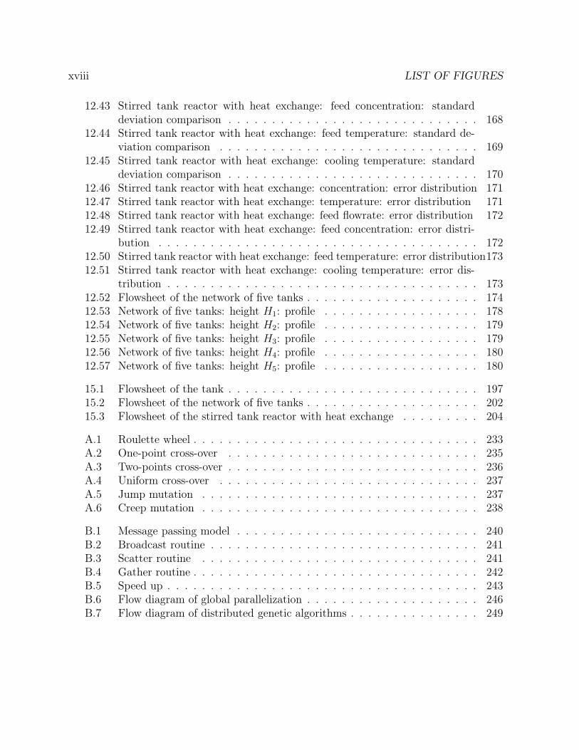
xviii LIST OF FIGURES
12.43 Stirred tank reactor with heat exchange: feed concentration: standarddeviation comparison . . . . . . . . . . . . . . . . . . . . . . . . . . . . . 168
12.44 Stirred tank reactor with heat exchange: feed temperature: standard de-viation comparison . . . . . . . . . . . . . . . . . . . . . . . . . . . . . . 169
12.45 Stirred tank reactor with heat exchange: cooling temperature: standarddeviation comparison . . . . . . . . . . . . . . . . . . . . . . . . . . . . . 170
12.46 Stirred tank reactor with heat exchange: concentration: error distribution 17112.47 Stirred tank reactor with heat exchange: temperature: error distribution 17112.48 Stirred tank reactor with heat exchange: feed flowrate: error distribution 17212.49 Stirred tank reactor with heat exchange: feed concentration: error distri-
bution . . . . . . . . . . . . . . . . . . . . . . . . . . . . . . . . . . . . . 17212.50 Stirred tank reactor with heat exchange: feed temperature: error distribution17312.51 Stirred tank reactor with heat exchange: cooling temperature: error dis-
tribution . . . . . . . . . . . . . . . . . . . . . . . . . . . . . . . . . . . . 17312.52 Flowsheet of the network of five tanks . . . . . . . . . . . . . . . . . . . . 17412.53 Network of five tanks: height H1: profile . . . . . . . . . . . . . . . . . . 17812.54 Network of five tanks: height H2: profile . . . . . . . . . . . . . . . . . . 17912.55 Network of five tanks: height H3: profile . . . . . . . . . . . . . . . . . . 17912.56 Network of five tanks: height H4: profile . . . . . . . . . . . . . . . . . . 18012.57 Network of five tanks: height H5: profile . . . . . . . . . . . . . . . . . . 180
15.1 Flowsheet of the tank . . . . . . . . . . . . . . . . . . . . . . . . . . . . . 19715.2 Flowsheet of the network of five tanks . . . . . . . . . . . . . . . . . . . . 20215.3 Flowsheet of the stirred tank reactor with heat exchange . . . . . . . . . 204
A.1 Roulette wheel . . . . . . . . . . . . . . . . . . . . . . . . . . . . . . . . . 233A.2 One-point cross-over . . . . . . . . . . . . . . . . . . . . . . . . . . . . . 235A.3 Two-points cross-over . . . . . . . . . . . . . . . . . . . . . . . . . . . . . 236A.4 Uniform cross-over . . . . . . . . . . . . . . . . . . . . . . . . . . . . . . 237A.5 Jump mutation . . . . . . . . . . . . . . . . . . . . . . . . . . . . . . . . 237A.6 Creep mutation . . . . . . . . . . . . . . . . . . . . . . . . . . . . . . . . 238
B.1 Message passing model . . . . . . . . . . . . . . . . . . . . . . . . . . . . 240B.2 Broadcast routine . . . . . . . . . . . . . . . . . . . . . . . . . . . . . . . 241B.3 Scatter routine . . . . . . . . . . . . . . . . . . . . . . . . . . . . . . . . 241B.4 Gather routine . . . . . . . . . . . . . . . . . . . . . . . . . . . . . . . . . 242B.5 Speed up . . . . . . . . . . . . . . . . . . . . . . . . . . . . . . . . . . . . 243B.6 Flow diagram of global parallelization . . . . . . . . . . . . . . . . . . . . 246B.7 Flow diagram of distributed genetic algorithms . . . . . . . . . . . . . . . 249
List of Tables
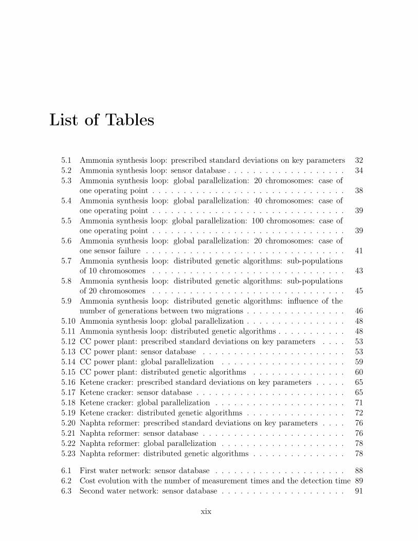
5.1 Ammonia synthesis loop: prescribed standard deviations on key parameters 325.2 Ammonia synthesis loop: sensor database . . . . . . . . . . . . . . . . . . . 345.3 Ammonia synthesis loop: global parallelization: 20 chromosomes: case of
one operating point . . . . . . . . . . . . . . . . . . . . . . . . . . . . . . . 385.4 Ammonia synthesis loop: global parallelization: 40 chromosomes: case of
one operating point . . . . . . . . . . . . . . . . . . . . . . . . . . . . . . . 39
5.5 Ammonia synthesis loop: global parallelization: 100 chromosomes: case ofone operating point . . . . . . . . . . . . . . . . . . . . . . . . . . . . . . . 39
5.6 Ammonia synthesis loop: global parallelization: 20 chromosomes: case ofone sensor failure . . . . . . . . . . . . . . . . . . . . . . . . . . . . . . . . 41
5.7 Ammonia synthesis loop: distributed genetic algorithms: sub-populationsof 10 chromosomes . . . . . . . . . . . . . . . . . . . . . . . . . . . . . . . 43
5.8 Ammonia synthesis loop: distributed genetic algorithms: sub-populationsof 20 chromosomes . . . . . . . . . . . . . . . . . . . . . . . . . . . . . . . 45
5.9 Ammonia synthesis loop: distributed genetic algorithms: influence of thenumber of generations between two migrations . . . . . . . . . . . . . . . . 46
5.10 Ammonia synthesis loop: global parallelization . . . . . . . . . . . . . . . . 485.11 Ammonia synthesis loop: distributed genetic algorithms . . . . . . . . . . . 48
5.12 CC power plant: prescribed standard deviations on key parameters . . . . 535.13 CC power plant: sensor database . . . . . . . . . . . . . . . . . . . . . . . 535.14 CC power plant: global parallelization . . . . . . . . . . . . . . . . . . . . 59
5.15 CC power plant: distributed genetic algorithms . . . . . . . . . . . . . . . 605.16 Ketene cracker: prescribed standard deviations on key parameters . . . . . 655.17 Ketene cracker: sensor database . . . . . . . . . . . . . . . . . . . . . . . . 65
5.18 Ketene cracker: global parallelization . . . . . . . . . . . . . . . . . . . . . 715.19 Ketene cracker: distributed genetic algorithms . . . . . . . . . . . . . . . . 725.20 Naphta reformer: prescribed standard deviations on key parameters . . . . 76
5.21 Naphta reformer: sensor database . . . . . . . . . . . . . . . . . . . . . . . 765.22 Naphta reformer: global parallelization . . . . . . . . . . . . . . . . . . . . 785.23 Naphta reformer: distributed genetic algorithms . . . . . . . . . . . . . . . 78
6.1 First water network: sensor database . . . . . . . . . . . . . . . . . . . . . 886.2 Cost evolution with the number of measurement times and the detection time 896.3 Second water network: sensor database . . . . . . . . . . . . . . . . . . . . 91
xix
xx LIST OF TABLES
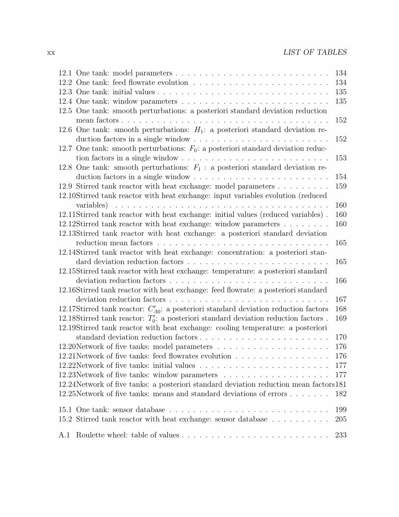
12.1 One tank: model parameters . . . . . . . . . . . . . . . . . . . . . . . . . . 13412.2 One tank: feed flowrate evolution . . . . . . . . . . . . . . . . . . . . . . . 13412.3 One tank: initial values . . . . . . . . . . . . . . . . . . . . . . . . . . . . . 13512.4 One tank: window parameters . . . . . . . . . . . . . . . . . . . . . . . . . 13512.5 One tank: smooth perturbations: a posteriori standard deviation reduction
mean factors . . . . . . . . . . . . . . . . . . . . . . . . . . . . . . . . . . . 15212.6 One tank: smooth perturbations: H1: a posteriori standard deviation re-
duction factors in a single window . . . . . . . . . . . . . . . . . . . . . . . 15212.7 One tank: smooth perturbations: F0: a posteriori standard deviation reduc-
tion factors in a single window . . . . . . . . . . . . . . . . . . . . . . . . . 15312.8 One tank: smooth perturbations: F1 : a posteriori standard deviation re-
duction factors in a single window . . . . . . . . . . . . . . . . . . . . . . . 15412.9 Stirred tank reactor with heat exchange: model parameters . . . . . . . . . 15912.10Stirred tank reactor with heat exchange: input variables evolution (reduced
variables) . . . . . . . . . . . . . . . . . . . . . . . . . . . . . . . . . . . . 16012.11Stirred tank reactor with heat exchange: initial values (reduced variables) . 16012.12Stirred tank reactor with heat exchange: window parameters . . . . . . . . 16012.13Stirred tank reactor with heat exchange: a posteriori standard deviation
reduction mean factors . . . . . . . . . . . . . . . . . . . . . . . . . . . . . 16512.14Stirred tank reactor with heat exchange: concentration: a posteriori stan-
dard deviation reduction factors . . . . . . . . . . . . . . . . . . . . . . . . 16512.15Stirred tank reactor with heat exchange: temperature: a posteriori standard
deviation reduction factors . . . . . . . . . . . . . . . . . . . . . . . . . . . 16612.16Stirred tank reactor with heat exchange: feed flowrate: a posteriori standard
deviation reduction factors . . . . . . . . . . . . . . . . . . . . . . . . . . . 16712.17Stirred tank reactor: C ′
A0: a posteriori standard deviation reduction factors 16812.18Stirred tank reactor: T ′
0: a posteriori standard deviation reduction factors . 16912.19Stirred tank reactor with heat exchange: cooling temperature: a posteriori
standard deviation reduction factors . . . . . . . . . . . . . . . . . . . . . . 17012.20Network of five tanks: model parameters . . . . . . . . . . . . . . . . . . . 17612.21Network of five tanks: feed flowrates evolution . . . . . . . . . . . . . . . . 17612.22Network of five tanks: initial values . . . . . . . . . . . . . . . . . . . . . . 17712.23Network of five tanks: window parameters . . . . . . . . . . . . . . . . . . 17712.24Network of five tanks: a posteriori standard deviation reduction mean factors18112.25Network of five tanks: means and standard deviations of errors . . . . . . . 182
15.1 One tank: sensor database . . . . . . . . . . . . . . . . . . . . . . . . . . . 19915.2 Stirred tank reactor with heat exchange: sensor database . . . . . . . . . . 205
A.1 Roulette wheel: table of values . . . . . . . . . . . . . . . . . . . . . . . . . 233
Nomenclature
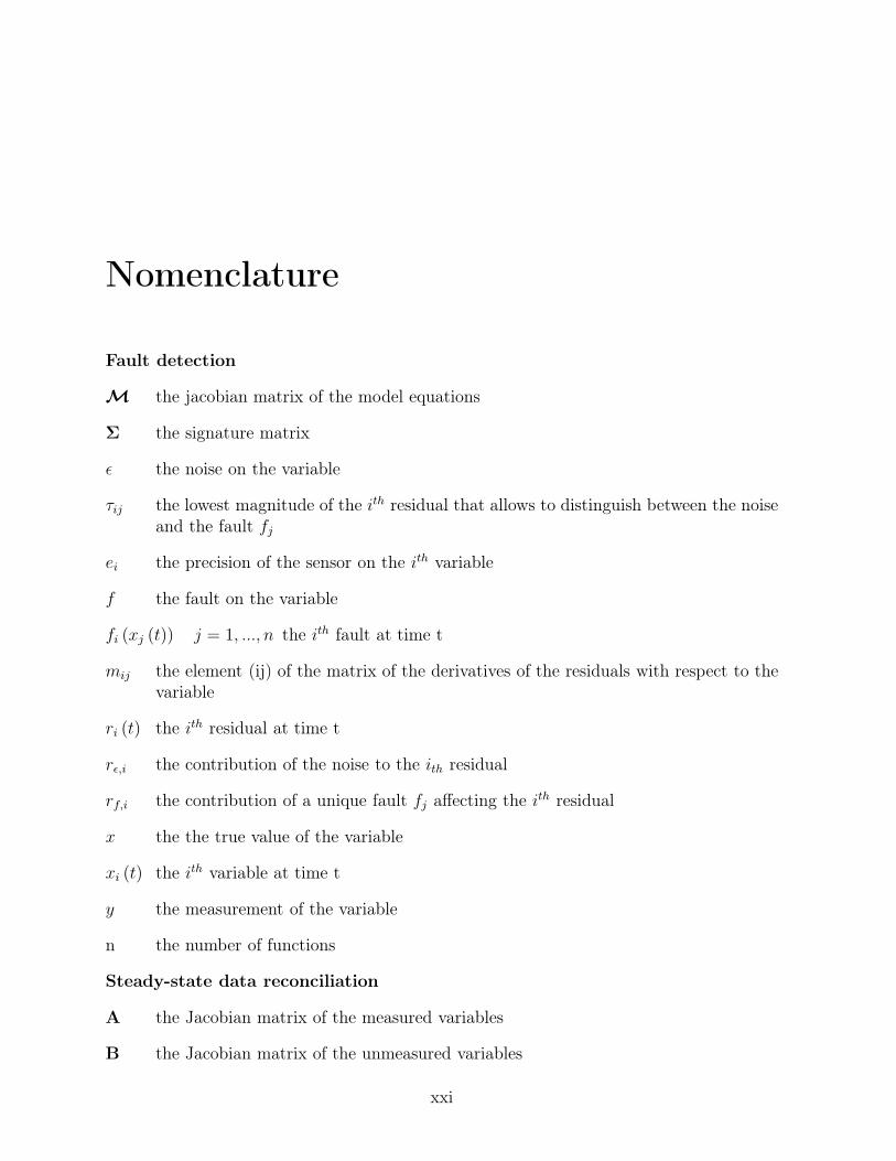
Fault detection
퓜 the jacobian matrix of the model equations
Σ the signature matrix
� the noise on the variable
�ij the lowest magnitude of the itℎ residual that allows to distinguish between the noiseand the fault fj
ei the precision of the sensor on the itℎ variable
f the fault on the variable
fi (xj (t)) j = 1, ..., n the itℎ fault at time t
mij the element (ij) of the matrix of the derivatives of the residuals with respect to thevariable
ri (t) the itℎ residual at time t
r�,i the contribution of the noise to the itℎ residual
rf,i the contribution of a unique fault fj affecting the itℎ residual
x the the true value of the variable
xi (t) the itℎ variable at time t
y the measurement of the variable
n the number of functions
Steady-state data reconciliation
A the Jacobian matrix of the measured variables
B the Jacobian matrix of the unmeasured variables
xxi

xxii NOMENCLATURE
C the vector of the independent terms of the constraints
f (x, z) the link equations
W the weight matrix (size= m x m)
x the vector of reconciled variables (size= m)
y the vector of measured variables (size= m)
z the vector of unmeasured variables (size= n)
m the number of measured variables
n the number of unmeasured variables
p the number of equations of the model
var(a) the variance of variable a
Dynamic data reconciliation
Λ the lagrange multipliers
퓔 the jacobian matrix of process and collocation constraints
퓟 the global weight matrix of the process variables
Φ the goal function to minimize
� the precisions of the measurements
�ui,jthe standard deviation on the input variable i at measurement time j
�xi,jthe standard deviation on the differential state variable i at measurement time j
�zi,j the standard deviation on the algebraic state variable i at measurement time j
A the link equations
B the relations between the differential state variables and the Lagrange interpolationpolynomials
C the linear interpolations of the values of input variables
D the residuals of the differential state equations at all collocation nodes
E the continuity constraints of the differential state variables between two discretiza-tion intervals

NOMENCLATURE xxiii
F the vector of independant terms of the linearisation of the link equations at themeasurement times
f the differential constraints
Fc the vector of independant terms of the linearisation of the link equations at thecollocation times
G the vector of independant terms of the linearisation of the D constraints at thecollocation times
g the unequality constraints
h the equality constraints
M the sensitivity matrix
Pu the global weight matrix for the input variables
Px the global weight matrix for the differential state variables
Pz the global weight matrix for the algebraic variables
Ru the relaxation factor of the input variables at the initial time of the moving horizon
Rx the relaxation factor of the differential state variables at the initial time of themoving horizon
Wu the weight matrix of the input state variables
Wx is the weight matrix of the differential state variables
Wz the weight matrix of the algebraic state variables
�k the collocation times
Fgoal the the goal function
ℎ1 the measurement frequency
ℎ2 the size of the interpolation interval of the input variables
ℎ3 the size of the discretization interval of the differential state variables
ℎ4 the size of the window
ℎ5 the move of the window
N the size of the sensitivity matrix M
xxiv NOMENCLATURE
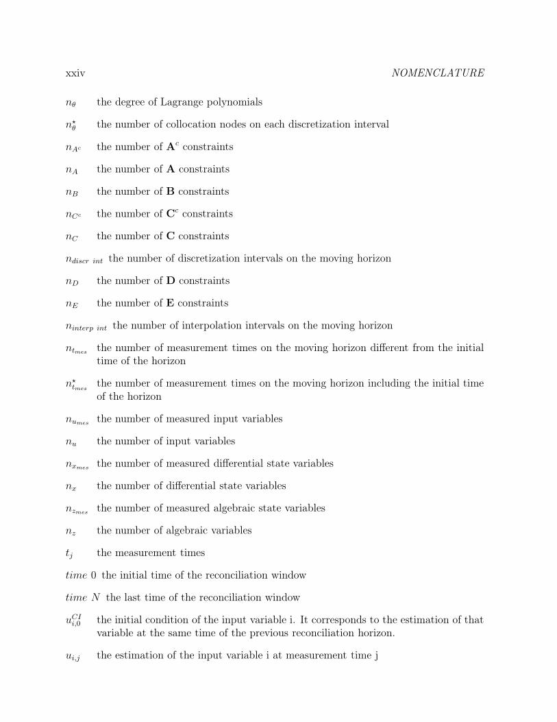
n� the degree of Lagrange polynomials
n★� the number of collocation nodes on each discretization interval
nAc the number of Ac constraints
nA the number of A constraints
nB the number of B constraints
nCc the number of Cc constraints
nC the number of C constraints
ndiscr int the number of discretization intervals on the moving horizon
nD the number of D constraints
nE the number of E constraints
ninterp int the number of interpolation intervals on the moving horizon
ntmesthe number of measurement times on the moving horizon different from the initialtime of the horizon
n★tmes
the number of measurement times on the moving horizon including the initial timeof the horizon
numesthe number of measured input variables
nu the number of input variables
nxmesthe number of measured differential state variables
nx the number of differential state variables
nzmesthe number of measured algebraic state variables
nz the number of algebraic variables
tj the measurement times
time 0 the initial time of the reconciliation window
time N the last time of the reconciliation window
uCIi,0 the initial condition of the input variable i. It corresponds to the estimation of that
variable at the same time of the previous reconciliation horizon.
ui,j the estimation of the input variable i at measurement time j

NOMENCLATURE xxv
umi,j the measurement of the input variable i at measurement time j
var(a) the variance of variable a
xCIi,0 the initial condition of the differential state variable i. It corresponds to the estima-
tion of that variable at the same time of the previous reconciliation horizon
xi,j the estimation of the differential state variable i at measurement time j
xmi,j the measurement of the differential state variable i at measurement time j
zi,j the estimation of the algebraic state variable i at measurement time j
zmi,j the measurement of the algebraic state variable i at measurement time j
Filtering methods
xj the mean value of variables x at time step j
yj the mean value of variables y at time step j
f (xj−1,uj−1,vj−1) a set of non linear functions of x, u and v at time step j-1
Fj the Jacobian matrix of partial derivatives of f with respect to x at time step j(extended Kalman filter)
h (xj,wj) a set of non linear functions of x and w at time step j
Hj the Jacobian matrix of partial derivatives of h with respect to x at time step j(extended Kalman filter)
Pj∣j−1 the covariance matrix of estimation errors at time step j
Pj∣j the covariance matrix of prediction errors at time step j
Qj the process noises covariance matrix
Rj the measurement noises covariance matrix
uj−1 the vector of input variables at time step j-1
vj−1 the vector of process noises at time step j-1
Vj the Jacobian matrix of partial derivatives of f with respect to v at time step j(extended Kalman filter)
wj the vector of measurement noises at time step j
Wj the Jacobian matrix of partial derivatives of h with respect to w at time step j(extended Kalman filter)

xxvi NOMENCLATURE
xj the vector of state variables at time step j
yj the vector of measurements at time step j
xj∣j−1 the vector of predicted states at time step j
xj∣j the vector of estimated states at time step j
Kj the gain matrix at time step j
Sensor network design
penaltysingular matrix the penalty factor for a singular sensitivity matrix
penaltytarget the penalty factor for the non-respected targets on key parameters
�i the accuracy obtained by the sensor network for the key variable i
�targeti the accuracy required for the key parameter i
Cmax the cost of the most expensive sensor network
fitness the goal function
Nkey variables the number of process key variables
Noperating points the number of operating points
Nwindows the number of reconciliation windows chosen for the sensor network design
N★tmes
the number of measurement times on the moving horizon including the initial timeof the horizon
Parallelization
kcℎrom the number of individuals estimated by one processor
nsensors the number of sensors in the network
neval the number of goal function evaluations carried out by one processor for one indi-vidual
Npop the size of the population
rsensors the remainder of the division of the number of sensors in the chromosomes plusone by the number of processors
rcℎrom the remainder of the division of the number of chromosomes by the number ofprocessors
T1 the time required to solve a problem B on a sequential computer
Tp the time required to solve a problem B on a cluster of p processors
Chapter 1
Introduction
1.1 Problem position
Nowadays, despite the progress achieved since the invention of the concept of controlcharts by Shewhart in the twenties, process control and monitoring remain challengingproblems. Indeed, food and pharmaceutical industries, industries who produce high addedvalue products, need very pure components. Security and environmental rules becomemore and more strict. Moreover, one always wants to produce more and less expensive.Thus the knowledge of the processes has to be more and more precise and one can notanymore achieve satisfactory process control by measuring only a few process variables.Process faults (pipes or tanks failure, catalyst deactivation,...) must be detected andlocalised faster, and any deviation from the nominal operating points must be correctedimmediately.One could imagine to quickly solve the problem by measuring all process variables but thiswould not be enough. Indeed, how could the efficiency of a compressor, the productivityof a plant, a reaction conversion ... be measured by a sensor? Moreover all measurementsare erroneous to some extend and the precision reached on the estimates of unmeasurablevariables is a function of the measurements precision. Furthermore, the measurement ofsome variables requires expensive sensors (concentration measurements). So one will prefer,if the precision constraints on key variables remained satisfied, estimating those variablesfrom the measurements of other process variables instead of buying expensive measurementtools.The technique of data reconciliation allows to estimate unmeasured variables and theiraccuracies. If redundant measurements are available, measurements are corrected and theuncertainty due to measurement errors can be reduced, so that measured variables arebetter known.However, the number, the location and the precision of the sensors influence the accuracyof the estimates. The choice of the required sensors appears thus to be a very importanttask for industrial control and monitoring.As it would be shown in the state of the art (chapter 2), the problem of sensor networks
1
2 CHAPTER 1. INTRODUCTION
design has been approached by several researchers during the last two decades.
1.2 Objectives
The thesis adresses two main objectives:
∙ The first objective is the development of a systematic method to design the cheapestsensor network that allows to satisfy all the following constraints for dynamic as wellas steady-state processes:
– all the process variables should be computable, even if they can not be directlymeasured (efficiency of a particular unit, reaction conversion...);
– all key variables should be estimated within a prescribed accuracy;
– if the process has several operating modes, the sensor network should be ableto satisfy the two first conditions for all of them;
– sometimes, one may want to be sure that the sensor network will be able tosatisfy the two first conditions even in the case of one sensor failure or if onesensor is switched off for maintenance. So, one has to test those conditions forall configurations of the sensor network obtained by switching off one sensor.
A variant of the method should allow the search of the cheapest sensor network thatis able to detect and locate specific process faults in steady-sate processes.
∙ Secondly the development of a method to estimate a posteriori variances in the case ofdynamic processes. That objective requires a dynamic data reconciliation algorithmthat allows to estimate input variables as well as differential state and algebraicvariables, and can generate a linearized sensitivity matrix.
1.3 Summary
In this study a general method to design the cheapest sensor network able to estimate allprocess key variables within a prescribed accuracy has been developed for stationary pro-cesses. It is based on a posteriori variances estimation method developed for steady-statedata reconciliation. Using linearization of the process model at the nominal operatingpoint, it allows to deal with non linear equations and to treat energy balances as well asmass balances.In the suggested method, the problem is formulated as an optimization problem whoseobjective function depends on the annualized costs of the chosen sensors and on the accu-racies achieved for the process key variables. A binary decision is assigned to each possiblesensor (the presence or the absence of the sensor in the final network). Thus the optimiza-tion problem is not derivable but is often multimodal. We proposed to solve it using agenetic algorithm. When the process needs to be monitored for a wide range of operating
1.3. SUMMARY 3
conditions, a single linearization might not be adequate for all of them. Thus one shouldconsider optimizing simultaneously several linearized systems to identify a suitable com-promise.The computer time required to reach the solution is rather long with the proposed methodand, because of sensitivity matrix inversions necessary to variances estimation, it increasesmore quickly than the size of the problem. Fortunately genetic algorithms can easily beparallelized. A global method and distributed genetic algorithms are approached in thisstudy.A variant of our sensor network design method allowing to detect and locate process faultis presented. The objective function does not depends anymore on the accuracies reachedfor the key variables, but depends on the dectectability and the isolability of the fault.The algorithm uses a method of process fault detection and localisation similar to the onedescribed by Ragot (Ragot and Maquin, 2006).
Several techniques to correct dynamic data exist. Most of them seek the estimation ofstates or parameters. Other include the possibility to correct input variables. The main dy-namic data reconciliation techniques are filtering methods and moving-horizon approaches.Nowadays, no dynamic data reconciliation method has proved is superiority on the otherones for all cases.To transpose the sensor design method to dynamic data reconciliation, a posteriori vari-ances must be evaluated analytically. We derived the equations allowing to estimate themin a general way.The method proposed in this thesis is a moving-horizon approach. The discretization of dif-ferential equations is carried out by orthogonal collocations. The optimization of processand discretization variables is carried out simultaneously using the successive quadraticprogramming algorithm developed by Kyriakopoulou (Kyriakopoulou, 1997). The methodprovides a linearized system of equations like in the steady-state case. A sensitivity matrixcan thus be evaluated and its non singularity is an a posteriori observability criterion ofthe system.
The thesis begins with an introductive chapter followed by a chapter devoted to the stateof the art. The study is divided in three parts. The first part of the thesis (chapters 3 to9) is devoted to the problem of sensor networks design for steady-state processes. Beforedeveloping the method based on steady-state data reconciliation and genetic algorithms,the problem of steady-state data reconciliation is formulated, a posteriori variances esti-mation is clarified and evolutionary algorithms are described.Message passing interface algorithms are then used to develop parallelization techniquesallowing to reduce the computing time. Global parallelization and distributed genetic al-gorithms are described and tested on several examples.The sensor network design algorithm is finally modified to detect and locate process faultsfrom a list of simulated faults.
The second part of the study (chapters 10 to 15) approaches the problems of dynamicdata reconciliation and a posteriori variances estimation. First of all, the dynamic data
4 CHAPTER 1. INTRODUCTION
reconciliation problem is formulated. Then several filtering and moving horizon techniquesare described: the extended Kalman filter and two moving horizon methods coupled witha successive quadratic programming optimization. In the first moving window method theintegration of differential equations is carried out by means of the fourth order Runge-Kutta method. In the case of the second moving horizon technique, differential equationsare discretized by means of orthogonal collocations. The process and discretization vari-ables can be optimized sequentially or simultaneously. Those methods are compared ontwo examples.The simultaneous orthogonal collocations based method being the most advantageous forthe remaining of the project, it is chosen.A method to estimate a posteriori variances from the discretized differential equations isdeveloped: the constrained discretized optimization problem is transformed into an un-constrained one using Lagrange multipliers. If the optimality conditions are satisfied, oneobtains the sensitivity matrix of the problem from which a posteriori variances can bededuced. The method is validated on several small examples.
The last part of the thesis (chapters 16 to 18) addresses the design of sensor networks fordynamic processes. A method based on the analysis of the sensitivity matrix is proposedlike for the steady-state case. An a posteriori observability criterion is defined on the basesof that analysis. The algorithm is tested on the same examples that the dynamic datareconciliation method developed in the second part.
The general conclusions and future perspectives are presented in chapter 19.

Chapter 2
State of the art
This chapter is devoted to a bibliography study concerning the four main research areasuseful to reach the objectives aimed by the thesis.
Sensor network design
During the last two decades, several researchers have pprposed methods to solve the prob-lem of sensor network design. In 1987, Kretsovalis and Mah (Kretsovalis and Mah, 1987)developed methods based on linear algebra to design sensor networks that maximise theestimation accuracy. As they assumed that all variables are observable, their objective wasto optimize the placement of redundant sensors.Some years after, Madron (Madron, 1992) solved the problem of the design of the cheapestsensor network by using a graph oriented-method.Ali and Narasimhan (Ali and Narasimhan, 1993) introduced the concept of reliability ofestimation of a variable which is the probability with which a variable can be estimatedwhen sensors are likely to fail. They have applied it to the design of observable sensornetworks for stationary linear processes. They extended their work to redundant sensornetworks (Ali and Narasimhan, 1995). They used a branch and bound optimization methodto minimize the cost.Sen et al (Sen et al., 1998) combined the concepts of graph theory and genetic algorithmin the case of linear processes. Their algorithm allowed to optimize a single criterion,either minimal cost, or maximum estimation accuracy. They limited their research to non-redundant sensor networks.Bagajewicz (Bagajewicz, 1997) proposed a MINLP method to solve the problem of thecheapest sensor network for linear processes that can be submitted to constraints like aprescribed precision. The method is based on graph theory and linear algebra. He estab-lished with Sanchez (Bagajewicz and Sanchez, 1999b) the duality between the model of themaximum precision and the model of the minimum cost. They also presented a methodfor upgrading a sensor network with the goal of achieving a certain degree of observabilityor redundancy for a specified set of variables (Bagajewicz and Sanchez, 1999a).
5
6 CHAPTER 2. STATE OF THE ART
Heyen et al proposed (Heyen and Gerkens, 2002), (Heyen et al., 2002) a general formula-tion for the sensor placement problem. Their goal is to reduce the noise while computingthe estimates of all key variables within a prescribed accuracy. Studied problems are nolonger limited to flow measurements and linear constraints. Optimization is carried out bymeans of genetic algorithms.Carnero et al (Carnero et al., 2005) used an evolutionary technique based on genetic algo-rithms. It combines the use of structured populations in the form of neighborhood and alocal search strategy. This method was applied to mass balances only.Bhushan et al (Bhushan et al., 2008) used the concept of lexicographic optimization tosolve the problem of the design of robust sensor network for fault diagnosis. Wailly at al(Wailly and Héraud, 2005), (Wally et al., 2008) also used the lexicographic programmingand the Groëber bases to solve the sensor placement problem. The advantage of thosemethods is to allow to extend the mathematical process to the n-linear case.Muradore et al presented (Muradore et al., 2006) a method for determining the optimallocation of sensor in distributed sensor systems. This method has the advantage not dorequire an explicit model of the process. It is based on a sequential algorithm that selectsthe most informative measurement input at each iteration and updates the input and out-put spaces by subtracting information coming from the regressor.Singh and Hahn (Singh and Hahn, 2005) proposed a method to determine the position ofthe sensor inside the process unit. This technique can be applied to linear and non-linearsystems, to determine the optimal sensor network for states or for parameters estimation.It combines the computation of the observability covariance matrix with established mea-sures for locating sensors in the case of linear processes. Van de Wouwer et al (de Wouweret al., 2000) developed a criterion based on the test of independence between the responseof the sensors in the case of state estimation or between the parameters sensitivities inthe case of parameter estimation. That independence is measured by means of the Gramdeterminant. The advantage of this technique is avoiding the manipulation of covariancematrices. Waldraff et al (Walfraff et al., 1998) presented several observability measuresbased on observability matrix, observability gramian and the Popov-Belevitch-Hautus ranktest. Those measures are only possible if input variables are considered as perfectly known.The authors used them to choose the optimal location of sensors in a tubular reactor.Wong et al (Wang et al., 2002) optimized sensor location in a way to ensure fault ob-servability and the fault resolution. Their technique is based on graph and on principalcomponent analysis.In the case of the dynamic processes, Benqlilou et al (Benqlilou et al., 2003), (Benqlilou,2004) and (Benqlilou et al., 2005) solved the problem of sensor placement in the case wherethe dynamic reconciliation is made by means of Kalman filter. This involves that inputvariables are considered as perfectly known. Only mass balances were solved in his study.Genetic algorithms are used to perform optimization.
7
Heuristic algorithms
In the sixties, Fogel (Fogel et al., 1966) developed evolutionary programming to design statemachines for predicting sequences and symbols. This method evolved in the eighties andbecame similar to evolution strategy. That method developed by Rechenberg (Rechenberg,1971) and Schwefel (Schwefel, 1974) is based on the ideas of adaptation and evolution.In the beginning of the seventies, John Holland and his colleagues described the learningclassifiers systems and developed genetic algorithms (Holland, 1975). Those algorithms aredescribed and illustrated in the book of Goldberg (Goldberg, 1989). In their paper, Herreraet al (Herrera et al., 1999) described several methods to distribute genetic algorithms,especially the method that is used in section B.2.2.Other heuristic methods similar to genetic algorithms have been developed at the end ofthe eighties and at the beginning of the nineties. One can cite
∙ Greedy randomized adaptive search procedures developed by Feo and Resende in1989 (Feo and Resende, 1995). Those algorithms consist of successive constructionsof a greedy randomized solution improved by means of a local search. A greedyrandomized solution is generated by choosing elements from a list in which they areranked by a greedy function according to the quality they can achieve. Solutionvariability is achieved by placing good elements in a restrictive list from which theyare chosen at random.
∙ Tabu search developed by Fred Glover (Glover and Laguna, 1997). This optimiza-tion method is based on the premise that an intelligent technique to solve problemmust incorporate adaptive memory and responsive exploration. It is inspired by thetraditional transmission of tabus by means of social memory which is subject tomodifications over time. The status of the forbidden elements of tabu search beingrelated to evolving memory can be changed according to time and circumstances.
∙ Ant algorithms developed by Dorigo (Colorni et al., 1996), (Dorigo et al., 2000).Those metaheuristics are multi-agents systems inspired by the observation of thebehavior of ant colonies searching for food. Ants are able to solve shortest pathproblem in their natural environment: they can find shortest path to reach a foodsource from their nest without a good vision. Indeed, they use an aromatic essencecalled pheromone to give information to their colony about the food source. Whilean ant moves to the food source, it lays pheromone on the ground. The quantity ofthe deposit of pheromone depends on the quality of the food source and of the lengthof the path. As ants have a tendency to follow pheromone trails instead of choosinga new path, they will choose the path containing the largest amount of pheromone.After a certain period of time, shorter paths will be traversed more often than longerones and will thus obtain larger amount of pheromone so that other ants will beattracted by those trails who will then be intensified. New ants will than be stimu-lated and the trails will be reinforced once more. Roughly speaking pheromone trailsleading to rich, nearby food sources will be more frequented and will grow faster
8 CHAPTER 2. STATE OF THE ART
than trails leading to poor, far away food sources. Travelling salesman, quadraticassignment, vehicle routing, job shop scheduling, graph coloring, time tabling... aresome examples of ant algorithms applications. Gutjahr (Gutjahr, 2000) described ageneral framework based on construction graph for solving combinatorial optimiza-tion problem by way of ant strategies. Ant algorithms can be parallelized like geneticalgorithm as shown in the papers from Bullnheimer et al (Bullnheimer et al., 1997),Talbi et al (Talbi et al., 2001) and Shekolar et al (Shelokar et al., 2004).
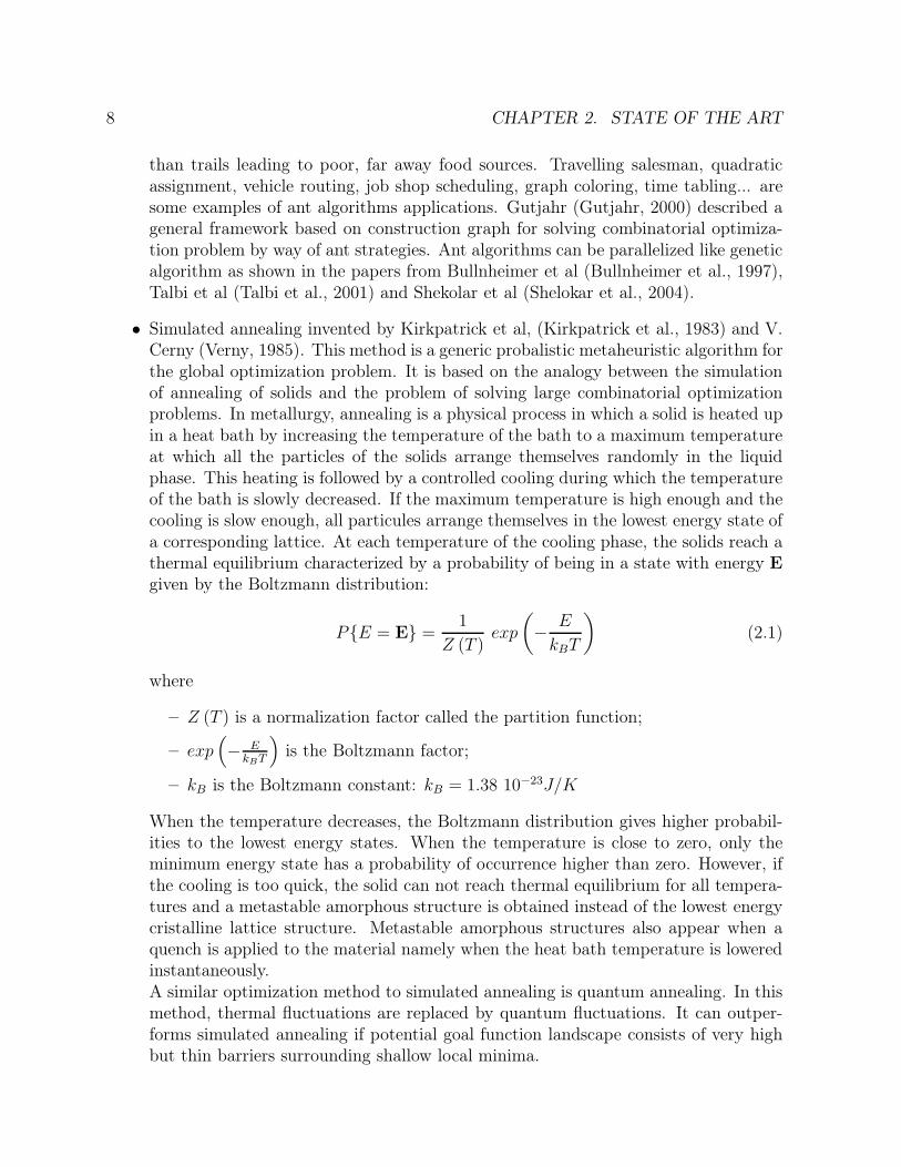
∙ Simulated annealing invented by Kirkpatrick et al, (Kirkpatrick et al., 1983) and V.Cerny (Verny, 1985). This method is a generic probalistic metaheuristic algorithm forthe global optimization problem. It is based on the analogy between the simulationof annealing of solids and the problem of solving large combinatorial optimizationproblems. In metallurgy, annealing is a physical process in which a solid is heated upin a heat bath by increasing the temperature of the bath to a maximum temperatureat which all the particles of the solids arrange themselves randomly in the liquidphase. This heating is followed by a controlled cooling during which the temperatureof the bath is slowly decreased. If the maximum temperature is high enough and thecooling is slow enough, all particules arrange themselves in the lowest energy state ofa corresponding lattice. At each temperature of the cooling phase, the solids reach athermal equilibrium characterized by a probability of being in a state with energy Egiven by the Boltzmann distribution:
P{E = E} =1
Z (T )exp
(− E
kBT
)(2.1)
where
– Z (T ) is a normalization factor called the partition function;
– exp(− E
kBT
)is the Boltzmann factor;
– kB is the Boltzmann constant: kB = 1.38 10−23J/K
When the temperature decreases, the Boltzmann distribution gives higher probabil-ities to the lowest energy states. When the temperature is close to zero, only theminimum energy state has a probability of occurrence higher than zero. However, ifthe cooling is too quick, the solid can not reach thermal equilibrium for all tempera-tures and a metastable amorphous structure is obtained instead of the lowest energycristalline lattice structure. Metastable amorphous structures also appear when aquench is applied to the material namely when the heat bath temperature is loweredinstantaneously.A similar optimization method to simulated annealing is quantum annealing. In thismethod, thermal fluctuations are replaced by quantum fluctuations. It can outper-forms simulated annealing if potential goal function landscape consists of very highbut thin barriers surrounding shallow local minima.

9
Data reconciliation
Kuehn and Davidson (1961) first used steady-state data reconciliation in industry. Theirobjective was to correct process data in a way to satisfy mass balances. Some years later,Vaclavek (Vaclavek, 1968), (Vaclavek, 1969) also worked on the variable classification prob-lem and on the formulation of the reconciliation model. Mah et al. suggested a procedure ofvariable classification based on graph theory (Mah et al., 1976). Crowe (Crowe, 1989) pro-posed an analysis based on a projection matrix method allowing to obtain a reduced system.A classification algorithm for general non linear equation systems was proposed by Jorisand Kalitventzeff (Joris and Kalitventzeff, 1987). Heyen et al (Heyen et al., 1996) proposeda method based on the Jacobian matrix analysis to perform sensibility analysis: influenceof the measurements and their accuracies on the accuracies of state variables, detection ofstate variables influenced by the accuracy of a particular measurement. Narasimhan andJordache (Narasimhan and Jordache, 2000) provide a detailed perspective on the historyof data reconciliation.
In the case of dynamic data reconciliation, several techniques exists. We were first in-terested in filtering techniques , in particular the Kalman filters, then our attention wasturned on the moving horizon methods.Kalman filter is said to be proposed by Kalman in 1960 (Kalman, 1960), (Kalman andBucy, 1961) though Thiele and Swerling developed a similar algorithm earlier. That algo-rithm was first implemented by Schmidt (Schmidt, 1980) to solve the trajectory estimationproblem for the Apollo program. This linear Kalman filter is used to carry out the recon-ciliation of linear dynamic processes.It has been extended to deal with non linear systems (Karjala and Himmelblau, 1996),(Narasimhan and Jordache, 2000): the non linear part of the model is linearized thanks toa first order Taylor serie around the current estimated. This second filter is called extendedKalman filter. Kalman filter are well described in (Rousseaux-Peigneux, 1988) and (Welchand Bishop, 2001). Some authors, compared the extended Kalman filter with the movinghorizon estimation (Jang et al., 1986), (Albuquerque and Biegler, 1995), (Haseltine andRawlings, 2005). They showed that the results obtained by the moving horizon estimationare better than the one obtained with the extended Kalman filter but at the cost of morecomputing ressources.A third method based on second order divided differences is also used in the case of nonlinear systems (Norgaard et al., 2000).Nowadays, a wide variety of filtering methods has been developed (see for example (Baiet al., 2006), (Moraal and Grizzle, 1995), (Chen et al., 2008))and is widely used in engi-neering applications such as radars, computer vision, autonomous or assisted navigation.
Jang et al (Jang et al., 1986) introduced in 1986 the notion the moving horizon technique.It has been used afterwards by several authors like (Kim et al., 1991), (Liebman et al.,1992), (McBrayer et al., 1998), (Kong et al., 2000), (Barbosa et al., 2000), (Vachhani et al.,2001), (Abu-el zeet et al., 2002).Differential equations can be discretized by means of orthogonal collocations. Frazer, Jones
10 CHAPTER 2. STATE OF THE ART
and Skan and Lanczos applied for the first time collocation methods to differential equa-tions in the thirties. Villadsen and his coauthor (Villadsen and Michelsen, 1978) haveshown that the collocation nodes chosen at the zeros of orthogonal polynomials give thebest results for the solving of differential equations. Other authors like Mingfang et al.(Kong et al., 2000) proposed to choose the measurement times as collocation nodes in thecase of dynamic data reconciliation.Biegler (Biegler, 1984) used orthogonal collocations to reduce the dynamic optimizationproblem to a constrained non linear optimization problem. He solved the resulting opti-mization problem thanks to a successive quadratic programming method. He also proposedto solve simultaneously collocation and process equations. Later, he presented with Albu-querque (Albuquerque and Biegler, 1995), (Albuquerque and Biegler, 1996) a method fordecomposing the optimization algorithm in a way to reduce the computing effort. Theirapproach is based on line search, hessian update (Gauss-Newton or BFGS), and quadraticprogramming subproblem solving in the parameters space. Some years after, Biegler andhis colleagues (Cervantes et al., 2000), (Biegler et al., 2002) applied an interior pointmethod to non linear programming problem: they developed a reduced space decompo-sition for the NLP problem and applied quasi-Newton methods to the reduced Hessian.That approach allowed them applying their decomposition method to orthogonal colloca-tions but it requires analytical derivatives. Kameswaran and Biegler (Kameswaran andBiegler, 2006), presented the advantages of simultaneous dynamic optimization strategies.Biegler and Lang (Biegler, 2007), (Lang and Biegler, 2007) described their simultaneousdynamic optimization method. In this method, they discretized state and input variablesusing collocations on finite elements. The differential equations are discretized by meansof Radau collocations because they allow constraints to be set at the end of each elementso that the system is better stabilized. Those authors also presented a description of theirmoving window.Kabouris and Georgakakos (Kabouris and Georgakavos, 1996) extended the simplified max-imum likelihood estimators for linear moving-window proposed by Maybeck in 1982. Thistechnique is theoretically advantageous compared to the bayesian estimation approach thatleads to the extended Kalman filter.Barbosa et al (Barbosa et al., 2000) also transformed the differential equations using or-thogonal collocations. They solved the constrained non linear problem using a successivequadratic programming method. BFGS (Broyden-Fletcher-Goldfrab-Shanno) techniquewas used to update the hessian matrix.Vacchani et al (Vachhani et al., 2001) proposed a two-level approach to perform non lin-ear dynamic data reconciliation and parameter bias detection. The first level consists ofidentifying biased parameter by means of fault diagnosis methods. In the second level,the non linear programming problem is solved so that measurement are reconciled andthe biased parameter is estimated. In 2006, they combined the unscented Kalman filterused for non linear systems with recursive non linear dynamic data reconciliation (Vach-hani et al., 2006). Their approach called the unscented recursive non linear dynamic datareconciliation is able to achieve state and parameter estimation. Accuracies of estimates isimproved because the non linearity is not approximated during state and error covariance
11
matrix estimation.Kim et al (Kim et al., 1990) compared three non linear error-in-variables parameter es-timation: simultaneous parameter estimation and data reconciliation, two-stage error-in-variables using non linear programming and nested error-in-variables using non linear pro-gramming. They concluded that two-stage error-in-variables using non linear programmingis superior with respect to robustness and computing efficiency, and is recommended invery non linear regions. They proposed a sequential approach based on numerical inte-gration for parameter estimation and compared it with least-square based methods andnon linear dynamic estimation using orthogonal collocations (Kim et al., 1991). Their nonlinear dynamic error-in-variable model gave better estimates than the least-square basedmethods, especially in presence of measurement bias. It is faster than the approach usingorthogonal collocations and the optimization problem to be solved is smaller. Liebmanet al (Liebman et al., 1992) presented a similar technique which is no longer limited toproblem without constraints on the states. The method is able to performs as well dynamicdata reconciliation as steady-state data reconciliation, it can estimate unknown parametersand unmeasured input variables. Liebman et al described the discretization of the differ-ential equations by means of orthogonal collocations, thus generating a set of algebraicconstrained equations. The time horizon is briefly described as well as the jacobian matrixof the constraints. The method is illustrated on a reactor test case that has become a wellknown reference. The approach was extended by McBrayer et al (McBrayer et al., 1998)so that it allowed measurement bias detection.Renfro et al suggested (Renfro et al., 1987) to use the spline collocations instead of or-thogonal collocations. The advantage of those collocations is that they allow to optimizelarger and more difficult systems. Like Kameswaran and Biegler (Kameswaran and Biegler,2006), they recommended a simultaneous approach for optimization and discretization.Chen and Romagnoli (Chen and Romagnoli, 1998) suggested a formulation of dynamicdata reconciliation that includes the outlier information so that dynamic data reconcilia-tion and outliers detection can be carried out simultaneously.Raff et al (Raff et al., 2005) suggested a moving window state estimation approach withglobal guaranteed convergence. In that method, they integrated optimization-based esti-mators and observability maps in the moving window approach.Bagajewicz and Jiang (Bagajewicz and Jiang, 1997) presented a technique for dynamicdata reconciliation based on an integral form of the equation system. This approach canbe used in the presence of gross errors.Binder et al (Binder et al., 1998) presented a deterministic formulation of the dynamic datareconciliation problem. That formulation is based on the theory of inverse problems. Theyalso proposed a mathematical framework based on multiscale techniques for the discretiza-tion of the problem and for the solution of the discretized non linear equation system.Then they proposed a method to generate automatically a hierarchy of discretization gridsto reach the best compromise between data and regulation error (Binder et al., 2002).Wongrat et al (Wongrat et al., 2005) solved the problem of non-linear steady-state datareconciliation using genetic algorithm. In this method, the parameters of the genetic algo-rithm are first of all searched before the data reconciliation problem is solved. The method

12 CHAPTER 2. STATE OF THE ART
is more time consuming than the other ones.
Fault detection
Gross errors and systematic biases must generally be eliminated before data reconciliationis carried out.In the twenties, Shewhart invented the concept of control charts.In the sixties and the seventies three types of statistical tests have been proposed forgross error detection (Reilly and Carpani, 1963), (Almasy, 1975) and (Mah et al., 1976).They are based on the residuals, individually or collectively (chi-square tests). Mah andTamhane (Mah and Tamhane, 1982) proposed an identification test to identify the sourcesand location of gross errors.Romagnoli and Stephanopoulos (Romagnoli and Stephanopoulos, 1981) presented a tech-nique to analyse a set of measurements in the presence of gross errors. Based on thecriterion of satisfaction of mass and energy balances, the method allows to quickly identifythe source of errors. It work by serial deletion of one or more measurements from the setwithout requiring each time a new computation of the problem because available informa-tion coming from the original problem is used.Narasimhan and Mah (Narasimhan and Mah, 1987) proposed a general method for iden-tifying gross errors for steady-state processes. Their generalized likelihood ratio techniqueis based on the likelihood ratio statistical test. It allows the identification of all types ofgross errors. They also developed a strategy that allows to identify multiple gross errorsby using serial compensation of gross errors. Those authors extended their method todynamic processes (Narasimhan and Mah, 1988).Amand et al (Amand, 1999) and (Amand et al., 2001) developed a method to detect faultin chemical processes based on principal component analysis combined with data reconcili-ation. This method allows to reduce the number of variables that have to be monitored. Itis decomposed in two steps: the fault detection (if some components are out of their con-fidence region) and the cause localisation (by estimation of the effect of those componentson the original variables). In 2002, Wang et al (Wang et al., 2002) improved the principalcomponent analysis technique. They replaced the Q statistic used in conventional prin-cipal component analysis by two new statistics: the principal-component-related variableresiduals and the common variables residuals.Jia et al (Jia et al., 1998) proposed a non linear principal component analysis techniquebased on the input-training neural network. They defined multivariate statistical processcontrol charts with non-parametric control limits instead of the traditional limits based onthe normality assumption.Ragot et al proposed (Ragot et al., 2003) a blind approach to detect and isolate sensorfaults. That method does not need any knowledge about the process model. It is onlybased on the analysis of the data so that it requires strong hypothesis about the input sig-nals of the studied process. Later (Ragot and Maquin, 2006), they developed a techniquefor fault measurement detection in an urban water network. We used this method based
13
on the analysis of the signature matrix and fuzzy rules for the design of sensor networksallowing to detect and locate process faults.Mc Brayer and Edgar (McBrayer and Edgar, 1995) proposed a method for bias detectionand estimation for dynamic processes. Their method is based on the examination of theresiduals.Kong et al (Kong et al., 2004) developed a gross error identification strategy based onparameter estimation. This method suits for dynamic processes and allow the detection ofsimultaneous measurement gross errors. They described the condition for which a systemis identifiable for gross error detection: let the system of equations:
{dxdt
= f (x, u)dxdt
= f (x+ �x, u+ �u)
If the column vectors of ▽f are linearly independent, the system of equations has a uniquesolution of �x and �u and then the system is identifiable for gross error detection. Theauthors obtained the same conclusion for differential algebraic equation systems.Bagajewicz and Jiang (Bagajewicz and Jiang, 1998) developed a technique for multiplegross error detection based on the integral approach for linear dynamic data reconciliationthey presented earlier (Bagajewicz and Jiang, 1997).Wang et al (Wang et al., 2004) presented an improvement in the measurement test - nodaltest proposed by Yang. Their approach is used to solve the decrease of matrix rank in grosserror detection and data reconciliation. Gross errors are detected before being correctedby successive iterations.Bhagwat et al (Bhagwat et al., 2003a), (Bhagwat et al., 2003b) presented a method todetect process fault during the transition operations. In this model-based fault detectionscheme, non linear transient systems are decomposed into multiple linear modeling regimes.State estimation and residuals computation are carried out by means of Kalman filters andopen-loop observers. On-line detection and localisation of faults are enabled thanks toresiduals analysis by means of thresholds, fault tags and logic charts.


Part I
Network design for steady-state
processes
15


Chapter 3
Steady-state data reconciliation
Chemical plants must be efficiently monitored to allow production accounting as well asfor the enforcement of safety and environmental rules. Process control can only take placeif enough measurements are carried out on the plant. Those measurements and laboratoryanalysis are generally erroneous. So information about the process is inaccurate, the state ofthe process at a certain time is misrepresented and the control of the plant is not as efficientas it could be so that the process conditions may be not met, the efficiency indicators maybe badly estimated and the safety rules may be unsatisfied. Some errors come from themeasurement tool itself: indeed, each sensor has a limited precision. Moreover, most ofthe sensors must be calibrated regularly to avoid systematic errors due to a sensor givingalways an under or an over estimated value. Finally, during the transmission and theconversion of the signal, noise is added to the initial measurement value. Another sourceof error comes from the fact that the measurement frequency depends on the kind of sensor:the fastest measurements are carried out in some seconds while compositions analysis cantake up to several hours. It is thus impossible to have the information about the wholeplant at a precise time. This problem can be partly solved by taking average values ofmeasurements that can be done in the case of steady-state processes. The location of thesensors in the unit is also important for the validity of measurements: indeed, the valuewill be different following, for example, if the sensor is placed in the middle of a reactor ornear its walls, or if the region where the sensor is placed is turbulent or not. Finally grosserrors can appear if a sensor fails.The relationship between a measurement of a variable and its true value can be representedas follow:
ymeasured = ytrue + ey (3.1)
where
∙ ymeasured is the measured value of the variable y;
∙ ytrue is the true value of the variable y;
∙ ey is the error on the variable y.
17
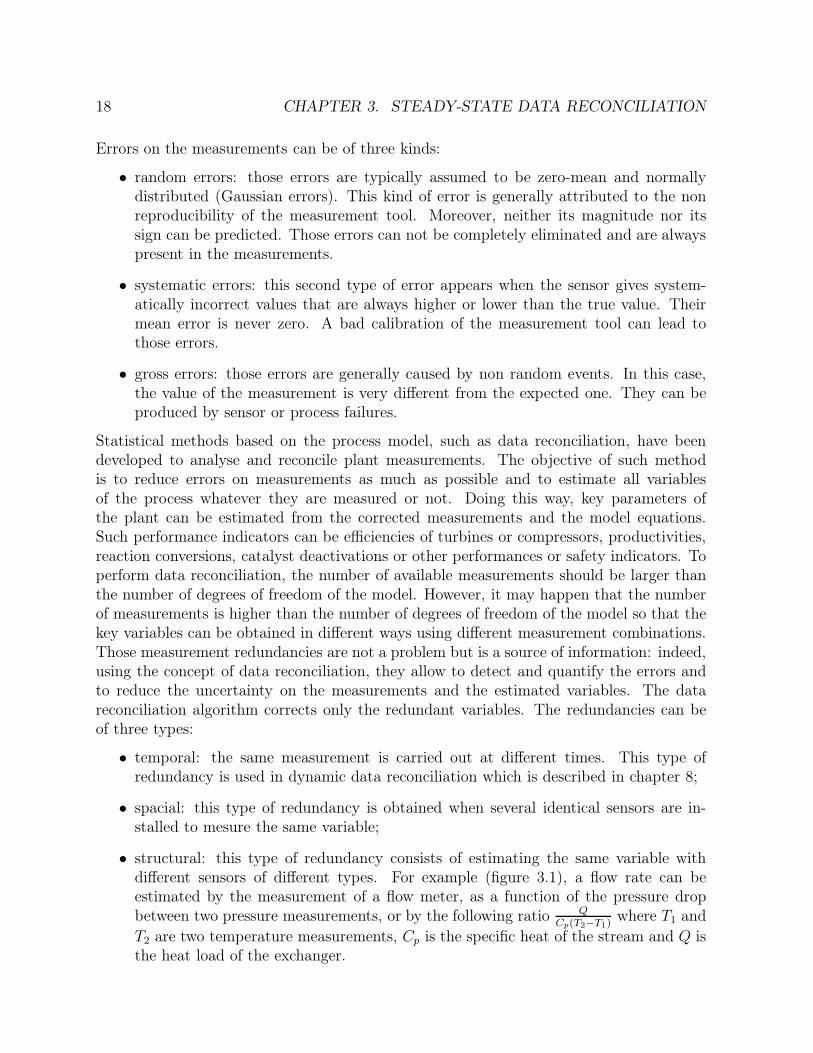
18 CHAPTER 3. STEADY-STATE DATA RECONCILIATION
Errors on the measurements can be of three kinds:
∙ random errors: those errors are typically assumed to be zero-mean and normallydistributed (Gaussian errors). This kind of error is generally attributed to the nonreproducibility of the measurement tool. Moreover, neither its magnitude nor itssign can be predicted. Those errors can not be completely eliminated and are alwayspresent in the measurements.
∙ systematic errors: this second type of error appears when the sensor gives system-atically incorrect values that are always higher or lower than the true value. Theirmean error is never zero. A bad calibration of the measurement tool can lead tothose errors.
∙ gross errors: those errors are generally caused by non random events. In this case,the value of the measurement is very different from the expected one. They can beproduced by sensor or process failures.
Statistical methods based on the process model, such as data reconciliation, have beendeveloped to analyse and reconcile plant measurements. The objective of such methodis to reduce errors on measurements as much as possible and to estimate all variablesof the process whatever they are measured or not. Doing this way, key parameters ofthe plant can be estimated from the corrected measurements and the model equations.Such performance indicators can be efficiencies of turbines or compressors, productivities,reaction conversions, catalyst deactivations or other performances or safety indicators. Toperform data reconciliation, the number of available measurements should be larger thanthe number of degrees of freedom of the model. However, it may happen that the numberof measurements is higher than the number of degrees of freedom of the model so that thekey variables can be obtained in different ways using different measurement combinations.Those measurement redundancies are not a problem but is a source of information: indeed,using the concept of data reconciliation, they allow to detect and quantify the errors andto reduce the uncertainty on the measurements and the estimated variables. The datareconciliation algorithm corrects only the redundant variables. The redundancies can beof three types:
∙ temporal: the same measurement is carried out at different times. This type ofredundancy is used in dynamic data reconciliation which is described in chapter 8;
∙ spacial: this type of redundancy is obtained when several identical sensors are in-stalled to mesure the same variable;
∙ structural: this type of redundancy consists of estimating the same variable withdifferent sensors of different types. For example (figure 3.1), a flow rate can beestimated by the measurement of a flow meter, as a function of the pressure dropbetween two pressure measurements, or by the following ratio Q
Cp(T2−T1)where T1 and
T2 are two temperature measurements, Cp is the specific heat of the stream and Q isthe heat load of the exchanger.

3.1. FORMULATION FOR NON LINEAR STEADY-STATE SYSTEMS 19
F
F1 ΔP
F2 = f(ΔP )
T1 T2
F3 =Q
Cp(T2 − T1)
Q
Figure 3.1: Flow rate measurements
Kuehn and Davidson (Kuehn and Davidson, 1961) were the first to use steady-state datareconciliation in industry. Their objective was to correct process data so that the massbalances were satisfied. Nowadays data reconciliation methods correct energy balances aswell as mass balances.
3.1 Formulation for non linear steady-state systems
This section on data reconciliation treats non linear steady-state problems where all vari-ables are not necessary measured. The equations of the model are mass, component andenergy balances, equilibrium equations and link equations that relates measurements tostate or key variables. This reconciliation problem can be formulated this way:
minx,z
(x − y)T W (x − y)
s.t. f (x, z) = 0 (3.2)
where
∙ x is the vector of estimated variables (size= m);
∙ y is the vector of measured variables (size= m);
∙ z is the vector of unmeasured variables (size= n);
∙ W is the weight matrix (usually the inverse of the measurements errors covariance)(size= m x m);
∙ f (x, z) are the link equations.
This constrained minimization problem can be transformed into an unconstrained mini-mization problem using the vector of Lagrange multipliers Λ:
minx,z,Λ
L (x, z,Λ) = (x − y)T W (x − y) + 2 ΛT f (x, z) (3.3)
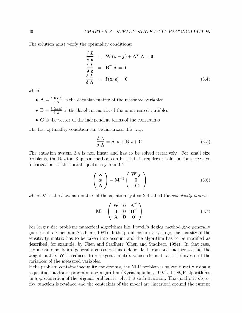
20 CHAPTER 3. STEADY-STATE DATA RECONCILIATION
The solution must verify the optimality conditions:
� L
� x= W (x − y) + AT
Λ = 0
� L
� z= BT
Λ = 0
� L
� Λ= f (x, z) = 0 (3.4)
where
∙ A = � f(x,z)� x
is the Jacobian matrix of the measured variables
∙ B = � f(x,z)� z
is the Jacobian matrix of the unmeasured variables
∙ C is the vector of the independent terms of the constraints
The last optimality condition can be linearized this way:
� L
� Λ= A x + B z + C (3.5)
The equation system 3.4 is non linear and has to be solved iteratively. For small sizeproblems, the Newton-Raphson method can be used. It requires a solution for successivelinearizations of the initial equation system 3.4:
⎛⎝
xzΛ
⎞⎠ = M−1
⎛⎝
W y0-C
⎞⎠ (3.6)
where M is the Jacobian matrix of the equation system 3.4 called the sensitivity matrix :
M =
⎛⎝
W 0 AT
0 0 BT
A B 0
⎞⎠ (3.7)
For larger size problems numerical algorithms like Powell’s dogleg method give generallygood results (Chen and Stadherr, 1981). If the problems are very large, the sparsity of thesensitivity matrix has to be taken into account and the algorithm has to be modified asdescribed, for example, by Chen and Stadherr (Chen and Stadherr, 1984). In that case,the measurements are generally considered as independent from one another so that theweight matrix W is reduced to a diagonal matrix whose elements are the inverse of thevariances of the measured variables.If the problem contains inequality constraints, the NLP problem is solved directly using asequential quadratic programming algorithm (Kyriakopoulou, 1997). In SQP algorithms,an approximation of the original problem is solved at each iteration. The quadratic objec-tive function is retained and the contraints of the model are linearized around the current

3.1. FORMULATION FOR NON LINEAR STEADY-STATE SYSTEMS 21
estimate of the solution.Once the problem has converged, a sensitivity analysis can be carried out using the lin-earized equation system 3.6. This equation system shows that the reconciled values ofvariables x, z and Λ are linear combinations of the measurements. So, the sensitivitymatrix M allows to evaluate how the reconciled values of the model variables depend onthe measurements and their standard deviations. x and z variables are thus estimated thisway:
xi =
m+n+p∑
j=1
(M)−1i,j
⎛⎝
W y0-C
⎞⎠
j
=m∑
j=1
(M)−1i,j Wi,j yj −
p∑
j=1
(M)−1i,m+n+j Cj (3.8)
zi =
m+n+p∑
j=1
(M)−1m+i,j
⎛⎝
W y0-C
⎞⎠
j
=m∑
j=1
(M)−1m+i,j Wi,j yj −
p∑
j=1
(M)−1m+i,m+n+j Cj (3.9)
where
∙ m is the number of measured variables;
∙ n is the number of unmeasured variables;
∙ p is the number of equations of the model.
Knowing that the variance of a linear combination LC of several variables xi is given by:
LC =m∑
i=1
ai xi (3.10)
var (LC) =
m∑
i=1
ai2 var (xi) (3.11)
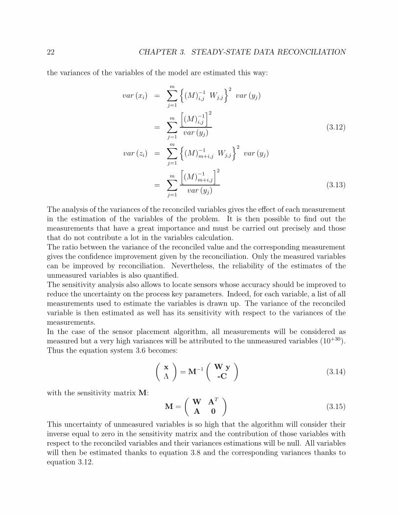
22 CHAPTER 3. STEADY-STATE DATA RECONCILIATION
the variances of the variables of the model are estimated this way:
var (xi) =
m∑
j=1
{(M)−1
i,j Wj,j
}2
var (yj)
=
m∑
j=1
[(M)−1
i,j
]2
var (yj)(3.12)
var (zi) =m∑
j=1
{(M)−1
m+i,j Wj,j
}2
var (yj)
=m∑
j=1
[(M)−1
m+i,j
]2
var (yj)(3.13)
The analysis of the variances of the reconciled variables gives the effect of each measurementin the estimation of the variables of the problem. It is then possible to find out themeasurements that have a great importance and must be carried out precisely and thosethat do not contribute a lot in the variables calculation.The ratio between the variance of the reconciled value and the corresponding measurementgives the confidence improvement given by the reconciliation. Only the measured variablescan be improved by reconciliation. Nevertheless, the reliability of the estimates of theunmeasured variables is also quantified.The sensitivity analysis also allows to locate sensors whose accuracy should be improved toreduce the uncertainty on the process key parameters. Indeed, for each variable, a list of allmeasurements used to estimate the variables is drawn up. The variance of the reconciledvariable is then estimated as well has its sensitivity with respect to the variances of themeasurements.In the case of the sensor placement algorithm, all measurements will be considered asmeasured but a very high variances will be attributed to the unmeasured variables (10+30).Thus the equation system 3.6 becomes:
(xΛ
)= M−1
(W y-C
)(3.14)
with the sensitivity matrix M:
M =
(W AT
A 0
)(3.15)
This uncertainty of unmeasured variables is so high that the algorithm will consider theirinverse equal to zero in the sensitivity matrix and the contribution of those variables withrespect to the reconciled variables and their variances estimations will be null. All variableswill then be estimated thanks to equation 3.8 and the corresponding variances thanks toequation 3.12.

Chapter 4
Description of the optimal sensor
network design algorithm
In this chapter, a method to design the best sensor networks for the steady-state case willbe proposed. The networks suggested by the method should be the less expensive onesthat allow to satisfy all the following constraints:
∙ all the variables of the process should be computable, even unmeasurable variables(efficiency of a particular unit, reaction conversion...);
∙ all key variables should be estimated within a prescribed accuracy;
∙ if the process has several operating modes, the sensor network should be able tosatisfy the two first conditions for all of them;
∙ sometimes, one may want to be sure that the sensor network will be able to satisfy thetwo first conditions even in the case of one sensor failure or if one sensor is switchedoff for maintenance. So, one has to test those conditions for all configurations of thesensor network obtained by switching off one sensor.
In most of the cases, the objective function of this problem is multimodal. Moreover, theproblem is not derivable and contained a large number of binary parameters (the sensorsare chosen or not) so that a genetic algorithm is used to perform the optimization. Theimplementation that is adopted is based on the freeware code developed by Carroll (Carroll,2001). The selection of individuals involves tournament selection with a shuffling techniquefor choosing pairs for mating. The evolution algorithm includes single-point cross-over andjump mutation. Evolution algorithms are described in annex A.
The optimal sensor network design algorithm is carried out in five steps, which are describedin details in this chapter:
1. Formulation of the reconciliation model and model linearisation;
2. Specification of sensor database, precision requirements and sensor requirements;
23
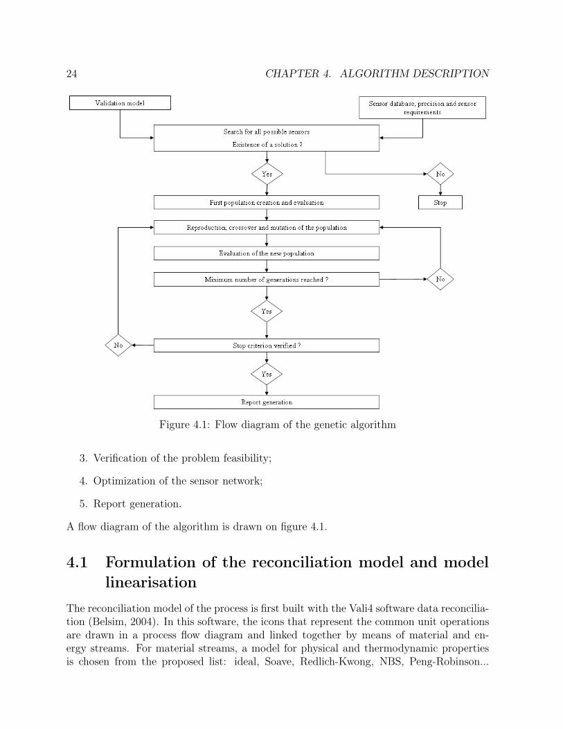
24 CHAPTER 4. ALGORITHM DESCRIPTION
Figure 4.1: Flow diagram of the genetic algorithm
3. Verification of the problem feasibility;
4. Optimization of the sensor network;
5. Report generation.
A flow diagram of the algorithm is drawn on figure 4.1.
4.1 Formulation of the reconciliation model and model
linearisation
The reconciliation model of the process is first built with the Vali4 software data reconcilia-tion (Belsim, 2004). In this software, the icons that represent the common unit operationsare drawn in a process flow diagram and linked together by means of material and en-ergy streams. For material streams, a model for physical and thermodynamic propertiesis chosen from the proposed list: ideal, Soave, Redlich-Kwong, NBS, Peng-Robinson...
4.2. FILES OF REQUIREMENTS 25
The values of some measurements are specified in the Vali4 software. The number of themeasurements must at least be equal to the number of degrees of freedom of the processto allow the equation system to be solved. Redundancy gives supplementary informationand the reconciliation algorithm gives a least square solution. As all variables are notstate variables (enthalpy, pressure, partial molar flow rate...), the Vali4 software writesautomatically the link equations for standard measurements types that are not state vari-ables (mass flow rates, molar fractions, temperatures...). For non-standard unmeasuredvariables (heat transfert coefficient, compressor efficiency, pressure drop, reaction conver-sion...), which need often to be known within a prescribed accuracy, links equations haveto be created. Once the process is modeled, the reconciliation problem is solved usingeither the Lagrange multiplier method or the SQP solver. When the solution is obtained,the sensitivity analysis is carried out (Heyen et al., 1996) and a report file is generated. Itcontains the value of all variables and their reconciled accuracy, the linearised equationsand the non-zero coefficients of the jacobian matrix. As the equations of the model arelinearised at the operating point, a report is needed for each operating point for whichthe measurement system has to be designed. Moreover, a report is necessary for the firstoperating point calculated with ideal thermodynamics. Indeed, in certain thermodynamicmodels, the enthalpy is lightly influenced by the pressure. So, in the jacobian matrix ofthe constraints, zeros are replaced by the contributions of the pressures on the enthalpies.The sensitivity matrix is thus a little different from the one obtained with the ideal ther-modynamic. To ensure that the observability criterion, which is the non singularity of thesensitivity matrix, is satisfied, the chosen sensor network has to be tested on the sensitiv-ity matrix corresponding to the ideal thermodynamic. The thermodynamic specific to themodel are used to estimate properly the values of a posteriori variances.
4.2 Specification of sensor database, precision require-
ments and sensor requirements
Besides the Vali4 reports, the program needs three data files. Those files contain the sensordatabase, the precision requirements and the sensor requirements.
4.2.1 Sensor database
The sensor database is a list of sensors from which the algorithm must choose all thepossible sensor placements for the studied plant. It must include, for each sensor, thefollowing information:
∙ the name of the sensor;
∙ the annualized cost of the sensor. This cost must take into account:

26 CHAPTER 4. ALGORITHM DESCRIPTION
– the annualized purchase cost;
– the annualized installation cost;
– the annualized operating cost.
All those costs depend on the studied process: indeed, for example, the cost of thesensor will be different if it is placed in a flow of water or if it must resists to acid orbase.
∙ the parameters �Aiand �Bi
that allow the estimation of the sensor standard deviation�j for the measured variable X
′
j :
�j = �Ai+ �Bi
∗X ′
j (4.1)
∙ the type of measurement place:
– S for a stream variable (temperature, pressure);
– M for a mixing variable (flowrate, concentration);
– U for a unit variable (efficiency of the unit);
∙ the minimal and maximal values of the sensor measurement range;
∙ the type of variable the sensor is able to measure. Types of variable are defined asin Vali4 :
– T for a temperature;
– P for a pressure;
– DP* for a pressure drop;
– MF* for a molar fraction;
– MOLF for a molar flow rate;
– MASSF for a mass flow rate.
4.2.2 Precision requirements
In this file, key variables that have to be known precisely are listed with their requiredtarget accuracy (maximum standard deviation). Those variables are, for instance, turbineefficiency, catalyst deactivation, productivity, reactive conversion...At each generation of the genetic algorithm, it is checked whether the key variables accu-racies are achieved or not. In the case they are not acceptable, a penalty is added to thegoal function of the optimization problem; otherwise, a bonus is added.
4.3. VERIFICATION OF THE PROBLEM FEASIBILITY 27
4.2.3 Sensor requirements
A file is proposed to list
∙ existing sensors that should not be removed;
∙ plant locations where sensor placements have to be avoided;
∙ plant locations where sensor locations are mandatory.
4.3 Verification of the problem feasibility
This step of the program begins by computing the list of all the sensors that can be placedin the plant. Each chromosome created by the algorithm will contain a number of binarydecisions equal to the maximum number of sensors. The binary genes take the value 1 or 0depending if the corresponding sensors are chosen or not. To check the problem feasibility,the algorithm first generates an individual whose genes are all set to "1", thus implementingall possible sensors. This is the most expensive solution, but it should also result in themost precise estimates for the key process variables. Thus, if the required precision is notarchived for this solution, one may conclude that the problem has no solution. If severalsensors measure the same variables, only the variance of the most accurate one is takeninto account.To ensure there exists a solution to the studied problem, the two following conditions haveto be met:
∙ The sensitivity matrix of the problem is non-singular for the ideal thermodynamiccase as well as for all operating points. If this condition is not met, the programstops.
∙ The accuracies on all key parameters have to be acceptable. If this condition is notmet, the program may continue, but a penalty is added to the goal function.
There are different ways to cure those problems:
∙ adding more accurate sensors to the data base;
∙ adding sensors able to measure other types of variable;
∙ adding more extra measurable variables so that more variables can be measured.
Individuals of the first generation are chosen randomly by biasing the initial chromosome:to be sure that the number of chosen sensors is at least equal to the number of degrees offreedom of the problem, a high probability of selection if fixed for each sensor. A valueof 80 % is typically chosen but this parameter appears not to be critical for the problemof optimal sensor design. For the other parameters of the genetic algorithm, the followingvalues are generally chosen:
28 CHAPTER 4. ALGORITHM DESCRIPTION
∙ the population size, which does not either appear to be critical , was most of thetime chosen to 20 individuals per population;
∙ the probability of reproduction was fixed to 50 %;
∙ the probability of single-point cross-over was chosen to 50 %
∙ the probability of jump mutation after reproduction and cross-over is 1 %.
4.4 Optimization of the sensor network
Knowing that a feasible solution exists, the search for the optimal sensor configuration canbegin. The fitness function is evaluated as follows:
∙ If the sensitivity matrix is singular:
Fitness = −Cmax penaltysingular matrix (4.2)
where
– Cmax is the cost relative to the most expensive sensor network which correspondsto the first chromosome;
– penaltysingular matrix is the penalty factor for a singular sensitivity matrix and isgenerally chosen equal to 2.
∙ otherwise
Fitness = −cost −Nkey variables∑
i=1
⎧⎨⎩
− �i
�targeti
�2
i(�targeti
)2
Cmax penaltytarget
Nkey variables
102Cmax penaltytarget
Nkey variables
if �i
�targeti
≤ 1
if 1 < �i
�targeti
< 10
if �i
�targeti
≥ 10
(4.3)where
– Nkey variables is the number of process key variables;
– penaltytarget is the penalty factor for the targets on key parameters that are notrespected and is fixed equal to 2;
– �i is the accuracy obtained by the sensor network for the key variable i ;
– �targeti is the accuracy required for the key parameter i.
In this second case, a penalty is added to the objective function if the requiredaccuracy on a key parameter is not satisfied. Otherwise a gain is added.

4.5. REPORT GENERATION 29
If the sensor network has to be available for several operating points, the fitness becomes:
Fitness =
Noperating points∑
j=1
fitnessj − (Noperating points − 1) cost (4.4)
where Noperating points is the number of operating points.If a measurement system observable in the case of one sensor failure has to be carried out,the fitness is evaluated for all configurations obtained by eliminating successively one ofthe sensors, and the worst one is kept.Once the population has been generated the goal function has to be evaluated. In or-der to estimate reconciled variances of all variables, the sensitivity matrix correspondingto the specific thermodynamic has to be inverted before a posteriori variances are esti-mated by means of equations 3.6. The sensitivity matrix being symmetric, the subroutine"MA29AD" from Harwell library (Harwell, 1990), which allows to factorize a symmetricmatrix, was first used. However, the problem that is attempted to be solved contains alarge number of variables and equations and its sensitivity matrix is very sparse. Thus asparse matrix factorisation code, available in Belsim, was selected. This code is based onthe algorithm proposed by Chen and Stadherr (Chen and Stadherr, 1984). It allows toreduce the computing time by 25 for matrices of size 300 so that it was finally chosen.At each generation, the best individual is kept and duplicated in the case it would mutateduring the next generation.If after a specified number of generations (n) the best chromosome remains unchanged, itis considered has the solution of the problem. There is no certainty that this solution isthe best one, but it is available and much better than the first individual.The computing times to reach the solution with the algorithm can be very important forlarge scale problems has it is illustrated in annex B. That is why parallelization has beenused as described in chapter 5. Parallelization results are presented on chapter 6.
4.5 Report generation
At the last step, the programme generates a report containing the list of all possible sensorsand the list of chosen sensors with their location. It also gives, for the key parameters,a comparison between the accuracies obtained by the best network and the target ones.Finally, files containing the name of the variables with their values, a priori accuracies andphysical units are generated. Those files can be used as measurements files directly in theVali4.


Chapter 5
Case studies
Several processes have been studied to test the performance of the algorithm and comparethe ways it has been parallelized. Four of them are described in this chapter:
∙ an ammonia synthesis loop: this process is a middle size problem (224 variables)whose data have been obtained by simulation;
∙ a combined cycle electricity generation plant: the size of this problem is similar tothe ammonia synthesis loop (260 variables) but the values of the variables have beencollected by measurement;
∙ a ketene cracker: this problem is a quite larger size problem (631 variables) whosevariables have also been measured;
∙ a naphta reformer: this process is a larger size problem (1263 variables) whose datahave been obtained by simulation;
For all the examples, genetic algorithm as been stopped after 200 generations without anyprogress.
5.1 Ammonia synthesis loop
5.1.1 Process description
The gas interring into the plant (see figure 5.2), composed of nitrogen, hydrogen, argon andmethane, is compressed to 280 bar by a two stages compressor with two intercoolers. Athird compressor stage allows to compress the recycled gas. The gas is then heated beforeentering the reactor where the ammonia synthesis takes place. The reactor product mustbe cooled and partially condensed to recover the ammonia. This cooling takes place in foursteps: the gaseous products first go through a waste heat boiler, then they heat the reactorfeed, they are chilled in a water cooled exchanger, and finally in the evaporator of anammonia refrigeration loop. The condensation product is later flashed to a lower pressure
31

32 CHAPTER 5. CASE STUDIES
so that ammonia with a purity of 99.9 % can be obtained at the exit of the flash drum.The gaseous stream that exits the liquid-vapor separator is recycled to recover unreactedhydrogen. A part of this stream must however be purged to avoid accumulation of inerts.This process is composed of:
∙ 14 units: 1 two-stage compressor with two intercoolers, 1 ammonia converter, 1recycle mixer, 1 recycle compressor, 1 reactor preheater, 1 waste heat boiler, 1 wasteheat condenser, 1 purge divider, 1 liquid-vapor separator and 1 flash drum;
∙ 19 material streams composed of ammonia, argon, methane, hydrogen and nitrogen;
∙ 10 utility streams composed of steam and cooling water;
∙ 4 mechanical streams;
∙ 224 variables;
∙ 177 constraints equations.
Key parameters
The process comprises 52 key parameters to be monitored. They are listed with theirprescribed standard deviations in the table below (Table 5.1).
Table 5.1: Ammonia synthesis loop: prescribed standard deviations on key parameters
Variable name Standard deviationAmmonia partial molar flow rate of stream AM1 5 %Mass flow rate of stream BFW 2 %Temperature of stream BFW 1 KPressure of stream BFW 0.5 barMass flow rate of stream CW1 2 %Temperature of stream CW1 1 KPressure of stream CW1 0.1 barTemperature of stream CWR1 1 KPressure of stream CWR1 1 %Mass flow rate of stream CW2 2 %Pressure of stream CWR2 1 %Mass flow rate of stream CW3 2 %Pressure of stream CWR3 1 %Temperature of stream STM 1 KPressure of stream STM 0.5 bar
continued on next page
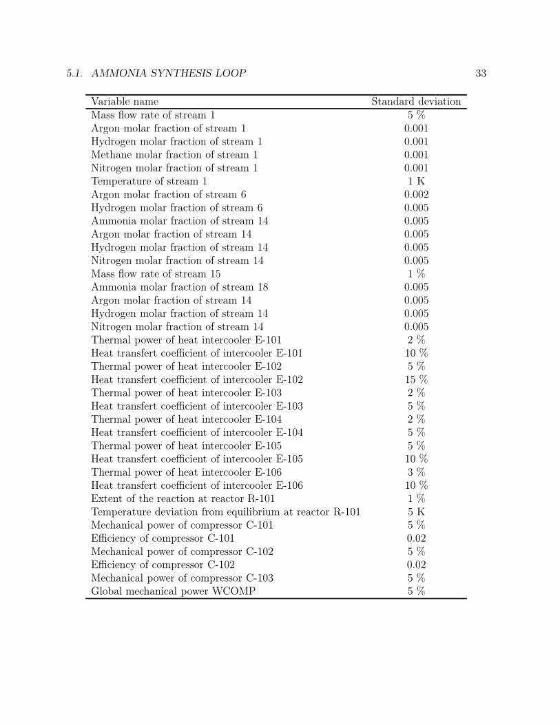
5.1. AMMONIA SYNTHESIS LOOP 33
Variable name Standard deviationMass flow rate of stream 1 5 %Argon molar fraction of stream 1 0.001Hydrogen molar fraction of stream 1 0.001Methane molar fraction of stream 1 0.001Nitrogen molar fraction of stream 1 0.001Temperature of stream 1 1 KArgon molar fraction of stream 6 0.002Hydrogen molar fraction of stream 6 0.005Ammonia molar fraction of stream 14 0.005Argon molar fraction of stream 14 0.005Hydrogen molar fraction of stream 14 0.005Nitrogen molar fraction of stream 14 0.005Mass flow rate of stream 15 1 %Ammonia molar fraction of stream 18 0.005Argon molar fraction of stream 14 0.005Hydrogen molar fraction of stream 14 0.005Nitrogen molar fraction of stream 14 0.005Thermal power of heat intercooler E-101 2 %Heat transfert coefficient of intercooler E-101 10 %Thermal power of heat intercooler E-102 5 %Heat transfert coefficient of intercooler E-102 15 %Thermal power of heat intercooler E-103 2 %Heat transfert coefficient of intercooler E-103 5 %Thermal power of heat intercooler E-104 2 %Heat transfert coefficient of intercooler E-104 5 %Thermal power of heat intercooler E-105 5 %Heat transfert coefficient of intercooler E-105 10 %Thermal power of heat intercooler E-106 3 %Heat transfert coefficient of intercooler E-106 10 %Extent of the reaction at reactor R-101 1 %Temperature deviation from equilibrium at reactor R-101 5 KMechanical power of compressor C-101 5 %Efficiency of compressor C-101 0.02Mechanical power of compressor C-102 5 %Efficiency of compressor C-102 0.02Mechanical power of compressor C-103 5 %Global mechanical power WCOMP 5 %
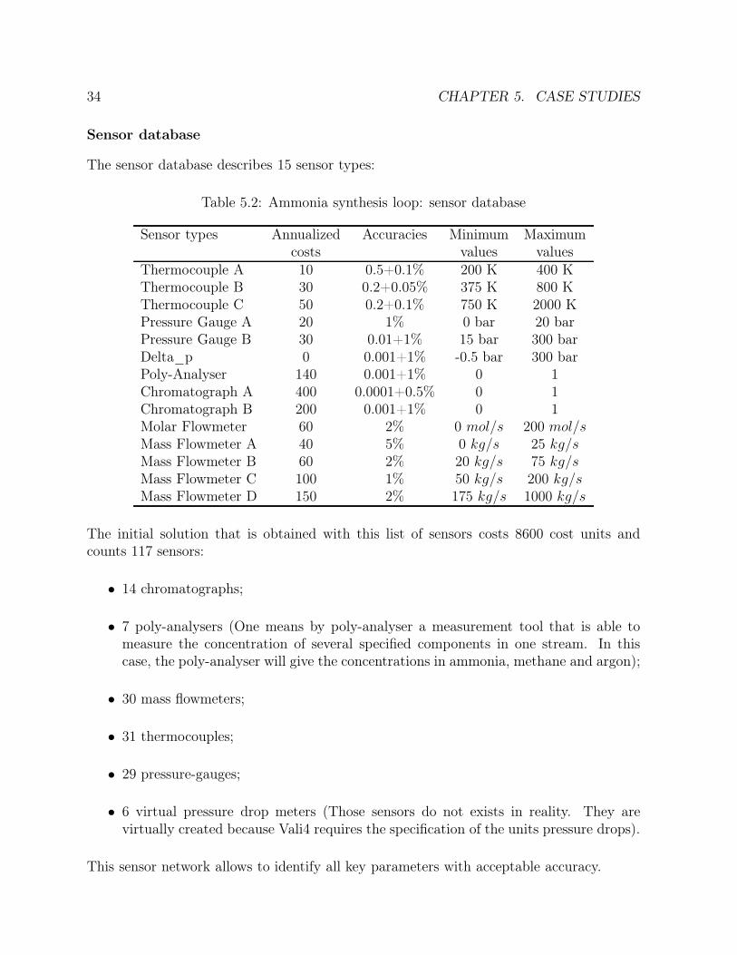
34 CHAPTER 5. CASE STUDIES
Sensor database
The sensor database describes 15 sensor types:
Table 5.2: Ammonia synthesis loop: sensor database
Sensor types Annualized Accuracies Minimum Maximumcosts values values
Thermocouple A 10 0.5+0.1% 200 K 400 KThermocouple B 30 0.2+0.05% 375 K 800 KThermocouple C 50 0.2+0.1% 750 K 2000 KPressure Gauge A 20 1% 0 bar 20 barPressure Gauge B 30 0.01+1% 15 bar 300 barDelta_p 0 0.001+1% -0.5 bar 300 barPoly-Analyser 140 0.001+1% 0 1Chromatograph A 400 0.0001+0.5% 0 1Chromatograph B 200 0.001+1% 0 1Molar Flowmeter 60 2% 0 mol/s 200 mol/sMass Flowmeter A 40 5% 0 kg/s 25 kg/sMass Flowmeter B 60 2% 20 kg/s 75 kg/sMass Flowmeter C 100 1% 50 kg/s 200 kg/sMass Flowmeter D 150 2% 175 kg/s 1000 kg/s
The initial solution that is obtained with this list of sensors costs 8600 cost units andcounts 117 sensors:
∙ 14 chromatographs;
∙ 7 poly-analysers (One means by poly-analyser a measurement tool that is able tomeasure the concentration of several specified components in one stream. In thiscase, the poly-analyser will give the concentrations in ammonia, methane and argon);
∙ 30 mass flowmeters;
∙ 31 thermocouples;
∙ 29 pressure-gauges;
∙ 6 virtual pressure drop meters (Those sensors do not exists in reality. They arevirtually created because Vali4 requires the specification of the units pressure drops).
This sensor network allows to identify all key parameters with acceptable accuracy.
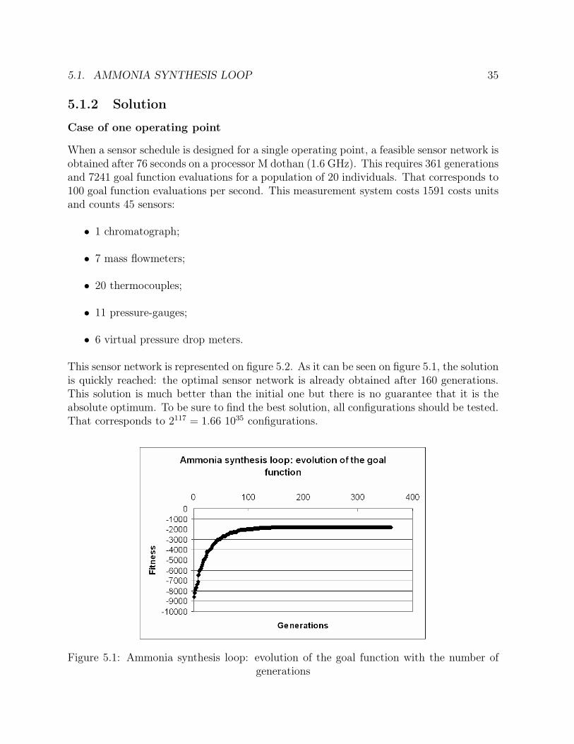
5.1. AMMONIA SYNTHESIS LOOP 35
5.1.2 Solution
Case of one operating point
When a sensor schedule is designed for a single operating point, a feasible sensor network isobtained after 76 seconds on a processor M dothan (1.6 GHz). This requires 361 generationsand 7241 goal function evaluations for a population of 20 individuals. That corresponds to100 goal function evaluations per second. This measurement system costs 1591 costs unitsand counts 45 sensors:
∙ 1 chromatograph;
∙ 7 mass flowmeters;
∙ 20 thermocouples;
∙ 11 pressure-gauges;
∙ 6 virtual pressure drop meters.
This sensor network is represented on figure 5.2. As it can be seen on figure 5.1, the solutionis quickly reached: the optimal sensor network is already obtained after 160 generations.This solution is much better than the initial one but there is no guarantee that it is theabsolute optimum. To be sure to find the best solution, all configurations should be tested.That corresponds to 2117 = 1.66 1035 configurations.
Figure 5.1: Ammonia synthesis loop: evolution of the goal function with the number ofgenerations
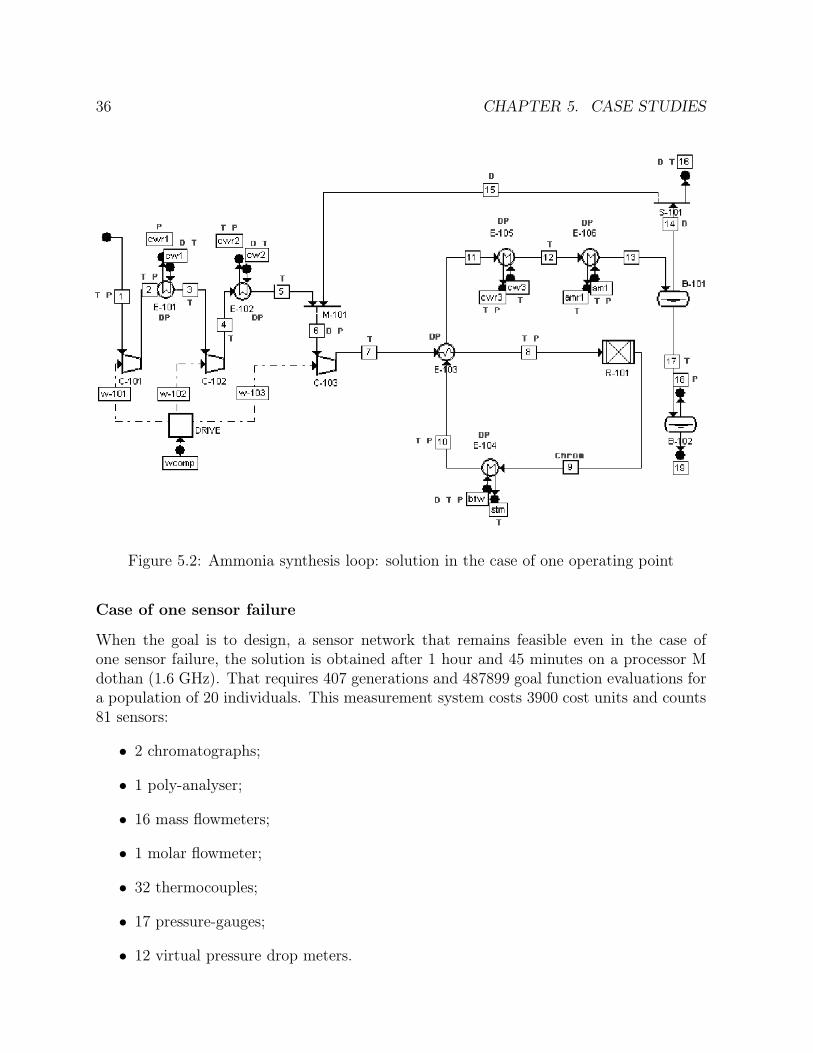
36 CHAPTER 5. CASE STUDIES
Figure 5.2: Ammonia synthesis loop: solution in the case of one operating point
Case of one sensor failure
When the goal is to design, a sensor network that remains feasible even in the case ofone sensor failure, the solution is obtained after 1 hour and 45 minutes on a processor Mdothan (1.6 GHz). That requires 407 generations and 487899 goal function evaluations fora population of 20 individuals. This measurement system costs 3900 cost units and counts81 sensors:
∙ 2 chromatographs;
∙ 1 poly-analyser;
∙ 16 mass flowmeters;
∙ 1 molar flowmeter;
∙ 32 thermocouples;
∙ 17 pressure-gauges;
∙ 12 virtual pressure drop meters.

5.1. AMMONIA SYNTHESIS LOOP 37
This sensor network is represented on figure 5.3.
Figure 5.3: Ammonia synthesis loop: solution in the case of one sensor failure
5.1.3 Global parallelization
For the ammonia synthesis loop, parallelization results have been obtained thanks to thecomputer cluster of the Hemeris Society. This cluster is composed of 64 nodes (ApplePower Mac G4 bi-processors) interconnected by fast and giga Ethernet.
Case of one operating point
In the case of the obtention of a redundant sensor network, global parallelization has beenapplied to populations of respectively 20, 40 and 100 individuals. The search was stoppedafter 200 generations without progress in all cases. In the case of a population of 20individuals, the results are presented on table 5.3 and on figure 5.4.
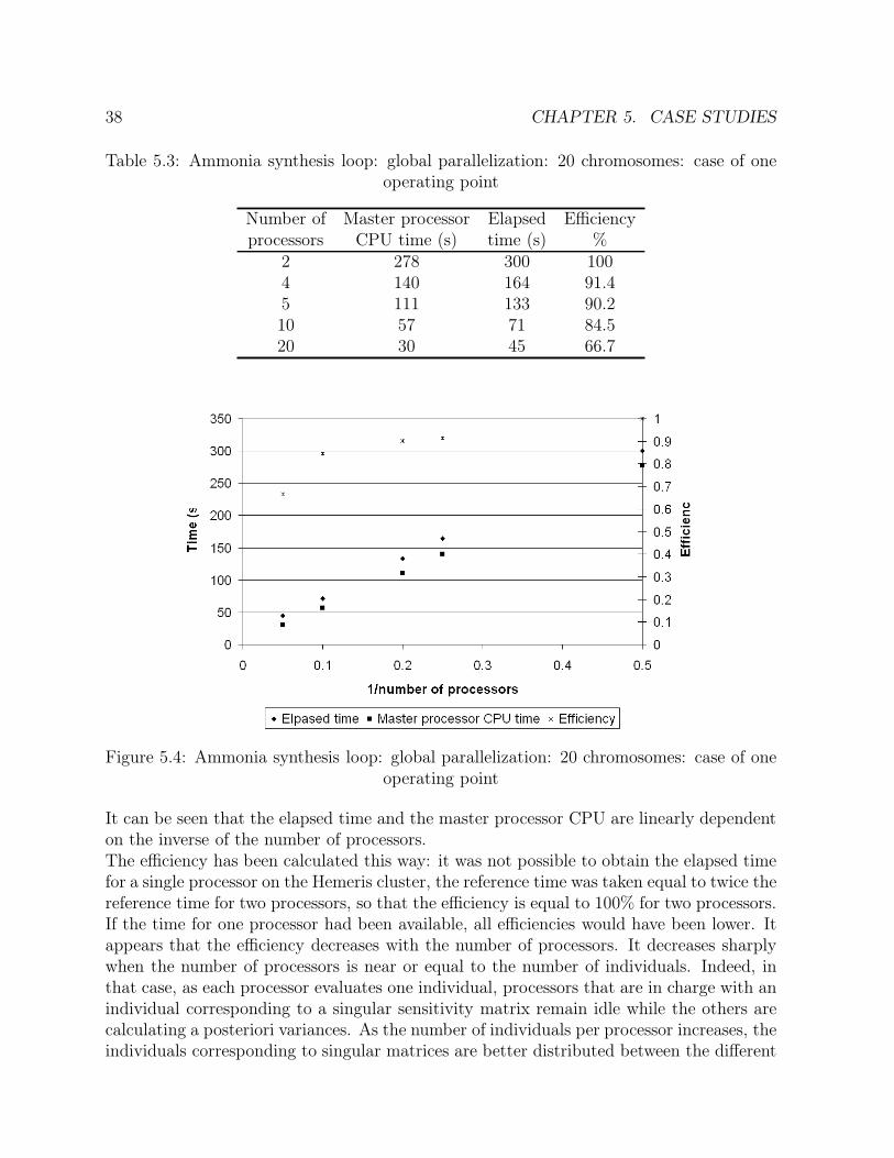
38 CHAPTER 5. CASE STUDIES
Table 5.3: Ammonia synthesis loop: global parallelization: 20 chromosomes: case of oneoperating point
Number of Master processor Elapsed Efficiencyprocessors CPU time (s) time (s) %
2 278 300 1004 140 164 91.45 111 133 90.210 57 71 84.520 30 45 66.7
Figure 5.4: Ammonia synthesis loop: global parallelization: 20 chromosomes: case of oneoperating point
It can be seen that the elapsed time and the master processor CPU are linearly dependenton the inverse of the number of processors.The efficiency has been calculated this way: it was not possible to obtain the elapsed timefor a single processor on the Hemeris cluster, the reference time was taken equal to twice thereference time for two processors, so that the efficiency is equal to 100% for two processors.If the time for one processor had been available, all efficiencies would have been lower. Itappears that the efficiency decreases with the number of processors. It decreases sharplywhen the number of processors is near or equal to the number of individuals. Indeed, inthat case, as each processor evaluates one individual, processors that are in charge with anindividual corresponding to a singular sensitivity matrix remain idle while the others arecalculating a posteriori variances. As the number of individuals per processor increases, theindividuals corresponding to singular matrices are better distributed between the different

5.1. AMMONIA SYNTHESIS LOOP 39
processors. This loss of efficiency can not be predicted precisely a priori. Other losses ofefficiency come from the connections between processors and from the sequential part ofthe program. In this case efficiency losses are less important than the one coming from thesingular matrices, but their contribution to the total loss of efficiency increases when thenumber of processors decreases.Results are presented on table 5.4 and on figure 5.5 in the case of a population of 40individuals, and on table 5.5 and on figure 5.6 in the case of a population of 100 individuals.The same conclusions as in the case of a population of 20 chromosomes can be made. Whenthe number of processors is equal to the number of individuals, it appears that the efficiencydecreases more in the case of 40 chromosomes than in the case of 20, and in the case of100 than in the case of 40.
Table 5.4: Ammonia synthesis loop: global parallelization: 40 chromosomes: case of oneoperating point
Number of Master processor Elapsed Efficiencyprocessors CPU time (s) time (s) %
2 382 408 1004 191 216 94.45 153 178 91.78 96 117 87.210 77 96 8520 40 52 78.540 22 41 49.8
Table 5.5: Ammonia synthesis loop: global parallelization: 100 chromosomes: case of oneoperating point
Number of Master processor Elapsed Efficiencyprocessors CPU time (s) time (s) %
2 1454 1506 1004 723 790 95.35 580 643 93.710 291 345 87.720 147 183 82.325 118 155 77.750 63 108 55.8100 41 86 35
Case of one sensor failure
When designing a measurement system that remains redundant in the case of one sensorfailure, the global parallelization results are given on table 5.6 and on figure 5.7 for a

40 CHAPTER 5. CASE STUDIES
Figure 5.5: Ammonia synthesis loop: global parallelization: 40 chromosomes: case of oneoperating point
Figure 5.6: Ammonia synthesis loop: global parallelization: 100 chromosomes: case of oneoperating point
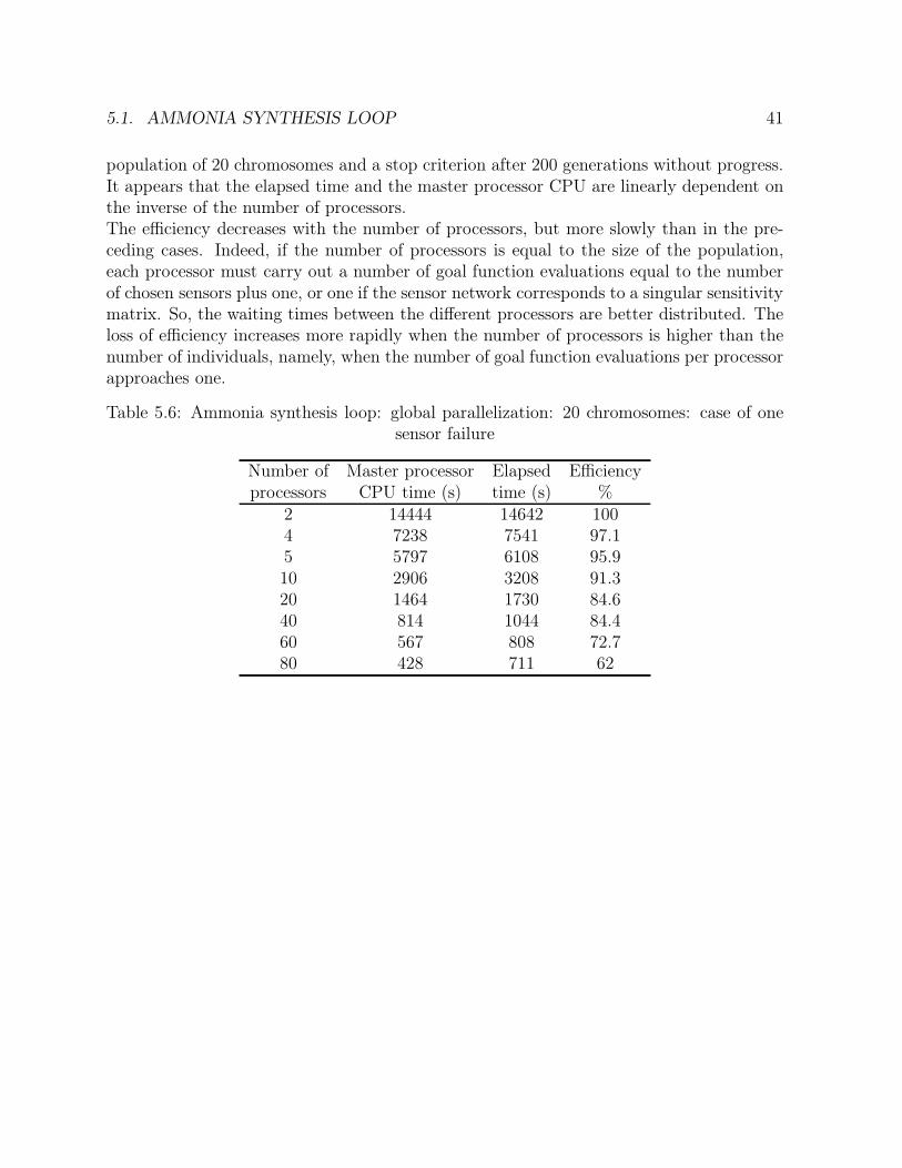
5.1. AMMONIA SYNTHESIS LOOP 41
population of 20 chromosomes and a stop criterion after 200 generations without progress.It appears that the elapsed time and the master processor CPU are linearly dependent onthe inverse of the number of processors.The efficiency decreases with the number of processors, but more slowly than in the pre-ceding cases. Indeed, if the number of processors is equal to the size of the population,each processor must carry out a number of goal function evaluations equal to the numberof chosen sensors plus one, or one if the sensor network corresponds to a singular sensitivitymatrix. So, the waiting times between the different processors are better distributed. Theloss of efficiency increases more rapidly when the number of processors is higher than thenumber of individuals, namely, when the number of goal function evaluations per processorapproaches one.
Table 5.6: Ammonia synthesis loop: global parallelization: 20 chromosomes: case of onesensor failure
Number of Master processor Elapsed Efficiencyprocessors CPU time (s) time (s) %
2 14444 14642 1004 7238 7541 97.15 5797 6108 95.910 2906 3208 91.320 1464 1730 84.640 814 1044 84.460 567 808 72.780 428 711 62
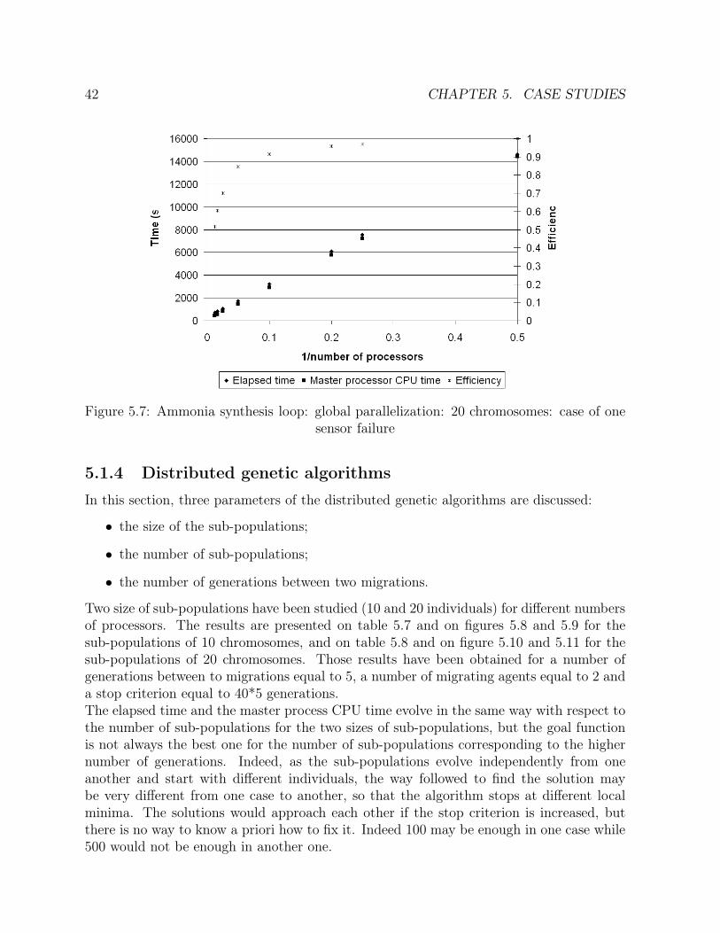
42 CHAPTER 5. CASE STUDIES
Figure 5.7: Ammonia synthesis loop: global parallelization: 20 chromosomes: case of onesensor failure
5.1.4 Distributed genetic algorithms
In this section, three parameters of the distributed genetic algorithms are discussed:
∙ the size of the sub-populations;
∙ the number of sub-populations;
∙ the number of generations between two migrations.
Two size of sub-populations have been studied (10 and 20 individuals) for different numbersof processors. The results are presented on table 5.7 and on figures 5.8 and 5.9 for thesub-populations of 10 chromosomes, and on table 5.8 and on figure 5.10 and 5.11 for thesub-populations of 20 chromosomes. Those results have been obtained for a number ofgenerations between to migrations equal to 5, a number of migrating agents equal to 2 anda stop criterion equal to 40*5 generations.The elapsed time and the master process CPU time evolve in the same way with respect tothe number of sub-populations for the two sizes of sub-populations, but the goal functionis not always the best one for the number of sub-populations corresponding to the highernumber of generations. Indeed, as the sub-populations evolve independently from oneanother and start with different individuals, the way followed to find the solution maybe very different from one case to another, so that the algorithm stops at different localminima. The solutions would approach each other if the stop criterion is increased, butthere is no way to know a priori how to fix it. Indeed 100 may be enough in one case while500 would not be enough in another one.

5.1. AMMONIA SYNTHESIS LOOP 43
It does not seem to be interesting to take too many sub-populations. Indeed, if the numberof sub-populations increases, the elapsed time does not always decreases. Moreover, thetotal work (elapsed time ∗ number of processors) generally increases with the number ofprocessors. An increase of the number of sub-populations has always for impact a useof more computing ressources to obtain, after a more important work, a solution that isnot always better than in the case of a smaller number of sub-populations. A number ofsub-populations of five seems to be a good compromise.The goal function values variate in the same intervalle following that sub-populationscontains 10 or 20 chromosomes. The computing time being smaller for sub-populations of10 chromosomes, it is favorable to take sub-populations of 10 chromosomes. If a too smallsize of sub-populations is taken, information contained in the initial individuals can be lostquite fast and the algorithm may converge quickly to a local minimum far away from theglobal minimum.
Table 5.7: Ammonia synthesis loop: distributed genetic algorithms: sub-populations of 10chromosomes
Number of Master processor Elapsed Goal Number ofprocessors CPU time (s) time (s) function generations
2 387 421 1521 7653 211 226 1491 3954 303 328 1611 5505 238 258 1591 4356 434 459 1541 8257 504 551 1490 9808 374 421 1551 7209 345 385 1551 65010 383 433 1470 74512 257 305 1511 55514 193 231 1470 36016 371 450 1511 73018 435 516 1470 85020 265 332 1470 515
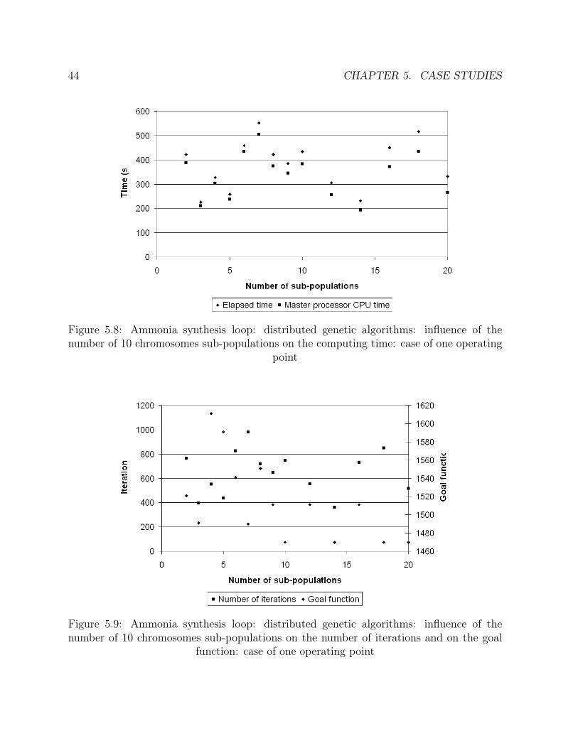
44 CHAPTER 5. CASE STUDIES
Figure 5.8: Ammonia synthesis loop: distributed genetic algorithms: influence of thenumber of 10 chromosomes sub-populations on the computing time: case of one operating
point
Figure 5.9: Ammonia synthesis loop: distributed genetic algorithms: influence of thenumber of 10 chromosomes sub-populations on the number of iterations and on the goal
function: case of one operating point

5.1. AMMONIA SYNTHESIS LOOP 45
Table 5.8: Ammonia synthesis loop: distributed genetic algorithms: sub-populations of 20chromosomes
Number of Master processor Elapsed Goal Number ofprocessors CPU time (s) time (s) function generations
2 583 607 1501 5453 496 521 1470 4754 480 513 1551 4405 680 716 1590 6106 416 451 1471 3907 656 710 1470 6258 578 638 1511 5559 454 528 1471 44510 393 434 1540 34512 898 1001 1511 85014 574 650 1470 55516 783 881 1470 77018 490 564 1470 46020 417 499 1470 395
Figure 5.10: Ammonia synthesis loop: distributed genetic algorithms: influence of thenumber of 20 chromosomes sub-populations on the time: case of one operating point

46 CHAPTER 5. CASE STUDIES
Figure 5.11: Ammonia synthesis loop: distributed genetic algorithms: influence of thenumber of 20 chromosomes sub-populations on the number of iterations and on the goal
function: case of one operating point
To study the influence of the number of generations between two consecutive migrations,the size of the global population was fixed to 50, the size of the sub-populations to 10 andthe stop criterion to 200. The results can be seen on table 5.9 and on figures 5.12 and 5.13.
Table 5.9: Ammonia synthesis loop: distributed genetic algorithms: influence of the num-ber of generations between two migrations
Number of generations Master processor Elapsed Goal Number ofbetween 2 migrations CPU time (s) time (s) function generations
2 221 226 1491 4555 238 258 1591 43510 289 322 1591 54020 309 320 1541 560
The value of the goal function, the computing time and the total number of generationsvary independently of the number of generations between two successive migrations. Thevalue of five generations between two successive migrations found in the literature seemsto be a good compromise.

5.1. AMMONIA SYNTHESIS LOOP 47
Figure 5.12: Ammonia synthesis loop: distributed genetic algorithms: influence on thecomputing time of the number of generations between 2 migrations: case of one operating
point
Figure 5.13: Ammonia synthesis loop: distributed genetic algorithms: influence on thenumber of iterations and on the goal function of the number of generations between 2
migrations: case of one operating point

48 CHAPTER 5. CASE STUDIES
5.1.5 Methods comparison
To decide which parallelization method is the most efficient, the times, the number ofiterations, the final values of the goal function and the efficiencies have been compared.In all the cases, the global size of the population was fixed to 50 individuals and the stopcriterion was taken equal to 200 for global parallelization and 40∗5 for distributed geneticalgorithms. For distributed genetic algorithms, the number of generations between twosuccessive migrations was fixed to 5 and the number of migrating individuals was takenequal to 2. The results are given in the tables 5.10 for global parallelization and 5.11 fordistributed genetic algorithms.
Table 5.10: Ammonia synthesis loop: global parallelization
Global parallelizationNumber of Master processor Elapsed Goal Number of Efficiencyprocessors CPU time (s) time (s) function generations (%)
2 766 798 1591 543 1005 305 349 1591 543 91.510 154 199 1591 543 80.2
Table 5.11: Ammonia synthesis loop: distributed genetic algorithms
Distributed genetic algorithmsNumber of Master processor Elapsed Goal Number of Efficiencyprocessors CPU time (s) time (s) function generations (%)
2 652 676 1471 466 1185 238 258 1591 431 123.710 77 133 1470 381 120
It can be seen on figure 5.14 that the elapsed time and the master processor CPU time arebetter for the distributed genetic algorithms. The same tendency is observed in the caseof the total number of generations (figure 5.16).The goal function values are also better in the case of distributed genetic algorithms (figure5.16). Indeed, they do not change with the number of processors in the case of globalparallelization because the evolution of the population does not depend on that number inthat case. In contrary, for distributed genetic algorithms, the global population evolutiondepends on the number of sub-populations: indeed,
∙ the size of the sub-populations depends on the number of sub-populations;
∙ individuals migrate from one sub-population to another one so that mating chromo-somes is different in function of the way they move.

5.1. AMMONIA SYNTHESIS LOOP 49
Figure 5.14: Ammonia synthesis loop: times comparison
Figure 5.15: Ammonia synthesis loop: number of generations comparison

50 CHAPTER 5. CASE STUDIES
Figure 5.16: Ammonia synthesis loop: goal function comparison
Thus, the way followed to obtain the solution is different for each sub-population number,so that, as the optimal solution found by the algorithm may not be the best one, values ofthe goal function may be a little different.It appears on figure 5.17 that the efficiency is much better in the case of distributedgenetic algorithms. The efficiency is even better than 100% in some cases. Indeed, assub-populations are subject to migrations and contain different initial individuals, the wayfollowed by the algorithm to reach the solution is different. Moreover, the gain of timegiven by the reduction of the number of iterations is higher than the loss of time causedby the migration operations between sub-populations.In the case of the ammonia synthesis loop, both parallelization methods allowed to reducethe computing time, but distributed genetic algorithms are better in all points of view.

5.1. AMMONIA SYNTHESIS LOOP 51
Figure 5.17: Ammonia synthesis loop: efficiency comparison
52 CHAPTER 5. CASE STUDIES
5.2 Combined cycle power plant
5.2.1 Process description
The second process is a combined cycle power plant. In this process, air is compressedbefore entering the combustion chamber where it reacts with the fuel (natural gas, modeledas a methane-ethane mixture). The combustion gas is later expanded in two successiveturbines. Then it is cooled in a steam generator before being rejected to the environment.The generator allows to raise super heated steam at two pressure levels. Superheated steamfeeds two turbines and is condensed before being recirculated to a boiler.This process is composed of:
∙ 28 units: 1 air compressor, 1 combustion chamber, 2 turbines at the exit of thecombustion chamber, 1 high pressure superheater, 1 high pressure vaporiser, 2 highpressure economizers, 1 low pressure superheater, 1 low pressure vaporiser, 1 lowpressure economizer, 1 heater, 5 pumps, 1 high pressure turbine, 1 low pressureturbine, 1 condenser, 2 steam drums, 2 liquid-vapor separators, 1 stream divider, 2stream mixers and 1 purge divider;
∙ 17 material streams composed of oxygen, water, nitrogen, methane, ethane and car-bon dioxide;
∙ 28 utility streams composed of vapor and cooling water;
∙ 10 mechanical streams;
∙ 1 thermal stream;
∙ 260 variables;
∙ 216 constraints equations.
This example will be first studied in the case of the nominal operating point. Secondly, itwill be studied considering two operating points simultaneously: the nominal conditionsand the summer operating conditions. Performance of the parallelized algorithm will beanalyzed for this later case.
Key parameters
The process comprises 10 key parameters which are listed with their prescribed standarddeviations in the table below (Table 5.12).
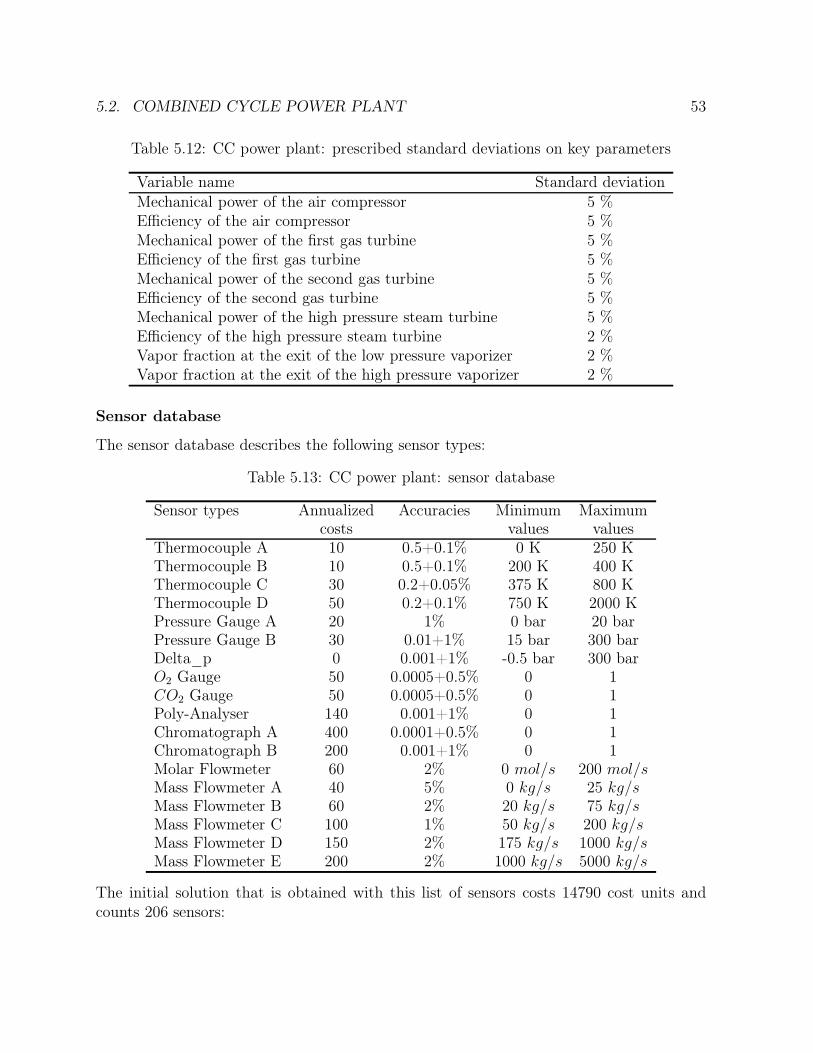
5.2. COMBINED CYCLE POWER PLANT 53
Table 5.12: CC power plant: prescribed standard deviations on key parameters
Variable name Standard deviationMechanical power of the air compressor 5 %Efficiency of the air compressor 5 %Mechanical power of the first gas turbine 5 %Efficiency of the first gas turbine 5 %Mechanical power of the second gas turbine 5 %Efficiency of the second gas turbine 5 %Mechanical power of the high pressure steam turbine 5 %Efficiency of the high pressure steam turbine 2 %Vapor fraction at the exit of the low pressure vaporizer 2 %Vapor fraction at the exit of the high pressure vaporizer 2 %
Sensor database
The sensor database describes the following sensor types:
Table 5.13: CC power plant: sensor database
Sensor types Annualized Accuracies Minimum Maximumcosts values values
Thermocouple A 10 0.5+0.1% 0 K 250 KThermocouple B 10 0.5+0.1% 200 K 400 KThermocouple C 30 0.2+0.05% 375 K 800 KThermocouple D 50 0.2+0.1% 750 K 2000 KPressure Gauge A 20 1% 0 bar 20 barPressure Gauge B 30 0.01+1% 15 bar 300 barDelta_p 0 0.001+1% -0.5 bar 300 barO2 Gauge 50 0.0005+0.5% 0 1CO2 Gauge 50 0.0005+0.5% 0 1Poly-Analyser 140 0.001+1% 0 1Chromatograph A 400 0.0001+0.5% 0 1Chromatograph B 200 0.001+1% 0 1Molar Flowmeter 60 2% 0 mol/s 200 mol/sMass Flowmeter A 40 5% 0 kg/s 25 kg/sMass Flowmeter B 60 2% 20 kg/s 75 kg/sMass Flowmeter C 100 1% 50 kg/s 200 kg/sMass Flowmeter D 150 2% 175 kg/s 1000 kg/sMass Flowmeter E 200 2% 1000 kg/s 5000 kg/s
The initial solution that is obtained with this list of sensors costs 14790 cost units andcounts 206 sensors:
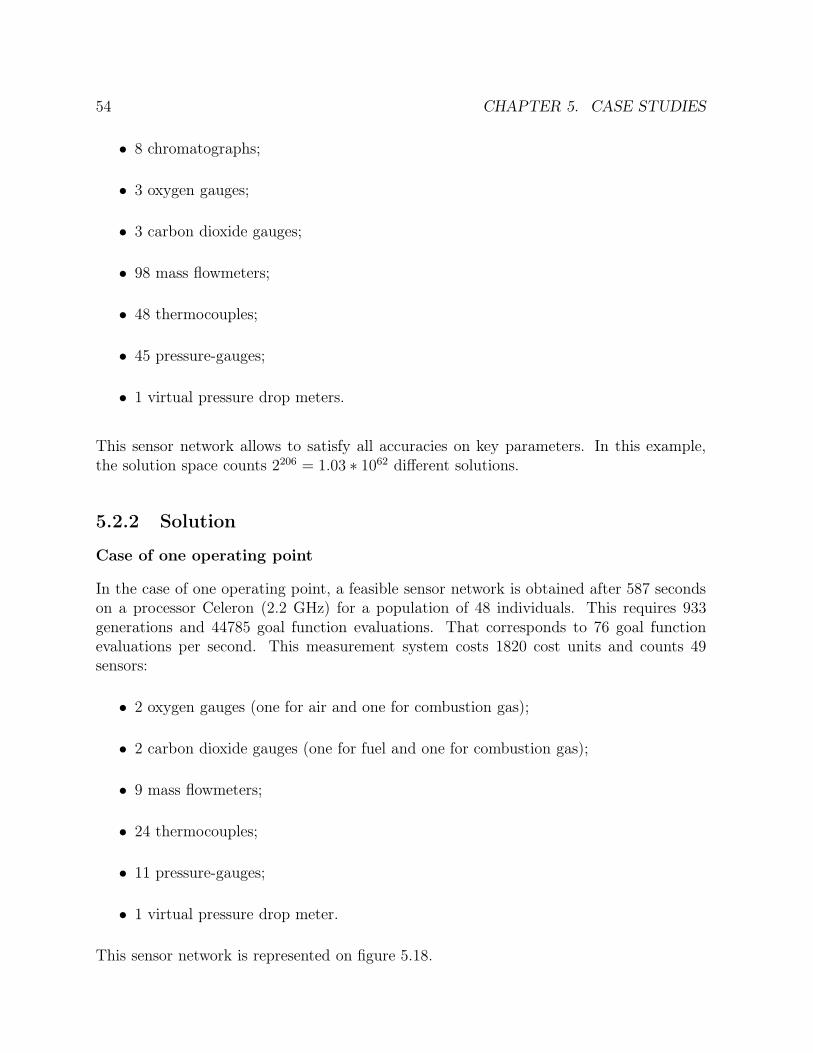
54 CHAPTER 5. CASE STUDIES
∙ 8 chromatographs;
∙ 3 oxygen gauges;
∙ 3 carbon dioxide gauges;
∙ 98 mass flowmeters;
∙ 48 thermocouples;
∙ 45 pressure-gauges;
∙ 1 virtual pressure drop meters.
This sensor network allows to satisfy all accuracies on key parameters. In this example,the solution space counts 2206 = 1.03 ∗ 1062 different solutions.
5.2.2 Solution
Case of one operating point
In the case of one operating point, a feasible sensor network is obtained after 587 secondson a processor Celeron (2.2 GHz) for a population of 48 individuals. This requires 933generations and 44785 goal function evaluations. That corresponds to 76 goal functionevaluations per second. This measurement system costs 1820 cost units and counts 49sensors:
∙ 2 oxygen gauges (one for air and one for combustion gas);
∙ 2 carbon dioxide gauges (one for fuel and one for combustion gas);
∙ 9 mass flowmeters;
∙ 24 thermocouples;
∙ 11 pressure-gauges;
∙ 1 virtual pressure drop meter.
This sensor network is represented on figure 5.18.
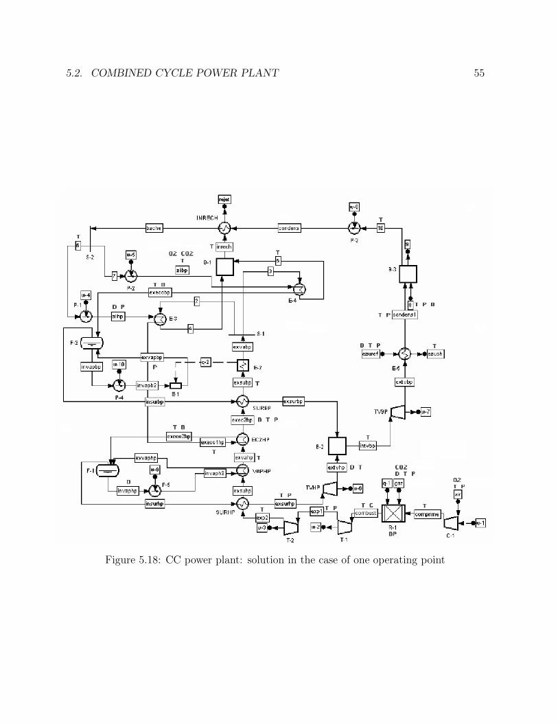
5.2. COMBINED CYCLE POWER PLANT 55
Figure 5.18: CC power plant: solution in the case of one operating point

56 CHAPTER 5. CASE STUDIES
Case of two operating points
In the case of two operating points, a feasible sensor network is obtained after 1595 secondson a processor Celeron (2.2 GHz) for a population of 48 individuals. This requires 1343generations and 128930 goal function evaluations. This measurement system costs 1820cost units and counts 44 sensors:
∙ 1 chromatograph for the combustion gas (replacing one oxygen and one carbon diox-ide gauges);
∙ 1 oxygen sonde for the air;
∙ 1 carbon dioxide sonde for the fuel;
∙ 7 mass flowmeters;
∙ 23 thermocouples;
∙ 10 pressure-gauges;
∙ 1 virtual pressure drop meter.
This sensor network is represented on figure 5.19.
Case of one sensor failure
In the case of one operating point, an observable sensor network in the case of one sensorfailure is obtained after 486 minutes on a processor Celeron (2.2 GHz) for a population of48 individuals. That requires 823 generations and 3139426 goal function evaluations. Thismeasurement system costs 3840 cost units and counts 78 sensors:
∙ 2 chromatographs;
∙ 2 oxygen gauges (one for the air and one for the combustion gas);
∙ 16 mass flowmeters;
∙ 37 thermocouples;
∙ 19 pressure-gauges;
∙ 2 virtual pressure drop meters.
This sensor network is represented on figure 5.20.
5.2. COMBINED CYCLE POWER PLANT 57
Figure 5.19: CC power plant: solution in the case of two operating points
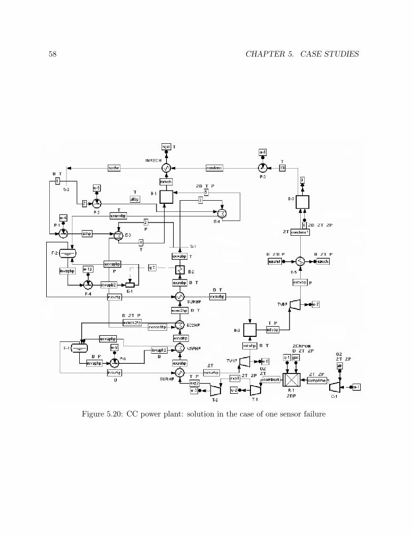
58 CHAPTER 5. CASE STUDIES
Figure 5.20: CC power plant: solution in the case of one sensor failure
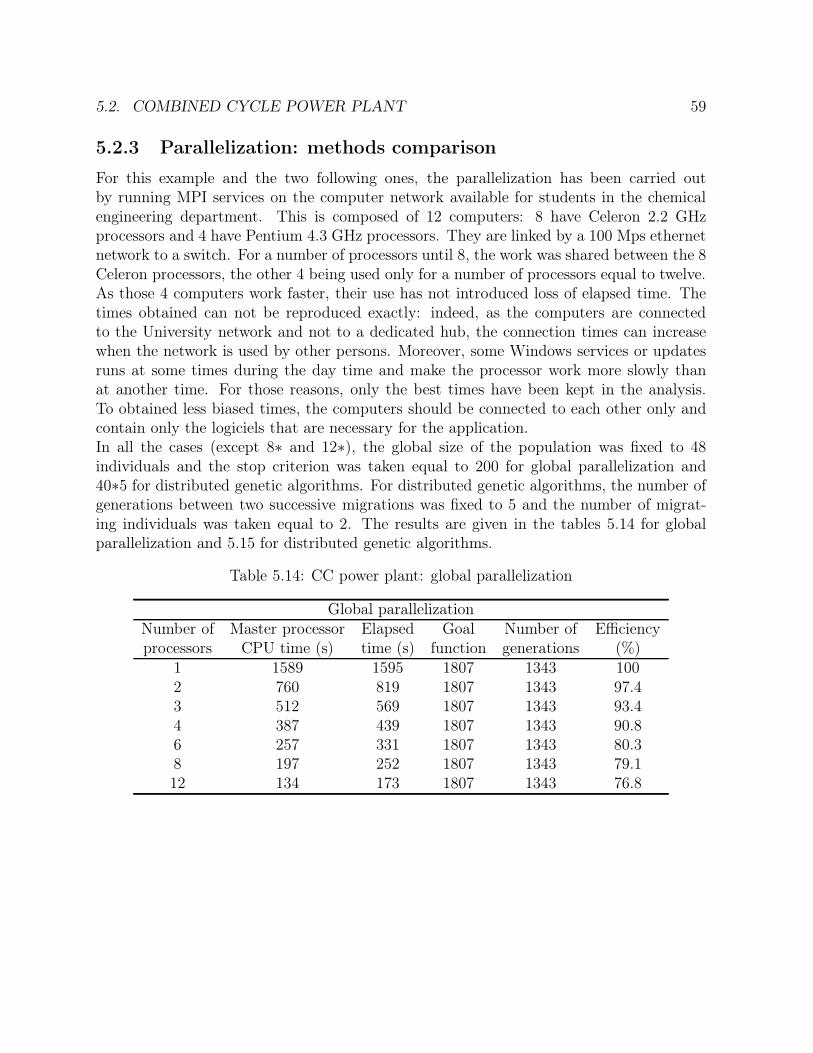
5.2. COMBINED CYCLE POWER PLANT 59
5.2.3 Parallelization: methods comparison
For this example and the two following ones, the parallelization has been carried outby running MPI services on the computer network available for students in the chemicalengineering department. This is composed of 12 computers: 8 have Celeron 2.2 GHzprocessors and 4 have Pentium 4.3 GHz processors. They are linked by a 100 Mps ethernetnetwork to a switch. For a number of processors until 8, the work was shared between the 8Celeron processors, the other 4 being used only for a number of processors equal to twelve.As those 4 computers work faster, their use has not introduced loss of elapsed time. Thetimes obtained can not be reproduced exactly: indeed, as the computers are connectedto the University network and not to a dedicated hub, the connection times can increasewhen the network is used by other persons. Moreover, some Windows services or updatesruns at some times during the day time and make the processor work more slowly thanat another time. For those reasons, only the best times have been kept in the analysis.To obtained less biased times, the computers should be connected to each other only andcontain only the logiciels that are necessary for the application.In all the cases (except 8∗ and 12∗), the global size of the population was fixed to 48individuals and the stop criterion was taken equal to 200 for global parallelization and40∗5 for distributed genetic algorithms. For distributed genetic algorithms, the number ofgenerations between two successive migrations was fixed to 5 and the number of migrat-ing individuals was taken equal to 2. The results are given in the tables 5.14 for globalparallelization and 5.15 for distributed genetic algorithms.
Table 5.14: CC power plant: global parallelization
Global parallelizationNumber of Master processor Elapsed Goal Number of Efficiencyprocessors CPU time (s) time (s) function generations (%)
1 1589 1595 1807 1343 1002 760 819 1807 1343 97.43 512 569 1807 1343 93.44 387 439 1807 1343 90.86 257 331 1807 1343 80.38 197 252 1807 1343 79.112 134 173 1807 1343 76.8
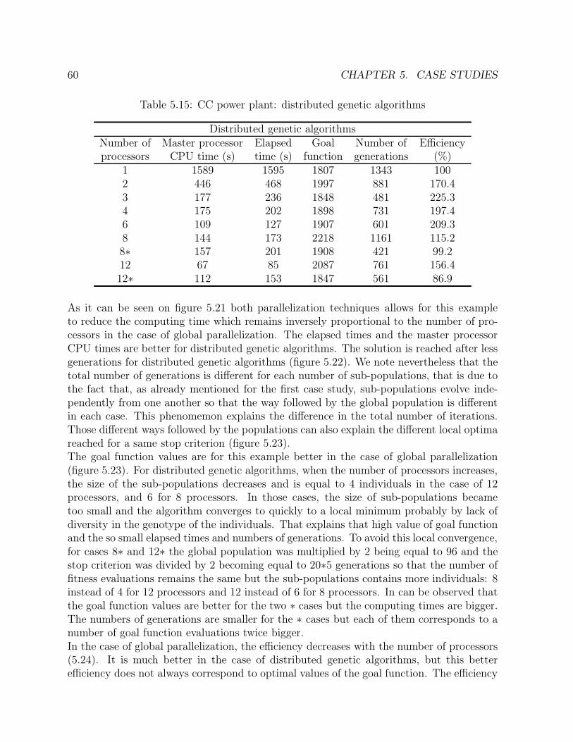
60 CHAPTER 5. CASE STUDIES
Table 5.15: CC power plant: distributed genetic algorithms
Distributed genetic algorithmsNumber of Master processor Elapsed Goal Number of Efficiencyprocessors CPU time (s) time (s) function generations (%)
1 1589 1595 1807 1343 1002 446 468 1997 881 170.43 177 236 1848 481 225.34 175 202 1898 731 197.46 109 127 1907 601 209.38 144 173 2218 1161 115.28∗ 157 201 1908 421 99.212 67 85 2087 761 156.412∗ 112 153 1847 561 86.9
As it can be seen on figure 5.21 both parallelization techniques allows for this exampleto reduce the computing time which remains inversely proportional to the number of pro-cessors in the case of global parallelization. The elapsed times and the master processorCPU times are better for distributed genetic algorithms. The solution is reached after lessgenerations for distributed genetic algorithms (figure 5.22). We note nevertheless that thetotal number of generations is different for each number of sub-populations, that is due tothe fact that, as already mentioned for the first case study, sub-populations evolve inde-pendently from one another so that the way followed by the global population is differentin each case. This phenomemon explains the difference in the total number of iterations.Those different ways followed by the populations can also explain the different local optimareached for a same stop criterion (figure 5.23).The goal function values are for this example better in the case of global parallelization(figure 5.23). For distributed genetic algorithms, when the number of processors increases,the size of the sub-populations decreases and is equal to 4 individuals in the case of 12processors, and 6 for 8 processors. In those cases, the size of sub-populations becametoo small and the algorithm converges to quickly to a local minimum probably by lack ofdiversity in the genotype of the individuals. That explains that high value of goal functionand the so small elapsed times and numbers of generations. To avoid this local convergence,for cases 8∗ and 12∗ the global population was multiplied by 2 being equal to 96 and thestop criterion was divided by 2 becoming equal to 20∗5 generations so that the number offitness evaluations remains the same but the sub-populations contains more individuals: 8instead of 4 for 12 processors and 12 instead of 6 for 8 processors. In can be observed thatthe goal function values are better for the two ∗ cases but the computing times are bigger.The numbers of generations are smaller for the ∗ cases but each of them corresponds to anumber of goal function evaluations twice bigger.In the case of global parallelization, the efficiency decreases with the number of processors(5.24). It is much better in the case of distributed genetic algorithms, but this betterefficiency does not always correspond to optimal values of the goal function. The efficiency
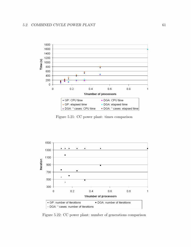
5.2. COMBINED CYCLE POWER PLANT 61
Figure 5.21: CC power plant: times comparison
Figure 5.22: CC power plant: number of generations comparison
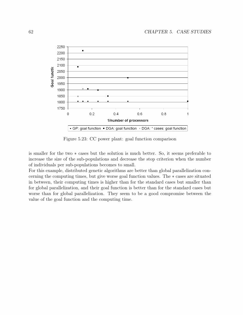
62 CHAPTER 5. CASE STUDIES
Figure 5.23: CC power plant: goal function comparison
is smaller for the two ∗ cases but the solution is much better. So, it seems preferable toincrease the size of the sub-populations and decrease the stop criterion when the numberof individuals per sub-populations becomes to small.For this example, distributed genetic algorithms are better than global parallelization con-cerning the computing times, but give worse goal function values. The ∗ cases are situatedin between, their computing times is higher than for the standard cases but smaller thanfor global parallelization, and their goal function is better than for the standard cases butworse than for global parallelization. They seem to be a good compromise between thevalue of the goal function and the computing time.
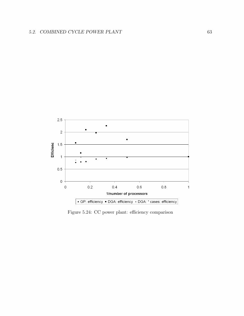
5.2. COMBINED CYCLE POWER PLANT 63
Figure 5.24: CC power plant: efficiency comparison
64 CHAPTER 5. CASE STUDIES
5.3 Ketene cracker
5.3.1 Process description
The third example is a ketene cracker. The plant model has been provided by Belsimcompany. It has been developed for Wacker Chemie and represent the ketene plant ontheir Burghausen site.In this process, acetic acid is evaporated in a preheater before it enters into a furnace wherethe catalytic pyrolysis occurs. The catalyst, triethyl phosphate (TEP), allows the crackingof acetic acid into ketene and water. TEP is first transformed into phosphoric acid, whichloses a water molecule. Acetic acid is then added to meta phosphoric acid and, finally,acetic anhydride is rearranged into ketene and phosphoric acid. TEP is used as catalystinstead of phosphoric acid because if phosphoric acid is directly injected in the furnace, itreacts with itself to form a dimer. If TEP is injected at the right place, this dimerisationdoes not occur.The furnace is heated so that the outlet gas reaches a temperature of approximately 700∘C.The exhaust gas is cooled rapidly in two chillers (a water one and a brine one). Theliquid phase (containing mainly water and unconverted acetic acid) is separated from thevapor phase (containing mainly ketene) to avoid backward reaction. This vapor phaseis further purified in distillation columns. Although the pyrolysis reaction is catalyzed,parallel reactions occur and ketene contains impurities such as ethene, methane, carbonmonoxide, carbon dioxide... The ketene contained in the liquid phase is then transformedinto acetic anhydride, itself transformed into acetic acid that will be reused in the plant.This process is composed of:
∙ 23 units: 1 compressor, 1 ketene cracker, 4 reactors, 7 heat exchangers, 5 liquid-vaporseparators, 4 stream mixers and 1 pump;
∙ 34 material streams composed of keten, triethylphosphate, phosphoric acid, aceticacid, acetic anhydride, water, carbon dioxide, carbon monoxide, oxygen, nitrogen,methane, ethane, ethene, propadiene, propylène, normal-butane, ammonium phos-phate and ammonia;
∙ 12 utility streams composed of vapor and water;
∙ 2 mechanical streams;
∙ 4 thermal streams;
∙ 631 variables;
∙ 557 constraints equations.
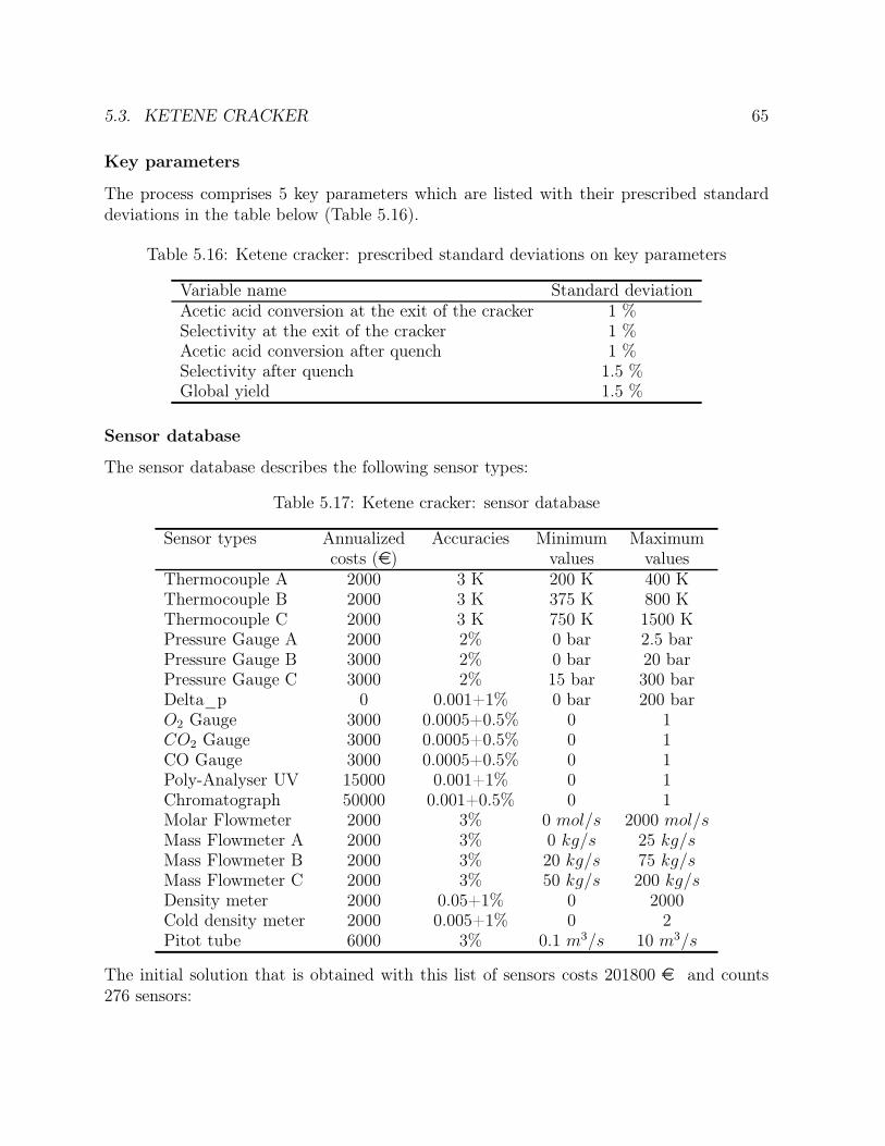
5.3. KETENE CRACKER 65
Key parameters
The process comprises 5 key parameters which are listed with their prescribed standarddeviations in the table below (Table 5.16).
Table 5.16: Ketene cracker: prescribed standard deviations on key parameters
Variable name Standard deviationAcetic acid conversion at the exit of the cracker 1 %Selectivity at the exit of the cracker 1 %Acetic acid conversion after quench 1 %Selectivity after quench 1.5 %Global yield 1.5 %
Sensor database
The sensor database describes the following sensor types:
Table 5.17: Ketene cracker: sensor database
Sensor types Annualized Accuracies Minimum Maximumcosts (e) values values
Thermocouple A 2000 3 K 200 K 400 KThermocouple B 2000 3 K 375 K 800 KThermocouple C 2000 3 K 750 K 1500 KPressure Gauge A 2000 2% 0 bar 2.5 barPressure Gauge B 3000 2% 0 bar 20 barPressure Gauge C 3000 2% 15 bar 300 barDelta_p 0 0.001+1% 0 bar 200 barO2 Gauge 3000 0.0005+0.5% 0 1CO2 Gauge 3000 0.0005+0.5% 0 1CO Gauge 3000 0.0005+0.5% 0 1Poly-Analyser UV 15000 0.001+1% 0 1Chromatograph 50000 0.001+0.5% 0 1Molar Flowmeter 2000 3% 0 mol/s 2000 mol/sMass Flowmeter A 2000 3% 0 kg/s 25 kg/sMass Flowmeter B 2000 3% 20 kg/s 75 kg/sMass Flowmeter C 2000 3% 50 kg/s 200 kg/sDensity meter 2000 0.05+1% 0 2000Cold density meter 2000 0.005+1% 0 2Pitot tube 6000 3% 0.1 m3/s 10 m3/s
The initial solution that is obtained with this list of sensors costs 201800 e and counts276 sensors:

66 CHAPTER 5. CASE STUDIES
∙ 27 chromatographs;
∙ 11 poly-analysers (measurement tool able to give the concentration in acetic acid,keten and acetic anhydride);
∙ 1 oxygen gauge;
∙ 1 carbon monoxide gauge;
∙ 88 mass flowmeters;
∙ 8 molar flowmeters;
∙ 47 thermocouples;
∙ 78 pressure-gauges;
∙ 1 Pitot tube;
∙ 1 density meters;
∙ 2 cold density meters;
∙ 8 virtual pressure drop meters.
This sensor network allows to satisfy all accuracies on key parameters. In this example,the solution space counts 2276 = 1.21 ∗ 1083 different solutions.
In the case of the ketene cracker, four sensors have to be placed in the plant at the operator’srequest:
∙ 1 Pitot tube on stream keten2;
∙ 1 density meter on stream dunnsr6;
∙ 1 cold density meter on stream dunnsrd;
∙ 1 cold density meter on stream 3essig1.
5.3.2 Solution
Case of one operating point
In the case of one operating point, a feasible sensor network is obtained after 9 hours40 minutes on a processor Celeron (2.2 GHz) for a population of 48 individuals. Thisrequires 1550 generations and 74401 goal function evaluations. That corresponds to 124goal function evaluations per minute. This measurement system costs 168000 e and counts65 sensors:

5.3. KETENE CRACKER 67
∙ 1 chromatograph;
∙ 1 carbon dioxide gauge;
∙ 13 mass flowmeters;
∙ 1 molar flowmeter;
∙ 25 thermocouples;
∙ 11 pressure-gauges;
∙ 1 Pitot tube;
∙ 1 density meter;
∙ 2 cold density meters;
∙ 8 virtual pressure drop meters.
This sensor network is represented on figures 5.25 and 5.26.
Case of one sensor failure
In the case of one operating point, a feasible sensor network in the case of one sensor failureis obtained after 61 hours on computer network composed of four processors Pentium4 (3GHz) for a population of 48 individuals. That requires 1281 generations and 4 242 413 goalfunction evaluations. This measurement system costs 260000 e and counts 81 sensors:
∙ 2 chromatographs;
∙ 1 carbon dioxide gauge;
∙ 12 mass flowmeters;
∙ 20 thermocouples;
∙ 35 pressure-gauges;
∙ 1 Pitot tube;
∙ 1 density meter;
∙ 2 cold density meters;
∙ 14 virtual pressure drop meters.
This sensor network is represented on figures 5.27 and 5.28.
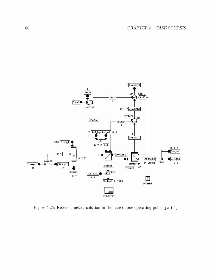
68 CHAPTER 5. CASE STUDIES
Figure 5.25: Ketene cracker: solution in the case of one operating point (part 1)

5.3. KETENE CRACKER 69
Figure 5.26: Ketene cracker: solution in the case of one operating point (part2)
5.3.3 Parallelization: methods comparison
In all the cases, the global size of the population was fixed to 48 individuals and the stopcriterion was taken equal to 200 for global parallelization and 40∗5 for distributed geneticalgorithms. Calculation were run on the 12 computers of the student network. As forthe combined cycle power plant, distributed genetic algorithms have also been tested for atotal population of 96 individuals and a stop criterion equal to 20∗5 generations (for 8 and12 processors). For distributed genetic algorithms, the number of generations between twosuccessive migrations was fixed to 5 and the number of migrating individuals was takenequal to 2. The results are given in the tables 5.18 for global parallelization and 5.19 fordistributed genetic algorithms.
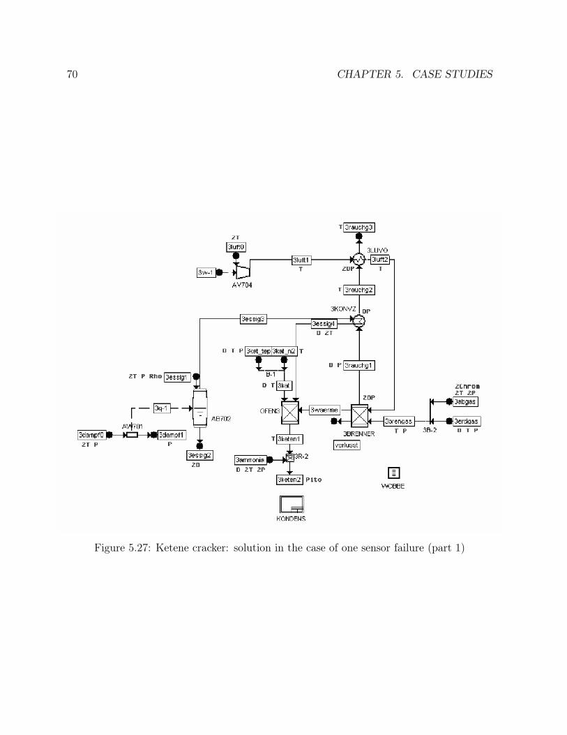
70 CHAPTER 5. CASE STUDIES
Figure 5.27: Ketene cracker: solution in the case of one sensor failure (part 1)
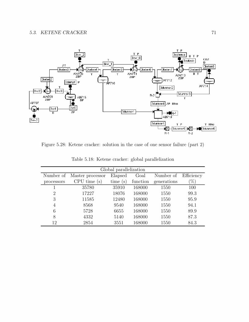
5.3. KETENE CRACKER 71
Figure 5.28: Ketene cracker: solution in the case of one sensor failure (part 2)
Table 5.18: Ketene cracker: global parallelization
Global parallelizationNumber of Master processor Elapsed Goal Number of Efficiencyprocessors CPU time (s) time (s) function generations (%)
1 35780 35910 168000 1550 1002 17227 18076 168000 1550 99.33 11585 12480 168000 1550 95.94 8568 9540 168000 1550 94.16 5728 6655 168000 1550 89.98 4332 5140 168000 1550 87.312 2854 3551 168000 1550 84.3
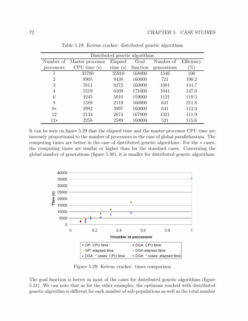
72 CHAPTER 5. CASE STUDIES
Table 5.19: Ketene cracker: distributed genetic algorithms
Distributed genetic algorithmsNumber of Master processor Elapsed Goal Number of Efficiencyprocessors CPU time (s) time (s) function generations (%)
1 35780 35910 168000 1546 1002 8905 9438 160000 721 190.23 7611 8272 160000 1001 144.74 5519 6109 171000 1041 147.06 4245 5010 159000 1121 119.58 1589 2119 160000 641 211.88∗ 2982 3997 160000 641 112.312 2134 2674 167000 1321 111.912∗ 2258 2589 160000 521 115.6
It can be seen on figure 5.29 that the elapsed time and the master processor CPU time areinversely proportional to the number of processors in the case of global parallelization. Thecomputing times are better in the case of distributed genetic algorithms. For the ∗ cases,the computing times are similar or higher than for the standard cases. Concerning theglobal number of generations (figure 5.30), it is smaller for distributed genetic algorithms.
Figure 5.29: Ketene cracker: times comparison
The goal function is better in most of the cases for distributed genetic algorithms (figure5.31). We can note that as for the other examples, the optimum reached with distributedgenetic algorithm is different for each number of sub-populations as well as the total number

5.3. KETENE CRACKER 73
Figure 5.30: Ketene cracker: number of generations comparison
of generations. The explanation remains the independent evolution of the sub-populations.For the ∗ cases, it is better or equal than for the standard cases. It appears that an increasein computing time for the ∗ cases does not necessary implies a better goal function for thisexample.In this example, the efficiency also decreases with the number of processors (figure 5.32)in the case of global parallelization. It is always better for distributed genetic algorithms.For this example, distributed algorithms are better than global parallelization in all pointsof view. The ∗ cases are sometimes better and sometimes worse than the standard cases.This depends mainly on the way followed to reach the solution which is different for everycase while distributed genetic algorithms are used.
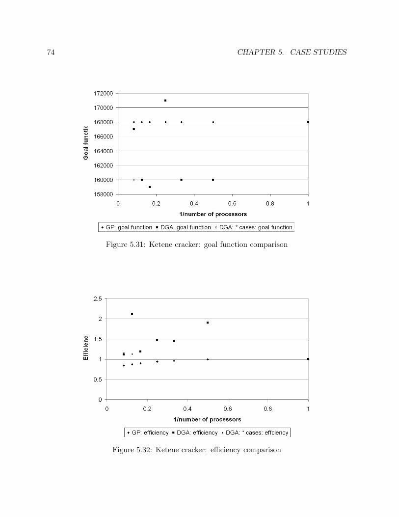
74 CHAPTER 5. CASE STUDIES
Figure 5.31: Ketene cracker: goal function comparison
Figure 5.32: Ketene cracker: efficiency comparison
5.4. NAPHTA REFORMER 75
5.4 Naphta reformer
5.4.1 Process description
The last example is a naphta reformer. This catalytic reforming process is a typical refiningprocess. Its original function is to upgrade low octane straight-run naphtha to higheroctane number, by converting n-paraffins to iso-paraffins and naphtenes to aromatics. Thehydrogen generated by the aromatic producing reactions also plays a major role in varioushydrotreating units. The key performance indicators of the catalytic reforming process are,among others, the C5+ yields as well as the yields of light compounds, and especially H2.This process is made of 4 main sections:
∙ the preheat of the feed;
∙ the reaction section, with intermediate reheaters between the reactors;
∙ the gas-liquid separation (and compression) section;
∙ the stabilizer section were the liquid from the gas-liquid separation section is frac-tionated into the product streams.
This process is composed of:
∙ 80 units;
∙ 104 material streams composed of hydrogen, methane, ethane, propane, iso-butane,normal-butane, 2-methylbutane, normal-pentane, 2-2-dimethylbutane, normal-hexane,cyhexane, benzene, methylcyhexane, 1-1-dimethylcyhexane, 2-2-dimethylpentane, normal-heptane, toluene, ethylbenzene, normal-octane, 2-2-dimethylhexane, 2-2-3-trimethylhexane,3-3-5-trimethylheptane, normal-nonane, normal-decane, normal-propylcyclohexane,iso-butylcyclohexane, 1-ethyl-2-methylbenzene and 1-3-diethylbenzene;
∙ 10 utility streams composed of steam and water;
∙ 12 mechanical streams;
∙ 21 thermal streams;
∙ 1263 variables;
∙ 1116 constraints equations.
Key parameters
The process comprises 9 key parameters which are listed with their prescribed standarddeviations in the table below (Table 5.20).

76 CHAPTER 5. CASE STUDIES
Table 5.20: Naphta reformer: prescribed standard deviations on key parameters
Variable name Standard deviationHydrogen yields (weight %) 10 %Methane yields (weight %) 10 %Ethane yields (weight %) 10 %Propane yields (weight %) 10 %Normal-butane yields (weight %) 10 %Iso-butane yields (weight %) 10 %Normal-pentane yields (weight %) 10 %2-methylbutane yields (weight %) 10 %C+
5 (weight %) 10 %
Sensor database
The sensor database counts the following types of sensors:
Table 5.21: Naphta reformer: sensor database
Sensor types Annualized Accuracies Minimum Maximumcosts values values
Thermocouple A 20 0.2+0.1% 0 K 200 KThermocouple B 10 0.5+0.1% 200 K 400 KThermocouple C 30 0.2+0.05% 375 K 800 KThermocouple D 50 0.2+0.1% 750 K 2000 KPressure Gauge A 20 1% 0 bar 20 barPressure Gauge B 30 0.01+1% 15 bar 300 barPressure Gauge C 30 0.01+1% 290 bar 3000 barDelta_p 0 0.001+1% -0.5 bar 300 barChromatograph A 400 0.0001+0.5% 0 1Chromatograph B 200 0.001+1% 0 1Molar Flowmeter 60 2% 0 mol/s 20000 mol/sMass Flowmeter A 40 5% 0 kg/s 25 kg/sMass Flowmeter B 60 2% 20 kg/s 75 kg/sMass Flowmeter C 100 1% 50 kg/s 200 kg/sMass Flowmeter D 150 2% 175 kg/s 10000 kg/sVolume Flowmeter 60 2% 0 m3/ℎ 20000 m3/ℎCold Volume Flowmeter 60 2% 0 m3/ℎ 2000 m3/ℎDensity Meter C 60 2% 0 kg/s 2000CFDP Meter D 10 1% -0.5 300
The initial solution that is obtained with this list of sensors costs 20930 cost units andcounts 276 sensors:
∙ 24 chromatographs;
∙ 176 mass flow meters;
5.4. NAPHTA REFORMER 77
∙ 20 molar flow meters;
∙ 106 thermocouples;
∙ 102 pressure-gauges;
∙ 7 density meters;
∙ 1 volume flow meter;
∙ 12 cold volume flow meters;
∙ 25 virtual pressure drop meters.
This sensor network allows to satisfy all accuracies on key parameters. In this example,the solution space counts 2473 = 1.21 ∗ 1083 different solutions.This example is more complex than the previous ones: more sensors can be selected andthe process involves more variables and equations.
5.4.2 Solution
Case of one operating point
In the case of one operating point, a feasible sensor network is obtained after 6 days and4 hours on a processor Celeron (2.2 GHz) for a population of 48 individuals. This requires1618 generations and 77665 goal function evaluations. That corresponds to 9 goal functionevaluations per minute. This measurement system costs 1960 cost units and counts 97sensors:
∙ 3 chromatographs;
∙ 10 mass flow meters;
∙ 45 thermocouples;
∙ 13 pressure-gauges;
∙ 1 density meter;
∙ 25 virtual pressure drop meters.
Case of one sensor failure
The case of the obtention of a redundant sensor network in the case of one sensor failurehas not been treated. Indeed, it was estimated that the computing time would have beenin the order of three months if the computing work was shared on the twelve availablecomputers.

78 CHAPTER 5. CASE STUDIES
5.4.3 Parallelization: methods comparison
In all the cases, the global size of the population was fixed to 48 individuals and the stopcriterion was taken equal to 200 for global parallelization and 40∗5 for distributed ge-netic algorithms. As for the two other examples, distributed genetic algorithms have alsobeen tested for a global population of 96 individuals and a stop criterion equal to 20∗5generations (for 8 and 12 processors). For distributed genetic algorithms, the number ofgenerations between two successive migrations was fixed to 5 and the number of migrat-ing individuals was taken equal to 2. The results are given in the tables 5.22 for globalparallelization and 5.23 for distributed genetic algorithms.
Table 5.22: Naphta reformer: global parallelization
Global parallelizationNumber of Master processor Elapsed Goal Number of Efficiencyprocessors CPU time (min) time (min) function generations (%)
1 8888 8905 1955 1618 1002 4368 4527 1955 1618 98.33 2910 3044 1955 1618 97.54 2107 2341 1955 1618 95.16 1548 1619 1955 1618 91.78 1042 1240 1955 1618 89.812 711 845 1955 1618 87.8
Table 5.23: Naphta reformer: distributed genetic algorithms
Distributed genetic algorithmsNumber of Master processor Elapsed Goal Number of Efficiencyprocessors CPU time (min) time (min) function generations (%)
1 8888 8905 1955 1618 1002 2853 3007 2066 1041 148.13 1562 1904 2067 1161 155.94 1694 1832 2335 1281 121.56 891 1019 1978 1081 145.68 957 1227 1708 1961 90.78∗ 1647 1731 1976 1281 64.312 545 603 2237 1361 123.112∗ 1250 1354 1846 1461 54.8
It can be seen on figure 5.33 that the elapsed time and the master processor CPU time areinversely proportional to the number of processors in the case of global parallelization. Thecomputing times are better in the case of distributed genetic algorithms. For the ∗ cases,the computing times are the worst. Concerning the global number of generations (figure
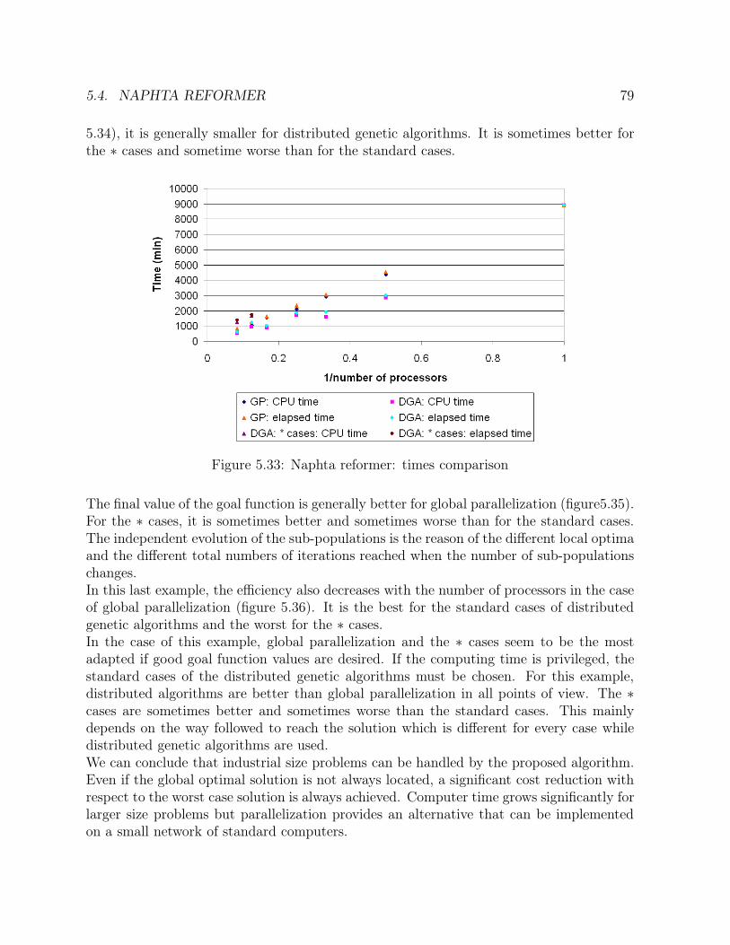
5.4. NAPHTA REFORMER 79
5.34), it is generally smaller for distributed genetic algorithms. It is sometimes better forthe ∗ cases and sometime worse than for the standard cases.
Figure 5.33: Naphta reformer: times comparison
The final value of the goal function is generally better for global parallelization (figure5.35).For the ∗ cases, it is sometimes better and sometimes worse than for the standard cases.The independent evolution of the sub-populations is the reason of the different local optimaand the different total numbers of iterations reached when the number of sub-populationschanges.In this last example, the efficiency also decreases with the number of processors in the caseof global parallelization (figure 5.36). It is the best for the standard cases of distributedgenetic algorithms and the worst for the ∗ cases.In the case of this example, global parallelization and the ∗ cases seem to be the mostadapted if good goal function values are desired. If the computing time is privileged, thestandard cases of the distributed genetic algorithms must be chosen. For this example,distributed algorithms are better than global parallelization in all points of view. The ∗cases are sometimes better and sometimes worse than the standard cases. This mainlydepends on the way followed to reach the solution which is different for every case whiledistributed genetic algorithms are used.We can conclude that industrial size problems can be handled by the proposed algorithm.Even if the global optimal solution is not always located, a significant cost reduction withrespect to the worst case solution is always achieved. Computer time grows significantly forlarger size problems but parallelization provides an alternative that can be implementedon a small network of standard computers.
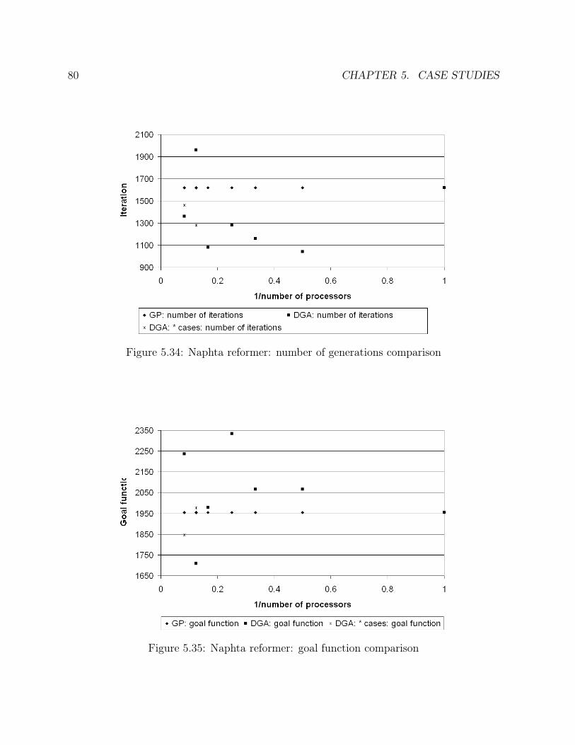
80 CHAPTER 5. CASE STUDIES
Figure 5.34: Naphta reformer: number of generations comparison
Figure 5.35: Naphta reformer: goal function comparison
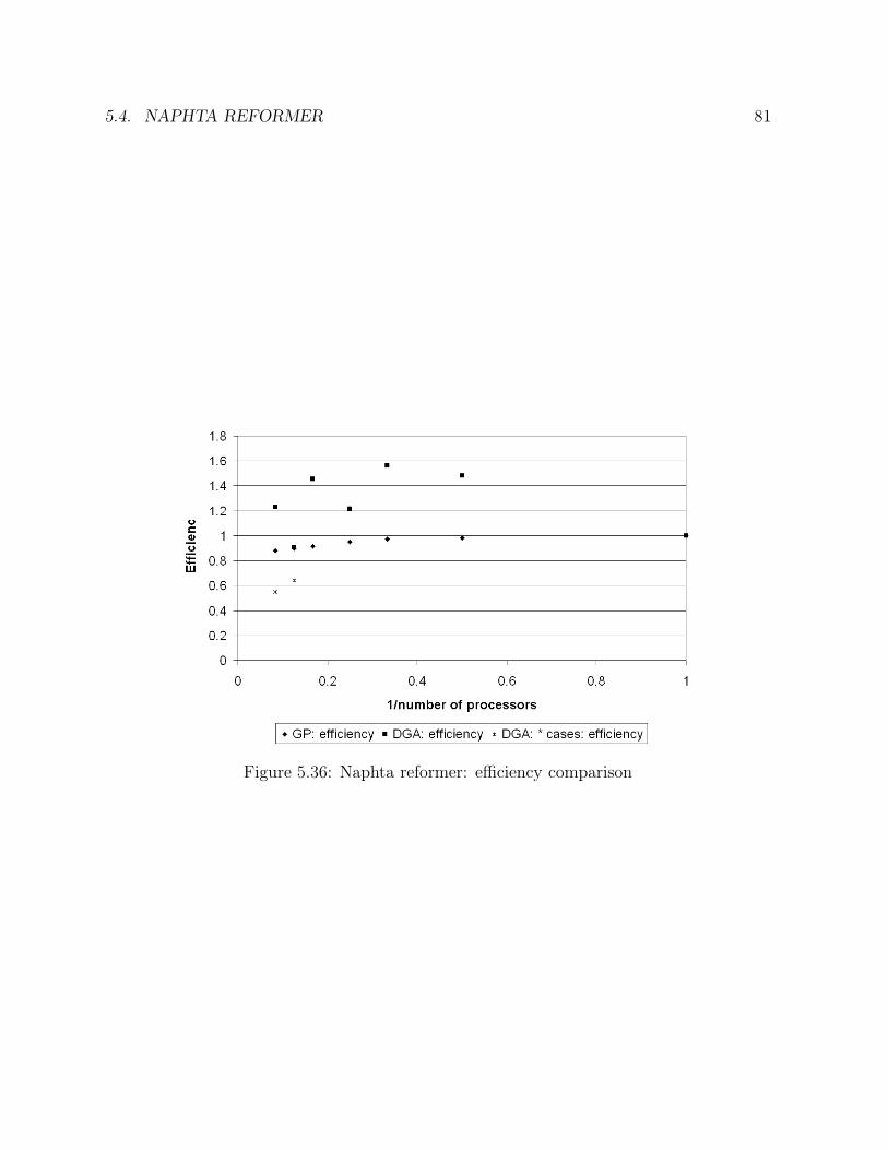
5.4. NAPHTA REFORMER 81
Figure 5.36: Naphta reformer: efficiency comparison

Chapter 6
Fault detection and localisation
Fault detection and isolation is another important subject in process monitoring. We willhandle here an example where the objective is to detect leaks in a pipe network, based onflow measurements. Indeed, fluid leaks are expensive and must be detected as quickly aspossible. However, all measurements are erroneous and the sensor precision has a greatinfluence on the detectability and isolability of process faults, so that the sensor precisionmust be taken into account when a network is chosen. In this chapter, a general methodto design the cheapest sensor network able to detect and locate a list of faults in a givenprocess is proposed. The method is based on the fault detection method proposed byJ. Ragot and D. Maquin (Ragot and Maquin, 2006). Those authors use the notion ofsensibility to fault to decide weather a residual is influenced or not by a specified fault onthe process.The problem is similar to the problem of design of the cheapest sensor network allowing toreconcile the process and estimate all process key parameters within a prescribed accuracy:it is also multimodal, not derivable and involves many binary variables. That is why thegenetic algorithm has been used with a different goal function.The method is illustrated for two water networks of different sizes. The detected faults areleaks from pipes and storage tanks leaks but other types of fault could also be simulatedand detected.
6.1 Fault detection and isolation
The objective of fault detection is to determine whether the measurements remain in therange of the values given by the process model for a chosen operating mode of the plant. Ifthe distance between measurements and estimations is too important, a fault is detected.The fault detection and localisation techniques are carried out in two steps: the estimationof the residuals and the decision. In a way to be sure that all the faults that can occurin a process are detectable, the signature matrix Σ must be analysed. This matrix is theoccurrence matrix of the variables in the residual equations. As an example, let us consider
83
84 CHAPTER 6. FAULT DETECTION AND LOCALISATION
the following process containing four residuals and six variables at time t:
r1 (t) = f1 (x1 (t) , x2 (t) , x5 (t) , x6 (t))
r2 (t) = f2 (x1 (t) , x2 (t) , x3 (t) , x5 (t) , x6 (t))
r3 (t) = f3 (x3 (t) , x5 (t) , x6 (t))
r4 (t) = f4 (x2 (t) , x4 (t) , x5 (t)) (6.1)
The corresponding signature matrix has the form:
Σ =
∣∣∣∣∣∣∣∣
X X 0 0 X XX X X 0 X X0 0 X 0 X X0 X 0 X X 0
∣∣∣∣∣∣∣∣(6.2)
A fault is detectable if the corresponding column in the signature matrix contains atleast one non-zero element. A fault can be located if the corresponding column in thesignature matrix is different from all other columns of the signature matrix. The faultlocalisation consists of deducing what is the fault from the values of the residuals. Forthat purpose, fuzzy rules are elaborated from the signature matrix. They are linguistic"if-then" constructions of the general form "if A then B" where A are the premises and Bthe consequences of the rule.As noise influences the value of the residuals, some random perturbations which are notcaused by any fault in the process can reach magnitude such that the corresponding resid-uals are then associated to faults. Thus faults may be detected even when none occursand false alarms are then triggered. Taking into account temporal persistence allows toimprove the detection procedure. For that purpose, one takes the average of the values ofthe variables for the k last measurement times, instead of instantaneous measurements.The sensitivities of residuals to a given fault situation are different so that the magnitudeof the residual deviations allows to characterize a fault situation. The detectability andisolability of faults can then be improved by using this difference of sensitivity. Let y(t)be the measurement of a variable of the process at measurement time t. It is always thesum of the true value x(t), the noise �(t) and the fault f(t):
y(t) = x(t) + �(t) + f(t) (6.3)
The true value satisfying completely the process model, the residual is composed of twoterms: the contribution of the noise r� and the contribution of the fault rf so that the effectof the fault can be masked by the effect of the noise according to their relative magnitudes.The noise contribution to the itℎ residual is defined as follows:
r�,i =n∑
j=1
mij�j (6.4)
where mij are the elements of the matrix ℳ of the derivatives of the residuals with respectto the variables. If the errors are replaced by the precision of the sensors ej, one obtains
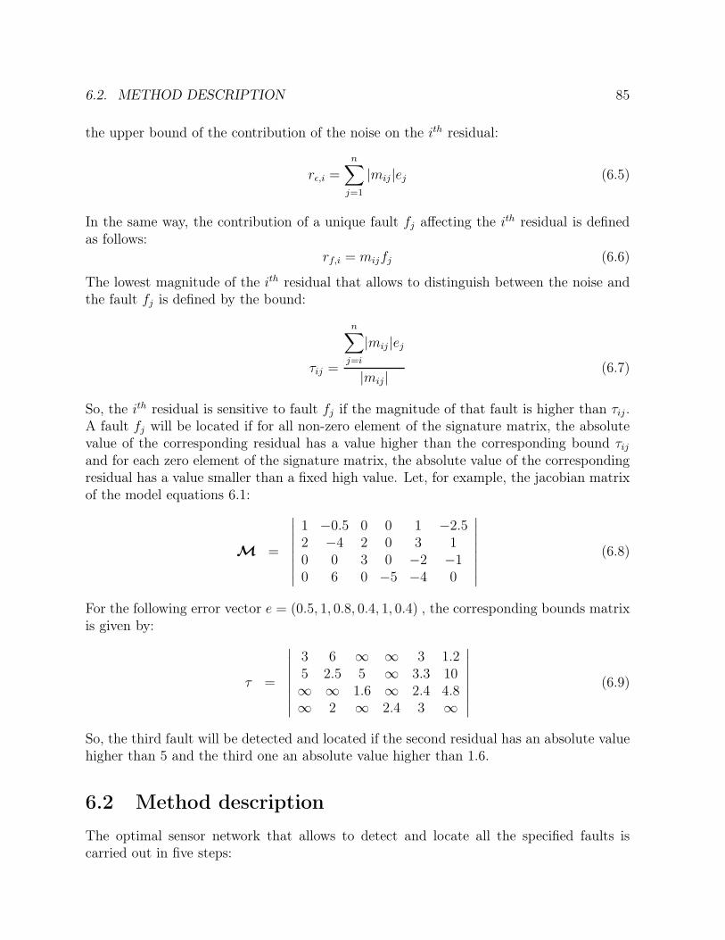
6.2. METHOD DESCRIPTION 85
the upper bound of the contribution of the noise on the itℎ residual:
r�,i =n∑
j=1
∣mij ∣ej (6.5)
In the same way, the contribution of a unique fault fj affecting the itℎ residual is definedas follows:
rf,i = mijfj (6.6)
The lowest magnitude of the itℎ residual that allows to distinguish between the noise andthe fault fj is defined by the bound:
�ij =
n∑
j=i
∣mij ∣ej
∣mij∣(6.7)
So, the itℎ residual is sensitive to fault fj if the magnitude of that fault is higher than �ij .A fault fj will be located if for all non-zero element of the signature matrix, the absolutevalue of the corresponding residual has a value higher than the corresponding bound �ijand for each zero element of the signature matrix, the absolute value of the correspondingresidual has a value smaller than a fixed high value. Let, for example, the jacobian matrixof the model equations 6.1:
퓜 =
∣∣∣∣∣∣∣∣
1 −0.5 0 0 1 −2.52 −4 2 0 3 10 0 3 0 −2 −10 6 0 −5 −4 0
∣∣∣∣∣∣∣∣(6.8)
For the following error vector e = (0.5, 1, 0.8, 0.4, 1, 0.4) , the corresponding bounds matrixis given by:
� =
∣∣∣∣∣∣∣∣
3 6 ∞ ∞ 3 1.25 2.5 5 ∞ 3.3 10∞ ∞ 1.6 ∞ 2.4 4.8∞ 2 ∞ 2.4 3 ∞
∣∣∣∣∣∣∣∣(6.9)
So, the third fault will be detected and located if the second residual has an absolute valuehigher than 5 and the third one an absolute value higher than 1.6.
6.2 Method description
The optimal sensor network that allows to detect and locate all the specified faults iscarried out in five steps:

86 CHAPTER 6. FAULT DETECTION AND LOCALISATION
∙ Process and faults simulation;
∙ Specification of the sensor database and the sensor requirements;
∙ Verification of the problem feasibility;
∙ Optimisation of the sensor network;
∙ Report generation.
6.2.1 Process and faults simulation
We consider here processes consisting in tanks, pipes, mixers and dividers, such as the oneshown in figure 6.3. The process is first simulated for a normal, fault free operating. Thedifferential balance equations are integrated by means of the fourth order Runge-Kuttamethod. Then, for each possible fault one decides the minimal magnitude of the fault thatshould be detected by the sensor network, for example a leak of 1% of a stream flow rate.The faults are simulated one by one by increasing progressively their magnitude until theminimal fault that should be detected is reached. The values of the flowrates at both endsof each pipe are recorded for each fault. No noise is added to the variables at this stepbecause the noise will depend on the precision of the measurement tools. The number oftime measurements that are used for computing the variables mean values depends on thefrequency of the measurements and the speed at which the fault should be detected. Ifthe number of measurement times is higher, the fault detection and localisation is slowerand better. If this number is too small, the noise influences more the magnitude of theresiduals and the fault detection is more difficult. The value of that parameter has beenchosen to five. This parameter, as well as the time at which the fault should be detected,is studied for the first example presented here after.
6.2.2 Specification of the sensor database and the sensor require-ments
The sensor database and the sensor requirements files contain the same information as theones defined in the first part of the thesis.
6.2.3 Verification of the problem feasibility
The step of feasibility of the problem verification begins by listing all the sensors that canbe placed in the plant. For each sensor of this list, a binary gene is created. If a variableis measured by more than one sensor, the precision of the most accurate one is taken intoaccount for the bounds calculation. The residual bounds and the residuals are estimatedfor the initial sensor network: indeed, a noise bounded by the accuracy of the sensor is
6.2. METHOD DESCRIPTION 87
added to each variable for each measurement time before the mean of the variables andthe residuals are calculated. The noise on the variables and then their values depend thuson the sensor network as well as on the residual bounds. To ensure that a solution existsto the studied problem, the next condition has to be met: the initial sensor network hasto be able to detect all the simulated faults. If it is not the case, new sensor types that aremore precise can be added to the data base or the minimal magnitudes of the faults thatshould be detected should be increased.
6.2.4 Optimisation of the sensor network
Once one is sure that a solution exists, it can be optimized. The objective function to beminimized is evaluated this way:
∙ if all the faults can be detected and located, the goal function is the sum of the costsof all the sensors in the chosen network;
∙ if at least one fault can not be detected or located, the goal function is a multiple (2has been chosen) of the maximum cost .
The goal function being generally multimodal, the problem being not derivable and con-taining only binary parameters, the genetic algorithm is still used for this version of theprogram. The probabilities of the evolution mechanisms remain unchanged as well as thesize of the population:
∙ probability for each gene to be chosen at first generation: 80%;
∙ size of the population: 20 individuals;
∙ probability of reproduction: 50%
∙ probability of single-point cross-over: 50%;
∙ probability of jump mutation: 1%.
The goal function of each individual of the new population is evaluated. The best oneis then kept and duplicated. The solution is still reached if after a specified number ofgenerations the goal function of the best one remains unchanged.
6.2.5 Report generation
The report generated here contains the same information as the one generated for the firstversion of the program. The only difference is that there is no prescribed accuracy on keyvariables.

88 CHAPTER 6. FAULT DETECTION AND LOCALISATION
6.3 Cases study
In this paragraph, two water networks are studied.
6.3.1 First example
This first one is composed of five storage tanks and ten water pipes (6.1).
F0
F1A F1B
F1
H1
F2A F2B
F2
H2
F3
H3
F5
H5
F4
H4
Figure 6.1: Flow sheet of the first example of fault detection
The fifteen faults that should be detected and located are water leaks in the storage tanksor in the pipes. In the storage tanks, the level meters can be situated at one place andthe flow rate in the pipes can be measured at the beginning and at the end of each pipe,which means 25 possible sensor locations. The sensor database contains three level meterswith different accuracies and prices, and 10 flowmeters with different accuracies, prices andmeasurement domains:
Table 6.1: First water network: sensor database
Sensor types Annualized Accuracies Minimum Maximumcosts values values
Height A 40 0.05 0 m 70 dmHeight B 50 0.03 0 m 70 dm
continued on next page
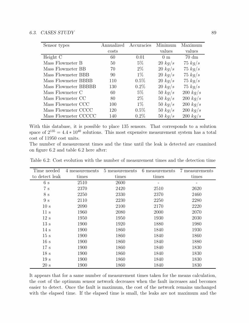
6.3. CASES STUDY 89
Sensor types Annualized Accuracies Minimum Maximumcosts values values
Height C 60 0.01 0 m 70 dmMass Flowmeter B 50 5% 20 kg/s 75 kg/sMass Flowmeter BB 70 2% 20 kg/s 75 kg/sMass Flowmeter BBB 90 1% 20 kg/s 75 kg/sMass Flowmeter BBBB 110 0.5% 20 kg/s 75 kg/sMass Flowmeter BBBBB 130 0.2% 20 kg/s 75 kg/sMass Flowmeter C 60 5% 50 kg/s 200 kg/sMass Flowmeter CC 80 2% 50 kg/s 200 kg/sMass Flowmeter CCC 100 1% 50 kg/s 200 kg/sMass Flowmeter CCCC 120 0.5% 50 kg/s 200 kg/sMass Flowmeter CCCCC 140 0.2% 50 kg/s 200 kg/s
With this database, it is possible to place 135 sensors. That corresponds to a solutionspace of 2135 = 4.4 ∗ 1040 solutions. This most expensive measurement system has a totalcost of 11950 cost units.The number of measurement times and the time until the leak is detected are examinedon figure 6.2 and table 6.2 here after:
Table 6.2: Cost evolution with the number of measurement times and the detection time
Time needed 4 measurements 5 measurements 6 measurements 7 measurementsto detect leak times times times times
6 s 2510 2600 - -7 s 2370 2420 2510 26208 s 2250 2330 2370 24609 s 2110 2230 2250 228010 s 2090 2100 2170 222011 s 1960 2080 2000 207012 s 1950 1950 1930 203013 s 1900 1920 1880 198014 s 1900 1860 1840 193015 s 1900 1860 1840 186016 s 1900 1860 1840 188017 s 1900 1860 1840 183018 s 1900 1860 1840 183019 s 1900 1860 1840 183020 s 1900 1860 1840 1830
It appears that for a same number of measurement times taken for the means calculation,the cost of the optimum sensor network decreases when the fault increases and becomeseasier to detect. Once the fault is maximum, the cost of the network remains unchangedwith the elapsed time. If the elapsed time is small, the leaks are not maximum and the
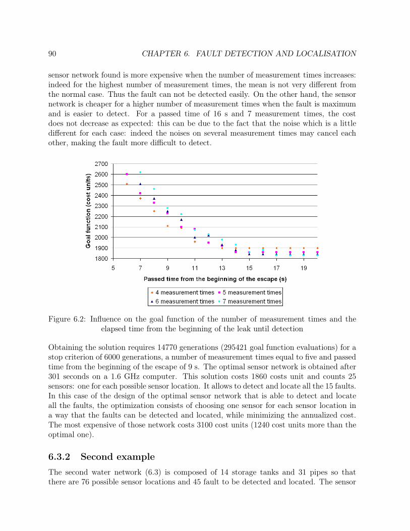
90 CHAPTER 6. FAULT DETECTION AND LOCALISATION
sensor network found is more expensive when the number of measurement times increases:indeed for the highest number of measurement times, the mean is not very different fromthe normal case. Thus the fault can not be detected easily. On the other hand, the sensornetwork is cheaper for a higher number of measurement times when the fault is maximumand is easier to detect. For a passed time of 16 s and 7 measurement times, the costdoes not decrease as expected: this can be due to the fact that the noise which is a littledifferent for each case: indeed the noises on several measurement times may cancel eachother, making the fault more difficult to detect.
Figure 6.2: Influence on the goal function of the number of measurement times and theelapsed time from the beginning of the leak until detection
Obtaining the solution requires 14770 generations (295421 goal function evaluations) for astop criterion of 6000 generations, a number of measurement times equal to five and passedtime from the beginning of the escape of 9 s. The optimal sensor network is obtained after301 seconds on a 1.6 GHz computer. This solution costs 1860 costs unit and counts 25sensors: one for each possible sensor location. It allows to detect and locate all the 15 faults.In this case of the design of the optimal sensor network that is able to detect and locateall the faults, the optimization consists of choosing one sensor for each sensor location ina way that the faults can be detected and located, while minimizing the annualized cost.The most expensive of those network costs 3100 cost units (1240 cost units more than theoptimal one).
6.3.2 Second example
The second water network (6.3) is composed of 14 storage tanks and 31 pipes so thatthere are 76 possible sensor locations and 45 fault to be detected and located. The sensor

6.3. CASES STUDY 91
F0A
F1A F1B
F1
H1
F2A F2B
F2
H2
F3
H3
F5
H5
F4
H4
F10
H10
F11
H11
F12
H12
F13
H13
F13B
F13A
F14
H14
F0B
F6A F6C
F6
F6B
H6
F7
H7
F8A F8B
F8
H8
F9A F9B
F9
H9
F7A
F15
Figure 6.3: Flow sheet of the second example of fault detection
database contains this time three level meters with different accuracies and prices, and 15flowmeters with different accuracies, prices and measurement domains.
Table 6.3: Second water network: sensor database
Sensor types Costs Accuracies Minimum Maximumvalues values
Height A 40 0.05 0 m 70 dmHeight B 50 0.03 0 m 70 dmHeight C 60 0.01 0 m 70 dmMass Flowmeter A 40 5% 0 kg/s 25 kg/sMass Flowmeter AA 60 2% 0 kg/s 25 kg/sMass Flowmeter AAA 80 1% 0 kg/s 25 kg/sMass Flowmeter AAAA 100 0.5% 0 kg/s 25 kg/sMass Flowmeter AAAAA 120 0.2% 0 kg/s 25 kg/sMass Flowmeter B 50 5% 20 kg/s 75 kg/sMass Flowmeter BB 70 2% 20 kg/s 75 kg/sMass Flowmeter BBB 90 1% 20 kg/s 75 kg/sMass Flowmeter BBBB 110 0.5% 20 kg/s 75 kg/sMass Flowmeter BBBBB 130 0.2% 20 kg/s 75 kg/sMass Flowmeter C 60 5% 50 kg/s 200 kg/sMass Flowmeter CC 80 2% 50 kg/s 200 kg/s
continued on next page
92 CHAPTER 6. FAULT DETECTION AND LOCALISATION
Sensor types Costs Accuracies Minimum Maximumvalues values
Mass Flowmeter CCC 100 1% 50 kg/s 200 kg/sMass Flowmeter CCCC 120 0.5% 50 kg/s 200 kg/sMass Flowmeter CCCCC 140 0.2% 50 kg/s 200 kg/s
The initial network counts 392 possible sensors. This corresponds to a solution spaceof 2392 = 10118 solutions. This sensor network has a total cost of 34100 costs units.Obtaining the solution requires 26104 generations (522101 goal function evaluations) fora stop criterion of 6000 generations, a number of measurement times equal to five anda detection time from the beginning of the leak of 15 s. The optimal sensor network isobtained after 5667 seconds on a 1.6 GHz computer. This solution costs 6200 cost unitsand counts 76 sensors: one by possible sensor location and allows to detect and locate allthe 45 faults. In this case also the design of the optimal sensor network able to detect andlocate all the faults consists of optimizing the selection of one sensor for each location ina way that the faults can be detected and located, while minimizing the annualized cost.The most expensive of those networks costs this time 9000 cost units (2800 cost units morethan the optimal one).
6.3.3 Conclusions
The proposed method allows to determine a sensor network that is able to detect andlocate a specified list of tank and pipe leaks. This network is much cheaper than the initialone but due to the optimization method, there is no guarantee that it is always the bestone.The number of measurement times required to declare a fault must be chosen as a functionof the problem. It should not be to high because it increases the time elapsed between theoccurrence of the fault and its detection, or the sensor network required is more expensive.On the other hand, a too small number of measurement times may cause the detection offaults that does not exists.This method could be transposed for other types of faults such as the catalyst deactivationor the loss of efficiency in a compressor.As computing times becomes important when the size of the problem increases, a paral-lelisation of the method could be envisaged for larger size problems.

Chapter 7
Conclusions part I
The proposed method allows to achieve an important progress in the design of sensornetworks in the case of steady-state processes. Indeed, the method using the linearisedequations of the model at the operating point can be treated easily for models includingenergy balances and non linear equations in addition to the mass balances. Moreover, thecalculation of a posteriori standard deviations based on steady-state data reconciliationallows to introduce a term in the goal function that takes into account the accuracy of somekey variables of the process that have to be known precisely for the efficient monitoring ofthe plant.The design of sensor networks allowing to detect a specified list of process faults has alsobeen envisaged and gives good results. A compromise has to be done between the speedof fault detection and the necessity to make the difference between punctual measurementerror and process faults.The optimization method based on genetic algorithms allows to find a solution which ismuch better than the initial one for all the studied examples. This solution found lightdiffers from the global optimum since all possible solutions are not tested but it is reachedwithin a computing time that is reasonable in comparison to the one required for theevaluation of all possible solutions.The systematic application of such a method while creating a new plant should allow toachieve important savings. Indeed, sensor networks installed on the industries are generallyreduced to the minimum because of the cost of the sensors. Some variables that seem to bewithout interest at a moment can however appear to be very important for the control ofthe process or for the evaluation of a key performance parameter. It is then very expensiveto install new sensors after the plant has been put in operation. Moreover the global costof a sensor network upgrade can then reveal to be more important than the one that wouldhave been determined by design method.The method also allows to treat in a unique calculation several operating points and thusfind sensor networks that limit the uncertainty on key performance indicators when theplant changes its operating point to obtain, for example, a product with other specifications.Being able to design a sensor network that remains efficient in the case of one sensor failureis also interesting: indeed, it improved the system availability and allows to repair without
93
94 CHAPTER 7. CONCLUSIONS PART I
interrupting the plant operation.The parallelization of the program allowed to reduce the computing time whatever themethod that is used and the studied example. In the case of global parallelization, thecomputing time is always inversely proportional to the number of processors and the ef-ficiency decreases when the number of processors increases. The efficiency loss increasesmore quickly when the number of processors becomes nearer to the number of goal func-tions that has to be evaluated at each generation. So that, a compromise has to be foundbetween the number of processors and the computing time.In the case of distributed genetic algorithms, those tendencies can not be reproduced.Indeed, since the path followed to reach the solution is different, the network that is founddiffers from the one found with global parallelization if local minima are reached insteadof the global solution. The computing time can also be different according to the numberof generations needed to produce by random evolution an efficient solution. Following thestudied example, distributed genetic algorithms are sometimes better and sometimes worsethan global parallelization. For a same example, the choice between global parallelizationand distributed genetic algorithms is not always clear-cut. One method may need lesstime to detect convergence, but remain stuck in a local optimum, but the ranking maychange when a different number of processors is used. Moreover, it also appears from theexamples, that it is usually preferable if the size of the sub-populations is small in the caseof distributed genetic algorithms to decrease the stop criterion and increase the size of thesub-populations by the same factor. So, when the user decides to use a parallelised versionof the software, he never knows in advance if he has chosen the best method but he is sureto reach the solution within a shorter computing time.

Part II
Dynamic data reconciliation
95


Chapter 8
Formulation of the dynamic data
reconciliation problem
The dynamic data reconciliation allows to use temporal redundancies by taking into ac-count several discrete measurements for some state variables. The general dynamic datareconciliation problem can be formulated as in (Liebman et al., 1992), (Rao, 2000):
minxi,j ,zi,j ,ui,j
Φ[xi,j , x
mi,j, zi,j, z
mi,j, ui,j, u
mi,j, �
](8.1)
subject to
∙ differential constraints:
f
(dxi,j
dt, xi,j , zi,j, ui,j
)= 0 (8.2)
∙ equality constraints:h [xi,j , zi,j, ui,j] = 0 (8.3)
∙ inequality constraints:g [xi,j , zi,j, ui,j] ≥ 0 (8.4)
with the initial conditions:
xi,0 = xCIi,0 (8.5)
where
∙ xi,j is the estimation of the differential state variable i at measurement time j;
∙ xmi,j is the measurement of the differential state variable i at measurement time j;
∙ xCIi,0 is the initial condition of the differential state variable i. It corresponds to the
estimation of that variable at the same time of the previous reconciliation horizon.
97
98 CHAPTER 8. FORMULATION DYNAMIC DATA RECONCILIATION
∙ zi,j is the estimation of the algebraic state variable i at measurement time j;
∙ zmi,j is the measurement of the algebraic state variable i at measurement time j;
∙ ui,j is the estimation of the input variable i at measurement time j;
∙ umi,j is the measurement of the input variable i at measurement time j;
∙ � are the precisions of the measurements.
For most applications, the objective function is the sum for all the times and all themeasurements of weighted square residues:
Φ[xi,j, x
mi,j, zi,j , z
mi,j, ui,j, u
mi,j, �
]=
time N∑
j=time 0
nxmes∑
i=1
(xi,j − xm
i,j
�xi,j
)2
+time N∑
j=time 0
nzmes∑
i=1
(zi,j − zmi,j
�zi,j
)2
+time N∑
j=time 0
numes∑
i=1
(ui,j − um
i,j
�ui,j
)2
(8.6)
where
∙ nxmesis the number of measured differential state variables;
∙ nzmesis the number of measured algebraic state variables;
∙ numesis the number of measured input variables;
∙ �xi,jis the standard deviation on the differential state variable i at measurement time
j;
∙ �zi,j is the standard deviation on the algebraic state variable i at measurement timej;
∙ �ui,jis the standard deviation on the input variable i at measurement time j.
When the objective function is formulated this way, all the measurements that are carriedout between time 0 and time N are reconciled simultaneously. When the time horizonincreases (when new measurements are carried out), the calculation efforts increase. Attime N, the measurements carried out in time zero are reconciled N+1 times with differentneighboring measurements. The choice of the best reconciled values remains an openquestion: for on-line control, one should probably choose the value corresponding to thelast measurement time; for archiving or for off-line calculations, the values of the middleof the time horizon are preferred.

99
In the filtering method which is described in chapter 9, the information contained in theN − 1 first times is summarized in the prediction vector. So that, only the measurementscarried out at the last time step of time horizon is used at each reconciliation time.In chapter 10, the moving window methods are explained. They also allow to use only apart of the measurements carried out during the time horizon.

Chapter 9
Filtering methods
9.1 Introduction
In this chapter, some generalities are given concerning filtering methods. Then the ex-tended Kalman filter is described. This is a sequential estimation algorithm that producesminimum variance linear estimates of state variables.Kalman filter is said to be invented by Rudolf E. Kalman in 1960 (Kalman and Bucy,1961), (Kalman, 1960) though Thorvald N. Thiele and Peter Swerling developed a similaralgorithm earlier. The first implementation of Kalman filter was carried out by StanleySchmidt (Schmidt, 1980) to solve the trajectory estimation problem for the Apollo program.This first filter called linear Kalman filter is used to the reconciliation of linear dynamicprocesses. The Kalman filter has then been extended to deal with non linear systems(Karjala and Himmelblau, 1996), (Narasimhan and Jordache, 2000): the non linear partof the model is linearized thanks to a first order Taylor serie around the current estimated.This second filter is called extended Kalman filter. An other method based on secondorder divided differences is also used in the case of non linear systems (Norgaard et al.,2000). Nowadays, a wide variety of Kalman filters has been developed and is widelyused in engineering applications such as radars, computer vision, autonomous or assistednavigation.
Dynamic systems can be described by means of two models:
∙ the dynamic model;
∙ the observation model.
Filtering methods proceed in two steps for each estimation:
∙ the time update: the state variables and the covariance matrix of the predictionerrors are predicted from the dynamic model;
∙ the observation update: the gain matrix is first calculated by weighting measurementswith predicted state. The states and the covariance matrix of the estimation errorsare then carried out.
101
102 CHAPTER 9. FILTERING METHODS
9.2 Extended Kalman Filter
In the case of the extended Kalman filter, the dynamic model is a set of non linear dynamicdifference equations:
xj = f (xj−1,uj−1,vj−1) (9.1)
and the observation model:
yj = h (xj ,wj) (9.2)
In those equations,
∙ xj is the vector of state variables at time step j;
∙ uj−1 is the vector of input variables at time step j-1;
∙ vj−1 is the vector of process noises at time step j-1;
∙ yj is the vector of measurements at time step j;
∙ wj is the vector of measurement noises at time step j;
∙ f (xj−1,uj−1,vj−1) is a set of non linear functions of x, u and v at time step j-1;
∙ ℎ (xj,wj) is a set of non linear functions of x and w at time step j;
∙ v and w are assumed to be white noises, independent from one another and withzero mean:
E[vj wT
l
]= 0 ∀j, l (9.3)
E [vj] = 0 ∀j (9.4)
E[vj vT
l
]= Qj�j,l (9.5)
E [wj] = 0 ∀j (9.6)
E[wj wT
l
]= Rj �j,l (9.7)
where
– Qj is the process noises covariance matrix. This matrix may change at eachtime step;
– Rj is the measurement noises covariance matrix. This matrix may change ateach time step.
The filter counts four initial conditions:
∙x0∣0 = E [x0] = x0 (9.8)
9.2. EXTENDED KALMAN FILTER 103
∙P0∣0 = cov (x0) = E
[(x0 − x0) (x0 − x0)
T]= P0 (9.9)
∙ x0 and wj are not correlated:
E[x0 wT
j
]= 0 ∀j (9.10)
∙ x0 and vj are not correlated:
E[x0 vT
j
]= 0 ∀j (9.11)
As the noises vectors vj and wj are zero mean and can not be known at each time stepin practice, the model equations 9.1 and 9.2 can be approximated by considering they arenull:
xj = f(xj−1∣j−1,uj−1, 0
)(9.12)
yj = h (xj, 0) (9.13)
If one linearizes those estimates:
xj ≈ xj + Fj−1
(xj−1 − xj−1∣j−1
)+ Vj−1 vj−1 (9.14)
yj ≈ yj + Hj (xj − xj) + Wj wj (9.15)
where
∙ Fj−1 is the Jacobian matrix of partial derivatives of f with respect to x:
Fj−1 (k, l) =�f (k)
�x (l)
∣∣∣∣x=xj∣j−1,u=uj−1,v=0
(9.16)
∙ Vj−1 is the Jacobian matrix of partial derivatives of f with respect to v:
Vj−1 (k, l) =�f (k)
�v (l)
∣∣∣∣x=xj∣j−1,u=uj−1,v=0
(9.17)
∙ Hj−1 is the Jacobian matrix of partial derivatives of h with respect to x:
Hj−1 (k, l) =�ℎ (k)
�x (l)
∣∣∣∣x=xj ,w=0
(9.18)
∙ Wj−1 is the Jacobian matrix of partial derivatives of h with respect to w:
Wj−1 (k, l) =�ℎ (k)
�w (l)
∣∣∣∣x=xj ,w=0
(9.19)
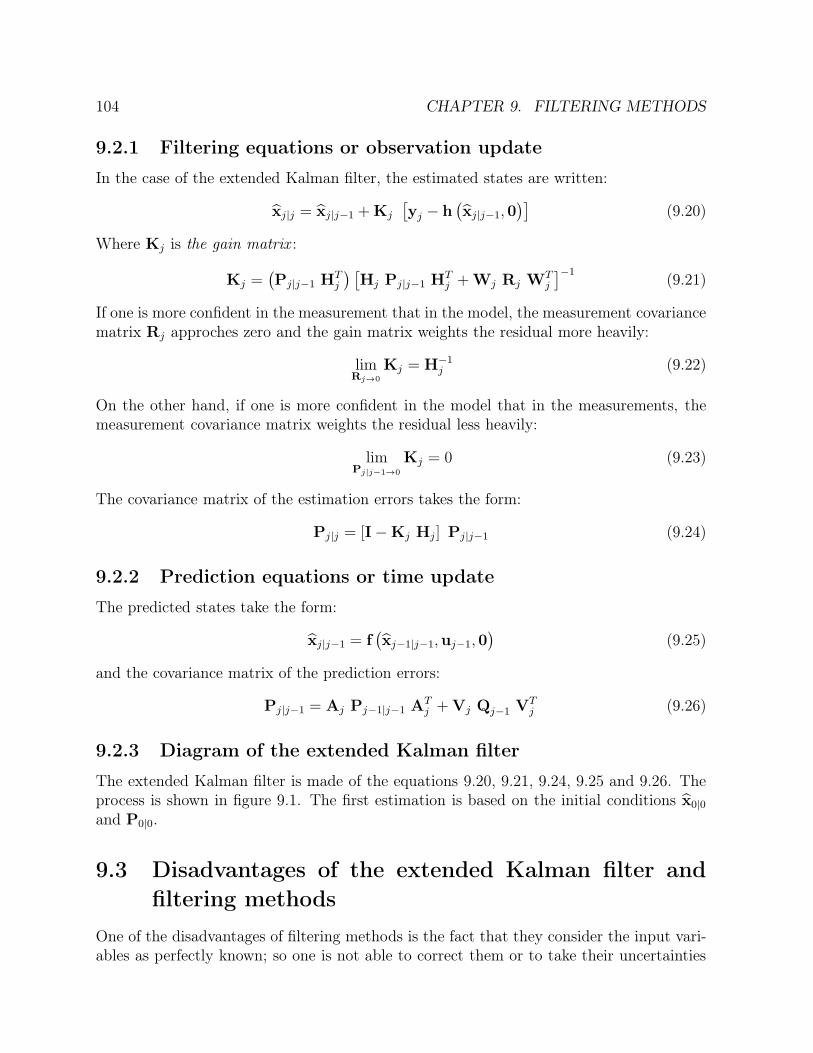
104 CHAPTER 9. FILTERING METHODS
9.2.1 Filtering equations or observation update
In the case of the extended Kalman filter, the estimated states are written:
xj∣j = xj∣j−1 + Kj
[yj − h
(xj∣j−1, 0
)](9.20)
Where Kj is the gain matrix :
Kj =(Pj∣j−1 HT
j
) [Hj Pj∣j−1 HT
j + Wj Rj WTj
]−1(9.21)
If one is more confident in the measurement that in the model, the measurement covariancematrix Rj approches zero and the gain matrix weights the residual more heavily:
limRj→0
Kj = H−1j (9.22)
On the other hand, if one is more confident in the model that in the measurements, themeasurement covariance matrix weights the residual less heavily:
limPj∣j−1→0
Kj = 0 (9.23)
The covariance matrix of the estimation errors takes the form:
Pj∣j = [I − Kj Hj ] Pj∣j−1 (9.24)
9.2.2 Prediction equations or time update
The predicted states take the form:
xj∣j−1 = f(xj−1∣j−1,uj−1, 0
)(9.25)
and the covariance matrix of the prediction errors:
Pj∣j−1 = Aj Pj−1∣j−1 ATj + Vj Qj−1 VT
j (9.26)
9.2.3 Diagram of the extended Kalman filter
The extended Kalman filter is made of the equations 9.20, 9.21, 9.24, 9.25 and 9.26. Theprocess is shown in figure 9.1. The first estimation is based on the initial conditions x0∣0
and P0∣0.
9.3 Disadvantages of the extended Kalman filter and
filtering methods
One of the disadvantages of filtering methods is the fact that they consider the input vari-ables as perfectly known; so one is not able to correct them or to take their uncertainties

9.3. DISADVANTAGES 105
Figure 9.1: Diagram of the extended Kalman filter
into account. However all measurements are erroneous and it would be interesting to con-sider the uncertainties on those measurements to correct the other variables and estimatetheir a posteriori uncertainties.Another disadvantage of filtering methods is that they don’t take into account inequalityconstraints as well as the bounds on the filtered variables so they may appear out of boundsafter filtering. The advantage of filtering is that it is much faster than the moving horizonmethods.In the case of very non linear differential equations, the convergence is not easy to achievewith the extended Kalman filter. Moreover, one needs the partial derivatives of the dynamicand of the observation model which can not always be achieved.Considering all those disadvantages, we decided to turn towards another dynamic datareconciliation method based on the moving horizon idea.


Chapter 10
Moving-Horizon estimation
As indicated in chapter 8, solving the dynamic reconciliation problem would involve anincreasing complex problem if all measurements collected since start-up are considered.The moving window techniques described in this chapter allow to reduce the size of theoptimization problem because they only take into account the last measurements collectedduring a limited time frame. Those methods carry out an optimization for a part or allthe measurements for each window. The data collected before the current window arenot considered in the estimation for current time. For example, on figure 10.1, only themeasurements carried out between the time t0 and t6 are reconciled.
Figure 10.1: Reconciliation window
The most complex algorithms allow to treat variables that are not measured at the same
107

108 CHAPTER 10. MOVING-HORIZON ESTIMATION
time or are sampled at different frequencies.The size of the reconciliation horizon and the moving of the window are chosen in away to ensure a sufficient temporal redundancy while keeping an optimization problem ofreasonable size. Moreover, they depend on the studied problem and on the measurementsfrequency relative to the system dynamics. If measurements are very frequent, averagingthe measurements may be used to maintain a non-linear problem of manageable dimension.A window movement is described by three parameters as shown in figure 10.1:
∙ ℎ1 is the measurement frequency;
∙ ℎ4 is the window length;
∙ ℎ5 is the window movement between two successive optimizations: ℎ5 ≤ ℎ4.
Those parameters are represented on figure 10.1. In this chapter, two moving windowmethods will be described:
∙ the explicit integration of the differential equations by means of the fourth orderRunge-Kutta method;
∙ the discretization of the system equations thanks to orthogonal collocations.
10.1 Explicit integration method
In this moving horizon method, the dynamic reconciliation problem is formulated underthe form of a general non-linear programming problem. The dynamic model is integratedexplicitly on the reconciliation window thanks to the fourth order Runge-Kutta integrationmethod, assuming that the initial conditions and the evolution of input variables (inputvariables are represented by linear interpolations) are known. This method is representedon figure 10.2 and can be decomposed in nine steps, which are described here after.
1. Variables classification: the variables are classified in three types, each of them beingdecomposed in two groups: the measured and the unmeasured variables:
∙ the differential state variables, which are the integration variables that constitutethe differential equations corresponding to mass and energy balances;
∙ the input variables of the system: they can be the feed flow rate, the reflux flowrate, the temperature of an incoming stream,...
∙ the algebraic state variables, which are calculated from the differential statevariables and the input variables.
2. Initialisation of the window parameters: the three parameters of the window (de-scribed in the preceding paragraph) have to be specified in this step. In the case ofexplicit integration method, a fourth parameter has to be defined: the size of the
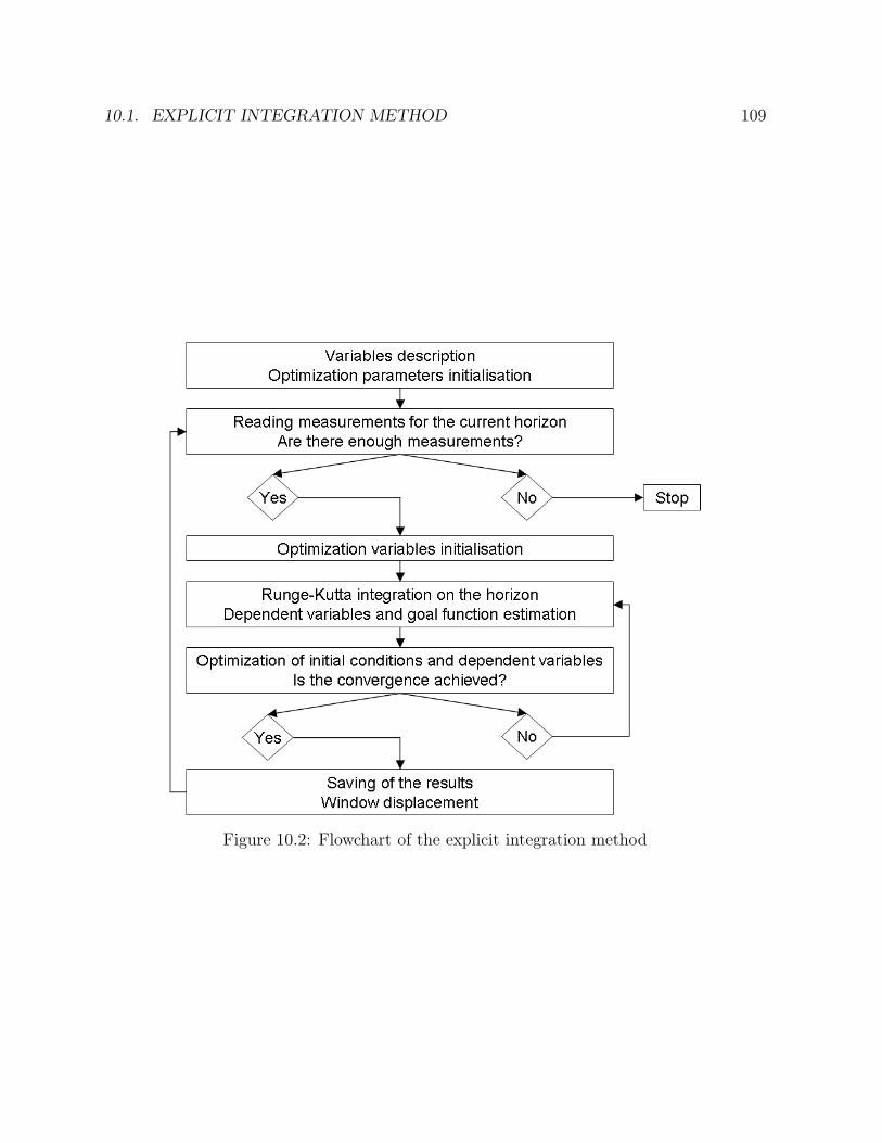
10.1. EXPLICIT INTEGRATION METHOD 109
Figure 10.2: Flowchart of the explicit integration method
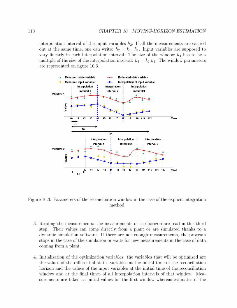
110 CHAPTER 10. MOVING-HORIZON ESTIMATION
interpolation interval of the input variables ℎ2. If all the measurements are carriedout at the same time, one can write: ℎ2 = k1a ℎ1. Input variables are supposed tovary linearly in each interpolation interval. The size of the window ℎ4 has to be amultiple of the size of the interpolation interval: ℎ4 = k2 ℎ2. The window parametersare represented on figure 10.3.
Figure 10.3: Parameters of the reconciliation window in the case of the explicit integrationmethod
3. Reading the measurements: the measurements of the horizon are read in this thirdstep. Their values can come directly from a plant or are simulated thanks to adynamic simulation software. If there are not enough measurements, the programstops in the case of the simulation or waits for new measurements in the case of datacoming from a plant.
4. Initialisation of the optimization variables: the variables that will be optimized arethe values of the differential states variables at the initial time of the reconciliationhorizon and the values of the input variables at the initial time of the reconciliationwindow and at the final times of all interpolation intervals of that window. Mea-surements are taken as initial values for the first window whereas estimates of the

10.1. EXPLICIT INTEGRATION METHOD 111
previous window are taken in the other cases. Optimized variables are scaled toimprove the efficiency of the optimization algorithm.
5. Integration of the differential equations of the process by the fourth order Runge-Kutta method: the principle of this method is to obtain an approached numericalsolution of differential equations of the system.
6. Estimation of the algebraic variables: the algebraic variables are estimated at eachintegration step by Runge-Kutta.
7. Calculation of the goal function Fgoal on the reconciliation horizon:
Fgoal =time N∑
j=time 0
nxmes∑
i=1
(xi,j − xm
i,j
�xi,j
)2
+
time N∑
j=time 0
nzmes∑
i=1
(zi,j − zmi,j
�zi,j
)2
+
time N∑
j=time 0
numes∑
i=1
(ui,j − um
i,j
�ui,j
)2
+
nxmes∑
i=1
(xi,0 − xCI
i,0
)2
R2xi
+
numes∑
i=1
(ui,0 − uCI
i,0
)2
R2ui
(10.1)
where
∙ xi,j is the estimation of the differential state variable i at measurement time j;
∙ xmi,j is the measurement of the differential state variable i at measurement time
j;
∙ xCIi,0 is the initial condition of the differential state variable i. It corresponds to
the estimation of that variables in the previous reconciliation horizon.
∙ zi,j is the estimation of the algebraic state variable i at measurement time j;
∙ zmi,j is the measurement of the algebraic state variable i at measurement time j;
∙ ui,j is the estimation of the input variable i at measurement time j;
∙ umi,j is the measurement of the input variable i at measurement time j;
∙ uCIi,0 is the initial condition of the input variable i. It corresponds to the estima-
tion of that variable at the same time of the previous reconciliation horizon.
∙ nxmesis the number of measured differential state variables;
∙ nzmesis the number of measured algebraic state variables;
∙ numesis the number of measured input variables;
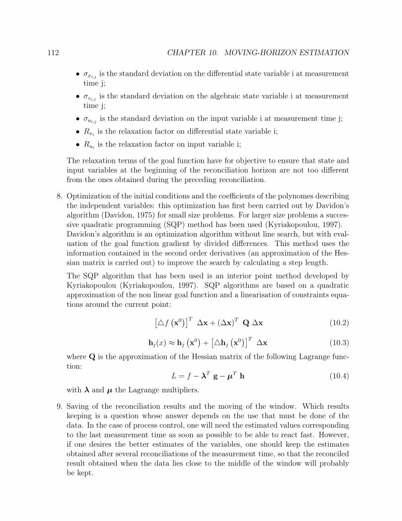
112 CHAPTER 10. MOVING-HORIZON ESTIMATION
∙ �xi,jis the standard deviation on the differential state variable i at measurement
time j;
∙ �zi,j is the standard deviation on the algebraic state variable i at measurementtime j;
∙ �ui,jis the standard deviation on the input variable i at measurement time j;
∙ Rxiis the relaxation factor on differential state variable i;
∙ Ruiis the relaxation factor on input variable i;
The relaxation terms of the goal function have for objective to ensure that state andinput variables at the beginning of the reconciliation horizon are not too differentfrom the ones obtained during the preceding reconciliation.
8. Optimization of the initial conditions and the coefficients of the polynomes describingthe independent variables: this optimization has first been carried out by Davidon’salgorithm (Davidon, 1975) for small size problems. For larger size problems a succes-sive quadratic programming (SQP) method has been used (Kyriakopoulou, 1997).Davidon’s algorithm is an optimization algorithm without line search, but with eval-uation of the goal function gradient by divided differences. This method uses theinformation contained in the second order derivatives (an approximation of the Hes-sian matrix is carried out) to improve the search by calculating a step length.
The SQP algorithm that has been used is an interior point method developed byKyriakopoulou (Kyriakopoulou, 1997). SQP algorithms are based on a quadraticapproximation of the non linear goal function and a linearisation of constraints equa-tions around the current point:
[△f
(x0)]T
Δx + (Δx)T Q Δx (10.2)
hj(x) ≈ hj
(x0)+[△hj
(x0)]T
Δx (10.3)
where Q is the approximation of the Hessian matrix of the following Lagrange func-tion:
L = f − �T g − �T h (10.4)
with � and � the Lagrange multipliers.
9. Saving of the reconciliation results and the moving of the window. Which resultskeeping is a question whose answer depends on the use that must be done of thedata. In the case of process control, one will need the estimated values correspondingto the last measurement time as soon as possible to be able to react fast. However,if one desires the better estimates of the variables, one should keep the estimatesobtained after several reconciliations of the measurement time, so that the reconciledresult obtained when the data lies close to the middle of the window will probablybe kept.

10.2. METHOD BASED ON ORTHOGONAL COLLOCATIONS 113
The main disadvantage of this method is that, unlike the filtering algorithms, there is noexplicit method to calculate a posteriori variances from the results. If this method is usedin the future, an algorithm allowing to calculate them must be developed.
10.2 Method based on orthogonal collocations
In this method, the differential equations of the system are solved by means of orthog-onal collocations. State variables and their derivatives are represented by polynomials.Differential equations are transformed into algebraic equations whose unknowns are thepolynomial coefficients. Those algebraic equations must be satisfied at several discretetimes chosen to minimize the numerical approximation errors.The main advantage of this method is that it will be possible to calculate a posteriorivariances by modifying the theory that is used in steady-state data reconciliation (Heyenet al., 1996).In this section, the collocations constraints and the different steps of the method aredescribed. Examples of polynomial approximations and the way to choose the collocationnodes are explained in annex C.
10.2.1 Description of the moving window algorithm
The algorithm allowing to apply the orthogonal collocations method to a moving windowis defined by five parameters in the case of orthogonal collocations. They are representedon figure 10.4.The parameters ℎ1, ℎ2, ℎ4 and ℎ5 of the window are the same as the ones defined previouslyin this chapter. The size ℎ3 of discretization interval of the differential state variables isan additional parameter. This interval has been chosen as a multiple of the measurementfrequency: ℎ3 = k1b ℎ1. The size of the window ℎ4 has to be a multiple of the size of thediscretization interval: ℎ4 = k3 ℎ3. The last parameter that has to be specified is the orderof Lagrange polynomials.The times �k represent the collocation times of the different discretization intervals of thewindow. The sequential algorithm is written so that the discretization and the interpolationintervals have the same size. The distinction between them must only be done in the caseof the simultaneous algorithm. The times tj are the measurement times. The choice ofthe window parameters depends on the studied problem. One has to take into account thefollowing remarks:
∙ The more the window increases, the more the number of opimization variables in-crease, and so do the computing time. So, the size of the window has to be chosenin a way to keep reasonable computing times. Moreover, if the size of the window istoo important, convergence problems may occur.
∙ Contrary, one has to keep redundancy in the problem, so that the size of the recon-ciliation window has to contain enough measurement times.

114 CHAPTER 10. MOVING-HORIZON ESTIMATION
Figure 10.4: Parameters of the reconciliation window in the case of orthogonal collocations

10.2. METHOD BASED ON ORTHOGONAL COLLOCATIONS 115
∙ The size of the discretization interval and the order of the Lagrange polynomialsmust be chosen to allow to follow the process while keeping redundancy.
∙ For the frequency of measurements, one can take all measurement times, or if theprocess variables don’t vary very much, calculate mean values on several measurementtimes. This second proposition allows to make a first filter on the variables byreducing the effect of the noise.
10.2.2 Constraints of the optimization problem
In the case of orthogonal collocations, the goal function is submitted to five sets of con-straints:
∙ the link equations: they are relations between all process variables. Those constraintshave to be satisfied as well at the measurements times as at the collocations nodes:
A = f (tj ,x, z,u) = 0 ∀tj (10.5)
Ac = f c (�k,xc, zc,uc) = 0 ∀�k (10.6)
∙ the relations between the differential state variables and the Lagrange interpolationpolynomials at all measurement times of the mowing horizon except at the initialtimes of the discretization intervals tCI :
Bi,j = xi,j −n�∑
k=0
lk(tj) xci,k = 0 ∀i, ∀tj ∕= tCI (10.7)
∙ the linear interpolations of the values of input variables between times tini and tf ofthe interpolation horizon at the other times of that horizon:
Ci,j = ui,j − ui,tini− tj − tini
tf − tini
(ui,tf − ui,tini
)= 0 ∀i, ∀tj ∕= tini, tf (10.8)
Cci,j = uc
i,k − ui,tini− �k − tini
tf − tini
(ui,tf − ui,tini
)= 0 ∀i, ∀�k (10.9)
∙ the residuals of the differential state equations at all collocation nodes:
Di,j =
n�∑
s=0
ls(�k) xci,�s
− g (�k,xck, z
ck,u
ck) = 0 ∀i, ∀�k ∕= tini (10.10)
∙ the continuity constraints of the differential state variables between two discretizationintervals:
Ei,j =
[n�∑
k=0
k(tf) xci,k
]
tf ,discr int q−1
−[
n�∑
k=0
lk(tini) xci,k
]
tini,discr int q
= 0 ∀i
(10.11)
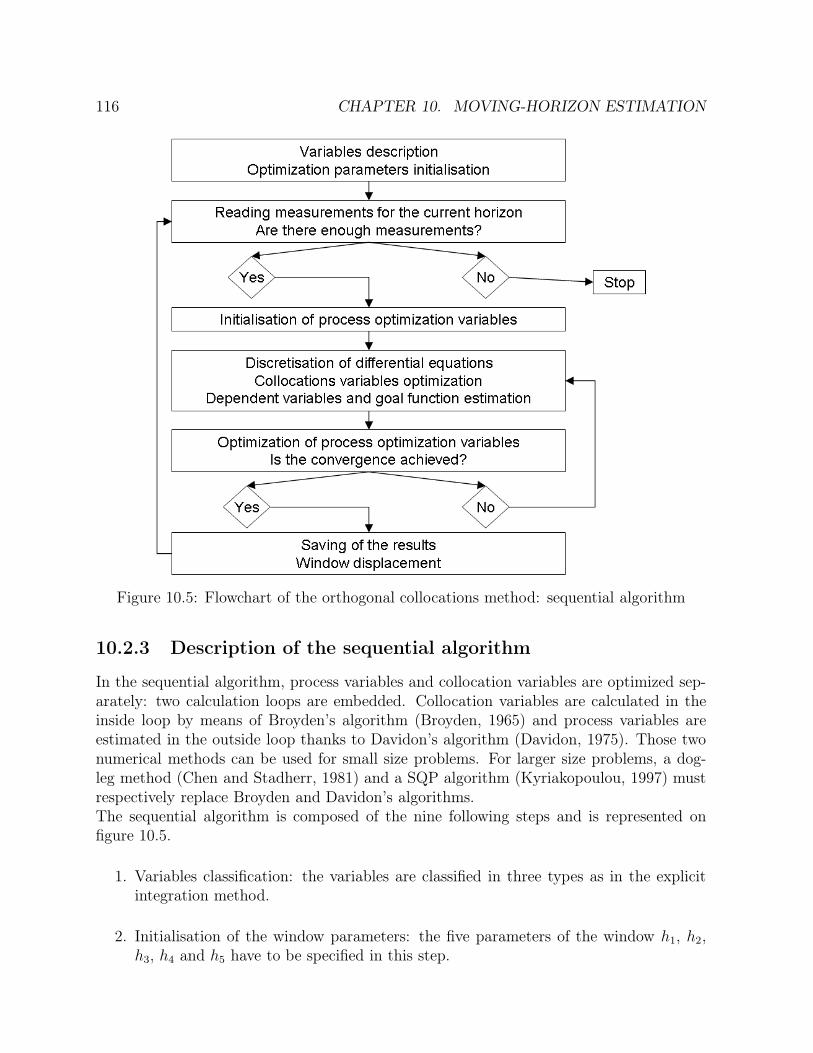
116 CHAPTER 10. MOVING-HORIZON ESTIMATION
Figure 10.5: Flowchart of the orthogonal collocations method: sequential algorithm
10.2.3 Description of the sequential algorithm
In the sequential algorithm, process variables and collocation variables are optimized sep-arately: two calculation loops are embedded. Collocation variables are calculated in theinside loop by means of Broyden’s algorithm (Broyden, 1965) and process variables areestimated in the outside loop thanks to Davidon’s algorithm (Davidon, 1975). Those twonumerical methods can be used for small size problems. For larger size problems, a dog-leg method (Chen and Stadherr, 1981) and a SQP algorithm (Kyriakopoulou, 1997) mustrespectively replace Broyden and Davidon’s algorithms.The sequential algorithm is composed of the nine following steps and is represented onfigure 10.5.
1. Variables classification: the variables are classified in three types as in the explicitintegration method.
2. Initialisation of the window parameters: the five parameters of the window ℎ1, ℎ2,ℎ3, ℎ4 and ℎ5 have to be specified in this step.
10.2. METHOD BASED ON ORTHOGONAL COLLOCATIONS 117
3. Reading of the measurements: this step is the same as in the explicit integrationmethod.
4. Initialisation of the optimization variables of the process: the variables that will beoptimized are the values of the differential state variables at the collocation nodesof the reconciliation horizon and the values of the input variables at the initial timeof the reconciliation window and at the final times of all interpolation intervals ofthat window. Measurements are taken as initial values for the first window whereasestimates of the previous window are taken in the other cases.To ensure that each optimization variable will have a similar weight, they are multi-plied by a scaling factor before being optimized.
5. Discretization of the differential equations of the process: the collocation nodes arechosen as the zeros of Jacobi orthogonal polynomial and differential state variablesand their derivatives are interpolated by Lagrange polynomials. Constraints D andE are written and solved using to Broyden’s algorithm (Broyden, 1965) if the numberof variables is not too important. For larger size problem, a dogleg method (Chenand Stadherr, 1981) is used.Once the collocation variables are obtained, one can estimate the values of differentialstate variables at all measurement times.
6. Estimation of the algebraic variables: the algebraic variables are deduced from theestimates of differential state variables and the interpolation of input variables.
7. Calculation of the goal function Fgoal on the reconciliation horizon: the goal functionis the same as for the explicit integration method 10.1.
8. Optimization of process optimization variables: this optimization has first been car-ried out by the Davidon algorithm (Davidon, 1975) for small size problems. Forlarger size problems a successive quadratic programming (SQP) method has beenused (Kyriakopoulou, 1997).As long as the convergence is not achieved, one must go back to step five and use thenew values of the process optimization variables. Otherwise, one can continue to thenext step.
9. Saving of the reconciliation results and moving of the window.
10.2.4 Description of the simultaneous algorithm
Contrary to the sequential algorithm, the simultaneous algorithm optimizes in one stepall variables: process variables (the values of the differential state variables at the initialtime of the optimization window, the values of the input variables at the initial time of thereconciliation window and at the final times of all interpolation intervals of that window)and the collocations variables (the values of the differential state variables at the collocationnodes).
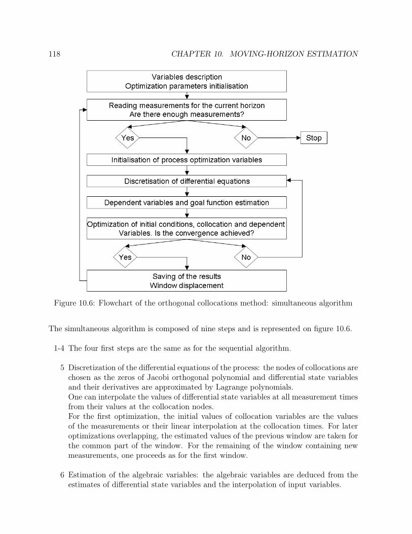
118 CHAPTER 10. MOVING-HORIZON ESTIMATION
Figure 10.6: Flowchart of the orthogonal collocations method: simultaneous algorithm
The simultaneous algorithm is composed of nine steps and is represented on figure 10.6.
1-4 The four first steps are the same as for the sequential algorithm.
5 Discretization of the differential equations of the process: the nodes of collocations arechosen as the zeros of Jacobi orthogonal polynomial and differential state variablesand their derivatives are approximated by Lagrange polynomials.One can interpolate the values of differential state variables at all measurement timesfrom their values at the collocation nodes.For the first optimization, the initial values of collocation variables are the valuesof the measurements or their linear interpolation at the collocation times. For lateroptimizations overlapping, the estimated values of the previous window are taken forthe common part of the window. For the remaining of the window containing newmeasurements, one proceeds as for the first window.
6 Estimation of the algebraic variables: the algebraic variables are deduced from theestimates of differential state variables and the interpolation of input variables.

10.2. METHOD BASED ON ORTHOGONAL COLLOCATIONS 119
7 Calculation of the goal function Fgoal on the reconciliation horizon: the goal functionis the same as for the sequential method 10.1.
8 Optimization of all optimization variables: this optimization is carried out by asuccessive quadratic programming (SQP) method (Kyriakopoulou, 1997).If the convergence is not achieved, one must go back to step five. Otherwise, one cancontinue to the next step.
9 Saving of the reconciliation results and moving of the window.
As it will be illustrated in the next chapter for the first example, the simultaneous algorithmgives better results than the sequential one. Those results agree with the study of Biegler(Biegler, 1984).

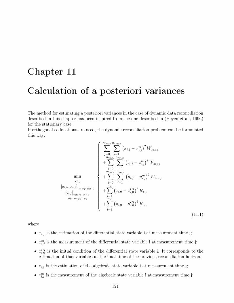
Chapter 11
Calculation of a posteriori variances
The method for estimating a posteriori variances in the case of dynamic data reconciliationdescribed in this chapter has been inspired from the one described in (Heyen et al., 1996)for the stationary case.If orthogonal collocations are used, the dynamic reconciliation problem can be formulatedthis way:
minxci,k
[ui,ini,ui,f ]interp int 1
[ui,f ]interp int s
∀k, ∀s ∕=1, ∀i
⎧⎨⎩
ntmes∑
j=0
nxmes∑
i=1
(xi,j − xm
i,j
)2Wxi,i,j
+
ntmes∑
j=0
nzmes∑
i=1
(zi,j − zmi,j
)2Wzi,i,j
+
ntmes∑
j=0
numes∑
i=1
(ui,j − um
i,j
)2Wui,i,j
+
nx∑
i=1
(xi,0 − xCI
i,0
)2Rxi,i
+
nu∑
i=1
(ui,0 − uCI
i,0
)2Rui,i
(11.1)
where
∙ xi,j is the estimation of the differential state variable i at measurement time j;
∙ xmi,j is the measurement of the differential state variable i at measurement time j;
∙ xCIi,0 is the initial condition of the differential state variable i. It corresponds to the
estimation of that variables at the final time of the previous reconciliation horizon.
∙ zi,j is the estimation of the algebraic state variable i at measurement time j;
∙ zmi,j is the measurement of the algebraic state variable i at measurement time j;
121

122 CHAPTER 11. CALCULATION OF A POSTERIORI VARIANCES
∙ ui,j is the estimation of the input variable i at measurement time j;
∙ umi,j is the measurement of the input variable i at measurement time j;
∙ uCIi,0 is the initial condition of the input variable i. It corresponds to the estimation
of that variable at the same time of the previous reconciliation horizon.
∙ xci,k is the collocation variable i at collocation time k;
∙ zci,k is the value of algebraic state variable i at collocation time k;
∙ uci,k is the value of input variable i at collocation time k;
∙ Wx is the weight matrix of the differential state variables;
∙ Wz is the weight matrix of the algebraic state variables;
∙ Wu is the weight matrix of the input state variables;
∙ Rx is the relaxation factor of the differential state variables at the initial time of themoving horizon;
∙ Ru is the relaxation factor of the input variables at the initial time of the movinghorizon.
This objective function is submitted to the five kinds of constraints described in section10.2:
A = f (tj ,x, z,u) = 0 ∀tj (11.2)
Ac = f c (�k,xc, zc,uc) = 0 ∀�k (11.3)
Bi,j = xi,j −n�∑
k=0
lk(tj) xci,k = 0 ∀i, ∀tj ∕= tCI (11.4)
Ci,j = ui,j − ui,tini− tj − tini
tf − tini
(ui,tf − ui,tini
)= 0 ∀i, ∀tj ∕= tini, tf (11.5)
Cci,j = uc
i,k − ui,tini− �k − tini
tf − tini
(ui,tf − ui,tini
)= 0 ∀i, ∀�k (11.6)
Di,j =
n�∑
s=0
ls(�k) xci,�s
− g (�k,xck, z
ck,u
ck) = 0 ∀i, ∀�k ∕= tini (11.7)
Ei,j =
[n�∑
k=0
lk(tf) xci,k
]
tf ,discr int q−1
−[
n�∑
k=0
lk(tini) xci,k
]
tini,discr int q
= 0 ∀i (11.8)
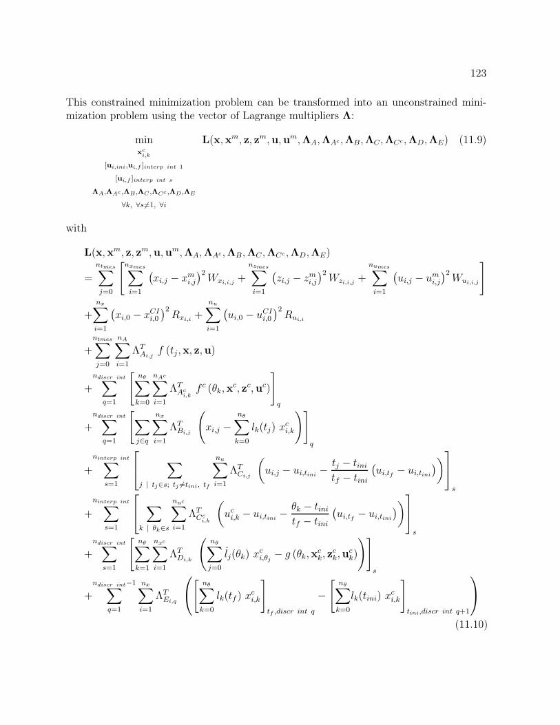
123
This constrained minimization problem can be transformed into an unconstrained mini-mization problem using the vector of Lagrange multipliers Λ:
minxci,k
[ui,ini,ui,f ]interp int 1
[ui,f ]interp int s
ΛA,ΛAc ,ΛB,ΛC ,ΛCc ,ΛD,ΛE
∀k, ∀s ∕=1, ∀i
L(x,xm, z, zm,u,um,ΛA,ΛAc ,ΛB,ΛC ,ΛCc ,ΛD,ΛE) (11.9)
with
L(x,xm, z, zm,u,um,ΛA,ΛAc ,ΛB,ΛC ,ΛCc ,ΛD,ΛE)
=
ntmes∑
j=0
[nxmes∑
i=1
(xi,j − xm
i,j
)2Wxi,i,j
+
nzmes∑
i=1
(zi,j − zmi,j
)2Wzi,i,j +
numes∑
i=1
(ui,j − um
i,j
)2Wui,i,j
]
+
nx∑
i=1
(xi,0 − xCI
i,0
)2Rxi,i
+
nu∑
i=1
(ui,0 − uCI
i,0
)2Rui,i
+ntmes∑
j=0
nA∑
i=1
ΛTAi,j
f (tj ,x, z,u)
+
ndiscr int∑
q=1
[n�∑
k=0
nAc∑
i=1
ΛTAc
i,kf c (�k,x
c, zc,uc)
]
q
+
ndiscr int∑
q=1
[∑
j∈q
nx∑
i=1
ΛTBi,j
(xi,j −
n�∑
k=0
lk(tj) xci,k
)]
q
+
ninterp int∑
s=1
⎡⎣ ∑
j ∣ tj∈s; tj ∕=tini, tf
nu∑
i=1
ΛTCi,j
(ui,j − ui,tini
− tj − tinitf − tini
(ui,tf − ui,tini
))⎤⎦
s
+
ninterp int∑
s=1
⎡⎣ ∑
k ∣ �k∈s
nuc∑
i=1
ΛTCc
i,k
(uci,k − ui,tini
− �k − tinitf − tini
(ui,tf − ui,tini
))⎤⎦s
+
ndiscr int∑
s=1
[n�∑
k=1
nxc∑
i=1
ΛTDi,k
(n�∑
j=0
lj(�k) xci,�j
− g (�k,xck, z
ck,u
ck)
)]
s
+
ndiscr int−1∑
q=1
nx∑
i=1
ΛTEi,q
⎛⎝[
n�∑
k=0
lk(tf ) xci,k
]
tf ,discr int q
−[
n�∑
k=0
lk(tini) xci,k
]
tini,discr int q+1
⎞⎠
(11.10)
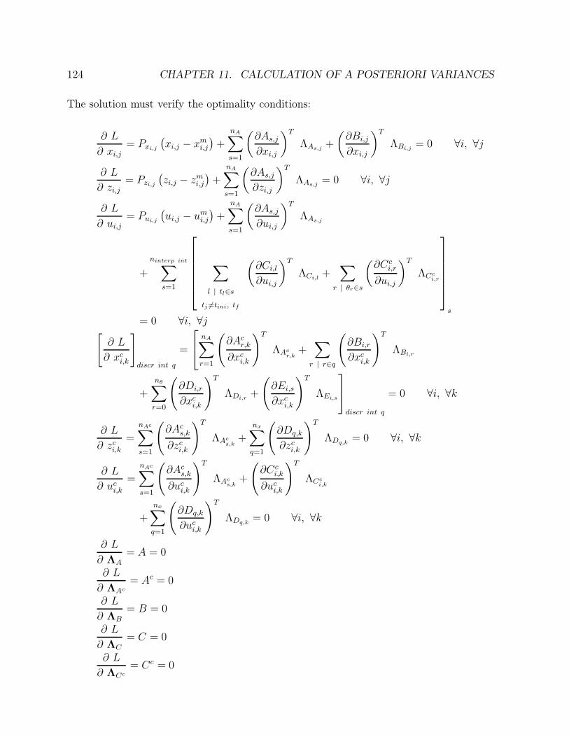
124 CHAPTER 11. CALCULATION OF A POSTERIORI VARIANCES
The solution must verify the optimality conditions:
∂ L
∂ xi,j
= Pxi,j
(xi,j − xm
i,j
)+
nA∑
s=1
(∂As,j
∂xi,j
)T
ΛAs,j+
(∂Bi,j
∂xi,j
)T
ΛBi,j= 0 ∀i, ∀j
∂ L
∂ zi,j= Pzi,j
(zi,j − zmi,j
)+
nA∑
s=1
(∂As,j
∂zi,j
)T
ΛAs,j= 0 ∀i, ∀j
∂ L
∂ ui,j
= Pui,j
(ui,j − um
i,j
)+
nA∑
s=1
(∂As,j
∂ui,j
)T
ΛAs,j
+
ninterp int∑
s=1
⎡⎢⎢⎢⎢⎢⎣
∑
l ∣ tl∈s
tj ∕=tini, tf
(∂Ci,l
∂ui,j
)T
ΛCi,l+
∑
r ∣ �r∈s
(∂Cc
i,r
∂ui,j
)T
ΛCci,r
⎤⎥⎥⎥⎥⎥⎦
s
= 0 ∀i, ∀j[
∂ L
∂ xci,k
]
discr int q
=
⎡⎣
nA∑
r=1
(∂Ac
r,k
∂xci,k
)T
ΛAcr,k
+∑
r ∣ r∈q
(∂Bi,r
∂xci,k
)T
ΛBi,r
+
n�∑
r=0
(∂Di,r
∂xci,k
)T
ΛDi,r+
(∂Ei,s
∂xci,k
)T
ΛEi,s
⎤⎦
discr int q
= 0 ∀i, ∀k
∂ L
∂ zci,k=
nAc∑
s=1
(∂Ac
s,k
∂zci,k
)T
ΛAcs,k
+
nx∑
q=1
(∂Dq,k
∂zci,k
)T
ΛDq,k= 0 ∀i, ∀k
∂ L
∂ uci,k
=
nAc∑
s=1
(∂Ac
s,k
∂uci,k
)T
ΛAcs,k
+
(∂Cc
i,k
∂uci,k
)T
ΛCci,k
+nx∑
q=1
(∂Dq,k
∂uci,k
)T
ΛDq,k= 0 ∀i, ∀k
∂ L
∂ ΛA
= A = 0
∂ L
∂ ΛAc
= Ac = 0
∂ L
∂ ΛB
= B = 0
∂ L
∂ ΛC
= C = 0
∂ L
∂ ΛCc
= Cc = 0
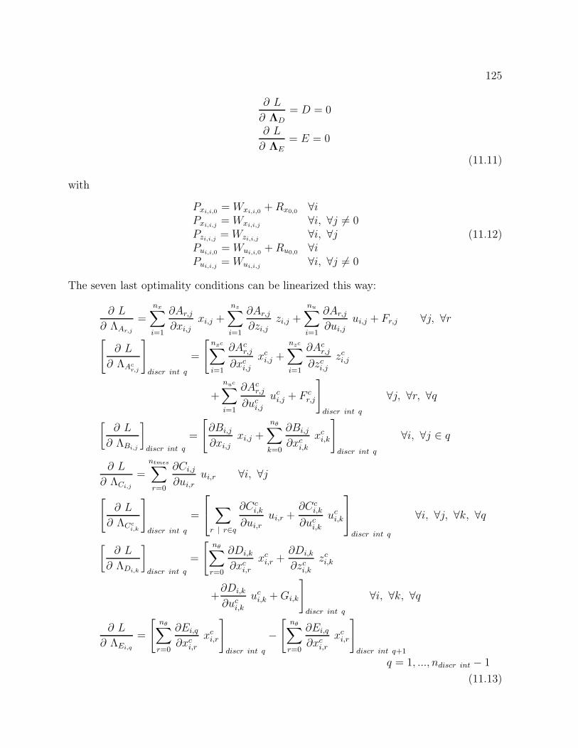
125
∂ L
∂ ΛD
= D = 0
∂ L
∂ ΛE
= E = 0
(11.11)
with
Pxi,i,0= Wxi,i,0
+Rx0,0
Pxi,i,j= Wxi,i,j
Pzi,i,j = Wzi,i,j
Pui,i,0= Wui,i,0
+Ru0,0
Pui,i,j= Wui,i,j
∀i∀i, ∀j ∕= 0∀i, ∀j∀i∀i, ∀j ∕= 0
(11.12)
The seven last optimality conditions can be linearized this way:
∂ L
∂ ΛAr,j
=
nx∑
i=1
∂Ar,j
∂xi,j
xi,j +
nz∑
i=1
∂Ar,j
∂zi,jzi,j +
nu∑
i=1
∂Ar,j
∂ui,j
ui,j + Fr,j ∀j, ∀r[
∂ L
∂ ΛAcr,j
]
discr int q
=
[nxc∑
i=1
∂Acr,j
∂xci,j
xci,j +
nzc∑
i=1
∂Acr,j
∂zci,jzci,j
+
nuc∑
i=1
∂Acr,j
∂uci,j
uci,j + F c
r,j
]
discr int q
∀j, ∀r, ∀q
[∂ L
∂ ΛBi,j
]
discr int q
=
[∂Bi,j
∂xi,j
xi,j +
n�∑
k=0
∂Bi,j
∂xci,k
xci,k
]
discr int q
∀i, ∀j ∈ q
∂ L
∂ ΛCi,j
=
ntmes∑
r=0
∂Ci,j
∂ui,r
ui,r ∀i, ∀j[
∂ L
∂ ΛCci,k
]
discr int q
=
⎡⎣ ∑
r ∣ r∈q
∂Cci,k
∂ui,r
ui,r +∂Cc
i,k
∂uci,k
uci,k
⎤⎦
discr int q
∀i, ∀j, ∀k, ∀q
[∂ L
∂ ΛDi,k
]
discr int q
=
[n�∑
r=0
∂Di,k
∂xci,r
xci,r +
∂Di,k
∂zci,kzci,k
+∂Di,k
∂uci,k
uci,k +Gi,k
]
discr int q
∀i, ∀k, ∀q
∂ L
∂ ΛEi,q
=
[n�∑
r=0
∂Ei,q
∂xci,r
xci,r
]
discr int q
−[
n�∑
r=0
∂Ei,q
∂xci,r
xci,r
]
discr int q+1
q = 1, ..., ndiscr int − 1
(11.13)
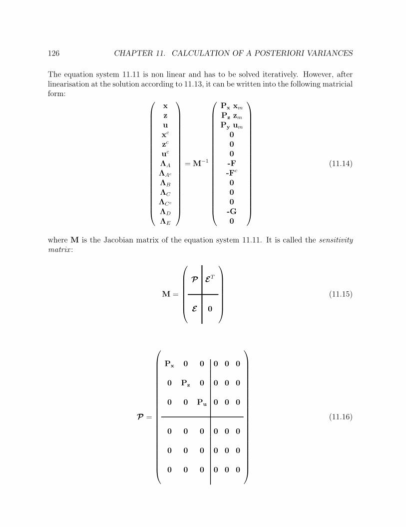
126 CHAPTER 11. CALCULATION OF A POSTERIORI VARIANCES
The equation system 11.11 is non linear and has to be solved iteratively. However, afterlinearisation at the solution according to 11.13, it can be written into the following matricialform:
⎛⎜⎜⎜⎜⎜⎜⎜⎜⎜⎜⎜⎜⎜⎜⎜⎜⎜⎜⎜⎜⎝
xzuxc
zc
uc
ΛA
ΛAc
ΛB
ΛC
ΛCc
ΛD
ΛE
⎞⎟⎟⎟⎟⎟⎟⎟⎟⎟⎟⎟⎟⎟⎟⎟⎟⎟⎟⎟⎟⎠
= M−1
⎛⎜⎜⎜⎜⎜⎜⎜⎜⎜⎜⎜⎜⎜⎜⎜⎜⎜⎜⎜⎜⎝
Px xm
Pz zmPy um
000-F-Fc
000-G0
⎞⎟⎟⎟⎟⎟⎟⎟⎟⎟⎟⎟⎟⎟⎟⎟⎟⎟⎟⎟⎟⎠
(11.14)
where M is the Jacobian matrix of the equation system 11.11. It is called the sensitivitymatrix :
M =
⎛⎜⎜⎜⎜⎜⎜⎝
퓟 퓔T
퓔 0
⎞⎟⎟⎟⎟⎟⎟⎠
(11.15)
퓟 =
⎛⎜⎜⎜⎜⎜⎜⎜⎜⎜⎜⎜⎜⎜⎜⎜⎜⎜⎜⎜⎜⎜⎜⎝
Px 0 0 0 0 0
0 Pz 0 0 0 0
0 0 Pu 0 0 0
0 0 0 0 0 0
0 0 0 0 0 0
0 0 0 0 0 0
⎞⎟⎟⎟⎟⎟⎟⎟⎟⎟⎟⎟⎟⎟⎟⎟⎟⎟⎟⎟⎟⎟⎟⎠
(11.16)

127
퓔 =
⎛⎜⎜⎜⎜⎜⎜⎜⎜⎜⎜⎜⎜⎜⎜⎜⎜⎜⎜⎜⎜⎜⎜⎜⎜⎝
∂A∂x
∂A∂z
∂A∂u
0 0 0
0 0 0 ∂Ac
∂xc∂Ac
∂zc∂Ac
∂uc
∂B∂x
0 0 ∂B∂xc 0 0
0 0 ∂C∂u
0 0 0
0 0 ∂Cc
∂u0 0 ∂Cc
∂uc
0 0 0 ∂D∂xc
∂D∂zc
∂D∂uc
0 0 0 ∂E∂xc 0 0
⎞⎟⎟⎟⎟⎟⎟⎟⎟⎟⎟⎟⎟⎟⎟⎟⎟⎟⎟⎟⎟⎟⎟⎟⎟⎠
(11.17)
As for the stationary case, the sparsity of the sensitivity matrix has to be taken into accountand the algorithm has to be modified as described, for example, by Chen and Stadherr(Chen and Stadherr, 1984) if the problems are very large. In that case, the measurementsremain generally considered as independent from one another so that the weight matrixW is reduced to a diagonal matrix whose elements are the inverse of the variances of themeasured variables.If the problem contains inequality constraints, the NLP problem is solved directly using asequential quadratic programming algorithm (Kyriakopoulou, 1997).Once the problem has been solved, a sensitivity analysis can be carried out using thelinearized equation system 11.14. This equation system shows that the reconciled valuesof variables x, z, u, xc, zc, uc, ΛA, ΛAc , ΛB, ΛC , ΛCc , ΛD and ΛE are linear combinationsof the measurements. So, the sensitivity matrix M allows to evaluate how the reconciledvalues of the model variables depends on the measurements and their standard deviations.The variables x, z and u are thus estimated this way:
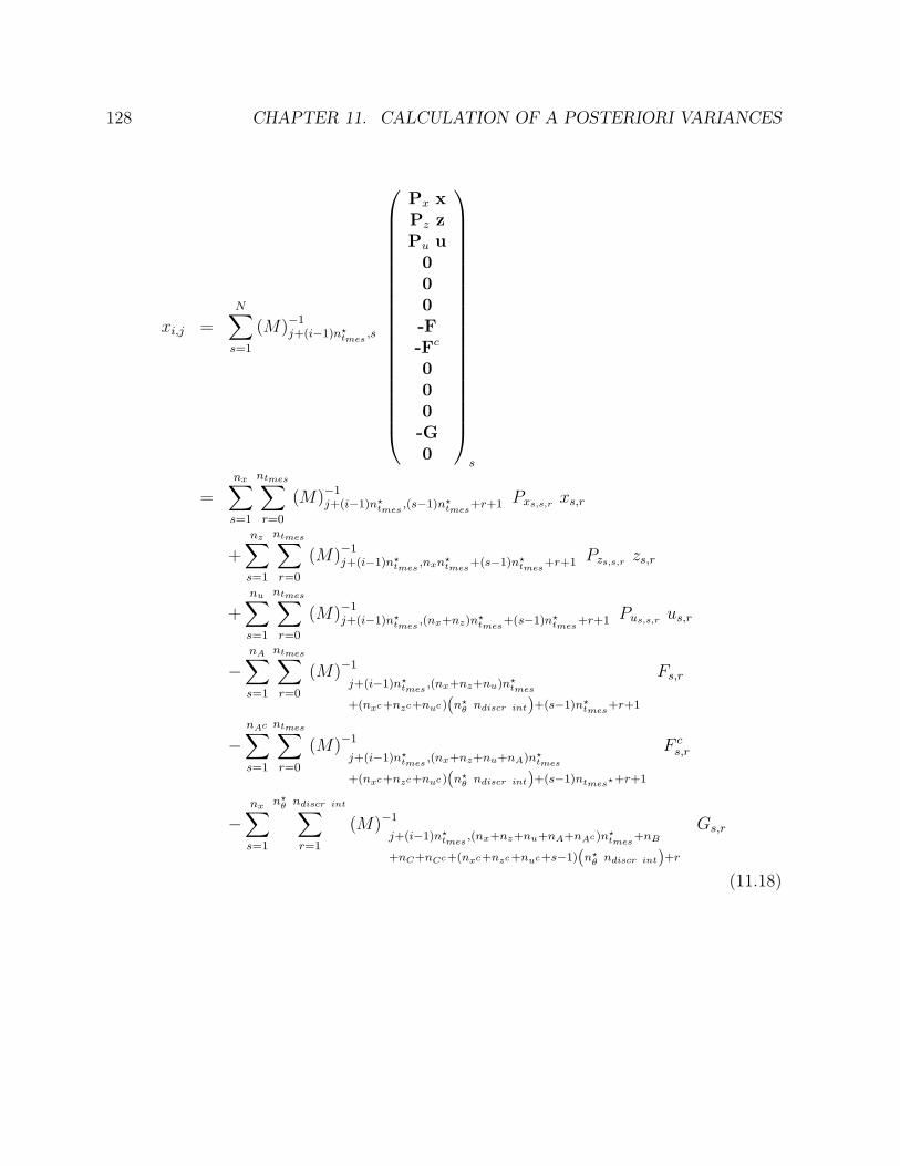
128 CHAPTER 11. CALCULATION OF A POSTERIORI VARIANCES
xi,j =
N∑
s=1
(M)−1j+(i−1)n★
tmes,s
⎛⎜⎜⎜⎜⎜⎜⎜⎜⎜⎜⎜⎜⎜⎜⎜⎜⎜⎜⎜⎜⎝
Px xPz zPu u
000-F-Fc
000-G0
⎞⎟⎟⎟⎟⎟⎟⎟⎟⎟⎟⎟⎟⎟⎟⎟⎟⎟⎟⎟⎟⎠
s
=nx∑
s=1
ntmes∑
r=0
(M)−1j+(i−1)n★
tmes,(s−1)n★
tmes+r+1 Pxs,s,r
xs,r
+
nz∑
s=1
ntmes∑
r=0
(M)−1j+(i−1)n★
tmes,nxn
★tmes
+(s−1)n★tmes
+r+1 Pzs,s,r zs,r
+
nu∑
s=1
ntmes∑
r=0
(M)−1j+(i−1)n★
tmes,(nx+nz)n★
tmes+(s−1)n★
tmes+r+1 Pus,s,r
us,r
−nA∑
s=1
ntmes∑
r=0
(M)−1
j+(i−1)n★tmes
,(nx+nz+nu)n★tmes
+(nxc+nzc+nuc)(n★�
ndiscr int)+(s−1)n★tmes
+r+1
Fs,r
−nAc∑
s=1
ntmes∑
r=0
(M)−1
j+(i−1)n★tmes
,(nx+nz+nu+nA)n★tmes
+(nxc+nzc+nuc)(n★�
ndiscr int)+(s−1)ntmes★+r+1
F cs,r
−nx∑
s=1
n★�
ndiscr int∑
r=1
(M)−1
j+(i−1)n★tmes
,(nx+nz+nu+nA+nAc)n★tmes
+nB
+nC+nCc+(nxc+nzc+nuc+s−1)(n★�
ndiscr int)+r
Gs,r
(11.18)
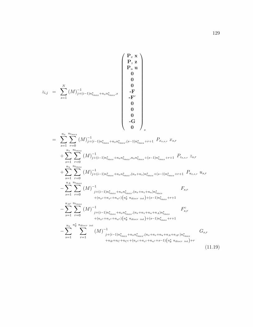
129
zi,j =
N∑
s=1
(M)−1j+(i−1)n★
tmes+nxn
★tmes
,s
⎛⎜⎜⎜⎜⎜⎜⎜⎜⎜⎜⎜⎜⎜⎜⎜⎜⎜⎜⎜⎜⎝
Px xPz zPu u
000-F-Fc
000-G0
⎞⎟⎟⎟⎟⎟⎟⎟⎟⎟⎟⎟⎟⎟⎟⎟⎟⎟⎟⎟⎟⎠
s
=nx∑
s=1
ntmes∑
r=0
(M)−1j+(i−1)n★
tmes+nxn★
tmes,(s−1)n★
tmes+r+1 Pxs,s,r
xs,r
+
nz∑
s=1
ntmes∑
r=0
(M)−1j+(i−1)n★
tmes+nxn
★tmes
,nxn★tmes
+(s−1)n★tmes
+r+1 Pzs,s,r zs,r
+
nu∑
s=1
ntmes∑
r=0
(M)−1j+(i−1)n★
tmes+nxn
★tmes
,(nx+nz)n★tmes
+(s−1)n★tmes
+r+1 Pus,s,rus,r
−nA∑
s=1
ntmes∑
r=0
(M)−1
j+(i−1)n★tmes
+nxn★tmes
,(nx+nz+nu)n★tmes
+(nxc+nzc+nuc)(n★�
ndiscr int)+(s−1)n★tmes
+r+1
Fs,r
−nAc∑
s=1
ntmes∑
r=0
(M)−1
j+(i−1)n★tmes
+nxn★tmes
,(nx+nz+nu+nA)n★tmes
+(nxc+nzc+nuc)(n★�
ndiscr int)+(s−1)n★tmes
+r+1
F cs,r
−nx∑
s=1
n★�
ndiscr int∑
r=1
(M)−1
j+(i−1)n★tmes
+nxn★tmes
,(nx+nz+nu+nA+nAc)n★tmes
+nB+nC+nCc+(nxc+nzc+nuc+s−1)(n★�
ndiscr int)+r
Gs,r
(11.19)
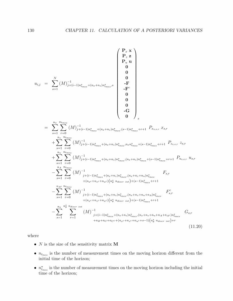
130 CHAPTER 11. CALCULATION OF A POSTERIORI VARIANCES
ui,j =
N∑
s=1
(M)−1j+(i−1)n★
tmes+(nx+nz)n★
tmes,s
⎛⎜⎜⎜⎜⎜⎜⎜⎜⎜⎜⎜⎜⎜⎜⎜⎜⎜⎜⎜⎜⎝
Px xPz zPu u
000-F-Fc
000-G0
⎞⎟⎟⎟⎟⎟⎟⎟⎟⎟⎟⎟⎟⎟⎟⎟⎟⎟⎟⎟⎟⎠
s
=
nx∑
s=1
ntmes∑
r=0
(M)−1j+(i−1)n★
tmes+(nx+nz)n★
tmes,(s−1)n★
tmes+r+1 Pxs,s,r
xs,r
+nz∑
s=1
ntmes∑
r=0
(M)−1j+(i−1)n★
tmes+(nx+nz)n★
tmes,nxn
★tmes
+(s−1)n★tmes
+r+1 Pzs,s,r zs,r
+
nu∑
s=1
ntmes∑
r=0
(M)−1j+(i−1)n★
tmes+(nx+nz)n★
tmes,(nx+nz)n★
tmes+(s−1)n★
tmes+r+1 Pus,s,r
us,r
−nA∑
s=1
ntmes∑
r=0
(M)−1
j+(i−1)n★tmes
+(nx+nz)n★tmes
,(nx+nz+nu)n★tmes
+(nxc+nzc+nuc)(n★�
ndiscr int)+(s−1)n★tmes
+r+1
Fs,r
−nAc∑
s=1
ntmes∑
r=0
(M)−1
j+(i−1)n★tmes
+(nx+nz)n★tmes
,(nx+nz+nu+nA)n★tmes
+(nxc+nzc+nuc)(n★�
ndiscr int)+(s−1)n★tmes
+r+1
F cs,r
−nx∑
s=1
n★�
ndiscr int∑
r=1
(M)−1
j+(i−1)n★tmes
+(nx+nz)n★tmes
,(nx+nz+nu+nA+nAc)n★tmes
+nB+nC+nCc+(nxc+nzc+nuc+s−1)(n★�
ndiscr int)+r
Gs,r
(11.20)
where
∙ N is the size of the sensitivity matrix M
∙ ntmesis the number of measurement times on the moving horizon different from the
initial time of the horizon;
∙ n★tmes
is the number of measurement times on the moving horizon including the initialtime of the horizon;
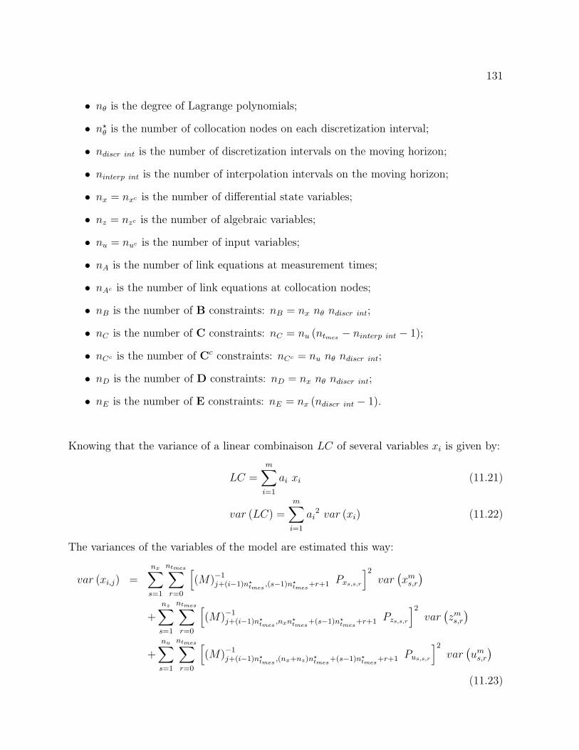
131
∙ n� is the degree of Lagrange polynomials;
∙ n★� is the number of collocation nodes on each discretization interval;
∙ ndiscr int is the number of discretization intervals on the moving horizon;
∙ ninterp int is the number of interpolation intervals on the moving horizon;
∙ nx = nxc is the number of differential state variables;
∙ nz = nzc is the number of algebraic variables;
∙ nu = nuc is the number of input variables;
∙ nA is the number of link equations at measurement times;
∙ nAc is the number of link equations at collocation nodes;
∙ nB is the number of B constraints: nB = nx n� ndiscr int;
∙ nC is the number of C constraints: nC = nu (ntmes− ninterp int − 1);
∙ nCc is the number of Cc constraints: nCc = nu n� ndiscr int;
∙ nD is the number of D constraints: nD = nx n� ndiscr int;
∙ nE is the number of E constraints: nE = nx (ndiscr int − 1).
Knowing that the variance of a linear combinaison LC of several variables xi is given by:
LC =
m∑
i=1
ai xi (11.21)
var (LC) =m∑
i=1
ai2 var (xi) (11.22)
The variances of the variables of the model are estimated this way:
var (xi,j) =
nx∑
s=1
ntmes∑
r=0
[(M)−1
j+(i−1)n★tmes
,(s−1)n★tmes
+r+1 Pxs,s,r
]2var
(xms,r
)
+nz∑
s=1
ntmes∑
r=0
[(M)−1
j+(i−1)n★tmes
,nxn★tmes
+(s−1)n★tmes
+r+1 Pzs,s,r
]2var
(zms,r)
+
nu∑
s=1
ntmes∑
r=0
[(M)−1
j+(i−1)n★tmes
,(nx+nz)n★tmes
+(s−1)n★tmes
+r+1 Pus,s,r
]2var
(ums,r
)
(11.23)

132 CHAPTER 11. CALCULATION OF A POSTERIORI VARIANCES
var (zi,j) =nx∑
s=1
ntmes∑
r=0
[(M)−1
j+(i−1)n★tmes
+nxn★tmes
,(s−1)n★tmes
+r+1 Pxs,s,r
]2var
(xms,r
)
+
nz∑
s=1
ntmes∑
r=0
⎡⎢⎢⎣(M)−1
j+(i−1)n★tmes
+nxn★tmes
,nx∗ntmes
+(s−1)n★tmes
+r+1
Pzs,s,r
⎤⎥⎥⎦
2
var(zms,r)
+
nu∑
s=1
ntmes∑
r=0
⎡⎢⎢⎣(M)−1
j+(i−1)n★tmes
+nxn★tmes
,(nx+nz)n★tmes
+(s−1)n★tmes
+r+1
Pus,s,r
⎤⎥⎥⎦
2
var(ums,r
)
(11.24)
var (ui,j) =nx∑
s=1
ntmes∑
r=0
[(M)−1
j+(i−1)n★tmes
+(nx+nz)n★tmes
,(s−1)n★tmes
+r+1 Pxs,s,r
]2var
(xms,r
)
+nz∑
s=1
ntmes∑
r=0
⎡⎢⎢⎣(M)−1
j+(i−1)n★tmes
+(nx+nz)n★tmes
,nxn★tmes
+(s−1)n★tmes
+r+1
Pzs,s,r
⎤⎥⎥⎦
2
var(zms,r)
+nu∑
s=1
ntmes∑
r=0
⎡⎢⎢⎣(M)−1
j+(i−1)n★tmes
+(nx+nz)n★tmes
,(nx+nz)n★tmes
+(s−1)n★tmes
+r+1
Pus,s,r
⎤⎥⎥⎦
2
var(ums,r
)
(11.25)
Thus the calculation of sensitivity matrix M allows to assess the variance of reconciledvariables, knowing the variances of all measured variables.

Chapter 12
Cases study
In this chapter, three examples from the ones that have been studied will be treated:
∙ one tank;
∙ a stirred tank reactor with heat exchange;
∙ a network of five tanks.
For each of them the results of the reconciliation and the estimation of a posteriori varianceswill be discussed.
12.1 One tank
This first example is very simple, but it allows to illustrate all concepts developed in theprevious chapters.It consists of a dynamic balance for a tank, whose feed flowrate F0 is the independentvariable. The outlet flowrate F1 is proportional to the level of the tank. The section of thetank is considered constant. The tank is represented on figure 12.1.
F0
F1
H1
Figure 12.1: Flowsheet of the tank
133
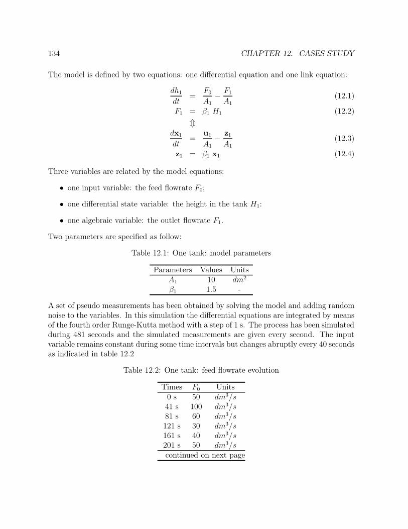
134 CHAPTER 12. CASES STUDY
The model is defined by two equations: one differential equation and one link equation:
dℎ1
dt=
F0
A1− F1
A1(12.1)
F1 = �1 H1 (12.2)
⇕dx1
dt=
u1
A1
− z1A1
(12.3)
z1 = �1 x1 (12.4)
Three variables are related by the model equations:
∙ one input variable: the feed flowrate F0;
∙ one differential state variable: the height in the tank H1:
∙ one algebraic variable: the outlet flowrate F1.
Two parameters are specified as follow:
Table 12.1: One tank: model parameters
Parameters Values UnitsA1 10 dm2
�1 1.5 -
A set of pseudo measurements has been obtained by solving the model and adding randomnoise to the variables. In this simulation the differential equations are integrated by meansof the fourth order Runge-Kutta method with a step of 1 s. The process has been simulatedduring 481 seconds and the simulated measurements are given every second. The inputvariable remains constant during some time intervals but changes abruptly every 40 secondsas indicated in table 12.2
Table 12.2: One tank: feed flowrate evolution
Times F0 Units0 s 50 dm3/s41 s 100 dm3/s81 s 60 dm3/s121 s 30 dm3/s161 s 40 dm3/s201 s 50 dm3/scontinued on next page
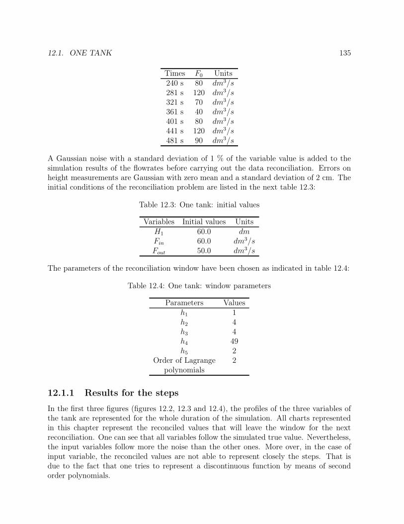
12.1. ONE TANK 135
Times F0 Units240 s 80 dm3/s281 s 120 dm3/s321 s 70 dm3/s361 s 40 dm3/s401 s 80 dm3/s441 s 120 dm3/s481 s 90 dm3/s
A Gaussian noise with a standard deviation of 1 % of the variable value is added to thesimulation results of the flowrates before carrying out the data reconciliation. Errors onheight measurements are Gaussian with zero mean and a standard deviation of 2 cm. Theinitial conditions of the reconciliation problem are listed in the next table 12.3:
Table 12.3: One tank: initial values
Variables Initial values UnitsH1 60.0 dmFin 60.0 dm3/sFout 50.0 dm3/s
The parameters of the reconciliation window have been chosen as indicated in table 12.4:
Table 12.4: One tank: window parameters
Parameters Valuesℎ1 1ℎ2 4ℎ3 4ℎ4 49ℎ5 2
Order of Lagrange 2polynomials
12.1.1 Results for the steps
In the first three figures (figures 12.2, 12.3 and 12.4), the profiles of the three variables ofthe tank are represented for the whole duration of the simulation. All charts representedin this chapter represent the reconciled values that will leave the window for the nextreconciliation. One can see that all variables follow the simulated true value. Nevertheless,the input variables follow more the noise than the other ones. More over, in the case ofinput variable, the reconciled values are not able to represent closely the steps. That isdue to the fact that one tries to represent a discontinuous function by means of secondorder polynomials.

136 CHAPTER 12. CASES STUDY
0 50 100 150 200 250 300 350 400 45010
20
30
40
50
60
70
80
90
Time (s)
H1
(d
m)
Validation
Measurement
Without noise
Figure 12.2: One tank: steps: height: profile
0 50 100 150 200 250 300 350 400 45020
40
60
80
100
120
140
Time
F0
(d
m³/
s)
Validation
Measurement
Without noise
Figure 12.3: One tank: steps: feed flowrate: profile
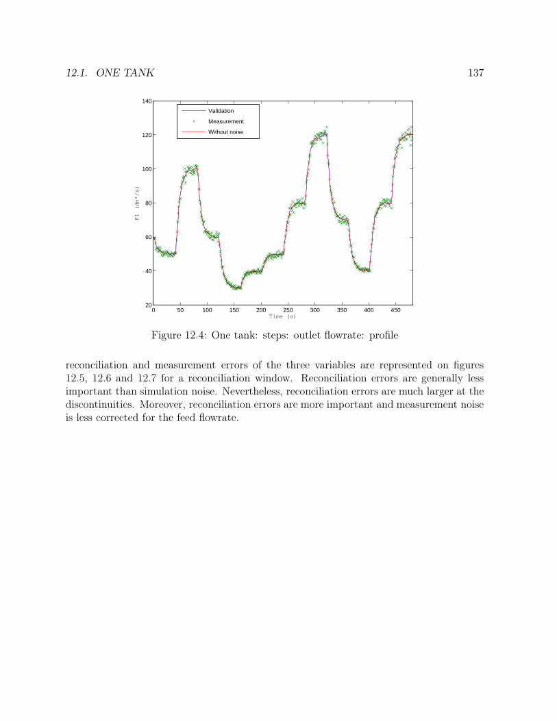
12.1. ONE TANK 137
0 50 100 150 200 250 300 350 400 45020
40
60
80
100
120
140
Time (s)
F1
(d
m³/
s)
Validation
Measurement
Without noise
Figure 12.4: One tank: steps: outlet flowrate: profile
reconciliation and measurement errors of the three variables are represented on figures12.5, 12.6 and 12.7 for a reconciliation window. Reconciliation errors are generally lessimportant than simulation noise. Nevertheless, reconciliation errors are much larger at thediscontinuities. Moreover, reconciliation errors are more important and measurement noiseis less corrected for the feed flowrate.
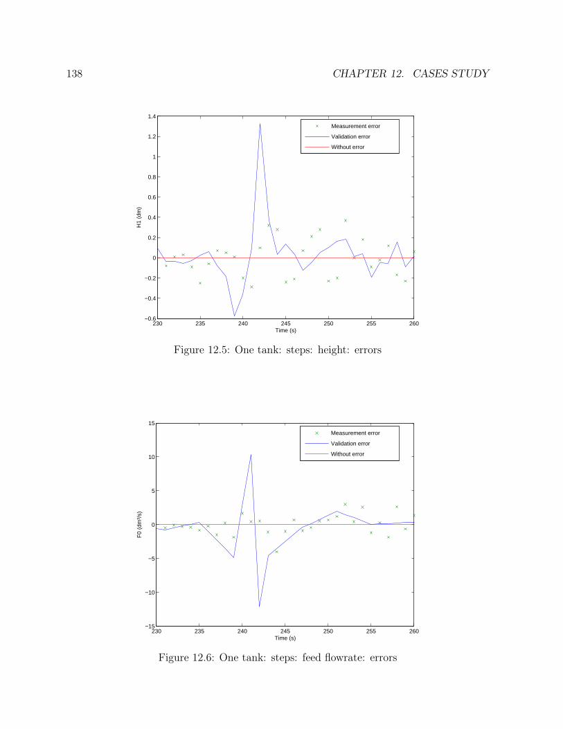
138 CHAPTER 12. CASES STUDY
230 235 240 245 250 255 260−0.6
−0.4
−0.2
0
0.2
0.4
0.6
0.8
1
1.2
1.4
Time (s)
H1
(dm
)
Measurement error
Validation error
Without error
Figure 12.5: One tank: steps: height: errors
230 235 240 245 250 255 260−15
−10
−5
0
5
10
15
Time (s)
F0
(dm
³/s)
Measurement error
Validation error
Without error
Figure 12.6: One tank: steps: feed flowrate: errors
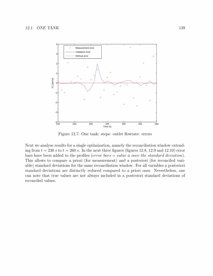
12.1. ONE TANK 139
230 235 240 245 250 255 260−4
−3
−2
−1
0
1
2
3
4
Time (s)
F1
(dm
³/s)
Measurement error
Validation error
Without error
Figure 12.7: One tank: steps: outlet flowrate: errors
Next we analyse results for a single optimization, namely the reconciliation window extend-ing from t = 230 s to t = 260 s. In the next three figures (figures 12.8, 12.9 and 12.10) errorbars have been added to the profiles (error bars = value± once tℎe standard deviation).This allows to compare a priori (for measurement) and a posteriori (for reconciled vari-able) standard deviations for the same reconciliation window. For all variables a posterioristandard deviations are distinctly reduced compared to a priori ones. Nevertheless, onecan note that true values are not always included in a posteriori standard deviations ofreconciled values.
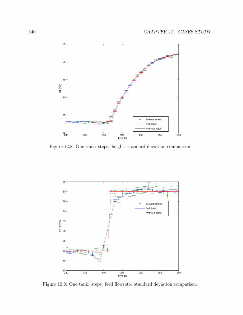
140 CHAPTER 12. CASES STUDY
230 235 240 245 250 255 26030
35
40
45
50
55
Time (s)
H1
(dm
)
Measurement
Validation
Without noise
Figure 12.8: One tank: steps: height: standard deviation comparison
230 235 240 245 250 255 26040
45
50
55
60
65
70
75
80
85
Time (s)
F0
(dm
³/s)
Measurement
Validation
Without noise
Figure 12.9: One tank: steps: feed flowrate: standard deviation comparison

12.1. ONE TANK 141
230 235 240 245 250 255 26045
50
55
60
65
70
75
80
85
Time (s)
F1
(dm
³/s)
Measurement
Validation
Without noise
Figure 12.10: One tank: steps: outlet flowrate: standard deviation comparison
Because of the discontinuity that appears at the steps, we have also simulated a case whereinput variations are smoother: linear variations of feed and smooth variations according toa first order response dx
dt= 0.1 (x− xtarget) where xtarget is the target value of the variable
x ate the end of the perturbation..
12.1.2 Results for the linear variations of feed
The linear variations have been defined with a constant slope (±2 unit flow/unit time)until the next target value is reached.
If one compares the profiles of the three variables of the complete simulation time (figures12.11, 12.12 and 12.13), one can see that the reconciled values follow the true values for allvariables. The discontinuities at the time corresponding to the input variable variationsare much smaller than for the step transitions.

142 CHAPTER 12. CASES STUDY
0 50 100 150 200 250 300 350 400 45010
20
30
40
50
60
70
80
90
Time (s)
H1
(d
m)
Validation
Measurement
Without noise
Figure 12.11: One tank: linear variations of feed: height: profile
0 50 100 150 200 250 300 350 400 45020
40
60
80
100
120
140
Time
F0
(d
m³/
s)
Validation
Measurement
Without noise
Figure 12.12: One tank: linear variations of feed: feed flowrate: profile
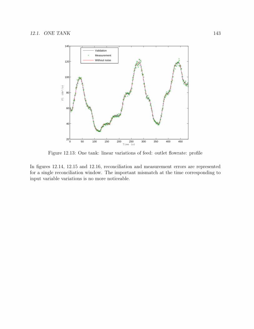
12.1. ONE TANK 143
0 50 100 150 200 250 300 350 400 45020
40
60
80
100
120
140
Time (s)
F1
(d
m³/
s)
Validation
Measurement
Without noise
Figure 12.13: One tank: linear variations of feed: outlet flowrate: profile
In figures 12.14, 12.15 and 12.16, reconciliation and measurement errors are representedfor a single reconciliation window. The important mismatch at the time corresponding toinput variable variations is no more noticeable.
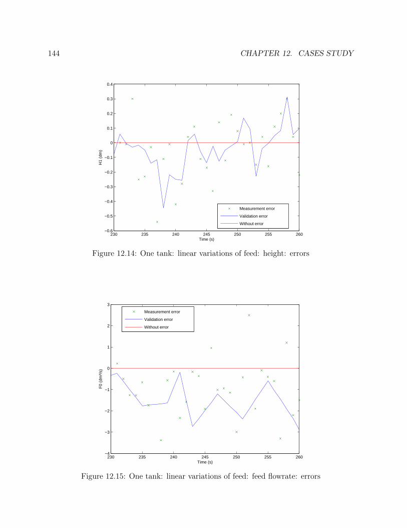
144 CHAPTER 12. CASES STUDY
230 235 240 245 250 255 260−0.6
−0.5
−0.4
−0.3
−0.2
−0.1
0
0.1
0.2
0.3
0.4
Time (s)
H1
(dm
)
Measurement error
Validation error
Without error
Figure 12.14: One tank: linear variations of feed: height: errors
230 235 240 245 250 255 260−4
−3
−2
−1
0
1
2
3
Time (s)
F0
(dm
³/s)
Measurement error
Validation error
Without error
Figure 12.15: One tank: linear variations of feed: feed flowrate: errors
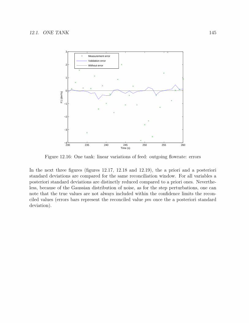
12.1. ONE TANK 145
230 235 240 245 250 255 260−4
−3
−2
−1
0
1
2
3
Time (s)
F1
(dm
³/s)
Measurement error
Validation error
Without error
Figure 12.16: One tank: linear variations of feed: outgoing flowrate: errors
In the next three figures (figures 12.17, 12.18 and 12.19), the a priori and a posterioristandard deviations are compared for the same reconciliation window. For all variables aposteriori standard deviations are distinctly reduced compared to a priori ones. Neverthe-less, because of the Gaussian distribution of noise, as for the step perturbations, one cannote that the true values are not always included within the confidence limits the recon-ciled values (errors bars represent the reconciled value pm once the a posteriori standarddeviation).

146 CHAPTER 12. CASES STUDY
230 235 240 245 250 255 26050
52
54
56
58
60
62
64
66
68
70
Time (s)
H1
(dm
)
Measurement
Validation
Without noise
Figure 12.17: One tank: linear variations of feed: height: standard deviation comparison
230 235 240 245 250 255 26075
80
85
90
95
100
105
110
115
120
Time (s)
F0
(dm
³/s)
Measurement
Validation
Without noise
Figure 12.18: One tank: linear variations of feed: feed flowrate: standard deviation com-parison
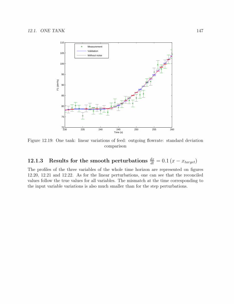
12.1. ONE TANK 147
230 235 240 245 250 255 26070
75
80
85
90
95
100
105
110
Time (s)
F1
(dm
³/s)
Measurement
Validation
Without noise
Figure 12.19: One tank: linear variations of feed: outgoing flowrate: standard deviationcomparison
12.1.3 Results for the smooth perturbations dxdt
= 0.1 (x− xtarget)
The profiles of the three variables of the whole time horizon are represented on figures12.20, 12.21 and 12.22. As for the linear perturbations, one can see that the reconciledvalues follow the true values for all variables. The mismatch at the time corresponding tothe input variable variations is also much smaller than for the step perturbations.
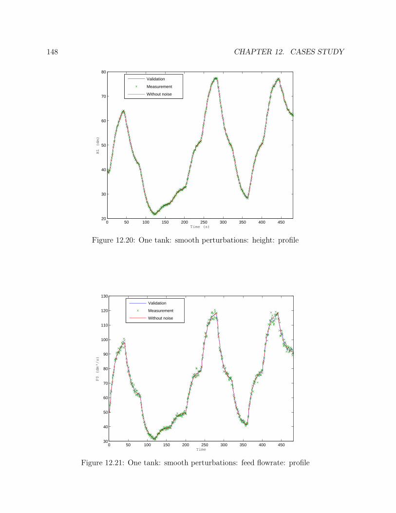
148 CHAPTER 12. CASES STUDY
0 50 100 150 200 250 300 350 400 45020
30
40
50
60
70
80
Time (s)
H1
(d
m)
Validation
Measurement
Without noise
Figure 12.20: One tank: smooth perturbations: height: profile
0 50 100 150 200 250 300 350 400 45030
40
50
60
70
80
90
100
110
120
130
Time
F0
(d
m³/
s)
Validation
Measurement
Without noise
Figure 12.21: One tank: smooth perturbations: feed flowrate: profile
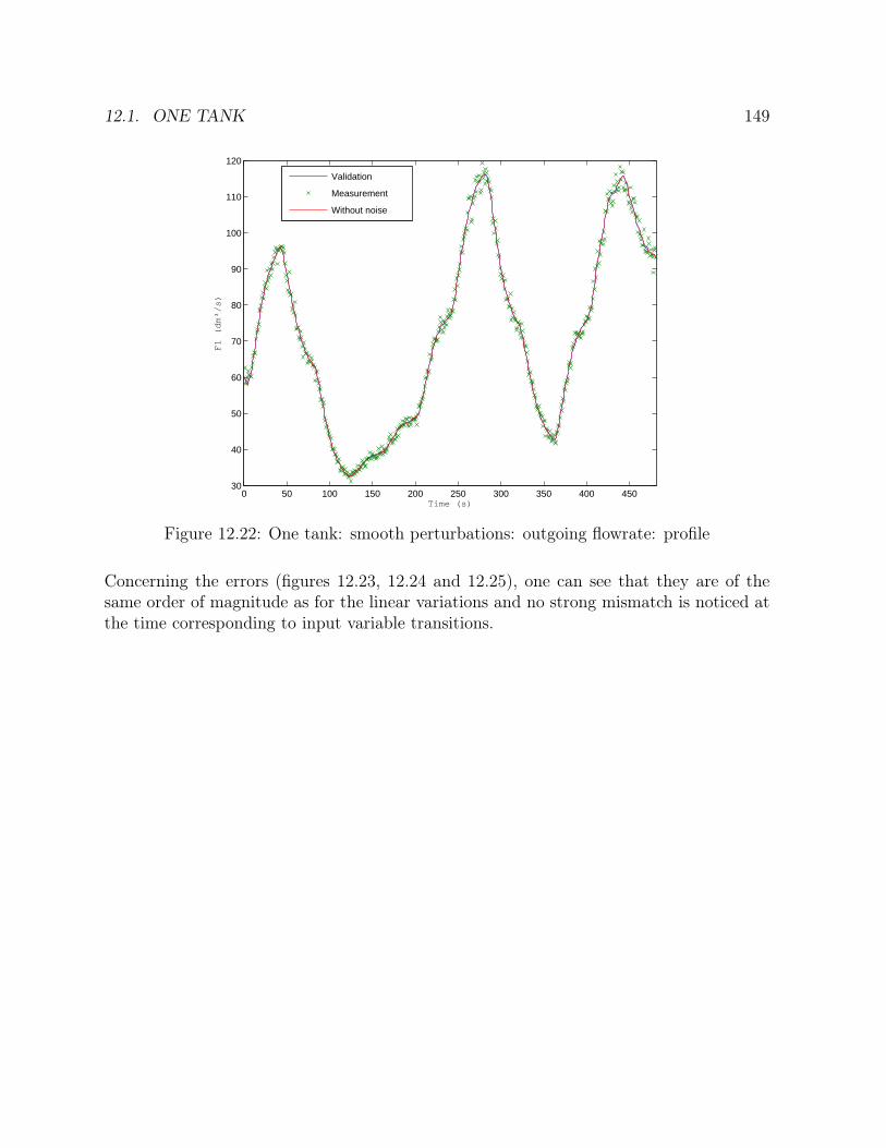
12.1. ONE TANK 149
0 50 100 150 200 250 300 350 400 45030
40
50
60
70
80
90
100
110
120
Time (s)
F1
(d
m³/
s)
Validation
Measurement
Without noise
Figure 12.22: One tank: smooth perturbations: outgoing flowrate: profile
Concerning the errors (figures 12.23, 12.24 and 12.25), one can see that they are of thesame order of magnitude as for the linear variations and no strong mismatch is noticed atthe time corresponding to input variable transitions.
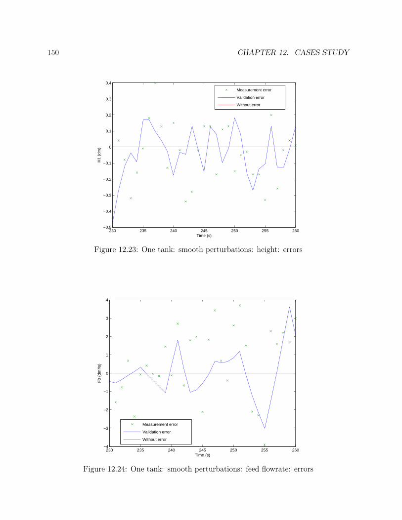
150 CHAPTER 12. CASES STUDY
230 235 240 245 250 255 260−0.5
−0.4
−0.3
−0.2
−0.1
0
0.1
0.2
0.3
0.4
Time (s)
H1
(dm
)
Measurement error
Validation error
Without error
Figure 12.23: One tank: smooth perturbations: height: errors
230 235 240 245 250 255 260−4
−3
−2
−1
0
1
2
3
4
Time (s)
F0
(dm
³/s)
Measurement error
Validation error
Without error
Figure 12.24: One tank: smooth perturbations: feed flowrate: errors
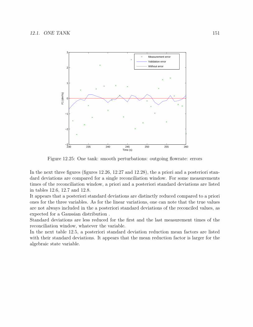
12.1. ONE TANK 151
230 235 240 245 250 255 260−3
−2
−1
0
1
2
3
Time (s)
F1
(dm
³/s)
Measurement error
Validation error
Without error
Figure 12.25: One tank: smooth perturbations: outgoing flowrate: errors
In the next three figures (figures 12.26, 12.27 and 12.28), the a priori and a posteriori stan-dard deviations are compared for a single reconciliation window. For some measurementstimes of the reconciliation window, a priori and a posteriori standard deviations are listedin tables 12.6, 12.7 and 12.8.It appears that a posteriori standard deviations are distinctly reduced compared to a prioriones for the three variables. As for the linear variations, one can note that the true valuesare not always included in the a posteriori standard deviations of the reconciled values, asexpected for a Gaussian distribution .Standard deviations are less reduced for the first and the last measurement times of thereconciliation window, whatever the variable.In the next table 12.5, a posteriori standard deviation reduction mean factors are listedwith their standard deviations. It appears that the mean reduction factor is larger for thealgebraic state variable.
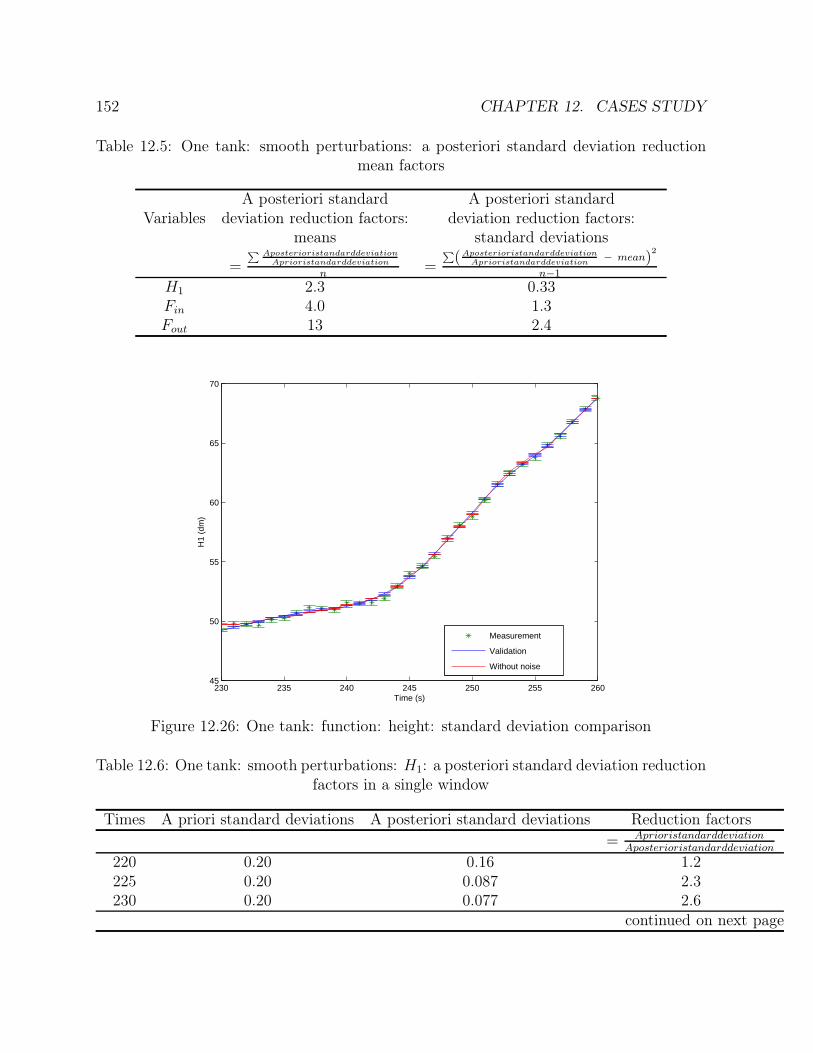
152 CHAPTER 12. CASES STUDY
Table 12.5: One tank: smooth perturbations: a posteriori standard deviation reductionmean factors
A posteriori standard A posteriori standardVariables deviation reduction factors: deviation reduction factors:
means standard deviations
=∑ Aposterioristandarddeviation
Aprioristandarddeviation
n=
∑(Aposterioristandarddeviation
Aprioristandarddeviation− mean)
2
n−1
H1 2.3 0.33Fin 4.0 1.3Fout 13 2.4
230 235 240 245 250 255 26045
50
55
60
65
70
Time (s)
H1
(dm
)
Measurement
Validation
Without noise
Figure 12.26: One tank: function: height: standard deviation comparison
Table 12.6: One tank: smooth perturbations: H1: a posteriori standard deviation reductionfactors in a single window
Times A priori standard deviations A posteriori standard deviations Reduction factors
= Aprioristandarddeviation
Aposterioristandarddeviation
220 0.20 0.16 1.2225 0.20 0.087 2.3230 0.20 0.077 2.6
continued on next page

12.1. ONE TANK 153
Times A priori standard deviations A posteriori standard deviations Reduction factors
= Aprioristandarddeviation
Aposterioristandarddeviation
235 0.20 0.076 2.6240 0.20 0.086 2.3245 0.20 0.089 2.2250 0.20 0.082 2.4255 0.20 0.081 2.4260 0.20 0.094 2.1265 0.20 0.096 2.1
230 235 240 245 250 255 26070
75
80
85
90
95
100
105
110
115
120
Time (s)
F0
(dm
³/s)
Measurement
Validation
Without noise
Figure 12.27: One tank: smooth perturbations: feed flowrate: standard deviation compar-ison
Table 12.7: One tank: smooth perturbations: F0: a posteriori standard deviation reductionfactors in a single window
Times A priori standard deviations A posteriori standard deviations Reduction factors220 1.49 0.99 1.5225 1.48 0.31 4.8230 1.50 0.39 3.8235 1.56 0.60 2.6240 1.57 0.39 4.0
continued on next page
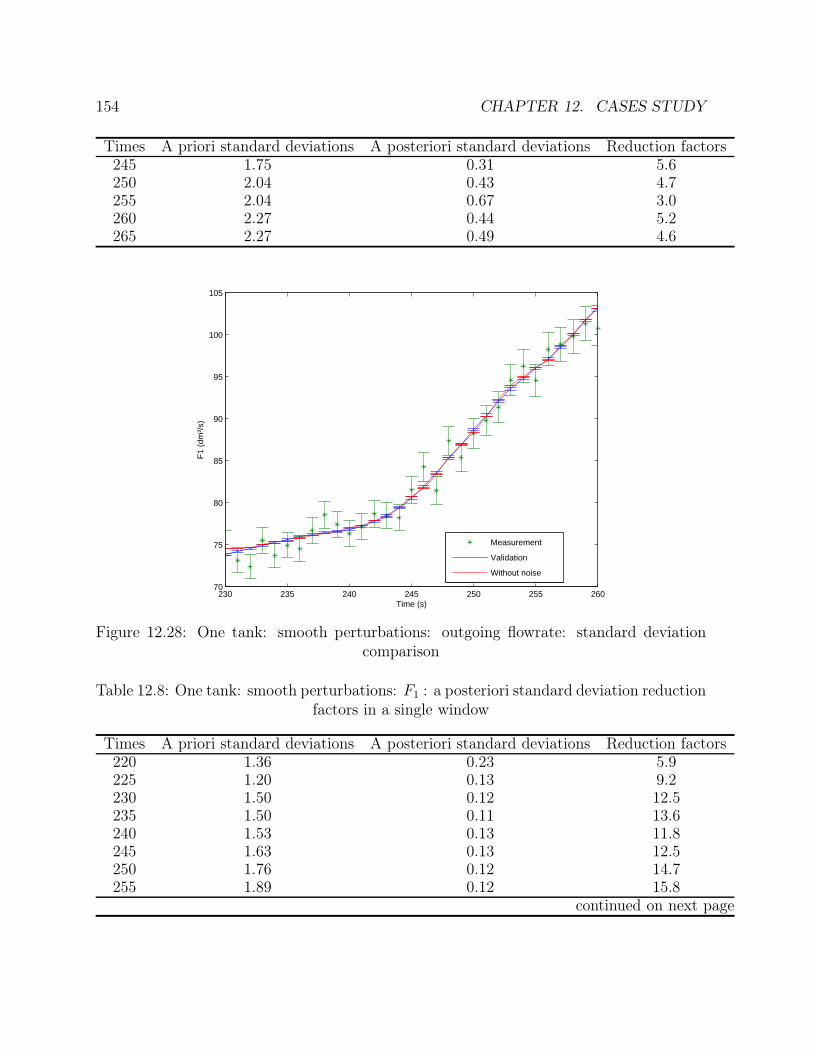
154 CHAPTER 12. CASES STUDY
Times A priori standard deviations A posteriori standard deviations Reduction factors245 1.75 0.31 5.6250 2.04 0.43 4.7255 2.04 0.67 3.0260 2.27 0.44 5.2265 2.27 0.49 4.6
230 235 240 245 250 255 26070
75
80
85
90
95
100
105
Time (s)
F1
(dm
³/s)
Measurement
Validation
Without noise
Figure 12.28: One tank: smooth perturbations: outgoing flowrate: standard deviationcomparison
Table 12.8: One tank: smooth perturbations: F1 : a posteriori standard deviation reductionfactors in a single window
Times A priori standard deviations A posteriori standard deviations Reduction factors220 1.36 0.23 5.9225 1.20 0.13 9.2230 1.50 0.12 12.5235 1.50 0.11 13.6240 1.53 0.13 11.8245 1.63 0.13 12.5250 1.76 0.12 14.7255 1.89 0.12 15.8
continued on next page

12.1. ONE TANK 155
Times A priori standard deviations A posteriori standard deviations Reduction factors260 2.02 0.14 14.4265 2.06 0.14 14.7
Four distributions of errors will be compared (see figure 12.29):
∙ the distribution of measurement errors;
∙ the distribution of the values that have been reconciled one time (corresponding to theℎ5 more recent measurement times of the reconciliation window). This distributioncurve is called beginning.
∙ the distribution of the reconciled values that leave that reconciliation window (cor-responding to the ℎ5 oldest measurement times of the reconciliation window). Thisdistribution curve is called end.
∙ the distribution of the reconciled values that are situated at the middle of the recon-ciliation window (ℎ5 measurement times for each reconciliation). This distributioncurve is called middle.
Timet0 t1 t2 t3 t4 t5 t6 t7 t8 t9 t10 t11 t12
ℎ5
ℎ4
End Middle Beginning
Estimated variables Measured variables
Valu
es
Figure 12.29: One tank: smooth perturbations: schema of the error distributions
The last three figures (figures 12.30, 12.31 and 12.32) represent the distributions of theerrors for all variables. One can see the means of errors are nearly zero, so that the normalnoise with zero mean that was imposed for the simulation data is well reproduced for thereconciliation distributions.It also appears that the error distribution is reduced while reconciling the data: indeed thedistributions are larger for the measurements errors than the three other ones.

156 CHAPTER 12. CASES STUDY
Concerning the way of saving the data, the best curve is the same for the algebraic statevariable and for the differential state variable since they are related by a constraint equa-tion. For differential state variable and algebraic state variable, there is not a big differencebetween the three cuves while the difference is more important for the input variable.
Figure 12.30: One tank: smooth perturbations: height: error distribution
Figure 12.31: One tank: smooth perturbations: feed flowrate: error distribution

12.1. ONE TANK 157
Figure 12.32: One tank: smooth perturbations: outgoing flowrate: error distribution
For the other examples, only smooth perturbations of the inputs will be carried out.
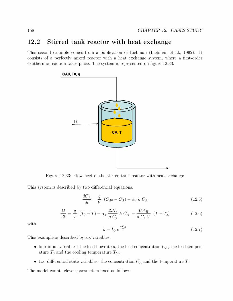
158 CHAPTER 12. CASES STUDY
12.2 Stirred tank reactor with heat exchange
This second example comes from a publication of Liebman (Liebman et al., 1992). Itconsists of a perfectly mixed reactor with a heat exchange system, where a first-orderexothermic reaction takes place. The system is represented on figure 12.33.
Figure 12.33: Flowsheet of the stirred tank reactor with heat exchange
This system is described by two differential equations:
dCA
dt=
q
V(CA0 − CA)− �d k CA (12.5)
dT
dt=
q
V(T0 − T )− �d
ΔHr
� Cp
k CA − UAR
� Cp V(T − Tc) (12.6)
withk = k0 e
−EAT (12.7)
This example is described by six variables:
∙ four input variables: the feed flowrate q, the feed concentration CA0,the feed temper-ature T0 and the cooling temperature TC ;
∙ two differential state variables: the concentration CA and the temperature T .
The model counts eleven parameters fixed as follow:
12.2. STIRRED TANK REACTOR WITH HEAT EXCHANGE 159
Table 12.9: Stirred tank reactor with heat exchange: model parameters
Parameters Values UnitsV 1000 cm3
ΔHr -27000 cal/mol� 0.001 g/cm3
Cp 1 cal/mol KU 5e−4 cal/cm2 s KAR 10 cm2
�d 1 -k0 7.86e12 s−1
EA 14090 KCAr 1e−6 mol/cm3
Tr 100 K
The model can be transformed into dimensionless equations by normalizing the concentra-tion and the temperature by a reference concentration Ar and a reference temperature Tr
so that the equations of the system are transformed into:
dC ′A
dt=
q
V(C ′
A0 − C ′A)− �d k C ′
A (12.8)
dT ′
dt=
q
V(T ′
0 − T ′)− �d
ΔHr CAr
� Cp
k C ′A − UAR
� Cp V(T ′ − T ′
C) (12.9)
k = k0 e−EAT ′ Tr (12.10)
⇕dx1
dt=
q
V(u2 − x1)− �d k x1 (12.11)
dx2
dt=
q
V(u3 − x2)− �d
ΔHr CAr
� Cp
k x1 − UAR
� Cp V(x2 − u4) (12.12)
k = k0 e−EAx2 Tr (12.13)
In those equations, the quote represent the scaled variables: C ′A = CA
CAr, C ′
A0 = CA0
CArand
T ′ = TTr
.
A set of pseudo-measurements has been obtained by a dynamic simulation of the process. Inthis simulation the differential equations are integrated using the fourth order Runge-Kuttamethod with a time step of 0.5 s. The process has been simulated during 1251 seconds andthe simulated measurements are given every 10 seconds. Input variables evolve as followduring the simulation: transitions between feed temperature set points have been modeledas first order responses with a 200 seconds time constant and feed concentration transitionswith a 50 seconds time constant.
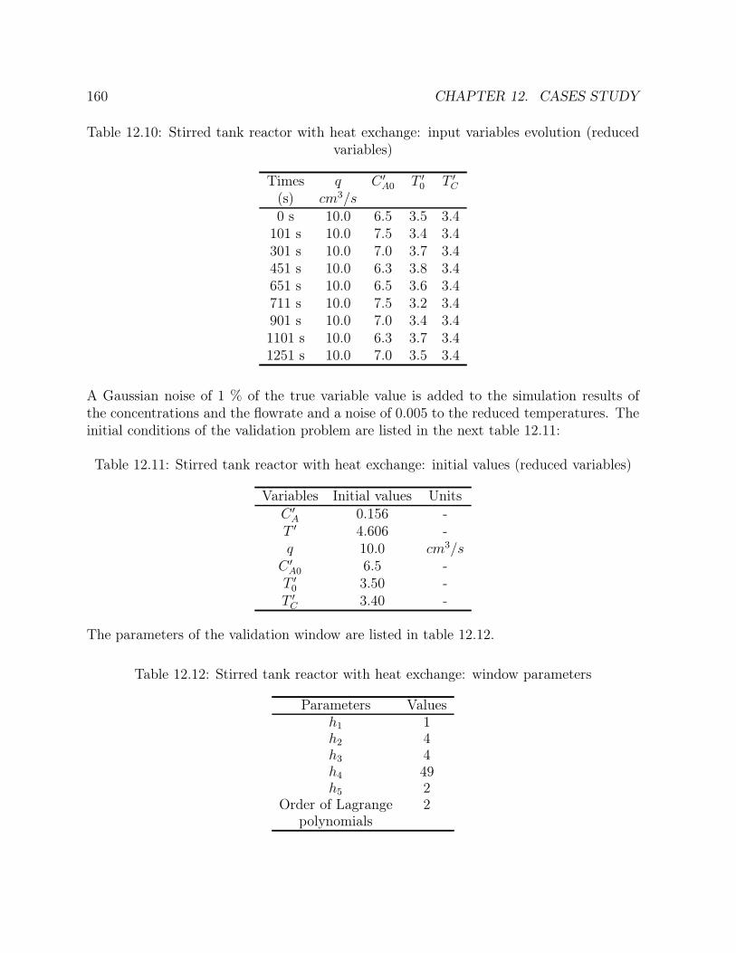
160 CHAPTER 12. CASES STUDY
Table 12.10: Stirred tank reactor with heat exchange: input variables evolution (reducedvariables)
Times q C ′A0 T ′
0 T ′C
(s) cm3/s0 s 10.0 6.5 3.5 3.4
101 s 10.0 7.5 3.4 3.4301 s 10.0 7.0 3.7 3.4451 s 10.0 6.3 3.8 3.4651 s 10.0 6.5 3.6 3.4711 s 10.0 7.5 3.2 3.4901 s 10.0 7.0 3.4 3.41101 s 10.0 6.3 3.7 3.41251 s 10.0 7.0 3.5 3.4
A Gaussian noise of 1 % of the true variable value is added to the simulation results ofthe concentrations and the flowrate and a noise of 0.005 to the reduced temperatures. Theinitial conditions of the validation problem are listed in the next table 12.11:
Table 12.11: Stirred tank reactor with heat exchange: initial values (reduced variables)
Variables Initial values UnitsC ′
A 0.156 -T ′ 4.606 -q 10.0 cm3/s
C ′A0 6.5 -T ′0 3.50 -
T ′C 3.40 -
The parameters of the validation window are listed in table 12.12.
Table 12.12: Stirred tank reactor with heat exchange: window parameters
Parameters Valuesℎ1 1ℎ2 4ℎ3 4ℎ4 49ℎ5 2
Order of Lagrange 2polynomials
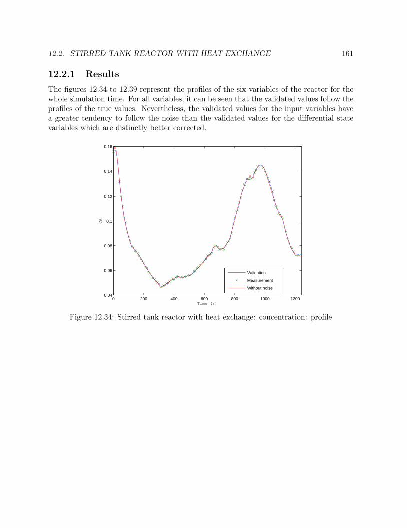
12.2. STIRRED TANK REACTOR WITH HEAT EXCHANGE 161
12.2.1 Results
The figures 12.34 to 12.39 represent the profiles of the six variables of the reactor for thewhole simulation time. For all variables, it can be seen that the validated values follow theprofiles of the true values. Nevertheless, the validated values for the input variables havea greater tendency to follow the noise than the validated values for the differential statevariables which are distinctly better corrected.
0 200 400 600 800 1000 12000.04
0.06
0.08
0.1
0.12
0.14
0.16
Time (s)
CA
Validation
Measurement
Without noise
Figure 12.34: Stirred tank reactor with heat exchange: concentration: profile
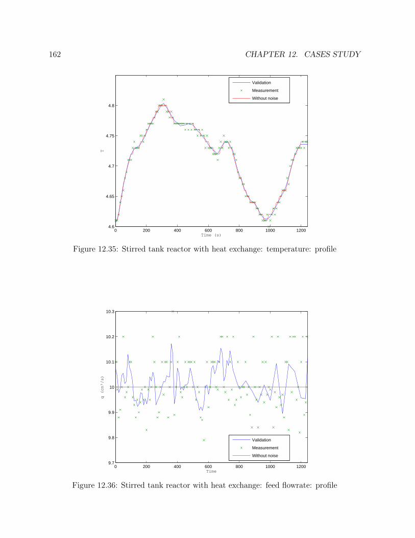
162 CHAPTER 12. CASES STUDY
0 200 400 600 800 1000 12004.6
4.65
4.7
4.75
4.8
Time (s)
T
Validation
Measurement
Without noise
Figure 12.35: Stirred tank reactor with heat exchange: temperature: profile
0 200 400 600 800 1000 12009.7
9.8
9.9
10
10.1
10.2
10.3
Time
q (
cm³/
s)
Validation
Measurement
Without noise
Figure 12.36: Stirred tank reactor with heat exchange: feed flowrate: profile
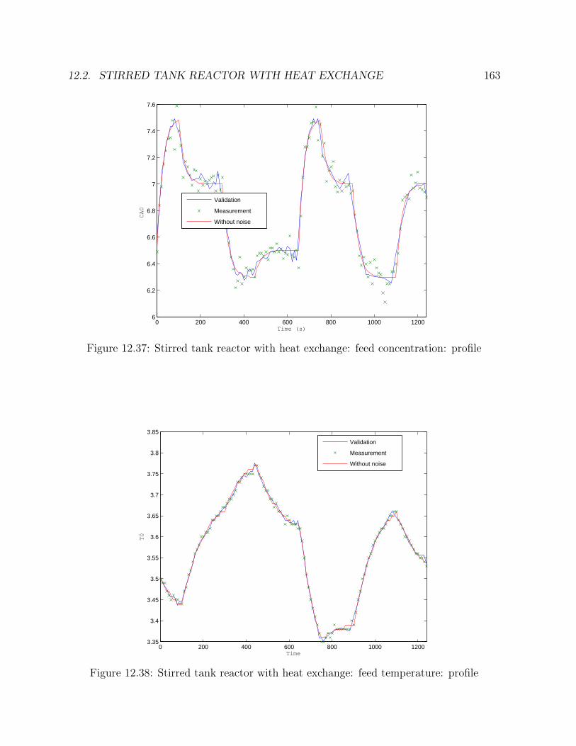
12.2. STIRRED TANK REACTOR WITH HEAT EXCHANGE 163
0 200 400 600 800 1000 12006
6.2
6.4
6.6
6.8
7
7.2
7.4
7.6
Time (s)
CA
0
Validation
Measurement
Without noise
Figure 12.37: Stirred tank reactor with heat exchange: feed concentration: profile
0 200 400 600 800 1000 12003.35
3.4
3.45
3.5
3.55
3.6
3.65
3.7
3.75
3.8
3.85
Time
T0
Validation
Measurement
Without noise
Figure 12.38: Stirred tank reactor with heat exchange: feed temperature: profile
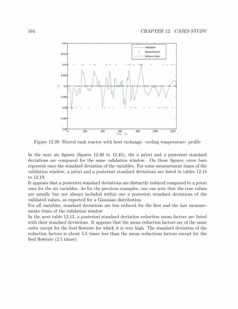
164 CHAPTER 12. CASES STUDY
0 200 400 600 800 1000 12003.38
3.385
3.39
3.395
3.4
3.405
3.41
3.415
3.42
Time (s)
TC
Validation
Measurement
Without noise
Figure 12.39: Stirred tank reactor with heat exchange: cooling temperature: profile
In the next six figures (figures 12.40 to 12.45), the a priori and a posteriori standarddeviations are compared for the same validation window. On those figures, error barsrepresent once the standard deviation of the variables. For some measurement times of thevalidation window, a priori and a posteriori standard deviations are listed in tables 12.14to 12.19.It appears that a posteriori standard deviations are distinctly reduced compared to a prioriones for the six variables. As for the previous examples, one can note that the true valuesare usually but not always included within one a posteriori standard deviations of thevalidated values, as expected for a Gaussian distribution.For all variables, standard deviations are less reduced for the first and the last measure-ments times of the validation windowIn the next table 12.13, a posteriori standard deviation reduction mean factors are listedwith their standard deviations. It appears that the mean reduction factors are of the sameorder except for the feed flowrate for which it is very high. The standard deviation of thereduction factors is about 5.5 times less than the mean reductions factors except for thefeed flowrate (2.5 times).

12.2. STIRRED TANK REACTOR WITH HEAT EXCHANGE 165
Table 12.13: Stirred tank reactor with heat exchange: a posteriori standard deviationreduction mean factors
A posteriori standard A posteriori standardVariables deviation reduction factors: deviation reduction factors:
means standard deviationsCA 2.0 0.37T 6.0 1.1q 54 22
CA0 2.1 0.37T0 2.1 0.37TC 2.1 0.37
400 450 500 550 600 650 700 750 800 8500.04
0.05
0.06
0.07
0.08
0.09
0.1
0.11
0.12
0.13
0.14
Time (s)
CA
Measurement
Validation
Without noise
Figure 12.40: Stirred tank reactor with heat exchange: concentration: standard deviationcomparison
Table 12.14: Stirred tank reactor with heat exchange: concentration: a posteriori standarddeviation reduction factors
Times A priori standard deviation A posteriori standard deviation Reduction factors401 5.28 10−4 3.33 10−4 1.6451 5.48 10−4 2.93 10−4 1.9
continued on next page
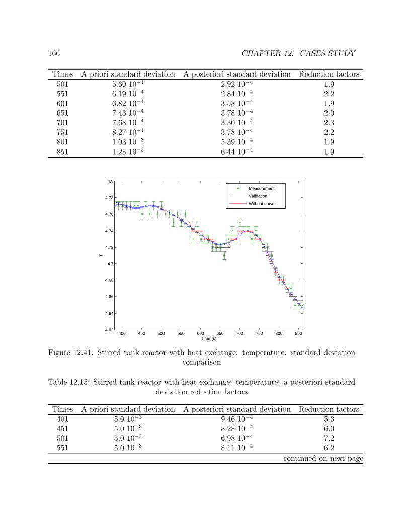
166 CHAPTER 12. CASES STUDY
Times A priori standard deviation A posteriori standard deviation Reduction factors501 5.60 10−4 2.92 10−4 1.9551 6.19 10−4 2.84 10−4 2.2601 6.82 10−4 3.58 10−4 1.9651 7.43 10−4 3.78 10−4 2.0701 7.68 10−4 3.30 10−4 2.3751 8.27 10−4 3.78 10−4 2.2801 1.03 10−3 5.39 10−4 1.9851 1.25 10−3 6.44 10−4 1.9
400 450 500 550 600 650 700 750 800 8504.62
4.64
4.66
4.68
4.7
4.72
4.74
4.76
4.78
4.8
Time (s)
T
Measurement
Validation
Without noise
Figure 12.41: Stirred tank reactor with heat exchange: temperature: standard deviationcomparison
Table 12.15: Stirred tank reactor with heat exchange: temperature: a posteriori standarddeviation reduction factors
Times A priori standard deviation A posteriori standard deviation Reduction factors401 5.0 10−3 9.46 10−4 5.3451 5.0 10−3 8.28 10−4 6.0501 5.0 10−3 6.98 10−4 7.2551 5.0 10−3 8.11 10−4 6.2
continued on next page

12.2. STIRRED TANK REACTOR WITH HEAT EXCHANGE 167
Times A priori standard deviation A posteriori standard deviation Reduction factors601 5.0 10−3 8.59 10−4 5.8651 5.0 10−3 7.68 10−4 6.5701 5.0 10−3 6.89 10−4 7.2751 5.0 10−3 8.04 10−4 6.2801 5.0 10−3 8.63 10−4 5.8851 5.0 10−3 9.16 10−4 5.4
400 450 500 550 600 650 700 750 800 850
9.7
9.8
9.9
10
10.1
10.2
10.3
10.4
10.5
Time (s)
q (c
m³/
s)
Measurement
Validation
Without noise
Figure 12.42: Stirred tank reactor with heat exchange: feed flowrate: standard deviationcomparison
Table 12.16: Stirred tank reactor with heat exchange: feed flowrate: a posteriori standarddeviation reduction factors
Times A priori standard deviation A posteriori standard deviation Reduction factors401 0.10 3.75 10−3 27451 0.10 1.77 10−3 56501 0.10 2.93 10−3 34551 0.10 1.75 10−3 57601 0.10 1.11 10−3 90651 0.10 1.67 10−3 60
continued on next page
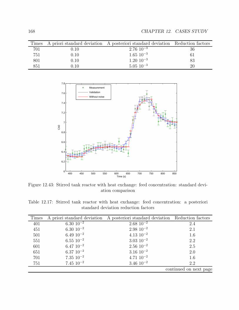
168 CHAPTER 12. CASES STUDY
Times A priori standard deviation A posteriori standard deviation Reduction factors701 0.10 2.76 10−3 36751 0.10 1.65 10−3 61801 0.10 1.20 10−3 83851 0.10 5.05 10−3 20
400 450 500 550 600 650 700 750 800 8506
6.2
6.4
6.6
6.8
7
7.2
7.4
7.6
7.8
Time (s)
CA
0
Measurement
Validation
Without noise
Figure 12.43: Stirred tank reactor with heat exchange: feed concentration: standard devi-ation comparison
Table 12.17: Stirred tank reactor with heat exchange: feed concentration: a posterioristandard deviation reduction factors
Times A priori standard deviation A posteriori standard deviation Reduction factors401 6.30 10−2 2.68 10−2 2.4451 6.30 10−2 2.98 10−2 2.1501 6.49 10−2 4.13 10−2 1.6551 6.55 10−2 3.03 10−2 2.2601 6.47 10−2 2.56 10−2 2.5651 6.37 10−2 3.16 10−2 2.0701 7.35 10−2 4.71 10−2 1.6751 7.45 10−2 3.46 10−2 2.2
continued on next page
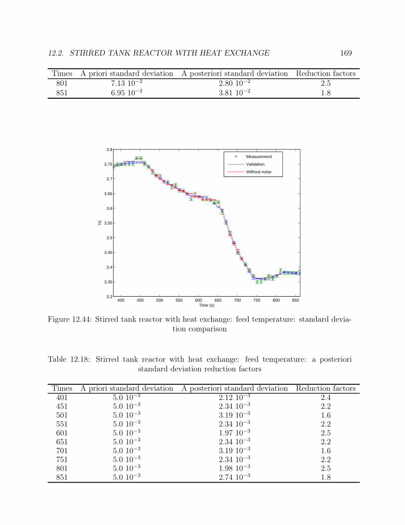
12.2. STIRRED TANK REACTOR WITH HEAT EXCHANGE 169
Times A priori standard deviation A posteriori standard deviation Reduction factors801 7.13 10−2 2.80 10−2 2.5851 6.95 10−2 3.81 10−2 1.8
400 450 500 550 600 650 700 750 800 8503.3
3.35
3.4
3.45
3.5
3.55
3.6
3.65
3.7
3.75
3.8
Time (s)
T0
Measurement
Validation
Without noise
Figure 12.44: Stirred tank reactor with heat exchange: feed temperature: standard devia-tion comparison
Table 12.18: Stirred tank reactor with heat exchange: feed temperature: a posterioristandard deviation reduction factors
Times A priori standard deviation A posteriori standard deviation Reduction factors401 5.0 10−3 2.12 10−3 2.4451 5.0 10−3 2.34 10−3 2.2501 5.0 10−3 3.19 10−3 1.6551 5.0 10−3 2.34 10−3 2.2601 5.0 10−3 1.97 10−3 2.5651 5.0 10−3 2.34 10−3 2.2701 5.0 10−3 3.19 10−3 1.6751 5.0 10−3 2.34 10−3 2.2801 5.0 10−3 1.98 10−3 2.5851 5.0 10−3 2.74 10−3 1.8
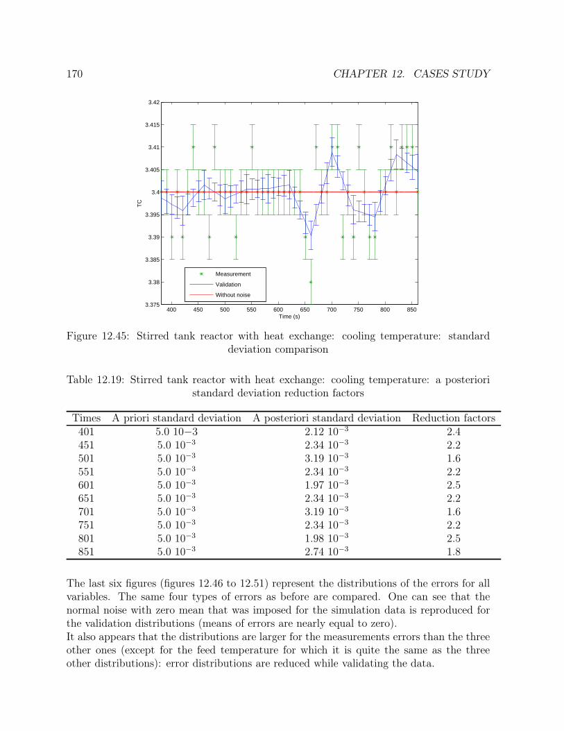
170 CHAPTER 12. CASES STUDY
400 450 500 550 600 650 700 750 800 8503.375
3.38
3.385
3.39
3.395
3.4
3.405
3.41
3.415
3.42
Time (s)
TC
Measurement
Validation
Without noise
Figure 12.45: Stirred tank reactor with heat exchange: cooling temperature: standarddeviation comparison
Table 12.19: Stirred tank reactor with heat exchange: cooling temperature: a posterioristandard deviation reduction factors
Times A priori standard deviation A posteriori standard deviation Reduction factors401 5.0 10−3 2.12 10−3 2.4451 5.0 10−3 2.34 10−3 2.2501 5.0 10−3 3.19 10−3 1.6551 5.0 10−3 2.34 10−3 2.2601 5.0 10−3 1.97 10−3 2.5651 5.0 10−3 2.34 10−3 2.2701 5.0 10−3 3.19 10−3 1.6751 5.0 10−3 2.34 10−3 2.2801 5.0 10−3 1.98 10−3 2.5851 5.0 10−3 2.74 10−3 1.8
The last six figures (figures 12.46 to 12.51) represent the distributions of the errors for allvariables. The same four types of errors as before are compared. One can see that thenormal noise with zero mean that was imposed for the simulation data is reproduced forthe validation distributions (means of errors are nearly equal to zero).It also appears that the distributions are larger for the measurements errors than the threeother ones (except for the feed temperature for which it is quite the same as the threeother distributions): error distributions are reduced while validating the data.
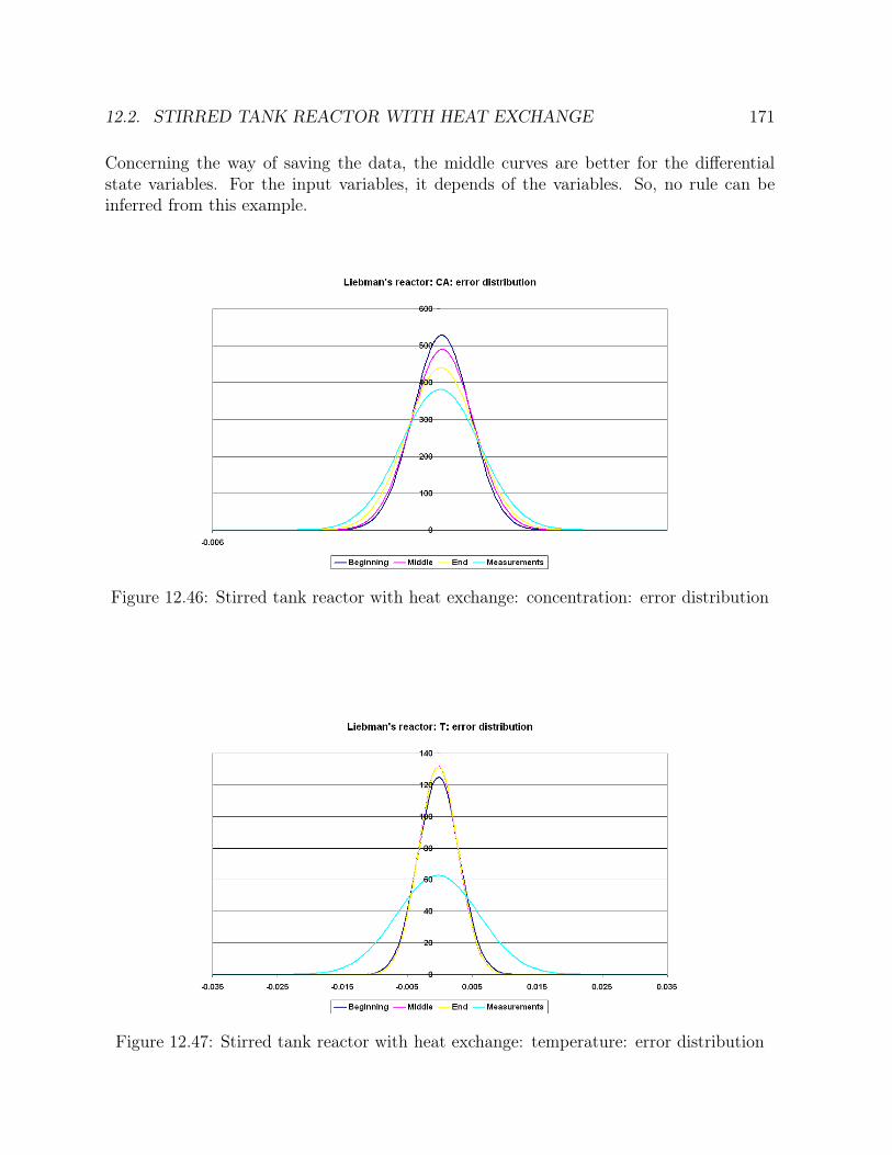
12.2. STIRRED TANK REACTOR WITH HEAT EXCHANGE 171
Concerning the way of saving the data, the middle curves are better for the differentialstate variables. For the input variables, it depends of the variables. So, no rule can beinferred from this example.
Figure 12.46: Stirred tank reactor with heat exchange: concentration: error distribution
Figure 12.47: Stirred tank reactor with heat exchange: temperature: error distribution
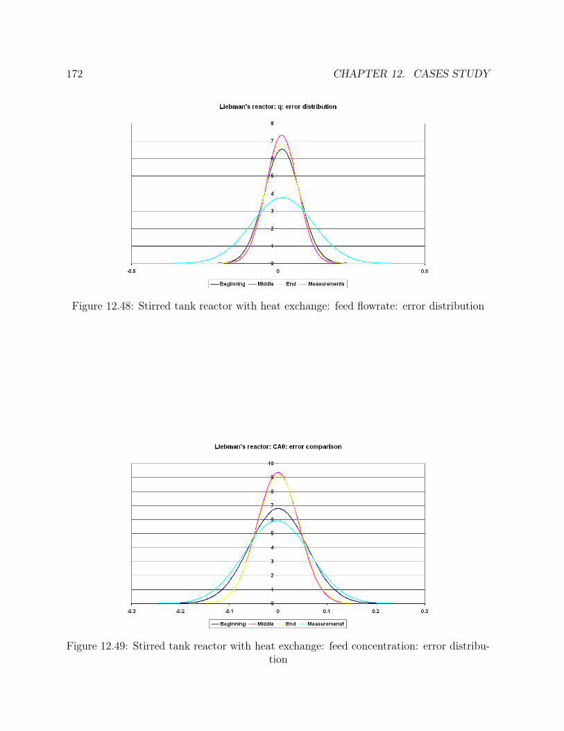
172 CHAPTER 12. CASES STUDY
Figure 12.48: Stirred tank reactor with heat exchange: feed flowrate: error distribution
Figure 12.49: Stirred tank reactor with heat exchange: feed concentration: error distribu-tion

12.2. STIRRED TANK REACTOR WITH HEAT EXCHANGE 173
Figure 12.50: Stirred tank reactor with heat exchange: feed temperature: error distribution
Figure 12.51: Stirred tank reactor with heat exchange: cooling temperature: error distri-bution

174 CHAPTER 12. CASES STUDY
12.3 A network of five tanks
In this last example, five tanks are interconnected. The first tank is fed by stream F0A andthe recirculated stream F4B coming from tank 4. The second tank receives the feed streamF0B and the stream F1A coming from tank 1. The third tank receives the feed stream F0C
and the stream F1B coming from tank 1. The fourth tank is feeded by stream F3B comingfrom tank 3. The fifth tank receives stream F2 from tank 2 and stream F3A from tank 3.This example is represented on figure 12.52.
F0A
F1A F1B
H1
H4
F4A F4B
F2
H2
F0B
H3
F3B
F3A
F0C
F5
H5
Figure 12.52: Flowsheet of the network of five tanks

12.3. A NETWORK OF FIVE TANKS 175
The model is defined by 13 equations: 5 differential equations and 8 link equations:
dℎ1
dt=
F0A + F4B
A1
− F1A + F1B
A1
(12.14)
dℎ2
dt=
F0B + F1A
A2− F2
A2(12.15)
dℎ3
dt=
F0C + F1B
A3− F3A + F3B
A3(12.16)
dℎ4
dt=
F3B
A4− F4A + F4B
A4(12.17)
dℎ5
dt=
F2 + F3A
A5− F5
A5(12.18)
F1A = �1 H1 �1 (12.19)
F1B = �1 H1 (1− �1) (12.20)
F2 = �2 H2 (12.21)
F3A = �1 H3 �3 (12.22)
F3B = �3 H3 (1− �3) (12.23)
F4A = �4 H4 �4 (12.24)
F4A = �4 H4 (1− �4) (12.25)
F5 = �5 H5 (12.26)
⇕dx1
dt=
u1 + z7A1
− z1 + z2A1
(12.27)
dx2
dt=
u2 + z1A2
− z3A2
(12.28)
dx3
dt=
u3 + z2A3
− z4 + z5A3
(12.29)
dx4
dt=
z5A4
− z6 + z7A4
(12.30)
dx5
dt=
z3 + z4A5
− z8A5
(12.31)
z1 = �1 x1 �1 (12.32)
z2 = �1 x1 (1− �1) (12.33)
z3 = �2 x2 (12.34)
z4 = �3 x3 �3 (12.35)
z5 = �3 x3 (1− �3) (12.36)
z6 = �4 x4 �4 (12.37)
z7 = �4 x4 (1− �4) (12.38)
z8 = �5 x5 (12.39)

176 CHAPTER 12. CASES STUDY
This example counts sixteen variables:
∙ three input variables: the feed flowrates F0A, F0B and F0C ;
∙ five differential state variables: the heights in the tanks , H1, H2, H3, H4 and H5;
∙ eight algebraic variables: the flowrates F1A, F1B, F2, F3A, F3B , F4A, F4B and F5.
The model counts thirteen parameters fixed as follow:
Table 12.20: Network of five tanks: model parameters
Parameters Values UnitsA1 8 dm2
A2 10 dm2
A3 5 dm2
A4 10 dm2
A5 7 dm2
�1 1.2 -�2 0.9 -�3 1.0 -�4 1.5 -�5 1.1 -�1 0.5 -�2 0.3 -�3 0.8 -
A data set has been obtained by a dynamic simulation of the process. In this simulationdifferential equations are integrated by means of the fourth order Runge-Kutta methodwith a step of 1 s. The process has been simulated during 261 seconds and the simulatedmeasurements are given every second. Feed flowrates evolve as follow during the simulation:transitions between feed flowrate set points have been modeled as first order responses witha 10 seconds time constant.
Table 12.21: Network of five tanks: feed flowrates evolution
Times F0A F0B F0C
(s) (dm3/s) (dm3/s) (dm3/s)0 s 50 30 2031 s 100 30 2081 s 60 30 20111 s 60 20 40continued on next page

12.3. A NETWORK OF FIVE TANKS 177
Times F0A F0B F0C
(s) (dm3/s) (dm3/s) (dm3/s)151 s 40 35 20211 s 60 40 10261 s 80 35 20
A Gaussian noise (zero mean and standard deviation set at 2% of the true value) is addedto the simulation results of the flowrates. Similarly, Gaussian noise (standard deviationset at 2 cm) is added to the simulated height before carrying out the data reconciliation.The initial conditions of the validation problem are listed in the next table 12.22:
Table 12.22: Network of five tanks: initial values
Variables Initial values UnitsH1 42.0 dmH2 12.0 dmH3 39.0 dmH4 33.0 dmH5 25.0 dmF0A 50.0 dm3/sF0B 30.0 dm3/sF0C 20.0 dm3/sF1A 25.2. dm3/sF1B 25.2 dm3/sF2 10.8 dm3/sF3A 10.7 dm3/sF3B 27.3 dm3/sF4A 39.6 dm3/sF4B 9.9 dm3/sF5 27.5 dm3/s
The parameters of the validation windows are listed in table 12.23.
Table 12.23: Network of five tanks: window parameters
Parameters Valuesℎ1 1ℎ2 4ℎ3 4ℎ4 49ℎ5 2
continued on next page

178 CHAPTER 12. CASES STUDY
Parameters ValuesOrder of Lagrange 2
polynomials
12.3.1 Results
For all variables, the validated values follow the curves of the simulation without noiseand the measurements are corrected. The profiles of the differential state variables arerepresented on figures 12.53 to 12.57 for the whole time horizon. The values that are savedare the validated values of the measurements entering the validation window.
0 50 100 150 200 25030
40
50
60
70
80
90
Time (s)
H1
(d
m)
Validation
Measurement
Without noise
Figure 12.53: Network of five tanks: height H1: profile
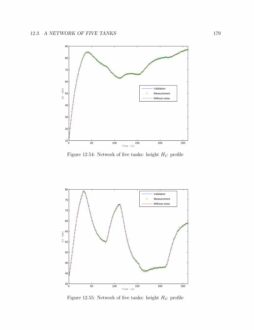
12.3. A NETWORK OF FIVE TANKS 179
0 50 100 150 200 25010
20
30
40
50
60
70
80
90
Time (s)
H2
(d
m)
Validation
Measurement
Without noise
Figure 12.54: Network of five tanks: height H2: profile
0 50 100 150 200 25035
40
45
50
55
60
65
70
75
80
Time (s)
H3
(d
m)
Validation
Measurement
Without noise
Figure 12.55: Network of five tanks: height H3: profile

180 CHAPTER 12. CASES STUDY
0 50 100 150 200 25018
20
22
24
26
28
30
32
34
36
38
Time (s)
H4
(d
m)
Validation
Measurement
Without noise
Figure 12.56: Network of five tanks: height H4: profile
0 50 100 150 200 25020
30
40
50
60
70
80
90
Time (s)
H5
(d
m)
Validation
Measurement
Without noise
Figure 12.57: Network of five tanks: height H5: profile
In the next table 12.24, a posteriori standard deviation reduction factors of all variablesare listed with their standard deviations. In this example, it appears that the algebraic

12.3. A NETWORK OF FIVE TANKS 181
state variables have better a posteriori standard deviation reduction factors that input anddifferential state variables. In fact, since algebraic variables and differential variables arelinked by the model equations 14.19 to 14.26, the standard deviations of their validatedvalues are similarly linked. However level measurement are more precise (standard devi-ation = 2 cm and true value ∼ 500 cm) than flowrates (standard deviation = 2% of thetrue value). The reduction factor is better for flowrates.
Table 12.24: Network of five tanks: a posteriori standard deviation reduction mean factors
A posteriori standard A posteriori standardVariables deviation reduction factors: deviation reduction factors:
means standard deviationsH1 4.6 1.1H2 4.5 0.96H3 2.9 0.54H4 11 4.1H5 6.2 1.6F0A 6.0 2.5F0B 2.0 0.39F0C 2.0 0.39F1A 23 5.6F1B 23 5.8F2 30 6.6F3A 17 3.8F3B 17 3.7F4A 31 11F4B 31 11F5 44 11
As can been seen in table 12.25, the means of errors still correspond with the normal noiseswith zero mean that were imposed during the simulation.Concerning the distributions, one can see they are wider for the measurements, that meansthat the errors are corrected during the validation. In the case of input variables, thevalidated values obtained at the end of the window have narrower distributions that theones at the beginning and middle curves.In the case of the differential state variables, no clear trend can be identified concerningthe best time to keep the validated values.As expected, the algebraic state variables have distributions similar to ones of the statevariables they depend.No rule concerning the best way of saving the data can be made from this example.

182 CHAPTER 12. CASES STUDY
Table 12.25: Network of five tanks: means and standard deviations of errors
Variables Means Standard deviations
=∑
error
n=
∑(error − mean error)2
n−1
Beginning Middle End Meas. Beginning Middle End Meas.H1 -0.003 -0.008 -0.018 -0.012 0.10 0.096 0.10 0.19H2 -0.018 -0.018 -0.014 -0.020 0.087 0.059 0.063 0.21H3 0.022 0.021 0.019 0.024 0.10 0.079 0.072 0.20H4 -0.010 0.009 0.003 -0.009 0.024 0.025 0.049 0.18H5 -0.012 -0.013 -0.005 -0.011 0.033 0.038 0.065 0.20F0A 0.062 0.040 0.037 0.080 0.71 0.59 0.54 1.2F0B -0.007 -0.002 -0.015 -0.019 0.42 0.27 0.21 0.71F0C 0.024 0.027 0.024 0.012 0.28 0.28 0.23 0.42F1A -0.002 -0.005 -0.010 0.042 0.063 0.058 0.060 0.70F1B -0.002 -0.005 -0.012 -0.046 0.063 0.058 0.060 0.72F2 -0.016 -0.016 -0.006 -0.094 0.079 0.053 0.057 1.3F3A 0.007 0.006 0.038 0.038 0.030 0.024 0.022 0.35F3B 0.016 0.015 0.013 -0.033 0.071 0.056 0.050 0.85F4A 0.012 0.010 0.003 -0.0001 0.029 0.030 0.059 0.67F4B 0.003 0.003 0.001 -0.006 0.007 0.007 0.015 0.16F5 -0.013 -0.014 -0.006 -0.043 0.036 0.042 0.072 1.57
12.4 Conclusions
The validation techniques tested in this study allowed to validate the data of all the smallexamples we studied. The validated profiles match closely the simulated ones. However itappears that the validated profiles of input variables, are more affected by the noise thanfor the other variables.Validation allows to reduce the uncertainty (�) on the measured variables. However, forall studied examples, the procedure is less effective with respect to input variables. Whenmeasurement errors follow a normal, zero mean distribution, a similar distribution is ob-served for validation errors. As expected, the spread of validation errors is narrower, sothat validation allows to better know the variables. There is no clearcut rule allowing topredict which validation estimate is the most reliable when a measurement is used severaltimes in successive validation runs. Typically the results obtained by the first validation,as soon as the measurement becomes available, will be used for process control. Resultscalculated when the measurement is in the middle of the window might be more reliableand used for archival.For all variables of all examples, a posteriori standard deviations are distinctly reducedcompared to a priori ones, but true values are not always included in error bars drawnaround the validated values. A posteriori standard deviation at the beginning and at theend of the validation window are larger that in the middle of the window where the values

12.4. CONCLUSIONS 183
of the variables are better known.The validation being less efficient for input variables, we suggest to replace their linearinterpolation by orthogonal collocations. Doing that, it should be decided if the order ofthe polynomials and the size of the discretization intervals should be the same as for thedifferential state variables.One can also choose to place the nodes of orthogonal collocations at the measurement times,even if it could be less precise, since it would reduce the computing ressources needed.


Chapter 13
Conclusions part II
Several techniques have been tested to reconcile dynamic processes: the extended Kalmanfilter, the integration of the differential equation by means of Runge-Kutta method cou-pled with optimization algorithms (Davidon, 1975) or SQPIP (Kyriakopoulou, 1997), thediscretization of differential equations by means of orthogonal collocations coupled withthe same optimization methods.From the cases that were studied, it appeared that, even if all methods allow reconcilingthe data, the simultaneous method using orthogonal collocations was the best one in ourcase: other methods were not able to achieve the minimum of the goal function, probablyas a consequence of numerical noise or limited precision in the approximations of deriva-tives by numerical differentiation. Moreover, very non linear problems can not be solvedproperly using Kalman filters. With the design of sensor network for dynamic process as anobjective, one has to know a posteriori uncertainty on input variables. The problem withfiltering method is that they consider the input variables as perfectly known so that theyare not corrected and their a posteriori uncertainty can not be estimate. Concerning theexplicit integration, the main problem is that there does not exists a method allowing to es-timate a posteriori variances. This could be obtained by integrating sensitivity equationsin parallel with the model equations, but this strategy would be difficult to generalizedand implement. In the case of orthogonal collocations, as the differential equations arediscretized, we could transpose the method of a posteriori variances estimations developedfor the stationary case (Heyen et al., 1996).Good results have been obtained with orthogonal collocations for all small examples treated:the reconciled values follow the simulated ones, a posteriori variances are smaller than apriori ones (as expected) and are better inside the reconciliation window than for the firstand the last measurement times, uncertainties are reduced.Nevertheless there remains one problem with input variables, which follow more the noisethan other variables. Using orthogonal collocations also for inputs variables could allow toaddress that problem.
185


Part III
Networks design for dynamic processes
187

Chapter 14
Design of sensor networks for dynamic
processes
14.1 Introduction
The objective of this third part of the theses is to create an algorithm able to design thecheapest sensor network allowing to observe all process variables and to estimate processkey variables within a prescribed accuracy.Chouaib Benqlilou (Benqlilou et al., 2003), (Benqlilou, 2004), (Benqlilou et al., 2005) solvedthe problem of sensor placement for dynamic problem in the case where the dynamicreconciliation is made by means of Kalman filter. This implies that input variables areconsidered as being perfectly known. Only mass balances were solved in his study. He usesgenetic algorithm to perform optimization.The method proposed here after allows to solve more general problems involving mass andenergy balances. It is based on the dynamic reconciliation results obtained with the methoddescribed in the second part of the theses. The formulation used in this reconciliationtechnique allows (as presented in chapter 11) to estimate a posteriori variances whichare necessary to the sensor placement. One peculiarity of the dynamic version of thesensor placement problem is the consideration of an extra degree of freedom, namely themeasurement frequency.
14.2 Observability and variable discretization
As for the stationary case, the observability condition implies that the sensitivity matrix isnon-singular. This matrix is defined by the equations 11.15, 11.16 and 11.17. Indeed, if thiscondition is met, it is possible to estimate all a posteriori variances (see equations 11.23,11.24 and 11.25). To estimate the variables one has to know the independent terms -F,-Fc and -G coming from the linearisation of the constraints in A, Ac, and D respectively(see equations 11.18, 11.19 and 11.20). The terms -F, -Fc and -G can be estimated by
189

190 CHAPTER 14. ALGORITHM DESCRIPTION
solving the constraints equations that are part of the optimality conditions :
∂ L
∂ ΛAr,j
=nx∑
i=1
∂Ar,j
∂xi,j
xi,j +nz∑
i=1
∂Ar,j
∂zi,jzi,j +
nu∑
i=1
∂Ar,j
∂ui,j
ui,j + Fr,j = 0 ∀j, ∀r[
∂ L
∂ ΛAcr,j
]
discr int s
=
[nxc∑
i=1
∂Acr,j
∂xci,j
xci,j +
nzc∑
i=1
∂Acr,j
∂zci,jzci,j
+
nuc∑
i=1
∂Acr,j
∂uci,j
uci,j + F c
r,j
]
discr int s
= 0 ∀j, ∀r, ∀s
[∂ L
∂ ΛDi,k
]
discr int s
=
[n�∑
r=0
∂Di,k
∂xci,r
xci,r +
∂Di,k
∂zci,kzci,k
+∂Di,k
∂uci,k
uci,k +Gi,k
]
discr int s
= 0 ∀i, ∀k, ∀s
(14.1)
Nevertheless, the optimization algorithm need some information about the initial valuesof input and differential state variables to start the optimization. Indeed, those values arenecessary for the linearisation of the inputs and the creation of the Lagrange’s polynomialsused in the discretization of differential equations. So, the observability criterion describedbefore can only be verified a posteriori.If the SQP program starts the optimization with random initial values that can be very farfrom the solution, it can be very difficult or even impossible for the optimization programto find the solution, especially if the process has a tendency to become unstable. So, wehave decided to impose the measurement of the input and differential variables at leastonce for each reconciliation window.In the case of sensor network design, one has to ensure that the sensor network is evalu-ated for the minimum number of measurements that can be carried out with the chosenmeasurement tools. For example, if the measurement frequency of a sensor is five, a mea-surement is carried out every fifth time step. For a window containing 49 times, if the first,the second, the third or the fourth time of the window corresponds to the first measure-ment time, 10 measurements are carried out. But, if the fifth time of the window is thefirst measurement time of the widow, only 9 measurements are carried out. That’s is whyit has been decided that if the frequency of a sensor is k, the first measurement will takeplace at the ktℎ time of the window.
14.3 Method description
The optimal design of sensor network can be decomposed in five steps:
1. Formulation of the reconciliation model and model linearisation;
14.3. METHOD DESCRIPTION 191
2. Specification of sensor database, precision requirements and sensor requirements;
3. Verification of the problem feasibility;
4. Optimization of the goal function;
5. Report generation.
The flow diagram of the algorithm is presented on figure 4.1.The algorithm implemented for steady-state processes has been modified to take the dy-namic into account. The modifications are described here after.
14.3.1 Formulation of the reconciliation model and model lineari-
sation
First of all, a dynamic simulation of the process has to be carried out to obtain a dataset. The differential equations are integrated by means of the fourth order Runge-Kutta’smethod. A noise is then added to the simulation values. This noise agrees with themeasurement noise that would be expected if the values were plant measurements.The second part of this step is the reconciliation of the noised data set. This reconciliationis carried out using the moving horizon method that was developed in section 10.2. Inthis dynamic reconciliation technique, differential equations are discretized by means oforthogonal collocations. At the beginning of the reconciliation, a small file is created. Itcontains the parameter of the reconciliation window: size of the window, size of the dis-cretizetion and the interpolation intervals, displacement of the window, order of Lagrange’spolynomials.Once the solution is reached for a reconciliation window, the elements of the Jacobianmatrix 퓔 (see equation 11.17) of the process model are estimated. A file is created for eachreconciliation window. It contains
∙ the number of process variables: the number of variables contained in the processmodel multiplied by the number of measurement times contained in the reconciliationwindow;
∙ the number of constraints of the reconciliation window: namely constraints A, Ac,B, C, Cc, D and E defined in 10.2;
∙ the value, the physical unit and the type (concentration, temperature, level, massflowrate...) of each process variable;
∙ the Jacobian matrix 퓔 of the equation system.
To be sure that the sensor network will be able to handle all expected profiles, several ofthose files are generated. The files are chosen this way:
∙ the first file to be chosen is the file corresponding to the first reconciliation window;
192 CHAPTER 14. ALGORITHM DESCRIPTION
∙ for the other files, it is imposed that at least the first measurement time of the chosenwindow is contained in the previous one. The amount of overlaps between successivewindows will depend on the window displacement.
14.3.2 Specification of sensor database, precision requirements and
sensor requirements
Besides the files coming from the reconciliation phase, the program needs three data files.Those files contain the sensor database, the precision requirements and the sensor require-ments.
Sensor database
The sensor database is a list of sensor from which the algorithm must choose all thepossible sensor placements for the studied plant. It must include, for each sensor, thefollowing information:
∙ the name of the sensor;
∙ the annualized cost of the sensor. This cost must take into account:
– the annualized purchase cost;
– the annualized installation cost;
– the annualized operating cost.
All those costs depend on the studied process: indeed, for example, the cost of thesensor will be different if it is placed in a flow of water or if it must resists to acidor base. Moreover, costs evolves with the technologic progress and with the time sothat annualized costs will be written in cost units for the studied cases in the nextchapter.
∙ the parameters �Aiand �Bi
that allow the estimation of the sensor standard deviation�j for the measured variable X
′
j :
�j = �Ai+ �Bi
∗X ′
j (14.2)
∙ the minimal and maximal values of the sensor measurement range;
∙ the type of variable the sensor is able to measure. For exemple:
– TEMP for a temperature;
– LEVEL for a level;
– MASSF for a mass flowrate;

14.3. METHOD DESCRIPTION 193
– CONC for a concentration;
∙ the frequency of the measurement. If a sensor is listed in the database for severalmeasurement frequencies the costs will decrease with decreasing measurement fre-quency so that a small frequency is preferentially chosen if it allows to reach thespecified performances of the sensor network. This decrease in price can be justifiedby the fact that sensors used more frequently will generate more data to stock andtreat. In some cases (for example chromatographs), they consume reactants or needto be service or calibrated more often.
Precision requirements and sensor requirements
Those files are exactly the same as for the stationary case (see section 4.2).
14.3.3 Verification of the problem feasibility
This step of the program begins by carrying out the list of all the sensors that can be locatedin the plant and used at each time step. Individuals are created as for the stationary case:the binary genes take the value 1 or 0 depending if the corresponding sensors are chosenor not. Afterwards, the algorithm checks whether there exists a solution to the problemfor the first individual containing all possible sensors. If several sensors measure the samevariables, only the variance of the most accurate one is taken into account.To ensure there exists a solution to the studied problem, four conditions have to be met:
∙ The sensitivity matrix of the problem is non-singular for the ideal thermodynamiccase. If this condition is not met, the program stops. This condition is not verifiedfor the examples of the next chapter because thermodynamic models are not used inthose examples.
∙ The sensitivity matrix of the problem is non-singular for the process specific thermo-dynamic.
∙ If one refers to the way the dynamic reconciliation program works, initial condi-tions on input and differential variables have to be known to carry out the dynamicdata reconciliation. Thus all input and differential variables must be measured atleast once for each chosen reconciliation window. If this is not the case for the firstindividual, the program may not continue.
∙ The accuracy target of all key parameters must be achieved for all times of all thereconciliation windows chosen by the program. If this condition is not net, theprogram may continue, but a penalty is added to the goal function.
There are different ways to cure those problems:
∙ adding more accurate sensors;

194 CHAPTER 14. ALGORITHM DESCRIPTION
∙ adding sensors whose measurement frequency is higher;
∙ adding sensors able to measure other types of variables;
∙ adding more extra measurable variables with their link equations so that more vari-ables can be measured.
14.3.4 Optimization of the sensor network
Knowing that a feasible solution exists, the search for the optimal sensor configuration canbegin. The goal function to maximise is evaluated this way:
∙ If the sensitivity matrix is singular:
Fitness = −Cmax penaltysingular matrix (14.3)
where
– Cmax is the cost relative to the most expensive sensor network (which corre-sponds to the first chromosome);
– penaltysingular matrix is the penalty factor for a singular sensitivity matrix and isgenerally chosen equal to 2.
∙ otherwise
Fitness = −cost −Nkey variables ⋅ N★
tmes∑
i=1
⎧⎨⎩
− �i
�targeti
�2
i(�targeti
)2
Cmax penaltytarget
Nkey variables
102Cmax penaltytarget
Nkey variables
if �i
�targeti
≤ 1
if 1 < �i
�targeti
< 10
if �i
�targeti
≥ 10
(14.4)where
– Nkey variables is the number of process key variables;
– N★tmes
is the number of measurement times on the moving horizon including theinitial time of the horizon;
– penaltytarget is the penalty factor for the targets on key parameters that are notrespected and is fixed equal to 2;
– �i is the accuracy obtained by the sensor network for the key variable i ;
– �targeti is the accuracy required for the key parameter i.
If the sensor network has to be designed for several reconciliation windows, the fitnessbecomes:
Fitness =
Nwindows∑
j=1
fitnessj − (Nwindows − 1) cost (14.5)

14.3. METHOD DESCRIPTION 195
where Nwindows is the number of reconciliation windows chosen for the sensor networkdesign.If a measurement system observable in the case of one sensor failure has to be carried out,the fitness is evaluated for all configurations obtained by eliminating successively one ofthe sensors, and the worst one is kept.The genetic algorithm developped by Carroll (Carroll, 2001) described in section A for thestationary case is used to perform this optimization.Individuals of the first generation are chosen randomly, making sure that the number ofchosen sensors is at least equal to the number of degrees of freedom of the problem. Ahigh probability of selection if fixed for each sensor. A value of 80 % is typically chosenbut this parameter appears not to be critical for the problem of optimal sensor design. Forthe other parameters of the genetic algorithm, the following values are recommended:
∙ the population size, generally chosen to 20 individuals;
∙ the probability of reproduction was fixed to 50 %;
∙ the probability of single-point cross-over was chosen to 50 %
∙ the probability of jump mutation after reproduction and cross-over is 1 %.
Once the population has been generated the goal function has to be evaluated to estimatereconciled variances of all variables, the sensitivity has to be inverted. This matrix is verysparse that’s why one continues to use Belsim’s routine to factorize the matrix.At each generation, the best individual is kept and duplicated in the case it would mutateduring the next generation.If after a specified number of generations (n) the best chromosome remains unchanged, itis considered has the solution of the problem. There is no certainty that this solution isthe best one, but it is available and much better than the first individual.The computing times to reach the solution with the algorithm can be very important evenfor small problems likes the ones studied in the next chapter that is why a parallelizedversion of the code is necessary.
14.3.5 Report generation
The programme finally generates the same reports files as in the stationary case (see section4.5).

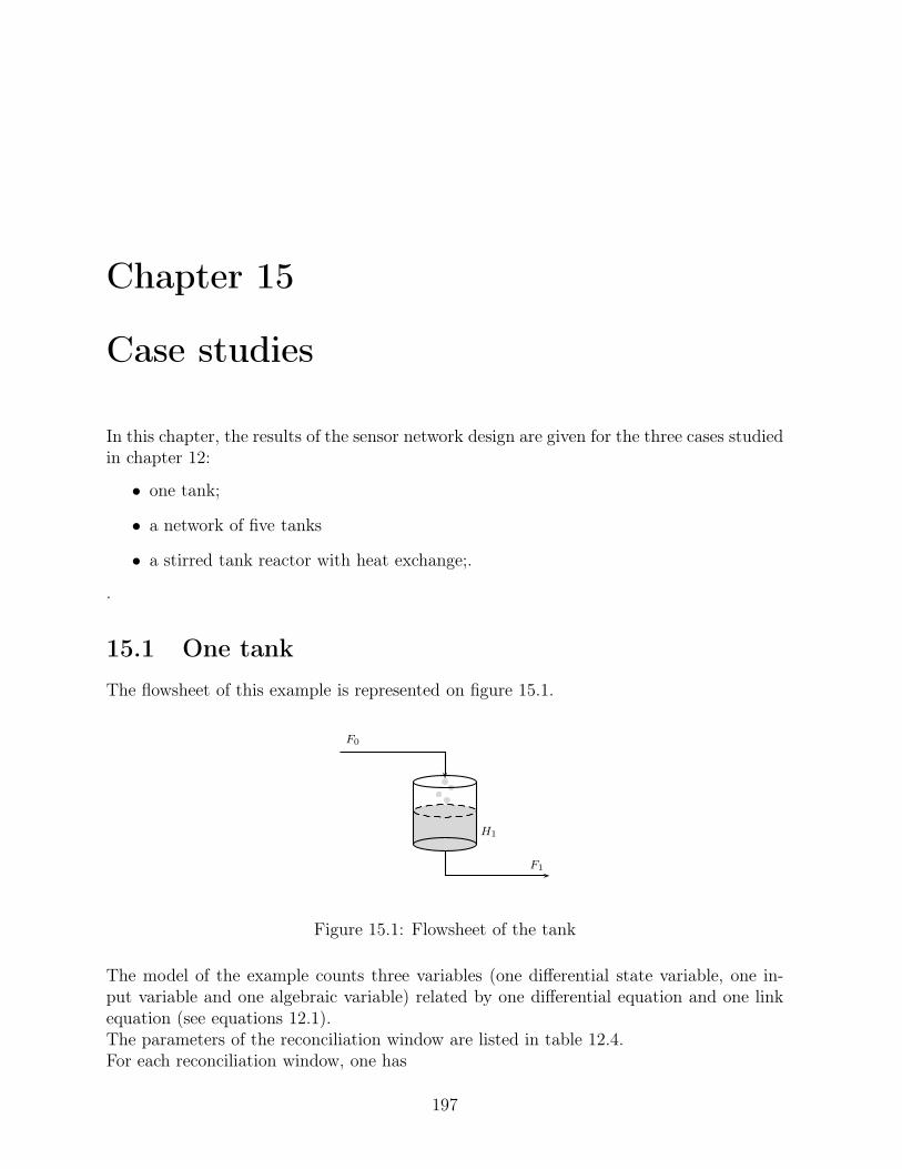
Chapter 15
Case studies
In this chapter, the results of the sensor network design are given for the three cases studiedin chapter 12:
∙ one tank;
∙ a network of five tanks
∙ a stirred tank reactor with heat exchange;.
.
15.1 One tank
The flowsheet of this example is represented on figure 15.1.
F0
F1
H1
Figure 15.1: Flowsheet of the tank
The model of the example counts three variables (one differential state variable, one in-put variable and one algebraic variable) related by one differential equation and one linkequation (see equations 12.1).The parameters of the reconciliation window are listed in table 12.4.For each reconciliation window, one has
197
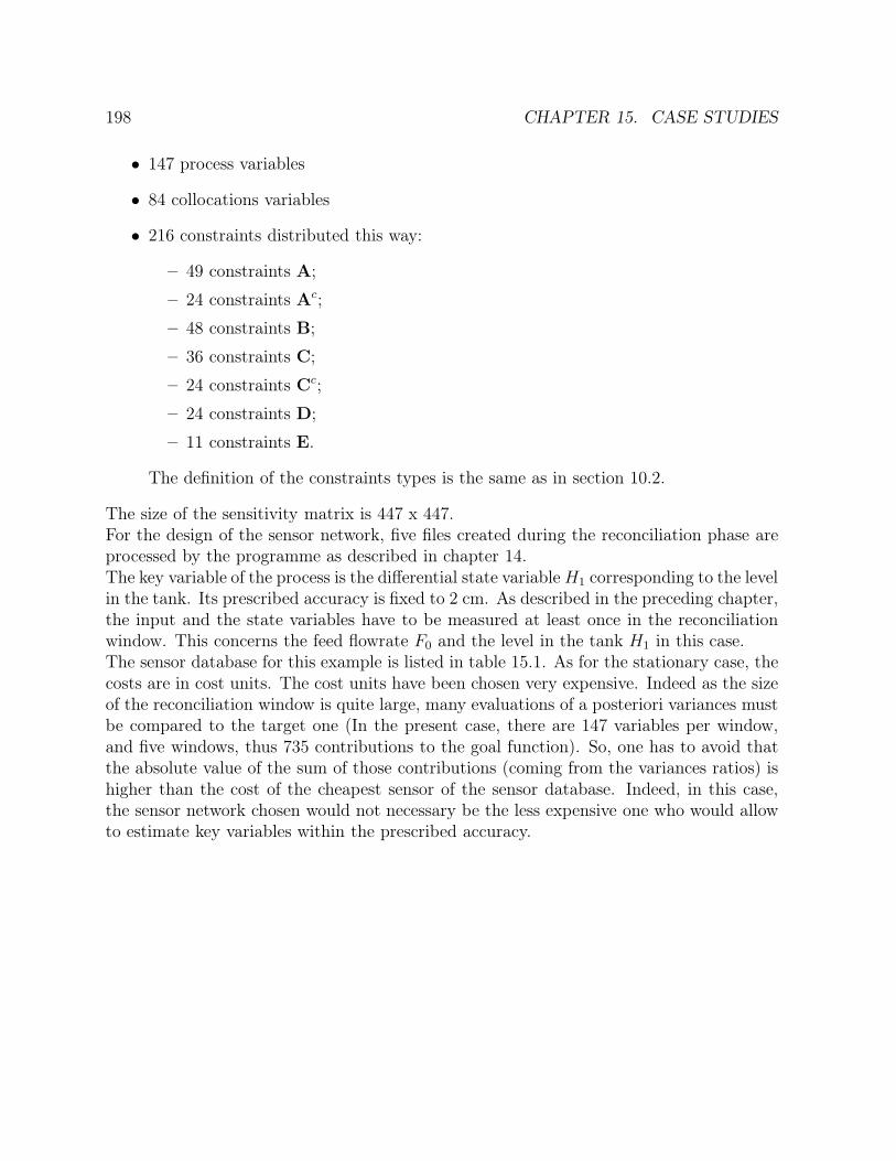
198 CHAPTER 15. CASE STUDIES
∙ 147 process variables
∙ 84 collocations variables
∙ 216 constraints distributed this way:
– 49 constraints A;
– 24 constraints Ac;
– 48 constraints B;
– 36 constraints C;
– 24 constraints Cc;
– 24 constraints D;
– 11 constraints E.
The definition of the constraints types is the same as in section 10.2.
The size of the sensitivity matrix is 447 x 447.For the design of the sensor network, five files created during the reconciliation phase areprocessed by the programme as described in chapter 14.The key variable of the process is the differential state variable H1 corresponding to the levelin the tank. Its prescribed accuracy is fixed to 2 cm. As described in the preceding chapter,the input and the state variables have to be measured at least once in the reconciliationwindow. This concerns the feed flowrate F0 and the level in the tank H1 in this case.The sensor database for this example is listed in table 15.1. As for the stationary case, thecosts are in cost units. The cost units have been chosen very expensive. Indeed as the sizeof the reconciliation window is quite large, many evaluations of a posteriori variances mustbe compared to the target one (In the present case, there are 147 variables per window,and five windows, thus 735 contributions to the goal function). So, one has to avoid thatthe absolute value of the sum of those contributions (coming from the variances ratios) ishigher than the cost of the cheapest sensor of the sensor database. Indeed, in this case,the sensor network chosen would not necessary be the less expensive one who would allowto estimate key variables within the prescribed accuracy.
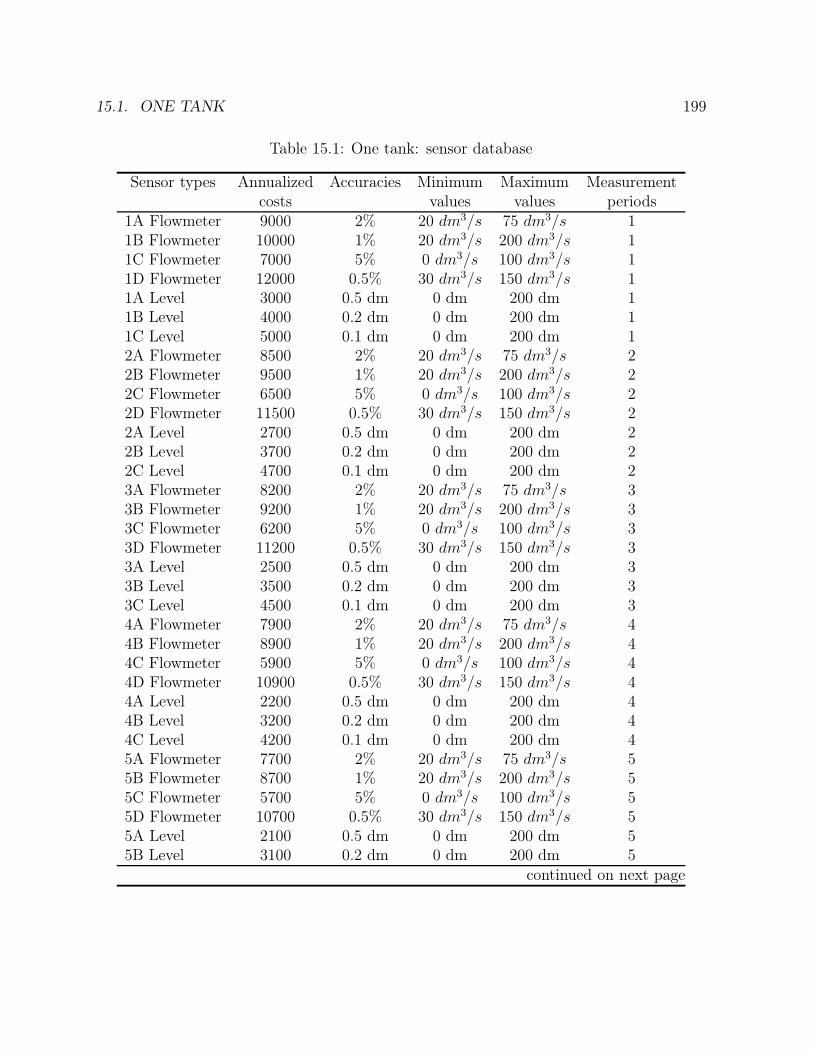
15.1. ONE TANK 199
Table 15.1: One tank: sensor database
Sensor types Annualized Accuracies Minimum Maximum Measurementcosts values values periods
1A Flowmeter 9000 2% 20 dm3/s 75 dm3/s 11B Flowmeter 10000 1% 20 dm3/s 200 dm3/s 11C Flowmeter 7000 5% 0 dm3/s 100 dm3/s 11D Flowmeter 12000 0.5% 30 dm3/s 150 dm3/s 11A Level 3000 0.5 dm 0 dm 200 dm 11B Level 4000 0.2 dm 0 dm 200 dm 11C Level 5000 0.1 dm 0 dm 200 dm 12A Flowmeter 8500 2% 20 dm3/s 75 dm3/s 22B Flowmeter 9500 1% 20 dm3/s 200 dm3/s 22C Flowmeter 6500 5% 0 dm3/s 100 dm3/s 22D Flowmeter 11500 0.5% 30 dm3/s 150 dm3/s 22A Level 2700 0.5 dm 0 dm 200 dm 22B Level 3700 0.2 dm 0 dm 200 dm 22C Level 4700 0.1 dm 0 dm 200 dm 23A Flowmeter 8200 2% 20 dm3/s 75 dm3/s 33B Flowmeter 9200 1% 20 dm3/s 200 dm3/s 33C Flowmeter 6200 5% 0 dm3/s 100 dm3/s 33D Flowmeter 11200 0.5% 30 dm3/s 150 dm3/s 33A Level 2500 0.5 dm 0 dm 200 dm 33B Level 3500 0.2 dm 0 dm 200 dm 33C Level 4500 0.1 dm 0 dm 200 dm 34A Flowmeter 7900 2% 20 dm3/s 75 dm3/s 44B Flowmeter 8900 1% 20 dm3/s 200 dm3/s 44C Flowmeter 5900 5% 0 dm3/s 100 dm3/s 44D Flowmeter 10900 0.5% 30 dm3/s 150 dm3/s 44A Level 2200 0.5 dm 0 dm 200 dm 44B Level 3200 0.2 dm 0 dm 200 dm 44C Level 4200 0.1 dm 0 dm 200 dm 45A Flowmeter 7700 2% 20 dm3/s 75 dm3/s 55B Flowmeter 8700 1% 20 dm3/s 200 dm3/s 55C Flowmeter 5700 5% 0 dm3/s 100 dm3/s 55D Flowmeter 10700 0.5% 30 dm3/s 150 dm3/s 55A Level 2100 0.5 dm 0 dm 200 dm 55B Level 3100 0.2 dm 0 dm 200 dm 5
continued on next page
200 CHAPTER 15. CASE STUDIES
Sensor types Annualized Accuracies Minimum Maximum Measurementcosts values values periods
5C Level 4100 0.1 dm 0 dm 200 dm 510A Flowmeter 7500 2% 20 dm3/s 75 dm3/s 1010B Flowmeter 8500 1% 20 dm3/s 200 dm3/s 1010C Flowmeter 5500 5% 0 dm3/s 100 dm3/s 1010D Flowmeter 10500 0.5% 30 dm3/s 150 dm3/s 1010A Level 2000 0.5 dm 0 dm 200 dm 1010B Level 3000 0.2 dm 0 dm 200 dm 1010C Level 4000 0.1 dm 0 dm 200 dm 1024A Flowmeter 7300 2% 20 dm3/s 75 dm3/s 2424B Flowmeter 8300 1% 20 dm3/s 200 dm3/s 2424C Flowmeter 5300 5% 0 dm3/s 100 dm3/s 2424D Flowmeter 10300 0.5% 30 dm3/s 150 dm3/s 2424A Level 1800 0.5 dm 0 dm 200 dm 2424B Level 2800 0.2 dm 0 dm 200 dm 2424C Level 3800 0.1 dm 0 dm 200 dm 2448A Flowmeter 7100 2% 20 dm3/s 75 dm3/s 4848B Flowmeter 8100 1% 20 dm3/s 200 dm3/s 4848C Flowmeter 5100 5% 0 dm3/s 100 dm3/s 4848D Flowmeter 10100 0.5% 30 dm3/s 150 dm3/s 4848A Level 1600 0.5 dm 0 dm 200 dm 4848B Level 2600 0.2 dm 0 dm 200 dm 4848C Level 3600 0.1 dm 0 dm 200 dm 48
With this sensor database, the maximum number of sensors that can be chosen for theprocess is 56, that is to say a solution space of 256 = 7.2∗1016 solutions. This first solutioncosts 394500 cost units.The solution found by the program costs 16100 cost units and contains two sensors:
∙ a 48B Flowmeter is chosen for the feed flowrate;
∙ the level is measured by a 1B Level sensor.
This solution counts the minimum number of sensors and the maximum frequency ofmeasurement that can be expected. It is the optimum solution of the problem.The computing time per iteration is about the half of the one for the stationary case becauseone has only one matrix to invert for each individual (because we do not used thermody-namic models). To avoid very long computing times, we decided to fix the stop criterionto 100 and to restart the computation with new parameters. Indeed the first solution forthis small problem is obtained after about 10 minutes on a 1.6 GHz computer. If one isnot satisfied with that first sensor network, one can for example restart the optimizationalgorithm with a reduced sensor database. Indeed, one can already say from the first onethat some types of sensor would never be chosen in the optimized solution because of their

15.1. ONE TANK 201
cost, precision or measurement period. One can also restart the program with a modifiedrestart file in which the initial worst solution would be replaced by alternative solutionsbased on the user’s intuition and common sense.
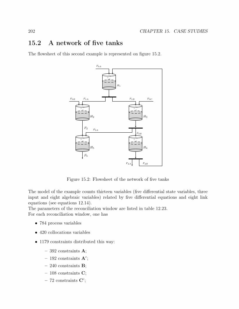
202 CHAPTER 15. CASE STUDIES
15.2 A network of five tanks
The flowsheet of this second example is represented on figure 15.2.
F0A
F1A F1B
H1
H4
F4A F4B
F2
H2
F0B
H3
F3B
F3A
F0C
F5
H5
Figure 15.2: Flowsheet of the network of five tanks
The model of the example counts thirteen variables (five differential state variables, threeinput and eight algebraic variables) related by five differential equations and eight linkequations (see equations 12.14).The parameters of the reconciliation window are listed in table 12.23.For each reconciliation window, one has
∙ 784 process variables
∙ 420 collocations variables
∙ 1179 constraints distributed this way:
– 392 constraints A;
– 192 constraints Ac;
– 240 constraints B;
– 108 constraints C;
– 72 constraints Cc;
15.2. A NETWORK OF FIVE TANKS 203
– 120 constraints D;
– 55 constraints E.
The size of the sensitivity matrix is 2381 x 2381.For the design of the sensor network for this last example, three data files created duringthe reconciliation phase are processed by the programme .The key variables of the process are the levels in the tanks H1, H2, H3, H4 and H5. Theirprescribed accuracies are fixed to 2 cm. The levels in all the five tanks and the feedflowrates F0A, F0B and F0C have to measured at least once in each reconciliation window.The sensor database is the same as for the first example (see table 15.1).The maximum number of sensors that can be chosen for the process is 256, that is to saya solution space of 2256 = 1.2 ∗ 1077 solutions. This first solution costs 1309700 cost units.The solution found by the program costs 91800 cost units and contains the thirteen fol-lowing sensors:
∙ 1C Flowmeters are chosen for the flowrates of the streams F3A, F3B and F4A;
∙ 2C Flowmeters are chosen for the flowrates of the streams F0B and F1A;
∙ 3C Flowmeters are chosen for the flowrates of the streams F0C and F1B;
∙ 48C Flowmeters are chosen for the flowrates of the streams F0A, F2, F4B and F5;
∙ the levels in all tanks are measured by 1C Level sensors.
The number of sensors proposed in this solution is much higher than the minimum numberof sensors required to measure at least one time for each reconciliation window each inputand differential variables. The data files have been modified in a way to constrain thealgorithm to choose sensors with smaller measurement periods but he found no cheapestsolution than the presented one. This is probably due to the process dynamic. To reducethe computing time, this could be done in two times: first of all looking for sensor locationsand then optimizing the measurement periods. The proposed solution is much better thanthe initial one but it can not be certified that it is the best one.

204 CHAPTER 15. CASE STUDIES
15.3 Stirred tank reactor with heat exchange
This third example is represented on figure 15.3.
Figure 15.3: Flowsheet of the stirred tank reactor with heat exchange
The model of the example counts six variables (two differential state variables and fourinput variables) related by two differential equations (see equations 12.8).The parameters of the reconciliation window are listed in table 12.12.For each reconciliation window, one has
∙ 294 process variables
∙ 168 collocations variables
∙ 406 constraints distributed this way:
– 0 constraints A;
– 0 constraints Ac;
– 96 constraints B;
– 144 constraints C;
– 96 constraints Cc;
– 48 constraints D;
– 22 constraints E.
The size of the sensitivity matrix is 868 x 868.For the design of the sensor network for this last example, two data files created duringthe reconciliation phase are processed by the programme .The key variables of the process are the differential state variables, namely the reducedtemperature T and the reduced concentration CA in the reactor. The prescribed accuraciesare fixed to 0.005 and 1 % for the reduced temperature and the reduced concentrationrespectively. As the process variables are all differential state variables or input variables,all of them have to be measured at least once in each reconciliation window.The sensor database for this example is listed on table 15.2. As the values of tempera-tures and concentrations are reduced ones in the reconciliation files, the precision and themeasurement areas of the sensors have been changed accordingly.
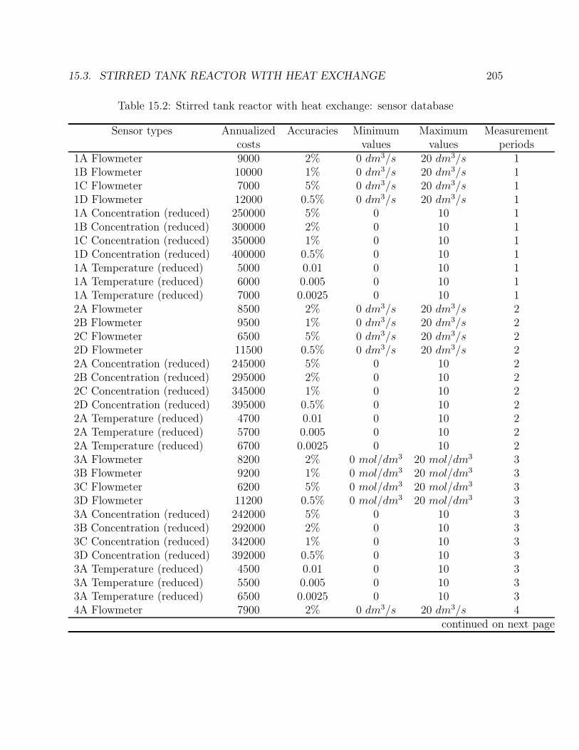
15.3. STIRRED TANK REACTOR WITH HEAT EXCHANGE 205
Table 15.2: Stirred tank reactor with heat exchange: sensor database
Sensor types Annualized Accuracies Minimum Maximum Measurementcosts values values periods
1A Flowmeter 9000 2% 0 dm3/s 20 dm3/s 11B Flowmeter 10000 1% 0 dm3/s 20 dm3/s 11C Flowmeter 7000 5% 0 dm3/s 20 dm3/s 11D Flowmeter 12000 0.5% 0 dm3/s 20 dm3/s 11A Concentration (reduced) 250000 5% 0 10 11B Concentration (reduced) 300000 2% 0 10 11C Concentration (reduced) 350000 1% 0 10 11D Concentration (reduced) 400000 0.5% 0 10 11A Temperature (reduced) 5000 0.01 0 10 11A Temperature (reduced) 6000 0.005 0 10 11A Temperature (reduced) 7000 0.0025 0 10 12A Flowmeter 8500 2% 0 dm3/s 20 dm3/s 22B Flowmeter 9500 1% 0 dm3/s 20 dm3/s 22C Flowmeter 6500 5% 0 dm3/s 20 dm3/s 22D Flowmeter 11500 0.5% 0 dm3/s 20 dm3/s 22A Concentration (reduced) 245000 5% 0 10 22B Concentration (reduced) 295000 2% 0 10 22C Concentration (reduced) 345000 1% 0 10 22D Concentration (reduced) 395000 0.5% 0 10 22A Temperature (reduced) 4700 0.01 0 10 22A Temperature (reduced) 5700 0.005 0 10 22A Temperature (reduced) 6700 0.0025 0 10 23A Flowmeter 8200 2% 0 mol/dm3 20 mol/dm3 33B Flowmeter 9200 1% 0 mol/dm3 20 mol/dm3 33C Flowmeter 6200 5% 0 mol/dm3 20 mol/dm3 33D Flowmeter 11200 0.5% 0 mol/dm3 20 mol/dm3 33A Concentration (reduced) 242000 5% 0 10 33B Concentration (reduced) 292000 2% 0 10 33C Concentration (reduced) 342000 1% 0 10 33D Concentration (reduced) 392000 0.5% 0 10 33A Temperature (reduced) 4500 0.01 0 10 33A Temperature (reduced) 5500 0.005 0 10 33A Temperature (reduced) 6500 0.0025 0 10 34A Flowmeter 7900 2% 0 dm3/s 20 dm3/s 4
continued on next page
206 CHAPTER 15. CASE STUDIES
Sensor types Annualized Accuracies Minimum Maximum Measurementcosts values values periods
4B Flowmeter 8900 1% 0 dm3/s 20 dm3/s 44C Flowmeter 5900 5% 0 dm3/s 20 dm3/s 44D Flowmeter 10900 0.5% 0 dm3/s 20 dm3/s 44A Concentration (reduced) 239000 5% 0 10 44B Concentration (reduced) 289000 2% 0 10 44C Concentration (reduced) 339000 1% 0 10 44D Concentration (reduced) 389000 0.5% 0 10 44A Temperature (reduced) 4300 0.01 0 10 44B Temperature (reduced) 5300 0.005 0 10 44C Temperature (reduced) 6300 0.0025 0 10 45A Flowmeter 7700 2% 0 dm3/s 20 dm3/s 55B Flowmeter 8700 1% 0 dm3/s 20 dm3/s 55C Flowmeter 5700 5% 0 dm3/s 20 dm3/s 55D Flowmeter 10700 0.5% 0 dm3/s 20 dm3/s 55A Concentration (reduced) 237000 5% 0 10 55B Concentration (reduced) 287000 2% 0 10 55C Concentration (reduced) 337000 1% 0 10 55D Concentration (reduced) 387000 0.5% 0 10 55A Temperature (reduced) 4100 0.01 0 10 55B Temperature (reduced) 5100 0.005 0 10 55C Temperature (reduced) 6100 0.0025 0 10 510A Flowmeter 7500 2% 0 dm3/s 20 dm3/s 1010B Flowmeter 8500 1% 0 dm3/s 20 dm3/s 1010C Flowmeter 5500 5% 0 dm3/s 20 dm3/s 1010D Flowmeter 10500 0.5% 0 dm3/s 20 dm3/s 1010A Concentration (reduced) 235000 5% 0 10 1010B Concentration (reduced) 285000 2% 0 10 1010C Concentration (reduced) 335000 1% 0 10 1010D Concentration (reduced) 385000 0.5% 0 10 1010A Temperature (reduced) 3900 0.01 0 10 1010B Temperature (reduced) 4900 0.005 0 10 1010C Temperature (reduced) 5900 0.0025 0 10 1024A Flowmeter 7300 2% 0 dm3/s 20 dm3/s 2424B Flowmeter 8300 1% 0 dm3/s 20 dm3/s 2424C Flowmeter 5300 5% 0 dm3/s 20 dm3/s 2424D Flowmeter 10300 0.5% 0 dm3/s 20 dm3/s 2424A Concentration (reduced) 233000 5% 0 10 2424B Concentration (reduced) 283000 2% 0 10 24
continued on next page

15.3. STIRRED TANK REACTOR WITH HEAT EXCHANGE 207
Sensor types Annualized Accuracies Minimum Maximum Measurementcosts values values periods
24C Concentration (reduced) 333000 1% 0 10 2424D Concentration (reduced) 383000 0.5% 0 10 2424A Temperature (reduced) 3700 0.01 0 10 2424B Temperature (reduced) 4700 0.005 0 10 2424C Temperature (reduced) 5700 0.0025 0 10 2448A Flowmeter 7100 2% 0 dm3/s 20 dm3/s 4848B Flowmeter 8100 1% 0 dm3/s 20 dm3/s 4848C Flowmeter 5100 5% 0 dm3/s 20 dm3/s 4848D Flowmeter 10100 0.5% 0 dm3/s 20 dm3/s 4848A Concentration (reduced) 231000 5% 0 10 4848B Concentration (reduced) 281000 2% 0 10 4848C Concentration (reduced) 331000 1% 0 10 4848D Concentration (reduced) 381000 0.5% 0 10 248A Temperature (reduced) 3500 0.01 0 10 248B Temperature (reduced) 4500 0.005 0 10 248C Temperature (reduced) 5500 0.0025 0 10 2
The maximum number of sensors that can be chosen for the process is 168, resulting in asolution space of 2168 = 3.7 ∗ 1050 solutions. This first solution costs 20739600 cost units.The solution found by the program costs 614100 cost units and contains the six followingsensors:
∙ a 5C flowmeters is chosen for the feed flowrate Q;
∙ a 3A Concentration (reduced) is chosen for the feed concentration CA0 ;
∙ a 1C Concentration (reduced) is chosen for the concentration in the reactor CA;
∙ the feed temperature T0 is measured by a 2B Temperature (reduced) thermocouple;
∙ the cooling temperature T is measured by a 1B Temperature (reduced)thermocouple;
∙ the temperature in the reactor TC is measured by a 2A Temperature (reduced) ther-mocouple.
As for the previous example, the solution presented before is the best one that has beenobtained. The number of sensors is the smallest that can be expected (because of the factthat input and differential variables have to be measured at least once in each reconciliationwindow) but we have no guarantee that they represent the global optimal solution for thisreactor.


Chapter 16
Conclusions part III
A method has been proposed to carry out the design of sensor networks for dynamicprocesses. It is based on the estimation of a posteriori variances that can be calculatedwhen differential equations are discretized by means of orthogonal collocations.This method provides also an observability criterion. To complete the requirements, initialconditions on input and differential variables have to be known to allow dynamic datareconciliation.The proposed method goes a step further than the one described by Benqlilou, which isbased on the state estimation by Kalman filter (Benqlilou et al., 2003), (Benqlilou, 2004),(Benqlilou et al., 2005). Indeed energy balances can be taken into account and inputsneed not to be considered as perfectly known. Thus they can be estimated as well astheir a posteriori variances. This implies that the variances of the input variables have acontribution to the variances of the other process variables to which they are related. Thechoice of the sensors that will measure them is thus of a great importance.The time redundancy is also considered for each measured variable. The measurementfrequency allowing to reach the imposed constraints can be optimized.The method allowed to find a solution for all studied examples. Those solutions are alwaysmuch better than the initial ones but there is no guarantee global optimal solution hasbeen located.
209

Chapter 17
General conclusions and future work
This study proposed several variants of a technique allowing sensor network design basedon data reconciliation and a posteriori variances estimation. The choice of a sensor beinga binary decision, the problem is highly combinatorial. Furthermore, it is non derivableand often multimodal. So, the optimization is carried out with a genetic algorithm.Important savings could be achieved if such a method was systematically applied beforethe construction of a new plant. Indeed, people who invest in industries always think toreduce the investment: the sensor networks that are installed are generally reduced so thatthe minimum control can be carried out. However, some variables whose knowledge seemsto be without interest at the first look may reveal to be very important for the knowledgeand control of the entire process. The installation of new sensors once the production hasbeen started can be very expensive because of the loss of production due to the plant shutdown that may be required during the installation. Moreover the global cost of the newsensor network can then reveal to be more important than the one that would have beendetermined by design method.This method has first been developed for steady-state processes. In that case, the sensornetwork selected by the algorithm should be the cheapest one which allows the computationof all process variables and the estimation of all process key variables within a prescribedaccuracy. Process equations are linearized to carry out the data reconciliation problem andthe estimation of a posteriori variances, thus non linear processes can be treated as wellas linear ones so that energy balances can also be treated. However, one should note that,because of the linearisation, the conclusions concerning the sensor network found by theprogram for a specified operating point can not be transposed to another operating point.So, when a process has several possible operating points, the sensor network is testedfor all of them despite an increase of the computing time. The proposed method givesgood results for all studied processes. However, as genetic algorithms are used to carryout the optimization, one can not guarantee that the solution obtained by the algorithmcorresponds to the global optimum. One can just note that it is much better than theinitial one. The only way to ensure that the optimal solution is reached should be to testall of them. Unfortunately, that would take more than a human being life time.The computing time appears to be quite long for larger problems, and, due to the sensitivity
211
212 CHAPTER 17. GENERAL CONCLUSIONS AND FUTURE WORK
matrix inversion, it increases more quickly than the size of the process. That time can bereduced using parallelization techniques. Global parallelization and distributed geneticalgorithms allow reducing the computing time. No method appears to outperforms theother for all studied processes. In the case of global parallelization, one can note thatthe computing time is inversely proportional to the number of processors but, as timedevoted to communications increases with the number of processors, the efficiency alsodecreases when the number of processors increases. This loss of efficiency becomes quicklyvery important when the number of processors gets close to the number of goal functionevaluations per generation. So, to optimize the computing ressources, one has to find atrade off between the computing time and the number of processors. Such phenomena doesnot appear for distributed genetic algorithm. Indeed, the way followed to find the solutionis different for each number of sub-populations. Moreover, in the case of distributed geneticalgorithms, when the size of sub-populations is small, it is sometimes better to relax thestop criterion and increase the size of sub-populations by the same factor. So, the user ofthe parallelized algorithm never knows in advance if he has chosen the fastest method buthe is sure to reach the solution within a shorter computing time.The option of the design of a sensor network that remains observable in the case of onesensor failure has been developed. The advantage of such network is that locating thefailing sensor is made easier by the redundancy that has been introduced. Moreover theplant remains controllable despite the failure.
The sensor network design algorithm as been modified to solve the problem of process faultdetection and localisation. In that case, the faults that should be detected are simulatedand the chosen sensor network has to be able to detect and locate all of them. Leaksin storage tanks and pipes have been simulated in water networks but other faults canbe simulated. To detect a fault, the residuals connected to that fault have to be higherthan a lower threshold several consecutive times. The necessary number of measurementtimes to declare a fault is a trade off between the speed of detection and the necessity todifferentiate between temporary measurement errors and process faults.
The last variant of the sensor network design algorithm is devoted to dynamic processes.This method being based on the estimation of a posteriori variances, a technique allowing toreconcile process variables at all measurement times and to estimates a posteriori variancesin the case of dynamic processes was necessary.Several dynamic data reconciliation approached were studied:
∙ one filtering technique: the extended Kalman filter;
∙ two moving horizon techniques:
– the explicit integration of differential equations using the fourth order Runge-Kutta method;
– the discretization of differential equations by orthogonal collocations.
In those two methods, a successive quadratic programming algorithm is used to carryout the optimization. When orthogonal collocations are applied, process variables

213
and variables coming from the discretization can be optimized sequentially or simul-taneously.
All methods allow to reconcile the data but the simultaneous moving horizon algorithmbased on orthogonal collocations gives the best reconciled values. Technically, Kalmanfilter and the explicit integration method can not be recommended in the case of ourstudy. Indeed, filtering methods do not allow to estimate input variables, so that it is notpossible to develop a method to estimate a posteriori variances taking precisions of inputvariables into account. Moreover, the extended Kalman filter is not able to solve properlystrongly non linear problems. The explicit integration method can hardly be extendedby an algorithm to estimate a posteriori variances. On the other hand methods usedin steady-state for a posteriori variances computing can be transposed to the integrationmethod based on orthogonal collocations.Orthogonal collocation-based methods gives good results for all the studied examples: theprofiles of reconciled values follow the simulated values, a posteriori variances are muchsmaller than a priori ones and are better inside the reconciliation window than at itsextremities, and errors are distinctly reduced. There remains nevertheless a problem withinput variables whose reconciled values follow more the noise than reconciled values ofdifferential state and algebraic variables.From the discretized differential equations and the Lagrangian formulation of the dynamicdata reconciliation problem, the sensitivity matrix of the global system of equations (pro-cess equations and equations coming from the discretization) can be estimated. If thatmatrix is non singular, all process variables can be computed for all measurement timeswith their a posteriori standard deviations. So, the non singularity of the sensitivity matrixappears to be an observability criterion that can be verified after reconciliation. Never-theless, that a posteriori observability criterion is not enough to ensure data reconciliationwith orthogonal collocations. Indeed, initial conditions for input and differential variableshave to be known to start the data reconciliation.
The sensor network design algorithm suggested here for the dynamic problems goes furtherthan the one described by Benqlilou based on the state estimation by means of Kalmanfilter. Indeed, it allows to deal with energy balances and measured input variables. So,the precision of the input variables has an influence on a posteriori standard deviation ofdifferential state and algebraic variables. The choice of sensors that will measure inputvariables is not innocent. The choice of frequency of the measurement has been introducedin the algorithm to take into account the temporal redundancy. The method gives satisfyingresults for all studied examples.
A way to improve the convergence of the successive quadratic programming in the case ofthe dynamic data reconciliation should be to deal with semi-analytical derivatives insteadof numerical derivatives. So, one could compute the analytical derivative of the part of theobjective function that is common for all processes and use numerical differentiation forthe part related to constraints A, Ac, D which are different for each process. With such amethod, one can also try the interior point optimization algorithm developed by Cervantes

214 CHAPTER 17. GENERAL CONCLUSIONS AND FUTURE WORK
et al. Indeed, this method is sensitive to numerical noise, and is known not to be able togive good results with numerical derivatives.Another improvement that should be done in the dynamic data reconciliation algorithmis the modification of input variables representation. Indeed, in the proposed version,input variables are linearized inside the interpolation interval. Another approach couldbe the use of orthogonal collocations. In that case, one has to choose if the discretizationintervals are the same for input and differential state variables or not. When input variablesare simulated as constant for the whole discretization or interpolation interval, the bestapproach should be to set them constant on the interval instead of trying to model themeasurements by a polynomial. So, a mixed version allowing to chose between those threerepresentations in function of the context would probably be the best approach concerninginput variables.

Publications
C.Gerkens, C.Ullrich, and G.Heyen (2009). Use of a moving horizon dynamic data valida-tion method based on orthogonal collocations for the design of sensor networks. Submittedto Computers and Chemical Engineering.
Gerkens, C. (2002). Conception rationnelle de systèmes de mesure dans les procédéschimiques. Master’s thesis, University of Liège, Applied Science Faculty, Laboratoired’analyse et de synthèse des systèmes chimiques.
Gerkens, C. (2003). Synthèse optimale de réseaux de capteurs : résolution au moyen de cal-culateurs parallèles. d.e.a.’s thesis, university of liège, applied science faculty, laboratoired’analyse et de synthèse des systèmes chimiques.
Gerkens, C. and Heyen, G. (2004a). Sensor network design using genetic algorithm. Pro-ceedings of MMM IFAC Symposium.
Gerkens, C. and Heyen, G. (2004b). Use of parallel computers in rational design of redun-dant sensor networks. Proceedings of Escape 14 Congress.
Gerkens, C. and Heyen, G. (2005). Use of parallel computers in rational design of redundantsensor networks. Computers and Chemical Engineering, 29(6):1379–1387.
Gerkens, C. and Heyen, G. (2008). Sensor placement for fault detection and localisation.Proceeding of Escape 18 Congress.
Gerkens, C., Ullrich, C., Mateus, M., and G.Heyen (2006). Comparaison de techniques devalidation dynamique de données. Proceedings of SIMO 2006 Congress.
Heyen, G. and Gerkens, C. (2002). Application d’algorithmes génétiques à la synthèse desystèmes de mesure redondants. Proceedings of SIMO 2002 Congress.
Ullrich, C., Heyen, G., and Gerkens, C. (2009). Variance of estimates in dynamic datareconciliation. Proceeding of Escape 19 Congress.
215


Bibliography
Abu-el zeet, Z. H., Becerra, V. M., and Roberts, P. D. (2002). Combined bias ansd outlieridentification in dynamic data reconciliation. Computers chem. Engng., 26:921–935.
Albuquerque, J. and Biegler, L. (1995). Decomposition algorithms for on-line estimationwith nonlinear models. Computers and Chemical Engineering, 19(10):1031–1039.
Albuquerque, J. and Biegler, L. (1996). Decomposition algorithms for on-line estimationwith nonlinear dae models. Computers and Chemical Engineering, 21(13):283–299.
Ali, Y. and Narasimhan, S. (1993). Sensor network design for maximizing reliaility of linearprocesses. AICHE Journal, 39(5):820–828.
Ali, Y. and Narasimhan, S. (1995). Redundant sensor network for linear processes. AICheJournal, 41:2237–2249.
Almasy, G. (1975). Checking and correction of measurements on the basis of linear systemmodel. Porblem of Control and Information Theory, 4:57.
Amand, T. (1999). Application de la validation en ligne à la détection et la localisationde pannes. Master’s thesis, University of Liège, Applied Science Faculty, Laboratoired’analyse et de synthèse des systèmes chimiques.
Amand, T., Heyen, G., and Kalitventzeff, B. (2001). Plant monitoring and fault detection:synergy between data reconciliation and principal component analysis. Computers andChemical Engineering, 25(4-6):501–507.
Bagajewicz, M. (1997). Process plant instrumentation : design and upgrade (Chapter 6).Technomic Publishing Company, Lancaster, Pensiylvania.
Bagajewicz, M. and Jiang, Q. (1997). Integral approach to plant linear dynamic reconcili-ation. AICHE Journal, 43(10):2546–2558.
Bagajewicz, M. and Jiang, Q. (1998). Gross error modelling and detection in plant lineardynamic recoonciliation. Computers and Chemical Engineering, 22(12):1789–1809.
Bagajewicz, M. and Sanchez, M. (1999a). Design and upgrade of non redundant andredundant linear sensor networks. AICHE Journal, 45(9):1927–1938.
217

218 BIBLIOGRAPHY
Bagajewicz, M. and Sanchez, M. (1999b). Duality of sensor network design models forparameter estimation. AICHE Journal, 45(3):661–664.
Bai, S., Thibault, J., and McLean, D. (2006). Dynamic data reconciliation: an alterntiveto kalman filter. Journal of Process Control, 16:485–498.
Barbosa, V., Wolf, M., and Fo, R. (2000). Development of data reconciliation for dynamicnonlinear system: application the polymerisation reactor. Computers and ChemicalEngineering, 24:501–506.
Belsim (2004). Vali4 User’s Guide. B-4470 Saint-Gerges-sur-Meuse, Belgium.
Benqlilou, C. (2004). Data reconciliation as a framework for chemical processes optimiza-tion and control. PhD thesis, Universitat Politècnica de Catalunya.
Benqlilou, C., Musulin, E., Bagajewicz, M., and Puigjaner, L. (2003). Intrumentationdesign and upgrade for optimal kalman filtering. Computer Aided Chemical Engineering,14:371–376.
Benqlilou, C., Musulin, E., Bagajewicz, M., and Puigjaner, L. (2005). Instrumentationdesign and upgrade for optimal kalman filtering. Journal of process control, 15(6):629–638.
Bhagwat, A., Srinivasan, R., and Krishnaswamy, P. (2003a). Fault detection during processtransitions. Chemical Engineering Science, 58(2):309–325.
Bhagwat, A., Srinivasan, R., and Krishnaswamy, P. (2003b). Multi-linear model-basedfault detection during process transitions. Chemical Engineering Science, 58(9).
Bhushan, M., Narasimhan, S., and Rengaswamy, . R. (2008). Robust sensor network designfor fault diagnosis. Computers and Chemical Engineering, 32:1067–1084.
Biegler, L. (1984). Solution of dynamic optimization problems by successive quadraticprogramming and orthogonal collocation. Computers and Chemical Engineering,8(3/4):243–248.
Biegler, L. (2007). An overview of simultaneous strategies for dynamic optimization. Chem-ical Engineering and Processing, 46(11):1043–1053.
Biegler, L., Cervantes, A., and Wächter, A. (2002). Advances in simultaneous strategiesofr dynamic process optimization. Chemical Engineering Science, 57:575–593.
Binder, T., Blank, L., Dahmen, W., and Marquardt, W. (1998). Nonlinear model basedprocess control, chapter Towards multiscale dynamic data reconciliation, pages 623–665.NATO ASI Series. Kluwer Academic Publishers.
Binder, T., Blank, L., Dahmen, W., and Marquardt, W. (2002). On the regularization ofdynamic data reconciliation problems. Journal of Process Control, 12:557–567.
BIBLIOGRAPHY 219
Broyden, C. (1965). A class of methods for solving non linear simultaneous equations.Mathematics of Compututations, 19:577–593.
Bullnheimer, B., Kotsis, G., and Strau, C. (1997). Parallelization strategies for the antsystem. http://www.ani.univie.ac.at/ gabi/papers/kluwer.ps.gz.
Carnero, M., Hernandez, J., Sanchez, M., and Bandoni, A. (2005). On the solution ofthe instrumentation selection problem. Industrial and Engineering Chemical Research,44:358–367.
Carroll, D. (2001). Fortran genetic algorithm driver version 1.7.cuaerospace.com/carroll/ga.html, consulted on May 2004.
Cervantes, A., Wächter, A., Tütüncü, R., and Biegler, L. (2000). A reduce space interiorpoint strategy for optimization of differential algebraic systems. Computers and ChemicalEngineering, 24:39–51.
Chen, H. and Stadherr, M. (1981). A modification of powell’dogleg algorithm for solvingsystems of non-linear equations. Computers and Chemical Engineering, 5(3):143–150.
Chen, H. and Stadherr, M. (1984). On solving large sparse nonlinear equation systems.Computers and Chemical Engineering, 8(1):1–7.
Chen, J. and Romagnoli, J. (1998). A strategy for simultaneous dynamic data reconciliationand outlier detection. Computers and Chemical Engineering, 22(4/5):559–562.
Chen, T., Morris, J., and Martin, E. (2008). Dynamic data rectification using particlefilters. Computers and Chemical Engineering, 32:451–462.
Colorni, A., Dorigo, M., Maffiolo, F., Maniezzo, V., Righini, G., and Trubian, M. (1996).Heuristics form nature for hard combinatorial optimization problems. Int. Trans. Opl.Res., 3(1):1–21.
Crowe, M. (1989). Observalibilty and redundancy of process data for steady-state recon-ciliation. Chemical Engineering Science, 44:2909–2917.
Davidon, W. (1975). Optimally conditionned optimization algorithm without line search.Math. Programming, 9:1–30.
de Wouwer, A. V., Point, N., Porteman, S., and Remy, M. (2000). An approach to theselection of optimal sensor locations in distributed parameter systems. Journal of ProcessControl, 10:291–300.
Dorigo, M., Bonabeau, E., and Theraulaz, G. (2000). Ant algorithm and stimergy. Futuregeneration computers systems, 16:851–871.
Feo, T. and Resende, M. (1995). Greedy randomized adaptive search procedure. Journalof Global Optimization.

220 BIBLIOGRAPHY
Fogel, L., Owens, A., and Walsh, M. (1966). Artificial Intelligence through SimulatedEvolution. John Wiley.
Glover, F. and Laguna, M. (1997). Tabu Search. Kluwer, Norwell, MA.
Goldberg, D. (1989). Genetic algorithms in search, optimisation and machine learning.Addison-Wesley Publishing Company, Reading, Massachusetts.
Gropp, W. (2005). MPICH2 User’s Guide. Mathematics and Computer Science DivisionArgonne National Laboratory, version 1.0.3 edition.
Gropp, W., Lust, E., and Skjellum, A. (1999a). Using MPI: portabe parallel programmingwith the message passing interface. The MIT Press, Cambridge, London, second edition.
Gropp, W., Lust, E., and Thakur, R. (1999b). Using MPI-2: advanced features of themessage-passing interface. The MIT Press, second edition.
Gutjahr, W. (2000). A graph-based ant system and its convergence. Future GenerationComputer Systems, 16:873–888.
Harwell (1990). Harwell subroutine library. Oxfordshire.
Haseltine, E. and Rawlings, J. (2005). Critical evaluation of extended kalman filtering andmoving-horizon estimation. Industry and Engineering Chemical Research, 44(8):2451–2460.
Herrera, F., Lozano, M., and Moraga, C. (1999). Hierarchical distributed genetic algo-rithms. International Journal of Intelligent Systems, 14(11):1099–1121.
Heyen, G., Dumont, M., and Kalitventzeff, B. (2002). Computer-aided design of redundantsensor networks. Proceedings of Escape 12.
Heyen, G. and Gerkens, C. (2002). Application d’algorithmes génétiques à la synthèse desystèmes de mesure redondants. Proceedings of SIMO 2002 Congress.
Heyen, G., Maréchal, E., and Kalitventzeff, B. (1996). Sensitivity calculations and vari-ance analysis in process plant measurement reconciliation. Computers and ChemicanEngineering, 20S:530–544.
Holland, J. (1975). Adaptation in Natural and Artificial Systems. University of MichiganPress.
Jang, S.-S., Joseph, B., and Mukai, H. (1986). Comparison of two approaches to on-lineparameter and state estimation of nonlinear systems. Ind. Eng. Chem. Process Des.Dev., 25:809–814.
Jia, F., Martin, E., and Morris, A. (1998). Non-linear principal components analysis forprocess fault detection. Computers and Chemical Engineering, 22(Suppl):S851–S854.
BIBLIOGRAPHY 221
Joris, P. and Kalitventzeff, B. (1987). Process measurements analysis and validation. Pro-ceedings of Chemical Engineering Conference: use of computers in chemical engineering,pages 41–46.
Kabouris, J. and Georgakavos, A. (1996). Parameter and state estimation of the activatedsludge process: on-line algorithm. Wat. Res., 30(12):3115–3129.
Kalman, R. (1960). A new approach to linear filtering and prediction problems. Transac-tions of the ASME-Jornal of Basic Engineering, 82:35–45.
Kalman, R. and Bucy, R. (1961). New results in linear filtering and prediction problems.Transactions of the ASME-Jornal of Basic Engineering, 83:95–107.
Kameswaran, S. and Biegler, L. (2006). Simultaneous dynamic optimization strategies:recent advances and challenges. Computers and Chemical Engineering, 30:1560–1575.
Karjala, T. and Himmelblau, D. (1996). Dynamic rectification of data via recurrent neuralnets and the extended kalman filter. AICHE Journal, 42(8):2225–2239.
Kim, I.-W., Liebman, M., and Edgar, T. (1990). Robust error-in-variables estimation usingnonlinear programming techniques. AICHE Journal, 36(7):985–993.
Kim, I.-W., Liebman, M., and Edgar, T. (1991). A sequential error-in-variables methodfor nonlinear dynamic systems. Computers and Chemical Engineering, 15(9):663–670.
Kirkpatrick, S., Gelatt, C. D., and Vecchi, M. P. (1983). Optimization by simulatedannealing. Science, 220:671–680.
Kong, M., Chen, B., He, X., and Hu, S. (2004). Gross error identification for dynamicsystem. Computers and Chemical Engineering, 29(1):191–197.
Kong, M., Chen, B., and Li, B. (2000). An integral approach to dynamic data rectification.Computers and Chemical Engineering, 24:749–753.
Kretsovalis, A. and Mah, R. (1987). Effect of redundancy on estimation accuracy in processdata reconciliation. Chemical Engineering Science, 42(9):2115–2121.
Kuehn, D. and Davidson, H. (1961). Computer control ii: mathematics of control. ChemicalEngineering Progress, 16(10/11):1653–1672.
Kyriakopoulou, D. (1997). Development and implementation of an interior point optimiza-tion algorithm for process engineering. PhD thesis, Université de Liège.
Lang, Y.-D. and Biegler, L. (2007). A software environment for simultaneous dynamicoptimization. Computers and Chemical Engineering, 31:931–942.
222 BIBLIOGRAPHY
Liebman, M., Edgar, T., and Lasdon, L. (1992). Efficient data reconciliation and estimationfor dynamic processes using nonlinear programing techniques. Computers and ChemicalEngineering, 16(10/11):963–986.
Madron, F. (1992). Process plant performance, measurement and data processing for opti-mization and retrofit (section 6.3). Ellis Horwood, New-York.
Mah, R., Stanley, G., and Downing, D. (1976). Reconciliation and rectification of processflow and inventory data. Ind. Eng. Chem., Process Des. Dev., 15:175–183.
Mah, R. and Tamhane, A. (1982). Detection of gross error in process data. AICHE Journal,28(5):828–830.
McBrayer, K. and Edgar, T. (1995). Bias detection and estimation in dynamic datareconciliation. Journal of Process Control, 5(4):285–289.
McBrayer, K., Soderstrom, T., Edgar, T., and Young, R. (1998). The application of nonlinear dynamic data reconciliation to plant data. Computers and Chemical Engineering,22(12):1907–1911.
Moraal, P. and Grizzle, J. (1995). Observer design for nonlinear systems with discrete-timemeasurements. IEEE Transaction on Automatic Control, 40(3):395–404.
Muradore, R., Bezzo, F., and Barolo, M. (2006). Optimal sensor location for distributed-sensor systems using multivariate regression. Computers and Chemical Engineering,30:521–534.
Narasimhan, S. and Jordache, C. (2000). Data reconciliation and gross error detection: anintelligent use of process data. Gulf Publishing Company, Houston, Texas.
Narasimhan, S. and Mah, R. (1987). Generalized likelihood ratio method for gross errorsidentification. AICHE Journal, 33(9):1514–1521.
Narasimhan, S. and Mah, R. (1988). Generalized likelihood ratios for gross errors identifi-cation in dynamic processes. AICHE Journal, 34(8):1321–1331.
Norgaard, M., Poulsen, N., and Ravn, O. (2000). New developpements in state estimationfor nonlinear systems. Automatica, 36:1627–1638.
Raff, T., Ebenbauer, C., Findeisen, R., and Allgöer, F. (2005). Control and observerdesign for non linear finite and infinite dimensional systems, chapter Remarks on movinghorizon state estimation with guaranteed convergence, pages 67–80. Springer.
Ragot, J. and Maquin, D. (2006). Fault measurement detection in an urban water supplynetwork. Journal of Process Control, 16(9):887–902.
BIBLIOGRAPHY 223
Ragot, J., Maquin, D., and Dibo, M. A. (2003). Sensor fault detection and isolation. a blindapproach. Proceedings of the Fifth international symposium on intelligent componentsand instruments for control.
Rao, V. (2000). Moving horizon strategies for the constrained monitoring and control ofnonlinear discrete-time systems. PhD thesis, University of Wisconsin-Madison.
Rechenberg, I. (1971). Evolutionsstrategie - Optimierung technischer Systeme nach Prinzip-ien der biologischen Evolution. PhD thesis, Technical University of Berlin. reprinted byFromman-Holzboog (1973).
Reilly, D. and Carpani, R. (1963). Application of statistical theory of adjustment of ma-terial balances. Proceedings of the 13th Canadian Chemical Engineering Congress.
Renfro, J., Morshedi, A., and Asbjornsen, O. (1987). Simultaneous optimization and solu-tion of systems described by differential/algebraic equations. Computers and ChemicalEngineering, 11(5):503–517.
Romagnoli, J. and Stephanopoulos, G. (1981). Rectification of process measurement datain the presence of gross error. Chemical Engineering Science, 16(11):1849–1863.
Rousseaux-Peigneux, P. (1988). Filtre de Kalman hierarchisé pour l’estimation d’état dy-namique de grands systèmes électriques. PhD thesis, Université de Liège.
Schmidt, S. (1980). The kalman filter: its recognition and development for aerospaceapplications. Journal of Guidance and Control, 4(1):4–10.
Schwefel, H.-P. (1974). Numerische Optimierung von Computer-Modellen. PhD thesis,University of Berlin. reprinted by Birkhäuser (1977).
Sen, S., Narasimhan, S., and Deb, K. (1998). Sensor network design of linear processesusing genetic algorithms. Computers and Chemical Engineering, 22(3):385–390.
Shelokar, P., Jayaraman, V., and Kulkarni, B. (2004). An ant colony approach for cluster-ing. Analytica Chimica Acta, 509:187–195.
Singh, A. and Hahn, J. (2005). Determining optimal sensor locations for state and pa-rameter estimation for stable nonlinear systems. Industry and Engineering ChemicalResearch, pages 5645–5659.
Talbi, E., Roux, O., Fonlupt, C., and Robillard, D. (2001). Parallel ant colonies for thequadratic assignement problem. Future Generation Computer Systems, 17:441–449.
Vachhani, P., Narasimhan, S., and Rengaswamy, R. (2006). Robust and reliable estima-tion via unscented recursive nonlinear dynamic data reconciliation. Journal of ProcessControl, 16(10):1075–1086.
224 BIBLIOGRAPHY
Vachhani, P., Rengaswamy, R., and Venkatasubramanian, V. (2001). A framework forintegrating diagnostic knowledge with non linear optimisation for data reconciliationand parameter estimayion in dynamic systems. Chemical Engineering Science, 56:2133–2148.
Vaclavek, V. (1968). Studies on system engineering: on the application of the calculusof observations in calculuations of chemical engineering balances. Coll. Czech. Chem.Commun., 34:3653–3660.
Vaclavek, V. (1969). Studies on system engineering: optimal choice of the balance mea-surements in complicated chemical engineering systems. Chemical Engineering Science,24:947–955.
Verny, V. (1985). A thermodynamical approach to the travelling salesman problem: anefficient simulation algorithm. Journal of Optimization Theory and Applications, 45:41–51.
Villadsen, J. and Michelsen, M. (1978). Solution of differential equation models by polyno-mial approximation. Prentice-Hall, Englewood Cliffs, New Jersey.
Villadsen, J. and Stewart, W. (1967). Solution of boundary-value problems by orthogonalcollocation. Chemical Engineering Science, 22:1483–1501.
Wailly, O. and Héraud, N. (2005). Cost-optimal design of reliable sensor networks extendedto multi-linear system. Computers and Chemical Engineering, 29:1083–1087.
Walfraff, W., Dochain, D., Bourrel, S., and Magnus, A. (1998). On the use of observabilitymeasures for sensor location in tubular reactor. Journal of Process Control, 8(5-6):497–505.
Wally, O., Héraud, N., and Malasse, O. (2008). Design of instrumentation in process plantsusing groëbner bases. Computers and Chemical Engineering, 32:2179–2188.
Wang, F., Jia, X., Zheng, S., and Yue, J. (2004). An improved mt-nt method for gross errordetection and data reconciliation. Computers and Chemical Engineering, 28:2189–2192.
Wang, H., Song, Z., and Wang, H. (2002). Statistical process monitoring using improvedpca with optimized sensor locations. Journal of Process Control, 12(6):735–744.
Welch, G. and Bishop, G. (2001). Annual conference on computer graphics and interactivetechniques, chapter An introduction to Kalman Filter. ACM Press, Addison-Wesley, LosAngeles, Californie, USA, 2001 edition.
Wongrat, W., Srinophakun, T., and Srinophakun, P. (2005). Modified genetic algorithm fornonlinear data reconciliation. Computers and Chemical Engineering, 29(5):1059–1067.
Appendix A
Sensor network optimization method
A.1 Introduction
Many optimization problems dealing with engineering computer science, management, ad-ministration... can not be solved satisfactory or practically by a problem-specific algorithm.Metaheuristic methods have been created to solve such problems. They consist of heuristicmethods for solving very large classes of computational problems by combining severalblack-box procedures given by the user in an efficient way. Those procedures are generallyalso heuristic methods. Metaheuristics are commonly used to solve combinatorial opti-mization problems or problems that can be translated into that form. Many methods ofthis class model processes that take place in nature.The goal of combinatorial optimization is to find a discrete mathematical object thatminimizes or maximizes an arbitrary objective function given by the user. Those objectsare called states and the set of all candidate states, the search space. The nature of thestates and the search space depends on the optimization problem. The objective functionto be optimized is called the goal function and is given by the user in the form of a black-box procedure that evaluates the function of the studied state. More besides the objectivefunction, it may be asked to the user to provide other black-box procedures that producea new random state or several variants of a given state, choose one state between several,give upper and lower bounds for the objective function...Metaheuristics can be classified between iterative and constructive heuristics:
∙ Iterative heuristics start with a complete feasible solution and change this currentstate thanks to an iterative process in order to improve the value of the goal function.A typical case of iterative heuristics is local search. In that method, the new state isderived from the current solution, which is always complete and feasible, by meansof a mutator procedure. The set of new states produced by the mutator is called theneighborhood of the current state.
∙ In constructive heuristics the solution is generated "from scratch" by successive ad-ditions of certains elements or components, with or without backtracking (removal
225

226 APPENDIX A. SENSOR NETWORK OPTIMIZATION METHOD
of the elements that have been added at an earlier step). A typical case of con-structive heuristics is the greedy heuristics. In that method, the final solution issuccessively built up in a linear process without backtracking, governed by the gainsof the components that are allowed to be added at a certain step.
An other classification can be made between single-run and repetitive heuristics:
∙ In the case of single-run heuristics, the algorithm stops as soon as a certain internalcondition is satisfied. For example, this condition is reaching a local optimum in thecase of local search and having finished the construction procedure in the case ofgreedy heuristics.
∙ In repetitive heuristics the user may control the amount of computation time he wantsto invest so that the quality of the final solution is a function of the invested compu-tation time. Genetic algorithms, simulated annealing, greedy randomized adaptivesearch procedure are representatives of this class.
Repetitive heuristics may reach solutions of very high quality but at a price of very largecomputational time, whereas single-run heuristics are generally faster but often providesolutions of moderate quality.
In this chapter, genetic algorithms are described. That algorithm has been chosen becausethe sensor network design problem is generally multimodal and involves many binary de-cisions. Moreover, as it will be shown in the examples of chapter 5, the computing timeincreases rapidly with the size of the studied process so that one had to chose an algorithmthat could be parallelized.
A.2 What are evolutionary algorithms ?
Evolutionary algorithms are population-based metaheuristic optimization algorithms thatuse mechanisms inspired from Darwin’s evolution theory. Their basic principle is to mimicthe behavior of populations of living beings, which adapt to their surroundings thanks tophenomena like natural selection and genotype. The artificial version of Darwin’s theoryis extremely simplified and is also called artificial Darwinism.The best known evolutionary algorithms are genetic algorithms, which will be described inthe next section, but evolutionary strategies, evolutionary programming, genetic program-ming and learning systems classifiers are also largely used (they are briefly described in thissection). All those algorithms have in common the fact that they manipulate an artificialpopulation whose evolution is simulated thanks to two types of random operations:
∙ a selection of individuals that will be allowed to generate children based on theperformance of the individuals, namely their more or less good correspondance withwhat is searched;
∙ genetic operators, generally cross-over and mutation, that produce new individualsin the population.

A.2. WHAT ARE EVOLUTIONARY ALGORITHMS ? 227
Those operations are repeated in loop, often in the form of generations, until the populationconverges.The success of such methods comes from the fact that they represent optimization toolsadapted to difficult, complex and irregular functions and problems. Nevertheless this evo-lutionary search has a computing cost that can be important; indeed this is an iterativemethod that proceeds by random directed trial and error. Those techniques are comple-mentary to more standard optimization methods like deterministic optimization methodsthat often make regularly hypothesis on the functions to be optimized.Evolutionary algorithms have been successfully applied in the fields of engineering, art,biology, economics, genetics, operations research, robotics, social sciences, physics, chem-istry...Evolutionary algorithms have also been used as an experimental framework to validatetheories about biological evolution and natural selection, particularly in the field of ar-tificial life. Techniques coming from evolutionary algorithms used to model biologicalevolution are generally limited to the modeling of microevolutionary processes. Howeversome macroevolutionary dynamics have been modeled.A limitation of evolutionary algorithms is that they do not clearly distinguish genotypeand phenotype. For example, in nature, the fertilized egg cell undergoes a complex processcalled embryogenesis to become a mature phenotype. This indirect encoding is believed tomake the genetic search more robust, namely it reduces the probability of fatal mutations,and may improve the evolvability of the organism. Some recent works try to take thisphenomenon into account.
A.2.1 Evolution strategy
The evolution strategy was developed by I. Rechenberg (Rechenberg, 1971) and H.P. Schwe-fel (Schwefel, 1974) of the Technical University of Berlin. This evolutionary algorithm isbased on the ideas of adaptation and evolution.In its first form, this method was not population based: indeed, child created from a singleindividual, which contains a vector of design parameters, mutates by adding a randomvector that is normally distributed with a mean of zero and a variance identical in alldimensions. The best individual between the parent and the child is used as the next indi-vidual. This strategy is called a (1 + 1) evolution strategy, namely the current individualgenerate a child and the best individual between those two individuals generates the nextindividual. In this first version, no cross-over occurs between individuals. A rule for chang-ing the variance of mutations was determined from the convergence rate theory developedby I. Rechenberg (Rechenberg, 1971): it appears that 20% of the children should replacetheir parent. If there are more good children, the search space is too small the varianceshould be increased and inversely if less children are able to replace their parents.A second form of evolution strategy is the (�+1) evolution strategy proposed by I. Rechen-berg (Rechenberg, 1971). In this method, a population of � individuals is used to generatea new child thanks to cross-over and mutations. This new individual replace the worst onein the population if it is better.
228 APPENDIX A. SENSOR NETWORK OPTIMIZATION METHOD
Schwefel (Schwefel, 1974) extended this second form in two ways in which it is possible togive a particular mutation variance to each individual:
∙ the (�+�) evolution strategy: in this strategy, the new population of � individualsis made of the � best individuals from the � parents and the � children.
∙ the (�,�) evolution strategy: in this case, the � best individuals for the new popu-lation are chosen between the � children only, so that � > �. The best individualsof the parent population are not kept from generation to generation so that the con-vergence can not be guaranteed. Despite this disadvantage, this second extension isgenerally preferred because with the population evolution, the information containedin older individuals genes become quickly out of date so that those individuals canbe removed without important loss of information.
There are several combination operators that can be used in evolution strategies. Theyare classified into two families:
∙ the sexual combination: the parameters are generated from two chosen parents;
∙ the panmitic combination: one fixed parent is chosen and for each parameter, anotherparent is chosen in the population for combination, so that the whole populationcontributes to each new individual.
Recently, two new parameters have been added to the (�,�) evolution strategy: � the max-imum lifespan of an individual and � the number of parents involved in the combination.
A.2.2 Evolutionary programming
The evolutionary programming was developed by L.J. Fogel (Fogel et al., 1966) in the sixtiesin order to design state machines for predicting sequences and symbols. This method wascriticized because the predicted sequences were relatively simple and penalty functionsfor mis-prediction were needed to obtain good results. In the eighties, the method wastransformed to solve real-value optimization problems. This new version of the method issimilar to evolution strategy but differs from it by two points:
∙ In evolutionary programming, there is no cross-over because in the sense of evolution-ary programming, individuals represent entire species and not members of a singlespecies.
∙ The selection of the new population is different: indeed in evolutionary strategy, theselection is deterministic, the best � individuals are chosen for the next population,whereas in evolutionary programming, a stochastic method is used: the tournamentselection. This selection mechanism is described in the next section with the geneticalgorithm. Its advantage is that the set of potential solutions is more diverse. Thismeans that the population will grow less frequently around a local minimum and there
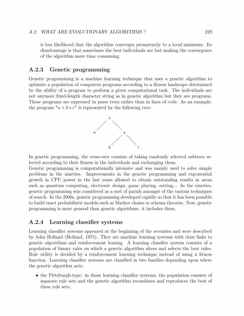
A.2. WHAT ARE EVOLUTIONARY ALGORITHMS ? 229
is less likelihood that the algorithm converges prematurely to a local minimum. Itsdisadvantage is that sometimes the best individuals are lost making the convergenceof the algorithm more time consuming.
A.2.3 Genetic programming
Genetic programming is a machine learning technique that uses a genetic algorithm tooptimize a population of computers programs according to a fitness landscape determinedby the ability of a program to perform a given computational task. The individuals arenot anymore fixed-length character string as in genetic algorithm but they are programs.Those programs are expressed in parse trees rather than in lines of code. As an example,the program "a+ b ★ c" is represented by the following tree:
+
@@@@
@@@
~~~~
~~~
a ★
>>>>
>>>>
����
����
b c
In genetic programming, the cross-over consists of taking randomly selected subtrees se-lected according to their fitness in the individuals and exchanging them.Genetic programming is computationally intensive and was mainly used to solve simpleproblems in the nineties. Improvements in the genetic programming and exponentialgrowth in CPU power in the last years allowed to obtain outstanding results in areassuch as quantum computing, electronic design, game playing, sorting... In the nineties,genetic programming was considered as a sort of pariah amongst of the various techniquesof search. In the 2000s, genetic programming developed rapidly so that it has been possibleto build exact probabilistic models such as Markov chains or schema theories. Now, geneticprogramming is more general than genetic algorithms: it includes them.
A.2.4 Learning classifier systems
Learning classifier systems appeared at the beginning of the seventies and were describedby John Holland (Holland, 1975). They are machine learning systems with close links togenetic algorithms and reinforcement leaning. A learning classifier system consists of apopulation of binary rules on which a genetic algorithm alters and selects the best rules.Rule utility is decided by a reinforcement learning technique instead of using a fitnessfunction. Learning classifier systems are classified in two families depending upon wherethe genetic algorithm acts:
∙ the Pittsburgh-type: in those learning classifier systems, the population consists ofseparate rule sets and the genetic algorithm recombines and reproduces the best ofthese rule sets;

230 APPENDIX A. SENSOR NETWORK OPTIMIZATION METHOD
∙ the Michigan-type: in that type of learning classifier systems, there is only a singlepopulation and the genetic algorithm focuses on selecting the best classifiers withinthat rule set. They have two main types of reinforcement learning: fitness sharingand accuracy-based.
At the beginning, learning classifier systems used binary rules, but thanks to the recentresearch, they can now use populations of neural networks and other methods.Learning classifier systems are not well defined in a mathematical point of view and remainan area of research even if they have been applied successfully to many different types ofproblems.
A.3 Genetic algorithms
Genetic algorithms are random research algorithms based on natural selection and geneticmechanisms. They were created by John Holland (Holland, 1975), his students and col-leagues at the beginning of the sixties in the University of Michigan. His objectives werethe abstraction and the rigorous explanation of the processes of natural systems adaptationas well as the design of artificial systems from a software using the same mechanisms thannatural systems.Genetic algorithms combine the survival of the best individuals of the parent populationwith a structured and random exchange of information between individuals. At eachgeneration, a set of new individuals (children) is created using parts of the best parents.Genetic algorithm exploit efficiently information from the previous population to searchfor children with better goal function or fitness.Robustness is one the the main advantages of genetic algorithms. Indeed, robustness impli-cations for artificial systems are numerous: if artificial systems can be made more robust,the most expensive solutions can be eliminated or reduced; if higher level of adaptation canbe achieved, systems can carry out their function during a longer time and more efficiently.Biological systems are robust, efficient and flexible. Laws governing those systems areselection, reproduction, cross-over and mutation. They appear only in a rough way inartificial systems so that nature always remains more efficient in the robustness point ofview. Moreover, genetic algorithms have given proofs of their robustness as well in themathematical point of view than in the empirical point of view.Genetic algorithms differ from traditional optimization methods. Indeed:
A.3. GENETIC ALGORITHMS 231
∙ Genetic algorithms code the parameter set instead of the parameters themselves;
∙ The search carried out by genetic algorithms are made from a population of pointsinstead of a single-point;
∙ Genetic algorithms use information coming from a goal function instead of derivativesor other auxiliary knowledge;
∙ Genetic algorithms use probabilistic transition rules instead of deterministic rules.
Applications of genetic algorithms are numerous and from very different domains: opti-mization of difficult numerical function (discontinuous, multimodal, with noise...), picturesprocessing, timetable optimization, design optimization, industrial systems control, learn-ing of neural networks... Genetic algorithms can be used to control time involving systems(production lines, nuclear power plants) because the population can adapt to conditionchanges. They can also be used to find the parameter of a model from the experimentalmeasurements, to optimize networks for water or gas distribution. They can be integratedin electronic chips so that they would be able to reconfigure themselves in function of theirsurroundings.
A.3.1 Individuals coding
Genetic algorithms use a population of points also called individuals or chromosomes. Eachchromosome is made of a set of parameters that are translated in a binary form. Eachcoded parameter is named gene. There are three types of genes:
∙ boolean genes made of a single binary character. They translate parameters thathave only two possible values, they translate binary decisions. In the case of sensornetwork design, they translate the decision to put or not a sensor at a specifiedlocation.
∙ integer genes made of several binary characters. They translate integer parameters;
∙ real genes made of several binary characters. They translate real parameters.
In our implementation of the algorithm, when the first individual is created, a gene isadded for each parameter of the problem. In addition to the gene, different characteristicof the gene are also coded:
∙ the number of the gene in the chromosome;
∙ the name of the gene;
∙ the type of the gene;
∙ the length of the gene;

232 APPENDIX A. SENSOR NETWORK OPTIMIZATION METHOD
∙ the minimal value of the parameter represented by the gene;
∙ the position of the first binary character of the gene in the chromosome;
∙ the length of the chromosome after the insertion of the gene.
The values of the parameters of the first chromosomes are fixed arbitrarily while the valuesof the parameters of the other chromosomes of the first population are determined atrandom knowing that each parameter has a fixed probability to have the arbitrary valuesfixed for the first chromosome.
A.3.2 Natural mechanisms description
In this section, four useful genetic mechanisms are described: the selection, the reproduc-tion, the cross over and the mutation. As in the case of sensor network design there are onlybinary choices (presence or absence of sensors in the plant), all those mechanisms are ex-plained for binary decisions only, although those algorithms can be used for combinatorialproblems for which the choice can be made between more than two solutions.
Selection
Individuals are selected in function of an objective function called fitness. Individuals withthe best fitness have a higher probability to be chosen. This fitness operator is an artificialversion of natural selection in which only the best individuals survive. In the nature,the fitness represents the capacity to survive to predators, diseases and all obstacles thatprevent reaching the adult age and excluding reproduction. In the case of artificial systems,the fitness decides if individuals can live or if they have to die.Two selection methods are described here after: the roulette wheel and the tournamentselection.
6. Tournament selectionIn tournament selection mechanism, two individuals are chosen at random. Theone with the best fitness is kept as the father individual. A mother individual ischosen in the same way. To make the choice of the pairs of individual random, allthe individuals of the population are numbered at random before the first selection.They are then compared two by two following this new order: the first one withthe second one to give the father, the third one with the fourth one to give themother... Let N be the size of the population. Individuals are renumbered each timethe number of chosen parents is N
2if N is even and N−1
2if N is odd. In this method,
the individual with the lowest fitness, is never chosen and individuals with the bestfitness have a great probability to be chosen.This technique can be used as well if the fitness has to be maximized as if it has tobe minimized.This method has been chosen for the genetic algorithm used in this research.
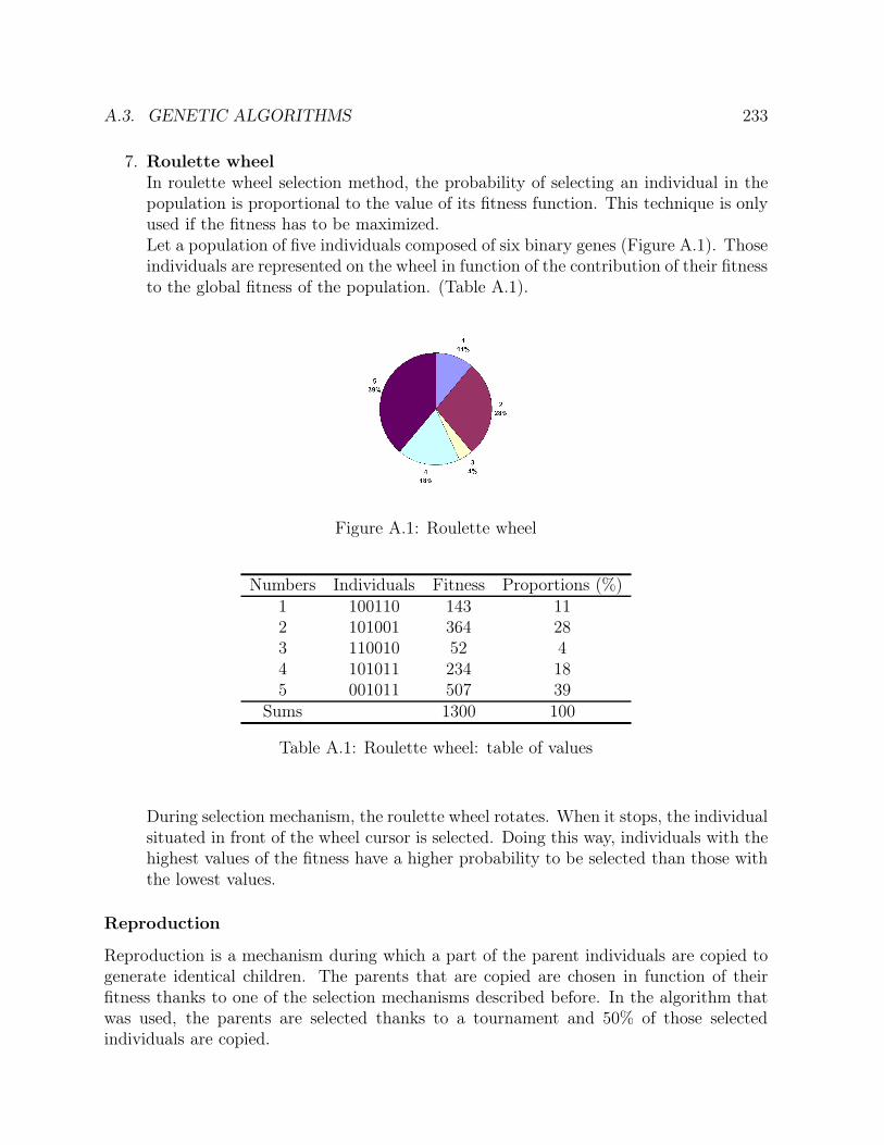
A.3. GENETIC ALGORITHMS 233
7. Roulette wheelIn roulette wheel selection method, the probability of selecting an individual in thepopulation is proportional to the value of its fitness function. This technique is onlyused if the fitness has to be maximized.Let a population of five individuals composed of six binary genes (Figure A.1). Thoseindividuals are represented on the wheel in function of the contribution of their fitnessto the global fitness of the population. (Table A.1).
Figure A.1: Roulette wheel
Numbers Individuals Fitness Proportions (%)1 100110 143 112 101001 364 283 110010 52 44 101011 234 185 001011 507 39
Sums 1300 100
Table A.1: Roulette wheel: table of values
During selection mechanism, the roulette wheel rotates. When it stops, the individualsituated in front of the wheel cursor is selected. Doing this way, individuals with thehighest values of the fitness have a higher probability to be selected than those withthe lowest values.
Reproduction
Reproduction is a mechanism during which a part of the parent individuals are copied togenerate identical children. The parents that are copied are chosen in function of theirfitness thanks to one of the selection mechanisms described before. In the algorithm thatwas used, the parents are selected thanks to a tournament and 50% of those selectedindividuals are copied.
234 APPENDIX A. SENSOR NETWORK OPTIMIZATION METHOD
Cross-over
Cross-over mechanism consists of combining the genotypes of a mother individual and afather individual in a way that the two children obtained genetic characteristics from bothparents. Three cross-over methods are described here after: one-point cross-over, two-points cross-over and uniform crossover. Only the one-point cross-over is applied in thegenetic algorithm used in this research.Cross-over concern the parents pairs that have not given children by reproduction, thatmeans the halve of the parent pairs.
8. One-point cross-overIn the case of one-point cross-over, the crossing point is chosen randomly at thebinary level. If the genes are made of more than one binary decision, the crossingpoint can be situated in the middle of a gene, whose binary characters are sharedout between the two children. The distribution between the binary characters of theparents is made in the following way (figure A.2):
∙ The first child is made with the binary characters of the father that are situatedon the left of the crossing point and those from the mother that are on the rightof that point;
∙ The second child is made with the binary characters of the mother that aresituated on the left of the crossing point and those from the father that are onthe right of that point.
Chromosomes are divided in 32 bits parts which are examined one after the other:
∙ If the crossing point is on the left of the itℎ part, the itℎ part of the father iscopied in the itℎ place of the first child and the itℎ part of the mother is copiedin the itℎ place of the second child;
∙ If the crossing point is on the right of the itℎ part, the itℎ part of the fatheris copied in the itℎ place of the second child and the itℎ part of the mother iscopied in the itℎ place of the first child;
∙ If the crossing point is inside the itℎ part, the binary characters of the itℎ partof the father that are on the left of the crossing point are copied in the left partof the itℎ place of the first child and the ones situated on the right, in the rightpart of the itℎ place of the second child. The binary characters of the itℎ part ofthe mother that are on the left of the crossing point are copied in the left partof the itℎ place of the second child and the ones situated on the right, in theright part of the itℎ place of the first child.
9. Two points cross-overTwo-points cross-over is similar to the one-point cross-over. It is generally said to bemore efficient. The distribution between the binary characters of the parents is nowmade as can be seen on figure A.3:
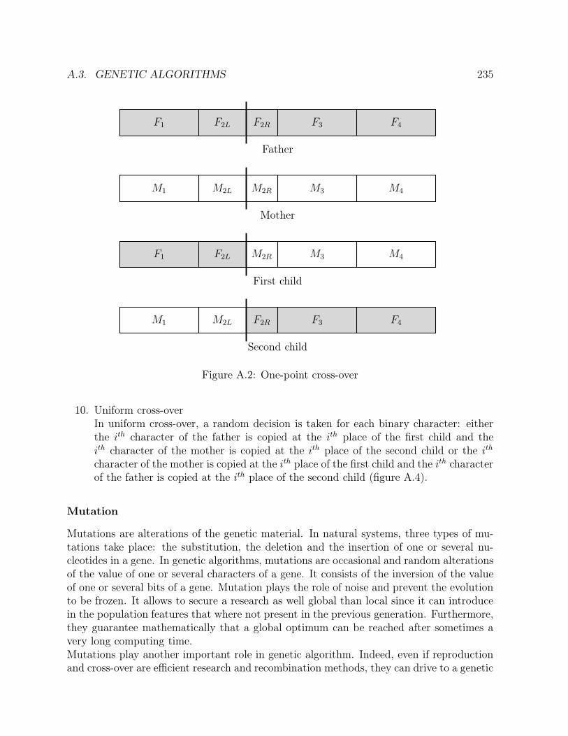
A.3. GENETIC ALGORITHMS 235
Father
Mother
First child
Second child
F1 F2L F2R F3 F4
M1 M2L M2R M3 M4
F1 F2L M2R M3 M4
M1 M2L F2R F3 F4
Figure A.2: One-point cross-over
10. Uniform cross-overIn uniform cross-over, a random decision is taken for each binary character: eitherthe itℎ character of the father is copied at the itℎ place of the first child and theitℎ character of the mother is copied at the itℎ place of the second child or the itℎ
character of the mother is copied at the itℎ place of the first child and the itℎ characterof the father is copied at the itℎ place of the second child (figure A.4).
Mutation
Mutations are alterations of the genetic material. In natural systems, three types of mu-tations take place: the substitution, the deletion and the insertion of one or several nu-cleotides in a gene. In genetic algorithms, mutations are occasional and random alterationsof the value of one or several characters of a gene. It consists of the inversion of the valueof one or several bits of a gene. Mutation plays the role of noise and prevent the evolutionto be frozen. It allows to secure a research as well global than local since it can introducein the population features that where not present in the previous generation. Furthermore,they guarantee mathematically that a global optimum can be reached after sometimes avery long computing time.Mutations play another important role in genetic algorithm. Indeed, even if reproductionand cross-over are efficient research and recombination methods, they can drive to a genetic
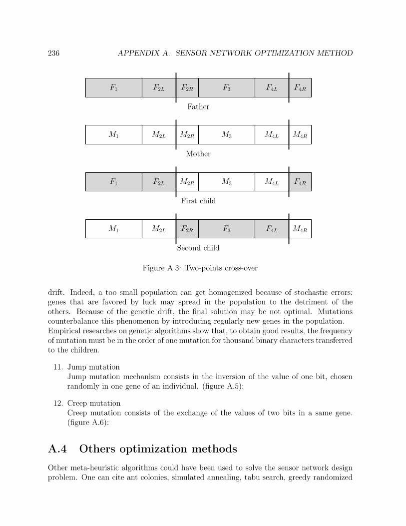
236 APPENDIX A. SENSOR NETWORK OPTIMIZATION METHOD
Father
Mother
First child
Second child
F1 F2L F2R F3 F4L F4R
M1 M2L M2R M3 M4L M4R
F1 F2L M2R M3 M4L F4R
M1 M2L F2R F3 F4L M4R
Figure A.3: Two-points cross-over
drift. Indeed, a too small population can get homogenized because of stochastic errors:genes that are favored by luck may spread in the population to the detriment of theothers. Because of the genetic drift, the final solution may be not optimal. Mutationscounterbalance this phenomenon by introducing regularly new genes in the population.Empirical researches on genetic algorithms show that, to obtain good results, the frequencyof mutation must be in the order of one mutation for thousand binary characters transferredto the children.
11. Jump mutationJump mutation mechanism consists in the inversion of the value of one bit, chosenrandomly in one gene of an individual. (figure A.5):
12. Creep mutationCreep mutation consists of the exchange of the values of two bits in a same gene.(figure A.6):
A.4 Others optimization methods
Other meta-heuristic algorithms could have been used to solve the sensor network designproblem. One can cite ant colonies, simulated annealing, tabu search, greedy randomized

A.4. OTHERS OPTIMIZATION METHODS 237
Father
Mother
First child
Second child
F1 F2 F3 F4 F5 F6 F7 F8 F9 F10 F11 F12 F13 F14 F15 F16
M1 M2 M3 M4 M5 M6 M7 M8 M9 M10 M11 M12 M13 M14 M15 M16
M1 F2 M3 M4 F5 F6 F7 M8 M9 F10 M11 M12 F13 F14 F15 M16
F1 M2 F3 F4 M5 M6 M7 F8 F9 M10 M11 F12 M13 M14 M15 F16
Figure A.4: Uniform cross-over
Individual before mutation
Individual after mutation
1 1 0 0 0 1 0 1 1 1 0 1 0 0 1 0
1 1 0 0 0 0 0 1 1 1 0 1 0 0 1 0
Figure A.5: Jump mutation
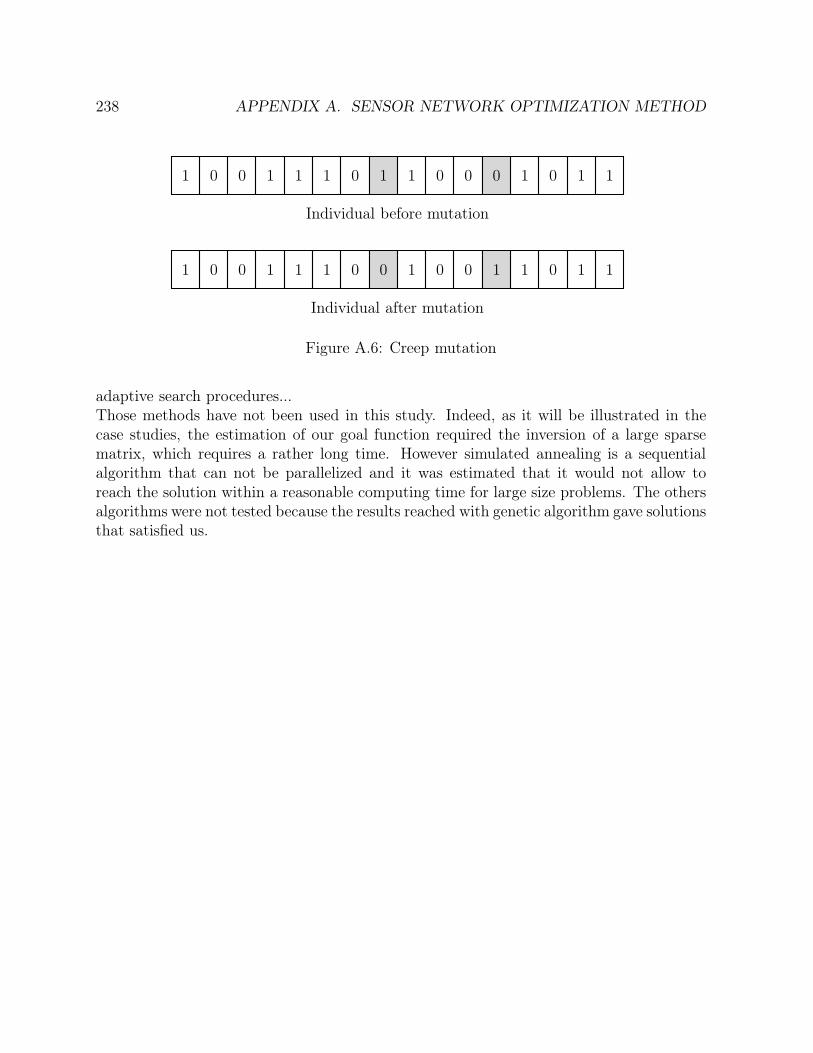
238 APPENDIX A. SENSOR NETWORK OPTIMIZATION METHOD
Individual before mutation
Individual after mutation
1 0 0 1 1 1 0 1 1 0 0 0 1 0 1 1
1 0 0 1 1 1 0 0 1 0 0 1 1 0 1 1
Figure A.6: Creep mutation
adaptive search procedures...Those methods have not been used in this study. Indeed, as it will be illustrated in thecase studies, the estimation of our goal function required the inversion of a large sparsematrix, which requires a rather long time. However simulated annealing is a sequentialalgorithm that can not be parallelized and it was estimated that it would not allow toreach the solution within a reasonable computing time for large size problems. The othersalgorithms were not tested because the results reached with genetic algorithm gave solutionsthat satisfied us.

Appendix B
Parallelization
B.1 Notions of parallelization
The development in sciences was traditionally based on a theoretical or on an experimentalapproach. Thanks to more and more powerful and fast computers, scientists can nowadayssimulate problems that are too complex to be reliably predicted by theory, too dangerousor too expensive to be reproduced in the laboratory. The demand on supercomputers hasstrongly increased during the last years.At the same time, parallel computers have evolved from theoretical concept to everydaytool to solve problems needing more and more computer ressources. Several factors havesimulated this evolution: the speed of computers is limited by the speed of the light and theefficiency of heat dissipation, the cost of powerful computer increased more rapidly thantheir power, and the ratio between the cost and the performance is favorable if the computerressources can be found instead of bought. This last factor has simulated laboratories toexploit existing computers in parallel and the development of clusters of computers. Therise in performance and capacity of wide-area networks has made it possible to writeapplications that span the world. The concept of a grid of computational ressources andconnections is being explored. This concept is analogous to the electric power grid.Thus, parallelization seems to be the best compromise between performance and the ratiobetween cost and performance. However there remains some obstacles to an universal useof parallelization coming from the material or from the software, but most of the time themain obstacle comes from an inadequate software environment. The ideal mechanism tocommunicate between a parallel algorithm and a parallel computer must be expressive,efficient and portable.There exists several parallel computational models: data parallelism, shared memory, mes-sage passing, remote memory operations, threads and combined models.For parallelizing the optimal sensor network design algorithm, a message passing model,the message passing interface, has been used. That kind of model consists of a set ofprocessors that have only local memory and can communicate with other processors bysending and receiving messages. Data transfer from the local memory of one processor to
239
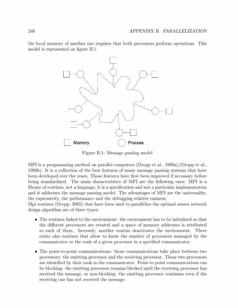
240 APPENDIX B. PARALLELIZATION
the local memory of another one requires that both processors perform operations. Thismodel is represented on figure B.1.
Figure B.1: Message passing model
MPI is a programming method on parallel computers (Gropp et al., 1999a),(Gropp et al.,1999b). It is a collection of the best features of many message passing systems that havebeen developed over the years. Those features have first been improved if necessary beforebeing standardized. The main characteristics of MPI are the following ones: MPI is alibrary of routines, not a language, it is a specification and not a particular implementationand it addresses the message passing model. The advantages of MPI are the universality,the expressivity, the performance and the debugging relative easiness.Mpi routines (Gropp, 2005) that have been used to parallelize the optimal sensor networkdesign algorithm are of three types:
∙ The routines linked to the environment: the environment has to be initialized so thatthe different processors are created and a space of memory addresses is attributedto each of them. Inversely, another routine deactivates the environment. Thereexists also routines that allow to know the number of processors managed by thecommunicator or the rank of a given processor in a specified communicator.
∙ The point-to-point communications: those communications take place between twoprocessors: the emitting processor and the receiving processor. Those two processorsare identified by their rank in the communicator. Point-to point communications canbe blocking: the emitting processor remains blocked until the receiving processor hasreceived the message, or non-blocking: the emitting processor continues even if thereceiving one has not received the message.
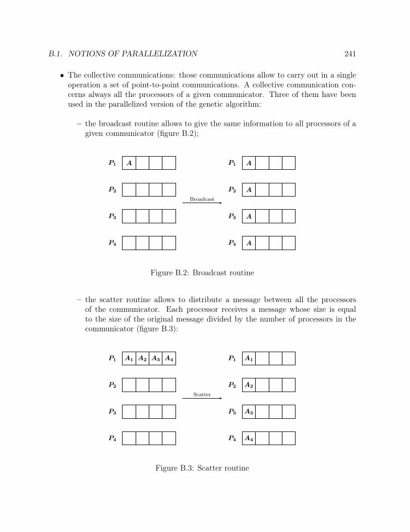
B.1. NOTIONS OF PARALLELIZATION 241
∙ The collective communications: those communications allow to carry out in a singleoperation a set of point-to-point communications. A collective communication con-cerns always all the processors of a given communicator. Three of them have beenused in the parallelized version of the genetic algorithm:
– the broadcast routine allows to give the same information to all processors of agiven communicator (figure B.2);
P4 P4 A
P3 P3 A
P2 P2 A
P1 P1A A
Broadcast
Figure B.2: Broadcast routine
– the scatter routine allows to distribute a message between all the processorsof the communicator. Each processor receives a message whose size is equalto the size of the original message divided by the number of processors in thecommunicator (figure B.3):
P4 P4 A4
P3 P3 A3
P2 P2 A2
P1 P1A1 A2 A3 A4 A1
Scatter
Figure B.3: Scatter routine
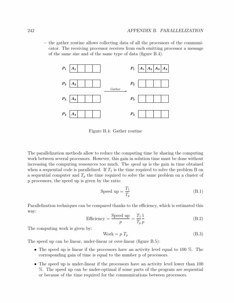
242 APPENDIX B. PARALLELIZATION
– the gather routine allows collecting data of all the processors of the communi-cator. The receiving processor receives from each emitting processor a messageof the same size and of the same type of data (figure B.4).
P4 P4A4
P3 P3A3
P2 P2A2
P1 P1A1 A1 A2 A3 A4
Gather
Figure B.4: Gather routine
The parallelization methods allow to reduce the computing time by sharing the computingwork between several processors. However, this gain in solution time must be done withoutincreasing the computing ressources too much. The speed up is the gain in time obtainedwhen a sequential code is parallelized. If T1 is the time required to solve the problem B ona sequential computer and Tp the time required to solve the same problem on a cluster ofp processors, the speed up is given by the ratio:
Speed up =T1
Tp
(B.1)
Parallelization techniques can be compared thanks to the efficiency, which is estimated thisway:
Efficiency =Speed up
p=
T1
Tp
1
p(B.2)
The computing work is given by:Work = p Tp (B.3)
The speed up can be linear, under-linear or over-linear (figure B.5):
∙ The speed up is linear if the processors have an activity level equal to 100 %. Thecorresponding gain of time is equal to the number p of processors.
∙ The speed up is under-linear if the processors have an activity level lower than 100%. The speed up can be under-optimal if some parts of the program are sequentialor because of the time required for the communications between processors.

B.2. ALGORITHMS PARALLELIZATION 243
Figure B.5: Speed up
∙ The speed up is over-linear if the processors have an activity level higher than 100%. That seems impossible under Amdhal’s rule.Let B a problem implemented in parallel. f is the part of the program that has tobe executed sequentially and p the number of processors. The Amdhal’s rule is thefollowing one:
Speed up ≤ 1
f + 1−f
p
≤ 1
f(B.4)
This rule is optimist in the sense that it does not take into account the additionalwork due to parallelization (communications between processors). It is pessimist inthe sense that it does not take into account the algorithm that is used, the use ofhierarchic memory and the part of sequential time of the application, which is adecreasing function of the global time.An over-linear speed up can nevertheless occurs: indeed, in the case of a multi-processors computer, the parallel algorithm can allow a better use of hierarchic mem-ory. It can also occurs when the parallel algorithm look for different ways to solvethe problem more quickly.
B.2 Parallelization of the optimal sensor network design
algorithm
To reduce the computing time, the optimal sensor network design algorithm has beenparallelized in two ways, which are explained in this section: global parallelization anddistributed genetic algorithms.Both parallelized versions of the algorithm have been tested on two different computerclusters:
∙ the first cluster was placed to our disposal during some months by the companyHemeris (http://www.hemeris.com). It was composed 64 nodes (Apple Power Mac
244 APPENDIX B. PARALLELIZATION
G4 bi-processors).
∙ the second one was composed of 12 computers of the network available for students inthe chemical engineering department. Eight of them had Celeron 2.2 GHz processorswhile the four others had Pentium 4.3 GHz processors.
B.2.1 Global parallelization (GP)
The objective of parallelization is to decrease the computing time while keeping an optimalefficiency. In our case, the limiting task is the evaluation of the fitness function of eachindividual of the population. This evaluation requires the factorization of at least twosquare matrices (whose size is equal to the sum of the number of equations and the numberof variables of the problem):
∙ the first matrix that is factorized is the sensitivity matrix of the model, evaluatedassuming ideal thermodynamic. This matrix is used to ensure that the incidencesof the pressures on the enthalpies are not taken into account in the analysis of theoccurrence matrix of the problem.
∙ the other matrices are the incidence matrices of all the operating points. The in-version of those matrices allows to estimates a posteriori variances for the candidatesensor network.
The fitness evaluations can be shared between several processors, each of them calculat-ing the goal function of one or several individuals of the population. The other tasks arecarried out by the master processor only. They consists of the population evolution, thedistribution of the individuals between the different processors, the search of the optimalfitness value between those of the current population, the report generation. Those op-erations take very little time in comparison to matrix inversions, so that their sequentialtreatment only introduces very small losses of efficiency. Another loss of efficiency comesfrom the communications between the master processor and his slaves.In a first time, the task of fitness evaluation has been shared between a number of processorsp equal to the size of the population Npop. If the master processor remains idle while eachslave is evaluating the fitness of one individual, there will be a great loss of efficiency,so that is was decided that the master processor would also estimate the fitness of oneindividual. Thus there is one master processor and Npop − 1 slaves.Once the environment has been initialized, all processors execute several identical opera-tions:
∙ reading the Vali4 reports model files and the data files;
∙ determination of all possible sensors for the processor;
∙ evaluation of the fitness of the first individual;
∙ creation of the first population of individuals.
B.2. ALGORITHMS PARALLELIZATION 245
This list of operations is executed by all the processors because all the slaves need to knowmost of the information contained in the files and the information about the potentialsensors. If all processors did not carry out all those operations, the information shouldbe transferred to each of them by means of collective communications. Moreover, thosecommunications between the master and the slaves would introduce losses of efficiency.While the master was alone to carry out those operations, the slaves would remain idle.Requiring of the slaves to carry out those operations in parallel does not change the elapsedcomputing time and should not create losses of efficiency.Once all those operations have been completed, each processor evaluates the goal functionof one individual and sends the value to the master that receives it. To avoid to carry outone point-to-point operation by slave, the gather routine is used.After reception of the values of the fitness, the master processor compares those valuesto the value corresponding to the current best solution. If one of them is better, thechromosome corresponding to this new best network is kept in memory.Then, the master prepares the next generation by means of selection, reproduction, cross-over and mutation. New chromosomes are stocked in a vector which is distributed to allprocessors by means of the scatter routine. Each processor evaluates the fitness of thereceived chromosome and sends the value to the master, and so on until the solution isachieved. When the convergence is detected, the master reevaluates the best individualand generates the report before the environment is deactivated.A flow diagram of this parallelization mode of the programme is drawn in figure B.6.The global parallelization of the optimal sensor network design algorithm allows a gainof time smaller than the number of active processors, so that the efficiency is lower than100 %. As it was mentioned before, the losses of efficiency come from the communicationsbetween the master processors and the slaves and from the sequential parts of the program.However, another source of efficiency loss comes from the fact that some individuals corre-spond to singular sensitivity matrices. In that case, the inversion of the sensitivity matricesrelative to the operating points is not carried out and the corresponding processor remainsidle until the next call of the gather routine, which allows to collect the fitness values ofall individuals. Moreover, if all machines were not identical, the gain should be smallerbecause they would not have the same execution speed so that some machines should waita longer time before the call of the gather routine.
In a second attempt, the program has been transformed so that the number of processorscould be smaller than the number of individuals of the population. In this case, eachprocessor estimates the fitness of a number kcℎrom of chromosomes determined as follow:
∙ if the number of processors is a divisor of the size of the population Npop:
kcℎrom =Npop
p(B.5)
∙ if the number of processors is not a divisor of the size of the population and if rcℎromis the remainder of the division of the number of chromosomes by the number of
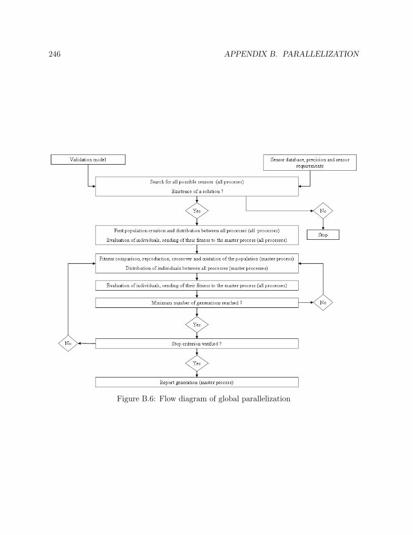
246 APPENDIX B. PARALLELIZATION
Figure B.6: Flow diagram of global parallelization

B.2. ALGORITHMS PARALLELIZATION 247
processors:
kcℎrom =Npop
p+ 1 (B.6)
for the rcℎrom first processors and
kcℎrom =Npop
p(B.7)
for the other processors.
To achieve the best possible efficiency, the number of processors must be a divisor of thenumber of chromosomes. In that case, each processor has the same work if it is not takeninto account that some individuals correspond to a singular sensitivity matrix. The lossesof efficiency have the same origines has explained before.
In a last attempt, the case of a number of processors higher than the size of the populationhas been studied. This version of the program can only be used if the objective is todetermine a sensor network that remains observable in the case of one sensor failure.Indeed, the number of fitness evaluation per chromosome is then equal to the number ofsensors in the network plus one, so that several processors can carry out those evaluations.Let nsensors be the number of sensors in the network and rsensors the remainder of thedivision of the number of sensors in the chromosomes plus one by the number of processors.The number of evaluations neval that are carried out by one processor for one chromosomeis determined this way:
neval =nsensors + 1
p+ 1 (B.8)
for the rsensors first processes and
neval =nsensors
p+ 1 (B.9)
for the other processors.Information is transferred this way: the first processor that is in charge of one chromosome,receives the fitness values from the other processors in charge of this chromosome and lookfor the worst one. The worst fitness values of each chromosome are then collected by themaster processor, which compares them as before.This version of the algorithm needs a lot of computing ressources to be applied, so that isis not the most interesting one.
B.2.2 Distributed genetic algorithms (DGA)
Another way to parallelize the genetic algorithm is to distribute the individuals of the pop-ulation between several sub-populations. This parallelization method is called distributedgenetic algorithms. It allows to avoid premature convergence to a local minimum that isdifferent from the optimal one and should be faster than the global parallelization.
248 APPENDIX B. PARALLELIZATION
This method has been implemented this way: after the verification of the existence of asolution for the problem, the individuals of the first generation are shared between thesub-populations, so that each sub-population starts with different individuals. The firstindividual of each sub-population is then replaced by the chromosome corresponding to thesensor network containing all possible measurement tools. This way, we ensure that eachsub-population contains at least one individual that corresponds to a feasible solution forthe problem. Each sub-population evolves independently from one another tanks to thegenetic algorithm mechanisms (tournament selection, reproduction, single-point cross-overand jump mutation). As the individuals are different at the beginning of the search, eachsub-population evolves in a different way. After a number ngeneration of generations, thefitness value of the best solution of each sub-population is collected by the master proces-sor, which compares all of them. If this value remains unchanged after N collects of themaster processor (N ∗ ngeneration generations in the sub-populations), the stop criterionis satisfied and the solution is reached. If the stop criterion is not satisfied, a fixed numberof individuals are chosen at random in each sub-populations and are sent to the masterprocessor, which redistributes them at random in the different sub-populations. The twochromosomes that are replaced by the moving ones in each sub-populations are also chosenat random. If one of the replaced chromosome corresponds to the best solution of the sub-population, it is not replaced and the sub-population has only one new individual. Themove of individuals is called migration. Instead of being chosen at random, the movingchromosomes could be the best ones of each sub-population, and the replaced individuals,the worst ones of each sub-population. This method for choosing chromosomes has notbeen adopted, even if it would converge faster, because it would have been the same askeeping only the best individuals of each sub-population and would have lead to a loss ofinformation contained in the global population. Indeed, even if they have a worse fitnessthan the best individuals, those chromosomes that would be eliminated contain genes thatcan make the sub-populations evolve favorably. A flow diagram of distributed genetic al-gorithms is drawn on figure B.7.
There are four parameters in distributed genetic algorithms that can be modified to obtainmore quickly the solution and with as few computing ressources as possible:
∙ The size of the sub-populations: it must be high enough to allow a continuous evo-lution of the individuals of each sub-population until the obtention of the solution,independently of the migrations. Moreover, if it is too small, the algorithm convergesprematurely to a local minimum. A size of sub-populations comprises between 10and 20 seems to be reasonable as the size of the population was fixed to 20 forthe initial non-parallelized algorithm. In the next chapter, results are discussed forsub-populations of 10 and 20 individuals in the case of an ammonia synthesis loop.
∙ The number of sub-populations: this parameter is also studied in the next chapter;
∙ The number of generations in the sub-populations between two migrations. In liter-ature, a value of five can be found. To confirm this value, tests have been done on

B.2. ALGORITHMS PARALLELIZATION 249
Figure B.7: Flow diagram of distributed genetic algorithms

250 APPENDIX B. PARALLELIZATION
the ammonia synthesis loop and the results are presented in the next chapter.
∙ The number of migrating chromosomes was fixed to 2 what seems to be reasonable.
Appendix C
Orthogonal collocations
In this chapter, some polynomial approximations are discussed before the choice of collo-cation points (Villadsen and Stewart, 1967), (Villadsen and Michelsen, 1978).
C.0.3 Polynomial approximations
Taylor series
To illustrate this method, we apply it to the solution of a differential equation of the form:
d2y (t)
dt2+
1
t
dy (t)
dt− Φ2 y (t)n = 0 (C.1)
This equation has for boundary conditions:
dy(t)dt
= 0y (t) = 1
for t = 0for t = 1
(C.2)
The derivatives of the Taylor series take a simpler form if equation C.1 is rewritten in termsof u = t2 for 0 ≤ t ≤ 1 :
dy
dt=
dy
du
du
dt=
dy
du2√u for u ≥ 0 (C.3)
d2y
dt2=
d
dt
(2√u
dy
du
)= 2
d
du
(√u
dy
du
)du
dt= 2
dy
du+ 4 u
d2y
du2(C.4)
Thus one obtains:
ud2y
du2+
dy
du=
Φ2
4y = py (C.5)
The first boundary conditiondy
dt
∣∣∣∣t=0
= 0 (C.6)
is satisfied in equation C.5 as y = f(u = t2).
251
252 APPENDIX C. ORTHOGONAL COLLOCATIONS
Thus the boundary conditions of equation C.5 are
y∣u=1 = 0 (C.7)
dky
duk
∣∣∣∣u=0
= y(k)∣∣u=0
finite for k=0,1,... (C.8)
If one differentiates equation C.5 k times with respect to u, one obtains:
u y(3) + 2 y(2) = p y(1)
u y(4) + 3 y(3) = p y(2)
u y(k+2) + (k + 1) y(k+1) = p y(k) (C.9)
The following recurrence formula allows thus to build derivatives of any order at u = 0:
y(k+1)∣∣u=0
= y(k+1)0 =
p
k + 1y(k)0 =
p2
(k + 1) ky(k−1)0 = ... =
pk+1
(k + 1)!y0 (C.10)
The Taylor series for y (u) from u = 0 is defined by:
y (u) =
∞∑
k=0
1
k!y(k)0 uk =
∞∑
k=0
bk uk =
∞∑
k=0
1
k!
pk
k!y0 uk =
∞∑
k=0
pk
(k!)2y0 uk (C.11)
The boundary condition y∣u=1 = 1 allows to determine y0 :
y0 =1
∞∑
k=0
pk
(k!)2
(C.12)
Finally, one obtains for yN (u) :
yN (u) =N∑
k=0
bk uk =
N∑
k=0
pk
(k!)2uk
N∑
k=0
pk
(k!)2
N = 1, 2, ...,∞ (C.13)
The way the coefficients bk have been built shows that the residual Rn (u) and its (N − 1)st
derivatives are zero at u = 0. Conversely the Taylor series is a method in which the Nconstants bi are the solution of the following equations:
R(k)N [yN (u)]
∣∣∣u=0
= R(k)N (u)
∣∣∣u=0
= 0 k = 0, 1, ..., N − 1 (C.14)
The approximations by Taylor series are unsatisfactory in the way that other approximationmethods converge more quickly.

253
Lowest-order MWR (Weighted residuals method): y1 (t) approximation
To illustrate this technique, let us solve equation C.1 in which n = 1. One obtains
y (t) =I0 (Φt)
I0 (Φ)(C.15)
where I0 is a first order Bessel function :
I0 (x) =
∞∑
i=0
(14x2)i
(i!)2= 1 +
1
4x2 +
1
4
(1
4x2
)2
+1
36
(1
4x2
)3
+ ... (C.16)
So, equation C.15 becomes:
y (t) =1 +
(Φ2t2
4
)+ 1
4
(Φ2t2
4
)2+ 1
36
(Φ2t2
4
)3+ ...
1 +(Φ2
)+ 1
4
(Φ2
)4+ 1
36
(Φ2
)6+ ...
(C.17)
In first approximation, equation C.1 can be written
y1 (t) = 1 + a1(1− t2
)(C.18)
The term a1 (1− t2) is a perturbation of the known boundary value y (t) = 1 at t = 1. Theequation C.18 satisfies both boundary conditions C.2. For the preceding serie C.17, y1 (t)takes the form:
y1 (t) =1 + Φ t2
2
1 + Φ2
2
(C.19)
By transforming y1 (t) :
y1 (t) =4 + Φ2 − Φ2 + Φ2 t2
4 + Φ2
= 1− Φ2 (1− t2)
4 + Φ2(C.20)
one obtains for a1 :
a1 = − Φ2
4 + Φ2(C.21)
Replacing y1 (t) from equation C.18 in equation C.1 for n = 1, the following residual isobtained:
R (y1 (t)) = R (a1, t) = −4 a1 − Φ2[1− a1
(1− t2
)](C.22)
a1 is determined so that the weighted residual W ∗ R has a zero mean value, or in anequivalent way : ∫ 1
0
R1 (a1, t) W (t) dt2 = 0 (C.23)
where W (t) is a weighting function which depends on the MWR method that is chosen.Some of those methods are described later in this section.

254 APPENDIX C. ORTHOGONAL COLLOCATIONS
Higher-order MWR: yN (t) approximation
If one approximates yN (t) by the following series :
yN (t) = T0 +n∑
i=1
ai Ti (C.24)
where,
∙ T0 satisfies the boundary conditions C.2 of the differential equation C.1;
∙ les Ti are boundary conditions satisfying the boundary conditions of the problem,namely:
dTi
dt
∣∣∣∣t=0
= Ti∣t=1 = 0 ∀i > 0 (C.25)
The choice of those functions is generally free as long as they satisfy the conditionsC.25 and are linearly independent. The following polynomial functions satisfy theconditions C.25 for equation C.1:
T0 = 1
Ti =(1 + t2
)t2i−2 i = 1, 2, ... (C.26)
yN (t) can thus be written :
yN (t) = 1 +(1 + t2
) n∑
i
ai t2i−2 (C.27)
If a change of variable is carried out in equation C.1:
ud2y (u)
du2+
dy (u)
du− p y (u) = 0 (C.28)
with
p =Φ2
4(C.29)
and with boundary conditions :
y (u)∣u=1 = 1
yk (u)∣u=0 finite for k ≥ 0 (C.30)
yN can then be written in the following way:
yN (u) = 1 + (1− u)
N∑
i=1
ai ui−1 (C.31)
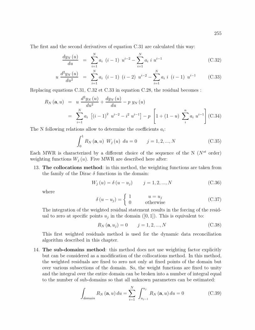
255
The first and the second derivatives of equation C.31 are calculated this way:
dyN (u)
du=
N∑
i=1
ai (i− 1) ui−2 −N∑
i=1
ai i ui−1 (C.32)
ud2yN (u)
du2=
N∑
i=1
ai (i− 1) (i− 2) ui−2 −N∑
i=1
ai i (i− 1) ui−1 (C.33)
Replacing equations C.31, C.32 et C.33 in equation C.28, the residual becomes :
RN (a, u) = ud2yN (u)
du2+
dyN (u)
du− p yN (u)
=
N∑
i=1
ai[(i− 1)2 ui−2 − i2 ui−1
]− p
[1 + (1− u)
n∑
i
ai ui−1
](C.34)
The N following relations allow to determine the coefficients ai:∫ 1
0
RN (a, u) Wj (u) du = 0 j = 1, 2, ..., N (C.35)
Each MWR is characterized by a different choice of the sequence of the N (N st order)weighting functions Wj (u). Five MWR are described here after:
13. The collocations method: in this method, the weighting functions are taken fromthe family of the Dirac � functions in the domain:
Wj (u) = � (u− uj) j = 1, 2, ..., N (C.36)
where
� (u− uj) =
{10
u = uj
otherwise(C.37)
The integration of the weighted residual statement results in the forcing of the resid-ual to zero at specific points uj in the domain ([0, 1]). This is equivalent to:
RN (a, uj) = 0 j = 1, 2, ..., N (C.38)
This first weighted residuals method is used for the dynamic data reconciliationalgorithm described in this chapter.
14. The sub-domains method: this method does not use weighting factor explicitlybut can be considered as a modification of the collocations method. In this method,the weighted residuals are fixed to zero not only at fixed points of the domain butover various subsections of the domain. So, the weight functions are fixed to unityand the integral over the entire domain can be broken into a number of integral equalto the number of sub-domains so that all unknown parameters can be estimated:
∫
domain
RN (a, u) du =
N∑
i=1
∫ uj
uj−1
RN (a, u) du = 0 (C.39)

256 APPENDIX C. ORTHOGONAL COLLOCATIONS
15. The least squares method: this method consists of the continuous minimizationof the sum of squared residuals:
S =
∫
domain
RN (a, u) RN (a, u) du =
∫
domain
R2N (a, u) du (C.40)
The minimum of this function is reached when its derivative with respect to theunknown parameters aj is zero:
∂S
∂aj= 0 = 2
∫
domain
RN (a, u)∂RN (a, u)
∂ajdu j = 1, 2, ..., N (C.41)
So that the weighting functions are:
Wj = 2∂RN (a, u)
∂ajdu j = 1, 2, ..., N (C.42)
The "2" factor can be dropped so that the weighting functions for this method arejust the derivatives of the residuals with respect to the unknown parameters aj :
Wj =∂RN (a, u)
∂ajdu j = 1, 2, ..., N (C.43)
16. The Galerkin method: this method can be considered as a modification of the leastsquares method in which the derivative of the approximating function with respectto the unknown parameters aj is used instead of the derivative of the residual:
Wj (u) = Tj =∂yN∂aj
= (1− u) uj−1 (C.44)
This is equivalent to:
∫ 1
0
RN (a, u) (1− u) uj−1 du = 0 j = 1, 2, ..., N (C.45)
17. The method of moments: in this last method, the weighting functions are chosenfrom the family of polynomials:
Wj (u) = uj−1j j = 1, 2, ..., N (C.46)
This is equivalent to:
∫ 1
0
RN (a, u) uj−1 du = 0 j = 1, 2, ..., N (C.47)
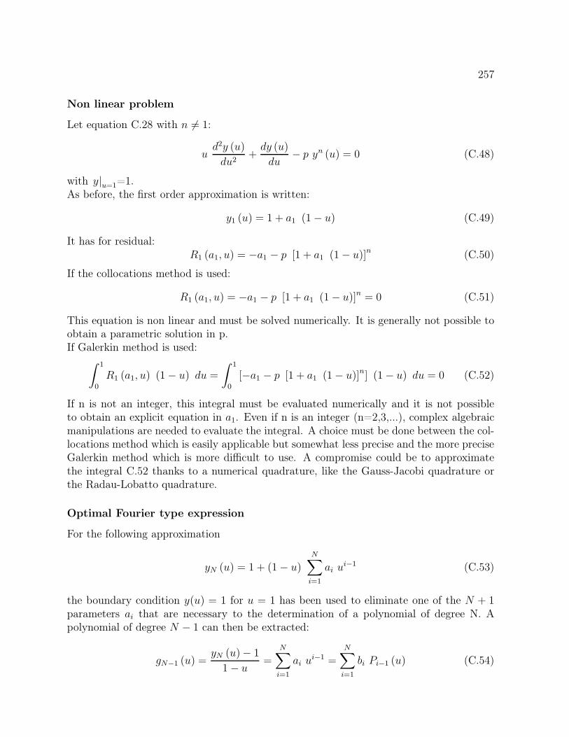
257
Non linear problem
Let equation C.28 with n ∕= 1:
ud2y (u)
du2+
dy (u)
du− p yn (u) = 0 (C.48)
with y∣u=1=1.As before, the first order approximation is written:
y1 (u) = 1 + a1 (1− u) (C.49)
It has for residual:R1 (a1, u) = −a1 − p [1 + a1 (1− u)]n (C.50)
If the collocations method is used:
R1 (a1, u) = −a1 − p [1 + a1 (1− u)]n = 0 (C.51)
This equation is non linear and must be solved numerically. It is generally not possible toobtain a parametric solution in p.If Galerkin method is used:
∫ 1
0
R1 (a1, u) (1− u) du =
∫ 1
0
[−a1 − p [1 + a1 (1− u)]n] (1− u) du = 0 (C.52)
If n is not an integer, this integral must be evaluated numerically and it is not possibleto obtain an explicit equation in a1. Even if n is an integer (n=2,3,...), complex algebraicmanipulations are needed to evaluate the integral. A choice must be done between the col-locations method which is easily applicable but somewhat less precise and the more preciseGalerkin method which is more difficult to use. A compromise could be to approximatethe integral C.52 thanks to a numerical quadrature, like the Gauss-Jacobi quadrature orthe Radau-Lobatto quadrature.
Optimal Fourier type expression
For the following approximation
yN (u) = 1 + (1− u)
N∑
i=1
ai ui−1 (C.53)
the boundary condition y(u) = 1 for u = 1 has been used to eliminate one of the N + 1parameters ai that are necessary to the determination of a polynomial of degree N. Apolynomial of degree N − 1 can then be extracted:
gN−1 (u) =yN (u)− 1
1− u=
N∑
i=1
ai ui−1 =
N∑
i=1
bi Pi−1 (u) (C.54)

258 APPENDIX C. ORTHOGONAL COLLOCATIONS
The Pi (u) are often chosen as orthogonal polynomials of degree N in u and satisfying thefollowing equation:
∫ 1
0
u� (1− u)� uj P �,�N (u) du = 0 j = 0, 1, ..., N − 1 (C.55)
Those polynomials can also take the form:
P �,�i (u) = i u
i − i−1 ui−1 + i−2 ui−2 − ... + (−1)i (C.56)
They can also be normalized so that the leading coefficient is 1:
P �,�i (u) = ui −
′
i−1 ui−1 + ′
i−2 ui−2 − ...+ (−1)i ′
0 (C.57)
In equations C.56 and C.57, all i and ′
i are positives.The advantage of this reformulation of equation C.31 is that the coefficients bi allow toobtain a more rapid convergence than the ai series that decreases less quickly.
Lagrange interpolation polynomials
Two kinds of polynomial approximations of degree N have been discussed previously:
yN =N∑
i=0
ai xi (C.58)
yN =
N∑
i=0
bi Pi (t) (C.59)
In this paragraph, a third type of approximations is discussed: the Lagrange interpolationpolynomials:
yN =N∑
i=0
yi li (t) (C.60)
In this formula:
∙ the yi are the values of yN at the interpolation points ti;
∙ the li (t) are Lagrange interpolation polynomial of degree N defined as follow:
li (t) =pN (t)
(t− ti) p(1)N (t)
(C.61)
∙ pN (t) is a polynomial of degree N with a leading coefficient equal to 1, called thenode polynomial.
pN (t) = (t− t0) (t− t2) ... (t− tN) (C.62)
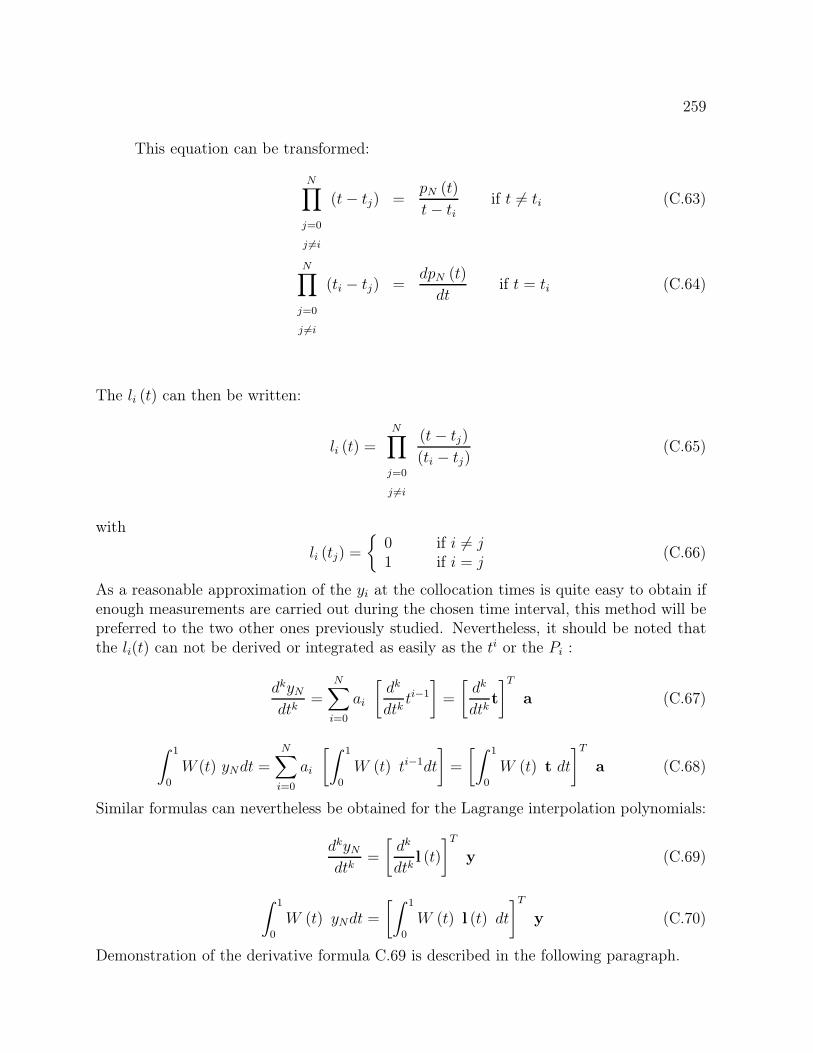
259
This equation can be transformed:
N∏
j=0
j ∕=i
(t− tj) =pN (t)
t− tiif t ∕= ti (C.63)
N∏
j=0
j ∕=i
(ti − tj) =dpN (t)
dtif t = ti (C.64)
The li (t) can then be written:
li (t) =
N∏
j=0
j ∕=i
(t− tj)
(ti − tj)(C.65)
with
li (tj) =
{01
if i ∕= jif i = j
(C.66)
As a reasonable approximation of the yi at the collocation times is quite easy to obtain ifenough measurements are carried out during the chosen time interval, this method will bepreferred to the two other ones previously studied. Nevertheless, it should be noted thatthe li(t) can not be derived or integrated as easily as the ti or the Pi :
dkyNdtk
=
N∑
i=0
ai
[dk
dtkti−1
]=
[dk
dtkt
]Ta (C.67)
∫ 1
0
W (t) yNdt =
N∑
i=0
ai
[∫ 1
0
W (t) ti−1dt
]=
[∫ 1
0
W (t) t dt
]Ta (C.68)
Similar formulas can nevertheless be obtained for the Lagrange interpolation polynomials:
dkyNdtk
=
[dk
dtkl (t)
]Ty (C.69)
∫ 1
0
W (t) yNdt =
[∫ 1
0
W (t) l (t) dt
]Ty (C.70)
Demonstration of the derivative formula C.69 is described in the following paragraph.
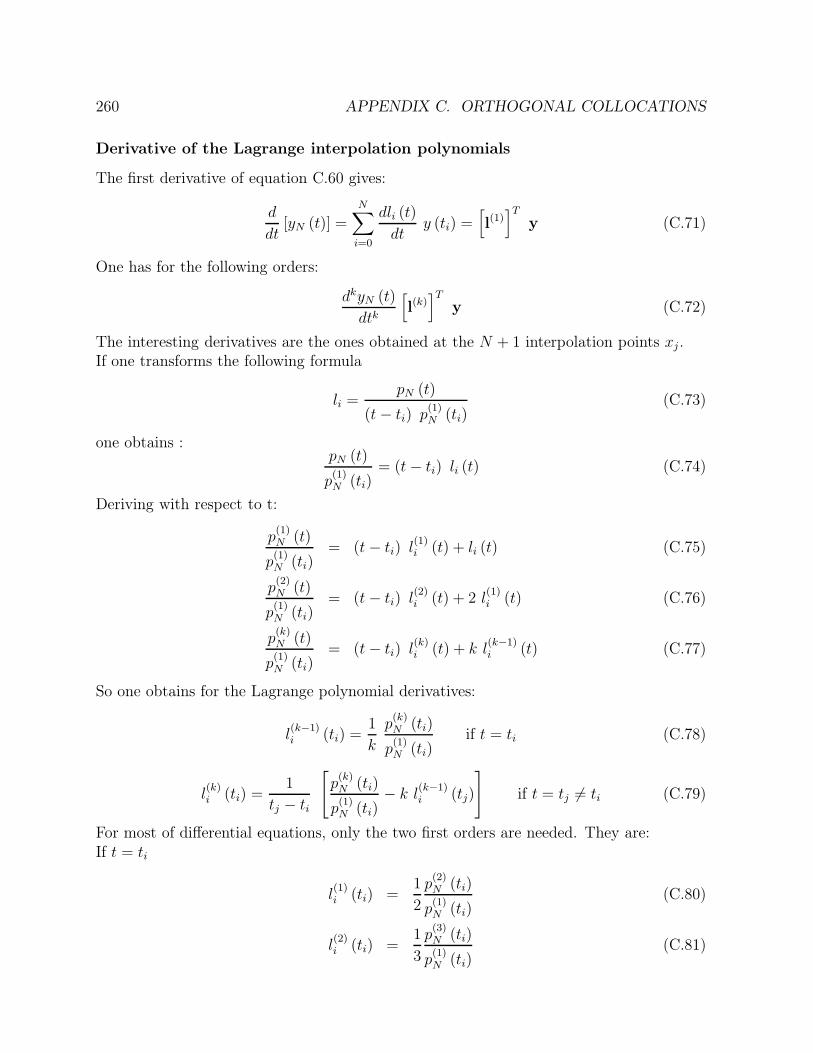
260 APPENDIX C. ORTHOGONAL COLLOCATIONS
Derivative of the Lagrange interpolation polynomials
The first derivative of equation C.60 gives:
d
dt[yN (t)] =
N∑
i=0
dli (t)
dty (ti) =
[l(1)]T
y (C.71)
One has for the following orders:
dkyN (t)
dtk
[l(k)]T
y (C.72)
The interesting derivatives are the ones obtained at the N + 1 interpolation points xj .If one transforms the following formula
li =pN (t)
(t− ti) p(1)N (ti)
(C.73)
one obtains :pN (t)
p(1)N (ti)
= (t− ti) li (t) (C.74)
Deriving with respect to t:
p(1)N (t)
p(1)N (ti)
= (t− ti) l(1)i (t) + li (t) (C.75)
p(2)N (t)
p(1)N (ti)
= (t− ti) l(2)i (t) + 2 l
(1)i (t) (C.76)
p(k)N (t)
p(1)N (ti)
= (t− ti) l(k)i (t) + k l
(k−1)i (t) (C.77)
So one obtains for the Lagrange polynomial derivatives:
l(k−1)i (ti) =
1
k
p(k)N (ti)
p(1)N (ti)
if t = ti (C.78)
l(k)i (ti) =
1
tj − ti
[p(k)N (ti)
p(1)N (ti)
− k l(k−1)i (tj)
]if t = tj ∕= ti (C.79)
For most of differential equations, only the two first orders are needed. They are:If t = ti
l(1)i (ti) =
1
2
p(2)N (ti)
p(1)N (ti)
(C.80)
l(2)i (ti) =
1
3
p(3)N (ti)
p(1)N (ti)
(C.81)

261
Otherwise, t = tj ∕= ti
l(1)i (tj) =
1
tj − tias li (tj) = 0 (C.82)
l(2)i (tj) =
1
tj − ti
[p(2)N (ti)
p(1)N (ti)
− 2 l(1)i (tj)
](C.83)
= l(1)i (tj)
[p(2)N (ti)
p(1)N (ti)
− 21
tj − ti
]as l
(1)i (tj) =
1
tj − ti(C.84)
= 2 l(1)i (tj)
[p(2)N (ti)
2 p(1)N (ti)
− 1
tj − ti
](C.85)
= 2 l(1)i (tj)
[l(1)j (tj)−
1
tj − ti
](C.86)
The next formula allows to calculate the derivatives of the node polynomial at the inter-polation points tj
pN (t) =
N∏
i=0
(t− ti) (C.87)
From there, one has the following recurrence formula:
p0(t) = 1
pj (t) = (t− tj) pj−1 (t) j = 0, 1, 2, ..., N (C.88)
Deriving the equation C.88, one obtains
p(1)j (t) = (t− tj) p
(1)j−1 (t) + pj−1 (C.89)
p(2)j (t) = (t− tj) p
(2)j−1 (t) + 2 p
(1)j−1 (C.90)
p(3)j (t) = (t− tj) p
(3)j−1 (t) + 2 p
(2)j−1 (C.91)
withp(1)0 (t) = p
(2)0 (t) = p
(3)0 (t) = 0
If t is replaced by ti and if the interpolation points are reordered in a way that the tiat which the derivatives are calculated is placed in first position, the preceding equationsbecome:
p0 (ti) = 1 (C.92)
p(k)0 (ti) = 0 k = 1, 2, 3 (C.93)
p1 (ti) = (ti − ti) p0 (ti) = 0 (C.94)
p(1)1 (ti) = (ti − ti) p
(1)0 (ti) + p0 (ti) = 1 (C.95)
p(2)1 (ti) = (ti − ti) p
(2)0 (ti) + 2 p
(1)0 (ti) = 0 (C.96)
p(3)1 (ti) = (ti − ti) p
(3)0 (ti) + 3 p
(2)0 (ti) = 0 (C.97)
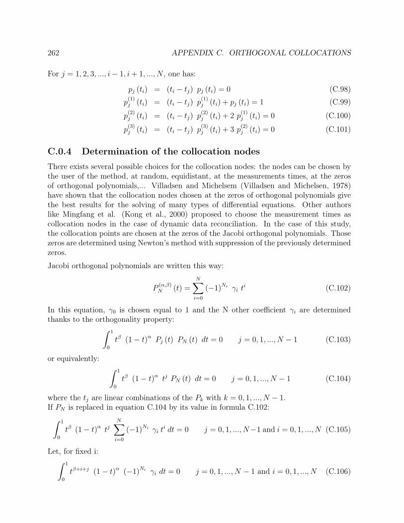
262 APPENDIX C. ORTHOGONAL COLLOCATIONS
For j = 1, 2, 3, ..., i− 1, i+ 1, ..., N , one has:
pj (ti) = (ti − tj) pj (ti) = 0 (C.98)
p(1)j (ti) = (ti − tj) p
(1)j (ti) + pj (ti) = 1 (C.99)
p(2)j (ti) = (ti − tj) p
(2)j (ti) + 2 p
(1)j (ti) = 0 (C.100)
p(3)j (ti) = (ti − tj) p
(3)j (ti) + 3 p
(2)j (ti) = 0 (C.101)
C.0.4 Determination of the collocation nodes
There exists several possible choices for the collocation nodes: the nodes can be chosen bythe user of the method, at random, equidistant, at the measurements times, at the zerosof orthogonal polynomials,... Villadsen and Michelsem (Villadsen and Michelsen, 1978)have shown that the collocation nodes chosen at the zeros of orthogonal polynomials givethe best results for the solving of many types of differential equations. Other authorslike Mingfang et al. (Kong et al., 2000) proposed to choose the measurement times ascollocation nodes in the case of dynamic data reconciliation. In the case of this study,the collocation points are chosen at the zeros of the Jacobi orthogonal polynomials. Thosezeros are determined using Newton’s method with suppression of the previously determinedzeros.
Jacobi orthogonal polynomials are written this way:
P(�,�)N (t) =
N∑
i=0
(−1)Ni i ti (C.102)
In this equation, 0 is chosen equal to 1 and the N other coefficient i are determinedthanks to the orthogonality property:
∫ 1
0
t� (1− t)� Pj (t) PN (t) dt = 0 j = 0, 1, ..., N − 1 (C.103)
or equivalently:∫ 1
0
t� (1− t)� tj PN (t) dt = 0 j = 0, 1, ..., N − 1 (C.104)
where the tj are linear combinations of the Pk with k = 0, 1, ..., N − 1.If PN is replaced in equation C.104 by its value in formula C.102:
∫ 1
0
t� (1− t)� tjN∑
i=0
(−1)Ni i ti dt = 0 j = 0, 1, ..., N−1 and i = 0, 1, ..., N (C.105)
Let, for fixed i:∫ 1
0
t�+i+j (1− t)� (−1)Ni i dt = 0 j = 0, 1, ..., N − 1 and i = 0, 1, ..., N (C.106)

263
Knowing that: ∫ 1
0
tm (1− t)n =Γ (m+ 1) Γ (n+ 1)
Γ (m+ n+ 2)(C.107)
one obtains:
(−1)Ni i
∫ 1
0
t�+i+j (1− t)� = (−1)Ni iΓ (� + i+ j + 1) Γ (� + 1)
Γ (� + � + i+ j + 2)
j = 0, 1, ..., N − 1 and i = 0, 1, ..., N (C.108)
If � = 0 and � = 0, Legendre polynomials are obtained :
(−1)Ni i
∫ 1
0
ti+j (1− t)0 = (−1)Ni iΓ (i+ j + 1) Γ (1)
Γ (i+ j + 2)
j = 0, 1, ..., N − 1 and i = 0, 1, ..., N (C.109)
Now, by definition:
Γ (1) = 1 (C.110)
Γ (n + 1) = n Γ (n) = Γ (1) (n− 1)! (C.111)
Thus one obtains:
(−1)Ni i
∫ 1
0
ti+j (1− t)0 = (−1)Ni i(i+ 1)!
Γ (i+ j + 1)!
j = 0, 1, ..., N − 1 and i = 0, 1, ..., N (C.112)
The next formula allows to obtain the i :
i =N !
i! (N − i)!
Γ (N + � + � + i+ 1) Γ (� + 1)
Γ (N + � + � + 1) Γ (� + i+ 1)(C.113)
From there, the following recurrence formula is obtained:
i =N − i+ 1
i
N + � + � + i� + i i−1 0 = 1 and i = 1, 2, ..., N (C.114)