econstor www.econstor.eu

Der Open-Access-Publikationsserver der ZBW – Leibniz-Informationszentrum WirtschaftThe Open Access Publication Server of the ZBW – Leibniz Information Centre for Economics

Standard-Nutzungsbedingungen:

Die Dokumente auf EconStor dürfen zu eigenen wissenschaftlichenZwecken und zum Privatgebrauch gespeichert und kopiert werden.

Sie dürfen die Dokumente nicht für öffentliche oder kommerzielleZwecke vervielfältigen, öffentlich ausstellen, öffentlich zugänglichmachen, vertreiben oder anderweitig nutzen.

Sofern die Verfasser die Dokumente unter Open-Content-Lizenzen(insbesondere CC-Lizenzen) zur Verfügung gestellt haben sollten,gelten abweichend von diesen Nutzungsbedingungen die in der dortgenannten Lizenz gewährten Nutzungsrechte.

Terms of use:

Documents in EconStor may be saved and copied for yourpersonal and scholarly purposes.

You are not to copy documents for public or commercialpurposes, to exhibit the documents publicly, to make thempublicly available on the internet, or to distribute or otherwiseuse the documents in public.

If the documents have been made available under an OpenContent Licence (especially Creative Commons Licences), youmay exercise further usage rights as specified in the indicatedlicence.

zbw Leibniz-Informationszentrum WirtschaftLeibniz Information Centre for Economics

von Ehrlich, Maximilian; Seidel, Tobias

Working Paper

The Persistent Effects of Place-Based Policy:Evidence from the West-German Zonenrandgebiet

CESifo Working Paper, No. 5373

Provided in Cooperation with:Ifo Institute – Leibniz Institute for Economic Research at the University ofMunich

Suggested Citation: von Ehrlich, Maximilian; Seidel, Tobias (2015) : The Persistent Effects ofPlace-Based Policy: Evidence from the West-German Zonenrandgebiet, CESifo Working Paper,No. 5373

This Version is available at:http://hdl.handle.net/10419/110873

The Persistent Effects of Place-Based Policy: Evidence from the West-German Zonenrandgebiet

Maximilian von Ehrlich Tobias Seidel

CESIFO WORKING PAPER NO. 5373 CATEGORY 1: PUBLIC FINANCE

MAY 2015

An electronic version of the paper may be downloaded • from the SSRN website: www.SSRN.com • from the RePEc website: www.RePEc.org

• from the CESifo website: Twww.CESifo-group.org/wp T

ISSN 2364-1428

CESifo Working Paper No. 5373

The Persistent Effects of Place-Based Policy: Evidence from the West-German Zonenrandgebiet

Abstract Using a natural experiment from Germany, we show that temporary place-based subsidies generate persistent effects on economic density. We identify employment and capital formation as main channels for higher income per square kilometer. As the spatial regression discontinuity design allows us to control for all spatially-continuous determinants of agglomeration (e.g. homemarket effects, knowledge spillovers), we attribute an important role to capital formation in explaining persistent spatial patterns of economic activity. However, estimates of externalities at the treatment border point to small net effects of the policy. We find strong evidence that pre-treatment land owners have benefitted substantially from the program and that transfers have shown larger effects in high-density places. Finally, accounting for regional subsidies raises the causal effect of market access for economic development as identified in Redding and Sturm (2008) by about 45 percent.

JEL-Code: H250, H400, H540, O150, O180, R120.

Keywords: place-based policy, regional policy, economic geography, persistence, regression discontinuity, locational advantage, land value capitalization.

Maximilian von Ehrlich University of Bern Bern / Switzerland

maximilian.vonehrlich@vwi.unibe.ch

Tobias Seidel University of Duisburg-Essen

Duisburg / Germany tobias.seidel@uni-due.de

This version: May 2015 We thank Peter Egger, Joshua D. Gottlieb, Wolfgang Keller, Diego Puga, Esteban Rossi-Hansberg, Blaise Melly, Jens Suedekum, Daniel Sturm, Marcel Thum, and Jos van Ommeren for many helpful comments. We benefitted from numerous comments of participants of the IEB Workshop on Urban Economics in Barcelona, the CESifo Global Area and Public Sector conferences in Munich, the UEA meetings in Washington DC, the IIPF in Lugano, the German Economic Association Meetings in Hamburg, the International Economics Workshop in Goettingen, the CRED workshop in Bern, the ETSG in Munich and seminars at the universities in Aarhus, Munich (LMU), Nijmegen, Rotterdam, and Zurich (ETH and UZH).

1 Introduction

When supporting underdeveloped regions, policy makers often hope that temporary trans-

fers establish self-sustaining long-run economic development. The effort is substantial. For

example, the EU dedicates about one third of its overall budget 2014-2020 to regional pol-

icy amounting to more than 350 billion euros (EU Commission, 2011). The US does not

have a unified regional policy, but annual spending on regional development programs is

estimated at about 95 billion US dollars per year (Kline and Moretti, 2014). Also China

has installed regional policies that resemble those in the EU in terms of instruments and

magnitude (EU Commission, 2010).

Despite these efforts, little is known about the long-term consequences of these pro-

grams and their underlying mechanisms (Neumark and Simpson, 2015).1 Using a natural

experiment from Germany allows us to make progress in this direction. We uncover the

channels that create persistence and disentangle the role of capital accumulation from ag-

glomeration economies. Second, we estimate (local) external effects of the policy to make

statements about the net effect of the program. Third, we examine the distributional con-

sequences by estimating the capitalization of transfers in land prices. Fourth, we reassess

the importance of market access for economic development and look for heterogeneous

treatment effects between low-density and high-density places.

In 1971, the West German government started a large scale transfer program to stimu-

late economic development in a well-defined geographical area adjacent to the Iron Curtain.

All districts that accommodated either 50 percent of their area or population within a dis-

tance of 40 kilometers to the inner-German and Czechoslovakian border on January 1,

1971 became part of the Zonenrandgebiet (ZRG).2 As shown in Figure 1, it stretched from

the Danish border in the North to the Austrian border in the South running through four

states (Bavaria, Hesse, Lower-Saxony, and Schleswig-Holstein). A major reason for this

privileged treatment was to compensate firms and households close to the eastern border

for being cut off adjacent markets on the other side of the Iron Curtain. The remoteness

1The literature on placed-based policies has mostly looked into the effects of transfers during programs,e.g. Busso, Gregory, and Kline (2013) evaluate the federal empowerment zones program in the US, Glaeserand Gottlieb (2008) examine the place-based policy Appalachian Regional Commission, Gobillon, Magnac,and Selod (2012) study the French enterprise zone program, Becker, Egger, and Ehrlich (2010, 2012) focuson income and employment effects of EU Structural Funds.

2See Deutscher Bundestag (1970), Drucksache VI/796 and Ziegler (1992, p.9). Zonenrandgebiet literallymeans area adjacent to the (Soviet occupation) zone, that became the German Democratic Republic. Itwas common in West Germany to refer to the German Democratic Republic as the “Zone”.

1

Figure 1: The German Zonenrandgebiet, 1971-1994

Note: The blue lines mark the western border of the ZRG and the Iron Curtain, respectively. The grey linesrepresent the municipalities according to the 1997 classification while the red lines define State borders. The borderof the ZRG follows the administrative districts according to the 1971 classifications which was modified substantiallyin the mid-1970s. In most of our analysis we consider the states (Lander) Schleswig-Holstein (SH), Lower Saxony(LS), North Rhine-Westphalia (NRW), Hesse (HE), and Bavaria (BA).

was feared to cause substantial outmigration to the western parts of the country.3 The

program was not intended for a fixed number of years and its termination came as un-

expectedly as German reunification. As transfers were redirected towards East Germany

after 1990, the place-based policy was phased out until 1994.

3See Ziegler (1992) for a more detailed exposition.

2

The institutional setting of the ZRG gives rise to two types of discontinuities that we

can use for identification of causal effects. First, we apply a spatial regression discontinuity

design based on municipalities (and grid cells) in a close neighborhood on either side of

the treatment border. If other relevant factors vary continuously at the ZRG-border, a

discontinuity in economic activity at this border can be interpreted as the causal effect

of the place-based policy. As the treatment border does not separate areas with different

institutions, many concerns of other discontinuities that are important at country borders

can be ruled out. Nevertheless, administrative borders are unlikely to be drawn randomly.

To establish more credibility of our results, we also exploit the political rule which gov-

erned the location of the treatment border. As the treatment probability of districts jumps

at a distance of 40 kilometers from the Iron Curtain, we apply a classical regression dis-

continuity design. The advantage is that the 40-kilometer rule does not coincide with any

administrative boundary nor with geographic features that may cause discontinuities in

relevant determinants for outcome. Depending on parametric or non-parametric estima-

tion and the choice of the control function, we find that regional transfers led to higher

income per square kilometer in the treatment area by about 30-50 percent in 1986. Un-

dertaking the same exercise for 2010, that is 16 years after the program was eventually

stopped, we find no evidence that the estimated effects have diminished.

To better understand underlying mechanisms of this outcome, we examine the pro-

gram’s effects on capital and labor at the treatment border. First, and foremost, transfers

were dedicated to subsidize firm investments and to finance public infrastructure. We find

strong and significant effects with respect to both private and public capital intensity. A

second reason for higher economic activity could be migration of people into the treatment

area. We find that the place-based policy led to a 20-40 percent higher population density

both in the mid-1980s and in 2010. The response in employment is even higher indicating

substantial commuting into the Zonenrandgebiet. However, we find no evidence that the

educational composition of the workforce was affected.

There is a lively debate in the literature to what extent agglomeration economies play a

role in shaping the spatial distribution of economic activity in the long run.4 For example,

Bleakley and Lin (2012) show that historical portage sites in the US serve as a good

predictor for the location of cities today. As they do not find substantial differences in

4For syntheses of the theoretical literature on agglomeration economies see Duranton and Puga (2004)and Puga (2010).

3

the capital stock or capital intensity between portage and non-portage sites, Bleakley and

Lin (2012) interpret their findings as evidence in favor of agglomeration economies as an

important explanation for this path dependency rather than capital structures. Kline and

Moretti (2014) analyze the effects of the Tennessee Valley Authority program showing

that manufacturing employment continued to grow after transfers into this region were

stopped in 1960. They argue that initial capital investments before 1960 are unlikely to

be responsible for this long-run effect as the capital stock would have depreciated several

decades later.5

Agglomeration economies cannot explain our findings. As long as these benefits of

density (like labor-market pooling, technology spillovers, or the home-market effect, among

others) dissipate continuously with distance, these determinants can be shown to cancel

in our econometric approach. But why do firms have an incentive to maintain investment

levels (and thus the discontinuity in the capital stock) even in the absence of subsidies?

We suggest the following interpretation: Subsidies for private capital investment raised

demand for premises and public infrastructure that local governments needed to provide.

At the end of the treatment period, the Zonenrandgebiet was equipped not only with a

larger capital stock (that would depreciate over time), but also with new industrial parks,

roads, power networks, and sewage systems that generate a locational advantage in the

long run. Although these investments also depreciate over time, the maintenance could

be cheaper than planning new industrial parks elsewhere. What matters for firms, these

investments reduce costs, provide premises to locate in the area in the first place or act

as a coordination device. In this regard, our paper links to Davis and Weinstein (2002,

2008) attributing a key role to local structures in explaining the long-term spatial pattern

of economic activity.

Despite these persistent discontinuities, it is not ensured that the policy generated

new economic activity in the ZRG. As our identification strategy builds on municipalities

that are close to each other, entrepreneurs outside the Zonenrandgebiet have an incentive

to move their business into the treatment area. This incentive is not continuous at the

border because entrepreneurs are not indifferent between locating one meter to the left or

5Schumann (2014) documents persistent effects of different levels of local population due to differentsettlement policies for refugees in the American and French occupation zones in Germany after WorldWar II. Redding, Sturm, and Wolf (2011) regard the persistent relocation of the main German airportfrom Berlin to Frankfurt (initiated during the Cold War) as evidence for multiple spatial equilibria whileAhlfeldt, Maennig, and Richter (2014) find no persistent effect of urban renewal policies in Berlin.

4

to the right of the ZRG-border. Hence, the average treatment effect we are identifying

could be driven by a relocation of economic activity from non-treated to treated regions

leaving a zero net effect of the policy. In order to quantify these externalities, we follow

approaches introduced by Rossi-Hansberg, Sarte, and Owens (2010) in the case of land

prices and urban revitalization investments and Turner, Haughwout, and van der Klaauw

(2014) in the case of land use regulation. We focus on units that did not directly benefit

from regional transfers but were located in the proximity of the treated areas. Indeed, the

evidence suggests that negative relocation externalities are prevalent and quantitatively

important.

A further aspect of this paper deals with the beneficiaries of the regional subsidies. Pol-

icy makers often initiate place-based policies to raise wages and employment, in particular

of poor households. However, there is wide-spread concern that regional transfers eventu-

ally capitalize in higher land rents (Glaeser and Gottlieb, 2008) such that the beneficiaries

of the policy are those households that owned property before the program. Using detailed

information on land prices our results confirm these concerns. We find that ZRG-transfers

raised land rents by around 30 percent both in 1988 and 2010 which approximately offset

the nominal per-capita income gain in the recipient regions.

Although the average treatment effect at the border cannot be explained by spatially-

continuous agglomeration economies, this does not mean that they do not operate. As a

further contribution, we analyze the interaction between market access and policy-induced

locational advantage of ZRG municipalities. In their seminal paper, Redding and Sturm

(2008) have shown that cities close to the Iron Curtain suffered from the lack of market

access resulting in lower population growth rates of about one percentage point during

the time of German division compared to cities located further away from the border.

Although they acknowledge the relevance of regional transfers into the Zonenrandgebiet,

Redding and Sturm (2008) are unable to explicitly control for this effect. As our find-

ings point to a substantial role of federal subsidies for the location decision of firms and

households, we re-estimate their regression with their (and our) data while accounting for

regional transfers. We show that controlling for transfers leads to a market access effect

that is about 45 percent higher. Finally, we take advantage of German reunification and

EU-Enlargement in 2004 to show that access to markets in the East has led to a head

start of municipalities in the former Zonenrandgebiet, arguably due to policy-generated

locational advantage. This indicates higher returns of transfers in high-density places.

5

The paper is organized as follows. In the next section, we provide an overview of the

historical and institutional background of the transfer program. In section 3, we discuss

the data and descriptive statistics. Section 4 deals with contemporaneous and persistent

average treatment effects of the place-based policy. We shed light on the net effect of

the policy intervention in section 5 and study responses in land rents in section 6 to

identify the incidence of regional transfers. Section 7 considers the role of ZRG-treatment

for estimating the costs of remoteness as in Redding and Sturm (2008) and highlights

interaction effects of exogenous expansions in market access with the policy. Section 8

concludes.

2 Historical background

As Germany’s surrender in the Second World War became more likely, the Allied Forces

started negotiations about the borders of post-war Germany and the division among the

US, the UK, France and the Soviet Union in 1943. Different political ideologies caused

growing tensions between the Western Allies and the Soviet Union and eventually led to

the division of the country into the Federal Republic of Germany (West Germany) and the

German Democratic Republic (East Germany). When the government in East Germany

began to install fences and even a death strip at the inner-German border in 1952, passage

of goods and people became impossible. Regular transit was only allowed between East

and West Berlin until the erection of the Berlin Wall on August 13, 1961 finally closed

this last loop hole for nearly 30 years.

While regional transfers in the 1950s targeted primarily former industrial centers that

were heavily bombed during the war, politicians in West Germany also responded to the

new situation of a divided state.6 Districts at the inner-German border received support

to prevent outmigration of residents and firms. This was a serious concern as the Iron

Curtain deteriorated the living conditions for both psychological and economic reasons.

At this point, West German policy makers widely regarded the division of Germany as a

temporary phenomenon such that transfers were justified to preserve the economic position

of the geographical center of pre-war Germany for the time after reunification.7 Hence,

politicians recognized the potentially long-lasting consequence of an event which was then

6See Karl (2008) for a more detailed review of regional policy in West Germany.7Bundesministerium fur innerdeutsche Beziehungen (1987).

6

still considered temporary. A further motivation for privileged treatment of the ZRG was

geopolitical. An economically strong border region was expected to provide a better buffer

against a potential attack of Warsaw Pact troops (Ziegler, 1992).

However, there was no clear rule yet for the allocation of resources. It was not until

the late 1960s that the Federal Ministry of Economics suggested a better coordination of

regional policy leading to two important laws in 1969: (i) the Joint Task “Improvement

of the Regional Economic Structure” (Gemeinschaftsaufgabe Verbesserung der regionalen

Wirtschaftsstruktur, GRW)8 and (ii) the Investment Premium Law (Investititionszula-

gengesetz). While a politically-installed committee decided about the eligibility of regions

to receive transfers, the Zonenrandgebiet was guaranteed privileged support by law (Zo-

nenrandforderungsgesetz, 1971) within this framework. The federal law of 1971 provided

a transparent definition of the ZRG that was never modified until ZRG treatment was

eventually stopped in 1994: All districts that accommodated at least 50 percent of their

area or population within 40 kilometers to the inner-German or Czechoslovakian border

on January 1, 1971 became part of the Zonenrandgebiet.9 It is remarkable that the ZRG

boundaries were never modified despite substantial changes in district and municipality

borders, especially in the mid-1970s. The ZRG program lost its status in 1994 when Ger-

many was reunified and the focus of regional policy abruptly shifted to the development

of the ‘New Lander’.

The Zonenrandgebiet accounted for 18.6 percent of the West German territory ac-

commodating 12.3 percent of the population (see Table A1). The ZRG transfer scheme

comprised a menu of measures. A major focus was laid on subsidies for firm investment.

Firms inside the Zonenrandgebiet could apply for investment subsidies of up to 25 percent.

For initial investment, the total value of direct subsidies and tax deductions could even

reach about 50 percent of the investment volume.10 Further, firms were eligible for supe-

rior credit conditions of the public bank KfW (Kreditanstalt fur Wiederaufbau), capital

allowances were more generous, and there was a large program of public debt guarantees.

8See Eckey (2008) for a historical overview of the Joint Task.9See Deutscher Bundestag (1970), Drucksache VI/796 and Ziegler (1992, p.9). According to a statement

by state secretary Sauerborn, the 40-kilometer rule also included less needy regions, but was appealing forpractical reasons in the first place (see Protocol of the 39th session of the cabinet committee of economics).It was recognized in the parliamentary debate on June 17, 1971 that the treatment border must remainfixed over time in order to rule out strategic modifications of local district borders (see Protocol of the128th session of the Bundestag).

10See Ziegler (1992) and Zonenrandforderungsgesetz (ZRFG), 1971, available athttp://dipbt.bundestag.de/dip21/btd/11/050/1105099.pdf (Anhang 3).

7

Moreover, companies located in the ZRG were treated with priority in public tendering.

Beyond firm subsidies, a substantial share of the budget was dedicated towards public in-

frastructure projects and transfers could also be used for renovation of houses, investments

in social housing, day care centers, education and cultural activities. This heterogeneity

of measures makes it impossible to report a single money value of the ZRG program.

While the overall figure is unavailable, we do have data on certain parts of the ZRG

program, especially the Joint Task and the Investment Premium Law. This allows us to

document that the ZRG received the lion’s share of the transfer budget. Between 1984

and 1987 about 60 and 85 percent of total public transfers in the states we consider was

directed to the ZRG.11 Note that data on tax deductions, the value of public tenders, and

other monetary advantages that applied specifically to the ZRG are not available such

that the treatment intensity of the ZRG was even higher than these numbers suggest. To

get an idea about the overall size of the program, estimates range between 1.3-2.5 billion

euros (at 2010 prices) per year in the 1980s which amounts to about 194-373 euros per

capita.12 This makes it comparable to the size of current EU Structural Funds amounting

to about 230 euros per capita in regions with the highest transfer intensity (Becker, Egger,

and Ehrlich, 2010).

3 Data

The basis of our empirical work is geographical and administrative data from municipalities

and the exact location of the Zonenrandgebiet border. According to the precise definition

of the ZRG, we georeference a map of West German districts in 1971 to identify the exact

location of both the Iron Curtain (inner-German and Czechoslovakian border) and the

ZRG border that separates the treatment from the control area.13

We use two different samples based on municipalities and districts, respectively (Table

1). This is required by the econometric approaches we introduce below. We consider the

five states (Lander) that include or border the treated region: Schleswig-Holstein, Lower

Saxony, North Rhine-Westphalia, Hesse, and Bavaria comprising in total 4,991 and 5,018

11Documentation of the Joint Task, Rahmenplan No. 13, available at www.bundestag.de.12See Ziegler (1992) and Wirtschaftswoche, 1990 Nr. 99/4. About 6.7 million individuals were living in

the ZRG in 1961.13The map we use is provided by the former Bundesforschungsanstalt fur Landeskunde und Raum-

forschung at a scale of 1:1,000,000.

8

Table 1: Observational units

No. municipalities

Total Boundary sample No. districts

1986 2010 1986 2010 Total Boundary sample

Non-ZRG 3,367 3,391 2,298 2,305 396 202

ZRG 1,573 1,576 1,572 1,576 106 107

Total 4,940 4,967 3,870 3,881 502 309

Notes: We consider the states States (Lander) Schleswig-Holstein, Lower Saxony, North Rhine-Westphalia,Hesse, and Bavaria. These five states comprise in total 4,991 and 5,018 populated municipalities in 1986 and 2010,respectively. We lose 51 municipalities due to partial treatment (i.e. ZRG border crosses the municipality) andimprecise assignment to municipal boundaries in the digital maps (see Appendix A for details). The boundarysample on the municipality level contains all municipalities with a distance to the ZRG border of less than 100km;the boundary sample on the district level includes all districts with Md ≤ 150 (see section 4.1). Districts are basedon the 1969 classification, municipalities on the 1997 and 2010 classifications.

populated municipalities in 1986 and 2010, respectively. To georeference municipality data,

we use digital maps (shape files) from the Bundesamt fur Kartographie und Geodasie. As

they are only available since 1997, we assign each municipality to a district in 1971 and

drop all observations where the municipality cannot be linked to a district with at least 90

percent of its area (20 municipalities or about 0.4 percent of the sample).14 Moreover, we

drop 31 municipalities due to partial treatment (i.e. ZRG-border crosses the municipality

based on the 1997 or 2010 classification, see Appendix A for details). The boundary sample

of municipalities contains all jurisdictions with a distance to the ZRG border of less than

100 kilometers. This includes all municipalities in the treated region and about 68 percent

of the municipalities in the five states west of the ZRG border. For the boundary sample

at the district level, we limit the observations to jurisdictions that are sufficiently close

to the threshold determining transfer eligibility which will be described in detail below.

This includes again all treated observations and about 50 percent of the districts outside

the treated area and in the five states. Note that all our analyses are based on the 1971

district classification such that the number of districts remains constant over time.

This georeferencing provides us with relevant distance measures for each municipality

and coordinates that we use as controls in several econometric specifications. We compile

14This may happen due to changes in administrative boundaries that were frequent especially in the1970s. Note that all our results are robust to the exclusion of all municipalities that could not perfectlybe assigned to a 1971 district.

9

a unique dataset on municipality characteristics between 1984 and 2010 and merge it with

the information on location and district affiliation in 1971. Table 2 provides an overview

of all outcome variables we use. While we can refer to the year 2010 for all variables in

the analysis on long-run effects (Persistent), data availability is poorer for the treatment

period 1971-1994 (Contemporaneous). Regional data at the municipality level are generally

not available before 1975 for Germany with the exception of population. Further, as not

all variables are available for each year, we take 1986 or the available date between 1984

and 1988, depending on the variable.

We use (taxable) nominal income as our main proxy of overall economic activity. Using

the area of each municipality, we weight this measure by square kilometers. To obtain a

better understanding of potential reasons for changes in income per km2, we use data on

population, employment, and human capital (share of residents with tertiary degree) to

capture the labor side. To proxy capital stock responses, we distinguish between private

and public capital. public capital measures the area share of a municipality covered by

public infrastructure like streets, railway tracks, airports, seaports, public squares, or pub-

lic buildings. Similarly, private capital represents the area share of a municipality covered

by industrial parks, commercial buildings and residential homes. Relating commercial

capital to total private structures (industrial/private capital) allows for insights into the

relative importance of business activity versus residences. A further proxy for private

capital stock is the business tax base which is defined homogeneously across all munici-

palities. We finally use information on land prices per square meter (“Bodenrichtwert”)

which is net of the value of built structures. In Germany, independent expert committees

are commissioned by federal legislation to investigate at least biannually land values based

on transactions data and adjust it according to structure quality, size, type, or layout. In

contrast to common real estate offer prices these data refer to homogeneous transaction

prices and do not require us to collect information on detailed property characteristics.

Moreover, it is available at a fine spatial scale and for different types of land usages.15 The

data on land prices are provided by the states’ expert committees and by F&B real estate

consulting whereas all other data was supplied by the Statistical Offices of the Lander and

the Federal Statistical Office (see Appendix A for more details on data sources).

15We focus on municipality level variation and averages across types while our results are robust tospecific categories and within municipality variation.

10

Table 2: Descriptive statistics of outcome variables

Contemporaneous Persistent

Mean Std.dev. Obs. Year Mean Std.dev. Obs. Year

area in km2 33.042 33.378 3,870 1986 33.167 33.572 3,881 2010

income/km2 1522.511 2965.65 3,870 1986 2848.013 4701.864 3,881 2010

population/km2 160.083 238.896 3,870 1986 178.333 258.123 3,881 2010

employment/km2 39.074 99.598 3,845 1986 48.798 119.153 3,672 2010

income/capita 24.716 11.010 3,870 1986 31.461 7.247 3,881 2010

human capital 0.028 0.024 1,782 1985 0.061 0.048 2,576 2010

public capital 0.044 0.020 3,856 1984 0.051 0.023 3,866 2010

private capital 0.048 0.048 3,856 1984 0.067 0.057 3,866 2010

industrial/private capital 0.094 0.083 1,315 1988 0.069 0.069 3,851 2010

business taxbase/km2 7.606 23.929 3,709 1986 18.194 77.084 3,870 2010

business taxbase/employee 0.201 0.403 3,667 1986 0.425 0.626 3,642 2010

land price 26.197 21.016 982 1988 74.188 70.601 3,635 2010

Notes: We consider the states (Lander) Schleswig-Holstein, Lower Saxony, North Rhine-Westphalia, Hesse,and Bavaria. We restrict the sample to observations located within 100km of the ZRG border. income and businesstaxbase are measured in current 1,000 euros, human capital refers to the share of residents with tertiary education,public capital and private capital measure the area share of a municipality covered by public infrastructure (areaused for streets, railway, airports, seaports, public squares, public buildings etc.) and private structures (industry,business, and housing), respectively. industrial/private capital refers to the ratio of industry and business structuresin total private structures. Land prices correspond to current prices per m2.

11

The average income per square kilometer in the boundary sample was about 1.5 million

euros during the transfer program and it increased to about 2.8 million euros in 2010. Note

that averages across municipalities deviate from the country average because cities receive

the same weight as small municipalities. Municipalities are the smallest administrative

units comprising on average about 33 square kilometers with a high standard deviation

and a minimum of 0.45 square kilometers while the largest municipality stretches over 359

square kilometers. Accordingly, the municipal average of population density reaches about

160 (178 in 2010) individuals per square kilometer which is well below the German average

of about 220. Likewise, per capita income and employment density average at relatively

low levels of about 25,000 euros and 40 employees per square kilometer. Note also that

19 (7) municipalities exist in 1986 (2010) that have no employment and taxable business

income such that they will be dropped when specifying these outcomes in logarithmic

terms. Simple t-tests about the equivalence of the averages in the groups of transfer

recipients and controls suggest for many variables significant differences across groups.

For instance, income per square kilometer and population density are higher by about 10

and 27 percent in the control group than in the treatment group and these differences

turn out significant at conventional levels. This points to the expectable selection issue

and implies that an unconditional comparison may lead to false conclusions.

4 Effects on local economic activity

Regional policy usually targets very specific groups of recipients. For instance, these

can be regions lagging behind in terms of economic performance, cities being confronted

with a high degree of poverty and emigration, or firms lacking private funds. Hence, public

subsidies are not distributed randomly impeding a causal evaluation of such programs. The

major part of regional subsidies in Germany during the period we analyze was allocated

to a well-defined area and according to a precise geographic rule. This unique program

gives rise to two types of discontinuities that are the basis of most of our econometric

exercises. First, we examine observations in a close neighborhood on either side of the

treatment border. Provided that other regional characteristics vary smoothly in space, a

discontinuous jump in the outcomes of interest at the ZRG border can be attributed to

the place-based policy. This approach is referred to as Spatial Discontinuity Design or

12

Boundary Discontinuity Design (Holmes, 1998).16 Second, we exploit a discontinuity in

the political rule that governed the treatment eligibility of regions and allows for local

randomization of transfer recipience.

4.1 Identification strategy

We denote by Yi0 and Yi1 the potential outcomes of a municipality i in the situations

with and without transfers, respectively. Our aim is to identify the effect of a transfer

Ti which corresponds to τ = Yi0 − Yi1. As counterfactual situations for individual units

are unobservable, we aim at estimating an average treatment effect E[τi] for a group of

comparable treated and control units. Our outset represents a special case of a two-

dimensional RDD where the location of each municipality relative to the threshold is

described by latitude and longitude, Li = (Lix, Liy). Similarly, the boundary between the

treatment area At and the control area Ac consists of an infinite number of border points

b = (bx, by) ∈ B.

Due to the geographic nature of the policy measure, assignment to treatment is a dis-

continuous function of location, T = 1{Li ∈ At}, where units east of B receive treatment

while those to the west do not. In the spatial discontinuity design, location acts as the

so-called forcing variable and we focus on the discontinuity of expected outcome at the

geographical border:

τ(b) ≡ E[Yi1 − Yi0|l = b] = limlt→b

E[Yi|Li = lt]− limlc→b

E[Yi|Li = lc], (1)

where lt ∈ At and lc ∈ Ac refer to locations in treated and control areas, respectively.

Accordingly, τ(b) identifies the average treatment effect at the border point b. In contrast

to a one-dimensional regression discontinuity design, our approach yields a function of

treatment effects evaluated at each border point b ∈ B. For most of our analysis we

consider the average treatment effect along the whole border while we explore variations

in the treatment effects across locations for sensitivity checks as well as for the interactions

with market-access variations.17

16Recent applications include Bayer, Ferreira, and McMillan (2007) focussing on school district bound-aries to quantify the willingness to pay for a more educated neighborhood, Lalive (2008) identifying theeffects of unemployment benefits on the duration of unemployment, Dell (2010) documenting the long-runimpact of historical labor market institutions.

17See Papay, Willett, and Murnane (2011) for treatment effect heterogeneity in a two-dimensional RDDand non-geographic context. Importantly, this design allows us to limit the estimation to border segments

13

The identification strategy of a regression discontinuity rests on two comparably weak

assumptions (see Hahn, Todd, and van der Klaauw, 2001). First, counterfactual outcomes

E[Yi0|Li] and E[Yi1|Li] have to be continuous at the border, that is all relevant variables

besides treatment must change smoothly. Second, selective sorting at the border must be

ruled out to ensure that treatment is “as good as” randomly assigned (Lee and Lemieux,

2010). Hence, municipalities must not be able to (precisely) manipulate their location

relative to the treatment border. Since the treatment effect in the geographic discontinuity

design is identified for units converging to the boundary, we pursue robustness checks using

information on land coverage and luminosity that vary at a very fine spatial scale (e.g.

grid cells of 100m× 100m) around the border (see Appendix D).

The first assumption is fulfilled if the ZRG border was drawn randomly. However,

there is reason to argue that administrative boundaries are usually not set at random,

but follow some specific features such as rivers, mountains or cultural borders which may

lead to discontinuities in other characteristics that matter for outcome. Common ways

to address this issue include testing for discontinuities in relevant covariates (Dell, 2010)

and removing border segments from the sample that seem to follow a problematic pattern

(Black, 1999). While we pursue both robustness checks, we emphasize they are naturally

limited in the sense that only a selection of covariates can be checked. Following this path,

we thus cannot rule out a discontinuity in another relevant factor with certainty. We use

two institutional features in our specific context to rebut these concerns. First, the ZRG

border separates a set of 75 individual district pairs over a distance of 1,737 kilometers.

These pairs may be divided according to historical routes, but there is no reason to expect

that the ones in the treated area had systematically superior or inferior characteristics

than the ones in the control area across all 75 pairs. Second, the district borders were

modified substantially only a few years after the start of the ZRG-treatment whereas the

ZRG border remained fully unchanged. Hence, the largest part of the ZRG border did

not coincide with the relevant administrative district borders during the time we study.18

To further improve confidence in our results, we will contrast the discontinuity at the

threshold prior to the start of the program with the contemporaneous effects such that

time invariant confounding discontinuities will cancel. Finally and most importantly, we

will exploit the 40-kilometer rule that determined the actual treatment border, but did

where the identifying assumptions are likely to be met.18Roughly 57 percent of the 1,737km ZRG border ceased to represent a district border already between

1971 and 1978.

14

not coincide with any administrative or geographical boundary.

The second identifying assumption requires that districts or municipalities cannot (or

only imprecisely) select themselves into treatment. In practice this means that municipali-

ties in the control area must not be able to receive transfers by merging with municipalities

located inside the originally-defined ZRG or influence the location of the border. As At

was never changed (despite changes in jurisdictional boundaries), this assumption is jus-

tified.19 Note, however, that individuals and firms may choose their place of residence

and thus sort across the border. This is exactly what we are interested in as it is the

consequence of treatment. As in Dell (2010), migration across treated and control regions

is one of the channels we study.

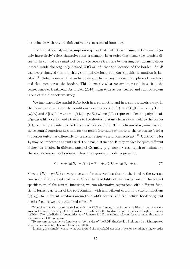
We implement the spatial RDD both in a parametric and in a non-parametric way. In

the former case we state the conditional expectations in (1) as E[Yi0|Li] = α + f(Li) +

g0(Di) and E[Yi1|Li] = α+ τ + f(Li) + g1(Di) where f(Li) represents flexible polynomials

of geographic location and Di refers to the shortest distance from i’s centroid to the border

(B), i.e. the perpendicular to the closest border point. The inclusion of asymmetric dis-

tance control functions accounts for the possibility that proximity to the treatment border

influences outcomes differently for transfer recipients and non-recipients.20 Controlling for

Li may be important as units with the same distance to B may in fact be quite different

if they are located in different parts of Germany (e.g. north versus south or distance to

the sea, state/country borders). Thus, the regression model is given by:

Yi = α+ g0(Di) + f(Li) + Ti[τ + g1(Di)− g0(Di)] + εi. (2)

Since g1(Di) − g0(Di) converges to zero for observations close to the border, the average

treatment effect is captured by τ . Since the credibility of the results rest on the correct

specification of the control functions, we run alternative regressions with different func-

tional forms (e.g. order of the polynomials), with and without coordinate control functions

(f(Li)), for different windows around the ZRG border, and we include border-segment

fixed effects as well as state fixed effects.21

19Municipalities that were located outside the ZRG and merged with municipalities in the treatmentarea could not become eligible for transfers. In such cases the treatment border passes through the munic-ipalities. The jurisdictional boundaries as of January 1, 1971 remained relevant for treatment throughoutthe duration of the program.

20By presuming symmetric functions on both sides of the RDD threshold, a kink may be misinterpretedas a discontinuity (see Lee and Lemieux, 2010).

21Limiting the sample to small windows around the threshold can substitute for including a higher order

15

Table 3: Distance & assignment variable

ZRG Non-ZRG

Mean Std. Min Max Mean Std. Min Max

Distance to B (Di) 22,702 15,807 88 97,603 40,203 28,497 183 99,953

Distance to G (DGi) 19,647 13,126 3 59,451 87,425 30,298 17,923 157,786

Md 20.337 11.322 3 45 88.021 29.664 42 149

Notes: Distances are in meters and refer to municipality centroids. The assignment variable Md is definedas the minimum distance (in km) from the Iron Curtain that includes the majority share of the district area. Itis determined at the district level according to the 1971 classification. Each municipality is uniquely assigned to adistrict. Three districts (Schluchtern, Einbeck, and Peine) were misassigned as they received treatment althoughnot being eligible according to the rule. Of those districts being eligible all received treatment. We dropped allobservations with a distance of more than 150km to the ZRG border and districts with Md > 150.

The assumptions about the form of the geographic control functions can be further

relaxed by estimating the treatment effect in a non-parametric way. To do so, we employ

local linear regressions and estimate the conditional expectations at the border as stated

in (1). Notice that we base our estimates for E[Yi0|Li = b] and E[Yi1|Li = b] only on

observations in At and Ac, respectively. As in the parametric approach, we may condition

either on a one-dimensional forcing variable Dib or on the location vector Li. In the former

case, we estimate univariate local linear regressions for a set of 20 border points b1, ...,b20

which are allocated at equal distances along the border. The alternative approach follows

Papay, Willett, and Murnane (2011) using a bivariate non-parametric regression with the

arguments Lix and Liy. Due to the well-known curse of dimensionality bivariate local

linear regressions require a much higher density of data. For this reason we favor the

univariate non-parametric approach.22 The corresponding results crucially depend on the

choice of bandwidth. We derive the optimal bandwidth h∗ according to the criterion

suggested by Imbens and Kalyanaraman (2012) and use a triangular kernel (see Fan and

Gijbels, 1996, and Imbens and Lemieux, 2008).23

Table 3 reports descriptive statistics on the distance of observations from the ZRG

border B and from the Iron Curtain G. Although the treated area corresponds mostly

to a narrow band of 40 kilometers there are treated observations in the north-east (in

control function but requires a sufficient density of observations.22We check the sensitivity of our results with 10 and 30 border points. All our results are robust to the

bivariate non-parametric regression approach. See Appendix B, Figure B1 for a more detailed descriptionof the non-parametric specifications.

23Alternatively, we use cross-validation procedures and vary the bandwidth manually.

16

particular on the island Fehmarn) located at a distance of up to 100 kilometers from the

ZRG border. The closest municipal centroids lie at about 88 and 183 meters from the ZRG

border for the treated and control groups, respectively. The distances to the Iron Curtain

G range from 3 meters to 158 kilometers. As an alternative to the centroids’ distances

from B and G – which can be very small with narrow municipalities – we approximate

the location of a municipality by the average over a sufficiently large number of grid cells

within the municipal boundaries. All our results are robust to this alternative.24 Due to

the nature of the transfer program the distance to the Iron Curtain is positively correlated

with the distances to the ZRG border. However, as the location of B is determined by the

districts’ shape, size, and location the correlation between distance to B and G is only

about 0.6 for the boundary sample and reduces to less than 0.05 when we limit the sample

to a 20-kilometer window from B.

This points to an important advantage of our setting, namely the clear geographic

criterion that defined the Zonenrandgebiet. Recall that those districts that accommodated

either 50 percent of its area or population within a band of 40 kilometers to the Iron

Curtain at the beginning of 1971 became part of the ZRG. The blue-shaded area in Panel

A of Figure 2 illustrates the 40-kilometer buffer. It is evident that the ZRG border

roughly follows the buffer, but we observe pixel and municipalities at the same distance

from the Iron Curtain featuring a different treatment status. The political rule allows

us to generate an assignment variable, denoted by Md, indicating a district’s minimum

distance from the Iron Curtain that includes the majority share of the district’s area.

Hence, this assignment criterion does not only depend on a municipality’s distance from

the Iron Curtain but also on the shape of the superordinate district it belongs to. At

M0 = 40, we should expect a discontinuity in the probability of receiving treatment which

we can exploit as exogenous variation to identify the causal effect of transfers on economic

outcomes. As the 40-kilometer buffer has no natural relevance and does not correspond

to administrative borders, it is uncritical to presume that there are no discontinuities in

other relevant factors at M0.

We compute isodistance-curves from the Iron Curtain using GIS software as illustrated

in Panel B of Figure 2. This allows us to compute the area share of each district for each

distance to the Iron Curtain. Finally, we determine for each district the minimum distance

24In this case we split each municipality into 100m× 100m grids, determine longitude, latitude as wellas distances from B and G for each grid cell and take the municipal averages across grid cells to obtaing(D) and f(L).

17

Figure 2: Assignment variable

Panel A. Panel B.

Notes: The above maps show district borders according to the 1971 classification. The light blue area in the lefthand map marks the 40-kilometer distance from the Iron Curtain, the dark blue line refers to the ZRG border. Theright hand map illustrates the buffer lines (in red) drawn in 1km intervals from the Iron Curtain.

buffer where the area share exceeds 50 percent. Table 3 reports descriptive statistics of

Md for the treatment and control groups.25 Apparently, none of the control observations

was eligible for treatment and all exceptions belong to the treatment group. If these

exemptions from the 40-kilometer rule were not too frequent, we should observe a jump

25An alternative translation of the treatment rule would be to compute the area share of a districtwithin the 40-kilometer buffer Sd. We did this as a robustness check and find a pronounced discontinuityat Sd = 0.5 as suggested by the rule. Yet, this assignment variable has the drawback of clustering atSd = 0 and accordingly is less powerful.

18

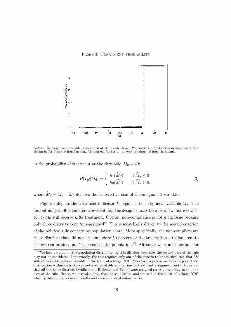
Figure 3: Treatment probability

Notes: The assignment variable is measured at the district level. We consider only districts overlapping with a150km buffer from the Iron Curtain. All districts further to the west are dropped from the sample.

in the probability of treatment at the threshold M0 = 40:

P (Tid|Md) =

{h1(Md) if Md ≤ 0

h0(Md) if Md > 0,(3)

where Md = Md −M0 denotes the centered version of the assignment variable.

Figure 3 depicts the treatment indicator Tid against the assignment variable Md. The

discontinuity at 40 kilometers is evident, but the design is fuzzy because a few districts with

Md > M0 still receive ZRG treatment. Overall, non-compliance is not a big issue because

only three districts were “mis-assigned”. This is most likely driven by the second criterion

of the political rule concerning population share. More specifically, the non-compliers are

those districts that did not accommodate 50 percent of the area within 40 kilometers to

the eastern border, but 50 percent of the population.26 Although we cannot account for

26We lack data about the population distribution within districts such that the second part of the rulemay not be considered. Importantly, the rule requires only one of the criteria to be satisfied such that Md

suffices as an assignment variable in the spirit of a fuzzy RDD. Moreover, a precise measure of populationdistribution within districts was not even available at the time of treatment assignment and it turns outthat all but three districts (Schluchtern, Einbeck, and Peine) were assigned strictly according to the firstpart of the rule. Hence, we may also drop those three districts and proceed in the spirit of a sharp RDDwhich yields almost identical results and even smaller standard errors.

19

this second criterion due to data limitations, we can obtain consistent estimators of the

treatment effect by exploiting the discontinuity in the probability. The average treatment

effect in this case is given by the ratio between the jump in the outcome and the jump in

the treatment probability at M0 (see Lee and Lemieux, 2010 for details).

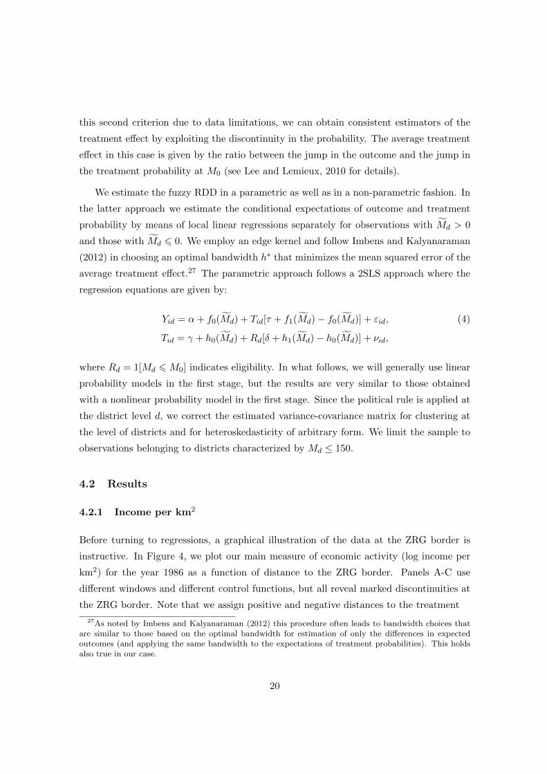
We estimate the fuzzy RDD in a parametric as well as in a non-parametric fashion. In

the latter approach we estimate the conditional expectations of outcome and treatment

probability by means of local linear regressions separately for observations with Md > 0

and those with Md 6 0. We employ an edge kernel and follow Imbens and Kalyanaraman

(2012) in choosing an optimal bandwidth h∗ that minimizes the mean squared error of the

average treatment effect.27 The parametric approach follows a 2SLS approach where the

regression equations are given by:

Yid = α+ f0(Md) + Tid[τ + f1(Md)− f0(Md)] + εid, (4)

Tid = γ + h0(Md) +Rd[δ + h1(Md)− h0(Md)] + νid,

where Rd = 1[Md 6M0] indicates eligibility. In what follows, we will generally use linear

probability models in the first stage, but the results are very similar to those obtained

with a nonlinear probability model in the first stage. Since the political rule is applied at

the district level d, we correct the estimated variance-covariance matrix for clustering at

the level of districts and for heteroskedasticity of arbitrary form. We limit the sample to

observations belonging to districts characterized by Md ≤ 150.

4.2 Results

4.2.1 Income per km2

Before turning to regressions, a graphical illustration of the data at the ZRG border is

instructive. In Figure 4, we plot our main measure of economic activity (log income per

km2) for the year 1986 as a function of distance to the ZRG border. Panels A-C use

different windows and different control functions, but all reveal marked discontinuities at

the ZRG border. Note that we assign positive and negative distances to the treatment

27As noted by Imbens and Kalyanaraman (2012) this procedure often leads to bandwidth choices thatare similar to those based on the optimal bandwidth for estimation of only the differences in expectedoutcomes (and applying the same bandwidth to the expectations of treatment probabilities). This holdsalso true in our case.

20

Figure 4: Discontinuities in economic activity - Contemporaneous effect

Panel A Panel B

Panel C

Note: We run separate regressions on each side of the threshold and control for latitude in a linear form. We usea 3rd-order polynomial distance control function for the 100km window (Panel A), a quadratic control function forthe 40km window (Panel B), and a linear control function for the 10km window (Panel C). The grey-shaded arearepresents the 90-percent confidence interval.

and control region, respectively. By collapsing the two-dimensional location to a scalar

measure of distance from B we cannot ensure that observations to the left and right of

the threshold are de facto located in a short distance from each other. As the ZRG border

runs more or less straight from the south to the north we can mitigate this shortcoming

of the graphical analysis by controlling for a linear trend of latitude.28 It is evident from

Panel A that economic activity declines towards the Iron Curtain. This result is in line

28An alternative and qualitatively equivalent way of displaying the discontinuities would be to regress thevariable in question on border-segment fixed effects and dummy variables for each bin where the coefficientson these distance dummies correspond to points on the polynomial fit displayed in our figures.

21

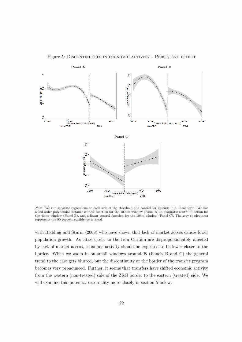
Figure 5: Discontinuities in economic activity - Persistent effect

Panel A Panel B

Panel C

Note: We run separate regressions on each side of the threshold and control for latitude in a linear form. We usea 3rd-order polynomial distance control function for the 100km window (Panel A), a quadratic control function forthe 40km window (Panel B), and a linear control function for the 10km window (Panel C). The grey-shaded arearepresents the 90-percent confidence interval.

with Redding and Sturm (2008) who have shown that lack of market access causes lower

population growth. As cities closer to the Iron Curtain are disproportionately affected

by lack of market access, economic activity should be expected to be lower closer to the

border. When we zoom in on small windows around B (Panels B and C) the general

trend to the east gets blurred, but the discontinuity at the border of the transfer program

becomes very pronounced. Further, it seems that transfers have shifted economic activity

from the western (non-treated) side of the ZRG border to the eastern (treated) side. We

will examine this potential externality more closely in section 5 below.

22

As the ZRG program was eventually stopped in 1994, we inspect whether the jump

in economic activity is still observable at the former treatment border in 2010. Figure 5

contains the same panels as the figure on contemporaneous effects. Although the over-

all level in economic activity has increased over time and the slopes of the curves have

changed, the discontinuities are still visible and the 90 percent confidence intervals do not

overlap. While such graphical analyses provide a transparent first assessment of whether

a discontinuity exists, they provide only limited information about statistical significance

and the magnitude of the effects. We thus turn to regression analysis.

Starting with the spatial RDD, Table 4 confirms the first impressions from the plots:

Regional transfers to the Zonenrandgebiet exerted a strong and significant effect on eco-

nomic activity. We run three types of regressions. First, we include a distance control

function using asymmetric 3rd- and 5th-order polynomials with segment and state fixed

effects. We choose the polynomial orders on the basis of the AIC. Second, we directly

control for the location of each municipality by including coordinates in addition to the

Euclidean distance. Here we choose 2nd- and 3rd-order polynomials and add state fixed

effects.29 In each case we report robust standard errors as well as standard errors that

correct for spatial dependence of unknown form using the method introduced by Conley

(1999).Finally, we run non-parametric regressions where the optimal bandwidth h∗ is com-

puted according to Imbens and Kalyanaraman (2012) and varied manually for sensitivity

analysis in columns (6)-(7).

Among the parametric regressions both the adjusted R2 and the AIC suggest that the

5th-order and 3rd-order polynomials are preferred in case of the distance and coordinate

control functions, respectively. However, the reduction in AIC is only marginal which

indicates that there is no further gain to adding higher order terms. Coordinates cap-

ture location more precisely than distance from simple segment fixed effects such that we

favor the specifications in columns (4) and (5). The latter refers to the non-parametric

approach with optimal bandwidth h∗ which requires less restrictive functional form as-

sumptions. We find that income per km2 is predicted to be about 30-50 percent higher

than in the counterfactual without regional subsidies in 1986, depending on the speci-

fication. Moreover, we can reject the zero for all specifications at a confidence level of

29The cubic polynomial of latitude and longitude is defined as Lix + Liy + L2ix + L2

iy + L3ix + L3

iy +LixLiy + L2

ixLiy + LixL2iy. Note that we choose lower order polynomials for f(.) than for g(.) because

the bivariate control function requires more parameters to be estimated than the corresponding univariatecontrol function.

23

Table 4: Spatial RDD: Income per km2

Distance control Coordinate control Non-parametric3rd 5th 2nd 3rd h∗ 0.8× h∗ 1.2× h∗

Contemporaneous effect

ATE 0.484∗∗∗ 0.583∗∗∗ 0.296∗∗∗ 0.528∗∗∗ 0.311∗∗∗ 0.552∗∗∗ 0.239∗∗∗

(0.099) (0.147) (0.079) (0.099) (0.079) (0.099) (0.069)[0.111] [0.157] [0.089] [0.110] - - -

R2 0.16 0.17 0.14 0.16 - - -AIC 10,750 10,732 10,869 10,741 - - -Obs. 3,870 3,870 3,870 3,870 3,143 2,297 3,694

Persistent effect

ATE 0.503∗∗∗ 0.542∗∗∗ 0.296∗∗∗ 0.535∗∗∗ 0.370∗∗∗ 0.518∗∗∗ 0.288∗∗∗

(0.095) (0.142) (0.076) (0.095) (0.077) (0.097) (0.067)[0.108] [0.154] [0.086] [0.107] - - -

R2 0.21 0.22 0.20 0.22 - - -AIC 10,454 10,438 10,541 10,404 - - -Obs. 3,881 3,881 3,881 3,881 3,095 2,203 3,652

Notes: ∗∗∗, ∗∗, ∗ denote significance at the 1-, 5-, and 10-percent level, respectively. Robust standard er-rors in parenthesis, Conley (1999) standard errors in squared brackets. We drop all observations outside a 100kmwindow of the ZRG border in the parametric specifications. Columns (1)-(4) include state indicators, where (1)and (2) include segment fixed effects in addition. Columns (5)-(7) refer to non-parametric specifications where thebandwidth h∗ is computed according the algorithm introduced by Imbens and Kalyanaraman (2012) and standarderrors are computed according to Imbens and Lemieux (2008).

99 percent. The lower panel displays the corresponding specifications for the persistent

effects of transfers measured in 2010. Notably, all specifications indicate again a positive

and highly significant effect. Most importantly, these estimates remain remarkably similar

for each type of specification in the two panels.

As we have argued before, we can identify causal effects of regional transfers under

even weaker identifying assumptions by exploiting the discontinuity in the probability of

receiving transfers at a distance of 40 kilometers from the ZRG-border. It can be virtually

ruled out that the 40-kilometer threshold mattered for economic outcomes in the absence

of the ZRG program such that this approach is unaffected by potential confounding fac-

tors. However, it comes at the cost of lower efficiency as treatment assignment is carried

out on the district level. Columns (1) and (2) in Table 5 show regressions that use 2nd-

and 3rd-order polynomials of Md as control functions while columns (3)-(5) report non-

parametric regression outcomes with the optimal bandwidth h∗ and manual adjustments.

Standard errors are generally clustered on the level of districts and we obtain qualitatively

24

Table 5: Fuzzy RDD: Income per km2

Parametric Md Non-parametric2nd 3rd h∗ 0.8× h∗ 1.2× h∗

Contemporaneous effect

ATE 0.428∗∗ 0.482∗∗ 0.535∗∗∗ 0.476∗∗∗ 0.564∗∗∗

(0.198) (0.199) (0.087) (0.098) (0.082)

R2 0.077 0.083 - - -AIC 11,110 11,088 - - -Obs. 3,875 3,875 2,143 1,617 2,581

Persistent effect

ATE 0.435∗∗ 0.485∗∗ 0.360∗∗∗ 0.255∗∗∗ 0.424∗∗∗

(0.207) (0.211) (0.076) (0.079) (0.073)

R2 0.134 0.139 - - -AIC 10,793 10,773 - - -Obs. 3,885 3,885 2,874 2,664 3,041

Notes: ∗∗∗, ∗∗, ∗ denote significance at the 1-, 5-, and 10-percent level, respectively. Robust standard er-rors clustered at the district level in parenthesis. Observations with Md > 150 are dropped from the sample.Columns (1) and (2) refer to fuzzy RDD specifications using a two-stage instrumental variables procedure andinclude state indicators. Note that the instrument is highly relevant in each of the first stages. Specifications (3)-(5)refer to non-parametric specification where we compute the bandwidth h∗ according the algorithm introduced byImbens and Kalyanaraman (2012). Standard errors in columns (3)-(5) are computed according to Imbens andLemieux (2008).

identical results if we estimate the specifications on a sample collapsed by districts. Note

that the non-parametric and contemporaneous estimate increases somewhat compared to

the spatial RDD, but the overall picture shows very similar results when comparing the

estimates to the corresponding coefficients in the spatial RDD in Table 4. This establishes

confidence in the consistent estimation of the treatment effect. Notice that all specifica-

tions yield highly significant treatment effects at conventional levels.

Talking about economic magnitude, the effects might appear fairly high at first sight,

but need to be qualified in at least two respects. First, the predicted average treatment

effect in 1986 is the consequence of subsidies since 1971. As we have documented in section

2, transfers to the Zonenrandgebiet have been quite substantial every year. Second, it is

quite plausible that these estimates include negative externalities of shifting activity from

the control area to the treatment area, so these estimates must not be interpreted as

new economic activity generated by the place-based policy. However, we argue that the

estimates reflect the total causal effect of transfers into the Zonenrandgebiet on the spatial

equilibrium. We provide a more detailed discussion of results in subsection 4.2.3 below.

25

Table 6: Pre-treatment – 1961

Parametric Md Non-parametricIncome per km2 2nd 3rd h∗ 0.8× h∗ 1.2× h∗

ATE 0.023 0.008 -0.186 -0.297 -0.189(0.440) (0.443) (0.601) (0.737) (0.541)

R2 0.350 0.352 - - -AIC 1,040 1,041 - - -Obs. 309 309 176 141 193

Notes: ∗∗∗, ∗∗, ∗ denote significance at the 1-, 5-, and 10-percent level, respectively. Robust standard er-rors in parenthesis. Regressions are based on district level data. Observations with Md > 150 are dropped fromthe sample. Columns (1) and (2) refer to fuzzy RDD specifications using a two-stage instrumental variablesprocedure and include state indicators. Note that the instrument is highly relevant in each of the first stages.Specifications (3)-(5) refer to non-parametric specification where the bandwidth h∗ is computed according thealgorithm introduced by Imbens and Kalyanaraman (2012) and standard errors are computed according to Imbensand Lemieux (2008).

Although we have discussed identifying assumptions and their plausibility in this con-

text in detail, a straightforward placebo test is to check whether there was a discontinuity

in economic activity prior to treatment. Unfortunately, income data is unavailable at the

municipality level before 1975, so we take GDP data at the more aggregated district level.

Using estimates for 1961, it is immediate from Table 6 that none of the specifications reveal

higher economic activity in the Zonenrandgebiet that was established only ten years later.

The point estimates are positive in the parametric and negative in the non-parametric

specifications, but all of the estimates are far from being statistically significant. Further,

we use pre-treatment information about population density which is available at the mu-

nicipality level and confirms that there are no discontinuities at the ZRG border prior to

the start of the program (see Figure 6).

4.2.2 Economic channels

What are the underlying channels of higher economic activity in the Zonenrandgebiet? We

study a number of potential mechanisms through which regional transfers might operate.

Most obviously, as transfers were primarily targeted to subsidize firm investments and

public infrastructure, we employ data on private and public capital to explore whether

discontinuities prevail. The German Statistical Office provides information about the area

share covered by plants, residential structures, or roads and railways. We also use the

business tax base as an alternative proxy for the private capital stock.

26

Table 7: Channels I: Capital

Contemporaneous effects Persistent effects

Coordinate control Nonparametric Coordinate control Nonparametric

2nd 3rd h∗ 2nd 3rd h∗

Business tax base per km2

ATE 0.366∗∗∗ 0.720∗∗∗ 0.652∗∗∗ 0.463∗∗∗ 0.848∗∗∗ 0.800∗∗∗

(0.124) (0.157) (0.148) (0.114) (0.144) (0.142)

R2 0.17 0.19 - 0.18 0.20 -

AIC 12,795 12,718 - 13,244 13,161 -

Obs. 3,533 3,533 2,318 3,792 3,792 2,299

Private capital stock

ATE 0.197∗∗∗ 0.341∗∗∗ 0.291∗∗∗ 0.193∗∗∗ 0.298∗∗∗ 0.278∗∗∗

(0.062) (0.078) (0.070) (0.058) (0.073) (0.066)

R2 0.11 0.13 - 0.07 0.08 -

AIC 8,895 8,830 - 8,420 8,369 -

Obs. 3,845 3,845 2,730 3,851 3,851 2,839

Industrial/private capital stock

ATE 0.113 0.346∗ 0.581∗∗ 0.134∗ 0.179∗ 0.174∗∗

(0.139) (0.181) (0.230) (0.076) (0.098) (0.079)

R2 0.10 0.11 - 0.08 0.09 -

AIC 3,074 3,068 - 7,982 7,966 -

Obs. 1,259 1,259 316 3,230 3,230 2,507

Public capital stock

ATE 0.147∗∗∗ 0.111∗∗∗ 0.153∗∗∗ 0.172∗∗∗ 0.138∗∗∗ 0.207∗∗∗

(0.032) (0.040) (0.039) (0.032) (0.040) (0.040)

R2 0.27 0.27 - 0.25 0.26 -

AIC 3,885 3,851 - 3,760 3,718 -

Obs. 3,855 3,855 2,433 3,865 3,865 2,312

Notes: ∗∗∗, ∗∗, ∗ denote significance at the 1-, 5-, and 10-percent level, respectively. Robust standard er-

rors in parenthesis. We drop all observations outside a 100km window of the ZRG border in the parametric

specifications. Columns (1)-(2) and (4)-(5) refer to parametric specifications and include state indicators. Columns

(3) and (6) refer to non-parametric specifications where the bandwidth h∗ is computed according the algorithm

introduced by Imbens and Kalyanaraman (2012) and standard errors are computed according to Imbens and

Lemieux (2008). Business tax base per km2 and Business tax base per employee are measured in logarithmic terms.

The three measures of capital stocks are bounded between zero and unity and which renders estimating linear

models inappropriate. Thus we apply a logit transformation to public capital, private capital and industrial/private

capital.

27

A second reason for higher economic activity per square kilometer could be changes in

population and employment. Investment subsidies may also raise labor demand and labor

productivity (arguably through higher capital stock) affecting the migration decision of

households. Furthermore, the ZRG program also supported renovation of private homes,

social housing, and cultural activities rendering living in the treatment area more appeal-

ing. Finally, we explore whether the human capital of the workforce differs systematically

between the treatment and the control area.

For the sake of brevity, we show results from the spatial RDD stressing that the findings

are robust to using fuzzy RDD.30 Table 7 summarizes contemporaneous and persistent

effects of the transfer program on capital. We only report 2nd- and 3rd- order polynomials

of the augmented coordinate control specifications and non-parametric regressions based

on the optimal bandwidth h∗. The estimates suggest that the ZRG treatment has led to

a markedly higher stock of both private and public capital. For example, the business tax

base per square kilometer is predicted to be around 60-70 percent higher in 1986. Looking

at persistence in 2010, we still find a highly significant effect at an even higher level of

around 80 percent. Taking the area share covered by plants and residential structures, our

estimates suggest that transfers have raised the capital stock by about 30 percent both in

1984 and 2010. Distinguishing between industrial and residential struc-tures, we observe

that ZRG treatment led to a higher increase in industrial premises. The public capital

stock is predicted to be about 10-20 percent higher compared to the counterfactual.

Turning to labor as a potential channel for higher economic activity and using the same

specifications as above, Table 8 reveals that population density was raised by about 40

percent with no indication of a decline in the long term. Econometrically speaking, com-

muting is costless at the ZRG-border so the change in population can only be attributed to

subsidies for social housing and renovation of private residences. The discontinuity in em-

ployment per square kilometer is even more pronounced at about 60-70 percent indicating

substantial commuting into the Zonenrandgebiet. However, we find no evidence that the

composition of the workforce with respect to skills was affected by treatment. The share

of high-skilled employees in the Zonenrandgebiet does not differ from the counterfactual

scenario without transfers.

It is informative to take a closer look at how the magnitude of effects has developed over

time. As we have argued in the previous subsection, GDP is only available at the district

30Results from the fuzzy RDD can be obtained from the authors upon request.

28

Table 8: Channels II: Labor

Contemporaneous effects Persistent effectsCoordinate control Nonparametric Coordinate control Nonparametric2nd 3rd h∗ 2nd 3rd h∗

Population per km2

ATE 0.239∗∗∗ 0.434∗∗∗ 0.372∗∗∗ 0.290∗∗∗ 0.473∗∗∗ 0.425∗∗∗

(0.069) (0.087) (0.077) (0.071) (0.089) (0.079)R2 0.19 0.21 - 0.18 0.21 -AIC 9,846 9,746 - 9,988 9,876 -Obs. 3,870 3,870 2,745 3,881 3,881 2,717

Employment per km2

ATE 0.418∗∗∗ 0.658∗∗∗ 0.692∗∗∗ 0.467∗∗∗ 0.723∗∗∗ 0.741∗∗∗

(0.108) (0.137) (0.124) (0.110) (0.140) (0.133)R2 0.18 0.20 - 0.16 0.17 -AIC 13,120 13,052 - 12,407 12,346 -Obs. 3,826 3,826 2,601 3,665 3,665 2,269

Human capital

ATE 0.016 0.213∗ 0.113 -0.076 0.116 -0.054(0.082) (0.109) (0.079) (0.071) (0.092) (0.074)

R2 0.13 0.14 - 0.12 0.14 -AIC 3,555 3,541 - 5,372 5,337 -Obs. 1,782 1,782 1,373 2,576 2,576 1,886

Notes: ∗∗∗, ∗∗, ∗ denote significance at the 1-, 5-, and 10-percent level, respectively. Robust standard er-rors in parenthesis. We drop all observations outside a 100km window of the ZRG border in the parametricspecifications. Columns (1)-(2) and (4)-(5) refer to parametric specifications and include state indicators. Columns(3) and (6) refer to non-parametric specifications where the bandwidth h∗ is computed according the algorithmintroduced by Imbens and Kalyanaraman (2012) and standard errors are computed according to Imbens andLemieux (2008). Population per km2, Employment per km2, and Income per capita are measured in logarithmicterms. Human capital is bounded between zero and unity and which renders estimating linear models inappropriate,thus we apply a logit transformation.

level and at fewer intervals than population data. Since we have found significant and large

effects of ZRG transfers on population density, we run the specification with coordinate

control functions for a number of years between 1961 and 2010. Panel A in Figure 6

reveals differences in population densities between the Zonenrandgebiet and the control

area, while Panel B plots differences in population growth rates for several periods. Note

that the points and bars illustrate the point estimates and confidence bands of parametric

specifications according to (2). These outcomes shed light on how transfers unfolded their

effects over time. Several interesting observations stand out. First, prior to treatment

29

Figure 6: Dynamics

Population density Population growth

Note: The outcomes are based on spatial RDD with 2nd-order asymmetric coordinate control functions, 100kmboundary sample, and – depending on data availability – between 3,523 (in 1950) and 3,881 (in 2010) municipalitiesper year. The vertical lines mark 90-percent confidence intervals. Average annual growth rates are computed forthe intervals 1950-1961, 1961-1975, and from then onwards in five-year intervals. The point estimates suggest a15-percent higher population density in the treated regions by 1975 which is well in line with the estimated increasein annualized population growth between 1961-1975 of about 1 percent.

there is neither a significant difference in population density nor in population growth.

This finding is in line with the insights from Table 6 that there was no discontinuity in

GDP per square kilometer in 1961. Second, with the introduction of the transfer scheme

the difference in population density developed rather quickly over the first five to ten years

while the difference in population growth steadily declined afterwards reaching an almost

equal level across treated and control units until the end of the 1980s. Third, there is a

surge in relative population growth in the decade after reunification in 1990. This points

to an interaction of access to markets in the East with locational advantages due to public

investments in the Zonenrandgebiet. We examine this aspect more closely in section 7.2

below.

4.2.3 Discussion: What explains persistence?

We have shown that transfers to the Zonenrandgebiet led to a persistent increase in in-

come per square kilometer in the target region, channelled through higher capital stock,

population and employment. This outcome can be interpreted as causal if the former

ZRG-border does not exhibit any other discontinuity ex post. For example, one can think

30

Table 9: Other policies

Local business tax rates (2010) Federal transfers per capita 1994-2010Coordinate control Nonparametric Coordinate control Nonparametric2nd 3rd h∗ 2nd 3rd h∗

ATE 0.011∗ -0.001 0.012 45.177 163.825 6.219(0.007) (0.008) (0.007) (159.865) (202.927) (33.509)

R2 0.30 0.31 - 0.01 0.04 -AIC -8,433 -8,450 - 69,799 69,795 -Obs. 3,881 3,881 2,783 3,870 3,870 1,168

Notes: ∗∗∗, ∗∗, ∗ denote significance at the 1-, 5-, and 10-percent level, respectively. Robust standard er-rors in parenthesis. We drop all observations outside a 100km window of the ZRG border in the parametricspecifications. Columns (1)-(2) and (4)-(5) refer to parametric specifications and include state indicators. Columns(3) and (6) refer to non-parametric specifications where the bandwidth h∗ is computed according the algorithmintroduced by Imbens and Kalyanaraman (2012) and standard errors are computed according to Imbens andLemieux (2008). We apply a logit transformation to business tax rates which are bounded between zero and unity.Federal transfers are aggregated over the years 1994-2010 and divided by the municipal population in 1994. We usethe absolute level of Federal transfers per capita (instead of logs) in order to account for zeros. These results arerobust to a zero-inflated Poisson model that accounts for the relatively high number of zero transfers.

about policy makers trying to compensate households and firms in the former treatment

area in various ways. However, German municipalities do not have control over many pol-

icy instruments. Important tax rates like income taxes are chosen at the federal level and

have to be approved by the states. And those taxes that municipalities can set themselves

are mostly too small to be relevant for location decisions. The business tax rate is an

important exception. One could hypothesize that municipalities in the Zonenrandgebiet

lowered their business tax rates after 1994 to compensate firms for the loss in subsidies.

Based on data from the German Statistical Office, Table 9 shows that there is no discon-

tinuity in business tax rates between 1994 and 2010. Our preferred specifications show

insignificant effects. Those that are significant rather point towards higher tax rates in

the Zonenrandgebiet.

Further, policy makers could have decided to compensate former ZRG-municipalities

by an alternative transfer scheme that substituted the old program, at least to some extent.

We use data from the main regional transfer program, the Joint Task, to illustrate that

there is no discontinuity in transfer recipience for municipalities at the former ZRG border

between 1994 and 2010 (Table 9, columns (4)-(6)). Instead, we observe a discontinuity

at the former inner-German border. This result fits into the general picture that regional

transfers moved to the new Lander after German reunification (Appendix C, Figure C1).

31

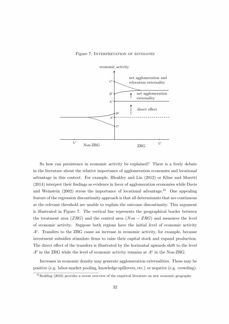
Figure 7: Interpretation of estimates

Non-ZRG ZRG

direct effect

net agglomerationexternality

net agglomeration andrelocation externality

Ac

At

Bc

Bt

Cc

Ct

economic activity

LtLc

So how can persistence in economic activity be explained? There is a lively debate

in the literature about the relative importance of agglomeration economies and locational

advantage in this context. For example, Bleakley and Lin (2012) or Kline and Moretti

(2014) interpret their findings as evidence in favor of agglomeration economies while Davis

and Weinstein (2002) stress the importance of locational advantage.31 One appealing

feature of the regression discontinuity approach is that all determinants that are continuous

at the relevant threshold are unable to explain the outcome discontinuity. This argument

is illustrated in Figure 7. The vertical line represents the geographical border between

the treatment area (ZRG) and the control area (Non − ZRG) and measures the level

of economic activity. Suppose both regions have the initial level of economic activity

Ac. Transfers to the ZRG cause an increase in economic activity, for example, because

investment subsidies stimulate firms to raise their capital stock and expand production.

The direct effect of the transfers is illustrated by the horizontal upwards shift to the level

At in the ZRG while the level of economic activity remains at Ac in the Non-ZRG.

Increases in economic density may generate agglomeration externalities. These may be

positive (e.g. labor-market pooling, knowledge spillovers, etc.) or negative (e.g. crowding).

31Redding (2010) provides a recent overview of the empirical literature on new economic geography.

32

For our example, we assume that the net externality is positive thus shifting the level of

economic activity further upwards.32 If this externality dissipates continuously in space,

there is a positive spillover to the control area. Inside the Non-ZRG, agents located

directly at the treatment border benefit most from this spillover so economic activity

increases the most at this point. The further one moves away from the border, the weaker

the spillover effect becomes. It vanishes entirely at the point where the level of economic

activity reaches Ac, the pre-treatment level. In the treatment area, however, the strength

of the externality is lowest at the ZRG-border because agents are negatively affected

by the lower level of economic activity on the other side of the border. The continuity

ensures that the difference Bt − Bc equals the direct effect At − Ac. Even if we observed

the former, it is straightforward that this discontinuity does not include the spatially-

continuous externality. In other words, the regression discontinuity approach perfectly

controls for continuous spillovers (see Turner, Haughwout, and van der Klaauw, 2014, for

a formal exposition) and thus agglomeration economies.

While this is an important point, our estimate of the average treatment effect is likely

to contain a relocation externality that does show a discontinuity at the treatment border.

Firms that are located in the Non-ZRG close to the treatment border are not indifferent

between locating one meter to the left and one meter to the right of the threshold. We

should thus expect that ZRG-treatment draws economic activity from the control area to

the Zonenrandgebiet. Assuming that migration costs are increasing in distance, we should

observe particularly strong relocation activities in a close neighborhood of the ZRG-border.

Combining this effect with the net agglomeration externality could result in a function that

is represented by the dashed curve in Figure 7. The way we have incorporated it implies

that the relocation externality dominates, but we have no priors about the magnitude

of this relocation externality. If this shifting of economic activity is relevant in size, our

estimates capture both the direct effect and the relocation externality. Note, however, that

the continuous agglomeration externalities still cancel. As one observes the discontinuity

Ct − Cc, it is important to estimate the gradient at the border to obtain the net effect

of the place-based policy, that is the sum of the direct effect and the net agglomeration

externality. We relegate this exercise to the next section.

Returning to the discussion of what explains persistence, we can be sure that it is not

agglomeration economies. But what is it instead? If the discontinuity in capital formation

32Of course, the same argument holds with negative net agglomeration externalities.

33

is the key explanation, why do we not observe a decline in the discontinuity over time?

Capital depreciates at least to some extent over 16 years. Firms must have an incentive to

replace depreciated equipment such that the difference in capital stock is maintained even

in the absence of investment subsidies. The interpretation we suggest is that there must be

sunk factors generating a locational advantage in the former treatment area. For example,

local governments had to provide public infrastructure for industrial parks to accommodate

higher firm activity in the Zonenrandgebiet. Industrial parks themselves needed to be

planned and undeveloped land had to be made ready for building. As these structures are

still available years after the subsidy program has ended, it is plausible that firms looking

for premises are drawn to these industrial parks within ZRG municipalities although no

subsidy draws them to that particular area. In this regard, our findings are closely related

to Davis and Weinstein (2002, 2008) who show that nuclear bombing in Japan in 1945

only had a temporary effect on population and industrial structure. In interpreting their

findings, Redding (2010) argues that “road networks and partially surviving commercial

and residential structures may serve as focal points around which reconstruction occurs.”

Our results are different because, first, it is public policy that changed the economic

structure and thus relative locational advantage between municipalities and, second, the

policy was expected to be long-lasting thus affecting expectations of households and firms.

As a consequence, the temporary policy intervention exhibited long-run implications for

the spatial structure of economic activity.

5 Externalities: What is the net effect of the policy?

5.1 Identification

The above results do not allow inference about the net effect of the policy as the treatment

may affect outcomes in the neighboring control group.33 Thus, in order to make statements

about the policy’s net effect, we need to address the issue of spillovers. In particular, it is

likely that place-based investment subsidies have attracted firms from the control region

to relocate their businesses into the ZRG. Further, net agglomeration externalities may

operate across the treatment border as argued in the previous section. While we cannot

disentangle the two types of externalities, we can estimate the overall magnitude to shed

33This is also referred to as the stable unit treatment value assumption (SUTVA) (Rubin, 1980) whichis often a problematic assumption in natural experiments.

34

light on the net effect of the policy, described by the sum of the direct effect and the net

agglomeration externality in Figure 7.

We follow two alternative approaches to quantify the externality at the border. The

first approach is referred to as spatial exclusion as it relies on estimating the effect for

treatment and control observations that are located sufficiently distant from each other.

The idea is that these municipalities are not affected by (local) externalities of the policy

(see Neumark and Kolko, 2010). Obviously, this approach contradicts the identification

strategy of the spatial RDD which relies on the comparison of outcomes for observations

in a close neighborhood. However, we may execute this exercise in the fuzzy RDD. We

exploit the fact that each district with Md ∼M0 accommodates a number of municipalities

with varying distances to the treatment border. Thus, by excluding municipalities in the

close neighborhood of B we can remove the part of district outcome that is potentially

contaminated by spillovers (see Appendix E, Figure E1 for details). We estimate (4) for a

sub-sample that excludes all municipalities bordering B and additionally establish mini-

mum distances between treatment and control units of 10 kilometers and 20 kilometers in

two alternative specifications. Yet, the requirement to maintain a high density of districts

at the threshold M0 limits the minimum distance we can establish between treatment and

control observations. It may therefore be impossible to eliminate spillovers completely.

In order to address this limitation, we pursue a complementary approach introduced

by Turner, Haughwout, and van der Klaauw (2014) which aims to estimate the outcome

gradient in the control area. In particular, this gradient approach quantifies the differences

in outcomes for control units close to the treatment border and the average value in

the control region. In accordance with Figure 7, this approach delivers an estimate of

Ac − Cc. In the spirit of Turner, Haughwout, and van der Klaauw (2014), we assume

that the externality is symmetric around B such that we cannot reject a zero net effect

if 2(Ac − Cc) equals the discontinuity Ct − Cc we have identified above. The assumption

of symmetric relocation externalities is plausible with moving costs being a continuous

function of distance. For instance, households prefer to stay close to their acquaintances

and friends or firms face increasing costs if they move further away from the suppliers

they have established a relationship with. Defining a binary indicator Iid which is unity

for municipalities within a certain maximum distance from the treatment border and

35

restricting the sample to districts bordering with B, we estimate

Y cid = α+ θd + χIid + f(DGid) + g(DDid) + εi. (5)

We add district fixed effects θd as well as flexible control functions of distance from the

Iron Curtain DGid and distance from the district border DDid in order to control for

confounding factors. The latter should account for economic cores being located in the

district centers and the former should control for the general declining trend in economic

activity towards the Iron Curtain. Note that a large part of this trend is already absorbed

by θd. Moreover, as B follows district borders, it is not highly correlated with G such

that we observe variation in Iid for observations with almost identical distance to the Iron

Curtain.34

To implement the gradient approach, we do not only exploit municipality-level vari-

ation in income per square kilometer, but also proxies for the stock of private capital –

which turned out as one of the primary channels in section 4.2.2 – at a very fine spatial

scale. We use information from satellite images on land coverage at a 100m × 100m res-

olution provided by the European Environmental Agencies CORINE project for the year

1990.35 This allows us to specify proximity to the treatment border Iid at very narrow

intervals to increase the precision of our estimates.36

5.2 Results

The estimation results for the spatial exclusion approach are highlighted in Panel A of

Table 10. There are three specifications: (i) “border” excludes all municipalities adjacent

to the treatment border, (ii) “5,000m” ignores all jurisdictions whose centroid is located

within 5 kilometers to the ZRG border, and (iii) “10,000m” is a similar exercise for the

10-kilometer range. Note that all results are based on the contemporaneous sample.

Starting with the baseline results in columns (2) and (3) of Table 5, we observe from

specification “border” that the average treatment effect drops from 0.482 to 0.449 and from

34The correlation coefficient of Iid and DGid ranges for our municipality- and grid-cell-level samplesbetween 0.18 and 0.28.

35Burchfield, Overman, Puga, and Turner (2006) use similar data for the US to study the determinantsof urban sprawl.

36With the grid-cell data, we add a flexible polynomial of distance to the municipality border to (5) tocontrol for the within-municipality distribution of private capital.

36

0.535 to 0.465 in the parametric and nonparametric specifications, respectively. Further

restricting the sample to minimum distances of up to 10,000 meters yields a reduction of the

point estimates of about 30 and 33 percent compared to the benchmark results. Hence,

assuming that the externality dissipates linearly implies that relocation activities must

occur within 60km to explain the total effect. Note, however, that this would comprise

a substantial part of West Germany as the mean distance to B across all non-treated

municipalities (in all states) is about 113km. With a minimum distance of 10,000m we

loose efficiency and the share of observations displaying a level of Md in the neighborhood

of 40 drops considerably.37 Accordingly, this approach provides evidence for substantial

relocation externalities, but we may not completely determine the spatial extent of these

negative spillovers.

Panel B of Table 10 reports the findings from the gradient approach where columns

(1)-(3) display the results for income per square kilometer with distance bands of 1,500m,

2,500m, and 5,000m from the treatment border to identify observations in the control

region that are particularly prone to the relocation externality. Each of the coefficients

on these indicators shows a negative sign of about 0.2. Thus, assuming symmetry of

the externality and taking our benchmark discontinuity estimates of 0.528 (see column

(4) in Table 4), we argue that the negative point estimates of the externalities results

in a low net effect. We attribute the negative sign of the sum of externalities mainly

to relocation activities while it could in principle also reveal negative net agglomeration

externalities. However, given the low density of municipalities in this region, we find

the latter interpretation rather implausible. Accounting for the imprecise nature of the

estimates, we cannot reject that the discontinuity at the ZRG border is fully driven by a

relocation of economic activity from western regions towards the subsidized municipalities.

Columns (4)-(6) refer to the grid-cell data on private capital stock. We estimate lin-

ear probability models with the corresponding main discontinuity effects being reported

in Table D1 in the Appendix. Exploiting distance bands of 500m, 1,000m, and 1,500m

from the treatment border confirms the previous result. We find that cells outside and

in the close neighborhood of the treatment area are significantly less likely to be covered

by private buildings. Moreover, the direct effect suggests that ZRG treatment increases

the probability of a grid-cell being covered by private capital by about 1.6 percentage

37While Md ∈ [30, 50] holds for about 15 percent of the observations in our benchmark specification,this share drops to about 8 percent with the 10km-exclusion window.

37

Table 10: Externalities

A. Spatial exclusion approach

Log income 3rd. order polynomial of Md Nonparametric h∗

per km2 border 5,000m 10,000m border 5,000m 10,000m

ATE 0.449∗∗ 0.396∗ 0.336 0.465∗∗ 0.435∗∗ 0.358(0.220) (0.209) (0.239) (0.217) (0.218) (0.259)

R2 0.09 0.09 0.10 - - -Obs. 3,514 3,408 3,084 1,784 1,678 1,360

B. Gradient approach

Log income per km2 Prob(PrivateCapital = 1)1,500m 2,500m 5,000m 500m 1,000m 1,500m

χ -0.183 -0.198∗ -0.224∗∗ -0.008∗∗ -0.007∗ -0.008∗∗

(0.154) (0.117) (0.103) (0.003) (0.004) (0.004)

3rd. order distance to municipal borderall specifications include district fixed effects and 3rd. order distance to G

R2 0.33 0.33 0.33 0.03 0.03 0.03Obs. 466 466 466 2,330,077 2,330,077 2,330,077

Notes: ∗∗∗, ∗∗, ∗ denote significance at the 1-, 5-, and 10-percent level, respectively. Panel A. excludes allmunicipalities that are bordering B (columns (1), (6)), and are within a distance of 5km and 10km from B (columns(2),(3) and (5),(6)). We estimate the fuzzy RDD specifications using a parametric 2SLS approach in columns(1)-(3) and the nonparametric approach in columns (4)-(6). Observations with Md > 150 are dropped from thesample and standard errors are clustered at the district level. Panel B. estimates the gradient for observationsoutside of the ZRG and within a district that borders B. The dependent variable in columns (1)-(3) is income perkm2 measured on the municipality level; the dependent variable in columns (4)-(6) refers to a binary indicatorwhich is unity if a 100m × 100m grid is covered by private buildings and zero otherwise. χ is the coefficient onan indicator being unity for observations in a certain distance from B: 1,500m-5,000m with municipality data incolumns (1)-(3) and 500m-1,500m with grid cell data in columns (4)-(6). Standard errors are clustered on themunicipality level in the specifications using grid cell data.

points (see column (3) in Table D1) which is about twice the magnitude of the negative

externality.38 Thus, both approaches and both levels of data variation point to a consid-

erable relocation of economic activity. This is consistent with our finding that a shift of

population towards the subsidized regions is among the key drivers of the aggregate effect

on income per square kilometer.

38Note that the discontinuity estimates for Prob(PrivateCapital = 1) on the grid-cell level are wellin line with the estimates for the area share of a municipality covered by private capital as displayed inTable 7. These estimates indicated that the logit-transformed area share, i.e. the odds ratio, increased by19.7-34.1 percent due to transfers. Given that Prob(PrivateCapital = 1) is about 6 percent in our data,a 1.6 percentage points increase in Prob(PrivateCapital = 1) corresponds to ln( 0.076

1−0.0761−0.060.06

) ≈ 0.253,i.e. an increase of about 25.3 percent in the odds ratio.

38

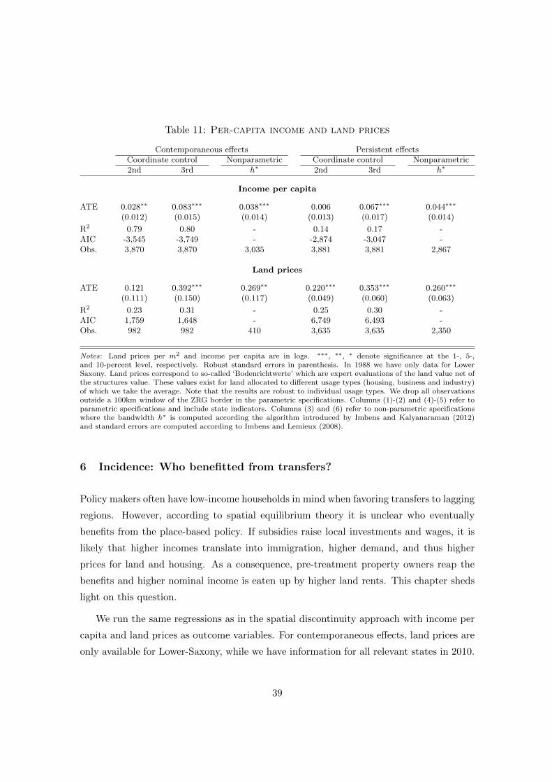
Table 11: Per-capita income and land prices

Contemporaneous effects Persistent effectsCoordinate control Nonparametric Coordinate control Nonparametric2nd 3rd h∗ 2nd 3rd h∗

Income per capita

ATE 0.028∗∗ 0.083∗∗∗ 0.038∗∗∗ 0.006 0.067∗∗∗ 0.044∗∗∗

(0.012) (0.015) (0.014) (0.013) (0.017) (0.014)

R2 0.79 0.80 - 0.14 0.17 -AIC -3,545 -3,749 - -2,874 -3,047 -Obs. 3,870 3,870 3,035 3,881 3,881 2,867

Land prices

ATE 0.121 0.392∗∗∗ 0.269∗∗ 0.220∗∗∗ 0.353∗∗∗ 0.260∗∗∗

(0.111) (0.150) (0.117) (0.049) (0.060) (0.063)

R2 0.23 0.31 - 0.25 0.30 -AIC 1,759 1,648 - 6,749 6,493 -Obs. 982 982 410 3,635 3,635 2,350

Notes: Land prices per m2 and income per capita are in logs. ∗∗∗, ∗∗, ∗ denote significance at the 1-, 5-,and 10-percent level, respectively. Robust standard errors in parenthesis. In 1988 we have only data for LowerSaxony. Land prices correspond to so-called ‘Bodenrichtwerte’ which are expert evaluations of the land value net ofthe structures value. These values exist for land allocated to different usage types (housing, business and industry)of which we take the average. Note that the results are robust to individual usage types. We drop all observationsoutside a 100km window of the ZRG border in the parametric specifications. Columns (1)-(2) and (4)-(5) refer toparametric specifications and include state indicators. Columns (3) and (6) refer to non-parametric specificationswhere the bandwidth h∗ is computed according the algorithm introduced by Imbens and Kalyanaraman (2012)and standard errors are computed according to Imbens and Lemieux (2008).

6 Incidence: Who benefitted from transfers?

Policy makers often have low-income households in mind when favoring transfers to lagging

regions. However, according to spatial equilibrium theory it is unclear who eventually

benefits from the place-based policy. If subsidies raise local investments and wages, it is

likely that higher incomes translate into immigration, higher demand, and thus higher

prices for land and housing. As a consequence, pre-treatment property owners reap the

benefits and higher nominal income is eaten up by higher land rents. This chapter sheds

light on this question.

We run the same regressions as in the spatial discontinuity approach with income per

capita and land prices as outcome variables. For contemporaneous effects, land prices are

only available for Lower-Saxony, while we have information for all relevant states in 2010.

39

We observe from Table 11 that nominal income per capita has increased by about 4-8

percent both contemporaneously and persistently. However, land prices went up by about

25-35 percent, depending on the specification. As households in Germany spend about 30

percent of their net income on rents,39 real wages in the target region have not increased.

These results stand in contrast with the assessment of the federal empowerment zones

program in the US by Busso, Gregory, and Kline (2013). The reason why they do not

find a significant response of population and rental rates in the targeted zones may be

differences in the time-horizon of the policy. Migration decisions are forward-looking and

build on expectations. As ZRG treatment was expected to last for the time of German

division, migration incentives could have been stronger in this case.

Note that local subsidies are likely to exert positive externalities on land prices in the

neighboring regions as shown by Rossi-Hansberg, Sarte, and Owens (2010) for an urban

revitalization program in Richmond (VA). As this externality is continuous in space, our

discontinuity estimates again reflect the direct effect on land prices in the treated area

which does not include potential externalities (see section 4.2.3).

7 Locational advantage and access to markets

We have argued so far that spatially-continuous determinants of economic activity cancel

in the regression discontinuity design and therefore cannot explain our findings of persis-

tence. This does not mean, however, that these factors are unimportant to understand

spatial equilibria. In this section, we study interaction effects of policy-induced locational

advantage with market access to address two important issues. First, we re-estimate the

role of market access for economic development by explicitly accounting for place-based

subsidies to the ZRG in the study of Redding and Sturm (2008). Second, we use German

reunification and EU Eastern enlargement to examine whether this exogenous variation

in market access has caused a head start for ZRG municipalities (due to higher capital

stock). These results inform the debate about whether places with higher density exhibit

higher returns of regional transfers.

39Source: Federal Statistical Office, 2012, Fachserie 15 Reihe 1, Wirtschaftsrechnungen.

40

7.1 Redding and Sturm (2008) revisited

The importance of regional subsidies for the location decision of firms and households has

immediate implications for the findings of Redding and Sturm (2008). In their seminal

paper, Redding and Sturm (2008) have used the natural experiment of German division

to identify a causal effect of market access for economic development. The authors show

that West German cities located closer to the Iron Curtain exhibited lower population

growth rates due to a disproportionate loss in market access. Although they mention

regional subsidies to cities close to the border and discuss their potential relevance for their

estimation, they are unable to control for this influence. As our regression discontinuity

approach has identified large positive effects of these transfers for population density and

population growth close to the former Iron Curtain, we expect market access to have an

even larger impact as suggested by Redding and Sturm (2008) when accounting for the

place-based policy. We rerun their suggested difference-in-differences specification with

their data on 119 West German cities covering the period 1919-1988 and add a dummy

for being located in the Zonenrandgebiet (ZRGi) plus an interaction term of this dummy

and an indicator variable for ZRG-treatment (Transferst) in the 1970s and 1980s. Note

that ZRGi is not equal to our cross-sectional treatment indicator Ti in section 4 because

location in the Zonenrandgebiet implied treatment only from 1971 onwards. Specifically,

we estimate

Popgrowthit =β1Borderi + β2(Borderi ×Divisiont)

+ γ1ZRGi + γ2(ZRGi × Transferst) + θt + εit, (6)

where Popgrowthit is the per-year population growth rate of city i in period t. We follow

Redding and Sturm (2008) in using the same time periods, namely 1919-1925, 1925-1933,

1933-1939, 1950-1960, 1970-1980, and 1980-1988. Borderi indicates whether a city is

located within 75 kilometers to the Iron Curtain and Divisiont is a dummy variable equal

to one after 1950 and zero otherwise. The time-fixed effect θt captures all period-specific

effects applying to all cities alike. Columns (1) and (3) of Table 12 report the results in

columns (1) and (3) of Table 2 in Redding and Sturm (2008). Columns (2) and (4) show

estimates of our specification accounting for place-based policies.

41

Table 12: The costs of remoteness revisited

RS baseline incl. transfers RS distance brackets incl. transfers

Population growth (1) (2) (3) (4)

Border x Division -0.746∗∗∗ -1.084∗∗∗

(0.182) (0.272)

Border 0-25km x Division -0.702∗∗∗ -1.231∗∗∗

(0.257) (0.297)

Border 25-50km x Division -0.783∗∗∗ -1.236∗∗∗

(0.189) (0.253)

Border 50-75km x Division -0.620∗ -0.796∗

(0.374) (0.444)

Border 75-100km x Division 0.399 0.399(0.341) (0.341)

ZRG -0.595∗∗ -0.442(0.281) (0.279)

ZRG x Transfers 0.600∗∗ 0.704∗∗

(0.288) (0.283)

All specifications include border main effects & period fixed effects

R2 0.21 0.22 0.21 0.22

Obs. 833 833 833 833

Notes: ∗∗∗, ∗∗, ∗ denote significance at the 1-, 5-, and 10-percent level, respectively. Robust standard er-rors in parenthesis. We use the data provided by Redding and Sturm (2008) which contains only cities. Theresults are robust to using our main dataset comprising all municipalities. The data spans from 1919 to 1988 wherethe indicators Division and Transfers are unity for post 1950 and post 1971, respectively and zero otherwise.The indicator ZRG is unity for observations located in the subsidized Zonenrandgebiet and Border is unityfor observations within 75km from the inner-German border. Further distance brackets at 25-100km from theinner-German border are included. The correlation between Border × Division and ZRG × Transfers is about0.5.

It is immediate from comparing columns (1) and (2) that the role of market access

for economic development increases by about 45 percent. Cities within 75 kilometers to

the Eastern border exhibit a population growth that is 1.08 percentage points lower than

cities located further west. According to the difference-in-differences specification, ZRG

treatment raised population growth of cities located in this area by 0.6 percentage points

compared to cities outside the ZRG. Note that ZRG and Border differ because the border

of the Zonenrandgebiet is characterized by a distance of less than 75 kilometers to the Iron

Curtain, but some cities fall into both categories (see Table 3). Further, while Division

receives a value of unity from 1950-1988, Transfers only start in the early 1970s.

42

Allowing for different distance brackets to the Eastern border reveals an even stronger

deviation from the results in Redding and Sturm (2008). Comparing columns (3) and

(4) shows that the role of market access is about 75 percent higher within the first 25

kilometers to the Iron Curtain. This effect declines if we move further west. It is 58

percent higher within 25-50 kilometers, and 28 percent higher within 50-75 kilometers

distance. As cities located more than 75 kilometers away from the border generally did

not receive treatment, the difference in the estimates vanishes completely.

7.2 Did the ZRG benefit more from reunification and EU Enlargement?

Do place-based subsidies exhibit higher returns in lagging regions with lower density? Or

should the money rather be invested in highly-agglomerated areas? Glaeser and Gottlieb

(2008) argue that “current transportation spending subsidizes low-income, low-density

places where agglomeration effects are likely to be weakest.” While this statement refers

to the US, European regional policy has a similar focus.

To better understand marginal effects of regional transfers, we look at the interaction

between policy-generated locational advantage and market access. Better market access

implies stronger home-market effects boosting productivity and income. We thus take

advantage of German reunification and EU Eastern enlargement in 2004 as sources of

exogenous variation in market access to examine whether municipalities in the ZRG bene-

fitted more from market access than jurisdictions outside the treatment area.40 Based on

the findings above, we could attribute heterogeneous effects to policy-induced differences

in capital stock or locational advantage.

To identify the effects, we combine the discontinuity approach with the time variation

to examine whether discontinuities differ before and after the events. This design is referred

to as “differences-in-discontinuities” in the literature (Grembi, Nannicini, and Troiano,

2014).41 Comparing municipalities in the close neighborhood of the ZRG-border ensures

that municipalities are affected similarly by changes in market access. Moreover, we

should expect that municipalities closer to the inner-German border benefitted more from

40In a related difference-in-differences approach, Brulhart, Carrere, and Trionfetti (2012) study theemployment response in Austrian municipalities due to the Fall of the Iron Curtain.

41Typically, regression discontinuity identification is combined with differences over time if the RDassumptions are not satisfied due to confounding discontinuities. As the RD assumptions are valid in ourcase, we can use the additional variation to exploit treatment effect heterogeneity.

43

market integration with East Germany than municipalities located further south in the

neighborhood of the Czech Republic and Austria (see Figure 1). We thus restrict the

sample to those jurisdictions being closer to the inner-German compared to the Czech-

German border in the first exercise and vice versa for EU enlargement.

Starting with German reunification, we use the time periods 1980-1985, 1985-1991,

1991-1995, and 1995-2000. Our difference-in-discontinuities specification can be directly

derived from (2) where ZRGi indicates again whether a municipality is located in the

Zonenrandgebiet and Reunificationt is a dummy variable equal to one after 1990 and

zero otherwise. Hence, we estimate

Popgrowthit =α+ g0(Di) + f(Li) + ZRGi[τ + βReunificationt + g1(Di)− g0(Di)]

+Reunificationt + εit, (7)

where flexible and asymmetric polynomials of distance to B and of Cartesian coordinates

are included. We focus on population growth due to superior data coverage. The corre-

sponding results are reported in Panel A of Table 13. The first two columns refer to the

entire boundary sample while columns (3) and (4) exclude observations that are closer to

the border to the Czech Republic than to the inner-German border. Indeed, we observe

across all specifications that the interaction Reunificationt × ZRGi enters significantly

positive. Moreover, the effect tends to be somewhat more pronounced for the sub-sample

of municipalities at the inner-German border and we find that the main effect of ZRGi

ceases to be significant with the 3rd-order polynomial. In sum, reunification raised pop-

ulation growth in the ZRG by about 0.13-0.17 percent. Note that the boundary sample

focuses on municipalities in the eastern part of West Germany and accordingly, we observe

that population growth rates increased due to reunification also for units outside the ZRG.

The second exercise (EU enlargement) focuses on the time periods 1995-2003 and 2004-

2010 and substitutes Reunificationt in (7) with an indicator Integrationt being equal to

one after the integration of the Czech Republic into the European Union in 2004 and

zero otherwise. The corresponding results in Panel B of Table 13 are structured in the

same way as in the case of reunification. However, columns (3) and (4) are now confined

to municipalities that are located closer to the Czech-German border (stretching about

356km) than to the inner-German border.

44

Table 13: Reunification & EU integration

A. Reunification: 1980-2000

Boundary sample Dist(GDR)<Dist(CZ)Population growth 2nd. order 3rd. order 2nd. order 3rd. order

ZRG 0.231∗∗∗ 0.136∗ 0.220∗∗∗ 0.122(0.061) (0.075) (0.063) (0.077)

Reunification 0.724∗∗∗ 0.724∗∗∗ 0.744∗∗∗ 0.744∗∗∗

(0.029) (0.029) (0.030) (0.030)Reunification × ZRG 0.139∗∗∗ 0.140∗∗∗ 0.174∗∗∗ 0.174∗∗∗

(0.046) (0.046) (0.048) (0.048)

includes coordinate controls

R2 0.11 0.11 0.12 0.12AIC 51976.69 51926.77 49533.16 49497.36Obs. 14,948 14,948 14,156 14,156

B. EU integration: 1995-2010

Boundary sample Dist(CZ)<Dist(GDR)Population growth 2nd. order 3rd. order 2nd. order 3rd. order

ZRG 0.257∗∗∗ 0.223∗∗∗ -0.072 -0.292(0.052) (0.065) (0.201) (0.273)

Integration -0.839∗∗∗ -0.839∗∗∗ -0.899∗∗∗ -0.901∗∗∗

(0.025) (0.025) (0.073) (0.072)Integration × ZRG -0.114∗∗∗ -0.114∗∗∗ 0.350∗∗∗ 0.353∗∗∗

(0.039) (0.039) (0.113) (0.112)

includes coordinate controls

R2 0.31 0.32 0.56 0.58AIC 18793.17 18724.79 717.49 705.18Obs. 7,564 7,564 419 419

Notes: ∗∗∗, ∗∗, ∗ denote significance at the 1-, 5-, and 10-percent level, respectively. Robust standard er-rors in parenthesis. We drop all observations outside a 100km window of the ZRG border. ZRG indicates locationin the Zonenrandgebiet, Reunification and Integration are unity for after 1990 and 2004, respectively and zerootherwise. Panel A uses four periods 1980-1985, 1985-1989, 1990-1995, 1995-2000 whereas Panel B uses the periods1995-2003, 2004-2010. Columns (3) and (4) in Panel A (Panel B) refer to sub-samples of municipalities that arelocated closer to the former GDR than to the Czech Republic (closer to the Czech Republic than to the formerGDR).

For the full boundary sample the results indicate that population growth was signifi-

cantly lower after 2004 in the ZRG. However, the majority of ZRG-municipalities is located

closer to the inner-German border being affected by EU enlargement only marginally. If

45

we restrict the sample to those jurisdictions being located close to the Czech-German

border, we find strong and significantly positive effects. Better market access has raised

population growth by 0.35 percent in the ZRG compared to the counterfactual without

transfer recipience. This suggests that the formerly subsidized municipalities in the south

of West Germany did not experience a higher gain from reunification than the control

regions, but experienced such a head start a few years later when markets at their closest

border were integrated.

Our findings from both events point to an important interaction between policy-

induced locational advantage and market access. The results imply that regional transfers

are more effective at places that already exhibit a higher level of market access – like

high-density locations. This stands in sharp contrast with the actual allocation of most

regional transfers to low density places.

8 Conclusions

We have shown in this paper that temporary regional transfers are able to affect the spa-

tial pattern of economic activity in the long run. As the policy was connected to German

division, households and firms expected subsidies to be paid for a longer period and the

volume of transfers was substantial. These circumstances were likely influential as migra-

tion and location decisions are forward-looking. Uncovering underlying mechanisms of this

outcome, we have stressed the importance of capital formation in generating persistence as

our identification approach controls for all spatially-continuous agglomeration economies.

While the policy was effective in changing the economic landscape, we are rather pes-

simistic regarding the net effect of the policy. Estimating local spillovers at the treatment

border points to substantial relocation activities. Our results do not allow us to rule out

that the place-based policy did not generate new economic activity. Moreover, we have

entirely ignored the cost side of the program raising further doubts concerning the effi-

ciency of regional aid. With regard to distributional implications our findings point to

large increases in land rents, so transfers primarily benefitted pre-treatment land owners

in the Zonenrandgebiet rather than raising real wages.

Finally, we have exploited interaction effects between capital structures and market

access to show that municipalities in the Zonenrandgebiet benefitted more from better

46

access to markets in the East than jurisdictions outside the former treatment area. This

indicates that places with larger home markets (higher density) respond more to transfers

than low-density places.

References

Ahlfeldt, Gabriel, Wolfgang Maennig, and Felix Richter. 2013. “Urban Renewal

After the Berlin Wall: A Place-Based Policy Evaluation.” CESifo WP No. 4506.

Bayer, Patrick, Fernando Ferreira, and Robert McMillan. 2007. “A Unified

Framework for Measuring Preferences for Schools and Neighborhoods.” Journal of

Political Economy 115(4): 588-638.

Becker, Sascha, Peter Egger, and Maximilian von Ehrlich. 2010. “Going NUTS:

The Effect of EU Structural Funds on Regional Performance.” Journal of Public

Economics 94(9-10): 578-590.

Becker, Sascha, Peter Egger, and Maximilian von Ehrlich. 2012. “Too Much

of a Good Thing? On the Growth Effects of the EU’s Regional Policy.” European

Economic Review 56(4): 648-668.

Black, Sandra. 1999. “Do Better Schools Matter? Parental Valuation of Elementary

Education.” Quarterly Journal of Economics 114(2): 577-599.

Bleakley, Hoyt, and Jeffrey Lin. 2012. “Portage and Path Dependence.” Quarterly

Journal of Economics 127(2): 587-644.

Brulhart, Marius, Celine Carrere, and Federico Trionfetti. 2012. “How Wages

and Employment Adjust to Trade Liberalization: Quasi-Experimental Evidence from

Austria.” Journal of International Economics 68(1): 68-81.

Bundesministerium fur innerdeutsche Beziehungen. 1987. “Ratgeber Zonen-

randforderung.” Bonn.

Burchfield, Marcy, Henry G. Overman, Diego Puga, and Matthew A. Turner.

2006. “Causes of Sprawl: A portrait from Space.” Quarterly Journal of Economics

121(1): 587-633.

47

Busso, Matias, Jesse Gregory, and Patrick Kline. 2013. “Assessing the Incidence

and Efficiency of a Prominent Place Based Policy.” American Economic Review

103(2): 897-947.

Conley, Timothy C. 1999. “GMM Estimation with Cross Sectional Dependence.”

Journal of Econometrics 92(1): 1-45.

Davis, Donald, and David Weinstein. 2002. “Bones, Bombs, and Break Points: The

Geography of Economic Activity.” American Economic Review 92(5): 1269-1289.

Davis, Donald, and David Weinstein. 2008. “A Search for Multiple Equilibria in

Urban Industrial Structure.” Journal of Regional Science 48(1): 29-65.

Dell, Melissa. 2010. “The Persistent Effects of Peru’s Mining MITA.” Econometrica

78(1): 1863-1903.

Duranton, Gilles and Diego Puga. 2004. “Micro-foundations of urban agglomeration

economies.” in Henderson, Vernon and Jacques Francois Thisse (eds.), Handbook

of Regional & Urban Economics, Vol. 4., Amsterdam: North-Holland, 2063-2117.

Eckey, Hans-Friedrich. 2008. “Verbesserung der regionalen Wirtschaftsstruktur.

Gesetz uber die Gemeinschaftsaufgabe vom 6. Oktober 1969.” in: Eberstein, H.H.

and H. Karl (eds.): Handbuch der regionalen Wirtschaftsforderung, Abschnitt V,

Koln.

EU Commission. 2010. “EU-China Cooperation Activity on ’Regional Policy’ within

the Policy Dialogue between DG Regio and NDRC. Final Report of the Chinese

Exports.” available at http://ec.europa.eu/regional_policy/international/

pdf/china_study_report_en.pdf.

EU Commission. 2011. “Panorama Inforegio 40 – Cohesion Policy 2014-2020. Invest-

ing in Europe’s Regions.” available at http://ec.europa.eu/regional_policy/

sources/docgener/panorama/pdf/mag40/mag40_en.pdf.

Fan, Jianqing, and Irene Gijbels 1996. “Local Polynomial Modelling and its Appli-

cations.” Chapman and Hall, London.

Glaeser, Edvard, and Joshua Gottlieb. 2008. “The Economics of Place-Making

Policies.” Brookings Papers on Economic Activity Spring: 155-253.

48

Gobillon, Laurent, Thierry Magnac, and Harris Selod. 2012. “Do unemployed

workers benefit from enterprise zones? The French experience.” Journal of Public

Economics 96(9-10): 881-892.

Hahn, Jinyong, Petra Todd, and Wilbert van der Klaauw. 2001. “Identifica-

tion and Estimation of Treatment Effects with a Regression-Discontinuity Design.”

Econometrica 69(1): 201-209.

Henderson, Vernon, Adam Storeygard, and David Weil. 2012. “Measuring

Economic Growth from Outer Space.” American Economic Review 102(2): 994-

1028.

Holmes, Thomas. 1998. “The Effects of State Policies on the Location of Industry:

Evidence from State Borders.” Journal of Political Economy 106(4): 667-705.

Imbens, Guido, and Karthik Kalyanaraman. 2012. “Optimal Bandwidth Choice

for the Regression Discontinuity Estimator.” Review of Economic Studies 79(3):

933-959.

Imbens, Guido, and Thomas Lemieux. 2008. “Regression Discontinuity Designs:

A Guide to Practice.” Journal of Econometrics 142(2): 615-635.

Karl, Helmut. 2008. “Entwicklung und Ergebnisse regionaler Wirtschaftspolitik in

Deutschland.” in: Eberstein, H.H. and H. Karl (eds.): Handbuch der regionalen

Wirtschaftsforderung, Abschnitt II, Koln.

Kline, Patrick, and Enrico Moretti. 2014. “Local Economic Development, Agglom-

eration Economies and the Big Push: 100 Years of Evidence from the Tennessee

Valley Authority.” Quarterly Journal of Economics 129(1): 275-331.

Lalive, Rafael. 2008. “How do Extended Benefits Affect Unemployment Duration? A

Regression Discontinuity Approach.” Journal of Econometrics 142(2): 785-806.

Lee, David, and Thomas Lemieux. 2010. “Regression Discontinuity Designs in

Economics.” Journal of Economic Literature 48(2): 281-335.

Neumark, David, and Helen Simpson. 2015. “Place-Based Policies.” in Duranton,

Gilles, Vernon Henderson, and William C. Strange (eds): Handbook of Regional &

Urban Economics - Volume 5, 1197-1287.

49

Neumark, David, and Jed Kolko. 2010. “Do Enterprise Zones Create Jobs? Ev-

idence from California’s Enterprise Zone Program.” Journal of Urban Economics

68(1): 1-19.

Papay, John, John Willett, and Richard Murnane. 2011. “Extending the Re-

gression Discontinuity Approach to Multiple Assignment Variables.” Journal of

Econometrics 161(2): 203-207.

Puga, Diego. 2010. “The Magnitude and Causes of Agglomeration Economies.” Jour-

nal of Regional Science 50(1): 203-219.

Redding, Stephen. 2010. “The Empirics of New Economic Geography.” Journal of

Regional Science 50(1): 297-311.

Redding, Stephen, and Daniel Sturm. 2008. “The Costs of Remoteness: Evidence

from German Division and Reunification.” American Economic Review 98(5): 1766-

1797.

Redding, Stephen, Daniel Sturm, and Nikolaus Wolf. 2011. “History and Indus-

try Location: Evidence from German Airports.” Review of Economics and Statistics

93(3): 814-831.

Rossi-Hansberg, Esteban, Pierre-Daniel Sarte, and Raymond Owens III. 2010.

“Housing Externalities.” Journal of Political Economy 118(3): 485-535.

Rubin, Donald B. 1980. “Randomization Analysis of Experimental Data: The Fisher

Randomization Test Comment.” Journal of the American Statistical Association

75(371): 591-593.

Schumann, Abel. 2014. “Persistence of Population Shocks: Evidence from the Occu-

pation of West Germany after World War II.” American Economic Journal: Applied

Economics 6(3): 189-205.

Turner, Matthew, Andrew Haughwout, and Wilbert van der Klaauw. 2014.

“Land Use Regulation and Welfare.” Econometrica 82(4): 1341-1403.

Ziegler, Astrid. 1992. “Regionale Strukturpolitik: Zonenrandforderung – ein Weg-

weiser?” Koln: Bund-Verlag.

50

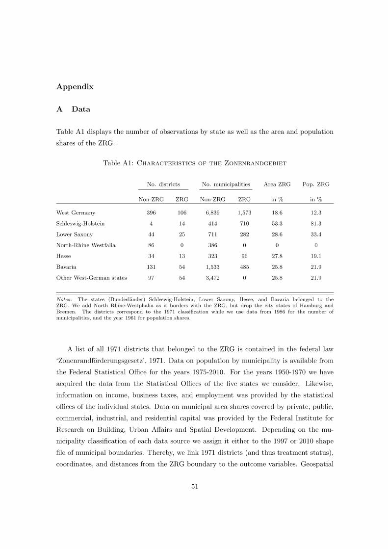
Appendix

A Data

Table A1 displays the number of observations by state as well as the area and population

shares of the ZRG.

Table A1: Characteristics of the Zonenrandgebiet

No. districts No. municipalities Area ZRG Pop. ZRG

Non-ZRG ZRG Non-ZRG ZRG in % in %

West Germany 396 106 6,839 1,573 18.6 12.3

Schleswig-Holstein 4 14 414 710 53.3 81.3

Lower Saxony 44 25 711 282 28.6 33.4

North-Rhine Westfalia 86 0 386 0 0 0

Hesse 34 13 323 96 27.8 19.1

Bavaria 131 54 1,533 485 25.8 21.9

Other West-German states 97 54 3,472 0 25.8 21.9

Notes: The states (Bundeslander) Schleswig-Holstein, Lower Saxony, Hesse, and Bavaria belonged to theZRG. We add North Rhine-Westphalia as it borders with the ZRG, but drop the city states of Hamburg andBremen. The districts correspond to the 1971 classification while we use data from 1986 for the number ofmunicipalities, and the year 1961 for population shares.

A list of all 1971 districts that belonged to the ZRG is contained in the federal law

‘Zonenrandforderungsgesetz’, 1971. Data on population by municipality is available from

the Federal Statistical Office for the years 1975-2010. For the years 1950-1970 we have

acquired the data from the Statistical Offices of the five states we consider. Likewise,

information on income, business taxes, and employment was provided by the statistical

offices of the individual states. Data on municipal area shares covered by private, public,

commercial, industrial, and residential capital was provided by the Federal Institute for

Research on Building, Urban Affairs and Spatial Development. Depending on the mu-

nicipality classification of each data source we assign it either to the 1997 or 2010 shape

file of municipal boundaries. Thereby, we link 1971 districts (and thus treatment status),

coordinates, and distances from the ZRG boundary to the outcome variables. Geospatial

51

data processes have been performed and documented in ArcGIS.

B Non-parametric estimation

For the nonparametric identification strategy we resort to local linear regressions as these

are particular well-suited for inference in the RDD (see Fan and Gijbels, 1996; Imbens

and Lemieux, 2008). We employ an edge kernel function and choose different bandwidths

according to optimality criteria. We compute the distance of each municipality’s centroid

to 20 (or 30) border points that are allocated at equal distances along B as shown in Figure

B1. Then, we assign municipalities to the closest border point, add border-point fixed

effects, and use the distance to the respective border point in the local linear regressions

to estimate E[Yi0|Li = b] and E[Yi1|Li = b]. All our results are insensitive to choosing

20 or 30 border points (red dots and blue triangles in Figure B1, respectively).

As a further robustness check, we refrain from allocating border points and estimate

bivariate local linear regressions based on Cartesian coordinates. In this approach we use

a product kernel Khx(Lix − L0x)Khy(Liy − L0y) and minimize:

n∑i=1

{Yi − α− (Lix − L0x)β1 − (Liy − L0y)β1}2Khx(Lix − L0x)Khy(Liy − L0y). (B.1)

Again, this is done separately for units west and east of B to obtain α for both sides.

The pair of bandwidths is chosen according to a cross-validation criterion. In practise

this approach is less efficient than the univariate approach based on border points because

the additional dimension requires disproportionately more observations. Therefore, we

present our non-parametric results generally for the border point approach and note that

all results are robust to employing bivariate local linear regressions (corresponding tables

are available upon request).

52

Figure B1: Border points

Notes: The red dots (green triangles) mark the 20 (30) border points we employ in our analysis. These are allocated

at equal distances along the ZRG border. The black lines mark the inner-German border and the state borders. The

treated states were Bavaria (B), Hesse (H), Lower Saxony (LS) and Schleswig-Holstein (SH). The Czechoslovakian

border is marked in purple. When splitting up the sample into treated units closer to the former GDR or to

Czechoslovakia we use the perpendicular distances of municipal centroids or pixels to the respective borders.

C Regional transfers after 1994

Information on federal regional transfers by recipient municipality, year, and transfer type

was provided by the Federal Office for Economic Affairs and Export Control. We aggregate

over transfer types (infrastructure and subsidies to the private sector) and over years.

While it still holds true after 1994 that transfers are channeled to the east of Germany,

we do not observe a discontinuity at the former ZRG border as is shown in Figure C1.

The left-hand plot corresponds to the results presented in Table 9. Taking into account

that the program was terminated in 1994 and that the former ZRG border does not

correspond to district borders while transfer intensities are determined by districts, this is

not surprising. Moreover, from the right-hand plot in Figure C1 we observe a pronounced

53

discontinuity of transfer intensity at the former inner-German border. In addition to

federal transfers we have accounted for resources redistributed within states according to

municipal fiscal equalization schemes (in the case of Bavaria). These within state transfers

‘Bedarfszuweisungen’ are at much lower scale (about 0.3 percent of the federal transfers)

and display no discontinuity at B.

Figure C1: Transfers 1994-2010

ZRG border Inner-German border

D Grid-cell data

We use data on PrivateCapital and Radiance for grids of 100m× 100m and 30× 30 arc-

seconds (about 926m×926m at the equator), respectively. Radiance of grids is computed

according to digital integer numbers reported by satellite data of the Defence Meteoro-

logical Satellites Program – Operational Linescan System (DMSP-OLS).42 These data

measure night-time lights in the year 1992 and are widely used in research (see, e.g., Hen-

derson, Storeygard, and Weil, 2012). The information on PrivateCapital is provided by

the European Environmental Agencies CORINE project for the year 1990. The data con-

tains a variable that indicates 44 different land cover classes. We set PrivateCapital = 1 if

a place is covered by ‘Continuous urban fabric’, ‘Discontinuous urban fabric’, ‘Industrial or

commercial units’, or ‘Construction sites’ and zero otherwise. Note that the area-weighted

42The satellite data report digital integer numbers ranging from 0 to 63. These may be converted toradiance as a measure of night luminosity by using the formula radiance = digitalnumber1.5 for a spatialunit which is denoted in terms of Watts/cm2/sr/nm (in words: Watts per squared centimeter per steradianper nanometer of wave length).

54

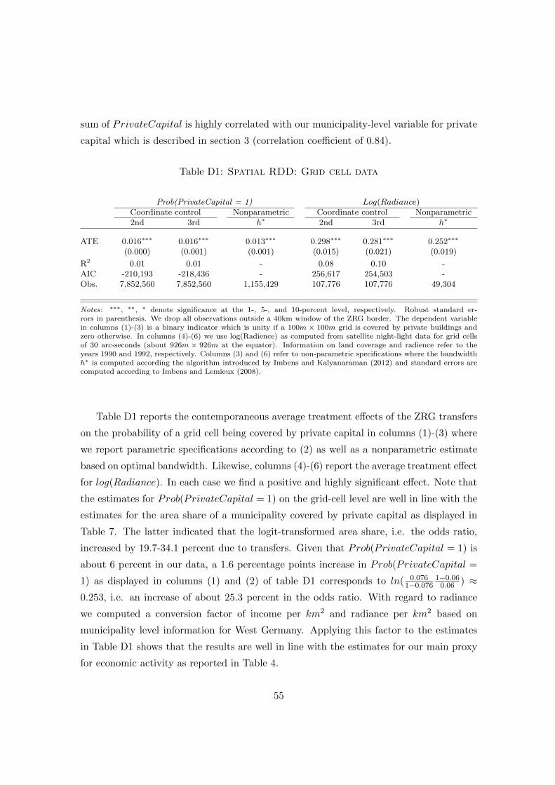
sum of PrivateCapital is highly correlated with our municipality-level variable for private

capital which is described in section 3 (correlation coefficient of 0.84).

Table D1: Spatial RDD: Grid cell data

Prob(PrivateCapital = 1) Log(Radiance)Coordinate control Nonparametric Coordinate control Nonparametric2nd 3rd h∗ 2nd 3rd h∗

ATE 0.016∗∗∗ 0.016∗∗∗ 0.013∗∗∗ 0.298∗∗∗ 0.281∗∗∗ 0.252∗∗∗

(0.000) (0.001) (0.001) (0.015) (0.021) (0.019)

R2 0.01 0.01 - 0.08 0.10 -AIC -210,193 -218,436 - 256,617 254,503 -Obs. 7,852,560 7,852,560 1,155,429 107,776 107,776 49,304

Notes: ∗∗∗, ∗∗, ∗ denote significance at the 1-, 5-, and 10-percent level, respectively. Robust standard er-rors in parenthesis. We drop all observations outside a 40km window of the ZRG border. The dependent variablein columns (1)-(3) is a binary indicator which is unity if a 100m × 100m grid is covered by private buildings andzero otherwise. In columns (4)-(6) we use log(Radience) as computed from satellite night-light data for grid cellsof 30 arc-seconds (about 926m × 926m at the equator). Information on land coverage and radience refer to theyears 1990 and 1992, respectively. Columns (3) and (6) refer to non-parametric specifications where the bandwidthh∗ is computed according the algorithm introduced by Imbens and Kalyanaraman (2012) and standard errors arecomputed according to Imbens and Lemieux (2008).

Table D1 reports the contemporaneous average treatment effects of the ZRG transfers

on the probability of a grid cell being covered by private capital in columns (1)-(3) where

we report parametric specifications according to (2) as well as a nonparametric estimate

based on optimal bandwidth. Likewise, columns (4)-(6) report the average treatment effect

for log(Radiance). In each case we find a positive and highly significant effect. Note that

the estimates for Prob(PrivateCapital = 1) on the grid-cell level are well in line with the

estimates for the area share of a municipality covered by private capital as displayed in

Table 7. The latter indicated that the logit-transformed area share, i.e. the odds ratio,

increased by 19.7-34.1 percent due to transfers. Given that Prob(PrivateCapital = 1) is

about 6 percent in our data, a 1.6 percentage points increase in Prob(PrivateCapital =

1) as displayed in columns (1) and (2) of table D1 corresponds to ln( 0.0761−0.076

1−0.060.06 ) ≈

0.253, i.e. an increase of about 25.3 percent in the odds ratio. With regard to radiance

we computed a conversion factor of income per km2 and radiance per km2 based on

municipality level information for West Germany. Applying this factor to the estimates

in Table D1 shows that the results are well in line with the estimates for our main proxy

for economic activity as reported in Table 4.

55

E Spatial exclusion approach

The spatial exclusion approach is illustrated in Figure E1 where the blue line marks

the ZRG border. Blue and yellow shaded areas refer to municipalities in our boundary

sample that belong to treated and non-treated areas, respectively. District boundaries

(according to the 1971 classification) and municipal boundaries are drawn in red and

black, respectively. In the spatial exclusion approach, we drop all treated (non-treated)

municipalities within a certain distance from the closest non-treated (treated) municipality.

The excluded municipalities are located between the blue and yellow areas (the map

corresponds to a 20-kilometer minimum distance between the treatment and the control

group). By dropping those municipalities in the close neighborhood of the treatment

border, we remove the share of GDP of a district that is potentially affected by positive

or negative spillover effects.

Figure E1: Relocation Externalities – Spatial Exclusion Approach

56