Verschrankungsnachweise¨ mit Anwendungen in der ... · iii Quantum Information Theory Group...
131
Verschr¨ ankungsnachweise mit Anwendungen in der Quantenkommunikation Den Naturwissenschaftlichen Fakult¨ aten der Friedrich-Alexander-Universit¨ at Erlangen-N ¨ urnberg zur Erlangung des Doktorgrades Dr. rer. nat. vorgelegt von Hauke H¨ aseler aus T ¨ onning
Transcript of Verschrankungsnachweise¨ mit Anwendungen in der ... · iii Quantum Information Theory Group...
Verschrankungsnachweisemit Anwendungen in derQuantenkommunikation
Den Naturwissenschaftlichen Fakultatender Friedrich-Alexander-Universitat Erlangen-Nurnberg
zurErlangung des Doktorgrades Dr. rer. nat.
vorgelegt vonHauke Haseleraus Tonning

ii
Als Dissertation genehmigt von denNaturwissenschaftlichen Fakultaten der
Universitat Erlangen-Nurnberg
Tag der mundlichen Prufung: 16/02/2010
Vorsitzender der Promotionskommission: Prof. Dr. Eberhard BanschErstberichterstatter: Prof. Dr. Norbert LutkenhausZweitberichterstatter: Prof. Dr. Paul-Gerhard Reinhard

iii
Quantum Information Theory GroupTheoretische Physik I
Lehrstuhl fur OptikInstitut fur Optik, Information und Photonik
Max Planck Forschungsgruppe
Erlangen 2010

iv

v
Summary
In this thesis, we investigate the uses of entanglement and its verification in quantum commu-nication. Typically, it is the presence of entanglement which allows quantum communicationprotocols to outperform their classical counterparts, or to achieve tasks which are infeasible withclassical physics. Therefore, the verification of entanglement can provide fundamental tests tocertify that experimental implementations of such protocols operate quantum mechanically. Themain object here is to develop a verification procedure which is adaptable to a wide range ofapplications, and whose implementation has low requirements on experimental resources. Wepresent such a procedure in the form of the Expectation Value Matrix. The structure of this thesisis as follows:
Chapters 1 and 2 give a short introduction and background information on quantum theoryand the quantum states of light. In particular, we discuss the basic postulates of quantum mecha-nics, quantum state discrimination, the description of quantum light and the homodyne detector.Chapter 3 gives a brief introduction to quantum information and in particular to entanglement,and we discuss the basics of quantum key distribution and teleportation. The general frameworkof the Expectation Value Matrix is introduced.
The main matter of this thesis is contained in the subsequent three chapters, which descri-be different quantum communication protocols and the corresponding adaptation of the entan-glement verification method. The subject of Chapter 4 is quantum key distribution, where thedetection of entanglement is a means of excluding intercept-resend attacks, and the presence ofquantum correlations in the raw data is a necessary precondition for the generation of secret key.We investigate a continuous-variable version of the two-state protocol and develop the Expec-tation Value Matrix method for such qubit-mode systems. Furthermore, we analyse the role ofthe phase reference with respect to the security of the protocol and raise awareness of a corre-sponding security threat. For this, we adapt the verification method to different settings of Stokesoperator measurements.
In Chapter 5, we investigate quantum memory channels and propose a fundamental bench-mark for these based on the verification of entanglement. After describing some physical effectswhich can be used for the coherent storage of light, we focus on the storage of squeezed light.This situation requires an extension of our verification procedure to sources of mixed input states.We propose such an extension, and give a detailed analysis of its application to squeezed ther-mal states, displaced thermal states and mixed qubit states. This is supplemented by finding theoptimal entanglement-breaking channels for each of these situations, which provides us with anindication of the strength of the extension to our entanglement criterion.
The subject of Chapter 6 is also the benchmarking of quantum memory or teleportation ex-periments. Considering a number of recently published benchmark criteria, we investigate thequestion which one is most useful to actual experiments. For this, a criterion must be both strong,i.e., easy to overcome, and it must be implementable with a reasonable amount of experimen-

vi
tal resources. We first compare the different criteria for typical settings and sort them accordingto their resilience to excess noise. Then, we introduce a further improvement to the Expectati-on Value Matrix method, which results in the desired optimal benchmark criterion. Finally, weinvestigate naturally occurring phase fluctuations and find them to further simplify the implemen-tation of our criterion. Thus, we formulate the first truly useful way of validating experiments forthe quantum storage or transmission of light.

vii
Zusammenfassung
In der vorliegenden Arbeit untersuchen wir den Gebrauch und die Verifizierung von Ver-schrankung in der Quantenkommunikation. Ublicherweise ist es die Verfugbarkeit von Ver-schrankung, die es der Quantenkommunikation erlaubt, korrespondierende klassische Protokollezu verbessern oder klassisch unmogliche Prozesse umzusetzen. Demzufolge konnen aus Ver-schrankungsnachweisen fundamentale Benchmark-Verfahren abgeleitet werden, die die quanten-mechanische Wirkungsweise von Experimenten in der Quantenkommunikation belegen. Wichtigist es hierbei, theoretische Kriterien herzuleiten, die in weitreichenden Situationen Anwendungfinden und deren Realisierungen wenig experimentellen Aufwand erforderen. Ein solches Krite-rium wird in Form der Erwartungswert-Matrix eingefuhrt. Diese Arbeit ist wie folgt strukturiert:
Kapitel 1 und 2 geben eine kurze Einleitung und den notigen Hintergrund zur Quantentheo-rie und zu den Quantenzustanden des Lichts. Im Einzelnen werden die grundlegenden Postu-late der Quantenmechanik, die Quantenzustandsunterscheidung, die quantenmechanische Be-schreibung des Lichts und die Homodyn-Messung behandelt. Kapitel 3 gibt eine Einfuhrungzur Quanteninformationstheorie, insbesondere zu Verschrankung, und es werden Grundzugeder Quantenschlusselverteilung und der Teleportation erklart. Die generelle Formulierung derErwartungswert-Matrix-Methode wird eingefuhrt.
Der Hauptteil dieser Arbeit besteht aus den nachfolgenden drei Kapiteln, die verschiedeneQuantenkommunikationsprotokolle und die erforderlichen Anpassungen der Verifizierungsme-thode beschreiben. Kapitel 4 befasst sich mit der Quantenschlusselverteilung, fur die der Nach-weis von Verschrankung benutzt wird, um intercept-resend Angriffe auszuschließen. Die Exis-tenz von Quantenkorrelationen in den zugrundeliegenden Daten ist eine notwendige Vorrausset-zung fur die Erzeugung von geheimen Schlusseln. Wir betrachten ein zwei-Zustands Protokollmit kontinuierlichen Variablen und konstruieren die Erwartungswert-Matrix-Methode fur solcheQubit-Moden-Systeme. Des weiteren untersuchen wir die Rolle der Phasenrefenrenz in Hinsichtauf die Sicherheit des Protokolls und weisen auf eine daraus resultierende Sicherheitslucke hin.Hierfur wird der Verschrankungsnachweis auf verschiede Messungen der Stokes Operatoren an-gepasst.
In Kapitel 5 untersuchen wir Quantenspeicher-Kanale und erstellen dafur auf Ver-schrankungsnachweisen beruhende Benchmark-Verfahren. Wir beschreiben verschiedene phy-sikalische Effekte, die zur Quantenspeicherung genutzt werden konnen, insbesondere die Spei-cherung von gequetschtem Licht. Dies verlangt die Erweiterung unserer Nachweismethodeauf gemischte Eingangszustande. Wir entwickeln eine solche Erweiterung und wenden sieauf gequetschte thermische Zustande, verschobene thermische Zustande und gemischte Qubit-Zustande an. Dies wird erganzt durch die Herleitung von optimierten verschrankungsbrechendenKanalen, wodurch die Starke des Verschrankungsnachweises gepruft werden kann.
Auch Kapitel 6 befasst sich mit Benchmark-Verfahren fur experimentelle Quantenspei-cherung oder Quanten-Transmission. Hier beantworten wir fur mehrere aktuelle Benchmark-

viii
Kriterien die Frage, welches das zweckdienlichste fur tatsachliche Experimente ist. Ein sol-ches Kriterium muss einfach zu erfullen sein und gleichzeitig mit moglichst geringem expe-rimentellem Aufwand implementiert werden konnen. Wir vergleichen zuerst die verschiede-nen Kriterien fur typische Aufbauten und ordnen sie nach Rauschresistenz. Dann erweiternwir die Erwartungswert-Matrix-Methode erneut, was zum gewunschten optimalen Benchmark-Verfahren fuhrt. Abschließend berucksichtigen wir Phasenfluktuationen bei gepulsten Laserquel-len, welche unser Verfahren weiter vereinfachen. Unsere Analyse fuhrt somit zum ersten zweck-dienlichen Benchmark-Verfahren fur Quantenspeicherungs- oder Teleportationsexperimente.
Contents
Summary/Zusammenfassung v
1 Introduction 1
2 Physics background 52.1 Four basic postulates . . . . . . . . . . . . . . . . . . . . . . . . . . . . . . . . 5
2.1.1 State discrimination . . . . . . . . . . . . . . . . . . . . . . . . . . . . 92.2 The quantum state of light . . . . . . . . . . . . . . . . . . . . . . . . . . . . . 10
2.2.1 Phase-space . . . . . . . . . . . . . . . . . . . . . . . . . . . . . . . . . 112.2.2 Gaussian states . . . . . . . . . . . . . . . . . . . . . . . . . . . . . . . 122.2.3 Homodyne detection . . . . . . . . . . . . . . . . . . . . . . . . . . . . 13
3 Quantum information and communication 153.1 Separability and entanglement . . . . . . . . . . . . . . . . . . . . . . . . . . . 153.2 Entanglement criteria . . . . . . . . . . . . . . . . . . . . . . . . . . . . . . . . 17
3.2.1 Non-operational criteria . . . . . . . . . . . . . . . . . . . . . . . . . . 173.2.2 Operational criteria . . . . . . . . . . . . . . . . . . . . . . . . . . . . . 18
3.3 Effective entanglement . . . . . . . . . . . . . . . . . . . . . . . . . . . . . . . 193.4 The Expectation Value Matrix . . . . . . . . . . . . . . . . . . . . . . . . . . . 20
3.4.1 The EVM criterion . . . . . . . . . . . . . . . . . . . . . . . . . . . . . 223.5 Applications . . . . . . . . . . . . . . . . . . . . . . . . . . . . . . . . . . . . . 23
3.5.1 Teleportation . . . . . . . . . . . . . . . . . . . . . . . . . . . . . . . . 233.5.2 Quantum Key Distribution . . . . . . . . . . . . . . . . . . . . . . . . . 24
4 The phase reference in quantum key distribution 274.1 The B92 protocol . . . . . . . . . . . . . . . . . . . . . . . . . . . . . . . . . . 28

x
4.1.1 Continuous-variable variant . . . . . . . . . . . . . . . . . . . . . . . . 284.2 EVM for quadrature detection . . . . . . . . . . . . . . . . . . . . . . . . . . . 29
4.2.1 Modelling of experimental data and results . . . . . . . . . . . . . . . . 314.2.2 Optimal intercept-resend attacks . . . . . . . . . . . . . . . . . . . . . . 334.2.3 Asymmetric variances . . . . . . . . . . . . . . . . . . . . . . . . . . . 35
4.3 Including the local oscillator . . . . . . . . . . . . . . . . . . . . . . . . . . . . 364.3.1 The quantum Stokes operators . . . . . . . . . . . . . . . . . . . . . . . 364.3.2 Entanglement verification with Stokes measurements . . . . . . . . . . . 374.3.3 Intercept-resend attacks exploiting the phase reference . . . . . . . . . . 394.3.4 Additional measurements: 〈S1〉 . . . . . . . . . . . . . . . . . . . . . . 394.3.5 Additional measurements: the total intensity . . . . . . . . . . . . . . . 414.3.6 Channel losses . . . . . . . . . . . . . . . . . . . . . . . . . . . . . . . 44
4.4 Experimental implementation . . . . . . . . . . . . . . . . . . . . . . . . . . . . 45
5 Quantum memory and mixed states 475.1 Implementations of quantum memory . . . . . . . . . . . . . . . . . . . . . . . 48
5.1.1 Atomic ensembles . . . . . . . . . . . . . . . . . . . . . . . . . . . . . 485.1.2 Photon echo . . . . . . . . . . . . . . . . . . . . . . . . . . . . . . . . . 485.1.3 EIT media . . . . . . . . . . . . . . . . . . . . . . . . . . . . . . . . . . 49
5.2 Benchmarking with the EVM . . . . . . . . . . . . . . . . . . . . . . . . . . . . 505.2.1 Pure squeezed test states . . . . . . . . . . . . . . . . . . . . . . . . . . 515.2.2 Optimal measure & prepare channels . . . . . . . . . . . . . . . . . . . 52
5.3 Optimal measure & prepare channels for mixed states . . . . . . . . . . . . . . . 565.4 Mixed test states . . . . . . . . . . . . . . . . . . . . . . . . . . . . . . . . . . 59
5.4.1 Source purifications . . . . . . . . . . . . . . . . . . . . . . . . . . . . 595.4.2 Including ρAC . . . . . . . . . . . . . . . . . . . . . . . . . . . . . . . . 61
5.5 Displaced thermal states . . . . . . . . . . . . . . . . . . . . . . . . . . . . . . 635.6 Mixed qubit states . . . . . . . . . . . . . . . . . . . . . . . . . . . . . . . . . . 64
6 Optimal benchmark criteria 676.1 General setting and previous work . . . . . . . . . . . . . . . . . . . . . . . . . 68
6.1.1 Discarding the unit gain constraint . . . . . . . . . . . . . . . . . . . . . 706.1.2 Benchmarks based on entanglement . . . . . . . . . . . . . . . . . . . . 71
6.2 Benchmark comparison . . . . . . . . . . . . . . . . . . . . . . . . . . . . . . . 716.2.1 Comparison . . . . . . . . . . . . . . . . . . . . . . . . . . . . . . . . . 726.2.2 Approximating the fidelity . . . . . . . . . . . . . . . . . . . . . . . . . 76
6.3 The EVM for three states . . . . . . . . . . . . . . . . . . . . . . . . . . . . . . 786.4 Phase fluctuations . . . . . . . . . . . . . . . . . . . . . . . . . . . . . . . . . . 79
6.4.1 Application to experiments . . . . . . . . . . . . . . . . . . . . . . . . . 82

xi
7 Concluding remarks 85
A Semidefinite programmes 89A.1 Theory . . . . . . . . . . . . . . . . . . . . . . . . . . . . . . . . . . . . . . . . 89A.2 The EVM method as an SDP . . . . . . . . . . . . . . . . . . . . . . . . . . . . 90
B Equivalent methods 93
C A USD-type strategy for two squeezed thermal states 95
D Fidelity and trace distance for qubit states 97
Bibliography 99
Acknowledgements 109
List of publications 111
Curriculum vitae 113

xii

List of Figures
2.1 The homodyne detector. A phase shift φ on the local oscillator mode effectivelyrotates the phase space orientation of detection. . . . . . . . . . . . . . . . . . . 13
3.1 Geometric interpretation of entangled witnesses: W ′ is finer than W and alsooptimal. W ′′ represents a non-linear witness. . . . . . . . . . . . . . . . . . . . 19
3.2 An equivalence class of states. The overlap with the set of separable states showsthat entanglement verification is not possible. . . . . . . . . . . . . . . . . . . . 21
4.1 Results of the EVM method for quadrature detection. The amount of tolerableexcess noise ∆ is plotted for all values of the channel transmission η and theinput state overlap 〈−α|α〉. . . . . . . . . . . . . . . . . . . . . . . . . . . . . . 32
4.2 a) Marginal distribution for the input state |ψ0〉= |α〉. b) Bob’s conditional stateρ
B,E0 after the interaction of the eavesdropper. With probability (1− e), Eve
resent |ψE0 〉; with probability e, she erroneously resent |ψE
1 〉. . . . . . . . . . . . 34
4.3 The minimisation runs over one common variable, which is distributed asym-metrically between Var(x) and Var(p). An appropriately chosen intercept-resendattack can exactly reproduce the curves. . . . . . . . . . . . . . . . . . . . . . . 35
4.4 Signal-state overlap plotted against the Stokes operator variance for a losslesschannel and local oscillator amplitude αLO = 100. Only data points above thegrey shaded area are physically allowed. Solid curve: entanglement verifica-tion without additional measurements. Dashed line: Intercept-resend attack withequal amplitudes in both modes. Dotted line: input state variance for reference. . 38

xiv List of Figures
4.5 Signal state overlap plotted against the Stokes operator variance for the losslesscase with αLO = 100. The renormalised quadrature variances (white circles)coincide with the Stokes operator variances when S1 is measured. Dashed line:input state variance for reference. . . . . . . . . . . . . . . . . . . . . . . . . . . 40
4.6 Variance distribution for a spin coherent state (left) and for a squeezed spin state(right) . . . . . . . . . . . . . . . . . . . . . . . . . . . . . . . . . . . . . . . . 43
4.7 4.7(a): Intercept-resend attacks when Bob monitors the total intensity. Dashed:entanglement verification with quadrature measurements. Solid: intercept-resend attack with two-axis countertwisting. 4.7(b): different attacks for a totalintensity of 104. Dashed: entanglement verification with quadrature detection.Solid line: attack with a mixture of 2-axis twisted and quadrature squeezed states.Dotted line: the same attack with two-mode squeezing instead of two-axis coun-tertwisting. . . . . . . . . . . . . . . . . . . . . . . . . . . . . . . . . . . . . . 44
4.8 The above Stokes operator variances for a channel which transmits half of theinput intensity. The upper two curves scale with the channel transmission η ,while the lower two curves scale with η2. . . . . . . . . . . . . . . . . . . . . . 45
4.9 Wittmann et al. [WFW+09]: Experimental data and theoretical bounds on thenormalised Stokes operator variance. The dashed lines around the EVM bound(solid line) show the margin of statistical errors. The circles represent measuredvariances. . . . . . . . . . . . . . . . . . . . . . . . . . . . . . . . . . . . . . . 46
5.1 Illustration of the photon echo process for two incident light pulses. . . . . . . . 495.2 Three atomic levels in Λ-configuration. The probe field is the input light to be
stored, and the control field drives the transition to the metastable state |c〉. . . . . 505.3 Entanglement verification for pure squeezed states. 5.3(a): Some parameter pairs
are excluded by the uncertainty relation. 5.3(b): boundaries of the detected quan-tum domains for different input overlaps. . . . . . . . . . . . . . . . . . . . . . . 52
5.4 Optimal measure & re-prepare strategy for two squeezed test states. The bound-aries of the classical and the quantum domains coincide. Optimal measurementsin region (A): minimum error discrimination; region (B): unambiguous state dis-crimination and minimum error discrimination . . . . . . . . . . . . . . . . . . . 54
5.5 Schematic of the optimal USD strategy for pure squeezed input states. . . . . . . 555.6 Optimal MP strategy for two a protocol with squeezed thermal states. The un-
physical domain is not shown here. . . . . . . . . . . . . . . . . . . . . . . . . . 595.7 Schematic of a mixed state source, decomposed into a pure state source and a
mixing process. Attributing the mixing process to the quantum channel gives asimple, but suboptimal benchmark. . . . . . . . . . . . . . . . . . . . . . . . . . 60
5.8 Entanglement verification using purifications of the mixed input states. The de-tected quantum domain is slightly smaller than the actual quantum domain. . . . 61

List of Figures xv
5.9 Entanglement verification from different EVMs. Shaded area: no information onthe purifying system; dashed line: one generalised spin operator on the purifyingsystem; dotted line: three generalised spin operators; dashed-dotted line: fivegeneralised spin operators; Solid line: actual boundary of the quantum domain. . 62
5.10 Quantum domain for displaced thermal test states. (a): the quantum domainincreases in size for mixed states. (b): improvements of the entanglement ver-ification by adding two unitary operators to the EVM (dashed) and optimisedmeasure & re-prepare strategy (dashed-dotted) . . . . . . . . . . . . . . . . . . . 63
5.11 Source-replacement scheme for a source of mixed qubit states. An interactionthrough a c-phase gate mixes the initially pure test states. . . . . . . . . . . . . . 65
5.12 Results of the EVM method with qubit states. . . . . . . . . . . . . . . . . . . . 66
6.1 Visualisation of different input ensembles. The Gaussian distribution 6.1(a) andthe ring of coherent states 6.1(b) are infinite sets. . . . . . . . . . . . . . . . . . 69
6.2 Benchmark comparison. Solid: Gaussian distribution of input states [NKI08].Dashed-dotted: The same with unit-gain constraint [HWPC05]. Dotted: Ring ofcoherent states [CAnTB09]. Dashed: Two input states and homodyne detection[HML08]. Circles: Two input states, fidelity-based benchmark [Nam08]. . . . . . 74
6.3 Estimation of a fidelity-based benchmark in terms of quadrature moments. Dot-ted line: Koashi’s criterion with the fidelity approximation from quadrature mo-ments. Circles: The EVM criterion for three input states. . . . . . . . . . . . . . 77
6.4 The dependence of the EVM method on the cardinality N of the input ensemble. . 796.5 Local oscillator and absolute phase reference. Input pulses carry a phase Φ with
respect to the absolute phase reference, which is present on both signal and localoscillator modes. 6.5(c): Equivalent phase shifts: the tested channel is automati-cally phase-randomised. . . . . . . . . . . . . . . . . . . . . . . . . . . . . . . 80
6.6 Rough comparison of experimental results with the EVM method. Solid line:Boundary of the detected quantum domain, with three squeezed input states.Circle: measurement outcomes on the output states, taken from [AFKL07]. . . . 83
C.1 Schematic plot of the two different optimal measure and prepare strategies. . . . 96

xvi List of Figures
1Introduction
The field of quantum information science is still reasonably young, with mainstream interestin it dating back to the early nineties. At the same time, the field is developing and expandingvery rapidly. This can without doubt be explained by the interest it has created in very differentfields, both theoretically and experimentally. Theoretical quantum information on the onehand receives input from theoretical and mathematical physicists, who take an interest in theconnections between information theory and the fundamentals of physics. On the other hand,quantum information has overlap with computer science, due to the new rules for computationalalgorithms it offers and the new ways of communicating information or conducting cryptogra-phy. The experimental side also draws attention from very different areas of physics. Especiallyfor quantum computing, the physical systems which are currently pursued for building alarge-scale quantum computer range from ion-traps to superconducting devices and even tooptical implementations. For any implementation, building a quantum computer is immenselychallenging and requires cutting-edge technologies and the need for further development ofmaterials and manufacturing processes.
In this thesis, we concentrate on quantum communication, i.e., the use of quantum mechani-cally behaving systems to enhance information transfer. A number of theoretical proposals haveemerged in the early days of quantum information science, including quantum key distribution.This is the task of sharing keys in a manner which is unconditionally secure, that is to say, secureagainst an all-powerful eavesdropper, who is limited only by the laws of physics. Another taskwhich is classically impossible is the faithful transmission of an unknown quantum state, knownas teleportation. Here, the resource of an entangled state is directly used by the sender to transmitpart of the information required by the receiver to fully reconstruct the transmitted state. Otherquantum communication tasks, such as superdense coding [BW92], provide enhancements ofclassical protocols.
2 1. Introduction
Experimental implementations of these quantum communication protocols use almost exclu-sively the medium of light. Photons are very apt information carriers, because they hardly interactwith their environment and are therefore relatively simple to shield from loss and noise, and theymove fast in typically used media, such as optical fibre or the atmosphere. The implementationsof qubit protocols typically employ single photon states, or good approximations to these. Thequbit is then formed by two separate modes, and the probability of finding the single photon ineither one of them. Typical detection setups at the receiver’s end use so-called “click/no-click”detectors, i.e. avalanche photodetectors which have single-photon sensitivity, but can only dis-tinguish the absence and the presence of light. This stands in contrast to continuous-variableschemes, which derive their name from continuously distributed measurement outcomes, whichoccur, for example, when the receiver measures the field quadratures of the incoming light. Typ-ical light sources here are pulsed or continuous-wave lasers, which allow for the preparationof low-intensity coherent light or squeezed light. Whether to choose the qubit regime or thecontinuous-variable regime for an implementation of a quantum communication protocol de-pends on requirements on the performance. Very roughly speaking, single-photon implemen-tations can achieve tasks with very high fidelity, but only probabilistically, which may requirerepeated runs. Continuous-variable implementations operate deterministically, but typically per-form tasks with much lower fidelity. Other performance issues are related to technological ad-vances, especially to the properties of single-photon detectors and true single-photon sources.
In general, quantum communication protocols can be implemented very efficiently withthe well-established tools of optics experiments. Linear optics, i.e., the manipulation of lightwith passive optical elements such as beam splitters, mirrors and phase shifters, can achievesurprisingly much from the viewpoint of information processing. The addition of non-linearprocesses, such as parametric down-conversion or the Kerr interaction make it possible toimplement many of the aforementioned protocols with a small number of optical elements.Herein lies another reason for the popularity and the fast spread which quantum communicationhas experienced over the last two decades.
An inevitable side-effect of keen experimental effort is that the implementation of a protocolmay be overly dictated by technological constraints, thus performing a slightly altered protocol.In extreme cases, this can lead to false interpretations of the experimental data. Certainly, the-oretical proposals can also be blamed for this, if they contain hidden assumptions, convolutedrequirements on symmetry or similar pitfalls. Undoubtedly, there is a certain gap between theoryand experiments in quantum communication, and indeed quantum computation.
The work presented in this thesis addresses certain aspects of this gap between theoryand experimental implementation. In particular, we develop a method for the verificationor validation of quantum communication experiments. The aim is to show that a particularimplementation is actually of a quantum mechanical nature, in other words, its output is not

3
classically simulatable1. For a state of light, the question whether it is a classical or a quantumstate has a history of discussion, but no unique answer. Here, we avoid this question andconcentrate on the presence of entanglement, which is an undisputed quantum mechanicalfeature and is the minimal requirement for enhanced quantum communication. This makessense in the light that entanglement is a property of bipartite (or multipartite) systems, and wetypically deal with two communicating parties, which provides a natural bipartite structure.
This thesis has the following structure: Chapter 2 gives a brief account of the required physicsbackground, with a definite information-theoretic flavour. The basic postulates of quantum the-ory are listed, and two examples of quantum measurements, which will be of importance at alater point, are detailed. Furthermore, some aspects of the quantum theory of light and its detec-tion are reviewed. Chapter 3 deals with entanglement and its detection. The concept of effectiveentanglement and the basic formalism of the Expectation Value Matrix (EVM) are introduced.This EVM can be used to formulate entanglement criteria which are both general and practical.We then give a brief description of quantum teleportation and quantum key distribution. Thepresentation of our main work starts with Chapter 4, which deals with the subject of using twoweak coherent states for key distribution. In the description of this continuous-variable protocol,we explicitly include the phase reference, which may lead to a security leak. We then constructan EVM for a binary input state ensemble and quadrature detection and use it to check the pro-tocol against intercept-resend attacks. A second construction in terms of Stokes operators allowsus to analyse the role of the phase reference. Chapter 5 applies the method to the validation ofquantum memories, and the storage of squeezed light in particular. This application raises thenecessity to expand the EVM formalism to mixed input states. The concept of memory valida-tion or benchmarking is developed further in Chapter 6. Here, we attempt to unify a number ofrecent benchmark criteria, by comparing them and distilling the essential ingredients for a strongbenchmark. We find an optimal criterion, which is again formulated as a separability problem,and solved by a suitably constructed EVM. This provides a test which can be administered witha minimal amount of experimental resources.
1We are aware that “simulatable” is not actually a word, but it is just too fitting not to be used here

4 1. Introduction

2Physics background
Quantum information is inextricably linked to the laws of physics, because any active processingof information is performed by apparatuses which are governed by these laws. Any work in thearea of quantum information processing must therefore be founded in an understanding of thelaws of quantum mechanics. Here, we give a brief account of the basic postulates of quantumtheory, underlining those aspects which are most relevant to the work presented in this thesis.
We begin by observing that every experiment in quantum physics can be decomposed intothree parts [Aud05]:
1. State preparation: The initial preparation of the quantum system is typically under theexperimentalist’s control and this initial state can be prepared repeatedly.
2. Evolution: In the time between preparation and measurement, the quantum system evolvesto a different state. This happens either in a controlled manner or by virtue of unwantedinteractions with the surroundings.
3. Measurement: Information on the output state is obtained by interactions with a mea-surement apparatus. Repeated experimental runs with different measurement settings willallow for a more and more complete description of the state of the system.
Each of these parts has a postulate associated with it, enabling a theoretical description of exper-iments. A forth postulate concerns the description of composite systems.
2.1 Four basic postulates
A theoretical description of a quantum system aims to provide an understanding of experimentalobservations as well as to provide predictions for future experiments. It does so by mappingphysical systems to a mathematical framework, in which the concepts of states, evolution andmeasurement are clearly defined. Since the number of experiments we can perform to probe
6 2. Physics background
quantum theory is limited, the theory used to describe quantum mechanics can never be fullytested. Therefore, the formulation of this mathematical framework is based on postulates. Sincequantum theory was developed by a number of different people over a significant timespan, thereis no generally accepted set of postulates which are necessary to formulate quantum theory. Eachtextbook appears to offer its own account of which aspects are truly fundamental and whichcan be derived from others. Here, we loosely follow the presentation given in [NC00], whichinevitably means that we take the viewpoint of quantum information. The first postulate concernsthe description of the state of a physical system:
Postulate 1 Pure states:The state space of a quantum system is a Hilbert space H , and each state is described by acomplex-valued unit vector |ψ〉.
It turns out that pure states are very rare in real-life experiments and arguably only exist in anapproximate manner. More commonly, a system may be in a number of possible pure states |ψi〉,in which case it must be described as a statistical mixture
ρ =N
∑i=1
pi|ψi〉〈ψi|. (2.1)
The pi form a probability distribution and ρ is commonly called the density operator, or densitymatrix. There are two ways of thinking about statistical mixtures: The first is to imagine asystem which is prepared randomly in a state labelled by i, with the associated probability pi.Alternatively, a mixed state may be interpreted as part of the pure state of a larger system. Moredetail on this will be given below, in the context of composite systems.
A general operator on H is a valid density operator if and only if it is positive-semidefiniteand normalised:
ρ ≥ 0 (2.2)
tr(ρ) = 1. (2.3)
The degree of purity of a state ρ is defined as tr(ρ2), with tr(ρ2) = 1⇔ ρ = |ψ〉〈ψ|.
The second postulate concerns the evolution of states:
Postulate 2 Unitary evolutionFor a closed quantum system, the evolution between two times t0 and t1 is described by aunitary operator U(t0, t1), such that an initial state |ψ〉 evolves to the final state |ψ ′〉 =U(t0, t1)|ψ〉.
Alternatively, the time-independent Hamiltonian Hof the system can be used to describe its evo-lution. In this case, a closed quantum system evolves according to the Schrodinger Equation
ihd|ψ〉
dt= H|ψ〉, (2.4)

2.1. Four basic postulates 7
and the eigenvalues of the Hamiltonian represent the energy of the state. In most cases, and forthe remainder of this thesis, we simplify notation by setting h = 1.
Again, the closed quantum system is an idealised concept, since no real system can be per-fectly shielded from its surroundings. For bosonic systems, such as optical setups, the unwantedinteractions with the environment may be negligible and a description as a closed quantum sys-tem very accurate.
In the context of quantum information, the general evolution of an initial state ρ in to a finalstate ρout of an open quantum system is attributed to a so-called quantum channel, that is a mapΛ which implements the transformation Λ(ρ in) = ρout . Note that the input and output Hilbertspaces need not be identical. It is a reasonable property of this map to be linear, and, since ittakes density operators to density operators, it must be positive and trace-preserving:
Λ(A†A) ≥ 0 ∀ A (2.5)
tr(Λ(A)) = tr(A) ∀ A. (2.6)
A final property, called complete positivity, will be discussed in the context of composite systems.
The third postulate defines the concept of measurements on quantum systems:
Postulate 3 MeasurementsMeasurements on quantum systems are described by a set of measurement operators Mm,which act on the state space and fulfil the completeness relation ∑m M†
mMm = 1.
The measurement has two effects: Firstly, it delivers a measurement outcome, m, which occurswith probability 〈ψ|M†
mMm|ψ〉. Secondly, it acts as a regular quantum channel, i. e., it enforcesthe evolution of an input state |ψ〉 to the state directly after the measurement,
Mm|ψ〉√〈ψ|M†
mMm|ψ〉, (2.7)
given that the measurement outcome m occurred.There are two alternative ways of describing measurements, namely projective measurements
and POVMs, which will be used throughout this thesis in favour of the general formalism above.Projective measurements seem like a restricted class of measurements at first, since they aredefined in analogy to Postulate 3, with the additional property that the measurement operators Mm
are orthogonal projectors, i.e., MmMn = δm,nMm. We will see that this is indeed not a restrictionin the context of composite systems. Out of these projectors, we can build so-called observables
M = ∑m
mM†mMm, (2.8)
8 2. Physics background
which correspond to physically measurable quantities. The most prominent example for ourpurposes are the field quadratures, which describe the electric field amplitude of quantum light,or the position and momentum of the quantum harmonic oscillator.
In the same way that mixed states are the generalisation of pure states, projective measure-ments generalise to POVMs. Typically, the POVM formalism is used in situations where thepost-measurement state is not important, but the distribution of outcomes m is. To each outcome,we associate a POVM-element Pm, with the properties
Pm ≥ 0 (2.9)
∑m
Pm = 1. (2.10)
The relation to the general formalism is Pm = M†mMm.
These three postulates provide the mathematical groundwork to describe state preparation,evolution and the measurement process, and should therefore suffice to describe any experimentin quantum mechanics. There is, however, one aspect which we have only hinted at before, andthat is the question of how to combine different quantum systems, i.e., how to form a new Hilbertspace which describes the composite system. Again, we will present this in form a of postulate.
Postulate 4 Composite systemsThe state space of a composite quantum system is the tensor product of the state spaces ofthe individual systems. If two individual systems are in states |ψ〉A and |ψ〉B, respectively,then the combined system is in state |ψ〉A⊗|ψ〉B.
In quantum communication, where two or more spatially separated parties are involved, theconcatenation of their individual systems to a composite system is ubiquitous.
We can now introduce the concept of purification. To any mixed state of a quantum systemA, we can associate a pure state |Ψ〉AB, where system B is a copy of A, with the property
trB(|Ψ〉AB〈Ψ|AB) = ρA. (2.11)
If the mixed state is given in its spectral decomposition
ρA = ∑i
λi|i〉〈i|, (2.12)
then a purification of ρA is given by
|Ψ〉AB = ∑i
√λi|i〉A|i〉B. (2.13)

2.1. Four basic postulates 9
The property (2.11) shows that there is flexibility in the choice of purification. If |Ψ〉AB is a validpurification for the state ρA, then so is
|Ψ′〉= (1A⊗UB)|Ψ〉AB, (2.14)
for any unitary operator UB acting on system B.
A somewhat similar result connects projection measurements and POVMs. It was shownby Naimark [Nai40], that for any POVM {πi} on a space HA, there exists a correspondingprojective measurement {Pi} on a higher-dimensional space HA⊗HB, with HB of sufficientlyhigh dimension. They are related through
πi = trB([1A⊗ρB]Pi), (2.15)
for some pure state ρB.
2.1.1 State discrimination
One of the most basic quantum phenomena is the impossibility to distinguish non-orthogonalquantum states. To be precise, it is not possible to distinguish two quantum states |ψ0〉 and |ψ1〉,with 0 < |〈ψ0|ψ1〉|< 1, by a single-shot measurement with unit probability. The question for theoptimal distinguishability is an interesting one which has been studied intensely for many differ-ent situations. The most important measurement schemes are minimum error discrimination andunambiguous state discrimination, both of which will be used later on in this thesis.
In the simplest state discrimination setting, two pure states |ψ0〉 and |ψ1〉 enter the measure-ment device with probabilities p0 and p1, respectively. The minimum error discrimination ap-paratus has an indicator showing either “0” or “1”. These outcomes have corresponding POVMelements π0 and π1, which act on the two-dimensional state-space spanned by |ψ0〉 and |ψ1〉. Anerror occurs with probability
perr = 1−1
∑i=0
pi〈ψi|πi|ψi〉. (2.16)
The smallest possible perr is given by the Helstrom bound [Hel76], which reads
minπi
perr =12
(1−√
1−4p0 p1|〈ψ0|ψ1〉|2)
. (2.17)
The more general form for two mixed states becomes
minπi
perr =12− 1
2‖p1ρ1− p0ρ0‖. (2.18)

10 2. Physics background
Here, ‖ . . .‖ denotes the trace distance tr(| . . . |) with |A| =√
A†A. The POVM which achievesthis optimum is also known [Hel76]. However, the general problem of minimum error discrimi-nation of N input states with arbitrary a priori distributions is still an open one.
In unambiguous state discrimination [Iva87] (USD) between two states, the measurementapparatus has three indicators: One unambiguously identifies the state ρ0, with the correspondingPOVM element π0, the second identifies ρ1 with π1 and the third outcome is inconclusive, withπ? = 1− (π0 + π1). An optimal USD scheme is one for which the probability of obtaining aninconclusive outcome, p?, is minimal. For pure states which occur with equal probability, theminimum value is simply given by the overlap:
p? = |〈ψ0|ψ1〉|. (2.19)
The general case of distinguishing two mixed states unambiguously turns out to be very hard tosolve, and a full solution is not known yet. For a compilation of recent results and some upperand lower bounds on p?, see Ref. [Ray06].
2.2 The quantum state of light
Light, being composed of bosons, is relatively easy to shield from its environment, and eveninteractions of photons with one another are difficult to administer. This makes the photon a goodmedium to transmit quantum information, and the physical systems considered in this thesis willalmost exclusively be optical ones.
For a theoretical description, a field of light can be decomposed into normal modes, andeach mode can be treated as an independent quantum harmonic oscillator, leading to a theorydescribing the entire field. Throughout this thesis, we make the single-mode assumption and wework in units of ω = 1 and m = 1. A convenient countable basis for the state space of a mode oflight is formed by the Fock states, or photon number states {|n〉}. The ladder operators increaseor decrease this photon number:
a|n〉=√n|n−1〉 (2.20)
a†|n〉=√
n + 1|n + 1〉, (2.21)
and their product forms the number operator n = a†a. All other states and operators can beexpressed in terms of Fock states and ladder operators. A good review of commonly occurringquantum states and commonly used operators is found in [BR97]. Here, we restrict ourselves totwo examples: The coherent state and the quadrature operators.
Coherent states are the eigenstates of the annihilation operator,
a|α〉= α|α〉, (2.22)

2.2. The quantum state of light 11
and are decomposed into Fock states as follows:
|α〉= exp(−12|α|2)
∞
∑n=0
αn√
n!|n〉, (2.23)
where α is complex-valued. The fact that the output field of a laser is well described by acoherent state makes them ubiquitous in modern optics and in quantum communication. Butthe language of coherent states extends beyond the quantum theory of light. Defining them asminimum uncertainty states with equally distributed variances extends their applicability to awide variety of physical systems [KS85]. Spin coherent states will be used in Chapter 4 of thisthesis.
The quadrature operators are simple linear combinations of the ladder operators to formobservables:
x =1√2(a† + a) (2.24)
p =i√2(a†− a). (2.25)
Physically, these operators measure the position and momentum of the electromagnetic oscillator.The two operators do not commute, [x, p] = i, and therefore obey a Heisenberg uncertaintyrelation
Var(x)Var( p) ≥ 14
, (2.26)
with Var(x) = 〈x2〉− 〈x〉2. The quadratures have a continuous set of eigenvalues x and p withcorresponding eigenstates |x〉 and |p〉,
x =∫
∞
−∞
dx x |x〉〈x| (2.27)
p =∫
∞
−∞
dp p |p〉〈p|. (2.28)
2.2.1 Phase-space
The main complication with a description of light in terms of state vectors or density matri-ces is the fact that the underlying Hilbert space is infinite-dimensional. In some cases, a low-dimensional description approximates the actual physical state very well, for example for opticalqubits, where the probability of finding more than one photon in a mode is negligible. In a gen-eral description of a state of light, however, truncation of the Hilbert space bears certain pitfalls,as outlined in [Per93].
In analogy to classical optics, a quantum state of light can be represented by a distributionfunction on the space spanned by the two variables x and p, the so-called phase-space. The most

12 2. Physics background
commonly used phase-space distribution function is the Wigner function [Wig32],
W (x, p) =1
2π
∫∞
−∞
dξ exp(−ip)〈x + ξ
2 |ρ|x−ξ
2 〉. (2.29)
When integrating over either x or p, we find the quasi-probability distribution for the respectiveother phase space variable. The Wigner function also allows us to compute state overlaps andexpectation values [Leo97].
The other two well-known phase-space distribution functions are the P-function [Gla63,Sud63], which is most intuitively defined implicitly:
ρ =∫
∞
−∞
d2α P(α) |α〉〈α|. (2.30)
The P-function is very useful for the calculation of normally-ordered expectation values due tothe relation
〈a†man〉=∫
∞
−∞
d2α P(α)α
∗mα
n. (2.31)
On the down-side, P(α) is often ill-behaved. The third distribution function is the Q-function(see, e.g., [Sch01])
Q(α) =1π〈α|ρ|α〉, (2.32)
which is normalised, positive semidefinite and bounded,∫dα
2Q(α) = 1 (2.33)
0≤ Q(α) ≤ 1π
, (2.34)
and “well-behaved” for any quantum state ρ . The Q-function will appear again in the context ofheterodyne detection, below.
2.2.2 Gaussian states
Gaussian states are those states which have a Gaussian Wigner function. They play a specialrole in both theoretical and experimental quantum optics. The theoretical description of Gaus-sian states is quite simple, since they are fully characterised by the first and second quadraturemoments. Defining the vector of operators
~O = (O1, O2, . . . , O2n)T = (x1, p1, . . . , xn, pn)T , (2.35)
where xi and pi are the quadrature operators of the ith mode of light, the first moments can bestored in the vector of displacements
~D = 〈~O〉ρ
, (2.36)

2.2. The quantum state of light 13
local oscillator
signal
50/50
φ
(a) Homodyne detection setup.
xφ
φ
x
p
(b) Phase-space orientation of the de-tected quadrature.
Figure 2.1: The homodyne detector. A phase shift φ on the local oscillator mode effectivelyrotates the phase space orientation of detection.
and the second moments in the covariance matrix
γ j,k = 2 Re tr(
ρ(O j−〈O j〉ρ)(Ok−〈Ok〉ρ))
. (2.37)
Gaussian operations are those state transformations which preserve the Gaussian character, ex-amples of which are the beam splitter and phase shifts. Therefore, these can be expressed asoperations on ~D and γ . This simple calculus will be used to determine the separability of atwo-mode squeezed state in Chapter 6. In optics experiments, Gaussian states are very common.An exhaustive list of single-mode Gaussians is the following: coherent states, squeezed states,thermal states, displaced thermal states and squeezed thermal states.
2.2.3 Homodyne detection
In a typical detector for the intensity of light, the incoming photons trigger an electric currentthrough ionisation processes. Avalanche photodiodes can achieve high levels of sensitivity andare even able to detect single photons. However, the amount of output current is not propor-tional to the intensity of the incident light; they work on a “click/no-click” level. In contrast,linear-response photodiodes (PIN diodes) produce an output current which is proportional to thenumber of incident photons. However, single-photon resolution is not achieved.
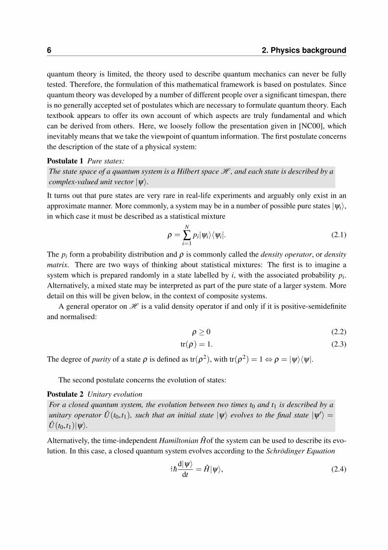
Combining two PIN-diodes and a beamsplitter as shown in Fig. 2.1 allow us to measure thequadratures. In this homodyne detection setup [YC83], the signal mode is combined on a 50/50beamsplitter with a phase reference mode in an intense coherent state. The output arms of thebeamsplitter impinge on the two photodetectors and the difference of their output photocurrentsis recorded. Since each photocurrent is proportional to the intensity of the incoming light, the
14 2. Physics background
homodyne measurement is correctly described by the observable
n21 = n2− n1, (2.38)
which we will later identify as one of the Stokes operators. However, since the state of the localoscillator is very intense, it can be treated classically, i.e., aLO→|αLO|1LO, and the measurementis reduced to single mode detection. The observable (2.38) reduces to [Leo97]
Xφ =√
2|αLO|xφ , (2.39)
with xφ = xcos(φ ) + psin(φ ), where φ denotes the phase shift induced by retardation of thelocal oscillator with respect to the signal.
If a large enough number of copies of a state ρ are at hand, the homodyne detector can be usedto perform tomography on that state. This is typically done as follows: A subset of the copiesof the state are used to record the quadrature quasi-probability distribution, for a fixed phase φ .Then, this phase is incremented and the procedure repeats. This is done for a large number ofphase settings 0≤ φ ≤ π . Graphically, this amounts to recording the marginal distributions alongall orientations in phase space, thus mapping out the complete Wigner function and allowing forthe reconstruction of ρ .
A second way of performing tomography on a quantum state of light is heterodyne detection,or eight-port homodyne detection. Here, the incoming signal is split symmetrically and eacharm enters its own homodyne apparatus. These two apparatuses are set to detect two orthogonalquadratures. The POVM describing this measurement is {|α〉〈α|}, i.e., projections onto allcoherent states [LH89]. Equation (2.32) shows that this POVM maps out the Q-function of ρ
and therefore, heterodyne detection is a means of performing quantum state tomography.
3Quantum information and communication
3.1 Separability and entanglement
Undoubtedly, entanglement lies at the heart of quantum information science, since virtually anyquantum information processing protocol depends on it in some way. Somewhat in contrast tothis, the concept of entanglement has caused confusion ever since the famous EPR paper [EPR35]and continues to do so. The controversy lies in the fact that entanglement is a global propertyof a state of multiple physical systems, which allows for a description of the complete system,without revealing any information about each individual subsystem. This conflicts with ourintuition from classical physics, where we naturally understand that a complete characterisationof a large system contains within itself complete characterisations of its constituent parts.
In this thesis, a deeper discussion of these issues is purposefully avoided, and we follow theparticular interpretation of quantum mechanics, “Shut up and calculate”1. Essentially, we can dothis because the definition of entangled states is rather straight-forward:
Definition 1 EntanglementA state of two (or more) spatially separated parties is called entangled, if it cannot beprepared by local operations and the exchange of classical information.
Conversely, a state which can be thus prepared is called separable and can be written as [Wer89]
ρsep = ∑
ipiρ
iA⊗ρ
iB, (3.1)
where the pi form a probability distribution and ρ iA and ρ i
B are proper states of the respectivesubsystems. A special role is played by maximally entangled states for systems of dimensionN⊗N, which can be written
|ψmax〉= 1√N
N
∑i=1|ei〉|ei〉, (3.2)
1This quote is attributed to Richard Feynman

16 3. Quantum information and communication
with the orthonormal basis {|ei〉}. For systems of two qubits, the four Bell states
|ψ±〉= 1√2[|0〉|1〉± |1〉|0〉], |φ±〉= 1√
2[|0〉|0〉± |1〉|1〉] (3.3)
are maximally entangled and form a basis for the two-qubit Hilbert space. These states showthe counter-intuitive behaviour of entangled states. Measuring either subsystem on its own, onefinds either |0〉 or |1〉. These outcomes occur with equal probability and truly randomly, in otherwords, tracing out either subsystem leaves the other in the maximally mixed state ρ = 1N/N.In contrast, measurements in the same basis on both subsystems are always perfectly correlated.Due to this behaviour, the Bell states find common use in the theory of quantum information.
Naturally, there are also partially entangled states. A good example would be a pure stateof the form of Eqn. (3.2), but with varying weight factors for the different terms. For purebipartite states, there exists a clear way to quantify the amount of entanglement, which dependson exactly these weight factors. It is defined as the von Neumann entropy of one of the reduceddensity matrices,
E(ρ) = −tr(ρA logρA). (3.4)
The quantification of entanglement for mixed states is much more complicated, and there is nounique function which is widely recognised and used. In fact, even the properties which such afunction should have are not always agreed upon. Some of the less debatable properties are thefollowing: For separable state, the entanglement measure should read E(ρsep) = 0. Then, theamount of entanglement should be non-increasing under local operations and classical communi-cation, and, as a consequence of this, E(ρ) must be invariant under local unitary transformations.Furthermore, mixing of different states should not increase the amount of entanglement, i.e., anentanglement measure should have the convexity property
∑i
piE(ρi) ≥ E
(∑
ipiρi
). (3.5)
Functions which obey these properties are often called entanglement monotones. Commonlyused examples of these are Concurrence or the Entanglement of Formation [BDSW96, HW97]and the Negativity [VW02]. Good reviews of entanglement monotones and other entanglementmeasures can be found in Bengtsson’s book [BZ06] or in Ref. [PV07].
It is possible to increase entanglement, which is known as entanglement distillation[BBP+96, BBPS96]. This procedure only works if multiple copies of an initial, weakly entan-gled state are available. By sacrificing some of these copies, a smaller number of states withhigher degrees of entanglement can be produced. For pure states, entanglement concentrationprocedures basically average the Schmidt coefficients. An important application of entanglementdistillation is entanglement-based quantum key distribution, the workings of which are outlinedbelow.

3.2. Entanglement criteria 17
In the following chapters, we are more concerned about the qualitative question whether astate is entangled or not, rather than a quantification of entanglement. As we will see, entangle-ment has a rather rich structure and a solution to the separability problem which is general, aswell as practical, is yet to be found.
3.2 Entanglement criteria
The question whether a given density matrix admits a decomposition (3.1) is very hard to answerin general, and significant research has been invested in the search for entanglement tests orcriteria. Ideally, such a test fulfils three criteria: It is applicable to a large class of states, it shouldbe a necessary and sufficient criterion for separability and it should be easily implemented in thelaboratory. This last requirement presents a natural way of splitting entanglement criteria intoa group of those which fulfil it (operational criteria) and those which do not (non-operationalcriteria). We now present a short list of entanglement criteria, with an emphasis on those whichappear in later Chapters of this thesis. Very good reviews of recent progress on the separabilityproblem are presented in Refs. [HHHH09, GT09].
3.2.1 Non-operational criteria
Non-operational criteria are those which cannot directly be implemented in the laboratory. Theyare reformulations of the separability problem, in the hope that solutions may be found moreeasily in different mathematical frameworks. Here, we present two non-operational criterial,which are both necessary and sufficient for bi-partite entanglement:
Positive maps: As the name suggests, a positive map Λ takes positive operators to positiveoperators. For bi-partite states, Λ can be applied to just one of the subsystems. Due to thestructure of separable states, this leads to the following criterion: A state ρAB is separable if andonly if
(1A⊗ΛB)ρAB ≥ 0, (3.6)
for any positive map ΛB [HHH96]. A positive map, whose extensions 1⊗Λ to arbitrary higherdimensions are again positive maps, is called completely positive. Clearly, the criterion (3.6)is concerned with positive, but not completely positive (PNCP) maps. Unfortunately, there isno complete characterisation of such maps, except in systems of dimension 2× 2 or 2× 3 (seebelow).
Entanglement witnesses: An entanglement witness is a Hermitian operator W with the twoproperties
tr(ρW ) 6≥ 0 (3.7)
tr(ρsepW ) ≥ 0, ∀ ρ
sep. (3.8)

18 3. Quantum information and communication
Now, a given state ρ is entangled if and only if there exists an entanglement witness for whichtr(ρW ) < 0, i.e., a witness which detects ρ . However, how to find a complete set of entanglementwitnesses is not known.
3.2.2 Operational criteria
Operational entanglement criteria are those which are easy to check in practice. For pure states,there exists an operational criterion which is also necessary and sufficient. It states that a purestate |ψ〉 is separable if and only if its Schmidt rank is equal to one, where the Schmidt rank isgiven by the number of terms in the Schmidt decomposition [Per93].
It is the entanglement of mixed states which is difficult to characterise and detect with simpleexperimental tests. We will give two examples of such tests, which are both restricted cases ofthe two non-operational criteria described above.
Partial transposition: Transposition is a PNCP map, and it is certainly very easy to imple-ment on a known density matrix. For bi-partite systems of dimension 2×2 or 2×3, it turns outthat every PNCP map can be decomposed into partial transposition and the action of completelypositive local maps, which are of no interest to the separability question. Therefore, positivityof a partially transposed state of these dimensions is a necessary and sufficient condition for itsseparability. In higher dimensions, the criterion is only necessary, but not sufficient [Per96]. Ininfinite-dimensional systems, partial transposition is necessary and sufficient for the separabilityof bipartite Gaussian states with a 1×N mode structure [WW01].
Entanglement witnesses: Although entanglement witnesses are classified above as a non-operational criterion, each single witness can detect a certain number of entangled states. Thefact that a witness operator is Hermitian and therefore directly observable makes it, in a way, thequintessential operational criterion. Witnesses also have a well-known graphical representation,which is shown in Fig. 3.1. Any entangled state can be separated from the convex set of separablestates by a hyperplane representing the expression tr(ρABW ) = 0. Separable states lie on theside tr(ρABW ) ≥ 0. Since this expression is linear in ρAB, it is represented by a straight linein Fig. 3.1. By introducing a dependence of W on the state itself, the witness can be “bent”to better approximate the set of separable states. Such nonlinear witnesses were introduced inRef. [GL06] and further developed in Ref. [MGL08].
A witness W ′ is called finer than W , if it detects the same entangled states and some ad-ditional ones. If there are no finer witnesses than some W ′, then this W ′ is called the optimalwitness.

3.3. Effective entanglement 19
separable states
ρAB
W 'W
W ''
Figure 3.1: Geometric interpretation of entangled witnesses: W ′ is finer than W and also opti-mal. W ′′ represents a non-linear witness.
3.3 Effective entanglement
This chapter started with the claim that entanglement is quintessential to quantum commu-nication, yet the first and arguably most famous protocol, the BB84 key distribution scheme[BB84], works completely without entanglement. Instead, it uses a set of non-orthogonal statesto transmit quantum information. A key distribution scheme which explicitly employs sharedentanglement was later introduced by Ekert [Eke91]. Soon after the introduction of this firstentanglement-based QKD scheme, Bennett et al. [BBM92] realised a connection, which putboth types of protocols on equal footing:
Observation 1 Effective entanglement [BBM92]Creating an ensemble {pi, |ψi〉} of quantum states is equivalent to the generation of a bipar-tite entangled state |Ψ〉= ∑i
√pi|i〉A|ψi〉B, followed by the projective measurement {|i〉A〈i|}.
Here, the |i〉 form an orthonormal basis for HA.
This observation implies that any source of non-orthogonal states admits an equivalent descrip-tion, which introduces entanglement in protocols which originally do not make use of entangledstates. Hence, entanglement detection can be used to test whether a given experiment is in prin-ciple suitable for quantum communication. For QKD, it was explicitly shown that measurementdata compatible with separable states cannot provide secret key [CLL04]. Implementations ofquantum memory or teleportation protocols can be benchmarked in a similar fashion using thelanguage of effective entanglement, which will be the subject of Chapter 5 and Chapter 6.
It is important to note that tomography will oftentimes not be possible on the effective bi-partite states as given in Observation 1, due to the restricted measurements on system A. At thesame time, the reduced density matrix ρA is fully known, because it stores the a priori probabil-ities and the overlaps of the input states, which are under the experimentalist’s control.

20 3. Quantum information and communication
There are variations of Observation 1, as the following example shows: Arguably the mostfamous implementation of continuous-variable QKD uses an ensemble of coherent states, whichare drawn according to a Gaussian distribution by Alice and then sent to Bob [GvAW+03].The corresponding entanglement-based state preparation consists of the generation of a two-mode squeezed state [BR97], followed by the POVM {|α〉〈α|} on Alice’s subsystem. Then,the squeezing parameter of the effective two-mode squeezed state is linked to the width of theGaussian distribution of input states.
3.4 The Expectation Value Matrix
The object of central interest to this thesis is the Expectation Value Matrix (EVM), together withits application to the separability problem. This object was initially introduced in Ref. [RGL06]and then defined more generally in Ref. [HML08]. The equivalence of both methods is demon-strated in Appendix B.
The derivation of the EVM method was motivated by a problem which almost all quantuminformation experiments share, namely that of partial information. In general, quantum statetomography is a very challenging task: For a single qubit state, three independent measurementsettings are needed. Tomography on a two-qubit state requires 15 independent measurementsettings, and this number increases fast for higher dimensional systems. Tomography on a modeof light is possible with finitely many measurement settings with the help of maximum likelihoodalgorithms, but the required measurement samples need to be very large.
In light of this, a good entanglement criterion must work with fewer measurements, whichare more easily implemented. The outcome of these measurements, i.e., a set of expectationvalues, comprises the available knowledge. In the absence of tomography, this knowledge doesnot suffice to uniquely deduce a state ρAB of the system. Instead, there will be a set of possiblestates which are all compatible with the measured set of expectation values, and we call this setan equivalence class of states. Now, the only possibility to certify that the system was entangledis to show that the equivalence class contains exclusively entangled states. We summarise thispoint in form of the following observation:
Observation 2 Partial informationIf an experiment allows access to only partial information, the measurement outcomes definean equivalence class of states. The measurement data can exhibit quantum correlations, ifthe equivalence class contains no separable state.
Figure 3.2 illustrates this Observation: The equivalence class of states overlaps with the setof separable states, so entanglement verification is not possible, and the measured data set canbe simulated by local operations and classical communication. An alternative formulation ofthe problem of partial information for entanglement verification is presented in Refs. [CLL04,CGLL05], together with constructions of optimal entanglement witnesses.

3.4. The Expectation Value Matrix 21
separable statesall states
equiv. class
Figure 3.2: An equivalence class of states. The overlap with the set of separable states showsthat entanglement verification is not possible.
The EVM contains all classical data available from an experiment and therefore forms acompact representation of the corresponding equivalence class of states. Any knowledge wehave about a system’s state can be expressed as the outcomes of measurements. These measure-ments are either actually performed in practice or they can be part of a thought setup to includesymmetries or assumptions about the state. Let Alice’s and Bob’s measurements be described byoperators A†
i Ak and B†j Bl , respectively, for appropriate sets {Ai} and {B j}. At this point, we put
no restrictions on these operators, other than to require the correct dimensions. Now, the entriesof the bipartite EVM are defined by
[χ(ρAB)]i j,kl = tr(ρAB A†i Ak⊗ B†
j Bl). (3.9)
Even without specifying operator sets, the resulting matrix χ(ρAB) has the following property:
Observation 3 Positivity of χ
The EVM as defined by Eqn. (3.9) is positive-semidefinite for all physical states ρAB.
Proof: Given a physical state ρAB, the quantity tr(ρABM†M) is non-negative for all operators M.Taking the general bipartite form M = ∑i, j ci jAi⊗ B j with the above sets {Ai} and {Bi}, we find
0≤ tr(ρABM†M)
= ∑i j,kl
c∗i j tr(ρABA†i Ak⊗ B†
j Bl)ckl
= ∑i j,kl
c∗i j [χ(ρAB)]i j,kl ckl ,
=~c †χ(ρAB)~c, ∀~c
so χ(ρAB) is a positive-semidefinite matrix. �

22 3. Quantum information and communication
3.4.1 The EVM criterion
The structure of the EVM (3.9) shows that separable states will always map to separable EVMs,i.e.,
χ(ρsepAB ) = ∑
ipi χ
iA⊗χ
iB, (3.10)
with the local EVMs
[χA]i, j = tr(ρA A†i A j) (3.11)
[χB]i, j = tr(ρB B†i B j). (3.12)
By normalising χ(ρAB), we can interpret it as a quantum state, and test its separability. If itis provably not separable, is must stem from an entangled state. In other words, we can applyan entanglement test to the normalised EVM to obtain a criterion sufficient for entanglement ofρAB. For most applications in the following chapters, the dimension of the EVM does not exceed2× 3, so we will use partial transposition to test for separability. Furthermore, since the partialtransposition test concerns only the positivity, normalisation of χ(ρAB) is actually not important.Our entanglement criterion therefore reads
χTA(ρAB) 6≥ 0 → ρAB entangled. (3.13)
In fact, a positivity requirement on a matrix, like Eqn. (3.13) above, gives rise to a family ofinequalities (c.f. [SV05, MP06]), since Eqn. (3.13) holds true if and only if all principle sub-matrices of χ(ρ
TAAB) have non-negative determinants [Str88]. To clarify this criterion, let M be a
general Hermitian matrix and let M~r,~r = (r1, . . . ,rN) denote the sub-matrix obtained by deletingall rows and columns except those labelled by r1, . . . ,rN . Then M is positive semidefinite ifand only if det(M~r) ≥ 0, for any ~r with 1 ≤ r1 < r2 < · · · < rN and N = 1,2, . . . . For theseparability of χ(ρ)AB, this means that negativity of any one of these sub-determinants providesa sufficient entanglement criterion. Note the similarity to the separability criteria derived inRefs. [SV05, MPHH09].
We have now successfully described the separability of a partially known state ρAB in termsof the EVM χAB. However, it would be very surprising if the available experimental data exactlyfilled the EVM. More generally, χAB will itself be only partially known. This problem is nowtractable, because the EVM is typically of small dimension. Every undetermined entry of χAB
must be represented by a free, complex-valued parameter xi and we denote the resulting partiallyknown EVM
χ~xAB. (3.14)
The separability of this EVM must now be reformulated to include these free parameters.

3.5. Applications 23
Observation 4 Free parametersA partially known EVM corresponds to an entangled state, if an exhaustive search throughthe free parameters~x does not produce a set which satisfies
χ~xAB ≥ 0 (3.15)
(χ~xAB)TA ≥ 0. (3.16)
The term “exhaustive” indicates that in most situations, numerical methods will be required toevaluate the conditions (3.13). Such feasibility problems with linear matrix inequality constraintsare very efficiently handled by a field of convex optimisation called Semidefinite Programming(SDP). This relatively new technique has found widespread applications in quantum informa-tion theory, and it is well suited for our problem at hand. More details on SDP theory and itsapplication to the separability of the EVM are given in Appendix A.
Up to now, we assumed that each free parameter can take any complex value. However,the entries of the EVM will have certain restrictions, since not any matrix of fitting dimensionforms a physical EVM. One physicality condition holds for any χ(ρ), and that is positivity.Other conditions will depend on the operator sets used in the construction of the EVM. Clearly,a characterisation of physical EVMs will improve the entanglement criterion, since we canexclude solutions ~x which are unphysical. Unfortunately, even for the small-dimensional casesused in Chapters 4 and 5, the complete set of physicality conditions is not known.
The EVM method combines the advantages of several entanglement criteria. It can be appliedto a wide variety of scenarios because of its completely general definition in terms of unspecifiedoperator sets {Ai} and {B j}. Still, the EVM criterion should be classified as an operationalcriterion, since its evaluation typically involves the positivity of low-dimensional matrices. Eventhe reformulation as an SDP can be regarded as an operational criterion due to the robust natureof SDPs.
3.5 Applications
3.5.1 Teleportation
Quantum teleportation [BBJ+93], is the task of transmitting an unknown quantum state σ fromAlice to Bob, with the help of classical communication and one pair of maximally entangledparticles. Classically, i.e., in the absence of the entangled state, the task could only be attemptedby Alice measuring the unknown state, and sending her measurement results to Bob, who canprepare a new quantum state accordingly. However, this will lead to a state transfer of verylow fidelity, since Alice cannot fully learn the initially unknown quantum state in a single-shot

24 3. Quantum information and communication
measurement. Even if she did know it, the transmission of an infinite amount of classical bits isrequired to allow Bob to reconstruct the state faithfully.
Adding the resource of one entangled state can resolve this problem and lead to state transferwith unit fidelity, at least in theory. Teleportation of an unknown qubit state |φ in〉 = a|0〉+ b|1〉works as follows: The initial quantum state, including the entangled resource, is given by
|ψ〉AA′B = |φ in〉A⊗1√2[|0〉|0〉+ |1〉|1〉]A′B. (3.17)
We can re-write this state in terms of the four Bell states [c.f. Eqn. (3.3)],
|ψ〉AA′B =12
[|φ+〉AA′(a|0〉B + b|1〉B)+ |φ−〉AA′(a|0〉B−b|1〉B)
|ψ+〉AA′(a|1〉B + b|0〉B)+ |ψ−〉AA′(a|1〉B−b|0〉B)] .(3.18)
By means of a projective measurement of system AA′ in the Bell basis, Alice induces the fourcorresponding states on Bob’s system with equal probability. The outcome of her Bell measure-ment tells her which of the four states Bob holds. She can then communicate this outcome toBob, by sending just two classical bits, and Bob can apply a corresponding rotation on his systemto recover the state |φ in〉.
There are two important points to note: Firstly, Bob has no means of recovering the state|ψ in〉 before he receives Alice’s classical information. The information transfer is therefore notfaster than the classical transmission, and locality is observed. Secondly, Alice does not knowthe input state at any point in the protocol, and at the end of the protocol, she holds just one ofthe Bell states. Thus, the no-cloning theorem [WZ82, Die82] is observed.
One of the key advantages of teleportation over the direct transmission of the qubit is that theentanglement can be shared in advance. Then, the quantum channel does not have to be used atthe precise time of the state transmission.
Experimentally, teleportation of qubits has been realised multiple times (see, e.g., [BPM+97,UJA+04]), with reasonably high fidelities. In the continuous-variable regime, the typical entan-gled resource for teleportation experiments is the two-mode squeezed state [Bar97]. The firstimplementation of continuous-variable teleportation was reported in Ref. [FSB+98].
The question when a teleportation experiment can be dubbed successful is treated in Chapter6 of this thesis.
3.5.2 Quantum Key Distribution
Quantum Key Distribution (QKD) was one of the first applications of quantum information andit is without doubt the most successful. It is based on the observation that the computationalprocesses which are involved in hiding and revealing information are inextricably linked to the
3.5. Applications 25
underlying physical apparatuses and to the laws which govern their behaviour. Quantum cryptog-raphy takes into account the additional computational possibilities offered by quantum mechanicsand derives security statements from the physical constraints posed by quantum theory2.
The first proposal for QKD by Bennett and Brassard [BB84], which was based on ideas byWiesner [Wie83], roughly works as follows: Alice holds a bit-string, which she wishes to sharewith Bob for use in a one-time-pad encryption [Ver26]. It is assumed that an eavesdropper (Eve)has full control of the communication channel, limited only by the laws of physics. With onlyclassical communication, it is not possible to establish a shared secret bit-string against such aneavesdropper. Allowing Alice to encode her bit values in quantum states makes the task feasible.For each bit value, Alice randomly chooses one of two possible states, the so-called basis choice,and sends them to Bob. For example, she might encode “0” in
|0〉 or |+〉= 1√2(|0〉+ |1〉), (3.19)
and the bit value “1” in|1〉 or |−〉= 1√
2(|0〉− |1〉). (3.20)
For each incoming signal, Bob sets his measurement apparatus to project in the “0,1”-basis orthe “+,−”-basis and stores the binary measurement outcomes in each case. All further stepsin the protocol involve only classical communication and data processing. First Alice and Bobdetermine, by public communication, the bits for which encoding and measurement were donein the same basis, and they discard all other bits. They use a randomly chosen portion of theremaining bits to determine the bit error rate, from which they can estimate the amount ofleaked information. If satisfied, they apply error correction [NC00] and privacy amplification[BBM95, RK05] protocols to generate secret shared bits. Otherwise, they abort and restart theprotocol.
An altogether different approach to the problem of distributing secret key was taken byEkert [Eke91]. It explicitly uses entangled particle pairs, which are created by a central sourceand distributed to Alice and Bob. The particles, which ideally arrive at the receiver in a singletstate |ψ−〉, enter detection devices, which can project along rectilinear or diagonal bases.The basis settings are chosen by Alice and Bob in a random and independent manner. Thesubsequent classical data processing and classical communication are quite similar to the BB84protocol, described above. Alice and Bob publicly compare their basis choices and keep onlythose occurrences in which both detectors registered a particle. Then, the two parties revealthe outcomes of those events for which their detector settings did not agree and use these tocompute their value of the CHSH inequality [CHSH69]. The security of the system originates in
2The assumption here is that quantum theory is complete in the sense that it can provide the full information onany system it describes.
26 3. Quantum information and communication
the fact that any actions undertaken by the eavesdropper to learn Alice’s and Bob’s unrevealedmeasurement outcomes, including the replacement of the source, will weaken the correlationsbetween the two distributed particles. Naturally, it is not experimentally feasible to directlydistribute a maximally entangled state, but the two communicating parties can use entanglementdistillation protocols to approach the ideal case.
As discussed above in the context of effective entanglement, the BB84 protocol and a sightlymodified version of Ekert’s protocol were later shown to admit equivalent theoretical descriptions[BBM92]. A number of different QKD protocols have been worked out since then, such as thesix-state protocol [Bru98] and the two-state protocol [Ben92]. The latter will be the subject ofChapter 4 of this thesis.
Furthermore, QKD is not limited to qubit systems. Continuous distributions of coherentstates [GG02, GvAW+03] or squeezed states of light [Hil00, CLVA01] can be used in con-junction with homodyne or heterodyne detection to generate secret key. Recently, continuous-variable versions of the two-state protocol [LRH+06, WFW+09] and the BB84 protocol[HY+03, LKL04] have been implemented.

4The phase reference in quantum key distribution
In this chapter, we describe a QKD protocol based on two coherent states and the correspondingentanglement verification procedure. This chapter builds on a certain connection between thedistillation of secret key and the verification of entanglement. Assume two parties, Alice andBob, share a quantum channel and a classical channel and wish to use those to generate secretkey. They initiate their protocol by distributing quantum states and collecting classical data onthose via measurements. Then, the following Observation is a necessary precondition for theprotocol to proceed:
Observation 5 Curty et al. [CLL04]Assume that the classical data held by Alice and Bob can be interpreted as coming from aseparable state ρ
sepAB . Then no secret key can be distilled via public communication from the
shared classical data.
In other words, the ability to verify entanglement from the classical data obtained in a QKDprotocol is a necessary precondition for the generation of secret key. For prepare and measureprotocols, we verify effective entanglement. The above observation is equivalent to the statementthat intercept-resend attacks lead to upper bounds on the secret key rate. In such attacks, theeavesdropper (Eve) replaces part of the quantum channel by a classical communication channel.Therefore, the resulting bi-partite states originate from local operations and classical commu-nication, i.e., they are separable. By verifying entanglement, we can exclude intercept-resendattacks and show that an implementation of a QKD protocol can be suited to generate secret key.
We will describe the entanglement verification method with the help of the so-called B92protocol [BBS+92], which is detailed below, in both its original form and its adaptation to thecontinuous-variable regime. Using just two signal states, this is arguably the simplest QKDprotocol. We show how to construct and use the EVM method and give results for typical exper-imental situations. Complementary to this method, we construct the explicit form of the optimalintercept-resend attack, which serves as a means to check the strength of our entanglement crite-rion.
28 4. The phase reference in quantum key distribution
The second part of this chapter deals with a problem which is common to most CVimplementations of QKD protocols, namely the issue of the phase reference. Again using theEVM method in conjunction with specific intercept-resend strategies, we assess whether attackson the phase reference can compromise the security of the protocol.
4.1 The B92 protocol
In the original B92 paper [BBS+92], there is great emphasis on the fact that any two non-orthogonal states can be used to establish secret key. Let |ψ0〉 and |ψ1〉 denote such twostates, then the protocol suggests that Bob randomly chooses to project incoming signals ontoP0 = 1− |ψ1〉〈ψ1| or P1 = 1− |ψ0〉〈ψ0|. Bob then communicates to Alice the instances whenhis measurements had a positive result, and all other instances are discarded. Alice and Bob nowhold correlated bit-strings, which can be distilled to secret key by appropriate error correctionand privacy amplification steps.
Reference [BBS+92] also suggests a particular way to implement the protocol. The proposedinput states are coherent states |±α ,β 〉, prepared in two timing modes, with |α| � |β |. Bob’sdetector consists of an interferometric setup, allowing him to randomly choose a 180◦ phase shifton one arm, similar to Alice’s encoding step. The resulting three time modes enter a “click/no-click” detector. The crucial middle pulse will lead to a click only if Alice and Bob chose thesame phase shift, thus implementing operators analogous to P0 and P1.
4.1.1 Continuous-variable variant
In the continuous-variable adaptation of the two-state protocol [LRH+06, EBH+09, WFW+09],the input states are encoded as above. A signal mode contains weak coherent states |α〉s or|−α〉s and a phase reference mode is in a very bright coherent state |β 〉LO. For free-spaceimplementations, one would typically use orthogonal polarisation modes for signal and phasereference, whereas fibre-based implementations separate the modes in time.
The continuous-variable character becomes apparent at Bob’s detection stage. The signal’sphase is decoded by measuring the x-quadrature of the incoming pulses. For security, the p-quadrature and the variances must also be measured. In the following, we will often, in aslightly sloppy use of terminology, speak of detection of the first and second quadrature mo-ments. Strictly speaking, this implies that Bob can measure
{〈x〉,〈p〉,〈x2〉,〈p2〉, 12(〈x p〉+ 〈px〉)}. (4.1)
The last term in this set is not accessible by measuring in the x and p-directions, but requiresa third phase setting of the homodyne detector. However, none of the results presented in this
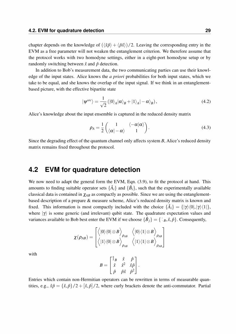
4.2. EVM for quadrature detection 29
chapter depends on the knowledge of (〈x p〉+ 〈px〉)/2. Leaving the corresponding entry in theEVM as a free parameter will not weaken the entanglement criterion. We therefore assume thatthe protocol works with two homodyne settings, either in a eight-port homodyne setup or byrandomly switching between x and p detection.
In addition to Bob’s measurement data, the two communicating parties can use their knowl-edge of the input states. Alice knows the a priori probabilities for both input states, which wetake to be equal, and she knows the overlap of the input signal. If we think in an entanglement-based picture, with the effective bipartite state
|ψsrc〉= 1√2
(|0〉A|α〉B + |1〉A|−α〉B) , (4.2)
Alice’s knowledge about the input ensemble is captured in the reduced density matrix
ρA =12
(1 〈−α|α〉
〈α|−α〉 1
). (4.3)
Since the degrading effect of the quantum channel only affects system B, Alice’s reduced densitymatrix remains fixed throughout the protocol.
4.2 EVM for quadrature detection
We now need to adapt the general form the EVM, Eqn. (3.9), to fit the protocol at hand. Thisamounts to finding suitable operator sets {Ai} and {Bi}, such that the experimentally availableclassical data is contained in χAB as compactly as possible. Since we are using the entanglement-based description of a prepare & measure scheme, Alice’s reduced density matrix is known andfixed. This information is most compactly included with the choice {Ai} = {|γ〉〈0|, |γ〉〈1|},where |γ〉 is some generic (and irrelevant) qubit state. The quadrature expectation values andvariances available to Bob best enter the EVM if we choose {B j}= {1B, x, p}. Consequently,
χ(ρAB) =
⟨|0〉〈0|⊗B
⟩ρAB
⟨|0〉〈1|⊗B
⟩ρAB⟨
|1〉〈0|⊗B⟩
ρAB
⟨|1〉〈1|⊗B
⟩ρAB
with
B =
1B x px x2 x pp px p2
.
Entries which contain non-Hermitian operators can be rewritten in terms of measurable quan-tities, e.g., x p = {x, p}/2 + [x, p]/2, where curly brackets denote the anti-commutator. Partial

30 4. The phase reference in quantum key distribution
transposition is best performed on system A, so that it leads to a simple block transposition ofχAB.
Clearly, not all entries of this EVM are experimentally accessible. Both off-diagonal blocks,for example, are completely unknown with the exception of their (1,1) entries, which have theform tr(ρAB|0〉〈1| ⊗1B) = 〈α|−α〉/2. As described in the previous Chapter, each unknownentry is represented by a complex number, so that the EVM is parameterised as
χAB =12
1 〈x〉0 〈p〉0〈x〉0 〈x2〉0 a + i
2〈p〉0 a− i
2 〈p2〉0s
1 c dc f gd g− i h
s
1 c∗ d∗
c∗ f ∗ g∗+ i
d∗ g∗ h∗
1 〈x〉1 〈p〉1〈x〉1 〈x2〉1 b + i
2〈p〉1 b− i
2 〈p2〉1
, (4.4)
where s = 〈−α|α〉, a and b are real parameters and {c, . . . ,h} are complex. Evaluating theentanglement criterion is now a matter of finding parameter sets {a,b, . . . ,h} such that the EVMsatisfies the conditions given in Eqn. (3.15). We evaluate this semidefinite programme using thesolvers SDPT3 [TTT99] or SeDuMi [Stu99], which can be implemented in MATLAB with thehelp of the parser YALMIP [L04]. For any set of physical measurement data, the EVM criterioncan now be evaluated efficiently.
Interestingly, PPT-entanglement does not play a role, because it cannot be detected with therestricted set of available information.
Observation 6 PPT-entanglementLet σ be a PPT-entangled state which is not detected by the EVM method. Then there existsa separable state compatible with the same measurement data.
Proof: We start the proof with an auxiliary calculation to show that χTA(ρ) = χ(ρTA). Takingan example entry and using the invariance of the trace under partial transposition, we find
[χ(ρTA)]6,2 = tr(ρ
TA [|0〉〈1|⊗ x p])= tr(ρ [|0〉〈1|⊗ x p]TA)= tr(ρ [|1〉〈0|⊗ x p])= [χ(ρ)]2,6 (4.5)
and similarly for the other entries. Hence, χ(ρTA) is the block transposition of χ(ρ).Since all measurement results are stored in the diagonal blocks of χ(ρ), its block trans-
position χTA(ρ) = χ(ρTA) fits the same experimental data. Then so does the sum (χ(ρTA) +χ(ρ))/2, which is the EVM of ρ = (ρTA + ρ)/2. This state ρ is invariant under transpositionof subsystem A, and Theorem 2 in Ref. [KCKL00] states that any such state of dimension 2×N

4.2. EVM for quadrature detection 31
is separable. We now argue that this theorem is applicable to the infinite-dimensional state ρ . Tothis end, we approximate ρ by finite-dimensional states
σ(N)AB = N (1A⊗P(N)
B )ρ(1A⊗P(N)B ), (4.6)
with normalisation factor N and the projection operator
P(N)B =
N
∑k=1|k〉B〈k|. (4.7)
The vectors {|k〉B}∞k=1 form a basis for system B. Intuitively,
‖ρ−σ(N)AB ‖ ≡ δN , (4.8)
limN→∞
δN = 0 (4.9)
where ‖ . . .‖ denotes the trace norm. In other words, the sequence {δN} is convergent. Therefore,∀ε , ∃ n ∈N such that ρ and σ
(n)AB are closer than ε in trace distance.
Furthermore, σ(n)AB is invariant under transposition of system A:
(σ(n)AB )TA = N [(1A⊗P(n)
B )ρ(1A⊗P(n)B )]TA (4.10)
= N [(1A⊗P(n)B )TA ρ
TA(1A⊗P(n)B )TA ] (4.11)
= N [(1A⊗P(n)B )ρ
TA(1A⊗P(n)B )] (4.12)
= N [(1A⊗P(n)B )ρ(1A⊗P(n)
B )] (4.13)
= σ(n)AB , (4.14)
as by assumption, ρTA = ρ . Therefore, σ(n)AB is separable. Consequently, ρ is approximated by a
convex combination of product states, so ρ is separable [Wer89]. �
4.2.1 Modelling of experimental data and results
Since we did not run an experiment to demonstrate the EVM method, we model the possiblemeasurement outcomes and express the results of the entanglement verification in terms of theparameters of this model. There are two main causes of signal degradation in optical trans-mission, namely photon losses and noise. The noise typically affects both quadratures equally,so that it can be modelled by a single parameter ∆, which describes the broadening of observedvariances. The loss shall be denoted by η , such that the first moments are scaled as 〈x〉→√η〈x〉.
It is important to note that we are not modelling the quantum channel, but merely parame-terise the set of possible measurement outcomes. Neither do we assume the output conditional

32 4. The phase reference in quantum key distribution
00.25
0.50.75
1
00.2
0.40.6
0.81
0.5
0.55
0.6
0.65
0.7
0.75
0.8
0.85
!" ! |! #
transmission "
exce
ssno
ise
!
Figure 4.1: Results of the EVM method for quadrature detection. The amount of tolerable excessnoise ∆ is plotted for all values of the channel transmission η and the input state overlap 〈−α|α〉.
states to be Gaussian. Higher quadrature moments would be required to reveal whether a state isGaussian or not.
There is one more parameter to consider, namely the amplitude |α| of the input states,which can be chosen by the experimentalist. Now, for each value of the triple (α ,η ,∆), we canevaluate the feasibility problem associated with the EVM criterion. If the SPD is infeasible,the data must stem from an entangled state. If, on the other hand, the SDP is feasible, theentanglement criterion is inconclusive. The results are shown in Fig. 4.1. The input overlap〈−α|α〉 and the channel loss parameter η span the xy plane and the plotted height values showthe amount of excess noise required to produce a feasible problem. Therefore, data below thesurface corresponds to entangled states. Clearly, for fixed η , more excess noise is tolerableas the input signals overlap more, i.e., |α| decreases. This amount of excess noise decreaseslinearly with the channel transmission η .

4.2. EVM for quadrature detection 33
4.2.2 Optimal intercept-resend attacks
It remains to investigate the area above the surface in Fig. 4.1. There are two possibilities for datain this area: It can either stem from entangled states, which are not detected by the EVM methodor there is a separable state compatible with this data 1. One way of probing the extent to whichdata sets are compatible with separable states is to construct explicit intercept-resend attacks.To this end, we introduce the eavesdropper Eve, who performs destructive measurements on theinput states to learn the phase for each instance, and resends newly prepared states to evade beingdetected. In her choice of measurement and resent states, Eve is restricted by our model of Bob’sobservations. She needs to induce such measurement data for Bob which give the correct firstmoments and equal quadrature variances.
Intuitively, the non-orthogonality of the signal states protects against such attacks. When Evetries to distinguish |α〉 and |−α〉 and reassign new signals accordingly, she inevitably makeserrors which will be detectable in Bob’s observations. In our case, these errors will manifestthemselves in the form of increased uncertainties. Hence, for large measured variances we alwaysexpect to find an intercept-resend attack, in analogy to bit-error rates above 25% in the qubit-based BB84 protocol [MCL06].
A promising, and ultimately successful, choice of measurement for the eavesdropper is aminimum-error discrimination strategy. For the signal states |±α〉, the resulting error probabil-ity is given by
e =12− 1
2
√1−|〈−α|α〉|2. (4.15)
In other words, if we assume Eve to resend either |ψE0 〉 or |ψE
1 〉, she makes a wrong choice withprobability e. As a result, Bob’s states, conditioned on the original bit-values, become
ρB,E0 = (1− e)|ψE
0 〉〈ψE0 |+ e|ψE
1 〉〈ψE1 |, (4.16)
ρB,E1 = (1− e)|ψE
1 〉〈ψE1 |+ e|ψE
0 〉〈ψE0 |. (4.17)
The exact form now depends on the choice of |ψE0/1〉.
We note here that since the original coherent amplitudes α have been chosen to be real,the expected variance broadening from the attack will only occur in the x-direction (cf. Fig. 4.2).However, Bob expects to observe equal variances in x and p, which is achieved by the eavesdrop-per with appropriate squeezing operations. Hence, a natural choice of states for Eve to resendis
|ψE0/1〉= D(±β )S(r)|0〉, (4.18)
where D(β ) and S(r) are the displacement and squeezing operators, respectively, and r is a realsqueezing parameter [BR97].
1In principle, there is the third possibility that data sets are unphysical. In this case, however, Fig. 4.1 quiteclearly shows only physical values for η , α and ∆.

34 4. The phase reference in quantum key distribution
x
pr
x
pra)|α〉
α-α
b)
α β
|ψ 〉 with prob. (1-e)
0E
|ψ 〉 with prob. e1E
-α
Figure 4.2: a) Marginal distribution for the input state |ψ0〉 = |α〉. b) Bob’s conditional stateρ
B,E0 after the interaction of the eavesdropper. With probability (1− e), Eve resent |ψE
0 〉; withprobability e, she erroneously resent |ψE
1 〉.
For each input overlap, the parameters β and r can now be adjusted to reproduce the values〈x〉0/1 and 〈p〉0/1 expected by Bob, while inducing the least possible excess variance. Let uscompare Bob’s measurement outcomes with (superscript “E”) and without this attack. For thefirst moments, we find
〈x〉0/1 = ±√
2ηα (4.19)
and
〈x〉E0/1 = ±√
2β (1−2e). (4.20)
Hence, Eve’s states must have amplitudes β = ηα/(1− 2e) = ηα/√
1− s2, where s againdenotes the input state overlap. For the measured variances, we find
Var(x)E0 =
12e−2r + 2β
2s2 (4.21)
=12e−2r + η
2 s2 lnss2−1
(4.22)
Var( p)E0 =
12e
2r. (4.23)
Eve can then adjust the squeezing parameter r such that both variances are equal. This leads tothe final expression for the excess noise which Eve’s strategy induces in Bob’s observations:
VarB,E(x) = VarB,E( p) =12(
f +√
f 2 + 1),
f = ηs2 lnss2−1
.
This analytic expression coincides, within the numerical accuracy of the SDP, with the resultsshown in Fig. 4.1. Therefore, the combination of this attack with the entanglement verifica-tion method is necessary and sufficient to decide whether measured data is compatible with aseparable state or not, for all possible data sets.

4.2. EVM for quadrature detection 35
a = 0.8no loss
mea
sure
d va
rianc
e
0.5
0.6
0.7
0.8
0.9
input overlap 〈-α|α〉0 0.1 0.2 0.3 0.4 0.5 0.6 0.7 0.8 0.9 1.0
Var(x), optimisedVar(p), optimisedVar(x), from i.-r. attackVar(p), from i.-r. attack
Figure 4.3: The minimisation runs over one common variable, which is distributed asymmetri-cally between Var(x) and Var( p). An appropriately chosen intercept-resend attack can exactlyreproduce the curves.
4.2.3 Asymmetric variances
We conclude this section with a note on the assumption of equal variances for position andmomentum in Bob’s observations, which may be unjustified in some situations. An extensionof the above scheme to unbalanced excess noise is straightforward. The total measured variancewill be comprised of the input state variance and the excess noise, i.e.,
Vartot(x) = Varin(x)+V ex(x) =12
+V ex(x), (4.24)
and similarly for p. Asymmetric variances, i.e., V ex(x) 6= V ex( p), can be modelled by introduc-ing a degree of asymmetry a, such that
V ex(x) = aV opt (4.25)
V ex( p) =1a
V opt . (4.26)
We can now find the maximum V opt for which the EVM-method detects effective entanglement.The optimal intercept-resend attack for this asymmetric situation can also be found. It turnsout that it is of the same form as the optimal attack for the symmetric case, but with adjustedsqueezing levels for the resent states. As shown in Fig. 4.3, the boundary of the entangled areaand the optimal attack again coincide.

36 4. The phase reference in quantum key distribution
4.3 Including the local oscillator
This section examines the protocol more closely by including the phase reference mode, whichis typically labelled local oscillator. This auxiliary light beam is used to define the signal states’phase and is necessary for homodyne detection. If the local oscillator is in a coherent state of highintensity compared to the signal, the detection setup can be used to measure the field quadratures,as described in the previous section.
Ideally, the phase reference is prepared locally, but to ensure phase stability, it is commonpractice to split off the local oscillator in the signal preparation process and send it to Bob overthe same quantum channel as the signal. The local oscillator then inevitably passes through theinsecure domain controlled by the eavesdropper. It is therefore not justified to make assumptionsabout the state of the local oscillator unless these are verified by Bob. Consequently, the detectionprocess should be regarded as a true two-mode measurement and we will employ the Stokesoperators to describe it.
4.3.1 The quantum Stokes operators
Typically, the Stokes operators [JR55] describe the quantum polarisation of light, using a de-composition into two orthogonal polarisation modes (see, e.g., Ref. [KLL+02]). In our case,the modes may be spatially separated and we will label them with subscripts “s” and “LO” todenote the signal and the local oscillator, respectively. The input signals are now described bythe two-mode states
|ψ〉0/1 = |αLO,±αs〉. (4.27)
The Stokes operators are defined in terms of creation and annihilation operators as
S1 = a†s as− a†
LOaLO
S2 = a†s aLO + a†
LOas
S3 = i(a†LOas− a†
s aLO),
and the total intensity is often included in the set:
S0 = a†s as + a†
LOaLO. (4.28)
The commutation relations of the Stokes operators are those of the SU(2) algebra, namely,
[Si, S j] = 2iεi jk Sk (4.29)
for {i, j,k} = {1,2,3}, and εi jk is the Levi-Civita symbol. S0 commutes with the other Stokesoperators. As a consequence of Eqn. (4.29), the minimum uncertainty product of any two Stokesoperators depends on the expectation value of the third:
Var(Si)Var(S j) ≥ |〈Sk〉|2. (4.30)

4.3. Including the local oscillator 37
One other property worth mentioning is the operator identity
S21 + S2
2 + S23 = S2
0 + 2S0. (4.31)
The Stokes operators are measured by direct detection of intensity differences [SBT+03].If the two incoming light modes are spatially separated, the setup is identical to that of a ho-modyne apparatus. Detecting the x-quadrature then corresponds to an S2-measurement and thep-quadrature to S3. We therefore assume that the two-mode detection process gives access to theexpectation values and variances of S2 and S3.
4.3.2 Entanglement verification with Stokes measurements
An EVM for the Stokes operators is constructed analogously to Eqn. (4.4), with the simplereplacements
x→ S2 (4.32)
p→ S3. (4.33)
The crucial difference to the EVM for quadratures is the commutator. Since the third Stokesoperator S1 is not measured in this setting, the commutator [S2, S3] is unknown, and must betreated as a further open parameter.
The known entries of this EVM are modelled to reflect actual experimental data. As before,losses are modelled by scaling down the first moments and noise has the effect of broadening thevariances of S2 and S3.
Numerical results are shown in Fig. 4.4, again in the setting where observed variances ofS2 and S3 are equal. Figure 4.4 and all following figures are drawn for the lossless case, sincechannel loss does not qualitatively change the results. A brief discussion of channel losses willbe presented at the end of this Chapter, in Subsection 4.3.6. There are two important pointsto note in Fig. 4.4: Firstly, for the quadrature detection, the input-state variance is equal to 1/2,independently of the intensity |α|. In contrast, the variances of the Stokes operators are intensity-dependent for coherent state input of the form of Eqn. (4.27). In fact, Var(Si) = 〈S0〉 holdstrue for all four Stokes operators when evaluated on coherent states [KLL+02]. This explainsthe unusual scale of measured variances in Fig. 4.4, and the input state noise level is plottedexplicitly. Typical experimental variances are expected to lie just above this input noise level.
Secondly, one can show that data sets below the entanglement verification curve are in factunphysical. We know that the variances of two Stokes operators must obey the uncertaintyrelation (4.30). In our case, the third Stokes operator is unknown, leaving the uncertainty unde-termined, and allowing, for example, unconstrained simultaneous squeezing of S2 and S3. Thenagain, the extra knowledge about the input states will most likely affect the question of physicaldata sets. As it turns out, the EVM itself provides us with a compact set of physicality conditions.

38 4. The phase reference in quantum key distribution
existence curvecoherent state varianceequal amplitude attack
unphysical data
ILO = 104
Var(Ŝ
2) = V
ar(Ŝ
3)
103
0
2
4
6
8
10
input state overlap 〈-αs|αs〉0 0.2 0.4 0.6 0.8 1.0
Figure 4.4: Signal-state overlap plotted against the Stokes operator variance for a lossless channeland local oscillator amplitude αLO = 100. Only data points above the grey shaded area arephysically allowed. Solid curve: entanglement verification without additional measurements.Dashed line: Intercept-resend attack with equal amplitudes in both modes. Dotted line: inputstate variance for reference.
As mentioned above, every valid physical state must lead to a positive semidefinite EVM. Thisimplies that all principle minors of χ(ρ) must have non-negative determinants. Taking rows andcolumns (1,2,4) to form a particular sub-matrix, we require
det
1 〈S2〉0 s〈S2〉0 〈S2
2〉0 cs c∗ 1
≥ 0, (4.34)
with s = 〈−αs|αs〉 as before and c denotes a free parameter (c.f. Eqn. (4.4)). Evaluating thedeterminant leads to
Var0(S2) ≥〈S2〉20s2−2s〈S2〉0Re(c)+ |c|2
1− s2 . (4.35)
Positivity of the sub-determinant (1,4,5) translates to the similar condition
Var1(S2) ≥〈S2〉21s2−2s〈S2〉1Re(c)+ |c|2
1− s2 . (4.36)
According to the noise model, 〈S2〉0 = −〈S2〉1 and Var0(S2) = Var1(S2) ≡ Var(S2). Adding(4.35) and (4.36) then gives the final condition
Var(S2) ≥s2〈S2〉20 + |c|2
1− s2 , (4.37)
4.3. Including the local oscillator 39
which is obviously minimised for c = 0. We now have an analytic form for the minimumallowed variances of S2 and S3, which is shown in Fig. 4.4. We observe that the entanglementverification coincides with this existence curve. Consequently, the current measurement settingsare not sufficient to detect any entangled states.
4.3.3 Intercept-resend attacks exploiting the phase reference
The interesting question, as far as QKD is concerned, is whether the entanglement curve can bereached from above by a particular intercept-resend strategy. Here, we can draw analogies tothe optimal attack for the case of quadrature detection. The two input states, for example, havethe same overlap as before; explicitly taking into account the local oscillator mode makes nodifference here. We therefore consider the same minimum error detection as before. When itcomes to resending new states, however, the local oscillator mode gives Eve more freedom. Itturns out that the optimal choice of resent states is of the form
|ψE〉0/1 = DLO(β )Ds(±β )Ss(r)|0〉LO|0〉s, (4.38)
with appropriately chosen parameters. The intuition behind this particular choice is that equalcoherent amplitudes for signal and local oscillator can lead to the same first moments of S2 andS3 as the original signals, but the total intensity is significantly decreased. Since the Stokesoperator variances depend on the total intensity, this equal-amplitude attack can in principlelead to lower variances in Bob’s observations than the input states would give. This is indeedthe case, as illustrated in Fig. 4.4. In fact, in the limit of high photon numbers, the gap betweenexistence curve and attack vanishes.
In summary, any typical data set is compatible with a separable state and a correspondingintercept-resent attack. No secret key can be generated with this protocol, unless Bob’s measure-ments are extended.
Since homodyne detection is a standard tool for continuous-variable quantum commu-nication, such as quantum key distribution with a Gaussian distribution of coherent states[GvAW+03, HL07], the above attack may be a pitfall for a variety of protocols. Care mustbe taken that indeed the field quadratures are measured.
4.3.4 Additional measurements: 〈S1〉When considering additional measurements, a very natural choice is the detection of the thirdStokes operator, S1. Intuitively, its expectation value should greatly improve the entanglementdetection, because it gives access to the commutator and the uncertainty relation of S2 and S3.

40 4. The phase reference in quantum key distribution
There is no need to construct a new EVM, since S1 is already contained in the above constructionof χAB, albeit as a free parameter. Access to this parameter leads to the explicit matrix
χAB =12
1 〈S2〉0 〈S3〉0〈S2〉0 〈S2
2〉0 a + i〈S1〉0〈S3〉0 a− i〈S1〉0 〈S2
3〉0s
1 c dc f gd g−2i j h
s
1 c∗ d∗
c∗ f ∗ g∗+ 2i j∗
d∗ g∗ h∗
1 〈S2〉1 〈S3〉1〈S2〉1 〈S2
2〉1 b + i〈S1〉1〈S3〉1 b− i〈S1〉1 〈S2
3〉1
, (4.39)
As before, we use semidefinite programming to check how much broadening in the variancesof S2 and S3 can be tolerated before the detectable entanglement vanishes. The results, shownin Fig. 4.5, demonstrate that the knowledge of 〈S1〉 indeed leads to much stronger entanglementdetection.
entanglement verification with S1
input state variancerenormalized quadratures
ILO = 104
Var(Ŝ
2) = V
ar(Ŝ
3)
104
0
0.5
1.0
1.5
input state overlap 〈-αs|αs〉0 0.2 0.4 0.6 0.8 1.0
Figure 4.5: Signal state overlap plotted against the Stokes operator variance for the lossless casewith αLO = 100. The renormalised quadrature variances (white circles) coincide with the Stokesoperator variances when S1 is measured. Dashed line: input state variance for reference.
There is an intuitive explanation for these results. Since 〈S1〉 quantifies the differencebetween the intensity of the signal and that of the local oscillator, measuring 〈S1〉 is a way ofverifying that the phase reference is indeed much more intense than the signal. In this case, weexpect to be able to measure the quadratures. These results can be compared to the results forquadrature detection in Fig. 4.1, simply by scaling the quadrature variances up by 2〈nLO〉. Notsurprisingly, quadrature detection (circles in Fig. 4.5) and Stokes measurements (solid line) givethe same results.
4.3. Including the local oscillator 41
A conceivably simpler additional measurement is to monitor the local oscillator intensityseparately. In this case, we cannot directly extract the value of 〈[S2, S3]〉 = 2i〈S1〉, but we canderive the following lower bound on it:
Direct calculation leads to the relation
S22 + S2
3 = 2(S0 + 2nLOns), (4.40)
This equation contains two quantities which are not accessible in our experiment, namely S0 andns. The latter is easily replaced by the relation
ns =12(S0− S1), (4.41)
leading to
S1 = S0(1 +1
nLO)− S2
2 + S23
2nLO. (4.42)
Finally, we use the relation 〈S0〉 ≥ 〈nLO〉 to arrive at the desired bound
〈S1〉 ≥ 1 + 〈nLO〉−〈S2
2 + S23〉
2〈nLO〉. (4.43)
For the settings shown in Fig. 4.5, using this approximation instead of the actual value of 〈S1〉has essentially no effect on the entanglement verification. The results are not shown becausethey coincide with the solid line in Fig. 4.5.
4.3.5 Additional measurements: the total intensity
The additional measurements introduced in the previous subsection both required a change of theexperimental setup. In this subsection, we investigate whether the verification of entanglement ispossible without changing the optical setup. The setup of the homodyne detector, Fig. 2.1, showsthat the measured photocurrents are subtracted from one another. Simply adding them 2 wouldgive an additional measurement setting “for free”, and allow access to the total intensity 〈S0〉.
Constructing an EVM from the operator set {Bi} = {1, S0, S2, S3} gives no advantage overthe case when S0 is not included. As far as entanglement detection is concerned, the results areidentical to those shown in Fig. 4.4 above. The powerful intercept-resent attack [Eqn. (4.38)],however, changes the total intensity, and is therefore not possible anymore. The intercept-resendattack which is optimal for quadrature detection still works in this scenario, but it leads to themuch higher noise values shown in Fig. 4.5. In between this curve and the boundary of the
2Whether this is simple to do in practice depends on the exact construction of the detector. The subtraction ofthe photocurrents is sometimes embedded in the amplification circuitry.
42 4. The phase reference in quantum key distribution
unphysical domain, lies a large gap and an inconclusive region. We will ultimately not be ableto close this gap or indeed improve the entanglement criterion. We will, however, construct abetter intercept-resend attack for this scenario, thus showing that the ability to perform QKD isnot recovered by monitoring the total intensity.
The search for the optimal intercept-resend attack is focused on the “resend” part, sinceminimum error discrimination appears to be the optimal measurement strategy for Eve, indepen-dently of Bob’s detection. In turn, the search for the optimal choice of resent states is connectedto squeezing, as we have seen above. In this case, we are interested in polarisation squeezing,a review of which can be found in Ref. [KLL+02]. To be precise, we need to know how muchtwo Stokes operator variances can be squeezed simultaneously, with additional constraints onthe fist moments coming from Bob’s expected measurement data. Unfortunately, the theory ofpolarisation squeezing is mostly developed for experimentally interesting cases, rather than forquestions about fundamental physicality. In contrast, the theory of spin squeezing has enjoyed asomewhat more extensive development, and we can make use of this due to the correspondencebetween a collection of photons in two polarisation modes and an ensemble of spin-half particlesaligned along some quantisation axis. In fact, the Schwinger representation of spin operators[Sch65] differs from the above definition of the Stokes operators only by factors of 2:
S1,2,3 = 2Jz,x,y. (4.44)
The concept of squeezed spin states was established in Ref. [KU93]. Therein, the generalsetting is the following (c.f. Fig 4.6): A collection of 2J spin-half particles are aligned to forma macroscopic spin vector, pointing in the z-direction. The spin components in the x and y-directions will exhibit a variance, which, in the case of the coherent spin state [Rad71], is equalto J/2. A squeezing operation introduces correlations among the individual spins, which leadto reduced fluctuations in a direction normal to z. Reference [KU93] introduces two squeezingoperations, namely one-axis twisting and two-axis countertwisting. The latter operation is theone we are interested in, since it is more powerful, in the sense that it can achieve the optimaldecrease in variance. The value of this minimum attainable variance is 1/2, independently of thetotal spin number J. The squeezing operator corresponding to two-axis countertwisting is
U(µ) = exp(−µ
8(J2
+− J2−)), (4.45)
with J± = Jx± iJy.For the construction of Eve’s states, there is now a rather systematic method: We start with
a state | j, j〉 of all spins aligned. The variances can now be adjusted by applying the two-axissqueezing operation (4.45), and the first moments are varied by rotations
R(θ ,φ ) = exp(
12
θ [exp(−iφ )J+− exp(iφ )J−])
. (4.46)

4.3. Including the local oscillator 43
x
z
y
spin coherent state
x
z
y
squeezed spin stateJ
Figure 4.6: Variance distribution for a spin coherent state (left) and for a squeezed spin state(right)
Both the squeezing operation and the rotations preserve the number of spins, i.e., the light inten-sity.
In this way, we can search for a pair of states for Eve to resend. The ultimately most success-ful choice is
ρE0/1 = p|ψ (n−)
0/1 〉〈ψ(n−)0/1 |+(1− p)|ψ (n+)
0/1 〉〈ψ(n+)0/1 | (4.47)
|ψ (n−)0/1 〉= R(±π
2,0)U(µ)| j, j〉 (4.48)
|ψ (n+)0/1 〉= R(±ζ ,0)U(µ)| j, j〉. (4.49)
Here, ζ is a small rotation angle which must be adjusted to induce the correct first moments inBob’s observations. The two photon numbers n+ (n−) are larger (smaller) than the total photonnumber Bob expects to measure. This choice is almost certainly not optimal, and we expectthat more sophisticated mixtures of different photon number contributions will produce morepowerful attacks. However, the above choice is sufficient for our purpose to find an intercept-resent attack which penetrates the quantum domain for quadrature detection. This is illustratedin Fig. 4.7(a). Unfortunately, numerical restrictions preclude the simulation of this attack forphoton numbers higher than about 100. To show that the penetration of the quadrature quantumdomain still occurs at realistic intensities, we evaluate a slightly modified attack. We simplyreplace the high-intensity contribution, Eqn. (4.49), by a quadrature squeezed state, i.e.
|ψ (n+)0/1 〉= DLO(αLO)Ds(±αs)Ss(r+)|0〉LO|0〉s.
The need for numerical evaluation of the attack is completely removed by the further simplifica-tion
|ψ (n−)0/1 〉= DLO(β )Ds(±β )SLO,s(r−)|0〉LO|0〉s, (4.50)
where SLO,s is the two-mode squeezing operator. The resulting variance broadenings induced bythese modified attacks are shown in Fig. 4.7(b). Clearly, the quantum domain is qualitativelydifferent from the one corresponding to quadrature detection. Therefore, adding a measurement

44 4. The phase reference in quantum key distribution
ent. verif. with quadratures2-axis squeezing attack
Itot = 100
Var(Ŝ
2) = V
ar(Ŝ
3)
90100110120130140150160
input overlap 〈-αs|αs〉
0 0.2 0.4 0.6 0.8 1.0
(a) Two-axis squeezing attack with mixing from twophoton subspaces.
ent. verif. from quadratures2-axis and quad. squeezingquadrature squeezing
Itot = 104
Var(Ŝ
2) = V
ar(Ŝ
3)
104
1.0
1.1
1.2
1.3
input overlap 〈-αs|αs〉0 0.1 0.2 0.3 0.4 0.5 0.6 0.7
(b) Solid line: two-axis and quadrature squeezing at-tacks; dotted line: quadrature squeezing attack.
Figure 4.7: 4.7(a): Intercept-resend attacks when Bob monitors the total intensity. Dashed:entanglement verification with quadrature measurements. Solid: intercept-resend attack withtwo-axis countertwisting. 4.7(b): different attacks for a total intensity of 104. Dashed: entangle-ment verification with quadrature detection. Solid line: attack with a mixture of 2-axis twistedand quadrature squeezed states. Dotted line: the same attack with two-mode squeezing insteadof two-axis countertwisting.
of the total intensity does not recover the ability to perform quantum key distribution with theprotocol.
4.3.6 Channel losses
This final Subsection concerns the effects of channel loss on all above results involving theStokes operators. We assume here that signal and local oscillator modes experience thesame loss. The expectation values of the Stokes operators are essentially photon numbermeasurements and therefore scale as the channel transmission η . The same is true for thereference coherent-state variance. The existence curve, Eqn. (4.37), however, scales as thesquare of the Stokes expectation values, i.e., as η2, and so does the corresponding intercept-resend attack. The resulting variance bounds are shown in Fig. 4.8 for fifty percent channeltransmission, together with the entanglement verification including 〈S1〉. We observe that theonly qualitative change from the lossless case is the enlarged gap between the existence curveand the input state variance. The main conclusions, however, remain unchanged: Withoutadditional measurements, no entanglement can be detected, and the assumption that thequadratures are measured opens the possibility for undetectable intercept-resend attacks. Addi-tionally detecting the third Stokes operator 〈S1〉 or the local oscillator intensity 〈nLO〉 recoversthe ability to verify entanglement, and leads to the same results as true quadrature measurements.

4.4. Experimental implementation 45
ILO = 104 loss = 50 %
Var(Ŝ
2) = V
ar(Ŝ
3)
0
2000
4000
6000
input state overlap 〈-αs|αs〉
0 0.2 0.4 0.6 0.8 1.0
coherent state varianceexistence curveattack with lossverification with 〈Ŝ1〉
Figure 4.8: The above Stokes operator variances for a channel which transmits half of the inputintensity. The upper two curves scale with the channel transmission η , while the lower twocurves scale with η2.
4.4 Experimental implementation
The first continuous-variable OKD experiment which explicitly takes the phase reference intoaccount was conducted very recently [WFW+09]. In this implementation, a pulsed laser sourceis split asymmetrically into a local oscillator pulse and a weak signal pulse. The intensity of thelocal oscillator is about 108 photons per pulse and lies thus well above the values consideredin the above theoretical analysis. The bit-value is encoded by applying a π phase shift onthe signal pulse. The two spatial modes are then converted to time and polarisation separatedmodes and sent through a fibre channel to Bob. Here, the modes are converted back to a spatialseparation and then fed into a double-homodyne detection setup, which records the expectationvalues and variances of S2 and S3. This is done by statistical analysis of large samples (of theorder of 103) of detected pulses. Before entering this detector, a fraction of the phase referencebeam is split off and routed into a calibrated intensity monitor, thus giving access to 〈nLO〉.According to Eqn. (4.43), this provides us with a good lower bound on the expectation valueof S1, which means that entanglement verification is possible for realistic values of channelloss and noise. This is indeed confirmed by the experimental outcomes, as shown in Fig. 4.9.This figure shows the Stokes operator variance, normalised by 〈nLO〉, plotted against the inputsignal amplitude α . The measured noise values, shown as circles, are within a 10% marginof the minimum input state variance. The dashed lines above and below the theoretical boundfor quantum correlations represent an error margin. Therefore, measurement outcomes be-
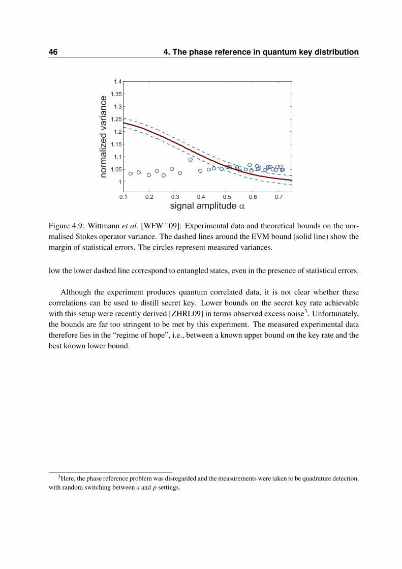
46 4. The phase reference in quantum key distribution
Figure 4.9: Wittmann et al. [WFW+09]: Experimental data and theoretical bounds on the nor-malised Stokes operator variance. The dashed lines around the EVM bound (solid line) show themargin of statistical errors. The circles represent measured variances.
low the lower dashed line correspond to entangled states, even in the presence of statistical errors.
Although the experiment produces quantum correlated data, it is not clear whether thesecorrelations can be used to distill secret key. Lower bounds on the secret key rate achievablewith this setup were recently derived [ZHRL09] in terms observed excess noise3. Unfortunately,the bounds are far too stringent to be met by this experiment. The measured experimental datatherefore lies in the “regime of hope”, i.e., between a known upper bound on the key rate and thebest known lower bound.
3Here, the phase reference problem was disregarded and the measurements were taken to be quadrature detection,with random switching between x and p settings.
5Quantum memory and mixed states
Nearly all quantum information processing protocols crucially depend on entangled states. Asdescribed in Chapter 3, this is the case for Quantum Key Distribution, which has been imple-mented across distances nearing 150km [UTSM+07]. Problems arise when the distance betweenthe two communicating parties is large, because increasing photon losses and noise deterioratethe shared entanglement or even break it. A remedy comes from so-called quantum repeaters[CZKM97, DLCZ01], which can help to distribute entanglement over very large distances. Theefficient operation of a quantum repeater requires the ability to store a quantum state of lightfor short periods of time, i.e., a quantum memory. Naturally, there are other applications ofquantum memories. A quantum computer, for example, can be thought of as a multi-particlequantum memory with added gate operations. Numerous quantum memory experiments havebeen conducted, using a variety of physical systems [JSC+04, AFK+08, HAA+08].
In contrast to quantum memory, classical storage or transmission of quantum states is de-scribed by measure & prepare (MP) schemes. In these schemes, input states are converted intoclassical data by a destructive measurement. This classical data is transmitted or stored, and newoutput states are prepared accordingly. MP schemes are equivalent to entanglement-breakingchannels [HSR03]. Therefore, as a minimal requirement, any quantum memory or teleportationexperiment must produce data which is qualitatively distinct from data obtained in such classicalschemes. This is the natural definition of the quantum domain.
Definition 2 Quantum domainIn a quantum communication experiment, data which is not compatible with any MP channelis said to belong to the quantum domain. All other data belongs to the classical domain. Afundamental requirement for quantum storage or teleportation experiments is the ability toproduce data in the quantum domain.
48 5. Quantum memory and mixed states
5.1 Implementations of quantum memory
The subject of quantum memory for optical signals is a most interesting one, because it leaves therealm of pure optics. Typically, the storage of a quantum state of light is achieved by transferringit to an atomic system. A number of requirements need to be met for a quantum memory tobe useful. Naturally, the memory should be capable of storing a variety of different quantumstates, such as arbitrary qubit states, or coherent states of any amplitude or phase. Then, thememory should have storage times sufficiently long to be useful for quantum communicationapplications [RFL08]. Another, rather natural requirement, is the ability to retrieve the storedlight at a precisely controllable time and to couple it into a fibre channel.
In the simplest scenario, a single photon is absorbed by a single atom, exciting it from itsinitial ground state to an excited state. At a later time, the atom decays to the ground state andre-emits a photon. In practice, most approaches to quantum storage employ atomic ensembles.Then, a variety of interesting physical effects can be used to enhance the coherence time of thequantum memory, a small subset of which is presented below.
5.1.1 Atomic ensembles
An early implementation of a quantum memory for coherent states was achieved in the groupof Polzik [JSC+04]. Using two atomic ensembles in coherent spin states with opposite meanspin vectors, high-fidelity transfer of the coherent states of light to the atomic states was demon-strated. In this approach, the input light is not fully absorbed by the atomic media, but ratherpasses through the atoms, becoming entangled with them in the process. The state of the emerg-ing light is measured and used for feedback on the atomic ensembles. After a storage time ofabout 4 milliseconds, another optical pulse is used to probe the state of the atomic memory. Bycomparing the spin operators describing the atomic ensemble to the Stokes operators describingthe state of light, the fidelity between input light and atomic state after the storage can be estab-lished. Because the stored light is not retrieved in this protocol, the achieved fidelities are ratherhigh, up to 70% for an input ensemble of coherent states with intensities 〈n〉 < 4 and randomphases.
Although Ref. [JSC+04] quotes a value of the maximum classical fidelity for such inputensembles, such a benchmark was never derived in full rigour.
5.1.2 Photon echo
Like many techniques used in quantum information processing, the so-called photon echo effectwas proposed [KN63, KAH64] long before the advent of quantum communication. Being theanalogue of spin echo [Hah50], the effect can occur in media with inhomogeneously broadenedabsorption spectra. The absorption of a light pulse and the following de-phasing of the atomic

5.1. Implementations of quantum memory 49
z
xy
initial π/2 pulse
y
x
de-phasing
y
x
π pulse
re-phasing
y
x
echo pulse emission
Figure 5.1: Illustration of the photon echo process for two incident light pulses.
excitations can be reversed, leading to re-phasing and re-emission of the light pulse. This isillustrated in Fig. 5.1. We consider the medium as a collection of two-level systems, each withan assigned Bloch vector describing its state. Assuming that all Bloch vectors are initially alignedwith what we define as the z-axis, we can rotate the resulting macroscopic dipole moment withan optical pulse through π/2. Inhomogeneous broadening leads to de-phasing of the individualBloch vectors in the xy-plane. After sending a π-pulse at time t, which mirrors all vectors on they-axis, the Bloch vectors start to re-phase. At time 2t, they will again form a macroscopic dipolemoment, which leads to the emission of the echo light pulse (c.f., super-radiance [Dic54]). Aninteresting variation of this scheme is produced by splitting the π-pulse into two time-separatedπ/2 pulses. By adjusting the separation times between the different pulses, the emission of theecho can be triggered at a specific time, which is important for a quantum memory. In fact, withthe right choice of write and read pulses, it is possible to store a series of data pulses, and retrievetheir echos (see, e.g. [HSH+09]).
The storage of very weak pulses, such as single photon pulses is still a challenge. A proposalfor photon echo-based storage of single photons is found in Ref. [KTG+06].
5.1.3 EIT media
The abbreviation EIT stands for electromagnetically induced transparency, which is a techniquefor rendering a medium transparent to a propagating light field. This technique was discoveredlong before the advent of quantum memories and it has been studied extensively. Here, we justoutline how EIT can be of advantage to the storage of light. In a typical setup, a single mode oflight passes though an optically dense medium, such as a container of atomic vapour. Three ofthe atomic states are of interest to us. The atoms are initially in the ground state |g〉, and a modeof light (the probe light) can excite them to an excited state |e〉. Via a different transition, an atomcan de-excite to a third state |c〉, which has a long lifetime. This transition is driven by a secondlaser field, called the control field. This setup is shown in Fig. 5.2 in a Λ-configuration. The keyto the transparency of the medium to the probe field lies in coherent population trapping: There

50 5. Quantum memory and mixed states
|g〉
|e〉
|c〉
control fieldprobe field
Figure 5.2: Three atomic levels in Λ-configuration. The probe field is the input light to be stored,and the control field drives the transition to the metastable state |c〉.
are two ways for an excitation from |g〉 to |e〉 to occur, namely the direct transition g→ e and thetransition g→ e→ c→ e. If the probability amplitudes of both of these transitions are equal, butoppositely phased, they cancel each other. Consequently, no more photons from the probe fieldwill be absorbed, and the medium becomes transparent at that frequency. The atoms will be in asuperposition of |g〉 and |c〉, with the excited state unoccupied (dark state).
For memory of light, the EIT medium presents the possibility to store photonic excitations bypopulating the atomic state |c〉, which has a long lifetime as long as the control field is switchedoff, as it should be during storage. The storage process is reversible, by turning the control fieldback on, and the photonic state can be retrieved.
This technique has been employed for the storage of classical light (see, e.g., [HSH+09]) aswell as quantum states, such as squeezed states of light [AFK+08, HAA+08].
5.2 Benchmarking with the EVM
The EVM criterion is well suited to verify operation of a quantum memory in the quantumdomain [HL09a]. It is adapted to discrete-continuous systems, such as effective bi-partite formu-lations of CV protocols with a finite number of signal states. In fact, just as two non-orthogonalstates suffice to perform QKD, the binary input ensemble should be suited to test quantum mem-ories. We start this Section by developing a benchmarking test for the storage of pure squeezedlight. This setting requires only small adjustments of the EVM method presented in the previousChapter. We then proceed to extend the EVM method to sources of mixed signal states. This isof particular importance to squeezed states, which cannot be generated with unit purity. We closethis Chapter with the application of the EVM method to two further examples: a source whichemits displaced thermal states, to supplement the results of the previous Chapter, and a source ofmixed qubit states, to demonstrate the method for a small-dimensional system.

5.2. Benchmarking with the EVM 51
5.2.1 Pure squeezed test states
Here, we apply the EVM method to a quantum memory for squeezed light. We begin the analysisby considering the two pure test states
|ψ in0 〉= S(rin)|0〉 (5.1)
|ψ in1 〉= S(−rin)|0〉, (5.2)
which are passed through the quantum memory. Bob receives two corresponding conditionalstates ρout
0 and ρout1 , on which he measures expectation values and variances of x and p. There-
fore, eight parameters suffice for a complete characterisation of possible measurement out-comes. The parameterisation simplifies further when taking in account two properties whichseem generic to quantum memory channels: Firstly, we do not expect the channel to induce dis-placements away from the vacuum. If the input states are centred at the origin in phase space,then the output states will be, too. The second property is phase covariance, i.e.,
Λ(UΦρU†Φ) = UΦ Λ(ρ) U†
Φ, (5.3)
where Λ denotes the action of the memory channel. Intuitively, this must be true because thephase of the signal states is defined only in reference to a local oscillator, with which the memoryis not connected.
The first property ensures that all first moments measured by Bob are zero, and the secondproperty links the observed variances:
Varρout0
(x) = Varρout1
( p) (5.4)
Varρout0
( p) = Varρout1
(x). (5.5)
Hence, two parameters are indeed sufficient to characterise a distinct set of measurement data,which is particularly convenient for the visualisation of results. Figure 5.3(a) plots Varρout
0( p)
against Varρout0
(x), which spans the parameter space. The physicality condition here is simplythe Heisenberg uncertainty relation [Eqn. (2.26)].
For small amounts of variance broadening, we expect to be able to identify a quantum do-main. Unlike the setting for the binary coherent signal in Chapter 4, the first moments do notplay a role here, so we construct an EVM which contains the second moments only:
χ(ρAB) =
Var0(x) b1 + i
2 c1 c2 + i
2sb1− i
2 Var0( p) c2− i
2s c3
c∗1 c∗2 + i
2s Var0( p) b2 + i
2c∗2− i
2s c∗3 b2− i
2 Var0(x)
, (5.6)
where s denotes the overlap 〈−rin|rin〉, bi ∈R and ci ∈C. Naturally, the separability condition,Eqn. (3.13), remains the same and can again be checked as an SDP. The results are shown in
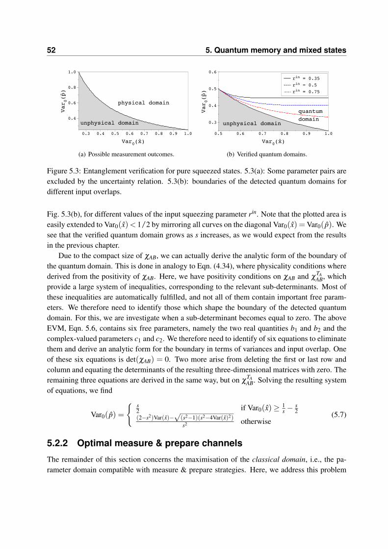
52 5. Quantum memory and mixed states
physical domain
unphysical domain
Var0(p)
0.4
0.6
0.8
1.0
Var0(x)0.3 0.4 0.5 0.6 0.7 0.8 0.9 1.0
(a) Possible measurement outcomes.
quantumdomain
unphysical domain
Var0(p)
0.3
0.4
0.5
0.6
Var0(x)0.5 0.6 0.7 0.8 0.9 1.0
rin = 0.35rin = 0.5rin = 0.75
(b) Verified quantum domains.
Figure 5.3: Entanglement verification for pure squeezed states. 5.3(a): Some parameter pairs areexcluded by the uncertainty relation. 5.3(b): boundaries of the detected quantum domains fordifferent input overlaps.
Fig. 5.3(b), for different values of the input squeezing parameter rin. Note that the plotted area iseasily extended to Var0(x) < 1/2 by mirroring all curves on the diagonal Var0(x) = Var0( p). Wesee that the verified quantum domain grows as s increases, as we would expect from the resultsin the previous chapter.
Due to the compact size of χAB, we can actually derive the analytic form of the boundary ofthe quantum domain. This is done in analogy to Eqn. (4.34), where physicality conditions wherederived from the positivity of χAB. Here, we have positivity conditions on χAB and χ
TAAB, which
provide a large system of inequalities, corresponding to the relevant sub-determinants. Most ofthese inequalities are automatically fulfilled, and not all of them contain important free param-eters. We therefore need to identify those which shape the boundary of the detected quantumdomain. For this, we are investigate when a sub-determinant becomes equal to zero. The aboveEVM, Eqn. 5.6, contains six free parameters, namely the two real quantities b1 and b2 and thecomplex-valued parameters c1 and c2. We therefore need to identify of six equations to eliminatethem and derive an analytic form for the boundary in terms of variances and input overlap. Oneof these six equations is det(χAB) = 0. Two more arise from deleting the first or last row andcolumn and equating the determinants of the resulting three-dimensional matrices with zero. Theremaining three equations are derived in the same way, but on χ
TAAB. Solving the resulting system
of equations, we find
Var0( p) =
{ s2 if Var0(x) ≥ 1
s − s2
(2−s2)Var(x)−√
(s2−1)(s2−4Var(x)2)s2 otherwise
(5.7)
5.2.2 Optimal measure & prepare channels
The remainder of this section concerns the maximisation of the classical domain, i.e., the pa-rameter domain compatible with measure & prepare strategies. Here, we address this problem

5.2. Benchmarking with the EVM 53
from a numerical viewpoint. Eve’s strategy is equivalent to an entanglement-breaking channel[HSR03],
ρoutk = ∑
itr(ρ
ink πi)|ψi〉〈ψi|, (5.8)
where ρ ink are the two input states [Eqs. (5.1) and (5.2)], and the operators πi form a positive
operator valued measure (POVM), i.e., they are positive semidefinite and sum to the identity.Resulting from this strategy, Bob will measure variances of the form
Varρout0
( p) =12 ∑
itr(πiρ
in0 )〈ψi|p2|ψi〉 (5.9)
Varρout0
(x) =12 ∑
itr(πiρ
in0 )〈ψi|x2|ψi〉. (5.10)
Maximising the classical domain now amounts to a minimisation of (5.9) for each fixed value ofVar(x) (c.f. Fig. 5.3).
Let us first consider the re-prepared states {|ψi〉}. Since the figure of merit is a variance, theoptimal re-prepared states must be minimum uncertainty states. Furthermore, since Bob expectsall first moments to be zero, displacements in {|ψi〉} have the effect of increasing the quadraturevariances (see, e. g. [BR97]). This leaves the class of squeezed vacuum states, with the squeezingaxis aligned with the axis of Bob’s quadrature detection. Therefore, each re-prepared state |ψi〉can be parameterised by a single real parameter, namely its squeezing parameter ri. Explicitly,Bob’s measured variances are given by
Varρout0
( p) =12 ∑
itr(πiρ
in0 )exp(−2ri), (5.11)
Varρout0
(x) =12 ∑
itr(πiρ
in0 )exp(2ri), (5.12)
and the minimisation problem is the following:
minπi,ri
Varρout0
( p) (5.13)
s. t. Varρout0
(x) = c, (5.14)
πi ≥ 0 (5.15)
∑i
πi = 1, (5.16)
and we solve this problem for any c ≥ 0.5 [c.f. Fig. 5.3(b)]. Since there are only two pure teststates, each POVM element is described by a two-dimensional matrix. Assuming that the numberof POVM elements is small, the optimal solution can easily be found numerically. The resultsof such a numerical optimisation are shown in Fig. 5.4, with the number of POVM elementsset to four. We see that this optimised measure & re-prepare strategy reaches the boundary of

54 5. Quantum memory and mixed states
rin = 0.5
opt. classical channel
classical domain
unphysical domainquantum domain
(A)(B)V
ar0(p)
0.25
0.30
0.35
0.40
0.45
0.50
0.55
0.60
Var0(x)
0.5 0.6 0.7 0.8 0.9 1.0
Figure 5.4: Optimal measure & re-prepare strategy for two squeezed test states. The boundariesof the classical and the quantum domains coincide. Optimal measurements in region (A): min-imum error discrimination; region (B): unambiguous state discrimination and minimum errordiscrimination
the quantum domain. Therefore, any experimental outcome in our parameterisation is unam-biguously sorted into one of three domains: the unphysical domain, the quantum domain asdetermined by the EVM method, and the classical domain.
It is natural to ask whether this optimal POVM corresponds to minimum error discrimination,in analogy to the coherent state protocol. It turns out that this is true only partially. The boundaryof the quantum domain shown in Fig. 5.4 is a concatenation of a curved part (A) and a straightline with slope zero (B) [c.f., Eqs. (5.7)]. This behaviour arises from the fact that the first eigen-value of the EVM to become negative is different in regions (A) and (B). Therefore, the optimalmeasure & re-prepare strategies and in particular the POVMs are also likely to be different inboth regions. It turns out that the optimal measurement for region (A) is indeed minimum errordiscrimination. We can derive the analytic form of variances which this attack induces in Bob’sobservations. Since Eve resends states with quadrature expectation values equal to zero, theirvariances are linear functions of the state. Consequently, Bob will measure
VarB0 ( p) = (1− perr)VarMP
0 ( p)+ perrVarMP0 (x) (5.17)
VarB0 (x) = (1− perr)VarMP
0 (x)+ perrVarMP0 ( p), (5.18)
where we have used VarMP0 (x) = VarMP
1 ( p), and VarMP0 (x) stands for 〈ψi|x2|ψi〉. We can fur-
thermore eliminate VarMP0 ( p) by using the fact that Eve resends minimum uncertainty states.

5.2. Benchmarking with the EVM 55
|ψ0〉in
|ψ1〉in
|r〉
|vac〉
|-r〉
p0
p?
p1
USD
Figure 5.5: Schematic of the optimal USD strategy for pure squeezed input states.
Therefore,
VarB0 ( p) = (1− perr)(4VarMP
0 (x))−1 + perrVarMP0 (x) (5.19)
VarB0 (x) = (1− perr)VarMP
0 (x)+ perr(4VarMP0 (x))−1. (5.20)
Finally, we can eliminate VarMP0 (x) to find the following relation between Bob’s observed vari-
ances:
VarB0 ( p) =
(2− s2)VarB0 (x)−
√(s2−1)(s2−4VarB
0 (x)2)
s2 , (5.21)
which is identical to the boundary of the detected quantum domain, Eqn. (5.7).The optimal measurement in region (B) turns out to be connected to a USD measurement.
To be precise, it is possible to show that in the limit VarB0 (x)→ ∞, a USD strategy can reach
VarB0 ( p) = s/2. By linearity, combinations of this strategy with the above minimum error strat-
egy lead to the straight line which forms the boundary for region (B).Figure 5.5 shows a schematic of the USD-based measure and prepare setting. When the
input state is unambiguously identified to be |ψ in0/1〉, a squeezed vacuum state |± r〉 is resent.
When the measurement is inconclusive, the vacuum state is resent. We furthermore know thatthe probabilities of the different outcomes of the USD measurement are related by p0 = p1 =(1− p?)/2. Therefore, this attack will induce the variances
VarB0 ( p) =
12(1− p?)
12e−2r + p?
12
(5.22)
VarB0 (x) =
12(1− p?)
12e
2r + p?12
(5.23)
Inserting the optimal value p? = s, and taking the limit r→ ∞, we find
VarB0 ( p)→ s
2(5.24)
VarB0 (x)→ ∞. (5.25)
56 5. Quantum memory and mixed states
Thus, this strategy can reach the value VarB0 ( p) = s/2, at diverging VarB
0 (x). Again, since themeasured variances are linear functions of ρout
0 , any convex combination of two MP strategiesresults in another valid MP strategy. Therefore, the USD strategy can explain the numericalresults for region (B) in Fig. 5.4.
With the combination of minimum error measurement and unambiguous state discrimina-tion, we have shown the analytic agreement of the quantum domain boundary with the optimalMP strategy. Therefore, the EVM method witnesses all entangled states which are detectable bythe given measurements. The resulting quantum domain cannot be enlarged by any other veri-fication method. This is in accordance with the results for two coherent test states |α〉 and |−α〉.
The important observation, as far as the validation of memory experiments is concerned, isthat the detection of squeezing in the retrieved light does not suffice. A quantum memory isprovably working in the quantum domain if and only if the measured variances are below theboundary given by Eqn. (5.7).
5.3 Optimal measure & prepare channels for mixedstates
It was already mentioned earlier that the generation of pure squeezed states is in practice infeasi-ble, due to inevitable photon losses in the out-coupling of the squeezing process. A good modelfor this is the mixing of a pure squeezed state with the vacuum on a slightly reflecting beamsplitter. The output state (in both ports) will be a squeezed thermal state [FC88, KdOK89], i.e.,a mixed state. Therefore, the two squeezed vacuum states (5.1) and (5.2) are, in practice, twosqueezed thermal states
ρin0 =
11 + n ∑
n
(n
1 + n
)n
S(rin)|n〉〈n|S†(rin) (5.26)
ρin1 =
11 + n ∑
n
(n
1 + n
)n
S(rin)|n〉〈n|S†(rin). (5.27)
This serves as a motivation to extend our verification procedure beyond pure test states.As it turns out, the extension of the EVM method to mixed states is an intricate matter,
with a trade-off between complexity and the strength of the resulting entanglement criterion. Toevaluate the latter, it is most useful to first know the optimal MP channel, and hence the boundaryof the quantum domain. One may question the usefulness of the EVM criterion if the quantumdomain can just as well be revealed by optimising over MP channels. However, once developed,the EVM method for mixed states can be applied to a wide variety of systems, whereas theoptimal MP channel must be found anew each time. Moreover, the involved optimisation is byno means trivial.

5.3. Optimal measure & prepare channels for mixed states 57
An optimisation over MP channels for pure squeezed input states was performed above, inSection 5.2.2. We recall the above figure of merit: The optimal entanglement-breaking channelminimises Var0( p) for a fixed value of Var0(x), and the optimisation runs over the POVM {πi}and the re-prepared states {|ψi〉}. It was argued above that the re-prepared states {|ψi〉} shouldbe drawn from the set of squeezed vacuum states. Naturally, this is also true when mixed inputstates are used to test the channel. Therefore, we are faced with the optimisation problem posedin Eqn. (5.13), with an additional constraint coming from the phase-symmetry, Eqs. (5.4) and(5.5).
It is instructive to start with the simplified problem of finding the global minimum ofVarρout
0( p), while ignoring the constraint Varρout
0(x) = c, for the moment. The phase-symmetry
of the output is achieved quite easily, by considering entanglement-breaking strategies whichautomatically obey this symmetry. If {πi, |ψi〉} is a particular valid MP strategy, then the phase-rotated strategy {Uπ
2πiU
†π
2,Uπ
2|ψi〉} leads to the same observations. Here,
Uπ
2= exp(−iπ
2n) (5.28)
is a phase shift operator. An equal mixture of both strategies will then automatically satisfy theconstraints (5.4) and (5.5). The figure of merit now becomes
Varρout0
( p) =12
(∑
itr(πiρ
in0 )〈ψi|p2|ψi〉+∑
itr(Uπ
2πiU
†π
2ρ
in0 )〈ψi|U†
π
2p2Uπ
2|ψi〉
)
=12
(∑
itr(πiρ
in0 )〈ψi|p2|ψi〉+∑
itr(πiρ
in1 )〈ψi|x2|ψi〉
)
=14
(∑
itr(πiρ
in0 )e−2ri +∑
itr(πiρ
in1 )e2ri
). (5.29)
Each term in the summation can be independently optimised over ri, which leads to the muchshorter expression
Varρout0
( p) =12 ∑
i
√tr(πiρ
in0 )tr(πiρ
in1 ). (5.30)
It remains to find the POVM which minimises this output variance. In the previous section, thetwo pure input states spanned a two-dimensional space and the POVM elements were conse-quently represented by two-dimensional matrices. Here, the two input states act on an infinite-dimensional Hilbert space. Nevertheless, the optimal POVM can be found analytically. Thecorresponding derivation is found in [Fuc95], and here, we borrow the final result
minπi
∑i
√tr(πiρ
in0 )tr(πiρ
in1 ) = F(ρ
in0 ,ρ in
1 ), (5.31)
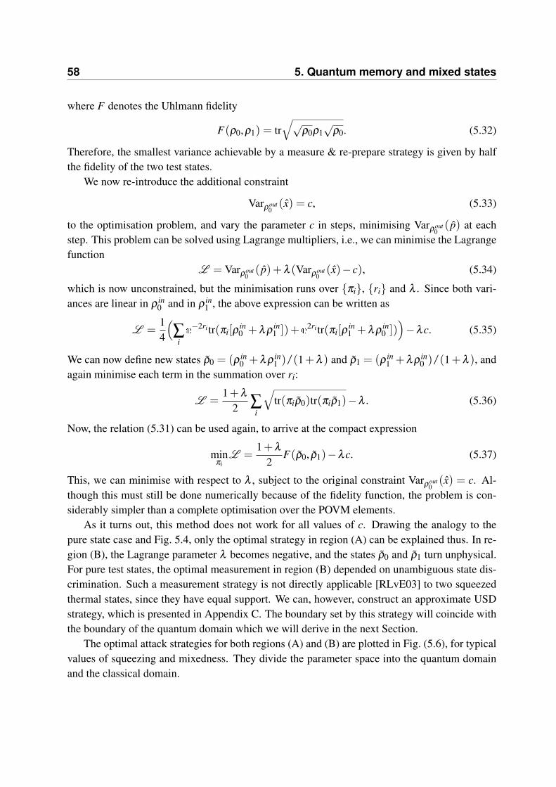
58 5. Quantum memory and mixed states
where F denotes the Uhlmann fidelity
F(ρ0,ρ1) = tr√√
ρ0ρ1√
ρ0. (5.32)
Therefore, the smallest variance achievable by a measure & re-prepare strategy is given by halfthe fidelity of the two test states.
We now re-introduce the additional constraint
Varρout0
(x) = c, (5.33)
to the optimisation problem, and vary the parameter c in steps, minimising Varρout0
( p) at eachstep. This problem can be solved using Lagrange multipliers, i.e., we can minimise the Lagrangefunction
L = Varρout0
( p)+ λ (Varρout0
(x)− c), (5.34)
which is now unconstrained, but the minimisation runs over {πi}, {ri} and λ . Since both vari-ances are linear in ρ in
0 and in ρ in1 , the above expression can be written as
L =14
(∑
ie−2ritr(πi[ρ in
0 + λρin1 ])+e
2ritr(πi[ρ in1 + λρ
in0 ]))−λc. (5.35)
We can now define new states ρ0 = (ρ in0 +λρ in
1 )/(1+λ ) and ρ1 = (ρ in1 +λρ in
0 )/(1 +λ ), andagain minimise each term in the summation over ri:
L =1 + λ
2 ∑i
√tr(πiρ0)tr(πiρ1)−λ . (5.36)
Now, the relation (5.31) can be used again, to arrive at the compact expression
minπi
L =1 + λ
2F(ρ0, ρ1)−λc. (5.37)
This, we can minimise with respect to λ , subject to the original constraint Varρout0
(x) = c. Al-though this must still be done numerically because of the fidelity function, the problem is con-siderably simpler than a complete optimisation over the POVM elements.
As it turns out, this method does not work for all values of c. Drawing the analogy to thepure state case and Fig. 5.4, only the optimal strategy in region (A) can be explained thus. In re-gion (B), the Lagrange parameter λ becomes negative, and the states ρ0 and ρ1 turn unphysical.For pure test states, the optimal measurement in region (B) depended on unambiguous state dis-crimination. Such a measurement strategy is not directly applicable [RLvE03] to two squeezedthermal states, since they have equal support. We can, however, construct an approximate USDstrategy, which is presented in Appendix C. The boundary set by this strategy will coincide withthe boundary of the quantum domain which we will derive in the next Section.
The optimal attack strategies for both regions (A) and (B) are plotted in Fig. (5.6), for typicalvalues of squeezing and mixedness. They divide the parameter space into the quantum domainand the classical domain.
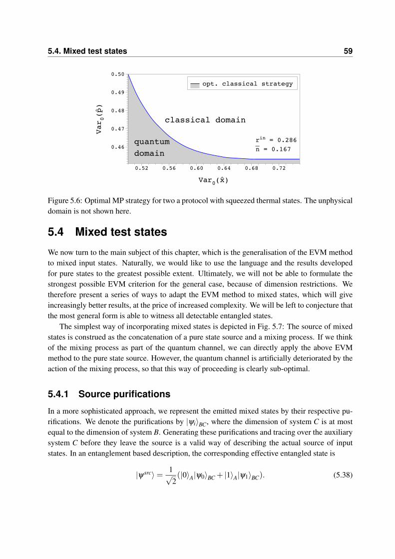
5.4. Mixed test states 59
rin = 0.286n = 0.167
classical domain
quantumdomain
Var0(p)
0.46
0.47
0.48
0.49
0.50
Var0(x)
0.52 0.56 0.60 0.64 0.68 0.72
opt. classical strategy
Figure 5.6: Optimal MP strategy for two a protocol with squeezed thermal states. The unphysicaldomain is not shown here.
5.4 Mixed test states
We now turn to the main subject of this chapter, which is the generalisation of the EVM methodto mixed input states. Naturally, we would like to use the language and the results developedfor pure states to the greatest possible extent. Ultimately, we will not be able to formulate thestrongest possible EVM criterion for the general case, because of dimension restrictions. Wetherefore present a series of ways to adapt the EVM method to mixed states, which will giveincreasingly better results, at the price of increased complexity. We will be left to conjecture thatthe most general form is able to witness all detectable entangled states.
The simplest way of incorporating mixed states is depicted in Fig. 5.7: The source of mixedstates is construed as the concatenation of a pure state source and a mixing process. If we thinkof the mixing process as part of the quantum channel, we can directly apply the above EVMmethod to the pure state source. However, the quantum channel is artificially deteriorated by theaction of the mixing process, so that this way of proceeding is clearly sub-optimal.
5.4.1 Source purifications
In a more sophisticated approach, we represent the emitted mixed states by their respective pu-rifications. We denote the purifications by |ψi〉BC, where the dimension of system C is at mostequal to the dimension of system B. Generating these purifications and tracing over the auxiliarysystem C before they leave the source is a valid way of describing the actual source of inputstates. In an entanglement based description, the corresponding effective entangled state is
|ψsrc〉= 1√2(|0〉A|ψ0〉BC + |1〉A|ψ1〉BC). (5.38)

60 5. Quantum memory and mixed states
pure states
mixing Channel
Figure 5.7: Schematic of a mixed state source, decomposed into a pure state source and a mixingprocess. Attributing the mixing process to the quantum channel gives a simple, but suboptimalbenchmark.
To perform the entanglement verification, we must construct a tripartite EVM, of the generalform
[χ(ρABC)]i jklmn = tr(ρABC A†i Al⊗ B†
j Bm⊗C†kCn). (5.39)
The operator sets {Ai} and {B j} should be chosen as before. In order to retrieve the actual inputstates ρi, the auxiliary system C must be traced out, which implies for the construction of atripartite EVM that the operator set {Ck} has 1C as its only member. Therefore, χABC will be ofthe form
[χ(ρABC)]i jlm = tr(ρABC A†i Al⊗ B†
j Bm⊗1C), (5.40)
which is almost identical to the bipartite EVM, Eqn. (4.4). There is, however, one crucial differ-ence: the overlap s of two pure input states is replaced by the overlap of the two purifications. Infact, this overlap is the only point where the choice of purifications becomes important. Accord-ing to Eqn. (2.14), there is unitary freedom in the choice of purifications, which we can exploitto increase the strength of the EVM criterion. As it turns out, the strongest criterion comes fromchoosing this overlap maximal. Physically, this choice makes it hardest to distinguish the twopurifications from each other, which means that MP channels will be most easily detected.
Finding the purifications with maximum overlap may, in practice, be quite involved, but thisis not actually necessary. For the construction of χABC, we are only interested in the value of thisoverlap, and this is given by Uhlmann’s theorem [Uhl76]. It states that
max|ψ0〉,|ψ1〉
|〈ψ0|ψ1〉|= F(ρin0 ,ρ in
1 ), (5.41)
where the maximisation runs over all purifications |ψi〉 of the states ρ ini , and F denotes the fidelity
[Eqn. (5.32)].This makes the extension of the EVM method very compact indeed, and we summarise:
Observation 7 Extension via purificationsThe bipartite EVM [(4.4) or (5.6)] is generalised to sources of mixed states by replacing thepure-state overlap 〈ψ0|ψ1〉 by the mixed-state fidelity F(ρ0,ρ1).
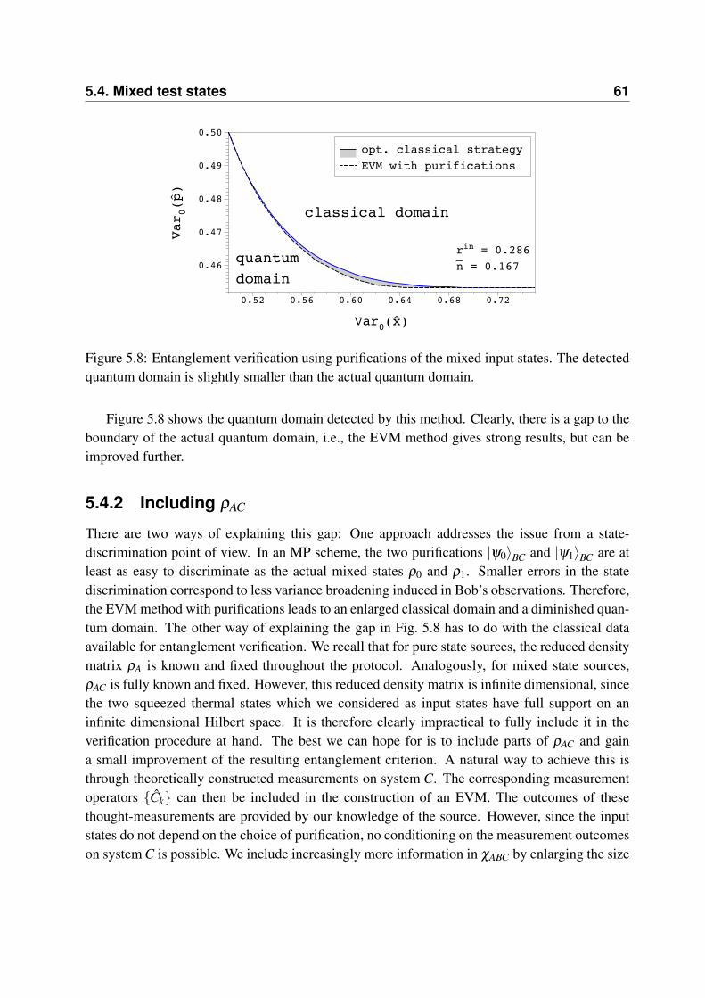
5.4. Mixed test states 61
rin = 0.286n = 0.167
quantumdomain
classical domain
Var0(p)
0.46
0.47
0.48
0.49
0.50
Var0(x)
0.52 0.56 0.60 0.64 0.68 0.72
opt. classical strategyEVM with purifications
Figure 5.8: Entanglement verification using purifications of the mixed input states. The detectedquantum domain is slightly smaller than the actual quantum domain.
Figure 5.8 shows the quantum domain detected by this method. Clearly, there is a gap to theboundary of the actual quantum domain, i.e., the EVM method gives strong results, but can beimproved further.
5.4.2 Including ρAC
There are two ways of explaining this gap: One approach addresses the issue from a state-discrimination point of view. In an MP scheme, the two purifications |ψ0〉BC and |ψ1〉BC are atleast as easy to discriminate as the actual mixed states ρ0 and ρ1. Smaller errors in the statediscrimination correspond to less variance broadening induced in Bob’s observations. Therefore,the EVM method with purifications leads to an enlarged classical domain and a diminished quan-tum domain. The other way of explaining the gap in Fig. 5.8 has to do with the classical dataavailable for entanglement verification. We recall that for pure state sources, the reduced densitymatrix ρA is known and fixed throughout the protocol. Analogously, for mixed state sources,ρAC is fully known and fixed. However, this reduced density matrix is infinite dimensional, sincethe two squeezed thermal states which we considered as input states have full support on aninfinite dimensional Hilbert space. It is therefore clearly impractical to fully include it in theverification procedure at hand. The best we can hope for is to include parts of ρAC and gaina small improvement of the resulting entanglement criterion. A natural way to achieve this isthrough theoretically constructed measurements on system C. The corresponding measurementoperators {Ck} can then be included in the construction of an EVM. The outcomes of thesethought-measurements are provided by our knowledge of the source. However, since the inputstates do not depend on the choice of purification, no conditioning on the measurement outcomeson system C is possible. We include increasingly more information in χABC by enlarging the size
62 5. Quantum memory and mixed states
rin = 0.286n = 0.167
Var0(p)
0.455
0.460
0.465
0.470
Var0(x)
0.54 0.56 0.58 0.60 0.62 0.64 0.66 0.68
EVM with purificationsone unitarythree unitariesfive unitariesoptimal MP channel
Figure 5.9: Entanglement verification from different EVMs. Shaded area: no information onthe purifying system; dashed line: one generalised spin operator on the purifying system; dottedline: three generalised spin operators; dashed-dotted line: five generalised spin operators; Solidline: actual boundary of the quantum domain.
of the operator set {Ck}. Unfortunately, it is not known which operators to choose in order toachieve the biggest improvement of the entanglement criterion. We therefore choose the opera-tors from a generic set, namely the generalised spin operators (see, e.g., [PR04]), which can beregarded as a generalisation of the Pauli operators to higher dimensions. For an N-dimensionalsystem, the generalised spin operators are defined as
Si, j =N−1
∑n=0
ξni|en〉〈en+ j|. (5.42)
Here, ξ = exp(2πi/N) and the set {|ei〉, i ∈ ZN} forms an orthonormal basis for the Hilbertspace HN , where all indices are integers modulo N. The complete set of N2 generalised spinoperators form an operator basis for the space of operators acting on HN .
For the construction of the EVM, we work in a truncated Fock basis with maximum photonnumber nmax = N − 1 = 16. But even in this truncated space, we cannot include a completeoperator basis for system C, since each additional member in the set {Ck} enlarges the dimensionof the EVM. Here, we have evaluated the entanglement criterion with up to five generalised spinoperators on system C. The resulting detected quantum domains are shown in Fig. 5.9. Clearly,the gap between the borders of the detected quantum domain and the actual quantum domainreduces in size as more information is included in χABC. Although the gap does not altogetherdisappear, it appears that it can be closed by using an EVM of sufficient size.

5.5. Displaced thermal states 63
detectedquantum domain
n = 0.1
Var(x) = Var(p)
0.5
0.6
0.7
0.8
0.9
<-α|α>0 0.2 0.4 0.6 0.8 1.0
mixed test statespure test states
(a) pure vs. mixed test states
quantum domain
classicaldomain
n = 0.1
Var(x) = Var(p)
0.5
0.6
0.7
0.8
<-α|α>0 0.2 0.4 0.6 0.8 1.0
opt. purificationstwo unitariesclassical strategy
(b) quantum and classical domains
Figure 5.10: Quantum domain for displaced thermal test states. (a): the quantum domain in-creases in size for mixed states. (b): improvements of the entanglement verification by addingtwo unitary operators to the EVM (dashed) and optimised measure & re-prepare strategy (dashed-dotted)
5.5 Displaced thermal states
Now, we briefly examine the case of two displaced thermal states as test states. Experimentally,coherent states can be generated essentially noiselessly, so a test with pure states is possible.Still, the addition of noise to the test states may be of advantage to the protocol at hand [RGK05].This second physical setup in the continuous-variable domain will also supplement the resultsfor coherent states from the previous Chapter and allow us to draw a comparison to squeezedthermal states.
In the Fock basis, two coherent states with thermal noise are given by
ρin0 =
1n + 1
∞
∑n=0
(n
n + 1
)n
D(α)|n〉〈n|D†(α) (5.43)
ρin1 =
1n + 1
∞
∑n=0
(n
n + 1
)n
D(−α)|n〉〈n|D†(−α). (5.44)
Here, D(α) denotes the displacement operator [BR97] and we take α to be real. These two teststates pass through the quantum channel and, as before, homodyne detection is performed on theoutput states. We will adopt the same parameterisation of the possible measurement outcomesas in Chapter 4. Specifically, the observed variances of the x and p quadratures are assumed tobe equal, and losses act as a simple down-scaling of the observed first moments. The results forpure test states [RGL06, HML08] are displayed in Fig. 5.10(a).
As before, a good approximation to the source of mixed test states is a source of correspond-ing purifications. Following Observation 7, we can easily perform the entanglement verificationfor the optimal choice of purifications. The corresponding results are displayed in Fig. 5.10(a).
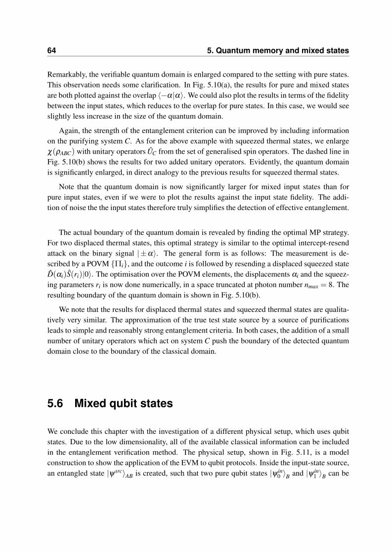
64 5. Quantum memory and mixed states
Remarkably, the verifiable quantum domain is enlarged compared to the setting with pure states.This observation needs some clarification. In Fig. 5.10(a), the results for pure and mixed statesare both plotted against the overlap 〈−α|α〉. We could also plot the results in terms of the fidelitybetween the input states, which reduces to the overlap for pure states. In this case, we would seeslightly less increase in the size of the quantum domain.
Again, the strength of the entanglement criterion can be improved by including informationon the purifying system C. As for the above example with squeezed thermal states, we enlargeχ(ρABC) with unitary operators UC from the set of generalised spin operators. The dashed line inFig. 5.10(b) shows the results for two added unitary operators. Evidently, the quantum domainis significantly enlarged, in direct analogy to the previous results for squeezed thermal states.
Note that the quantum domain is now significantly larger for mixed input states than forpure input states, even if we were to plot the results against the input state fidelity. The addi-tion of noise the the input states therefore truly simplifies the detection of effective entanglement.
The actual boundary of the quantum domain is revealed by finding the optimal MP strategy.For two displaced thermal states, this optimal strategy is similar to the optimal intercept-resendattack on the binary signal |±α〉. The general form is as follows: The measurement is de-scribed by a POVM {Πi}, and the outcome i is followed by resending a displaced squeezed stateD(αi)S(ri)|0〉. The optimisation over the POVM elements, the displacements αi and the squeez-ing parameters ri is now done numerically, in a space truncated at photon number nmax = 8. Theresulting boundary of the quantum domain is shown in Fig. 5.10(b).
We note that the results for displaced thermal states and squeezed thermal states are qualita-tively very similar. The approximation of the true test state source by a source of purificationsleads to simple and reasonably strong entanglement criteria. In both cases, the addition of a smallnumber of unitary operators which act on system C push the boundary of the detected quantumdomain close to the boundary of the classical domain.
5.6 Mixed qubit states
We conclude this chapter with the investigation of a different physical setup, which uses qubitstates. Due to the low dimensionality, all of the available classical information can be includedin the entanglement verification method. The physical setup, shown in Fig. 5.11, is a modelconstruction to show the application of the EVM to qubit protocols. Inside the input-state source,an entangled state |ψsrc〉AB is created, such that two pure qubit states |ψ in
0 〉B and |ψ in1 〉B can be

5.6. Mixed qubit states 65
A B
Cc-phaseφ
ÛC
source
|0�+ |1�√2
|ψsrc�AB
Figure 5.11: Source-replacement scheme for a source of mixed qubit states. An interactionthrough a c-phase gate mixes the initially pure test states.
prepared by projective measurements on system A. It is convenient to choose them
|ψ in0 〉B = cos(
θ
2)|0〉B + sin(
θ
2)|1〉B, (5.45)
|ψ in1 〉B = cos(
θ
2)|0〉B− sin(
θ
2)|1〉B. (5.46)
Still inside the source, these states are mixed by the interaction with an auxiliary qubit system Cthrough the action of a conditional phase gate. This auxiliary system is initially in the superposi-tion state (|0〉+ |1〉)/
√2, resulting in the two mixed input states
ρin0/1 =
(cos2(θ
2 ) ±12(1 +e
−iφ )cos(θ
2 ) sin(θ
2 )±1
2(1 +eiφ )cos(θ
2 ) sin(θ
2 ) sin2(θ
2 )
). (5.47)
Adjusting the phase φ allows us to vary the mixedness of the conditional states in system Bcontinuously. In this setting, φ = 0 corresponds to pure test states.
The two mixed input states are transmitted to Bob, who measures the expectation values ofall three Pauli operators on the output states. We assume that his observations are accuratelymodelled by a depolarising channel
ρouti = Λp(ρ
ini ) = p
1B
2+(1− p)ρ
ini , (5.48)
with depolarising parameter p. The boundary of the quantum domain is determined by the max-imum value of the depolarising parameter for which effective entanglement can be verified.
Again, we begin by determining the boundary of the quantum domain through the optimisedMP strategy. It turns out that this optimal strategy consists of a minimum error discriminationmeasurement and the re-preparation of two states of the same form as the input states. Theconditional states which Bob receives will depend on the minimum error probability perr. Sincethe signal source emits mixed states, the optimal perr depends on the trace distance between thetwo input states [see Eqn. (2.18)], and takes the explicit form
perr =12− cos(θ ) sin(θ )cos(
φ
2). (5.49)
66 5. Quantum memory and mixed states
φ= π4
quantum domain
depol. parameter p
0
0.05
0.10
0.15
0.20
0.25
0.30
θ0 0.1 0.2 0.3 0.4 0.5 0.6 0.7 0.8 0.9
optimal purificationsnon-optimal purif.optimal MP strategy
Figure 5.12: Results of the EVM method with qubit states.
The higher probabilities of error occurring with increasing mixedness will show in Bob’s obser-vations as higher degrees of depolarisation. This is displayed in Fig. 5.12, for fixed mixedness φ
and different values of θ .Since the subsystems A, B and C are all two-dimensional, we can easily construct an EVM
from tomographically complete operator sets for all three subsystems. The EVM then certainlycontains all available classical information and the number of free parameters is quite small. Withthis construction, there is no gap between verified quantum domain and optimal MP strategy (seeFig. 5.12).
For comparison, we can also use the approximate verification method described in Observa-tion 7, i.e., use optimal purifications of the mixed input states. Interestingly, this extension ofthe EVM method also provides an entanglement criterion of maximum strength for this qubitprotocol, as shown in Fig. 5.12. This appears to be a peculiarity of qubit protocols and it has todo with a special relation between the fidelity and the trace distance, namely
Dtr(ρ ,σ) =√
1−F(ρ ,σ), (5.50)
which holds for qubits states ρ and σ of equal degree of mixedness. A proof of this is given inAppendix D.
6Optimal benchmark criteria
The previous chapter introduced the concept of testing quantum memory or teleportation chan-nels by verifying effective entanglement. The key to such a test is captured in Definition 2: Aquantum memory or teleportation experiment must not be classically simulatable, i.e., the ob-tained data must not be compatible with a measure and prepare (MP) channel. This definition ofthe quantum domain is by no means new. It can already be found in early proposals for quantumbenchmarks, for example in Ref. [BFK00], albeit in a somewhat convoluted form. The interest inbenchmarking procedures was recently revived with the advent of more sophisticated quantummemory experiments, such as the storage of squeezed light [AFK+08, HAA+08].
Over the last four or five years, a number of benchmark criteria were published, for coher-ent states, squeezed states and mixed input states [HWPC05, AC08, Nam08, OPP+08, NKI08,CAnTB09, HML08, HL09a]. The problem with this series of proposed quantum benchmarks isthat they do not converge to a single optimal benchmark criterion. On the contrary, the multitudeof different approaches to benchmarking very much conceals which aspects are important andwhich are not. In this chapter, we attempt to distill the important aspects of quantum bench-marking. We do this by first comparing a number of recently published criteria for a typicalexperimental setup. We then consider the experimental resources involved in the implementationof these benchmarks and attempt to reduce those as much as possible without deteriorating thebenchmark criterion. Not surprisingly, the optimally reduced criterion will be an extension ofthe EVM method presented in the previous two chapters.
We begin by fixing some notational conventions and establish the connections to the previouschapters. We then give a short review of benchmark criteria based on the fidelity. The main partof this chapter deals with the benchmark comparison and the associated extension of the EVMmethod. Finally, we address the question whether naturally occurring phase fluctuations can beof use for benchmarking. This Chapter is an extension of Ref. [HL09b].

68 6. Optimal benchmark criteria
6.1 General setting and previous work
Typically, Definition 2 is used for the derivation of benchmarks. In addition, a benchmark cri-terion must fix the set of input states used for implementing it, and, from the experimental side,additional constraints may come from the measurements on the output states. For example, to-mography of the output states may not always be possible.
We will denote each input state by |ψ ini 〉 and the probability of its preparation by pi. These
quantities form the input ensemble {|ψ ini 〉, pi}N
i=1. The action of the channel is described by thesuper-operator Λ, so that we can associate with each input state an output state
ρouti = Λ(|ψ in
i 〉〈ψ ini |). (6.1)
Naturally, the channel Λ should not explicitly enter the benchmark criterion, since it is in generalunknown. Entanglement-breaking channels, defined in Eqn. (5.8), shall be denoted by ΛEB.
A very natural way of contriving a quantum benchmark was proposed in Ref. [BFK00]. Theauthors use a figure of merit which quantifies the degree of degradation of the input states causedby the channel, namely, the average fidelity
F = ∑i
piF(|ψ ini 〉,ρout
i ). (6.2)
Here, the fidelity is defined as
F(ρ ,σ) =(
tr√√
ρσ√
ρ
)2
. (6.3)
and the summation in Eqn. (6.2) runs over the whole input ensemble. Please note that this defini-tion of the fidelity differs from the fidelity in Eqn. (5.32), which arises from a rather inexplicablemismatch of conventions in different areas of quantum information. Now, the quantum bench-mark is obtained by maximising the average fidelity over all entanglement-breaking channels:
Fcl = maxΛEB ∑
ipi〈ψ in
i |ΛEB(|ψ ini 〉〈ψ in
i |)|ψ ini 〉. (6.4)
The fidelity seems like a good choice for a figure of merit for two reasons. Firstly, it is a goodmeasure of distance between two quantum states1. Secondly, the fidelity between two states canbe construed as the minimal distance between outcomes of a POVM performed on these states.We already exploited this relation in the previous Chapter [see Eqn. (5.31)]. In this sense, thefidelity function is linked to experiments and measurement outcomes.
Accepting Fcl as a good benchmark for the moment, we turn our attention to the choiceof input ensemble. For finite-dimensional systems, a natural starting point is to consider the
1The fidelity is directly related to the so-called Bures distance [Bur69].

6.1. General setting and previous work 69
ensemble of all states, drawn with equal probability. For this case, the maximal classical fidelityscales with the dimension d [BM99]:
Fcl =2
d + 1. (6.5)
Clearly, this bound becomes meaningless for infinite-dimensional systems, since it approacheszero in the limit d→ ∞. Then, any measured value of the average fidelity above zero would beatthe benchmark, but, from a practical point of view, unavoidable errors or imprecisions will givesuch a non-zero value. More importantly, only a very restricted set of states can be generatedin optics experiments. Most fundamental classes, such as Fock states of arbitrary photon num-bers, are not available at the current state of technology. In fact, the only class of states whosegeneration requires relatively small experimental effort is the class of coherent states, possiblywith thermal noise. Therefore, CV-teleportation experiments can never demonstrate the abilityto transmit any arbitrary quantum state2, and likewise, quantum memories can realistically onlybe tested with a small subset of states. What does this mean for the construction of a benchmarkcriterion? Clearly, a good criterion should only require input ensembles whose generation isexperimentally feasible. Therefore, in the following discussion, we abandon the requirement onteleportation or memory channels to work in the quantum domain for any input state. Instead,we concentrate on demonstrating operation in the quantum domain for some states, which maybe chosen according to experimental convenience.
In early proposals for teleportation benchmarks, the Gaussian distribution of coherent states[Fig. 6.1(a)] was favoured as an input ensemble. The corresponding maximisation of the average
Re(!) Im(!)
prob.
(a) Gaussian distribu-tion.
x
p
|α|
(b) Phase covariant en-semble.
x
p
(c) Three input states.
x
p
+α-α
(d) Binary input ensem-ble.
Figure 6.1: Visualisation of different input ensembles. The Gaussian distribution 6.1(a) and thering of coherent states 6.1(b) are infinite sets.
classical fidelity was performed by Hammerer et al. [HWPC05]. They found the benchmarkvalue of
Fcl =1 + λ
2 + λ, (6.6)
2As usual, we restrict the discussion to states of a well-defined single mode.
70 6. Optimal benchmark criteria
for the Gaussian distribution P(α) = λ /π exp(−λ |α|2). Therefore, in the limit of a flat dis-tribution of coherent states, i.e., λ → 0, a measured fidelity F > 1/2 guarantees operationin the quantum domain. Clearly, a flat distribution is not implementable because of energyconstraints, which are, strictly speaking, also valid for any finite width of the distribution. Adifferent benchmark criterion, which circumvents this issue, was recently published by Cal-samiglia et al. [CAnTB09]. The authors consider the input ensemble of equiprobable states{α = |α|exp(iθ ) : 0 ≤ θ ≤ 2π}, i.e., a ring of coherent states [see Fig. 6.1(b)]. Unfortunately,their analysis does not lead to a simple benchmark formula, like Eqn. (6.6) above, but is formu-lated as a semidefinite programme.
6.1.1 Discarding the unit gain constraint
For perfect teleportation of coherent states, the process must have unit gain, i.e., the phase spacedisplacements of input and output states must be equal. However, since all optical componentsare inevitably lossy, some kind of gain control or amplification must be performed to achieveunit gain transmission (see, e.g., [BTB+03]). The fact that amplification introduces excess noise,which may, depending on the application, be more harmful than the compensated losses, raisesthe question whether unit gain transmission is necessary. In fact, if we are interested only inoperation in the quantum domain, we must consider non-unit gain channels as well.
A generalisation of fidelity-based benchmarks which explicitly drops the unit-gain constraintwas recently published by Namiki [Nam08]. Here, the average fidelity is computed between thechannel output and a general set of target states. When maximising the classical fidelity, thesetarget states are also varied to find the optimal set. Namiki derives benchmark criteria for thesmallest non-trivial input ensemble, namely just two states |ψ in
0 〉 and |ψ in1 〉. The average fidelity
is then computed with respect to two corresponding target states |ψ ′0/1〉.Another work which underlines the artificial character of the unit-gain constraint for verifying
operation in the quantum domain is found in Ref. [NKI08]. Here, benchmarks are derived forthe Gaussian input ensemble of coherent states. Again, each output state is not compared to thecorresponding input state |α〉, but to a target state |√ηα〉. The average fidelity then becomes
F =∫
d2α P(α) 〈√ηα|ρout
α |√
ηα〉. (6.7)
The maximisation of this quantity over all output states from MP channels leads to a benchmarkfree of the unit-gain constraint,
Fcl(η) =1 + λ
1 + λ + η. (6.8)
Although this quantity is never lower than the benchmark for unit gain channels, Eqn. (6.6),it will in practice be easier to overcome, because the experimentally measured fidelity is alsoloss-corrected [c.f., Eqn. (6.7)]. The authors proceed to show that this benchmark can detect allGaussian channels in the quantum domain.
6.2. Benchmark comparison 71
Hammerer [HWPC05] Gaussian distribution, fidelity-based, unit gainKoashi [NKI08] Gaussian distribution, fidelity-based, non-unit gainCalsamiglia [CAnTB09] ring of coherent states, fidelity-based, unit gainNamiki [Nam08] two coherent states, fidelity-based, non-unit gainHaseler [HML08] two coherent states, entanglement-based
Table 6.1: A list of quantum benchmarks together with the input ensembles and regimes forwhich they were derived.
6.1.2 Benchmarks based on entanglement
In the previous chapters, the EVM method was used to derive benchmarks based on the verifica-tion of effective entanglement. In particular, we considered binary input ensembles of coherentand squeezed states. In this chapter, we will assess how the results for coherent states compareto the various fidelity-based benchmarks.
Let us demonstrate the construction of entanglement-based benchmarks with the help of an-other example. The benchmarks based on the Gaussian ensemble of coherent states can quiteeasily be derived with the help of effective entanglement. Drawing coherent states according toa Gaussian distribution is equivalent to the generation of a two-mode squeezed state, followedby heterodyne detection on one of the subsystems [GCW+03]. This initial two-mode entan-gled state evolves to some mixed state ρout
AB under the action of the channel. Assuming Bob alsoperforms heterodyne detection on the output states, this effective bipartite output state can bereconstructed, and it can be checked for entanglement. For the case of Gaussian channels, theoutput state will be a two-mode Gaussian, in which case partial transposition provides a neces-sary and sufficient criterion for entanglement. We will see in the next Section that the benchmarkin Eqn. (6.8) can actually be recovered this way.
6.2 Benchmark comparison
We now turn to the question of which of the above benchmarks should be used in practice,in a typical experimental situation. We will refer to each benchmark by the name of the firstauthor of the corresponding publication, with the exception of Namiki, who has published twobenchmark papers. The benchmark in Eqn. (6.8) will therefore be referred to by the secondauthor’s name, Koashi. Table 6.1 lists the criteria we will compare and summarises the regimesfor which they were derived.
In the previous Chapters, we never assumed a particular channel model. Instead, we parame-terised the possible measurement outcomes in such a way as to reflect typical experimental data.
72 6. Optimal benchmark criteria
This distinction may, in practice, not always be clear, but it is very important from a conceptualpoint of view. Let us demonstrate this with the most common channel model in the CV domain:the model for a lossy and noisy transmission line. In order to model loss and noise, the actualchannel is modelled by a perfect channel with an inserted beam splitter. The reflectivity 1−η ofthis beam splitter quantifies the channel loss. Noise is modelled by a thermal state of mean pho-ton number n entering the beam splitter’s second input port. With this channel model, the fidelitybetween a coherent input state and the corresponding output becomes a simple function of α , η
and n. There is quite a number of published formulae for the fidelity between Gaussian states,FG. Here we will use the one found in Ref. [JRB07]. Without the Gaussian channel model, andwithout fully specifying the output states, the fidelity function cannot be evaluated.
The situation is quite different for benchmarks based on quadrature expectation values andvariances. A coherent state |α〉, subjected to the above channel, will result in the output variances
Var(x) = Var( p) =12
+(1−η)n, (6.9)
and the first moments are simply scaled down by the channel loss:
〈x〉=√
2√
ηReα (6.10)
〈p〉=√
2√
ηImα . (6.11)
We can therefore interpret η and n as parameters of the measurement outcomes. The exact actionof the channel and whether it is a Gaussian channel does not matter then.
We will start our comparison for a lossy and noisy channel. In a second step, we will dropthe channel model, by approximating the fidelity by a function of the quadrature moments, thusderiving a comparison which is independent of assumptions about the channel.
6.2.1 Comparison
First, we must clarify what we mean by a “strong” benchmark. The strength of each benchmarkis determined by the size of the quantum domain it is able to detect. In the context of the lossyand noisy channel, this size is to be expressed in terms of the channel parameters η and n. Inother words, for a fixed amount of channel loss, we compare the benchmarks’ resiliences tonoise.
Each of the aforementioned benchmark criteria has a degree of flexibility in the choice of theinput ensemble. Calsamiglia’s criterion, for example, depends on the coherent state amplitude|α|, and Hammerer’s benchmark depends on the width of the Gaussian distribution, i.e., on λ .Similarly, the other three criteria also depend on a single parameter of the input ensemble. In ourcomparison, we always choose this parameter such that it delivers the strongest benchmark.

6.2. Benchmark comparison 73
For Hammerer’s benchmark, this works as follows: The measured average fidelity will begiven by
F =∫
∞
−∞
d2α
λ
πexp(−λ |α|2) F(|α〉〈α|,ρout
α ). (6.12)
Since the channel in our model is phase-covariant and the fidelity function is unitarily invariant,the integrand depends only on the coherent amplitude |α|, but not on the phase of φ . We thereforechange the integration variables (α ,α∗) to (|α|,φ ), leading to
F =∫ 2π
0dφ
∫∞
0d|α|
[2|α|λ
πexp(−λ |α|2)F(|α|)
](6.13)
= 2π
∫∞
0d|α|
[2|α|λ
πexp(−λ |α|2)F(|α|)
]. (6.14)
Lastly, we insert the explicit form for F(|α|), taken from Ref. [JRB07]:
F(|α|) =1
1 +(1−η)nexp(− 4|α|2η
1 +(1−η)n
), (6.15)
and solve the resulting Gaussian integral. We find
F =λ
(2−2√
η)2 + λ (1 + n + nη). (6.16)
We now require this measured average fidelity to beat the benchmark, Eqn. (6.6), and solve theresulting inequality for n:
n≤ 4η(λ + 1)−8√
η(λ + 1)+ 3λ + 4(η−1)λ (λ + 1)
≡ ntol . (6.17)
Minimising this expression over λ gives us an analytic form for the noise tolerance:
ntol =(1−2
√η)2
1−η. (6.18)
For Koashi’s benchmark, the derivation is even simpler. This is because the fidelity betweenan output state ρout
α and the corresponding target state |√ηα〉 takes the particularly simple form
〈√ηα|ρoutα |√
ηα〉= 〈0|ρout0 |0〉= 1/(1 + n(1−η)), (6.19)
where ρout0 = D(−√ηα)ρoutD(
√ηα). In other words, the fidelity is independent of α , which
makes the evaluation of the Gaussian integral (6.12) trivial:
F =1
1 + n(1−η). (6.20)
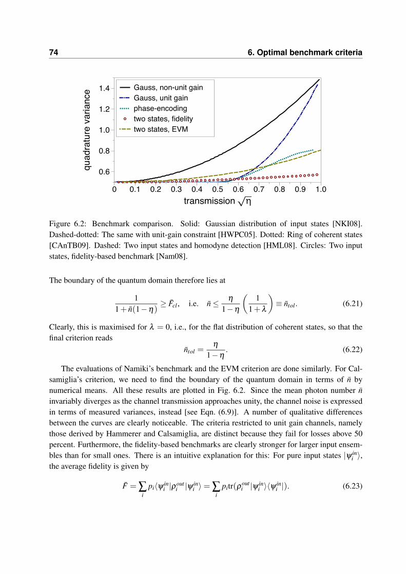
74 6. Optimal benchmark criteria
quad
ratu
re v
aria
nce
0.6
0.8
1.0
1.2
1.4
transmission η0 0.1 0.2 0.3 0.4 0.5 0.6 0.7 0.8 0.9 1.0
Gauss, non-unit gainGauss, unit gainphase-encodingtwo states, fidelitytwo states, EVM
Figure 6.2: Benchmark comparison. Solid: Gaussian distribution of input states [NKI08].Dashed-dotted: The same with unit-gain constraint [HWPC05]. Dotted: Ring of coherent states[CAnTB09]. Dashed: Two input states and homodyne detection [HML08]. Circles: Two inputstates, fidelity-based benchmark [Nam08].
The boundary of the quantum domain therefore lies at
11 + n(1−η)
≥ Fcl , i.e. n≤ η
1−η
(1
1 + λ
)≡ ntol . (6.21)
Clearly, this is maximised for λ = 0, i.e., for the flat distribution of coherent states, so that thefinal criterion reads
ntol =η
1−η. (6.22)
The evaluations of Namiki’s benchmark and the EVM criterion are done similarly. For Cal-samiglia’s criterion, we need to find the boundary of the quantum domain in terms of n bynumerical means. All these results are plotted in Fig. 6.2. Since the mean photon number ninvariably diverges as the channel transmission approaches unity, the channel noise is expressedin terms of measured variances, instead [see Eqn. (6.9)]. A number of qualitative differencesbetween the curves are clearly noticeable. The criteria restricted to unit gain channels, namelythose derived by Hammerer and Calsamiglia, are distinct because they fail for losses above 50percent. Furthermore, the fidelity-based benchmarks are clearly stronger for larger input ensem-bles than for small ones. There is an intuitive explanation for this: For pure input states |ψ in
i 〉,the average fidelity is given by
F = ∑i
pi〈ψ ini |ρout
i |ψ ini 〉= ∑
ipitr(ρ
outi |ψ in
i 〉〈ψ ini |). (6.23)

6.2. Benchmark comparison 75
Hence, a measurement of F requires projections onto all input or target states. For the Gaus-sian input ensemble, this leads to a tomographically complete POVM. For the other extreme,the binary input ensemble, only two projections are involved. Larger input ensembles implymore extensive measurements which extract more information on the output states. This is animportant observation: For fidelity-based benchmarks, the chosen input ensemble affects thecomplexity of Bob’s measurements. Small input ensembles should be avoided.
This is not true for benchmarks based on quadrature moments, where Bob’s measurementsare independent of the input ensemble. Fig. 6.2 clearly shows that the EVM method with itsbinary input ensemble performs significantly better than Namiki’s two-state benchmark. This isto be expected, since the quadrature detection underlying the EVM method provides tomographyfor the Gaussian output states.
Before turning to approximation formulae for the fidelity, we show how Koashi’s benchmarkcan be derived from an entanglement-based picture. We start with a two-mode squeezed state
|r〉AB = sinh(r)∞
∑n=0
(−tanh(r))n|n〉A|n〉B. (6.24)
Alice can prepare the correct input ensemble from this by projections onto all coherent states{|α〉〈α|}. This effective bipartite state is more compactly represented by its covariance matrix
12
(γA CCT γB
), (6.25)
with γA = γB = diag[cosh(2r), cosh(2r)] and C = diag[sinh(2r),−sinh(2r)] (see, e.g., [BL07].Then, the bipartite output state will be
12
(γA
√ηC√
ηCT ηγB +(1−η)D
), (6.26)
with D = diag[1/2 + n,1/2 + n]. This covariance matrix is entangled if its partial transpose isunphysical [Sim00]. This is the case when
n≤ η
(1−η), (6.27)
i.e., we recover Koashi’s result. There are two things to note: Firstly, avoiding the use of thefidelity freed us from relying on the channel model. The output covariance matrix merely con-tains a parameterisation of measurement outcomes. If the output states were not Gaussians, thebenchmark would still hold true. Secondly, we note that an optimisation over the input ensemblewas not required. The width of the Gaussian distribution is linked to the squeezing parameter r inEqn. (6.24), but the final result has no more dependence on r. Therefore, the derived benchmarkholds for all (finite) values of λ . Evidently, the use of the average fidelity overly emphasises thea priory probabilities pi and consequently does not lead to the most general benchmark criterion.

76 6. Optimal benchmark criteria
6.2.2 Approximating the fidelity
In some sense, the above comparison is not quite fair, because Bob’s measurement settings aredifferent for different criteria. We can remove this “unfairness” by expressing the fidelity-basedcriteria in terms of quadrature measurements. In the general case, this is a very difficult task.Although the fidelity between two Gaussian states can be expressed in terms of quadrature mo-ments, it is unclear how the fidelity between general states stands in relation to this. The fol-lowing example shows that the fidelity between two Gaussian states is neither a lower nor anupper bound on the fidelity between non-Gaussians with the same first and second quadraturemoments. Consider the two states
ρG = ρth(n) (6.28)
ρNG = (1− p)|0〉〈0|+ p|n〉〈n|, (6.29)
and require that both states have equal first and second quadrature moments, i.e.,
VarG(x) = VarNG(x) (6.30)
n +12
= (1− p)12
+ p(n +12) (6.31)
n = np. (6.32)
The variance in any other phase-space direction gives the same condition, and the first quadraturemoments are zero for both ρG and ρNG. We proceed by computing the fidelities of both stateswith the vacuum |0〉, and find
FG =1
1 + n(6.33)
FNG = 1− nn
. (6.34)
We can now insert particular values for n and n. For example, choosing n = 2/3 and n = 1 leadsto
FNG =13
& FG =35
, i.e. FG > FNG. (6.35)
On the other hand, taking the limit n→ ∞ leads to
FNG→ 1 & FG =1
1 + n, i.e. FG ≤ FNG. (6.36)
Therefore, there is no clear ordering of FG and FNG. As a consequence, it becomes questionablewhether a general bound on the fidelity can be derived in terms of quadrature moments.
In the non-unit gain scenario, however, we can find bounds. For the criteria by Namiki andKoashi, the fidelity is taken between output and target states, and the best choice of target state
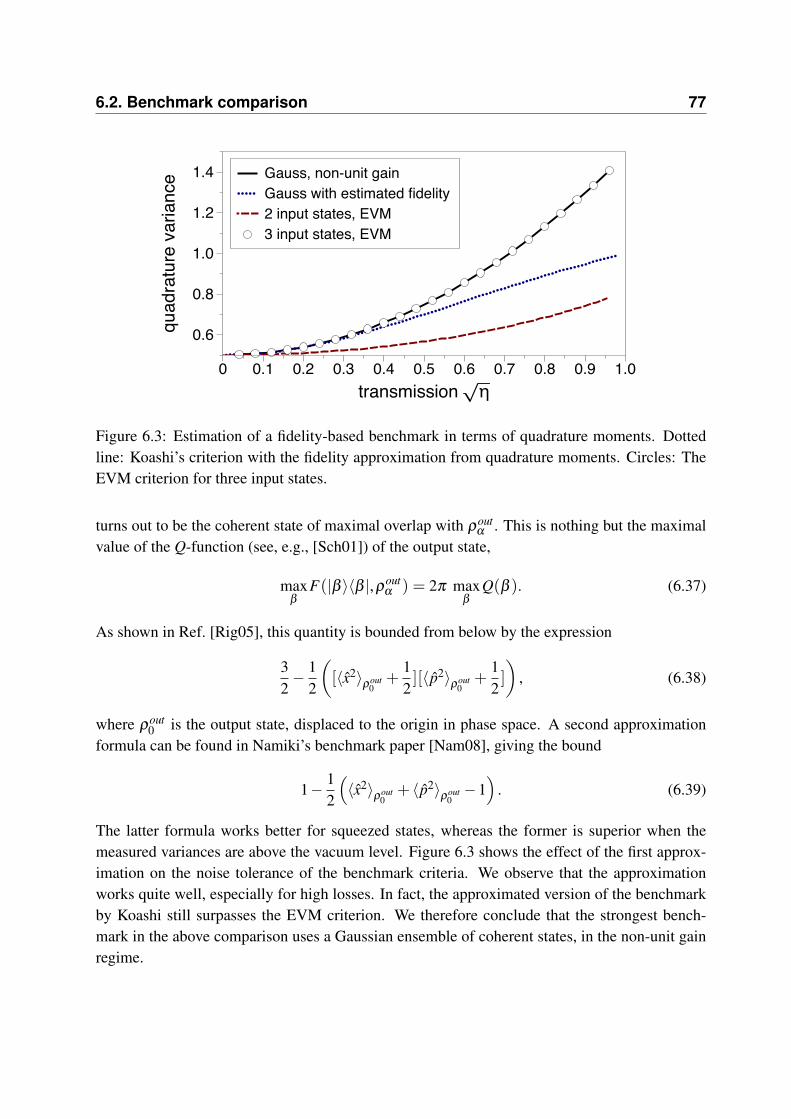
6.2. Benchmark comparison 77
quad
ratu
re v
aria
nce
0.6
0.8
1.0
1.2
1.4
transmission η0 0.1 0.2 0.3 0.4 0.5 0.6 0.7 0.8 0.9 1.0
Gauss, non-unit gainGauss with estimated fidelity2 input states, EVM3 input states, EVM
Figure 6.3: Estimation of a fidelity-based benchmark in terms of quadrature moments. Dottedline: Koashi’s criterion with the fidelity approximation from quadrature moments. Circles: TheEVM criterion for three input states.
turns out to be the coherent state of maximal overlap with ρoutα . This is nothing but the maximal
value of the Q-function (see, e.g., [Sch01]) of the output state,
maxβ
F(|β 〉〈β |,ρoutα ) = 2π max
β
Q(β ). (6.37)
As shown in Ref. [Rig05], this quantity is bounded from below by the expression
32− 1
2
([〈x2〉
ρout0
+12][〈p2〉
ρout0
+12])
, (6.38)
where ρout0 is the output state, displaced to the origin in phase space. A second approximation
formula can be found in Namiki’s benchmark paper [Nam08], giving the bound
1− 12
(〈x2〉
ρout0
+ 〈p2〉ρout
0−1)
. (6.39)
The latter formula works better for squeezed states, whereas the former is superior when themeasured variances are above the vacuum level. Figure 6.3 shows the effect of the first approx-imation on the noise tolerance of the benchmark criteria. We observe that the approximationworks quite well, especially for high losses. In fact, the approximated version of the benchmarkby Koashi still surpasses the EVM criterion. We therefore conclude that the strongest bench-mark in the above comparison uses a Gaussian ensemble of coherent states, in the non-unit gainregime.
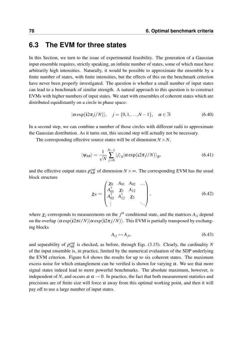
78 6. Optimal benchmark criteria
6.3 The EVM for three states
In this Section, we turn to the issue of experimental feasibility. The generation of a Gaussianinput ensemble requires, strictly speaking, an infinite number of states, some of which must havearbitrarily high intensities. Naturally, it would be possible to approximate the ensemble by afinite number of states, with finite intensities, but the effects of this on the benchmark criterionhave never been properly investigated. The question is whether a small number of input statescan lead to a benchmark of similar strength. A natural approach to this question is to constructEVMs with higher numbers of input states. We start with ensembles of coherent states which aredistributed equidistantly on a circle in phase space:
|α exp(i2π j/N)〉, j = {0,1, . . . ,N−1}, α ∈R (6.40)
In a second step, we can combine a number of those circles with different radii to approximatethe Gaussian distribution. As it turns out, this second step will actually not be necessary.
The corresponding effective source states will be of dimension N×N,
|ψAB〉=1√N
N−1
∑j=0| j〉A|α exp(i2π j/N)〉B, (6.41)
and the effective output states ρoutAB of dimension N×∞. The corresponding EVM has the usual
block structure
χN =
χ0 A01 A02 . . .
A†01 χ1 A12
A†02 A†
12 χ2... . . .
, (6.42)
where χ j corresponds to measurements on the jth conditional state, and the matrices Ai j dependon the overlap 〈α exp(i2πi/N)|α exp(i2π j/N)〉. This EVM is partially transposed by exchang-ing blocks
Ai j↔ A ji, (6.43)
and separability of ρoutAB is checked, as before, through Eqs. (3.15). Clearly, the cardinality N
of the input ensemble is, in practice, limited by the numerical evaluation of the SDP underlyingthe EVM criterion. Figure 6.4 shows the results for up to six coherent states. The maximumexcess noise for which entanglement can be verified is shown for varying α . We see that moresignal states indeed lead to more powerful benchmarks. The absolute maximum, however, isindependent of N, and occurs at α→ 0. In practice, the fact that both measurement statistics andprecisions are of finite size will force α away from this optimal working point, and then it willpay off to use a large number of input states.

6.4. Phase fluctuations 79
varia
nce
0.6
0.8
1.0
1.2
1.4
amplitude |α|0 0.2 0.4 0.6 0.8 1.0 1.2 1.4 1.6 1.8
N = 3N = 4N = 5N = 6
Figure 6.4: The dependence of the EVM method on the cardinality N of the input ensemble.
Placing these benchmarks in the above comparison (for α → 0) shows a surprising result:The three-state benchmark is equally strong as Koashi’s benchmark for a Gaussian input ensem-ble (see Fig. 6.3). Evidently, testing a channel with three coherent states is significantly moreresilient to loss and noise than using two states. An intuitive understanding of this result maycome from state discrimination. The performance of an MP channel naturally depends on theability to distinguish the input states. Wrong identifications lead to erroneous re-preparations,which will show as broadened variances in Bob’s observations. In discriminating two coherentstates, errors will only occur in one of two orthogonal phase-space directions, while the otherdirection remains error free. This can be exploited to limit the variance-broadening induced bythe MP channel (c.f. [HML08]). The situation is different for the above arrangement of threecoherent states, where measurement errors will occur along any direction in phase-space. Hence,a corresponding MP strategy will induce more variance broadening in Bob’s observations.
As a side-remark, we note that our analysis supplies the entanglement verification fordiscretely-modulated quantum key distribution protocols [LG09, SL09], which can have advan-tages over protocols with Gaussian modulation [GvAW+03]. In Ref. [LG09], it is argued that aprotocol based on the transmission of four coherent states can generate key at a rate at least ashigh as protocols based on Gaussian modulation, and is in fact able to outperform the latter dueto advantages in the classical information processing steps.
6.4 Phase fluctuations
We have now established that phase-encoded input ensembles lead to very strong benchmarks,and additional amplitude encoding bears no further improvement. And although encoding a

80 6. Optimal benchmark criteria
source
absolute phase reference
detection apparatus
Φ
(a) Random phases Φ of the input states.
source
absolute phase reference
detection apparatus
Φ
fixed
Φ
(b) Equivalent phase shifts
source detection apparatus
Φ -Φ
(c) Phase-randomised channel
Figure 6.5: Local oscillator and absolute phase reference. Input pulses carry a phase Φ with re-spect to the absolute phase reference, which is present on both signal and local oscillator modes.6.5(c): Equivalent phase shifts: the tested channel is automatically phase-randomised.
phase is simply a matter of changing the optical path of the signal beam with respect to itsphase reference, we seek further simplifications and ask whether it may be possible to avoidactive encoding altogether. For pulsed laser sources, the phases between subsequent pulses arerandom. The question is whether these random phases can encode the desired input ensemble.
Let us consider a typical experimental setup [Fig. 6.5(a)]: A master laser emits a seriesof pulses and each of them is split on a highly asymmetric beam splitter into signal and localoscillator modes. The signal then passes through the memory or teleportation channel, and bothmodes are recombined in a homodyne detection apparatus. In order to keep track of phase,we introduce a reference frame and call this frame the absolute phase reference (see Fig. 6.5),which is a theoretically constructed, perfectly bright light beam. We will denote the phase of apulse emitted by the master laser by Φ. An equivalent preparation is the generation of a trainof pulses of equal phase Φ = 0, which are phase randomised after the splitting into signal andlocal oscillator modes [Fig. 6.5(b)]. We now separately consider the effect of the phase changeUΦ in the local oscillator mode. Effectively, this rotates the axes of the homodyne detectionwith respect to the absolute phase reference. The same measurement outcomes would ensue if,instead of applying UΦ on the local oscillator, the inverse phase rotation U−Φ was applied to theoutput of the signal mode (Fig. 6.5(c)). Hence, a random phase on a master pulse is equivalentto wedging the channel between a phase shift and its inverse. The original channel Λ thereforeis effectively described by a new, phase-randomised channel
Λ(ρ) =1
2π
∫ 2π
0dφ U†
φΛ(Uφ ρU†
φ)Uφ . (6.44)

6.4. Phase fluctuations 81
This new channel is easily shown to be phase-covariant:
Λ(Uθ ρU†θ) =
12π
∫ 2π
0dφ U†
φΛ(Uφ+θ ρU†
φ+θ)Uφ (6.45)
=1
2π
∫ 2π
0dξ U†
ξ−θΛ(Uξ ρU†
ξ)Uξ−θ (6.46)
= Uθ
12π
∫ 2π
0dξ U†
ξΛ(Uξ ρU†
ξ)Uξ U†
θ(6.47)
= Uθ Λ(ρ)U†θ
. (6.48)
Since our desired input ensemble is phase-encoded, phase-covariance is a crucial property of thechannel, which allow us to extrapolate measurement outcomes for phase shifted pulses. Supposea particular input setting |α〉 gives the measurement outcomes
χ0 =
1 〈x〉 〈p〉〈x〉 〈x2〉 〈x p〉〈p〉 〈px〉 〈p2〉
. (6.49)
Then, phase-covariance guarantees that a phase-shifted input state Uφ |α〉 will result in the EVMR(φ )χBR(φ )T , with the rotation matrix
R(φ ) =
1 0 00 cos(φ ) −sin(φ )0 sin(φ ) cos(φ )
. (6.50)
These conditional EVMs and the table of overlaps of the different input states suffice to build abipartite EVM for phase-encoded input ensembles of arbitrary size. Therefore, random phasesbetween pulses can generate the required effective entanglement, with no active phase-encodingrequired.
From a practical point of view, we cannot actually construct an EVM for an infinitesimallyspaced ring of coherent input states. However, phase-covariance of the channel simplifies theconstruction of χAB for larger input ensembles. We know that a phase rotation on the input statescan be undone by the inverse operation on the output states. In other words, the output states ρAB
are guaranteed to be invariant under transformations of the form(N−1
∑i=0|i + 1〉A〈i|
)⊗U (N)
B , (6.51)
with U (N)B = exp(−i2π
N n). Similarly, the EVM χAB is invariant under transformations of the
same form, with U (N)B replaced by Eqn. (6.50). The EVMs of different sizes will therefore all

82 6. Optimal benchmark criteria
have the structure
χ3 =
χ0 A1 U†A†1U
A†1 Uχ0U† UA1U†
UA1U† UA†1U† U†χ0U
, χ4 =
χ0 A1 A2 U†A†
1UA†
1 Uχ0U† UA1U† UA2U†
A†2 UA†
1 U2χ0U†2 U2A1U†2
U†A1U UA†2U† U2A1U†2 U†χ0U
,
and similarly for higher dimensions, with U chosen appropriately. Here, we have used the cyclicproperties U2 = U† for χ3 and U3 = U† for χ4. The number of blocks Ai with free parameters isnow greatly reduced, and equal to the number of different overlaps between signal states. Thiswill allow the evaluation of the EVM criterion for significantly higher N.
6.4.1 Application to experiments
Due to the novelty of our criterion, it has not been applied to verify a quantum memory experi-ment. It is of course possible to use published data from memory experiments, and insert themin the EVM method. Unfortunately, results are rarely published in a form which allows us toextract the necessary data.
Consider the quantum storage experiment by Appel et al. [AFK+08], and the subsequentprocess-tomography experiment [LKFL09]. The channel tomography was achieved by gener-ating an array of coherent states, densely spaced in phase space, and passing them through thememory channel. On each corresponding output state, quantum tomography was performed. Toknow the exact action of the channel on any coherent state means to know it on any other state,as we can easily see by the P-function decomposition, Eqn. (2.30). Hence, the data necessaryto apply the EVM method is in principle available, but, naturally, not explicitly given in thepublication.
The original storage experiment [AFK+08] used squeezed light, and the squeezing and anti-squeezing values for both input and output states are explicitly given. With the additional as-sumptions that input and output are Gaussian states and the memory channel is phase covariant,we can check the experimental outcomes against an EVM benchmark. We face an additionalcomplication from the fact that the input states are mixed, i.e., we need to combine the methodsdeveloped in this Chapter with those from Chapter 5. Here, we take a simple approach with threesignal states, and we use the approximate detection method described in Observation 7.
From the input squeezing and anti-squeezing values, we can derive the mixedness and thesqueezing parameter for the input states. This leads to the detected quantum domain shown inFig. 6.6. The output squeezing and anti-squeezing values define a point in this figure3. This pointlies outside the detected quantum domain, but it is very close to the boundary. Certainly, if weused a more refined EVM criterion, as described in Chapter 5, and more than three input states,
3Here, we used the values quoted in an early preprint [AFKL07]. The final publication [AFK+08] containsdifferently processed results, which show less output squeezing, but smaller error bars.

6.4. Phase fluctuations 83
r = 0.286nth = 0.167
Var0(p)
0.46
0.47
0.48
0.49
0.50
Var0(x)
0.5 0.6 0.7 0.8 0.9 1.0 1.1 1.2 1.3 1.4
3-state EVM, using purificationsdata from Appel et al.
Figure 6.6: Rough comparison of experimental results with the EVM method. Solid line: Bound-ary of the detected quantum domain, with three squeezed input states. Circle: measurementoutcomes on the output states, taken from [AFKL07].
the quantum domain could be extended to include the measurements on the output states. Wealso note that the experiment was not optimised in any way with respect to meeting the EVMcriterion.
In summary, it is probably fair to say that it is still challenging for continuous-variable quan-tum memories to achieve operation in the quantum domain, for coherence times of the order ofmicroseconds, at the current state of technology. However, the methods presented in this Chap-ter make it possible to verify such operation with very little experimental effort. It is reasonableto assume that most experiments on quantum storage or teleportation of light could be verifiedretrospectively, if the necessary data was made available.

84 6. Optimal benchmark criteria

7Concluding remarks
When it comes to the investigation of entanglement and its applications, there are many anglesof approach. Theoretically, it is most intriguing to explore the structure of entangled states, i.e.,find certain classes which share common properties and order different entanglement criteriaaccording to which of these classes of states they can detect. This can be done, and often isdone, in complete disregard of the fact that only a limited set of states can be generated inthe laboratory, and an even smaller set can be generated reliably and fast. Experimentally, onthe other hand, no state can be created perfectly, and restriction from the available technologyoftentimes lead modifications, or loopholes, in the implemented protocol. In other words,experiments are sometimes conducted in disregard of some theoretical subtleties.
In this thesis, we addressed some issues which can arise from this discrepancy between the-ory and experiment. Our main tool, the Expectation Value Matrix, was used for to detect entan-glement in a number of different physical settings. Here, we took great care to use only suchinformation which is directly accessible in an experiment. This is the first major advantage ofour verification method over most others: It can handle partial information very well, and mea-surement data and additional classical information can be directly entered in the ExpectationValue Matrix. The second advantage is its applicability to systems of “unusual” dimensionality.An Expectation Value Matrix for two-qubit systems, for example, can easily be constructed tocontain the full density matrix. For discrete-continuous systems, we constructed ExpectationValue Matrices of very low dimensions, which contained sufficient information to deliver strongentanglement criteria for continuous-variable protocols with binary input ensembles. Extensionsto larger input ensembles were easy to administer, due to the block structure of the Expecta-tion Value Matrix, and even the extension to ensembles of mixed input states could be done, byconstructing a tripartite matrix and embedding the accessible data in it.
Other constructions of Expectation Value Matrices should be straightforward. One could, forexample, address the problem of attacks on the phase reference for continuous-variable QKD

86 7. Concluding remarks
protocols with a Gaussian distribution of input states. For this, an Expectation Value Matrixcould be constructed from quadrature moments on system A and Stokes operator moments onsystem B. Similarly, constructions from Stokes operators for both parties could lead to newcriteria for continuous-variable polarisation entanglement.
In addition to the development of this particularly flexible entanglement detection method,its applications lead to a number of interesting results. For continuous-variable QKD, we foundthat the local oscillator beam forms a security threat. An eavesdropper can perform an intercept-resend attack and remain undetected by changing the amplitudes of signal and local oscillator.We furthermore found a number of simple remedies for this problem, which can be implementedwith small additions to the homodyne detection setup.
For the validation of quantum memories, our method is a conceptual simplification of exist-ing benchmark criteria, which are all derived by optimising over measure and prepare strategies.Clearly, since the object is to exclude such entanglement-breaking strategies, our approach ofdetecting entanglement between input and output is much more direct. The extension of theExpectation Value Matrix method to sources of mixed input states provides the necessary gen-erality for this test to be applicable to virtually any situation. We applied this test to memoriesof squeezed light and expressed the resulting benchmark criteria in terms of directly observablequantities.
Furthermore, we tried to find unifying features in the multitude of published benchmarkcriteria. We did this by comparing a number of those and distilling which assumptions oridiosyncrasies are essential to benchmarking and which add unwanted complication. Fromthis, we were able to construct a criterion which is optimal in its ability to detect measure andprepare strategies and which can be implemented with a small number of coherent test statesand homodyne detection of the channel output. Thus, we were able to bridge the gap betweenquantum memory or teleportation experiments and theoretically derived benchmark criteria.
There are certainly a number of other applications to our method. The most obvious onemay be physical systems with a real qubit-mode structure, as opposed to the virtual qubit sys-tems introduced through effective entanglement throughout this thesis. There are, for example,proposals to use the interaction of a single qubit with a mode of light to build quantum repeaternetworks [vLLS+06, LLN+06]. For such a network, it will be required to produce states of theatom-light system with high degrees of entanglement, so that the performance must ultimately bemeasured by an entanglement monotone. However, since building a quantum repeater is a verychallenging task, a first step is to verify the general ability of such an experiment to entangleatom and light. For this, the Expectation Value Matrix is a very suitable tool. The presence of aphysical qubit will change the available classical data, but the structure of the Expectation ValueMatrix for quadrature detection should be directly usable.

87
Another possible direction of future research is the quantification of entanglement in qubit-mode systems. The Expectation Value Matrix can be interpreted as a mapping of the state ρAB toa new (unnormalised) state χ(ρAB), and one can show that this mapping is LOCC, i.e., it does notincrease the entanglement. Therefore, evaluating an entanglement monotone on χAB will providea lower bound on the entanglement of ρAB. Problems may arise from the fact that the quadratureoperators are unbounded. We expect, however, that non-zeros lower bounds on the entanglementcan be extracted from an appropriately constructed Expectation Value Matrix.

88 7. Concluding remarks

ASemidefinite programmes
A.1 Theory
A semidefinite programme [VB96] is a particular type of convex optimisation setup which has aprimal problem and an associated dual problem. The general form of the primal problem is
min~x
~xT~c (A.1)
s.t. F(~x) = F0 +m
∑i=1
xiFi ≥ 0, (A.2)
where the vector ~c and the symmetric matrices Fi are given, and ~xT~c is the linear objectivefunction. The associated dual problem can be stated as
maxZ− tr(ZF0) (A.3)
s.t. Z≥ 0 (A.4)
tr(ZFi) = ci ∀ i, (A.5)
with the Hermitian matrix Z as the open variable. The key importance of the dual problem liesin the fact that it provides bounds on the value of the primal problem, and vice versa. For everyprimal feasible~x and dual feasible Z, we have
~cT~x + tr(F0Z) =m
∑i=1
tr(FiZ)xi + tr(F0Z) = tr(ZF(~x))≥ 0, (A.6)
which holds because both Z and F(~x) are positive semidefinite matrices. Consequently,
−tr(F0Z) ≤~cT~x, (A.7)
i.e., the objective value of any feasible dual problem is smaller than or equal to the objectivevalue of the corresponding (feasible) primal problem. This property is called weak duality, and

90 A. Semidefinite programmes
the difference ~cT~x + tr(F0Z) is referred to as the duality gap η . There is an even strongerconnection between primal and dual problem, which we will present here without proof. Letus denote the optimal solutions to the primal and dual problems by p∗ and d∗, respectively, thenwe have:
Theorem 1 Strong duality:One has p∗ = d∗ if one of the following two conditions is fulfilled:
• The primal problem is strictly feasible, i.e., ∃~x : F(~x) > 0
• The dual problem is strictly feasible, i.e., ∃ Z : F > 0, tr(ZFi) = ci.
For numerical solvers for SPDs, the primal-dual formulation has important consequences. Inmost problems, the hypothesis in Theorem 1 holds and p∗ = d∗. The solver can then generatea sequence of primal and dual feasible points ~x(k) and Z(k), each of which will be (most likely)suboptimal, i.e., p∗ ≤~cT~x(k). Strong duality also assures that p∗ ≥ −tr(F0Z(k)). This providesan upper bound on the sub-optimality of the current iteration, since
~cT~x(k)− p∗ ≤~cT~x(k) + tr(F0Z(k)) = η(k). (A.8)
Therefore, the stopping criterion
~cT~x(k) + tr(F0Z(k)) ≤ ε (A.9)
guarantees ε sub-optimality upon exit.
A.2 The EVM method as an SDP
Here, we briefly illustrate how to obtain results like the ones shown in Fig. 4.1. In principle, thisfigure is generated by first fixing the values of transmission and overlap (the x and y coordinates),and then gradually increasing the excess noise (the z coordinate), and asking at each point for afeasible solution to the two conditions χAB ≥ 0 and χ
TAAB ≥ 0 (c.f., Obs. 4). In practice, it is much
faster to incorporate the search for the maximum amount of tolerable excess noise in the SDP.Since the excess noise, or measured variance, does not explicitly appear in χAB [c.f. Eqn. (4.4)]we need to incorporated it by making the replacements
〈x2〉i = 〈x〉2i + Vari(x) and 〈p2〉i = 〈p〉2i + Vari( p). (A.10)

A.2. The EVM method as an SDP 91
We can give the excess noise the specific label ∆, with ∆ = Vari(x)−1/2. Now, the separabilityof χAB is already in the form of an SDP:
min ∆ (A.11)
s.t. χAB ≥ 0 (A.12)
χTAAB ≥ 0. (A.13)
Complex-valued free parameters are handled simply by splitting them into real and imaginaryparts, so that the vector~x contains those free parameters as well as ∆.

92 A. Semidefinite programmes

BEquivalent methods
In Ref. [RGL06], the constructed entanglement criterion is based on uncertainty relations. Wewill show that this approach is equivalent to our method based on partial transposition. Rigas etal. [RGL06] construct a symmetric version of the EVM defined as
χs(ρ) :=
⟨|0〉〈0|⊗Bs
⟩ρ
⟨|0〉〈1|⊗Bs
⟩ρ⟨
|1〉〈0|⊗Bs⟩
ρ
⟨|1〉〈1|⊗Bs
⟩ρ
(B.1)
with Bs given by
Bs :=
1 x px x2 1
2(x p + px)p 1
2(x p + px) p2
. (B.2)
Then the inequalities
χs(ρ)± i
2ρA⊗ J ≥ 0, (B.3)
with
J =
0 0 00 0 −10 1 0
,
are satisfied by all separable states, and violation implies entanglement.
These two inequalities turn out to be equivalent to the conditions
χ(ρ) ≥ 0 and χ(ρTB) ≥ 0 (B.4)
94 B. Equivalent methods
for the unsymmetrised EVM. Product entries can be split into their symmetrised product andcommutator:
x p =12(x p + px)+
12[x, p] (B.5)
=12(x p + px)+
12i, (B.6)
so that χ(ρ) = χs(ρ)− i/2 ρA⊗ J.
Since Bob’s operators are transposed according to the rule x→ x and p→−p, we find that
χ(ρTB) = U χ(ρ)U†, (B.7)
where U = 1A⊗diag[1,1,−1] and χ(ρ) is given by (B.1), with Bs replaced by
B :=
1 x px x2 pxp x p p2
. (B.8)
Then χ(ρ) = χs(ρ)+ i/2 ρA⊗ J, i.e., the two conditions in Eqs. (B.3) are, up to a local unitarytransformation, equivalent to (B.4).

CA USD-type strategy for two squeezed thermal states
Here, we derive a measure and prepare strategy for two squeezed thermal states as test states, forthe region (B) (Fig. C.1). To be precise, we consider the slope of the straight line which joins thepoint p in Fig. C.1 and a the point arising from an entanglement-breaking channel in the limitVarρout
0(x)→ ∞.
Let the coordinates of p be denoted by (vx,vp), then the slope of the straight line joining pand any other point is given by
m =Varρout
0( p)− vp
Varρout0
(x)− vx, (C.1)
where Varρout0
( p) is given by Eqn. (5.29) and the variance of x is defined accordingly.The strategy which minimises this slope is essentially an approximation to unambiguous
state discrimination. We define a three-element POVM with Π0, Π1 = U†π/2Π0Uπ/2 and Π?,
and corresponding re-prepared states |ψ0〉= |r〉, |ψ1〉= |− r〉, and |ψ?〉= |0〉. Consequently,
Varρout0
( p) =12(tr(ρ
in0 π0)e−2r + tr(ρ
in1 π0)e2r + tr(ρ
in0 π?))
Varρout0
(x) =12(tr(ρ
in0 π0)e2r + tr(ρ
in1 π0)e−2r + tr(ρ
in0 π?)).
Inserting into Eqn. (C.1) and taking the limit r→ ∞, we find
limr→∞
m =tr(ρ in
1 π0)tr(ρ in
0 π0). (C.2)
All that is left to do now is to find a POVM element π0 for which the slope m tends to zero.Setting π0 = |α〉〈α|, where |α〉 is a coherent state, achieves this. In this case, m becomes aquotient of Husimi Q-functions:
m =〈α|ρ1|α〉〈α|ρ0|α〉
=Q1(α)Q0(α)
. (C.3)

96 C. A USD-type strategy for two squeezed thermal states
Var(p)
0.45
0.46
0.47
0.48
0.49
0.50
Var (x)0.5 0.6 0.7 0.8 0.9 1.0
region (A)
p
region (B)
Figure C.1: Schematic plot of the two different optimal measure and prepare strategies.
The Q-function Qi(α) of the squeezed thermal state ρi, i ∈ {0,1}, is given by [MM93]
1
π√
(1 + Ai)2−|Bi|2exp[(Ai−1)|α|2− 1
2(Biα
∗2 + B∗i α2)],
with the definitions
A0 = n +(2n + 1) sinh2(r) = A1 (C.4)
B0 = −(2n + 1) sinh(r)cosh(r) = −B1 (C.5)
A0 =n(n + 1)
n2 +(n + 12)(1 + cosh(2r))
= A1 (C.6)
B0 = − (n + 12) sinh(2r)
n2 +(n + 12)(1 + cosh(2r))
= −B1. (C.7)
Inserting these expressions into Eqn. (C.3), we find
m =exp[−1
2 B1(α∗2 + α2)]exp[1
2 B1(α∗2 + α2)]= exp[−B1(α
∗2 + α2)].
For increasing α ∈ R, this final expression tends to zero exponentially fast. Therefore, it ispossible to reach the boundary of the quantum domain in Fig. C.1 for the whole parameterdomain.

DFidelity and trace distance for qubit states
There is a well known relation between fidelity and trace distance, which reads [NC00]
Dtr(ρ ,σ) ≤√
1−F(ρ ,σ). (D.1)
Here, we perform a direct calculation which shows that this relation is fulfilled with equalityif ρ and σ are qubit states of equal degree of mixedness. The fidelity between qubit states isexplicitly given by [H92]
F(ρ0,ρ1) =12
(1 +~r0 ·~r1 +
√1−|~r0|2
√1−|~r1|2
), (D.2)
where we used the Bloch vector notation
ρi =12
(1+~σ ·~ri) . (D.3)
Since we consider qubit states of equal mixedness, the Bloch vectors ~r0 and ~r1 have the samelength, and the fidelity simplifies to
F(ρ0,ρ1) =12(1 + |~r0|2 cos(θ )+ 1−|~r0|2
), (D.4)
where θ denotes the angle between the two Bloch vectors. The right-hand side of Eqn. (D.1)therefore becomes √
12|~r0|2(1− cos(θ )). (D.5)
The trace distance between two qubit states has the well-known [NC00] simple formula
Dtr(ρ0,ρ1) =|~r0−~r1|
2. (D.6)
For |~r1|= |~r0|, this reduces to
Dtr(ρ0,ρ1) =√
2|~r0|2−2|~r0|2 cos(θ )2
, (D.7)
which is equal to expression (D.5). This proves our claim.

98 D. Fidelity and trace distance for qubit states

Bibliography
[AC08] G. Adesso and G. Chiribella. Quantum benchmark for teleportation and storage ofsqueezed states. Phys. Rev. Lett. 100, 170503 (2008).
[AFK+08] J. Appel, E. Figueroa, D. Korystov, M. Lobino, and A. I. Lvovsky. Quantummemory for squeezed light. Phys. Rev. Lett. 100, 093602 (2008).
[AFKL07] J. Appel, E. Figueroa, D. Korystov, and A. I. Lvovsky. Quantum memory forsqueezed light. quant-ph/0709.2258v2 (2007).
[Aud05] J. Audretsch. Verschrankte Systeme - Die Quantenphysik auf neuen Wegen. Wiley-VCH, Berlin, 2005.
[Bar97] S. M. Barnett. Quantum information via novel measurements. Philosophi-cal Transactions: Mathematical, Physical and Engineering Sciences 355, 2279(1997).
[BB84] C. H. Bennett and G. Brassard. Quantum cryptography: Public key distributionand coin tossing. In Proceedings of IEEE International Conference on Computers,Systems, and Signal Processing, Bangalore, India, 175, New York, (1984).
[BBJ+93] C. H. Bennett, G. Brassard, C. Jozsa, R. Crepeau, A. Peres, and W. K. Wooters.Teleporting an unknown quantum state via dualclassical and einstein- podolsky-rosen channels. Phys. Rev. Lett. 70, 1895 (1993).
[BBM92] C. H. Bennett, G. Brassard, and N. D. Mermin. Quantum cryptography withoutBell‘s theorem. Phys. Rev. Lett. 68, 557–559 (1992).
[BBM95] C. H. Bennett, G. Brassard, and U. M. Maurer. Generalized privacy amplification.IEEE Trans. Inf. Theory 41, 1915 (1995).

100 Bibliography
[BBP+96] C. H. Bennett, G. Brassard, S. Popescu, B. Schumacher, J. A. Smolin, andW. K. Wootters. Purification of noisy entaglement and faithful teleportation vianoisy channels. Phys. Rev. Lett. 76, 722 (1996).
[BBPS96] C. H. Bennett, H. J. Bernstein, S. Popescu, and B. Schumacher. Concentratingpartial entanglement by local operations. Phys. Rev. A 53, 2046, (1996).
[BBS+92] C. H. Bennett, F. Bessette, L. Salvail, G. Brassard, and J. Smolin. Experimentalquantum cryptography. J. Cryptology 5, 28 (1992).
[BDSW96] C. H. Bennett, D. P. DiVincenzo, J. A. Smolin, and W. K. Wootters. Mixed stateentanglement and quantum error correction. Phys. Rev. A 54, 3824 (1996).
[Ben92] C. H. Bennett. Quantum cryptography using any two nonorthogonal states. Phys.Rev. Lett. 68, 3121 (1992).
[BFK00] S. L. Braunstein, C. A. Fuchs, and H. J. Kimble. Criteria for continuous-variablequantum teleportation. J. Mod. Opt. 47, 267 (2000).
[BL07] D. Brußand G. Leuchs, editors. Lectures on Quantum Information. Wiley-VCH,Weinheim, 2007.
[BM99] D. Bruß and C. Macchiavello. Optimal state estimation for d-dimensional quantumsystems. Physics Letters A 253, 249 (1999).
[BPM+97] D. Bouwmeester, J. W. Pan, K. Mattle, M. Eibl, H. Weinfurter, and A. Zeilinger.Experimental quantum teleportation. Nature 390, 575 (1997).
[BR97] S. M. Barnett and P. M. Radmore. Methods in Theoretical Quantum Optics. OxfordUniversity Press, Oxford, 1997.
[Bru98] D. Bruß. Optimal eavesdropping in quantum cryptography with six states. Phys.Rev. Lett. 81, 3018 (1998).
[BTB+03] W. P. Bowen, N. Treps, B. C. Buchler, R. Schnabel, T. C. Ralph, T. Symul, andP. K. Lam. Unity gain and nonunity gain quantum teleportation. IEEE J. QuantumElectronics 9, 1519 (2003).
[Bur69] D. J. C. Bures. An extension of Kakutani’s theorem on infinite product measuresto the tensor product of semifinite w∗ -algebras. Trans. Am. Math. Soc. 135, 199(1969).
[BW92] C. H. Bennett and S. J. Wiesner. Communication via one- and two-particle opera-tors on Einstein-Podolsky-Rosen states. Phys. Rev. Lett. 69, 2881, (1992).
Bibliography 101
[BZ06] Bengtsson and Zyczkowski. Geometry of Quantum States. Cambridge UniversityPress, 2006.
[CAnTB09] J. Calsamiglia, M. Aspachs, R. Mu noz Tapia, and E. Bagan. Phase-covariantquantum benchmarks. Phys. Rev. A 79, 050301 (2009).
[CGLL05] M. Curty, O. Guhne, M. Lewenstein, and N. Lutkenhaus. Detecting two-partyquantum correlations in quantum key distribution protocols. Phys. Rev. A 71,022306 (2005).
[CHSH69] J. F. Clauser, M. A. Horne, A. Shimony, and R. A. Holt. Proposed experiment totest local hidden-variable theories. Phys. Rev. Lett. 23, 880 (1969). Erratum: ibid24.
[CLL04] M. Curty, M. Lewenstein, and N. Lutkenhaus. Entanglement as precondition forsecure quantum key distribution. Phys. Rev. Lett. 92, 217903 (2004).
[CLVA01] N. J. Cerf, M. Levy, and G. van Assche. Quantum distribution of Gaussian keysusing squeezed states. Phys. Rev. A 63, 052311 (2001).
[CZKM97] J. I. Cirac, P. Zoller, H. J. Kimble, and H. Mabuchi. Quantum state transfer andentanglement distribution among distant nodes in a quantum network. Phys. Rev.Lett. 78, 3221 (1997).
[Dic54] R. H. Dicke. Coherence in spontaneous radiation processes. Phys. Rev. 93, 99,(1954).
[Die82] D. Dieks. Communication by EPR devices. Physics Letters A 92, 271 (1982).
[DLCZ01] L. M. Duan, M. D. Lukin, J. I. Cirac, and P. Zoller. Long-distance quantum com-munication with atomic ensembles and linear optics. Nature 414, 413 (2001).
[EBH+09] D. Elser, T. Bartley, B. Heim, C. Wittmann, D. Sych, and G. Leuchs. Feasibility offree space quantum key distribution with coherent polarization states. New Journalof Physics 11, 045014 (2009).
[Eke91] A. Ekert. Quantum cryptography based on Bell’s theorem. Phys. Rev. Lett. 67, 661(1991).
[EPR35] A. Einstein, B. Podolsky, and N. Rosen. Can quantum-mechanical description ofphysical reality be considered complete? Phys. Rev. 47, 777 (1935).
[FC88] H. Fearn and M. J. Collett. Representations of squeezed states with thermal noise.J. of Modern Optics 35, 553 (1988).

102 Bibliography
[FSB+98] A. Furusawa, J. L. Soslash;rensen, S. L. Braunstein, C. A. Fuchs, H. J. Kimble,and E. S. Polzik. Unconditional Quantum Teleportation. Science 282, 706 (1998).
[Fuc95] C. A. Fuchs. Distinguishability and Accessible Information in Quantum Theory.PhD thesis, University of Mexico, Mexico, 1995.
[GCW+03] F. Grosshans, N. J. Cerf, J. Wenger, R. Tualle-Brouri, and P. Grangier. Virtualentanglement and reconcillation protocols for quantum cryptography with contin-uous variables. Quantum Information and Computation 3, 535 (2003).
[GG02] F. Grosshans and P. Grangier. Continuous variable quantum cryptography usingcoherent states. Phys. Rev. Lett. 88, 057902 (2002).
[GL06] O. Guhne and N. Lutkenhaus. Nonlinear entanglement witnesses. Phys. Rev. Lett.96, 170502 (2006).
[Gla63] R. J. Glauber. Photon correlations. Phys. Rev. Lett. 10, 84 (1963).
[GT09] O. Guhne and G. Toth. Entanglement detection. Phys. Rept. 474, 1 (2009).
[GvAW+03] F. Grosshans, G. van Assche, J. Wenger, R. Brouri, N. J. Cerf, and P. Grangier.Quantum key distribution using Gaussian-modulated coherent states. Nature 421,238 (2003).
[H92] M. Hubner. Explicit computation of the Bures distance for density matrices. Phys.Lett. A 163, 239 (1992).
[HAA+08] K. Honda, D. Akamatsu, M. Arikawa, Y. Yokoi, K. Akiba, S. Nagatsuka, T. Tan-imura, A. Furusawa, and M. Kozuma. Storage and retrieval of a squeezed vacuum.Phys. Rev. Lett. 100, 093601 (2008).
[Hah50] E. L. Hahn. Spin echoes. Phys. Rev. 80, 580, (1950).
[Hel76] C. W. Helstrom. Quantum detection and estimation theory. Academic Press, NewYork, 1976.
[HHH96] M. Horodecki, P. Horodecki, and R. Horodecki. Separability of mixed states:necessary and sufficient conditions. Phys. Lett. A 223, 1 (1996).
[HHHH09] R. Horodecki, P. Horodecki, M. Horodecki, and K. Horodecki. Quantum entan-glement. Reviews of Modern Physics 81, 865 (2009).
[Hil00] M. Hillery. Quantum cryptography with squeezed states. Phys. Rev. A 61, 022309(2000).
Bibliography 103
[HL07] M. Heid and N. Lutkenhaus. Security of coherent-state quantum cryptography inthe presence of Gaussian noise. Phys. Rev. A 76, 022313 (2007).
[HL09a] H. Haseler and N. Lutkenhaus. Probing the quantumness of channels with mixedstates. Phys. Rev. A 80, 042304 (2009).
[HL09b] H. Haseler and N. Lutkenhaus. Quantum benchmarks from minimal resources.arXiv/0910.1458 (2009).
[HML08] H. Haseler, T. Moroder, and N. Lutkenhaus. Testing quantum devices: Practicalentanglement verification in bipartite optical systems. Phys. Rev. A 77, 032303(2008).
[HSH+09] M. Hosseini, B. M. Sparkes, G. Hetet, J. J. Longdell, P. K. Lam, and B. C. Buch-ler. Coherent optical pulse sequencer for quantum applications. Nature, 461, 241(2009).
[HSR03] M. Horodecki, P. W. Shor, and M. B. Ruskai. Entanglement breaking channels.Rev. Math. Phys. 15, 629 (2003).
[HW97] S. Hill and W. K. Wootters. Entanglement of a pair of quantum bits. Phys. Rev.Lett. 78, 5022 (1997).
[HWPC05] K. Hammerer, M. M. Wolf, E. S. Polzik, and J. I. Cirac. Quantum benchmark forstorage and transmission of coherent states. Phys. Rev. Lett. 94, 150503 (2005).
[HY+03] T. Hirano, , H. Yamanaka, M. Ashikaga, T. Konishi, and R. Namiki. Quantumcryptography using pulsed homodyne detection. Phys. Rev. A 68, 042331 (2003).
[Iva87] I. D. Ivanovic. How to differentiate between non-orthogonal states. Phys. Lett. A123, 257 (1987).
[JR55] J. M. Jauch and F. Rohrlich. The Theory of Photons and Electrons. Addison-Wesley, Reading, MA, 1955.
[JRB07] H. Jeong, T. C. Ralph, and W. P. Bowen. Quantum and classical fidelities forGaussian states. Journal Opt. Soc. Am. B 24, 355 (2007).
[JSC+04] B. Julsgaard, J. Sherson, J. I. Cirac, J. Fiurasek, and E. S. Polzik. Experimentaldemonstration of quantum memory for light. Nature 432, 482 (2004).
[KAH64] N. A. Kurnit, I. D. Abella, and S. R. Hartmann. Observation of a photon echo.Phys. Rev. Lett. 13, 567 (1964).

104 Bibliography
[KCKL00] B. Kraus, J. I. Cirac, S. Karnas, and M. Lewenstein. Separability in 2×n compositequantum systems. Phys. Rev. A 61, 062302 (2000).
[KdOK89] M. Kim, F. de Oliveira, and P. Knight. Properties of squeezed number states andsqueezed thermal states. Physical Review A 40, 2494 (1989).
[KLL+02] N. Korolkova, G. Leuchs, R. Loudon, T. C. Ralph, and C. Silberhorn. Polarizationsqueezing and continuous-variable polarization entanglement. Phys. Rev. A 65,052306 (2002).
[KN63] U. G. Kopvil’em and V. R. Nagibarov. (in Russian). Fiz. Metal. Metalloved 2, 313(1963).
[KS85] J. R. Klauder and B. Skagerstam. Coherent States: Applications in Physics andMathematical Physics. World Scientific Pub. Co. Inc., Singapore, 1985.
[KTG+06] B. Kraus, W. Tittel, N. Gisin, M. Nilsson, S. Kroll, and J. I. Cirac. Quantum mem-ory for nonstationary light fields based on controlled reversible inhomogeneousbroadening. Phys. Rev. A 73, 020302 (2006).
[KU93] M. Kitagawa and M. Ueda. Squeezed spin states. Phys. Rev. A 47, 5138 (1993).
[L04] J. Lofberg. Yalmip : A toolbox for modeling and optimization in MATLAB. InProceedings of the CACSD Conference, Taipei, Taiwan, 2004.
[Leo97] U. Leonhardt. Measuring the Quantum State of Light. Cambridge University Press,Cambridge, 1997.
[LG09] A. Leverrier and P. Grangier. Unconditional security proof of long-distancecontinuous-variable quantum key distribution with discrete modulation. Phys. Rev.Lett. 102, 180504 (2009).
[LH89] Y. Lai and H. A. Haus. Characteristic functions and quantum measurements ofoptical observables. Quantum Optics: Journal of the European Optical SocietyPart B, 1, 99 (1989).
[LKFL09] M. Lobino, C. Kupchak, E. Figueroa, and A. I. Lvovsky. Memory for light as aquantum process. Phys. Rev. Lett. 102, 203601 (2009).
[LKL04] S. Lorenz, N. Korolkova, and G. Leuchs. Continuous variable quantum key dis-tribution using polarization encoding and post selection. Appl. Phys. B 79, 273(2004).

Bibliography 105
[LLN+06] T. D. Ladd, P. van Loock, K. Nemoto, W. J. Munro, and Y. Yamamoto. Hybridquantum repeater based on dispersive cqed interactions between matter qubits andbright coherent light. New J. Phys. 8, 184 (2006).
[LRH+06] S. Lorenz, J. Rigas, M. Heid, U. L. Andersen, N. Lutkenhaus, and G. Leuchs.Witnessing effective entanglement in a continuous variable prepare-and-measuresetup and application to a quantum key distribution scheme using postselection.Phys. Rev. A 74, 042326 (2006).
[MCL06] T. Moroder, M. Curty, and N. Lutkenhaus. Upper bound on the secret key ratedistillable from effective quantum correlations with imperfect detectors. Phys.Rev. A 73, 012311 (2006).
[MGL08] T. Moroder, O. Guhne, and N. Lutkenhaus. Iterations of nonlinear entanglementwitnesses. Phys. Rev. A 78, 032326 (2008).
[MM93] P. Marian and T. A. Marian. Squeezed states with thermal noise. i. Photon-numberstatistics. Phys. Rev. A 47, 4474 (1993).
[MP06] A. Miranowicz and M. Piani. Comment on “Inseparability criteria for continuousbipartite quantum states”. Phys. Rev. Lett. 97, 058901 (2006).
[MPHH09] A. Miranowicz, M. Piani, P. Horodecki, and R. Horodecki. Inseparability criteriabased on matrices of moments. Phys. Rev. A 80, 052303 (2009).
[Nai40] M. A. Naimark. Spectral functions of a symmetric operator. Izv. Akad. Nauk SSSR,Ser. Mat. 4, 277 (1940). in Russian.
[Nam08] R. Namiki. Verification of the quantum-domain process using two nonorthogonalstates. Phys. Rev. A 78, 032333 (2008).
[NC00] M. A. Nielsen and I. L. Chuang. Quantum Computation and Quantum Information.Cambridge University Press, Cambridge, 2000.
[NKI08] R. Namiki, M. Koashi, and N. Imoto. Fidelity criterion for quantum-domain trans-mission and storage of coherent states beyond the unit-gain constraint. Phys. Rev.Lett. 101, 100502 (2008).
[OPP+08] M. Owari, M. B. Plenio, E. S. Polzik, A. Serafini, and M. M. Wolf. Squeezing thelimit: quantum benchmarks for the teleportation and storage of squeezed states.New Journal of Physics 10, 113014 (2008).
[Per93] A. Peres. Quantum Theory: Concepts and Methods. Kluwer, Dordrecht, 1993.
106 Bibliography
[Per96] A. Peres. Separability criterion for density matrices. Phys. Rev. Lett. 77, 1413(1996).
[PR04] A. O. Pittenger and M. H. Rubin. Mutually unbiased bases, generalized spin ma-trices and separability. Linear Algebra and its Applications 390, 255 (2004).
[PV07] M. B. Plenio and S. Virmani. An introduction to entanglement measures. Quant.Inf. Comp. 7, 1 (2007).
[Rad71] J. M. Radcliffe. Some properties of coherent spin states. Journal of Physics A:General Physics 4, 313 (1971).
[Ray06] P. Raynal. Unambiguous state discrimination of two density matrices in quantuminformation theory. arXiv:quant-ph/0611133 (2006).
[RFL08] M. Razavi, H. Farmanbar, and N. Lutkenhaus. Long-distance quantum communi-cation with multiple quantum memories. OFC’08, Technical Digest:Paper JWA48,San Diego, CA, 2008.
[RGK05] R. Renner, N. Gisin, and B. Kraus. Information-theoretic security proof forquantum-key-distribution protocols. Phys. Rev. A 72, 012332 (2005).
[RGL06] J. Rigas, O. Guhne, and N. Lutkenhaus. Entanglement verification for quantum-key-distribution systems with an underlying bipartite qubit-mode structure. Phys.Rev. A 73, 012341 (2006).
[Rig05] J. Rigas. Detection of prepare&measurement entanglement in continuous variablequantum key distribution. Diploma thesis, University of Erlangen-Nuremberg,2005.
[RK05] R. Renner and R. Konig. Universally composable privacy amplification againstquantum adversaries. Lecture Notes in Computer Science 3378, 407 (2005).
[RLvE03] P. Raynal, N. Lutkenhaus, and S. J. van Enk. Reduction theorems for optimalunambiguous state discrimination of density matrices. Phys. Rev. A 68, 022308(2003).
[SBT+03] R. Schnabel, W. P. Bowen, N. Treps, T. C. Ralph, H.-A. Bachor, and P. K. Lam.Stokes-operator-squeezed continuous-variable polarization states. Phys. Rev. A 67,012316 (2003).
[Sch65] J. Schwinger. Quantum theory of angular momentum. New York: Academic Press,New York, 1965. eds.: L. Biedenharn and H. van Dam.

Bibliography 107
[Sch01] W. P. Schleich. Quantum Optics in Phase Space. Wiley-VCH, Berlin, 1st edition,2001.
[Sim00] R. Simon. Peres-Horodecki separability criterion for continuous variable systems.Phys. Rev. Lett. 84, 2726 (2000).
[SL09] D. Sych and G. Leuchs. Coherent state quantum key distribution with multi letteralphabets. quant-ph/0902.1895 (2009).
[Str88] G. Strang. Linear Algebra and its Applications. Thomson Learning, New York,1988.
[Stu99] J. F. Sturm. Using Sedumi 1.02, a Matlab toolbox for optimization over symmetriccones. Optimization Methods and Software 11, 625 (1999).
[Sud63] E. G. C. Sudarshan. Equivalence of semiclassical and quantum mechanical de-scriptions of statistical light beams. Phys. Rev. Lett. 10, 277 (1963).
[SV05] E. Shchukin and W. Vogel. Inseparability criteria for continuous bipartite quantumstates. Phys. Rev. Lett. 95, 230502 (2005).
[TTT99] K. C. Toh, R. H. Tutuncu, and M. J. Todd. Sdpt3–a Matlab software package forsemidefinite programming. Optimization Methods and Software 11, 545 (1999).
[Uhl76] A. Uhlmann. The ”transition porbability” in the state space of a *-algebra. Reportson Mathematical Physics 9, 273 (1976).
[UJA+04] R. Ursin, T. Jennewein, M. Aspelmeyer, R. Kaltenbaek, M. Lindenthal, P. Walther,and A. Zeilinger. Quantum teleportation across the danube. Nature 430, 849(2004).
[UTSM+07] R. Ursin, F. Tiefenbacher, T. Schmitt-Manderbach, H. Weier, T. Scheidl, M. Lin-denthal, B. Blauensteiner, T. Jennewein, J. Perdigues, P. Trojek, B. Omer, M. Furst,M. Meyenburg, J. Rarity, Z. Sodnik, C. Barbieri, H. Weinfurter, and A. Zeilinger.Entanglement-based quantum communication over 144km. Nature Physics 3, 481(2007).
[VB96] L. Vandenberghe and S. Boyd. Semidefinite programming. SIAM Review 38, 49(1996).
[Ver26] G. S. Vernam. Cipher printing telegraph systems. Journal of the AIEE 45, 295(1926).

108
[vLLS+06] P. van Loock, T. D. Ladd, K. Sanaka, F. Yamaguchi, K. Nemoto, W. J. Munro, andY. Yamamoto. Hybrid quantum repeater using bright coherent light. Phys. Rev.Lett. 96, 240501 (2006).
[VW02] G. Vidal and R. F. Werner. Computable measure of entanglement. Phys. Rev. A65, 32314 (2002).
[Wer89] R. F. Werner. Quantum states with Einstein-Podolsky-Rosen correlations admittinga hidden-variable model. Phys. Rev. A 40, 4277 (1989).
[WFW+09] C. Wittmann, J. Furst, C. Wiechers, D. Elser, H. Haseler, N. Lutkenhaus, andGerd Leuchs. Witnessing effective entanglement over a 2km fiber channel.arXiv/0911.3032 (2009).
[Wie83] S. Wiesner. Conjugate coding. Sigact News 15, 78 (1983).
[Wig32] E. P. Wigner. On the quantum correction for thermodynamic equilibrium. Phys.Rev. 40, 749 (1932).
[WW01] R. F. Werner and M. M. Wolf. Bound entangled Gaussian states. Phys. Rev. Lett.86, 3658 (2001).
[WZ82] W. K. Wooters and W. H. Zurek. A single quantum cannot be cloned. Nature 299,802 (1982).
[YC83] H. P. Yuen and V. W. S. Chan. Noise in homodyne and heterodyne detection. Opt.Lett. 8, 177 (1983).
[ZHRL09] Y. B. Zhao, M. Heid, J. Rigas, and N. Lutkenhaus. Asymptotic security of binarymodulated continuous-variable quantum key distribution under collective attacks.Phys. Rev. A 79, 012307 (2009).

Acknowledgements
• My first thanks go to my supervisor Prof. Dr. Norbert Lutkenhaus, for providing the helpand support to make my PhD studies a very enjoyable experience. His suggestions forresearch directions lead me to complete three most interesting projects which were flex-ible enough to bear my own ideas, and his readiness to discuss even the most tedious ofmy problem details was at times puzzling. I am further indebted for the opportunity toexperience Canada and the Institute for Quantum Computing and the help I received inconnection with it.
• Secondly, I am very grateful to my family for support in all aspects of life. Particularly tomy parents Ingo and Monika for helping me to manage my affairs “remotely”. Additionalthanks go to Ioana for her help with all my clever physics questions, her patience with allthe stupid ones and her shared expertise on Mathematica and LATEX.
• Naturally, a nice working environment is important and was provided by all members of theOQCT-group. Many thanks to: Tobias Moroder, Matthias Heid, Geir-Ove Myhr, NathanKilloran, Agnes Ferenczi, Normand Beaudry, Volkher Scholz, Marco Piani, MohsenRazavi, Caterina Mora, Xiongfeng Ma, William Matthews, and anyone I forgot to listhere.
• I would like to thank everyone at IQC, for making my stay in Canada a wonderful expe-rience. In particular, I would like to thank the following people: Raymond Laflamme, formaking the stay possible; everyone at IQC who helped me along with my research; thevolleyball team, i.e., Chris, Gina and Martin; Tobi for wearing down my ego on the tenniscourt; Mohsen for rebuilding it at the Table Tennis table; Xiongfeng, for a fun hiking tripand Squash; Geir-Ove, for infinite patience with computer- and physics-related questions;Austin, for being a good friend and all the fun activities; Nathan for a good time in Tokyoand afterwards; Jonathan for being Jonathan; Chris and Mike for the golf-battles; Norbert

110
for our sailing trips; Mike and Mike for a fun Basketball season; my house mates Osama,Chris and Mike (and Gina) for making the final four months of my stay, against all odds,enjoyable.
• Finally, I am grateful to Will for proofreading this thesis and to Apple computers andTextmate for not failing once during the writing process.

List of publications
Published papers
• H. Haseler, T. Moroder and N. Lutkenhaus. Testing quantum devices: Practical entangle-ment verification in bipartite optical systems. Phys. Rev. A, 77, 032303 (2008).
• Hauke Haseler and Norbert Lutkenhaus. Probing the quantumness of channels with mixedstates. Phys. Rev. A, 80, 042304 (2009).
• Hauke Haseler and Norbert Lutkenhaus. Quantum benchmarks from minimal resources.arXiv/0910.1458 (2009), submitted to Physical Review Letters.
• C. Wittmann, J. Furst, C. Wiechers, D. Elser, H. Haseler, N. Lutkenhaus and Gerd Leuchs.Witnessing effective entanglement over a 2km fiber channel. arXiv/0911.3032 (2009),submitted to Optics Express
Conference proceedings
• H. Haseler, J. Rigas, O. Guhne and N. Lutkenhaus. Verifying entanglement in quantumoptical systems. Eighth International Conference on Quantum Communication, Measure-ment and Computing. (2006)
• H. Haseler, and N. Lutkenhaus. Testing Quantum Memories Via Entanglement Verifi-cation. Ninth International Conference on Quantum Communication, Measurement andComputing. (2008)

112

Curriculum vitae
Personal information
Name: Hauke HaselerDate of birth: 27.11.1983Place of birth: Tonning, GermanyNationality: GermanParents: Ingo Haseler and Monika Gunther
Education
• Jan. 2006 - Sep. 2009: Research conducted at the Institute for Quantum Computing, Wa-terloo, Canada
• Aug. 2005 - Dec. 2009: PhD student in the group of professor Nobert Lutkenhaus at theUniversity Erlangen-Nurnberg, Germany
• June 2005: Master of Physics (Honours), Theoretical Physics, 1st class degree, Universityof St. Andrews, Scotland
• April 2005: Master thesis “Entanglement distillation in continuous-variable systems” inthe group of professor Natalia Korolkova
• Sept. 2001 - June 2005: undergraduate in theoretical physics and mathematics, Universityof St. Andrews, Scotland
• June 2001: Abitur at the Gymnasium Heide-Ost, Heide, Germany

114
Conferences
• “XII International Conference on Quantum Optics and Quantum Information”, Vilnius,Lithuania, Sept. 08, Poster: Testing Quantum Memories via Entanglement Verification.
• “Ninth International Conference on Quantum Communication, Measurement and Com-puting”, Calgary, Canada, Aug. 08, Poster: Testing Quantum Memories via EntanglementVerification.
• “APS March Meeting”, New Orleans, USA, Talk: Testing Quantum Devices: Entangle-ment Verification in Qubit-Mode Systems.
• “Canadian Quantum Information Students’ Conference”, Waterloo, Canada, June 07, Talk:Mode-Mode and Qubit-Mode Entanglement.
• “APS March Meeting”, Denver, USA, March 07, Poster: Entanglement Verification fromPartial Knowledge in Arbitrary Systems.
• “Canadian Quantum Information Students’ Conference”, Calgary, Canada, Aug. 06, Talk:Entanglement verification in QKD.
Workshops
• “The annual international Laser Physics Workshop”, Barcelona, Spain, July 09, InvitedTalk: Benchmarks for quantum communication experiments.
• “Continuous Variable Quantum Information Processing Workshop”, St Andrews, Scot-land, April 08, Invited talk: Entanglement Verification in Qubit-Mode Systems.
• “SECOQC-QIT Workshop”, Vienna, Austria, Aug. 06 and Dec. 07.
Summer schools
• “Information Security in a Quantum World”, Waterloo, Canada, Aug. 08.
• “The Sixth Canadian Summer School on Quantum Information”, Calgary, Canada,Aug. 06.
Research visits
• National Institute of Informatics, Tokyo, Japan, Feb. 09, visiting research group ofProf. Kae Nemoto, Talk: Qubit-Mode Systems and Entanglement.

115
• Leiden University, Netherlands, Dec. 08, visiting Prof. Han Woerdman, Talk: EffectiveEntanglement for testing Quantum Processes.
• University of Calgary, Canada, Nov. 07, visiting Prof. Alex Lvovsky, Talk: Testing Quan-tum Devices: Entanglement Verification in Qubit-Mode Systems.