Technische Universität München

Fakultät für Bauingenieur- und Vermessungswesen

Lehrstuhl für Kartographie

Prof. Dr.-Ing. Liqiu Meng

Visual Exploration of Spatial-Temporal

Traffic Congestion Patterns Using Floating

Car Data

Candra Sari Djati Kartika

Master’s Thesis

Course of study : Cartography (Master)

Supervisors : M. Sc. Linfang Ding

2015

ii

Abstract

Nowadays, traffic congestion becomes a big concern in transportation management. There are

many negative effects caused by traffic congestion, such as the increasing of travel time, air

pollution and carbon dioxide (CO2) emissions. Therefore, this problem need to be solved so

that efficiency in the road management could be achieved. As mostly traffic congestions are

recurrent events which happened in particular road section during particular time of the day

where the demand of road space exceeds supply, find traffic congestion pattern by answering

questions on when, where and how long the traffic congestion usually occur could be one of

the effective solutions.

The main objective of the study is to do visual exploration of spatial-temporal traffic congestion

based on Floating Car Data. Floating Car Data is chosen because this data acquisition method

provides accurate data and is less cost than the other methods. Visual analytics methods are

used to utilize spatio-temporal visualization of traffic data derived from FCD, to find traffic

congestion patterns to answer questions about the conditions of traffic congestion, when, where

and how long the traffic congestion is.

The visualization method that has been chosen are density mapping, visualization on the road

network and three dimentional spatio-temporal data visualization. Density mapping can easily

illustrate density and expose large patterns and fine features from a combined density fields

using different radius. Visualizing traffic congestion based on the road network will bring a

betterand intuitive understanding about the spatial dimension of the traffic congestion. Three

dimentional spatio-temporal data visualization, integrating animation technique is useful to

visualize data which represent changes in both temporal and spatial dimensions.

This study result reveals the spatio-temporal distribution of traffic congestion in Shanghai and

could be used as a basis for traffic monitoring and estimation. The result shows that the peak

of traffic congestion in Shanghai are from 07:00 AM to 09:00 AM in the morning and from

17:00 PM to 18:00 PM in the evening. And most traffic congestions last for about 15 minutes

until 25 minutes. The most congested road sections are the expressway/elevated road and the

main arterial roads heading to the city center area.

Keywords: Visual Analytics, Traffic Congestion, Pattern, FCD, Shanghai

iii

Acknowledgement

Foremost, I would like to express my deep and sincere gratitude to my academic advisor,

Linfang Ding, M.Sc, for supporting me to successfully completing my thesis, and for her kind

assistance, insightful comments and knowledge that added considerably to my academic

experience. I really appreciate her kindness assistance and support. My research would not

have succeeded without her help.

Equally, i would like to express my sincere gratitude to all people who helped me through this

Master study periode. It would not be a fun and joyful experience for me to attend this Master

study without support from all of people in the second batch of Master of Cartography and all

the lecturers, especially Stefan and Juliana who help me a lot at the beginning and at the end

of my study. It is a really great experience to find a new international family and study with all

of you. My deep gratitude and love to each one of you.

I would like to send a huge gratefulness to my beloved family. Papa and Mama who always

there for me and supported me through all this things. I love you both the most and I won’t be

here now without you both. Thank you for always believe in me. And to my beloved sister, I

love you so much eventhough I never said it to you and I know that you love me too. I am sorry

that I could not be there for you when you’re struggling and finally find your peace. There are

so many things that I wanted to tell you but I can not do it anymore but I am happy that you’re

no longer in pain. And I am sure that you are happier now. Thank you for being my sister, my

friend, my foe, my advisor, my everything. I will always love you and miss you.

Very special thanks to Keluarga Cemara fam a.k.a Milberthshofen fam (Mas Surya, Mas

Agung, Kak Riky, Rindra, Januar, and Jennifer) and all my friends in Indonesia whose name I

cannot mention one by one. Thank you for your support and all the laugh.

Last but not least, thank you Allah SWT for everything You give me until now.

iv

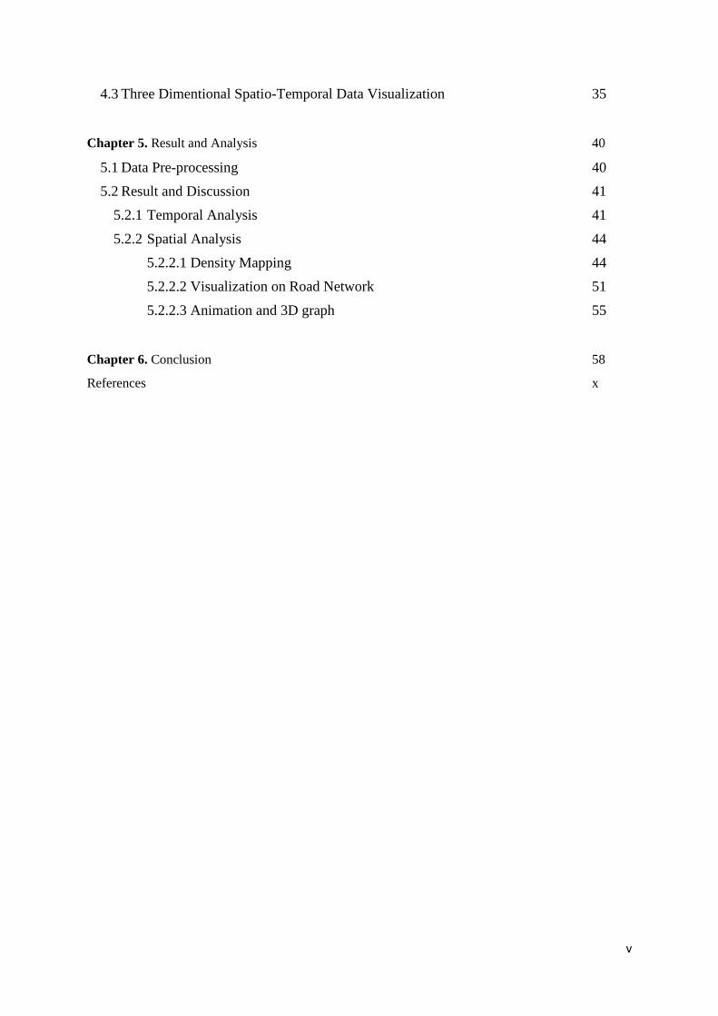
Table of Contents

Abstract ii

Acknowledgement iii

Table of Contents iv

List of Figures vi

List of Tables viii

List of Equation viii

List of Abbreviations ix

Chapter 1. Introduction 1

1.1 Related Works 1

1.2 Research Goals 4

Chapter 2. Methodological Framework and State of The Art of Traffic Congestion 6

Analysis Based on Floating Car Data

2.1 Concept on Traffic Congestion 6

2.2 Floating Car Data 10

2.3 Visual Analytics 13

2.3.1 Data Mining 14

2.3.2 Spatial and Temporal Data Visualization 18

2.3 Traffic Congestion Monitoring and Analysis Based on Floating Car Data 21

Chapter 3. Initial Test Data Properties 26

3.1 Study Area Location and Characteristics 26

3.1.1 Physical Characteristics 27

3.1.2 Socio-Economic Characteristics 27

3.1.1 Transportation System 27

3.2 Floating Car Data Properties 28

Chapter 4. Visualization Methods 30

4.1 Density Mapping 30

4.2 Visualization of Traffic Congestion on Road Network 34

v

4.3 Three Dimentional Spatio-Temporal Data Visualization 35

Chapter 5. Result and Analysis 40

5.1 Data Pre-processing 40

5.2 Result and Discussion 41

5.2.1 Temporal Analysis 41

5.2.2 Spatial Analysis 44

5.2.2.1 Density Mapping 44

5.2.2.2 Visualization on Road Network 51

5.2.2.3 Animation and 3D graph 55

Chapter 6. Conclusion 58

References x

vi

List of Figures

Figure 2.1 Percentage of Traffic Congestion Causes (FHWA, 2005) 7

Figure 2.2 Communication from GPS (FHWA, 1998) 11

Figure 2.3 Communication from cellular phone (FHWA, 1998) 12

Figure 2.4 Visual Analytics Process 14

Figure 2.5 Spatial clustering by using density method (left) and partitioning or k-means

method (right) (Chire, 2011) 17

Figure 2.6 Different scales are using to show different paterns for visual analytics results

(Andrienko, N and Andrienko, G., 2006) 19

Figure 2.7 . An interactive map display dynamic changes (different color shades) in some

areas from different time period (Andrienko, N and Andrienko, G., 2006) 20

Figure 2.8 The congestion index by time of day on weekdays (Beijing, June 2006 VS

June 2007) (Sun, et al, 2009) 22

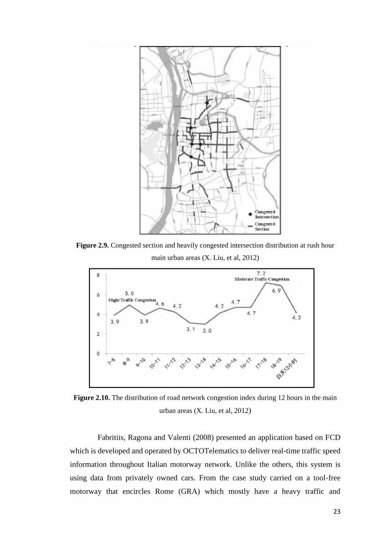
Figure 2.9 Congested section and heavily congested intersection distribution at rush hour main

urban areas (X. Liu, et al, 2012) 23

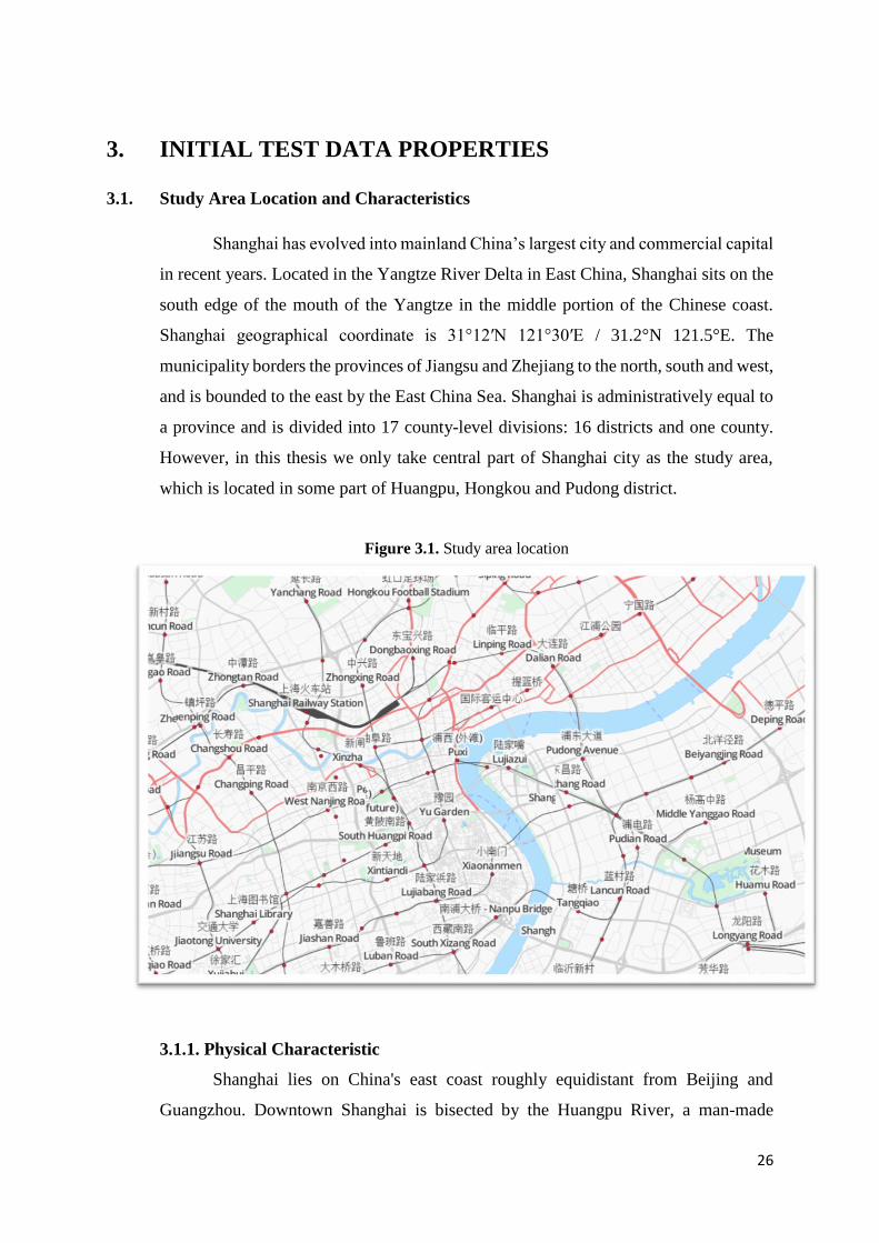
Figure 2.10 The distribution of road network congestion index during 12 hours in the main

urban areas (X. Liu, et al, 2012) 23

Figure 2.11 Spatio-temporal travel speed estimates of GRA

(Fabritiis, Ragona and Valenti, 2008) 24

Figure 2.12 Spatial-temporal related record in congestion

(Lin Xu, Yang Yue and Qingquan Li, 2013) 25

Figure 2.13 Recurrent traffic congestion event on the road network (Lin Xu, Yang Yue and

Qingquan Li, 2013) 25

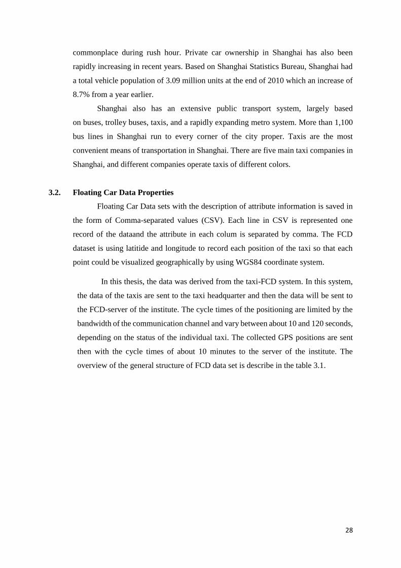
Figure 3.1 Study Area Location 26

Figure 4.1 Dot map of taxi distribution in Shanghai based on instaneous velocity

(Keler, A., 2013) 30

Figure 4.2 Continous spatial aggregation of vessel trajectories using Kernel Density Estimation

method (Willems et al, 2009) 32

Figure 4.3 Spatio-temporal cluster visualized according to taxi lifetime during rush hour

(Xintao Liu and Yifang Ban, 2013) 33

Figure 4.4 . Hotspots distribution of road accidents associated with educational institutions

(left) and religious place (right) (Prasannakumar, et al., 2011) 34

Figure 4.5 Hotspots distribution of road accidents associated with monsoon period (left) and

non-monsoon period (right) (Prasannakumar, et al., 2011) 34

Figure 4.6 Traffic congestion visualization on road segment (Keler, A., 2013) 35

Figure 4.7 Time slider animation of hurricane paths changing with the passage of time 36

Figure 4.8 Animation of taxis distribution based on time series in raining day in Singapore 37

vii

Figure 4.9 3D visualization of transportation delay in Salt Lake City in 2006 by Wasatch

Front Regional Council (Grant M. et al, 2011) 38

Figure 4.10 Comparison of two different time window of taxis density based on grid

elements extrusion visualization (Keler, A., 2013) 39

Figure 5.1 Exampe of data errors of the time attribute 40

Figure 5.2 Map matching result for GPS points from FCD 41

Figure 5.3 Mean speed (km/h) which calculate from a different time period in a day 42

Figure 5.4 Comparison of percentage of speed for different time period 43

Figure 5.5 Temporal Distribution of Traffic Congestion in the Road Segment 43

Figure 5.6 Kernel Density Map of Taxis Distribution in Shanghai at 08:00 – 09:00 AM (top left),

12:00 – 13:00 PM (top right), 17:00 – 18:00 PM (bottom left), and 22:00 – 23:00 PM

(bottom right) 45

Figure 5.7 Kernel Density Map of Trajectories of Taxis in Shanghai at the morning peak (08:00

– 09.00 AM) (left) and at the evening peak (17:00 – 18:00 PM) (right) 47

Figure 5.8 Kernel Density Map of Trajectories of Taxis in Shanghai at 12:00 – 13:00 PM 48

Figure 5.9 Stop Taxis Clustering at 07:00 – 08:00 AM time period 50

Figure 5.10 Traffic Congestion Level in Shanghai 08:00 – 09:00 AM Time Period 51

Figure 5.11 Distribution of Traffic Congestion Level in Shanghai at 08:00 AM - 09:00 AM

for Each Road Type 51

Figure 5.12 Traffic Congestion Level in Shanghai 17:00 PM – 18:00 PM Time Period 52

Figure 5.13 Distribution of Traffic Congestion Level in Shanghai at 17:00 PM – 18:00 PM Time

Period for Each Road Type 53

Figure 5.14 Traffic Density Level in Shanghai at 17:00 PM – 18:00 PM Time Period 54

Figure 5.15 Time Slider Animation of Traffic Congestion Level in Shanghai at 06:00 AM

to 23:00 PM in different time interval 56

Figure 5.16 Extrusion Graph of Traffic Congestion Level in Shanghai at 17:00 PM – 18:00 PM Time

Interval 57

viii

List of Tables

Table 2.1 LOS for Urban Roads Depend on Road Class and Travel Speed (HCM, 2005) 9

Table 2.2 LOS for Signalized Intersections Depending on Delay (HCM, 2005) 10

Table 2.3 Classification of traffic congestion (km/h) (Duan, Liu and Sun, 2009) 10

Table 2.5 Potential applications derived from the FCD Technology 12

Table 2 6 Traffic congestion performance measures 21

Table 3.1 Description of the data format of Shanghai FCD 29

Table 5.1 Daily variation of traffic congestion events on the road network 53

List of Equation

Equation 1. Traffic Flow formula 8

ix

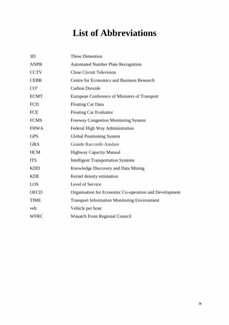
List of Abbreviations

3D Three Dimention

ANPR Automated Number Plate Recognition

CCTV Close Circuit Television

CEBR Centre for Economics and Business Research

CO2 Carbon Dioxide

ECMT European Conference of Ministers of Transport

FCD Floating Car Data

FCE Floating Car Evaluator

FCMS Freeway Congestion Monitoring System

FHWA Federal High Way Administration

GPS Global Positioning System

GRA Grande Raccordo Anulare

HCM Highway Capacity Manual

ITS Intelligent Transportation Systems

KDD Knowledge Discovery and Data Mining

KDE Kernel density estimation

LOS Level of Service

OECD Organisation for Economic Co-operation and Development

TIME Transport Information Monitoring Environment

veh Vehicle per hour

WFRC Wasatch Front Regional Council

1

1. INTRODUCTION

Rapid urbanization and economic growth caused by rapid growth of population

in big cities in developing or even developed country actuates rapid traffic movement

of people and goods from one place to another in a certain time. This development

brings up a problem for the transportation system as the number of vehicles in the city

is increasing annually which then cause traffic congestion in the city area. But the high

volume of vehicles is not the only cause of the traffic congestion. Inadequate

infrastructure, the imbalance distribution of developing area and irregularity of traffic

management are also the main causes of the traffic congestion.

Traffic congestion has many effects. It increases travel time, air pollution,

carbon dioxide (CO2) emissions and fuel. In 2013, INRIX collaborated with the Centre

for Economics and Business Research (CEBR) delivered a report of the environmental

and economic impact of congestion [1]. The result was a shocking, as traffic congestion

cost the US economy $124 billion. And if there are no changes to a better traffic

management this cost is expected to increase 50 percent to $186 billion by 2030. Air

pollution and stressed out for stuck in traffic jam for a long time also could make a

health problem for the drivers. The carbon particles from the smoke not only could

cause a heart disease, cancer and respiratory ailments, but also may injure brain cells.

TomTom in 2014 released a report that drivers in China lose nine working days per

year due to traffic [2].

With so many negative effects that caused by traffic congestion, this problem

needs to be solved so that efficiency in the road management could be achieve. Some

people might think that building new road segments as the solution, but it is not

absolutely the right answer for this problem. One of the effective solution that can be

used is by finding traffic congestion patterns which will answer the question about

when, where and how long the traffic congestion usually occur as mostly traffic

congestions are recurrent events which happened in particular road sections during

particular time of the day where the demand of road space exceeds supply. This solution

will also help traffic management to find an effective solution to reduce traffic

congestion in certain roads and also for monitoring and estimating traffic congestion.

[1] http://www.inrix.com/economic-environment-cost-congestion/

[2] http://www.tomtom.com/en_gb/trafficindex/

2

However, for the analysis of traffic congestion patterns, accurate traffic data are

needed. In recent years, the Intelligent Transportation Systems (ITS) term has become

a big issues in the transportation management, especially in term of traffic monitoring

systems by using traffic information data which derived from the traffic sensors . ITS

is built with hope to bring innovation to improve transportation systems so that

transportation problem such as traffic congestion could be solved. It deals with data

information and communication technology in vehicles, between vehicles (e.g. car-to-

car), and between vehicles and fixed location (e.g. car-to-infrastructure) that could be

used to provide road information to guide transportation systems users and traffic

monitoring. There are many technologies that have been developed to provide traffic

data in ITS. The conventional and most common method is by using sensors, such as

inductive loops. An inductive-loop detector senses the presence of a conductive metal

object by inducing currents in the object, which reduces the loop inductance. Inductive-

loop detectors are installed in the roadway surface. This sensor gathers traffic

information from vehicles which pass the sensor. Therefore this information has a big

limitation as it could only provide information traffic estimation in a certain road

segment which could not be an accurate representation for all road segments. Another

limitations is that these sensors are quite expensive and need to be placed on the road

which prone to be broken because of heavy vehicles, short lifetime. In addition, for a

long road segment, the sensors need to be place in several places in a certain interval to

maintain an accurate measurement (Jain, Sharma and Subramanian, 2012).

Another method that can be used to gather traffic information is by using CCTV

camera. This method used to monitor real-time-traffic by utilizing CCTV camera

images for measuring density of the vehicles. The advantage of using this method is the

installation of cameras does not involve breaking up pavement, which is a necessity for

installing ground sensors. However this method also has some disadvantages, such as

low camera resolution resulting in highly noisy images, traffic camera’s limited field of

view and light illumination from multiple reflecting sources distorting vehicle

classification capabilities.

With the development of the Global Positioning System (GPS) technology, a

novel technology was developed which called Floating Car Data (FCD). FCD is a

method to gather road information based on the exchange of information between a

fleet of floating cars traveling on a road network and a central data system (Fabritiis,

Ragona and Valenti, 2008). Cars which equipped with GPS receiver act as agents to

3

gather information about traffic condition. This method provides a network-wide,

accurate and real time information, which is less cost and constantly accessible which

make this method gain popularity to provide data for traffic management system.

The data provided by different sensors are spatio–temporal data which contain

both the spatial locations of the vehicles and the time recorded. By collecting and

processing this kind of data, traffic information, in this case traffic congestion, could be

analyzed in different period of time. Therefore identification of traffic congestion for

different time intervals could be done and the patterns of the traffic congestion could

be explore by comparing the traffic congestion events for each period of time to answer

and help solving the traffic congestion problems.

1.1 Related Works

Several research works have been investigated related to the identification of

traffic congestion. Wang, et al (2002) proposed an approach by using a measurements

from single-loop detectors produces traffic congestion information based on estimated

speeds for Freeway. This procedure is divided into three steps: loop data pre-processing,

traffic speed estimation and congestion detection. They also built an automate

procedure called Freeway Congestion Monitoring System (FCMS) which performed

well under both congested and un-congested conditions. The results from this study are

this approach could calculate congestion onset, dissipation and duration which are quite

accurate.

Bacon, et al (2008) developed a project called TIME (Transport Information

Monitoring Environment) project to investigate real-time road traffic data for

congestion evaluation. They were using many sensors to gather information to

determine the state of the road network such as static sensors (inductive loops at

junctions, infra-red counting) and mobile sensors (bus probe). They believe that

combining many data from different sensors will give a whole and better picture of

traffic situation. They estimated the congestion by calculating the travel time of the

buses from one station to another station which will be different depending on the

situation. Travel time on school days take longer than travel time on non-school days,

and when an accident happens on the road, the travel will also take a longer time. They

also concluded that public transport data in this case buses probe is a really a great

source of data because its minimum cost and vast coverage in terms of space and time.

4

Hong-Li Zeng, et al (2009) studied congestion patterns of traffic in Nanjing city

by using dual graph to represent the Nanjing city map on which they implement and

stimulate the traffic model with two important features: navigation and queuing. The

model adopted the idea of the traffic of information on the Internet, where information

travel to a specified address being navigated and are queuing at nodes along their paths.

The dual graph was chosen because it highlights certain topological feature of the city

road structure and their contribution in the spatio-temporal congestion patterns. Then

they analyze the load on nodes and edges to reveal the congestion patterns and map it

back to the geographical space. The traffic patterns could also be obtained by analyzing

the eigenvalue spectrum of the network.

Wei Zhang, et al (2012) presented a model and algorithms for traffic congestion

evaluation and optimal traffic light control based on wireless sensor networks. They

introduced the congestion factor based on traffic data and the principle of traffic

congestion parameter to evaluate the degree of traffic congestion along the road

segments and to predict the subcritical state of traffic jams. Traffic congestion model

named Jamitons and LWR model were used to gather information about traffic flow

density and speed to evaluate traffic congestion. They were using Mobile Century

dataset and working on VISSIM platform. The result of this study are algorithms to

calculate congestion and its influence on future traffic flow, in this case in the

intersection road, to help traffic control system so that average delay and maximum

queue length at the intersection could be reduced.

Fusco and Colombaroni (2013) presented an integrated method for the short-

term prediction of road traffic conditions. They were using fusion data from inductive

loop monitoring and RFID detectors in 223 km long stretch motorway in Italy which

then are processed by using some methods such as Artificial Neural Network, automatic

incident detection and road traffic network model. As the results, time-series models

provide quick and sufficiently accurate short-term predictions when variation of traffic

is mainly caused by random disturbance. While traffic simulation is necessary for

accidents or other anomalous traffic pattern.

1.2. Research Goals

This goals of this study is to do a spatio-temporal visual exploration of traffic

congestion patterns which is derived from Floating Car Data (FCD) in some part of

Shanghai city. This study wants to try to answer the questions about traffic congestion

5

pattern from the analysis, such as how the traffic congestion level in Shanghai city based

on the Floating Car Data (FCD), in which part of the city that the traffic congestion is

most likely occur in which time period and how long the traffic congestion is in the

bottleneck area or in the congested road segment.

6

2. METHODOLOGICAL FRAMEWORK AND STATE OF

THE ART OF TRAFFIC CONGESTION ANALYSIS

BASED ON FLOATING CAR DATA

This chapter reviews some basic concepts that will be used as basic knowledge

for further analysis in the next chapters. This chapter is divided into four sections, the

first section explains about the basic concept of traffic congestion including some

formulas to describe how traffic congestion could be classified. The second section is

about the basic concept of Floating Car Data (FCD) and how it can be used as a data

source for traffic monitoring. Third section is about the basic theories about visual

analytics that could be used for spatio-temporal data analysis. The fourth section will

discuss some literature review about traffic congestion monitoring and analysis of FCD

data.

2.1. Concept of Traffic Congestion

Traffic congestion actually does not have an exact and broadly accepted

definition because traffic congestion is a physical phenomenon relating to the manner

in which vehicles impede each other’s progression as demand for limited road space

approaches full capacity and also a relative phenomenon relating to user expectation

vis-à-vis road system performance (OECD/ECMT, 2004). Basically traffic congestion

could be define as a situation in which demand for road space exceeds supply or traffic

volume exceeds road capacity. By the type, traffic congestion could be classified as

recurrent traffic congestion which happened in particular road section during particular

time of the day where the demand of road space exceeds supply and non-recurrent

traffic congestion which happened because of special or random occasions such as road

construction or accidents that makes a temporary increase of demand or reduce the road

capacity.

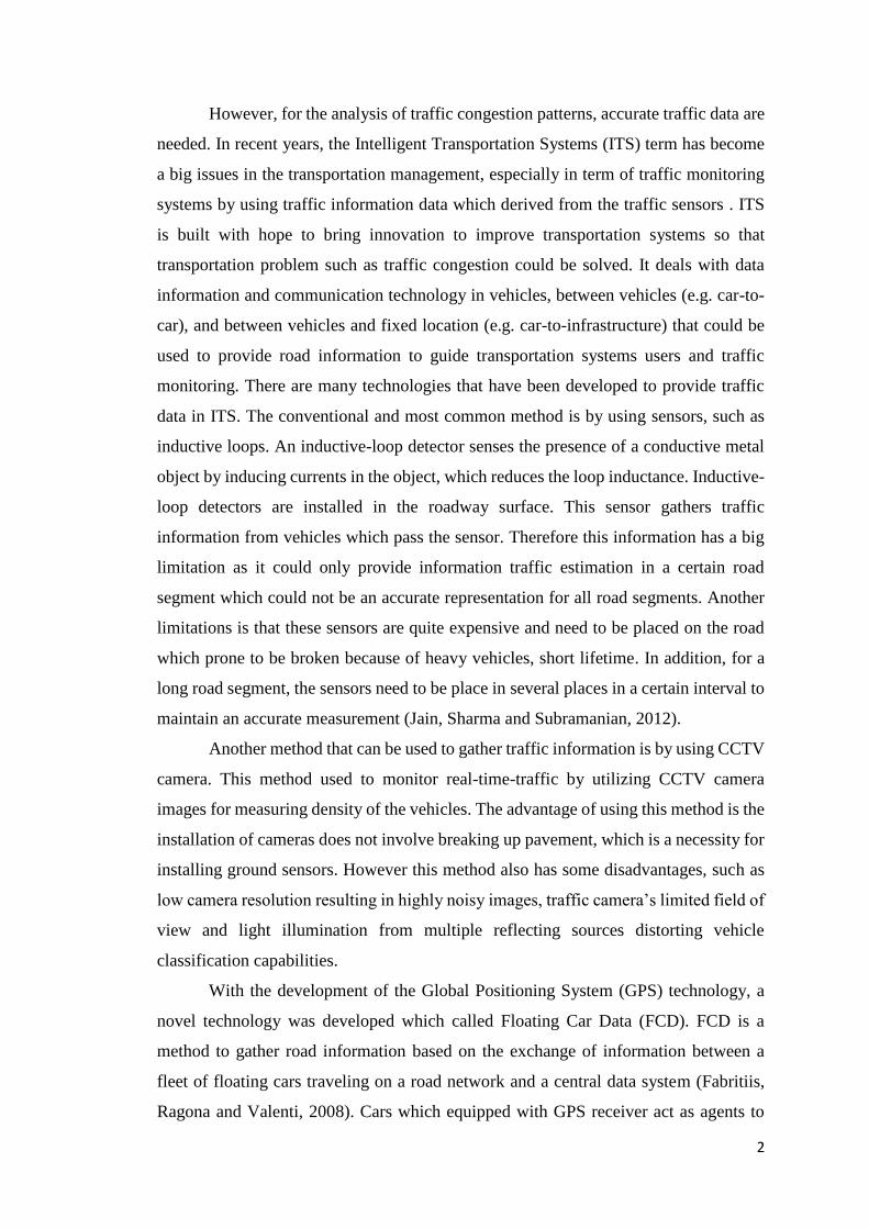
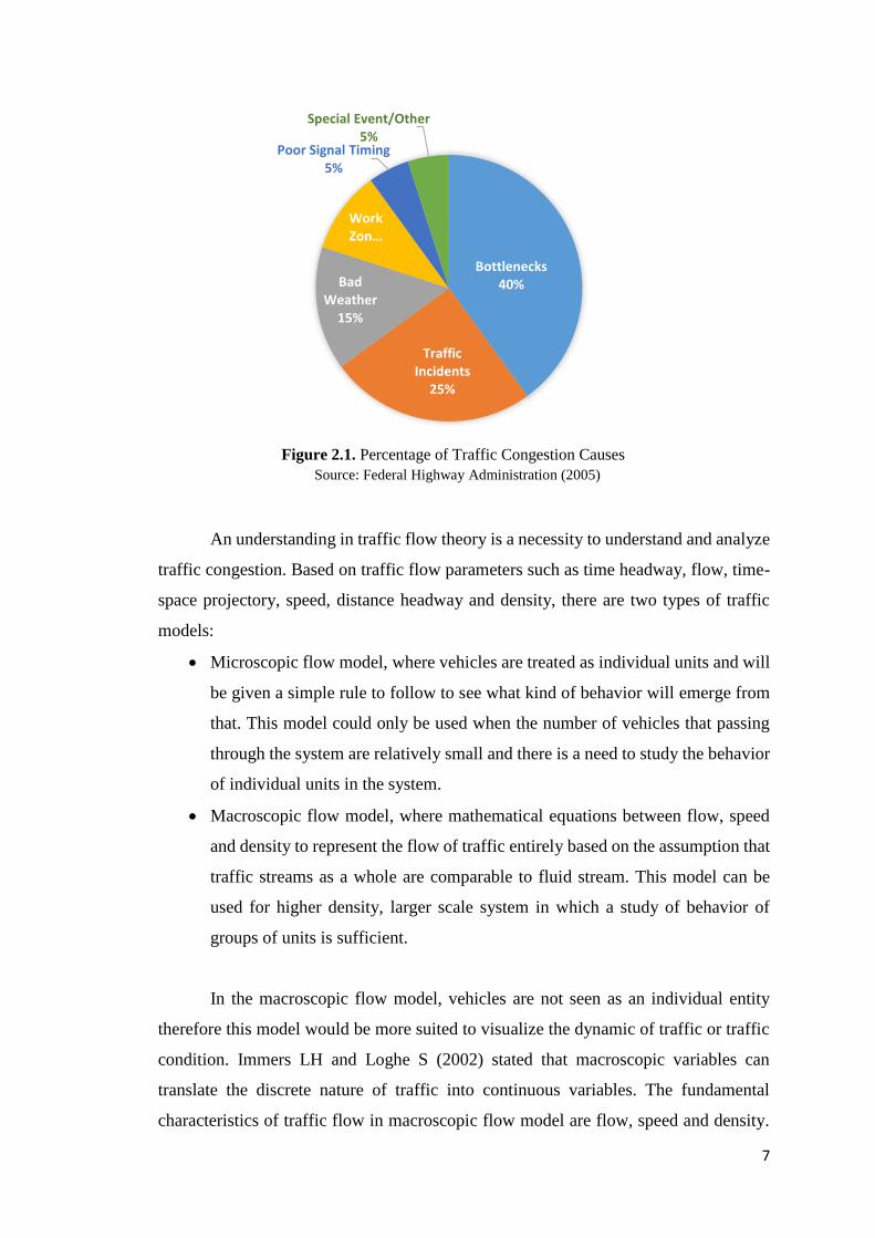
Based on Federal Highway Administration (2005), there are seven causes of

traffic congestion, which are physical bottlenecks, traffic incidents, work zone, bad

weather, poor signal timing, special events and fluctuations in normal traffic. From the

percentage of the causes of traffic congestions, physical bottlenecks, traffic incidents

and bad weather are the main causes of traffic congestions. Every cause has a different

level of frequency, therefore traffic congestion pattern or type could change or develop

from time to time.

7

An understanding in traffic flow theory is a necessity to understand and analyze

traffic congestion. Based on traffic flow parameters such as time headway, flow, time-

space projectory, speed, distance headway and density, there are two types of traffic

models:

Microscopic flow model, where vehicles are treated as individual units and will

be given a simple rule to follow to see what kind of behavior will emerge from

that. This model could only be used when the number of vehicles that passing

through the system are relatively small and there is a need to study the behavior

of individual units in the system.

Macroscopic flow model, where mathematical equations between flow, speed

and density to represent the flow of traffic entirely based on the assumption that

traffic streams as a whole are comparable to fluid stream. This model can be

used for higher density, larger scale system in which a study of behavior of

groups of units is sufficient.

In the macroscopic flow model, vehicles are not seen as an individual entity

therefore this model would be more suited to visualize the dynamic of traffic or traffic

condition. Immers LH and Loghe S (2002) stated that macroscopic variables can

translate the discrete nature of traffic into continuous variables. The fundamental

characteristics of traffic flow in macroscopic flow model are flow, speed and density.

Bottlenecks40%

Traffic Incidents

25%

Bad Weather

15%

Work Zon…

Poor Signal Timing5%

Special Event/Other5%

Figure 2.1. Percentage of Traffic Congestion Causes

Source: Federal Highway Administration (2005)

8

These three fundamental characteristics are not independent, there is a fundamental

relationship which connect them that shown in equation.

𝑞 = 𝜌 . 𝜐 ........................................................ (1)

𝑞 (𝑥, 𝑡) is the flow rate or volume at location x and time t, which is defined as

the number of vehicles passing through the location in a unit of time.

𝜌 (𝑥, 𝑡) is the density at location x and time t, which is defined as the number of

vehicles in a distance.

𝑣 (𝑥, 𝑡) is the speed of the vehicles at location x and time t.

These three basic parameters can be used to describe traffic on any roadway. Volume

or flow rate are variables that quantify demand, that is, the number of vehicles who

desire to use the road during the specific time period. Congestion can influence demand,

and observed volumes sometimes reflect capacity constraints rather than true demand.

Volume and flow rate have a different definition, as volume is the number of vehicles

observed or predicted to pass a point during a time interval while flow rate is the number

of vehicles passing a point during a time interval less than one hour, but expressed as

an equivalent hourly rate. For example, the number of vehicles observed for four

consecutive 15 minutes period are 1,000, 1,200, 1,100 and 1,000. These are flow rate,

and the volume is the sum of these numbers or 4,300 vehicles. The peak flow rates is

important in capacity analysis, because sometimes the peak flow rates exceed the

capacity number even though the volume is less than capacity during the full hour

which could trigger a congestion in the road segment. The flow rate as a variable

describing traffic quantities inside a map representation may deliver meaningful

illustrations in the background of detecting traffic congestions (Keller, 2013).

Speed is defined as a rate of motion expressed as distance per unit of time,

generally as kilometer per hour (km/h). It is an important measure of the quality

(effectiveness defining levels) of the traffic service. In most cases, space mean speed is

used as the speed measure because it easily computed from observations of individual

vehicles within the traffic stream and is the most statistically relevant measure in

relationships with other valuable. It is computed by dividing the length of road section

by the average travel time of the vehicles traversing it.

Density is the number of vehicles occupying a given length of lane or roadway

at a particular instant, which usually expressed as vehicles per kilometer (veh/km).

9

Unlike flow rate and speed, density could not be measure directly in the field, however

density can be computed from the average speed and flow rate data. Density is a critical

parameter to characterize the quality of traffic operation because it describes the

proximity of vehicles to one another and reflects the freedom to maneuver within the

traffic stream.

From the study of the relation between these parameters, it shows that a zero

flow rate occurs under two different conditions, when there are no vehicles on the

facility (density is zero) and when density becomes so high that all vehicles must stop

so there are no movement or congestion occurs. It also show that flow rate and density

are linked in interesting way, because normally flow rate increase as density increase.

However, when density reaches a so called ‘critical density’, the flow rate begins to

decrease and congestion occurs (He Shulin, 2012).

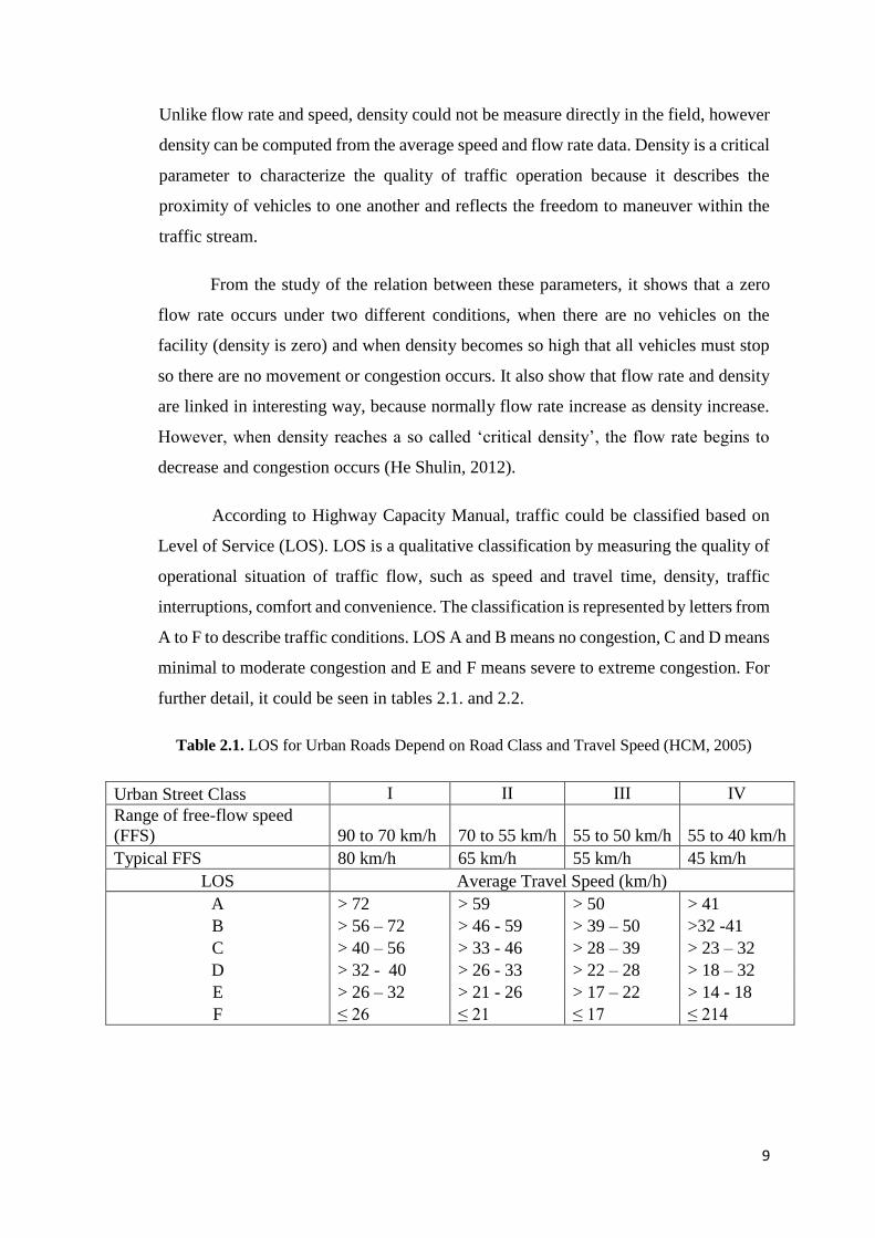
According to Highway Capacity Manual, traffic could be classified based on

Level of Service (LOS). LOS is a qualitative classification by measuring the quality of

operational situation of traffic flow, such as speed and travel time, density, traffic

interruptions, comfort and convenience. The classification is represented by letters from

A to F to describe traffic conditions. LOS A and B means no congestion, C and D means

minimal to moderate congestion and E and F means severe to extreme congestion. For

further detail, it could be seen in tables 2.1. and 2.2.

Table 2.1. LOS for Urban Roads Depend on Road Class and Travel Speed (HCM, 2005)

Urban Street Class I II III IV

Range of free-flow speed

(FFS) 90 to 70 km/h 70 to 55 km/h 55 to 50 km/h 55 to 40 km/h

Typical FFS 80 km/h 65 km/h 55 km/h 45 km/h

LOS Average Travel Speed (km/h)

A > 72 > 59 > 50 > 41

B > 56 – 72 > 46 - 59 > 39 – 50 >32 -41

C > 40 – 56 > 33 - 46 > 28 – 39 > 23 – 32

D > 32 - 40 > 26 - 33 > 22 – 28 > 18 – 32

E > 26 – 32 > 21 - 26 > 17 – 22 > 14 - 18

F ≤ 26 ≤ 21 ≤ 17 ≤ 214

10

Table 2.2. LOS for Signalized Intersections Depending on Delay (HCM, 2005)

LOS Control Delay per Vehicle

(s/veh)

A ≤ 10

B > 10 -20

C > 20 -35

D > 35 – 55

E > 55 – 80

F > 80

Duan, Liu and Sun (2009) have researched about traffic congestion in

Shanghai based on FCD. They were using data collection from 6,000 taxis for a month.

Based on the percentile of average speed for each class of the road, they set a threshold

and define traffic congestion in 5 states (seen in table 2.3).

Table 2.3. Classification of traffic congestion (km/h) (Duan, Liu and Sun, 2009)

Road type State 1 State 2 State 3 State 4 State 5

Elevated road < 20 20 - 35 35 - 55 55 – 75 > 75

Expressway < 20 20 - 30 30 - 40 40 – 75 > 75

Main arterial road < 15 15 - 20 20 - 25 25 - 40 > 40

Arterial road < 15 15 - 20 20 - 25 25 - 40 > 40

Collector road < 13 13 - 18 18 - 23 23 - 33 > 33

Branch road < 13 13 - 18 18 - 23 23 - 33 > 33

2.2. Floating Car Data

Floating Car Data is one of a method to gather information about traffic by

collecting real-time traffic data from vehicles via mobile phones or GPS over the entire

road network. The data will be sent to a central processing center to be processed to

extract information about the traffic condition. The floating car data technology is a

new approach to gather traffic information for ITS. This method is quite useful because

it could represent a full coverage of monitored areas automatically in real time with

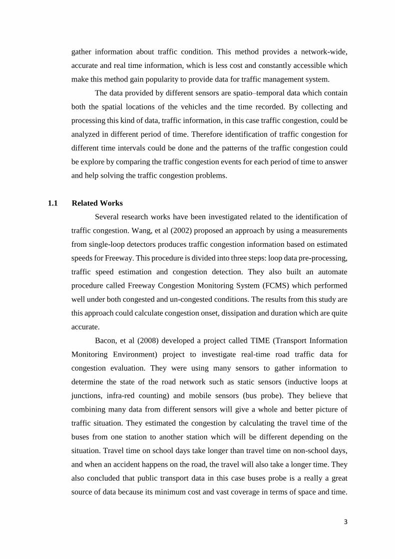
minimum cost and still generate a high quality of data. Basically, there are two types of

FCD, GPS and cellular-based systems. GPS system utilizes the GPS receiver system

11

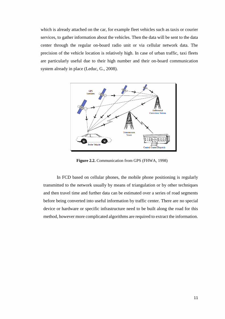
which is already attached on the car, for example fleet vehicles such as taxis or courier

services, to gather information about the vehicles. Then the data will be sent to the data

center through the regular on-board radio unit or via cellular network data. The

precision of the vehicle location is relatively high. In case of urban traffic, taxi fleets

are particularly useful due to their high number and their on-board communication

system already in place (Leduc, G., 2008).

Figure 2.2. Communication from GPS (FHWA, 1998)

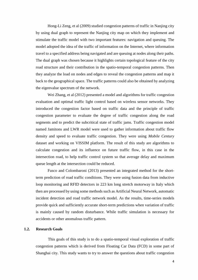
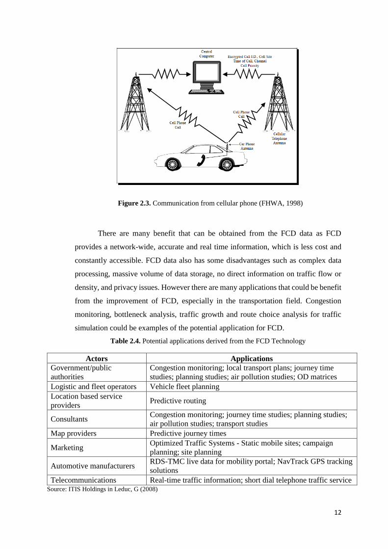
In FCD based on cellular phones, the mobile phone positioning is regularly

transmitted to the network usually by means of triangulation or by other techniques

and then travel time and further data can be estimated over a series of road segments

before being converted into useful information by traffic center. There are no special

device or hardware or specific infrastructure need to be built along the road for this

method, however more complicated algorithms are required to extract the information.

12

Figure 2.3. Communication from cellular phone (FHWA, 1998)

There are many benefit that can be obtained from the FCD data as FCD

provides a network-wide, accurate and real time information, which is less cost and

constantly accessible. FCD data also has some disadvantages such as complex data

processing, massive volume of data storage, no direct information on traffic flow or

density, and privacy issues. However there are many applications that could be benefit

from the improvement of FCD, especially in the transportation field. Congestion

monitoring, bottleneck analysis, traffic growth and route choice analysis for traffic

simulation could be examples of the potential application for FCD.

Table 2.4. Potential applications derived from the FCD Technology

Actors Applications

Government/public

authorities

Congestion monitoring; local transport plans; journey time

studies; planning studies; air pollution studies; OD matrices

Logistic and fleet operators Vehicle fleet planning

Location based service

providers Predictive routing

Consultants Congestion monitoring; journey time studies; planning studies;

air pollution studies; transport studies

Map providers Predictive journey times

Marketing Optimized Traffic Systems - Static mobile sites; campaign

planning; site planning

Automotive manufacturers RDS-TMC live data for mobility portal; NavTrack GPS tracking

solutions

Telecommunications Real-time traffic information; short dial telephone traffic service Source: ITIS Holdings in Leduc, G (2008)

13

There has been many projects related to FCD applications. Reinthaler, et al

(2007) proposed a project called Dmotion which aims to provide an effective traffic

management strategy for regional and local authorities. This project tries to provide an

efficient way for estimating speeds and traffic state based on FCD data from taxi fleets

and public transport. The data is provided by 1,200 taxis, then a multi-stage algorithm

(Floating Car Evaluator, FCE) is employed to calculate the speed per road link. Data

from public transport are used to complete missing data from FCD. As a result, the

estimated path speed based on FCD follow the trend of the average path speed measured

by ANPR (Automated Number Plate Recognition) but the level of estimated speeds is

lower than average path speeds. However this result shows that temporal trends of

average speeds during a day could be captured by FCD data and this data prove to be a

reliable and cheap additional data source for urban traffic state estimation.

Another application is proposed by Tang, et al (2012) which tries to utilize FCD

data to detect and update changes in the road network. They choose taxi fleets data

because taxis travel all over the city every day. The road network change detection and

update follows these steps: data preprocessing, map matching, incremental detection,

new data sampling, road network update and new road network detection. The most

crucial part in this study is the map matching process as this step will detect whether

the position of GPS point data match with the existing road network or not which means

that an addition to the road network is needed.

In Europe, there were many FCD projects that has been conducted throughout

last decade. OPTIS in Sweden is using FCD to collect data of traffic condition to

provide traffic information for travelers. From the trials, FCD is proven to be a cost-

effective method to provide accurate real-time traffic information for the user.

Mediamobile in France is using FCD data which are gathered from 1,700 taxis

operating in Paris to provide live traffic information on motorway congestion and traffic

congestion for Paris.

2.3. Visual Analytics

Visual analytics is the science of analytical reasoning supported by interactive

visual interfaces (Thomas,J., Cook, K., 2005). A more specific definition would be:

“Visual analytics combines automated analysis techniques with interactive

visualisations for an effective understanding, reasoning and decision making on the ba-

14

sis of very large and complex datasets” [3]. It is an integral approach combining

visualization, human factors, and data analysis, which allow users to combine their

knowledge with the automation data processing and analysis which done by computer

to explore and gain more information from the data.

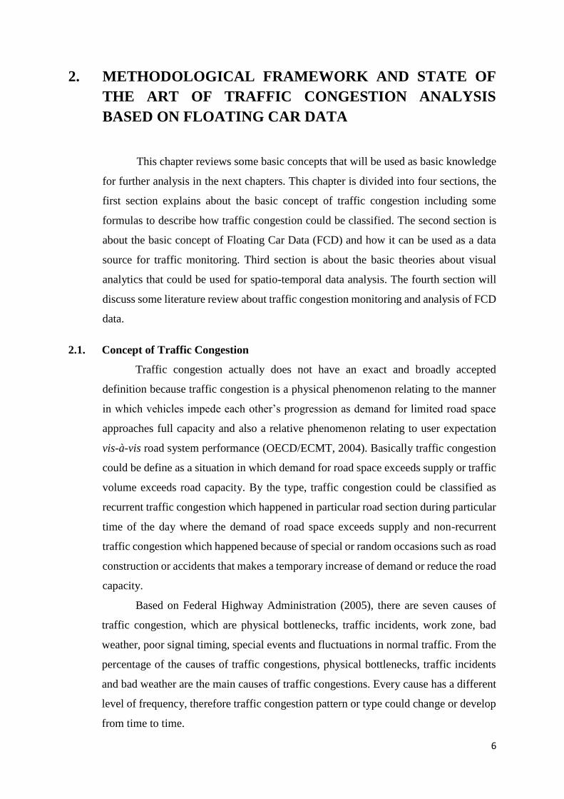
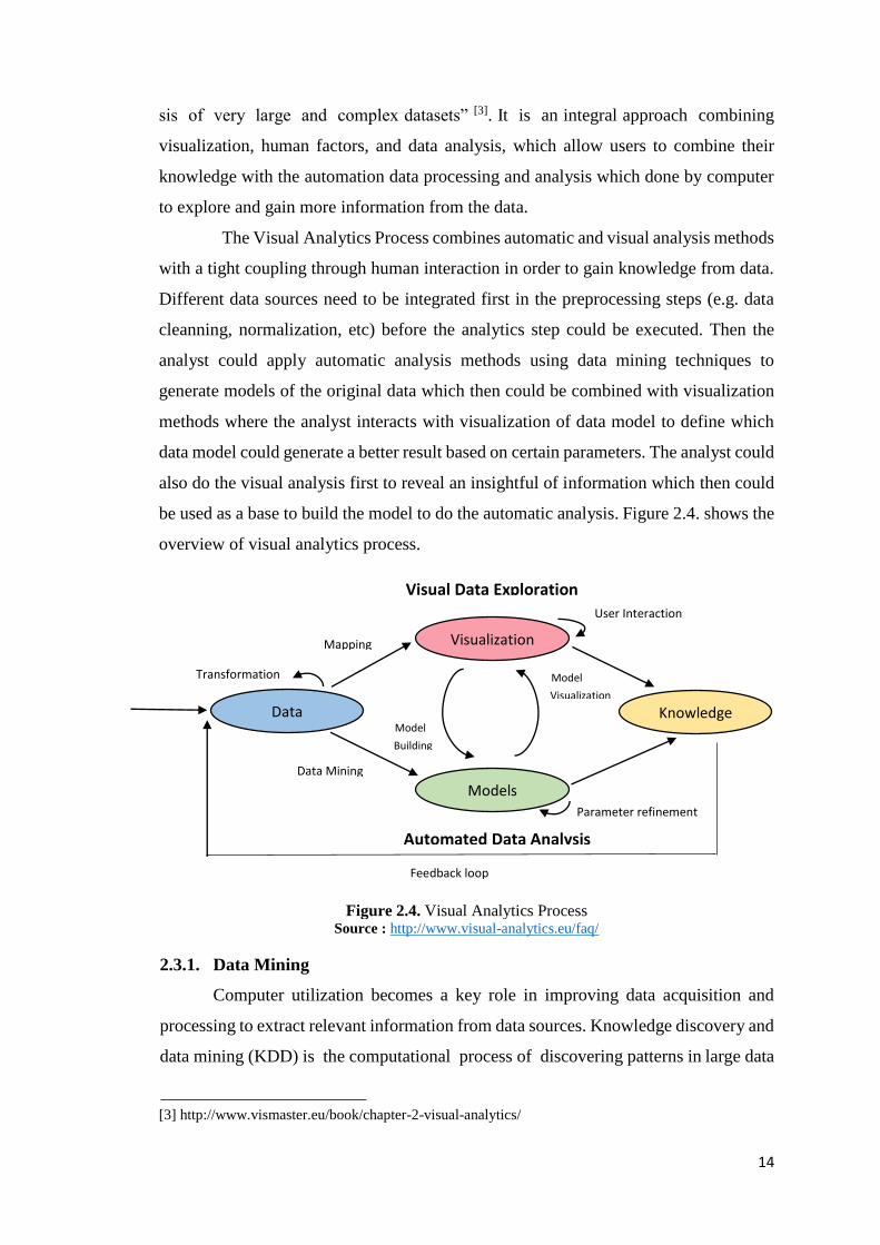
The Visual Analytics Process combines automatic and visual analysis methods

with a tight coupling through human interaction in order to gain knowledge from data.

Different data sources need to be integrated first in the preprocessing steps (e.g. data

cleanning, normalization, etc) before the analytics step could be executed. Then the

analyst could apply automatic analysis methods using data mining techniques to

generate models of the original data which then could be combined with visualization

methods where the analyst interacts with visualization of data model to define which

data model could generate a better result based on certain parameters. The analyst could

also do the visual analysis first to reveal an insightful of information which then could

be used as a base to build the model to do the automatic analysis. Figure 2.4. shows the

overview of visual analytics process.

Figure 2.4. Visual Analytics Process Source : http://www.visual-analytics.eu/faq/

2.3.1. Data Mining

Computer utilization becomes a key role in improving data acquisition and

processing to extract relevant information from data sources. Knowledge discovery and

data mining (KDD) is the computational process of discovering patterns in large data

[3] http://www.vismaster.eu/book/chapter-2-visual-analytics/

Model

Model

Visualization

Building

User Interaction

Transformation

Mapping

Data Mining

Feedback loop

Parameter refinement

Visual Data Exploration

Visualization

Models

Knowledge Data

Automated Data Analysis

15

set involving methods at the intersection of artificial intelligence, machine

learning, statistics, and database systems. KDD methods are mostly suitable for

evaluating the quality of the proposed solutions of the problem. Therefore this methods

do not take analysist knowledge into account to provide a solution for a problem.

The main idea of KDD is to extract information from large datasets. In KDD,

there are some stages of process to transform data into various model or representation

to obtain the pattern that represent the implicit information within the data. The KDD

process consists of data selection, data pre-processing, data transformation, data mining

and interpretation or evaluation. In pre-processing stage, the dataset will be cleaned

from the noises and missing data and formatted to suit the data mining algorithms. This

stage is an essential process as the data could be heterogeneous (e.g. textual data, data

stored in database, satellite imagery, etc) therefore it requires effective methods for data

cleaning and integration. The output of this stage then will be transformed into a form

that can be understood by the analyst.

Data mining tasks can be divided into predictive task and descriptive tasks. In

predictive tasks, such as classification and regression, data are analysed to build a global

model to be able to predict the value of target attributes based on the observed values

of the explanatory attributes. In descriptive tasks, such as clustering and pattern mining,

the data will be summarised by using local patterns which describes the implicit

relationship and characteristics of the data itself. The last stage is to verify the patterns

produced by the data mining process to meet the desired standard because some patterns

found by the data mining algorithms are not necessarily valid. When the results are in

accordance with the standards, the results then can be interpreted to gain knowledge

about the information.

The current KDD methods are not directly applicable in visual analytics

scenarios and only support limited user interaction. The models and patterns extracted

by traditional KDD from a larger dataset could also be difficult to interpret in which

the information within the dataset might still hidden in the large number of data. Hence

for data mining method to be useful in visual analytics it should be (Keim et al, 2010):

Fast enough – sub-second response is needed for efficient interaction

16

Parameters of the method should be representable and understandable using

visualizations

Parameters shoul be adjustable by visual controls.

An example of data mining is spatial data mining. Spatial data mining could

be interpreted as a process of discovering interesting and previously unknown, but

potentially useful patterns from spatial databases (Sumathi, et al., 2008). Spatial

databases contain spatial and non-spatial attributes of the areas under the study, in

which spatial data mining could be done to find implicit rules or patterns hidden in

spatial databases that could be helpful for some fields such as geo-marketing or traffic

control. The basic tasks of spatial data mining are classification, association rules,

characteristic rules, discriminate rules, clustering and trend detection.

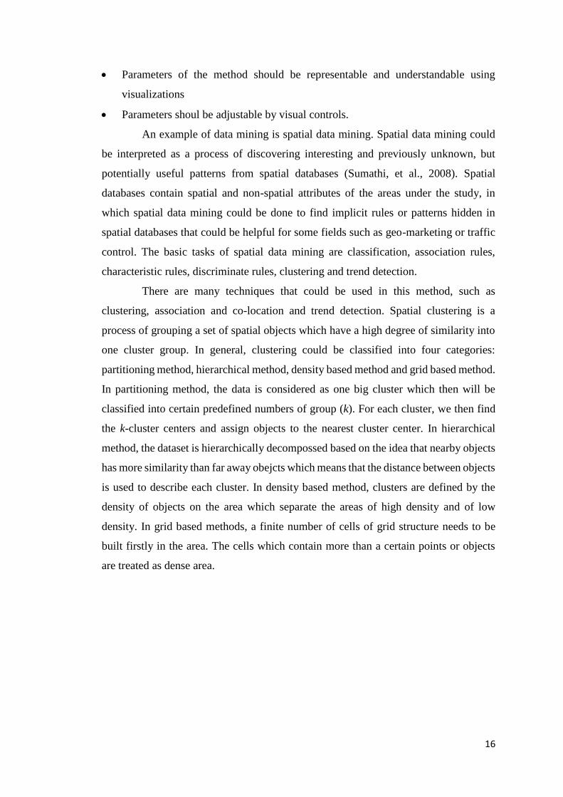
There are many techniques that could be used in this method, such as

clustering, association and co-location and trend detection. Spatial clustering is a

process of grouping a set of spatial objects which have a high degree of similarity into

one cluster group. In general, clustering could be classified into four categories:

partitioning method, hierarchical method, density based method and grid based method.

In partitioning method, the data is considered as one big cluster which then will be

classified into certain predefined numbers of group (k). For each cluster, we then find

the k-cluster centers and assign objects to the nearest cluster center. In hierarchical

method, the dataset is hierarchically decompossed based on the idea that nearby objects

has more similarity than far away obejcts which means that the distance between objects

is used to describe each cluster. In density based method, clusters are defined by the

density of objects on the area which separate the areas of high density and of low

density. In grid based methods, a finite number of cells of grid structure needs to be

built firstly in the area. The cells which contain more than a certain points or objects

are treated as dense area.

17

Source: http://en.wikipedia.org/wiki/Cluster_analysis

Association and co-location are a data mining function that discovers the

probability of the co-occurrence of items in a collection [4]. This function is sometimes

referred to as market basket analysis. In this function, association rules between objects

are used to define the relations between data. Association rules are created by analyzing

data for frequent if/then patterns and using the criteria support and confidence to

identify the most important relationship [5]. Support indicates the frequency the items

appear in the database, while confidence indicates how many times the statement is

true.

Trend detection or frequent pattern mining is a technique to find existing

patterns in data which then could be used to predict trends of the attribute changes with

respect to the neighborhood of some spatial objects. This function is the most basic

function in data mining. Frequent patterns are those patterns that occur frequently in

the database. Those patterns could be used to find predictive trends of the data. For

example, when people go to their offices they have frequent routes that they choose.

Based on those patterns we can predict the trends of the routes and the road segments

which are mostly passed on.

As above mentioned, KDD methods are useful but still limited. Therefore an

integration with data visualization methods is needed to support this method, especially

for pattern identification for spatial dataset.

[4] http://docs.oracle.com/cd/B28359_01/datamine.111/b28129/market_basket.htm#DMCON009 [5] http://searchbusinessanalytics.techtarget.com/definition/association-rules-in-data-mining

Figure 2.5. Spatial clustering by using density method (left) and partitioning or k-means

method (right) (Chire, 2011)

18

2.3.2. Spatial and Temporal Data Visualization

The decision making process for a problem depends on where and when the

problem occurs. Therefore, traditionally maps were used as representative models of

the real world to help people orient the problem in spatial scope to gain more knowledge

about the problem and its evolution in time to find a better solution to solve these

problems. However, with the revolution of information technology which brings larger

datasets and more complex systems, simple maps are no longer sufficient. Sophisticated

maps and advanced computational techniques which are interdependent and synergetic,

accessible and usable, and support decision making process are needed to overcome

this problem. These maps allow people to compare possible options and strategies and

make decisions by visualy analyzing it. As spatio-temporal analysts, they must be

enabled to gain information from the data effectively and efficiently and then record,

report and share the information.

Spatial and temporal data have different properties from other types of data. The

processing, integration and analysis of spatio-temporal data are constrained and

underpinned by the fundamental concept of spatio and temporal dependences, in which

in spatial domain it is often referred as “Tobler’s first law”: “everything is related to

everything else, but near things are more related than distant things” (Keim,et al, 2010).

This concept also applies for temporal dependence. These dependencies could also be

used to give more values to the information in data processing and analysis by doing

interpolation and extrapolation to fill the gaps for incomplete data, integration of

different type of data using common locations as references, and many other operations.

Spatio-temporal data also have uncertainty, therefore uncertainty needs to be

considered to generate an effective analysis of spatio-temporal data.

Spatio-temporal events and processes exist and operate at different spatial and

temporal extents. The dimension of time can include a single or multiple levels of scale,

hence temporal primitives could be aggregated or disagregated into larger or smaller

conceptual units. The scale of spatial analysis is reflected in the size of the units in

which events are measured and the size of the units in which the measurements are

aggregated, which may significantly affects the results. Identifying the correct scale of

events is important to accurately observe the events. The scale of analysis should also

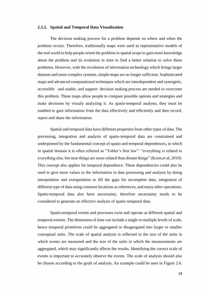
be chosen according to the goals of analysis. An example could be seen in Figure 2.6.

19

where individual trajectories visualized in different spatial scales and levels of

aggregation. The appropriate scale depends on the need of analyst, whether they need

to investigate movements in particular road section or to investigate movements in

larger areas.

Figure 2.6. Different scales are using to show different paterns for visual analytics results

(Andrienko, N and Andrienko, G., 2006)

From the example, the use of map as a representation of real world in space

dimension is one key point of spatio-temporal data visualization. Maps have the ability

to present and simplify the complexity in real world into two dimensional plane which

makes the analysis process much easier. Cartography discipline also developed

guidelines to help to improve the design of maps to produce maps which offers insight

in spatial patterns and realtion in particular contexts. Cartographic generalisation is

used to filter unnecessary information and preserve the important and relevant

information which are different based on the scale. Because all of these advantages,

20

maps are very suitable for visual analysis. Maps offer interaction with the data spatially

and encourage deeper exploration about geospatial patterns, relationships and trends.

While spatial data could be easily visualized by using maps, temporal data

visualization is a big challenge to all disciplines of data visualization and analysis. The

existing approaches in general proposed visualize time and temporal data by creating a

spatial arrangement of the time axis on the display or utilizing real world time so that

an animation shows visual representation of different time steps in quick succesion.

Visualization methods of temporal data also depend on wheteher temporal attributes

are conceptually modelled as time points or time intervals. Integrating appropriate

interaction methods for temporal data in visual analytics for spatio-temporal data need

to be done in order to allow analyst to adapt to the visualization and do a variety of

tasks to analyze and explore the data.

An interactive method to combine the visualization for spatio-temporal data is

by using animated maps. Animated maps portray time-dependent data and dynamic

event by mapping the temporal dimension of the data to physical time. It implements

the idea that space and time are inseparable and suggestd a three-dimensional visual

representation where two dimensions encode spatial aspects of data and the third

dimension represents time. The analysis of the data is done in a single display with the

maps are displayed simultaneously by the sequence of the events. In Figure 2.7., an

interactive map is used to display changes in some areas in different time periods.

Figure 2.7. An interactive map display dynamic changes (different color shades) in some areas from

different time period (Andrienko, N and Andrienko, G., 2006)

21

2.4. Traffic Congestion Monitoring and Analysis Based On Floating Car Data

In the recent years, FCD became one of the most essential part in transportation

information system as a reliable and low cost source to gather traffic information for

traffic monitoring. FCD also begun to show its potential as a source for real-time traffic

information systems, which is already applied in some countries.

Sun, et al (2009) has done the research to improve metropolitan congestion

performance measurement method based on floating car data. With this method,

congestion performance measurement could be done at different types of road classes

in real time including freeway, arterial road and even local streets. In this research, they

measure traffic congestion based on ‘five-dimensional’ traffic congestion performance

measure that could be seen in this Table 2.5.

Characteristic Sort Code Index name

congestion intensity K1 Traffic congestion index

congestion spatial

distribution K2

The kilometrage proportion on different

congestion grade

congestion temporal

distribution K3 Congestion grade duration by time of the day

traffic bottlenecks

(congestion frequency) K4

The number and distribution of recurrent

congested nodes and segments

Reliability K5 Road network reliability index

Table 2.5. Traffic congestion performance measures

Travel time is used as a basic parameter to calculate the average speed for

congestion performance measurement after map matching process has been done. Then

congestion performance measurement could be done as these steps: aggregate the 5

minutes interval travel speed data from FCD to 15 minutes for each link, identify each

link belong to which congestion grade according to the speed level criteria, sum up the

kilometrage in each congestion grade for each road class separately then classified,

select out the AM peak (PM peak) and average proportion values during the peak,

establish a linear function between road network kilometrage proportion and the traffic

congestion grade to transforms the road network kilometrage proportion to a no unit

index to describe congestion grade, identify the recurrent links considering the AM

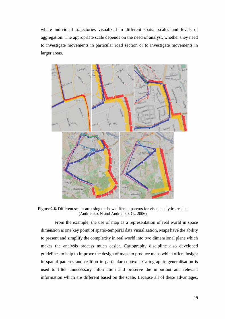
peak and PM peak according to frequency of congestion occur. As the result, the road

network in Beijing is at severe congested level between 7:45 AM and 8:45 AM, and

between 17.15 PM and 18:45 PM on weekdays. And implementation of congestion

performance measurement based on road network dynamic data could be used in traffic

congestion characters and trends monitoring in actual and detail way.

22

Figure 2.8. The congestion index by time of day on weekdays

(Beijing, June 2006 VS June 2007) (Sun, et al, 2009)

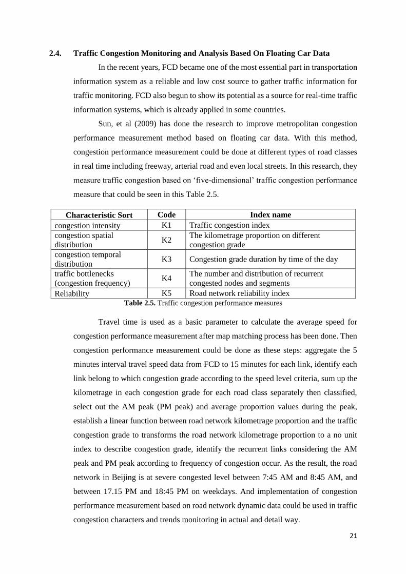
X. Liu, et al (2012) used FCD data from 6000 taxis in Changsha city to detect

urban traffic conditions of road network. This study evaluates road condition through

three levels that are respectively point, line and area, which is ‘road joint_road

section_zone’ model. For road joint, the evaluation is based on the average stop

frequency of traffic lights at intersection at a certain time period, which the bigger the

value, the longer the time to wait and the more crowded or congested the crossroad. As

for road section, driving speed is used to evaluate this index. Based on road grade and

vehicle speed, road condition is classify into five grades: very smooth, unblocked, slight

traffic congestion, moderate traffic congestion, and serious traffic congestion. As a

result, from spatial distribution of road congestion, 12.7% roads are in heavy congestion

degree which mainly concentrated in center zone (as Changsha is a single-center city).

And from temporal distribution of road congestion, 8.00 – 8.15 is the morning peak

hour with average speed of 19.3 km/h, and 17.45 – 18.00 is the evening peak hour with

average speed of 16.3 km/h.

23

Figure 2.9. Congested section and heavily congested intersection distribution at rush hour

main urban areas (X. Liu, et al, 2012)

Figure 2.10. The distribution of road network congestion index during 12 hours in the main

urban areas (X. Liu, et al, 2012)

Fabritiis, Ragona and Valenti (2008) presented an application based on FCD

which is developed and operated by OCTOTelematics to deliver real-time traffic speed

information throughout Italian motorway network. Unlike the others, this system is

using data from privately owned cars. From the case study carried on a tool-free

motorway that encircles Rome (GRA) which mostly have a heavy traffic and

24

experienced traffic jams in some part, the travel speed of vehicles which travelled across

GRA for five days has been calculated and grouped into 6 classes. By visualizing the

data, the spatio-temporal patterns of occurrence, propagation and dissipation of traffic

congestion can be easily observed.

Figure 2.11. Spatio-temporal travel speed estimates of GRA

(Fabritiis, Ragona and Valenti, 2008)

Wang, et al (2010) created a web-based real-time traffic congestion

information system based on FCD data provided by a 500 taxis fleet. Traffic

information is needed to improve traffic management system to maximize the capacity

of existing road infrastructure and transportation network. A multi-stage algorithm is

applied to calculate the average speed which is then used to define the traffic congestion

state of the road links. Web-based map visualization is used to deploy the traffic

information in real time.

Lin Xu, Yang Yue and Qingquan Li (2013) proposed a FCD analysis method

for congestion exploration based on data cube. A historical FCD dataset from about

1,200 taxis for one week is used. Traffic congestion is identified based on spatio-

temporal related relationship of slow-speed road segment, then it is aggregated by a

cluster method to derive the traffic pattern. Congestion aggregation is done to identify

recurrent congestion which appear around the same location and time but on different

25

days. Aggregated location, time period and duration for recurrent congestion are used

to represent the congestion pattern.

Figure 2.12. Spatial-temporal related record in congestion

(Lin Xu, Yang Yue and Qingquan Li, 2013)

Figure 2.13. Recurrent traffic congestion event on the road network (Lin Xu, Yang Yue and

Qingquan Li, 2013)

26

3. INITIAL TEST DATA PROPERTIES

3.1. Study Area Location and Characteristics

Shanghai has evolved into mainland China’s largest city and commercial capital

in recent years. Located in the Yangtze River Delta in East China, Shanghai sits on the

south edge of the mouth of the Yangtze in the middle portion of the Chinese coast.

Shanghai geographical coordinate is 31°12′N 121°30′E / 31.2°N 121.5°E. The

municipality borders the provinces of Jiangsu and Zhejiang to the north, south and west,

and is bounded to the east by the East China Sea. Shanghai is administratively equal to

a province and is divided into 17 county-level divisions: 16 districts and one county.

However, in this thesis we only take central part of Shanghai city as the study area,

which is located in some part of Huangpu, Hongkou and Pudong district.

Figure 3.1. Study area location

3.1.1. Physical Characteristic

Shanghai lies on China's east coast roughly equidistant from Beijing and

Guangzhou. Downtown Shanghai is bisected by the Huangpu River, a man-made

27

tributary of the Yangtze. Shanghai is located on an alluvial plain which means that the

vast majority of its 6,340.5 km2 (2,448.1 square miles) land area is flat, with an average

elevation of 4 m (13 feet). The city contains 53.1 km (33.0 miles) of rivers and streams

and is known for its rich water resources as part of the Lake Tai drainage area. Shanghai

has a humid subtropical climate and experiences four distinct seasons. Air pollution in

Shanghai is low compared to other Chinese cities such as Beijing.

3.1.2. Socio-Economic Characteristic

Shanghai is an important economic, financial, trade and shipping center in

China. Due to its excellent port, Shanghai has been a leading power of China's

economic and trade development since ancient times. The great leap of Shanghai's

economy benefited from the amazingly fast development of industry. The manufacture

of automobiles, electronic and communication equipment, petrochemicals, steel

products, equipment assemblies and biomedicine had once been promoted as the six

pillar-industries of Shanghai.

Shanghai is China's most populous city, estimated about 23.9 million. It has a

population density of 3,700 people per square kilometer. More than 39% of Shanghai's

residents are long-term migrants, a number that has tripled in ten years. Migrants are

primarily from Anhui (29%), Jiangsu (16.8%), Henan (8.7%) and Sichuan (7.0%),

while almost 80% are from rural areas. Like most of China, the vast majority (98.8%)

of Shanghai's residents are of Han Chinese ethnicity, with only 1.2% belonging to

minority groups. Shanghai also has 150,000 officially registered foreigners, including

31,500 Japanese, 21,000 Americans and 20,700 Koreans. Of course, this is based on

official figures, so the real number of foreign citizens in the city is probably much

higher.

3.1.3. Transportation System

Shanghai has an expansive grade-separated highway and expressway network

consisting of 14 city elevated and surface expressways, 9 provincial-level expressways,

and 8 national-level expressways. Expressways from Nanjing (Shanghai-Nanjing

Expressway) and Hangzhou (Shanghai-Hangzhou Expressway) terminate at Shanghai,

allowing direct access to different directions of China. In the city center, there are

numerous elevated expressways (skyways), which lessen the traffic pressure of normal

roads. However, traffic in and around Shanghai is often heavy and traffic jams are

28

commonplace during rush hour. Private car ownership in Shanghai has also been

rapidly increasing in recent years. Based on Shanghai Statistics Bureau, Shanghai had

a total vehicle population of 3.09 million units at the end of 2010 which an increase of

8.7% from a year earlier.

Shanghai also has an extensive public transport system, largely based

on buses, trolley buses, taxis, and a rapidly expanding metro system. More than 1,100

bus lines in Shanghai run to every corner of the city proper. Taxis are the most

convenient means of transportation in Shanghai. There are five main taxi companies in

Shanghai, and different companies operate taxis of different colors.

3.2. Floating Car Data Properties

Floating Car Data sets with the description of attribute information is saved in

the form of Comma-separated values (CSV). Each line in CSV is represented one

record of the dataand the attribute in each colum is separated by comma. The FCD

dataset is using latitide and longitude to record each position of the taxi so that each

point could be visualized geographically by using WGS84 coordinate system.

In this thesis, the data was derived from the taxi-FCD system. In this system,

the data of the taxis are sent to the taxi headquarter and then the data will be sent to

the FCD-server of the institute. The cycle times of the positioning are limited by the

bandwidth of the communication channel and vary between about 10 and 120 seconds,

depending on the status of the individual taxi. The collected GPS positions are sent

then with the cycle times of about 10 minutes to the server of the institute. The

overview of the general structure of FCD data set is describe in the table 3.1.

29

Fieldname Field Value Details

Date 20100617 8-digits number

Time 230717 6-digits number

Car ID 11692 The unique ID of the taxi, 5 digits

Company Code QS Initials of the taxi company

Driving Direction 6 Direction in 2 digits

Longitude 12.161.365 in degree; accurate to the 6th decimal place

Latitude 31.201.005 in degree; accurate to the 6th decimal place

Instaneous Velocity 34.9 accurate to 0.1 km/h

Instaneous Altitude 255 accurate to 1 m

Car Status 0 0 for empty; 1 otherwise

GPS Effectiveness 0 1 for effective; 0 otherwise

Record Time Stamp 17-06-2010 23:07:17 In form of YYYY-MM-DD hh:mm:ss

Table 3.1. Description of the data format of Shanghai FCD

From the table, the most important information are the longitude and latitude

position of the taxi, the vehicle ID and velocity. The position of the vehicles could be

used to calculate the flow rate or volume for each road section, and the vehicle ID is

needed to distinguish the vehicles. Velocity is important factor to determine traffic

congestion as traffic congestion is mostly occur when the velocity is low. From the

calculation of flow rate and average speed from velocity data, then density information

could also be calculated. Another important information is the time stamp of each

data, which is really necessary when the detail information about when an event such

as traffic congestion exactly occurs are needed.

30

4. VISUALIZATION METHODS

Data visualization is a method to convert data into a visual representation.

Because a picture worth a thousand words, it will be easier for users to understand a

huge amount of data from just a visual data representation such a graph, map or even a

table. The main goal of data visualization is to communicate information clearly and

effectively (Friedman, 2008). Therefore effective visualization methods are needed to

convey the information to the user which not only consider about the functionality

aspects but also aesthetic aspects. A nice data visualization could help enhance the

analysis performance which result in better decision making.

Visualization is one of the most important parts in cartography, as a map is also

one of visualized products. Cartographic visualization is mainly concerned with visual

representation of spatial data. It not only deals with data presentation but also

exploration of data. Exploration means to discover unknown information from the data

or analytical process of data. From exploration processes, not only spatial information

about the data could be obtain but also the relationships and patterns inside of the data.

In this thesis, traffic data will be visualized as a map so that trends and patterns

inside the data could be detected. Traffic data is basically movement data, which are

often regarded as points. In order that its spatial distribution in a period of time could

be represented in effective way, map is a natural choice. Andrienko N. & Andrienko G

(2007) stated that because movement data are very numerous therefore their positions

have to be presented in an aggregated way. Aggregation is needed to handle large

amount of data, in particular aggregation enables an overall view of the spatial and

temporal distribution of movement data.

4.1. Density Mapping

The most common method to display FCD data pattern is dot mapping. Each

point of data represents a taxi position with many attributes that can be chosen to show

different kinds of information such as velocity or taxi status. This method is quite simple

and accurate to represent the spatial distribution of data however the interpretation of

spatial patterns and hot spots could be very difficult due to the clutter effect especially

with the large amount of data.

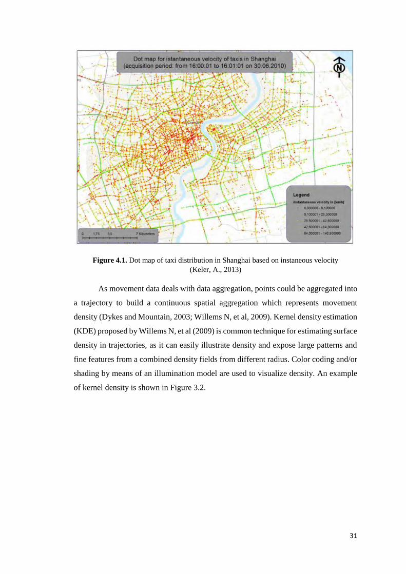
31

Figure 4.1. Dot map of taxi distribution in Shanghai based on instaneous velocity

(Keler, A., 2013)

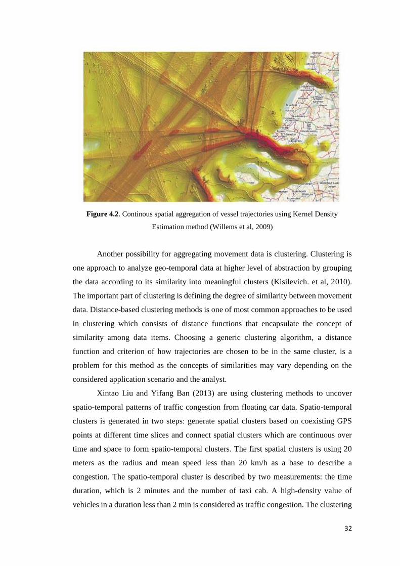
As movement data deals with data aggregation, points could be aggregated into

a trajectory to build a continuous spatial aggregation which represents movement

density (Dykes and Mountain, 2003; Willems N, et al, 2009). Kernel density estimation

(KDE) proposed by Willems N, et al (2009) is common technique for estimating surface

density in trajectories, as it can easily illustrate density and expose large patterns and

fine features from a combined density fields from different radius. Color coding and/or

shading by means of an illumination model are used to visualize density. An example

of kernel density is shown in Figure 3.2.

32

Figure 4.2. Continous spatial aggregation of vessel trajectories using Kernel Density

Estimation method (Willems et al, 2009)

Another possibility for aggregating movement data is clustering. Clustering is

one approach to analyze geo-temporal data at higher level of abstraction by grouping

the data according to its similarity into meaningful clusters (Kisilevich. et al, 2010).

The important part of clustering is defining the degree of similarity between movement

data. Distance-based clustering methods is one of most common approaches to be used

in clustering which consists of distance functions that encapsulate the concept of

similarity among data items. Choosing a generic clustering algorithm, a distance

function and criterion of how trajectories are chosen to be in the same cluster, is a

problem for this method as the concepts of similarities may vary depending on the

considered application scenario and the analyst.

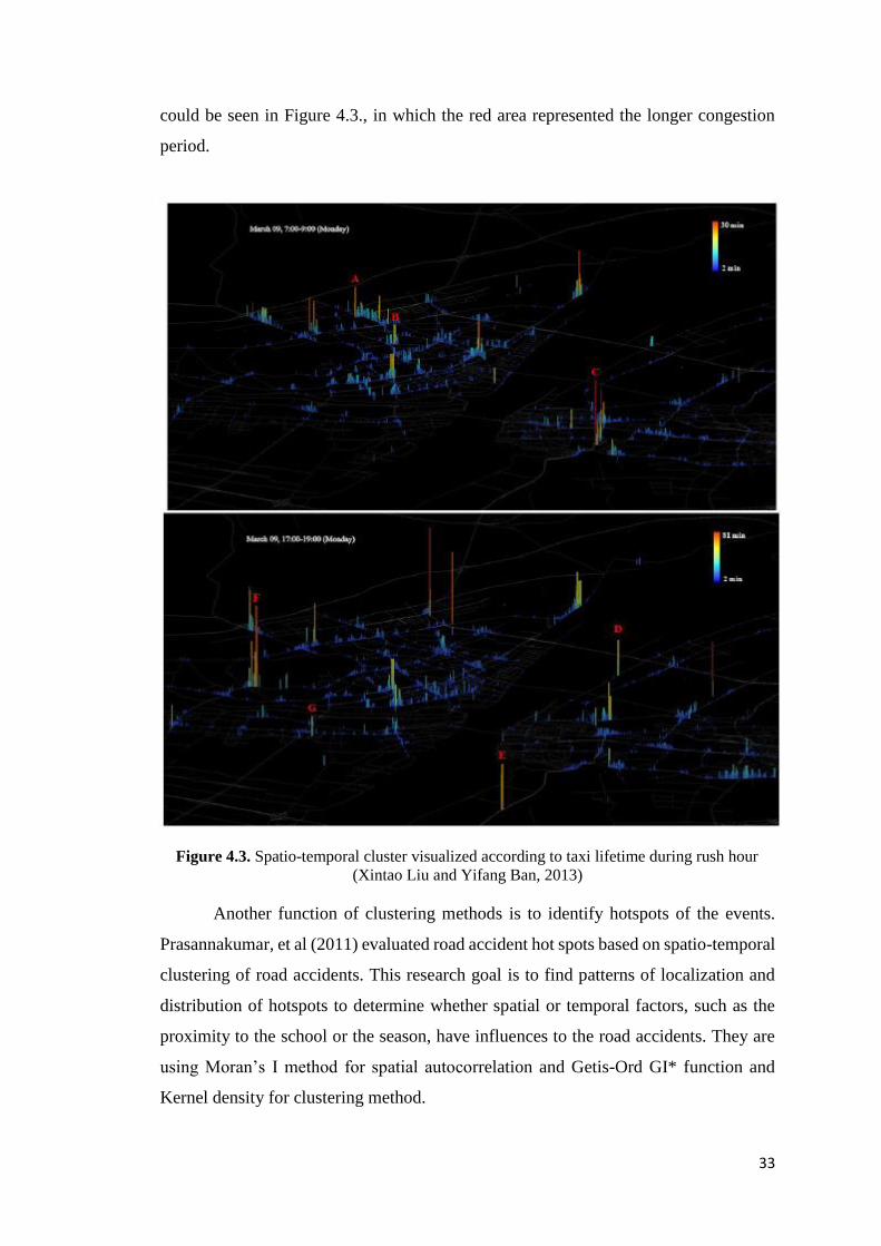
Xintao Liu and Yifang Ban (2013) are using clustering methods to uncover

spatio-temporal patterns of traffic congestion from floating car data. Spatio-temporal

clusters is generated in two steps: generate spatial clusters based on coexisting GPS

points at different time slices and connect spatial clusters which are continuous over

time and space to form spatio-temporal clusters. The first spatial clusters is using 20

meters as the radius and mean speed less than 20 km/h as a base to describe a

congestion. The spatio-temporal cluster is described by two measurements: the time

duration, which is 2 minutes and the number of taxi cab. A high-density value of

vehicles in a duration less than 2 min is considered as traffic congestion. The clustering

33

could be seen in Figure 4.3., in which the red area represented the longer congestion

period.

Figure 4.3. Spatio-temporal cluster visualized according to taxi lifetime during rush hour

(Xintao Liu and Yifang Ban, 2013)

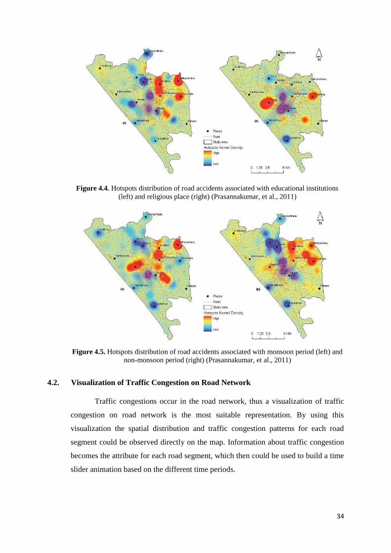
Another function of clustering methods is to identify hotspots of the events.

Prasannakumar, et al (2011) evaluated road accident hot spots based on spatio-temporal

clustering of road accidents. This research goal is to find patterns of localization and

distribution of hotspots to determine whether spatial or temporal factors, such as the

proximity to the school or the season, have influences to the road accidents. They are

using Moran’s I method for spatial autocorrelation and Getis-Ord GI* function and

Kernel density for clustering method.

34

Figure 4.4. Hotspots distribution of road accidents associated with educational institutions

(left) and religious place (right) (Prasannakumar, et al., 2011)

Figure 4.5. Hotspots distribution of road accidents associated with monsoon period (left) and

non-monsoon period (right) (Prasannakumar, et al., 2011)

4.2. Visualization of Traffic Congestion on Road Network

Traffic congestions occur in the road network, thus a visualization of traffic

congestion on road network is the most suitable representation. By using this

visualization the spatial distribution and traffic congestion patterns for each road

segment could be observed directly on the map. Information about traffic congestion

becomes the attribute for each road segment, which then could be used to build a time

slider animation based on the different time periods.

35

Traffic congestion classes could be represented by using different colors to

distinguish each class. The use of colors will help the analyzing process as colors could

easily depict different features which could be seen easily with bare eyes. The changes

for each segment could also be observed by the changes of color for different periods

of time. Patterns and trends of traffic congestion could be determined by observing the

frequent congested road segments.

Figure 4.6. Traffic congestion visualization on road segment (Keler, A., 2013)

4.3. Three-Dimensional Spatio-Temporal Data Visualization

Traffic congestion could also represented by using 3D space. 3D view provides

a better overview for certain quantitative values (Andrienko N, Andrienko G, 2007).

By using 3D data visualization, the dynamic nature of social events such as traffic could

interactively explored. In GIS, temporal data is commonly visualize by animations

which represent changes in data (Tominski, et al., 2005). Animation is a useful

technique to scan data from different period of time, and if the data from each time

period is correlated then the animations will show smooth evolution. With animation

map, users can catch the change of the object easily and have a deep impression. A

36

simple animation map could be built from series of static maps that are put in order of

temporal sequence. With the addition of a time-slider, users can navigate back and forth

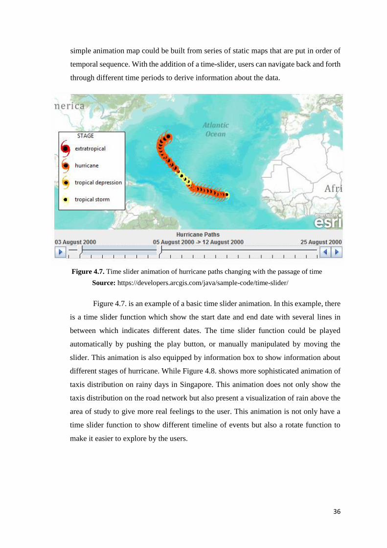
through different time periods to derive information about the data.

Figure 4.7. is an example of a basic time slider animation. In this example, there

is a time slider function which show the start date and end date with several lines in

between which indicates different dates. The time slider function could be played

automatically by pushing the play button, or manually manipulated by moving the

slider. This animation is also equipped by information box to show information about

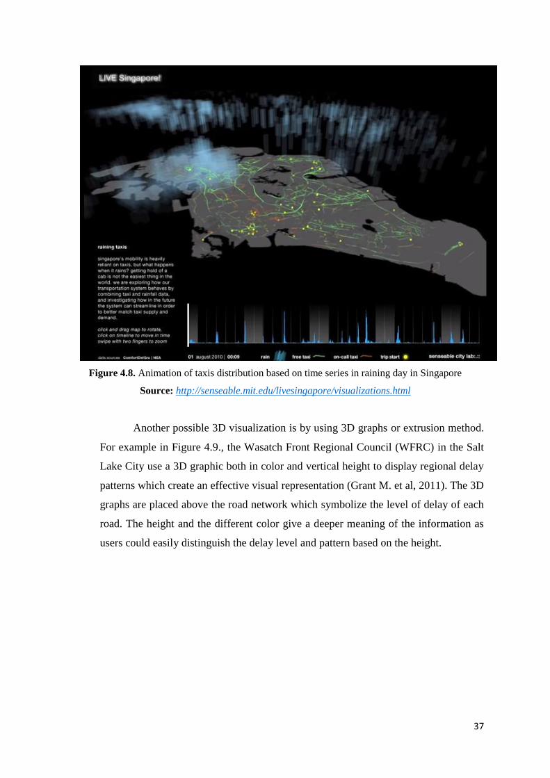
different stages of hurricane. While Figure 4.8. shows more sophisticated animation of

taxis distribution on rainy days in Singapore. This animation does not only show the

taxis distribution on the road network but also present a visualization of rain above the

area of study to give more real feelings to the user. This animation is not only have a

time slider function to show different timeline of events but also a rotate function to

make it easier to explore by the users.

Figure 4.7. Time slider animation of hurricane paths changing with the passage of time

Source: https://developers.arcgis.com/java/sample-code/time-slider/

37

Figure 4.8. Animation of taxis distribution based on time series in raining day in Singapore

Source: http://senseable.mit.edu/livesingapore/visualizations.html

Another possible 3D visualization is by using 3D graphs or extrusion method.

For example in Figure 4.9., the Wasatch Front Regional Council (WFRC) in the Salt

Lake City use a 3D graphic both in color and vertical height to display regional delay

patterns which create an effective visual representation (Grant M. et al, 2011). The 3D

graphs are placed above the road network which symbolize the level of delay of each

road. The height and the different color give a deeper meaning of the information as

users could easily distinguish the delay level and pattern based on the height.

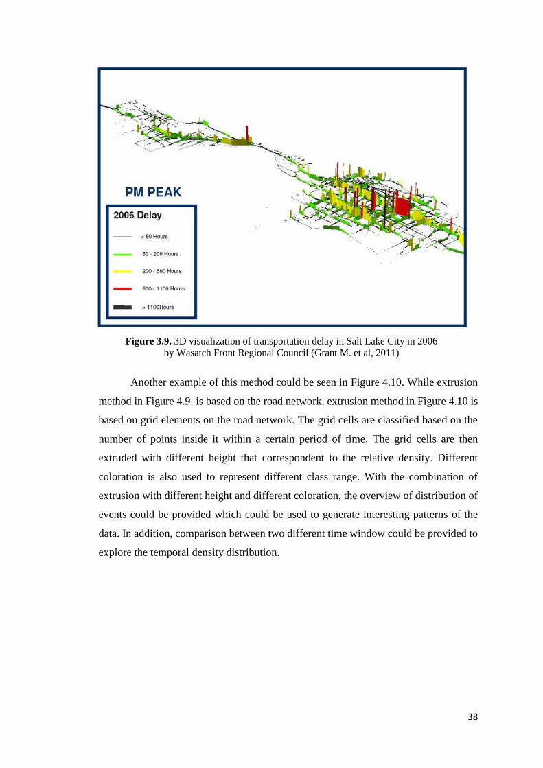
38

Figure 3.9. 3D visualization of transportation delay in Salt Lake City in 2006

by Wasatch Front Regional Council (Grant M. et al, 2011)

Another example of this method could be seen in Figure 4.10. While extrusion

method in Figure 4.9. is based on the road network, extrusion method in Figure 4.10 is

based on grid elements on the road network. The grid cells are classified based on the

number of points inside it within a certain period of time. The grid cells are then

extruded with different height that correspondent to the relative density. Different

coloration is also used to represent different class range. With the combination of

extrusion with different height and different coloration, the overview of distribution of

events could be provided which could be used to generate interesting patterns of the

data. In addition, comparison between two different time window could be provided to

explore the temporal density distribution.

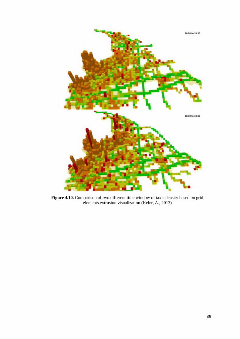
39

Figure 4.10. Comparison of two different time window of taxis density based on grid

elements extrusion visualization (Keler, A., 2013)

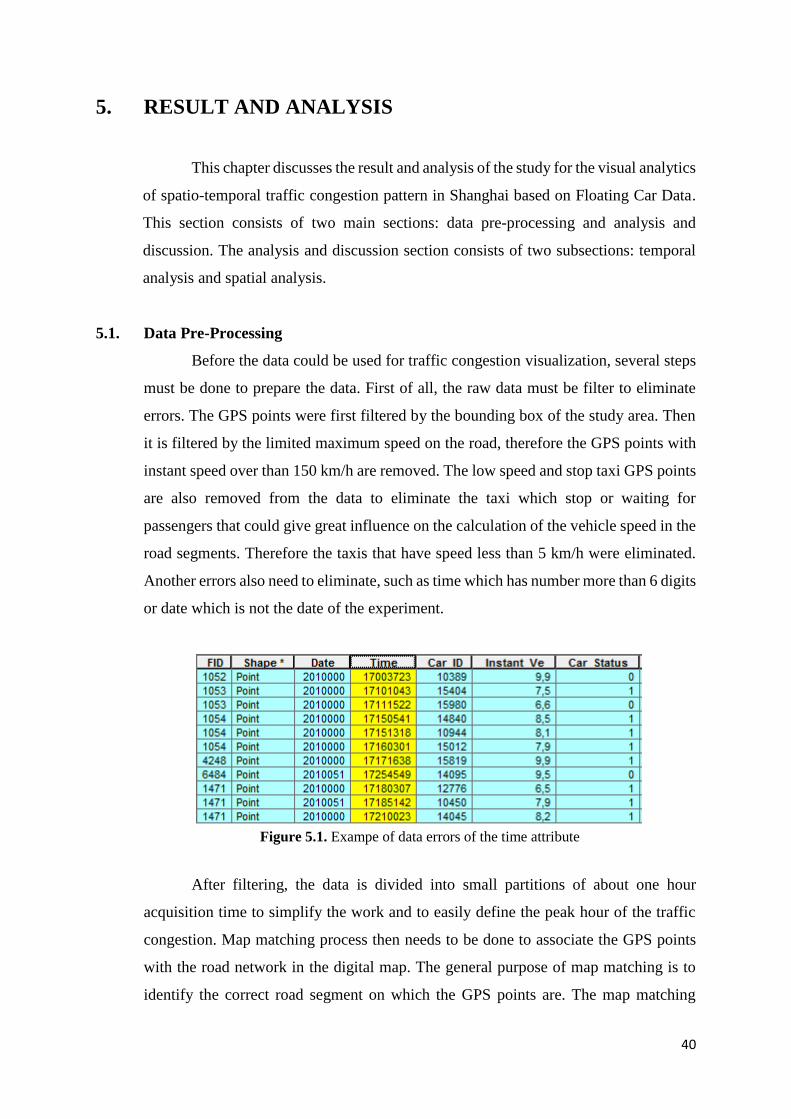
40

5. RESULT AND ANALYSIS

This chapter discusses the result and analysis of the study for the visual analytics

of spatio-temporal traffic congestion pattern in Shanghai based on Floating Car Data.

This section consists of two main sections: data pre-processing and analysis and

discussion. The analysis and discussion section consists of two subsections: temporal

analysis and spatial analysis.

5.1. Data Pre-Processing

Before the data could be used for traffic congestion visualization, several steps

must be done to prepare the data. First of all, the raw data must be filter to eliminate

errors. The GPS points were first filtered by the bounding box of the study area. Then

it is filtered by the limited maximum speed on the road, therefore the GPS points with

instant speed over than 150 km/h are removed. The low speed and stop taxi GPS points

are also removed from the data to eliminate the taxi which stop or waiting for

passengers that could give great influence on the calculation of the vehicle speed in the

road segments. Therefore the taxis that have speed less than 5 km/h were eliminated.

Another errors also need to eliminate, such as time which has number more than 6 digits

or date which is not the date of the experiment.

Figure 5.1. Exampe of data errors of the time attribute

After filtering, the data is divided into small partitions of about one hour

acquisition time to simplify the work and to easily define the peak hour of the traffic

congestion. Map matching process then needs to be done to associate the GPS points

with the road network in the digital map. The general purpose of map matching is to

identify the correct road segment on which the GPS points are. The map matching

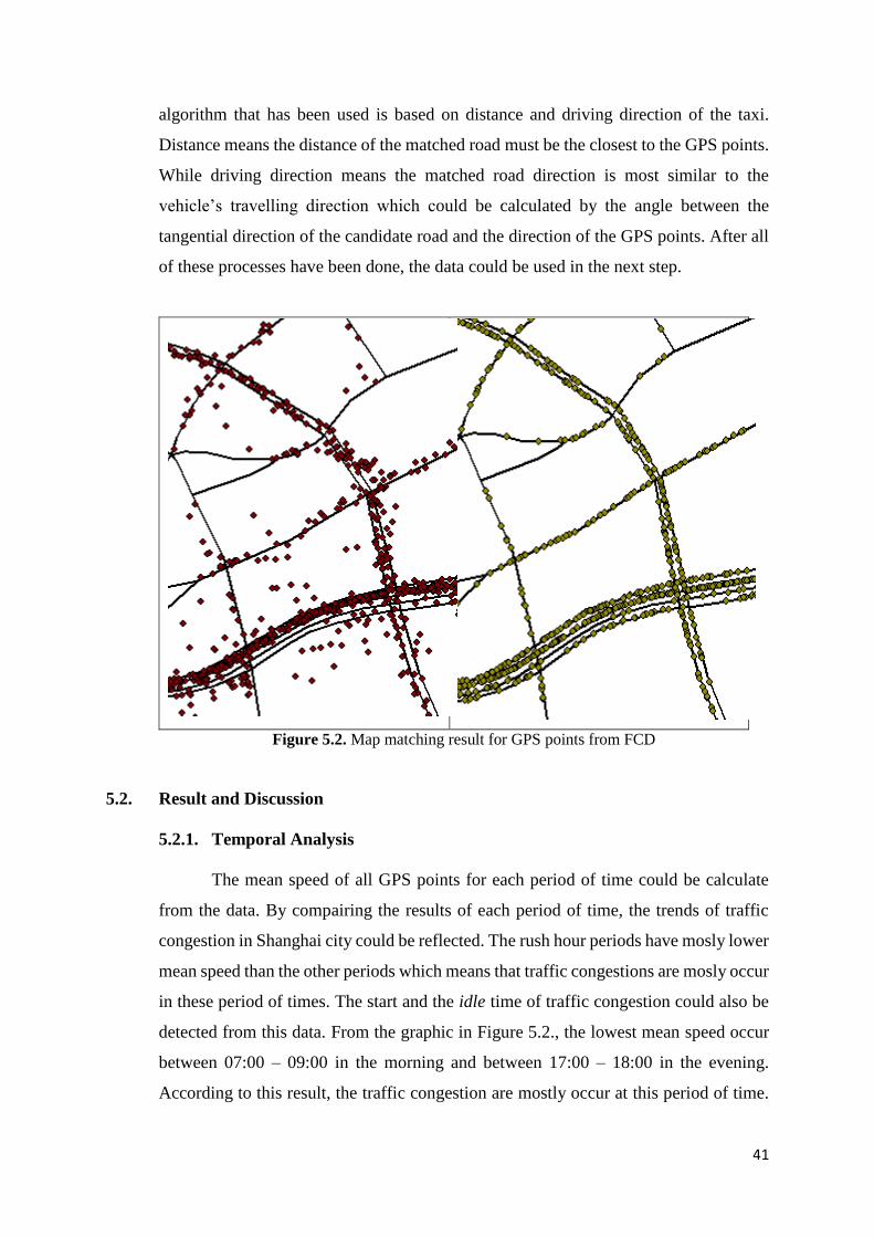
41

algorithm that has been used is based on distance and driving direction of the taxi.

Distance means the distance of the matched road must be the closest to the GPS points.

While driving direction means the matched road direction is most similar to the

vehicle’s travelling direction which could be calculated by the angle between the

tangential direction of the candidate road and the direction of the GPS points. After all

of these processes have been done, the data could be used in the next step.

Figure 5.2. Map matching result for GPS points from FCD

5.2. Result and Discussion

5.2.1. Temporal Analysis

The mean speed of all GPS points for each period of time could be calculate

from the data. By compairing the results of each period of time, the trends of traffic

congestion in Shanghai city could be reflected. The rush hour periods have mosly lower

mean speed than the other periods which means that traffic congestions are mosly occur

in these period of times. The start and the idle time of traffic congestion could also be

detected from this data. From the graphic in Figure 5.2., the lowest mean speed occur

between 07:00 – 09:00 in the morning and between 17:00 – 18:00 in the evening.

According to this result, the traffic congestion are mostly occur at this period of time.

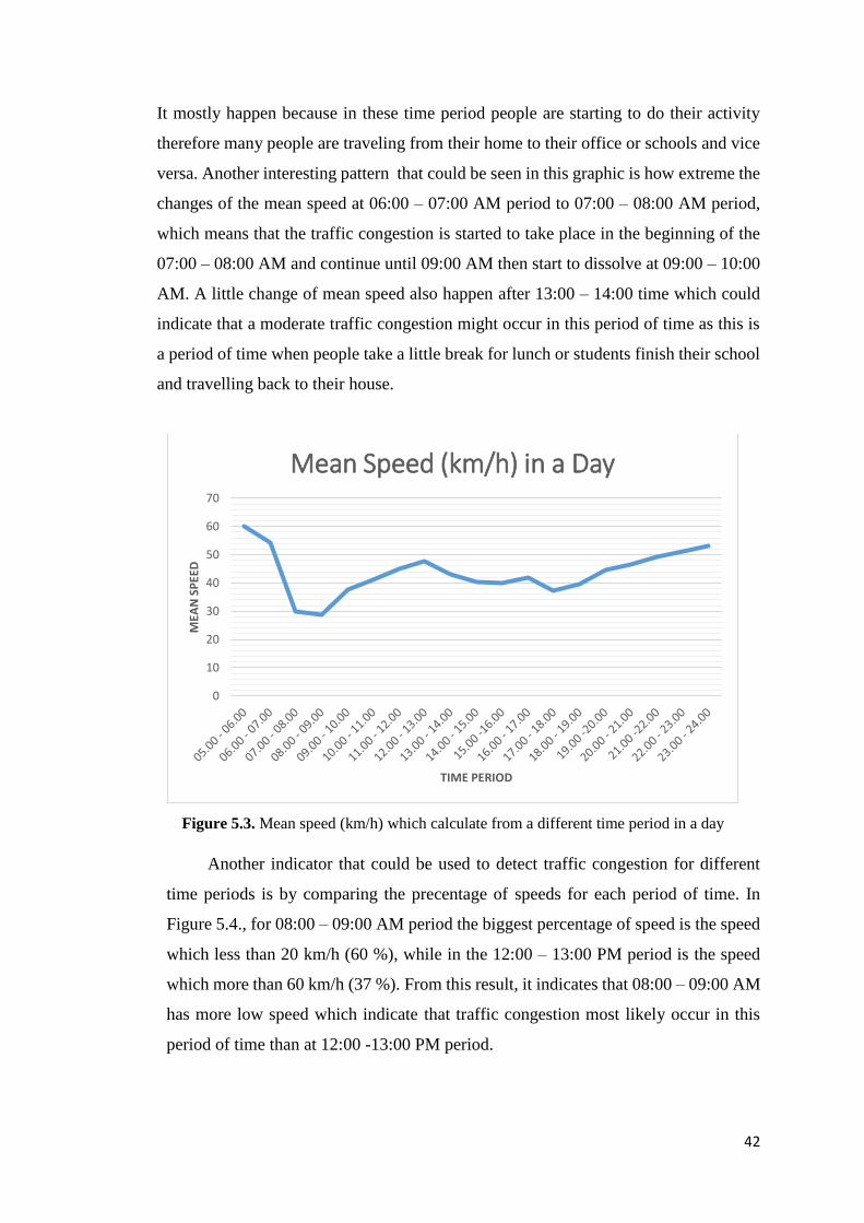
42

It mostly happen because in these time period people are starting to do their activity

therefore many people are traveling from their home to their office or schools and vice

versa. Another interesting pattern that could be seen in this graphic is how extreme the

changes of the mean speed at 06:00 – 07:00 AM period to 07:00 – 08:00 AM period,

which means that the traffic congestion is started to take place in the beginning of the

07:00 – 08:00 AM and continue until 09:00 AM then start to dissolve at 09:00 – 10:00

AM. A little change of mean speed also happen after 13:00 – 14:00 time which could

indicate that a moderate traffic congestion might occur in this period of time as this is

a period of time when people take a little break for lunch or students finish their school

and travelling back to their house.

Figure 5.3. Mean speed (km/h) which calculate from a different time period in a day

Another indicator that could be used to detect traffic congestion for different

time periods is by comparing the precentage of speeds for each period of time. In

Figure 5.4., for 08:00 – 09:00 AM period the biggest percentage of speed is the speed

which less than 20 km/h (60 %), while in the 12:00 – 13:00 PM period is the speed

which more than 60 km/h (37 %). From this result, it indicates that 08:00 – 09:00 AM

has more low speed which indicate that traffic congestion most likely occur in this

period of time than at 12:00 -13:00 PM period.

0

10

20

30

40

50

60

70

MEA

N S

PEE

D

TIME PERIOD

Mean Speed (km/h) in a Day

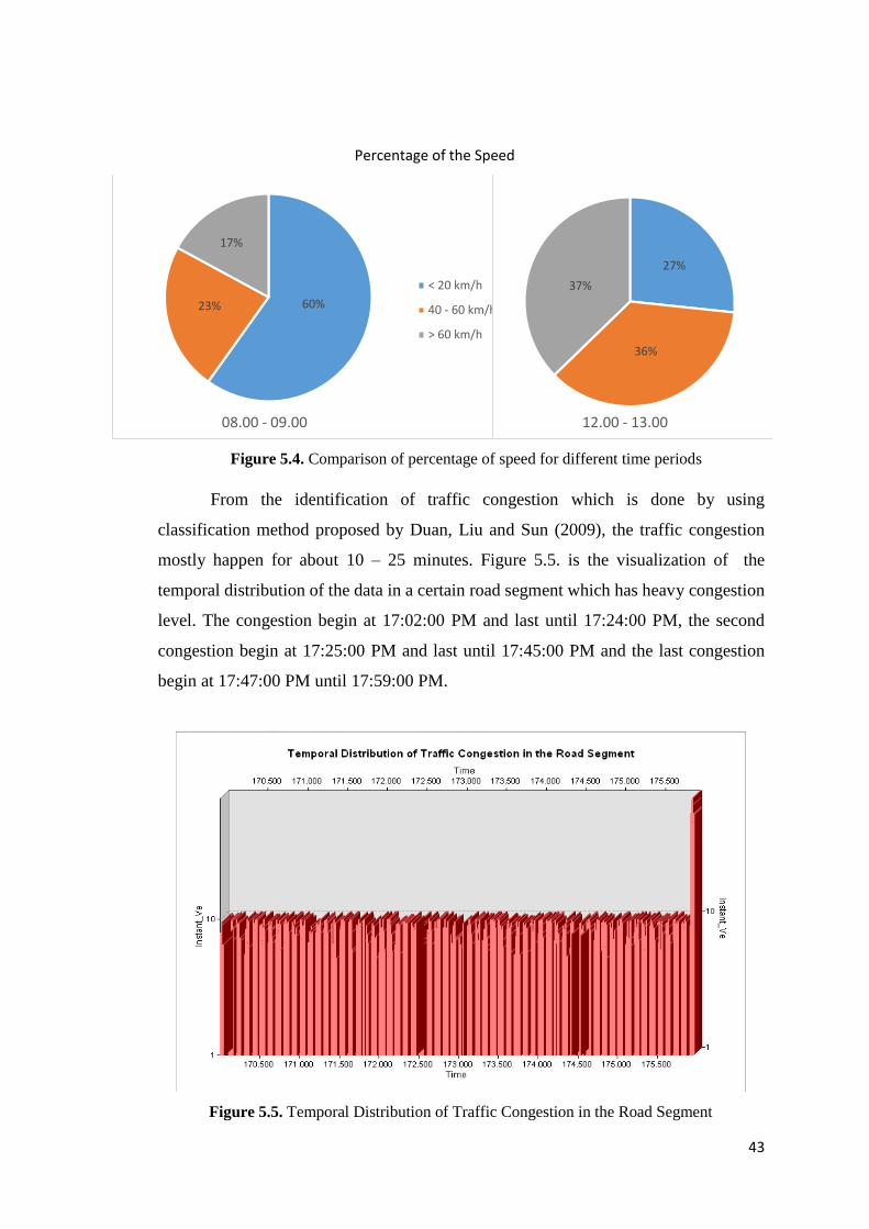
43

Percentage of the Speed

Figure 5.4. Comparison of percentage of speed for different time periods

From the identification of traffic congestion which is done by using

classification method proposed by Duan, Liu and Sun (2009), the traffic congestion

mostly happen for about 10 – 25 minutes. Figure 5.5. is the visualization of the

temporal distribution of the data in a certain road segment which has heavy congestion

level. The congestion begin at 17:02:00 PM and last until 17:24:00 PM, the second

congestion begin at 17:25:00 PM and last until 17:45:00 PM and the last congestion

begin at 17:47:00 PM until 17:59:00 PM.

Figure 5.5. Temporal Distribution of Traffic Congestion in the Road Segment

60%23%

17%

08.00 - 09.00

< 20 km/h

40 - 60 km/h

> 60 km/h

27%

36%

37%

12.00 - 13.00

44

5.2.2. Spatial Analysis

The spatial distribution of the road congestion could be identified directly on

the map. Based on the distribution, the most congested road segment could be

identified. In this cpahter, the congested segment will be identified using various type

of visualization.

5.2.2.1. Density Mapping

Point density map describes the closeness of GPS points which situated in the

same area. Therefore only points that fall within the neighborhood area considered in

this method. This visualization is choosen to smooth out the information represented

by a collection of points. In this visualization, kernel density method is used to produce

a smooth visualization of the point density. With this visualization and then combined

with the road network visualization, the spatial distribution of taxi density in a certain

period of time could be seen. This density map could be seen in Figure 5.6.

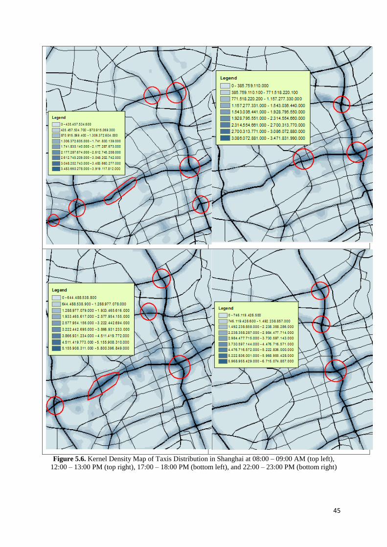
45

Figure 5.6. Kernel Density Map of Taxis Distribution in Shanghai at 08:00 – 09:00 AM (top left),

12:00 – 13:00 PM (top right), 17:00 – 18:00 PM (bottom left), and 22:00 – 23:00 PM (bottom right)

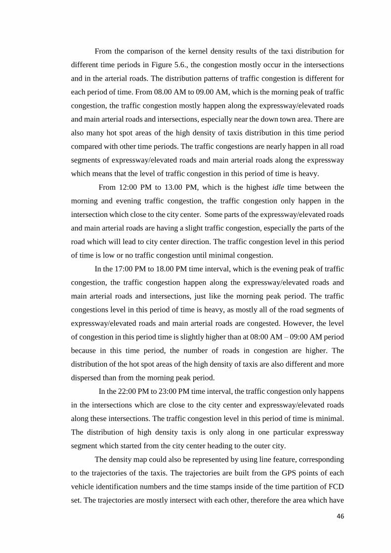
46

From the comparison of the kernel density results of the taxi distribution for

different time periods in Figure 5.6., the congestion mostly occur in the intersections

and in the arterial roads. The distribution patterns of traffic congestion is different for

each period of time. From 08.00 AM to 09.00 AM, which is the morning peak of traffic

congestion, the traffic congestion mostly happen along the expressway/elevated roads

and main arterial roads and intersections, especially near the down town area. There are

also many hot spot areas of the high density of taxis distribution in this time period

compared with other time periods. The traffic congestions are nearly happen in all road

segments of expressway/elevated roads and main arterial roads along the expressway

which means that the level of traffic congestion in this period of time is heavy.

From 12:00 PM to 13.00 PM, which is the highest idle time between the

morning and evening traffic congestion, the traffic congestion only happen in the

intersection which close to the city center. Some parts of the expressway/elevated roads

and main arterial roads are having a slight traffic congestion, especially the parts of the

road which will lead to city center direction. The traffic congestion level in this period

of time is low or no traffic congestion until minimal congestion.

In the 17:00 PM to 18.00 PM time interval, which is the evening peak of traffic

congestion, the traffic congestion happen along the expressway/elevated roads and

main arterial roads and intersections, just like the morning peak period. The traffic

congestions level in this period of time is heavy, as mostly all of the road segments of

expressway/elevated roads and main arterial roads are congested. However, the level

of congestion in this period time is slightly higher than at 08:00 AM – 09:00 AM period

because in this time period, the number of roads in congestion are higher. The

distribution of the hot spot areas of the high density of taxis are also different and more

dispersed than from the morning peak period.

In the 22:00 PM to 23:00 PM time interval, the traffic congestion only happens

in the intersections which are close to the city center and expressway/elevated roads

along these intersections. The traffic congestion level in this period of time is minimal.

The distribution of high density taxis is only along in one particular expressway

segment which started from the city center heading to the outer city.

The density map could also be represented by using line feature, corresponding

to the trajectories of the taxis. The trajectories are built from the GPS points of each

vehicle identification numbers and the time stamps inside of the time partition of FCD

set. The trajectories are mostly intersect with each other, therefore the area which have

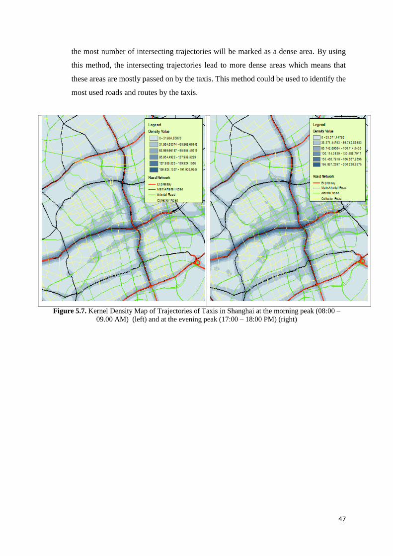
47

the most number of intersecting trajectories will be marked as a dense area. By using

this method, the intersecting trajectories lead to more dense areas which means that

these areas are mostly passed on by the taxis. This method could be used to identify the

most used roads and routes by the taxis.

Figure 5.7. Kernel Density Map of Trajectories of Taxis in Shanghai at the morning peak (08:00 –

09.00 AM) (left) and at the evening peak (17:00 – 18:00 PM) (right)

48

Figure 5.8. Kernel Density Map of Trajectories of Taxis in Shanghai at 12:00 – 13:00 PM

From Figure 5.7., the expressway/elevated roads and main arterial roads have

the highest density comparing with the other road types. This means that these roads

have the highest frequency to be used for travelling by taxi users. Therefore these types

of roads have the greatest possibility to be congested. In the morning peak period, the

frequently used roads are the expreesway/elevated roads and the main arterial roads

alongside the expressway. Some main arterial roads and arterial roads which are located

closed to the expressway/elevated roads and city center are also used frequently in this

time period.

The evening peak period has the slightly different patterns from the morning

peak period. The number of the frequent roads is higher than the morning peak, thus

the distribution of the frequent roads is more dispersed. This might be because people

tend to not use the expressway/elevated road to avoid the traffic congestion or people

are having gathering or dinner in the area near city center before they are going home

so that the traffic flow are not really concentrated in the expressway/elevated roads and

the main arterial roads alongside it.

In the Figure 5.8, the highest peak of idle time between morning peak and

evening peak (12:00 – 13:00 PM), the pattern of the frequently used roads is almost the

same with the morning peak period. But the intensity of the frequent roads is different

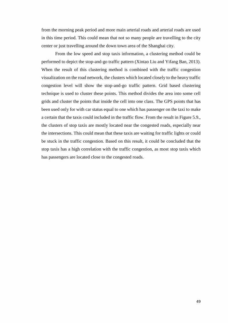
49

from the morning peak period and more main arterial roads and arterial roads are used

in this time period. This could mean that not so many people are travelling to the city

center or just travelling around the down town area of the Shanghai city.

From the low speed and stop taxis information, a clustering method could be

performed to depict the stop-and-go traffic pattern (Xintao Liu and Yifang Ban, 2013).

When the result of this clustering method is combined with the traffic congestion

visualization on the road network, the clusters which located closely to the heavy traffic

congestion level will show the stop-and-go traffic pattern. Grid based clustering

technique is used to cluster these points. This method divides the area into some cell

grids and cluster the points that inside the cell into one class. The GPS points that has

been used only for with car status equal to one which has passenger on the taxi to make

a certain that the taxis could included in the traffic flow. From the result in Figure 5.9.,

the clusters of stop taxis are mostly located near the congested roads, especially near

the intersections. This could mean that these taxis are waiting for traffic lights or could

be stuck in the traffic congestion. Based on this result, it could be concluded that the

stop taxis has a high correlation with the traffic congestion, as most stop taxis which

has passengers are located close to the congested roads.

50

Figure 5.9. Stop Taxis Clustering at 07:00 – 08:00 AM time period

5.2.2.2. Visualization on Road Network

Visualization of traffic congestion in road network will give an actual

representation of traffic condition in real world as traffic congestion happened in the

road network. The spatial distribution of road congestion could also be easily depicted

by using different color for each level of congestion on the road network. With this

visulization, indetifying which road segments are congested would be easier.

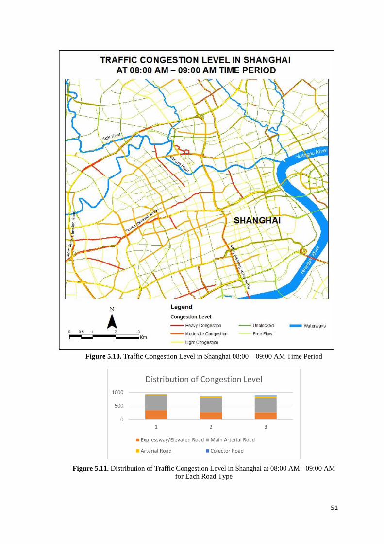
51

Figure 5.10. Traffic Congestion Level in Shanghai 08:00 – 09:00 AM Time Period

Figure 5.11. Distribution of Traffic Congestion Level in Shanghai at 08:00 AM - 09:00 AM

for Each Road Type

0

500

1000

1 2 3

Distribution of Congestion Level

Expressway/Elevated Road Main Arterial Road

Arterial Road Colector Road

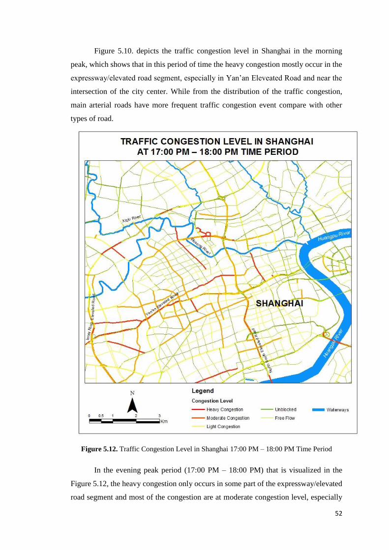
52

Figure 5.10. depicts the traffic congestion level in Shanghai in the morning

peak, which shows that in this period of time the heavy congestion mostly occur in the

expressway/elevated road segment, especially in Yan’an Eleveated Road and near the

intersection of the city center. While from the distribution of the traffic congestion,

main arterial roads have more frequent traffic congestion event compare with other

types of road.

Figure 5.12. Traffic Congestion Level in Shanghai 17:00 PM – 18:00 PM Time Period

In the evening peak period (17:00 PM – 18:00 PM) that is visualized in the

Figure 5.12, the heavy congestion only occurs in some part of the expressway/elevated

road segment and most of the congestion are at moderate congestion level, especially

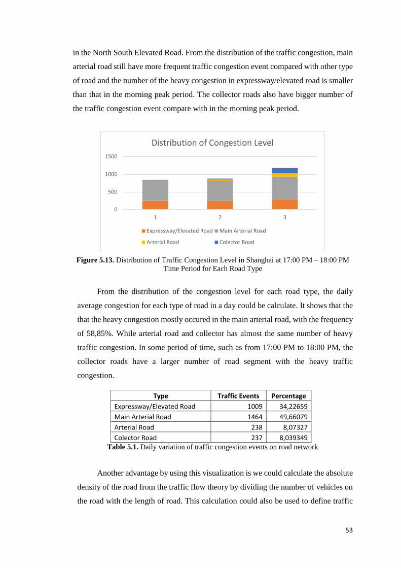
53

in the North South Elevated Road. From the distribution of the traffic congestion, main

arterial road still have more frequent traffic congestion event compared with other type

of road and the number of the heavy congestion in expressway/elevated road is smaller

than that in the morning peak period. The collector roads also have bigger number of

the traffic congestion event compare with in the morning peak period.

Figure 5.13. Distribution of Traffic Congestion Level in Shanghai at 17:00 PM – 18:00 PM

Time Period for Each Road Type

From the distribution of the congestion level for each road type, the daily

average congestion for each type of road in a day could be calculate. It shows that the

that the heavy congestion mostly occured in the main arterial road, with the frequency

of 58,85%. While arterial road and collector has almost the same number of heavy

traffic congestion. In some period of time, such as from 17:00 PM to 18:00 PM, the

collector roads have a larger number of road segment with the heavy traffic

congestion.

Type Traffic Events Percentage

Expressway/Elevated Road 1009 34,22659

Main Arterial Road 1464 49,66079

Arterial Road 238 8,07327

Colector Road 237 8,039349 Table 5.1. Daily variation of traffic congestion events on road network

Another advantage by using this visualization is we could calculate the absolute

density of the road from the traffic flow theory by dividing the number of vehicles on

the road with the length of road. This calculation could also be used to define traffic

0

500

1000

1500

1 2 3

Distribution of Congestion Level

Expressway/Elevated Road Main Arterial Road

Arterial Road Colector Road

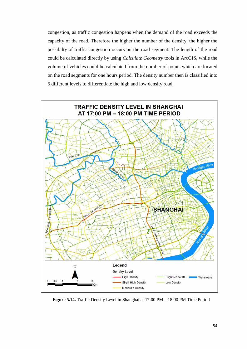
54

congestion, as traffic congestion happens when the demand of the road exceeds the

capacity of the road. Therefore the higher the number of the density, the higher the

possibilty of traffic congestion occurs on the road segment. The length of the road

could be calculated directly by using Calculate Geometry tools in ArcGIS, while the

volume of vehicles could be calculated from the number of points which are located

on the road segments for one hours period. The density number then is classified into

5 different levels to differentiate the high and low density road.

Figure 5.14. Traffic Density Level in Shanghai at 17:00 PM – 18:00 PM Time Period

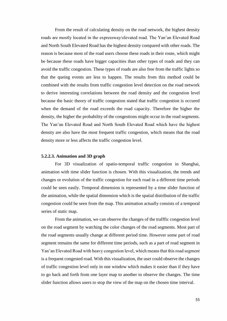
55

From the result of calculating density on the road network, the highest density

roads are mostly located in the expressway/elevated road. The Yan’an Elevated Road

and North South Elevated Road has the highest density compared with other roads. The

reason is because most of the road users choose these roads in their route, which might

be because these roads have bigger capacities than other types of roads and they can

avoid the traffic congestion. These types of roads are also free from the traffic lights so

that the queing events are less to happen. The results from this method could be

combined with the results from traffic congestion level detection on the road network

to derive interesting correlations between the road density and the congestion level

because the basic theory of traffic congestion stated that traffic congestion is occured

when the demand of the road exceeds the road capacity. Therefore the higher the

density, the higher the probability of the congestions might occur in the road segments.

The Yan’an Elevated Road and North South Elevated Road which have the highest

density are also have the most frequent traffic congestion, which means that the road

density more or less affects the traffic congestion level.

5.2.2.3. Animation and 3D graph

For 3D visualization of spatio-temporal traffic congestion in Shanghai,

animation with time slider function is chosen. With this visualization, the trends and

changes or evolution of the traffic congestion for each road in a different time periods

could be seen easily. Temporal dimension is represented by a time slider function of

the animation, while the spatial dimension which is the spatial distribution of the traffic

congestion could be seen from the map. This animation actually consists of a temporal

series of static map.

From the animation, we can observe the changes of the trafffic congestion level

on the road segment by watching the color changes of the road segments. Most part of

the road segments usually change at different period time. However some part of road

segment remains the same for different time periods, such as a part of road segment in

Yan’an Elevated Road with heavy congestion level, which means that this road segment

is a frequent congested road. With this visualization, the user could observe the changes

of traffic congestion level only in one window which makes it easier than if they have

to go back and forth from one layer map to another to observe the changes. The time

slider function allows users to stop the view of the map on the chosen time interval.

56

Figure 5.15. Time Slider Animation of Traffic Congestion Level in Shanghai at 06:00 AM to

23:00 PM in different time interval

Another method is by using 3D graph or extrusion of the attribute value on the

surface of the road network to depict the level of congestion by using height and color.

By using this visualization, the differences between each level of traffic congestion will

be shown clearly by the height of the extrusion. The color also emphasize the

differences between each level, especially if the road segment is located close to each

others. In the Figure 5.15, the heavy congestion level is depicted by using the heighest

extrusion and the red color. From the result we could see that most of the heavy

congestion roads are on the expressway/elevated roads, especially in Yan’an Elevated

Road.

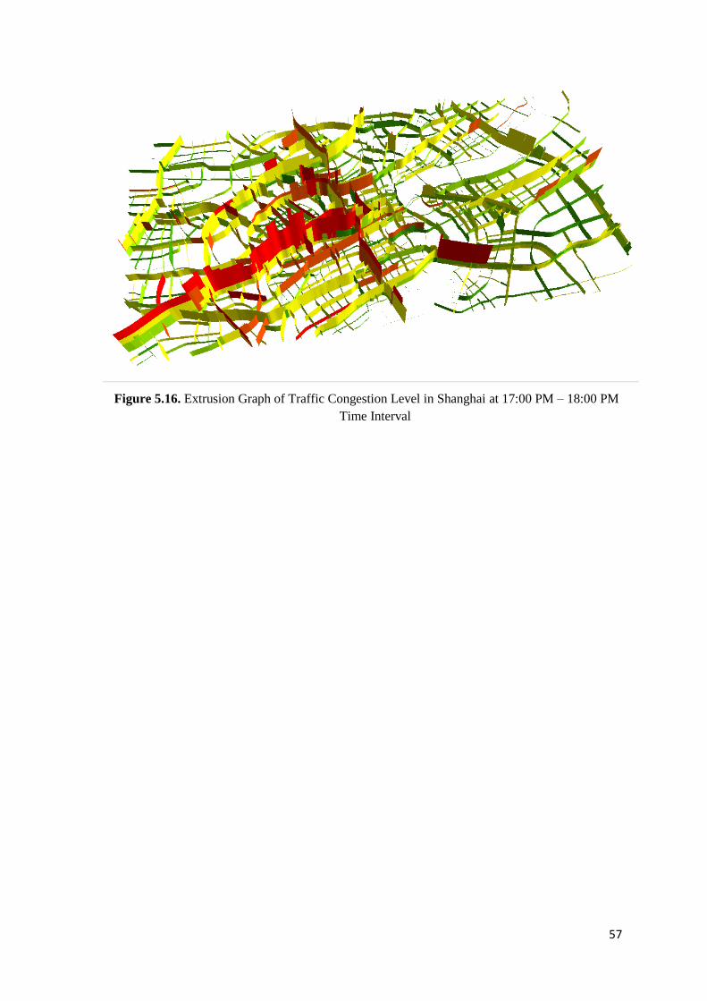
57

Figure 5.16. Extrusion Graph of Traffic Congestion Level in Shanghai at 17:00 PM – 18:00 PM

Time Interval

58

6. CONCLUSION AND OUTLOOK

In this thesis, a one-day test dataset of FCD from taxi trajectory in Shanghai city

is used to extract information about traffic congestion level in the city. The extracted

information could be visualized and analyzed to provide deeper knowledges about the

spatial and temporal patterns of the traffic congestion. The visualization technique that

have been used are density mapping of the point data and trajectories, visualization of

traffic congestion level based on the road surface network, animation using time slider

and three dimensional visualization based on the extrusion of the attributes.

From the result by using visual analytics methods for spatio-temporal data, it

can be concluded that FCD is a very useful data source to derive information about

spatio-temporal patterns of traffic congestion in the city area. From the calculation, the

traffic congestion in Shanghai city have two peak time periods, which are from 07:00

AM to 09:00 AM in the morning and from 17:00 PM to 18:00 PM in the evening, while

the highest idle time between these two peak is from 12:00 PM to 13:00 PM in the

afternoon. The congestion on the road network mostly last about 15 – 25 minutes. In

spatial dimention, the congesstion mostly occured in the expressway/elevated roads and

the main roads. The frequent congestions road segment are located in Yan’an Elevated

Road, North South Elevated Road and the intersections which are located near the city

center. In conclusion, the result of this study could answer all the research goals of this

study which means that FCD set is useful as a data source to calculate the traffic

congestion level on the road network and visual analytics method could be applied to

extract more information such as spatio-temporal pattern from the traffic congestion

information.

FCD sets could also be used to calclulate the road density based on the traffic

flow theory by dividing the number of the points on the each road segment which

represented the number of vehicles within the length of the road. The results from this

method could be combined with the results from traffic congestion level detection on

the road network to derive interesting correlations between the road density. The

Yan’an Elevated Road and North South Elevated Road which have the highest density

are also have the most frequent traffic congestion, which means that the road density

have a possitive correlations with the traffic congestion level.

59

From the pre-processing and processing steps, map-matching and clustering

techniques should be chosen wisely so that the results could really represented the actual

condition of the traffic congestion. A suitable time ranges and classfication ranges

should be chosen according to the data set to give a better representation of the traffic

congestion as the result will be different with the different time ranges and different

classification.

For the further study about visual analytics of spatio-temporal data derived from

FCD set, a larger dataset which contain more than a day data could be used to detect a

different pattern of traffic congestion. More sophisticated data mining and

visualizations methods could be used to explore in depth about the result from the

processing of FCD set. The result could then be compared with result from different

methods to give an insight which method could extract a better and actual information

about traffic congestion.

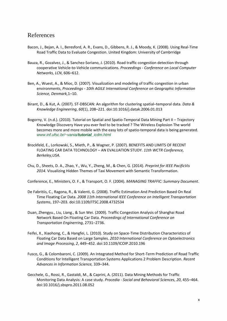
x

References

Bacon, J., Bejan, A. I., Beresford, A. R., Evans, D., Gibbens, R. J., & Moody, K. (2008). Using Real-Time Road Traffic Data to Evaluate Congestion. United Kingdom: University of Cambrridge

Bauza, R., Gozalvez, J., & Sanchez-Soriano, J. (2010). Road traffic congestion detection through cooperative Vehicle-to-Vehicle communications. Proceedings - Conference on Local Computer Networks, LCN, 606–612.

Ben, A., Wuest, A., & Mioc, D. (2007). Visualization and modeling of traffic congestion in urban environments, Proceedings - 10th AGILE International Conference on Geographic Information Science, Denmark,1–10.

Birant, D., & Kut, A. (2007). ST-DBSCAN: An algorithm for clustering spatial–temporal data. Data & Knowledge Engineering, 60(1), 208–221. doi:10.1016/j.datak.2006.01.013

Bogorny, V. (n.d.). (2010). Tutorial on Spatial and Spatio-Temporal Data Mining Part II – Trajectory Knowledge Discovery Have you ever feel to be tracked ? The Wireless Explosion The world becomes more and more mobile with the easy lots of spatio-temporal data is being generated. www.inf.ufsc.br/~vania/tutorial_icdm.html

Brockfeld, E., Lorkowski, S., Mieth, P., & Wagner, P. (2007). BENEFITS AND LIMITS OF RECENT FLOATING CAR DATA TECHNOLOGY – AN EVALUATION STUDY. 11th WCTR Conference, Berkeley,USA.

Chu, D., Sheets, D. A., Zhao, Y., Wu, Y., Zheng, M., & Chen, G. (2014). Preprint for IEEE PacificVis 2014. Visualizing Hidden Themes of Taxi Movement with Semantic Transformation.

Conference, E., Ministers, O. F., & Transport, O. F. (2004). MANAGING TRAFFIC: Summary Document.

De Fabritiis, C., Ragona, R., & Valenti, G. (2008). Traffic Estimation And Prediction Based On Real Time Floating Car Data. 2008 11th International IEEE Conference on Intelligent Transportation Systems, 197–203. doi:10.1109/ITSC.2008.4732534

Duan, Zhengyu., Liu, Liang., & Sun Wei. (2009). Traffic Congestion Analysis of Shanghai Road Network Based On Floating Car Data. Proceedings of International Conference on Transportation Enginerring, 2731–2736.

Feifei, X., Xiaohong, C., & Hangfei, L. (2010). Study on Space-Time Distribution Characteristics of Floating Car Data Based on Large Samples. 2010 International Conference on Optoelectronics and Image Processing, 2, 449–452. doi:10.1109/ICOIP.2010.196

Fusco, G., & Colombaroni, C. (2009). An Integrated Method for Short-Term Prediction of Road Traffic Conditions for Intelligent Transportation Systems Applications 2 Problem Description. Recent Advances in Information Science, 339–344.

Gecchele, G., Rossi, R., Gastaldi, M., & Caprini, A. (2011). Data Mining Methods for Traffic Monitoring Data Analysis: A case study. Procedia - Social and Behavioral Sciences, 20, 455–464. doi:10.1016/j.sbspro.2011.08.052

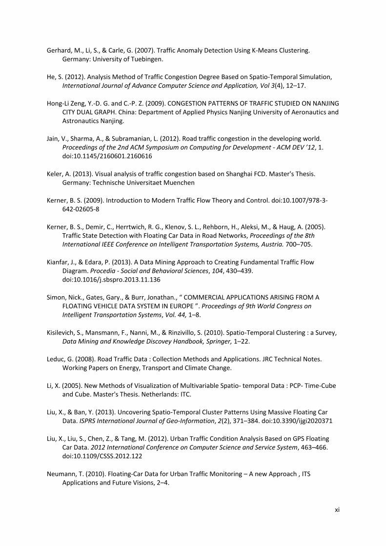
xi

Gerhard, M., Li, S., & Carle, G. (2007). Traffic Anomaly Detection Using K-Means Clustering. Germany: University of Tuebingen.

He, S. (2012). Analysis Method of Traffic Congestion Degree Based on Spatio-Temporal Simulation, International Journal of Advance Computer Science and Application, Vol 3(4), 12–17.

Hong-Li Zeng, Y.-D. G. and C.-P. Z. (2009). CONGESTION PATTERNS OF TRAFFIC STUDIED ON NANJING CITY DUAL GRAPH. China: Department of Applied Physics Nanjing University of Aeronautics and Astronautics Nanjing.

Jain, V., Sharma, A., & Subramanian, L. (2012). Road traffic congestion in the developing world. Proceedings of the 2nd ACM Symposium on Computing for Development - ACM DEV ’12, 1. doi:10.1145/2160601.2160616

Keler, A. (2013). Visual analysis of traffic congestion based on Shanghai FCD. Master's Thesis. Germany: Technische Universitaet Muenchen

Kerner, B. S. (2009). Introduction to Modern Traffic Flow Theory and Control. doi:10.1007/978-3-642-02605-8

Kerner, B. S., Demir, C., Herrtwich, R. G., Klenov, S. L., Rehborn, H., Aleksi, M., & Haug, A. (2005). Traffic State Detection with Floating Car Data in Road Networks, Proceedings of the 8th International IEEE Conference on Intelligent Transportation Systems, Austria. 700–705.

Kianfar, J., & Edara, P. (2013). A Data Mining Approach to Creating Fundamental Traffic Flow Diagram. Procedia - Social and Behavioral Sciences, 104, 430–439. doi:10.1016/j.sbspro.2013.11.136

Simon, Nick., Gates, Gary., & Burr, Jonathan., “ COMMERCIAL APPLICATIONS ARISING FROM A FLOATING VEHICLE DATA SYSTEM IN EUROPE ”. Proceedings of 9th World Congress on Intelligent Transportation Systems, Vol. 44, 1–8.

Kisilevich, S., Mansmann, F., Nanni, M., & Rinzivillo, S. (2010). Spatio-Temporal Clustering : a Survey, Data Mining and Knowledge Discovey Handbook, Springer, 1–22.

Leduc, G. (2008). Road Traffic Data : Collection Methods and Applications. JRC Technical Notes. Working Papers on Energy, Transport and Climate Change.

Li, X. (2005). New Methods of Visualization of Multivariable Spatio- temporal Data : PCP- Time-Cube and Cube. Master's Thesis. Netherlands: ITC.

Liu, X., & Ban, Y. (2013). Uncovering Spatio-Temporal Cluster Patterns Using Massive Floating Car Data. ISPRS International Journal of Geo-Information, 2(2), 371–384. doi:10.3390/ijgi2020371

Liu, X., Liu, S., Chen, Z., & Tang, M. (2012). Urban Traffic Condition Analysis Based on GPS Floating Car Data. 2012 International Conference on Computer Science and Service System, 463–466. doi:10.1109/CSSS.2012.122

Neumann, T. (2010). Floating-Car Data for Urban Traffic Monitoring – A new Approach , ITS Applications and Future Visions, 2–4.

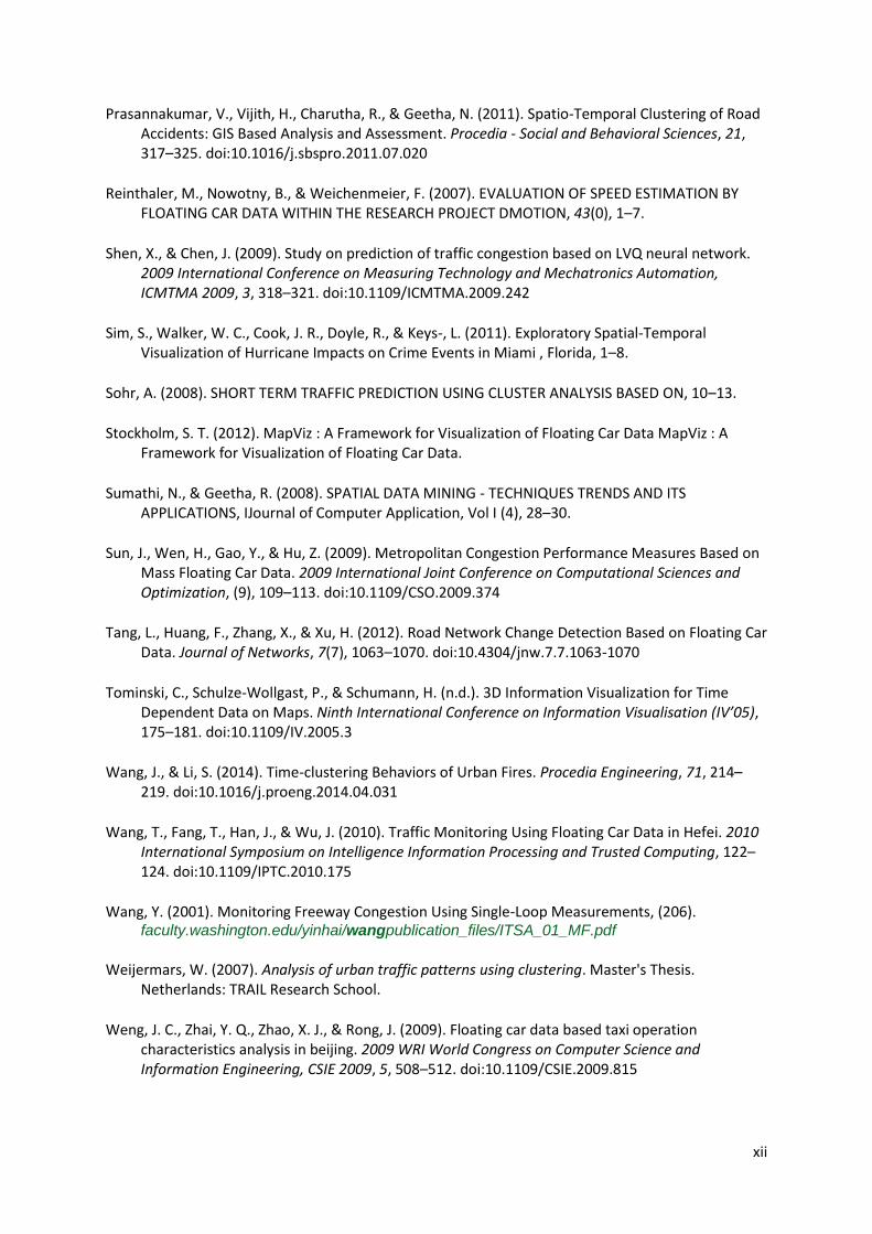
xii

Prasannakumar, V., Vijith, H., Charutha, R., & Geetha, N. (2011). Spatio-Temporal Clustering of Road Accidents: GIS Based Analysis and Assessment. Procedia - Social and Behavioral Sciences, 21, 317–325. doi:10.1016/j.sbspro.2011.07.020

Reinthaler, M., Nowotny, B., & Weichenmeier, F. (2007). EVALUATION OF SPEED ESTIMATION BY FLOATING CAR DATA WITHIN THE RESEARCH PROJECT DMOTION, 43(0), 1–7.

Shen, X., & Chen, J. (2009). Study on prediction of traffic congestion based on LVQ neural network. 2009 International Conference on Measuring Technology and Mechatronics Automation, ICMTMA 2009, 3, 318–321. doi:10.1109/ICMTMA.2009.242

Sim, S., Walker, W. C., Cook, J. R., Doyle, R., & Keys-, L. (2011). Exploratory Spatial-Temporal Visualization of Hurricane Impacts on Crime Events in Miami , Florida, 1–8.

Sohr, A. (2008). SHORT TERM TRAFFIC PREDICTION USING CLUSTER ANALYSIS BASED ON, 10–13.

Stockholm, S. T. (2012). MapViz : A Framework for Visualization of Floating Car Data MapViz : A Framework for Visualization of Floating Car Data.

Sumathi, N., & Geetha, R. (2008). SPATIAL DATA MINING - TECHNIQUES TRENDS AND ITS APPLICATIONS, IJournal of Computer Application, Vol I (4), 28–30.

Sun, J., Wen, H., Gao, Y., & Hu, Z. (2009). Metropolitan Congestion Performance Measures Based on Mass Floating Car Data. 2009 International Joint Conference on Computational Sciences and Optimization, (9), 109–113. doi:10.1109/CSO.2009.374

Tang, L., Huang, F., Zhang, X., & Xu, H. (2012). Road Network Change Detection Based on Floating Car Data. Journal of Networks, 7(7), 1063–1070. doi:10.4304/jnw.7.7.1063-1070

Tominski, C., Schulze-Wollgast, P., & Schumann, H. (n.d.). 3D Information Visualization for Time Dependent Data on Maps. Ninth International Conference on Information Visualisation (IV’05), 175–181. doi:10.1109/IV.2005.3

Wang, J., & Li, S. (2014). Time-clustering Behaviors of Urban Fires. Procedia Engineering, 71, 214–219. doi:10.1016/j.proeng.2014.04.031

Wang, T., Fang, T., Han, J., & Wu, J. (2010). Traffic Monitoring Using Floating Car Data in Hefei. 2010 International Symposium on Intelligence Information Processing and Trusted Computing, 122–124. doi:10.1109/IPTC.2010.175

Wang, Y. (2001). Monitoring Freeway Congestion Using Single-Loop Measurements, (206). faculty.washington.edu/yinhai/wangpublication_files/ITSA_01_MF.pdf

Weijermars, W. (2007). Analysis of urban traffic patterns using clustering. Master's Thesis. Netherlands: TRAIL Research School.

Weng, J. C., Zhai, Y. Q., Zhao, X. J., & Rong, J. (2009). Floating car data based taxi operation characteristics analysis in beijing. 2009 WRI World Congress on Computer Science and Information Engineering, CSIE 2009, 5, 508–512. doi:10.1109/CSIE.2009.815

xiii

Xiao, L., Gerth, J., & Hanrahan, P. (2006). Enhancing Visual Analysis of Network Traffic Using a Knowledge Representation. 2006 IEEE Symposium On Visual Analytics And Technology, 107–114. doi:10.1109/VAST.2006.261436

Xu, L., Yue, Y., & Li, Q. (2013). Identifying Urban Traffic Congestion Pattern from Historical Floating Car Data. Procedia - Social and Behavioral Sciences, 96(Cictp), 2084–2095. doi:10.1016/j.sbspro.2013.08.235

Zhang, W., Tan, G., Ding, N., & Wang, G. (2012). Traffic Congestion Evaluation and Signal Control Optimization Based on Wireless Sensor Networks: Model and Algorithms. Mathematical Problems in Engineering, 2012, 1–17. doi:10.1155/2012/573171

Zhao, Y., Qin, Q., Li, J., Xie, C., & Chen, R. (2012). HIGHWAY MAP MATCHING ALGORITHM BASED ON FLOATING CAR, China: University of Beijing.