WS 2006-07 Algorithmentheorie 14 – Binomial Queues Prof. Dr. Th. Ottmann.
date post
20-Dec-2015Category
view
221download
0
Voronoi Diagrams
Computational Geometry, WS 2006/07Lecture 10
Prof. Dr. Thomas Ottmann
Algorithmen & Datenstrukturen, Institut für InformatikFakultät für Angewandte WissenschaftenAlbert-Ludwigs-Universität Freiburg
Computational Geometry, WS 2006/07Prof. Dr. Thomas Ottmann 2
Overview
• Motivation• Voronoi definitions• Characteristics• Size and storage• Construction
– Divide and Conquer
– Fortune’s Algorithm
• Applications
Computational Geometry, WS 2006/07Prof. Dr. Thomas Ottmann 3
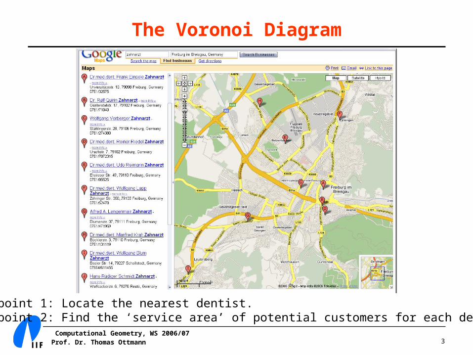
The Voronoi Diagram
Viewpoint 1: Locate the nearest dentist.Viewpoint 2: Find the ‘service area’ of potential customers for each dentist.
Computational Geometry, WS 2006/07Prof. Dr. Thomas Ottmann 4
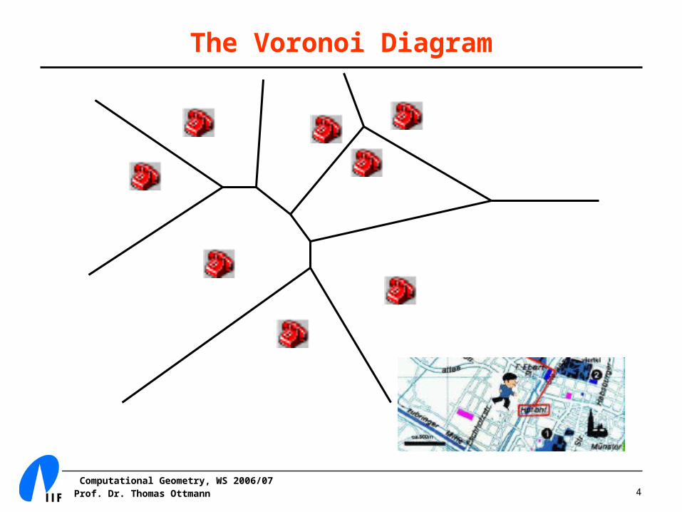
The Voronoi Diagram
Computational Geometry, WS 2006/07Prof. Dr. Thomas Ottmann 5
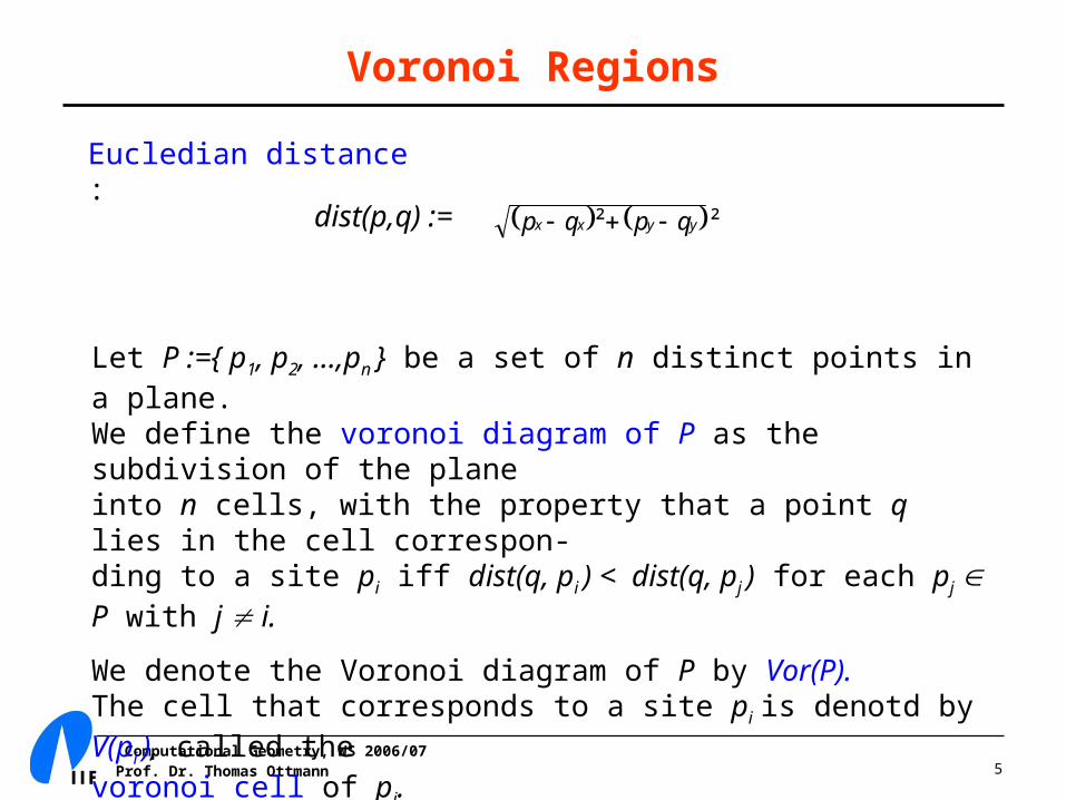
Voronoi Regions
Eucledian distance :
dist(p,q) := ²² yyxx qpqp
Let P :={ p1, p2, ...,pn } be a set of n distinct points in a plane.We define the voronoi diagram of P as the subdivision of the planeinto n cells, with the property that a point q lies in the cell correspon-ding to a site pi iff dist(q, pi ) < dist(q, pj ) for each pj P with j i.
We denote the Voronoi diagram of P by Vor(P).The cell that corresponds to a site pi is denotd by V(pi ), called thevoronoi cell of pi.
Computational Geometry, WS 2006/07Prof. Dr. Thomas Ottmann 6
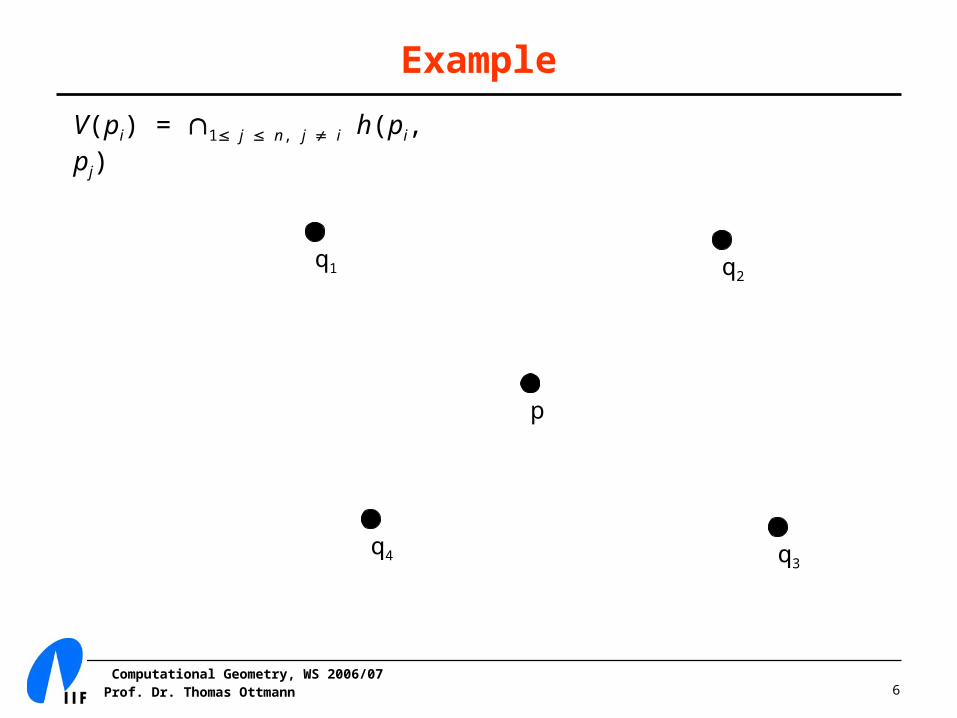
Example
V(pi) = 1 j n, j i h(pi, pj)
q4
q1
q3
q2
p
Computational Geometry, WS 2006/07Prof. Dr. Thomas Ottmann 7
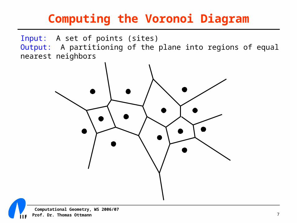
Computing the Voronoi Diagram
Input: A set of points (sites) Output: A partitioning of the plane into regions of equal nearest neighbors

Computational Geometry, WS 2006/07Prof. Dr. Thomas Ottmann 8
Voronoi Diagram Animations
Java applet animation of the Voronoi Diagram by: Christian Icking, Rolf Klein, Peter Köllner, Lihong Ma (FernUniversität Hagen)
Computational Geometry, WS 2006/07Prof. Dr. Thomas Ottmann 9
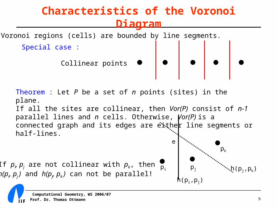
Characteristics of the Voronoi Diagram
(1) Voronoi regions (cells) are bounded by line segments.
Special case :
Collinear points
Theorem : Let P be a set of n points (sites) in the plane. If all the sites are collinear, then Vor(P) consist of n-1 parallel lines and n cells. Otherwise, Vor(P) is a connected graph and its edges are either line segments or half-lines.
e
pi pj
pk
h(pi,pj)
h(pj,pk)If pi, pj are not collinear with pk, thenh(pi, pj ) and h(pj, pk ) can not be parallel!

Computational Geometry, WS 2006/07Prof. Dr. Thomas Ottmann 10
Vor(P) is Connected
If Vor(P) is not connected then there would be a Voronoicell V(Pi ) splitting the plane into two halfes. Because Voronoi cells are convex, V(Pi ) would consist of a strip bounded by two parallel full lines, but we know that edges of Voronoi diagram cannot be full lines, hence a contradiction.
Claim: Vor(P) is connected
Proof by contradiction:
Computational Geometry, WS 2006/07Prof. Dr. Thomas Ottmann 11
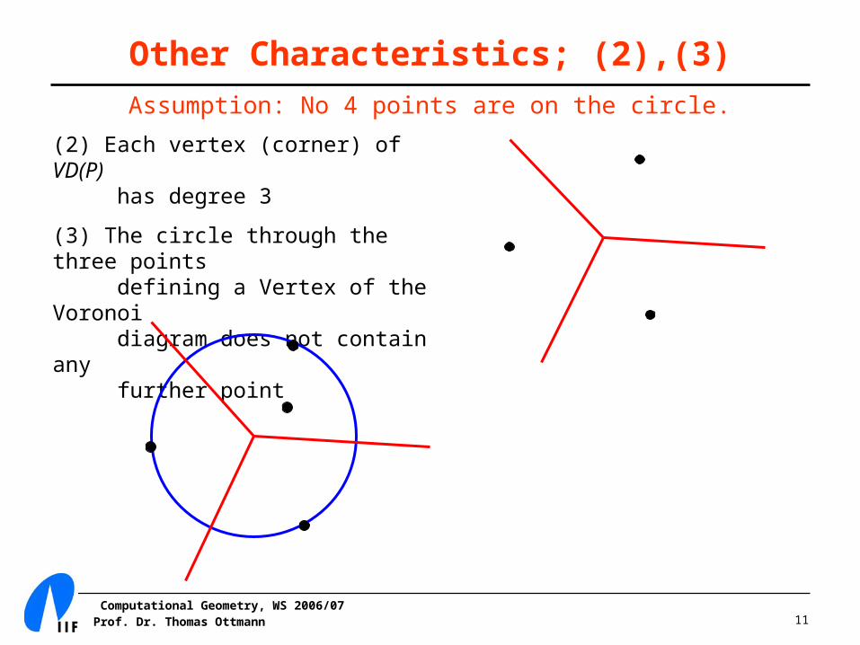
Other Characteristics; (2),(3)
Assumption: No 4 points are on the circle.
(2) Each vertex (corner) of VD(P) has degree 3
(3) The circle through the three points defining a Vertex of the Voronoi diagram does not contain any further point
Computational Geometry, WS 2006/07Prof. Dr. Thomas Ottmann 12
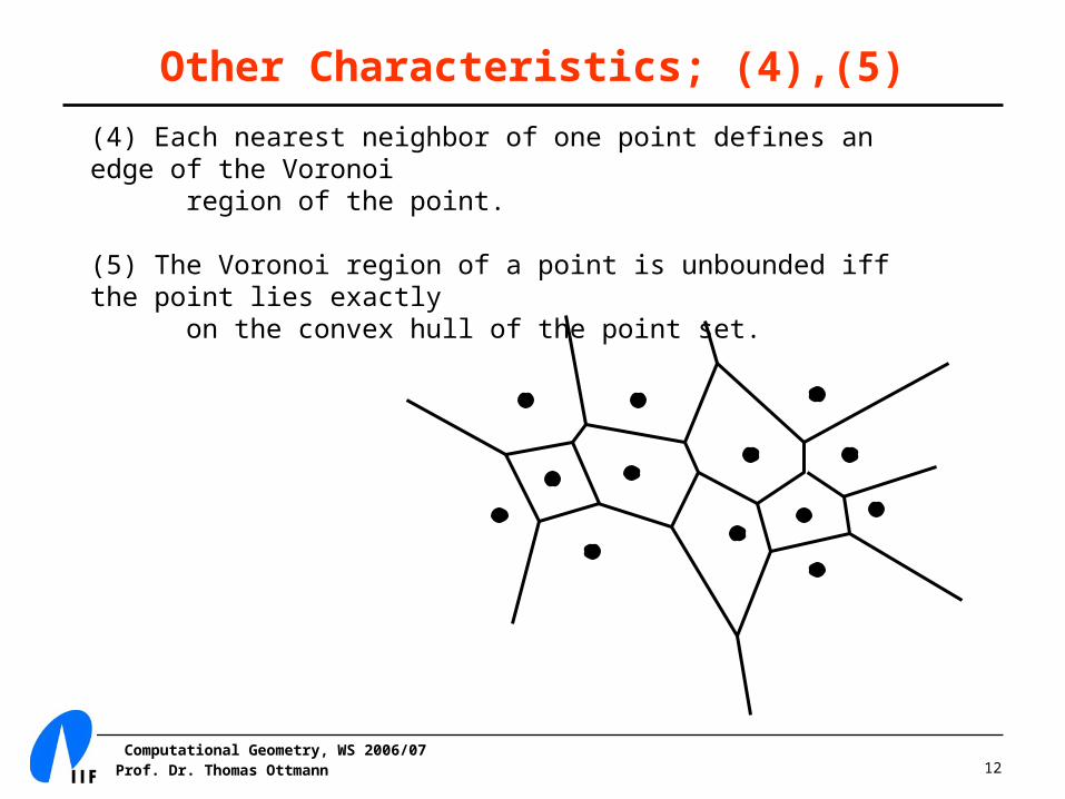
Other Characteristics; (4),(5)
(4) Each nearest neighbor of one point defines an edge of the Voronoi region of the point.
(5) The Voronoi region of a point is unbounded iff the point lies exactly on the convex hull of the point set.
Computational Geometry, WS 2006/07Prof. Dr. Thomas Ottmann 13
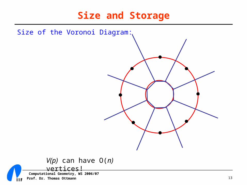
Size and Storage
Size of the Voronoi Diagram:
V(p) can have O(n) vertices!
Computational Geometry, WS 2006/07Prof. Dr. Thomas Ottmann 14
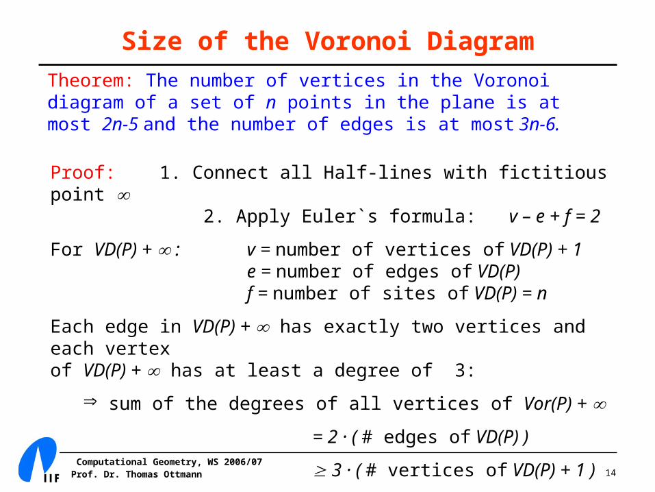
Size of the Voronoi Diagram
Theorem: The number of vertices in the Voronoi diagram of a set of n points in the plane is at most 2n-5 and the number of edges is at most 3n-6.
Proof: 1. Connect all Half-lines with fictitious point 2. Apply Euler`s formula:v – e + f = 2
For VD(P) + : v = number of vertices of VD(P) + 1e = number of edges of VD(P) f = number of sites of VD(P) = n
Each edge in VD(P) + has exactly two vertices and each vertex of VD(P) + has at least a degree of 3:
sum of the degrees of all vertices of Vor(P) +
= 2 · ( # edges of VD(P) )
3 · ( # vertices of VD(P) + 1 )
Computational Geometry, WS 2006/07Prof. Dr. Thomas Ottmann 15
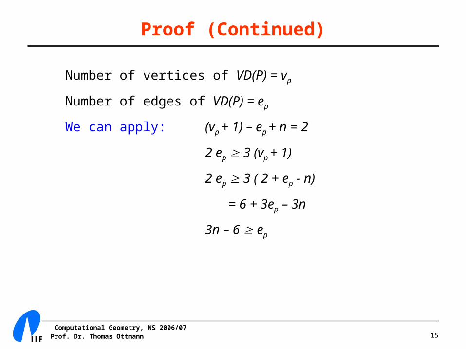
Proof (Continued)
Number of vertices of VD(P) = vp
Number of edges of VD(P) = ep
We can apply: (vp + 1) – ep + n = 2
2 ep 3 (vp + 1)
2 ep 3 ( 2 + ep - n)
= 6 + 3ep – 3n
3n – 6 ep
Computational Geometry, WS 2006/07Prof. Dr. Thomas Ottmann 16
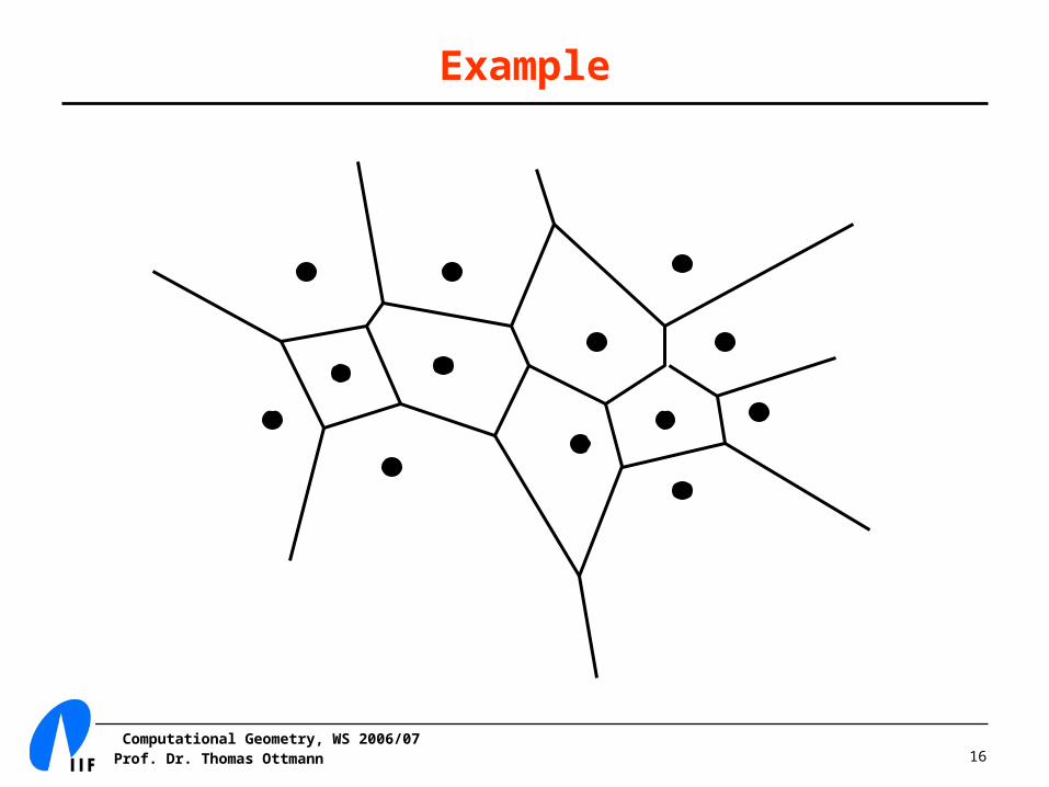
Example
Computational Geometry, WS 2006/07Prof. Dr. Thomas Ottmann 17
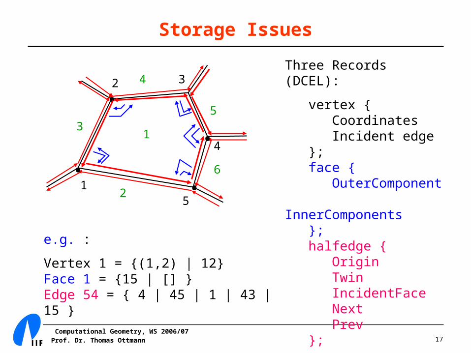
Storage Issues
1
1
3
4
5
6
2
2 3
4
5
•
•
•
•
Three Records (DCEL):
vertex {CoordinatesIncident edge
}; face {
OuterComponentInnerComponents
}; halfedge {
OriginTwinIncidentFaceNextPrev
};
e.g. :
Vertex 1 = {(1,2) | 12}Face 1 = {15 | [] }Edge 54 = { 4 | 45 | 1 | 43 | 15 }
Computational Geometry, WS 2006/07Prof. Dr. Thomas Ottmann 18
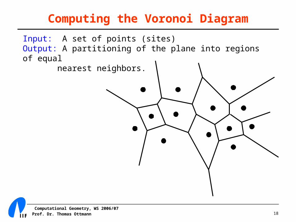
Computing the Voronoi Diagram
Input: A set of points (sites) Output: A partitioning of the plane into regions of equal
nearest neighbors.
Computational Geometry, WS 2006/07Prof. Dr. Thomas Ottmann 19
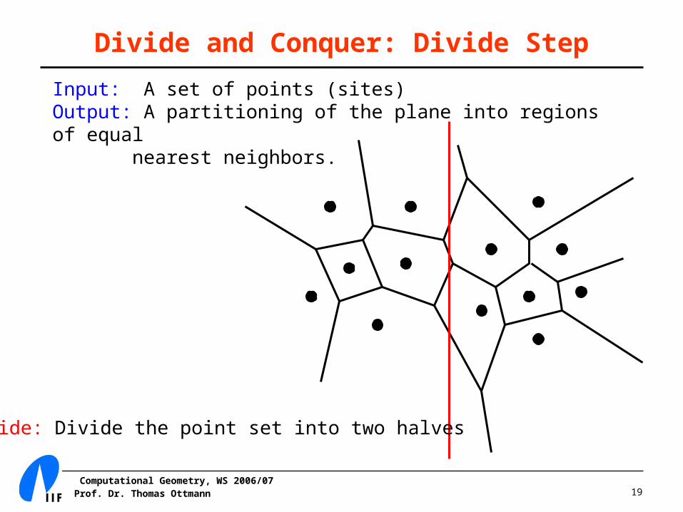
Divide and Conquer: Divide Step
Input: A set of points (sites) Output: A partitioning of the plane into regions of equal
nearest neighbors.
Divide: Divide the point set into two halves
Computational Geometry, WS 2006/07Prof. Dr. Thomas Ottmann 20
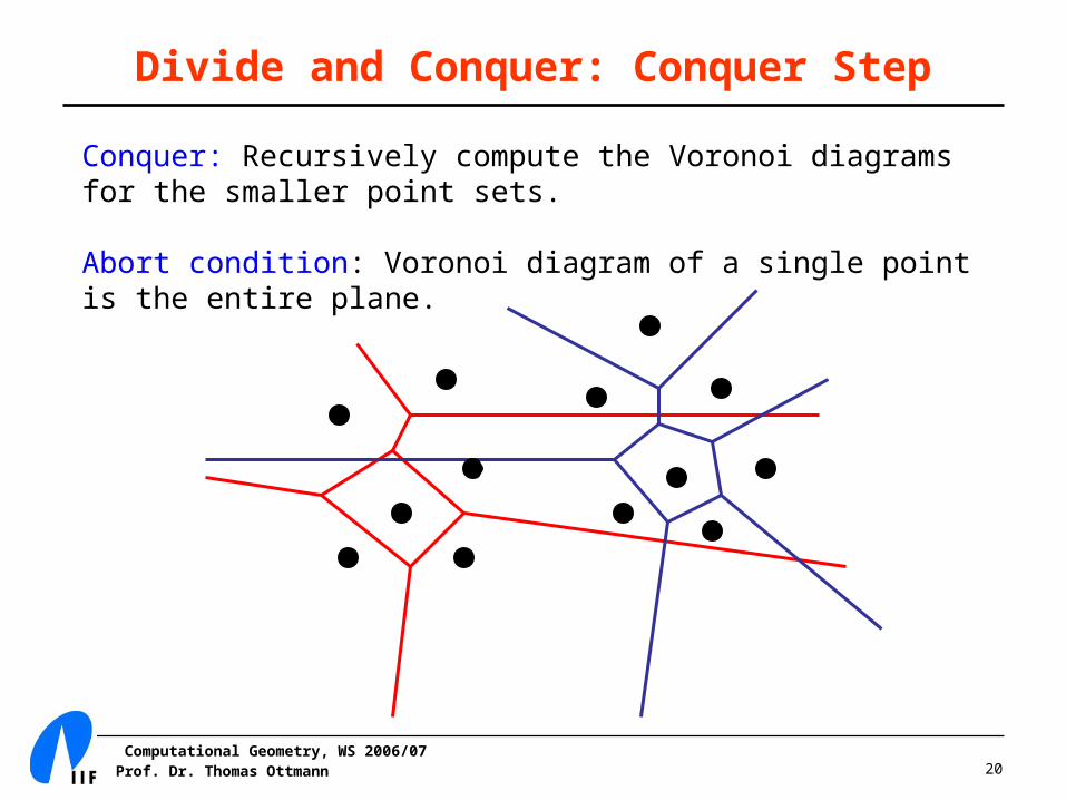
Divide and Conquer: Conquer Step
Conquer: Recursively compute the Voronoi diagrams for the smaller point sets.
Abort condition: Voronoi diagram of a single point is the entire plane.
Computational Geometry, WS 2006/07Prof. Dr. Thomas Ottmann 21
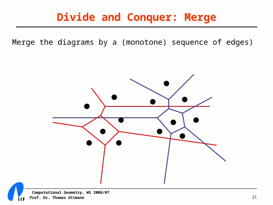
Divide and Conquer: Merge
Merge the diagrams by a (monotone) sequence of edges)
Computational Geometry, WS 2006/07Prof. Dr. Thomas Ottmann 22
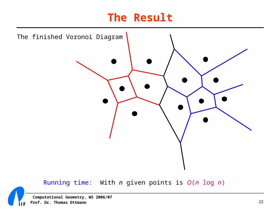
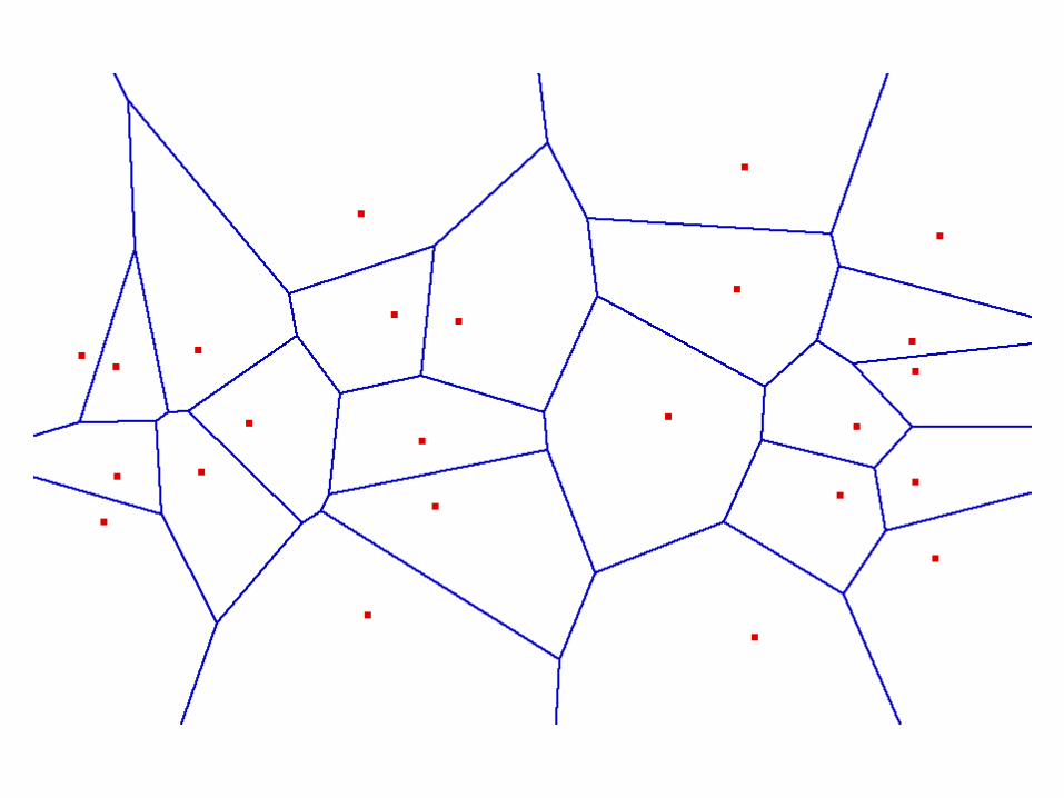
The Result
The finished Voronoi Diagram
Running time: With n given points is O(n log n)
Computational Geometry, WS 2006/07Prof. Dr. Thomas Ottmann 23
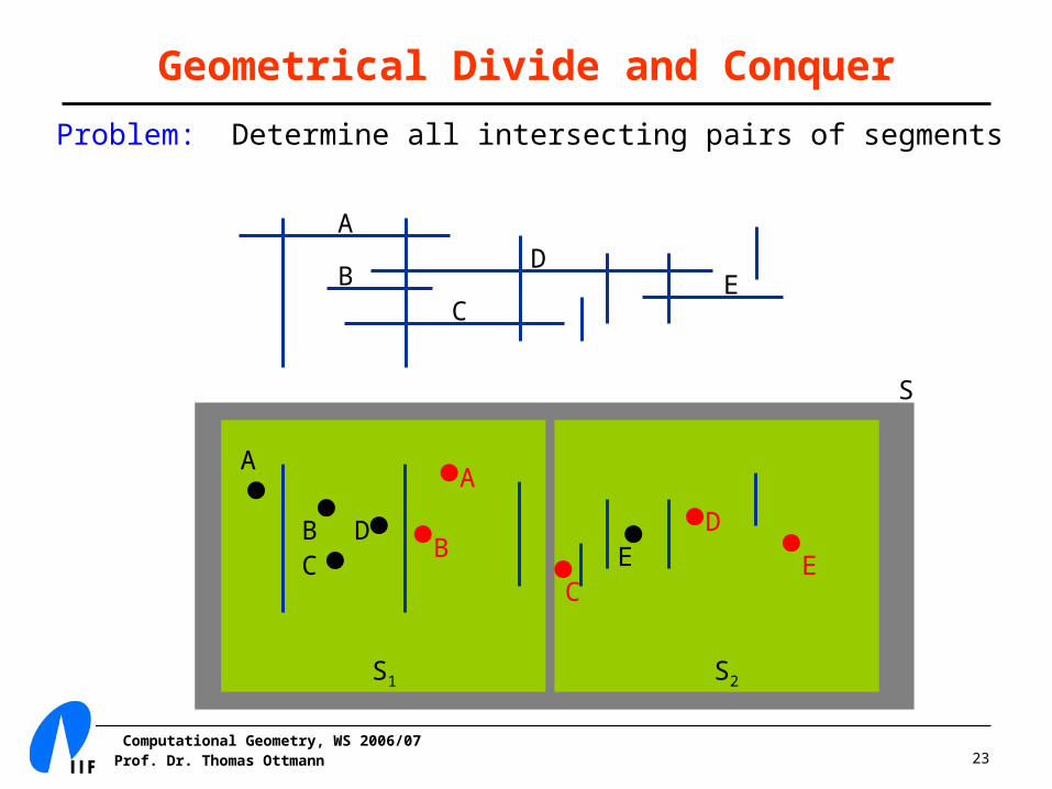
Geometrical Divide and Conquer
Problem: Determine all intersecting pairs of segments
A
BC
DE
A
BC
DE
S1 S2
S
EC
D
A
B
Computational Geometry, WS 2006/07Prof. Dr. Thomas Ottmann 24
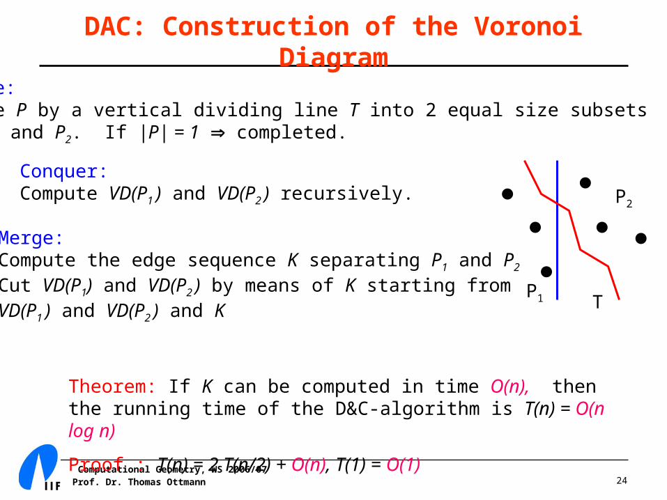
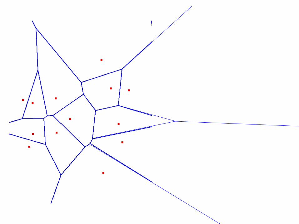
DAC: Construction of the Voronoi Diagram
Divide:Divide P by a vertical dividing line T into 2 equal size subsets say P1 and P2. If |P| = 1 completed.
Conquer:Compute VD(P1 ) and VD(P2 ) recursively.
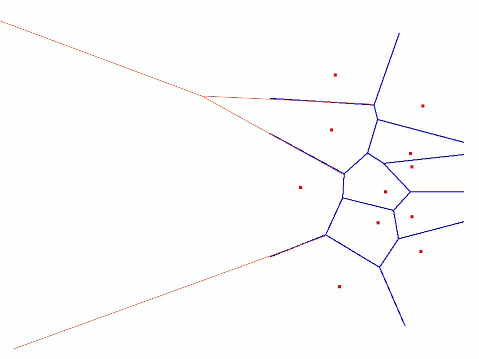
Merge: Compute the edge sequence K separating P1 and P2 Cut VD(P1) and VD(P2 ) by means of K starting from VD(P1 ) and VD(P2 ) and K
P1
P2
T
Theorem: If K can be computed in time O(n), then the running time of the D&C-algorithm is T(n) = O(n log n)
Proof : T(n) = 2 T(n/2) + O(n), T(1) = O(1)
Computational Geometry, WS 2006/07Prof. Dr. Thomas Ottmann 25
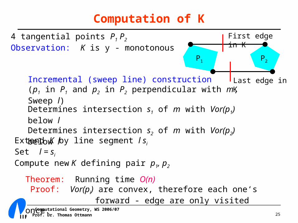
Computation of K
P1 P2
First edge in K
Last edge in K
4 tangential points P1 P2 Observation: K is y - monotonous
Determines intersection s1 of m with Vor(p1) below l Determines intersection s2 of m with Vor(p2) below l
Incremental (sweep line) construction(p1 in P1 and p2 in P2 perpendicular with m, Sweep l)
Extend K by line segment l si
Set l = si
Compute new K defining pair p1, p2
Theorem: Running time O(n) Proof: Vor(pi) are convex, therefore each one‘s forward - edge are only visited once.
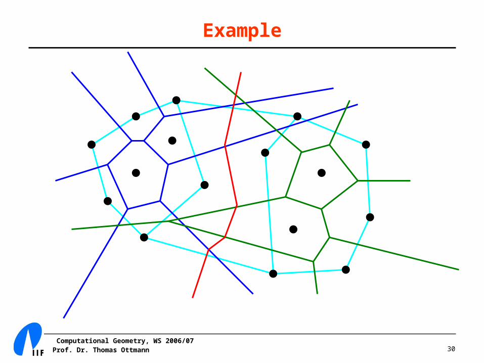
Computational Geometry, WS 2006/07Prof. Dr. Thomas Ottmann 30
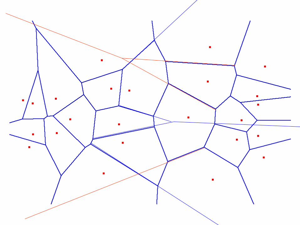
Example
Computational Geometry, WS 2006/07Prof. Dr. Thomas Ottmann 31
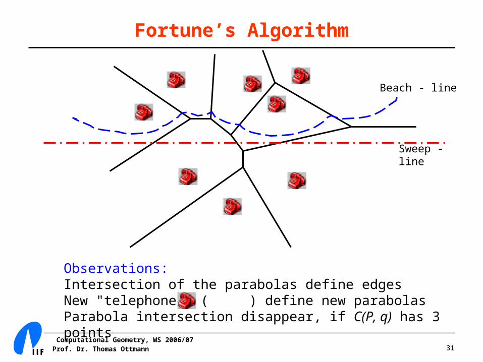
Fortune’s Algorithm
Beach - line
Sweep - line
Observations: Intersection of the parabolas define edgesNew "telephones" ( ) define new parabolas Parabola intersection disappear, if C(P, q) has 3 points
Computational Geometry, WS 2006/07Prof. Dr. Thomas Ottmann 32
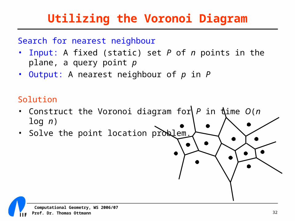
Utilizing the Voronoi Diagram
Search for nearest neighbour• Input: A fixed (static) set P of n points in the plane, a query point p• Output: A nearest neighbour of p in P
Solution• Construct the Voronoi diagram for P in time O(n log n)• Solve the point location problem.
Computational Geometry, WS 2006/07Prof. Dr. Thomas Ottmann 33
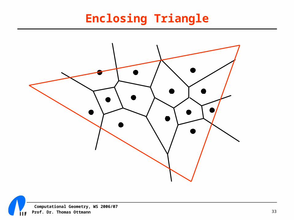
Enclosing Triangle
Computational Geometry, WS 2006/07Prof. Dr. Thomas Ottmann 34
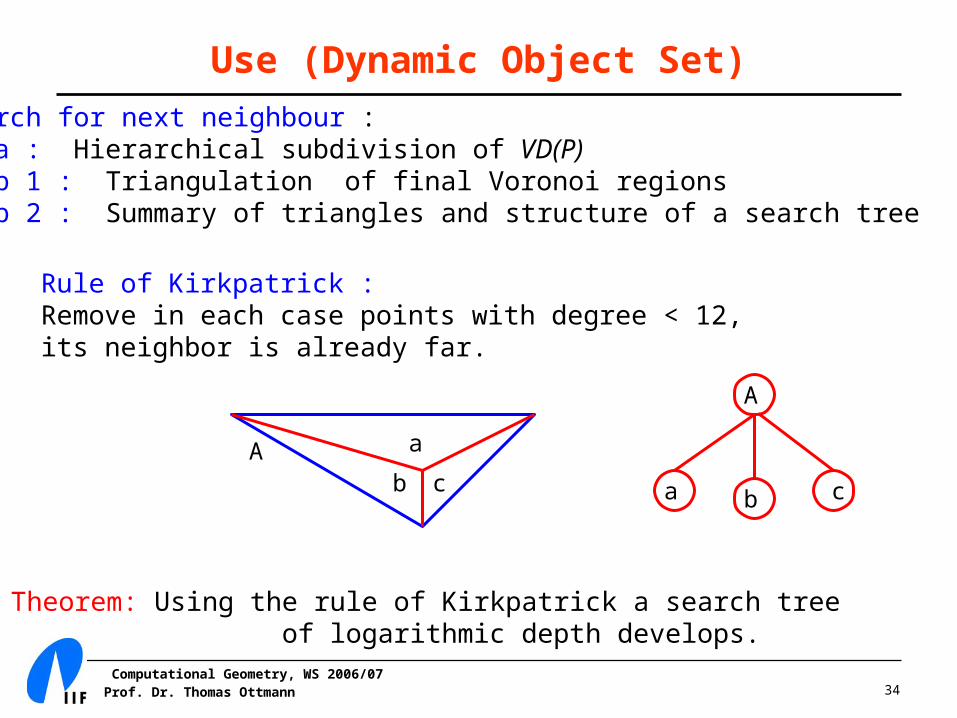
Use (Dynamic Object Set)
Search for next neighbour :Idea : Hierarchical subdivision of VD(P) Step 1 : Triangulation of final Voronoi regions Step 2 : Summary of triangles and structure of a search tree
Rule of Kirkpatrick : Remove in each case points with degree < 12,its neighbor is already far.
Theorem: Using the rule of Kirkpatrick a search tree of logarithmic depth develops.
A a
b c a b c
A
Computational Geometry, WS 2006/07Prof. Dr. Thomas Ottmann 35
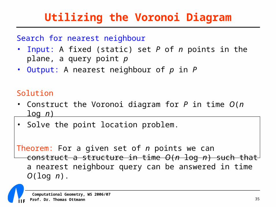
Utilizing the Voronoi Diagram
Search for nearest neighbour• Input: A fixed (static) set P of n points in the plane, a query point p• Output: A nearest neighbour of p in P
Solution• Construct the Voronoi diagram for P in time O(n log n)• Solve the point location problem.
Theorem: For a given set of n points we can construct a structure in time O(n log n) such that a nearest neighbour query can be answered in time O(log n).
Computational Geometry, WS 2006/07Prof. Dr. Thomas Ottmann 36
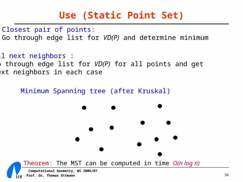
Use (Static Point Set)
Closest pair of points: Go through edge list for VD(P) and determine minimum
All next neighbors :Go through edge list for VD(P) for all points and get next neighbors in each case
Minimum Spanning tree (after Kruskal)
Theorem: The MST can be computed in time O(n log n)

Computational Geometry, WS 2006/07Prof. Dr. Thomas Ottmann 37
MST (after Kruskal): Informal Algorithm
Minimum Spanning Tree (after Kruskal):
Construct for a graph G = (V, E) a minimum spanning tree in time O(|E| log |E|).
1. Each point p from P defines 1-node tree; start with the forest of these 1-node trees.
2. If there are more than one tree T in the current forest, 2.1) find p, p´ with p in T and p´ not in T with d(p, p´)
minimal. 2.2) connect T containing p and T´ containing p´
(union of T and T´)
Computational Geometry, WS 2006/07Prof. Dr. Thomas Ottmann 38
Kruskal’s Algorithm
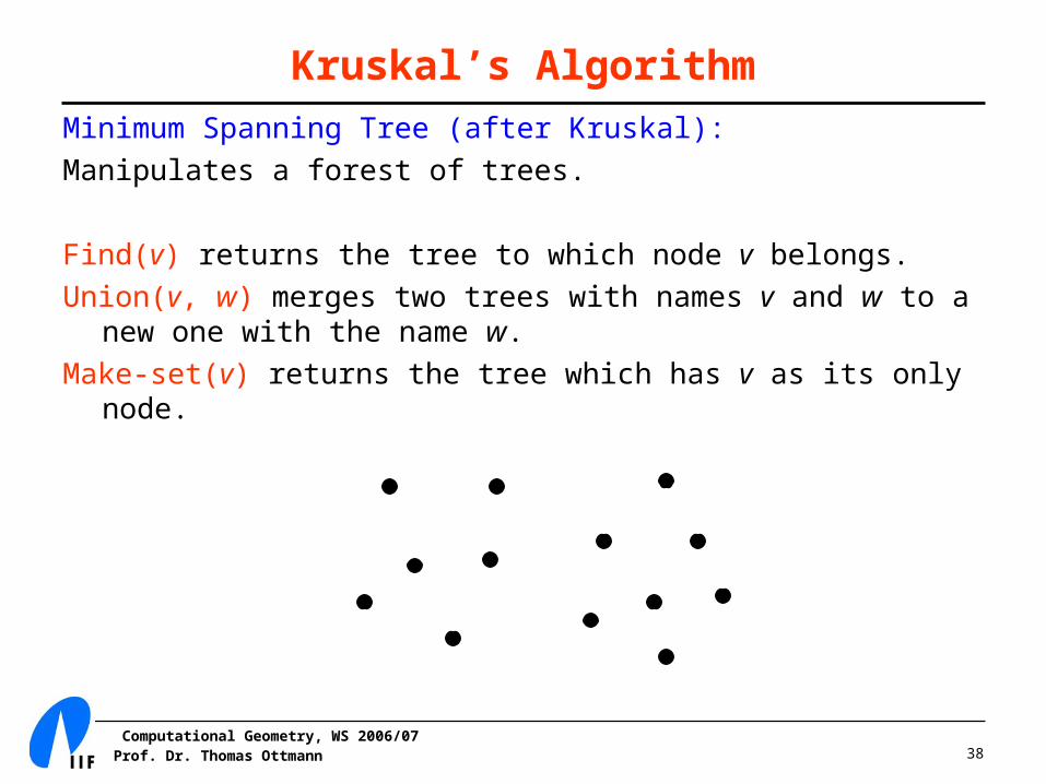
Minimum Spanning Tree (after Kruskal):
Manipulates a forest of trees.
Find(v) returns the tree to which node v belongs.
Union(v, w) merges two trees with names v and w to a new one with the name w.
Make-set(v) returns the tree which has v as its only node.
Computational Geometry, WS 2006/07Prof. Dr. Thomas Ottmann 39
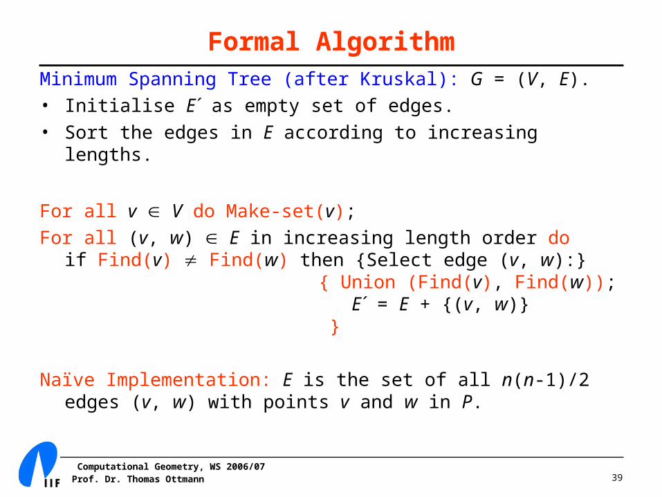
Formal AlgorithmMinimum Spanning Tree (after Kruskal): G = (V, E).• Initialise E´ as empty set of edges.• Sort the edges in E according to increasing lengths.
For all v V do Make-set(v);
For all (v, w) E in increasing length order doif Find(v) Find(w) then {Select edge (v, w):}
{ Union (Find(v), Find(w)); E´ = E + {(v, w)} }
Naïve Implementation: E is the set of all n(n-1)/2 edges (v, w) with points v and w in P.
Computational Geometry, WS 2006/07Prof. Dr. Thomas Ottmann 40
Summary
Minimum Spanning Tree (after Kruskal)
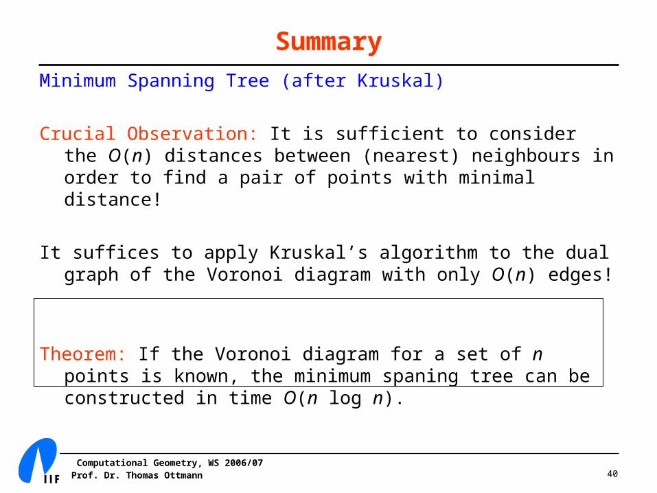
Crucial Observation: It is sufficient to consider the O(n) distances between (nearest) neighbours in order to find a pair of points with minimal distance!
It suffices to apply Kruskal’s algorithm to the dual graph of the Voronoi diagram with only O(n) edges!
Theorem: If the Voronoi diagram for a set of n points is known, the minimum spaning tree can be constructed in time O(n log n).