


Sprachen
Seiten
Rechtliche


I
Risk Management in International
Real Estate and Capital Markets
Dissertation zur Erlangung des Grades eines Doktors der Wirtschaftswissenschaft
eingereicht an der Fakultät für Wirtschaftswissenschaften der Universität Regensburg
vorgelegt von:
Cay Philip Oertel
Berichterstatter:
Prof. Dr. Sven Bienert, Universität Regensburg
Prof. Dr. Steffen Sebastian, Universität Regensburg
Tag der Disputation:
22. Juli 2020

I
Contents
List of Tables ...........................................................................................................................................III
List of Figures ......................................................................................................................................... IV
1 Introduction ..........................................................................................................................................1
1.1 Risk in real estate, the impact of securitization and derived research ..........................................2
1.2 Bibliography ....................................................................................................................................7
2 The relationship between domestic and global Economic Political Uncertainty and European
Direct Commercial Real Estate Returns ..................................................................................................9
2.1 Introduction ................................................................................................................................. 10
2.2 Theoretical background, related literature and hypotheses derivation ..................................... 11
2.3 Research design and measurement of uncertainty .................................................................... 15
2.4 Data and descriptive statistics ..................................................................................................... 17
2.5 Methodology ............................................................................................................................... 20
2.6 Empirical results .......................................................................................................................... 21
2.7 Conclusion and further remarks .................................................................................................. 24
2.8 Bibliography ................................................................................................................................. 28
2.9 Appendix ...................................................................................................................................... 32
3 Do Cross-Border Investors Benchmark Commercial Real Estate Markets? Evidence from Relative
Yields and Risk Premia for a European Investment Horizon ............................................................... 33
3.1 Introduction ................................................................................................................................. 34
3.2 Related literature and hypotheses derivation ............................................................................ 35
3.3 Data, sample description and methodology ............................................................................... 38
3.4 Empirical results .......................................................................................................................... 46
3.5 Conclusion and further aspects ................................................................................................... 53
3.6 Bibliography ................................................................................................................................. 55
3.7 Appendix ...................................................................................................................................... 58
4 Volatility Targeting for US Equity REITs – A strategy for Minimizing Extreme Downside Risk? ..... 59
4.1 Introduction ................................................................................................................................. 60

II
4.2 Literature review and hypothesis derivation .............................................................................. 61
4.3 Data and descriptive statistics ..................................................................................................... 64
4.4 Methodology ............................................................................................................................... 66
4.5 Empirical results .......................................................................................................................... 68
4.6 Conclusion, practical implications and further research ............................................................. 75
4.7 Bibliography ................................................................................................................................. 77
4.8 Appendix ...................................................................................................................................... 80
5 AR-GARCH-EVT-Copula for Securitized Real Estate: An approach to improving risk forecasts? .... 83
5.1 Introduction ................................................................................................................................. 84
5.2 Literature review and hypothesis derivation .............................................................................. 86
5.3 Methodology ............................................................................................................................... 86
5.4 Data and descriptive statistics ..................................................................................................... 96
5.5 Empirical results .......................................................................................................................... 99
5.6 Conclusion ................................................................................................................................. 111
5.7 Bibliography ............................................................................................................................... 113
5.8 Appendix .................................................................................................................................... 118
6 Conclusion ........................................................................................................................................ 119
6.1 Conclusion ................................................................................................................................. 120
6.2 Bibliography ............................................................................................................................... 124
III
List of Tables
Table 1: Data description and variable selection for total return models ............................................ 17
Table 2: Descriptive statistics for variables of the total return models ................................................ 18
Table 3: Correlation matrix of the total return data set ....................................................................... 19
Table 4: Pooled OLS estimation results (total return) ........................................................................... 22
Table 5: Explanatory power of total return models without DEPUI / GEPUI ........................................ 24
Table 6: Levin-Lu-Chu stationarity test for total return model variables .............................................. 32
Table 7: Control variable description for cross-border volume models ............................................... 42
Table 8: Descriptive statistics for variables of the cross-border transaction volume models .............. 43
Table 9: Correlation matrix for cross-border transaction volume model variables .............................. 44
Table 10: Granger causality test (RNMRP & RNMY – cross-border transaction volume) ..................... 46
Table 11: Pooled OLS estimation results (cross-border transaction volume) ....................................... 47
Table 12: GAMM estimation results for penalized spline functions of non-parametric covariates ..... 50
Table 13: Levin-Lin-Chu stationarity test for cross-border transaction volume model variables ......... 58
Table 14: Descriptive statistics of daily US equity REIT returns (01/01/1999 – 01/01/2019)............... 64
Table 15: Maximum STARR (Buy and Hold & VT (hist. Vol, VIX & GARCH)) .......................................... 74
Table 16: Correlation matrix (Office REITs) ........................................................................................... 80
Table 17: Correlation matrix (Residential REITs) ................................................................................... 80
Table 18: Correlation matrix (Industrial REITs) ..................................................................................... 80
Table 19: Correlation matrix (Retail REITs) ........................................................................................... 81
Table 20: Correlation matrix (Diversified REITs) ................................................................................... 82
Table 21: Correlation matrix (Health Care REITs) .................................................................................. 82
Table 22: Correlation matrix (Lodging & Resorts REITs) ....................................................................... 82
Table 23: Descriptive statistics .............................................................................................................. 98
Table 24: Empirical results for VaR forecasts ...................................................................................... 101
Table 25: Empirical results for CVaR forecasts .................................................................................... 104
Table 26: Results of the autoregressive modelling ............................................................................. 106
Table 27: Empirical results for the copulae estimation ....................................................................... 109
Table 28: List of applied copulae ......................................................................................................... 118

IV
List of Figures
Figure 1: Adjusted GEPUI scores (Q1/2008 – Q3/2018) ........................................................................ 16
Figure 2: European commercial real estate investment volume in Mio. Euro (Q1/2008 – Q3/2018) .. 39
Figure 3: Penalized spline functions of RNMPR 10y and RNMRP 5y – models G.2 & G.3 ..................... 51
Figure 4: Efficiency frontiers within mean-CVaR0.95-framework (All REITs) ....................................... 69
Figure 5: Efficiency frontiers within mean-CVaR0.95-framework (Office REITs) ................................. 70
Figure 6: Efficiency frontiers within mean-CVaR0.95-framework (Retail REITs) ................................. 70
Figure 7: Efficiency frontiers within mean-CVaR0.95-framework (Industrial REITs) ........................... 71
Figure 8: Efficiency frontiers within mean-CVaR0.95-framework (Residential REITs) ......................... 71
Figure 9: Efficiency frontiers within mean-CVaR0.95-framework (Diversified REITs) ......................... 72
Figure 10: Efficiency frontiers within mean-CVaR0.95-framework (Lodging and Resort REITs) .......... 72
Figure 11: Efficiency frontiers within mean-CVaR0.95-framework (Health Care REITs) ...................... 73
Figure 12: VaR0.95 estimates for Real Estate–Stocks portfolio (US) ................................................... 85
Figure 13: Cumulated return series for real estate, stocks and bonds (US) ......................................... 97
Figure 14: VaR0.95-fr estimates for Real Estate – Stocks & Real Estate - Bonds portfolio (US) ........ 100

1
1 Introduction

Introduction
2
1.1 Risk in real estate, the impact of securitization and derived research
The presence of risk is an essential part of finance since risk-taking is the natural economic necessity
to generate excess returns (dating back to Knight, 1921). Although a single and unanimously accepted
definition of the term is missing across different sciences, the meaning of risk in finance entails two
decisive elements: The potential of a negative divergence from expected values and a corresponding
monetary loss due to the negative divergence (McNeil et al., 2015).
Based on these two components, the term risk in academia is strongly connected to uncertainty and
randomness. Investors face situations in which the future financial performance of assets, like real
estate, is uncertain. Thus, any decision entails ex ante uncertainty about its outcome in the future. In
terms of statistical language and real estate, the interpretation is that these risks or concrete risk
factors, such as rental growth, maintenance expenses, construction costs, financing costs, etc., are
modelled as random variables (French & Gabrielli, 2004).
Financial risk management has focused on the application of probability theory to model these random
variables in a decision under uncertainty. According models were introduced by Kolmogorov (1933) to
oppose purely deterministic models. This pioneering work still provides the common terminology for
risk-related scientific discussion. The application of probability in the real estate literature and in the
context of risk represents the class of so-called stochastic models. In contrast to deterministic models,
their stochastic peers allow the explicit modelling of risk using the corresponding distribution functions
of the risk factors in the future to account for their randomness (Pfnür & Armonat, 2013).
The financial risk management of investment positions is implemented in practice by institutional
investors using a comprehensive and recursive risk management system, which is supposed to ensure
the identification, quantification, steering, and surveillance of risks. This procedure applies to investors
of classic capital market products, such as stocks or bonds and alternatives, like real estate mostly
alike, because legal requirements generally do not differ between the assets of the investment
company. In this context, a clear development of legal tightening can be observed in the aftermath of
the global financial crisis in 2008.1 Additionally, risk management has moved into the center of
attention from an economic point of view because of concerns about potential over-valuations of
property assets have risen due to the extensive global monetary expansion (Hayunga & Lung, 2011;
Abildgren et al., 2018; Fabozzi & Xiao, 2019) and the economic turmoil due to the COVID-19 pandemic.
1 In Germany, for example, the introduction of the “Kapitalanlagegesetzbuch” in 2013, and subsequently the “Mindestanforderungen an das Risikomanagement von Kapitalverwaltungsgesellschaften” in 2017. Both regulatory adjustments are based on European law, namely the Alternative Investment Fund Manager Directive (AIFMD), illustrating an international scale of regulation.
Introduction
3
However, the concrete methodological implementation of a stochastic approach is subject to the asset
class specifics of the managed positions. These asset class specifics are highly relevant for the present
thesis because the articles address the abovementioned types of products: Firstly, alternative
investments like direct real estate and secondly, classic investment products like stocks including
securitized real estate and bonds. The decisive mechanism that separates the articles and the
methodology is the securitization function of indirect investment vehicles in capital markets. On the
one hand, direct real estate as an asset class can be characterized as heterogeneous, illiquid, having
high transaction costs and durations, and entailing low fungibility and transparency (or information
respectively), among others. Indirect or securitized real estate, on the other hand, transforms these
specifics of the underlying assets. Accordingly, the risk management methodology changes as well,
because capital markets provide homogeneity, liquidity, fungibility, information, relatively low
transaction costs and durations. Lastly, debt positions focus methodologically on aspects arising from
the individual credit agreement and the borrower, urging to model metrics like probability of default
(PD), loss given default (LGD) or exposure at default (EAD), etc. (for a summary see Booth et al., 2002).
The modelling within the real estate industry focused historically on qualitative approaches to manage
the risk of their positions. However, due to the legal requirements as well as higher data availability
and probability functions of risk factors (Amédée-Manesme & Barthélémy, 2018), more quantitative
approaches including stochastic modelling in the sense of Kolmogorov (1933) have been established.
Accordingly, for direct real estate, the most feasible stochastic approach to quantify the residual risk
of the assets is the Monte Carlo Simulation (MCS; Hoesli et al., 2006; Baroni et al., 2007). For the
simulation of the cash flows of the properties, however, the macroeconomic environment and the
relevant risk factors of the assets need to be identified correctly because real estate assets are highly
dependent on the macroeconomic circumstances. Central for this modelling is the question, what risk
factors can affect the cash flows of the property? Therefore, it is crucial to identify the functional chain
in risk factors models (e.g., as described by Ho et al., 2015) before quantifying the impact on the
individual asset level. The thesis derived the following selected aspects of risk management in
international real estate and capital markets based on these considerations of risk identification,
quantification, steering, and surveillance in direct as well as securitized real estate markets.
The first article of the thesis presents a typical fundamental risk factor model described above. It aims
at assessing the potential impact of domestic and global economic political uncertainty on commercial
real estate markets. Recently, politics-related uncertainties like Brexit have gained large interest
(French, 2019). However, the existing body of literature has mainly focused on residential markets in
this context (e.g., Monfared & Pavlov, 2019). Thus, the paper “The relationship between domestic and
global economic political uncertainty and European direct commercial real estate returns” estimates
linear models to isolate the effect of the target covariates on total returns of office properties in
Introduction
4
Europe. Additionally, the independent covariates are divided into domestic and global economic
political uncertainty to find thinkable cross-border effects of uncertainty after controlling for the
domestic peer to detect a potential “safe haven effect,” namely a positive influence of foreign
uncertainty on domestic properties.
The second article on direct property markets “Do Cross-Border Investors Benchmark Commercial Real
Estate Markets? Evidence from Relative Yields and Risk Premia for a European Investment Horizon”
addresses the determinants of cross-border investment flows in real estate markets. So far, literature
has widely focused on economic or institutional pull factors, which attract capital (e.g., Lieser & Groh,
2014). The article extends the existing literature by constructing a synthetic index for European
investment locations to test for the relative attractiveness of a market as a determinant of inflowing
capital. Methodologically, linear as well as non-linear regression models are used for European panel
data. Nonetheless, one may ask about the connection between foreign capital flows and risk
management. Market liquidity of direct real estate markets can be an important risk factor, which may
cause deviations from expected values of, e.g., transaction durations, time on the market, etc. Thus,
the article contributes to the understanding of the underlying functional chain of market liquidity,
which is a commonly known risk factor.
Next, the thesis turns towards the risk management of securitized real estate positions in capital
markets. As outlined above, the transformation functions of indirect vehicles allow investors to steer
the risk of their indirect positions differently from their direct peers. Here, the paper “Volatility
Targeting for US Equity REITs – A Strategy for Minimizing Extreme Downside Risk?” presents the so-
called Volatility Targeting rebalancing algorithm for REIT securities as an active management tool for
risk steering. Since daily returns of REITs are showing even stronger volatility clustering and leverage
effect than classic equities (Cotter & Stevenson, 2007; Jirasakuldech et al., 2009), the asset class
appears to be very promising for research on volatility-based risk strategies. To the author’s
knowledge, no article has carried out an empirical study on the specified technique of REIT securities
to analyze the characteristics of REIT volatility explicitly from an applied risk management point of
view. To provide insight, at first a back testing approach simulates returns from the volatility targeting
algorithm. The strategy bases on various volatility estimators, such as historical volatility, the CBOE
Volatility Index based on broader stock market option prices, and on one-day-ahead forecasts of a
generalized autoregressive conditional heteroscedasticity (GARCH) model. The realized returns of the
strategies are then analyzed in a portfolio optimization framework to identify the strategies’ economic
efficiency compared to a classic buy and hold investment scenario.
The last paper extends the investment horizon to classic stocks and bond positions. The paper “AR-
GARCH-EVT-Copula for Securitized Real Estate: An approach to improving risk forecasts” is the first

Introduction
5
study to apply the so-called AR-GARCH-EVT-Copula model to bivariate portfolios, which contain
securitized real estate in addition to the abovementioned capital market products. Different from the
previous article, this paper does not aim at economic efficiency and its frontiers but forecasting risk
metrics. The primary motivation for the paper is the stylized facts about financial market data. The
data have repeatedly shown leptokurtosis, skew and fat tails (largely discussed by McNeil & Frey,
2000), which provokes the application of a GARCH-standardization to model the dependency of
securitized real estate and other asset classes. In addition, dynamic and asymmetric dependency
appears to be necessary since real estate is an asset class, which co-moves to stocks and bonds in
timely variant, skewed, and over-proportional fashion. The approach aims at solving for the named
issues and compares the method to classic historical simulation or variance-covariance method to
obtain risk metric forecasts. Based on the entire aforementioned derived research, the following
questions are central for the empirical studies of the thesis:
1. The relationship between domestic and global Economic Political Uncertainty and
European Direct Commercial Real Estate Returns
I. Does domestic economic political uncertainty affect total returns of direct office property
investments?
II. Is foreign economic political uncertainty a driver of domestic direct commercial property
returns?
2. Do Cross-Border Investors Benchmark Commercial Real Estate Markets? Evidence from
Relative Yields and Risk Premia for an European Investment Horizon
I. Is there a relationship between the relative yield or risk premia attractiveness of an investment
location and inflowing cross-border transaction volumes?
II. Is there empirical evidence for a non-linear relationship between the relative attractiveness
proxy and inflowing cross-border transaction volumes?
III.
3. Volatility Targeting for US Equity REITs – A Strategy for Minimizing Extreme Downside Risk?
I. Is the application of Volatility Targeting for US Equity REITs economically efficient compared
to a benchmark buy and hold strategy in a mean-tail-risk-optimization framework?
II. What volatility measurement provides the highest economic efficiency in the mean-tail-risk-
optimization framework?

Introduction
6
4. AR-GARCH-EVT-Copula for Securitized Real Estate: An approach to improving risk
forecasts?
I. Does the AR-GARCH-EVT-Copula approach provide more accurate risk metric forecasts
compared to the variance-covariance or historical simulation method?
The thesis is structured as follows to provide insight. The next chapters reproduce the empirical studies
that are related to the abovementioned research questions. Every article is introduced by a page that
states the full list of authors in the order of the publication, the status of the article, and a short
abstract. The abstract matches the submitted or published article abstract in case the respective
medium reports an abstract. In case this does not apply, an unpublished abstract has been added. The
last chapter contains the conclusion stating a summary of the articles, the definite answer of the
derived hypothesis, the joint conclusions of the thesis, the research limitations, and potential future
research in real estate risk management.
Introduction
7
1.2 Bibliography
Abildgren, K., Hansen, N. L., & Kuchler, A. (2018). Overoptimism and house price bubbles. Journal of
Macroeconomics, 56(1), pp. 1–14.
Amédée-Manesme, C.H. & Barthélémy, F. (2018). Ex-ante real estate Value at Risk calculation method.
Annals of Operations Research, 262(2), pp. 257–285.
Baroni, M., Barthélémy, F., & Mokrane, M. (2006). Monte Carlo Simulations versus DCF in Real Estate
Portfolio Valuation. ESSEC Working Papers. Cergy-Pontoise.
Booth, P., & Matysiak, G., Ormerod, P. (2002). Risk Measurement and Management for Real Estate
Porfolios. Investment Property Forum. London.
Cotter, J., & Stevenson, S. (2007). Uncovering Volatility Dynamics in Daily REIT Returns. The Journal of
Real Estate Portfolio Management, 13(2), pp. 119–128.
Fabozzi, F. J., & Xiao, K. (2019). The Timeline Estimation of Bubbles: The Case of Real Estate. Real Estate
Economics, 47(2), pp. 564–594.
French, N. (2019). Brexit and the Moon. Journal of Property Investment & Finance, 37(6), pp. 522–523.
French, N., & Gabrielli, L. (2004). The uncertainty of valuation. Journal of Property Investment &
Finance, 22(6), pp. 484–500.
Hayunga, D. K., & Lung, P. P. (2011). Explaining Asset Mispricing Using the Resale Option and Inflation
Illusion. Real Estate Economics, 32(2), pp. 313–344.
Ho, D. K. & Addae-Dapaah, K. & Glascock, J. (2015). International Direct Real Estate Risk Premiums in
a Multi-factor Estimation model. The Journal of Real Estate Finance and Economics, 51(1), pp.
52–85.
Hoesli, M., Jani, E., & Bender, A. (2006). Monte Carlo simulations for real estate valuation. Journal of
Property Investment & Finance, 24(2), pp. 102–122.
Jirasakuldech, B., Campbell, R. D., & Emekter, R. (2009). Conditional Volatility of Equity Real Estate
Investment Trust Returns: A Pre- and Post-1993 Comparison. The Journal of Real Estate
Finance and Economics, 38(2), pp. 137–154.
Knight, F. H. (1921). Risk, uncertainty and profit. Mifflin. Boston & New York.
Introduction
8
Kolmogorov, A. N. (1933). Sulla determinazione empirica di una legge di distribuzione. Giornale
dell’Istituto Italiano degli Attuari, 4, pp. 83–91.
Lieser, K., & Groh, A. P. (2014). The Determinants of International Commercial Real Estate Investment.
The Journal of Real Estate Finance and Economics, 48(4), pp. 611–659.
McNeil, A. J., & Frey, R. (2000). Estimation of tail-related risk measures for heteroscedastic financial
time series: an extreme value approach. Journal of Empirical Finance, 7(3), pp. 271–300.
McNeil, A. J., Frey, R., & Embrechts, P. (2015). Quantitative Risk Management. Priceton University
Press. Princeton.
Monfared, S., & Pavlov, A. (2019). Political Risk Affects Real Estate Markets. The Journal of Real Estate
Finance and Economics, 58(1), pp. 1–20.
Pfnür, A. & Armonat, S. (2013). Modelling uncertain operational cash flows of real estate investments
using simulations of stochastic processes. Journal of Property Investment & Finance, 31(5), pp.
481–501.

9
2 The relationship between domestic and global
Economic Political Uncertainty and European
Direct Commercial Real Estate Returns
Cay Oertel, Sven Bienert, Werner Gleißner
Journal of European Real Estate Research (Revised)
Abstract
The aim of the study is to investigate the impact of domestic as well as global economic political
uncertainty on direct real estate returns at the European City-level. The empirical study uses OLS
estimation for a European direct real estate panel data set containing 20 cities across 9 European
countries, with quarterly observations from Q1/2008 – Q3/2018. After controlling for empirically
proven explanatory covariates of total returns, the model is extended by proxies for domestic and
global political uncertainty. The study finds c.p., on average a statistically significant lagged negative
influence of domestic economic political uncertainty on European direct commercial property total
returns. Global economic political uncertainty c.p. positively affects total returns, indicating a “safe
haven effect”.

The relationship between domestic and global Economic Political Uncertainty and European Direct
Commercial Real Estate Returns
10
2.1 Introduction
Economic political uncertainty (EPU) has recently moved into the center of attention. Brexit, the severe
military tensions between the US and Iran, US-Chinese trade conflict, civil right activism in Hong Kong
and persistent worrying signs from North Korea, all of which affect the international community are
just a few prominent examples of a seemingly endless list of current political uncertainties with a
potential economic impact. In this uncertain global environment, European real estate markets have
been considered a “safe haven” for investors. Nonetheless, due to increased political uncertainties for
example in the UK, the issue has reached European market participants as well (French, 2019). The
question inevitably arises for market participants, as to whether and how this current domestic EPU
(DEPU) is affecting real estate returns. The literature has repeatedly shown the impact of DEPU on
direct residential property returns (e.g. Monfared & Pavlov, 2019). Does this also apply explicitly to
commercial real estate returns and EPU in Europe?
Additionally, for various reasons not only domestic but also non-domestic or global economic political
uncertainties (GEPU) may also reveal contagious spillover effects on European property returns. Most
importantly, due to its central geographic location, Europe can be assumed to be exposed to GEPU.
Secondly, European economies are well-developed and thus globally integrated, for example through
intense trade-related dependencies. Accordingly, these locations are expected to be more dependent
on the global political environment, due to strong international economic connections (e.g. as recently
discussed regarding European markets and the US by Oertel et al., 2019).
There is a literature on the impact of non-fundamental drivers such as EPU on real-estate-related
parameters. However, these articles generally include market sentiment in terms of the economic
environment, in order to quantify the impact on property market agents (e.g. Clayton et al., 2009;
Marcato & Nanda, 2016). To the best of the authors’ knowledge, there is no empirical study that
isolates the impact of uncertainties from the economic political environment on direct commercial
property returns. Accordingly, the central research question can be formulated as follows: Is there a
statistically significant relationship between EPU and direct commercial real estate returns?
The article contributes to the existing body of literature in several ways. It is the first article to show
the relationship between European and especially city-level direct commercial property returns and
EPU at both the domestic and global levels. By contrast, previous articles have focused on national-
level index housing data in the US (e.g. Antonakakis et al., 2015). Secondly, not only country-specific
DEPU is assessed, but also GEPU as a potential factor that influences direct real estate returns. Thus,
the relationship is expanded by analyzing not only the relationship at the individual level, but also with
regard to the entire global environment.

The relationship between domestic and global Economic Political Uncertainty and European Direct
Commercial Real Estate Returns
11
The study is structured as follows. The next section outlines the theoretical related literature and
derives the hypotheses for the empirical work. Based on the literature, the research design including
the measurement for both types of EPU is described. The underlying data and the control variables for
isolating the impact of the target variables are then explained. The ensuing sections contain the
methodology and the empirical results. The final section concludes, describes practical implications
and designs potential further research possibilities.
2.2 Theoretical background, related literature and hypotheses derivation
The present study considers total returns as the dependent variable of interest. The underlying theory
for connecting EPU and returns stems mainly from a behavioral approach, which assumes investors to
be affected by assumptions about future cash flows and investment risks (Baker & Wurgler, 2007). In
order to derive the hypotheses and the methodological approach for a new empirical study, the
literature on the following two issues needs to be considered: Theoretical transmission channels of
DEPU and GEPU on total real estate returns, as well as existing empirical studies on other determinants
of the specified returns. The latter part of the literature review is required to justify of the control
variable set.
According to basic real estate theory, property returns are generated from changes in capital values
and income (as formally expressed by the IPD):
𝑇𝑅𝑡 =𝐶𝑉𝑡 − 𝐶𝑉𝑡−1 − 𝐶𝑒𝑥𝑝,𝑡 + 𝐶𝑟𝑒𝑐,𝑡 +𝑁𝐼𝑡
𝐶𝑉𝑡−1 + 𝐶𝑒𝑥𝑝,𝑡
(1)
where the total return, 𝑇𝑅𝑡 , is a function of the capital values 𝐶𝑉 in the current (𝑡) and previous period
(𝑡 − 1), total capital expenditures, 𝐶𝑒𝑥𝑝,𝑡, capital receipts, 𝐶𝑟𝑒𝑐,𝑡 , and the net income 𝑁𝐼𝑡 . The capital
values can be broken down into more granular components, as formulated, for example, in Gunnelin
et al. (2004):
𝐶𝑉𝑡 =∑𝑅𝑡
(1 + 𝑖)𝑡
𝑇
𝑡=1
+𝑅𝑇
(1 + 𝑖)𝑇(𝑐 − 𝑔) (2)
where 𝑅𝑡 denotes the net rental income, discounted by the rate 𝑖. In the terminal period, 𝑅𝑇 is
capitalized by an exit capitalization rate (𝑐) less an expected growth rate of cash-flows (𝑔). The exit
capitalization rate can further be decomposed by the Gordon model into risk-free interest 𝑟𝑓, and a
risk premium for placing capital in a property investment, 𝑟𝑝:

The relationship between domestic and global Economic Political Uncertainty and European Direct
Commercial Real Estate Returns
12
𝑐 = 𝑟𝑓 + 𝑟𝑝 (3)
Given these equations, the theoretical mechanisms for non-fundamental determinants such as EPU to
affect the total returns, can be described. Firstly, the 𝐶𝑉𝑡 can be affected by the assumptions made by
market participants about the abovementioned risky components of the future rental income
components across the holding period, 𝑅𝑡 , 𝑡 𝜖 (𝑡, … , 𝑇). As noted by Ball et al. (2009), the rental
income generation of commercial properties is time-lagged dependent on economic performance.
Economic performance again is partially a function of EPU (Smales, 2017). Secondly, increased
uncertainty can also increase discount rates 𝑖, leading to a higher “penalization” of future cash-flows,
and vice versa.
Lastly, the EPU can transmit through the exit capitalization (𝑐) of the property by means of a higher
risk premium (𝑟𝑝) in equation (3). These premia on exit capitalization rates are dependent on the
assumptions and perceptions of market participants, as noted by Netzell (2009). Hence, it can be
assumed from a theoretical point of view, that a statistically significant effect of EPU on the total
returns is driven substantially by the appreciation return side. This assumption can be connected with
the study of Chaney & Hoesli (2012), who identify the cap rates of commercial real estate as statistically
significantly impacted by sentiment, thus potentially also by EPU. Since cap rates are highly relevant
for the appreciation expressed in equations (2) and (3) above, this may provide an explanation. Due to
the long-lasting nature of real estate rental agreements, however, this general finding should be
evaluated as economically trivial.
For the income side on the other hand, the decisive determinants are net income receivables as a
percentage of capital employed. These receivables from property investments are dependent on
vacancy rates and expected rental growth (Gunnelin et al., 2004). Such receivables are theoretically
potentially negatively affected by EPU through assumptions made by market agents, if potential
tenants reduce their space demand or by negative rent growth, reducing 𝑁𝐼𝑡. However, due to the
above mentioned potential long-term rental agreements, especially short-term shocks in EPU are
theoretically substantially eased for the income side of office property investments.
The empirical literature on non-fundamental determinants of property returns dates back to the work
of Case & Shiller (1989), who introduce the impact of sentiment and the respective indices on
residential property markets. Ensuing articles on residential and commercial real estate returns have
broadly confirmed a statistically significant relationship between economic market sentiment and real
estate market parameters and especially direct returns (e.g. Clayton et al., 2009; Tsolacos et al., 2014;
Ling et al., 2015; Marcato & Nanda, 2016).
The relationship between domestic and global Economic Political Uncertainty and European Direct
Commercial Real Estate Returns
13
Based on this broader term of market sentiment, the politics-related component of DEPU has been
analyzed in only a few articles in the real estate literature. Monfared & Pavlov (2019) recently showed
the impact of political uncertainty or risk on housing prices in London, by estimating difference-in-
difference models to isolate the impact of the 2016 Brexit referendum. Since this study assessed a
single political event, the universality of the results should nonetheless be questioned. Additionally,
Antonakakis et al. (2015) modeled the time-varying relationship between DEPU and housing market
returns for the US in a GCC-GARCH framework for conditional mean and variance estimation. The
authors find evidence of a statistically significant negative impact of DEPU on the conditional mean
and a positive impact on the conditional volatility. From a methodological point of view, the
parameterization of conditional volatility models in direct real estate markets is problematic, due to
the typically low frequency and absolute number of observations.
In addition to DEPU, the literature has also incorporated its foreign or global counterpart to explain
domestic real estate market parameters. Badarinza & Ramadorai (2018) isolate a statistically
significant positive effect of foreign country EPU on prices in the residential real estate market of
London. However, the underlying explanation of increased migration, especially from countries with
large migrant groups such as Russia, cannot be applied to commercial properties. For commercial real
estate properties on the other hand, and from a theoretical perspective, GEPU does not impact on
total returns through the abovementioned transmission channel of migration and the associated space
demand. In this context, the decisive factor may be global economic integration and transmission due
to spillover effects. In this respect, Colombo (2013) has shown that political uncertainty in the US leads
to statistically significant negative shocks to European productivity and thus to economic stability.
Accordingly, as for its domestic peer, the GEPU is expected to negatively affect direct property returns.
These considerations about domestic and global EPU as part of market sentiment should then logically
be linked to the body of existing empirical studies on determinants of direct real estate returns, so to
as review other relevant variables, which are subsequently methodologically valuable as controlling
covariates. Generally, the literature on determinants of direct real estate returns splits the relevant
parameters into macroeconomic and property-related variables (e.g Ling, 1997; Kohlert, 2010;
Akinsomi et al., 2018). On the macroeconomic side, various studies quantify a statistically significant
coefficient for the GDP as the central impact factor on direct commercial real estate returns across the
UK (Kohlert, 2010), Finland (Karakozova, 2005) or globally (De Wit & Van Dijk, 2003). The positive
relationship between the overall economic development of a country and the corresponding real
estate markets is economically obvious. Secondly, unemployment rates are empirically proven to
impact direct commercial real estate returns (Liang & McIntosh, 1998; De Wit & Van Dijk, 2003;
Kohlert, 2010). The statistically significant relationship between inflation rates and total returns has
The relationship between domestic and global Economic Political Uncertainty and European Direct
Commercial Real Estate Returns
14
been demonstrated empirically by Bond & Seiler (1998), explicitly for the US, abovementioned regions,
by Karakozova (2005), Kohlert (2010), De Wit & Van Dijk (2003) and for the UK by Brooks & Tsolacos
(1999). With regard to the broader capital market environment, Macgregor & Schwann (2003), Baum
(2015), Clayton et al., (2009) and Marcato & Nanda (2016) revealed the statistically significant impact
of bond yields on total returns.
Secondly, directly real-estate-related explanatory variables have repeatedly been the subject of
empirical studies on commercial direct real estate returns. De Wit & Van Dijk (2003) reveal the
statistically significant impact of rental prices on total returns. Other studies confirm these findings
with regard to ex ante (Clayton et al., 2009) or ex post (De Wit & Van Dijk, 2003; Karakozova, 2005)
rental growth. Since the rental growth is c.p. the central return generating determinant on the income
side of a direct property investment, the relationship is economically well-justifiable due to an
increased willingness-to-pay of tenants. West & Worthington (2006) contribute to the empirical
literature by isolating the relationship between construction activities, or the stock of commercial real
estate space respectively, and total returns for an Australian data set. Baker & Saltes (2005) suggest
incorporating construction-related sentiment (Architecture Billing Index) into return models. Vacancy
rates as a determinant on the demand side, which contributes to total returns, are quantified by De
Wit & Van Dijk (2003) at the multi-national level, and by Akinsomi et al. (2018) for South Africa. Hekman
(1985) empirically underlines the statistically significant negative relationship between vacancy and
rental prices.
Based on the literature review, the hypothesis derivation for the empirical study can be presented. As
the primary hypothesis, DEPU is c.p. and on average expected to show a statistically significant
negative impact on direct commercial real estate returns. This hypothesis is mainly based on the
reductions of appreciation returns due to decreased market agent expectations in ensuing market
periods:
Hypothesis 1 – Domestic economic political uncertainty displays c.p. a timely lagged statistically
significant negative impact on European direct commercial real estate returns.
Secondly, not only domestic or internal political uncertainty affects real estate markets. After
controlling for DEPU, GEPU is also a significant factor in determining commercial direct real estate
returns. Global macroeconomic integration of real estate markets is the underlying theory for this
hypothesis:

The relationship between domestic and global Economic Political Uncertainty and European Direct
Commercial Real Estate Returns
15
Hypothesis 2 – After controlling for domestic economic political uncertainty, global economic political
uncertainty displays a lagged statistically significant negative impact on direct real estate returns in
Europe.
2.3 Research design and measurement of uncertainty
Based on the abovementioned empirically proven determinants of direct commercial real estate
returns, the aim of the present study is to isolate the potential impact of EPU on direct commercial
real estate returns. EPU proxies generally quantify the exposure of a region to insecurities caused by
political events with a potential impact on economic performance. Methodologically, these indices
condense information through textual analysis of national newspapers and their relative frequency of
using terms that indicate EPU. These indices quantify the level of uncertainty expressed by public
media, which is also available to real estate market agents. The typically applied index within the
relevant body of real estate literature (e.g. Antonakakis et al., 2015) is the Economic Policy Uncertainty
Index (EPUI), introduced by Baker et al. (2011).
The EPUI publishes two different data series. Firstly, a country-level index is published for 20 countries
across the globe. This index is used as the study’s proxy for the domestic EPUI (DEPUI) [1]. The DEPUI
counts native language newspaper articles containing the combination of terms “economy” (E),
“policy” (P) and “uncertainty” (U) or similar words as the share of the total number of articles in the
same period. Based on this ratio, the calculated value is then normalized by the total number of words
and rescaled by multiplying it by 1,000 (based on Davis, 2016). Thus, a higher DEPUI represents a higher
level of uncertainty and vice versa. Examples of newspapers in the countries of the data set are
Handelsblatt and Frankfurter Allgemeine Zeitung (Germany), Le Figaro and Le Monde (France), The
Times of London and Financial Times (UK) or Corriere Della Sera and La Republicca (Italy).
Secondly, the global EPUI (GEPUI) is calculated as the GDP-weighted national DEPUI scores, which are
calculated as described above. The GDP-weighting is in line with logical expectations of economically
larger nations exerting a stronger impact on the overall global political environment. The constituents
of the GEPUI account for about 70% of the PPP-adjusted global economic output.
Nonetheless, a decisive methodological adjustment needs to be made at this point. As described, the
GEPUI condenses all national EPUI scores into a single figure. Thus, the proxy includes the country’s
own score as well. This inclusion, however, is inappropriate for the present approach of separating the
impact of the GEPU from the DEPU. Therefore, an adjusted GDP-weighted GEPUI is calculated, which
is the mean over all other countries (n -1), but explicitly without the country’s own score:
The relationship between domestic and global Economic Political Uncertainty and European Direct
Commercial Real Estate Returns
16
𝐴𝑑𝑗𝑢𝑠𝑡𝑒𝑑 𝐺𝐸𝑃𝑈𝐼𝑖,𝑡 =1
𝑛 − 1∑
𝐺𝐷𝑃𝑗,𝑡
∑ 𝐺𝐷𝑃𝑘,𝑡 𝑛−1 𝑘=1
× 𝐷𝐸𝑃𝑈𝐼𝑗,𝑡
𝑛−1
𝑗≠𝑖
(4)
In addition, the adjustment of the GEPUI is important for econometric reasons. A missing adjustment
causes a missing variation across the individuals of the data set, because the value would be identical
for all individuals in the same period. Accordingly, the only variation was across time. Time fixed
effects, however, capture exactly the specified variation across time.2
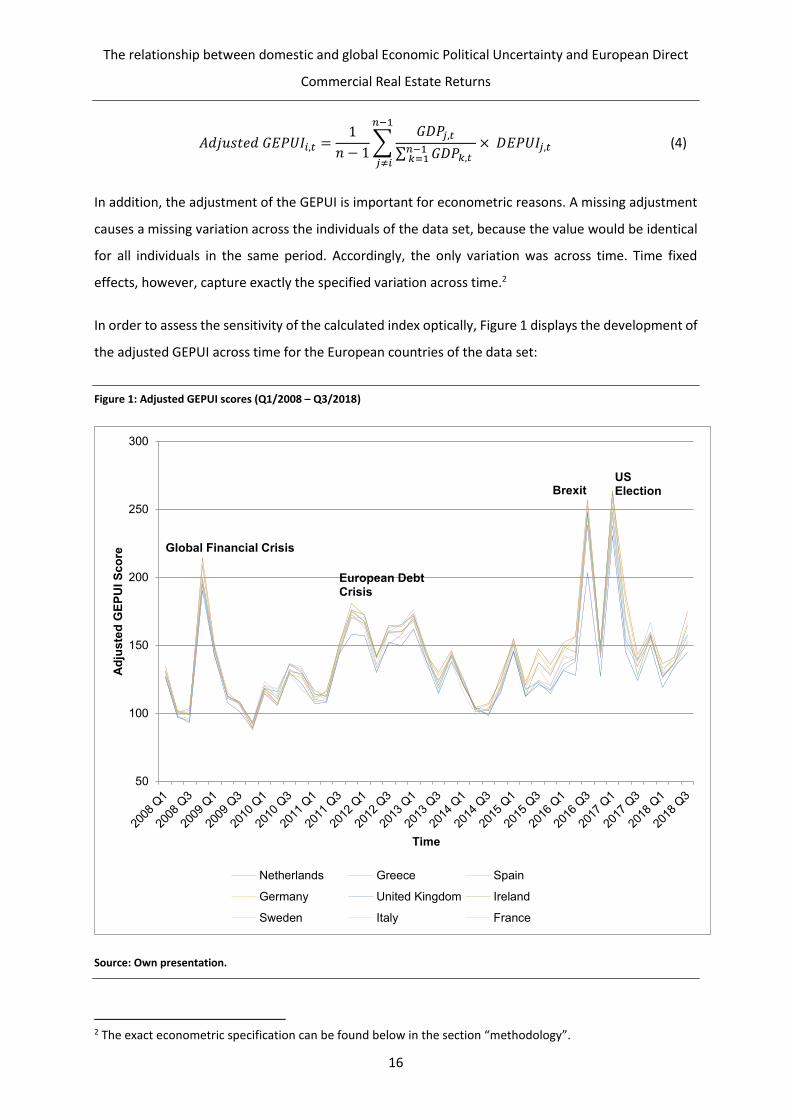
In order to assess the sensitivity of the calculated index optically, Figure 1 displays the development of
the adjusted GEPUI across time for the European countries of the data set:
Figure 1: Adjusted GEPUI scores (Q1/2008 – Q3/2018)
Source: Own presentation.
2 The exact econometric specification can be found below in the section “methodology”.
50
100
150
200
250
300
Ad
jus
ted
GE
PU
I S
co
re
Time
Netherlands Greece Spain
Germany United Kingdom Ireland
Sweden Italy France
Global Financial Crisis
European DebtCrisis
BrexitUS Election
The relationship between domestic and global Economic Political Uncertainty and European Direct
Commercial Real Estate Returns
17
The adjusted GEPUI clearly shows spikes in phases of prominent recent political events, which are
generally associated with periods of increased political uncertainty, like the global financial crisis in
08/09, the European debt crisis in 11/12, the 2016 Brexit referendum and the election of the 45th
President of the US. In sum, due to the extensive coverage of global economic output and clear
measurement of political turmoil, the DEPUI and the adjusted GEPUI both appear to be legitimate
proxies for DEPU and GEPU.
2.4 Data and descriptive statistics
The panel data covers observations from 20 European cities (n = 20) in 9 countries [2], with quarterly
observations for office properties from Q1/08 to Q3/18 (t = 43). The limiting factor for including
markets in the data set is the availability of the DEPUI, which needs to be observable for each market
in each period.
On the dependent side, total returns represent the variable of interest, because they are a classic and
well-known proxy for property investment performance. The total returns were obtained from CoStar.
The named data provider aggregated the returns from cash-flows as well as from a repeated-sale
regression model, which accounts for potential autocorrelation of the data. In order to isolate the
impact of the DEPU and GEPU on the direct total returns of direct real estate investments in Europe,
the literature review provides the foundation for the variable selection process of the controls. Here,
the empirically proven macroeconomic and real-estate-market-related variables were taken from the
literature for similar markets and data sets, in order to construct a robust set of control variables to
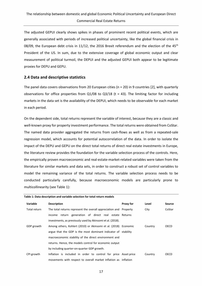
model the remaining variance of the total returns. The variable selection process needs to be
conducted particularly carefully, because macroeconomic models are particularly prone to
multicollinearity (see Table 1):
Table 1: Data description and variable selection for total return models
Variable Description Proxy for Level Source
Total return The total returns represent the overall appreciation and
income return generation of direct real estate
investments, as previously used by Akinsomi et al. (2018).
Property
Returns
City CoStar
GDP growth Among others, Kohlert (2010) or Akinsomi et al. (2018)
argue that the GDP is the most dominant indicator of
macroeconomic stability of the direct environment and
returns. Hence, the models control for economic output
by including quarter-on-quarter GDP growth.
Economic
stability
Country OECD
CPI growth Inflation is included in order to control for price
movements with respect to overall market inflation as
Asset price
inflation
Country OECD
The relationship between domestic and global Economic Political Uncertainty and European Direct
Commercial Real Estate Returns
18
noted by e.g. Bond & Seiler (1998) or Brooks & Tsolacos
(1999).
Unemployment
rate
Employment is often perceived as another indicator of
economic health and success. E.g. Liang & McIntosh
(1998) use the proxy to isolate the effect of labour-
market-related return generation.
Labor market
and income
Country OECD
Gov. bond (10
year maturity)
In line with previous literature (e.g. Macgregor &
Schwann, 2003; Baum, 2015), the government bond as an
indicator of the overall interest level of other investments
is incorporated.
Investment
environment
Country OECD
Economic
Sentiment
Index
In order to distinguish between economic sentiment and
EPU, a proxy for the former is introduced (e.g. Tsolacos et
al., 2014; Ling et al., 2015). Only by doing so, can the
impact of EPU be isolated from the overall economic
sentiment.
Economic
sentiment
Country Eurostat
Vacancy Office vacancy serves as an indication of the current state
of demand in a real estate market, so as to isolate the
impact of the markets’ demand side (e.g. in line with De
Wit & Van Dijk, 2003; Akinsomi et al., 2018).
Office demand City CoStar
Stock Stock indicates the available office floor space and
therefore shows the size of the market and / or the
building activity. It is supposed to control for the office
supply, in line with West & Worthington (2006).
Office
supply
City CoStar
Rent growth Year-on-year rent growth shows the income growth
potential of office buildings in the respective market, as
proposed by Clayton et al. (2009).
Income
expectations
City CoStar
Source: Own presentation.
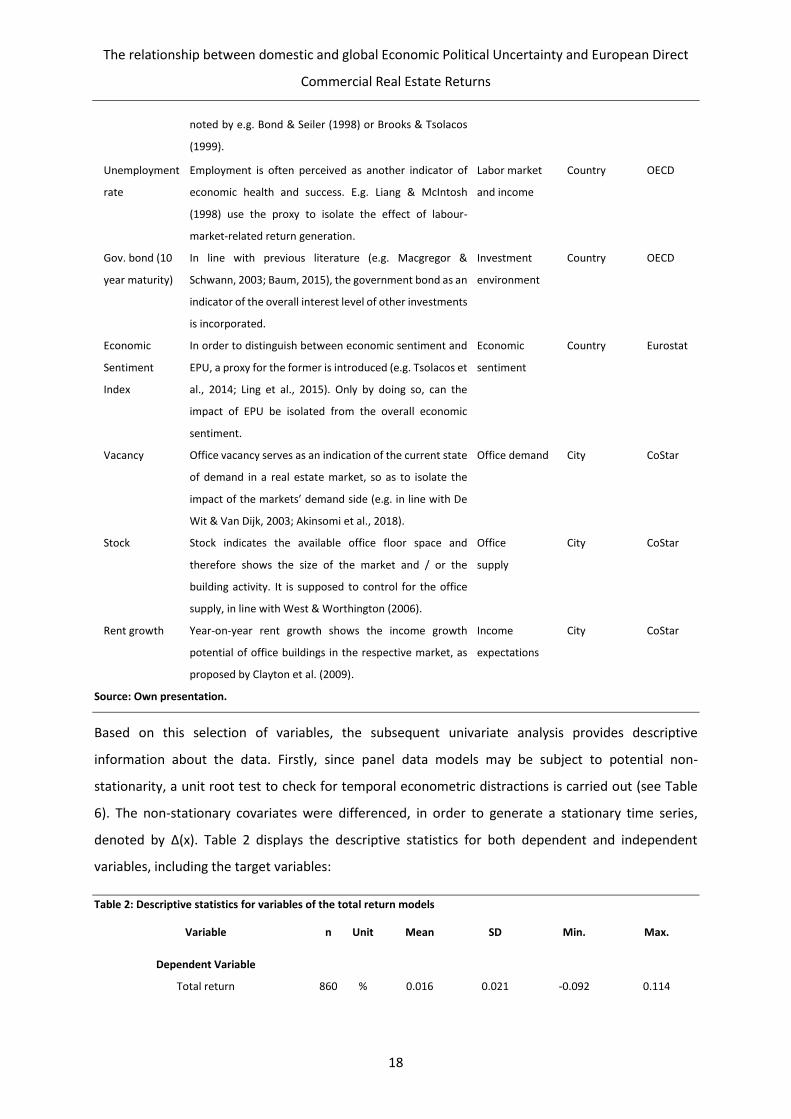
Based on this selection of variables, the subsequent univariate analysis provides descriptive
information about the data. Firstly, since panel data models may be subject to potential non-
stationarity, a unit root test to check for temporal econometric distractions is carried out (see Table
6). The non-stationary covariates were differenced, in order to generate a stationary time series,
denoted by ∆(x). Table 2 displays the descriptive statistics for both dependent and independent
variables, including the target variables:
Table 2: Descriptive statistics for variables of the total return models
Variable n Unit Mean SD Min. Max.
Dependent Variable
Total return 860 % 0.016 0.021 -0.092 0.114
The relationship between domestic and global Economic Political Uncertainty and European Direct
Commercial Real Estate Returns
19
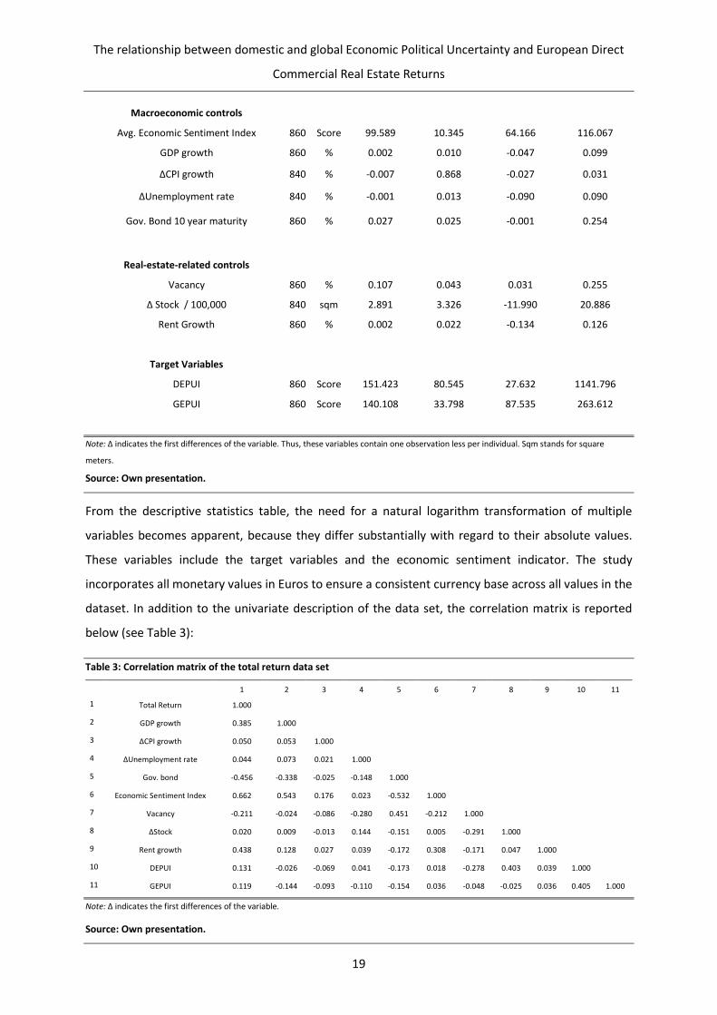
Macroeconomic controls
Avg. Economic Sentiment Index 860 Score 99.589 10.345 64.166 116.067
GDP growth 860 % 0.002 0.010 -0.047 0.099
∆CPI growth 840 % -0.007 0.868 -0.027 0.031
∆Unemployment rate 840 % -0.001 0.013 -0.090 0.090
Gov. Bond 10 year maturity 860 % 0.027 0.025 -0.001 0.254
Real-estate-related controls
Vacancy 860 % 0.107 0.043 0.031 0.255
∆ Stock / 100,000 840 sqm 2.891 3.326 -11.990 20.886
Rent Growth 860 % 0.002 0.022 -0.134 0.126
Target Variables
DEPUI 860 Score 151.423 80.545 27.632 1141.796
GEPUI 860 Score 140.108 33.798 87.535 263.612
Note: ∆ indicates the first differences of the variable. Thus, these variables contain one observation less per individual. Sqm stands for square
meters.
Source: Own presentation.
From the descriptive statistics table, the need for a natural logarithm transformation of multiple
variables becomes apparent, because they differ substantially with regard to their absolute values.
These variables include the target variables and the economic sentiment indicator. The study
incorporates all monetary values in Euros to ensure a consistent currency base across all values in the
dataset. In addition to the univariate description of the data set, the correlation matrix is reported
below (see Table 3):
Table 3: Correlation matrix of the total return data set
1 2 3 4 5 6 7 8 9 10 11
1 Total Return 1.000
2 GDP growth 0.385 1.000
3 ∆CPI growth 0.050 0.053 1.000
4 ∆Unemployment rate 0.044 0.073 0.021 1.000
5 Gov. bond -0.456 -0.338 -0.025 -0.148 1.000
6 Economic Sentiment Index 0.662 0.543 0.176 0.023 -0.532 1.000
7 Vacancy -0.211 -0.024 -0.086 -0.280 0.451 -0.212 1.000
8 ∆Stock 0.020 0.009 -0.013 0.144 -0.151 0.005 -0.291 1.000
9 Rent growth 0.438 0.128 0.027 0.039 -0.172 0.308 -0.171 0.047 1.000
10 DEPUI 0.131 -0.026 -0.069 0.041 -0.173 0.018 -0.278 0.403 0.039 1.000
11 GEPUI 0.119 -0.144 -0.093 -0.110 -0.154 0.036 -0.048 -0.025 0.036 0.405 1.000
Note: ∆ indicates the first differences of the variable.
Source: Own presentation.

The relationship between domestic and global Economic Political Uncertainty and European Direct
Commercial Real Estate Returns
20
From the correlation matrix, various insights can be obtained. Most importantly, the matrix displays
linear correlations that differ from zero for the dependent variable on one hand and the target
variables of interest on the other (DEPUI: 0.131; GEPUI: 0.119). Additionally and from a methodologic
point of view, other positive correlation values above 0.25 (in line with e.g. Oertel et al., 2020) are
defined as the threshold for econometric issues among the independent controlling covariates to
monitor multicollinearity (namely GDP growth, rent growth, vacancy and economic sentiment). Thus,
the estimation of a clean relationship between the dependent and the target variable are ensured.
Nonetheless, it needs to be highlighted, that the target variables potentially yield information and thus
reveal a correlation with other macroeconomic controls.3 Accordingly, a base model with all variables
is estimated, because the variable selection process above suggests the inclusion of all these variables
from an economic perspective. However, from an econometric perspective, the variables mentioned
above are systematically excluded in order to carry out robustness checks against potential distractions
due to the outlined multicollinearity.
2.5 Methodology
The methodological framework is a classic OLS estimation for the described panel data set. Total
returns are the dependent variable, and a multivariate model is specified to estimate the parameters
for the covariates:
Total Returni,t = βi,t−kmi,t−k + βi,t−kri,t−k + βi,t−kdomestic EPUi,t−k
+ βt−kglobal EPUi,t−k + βttimet + βicityi + εi,t (5)
Here, the dependent total return observed in a market i in quarter t is a function of the
abovementioned domestic macroeconomic controls captured in vector mi,t−k, and real-estate-related
variables in the vector ri,t−k. More importantly, the scalars domestic EPUi,t−k and global EPUt−k yield
the proxies for the variables of interest:
mi,t−k =
{
ln (Economic Sentiment)
GDP growth∆(CPI growth)
∆(Unemployment rate)Gov. Bond 10 yr maturity
(6)
ri,t−k = {
Vacancy
∆(Stock)Rent growth
(7)
3 The orthogonalization of the relationship can be an alternative methodological approach to separate the information from the target variable and the control set.
The relationship between domestic and global Economic Political Uncertainty and European Direct
Commercial Real Estate Returns
21
domestic EPUi,t−k = ln (DEPUI) (8)
global EPUi,t−k = ln (adjusted GEPUI) (9)
Since there may be temporal heterogeneity of returns, dummy variables labeled as time for each year
of the sample are incorporated (base = 2008). City heterogeneity is captured throughout all models by
including city dummies (as noted by Monfared & Pavlov, 2019). Frankfurt is chosen as the reference,
because of its geographic centrality, and εi,t represents the error term for each specification.
Furthermore, the relationship between non-fundamentals and direct real estate returns are known for
their lagged effects (Case & Shiller, 2003; Case et al., 2014). Accordingly, each model contains lagged
terms up to the fourth quarter for the covariates (k = 4, in line with Antonakakis et al., 2015).
An additional remark needs to be made concerning the potential autocorrelation of the dependent
variable. In order to account for potential autocorrelation, literature has repeatedly used vector
autoregressive models (e.g. Clayton et al., 2009). However, since the present study uses a ML-based
OLS estimation in line with Akinsomi et al. (2018), it needs to be highlighted, that the data uses
transaction-based capital value returns. In contrast to appraisal-based appreciation, these returns
generally do not suffer from appraisal smoothing due to anchoring (in line with Geltner et al., 2003).
Therefore, no autoregressive component is added.
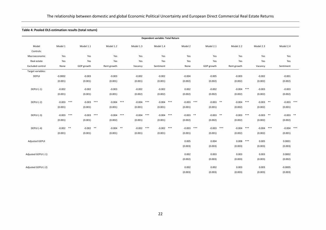
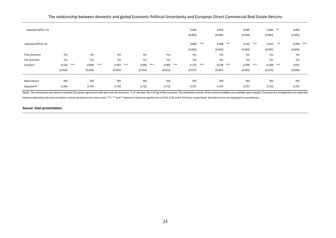
2.6 Empirical results
The results for the OLS models can be found below (see Table 4). The base model in the first column
includes all control variables, which were identified above in related studies as important determinants
of the total returns. The subsequent models individually exclude the variables of GDP growth, rent
growth, vacancy and the economic sentiment index, so as to check for econometric robustness of the
beta coefficients of the target variables. The specified variables were systematically exchanged, due to
the reported correlation findings. From an economic point of view, the first column displays the central
and most important econometric models, containing all relevant controls. Subsequent models are
used to conduct various robustness checks.
The models 2.x are specified to assess the second hypothesis regarding the impact of the GEPU. Here,
the DEPUI scores are considered to be part of the control variables in addition to the remaining controls
of the base model specification. The models are then extended by the adjusted GEPUI scores.
The relationship between domestic and global Economic Political Uncertainty and European Direct Commercial Real Estate Returns
22
Table 4: Pooled OLS estimation results (total return)
Dependent variable: Total Return
Model Model 1
Model 1.1
Model 1.2
Model 1.3
Model 1.4
Model 2
Model 2.1
Model 2.2
Model 2.3 Model 2.4
Controls:
Macroeconomic Yes
Yes
Yes
Yes
Yes
Yes
Yes
Yes
Yes Yes
Real estate Yes
Yes
Yes
Yes
Yes
Yes
Yes
Yes
Yes Yes
Excluded control None
GDP growth
Rent growth
Vacancy
Sentiment
None
GDP growth
Rent growth
Vacancy Sentiment
Target variables:
DEPUI -0.0002 -0.003 -0.003 -0.002 -0.002 -0.004 -0.005 -0.003 -0.002 -0.001
(0.001) (0.001) (0.001) (0.001) (0.001) (0.002) (0.002) (0.002) (0.002) (0.002)
DEPUI (-1) -0.002 -0.002 -0.003 -0.002 -0.002 0.002 -0.002 -0.004 *** -0.003 -0.003
(0.001) (0.001) (0.001) (0.002) (0.002) (0.002) (0.002) (0.002) (0.002) (0.002)
DEPUI (-2) -0.003 *** -0.003 *** -0.004 *** -0.004 *** -0.004 *** -0.003 *** -0.003 ** -0.004 *** -0.003 ** -0.003 ***
(0.001) (0.001) (0.001) (0.001) (0.001) (0.001) (0.001) (0.002) (0.002) (0.001)
DEPUI (-3) -0.003 *** -0.003 *** -0.004 *** -0.004 *** -0.004 *** -0.003 ** -0.003 ** -0.003 *** -0.003 ** -0.003 **
(0.001) (0.001) (0.002) (0.001) (0.001) (0.002) (0.002) (0.002) (0.002) (0.002)
DEPUI (-4) -0.002 ** -0.002 ** -0.004 ** -0.002 *** -0.002 *** -0.003 *** -0.003 *** -0.004 *** -0.004 *** -0.004 ***
(0.001) (0.001) (0.001) (0.001) (0.001) (0.001) (0.001) (0.002) (0.002) (0.001)
Adjusted GEPUI 0.005 0.004 0.008 *** 0.005 0.0001
(0.003) (0.003) (0.003) (0.003) (0.003)
Adjusted GEPUI (-1) 0.002 0.003 0.003 0.003 0.0002
(0.002) (0.003) (0.003) (0.003) (0.002)
Adjusted GEPUI (-2) 0.002 0.002 0.003 0.003 -0.0005
(0.003) (0.003) (0.003) (0.003) (0.003)
The relationship between domestic and global Economic Political Uncertainty and European Direct Commercial Real Estate Returns
23
Adjusted GEPUI (-3) 0.004 0.004 0.005 0.006 ** 0.005
(0.003) (0.003) (0.003) (0.003) (0.003)
Adjusted GEPUI (-4) 0.008 *** 0.008 *** 0.010 *** 0.010 ** 0.008 ***
(0.003) (0.003) (0.003) (0.003) (0.003)
Time dummies Yes Yes Yes Yes Yes Yes Yes Yes Yes Yes City dummies Yes Yes Yes Yes Yes Yes Yes Yes Yes Yes Constant -0.140 *** -0.099 *** -0.303 *** 0.090 *** -0.009 *** -0.276 *** -0.238 *** -0.490 *** -0.368 *** 0.031
(0.056) (0.049) (0.065) (0.014) (0.014) (0.075) (0.067) (0.082) (0.079) (0.036)
Observations 760 760 760 760 760 760 760 760 760 760
Adjusted R2 0.766 0.764 0.702 0.722 0.753 0.767 0.767 0.707 0.726 0.755
Notes: The estimations are based on pooled OLS panel regressions with year and city dummies. “(-t)” denotes the t-th lag of the covariate. The estimation results of the control variables are available upon request. Dummies are included but not reported.
Heteroscedasticity and autocorrelation-robust standard errors were used. ***, ** and * represent statistical significance at 0.01, 0.05 and 0.10 levels, respectively. Standard errors are displayed in parentheses.
Source: Own presentation.

The relationship between domestic and global Economic Political Uncertainty and European Direct
Commercial Real Estate Returns
24
With regard to the overall explanatory power of the econometric models, the results generally yield
adjusted R² values around 0.75 – 0.80 for the total returns, which are in line with those in the literature
(e.g. recently from Akinsomi et al., 2018). The potential threat of omitted variable bias is sufficiently
accounted for, because the explanatory power of the models of the present study yields similar results
to existing equivalent studies. Heavy distractions from omitted variables in the control variable set are
unlikely to be present. The incremental value of the newly added variables cannot be extracted directly
from Table 4. Therefore the same models as above are estimated, but without the DEPUI and GEPUI
variables. By doing so, it is possible to show differences in explanatory power of the models without
the targets and thus show the incremental value of the newly added target variables (see Table 5):4
Table 5: Explanatory power of total return models without DEPUI / GEPUI
Model Model 1
Model 1.1
Model 1.2
Model 1.3
Model 1.4
Controls:
Macroeconomic Yes
Yes
Yes
Yes
Yes
Real estate Yes
Yes
Yes
Yes
Yes
Excluded control None
GDP growth
Rent growth
Vacancy
Sentiment
Observations 760 760 760 760 760
Adjusted R2 0.757 0.755 0.685 0.714 0.742
Source: Own presentation.
As displayed on Table 5, the explanatory power of the models without the DEPUI and the GEPUI reveal
lower adjusted R² values for all specifications in comparison to the models reported above. Thus, the
introduction of the DEPUI provides an initial value in explanatory power for the modelling of total
returns. Since the explanatory power of the models with the GEPUI is again higher than the models
including only the DEPUI, the incremental value for both variables can be confirmed (see Table 4).
However, the deltas of the explanatory power values between the models, including the GEPUI proxy
and those excluding the specified variable are limited. Thus, general statistical significance can be
observed, whereas the low explanatory power of the GEPUI proxy needs to be acknowledged.
Turning to the individual coefficients, the empirical results show c.p. on average a statistically
significant negative impact of all lags between the second and fourth period on the DEPUI and the total
returns across all specifications. The beta coefficients for the DEPUI reveal a range between -0.003 and
-0.004. Since the target variables are transformed by a natural logarithm and the index is denoted in a
4 Estimates for the beta coefficients are explicitly not reported, because these are of minor interest only. In order to isolate the incremental value of the estimates for the DEPUI and GEPUI, however, the explanatory power of the models is sufficient.

The relationship between domestic and global Economic Political Uncertainty and European Direct
Commercial Real Estate Returns
25
number and the total returns in percentages, the c.p. interpretation of the estimated coefficients is as
follows. A one unit increase in DEPUI results on average, c.p. in a decrease in total return of -0.003 – (-
0.004) % and vice versa, because the total returns are denoted on a decimal scale.5 Accordingly, the
marginal effect needs to be divided by 100, whereas the recalculation from decimal figures to
percentages requires the multiplication by 100. Thus, the coefficient can be interpreted as it is
reported in the regression output. The relatively small magnitude of the marginal effect is also as
expected, because the fundamental determinants such as GDP growth etc. are assumed to be the
dominant impact factors. With regard to the first hypothesis, there is no empirical proof for
falsification. In fact, the results support the idea of a c.p. performance lowering effect of increased
DEPU, and vice versa.
Nonetheless, the empirical results reveal a statistical significant negative relationship between the
DEPUI and total returns. This finding is somewhat puzzling, because the correlation matrix showed a
positive correlation between total returns and the DEPUI variable. In this context, a methodological
remark needs to be made. The Pearson correlation coefficient identifies a linear relationship between
two variables without an a priori assumption of direction. The beta coefficients on the other hand
estimate the linear relationship between a dependent and an independent variable, explicitly given
other impact factors. Especially for a non-fundamental factor such as the DEPU, there is no economic
justification for an impact without other controlling variables. Thus, the significance of the correlation
coefficient is severly limited. Other and most importantly, fundamental impact factors, need to be
included in total return models. These models have to be analyzed as a whole and with an economically
justified specification of a joint impact pattern.6
Secondly, the extended models, which also include the adjusted GEPUI score, yield robust statistically
significant contrary signs for the total returns, predominantly in the fourth lag. Here the beta
coefficients show betas of 0.008 – 0.010. A change in one unit of the GEPUI results on average, c.p. to
a positive change of 0.008 – 0.010 %, and vice versa.7 Interestingly, the betas are larger than for the
DEPUI. Thus, the individual strength of effect of the GEPUI is larger than for each of the lags of the
DEPUI. In sum, it can be stated that increasing uncertainty in foreign countries supports the
performance of domestic commercial properties. This finding provides evidence for the existence of a
potential “safe haven effect”, namely the performance boost of domestic properties in phases of
5 Accordingly, an increase in 100 points in DEPUI for example leads to 0.3 - 0.4% or 30 - 40 base points total return, and vice versa. 6 The justification for the present specification is presentedabove in the section “Data and descriptive statistics”. 7 In line with the interpretation of the DEPUI, a rise of 100 points in GEPUI leads to an increase of 0.8 – 1.0 % or 80 – 100 base points, and vice versa.
The relationship between domestic and global Economic Political Uncertainty and European Direct
Commercial Real Estate Returns
26
elevated foreign EPU. For other lags, the statistical significance of coefficients is not robust across the
model variations. Besides the statistical significance, especially for the contemporary coefficient of the
GEPUI, the economic significance is questionable. A direct effect in the same period is economically
problematic, because market agents are expected to price uncertainty in later periods, as mentioned
by Case & Shiller (2003) or Case et al., (2014).
The abovementioned expectations of a negative impact of GEPU on domestic commercial real estate
returns or the second hypothesis can thus be falsified. Instead, the results are in line with those findings
from the residential sector, which reveal c.p. a positive relationship between total returns and GEPUI.
An increase in demand by domestic as well as foreign market agents for local properties constitutes a
credible channel for commercial properties.
2.7 Conclusion and further remarks
This study presents a new approach to explaining the relationship between EPU and direct commercial
real estate returns in an OLS framework for a panel data set. The study reveals the impact of DEPU and
GEPU on total returns of major European commercial property markets. The main finding is that on
the one hand, DEPU shows c.p. on average a lagged statistically significant negative effect on total
returns, whereas GEPU has c.p. a positive impact on the total returns of domestic properties.
Thus, GEPU does not directly transmit a negative effect from foreign countries to commercial real
estate returns into another country. Thus, the potential for spillover effects, as outlined in the
macroeconomic literature, cannot be confirmed for commercial real estate markets. Instead, the
results of the present study confirm the empirical findings of previous articles referring to a “safe haven
effect” (e.g. Badarinza & Ramadorai, 2018). Nonetheless, for both parts of the EPU, the impact is much
smaller than for the fundamental impact factors, as can be extracted from the incremental values of
the models without the DEPUI and the GEPUI (as reported on Table 4 & 5).
The transmission channels from EPU to the total returns are yet to be quantified empirically. This
applies to the DEPU as well as the GEPU. The theoretical background underlines the importance of the
appreciation side as main driver for the EPU to influence total returns, as discussed in the literature
review. However, the exact channels, especially for the GEPU and the “safe haven effect”, remain
uncertain and should be subjected to further investigation. Cross-border investments may be a
plausible transmission channel in this context. Since potential additional foreign demand could explain
increased total returns, an subsequent empirical study on cross-border capital flows as a function of
political uncertainty, appears to be promising. A statistically significant, c.p. and on average positive

The relationship between domestic and global Economic Political Uncertainty and European Direct
Commercial Real Estate Returns
27
impact of GEPU on cross-border capital flows was the logical working hypothesis for assessing the
transmission channel.
Additional research could also be conducted on other usage types. In this context, especially logistic
properties may be of interest, since the asset class is known for its heavy dependency on global trade
and the political stability of international economic linkages (Boutchakova et al., 2012). A potential
proxy for quantifying the impact of trade-related political uncertainties could be the Trade Policy
Uncertainty (TPU) Index from the Federal Reserve Board. Lastly, future research could integrate the
bodies of literature on different measures of EPU (for a broader discussion, see Ghirelli et al., 2019)
with machine learning approaches such as Braun et al. (2019). A potentially beneficial outcome could
be machine-learning-based EPU indices that learn dynamically to adjust the textual tone of the
underlying dictionary.
Some practical implications can be derived especially for the risk management of investors from a
corporate point of view, as well as for political stakeholders from an administrative perspective. The
present study underlines the importance of monitoring the political environment, both domestically
and globally, since they represent statistically significant drivers of direct commercial property returns.
Thus, risk surveillance procedures should be implemented to monitor the political environment of the
assets, especially regarding the potential acquisition of properties in regions of elevated DEPU. This
would be especially fruitful, because the study reveals a timely lagged impact pattern. Thus, investors
could gain a competitive advantage over other market participants who do not monitor the political
environment due to the correct anticipation and pricing of EPU-related risk. A possible specific
implementation could be an early warning system, which tracks the development of the political
environment in order to predict potential downturns in future total returns. In combination with the
abovementioned machine-learning-based future research, a joint approach to construct an early
warning system based on dynamic learning algorithms could be the best practice for applied risk
management in real estate to anticipate downturns. For political stakeholders, the results should
increase their awareness of the potentially negative impact of uncertainty-inducing statements. By
contrast, the use of risk-averse communication of administrative personnel may protect domestic real
estate markets by decreasing the EPU of the news media landscape.

The relationship between domestic and global Economic Political Uncertainty and European Direct
Commercial Real Estate Returns
28
2.8 Bibliography
Akinsomi, O., Mkhabela, N., & Taderera, M. (2018). The role of macro-economic indicators in
explaining direct commercial real estate returns: evidence from South Africa. Journal of
Property Research, 35(1), pp. 28–52.
Antonakakis, N., Gupta, R., & Andre, C. (2015). Dynamic Co-Movements between Economic Policy
Uncertainty and Housing Market Returns. Journal of Real Estate Portfolio Management, 21(1),
pp. 53–60.
Badarinza, C., & Ramadorai, T. (2018). Home away from home? Foreign demand and London house
prices. Journal of Financial Economics, 130(3), pp. 532–555.
Baker, K., & Saltes, D. (2005). Architecture Billings as a Leading Indicator of Construction. Business
Economics, 40(4), pp. 67–73.
Baker, M. P., & Wurgler, J. (2007). Investor Sentiment in the Stock Market. Journal of Economic
Perspectives, 21(2), pp. 129–152.
Baker, M. P., Wurgler, J., & Yuan, Y. (2011). Global, Local, and Contagious Investor Sentiment. Journal
of Financial Economics, 104(2), pp. 272–287.
Ball, M., Lizieri, C., & McGregor, B. D. (2009). The economics of commercial property markets (2. ed.).
Routledge. London.
Baum, A. (2015). Real Estate Investment. Routledge. London.
Bond, M., & Seiler, M. (1998). Real Estate Returns and Inflation: An Added Variable Approach. Journal
of Real Estate Research, 15(3), pp. 327–338.
Boutchkova, M., Doshi, H., Durnev, A., & Molchanov, A. (2012). Precarious Politics and Return
Volatility. Review of Financial Studies, 25(4), pp. 1111–1154.
Braun, J., Hausler, J., & Schäfers, W. (2019). Artificial intelligence, news sentiment, and property
market liquidity. Journal of Property Investment & Finance, ahead-of-print.
Brooks, C., & Tsolacos, S. (1999). The impact of economic and financial factors on UK property
performance. Journal of Property Research, 16(2), pp. 139–152.
The relationship between domestic and global Economic Political Uncertainty and European Direct
Commercial Real Estate Returns
29
Case, K. E., & Shiller, R. J. (1989). The Efficiency of the Market for Single-Family Homes. American
Economic Review, 79(1), pp. 125–137.
Case, K. E., & Shiller, R. J. (2003). Is There a Bubble in the Housing Market? Brookings Papers on
Economic Activity, 34(2), pp. 299–362.
Case, K. E., Shiller, R. J., & Thompson, A. (2014). What Have They Been Thinking? Homebuyer Behavior
in Hot and Cold Markets — A 2014 Update. Cowles Foundation Discussion Paper, 1876.
Chaney, A., & Hoesli, M. (2012). Transaction-Based and Appraisal-Based Capitalization Rate
Determinants. Swiss Finance Institute Research Paper Series, 12-28.
Clayton, J., Ling, D. C., & Naranjo, A. (2009). Commercial Real Estate Valuation: Fundamentals Versus
Investor Sentiment. The Journal of Real Estate Finance and Economics, 38(1), pp. 5–37.
Colombo, V. (2013). Economic policy uncertainty in the US: Does it matter for the Euro area? Economics
Letters, 121(1), pp. 39–42.
Davis, S. J. (2016). An Index of Global Economic Policy Uncertainty. NBER Working Papers, 22740.
French, N. (2019). Brexit and the Moon. Journal of Property Investment & Finance, 37(6), pp.
522–523.
Geltner, D., MacGregor, B. D., Schwann, G. M. (2003). Appraisal Smoothing and Price Discovery in Real
Estate Markets. Urban Studies, 40(5-6), pp. 1047 - 1064.
Ghirelli, C., Gil, M., Pérez, J. J., & Urtasun, A. (2019). Measuring economic and economic policy
uncertainty and their macroeconomic effects: the case of Spain. Empirical Economics, 34(3),
pp. 437–468.
Gunnelin, A., Hendershott, P., Hoesli, M., & Söderberg, B. (2004). Determinants of Cross‐Sectional
Variation in Discount Rates, Growth Rates and Exit Cap Rates. Real Estate Economics, 32(2),
pp. 217–237.
Hekman, J. S. (1985). Rental Price Adjustment and Investment in the Office Market. Real Estate
Economics, 13(1), pp. 32–47.
Karakozova, O. (2005). Modelling and Forecasting Property Rents and Returns. School of Economics
and Business Administration, Helsinki.
The relationship between domestic and global Economic Political Uncertainty and European Direct
Commercial Real Estate Returns
30
Kohlert, D. (2010). The determinants of regional real estate returns in the United Kingdom: A vector
error correction approach. Journal of Property Research, 27(1), pp. 87–117.
Liang, Y., McIntosh, W. (1998). Employment growth and real estate return: Are they linked? Journal of
Real Estate Portfolio Management, 4(2), pp. 125–133.
Ling, D. C. (1997). Economic Risk Factors and Commercial Real Estate Returns. Journal of Real Estate
Finance and Economics, 15(3), pp. 283–307.
Ling, D. C., Ooi, J., & Le, T. (2015). Explaining House Price Dynamics: Isolating the Role of
Nonfundamentals. Journal of Money, Credit and Banking, 47(1), pp. 87–125.
MacGregor, B., & Schwann, G. (2003). Common features in UK commercial real estate returns. Journal
of Property Research, 20(1), pp. 23–48.
Marcato, G., & Nanda, A. (2016). Information Content and Forecasting Ability of Sentiment Indicators:
Case of Real Estate Market. Journal of Real Estate Research, 38(2), pp. 165–203.
Monfared, S., & Pavlov, A. (2019). Political Risk Affects Real Estate Markets. The Journal of Real Estate
Finance and Economics, 58(1), pp. 1–20.
Netzell, O. (2009). A study of micro‐level variation in appraisal‐based capitalisation rates. Journal of
Property Research 26(3), pp. 235-263.
Oertel, C., Gütle, T., Klisa, B., & Bienert, S. (2019). US real estate as target assets for European investors.
Journal of Property Investment & Finance, 37(4), pp. 398–404.
Oertel, C., Willwersch, J., & Cajias, M. (2020). Do Cross-Border Investors Benchmark Commercial Real
Estate Markets? Evidence from Relative Yields and Risk Premia for a European Investment
Horizon. Journal of European Real Estate Research, 13(1), pp. 83–103.
Smales, L. A. (2017). “Brexit”: A Case Study in the Relationship Between Political and Financial Market
Uncertainty. International Review of Finance, 17(3), pp. 451–459.
Tsolacos, S., Brooks, C., & Nneji, O. (2014). On the Predictive Content of Leading Indicators: The Case
of U.S. Real Estate Markets. Journal of Real Estate Research, 36(4), pp. 541–574.
West, T., & Worthington, A. C. (2006). Macroeconomic risk factors in Australian commercial real estate,
listed property trust and property sector stock returns. Journal of Financial Management of
Property and Construction, 11(2), pp. 105–116.

The relationship between domestic and global Economic Political Uncertainty and European Direct
Commercial Real Estate Returns
31
Wit, I., & van Dijk, R. (2003). The Global Determinants of Direct Office Real Estate Returns. The Journal
of Real Estate Finance and Economics, 26(1), pp. 27–45.

The relationship between domestic and global Economic Political Uncertainty and European Direct
Commercial Real Estate Returns
32
2.9 Appendix
Table 6: Levin-Lu-Chu stationarity test for total return model variables
Variable Test statistic P-Value Variable with ∆ Test statistic P-Value
Dependent Variables
Total return -2.026 0.021
Macroeconomic variables
GDP growth -8.509 0.000
CPI growth 2.817 0.998
CPI growth ∆ -20.714 0.000
Unemployment rate 17.571 1.000
Unemployment rate ∆ -237.348 0.000
Gov. Bond 10 yr. maturity -3.435 0.000
Real-estate-related
variables
Vacancy -6.534 0.000
Stock -0.390 0.348
Stock ∆ -3.003 0.001
Rent Growth -12.858 0.000
Target Variables
DEPUI -18.964 0.000
GEPUI -5.247 0.000
Note: ∆ indicates the first differences of the variable. The maximum lag was set to 4, since our maximum time lag within the econometric model is
equals to 4.
Source: Own presentation.

33
3 Do Cross-Border Investors Benchmark
Commercial Real Estate Markets? Evidence from
Relative Yields and Risk Premia for a European
Investment Horizon
Cay Oertel, Jonas Willwersch, Marcelo Cajias
Journal of European Real Estate Research, 13(1) (published)
Abstract
The purpose of the study is to introduce a new perspective on determinants of cross-border
investments in commercial real estate, namely the relative attractiveness of a target market. So far,
the literature has analyzed only absolute measures of investment attractiveness as determinants of
cross-border investment flows. The empirical study uses a classic OLS estimation for a European panel
data set containing 28 cities in 18 countries, with quarterly observations from Q1/2008 – Q3/2018.
After controlling for empirically proven explanatory covariates, the model is extended by the new
relative measurement based on relative yields/cap rates and relative risk premia. Additionally, the
study applies a generalized additive mixed model, to investigate a potentially nonlinear relationship.
The study finds on average a c.p., statistically significant lagged influence of the proxy for relative
attractiveness. Nonetheless, a differentiation is needed; relative risk premia are statistically significant,
whereas relative yields are not. Moreover, the generalized additive mixed model confirms a nonlinear
relationship for relative risk premia and cross-border transaction volumes.
Do Cross-Border Investors Benchmark Commercial Real Estate Markets? Evidence from Relative
Yields and Risk Premia for an European Investment Horizon
34
3.1 Introduction
Direct cross-border investments in commercial properties have increased steadily over the past two
decades. Accordingly, the related research and market participants have demonstrated an increased
interest in understanding the determinants of capital flows across national borders.
Institutional economics theory defines the attractiveness of a target investment market as a function
of its socio-economic environment and institutional framework (Fuerst et al., 2015). In line with this
theory, Lieser & Groh (2014) provided empirical evidence of the importance of economic growth,
demographics, urbanization or political stability of a particular country. However, other authors
highlight the importance of additional factors on cross-border capital flows. Yet, the literature has
described the attractiveness of an investment location solely with absolute measures of potential
determinants.
The present article introduces a new approach to explaining inflowing cross-border capital into real
estate market, namely relative attractiveness. As opposed to previous studies, it sheds light on
whether cross-border investors benchmark investment opportunities against each other. More
precisely, the study investigates whether relative attractiveness in the form of relative yields or relative
risk premia determines the capital allocation of investors. In this context, the analysis concentrates on
European real estate markets, as classic prime European investment markets represent rather
homogenous, substantially economically integrated and geographically densely located competing
investment markets. Thus, relative attractiveness appears to be a potential driver, but solely for
geographical reasons. At the same time, as outlined by Devaney et al. (2017a), data availability issues
in Europe especially at the city level have hampered research on cross-border transaction activity.
Consequently, work at this level requires new empirical evidence.
The paper is structured as follows: A comprehensive literature review builds the foundation for the
empirical study. The essence is the existing body of literature on the one hand, while legitimating the
approach of introducing relative attractiveness as a further driver of cross-border investment activity
on the other. The section concludes with a statement of the hypotheses for the empirical work.
Subsequently, the paper outlines the data set and research design, including the new target variables
for measuring the relative attractiveness of a city. It also reports the descriptive statistics. Since
macroeconomic models on cross-border investment activities in real estate markets are subject to
severe methodological challenges and data availability issues, the variable selection process and the
econometric approaches are discussed extensively. Afterwards, the empirical results are presented,
and some conclusions drawn.
Do Cross-Border Investors Benchmark Commercial Real Estate Markets? Evidence from Relative
Yields and Risk Premia for an European Investment Horizon
35
3.2 Related literature and hypotheses derivation
Several studies have tried to identify common determinants of cross-border real estate investment in
the view of various investor types and investment styles. From a portfolio point of view, national and
regional diversification benefits are often perceived as one of the driving forces behind international
capital allocation in real estate. Amongst others, Sirmans & Worzala (2003) and Holsapple et al. (2006)
argued that the diversification of country-specific economic drivers is decisive. The abovementioned
literature on diversification, however, often suffers from data unavailability on investors who cause
the transaction flows. Thus, the relationship between investor, relevant portfolio and investment flow
cannot be established. Accordingly, a growing body of literature has focused on investor-unrelated and
general institutional and macroeconomic determinants of cross-border investment flows. Hence,
several studies have investigated investment drivers and barriers on global and regional levels.
A comprehensive empirical study on the economic and institutional environment was conducted by
Lieser & Groh (2011). First, they defined six relevant areas for cross-border investments, namely
economic activity, real estate investment opportunities, the depth and sophistication of capital
markets, investor protection and the legal framework, administrative burdens and regulatory
limitations, as well as the socio-cultural and political environment. In a second step, they quantified
the attractiveness of countries via a composite index approach. In a second paper, Lieser & Groh (2014)
analyzed which of these country characteristics impact on foreign real estate investment volumes.
After investigating 47 countries, they illustrated a significant relationship between foreign real estate
investment activity as the dependent variable and real estate investment opportunities, the depth and
sophistication of capital markets, investor protection and the legal framework, administrative burdens
and regulatory limitations as explanatories. In line with this study, Devaney et al. (2017a) found that
in European and Asian Pacific countries, the size and wealth of a country, the specific country risk, and
property rights, as well as the performance of the real estate markets, mainly determine transaction
activity.8
A second stream of papers narrowed the geographic focus and carried out empirical studies on
national or city-level determinants. Chin et al. (2006) and Pi-Ying Lai & Fischer (2007) identified
patterns in Asian regions and cities. They highlighted that political stability and legal regulations, as
well as sound financial and economic structures, and the strength and stability of the current economy,
are of major importance for investments in these areas. He & Zhu (2010) added that aside from a
8 Transaction activity was measured from turnover rates of the total transaction volume taking foreign and domestic investments together.
Do Cross-Border Investors Benchmark Commercial Real Estate Markets? Evidence from Relative
Yields and Risk Premia for an European Investment Horizon
36
favorable institutional environment, Chinese cities and their real estate markets attract capital through
population and market size. For Eastern Europe, McGreal et al. (2001) argued that foreign real estate
investment activity can be affected negatively, especially by non-transparency, overall economic
conditions, corruption, and bureaucracy. Salem & Baum (2016) found that foreign money flows into
real estate markets in the Middle East and northern African countries are mainly influenced by political
stability. Devaney et al. (2017b) investigated transaction activity in U.S. metropolitan office markets.
Economic growth and market size were positively related to turnover rates, whereas vacancy rates and
risk showed a negative relationship.
The studies presented thus far indicate that the institutional framework and the macroeconomic
conditions shape cross-border investment. However, real-estate-related factors also influence cross-
border capital flows, since investment success is not only linked to country characteristics, but also to
the underlying real estate market and the property itself. A number of authors have therefore included
various proxies of real estate markets into their investigations. Ford et al. (1998) found that market
activity and rent levels of US real estate markets determine foreign investment behavior. Moreover,
according to Laposa & Lizieri (2005) office construction attracts foreign investment in Eastern Europe.
For China, He and Zhu (2010) showed that aside from satisfactory demographic conditions, already
invested foreign capital attracts both foreign developers as well as more cross-border investors. In
addition, Rodríguez & Bustillo (2010), Gholipour Fereidouni & Ariffin Masron (2013) and Farzanegan &
Fereidouni (2014) observed market-specific property prices to be influential. Interestingly, Gholipour
Fereidouni & Ariffin Masron (2013) found real estate market transparency to be an important
determinant for foreign investors, but Farzanegan & Fereidouni (2014) did not confirm this finding.
Fuerst et al. (2015) established a positive relationship between market liquidity and cross-border
capital inflows, since the ability to sell properties increases. Devaney et al. (2017a) noted a negative
relationship between office vacancy rates and turnover rates. With particular respect to property
characteristics, Devaney et al. (2018) demonstrated that cross-border investors in U.S. gateway cities
favor large and new buildings close to CBD locations.
To gauge investment potential and to explain capital flows, risk characteristics such as the previously
documented institutional, macroeconomic and real estate related variables constitute crucial
considerations. Nonetheless, income opportunities, which may additionally influence investors, can be
assessed by analyzing yields and pricing. A common method of early real estate investment evaluation
is the capitalization (cap) rate. It is usually computed as the ratio of a property’s net operating income
to its price and therefore serves as an opportunity to compare assets and markets. When assessing the

Do Cross-Border Investors Benchmark Commercial Real Estate Markets? Evidence from Relative
Yields and Risk Premia for an European Investment Horizon
37
main determinants of cap rates, the literature refers to the Gordon-growth model (see e.g. McAllister
& Nanda (2016a)):
𝐶𝑎𝑝𝑖𝑡𝑎𝑙𝑖𝑧𝑎𝑡𝑖𝑜𝑛 𝑅𝑎𝑡𝑒 = 𝑁𝑜𝑚𝑖𝑛𝑎𝑙 𝑟𝑖𝑠𝑘-𝑓𝑟𝑒𝑒 𝑟𝑎𝑡𝑒 + 𝑅𝑖𝑠𝑘 𝑝𝑟𝑒𝑚𝑖𝑢𝑚 − 𝐼𝑛𝑐𝑜𝑚𝑒 𝑔𝑟𝑜𝑤𝑡ℎ (10)
The nominal risk-free rate is often approximated by a long-term government bond, whereas the risk
premium marks the difference between the government bond and an individual asset yield. The
income growth measures the growth of rents or net operating income. Research companies, brokers
and other market participants regularly provide cap rates and therefore enable investors to measure
and compare investment potential. To the best knowledge of the authors, only a little research has
investigated the cap rate/yield and investment flow relationship, even though a direct relationship
between both seems reasonable.
With respect to foreign investment, McAllister & Nanda (2016a) and Oikarinen & Falkenbach (2017)
detected that foreign capital decreases cap rates. For the present study, the subsequent question of
whether the reverse relationship holds true and that cap rates impact investment activity has barely
been analyzed. Considering American real estate, Ford et al. (1998) argued that foreign investors react
to changes in cap rates. Considering turnover rates in international office markets, Devaney et al.
(2019) could not prove that cap rates influence general investment activity. To shed more light on this
topic, we suggest a new approach to analyzing cap rates and cross-border flow dynamics. So far,
potential and actual determinants in the literature were taken into account in order to display the
absolute attractiveness of real estate markets. However, we are interested in whether cross-border
investors not only look at specific market characteristics representing the absolute attractiveness, but
also benchmark certain key determinants such as yields and specifically cap rates against neighboring
and competing markets.
More precisely, when cross-border investors choose among target locations, we expect them to look
for outperformance opportunities within a predefined investment horizon. Thus, investors search for
relative attractiveness among a given set of markets at the time of deploying capital. A straightforward
way to evaluate outperformance is to benchmark key metrics such as yields and risk compensation.
Therefore, the present study analyzes empirically whether cap-rate-based relative yields and relative
risk premia contribute to the relative attractiveness affecting cross-border investments. This leads to
the first hypothesis:
Hypothesis 1: The relative attractiveness of real estate markets affects cross-border capital inflows.

Do Cross-Border Investors Benchmark Commercial Real Estate Markets? Evidence from Relative
Yields and Risk Premia for an European Investment Horizon
38
The vast majority of the abovementioned articles use classic linear models, based mainly on panel
models and OLS estimations. The present study aims at contributing to the existing body of literature
by relaxing the assumption of a constant effect of the explanatory variables on cross-border
investment volumes, as proposed by Devaney et al. (2017a). Possible reasons are potential investor
heterogeneity with regard to risk appetite, differences in funding and investor herding behavior.
Inspired by the real estate literature on hedonic pricing models (Cajias & Ertl, 2018), the present paper
uses a generalized additive mixed model (GAMM). Accordingly, a potential nonlinear relationship
between the variable of interest and the dependent variable will be assessed, addressing the following
hypothesis:
Hypothesis 2: The relative attractiveness of real estate markets has a nonlinear relationship with cross-
border capital inflows.
In order to provide insight into the abovementioned hypotheses, the following sections describe the
data and the applied methodology. Subsequently the empirical results are presented, which lay the
foundation for the assessment of hypotheses. The latter is stated in the conclusion section.
3.3 Data, sample description and methodology
The analyzed data sample contains 28 European cities (n = 28) across 18 countries,9 with quarterly
observations of transaction volumes for office properties from Q1/2008 to Q3/2018 (t = 43). The data
is from various data providers. The dependent variable covers quarterly aggregated cross-border
transaction volumes of office buildings provided by Real Capital Analytics, Inc. (RCA). RCA is a data-
specialist that tracks commercial real estate transactions worldwide including single properties,
portfolios and units which mainly consist of commercial real estate. The company applies a standard
price floor of 5 Mio. EUR or greater in Europe to consider them in its statistics. Moreover, it sources
information about transactions from a variety of investors, brokerage firms, media companies and
others. RCA labels a transaction as “foreign” or “cross-border” if the buyer’s or the major capital
partner’s headquarter is not situated in the same country as the property. The buyers typically consist
of institutional (equity and pension funds, insurances, banks, etc.), listed (REITs, REOCs and listed
funds) and private investors (high net worth individuals, non-traded REITs, developers, owners and
operators) as well as others (governments, corporates, non-profit, educational and religious users).
9 The cities in the panel are Amsterdam, Barcelona, Berlin, Brussels, Budapest, Cologne, Copenhagen, Dublin, Dusseldorf, Frankfurt, Gothenburg, Hamburg, Helsinki, Lyon, Madrid, Malmo, Moscow, Munich, Oslo, Paris, Prague, Rome, Stockholm, Stuttgart, Vienna, Warsaw, London and Zurich. As the capital of Russia, Moscow is the only city in the sample outside central Europe.
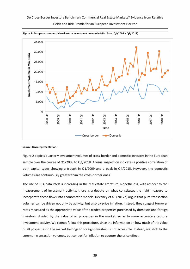
Do Cross-Border Investors Benchmark Commercial Real Estate Markets? Evidence from Relative
Yields and Risk Premia for an European Investment Horizon
39
Figure 2: European commercial real estate investment volume in Mio. Euro (Q1/2008 – Q3/2018)
Source: Own representation.
Figure 2 depicts quarterly investment volumes of cross-border and domestic investors in the European
sample over the course of Q1/2008 to Q3/2018. A visual inspection indicates a positive correlation of
both capital types showing a trough in Q1/2009 and a peak in Q4/2015. However, the domestic
volumes are continuously greater than the cross-border ones.
The use of RCA data itself is increasing in the real estate literature. Nonetheless, with respect to the
measurement of investment activity, there is a debate on what constitutes the right measure to
incorporate these flows into econometric models. Devaney et al. (2017b) argue that pure transaction
volumes can be driven not only by activity, but also by price inflation. Instead, they suggest turnover
rates measured as the appropriate value of the traded properties purchased by domestic and foreign
investors, divided by the value of all properties in the market, so as to more accurately capture
investment activity. We cannot follow this procedure, since the information on how much of the value
of all properties in the market belongs to foreign investors is not accessible. Instead, we stick to the
common transaction volumes, but control for inflation to counter the price effect.
0
5.000
10.000
15.000
20.000
25.000
30.000
35.000
200
8 Q
1
200
9 Q
1
201
0 Q
1
201
1 Q
1
201
2 Q
1
201
3 Q
1
201
4 Q
1
201
5 Q
1
201
6 Q
1
201
7 Q
1
201
8 Q
1
Inve
stm
en
t V
olu
me
in
Mio
. E
uro
Time
Cross-border Domestic
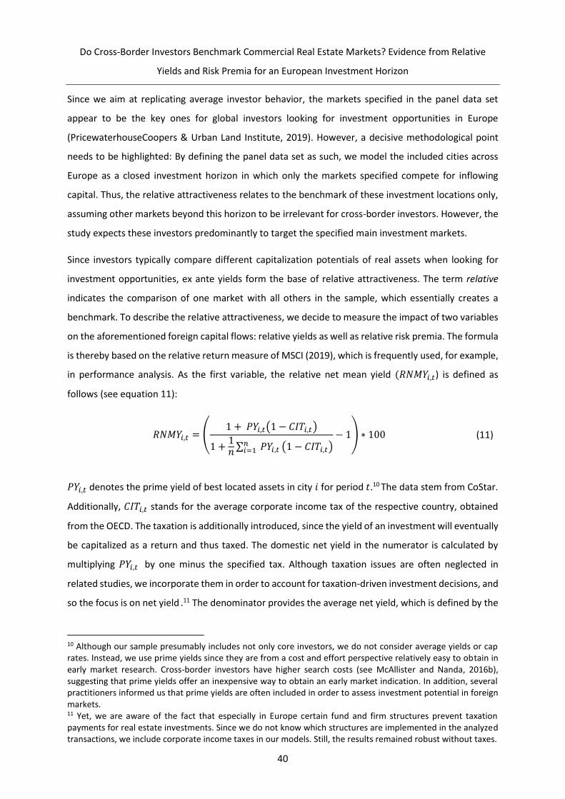
Do Cross-Border Investors Benchmark Commercial Real Estate Markets? Evidence from Relative
Yields and Risk Premia for an European Investment Horizon
40
Since we aim at replicating average investor behavior, the markets specified in the panel data set
appear to be the key ones for global investors looking for investment opportunities in Europe
(PricewaterhouseCoopers & Urban Land Institute, 2019). However, a decisive methodological point
needs to be highlighted: By defining the panel data set as such, we model the included cities across
Europe as a closed investment horizon in which only the markets specified compete for inflowing
capital. Thus, the relative attractiveness relates to the benchmark of these investment locations only,
assuming other markets beyond this horizon to be irrelevant for cross-border investors. However, the
study expects these investors predominantly to target the specified main investment markets.
Since investors typically compare different capitalization potentials of real assets when looking for
investment opportunities, ex ante yields form the base of relative attractiveness. The term relative
indicates the comparison of one market with all others in the sample, which essentially creates a
benchmark. To describe the relative attractiveness, we decide to measure the impact of two variables
on the aforementioned foreign capital flows: relative yields as well as relative risk premia. The formula
is thereby based on the relative return measure of MSCI (2019), which is frequently used, for example,
in performance analysis. As the first variable, the relative net mean yield (𝑅𝑁𝑀𝑌𝑖,𝑡) is defined as
follows (see equation 11):
𝑅𝑁𝑀𝑌𝑖,𝑡 = (1 + 𝑃𝑌𝑖,𝑡(1 − 𝐶𝐼𝑇𝑖,𝑡)
1 +1𝑛∑ 𝑃𝑌𝑖,𝑡𝑛𝑖=1 (1 − 𝐶𝐼𝑇𝑖,𝑡)
− 1) ∗ 100 (11)
𝑃𝑌𝑖,𝑡 denotes the prime yield of best located assets in city 𝑖 for period 𝑡.10 The data stem from CoStar.
Additionally, 𝐶𝐼𝑇𝑖,𝑡 stands for the average corporate income tax of the respective country, obtained
from the OECD. The taxation is additionally introduced, since the yield of an investment will eventually
be capitalized as a return and thus taxed. The domestic net yield in the numerator is calculated by
multiplying 𝑃𝑌𝑖,𝑡 by one minus the specified tax. Although taxation issues are often neglected in
related studies, we incorporate them in order to account for taxation-driven investment decisions, and
so the focus is on net yield .11 The denominator provides the average net yield, which is defined by the
10 Although our sample presumably includes not only core investors, we do not consider average yields or cap rates. Instead, we use prime yields since they are from a cost and effort perspective relatively easy to obtain in early market research. Cross-border investors have higher search costs (see McAllister and Nanda, 2016b), suggesting that prime yields offer an inexpensive way to obtain an early market indication. In addition, several practitioners informed us that prime yields are often included in order to assess investment potential in foreign markets. 11 Yet, we are aware of the fact that especially in Europe certain fund and firm structures prevent taxation payments for real estate investments. Since we do not know which structures are implemented in the analyzed transactions, we include corporate income taxes in our models. Still, the results remained robust without taxes.
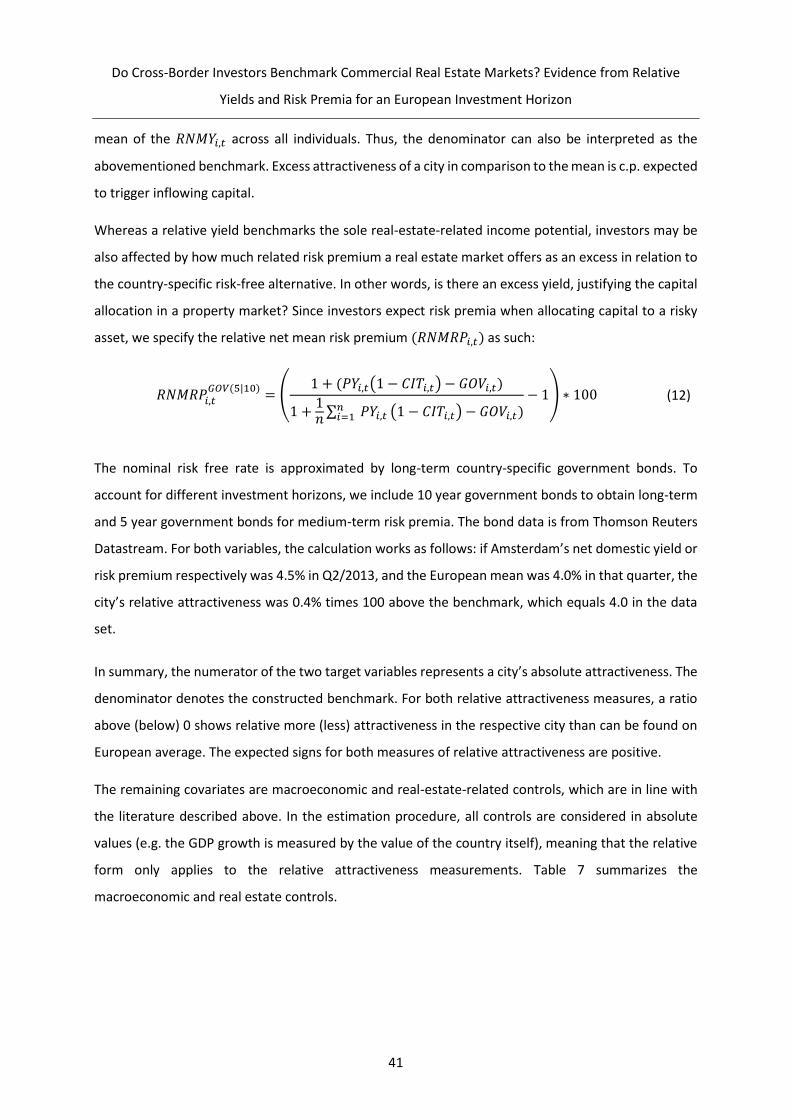
Do Cross-Border Investors Benchmark Commercial Real Estate Markets? Evidence from Relative
Yields and Risk Premia for an European Investment Horizon
41
mean of the 𝑅𝑁𝑀𝑌𝑖,𝑡 across all individuals. Thus, the denominator can also be interpreted as the
abovementioned benchmark. Excess attractiveness of a city in comparison to the mean is c.p. expected
to trigger inflowing capital.
Whereas a relative yield benchmarks the sole real-estate-related income potential, investors may be
also affected by how much related risk premium a real estate market offers as an excess in relation to
the country-specific risk-free alternative. In other words, is there an excess yield, justifying the capital
allocation in a property market? Since investors expect risk premia when allocating capital to a risky
asset, we specify the relative net mean risk premium (𝑅𝑁𝑀𝑅𝑃𝑖,𝑡) as such:
𝑅𝑁𝑀𝑅𝑃𝑖,𝑡𝐺𝑂𝑉(5|10)
= (1 + (𝑃𝑌𝑖,𝑡(1 − 𝐶𝐼𝑇𝑖,𝑡) − 𝐺𝑂𝑉𝑖,𝑡)
1 +1𝑛∑ 𝑃𝑌𝑖,𝑡𝑛𝑖=1 (1 − 𝐶𝐼𝑇𝑖,𝑡) − 𝐺𝑂𝑉𝑖,𝑡)
− 1) ∗ 100 (12)
The nominal risk free rate is approximated by long-term country-specific government bonds. To
account for different investment horizons, we include 10 year government bonds to obtain long-term
and 5 year government bonds for medium-term risk premia. The bond data is from Thomson Reuters
Datastream. For both variables, the calculation works as follows: if Amsterdam’s net domestic yield or
risk premium respectively was 4.5% in Q2/2013, and the European mean was 4.0% in that quarter, the
city’s relative attractiveness was 0.4% times 100 above the benchmark, which equals 4.0 in the data
set.
In summary, the numerator of the two target variables represents a city’s absolute attractiveness. The
denominator denotes the constructed benchmark. For both relative attractiveness measures, a ratio
above (below) 0 shows relative more (less) attractiveness in the respective city than can be found on
European average. The expected signs for both measures of relative attractiveness are positive.
The remaining covariates are macroeconomic and real-estate-related controls, which are in line with
the literature described above. In the estimation procedure, all controls are considered in absolute
values (e.g. the GDP growth is measured by the value of the country itself), meaning that the relative
form only applies to the relative attractiveness measurements. Table 7 summarizes the
macroeconomic and real estate controls.

Do Cross-Border Investors Benchmark Commercial Real Estate Markets? Evidence from Relative
Yields and Risk Premia for an European Investment Horizon
42
Table 7: Control variable description for cross-border volume models
Variable Description Proxy for Level Source
GDP growth Amongst others, Lieser and Groh (2014) argue that a
sound and healthy economy is a driving factor for direct real estate investments. Hence, we control for economic stability by including quarter-on-quarter GDP growth in the econometric analysis.
Economic stability
Country OECD
CPI growth Inflation is added in order to control for price movements with respect to cross-border transaction volumes. Consequently, quarter-on-quarter CPI growth serves as a control variable that adjusts for changes in the dependent variable due to market conditions.
Asset price inflation
Country OECD
Unemployment rate
Employment is often perceived as another indicator of economic health and success. Fuerst et al. (2015) state that foreign investors are attracted by good employment conditions. Thus, we use the unemployment rate to capture the labor market and income situation.
Labor market and income
Country OECD
Global Competitiveness Index (GCI)
In line with previous literature, a condensed country risk measure is central when choosing among international investment opportunities. We decide to control for country risk by using the GCI. The construction of the index is based upon twelve core areas, which cover e.g. institutions, infrastructure, the adoption of information and technologies and others (World Economic Forum, 2018).12
Country risk Country World Economic Forum
Vacancy Office vacancy serves as an indication of the current state of demand in a real estate market. According to Devaney et al. (2017b) vacancy captures conditions in the space market.
Office demand City CoStar
Stock Stock indicates the available office floor space and therefore shows the size of the market and / or the building activity. We incorporate it to control for the office supply.
Office supply
City CoStar
Prime rent growth
Year-on-year prime rent growth shows the income growth potential of prime office buildings in the respective market.13
Income expectations
City CoStar
Source: Own presentation.
The following section reports the univariate analysis for the abovementioned constituents of the data
set. Table 8 displays the descriptive statistics of the dependent and target variables as well as the
covariates.
12 Some researchers such as Devaney et al. (2017b) use government and or corporate bonds spreads to control for country risk. To avoid multicollinearity, we cannot include this proxy, since the second target variable relative risk premium is constructed based on government bonds. Additionally, the JLL Global Real Estate Transparency Index series may be an alternative proxy to control for country specific risk factors. Nonetheless, the specified index was not used, because the study incorporates a macroeconomic index to account for effects on a broader and national economic level. 13 We also controlled for non-prime rent growth. The results stayed robust, but were not reported.

Do Cross-Border Investors Benchmark Commercial Real Estate Markets? Evidence from Relative
Yields and Risk Premia for an European Investment Horizon
43
Table 8: Descriptive statistics for variables of the cross-border transaction volume models
Variable n Unit Mean SD Min. Max.
Dependent Variable
Cross-border transaction volume 1204 T € 277,195 705,530 0 7,384,621
Macroeconomic variables
GDP growth 1204 % 0.298 0.957 -6.842 9.928
CPI growth ∆ 1176 % -0.007 0.868 -5.035 4.575
Unemployment rate ∆ 1176 % -0.045 1.192 -8.997 8.996
Global Competitive Index 1204 Index 5.168 0.439 4.153 5.858
Real estate related variables
Vacancy 1204 % 10.581 4.218 2.310 25.474
Stock ∆ 1176 sqm 347,905 454,964 -1,199,068 3,797,188
Prime Rent Growth 1204 % 0.926 7.725 -54.930 48.072
1. Target Variable
RNMY 1204 % 0.000 24.793 -44.784 134.013
2. Target Variable
RNMRP 10y 1204 % 0.000 8.985 -29.913 19.943
RNMRP 5y 1204 % 0.000 8.956 -29.858 19.999
Note: ∆ indicates the first differences of the variable. Sqm stands for square meters.
Source: Own presentation.
From the descriptive statistics table, the need for a natural logarithm transformation of cross-border
transaction volume and the stock is apparent, because variables vary substantially with regard to their
absolute values. Since the origin of the investment volumes is not available, we are unable to control
for exchange rate stability. Yet, we incorporate all monetary values in Euros (€) to form a uniform
currency base. Additionally, a correlation matrix provides insights into the common movement of the
covariates (see Table 9):14
14 Correlations between timely lagged covariates are not reported. However, the indication of the contemporary realizations sufficiently reveals the potential of crucial correlations.

Do Cross-Border Investors Benchmark Commercial Real Estate Markets? Evidence from Relative
Yields and Risk Premia for an European Investment Horizon
44
Table 9: Correlation matrix for cross-border transaction volume model variables
1 2 3 4 5 6 7 8 9 10 11
1 Cross-border transaction volume
1.000
2 GDP growth 0.057 1.000
3 CPI growth ∆ 0.005 0.037 1.000
4 Unemployment rate ∆
-0.014 -0.063 0.023 1.000
5 Global competitive index
0.122 0.045 0.014 0.021 1.000
6 Vacancy -0.165 0.048 0.001 0.003 -0.451 1.000
7 Stock ∆ 0.095 -0.116 0.000 0.003 -0.269 0.104 1.000
8 Prime rent growth 0.033 0.076 -0.018 -0.014 0.156 -0.197 -0.215 1.000
9 RNMY -0.233 -0.003 -0.013 -0.005 -0.621 0.552 0.279 -0.183 1.000
10 RNMRP 10y -0.103 0.080 -0.005 -0.011 0.242 0.063 -0.119 0.027 0.244 1.000
11 RNMRP 5y -0.102 0.080 -0.006 -0.011 0.244 0.060 -0.131 0.031 0.234 0.999 1.000
Note: ∆ indicates the first differences of the variable.
Source: Own presentation.
In line with previous research, we define absolute values greater than 0.25 define as threshold for any
econometric issues. The target variable RNMY shows critical correlations with the Global Competitive
Index, vacancy and stock. Among the controls, Global Competitive Index yields correlations with stock
and vacancy below -0.25. Stock and vacancy show a correlation above 0.25. Even though we estimate
a base model with all correlated variables, we try to control for multicollinearity by comparing the
results of the specified model with the results of model variations. These variations individually exclude
one of the correlated variables.
Lastly, since panel data models may be subject to potential non-stationarity, we carried out panel unit
root test to check for econometric distractions (see appendix). For those covariates which suffer from
non-stationarity, we used a differencing procedure, in order to generate a stationary time series. After
a first differencing, we observe stationary covariates, denoted ∆(x).
To assess the outlined hypotheses, two different methodologies are applied: Pooled OLS, as well as a
GAMM. Firstly, an OLS model estimates the linear predictors to evaluate the first hypothesis. The
model specification yields the following equation 13:
𝑙𝑛(𝑣𝑖,𝑡) = 𝛽𝑚𝑖,𝑡−𝑘 + 𝛽𝑟𝑖,𝑡−𝑘 + 𝛽𝑟𝑒𝑙𝑎𝑡𝑖𝑣𝑒 𝑎𝑡𝑡𝑟𝑎𝑐𝑡𝑖𝑣𝑒𝑛𝑒𝑠𝑠𝑖,𝑡−𝑘 + 𝛽𝑡𝑖𝑚𝑒𝑡 + 𝛽𝑐𝑖𝑡𝑦𝑖 + 𝜀𝑖,𝑡 (13)
Here, the natural logarithm of the cross-border transaction volume 𝑙𝑛(𝑣𝑖,𝑡) observed in a market 𝑖 in
quarter 𝑡 is a function of the abovementioned domestic macroeconomic variables captured in the
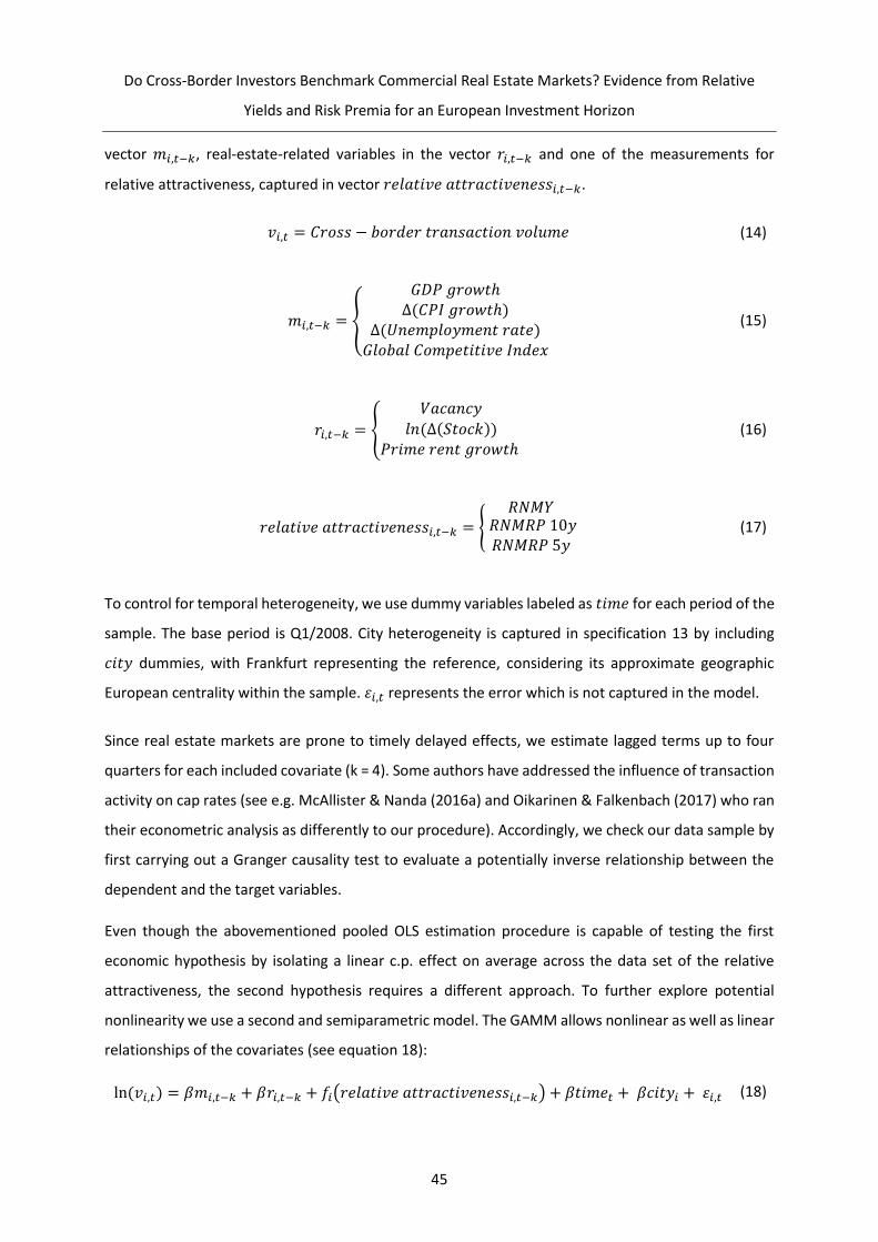
Do Cross-Border Investors Benchmark Commercial Real Estate Markets? Evidence from Relative
Yields and Risk Premia for an European Investment Horizon
45
vector 𝑚𝑖,𝑡−𝑘, real-estate-related variables in the vector 𝑟𝑖,𝑡−𝑘 and one of the measurements for
relative attractiveness, captured in vector 𝑟𝑒𝑙𝑎𝑡𝑖𝑣𝑒 𝑎𝑡𝑡𝑟𝑎𝑐𝑡𝑖𝑣𝑒𝑛𝑒𝑠𝑠𝑖,𝑡−𝑘.
𝑣𝑖,𝑡 = 𝐶𝑟𝑜𝑠𝑠 − 𝑏𝑜𝑟𝑑𝑒𝑟 𝑡𝑟𝑎𝑛𝑠𝑎𝑐𝑡𝑖𝑜𝑛 𝑣𝑜𝑙𝑢𝑚𝑒 (14)
𝑚𝑖,𝑡−𝑘 = {
𝐺𝐷𝑃 𝑔𝑟𝑜𝑤𝑡ℎ∆(𝐶𝑃𝐼 𝑔𝑟𝑜𝑤𝑡ℎ)
∆(𝑈𝑛𝑒𝑚𝑝𝑙𝑜𝑦𝑚𝑒𝑛𝑡 𝑟𝑎𝑡𝑒)𝐺𝑙𝑜𝑏𝑎𝑙 𝐶𝑜𝑚𝑝𝑒𝑡𝑖𝑡𝑖𝑣𝑒 𝐼𝑛𝑑𝑒𝑥
(15)
𝑟𝑖,𝑡−𝑘 = {
𝑉𝑎𝑐𝑎𝑛𝑐𝑦
𝑙𝑛 (∆(𝑆𝑡𝑜𝑐𝑘))𝑃𝑟𝑖𝑚𝑒 𝑟𝑒𝑛𝑡 𝑔𝑟𝑜𝑤𝑡ℎ
(16)
𝑟𝑒𝑙𝑎𝑡𝑖𝑣𝑒 𝑎𝑡𝑡𝑟𝑎𝑐𝑡𝑖𝑣𝑒𝑛𝑒𝑠𝑠𝑖,𝑡−𝑘 = {𝑅𝑁𝑀𝑌
𝑅𝑁𝑀𝑅𝑃 10𝑦 𝑅𝑁𝑀𝑅𝑃 5𝑦
(17)
To control for temporal heterogeneity, we use dummy variables labeled as 𝑡𝑖𝑚𝑒 for each period of the
sample. The base period is Q1/2008. City heterogeneity is captured in specification 13 by including
𝑐𝑖𝑡𝑦 dummies, with Frankfurt representing the reference, considering its approximate geographic
European centrality within the sample. 𝜀𝑖,𝑡 represents the error which is not captured in the model.
Since real estate markets are prone to timely delayed effects, we estimate lagged terms up to four
quarters for each included covariate (k = 4). Some authors have addressed the influence of transaction
activity on cap rates (see e.g. McAllister & Nanda (2016a) and Oikarinen & Falkenbach (2017) who ran
their econometric analysis as differently to our procedure). Accordingly, we check our data sample by
first carrying out a Granger causality test to evaluate a potentially inverse relationship between the
dependent and the target variables.
Even though the abovementioned pooled OLS estimation procedure is capable of testing the first
economic hypothesis by isolating a linear c.p. effect on average across the data set of the relative
attractiveness, the second hypothesis requires a different approach. To further explore potential
nonlinearity we use a second and semiparametric model. The GAMM allows nonlinear as well as linear
relationships of the covariates (see equation 18):
ln (𝑣𝑖,𝑡) = 𝛽𝑚𝑖,𝑡−𝑘 + 𝛽𝑟𝑖,𝑡−𝑘 + 𝑓𝑖(𝑟𝑒𝑙𝑎𝑡𝑖𝑣𝑒 𝑎𝑡𝑡𝑟𝑎𝑐𝑡𝑖𝑣𝑒𝑛𝑒𝑠𝑠𝑖,𝑡−𝑘) + 𝛽𝑡𝑖𝑚𝑒𝑡 + 𝛽𝑐𝑖𝑡𝑦𝑖 + 𝜀𝑖,𝑡 (18)

Do Cross-Border Investors Benchmark Commercial Real Estate Markets? Evidence from Relative
Yields and Risk Premia for an European Investment Horizon
46
Here, the function 𝑓𝑖 denotes the smoothing function for the relative attractiveness proxy, which is
used to check for potential nonlinearity. Thus, we do not estimate a linear predictor for the variables
of interest, in contrast to the OLS model. Since the potential nonlinear behavior of the macroeconomic
and real-estate-related controls is of minor interest, we introduce a smoothing function only for the
target variables. The number of knots is set equal to 20.
3.4 Empirical results
Due to potential inverse relationships between yields and capital flows, we firstly conduct a Granger
causality test to detect potential simultaneity bias in our sample (see Table 10):
Table 10: Granger causality test (RNMRP & RNMY – cross-border transaction volume)
Inverse relationship
Dependent Independent F statistic p-value
RNMRP 10y ln(Cross-border transaction volume) 0.6708 0.6123
RNMRP 5y ln(Cross-border transaction volume) 0.6542 0.6240
RNMY ln(Cross-border transaction volume) 2.1227 0.0753 *
Source: Own calculation.
As displayed above, we find strong empirical proof against a potential inverse relationship between
cross-border volumes and both RNMRPs. Only for the RNMY is the relationship inversely statistically
significant and may therefore cause simultaneity. The standard methodical procedure for accounting
for simultaneity is to use an instrument variable approach such as two stage least squares. However,
since target variables are of particular interest – unlike controls – we do not search for instruments,
but emphasize the potential presence of simultaneity bias with regard to the RNMY.
To test the first hypothesis, we run pooled OLS estimations. The results can be found in Table 11. For
each of the three target variables, we estimate the same four specifications. The base model includes
all control variables, whereas the second, third and fourth models individually exclude the variables
Global Competitive Index (GCI), vacancy and stock, to check for robustness. The selected variables
were systematically exchanged, due to the findings within the correlation matrix and to account for
potential multicollinearity.

Do Cross-Border Investors Benchmark Commercial Real Estate Markets? Evidence from Relative Yields and Risk Premia for an European Investment Horizon
47
Table 11: Pooled OLS estimation results (cross-border transaction volume)
Dependent variable: ln (cross-border transaction volume)
Model Model 1 Model 1.1 Model 1.2 Model 1.3 Model 2 Model 2.1 Model 2.2 Model 2.3 Model 3 Model 3.1 Model 3.2 Model 3.3
Controls:
Macroeconomic Yes Yes Yes Yes Yes Yes Yes Yes Yes Yes Yes Yes Real estate Yes Yes Yes Yes Yes Yes Yes Yes Yes Yes Yes Yes Excluded control None GCI Vacancy Stock None GCI Vacancy Stock None GCI Vacancy Stock
Target variables:
RNMY -0.094 -0.091 -0.086 -0.102
(0.082) (0.082) (0.087) (0.083)
RNMY (-1) 0.086 0.083 0.048 0.099
(0.110) (0.110) (0.117) (0.111)
RNMY (-2) 0.088 0.086 0.111 0.083
(0.102) (0.102) (0.107) (0.103)
RNMY (-3) -0.163 -0.158 -0.175 -0.180
(0.113) (0.113) (0.114) (0.113)
RNMY (-4) 0.087 0.083 0.093 0.108
(0.075) (0.075) (0.072) (0.076)
RNMRP 10y 0.164 0.158 0.203 * 0.183
(0.113) (0.112) (0.111) (0.111)
RNMRP 10y (-1) -0.222 -0.230 -0.229 -0.217
(0.157) (0.155) (0.159) (0.159)
RNMRP 10y (-2) 0.335 ** 0.339 ** 0.306 ** 0.333 **
(0.155) (0.152) (0.155) (0.155)
RNMRP 10y (-3) -0.265 -0.257 -0.247 -0.260
(0.173) (0.169) (0.173) (0.174)
RNMRP 10y (-4) 0.108 0.086 0.116 0.093
(0.140) (0.136) (0.139) (0.142)
RNMRP 5y 0.111 0.106 0.141 0.129
(0.117) (0.117) (0.117) (0.116)
RNMRP 5y (-1) -0.149 -0.161 -0.149 -0.141
(0.159) (0.158) (0.162) (0.161)
RNMRP 5y (-2) 0.311 ** 0.320 ** 0.282 * 0.307 **
(0.154) (0.152) (0.155) (0.154)
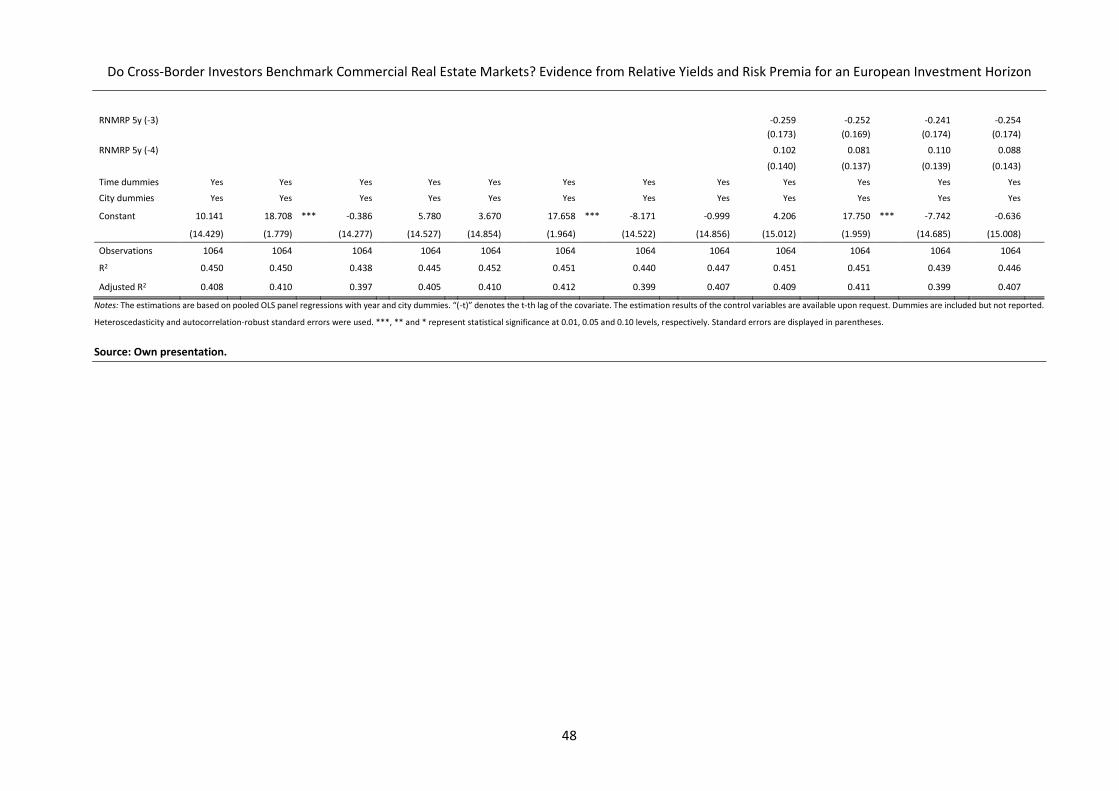
Do Cross-Border Investors Benchmark Commercial Real Estate Markets? Evidence from Relative Yields and Risk Premia for an European Investment Horizon
48
RNMRP 5y (-3)
-0.259 -0.252 -0.241 -0.254
(0.173) (0.169) (0.174) (0.174)
RNMRP 5y (-4) 0.102 0.081 0.110 0.088
(0.140) (0.137) (0.139) (0.143)
Time dummies Yes Yes Yes Yes Yes Yes Yes Yes Yes Yes Yes Yes
City dummies Yes Yes Yes Yes Yes Yes Yes Yes Yes Yes Yes Yes
Constant 10.141 18.708 *** -0.386 5.780 3.670 17.658 *** -8.171 -0.999 4.206 17.750 *** -7.742 -0.636
(14.429) (1.779) (14.277) (14.527) (14.854) (1.964) (14.522) (14.856) (15.012) (1.959) (14.685) (15.008)
Observations 1064 1064 1064 1064 1064 1064 1064 1064 1064 1064 1064 1064
R2 0.450 0.450 0.438 0.445 0.452 0.451 0.440 0.447 0.451 0.451 0.439 0.446
Adjusted R2 0.408 0.410 0.397 0.405 0.410 0.412 0.399 0.407 0.409 0.411 0.399 0.407
Notes: The estimations are based on pooled OLS panel regressions with year and city dummies. “(-t)” denotes the t-th lag of the covariate. The estimation results of the control variables are available upon request. Dummies are included but not reported.
Heteroscedasticity and autocorrelation-robust standard errors were used. ***, ** and * represent statistical significance at 0.01, 0.05 and 0.10 levels, respectively. Standard errors are displayed in parentheses.
Source: Own presentation.

Do Cross-Border Investors Benchmark Commercial Real Estate Markets? Evidence from Relative
Yields and Risk Premia for an European Investment Horizon
49
Firstly, the explanatory power of the models is in line with related research, ranging around an adjusted
R2 of 0.35 – 0.40. However, when we exclude binaries for the city individuals, we observe estimations
(not reported) with declining adjusted R² values around 0.10, showing city-specific heterogeneity. Both
specified findings are in line with related literature e.g. Devaney et al. (2019). The temporal binaries
are predominantly statistically insignificant, indicating temporal homogeneity.
Focusing on the linear predictors of interest, we find on average a positive and statistically significant,
c.p. relationship for the RNMRP 10y and 5y within the base models 2 and 3 for the second lag. The
model variations 2.1 – 2.3 and 3.1 – 3.3 provide similar results, emphasizing the robustness of the
results. One can derive two insights from these findings. First, cross-border investors favor higher risk
premia when looking for investment opportunities in Europe. Interestingly, this also applies to
investors who anticipate long- and medium-term holding-periods. The models report a c.p. effect on
average around 0.3% per base point relative risk premium (since betas range around 0.3).
Second, if a city offers a relative risk premium above the European mean, it generally takes six months
until cross-border capital flows into the respective market. The specified finding is in line with
expectations due to search and transaction phases in direct markets. Crosby & McAllister (2004) and
Bond et al. (2007) state an average transaction period in UK commercial real estate markets of
approximately six to nine months. Model 2.2 also shows a statistically significant positive sign for
RNMRP 10y for the contemporary covariate (lag = 0), which however is not investigated any further.
Considering the target variable RNMY, no statistically significant relationship between relative yield
and inflowing transaction volume could be revealed. This finding adds to the study of Devaney et al.
(2019), who find an insignificant relationship between cap rates and general transaction activity in
commercial real estate markets. Concluding the OLS result section, the first hypothesis can be
confirmed after differentiating between yields and risk premia. Thus, relative attractiveness
contributes to the existing absolute measures of determinants of cross-border transactions. However,
relative attractiveness of cross-border investors is only perceived in terms of relative risk premia and
not relative yields.
In addition to the fully parametric model, we assess hypothesis two by specifying semi-parametric
GAMMs. We use smoothing functions for the RNMRP only, since the RNMY has not shown significance
in the fully parametric approach (models 1 – 1.3). The GAMM specifications are identical to the linear
ones and denoted with a “G”, to ensure easy comparability with the OLS peer. All other covariates are
still included with a linear predictor. However, we do not report the coefficients of still parametrized
lags of the RNMRP, since they are already reported above (see Table 11). Instead, Table 12 presents
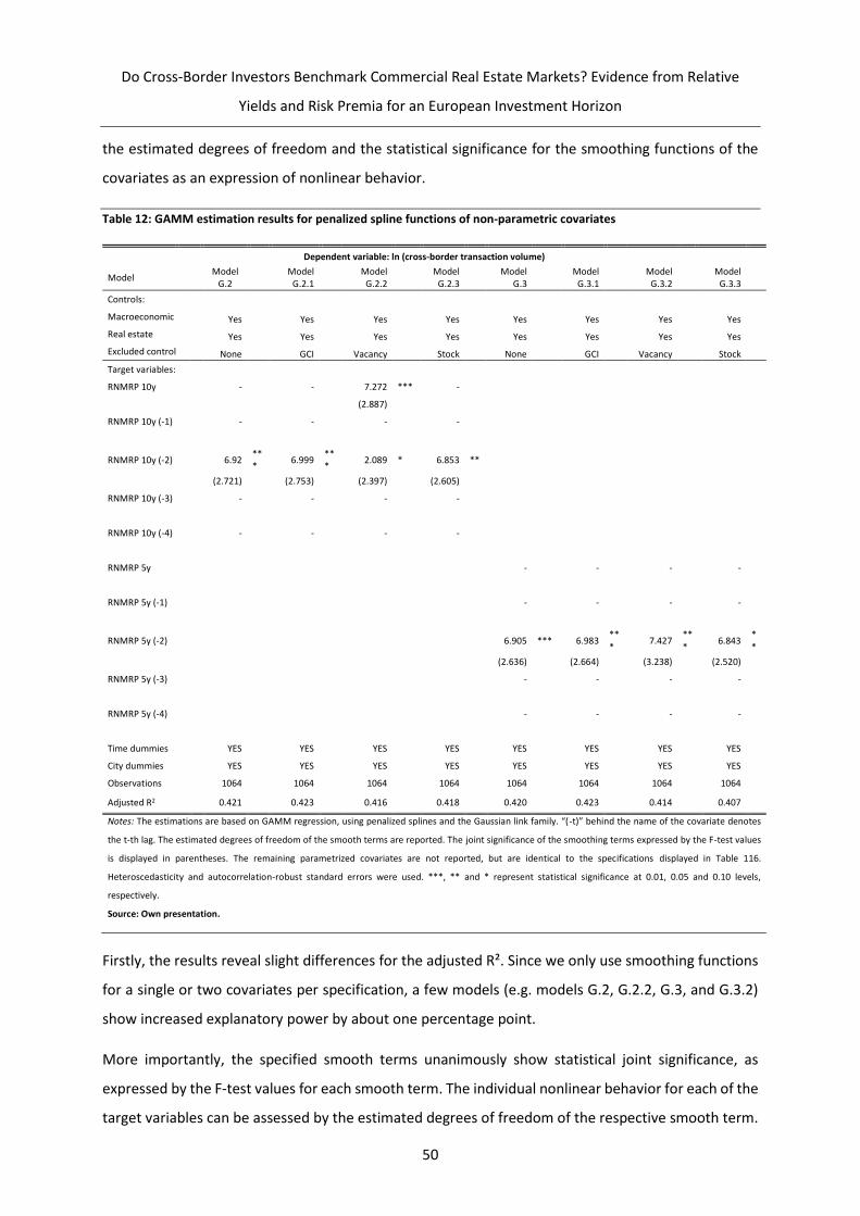
Do Cross-Border Investors Benchmark Commercial Real Estate Markets? Evidence from Relative
Yields and Risk Premia for an European Investment Horizon
50
the estimated degrees of freedom and the statistical significance for the smoothing functions of the
covariates as an expression of nonlinear behavior.
Table 12: GAMM estimation results for penalized spline functions of non-parametric covariates
Dependent variable: ln (cross-border transaction volume)
Model
Model G.2
Model G.2.1
Model G.2.2
Model G.2.3
Model G.3
Model G.3.1
Model G.3.2
Model G.3.3
Controls:
Macroeconomic Yes Yes Yes Yes Yes Yes Yes Yes
Real estate Yes Yes Yes Yes Yes Yes Yes Yes
Excluded control None GCI Vacancy Stock None GCI Vacancy Stock
Target variables:
RNMRP 10y - - 7.272 *** -
(2.887)
RNMRP 10y (-1) - - - -
RNMRP 10y (-2) 6.92 ***
6.999 ***
2.089 * 6.853 **
(2.721) (2.753) (2.397) (2.605)
RNMRP 10y (-3) - - - -
RNMRP 10y (-4) - - - -
RNMRP 5y - - - -
RNMRP 5y (-1) - - - -
RNMRP 5y (-2) 6.905 *** 6.983 ***
7.427 ***
6.843 **
(2.636) (2.664) (3.238) (2.520)
RNMRP 5y (-3) - - - -
RNMRP 5y (-4) - - - -
Time dummies YES YES YES YES YES YES YES YES
City dummies YES YES YES YES YES YES YES YES
Observations 1064 1064 1064 1064 1064 1064 1064 1064
Adjusted R2 0.421 0.423 0.416 0.418 0.420 0.423 0.414 0.407
Notes: The estimations are based on GAMM regression, using penalized splines and the Gaussian link family. “(-t)” behind the name of the covariate denotes
the t-th lag. The estimated degrees of freedom of the smooth terms are reported. The joint significance of the smoothing terms expressed by the F-test values
is displayed in parentheses. The remaining parametrized covariates are not reported, but are identical to the specifications displayed in Table 116.
Heteroscedasticity and autocorrelation-robust standard errors were used. ***, ** and * represent statistical significance at 0.01, 0.05 and 0.10 levels,
respectively.
Source: Own presentation.
Firstly, the results reveal slight differences for the adjusted R². Since we only use smoothing functions
for a single or two covariates per specification, a few models (e.g. models G.2, G.2.2, G.3, and G.3.2)
show increased explanatory power by about one percentage point.
More importantly, the specified smooth terms unanimously show statistical joint significance, as
expressed by the F-test values for each smooth term. The individual nonlinear behavior for each of the
target variables can be assessed by the estimated degrees of freedom of the respective smooth term.

Do Cross-Border Investors Benchmark Commercial Real Estate Markets? Evidence from Relative
Yields and Risk Premia for an European Investment Horizon
51
The interpretation works as follows: Estimated degrees of freedom equal to one represent an entirely
linear relationship between the dependent and independent variables across the entire distribution.
Hence, the larger the difference of the estimated degrees of freedom from one, the stronger the
nonlinearity within the relationship becomes.
Here, most smoothing functions show estimated degrees of freedom around 7. Only the second lag of
the RNMRP 10y in model G.2.2 shows a much smaller value. Nonetheless, the function is still
statistically significant. Thus, we can confirm the nonlinear behavior of the target variables across all
specifications.
Since smoothing functions of GAMMs do not report a single estimate, a numerical interpretation is not
possible. Instead, we report the graphical illustration of selected and representative functions and the
respective partial residuals, as displayed below (see Figure 3). The functions were chosen from the
base models G.2 and G.3. Other models show similar results.
Figure 3: Penalized spline functions of RNMPR 10y and RNMRP 5y – models G.2 & G.3
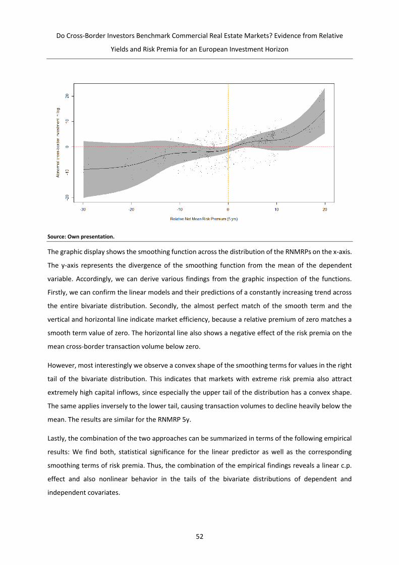
Do Cross-Border Investors Benchmark Commercial Real Estate Markets? Evidence from Relative
Yields and Risk Premia for an European Investment Horizon
52
Source: Own presentation.
The graphic display shows the smoothing function across the distribution of the RNMRPs on the x-axis.
The y-axis represents the divergence of the smoothing function from the mean of the dependent
variable. Accordingly, we can derive various findings from the graphic inspection of the functions.
Firstly, we can confirm the linear models and their predictions of a constantly increasing trend across
the entire bivariate distribution. Secondly, the almost perfect match of the smooth term and the
vertical and horizontal line indicate market efficiency, because a relative premium of zero matches a
smooth term value of zero. The horizontal line also shows a negative effect of the risk premia on the
mean cross-border transaction volume below zero.
However, most interestingly we observe a convex shape of the smoothing terms for values in the right
tail of the bivariate distribution. This indicates that markets with extreme risk premia also attract
extremely high capital inflows, since especially the upper tail of the distribution has a convex shape.
The same applies inversely to the lower tail, causing transaction volumes to decline heavily below the
mean. The results are similar for the RNMRP 5y.
Lastly, the combination of the two approaches can be summarized in terms of the following empirical
results: We find both, statistical significance for the linear predictor as well as the corresponding
smoothing terms of risk premia. Thus, the combination of the empirical findings reveals a linear c.p.
effect and also nonlinear behavior in the tails of the bivariate distributions of dependent and
independent covariates.
Do Cross-Border Investors Benchmark Commercial Real Estate Markets? Evidence from Relative
Yields and Risk Premia for an European Investment Horizon
53
3.5 Conclusion and further aspects
This study presents a new approach to explaining commercial cross-border transaction activity, namely
the development of a city’s relative attractiveness in comparison to its peers. We find an on average,
c.p. and statistically significant relationship between relative risk premia and inflowing cross-border
capital into office properties in Europe. We thus confirm the existence of a risk-premium-chasing
behavior of cross-border investors with regard to relative city attractiveness. Moreover, we find
empirical evidence for a timely lagged effect, since statistical significance can be observed
predominantly for the two-quarter-delayed covariates.
However, a decisive differentiation for the economic finding is needed. The measurement of relative
yields is unanimously statistically insignificant, underlining the importance of risk premia instead of
pure yields as explanatory variable for cross-border inflows. Nonetheless, we conclude and also extend
the existing body of literature by showing the relationship between the investor calculus of relative
attractiveness and capital flows as a new determinant. Thus, we can partly justify our first hypothesis,
while highlighting the importance of differentiating between relative yields and risk premia.
Moreover, we find evidence for a potential nonlinear behavior of the relative attractiveness measures,
expressed by the statistical significance of the smoothing terms in the GAMM. Consequently, we see
evidence in favor of the second hypothesis. Interestingly, we find a curvy or convex shape of the
smoothing functions, especially in the tails. This finding indicates extreme capital inflow behavior for
locations which also offer extreme relative premia. Thus, we conclude, that especially risk-friendly
cross-border investors trigger abnormally high investment flows into real estate markets.
Some limitations apply to the used data. Firstly, we analyze European data only. The same analysis on
a larger scale appears promising, as proposed on a global level by Devaney et al. (2019). Secondly, the
depth of the data can be discussed. As outlined by Lieser & Groh (2014), a large variety of covariates
show a statistically significant relationship with foreign investment volumes. However, since we
control for the most important types of impact variables, the explanatory power of the models are in
line with previous studies. Thus, we perceive the selected controls as a sufficient set of variables.
Econometric robustness tests also confirm the stability of the results across various specifications.
Practical implications can be derived from an investment management and risk controlling perspective.
The understanding of determinants in market transaction volumes is an important factor for
anticipating inflowing capital and potential capital value changes. Therefore, for example positive
divergence from the benchmark is expected to cause on average higher inflows of cross-border capital.
Equity investors can use the insights especially for their disinvestment strategies. In this context, they
Do Cross-Border Investors Benchmark Commercial Real Estate Markets? Evidence from Relative
Yields and Risk Premia for an European Investment Horizon
54
can specifically address foreign buyers, when risk premia in markets of their existing property
investments move above the European mean, since cross-border investors are expected to invest in
these locations. Financing debt investors on the other hand can expect sales of standing investments
to cross-border investors in advance of their expected maturity, if risk premia of the market move
above the European mean. Secondly, financing institutions can benefit from cross-border investors by
offering funds to them and consequently expect new business opportunities. Early anticipation of
potential financing requests will help to plan refinancing and money allocation activities.
Further useful research may be undertaken by differentiating between the geographic origin and type
of investor. Considering return chase behavior, Devaney et al. (2018) noted that different nationalities
may matter. Moreover, focusing on other property types would reveal whether the relative
attractiveness is generally applicable to other markets and not a phenomenon unique to the
commercial- and office sector. Lastly, extending the present approach of relative attractiveness not
only to the yield and risk premium side of a market, but to other covariates, may provide further
insights.

Do Cross-Border Investors Benchmark Commercial Real Estate Markets? Evidence from Relative
Yields and Risk Premia for an European Investment Horizon
55
3.6 Bibliography
Bond, S.A., Hwang, S., Lin, Z. & Vandell, K.D. (2007). Marketing Period Risk in a Portfolio Context:
Theory and Empirical Estimates from the UK Commercial Real Estate Market. The Journal of
Real Estate Finance and Economics, 34(4), pp. 447–461.
Cajias, M. & Ertl, S. (2018). Spatial effects and non-linearity in hedonic modeling. Journal of Property
Investment & Finance, 36(1), pp. 32–49.
Chin, W., Dent, P. & Roberts, C. (2006). An exploratory analysis of barriers to investment and market
maturity in southeast Asian cities. Journal of Real Estate Portfolio Management, 12(1), pp. 49–
57.
Crosby, N. & McAllister, P. (2004). Liquidity in commercial property markets. Deconstructing the
transaction process. Working Paper, The University of Reading Business School, Reading.
Devaney, S., Livingstone, N., McAllister, P., & Nanda, A. (2019). Capitalization rates and transaction
activity in international office markets: A global perspective. Global Finance Journal, 42.
Devaney, S., McAllister, P. & Nanda, A. (2017a). Determinants of transaction activity in commercial real
estate markets: evidence from European and Asia-Pacific countries. Journal of Property
Research, 34(4), pp. 251–268.
Devaney, S., McAllister, P. & Nanda, A. (2017b). Which factors determine transaction activity across
U.S. metropolitan office markets? The Journal of Portfolio Management, 43(6), pp. 90–104.
Devaney, S., Scofield, D. & Zhang, F. (2018). Only the best? Exploring cross-border investor preferences
in US gateway cities. The Journal of Real Estate Finance and Economics, 32(1), pp. 1–24.
Falkenbach, H. (2009). Market selection for international real estate investments. International Journal
of Strategic Property Management, 13(4), pp. 299–308.
Farzanegan, M.R. & Fereidouni, H.G. (2014). Does real estate transparency matter for foreign real
estate investments? International Journal of Strategic Property Management, 18(4), pp. 317–
331.
Fisher, J., Gatzlaff, D., Geltner, D. & Haurin, D. (2004). An analysis of the determinants of transaction
frequency of institutional commercial real estate investment property. Real Estate Economics,
32(2), pp. 239–264.

Do Cross-Border Investors Benchmark Commercial Real Estate Markets? Evidence from Relative
Yields and Risk Premia for an European Investment Horizon
56
Fisher, J., Ling, D.C. & Naranjo, A. (2009). Institutional capital flows and return dynamics in private
commercial real estate markets. Real Estate Economics, 37(1), pp. 85–116.
Ford, D.A., Fung, H.-G. & Gerlowski, D.A. (1998). Factors affecting foreign investor choice in types of
U.S. real estate, Journal of Real Estate Research, 16(1), pp. 99–111.
Fuerst, F., Milcheva, S. & Baum, A. (2015). Cross-border capital flows into real estate. Real Estate
Finance, 31(3), pp. 103–122.
Gholipour Fereidouni, H. & Ariffin Masron, T. (2013). Real estate market factors and foreign real estate
investment, Journal of Economic Studies, 40(4), pp. 448–468.
He, C. & Zhu, Y. (2010). “Real estate FDI in Chinese cities: Local market conditions and regional
institutions”, Eurasian Geography and Economics, 51(3), pp. 360–384.
Holsapple, E.J., Ozawa, T. & Olienyk, J. (2006). Foreign "direct" and "portfolio" investment in real
estate: An electic paradigm”, Journal of Real Estate Portfolio Management, 12(1), pp. 37–47.
Laposa, S. & Lizieri, C. (2005). Real estate capital flows and transitional economies. Conference Paper,
American Real Estate Society Meeting, Santa Fe, NM, 2005.
Lieser, K. & Groh, A.P. (2011). The attractiveness of 66 countries for institutional real estate
investments. Journal of Real Estate Portfolio Management, 17(3), pp. 191–211.
Lieser, K. & Groh, A.P. (2014). The determinants of international commercial real estate investment.
The Journal of Real Estate Finance and Economics, 48(4), pp. 611–659.
Ling, D. & Naranjo, A. (2003). The dynamics of REIT capital flows and returns. Real Estate Economics,
31(3), pp. 405–434.
Ling, D.C., Marcato, G. & McAllister, P. (2009). Dynamics of asset prices and transaction activity in
illiquid markets: the case of private commercial real estate. The Journal of Real Estate Finance
and Economics, 39(3), pp. 359–383.
Ling, D.C. & Naranjo, A. (2006). Dedicated REIT mutual fund flows and REIT performance. The Journal
of Real Estate Finance and Economics, 32(4), pp. 409–433.
McAllister, P. & Nanda, A. (2016a). Do foreign buyers compress office real estate cap rates? Journal of
Real Estate Research, 38(4), pp. 569–594.
Do Cross-Border Investors Benchmark Commercial Real Estate Markets? Evidence from Relative
Yields and Risk Premia for an European Investment Horizon
57
McAllister, P. & Nanda, A. (2016b). Does real estate defy gravity? An analysis of foreign real estate
investment flows. Review of International Economics, 24(5), pp. 924–948.
McGreal, S., Parsa, A. & Keivani, R. (2001). Perceptions of real estate markets in Central Europe: A
survey of European Investors. Journal of Real Estate Literature, 9(2), pp. 147–160.
MSCI (2019). MSCI Property Indexes Methodology: Index construction objectives, guiding principles
and methodology for the MSCI Property Indexes, available at:
https://www.msci.com/documents/1296102/1311232/MSCI+Property+Indexes+Methodolog
y.pdf/a33f5a6c-a5e4-4d18-f460-d8c537ded968?t=1560423258726 (accessed 10 August
2019).
Oikarinen, E. & Falkenbach, H. (2017). Foreign investors’ influence on the real estate market
capitalization rate – evidence from a small open economy. Applied Economics, 49(32), pp.
3141–3155.
Pi-Ying Lai, P. & Fischer, D. (2007). The determinants of foreign real estate investment in Taiwan. Pacific
Rim Property Research Journal, 13(3), pp. 263–279.
PriceWaterhouseCoopers & Urban Land Institute (2019). Emerging trends in real estate: Creating an
impact. Europe 2019, available at: https://www.pwc.com/gx/en/financial-
services/assets/pdf/pwc-etre-europe-2019.pdf (accessed 22 August 2019).
Rodríguez, C. & Bustillo, R. (2010). Modelling foreign real estate investment: The spanish case. The
Journal of Real Estate Finance and Economics, 41(3), pp. 354–367.
Salem, M. & Baum, A. (2016). Determinants of foreign direct real estate investment in selected MENA
countries. Journal of Property Investment & Finance, 34(2), pp. 116–142.
Sirmans, C.F. & Worzala, E. (2003). International direct real estate investment: A review of the
literature. Urban Studies, 40(5), pp. 1081–1114.

Do Cross-Border Investors Benchmark Commercial Real Estate Markets? Evidence from Relative
Yields and Risk Premia for an European Investment Horizon
58
3.7 Appendix
Table 13: Levin-Lin-Chu stationarity test for cross-border transaction volume model variables
Variable Test statistic P-Value Variable with ∆ Test statistic P-Value
Dependent Variable
Cross-border transaction volume
-4.036 0.000
Macroeconomic variables
GDP growth -11.571 0.000 CPI growth 0.904 0.900 CPI growth ∆ -21.245 0.000
Unemployment rate 14.910 1.000 Unemployment rate ∆ -7.503 0.000
Global Competitive Index -3.552 0.000
Real estate related variables
Vacancy -8.816 0.000
Stock 1.276 0.899 Stock ∆ -5.293 0.000
Prime Rent Growth -1.958 0.030 1. Target Variable
RNMY -1.226 0.110 2. Target Variable
RNMRP 10y -1.355 0.090 RNMRP 5y -1.694 0.050
Note: ∆ indicates the first differences of the variable. The maximum lag was set to 4, since our maximum time lag within the econometric model is
equal to 4.
Source: Own presentation.
59
4 Volatility Targeting for US Equity REITs – A
strategy for Minimizing Extreme Downside Risk?
Cay Oertel (Single author)
Journal of Real Estate Portfolio Management (accepted for publication)
Abstract
The study examines the feasibility of the so-called Volatility Targeting investment style to minimize
extreme downside risk for US Equity REITs. The empirical study applies a two-stage approach: First, a
back test of buy and hold, and VT based on various volatility estimators for each equity REIT security
between 01/01/1999 and 01/01/2019 is performed. Subsequently, a mean-𝐶𝑉𝑎𝑅𝛼-optimization for
the entire data set as well as the different equity REIT subclasses is carried out. The study finds 𝐶𝑉𝑎𝑅𝛼
reductions of the Volatility Targeting strategy in comparison to buy and hold across the majority of
subclasses, as well as the entire sample. Interestingly, these improvements differ across the REIT
subclasses and volatility estimators.
Volatility Targeting for US Equity REITs – A strategy for Minimizing Extreme Downside Risk?
60
4.1 Introduction
The risk management of securitized equity positions such as equity REITs is a central field of interest
for institutional investors as well as for academia. Classic tools to protect positions from extreme losses
are derivative overlay strategies including put options (Hocquard et al., 2013), stop-loss-strategies,
constant portfolio insurance or market-signal approaches based on macro data like the OECD leading
indicator (Hocquard et al., 2015).
Nonetheless, these management tools can entail OTC costs and counterparty risk. Accordingly, the
scientific discussion has shifted towards alternative techniques. In this context, the debate has focused
on using the volatility of a position in order to manage its risk through active asset allocation. The
described logic is the foundation of the newly developed approach of the so-called Volatility Targeting
(VT).
VT describes the active allocation management based on a volatility measure, to target a predefined
level of volatility, or risk respectively. Thus, VT adjusts the allocation dynamically and hence the risk
exposure, in order to stabilize the realized volatility across time and thus minimize the probability of
extreme losses (Fleming et al., 2001). Since extreme losses are more likely in periods of increased
market volatility, the idea of managing the extreme downturn risk of equity REITs through allocation
management based on a volatility measurement does indeed appear promising.
Accordingly, and as essential prerequisites, the financial literature names two decisive characteristics
of financial time series of equity positions for VT, aimed at enhancing performance and protecting from
heavy downturn risk. These are the leverage effect as well as volatility clustering (Harvey et al., 2018).
For equity REITs, empirical studies have repeatedly shown the existence of the features referred to
above (e.g. Cotter & Stevenson, 2007). However, there has so far been no comprehensive, empirical
study on the risk management potential of VT in equity REIT markets. The issue thus constitutes a gap
in the literature. Interestingly, equity REITs can be of particular interest for volatility-based risk
management using the leverage effect since their business models are levered higher than
manufacturing or industrial companies due to the legal regulations for these vehicles (Chung et al.,
2016).
Thus, the central research question of the present study can be summarized as follows: Does VT offer
economically efficient downside risk protection for investors of securitized real estate positions,
namely equity REITs? Accordingly, the methodologically interesting question arises as to what volatility
estimator provides the most efficient tail risk protection for investors. In this context, the literature
cites the historical volatility of the individual security on the one hand, or implied volatility of the broad

Volatility Targeting for US Equity REITs – A strategy for Minimizing Extreme Downside Risk?
61
stock market and GARCH modelling as potential volatility estimators on the other hand (Cirelli et al.,
2017).
In order to provide insight into these issues, the article is structured as follows: Section 2 reviews the
literature on VT and the necessary equity REIT volatility characteristics. Subsequently, the section
derives the hypotheses for the empirical study. Section 3 describes the daily US equity REIT return data
for the study. In Section 4, the empirical methodology is explained, followed by Section 5 in which the
results are presented. Section 6 concludes and outlines potential further research on VT in REIT
markets.
4.2 Literature review and hypothesis derivation
The relevant bodies of literature for deriving the hypotheses for the own empirical approach can be
divided into the following two areas: Conceptual and empirical articles on VT, as well as volatility
characteristics of equity REIT returns. Conceptual literature on VT was first introduced by Fleming et
al. (2001). The basic idea is the adjustment of position inversely towards a volatility measurement,
since expected returns are a negative function in volatility. This mechanism is known in financial
literature as the leverage effect (Chorro et al., 2018), and the effect is highly relevant to REITs due to
two characteristics: Firstly, REITs have higher leverage ratios than industrial companies. Secondly,
REITs pay the vast majority of their earnings as dividends to their investors, and are heavily exposed
to liquidity risk (Chung et al., 2016).
The empirical literature on VT has so far covered various asset classes. Methodologically speaking, a
large portion of the literature has focused on using back testing procedures to test potential
improvements of VT in comparison to buy and hold strategies (Cooper, 2010; Hocquard et al., 2013;
Perchet et al., 2014; Cirelli et al., 2017). Regarding the target variable, the literature has analyzed both,
the return (e.g. Cooper, 2010; Perchet et al., 2014) as well as explicitly the (downside) risk side of
positions (Hocquard et al., 2013). The analyzed asset classes contain mainly classic public equities
(Fleming et al., 2001; Cooper, 2010; Hallerbach, 2012; Hocquard et al., 2013), currencies, bonds as well
as commodities (Harvey et al., 2018).
Fleming et al. (2001) represents the starting point within the literature, using a dynamic portfolio
optimization approach. Their study analyzes equity positions from 03/01/1983 through 31/12/1997.
Their volatility-timed portfolios outperform the ex ante optimal static strategies, measured by the
Sharpe Ratio. Cooper (2010) has demonstrated the benefit of VT for global equity indices. For a back
test performed between 1950 and 2009, the author presents improvements in ex post annual returns
as well as volatility and maximum drawdown, when using VT based on historical volatility. For
European indexed equities, namely EURO STOXX, Hallerbach (2012) empirically proves the superior
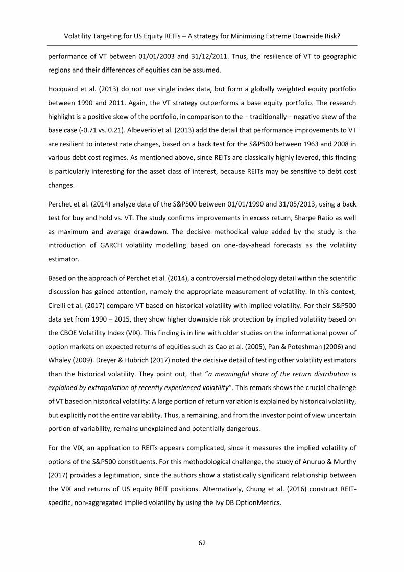
Volatility Targeting for US Equity REITs – A strategy for Minimizing Extreme Downside Risk?
62
performance of VT between 01/01/2003 and 31/12/2011. Thus, the resilience of VT to geographic
regions and their differences of equities can be assumed.
Hocquard et al. (2013) do not use single index data, but form a globally weighted equity portfolio
between 1990 and 2011. Again, the VT strategy outperforms a base equity portfolio. The research
highlight is a positive skew of the portfolio, in comparison to the – traditionally – negative skew of the
base case (-0.71 vs. 0.21). Albeverio et al. (2013) add the detail that performance improvements to VT
are resilient to interest rate changes, based on a back test for the S&P500 between 1963 and 2008 in
various debt cost regimes. As mentioned above, since REITs are classically highly levered, this finding
is particularly interesting for the asset class of interest, because REITs may be sensitive to debt cost
changes.
Perchet et al. (2014) analyze data of the S&P500 between 01/01/1990 and 31/05/2013, using a back
test for buy and hold vs. VT. The study confirms improvements in excess return, Sharpe Ratio as well
as maximum and average drawdown. The decisive methodical value added by the study is the
introduction of GARCH volatility modelling based on one-day-ahead forecasts as the volatility
estimator.
Based on the approach of Perchet et al. (2014), a controversial methodology detail within the scientific
discussion has gained attention, namely the appropriate measurement of volatility. In this context,
Cirelli et al. (2017) compare VT based on historical volatility with implied volatility. For their S&P500
data set from 1990 – 2015, they show higher downside risk protection by implied volatility based on
the CBOE Volatility Index (VIX). This finding is in line with older studies on the informational power of
option markets on expected returns of equities such as Cao et al. (2005), Pan & Poteshman (2006) and
Whaley (2009). Dreyer & Hubrich (2017) noted the decisive detail of testing other volatility estimators
than the historical volatility. They point out, that “a meaningful share of the return distribution is
explained by extrapolation of recently experienced volatility”. This remark shows the crucial challenge
of VT based on historical volatility: A large portion of return variation is explained by historical volatility,
but explicitly not the entire variability. Thus, a remaining, and from the investor point of view uncertain
portion of variability, remains unexplained and potentially dangerous.
For the VIX, an application to REITs appears complicated, since it measures the implied volatility of
options of the S&P500 constituents. For this methodological challenge, the study of Anuruo & Murthy
(2017) provides a legitimation, since the authors show a statistically significant relationship between
the VIX and returns of US equity REIT positions. Alternatively, Chung et al. (2016) construct REIT-
specific, non-aggregated implied volatility by using the Ivy DB OptionMetrics.
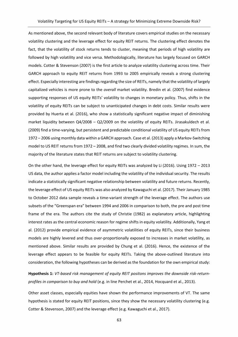
Volatility Targeting for US Equity REITs – A strategy for Minimizing Extreme Downside Risk?
63
As mentioned above, the second relevant body of literature covers empirical studies on the necessary
volatility clustering and the leverage effect for equity REIT returns. The clustering effect denotes the
fact, that the volatility of stock returns tends to cluster, meaning that periods of high volatility are
followed by high volatility and vice versa. Methodologically, literature has largely focused on GARCH
models. Cotter & Stevenson (2007) is the first article to analyze volatility clustering across time. Their
GARCH approach to equity REIT returns from 1993 to 2005 empirically reveals a strong clustering
effect. Especially interesting are findings regarding the size of REITs, namely that the volatility of largely
capitalized vehicles is more prone to the overall market volatility. Bredin et al. (2007) find evidence
supporting responses of US equity REITs’ volatility to changes in monetary policy. Thus, shifts in the
volatility of equity REITs can be subject to unanticipated changes in debt costs. Similar results were
provided by Huerta et al. (2016), who show a statistically significant negative impact of diminishing
market liquidity between Q4/2008 – Q2/2009 on the volatility of equity REITs. Jirasakuldech et al.
(2009) find a time-varying, but persistent and predictable conditional volatility of US equity REITs from
1972 – 2006 using monthly data within a GARCH approach. Case et al. (2013) apply a Markov-Switching
model to US REIT returns from 1972 – 2008, and find two clearly divided volatility regimes. In sum, the
majority of the literature states that REIT returns are subject to volatility clustering.
On the other hand, the leverage effect for equity REITs was analyzed by Li (2016). Using 1972 – 2013
US data, the author applies a factor model including the volatility of the individual security. The results
indicate a statistically significant negative relationship between volatility and future returns. Recently,
the leverage effect of US equity REITs was also analyzed by Kawaguchi et al. (2017). Their January 1985
to October 2012 data sample reveals a time-variant strength of the leverage effect. The authors use
subsets of the “Greenspan era” between 1994 and 2006 in comparison to both, the pre and post time
frame of the era. The authors cite the study of Christie (1982) as explanatory article, highlighting
interest rates as the central economic reason for regime shifts in equity volatility. Additionally, Yang et
al. (2012) provide empirical evidence of asymmetric volatilities of equity REITs, since their business
models are highly levered and thus over-proportionally exposed to increases in market volatility, as
mentioned above. Similar results are provided by Chung et al. (2016). Hence, the existence of the
leverage effect appears to be feasible for equity REITs. Taking the above-outlined literature into
consideration, the following hypotheses can be derived as the foundation for the own empirical study:
Hypothesis 1: VT-based risk management of equity REIT positons improves the downside risk-return-
profiles in comparison to buy and hold (e.g. in line Perchet et al., 2014, Hocquard et al., 2013).
Other asset classes, especially equities have shown the performance improvements of VT. The same
hypothesis is stated for equity REIT positions, since they show the necessary volatility clustering (e.g.
Cotter & Stevenson, 2007) and the leverage effect (e.g. Kawaguchi et al., 2017).

Volatility Targeting for US Equity REITs – A strategy for Minimizing Extreme Downside Risk?
64
Hypothesis 2: Volatility estimation based on implied volatility using the VIX Index and GARCH-based VT
strategies improve the downside risk protection of REIT positions in comparison to historical volatility
measurements (e.g. in line with Cirelli et al., 2017).
Implied volatility modelling has a higher explanatory power for future market behavior. Thus, implied
volatility, measured by the VIX on the S&P 500 reduces the downside risk for equity REIT positions in
comparison to historical volatility. Similar expectations apply to GARCH-based modelling of future
volatility, since equity REIT volatility may be predictable (Jirasakuldech et al., 2009).
4.3 Data and descriptive statistics
The study uses daily log US equity REIT close price returns between 01/01/1999 and 01/01/2019, with
a total number of 5,031 observations per security, generated from Yahoo Finance. The beginning of
the timeframe was chosen for two reasons. Firstly, the analysis is intended to cover the most recent
periods of prominent bearish markets (“tech bubble” starting in August 2000 as well as the financial
crisis starting in 2008), in order to stress how the strategy of interest deals with heavy downturns.
Secondly, the methodological homogeneity with important reference studies such as Hocquard et al.
(2013) are of interest, to ensure comparability with the existing body of literature in other asset
classes.
The securities were selected from the NAREIT database. In order to establish a stable data sample over
the entire horizon, the security has to be constituent of the index for the entire sample span from
01/01/1999 to 01/01/2019. The described selection pattern leads to 54 US equity REITs being part of
the data sample, with a complete sample size of 271,674 return observations.
Within the sample, eight subclasses were identified, according to the classification of the NAREIT
database: office, industrial, retail, residential, diversified, lodging and resorts, self-storage and health
care. For the sample of equity REITs, the following descriptive statistics could be obtained:
Table 14: Descriptive statistics of daily US equity REIT returns (01/01/1999 – 01/01/2019)
Security mean Std. dev. median min max range skew kurtosis
(ticker)
Office
ARE 0.001 0.019 0.001 - 0.241 0.181 0.422 -0.197 16.622
BDN 0.000 0.023 0.001 -0.242 0.255 0.497 0.416 23.877
BXP 0.001 0.020 0.000 -0.167 0.239 0.406 0.522 19.434
CLI 0.000 0.021 0.000 -0.226 0.237 0.463 0.732 22.504
CUZ 0.000 0.024 0.000 -0.257 0.326 0.583 0.966 26.915
HIW 0.001 0.021 0.000 -0.254 0.233 0.486 0.435 21.058
KRC 0.001 0.020 0.001 -0.247 0.204 0.452 0.254 18.741
OFC 0.001 0.021 0.000 -0.250 0.175 0.425 0.202 14.218

Volatility Targeting for US Equity REITs – A strategy for Minimizing Extreme Downside Risk?
65
SLG 0.001 0.026 0.001 -0.278 0.408 0.686 0.981 37.503
Industrial
DRE 0.001 0.025 0.001 -0.316 0.381 0.697 0.598 39.470
EGP 0.001 0.018 0.001 -0.194 0.159 0.354 -0.037 11.127
FR 0.001 0.030 0.001 -0.319 0.512 0.831 2.127 48.990
PLD 0.001 0.024 0.001 -0.301 0.263 0.564 0.208 29.842
PSB 0.001 0.017 0.000 -0.145 0.179 0.324 0.459 12.623
Retail
ADC 0.001 0.022 0.001 -0.291 0.290 0.581 0.727 26.951
AKR 0.001 0.019 0.000 -0.175 0.147 0.322 0.091 8.907
BFS 0.001 0.019 0.000 -0.166 0.149 0.315 0.233 8.417
CBL 0.000 0.031 0.001 -0.360 0.465 0.825 0.462 29.852
FRT 0.001 0.018 0.001 -0.224 0.217 0.441 0.434 21.475
KIM 0.001 0.023 0.001 -0.246 0.337 0.583 1.100 29.044
MAC 0.001 0.025 0.001 -0.268 0.318 0.586 0.551 28.093
NNN 0.001 0.018 0.001 -0.215 0.169 0.384 0.057 15.467
O 0.001 0.018 0.001 -0.198 0.216 0.413 0.921 20.781
PEI 0.000 0.029 0.000 -0.276 0.324 0.599 0.785 22.492
REG 0.001 0.020 0.000 -0.222 0.221 0.442 0.356 19.600
RPT 0.000 0.022 0.000 -0.241 0.324 0.565 0.495 26.862
SKT 0.001 0.018 0.001 -0.149 0.160 0.310 0.270 9.077
SPG 0.001 0.021 0.001 -0.200 0.254 0.454 0.936 21.632
TCO 0.001 0.022 0.000 -0.216 0.235 0.451 0.618 19.197
WRI 0.001 0.021 0.001 -0.220 0.255 0.476 1.160 26.605
Residential
AIV 0.001 0.023 0.001 -0.271 0.276 0.547 0.191 23.051
AVB 0.001 0.019 0.001 -0.171 0.181 0.352 0.365 13.717
BRT 0.001 0.024 0.000 - 0.196 0.405 0.602 2.640 48.217
CPT 0.001 0.020 0.001 -0.169 0.224 0.393 0.724 19.287
EQR 0.001 0.021 0.001 -0.216 0.236 0.452 0.834 24.249
ESS 0.001 0.018 0.001 -0.197 0.149 0.346 -0.020 13.359
MAA 0.001 0.019 0.001 -0.228 0.230 0.459 0.538 22.979
SUI 0.001 0.018 0.000 -0.192 0.156 0.348 0.179 13.260
UDR 0.001 0.020 0.001 -0.190 0.175 0.365 0.274 16.198
UMH 0.000 0.016 0.000 -0.117 0.127 0.244 0.327 7.400
Diversified
ALX 0.001 0.020 0.000 -0.228 0.249 0.477 0.493 22.274
LXP 0.001 0.027 0.000 -0.342 0.309 0.652 0.537 28.974
OLP 0.001 0.024 0.000 -0.218 0.344 0.561 1.960 36.296
VNO 0.001 0.020 0.000 -0.194 0.222 0.416 0.587 18.883
WRE 0.000 0.019 0.000 -0.200 0.188 0.388 0.268 15.550
Lodging & Resorts
HPT 0.001 0.022 0.001 -0.214 0.296 0.510 0.716 26.493
IHT 0.001 0.047 0.000 -0.275 0.436 0.711 1.059 12.173
Self Storage
PSA 0.001 0.019 0.001 -0.187 0.203 0.390 0.655 17.132
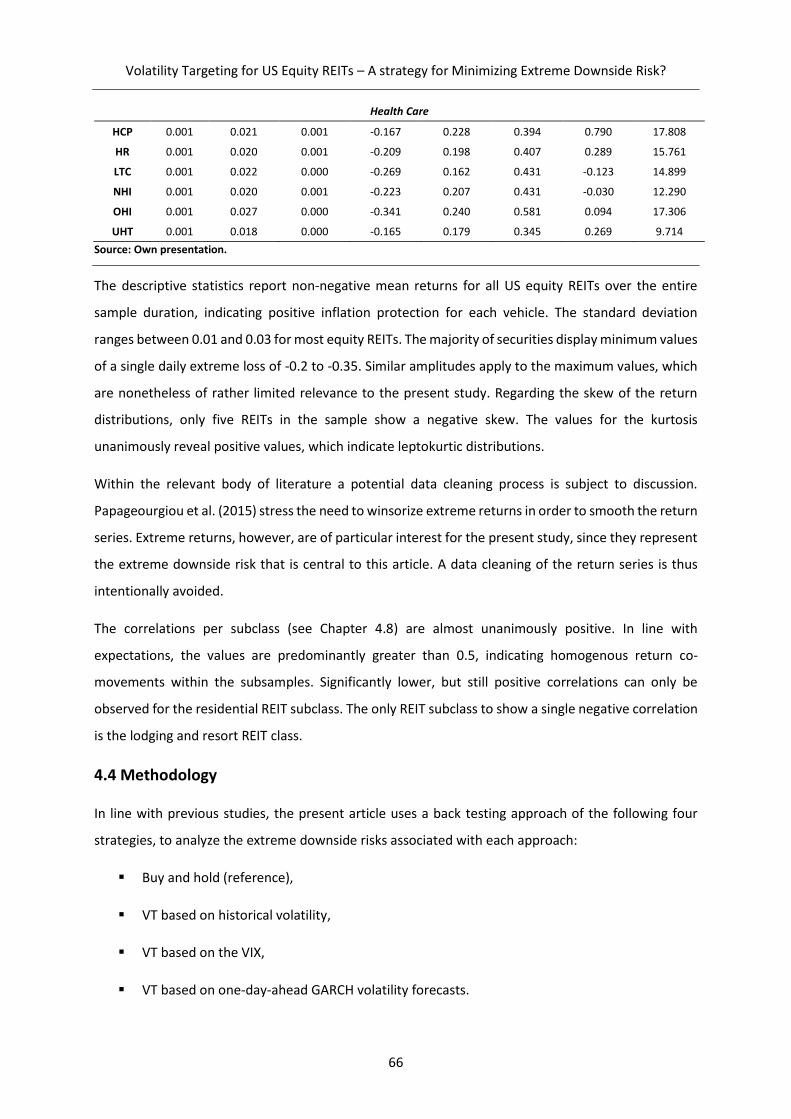
Volatility Targeting for US Equity REITs – A strategy for Minimizing Extreme Downside Risk?
66
Health Care
HCP 0.001 0.021 0.001 -0.167 0.228 0.394 0.790 17.808
HR 0.001 0.020 0.001 -0.209 0.198 0.407 0.289 15.761
LTC 0.001 0.022 0.000 -0.269 0.162 0.431 -0.123 14.899
NHI 0.001 0.020 0.001 -0.223 0.207 0.431 -0.030 12.290
OHI 0.001 0.027 0.000 -0.341 0.240 0.581 0.094 17.306
UHT 0.001 0.018 0.000 -0.165 0.179 0.345 0.269 9.714
Source: Own presentation.
The descriptive statistics report non-negative mean returns for all US equity REITs over the entire
sample duration, indicating positive inflation protection for each vehicle. The standard deviation
ranges between 0.01 and 0.03 for most equity REITs. The majority of securities display minimum values
of a single daily extreme loss of -0.2 to -0.35. Similar amplitudes apply to the maximum values, which
are nonetheless of rather limited relevance to the present study. Regarding the skew of the return
distributions, only five REITs in the sample show a negative skew. The values for the kurtosis
unanimously reveal positive values, which indicate leptokurtic distributions.
Within the relevant body of literature a potential data cleaning process is subject to discussion.
Papageourgiou et al. (2015) stress the need to winsorize extreme returns in order to smooth the return
series. Extreme returns, however, are of particular interest for the present study, since they represent
the extreme downside risk that is central to this article. A data cleaning of the return series is thus
intentionally avoided.
The correlations per subclass (see Chapter 4.8) are almost unanimously positive. In line with
expectations, the values are predominantly greater than 0.5, indicating homogenous return co-
movements within the subsamples. Significantly lower, but still positive correlations can only be
observed for the residential REIT subclass. The only REIT subclass to show a single negative correlation
is the lodging and resort REIT class.
4.4 Methodology
In line with previous studies, the present article uses a back testing approach of the following four
strategies, to analyze the extreme downside risks associated with each approach:
Buy and hold (reference),
VT based on historical volatility,
VT based on the VIX,
VT based on one-day-ahead GARCH volatility forecasts.
Volatility Targeting for US Equity REITs – A strategy for Minimizing Extreme Downside Risk?
67
A value of 12% p.a. was chosen as the target volatility, as proposed by Hocquard et al. (2015). However,
regarding the target annual volatility, Papageorgiou et al. (2015) point out that the targeted value
cannot be chosen wrongly. Instead, the target annual volatility is a sole function of investor risk-
appetite. Both Cooper (2010) and Albeverio et al. (2013) also show the resilience of VT efficiency
improvements to different levels of targeted annual volatility.
The back test uses the specified three other different volatility estimators for the VT, so as to assess
the second hypothesis. The study uses either the historical volatility of the individual security with a
30 day time frame, the implied volatility of the VIX, or a GARCH volatility forecast. The VIX value is
taken from the open price of the index on the day of reallocation. The latter estimator is defined by a
one-day-ahead forecast, with a standard GARCH(1,1) model, as introduced by Bollerslev (1986).
According to the volatility estimator of choice, the allocation or weight respectively 𝑤𝑡 towards a
particular security will be adjusted by (Perchet et al., 2014):
𝑤𝑡 =𝜅
𝜎𝑡, 0 < 𝑤𝑡 < ∞ (19)
with target volatility 𝜅, and the annualized estimated volatility 𝜎𝑡. For example, if the estimator
calculates a volatility of 20% p.a., given a target volatility of 12% p.a., the resulting weighting of the
security equals 𝑤𝑡 =0.12
0.2⁄ = 0.6.15 The VT-based return, denoted by 𝑟𝑡𝑉𝑇, equals the product of
the return 𝑟𝑡 of the actual time series multiplied by the weight, 𝑤𝑡:
𝑟𝑡𝑉𝑇 = 𝑟𝑡
𝜅
𝜎𝑡= 𝑟𝑡𝑤𝑡
(20)
The length between points of potential reallocation is set to 30 days (in line with Hocquard et al., 2013).
Several studies have shown the impact of changes to daily, weekly, or monthly rebalancing rhythm
(Morrison & Tadrowski, 2013), without significant changes to the results. Interestingly, Marra (2017)
proved a rescaling error caused by excessively frequent (weekly) rebalancing. Furthermore, Perchet et
al. (2015) show that the gains in the Sharpe Ratio are resilient to rescaling rhythm changes.
After back testing the strategies, the study applies modern portfolio theory in order to analyze whether
potential extreme downside risk minimizations are also economically efficient. The analysis uses the
entire sample as well as the specified subclasses according to the NAREIT Index, to check for potential
15 If 𝜅 > 𝜎𝑡 applies, the weight 𝑤𝑡 can also be >1.
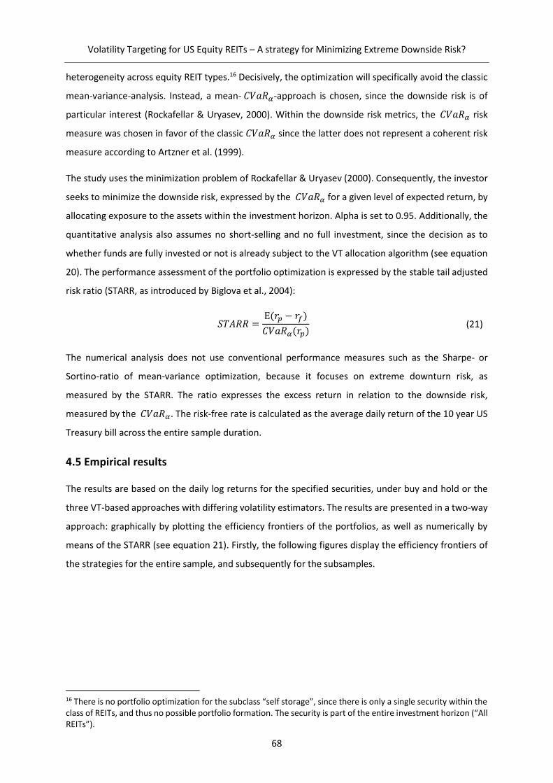
Volatility Targeting for US Equity REITs – A strategy for Minimizing Extreme Downside Risk?
68
heterogeneity across equity REIT types.16 Decisively, the optimization will specifically avoid the classic
mean-variance-analysis. Instead, a mean- 𝐶𝑉𝑎𝑅𝛼-approach is chosen, since the downside risk is of
particular interest (Rockafellar & Uryasev, 2000). Within the downside risk metrics, the 𝐶𝑉𝑎𝑅𝛼 risk
measure was chosen in favor of the classic 𝐶𝑉𝑎𝑅𝛼 since the latter does not represent a coherent risk
measure according to Artzner et al. (1999).
The study uses the minimization problem of Rockafellar & Uryasev (2000). Consequently, the investor
seeks to minimize the downside risk, expressed by the 𝐶𝑉𝑎𝑅𝛼 for a given level of expected return, by
allocating exposure to the assets within the investment horizon. Alpha is set to 0.95. Additionally, the
quantitative analysis also assumes no short-selling and no full investment, since the decision as to
whether funds are fully invested or not is already subject to the VT allocation algorithm (see equation
20). The performance assessment of the portfolio optimization is expressed by the stable tail adjusted
risk ratio (STARR, as introduced by Biglova et al., 2004):
𝑆𝑇𝐴𝑅𝑅 =Ε(𝑟𝑝 − 𝑟𝑓)
𝐶𝑉𝑎𝑅𝛼(𝑟𝑝) (21)
The numerical analysis does not use conventional performance measures such as the Sharpe- or
Sortino-ratio of mean-variance optimization, because it focuses on extreme downturn risk, as
measured by the STARR. The ratio expresses the excess return in relation to the downside risk,
measured by the 𝐶𝑉𝑎𝑅𝛼. The risk-free rate is calculated as the average daily return of the 10 year US
Treasury bill across the entire sample duration.
4.5 Empirical results
The results are based on the daily log returns for the specified securities, under buy and hold or the
three VT-based approaches with differing volatility estimators. The results are presented in a two-way
approach: graphically by plotting the efficiency frontiers of the portfolios, as well as numerically by
means of the STARR (see equation 21). Firstly, the following figures display the efficiency frontiers of
the strategies for the entire sample, and subsequently for the subsamples.
16 There is no portfolio optimization for the subclass “self storage”, since there is only a single security within the class of REITs, and thus no possible portfolio formation. The security is part of the entire investment horizon (“All REITs”).
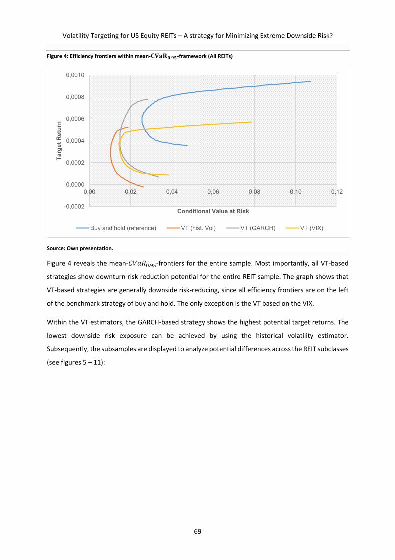
Volatility Targeting for US Equity REITs – A strategy for Minimizing Extreme Downside Risk?
69
Figure 4: Efficiency frontiers within mean-𝐂𝐕𝐚𝐑𝟎.𝟗𝟓-framework (All REITs)
Source: Own presentation.
Figure 4 reveals the mean-𝐶𝑉𝑎𝑅0.95-frontiers for the entire sample. Most importantly, all VT-based
strategies show downturn risk reduction potential for the entire REIT sample. The graph shows that
VT-based strategies are generally downside risk-reducing, since all efficiency frontiers are on the left
of the benchmark strategy of buy and hold. The only exception is the VT based on the VIX.
Within the VT estimators, the GARCH-based strategy shows the highest potential target returns. The
lowest downside risk exposure can be achieved by using the historical volatility estimator.
Subsequently, the subsamples are displayed to analyze potential differences across the REIT subclasses
(see figures 5 – 11):
-0,0002
0,0000
0,0002
0,0004
0,0006
0,0008
0,0010
0,00 0,02 0,04 0,06 0,08 0,10 0,12
Ta
rge
t R
etu
rn
Conditional Value at Risk
Buy and hold (reference) VT (hist. Vol) VT (GARCH) VT (VIX)
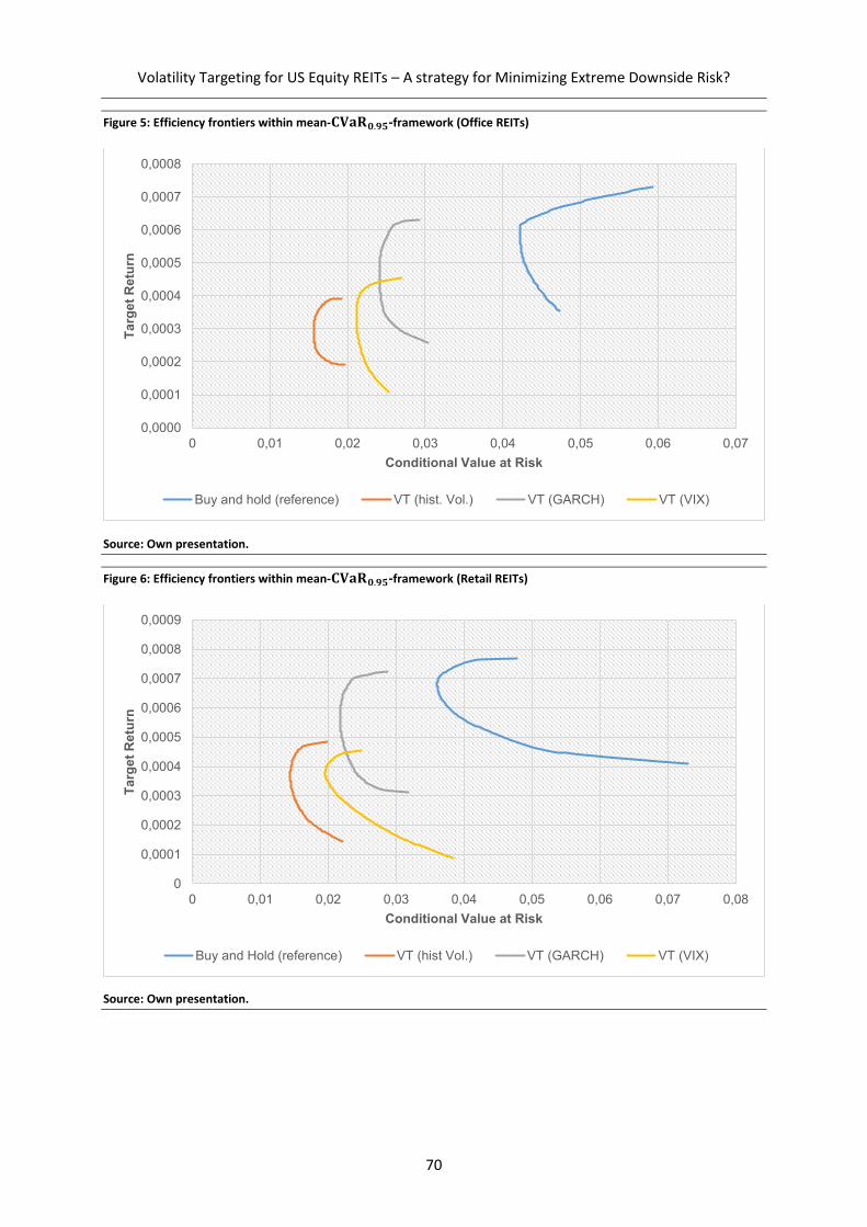
Volatility Targeting for US Equity REITs – A strategy for Minimizing Extreme Downside Risk?
70
Figure 5: Efficiency frontiers within mean-𝐂𝐕𝐚𝐑𝟎.𝟗𝟓-framework (Office REITs)
Source: Own presentation.
Figure 6: Efficiency frontiers within mean-𝐂𝐕𝐚𝐑𝟎.𝟗𝟓-framework (Retail REITs)
Source: Own presentation.
0,0000
0,0001
0,0002
0,0003
0,0004
0,0005
0,0006
0,0007
0,0008
0 0,01 0,02 0,03 0,04 0,05 0,06 0,07
Ta
rge
t R
etu
rn
Conditional Value at Risk
Buy and hold (reference) VT (hist. Vol.) VT (GARCH) VT (VIX)
0
0,0001
0,0002
0,0003
0,0004
0,0005
0,0006
0,0007
0,0008
0,0009
0 0,01 0,02 0,03 0,04 0,05 0,06 0,07 0,08
Ta
rge
t R
etu
rn
Conditional Value at Risk
Buy and Hold (reference) VT (hist Vol.) VT (GARCH) VT (VIX)
Volatility Targeting for US Equity REITs – A strategy for Minimizing Extreme Downside Risk?
71
Figure 7: Efficiency frontiers within mean-𝐂𝐕𝐚𝐑𝟎.𝟗𝟓-framework (Industrial REITs)
Source: Own presentation.
Figure 8: Efficiency frontiers within mean-𝐂𝐕𝐚𝐑𝟎.𝟗𝟓-framework (Residential REITs)
Source: Own presentation.
0
0,0001
0,0002
0,0003
0,0004
0,0005
0,0006
0,0007
0,0008
0 0,01 0,02 0,03 0,04 0,05 0,06 0,07
Ta
rge
t R
etu
rn
Conditional Value at Risk
Buy and Hold (reference) VT (hist. Vol) VT (GARCH) VT (VIX)
0
0,0001
0,0002
0,0003
0,0004
0,0005
0,0006
0,0007
0,0008
0,0009
0 0,005 0,01 0,015 0,02 0,025 0,03 0,035 0,04 0,045
Ta
rge
t R
etu
rn
Conditional Value at Risk
Buy and hold (reference) VT (hist. Vol.) VT (GARCH) VT (VIX)

Volatility Targeting for US Equity REITs – A strategy for Minimizing Extreme Downside Risk?
72
Figure 9: Efficiency frontiers within mean-𝐂𝐕𝐚𝐑𝟎.𝟗𝟓-framework (Diversified REITs)
Source: Own presentation.
Figure 10: Efficiency frontiers within mean-𝐂𝐕𝐚𝐑𝟎.𝟗𝟓-framework (Lodging and Resort REITs)
Source: Own presentation.
0
0,0001
0,0002
0,0003
0,0004
0,0005
0,0006
0,0007
0,0008
0 0,01 0,02 0,03 0,04 0,05 0,06
Ta
rge
t R
etu
rn
Conditional Value at Risk
Buy and Hold (reference) VT (hist. Vol) VT (GARCH) VT (VIX)
-0,0002
0
0,0002
0,0004
0,0006
0,0008
0,001
0 0,02 0,04 0,06 0,08 0,1 0,12
Ta
rge
t R
etu
rn
Conditional Value at Risk
Buy and hold (reference) VT (hist. Vol.) VT (GARCH) VT (VIX)

Volatility Targeting for US Equity REITs – A strategy for Minimizing Extreme Downside Risk?
73
Figure 11: Efficiency frontiers within mean-𝐂𝐕𝐚𝐑𝟎.𝟗𝟓-framework (Health Care REITs)
Source: Own presentation.
As revealed by the performance diagrams above, VT-based risk management of the equity REIT
positions reduces the 𝐶𝑉𝑎𝑅0.95, since the efficiency frontiers for all samples offer solutions on the left
of the buy and hold reference. The GARCH-based VT strategy generally provides the highest returns
compared to its peers. Historical volatility as an estimator provides the lowest 𝐶𝑉𝑎𝑅0.95 solutions in
all samples.17 Thus, from an investor point of view, the historical volatility approach suits risk-averse
investors best. Lodging and Resort REITs are, interestingly, most risk-aversely managed by using a VIX-
based volatility targeting scheme. However, across all other samples, the VIX-based strategy is
outperformed either on the return side by the GARCH-based VT or on the extreme downside risk side
by the historical volatility estimator.
In addition to the graphical analysis, the maximum STARR of the efficiency frontiers reveal numerical
proof of economic efficiency of the VT strategies. The figures show both interesting and puzzling
results, since they are heterogeneous across the REIT types (see Table 15):
17 Robustness checks for various timeframes regarding historical volatility estimation were tested, and results are consistent across different frames (30 – 60 days).
0
0,0001
0,0002
0,0003
0,0004
0,0005
0,0006
0,0007
0,0008
0,00 0,01 0,02 0,03 0,04 0,05 0,06
Ta
rge
t R
etu
rn
Conditional Value at Risk
Buy and hold (reference) VT (hist. Vol) VT (GARCH) VT (VIX)
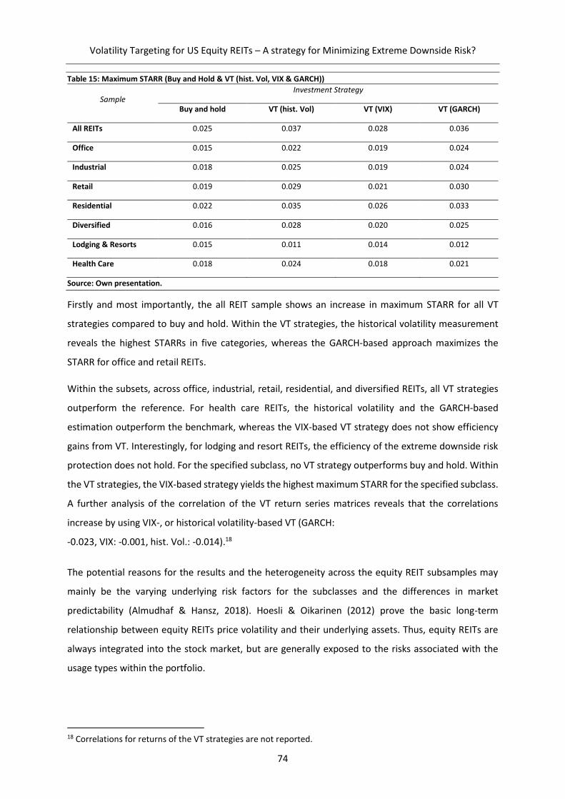
Volatility Targeting for US Equity REITs – A strategy for Minimizing Extreme Downside Risk?
74
Table 15: Maximum STARR (Buy and Hold & VT (hist. Vol, VIX & GARCH))
Sample Investment Strategy
Buy and hold VT (hist. Vol) VT (VIX) VT (GARCH)
All REITs 0.025 0.037 0.028 0.036
Office 0.015 0.022 0.019 0.024
Industrial 0.018 0.025 0.019 0.024
Retail 0.019 0.029 0.021 0.030
Residential 0.022 0.035 0.026 0.033
Diversified 0.016 0.028 0.020 0.025
Lodging & Resorts 0.015 0.011 0.014 0.012
Health Care 0.018 0.024 0.018 0.021
Source: Own presentation.
Firstly and most importantly, the all REIT sample shows an increase in maximum STARR for all VT
strategies compared to buy and hold. Within the VT strategies, the historical volatility measurement
reveals the highest STARRs in five categories, whereas the GARCH-based approach maximizes the
STARR for office and retail REITs.
Within the subsets, across office, industrial, retail, residential, and diversified REITs, all VT strategies
outperform the reference. For health care REITs, the historical volatility and the GARCH-based
estimation outperform the benchmark, whereas the VIX-based VT strategy does not show efficiency
gains from VT. Interestingly, for lodging and resort REITs, the efficiency of the extreme downside risk
protection does not hold. For the specified subclass, no VT strategy outperforms buy and hold. Within
the VT strategies, the VIX-based strategy yields the highest maximum STARR for the specified subclass.
A further analysis of the correlation of the VT return series matrices reveals that the correlations
increase by using VIX-, or historical volatility-based VT (GARCH:
-0.023, VIX: -0.001, hist. Vol.: -0.014).18
The potential reasons for the results and the heterogeneity across the equity REIT subsamples may
mainly be the varying underlying risk factors for the subclasses and the differences in market
predictability (Almudhaf & Hansz, 2018). Hoesli & Oikarinen (2012) prove the basic long-term
relationship between equity REITs price volatility and their underlying assets. Thus, equity REITs are
always integrated into the stock market, but are generally exposed to the risks associated with the
usage types within the portfolio.
18 Correlations for returns of the VT strategies are not reported.
Volatility Targeting for US Equity REITs – A strategy for Minimizing Extreme Downside Risk?
75
Accordingly, some REIT classes such as office, industrial and retail are sensitive to different economic
fundamentals (e.g. unemployment, GDP growth, consume sentiment), and thus react with less
different price movements to extreme economic meltdowns such as in 2008. In contrast, health care,
and self storage are seen as non-cyclical vehicles, since their income is relatively resilient to economic
fundamentals. The specified subclasses generally provide smoother returns. Self storage income can
even increase during recessions, due to lower space demand in residential markets, and higher
demand for temporal storage of furniture. Risk factors of non-residential REITs are classically
differentiated from residential REITs. The latter may also benefit from the cost of debt, since home
ownership rates decrease, and thus residential space demand increases (Almudhaf & Hansz, 2018).
These differences in return predictability and ex post volatility across the equity REIT subclasses can
cause the heterogeneity of the results.
4.6 Conclusion, practical implications and further research
The present study analyzed the feasibility of VT strategies for minimizing extreme downside risks of US
equity REIT positions. Accordingly, a two-stage procedure containing a back testing and subsequently
a mean-𝐶𝑉𝑎𝑅𝛼-portfolio-optimization was conducted. The latter expressed the extreme downside
risk-return profiles of the strategies by calculating the maximum STARR.
The results reveal the following findings. Firstly, VT-based strategies generally reduce extreme
downside risk, as illustrated by the position of the efficiency frontiers within the mean-𝐶𝑉𝑎𝑅𝛼-
diagram. Additionally, VT risk protection can also be evaluated as predominantly economically efficient
for REIT investors, expressed by increased STARRs. The only equity REIT subclass to be consistently
inefficient is lodging & resort REITs. Thus, the first hypothesis cannot be rejected.
Within the different volatility estimators, the lowest 𝐶𝑉𝑎𝑅𝛼 values are predominantly achieved by the
historical volatility estimator, as revealed by optical inspection. The majority of samples reveals the
highest efficiency for historical volatility measurement, followed by the GARCH approach. A VIX-based
estimation yields the lowest efficiency. Thus, a trading strategy based on the implied volatility
estimator of the S&P500 index appears to be problematic. From an investor point of view, the results
increase doubts as to a sufficient capital market integration of equity REITs within the broader stock
market. Accordingly, the second hypothesis needs to be rejected, since the VIX performs worse than
the historical volatility estimator in seven of eight samples. In sum, the individual security volatility
estimation seems to be more efficient than the modelling based on the entire stock market using the
VIX.
The practical contribution of the empirical study is straight forward: Any risk-averse US equity REIT
investor may apply VT in order to minimize extreme downside risk, since the 𝐶𝑉𝑎𝑅𝛼 of portfolios can
Volatility Targeting for US Equity REITs – A strategy for Minimizing Extreme Downside Risk?
76
be reduced. Additionally, investors can also improve the efficiency of their portfolios by using VT based
on a GARCH model or on historical volatility.
Limitations of the present paper apply to the data sample, which analyzes only US equity REIT data. A
comparison between equity and mortgage REITs or geographically at an international level, is not
possible. VT studies across different REIT markets could provide insight into investment strategy
usability across different geographic regions and also across market maturity levels (emerging vs.
matured). Additionally, methodological limitations apply to the heterogeneity of the portfolio sizes,
since the number of assets differs across the subsamples. Another point of potential criticism relate to
the ignorance of transaction costs, as recently highlighted by Zakamulin (2019).
Further research could address other historical volatility measures such as Garman & Klass (1980),
Parkinson (1980), Rogers & Satchell (1991) or Yang & Zhang (2000). Since the present study shows
efficiency gains from GARCH-based VT, further research in the field using asymmetric models including
exponential GARCH (Nelsen, 1991), threshold GARCH (Glosten et al., 1993) or asymmetric power
GARCH (Ding et al., 1993) to estimate volatility may be beneficial. Harvey & Lange (2018) recently
provided a comprehensive study for exponential GARCH modelling of broad US equities. Another field
of interest may entail intraday VT strategies, since Zhou (2017) demonstrates higher explanatory
power of these models for future return prediction. Models with higher data frequency may lead to
further risk reduction potential. With increasing data availability the intraday volatility measurement
has attracted greater interest. The authors highlights the need for HEAVY or GARCHX models, since
high frequency data is less prone to market microstructures such as bid-ask-diffusions, discrete price
observations or irregular trading.

Volatility Targeting for US Equity REITs – A strategy for Minimizing Extreme Downside Risk?
77
4.7 Bibliography
Albeverio, S., Steblovskaya, V., & Wallbaum, K. (2013). Investment instruments with volatility target
mechanism. Quantitative Finance, 13(10), pp. 1519–1528.
Almudhaf, F., & Hansz, A. J. (2018). Random Walks and Market Efficiency: Evidence from Real Estate
Investment Trusts (REIT) Subsectors. International Journal of Strategic Property Management,
22(2), pp. 81–92.
Anoruo, E., & Murthy, V. N. (2017). An examination of the REIT return–implied volatility relation: a
frequency domain approach. Journal of Economics and Finance, 41(3), pp. 581–594.
Artzner, P., Delbaen, F., Eber, J.-M., & Heath, D. (1999). Coherent Measures of Risk. Mathematical
Finance, 9(3), pp. 203–228.
Biglova, A., Ortobelli, S., Rachev, S. T., & Stoyanov, S. (2004). Different Approaches to Risk Estimation
in Portfolio Theory. The Journal of Portfolio Management, 31(1), pp. 103–112.
Bollerslev, T. (1986). Generalized autoregressive conditional heteroskedasticity. Journal of
Econometrics, 31(3), pp. 307–327.
Cao, C., Chen, Z., & Griffin, J. M. (2005). Informational Content of Option Volume Prior to Takeovers.
The Journal of Business, 78(3), pp. 1073–1109.
Case, B., Guidolin, M., & Yildirim, Y. (2013). Do We Need Non-Linear Models to Predict REIT Returns?
Manchster Business School Working Paper. Manchester.
Chorro, C., Guegan, D., Ielpo, F., & Lalaharison, H. (2018). Testing for leverage effects in the returns of
US equities. Journal of Empirical Finance, 48, pp. 290–306.
Christie, A. A. (1982). The stochastic behavior of common stock variances: Value, leverage and interest
rate effects. Journal of Financial Economics, 10(4), pp. 407–432.
Chung, R., Fung, S., Shilling, J. D., & Simmons-Mosley, T. X. (2016). REIT Stock Market Volatility and
Expected Returns. Real Estate Economics, 44(4), pp. 968–995.
Cirelli, S., Vitali, S., Ortobelli Lozza, S., & Moriggia, V. (2017). A conservative discontinuous target
volatility strategy. Investment Management and Financial Innovations, 14(2), pp. 176–190.
Cooper, T. (2010). Alpha Generation and Risk Smoothing Using Managed Volatility. Double Digit
Numerics.
Cotter, J., & Stevenson, S. (2007). Uncovering Volatility Dynamics in Daily REIT Returns. The Journal of
Real Estate Portfolio Management, 13(2), pp. 119–128.

Volatility Targeting for US Equity REITs – A strategy for Minimizing Extreme Downside Risk?
78
Ding, Z., Granger, C., & Engle, R. (1993). A long memory property of stock market returns and a new
model. Journal of Empirical Finance, 1(1), pp. 83–106.
Dreyer, A., & Hubrich, S. (2017). Tail Risk Mitigation with Managed Volatility Strategies. Journal of
Investment Strategies, 8(1), pp. 29–56.
Fleming, J., Kirby, C., & Ostdiek, B. (2001). The Economic Value of Volatility Timing. The Journal of
Finance, 56(1), pp. 329–352.
Garman, M. B., & Klass, M. J. (1980). On the Estimation of Security Price Volatilities from Historical
Data. The Journal of Business, 53(1), pp. 67–78.
Glosten, L., Jagannathan, R., & Runkle, D. (1993). On the Relation between the Expected Value and the
Volatility of the Nominal Excess Return on Stocks. The Journal of Finance, 48(5), pp. 1779–
1801.
Hallerbach, W. G. (2012). A proof of the optimality of volatility weighting over time. The Journal of
Investment Strategies, 1(4), pp. 87–99.
Harvey, A., & Lange, R.-J. (2018). Modeling the Interactions between Volatility and Returns using
EGARCH-M. Journal of Time Series Analysis, 39(6), pp. 909–919.
Harvey, C. R., Hoyle, E., Korgaonkar, R., Rattray, S., Sargaison, M., & van Hemert, O. (2018). The Impact
of Volatility Targeting. The Journal of Portfolio Management, 45(1), pp. 14–33.
Hocquard, A., Ng, S., & Papageorgiou, N. (2013). A Constant-Volatility Framework for Managing Tail
Risk. The Journal of Portfolio Management, 39(2), pp. 28–40.
Hocquard, A., Papageorgiou, N., & Remillard, B. (2015). The payoff distribution model: an application
to dynamic portfolio insurance. Quantitative Finance, 15(2), pp. 299–312.
Hoesli, M., & Oikarinen, E. (2012). Are REITs real estate? Evidence from international sector level data.
Journal of International Money and Finance, 31(7), pp. 1823–1850.
Huerta, D., Egly, P., & Escobari, D. (2016). The Liquidity Crisis, Investor Sentiment, and REIT Returns
and Volatility. Journal of Real Estate Portfolio Management, 22(1), pp. 47–62.
Jirasakuldech, B., Campbell, R. D., & Emekter, R. (2009). Conditional Volatility of Equity Real Estate
Investment Trust Returns: A Pre- and Post-1993 Comparison. The Journal of Real Estate
Finance and Economics, 38(2), pp. 137–154.
Kawaguchi, Y., Sa-Aadu, J., & Shilling, J. D. (2017). REIT Stock Price Volatility and the Effects of Leverage.
Real Estate Economics, 45(2), pp. 452–477.
Li, Y. (2016). Time Variation of Expected Returns on REITs: Implications for Market Integration and
Financial Crisis. Journal of Real Estate Research, 38(3), pp. 321–357.

Volatility Targeting for US Equity REITs – A strategy for Minimizing Extreme Downside Risk?
79
Marra, S. (2017). Dynamic Volatility Targeting. Lazard Asset Management Investment Research.
Morrison, S., & Tadrowski, L. (2013). Guarantees and Target Volatility Funds. Moody's Analytics.
Nelson, D. B. (1991). Conditional Heteroskedasticity in Asset Returns: A New Approach. Econometrica,
59(2), pp. 347–370.
Pan, J., & Poteshman, A. M. (2006). The Information in Option Volume for Future Stock Prices. Review
of Financial Studies, 19(3), pp. 871–908.
Papageorgiou, N. A., Reeves, J. J., & Sherris, M. (2015). Equity Investing with Targeted Constant
Volatility Exposure. FIRN Research Paper.
Parkinson, M. (1980). The Extreme Value Method for Estimating the Variance of the Rate of Return.
The Journal of Business, 53(1), pp. 61–65.
Perchet, R., Carvalho, R. L., Heckel, T., & Moulin, P. (2014). Inter-Temporal Risk Parity: A Constant
Volatility Framework for Equities and Other Asset Classes. SSRN Electronic Journal.
Perchet, R., Carvalho, R. L., Heckel, T., & Moulin, P. (2015). Predicting the Success of Volatility Targeting
Strategies: Application to Equities and Other Asset Classes. The Journal of Alternative
Investments, 18(3), pp. 21–38.
Rockafellar, R. T., & Uryasev, S. (2000). Optimization of conditional value-at-risk. The Journal of Risk,
2(3), pp. 21–41.
Rogers, L. C., & Satchell, S. E. (1991). Estimating Variance From High, Low and Closing Prices. The Annals
of Applied Probability, 1(4), pp. 504–512.
Whaley, R. E. (2009). Understanding the VIX. The Journal of Portfolio Management, 35(3), pp. 98–105.
Yang, D., & Zhang, Q. (2000). Drift Independent Volatility Estimation Based on High, Low, Open, and
Close Prices. The Journal of Business, 73(3), pp. 477–492.
Yang, J., Zhou, Y., & Leung, W. K. (2012). Asymmetric Correlation and Volatility Dynamics among Stock,
Bond, and Securitized Real Estate Markets. The Journal of Real Estate Finance and Economics,
45(2), pp. 491–521.
Zakamulin, V. (2019). Volatility Weighting Over Time in the Presence of Transaction Costs. Journal of
Wealth Management , 21(4), pp. 33–45.
Zhou, J. (2017). Forecasting REIT volatility with high-frequency data: a comparison of alternative
methods. Applied Economics, 49(26), pp. 2590–2605.
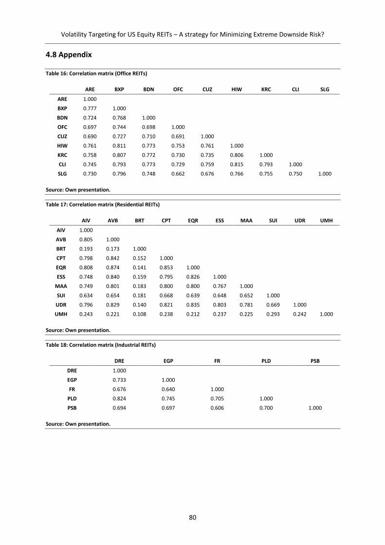
Volatility Targeting for US Equity REITs – A strategy for Minimizing Extreme Downside Risk?
80
4.8 Appendix
Table 16: Correlation matrix (Office REITs)
ARE BXP BDN OFC CUZ HIW KRC CLI SLG
ARE 1.000
BXP 0.777 1.000
BDN 0.724 0.768 1.000
OFC 0.697 0.744 0.698 1.000
CUZ 0.690 0.727 0.710 0.691 1.000
HIW 0.761 0.811 0.773 0.753 0.761 1.000
KRC 0.758 0.807 0.772 0.730 0.735 0.806 1.000
CLI 0.745 0.793 0.773 0.729 0.759 0.815 0.793 1.000
SLG 0.730 0.796 0.748 0.662 0.676 0.766 0.755 0.750 1.000
Source: Own presentation.
Table 17: Correlation matrix (Residential REITs)
AIV AVB BRT CPT EQR ESS MAA SUI UDR UMH
AIV 1.000
AVB 0.805 1.000
BRT 0.193 0.173 1.000
CPT 0.798 0.842 0.152 1.000
EQR 0.808 0.874 0.141 0.853 1.000
ESS 0.748 0.840 0.159 0.795 0.826 1.000
MAA 0.749 0.801 0.183 0.800 0.800 0.767 1.000
SUI 0.634 0.654 0.181 0.668 0.639 0.648 0.652 1.000
UDR 0.796 0.829 0.140 0.821 0.835 0.803 0.781 0.669 1.000
UMH 0.243 0.221 0.108 0.238 0.212 0.237 0.225 0.293 0.242 1.000
Source: Own presentation.
Table 18: Correlation matrix (Industrial REITs)
DRE EGP FR PLD PSB
DRE 1.000
EGP 0.733 1.000
FR 0.676 0.640 1.000
PLD 0.824 0.745 0.705 1.000
PSB 0.694 0.697 0.606 0.700 1.000
Source: Own presentation.
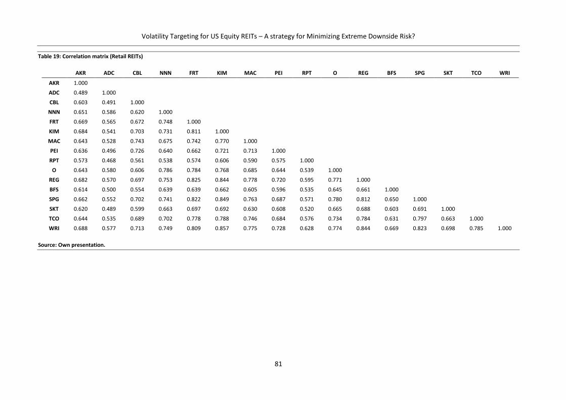
Volatility Targeting for US Equity REITs – A strategy for Minimizing Extreme Downside Risk?
81
Table 19: Correlation matrix (Retail REITs)
AKR ADC CBL NNN FRT KIM MAC PEI RPT O REG BFS SPG SKT TCO WRI
AKR 1.000
ADC 0.489 1.000
CBL 0.603 0.491 1.000
NNN 0.651 0.586 0.620 1.000
FRT 0.669 0.565 0.672 0.748 1.000
KIM 0.684 0.541 0.703 0.731 0.811 1.000
MAC 0.643 0.528 0.743 0.675 0.742 0.770 1.000
PEI 0.636 0.496 0.726 0.640 0.662 0.721 0.713 1.000
RPT 0.573 0.468 0.561 0.538 0.574 0.606 0.590 0.575 1.000
O 0.643 0.580 0.606 0.786 0.784 0.768 0.685 0.644 0.539 1.000
REG 0.682 0.570 0.697 0.753 0.825 0.844 0.778 0.720 0.595 0.771 1.000
BFS 0.614 0.500 0.554 0.639 0.639 0.662 0.605 0.596 0.535 0.645 0.661 1.000
SPG 0.662 0.552 0.702 0.741 0.822 0.849 0.763 0.687 0.571 0.780 0.812 0.650 1.000
SKT 0.620 0.489 0.599 0.663 0.697 0.692 0.630 0.608 0.520 0.665 0.688 0.603 0.691 1.000
TCO 0.644 0.535 0.689 0.702 0.778 0.788 0.746 0.684 0.576 0.734 0.784 0.631 0.797 0.663 1.000
WRI 0.688 0.577 0.713 0.749 0.809 0.857 0.775 0.728 0.628 0.774 0.844 0.669 0.823 0.698 0.785 1.000
Source: Own presentation.
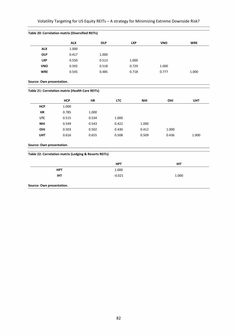
Volatility Targeting for US Equity REITs – A strategy for Minimizing Extreme Downside Risk?
82
Table 20: Correlation matrix (Diversified REITs)
ALX OLP LXP VNO WRE
ALX 1.000
OLP 0.417 1.000
LXP 0.550 0.513 1.000
VNO 0.592 0.518 0.729 1.000
WRE 0.545 0.485 0.718 0.777 1.000
Source: Own presentation.
Table 21: Correlation matrix (Health Care REITs)
HCP HR LTC NHI OHI UHT
HCP 1.000
HR 0.785 1.000
LTC 0.515 0.534 1.000
NHI 0.549 0.543 0.422 1.000
OHI 0.503 0.502 0.430 0.412 1.000
UHT 0.616 0.655 0.508 0.509 0.436 1.000
Source: Own presentation.
Table 22: Correlation matrix (Lodging & Resorts REITs)
HPT IHT
HPT 1.000
IHT -0.021 1.000
Source: Own presentation.
83
5 AR-GARCH-EVT-Copula for Securitized Real
Estate: An approach to improving risk forecasts?
Carsten Fritz, Cay Oertel
Journal of Property Research (Revised)
Abstract
This study presents a quantitative analysis of the so-called AR-GARCH-EVT-Copula model aimed at
forecasting risk metrics for multi-asset portfolios, including securitized real estate positions. The model
incorporates a non-linear dependence structure and time-varying volatility in asset returns.
Accordingly, an empirical study using data from six major global markets is carried out. The approach
is applied in order to forecast risk metrics, in comparison to classical methods like historical simulation
and variance-covariance models. Forecasts are then compared with realized returns, in order to
calculate hit sequences and conduct statistical interference on the respective models. It is empirically
shown that, the AR-GARCH-EVT-Copula model provides a superior forecast concerning risk metrics.
This is mainly due to the usage of copulas, allowing us to individually model the dependence structure
of random variables. Back testing and test results confirm the superiority of our model in comparison
with classic methods such as historical simulation and Variance-Covariance approach. The
decomposition of the univariate and multivariate models of the target model reveal the necessity to
allow for high order and thus long-lasting autoregressive modelling as well as asymmetric tail
dependence and rotated copulae across different portfolios.
AR-GARCH-EVT-Copula for Securitized Real Estate: An approach to improving risk forecasts?
84
5.1 Introduction
The risk modelling of investment positions has attracted larger interest, since the global financial crises
(GFC) in 2008 painfully demonstrated the vulnerability of international financial markets. Central issues
emerging from this turbulent period have included the contagion effects of direct real estate markets
and corresponding mortgage positions towards other asset classes such as equities, which were
affected by the triggered macroeconomic downturn (Hui & Chan, 2013).
Subsequently, institutional debt and equity investors have both experienced a tangible tightening of
the regulatory framework, including Basel III (and its addendum know as Basel III reform package) as
well as Solvency II. Especially banks and insurance companies are facing increased legal obligations
relating to their internal price risk models, in case they are holding public equity positions, which are
exposed to the risk of market price changes (Ergen, 2015). Risk measures for price risk such as the
Value at Risk (𝑉𝑎𝑅𝛼) or Conditional Value at Risk (𝐶𝑉𝑎𝑅𝛼) are typically underestimated and capital
requirements insufficient, if they are computed on the assumption of normality and independence,
while the returns of the multi-asset portfolios are in reality leptokurtic, and entail skew and
autocorrelation (Liow, 2008). Rossignolo et al. (2012) advise an application of extreme value theory
(EVT) as a potential response to the abovementioned regulatory challenge, including the correct
modelling of skewed and fat-tailed returns.
Accordingly, the potential to model the data of non-normal returns, as well as the dependence
structure of these positions so as to estimate joint extreme value losses, is of particular interest for the
risk management of institutional investors. The classic approach of using linear concepts such as the
Bravais-Pearson correlation coefficient for original time series data does not provide information about
the structure and assumes an elliptical joint distribution of the assets (Wu & Lin, 2014).
With regard to the price risk of securitized real estate, however, dependence structure modelling
towards other asset classes is scarce. Dependence modelling of securitized real estate either only
discusses the structures within the specified asset class itself (Knight et al., 2005, Goorah, 2007), or
with other asset classes, but without prior univariate AR-GARCH-EVT modelling (such as Dulgerov,
2009). Figure 12 shows the importance of a correct model to measure 𝑉𝑎𝑅𝛼 as well as
𝐶𝑉𝑎𝑅𝛼especially during times of crises.

AR-GARCH-EVT-Copula for Securitized Real Estate: An approach to improving risk forecasts?
85
Figure 12: VaR (α = 0.95) estimates for Real Estate–Stocks portfolio (US)
Notes: Figures for VaR 99%, CVaR 95% and CVaR 99% for real estate-stocks and real estate-bonds portfolios are available
upon request. All of these figures look similar to this figure concerning the hits of historical simulation and variance-
covariance models with the return series.
Source: Own presentation.
Historical simulation and variance-covariance are two conventional tools for measuring 𝑉𝑎𝑅𝛼 and
𝐶𝑉𝑎𝑅𝛼. Figure 12 shows the problem of the currently applied models, because the models for the
price risk of the portfolios are clearly failing to provide accurate price risk forecasts. Thus, the standard
methodology is not able to make valid statements about the actual risk exposure, leading to potentially
wrong risk bearing capabilities in terms of equity underlying. Hence, the need for a better model is
obvious. This necessity seems to be even more important when considering, that extreme
observations are particularly common in securitized real estate return series, due to the integration in
direct markets and potential herding behavior due to drastically changing return expectations (Hoesli
& Oikarinen, 2012).
The real estate literature has not been linked to the body of literature applying AR-GARCH-based
univariate modelling and EVT to account for heteroscedastic and autocorrelated time series, as
originally proposed by McNeil & Frey (2000). The connection between the abovementioned bodies of

AR-GARCH-EVT-Copula for Securitized Real Estate: An approach to improving risk forecasts?
86
literature, which leads to the so-called AR-GARCH-EVT-Copula approach and its subsequent empirical
study of the feasibility of enhancing price risk forecasting using the specified approach evaluation is
among other preliminary results, the main motivation of the present study.
Accordingly, the central research question is whether the AR-GARCH-EVT-Copula approach can
improve price risk forecasts for investors holding portfolios containing securitized real estate.
Therefore, the study sets up the AR-GARCH-EVT-Copula model to account for the abovementioned
statistical challenges associated with financial time series data. Subsequently, the study models the
dependence structures, and forecasts the 𝑉𝑎𝑅𝛼. And the 𝐶𝑉𝑎𝑅𝛼. based on these univariate and
multivariate models. Finally, a back-testing procedure compares forecasts with real returns to evaluate
the model in comparison to known approaches such as variance-covariance and historical simulation.
Thus, the paper contributes to the existing real estate literature in several ways. Predominantly, a
methodologically innovative application of the AR-GARCH-EVT-Copula technique including price risk
metric forecasting is provided. To the best of the authors’ knowledge, the approach has not yet been
applied to multi-asset portfolios which include securitized real estate.
This study is structured as follows in order to make the contribution described above: Section 2
reproduces the most important related literature and derives the hypothesis. Section 3 explains the
methodological approach. Section 4 describes the data and the ensuing section presents the results in
terms of the risk forecast accuracy and model errors across various copula types. Section 6 concludes
and outlines further research.
5.2 Literature review and hypothesis derivation
The following bodies of literature are relevant as framework for the present study, namely: Stylized
facts of financial time series and the underlying economic drivers which cause the problematic
statistical features (with special focus on securitized real estate, but also for stocks and bonds),
univariate conditional mean and volatility modelling including EVT and the corresponding
standardization procedures of the data, dependence modelling and the evaluation possibilities of risk
forecast models, as well as the subsequent risk management implications. The present literature
review is supposed to outline the actual problem set as well as existing studies in the field to illustrate
the research gap. The subsequent methodology section will then outline the actual models in a more
mathematical and formal way, including the equations of the approach.
The fundamental driver for the present study is the body of literature exploring stylized facts about
the returns of stocks, bonds and securitized real estate. Primarily, stylized facts of daily securitized real
estate returns are important for the present study. As shown by Hoesli & Oikarinen (2012), the
specified returns are predominantly a function of the returns of the vehicles’ underlying assets, and

AR-GARCH-EVT-Copula for Securitized Real Estate: An approach to improving risk forecasts?
87
explicitly not only of the overall stock market. Accordingly, the features of direct property markets are
highly relevant for the application of a price risk forecasting methodology for securitized real estate.
Since direct real estate returns are widely known for non-normality (Byrne & Lee, 1997; Young et al.,
2006; Richter et al., 2011), these underlying assets pass their statistical return characteristics through
the securitizing vehicle.
Additionally, direct property markets also show autocorrelation of their returns, especially for
appraisal-based capital value returns. In this context, various studies have shown the autocorrelation
and thus predictability of direct real estate returns, denying the classic assumption of market efficiency
or random walk behavior, empirically based on the specified returns (Wheaton et al., 1999; Payne &
Sahu, 2004; Coleman & Mansour, 2005). Reasons for this are relatively high transaction costs, low
turnover volumes, tax-related issues, asymmetric information and the heterogeneity of the
commodity itself (Schindler, 2010). Just like the stylized fact of non-normality, autocorrelation is also
passed through the securitizing vehicle, as empirically shown by e.g. Kuhle & Alvayay (2000). In this
context, the authors differentiate between short- and long-term autocorrelation. The main reason for
short-term autocorrelation in daily securitized real estate returns is assumed to arise mainly from
differing information availability across investors. Long-term autocorrelation of daily returns is mainly
caused by the long-lasting nature of cash flows from the leases of the underlying properties. Thus, a
clear relationship between the characteristics of the held real estate assets and the resulting stylized
facts of the return series of the securitizing vehicle can be identified.
At last and in addition to non-normality and autocorrelation, the volatility of securitized returns needs
to be addressed. The central finding in the existent body of literature is the heavy volatility clustering
with differing variance across time (Cotter & Stevenson, 2006; Jirasakuldech et al., 2009). From an
economic point of view, Letdin et al. (2019) review the underlying mechanisms for this phenomenon.
The authors name the low transparency and high capital volumes but also potentially suddenly
changing information about property markets and investments as decisive driver for simultaneous
investor decisions. These synchronic movements of investors are causing the volatility clustering.
Based on these stylized facts, it can be concluded, that a feasible price risk forecasting model for any
portfolio, containing securitized real estate positions needs to be able to account for the non-
normality, autocorrelation and volatility clustering of the return series.
In addition to securitized real estate, stocks and bonds are the typical investment targets for multi-
asset real estate investors seeking diversification (e.g. Hoesli et al., 2003). For market data concerning
stocks, studies analyzing the distributional characteristics date back to the 1960, doubting classic
Gaussian assumptions (Mandelbrot, 1963; Fama, 1965). Regarding normality, a large body of literature
has empirically shown the existence of negative skew and leptokurtosis and additional fat tails (e.g.
AR-GARCH-EVT-Copula for Securitized Real Estate: An approach to improving risk forecasts?
88
Officer, 1972; Bekaert & Harvey, 1998; Harris & Kücüközmen, 2001). Studies cite overreaction and
herding behavior as a potential explanation (de Bondt & Thaler, 1985). Consigli (2002) also highlights
the heterogeneity of financial markets, since they are especially prone to country- and period-specific
risk, causing heavy intertemporal autocorrelation and the associated volatility clustering.
Bond return data is also known for skewed and leptokurtic returns (Rachev et al., 2003, Wu & Lin,
2014). Just as for the previously described equity returns, bond returns across various maturity levels
are not normally distributed and are especially fat tailed, which are methodologically explored by
means of highly significant kurtosis parameters of stable distributions (Gabriel & Lau, 2014).
Summarizing the existent literature for the cross-section of assets, return series are highly
questionable regarding Gaussian assumptions. The named stylized facts cause biased related statistical
measures and false asset allocation (Dittmar, 2002). In addition, falsely modelled tails, assuming
perfectly elliptical asset returns, cause tail risk estimation and its hedging to fail which is highly
important for strategic portfolio management.
Based on these obstacles of non-normality, autocorrelation and heteroscedasticity of financial time
series data, McNeil & Frey (2000) have introduced the AR-GARCH-based standardization of returns, in
order to account for the outlined problematic stylized facts.19 Within the cited body of literature for
univariate volatility modelling, two central methodical questions are of interest: degrees of
autoregressive components of the conditional mean model and the distribution assumption of the
error terms for the conditional volatility model.
First of all, the autoregressive and moving average components need to be specified. Interestingly, the
literature agrees on an autoregressive component (see Rocco, 2014 for an overview). Regarding the
distribution of the errors of the conditional volatility model, normally- and (skewed) t-distributed error
terms are options. Skewed t-distributions have largely shown improvements in 𝑉𝑎𝑅𝛼 predictions
(Küster et al., 2006; Bali & Theodossiou, 2008; Mabrouk & Saadi, 2012).
Based upon the conditional volatility model of McNeil & Frey (2000), the decomposition of the
distribution to model fat tails is necessary. Therefore, EVT is applied to model the observations over a
threshold in the tails, assuming them to follow a Generalized Pareto Distribution (GPD). In combination
with the univariate GARCH modelling, the resulting combined GARCH-EVT approach has been used by
various studies (Bhattacharyya & Ritolia, 2008; Chan & Gray, 2006; Deng et al., 2011). The GARCH-EVT-
based univariate estimation of tail also entails two crucial advantages: It is based on well-established
statistical theory and also enables a parametric estimation (Karmakar, 2017). With regard to the goal
of the present study to forecast risk metrics more precisely, Bao et al. (2006), Küster et al. (2006), Bali
19 As well as EVT application to the fat tails, which will be reproduced in detail below.
AR-GARCH-EVT-Copula for Securitized Real Estate: An approach to improving risk forecasts?
89
(2007) are examples of enhanced risk metric forecasting performance, due explicitly to EVT application
to the tails. The so-far described procedure accounts for standardizing the data, and generating
independently, identically distributed observations. Classic approaches such as variance-covariance or
historical simulation do not apply the named procedure to the original return series. Thus, the return
series of these models still yield the specified issues and cause bias to the risk metrics.
Subsequently, the need to model the multi-asset dependence arises. The main economic reason for
potentially non-linear tail dependence is the similarity of the underlying macroeconomic drivers for
property market and returns of the broader stock market from industrial production etc.
(Christoffersen et al., 2014). Traditional linear correlation models such as the widely adopted Bravais-
Pearson’s coefficient, however, only measure the degree of explicitly linear dependence. It needs to
be highlighted that variance-covariance models for forecasting risk metrics exactly assume constant
and linear dependence across time. Accordingly, these models provide no information about the
structure of the dependence.
From an empirical point of view, especially the additional proposition of Hoesli & Oikarinen (2012)
regarding real estate’s integration into the broader stock market has gained attention, because equity
and securitized real estate returns are assumed to show heavy tail dependence for the outlined
reasons. Empirical findings of various studies confirm this tail dependence of securitized real estate
and stocks (Huang & Zhong, 2013; Yang et al., 2012).
The abovementioned reasons have motivated researchers to develop alternative concepts of
dependence structure modelling, as firstly proposed by Sklar (1959), and introducing copula functions.
Convening the usage of the correct copula, authors like Kole et al. (2007) and Hurd et al. (2007) find
that the goodness-of-fit of an Archimedean Student-t as well as other copulae is superior to that of an
elliptical Gaussian copula, for the reasons given of simultaneous heavy downturns and thus left tail
dependence.20 The described tail dependence for simultaneous extreme losses of securitized real
estate and stocks in the same nation are a direct consequence of the similarity of risk factors such as
fundamental macroeconomic drivers. This detail is especially crucial for risk management purposes,
since the copula function is supposed to correctly explicitly model the lower tail or asymmetric tail
dependence respectively.
The usage of copulae in real estate literature is scarce, although existing (Goorah, 2007; Dulgerov,
2009). Knight et al. (2005), as well as Chang et al. (2011), have adopted a non-linear modelling of multi-
asset portfolios including real estate.21 Nonetheless, the authors do not apply EVT to the univariate
20 Tail dependence of the individual copula families will be discussed in detail below. 21 For a more technical approach on the details of the methodology in the broader stock market, we recommend the study of Wei & Zhang (2004).

AR-GARCH-EVT-Copula for Securitized Real Estate: An approach to improving risk forecasts?
90
return distribution before modelling the bivariate tail dependence. However, they find heavy
asymmetric tail dependence, especially in downturn markets. Since they find time-variant
dependence, approaches which model dependence as constant across time are expected to perform
worse in comparison. Hoesli & Reka (2013) found the same time-variance of the co-movement,
especially for the tails of returns of securitized real estate and stocks. The associated asset class of
infrastructure equities was analyzed in a closely-related study by Chakkalakal et al. (2018). It should be
explicitly emphasized, that the named articles broadly assess parameters of the copulae, without any
risk metric forecasting context.
Lastly, the methodical approach used to evaluate improvements to risk models is important. In this
field, the literature has mainly focused on back testing of risk metric forecasts (summarized by Du &
Escanciano, 2017). Essentially, back-testing procedures estimate forecasts using the risk model and
compare these values with true realizations, as conducted by Wu & Lin (2014) or Sahamkhadam et al.
(2018). Whenever the model underestimates the risk metric for the period to be forecasted, a so-called
“hit” occurs. These hits are collected in a binary vector and compared to the confidence level of the
model (Kupiec, 1995 and Christoffersen, 2004). Normally, new approaches to forecast risk metrics are
compared to benchmark models of historical simulation and variance-covariance. Based on the
abovementioned literature, the following hypothesis is derived as the foundation for our own
empirical study of the AR-GARCH-EVT-Copula: The AR-GARCH-EVT-Copula approach to estimating
forecasts of risk metrics generates more accurate risk metric forecasts of portfolios containing
securitized real estate, in comparison to classic approaches such as historical simulation or variance-
covariance. This hypothesis is formulated, because risk models for multi-asset portfolios which account
for autocorrelation, skew and fat tails, as well as non-linear dependence, are assumed to outperform
their classic counterparts.
5.3 Methodology
The present study assesses the feasibility of the AR-GARCH-EVT-Copula approach to improving the
forecasts for the 𝑉𝑎𝑅𝛼. of multi-asset portfolios, which include securitized real estate. Based on the
above mentioned literature review, the methodology is supposed to describe the actual
methodological translation to set up the AR-GARCH-EVT-Copula model. As benchmark methodologies,
the study applies classic variance-covariance and historical simulation methods, which are not
extensively discussed here. However, the basic idea of price risk forecasting for financial portfolios is
the anticipation of future return changes based on available univariate or multivariate information
such as past returns or co-movements of the portfolio constituents.
Essentially, our AR-GARCH-EVT-Copula methodology of interest is an algorithm, which refits univariate
and multivariate models to rolling windows of time series data, in order to forecast the 𝑉𝑎𝑅𝛼. for the

AR-GARCH-EVT-Copula for Securitized Real Estate: An approach to improving risk forecasts?
91
day ahead of the analyzed part of the data by simulating return data for the profit-and-loss function
(P&L). Since the forecasting of portfolio returns and subsequent risk metric calculation require
univariate modelling of the individual return series as well as the dependence structure, these steps
are presented in detail.
The univariate AR-GARCH modelling for each window of the return time series containing daily log
returns 𝑟𝑡 , 𝑡 𝜖 [0, 𝑇] can be summarized by the following set of equations:
𝑟𝑡 = 𝜇𝑡 + 𝜀𝑡 = 𝜇𝑡 + 𝜎𝑡𝑧𝑡 (22)
𝜇𝑡 = 𝜇 +∑𝛾𝑖𝑟𝑡−𝑖
𝑠
𝑖=1
(23)
𝜎𝑡2 = 𝜔 +∑𝛼𝑖𝜀𝑡−𝑖
2
𝑞
𝑖=1
+∑𝛽𝑖𝜎𝑡−𝑖2
𝑝
𝑖=1
(24)
𝑧𝑡 ∼ 𝑠𝑘𝑒𝑤𝑒𝑑 − 𝑡(0,1) (25)
The return equation (1) is a function of the conditional mean and an error component 𝜀𝑡, which can
be rewritten as the product of the conditional volatility and the error 𝑧𝑡 . The conditional mean
equation (2) for 𝜇𝑡 yields past returns 𝑟𝑡−𝑖, and a constant term 𝜇. Thirdly, the conditional variance
𝜎𝑡2 is modelled by equation (3) as a function of past variance 𝜎𝑡−𝑖
2 as well as a quadratic error term 𝜀𝑡−𝑖2 .
Lastly, the error terms of the return equation (1) are assumed to follow a skewed t-distribution for the
outlined reasons of leptokurtic return behavior, as expressed by equation (4).
The order for the AR models are adjusted for each rolling window of 1000 observations by testing for
the minimum Akaike Information Criterion (AIC) up to order 5. For the conditional variance model, the
study follows Hansen & Lunde (2005) or Wang et al. (2010) by applying a GARCH(1,1) model.
Conditional on the available information of each rolling window, the model parameters of �̂� =
(�̂�, 𝛾, �̂�, �̂�, �̂�) are estimated. Additionally, the one day ahead conditional mean, as well as conditional
volatility are estimated, denoted by �̂�𝑡+1 and �̂�𝑡+1 for 𝑡 𝜖 [1000, 𝑇 − 1]. Thus, the first 1000 days of
the data set represents the burn-in sample, for which no risk metrics are calculated. The first day for
which the study estimates risk forecasts is the 1001st day. The estimates are saved for the later
simulation of the P&L function of the one-day-ahead returns.
More importantly, the estimated standardized residuals are extracted to model the dependence, since
they are expected to satisfy the assumption of independent and identical distribution, so as to produce
unbiased estimates:
�̂�𝑡 =𝑟𝑡 − �̂�𝑡𝜎𝑡
(26)

AR-GARCH-EVT-Copula for Securitized Real Estate: An approach to improving risk forecasts?
92
Nonetheless, these standardized residuals may still exhibit fat tails, which can be modeled directly by
EVT, in particular by the peak-over-threshold method assuming tails to follow a GPD, proposed by
McNeil et al. (2005). In choosing the correct threshold, there is a trade-off that should be noted. If
selected too low, there may not be enough data points in the tails to ensure an unbiased estimation,
and some data points which are relatively far from the actual kernel distribution are not considered in
the tails. By introducing a lower threshold, more observations from the center of the distribution are
introduced into the series we want to cut off which makes the estimator less volatile but increases the
bias of a tail distribution which should consist of extreme observations. Following DeMelo Mendes
(2005), we set the threshold to the 10% quantile for the left part and to the 90% quantile for the upper
part of the distribution. For a further assessment of the correct threshold selection, mean excess
functions and so-called Hill plots were considered, as well. (Wang et al., 2010).
Modelling the standardized residuals is achieved by using the GPDs for the marginal distributions of
the tails, in combination with the empirical distribution for the interior kernel. Equation (6) illustrates
the newly created distribution:
𝐹(𝑧)
{
𝑛𝐿𝑛{1 + 𝜉𝐿
(𝑧 − 𝑢𝐿)
𝜓𝐿}
−1 𝜉𝐿⁄
𝜙(𝑧)
1 −𝑛𝑅𝑛{1 + 𝜉𝑅
(𝑧 − 𝑢𝑅)
𝜓𝑅}
𝑧 < 𝑢𝐿
𝑢𝐿 < 𝑧 < 𝑢𝑅
𝑧 > 𝑢𝑅
(27)
where 𝑢𝐿, and 𝑢𝑅 are the lower and upper threshold respectively. 𝑛 denotes the overall number of
observations of 𝑧 and 𝑛𝐿, 𝑛𝑅 represent the number of observations that are in excess of the thresholds.
Scale (𝜓) and shape (𝜉) are then estimated via maximum likelihood. 𝜙(𝑧) represents the empirical
distribution of the Gaussian kernel. The specified procedure completes the univariate modelling and
preparation of standardized residuals for each of the 𝑇 − 1000 rolling windows.
Based upon the described univariate modelling, the second step is to model the multivariate
relationship, since the simulation of portfolio returns requires information about the dependence
structure of the assets. As outlined, various economic factors cause dependence structures to be non-
linear.
Thus, the present study uses copula functions to model the dependence, in contrast to classic
measures like the Bravais-Pearson correlation coefficient. A copula is a function that couples a
multivariate distribution function to its univariate marginal distributions, and does not require any
assumptions on the selection of the distribution function, as introduced by Sklar (1959) and Sklar
(1973).
AR-GARCH-EVT-Copula for Securitized Real Estate: An approach to improving risk forecasts?
93
Formally, a copula function 𝐶 can be expressed as a link of the marginal distributions between the
random variables, or in this specific case as a bivariate copula of the standardized residuals, �̂�𝑖,𝑡 , for
real estate positions and stocks or bonds:
𝐹(�̂�1,𝑡 , �̂�2,𝑡 ∨ �̂�3,𝑡) = 𝐶 (𝐹1(�̂�1,𝑡), 𝐹2(�̂�2,𝑡 ∨ �̂�3,𝑡)), for �̂�1, �̂�2, �̂�3 (28)
𝐶 is a bivariate distribution function containing the marginals 𝐹1and 𝐹2 of the two assets in the
portfolio of interest. If 𝐹𝑖 is the joint distribution function of a random vector with continuous
marginals of 𝐹1 and 𝐹2, then 𝐶 is unique and given by:
𝐶(𝑝1, 𝑝2) = 𝐹 (𝐹1−1(𝑝1), 𝐹2
−1(𝑝2)), for all (𝑝1, 𝑝2) 𝜖 [0,1]𝑛 (29)
There are mainly two main families of copulae, namely elliptical and Archimedean, containing a variety
of parametric copula types. As noted by Nelsen (1999), Archimedean copulae allow for asymmetry in
the tail dependence. Typical examples of such asymmetric copulae are the Frank, Gumbel, BB1, BB2
and BB7. As described above, the literature has shown the potential of asymmetric dependence,
especially in the tails between securitized real estate and stocks or bonds respectively. Accordingly,
Archimedean copulae are incorporated into the modelling.
In this context, different copulae also allow for different tail dependence. Each copula family has its
own formula to derive the lower and upper tail dependence. If the two tail dependences are equal,
there is symmetrical behaviour, which, due to the abovementioned reasons is rather unexpected.
For example, the common Gaussian copula has zero tail dependence, whereas the asymmetrical
Gumbel copula has right or upper tail dependence, but zero left or lower tail dependence. Other
copulae like BB1 and BB7 have tail dependence of different, non-zero, strength (e.g. Gumbel (1960),
Clayton (1978), Frank (1979), Joe (1993 & 1997) & Nelsen (1999)).
For each rolling window and its pair of standardized residuals, the named copulae are fitted to estimate
the model parameters following the inference-for-margins (IFM) approach proposed by Joe and Xu
(1996). The copula, which shows the lowest AIC for the respective window is chosen as dependence
structure model. In this study, copulae with one and two parameters as well as their 90°, 180° and 270°
rotated peers are tested (see Table 28 for the full list of the 28 copula types).
Based on the above pattern, the methodology models the individual asset returns as well as the
dependence structure between them for each window, as a foundation for the simulation of the one-
day-ahead forecast of returns. Nonetheless, one may wonder how the dependence modelling of
standardized residuals translates into return forecasts. Here, the decisive methodological step is

AR-GARCH-EVT-Copula for Securitized Real Estate: An approach to improving risk forecasts?
94
carried out: Probability integral transformation (PIT) of the standardized residuals.22 This
transformation uses random numbers from the multivariate distribution. Subsequently, the
correlation matrix of the copula is disintegrated, and the residuals for the univariate model are then
generated using the inverse of the joint distribution, namely 𝐹𝑖−1.This simulation of the one-day-ahead
residuals out of the named distribution is carried out M times to generate the simulated residuals,
�̂�𝑖,𝑡+1. For the simulation, 10,000 return scenarios from the estimated AR-GARCH-EVT-Copula model
are generated. Notably, to check whether the number of simulations is sufficient enough, the
simulation was also performed 50,000 times. The results were not significantly different, in fact, they
were the same. These residuals are then incorporated into equation (1), as expression for the
individual returns of the two assets of interest:
�̂�𝑖,𝑡+1 = 𝜇𝑖 + �̂�𝑖,𝑡+1�̂�𝑖,𝑡+1, 𝑖 = 1,2. (30)
Based on the simulated returns, the equal portfolio weights are introduced to calculate the portfolio
returns of the hypothetical two-asset portfolios. Given these weights, risk metrics for the simulated
portfolio-return P&L distribution can be calculated and compared with the actually observed returns,
in order to measure the accuracy of the forecast. For each portfolio, the forecasted 𝑉𝑎𝑅𝑡+1𝛼 and
𝐶𝑉𝑎𝑅𝑡+1𝛼 for any confidence level 𝛼 can be derived from the P&L of the simulated returns.
Lastly, the specified risk metrics are back-tested. Since, in comparison with the 𝐶𝑉𝑎𝑅𝛼, the 𝑉𝑎𝑅𝛼 is
known to be elicitable, different procedures have to be applied.23 For the 𝑉𝑎𝑅𝑡+1𝛼 , violation and
independence-based tests are carried out. In order to conduct these tests, the 𝑉𝑎𝑅𝑡+1𝛼 values from the
AR-GARCH-EVT-Copula model and the classic historical simulation and variance-covariance model and
are compared to the actual return series, so as to calculate so-called hit sequences (or
“violations”), 𝐼𝑡+1. These sequences represent the model violations, namely the negative exceedance
of realized returns over risk-metric forecasts:
𝐼𝑡+1(𝛼) = {1, 𝑖𝑓 𝑟𝑡+1 < −𝑉𝑎𝑅𝑡+1
𝛼
0, 𝑖𝑓 𝑟𝑡+1 > −𝑉𝑎𝑅𝑡+1𝛼 (31)
Firstly, a binominal test is applied to 𝐼𝑡+1(𝛼). The abovementioned hit sequence should be a Bernoulli-
distributed random variable with probability (𝛼) and the number of observations for which risk
forecasts are calculated (𝑛):
22 The transformation methodology differs across the copula families; nonetheless, the basic idea is consistent. See Wang et al. (2010) for more details on differences for elliptical and Archimedean copulae. 23 Accordingly, the approaches to back-test the 𝐶𝑉𝑎𝑅𝛼 are still subject to debate. See Nolde & Ziegel (2017) and Acerbi & Szekely (2017) for a detailed discussion.
AR-GARCH-EVT-Copula for Securitized Real Estate: An approach to improving risk forecasts?
95
𝐼𝑡+1(𝛼) ~ 𝐵(𝑛, 𝛼) (32)
Additionally, the Kupiec test is conducted. In order to conduct statistical inference on the specified
distributional property of the hit sequence and its accuracy, the test statistic 𝐾 ~ 𝜒(1) is calculated in
order to conduct a two-sided test of the null hypothesis, regarding whether the hit sequence follows
the specified distribution (Kupiec, 1995):
𝐾 = −2 ln[(1 − 𝑝)𝑛−𝑚𝑝𝑚] + 2 ln [(1 − 𝑚 𝑛⁄ )𝑛−𝑚(𝑚 𝑛⁄ )𝑚] (33)
In equation (12), 𝑝 denotes the assumed probability of occurrence, or 𝛼 respectively, 𝑚 the number
of hits of the model and 𝑛 the number of tests. Thus, the methodologies outlined above test whether
the AR-GARCH-EVT-Copula model or historical simulation and variance-covariance provide a
statistically sound modelling of the hit sequence for the 𝑉𝑎𝑅𝑡+1𝛼 forecasts.
Additionally, the independence-based test of Christoffersen (1998) is applied. In contrast to the
violation-based Bernoulli and Kupiec tests, this procedure not only measures the number of hits, but
also their occurrence across time. Since the null hypotheses address specific properties of
independence like exceedances not clustering, or loss quantiles not being autocorrelated,
independence tests are more relevant for deciding whether the corresponding model is superior.
Therefore, the null hypothesis states that the occurrence of violations 𝐼𝑡+1 = 1 cannot be described
by a first-order Markov Chain:
𝑃(𝐼𝑡+1 = 0|𝐼𝑡 = 0) = 𝑃(𝐼𝑡+1 = 0|𝐼𝑡 = 1) = 1 − 𝛼 (34)
For the 𝐶𝑉𝑎𝑅𝑡+1𝛼 on the other hand, a zero mean test is conducted, as proposed by McNeil et al. (2005).
The test essentially assesses whether the excess loss component, given that a hit of the 𝑉𝑎𝑅𝑡+1𝛼
occurred (𝐼𝑡+1 = 1), has a mean of zero. The procedure can be interpreted as a standard t test under
the assumption of i.i.d.:
𝑆 = (𝑟𝑡+1 − 𝐶𝑉𝑎𝑅𝑡+1𝛼 |𝐼𝑡+1 = 1) (35)
Here, the statistic 𝑆 is expected to have a zero mean (under the null hypothesis), implying that the
𝐶𝑉𝑎𝑅𝑡+1𝛼 is under- and overestimating the tail risk for the next day to an exactly similar extent, if the
𝑉𝑎𝑅𝑡+1𝛼 forecast generates a hit. A violation to the null hypothesis of a mean of zero showed a
divergence from this assumption and thus structural under- or overestimation of the risk exposure in
the tail of the return simulations. Since the present study is particularly interested in extreme risk and
tail-risk estimation of coherent measurements in line with the axioms of Artzner et al. (1999), the
analysis of the 𝐶𝑉𝑎𝑅𝑡+1𝛼 is of greater interest than the analysis of the 𝑉𝑎𝑅𝑡+1
𝛼 . Nonetheless, since the
AR-GARCH-EVT-Copula for Securitized Real Estate: An approach to improving risk forecasts?
96
𝑉𝑎𝑅𝑡+1𝛼 is a widely used measurement in the banking industry for example, its importance for market
participants is obvious.
5.4 Data and descriptive statistics
The data covers daily log return observations for securitized real estate, equity and debt indices
between January 4th 1999 and July 31st 2019. Due to data availability issues for some indices, we
restricted our whole sample to start in January 1999. The inclusion of a trading day depends on the
opening of all three asset class markets in the respective country. Thus, the number of observations
can differ across countries due to differing public holidays or other specific distractions and market
closure (such as 9/11 in the US). However, this heterogeneity does not affect the results, since the test
statistics themselves are dependent on the number of observations.
The included markets are Australia, France, Germany, Japan, the UK and the US. These nations were
chosen, since they represent the class of mature securitized real estate markets (e.g. as proposed by
Liow, 2008). For this study however, Hong Kong and Singapore were excluded, because these countries
do not provide a debt index of sufficient length. This sufficiency is defined as a time span which covers
several prominent critical market phases (most importantly the GFC in 2008 and the Dot-com bubble
in the late 1990s). This inclusion is important since the risk model is supposed to be tested and stressed
through multiple periods of intense downturns. Cross-country dependencies were excluded for two
reasons: Firstly, a clear market separation is supposed to be isolated to identify potential differences
across national borders. Secondly, the idea to use data per country provokes simultaneous heavy
downturns, since national markets are heavily integrated, causing additional stress on the risk
forecasting.
As a first insight, the following figure shows the performance of our three main asset classes for the
US market over the full sample period (see Figure 13):
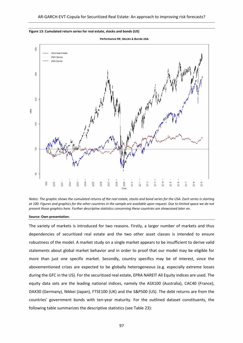
AR-GARCH-EVT-Copula for Securitized Real Estate: An approach to improving risk forecasts?
97
Figure 13: Cumulated return series for real estate, stocks and bonds (US)
Notes: The graphic shows the cumulated returns of the real estate, stocks and bond series for the USA. Each series is starting
at 100. Figures and graphics for the other countries in the sample are available upon request. Due to limited space we do not
present those graphics here. Further descriptive statistics concerning these countries are showcased later on.
Source: Own presentation.
The variety of markets is introduced for two reasons. Firstly, a larger number of markets and thus
dependencies of securitized real estate and the two other asset classes is intended to ensure
robustness of the model. A market study on a single market appears to be insufficient to derive valid
statements about global market behavior and in order to proof that our model may be eligible for
more than just one specific market. Secondly, country specifics may be of interest, since the
abovementioned crises are expected to be globally heterogeneous (e.g. especially extreme losses
during the GFC in the US). For the securitized real estate, EPRA NAREIT All Equity indices are used. The
equity data sets are the leading national indices, namely the ASX100 (Australia), CAC40 (France),
DAX30 (Germany), Nikkei (Japan), FTSE100 (UK) and the S&P500 (US). The debt returns are from the
countries’ government bonds with ten-year maturity. For the outlined dataset constituents, the
following table summarizes the descriptive statistics (see Table 23):
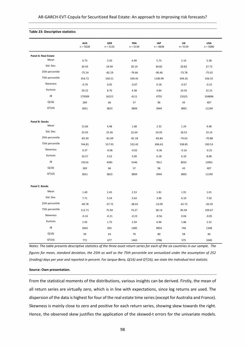
AR-GARCH-EVT-Copula for Securitized Real Estate: An approach to improving risk forecasts?
98
Table 23: Descriptive statistics
AUS n = 5028
GER n = 5132
FRA n = 5134
JAP n = 4838
UK n= 5159
USA n = 5080
Panel A: Real Estate
Mean 0.73 3.20 6.99 5.73 2.14 5.38
Std. Dev. 20.43 24.94 20.19 30.82 20.82 27.73
25th percentile -75.24 -82.19 -76.66 -90.46 -73.78 -75.02
75th percentile 354.72 530.51 439.45 1100.99 349.26 426.55
Skewness -0.70 0.05 -0.07 0.18 -0.57 -0.22
Kurtosis 29.22 8.70 4.38 4.84 10.35 22.25
JB 179309 16215 4111 4755 23323 104896
Q(16) 269 66 57 96 43 407
Q²(16) 3651 3823 3894 3944 3892 11249
Panel B: Stocks
Mean 12.66 4.48 1.68 2.32 1.24 4.48
Std. Dev. 25.03 23.36 22.64 24.05 18.53 19.14
25th percentile -83.39 -81.69 -81.18 -83.84 -74.63 -70.88
75th percentile 744.81 557.95 532.42 696.63 338.85 330.53
Skewness 0.37 -0.06 -0.02 -0.36 -0.16 -0.25
Kurtosis 10.57 4.52 5.09 6.18 6.10 8.08
JB 23516 4385 5546 7811 8032 13901
Q(16) 269 66 57 96 43 407
Q²(16) 3651 3823 3894 3944 3892 11249
Panel C: Bonds
Mean 1.40 2.45 2.53 1.81 1.91 1.01
Std. Dev. 7.71 5.54 5.63 3.96 6.19 7.50
25th percentile -49.78 -37.72 -38.03 -23.09 -42.73 -50.29
75th percentile 112.71 75.94 74.27 38.14 85.04 109.67
Skewness -0.14 -0.21 -0.23 -0.56 0.04 -0.05
Kurtosis 2.95 1.75 2.59 6.90 1.86 2.52
JB 1843 695 1485 9854 746 1348
Q(16) 59 63 70 80 58 60
Q²(16) 772 677 1465 3786 575 1040
Notes: The table presents descriptive statistics of the three asset return series for each of the six countries in our sample. The
figures for mean, standard deviation, the 25th as well as the 75th percentile are annualized under the assumption of 252
(trading) days per year and reported in percent. For Jarque-Bera, Q(16) and Q²(16), we state the individual test statistic.
Source: Own presentation.
From the statistical moments of the distributions, various insights can be derived. Firstly, the mean of
all return series are virtually zero, which is in line with expectations, since log returns are used. The
dispersion of the data is highest for four of the real estate time series (except for Australia and France).
Skewness is mainly close to zero and positive for each return series, showing skew towards the right.
Hence, the observed skew justifies the application of the skewed-t errors for the univariate models.
AR-GARCH-EVT-Copula for Securitized Real Estate: An approach to improving risk forecasts?
99
The large kurtosis of all returns indicates leptokurtic distributions. In addition to the statements about
return series volatility for securitized real estate, the minima reveal the largest downturns for the
specified asset class (except for France). In the context of risk management and metric forecasting,
these extreme values are of particular interest, since these returns are the most likely observations to
cause violations of the price risk forecast of the 𝑉𝑎𝑅𝛼 and the 𝐶𝑉𝑎𝑅𝛼 in comparison to the real return.
The descriptive statistics also reveal evidence of other statistical issues mentioned in the literature
review. These indicate a compelling need for the application of the AR-GARCH-EVT-Copula approach.
This applies especially to the securitized real estate data. Additionally, the Jarque-Bera tests yield very
strong empirical evidence of the violation of normality for each time series of the dataset. In addition,
serial correlation can be detected due to the findings of the Q(16) and Q²(16) statistics. Thus, the
application of statistical procedures to account for these issues is needed to ensure unbiased
univariate and multivariate modelling.
5.5 Empirical results
The empirical analysis covers the results of the back testing for the AR-GARCH-EVT-Copula and the two
benchmark methodologies, namely variance-covariance and historical simulation for the specified
return series.24 For each approach, risk forecasts for the equally weighted portfolio are calculated and
compared to the actual portfolio return. Graphically, the figures below display the 𝑉𝑎𝑅0.99 from the
AR-GARCH-EVT-Copula model as well as both benchmark methodologies for both portfolios from the
US (see Figure 14):
24 Implementing the AR-GARCH-EVT-Copula model leads to a load of typical estimates. Since the estimates
change over time due to the usage of rolling windows, those estimates can only be illustrated in figures. These
figures for AR-GARCH estimates, scale and shape as well as copula parameters are available upon request.

AR-GARCH-EVT-Copula for Securitized Real Estate: An approach to improving risk forecasts?
100
Figure 14: VaR (𝜶 = 𝟎. 𝟗𝟗) estimates for Real Estate – Stocks & Real Estate - Bonds portfolio (US)
Source: Own presentation.

AR-GARCH-EVT-Copula for Securitized Real Estate: An approach to improving risk forecasts?
101
From the graphical representation of the observed returns (black lines) and the risk forecasts, the
primary difference between the benchmark models and the AR-GARCH-EVT-Copula model is the
relative responsiveness of the latter approach to differing levels of market volatility, and especially
extreme losses (as displayed by the red lines). In comparison, the benchmark methods do not provide
this flexibility and react to periods of increasing volatility and heavy downturns (e.g. the GFC) and also
to decreased volatility too reluctantly and late (e.g. the brown and green graphs both respond in early
2013 by indicating significantly lower risk forecasts). This finding applies to both portfolio scenarios
alike as well as across all countries in our sample.
One explanation may be the increased correlation between asset classes especially in downturn
markets (Case et al., 2012), which can cause extreme simultaneous asset losses, contradicting heavily
with the assumption of constant correlation of the benchmark methodologies. Accordingly, refitting
the dependence structure appears to be a key element of appropriate risk metric forecasting, due to
breakdowns in correlation patterns during increased volatility.
Beside optical inspection, numerical measures provide deeper insight into the model accuracy. By
back-testing the methodologies through the data sample, the absolute and relative number of hits, the
corresponding Bernoulli as well as the Kupiec statistics are displayed for the 𝑉𝑎𝑅𝑡+1∝ (see Table 24).
Additionally, for the 𝐶𝑉𝑎𝑅𝑡+1∝ , the zero mean test results are shown on Table 24.25
Table 24: Empirical results for VaR forecasts
VaR
Country Portfolio Risk Metric Model Hits
Relative Hits
p-value Bernoulli
p-value Kupiec
p-value Christoffersen
Australia (n = 4026)
Real Estate - Stocks
𝑉𝑎𝑅𝑡+10.01
Variance-Covariance 94 2.33 0.00 0.00 0.00
Hist. Sim. 59 1.47 0.53 0.55 0.09
AR-GARCH-EVT-Copula 42 1.04 75.12 78.43 20.77
𝑉𝑎𝑅𝑡+10.05
Variance-Covariance 211 5.24 46.96 48.63 1.38
Hist. Sim. 216 5.37 29.42 29.32 0.83
AR-GARCH-EVT-Copula 225 5.59 8.91 9.23 23.88
Real Estate - Bonds
𝑉𝑎𝑅𝑡+10.01
Variance-Covariance 93 2.31 0.00 0.00 0.00
Hist. Sim. 59 1.47 0.53 0.55 0.00
AR-GARCH-EVT-Copula 55 1.37 2.60 2.70 1.17
𝑉𝑎𝑅𝑡+10.05
Variance-Covariance 209 5.19 56.29 57.99 0.00
Hist. Sim. 236 5.86 1.39 1.45 0.00
AR-GARCH-EVT-Copula 226 5.61 7.64 7.96 0.86
France (n = 4134)
Real Estate - Stocks
𝑉𝑎𝑅𝑡+10.01
Variance-Covariance 84 2.03 0.00 0.00 0.00
Hist. Sim. 44 1.06 63.89 67.84 0.04
AR-GARCH-EVT-Copula 49 1.19 23.98 24.34 3.66
𝑉𝑎𝑅𝑡+10.05
Variance-Covariance 185 4.48 12.49 11.68 0.00
Hist. Sim. 221 5.35 30.06 30.92 0.00
25 The results for the portfolios containing stocks and bonds are available upon request.
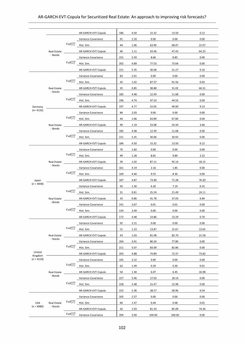
AR-GARCH-EVT-Copula for Securitized Real Estate: An approach to improving risk forecasts?
102
AR-GARCH-EVT-Copula 186 4.50 15.32 13.50 0.12
Real Estate - Bonds
𝑉𝑎𝑅𝑡+10.01
Variance-Covariance 91 2.20 0.00 0.00 0.00
Hist. Sim. 44 1.06 63.90 68.07 22.07
AR-GARCH-EVT-Copula 46 1.11 43.46 47.43 64.23
𝑉𝑎𝑅𝑡+10.05
Variance-Covariance 231 5.59 8.66 8.85 0.00
Hist. Sim. 202 4.89 77.53 73.64 0.00
AR-GARCH-EVT-Copula 221 5.35 30.08 31.27 0.10
Germany (n= 4132)
Real Estate - Stocks
𝑉𝑎𝑅𝑡+10.01
Variance-Covariance 83 2.01 0.00 0.00 0.00
Hist. Sim. 42 1.02 87.57 91.56 0.03
AR-GARCH-EVT-Copula 35 0.85 38.88 31.02 44.31
𝑉𝑎𝑅𝑡+10.05
Variance-Covariance 185 4.48 12.49 11.68 0.00
Hist. Sim. 196 4.74 47.53 44.55 0.00
AR-GARCH-EVT-Copula 197 4.77 52.05 49.00 9.13
Real Estate - Bonds
𝑉𝑎𝑅𝑡+10.01
Variance-Covariance 84 2.03 0.00 0.00 0.00
Hist. Sim. 44 1.06 63.89 67.84 0.04
AR-GARCH-EVT-Copula 49 1.19 23.98 24.34 3.66
𝑉𝑎𝑅𝑡+10.05
Variance-Covariance 185 4.48 12.49 11.68 0.00
Hist. Sim. 221 5.35 30.06 30.92 0.00
AR-GARCH-EVT-Copula 186 4.50 15.32 13.50 0.12
Japan (n = 3838)
Real Estate - Stocks
𝑉𝑎𝑅𝑡+10.01
Variance-Covariance 70 1.82 0.00 0.00 0.00
Hist. Sim. 49 1.28 8.81 9.89 2.22
AR-GARCH-EVT-Copula 39 1.02 87.11 92.14 18.15
𝑉𝑎𝑅𝑡+10.05
Variance-Covariance 161 4.19 2.16 1.85 0.00
Hist. Sim. 169 4.40 9.55 8.30 0.00
AR-GARCH-EVT-Copula 187 4.87 73.90 71.28 76.20
Real Estate - Bonds
𝑉𝑎𝑅𝑡+10.01
Variance-Covariance 50 1.30 6.20 7.19 0.31
Hist. Sim. 31 0.81 25.59 21.49 24.11
AR-GARCH-EVT-Copula 33 0.86 41.78 37.03 6.84
𝑉𝑎𝑅𝑡+10.05
Variance-Covariance 141 3.67 0.01 0.01 0.00
Hist. Sim. 134 3.49 0.00 0.00 0.00
AR-GARCH-EVT-Copula 172 4.48 14.86 13.29 0.70
United Kingdom
(n = 4159)
Real Estate - Stocks
𝑉𝑎𝑅𝑡+10.01
Variance-Covariance 92 2.21 0.00 0.00 0.00
Hist. Sim. 51 1.23 13.87 15.67 13.65
AR-GARCH-EVT-Copula 43 1.03 81.48 82.70 21.58
𝑉𝑎𝑅𝑡+10.05
Variance-Covariance 204 4.91 80.34 77.80 0.00
Hist. Sim. 211 5.07 83.09 82.86 0.00
AR-GARCH-EVT-Copula 203 4.88 74.89 72.37 73.82
Real Estate - Bonds
𝑉𝑎𝑅𝑡+10.01
Variance-Covariance 105 2.52 0.00 0.00 0.00
Hist. Sim. 62 1.49 0.29 0.30 0.01
AR-GARCH-EVT-Copula 54 1.30 6.07 6.45 16.98
𝑉𝑎𝑅𝑡+10.05
Variance-Covariance 227 5.46 17.63 18.14 0.00
Hist. Sim. 228 5.48 15.47 15.98 0.00
AR-GARCH-EVT-Copula 223 5.36 28.57 28.96 0.54
USA (n = 4080)
Real Estate - Stocks
𝑉𝑎𝑅𝑡+10.01
Variance-Covariance 105 2.57 0.00 0.00 0.00
Hist. Sim. 60 1.47 0.44 0.48 0.01
AR-GARCH-EVT-Copula 42 1.03 81.33 85.09 74.36
𝑉𝑎𝑅𝑡+10.05 Variance-Covariance 204 5.00 100.00 100.00 0.00
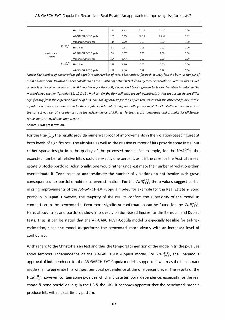
AR-GARCH-EVT-Copula for Securitized Real Estate: An approach to improving risk forecasts?
103
Hist. Sim. 221 5.42 22.19 22.80 0.00
AR-GARCH-EVT-Copula 206 5.05 88.57 88.59 3.87
Real Estate - Bonds
𝑉𝑎𝑅𝑡+10.01
Variance-Covariance 114 2.79 0.00 0.00 0.00
Hist. Sim. 68 1.67 0.01 0.01 0.00
AR-GARCH-EVT-Copula 56 1.37 2.20 2.36 3.80
𝑉𝑎𝑅𝑡+10.05
Variance-Covariance 264 6.47 0.00 0.00 0.00
Hist. Sim. 265 6.50 0.00 0.00 0.00
AR-GARCH-EVT-Copula 249 6.10 0.18 0.18 0.00
Notes: The number of observations (n) equals to the number of total observations for each country less the burn-in sample of
1000 observations. Relative hits are calculated as the number of actual hits divided by total observations. Relative hits as well
as p-values are given in percent. Null hypotheses for Bernoulli, Kupiec and Christoffersen tests are described in detail in the
methodology section (formulas 11, 12 & 13). In short, for the Bernoulli test, the null hypothesis is that the results do not differ
significantly from the expected number of hits. The null hypothesis for the Kupiec test states that the observed failure rate is
equal to the failure rate suggested by the confidence interval. Finally, the null hypothesis of the Christoffersen test describes
the correct number of exceedances and the independence of failures. Further results, back-tests and graphics for all Stocks-
Bonds pairs are available upon request.
Source: Own presentation.
For the 𝑉𝑎𝑅𝑡+1𝛼 , the results provide numerical proof of improvements in the violation-based figures at
both levels of significance. The absolute as well as the relative number of hits provide some initial but
rather sparse insight into the quality of the proposed model. For example, for the 𝑉𝑎𝑅𝑡+10.01, the
expected number of relative hits should be exactly one percent, as it is the case for the Australian real
estate & stocks portfolio. Additionally, one would rather underestimate the number of violations than
overestimate it. Tendencies to underestimate the number of violations do not involve such grave
consequences for portfolio holders as overestimation. For the 𝑉𝑎𝑅𝑡+10.05, the p-values suggest partial
missing improvements of the AR-GARCH-EVT-Copula model, for example for the Real Estate & Bond
portfolio in Japan. However, the majority of the results confirm the superiority of the model in
comparison to the benchmarks. Even more significant confirmation can be found for the 𝑉𝑎𝑅𝑡+10.01.
Here, all countries and portfolios show improved violation-based figures for the Bernoulli and Kupiec
tests. Thus, it can be stated that the AR-GARCH-EVT-Copula model is especially feasible for tail-risk
estimation, since the model outperforms the benchmark more clearly with an increased level of
confidence.
With regard to the Christoffersen test and thus the temporal dimension of the model hits, the p-values
show temporal independence of the AR-GARCH-EVT-Copula model. For 𝑉𝑎𝑅𝑡+10.01, the unanimous
approval of independence for the AR-GARCH-EVT-Copula model is supported, whereas the benchmark
models fail to generate hits without temporal dependence at the one percent level. The results of the
𝑉𝑎𝑅𝑡+10.05, however, contain some p-values which indicate temporal dependence, especially for the real
estate & bond portfolios (e.g. in the US & the UK). It becomes apparent that the benchmark models
produce hits with a clear timely pattern.
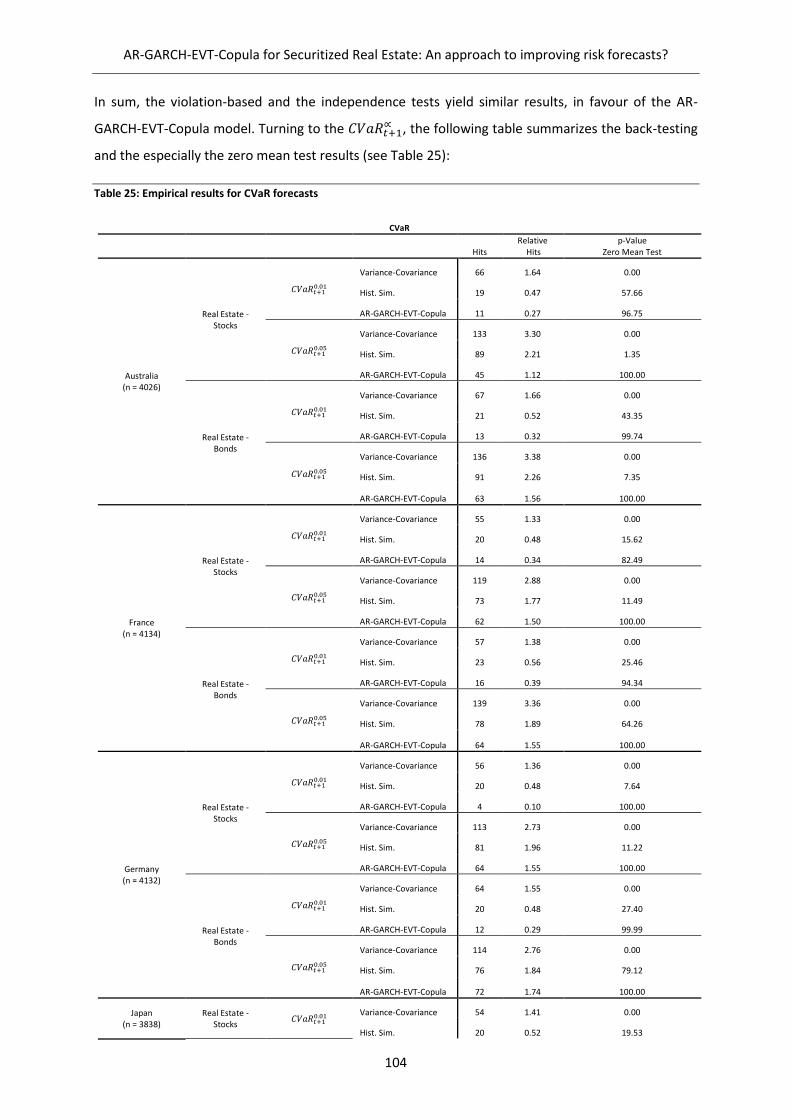
AR-GARCH-EVT-Copula for Securitized Real Estate: An approach to improving risk forecasts?
104
In sum, the violation-based and the independence tests yield similar results, in favour of the AR-
GARCH-EVT-Copula model. Turning to the 𝐶𝑉𝑎𝑅𝑡+1∝ , the following table summarizes the back-testing
and the especially the zero mean test results (see Table 25):
Table 25: Empirical results for CVaR forecasts
CVaR
Hits Relative
Hits p-Value
Zero Mean Test
Australia (n = 4026)
Real Estate - Stocks
𝐶𝑉𝑎𝑅𝑡+10.01
Variance-Covariance 66 1.64 0.00
Hist. Sim. 19 0.47 57.66
AR-GARCH-EVT-Copula 11 0.27 96.75
𝐶𝑉𝑎𝑅𝑡+10.05
Variance-Covariance 133 3.30 0.00
Hist. Sim. 89 2.21 1.35
AR-GARCH-EVT-Copula 45 1.12 100.00
Real Estate - Bonds
𝐶𝑉𝑎𝑅𝑡+10.01
Variance-Covariance 67 1.66 0.00
Hist. Sim. 21 0.52 43.35
AR-GARCH-EVT-Copula 13 0.32 99.74
𝐶𝑉𝑎𝑅𝑡+10.05
Variance-Covariance 136 3.38 0.00
Hist. Sim. 91 2.26 7.35
AR-GARCH-EVT-Copula 63 1.56 100.00
France (n = 4134)
Real Estate - Stocks
𝐶𝑉𝑎𝑅𝑡+10.01
Variance-Covariance 55 1.33 0.00
Hist. Sim. 20 0.48 15.62
AR-GARCH-EVT-Copula 14 0.34 82.49
𝐶𝑉𝑎𝑅𝑡+10.05
Variance-Covariance 119 2.88 0.00
Hist. Sim. 73 1.77 11.49
AR-GARCH-EVT-Copula 62 1.50 100.00
Real Estate - Bonds
𝐶𝑉𝑎𝑅𝑡+10.01
Variance-Covariance 57 1.38 0.00
Hist. Sim. 23 0.56 25.46
AR-GARCH-EVT-Copula 16 0.39 94.34
𝐶𝑉𝑎𝑅𝑡+10.05
Variance-Covariance 139 3.36 0.00
Hist. Sim. 78 1.89 64.26
AR-GARCH-EVT-Copula 64 1.55 100.00
Germany (n = 4132)
Real Estate - Stocks
𝐶𝑉𝑎𝑅𝑡+10.01
Variance-Covariance 56 1.36 0.00
Hist. Sim. 20 0.48 7.64
AR-GARCH-EVT-Copula 4 0.10 100.00
𝐶𝑉𝑎𝑅𝑡+10.05
Variance-Covariance 113 2.73 0.00
Hist. Sim. 81 1.96 11.22
AR-GARCH-EVT-Copula 64 1.55 100.00
Real Estate - Bonds
𝐶𝑉𝑎𝑅𝑡+10.01
Variance-Covariance 64 1.55 0.00
Hist. Sim. 20 0.48 27.40
AR-GARCH-EVT-Copula 12 0.29 99.99
𝐶𝑉𝑎𝑅𝑡+10.05
Variance-Covariance 114 2.76 0.00
Hist. Sim. 76 1.84 79.12
AR-GARCH-EVT-Copula 72 1.74 100.00
Japan (n = 3838)
Real Estate - Stocks
𝐶𝑉𝑎𝑅𝑡+10.01
Variance-Covariance 54 1.41 0.00
Hist. Sim. 20 0.52 19.53
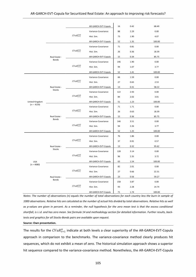
AR-GARCH-EVT-Copula for Securitized Real Estate: An approach to improving risk forecasts?
105
AR-GARCH-EVT-Copula 16 0.42 68.49
𝐶𝑉𝑎𝑅𝑡+10.05
Variance-Covariance 88 2.29 0.00
Hist. Sim. 73 1.90 4.07
AR-GARCH-EVT-Copula 52 1.35 100.00
Real Estate - Bonds
𝐶𝑉𝑎𝑅𝑡+10.01
Variance-Covariance 71 0.81 0.00
Hist. Sim. 26 0.36 18.39
AR-GARCH-EVT-Copula 15 0.34 85.75
𝐶𝑉𝑎𝑅𝑡+10.05
Variance-Covariance 146 1.90 0.00
Hist. Sim. 94 1.07 3.77
AR-GARCH-EVT-Copula 52 1.41 100.00
United Kingdom (n = 4159)
Real Estate - Stocks
𝐶𝑉𝑎𝑅𝑡+10.01
Variance-Covariance 66 1.59 0.00
Hist. Sim. 27 0.65 2.53
AR-GARCH-EVT-Copula 13 0.31 58.22
𝐶𝑉𝑎𝑅𝑡+10.05
Variance-Covariance 122 2.93 0.00
Hist. Sim. 84 2.02 3.01
AR-GARCH-EVT-Copula 51 1.23 100.00
Real Estate - Bonds
𝐶𝑉𝑎𝑅𝑡+10.01
Variance-Covariance 71 1.71 0.00
Hist. Sim. 26 0.63 18.39
AR-GARCH-EVT-Copula 15 0.36 85.75
𝐶𝑉𝑎𝑅𝑡+10.05
Variance-Covariance 146 3.51 0.00
Hist. Sim. 94 2.26 3.77
AR-GARCH-EVT-Copula 52 1.25 100.00
USA (n = 4080)
Real Estate - Stocks
𝐶𝑉𝑎𝑅𝑡+10.01
Variance-Covariance 76 1.86 0.00
Hist. Sim. 37 0.91 0.57
AR-GARCH-EVT-Copula 13 0.32 95.62
𝐶𝑉𝑎𝑅𝑡+10.05
Variance-Covariance 128 3.14 0.00
Hist. Sim. 96 2.35 3.72
AR-GARCH-EVT-Copula 63 1.54 100.00
Real Estate - Bonds
𝐶𝑉𝑎𝑅𝑡+10.01
Variance-Covariance 82 2.01 0.00
Hist. Sim. 27 0.66 22.31
AR-GARCH-EVT-Copula 23 0.56 59.27
𝐶𝑉𝑎𝑅𝑡+10.05
Variance-Covariance 158 3.87 0.00
Hist. Sim. 93 2.28 14.74
AR-GARCH-EVT-Copula 71 1.74 100.00
Notes: The number of observations (n) equals the number of total observations for each country less the burn-in sample of
1000 observations. Relative hits are calculated as the number of actual hits divided by total observations. Relative hits as well
as p-values are given in percent. As a reminder, the null hypothesis for the zero mean test is that the excess conditional
shortfall, is i.i.d. and has zero mean. See formula 14 and methodology section for detailed information. Further results, back-
tests and graphics for all Stocks-Bonds pairs are available upon request.
Source: Own presentation.
The results for the 𝐶𝑉𝑎𝑅𝑡+1∝ indicate at both levels a clear superiority of the AR-GARCH-EVT-Copula
approach in comparison to the benchmarks. The variance-covariance method clearly produces hit
sequences, which do not exhibit a mean of zero. The historical simulation approach shows a superior
hit sequence compared to the variance-covariance method. Nonetheless, the AR-GARCH-EVT-Copula

AR-GARCH-EVT-Copula for Securitized Real Estate: An approach to improving risk forecasts?
106
method shows the highest p-values across all markets and portfolios. Thus, the 𝐶𝑉𝑎𝑅𝑡+1∝ results
suggest outperformance of the benchmark at both levels of significance. The results can be interpreted
as confirmation for structural under- and overestimation of the 𝐶𝑉𝑎𝑅𝑡+1∝ , if 𝑉𝑎𝑅𝑡+1
∝ is violated. This
does not apply to the variance-covariance method, and only partially to the historical simulation.
Taking the graphical inspection into account, especially the heavy underestimation of losses during the
GFC may cause these results for the benchmarks.
In sum, the results provide empirical evidence, both graphically and numerically, of an improved risk
measurement of the AR-GARCH-EVT-Copula in comparison to the benchmark methodologies. In
particular, the re-estimation of dependence patterns appears to be a key feature for correctly
modelling its time-variance. Since the results also show greater improvements for risk measurements
of the tail (e.g. the larger confirmation of the 𝑉𝑎𝑅𝑡+10.99 than the 𝑉𝑎𝑅𝑡+1
0.95), the dependence patterns of
the analysed asset classes may also reveal a need to model non-linear relationships in contrast to the
strictly linear correlation measurement. This applies especially to critical market phases, since the
graphical inspection revealed heavy underestimation of the risk exposure in these periods (e.g. during
the GFC). Since the 𝐶𝑉𝑎𝑅𝑡+1𝛼 represents a coherent risk measurement in accordance with Artzner et
al. (1999), as proposed by Rockafellar & Uryasev (2000), the results imply the feasibility of the AR-
GARCH-EVT-Copula model especially for the named figure.
Based upon the empirical results of the back-testing, questions arise regarding the underlying
univariate and multivariate models. Since varying models are used for each rolling window of the AR-
GARCH-EVT-Copula approach, a deeper look into the results for the autoregressive and dependence
models for each portfolio may provide additional information. Therefore, Table 26 displays the results
of the goodness of fit for the autoregressive models for each time series. More precisely, Table 26
reports the discrete distribution for the highest fit of each autoregressive order across the respective
data series for the rolling windows (see Table 26):
Table 26: Results of the autoregressive modelling
Autoregressive Order
US Real Estate
UK Real Estate
DE Real Estate
FR Real Estate
AUS Real Estate
JP Real Estate
Sum
0 977 638 312 998 753 100 3778
1 999 1053 885 287 67 578 3869
2 244 401 387 506 265 268 2071
3 110 333 272 686 934 614 2949
4 475 628 594 416 390 868 3371
5 1275 1106 1682 1241 1617 1411 8332
US Stocks
UK Stocks
DE Stocks
FR Stocks
AUS Stocks
JP Stocks
Sum
0 0 268 749 244 965 1065 3291
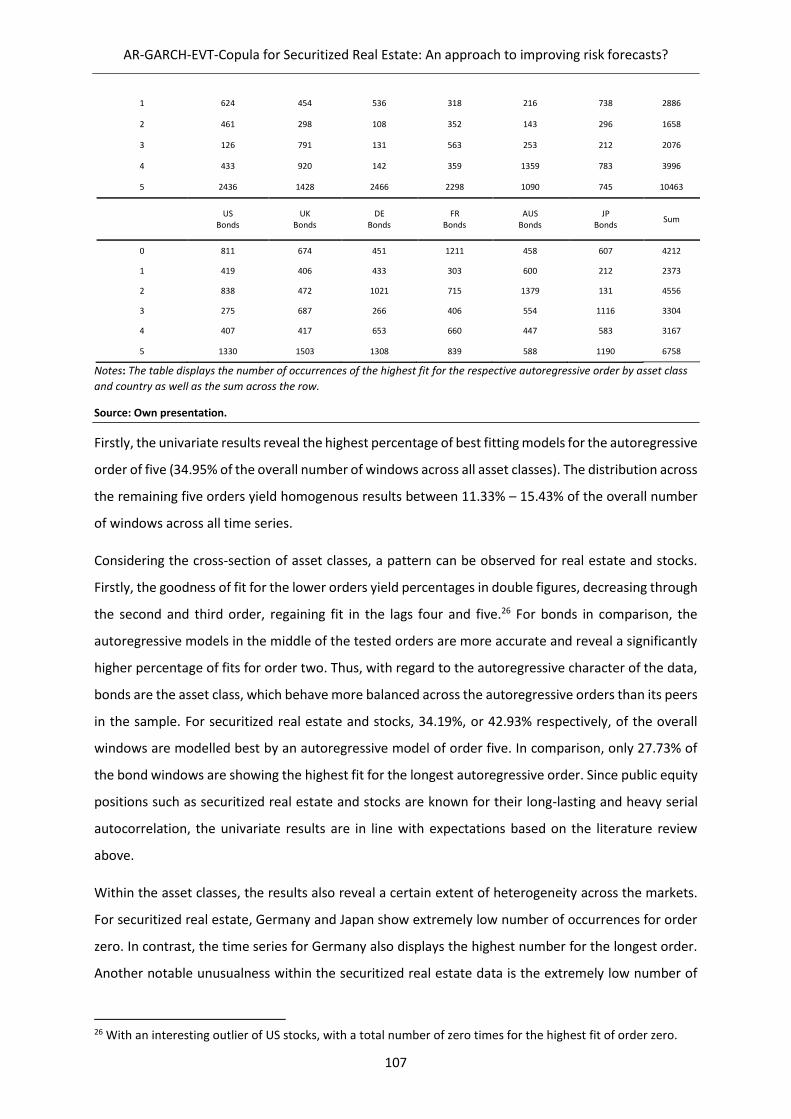
AR-GARCH-EVT-Copula for Securitized Real Estate: An approach to improving risk forecasts?
107
1 624 454 536 318 216 738 2886
2 461 298 108 352 143 296 1658
3 126 791 131 563 253 212 2076
4 433 920 142 359 1359 783 3996
5 2436 1428 2466 2298 1090 745 10463
US Bonds
UK Bonds
DE Bonds
FR Bonds
AUS Bonds
JP Bonds
Sum
0 811 674 451 1211 458 607 4212
1 419 406 433 303 600 212 2373
2 838 472 1021 715 1379 131 4556
3 275 687 266 406 554 1116 3304
4 407 417 653 660 447 583 3167
5 1330 1503 1308 839 588 1190 6758
Notes: The table displays the number of occurrences of the highest fit for the respective autoregressive order by asset class
and country as well as the sum across the row.
Source: Own presentation.
Firstly, the univariate results reveal the highest percentage of best fitting models for the autoregressive
order of five (34.95% of the overall number of windows across all asset classes). The distribution across
the remaining five orders yield homogenous results between 11.33% – 15.43% of the overall number
of windows across all time series.
Considering the cross-section of asset classes, a pattern can be observed for real estate and stocks.
Firstly, the goodness of fit for the lower orders yield percentages in double figures, decreasing through
the second and third order, regaining fit in the lags four and five.26 For bonds in comparison, the
autoregressive models in the middle of the tested orders are more accurate and reveal a significantly
higher percentage of fits for order two. Thus, with regard to the autoregressive character of the data,
bonds are the asset class, which behave more balanced across the autoregressive orders than its peers
in the sample. For securitized real estate and stocks, 34.19%, or 42.93% respectively, of the overall
windows are modelled best by an autoregressive model of order five. In comparison, only 27.73% of
the bond windows are showing the highest fit for the longest autoregressive order. Since public equity
positions such as securitized real estate and stocks are known for their long-lasting and heavy serial
autocorrelation, the univariate results are in line with expectations based on the literature review
above.
Within the asset classes, the results also reveal a certain extent of heterogeneity across the markets.
For securitized real estate, Germany and Japan show extremely low number of occurrences for order
zero. In contrast, the time series for Germany also displays the highest number for the longest order.
Another notable unusualness within the securitized real estate data is the extremely low number of
26 With an interesting outlier of US stocks, with a total number of zero times for the highest fit of order zero.

AR-GARCH-EVT-Copula for Securitized Real Estate: An approach to improving risk forecasts?
108
order one models for the Australian time series. In addition to the low number of order zero models,
Australia appears to be a market with more long-lasting autoregressive effects. The same applies to
Japan. The US and the UK on the other hand are markets with more occurrences (1,976 and 1,691) of
short autoregressive effects (zero and one).
For the other asset classes, a surprising finding is the missing occurrence for the zero. Thus, the US
stock time series entails autoregressive effects for every window. In fact, the data for the US stocks
time series is heavily long-lasting autoregressive (2,436 observations for the highest order). For the
bond data, the results reveal the highest occurrences for the middle orders (especially two and three),
as outlined above.
Nonetheless, from a methodological point of view, an extension to even higher autoregressive orders
could be thinkable for further model improvements especially for securitized real estate and stocks.
With regard to the implications for the price risk forecasting model of interest, the general necessity
to allow for individual order selection based on the respective goodness of fit can be extracted from
the results, since the asset classes and markets of the study show largely differing results and thus
individual specifics.
Based on these univariate findings, the multivariate results are assessed. In particular, the question is,
what types of copulae are providing the highest fit overall and for which specific portfolios or markets.
From the chosen type of copula alone, insights about the symmetry of the co-movements of the
portfolio constituents can be derived. Therefore, table 27 summarizes the discrete distribution of the
copulae with the highest fit among the tested ones for each rolling window across all asset classes and
countries (see Table 27):
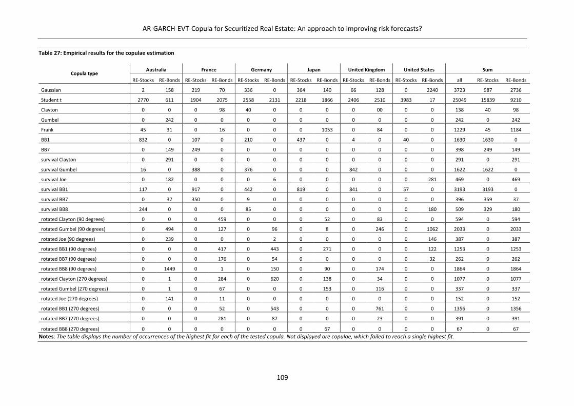
AR-GARCH-EVT-Copula for Securitized Real Estate: An approach to improving risk forecasts?
109
Table 27: Empirical results for the copulae estimation
Copula type Australia France Germany Japan United Kingdom United States Sum
RE-Stocks RE-Bonds RE-Stocks RE-Bonds RE-Stocks RE-Bonds RE-Stocks RE-Bonds RE-Stocks RE-Bonds RE-Stocks RE-Bonds all RE-Stocks RE-Bonds
Gaussian 2 158 219 70 336 0 364 140 66 128 0 2240 3723 987 2736
Student t 2770 611 1904 2075 2558 2131 2218 1866 2406 2510 3983 17 25049 15839 9210
Clayton 0 0 0 98 40 0 0 0 0 00 0 0 138 40 98
Gumbel 0 242 0 0 0 0 0 0 0 0 0 0 242 0 242
Frank 45 31 0 16 0 0 0 1053 0 84 0 0 1229 45 1184
BB1 832 0 107 0 210 0 437 0 4 0 40 0 1630 1630 0
BB7 0 149 249 0 0 0 0 0 0 0 0 0 398 249 149
survival Clayton 0 291 0 0 0 0 0 0 0 0 0 0 291 0 291
survival Gumbel 16 0 388 0 376 0 0 0 842 0 0 0 1622 1622 0
survival Joe 0 182 0 0 0 6 0 0 0 0 0 281 469 0 469
survival BB1 117 0 917 0 442 0 819 0 841 0 57 0 3193 3193 0
survival BB7 0 37 350 0 9 0 0 0 0 0 0 0 396 359 37
survival BB8 244 0 0 0 85 0 0 0 0 0 0 180 509 329 180
rotated Clayton (90 degrees) 0 0 0 459 0 0 0 52 0 83 0 0 594 0 594
rotated Gumbel (90 degrees) 0 494 0 127 0 96 0 8 0 246 0 1062 2033 0 2033
rotated Joe (90 degrees) 0 239 0 0 0 2 0 0 0 0 0 146 387 0 387
rotated BB1 (90 degrees) 0 0 0 417 0 443 0 271 0 0 0 122 1253 0 1253
rotated BB7 (90 degrees) 0 0 0 176 0 54 0 0 0 0 0 32 262 0 262
rotated BB8 (90 degrees) 0 1449 0 1 0 150 0 90 0 174 0 0 1864 0 1864
rotated Clayton (270 degrees) 0 1 0 284 0 620 0 138 0 34 0 0 1077 0 1077
rotated Gumbel (270 degrees) 0 1 0 67 0 0 0 153 0 116 0 0 337 0 337
rotated Joe (270 degrees) 0 141 0 11 0 0 0 0 0 0 0 0 152 0 152
rotated BB1 (270 degrees) 0 0 0 52 0 543 0 0 0 761 0 0 1356 0 1356
rotated BB7 (270 degrees) 0 0 0 281 0 87 0 0 0 23 0 0 391 0 391
rotated BB8 (270 degrees) 0 0 0 0 0 0 0 67 0 0 0 0 67 0 67
Notes: The table displays the number of occurrences of the highest fit for each of the tested copula. Not displayed are copulae, which failed to reach a single highest fit.
AR-GARCH-EVT-Copula for Securitized Real Estate: An approach to improving risk forecasts?
110
The major finding of the multivariate modelling is the clear dominance of the Student-t-Copula. Out of
the total number of windows, more than 51.53% of the dependence models reveal the highest
goodness of fit for the named copula, implying a symmetric but existing tail dependence. This finding,
however, is largely driven by the dependence of securitized real estate and stocks, since 63.23% of the
Student-t-Copula models apply the named portfolio constituents. This finding is in line with the
expectations based on the literature review, because previous studies have repeatedly shown this
simultaneous market behaviour of securitized real estate and stocks.
Interestingly, out of the entire data set the second-best fitting copula family is the Gaussian. 7.71% of
the relationships are modelled by a Gaussian copula, which is contradicting the assumption of non-
normality of the joint marginal. This finding, however, is largely impacted by the results of the US real
estate – bond portfolio, on its own already accounting for 2,240 out of the 3,723 total windows, which
are modelled by the Gaussian copula. This finding can be interpreted as a sign for no tail dependence
of the specified portfolio constituents. Other markets do not support the application of the Gaussian
copula, which reduces the finding to a market specific phenomenon.
Thirdly, the survival BB1 copula models 3,191 dependencies out of the sample. The named copula type
also shows an entirely skewed distribution across the portfolio constituents, since only real estate –
stocks portfolios are displayed. This 180-degree rotated copula, with lower tail dependence but higher
variance in the empirical density in the named tail reveals the potential for simultaneous but also less
dense realizations in the tail. Thus, portfolios tend to show higher variance in the tail observations, but
still existing asymmetric dependence.
Furthermore, the rotated copulae (both, 90 and 270°) are only used by securitized real estate and
bonds. This finding is highly important for securitized real investors, who seek multi-asset
diversification and correct portfolio modelling. Generally, these rotated copulae symbolize opposing
price movements, because they are used to model data, which explicitly shows positive (negative)
returns of one asset, when the other asset moves in the opposite direction. Thus, this finding implies
the strict necessity to apply the specified copulae, when securitized real estate and bond positions are
gathered in a portfolio to fully capture the nature of the data. This finding is especially of interest from
a strategic risk management point of view, because these occurrences imply the possibility to hedge
price risk movements of the named asset classes. Whereas this finding is not new to the real estate
literature, the empirical dependence modelling by using rotated copulae has not been extensively
studied.
AR-GARCH-EVT-Copula for Securitized Real Estate: An approach to improving risk forecasts?
111
5.6 Conclusion
The present study contributes to the existing body of real estate literature by extending the stream of
publications on copula dependence modelling with the empirical study, not only of the parameters of
the dependence structures and fit assessment, but by the actual application of nonlinear dependence
modelling to price risk metric forecasting. Therefore, the dependence modelling is extended and
enriched by univariate modelling and the Monte Carlo simulation, based on copula dependence using
the so-called AR-GARCH-EVT-Copula approach. After describing the conceptual construction of the risk
model, the empirical study reveals improvements in the specified methodology across different risk
metrics and levels of significance.
The study also reveals that the 𝑉𝑎𝑅𝛼 based on AR-GARCH-EVT-Copula provides better one-day-ahead
estimates, compared to the traditional 𝑉𝑎𝑅𝛼/𝐶𝑉𝑎𝑅𝛼 estimation methods (variance-covariance and
historical simulation). The results of simple violation ratios and additional test statistics like Kupiec,
Christoffersen and zero mean for our model at different significance levels, were within the range of a
superior estimation model. A detailed decomposition of the model revealed the necessity for
univariate modelling of high autoregressive orders. Additionally, the multivariate analysis showed the
predominant symmetric and negative tail dependence mainly for securitized real estate and stocks,
but also towards bonds. In addition, the results of the multivariate modelling of securitized real estate
and bonds showed evidence to incorporate rotated copulae at both levels of rotation to fully capture
the dependence correctly. A limitation on classic elliptical and Archimedean copulae does not provide
the necessary range of dependence structures.
The practical implications are the viable implementation of the presented approach and the
replacement of variance-covariance or historical simulation methods for the specified asset classes.
Especially in periods of extreme volatility and accordingly heavy negative daily returns, investors can
benefit from improved risk metric forecasts in comparison to classic models. 𝑉𝑎𝑅𝛼and 𝐶𝑉𝑎𝑅𝛼have
also been widely used as risk measures by many financial institutions and regulators, such as the Basel
Committee on Banking Supervision. Hence, our results also provide further insight into the correct
approach of estimating these risk measures for those market participants.
Future research may also incorporate cross-country dependencies, which were not studied in this
article. This could be especially useful for investors who diversify their portfolios across geographical
borders. An extensive focus on securitized real estate could be thinkable, by analyzing portfolios of
indirect property investment indices from different countries. Furthermore, an extension towards
different types of equity securities could be beneficial, such as small or medium cap or debt positions
like high or low yield. Additionally, it should be mentioned that only mature securitized real estate
markets were analyzed in the present study. An extension to less mature markets can be useful so as

AR-GARCH-EVT-Copula for Securitized Real Estate: An approach to improving risk forecasts?
112
to compare the feasibility of the model between mature and immature markets, although potential
data limitations may occur. Potentially interesting studies would include those on the underlying
copulae and a comparative study of them. Since the present approach uses switching copulae for each
window, the fixation of a copula type and subsequent simulation out of each copula across the entire
sample may be beneficial in detecting differences across varying dependence models. In this context,
the investigation of a true time-varying parameter model with Bayesian updates could be of interest.
Lastly, the option to investigate the ability to use the AR-GARCH-EVT-Copula approach as portfolio
optimization tool, as applied for example by Chakkalakal et al. (2018) could be subject to future
research.

AR-GARCH-EVT-Copula for Securitized Real Estate: An approach to improving risk forecasts?
113
5.7 Bibliography
Acerbi, C., & Szekely, B. (2017). General Properties of Backtestable Statistics. SSRN Electronic Journal.
Artzner, P., Delbaen, F., Eber, J.-M., & Heath, D. (1999). Coherent Measures of Risk. Mathematical
Finance, 9(3), pp. 203–228.
Bali, T. G. (2007). An Extreme Value Approach to Estimating Interest-Rate Volatility: Pricing
Implications for Interest-Rate Options. Management Science, 53(2), pp. 323–339.
Bali, T. G., & Theodossiou, P. (2008). Risk Measurement Performance of Alternative Distribution
Functions. The Journal of Risk and Insurance, 75(2), pp. 411–437.
Bao, Y., Lee, T.-H., & Saltoglu, B. (2006). Evaluating predictive performance of value-at-risk models in
emerging markets: a reality check. Journal of Forecasting, 25(2), pp. 101–128.
Bekaert, G., Erb, C. B., Harvey, C. R., & Viskanta, T. E. (1998). Distributional Characteristics of Emerging
Market Returns and Asset Allocation. The Journal of Portfolio Management, 24(2), pp. 102–
116.
Bhattacharyya, M., & Ritolia, G. (2008). Conditional VaR using EVT – Towards a planned margin scheme.
International Review of Financial Analysis, 17(2), pp. 382–395.
Bondt, W., & Thaler, R. (1985). Does the Stock Market Overreact? The Journal of Finance, 40(3), pp.
793–805.
Case, B., Yawei Y., & Yildiray Y. (2012). Dynamic Correlations Among Asset Classes: REIT and Stock
Returns. The Journal of Real Estate Finance and Economics, 44(3), pp. 298–318.
Byrne, P., & Lee, S. (1997). Real Estate Portfolio Analysis under Conditions of Non-Normality: The Case
of NCREIF. The Journal of Real Estate Portfolio Management, 3(1), pp. 37–46.
Chakkalakal, L., Hommel, U., & Li, W. (2018). Transport infrastructure equities in mixed-asset
portfolios: estimating risk with a Garch-Copula CVaR model. Journal of Property Research,
35(2), pp. 117–138.
Chan, K., & Gray, P. (2006). Using extreme value theory to measure value-at-risk for daily electricity
spot prices. International Journal of Forecasting, 22(2), pp. 283–300.
Chang, M.-S., Salin, V., & Jin, Y. (2011). Diversification effect of real estate investment trusts:
Comparing copula functions with kernel methods. Journal of Property Research, 28(3), pp.
189–212.
Christoffersen, P. (1998). Evaluating Interval Forecasts. International Economic Review, 39(4), pp. 841–
862.
Christoffersen, P. (2004). Backtesting Value-at-Risk: A Duration-Based Approach. Journal of Financial
Econometrics, 2(1), pp. 84–108.
Christoffersen, P., Errunza, V., Jacobs, K., & Jin, X. (2014). Correlation dynamics and international
diversification benefits. International Journal of Forecasting, 30(3), pp. 807–824.

AR-GARCH-EVT-Copula for Securitized Real Estate: An approach to improving risk forecasts?
114
Clayton, D. G. (1978). A model for association in bivariate life tables and its application in
epidemiological studies of familial tendency in chronic disease. Biometrika, 65(1), pp. 141–
151.
Coleman M.S., Mansour A. (2005). Real estate in the real world—dealing with non-normality and risk
in and asset allocation model. Journal of Real Estate Portfolio Management, 11(1), pp. 37–54
Cotter, J. & Stevenson, S.. (2006). Multivariate Modeling of Daily REIT Volatility. The Journal of Real
Estate Finance and Economics, 32(3), pp. 305–325.
Consigli, G. (2002). Tail estimation and mean–VaR portfolio selection in markets subject to financial
instability. Journal of Banking & Finance, 26(7), pp. 1355–1382.
Deng, L., Ma, C., & Yang, W. (2011). Portfolio Optimization via Pair Copula-GARCH-EVT-CVaR Model.
Systems Engineering Procedia, 2, pp. 171–181.
Dittmar, R.F. (2002). Nonlinear Pricing Kernels, Kurtosis Preference, and Evidence from the Cross
Section of Equity Returns. The Journal of Finance, 57(1), pp. 369–403.
Du, Z., & Escanciano, J. C. (2017). Backtesting Expected Shortfall: Accounting for Tail Risk. Management
Science, 63(4), pp. 940–958.
Dulguerov, M. (2009). Real estate and portfolio risk: an analysis based on copula functions. Journal of
Property Research, 26(3), pp. 265–280.
Ergen, I. (2015). Two-step methods in VaR prediction and the importance of fat tails. Quantitative
Finance, 15(6), pp. 1013–1030.
Fama, E. F. (1965). The Behavior of Stock-Market Prices. The Journal of Business, 38(1), pp. 34–105.
Frank, M. J. (1979). On the simultaneous associativity of F ( x, y ) and x + y − F ( x, y ). Aaequationes
mathematicae, 19(1), pp. 194–226.
Gabriel, C., & Lau, C. (2014). On the distribution of government bond returns: evidence from the EMU.
Financial Markets and Portfolio Management, 28(2), pp. 181–203.
Goorah, A. (2007). Real Estate Risk Management with Copulas. Journal of Property Research, 24(4), pp.
289–311.
Gumbel, E. J. (1960). Bivariate Exponential Distributions. Journal of the American Statistical
Association, 55(292), pp. 698–707.
Hansen, P. R., & Lunde, A. (2005). A forecast comparison of volatility models: does anything beat a
GARCH(1,1)? Journal of Applied Econometrics, 20(7), pp. 873–889.
Harris, R. D., & Kucukozmen, C. C. (2001). The Empirical Distribution of UK and US Stock Returns.
Journal of Business Finance Accounting, 28(5-6), S. 715–740.
Hiang Liow, K. (2008). Extreme returns and value at risk in international securitized real estate markets.
Journal of Property Investment & Finance, 26(5), S. 418–446.

AR-GARCH-EVT-Copula for Securitized Real Estate: An approach to improving risk forecasts?
115
Hoesli, M., & Oikarinen, E. (2012). Are REITs real estate? Evidence from international sector level data.
Journal of International Money and Finance, 31(7), pp. 1823–1850.
Hoesli, M., Lekander, J., & Witkiewicz, W. (2003). Real Estate in the Institutional Portfolio. The Journal
of Alternative Investments, 6(3), pp. 53–59.
Hoesli, M. & Reka, K. (2013). Volatility Spillovers, Comovements and Contagion in Securitized Real
Estate Markets. The Journal of Real Estate Finance and Economics, 47, pp. 1–35.
Huang, J.-Z., & Zhong, Z. (2013). Time Variation in Diversification Benefits of Commodity, REITs, and
TIPS. The Journal of Real Estate Finance and Economics, 46(1), pp. 152–192.
Hui, E. C., & Chan, K. K. (2013). The European sovereign debt crisis: contagion across European real
estate markets. Journal of Property Research, 30(2), pp. 87–102.
Hurd, M., Salmon, M., & Schleicher, C. (2007). Using Copulae to Construct Bivariate Foreign Exchange
Distributions with an Application to the Sterling Exchange Rate Index (No. 334). Bank of
England Working Paper.
Jirasakuldech, B., Campbell, R. D., & Emekter, R. (2009). Conditional Volatility of Equity Real Estate
Investment Trust Returns: A Pre- and Post-1993 Comparison. The Journal of Real Estate
Finance and Economics, 38(2), pp. 137–154.
Joe, H. (1993). Parametric Families of Multivariate Distributions with Given Margins. Journal of
Multivariate Analysis, 46(2), pp. 262–282.
Joe, H. (1997). Multivariate models and dependence concepts (1. CRC reprint, Volume 73). Boca Raton,
Fla.: Chapman & Hall/CRC.
Joe, H., & Xu, J. J. (1996). The Estimation Method of Inference Functions for Margins for Multivariate
Models.
Karmakar, M. (2017). Dependence structure and portfolio risk in Indian foreign exchange market: A
GARCH-EVT-Copula approach. The Quarterly Review of Economics and Finance, 64(1), pp. 275–
291.Knight, J., Lizieri, C., & Satchell, S. (2005). Diversification when It Hurts? The Joint
Distributions of Real Estate and Equity Markets. Journal of Property Research, 22(4), pp. 309–
323.
Kole, E., Koedijk, K. C., & Verbeek, M. (2007). Selecting Copulae for Risk Management. Journal of
Banking & Finance, 31(8), pp. 2405–2423.
Kuester, K., Mittnik, S., & Paolella, M. (2006). Value-at-Risk Prediction: A Comparison of Alternative
Strategies. Journal of Financial Econometrics, 4(1), pp. 53–89.
Kuhle, J. & Alvayay, J. (2000). The Efficiency of Equity REIT Prices. Journal of Real Estate Portfolio
Management, 6(4), pp. 349-354.
Kupiec, P. H. (1995). Techniques for Verifying the Accuracy of Risk Measurement Models. The Journal
of Derivatives, 3(2), pp. 73–84.
AR-GARCH-EVT-Copula for Securitized Real Estate: An approach to improving risk forecasts?
116
Mabrouk, S., & Saadi, S. (2012). Parametric Value-at-Risk analysis: Evidence from stock indices. The
Quarterly Review of Economics and Finance, 52(3), pp. 305–321.
Mandelbrot, B. (1963). The Variation of Certain Speculative Prices. The Journal of Business, 36(4), pp.
394 - 419.
McNeil, A. J., & Frey, R. (2000). Estimation of tail-related risk measures for heteroscedastic financial
time series: an extreme value approach. Journal of Empirical Finance, 7(3), pp. 271–300.
McNeil, A. J., Frey, R., Embrechts, P., & Frey, R. D. (2005). Quantitative Risk Management. New Jersey:
Princeton University Press.
Nolde N., & Ziegel, J. F. (2017). Elicitability and backtesting: Perspectives for banking regulation. The
Annals of Applied Statistics, 11(4), pp. 1833–1874.
Nelsen, R. B. (1999). An Introduction to Copulae (Second Edition). New York, NY: Springer
Science+Business Media Inc.
Officer, R. R. (1972). The Distribution of Stock Returns. Journal of the American Statistical Association,
67(340), pp. 807–812.
Payne, J., Sahu, A. (2004). Random walks, cointegration, and the transmission of shocks across global
real estate and equity markets. Journal of Economics and Finance, 28(2). pp. 198–210
Rockafellar, R.T., Uryasev, S. (2000). Optimization of Conditional Value-at-Risk. Journal of Risk, 2(3), pp.
21–41.
Rachev, S. T., Schwarz, E. S., & Khindanova, I. (2003). Stable modeling ofmarket and credit value-at-
risk. In S. T. Rachev, Handbook of Heavy Tailed Distributions in Finance (pp. 249–328).
Amsterdam: Elsevier.
Richter, J., Thomas, M., & Füss, R. (2011). German Real Estate Return Distributions: Is There Anything
Normal? Journal of Real Estate Portfolio Management, 17(2), pp. 161–179.
Rocco, M. (2014). Extreme Value Theory in Finance: A Survey. Journal of Economic Surveys, 28(1), pp.
82–108.
Rossignolo, A. F., Fethi, M. D., & Shaban, M. (2012). Value-at-Risk models and Basel capital charges.
Journal of Financial Stability, 8(4), pp. 303–319.
Sahamkhadam, M., Stephan, A., & Östermark, R. (2018). Portfolio optimization based on GARCH-EVT-
Copula forecasting models. International Journal of Forecasting, 34(3), pp. 497–506.
Schindler F. (2010) Further evidence on the (in-)efficiency of the U.S. housing market. Discussion paper,
vol 10-004. ZEW—Centre for European Economic Research, Mannheim
Sklar, A. (1959). Fonctions de répartition à n dimensions et leurs marges. Publications de l’Institut
Statistique de l’Université de Paris, 8, pp. 229–231.
Sklar, A. (1973). Random variables, joint distribution functions, and copulae. Kybernetika, 9(6), pp.
449–460.
AR-GARCH-EVT-Copula for Securitized Real Estate: An approach to improving risk forecasts?
117
de Melo Mendes, B. (2005). Asymmetric extreme interdependence in emerging equity markets.
Applied Stochastic Models in Business and Industry, 21(6), pp. 483–498.
Wang, Z.-R., Chen, X.-H., Jin, Y.-B., & Zhou, Y.-J. (2010). Estimating risk of foreign exchange portfolio:
Using VaR and CVaR based on GARCH–EVT-Copula model. Physica A: Statistical Mechanics and
its Applications, 389(21), pp. 4918–4928.
Wei, Y.-H. & Zhang S.-Y. (2004). Dependence Analysis of Finance Markets: Copula-GARCH Model and
Ist Application. Systems Engineering, 4.
Wheaton W.C., Torto R.G., Southard J.A. & Sivitanides P.S. (1999). Evaluating risk in real estate. Real
Estate Finance, 16, pp. 15–22.
Wu, C.-C., & Lin, Z.-Y. (2014). An economic evaluation of stock–bond return comovements with copula-
based GARCH models. Quantitative Finance, 14(7), pp. 1283–1296.
Yang, J., Zhou, Y., & Leung, W.K.. (2012). Asymmetric Correlation and Volatility Dynamics among Stock,
Bond, and Securitized Real Estate Markets. The Journal of Real Estate Finance and Economics,
45(2), pp. 491–521.
Young, M. S., Lee, S. L., & Devaney, S. P. (2006). Non‐Normal Real Estate Return Distributions by
Property Type in the UK. Journal of Property Research, 23(2), pp. 109–133.
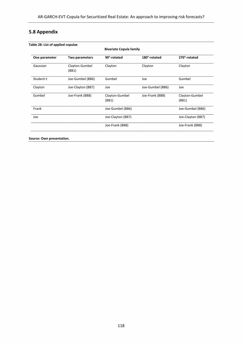
AR-GARCH-EVT-Copula for Securitized Real Estate: An approach to improving risk forecasts?
118
5.8 Appendix
Table 28: List of applied copulae Bivariate Copula family
One parameter Two parameters 90°-rotated 180°-rotated 270°-rotated
Gaussian Clayton-Gumbel
(BB1)
Clayton Clayton Clayton
Student-t Joe-Gumbel (BB6) Gumbel Joe Gumbel
Clayton Joe-Clayton (BB7) Joe Joe-Gumbel (BB6) Joe
Gumbel Joe-Frank (BB8) Clayton-Gumbel
(BB1)
Joe-Frank (BB8) Clayton-Gumbel
(BB1)
Frank Joe-Gumbel (BB6) Joe-Gumbel (BB6)
Joe Joe-Clayton (BB7) Joe-Clayton (BB7)
Joe-Frank (BB8) Joe-Frank (BB8)
Source: Own presentation.

119
6 Conclusion
Conclusion
120
6.1 Conclusion
The present thesis aims to explore selected aspects concerning the risk management of direct as well
as indirect real estate positions in times of prevailing low interest and legal tightening. To improve the
understanding of real estate risk management, chapter 1 outlines the motivation and the current
relevant issues in the scientific discussion of the academic discipline. Chapters 2 to 5 cover the articles
of the cumulative thesis. The articles are clearly separated along the securitizing function of indirect
investment vehicles since the first two articles analyze aspects of the risk management of direct real
estate markets, and the latter two in capital markets.
Chapter 2 presents a paper that aims to parameterize the impact of domestic or global political
uncertainty on total returns of office properties. The empirical analysis applies a classic OLS approach
to model total returns as a function of macroeconomic as well as real-estate-related controls.
Additionally, proxies for domestic and global economic political uncertainty are introduced. The
primary hypothesis states a negative relationship between domestic economic political uncertainty
and office returns. The empirical study does not provide any evidence to falsify the hypothesis because
the coefficients of the proxy are c.p., on average statistically significant and positive for different lags
across all specifications. The second hypothesis outlines a potential negative effect of the global
economic uncertainty on total returns due to macroeconomic spillover effects. In fact, the fourth lag
of the global economic political uncertainty proxy shows, c.p. on average a statistically significant
positive impact on the total returns throughout all specifications. Thus, the study provides empirical
evidence for rejecting the second hypothesis. In sum, the empirical investigation contributes to the
existing literature by adding the economic political environment as a significant part of the non-
fundamental drivers of real estate market performance and thus a potential risk factor for investors.
Chapter 3 analyzes the impact of the relative yield or risk premia attractiveness of a direct real estate
market compared to surrounding destinations on inflowing foreign capital. Both linear and non-linear
models are applied, isolating on average, c.p., a statistically significant and timely lagged positive
influence of the risk premia on cross-border transaction volumes. The relationship is statistically
insignificant for the relative yields. Thus, the first hypothesis can be falsified for the yields only. The
study reveals empirical evidence in favor of the second hypothesis and the spline functions of the
covariates, which showed a significant relationship in the linear models. The main contribution of the
study is the denial of the paradigm of absolute variables to explain the variation in international capital
flows. Methodologically, the study enriches the literature on cross-border real estate investments by
applying non-linear models to the field. These are predominantly known from hedonic pricing models
of real estate assets.
Conclusion
121
Chapter 4 back tests the feasibility of the VT trading scheme to REIT positions to minimize extreme
losses of the positions. Therefore, VT is applied to daily log returns of US Equity REIT positions. Since
the term volatility denotes fluctuation, but neither necessarily the statistical measurement of standard
deviation nor a direct relationship to historical data, the study provides interesting insights into the
meaning of volatility in the context of REIT investments and its risk management. REIT returns show
the essential stylized facts, such as volatility clustering and the leverage effect. Thus, the paper’s first
hypothesis states that VT is expected to show an economically efficient improvement in tail risk
reduction. Most importantly, the empirical results show improvements in the economic efficiency of
VT compared to a buy and hold strategy in a mean-𝐶𝑉𝑎𝑅𝛼-optimization-framework. Thus, the first
hypothesis cannot be rejected. However, the extent of the general economic efficiency is subject to
the REIT subclass. Secondly, the approximation of volatility is of interest. Not only historical volatility,
but also GARCH-modelled volatility, and lastly the VIX are tested because REITs are frequently seen as
integrated into the broader equity markets. The second hypothesis can be rejected for the VIX,
whereas the GARCH modelling of the return volatility yields the highest efficiency for at least two
subclasses. Thus, a direct reproduction of historical volatility in future returns and according utilization
for risk management appears feasible for REITs. Secondly, since implied volatility of the broader stock
market is unbeneficial, the integration of REITs as part of the overall stock market is in doubt from a
risk management point of view. Nonetheless, the abovementioned findings suggest that VT can
generally be seen as an economically efficient management tool for REIT positions.
Chapter 5 back tests the one-day-ahead risk metric forecasting accuracy of the AR-GARCH-EVT-Copula
compared to the variance-covariance and the historical simulation methodology for portfolios that
contain securitized real estate. In addition to the previous article, not only REIT volatility dynamics are
of interest, but also the co-movement patterns of REITs, stocks, and bond positions. Based on the
existing literature, the hypothesis states the expectation of improvements in risk metric forecasting
accuracy of the AR-GARCH-EVT-Copula model. The empirical results of the back-test show a general
reduction in model hits for the AR-GARCH-EVT-Copula approach in comparison to both benchmarks
across various international financial markets. Thus, there is empirical evidence in favor of the first
hypothesis. The improvements are, however, subject to the chosen risk metric, because the test results
indicate more substantial accuracy enhancements for the 𝐶𝑉𝑎𝑅𝛼 than for the 𝑉𝑎𝑅𝛼 of the portfolios.
The improvements are also subject to the portfolio constituents. Concerning the hypothesis, there is
empirical evidence for the general existence of enhancements of AR-GARCH-EVT-Copula in comparison
to the benchmarks.
Based on these individual findings, the derivation of joint conclusions is of interest. The first two articles
can be interpreted as contributions to the literature of return and liquidity risk factors of direct real
estate markets. Here, economic political uncertainty for the returns and the comparative
Conclusion
122
attractiveness for foreign liquidity inflows are identified as new risk factors. These findings are
especially interesting, because the specified variables are not part of classic fundamental risk factors,
such as the GDP, unemployment rates, the CPI, the rent growth, etc. Thus, there is new empirical
evidence for non-fundamental or comparative instead of absolute measures, which are determinants
of direct real estate markets. These findings are the main economic contribution of the present thesis.
Additionally, the connection of different methodological frameworks (especially GAMM from the
hedonic pricing literature applied to the field of international real estate investment) contributes to
the existing body of literature.
Secondly, both articles on securitized real estate positions show the transformation of volatility
features into practicable risk management tools. Here, the market liquidity of capital markets and the
high fungibility of the positions could be utilized to steer the risk exposure based on volatility measures.
Additionally, the last article provides further evidence in favor of the non-linear modelling of co-
movements of securitized real estate and other equity positions (as previously advocated by Knight et
al., 2005), to ensure sufficient underlying capital.
Nonetheless, the research is subject to various research limitations. In sum, the present thesis does
not directly provide a comprehensive picture of the risk management of either direct or indirect real
estate positions. Still, it states insights on selected areas of the discipline. Mainly due to the clear legal
requirements (in the sense of, e.g., the “Aktiengesetz”) to establish a full risk management system,
further research in this area may be fruitful. Turning towards the individual articles of the thesis, the
evidence of the first paper is subject to data limitations. Accordingly, the data quality of cross-border
investment flows in direct markets are challenging to obtain and may be in doubt since data providers
are still covering relatively low percentages of transactions and thus flows. Especially limiting are the
unknown capital origins and, accordingly, the missing information about the investors’ regional
diversification efforts (as newly addressed econometrically by Leone & Ravishankar, 2018, based on
the summary of Jackson, 2013) or currency risk hedging (as recently discussed by Bejol & Livingstone,
2018).
Classification and optimization issues limit the second study on VT. The official index classification of
REITs determined the portfolios. However, REITs are not necessarily holding the property types strictly
according to their official classification, but also show diversification on the individual portfolio level.
Thus, statements about the REIT types do not automatically apply to the assumed underlying
properties. Additionally, from a methodological point of view, the portfolio optimization problem is
subject to an asymmetric investment horizon because the subclasses differ by the number of REITs.
This problem arises from the classification and potential survivorship bias of REITs in the categories
across the entire sample duration. Since optimization comparisons should not be based on horizons
Conclusion
123
containing unevenly large sets of assets, a comparison of the results across the REIT types has to be
undertaken with care. Lastly, the article on the GARCH-EVT-Copula approach is mostly limited by the
assumption of bivariate portfolios. Since the study uses equally weighted portfolios, containing
securitized real estate and one other asset class, the analysis is limited to this predefined setting.
Additionally, the assumption of equal weights is subject to discussion. Also, the study uses index-level
data, which had to be replicated in reality. Accordingly, an extension towards multivariate portfolios
can be of interest.
Future research within the fields of the present thesis can be carried out on various aspects.
Concerning the general methodological challenges of direct real estate risk management, the thesis
does not address the methodology itself. Especially the human user and cognitive biases are of
increasing interest in the literature in combination with the MCS (as introduced by Harvard, 2001, and
further investigated by Wofford et al., 2010). The recent methodological publication of Amédée-
Manesme & Barthélémy (2018) is one example of the relevant literature from a corporate point of
view. Additionally, the topic of risk-related decision support systems in real estate has moved into the
center of attention for valuation (Tidwell & Gallimore, 2014) or transactions (Gleißner & Oertel, 2020).
Ensuing research on cross-border investment flows in a broader sense, especially the question, if the
analyzed relationship is robust to other regions or even on a global scale, can be of interest. Here the
article of Devaney et al. (2019) is one current example for modelling major investment locations on a
global scale as a closed investment horizon. The linkages between the underlying drivers of co-
movements of investment destinations can be further investigated, as recently shown by Zhu & Lizieri
(2020).

Conclusion
124
6.2 Bibliography
Amédée-Manesme, C.-O., & Barthélémy, F. (2018). Ex-ante real estate Value at Risk calculation
method. Annals of Operations Research, 262(2), pp. 257–285.
Bejol, P., & Livingstone, N. (2018). Revisiting currency swaps: hedging real estate investments in global
city markets. Journal of Property Investment & Finance, 36(2), pp. 191–209.
Devaney, S., Livingstone, N., McAllister, P., & Nanda, A. (2019). Capitalization rates and transaction
activity in international office markets: A global perspective. Global Finance Journal, 42.
Gleißner, W., & Oertel, C. (2020). Conceptual framework for real estate transactions: What risk metrics
are needed as decision support system? Considerations for German market participants.
Journal of Property Investment & Finance, ahead-of-print.
Havard, T. M. (2001). An experimental evaluation of the effect of data presentation on heuristic bias
in commercial valuation. Journal of Property Research, 18(1), pp. 51–67.
Jackson, C. (2013). Diversification of portfolio risk: reconciling theory and observed weightings. Journal
of Property Research, 30(4), pp. 266–297.
Knight, J., Lizieri, C., & Satchell, S. (2005). Diversification when It Hurts? The Joint Distributions of Real
Estate and Equity Markets. Journal of Property Research, 22(4), pp. 309–323.
Leone, V., & Ravishankar, G. (2018). Frontiers of commercial real estate portfolio performance: Are
sector-region-efficient diversification strategies a myth or reality? Journal of Property
Research, 35(2), pp. 95–116.
Tidwell, O. A., & Gallimore, P. (2014). The influence of a decision support tool on real estate valuations.
Journal of Property Research, 31(1), pp. 45–63.
Wofford, L. E., Troilo, M. L., & Dorchester, A. D. (2010). Managing cognitive risk in real estate. Journal
of Property Research, 27(3), pp. 269–287.
Zhu, B., & Lizieri, C. (2020). Connected Markets through Global Real Estate Investments. Real Estate
Economics, ahead-of-print.
Top Related