Chern-Simons Models on S2 x S

1,

Torus Gauge Fixing, and Link Invariants

Atle Hahn

no. 126

Diese Arbeit ist mit Unterstützung des von der Deutschen Forschungs-

gemeinschaft getragenen Sonderforschungsbereiches 611 an der Univer-

sität Bonn entstanden und als Manuskript vervielfältigt worden.

Bonn, Dezember 2003

Chern-Simons models on S2 × S1, torus gauge

fixing, and link invariants

Atle Hahn

Institut fur Angewandte Mathematik der Universitat BonnWegelerstraße 6, 53115 Bonn, Germany

E-Mail: hahn@uni-bonn.de

16 December 2003

Abstract

We study Abelian and Non-Abelian Chern-Simons models on manifolds M of theform M = Σ × S1 where Σ is a compact oriented surface. By applying the “torusgauge fixing” procedure of Blau and Thompson we derive a heuristic integral formulafor the corresponding Wilson loop observables (WLOs) which has some featuresthat make it a promising starting point for the search of a rigorous path integralrepresentation for the WLOs. For the special case Σ = S2 and G = U(1), G beingthe structure group of the model, we indeed obtain a rigorous version of the right-hand side of the aforementioned heuristic formula and thus a rigorous path integralrepresentation of the WLOs in terms of infinite-dimensional oscillatory integrals.This is achieved by combining certain regularization procedures like “loop smearing”and “framing” with methods from white noise analysis. We expect that similarconsiderations will eventually lead to a rigorous path integral representation of theWLOs also for Non-Abelian Chern-Simons models on M = S2 × S1 and to a newand purely geometric derivation of the R-matrices of Jones and Turaev.

Key words: Gauge field theory, Chern-Simons theory, Wilson loop observables,Link invariants

PACS: 81T08, 81T13, 60H30

1 Introduction

In recent years there has been considerable interest in the Chern-Simonsgauge theory. After Witten [32] succeeded in computing the partition functionand the Wilson loop observables (WLOs) for various compact base manifoldsM and structure groups G the Chern-Simons gauge theory was studied inten-sively by many different authors, see, e.g., [16,17,8,7,13,5,1,2].

However, even today there are still several important open questions in thefield. For example, by now only in the case of Abelian G it has been possibleto give a mathematically rigorous realization of the Feynman path integralsrepresenting the Wilson loop observables, see, e.g., [3,25]. The analogous prob-lem for Non-Abelian G and general base manifolds M seems to be very hard.If one restricts oneself to base manifolds M of product form M = Σ × Nwhere Σ is an oriented surface and N ∈ R, S1 the situation can be im-proved by applying suitable gauges which are then available. In [4,20,21] thespecial case Σ = R2, N = R, was studied in detail and it was shown thatusing axial gauge fixing it is indeed possible to define and compute the WLOsrigorously. The values for the WLOs which were obtained in [21] are similarto but do not totally agree with those values obtained before in the physicsliterature. It was conjectured in [21] that the origin for this deviation lies inthe fact that the manifold R3 ∼= R2 ×R is non-compact. In the present paperwe will test this conjecture by studying the compact product manifolds Mof the form M = Σ × S1 using a gauge fixing procedure which we will call“quasi-axial gauge fixing” in order to emphasize its similarity to axial gaugefixing in the case of M = R2×R. Using quasi-axial gauge fixing, which can beapplied in those cases where Σ or G is simply-connected, we will first derive aheuristic formula expressing the WLOs by certain multiple integrals, see (6.3).We observe that the two inner integrals in (6.3) are of “Gaussian type” andwe therefore expect that by combining constructions from white noise analysiswith certain regularization procedures like “loop smearing” and “framing” (cf.Sec. 9) one can eventually obtain a rigorous version of the right-hand side of(6.3) and consequently also a rigorous definition of the WLOs in terms of pathintegrals. In fact, for the special case G = U(1) we carry out the details of thisapproach and later also compute the values of the WLOs explicitly, cf. Secs.7–11.

Before one begins to study this approach more closely also for Non-AbelianG it is reasonable to ask first whether one can simplify the integral expressionsin (6.3) by replacing “quasi-axial gauge fixing” by a related gauge fixing pro-cedure which was called “torus gauge fixing” in [10,11]. If Σ is non-compactthis is indeed possible and as we will show in [18] when carrying out the detailsof this Ansatz one can obtain rigorous integral representations for the WLOswhich can be computed explicitly (cf. Sec. 11). If Σ is compact, which is thecase we are mainly interested in, one has to be more careful because in thiscase – due to certain topological obstructions (cf. Proposition 3.4 and [12]) – itis not clear whether torus gauge fixing is really a “proper” gauge fixing. Any-how, we believe that also for compact Σ it will eventually be possible to defineand compute the WLOs for Non-Abelian G after modifying our approach ina suitable way. In Sec. 11 we will discuss this point in more detail.

The present paper is organized as follows:After recalling some elementary but important results in Sec. 2 we introduce

in Sec. 3 quasi-axial and torus gauge fixing for manifolds of the form Σ×S1. Wethen analyze when quasi-axial gauge (resp. torus gauge) is a “proper” gauge

2

in the sense that at least every “regular” 1-form, i.e. every element of Areg

(cf. Subsec. 3.1), is gauge equivalent to a quasi-axial 1-form (resp. a 1-formin the torus gauge). In those situations in which quasi-axial gauge and torusgauge are “proper” gauges we then compute the Faddeev-Popov determinantsfor these gauge fixing procedures, see Sec. 4. In Sec. 5 we show how the actionfunction of Chern-Simons models on manifolds of the form Σ × S1 simplifieswhen restricted to the space of quasi-axial gauge 1-forms.

In Sec. 6 we combine the results of Sec. 4 and 5 and derive the three keyformulae of this paper, i.e. Eqs. (6.3), (6.4), and (6.6).

In order to find a rigorous realization of the right-hand sides of (6.4) and(6.6) we recall in Sec. 7 some basic results from white noise analysis. Theseresults are used in Sec. 8 for finding a rigorous realization of the heuristicintegral functional

∫ · · · dµ⊥B appearing in (6.4) and (6.6). If one wants to makerigorous sense of the whole inner integral in (6.4) and (6.6) it seems to benecessary to use two regularization procedures which we call “loop smearing”and “framing”. These two regularization procedures are introduced in Sec. 9.

In Subsec. 10.1 we compute the inner integral in (6.4) for the special casewhere G = U(1). Finally, in Subsec. 10.2 we also perform the outer integra-tions appearing in (6.4). In the present paper this is done at a heuristic level.We plan to give a rigorous treatment of the outer integrations in [18].

Note: The first part of the present paper, i.e. Secs. 2–5, is based on [19]which was written before we became aware of the work in [10–12]. Althoughthe presentation of the results in Secs. 2–5 is tailored to the requirements inSecs. 6–11 and is self-contained we recommend to our readers, especially tothose with a physics background, also to study the relevant sections in [10–12]as the presentation of the material given there differs considerably from ourpresentation and provides a complementary point of view.

2 Preliminaries

2.1 Basic definitions

Let M be a connected differentiable manifold and G a compact connectedLie group. Without loss of generality we will assume that G is a Lie subgroupof U(N), N ∈ N. We will identify the Lie algebra g of G with a Lie subalgebraof the Lie algebra u(N) of U(N).

Let Ad denote the right operation of G on itself by inner automorphisms.For every g ∈ G we will denote the corresponding orbit, i.e. the conjugacy classof g, by [g]. The set of all orbits is denoted by G/Ad(G). The vector space of allsmooth g-valued 1-forms on M will be denoted by AM or simply by A. By GM

or by G we will denote the group of all smooth G-valued mappings on M . It iswell-known that the space of connection 1-forms on the trivial principal fiberbundle P (M, G) with group G and base manifold M can be identified with A

3

and the gauge group of P (M, G) with the group G. Given these identificationsthe operation of the gauge group on the space of connection 1-forms inducesa right-operation · : A×G → A given by A ·Ω := AΩ := Ω−1dΩ + Ω−1AΩ forA ∈ A, Ω ∈ G. The orbit of an element A ∈ A under this operation will bedenoted by [A] and the set of all orbits by A/G.

2.2 Basic results concerning the case M = S1

Let M = S1, let iS1 (or simply i) denote the mapping [0, 1] 3 u 7→exp(2πiu) ∈ z ∈ C | ‖z‖ = 1 ∼= S1 and set t0 := iS1(0) ∈ S1. The re-striction of iS1 onto [0, 1), which is a bijective mapping [0, 1) → S1, will alsobe denoted by iS1 and its inverse will be denoted by i−1

S1 . i′S1(u), u ∈ [0, 1],will denote the tangent vector of S1 in the point iS1(u) which is induced bythe curve iS1 . Finally, by ∂

∂twe will denote the vector field on S1 given by

∂∂t

(iS1(u)) = i′S1(u) for u ∈ [0, 1] and by dt the real-valued 1-form on S1 whichis dual to ∂

∂t.

For A ∈ A let PA denote the unique solution P : [0, 1] → G of the ODEddt

P (t) − P (t) · AiS1 (t)(i′S1(t)) = 0, P (0) = 1. We set Pt(A) := PA(t), A ∈ A,

t ∈ [0, 1]. Observe that P1(A) is equal to Hol(A; iS1), i.e. the holonomy of Aaround the loop iS1 .

Finally, let G denote the subgroup of G given by G := Ω ∈ G | Ω(t0) = 1.

Proposition 2.1 i) The map j : A/G → G given by j([A]) = Hol(A; iS1)for all A ∈ A is a well-defined bijection.

ii) The map j : A/G → G/ Ad(G) given by j([A]) = [Hol(A; iS1)] for allA ∈ A is a well-defined bijection.

Proof. We will only prove part i) of the proposition. The proof of part ii)will then be obvious. It is easy to see that j is well-defined. Moreover, from thesurjectivity of exp : g → G (G was assumed to be compact and connected)we obtain j(A/G) ⊃ Hol(Bdt; iS1) | B ∈ g = exp(B) | B ∈ g = Gso j is surjective, too. Finally, let A,A′ ∈ A such that j([A]) = j([A′]), i.e.Hol(A; iS1) = Hol(A′; iS1), and let g denote the mapping [0, 1] → G given byg(t) = Pt(A

′)−1 · Pt(A) for all t ∈ [0, 1]. From Hol(A; iS1) = Hol(A′; iS1) weget g(0) = 1 = g(1) so the mapping Ω := g i−1

S1 : S1 → G is continuous and

Ω(t0) = 1. One can show that Ω is C∞, from which Ω ∈ G follows. A shortcomputation then shows that A = A′ · Ω. This proves that j is injective. ¤

Corollary 2.2 i) Let S be a subset of g which fulfills exp(B′) 6= exp(B)for B, B′ ∈ S, B′ 6= B, and which has the additional property that G =exp(B) | B ∈ S. Then the set Bdt | B ∈ S is a complete andminimal system of representatives of A/G.

ii) Let R be a subset of g with the property that exp(B) | B ∈ R is acomplete and minimal system of representatives of G/Ad(G). Then theset Bdt | B ∈ R is a complete and minimal system of representatives

4

of A/G.

Remark 2.1 The corollary above implies that the mapping ΦS1 : g × G 3(B, Ω) 7→ (Bdt) ·Ω ∈ A is surjective. Moreover, from the fundamental theoremon maximal tori (cf., e.g., Theorem 1.6 in [14], Chap. IV) it follows that alsothe mapping ΦS1 : t × G 3 (B, Ω) 7→ (Bdt) · Ω ∈ A is surjective: as everyelement g ∈ G is contained in a maximal torus and all the maximal tori arepairwise conjugated the set R in the assertion of Corollary 2.2 ii) can alwaysbe chosen to be a subset of the Lie algebra t of a maximal torus T of G. Forexample, in the special case where G is semisimple it is possible and naturalto choose R such that P ⊃ R ⊃ P where P is a fixed alcove of t (cf. Sec. V.7in [14]).

Proposition 2.3 Let A ∈ A. The stabilizer SA of A w.r.t. the G-operationon A is given by

SA = ωAg i−1

S1 | g ∈ C(Hol(A; iS1)) ⊂ G

where C(Hol(A; iS1)) is the centralizer of Hol(A; iS1) in G and where ωAg :

[0, 1] → G is given by ωAg (t) = Pt(A)−1 · g · Pt(A) for all t ∈ [0, 1].

Proposition 2.3 is easy to prove if one takes into account that AS1 (resp.GS1) can be considered as a subspace of AR (resp. as a subgroup of GR).

From Proposition 2.3 it follows immediately that G operates freely on A.Combining this with Corollary 2.2 i) we arrive at the following result.

Proposition 2.4 Let S ⊂ g be as in Corollary 2.2 i). Then the mappingψS : G× G → A given by (exp(B), Ω) 7→ (Bdt) · Ω for all B ∈ S, Ω ∈ G is awell-defined bijection.

3 Quasi-axial gauge fixing and torus gauge fixing for manifolds ofthe form M = Σ× S1

Let us now assume that M is of the form M = Σ × S1 where Σ is aconnected smooth manifold. By G we denote the subgroup of G given byG := Ω ∈ G | Ω((σ, t0)) = 1 for all σ ∈ Σ.

The 1-form dt (resp. the vector field ∂∂t

) on S1 induces a 1-form (resp. avector field) on M which will again be denoted by dt (resp. ∂

∂t).

Then we have A = A⊥ ⊕A|| where

A⊥ := A ∈ A | A( ∂∂t

) = 0, A|| := Bdt | B ∈ C∞(M, g)

For every A ∈ A, A⊥ and A|| will denote the unique elements of A⊥ resp. A||

such that A = A⊥ + A|| holds. Moreover, for a given A ∈ A we set A0 :=

5

A( ∂∂t

) ∈ C∞(M, g), i.e. A0 is the element of C∞(M, g) given by A|| = A0dt.

Let T be a maximal torus of G and let us denote the Lie algebra of T by t.An element A of A will be called “quasi-axial” (resp. “in the T -torus gauge”)if the functions A0((σ, ·)), σ ∈ Σ, on S1 are constant (resp. constant and t-valued). We will denote the set of all quasi-axial elements (resp. all elementsin the T -torus gauge) of A by Aqax (resp. Aqax(T )). Clearly, we have

Aqax = A⊥⊕Bdt | B ∈ C∞(Σ, g), Aqax(T ) = A⊥⊕Bdt | B ∈ C∞(Σ, t)

(here we have identified C∞(Σ, g) with the obvious subspace of C∞(M, g)).

In the following two subsections we will study the two mappings

Φ : Aqax × G 3 (A, Ω) 7→ A · Ω ∈ A, Φ : Aqax(T )× G 3 (A, Ω) 7→ A · Ω ∈ A

which generalize the two mappings in Remark 2.1. In particular, we will an-alyze under what conditions one can expect Φ and Φ to be “essentially” sur-jective.

Clearly, if G is Abelian there is a unique maximal torus T of G, namelyT = G, so in this situation we have Aqax(T ) = Aqax and Φ = Φ.

3.1 The mapping Φ

Let Greg denote the set of regular elements of G, i.e. the set of all g ∈ Gwhich are contained in a unique maximal torus of G. Similarly, let greg denotethe set of regular elements of g, i.e. the set of all B ∈ g which are containedin a unique maximal Abelian Lie subalgebra of g. We set g′reg := exp−1(Greg).

It is not difficult to see that g ∈ Greg (resp. B ∈ greg) if and only if theset of fix points of Ad(g) (resp. the kernel of ad(B)) is a maximal Abelian Liesubalgebra of g. From this it follows that g′reg ⊂ greg.

Let us set Areg := A ∈ A | ∀σ ∈ Σ : Hol(A; (σ, iS1)) ∈ Greg. Clearly,every A ∈ Areg gives rise to a function fA : Σ → Greg given by

fA(σ) = Hol(A; (σ, iS1)) = Hol(A0((σ, ·))dt; iS1) for all σ ∈ Σ (3.1)

Remark 3.1 Note that the codimension of G\Greg in G is at least 3 (cf.,e.g., the proof of Lemma 7.5 in [14], Chap. V). This means that if dim(Σ) ≤ 2then “almost all” elements of C∞(Σ, G) will be contained in C∞(Σ, Greg) and“almost all” elements of A will be contained in Areg. This heuristic argumentwill be of importance in Sec. 4.

One can show that the mapping exp : g′reg → Greg is a covering of Greg (cf.,e.g., the proof of Prop. 7.11 in V.7 in [14]). If Σ is simply connected the LiftingTheorem implies that every smooth mapping f : Σ → Greg has a smoothlift w.r.t. this covering. The same is true if G is simply-connected because

6

then also Greg is simply-connected (cf. Sec. V.7 in [14]) and consequentlyexp : g′reg → Greg is then a trivial covering.

In order to obtain uniqueness for the lift of a smooth mapping f : Σ → Greg

let us fix a point σ0 ∈ Σ and a set S as in Corollary 2.2 i). Then, if Σ or G issimply-connected, there is a unique smooth lift f such that f(σ0) ∈ S holds.This lift will be denoted by fσ0,S.

Proposition 3.1 If Σ or G is simply-connected and σ0, S are as above thenthe mapping

Ψσ0,S : A⊥ × C∞(Σ, Greg)× G 3 (A⊥, f, Ω) 7→ (A⊥ + fσ0,Sdt) · Ω ∈ A

is injective and Image(Ψσ0,S) ⊃ Areg.

Proof. i) Image(Ψσ0,S) ⊃ Areg: Let A ∈ Areg and let fA : Σ → Greg beas in (3.1). It is not difficult to see that f := fA is smooth so f := fσ0,S iswell-defined. Now we can apply for every σ ∈ Σ the surjectivity statement ofProposition 2.4 and thus we obtain a family Ωσ | σ ∈ Σ of elements of GS1

such that

(f(σ)dt) · Ωσ = A0(σ, ·)dt (3.2)

where dt is the 1-form on S1 defined in Sec. 2.

One can show that the function Ω : M → G given by Ω(σ, t) = Ωσ(t)is smooth and thus in GM . From (3.2) and Lemma 1 below it follows f =(A · Ω−1)0. Thus we get (A · Ω−1)− fdt ∈ A⊥ and finally A = Ψσ0,S((A · Ω−1)−fdt, f, Ω)).

ii) Ψσ0,S is injective: Let (A⊥1 , f1, Ω1), (A

⊥2 , f2, Ω2) ∈ A⊥×C∞(Σ, Greg)× G

with Ψσ0,S(A⊥1 , f1, Ω1) = Ψσ0,S(A⊥

2 , f2, Ω2) =: A. Then it is clear that (3.1)holds with fA replaced by f1 and with fA replaced by f2, from which f1 =f2 and therefore also (f1)σ0,S = (f2)σ0,S =: f follows. So we get (f(σ)dt) ·Ω1(σ, ·) = (f1(σ)dt) · Ω1(σ, ·) (∗)

= A0(σ, ·)dt(∗∗)= (f2(σ)dt) · Ω2(σ, ·) = (f(σ)dt) ·

Ω2(σ, ·) for every σ ∈ Σ. Here steps (∗) and (∗∗) follow from Lemma 1 below.From the injectivity part of Proposition 2.4 it then follows that Ω1(σ, ·) =Ω2(σ, ·) for all σ ∈ Σ, i.e. Ω1 = Ω2. This implies A⊥

1 = A⊥2 . ¤

Corollary 3.2 If Σ or G is simply-connected then Image(Φ) ⊃ Areg.

The proof of the following Lemma, which we have used above, is straight-forward and will be omitted.

Lemma 1 Let A ∈ A, Ω ∈ G. Then (A0(σ, ·)dt) · Ω(σ, ·) = (A · Ω)0(σ, ·)dt forall σ ∈ Σ where dt denotes the 1-form on S1 defined in Sec. 2.

Remark 3.2 If G is Abelian then G = Greg so if Σ is simply-connected thenΨσ0,S : A⊥ × C∞(Σ, G)× G → A is a bijection and Φ is surjective.

7

3.2 The mapping Φ

Let T be a fixed maximal torus of G. The Lie algebra of T will be denotedby t. Moreover, we set Treg := T ∩ Greg and t′reg := t ∩ g′reg. Note that t′reg isjust the union of the alcoves of t. One can show that exp−1(Treg) ⊂ t whichimplies t′reg = exp−1(Treg).

Proposition 3.3 Let Σ or G be simply-connected. Then the following threestatements are equivalent:

i) Image(Φ) ⊃ Areg

ii) ∀f ∈ C∞(Σ, Greg) : ∃g ∈ C∞(Σ, G), t ∈ C∞(Σ, Treg) : g · t · g−1 = fiii) Every smooth mapping h : Σ → G/T admits a smooth lift for the fibre

bundle π : G → G/T .

Proof. ii) ⇒ i): Let A ∈ Areg. Set f := fA ∈ C∞(Σ, Greg) and chooseg ∈ C∞(Σ, G) and t ∈ C∞(Σ, Treg) such that g · t · g−1 = f holds. Finally, letΩ0 ∈ G be given by Ω0(σ, u) = g(σ) for all σ ∈ Σ, u ∈ S1. From Corollary3.2 we know that there is a Aq ∈ Aqax and a Ω ∈ G such that Φ(Aq, Ω) = A.Clearly, (Aq·Ω0)·(Ω−1

0 ·Ω) = A and, taking into account that t′reg = exp−1(Treg),it is not difficult to see that Aq · Ω0 ∈ Aqax(T ) so A ∈ Image(Φ) follows.

i) ⇒ ii): Let f ∈ C∞(Σ, Greg) be arbitrary. As Σ or G is simply connectedthere is a B ∈ C∞(Σ, g′reg) such that exp B = f (cf. the discussion beforeProposition 3.1). Set A := Bdt ∈ A. Clearly, A ∈ Areg so from i) it followsthat there is a Aq ∈ Aqax(T ) and a Ω ∈ G such that Φ(Aq, Ω) = A. Obviously,we have fAq ∈ C∞(Σ, Treg) and f = fA = g · fAq · g−1 where g ∈ C∞(Σ, G) isgiven by Ω−1(σ, 0) = g(σ) for all σ ∈ Σ.

iii) ⇒ ii): Let f ∈ C∞(Σ, Greg). In order to find a g ∈ C∞(Σ, G) and at ∈ C∞(Σ, Treg) with g · t · g−1 = f we consider the covering

θ : G/T × Treg 3 (gT, t) 7→ g · t · g−1 ∈ Greg

of Greg, cf. Lemma 7.4 in [14], Chap. V. As Σ is simply-connected (resp.G and therefore also Greg are simply-connected) the Lifting Theorem (resp.the triviality of θ : G/T × Treg → Greg) implies that f has a lift (g, t) ∈C∞(Σ, G/T )×C∞(Σ, Treg) ∼= C∞(Σ, G/T ×Treg). From iii) it follows that g :Σ → G/T can be lifted to a smooth mapping g : Σ → G. We see immediatelythat g · t · g−1 = f where t is as above.

ii) ⇒ iii): Let h ∈ C∞(Σ, G/T ). For fixed t0 ∈ Treg let ft0 ∈ C∞(Σ, Greg)be given by ft0(σ) = θ(h(σ), t0) for all σ ∈ Σ. From ii) it follows that thereare functions g ∈ C∞(Σ, G) and t ∈ C∞(Σ, Treg) such that g · t · g−1 = ft0 .Setting g := π g where π : G → G/T is the canonical projection we haveθ(g(σ), t(σ)) = ft0(σ) for all σ ∈ Σ. The Weyl group W (G, T ) = N (T )/T of(G, T ) operates freely from the left on G/T × Treg by nT · (g′T, t′) = (g′T ·n−1, n·t′ ·n−1) = (g′n−1T, n·t′ ·n−1) for all n ∈ N (T ), g′ ∈ G, t′ ∈ T (note thatn−1T = Tn−1 if n ∈ N (T )). The orbits of this operation are just the fibers of

8

the covering θ : G/T × Treg → Greg (cf. the proof of Lemma 7.4 in [14], Chap.V). Thus there is a n ∈ N (T ) such that nT · (g(σ), t(σ)) = (h(σ), t0) holds forσ = σ0 and therefore for all σ ∈ Σ. So Σ 3 σ 7→ g(σ) · n−1 ∈ G is a smoothlift oft h. ¤

From Sec. 4 on we will only study manifolds Σ which are two dimensionaland from Sec. 5 on we will demand additionally that Σ is oriented. Proposi-tion 3.4 below is adapted to this situation. As we will explain in Remark 3.3below it follows from the general considerations in [12] that, for G and Σ asin the assumption of Proposition 3.4, statement iii) and thus also statementi) of Proposition 3.3 are fulfilled iff Σ is non-compact. For the convenienceof the reader we will present an alternative proof of Proposition 3.4 whichdoes not make use of obstruction theory and of universal bundles and is thus(somewhat) more elementary.

Proposition 3.4 Let G or Σ be simply-connected. Additionally, let us assumethat Σ is 2-dimensional and oriented and G Non-Abelian. Then Image(Φ) ⊃Areg holds if and only if Σ is non-compact.

Proof. First we observe that the assumptions on Σ and G imply that everycontinuous map Σ → G is 0-homotopic, i.e.

#[Σ, G] = 1 (3.3)

This can be seen as follows: If G is simply-connected then because of π2(G) = 0(cf., e.g., Theorem 7.1 in [14], Chap. V) it is also 2-connected and as dim(Σ) =2 Eq. (3.3) follows from Cor. 14 in [29], Chap. 7, Sec. 6. If G is not simply-connected then Σ must be simply-connected, which means that we have eitherΣ ∼= R2 or Σ ∼= S2. If Σ ∼= R2 then Eq. (3.3) follows immediately from thefact that R2 is contractible. If Σ ∼= S2 then Eq. (3.3) is implied by π2(G) = 0.

From Eq. (3.3) and the fact that π : G → G/T is a fibration, i.e. has thehomotopy lifting property, we can conclude that statement iii) of Proposition3.3 and therefore also Image(Φ) ⊃ Areg will hold if and only if

#[Σ, G/T ] = 1 (3.4)

Let us now distinguish between the following two cases:i) Σ is non-compact: Let us pick a complex-analytic structure on Σ. Then Σ

is a non-compact Riemannian surface and hence a so-called Stein space. Fromthis it follows, that Σ can be embedded bianalytically as a closed subset of Cn

for suitable n ∈ N. From Theorem 7.2 in [26] it follows that Σ is homotopyequivalent to a 1-dimensional CW-complex. As on the other hand G/T issimply-connected (cf. [14], Chap. V, Prop. 7.6) Eq. (3.4) is implied by Cor. 14in [29], Chap. 7, Sec. 6.

ii) Σ is compact: In this case Eq. (3.4) does not hold. In order to show this itis enough to find two continuous maps f : Σ → S2 and g : S2 → G/T such that

9

(g f)∗ : H2(Σ,Z) → H2(G/T,Z) is non-trivial. We have assumed above thatG is Non-Abelian so 1 π2(G/T ) 6= 0. As π2(S

2) ∼= Z this means that we canfind a continuous map g : S2 → G/T such that g∗ : π2(S

2) → π2(G/T ) is non-trivial. π2(G/T ) is torsion-free so g∗ is injective. As G/T is simply-connectedthe Hurewicz Theorem implies that also the induced homomorphism on thesecond homology groups, i.e. g∗ : H2(S

2,Z) → H2(G/T,Z) is injective. Inorder to complete the proof of the proposition it is therefore enough to finda continuous map f : Σ → S2 such that f∗ : H2(Σ,Z) → H2(S

2,Z) is non-trivial because then (g f)∗ = g∗ f∗ can not be trivial either. But fromthe assumption that Σ is a closed oriented surface it follows that Σ is eitherdiffeomorphic to S2 or to the connected sum of finitely many copies of the2-dimensional torus. For all these cases it is easy to find a map f with thedesired properties by using, e.g., a suitable triangulation or cell decompositionof Σ. ¤

Remark 3.3 Another proof of Proposition 3.4 can be obtained as follows:As observed in [12] statement iii) in Proposition 3.3 is equivalent to thestatement that for every smooth map f : Σ → G/T the induced bundleof π : G → G/T (under f) admits a section, i.e. is trivializable. If G issimply-connected then the bundle π : G → G/T is 2-universal (cf. [30]) soevery T -bundle on Σ is equivalent to a T -bundle on Σ induced by a mapf : Σ → G/T . This implies that there is a 1-1-correspondence between theelements of [Σ, G/T ] and the elements of the set of isomorphy classes of T -bundles on Σ. Using obstruction theory one can show that #[Σ, G/T ] = 1 iffH2(Σ, π2(G/T )) = 0. If Σ is non-compact the fact that Σ is homotopy equiva-lent to a 1-dimensional CW-complex which we have mentioned above impliesH2(Σ, π2(G/T )) = 0. If Σ is compact then from Poincare duality we obtainH2(Σ, π2(G/T )) ∼= H0(Σ, π2(G/T )) ∼= π2(G/T ) 6= 0.

4 Heuristic computation of the Faddeev-Popov determinant forquasi-axial gauge fixing and torus gauge-fixing

4.1 The Faddeev-Popov determinant: Some general considerations

Let M = Σ × S1 be as in Sec. 3. Let N be a G-invariant subset ofA and let F : A → C∞(M, g) be a mapping with the property that for

all A ∈ A\N there is exactly one ΩA ∈ G such that F (AΩA) = 0 holds.Then, using very similar arguments as in [28], one obtains

∫A\N χ(A)DA =

∫A\N χ(A)4[A]δ(F (A))DA for every G-invariant function χ : A → C. Here

1 According to [14], Chap. V, Th. 7.1, the group π2(G/T ) is isomorphic to the sub-group of the (torsion-free) group π1(T ) ∼= Ker(exp|t) ∼= Zdim(T ) which is generatedby the inverse roots. For every non-Abelian compact connected Lie group the set ofinverse roots is non-empty so π2(G/T ) is non-trivial (and torsion-free).

10

4[A], A ∈ A\N , is the “Faddeev-Popov-determinant” given by

4[A] = det δF (AΩ)

δΩ |Ω=ΩA. (4.1)

If N is sufficiently small that at a heuristic level one would expect

∫

Aχ(A)DA =

∫

A\Nχ(A)DA (4.2)

to hold one finally obtains

∫

Aχ(A)DA =

∫

A\Nχ(A)4[A]δ(F (A))DA (4.3)

4.2 The Faddeev-Popov determinant for quasi-axial gauge-fixing

Throughout the rest of this paper we will assume that Σ is 2-dimensional.Moreover, during the rest of Sec. 4, we will also demand that Σ or G is simply-connected. Let us fix σ0 ∈ Σ and a set S ⊂ g with the same properties as theset S in Corollary 2.2 i). Let F qax

σ0,S : A → C∞(M, g) be given by F qaxσ0,S(A) =

∂∂t

A0 + (1 − 1S(A0(σ0, t0))) for A ∈ A where A0 is given by A|| = A0dt andwhere 1S : g → 0, 1 is the indicator function of S.

According to Remark 3.1 one can argue at a heuristic level that the G-invariant set N qax := A\Areg is “negligible”. Thus we can expect Eq. (4.2) tohold with N replaced by N qax.

On the other hand it is easy to check that for A ∈ A we have F qaxσ0,S(A) = 0 iff

A ∈ Aqax and simultaneously A0(σ0, t0) ∈ S. Thus Proposition 3.1 implies that

for each A ∈ A\N qax = Areg there is a unique ΩA ∈ G such that F qaxσ0,S(AΩA) =

0 holds. Consequently, we obtain Eq. (4.3) with F = F qaxσ0,S. In order to interpret

the informal measure δ(F (A))DA on A\N qax = Areg note that

A ∈ Areg | F qaxσ0,S(A) = 0 = A⊥ ⊕ C∞(Σ, g′reg; σ0, S)

where C∞(Σ, g′reg; σ0, S) := B | B ∈ C∞(Σ, g′reg), B(σ0) ∈ S. So we makethe Ansatz δ(F (A))DA = DA⊥⊗DSB where DA⊥ is the informal “Lebesguemeasure” onA⊥, and where DSB is the measure on C∞(Σ, g′reg; σ0, S) obtained

as the image of Dg|C∞(Σ,Greg) under the mapping C∞(Σ, Greg) 3 f 7→ fσ0,S ∈C∞(Σ, g′reg; σ0, S). Here Dg is the informal Haar measure on C∞(Σ, G).

From Eq. (4.1) with F = F qaxσ0,S we get for A⊥ ∈ A⊥, B ∈ C∞(Σ, g′reg; σ0, S)

(taking into account that ΩA ≡ 1 for A := A⊥ + Bdt)

4[A⊥ + Bdt] ∼∣∣∣det

((∂∂t

+ ad(B))· ∂∂t

)∣∣∣ ∼∣∣∣det

(∂∂t

+ ad(B))∣∣∣ =: 4[B] (4.4)

where with ∂∂t

+ ad(B) and ∂∂t

we mean the obvious operators on C∞g (Σ× S1)

and where ∼ denotes equality up to a constant independent of B. So Eq. (4.3)

11

now reads

∫

Aχ(A)DA ∼

∫

C∞(Σ,g′reg ;σ0,S)

[∫

A⊥χ(A⊥ + Bdt)DA⊥

]4[B]DSB (4.5)

with ∼ denoting equality up to a constant independent of χ.

One can show that there is a sequence (Si)i∈N of subsets of g with the sameproperties as the set S above such that g′reg =

∐∞i=1(Si ∩ g′reg) holds where

∐

denotes “disjoint union”. For such a sequence (Si)i∈N we have

C∞(Σ, g′reg) =∞∐

i=1

C∞(Σ, g′reg; σ0, Si)

For each Si we can derive an analogue of Eq. (4.5) and by “averaging” overthe right-hand sides of these analogues of (4.5) we obtain

∫

Aχ(A)DA ∼

∫

C∞(Σ,g′reg)

[∫

A⊥χ(A⊥ + Bdt)DA⊥

]4[B]DB (4.6)

where DB :=∑

i DSiB. Here we have identified each DSi

B with the obviousmeasure on C∞(Σ, g′reg).

Heuristically, one should expect that DB is “of product form”, i.e. DB =(⊗Σµg′reg

)|C∞(Σ,g′reg) where µg′regis a suitable measure on g′reg. More precisely,

we should have µg′reg= (exp|g′reg

)∗µG where (exp|g′reg)∗µG denotes the “pull-

back” of the normalized Haar measure µG on G w.r.t. exp|g′reg(the notion of

pullback defined with the help of the associated volume forms w.r.t. to fixedorientations on G and g). By taking into account that the differential of exp

at the point B0 ∈ g′reg is given by d exp(B0) = exp(B0) · ∑∞n=0

(ad(B0))n

(n+1)!and

by using similar arguments 2 as in the proof of Prop. 1.8 in Chap. IV in [14]

we obtain µg′reg(dB0) ∼ det

(∑∞n=0

(ad(B0))n

(n+1)!

)λg(dB0) where λg is the Lebesgue

measure on g. This suggests the heuristic formula

DB = det( ∞∑

n=0

(ad(B))n

(n+1)!

)dB (4.7)

where dB is the informal Lebesgue measure on C∞(Σ, g). In particular, forAbelian G we should have DB = dB.

In Subsec. 4.3 below the following variant of (4.6) will be useful:

∫

Aχ(A)DA ∼

∫

C∞(Σ,S∗)

[∫

A⊥χ(A⊥ + Bdt)DA⊥

]4[B]DS∗B (4.8)

2 note that our ad differs from the ad in [14] by a minus sign

12

Here S∗ is a fixed connected component of g′reg and DS∗B :=∑

i∈I DSiB where

(Si)i∈I is a sequence of subsets of g with the same properties as the set S abovesuch that S∗ =

∐i∈I(Si∩g′reg) holds (note that I can be finite, e.g. in the case

where G is semisimple).

Remark 4.1 For functions χ : A → C with the property that∫A⊥ χ(A⊥ +

Bdt)4[A⊥ + Bdt]DA⊥ is of the form f(exp(B)) for a suitable function fone obtains immediately from Eq. (4.5) (using exp(fσ0,S) = f)

∫A χ(A)DA ∼∫

f(exp(B))DSB =∫C∞(Σ,Greg) f(g)Dg where Dg is as above. If f is even a

cylindrical function one can replace the space C∞(Σ, Greg) by the space (Greg)Σ

of arbitrary Greg-valued functions on Σ and the informal measure Dg by the

product measure ⊗Σ((µG)|Greg

)where µG is the normalized Haar measure on

G. Note that, even though Σ is uncountable, the measure ⊗Σ((µG)|Greg

)is

mathematically well-defined, cf., e.g., [9].

4.3 An analogue of (4.6) for torus gauge-fixing

Let (·, ·)g denote the (well-defined) scalar product g × g 3 (A,B) 7→−Tr(AB) ∈ R (!) on g. The norm associated to (·, ·)g will be denoted by| · |g. We fix once and for all a maximal torus T of G. By g0 we denote the(·, ·)g-orthogonal complement of t in g where t is the Lie algebra of T .

Let us consider the right-operation of the group GΣ = C∞(Σ, G) on thespace C∞(Σ, g) given by B · Ω0 = Ω−1

0 BΩ0 for B ∈ C∞(Σ, g), Ω0 ∈ GΣ. IfGΣ is identified with the obvious subgroup of G = GM = C∞(M, G) then GΣ

also operates on A = AM . As this operation is linear and as GΣ leaves thesubspace A⊥ of A invariant we have for every G-invariant function χ on A,every Ω0 ∈ GΣ ⊂ G and every B ∈ C∞(Σ, g):

∫χ(A⊥ + Bdt)DA⊥ =

∫χ((A⊥ + Bdt) · Ω0)DA⊥

=∫

χ(A⊥ · Ω0 + (Ω−10 BΩ0)dt)DA⊥ =

∫χ(A⊥ + (Ω−1

0 BΩ0)dt)DA⊥

(here the last step follows because GΣ leaves the informal measure DA⊥ on A⊥

invariant). This means that the function χ(B) : C∞(Σ, g) 3 B 7→ ∫χ(A⊥ +

Bdt)DA⊥ ∈ C is GΣ-invariant. Moreover, from Eq. (4.4) above we obtain forB ∈ C∞(Σ, g), Ω0 ∈ GΣ

4[B] =∣∣∣det

(∂∂t

+ ad(B))∣∣∣ (∗)

=∣∣∣det

(Ad(Ω0) ( ∂

∂t+ ad(B)) Ad(Ω−1

0 ))∣∣∣

(+)=

∣∣∣det(

∂∂t

+ ad(Ad(Ω0) ·B))∣∣∣ =

∣∣∣det(

∂∂t

+ ad(B · Ω0))∣∣∣ = 4[B · Ω0]

Here step (∗) follows because det(Ad(g)) = 1, g ∈ G (as G is compact) andstep (+) follows because ∂

∂tcommutes with Ad(Ω0) and because

∀g ∈ G : B0 ∈ g : Ad(g−1) ad(B0) Ad(g) = ad(Ad(g−1) ·B0) (4.9)

13

Thus the function 4[·] on C∞(Σ, g) is GΣ-invariant, too. By taking this intoaccount and by computing the functional determinant of the covering θ :G/T × t′reg → g′reg given by θ((gT, B)) = g · B · g−1, g ∈ G, B ∈ t′reg, oneobtains from Eq. (4.6)

∫

Aχ(A)DA ∼

∫

C∞(Σ,t′reg)

[∫

A⊥χ(A⊥ + Bdt)DA⊥

]4(B)DB (4.10a)

where now

DB = det( ∞∑

n=0

(ad(B))n

(n+1)!

)· det

(− ad(B)|g0

)dB

(∗)= det(idg0 − exp(ad(B)|g0))dB (4.10b)

with dB denoting the “Lebesgue measure” on C∞(Σ, t). Here step (∗) holds

because det(∑∞

n=0(ad(B))n

(n+1)!) = det(

∑∞n=0

(ad(B)|g0)n

(n+1)!).

In fact, a more careful analysis shows that in order to derive (4.10a)–(4.10b)one has to make use of condition iii) in Proposition 3.3. In particular, if Σ wasassumed to be oriented then according to Proposition 3.4 this means that wehave to demand additionally that Σ is non-compact. In order to demonstratethis let us concentrate for simplicity on the special case where G is semisim-ple. Then every connected component S∗ of g′reg is of the form Ad(G) · Pwhere P is a fixed alcove of t′reg. The restriction of θ : G/T × t′reg → g′reg

onto the set G/T × P is a bijection onto the set S∗. This induces a bijectionψ : C∞(Σ, G/T ) × C∞(Σ, P ) → C∞(Σ, S∗). Let j : C∞(Σ, S∗) → C∞(Σ, P )be given by j := pr2 ψ−1 where pr2 : C∞(Σ, G/T )× C∞(Σ, P ) → C∞(Σ, P )is the canonical projection.

Lemma 2 If Image(Φ) ⊃ Areg then f = f j for every GΣ-invariant f ∈C∞(Σ, S∗).

Proof. It is not difficult to see that j(B · Ω0) = j(B) for B ∈ C∞(Σ, S∗),Ω0 ∈ GΣ so it is enough to show that f(B) = f(j(B)) holds for all B in a com-plete system of representatives of C∞(Σ, S∗)/GΣ. The assumption on (Σ, G)that Image(Φ) ⊃ Areg holds and therefore also statement iii) in Proposition3.3 is fulfilled implies that C∞(Σ, P ) is a complete system of representativesof C∞(Σ, S∗)/GΣ. The assertion of Lemma 2 now follows from the fact that jrestricted to C∞(Σ, P ) is just the identity. ¤

So if Image(Φ) ⊃ Areg holds then using Lemma 2 and the GΣ-invariance of4 and χ we obtain from Eq. (4.8)

∫

Aχ(A)DA ∼

∫

C∞(Σ,S∗)

[∫

A⊥χ(A⊥ + Bdt)DA⊥

]4(B)DS∗B

=∫

C∞(Σ,S∗)χ(B)4(B)DS∗B =

∫

C∞(Σ,S∗)(χ j)(B)(4 j)(B)DS∗B

14

=∫

C∞(Σ,P )χ(B) 4(B)DP B =

∫

C∞(Σ,P )

[∫

A⊥χ(A⊥ + Bdt)DA⊥

]4(B)DP B

(4.11a)

where DP B denotes the image measure j∗(DS∗B) of DS∗B under j. One has

DP B = j∗(det(

∞∑

n=0

(ad(B))n

(n+1)!)1C∞(Σ,S∗)(B)dB

)

(∗)= det(

∞∑

n=0

ad(B)n

(n+1)!)1C∞(Σ,P )(B) det(− ad(B)|g0)dB (4.11b)

where the last dB denotes the heuristic Lebesgue measure on C∞(Σ, t). Here

step (∗) follows from j∗(dB) = det(− ad(B)|g0)dB and det(∑∞

n=0(ad(B))n

(n+1)!) =

det(∑∞

n=0ad(j(B))n

(n+1)!) (the latter equation follows easily from Eq. (4.9) above).

Using an infinite averaging procedure over all alcoves P one finally arrives at(4.10a) and (4.10b).

5 Chern-Simons models

5.1 Basic definitions

In this subsection M will denote an arbitrary compact, connected, andoriented 3-manifold. Let us fix k ∈ Z\0 and set λ := 1

k. The function

SCS : A 3 A 7→ k4π

∫

MTrMat(N,C)

(A ∧ dA + 2

3A ∧ A ∧ A

)∈ C (5.1)

will be called “the action function of the pure Chern-Simons model on Mwith structure group G and charge k”. Here we have embedded A into thespace AMat(N,C) of all smooth Mat(N,C)-valued 1-forms on M (recall that g ⊂u(N) ⊂ Mat(N,C)). In particular, ∧ denotes the wedge product of AMat(N,C).

Clearly, SCS is invariant under orientation-preserving diffeomorphisms. Ithas been suggested by Witten [32] (see also, e.g., [6]) that if one can makesense of the heuristic measure

µCS(dA) := 1Z

exp(iSCS(A))DA (5.2)

where “DA” is the heuristic “Lebesgue measure” on A and “Z” the normaliza-tion constant “

∫exp(iSCS(A))DA” one can obtain non-trivial link invariants

by integrating certain functions on A against µCS. More precisely, for a givenlink L in M , i.e. a tuple (l1, . . . , ln), n ∈ N, of loops in M whose arcs are pair-wise disjoint (a loop being a smooth embedding of S1 into M) let us considerthe function WLF(L) : A 3 A 7→ ∏n

i=1 Tr(Hol(A; li)) ∈ C where Hol(A; l)denotes the holonomy of A around l. Due to the diffeomorphism invariance ofSCS and hence also of µCS, the heuristic integral WLO(L) :=

∫WLF(L) dµCS,

15

the so-called “Wilson loop observable associated to the link L”, should dependonly on the isotopy class of L. So the mapping which maps every (sufficientlyregular) link L to WLO(L) should be a link invariant. According to the stan-dard literature in the special case M = S3 and G = SU(N) (resp. SO(N))this link invariant should be related to the Homfly (resp. the Kauffman) poly-nomial, cf. [24].

Remark 5.1 From k ∈ Z it follows that exp(iSSC) is gauge invariant eventhough SSC itself is not (cf., e.g., [32,16]).

5.2 Chern-Simons models on M = Σ× S1

Now we restrict our attention to Chern-Simons models on M = Σ × S1

where Σ is a compact oriented surface.

Proposition 5.1 Let A ∈ A and let A⊥ ∈ A⊥ and A|| ∈ A|| be given byA = A⊥ + A||. Then we have

SCS(A) = k4π

[∫Tr(A⊥ ∧ dA⊥) + 2

∫Tr(A⊥ ∧ A|| ∧ A⊥) + 2

∫Tr(A⊥ ∧ dA||)

]

(5.3)

Proof. We have A ∧A ∧A = (A⊥ + A||) ∧ (A⊥ + A||) ∧ (A⊥ + A||) = A⊥ ∧A||∧A⊥+A||∧A⊥∧A⊥+A⊥∧A⊥+A|| (the other 5 summands clearly vanish).Thus we obtain 2

3Tr(A∧A∧A) = 2

3· 3 ·Tr(A⊥∧A||∧A⊥). On the other hand

A∧dA = (A⊥+A||)∧(dA⊥+dA||) = (A⊥∧dA⊥)+(A||∧dA⊥)+(A⊥∧dA||)+0But d(A⊥ ∧ A||) = dA⊥ ∧ A|| − A⊥ ∧ dA|| and thus from Stokes Theorem wehave 0 =

∫d(Tr(A⊥ ∧ A||)) =

∫Tr(dA⊥ ∧ A||) − ∫

Tr(A⊥ ∧ dA||). If one takesinto account that Tr(A|| ∧ dA⊥) = Tr(dA⊥ ∧A||) one finally obtains (5.3). ¤

Definition 5.1 For every real vector space V and k ∈ 1, 2 we will denotethe space of V -valued k-forms on Σ by Ωk(Σ, V ). We will call a functionα : S1 → Ωk(Σ, V ) smooth if for every k-tuple (Xi)i≤k of C∞-vector fieldson Σ the function Σ × S1 3 (σ, t) 7→ (α(t)((Xi)i≤k))σ ∈ V is C∞. The spaceof all smooth functions S1 → Ωk(Σ, V ) will be denoted by C∞(S1, Ωk(Σ, V )).The mapping C∞(S1, Ωk(Σ, V )) 3 α 7→ ∂

∂tα ∈ C∞(S1, Ωk(Σ, V )) where ∂

∂tα is

given by ∂∂t

[α(t)((Xi)i≤k)σ] = ( ∂∂t

α)(t)((Xi)i≤k)σ for every k-tuple (Xi)i≤k ofC∞-vector fields on Σ and every σ ∈ Σ will be denoted by ∂

∂t. Finally, we will

set Ωk(Σ) := Ωk(Σ,C), AΣ,V := Ω1(Σ, V ), and AΣ := AΣ,g = Ω1(Σ, g).

During the rest of this paper we will identify A⊥ with C∞(S1,AΣ) in theobvious way. In particular, if A⊥ ∈ A⊥ and t ∈ S1 then A⊥(t) will denote anelement of AΣ.

Proposition 5.2 Let A ∈ Aqax and let A⊥ ∈ A⊥ ∼= C∞(S1,AΣ) and B ∈

16

C∞(Σ, g) be given by A = A⊥ + Bdt. Then we have

SCS(A) = SCS(A⊥ + Bdt)

= − k4π

∫

S1dt

[< A⊥(t), ( ∂

∂t+ ad(B) · A⊥(t) >Σ −2 < A⊥(t), dB >Σ

](5.4)

where < ·, · >Σ denotes the bilinear form on AΣ given by < A,A′ >Σ:=∫Σ Tr(A ∧ A′) for A,A′ ∈ AΣ ⊂ AΣ,Mat(N,C).

Proof. For every α ∈ C∞(S1, Ω2(Σ)) let i(α) denote the complex 2-formon Σ × S1 induced by α. Then we have Tr(A⊥ ∧ dA||) = Tr(A⊥ ∧ d(Bdt)) =Tr(A⊥ ∧ dB) ∧ dt = i(α1) ∧ dt with α1 ∈ C∞(S1, Ω2(Σ)) given by α1(t) =Tr[A⊥(t) ∧ dB], t ∈ S1. On the other hand 2 Tr(A⊥ ∧ A|| ∧ A⊥) = 2 Tr(A⊥ ∧Bdt∧A⊥) = −Tr(A⊥∧(ad(B)·A⊥))∧dt = i(α2)∧dt with α2 ∈ C∞(S1, Ω2(Σ))given by α2(t) = −Tr(A⊥(t) ∧ (ad(B) · A⊥(t))), t ∈ S1. Finally, using localcoordinates it is not difficult to show that Tr(A⊥∧dA⊥) = i(α3)∧dt with α3 ∈C∞(S1, Ω2(Σ)) given by α3(t) = −Tr(A⊥(t)∧( ∂

∂tA⊥(t))), t ∈ S1. The assertion

of the proposition now follows immediately from the following Lemma, whichis easy to prove. ¤

Lemma 3 For every α ∈ C∞(S1, Ω2(Σ)) the mapping S1 3 t 7→ ∫Σ α(t) ∈ C

is C∞ and we have∫Σ×S1 i(α) ∧ dt =

∫S1 [

∫Σ α(t)]dt

6 Quasi-axial gauge fixing and torus gauge fixing for Chern-Simonsmodels on Σ× S1

6.1 Application of quasi-axial gauge fixing

Let Σ be as in Subsec. 5.2. If we assume additionally that Σ or G is simply-connected then we can make use of (4.6) and the gauge invariance of WLF(L)and of exp(iSCS) (cf. Remark 5.1) and we then obtain informally, with ∼denoting equality up to a multiplicative constant, independent of L,

WLO(L) =∫

WLF (L)(A) 1Z

exp(iSCS(A))DA

∼∫

C∞(Σ,g′reg)

∫

A⊥WLF (L)(A⊥ + Bdt) exp(iSCS(A⊥ + Bdt))DA⊥4[B]DB

=∫

C∞(Σ,g′reg)

[∫

A⊥WLF (L)(A⊥ + Bdt)dµ⊥B(A⊥)

]4[B]DB (6.1)

where DA⊥ and DB are as in the Subsection 4.2 and µ⊥B, for B ∈ C∞(Σ, g′reg),is given informally by dµ⊥B(A⊥) := exp(iSCS(A⊥ + Bdt))DA⊥.

According to Proposition 5.2, for fixed B ∈ C∞(Σ, g′reg) the function SCS(A⊥+Bdt) on A⊥ is quadratic so the informal measure µ⊥B on A⊥ is of “Gauss-type”. If one tries to compute the informal “mean” and “covariance opera-

17

tor” of µ⊥B then, at least 3 for Abelian G, one is naturally lead to the de-composition A⊥ = A⊥ ⊕ A⊥

c where A⊥ := A⊥ ∈ A⊥ | A⊥(t0) = 0,A⊥

c := A⊥ ∈ A⊥ | A⊥(t) = A⊥(t0) ∀t ∈ S1 ∼= AΣ, cf. Remark 6.1, Remark6.2, and Remark 8.2 below. It is not difficult to see that SCS(A⊥ + Bdt) =

SCS(A⊥ + Bdt) − k4π

[∫S1 dt < A⊥(t), ad(B) · A⊥

c >Σ + < A⊥c , ad(B) · A⊥

c >Σ

−2 < A⊥c , dB >Σ

]so if one introduces Z(B) =

∫exp(iSCS(A⊥ + Bdt))DA⊥

and

dµ⊥B(A⊥) :=1

Z(B)exp(iSCS(A⊥ + Bdt))DA⊥ (6.2)

where DA⊥ denotes the informal Lebesgue measure on A⊥ one obtains from(6.1)

WLO(L) =1

Z ′

∫

C∞(Σ,g′reg)

[∫

A⊥c

[∫

A⊥WLF (L)(A⊥ + A⊥

c + Bdt)

× exp(−i k

4π

∫

S1dt < A⊥(t), ad(B)A⊥

c >Σ

)dµ⊥B(A⊥)

]exp(i k

2π< A⊥

c , dB >Σ)

× exp(−i k4π

< A⊥c , ad(B)A⊥

c >Σ)DA⊥c

]4[B]Z(B)DB (6.3)

where the normalization constant Z ′ is given by the integral expression ob-tained from the right-hand side of (6.3) by replacing the function WLF (L)(A⊥+A⊥

c + Bdt) by the constant function taking only the value 1.Let us now consider for a while the special case where G is Abelian. We

have assumed above that Σ or G is simply-connected. G can not be simply-connected if it is Abelian so we are forced to restrict ourselves to the case Σ ∼=S2. Furthermore, for Abelian G we have G = Greg, g = g′reg, ad(B)A⊥

c = 0 and

Z(B)4[B] does not depend on B which implies Z ′ = Z(0)4[0]∫

exp(i k2π

<A⊥

c , dB >Σ)DA⊥c DB. Thus (6.3) simplifies and we obtain

WLO(L) =1

Z ′′

∫

C∞(Σ,g)

[∫

A⊥c

[∫

A⊥WLF (L)(A⊥ + A⊥

c + Bdt)dµ⊥B(A⊥)

]

× exp(i k2π

< A⊥c , dB >Σ)DA⊥

c

]DB (6.4)

where Z ′′ =∫ ∫

exp(i k2π

< A⊥c , dB >Σ)DA⊥

c DB.In Secs. 7–10 we will show how one can make sense of the right-hand side

of (6.4).

Remark 6.1 The reader may wonder why we chose to use the measure µ⊥Bon A⊥ instead of the measure µ⊥B on A⊥ even though Eqs. (6.3) and (6.4)look more complicated than Eq. (6.1). From a computational point of view the

3 if G is Non-Abelian then it is possibly better to use the more complicated decom-position which is mentioned in the last paragraph of Subsec. 6.1

18

answer is that it is only because µ⊥B “lives” on A⊥ that we can identify its“mean” m(B) and its “covariance operator” C(B). E.g., in the special casewhere G is Abelian or where G is non-Abelian and B ∈ C∞(Σ, t′reg), m(B)is given by Eq. (8.7) below and C(B) is given by Eq. (8.5) in Proposition 8.1combined with Eq. (8.3). Note that Eqs. (8.7) and (8.3) are essential for theproof of Theorem 10.1: (8.7) is used in (10.4) and leads to the appearance ofthe expressions sgn(ljS1 ; u) in Eq. (10.1) in Theorem 10.1. Eq. (8.3) is used in(10.12) and later leads to the appearance of the linking number expressions inEq. (10.1). Closely related to this computational advantage is the conceptualadvantage that – based on the explicit expressions for m(B) and C(B) – it ispossible to give a rigorous meaning to the integral functional

∫ · · · dµ⊥B, at leastfor the special case B ∈ C∞(Σ, t′reg), cf. Subsec. 8.2 below.

Remark 6.2 One could try to avoid the decomposition A⊥ = A⊥⊕A⊥c or to

use the decomposition A⊥ = A⊥ ∈ A⊥ | ∫S1 A⊥(t) dt = 0 ⊕ A⊥

c instead, i.e.the decomposition of A⊥ into “zero-modes” and “non-zero modes”. The secondoption would at first look have the advantage that also for Non-Abelian G theterm exp(−i k

4π

∫S1 dt < A⊥(t), ad(B) · A⊥

c >Σ) in the inner integral in (6.3)

vanishes. However, one would still be forced to consider the space A⊥ later,cf. Remark 8.2 below. Moreover, one would then have to insert the expressionexp(−i k

4π< A⊥(t0), dB >Σ) into the inner integral in (6.3) which is clearly

more singular than exp(−i k4π

∫S1 dt < A⊥(t), ad(B) · A⊥

c >Σ).

Also for Non-Abelian G it should be possible to find a rigorous realizationof the integral functional

∫ · · · dµ⊥B by modifying the approach in Sec. 8 be-low. For example, the decomposition g = t ⊕ g0 which is used in Sec. 8 willhave to depend on σ (for each σ, t will have to be replaced by the maximalAbelian Lie subalgebra which contains B(σ)). By using this more compli-cated decomposition one obtains a version of Eq. (6.3) in which no terms like∫S1 dt < A⊥(t), ad(B) ·A⊥

c >Σ and < A⊥c , ad(B) ·A⊥

c >Σ appear. Accordingly,this modified version of Eq. (6.3) will look very similar to Eq. (6.6) below.

6.2 Application of torus gauge fixing

Before one studies the integral functional∫ · · · dµ⊥B in more detail also for

Non-Abelian G it is reasonable to ask first whether by using torus gauge fix-ing things can be simplified. As above let us assume that Σ is a compact ori-ented surface and Σ or G is simply-connected. Then, according to Proposition3.4, the relation Image(Φ) ⊃ Areg, which was used for the derivation of Eqs.(4.10a)–(4.10b) in Sec. 4, does not hold. Anyhow, let us study what happensif we assume that (4.10a)–(4.10b) still hold. Under this assumption one caneasily derive a “torus gauge analogue” of Eq. (6.1) by replacing C∞(Σ, g′reg)by C∞(Σ, t′reg). In particular, the measure DB will then be the measure of

Subsection 4.3. Let us now introduce a “new” decomposition A⊥ = A⊥ ⊕A⊥c

19

by setting

A⊥ := A⊥ ∈ A⊥ | πAΣ,t(A⊥(t0)) = 0 (6.5a)

A⊥c := A⊥ ∈ A⊥ | A⊥(t) = A⊥(t0) ∈ AΣ,t ∀t ∈ S1 ∼= AΣ,t (6.5b)

Here πAΣ,tis the projection operator onto the second term in the direct sum

AΣ∼= AΣ,g0 ⊕AΣ,t where g0 is as in Subsec. 4.3. Note that if A⊥

c is an elementof the “new” space A⊥

c then ad(B) ·A⊥c = 0. So we obtain the following “torus

gauge analogue” of Eq. (6.3)

WLO(L) =1

Z

∫

C∞(Σ,t′reg)

[∫

A⊥c

[∫

A⊥WLF (L)(A⊥ + A⊥

c + Bdt)dµ⊥B(A⊥)

]

× exp(i k2π

< A⊥c , dB >Σ)DA⊥

c

]4[B]Z(B)DB (6.6)

where Z(B) and µ⊥B are defined in a similar way as above (cf. (6.2)) and whereZ is given by

Z =∫

C∞(Σ,t′reg)

∫

A⊥cexp(i k

2π< A⊥

c , dB >Σ)4[B]Z(B)DA⊥c DB (6.7)

Below we will see that for B ∈ C∞(Σ, t′reg) one has informally Z(B) ∼| det( ∂

∂t+ad(B)

)|−1/2 (with∼ denoting equality up to a multiplicative constant

independent of B), so

Z(B)4[B] ∼| det( ∂

∂t+ ad(B)

)|

| det( ∂∂t

+ ad(B))|1/2

(6.8)

where the operator ∂∂t

+ ad(B) in the numerator is defined on C∞g (Σ × S1)

and the operator ∂∂t

+ ad(B) in the denominator is defined on C∞(S1,AΣ).If we compare Eq. (6.8) with equations (2.11) and (2.17) in [10] we see thatthe right-hand side of Eq. (6.7) coincides with equation (2.18) in [10] (cf. alsoequation (6.33) in [10] which shows that the first fraction in equation (2.11)in [10] is just a constant). By evaluating equation (2.18) in [10] explicitly Blauand Thompson finally obtained the Verlinde formula (7.13) in [10]. However,in order to derive their equation (7.13) they had to insert certain “correctionterms”, given by equation (7.7) in [10], into equation (7.5) in [10]. Later, in[12], they showed that these correction terms can be explained naturally asthose terms that appear if one modifies equation (7.5) in [10] in such a waythat it takes into account all the possible torus bundles on Σ and not onlythe trivial ones, cf. equation (6.8) in [12] (cf. also our Remark 3.3 above). Itis reasonable to expect that also for Eq. (6.6) above similar correction termshave to be considered. We expect that these correction terms will only affectthe outer integrations in (6.6). In the present paper we will mainly be con-cerned with the inner integration in Eq. (6.6) (below we will study the outer

20

integrations only for Abelian G for which there are no correction terms). Forthis reason we will postpone the search for the correct form of these correctionterms to a forthcoming paper, see [18].

Remark 6.3 So far we have only considered the case where Σ is compact.However, it is straightforward to extend the framework given in Sec. 5 sothat also non-compact oriented surfaces Σ can be treated, e.g., by replacingthe space A by the space of 1-forms on M with compact support and so on.According to Proposition 3.4, for non-compact oriented surfaces Σ the threeequivalent conditions in Proposition 3.3 hold. Thus non-compact surfaces Σhave the advantage that one can actually “derive” (a non-compact version of)Eq. (6.6) at an informal level. On the other hand non-compact surfaces alsohave several disadvantages. For example, it is not clear whether the conditionk ∈ Z in Remark 5.1 has to be replaced by a different condition, cf. [21]. Bystudying the non-compact version of (6.6) and the implications for the valuesof the WLOs we hope to be able to shed some new light on this point.

7 Some Notions and Results from White Noise Analysis

Let H be a real separable Hilbert space with norm ‖ · ‖. Let K be a self-adjoint invertible Hilbert-Schmidt operator onH whose Hilbert-Schmidt normis strictly less than 1. We define Np := Image(Kp), p ∈ N0 and N :=

⋂p∈N0

Np

and introduce the norms ‖ · ‖p := ‖K−p(·)‖, p ∈ N0, on N . Then we equip thespace N with the topology which is generated by the family (‖ · ‖p)p∈N0 . Wedenote the topological dual of N by N ∗.

According to the Minlos Theorem there is a unique Borel probability mea-sure µ on N ∗ with the property that for all x ∈ N the function N ∗ 3 T 7→(T, x) ∈ R is a real Gaussian random variable with mean 0 and variance ‖x‖2.Here and in the sequel (·, ·) is the canonical pairing between N ∗ and N . Forevery p ∈ N0, K−p induces a (densely defined) operator Γ(K−p) on L2(N ∗, µ)in a natural way, the so-called “second quantization” of K−p (see section 3 Cin [22]).

By P(N ) (resp. E(N )) we denote the subalgebra of CC(N ∗) generated bythe subset (·, x) | x ∈ N (resp. the set exp(i(·, x)) | x ∈ N) of CC(N ∗).We identify P(N) and E(N ) with the obvious subspaces of L2(N ∗, µ). It canbe shown (see section 3 C in [22]) that P(N ) is in the domain of all theoperators Γ(K−p), so we can define scalar products ¿ ·, · Àp on P(N ) by¿ φ, φ′ Àp:=¿ Γ(K−p)φ, Γ(K−p)φ′ À for every φ, φ′ ∈ P(N ) where ¿ ·, · Àis the scalar product on L2(N ∗, µ). We denote the norm associated to¿ ·, · Àp

by ‖ · ‖p and the completion of P(N ) w.r.t. ‖ · ‖p by (N )p. The extended normon (N )p will again be denoted by ‖ · ‖p. Moreover, we identify the space (N )0

with L2C(N ∗, µ) in the obvious way and the spaces (N )p, p ∈ N, with the ob-

vious subspaces of (N )0. Then we set (N ) :=⋂

p(N )p and equip (N ) with thetopology which is generated by the family (‖ · ‖p)p∈N0 . The topological dual of

21

(N ) will be denoted by (N )∗. It is not difficult to see that E(N ) ⊂ (N ).

Theorem 7.1 For every continuous quadratic form Q on N and every con-tinuous linear form a on N there is a unique element Φa,Q of (N )∗ such thatΦa,Q(exp(i(·, f))) = exp(ia(f)) exp(−1

2Q(f)) holds for all f ∈ N .

Proof. It can be shown that the map N 3 f 7→ exp(ia(f)) exp(−12Q(f)) ∈

C is a “U -functional” in the terminology of [22]. From Theorem 4.38 in [22]the assertion follows. ¤

Remark 7.1 We will call Φa,Q “the Gaussian element of (N )∗ with mean aand covariance Q” or simply “the Gaussian element of (N )∗ corresponding to(a,Q)”. By definition, Φa,Q is the unique element Φ of (N )∗ with the propertythat the mapping N 3 f 7→ Φ(exp(i(·, f))) ∈ C, called the “T -transform ofΦ” equals exp(ia(·)) exp(−1

2Q(·)). Note that the T -transform on (N )∗ can be

considered as a generalization of the Fourier transformation on the space ofbounded Borel measures on N ∗.

8 Rigorous implementation of the integral functional∫ · · · dµ⊥B in

(6.4) and (6.6)

In the present section we will make rigorous sense of the integral functional∫ · · · dµ⊥B, B ∈ C∞(Σ, t′reg), in Eq. (6.6) as a generalized distribution on a

suitable extension A⊥ of the space A⊥ given by (6.5a). As for Abelian G thetwo equations (6.6) and (6.4) coincide we will then also have made rigoroussense of the integral functional

∫ · · · dµ⊥B in (6.4).

8.1 Some Preparations

Recall that g0 denotes the (·, ·)g-orthogonal complement of t in g. As(·, ·)g is Ad-invariant g0 is ad|t-invariant. So if we fix B0 ∈ t′reg and makethe identification C∞(S1, g) ∼= C∞(S1, g0) ⊕ C∞(S1, t) then the operator∂∂t

+ ad(B0) : C∞(S1, g) → C∞(S1, g) will leave the two subspaces C∞(S1, g0)and C∞(S1, t) invariant.

From the fact that B0 is in t′reg it follows that for all complex roots αof g w.r.t. t and all k ∈ Z one has 2πik + α(B0) 6= 0 (cf. [15], 21.8.4.2).This implies that for every k ∈ Z the mapping (2πik · idg0 + ad(B0)|g0)⊗idC :g0 ⊗ C → g0 ⊗ C is injective and therefore also bijective. So by expandingeach f ∈ C∞(S1, g0 ⊗ C) in a Fourier series we see that the operator ∂

∂t+

ad(B0)⊗idC : C∞(S1, g0⊗C) → C∞(S1, g0⊗C) and therefore also the operator∂∂t

+ ad(B0) : C∞(S1, g0) → C∞(S1, g0) is bijective.On the other hand the constant functions on S1 taking values in t are in

the kernel but not in the image of the operator ∂∂t

+ ad(B0) : C∞(S1, t) →C∞(S1, t) so this operator is neither injective nor surjective. Let us therefore

22

consider the extension C∞(S1, t) of C∞(S1, t) consisting of all those t-valuedfunctions f on S1 which are C∞ when considered as functions on the semi-open interval [0, 1) and which have the additional property that the derivativef ′ is C∞ when considered as a function on S1 again. More precisely, C∞(S1, t)consists of those t-valued functions f on S1 such that f iS1 : [0, 1) → S1

is C∞ and, additionally, ∂∂t

f := (f iS1)′ i−1S1 is an element of C∞(S1, t)

(here (f iS1)′(0) is the obvious one-sided derivative in the point 0). It is notdifficult to derive the following explicit formula for C∞(S1, t), which will behelpful below:

C∞(S1, t) = C∞(S1, t)⊕ D0 · i−1S1 (·) | D0 ∈ t (8.1)

The operator ∂∂t

: C∞(S1, t) → C∞(S1, t) can be extended in an obviousway to an operator C∞(S1, t) → C∞(S1, t), which will also be denoted by ∂

∂t.

This operator is surjective but neither injective nor anti-symmetric w.r.t. theinner product of L2

t (S1, dt). However, there is a unique subspace C∞(S1, t) of

C∞(S1, t) such that the restriction ∂∂t

: C∞(S1, t) → C∞(S1, t) is both bijectiveand anti-symmetric w.r.t. the inner product of L2

t (S1, dt). Using (8.1) it is easy

to see that this subspace is given by

C∞(S1, t) = C∞(S1, t)⊕ D0 · (i−1S1 (·)− 1

2) | D0 ∈ t (8.2)

= f ∈ C∞(S1, t) | limu↓0

f(iS1(u)) + limu↑1

f(iS1(u)) = 0

where C∞(S1, t) := f ∈ C∞(S1, t) | f(t0) = 0.As the operator ∂

∂t: C∞(S1, t) → C∞(S1, t), which clearly coincides with

∂∂t

+ad(B0) : C∞(S1, t) → C∞(S1, t), is bijective we also obtain a bijective op-

erator ∂∂t

+ ad(B0) : C∞(S1, g) → C∞(S1, g) where we have set C∞(S1, g) :=

C∞(S1, g0) ⊕ C∞(S1, t). Moreover, this operator is anti-symmetric w.r.t. theinner product of L2

g(S1, dt). The inverse of this operator will be denoted by(

∂∂t

+ ad(B0))−1

. It has the following properties:

(O1) When restricted onto C∞(S1, t) the operator(

∂∂t

+ ad(B0))−1

coincides

with(

∂∂t

)−1: C∞(S1, t) → C∞(S1, t). It is given by

(( ∂

∂t+ ad(B0))

−1f)(iS1(u)) =

(∂∂t

−1f

)(iS1(u))

=1

2

[∫ u

0f(iS1(s))ds−

∫ 1

uf(iS1(s))ds

](8.3)

for all f ∈ C∞(S1, t), u ∈ [0, 1). In particular,(

∂∂t

+ ad(B0))−1

applied

to the constant function on S1 taking only the value D0 ∈ t equals thefunction S1 3 t 7→ (i−1

S1 (t)− 1/2) ·D0 ∈ t.

(O2)(

∂∂t

+ad(B0))−1

: C∞(S1, g) → C∞(S1, g) ⊂ L2g(S

1, dt) is anti-symmetric

w.r.t. the scalar product of L2g(S

1, dt).

23

(O3) Let ‖·‖∞ be the sup-norm on C∞(S1, g) (w.r.t. |·|g). Equation (8.3) shows

that(

∂∂t

)−1: C∞(S1, t) → C∞(S1, t) is ‖ · ‖∞-continuous. In Remark 8.1

below we show that the same is true for the restriction of(

∂∂t

+ad(B0))−1

onto C∞(S1, g0). From this it follows that also the original operator(

∂∂t

+

ad(B0))−1

: C∞(S1, g) → C∞(S1, g) is ‖ · ‖∞-continuous.

Remark 8.1 The operator(

∂∂t

+ ad(B0))−1

: C∞(S1, g0) → C∞(S1, g0) is

‖ · ‖∞-continuous. This can be seen as follows:

Let f ∈ C∞(S1, g0) and set g :=(

∂∂t

+ad(B0))−1 ·f ∈ C∞(S1, g0). Using the

method of “variation of constants” one can easily derive the following explicitformula for g:

∀u ∈ [0, 1] : g(iS1(u)) =∫ u

0exp((s− u) · ad(B0))f(iS1(s))ds

+ g(iS1(0)) exp(−u · ad(B0)) (8.4)

Because of g(iS1(1)) = g(t0) = g(iS1(0)) we obtain for the special case u = 1:

(exp(ad(B0)|g0)− idg0

)· g(t0) =

∫ 1

0exp(s · ad(B0))f(iS1(s))ds

From the assumption that B0 ∈ t′reg it follows that for every complex root α wehave α(B0) /∈ 2πiZ so 1 is not an eigenvalue of exp(ad(B0)|g0) which meansthat exp(ad(B0)|g0)− idg0 ∈ End(g0) is invertible. So we obtain

|g(t0)|g =

∣∣∣∣∣(exp(ad(B0)|g0)− idg0

)−1 ·∫ 1

0exp(s · ad(B0))f(iS1(s))ds

∣∣∣∣∣g

Without loss of generality we can assume that |g(t0)|g = ‖g‖∞ (note thatinstead of the mapping iS1 in (8.4) we can use any other mapping which is

obtained from iS1 by a translation). From this we obtain immediately ‖(

∂∂t

+

ad(B0))−1 · f‖∞ = ‖g‖∞ ≤ M‖f‖∞ with a suitable constant M > 0 indepen-

dent of f .

8.2 A rigorous implementation of∫ · · · dµ⊥B

Let us fix B ∈ C∞(Σ, t′reg). Let C∞(S1,AΣ) be defined in an analogousway as the space C∞(S1, g) above, i.e. we set C∞(S1,AΣ) := C∞(S1,AΣ,g0)⊕C∞(S1,AΣ,t) where C∞(S1,AΣ,t) := C∞(S1,AΣ,t)⊕D ·i−1

S1 (·) | D ∈ AΣ,t, cf.

(8.1) above. Moreover, we set C∞(S1,AΣ) := C∞(S1,AΣ,g0) ⊕ C∞(S1,AΣ,t)

where C∞(S1,AΣ,t) := C∞(S1,AΣ,t) ⊕ D · (i−1S1 (·) − 1/2) | D ∈ AΣ,t with

C∞(S1,AΣ,t) := A⊥ ∈ C∞(S1,AΣ,t) | A⊥(t0) = 0, cf. (8.2) above. ∂∂t

will de-note the obvious operator C∞(S1,AΣ) → C∞(S1,AΣ) and V F (Σ) the space

24

of smooth vector fields on Σ.

Definition 8.1 By < ·, · >M we denote the bilinear form on C∞(S1,AΣ)given by < A, A′ >M=

∫S1 < A(t), A′(t) >Σ dt for all A,A′ ∈ C∞(S1,AΣ).

Proposition 8.1 i) The operator ∂∂t

+ad(B) : C∞(S1,AΣ) → C∞(S1,AΣ)

is bijective and its inverse ( ∂∂t

+ ad(B))−1 : C∞(S1,AΣ) → C∞(S1,AΣ)is given by

(( ∂

∂t+ad(B))−1 ·A⊥)

(·)(Xσ) =(

∂∂t

+ad(B(σ)))−1 ·

(A⊥(·)(Xσ)

)(8.5)

for all A⊥ ∈ C∞(S1,AΣ), X ∈ V F (Σ), σ ∈ Σ where(

∂∂t

+ ad(B(σ)))−1

is as in Subsec. 8.1.ii) The operators ∂

∂t+ad(B) : C∞(S1,AΣ) → C∞(S1,AΣ) and ( ∂

∂t+ad(B))−1 :

C∞(S1,AΣ) → C∞(S1,AΣ) are anti-symmetric w.r.t. < ·, · >M .

Proof. Part i): That ∂∂t

+ ad(B) is injective follows immediately from the

fact that for each σ ∈ Σ the mapping ∂∂t

+ ad(B(σ)) : C∞(S1, g) → C∞(S1, g)

is injective. Moreover, as each ∂∂t

+ ad(B(σ)) : C∞(S1, g) → C∞(S1, g) isalso surjective the right-hand side of Eq. (8.5) is well-defined for all A⊥ ∈C∞(S1,AΣ), X ∈ V F (Σ), and σ ∈ Σ. Thus there is a unique function A⊥

0 :

S1 → AΣ such that A⊥0 (·)(Xσ) =

(∂∂t

+ ad(B(σ)))−1 ·

(A⊥(·)(Xσ)

)for all

X ∈ V F (Σ) and σ ∈ Σ. One can show that A⊥0 is indeed an element of

C∞(S1,AΣ). Finally, it is a trivial matter to check that(

∂∂t

+ad(B))·A⊥

0 = A⊥,

which implies that ∂∂t

+ ad(B) is surjective and that (8.5) holds.

Part ii): Making use of the fact that the maps ∂∂t

+ad(B(σ)) : C∞(S1, g) →C∞(S1, g), σ ∈ Σ, are anti-symmetric w.r.t. the inner product of L2

g(S1, dt) the

anti-symmetry of ∂∂t

+ad(B) follows from a short computation which involvesthe definitions of < ·, · >M and < ·, · >Σ. This implies immediately that also( ∂

∂t+ ad(B))−1 is anti-symmetric w.r.t. < ·, · >M . ¤Let us set

m(B) := ( ∂∂t

+ ad(B))−1 · dB = ( ∂∂t

)−1 · dB ∈ C∞(S1,AΣ,t) (8.6)

From Proposition 8.1 and (O1) above it follows that

m(B)(t) = (i−1S1 (t)− 1/2) · dB for all t ∈ S1 (8.7)

Let us recall the definition of the space A⊥ in (6.5a) (which coincides withthe space A⊥ in Subsec. 6.1 if G is Abelian). Clearly,

C∞(S1,AΣ) = C∞(S1,AΣ,g0)⊕ C∞(S1,AΣ,t)⊕ D · (i−1S1 (·)− 1/2) | D ∈ AΣ,t

= A⊥ ⊕ D · (i−1S1 (·)− 1/2) | D ∈ AΣ,t

25

so A⊥ −m(B) ∈ C∞(S1,AΣ) for every A⊥ ∈ A⊥ .Consequently, by taking into account Proposition 5.2, Eq. (8.6), the anti-

symmetry of ∂∂t

+ad(B) on C∞(S1,AΣ) w.r.t. the anti-symmetric bilinear form< ·, · >M , and the two relations < m(B), dB >M= 0 and ad(B)dB = 0 weobtain for A⊥ ∈ A⊥

SCS(A⊥ + Bdt) = − k

4π< A⊥−m(B), ( ∂

∂t+ ad(B)) · (A⊥−m(B)) >M (8.8)

Remark 8.2 Eq. (8.8) will not hold if we replace A⊥ ∈ A⊥ by a generalelement A⊥ ∈ A⊥. Instead, one then obtains

SCS(A⊥ + Bdt) = − k

4π

[< A⊥ −m(B), ( ∂

∂t+ ad(B)) · (A⊥ −m(B)) >M

+ < A⊥(t0), dB >Σ

]

So if we had not introduced the decomposition (6.5) above we would now belead to it more or less automatically in order to deal appropriately with thesingular term < A⊥(t0), dB >Σ.

At first look Eq. (8.8) seems to suggest that the heuristic measure (6.2) on

A⊥ is “Gaussian” with “mean” m(B) and “covariance operator” −2πik

(∂∂t

+

ad(B))−1 w.r.t. < ·, · >M . However, as < ·, · >M is not a scalar productone has to be more careful. In order to obtain a genuine scalar productlet us now fix an auxiliary Riemannian metric g on Σ, which we have sofar avoided. Then we obtain a scalar product ¿ ·, · ÀA⊥ on A⊥ given by

¿ A⊥1 , A⊥

2 ÀA⊥=∫S1

(∫Σ(A⊥

1 (t), A⊥2 (t))gdµg

)dt for all A⊥

1 , A⊥2 ∈ A⊥ where µg

denotes the Riemannian volume measure on Σ associated to g and where (·, ·)gis the fibre metric on the bundle Hom(TΣ, g) ∼= TΣ∗ ⊗ g induced by g and(·, ·)g. Note that ¿ ·, · ÀA⊥ is just the restriction onto A⊥ of the standardscalar product ¿ ·, · ÀL2 of the Hilbert space L2-Γ(Hom(TM, g), µg ⊗ dt)of L2-sections of the bundle Hom(TM, g) w.r.t. the measure µg ⊗ dt on M .Here we have equipped Hom(TM, g) ∼= TM∗ ⊗ g with the obvious fibremetric. In the sequel we will identify the completion (H,¿ ·, · ÀH) of thePre-Hilbert space (A⊥,¿ ·, · ÀA⊥) with the obvious closed subspace of L2-Γ(Hom(TM, g), µg ⊗ dt).

Remark 8.3 i) After the identifications mentioned above we have the in-clusion A⊥ ⊂ A⊥ ⊂ C∞(S1,AΣ) ⊂ H ⊂ L2-Γ(Hom(TM, g), µg ⊗ dt). Inparticular, we have A⊥ ⊂ H ∩A.

ii) The Hodge star operator ? on Ω1(M) ⊗ g ∼= A (where we have equippedM = Σ× S1 with the product of g with the standard Riemannian metricon S1) leaves the subspace A⊥ of A invariant. Thus we obtain a linearoperator on A⊥ → A⊥ which can be shown to be bijective and ‖ · ‖H-bounded. Its continuous extension to a linear isomorphism of H will also

26

be denoted by ?.

We can now rewrite (8.8) in the form

SCS(A⊥ + Bdt) = − k

4π¿ A⊥ −m(B),

(? ( ∂

∂t+ ad(B))

)· (A⊥ −m(B)) ÀH

(8.9)where ? : H → H is as in Remark 8.3 ii). Eq. (8.9) suggests that the heuris-tic measure (6.2) on A⊥ is “Gaussian” with “mean” m(B) and “covarianceoperator” C(B) := −2πi

k( ∂

∂t+ ad(B))−1 ?−1 w.r.t. ¿ ·, · ÀH and that

Z(B) ∼ | det( ∂∂t

+ ad(B))|−1/2. Informally, the Fourier transformation F µ⊥Bof µ⊥B is given by

F µ⊥B(A⊥0 ) =

∫exp(i ¿ A⊥

0 , A⊥ ÀH)dµ⊥B(A⊥)

= exp(i¿ A⊥0 ,m(B) ÀH)

× exp(iπλ ¿ A⊥0 ,

(( ∂

∂t+ ad(B))−1 ?−1

)A⊥

0 ÀH) ∀A⊥0 ∈ A⊥ (8.10)

Let us now explain how, with the help of (8.10), it is possible to make rigoroussense of the integral functional

∫ · · · dµ⊥B as a generalized distribution on a

suitable extension A⊥ of the space A⊥.Let 4 : Ω·(M) → Ω·(M) denote the Hodge-Laplace operator on M =

Σ × S1. It is easy to show that 4 leaves A⊥ invariant so 4|A⊥ can be con-sidered as an operator on H with dense domain A⊥. One can prove that theoperator K := (−4|A⊥ + 1)−1 is a self-adjoint Hilbert-Schmidt operator onH. So we can apply the machinery of Sec. 7 to the pair (H,K) obtaining thespaces N , N ∗, P(N ), E(N ), (N ), and (N )∗. Using a Sobolev embedding argu-ment one can prove that N = A⊥ ∼= C∞(S1,AΣ). Consequently, the followingdefinition makes sense:

Definition 8.2 Let a⊥B denote the linear form on N given by a⊥B(j) =¿j, m(B) ÀH for all j ∈ N . Let C0(B) : N → C∞(S1,AΣ) ⊂ H denotethe linear operator given by C0(B) ·j = (( ∂

∂t+ad(B))−1 ?−1) ·j for all j ∈ N .

and let Q⊥B denote the bilinear form on N given by

Q⊥B(j1, j2) =¿ j1, C0(B)j2 ÀH

(∗)= − < j1, (

∂∂t

+ ad(B))−1j2 >M (8.11)

for all j1, j2 ∈ N . Here step (∗) follows because ? · ( ∂∂t

+ ad(B))−1 = ( ∂∂t

+ad(B))−1 · ? and ?−1 = −?. From (8.11) and the fact that ( ∂

∂t+ ad(B))−1 :

N → C∞(S1,AΣ) is anti-symmetric w.r.t. < ·, · >M (cf. Proposition 8.1) andthe bilinear form < ·, · >M is anti-symmetric itself it follows immediately thatthe bilinear form Q⊥

B is symmetric. Hence, also the operator C0(B) on H issymmetric.

Remark 8.4 We observe that while the linear form a⊥B depends on the specialchoice of the Riemannian metric g on Σ the bilinear form Q⊥

B does not.

27

As the standard topology on N is finer than the topology induced by ‖ · ‖Hit follows immediately that the linear form a⊥B is continuous. One can showthat the densely defined operator C0(B) on H is bounded, from which it fol-lows immediately that also Q⊥

B is continuous. However, instead of giving thedetails of the last argument we prefer to give a direct proof for the the conti-nuity of Q⊥

B.

Proposition 8.2 The bilinear form Q⊥B on N is continuous.

Proof. Let ‖ · ‖∞ denote the norm on C∞(S1,AΣ) which is given by‖A⊥‖∞ = supt∈S1 supσ∈Σ supXσ∈TσΣ,‖Xσ‖g≤1 |A⊥(t)(Xσ)|g, A⊥ ∈ A⊥. It is easy

to see that < ·, · >M is a ‖ · ‖∞-continuous bilinear form on C∞(S1,AΣ).Moreover, we know from (O3) in Subsec. 8.1 that for each σ ∈ Σ the op-erator ( ∂

∂t+ ad(B(σ)))−1 : C∞(S1, g) → C∞(S1, g) considered as a densely

defined operator on C∞(S1, g) is continuous w.r.t. ‖ · ‖∞. Let ‖ · ‖ denotethe operator norm of (C∞(S1, g), ‖ · ‖∞). Then it is not difficult to see that

MB := supσ∈Σ ‖( ∂∂t

+ ad(B(σ)))−1‖ < ∞. Eq. (8.5) then implies ‖(( ∂

∂t+

ad(B))−1 · A⊥‖∞ ≤ MB‖A⊥‖∞ for every A⊥ ∈ C∞(S1,AΣ). The assertionnow follows from Eq. (8.11). ¤

Taking into account Theorem 7.1, Remark 7.1, Proposition 8.2, and Eq.(8.10) above we now arrive at the following rigorous realization of the informal

integral functional∫ · · · dµ⊥B as a generalized distribution Φ⊥

B on N ∗ =: A⊥.

Definition 8.3 The Gaussian element of (N )∗ corresponding to (a⊥B,−2πλiQ⊥B)

will be denoted by Φ⊥B.

9 Regularization techniques

9.1 Admissible links

Let πΣ (resp. πS1) denote the canonical projection Σ × S1 → Σ (resp.Σ×S1 → S1). For every curve c in Σ×S1, i.e. every smooth function [0, 1] →Σ× S1, we set cΣ := πΣ c and cS1 := πS1 c.

Let C = (c1, . . . , cr), r ∈ N, be an r-tuple of curves in Σ × S1. A doublepoint of C (resp. a triple point of C) is an element p of Σ with the propertythat the intersection of π−1

Σ (p) with the union of the arcs of the curvesc1, . . . , cr contains at least two (resp. three) elements. We will denote the setof double points of C by DP (C).

In the sequel we will identify every “loop” l in Σ×S1 in the sense of Subsec.5.1 with the curve l iS1 and every “link” in Σ × S1 with the obvious finitetuple of curves.

28

Definition 9.1 A link L = (l1, . . . , ln), n ∈ N, in Σ× S1 is called admissibleiff the following conditions are fulfilled:(A1) There are only finitely many double and no triple points of L.(A2) For all i, j ≤ n and all v, u ∈ [0, 1] such that liΣ(v) = ljΣ(u) the two

tangent vectors (liΣ)′(v) and (ljΣ)′(u) are not parallel to each other and. Inparticular, both vectors are non-zero.

(A3) (liS1)−1(t0) is finite for all i ≤ n.(A4) For all i ≤ n and u ∈ [0, 1] such that liΣ(u) ∈ DP (L) we have liS1(u) 6= t0

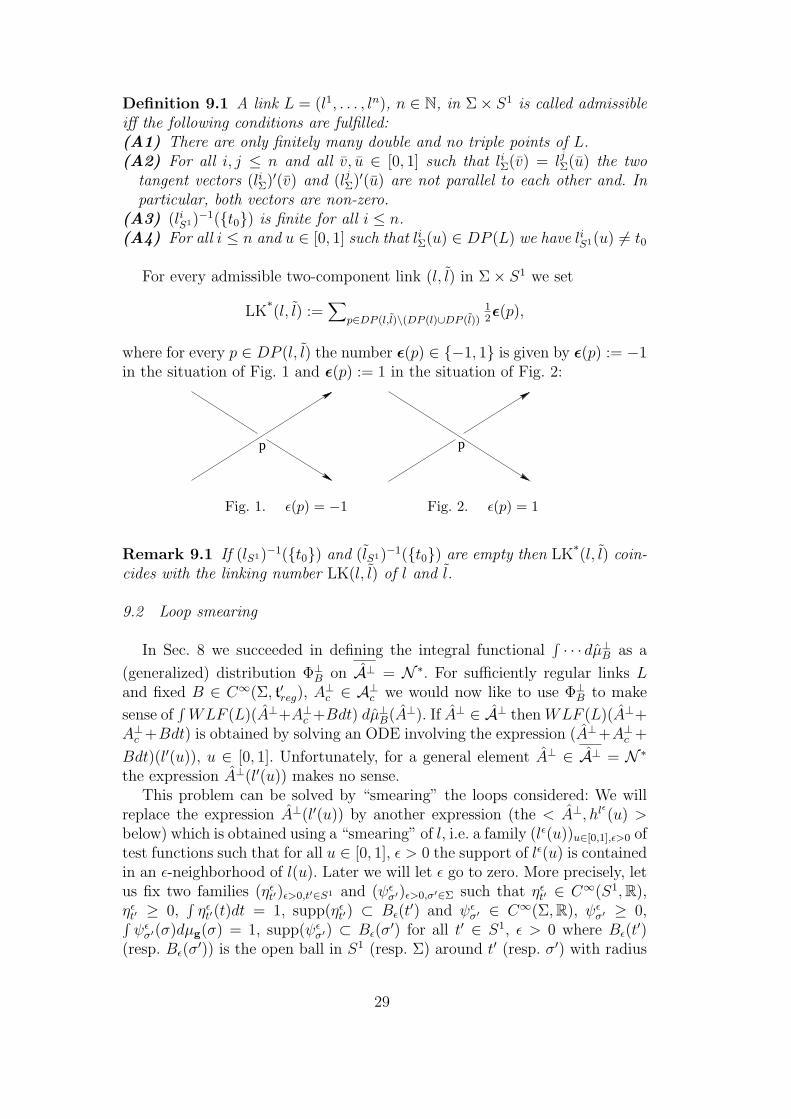
For every admissible two-component link (l, l) in Σ× S1 we set

LK*(l, l) :=∑

p∈DP (l,l)\(DP (l)∪DP (l))

12ε(p),

where for every p ∈ DP (l, l) the number ε(p) ∈ −1, 1 is given by ε(p) := −1in the situation of Fig. 1 and ε(p) := 1 in the situation of Fig. 2:

p

Fig. 1. ε(p) = −1

p

Fig. 2. ε(p) = 1

Remark 9.1 If (lS1)−1(t0) and (lS1)−1(t0) are empty then LK*(l, l) coin-cides with the linking number LK(l, l) of l and l.

9.2 Loop smearing

In Sec. 8 we succeeded in defining the integral functional∫ · · · dµ⊥B as a

(generalized) distribution Φ⊥B on A⊥ = N ∗. For sufficiently regular links L

and fixed B ∈ C∞(Σ, t′reg), A⊥c ∈ A⊥

c we would now like to use Φ⊥B to make

sense of∫

WLF (L)(A⊥+A⊥c +Bdt) dµ⊥B(A⊥). If A⊥ ∈ A⊥ then WLF (L)(A⊥+

A⊥c +Bdt) is obtained by solving an ODE involving the expression (A⊥+A⊥

c +

Bdt)(l′(u)), u ∈ [0, 1]. Unfortunately, for a general element A⊥ ∈ A⊥ = N ∗

the expression A⊥(l′(u)) makes no sense.This problem can be solved by “smearing” the loops considered: We will

replace the expression A⊥(l′(u)) by another expression (the < A⊥, hlε(u) >below) which is obtained using a “smearing” of l, i.e. a family (lε(u))u∈[0,1],ε>0 oftest functions such that for all u ∈ [0, 1], ε > 0 the support of lε(u) is containedin an ε-neighborhood of l(u). Later we will let ε go to zero. More precisely, letus fix two families (ηε

t′)ε>0,t′∈S1 and (ψεσ′)ε>0,σ′∈Σ such that ηε

t′ ∈ C∞(S1,R),ηε

t′ ≥ 0,∫

ηεt′(t)dt = 1, supp(ηε

t′) ⊂ Bε(t′) and ψε

σ′ ∈ C∞(Σ,R), ψεσ′ ≥ 0,∫

ψεσ′(σ)dµg(σ) = 1, supp(ψε

σ′) ⊂ Bε(σ′) for all t′ ∈ S1, ε > 0 where Bε(t

′)(resp. Bε(σ

′)) is the open ball in S1 (resp. Σ) around t′ (resp. σ′) with radius

29

ε w.r.t. the standard distance function dS1 on S1 (resp. the distance functiondg on Σ which is induced by g). Below (cf. Remark 9.2) we will give someadditional conditions which the family (ψε

σ′)ε>0,σ′∈Σ has to fulfill. For everyloop l in M and every u ∈ [0, 1] we define lε(u) ∈ C∞(M,R) by

lε(u)(σ, t) := ψεlΣ(u)(σ) ηε

lS1 (u)(t) for all σ ∈ Σ, t ∈ S1 (9.1)

Let C∞(S1, V F (Σ)) be defined in an analogous way as C∞(S1,AΣ) in Def-inition 5.1. As Σ is compact there is a ε0 > 0 such that for all σ1, σ2 ∈ Σ withdg(σ1, σ2) ≤ ε0 there is a unique segment γ(σ1, σ2) starting in σ1 and endingin σ2 (cf. [27], Chap. 5). For every u ∈ [0, 1] and ε < ε0 we therefore obtain anelement hlε(u) of C∞(S1, V F (Σ)) which is given by

[hlε(u)(t)

](σ) =

PTγ(lΣ(u),σ)(l′Σ(u)) lε(u)(σ, t) if σ ∈ Bε(lΣ(u)),

0 if σ /∈ Bε(lΣ(u))

for all t ∈ S1 where PTγ(lΣ(u),σ) is the parallel transport operator alongγ(lΣ(u), σ) w.r.t. the Levi-Civita connection.

Let < ·, · >: C∞(S1,AΣ) × C∞(S1, V F (Σ)) → g denote the bilinear

map given by < A⊥, h >=∫ [∫

A⊥(t)(h(t))dµg

]dt, A⊥ ∈ C∞(S1,AΣ), h ∈

C∞(S1, V F (Σ)). The expression < A⊥, hlε(u) >, A⊥ ∈ A⊥ ⊂ C∞(S1,AΣ),can be considered as a “smeared analogue” of A⊥(l′(u)). In order to find thegeneralization of < A⊥, hlε(u) > for an arbitrary element A⊥ of N ∗ we have torewrite the expression < A⊥, hlε(u) > in terms of the pairing (·, ·) between N ∗

and N . For this purpose consider the linear isomorphism ξ : V F (Σ) → AΣ,Rgiven by ασ(jσ) = (ασ, ξ(j)σ)g for all α ∈ AΣ,R, j ∈ V F (Σ), σ ∈ Σ where (·, ·)gdenotes the fiber metric on TΣ∗ which is induced by g. For each a ≤ dim g,u ∈ [0, 1], f lε

a (u) will denote the element of C∞(S1,AΣ,R) ⊗ g ∼= A⊥ = Ngiven by f lε

a (u)(t) := ξ(hlε(u)(t)) ⊗ Ta for all t ∈ S1 where (Ta)a is a fixedONB of g. Clearly, < A⊥, hlε(u) >=

∑a Ta(A

⊥, f lε

a (u)). As∑

a Ta(A⊥, f lε

a (u))is defined for arbitrary A⊥ ∈ N ∗ we can now introduce a “smeared” holon-omy Hol(A⊥, lε; A⊥

c , B) for A⊥ ∈ N ∗, A⊥c ∈ A⊥

c , B ∈ C∞(Σ, t′reg), by setting

Hol(A⊥, lε; A⊥c , B) := P lε

A⊥,A⊥c ,B(1) where (P lε

A⊥,A⊥c ,B(u))u∈[0,1] is the unique so-

lution of the ODE with values in Mat(N,C) given by P lε

A⊥,A⊥c ,B(0) = 1Mat(N,C)

and

ddu

P lε

A⊥,A⊥c ,B(u)− P lε

A⊥,A⊥c ,B(u) ·

(∑aTa(A

⊥, f lε

a (u)) + (A⊥c + Bdt)(l′(u))

)= 0

(9.2)for all u ∈ [0, 1]. Here “·” is the standard multiplication of Mat(N,C).

We set WLF (Lε)(A⊥ + A⊥c + Bdt) :=

∏ni=1 TrMat(N,C)(Hol(A⊥, lεi ; A

⊥c , B)).

The mapping N ∗ 3 A⊥ 7→ WLF (Lε)(A⊥+A⊥c +Bdt) ∈ C will be denoted by

WLF (Lε)(·+ A⊥c + Bdt).

30

Proposition 9.1 For every link L in Σ× S1, every ε > 0 and all A⊥c ∈ A⊥

c ,B ∈ C∞(Σ, t′reg) we have WLF(Lε)(·+ A⊥

c + Bdt) ∈ (N ).

Proposition 9.1 is obvious if G is Abelian because then one has WLF (Lε)(·+A⊥

c + Bdt) ∈ E(N ) ⊂ (N ), cf. Eq. (10.2) below. If G is non-Abelian the sit-uation is not so easy anymore but one can obtain a proof for Proposition 9.1also in the non-Abelian case by adapting the proof of Proposition 6 in [21] ina suitable way.

Remark 9.2 For the proof of Theorem 10.1 below to work it will be necessaryto impose a suitable smoothness condition on the function-valued mappingsΣ 3 σ′ 7→ ψε

σ′ ∈ C∞(Σ,R), ε > 0. Instead of trying to identify an appropriatesmoothness condition we will restrict ourselves to special families (ψε

σ′)ε>0,σ′∈Σ

of the form

ψεσ′ = 1

Nεσ′

1ε2

ψ(1εdg(·, σ′)) with N ε

σ′ := 1ε2

∫ψ(1

εdg(σ, σ′))dµg(σ)

for all σ′ ∈ Σ and ε < ε0 where ψ is any fixed smooth function R+ → R+ withsupp(ψ) ⊂ [0, 1] and the additional property that 4 ψ := ψ ‖ · ‖ ∈ C∞(R2,R)where ‖ · ‖ is the standard Euclidean norm on R2. The last condition impliesthat ψ(1

εdg(·, σ′)) is indeed C∞ for each σ′ ∈ Σ and each sufficiently small

ε > 0.

9.3 Framing

One could hope that limε→0 Φ⊥B(WLF(Lε)(· + A⊥

c + Bdt)) exists for B ∈C∞(Σ, t′reg), A⊥

c ∈ A⊥c , and L contained in a sufficiently large set L of links in

Σ×S1 and that after performing also the∫ · · ·DA⊥

c and∫ · · ·DB-integrations

in Eq. (6.6) one obtains a link invariant. However, when one tries to computethe limit limε→0 Φ⊥

B(WLF(Lε)(· + A⊥c + Bdt)) already in the simplest case

G = U(1) a problem arises, the so-called “self-linking problem”, cf., e.g.,[20,21]. Witten suggested in [32] to solve the self-linking problem by using aregularization procedure which he called “framing”. We will use an implemen-tation of this framing procedure which is adapted to our “quasi-axial setting”and which works well also for non-Abelian G (cf. again [20,21] for a motivationof this implementation):

We choose a suitable family (φs)s>0 of diffeomorphisms of Σ × S1 such

that φs lks→0−→ lk, k ≤ n. We can then compute WLO(Lε, φs; A

⊥c , B) :=

Φ⊥B,φs

(WLF(Lε)(·+ A⊥c + Bdt)) where Φ⊥

B,φsis the “deformed version” of Φ⊥

B

obtained by deforming the quadratic form Q⊥B on A⊥ = N in a certain way.

Later we let ε and s go to zero.

4 one can show that ψ ‖ · ‖ ∈ C∞(R2,R) if and only if ψ is the restriction ontoR+ of a smooth symmetric function R→ R

31

Proposition 9.2 Let φ be a diffeomorphism of Σ × S1 and let φ∗ : A → Adenote the pull-back of φ. Then the following three statements are equivalent:

(C1) φ∗(Aqax) = Aqax

(C2) φ∗(Aqax(T )) = Aqax(T ) where T is any fixed maximal torus of G.(C3) There is a (unique) diffeomorphism φ of Σ, a smooth mapping v : Σ →

S1 and a number β ∈ −1, 1 such that φ(σ, t) = (φ(σ), v(σ) · tβ) holds forall σ ∈ Σ, t ∈ S1, where “·” is the standard multiplication of S1 ∼= U(1).

Proof. It is easy to see that statement (C3) implies both (C1) and (C2).That, conversely, each of the two statements (C1) and (C2) implies (C3) ismore difficult to see but not essential for what follows, so we will omit thecorresponding proofs. ¤

Definition 9.2 A diffeomorphism φ of Σ × S1 fulfilling the three equivalentconditions (C1)–(C3) will be called “compatible with the quasi-axial gauge”.

Let φ be a diffeomorphism of Σ × S1 which is compatible with the quasi-axial gauge. One can show that statement (C3) implies φ∗(A⊥) = A⊥. In viewof this relation it is tempting to try to use the pullback φ∗ (or rather (φ−1)∗)for the deformation of the quadratic form Q⊥

B on A⊥ = N . However, it willturn out that this approach will not work, cf. [20,21] for the discussion of asimilar question which arises when studying Chern-Simons models on R3 inaxial gauge. Instead the elements of N = A⊥ ought to transform like vectorfields under the deformation by φ.

Let V F (M) denote the space of smooth vector fields on M and let us setV F⊥(M) := X ∈ V F (M) | dt(X) = 0. Let φ∗ denote the linear automor-phism of V F (M) ⊗ g which is induced by φ. φ∗ does not leave the subspaceV F⊥(M) ⊗ g ∼= A⊥ = N of V F (M) ⊗ g invariant but pr φ∗ does where pris the obvious projection V F (M)⊗ g → V F⊥(M)⊗ g (here we have used theidentification V F⊥(M)⊗ g ∼= A⊥ which is induced by the standard Rieman-nian metric on S1 and the linear mapping ξ : V F (Σ) → AΣ,R introduced inSubsec. 9.2). It is not difficult to see that prφ∗ : V F⊥(M)⊗g → V F⊥(M)⊗g

is a linear automorphism.

The linear automorphism on N = A⊥ obtained from pr φ∗ by trans-port with the isomorphism which identifies V F⊥(M) ⊗ g with N = A⊥ willbe denoted by φ∗. A straightforward computation shows that if j ∈ A⊥ ∼=V F⊥(M)⊗g then φ∗(j) ∈ A⊥ ∼= V F⊥(M)⊗g is given by (φ∗(j))(t) = φ∗(j(t))for all t ∈ S1 where φ∗ : TΣ → TΣ is the ordinary tangent mapping which isinduced by φ : Σ → Σ (cf. Proposition 9.2).

Definition 9.3 Let B ∈ C∞(Σ, t′reg) and let φ be a diffeomorphism of Σ×S1

which is compatible with the quasi-axial gauge. By Q⊥B,φ we will denote the

(continuous) real quadratic form on N given by Q⊥B,φ(j) = Q⊥

B(j, φ∗(j)) forall j ∈ N . Q⊥

B,φ will also denote the real symmetric bilinear form obtained by

32

polarization, i.e. the (continuous) real symmetric bilinear form on N given by

Q⊥B,φ(j1, j2) = 1

2

[Q⊥

B(j1, φ∗(j2)) + Q⊥B(j2, φ∗(j1))

]for all j1, j2 ∈ N (9.3)

Definition 9.4 Let B and φ be as above. We will denote the Gaussian elementof (N )∗ corresponding to (a⊥B,−2πλiQ⊥

B,φ) by Φ⊥B,φ (cf. Sec. 7).

Definition 9.5 Let L = (l1, . . . , ln), n ∈ N, be an admissible link in Σ× S1.An admissible framing of L is a family (φs)s>0 of diffeomorphisms of Σ× S1

with the following properties:

(F1) Each φs, s > 0, is compatible with the quasi axial gauge and we haveφ∗s(νg ∧ dt) = νg ∧ dt where νg is the positively oriented volume form asso-ciated to g.

(F2) For all i, j ≤ n and all sufficiently small s > 0 the pair (li, φs lj) is anadmissible link in Σ× S1.

(F3) ∀i ≤ n: φs lis→0−→ li dg-uniformly and lims→0 LK*(li, φs li) exists.

Remark 9.3 In [18] we will replace LK*(li, φs li) in (F3) by LK(li, φs li).

10 Computation of the WLOs for the special case Σ = S2 andG = U(1)

Let us now restrict ourselves to the situation of Eq. (6.4), i.e. let us assumethat G is Abelian and Σ = S2. Clearly, for Abelian G the bilinear form Q⊥

B

does not depend on B so we can set Q⊥ := Q⊥B.

In Subsec. 10.1 we will evaluate the inner integral of (6.4) at a rigorous levelusing the regularization procedures which we have introduced in Sec. 9. As wewill show in [18] it is also possible to give a rigorous meaning to the heuristic(Gauss-type) integral functional

∫ · · · exp(i k2π

< A⊥c , dB >Σ)DA⊥

c ⊗DB. In thepresent paper we content ourselves with dealing with this integral functionalat a heuristic level. We do this by integrating first against DB and thenagainst DA⊥

c in Subsec. 10.2 below. This is possible if the link L = (l1, . . . , ln)considered has the additional property that t0 /∈ Image(ljS1), j ≤ n.

10.1 The integration∫ · · · dµ⊥B

For simplicity we will only treat the special case N = 1 and G = U(1).In this case we have T = G = U(1) and t′reg = t = u(1). The results whichwe derive for this special Abelian group can be generalized easily to arbitraryN ∈ N and arbitrary closed connected Abelian subgroups of U(N). Takinginto account Proposition 9.1 we obtain

Theorem 10.1 Let L = (l1, . . . , ln), n ∈ N, be an admissible link in Σ × S1

33

and let (φs)s>0 be an admissible framing of L. Then

WLO(L, (φs)s>0; A⊥c , B) := lim

s0limε0

Φ⊥B,φs

(WLF (Lε)(·+ A⊥c + Bdt)) exists

for all A⊥c ∈ A⊥

c , B ∈ C∞(Σ, t) and setting ljΣ := (lj)Σ, ljS1 := (lj)S1, lk∗j :=

lims→0 LK*(lj, φs lj), and Ij := (ljS1)−1(t0) for j ≤ n, we obtain

WLO(L, (φs)s>0; A⊥c , B) =

∏

j

exp(λπi lk∗j)∏

j 6=k

exp(λπi LK*(lj, lk))

×∏

j

[exp(

∫

ljΣ

A⊥c ) exp

( ∑

u∈Ij

sgn(ljS1 ; u) ·B(ljΣ(u)))]

(10.1)

where sgn(ljS1 ; u) = 1 (resp. −1 resp. 0) if the loop ljS1 crosses t0 at u in thedirection of the orientation of S1 (resp. crosses t0 at u in the opposite directionresp. does not cross but only touches t0 at u).

Proof. Let L, n, (φs)s>0, A⊥c , and B be as in the assertion and let ε ∈ (0, ε0)

where ε0 is as in Subsec. 9.2. Clearly, i = T1 ∈ u(1) so setting f lεj(u) := flεj1 (u)

we have

WLF (Lε)(A⊥ + A⊥c + Bdt)

= exp(i(A⊥,∑

k

∫ 1

0f lεk(u)du))

∏

j

[exp(

∫

ljΣ

A⊥c ) exp(

∫

ljBdt)

](10.2)

so from Definition 9.4 we obtain

Φ⊥B,φs

(WLF (Lε)(·+ A⊥c + Bdt))

= exp(iπλQ⊥φs

(∑

k

∫ 1

0f lεk(u)du)) exp(i a⊥B(

∑

j

∫ 1

0f lεj(u)du))

×∏

j

[exp(

∫

ljΣ

A⊥c ) exp(

∫

ljBdt)

](10.3)

Let us set ljR := i−1S1 ljS1 − 1/2, j ≤ n. Then

limε→0

ia⊥B(∫ 1

0f lεj(u)du)

= i∫ 1

0

[limε→0

¿ f lεj(u),m(B) ÀH]du

(∗)=

∫ 1

0[ljR(u) d

duB(ljΣ(u))]du (10.4)

34

Here step (∗) follows from Eq. (8.7),∫S1(i−1

S1 (t)−1/2) ηεljS1 (u)

(t)dtε→0−→ ljR(u) for

all u /∈ Ij = (ljS1)−1(t0), and

∫

Σ

(T1 ⊗ ξ(PTγ(ljΣ(u),·)((l

jΣ)′(u)) ψε

ljΣ(u)), dB

)g

dµg

= −T1

∫

Σψε

ljΣ(u)dB(PTγ(ljΣ(u),·)((l

jΣ)′(u))) dµg

ε→0−→ 1idB((ljΣ)′(u)) = 1

iddu

B(ljΣ(u))

Here PTγ(ljΣ(u),·)((ljΣ)′(u)) denotes the vector field σ 7→ PTγ(ljΣ(u),σ)((l

jΣ)′(u)).

On the other hand from∫lj

Bdt =∫ 10 B(ljΣ(u)) · (ljS1)′(u) du and (ljS1)′(u) =

(ljR)′(u) it follows

exp(∫ 1

0ljR(u) d

duB(ljΣ(u))du) exp(

∫

ljBdt)

= exp

(∫ 1

0

ljR(u) d

duB(ljΣ(u)) + B(ljΣ(u)) · (ljR)′(u)

du

)(10.5)

Let nj := #Ij and let (si)i≤njbe the unique strictly increasing sequence of

[0, 1] such that Ij = si | i ≤ nj. Without loss of generality let us assume that0 ∈ Ij. Restricted onto each of the open intervals (si, si+1) the curve ljR will be

C1 and for u ∈ (si, si+1) we will have(

ddu

B(ljΣ(u)))·ljR(u)+B(ljΣ(u))·(ljR)′(u) =

ddu

[B(ljΣ(u)) · ljR(u)

]so we obtain

∫ 1

0

ljR(u) d

duB(ljΣ(u)) + B(ljΣ(u)) · (ljR)′(u)

du

=∑

i

∫ si+1

si

d

du

[ljR(u) ·B(ljΣ(u))

]du =

∑

i

sgn(ljS1 ; si) ·B(ljΣ(si))

because sgn(ljS1 ; si) = lims↑siljR(s)− lims↓si

ljR(s). Thus we have

limε→0

exp(ia⊥B(∫ 1

0f lεj(u)du)) exp(

∫

ljBdt) =

∏

i

exp(sgn(ljS1 ; si) ·B(ljΣ(si))

)

(10.6)

Finally, we have for j, k ≤ n, for all s > 0 and ε > 0

Q⊥φs

(∫ 1

0f lεk(v) dv,

∫ 1

0f lεj(v) dv

)=

∫ 1

0dv

∫ 1

0duQ⊥

φs

(f lεk(v), f lεj(u)

)

= 12

∫ 1

0dv

∫ 1

0du

[Q⊥(f lεk(v), (φs)∗(f

lεj(u))) + Q⊥((φs)∗(f lεk(v)), f lεj(u))]

(10.7)

Recall that (lj, φs lk) is admissible if s > 0 is sufficiently small (cf. (F2) inDefinition 9.5). So from Lemma 4 and Lemma 5 below and (F3) in Definition

35

9.5 we obtain

lims→0

limε→0

Q⊥φs

(∫ 1

0f lεk(v) dv,

∫ 1

0f lεj(v) dv

)

= 12lims→0

[LK*(lk, φs lj) + LK*(φs lk, lj)

]=

LK*(lj, lk) if j 6= k

lk∗j if j = k(10.8)

Eq. (10.1) now follows from Eqs. (10.3), (10.6), and (10.8). ¤

Lemma 4 For every admissible link (l, l) in Σ× S1 we have

limε→0

Q⊥(∫ 1

0f lε(v)dv,

∫ 1

0f lε(u)du

)= LK*(l, l),

Proof. According to the definition of LK*(l, l) it is enough to show thatfor all v′, v′′, u′, u′′ ∈ [0, 1] with v′ < v′′, u′ < u′′ and the additional prop-erty that lΣ([v′, v′′]) ∩ lΣ([u′, u′′]) contains exactly one element p of D :=DP (l, l)\(DP (l) ∪DP (l)) we have

limε→0

∫ v′′

v′dv

∫ u′′

u′du Q⊥(f lε(v), f lε(u)) = 1

2ε(p) (10.9)

Let v ∈ [v′, v′′], u ∈ [u′, u′′] be given by p = lΣ(v) = lΣ(u). For simplicity letus assume in the sequel that v, u /∈ 0, 1 (it is not difficult to generalize theproof to the general situation). Then it is easy to see that there is a δ > 1such that for sufficiently small ε > 0 we have

∫ v′′

v′dv

∫ u′′

u′du Q⊥(f lε(v), f lε(u)) =

∫ v+δε

v−δεdv

∫ u+δε

u−δεdu Q⊥(f lε(v), f lε(u))

(10.10)On the other hand

Q⊥(f lε(v), f lε(u)) =¿ f lε(v), ∂∂t

−1 · ?−1 · f lε(u)) ÀH

=∫

S1dt

∫

Σ

(T1 ⊗ ξ(hlε(v)(t)), ∂

∂t

−1 · ?−1 · (T1 ⊗ ξ(hlε(u)(t))))g

dµg

(∗)=

∫

S1dt

∫

Σνg

((hlε(v)

)(t), ∂

∂t

−1(hlε(u)

)(t)

)dµg

=∫

S1dt ηε

lS1 (v)(t)(∂∂t

−1ηε

lS1(u))(t)

×∫

Σνg

(PTγ(lΣ(v),·)(l

′Σ(v)), PTγ(lΣ(u),·)(l

′Σ(u))

)ψε

lΣ(v)ψεlΣ(u)

dµg (10.11)

where the last two “ ∂∂t

−1” denote the operator ∂

∂t

−1: C∞(S1,R) → C∞(S1,R)

defined in the obvious way. Step (∗) above holds because ∂∂t

−1commutes with

?−1 and because we have (ξ(j), ?−1 · ξ(j′))g = νg(j, j′) for all j, j′ ∈ V F (Σ),

which is easy to show.

36

Using (A4) in Definition 9.1 and the real-valued analogue of (8.3) it followsfor sufficiently small ε > 0

∫

S1ηε

lS1 (v)(t)∂∂t

−1ηε

lS1 (u)(t) dt = 1

2[1lS1 (u)<lS1 (v) − 1lS1 (v)<lS1 (u)] (10.12)

where < is the order relation on S1 which is induced by iS1 : [0, 1) → S1.Clearly, we have for all σ ∈ Σ

νg

(PTγ(lΣ(v),σ)(l

′Σ(v)), PTγ(lΣ(u),σ)(l

′Σ(u))

)= νg

(l′Σ(v), l′Σ(u))

)(10.13)

So we obtain

limε→0

∫ v+δε

v−δεdv

∫ u+δε

u−δεdu Q⊥(f lε(v), f lε(u))

(+)= 1

2[1lS1 (u)≤lS1 (v) − 1lS1 (v)≤lS1 (u)]

× limε→0

∫ v+δε

v−δεdv

∫ u+δε

u−δεdu νg

(l′Σ(v), l′Σ(u))

) ∫

Σψε

lΣ(v)ψεlΣ(u)

dµg

(∗)= 1

2[1lS1 (u)≤lS1 (v) − 1lS1(v)≤lS1 (u)] νg

(l′Σ(v), l′Σ(u))

)

× limε→0

∫ v+δε

v−δεdv

∫ u+δε

u−δεdu

∫

Σψε

lΣ(v)ψεlΣ(u)

dµg

provided that limε→0

∫ v+δεv−δε dv

∫ u+δεu−δε du

∫Σ ψε

lΣ(v)ψεlΣ(u)

dµg exists. Here step (+)

follows from (10.11)–(10.13) and step (∗) follows because the map (v, u) 7→νg

(l′Σ(v), l′Σ(u))

)is continuous and does not vanish in the point (v, u) and

is therefore either strictly positive or strictly negative on a neighborhood of(v, u). It is not difficult to see that ε(p) is given by

ε(p) = sgn(νg(l

′Σ(v), l′Σ(u))

)· [1lS1 (u)<lS1 (v) − 1lS1 (v)<lS1 (u)] (10.14)

so equation (10.9) will follow once we have shown that

limε→0

∫ v+δε

v−δεdv

∫ u+δε

u−δεdu

∫

Σψε

lΣ(v)ψεlΣ(u)

dµg = 1|νg(l′Σ(v),l′Σ(u))| (10.15)

We observe that for every chart x : U → V ⊂ R2 of Σ around p such thatνg(

∂∂x1

, ∂∂x2

)(p) = 1 we have νg(l′Σ(v), l′Σ(u))) = (l′Σ(v))1(l

′Σ(u))2−(l′Σ(v))2(l

′Σ(u))1

where (l′Σ(v))i and (l′Σ(u))i, i = 1, 2, denote the coordinates of l′Σ(v) and l′Σ(u)w.r.t. to ( ∂

∂x1, ∂

∂x2). If we take this into account and if we also take into ac-

count Remark 9.2 above and compare Eq. (10.15) above with equation (22)in [20] we see that Eq. (10.15) holds at least in the special case where theauxiliary Riemannian metric g was chosen such that each p ∈ DP (L) has anopen neighborhood U such that g is Euclidean on U . The proof of (10.15) inthe general situation will be given elsewhere. ¤

37

Lemma 5 For every admissible link (l, l) in Σ×S1 and every s > 0 such that(φs l, l) is admissible we have

limε→0

∫ 1

0dv

∫ 1

0du Q⊥((φs)∗(f lε(v)), f lε(u))

= limε→0

∫ 1

0dv

∫ 1

0du Q⊥(f (φsl)ε

(v), f lε(u)) (10.16)

Lemma 5 can be proved in a similar way as equation (29) in [20]. We will givea detailed proof of Lemma 5 elsewhere.

10.2 The integrations∫ · · ·DB and

∫ · · ·DA⊥c

Now that we made rigorous sense of the inner integral in Eq. (6.4) for everyfixed admissible framing (φs)s>0 we replace

∫WLF(L)(A⊥+A⊥

c +Bdt)dµ⊥B(A⊥)in Eq. (6.4) by WLO(L, (φs)s>0; A

⊥c , B) and set

WLO(L, (φs)s>0) :=

1

Z ′′

∫ ∫WLO(L, (φs)s>0; A

⊥c , B) exp(i k

2π< A⊥

c , dB >Σ)DA⊥c DB

For simplicity we will now restrict ourselves to (admissible) links L =(l1, . . . , ln), n ∈ N, with the additional property t0 /∈ Image((lj)S1), i.e. Ij = ∅,for every j ≤ n. In this special case WLO(L, (φs)s>0; A

⊥c , B) does not depend

on B and the two integrations∫ · · ·DB and

∫ · · ·DA⊥c can be performed in a

straightforward way. According to (10.1) and Remark 9.1 we then have

WLO(L, (φs)s>0) =∏

j

exp(λπi lk∗j)∏

j 6=k

exp(λπi LK*(lj, lk))

× 1

Z ′′

∫ ∫ ∏

j

exp(∫

ljΣ

A⊥c ) exp(i k

2π< A⊥

c , dB >Σ)DA⊥c DB

=∏

j

exp(λπi lkj)∏

j 6=k

exp(λπi LK(lj, lk)) (10.17)

because, informally,

1

Z ′′

∫ ∫ ∏

j

exp(∫

ljΣ

A⊥c ) exp(i k

2π< A⊥

c , dB >Σ)DA⊥c DB

(+)=

1

Z ′′

∫ [∫exp(i k

2π

∫

ΣTr(dA⊥

c ·B))DB

] ∏

j

exp(∫

ljΣ

A⊥c )DA⊥

c

(†)=

1

Z ′′

∫δ(dA⊥

c )∏

j

exp(∫

ljΣ

A⊥c )DA⊥

c

(∗)=

1

Z ′′

∫δ(dA⊥

c ) exp(0)DA⊥c

=1

Z ′′

∫ ∫exp(i k

2π

∫

ΣTr(dA⊥

c ·B))DBDA⊥c

(++)=

Z ′′

Z ′′ = 1

38

Step (†) follows from DB = dB (cf. Subsec. 5.2), step (∗) follows becauseH1(Σ) = 0 for Σ = S2. So A⊥

c is closed iff it is exact but for exact A⊥c one has∫

ljΣA⊥

c = 0. Steps (+) and (++) follow from Stokes’ Theorem.

Remark 10.1 In [18] we will consider the case of general admissible linksL = (l1, . . . , ln) in Σ×S1. It will turn out that there is an interesting interplaybetween the LK*(li, lj)-, the

∫ljΣ

A⊥c -, and the sgn(ljS1 ; u)B(ljΣ(u))-expressions

in Eq. (10.1) which finally leads to linking number expressions LK(li, lj) alsoin the more general situation where the winding numbers of liS1 and ljS1 vanishbut Ii and Ij are not necessarily empty 5 .

11 Conclusions and Outlook

In the present paper we studied Chern-Simons models on manifolds ofthe form M = Σ × S1 using quasi-axial gauge fixing and later also torusgauge fixing. For the case where Σ or the structure group G of the model issimply-connected we exploited the properties of quasi-axial gauge fixing andderived certain heuristic integral expressions for the WLOs of the model. Theseintegral expressions, i.e the right-hand sides of Eq. (6.3) and Eq. (6.4), which isthe Abelian special case of (6.3), have some promising features. In particular,the inner integrals in (6.3) and (6.4) are of “Gaussian type”. We expect thatbecause of this it will eventually be possible to find a rigorous realization ofthese expressions both in the case of Abelian and of Non-Abelian G.

Of course, for Abelian G it has already been demonstrated by other meth-ods that it is possible to obtain a rigorous definition of the WLOs in terms ofpath integral expression, cf., e.g., [3,25,1]. However, when using an approachbased on Lorentz gauge fixing like in [3,25] or one that is based on a suit-able discretization of the base manifold like in [1] the difference between theAbelian and the Non-Abelian situation seems to be so large that completelynew techniques are required for the treatment of the Non-Abelian case. Quasi-axial gauge fixing has the big advantage that when this gauge-fixing procedureis applied the difference between the Abelian and the Non-Abelian situationbecomes much smaller. Not surprisingly, there is also a price we have to paywhen we want to use quasi-axial gauge fixing: due to the appearance of somerather singular expressions on the right-hand side of Eq. (6.4) the treatment ofthe Abelian case is, at least at first look, more difficult than the treatment ofthe Abelian case in [3,25,1]. Anyhow, as we showed in Secs. 7–10 for the specialcase G = U(1) it is still possible to make sense of the right-hand side of Eq.(6.4) by using regularization procedures like “loop smearing” and “framing”and constructions from white noise analysis.

Before one tries to find a rigorous realization of the right-hand side of the

5 the winding numbers of liS1 and ljS1 vanish iff li and lj are 0-homologous. If li and

lj are not 0-homologous then LK(li, lj) is in general not defined

39

Non-Abelian generalization Eq. (6.3) of Eq. (6.4) it is reasonable to discussfirst the question whether, by using torus gauge fixing instead of quasi-axialgauge fixing, things can be simplified even further. For non-compact Σ torusgauge fixing is a “proper” gauge in the sense that at least every “regular”connection (i.e., every element of Areg) is gauge equivalent to a connection inthe torus gauge, cf. Proposition 3.4 and Remark 3.1. So Eq. (6.6) makes sensefor non-compact Σ and we expect that one can evaluate the WLOs explicitlyfor arbitrary G by using the “cluster decomposition” technique developed in[21] for the study of Chern-Simons models on the non-compact manifold R3

in axial gauge.

On the other hand, due to certain topological obstructions, torus gauge fix-ing can not be applied without modifications if Σ is compact. In other wordsone should expect that Eq. (6.6), to which one is lead if one neglects the topo-logical obstructions just mentioned, has to be replaced by a more complicatedequation. The considerations in [10–12] where torus gauge fixing was exploitedfor the study of the partition functions of Chern-Simons models on manifoldsof the form Σ × S1 give already a certain idea of how this modification ofEq. (6.6) has to look like. We will come back to this point in [18]. In thepresent paper we have restricted ourselves mainly to the study of the innerintegral in (6.6), which will most probably not be affected by the modifica-tion of (6.6) just mentioned. This study can thus be seen as the first step ofa program which, as we expect, will eventually lead both to a rigorous pathintegral representation for the WLOs of Non-Abelian Chern-Simons modelson the compact manifold M = S2 × S1 and to a new, non-perturbative, andpurely geometric derivation of the R-matrices of Jones and Turaev.

Acknowledgements. Part of this work was inspired by a joint project lastyear with Prof. Dr. Sergio Albeverio and Prof. Dr. Ambar N. Sengupta inwhich we studied possible applications of the Borel-Weil Theorem to Chern-Simons theory. I would like to thank Prof. Dr. Luigi Accardi for his hospitalityduring my research stay at the Centro Vito Volterra, University of Rome II,during which the main part of this work was elaborated. An EU scholarshipduring this research stay in Rome is gratefully acknowledged. Special thanksgo, as so often, to Prof. Dr. Sergio Albeverio for his constant support in nu-merous ways during the last year and to Prof. Dr. Dietmar Arlt for many veryuseful comments and remarks.

References

[1] D. H. Adams. A doubled discretization of abelian Chern-Simons theory. Phys.Rev. Lett., 78(22):4155–4158, 1997.

[2] D. H. Adams. The semiclassical approximation for the Chern-Simons partitionfunction. Phys. Lett. B, 417(1-2):53–60, 1998.

40

[3] S. Albeverio and J. Schafer. Abelian Chern-Simons theory and linking numbersvia oscillatory integrals. J. Math. Phys., 36(5):2135–2169, 1994.

[4] S. Albeverio and A.N. Sengupta. A Mathematical Construction of the Non-Abelian Chern-Simons Functional Integral. Commun. Math. Phys., 186:563–579, 1997.

[5] D. Altschuler and L. Freidel. Vassiliev knot invariants and Chern-Simonsperturbation theory to all orders. Comm. Math. Phys., 187:261–287, 1997.

[6] M. Atiyah. The Geometry and Physics of Knot Polynomials. Cambridge:University Press, 1990.

[7] S. Axelrod and I.M. Singer. Chern-Simons perturbation theory. II. J. Differ.Geom., 39(1):173–213, 1994.

[8] D. Bar-Natan. Perturbative Chern-Simons theory. J. Knot Theory and itsRamifications, 4:503–547, 1995.

[9] H. Bauer. Maß - und Integrationstheorie. de Gruyter, 1990.

[10] M. Blau and G. Thompson. Derivation of the Verlinde Formula from Chern-Simons Theory and the G/G model. Nucl. Phys., B408(1):345–390, 1993.

[11] M. Blau and G. Thompson. Lectures on 2d Gauge Theories: Topological Aspectsand Path Integral Techniques. In E. Gava et al., editor, Proceedings of the 1993Trieste Summer School on High Energy Physics and Cosmology, pages 175–244.World Scientific, Singapore, 1994.

[12] M. Blau and G. Thompson. On Diagonalization in Map(M, G). Commun.Math. Phys., 171:639–660, 1995.

[13] R. Bott and Taubes C. On the self-linking of knots. J. Math. Phys., 35(10):5247–5287, 1994.

[14] Th. Brocker and T. tom Dieck. Representations of compact Lie groups,volume 98 of Graduate Texts in Mathematics. Springer-Verlag, New York, 1985.

[15] J. A. Dieudonne. Foundations of Modern Analysis. Academic Press, New Yorkand London, 1968.

[16] J. Frohlich and C. King. The Chern-Simons Theory and Knot Polynomials.Commun. Math. Phys., 126:167–199, 1989.

[17] E. Guadagnini, M. Martellini, and M. Mintchev. Wilson Lines in Chern-Simonstheory and Link invariants. Nucl. Phys. B, 330:575–607, 1990.

[18] A. Hahn. Chern-Simons models on S2 × S1, torus gauge fixing, and linkinvariants II. in preparation.

[19] A. Hahn. Quasi-axial gauge fixing for Chern-Simons models on S2 × S1. SFB611 Preprint, No. 97, Bonn, 2003.

[20] A. Hahn. Chern-Simons theory on R3 in axial gauge: a rigorous approach. J.Funct. Anal., 211(2):483–507, 2004.

41

[21] A. Hahn. The Wilson loop observables of Chern-Simons theory on R3 in axialgauge. to appear in Commun. Math. Phys., 2004.

[22] T. Hida, H.-H. Kuo, J. Potthoff, and L. Streit. White Noise. An infinitedimensional Calculus. Dordrecht: Kluwer, 1993.

[23] V.F.R. Jones. On knot invariants related to some statistical mechanics models.Pacific J. Math., 137:311–388, 1989.

[24] L. Kauffman. Knots. Singapore: World Scientific, 1993.

[25] P. Leukert and J. Schafer. A Rigorous Construction of Abelian Chern-SimonsPath Integrals using White Noise Analysis. Rev. Math. Phys., 8(3):445–456,1996.

[26] J. Milnor. Morse theory. Princeton University Press, 1963.

[27] P. Petersen. Riemannian Geometry, volume 171 of Graduate Texts inMathematics. Springer-Verlag, New York, 1998.

[28] S. Pokorski. Gauge Field Theories. Cambridge University Press, 2000.

[29] E. H. Spanier. Algebraic Topology. Mc Graw-Hill Book Company, 1966.

[30] N. Steenrod. Fibre bundles. Princeton University Press, 1952.

[31] V.G. Turaev. The Yang-Baxter equation and invariants of links. Invent. Math.,92:527–553, 1988.

[32] E. Witten. Quantum Field Theory and the Jones Polynomial. Commun. Math.Phys., 121:351–399, 1989.

42

Bestellungen nimmt entgegen:

Institut für Angewandte Mathematikder Universität BonnSonderforschungsbereich 611Wegelerstr. 6D - 53115 Bonn

Telefon: 0228/73 3411Telefax: 0228/73 7864E-mail: anke@iam.uni-bonn.de Homepage: http://www.iam.uni-bonn.de/sfb611/

Verzeichnis der erschienenen Preprints ab No. 96

96. Rüdiger, Barbara: Stochastic Integration of Deterministic and Random Banach ValuedFunctions with Respect to Compensated Poisson Random Measures and the Lévy-Ito Formula (Review); erscheint in: Proceedings of Kree's Conference, StochasticAnalysis and Applications, Hammamet 2001

97. Hahn, Atle: Quasi-Axial Gauge Fixing for Chern-Simons Models on S2 x S

1; eingereicht

bei: Journal of Geometry and Physics

98. Albeverio, Sergio; Koshmanenko, Volodymyr; Pratsiovytyi, Mykola; Torbin, Grygoriy:Spectral Properties of Image Measures Under the Infinite Conflict Interaction;eingereicht bei: Positivity

99. Albeverio, Sergio; Nizhnik, Leonid: A Schrödinger Operator with a ä'-Interaction on a

Cantor Set and Krein-Feller Operators; eingereicht bei: Mathematische Nachrichten

100. Hoffmann, Karl-Heinz; Botkin, Nikolai D.; Starovoitov, Victor N.; Turova, Varvara L.:Treatment of the Interface Between Fine Elastic Structures and Fluids with Homogenization Method; eingereicht bei: SIAM Journal of Applied Mathematics

101. Giacomelli, Lorenzo; Otto, Felix: New Bounds for the Kuramoto-Sivashinsky Equation

102. Frehse, Jens; Goj, Sonja; Málek, Josef: A Uniqueness Result for a Model for Mixtures inthe Absence of External Forces and Interaction Momentum; eingereicht bei:Appl. Math.

103. Frehse, Jens; Goj, Sonja; Málek, Josef: Existence of Solutions to a Stokes-Like Systemfor Mixtures; eingereicht bei: SIAM Journal on Mathematical Analysis

104. Albeverio, Sergio; Popovici, Alex; Steblovskaya, Victoria: Numerical Analysis of the Extended Black-Scholes Model

105. Müller, Werner; Speh, Birgit (Appendix by Erez M. Lapid): On the Absolute Convergence ofthe Spectral Side of the Arthur Trace Formula for GLn

106. Haußer, Frank; Voigt, Axel: Weakly Anisotropic Surfaces Diffusion, a Numerical Approachby Parametric Finite Elements; eingereicht bei: IMA J. Num. Anal.

107. Müller, Werner: Weyl´s Law for the Cuspidal Spectrum of SLn

108. Albeverio, Sergio; Lytvynov, Eugene; Mahnig, Andrea: A Model of the Term Structure ofInterest Rates Based on Lévy Fields; eingereicht bei: Finance and Stochastics

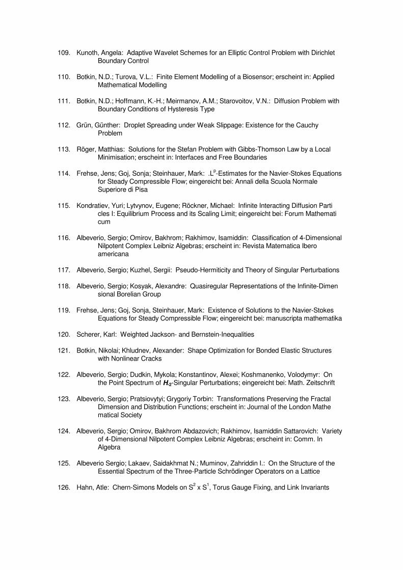
109. Kunoth, Angela: Adaptive Wavelet Schemes for an Elliptic Control Problem with DirichletBoundary Control

110. Botkin, N.D.; Turova, V.L.: Finite Element Modelling of a Biosensor; erscheint in: AppliedMathematical Modelling

111. Botkin, N.D.; Hoffmann, K.-H.; Meirmanov, A.M.; Starovoitov, V.N.: Diffusion Problem withBoundary Conditions of Hysteresis Type

112. Grün, Günther: Droplet Spreading under Weak Slippage: Existence for the CauchyProblem

113. Röger, Matthias: Solutions for the Stefan Problem with Gibbs-Thomson Law by a LocalMinimisation; erscheint in: Interfaces and Free Boundaries

114. Frehse, Jens; Goj, Sonja; Steinhauer, Mark: .Lp-Estimates for the Navier-Stokes Equations

for Steady Compressible Flow; eingereicht bei: Annali della Scuola NormaleSuperiore di Pisa

115. Kondratiev, Yuri; Lytvynov, Eugene; Röckner, Michael: Infinite Interacting Diffusion Particles I: Equilibrium Process and its Scaling Limit; eingereicht bei: Forum Mathematicum

116. Albeverio, Sergio; Omirov, Bakhrom; Rakhimov, Isamiddin: Classification of 4-DimensionalNilpotent Complex Leibniz Algebras; erscheint in: Revista Matematica Iberoamericana

117. Albeverio, Sergio; Kuzhel, Sergii: Pseudo-Hermiticity and Theory of Singular Perturbations

118. Albeverio, Sergio; Kosyak, Alexandre: Quasiregular Representations of the Infinite-Dimensional Borelian Group

119. Frehse, Jens; Goj, Sonja, Steinhauer, Mark: Existence of Solutions to the Navier-StokesEquations for Steady Compressible Flow; eingereicht bei: manuscripta mathematika

120. Scherer, Karl: Weighted Jackson- and Bernstein-Inequalities

121. Botkin, Nikolai; Khludnev, Alexander: Shape Optimization for Bonded Elastic Structureswith Nonlinear Cracks

122. Albeverio, Sergio; Dudkin, Mykola; Konstantinov, Alexei; Koshmanenko, Volodymyr: Onthe Point Spectrum of H-2-Singular Perturbations; eingereicht bei: Math. Zeitschrift

123. Albeverio, Sergio; Pratsiovytyi; Grygoriy Torbin: Transformations Preserving the FractalDimension and Distribution Functions; erscheint in: Journal of the London Mathematical Society

124. Albeverio, Sergio; Omirov, Bakhrom Abdazovich; Rakhimov, Isamiddin Sattarovich: Varietyof 4-Dimensional Nilpotent Complex Leibniz Algebras; erscheint in: Comm. InAlgebra

125. Albeverio Sergio; Lakaev, Saidakhmat N.; Muminov, Zahriddin I.: On the Structure of theEssential Spectrum of the Three-Particle Schrödinger Operators on a Lattice

126. Hahn, Atle: Chern-Simons Models on S2 x S

1, Torus Gauge Fixing, and Link Invariants