
A Numerical Study on Premixed Laminar Flame Front ...A Numerical Study on Premixed Laminar Flame...
69
Professur für Thermofluiddynamik MASTER A Numerical Study on Premixed Laminar Flame Front Instabilities in Thermoacoustic Systems Autor: Abdel Karim Idris Matrikel-No: 03649936 Betreuer: Dipl.-Ing.Thomas Steinbacher, M. Sc. Prof. Wolfgang Polifke, Ph. D. December 15, 2016 Professur für Thermofluiddynamik Prof. Wolfgang Polifke, Ph. D.
Transcript of A Numerical Study on Premixed Laminar Flame Front ...A Numerical Study on Premixed Laminar Flame...

Professur für Thermofluiddynamik
MASTER
A Numerical Study on Premixed Laminar Flame FrontInstabilities in Thermoacoustic Systems
Autor:Abdel Karim Idris
Matrikel-No:03649936
Betreuer:Dipl.-Ing.Thomas Steinbacher, M. Sc.
Prof. Wolfgang Polifke, Ph. D.
December 15, 2016
Professur für ThermofluiddynamikProf. Wolfgang Polifke, Ph. D.

Erklärung
Hiermit versichere ich, die vorliegende Arbeit selbstständig verfasst zu haben. Ich habe keineanderen Quellen und Hilfsmittel als die angegebenen verwendet.
Ort, Datum Abdel Karim Idris

Danksagung/Acknowledgement
This work is dedicated to M.Sc. Javier Achury, a former colleague at the "Professur für Ther-mofluiddynamik". The one whom I learned from a lot and who gave me the required prereq-uisites to start this work. I will be grateful to him for the rest of my life. May his body and soulrest in peace.
I would like to express my sincere gratitude to my master thesis supervisor Dipl.Ing. ThomasSteinbacher for the continuous support during the whole research period, for his patience,motivation, and immense knowledge. Not to mention the very useful research material sup-ported by him. The door to Steinbacher’s office was always open whenever I ran into a troubleor had a question about my research and he has always been steering me in the right direc-tion.
I would also like to thank Prof. Polifke for supporting the master thesis’s idea and find-ing the time to discuss it during my thesis defense and I am gratefully indebted for his veryvaluable comments on this thesis. Moreover, I would like to acknowledge M.Sc. Malte Merkfor helping me to find the topic and the "Professur für Thermofluiddynamik" for giving meaccess to the computer laboratory and the required facilities during my work period.
Finally, I must express my very profound gratitude to my parents and my family for provid-ing me with unfailing support and continuous encouragement throughout my years of studyand through the process of researching and writing this thesis. This accomplishment wouldnot have been possible without them. Thank you.
iv

Kurzfassung/Abstract
In this project, our target is to numerically determine the flame transfer function of a conicalflame, analyze the flame dynamics in response to the acoustic perturbations and try to findthe connection between them. We start by introducing the thermo-acoustic systems as a sim-ple model of several elements and briefly describe the flame transfer function. An analyticalrepresentation of the FTF is also represented. Regarding the flame dynamics we introduce thefundamental theories of laminar premixed flames. Moreover, we explain the flame instabilityand introduce two analytical models describing its growth rate. We then review some litera-ture that include experimental determination of the Darrieus-Landau instability of V-Flames.We briefly describe our numerical setup before showing the results.
In the results, we start by introducing two excitation approaches, velocity and base tem-perature, and verify their similarity according to the flame heat release response. We thendiscuss the gain and phase of the FTF where the gain appears to reach a maximum value ofhigher than unity at around 80 Hz. We switch afterwards to looking at the flame front behaviorfor different harmonic frequencies and analyze the one with highest instability also at around80 Hz. Results from the simulation are compared to theoretical relations from literature to ver-ify the growth rates at different harmonics. We then try to find the reason for this instabilityusing an impulsive excitation test, with an attempt to draw a conclusion from the observedunusual behavior of the FTF and the flame dynamics. The impulsive excitation produces asecondary wrinkle that lags the primary one with a time lag that is equivalent to 83 Hz. Fur-ther observations are then made with respect to the flame tip response which shows that thewrinkles are propagated with the convection velocity along the flame front. Another analysisin this chapter includes comparing results from the simulation to one of the analytical modelsdescribing the flame position to show that the model does not predict the Darreius Landauinstability.
v

Contents
Nomenclature viii
1 Introduction 1
2 Theoretical Background 32.1 Combustion Instabilities . . . . . . . . . . . . . . . . . . . . . . . . . . . . . . . . . . 62.2 Stability Analysis . . . . . . . . . . . . . . . . . . . . . . . . . . . . . . . . . . . . . . 8
2.2.1 Network Modeling . . . . . . . . . . . . . . . . . . . . . . . . . . . . . . . . . 82.2.2 Flames Transfer Function . . . . . . . . . . . . . . . . . . . . . . . . . . . . . 9
2.3 Flame dynamics . . . . . . . . . . . . . . . . . . . . . . . . . . . . . . . . . . . . . . . 112.3.1 Flame Front Kinematics . . . . . . . . . . . . . . . . . . . . . . . . . . . . . . 112.3.2 Level Set Approach . . . . . . . . . . . . . . . . . . . . . . . . . . . . . . . . . 142.3.3 Inclined Flame Model . . . . . . . . . . . . . . . . . . . . . . . . . . . . . . . 152.3.4 Instability in Premixed Combustion . . . . . . . . . . . . . . . . . . . . . . . 19
3 Literature review 233.1 System Response Analysis . . . . . . . . . . . . . . . . . . . . . . . . . . . . . . . . . 23
3.1.1 Proposed Analytical Models for the FTF . . . . . . . . . . . . . . . . . . . . . 243.2 Flame Front Instability . . . . . . . . . . . . . . . . . . . . . . . . . . . . . . . . . . . 26
3.2.1 Experimental Determination of Flame Growth . . . . . . . . . . . . . . . . . 26
4 Numerical Setup 304.1 Case setup . . . . . . . . . . . . . . . . . . . . . . . . . . . . . . . . . . . . . . . . . . 30
4.1.1 Geometry . . . . . . . . . . . . . . . . . . . . . . . . . . . . . . . . . . . . . . 304.1.2 Boundary conditions . . . . . . . . . . . . . . . . . . . . . . . . . . . . . . . . 32
4.2 Post processing . . . . . . . . . . . . . . . . . . . . . . . . . . . . . . . . . . . . . . . 34
5 Results 365.1 Velocity vs Temperature Excitation . . . . . . . . . . . . . . . . . . . . . . . . . . . . 365.2 Response analysis . . . . . . . . . . . . . . . . . . . . . . . . . . . . . . . . . . . . . . 375.3 Flame Front Growth Rates . . . . . . . . . . . . . . . . . . . . . . . . . . . . . . . . . 39
5.3.1 Harmonic Excitation . . . . . . . . . . . . . . . . . . . . . . . . . . . . . . . . 395.3.2 Impulsive Excitation . . . . . . . . . . . . . . . . . . . . . . . . . . . . . . . . 45
5.4 Flame Tip Response . . . . . . . . . . . . . . . . . . . . . . . . . . . . . . . . . . . . 475.4.1 Harmonic Excitation . . . . . . . . . . . . . . . . . . . . . . . . . . . . . . . . 475.4.2 Impulsive Excitation . . . . . . . . . . . . . . . . . . . . . . . . . . . . . . . . 49
vi

CONTENTS
5.5 Simulation vs Axial Convective Model . . . . . . . . . . . . . . . . . . . . . . . . . . 50
6 Summary and Outlook 54
vii

Nomenclature
Roman Symbols
R Specific gas constant [J/(kg K )]
V Specific volume [m3/kg ]
T Temperature [k]
m f Fuel lass flow [kg /s]
Q Global heat release flux [W ]
q Heat release flux per unit volume [W /m3]
T Oscillation period [s]
A Area [m2]
D th Thermal diffusivity [m2/s]
E Density ratio [−]
F r Froude number [−]
g Gravitational acceleration [m/s2]
H f Flame thickness at the base [m]
Hu Lower heating value [ j /kg ]
k Wave number [m−1]
L f Flame axial length [m]
M a Markstein number [−]
P Pressure [Pa]
Pr Prandtl number [−]
viii

CONTENTS
R Characteristic flame length [m]
SL Laminar flame speed [m/s]
t Time [s]
U Tangential velocity with respect to flame coordinates [m/s]
u Axial velocity [m/s]
V Normal-to-flame velocity with respect to flame coordinates [m/s]
V Volume [m3]
vu Unburnt gas inflow velocity [m/s]
Greek Symbols
α Flame angle [r ad ]
δ Thermal diffusion zone thickness [m]
Λ Air excess ratio [−]
λ Wave length [m]
ν Kinematic viscosity [mš/s]
ω Angular frequency [r ad/S]
φ Equivalence ratio [−]
ρ Density [kg /m3]
σ Temporal growth rate [s−1]
σx Spatial growth rate [m−1]
τ Flame transit time [s]
θ Reduced temperature [−]
τ Time delay [s]
ϕ Phase angle [r ad ]
ξ Flame position with respect to flame coordinates [m]
Acronyms
FTF Flame Transfer Function
ix
1 Introduction
In many applications continuous combustion is the vital process that converts the chemi-cal energy stored in the reactants into a useful thermal one, by which mechanical energy isproduced by the means of one or more of the thermodynamic processes. Examples of theseapplications include thermal power generation stations, heating facilities and propulsion ap-plications.
In a typical continuous combustion process, different dynamics are exhibited. One ofwhich involves the flame interaction with the acoustic field, which result in self sustained os-cillations of the flame. This kind of combustion oscillation, when uncontrolled, are accompa-nied by growth in heat release and pressure oscillations. These undesirable fluctuations doesnot only lead sometimes to high acoustic noise, but also mechanical damage inside the com-bustion chambers. It therefore remains one of the most challenging problems experienced byresearchers and engineers in the field of combustion engineering. Before getting into techni-cal detail, it might be interesting to get to know some facts about the history of combustionoscillations.
"A deaf man might have seen the harmony!", quoted by Le Conte in 1958 when he first dis-covered the "dancing flame" after observing the flame being pulsated with the audible musicbeats [13]. According to him, the trills of the musical instrument were perfectly reflected onthe sheet of flame. Moreover, the "singing flame" was discovered by Higgins in 1977, whicharoused the interest of other researchers who found that sound can be generated by havingthe flame in a larger tube diameter than that of the fuel supply tube, where the flame is an-chored on [13].
While some of the researchers are focusing on the determination of the so called FlameTransfer Function by dealing with the combustion chamber as a black box that is exposed toacoustic perturbations and trying to analyze the system response by tracking its output, someothers are more concerned with influence of these perturbations on the flame behavior. Inthis project, we are trying to work in both direction in parallel in order to find a connectionbetween them.
In this thesis, we start by introducing the thermo-acoustic systems in as a simple modelof several elements . We then focus on the flame and define the Flame Transfer Function. Inthe second part of chapter 2 we introduce the fundamental theories regarding the dynam-ics of laminar premixed flames. We then explain a field equation that describes the flameposition. From this equation we introduce a general model that describes an inclined flamefront displacement in 2D which makes us able to predict the effect of velocity perturbations.Moreover, we explain the flame instability and introduce two analytical models describing itsgrowth rate. An analytical representation of the FTF is derived in chapter 3. We then review
1
Introduction
the work of Searby [28] that includes the experimental determination of the Darrieus-Landauinstability of V-Flames. Chapter 4 starts with describing the case being experimented. The ge-ometry, mesh and boundary conditions are explained. This chapter ends by explaining thepost processing technique.
Finally the results are included in chapter 5. We start by comparing the heat release per-turbations in response to different excitation methods. We then discuss the gain and phase ofthe FTF. We switch afterwards to looking at the flame front behavior for different harmonicfrequencies and analyze the one with highest instability, try to find the reason using an impul-sive excitation test, with an attempt to draw a conclusion from the observed unusual behaviorof the FTF and the flame dynamics. Further observations are then made with respect to theflame tip response. Another analysis in this chapter includes comparing results from the sim-ulation to one of the analytical models explained in chapter 2.
2

2 Theoretical Background
Before going into details of thermo-acoustic systems, it could be useful to introduce somebasics about the combustion process and the reason why industries prefer the use premixedcombustion, which arises the appearance of thermo-acoustic problems.
Combustion
A gas turbine cycle might be an open or a closed one. In the latter a heat exchanger is usedto transfer heat to the air. In the open-cycle unit the fuel is sprayed directly into the air in acontinuous fashion [10], unlike that of the ICE where the combustion might be referred to ascyclic. There are mainly two types of continuous combustion systems for open cycles. In thefirst one, the compressed air coming from the compressor is divided into many streams whereeach one is supplied to separate cylindrical can-type combustion chamber. In the other one,the air flows from the compressor through an annular combustion chamber. In all of them,an electrical ignition normally initiates the combustion before the fuel starts to burn and theflame stabilizes [10].
The simplest continuous combustion process can be considered as a reacting mixtureflowing in a straight-walled duct connecting the compressor and turbine with a flame an-chored at a certain location in the duct. Ignition starts at the flame base leading to a release ofheat out of the chemical energy stored in the reactants, eventually the temperature is raisedand density is lowered [13].However, the high pressure drop of this design makes it undesir-able (the pressure drop from combustion is proportional to the square of the air velocity [15]).One idea in order to avoid this excessive pressure drop to an acceptable level is to install a dif-fuser. But in this case, the air velocity might still be too high to allow stable combustion [15].Engineers therefore came up with the idea of installing a baffle to anchor a flame; look Fig. 2.1.In this case, a low velocity region is acquired after the baffle. An eddy region is namely formedbehind the baffle that draws the gases in for complete combustion. This steady circulation ofthe flow stabilizes the flame and provides continuous ignition.
3

Theoretical Background
Figure 2.1: Flame stabilized using a baffle to form an eddy region [15].
Natural gas (methane) is a carbohydrate fuel that is very commonly used in gas turbines.The products of methane are normally carbon dioxide and water.
C H4 +2O2 −→CO2 +2H2O +heat (2.1)
However, pure oxygen is not normally used in combustion processes, but air is used instead.Since that air consists of 21% Oxygen and 79% nitrogen, nitrogen is involved with a consider-able amount (as four times as oxygen) in the reaction of methane. The complete combustionof methane therefore is
1C H4 +2(O2 +4N2) −→ 1CO2 +8N2 +8H2O +heat (2.2)
which means that in order to burn 1m3 of methane we essentially need 2m3 of oxygen and8m3 of nitrogen. Furthermore, during the combustion process, a secondary chemical reactionoccurs that leads to the formation of nitric acid. That is
2N +5O +H2O −→ 2NO +3O +H2O −→ 2H NO (2.3)
From reaction (2.3) we can deduce that the formation of nitric acid can is dependent on thethat of nitric oxide.
Of all the emission products from a combustor, NOx are of special interest due to its par-ticular behavior in air as pollutant [14]. It combines with O2 to form ozone in the lower atmo-sphere; which is very harmful for living organisms. If released in the upper atmosphere, NOx
causes depletion of the ozone layer; having the Ozone in the Stratosphere is very importantas it prevents intense UV rays from entering into the Earth’s atmosphere. Furthermore, NOx
together with SOx are responsible for the formation of acid rain. These reasons together withthe rising public awareness have led more strict regulations on the emission levels all aroundthe globe [12].
Fig. 2.2 shows the variation of different emissions with varying equivalence ratios. It couldbe seen that the NOx levels are maximum at air to fuel ratio just below the stoichiometric
4

Figure 2.2: Emission production vs equivalence ratio [14].
ratio [14]. Moreover, rich mixtures are unfavorable due to less efficiency and incomplete com-bustion that leads to other poisonous products like carbon monoxides. Furthermore, Forma-tion of NOx depends exponentially on the (local) temperature in the combustion zone [25];see Fig. 2.3. Therefore, keeping a uniform low temperature in the reaction zone would be infavor of low emission. Engineers have proposed several methods to control NOx emissions,whey can be divided into two main categories; dry and wet methods. The latter deals withinjecting liquids upstream of the combustion process in order to lower the peak temperatureinside the combustion chamber; demineralised water is commonly used [14]. Dry Methodsincorporate certain design changes to the combustor which would result in lower emissions.These changes might be either in geometry of combustors, the fuel scheduling of or in the ofutilization of the air fed into the combustion chamber. One of those methods deals with min-imizing the peak flame temperature by operating with a very lean primary zone. This methodis referred to as Lean Pre-mixed Pre-vaporised or LPP. The combination of a lean premixedflame and convectively cooled combustion chambers has led to the rise of another problem:combustion driven oscillations, or thermoacoustic instabilities. The absence of by-pass air inconvectively cooled combustion systems results in a decrease of acoustic damping and hencean increase in pulsation amplitudes. The mechanism of thermoacoustic instabilities due topremixed flames will be discussed in this work. [25]
5

Theoretical Background
Figure 2.3: Emission production vs temperature [14].
2.1 Combustion Instabilities
Thermoacoustic instabilities are self-sustained oscillations that originate from a coupling be-tween any kind of heat transfer or heat release and the acoustics of a technical system [12]. Ifthe heat release is generated by a flame, the oscillation is called a combustion instability.
Acoustic perturbations affects the flame by fluctuating the heat release, this implies a fluc-tuation in the volumetric expansion and eventually a generation of sound wave [12] The flamereacts to an acoustic perturbation by a fluctuation of the heat release and thus a fluctuationof the volumetric expansion that in turn is nothing else but a sound wave. That sound wavepropagates through the combustor, is reflected at the boundaries and propagates back to theflame, where it again causes an acoustic perturbation. This feedback is essential and leads -for favourable conditions - to an amplification of the perturbation for every repetition of thecycle. Without feedback, the flame acts just as a once-through amplifier of turbulent noiseand coherent vortex structures
Combustion chambers can be viewed as organ pipes in which acoustic pressure and ve-locity oscillations can be sustained. Flames, which are essentially surfaces across which re-actants are converted into products, not only possess their own inherent instabilities, but arealso known to respond readily to imposed fluctuations. The potential coupling between theunsteady components of pressure and heat release rate can lead to their resonant coupling,thus growth, an is referred to as thermoacoustic instability. [13]
6

2.1 Combustion Instabilities
Figure 2.4: Thermodynamic analogy of Rayleigh criterion [22]. Left: p-v diagram of isentropiccompression / expansion, with heat addition in-phase with pressure fluctuations (1-2’-3’-4’) and out-of phase (1-2”-3”-4”). The dashed gray lines represent lines of constant entropy.Right-top: Fluctuations of pressure (—) and velocity (- -). Right-middle/bottom: in-phase /out-of-phase fluctuations of heat release rate.
Rijke showed that sound can be generated in a vertical tube open at both ends by placinga heated metal gauze inside the tube. The sound was heard only when the heating elementwas placed in the lower half of the tube, specifically at a distance of a quarter the tube lengthfrom the bottom. [13]
The Rayleigh Stability Criterion
In 1878 Rayleigh was the first to set a hypothesis for combustion instability and propose a cri-terion that explains energy transfer to the acoustic oscillation. It states that for instability tooccur, heat must be released at the moment of greatest compression [22]. That is, if the pres-sure fluctuation is in phase with the heat release fluctuation, acoustic energy will be generatedthat will be greater than the lost energy, eventually a less stable system would be observed. Onthe other hand, if the pressure fluctuation and heat release are out of phase, the oscillationswill tend to damp (vibration discouraged).
In general, the mathematical formula of the Rayleigh criterion can be represented in thisinequality by taking the integration over time and volume [13]∫ V
0
∫ T
0q ′(t ,V ) ·p ′(t ,V )d t dV >
∫ V
0
∫ T
0Ψ(t ,V )d t dV (2.4)
where the notations p ′, q ′ andΨ stand for pressure perturbations,heat release perturbationsand wave energy dissipation, respectively. Whilst the integral runs over one oscillation periodT inside the control volume V .
7

Theoretical Background
The LHS term of Eq. (2.4) describes the energy added to the oscillation per one cycle dueto heat addition process. On this side of the equation, for acoustically compact flames (theflame extension is much smaller than the acoustic wavelength), the pressure perturbationterm reduces to p ′(t ) [12]. Moreover, the energy dissipated (RHS of Eq. (2.4)) can be assumedvery small (RHS~0) [13]. The Rayleigh criterion can then be given in it’s simplest form [12]∫ T
0Q ′(t ) ·p ′(t )d t > 0 (2.5)
with
Q ′(t ) =∫ V
0q ′(t ,V )dV. (2.6)
Researchers had came up with an analogy that enables us to perceive this criterion as athermodynamic cycle of a piston engine. However, in this case compression and expansion isachieved by the means of a standing acoustic wave [22]. Further, due to the fact that soundwaves are isentropic, change in volume will be made at a constant line of entropy. Now con-sider heat added periodically to an ideal gas inside a control volume such that
V = RT
P M(2.7)
with R being the specific gas constant, P the pressure and M is the total mass within thecontrol volume. According to Eq. (2.7) this will result in an increase in the specific volume. Ifthis happens at the point of maximum pressure, a clockwise cycle will be initiated, resulting inincrease of the oscillation energy that might lead to a self-excited instability; see Fig. 2.4. Thisis exactly what happens when a piston is at the top dead center (TDC), the engine delivers themaximum work.
On the other hand, if heat is added at a point where maximum pressure is not yet reached,the cycle efficiency will decrease and less energy will be added to the oscillation. In the casewhere heat is added at the point of minimum pressure, this will initiate a counterclockwisecycle (1- 2"- 3"- 4") and energy will be extracted from the oscillation leading to damping.Using the same piston engine analogy, if heat is added where piston is at BDC, the engine willslow down.
2.2 Stability Analysis
2.2.1 Network Modeling
Complex thermo-acoustic systems can be reduced into a simpler network of acoustic ele-ments to reduce its complexity. With each element corresponding to a specific component ofthe system. Those elements might include for example ducts, nozzles, burners, flames and/orboundary conditions for system termination as shown in Fig. 2.5. For a linear acoustic sys-tem, a low order model might be established in a simple way. System elements might be con-nected together via the Fourier-transformed fluctuations of the acoustic variables pressure p ′
8

2.2 Stability Analysis
Figure 2.5: Network model of a simple combustion system [22].
and velocity u′. However, a conversion between those variables and equivalent notations, re-ferred to as Riemann invariants is possible. Those alternative invariants are denoted as f andg and they represent downstream and upstream propagating acoustic waves [25] [12]. Onceall the elements are defined, control theory derived methods could be applied to solve thesystem [24]
In combustion systems, the flame is one element that is included in the network model.However, the detailed knowledge about fluctuations effects on the flame is still not very wellunderstandable [12]. For this reason several approaches including experimental, numericaland analytical ones are often employed to characterize the flame response in order to de-fine the appropriate element to be inserted into the low order model. In general they can becategorized into two methods: The Transfer Matrix method and the Flame Transfer Functionmethod. Since that within the context of this work we are more interested in the latter, there-fore we are going to focus on it
2.2.2 Flames Transfer Function
A Flame behavior could be characterised by a function that relates the upstream velocity fluc-tuations u′ to the total heat release fluctuations Q ′. This is known as the Flame Transfer Func-tion (FTF). Its mathematical relation states [12]
F T F = Q ′/Q
u′/u(2.8)
where Q and u are the mean values of the global heat release and the upstream velocityrespectively. However, this behavior depends on the oscillation frequency and therefore aFourier-transformation is usually applied to Eq. (2.8) to convert it into the frequency domain.This results is Eq. (2.9)
F T F (ω) = Q ′(ω)/Q
u′(ω)/u(2.9)
where F T F (ω) is the flame transfer function defined at the complex perturbations Q ′(ω) andu′(ω) of frequency ω.
For a sinusoidal harmonic input represented in the complex plane, the heat release and
9

Theoretical Background
velocity fluctuation could be represented as
Q ′(ω) = ˆQ(ω)e iωt+iϕQ (ω)
u′(ω) = u(ω)e iωt+iϕu (ω)(2.10)
whereas ˆQ(ω) and u denote the amplitudes of heat release and velocity whileϕQ (ω) andϕu(ω)are their phase angles. By substituting (2.10) into (2.9) the Flame Transfer Function could begiven in terms of amplitudes and phase angles as
F T F (ω) =ˆQ(ω)
u(ω)
u
Qe i [ϕQ (ω)−ϕu (ω)] (2.11)
Eq. (2.11) explicitly defines the amplitude and phase of the transfer function in terms of inputand output signals, thus we can deduce that the gain and phase shift are given as
F T F (ω) =ˆQ(ω)
u(ω)
u
Q
ϕF T F (ω) =ϕQ (ω)−ϕu(ω)
(2.12)
A time delay τ is usually observed in the heat release response to the velocity perturbation.That is the instantaneous heat release fluctuation at time t would be the response to that ofthe velocity at time (t −τ). This characteristic appears in the transfer function so that Eq. (2.8)writes
F T F = Q ′(t )/Q
u′(t −τ)/u. (2.13)
Convective characteristics, that depend on the flow velocity, are usually the main sourceof the time delay appearing in Eq. (2.13). Assuming a zero phase reference in Eq. (2.12) suchthat ϕu = 0 and considering the time delay in the heat release phase so that ϕQ = −ωτ. Withω= 2π/T , where T is the oscillation period, the phase shift of the Flame Transfer Function isthen given by
ϕF T F (ω) =−2πτ
T(2.14)
which means that with an increasing excitation frequency, decreasing T , the more the timedelay τ is the steeper the negative gradient of ϕF T F (ω). It could be concluded that since τ
controls the heat release phase, it could have a remarkable effect on the combustion stabilityaccording to Reyleigh’s criterion which is represented by Eq. (2.5) [12]
Considering an ideal homogeneous premixed mixture that does not have any nonunifor-mity neither in space nor in time, the system response in a low frequency limit should beequal to one. In other words, velocity fluctuations should translate into heat release fluctua-tions that is
u(ω)
u=
ˆQ(ω)
Q(2.15)
10

2.3 Flame dynamics
forlimω→ 0
F T F (ω) = 1 (2.16)
And for a time delay that is much smaller than the oscillation period τ¿T , one can deducefrom Eq. (2.14)
limω→ 0
ϕF T F (ω) = 0 (2.17)
As the frequency increases, the flame starts to lose its ability to capture the perturbations andeventually the gain of the FTF starts to decrease
limω→∞
F T F (ω) = 0 (2.18)
However, researchers have found that often intermediate frequencies have the tendency togive an amplitude peak higher than unity.
2.3 Flame dynamics
A transfer function correlates the heat release perturbations to the modulations of the gasvelocity. Since that the heat release perturbation Q ′ is assumed proportional to that of theflame area A′ (this will be explained in the next chapter), the prediction of the flame areabecomes necessary and for this we need to understand the flame dynamics.
2.3.1 Flame Front Kinematics
Bunsen burners are often used to generate laminar premixed flames. With a Bunsen burner,it is possible to control the velocity as well as the equivalence ratio of the jet entering intothe combustion chamber. The fuel enters with high momentum through the orifice whichleads to an underpressure that entrains air into the tube, which is then mixed with the fuel togenerate a homogeneous premixed mixture at the exit.
Flame Structure
In Fig. 2.6 a schematic representation of the flame structure is shown. If we consider that thesteady state case is normal to the x-direction where the unburnt mixture is on the left sideof the reaction zone and the burnt mixture on its right. The fuel and oxidizer are convectedfrom upstream with a burning velocity SL and diffuse into the reaction zone. The productsincrease during the chemical reaction from Y0 to YP,b and simultaneously release the heatwhich leads to this temperature rise from Tu to Tb in the reaction zone. However, due to con-centration difference, the products diffuse upstream and get mixed with the fresh mixture. Ina similar fashion, the heat is also conducted due to temperature difference between the twozones leading to the preheat zone. As soon as the inner temperature layer is reached fuel isconsumed and the temperature gradient increases. By the end of the reaction zone the fuel isentirely depleted and the remaining oxygen is convected downstream [21]
11

Theoretical Background
Figure 2.6: Flame structure of premixed laminar flame [20].
The Kinematic Balance
In steady state the velocity component normal to the flame front is locally equal to the flamefront propagation velocity or the laminar burning velocity SL which could be defined as thevelocity of the flame normal to the flame front and relative to the unburnt mixture [21]. Nowsuppose that we know the unburnt gas inflow velocity vu as well as the flame angleα. By split-ting vu into two components vn,u , which is normal to the flame front, and vn,t , the tangentialcomponent. The velocity balance in the normal component direction yields the relation
SL = vn,u = vu sinα (2.19)
Due to the large temperature gradient at the flame front, together with a constant pressure,a dramatic decrease in the density happens. This thermal expansion at the flame front leads toan increase in the normal velocity due to the mass balance between before and after the front.However, the tangential component remains the same. Vector addition of the componentson the burnt gas side leads to a deflected resultant vector vb from the direction of the burntmixture. An illustration of the deflected streamlines is shown in Fig 2.8
vn,b = vn,uρu
ρb
vt ,b = vt ,u
(2.20)
The tip of the flame usually experiences a special condition. Since that it is located at the sym-metry line, the tangential component becomes zero and the burning velocity becomes onlyequal to the normal component of the burnt side. This increasing the tip burning velocity bya factor of (1/sinα) over that of the oblique parts. This is well explained by a strong curvature
12

2.3 Flame dynamics
Figure 2.7: The kinematic balance of a steady oblique flame [21].
happening at the tip which leads to an increased preheating by the lateral parts (in additionto the preheating by conduction from the burnt side) [21] [20].
13

Theoretical Background
Figure 2.8: Laminar Bunsen flame [11].
Another experimental device that is used to measure laminar burning velocities is thespherical combustion vessel. In this one the flame is initiated by a spark at the center of thevessel where it starts to propagate on a radial shape. The propagation velocity then can be de-fined as the temporal rate of change in the radial displacement or dr f /d t and the kinematicbalance between the propagation velocity, flow velocity vu and the burning velocity SL couldbe given by [20]
dr f
d t= vu +SL,u (2.21)
2.3.2 Level Set Approach
The surface of the flame front can be described as the G0-level set of a scalar function G (e.g.,the temperature). Choosing as initial position a stationary position of the flamevfront, G is ini-tialised on the grid by applying the signed distance function. A generalization of the kinematicrelation (2.21) explained above is possible if one is to introduce a vector n which is normal tothe flame front [21], it gives
d x f
d t= v + sLn (2.22)
with the vector x f describing the flame position,d x f
d t is therefore its propagation velocity andv the velocity vector. If one is to define a spatiotemporal varying function G(x, t ) where itrepresents a certain scalar field (e.g. the temperature) [19]. Consider the surface of the frontto be described as the zero-level set of this scalar function or
G(x, t ) =G0 (2.23)
where G0 arbitrarily represents a stationary position of the surface. And the flame contourG(x, t ) = G0 divides the physical field into a region burnt gas where G > G0 and another re-
14

2.3 Flame dynamics
Figure 2.9: Propagating flame front [20].
gion of unburnt mixture where G <G0. Then the normal vector pointing towards the unburntmixture is then given by
n =−∇G
∇G(2.24)
By differentiating Eq. (2.23) with respect to t at G =G0 one obtains
∂G
∂T+∇G · d x
d t
∣∣∣G =G0
= 0 (2.25)
Now by substituting Eq. (2.22), Eq. (2.24) into Eq. (2.25) leads to the field equation, or theG −E quati on
∂G
∂T+v∇G = sL|∇G| (2.26)
2.3.3 Inclined Flame Model
If one is to recall the G-equation (2.26) in a two-dimensional velocity field it becomes
∂G
∂t+u
∂G
∂x+ v
∂G
∂y= SL
[(∂G
∂x
)2+
(∂G
∂y
)2]1/2(2.27)
Now consider an inclined flame anchored at the origin as in Fig. 2.10 such that, in the labora-tory reference flame (x, y), the uniform mean flow velocity is u = (0, v) and the steady flameposition is given by G0 = y −η(x) = 0. The flame position from Eq. (2.27) is then given by [27]
η(x) = x√( vSL
)2 −1= x
tanα(2.28)
15

Theoretical Background
If the incident velocity field is exposed to a small perturbation so that (0, v) becomes (u’, v+v’)with u′ and v ′ being much smaller than the mean flow velocity. As suggested by Boyer andQuinard [4], let (X ,Y ) be a new coordinate system aligned to the inclined flame. With respectto this coordinate system the perturbed flame position could be represented as
G = Y −ξ(X , t ) = 0 (2.29)
and the respective velocity components could be introduced as
U = v cosα
V = v sinα(2.30)
Now Eq. (2.27) could be reformulated with respect to the new frame of reference as [27]
∂ξ
∂t−V +U
∂ξ
∂X=−SL
[1+
( ∂ξ∂X
)2]1/2(2.31)
with U and V being the tangential and normal to flame front velocity components
U =U +U ′
V =V +V ′ (2.32)
while the tangential and normal to flame front flow perturbations are
U ′ = v ′ cosα+u′ sinα
V ′ = v ′ sinα−u′ cosα(2.33)
It could be then deduced that to first order in perturbations Eq. (2.31) yields
∂ξ
∂t+ (U +U ′)
∂ξ
∂X=V −SL +V ′ (2.34)
By balancing the velocity components of the Y axis normal to the flame, we find that V ′ and SL
cancel each other out. In addition U ′ could be neglected since U ′ <<U and Eq. (2.34) finallybecomes
V ′(X , t ) = ∂ξ
∂t+U
∂ξ
∂X(2.35)
16
2.3 Flame dynamics
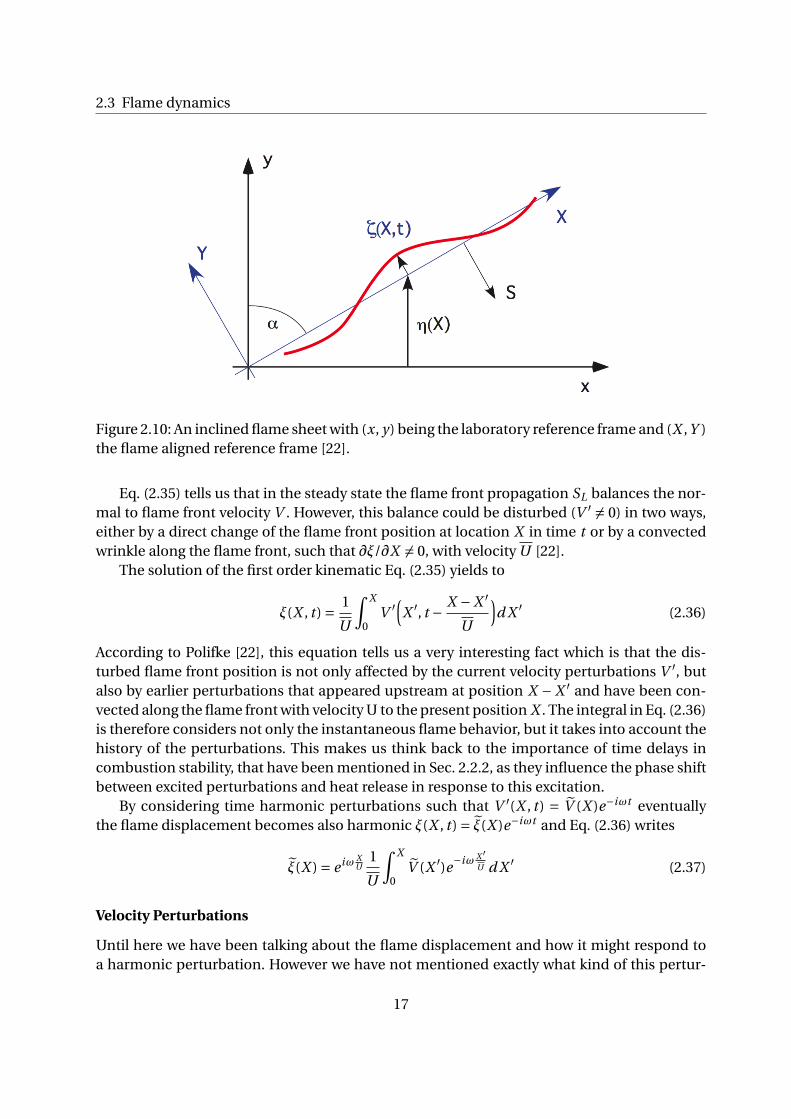
Figure 2.10: An inclined flame sheet with (x, y) being the laboratory reference frame and (X ,Y )the flame aligned reference frame [22].
Eq. (2.35) tells us that in the steady state the flame front propagation SL balances the nor-mal to flame front velocity V . However, this balance could be disturbed (V ′ 6= 0) in two ways,either by a direct change of the flame front position at location X in time t or by a convectedwrinkle along the flame front, such that ∂ξ/∂X 6= 0, with velocity U [22].
The solution of the first order kinematic Eq. (2.35) yields to
ξ(X , t ) = 1
U
∫ X
0V ′
(X ′, t − X −X ′
U
)d X ′ (2.36)
According to Polifke [22], this equation tells us a very interesting fact which is that the dis-turbed flame front position is not only affected by the current velocity perturbations V ′, butalso by earlier perturbations that appeared upstream at position X − X ′ and have been con-vected along the flame front with velocity U to the present position X . The integral in Eq. (2.36)is therefore considers not only the instantaneous flame behavior, but it takes into account thehistory of the perturbations. This makes us think back to the importance of time delays incombustion stability, that have been mentioned in Sec. 2.2.2, as they influence the phase shiftbetween excited perturbations and heat release in response to this excitation.
By considering time harmonic perturbations such that V ′(X , t ) = V (X )e−iωt eventuallythe flame displacement becomes also harmonic ξ(X , t ) = ξ(X )e−iωt and Eq. (2.36) writes
ξ(X ) = e iω XU
1
U
∫ X
0V (X ′)e−iω X ′
U d X ′ (2.37)
Velocity Perturbations
Until here we have been talking about the flame displacement and how it might respond toa harmonic perturbation. However we have not mentioned exactly what kind of this pertur-
17

Theoretical Background
bation could be. We here are going to discuss two approaches of modeling velocity modula-tions; Uniform velocity perturbation and axial convective wave. While the former deals withconfined combustion systems where the flame length L is much shorter than the wavelengthλ, the latter considers unconfined cases where the flame is long enough to observe the con-vected disturbances along the flame front.
In the modeling of uniform velocity perturbation the flame is considered compact and aharmonic and spatially homogeneous velocity modulation on the flame front is expressed by
u′ = 0, v ′ = v1e−iωt (2.38)
By substitution of Eq. (2.38) into the harmonic displacement ξ Eq. (2.37), after converting it tothe laboratory frame reference and variables, it yields
ξ(X )cosα
R= v1
v
1
iω∗
[e iω∗ x
R −1]
(2.39)
which appears to depend solely on the reduced frequency, ω∗ = (ωR)/SL cosα, with R beingthe flame extension along the x-axis [22]. This representation is a fairly good approximationof the flame displacement in the low frequency limit, i.e. as long as the wavelength λ is largerthan the characteristic scale R [27].
On the other hand, at relatively high frequencies the axial convective wave modeling ap-proach is more appropriate as it considers the upstream velocity modulations to be convectedin the axial direction and eventually also along the flame front. With the wave number k =ω/vthe velocity propagation in the y direction of the laboratory frame is given by
u′ = 0, v ′ = v1e i k y−iωt (2.40)
Again by substituting this into the harmonic displacement Eq. (2.37) in the laboratory coordi-nates it gives us
ξ(X )cosα
R= v1
v
1
iω∗1
1−cos2α
[e iω∗ x
R −e iω∗ xR cos2α
](2.41)
which makes the flame displacement now depend on a second parameter, which is the flameangle α, in addition to the reduced frequency ω∗, which has already been seen in the firstapproach as well.
It worth noting here that both expressions from the two models coincide as the flameangle α approaches π/2, or in the limit of cosα→ 0. The interpretation of this is that if theflame becomes normal to the flow direction, it acts as if it is subjected to a uniform velocityperturbation. In general, the flame displacement expression given by the second approach,Eq. (2.41), contains the expression from Eq. (2.39) and is expected to give more realistic re-sults at high as well as low frequencies. Both models are a good start point for an analyticalderivation of the Flame Transfer Function which will be discussed in chapter 3.
18

2.3 Flame dynamics
Figure 2.11: Wrinkling of flame front showing the hydrodynamics of streamlines and diffusivefluxes of heat and mass [26].
2.3.4 Instability in Premixed Combustion
Flame instability can appear in different forms and scales. Two main types of instability arereferred to as hydrodynamic instabilities and thermal-diffusive instabilities. The former typeis mainly a result of thermal expansion and is the dominant one in case of premixed flames.It is the major cause of sharp folds and creases that could be seen in the flame front and forthe wrinkles observed at the surface of expanding flames. On the other hand, diffusion flamesare more affected by the thermal-diffusive type on instability with thermal expansion playinga secondary role [18]. Since that this thesis is more concerned with premixed laminar flames,we are not going to talk in detail about the latter.
Darrieus(1938) had first discovered the hydrodynamic instability due to the thermal gasexpansion. With the flame being considered as a thin interface propagating towards the freshgas with a constant speed SL , he found that the heat release in a wrinkled premixed flamewill lead to gas expansion that will deviate flow lines across the front towards the normal tothe flame. Considering the incompressibility of the flame due to the low Mach number, theupstream lines are also deviated; Fig. 2.11. This would lead to flow divergence that wouldresult in velocity and pressure gradients and increases the flame wrinkling [28] [6].
Planar flames were predicted to be unconditionally unstable at all wavelengths later onby Landau(1994). Considering only the gas expansion, he approximated the wrinkling growth
19

Theoretical Background
rate to be [26]
σ= k ·SLE
E +1·(√
E 2 +E −1
E−1
)(2.42)
where k is the perturbation wave number and E is the gas expansion ratio between the freshand burnt gas sides, which is the same as the inverse of the temperature ratio
E = ρu
ρb= Tb
Ta. (2.43)
Clavin and Garcia [8] have derived a more complicated dispersion relation. The took intoaccount the influences of the flame front acceleration, the preferential diffusion as well as thetemperature dependent diffusion coefficients. Their dispersion relation for the amplitude ofsmall perturbations is governed by the second order equation:
(στt )2 A(k)+στt B(k)+C (k) = 0. (2.44)
Note that, for the sake of notation consistency with the rest of the text, Eq. (2.44) is taken notfrom the original work by Clavin and Garcia [8] but rather from the theoretical review done byTraffaut and Searby [28]. In this equation, the growth rate is represented in the real part of σwhile τt represents the flame transit time and is given by
τ= δ
SL
δ= Dth
SL
(2.45)
where δ and Dth are thermal diffusion zone thickness and the thermal diffusivity, respectively.The wave number dependent coefficients are mathematically defined as
A(k) = E +1
E+ E −1
Ekδ
(M a − J
E
E −1
)B(k) = 2kδ+2E(kδ)2(M a − J )
C (k) = E −1
E
kδ
F r− (E −1)(kδ)2
[1+ 1
EF r
(M a − J
E
E −1
)]+(E −1)(kδ)3[hb +
3E −1
E −1M a − E
E −12J + (2Pr −1)H
](2.46)
while the coefficients H and J account for the diffusivity dependence on the temperature andare represented in the integrals
H =∫ 1
0hb −h(θ)dθ
J = (E −1)∫ 1
0
h(θ)
1+ (E −1)θdθ
(2.47)
20
2.3 Flame dynamics
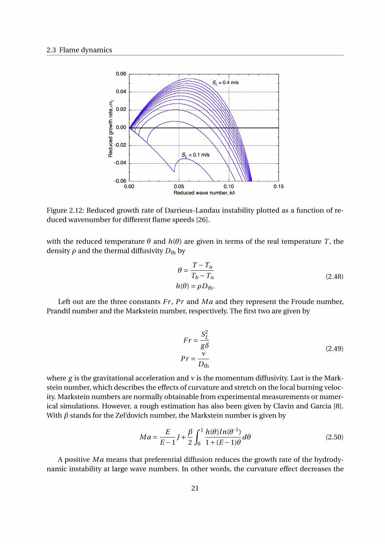
Figure 2.12: Reduced growth rate of Darrieus-Landau instability plotted as a function of re-duced wavenumber for different flame speeds [26].
with the reduced temperature θ and h(θ) are given in terms of the real temperature T , thedensity ρ and the thermal diffusivity Dth by
θ = T −Tu
Tb −Tu
h(θ) = ρDth.(2.48)
Left out are the three constants F r , Pr and M a and they represent the Froude number,Prandtl number and the Markstein number, respectively. The first two are given by
F r = S2L
gδ
Pr = ν
Dth
(2.49)
where g is the gravitational acceleration and ν is the momentum diffusivity. Last is the Mark-stein number, which describes the effects of curvature and stretch on the local burning veloc-ity. Markstein numbers are normally obtainable from experimental measurements or numer-ical simulations. However, a rough estimation has also been given by Clavin and Garcia [8].With β stands for the Zel’dovich number, the Markstein number is given by
M a = E
E −1J + β
2
∫ 1
0
h(θ)ln(θ-1)
1+ (E −1)θdθ (2.50)
A positive M a means that preferential diffusion reduces the growth rate of the hydrody-namic instability at large wave numbers. In other words, the curvature effect decreases the
21

Theoretical Background
burning velocity of a region that is convex towards the fresh gas side, thus the flame is thermo-diffusively stable [26]. This leads to a growth rate peak appearing at a wave number which isnot necessarily the highest one [28].
Growth rates are usually represented as a function of wave number in order to observe theDarrieus-Landau instability. In Fig. 2.12 the temporal growth rate is being represented as anon-dimensional quantity and plotted against the non-dimensional wave number; both aremultiplied by the flame transit time τt and the flame thickness δ respectively. As predicted byDarrieus and Landau, the growth rate increases linearly with small wave numbers. However, athigher wave numbers the thermal-diffusive effects counteracts the hydrodynamic ones caus-ing the growth rate to decrease again. Growth rate curves are shifted downwards due to theinfluence of gravity [26] which is more effective for flames with low burning velocities.
22
3 Literature review
3.1 System Response Analysis
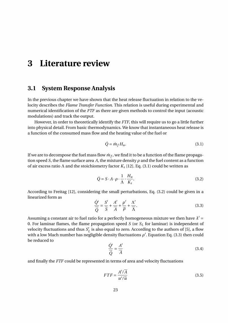
In the previous chapter we have shown that the heat release fluctuation in relation to the ve-locity describes the Flame Transfer Function. This relation is useful during experimental andnumerical identification of the FTF as there are given methods to control the input (acousticmodulations) and track the output.
However, in order to theoretically identify the FTF, this will require us to go a little furtherinto physical detail. From basic thermodynamics. We know that instantaneous heat release isa function of the consumed mass flow and the heating value of the fuel or
Q = m f Hu . (3.1)
If we are to decompose the fuel mass flow m f , we find it to be a function of the flame propaga-tion speed S, the flame surface area A, the mixture density ρ and the fuel content as a functionof air excess ratioΛ and the stoichiometry factor Ks [12]. Eq. (3.1) could be written as
Q = S · A ·ρ · 1
Λ· Hu
Ks. (3.2)
According to Freitag [12], considering the small perturbations, Eq. (3.2) could be given in alinearized form as
Q ′
Q= S′
S+ A′
A+ ρ′
ρ+ Λ
′
Λ. (3.3)
Assuming a constant air to fuel ratio for a perfectly homogeneous mixture we then have λ′ =0. For laminar flames, the flame propagation speed S (or SL for laminar) is independent ofvelocity fluctuations and thus S′
L is also equal to zero. According to the authors of [5], a flowwith a low Mach number has negligible density fluctuations ρ′. Equation Eq. (3.3) then couldbe reduced to
Q ′
Q= A′
A(3.4)
and finally the FTF could be represented in terms of area and velocity fluctuations
F T F = A′/A
u′/u(3.5)
23

Literature review
3.1.1 Proposed Analytical Models for the FTF
The fact that the variation in heat release is only controlled by that on the flame surface areais a good start for the theoretical analysis for the FTF. Schuller, Durox and Candel [27] forexample made use of the relation in Eq. (3.5) together with instantaneous flame front positiondescribed in Sec. 2.3.3 to come up with a unified FTF model for laminar flames.
Conical Flames
They considered for conical flames the flame surface area to be calculated by integrating theinstantaneous flame front position over the burner radius, the flame area fluctuations is thend A′ = 2π(R−x)dl . Since that the flame shape fluctuation results affects the flame surface area,the first order estimate of the area fluctuation in terms of the flame position ξ is given by
A′(t ) = 2π
tanα
∫ R
0(R −x)
∂ξ
∂xd x. (3.6)
We know by the Fourier transform that ξ(X , t ) = ξ(X )e−iωt and therefore the area too A′(t ) =A′e−iωt . We also know that the flame displacement at steady state is equal to zero, or ξ(0) = 0and therefore we get
A′ = 2π
tanα
∫ R
0ξd x. (3.7)
In Sec. 2.3.3 we have introduced two approaches for modeling velocity modulations. Samewere considered here for the determination of the FTF. Considering a uniform velocity per-turbation, substituting Eq.(2.39) into Eq.(3.7), for F T FUCO stands for a Uniformly perturbedConical Flame Transfer Function, they got for Eq.(3.5) the expression
F T FUCO(ω∗) = 2
ω2∗[1−e iω∗ + iω∗]. (3.8)
A similar analysis was made for axial convective wave model and a general expression forthe Convectively perturbed Conical Flame Transfer Function was found to be
F T FCCO(ω∗,α) = 2
ω2∗
1
1−cos2α
[1−e iω∗ + e iω∗ cos2α−1
cos2α
]. (3.9)
They came up then with three different expressions for three specific cases, they found that inthe limit of large cone angles, where the flame approaches being normal to the flow, they getthe same expression as the uniform velocity perturbation where it becomes only a function ofthe reduced frequency
limα→π/2
FCCO(ω∗,α) = FUCO(ω∗). (3.10)
As the angle decreases where the flame approaches being parallel to the flow the expression(3.9) becomes
limα→ 0
FCCO(ω∗,α) = 2
ω2∗
[(1− iω∗)e iω∗ −1
]. (3.11)
24

3.1 System Response Analysis
And in the case of long wavelength limit (kR) ¿ 1, where the case is considered compact incomparison with the perturbation wavelength the transfer function becomes
limω∗ → 0
FCCO(ω∗,α) = 1+ i (1+cos2α)1
3ω∗+O(ω2
∗). (3.12)
One of the weaknesses of the axial convective wave model is the violation of the continuityequation [2]. Cuquel, Durox and Schuller [2] have proposed another convective wave transferfunction model for the conical flame that actually satisfies the mass balance. We denote thepresent model as F T FCCOC which stands for Flame Transfer Function with Continuity satis-faction. This writes
F T FCCOC = 1
i (k∗−ω∗)·[
2(1−i
1
2k∗−1
2
k∗k∗−ω∗
)(e i k∗ −1
i k∗− e iω∗ −1
iω∗
)+
(e i k∗− e i k∗ −1
i k∗
)]. (3.13)
where k∗ and ω∗ are both dimensionless flow wavenumbers, while the latter is related toflame front deformations propagating at speed v0 cosα along the flame front. For a flamefront length L, flame height H and flame angleα, these numbers are given bu the expressions
k∗ = ω
v0H
ω∗ = ω
v0 cosαL
(3.14)
Results of the three models were compared and it was found that the gain of F T FCCOC
tends to be larger than the other models and is characterized by higher amplitude oscillations.However, its phase agrees with the model with uniform velocity modulation, F T FUCO , at lowfrequencies and features the correct asymptotic behavior at higher frequencies that has beenalready predicted by the convective model F T FCCO [2].
With regards to experimental validation in the low frequency range, F T FCCO appeared toover-predict the experimental data while F T FUCO does very well agree with it. The F T FCCOC
model however gives better results in that frequency range by satisfying the continuity.
25

Literature review
Figure 3.1: Gain and phase of the FTF the three models [2].Solid:F T FCCOC . Dashed-dotted:F T FUCO . Dashed:F T FCCO
3.2 Flame Front Instability
3.2.1 Experimental Determination of Flame Growth
Truffaut and Searby [28] have attempted to measure the growth rate of the instability on aninclined flame over a wide range of wavenumbers and flame speeds. They used a laminar slotburner for the sake of producing an inverted V premixed flame. The perturbation to the flamewas made via an electrostatic deflection system. To produce the laminar velocity profile atthe exit, they fed a propane-air-oxygen mixture at the burner bottom . The burner included adivergent section, a settling chamber, a convergent section and a nozzle. The incoming flowwas separated using glass beads that was inserted inside the divergent section. By means ofan aluminium honeycomb, followed by three metal grids of decreasing mesh size inside thesquare settling chamber, the flow turned into laminar. The flow was accelerated via the 2Dconvergent section and fluctuations were reduced to a negligible value of the mean flow. Fi-nally a 2D inverted V flame was provided at the exit. To avoid a strong thermal boundary layer,the convergent section and nozzle walls were water cooled at the fresh mixture temperature.
A thin tungsten rod was placed on one side of the flame in order to anchor it right at theexit see Fig. 3.2. An alternating high voltage is then applied to oscillate the tungsten rod andperturb the flame at the corresponding side. The resulting flame displacement produced sinu-soidal 2D wrinkling that has a parallel axis to the burner slot at the flame front. Furthermore,A precise control of the initial amplitude and the frequency of the wrinkle was possible via theapplied signal. The wrinkles were observed to be convected downstream by the gas flow andits amplitude was increasing exponentially. The laminar flame velocities (ranging from 0.43m/s to 0.27 m/s) were controlled via the equivalence ratios which ranged from 1.05 to 1.33 forthe propane-air flames. While for flames with 28% oxygen at equivalence ratios of 1.05 and
26

3.2 Flame Front Instability
Figure 3.2: Growth of Darrieus-Landua instability of a propane-air-oxygen flame [26].
1.33, the velocities were 0.69 m/s and 0.51 m/s. The gas flow velocities were 7.4 m/s, 6.05 m/sand 8.56 m/s.
Using a short exposure intensified camera, they were able to capture several snapshots ofthe wrinkled flame. They used then these images to obtain the amplitude and the wavelengthof the wrinkles as a function of the distance from the flame holder. After low pass filtering ofthe curve the maxima and minima were located, interpolated, and the peak to peak amplitudewas calculated as in Fig. 3.3.
In order to calculate the growth rate they considered the evolution of the peak to peak am-plitude of the flame front. They first ignored the initial points due to the electric field vibratedrod. They also ignored the downstream region where saturation starts to appear due to for-mation of cusps. To the rest of the points, where the exponential growth is observed (shownby the linear blue line on the semi-log plot in Fig. 3.4), they fitted an exponential function inorder to calculate a good estimate for the spatial growth rate σx . They converted the spatialgrowth rate into the temporal growth rate σ via multiplication by the convection velocity uc .
The non-dimensional growth rateστt was then plotted against the non-dimensional wavenumber kδ and compared to the theoretical dispersion relation described by Clavin and Gar-cia [8] in Eq. (2.44) where the gravitational acceleration set to zero. The Markstein numberwas tuned to the best fit of the measured results for each flame; Fig. 3.5
Observations and results
It has been observed by [28] that the wrinkles are propagating downstream with the a con-stant velocity equal the convected tangential component of the inflow velocity along the flamefront. Also the wrinkles amplitude was seen to grow exponentially up to the saturation pointwhere cusps start to form. They also found that the dimensional growth rate is typically be-tween 150s−1 and 300s−1. It can also be seen from Fig. 3.5 that the growth rate decreases againat very high wavenumbers, this is due to the combined effects of hydrodynamics and prefer-ential diffusion.
27

Literature review
Figure 3.3: Flame profile of wrinkling amplitude [26].
Figure 3.4: Semi-log profile of peak to peak wrinkling amplitude [26].
28

3.2 Flame Front Instability
Figure 3.5: Measured growth rate of Darrieus-Landau instability as a function of imposedwavenumber. Curves are calculated using the dispersion relation for the growth rate [26].
29

4 Numerical Setup
In this thesis OpenFOAM is used for CFD simulation and Paraview is used for visualizing theresults. Cases are constructed and submitted to the Leibniz-Rechenzentrum (LRZ) for paral-lel computation. Afterwards Matlab is used for post-processing purposes. In this case flamelaminar speed is very small such that the Mach number (SL/c) is much less than one. The flowis therefore considered incompressible. However the density can change due to temperaturevariation. The solver used here is the same one used by Jaensch et al. [23].
4.1 Case setup
4.1.1 Geometry
A common approach in CFD applications is, whenever possible, to reduce the case geome-try from a three-dimensional (3D) case into a two-dimensional (2D) one. This has the hugeadvantage of reducing the computational cost. The only cases where this approach is appli-cable and results in 2D simulations having the same results as 3D simulations is when thecase is actually symmetric. A very known example is the fluid flow in a straight pipe where thegeometry can be reduced to 2D due to the fact that the case is axis-symmetric.
In a similar way is our case, the one shown in Fig. 4.1. In this case we reduced the 3Dgeometry of a conical shaped flame into 2D, using the fact that the flame is axis-symmetricin the axial flow direction. It is for this reason that even the 3D preview in the figure lookslike a slit case. However, the geometry is created such that if it’s rotated around the lower axisin the flow direction, it will give us a cylindrical geometry. For this to be considered duringthe computations, a special boundary condition has to be applied, it is called a symmetricalboundary condition. It basically sets the values of the flow fields just adjacent to the solutiondomain as the values at the nearest cells inside the domain.
Fig. 4.2 shows us the flame profile of premixed lean mixture of air and natural gas afterreaching a steady state. This is the starting point of our numerical simulations. In this figure,the thin layer separating the fresh mixture (red) and the burnt gases (blue) is considered theflame front, where most of the physical and chemical properties changes take place. Since thatthe flame front is the most interesting zone for our analysis, it is necessary to avoid numericalerrors in this zone as much as possible.
30

4.1 Case setup
Figure 4.1: 3D surface view of the conical flame case.
Numerical accuracy in CFD is related to the flame resolution; the finer the mesh the moreaccurate the computations are as long as the mesh quality is maintained good (no skew faces,no high aspect rations between adjacent cells...etc.). Meanwhile, a too fine mesh implies that ahigher computational cost is required. This is due to more than a reason, one of which is thatwith a finer mesh we are necessarily increasing the number of cells, eventually the time re-quired for calculations per time step is also increased. Another reason is due to the limitationof the Courant number, which forces us to choose a small enough time step in order for thesolution to converge and produce accurate results. Since that a smaller time step means moreiterations are required per a certain period of simulation time, this is a determining factor inthe computational time required.
It is for all of the above mentioned reasons, the mesh resolution shown in Fig. 4.3 was agood compromise between a fine mesh at our zone of interest (the flame front and it’s ad-jacent layers) for fairly accurate calculations and a coarser mesh in the surroundings, wherethere is not a lot of physical and chemical changes happening, for reduced computationaltime.
31

Numerical Setup
Figure 4.2: Methane profile showing the flame front separating fresh and burnt gas sides.
Figure 4.3: Mesh being refined at the flame front.
4.1.2 Boundary conditions
Before discussing the fields boundary conditions let us first define the names given to themesh regions. Besides the axi s of symmetry, there are six more patches that describes themesh of our case, starting with the duct i nlet , where the mixture of air and methane comesfrom, at the west side of the geometry shown in Fig. 4.2. The radial duct wall, w allduct ,r ad ,is what prescribes the passage of the fresh gases before starting to diffuse in the chamber.The chamber wall boundaries consist of the one which is normal to the duct radial wall, inthis context we call it w allch , and the radial chamber wall, w allch,r ad , at the north side ofour geometry. We then have the outlet at the east side which allows the exit of the burntgases after the combustion process. Finally, the front and back sides of our geometry are thesymmetrical boundaries that allows the use of 2D simulation, we call them w alls ym .
32

4.1 Case setup
Boundary Ui nlet [ms−1] T [k] p [pa] Spi ci es
i nlet U (U ′A+1) fixedValue zeroGradient fixedValueoutlet zeroGradient zeroGradient fixedValue zeroGradientw allch fixedValue (0) T (T ′A+1) zeroGradient zeroGradient
w allch,r ad fixedValue (0) Heat flux zeroGradient zeroGradientw allduct ,r ad fixedValue (0) zeroGradient zeroGradient zeroGradient
w alls ym wedge wedge wedge wedgeaxi s empty empty empty empty
Table 4.1: Boundary types of physical properties.
Table 4.1 summarizes the boundary conditions applied to the physical fields. At the axi sno computations are supposed to be done and in theory there are no fields, the boundaryempt y is therefore applied to all the fields. The wed g e boundary condition is the one thatis used in OpenFOAM for axis-symmetric cases to define a symmetry wall, it is used in ourcase at the front and back symmetry walls for all of the fields. A f i xedGr adi ent bound-ary condition applies the Neumann condition, sets the derivative to a specific value. Whenthis value is zero, we can make use of the boundary condition zer oGr adi ent instead. Mean-while, the value-specified, Dirichlet, boundary condition is represented in OpenFOAM by thef i xedV alue. The g r oov yBC is a powerful tool that allows us to create a time varying bound-ary for a specific field; this is very useful in our case in order to be able to excite the steady statesimulation with different harmonics and/or impulses as will be explained later in this subsec-tion.
Because the velocity and pressure are usually coupled by the Navier-Stokes equations, itmight result in wrong calculations to set them both to defined values at the same location. Forthis reason, a common approach in CFD problems is whenever defining the value of either ata certain boundary to keep the other one floating, setting its derivative to zero is a fairly goodsolution. In our case, we set the velocity to zero at the walls considering the no-slip condition.Meanwhile the pressure gradient has been set to zero. It was again set to zero at the inlet wherethe velocity was defined using the g r oov yBC . At the outlet the p was set to the atmosphericpressure with the derivative of Ui nlet equal to zero.
The incoming fresh gas from the i nlet was considered to have a fixed temperature of300k (room temperature). The radial wall duct was assumed to be an adiabatic wall so that Tdoesn’t change and therefore zer oGr adi ent . Similarly at the outlet where burnt gases exitthe combustor while maintaining the same temperature. For flame base excitation purposesanother function was implemented for the temperature at the radial wall chamber.
Flame excitation
In this work, we decided to use two ways to excite the steady state flame. The first approachconsiders adding another velocity term to the inlet. The velocity function at the inlet then
33
Numerical Setup
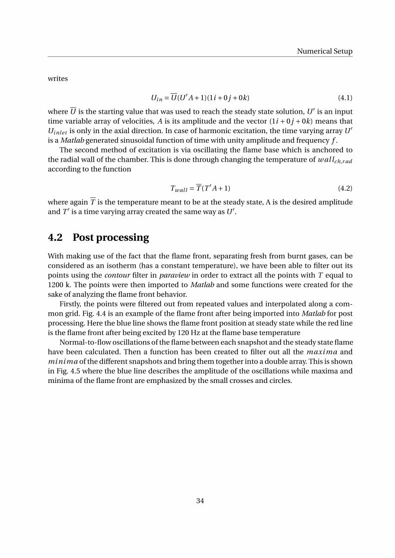
writes
Ui n =U (U ′A+1)(1i +0 j +0k) (4.1)
where U is the starting value that was used to reach the steady state solution, U ′ is an inputtime variable array of velocities, A is its amplitude and the vector (1i + 0 j + 0k) means thatUi nlet is only in the axial direction. In case of harmonic excitation, the time varying array U ′
is a Matlab generated sinusoidal function of time with unity amplitude and frequency f .The second method of excitation is via oscillating the flame base which is anchored to
the radial wall of the chamber. This is done through changing the temperature of w allch,r ad
according to the function
Tw all = T (T ′A+1) (4.2)
where again T is the temperature meant to be at the steady state, A is the desired amplitudeand T ′ is a time varying array created the same way as U ′.
4.2 Post processing
With making use of the fact that the flame front, separating fresh from burnt gases, can beconsidered as an isotherm (has a constant temperature), we have been able to filter out itspoints using the contour filter in paraview in order to extract all the points with T equal to1200 k. The points were then imported to Matlab and some functions were created for thesake of analyzing the flame front behavior.
Firstly, the points were filtered out from repeated values and interpolated along a com-mon grid. Fig. 4.4 is an example of the flame front after being imported into Matlab for postprocessing. Here the blue line shows the flame front position at steady state while the red lineis the flame front after being excited by 120 Hz at the flame base temperature
Normal-to-flow oscillations of the flame between each snapshot and the steady state flamehave been calculated. Then a function has been created to filter out all the maxi ma andmi ni ma of the different snapshots and bring them together into a double array. This is shownin Fig. 4.5 where the blue line describes the amplitude of the oscillations while maxima andminima of the flame front are emphasized by the small crosses and circles.
34

4.2 Post processing
Figure 4.4: Flame front instability excited at 120 Hz by temperature at the flame anchor.
Figure 4.5: Maxima and minima of the flame front excited at 120H z by temperature at theflame anchor.
35
5 Results
5.1 Velocity vs Temperature Excitation
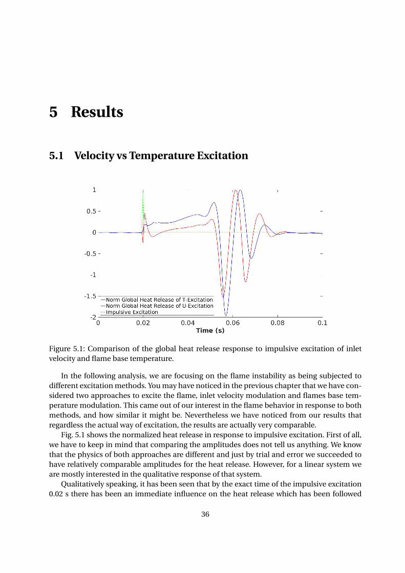
Figure 5.1: Comparison of the global heat release response to impulsive excitation of inletvelocity and flame base temperature.
In the following analysis, we are focusing on the flame instability as being subjected todifferent excitation methods. You may have noticed in the previous chapter that we have con-sidered two approaches to excite the flame, inlet velocity modulation and flames base tem-perature modulation. This came out of our interest in the flame behavior in response to bothmethods, and how similar it might be. Nevertheless we have noticed from our results thatregardless the actual way of excitation, the results are actually very comparable.
Fig. 5.1 shows the normalized heat release in response to impulsive excitation. First of all,we have to keep in mind that comparing the amplitudes does not tell us anything. We knowthat the physics of both approaches are different and just by trial and error we succeeded tohave relatively comparable amplitudes for the heat release. However, for a linear system weare mostly interested in the qualitative response of that system.
Qualitatively speaking, it has been seen that by the exact time of the impulsive excitation0.02 s there has been an immediate influence on the heat release which has been followed
36

5.2 Response analysis
by gradual increase. At 0.05 s the major effect of the impulse started to appear in the heatrelease as three consequent overshoots with the highest one in amplitude being the middleone happening shortly after 0.06 s.
Further analysis including a comparison between both excitation ways, but in terms of theflame front behavior is included is sections 5.4.2 and 5.5 .
5.2 Response analysis
Figure 5.2: Broadband input and output signals. Input and output signals are represented invelocity modulation (blue) and the resulting global heat oscillation (green).
As mentioned before, the FTF relates the velocity perturbations to heat release perturba-tions. However, determining the FTF using several different harmonic signals is very unprac-tical, since the simulation must be run for each forcing frequency. One alternative method isby using multi-tone signals to excite the flame [9]. This enables us to modulate the flame overa wide range of frequencies and obtain its FTF just at once. In this thesis a Matlab tool is usedto obtain a broadband signal which has been used as an input signal for the velocity excitation(U ′ in Eq.(4.1)). The inlet (velocity) and the output (heat release) signals are shown in Fig. 5.2.
37

Results
Transfer function
Figure 5.3: Gain and phase of FTF
Fig. 5.3 shows results for the gain (upper) and phase lag (lower) of the FTF. A gain of unityis obtained at very low frequencies. It then decreases and reaches a minimum of around 0.2at about 30 Hz. The gain increases again to reach values higher than unity for frequenciesmore than 60 Hz to reach a peak value of 1.7 at about 80 Hz. A small bump could be notedat about 50 Hz though. The flame then starts to act as a low frequency filter in response tohigher frequencies, causing the gain to progressively decrease. It reaches again lower thanunity at 110 Hz and the cutoff frequency (where the gain falls below 0.5) is 125 Hz.
The FTF phase lag starts from zero and decreases constantly with higher frequencies. Aninflection point could be seen at the frequency where the gain reached the minimum magni-tude (30 Hz). The gradient then becomes constant after 30 Hz and up to higher frequencies. Aqualitatively similar response has been found experimentally as well as numerically by Blan-
38
5.3 Flame Front Growth Rates
chard et el [17] when they tested an M-shaped laminar premixed methane-air flame.
5.3 Flame Front Growth Rates
In this section we are trying to analyze the instability of the flame front when it is being sub-jected to different methods of excitation. We are mainly interested to observe the effect of theDarrieus-Landau instability in order to find a the relation with the flames stability analysis.
5.3.1 Harmonic Excitation
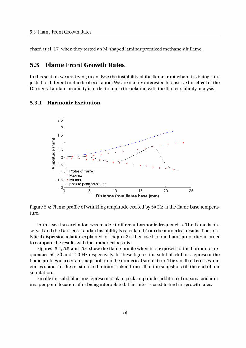
Figure 5.4: Flame profile of wrinkling amplitude excited by 50 Hz at the flame base tempera-ture.
In this section excitation was made at different harmonic frequencies. The flame is ob-served and the Darrieus-Landau instability is calculated from the numerical results. The ana-lytical dispersion relation explained in Chapter 2 is then used for our flame properties in orderto compare the results with the numerical results.
Figures 5.4, 5.5 and 5.6 show the flame profile when it is exposed to the harmonic fre-quencies 50, 80 and 120 Hz respectively. In these figures the solid black lines represent theflame profiles at a certain snapshot from the numerical simulation. The small red crosses andcircles stand for the maxima and minima taken from all of the snapshots till the end of oursimulation.
Finally the solid blue line represent peak to peak amplitude, addition of maxima and min-ima per point location after being interpolated. The latter is used to find the growth rates.
39
Results
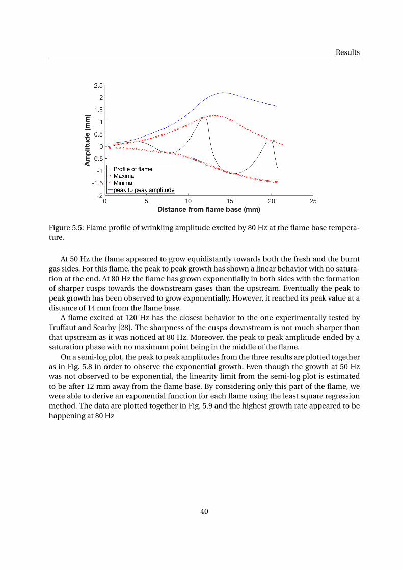
Figure 5.5: Flame profile of wrinkling amplitude excited by 80 Hz at the flame base tempera-ture.
At 50 Hz the flame appeared to grow equidistantly towards both the fresh and the burntgas sides. For this flame, the peak to peak growth has shown a linear behavior with no satura-tion at the end. At 80 Hz the flame has grown exponentially in both sides with the formationof sharper cusps towards the downstream gases than the upstream. Eventually the peak topeak growth has been observed to grow exponentially. However, it reached its peak value at adistance of 14 mm from the flame base.
A flame excited at 120 Hz has the closest behavior to the one experimentally tested byTruffaut and Searby [28]. The sharpness of the cusps downstream is not much sharper thanthat upstream as it was noticed at 80 Hz. Moreover, the peak to peak amplitude ended by asaturation phase with no maximum point being in the middle of the flame.
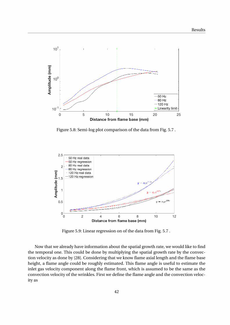
On a semi-log plot, the peak to peak amplitudes from the three results are plotted togetheras in Fig. 5.8 in order to observe the exponential growth. Even though the growth at 50 Hzwas not observed to be exponential, the linearity limit from the semi-log plot is estimatedto be after 12 mm away from the flame base. By considering only this part of the flame, wewere able to derive an exponential function for each flame using the least square regressionmethod. The data are plotted together in Fig. 5.9 and the highest growth rate appeared to behappening at 80 Hz
40

5.3 Flame Front Growth Rates
Figure 5.6: Flame profile of wrinkling amplitude excited by 120 Hz at the flame base tempera-ture.
Figure 5.7: Comparison of peak to peak spatial flame growth between 50, 80 & 120 Hz.
41
Results
Figure 5.8: Semi-log plot comparison of the data from Fig. 5.7 .
Figure 5.9: Linear regression on of the data from Fig. 5.7 .
Now that we already have information about the spatial growth rate, we would like to findthe temporal one. This could be done by multiplying the spatial growth rate by the convec-tion velocity as done by [28]. Considering that we know flame axial length and the flame baseheight, a flame angle could be roughly estimated. This flame angle is useful to estimate theinlet gas velocity component along the flame front, which is assumed to be the same as theconvection velocity of the wrinkles. First we define the flame angle and the convection veloc-ity as
42

5.3 Flame Front Growth Rates
α= tan−1 H f
L f(5.1)
uc = uinlet cosα (5.2)
where H f and L f are the flame’s thickness and axial length, respectively. We then calculate thecorresponding temporal growth rate as
σt =σxuc (5.3)
whereasσx is the spatial growth rate given by the exponent coefficients of the functions shownin Fig. 5.9. Table 5.1 summarizes the spatial and temporal growth rates of different harmonics.
σx [mm−1] σt [ms−1]
30 Hz 0.122 0.10550 Hz 0.182 0.15780 Hz 0.242 0.208
120 Hz 0.236 0.203300 Hz -0.300 -0.258
Table 5.1: Spatial and temporal growth rates for different harmonics.
From the Table 5.1 we noticed that the maximum growth rate appeared to happen ataround 80 Hz. We have expected this due to the high instability that was seen in Fig. 5.4.
Comparison to theoretical methods
In order to fairly compare the flame response to the excited frequency, it was necessary toconsider the effect of the flame thickness. The plot in Fig. 5.10 is therefore a plot of the reducedgrowth rate στ against the reduced wave number kδ where the parameters σ, τ and δ areexplained in chapter 2 and the wave number k is given by
k = 2π f
uc(5.4)
A derivation from the Landau model (2.42) that includes the curvature effect and thereforeconsiders the effect of the Markstein number in the flame growth was found in [7]. It writes:
σ= k ·SLE
E +1·(−M ak −1±
√(M ak −E)2 − (1+1/E)(E −1)2
)(5.5)
43

Results
Figure 5.10: Flame profile disturbed with two wrinkles after temperature excitation.
The black solid line in Fig. 5.10 shows the prediction of the Darrieus–Landau instabilityaccording to this model. Note that Markstein number M a was tuned to the best fit of theC F D prediction (red crosses). The effect of a +5% and −5% of this tuned M a is representedby the dashed lines below and above the solid line respectively. Moreover, the simple linearmodel by Landau is represented by the magenta solid line.
The dispersion relation that was given by Clavin and Garcia [8] and represented by Eq.(2.44) predicted the behavior of the blue dashed line using for the same M a (The method ofhow the flame parameters are calculated are given below). However using the same M a andfollowing the set of equations described in chapter 2, specially the integrals H and J describedby Eq. (2.47) or alternatively Eq. (5.8), we were not satisfied with the prediction of this model.We therefore decided to use the parameters given by the closest case we found in the paperby Searby [26] and fit a new M a to it, this is represented by the blue solid line. For this case,J = 3.87 and H = 1.067.
Calculation of the flame parameters
We know from our boundary conditions and the results of the simulation that the fresh gastemperature Tu is 300 k and the burnt gas temperature Tb is 2100 k. The flame thickness andtransit time are calculated using Eq. (2.45) with the flame speed SL calculated according to[16].
SL = AφB e−C (φ−D)2(5.6)
whereφ is the equivalence ratio while A,B ,C and D are constants that depend on the mixturecomposition, not to be confused with the constants defined for the dispersion relation (2.44).
44

5.3 Flame Front Growth Rates
The thermal diffusivity D th is calculated according to Chapman-Enskog equation [1]
D th = 0.00266T 3/2
M 1/2AB σ
2ABΩD
(5.7)
with MAB being the molar mass of the composition,σAB andΩAB are temperature dependentcoefficients. With the expansion ratio E given according to Eq. (2.43) and θ and h(θ) accordingto Eq. (2.48), the integrals H and J in Eq. (2.47) could be reevaluated in terms of temperatureT as
H =∫ Tb
Tu
(hb −h(θ)
) · 1
Tb −TudT
J = (E −1)∫ Tb
Tu
h(θ)
1+ (E −1)θ· 1
Tb −TudT
(5.8)
The numerical values of the flame parameters are represented in Table 5.2 in SI −uni t s
Flame parameter Value
ui nlet 0.9015α 0.3φ 0.8
Tu 300Tb 2100SL 0.2782
D th 2.2481×10⁻⁵
E 7ρu 1.12δ 8.0812×10⁻⁵
τt 2.9049×10⁻⁴
hb 9.6880×10⁻⁵
H 3.91×10⁻⁴
J -1.99×10⁻⁴
Table 5.2: Spatial and temporal growth rates for different harmonics.
5.3.2 Impulsive Excitation
In order to get a better understanding of the flame dynamics, it was important to separate theeffects of subsequent harmonic pulses and start to analyze the flame response as it is beingsubjected to one impulse. This impulse response test was run for the conical flame case withRe = 1240 and confinement ratio of 0.44.
45

Results
Figure 5.11: Flame profile disturbed with two wrinkles after temperature excitation.
In this context, two different methods of excitations are proposed: first method by excitingthe velocity inlet by an amplitude of 3% of the mean inlet velocity. The second one howeverconsiders exciting the temperature at the flame base by an amplitude of 30% of the meantemperature at the flame base. The magnitudes of the different excitations have been chosensuch that both approaches would have a quasi-similar amplitude of growth.
The flame front appearing in Fig. 5.11 was taken at 0.046 s. However, by considering all ofthe saved snapshots from start till the end of simulation, we could see how the flame actuallygrows in time as seen in Fig. 5.12. Considering that this is an impulse response test, we wouldhave expected to see one wrinkle along the flame front that propagates until the flame tip.However, if you have a look at Fig. 5.11, you may notice the flame front (the black solid line)has two wrinkles, this is a surprising observation for us. A Matlab function is created to sep-arate the two wrinkles of the flame front in order to observe the pattern of each, we call thefirst one primary wrinkle while we refer to the second one as a secondary wrinkle.
Fig. 5.11 shows us that when the flame is excited by the temperature impulse at its base, thefirst wrinkle had the tendency to grow faster towards the fresh gas side than the burnt side. Onthe contrary to the secondary wrinkle which grows more towards the burnt gas side. The peakto peak amplitudes, represented in the solid lines, are again calculated here for each wrinkleseparately in order to estimate the Darreius-Landau instability. Using the linear regression toderive an exponential model for both wrinkles, the spatial growth rate is calculated. Equations(5.1) - (5.3) are then used to calculate the temporal growth rate. The results are shown in table5.3.
46

5.4 Flame Tip Response
Figure 5.12: Flame front disturbance from time 0 s to 0.1 s after temperature excitation.
σx [mm−1] σt [ms−1]
Primary 0.174 0.149Secondary 0.189 0.163
Table 5.3: Spatial and temporal growth rates of IR.
From table 5.3 it could be seen that the growth rates of both primary and secondary wrin-kles resulting from the impulsive excitation are very comparable to that of the harmonic ex-citation represented by the data in table 5.1. In fact they are both shown to be higher thanimposing at 30 Hz. It could be then deduced that imposing at low frequencies could also havesome sort of damping effects.
5.4 Flame Tip Response
5.4.1 Harmonic Excitation
Fig. 5.13 shows what is happening to the flame tip at harmonic frequencies. As the excitationstarts to reach the flame tip, it begins to react linearly to the imposed frequency. The distur-bances shown in the figure shows that the flame tip oscillates at 50, 80 & 120 Hz respective tothe excitation frequency applied at the flame base temperature of each.
47

Results
Figure 5.13: Flame tip response excited by 50, 80 & 120 Hz at the flame base temperature.
Moreover, we have noticed that the flame is shortened by introducing higher frequencydisturbances. If the flame tip position at steady state is at 0 mm, after imposing the frequen-cies 80 & 120 Hz the flame tip started to oscillate around -2 mm; i.e. the flame tip is advancedby 2 mm towards the base.
An oscillation or change in the flame tip position implies an oscillation or a change in theflame area. We have already learned that a fluctuation in the flame area could be translated toheat release fluctuation. It could be then deduced that the phenomenon of the flame short-ening might have a direct effect on the heat release.
Fig. 5.14 shows that the phenomenon of shortening the flame is just temporary and ex-clusively depending on the harmonic frequency applied. We can see that after removing theexcitation of 120 Hz, the flame tip gets back to its normal position as the case in the steadystate.
48

5.4 Flame Tip Response
Figure 5.14: Flame tip response after the removal of excitation of 120 Hz.
5.4.2 Impulsive Excitation
Fig. 5.15 shows the response of the flame tip after being exposed to excitation at 0.02s. We cansee that in both excitation methods, it took the flame tip 0.03s to start to respond to the exci-tation. If we divide the inlet velocity component in the flame front direction by the flame frontlength, we also get the same time. This confirms the theory that the wrinkles are propagatingwith the convection velocity.
As mentioned in the above subsection, second observation we have seen here is that, eventhough it is just one impulse given at the flame base, unexpectedly we could see that thereis always a secondary oscillation happening at the flame tip. Surprisingly, with temperatureexcitation this secondary effect is greater in amplitude than the primary one.
If we consider the time shift between the two peaks, we find it to be around 0.012 s whichcorresponds to a frequency of 83.3 Hz. If you recall from the harmonic frequency test, 80 Hzfor this flame was the frequency with the highest growth rate. It is also the frequency with anamplified gain (higher the unity) in our FTF. This made us reckon that the secondary wrinkleand the growth rate peak at 80 Hz, which presumably lead to the amplified FTF gain, mightbe somehow correlated.
49

Results
Figure 5.15: Flame tip impulse response.
5.5 Simulation vs Axial Convective Model
In section 2.3.3 we have introduced two models for the prediction of the flame front behav-ior based on two approaches for velocity modulation. In this section we chose to comparethe axial convective velocity model to our simulation in terms of flame growth. A Matlab tooldeveloped by in the "Professur für Thermofluiddyanmik" that solves Eq.(2.41) based on finitedifferences method was used to model velocity perturbations of an inclined flame with angle0.28r ad , flame length L = 36 mm and Reynold’s number Re = 1300. The inlet velocity wasmodulated using the two harmonic frequencies 80 Hz and 120 Hz. The same post processingmethod is applied to the resulting simulations and the following observations were obtained.
Fig. 5.16 and Fig. 5.17 show the flame front behavior for the above mentioned two har-monic frequencies. In these figures, the blue line represents the steady state position of theflame while the red one is the perturbed flame front. The first observation we noticed here isregarding the flame tip. It has been seen that its oscillation is always around the steady stateposition. In that sense, the model expects that the flame length stays the same and not short-ened as we have seen for the respective frequencies in the OpenFOAM simulation, Fig. 5.13.
50

5.5 Simulation vs Axial Convective Model
Figure 5.16: Axial convective model flame front behavior at 80 Hz.
Figure 5.17: Axial convective model flame front behavior at 120 Hz.
51

Results
Figure 5.18: Axial convective model vs OF with 80 Hz U-Excitation.
Figure 5.19: Axial convective model vs OF with 120 Hz U-Excitation.
52
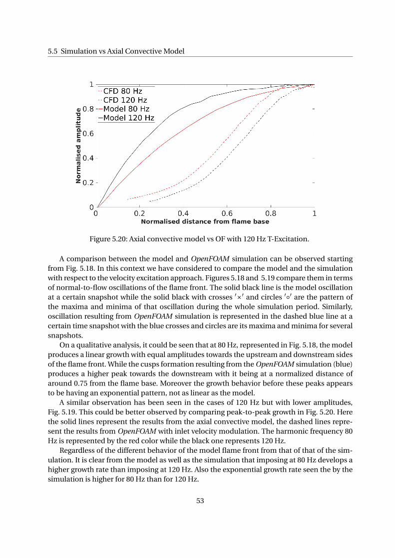
5.5 Simulation vs Axial Convective Model
Figure 5.20: Axial convective model vs OF with 120 Hz T-Excitation.
A comparison between the model and OpenFOAM simulation can be observed startingfrom Fig. 5.18. In this context we have considered to compare the model and the simulationwith respect to the velocity excitation approach. Figures 5.18 and 5.19 compare them in termsof normal-to-flow oscillations of the flame front. The solid black line is the model oscillationat a certain snapshot while the solid black with crosses ′×′ and circles ′′ are the pattern ofthe maxima and minima of that oscillation during the whole simulation period. Similarly,oscillation resulting from OpenFOAM simulation is represented in the dashed blue line at acertain time snapshot with the blue crosses and circles are its maxima and minima for severalsnapshots.
On a qualitative analysis, it could be seen that at 80 Hz, represented in Fig. 5.18, the modelproduces a linear growth with equal amplitudes towards the upstream and downstream sidesof the flame front. While the cusps formation resulting from the OpenFOAM simulation (blue)produces a higher peak towards the downstream with it being at a normalized distance ofaround 0.75 from the flame base. Moreover the growth behavior before these peaks appearsto be having an exponential pattern, not as linear as the model.
A similar observation has been seen in the cases of 120 Hz but with lower amplitudes,Fig. 5.19. This could be better observed by comparing peak-to-peak growth in Fig. 5.20. Herethe solid lines represent the results from the axial convective model, the dashed lines repre-sent the results from OpenFOAM with inlet velocity modulation. The harmonic frequency 80Hz is represented by the red color while the black one represents 120 Hz.
Regardless of the different behavior of the model flame front from that of that of the sim-ulation. It is clear from the model as well as the simulation that imposing at 80 Hz develops ahigher growth rate than imposing at 120 Hz. Also the exponential growth rate seen the by thesimulation is higher for 80 Hz than for 120 Hz.
53

6 Summary and Outlook
One of the most problematic issues of lean combustion systems is the occurrence of combus-tion instability, which is related to coupling between pressure and thermal fluctuations dueto unsteady heat release. This kind of instability is a critical issue; as it sometimes leads todamage in the mechanical components of the system. For this reason, it becomes importantto be able to predict the thermo-acoustic behavior of the system [3]. In this context, some re-searchers focus their efforts on the determination of the Flame Transfer Function by dealingwith the combustion chamber as a black box that is exposed to acoustic perturbations as aninput and produces thermal fluctuations as an output. In parallel, some other researchers aremore interested in the direct effect of these perturbations on the flame behavior and how itbecomes unstable. In this thesis, we have divided our efforts in both directions in order to tryto find a link between them.
Summary
We started by introducing the thermo-acoustic system as a network of small elements thatone of which is the flame. We then defined the FTF and we introduced the effect of the timedelay between the input and output perturbations in such a way that one would expect howthe gain and phase would look like. In the second part of chapter 2 we have introduced somebasic theories regarding the dynamics of laminar premixed flames until we defined the kine-matic relation (2.21). From this point we were able to derive the field equation describing theflame position (2.26). This equation gave us a starting point to introduce a general model thatdescribes an inclined flame front displacement in 2D (2.37), which made us able to predict theeffect of velocity perturbations by introducing the two models for uniform velocity perturba-tions and axial convective wave. In the final section of this chapter, we introduced the flameinstability and we focused on the hydrodynamic effects. We introduced the Landau modelthat considers only the hydrodynamic effects, Eq (2.42), then another dispersion relation thatadditionally takes into account the thermal-diffusive effects, Eq.(2.44).
In chapter 3 we started by deriving an alternative definition for the FTF that relates veloc-ity fluctuations to area fluctuations instead of heat release, Eq. (3.5). From this equation wewere able to represent an analytical FTF based on the flame displacement model approachesexplained in the previous chapter. Furthermore, we introduced the transfer function whichsatisfies the mass balance, Eq. (3.13). In section 3.2 we reviewed the work of Searby [28] thatincluded the experimental determination of the Darrieus-Landau instability of V-Flames. Ithas been seen that the wrinkles amplitude grows exponentially until the point of saturation.
The numerical setup of our case was introduced in chapter 4. OpenFOAM was used for ourCFD simulation of a lean premixed conical flame. A homogeneous mixture of air and methane
54

at room temperature is used in the inlet boundary condition. Due to the low speed that re-sulted in a low Mach number, we have considered an incompressible flow; nevertheless thedensity could still change due to temperature. The geometry of the combustion chamber hasa confinement ratio of 0.44. It was reduced to a 2D mesh for less computational cost and themesh was refined around the flame front for better computational accuracy. The average inletvelocity is 0.9015 m/s that has a Reynold’s number Re = 1240. No slip boundary condition wasapplied to the walls, which were all considered adiabatic except for the chamber radial wallthat allowed a heat transfer. Via a boundary condition named g r oov yBC two functions wereimplemented that allowed to perturb the flame front. Flame contour data were extracted aftersimulations and post processing was performed in Matlab. This included creating functionsto determine the normal-to-flow oscillation of the flame front, extracting its maxima and min-ima, finding the peak-to-peak amplitude and using least square regression to find the growthrates.
Finally the results were included in chapter 5. We started by comparing the heat releaseperturbations in response to the impulsive excitation of velocity inlet and temperature base.It was shown that both have a qualitatively quasi-similar behavior. The gain and phase ofthe FTF resulting from a broadband signal were discussed and it was found that the gain hasan amplified magnitude of higher than unity at around 80 Hz. The flame front behavior wastested for different harmonic frequencies up to the cutoff frequency (120 Hz) and it was foundthat when excitation at 80 Hz produced the highest instability (maximum growth rate) of theflame front. Moreover, an impulsive excitation test was made and a secondary wrinkle ap-peared to be lagging the primary wrinkle with a time delay that corresponds to 83 Hz. Weconcluded therefore that out of this phenomenon a superposition happened at 80 Hz thatlead to the gain amplification of the FTF.
Further observations were made for the flame tip response. The flame was found to beshortened when excited at higher frequencies. Also from the impulsive excitation test, thetime it took the flame tip to respond to the excitation matched the time calculated by dividingthe flame length by the convected velocity along the flame front; which confirmed the the-ory that wrinkles are convected via the mean inlet velocity component along the flame front.Results from the simulation were compared to results from the axial convective model whichhad been discussed in chapter 2. It was concluded that while the simulation expects an ex-ponential growth, the model produced a different pattern by predicting a linear growth of thewrinkling amplitude.
Outlook
Some other observations were noted. However, due to the lack of time that lead to insufficientamount of results, it was not possible to come up with conclusions for them. From the resultsof two simulations of a similar case but with a slit flame instead of conical one, it was foundthat the flame tip oscillates at an amplitude which is double the value of that for the conicalflame case, which indicates the higher instability of slit flames. Same work could be repeatedfor a slit case in order to determine the Darrieus-Landau instability of slit flames. On the otherhand, it was observed that with a confined flame exit, both cases get the same amplitude for
55
Summary and Outlook
the flame tip oscillations. Therefore, another test could be made regarding the effect of theconfinement ratio on the Darrieus-Landau instability.
We know that the area fluctuation is related to heat release fluctuation. Moreover, it wasobserved that the flame tip fluctuation has a similar pattern to the area fluctuation, whichcould be related as well to the heat release fluctuation. If one succeeded to develop an equa-tion of motion that describes the flame tip displacement, converting it in the frequency do-main could be a good start to develop another analytical FTF from a new perspective.
56

57

Bibliography
[1] https://chrisbharding.wordpress.com/tag/chapman-and-enskog/.
[2] D. Durox A. Cuquel and T. Schuller. Theoretical and experimental determination of theflame transfer function of confined premixed conical flames. Italian section of the com-bustion institute, 2011.
[3] Antonio Andreini Alessandro Innocenti and Bruno Facchini. Numerical identificationof a premixed flame transfer function and stability analysis of a lean burn combustor.Energy Procedia, 2015.
[4] Louis Boyer and J. Quinard. On the dynamics of anchored flames. Combustion andFlame, 82:51–65, 1990.
[5] Felix Guethe Francois Meili Peter Flohr Bruno Schuermans, Valter Bellucci and Chris-tian Oliver Paschereit. A detailed analysis of thermoacoustic interaction mechanisms ina turbulent premixed flame. Proceedings of ASME Turbo Expo, 2004.
[6] C. Clanet and G. Searby. First experimental study of the darrieus-landau instability.PHYSICAL REVIEW LETTERS, 80(17):3867–3870, November 1998.
[7] Dr. Andreas Class. Strömungen mit chemischen Reaktionen. Karlsruher Intstitut für Tech-nologie.
[8] Paul Clavin and P. L. Garcia-Ybarra. The influence of the temperature dependence ofdiffusivities on the dynamics of flame fronts. Journal de Physique Théorique et Appliquée,2(2):245–263, 1983.
[9] Alexis Cuquel. Dynamics and nonlinear thermo-acoustic stability analysis of premixedconical flames. PhD thesis, Ecole Centrale Paris, 2013.
[10] T. D. Eastop and A.McConkey. Applied Thermodynamics. Longman, 1993.
[11] Tarek Echekki and M. G. Mungal. Flame speed measurements at the tip of a slot burner:Effects of flame curvature and hydrodynamic stretch. Twnety Third Symposium on Com-bustion / The combustion Institute, pages 455–461, 1990.
58

BIBLIOGRAPHY
[12] Erwald Freitag. On the Measurement and Modelling of Flame Transfer Functions at Ele-vated Pressure. PhD thesis, Technische Universität München, Lehrstuhl für Thermody-namik, Garching bei München, Germany, December 2008.
[13] Jean-Pierre Hathout. Thermoacoustic instability. In Fundamentals and Modeling inCombustion, 1999.
[14] Bhupendra Khandelwal. Development of Gas Turbines Combustor Preliminary DesignMethodologies and Preliminary Assessments of Advanced Low Emission Combustor Con-cepts. PhD thesis, Cranfeld University, School of Engineering, July 2012.
[15] Philip Kiameh. Power Generation Handbook. McGraw-Hill, 2002.
[16] T. Lieuwen. Modeling premixed combustion-acoustic wave interactions: A review. JOUR-NAL OF PROPULSION AND POWER, 19, 2003.
[17] D. Sipp M. Blanchard, T. Schuller and P. J. Schmid. Response analysis of a laminarpremixed m-flame to flow perturbations using a linearized compressible navier-stokessolver. Physics of Fluids, 27, 2015.
[18] Moshe Matalon. Intrinsic flame instabilities in premixed and nonpremixed combustion.Annual Review of Fluid Mechanics, 39:163–191, 2007.
[19] L. P.M. De Goey J.H.M. ten Thije Boonkkamp R.M.M. Mattheij M.L. Bondar,K.R.A.M. Schreel. Flame dynamics using the level set equation.
[20] Norbert Peters. Combustion theory. CEFRC Summer School, Pricenton, 2010.
[21] Prof. Dr.-Ing. Heinz Pitsch. Laminar premixed flames: Kinematics and burning velocity.Lecture 4, CEFRC Combustion Summer School, 2014.
[22] Wolfgang Polifke. Combustion instabilities. Lehrstuhl für Thermodynamik, TechnischeUniversität München, Germany, 2004.
[23] E. A Gopalakrishnan S. Bomberg R. I. Sujith W. Polifke S. Jaensch, M. Merk. Hybridcfd/low-order modeling of nonlinear thermoacoustic oscillations. Combustion Sympo-sium number 36, 2016.
[24] T. Sattelmayer and W. Polifke. A novel method for the computation of the linear stabilityof combustors. Combustion Science and Technology, 2003.
[25] Bruno Schuermans. Modeling and Control of Thermoacoustic Instabilities. PhD thesis,École Polytechnique Fédérale de Lausanne, 2003.
[26] Geoff Searby. Experimental studies of instabilities of laminar premixed flames. Technicalreport, Institut de Recherche sur les Phénomènes Hors Équilibre, CNRS / Université deProvence, 49 rue Frédéric Joliot-Curie, 13384 MARSEILLES Cedex 13, France, 2004.
59

BIBLIOGRAPHY
[27] D. Durox T. Schuller and S. Candel. A unified model for the prediction of laminar flametransfer functions: comparisons between conical and v-flame dynamics. Combustionand Flame, 134:21–34, 2003.
[28] JEAN-MARIE TRUFFAUT and GEOFF SEARBY. Experimental study of the darrieus-landau instability on an inverted-‘v’ flame, and measurement of the markstein number.Combustion Science and Technology, 149(1-6):35–52, 1999.
60