POLITECNICO DI MILANOSCHOOL OF INDUSTRIAL AND INFORMATION ENGINEERING

MASTER OF SCIENCE IN ELECTRICAL ENGINEERING

Academic Year 2015-2016

Analysis of Grid Codes and Parameters identification for Load Frequency Control

Master’s thesis byAhmed Mohamed813412

Supervisors:Prof. Alberto Berizzi Politecnico di MilanoEng. Simone Pasquini CESI MilanoEng. Stefano Mandelli CESI MilanoEng. Emiliano Soda CESI Milano

Acknowledgements

First of all, I would like to thank the Technical University of Milan “Politecnico di Milano” for giving me the opportunity to proceed with my studies and earn my Master of Science in Electrical Engineering in one of the highly ranked universities all over the world.

Moreover, I would like to express my gratitude to my advisor, Professor Alberto Berizzi, for supporting me during the past three years, not only during my master’s thesis, but also during my Electric Power Systems university course.

I would like to extend my appreciation to Eng. Massimo Pozzi for giving me the chance to do my master’s thesis as an internship at Centro Elettrotecnico Sperimentale Italiano “CESI Milano” and introducing me to my co-tutors in CESI to help me in executing my work.

In addition, my sincere thanks goes to my co-tutor, Eng. Simone Pasquini, for his immediate help and guidance throughout the thesis, and advices in many stressful situations.

A supportive environment is important to accomplish the mission. I was lucky to encounter such environment in CESI along with my mentors; Eng. Stefano Mandelli and Eng. Emiliano Soda, as the work done and results achieved would not have been the same without their instructions.

Last but not least, I will forever be thankful to my family and friends, who are always giving me the support and motivation I need in order to become a better person and move forward. I will always be indebted to my mother who is always by my side with priceless love.

III | P a g e

Abstract

Recently, the complexity of the electric power systems has further increased as the national and regional power systems, instead of being small isolated systems, are now gradually being interconnected in a tendency towards a large interconnected electric power system at a continental level. The challenge is to adopt joint grid codes that are enforceable to all grids that are interconnected, to establish a framework for the cooperation between all entities that operate under the supervision of the organization responsible to ensure the secure and reliable operation of the bulk electric power system.

The activity of the thesis is a performance investigation. The thesis is divided into 2 parts: The first part is related to analyzing the main operational rules adopted by large interconnected power systems. The second part concerns the analysis of the measurements made by field trials to evaluate the performance of the generating units and their compliance with the requirements stated in the operational rules, with particular focus on the frequency regulation.

More details in the first part, it is required to perform a survey at international level of the main grid codes with the aim of highlighting common major differences emerged from the analysis of the networks and to identify an overview of the main implemented policies and the "common best practices" that are recommended to be adopted by a generic organization that is responsible for developing a plan for an electric power system ahead of time, its operation in real time, and evaluating its performance after the hour.

The second part will instead refer to the evaluation of the behavior of the generating units and their compliance with the requirements of the operational rules. Usually the operator performs a number of measurement campaigns to be carried out on the generating units, in order to assess compliance with the operational requirements. One of the main requirements concerns the primary frequency regulation. The execution of the tests would require the need to be able to operate on the units by changing the set-point power, resulting in an interruption of the generation or the deviation from the production plans. The aim is to develop a methodology for conducting performance analysis of the Load Frequency Control, using measurements carried out in normal operating conditions that offers the advantage of not interfering with the production plans and verifying the methodology developed with actual measurements provided by CESI through the use of analysis tools of the measurement signals.

IV | P a g e

Table of Contents

Introduction

1. Introduction..........................................................................................................................................1

1.1. Evolution of Power System...........................................................................................................1

1.2. Motivation and Aim ....................................................................................................................3

1.3. Scope ............................................................................................................................................4

1.4. Road-Map of the Document .........................................................................................................5

Part 1

2. Network Operation...............................................................................................................................7

2.1. Organizational Structure of ENTSO-E............................................................................................7

2.2. Organizational Structure of NERC...............................................................................................10

2.3. Summary of Major Differences in Organizational Structure ......................................................12

2.4. Grid Codes Imposed by ENTSO-E................................................................................................15

2.5. Grid Codes Imposed by NERC .....................................................................................................17

2.6. Summary of Major Differences in Grid Codes Structure ............................................................18

3. Load Frequency Control......................................................................................................................20

3.1. Introduction................................................................................................................................20

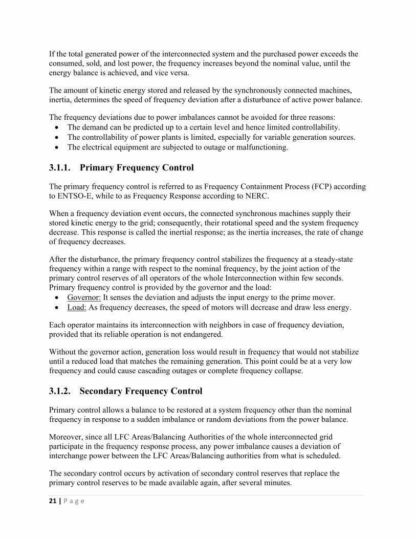
3.1.1. Primary Frequency Control .................................................................................................21

3.1.2. Secondary Frequency Control.............................................................................................21

3.1.3. Tertiary Frequency Control .................................................................................................22

3.2. Frequency Requirements............................................................................................................22

3.2.1. Frequency Requirements Proposed by ENTSO-E................................................................22

3.2.2. Frequency Requirements Proposed by NERC .....................................................................23

3.2.3. Key Differences Concerning Frequency Requirements.......................................................25

3.3. Frequency Response Requirements ...........................................................................................26

V | P a g e

3.4. Droop and Deadband Requirements ..........................................................................................27

3.4.1. Droop and Deadband Requirements Proposed by ENTSO-E ..............................................27

3.4.2. Droop and Deadband Requirements Proposed by NERC ...................................................27

3.5. Area Control Error (ACE) Requirements .....................................................................................28

3.5.1. ACE Requirements Proposed by ENTSO-E ..........................................................................28

3.5.2. ACE Requirements Proposed by NERC................................................................................29

3.5.3. Key Differences Concerning Area Control Error Requirements ..........................................31

3.6. Reserves Requirements ..............................................................................................................32

3.6.1. Reserves Requirements Proposed by ENTSO-E: .................................................................32

3.6.2. Reserve Requirements Proposed by NERC .........................................................................33

3.6.3. Key Differences Concerning Reserves Requirements .........................................................34

3.7. Time Durations and Activation Requirements............................................................................36

3.7.1. Time Durations and Activation Requirements Proposed by ENTSO-E................................36

3.7.2. Time Durations and Activation Requirements Proposed by NERC .....................................37

3.7.3. Key Differences Concerning Time Durations Requirements...............................................38

3.8. Time Control Process Requirements ..........................................................................................38

4. Operational Security and Emergency Operations ..............................................................................39

4.1. Introduction................................................................................................................................39

4.2. Operating Conditions of the Electric Power System...................................................................40

4.2.1. System States Defined by ENTSO-E ....................................................................................40

4.2.2. Operating Conditions Defined by NERC..............................................................................41

4.3. Events and Contingencies Classification .....................................................................................42

4.3.1. Incident Classification Scale Adopted by ENTSO-E .............................................................42

4.3.2. Classification of Contingencies According to ENTSO-E .......................................................45

4.3.3. Classification of Contingencies according to NERC.............................................................46

4.4. Operational Requirements during Contingencies ......................................................................47

4.4.1. Operational Requirements Imposed by ENTSO-E...............................................................47

4.4.2. Operational Requirements Imposed by NERC ....................................................................47

4.5. Remedial Actions ........................................................................................................................48

4.5.1. Remedial Actions Defined by ENTSO-E ...............................................................................48

4.5.2. Remedial Actions Defined by NERC ....................................................................................49

4.6. System Defense ..........................................................................................................................49

4.6.1. System Defense Plan Adopted by ENTSO-E ........................................................................50

4.6.2. System Defense According to NERC ...................................................................................51

VI | P a g e

4.7. Load Shedding............................................................................................................................52

4.7.1. Load Shedding According to ENTSO-E ................................................................................52

4.7.2. Load Shedding According to NERC......................................................................................53

4.8. System Restoration.....................................................................................................................55

4.8.1. System Restoration According to ENTSO-E.........................................................................55

4.8.2. System Restoration According to NERC..............................................................................56

4.9. System Protection.......................................................................................................................57

4.9.1. System Protection Adopted by ENTSO-E ............................................................................57

4.9.2. System Protection Adopted by NERC .................................................................................57

4.10. Monitoring and Data Exchange ..............................................................................................59

4.10.1. Monitoring and Data Exchange According to ENTSO-E ......................................................59

4.10.2. Monitoring and Data Exchange According to NERC............................................................61

4.11. Key Differences Concerning Operational Security and Emergency ........................................62

5. Operational Planning and Scheduling.................................................................................................65

5.1. Introduction................................................................................................................................65

5.2. Time Frames ...............................................................................................................................66

5.2.1. Time Frames According to ENTSO-E ...................................................................................67

5.2.2. Time Frames According to NERC.........................................................................................67

5.3. Network Models .........................................................................................................................68

5.3.1. Common Grid Models of ENTSO-E......................................................................................68

5.3.2. System Models of NERC......................................................................................................68

5.4. Planned Outage Coordination ....................................................................................................69

5.4.1. Planned Outage Coordination According to ENTSO-E ........................................................69

5.4.2. Planned Outage Coordination According to NERC .............................................................69

5.5. Load Forecast..............................................................................................................................70

5.5.1. Load Forecast According to ENTSO-E..................................................................................70

5.5.2. Load Forecast According to NERC.......................................................................................70

5.6. Adequacy ....................................................................................................................................71

5.6.1. Adequacy According to ENTSO-E ........................................................................................71

5.6.2. Adequacy According to NERC .............................................................................................71

5.7. Capacity Calculations ..................................................................................................................72

5.7.1. Capacity Calculations According to ENTSO-E......................................................................72

5.7.2. Capacity Calculations According to NERC ...........................................................................73

5.8. Key Differences Concerning Operational Planning and Scheduling............................................74

VII | P a g e

Part 2

6. Load Frequency Droop Control...........................................................................................................77

6.1. Main Components of a Generating Unit.....................................................................................77

6.1.1. Energy Conversion Source ..................................................................................................78

6.1.2. Synchronous Generator......................................................................................................79

6.1.3. Speed Governor ..................................................................................................................79

6.1.4. Excitation System................................................................................................................80

6.1.5. Classical Controllers of a Generating Unit ..........................................................................80

6.2. Droop Control of a Generating Unit ...........................................................................................81

6.3. Control Model of a Generating Unit ...........................................................................................84

6.3.1. Generator Model ................................................................................................................85

6.3.2. Load Model .........................................................................................................................86

6.3.3. Prime Mover Model............................................................................................................88

6.3.4. Governor Model .................................................................................................................88

6.3.5. Complete Model .................................................................................................................89

6.3.6. Simplified Model.................................................................................................................89

7. Data Processing ..................................................................................................................................90

7.1. Introduction................................................................................................................................90

7.2. Statistical Analysis of the Case Study..........................................................................................93

7.2.1. Maximum, Minimum Values, and Range............................................................................94

7.2.2. Histogram ...........................................................................................................................96

7.2.3. Mode...................................................................................................................................97

7.2.4. Median................................................................................................................................98

7.2.5. Mean...................................................................................................................................98

7.2.6. Variance and Standard Deviation .......................................................................................98

7.2.7. Skewness ............................................................................................................................99

7.2.8. Covariance and Correlation ..............................................................................................100

7.3. Pre-Processing ..........................................................................................................................101

7.3.1. Outlier Detection and Treatment .....................................................................................101

7.3.2. Noise Reduction................................................................................................................105

8. Parameters Estimation .....................................................................................................................108

8.1. Capacity of Generating Unit Estimation ...................................................................................108

8.2. Deadband Estimation ...............................................................................................................108

VIII | P a g e

8.3. Droop and Time Constant Estimation.......................................................................................112

8.3.1. Identifying the Parameters Analytically............................................................................118

8.3.2. Using the System Identification Toolbox of Matlab Software ..........................................121

8.4. Set Point Power Estimation ......................................................................................................128

8.4.1. The Input Power to the Governor.....................................................................................129

8.4.2. The Feedback Power.........................................................................................................131

8.4.3. The Set-point Power .........................................................................................................132

8.5. Electrical Power Estimation ......................................................................................................135

9. Methodology Validation ...................................................................................................................141

9.1. Data Processing ........................................................................................................................142

9.2. Deadband Estimation ...............................................................................................................143

9.3. Droop Estimation......................................................................................................................144

9.4. Time Constant Estimation.........................................................................................................146

9.5. Parameters Verification............................................................................................................147

Conclusion

10. Conclusion ....................................................................................................................................149

References

11. References ....................................................................................................................................152

IX | P a g e

List of Figures

Figure 1-1 Traditional Electric Power System..............................................................................................2Figure 2-1 Synchronous Areas of ENTSO-E [7] ..........................................................................................8Figure 2-2 Hierarchy of Geographical Areas Operated by TSOs [7] ...........................................................8Figure 2-3 Synchronous Areas, LFC Blocks, and LFC Areas [7] ................................................................9Figure 2-4 NERC Interconnections [9].......................................................................................................10Figure 2-5 NERC Regional Entities [9]......................................................................................................11Figure 2-6 NERC Reliability Coordinators [9]...........................................................................................12Figure 2-7 NERC Balancing Authorities [9] ..............................................................................................12Figure 2-8 Current and Future Network Codes of ENTSO-E.....................................................................16Figure 3-1 Generation-Load Balance .........................................................................................................20Figure 3-2 Frequency Quality Defining Parameters of ENTSO-E [7]........................................................23Figure 3-3 Frequency Measurable Event According to NERC [14] ...........................................................24Figure 3-4 Operating Reserves According to ENTSO-E ............................................................................32Figure 3-5 Operating Reserves According to NERC..................................................................................33Figure 3-6 Power Imbalance versus Deployment Time in CE ...................................................................37Figure 4-1 System States of ENTSO-E ......................................................................................................40Figure 4-2 Energy Emergency Alert Levels of NERC ..............................................................................41Figure 4-3 Incident Classification Scale of ENTSO-E ...............................................................................42Figure 4-4 Classifying Incidents According to Δf after the Alert State Trigger Time................................43Figure 4-5 Classifying Incidents According to Δf after the Time to Restore Frequency............................43Figure 4-6 Classifying Incidents According to the Minutes outside the Voltage Ranges...........................43Figure 4-7 Classifying Incidents Related to the Loss of Transmission Network Elements ........................43Figure 4-8 Classifying Incidents Related to the Loss of Power Generating Facilities................................44Figure 4-9 Classifying Incidents According to Number of Minutes for which 20% of FRR Lack ............44Figure 4-10 Classifying Incidents According to the Consequences on Load .............................................44Figure 4-11 Classifying Incidents According to the Loss of Tools and Facilities for 30 Minutes..............44Figure 4-12 Classification of Contingencies According to Probability of Occurrence...............................45Figure 4-13 Classification of Contingencies According to Location..........................................................46Figure 4-14 Classification of Contingencies According to NERC .............................................................46Figure 4-15 System Defense Plan of ENTSO-E .........................................................................................50Figure 4-16 Design Performance and Modeling Curves of Load Shedding Program ................................54Figure 4-17 Disturbance Monitoring Equipment of NERC ........................................................................58Figure 4-18 Protection System Devices of a NERC HV Transmission Line [27] ......................................58Figure 4-19 LFC Area, Responsibility Area, and Observability Area of ENTSO-E ..................................60

X | P a g e

Figure 5-1 Time Frames of Operational Planning and Planning [28] .........................................................66Figure 5-2 Relation between TTC, TRM, NTC, ATC, and AAC...............................................................72Figure 6-1 Scheme of a Hydro-Power Plant ...............................................................................................78Figure 6-2 LFC and AVR of a Synchronous Generator [32]......................................................................80Figure 6-3 Governor Steady-State Droop Characteristics ..........................................................................81Figure 6-4 Governor Steady State Droop Characteristics with Deadband..................................................83Figure 6-5 Effect of Change in Setting Power on Governor Steady State Speed Characteristics ...............83Figure 6-6 Exhausted Primary Frequency Reserves in Governor Steady State Droop Characteristics ......84Figure 6-7 Generator Block Diagram .........................................................................................................86Figure 6-8 Composite Load ........................................................................................................................86Figure 6-9 Effect of Composite Load on Governor Steady State Droop Characteristics............................87Figure 6-10 Generator and Load Block Diagram with Feedback Loop......................................................87Figure 6-11 Generator and Load Block Diagram without Feedback Loop.................................................87Figure 6-12 Turbine Block Diagram ..........................................................................................................88Figure 6-13 Governing System Block Diagram .........................................................................................88Figure 6-14 Complete Model of Load Frequency Control of an Isolated Power System ...........................89Figure 6-15 Simplified Model of Load Frequency Control of an Isolated Power System..........................89Figure 7-1 Primary Frequency Response to Imbalance of Active Power Balance on Machine Speed .......90Figure 7-2 Effect of Increasing the Droop on the Machine Speed..............................................................91Figure 7-3 Effect of Increasing the Time Constant on the Machine Speed ................................................91Figure 7-4 Effect of Using a Machine with Higher Inertia on Machine Speed ..........................................92Figure 7-5 Effect of Increasing the Power Imbalance on the Machine Speed ............................................92Figure 7-6 The Active Power and Frequency Deviation versus the 66 Hours for the case study ...............94Figure 7-7 The Active Power versus Frequency Deviation of the 66 Hours Dataset .................................95Figure 7-8 The Histogram of the Active Power of the 66 Hours Data .......................................................96Figure 7-9 The Histogram of the Frequency Deviation of the 66 Hours Data............................................97Figure 7-10 The Mean and 3σ Limits of the Segments of the Active Power Dataset ...............................103Figure 7-11 The Active Power Dataset for the 66 Hours after Removing the Outliers ............................103Figure 7-12 The Frequency Deviation Dataset for the 66 Hours after Removing the Outliers.................104Figure 7-13 n-domain Block Diagram of FIR Filter [38] .........................................................................106Figure 7-14 The Active Power and Frequency Deviation Datasets for the 66 Hours after Filtering ........107Figure 8-1 Extracted Active Power and Frequency Deviation Datasets 1 ................................................109Figure 8-2 Active Power versus Frequency Deviation of the Extracted Dataset 1 ...................................110Figure 8-3 Fitted Governor Steady State Droop Characteristics ..............................................................111Figure 8-4 Extracted Active Power and Frequency Deviation Datasets 2 ................................................113Figure 8-5 Active Power versus Frequency Deviation of the Extracted Dataset 2 ...................................114Figure 8-6 Extracted Active Power and Frequency Deviation Datasets 3 ................................................115Figure 8-7 Active Power versus Frequency Deviation of the Extracted Dataset 3 ...................................115Figure 8-8 Regression Line of the Linear Part of the Governor Steady State Characteristics ..................116Figure 8-9 Normalized Values of the Extracted Dataset 3 .......................................................................117Figure 8-10 Governing System Block Diagram Taking into Account the Deadband and Saturation.......117Figure 8-11 Importing the Datasets into System Identification Toolbox..................................................122Figure 8-12 Process Model in System Identification Toolbox .................................................................123Figure 8-13 Process Model Identified and Parameters Estimated by System Identification Toolbox ......123Figure 8-14 Unit Step Response between Frequency Deviation and Output Active Power .....................124Figure 8-15 Polynomial Model in System Identification Toolbox ...........................................................125Figure 8-16 ARX Model Identified and Coefficients Estimated by System Identification Toolbox ........126

XI | P a g e

Figure 8-17 Active Power Measured versus Estimated by the Process and ARX Models .......................127Figure 8-18 Load Frequency Controller of the Generating Unit in Africa ...............................................128Figure 8-19 Governing System Model of the Generating Unit in Africa .................................................128Figure 8-20 Prime Mover Model of the Generating Unit in Africa ..........................................................129Figure 8-21 Input and Output of the First Order Model of the Governor and Prime Mover ....................131Figure 8-22 Primary Frequency Response of the Generating Unit in Africa............................................131Figure 8-23 Primary Frequency Response Feedback Power ....................................................................132Figure 8-24 Estimated Set Point Power ....................................................................................................132Figure 8-25 Set Point Power of the Extracted Dataset 3...........................................................................133Figure 8-26 Set Point Power for the Extracted 111 Minutes ....................................................................133Figure 8-27 Set Point Power for the Extracted 180 Minutes ....................................................................134Figure 8-28 Governing System Model in Simulink..................................................................................134Figure 8-29 Estimated Output Active Power by Simulink .......................................................................135Figure 8-30 Generator and Load Model of the Generating Unit in Africa ...............................................136Figure 8-31 Estimated Electrical Power of the Load ................................................................................138Figure 8-32 Generator and Load Model in Simulink................................................................................139Figure 8-33 Load Frequency Controller in Simulink................................................................................139Figure 8-34 Estimated versus Measured Frequency Deviation in Hz.......................................................140Figure 8-35 Estimated versus Measured Mechanical Output Active Power in MW ................................140Figure 9-1 Active Power and Frequency Deviation versus the 147 Minutes in Europe ...........................141Figure 9-2 Active Power and Frequency Deviation Datasets after Removing the Outliers and Filtering 142Figure 9-3 Active Power versus Frequency Deviation for the Generating Unit in Europe.......................143Figure 9-4 Fitted Governor Steady State Droop Characteristics ..............................................................143Figure 9-5 Feedback Frequency ...............................................................................................................145Figure 9-6 Linear Variations between the Active Power and Frequency for Droop Estimation ..............145Figure 9-7 Active Power and Frequency Deviation for Time Constant Estimation .................................146Figure 9-8 Linear Variations between the Active Power and Frequency for Time Constant Estimation .147Figure 9-9 Governing System Model on Simulink ...................................................................................147Figure 9-10 Estimated versus Measured Output Active Power in MW....................................................148

XII | P a g e

List of Tables

Table 2-1 Organizational Structure of ENTSO-E and NERC ....................................................................14Table 2-2 General Part of Operation Handbook .........................................................................................15Table 2-3 Policies of Operation Handbook ................................................................................................15Table 2-4 Appendices of Operation Handbook .........................................................................................16Table 2-5 Grid Codes Development by ENTSO-E and NERC ..................................................................19Table 3-1 Frequency Quality Defining Parameters of ENTSO-E...............................................................23Table 3-2 Frequency Quality Target Parameter of ENTSO-E ....................................................................23Table 3-3 UFLS Trip Frequency of NERC Interconnections [15]..............................................................24Table 3-4 Starting Frequency of NERC Interconnections [16] ..................................................................24Table 3-5 CB Ratio of NERC Interconnections .........................................................................................24Table 3-6 Maximum Delta Frequency of NERC Interconnections.............................................................25Table 3-7 Frequency Requirements According to ENTSO-E and NERC ..................................................25Table 3-8 Frequency Response Requirements According to ENTSO-E and NERC ..................................26Table 3-9 Droop and Deadband of ENTSO-E Synchronous Areas ............................................................27Table 3-10 Droop and Deadband of NERC Interconnections ....................................................................27Table 3-11 Frequency Restoration Control Error Target Parameter of ENTSO-E Synchronous Areas .....28Table 3-12 Real Power Balance Control Performance Requirements ........................................................29Table 3-13 Real Power Balance Control Performance Compliance ...........................................................31Table 3-14 Area Control Error Requirements According to ENTSO-E and NERC ..................................31Table 3-15 Reserves Requirements According to ENTSO-E and NERC...................................................35Table 3-16 FCR and FRR Properties in ENTSO-E Synchronous Areas ....................................................36Table 3-17 Time Durations and Activation Requirements According to ENTSO-E and NERC................38Table 3-18 Time Control Process Requirement According to ENTSO-E and NERC ................................38Table 4-1 Types of Remedial Actions According to ENTSO-E .................................................................48Table 4-2 Low Frequency Demand Disconnection Scheme of ENTSO-E .................................................52Table 4-3 Under-frequency Load Shedding of Eastern and Quebec Interconnections ...............................54Table 4-4 Restoration Plan of ENTSO-E ...................................................................................................56Table 4-5 Key Differences Concerning Operational Security and Emergency Situations..........................64Table 5-1 Time Frames of Operational Planning and Scheduling According to ENTSO-E.......................67Table 5-2 Key Differences Concerning Operational Planning and Scheduling..........................................75Table 7-1 Technical Specifications of the Generating Unit in Africa.........................................................93Table 7-2 Bin Counts of the Histogram of the Active Power of the 66 Hours Data ...................................96Table 7-3 Bin Counts of the Histogram of the Frequency Deviation of the 66 Hours Data .......................97Table 7-4 Statistical Summary of the Processed Active Power and Frequency Deviation Datasets ........107

XIII | P a g e

Table 8-1 Summary of Estimated Parameters of the Load Frequency Controller ....................................127Table 9-1 Technical Specification of the Generating Unit in Europe .......................................................141

1 | P a g e

CHAPTER 11. Introduction

1.1. Evolution of Power SystemThe Electric Power System is the largest man-made system in the world [1]. The modern power system took a few centuries to develop to the level achieved nowadays. Before 1800, there were some initiatives from scientists such as William Gilbert, C. A. de Coulomb, Luigi Galvani, Benjamin Franklin, and the Italian scientist Alessandro Volta concerning electric and magnetic field principles, without probably knowing that their work will result in such engineering evolution in the future.

Between 1821 and 1831, at the same time that the English scientist Michael Faraday discovered the principle of electromagnetic induction and used it to build a machine generating electricity, the American scientist Joseph Henry was working independently on the applications of the induction principle on electromagnets.

The Pearl Street power station is the first electric power system established by Thomas Edison in 1882. It was a DC system designed to power the area of Lower Manhattan in New York City [2].

The invention of the transformer in 1885 to increase the voltage level and hence decrease the power losses, the invention of the induction motor in 1888 by the Italian physicist and electrical engineer Galileo Ferraris, and the simplicity of AC generator construction led to the move towards the AC Power Systems. In 1901, the English Engineer Charles Merz, designed the first 3-phase AC power system based on the poly-phase system.

With the growth of AC technology and the increase of generator’s size and transmission level voltages, the electric power could reach more and more people. The modern system contains hundreds of generators and thousands of buses with three dependent subsystems: generation, transmission, and distribution. The main components are synchronous generators, power transformers, transmission lines, substations, protection devices, measuring devices, active/reactive compensators, and controllers.

2 | P a g e

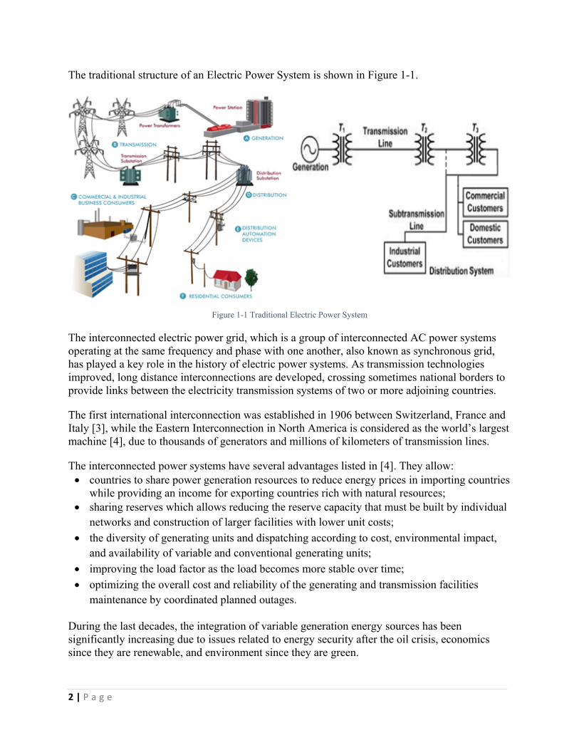
The traditional structure of an Electric Power System is shown in Figure 1-1.

Figure 1-1 Traditional Electric Power System

The interconnected electric power grid, which is a group of interconnected AC power systems operating at the same frequency and phase with one another, also known as synchronous grid, has played a key role in the history of electric power systems. As transmission technologies improved, long distance interconnections are developed, crossing sometimes national borders to provide links between the electricity transmission systems of two or more adjoining countries.

The first international interconnection was established in 1906 between Switzerland, France and Italy [3], while the Eastern Interconnection in North America is considered as the world’s largest machine [4], due to thousands of generators and millions of kilometers of transmission lines.

The interconnected power systems have several advantages listed in [4]. They allow: countries to share power generation resources to reduce energy prices in importing countries

while providing an income for exporting countries rich with natural resources; sharing reserves which allows reducing the reserve capacity that must be built by individual

networks and construction of larger facilities with lower unit costs; the diversity of generating units and dispatching according to cost, environmental impact,

and availability of variable and conventional generating units; improving the load factor as the load becomes more stable over time; optimizing the overall cost and reliability of the generating and transmission facilities

maintenance by coordinated planned outages.

During the last decades, the integration of variable generation energy sources has been significantly increasing due to issues related to energy security after the oil crisis, economics since they are renewable, and environment since they are green.

3 | P a g e

1.2. Motivation and AimThis thesis has been developed during an internship in CESI Milano. It is also important to mention that all the data used throughout the thesis are provided by CESI.Recent integration of renewable energy sources to the grid has further enhanced the complexity and uncertainty of the network, leading to increased concerns of actual prediction of generation and control of power flow, security, reliability, stability, efficiency, adequate sizing, and problems related to the bidirectional power flow across the system.

Moreover, the liberalization of electricity market caused great challenges due to the separation of production, transport, and supply of electrical energy with a large number of competitors [5].

Therefore, the introduction of the variable generation systems and market liberalization caused new challenges for the proper planning and operation of the power systems; therefore, grid codes are important in order to safeguard the electrical power system against these issues and it is the responsibility of the operator to check the compliance with the grid codes.

The grid codes are [1] Rules that specify technical and operational requirements of power plants and different

parties involved in the production, transportation, and utilization of power; Applicable to new and existing generation plants and users interested to connect to the grid

and act as standard procedures and requirements for including or prohibiting connection of the generation plants and loads to the grid; and

Published and continuously updated by each transmission system operator.

The great importance of the grid codes and their effect on having a secure power system and being able to meet the increasing market competitors and renewable energy sources, to combine with the current grid codes and increase cooperation among transmission system operators, raised the motivation for CESI to address this topic and the aim is to do a survey at international level of the operational rules of large interconnected systems, in particular, the European and the North American interconnected systems and identify the common best practices and the major differences between the grid codes of the analyzed networks.

One of the main issues related to the grid codes is monitoring, which is the periodic process used to assess, investigate, and evaluate, in order to measure compliance with the grid codes to ensure the secure operation of the power system and avoid sanctions in case of grid codes violations.

One of the important parameters facing periodic compliance monitoring is the generating unit’s Load Frequency Control model and its parameters, in particular, the parameters related to primary frequency response: dead-band, droop, and time constant. The performance of the generating unit in case of frequency deviation events should be monitored and compared to the standard values stated in the grid codes to measure its compliance.

The traditional method to perform this task is to plan a coordinated outage, take the generating unit out of service, and perform some field trials; in the form of applying a step of active power on the generating unit and observing the behavior of the frequency deviation, to evaluate the performance of the generating unit and compare the measured parameters with the standards.

4 | P a g e

This methodology has the following disadvantages: Economic losses due to the loss of the power of the tested generating unit. It is not always possible to have the control schemes available and have access to the control

system.

Based on the motivation stated above, the aim for CESI is to develop a methodology to conduct a performance analysis of the Load Frequency Controller of the generating unit related to the primary frequency control, using measurements carried out in normal operating conditions, that offers the advantage of not interfering with the production plans.

1.3. Scope

The thesis is divided into two parts. The scope of the thesis includes how to investigate the performance of the interconnected power grids, first by analyzing and highlighting the key differences between the grid codes related to these grids to determine the common best practice for an interconnected power grid, then by developing new methodologies to measure how these grids practically perform in real life with respect to the grid codes without the need to interfere with the production plans.

The scope for the task related to the first part is to introduce first the structure of the two organizations responsible for managing and operating both the European and North American interconnected grids, i.e. ENTSO-E and NERC, followed by an illustration of how the grid codes related to these two organizations are issued. The next step will be an analysis of how in both grids the following aspects are carried out:o Frequency Control,o Operational Security and Emergency Operations, ando Operational Planning.

The scope for the task related to the second part is to develop a methodology, exploiting the output active power and frequency deviation measured at the terminals of the generating unit, to assess the compliance of the performance of the Load Frequency Controller of the generating unit related to the primary frequency control with the grid codes. The following procedures are required to be done sequentially to reach the required objectives:o Pre-processing the measured data,o Estimating the dead band of the Load Frequency Controller of the generating unit,o Estimating the time constant and droop of the Load Frequency Controller of the

generating unit and verifying the results obtained,o Estimating the set point power that was adjusted by the operator and the electrical

power causing the disturbance to the Load Frequency Controller during the time period for which the measurements were acquired,

o Implementing the algorithms on other generating units to verify the methodology.

5 | P a g e

1.4. Road-Map of the Document

The remainder of the thesis is organized as follows:

First part:

Chapter 2 provides a description about the organizational structure of ENTSO-E and NERC, and the structure of the grid codes related to each network.

Chapter 3 focuses on how the Frequency Control is implemented in each system, and highlights the common major differences and best practice related to Frequency Control.

Chapter 4 focuses on how the Operational Security and Emergency Operations are implemented in each system, and highlights the common major differences and best practice related to Operational Security.

Chapter 5 focuses on how the Operational Planning and Scheduling are implemented in each system, and highlights the common major differences and best practice related to Operational Planning and Scheduling.

Second part:

Chapter 6 gives a description related to the main components of a generating unit, explains the principles of droop control and shows how the Load Frequency Controllers are modeled.

Chapter 7 introduces a case study on which the methodology should be implemented and focuses on pre-processing the measured data: removing the outliers and filtering the time series data by using a moving average filter.

Chapter 8 includes a procedure to estimate the capacity of generating unit, deadband, droop and time constant implemented in the Load Frequency Controller and identifying the transfer function representing it. The results obtained should be verified using the System Identification Toolbox built in Matlab software. This chapter also provides a method to estimate the set point power adjusted by the operator and the electrical power causing the disturbance to the Load Frequency Controller.

Chapter 9 implements the methodology on another generating unit with previously known parameters for validation.

Chapter 10 concludes the thesis and illustrates what kind of future work can be done to complement the work done in the thesis

6 | P a g e

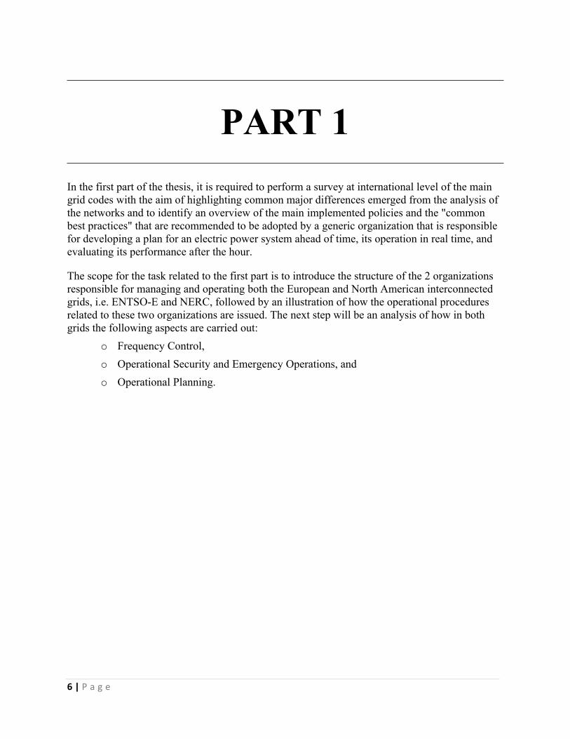
PART 1In the first part of the thesis, it is required to perform a survey at international level of the main grid codes with the aim of highlighting common major differences emerged from the analysis of the networks and to identify an overview of the main implemented policies and the "common best practices" that are recommended to be adopted by a generic organization that is responsible for developing a plan for an electric power system ahead of time, its operation in real time, and evaluating its performance after the hour.

The scope for the task related to the first part is to introduce the structure of the 2 organizations responsible for managing and operating both the European and North American interconnected grids, i.e. ENTSO-E and NERC, followed by an illustration of how the operational procedures related to these two organizations are issued. The next step will be an analysis of how in both grids the following aspects are carried out:

o Frequency Control,o Operational Security and Emergency Operations, ando Operational Planning.

7 | P a g e

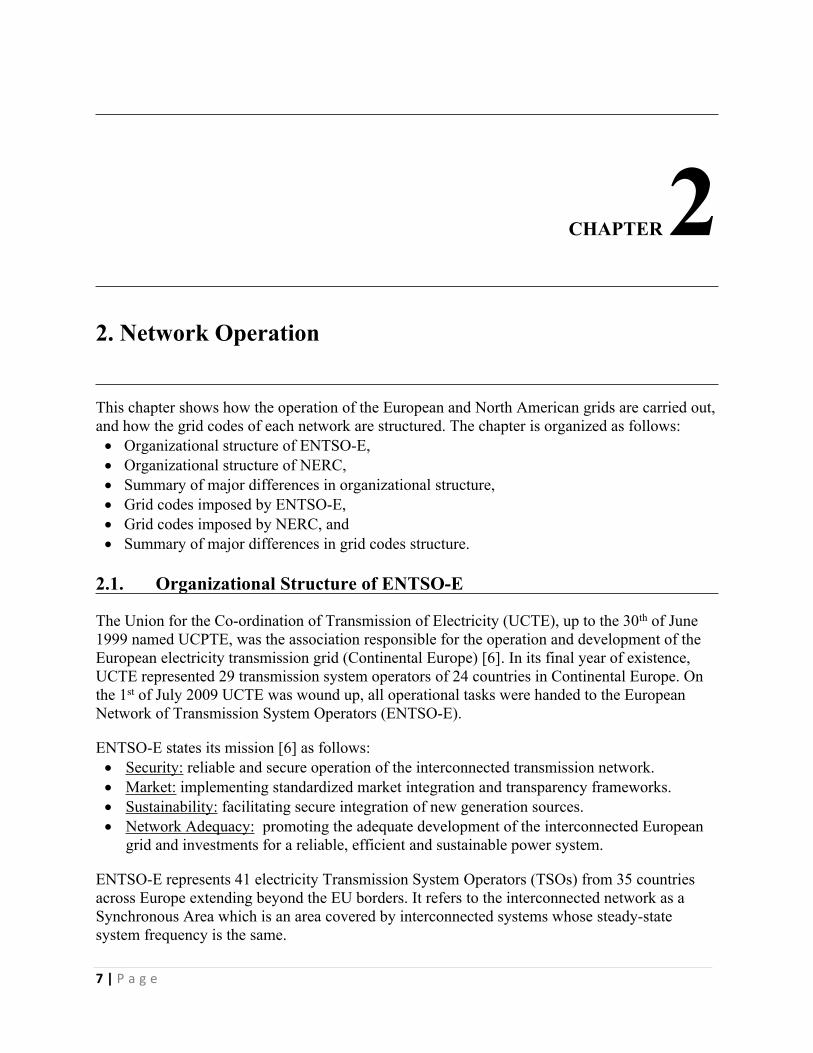
CHAPTER 22. Network Operation

This chapter shows how the operation of the European and North American grids are carried out, and how the grid codes of each network are structured. The chapter is organized as follows: Organizational structure of ENTSO-E, Organizational structure of NERC, Summary of major differences in organizational structure, Grid codes imposed by ENTSO-E, Grid codes imposed by NERC, and Summary of major differences in grid codes structure.

2.1. Organizational Structure of ENTSO-E

The Union for the Co-ordination of Transmission of Electricity (UCTE), up to the 30th of June 1999 named UCPTE, was the association responsible for the operation and development of the European electricity transmission grid (Continental Europe) [6]. In its final year of existence, UCTE represented 29 transmission system operators of 24 countries in Continental Europe. On the 1st of July 2009 UCTE was wound up, all operational tasks were handed to the European Network of Transmission System Operators (ENTSO-E).

ENTSO-E states its mission [6] as follows: Security: reliable and secure operation of the interconnected transmission network. Market: implementing standardized market integration and transparency frameworks. Sustainability: facilitating secure integration of new generation sources. Network Adequacy: promoting the adequate development of the interconnected European

grid and investments for a reliable, efficient and sustainable power system.

ENTSO-E represents 41 electricity Transmission System Operators (TSOs) from 35 countries across Europe extending beyond the EU borders. It refers to the interconnected network as a Synchronous Area which is an area covered by interconnected systems whose steady-state system frequency is the same.

8 | P a g e

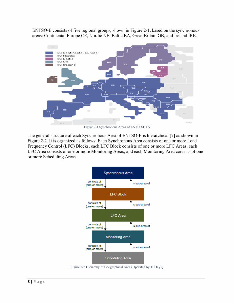
ENTSO-E consists of five regional groups, shown in Figure 2-1, based on the synchronous areas: Continental Europe CE, Nordic NE, Baltic BA, Great Britain GB, and Ireland IRE.

Figure 2-1 Synchronous Areas of ENTSO-E [7]

The general structure of each Synchronous Area of ENTSO-E is hierarchical [7] as shown in Figure 2-2. It is organized as follows: Each Synchronous Area consists of one or more Load Frequency Control (LFC) Blocks, each LFC Block consists of one or more LFC Areas, each LFC Area consists of one or more Monitoring Areas, and each Monitoring Area consists of one or more Scheduling Areas.

Figure 2-2 Hierarchy of Geographical Areas Operated by TSOs [7]

9 | P a g e

Each entity is responsible for number of obligations, some of which are: scheduling, monitoring and calculations of error and power interchange, frequency contamination, frequency restoration, and reserves dimensioning. Starting from the Scheduling Area towards the Synchronous Area, the obligations increase.

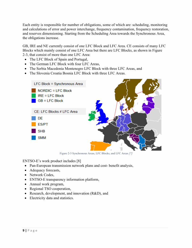
GB, IRE and NE currently consist of one LFC Block and LFC Area. CE consists of many LFC Blocks which mainly consist of one LFC Area but there are LFC Blocks, as shown in Figure 2-3, that consist of more than one LFC Area: The LFC Block of Spain and Portugal, The German LFC Block with four LFC Areas, The Serbia Macedonia Montenegro LFC Block with three LFC Areas, and The Slovenia Croatia Bosnia LFC Block with three LFC Areas.

Figure 2-3 Synchronous Areas, LFC Blocks, and LFC Areas [7]

ENTSO-E’s work product includes [8] Pan-European transmission network plans and cost- benefit analysis, Adequacy forecasts, Network Codes, ENTSO-E transparency information platform, Annual work program, Regional TSO cooperation, Research, development, and innovation (R&D), and Electricity data and statistics.

10 | P a g e

2.2. Organizational Structure of NERC

The North American Electric Reliability Corporation (NERC) was formed on March 28, 2006 as the successor to the North American Electric Reliability Council (also known as NERC). The original NERC was formed on June 1, 1968, in response to the 1965 blackout and the recommendation of the Federal Power Commission (predecessor of the Federal Energy Regulatory Commission) [9].

NERC is the Electric Reliability Organization (ERO) for North America, subject to oversight by the Federal Energy Regulatory Commission (FERC) and governmental authorities in Canada. NERC’s area of responsibility covers the United States, Canada, and the northern portion of Baja California, Mexico.

NERC is a not-for-profit international regulatory authority whose mission is to: Assure the reliability of the bulk power system in North America, Develop and enforce Reliability Standards, Annually assess seasonal and long term reliability, Monitor the bulk power system through system awareness, Supervise the responsibilities of Regional Entities, Impose sanction on non-compliant entities, and Educate, train, and certify industry personnel.

NERC refers to the interconnected network as an Interconnection. The North American power system, as shown in Figure 2-4, is divided into four major Interconnections: Western, Electric Reliability Council of Texas (ERCOT), Eastern, and Quebec.

Figure 2-4 NERC Interconnections [9]

11 | P a g e

All NERC’s interconnections operate at average 60 Hz. However, since the instantaneous frequency is not the same, they are tied via DC ties or by variable frequency transformers.

NERC reliability activities include the following: Reliability Standards, Reliability assessments, Compliance programs, Operator training and certification, Tools and systems for reliable operations, and Critical infrastructure protection.

In executing its responsibilities, NERC delegates certain authorities to organizations called Regional Entities [9]. Under NERC’s oversight, the Regional Entities perform certain aspects of NERC functions through delegation agreements, which are approved by FERC in the United States. The delegation agreements with each Regional Entity address the following: Development of regional Reliability Standards, Monitoring compliance and enforcing mandatory Reliability Standards, Reliability assessment and performance analysis, Network training and education, Event analysis, Reliability improvement, and Situation awareness and infrastructure security.

NERC’s responsibility area is divided into 8 Regional Entities as shown in Figure 2-5.

Figure 2-5 NERC Regional Entities [9]

The Reliability Coordinator is the entity that is the highest level of authority responsible for the reliable operation of the bulk electric system. NERC’s responsibility area is divided into 18 Reliability Coordinators as shown in Figure 2-6.

12 | P a g e

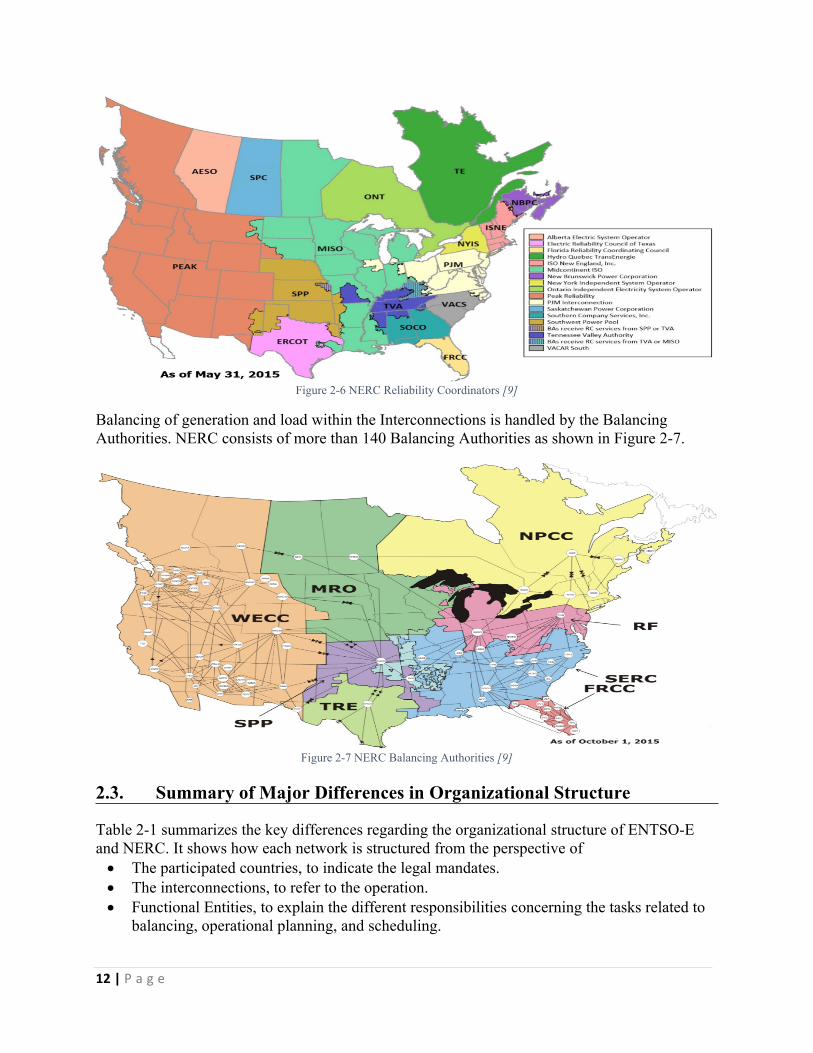
Figure 2-6 NERC Reliability Coordinators [9]

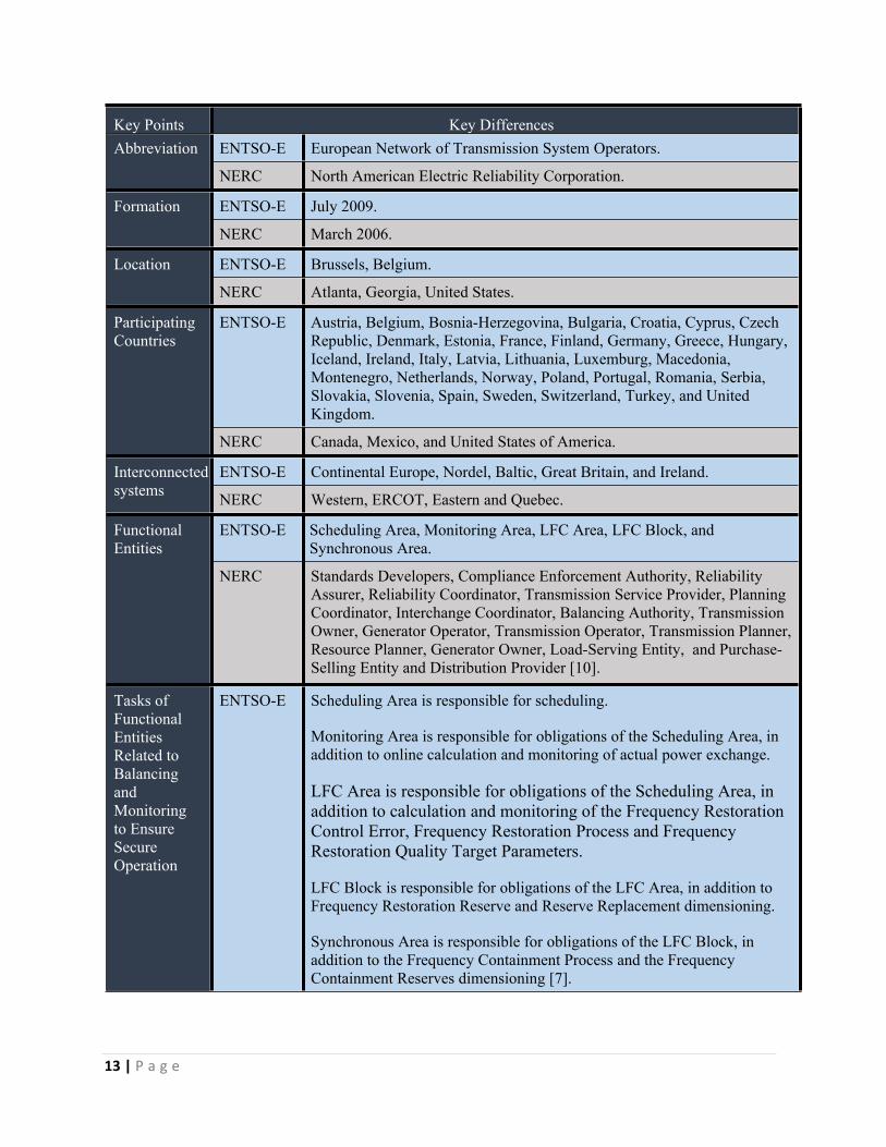
Balancing of generation and load within the Interconnections is handled by the Balancing Authorities. NERC consists of more than 140 Balancing Authorities as shown in Figure 2-7.

Figure 2-7 NERC Balancing Authorities [9]

2.3. Summary of Major Differences in Organizational Structure

Table 2-1 summarizes the key differences regarding the organizational structure of ENTSO-E and NERC. It shows how each network is structured from the perspective of The participated countries, to indicate the legal mandates. The interconnections, to refer to the operation. Functional Entities, to explain the different responsibilities concerning the tasks related to

balancing, operational planning, and scheduling.

13 | P a g e

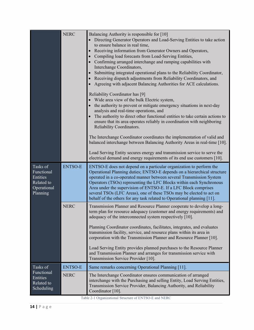
Key Points Key DifferencesENTSO-E European Network of Transmission System Operators.Abbreviation

NERC North American Electric Reliability Corporation.

ENTSO-E July 2009.Formation

NERC March 2006.

ENTSO-E Brussels, Belgium.Location

NERC Atlanta, Georgia, United States.

ENTSO-E Austria, Belgium, Bosnia-Herzegovina, Bulgaria, Croatia, Cyprus, Czech Republic, Denmark, Estonia, France, Finland, Germany, Greece, Hungary, Iceland, Ireland, Italy, Latvia, Lithuania, Luxemburg, Macedonia, Montenegro, Netherlands, Norway, Poland, Portugal, Romania, Serbia, Slovakia, Slovenia, Spain, Sweden, Switzerland, Turkey, and United Kingdom.

Participating Countries

NERC Canada, Mexico, and United States of America.

ENTSO-E Continental Europe, Nordel, Baltic, Great Britain, and Ireland.Interconnected systems NERC Western, ERCOT, Eastern and Quebec.

ENTSO-E Scheduling Area, Monitoring Area, LFC Area, LFC Block, and Synchronous Area.

Functional Entities

NERC Standards Developers, Compliance Enforcement Authority, Reliability Assurer, Reliability Coordinator, Transmission Service Provider, Planning Coordinator, Interchange Coordinator, Balancing Authority, Transmission Owner, Generator Operator, Transmission Operator, Transmission Planner, Resource Planner, Generator Owner, Load-Serving Entity, and Purchase-Selling Entity and Distribution Provider [10].

Tasks of Functional Entities Related to Balancing and Monitoring to Ensure Secure Operation

ENTSO-E Scheduling Area is responsible for scheduling.

Monitoring Area is responsible for obligations of the Scheduling Area, in addition to online calculation and monitoring of actual power exchange.

LFC Area is responsible for obligations of the Scheduling Area, in addition to calculation and monitoring of the Frequency Restoration Control Error, Frequency Restoration Process and Frequency Restoration Quality Target Parameters.

LFC Block is responsible for obligations of the LFC Area, in addition to Frequency Restoration Reserve and Reserve Replacement dimensioning.

Synchronous Area is responsible for obligations of the LFC Block, in addition to the Frequency Containment Process and the Frequency Containment Reserves dimensioning [7].

14 | P a g e

NERC Balancing Authority is responsible for [10] Directing Generator Operators and Load-Serving Entities to take action

to ensure balance in real time, Receiving information from Generator Owners and Operators, Compiling load forecasts from Load-Serving Entities, Confirming arranged interchange and ramping capabilities with

Interchange Coordinators, Submitting integrated operational plans to the Reliability Coordinator, Receiving dispatch adjustments from Reliability Coordinators, and Agreeing with adjacent Balancing Authorities for ACE calculations.

Reliability Coordinator has [9] Wide area view of the bulk Electric system, the authority to prevent or mitigate emergency situations in next-day

analysis and real-time operations, and The authority to direct other functional entities to take certain actions to

ensure that its area operates reliably in coordination with neighboring Reliability Coordinators.

The Interchange Coordinator coordinates the implementation of valid and balanced interchange between Balancing Authority Areas in real-time [10].

Load Serving Entity secures energy and transmission service to serve the electrical demand and energy requirements of its end use customers [10].

ENTSO-E ENTSO-E does not depend on a particular organization to perform the Operational Planning duties; ENTSO-E depends on a hierarchical structure operated in a co-operated manner between several Transmission System Operators (TSOs) representing the LFC Blocks within each Synchronous Area under the supervision of ENTSO-E. If a LFC Block comprises several TSOs (LFC Areas), one of these TSOs may be elected to act on behalf of the others for any task related to Operational planning [11].

Tasks of Functional Entities Related to Operational Planning

NERC Transmission Planner and Resource Planner cooperate to develop a long-term plan for resource adequacy (customer and energy requirements) and adequacy of the interconnected system respectively [10].

Planning Coordinator coordinates, facilitates, integrates, and evaluates transmission facility, service, and resource plans within its area in corporation with the Transmission Planner and Resource Planner [10].

Load Serving Entity provides planned purchases to the Resource Planner and Transmission Planner and arranges for transmission service with Transmission Service Provider [10].

ENTSO-E Same remarks concerning Operational Planning [11].Tasks of Functional Entities Related to Scheduling

NERC The Interchange Coordinator ensures communication of arranged interchange with the Purchasing and selling Entity, Load Serving Entities, Transmission Service Provider, Balancing Authority, and Reliability Coordinator [10].

Table 2-1 Organizational Structure of ENTSO-E and NERC

15 | P a g e

2.4. Grid Codes Imposed by ENTSO-E

Common understandings for the operation, control, and security of the interconnections of UCTE were required, and hence inspired the need for the “UCTE Operation Handbook” which is an up-to-date collection of operation principles and standards, enforced for transmission system operators in Europe to make consultation easier for members and the general public.

The Operation Handbook was originally adopted by UCTE. It is still enforceable up to now as its development and revision was handed to ENTSO-E’s Continental Europe [6].

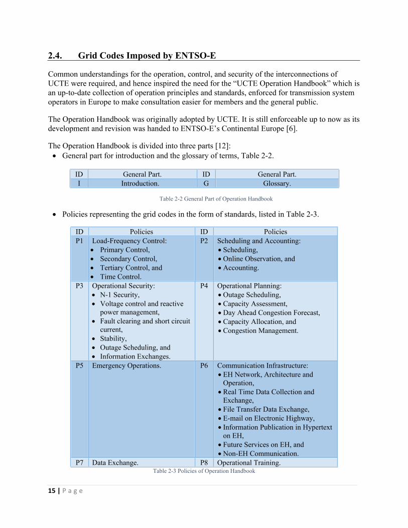
The Operation Handbook is divided into three parts [12]: General part for introduction and the glossary of terms, Table 2-2.

Table 2-2 General Part of Operation Handbook

Policies representing the grid codes in the form of standards, listed in Table 2-3.

ID Policies ID PoliciesP1 Load-Frequency Control:

Primary Control, Secondary Control, Tertiary Control, and Time Control.

P2 Scheduling and Accounting: Scheduling,Online Observation, andAccounting.

P3 Operational Security: N-1 Security, Voltage control and reactive

power management, Fault clearing and short circuit

current, Stability, Outage Scheduling, and Information Exchanges.

P4 Operational Planning:Outage Scheduling,Capacity Assessment,Day Ahead Congestion Forecast,Capacity Allocation, andCongestion Management.

P5 Emergency Operations. P6 Communication Infrastructure: EH Network, Architecture and

Operation,Real Time Data Collection and

Exchange, File Transfer Data Exchange, E-mail on Electronic Highway, Information Publication in Hypertext

on EH, Future Services on EH, andNon-EH Communication.

P7 Data Exchange. P8 Operational Training.Table 2-3 Policies of Operation Handbook

ID General Part. ID General Part.I Introduction. G Glossary.

16 | P a g e

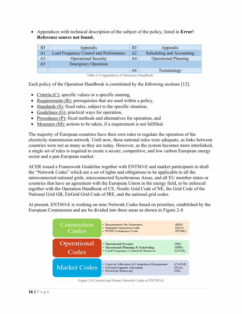
Appendices with technical description of the subject of the policy, listed in Error! Reference source not found..

ID Appendix ID AppendixA1 Load Frequency Control and Performance A2 Scheduling and AccountingA3 Operational Security A4 Operational PlanningA5 Emergency Operation

A8 TerminologyTable 2-4 Appendices of Operation Handbook

Each policy of the Operation Handbook is constituted by the following sections [12]:

Criteria (C): specific values or a specific naming, Requirements (R): prerequisites that are used within a policy, Standards (S): fixed rules, subject to the specific situation, Guidelines (G): practical ways for operation, Procedures (P): fixed methods and alternatives for operation, and Measures (M): actions to be taken, if a requirement is not fulfilled.

The majority of European countries have their own rules to regulate the operation of the electricity transmission network. Until now, these national rules were adequate, as links between countries were not as many as they are today. However, as the system becomes more interlinked, a single set of rules is required to create a secure, competitive, and low carbon European energy sector and a pan-European market.

ACER issued a Framework Guideline together with ENTSO-E and market participants to draft the “Network Codes” which are a set of rights and obligations to be applicable to all the interconnected national grids, interconnected Synchronous Areas, and all EU member states or countries that have an agreement with the European Union in the energy field, to be enforced together with the Operation Handbook of CE, Nordic Grid Code of NE, the Grid Code of the National Grid GB, EirGrid Grid Code of IRE, and the national grid codes.

At present, ENTSO-E is working on nine Network Codes based on priorities, established by the European Commission and are be divided into three areas as shown in Figure 2-8.

Figure 2-8 Current and Future Network Codes of ENTSO-E

17 | P a g e

2.5. Grid Codes Imposed by NERC

NERC refers to the grid codes as Reliability Standards which are “a set of requirements that define specific obligations of owners, operators, and users of the North American bulk power systems and the reliability requirements for its planning and operation” [9].

Reliability Standards are developed using a results-based approach that focuses on performance, risk management, and entity capabilities.

The Reliability Standards are divided into 14 main sections, each containing a number of Reliability Standards; Resource and Demand Balancing (BAL), Critical Infrastructure Protection (CIP), Communications (COM), Emergency Preparedness and Operations (EOP), Facilities Design, Connections and Maintenance (FAC), Interchange Scheduling and Coordination (INT), Interconnection Reliability Operations and Coordination (IRO), Modeling, Data and Analysis (MOD), Nuclear (NUC), Personnel Performance, Training and Qualifications (PER), Protection and Control (PRC), Transmission Operations (TOP), Transmission and Planning (TPL), and Voltage and Reactive (VAR).

Each Reliability Standard is constituted by the following sections: Title: to identify the topic of the Reliability Standard, Identification Number: to facilitate tracking and reference to the Reliability Standard, Purpose: to state the reason behind developing the Reliability Standard, Applicability: to identify which entities are involved with the requirements, Effective date: to determine when each requirement became effective in each jurisdiction, Requirement: to determine the actions or outcomes that must be achieved, Compliance Elements: to aid in the compliance monitoring, Measure: to identify the evidence that demonstrates compliance with the requirement, Violation Risk Factor: to identify the potential reliability significance of noncompliance, Violation Severity Level: to define the degree to which the compliance was not achieved, Version History: to list information regarding previous versions of the Reliability Standard, Variance: to state if the Reliability Standard is applicable to a specific geographic area, Application Guidelines: guidelines supporting the implementation of Reliability Standard, Procedures: procedures supporting implementation of Reliability Standard, and Compliance Enforcement Authority: to identify the entity that assesses performance and

determines if an entity is compliant with the Reliability Standard.

18 | P a g e

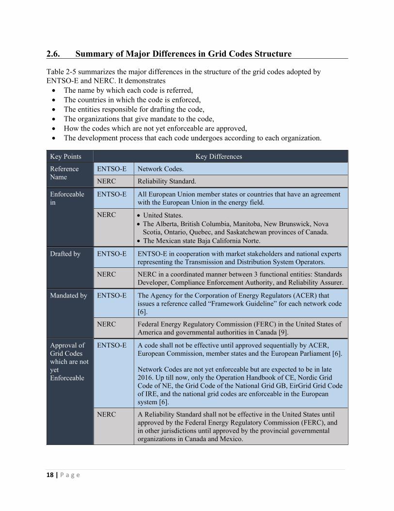
2.6. Summary of Major Differences in Grid Codes Structure

Table 2-5 summarizes the major differences in the structure of the grid codes adopted by ENTSO-E and NERC. It demonstrates The name by which each code is referred, The countries in which the code is enforced, The entities responsible for drafting the code, The organizations that give mandate to the code, How the codes which are not yet enforceable are approved, The development process that each code undergoes according to each organization.

Key Points Key Differences

ENTSO-E Network Codes.Reference Name NERC Reliability Standard.

ENTSO-E All European Union member states or countries that have an agreement with the European Union in the energy field.

Enforceable in

NERC United States. The Alberta, British Columbia, Manitoba, New Brunswick, Nova

Scotia, Ontario, Quebec, and Saskatchewan provinces of Canada. The Mexican state Baja California Norte.

ENTSO-E ENTSO-E in cooperation with market stakeholders and national experts representing the Transmission and Distribution System Operators.

Drafted by

NERC NERC in a coordinated manner between 3 functional entities: Standards Developer, Compliance Enforcement Authority, and Reliability Assurer.

ENTSO-E The Agency for the Corporation of Energy Regulators (ACER) that issues a reference called “Framework Guideline” for each network code [6].

Mandated by

NERC Federal Energy Regulatory Commission (FERC) in the United States of America and governmental authorities in Canada [9].

ENTSO-E A code shall not be effective until approved sequentially by ACER, European Commission, member states and the European Parliament [6].

Network Codes are not yet enforceable but are expected to be in late 2016. Up till now, only the Operation Handbook of CE, Nordic Grid Code of NE, the Grid Code of the National Grid GB, EirGrid Grid Code of IRE, and the national grid codes are enforceable in the European system [6].

Approval of Grid Codes which are not yet Enforceable

NERC A Reliability Standard shall not be effective in the United States until approved by the Federal Energy Regulatory Commission (FERC), and in other jurisdictions until approved by the provincial governmental organizations in Canada and Mexico.

19 | P a g e

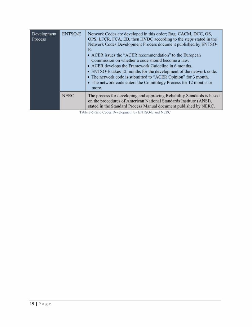
ENTSO-E Network Codes are developed in this order; Rag, CACM, DCC, OS, OPS, LFCR, FCA, EB, then HVDC according to the steps stated in the Network Codes Development Process document published by ENTSO-E: ACER issues the “ACER recommendation” to the European

Commission on whether a code should become a law. ACER develops the Framework Guideline in 6 months. ENTSO-E takes 12 months for the development of the network code. The network code is submitted to “ACER Opinion” for 3 month. The network code enters the Comitology Process for 12 months or

more.

Development Process

NERC The process for developing and approving Reliability Standards is based on the procedures of American National Standards Institute (ANSI), stated in the Standard Process Manual document published by NERC.

Table 2-5 Grid Codes Development by ENTSO-E and NERC

20 | P a g e

CHAPTER 33. Load Frequency Control

This chapter presents how ENTSO-E and NERC consider the Load Frequency Control during operation and is organized as follows: Introduction, Frequency requirements, Frequency response requirements, Droop and deadband requirements, Area control error requirements, Reserves requirements, Time duration and activation requirements, Time control process requirements, and Key differences concerning Load Frequency control.

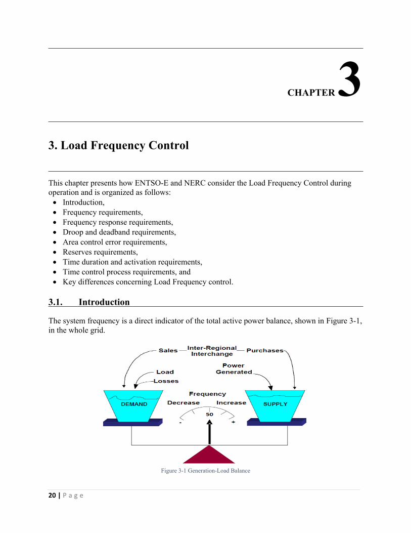
3.1. Introduction

The system frequency is a direct indicator of the total active power balance, shown in Figure 3-1, in the whole grid.

Figure 3-1 Generation-Load Balance

21 | P a g e

If the total generated power of the interconnected system and the purchased power exceeds the consumed, sold, and lost power, the frequency increases beyond the nominal value, until the energy balance is achieved, and vice versa.

The amount of kinetic energy stored and released by the synchronously connected machines, inertia, determines the speed of frequency deviation after a disturbance of active power balance.

The frequency deviations due to power imbalances cannot be avoided for three reasons: The demand can be predicted up to a certain level and hence limited controllability. The controllability of power plants is limited, especially for variable generation sources. The electrical equipment are subjected to outage or malfunctioning.

3.1.1. Primary Frequency Control

The primary frequency control is referred to as Frequency Containment Process (FCP) according to ENTSO-E, while to as Frequency Response according to NERC.

When a frequency deviation event occurs, the connected synchronous machines supply their stored kinetic energy to the grid; consequently, their rotational speed and the system frequency decrease. This response is called the inertial response; as the inertia increases, the rate of change of frequency decreases.

After the disturbance, the primary frequency control stabilizes the frequency at a steady-state frequency within a range with respect to the nominal frequency, by the joint action of the primary control reserves of all operators of the whole Interconnection within few seconds. Primary frequency control is provided by the governor and the load: Governor: It senses the deviation and adjusts the input energy to the prime mover. Load: As frequency decreases, the speed of motors will decrease and draw less energy.

Each operator maintains its interconnection with neighbors in case of frequency deviation, provided that its reliable operation is not endangered.

Without the governor action, generation loss would result in frequency that would not stabilize until a reduced load that matches the remaining generation. This point could be at a very low frequency and could cause cascading outages or complete frequency collapse.

3.1.2. Secondary Frequency Control

Primary control allows a balance to be restored at a system frequency other than the nominal frequency in response to a sudden imbalance or random deviations from the power balance.

Moreover, since all LFC Areas/Balancing Authorities of the whole interconnected grid participate in the frequency response process, any power imbalance causes a deviation of interchange power between the LFC Areas/Balancing authorities from what is scheduled.

The secondary control occurs by activation of secondary control reserves that replace the primary control reserves to be made available again, after several minutes.

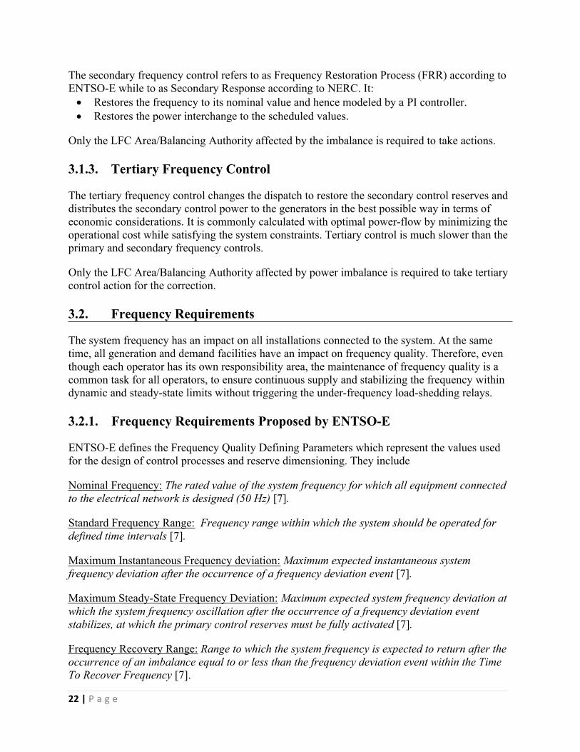
22 | P a g e

The secondary frequency control refers to as Frequency Restoration Process (FRR) according to ENTSO-E while to as Secondary Response according to NERC. It: Restores the frequency to its nominal value and hence modeled by a PI controller. Restores the power interchange to the scheduled values.

Only the LFC Area/Balancing Authority affected by the imbalance is required to take actions.

3.1.3. Tertiary Frequency Control

The tertiary frequency control changes the dispatch to restore the secondary control reserves and distributes the secondary control power to the generators in the best possible way in terms of economic considerations. It is commonly calculated with optimal power-flow by minimizing the operational cost while satisfying the system constraints. Tertiary control is much slower than the primary and secondary frequency controls.

Only the LFC Area/Balancing Authority affected by power imbalance is required to take tertiary control action for the correction.

3.2. Frequency Requirements

The system frequency has an impact on all installations connected to the system. At the same time, all generation and demand facilities have an impact on frequency quality. Therefore, even though each operator has its own responsibility area, the maintenance of frequency quality is a common task for all operators, to ensure continuous supply and stabilizing the frequency within dynamic and steady-state limits without triggering the under-frequency load-shedding relays.

3.2.1. Frequency Requirements Proposed by ENTSO-E

ENTSO-E defines the Frequency Quality Defining Parameters which represent the values used for the design of control processes and reserve dimensioning. They include

Nominal Frequency: The rated value of the system frequency for which all equipment connected to the electrical network is designed (50 Hz) [7].

Standard Frequency Range: Frequency range within which the system should be operated for defined time intervals [7].

Maximum Instantaneous Frequency deviation: Maximum expected instantaneous system frequency deviation after the occurrence of a frequency deviation event [7].

Maximum Steady-State Frequency Deviation: Maximum expected system frequency deviation at which the system frequency oscillation after the occurrence of a frequency deviation event stabilizes, at which the primary control reserves must be fully activated [7].

Frequency Recovery Range: Range to which the system frequency is expected to return after the occurrence of an imbalance equal to or less than the frequency deviation event within the Time To Recover Frequency [7].

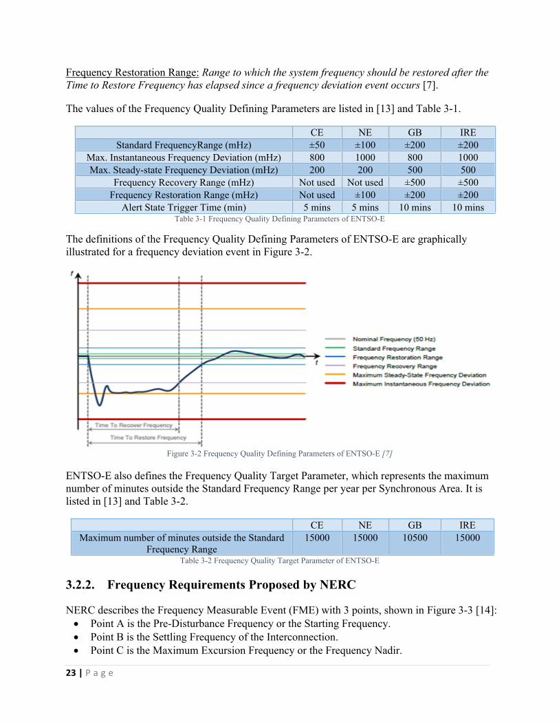
23 | P a g e

Frequency Restoration Range: Range to which the system frequency should be restored after the Time to Restore Frequency has elapsed since a frequency deviation event occurs [7].

The values of the Frequency Quality Defining Parameters are listed in [13] and Table 3-1.

CE NE GB IREStandard FrequencyRange (mHz) ±50 ±100 ±200 ±200

Max. Instantaneous Frequency Deviation (mHz) 800 1000 800 1000 Max. Steady-state Frequency Deviation (mHz) 200 200 500 500

Frequency Recovery Range (mHz) Not used Not used ±500 ±500 Frequency Restoration Range (mHz) Not used ±100 ±200 ±200

Alert State Trigger Time (min) 5 mins 5 mins 10 mins 10 minsTable 3-1 Frequency Quality Defining Parameters of ENTSO-E

The definitions of the Frequency Quality Defining Parameters of ENTSO-E are graphically illustrated for a frequency deviation event in Figure 3-2.

Figure 3-2 Frequency Quality Defining Parameters of ENTSO-E [7]

ENTSO-E also defines the Frequency Quality Target Parameter, which represents the maximum number of minutes outside the Standard Frequency Range per year per Synchronous Area. It is listed in [13] and Table 3-2.

CE NE GB IREMaximum number of minutes outside the Standard

Frequency Range15000 15000 10500 15000

Table 3-2 Frequency Quality Target Parameter of ENTSO-E

3.2.2. Frequency Requirements Proposed by NERC

NERC describes the Frequency Measurable Event (FME) with 3 points, shown in Figure 3-3 [14]: Point A is the Pre-Disturbance Frequency or the Starting Frequency. Point B is the Settling Frequency of the Interconnection. Point C is the Maximum Excursion Frequency or the Frequency Nadir.

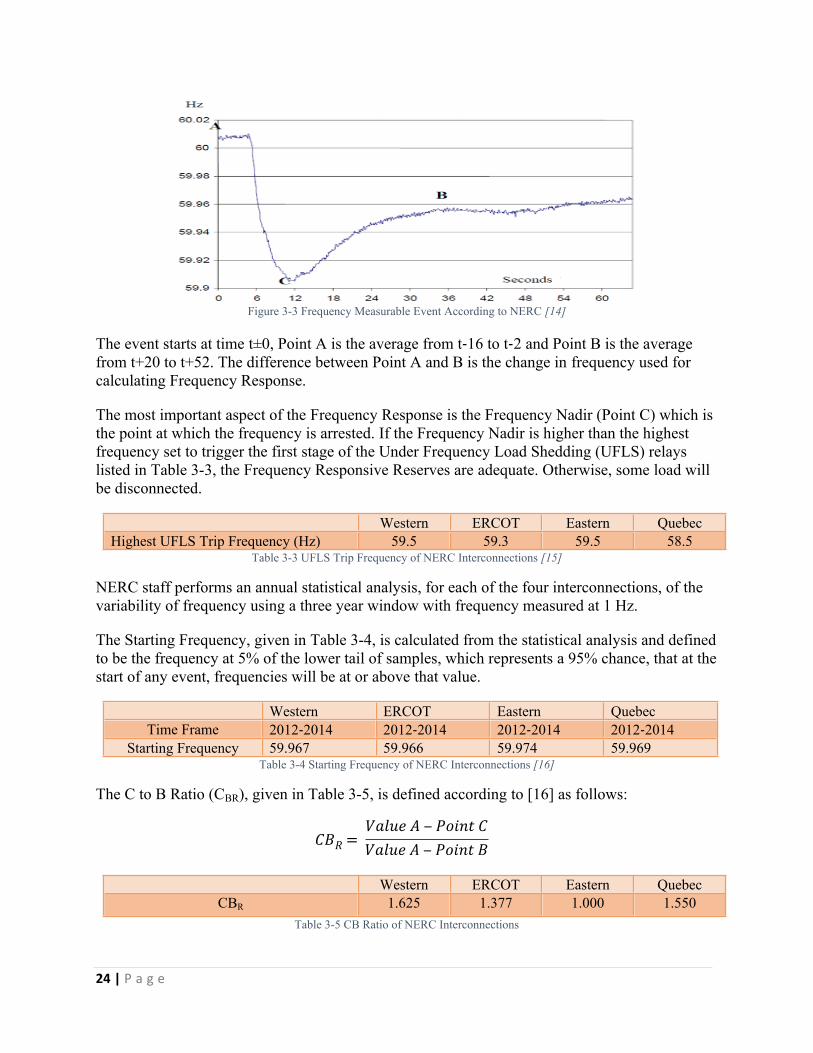
24 | P a g e

Figure 3-3 Frequency Measurable Event According to NERC [14]

The event starts at time t±0, Point A is the average from t‐16 to t‐2 and Point B is the average from t+20 to t+52. The difference between Point A and B is the change in frequency used for calculating Frequency Response.

The most important aspect of the Frequency Response is the Frequency Nadir (Point C) which is the point at which the frequency is arrested. If the Frequency Nadir is higher than the highest frequency set to trigger the first stage of the Under Frequency Load Shedding (UFLS) relays listed in Table 3-3, the Frequency Responsive Reserves are adequate. Otherwise, some load will be disconnected.

Western ERCOT Eastern QuebecHighest UFLS Trip Frequency (Hz) 59.5 59.3 59.5 58.5

Table 3-3 UFLS Trip Frequency of NERC Interconnections [15]

NERC staff performs an annual statistical analysis, for each of the four interconnections, of the variability of frequency using a three year window with frequency measured at 1 Hz.

The Starting Frequency, given in Table 3-4, is calculated from the statistical analysis and defined to be the frequency at 5% of the lower tail of samples, which represents a 95% chance, that at the start of any event, frequencies will be at or above that value.

Western ERCOT Eastern QuebecTime Frame 2012‐2014 2012‐2014 2012‐2014 2012‐2014

Starting Frequency 59.967 59.966 59.974 59.969Table 3-4 Starting Frequency of NERC Interconnections [16]

The C to B Ratio (CBR), given in Table 3-5, is defined according to [16] as follows:

𝐶𝐵𝑅 = 𝑉𝑎𝑙𝑢𝑒 𝐴 ‒ 𝑃𝑜𝑖𝑛𝑡 𝐶𝑉𝑎𝑙𝑢𝑒 𝐴 ‒ 𝑃𝑜𝑖𝑛𝑡 𝐵

Western ERCOT Eastern QuebecCBR 1.625 1.377 1.000 1.550

Table 3-5 CB Ratio of NERC Interconnections

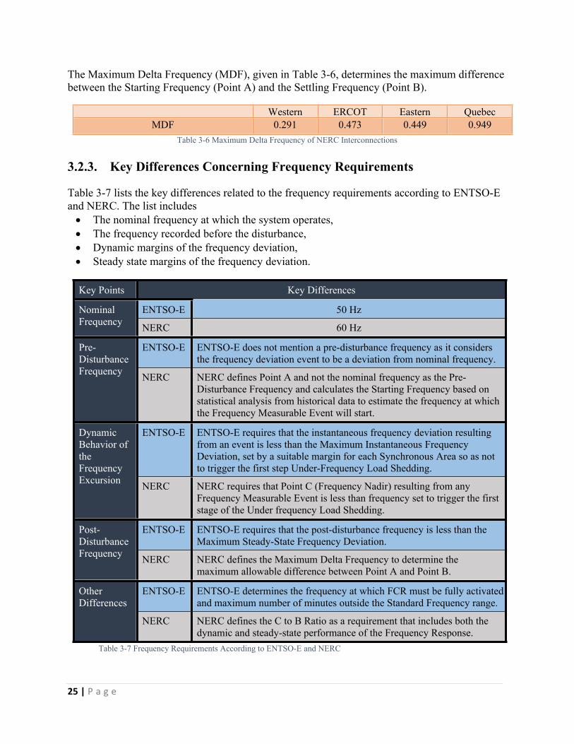
25 | P a g e

The Maximum Delta Frequency (MDF), given in Table 3-6, determines the maximum difference between the Starting Frequency (Point A) and the Settling Frequency (Point B).

Western ERCOT Eastern QuebecMDF 0.291 0.473 0.449 0.949

Table 3-6 Maximum Delta Frequency of NERC Interconnections

3.2.3. Key Differences Concerning Frequency Requirements

Table 3-7 lists the key differences related to the frequency requirements according to ENTSO-E and NERC. The list includes The nominal frequency at which the system operates, The frequency recorded before the disturbance, Dynamic margins of the frequency deviation, Steady state margins of the frequency deviation.

Key Points Key Differences

ENTSO-E 50 HzNominal Frequency NERC 60 Hz

ENTSO-E ENTSO-E does not mention a pre-disturbance frequency as it considers the frequency deviation event to be a deviation from nominal frequency.

Pre-Disturbance Frequency NERC NERC defines Point A and not the nominal frequency as the Pre-

Disturbance Frequency and calculates the Starting Frequency based on statistical analysis from historical data to estimate the frequency at which the Frequency Measurable Event will start.

ENTSO-E ENTSO-E requires that the instantaneous frequency deviation resulting from an event is less than the Maximum Instantaneous Frequency Deviation, set by a suitable margin for each Synchronous Area so as not to trigger the first step Under-Frequency Load Shedding.

Dynamic Behavior of the Frequency Excursion NERC NERC requires that Point C (Frequency Nadir) resulting from any

Frequency Measurable Event is less than frequency set to trigger the first stage of the Under frequency Load Shedding.

ENTSO-E ENTSO-E requires that the post-disturbance frequency is less than the Maximum Steady-State Frequency Deviation.

Post-Disturbance Frequency NERC NERC defines the Maximum Delta Frequency to determine the

maximum allowable difference between Point A and Point B.

ENTSO-E ENTSO-E determines the frequency at which FCR must be fully activated and maximum number of minutes outside the Standard Frequency range.

Other Differences

NERC NERC defines the C to B Ratio as a requirement that includes both the dynamic and steady-state performance of the Frequency Response.

Table 3-7 Frequency Requirements According to ENTSO-E and NERC

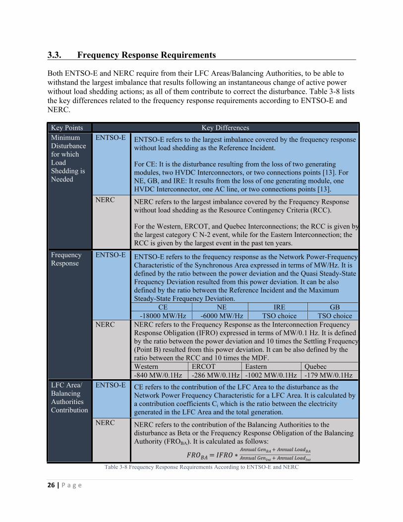
26 | P a g e

3.3. Frequency Response Requirements

Both ENTSO-E and NERC require from their LFC Areas/Balancing Authorities, to be able to withstand the largest imbalance that results following an instantaneous change of active power without load shedding actions; as all of them contribute to correct the disturbance. Table 3-8 lists the key differences related to the frequency response requirements according to ENTSO-E and NERC.

Key Points Key DifferencesENTSO-E ENTSO-E refers to the largest imbalance covered by the frequency response

without load shedding as the Reference Incident.

For CE: It is the disturbance resulting from the loss of two generating modules, two HVDC Interconnectors, or two connections points [13]. For NE, GB, and IRE: It results from the loss of one generating module, one HVDC Interconnector, one AC line, or two connections points [13].

Minimum Disturbance for which Load Shedding is Needed

NERC NERC refers to the largest imbalance covered by the Frequency Response without load shedding as the Resource Contingency Criteria (RCC).

For the Western, ERCOT, and Quebec Interconnections; the RCC is given by the largest category C N-2 event, while for the Eastern Interconnection; the RCC is given by the largest event in the past ten years.

ENTSO-E refers to the frequency response as the Network Power-Frequency Characteristic of the Synchronous Area expressed in terms of MW/Hz. It is defined by the ratio between the power deviation and the Quasi Steady-State Frequency Deviation resulted from this power deviation. It can be also defined by the ratio between the Reference Incident and the Maximum Steady-State Frequency Deviation.

CE NE IRE GB

ENTSO-E

-18000 MW/Hz -6000 MW/Hz TSO choice TSO choiceNERC refers to the Frequency Response as the Interconnection Frequency Response Obligation (IFRO) expressed in terms of MW/0.1 Hz. It is defined by the ratio between the power deviation and 10 times the Settling Frequency (Point B) resulted from this power deviation. It can be also defined by the ratio between the RCC and 10 times the MDF.Western ERCOT Eastern Quebec

Frequency Response

NERC

-840 MW/0.1Hz -286 MW/0.1Hz -1002 MW/0.1Hz -179 MW/0.1HzENTSO-E CE refers to the contribution of the LFC Area to the disturbance as the

Network Power Frequency Characteristic for a LFC Area. It is calculated by a contribution coefficients Ci which is the ratio between the electricity generated in the LFC Area and the total generation.

LFC Area/ Balancing Authorities Contribution

NERC NERC refers to the contribution of the Balancing Authorities to the disturbance as Beta or the Frequency Response Obligation of the Balancing Authority (FROBA). It is calculated as follows:

𝐹𝑅𝑂𝐵𝐴 = 𝐼𝐹𝑅𝑂 ∗𝐴𝑛𝑛𝑢𝑎𝑙 𝐺𝑒𝑛𝐵𝐴 + 𝐴𝑛𝑛𝑢𝑎𝑙 𝐿𝑜𝑎𝑑𝐵𝐴

𝐴𝑛𝑛𝑢𝑎𝑙 𝐺𝑒𝑛𝐼𝑛𝑡 + 𝐴𝑛𝑛𝑢𝑎𝑙 𝐿𝑜𝑎𝑑𝐼𝑛𝑡

Table 3-8 Frequency Response Requirements According to ENTSO-E and NERC

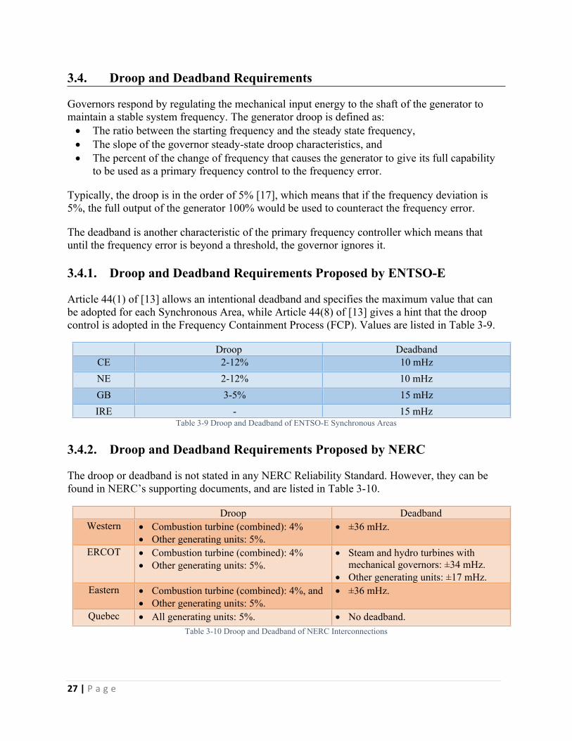
27 | P a g e

3.4. Droop and Deadband Requirements

Governors respond by regulating the mechanical input energy to the shaft of the generator to maintain a stable system frequency. The generator droop is defined as: The ratio between the starting frequency and the steady state frequency, The slope of the governor steady-state droop characteristics, and The percent of the change of frequency that causes the generator to give its full capability

to be used as a primary frequency control to the frequency error.

Typically, the droop is in the order of 5% [17], which means that if the frequency deviation is 5%, the full output of the generator 100% would be used to counteract the frequency error.

The deadband is another characteristic of the primary frequency controller which means that until the frequency error is beyond a threshold, the governor ignores it.

3.4.1. Droop and Deadband Requirements Proposed by ENTSO-E

Article 44(1) of [13] allows an intentional deadband and specifies the maximum value that can be adopted for each Synchronous Area, while Article 44(8) of [13] gives a hint that the droop control is adopted in the Frequency Containment Process (FCP). Values are listed in Table 3-9.

Droop DeadbandCE 2-12% 10 mHzNE 2-12% 10 mHzGB 3-5% 15 mHzIRE - 15 mHz

Table 3-9 Droop and Deadband of ENTSO-E Synchronous Areas

3.4.2. Droop and Deadband Requirements Proposed by NERC

The droop or deadband is not stated in any NERC Reliability Standard. However, they can be found in NERC’s supporting documents, and are listed in Table 3-10.

Droop DeadbandWestern Combustion turbine (combined): 4%

Other generating units: 5%. ±36 mHz.

ERCOT Combustion turbine (combined): 4% Other generating units: 5%.

Steam and hydro turbines with mechanical governors: ±34 mHz.

Other generating units: ±17 mHz.Eastern Combustion turbine (combined): 4%, and

Other generating units: 5%. ±36 mHz.

Quebec All generating units: 5%. No deadband.Table 3-10 Droop and Deadband of NERC Interconnections

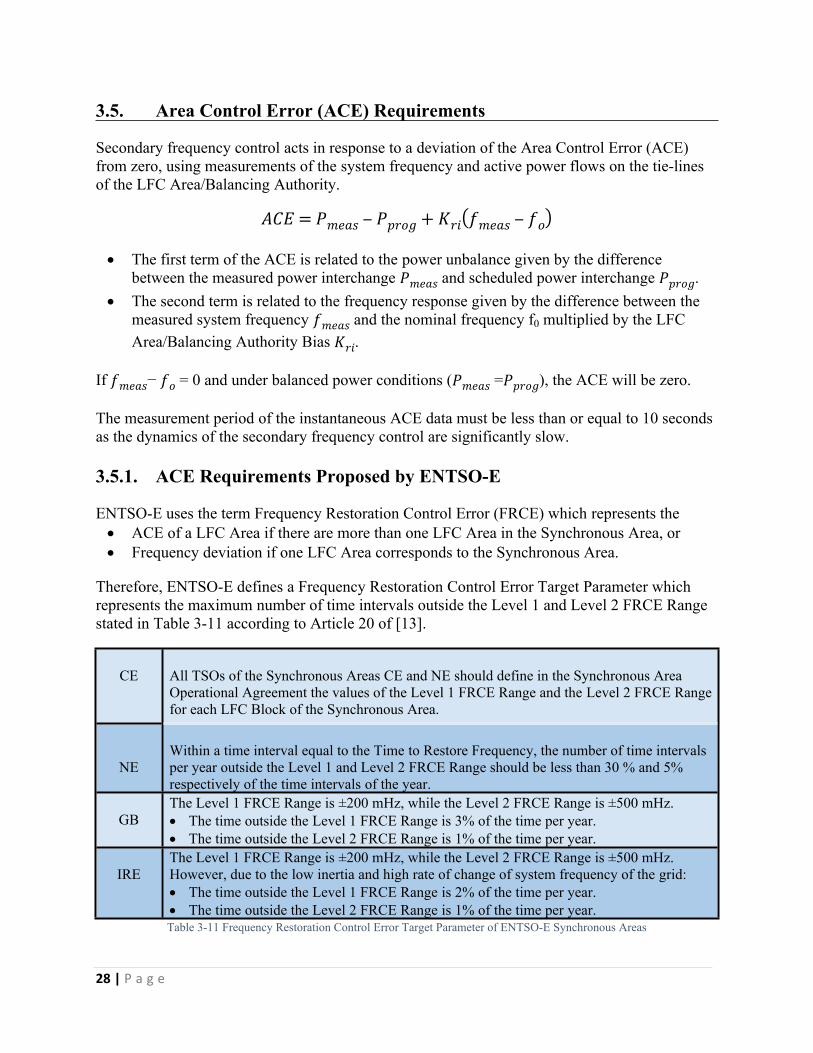
28 | P a g e

3.5. Area Control Error (ACE) Requirements

Secondary frequency control acts in response to a deviation of the Area Control Error (ACE) from zero, using measurements of the system frequency and active power flows on the tie-lines of the LFC Area/Balancing Authority.

𝐴𝐶𝐸 = 𝑃𝑚𝑒𝑎𝑠 ‒ 𝑃𝑝𝑟𝑜𝑔 + 𝐾𝑟𝑖(𝑓𝑚𝑒𝑎𝑠 ‒ 𝑓𝑜)

The first term of the ACE is related to the power unbalance given by the difference between the measured power interchange and scheduled power interchange .𝑃𝑚𝑒𝑎𝑠 𝑃𝑝𝑟𝑜𝑔

The second term is related to the frequency response given by the difference between the measured system frequency and the nominal frequency f0 multiplied by the LFC 𝑓𝑚𝑒𝑎𝑠Area/Balancing Authority Bias .𝐾𝑟𝑖

If − = 0 and under balanced power conditions ( = ), the ACE will be zero.𝑓𝑚𝑒𝑎𝑠 𝑓𝑜 𝑃𝑚𝑒𝑎𝑠 𝑃𝑝𝑟𝑜𝑔

The measurement period of the instantaneous ACE data must be less than or equal to 10 seconds as the dynamics of the secondary frequency control are significantly slow.

3.5.1. ACE Requirements Proposed by ENTSO-E

ENTSO-E uses the term Frequency Restoration Control Error (FRCE) which represents the ACE of a LFC Area if there are more than one LFC Area in the Synchronous Area, or Frequency deviation if one LFC Area corresponds to the Synchronous Area.

Therefore, ENTSO-E defines a Frequency Restoration Control Error Target Parameter which represents the maximum number of time intervals outside the Level 1 and Level 2 FRCE Range stated in Table 3-11 according to Article 20 of [13].

CE All TSOs of the Synchronous Areas CE and NE should define in the Synchronous Area Operational Agreement the values of the Level 1 FRCE Range and the Level 2 FRCE Range for each LFC Block of the Synchronous Area.

NEWithin a time interval equal to the Time to Restore Frequency, the number of time intervals per year outside the Level 1 and Level 2 FRCE Range should be less than 30 % and 5% respectively of the time intervals of the year.

GBThe Level 1 FRCE Range is ±200 mHz, while the Level 2 FRCE Range is ±500 mHz. The time outside the Level 1 FRCE Range is 3% of the time per year. The time outside the Level 2 FRCE Range is 1% of the time per year.

IREThe Level 1 FRCE Range is ±200 mHz, while the Level 2 FRCE Range is ±500 mHz.However, due to the low inertia and high rate of change of system frequency of the grid: The time outside the Level 1 FRCE Range is 2% of the time per year. The time outside the Level 2 FRCE Range is 1% of the time per year.Table 3-11 Frequency Restoration Control Error Target Parameter of ENTSO-E Synchronous Areas

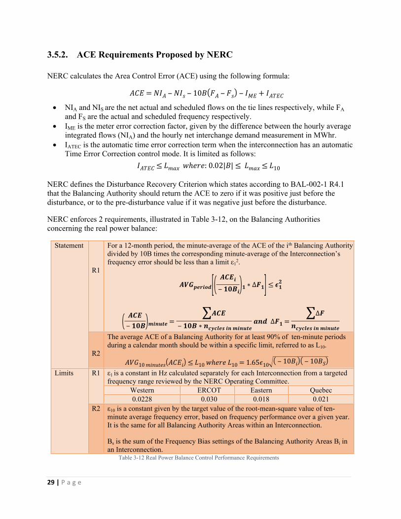
29 | P a g e

3.5.2. ACE Requirements Proposed by NERC

NERC calculates the Area Control Error (ACE) using the following formula:

𝐴𝐶𝐸 = 𝑁𝐼𝐴 ‒ 𝑁𝐼𝑠 ‒ 10𝐵(𝐹𝐴 ‒ 𝐹𝑠) ‒ 𝐼𝑀𝐸 + 𝐼𝐴𝑇𝐸𝐶

NIA and NIS are the net actual and scheduled flows on the tie lines respectively, while FA and FS are the actual and scheduled frequency respectively.

IME is the meter error correction factor, given by the difference between the hourly average integrated flows (NIA) and the hourly net interchange demand measurement in MWhr.

IATEC is the automatic time error correction term when the interconnection has an automatic Time Error Correction control mode. It is limited as follows:

𝐼𝐴𝑇𝐸𝐶 ≤ 𝐿𝑚𝑎𝑥 𝑤ℎ𝑒𝑟𝑒: 0.02|𝐵| ≤ 𝐿𝑚𝑎𝑥 ≤ 𝐿10

NERC defines the Disturbance Recovery Criterion which states according to BAL-002-1 R4.1 that the Balancing Authority should return the ACE to zero if it was positive just before the disturbance, or to the pre-disturbance value if it was negative just before the disturbance.

NERC enforces 2 requirements, illustrated in Table 3-12, on the Balancing Authorities concerning the real power balance:

R1

For a 12-month period, the minute-average of the ACE of the ith Balancing Authority divided by 10B times the corresponding minute-average of the Interconnection’s frequency error should be less than a limit ε1

2.

𝑨𝑽𝑮𝒑𝒆𝒓𝒊𝒐𝒅[( 𝑨𝑪𝑬𝒊

‒ 𝟏𝟎𝑩𝒊)𝟏 ∗ ∆𝑭𝟏] ≤ 𝝐𝟐𝟏

( 𝑨𝑪𝑬‒ 𝟏𝟎𝑩)𝒎𝒊𝒏𝒖𝒕𝒆 =

∑𝑨𝑪𝑬

‒ 𝟏𝟎𝑩 ∗ 𝒏𝒄𝒚𝒄𝒍𝒆𝒔 𝒊𝒏 𝒎𝒊𝒏𝒖𝒕𝒆 𝒂𝒏𝒅 ∆𝑭𝟏 =

∑∆𝑭

𝒏𝒄𝒚𝒄𝒍𝒆𝒔 𝒊𝒏 𝒎𝒊𝒏𝒖𝒕𝒆

Statement

R2

The average ACE of a Balancing Authority for at least 90% of ten-minute periods during a calendar month should be within a specific limit, referred to as L10.

𝐴𝑉𝐺10 𝑚𝑖𝑛𝑢𝑡𝑒𝑠(𝐴𝐶𝐸𝑖) ≤ 𝐿10 𝑤ℎ𝑒𝑟𝑒 𝐿10 = 1.65𝜖10 ( ‒ 10𝐵𝑖)( ‒ 10𝐵𝑆) ε1 is a constant in Hz calculated separately for each Interconnection from a targeted frequency range reviewed by the NERC Operating Committee.

Western ERCOT Eastern Quebec

R1

0.0228 0.030 0.018 0.021

Limits

R2 ε10 is a constant given by the target value of the root-mean-square value of ten-minute average frequency error, based on frequency performance over a given year. It is the same for all Balancing Authority Areas within an Interconnection.

Bs is the sum of the Frequency Bias settings of the Balancing Authority Areas Bi in an Interconnection.

Table 3-12 Real Power Balance Control Performance Requirements

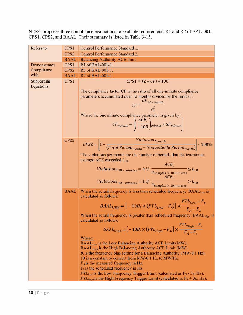
30 | P a g e

NERC proposes three compliance evaluations to evaluate requirements R1 and R2 of BAL-001: CPS1, CPS2, and BAAL. Their summary is listed in Table 3-13.

CPS1 Control Performance Standard 1.CPS2 Control Performance Standard 2.

Refers to

BAAL Balancing Authority ACE limit.CPS1 R1 of BAL-001-1.CPS2 R2 of BAL-001-1.

Demonstrates Compliance with BAAL R2 of BAL-001-1.

CPS1 𝐶𝑃𝑆1 = (2 ‒ 𝐶𝐹) ∗ 100

The compliance factor CF is the ratio of all one-minute compliance parameters accumulated over 12 months divided by the limit ε1

2.

𝐶𝐹 =𝐶𝐹12 ‒ 𝑚𝑜𝑛𝑡ℎ

𝜖21

Where the one minute compliance parameter is given by:

𝐶𝐹𝑚𝑖𝑛𝑢𝑡𝑒 = [( 𝐴𝐶𝐸𝑖

‒ 10𝐵𝑖)𝑚𝑖𝑛𝑢𝑡𝑒 ∗ ∆𝐹𝑚𝑖𝑛𝑢𝑡𝑒]CPS2

𝐶𝑃𝑆2 = [1 ‒𝑉𝑖𝑜𝑙𝑎𝑡𝑖𝑜𝑛𝑠𝑚𝑜𝑛𝑡ℎ

(𝑇𝑜𝑡𝑎𝑙 𝑃𝑒𝑟𝑖𝑜𝑑𝑚𝑜𝑛𝑡ℎ ‒ 𝑈𝑛𝑎𝑣𝑎𝑖𝑙𝑎𝑏𝑙𝑒 𝑃𝑒𝑟𝑖𝑜𝑑𝑚𝑜𝑛𝑡ℎ)] ∗ 100%

The violations per month are the number of periods that the ten-minute average ACE exceeded L10.

𝑉𝑖𝑜𝑙𝑎𝑡𝑖𝑜𝑛𝑠 10 ‒ 𝑚𝑖𝑛𝑢𝑡𝑒𝑠 = 0 𝑖𝑓 𝐴𝐶𝐸𝑖

𝑛𝑠𝑎𝑚𝑝𝑙𝑒𝑠 𝑖𝑛 10 𝑚𝑖𝑛𝑢𝑡𝑒𝑠≤ 𝐿10

𝑉𝑖𝑜𝑙𝑎𝑡𝑖𝑜𝑛𝑠 10 ‒ 𝑚𝑖𝑛𝑢𝑡𝑒𝑠 = 1 𝑖𝑓 𝐴𝐶𝐸𝑖

𝑛𝑠𝑎𝑚𝑝𝑙𝑒𝑠 𝑖𝑛 10 𝑚𝑖𝑛𝑢𝑡𝑒𝑠> 𝐿10

Supporting Equations

BAAL When the actual frequency is less than scheduled frequency, BAALLow is calculated as follows:

𝐵𝐴𝐴𝐿𝐿𝑂𝑊 = [ ‒ 10𝐵𝑖 × (𝐹𝑇𝐿𝐿𝑜𝑤 ‒ 𝐹𝑠)] ×𝐹𝑇𝐿𝐿𝑜𝑤 ‒ 𝐹𝑠

𝐹𝐴 ‒ 𝐹𝑠When the actual frequency is greater than scheduled frequency, BAALHigh is calculated as follows:

𝐵𝐴𝐴𝐿𝐻𝑖𝑔ℎ = [ ‒ 10𝐵𝑖 × (𝐹𝑇𝐿𝐻𝑖𝑔ℎ ‒ 𝐹𝑠)] ×𝐹𝑇𝐿𝐻𝑖𝑔ℎ ‒ 𝐹𝑠

𝐹𝐴 ‒ 𝐹𝑠Where:BAALLow is the Low Balancing Authority ACE Limit (MW).BAALHigh is the High Balancing Authority ACE Limit (MW).Bi is the frequency bias setting for a Balancing Authority (MW/0.1 Hz).10 is a constant to convert from MW/0.1 Hz to MW/Hz.FA is the measured frequency in Hz.FS is the scheduled frequency in Hz.FTLLow is the Low Frequency Trigger Limit (calculated as FS - 3ε1 Hz).FTLHigh is the High Frequency Trigger Limit (calculated as FS + 3ε1 Hz).

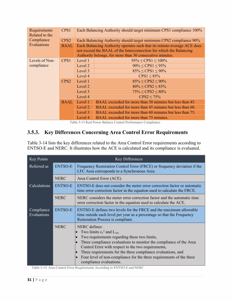
31 | P a g e

CPS1 Each Balancing Authority should target minimum CPS1 compliance 100%

CPS2 Each Balancing Authority should target minimum CPS2 compliance 90%

Requirements Related to the Compliance Evaluations BAAL Each Balancing Authority operates such that its minute-average ACE does

not exceed the BAAL of the Interconnection for which the Balancing Authority belongs, for more than 30 consecutive minutes.Level 1 95% ≤ CPS1 ≤ 100%Level 2 90% ≤ CPS1 ≤ 95%Level 3 85% ≤ CPS1 ≤ 90%

CPS1

Level 4 CPS1 ≤ 85%Level 1 85% ≤ CPS2 ≤ 90%Level 2 80% ≤ CPS2 ≤ 85%Level 3 75% ≤ CPS2 ≤ 80%

CPS2

Level 4 CPS2 ≤ 75%Level 1 BAAL exceeded for more than 30 minutes but less than 45.Level 2 BAAL exceeded for more than 45 minutes but less than 60.Level 3 BAAL exceeded for more than 60 minutes but less than 75.

Levels of Non-compliance

BAAL

Level 4 BAAL exceeded for more than 75 minutes.Table 3-13 Real Power Balance Control Performance Compliance

3.5.3. Key Differences Concerning Area Control Error Requirements

Table 3-14 lists the key differences related to the Area Control Error requirements according to ENTSO-E and NERC. It illustrates how the ACE is calculated and its compliance is evaluated.

Key Points Key Differences

ENTSO-E Frequency Restoration Control Error (FRCE) or frequency deviation if the LFC Area corresponds to a Synchronous Area.

Referred as

NERC Area Control Error (ACE).

ENTSO-E ENTSO-E does not consider the meter error correction factor or automatic time error correction factor in the equation used to calculate the FRCE.

Calculations

NERC NERC considers the meter error correction factor and the automatic time error correction factor in the equation used to calculate the ACE.

ENTSO-E ENTSO-E defines two levels for the FRCE and the maximum allowable time outside each level per year as a percentage so that the Frequency Restoration Process is compliant.

Compliance Evaluations

NERC NERC defines: Two limits ε1

2 and L10, Two requirements regarding these two limits, Three compliance evaluations to monitor the compliance of the Area

Control Error with respect to the two requirements, Three requirements for the three compliance evaluations, and Four level of non-compliance for the three requirements of the three

compliance evaluations. Table 3-14 Area Control Error Requirements According to ENTSO-E and NERC

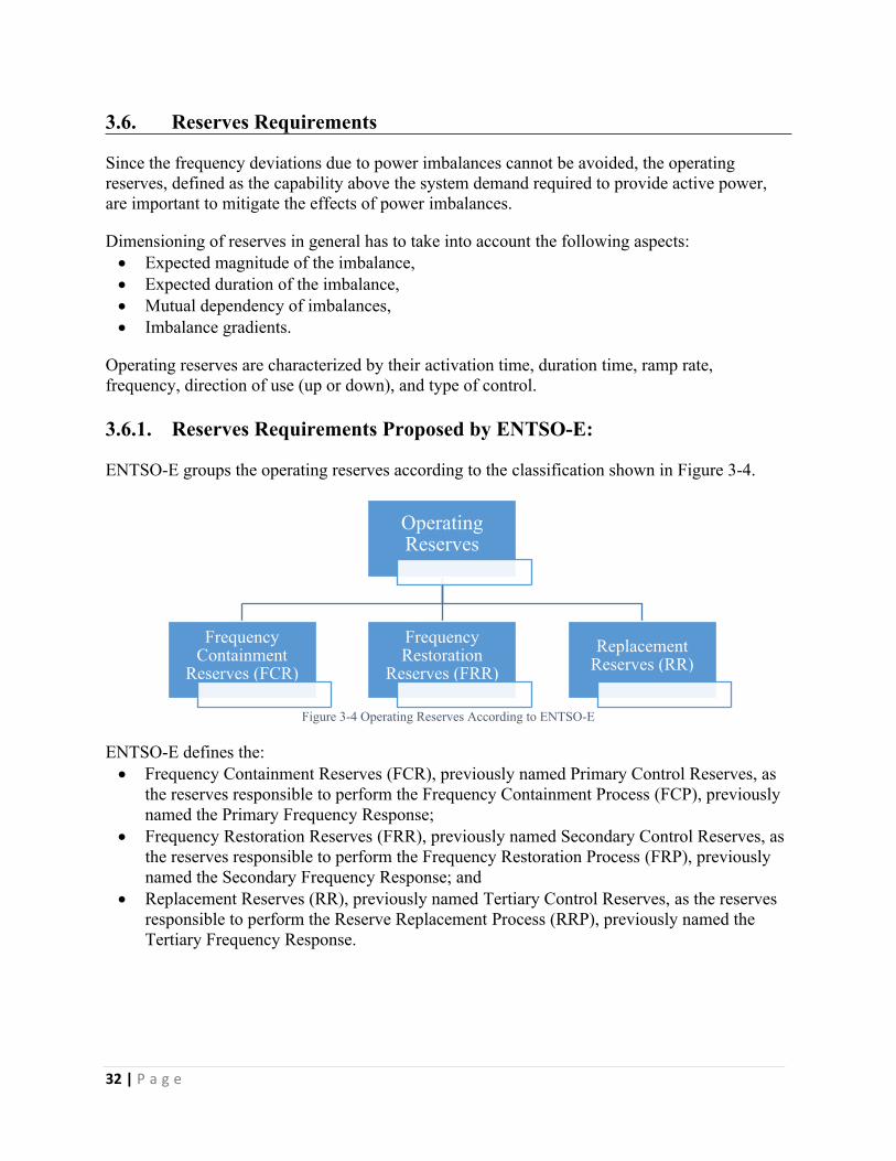
32 | P a g e

3.6. Reserves Requirements

Since the frequency deviations due to power imbalances cannot be avoided, the operating reserves, defined as the capability above the system demand required to provide active power, are important to mitigate the effects of power imbalances.

Dimensioning of reserves in general has to take into account the following aspects: Expected magnitude of the imbalance, Expected duration of the imbalance, Mutual dependency of imbalances, Imbalance gradients.

Operating reserves are characterized by their activation time, duration time, ramp rate, frequency, direction of use (up or down), and type of control.

3.6.1. Reserves Requirements Proposed by ENTSO-E:

ENTSO-E groups the operating reserves according to the classification shown in Figure 3-4.

Operating Reserves

Frequency Containment

Reserves (FCR)

Frequency Restoration

Reserves (FRR)Replacement

Reserves (RR)

Figure 3-4 Operating Reserves According to ENTSO-E

ENTSO-E defines the: Frequency Containment Reserves (FCR), previously named Primary Control Reserves, as

the reserves responsible to perform the Frequency Containment Process (FCP), previously named the Primary Frequency Response;

Frequency Restoration Reserves (FRR), previously named Secondary Control Reserves, as the reserves responsible to perform the Frequency Restoration Process (FRP), previously named the Secondary Frequency Response; and

Replacement Reserves (RR), previously named Tertiary Control Reserves, as the reserves responsible to perform the Reserve Replacement Process (RRP), previously named the Tertiary Frequency Response.

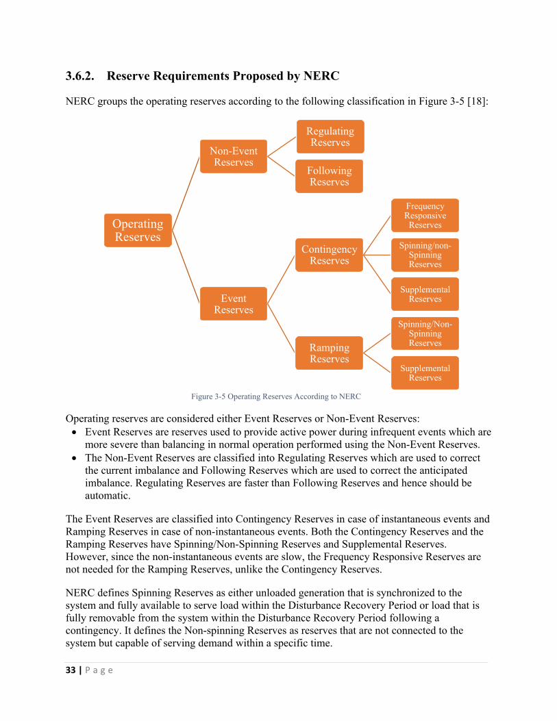
33 | P a g e

3.6.2. Reserve Requirements Proposed by NERC

NERC groups the operating reserves according to the following classification in Figure 3-5 [18]:

Operating Reserves

Non-Event Reserves

Regulating Reserves

Following Reserves

Event Reserves

Contingency Reserves

Frequency Responsive

Reserves

Spinning/non-Spinning Reserves

Supplemental Reserves

Ramping Reserves

Spinning/Non-Spinning Reserves

Supplemental Reserves

Figure 3-5 Operating Reserves According to NERC

Operating reserves are considered either Event Reserves or Non-Event Reserves: Event Reserves are reserves used to provide active power during infrequent events which are

more severe than balancing in normal operation performed using the Non-Event Reserves. The Non-Event Reserves are classified into Regulating Reserves which are used to correct

the current imbalance and Following Reserves which are used to correct the anticipated imbalance. Regulating Reserves are faster than Following Reserves and hence should be automatic.

The Event Reserves are classified into Contingency Reserves in case of instantaneous events and Ramping Reserves in case of non-instantaneous events. Both the Contingency Reserves and the Ramping Reserves have Spinning/Non-Spinning Reserves and Supplemental Reserves. However, since the non-instantaneous events are slow, the Frequency Responsive Reserves are not needed for the Ramping Reserves, unlike the Contingency Reserves.

NERC defines Spinning Reserves as either unloaded generation that is synchronized to the system and fully available to serve load within the Disturbance Recovery Period or load that is fully removable from the system within the Disturbance Recovery Period following a contingency. It defines the Non-spinning Reserves as reserves that are not connected to the system but capable of serving demand within a specific time.

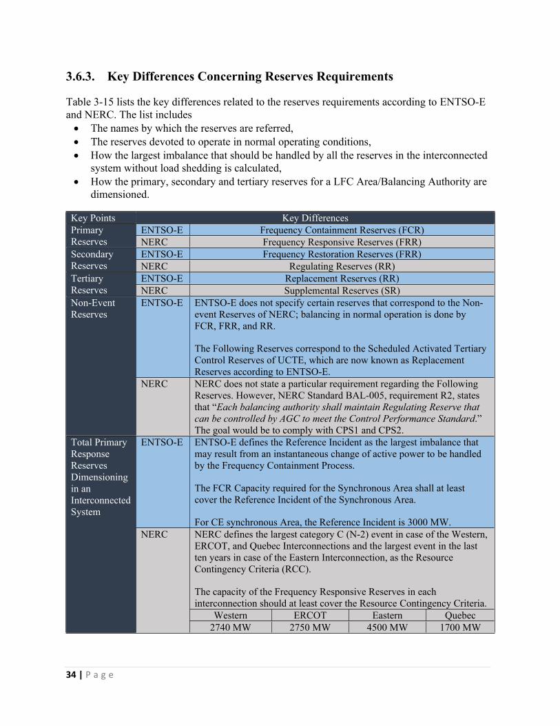
34 | P a g e

3.6.3. Key Differences Concerning Reserves Requirements

Table 3-15 lists the key differences related to the reserves requirements according to ENTSO-E and NERC. The list includes The names by which the reserves are referred, The reserves devoted to operate in normal operating conditions, How the largest imbalance that should be handled by all the reserves in the interconnected

system without load shedding is calculated, How the primary, secondary and tertiary reserves for a LFC Area/Balancing Authority are

dimensioned.

Key Points Key DifferencesENTSO-E Frequency Containment Reserves (FCR)Primary

Reserves NERC Frequency Responsive Reserves (FRR)ENTSO-E Frequency Restoration Reserves (FRR)Secondary

Reserves NERC Regulating Reserves (RR)ENTSO-E Replacement Reserves (RR)Tertiary

Reserves NERC Supplemental Reserves (SR)ENTSO-E ENTSO-E does not specify certain reserves that correspond to the Non-

event Reserves of NERC; balancing in normal operation is done by FCR, FRR, and RR.

The Following Reserves correspond to the Scheduled Activated Tertiary Control Reserves of UCTE, which are now known as Replacement Reserves according to ENTSO-E.

Non-Event Reserves

NERC NERC does not state a particular requirement regarding the Following Reserves. However, NERC Standard BAL-005, requirement R2, states that “Each balancing authority shall maintain Regulating Reserve that can be controlled by AGC to meet the Control Performance Standard.” The goal would be to comply with CPS1 and CPS2.

ENTSO-E ENTSO-E defines the Reference Incident as the largest imbalance that may result from an instantaneous change of active power to be handled by the Frequency Containment Process.

The FCR Capacity required for the Synchronous Area shall at least cover the Reference Incident of the Synchronous Area.

For CE synchronous Area, the Reference Incident is 3000 MW.NERC defines the largest category C (N-2) event in case of the Western, ERCOT, and Quebec Interconnections and the largest event in the last ten years in case of the Eastern Interconnection, as the Resource Contingency Criteria (RCC).

The capacity of the Frequency Responsive Reserves in each interconnection should at least cover the Resource Contingency Criteria.

Western ERCOT Eastern Quebec

Total Primary Response Reserves Dimensioning in an Interconnected System

NERC

2740 MW 2750 MW 4500 MW 1700 MW

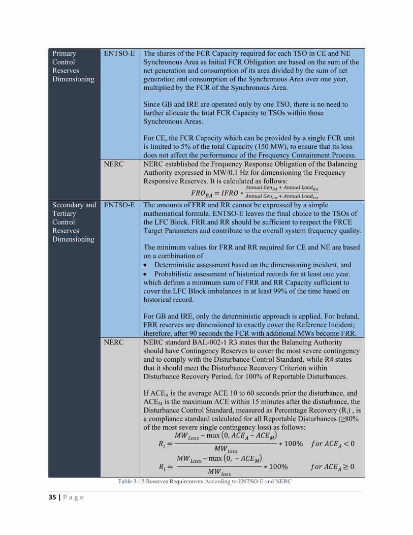
35 | P a g e

ENTSO-E The shares of the FCR Capacity required for each TSO in CE and NE Synchronous Area as Initial FCR Obligation are based on the sum of the net generation and consumption of its area divided by the sum of net generation and consumption of the Synchronous Area over one year, multiplied by the FCR of the Synchronous Area.

Since GB and IRE are operated only by one TSO, there is no need to further allocate the total FCR Capacity to TSOs within those Synchronous Areas.

For CE, the FCR Capacity which can be provided by a single FCR unit is limited to 5% of the total Capacity (150 MW), to ensure that its loss does not affect the performance of the Frequency Containment Process.

Primary Control Reserves Dimensioning

NERC NERC established the Frequency Response Obligation of the Balancing Authority expressed in MW/0.1 Hz for dimensioning the Frequency Responsive Reserves. It is calculated as follows:

𝐹𝑅𝑂𝐵𝐴 = 𝐼𝐹𝑅𝑂 ∗𝐴𝑛𝑛𝑢𝑎𝑙 𝐺𝑒𝑛𝐵𝐴 + 𝐴𝑛𝑛𝑢𝑎𝑙 𝐿𝑜𝑎𝑑𝐵𝐴

𝐴𝑛𝑛𝑢𝑎𝑙 𝐺𝑒𝑛𝐼𝑛𝑡 + 𝐴𝑛𝑛𝑢𝑎𝑙 𝐿𝑜𝑎𝑑𝐼𝑛𝑡

ENTSO-E The amounts of FRR and RR cannot be expressed by a simple mathematical formula. ENTSO-E leaves the final choice to the TSOs of the LFC Block. FRR and RR should be sufficient to respect the FRCE Target Parameters and contribute to the overall system frequency quality.

The minimum values for FRR and RR required for CE and NE are based on a combination of Deterministic assessment based on the dimensioning incident, and Probabilistic assessment of historical records for at least one year.which defines a minimum sum of FRR and RR Capacity sufficient to cover the LFC Block imbalances in at least 99% of the time based on historical record.

For GB and IRE, only the deterministic approach is applied. For Ireland, FRR reserves are dimensioned to exactly cover the Reference Incident; therefore, after 90 seconds the FCR with additional MWs become FRR.

Secondary and Tertiary Control Reserves Dimensioning

NERC NERC standard BAL-002-1 R3 states that the Balancing Authority should have Contingency Reserves to cover the most severe contingency and to comply with the Disturbance Control Standard, while R4 states that it should meet the Disturbance Recovery Criterion within Disturbance Recovery Period, for 100% of Reportable Disturbances.

If ACEA is the average ACE 10 to 60 seconds prior the disturbance, and ACEM is the maximum ACE within 15 minutes after the disturbance, the Disturbance Control Standard, measured as Percentage Recovery (Ri) , is a compliance standard calculated for all Reportable Disturbances (≥80% of the most severe single contingency loss) as follows:

𝑅𝑖 =𝑀𝑊𝐿𝑜𝑠𝑠 ‒ max (0, 𝐴𝐶𝐸𝐴 ‒ 𝐴𝐶𝐸𝑀)

𝑀𝑊𝑙𝑜𝑠𝑠∗ 100% 𝑓𝑜𝑟 𝐴𝐶𝐸𝐴 < 0

𝑅𝑖 = 𝑀𝑊𝐿𝑜𝑠𝑠 ‒ max (0, ‒ 𝐴𝐶𝐸𝑀)

𝑀𝑊𝑙𝑜𝑠𝑠∗ 100% 𝑓𝑜𝑟 𝐴𝐶𝐸𝐴 ≥ 0

Table 3-15 Reserves Requirements According to ENTSO-E and NERC

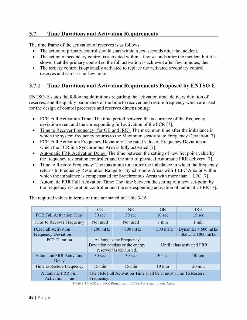
36 | P a g e

3.7. Time Durations and Activation Requirements

The time frame of the activation of reserves is as follows: The action of primary control should start within a few seconds after the incident, The action of secondary control is activated within a few seconds after the incident but it is

slower that the primary control so the full activation is achieved after few minutes, then The tertiary control is optionally activated to replace the activated secondary control

reserves and can last for few hours.

3.7.1. Time Durations and Activation Requirements Proposed by ENTSO-E

ENTSO-E states the following definitions regarding the activation time, delivery duration of reserves, and the quality parameters of the time to recover and restore frequency which are used for the design of control processes and reserves dimensioning:

FCR Full Activation Time: The time period between the occurrence of the frequency deviation event and the corresponding full activation of the FCR [7].

Time to Recover Frequency (for GB and IRE): The maximum time after the imbalance in which the system frequency returns to the Maximum steady state Frequency Deviation [7].

FCR Full Activation Frequency Deviation: The rated value of Frequency Deviation at which the FCR in a Synchronous Area is fully activated [7].

Automatic FRR Activation Delay: The time between the setting of new Set point value by the frequency restoration controller and the start of physical Automatic FRR delivery [7].

Time to Restore Frequency: The maximum time after the imbalance in which the frequency returns to Frequency Restoration Range for Synchronous Areas with 1 LFC Area or within which the imbalance is compensated for Synchronous Areas with more than 1 LFC [7].

Automatic FRR Full Activation Time: The time between the setting of a new set-point by the frequency restoration controller and the corresponding activation of automatic FRR [7].

The required values in terms of time are stated in Table 3-16.

CE NE GB IREFCR Full Activation Time 30 sec 30 sec 10 sec 15 sec

Time to Recover Frequency Not used Not used 1 min 1 minFCR Full Activation Frequency Deviation

± 200 mHz ± 500 mHz ± 500 mHz Dynamic: ± 500 mHz.Static: ± 1000 mHz.

FCR Duration As long as the Frequency Deviation persists or the energy

reservoir is exhausted.Until it has activated FRR.

Automatic FRR Activation Delay

30 sec 30 sec 30 sec 30 sec

Time to Restore Frequency 15 min 15 min 10 min 20 minAutomatic FRR Full

Activation TimeThe FRR Full Activation Time shall be at most Time To Restore Frequency.

Table 3-16 FCR and FRR Properties in ENTSO-E Synchronous Areas

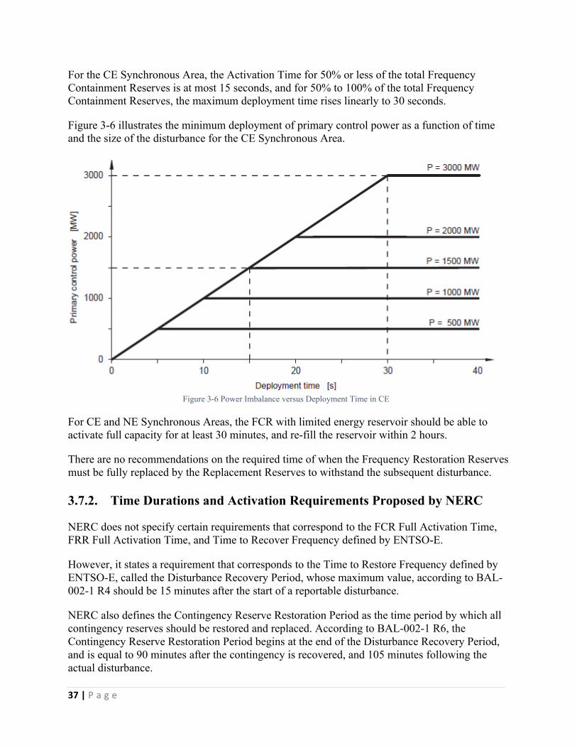
37 | P a g e

For the CE Synchronous Area, the Activation Time for 50% or less of the total Frequency Containment Reserves is at most 15 seconds, and for 50% to 100% of the total Frequency Containment Reserves, the maximum deployment time rises linearly to 30 seconds.

Figure 3-6 illustrates the minimum deployment of primary control power as a function of time and the size of the disturbance for the CE Synchronous Area.

Figure 3-6 Power Imbalance versus Deployment Time in CE

For CE and NE Synchronous Areas, the FCR with limited energy reservoir should be able to activate full capacity for at least 30 minutes, and re-fill the reservoir within 2 hours.

There are no recommendations on the required time of when the Frequency Restoration Reserves must be fully replaced by the Replacement Reserves to withstand the subsequent disturbance.

3.7.2. Time Durations and Activation Requirements Proposed by NERC

NERC does not specify certain requirements that correspond to the FCR Full Activation Time, FRR Full Activation Time, and Time to Recover Frequency defined by ENTSO-E.

However, it states a requirement that corresponds to the Time to Restore Frequency defined by ENTSO-E, called the Disturbance Recovery Period, whose maximum value, according to BAL-002-1 R4 should be 15 minutes after the start of a reportable disturbance.

NERC also defines the Contingency Reserve Restoration Period as the time period by which all contingency reserves should be restored and replaced. According to BAL-002-1 R6, the Contingency Reserve Restoration Period begins at the end of the Disturbance Recovery Period, and is equal to 90 minutes after the contingency is recovered, and 105 minutes following the actual disturbance.

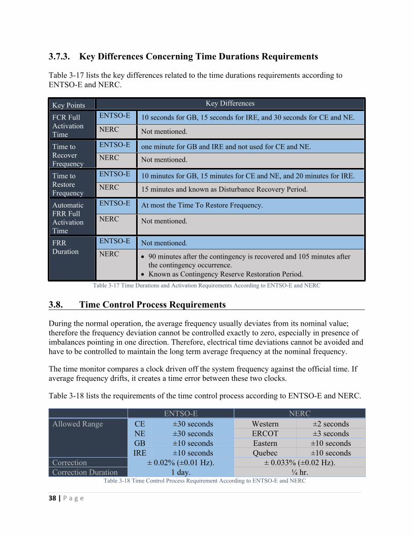
38 | P a g e

3.7.3. Key Differences Concerning Time Durations Requirements

Table 3-17 lists the key differences related to the time durations requirements according to ENTSO-E and NERC.

Key Points Key DifferencesENTSO-E 10 seconds for GB, 15 seconds for IRE, and 30 seconds for CE and NE.FCR Full

Activation Time

NERC Not mentioned.

ENTSO-E one minute for GB and IRE and not used for CE and NE.Time to Recover Frequency

NERC Not mentioned.

ENTSO-E 10 minutes for GB, 15 minutes for CE and NE, and 20 minutes for IRE.Time to Restore Frequency

NERC 15 minutes and known as Disturbance Recovery Period.

ENTSO-E At most the Time To Restore Frequency.Automatic FRR Full Activation Time

NERC Not mentioned.

ENTSO-E Not mentioned.FRR Duration NERC 90 minutes after the contingency is recovered and 105 minutes after

the contingency occurrence. Known as Contingency Reserve Restoration Period.

Table 3-17 Time Durations and Activation Requirements According to ENTSO-E and NERC

3.8. Time Control Process Requirements

During the normal operation, the average frequency usually deviates from its nominal value; therefore the frequency deviation cannot be controlled exactly to zero, especially in presence of imbalances pointing in one direction. Therefore, electrical time deviations cannot be avoided and have to be controlled to maintain the long term average frequency at the nominal frequency.

The time monitor compares a clock driven off the system frequency against the official time. If average frequency drifts, it creates a time error between these two clocks.

Table 3-18 lists the requirements of the time control process according to ENTSO-E and NERC.

ENTSO-E NERCCE ±30 seconds Western ±2 secondsNE ±30 seconds ERCOT ±3 secondsGB ±10 seconds Eastern ±10 seconds

Allowed Range

IRE ±10 seconds Quebec ±10 secondsCorrection ± 0.02% (±0.01 Hz). ± 0.033% (±0.02 Hz).Correction Duration 1 day. ¼ hr.

Table 3-18 Time Control Process Requirement According to ENTSO-E and NERC

39 | P a g e

CHAPTER 44. Operational Security and Emergency Operations

This chapter presents how ENTSO-E and NERC consider the Operational Security and Emergency Operations and is organized as follows: introduction, operating conditions of electric power systems, events and contingencies classification, operational requirements during contingencies, Remedial Actions, System Defense, Load Shedding, System Restoration, System Protection, Monitoring and Data Exchange.

4.1. Introduction

Recently, issues related to the Operational Security of interconnected power grids have further increased as new risks have been identified due to the following reasons [19]:

Market:

increasing power exchanges between interconnected grid operators, difficulties in forecasting load/generation variations due to normal operation evolution, and market imbalances at the end of the hour, causing periodic frequency deviations and

reserves activation, which endangers the Operational Security as it limits the reserves, which may be needed in case of a frequency deviation event due to loss of generation.

Renewable energy sources (RES):

The intermittent nature of the variable generation of the RES, and Low natural inertia provided by the RES compared to the conventional plants, leading to

larger frequency deviations at the end of each hour, during the off-peak periods when the generation is high and the demand is low, and during a frequency deviation event.

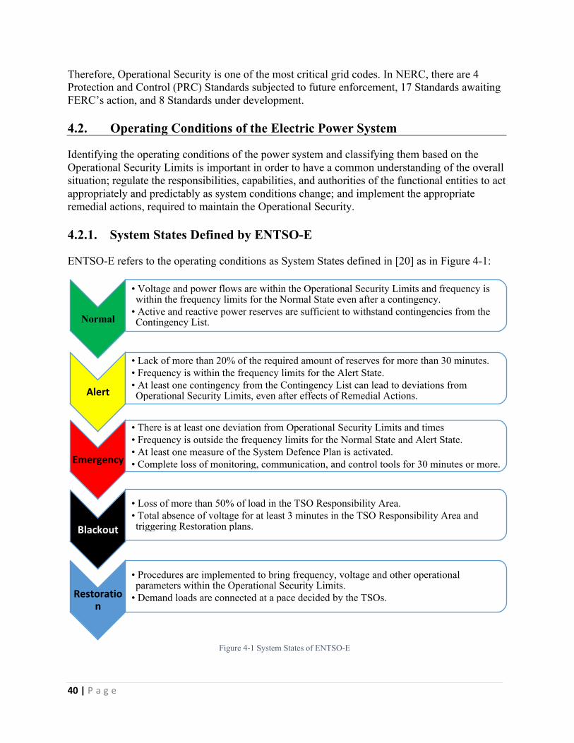
40 | P a g e

Therefore, Operational Security is one of the most critical grid codes. In NERC, there are 4 Protection and Control (PRC) Standards subjected to future enforcement, 17 Standards awaiting FERC’s action, and 8 Standards under development.

4.2. Operating Conditions of the Electric Power System

Identifying the operating conditions of the power system and classifying them based on the Operational Security Limits is important in order to have a common understanding of the overall situation; regulate the responsibilities, capabilities, and authorities of the functional entities to act appropriately and predictably as system conditions change; and implement the appropriate remedial actions, required to maintain the Operational Security.

4.2.1. System States Defined by ENTSO-E

ENTSO-E refers to the operating conditions as System States defined in [20] as in Figure 4-1:

Normal

• Voltage and power flows are within the Operational Security Limits and frequency is within the frequency limits for the Normal State even after a contingency.

• Active and reactive power reserves are sufficient to withstand contingencies from the Contingency List.

Alert

• Lack of more than 20% of the required amount of reserves for more than 30 minutes.• Frequency is within the frequency limits for the Alert State.• At least one contingency from the Contingency List can lead to deviations from Operational Security Limits, even after effects of Remedial Actions.

Emergency

• There is at least one deviation from Operational Security Limits and times• Frequency is outside the frequency limits for the Normal State and Alert State.• At least one measure of the System Defence Plan is activated.• Complete loss of monitoring, communication, and control tools for 30 minutes or more.

Blackout

• Loss of more than 50% of load in the TSO Responsibility Area.• Total absence of voltage for at least 3 minutes in the TSO Responsibility Area and triggering Restoration plans.

Restoration

• Procedures are implemented to bring frequency, voltage and other operational parameters within the Operational Security Limits.

• Demand loads are connected at a pace decided by the TSOs.

Figure 4-1 System States of ENTSO-E

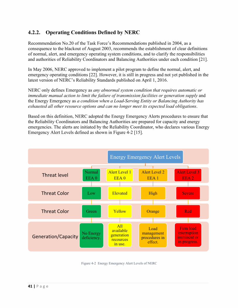
41 | P a g e

4.2.2. Operating Conditions Defined by NERC

Recommendation No.20 of the Task Force’s Recommendations published in 2004, as a consequence to the blackout of August 2003, recommends the establishment of clear definitions of normal, alert, and emergency operating system conditions, and to clarify the responsibilities and authorities of Reliability Coordinators and Balancing Authorities under each condition [21].

In May 2006, NERC approved to implement a pilot program to define the normal, alert, and emergency operating conditions [22]. However, it is still in progress and not yet published in the latest version of NERC’s Reliability Standards published on April 1, 2016.

NERC only defines Emergency as any abnormal system condition that requires automatic or immediate manual action to limit the failure of transmission facilities or generation supply and the Energy Emergency as a condition when a Load-Serving Entity or Balancing Authority has exhausted all other resource options and can no longer meet its expected load obligations.

Based on this definition, NERC adopted the Energy Emergency Alerts procedures to ensure that the Reliability Coordinators and Balancing Authorities are prepared for capacity and energy emergencies. The alerts are initiated by the Reliability Coordinator, who declares various Energy Emergency Alert Levels defined as shown in Figure 4-2 [15].

Generation/Capacity

Threat Color

Threat Color

Threat level

Energy Emergency Alert Levels

NormalEEA 0

Low

Green

No Energy deficiency.

Alert Level 1EEA 0

Elevated

Yellow

All available

generation recources

in use.

Alert Level 2EEA 1

High

Orange

Load management procedures in

effect.

Alert Level 3EEA 2

Severe

Red

Firm load interruption imminent or in progress.

Figure 4-2 Energy Emergency Alert Levels of NERC

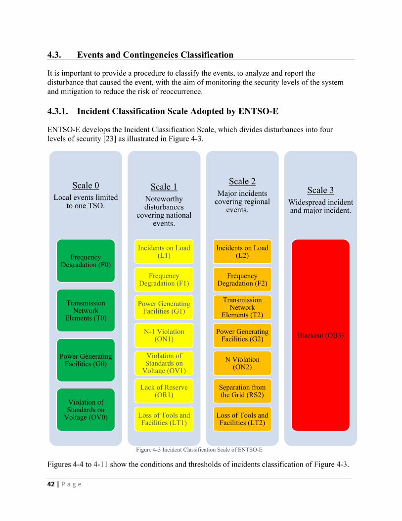
42 | P a g e

4.3. Events and Contingencies Classification

It is important to provide a procedure to classify the events, to analyze and report the disturbance that caused the event, with the aim of monitoring the security levels of the system and mitigation to reduce the risk of reoccurrence.

4.3.1. Incident Classification Scale Adopted by ENTSO-E

ENTSO-E develops the Incident Classification Scale, which divides disturbances into four levels of security [23] as illustrated in Figure 4-3.

Scale 0Local events limited

to one TSO.

Frequency Degradation (F0)

Transmission Network

Elements (T0)

Power Generating Facilities (G0)

Violation of Standards on

Voltage (OV0)

Scale 1Noteworthy disturbances

covering national events.

Incidents on Load (L1)

Frequency Degradation (F1)

Power Generating Facilities (G1)

N-1 Violation (ON1)

Violation of Standards on

Voltage (OV1)

Lack of Reserve (OR1)

Loss of Tools and Facilities (LT1)

Scale 2Major incidents

covering regional events.

Incidents on Load (L2)

Frequency Degradation (F2)

Transmission Network

Elements (T2)

Power Generating Facilities (G2)

N Violation (ON2)

Separation from the Grid (RS2)

Loss of Tools and Facilities (LT2)

Scale 3Widespread incident and major incident.

Blackout (OB3)

Figure 4-3 Incident Classification Scale of ENTSO-E

Figures 4-4 to 4-11 show the conditions and thresholds of incidents classification of Figure 4-3.

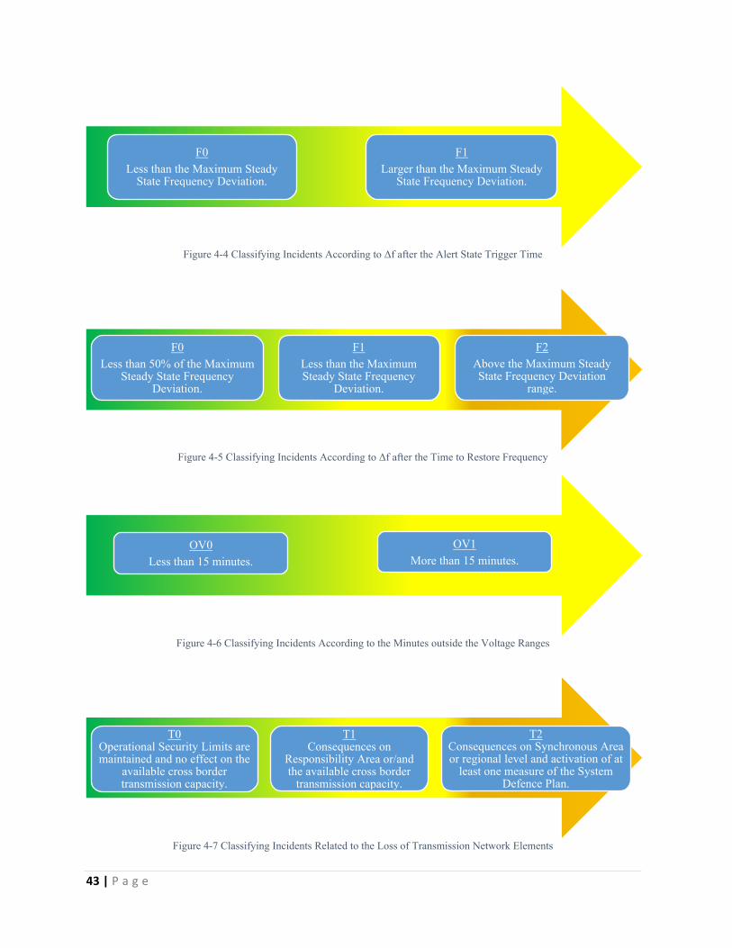
43 | P a g e

F0Less than the Maximum Steady

State Frequency Deviation.

F1Larger than the Maximum Steady

State Frequency Deviation.

Figure 4-4 Classifying Incidents According to Δf after the Alert State Trigger Time

F0Less than 50% of the Maximum

Steady State Frequency Deviation.

F1Less than the Maximum Steady State Frequency

Deviation.

F2Above the Maximum Steady State Frequency Deviation

range.

Figure 4-5 Classifying Incidents According to Δf after the Time to Restore Frequency

OV0Less than 15 minutes.

OV1More than 15 minutes.

Figure 4-6 Classifying Incidents According to the Minutes outside the Voltage Ranges

T0Operational Security Limits are maintained and no effect on the

available cross border transmission capacity.

T1Consequences on

Responsibility Area or/and the available cross border

transmission capacity.

T2Consequences on Synchronous Area or regional level and activation of at

least one measure of the System Defence Plan.

Figure 4-7 Classifying Incidents Related to the Loss of Transmission Network Elements

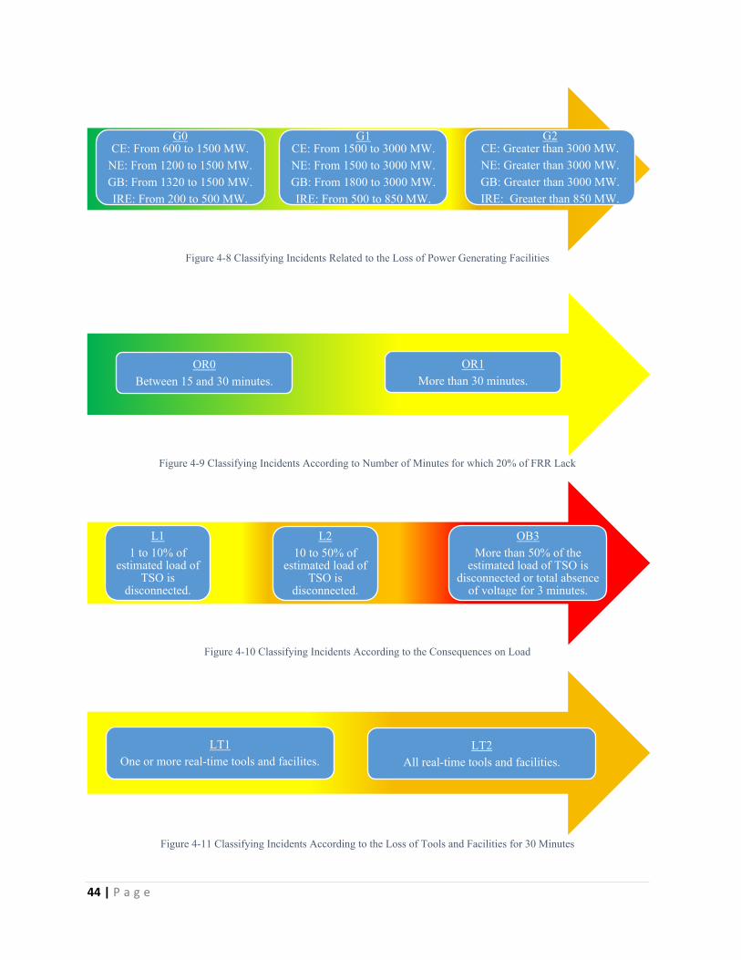
44 | P a g e

G0CE: From 600 to 1500 MW.

NE: From 1200 to 1500 MW.GB: From 1320 to 1500 MW.IRE: From 200 to 500 MW.

G1CE: From 1500 to 3000 MW.NE: From 1500 to 3000 MW.GB: From 1800 to 3000 MW.IRE: From 500 to 850 MW.

G2CE: Greater than 3000 MW.NE: Greater than 3000 MW.GB: Greater than 3000 MW.IRE: Greater than 850 MW.

Figure 4-8 Classifying Incidents Related to the Loss of Power Generating Facilities

OR0Between 15 and 30 minutes.

OR1More than 30 minutes.

Figure 4-9 Classifying Incidents According to Number of Minutes for which 20% of FRR Lack

L11 to 10% of

estimated load of TSO is

disconnected.

L210 to 50% of

estimated load of TSO is

disconnected.

OB3More than 50% of the

estimated load of TSO is disconnected or total absence

of voltage for 3 minutes.

Figure 4-10 Classifying Incidents According to the Consequences on Load

LT1One or more real-time tools and facilites.

LT2All real-time tools and facilities.

Figure 4-11 Classifying Incidents According to the Loss of Tools and Facilities for 30 Minutes

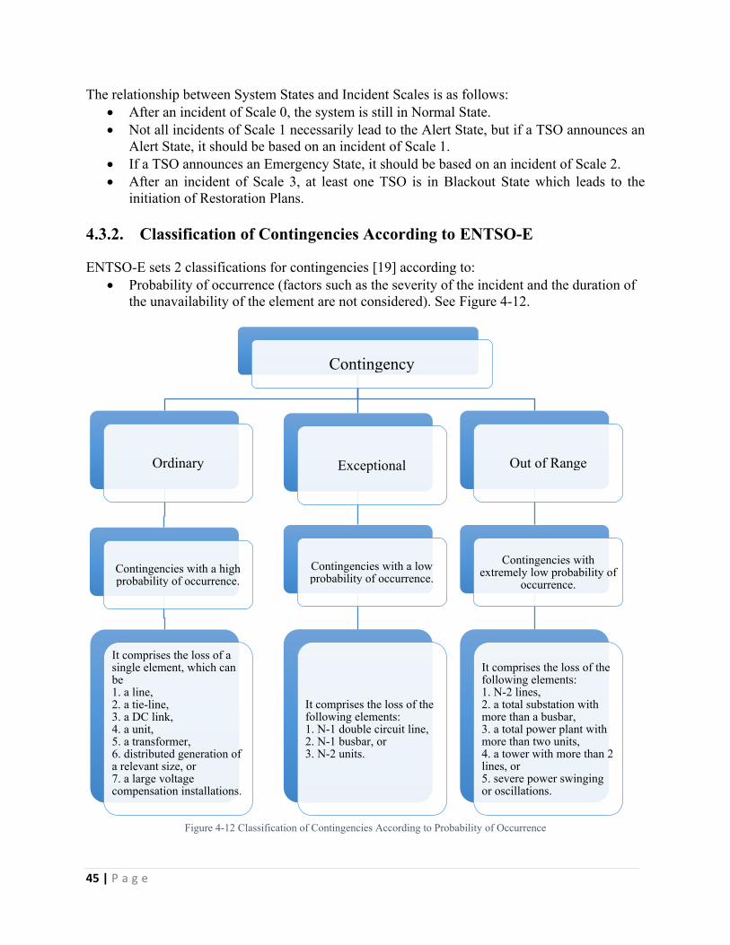
45 | P a g e

The relationship between System States and Incident Scales is as follows: After an incident of Scale 0, the system is still in Normal State. Not all incidents of Scale 1 necessarily lead to the Alert State, but if a TSO announces an

Alert State, it should be based on an incident of Scale 1. If a TSO announces an Emergency State, it should be based on an incident of Scale 2. After an incident of Scale 3, at least one TSO is in Blackout State which leads to the

initiation of Restoration Plans.

4.3.2. Classification of Contingencies According to ENTSO-E

ENTSO-E sets 2 classifications for contingencies [19] according to: Probability of occurrence (factors such as the severity of the incident and the duration of

the unavailability of the element are not considered). See Figure 4-12.

Contingency

Ordinary

Contingencies with a high probability of occurrence.

It comprises the loss of a single element, which can be1. a line,2. a tie-line,3. a DC link,4. a unit,5. a transformer,6. distributed generation of a relevant size, or7. a large voltage compensation installations.

Exceptional

Contingencies with a low probability of occurrence.

It comprises the loss of the following elements:1. N-1 double circuit line,2. N-1 busbar, or3. N-2 units.

Out of Range

Contingencies with extremely low probability of

occurrence.

It comprises the loss of the following elements:1. N-2 lines,2. a total substation with more than a busbar,3. a total power plant with more than two units,4. a tower with more than 2 lines, or5. severe power swinging or oscillations.

Figure 4-12 Classification of Contingencies According to Probability of Occurrence

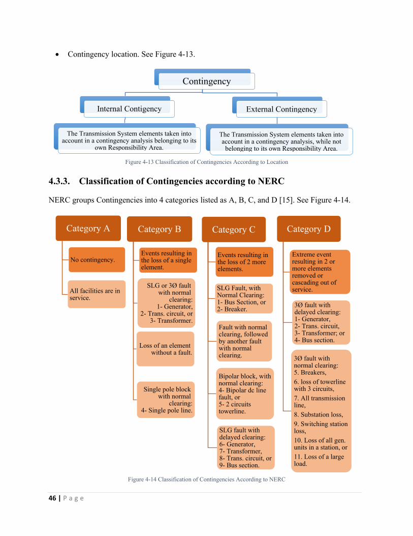
46 | P a g e

Contingency location. See Figure 4-13.

Contingency

Internal Contigency

The Transmission System elements taken into account in a contingency analysis belonging to its

own Responsibility Area.

External Contingency

The Transmission System elements taken into account in a contingency analysis, while not

belonging to its own Responsibility Area.

Figure 4-13 Classification of Contingencies According to Location

4.3.3. Classification of Contingencies according to NERC

NERC groups Contingencies into 4 categories listed as A, B, C, and D [15]. See Figure 4-14.

Category A

No contingency.

All facilities are in service.

Category B

Events resulting in the loss of a single element.

SLG or 3Ø fault with normal

clearing:1- Generator,

2- Trans. circuit, or3- Transformer.

Loss of an element without a fault.

Single pole block with normal

clearing:4- Single pole line.

Category C

Events resulting in the loss of 2 more elements.

SLG Fault, with Normal Clearing:1- Bus Section, or2- Breaker.

Fault with normal clearing, followed by another fault with normal clearing.

Bipolar block, with normal clearing:4- Bipolar dc line fault, or5- 2 circuits towerline.

SLG fault with delayed clearing:6- Generator,7- Transformer,8- Trans. circuit, or9- Bus section.

Category D

Extreme event resulting in 2 or more elements removed or cascading out of service.

3Ø fault with delayed clearing:1- Generator,2- Trans. circuit,3- Transformer; or4- Bus section.

3Ø fault with normal clearing:5. Breakers,6. loss of towerline with 3 circuits,7. All transmission line,8. Substation loss,9. Switching station loss,10. Loss of all gen. units in a station, or11. Loss of a large load.

Figure 4-14 Classification of Contingencies According to NERC

47 | P a g e

4.4. Operational Requirements during Contingencies

Contingencies according to each interconnected network were classified in the previous section. This section illustrates the operational requirements imposed by the two networks in case of occurrence of one or more contingencies listed above.

4.4.1. Operational Requirements Imposed by ENTSO-E

ENTSO-E adopts the N-1 Criterion, which states that any contingency from the contingency list must not endanger the Operational Security of the interconnected operation, taking into account available Remedial Actions [20]. The N-1 Criterion also forces the TSO to prevent the propagation of incident “No cascading with impact outside my borders”.

The N-1 is based on Risk assessment by each TSO, Contingencies and severity of their consequences, Area to be observed by each TSO, Operational Security Limits, Remedial Actions to cope with, and Strengthened coordination between TSOs to implement such stronger commitments.

4.4.2. Operational Requirements Imposed by NERC

As illustrated before, there are four categories of contingencies according to NERC [15]:

Category A, no contingency;TPL-001-0.1(i) R1 states that “with all transmission facilities in service and with normal (pre-contingency) operating procedures, the Network can be operated to supply projected customer demands and projected Firm Transmission Services at all Demand levels.”

Category B, events resulting in the loss of a single element;TPL-002-0(i)b R1 states that “Network can be operated to supply projected customer demands and projected Firm Transmission Services, at all demand levels over the range of forecast system demands, under contingency conditions defined in Category B.”

Category C, events resulting in the loss of 2 more elements; andTPL-003-0(i)b R1 states that “Network can be operated to supply projected customer demands and projected Firm Transmission Services, at all demand levels over the range of forecast system demands, under contingency conditions defined in Category C.”

Category D, extreme event resulting in 2 or more elements removed or cascading.TPL-004-0(i)a R1 states that “The interconnected transmission system is evaluated for the risks and consequences of a number of each of the extreme contingencies that are listed under Category D.”

It can be deduced from the requirements listed above, that NERC has more strict operational requirements beyond the N-1 Criterion adopted by ENTSO-E.

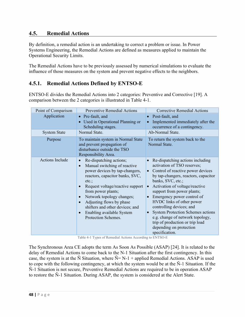
48 | P a g e

4.5. Remedial Actions

By definition, a remedial action is an undertaking to correct a problem or issue. In Power Systems Engineering, the Remedial Actions are defined as measures applied to maintain the Operational Security Limits.

The Remedial Actions have to be previously assessed by numerical simulations to evaluate the influence of those measures on the system and prevent negative effects to the neighbors.

4.5.1. Remedial Actions Defined by ENTSO-E

ENTSO-E divides the Remedial Actions into 2 categories: Preventive and Corrective [19]. A comparison between the 2 categories is illustrated in Table 4-1.

Point of Comparison Preventive Remedial Actions Corrective Remedial ActionsApplication Pre-fault, and

Used in Operational Planning or Scheduling stages.

Post-fault, and Implemented immediately after the

occurrence of a contingency.System State Normal State. Ab-Normal State.

Purpose To maintain system in Normal State and prevent propagation of disturbance outside the TSO Responsibility Area.

To return the system back to the Normal State.

Actions Include Re-dispatching actions; Manual switching of reactive

power devices by tap-changers, reactors, capacitor banks, SVC, etc.;

Request voltage/reactive support from power plants;

Network topology changes; Adjusting flows by phase

shifters and other devices; and Enabling available System

Protection Schemes.

Re-dispatching actions including activation of TSO reserves;

Control of reactive power devices by tap-changers, reactors, capacitor banks, SVC, etc.;

Activation of voltage/reactive support from power plants;

Emergency power control of HVDC links of other power controlling devices; and

System Protection Schemes actions e.g. change of network topology, trip of production or trip load depending on protection specification.

Table 4-1 Types of Remedial Actions According to ENTSO-E

The Synchronous Area CE adopts the term As Soon As Possible (ASAP) [24]. It is related to the delay of Remedial Actions to come back to the N-1 Situation after the first contingency. In this case, the system is at the Ñ Situation, where Ñ= N-1 + applied Remedial Actions. ASAP is used to cope with the following contingency, at which the system would be at the Ñ-1 Situation. If the Ñ-1 Situation is not secure, Preventive Remedial Actions are required to be in operation ASAP to restore the Ñ-1 Situation. During ASAP, the system is considered at the Alert State.

49 | P a g e

4.5.2. Remedial Actions Defined by NERC

NERC Reliability Standards use the term Special Protection System (SPS) and Remedial Action Scheme (RAS). It developed the Standards PRC-012-0, PRC-013-0, PRC-014-0, PRC-015-0, PRC-016-0.1 and PRC-017-0 related to the SPS and PRC-012-1, PRC-013-1, PRC-014-1, PRC-015-1, PRC-016-1 and PRC-017-1 related to RAS. However, there is a lack of clarity across the eight NERC regions concerning identifying what schemes are considered an SPS or RAS. This confusion leads to inconsistent and redundant application of the SPS or RAS related Reliability Standards [25].

Currently, both terms SPS and RAS, are used in the eight NERC regions. However, the Standard Drafting Team (SDT) recommends that the term RAS remains as the recognized term and the term SPS to be retired [25]; the Glossary of NERC Reliability Standards refers in the definition of SPS to the RAS in the Reliability Standards document published in April 2016. The term RAS: Is more illustrative of the purpose for which the scheme is installed, Eliminates the confusion between the two terms “Special Protection System” and

“Protection System”, and Is not related to “Protection Systems” but may share schemes with “Protection Systems”.

The Remedial Action Scheme has following objectives: Meet requirements identified in the NERC Reliability Standards, Maintain system stability, Maintain acceptable System voltages, Maintain acceptable power flows, Limit the impact of cascading, and Address other Bulk Electric System reliability concerns.

Some actions are considered as Protection that are not included in the Remedial Action Scheme: Out-of-step tripping and power swing blocking, Under-Frequency Load Shedding (UFLS), Under-Voltage Load Shedding (UVLS), and Fault conditions that must be isolated.

4.6. System Defense

It is important for every interconnected network to adopt a plan or program to be implemented in case of emergency, to prevent large disturbances and to mitigate the risk of frequency and voltage collapse, to protect all the electrical elements connected to the network against under/over-frequency and under/over-voltage operating conditions.

The System Defense measures are complementary to Remedial Actions and can be activated while Remedial Actions are ongoing. The System Defense is triggered only when the system is in Emergency State.

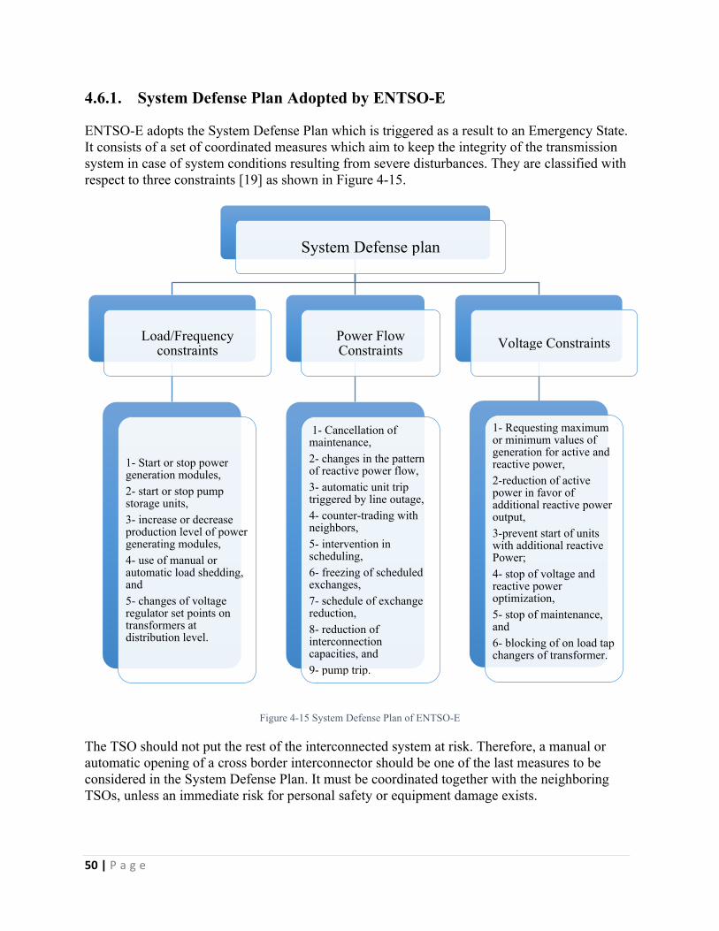
50 | P a g e

4.6.1. System Defense Plan Adopted by ENTSO-E

ENTSO-E adopts the System Defense Plan which is triggered as a result to an Emergency State. It consists of a set of coordinated measures which aim to keep the integrity of the transmission system in case of system conditions resulting from severe disturbances. They are classified with respect to three constraints [19] as shown in Figure 4-15.

System Defense plan

Load/Frequency constraints

1- Start or stop power generation modules,2- start or stop pump storage units,3- increase or decrease production level of power generating modules,4- use of manual or automatic load shedding, and5- changes of voltage regulator set points on transformers at distribution level.

Power Flow Constraints

1- Cancellation of maintenance,2- changes in the pattern of reactive power flow,3- automatic unit trip triggered by line outage,4- counter-trading with neighbors,5- intervention in scheduling,6- freezing of scheduled exchanges,7- schedule of exchange reduction,8- reduction of interconnection capacities, and9- pump trip.

Voltage Constraints

1- Requesting maximum or minimum values of generation for active and reactive power,2-reduction of active power in favor of additional reactive power output,3-prevent start of units with additional reactive Power;4- stop of voltage and reactive power optimization,5- stop of maintenance, and6- blocking of on load tap changers of transformer.

Figure 4-15 System Defense Plan of ENTSO-E

The TSO should not put the rest of the interconnected system at risk. Therefore, a manual or automatic opening of a cross border interconnector should be one of the last measures to be considered in the System Defense Plan. It must be coordinated together with the neighboring TSOs, unless an immediate risk for personal safety or equipment damage exists.

51 | P a g e

4.6.2. System Defense According to NERC

NERC adopts the Operating Plan whose one of its functions is to implement a set of plans to mitigate operating emergencies which should be coordinated with other Transmission Operators, Balancing Authorities, and Reliability Coordinators.

According to EOP-001, each Balancing Authority and Transmission Operator should develop and implement a set of plans in order to

Mitigate operating emergencies for insufficient generating capacity, Mitigate operating emergencies on the transmission system, Shed load.

The Emergency Plans should include Roles and responsibilities for activating the Operation Plans, Communication protocols to be used during emergencies, A list of controlling actions in case of emergency taking into account load-shedding, The tasks that are coordinated with other operators, Cancellation or recall of transmission and generation outage, Re-dispatch of generation requests, Staffing levels for the emergency ensuring that they have suitable knowledge, skills and

experience to operate safely.

Attachment 1 of EOP-001 and EOP-011 R2 list the applicable elements that should be considered in development of the Emergency Plan as

Fuel supply, Fuel switching, Maximum generator output and availability, Environmental constraints and reliability impacts of extreme weather conditions, System energy use, Load management, Interruptible and curtailable loads and demand response, Public appeals for voluntary Load reductions, Appeals to customers to use alternative fuels, Requests of government to implement their programs to achieve energy reductions, Notifications of government agencies, Notifications to operating entities.

The coordination with other operators include Reliable communication between interconnected systems, New interchange agreements, Transmission and generator maintenance schedule, Deliveries of electrical energy from remote systems through normal operating channels.

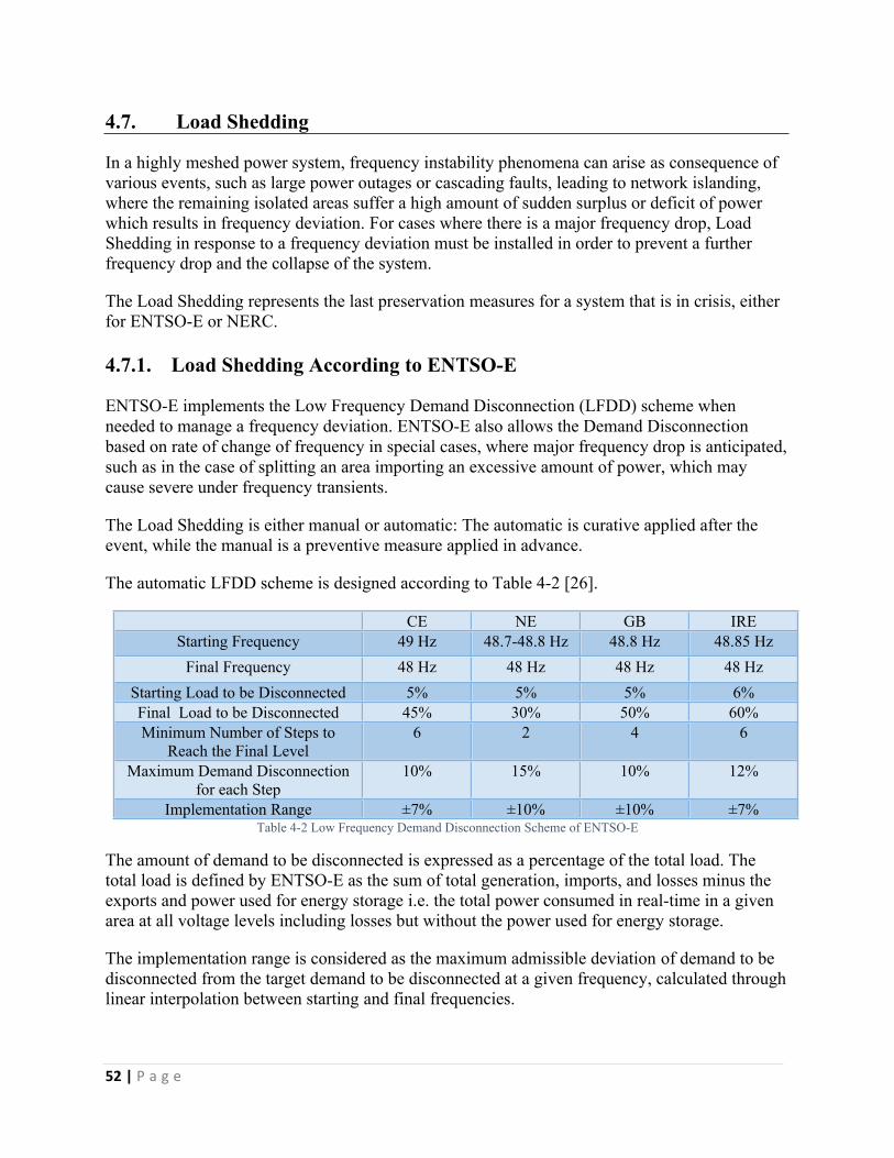
52 | P a g e

4.7. Load Shedding

In a highly meshed power system, frequency instability phenomena can arise as consequence of various events, such as large power outages or cascading faults, leading to network islanding, where the remaining isolated areas suffer a high amount of sudden surplus or deficit of power which results in frequency deviation. For cases where there is a major frequency drop, Load Shedding in response to a frequency deviation must be installed in order to prevent a further frequency drop and the collapse of the system.

The Load Shedding represents the last preservation measures for a system that is in crisis, either for ENTSO-E or NERC.

4.7.1. Load Shedding According to ENTSO-E

ENTSO-E implements the Low Frequency Demand Disconnection (LFDD) scheme when needed to manage a frequency deviation. ENTSO-E also allows the Demand Disconnection based on rate of change of frequency in special cases, where major frequency drop is anticipated, such as in the case of splitting an area importing an excessive amount of power, which may cause severe under frequency transients.

The Load Shedding is either manual or automatic: The automatic is curative applied after the event, while the manual is a preventive measure applied in advance.

The automatic LFDD scheme is designed according to Table 4-2 [26].

CE NE GB IREStarting Frequency 49 Hz 48.7-48.8 Hz 48.8 Hz 48.85 Hz

Final Frequency 48 Hz 48 Hz 48 Hz 48 HzStarting Load to be Disconnected 5% 5% 5% 6%Final Load to be Disconnected 45% 30% 50% 60%Minimum Number of Steps to

Reach the Final Level6 2 4 6

Maximum Demand Disconnection for each Step

10% 15% 10% 12%

Implementation Range ±7% ±10% ±10% ±7%Table 4-2 Low Frequency Demand Disconnection Scheme of ENTSO-E

The amount of demand to be disconnected is expressed as a percentage of the total load. The total load is defined by ENTSO-E as the sum of total generation, imports, and losses minus the exports and power used for energy storage i.e. the total power consumed in real-time in a given area at all voltage levels including losses but without the power used for energy storage.

The implementation range is considered as the maximum admissible deviation of demand to be disconnected from the target demand to be disconnected at a given frequency, calculated through linear interpolation between starting and final frequencies.

53 | P a g e

ENTSO-E imposes the following obligations in the LFDD scheme:

The implementation range does not allow disconnection of less demand than the demand required to be disconnected at the starting frequency.

The starting frequency value is determined by the minimum frequency of the automatic disconnection of pump-storage generating units, taking into consideration a necessary security margin.

When the frequency deviates between the starting frequency and the final frequency, the LFDD scheme should disconnect an amount of load inside the range between the starting demand to be disconnected and the final demand to be disconnected, with tolerance margin corresponding to the implementation range.

The Load Shedding is a stepwise mechanism. The number of steps and the value of the demand to be disconnected are chosen in order to avoid overcompensation or frequency stagnation at low values.

If the maximum allowed amplitude of a single step is exceeded, the TSO must increase the number of steps in order to comply with it.

Frequency should be stabilized within a suitable margin above the disconnection threshold for generating units which is 47.5 Hz.

The appropriate ideal frequency to the system after Load Shedding triggering is in the range of ± 200 mHz around 50 Hz.

The tripping time of Load Shedding relays is the sum of the time needed for measurement of frequency, trip action of auxiliary circuits, and circuit breaker opening time. ENTSO-E expects it to be in the range of 150 ms without any intentional delay.

The under-frequency events have greater effect when it comes to the loss of conventional generating units; therefore, ENTSO-E recommends to minimize the disconnection of the generating units with high inertia.

The Load Shedding plan is executed at a national level i.e. member states, due to the different characteristics of each system and implementation choice.

The Load Shedding plan should be implemented in a regionally, evenly geographical, and distributed way. However, from Synchronous Area point of view, the global amount of load that is shed in each country is important to be proportional among all the member states. But if locally, the amount of load shed differs, it is not a cross-border issue.

4.7.2. Load Shedding According to NERC

The Reliability Standard PRC-006-2 describes the criteria upon which the Load Shedding plan is implemented. Requirement R1 and R2 oblige each Planning Coordinator to select portions of the Bulk Electric System that form islands according to criteria that are based on system studies and historical events. These portions are designed to detach from the interconnection as a result of the operation of a relay scheme.

Requirement R3 states that the frequency should remain above the under-frequency performance characteristic curve and below the over-frequency performance characteristic curve, shown in Figure 4-16, either for 60 seconds or till a steady-state condition between 59.3 Hz and 60.7 Hz.

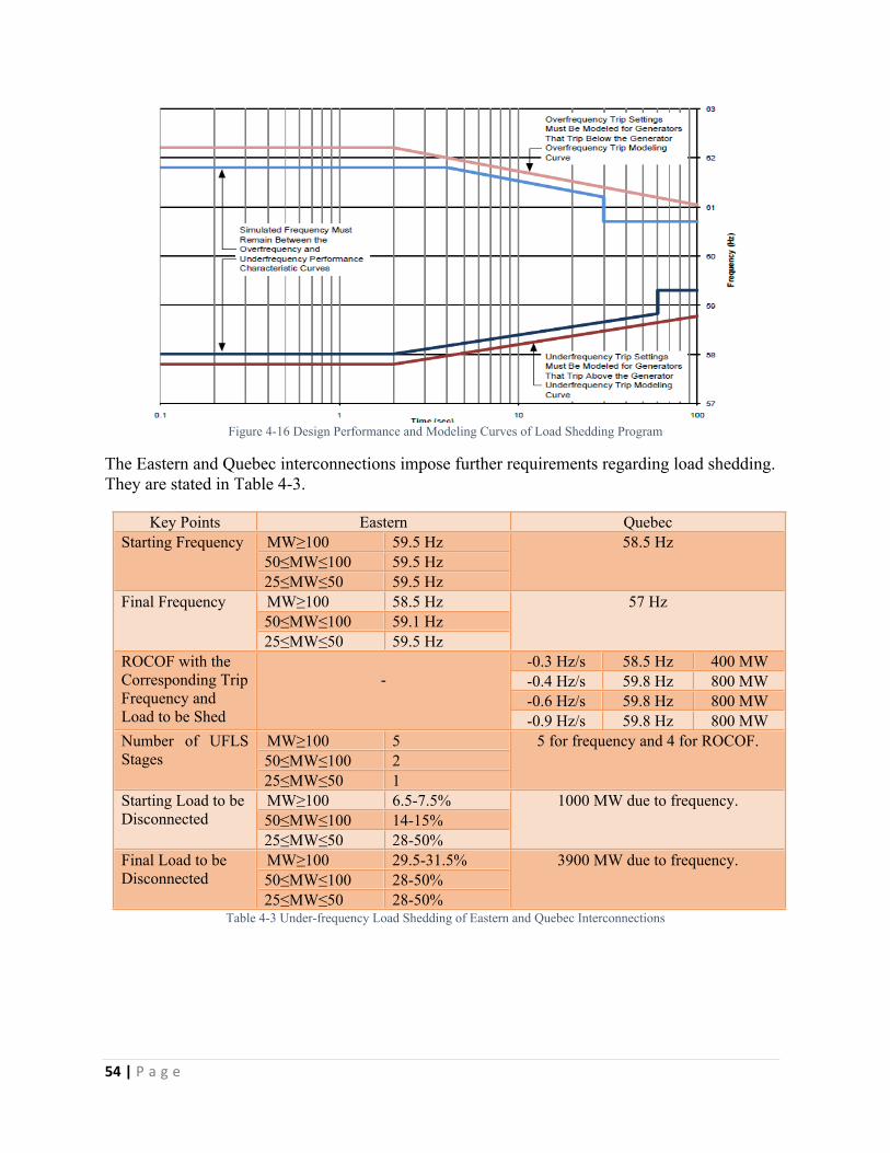
54 | P a g e

Figure 4-16 Design Performance and Modeling Curves of Load Shedding Program

The Eastern and Quebec interconnections impose further requirements regarding load shedding. They are stated in Table 4-3.

Key Points Eastern QuebecMW≥100 59.5 Hz50≤MW≤100 59.5 Hz

Starting Frequency

25≤MW≤50 59.5 Hz

58.5 Hz

MW≥100 58.5 Hz50≤MW≤100 59.1 Hz

Final Frequency

25≤MW≤50 59.5 Hz

57 Hz

-0.3 Hz/s 58.5 Hz 400 MW-0.4 Hz/s 59.8 Hz 800 MW-0.6 Hz/s 59.8 Hz 800 MW

ROCOF with the Corresponding Trip Frequency and Load to be Shed

-

-0.9 Hz/s 59.8 Hz 800 MWMW≥100 550≤MW≤100 2

Number of UFLS Stages

25≤MW≤50 1

5 for frequency and 4 for ROCOF.

MW≥100 6.5-7.5%50≤MW≤100 14-15%

Starting Load to be Disconnected

25≤MW≤50 28-50%

1000 MW due to frequency.

MW≥100 29.5-31.5%50≤MW≤100 28-50%

Final Load to be Disconnected

25≤MW≤50 28-50%

3900 MW due to frequency.

Table 4-3 Under-frequency Load Shedding of Eastern and Quebec Interconnections

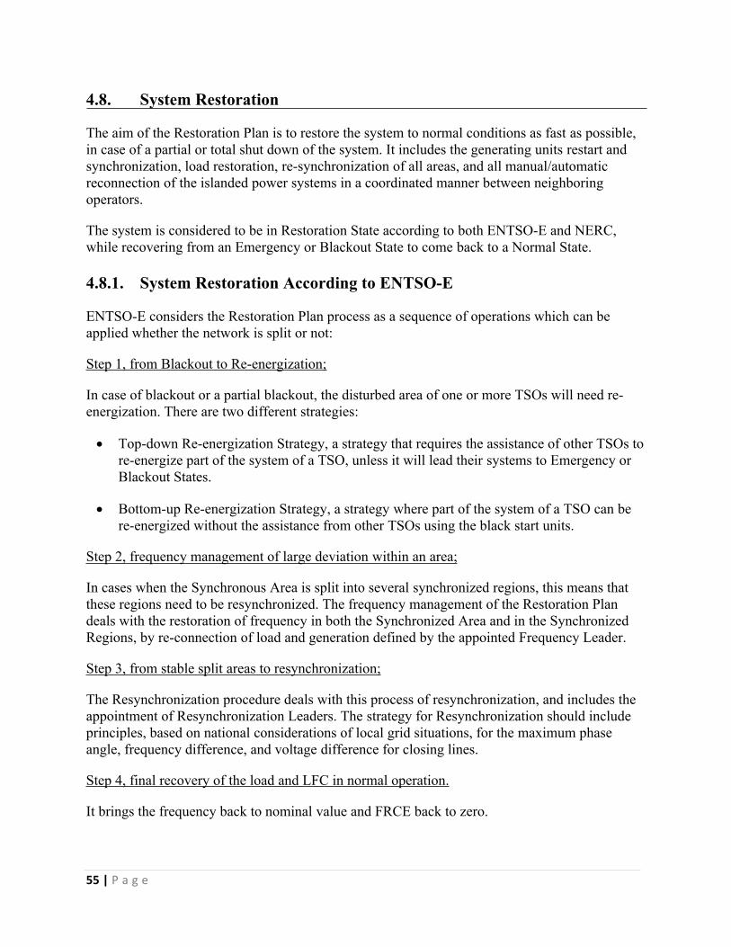
55 | P a g e

4.8. System Restoration

The aim of the Restoration Plan is to restore the system to normal conditions as fast as possible, in case of a partial or total shut down of the system. It includes the generating units restart and synchronization, load restoration, re-synchronization of all areas, and all manual/automatic reconnection of the islanded power systems in a coordinated manner between neighboring operators.

The system is considered to be in Restoration State according to both ENTSO-E and NERC, while recovering from an Emergency or Blackout State to come back to a Normal State.

4.8.1. System Restoration According to ENTSO-E

ENTSO-E considers the Restoration Plan process as a sequence of operations which can be applied whether the network is split or not:

Step 1, from Blackout to Re-energization;

In case of blackout or a partial blackout, the disturbed area of one or more TSOs will need re-energization. There are two different strategies:

Top-down Re-energization Strategy, a strategy that requires the assistance of other TSOs to re-energize part of the system of a TSO, unless it will lead their systems to Emergency or Blackout States.

Bottom-up Re-energization Strategy, a strategy where part of the system of a TSO can be re-energized without the assistance from other TSOs using the black start units.

Step 2, frequency management of large deviation within an area;

In cases when the Synchronous Area is split into several synchronized regions, this means that these regions need to be resynchronized. The frequency management of the Restoration Plan deals with the restoration of frequency in both the Synchronized Area and in the Synchronized Regions, by re-connection of load and generation defined by the appointed Frequency Leader.

Step 3, from stable split areas to resynchronization;

The Resynchronization procedure deals with this process of resynchronization, and includes the appointment of Resynchronization Leaders. The strategy for Resynchronization should include principles, based on national considerations of local grid situations, for the maximum phase angle, frequency difference, and voltage difference for closing lines.

Step 4, final recovery of the load and LFC in normal operation.

It brings the frequency back to nominal value and FRCE back to zero.

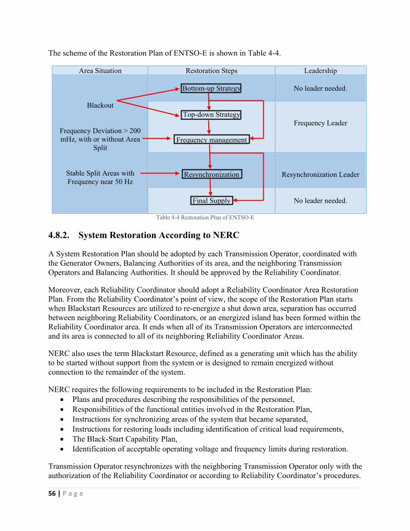
56 | P a g e

The scheme of the Restoration Plan of ENTSO-E is shown in Table 4-4.

Area Situation Restoration Steps Leadership

Bottom-up Strategy No leader needed.

Top-down Strategy

Frequency management

Frequency Leader

Resynchronization Resynchronization Leader

Blackout

Frequency Deviation > 200 mHz, with or without Area

Split

Stable Split Areas with Frequency near 50 Hz

Final Supply No leader needed.

Table 4-4 Restoration Plan of ENTSO-E

4.8.2. System Restoration According to NERC

A System Restoration Plan should be adopted by each Transmission Operator, coordinated with the Generator Owners, Balancing Authorities of its area, and the neighboring Transmission Operators and Balancing Authorities. It should be approved by the Reliability Coordinator.

Moreover, each Reliability Coordinator should adopt a Reliability Coordinator Area Restoration Plan. From the Reliability Coordinator’s point of view, the scope of the Restoration Plan starts when Blackstart Resources are utilized to re-energize a shut down area, separation has occurred between neighboring Reliability Coordinators, or an energized island has been formed within the Reliability Coordinator area. It ends when all of its Transmission Operators are interconnected and its area is connected to all of its neighboring Reliability Coordinator Areas.

NERC also uses the term Blackstart Resource, defined as a generating unit which has the ability to be started without support from the system or is designed to remain energized without connection to the remainder of the system.

NERC requires the following requirements to be included in the Restoration Plan: Plans and procedures describing the responsibilities of the personnel, Responsibilities of the functional entities involved in the Restoration Plan, Instructions for synchronizing areas of the system that became separated, Instructions for restoring loads including identification of critical load requirements, The Black-Start Capability Plan, Identification of acceptable operating voltage and frequency limits during restoration.

Transmission Operator resynchronizes with the neighboring Transmission Operator only with the authorization of the Reliability Coordinator or according to Reliability Coordinator’s procedures.

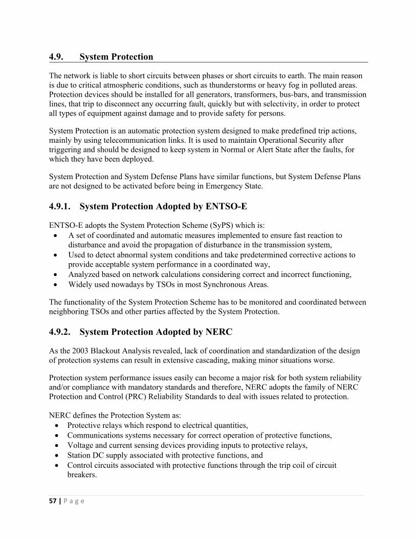
57 | P a g e

4.9. System Protection

The network is liable to short circuits between phases or short circuits to earth. The main reason is due to critical atmospheric conditions, such as thunderstorms or heavy fog in polluted areas. Protection devices should be installed for all generators, transformers, bus-bars, and transmission lines, that trip to disconnect any occurring fault, quickly but with selectivity, in order to protect all types of equipment against damage and to provide safety for persons.

System Protection is an automatic protection system designed to make predefined trip actions, mainly by using telecommunication links. It is used to maintain Operational Security after triggering and should be designed to keep system in Normal or Alert State after the faults, for which they have been deployed.

System Protection and System Defense Plans have similar functions, but System Defense Plans are not designed to be activated before being in Emergency State.

4.9.1. System Protection Adopted by ENTSO-E

ENTSO-E adopts the System Protection Scheme (SyPS) which is: A set of coordinated and automatic measures implemented to ensure fast reaction to

disturbance and avoid the propagation of disturbance in the transmission system, Used to detect abnormal system conditions and take predetermined corrective actions to

provide acceptable system performance in a coordinated way, Analyzed based on network calculations considering correct and incorrect functioning, Widely used nowadays by TSOs in most Synchronous Areas.

The functionality of the System Protection Scheme has to be monitored and coordinated between neighboring TSOs and other parties affected by the System Protection.

4.9.2. System Protection Adopted by NERC

As the 2003 Blackout Analysis revealed, lack of coordination and standardization of the design of protection systems can result in extensive cascading, making minor situations worse.

Protection system performance issues easily can become a major risk for both system reliability and/or compliance with mandatory standards and therefore, NERC adopts the family of NERC Protection and Control (PRC) Reliability Standards to deal with issues related to protection.

NERC defines the Protection System as: Protective relays which respond to electrical quantities, Communications systems necessary for correct operation of protective functions, Voltage and current sensing devices providing inputs to protective relays, Station DC supply associated with protective functions, and Control circuits associated with protective functions through the trip coil of circuit

breakers.

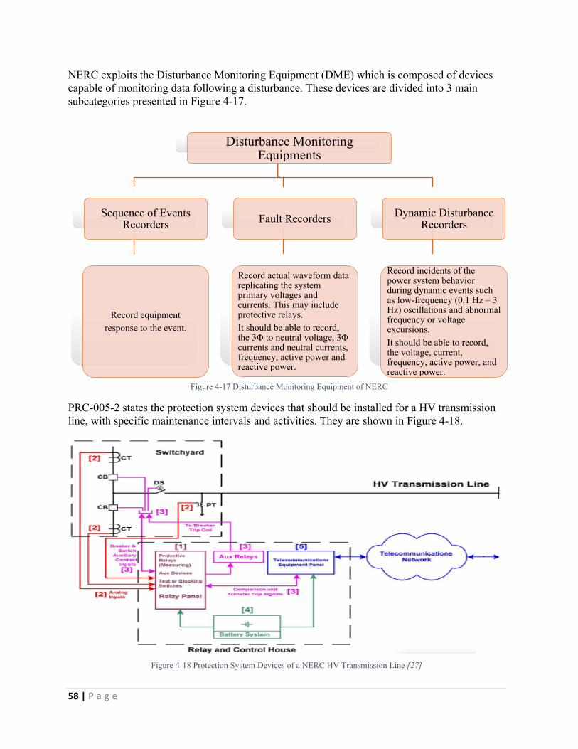
58 | P a g e

NERC exploits the Disturbance Monitoring Equipment (DME) which is composed of devices capable of monitoring data following a disturbance. These devices are divided into 3 main subcategories presented in Figure 4-17.

Disturbance Monitoring Equipments

Sequence of Events Recorders

Record equipmentresponse to the event.

Fault Recorders

Record actual waveform data replicating the system primary voltages and currents. This may include protective relays.It should be able to record, the 3Φ to neutral voltage, 3Φ currents and neutral currents, frequency, active power and reactive power.

Dynamic Disturbance Recorders

Record incidents of the power system behavior during dynamic events such as low-frequency (0.1 Hz – 3 Hz) oscillations and abnormal frequency or voltage excursions.It should be able to record, the voltage, current, frequency, active power, and reactive power.

Figure 4-17 Disturbance Monitoring Equipment of NERC

PRC-005-2 states the protection system devices that should be installed for a HV transmission line, with specific maintenance intervals and activities. They are shown in Figure 4-18.

Figure 4-18 Protection System Devices of a NERC HV Transmission Line [27]

59 | P a g e

4.10. Monitoring and Data Exchange

A key factor for the reliable operation of an electric power system is Monitoring. In order to be able to monitor and supervise the operation, all grid operators need to be equipped with a real-time data acquisition system, such as SCADA and PMUs. Monitoring mainly includes System States, Network topologies, System frequency, Area Control Error, Generation, consumption, and active/reactive power reserves availability, Active/reactive power flows, Voltage and current levels, Dynamic stability and short circuit calculations, Status of Transmission system equipment and protection systems devices.

Monitoring is an important function required to be performed by all operators, as it is useful to: Detect the disturbance events and register the pre-disturbance System State for analysis, Identify the causes of disturbance and prepare the appropriate Remedial Action to maintain

the system in normal operation or return to it as soon as possible, Provide the data necessary for state estimation, Identify and correct the causes of mis-operations of protection system devices, Ensure the reliability operation and maintain in real-time the parameters within the

Operational Security Limits defined by each power system, Monitor the compliance with respect to the Network Codes and Reliability Standards, Evaluate the system performance to be improved by short-term and long-term planning.

4.10.1. Monitoring and Data Exchange According to ENTSO-E

Due to the increase of the degree of interconnections between TSOs, market operations, and volatility of generation, Operational Security has become more and more interdependent. Therefore, ENTSO-E adopted the idea to define 3 types of areas for each TSO:

LFC Area; Part of the Synchronous Area physically limited by measurement points on the tie-lines to other LFC Areas, fulfilling the Area Process Obligations of a Control Area.

Responsibility Area;Part of the interconnected transmission system including interconnectors, operated by one TSO with connected Demand Facilities or Power Generating Modules.

Observability Area;Part of the interconnected transmission system that includes, the own transmission system of a TSO, the relevant parts of the distribution networks, and the transmission systems of the neighboring TSOs, on which the TSO implements real-time monitoring and modeling to ensure Operational Security in its Responsibility Area.

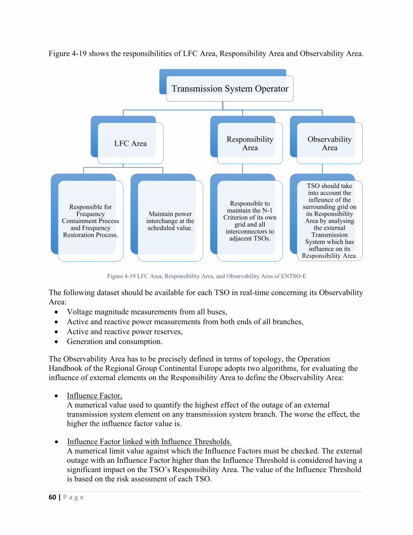
60 | P a g e

Figure 4-19 shows the responsibilities of LFC Area, Responsibility Area and Observability Area.

Transmission System Operator

LFC Area

Responsible for Frequency

Containment Process and Frequency

Restoration Process.

Maintain power interchange at the scheduled value.

Responsibility Area

Responsible to maintain the N-1

Criterion of its own grid and all

interconnectors to adjacent TSOs.

Observability Area

TSO should take into account the infleunce of the

surrounding grid on its Responsibility Area by analysing

the external Transmission

System which has influence on its

Responsibility Area.

Figure 4-19 LFC Area, Responsibility Area, and Observability Area of ENTSO-E

The following dataset should be available for each TSO in real-time concerning its Observability Area: Voltage magnitude measurements from all buses, Active and reactive power measurements from both ends of all branches, Active and reactive power reserves, Generation and consumption.

The Observability Area has to be precisely defined in terms of topology, the Operation Handbook of the Regional Group Continental Europe adopts two algorithms, for evaluating the influence of external elements on the Responsibility Area to define the Observability Area:

Influence Factor, A numerical value used to quantify the highest effect of the outage of an external transmission system element on any transmission system branch. The worse the effect, the higher the influence factor value is.

Influence Factor linked with Influence Thresholds.A numerical limit value against which the Influence Factors must be checked. The external outage with an Influence Factor higher than the Influence Threshold is considered having a significant impact on the TSO’s Responsibility Area. The value of the Influence Threshold is based on the risk assessment of each TSO.

61 | P a g e

4.10.2. Monitoring and Data Exchange According to NERC

NERC does not assign criteria to determine the Monitoring Area for the operators as ENTSO-E;

IRO-002-4 “Monitoring and Analysis” R1 states that:Each Reliability Coordinator shall have data exchange capabilities with its Balancing

Authorities and Transmission Operators, and with other entities it deems necessary, for it to perform its Operational Planning Analyses, Real‐time monitoring, and Real-time Assessments.

[15]”

Moreover, IRO-003-4 “Wide Area View” R1 states that:“Each Reliability Coordinator shall monitor all Bulk Electric System facilities, which may include sub-transmission information, within its Reliability Coordinator Area and adjacent Reliability Coordinator Areas, as necessary to ensure that, at any time, regardless of prior planned or unplanned events, the Reliability Coordinator is able to determine any potential System Operating Limit and Interconnection Reliability Operating Limit violations within its

Reliability Coordinator Area. [15]”

IRO-003-2 (R1 and R2) requires the Reliability Coordinator to monitor the state of its system.

Attachment 1 of TOP-005-2a “Operational Reliability Information” lists types of data that Balancing Authorities and Transmission Operators are expected to share with other Balancing Authorities and Transmission Operators:

Data that should be updated at least every 10 minutes:o Transmission data,o Generator data,o Operating reserves data,o Balancing Authority demand,o Interchange, o Area Control Error and frequency.

Data that should be updated as soon as possible:o Interconnection Reliability Operating Limits (IROLs) and System Operating

Limits (SOLs),o Forecast of operating reserves at peak,o Forecast peak demand,o Forecast changes in equipment status,o New facilities,o New or degraded special protection systems, o Emergency operating procedures.

The Attachment is provided as a guideline of what can be shared. The Attachment is not an obligation of what must be shared [15].

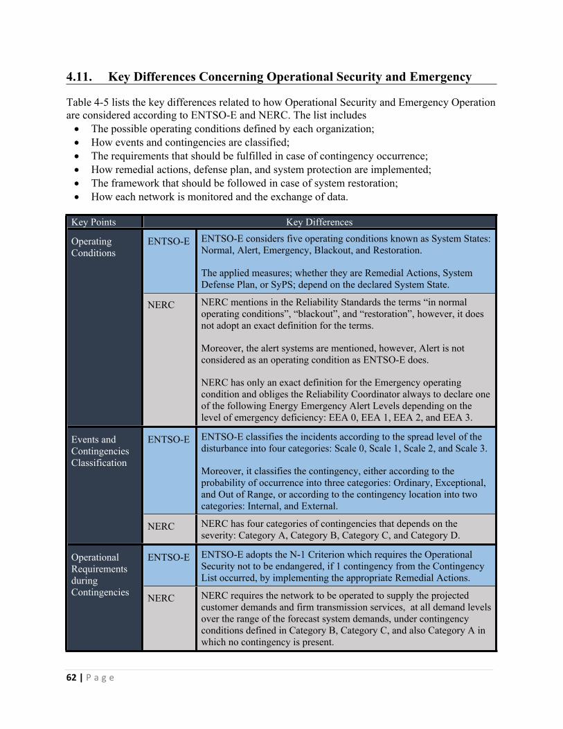
62 | P a g e

4.11. Key Differences Concerning Operational Security and Emergency

Table 4-5 lists the key differences related to how Operational Security and Emergency Operation are considered according to ENTSO-E and NERC. The list includes The possible operating conditions defined by each organization; How events and contingencies are classified; The requirements that should be fulfilled in case of contingency occurrence; How remedial actions, defense plan, and system protection are implemented; The framework that should be followed in case of system restoration; How each network is monitored and the exchange of data.

Key Points Key Differences

ENTSO-E ENTSO-E considers five operating conditions known as System States: Normal, Alert, Emergency, Blackout, and Restoration.

The applied measures; whether they are Remedial Actions, System Defense Plan, or SyPS; depend on the declared System State.

Operating Conditions

NERC NERC mentions in the Reliability Standards the terms “in normal operating conditions”, “blackout”, and “restoration”, however, it does not adopt an exact definition for the terms.

Moreover, the alert systems are mentioned, however, Alert is not considered as an operating condition as ENTSO-E does.

NERC has only an exact definition for the Emergency operating condition and obliges the Reliability Coordinator always to declare one of the following Energy Emergency Alert Levels depending on the level of emergency deficiency: EEA 0, EEA 1, EEA 2, and EEA 3.

ENTSO-E ENTSO-E classifies the incidents according to the spread level of the disturbance into four categories: Scale 0, Scale 1, Scale 2, and Scale 3.

Moreover, it classifies the contingency, either according to the probability of occurrence into three categories: Ordinary, Exceptional, and Out of Range, or according to the contingency location into two categories: Internal, and External.

Events and Contingencies Classification

NERC NERC has four categories of contingencies that depends on the severity: Category A, Category B, Category C, and Category D.

ENTSO-E ENTSO-E adopts the N-1 Criterion which requires the Operational Security not to be endangered, if 1 contingency from the Contingency List occurred, by implementing the appropriate Remedial Actions.

Operational Requirements during Contingencies NERC NERC requires the network to be operated to supply the projected

customer demands and firm transmission services, at all demand levels over the range of the forecast system demands, under contingency conditions defined in Category B, Category C, and also Category A in which no contingency is present.

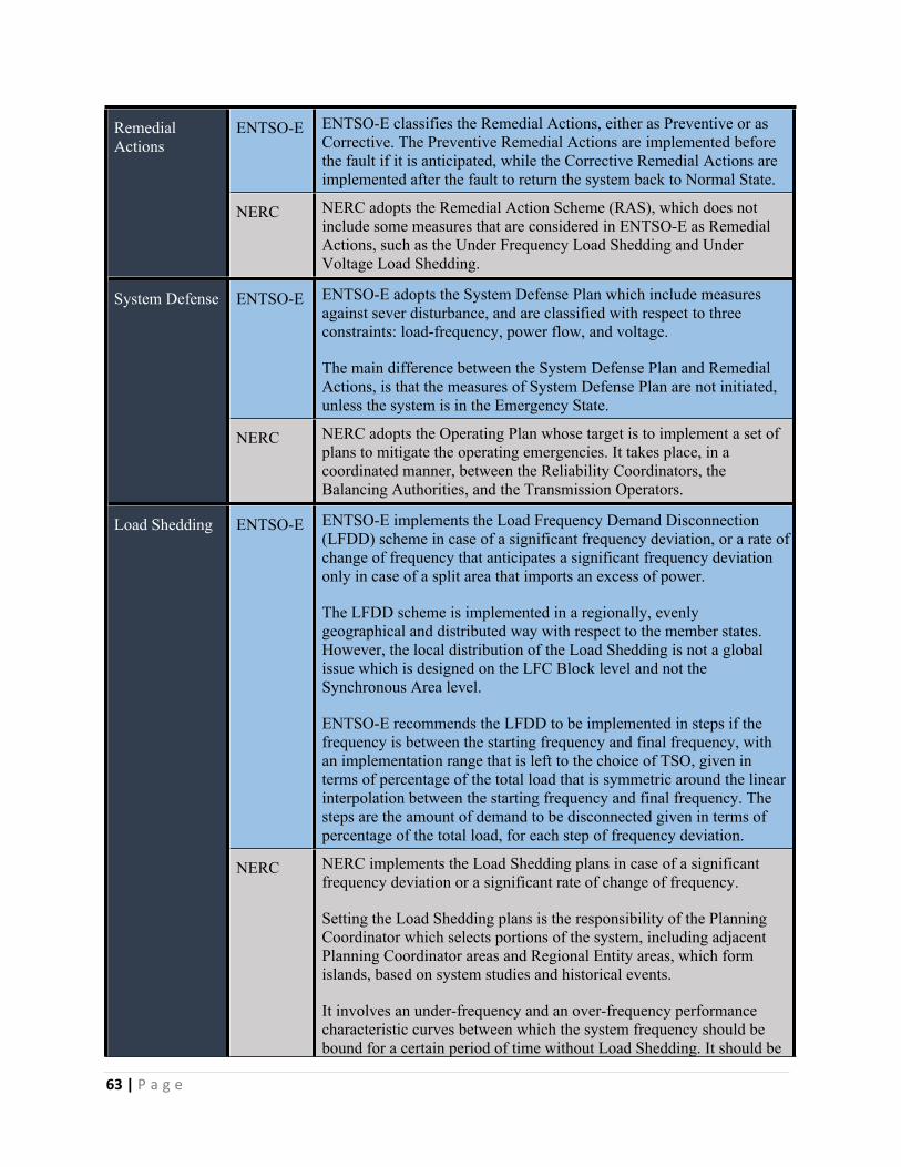
63 | P a g e

ENTSO-E ENTSO-E classifies the Remedial Actions, either as Preventive or as Corrective. The Preventive Remedial Actions are implemented before the fault if it is anticipated, while the Corrective Remedial Actions are implemented after the fault to return the system back to Normal State.

Remedial Actions

NERC NERC adopts the Remedial Action Scheme (RAS), which does not include some measures that are considered in ENTSO-E as Remedial Actions, such as the Under Frequency Load Shedding and Under Voltage Load Shedding.

ENTSO-E ENTSO-E adopts the System Defense Plan which include measures against sever disturbance, and are classified with respect to three constraints: load-frequency, power flow, and voltage.

The main difference between the System Defense Plan and Remedial Actions, is that the measures of System Defense Plan are not initiated, unless the system is in the Emergency State.

System Defense

NERC NERC adopts the Operating Plan whose target is to implement a set of plans to mitigate the operating emergencies. It takes place, in a coordinated manner, between the Reliability Coordinators, the Balancing Authorities, and the Transmission Operators.

ENTSO-E ENTSO-E implements the Load Frequency Demand Disconnection (LFDD) scheme in case of a significant frequency deviation, or a rate of change of frequency that anticipates a significant frequency deviation only in case of a split area that imports an excess of power.

The LFDD scheme is implemented in a regionally, evenly geographical and distributed way with respect to the member states. However, the local distribution of the Load Shedding is not a global issue which is designed on the LFC Block level and not the Synchronous Area level.

ENTSO-E recommends the LFDD to be implemented in steps if the frequency is between the starting frequency and final frequency, with an implementation range that is left to the choice of TSO, given in terms of percentage of the total load that is symmetric around the linear interpolation between the starting frequency and final frequency. The steps are the amount of demand to be disconnected given in terms of percentage of the total load, for each step of frequency deviation.

Load Shedding

NERC NERC implements the Load Shedding plans in case of a significant frequency deviation or a significant rate of change of frequency.

Setting the Load Shedding plans is the responsibility of the Planning Coordinator which selects portions of the system, including adjacent Planning Coordinator areas and Regional Entity areas, which form islands, based on system studies and historical events.

It involves an under-frequency and an over-frequency performance characteristic curves between which the system frequency should be bound for a certain period of time without Load Shedding. It should be

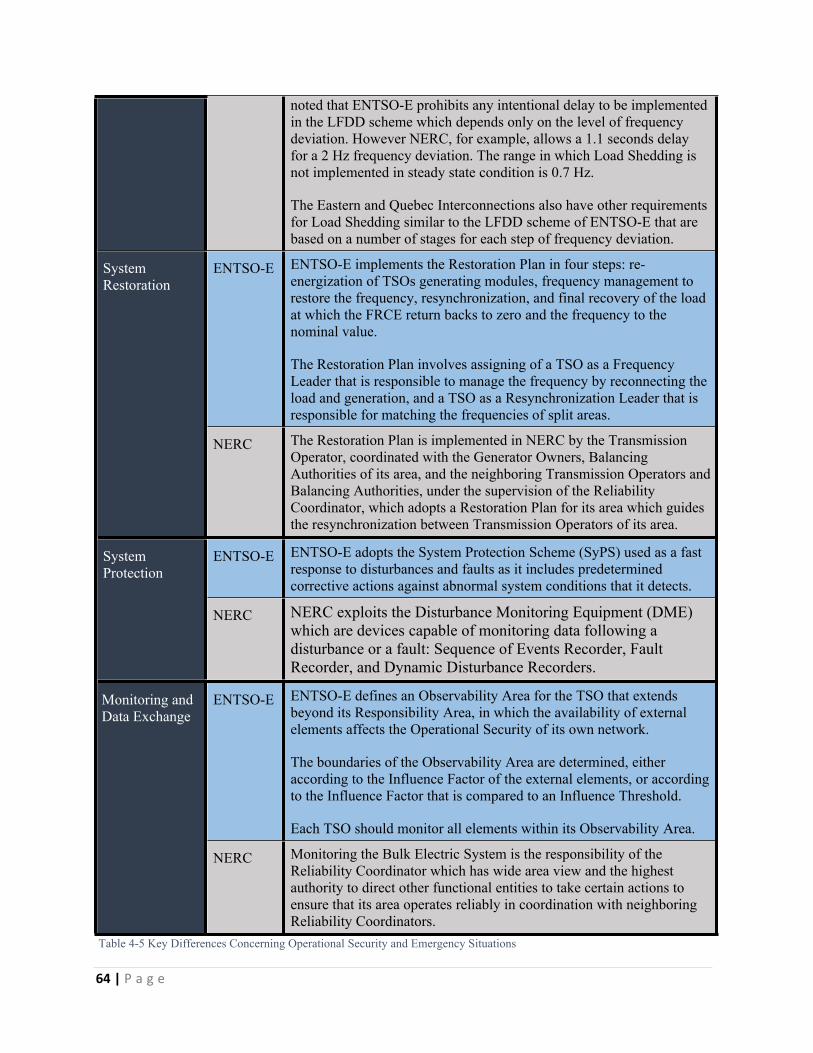
64 | P a g e

noted that ENTSO-E prohibits any intentional delay to be implemented in the LFDD scheme which depends only on the level of frequency deviation. However NERC, for example, allows a 1.1 seconds delay for a 2 Hz frequency deviation. The range in which Load Shedding is not implemented in steady state condition is 0.7 Hz.

The Eastern and Quebec Interconnections also have other requirements for Load Shedding similar to the LFDD scheme of ENTSO-E that are based on a number of stages for each step of frequency deviation.

ENTSO-E ENTSO-E implements the Restoration Plan in four steps: re-energization of TSOs generating modules, frequency management to restore the frequency, resynchronization, and final recovery of the load at which the FRCE return backs to zero and the frequency to the nominal value.

The Restoration Plan involves assigning of a TSO as a Frequency Leader that is responsible to manage the frequency by reconnecting the load and generation, and a TSO as a Resynchronization Leader that is responsible for matching the frequencies of split areas.

System Restoration

NERC The Restoration Plan is implemented in NERC by the Transmission Operator, coordinated with the Generator Owners, Balancing Authorities of its area, and the neighboring Transmission Operators and Balancing Authorities, under the supervision of the Reliability Coordinator, which adopts a Restoration Plan for its area which guides the resynchronization between Transmission Operators of its area.

ENTSO-E ENTSO-E adopts the System Protection Scheme (SyPS) used as a fast response to disturbances and faults as it includes predetermined corrective actions against abnormal system conditions that it detects.

System Protection

NERC NERC exploits the Disturbance Monitoring Equipment (DME) which are devices capable of monitoring data following a disturbance or a fault: Sequence of Events Recorder, Fault Recorder, and Dynamic Disturbance Recorders.

ENTSO-E ENTSO-E defines an Observability Area for the TSO that extends beyond its Responsibility Area, in which the availability of external elements affects the Operational Security of its own network.

The boundaries of the Observability Area are determined, either according to the Influence Factor of the external elements, or according to the Influence Factor that is compared to an Influence Threshold.

Each TSO should monitor all elements within its Observability Area.

Monitoring and Data Exchange

NERC Monitoring the Bulk Electric System is the responsibility of the Reliability Coordinator which has wide area view and the highest authority to direct other functional entities to take certain actions to ensure that its area operates reliably in coordination with neighboring Reliability Coordinators.

Table 4-5 Key Differences Concerning Operational Security and Emergency Situations

65 | P a g e

CHAPTER 55. Operational Planning and Scheduling

This chapter presents how ENTSO-E and NERC consider the Operational Planning and Scheduling and is organized as follows: introduction, time frames, network models, Planned Outage Coordination, Load Forecast, Adequacy, and Capacity Calculations.

5.1. Introduction

Changes due to the electricity market, increased the volume and volatility of cross border trade causing an increase in the operational complexity and congestion risks. Consequently, more coordination among operators is needed during the Operational Planning phase.

Secure and efficient power system operation is guaranteed only if there is a well-organized preparation of real time operation. This requires operators to have the necessary means to control the system in real time, either when the system is subject to normal changes of operating conditions or when it is facing incidents that affect generation, demand, or equipment.

The Operational Planning and Scheduling should provide the basis for this preparation by defining the minimum requirements, applicable to all operators and grid users, for ensuring a coherent and coordinated preparation of real-time operation of the power system. Moreover, Operational Planning and Scheduling should take into account the rapid growth of the volatile renewable energy sources and their impact on operation.

For the sake of the objectives mentioned above, ENTSO-E adopts the Operational Planning and Scheduling Network Code and publishes a supporting document for the code, while NERC published collections of regional planning criteria, and from those criteria, developed the current Reliability Standards concerning Planning, mentioned in the IRO, TOP, TPL, and INT series.

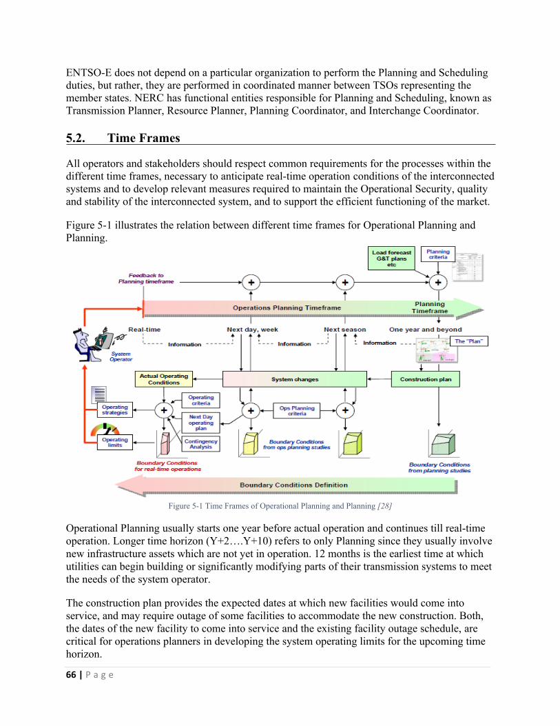
66 | P a g e

ENTSO-E does not depend on a particular organization to perform the Planning and Scheduling duties, but rather, they are performed in coordinated manner between TSOs representing the member states. NERC has functional entities responsible for Planning and Scheduling, known as Transmission Planner, Resource Planner, Planning Coordinator, and Interchange Coordinator.

5.2. Time Frames

All operators and stakeholders should respect common requirements for the processes within the different time frames, necessary to anticipate real-time operation conditions of the interconnected systems and to develop relevant measures required to maintain the Operational Security, quality and stability of the interconnected system, and to support the efficient functioning of the market.

Figure 5-1 illustrates the relation between different time frames for Operational Planning and Planning.

Figure 5-1 Time Frames of Operational Planning and Planning [28]

Operational Planning usually starts one year before actual operation and continues till real-time operation. Longer time horizon (Y+2….Y+10) refers to only Planning since they usually involve new infrastructure assets which are not yet in operation. 12 months is the earliest time at which utilities can begin building or significantly modifying parts of their transmission systems to meet the needs of the system operator.

The construction plan provides the expected dates at which new facilities would come into service, and may require outage of some facilities to accommodate the new construction. Both, the dates of the new facility to come into service and the existing facility outage schedule, are critical for operations planners in developing the system operating limits for the upcoming time horizon.

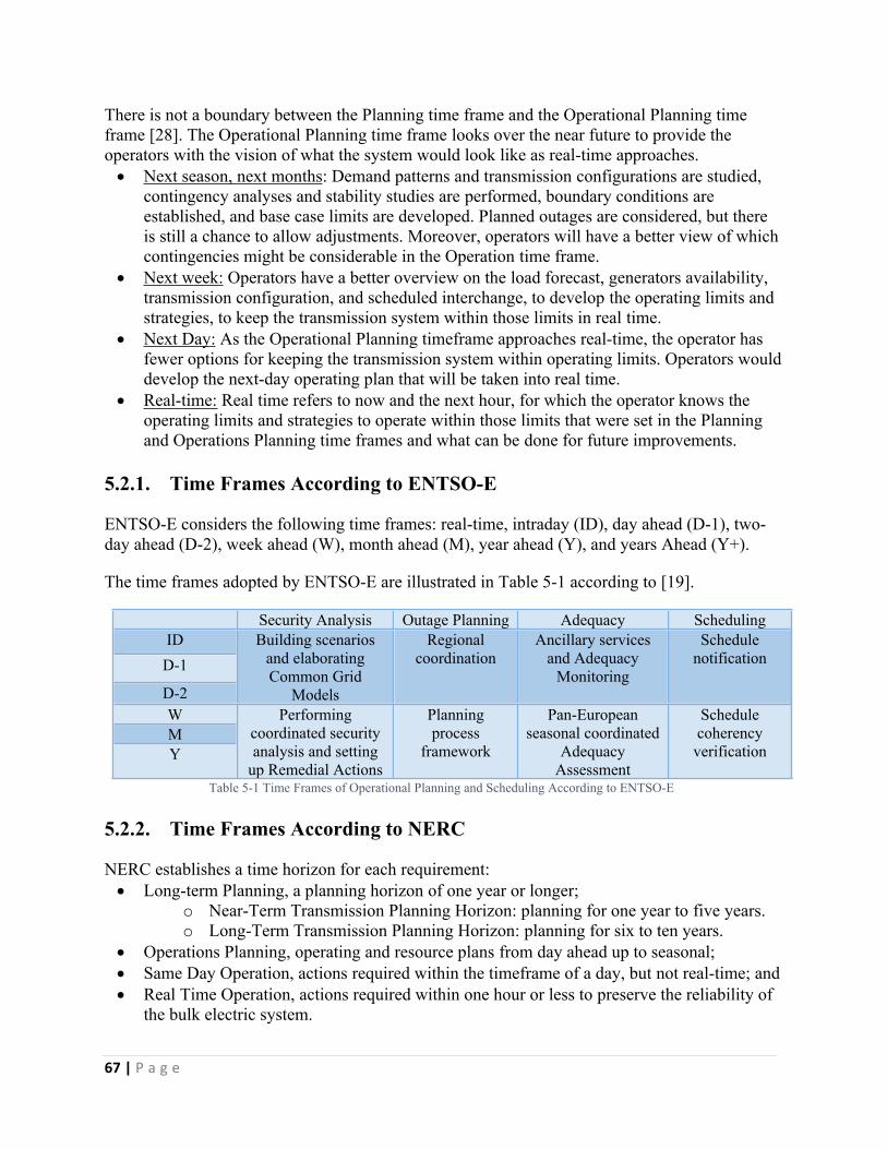
67 | P a g e

There is not a boundary between the Planning time frame and the Operational Planning time frame [28]. The Operational Planning time frame looks over the near future to provide the operators with the vision of what the system would look like as real-time approaches. Next season, next months: Demand patterns and transmission configurations are studied,

contingency analyses and stability studies are performed, boundary conditions are established, and base case limits are developed. Planned outages are considered, but there is still a chance to allow adjustments. Moreover, operators will have a better view of which contingencies might be considerable in the Operation time frame.

Next week: Operators have a better overview on the load forecast, generators availability, transmission configuration, and scheduled interchange, to develop the operating limits and strategies, to keep the transmission system within those limits in real time.

Next Day: As the Operational Planning timeframe approaches real-time, the operator has fewer options for keeping the transmission system within operating limits. Operators would develop the next-day operating plan that will be taken into real time.

Real-time: Real time refers to now and the next hour, for which the operator knows the operating limits and strategies to operate within those limits that were set in the Planning and Operations Planning time frames and what can be done for future improvements.

5.2.1. Time Frames According to ENTSO-E

ENTSO-E considers the following time frames: real-time, intraday (ID), day ahead (D-1), two-day ahead (D-2), week ahead (W), month ahead (M), year ahead (Y), and years Ahead (Y+).

The time frames adopted by ENTSO-E are illustrated in Table 5-1 according to [19].

Security Analysis Outage Planning Adequacy SchedulingIDD-1

D-2

Building scenarios and elaborating Common Grid

Models

Regional coordination

Ancillary services and Adequacy

Monitoring

Schedule notification

WMY

Performing coordinated security analysis and setting

up Remedial Actions

Planning process

framework

Pan-European seasonal coordinated

Adequacy Assessment

Schedule coherency

verification

Table 5-1 Time Frames of Operational Planning and Scheduling According to ENTSO-E

5.2.2. Time Frames According to NERC

NERC establishes a time horizon for each requirement: Long-term Planning, a planning horizon of one year or longer;

o Near-Term Transmission Planning Horizon: planning for one year to five years.o Long-Term Transmission Planning Horizon: planning for six to ten years.

Operations Planning, operating and resource plans from day ahead up to seasonal; Same Day Operation, actions required within the timeframe of a day, but not real-time; and Real Time Operation, actions required within one hour or less to preserve the reliability of

the bulk electric system.

68 | P a g e

5.3. Network Models

The network model is the model of the high voltage transmission system (220 kV and above), an equivalent model of the lower voltage grid, and the sum of generation and consumption in the nodes of the transmission system.

Network models are used to perform Security Analysis and Capacity Calculations, using the following data: Demand patterns, Availability of generators and their contribution, Renewable energy systems generation, Net position for bidding zones and for market balance areas.

5.3.1. Common Grid Models of ENTSO-E

ENTSO-E adopts the Common Grid Model (CGM) which is built by merging the Individual Grid Models (IGM) of the Responsibility Area of each TSO.

The Common Grid Model is prepared for different time frames: year ahead, week ahead, day ahead, and intraday. For Capacity Calculation, CGMs are established two days before the energy is delivered

and for the intraday timeframe. For Operational Security, a year ahead CGM is built and updated.

5.3.2. System Models of NERC

NERC requires the development of System Models and assigns for this task the Reliability Standards MOD-010 to MOD-015, divided among the two classifications of System Models: Steady State System Models, and Dynamic System Models.

System Models are used for calculating operating limits, planning studies for assessment of new generation and load growth, and performance assessments of protection schemes.

NERC mandates the Regional Reliability Organizations in cooperation with the Transmission Owners, Transmission Planners, Generator Owners, and Resource Planners to develop steady-state and dynamic data requirements, needed to model the system for each Interconnection. The Regional Reliability Organizations jointly develop the System Models annually for the selected study years.

The models should include the Near and Long Term Transmission Planning Horizons representing the system conditions for projected seasonal peak, minimum, and other demand levels.

69 | P a g e

5.4. Planned Outage Coordination

It is necessary to carry out maintenance work, which requires outages of assets to keep the network in secure operating condition, to guarantee a suitable level of security and market access. Therefore operators should: Determine suitable dates of outages and tests for maintenance, Exchange information about generation unit outages and tests, Request for modification of generator units outage planning.

5.4.1. Planned Outage Coordination According to ENTSO-E

ENTSO-E defines the Relevant Asset as any Relevant Demand Facility, Relevant Generating Module or Relevant Grid Element participating in the Outage Coordination Process whose availability status influences the cross-border Operational Security [29]. Each Relevant Asset should have one of three availability statuses: available, unavailable, or tested.

The elements for which the outages have to be coordinated, need to have some level of influence on each other; it would be inefficient to coordinate the outage between Responsibility Areas that are quite far apart, for instance Denmark and Spain. Therefore, ENTSO-E defines the Outage Coordination Region in order to establish an optimal Outage Coordination Process.

All Outage Coordinating TSOs should ensure that Each Responsibility Area is included within at least one Outage Coordination Region, When the availability status of a Relevant Asset located in one Responsibility Area has a

major cross border impact on Operational Security in another Responsibility Area, these Responsibility Areas are included within the same Outage Coordination Region,

Size of the Outage Coordination Regions allows an efficient Outage Coordination Process.

Planning the outages and tests takes place in three planning horizons: Long-term planning for the next year, Medium-term planning for the whole year revised each month, Short-term planning on Thursday before the concerned week.

5.4.2. Planned Outage Coordination According to NERC

NERC gives mandates to the Reliability Coordinator to develop and maintain an outage coordination process for generation and transmission outage, to be properly coordinated in the Operations Planning time horizon and Near-Term Transmission Planning Horizon with the Transmission Operator, Balancing Authority, Planning Coordinator, and Transmission Planner.

Moreover, NERC obliges the Generator Owner to provide outage information daily for the scheduled generator outage planned for the next day to the Transmission Operator which informs the affected Balancing Authorities and Transmission Operators if the outage would cause an SOL or IROL violation or a regional operating area limit. The Reliability Coordinator must resolve any scheduling of potential reliability conflict.

70 | P a g e

NERC also adopts the Generating Availability Data System (GADS) which includes data collected from all Generator Owners concerning the availability of conventional generating units. This database is used to improve the performance of electric generating equipment and support equipment reliability and availability analyses and decision-making by GADS users.

5.5. Load Forecast

Load Forecast is a vital process in the planning and the operation of electric power systems due to the facts concerning that The electric power must be consumed at the same time it is generated, Load cannot be controlled, but rather predicted.

Accurate forecasts lead to higher frequency quality, more stability, and less exhausted frequency responsive reserves; increased reliability of power supply and delivery system; better interchange scheduling; savings in operating and maintenance costs; Correct decisions for future development.

5.5.1. Load Forecast According to ENTSO-E

ENTSO-E implements forecasts for the D-1 and intraday time frames. For longer time frames, statistical scenarios are used. The difference between forecasts and scenarios is that forecasts are expectations of what will happen, while scenarios are examples of what could happen.

ENTSO- E obliges the TSOs to include up to date demand and generation forecasts in their Individual Grid Models. Forecast calculations are performed in a different manner in each member state depending on the national legislation of these member states. They are two methods to perform the forecast calculations: Forecast is calculated by the TSO, by developing its own numerical prediction models for

demand and renewable production, in addition to the weather data prediction and the real time measurements of these renewable productions.

Forecast calculated by responsible market parties in line with national legal framework, is delivered to the TSO.

5.5.2. Load Forecast According to NERC

NERC mandates the Load Serving Entities to develop load profiles and forecasts of end-user energy requirements for the current and next day, depending on weather forecast and past load patterns; collect individual load profiles; and submit it to Balancing Authorities, Purchasing-Selling Entities, Planning Coordinator, Resource Planners, and Transmission Planners.

Moreover, at the request of the Balancing Authority or Transmission Operator, Generator Operators should provide a forecast of expected real power output to assist in Operations Planning (a seven-day forecast of real output).

71 | P a g e

5.6. Adequacy

Adequacy ensures that generation is sufficient to meet the demand, and ensures the capability of the system to deliver the energy to the end user at all times, taking into account scheduled and reasonably expected unscheduled outages of system elements.

5.6.1. Adequacy According to ENTSO-E

Concerning Adequacy, ENTSO-E publishes the following documents [8]: Ten Year Network Development Plan (TYNDP),

TYNDP is updated each two years and is designed to increase the investment needs in the pan-European transmission systems, support decision-makers at regional and European level, and select the EU projects of common interest. Each project, whether transmission or storage, has to go through a cost-benefit analysis, developed by ENTSO-E in consultation with stakeholders, and adopted by the European Commission, to ensure that each project provides more benefits to EU citizens than they cost.

Scenario Outlook and Adequacy Forecast (SO & AF),The SO&AF looks at how system Adequacy Balance between supply and demand is likely to evolve in Europe up to 2025. This long-term system Adequacy Assessment is one of the tools ENTSO-E provides to stakeholders and decision makers, on which the investments and policy decisions are based.

Summer and Winter Generation Adequacy Outlooks,They present the views of Europe’s TSOs regarding national, regional, and pan-European security of supply for the summer and winter periods, and highlight possibilities for the neighboring countries to contribute to the generation demand balance in critical situations.

Six detailed regional investment plans, andSix regional groups are defined and designed to the challenges for grid development and the integration of new generation, especially renewable energy sources, at a regional level.

Adequacy Retrospect.The Adequacy Retrospect is produced annually to provide stakeholders in the European electrical market with an overview of generation and demand and their adequacy with a focus on the power balance, margins, and generation mix.

5.6.2. Adequacy According to NERC

NERC gives mandates to the Resource Planner to concern about Adequacy, in cooperation with the Transmission Planner, Transmission Service Providers, Reliability Coordinators, and Planning Coordinators. NERC publishes the following documents [9]: Long-Term Reliability Assessment (LTRA), and

The annual report states the electricity supply and demand, evaluates transmission system Adequacy, and discusses issues that could affect reliability of the Bulk Electric System in the United States and Canada over a 10-year period.

Summer and Winter Assessments.They assess the Adequacy of electricity supplies in the United States and Canada for the upcoming summer and winter peak demand periods.

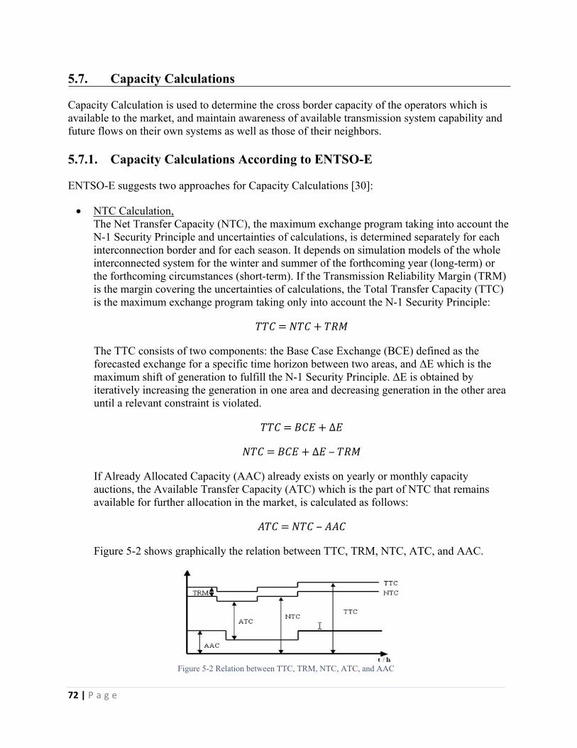
72 | P a g e

5.7. Capacity Calculations

Capacity Calculation is used to determine the cross border capacity of the operators which is available to the market, and maintain awareness of available transmission system capability and future flows on their own systems as well as those of their neighbors.

5.7.1. Capacity Calculations According to ENTSO-E

ENTSO-E suggests two approaches for Capacity Calculations [30]:

NTC Calculation,The Net Transfer Capacity (NTC), the maximum exchange program taking into account the N-1 Security Principle and uncertainties of calculations, is determined separately for each interconnection border and for each season. It depends on simulation models of the whole interconnected system for the winter and summer of the forthcoming year (long-term) or the forthcoming circumstances (short-term). If the Transmission Reliability Margin (TRM) is the margin covering the uncertainties of calculations, the Total Transfer Capacity (TTC) is the maximum exchange program taking only into account the N-1 Security Principle:

𝑇𝑇𝐶 = 𝑁𝑇𝐶 + 𝑇𝑅𝑀

The TTC consists of two components: the Base Case Exchange (BCE) defined as the forecasted exchange for a specific time horizon between two areas, and ΔE which is the maximum shift of generation to fulfill the N-1 Security Principle. ΔE is obtained by iteratively increasing the generation in one area and decreasing generation in the other area until a relevant constraint is violated.

𝑇𝑇𝐶 = 𝐵𝐶𝐸 + ∆𝐸

𝑁𝑇𝐶 = 𝐵𝐶𝐸 + ∆𝐸 ‒ 𝑇𝑅𝑀

If Already Allocated Capacity (AAC) already exists on yearly or monthly capacity auctions, the Available Transfer Capacity (ATC) which is the part of NTC that remains available for further allocation in the market, is calculated as follows:

𝐴𝑇𝐶 = 𝑁𝑇𝐶 ‒ 𝐴𝐴𝐶

Figure 5-2 shows graphically the relation between TTC, TRM, NTC, ATC, and AAC.

Figure 5-2 Relation between TTC, TRM, NTC, ATC, and AAC

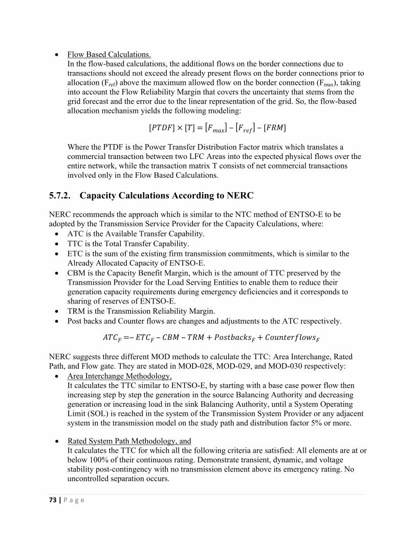
73 | P a g e

Flow Based Calculations.In the flow-based calculations, the additional flows on the border connections due to transactions should not exceed the already present flows on the border connections prior to allocation (Fref) above the maximum allowed flow on the border connection (Fmax), taking into account the Flow Reliability Margin that covers the uncertainty that stems from the grid forecast and the error due to the linear representation of the grid. So, the flow-based allocation mechanism yields the following modeling:

[𝑃𝑇𝐷𝐹] × [𝑇] = [𝐹𝑚𝑎𝑥] ‒ [𝐹𝑟𝑒𝑓] ‒ [𝐹𝑅𝑀]

Where the PTDF is the Power Transfer Distribution Factor matrix which translates a commercial transaction between two LFC Areas into the expected physical flows over the entire network, while the transaction matrix T consists of net commercial transactions involved only in the Flow Based Calculations.

5.7.2. Capacity Calculations According to NERC

NERC recommends the approach which is similar to the NTC method of ENTSO-E to be adopted by the Transmission Service Provider for the Capacity Calculations, where: ATC is the Available Transfer Capability. TTC is the Total Transfer Capability. ETC is the sum of the existing firm transmission commitments, which is similar to the

Already Allocated Capacity of ENTSO-E. CBM is the Capacity Benefit Margin, which is the amount of TTC preserved by the

Transmission Provider for the Load Serving Entities to enable them to reduce their generation capacity requirements during emergency deficiencies and it corresponds to sharing of reserves of ENTSO-E.

TRM is the Transmission Reliability Margin. Post backs and Counter flows are changes and adjustments to the ATC respectively.

𝐴𝑇𝐶𝐹 =‒ 𝐸𝑇𝐶𝐹 ‒ 𝐶𝐵𝑀 ‒ 𝑇𝑅𝑀 + 𝑃𝑜𝑠𝑡𝑏𝑎𝑐𝑘𝑠𝐹 + 𝐶𝑜𝑢𝑛𝑡𝑒𝑟𝑓𝑙𝑜𝑤𝑠𝐹

NERC suggests three different MOD methods to calculate the TTC: Area Interchange, Rated Path, and Flow gate. They are stated in MOD-028, MOD-029, and MOD-030 respectively: Area Interchange Methodology,

It calculates the TTC similar to ENTSO-E, by starting with a base case power flow then increasing step by step the generation in the source Balancing Authority and decreasing generation or increasing load in the sink Balancing Authority, until a System Operating Limit (SOL) is reached in the system of the Transmission System Provider or any adjacent system in the transmission model on the study path and distribution factor 5% or more.

Rated System Path Methodology, andIt calculates the TTC for which all the following criteria are satisfied: All elements are at or below 100% of their continuous rating. Demonstrate transient, dynamic, and voltage stability post-contingency with no transmission element above its emergency rating. No uncontrolled separation occurs.

74 | P a g e

Flow gate Methodology.It considers the Total Flow gate Capability (TFC) instead of the TTC, where the flow gate is defined as a boundary between two parts of a transmission system across which there may be congestion. According to the Flow gate Methodology, the TFC is considered equal to the SOL of the Flow gate for thermal, voltage, and stability limits. NERC also adopts the Interchange Distribution Calculator for the Eastern Interconnection used by its Reliability Coordinators to calculate the distribution of the interchange transactions over flow gates.

5.8. Key Differences Concerning Operational Planning and Scheduling

Table 5-2 lists the key differences related to how Operational Planning and Scheduling are regarded according to ENTSO-E and NERC. The list includes The different time frames for both, the operational planning and planning; How the network is modeled, How the outage is planned and coordinated, The execution of the Load Forecast calculations, The plans for the adequacy of the transmission network, The execution of the Capacity Calculations.

Key Points Key Differences

ENTSO-E Real-time, intraday (ID), day ahead (D-1), two-day ahead (D-2), week ahead (W), month ahead (M), year ahead (Y), and years Ahead (Y+).

Time Frames

NERC Long-term Planning, Operations Planning, Same Day Operations, and Real Time Operations.

ENTSO-E Common Grid Model.Network Model NERC System Model.

ENTSO-E It is performed in a coordinated manner between TSOs within the same Outage Coordination Region that is determined according to a methodology that depends on how the external asset is relevant.

Planned Outage Coordination

NERC It is performed under supervision of the Reliability Coordinator, by the Transmission Operator, Balancing Authority, Planning Coordinator, and Transmission Planner, in coordination with the affected Balancing Authorities and Transmission Operators. However, NERC does not recommend a methodology about determining the affected entities.

ENTSO-E Forecast calculations are performed in a different manner in each member state, either by the TSO or by the market parties.

Load Forecast

NERC Forecast calculations are performed by the Load Serving Entity which submits it to the Balancing Authorities, Purchasing-Selling Entities, Planning Coordinator, Resource Planners, and Transmission Planners.

Adequacy ENTSO-E ENTSO-E publishes the Ten Year Network Development Plan (TYNDP), the Scenario Outlook and Adequacy Forecast (SO & AF), the Summer and Winter Generation Adequacy Outlooks, the Six detailed regional investment plans, and the Adequacy Retrospect.

75 | P a g e

NERC NERC publishes the Long-Term Reliability Assessment and Summer and Winter Assessment.

ENTSO-E Capacity Calculations are done either by the NTC Calculation method or the Flow Based Calculations method. The TTC is calculated in a way similar to the Area Interchange methodology adopted by NERC.

Capacity Calculations

NERC Capacity Calculations are done in a way similar to the NTC Calculation method adopted by ENTSO-E. NERC suggests three methods to calculate the TTC: Area Interchange, Rated Path, and Flow gate.

Table 5-2 Key Differences Concerning Operational Planning and Scheduling

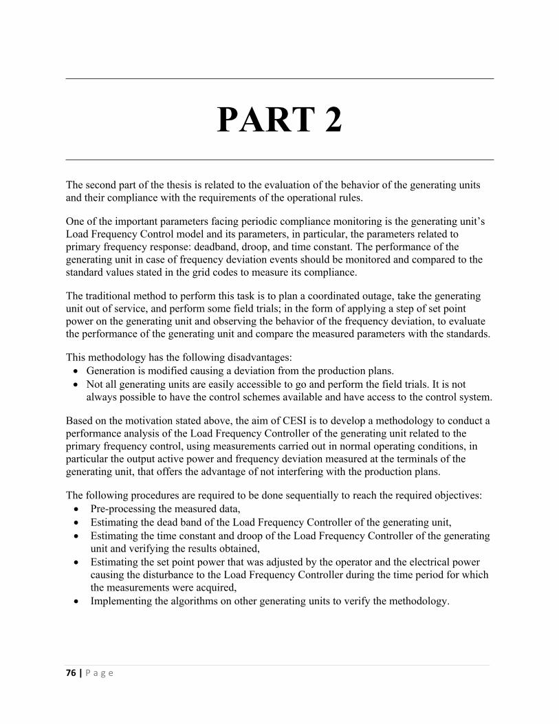
76 | P a g e

PART 2The second part of the thesis is related to the evaluation of the behavior of the generating units and their compliance with the requirements of the operational rules.

One of the important parameters facing periodic compliance monitoring is the generating unit’s Load Frequency Control model and its parameters, in particular, the parameters related to primary frequency response: deadband, droop, and time constant. The performance of the generating unit in case of frequency deviation events should be monitored and compared to the standard values stated in the grid codes to measure its compliance.

The traditional method to perform this task is to plan a coordinated outage, take the generating unit out of service, and perform some field trials; in the form of applying a step of set point power on the generating unit and observing the behavior of the frequency deviation, to evaluate the performance of the generating unit and compare the measured parameters with the standards.

This methodology has the following disadvantages: Generation is modified causing a deviation from the production plans. Not all generating units are easily accessible to go and perform the field trials. It is not

always possible to have the control schemes available and have access to the control system.

Based on the motivation stated above, the aim of CESI is to develop a methodology to conduct a performance analysis of the Load Frequency Controller of the generating unit related to the primary frequency control, using measurements carried out in normal operating conditions, in particular the output active power and frequency deviation measured at the terminals of the generating unit, that offers the advantage of not interfering with the production plans.

The following procedures are required to be done sequentially to reach the required objectives: Pre-processing the measured data, Estimating the dead band of the Load Frequency Controller of the generating unit, Estimating the time constant and droop of the Load Frequency Controller of the generating

unit and verifying the results obtained, Estimating the set point power that was adjusted by the operator and the electrical power

causing the disturbance to the Load Frequency Controller during the time period for which the measurements were acquired,

Implementing the algorithms on other generating units to verify the methodology.

77 | P a g e

CHAPTER 66. Load Frequency Droop Control

This chapter is concerned about the classical control of individual generating units to maintain the quality of the delivered power as required. It is organized as follows: The first section highlights the main components of the generating unit, followed by another section that explains the droop control which is implemented by most generating units currently present nowadays. The last section shows how the model of the generating unit’s controller is derived.

6.1. Main Components of a Generating Unit

Any electric power system can be subdivided into three dependent systems: Generation to generate the required active and reactive power at the nominal frequency, Transmission to transport the electric energy for long distances at high voltage, and Distribution to provide the electric energy at medium or low voltage to the end users, who

may be domestic, industrial or commercial.

This thesis will focus on Generation which is traditionally provided mainly by large power plants that consists of one or more generating units equipped with the LFC and AVR controllers explained in Section 6.1.5.

The generating unit refers to the unit that is responsible for generating electric energy from one of the available forms of energy with high degree of efficiency, quality, availability and reliability. It does not refer specifically to the generator only as the generator is one of the components of the generating unit, but does not form a generating unit solely.

Generating units should be controllable, to counteract sudden imbalances resulting from a sudden change of the demand load, sudden loss of a generator, or recently, imbalances due to hourly changes imposed by the electricity market which is currently considered as one of the main reason for imbalances [31]. They should be also predictable, to follow the load curve based on data given by load forecast, which mainly depend on statistical historical data. However, recent integration of renewable energies into the grids, to contribute to generation, required also to count on weather forecast data.

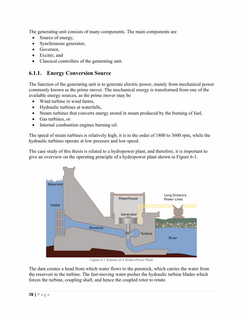
78 | P a g e

The generating unit consists of many components. The main components are Source of energy, Synchronous generator, Governor, Exciter, and Classical controllers of the generating unit.

6.1.1. Energy Conversion Source

The function of the generating unit is to generate electric power, mainly from mechanical power commonly known as the prime mover. The mechanical energy is transformed from one of the available energy sources, as the prime mover may be Wind turbine in wind farms, Hydraulic turbines at waterfalls, Steam turbines that converts energy stored in steam produced by the burning of fuel, Gas turbines, or Internal combustion engines burning oil.

The speed of steam turbines is relatively high; it is in the order of 1800 to 3600 rpm, while the hydraulic turbines operate at low pressure and low speed.

The case study of this thesis is related to a hydropower plant, and therefore, it is important to give an overview on the operating principle of a hydropower plant shown in Figure 6-1.

Figure 6-1 Scheme of a Hydro-Power Plant

The dam creates a head from which water flows to the penstock, which carries the water from the reservoir to the turbine. The fast-moving water pushes the hydraulic turbine blades which forces the turbine, coupling shaft, and hence the coupled rotor to rotate.

79 | P a g e

6.1.2. Synchronous Generator

The three-phase synchronous generator is the main source of electric energy in power systems [32]. It makes use of the mechanical energy of the prime mover to which it is coupled and transforms it into electric energy to be delivered to the network. It has two fields rotating at the same speed in synchronous operation: One field is produced by the rotor coupled to the prime mover which rotates it at the synchronous speed and excited by dc field produced by dc current of field winding mounted in the rotor. The other field is produced by the three-phase armature currents in the stator windings.

Synchronous generators coupled to steam turbines have cylindrical rotor of two poles for 3600 rpm and four poles for 1800 rpm, while those coupled to hydraulic turbines have salient type rotor with a lot of poles.

In a power station, one or more generators are operated in parallel to provide the required total power, connected to a common point known as a bus.

6.1.3. Speed Governor

The operation of the electric power systems depends only on one fundamental law of physics which states that if the electrical grid has no way to store energy, it is necessary that at every instant the amount of power generated to be equal to the power absorbed by the loads. Some energy is naturally stored in the inertia of large generators; however, this is only enough to compensate for small unbalances, which always occur and cause small frequency and voltage variations. Large violation of balance leads to large frequency variations, voltage perturbation, and electromechanical oscillations. If suitable corrective measures are not taken, the system may collapse leading to widespread blackouts.

Automation is the way to determine and actuate these measures via the generator’s controllers. The most important actuator used to control the generating unit is the speed governor which senses the change in speed and acts through the speed control mechanism to adjust the turbine’s input valve in case of conventional power plant or the water inlet to the turbine in case of hydro-power plant to change the mechanical power output to bring the system to a new steady-state.

The speed governor should include the following functions: A way to set speed, A way to sense speed, A way to compare the actual speed to the desired speed, and Ways for the governor to control and stabilize the prime mover.

The speed control mechanism includes equipment; such as, relays, servomotors, pressure or power amplifying devices, and linkages between the speed governor and gates.

The governor of hydro turbine can be either mechanical hydraulic or electrohydraulic. It is affected by the water inertia and its response to the change in speed settings is relatively slow.

80 | P a g e

6.1.4. Excitation System

Another important actuator is the excitation system whose purpose is to Control the terminal voltage of the generator and reactive power flow by controlling the

direct current in the field winding in the rotor of the synchronous generator, Respond to transient disturbances and perform control and protective functions, and Improve the system stability.

6.1.5. Classical Controllers of a Generating Unit

In order to keep the system in steady state, the active and reactive power output of the generating unit should be controlled. The aim of controlling the generating unit is to deliver power to the interconnected power system while keeping the frequency and voltage within permissible limits.

Controlling the generating unit is done using two separate control loops shown in Figure 6-2: The Load Frequency Control (LFC) controls the active power and frequency. The Automatic Voltage Regulator (AVR) controls the reactive power and voltage.

Figure 6-2 LFC and AVR of a Synchronous Generator [32]

More details, the LFC and AVR control loops act on each generating unit in an interconnected system. The control loops are set for certain loading conditions and operate in the case of a change in the load demand, to maintain the frequency and voltage within the permissible operating conditions. The change in the active power output mainly depends on the change of the frequency, while the change in the reactive power output mainly depends on the change of the voltage. Neglecting the cross-coupling between the LFC and AVR control loops is allowed as the time constant of the excitation system is much lower than that of the prime mover and the transient decays much faster and does not affect the dynamics of the LFC.

This method is used to control the generating unit individually, and eventually will contribute to the control of the whole interconnected system. It is performed using processed data obtained by remote acquisition systems either Supervisory Control And Data Acquisition (SCADA) systems, Phasor Measurement Unit (PMU) systems, or a combination of both systems.

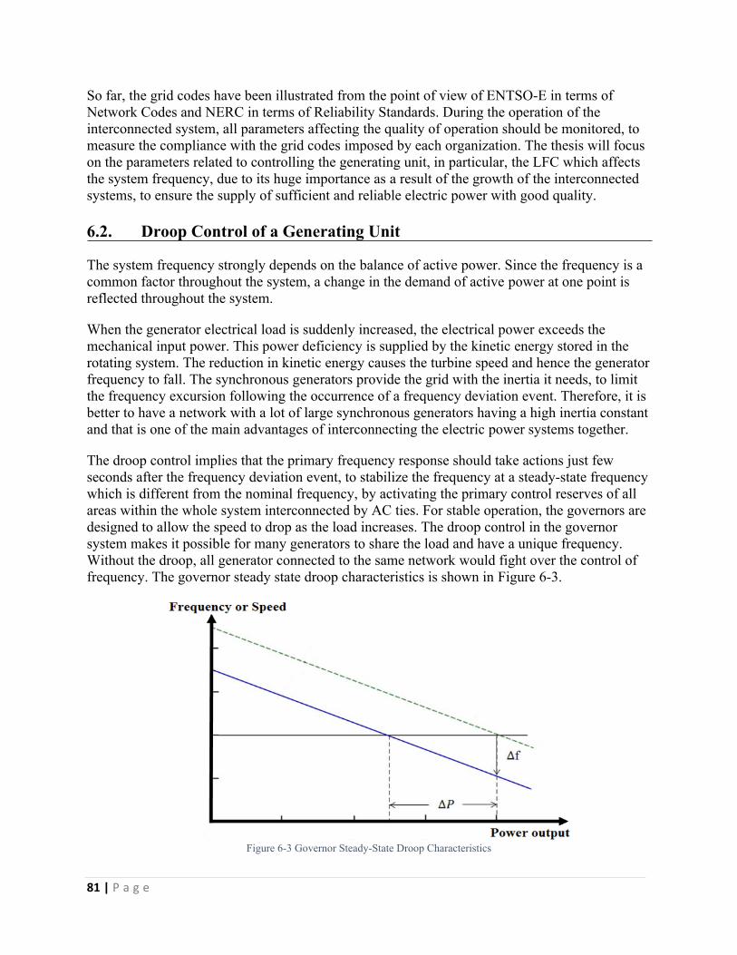
81 | P a g e

So far, the grid codes have been illustrated from the point of view of ENTSO-E in terms of Network Codes and NERC in terms of Reliability Standards. During the operation of the interconnected system, all parameters affecting the quality of operation should be monitored, to measure the compliance with the grid codes imposed by each organization. The thesis will focus on the parameters related to controlling the generating unit, in particular, the LFC which affects the system frequency, due to its huge importance as a result of the growth of the interconnected systems, to ensure the supply of sufficient and reliable electric power with good quality.

6.2. Droop Control of a Generating Unit

The system frequency strongly depends on the balance of active power. Since the frequency is a common factor throughout the system, a change in the demand of active power at one point is reflected throughout the system.

When the generator electrical load is suddenly increased, the electrical power exceeds the mechanical input power. This power deficiency is supplied by the kinetic energy stored in the rotating system. The reduction in kinetic energy causes the turbine speed and hence the generator frequency to fall. The synchronous generators provide the grid with the inertia it needs, to limit the frequency excursion following the occurrence of a frequency deviation event. Therefore, it is better to have a network with a lot of large synchronous generators having a high inertia constant and that is one of the main advantages of interconnecting the electric power systems together.

The droop control implies that the primary frequency response should take actions just few seconds after the frequency deviation event, to stabilize the frequency at a steady-state frequency which is different from the nominal frequency, by activating the primary control reserves of all areas within the whole system interconnected by AC ties. For stable operation, the governors are designed to allow the speed to drop as the load increases. The droop control in the governor system makes it possible for many generators to share the load and have a unique frequency. Without the droop, all generator connected to the same network would fight over the control of frequency. The governor steady state droop characteristics is shown in Figure 6-3.

Figure 6-3 Governor Steady-State Droop Characteristics

82 | P a g e

The slope of the governor steady state droop characteristics represents the generator droop or speed regulation and it is negative. The mechanical power increases with decreasing frequency. The generator droop can be expressed in terms of Hz/MW (kf) or as a percentage (R).

𝑘𝑓 =‒𝑓 ‒ 𝑓𝑜

𝑃 ‒ 𝑃𝑜

𝐻𝑧𝑀𝑊

𝑅 =‒(𝑓 ‒ 𝑓𝑜 ) 𝑓𝑜

(𝑃 ‒ 𝑃𝑜 ) 𝑃𝑛

%

Where, f is the actual frequency, fo is the nominal frequency, P is the actual output power at the terminals of the generator, Pn is the rated active power of the generator, and Po is the output power at the terminals of the generator at the nominal frequency without deadband i.e. the power obtained by extrapolating the governor steady state droop characteristics to intersect with the power axis.

Therefore the generator droop expressed as a percentage is the slope of the governor steady state droop characteristics, if the axes are in terms of per unit for the frequency and the power. While the generator droop expressed in terms of Hz/MW is the slope of the governor steady state droop characteristics, if the axes are in terms of Hz for the frequency and MW for the power.

The droop expressed as a percentage is in the order of few percent. If a generating unit has a Load Frequency Controller with 5% droop means that for 5% change in frequency, the generating unit will produce 100% of its output.

When a frequency deviation event occurs, not only the governor of the generating unit responds to the frequency deviation, but the load also has a frequency response which depends on the type of load connected to the power system: Resistive loads, such as lighting and heating loads, are not sensitive to the frequency. Inductive loads, such as motors, depend on the frequency change as they draw less energy

as the frequency decreases.

The load response is represented by a load damping constant D, expressed as a percentage given by the change in load divided by the change in frequency and it is in the order of 0-2%. D=1.5 implies that the load changes by 1.5% for 1% change in frequency.

Deadband is a part of the governor steady state droop characteristics centered around the nominal frequency where there is no frequency response; the governor neglects any frequency deviation within this band. Deadbands are generally classified as unintentional and intentional deadbands. The unintentional deadband is unavoidable and unadjustable and is represented by the inherent mechanical effect of a governor system, such as; sticky valves, loose gears, and hydraulic system nonlinearity. The intentional deadband is adopted in the Load Frequency Controllers of the generating units to reduce excessive controller activities and turbine mechanical wear for normal power system frequency variations. There are two ways to implement the droop characteristics: non-step implementation and step implementation. The difference is shown in Figure 6-4.

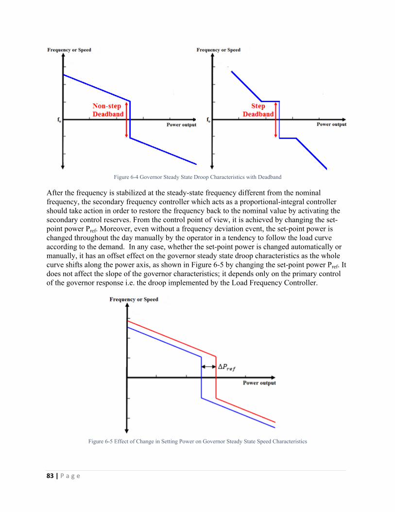
83 | P a g e

Figure 6-4 Governor Steady State Droop Characteristics with Deadband

After the frequency is stabilized at the steady-state frequency different from the nominal frequency, the secondary frequency controller which acts as a proportional-integral controller should take action in order to restore the frequency back to the nominal value by activating the secondary control reserves. From the control point of view, it is achieved by changing the set-point power Pref. Moreover, even without a frequency deviation event, the set-point power is changed throughout the day manually by the operator in a tendency to follow the load curve according to the demand. In any case, whether the set-point power is changed automatically or manually, it has an offset effect on the governor steady state droop characteristics as the whole curve shifts along the power axis, as shown in Figure 6-5 by changing the set-point power Pref. It does not affect the slope of the governor characteristics; it depends only on the primary control of the governor response i.e. the droop implemented by the Load Frequency Controller.

Figure 6-5 Effect of Change in Setting Power on Governor Steady State Speed Characteristics

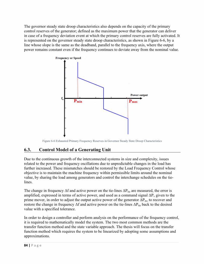
84 | P a g e

The governor steady state droop characteristics also depends on the capacity of the primary control reserves of the generator; defined as the maximum power that the generator can deliver in case of a frequency deviation event at which the primary control reserves are fully activated. It is represented on the governor steady state droop characteristics, as shown in Figure 6-6, by a line whose slope is the same as the deadband, parallel to the frequency axis, where the output power remains constant even if the frequency continues to deviate away from the nominal value.

Figure 6-6 Exhausted Primary Frequency Reserves in Governor Steady State Droop Characteristics

6.3. Control Model of a Generating Unit

Due to the continuous growth of the interconnected systems in size and complexity, issues related to the power and frequency oscillations due to unpredictable changes in the load has further increased. These mismatches should be restored by the Load Frequency Control whose objective is to maintain the machine frequency within permissible limits around the nominal value, by sharing the load among generators and control the interchange schedules on the tie-lines.

The change in frequency Δf and active power on the tie-lines ΔPtie are measured, the error is amplified, expressed in terms of active power, and used as a command signal ΔPv given to the prime mover, in order to adjust the output active power of the generator ΔPm, to recover and restore the change in frequency Δf and active power on the tie-lines ΔPtie back to the desired value with a specified tolerance.

In order to design a controller and perform analysis on the performance of the frequency control, it is required to mathematically model the system. The two most common methods are the transfer function method and the state variable approach. The thesis will focus on the transfer function method which requires the system to be linearized by adopting some assumptions and approximations.

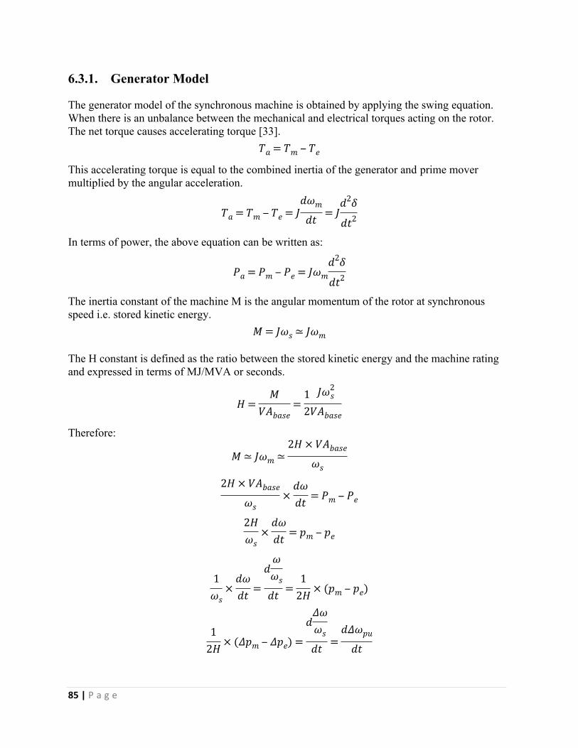
85 | P a g e

6.3.1. Generator Model

The generator model of the synchronous machine is obtained by applying the swing equation. When there is an unbalance between the mechanical and electrical torques acting on the rotor. The net torque causes accelerating torque [33].

𝑇𝑎 = 𝑇𝑚 ‒ 𝑇𝑒

This accelerating torque is equal to the combined inertia of the generator and prime mover multiplied by the angular acceleration.

𝑇𝑎 = 𝑇𝑚 ‒ 𝑇𝑒 = 𝐽𝑑𝜔𝑚

𝑑𝑡 = 𝐽𝑑2𝛿

𝑑𝑡2

In terms of power, the above equation can be written as:

𝑃𝑎 = 𝑃𝑚 ‒ 𝑃𝑒 = 𝐽𝜔𝑚𝑑2𝛿

𝑑𝑡2

The inertia constant of the machine M is the angular momentum of the rotor at synchronous speed i.e. stored kinetic energy.

𝑀 = 𝐽𝜔𝑠 ≃ 𝐽𝜔𝑚

The H constant is defined as the ratio between the stored kinetic energy and the machine rating and expressed in terms of MJ/MVA or seconds.

𝐻 =𝑀

𝑉𝐴𝑏𝑎𝑠𝑒=

12

𝐽𝜔2𝑠

𝑉𝐴𝑏𝑎𝑠𝑒

Therefore:

𝑀 ≃ 𝐽𝜔𝑚 ≃2𝐻 × 𝑉𝐴𝑏𝑎𝑠𝑒

𝜔𝑠

2𝐻 × 𝑉𝐴𝑏𝑎𝑠𝑒

𝜔𝑠×

𝑑𝜔𝑑𝑡 = 𝑃𝑚 ‒ 𝑃𝑒

2𝐻𝜔𝑠

×𝑑𝜔𝑑𝑡 = 𝑝𝑚 ‒ 𝑝𝑒

1𝜔𝑠

×𝑑𝜔𝑑𝑡 =

𝑑𝜔𝜔𝑠

𝑑𝑡 =1

2𝐻 × (𝑝𝑚 ‒ 𝑝𝑒)

12𝐻 × (𝛥𝑝𝑚 ‒ 𝛥𝑝𝑒) =

𝑑𝛥𝜔𝜔𝑠

𝑑𝑡 =𝑑𝛥𝜔𝑝𝑢

𝑑𝑡

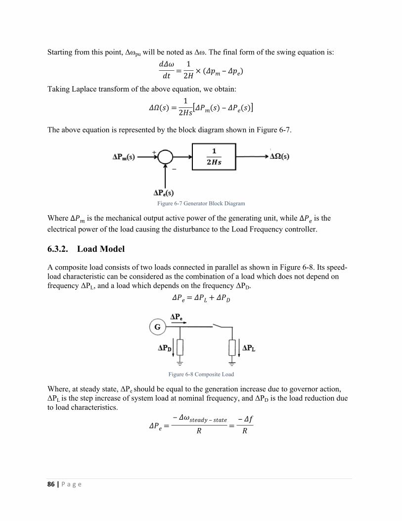
86 | P a g e

Starting from this point, Δωpu will be noted as Δω. The final form of the swing equation is:𝑑𝛥𝜔

𝑑𝑡 =1

2𝐻 × (𝛥𝑝𝑚 ‒ 𝛥𝑝𝑒)

Taking Laplace transform of the above equation, we obtain:

𝛥𝛺(𝑠) =1

2𝐻𝑠[𝛥𝑃𝑚(𝑠) ‒ 𝛥𝑃𝑒(𝑠)]

The above equation is represented by the block diagram shown in Figure 6-7.

Figure 6-7 Generator Block Diagram

Where is the mechanical output active power of the generating unit, while is the ∆𝑃𝑚 ∆𝑃𝑒electrical power of the load causing the disturbance to the Load Frequency controller.

6.3.2. Load Model

A composite load consists of two loads connected in parallel as shown in Figure 6-8. Its speed-load characteristic can be considered as the combination of a load which does not depend on frequency ΔPL, and a load which depends on the frequency ΔPD.

𝛥𝑃𝑒 = 𝛥𝑃𝐿 + 𝛥𝑃𝐷

Figure 6-8 Composite Load

Where, at steady state, ΔPe should be equal to the generation increase due to governor action, ΔPL is the step increase of system load at nominal frequency, and ΔPD is the load reduction due to load characteristics.

𝛥𝑃𝑒 =‒ 𝛥𝜔𝑠𝑡𝑒𝑎𝑑𝑦 ‒ 𝑠𝑡𝑎𝑡𝑒

𝑅 =‒ 𝛥𝑓

𝑅

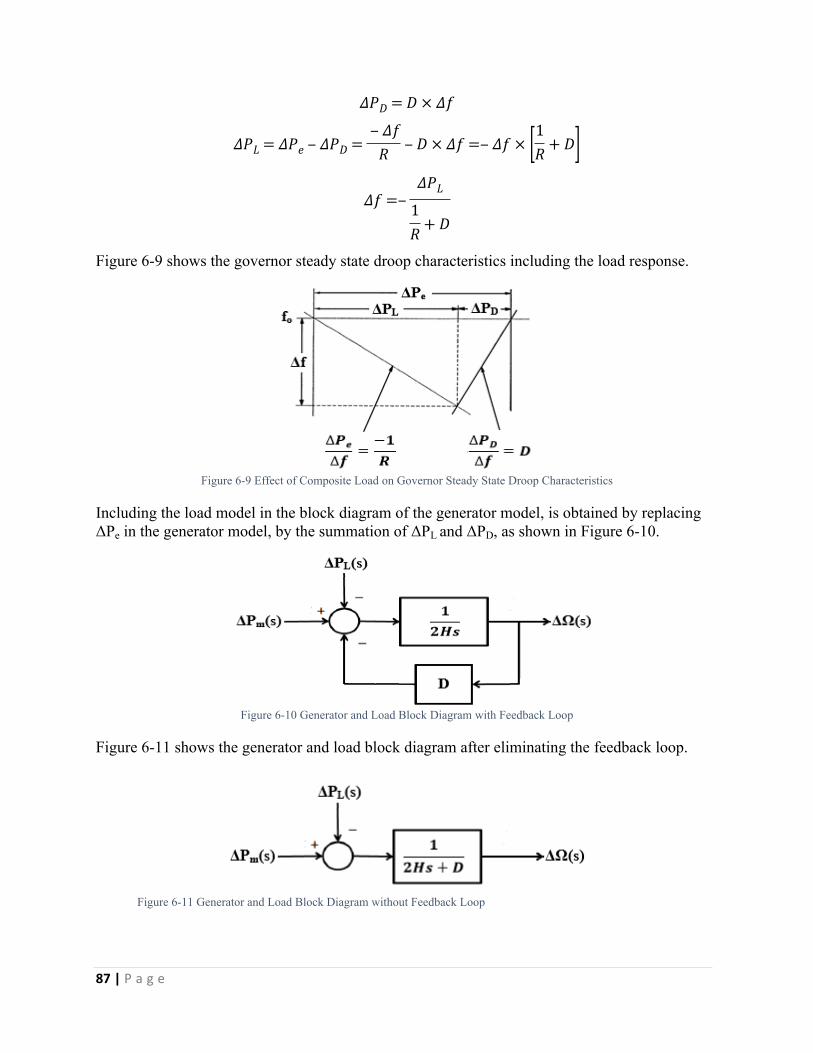
87 | P a g e

𝛥𝑃𝐷 = 𝐷 × 𝛥𝑓

𝛥𝑃𝐿 = 𝛥𝑃𝑒 ‒ 𝛥𝑃𝐷 =‒ 𝛥𝑓

𝑅 ‒ 𝐷 × 𝛥𝑓 =‒ 𝛥𝑓 × [1𝑅 + 𝐷]

𝛥𝑓 =‒𝛥𝑃𝐿

1𝑅 + 𝐷

Figure 6-9 shows the governor steady state droop characteristics including the load response.

Figure 6-9 Effect of Composite Load on Governor Steady State Droop Characteristics

Including the load model in the block diagram of the generator model, is obtained by replacing ΔPe in the generator model, by the summation of ΔPL and ΔPD, as shown in Figure 6-10.

Figure 6-10 Generator and Load Block Diagram with Feedback Loop

Figure 6-11 shows the generator and load block diagram after eliminating the feedback loop.

Figure 6-11 Generator and Load Block Diagram without Feedback Loop

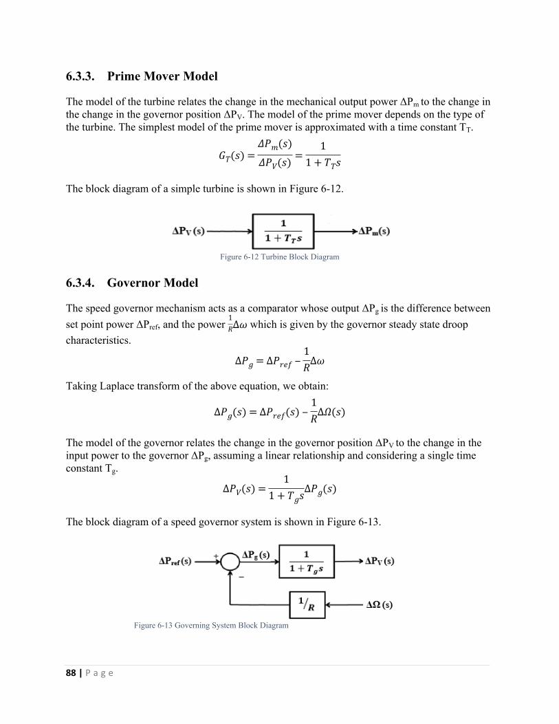
88 | P a g e

6.3.3. Prime Mover Model

The model of the turbine relates the change in the mechanical output power ΔPm to the change in the change in the governor position ΔPV. The model of the prime mover depends on the type of the turbine. The simplest model of the prime mover is approximated with a time constant ΤT.

𝐺𝑇(𝑠) =𝛥𝑃𝑚(𝑠)

𝛥𝑃𝑉(𝑠) =1

1 + 𝛵𝑇𝑠

The block diagram of a simple turbine is shown in Figure 6-12.

Figure 6-12 Turbine Block Diagram

6.3.4. Governor Model

The speed governor mechanism acts as a comparator whose output ΔPg is the difference between set point power ΔPref, and the power which is given by the governor steady state droop

1𝑅∆𝜔

characteristics.

∆𝑃𝑔 = ∆𝑃𝑟𝑒𝑓 ‒1𝑅∆𝜔

Taking Laplace transform of the above equation, we obtain:

∆𝑃𝑔(𝑠) = ∆𝑃𝑟𝑒𝑓(𝑠) ‒1𝑅∆𝛺(𝑠)

The model of the governor relates the change in the governor position ΔPV to the change in the input power to the governor ΔPg, assuming a linear relationship and considering a single time constant Τg.

∆𝑃𝑉(𝑠) =1

1 + 𝛵𝑔𝑠∆𝑃𝑔(𝑠)

The block diagram of a speed governor system is shown in Figure 6-13.

Figure 6-13 Governing System Block Diagram

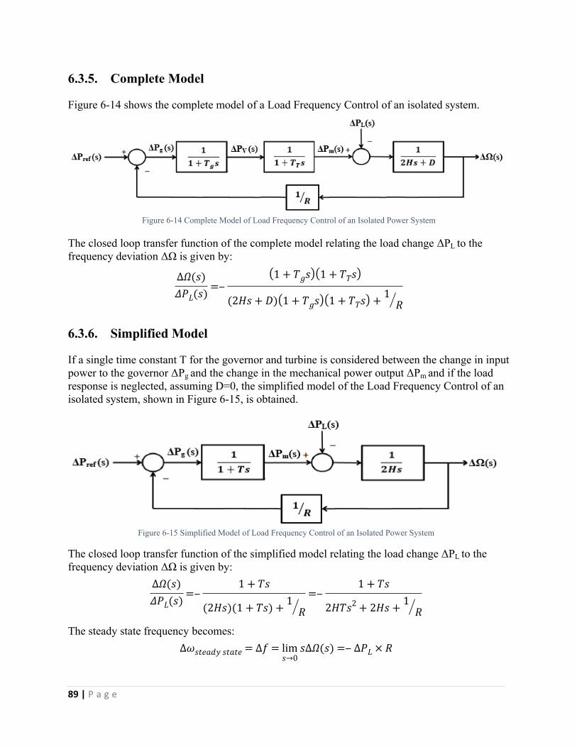
89 | P a g e

6.3.5. Complete Model

Figure 6-14 shows the complete model of a Load Frequency Control of an isolated system.

Figure 6-14 Complete Model of Load Frequency Control of an Isolated Power System

The closed loop transfer function of the complete model relating the load change ΔPL to the frequency deviation ΔΩ is given by:

∆𝛺(𝑠)𝛥𝑃𝐿(𝑠) =‒

(1 + 𝛵𝑔𝑠)(1 + 𝛵𝑇𝑠)

(2𝐻𝑠 + 𝐷)(1 + 𝛵𝑔𝑠)(1 + 𝛵𝑇𝑠) + 1𝑅

6.3.6. Simplified Model

If a single time constant Τ for the governor and turbine is considered between the change in input power to the governor ΔPg and the change in the mechanical power output ΔPm and if the load response is neglected, assuming D=0, the simplified model of the Load Frequency Control of an isolated system, shown in Figure 6-15, is obtained.

Figure 6-15 Simplified Model of Load Frequency Control of an Isolated Power System

The closed loop transfer function of the simplified model relating the load change ΔPL to the frequency deviation ΔΩ is given by:

∆𝛺(𝑠)𝛥𝑃𝐿(𝑠) =‒

1 + 𝛵𝑠

(2𝐻𝑠)(1 + 𝛵𝑠) + 1𝑅

=‒1 + 𝛵𝑠

2𝐻𝛵𝑠2 + 2𝐻𝑠 + 1𝑅

The steady state frequency becomes:∆𝜔𝑠𝑡𝑒𝑎𝑑𝑦 𝑠𝑡𝑎𝑡𝑒 = ∆𝑓 = lim

𝑠→0𝑠∆𝛺(𝑠) =‒ ∆𝑃𝐿 × 𝑅

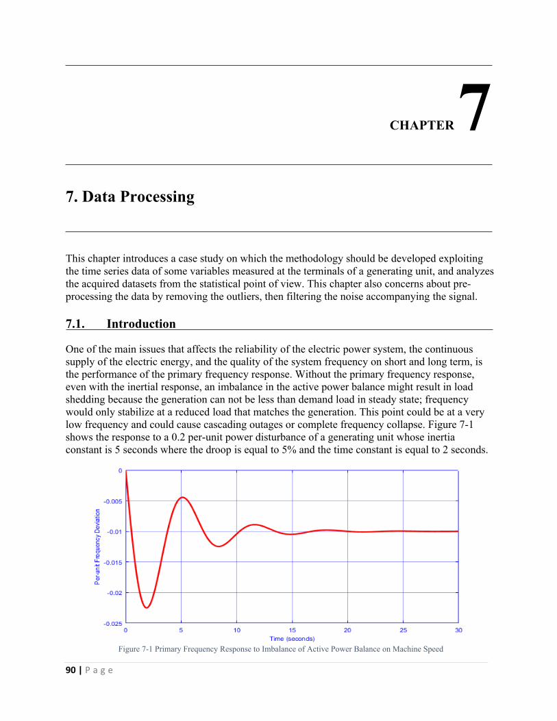
90 | P a g e

CHAPTER 77. Data Processing

This chapter introduces a case study on which the methodology should be developed exploiting the time series data of some variables measured at the terminals of a generating unit, and analyzes the acquired datasets from the statistical point of view. This chapter also concerns about pre-processing the data by removing the outliers, then filtering the noise accompanying the signal.

7.1. Introduction

One of the main issues that affects the reliability of the electric power system, the continuous supply of the electric energy, and the quality of the system frequency on short and long term, is the performance of the primary frequency response. Without the primary frequency response, even with the inertial response, an imbalance in the active power balance might result in load shedding because the generation can not be less than demand load in steady state; frequency would only stabilize at a reduced load that matches the generation. This point could be at a very low frequency and could cause cascading outages or complete frequency collapse. Figure 7-1 shows the response to a 0.2 per-unit power disturbance of a generating unit whose inertia constant is 5 seconds where the droop is equal to 5% and the time constant is equal to 2 seconds.

Figure 7-1 Primary Frequency Response to Imbalance of Active Power Balance on Machine Speed

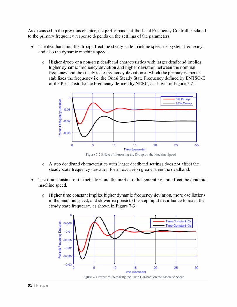
91 | P a g e

As discussed in the previous chapter, the performance of the Load Frequency Controller related to the primary frequency response depends on the settings of the parameters:

The deadband and the droop affect the steady-state machine speed i.e. system frequency, and also the dynamic machine speed.

o Higher droop or a non-step deadband characteristics with larger deadband implies higher dynamic frequency deviation and higher deviation between the nominal frequency and the steady state frequency deviation at which the primary response stabilizes the frequency i.e. the Quasi Steady State Frequency defined by ENTSO-E or the Post-Disturbance Frequency defined by NERC, as shown in Figure 7-2.

Figure 7-2 Effect of Increasing the Droop on the Machine Speed

o A step deadband characteristics with larger deadband settings does not affect the steady state frequency deviation for an excursion greater than the deadband.

The time constant of the actuators and the inertia of the generating unit affect the dynamic machine speed.

o Higher time constant implies higher dynamic frequency deviation, more oscillations in the machine speed, and slower response to the step input disturbance to reach the steady state frequency, as shown in Figure 7-3.

Figure 7-3 Effect of Increasing the Time Constant on the Machine Speed

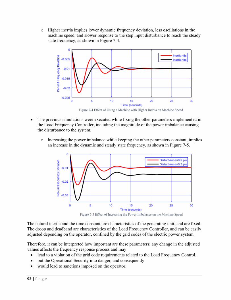
92 | P a g e

o Higher inertia implies lower dynamic frequency deviation, less oscillations in the machine speed, and slower response to the step input disturbance to reach the steady state frequency, as shown in Figure 7-4.

Figure 7-4 Effect of Using a Machine with Higher Inertia on Machine Speed

The previous simulations were executed while fixing the other parameters implemented in the Load Frequency Controller, including the magnitude of the power imbalance causing the disturbance to the system.

o Increasing the power imbalance while keeping the other parameters constant, implies an increase in the dynamic and steady state frequency, as shown in Figure 7-5.

Figure 7-5 Effect of Increasing the Power Imbalance on the Machine Speed

The natural inertia and the time constant are characteristics of the generating unit, and are fixed. The droop and deadband are characteristics of the Load Frequency Controller, and can be easily adjusted depending on the operator, confined by the grid codes of the electric power system.

Therefore, it can be interpreted how important are these parameters; any change in the adjusted values affects the frequency response process and may lead to a violation of the grid code requirements related to the Load Frequency Control, put the Operational Security into danger, and consequently would lead to sanctions imposed on the operator.

93 | P a g e

Therefore, the generating unit should undergo Compliance Testing periodically to monitor the performance of the generating unit in case of frequency deviation events, to be compared with the standard values stated in the grid codes to measure its compliance, ensure Operational Security, and avoid sanctions.

To perform this task, it is required either to Plan for a coordinated outage, take the generating unit out of service, and perform some

field trials, or at least, Deviate from the production plans by applying a step of active power on the generating unit

and observing the behavior of the frequency deviation.

In any case, either generation is interrupted or changed, a deviation from the production plans of the network would be a consequence. Moreover, the first methodology has another disadvantage; not all generating units are easily accessible to go and perform the field trials, while the second has another disadvantage; the disturbance that occurs in the system frequency by applying the step on the generating unit under inspection.

The aim of the second part of the thesis is to develop a methodology to test the performance of the Load Frequency Controller related to the primary frequency response implemented by a particular generator, only by acquiring the real time series data of the active power and the frequency measured at the terminals of the generating unit in normal operating conditions, without any limitations imposed on the production plans of the operator in its attempt to fulfill its obligation towards the market, and follow the demand load to maintain the quality of the system frequency as high as possible and the operation as secure as possible. However, the dataset should be large enough in order to obtain accurate results that match what are actually implemented.

7.2. Statistical Analysis of the Case Study

The case study of which the parameters of the Load Frequency Controller should be estimated is a generating unit whose technical specifications are listed in Table 7-1.

Technical SpecificationsLocation AfricaType of Power Plant Hydropower PlantRated Active Power (MW) 173Rated Apparent Power (MVA) 179.5H constant (seconds) 3 Secondary Frequency Controller Not installed

Table 7-1 Technical Specifications of the Generating Unit in Africa

The thesis will exploit the data provided by CESI Milano from real on-site measurements: The active power measured at the terminals of the generator (Pm) in MW, and The frequency deviation from 50 Hz or the difference between the synchronous speed and

the electrical speed of the machine measured at the terminals of the generator (ΔΩ) in Hz.

The data are measured with a sampling frequency 10 Hz, i.e. a sample each 0.1 second, for a 66 hours time span, i.e. 2 days and 18 hours. Therefore, the 2 datasets consist of 2376000 samples.

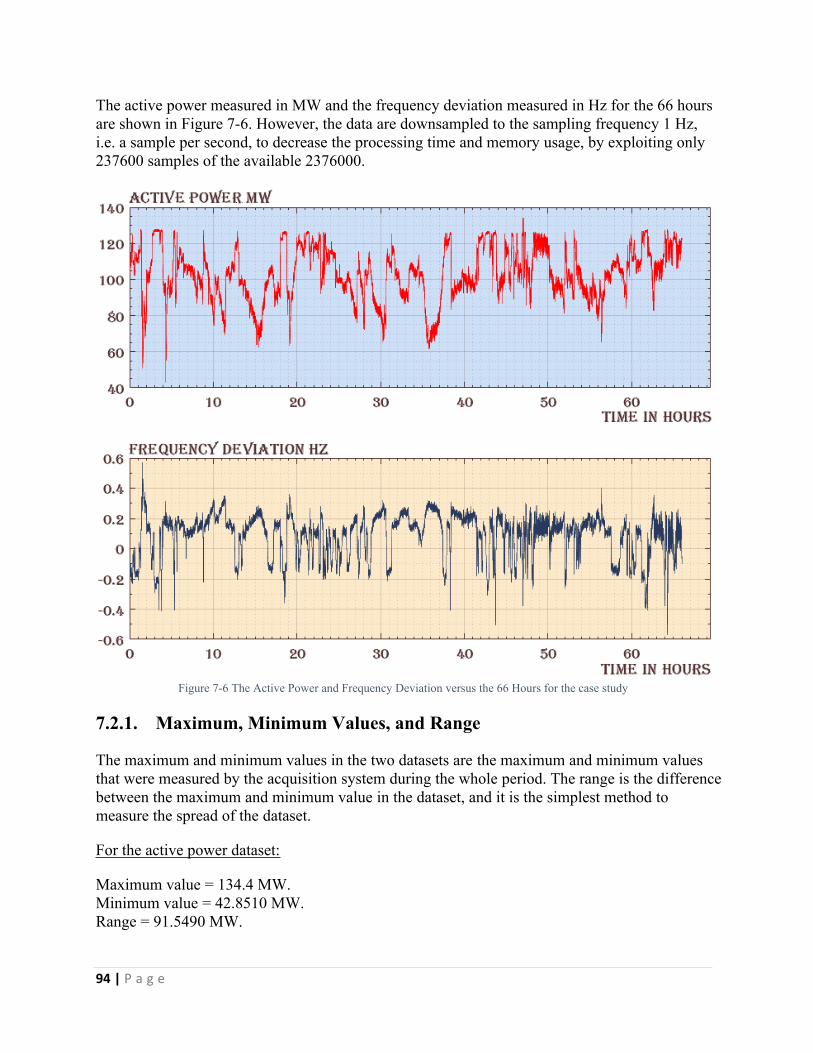
94 | P a g e

The active power measured in MW and the frequency deviation measured in Hz for the 66 hours are shown in Figure 7-6. However, the data are downsampled to the sampling frequency 1 Hz, i.e. a sample per second, to decrease the processing time and memory usage, by exploiting only 237600 samples of the available 2376000.

Figure 7-6 The Active Power and Frequency Deviation versus the 66 Hours for the case study

7.2.1. Maximum, Minimum Values, and Range

The maximum and minimum values in the two datasets are the maximum and minimum values that were measured by the acquisition system during the whole period. The range is the difference between the maximum and minimum value in the dataset, and it is the simplest method to measure the spread of the dataset.

For the active power dataset:

Maximum value = 134.4 MW.Minimum value = 42.8510 MW.Range = 91.5490 MW.

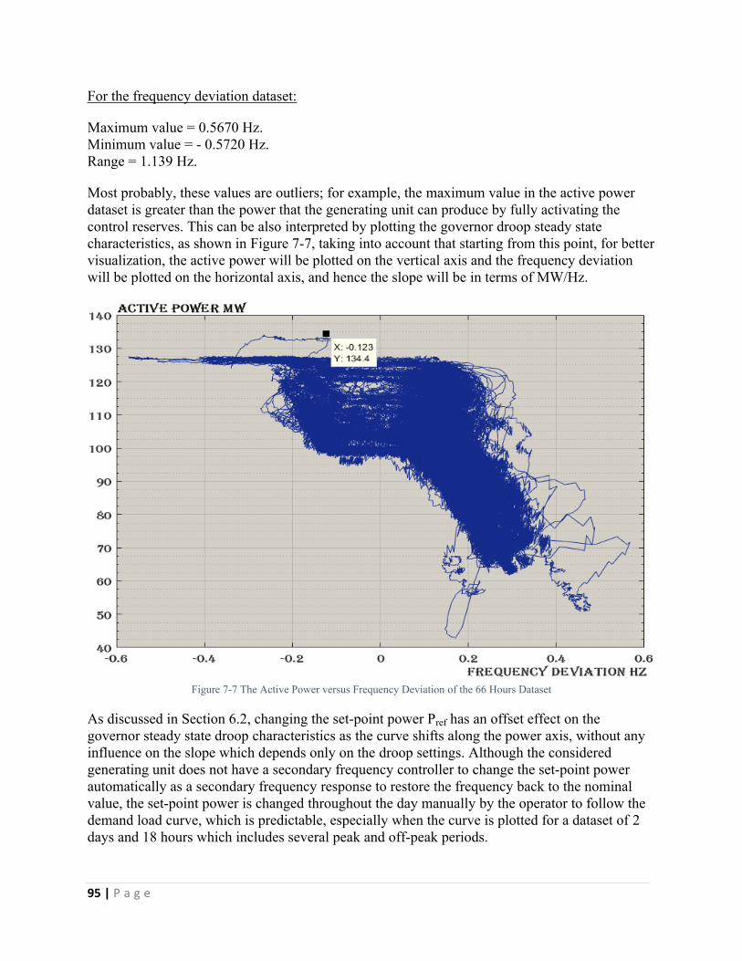
95 | P a g e

For the frequency deviation dataset:

Maximum value = 0.5670 Hz.Minimum value = - 0.5720 Hz.Range = 1.139 Hz.

Most probably, these values are outliers; for example, the maximum value in the active power dataset is greater than the power that the generating unit can produce by fully activating the control reserves. This can be also interpreted by plotting the governor droop steady state characteristics, as shown in Figure 7-7, taking into account that starting from this point, for better visualization, the active power will be plotted on the vertical axis and the frequency deviation will be plotted on the horizontal axis, and hence the slope will be in terms of MW/Hz.

Figure 7-7 The Active Power versus Frequency Deviation of the 66 Hours Dataset

As discussed in Section 6.2, changing the set-point power Pref has an offset effect on the governor steady state droop characteristics as the curve shifts along the power axis, without any influence on the slope which depends only on the droop settings. Although the considered generating unit does not have a secondary frequency controller to change the set-point power automatically as a secondary frequency response to restore the frequency back to the nominal value, the set-point power is changed throughout the day manually by the operator to follow the demand load curve, which is predictable, especially when the curve is plotted for a dataset of 2 days and 18 hours which includes several peak and off-peak periods.

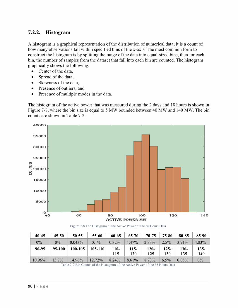
96 | P a g e

7.2.2. Histogram

A histogram is a graphical representation of the distribution of numerical data; it is a count of how many observations fall within specified bins of the x-axis. The most common form to construct the histogram is by splitting the range of the data into equal-sized bins, then for each bin, the number of samples from the dataset that fall into each bin are counted. The histogram graphically shows the following: Center of the data, Spread of the data, Skewness of the data, Presence of outliers, and Presence of multiple modes in the data.

The histogram of the active power that was measured during the 2 days and 18 hours is shown in Figure 7-8, where the bin size is equal to 5 MW bounded between 40 MW and 140 MW. The bin counts are shown in Table 7-2.

Figure 7-8 The Histogram of the Active Power of the 66 Hours Data

40-45 45-50 50-55 55-60 60-65 65-70 70-75 75-80 80-85 85-900% 0% 0.043% 0.1% 0.32% 1.47% 2.33% 2.5% 3.91% 4.83%90-95 95-100 100-105 105-110 110-

115115-120

120-125

125-130

130-135

135-140

10.96% 13.7% 14.96% 12.72% 8.24% 8.61% 8.73% 6.5% 0.08% 0%Table 7-2 Bin Counts of the Histogram of the Active Power of the 66 Hours Data

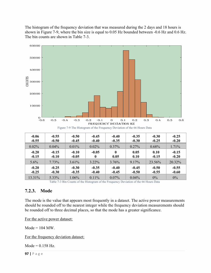
97 | P a g e

The histogram of the frequency deviation that was measured during the 2 days and 18 hours is shown in Figure 7-9, where the bin size is equal to 0.05 Hz bounded between -0.6 Hz and 0.6 Hz. The bin counts are shown in Table 7-3.

Figure 7-9 The Histogram of the Frequency Deviation of the 66 Hours Data

-0.06-0.55

-0.55-0.50

-0.50-0.45

-0.45-0.40

-0.40-0.35

-0.35-0.30

-0.30-0.25

-0.25-0.20

0.02% 0.04% 0.01% 0.02% 0.37% 0.27% 0.68% 1.71%-0.20-0.15

-0.15-0.10

-0.10-0.05

-0.050

00.05

0.050.10

0.10-0.15

-0.15-0.20

5.6% 7.73% 3.61% 3.22% 3.76% 9.17% 23.56% 20.32%-0.20-0.25

-0.25-0.30

-0.30-0.35

-0.35-0.40

-0.40-0.45

-0.45-0.50

-0.50-0.55

-0.55-0.60

13.31% 5.33% 1.06% 0.11% 0.07% 0.04% 0% 0%Table 7-3 Bin Counts of the Histogram of the Frequency Deviation of the 66 Hours Data

7.2.3. Mode

The mode is the value that appears most frequently in a dataset. The active power measurements should be rounded off to the nearest integer while the frequency deviation measurements should be rounded off to three decimal places, so that the mode has a greater significance.

For the active power dataset:

Mode = 104 MW.

For the frequency deviation dataset:

Mode = 0.158 Hz.

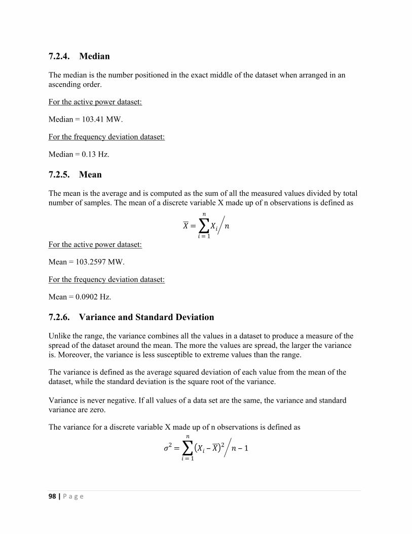
98 | P a g e

7.2.4. Median

The median is the number positioned in the exact middle of the dataset when arranged in an ascending order.

For the active power dataset:

Median = 103.41 MW.

For the frequency deviation dataset:

Median = 0.13 Hz.

7.2.5. Mean

The mean is the average and is computed as the sum of all the measured values divided by total number of samples. The mean of a discrete variable X made up of n observations is defined as

𝑋 =𝑛

∑𝑖 = 1

𝑋𝑖 𝑛

For the active power dataset:

Mean = 103.2597 MW.

For the frequency deviation dataset:

Mean = 0.0902 Hz.

7.2.6. Variance and Standard Deviation

Unlike the range, the variance combines all the values in a dataset to produce a measure of the spread of the dataset around the mean. The more the values are spread, the larger the variance is. Moreover, the variance is less susceptible to extreme values than the range.

The variance is defined as the average squared deviation of each value from the mean of the dataset, while the standard deviation is the square root of the variance.

Variance is never negative. If all values of a data set are the same, the variance and standard variance are zero.

The variance for a discrete variable X made up of n observations is defined as

𝜎2 =𝑛

∑𝑖 = 1

(𝑋𝑖 ‒ 𝑋)2 𝑛 ‒ 1

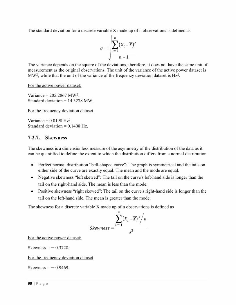
99 | P a g e

The standard deviation for a discrete variable X made up of n observations is defined as

𝜎 =

𝑛

∑𝑖 = 1

(𝑋𝑖 ‒ 𝑋)2

𝑛 ‒ 1The variance depends on the square of the deviations, therefore, it does not have the same unit of measurement as the original observations. The unit of the variance of the active power dataset is MW2, while that the unit of the variance of the frequency deviation dataset is Hz2.

For the active power dataset:

Variance = 205.2867 MW2.Standard deviation = 14.3278 MW.

For the frequency deviation dataset

Variance = 0.0198 Hz2.Standard deviation = 0.1408 Hz.

7.2.7. Skewness

The skewness is a dimensionless measure of the asymmetry of the distribution of the data as it can be quantified to define the extent to which the distribution differs from a normal distribution.

Perfect normal distribution “bell-shaped curve”: The graph is symmetrical and the tails on either side of the curve are exactly equal. The mean and the mode are equal.

Negative skewness “left skewed”: The tail on the curve's left-hand side is longer than the tail on the right-hand side. The mean is less than the mode.

Positive skewness “right skewed”: The tail on the curve's right-hand side is longer than the tail on the left-hand side. The mean is greater than the mode.

The skewness for a discrete variable X made up of n observations is defined as

𝑆𝑘𝑒𝑤𝑛𝑒𝑠𝑠 =

𝑛

∑𝑖 = 1

(𝑋𝑖 ‒ 𝑋)3 𝑛

𝜎3

For the active power dataset:

Skewness = ─ 0.3728.

For the frequency deviation dataset

Skewness = ─ 0.9469.

100 | P a g e

7.2.8. Covariance and Correlation

Covariance provides an indication about how two variables are related: A positive covariance indicates that the variables are positively related. A negative covariance indicates that the variables are inversely related. A zero covariance indicates that the variables are not related.

The covariance for two discrete variables X and Y made up of n observations is defined as

𝐶𝑂𝑉(𝑋,𝑌) =

𝑛

∑𝑖 = 1

(𝑋𝑖 ‒ 𝑋)(𝑌𝑖 ‒ 𝑌)

𝑛 ‒ 1

The covariance is usually displayed in the form of a covariance matrix. The diagonal elements show the variances of the variables X and Y, while the off-diagonal elements show the covariance between variables X and Y. Therefore, all covariance matrices are symmetrical.

Since, the covariance depends on the units of the data, it is difficult to compare the covariance among datasets that have different scales. A value that represents a strong linear relationship for one dataset might represent a very weak one in another.

Correlation is another way to determine how two variables are related. It does not only indicate whether variables are positively or inversely related, but it also indicates the degree to which the variables tend to move together by normalizing the covariance to the product of the standard deviations of the variables, creating a dimensionless quantity that facilitates the comparison of different datasets.

The correlation coefficient ranges between 1 and -1:

If the correlation coefficient is 1, the variables have a perfect positive correlation.o A positive correlation coefficient less than 1 indicates a less than perfect positive

correlation, which gets stronger approaching 1.

If the correlation coefficient is -1, the variables have a perfect negative correlation.o A negative correlation coefficient greater than -1 indicates a less than perfect negative

correlation, which gets stronger approaching -1.

If the correlation coefficient is 0, the variables have no correlation.

The correlation for two discrete variables X and Y made up of n observations is defined as

𝐶𝑜𝑟𝑟(𝑋,𝑌) =𝐶𝑂𝑉(𝑋,𝑌)

𝜎𝑥 × 𝜎𝑦

101 | P a g e

The correlation is usually displayed in the form of a correlation matrix. The diagonal elements are always 1, as expected; the correlation between a dataset and itself is always 1. The off-diagonal elements show the correlation between variable X and variable Y. Therefore, all correlation matrices are also symmetrical.

The covariance and correlation matrices between the active power and frequency deviation datasets, for these particular 66 hours, are

𝐶𝑜𝑣 = [205.2867 ‒ 1.3276‒ 1.3276 0.0198 ] 𝐶𝑜𝑟𝑟 = [ 1 ‒ 0.6582

‒ 0.6582 1 ]Concerning the covariance matrix, the diagonal elements are the variances of the active power and the frequency deviation datasets respectively, equal to the values of Section 7.2.6. The covariance between the active power and the frequency datasets, given by the off-diagonal elements, is equal to -1.3276 MW Hz. It is negative, as expected, because, in general, the under-frequency operation corresponds to an increase in the output active power, and vice versa. However, the value has a weak significance and does not indicate whether there is a strong or weak relationship.

Concerning the correlation matrix, the correlation coefficient is -0.6582: It is negative, which indicates an inverse correlation. It is not a perfect inverse correlation, i.e. -1, which is expected, due to

o Presence of deadband, in which the frequency changes but the active power is almost constant;

o Change of set-point power throughout the day according to the load, which occurs at almost constant frequency; and

o The time constant of the governor and turbine between the change in frequency and the mechanical output power of the generator.

7.3. Pre-Processing

It is necessary to reduce the effect of outliers and noise before using those raw data to identify the process model.

7.3.1. Outlier Detection and Treatment

The objective of a measurement is to determine an estimate for the true value of the measurand. The true value is the value that would be gained under ideal situations when using perfect measurement techniques. However, all measurements contain an error component, which implies that that values obtained from measurements will differ from the true values by a term, known as the error.

Measured value = true value + error

102 | P a g e

In the above equation, only the measured value is known; the error component cannot be calculated directly and requires estimation. Therefore, it is not possible to ascertain the true value of any measurement. The estimation of the error, obtained from reliability statistics provides information on how much of the measured value can be attributed to error and how much represents an accurate value.

One of the common causes of measurement errors is the random error, defined as statistical fluctuations, either positive or negative, in the measured data due to the accuracy of the device. Randomly different results are obtained by repeating the measurement.

Outliers are the observations that deviate so much from other observations as to arouse suspicion that it was generated by a different mechanism [34]. When the generating process behaves in an unusual way, it results in the creation of outliers. Therefore, an outlier often contains useful information about abnormal characteristics of the systems and entities, which impact the data generation process. Outlier detection is a primary step in many data-mining applications.

Standard deviation is influenced by outliers; one value could contribute to the results of the standard deviation, and therefore, it is a good indicator of the presence of outliers. One of the common methods to detect outliers is the 3σ rule which states that, for a normally distributed dataset, 99.73% of the data will fall within three standard deviations away from the mean, the remaining data are considered as outliers.

However, since the set-point power was changed several times during the 66 hours, the dataset is a time series data with changing means whose distribution is not perfectly normal. Therefore, it is not reasonable to apply the 3σ rule for the whole dataset. There are two strategies to follow:

Method 1 for the active power; using change point detection techniques:

This method proposes identifying the location of the m change points within a time series dataset to split the dataset into m+1 segments, then applying the 3σ rule for each segment.

Let us consider a dataset, that contains n data, . A change point is detected 𝑦1:𝑛 = (𝑦1,𝑦2,…,𝑦𝑛)within this dataset when there is a time , such that the statistical properties of 𝜏 ∈ {1,…,𝑛 ‒ 1}

and , etc, are different in some way. The most common approach to {𝑦1,…, 𝑦𝜏1} {𝑦𝜏1 + 1,…, 𝑦𝜏2}identify multiple change points according to [35] is to minimize:

𝑚 + 1

∑𝑖 = 1

[𝐶(𝑦(𝜏𝑖 ‒ 1 + 1):𝜏𝑖)] + 𝛽𝑓(𝑚)

Where C is the cost function for a segment and is a penalty against over fitting. The 𝛽𝑓(𝑚) solution of this minimization reduces from to solutions if m is known.2𝑛 ‒ 1 (𝑛 ‒ 1

𝑚 )

One of the algorithms used for minimizing is the Binary Segmentation Algorithm, available in the Change point package of the statistical software “R”. It identifies one change point in the dataset, if a change point is identified, the data is split into two segments. The single change point statistical test is repeated to the segments until no change points are identified.

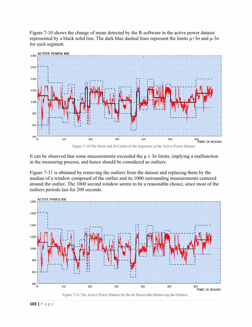
103 | P a g e

Figure 7-10 shows the change of mean detected by the R-software in the active power dataset represented by a black solid line. The dark blue dashed lines represent the limits μ+3σ and μ-3σ for each segment.

Figure 7-10 The Mean and 3σ Limits of the Segments of the Active Power Dataset

It can be observed that some measurements exceeded the μ ± 3σ limits, implying a malfunction in the measuring process, and hence should be considered as outliers.

Figure 7-11 is obtained by removing the outliers from the dataset and replacing them by the median of a window composed of the outlier and its 1000 surrounding measurements centered around the outlier. The 1000 second window seems to be a reasonable choice, since most of the outliers periods last for 200 seconds.

Figure 7-11 The Active Power Dataset for the 66 Hours after Removing the Outliers

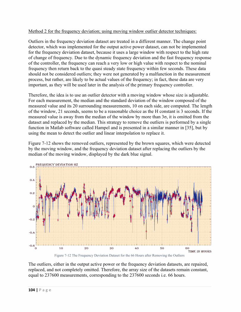
104 | P a g e

Method 2 for the frequency deviation; using moving window outlier detector techniques:

Outliers in the frequency deviation dataset are treated in a different manner. The change point detector, which was implemented for the output active power dataset, can not be implemented for the frequency deviation dataset, because it uses a large window with respect to the high rate of change of frequency. Due to the dynamic frequency deviation and the fast frequency response of the controller, the frequency can reach a very low or high value with respect to the nominal frequency then return back to the quasi steady state frequency within few seconds. These data should not be considered outliers; they were not generated by a malfunction in the measurement process, but rather, are likely to be actual values of the frequency; in fact, these data are very important, as they will be used later in the analysis of the primary frequency controller.

Therefore, the idea is to use an outlier detector with a moving window whose size is adjustable. For each measurement, the median and the standard deviation of the window composed of the measured value and its 20 surrounding measurements, 10 on each side, are computed. The length of the window, 21 seconds, seems to be a reasonable choice as the H constant is 3 seconds. If the measured value is away from the median of the window by more than 3σ, it is omitted from the dataset and replaced by the median. This strategy to remove the outliers is performed by a single function in Matlab software called Hampel and is presented in a similar manner in [35], but by using the mean to detect the outlier and linear interpolation to replace it.

Figure 7-12 shows the removed outliers, represented by the brown squares, which were detected by the moving window, and the frequency deviation dataset after replacing the outliers by the median of the moving window, displayed by the dark blue signal.

Figure 7-12 The Frequency Deviation Dataset for the 66 Hours after Removing the Outliers

The outliers, either in the output active power or the frequency deviation datasets, are repaired, replaced, and not completely omitted. Therefore, the array size of the datasets remain constant, equal to 237600 measurements, corresponding to the 237600 seconds i.e. 66 hours.

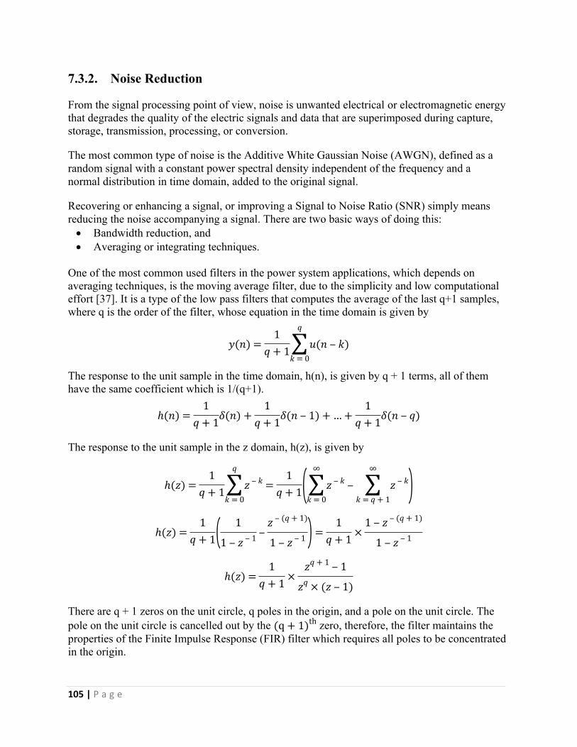
105 | P a g e

7.3.2. Noise Reduction

From the signal processing point of view, noise is unwanted electrical or electromagnetic energy that degrades the quality of the electric signals and data that are superimposed during capture, storage, transmission, processing, or conversion.

The most common type of noise is the Additive White Gaussian Noise (AWGN), defined as a random signal with a constant power spectral density independent of the frequency and a normal distribution in time domain, added to the original signal.

Recovering or enhancing a signal, or improving a Signal to Noise Ratio (SNR) simply means reducing the noise accompanying a signal. There are two basic ways of doing this: Bandwidth reduction, and Averaging or integrating techniques.

One of the most common used filters in the power system applications, which depends on averaging techniques, is the moving average filter, due to the simplicity and low computational effort [37]. It is a type of the low pass filters that computes the average of the last q+1 samples, where q is the order of the filter, whose equation in the time domain is given by

𝑦(𝑛) =1

𝑞 + 1

𝑞

∑𝑘 = 0

𝑢(𝑛 ‒ 𝑘)

The response to the unit sample in the time domain, h(n), is given by q + 1 terms, all of them have the same coefficient which is 1/(q+1).

ℎ(𝑛) =1

𝑞 + 1𝛿(𝑛) +1

𝑞 + 1𝛿(𝑛 ‒ 1) + … +1

𝑞 + 1𝛿(𝑛 ‒ 𝑞)

The response to the unit sample in the z domain, h(z), is given by

ℎ(𝑧) =1

𝑞 + 1

𝑞

∑𝑘 = 0

𝑧 ‒ 𝑘 =1

𝑞 + 1( ∞

∑𝑘 = 0

𝑧 ‒ 𝑘 ‒∞

∑𝑘 = 𝑞 + 1

𝑧 ‒ 𝑘)ℎ(𝑧) =

1𝑞 + 1( 1

1 ‒ 𝑧 ‒ 1 ‒𝑧 ‒ (𝑞 + 1)

1 ‒ 𝑧 ‒ 1 ) =1

𝑞 + 1 ×1 ‒ 𝑧 ‒ (𝑞 + 1)

1 ‒ 𝑧 ‒ 1

ℎ(𝑧) =1

𝑞 + 1 ×𝑧𝑞 + 1 ‒ 1

𝑧𝑞 × (𝑧 ‒ 1)

There are q + 1 zeros on the unit circle, q poles in the origin, and a pole on the unit circle. The pole on the unit circle is cancelled out by the zero, therefore, the filter maintains the (q + 1)th

properties of the Finite Impulse Response (FIR) filter which requires all poles to be concentrated in the origin.

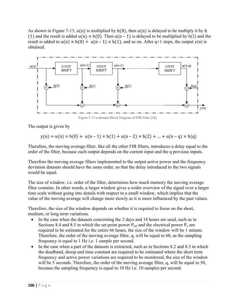
106 | P a g e

As shown in Figure 7-13, is multiplied by , then is delayed to be multiply it by u(n) h(0) u(n) h and the result is added . Then is delayed to be multiplied by h(2) and the (1) u(n) × h(0) u(n ‒ 1)

result is added to , and so on. After q+1 steps, the output y(n) is u(n) × h(0) + u(n ‒ 1) × h(1)obtained.

Figure 7-13 n-domain Block Diagram of FIR Filter [38]

The output is given by

y(n) = u(n) × h(0) + u(n ‒ 1) × h(1) + u(n ‒ 2) × h(2) + … + u(n ‒ q) × h(q)

Therefore, the moving average filter, like all the other FIR filters, introduces a delay equal to the order of the filter, because each output depends on the current input and the q previous inputs.

Therefore the moving average filters implemented to the output active power and the frequency deviation datasets should have the same order, so that the delay introduced to the two signals would be equal.

The size of window, i.e. order of the filter, determines how much memory the moving average filter contains. In other words, a larger window gives a wider overview of the signal over a larger time scale without going into details with respect to a small window, which implies that the value of the moving average will change more slowly as it is more influenced by the past values.

Therefore, the size of the window depends on whether it is required to focus on the short, medium, or long term variations. In the case when the datasets concerning the 2 days and 18 hours are used, such as in

Sections 8.4 and 8.5 in which the set point power Pref and the electrical power Pe are required to be estimated for the entire 66 hours, the size of the window will be 1 minute. Therefore, the order of the moving average filter, q, will be equal to 60, as the sampling frequency is equal to 1 Hz i.e. 1 sample per second.

In the case when a part of the datasets is extracted, such as in Sections 8.2 and 8.3 in which the deadband, droop and time constant are required to be estimated where the short term frequency and active power variations are required to be monitored, the size of the window will be 5 seconds. Therefore, the order of the moving average filter, q, will be equal to 50, because the sampling frequency is equal to 10 Hz i.e. 10 samples per second.

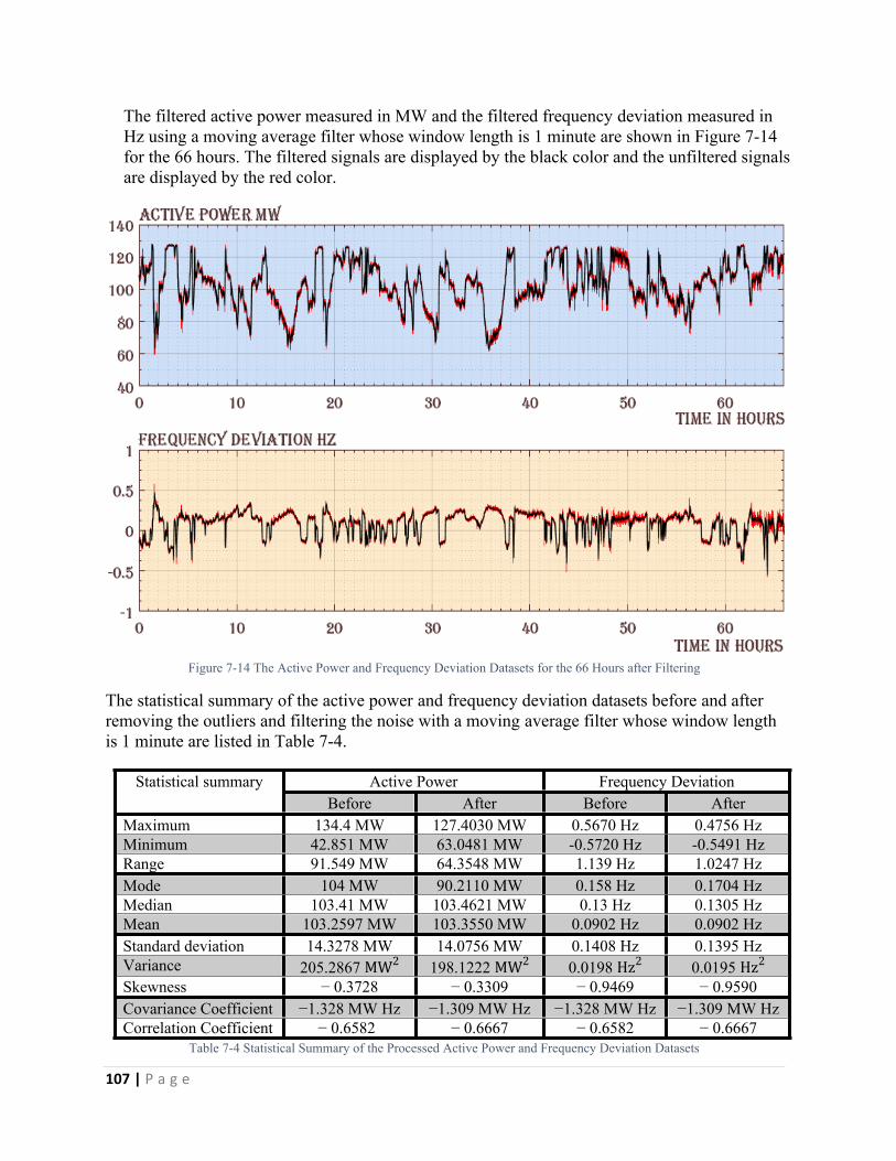
107 | P a g e

The filtered active power measured in MW and the filtered frequency deviation measured in Hz using a moving average filter whose window length is 1 minute are shown in Figure 7-14 for the 66 hours. The filtered signals are displayed by the black color and the unfiltered signals are displayed by the red color.

Figure 7-14 The Active Power and Frequency Deviation Datasets for the 66 Hours after Filtering

The statistical summary of the active power and frequency deviation datasets before and after removing the outliers and filtering the noise with a moving average filter whose window length is 1 minute are listed in Table 7-4.

Active Power Frequency DeviationStatistical summaryBefore After Before After

Maximum 134.4 MW 127.4030 MW 0.5670 Hz 0.4756 HzMinimum 42.851 MW 63.0481 MW -0.5720 Hz -0.5491 HzRange 91.549 MW 64.3548 MW 1.139 Hz 1.0247 HzMode 104 MW 90.2110 MW 0.158 Hz 0.1704 HzMedian 103.41 MW 103.4621 MW 0.13 Hz 0.1305 HzMean 103.2597 MW 103.3550 MW 0.0902 Hz 0.0902 HzStandard deviation 14.3278 MW 14.0756 MW 0.1408 Hz 0.1395 HzVariance 205.2867 MW2 198.1222 MW2 0.0198 Hz2 0.0195 Hz2

Skewness − 0.3728 − 0.3309 − 0.9469 − 0.9590Covariance Coefficient −1.328 MW Hz −1.309 MW Hz −1.328 MW Hz −1.309 MW HzCorrelation Coefficient − 0.6582 − 0.6667 − 0.6582 − 0.6667

Table 7-4 Statistical Summary of the Processed Active Power and Frequency Deviation Datasets

108 | P a g e

CHAPTER 88. Parameters Estimation

This chapter demonstrates the different methodologies to estimate the parameters of the Load Frequency Controller related to the primary frequency response, and is organized as follows: Capacity of generating unit estimation, Deadband estimation, Droop and time constant estimation, Set point power estimation, and Electrical power estimation.

8.1. Capacity of Generating Unit Estimation

The capacity of generating unit is defined as the maximum power that the generator can deliver in case of a frequency excursion at which the control reserves are fully activated. It can be estimated by finding the value in the active power dataset such that 99 percent of the data are less than or equal to it i.e. 99p percentile or 0.99 quantile.

The estimated capacity of generating unit = 126.9992 MW ≃ 127 MW.The result obtained is verified by CESI Milano.

It should be noted that the maximum value in the active power dataset after removing the outliers is 127.4 MW, which seems to be a reliable value, compared to the 134.4 MW that was present in the active power dataset before removing the outliers.

8.2. Deadband Estimation

Deadband is a part of the governor steady state droop characteristics centered around the nominal frequency, where there is no frequency response in case of small frequency variations; until the intentional deadband is reached, a change in system frequency does not correspond to a change in the output active power of the generating unit.

It is not possible to estimate the droop settings and the time constant of the Load Frequency Controller before having an estimate for the deadband settings adopted by the controller; as changing the deadband affects the estimation of the other parameters.

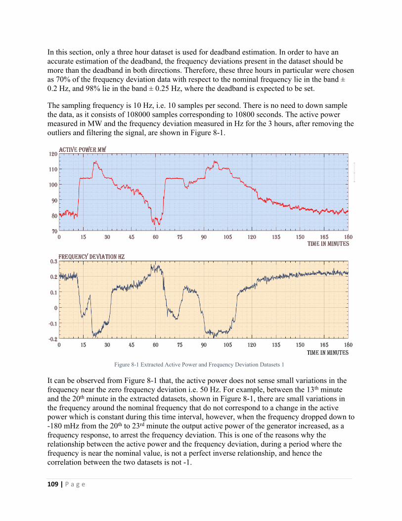
109 | P a g e

In this section, only a three hour dataset is used for deadband estimation. In order to have an accurate estimation of the deadband, the frequency deviations present in the dataset should be more than the deadband in both directions. Therefore, these three hours in particular were chosen as 70% of the frequency deviation data with respect to the nominal frequency lie in the band ± 0.2 Hz, and 98% lie in the band ± 0.25 Hz, where the deadband is expected to be set.

The sampling frequency is 10 Hz, i.e. 10 samples per second. There is no need to down sample the data, as it consists of 108000 samples corresponding to 10800 seconds. The active power measured in MW and the frequency deviation measured in Hz for the 3 hours, after removing the outliers and filtering the signal, are shown in Figure 8-1.

Figure 8-1 Extracted Active Power and Frequency Deviation Datasets 1

It can be observed from Figure 8-1 that, the active power does not sense small variations in the frequency near the zero frequency deviation i.e. 50 Hz. For example, between the 13th minute and the 20th minute in the extracted datasets, shown in Figure 8-1, there are small variations in the frequency around the nominal frequency that do not correspond to a change in the active power which is constant during this time interval, however, when the frequency dropped down to -180 mHz from the 20th to 23rd minute the output active power of the generator increased, as a frequency response, to arrest the frequency deviation. This is one of the reasons why the relationship between the active power and the frequency deviation, during a period where the frequency is near the nominal value, is not a perfect inverse relationship, and hence the correlation between the two datasets is not -1.

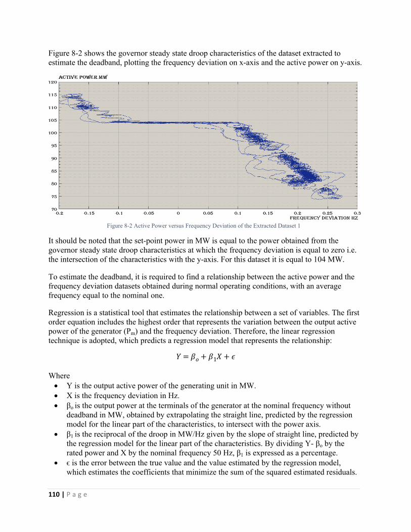
110 | P a g e

Figure 8-2 shows the governor steady state droop characteristics of the dataset extracted to estimate the deadband, plotting the frequency deviation on x-axis and the active power on y-axis.

Figure 8-2 Active Power versus Frequency Deviation of the Extracted Dataset 1

It should be noted that the set-point power in MW is equal to the power obtained from the governor steady state droop characteristics at which the frequency deviation is equal to zero i.e. the intersection of the characteristics with the y-axis. For this dataset it is equal to 104 MW.

To estimate the deadband, it is required to find a relationship between the active power and the frequency deviation datasets obtained during normal operating conditions, with an average frequency equal to the nominal one.

Regression is a statistical tool that estimates the relationship between a set of variables. The first order equation includes the highest order that represents the variation between the output active power of the generator (Pm) and the frequency deviation. Therefore, the linear regression technique is adopted, which predicts a regression model that represents the relationship:

𝑌 = 𝛽𝑜 + 𝛽1𝑋 + 𝜖

Where Y is the output active power of the generating unit in MW. X is the frequency deviation in Hz. βo is the output power at the terminals of the generator at the nominal frequency without

deadband in MW, obtained by extrapolating the straight line, predicted by the regression model for the linear part of the characteristics, to intersect with the power axis.

β1 is the reciprocal of the droop in MW/Hz given by the slope of straight line, predicted by the regression model for the linear part of the characteristics. By dividing Y- βo by the rated power and X by the nominal frequency 50 Hz, β1 is expressed as a percentage.

ϵ is the error between the true value and the value estimated by the regression model, which estimates the coefficients that minimize the sum of the squared estimated residuals.

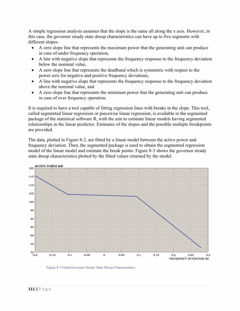
111 | P a g e

A simple regression analysis assumes that the slope is the same all along the x axis. However, in this case, the governor steady state droop characteristics can have up to five segments with different slopes: A zero slope line that represents the maximum power that the generating unit can produce

in case of under frequency operation, A line with negative slope that represents the frequency response to the frequency deviation

below the nominal value, A zero slope line that represents the deadband which is symmetric with respect to the

power axis for negative and positive frequency deviations, A line with negative slope that represents the frequency response to the frequency deviation

above the nominal value, and A zero slope line that represents the minimum power that the generating unit can produce

in case of over frequency operation.

It is required to have a tool capable of fitting regression lines with breaks in the slope. This tool, called segmented linear regression or piecewise linear regression, is available in the segmented package of the statistical software R, with the aim to estimate linear models having segmented relationships in the linear predictor. Estimates of the slopes and the possible multiple breakpoints are provided.

The data, plotted in Figure 8-2, are fitted by a linear model between the active power and frequency deviation. Then, the segmented package is used to obtain the segmented regression model of the linear model and estimate the break points. Figure 8-3 shows the governor steady state droop characteristics plotted by the fitted values returned by the model.

Figure 8-3 Fitted Governor Steady State Droop Characteristics

112 | P a g e

The values returned by R software for the 2 break points are:

Break point 1 = − 0.106 HzBreak point 2 = 0.093 Hz

The amplitude between the two break points is equal to 0.199 Hz i.e. 199 mHz. Since the deadband has to be symmetric with respect to the power axis i.e. zero frequency deviation,

The estimated deadband settings = ± 100 mHz.The result obtained is verified by CESI Milano.

8.3. Droop and Time Constant Estimation

The frequency response, expressed in terms of MW/Hz, is defined by the ratio between the power imbalance that caused the disturbance and the resultant steady state frequency deviation. It can be also defined by the ratio between the maximum power imbalance that the primary frequency reserves are required to cover and the maximum steady state frequency deviation proposed by the grid codes.

As a frequency response, all operators and generating units in the interconnected system are required to contribute in arresting the frequency and the correction of the disturbance with their respective contribution coefficient to primary control which is equal to the ratio between the rated output power of this generating unit with respect to the total capacity installed in the interconnected system.

This contribution coefficient determines the amount of active power by which each generating unit must change its output to share the power deficiency. Following any power imbalance of the active power balance, all the generating units are obliged to change their output by an amount equal to the contribution coefficient multiplied by the magnitude of the power imbalance.

Consequently, the value of the droop implemented in the Load Frequency Controllers of the generating unit is given by the contribution coefficient multiplied by the frequency response in MW/Hz. When several generators with governor speed regulations R1,R2,…..,Rn are connected to the system, the steady state frequency deviation is given by

∆𝜔𝑠𝑡𝑒𝑎𝑑𝑦 𝑠𝑡𝑎𝑡𝑒 = ∆𝑓 =‒ ∆𝑃𝐿

𝐷 + 1𝑅1

+ 1𝑅2

+ … + 1𝑅𝑛

The performance of dynamic systems in the time domain can be defined in terms of the time response to the step input, which is considered as a common input to control systems. If the response to the step input is known, it is mathematically possible to compute the response to any input.

The time constant, a parameter that characterizes the response to the step input and a measure of how fast is the system, is the time the control system needs to reach 1-1/e ≃ 63.2 % of the value of the step input.

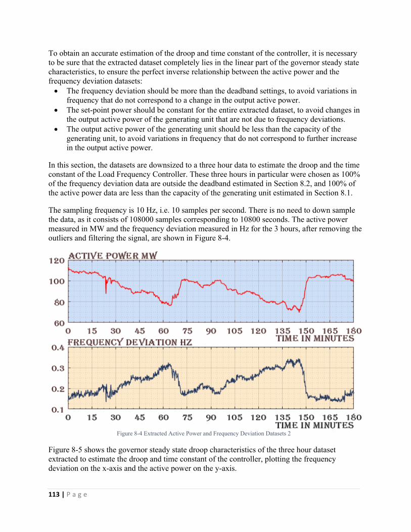
113 | P a g e

To obtain an accurate estimation of the droop and time constant of the controller, it is necessary to be sure that the extracted dataset completely lies in the linear part of the governor steady state characteristics, to ensure the perfect inverse relationship between the active power and the frequency deviation datasets: The frequency deviation should be more than the deadband settings, to avoid variations in

frequency that do not correspond to a change in the output active power. The set-point power should be constant for the entire extracted dataset, to avoid changes in

the output active power of the generating unit that are not due to frequency deviations. The output active power of the generating unit should be less than the capacity of the

generating unit, to avoid variations in frequency that do not correspond to further increase in the output active power.

In this section, the datasets are downsized to a three hour data to estimate the droop and the time constant of the Load Frequency Controller. These three hours in particular were chosen as 100% of the frequency deviation data are outside the deadband estimated in Section 8.2, and 100% of the active power data are less than the capacity of the generating unit estimated in Section 8.1.

The sampling frequency is 10 Hz, i.e. 10 samples per second. There is no need to down sample the data, as it consists of 108000 samples corresponding to 10800 seconds. The active power measured in MW and the frequency deviation measured in Hz for the 3 hours, after removing the outliers and filtering the signal, are shown in Figure 8-4.

Figure 8-4 Extracted Active Power and Frequency Deviation Datasets 2

Figure 8-5 shows the governor steady state droop characteristics of the three hour dataset extracted to estimate the droop and time constant of the controller, plotting the frequency deviation on the x-axis and the active power on the y-axis.

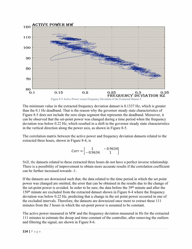
114 | P a g e

Figure 8-5 Active Power versus Frequency Deviation of the Extracted Dataset 2

The minimum value in the extracted frequency deviation dataset is 0.1337 Hz, which is greater than the 0.1 Hz deadband. That is the reason why the governor steady state characteristics of Figure 8-5 does not include the zero slope segment that represents the deadband. Moreover, it can be observed that the set-point power was changed during a time period when the frequency deviation was below 0.22 Hz, which resulted in a shift in the governor steady state characteristics in the vertical direction along the power axis, as shown in Figure 8-5.

The correlation matrix between the active power and frequency deviation datasets related to the extracted three hours, shown in Figure 8-4, is

𝐶𝑜𝑟𝑟 = [ 1 ‒ 0.9634‒ 0.9634 1 ]

Still, the datasets related to these extracted three hours do not have a perfect inverse relationship. There is a possibility of improvement to obtain more accurate results if the correlation coefficient can be further increased towards -1.

If the datasets are downsized such that, the data related to the time period in which the set point power was changed are omitted, the error that can be obtained in the results due to the change of the set-point power is avoided. In order to be sure, the data before the 39th minute and after the 150th minute are excluded from the extracted dataset shown in Figure 8-4 where the frequency deviation was below 0.22 Hz, predicting that a change in the set point power occurred in one of the excluded intervals. Therefore, the datasets are downsized once more to extract these 111 minutes from the 3 hours in which the set-point power is assumed to be constant.

The active power measured in MW and the frequency deviation measured in Hz for the extracted 111 minutes to estimate the droop and time constant of the controller, after removing the outliers and filtering the signal, are shown in Figure 8-6.

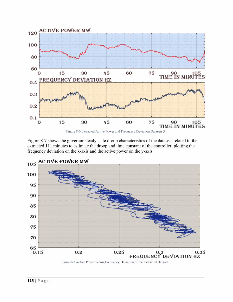
115 | P a g e

Figure 8-6 Extracted Active Power and Frequency Deviation Datasets 3

Figure 8-7 shows the governor steady state droop characteristics of the datasets related to the extracted 111 minutes to estimate the droop and time constant of the controller, plotting the frequency deviation on the x-axis and the active power on the y-axis.

Figure 8-7 Active Power versus Frequency Deviation of the Extracted Dataset 3

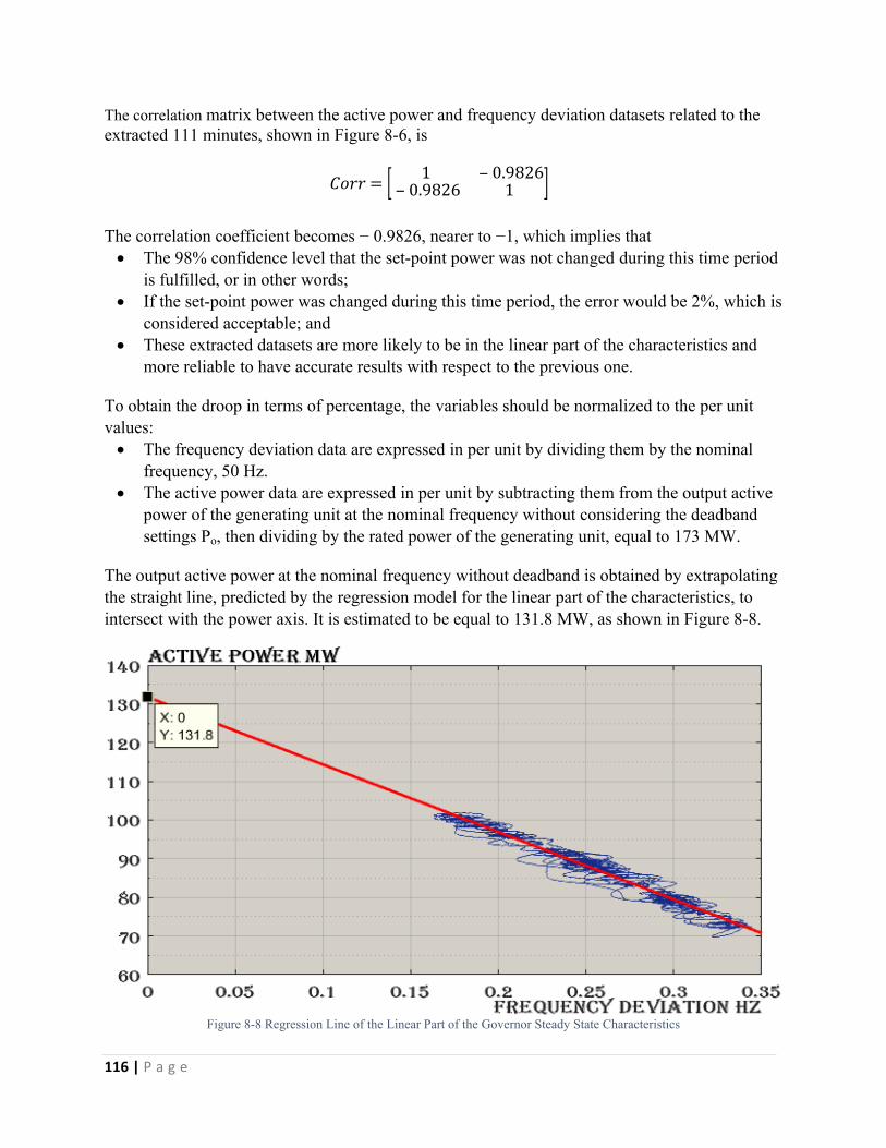
116 | P a g e

The correlation matrix between the active power and frequency deviation datasets related to the extracted 111 minutes, shown in Figure 8-6, is

𝐶𝑜𝑟𝑟 = [ 1 ‒ 0.9826‒ 0.9826 1 ]

The correlation coefficient becomes − 0.9826, nearer to −1, which implies that The 98% confidence level that the set-point power was not changed during this time period

is fulfilled, or in other words; If the set-point power was changed during this time period, the error would be 2%, which is

considered acceptable; and These extracted datasets are more likely to be in the linear part of the characteristics and

more reliable to have accurate results with respect to the previous one.

To obtain the droop in terms of percentage, the variables should be normalized to the per unit values: The frequency deviation data are expressed in per unit by dividing them by the nominal

frequency, 50 Hz. The active power data are expressed in per unit by subtracting them from the output active

power of the generating unit at the nominal frequency without considering the deadband settings Po, then dividing by the rated power of the generating unit, equal to 173 MW.

The output active power at the nominal frequency without deadband is obtained by extrapolating the straight line, predicted by the regression model for the linear part of the characteristics, to intersect with the power axis. It is estimated to be equal to 131.8 MW, as shown in Figure 8-8.

Figure 8-8 Regression Line of the Linear Part of the Governor Steady State Characteristics

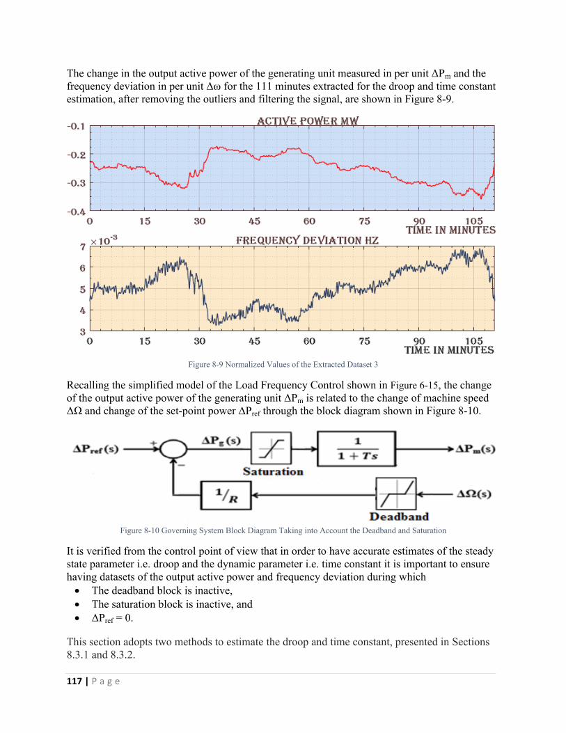
117 | P a g e

The change in the output active power of the generating unit measured in per unit ΔPm and the frequency deviation in per unit Δω for the 111 minutes extracted for the droop and time constant estimation, after removing the outliers and filtering the signal, are shown in Figure 8-9.

Figure 8-9 Normalized Values of the Extracted Dataset 3

Recalling the simplified model of the Load Frequency Control shown in Figure 6-15, the change of the output active power of the generating unit ΔPm is related to the change of machine speed ΔΩ and change of the set-point power ΔPref through the block diagram shown in Figure 8-10.

Figure 8-10 Governing System Block Diagram Taking into Account the Deadband and Saturation

It is verified from the control point of view that in order to have accurate estimates of the steady state parameter i.e. droop and the dynamic parameter i.e. time constant it is important to ensure having datasets of the output active power and frequency deviation during which The deadband block is inactive, The saturation block is inactive, and ΔPref = 0.

This section adopts two methods to estimate the droop and time constant, presented in Sections 8.3.1 and 8.3.2.

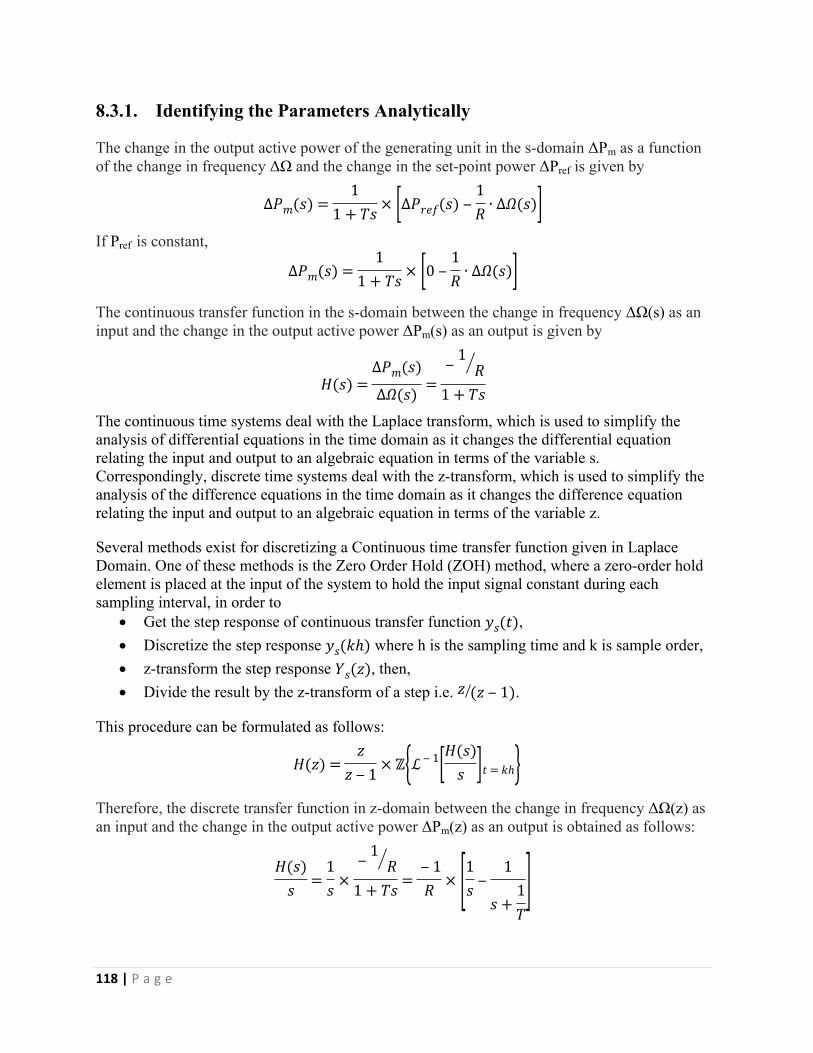
118 | P a g e

8.3.1. Identifying the Parameters Analytically

The change in the output active power of the generating unit in the s-domain ΔPm as a function of the change in frequency ΔΩ and the change in the set-point power ΔPref is given by

∆𝑃𝑚(𝑠) =1

1 + 𝑇𝑠 × [∆𝑃𝑟𝑒𝑓(𝑠) ‒1𝑅 ∙ ∆𝛺(𝑠)]

If Pref is constant,

∆𝑃𝑚(𝑠) =1

1 + 𝑇𝑠 × [0 ‒1𝑅 ∙ ∆𝛺(𝑠)]

The continuous transfer function in the s-domain between the change in frequency ΔΩ(s) as an input and the change in the output active power ΔPm(s) as an output is given by

𝐻(𝑠) =∆𝑃𝑚(𝑠)

∆𝛺(𝑠) =‒ 1

𝑅1 + 𝑇𝑠

The continuous time systems deal with the Laplace transform, which is used to simplify the analysis of differential equations in the time domain as it changes the differential equation relating the input and output to an algebraic equation in terms of the variable s.Correspondingly, discrete time systems deal with the z-transform, which is used to simplify the analysis of the difference equations in the time domain as it changes the difference equation relating the input and output to an algebraic equation in terms of the variable z.

Several methods exist for discretizing a Continuous time transfer function given in Laplace Domain. One of these methods is the Zero Order Hold (ZOH) method, where a zero-order hold element is placed at the input of the system to hold the input signal constant during each sampling interval, in order to

Get the step response of continuous transfer function ,𝑦𝑠(𝑡) Discretize the step response where h is the sampling time and k is sample order,𝑦𝑠(𝑘ℎ) z-transform the step response , then,𝑌𝑠(𝑧) Divide the result by the z-transform of a step i.e. .𝑧 (𝑧 ‒ 1)

This procedure can be formulated as follows:

𝐻(𝑧) =𝑧

𝑧 ‒ 1 × ℤ{ℒ ‒ 1[𝐻(𝑠)𝑠 ]𝑡 = 𝑘ℎ}

Therefore, the discrete transfer function in z-domain between the change in frequency ΔΩ(z) as an input and the change in the output active power ΔPm(z) as an output is obtained as follows:

𝐻(𝑠)𝑠 =

1𝑠 ×

‒ 1𝑅

1 + 𝑇𝑠 =‒ 1𝑅 × [1

𝑠 ‒1

𝑠 +1𝑇

]

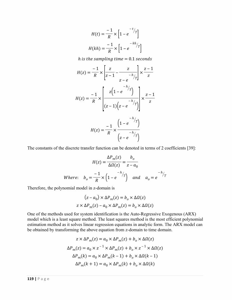
119 | P a g e

𝐻(𝑡) =‒ 1𝑅 × [1 ‒ 𝑒

‒ 𝑡𝑇]

𝐻(𝑘ℎ) =‒ 1𝑅 × [1 ‒ 𝑒

‒ 𝑘ℎ𝑇]

ℎ 𝑖𝑠 𝑡ℎ𝑒 𝑠𝑎𝑚𝑝𝑙𝑖𝑛𝑔 𝑡𝑖𝑚𝑒 = 0.1 𝑠𝑒𝑐𝑜𝑛𝑑𝑠

𝐻(𝑧) =‒ 1𝑅 × [ 𝑧

𝑧 ‒ 1 ‒𝑧

𝑧 ‒ 𝑒‒ ℎ

𝑇] ×

𝑧 ‒ 1𝑧

𝐻(𝑧) =‒ 1𝑅 × [ 𝑧(1 ‒ 𝑒

‒ ℎ𝑇)

(𝑧 ‒ 1)(𝑧 ‒ 𝑒‒ ℎ

𝑇)] ×𝑧 ‒ 1

𝑧

𝐻(𝑧) =‒ 1𝑅 ×

(1 ‒ 𝑒‒ ℎ

𝑇)(𝑧 ‒ 𝑒

‒ ℎ𝑇)

The constants of the discrete transfer function can be denoted in terms of 2 coefficients [39]:

𝐻(𝑧) =∆𝑃𝑚(𝑧)

∆𝛺(𝑧) =𝑏𝑜

𝑧 ‒ 𝑎0

𝑊ℎ𝑒𝑟𝑒: 𝑏𝑜 =‒ 1𝑅 × (1 ‒ 𝑒

‒ ℎ𝑇) 𝑎𝑛𝑑 𝑎𝑜 = 𝑒

‒ ℎ𝑇

Therefore, the polynomial model in z-domain is

(𝑧 ‒ 𝑎0) × ∆𝑃𝑚(𝑧) = 𝑏𝑜 × ∆𝛺(𝑧)

𝑧 × ∆𝑃𝑚(𝑧) ‒ 𝑎0 × ∆𝑃𝑚(𝑧) = 𝑏𝑜 × ∆𝛺(𝑧)

One of the methods used for system identification is the Auto-Regressive Exogenous (ARX) model which is a least square method. The least squares method is the most efficient polynomial estimation method as it solves linear regression equations in analytic form. The ARX model can be obtained by transforming the above equation from z-domain to time domain.

𝑧 × ∆𝑃𝑚(𝑧) = 𝑎0 × ∆𝑃𝑚(𝑧) + 𝑏𝑜 × ∆𝛺(𝑧)

∆𝑃𝑚(𝑧) = 𝑎0 × 𝑧 ‒ 1 × ∆𝑃𝑚(𝑧) + 𝑏𝑜 × 𝑧 ‒ 1 × ∆𝛺(𝑧)

∆𝑃𝑚(𝑘) = 𝑎0 × ∆𝑃𝑚(𝑘 ‒ 1) + 𝑏𝑜 × ∆𝛺(𝑘 ‒ 1)

∆𝑃𝑚(𝑘 + 1) = 𝑎0 × ∆𝑃𝑚(𝑘) + 𝑏𝑜 × ∆𝛺(𝑘)

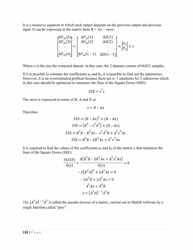
120 | P a g e

It is a recursive equation in which each output depends on the previous output and previous input. It can be expressed in the matrix form B = Ax + error:

[∆𝑃𝑚(2)∆𝑃𝑚(3)

.

.∆𝑃𝑚(𝑛)

] = [ ∆𝑃𝑚(1) ∆𝛺(1)∆𝑃𝑚(2) ∆𝛺(2)

.

.∆𝑃𝑚(𝑛 ‒ 1)

.

.∆𝛺(𝑛 ‒ 1)

] × [𝑎𝑜𝑏𝑜] + 𝜖

Where n is the size the extracted dataset. In this case, the 2 datasets consist of 66422 samples.

If it is possible to estimate the coefficients a0 and b0, it is possible to find out the parameters. However, it is an overestimated problem because there are n−1 equations for 2 unknowns which in this case should be optimized to minimize the Sum of the Square Errors (SSE):

𝑆𝑆𝐸 = 𝜖𝑇𝜖

The error is expressed in terms of B, A and X as

𝜖 = 𝐵 ‒ 𝐴𝑥Therefore

𝑆𝑆𝐸 = (𝐵 ‒ 𝐴𝑥)𝑇 × (𝐵 ‒ 𝐴𝑥)

𝑆𝑆𝐸 = (𝐵𝑇 ‒ 𝑥𝑇𝐴𝑇) × (𝐵 ‒ 𝐴𝑥)

𝑆𝑆𝐸 = 𝐵𝑇𝐵 ‒ 𝐵𝑇𝐴𝑥 ‒ 𝑥𝑇𝐴𝑇𝐵 + 𝐴𝑇𝑥𝑇𝐴𝑥

𝑆𝑆𝐸 = 𝐵𝑇𝐵 ‒ 2𝐵𝑇𝐴𝑥 + 𝐴𝑇𝑥𝑇𝐴𝑥

It is required to find the values of the coefficients a0 and b0 of the matrix x that minimize the Sum of the Square Errors (SSE):

∂(𝑆𝑆𝐸)∂(𝑥) =

∂(𝐵𝑇𝐵 ‒ 2𝐵𝑇𝐴𝑥 + 𝐴𝑇𝑥𝑇𝐴𝑥)∂(𝑥) = 0

‒ 2(𝐵𝑇𝐴)𝑇 + 2𝐴𝑇𝐴𝑥 = 0

‒ 2𝐴𝑇𝐵 + 2𝐴𝑇𝐴𝑥 = 0

𝐴𝑇𝐴𝑥 = 𝐴𝑇𝐵

𝑥 = (𝐴𝑇𝐴) ‒ 1𝐴𝑇𝐵

The is called the pseudo-inverse of a matrix, carried out in Matlab software by a (𝐴𝑇𝐴) ‒ 1𝐴𝑇

single function called “pinv”.

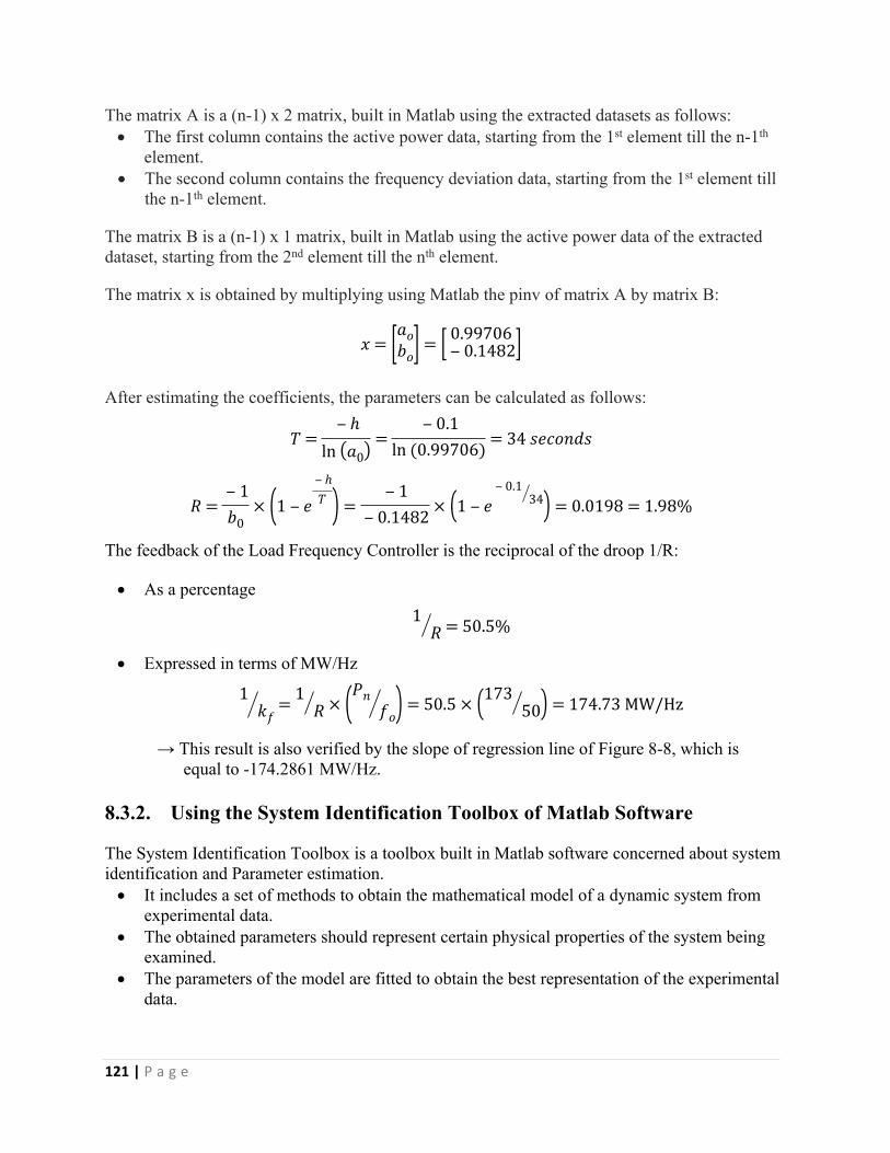
121 | P a g e

The matrix A is a (n-1) x 2 matrix, built in Matlab using the extracted datasets as follows: The first column contains the active power data, starting from the 1st element till the n-1th

element. The second column contains the frequency deviation data, starting from the 1st element till

the n-1th element.

The matrix B is a (n-1) x 1 matrix, built in Matlab using the active power data of the extracted dataset, starting from the 2nd element till the nth element.

The matrix x is obtained by multiplying using Matlab the pinv of matrix A by matrix B:

𝑥 = [𝑎𝑜𝑏𝑜] = [ 0.99706

‒ 0.1482]After estimating the coefficients, the parameters can be calculated as follows:

𝑇 =‒ ℎ

ln (𝑎0) =‒ 0.1

ln (0.99706) = 34 𝑠𝑒𝑐𝑜𝑛𝑑𝑠

𝑅 =‒ 1𝑏0

× (1 ‒ 𝑒‒ ℎ𝑇 ) =

‒ 1‒ 0.1482 × (1 ‒ 𝑒

‒ 0.134) = 0.0198 = 1.98%

The feedback of the Load Frequency Controller is the reciprocal of the droop 1/R:

As a percentage1

𝑅 = 50.5%

Expressed in terms of MW/Hz

1𝑘𝑓

= 1𝑅 × (𝑃𝑛

𝑓𝑜) = 50.5 × (17350) = 174.73 MW/Hz

→ This result is also verified by the slope of regression line of Figure 8-8, which is equal to -174.2861 MW/Hz.

8.3.2. Using the System Identification Toolbox of Matlab Software

The System Identification Toolbox is a toolbox built in Matlab software concerned about system identification and Parameter estimation. It includes a set of methods to obtain the mathematical model of a dynamic system from

experimental data. The obtained parameters should represent certain physical properties of the system being

examined. The parameters of the model are fitted to obtain the best representation of the experimental

data.

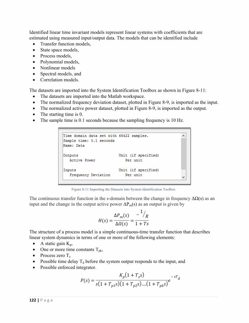
122 | P a g e

Identified linear time invariant models represent linear systems with coefficients that are estimated using measured input/output data. The models that can be identified include Transfer function models, State space models, Process models, Polynomial models, Nonlinear models Spectral models, and Correlation models.

The datasets are imported into the System Identification Toolbox as shown in Figure 8-11: The datasets are imported into the Matlab workspace. The normalized frequency deviation dataset, plotted in Figure 8-9, is imported as the input. The normalized active power dataset, plotted in Figure 8-9, is imported as the output. The starting time is 0. The sample time is 0.1 seconds because the sampling frequency is 10 Hz.

Figure 8-11 Importing the Datasets into System Identification Toolbox

The continuous transfer function in the s-domain between the change in frequency ΔΩ(s) as an input and the change in the output active power ΔPm(s) as an output is given by

𝐻(𝑠) =∆𝑃𝑚(𝑠)

∆𝛺(𝑠) =‒ 1

𝑅1 + 𝑇𝑠

The structure of a process model is a simple continuous-time transfer function that describes linear system dynamics in terms of one or more of the following elements: A static gain Kp, One or more time constants Tpk, Process zero Tz Possible time delay Td before the system output responds to the input, and Possible enforced integrator.

𝑃(𝑠) =𝐾𝑝(1 + 𝑇𝑧𝑠)

𝑠(1 + 𝑇𝑝1𝑠)(1 + 𝑇𝑝2𝑠)….(1 + 𝑇𝑝𝑘𝑠)𝑒‒ 𝑠𝑇𝑑

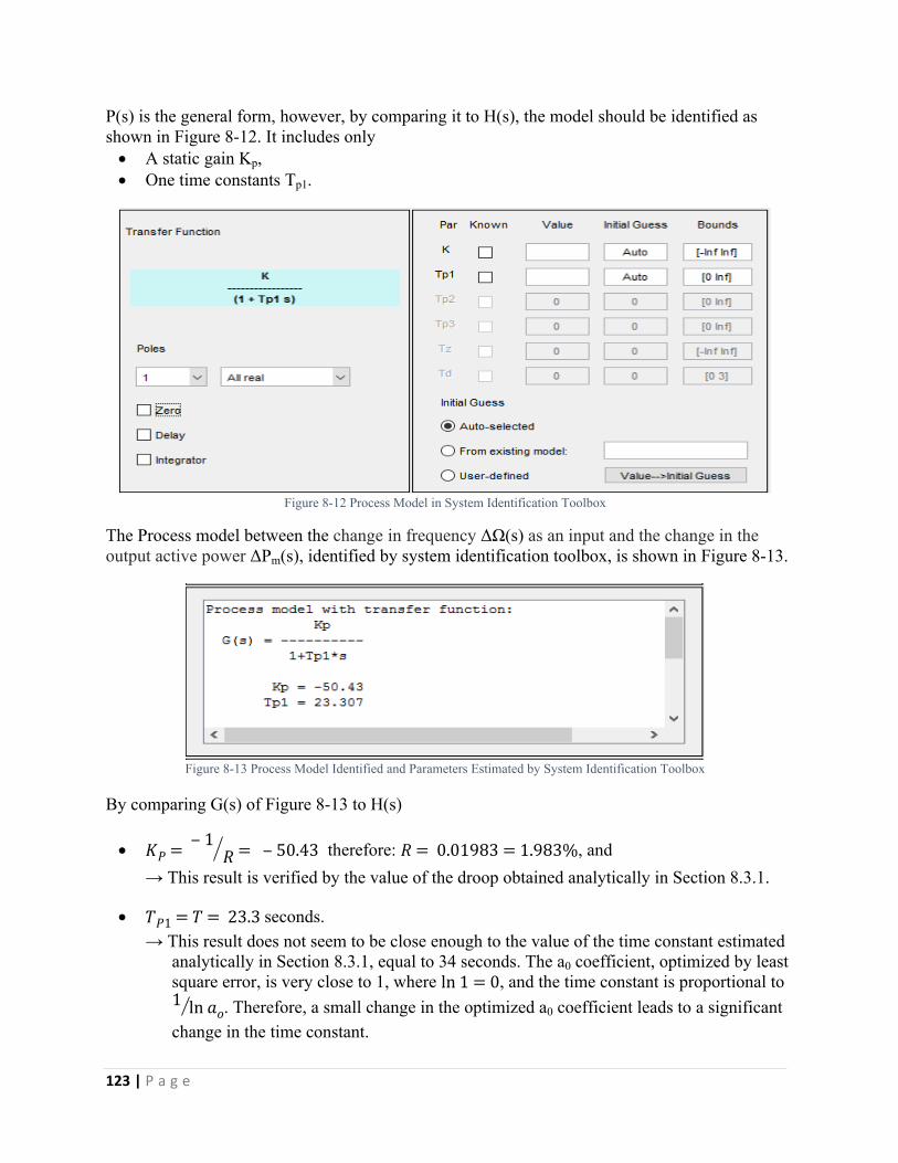
123 | P a g e

P(s) is the general form, however, by comparing it to H(s), the model should be identified as shown in Figure 8-12. It includes only A static gain Kp, One time constants Tp1.

Figure 8-12 Process Model in System Identification Toolbox

The Process model between the change in frequency ΔΩ(s) as an input and the change in the output active power ΔPm(s), identified by system identification toolbox, is shown in Figure 8-13.

Figure 8-13 Process Model Identified and Parameters Estimated by System Identification Toolbox

By comparing G(s) of Figure 8-13 to H(s)

therefore: , and 𝐾𝑃 = ‒ 1𝑅 = ‒ 50.43 𝑅 = 0.01983 = 1.983%

→ This result is verified by the value of the droop obtained analytically in Section 8.3.1.

seconds.𝑇𝑃1 = 𝑇 = 23.3 → This result does not seem to be close enough to the value of the time constant estimated

analytically in Section 8.3.1, equal to 34 seconds. The a0 coefficient, optimized by least square error, is very close to 1, where , and the time constant is proportional to ln 1 = 0

. Therefore, a small change in the optimized a0 coefficient leads to a significant 1 ln 𝑎𝑜change in the time constant.

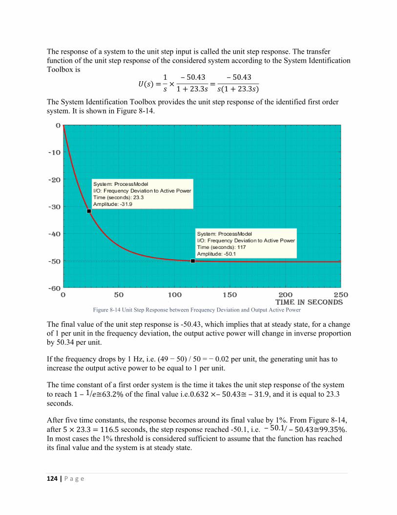
124 | P a g e

The response of a system to the unit step input is called the unit step response. The transfer function of the unit step response of the considered system according to the System Identification Toolbox is

𝑈(𝑠) =1𝑠 ×

‒ 50.431 + 23.3𝑠 =

‒ 50.43𝑠(1 + 23.3𝑠)

The System Identification Toolbox provides the unit step response of the identified first order system. It is shown in Figure 8-14.

Figure 8-14 Unit Step Response between Frequency Deviation and Output Active Power

The final value of the unit step response is -50.43, which implies that at steady state, for a change of 1 per unit in the frequency deviation, the output active power will change in inverse proportion by 50.34 per unit.

If the frequency drops by 1 Hz, i.e. (49 − 50) / 50 = − 0.02 per unit, the generating unit has to increase the output active power to be equal to 1 per unit.

The time constant of a first order system is the time it takes the unit step response of the system to reach of the final value i.e. , and it is equal to 23.3 1 ‒ 1 𝑒≅63.2% 0.632 ×‒ 50.43≅ ‒ 31.9seconds.

After five time constants, the response becomes around its final value by 1%. From Figure 8-14, after seconds, the step response reached -50.1, i.e. . 5 × 23.3 = 116.5 ‒ 50.1 ‒ 50.43≅99.35%In most cases the 1% threshold is considered sufficient to assume that the function has reached its final value and the system is at steady state.

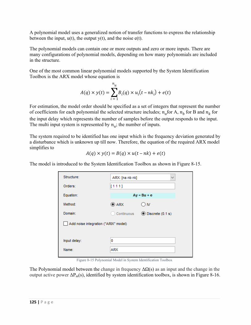
125 | P a g e

A polynomial model uses a generalized notion of transfer functions to express the relationship between the input, u(t), the output y(t), and the noise e(t).

The polynomial models can contain one or more outputs and zero or more inputs. There are many configurations of polynomial models, depending on how many polynomials are included in the structure.

One of the most common linear polynomial models supported by the System Identification Toolbox is the ARX model whose equation is

𝐴(𝑞) × 𝑦(𝑡) =

𝑛𝑢

∑𝑖 = 1

𝐵𝑖(𝑞) × 𝑢𝑖(𝑡 ‒ 𝑛𝑘𝑖) + 𝑒(𝑡)

For estimation, the model order should be specified as a set of integers that represent the number of coefficients for each polynomial the selected structure includes; for A, for B and for 𝑛𝑎 𝑛𝑏 𝑛𝑘the input delay which represents the number of samples before the output responds to the input. The multi input system is represented by ; the number of inputs.𝑛𝑢

The system required to be identified has one input which is the frequency deviation generated by a disturbance which is unknown up till now. Therefore, the equation of the required ARX model simplifies to

𝐴(𝑞) × 𝑦(𝑡) = 𝐵(𝑞) × 𝑢(𝑡 ‒ 𝑛𝑘) + 𝑒(𝑡)

The model is introduced to the System Identification Toolbox as shown in Figure 8-15.

Figure 8-15 Polynomial Model in System Identification Toolbox

The Polynomial model between the change in frequency ΔΩ(s) as an input and the change in the output active power ΔPm(s), identified by system identification toolbox, is shown in Figure 8-16.

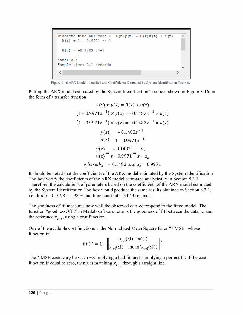
126 | P a g e

Figure 8-16 ARX Model Identified and Coefficients Estimated by System Identification Toolbox

Putting the ARX model estimated by the System Identification Toolbox, shown in Figure 8-16, in the form of a transfer function

𝐴(𝑧) × 𝑦(𝑧) = 𝐵(𝑧) × 𝑢(𝑧)

(1 ‒ 0.9971𝑧 ‒ 1) × 𝑦(𝑧) =‒ 0.1482𝑧 ‒ 1 × 𝑢(𝑧)

(1 ‒ 0.9971𝑧 ‒ 1) × 𝑦(𝑧) =‒ 0.1482𝑧 ‒ 1 × 𝑢(𝑧)

𝑦(𝑧)𝑢(𝑧) =

‒ 0.1482𝑧 ‒ 1

1 ‒ 0.9971𝑧 ‒ 1

𝑦(𝑧)𝑢(𝑧) =

‒ 0.1482𝑧 ‒ 0.9971 =

𝑏𝑜

𝑧 ‒ 𝑎𝑜

𝑤ℎ𝑒𝑟𝑒:𝑏𝑜 =‒ 0.1482 𝑎𝑛𝑑 𝑎𝑜 = 0.9971

It should be noted that the coefficients of the ARX model estimated by the System Identification Toolbox verify the coefficients of the ARX model estimated analytically in Section 8.3.1. Therefore, the calculations of parameters based on the coefficients of the ARX model estimated by the System Identification Toolbox would produce the same results obtained in Section 8.3.1, i.e. droop = 0.0198 = 1.98 % and time constant = 34.43 seconds.

The goodness of fit measures how well the observed data correspond to the fitted model. The function “goodnessOffit” in Matlab software returns the goodness of fit between the data, x, and the reference, , using a cost function.𝑥𝑟𝑒𝑓

One of the available cost functions is the Normalized Mean Square Error “NMSE” whose function is

fit (i) = 1 ‒ ‖ xref(:,i) ‒ x(:,i)

xref(:,i) ‒ mean(xref(:,i))‖2

The NMSE costs vary between −∞ implying a bad fit, and 1 implying a perfect fit. If the cost function is equal to zero, then x is matching through a straight line.𝑥𝑟𝑒𝑓

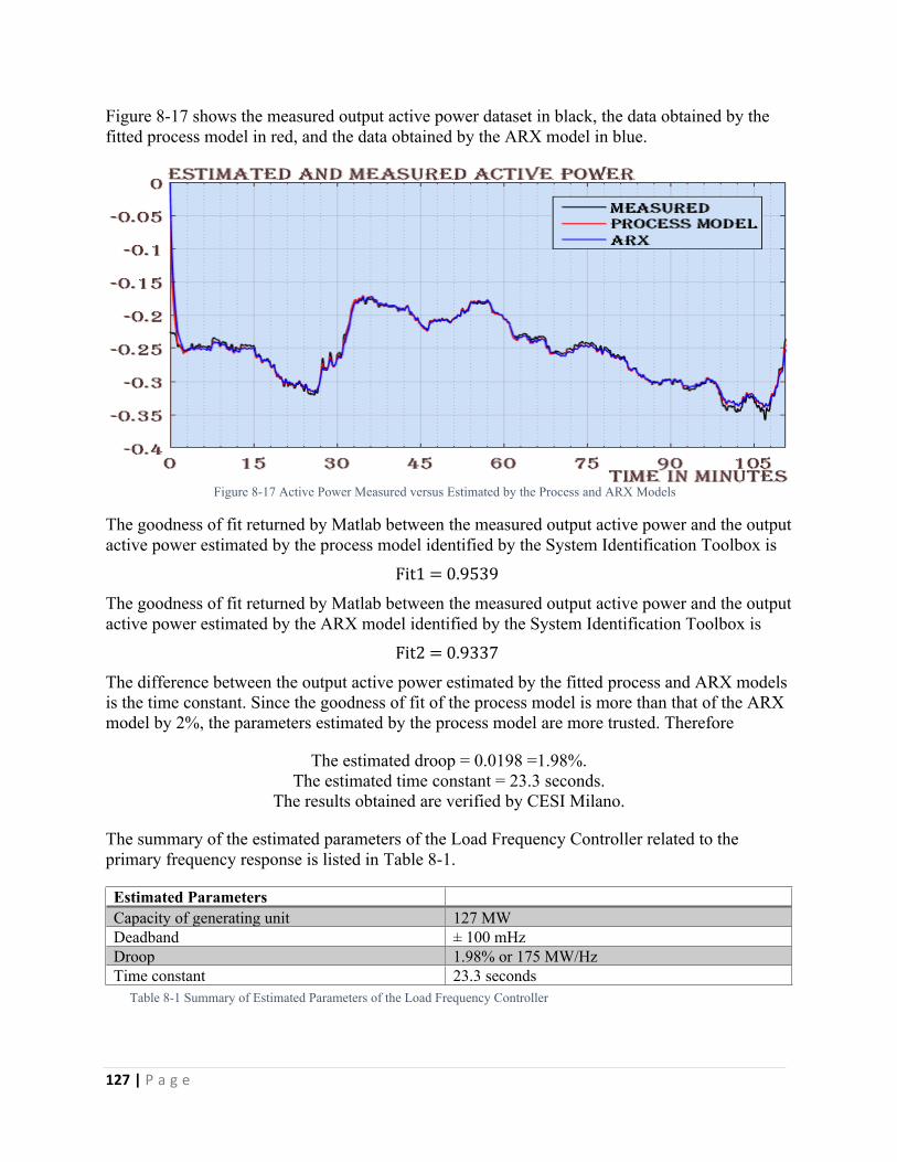
127 | P a g e

Figure 8-17 shows the measured output active power dataset in black, the data obtained by the fitted process model in red, and the data obtained by the ARX model in blue.

Figure 8-17 Active Power Measured versus Estimated by the Process and ARX Models

The goodness of fit returned by Matlab between the measured output active power and the output active power estimated by the process model identified by the System Identification Toolbox is

Fit1 = 0.9539

The goodness of fit returned by Matlab between the measured output active power and the output active power estimated by the ARX model identified by the System Identification Toolbox is

Fit2 = 0.9337

The difference between the output active power estimated by the fitted process and ARX models is the time constant. Since the goodness of fit of the process model is more than that of the ARX model by 2%, the parameters estimated by the process model are more trusted. Therefore

The estimated droop = 0.0198 =1.98%.The estimated time constant = 23.3 seconds.

The results obtained are verified by CESI Milano.

The summary of the estimated parameters of the Load Frequency Controller related to the primary frequency response is listed in Table 8-1.

Estimated ParametersCapacity of generating unit 127 MWDeadband ± 100 mHzDroop 1.98% or 175 MW/HzTime constant 23.3 seconds

Table 8-1 Summary of Estimated Parameters of the Load Frequency Controller

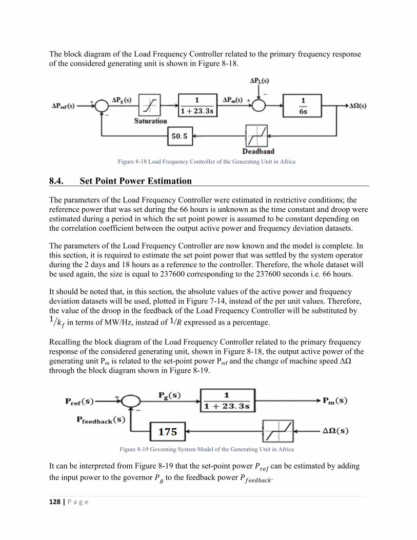
128 | P a g e

The block diagram of the Load Frequency Controller related to the primary frequency response of the considered generating unit is shown in Figure 8-18.

Figure 8-18 Load Frequency Controller of the Generating Unit in Africa

8.4. Set Point Power Estimation

The parameters of the Load Frequency Controller were estimated in restrictive conditions; the reference power that was set during the 66 hours is unknown as the time constant and droop were estimated during a period in which the set point power is assumed to be constant depending on the correlation coefficient between the output active power and frequency deviation datasets.

The parameters of the Load Frequency Controller are now known and the model is complete. In this section, it is required to estimate the set point power that was settled by the system operator during the 2 days and 18 hours as a reference to the controller. Therefore, the whole dataset will be used again, the size is equal to 237600 corresponding to the 237600 seconds i.e. 66 hours.

It should be noted that, in this section, the absolute values of the active power and frequency deviation datasets will be used, plotted in Figure 7-14, instead of the per unit values. Therefore, the value of the droop in the feedback of the Load Frequency Controller will be substituted by

in terms of MW/Hz, instead of expressed as a percentage.1 𝑘𝑓1 𝑅

Recalling the block diagram of the Load Frequency Controller related to the primary frequency response of the considered generating unit, shown in Figure 8-18, the output active power of the generating unit Pm is related to the set-point power Pref and the change of machine speed ΔΩ through the block diagram shown in Figure 8-19.

Figure 8-19 Governing System Model of the Generating Unit in Africa

It can be interpreted from Figure 8-19 that the set-point power can be estimated by adding 𝑃𝑟𝑒𝑓 the input power to the governor to the feedback power .𝑃𝑔 𝑃𝑓𝑒𝑒𝑑𝑏𝑎𝑐𝑘

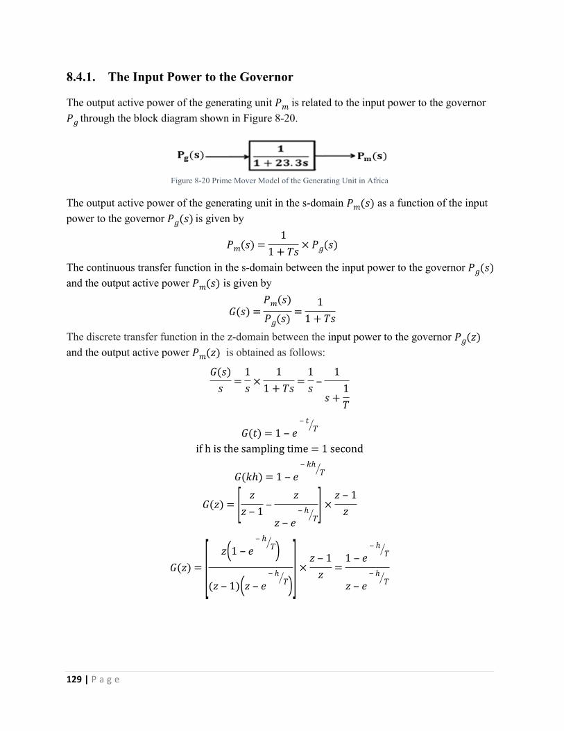
129 | P a g e

8.4.1. The Input Power to the Governor

The output active power of the generating unit is related to the input power to the governor 𝑃𝑚

through the block diagram shown in Figure 8-20.𝑃𝑔

Figure 8-20 Prime Mover Model of the Generating Unit in Africa

The output active power of the generating unit in the s-domain as a function of the input 𝑃𝑚(𝑠)power to the governor is given by𝑃𝑔(𝑠)

𝑃𝑚(𝑠) =1

1 + 𝑇𝑠 × 𝑃𝑔(𝑠)

The continuous transfer function in the s-domain between the input power to the governor 𝑃𝑔(𝑠)and the output active power is given by𝑃𝑚(𝑠)

𝐺(𝑠) =𝑃𝑚(𝑠)

𝑃𝑔(𝑠) =1

1 + 𝑇𝑠The discrete transfer function in the z-domain between the input power to the governor 𝑃𝑔(𝑧)and the output active power is obtained as follows:𝑃𝑚(𝑧)

𝐺(𝑠)𝑠 =

1𝑠 ×

11 + 𝑇𝑠 =

1𝑠 ‒

1

𝑠 +1𝑇

𝐺(𝑡) = 1 ‒ 𝑒‒ 𝑡

𝑇

if h is the sampling time = 1 second

𝐺(𝑘ℎ) = 1 ‒ 𝑒‒ 𝑘ℎ

𝑇

𝐺(𝑧) = [ 𝑧𝑧 ‒ 1 ‒

𝑧

𝑧 ‒ 𝑒‒ ℎ

𝑇] ×

𝑧 ‒ 1𝑧

𝐺(𝑧) = [ 𝑧(1 ‒ 𝑒‒ ℎ

𝑇)(𝑧 ‒ 1)(𝑧 ‒ 𝑒

‒ ℎ𝑇)] ×

𝑧 ‒ 1𝑧 =

1 ‒ 𝑒‒ ℎ

𝑇

𝑧 ‒ 𝑒‒ ℎ

𝑇

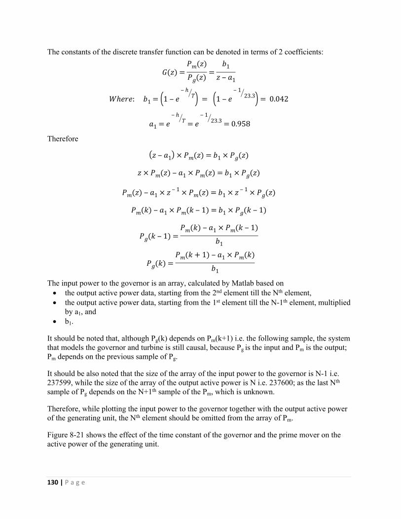
130 | P a g e

The constants of the discrete transfer function can be denoted in terms of 2 coefficients:

𝐺(𝑧) =𝑃𝑚(𝑧)

𝑃𝑔(𝑧) =𝑏1

𝑧 ‒ 𝑎1

𝑊ℎ𝑒𝑟𝑒: 𝑏1 = (1 ‒ 𝑒‒ ℎ

𝑇) = (1 ‒ 𝑒‒ 1

23.3) = 0.042

𝑎1 = 𝑒‒ ℎ

𝑇 = 𝑒‒ 1

23.3 = 0.958

Therefore

(𝑧 ‒ 𝑎1) × 𝑃𝑚(𝑧) = 𝑏1 × 𝑃𝑔(𝑧)

𝑧 × 𝑃𝑚(𝑧) ‒ 𝑎1 × 𝑃𝑚(𝑧) = 𝑏1 × 𝑃𝑔(𝑧)

𝑃𝑚(𝑧) ‒ 𝑎1 × 𝑧 ‒ 1 × 𝑃𝑚(𝑧) = 𝑏1 × 𝑧 ‒ 1 × 𝑃𝑔(𝑧)

𝑃𝑚(𝑘) ‒ 𝑎1 × 𝑃𝑚(𝑘 ‒ 1) = 𝑏1 × 𝑃𝑔(𝑘 ‒ 1)

𝑃𝑔(𝑘 ‒ 1) =𝑃𝑚(𝑘) ‒ 𝑎1 × 𝑃𝑚(𝑘 ‒ 1)

𝑏1

𝑃𝑔(𝑘) =𝑃𝑚(𝑘 + 1) ‒ 𝑎1 × 𝑃𝑚(𝑘)

𝑏1

The input power to the governor is an array, calculated by Matlab based on the output active power data, starting from the 2nd element till the Nth element, the output active power data, starting from the 1st element till the N-1th element, multiplied

by a1, and b1.

It should be noted that, although Pg(k) depends on Pm(k+1) i.e. the following sample, the system that models the governor and turbine is still causal, because Pg is the input and Pm is the output; Pm depends on the previous sample of Pg.

It should be also noted that the size of the array of the input power to the governor is N-1 i.e. 237599, while the size of the array of the output active power is N i.e. 237600; as the last Nth sample of Pg depends on the N+1th sample of the Pm, which is unknown.

Therefore, while plotting the input power to the governor together with the output active power of the generating unit, the Nth element should be omitted from the array of Pm.

Figure 8-21 shows the effect of the time constant of the governor and the prime mover on the active power of the generating unit.

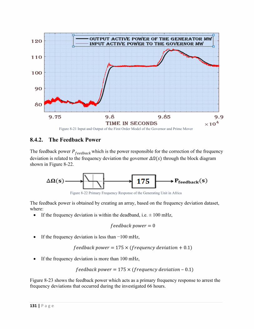
131 | P a g e

Figure 8-21 Input and Output of the First Order Model of the Governor and Prime Mover

8.4.2. The Feedback Power

The feedback power which is the power responsible for the correction of the frequency 𝑃𝑓𝑒𝑒𝑑𝑏𝑎𝑐𝑘 deviation is related to the frequency deviation the governor through the block diagram 𝛥𝛺(𝑠)shown in Figure 8-22.

Figure 8-22 Primary Frequency Response of the Generating Unit in Africa

The feedback power is obtained by creating an array, based on the frequency deviation dataset, where: If the frequency deviation is within the deadband, i.e. ± 100 mHz,

𝑓𝑒𝑒𝑑𝑏𝑎𝑐𝑘 𝑝𝑜𝑤𝑒𝑟 = 0

If the frequency deviation is less than −100 mHz,

𝑓𝑒𝑒𝑑𝑏𝑎𝑐𝑘 𝑝𝑜𝑤𝑒𝑟 = 175 × (𝑓𝑟𝑒𝑞𝑢𝑒𝑛𝑐𝑦 𝑑𝑒𝑣𝑖𝑎𝑡𝑖𝑜𝑛 + 0.1)

If the frequency deviation is more than 100 mHz,

𝑓𝑒𝑒𝑑𝑏𝑎𝑐𝑘 𝑝𝑜𝑤𝑒𝑟 = 175 × (𝑓𝑟𝑒𝑞𝑢𝑒𝑛𝑐𝑦 𝑑𝑒𝑣𝑖𝑎𝑡𝑖𝑜𝑛 ‒ 0.1)

Figure 8-23 shows the feedback power which acts as a primary frequency response to arrest the frequency deviations that occurred during the investigated 66 hours.

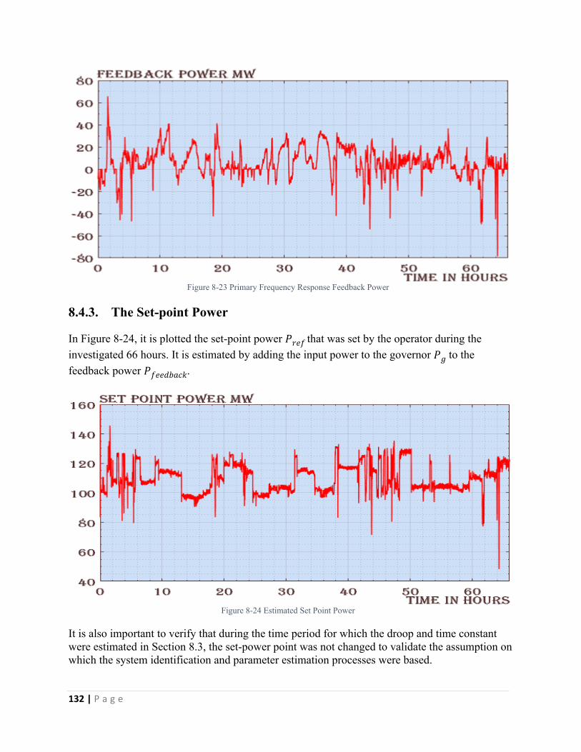
132 | P a g e

Figure 8-23 Primary Frequency Response Feedback Power

8.4.3. The Set-point Power

In Figure 8-24, it is plotted the set-point power that was set by the operator during the 𝑃𝑟𝑒𝑓 investigated 66 hours. It is estimated by adding the input power to the governor to the 𝑃𝑔feedback power .𝑃𝑓𝑒𝑒𝑑𝑏𝑎𝑐𝑘

Figure 8-24 Estimated Set Point Power

It is also important to verify that during the time period for which the droop and time constant were estimated in Section 8.3, the set-power point was not changed to validate the assumption on which the system identification and parameter estimation processes were based.

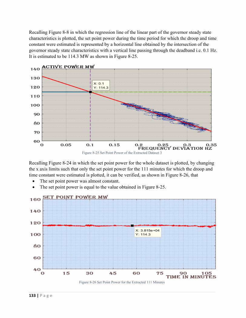
133 | P a g e

Recalling Figure 8-8 in which the regression line of the linear part of the governor steady state characteristics is plotted, the set point power during the time period for which the droop and time constant were estimated is represented by a horizontal line obtained by the intersection of the governor steady state characteristics with a vertical line passing through the deadband i.e. 0.1 Hz. It is estimated to be 114.3 MW as shown in Figure 8-25.

Figure 8-25 Set Point Power of the Extracted Dataset 3

Recalling Figure 8-24 in which the set point power for the whole dataset is plotted, by changing the x axis limits such that only the set point power for the 111 minutes for which the droop and time constant were estimated is plotted, it can be verified, as shown in Figure 8-26, that The set point power was almost constant. The set point power is equal to the value obtained in Figure 8-25.

Figure 8-26 Set Point Power for the Extracted 111 Minutes

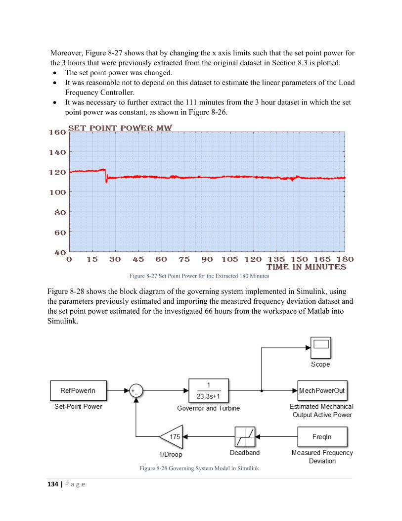
134 | P a g e

Moreover, Figure 8-27 shows that by changing the x axis limits such that the set point power for the 3 hours that were previously extracted from the original dataset in Section 8.3 is plotted: The set point power was changed. It was reasonable not to depend on this dataset to estimate the linear parameters of the Load

Frequency Controller. It was necessary to further extract the 111 minutes from the 3 hour dataset in which the set

point power was constant, as shown in Figure 8-26.

Figure 8-27 Set Point Power for the Extracted 180 Minutes

Figure 8-28 shows the block diagram of the governing system implemented in Simulink, using the parameters previously estimated and importing the measured frequency deviation dataset and the set point power estimated for the investigated 66 hours from the workspace of Matlab into Simulink.

Figure 8-28 Governing System Model in Simulink

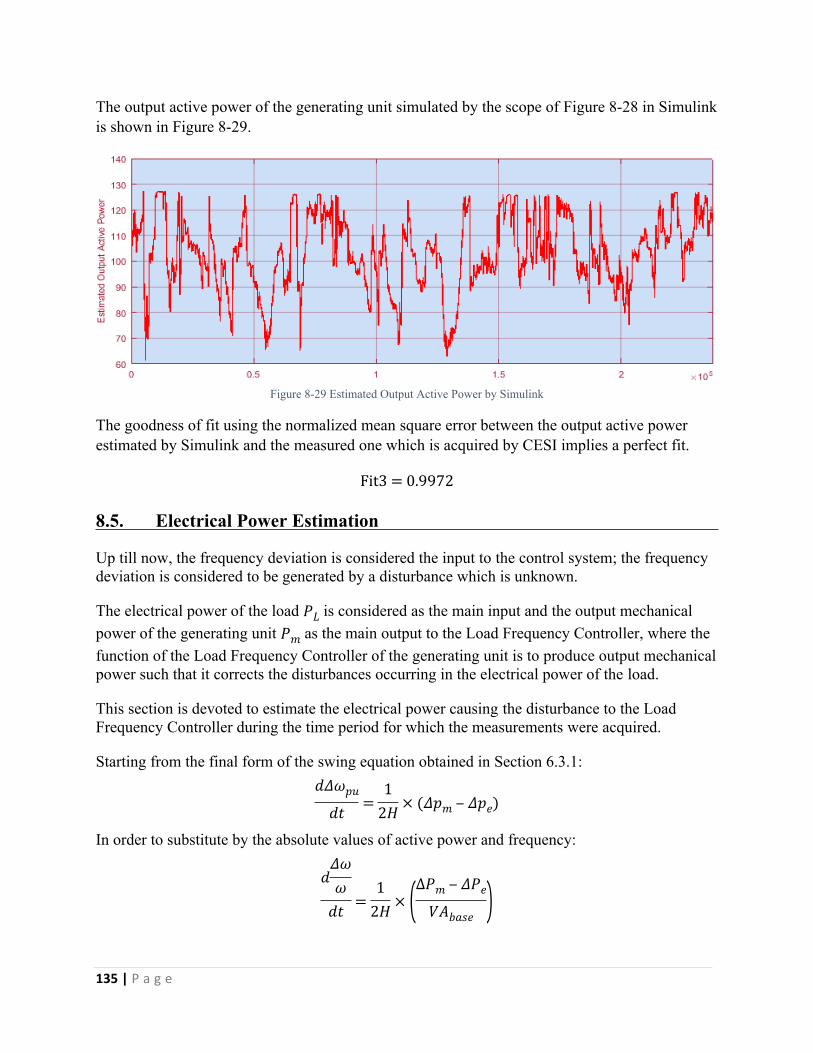
135 | P a g e

The output active power of the generating unit simulated by the scope of Figure 8-28 in Simulink is shown in Figure 8-29.

Figure 8-29 Estimated Output Active Power by Simulink

The goodness of fit using the normalized mean square error between the output active power estimated by Simulink and the measured one which is acquired by CESI implies a perfect fit.

Fit3 = 0.9972

8.5. Electrical Power Estimation

Up till now, the frequency deviation is considered the input to the control system; the frequency deviation is considered to be generated by a disturbance which is unknown.

The electrical power of the load is considered as the main input and the output mechanical 𝑃𝐿power of the generating unit as the main output to the Load Frequency Controller, where the 𝑃𝑚function of the Load Frequency Controller of the generating unit is to produce output mechanical power such that it corrects the disturbances occurring in the electrical power of the load.

This section is devoted to estimate the electrical power causing the disturbance to the Load Frequency Controller during the time period for which the measurements were acquired.

Starting from the final form of the swing equation obtained in Section 6.3.1:𝑑𝛥𝜔𝑝𝑢

𝑑𝑡 =1

2𝐻 × (𝛥𝑝𝑚 ‒ 𝛥𝑝𝑒)

In order to substitute by the absolute values of active power and frequency:

𝑑𝛥𝜔𝜔

𝑑𝑡 =1

2𝐻 × (∆𝑃𝑚 ‒ 𝛥𝑃𝑒

𝑉𝐴𝑏𝑎𝑠𝑒 )

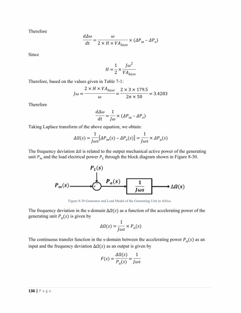
136 | P a g e

Therefore𝑑𝛥𝜔

𝑑𝑡 =𝜔

2 × 𝐻 × 𝑉𝐴𝑏𝑎𝑠𝑒× (𝛥𝑃𝑚 ‒ 𝛥𝑃𝑒)

Since

𝐻 =12 ×

𝐽𝜔2

𝑉𝐴𝑏𝑎𝑠𝑒

Therefore, based on the values given in Table 7-1:

𝐽𝜔 =2 × 𝐻 × 𝑉𝐴𝑏𝑎𝑠𝑒

𝜔 =2 × 3 × 179.5

2𝜋 × 50 = 3.4283

Therefore𝑑𝛥𝜔

𝑑𝑡 =1

𝐽𝜔 × (𝛥𝑃𝑚 ‒ 𝛥𝑃𝑒)

Taking Laplace transform of the above equation, we obtain:

𝛥𝛺(𝑠) =1

𝐽𝜔𝑠[𝛥𝑃𝑚(𝑠) ‒ 𝛥𝑃𝑒(𝑠)] =

1𝐽𝜔𝑠 × 𝛥𝑃𝑎(𝑠)

The frequency deviation is related to the output mechanical active power of the generating ∆𝛺unit and the load electrical power through the block diagram shown in Figure 8-30.𝑃𝑚 𝑃𝐿

Figure 8-30 Generator and Load Model of the Generating Unit in Africa

The frequency deviation in the s-domain as a function of the accelerating power of the ∆𝛺(𝑠)generating unit is given by𝑃𝑎(𝑠)

𝛥𝛺(𝑠) =1

𝐽𝜔𝑠 × 𝑃𝑎(𝑠)

The continuous transfer function in the s-domain between the accelerating power as an 𝑃𝑎(𝑠)input and the frequency deviation as an output is given by∆𝛺(𝑠)

𝐹(𝑠) =𝛥𝛺(𝑠)𝑃𝑎(𝑠) =

1𝐽𝜔𝑠

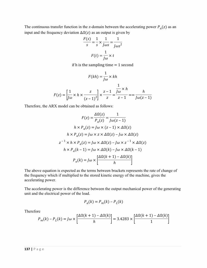
137 | P a g e

The continuous transfer function in the z-domain between the accelerating power as an 𝑃𝑎(𝑧)input and the frequency deviation as an output is given by∆𝛺(𝑧)

𝐹(𝑠)𝑠 =

1𝑠 ×

1𝐽𝜔𝑠 =

1

𝐽𝜔𝑠2

𝐹(𝑡) =1

𝐽𝜔 × 𝑡

if h is the sampling time = 1 second

𝐹(𝑘ℎ) =1

𝐽𝜔 × 𝑘ℎ

𝐹(𝑧) = [ 1𝐽𝜔 × ℎ ×

𝑧

(𝑧 ‒ 1)2] ×𝑧 ‒ 1

𝑧 =

1𝐽𝜔 × ℎ

𝑧 ‒ 1 ==ℎ

𝐽𝜔(𝑧 ‒ 1)

Therefore, the ARX model can be obtained as follows:

𝐹(𝑧) =𝛥𝛺(𝑧)𝑃𝑎(𝑧) =

1𝐽𝜔(𝑧 ‒ 1)

ℎ × 𝑃𝑎(𝑧) = 𝐽𝜔 × (𝑧 ‒ 1) × 𝛥𝛺(𝑧)

ℎ × 𝑃𝑎(𝑧) = 𝐽𝜔 × 𝑧 × 𝛥𝛺(𝑧) ‒ 𝐽𝜔 × 𝛥𝛺(𝑧)

𝑧 ‒ 1 × ℎ × 𝑃𝑎(𝑧) = 𝐽𝜔 × 𝛥𝛺(𝑧) ‒ 𝐽𝜔 × 𝑧 ‒ 1 × 𝛥𝛺(𝑧)

ℎ × 𝑃𝑎(𝑘 ‒ 1) = 𝐽𝜔 × 𝛥𝛺(𝑘) ‒ 𝐽𝜔 × 𝛥𝛺(𝑘 ‒ 1)

𝑃𝑎(𝑘) = 𝐽𝜔 × [𝛥𝛺(𝑘 + 1) ‒ 𝛥𝛺(𝑘)ℎ ]

The above equation is expected as the terms between brackets represents the rate of change of the frequency which if multiplied to the stored kinetic energy of the machine, gives the accelerating power.

The accelerating power is the difference between the output mechanical power of the generating unit and the electrical power of the load.

𝑃𝑎(𝑘) = 𝑃𝑚(𝑘) ‒ 𝑃𝐿(𝑘)

Therefore

𝑃𝑚(𝑘) ‒ 𝑃𝐿(𝑘) = 𝐽𝜔 × [𝛥𝛺(𝑘 + 1) ‒ 𝛥𝛺(𝑘)ℎ ] = 3.4283 × [𝛥𝛺(𝑘 + 1) ‒ 𝛥𝛺(𝑘)

1 ]

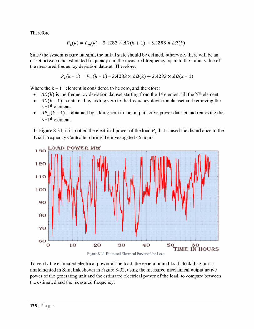
138 | P a g e

Therefore

𝑃𝐿(𝑘) = 𝑃𝑚(𝑘) ‒ 3.4283 × 𝛥𝛺(𝑘 + 1) + 3.4283 × 𝛥𝛺(𝑘)

Since the system is pure integral, the initial state should be defined, otherwise, there will be an offset between the estimated frequency and the measured frequency equal to the initial value of the measured frequency deviation dataset. Therefore:

𝑃𝐿(𝑘 ‒ 1) = 𝑃𝑚(𝑘 ‒ 1) ‒ 3.4283 × 𝛥𝛺(𝑘) + 3.4283 × 𝛥𝛺(𝑘 ‒ 1)

Where the k – 1th element is considered to be zero, and therefore: is the frequency deviation dataset starting from the 1st element till the Nth element.𝛥𝛺(𝑘) is obtained by adding zero to the frequency deviation dataset and removing the 𝛥𝛺(𝑘 ‒ 1)

N+1th element. is obtained by adding zero to the output active power dataset and removing the 𝛥𝑃𝑚(𝑘 ‒ 1)

N+1th element.

In Figure 8-31, it is plotted the electrical power of the load that caused the disturbance to the 𝑃𝑒 Load Frequency Controller during the investigated 66 hours.

Figure 8-31 Estimated Electrical Power of the Load

To verify the estimated electrical power of the load, the generator and load block diagram is implemented in Simulink shown in Figure 8-32, using the measured mechanical output active power of the generating unit and the estimated electrical power of the load, to compare between the estimated and the measured frequency.

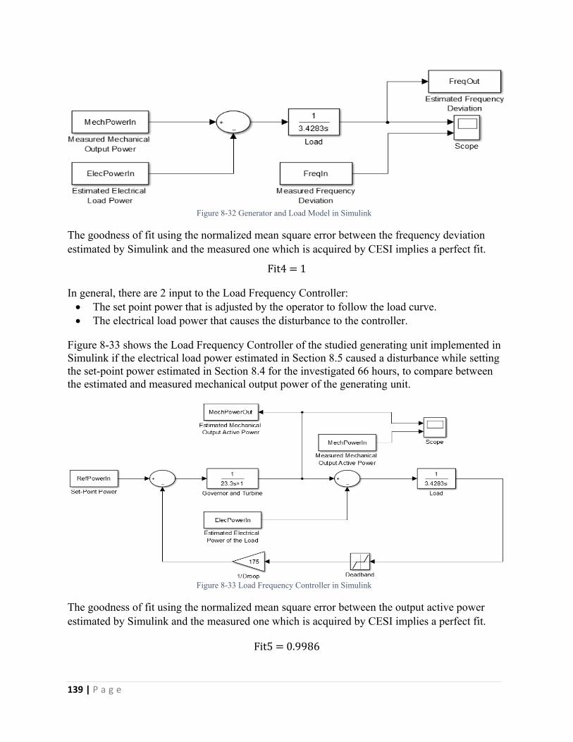
139 | P a g e

Figure 8-32 Generator and Load Model in Simulink

The goodness of fit using the normalized mean square error between the frequency deviation estimated by Simulink and the measured one which is acquired by CESI implies a perfect fit.

Fit4 = 1

In general, there are 2 input to the Load Frequency Controller: The set point power that is adjusted by the operator to follow the load curve. The electrical load power that causes the disturbance to the controller.

Figure 8-33 shows the Load Frequency Controller of the studied generating unit implemented in Simulink if the electrical load power estimated in Section 8.5 caused a disturbance while setting the set-point power estimated in Section 8.4 for the investigated 66 hours, to compare between the estimated and measured mechanical output power of the generating unit.

Figure 8-33 Load Frequency Controller in Simulink

The goodness of fit using the normalized mean square error between the output active power estimated by Simulink and the measured one which is acquired by CESI implies a perfect fit.

Fit5 = 0.9986

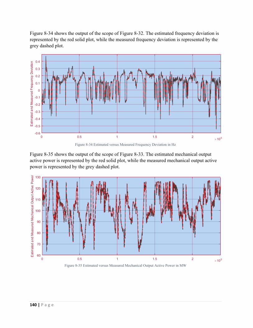
140 | P a g e

Figure 8-34 shows the output of the scope of Figure 8-32. The estimated frequency deviation is represented by the red solid plot, while the measured frequency deviation is represented by the grey dashed plot.

Figure 8-34 Estimated versus Measured Frequency Deviation in Hz

Figure 8-35 shows the output of the scope of Figure 8-33. The estimated mechanical output active power is represented by the red solid plot, while the measured mechanical output active power is represented by the grey dashed plot.

Figure 8-35 Estimated versus Measured Mechanical Output Active Power in MW

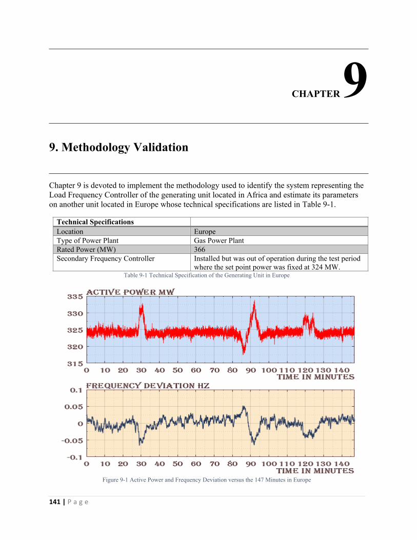
141 | P a g e

CHAPTER 99. Methodology Validation

Chapter 9 is devoted to implement the methodology used to identify the system representing the Load Frequency Controller of the generating unit located in Africa and estimate its parameters on another unit located in Europe whose technical specifications are listed in Table 9-1.

Technical SpecificationsLocation EuropeType of Power Plant Gas Power PlantRated Power (MW) 366Secondary Frequency Controller Installed but was out of operation during the test period

where the set point power was fixed at 324 MW.Table 9-1 Technical Specification of the Generating Unit in Europe

Figure 9-1 Active Power and Frequency Deviation versus the 147 Minutes in Europe

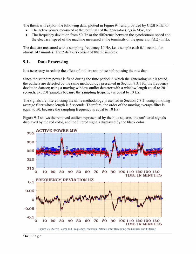
142 | P a g e

The thesis will exploit the following data, plotted in Figure 9-1 and provided by CESI Milano: The active power measured at the terminals of the generator (Pm) in MW, and The frequency deviation from 50 Hz or the difference between the synchronous speed and

the electrical speed of the machine measured at the terminals of the generator (ΔΩ) in Hz.

The data are measured with a sampling frequency 10 Hz, i.e. a sample each 0.1 second, for almost 147 minutes. The 2 datasets consist of 88189 samples.

9.1. Data Processing

It is necessary to reduce the effect of outliers and noise before using the raw data.

Since the set point power is fixed during the time period in which the generating unit is tested, the outliers are detected by the same methodology presented in Section 7.3.1 for the frequency deviation dataset; using a moving window outlier detector with a window length equal to 20 seconds, i.e. 201 samples because the sampling frequency is equal to 10 Hz.

The signals are filtered using the same methodology presented in Section 7.3.2; using a moving average filter whose length is 5 seconds. Therefore, the order of the moving average filter is equal to 50, because the sampling frequency is equal to 10 Hz.

Figure 9-2 shows the removed outliers represented by the blue squares, the unfiltered signals displayed by the red color, and the filtered signals displayed by the black color.

Figure 9-2 Active Power and Frequency Deviation Datasets after Removing the Outliers and Filtering

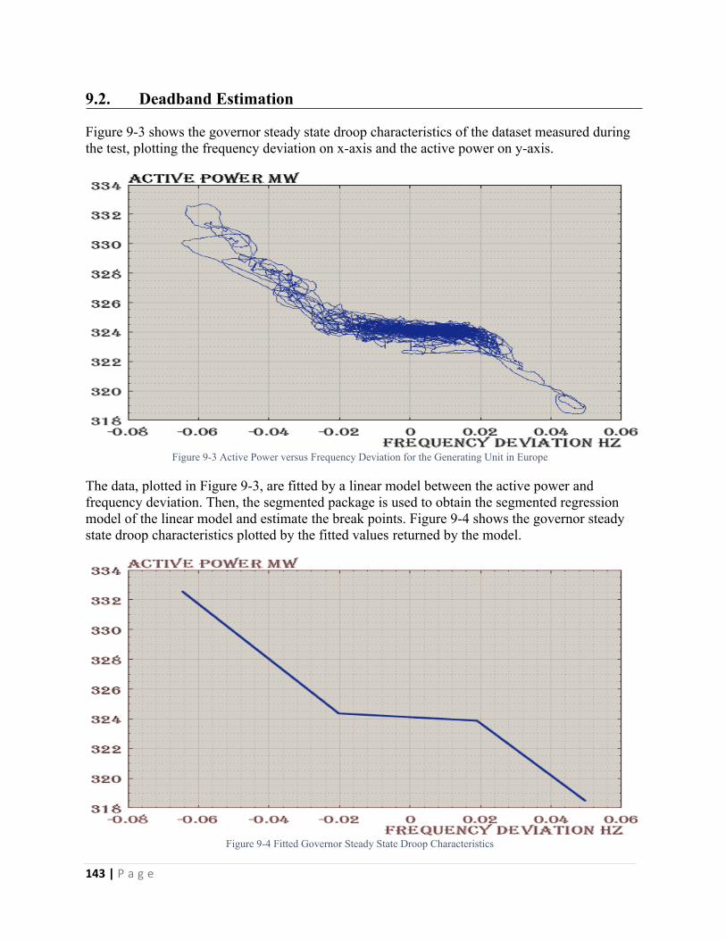
143 | P a g e

9.2. Deadband Estimation

Figure 9-3 shows the governor steady state droop characteristics of the dataset measured during the test, plotting the frequency deviation on x-axis and the active power on y-axis.

Figure 9-3 Active Power versus Frequency Deviation for the Generating Unit in Europe

The data, plotted in Figure 9-3, are fitted by a linear model between the active power and frequency deviation. Then, the segmented package is used to obtain the segmented regression model of the linear model and estimate the break points. Figure 9-4 shows the governor steady state droop characteristics plotted by the fitted values returned by the model.

Figure 9-4 Fitted Governor Steady State Droop Characteristics

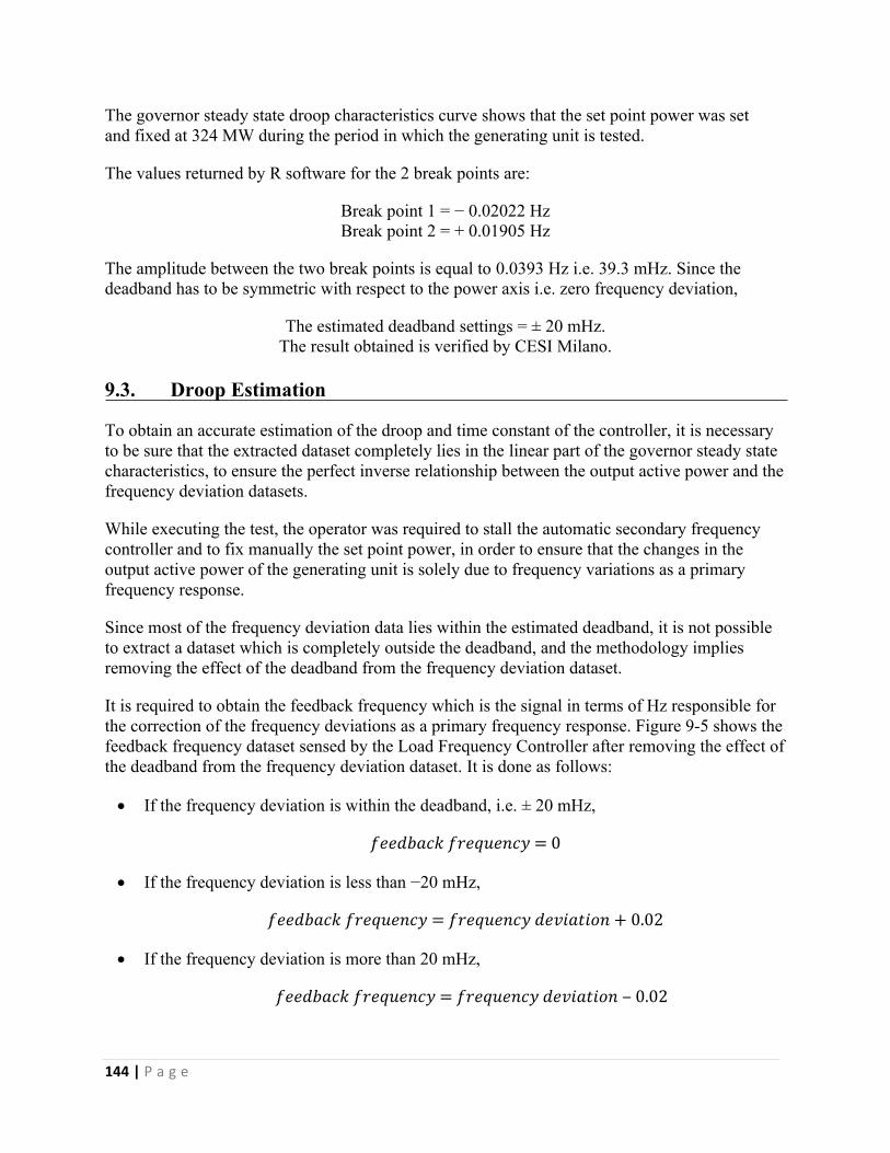
144 | P a g e

The governor steady state droop characteristics curve shows that the set point power was set and fixed at 324 MW during the period in which the generating unit is tested.

The values returned by R software for the 2 break points are:

Break point 1 = − 0.02022 HzBreak point 2 = + 0.01905 Hz

The amplitude between the two break points is equal to 0.0393 Hz i.e. 39.3 mHz. Since the deadband has to be symmetric with respect to the power axis i.e. zero frequency deviation,

The estimated deadband settings = ± 20 mHz.The result obtained is verified by CESI Milano.

9.3. Droop Estimation

To obtain an accurate estimation of the droop and time constant of the controller, it is necessary to be sure that the extracted dataset completely lies in the linear part of the governor steady state characteristics, to ensure the perfect inverse relationship between the output active power and the frequency deviation datasets.

While executing the test, the operator was required to stall the automatic secondary frequency controller and to fix manually the set point power, in order to ensure that the changes in the output active power of the generating unit is solely due to frequency variations as a primary frequency response.

Since most of the frequency deviation data lies within the estimated deadband, it is not possible to extract a dataset which is completely outside the deadband, and the methodology implies removing the effect of the deadband from the frequency deviation dataset.

It is required to obtain the feedback frequency which is the signal in terms of Hz responsible for the correction of the frequency deviations as a primary frequency response. Figure 9-5 shows the feedback frequency dataset sensed by the Load Frequency Controller after removing the effect of the deadband from the frequency deviation dataset. It is done as follows:

If the frequency deviation is within the deadband, i.e. ± 20 mHz,

𝑓𝑒𝑒𝑑𝑏𝑎𝑐𝑘 𝑓𝑟𝑒𝑞𝑢𝑒𝑛𝑐𝑦 = 0

If the frequency deviation is less than −20 mHz,

𝑓𝑒𝑒𝑑𝑏𝑎𝑐𝑘 𝑓𝑟𝑒𝑞𝑢𝑒𝑛𝑐𝑦 = 𝑓𝑟𝑒𝑞𝑢𝑒𝑛𝑐𝑦 𝑑𝑒𝑣𝑖𝑎𝑡𝑖𝑜𝑛 + 0.02

If the frequency deviation is more than 20 mHz,

𝑓𝑒𝑒𝑑𝑏𝑎𝑐𝑘 𝑓𝑟𝑒𝑞𝑢𝑒𝑛𝑐𝑦 = 𝑓𝑟𝑒𝑞𝑢𝑒𝑛𝑐𝑦 𝑑𝑒𝑣𝑖𝑎𝑡𝑖𝑜𝑛 ‒ 0.02

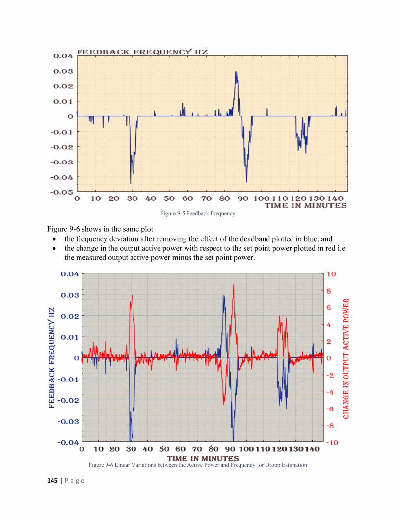
145 | P a g e

Figure 9-5 Feedback Frequency

Figure 9-6 shows in the same plot the frequency deviation after removing the effect of the deadband plotted in blue, and the change in the output active power with respect to the set point power plotted in red i.e.

the measured output active power minus the set point power.

Figure 9-6 Linear Variations between the Active Power and Frequency for Droop Estimation

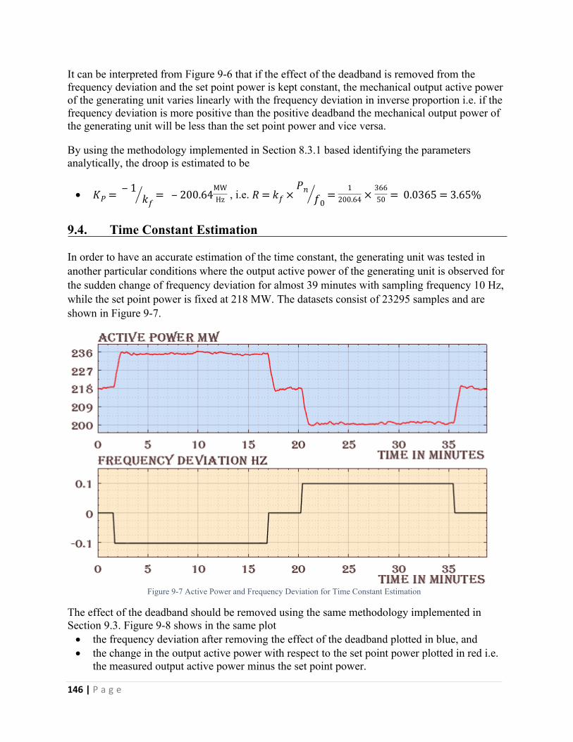
146 | P a g e

It can be interpreted from Figure 9-6 that if the effect of the deadband is removed from the frequency deviation and the set point power is kept constant, the mechanical output active power of the generating unit varies linearly with the frequency deviation in inverse proportion i.e. if the frequency deviation is more positive than the positive deadband the mechanical output power of the generating unit will be less than the set point power and vice versa.

By using the methodology implemented in Section 8.3.1 based identifying the parameters analytically, the droop is estimated to be

, i.e. 𝐾𝑃 = ‒ 1𝑘𝑓

= ‒ 200.64MWHz 𝑅 = 𝑘𝑓 ×

𝑃𝑛𝑓0

=1

200.64 ×36650 = 0.0365 = 3.65%

9.4. Time Constant Estimation

In order to have an accurate estimation of the time constant, the generating unit was tested in another particular conditions where the output active power of the generating unit is observed for the sudden change of frequency deviation for almost 39 minutes with sampling frequency 10 Hz, while the set point power is fixed at 218 MW. The datasets consist of 23295 samples and are shown in Figure 9-7.

Figure 9-7 Active Power and Frequency Deviation for Time Constant Estimation

The effect of the deadband should be removed using the same methodology implemented in Section 9.3. Figure 9-8 shows in the same plot the frequency deviation after removing the effect of the deadband plotted in blue, and the change in the output active power with respect to the set point power plotted in red i.e.

the measured output active power minus the set point power.

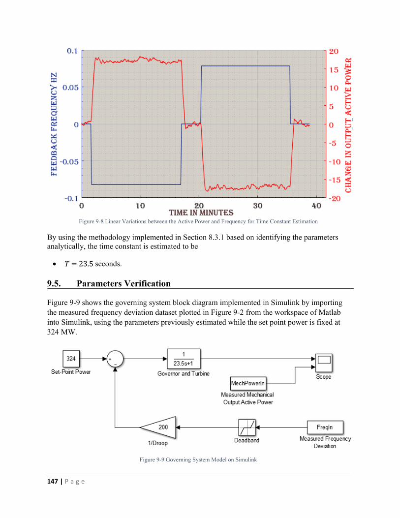
147 | P a g e

Figure 9-8 Linear Variations between the Active Power and Frequency for Time Constant Estimation

By using the methodology implemented in Section 8.3.1 based on identifying the parameters analytically, the time constant is estimated to be

seconds.𝑇 = 23.5

9.5. Parameters Verification

Figure 9-9 shows the governing system block diagram implemented in Simulink by importing the measured frequency deviation dataset plotted in Figure 9-2 from the workspace of Matlab into Simulink, using the parameters previously estimated while the set point power is fixed at 324 MW.

Figure 9-9 Governing System Model on Simulink

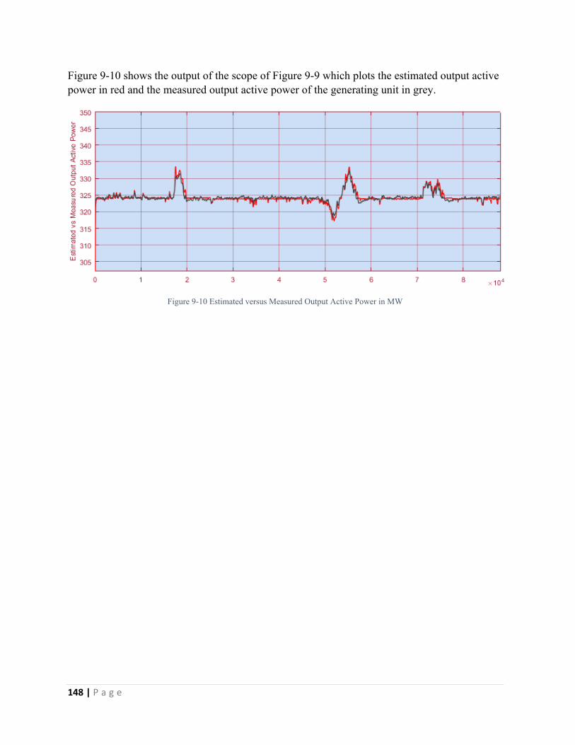
148 | P a g e

Figure 9-10 shows the output of the scope of Figure 9-9 which plots the estimated output active power in red and the measured output active power of the generating unit in grey.

Figure 9-10 Estimated versus Measured Output Active Power in MW

149 | P a g e

CHAPTER 1010. Conclusion

The thesis is divided into two parts:

First part:

Grid codes are the operational procedures imposed on all stakeholders developed to simplify the operation and planning of the electric power system. The first part is assigned for studying the operational procedures that govern the European and the North American interconnected power systems operated by ENTSO-E and NERC respectively in terms of the minimum requirements imposed by each organization and the criteria used to measure the compliance with the grid codes, and highlighting the differences between them to identify the common best practice.

The first part started with Chapter 2 in which the organizational structure of ENTSO-E and NERC were demonstrated. It stated the mission of each organization, the responsibilities shared between the different entities and the manner in which the two interconnected systems operate. Chapter 2 included also a presentation of the grid codes adopted by each organization in terms of how they are organized and the manner by which they are drafted, developed, and enforced.

The thesis was aimed to focus only on the operational grid codes:

Chapter 3 was devoted to investigate the Load Frequency Control from the point of view of ENTSO-E and NERC. It listed the minimum requirements that should be satisfied in the attempt to maintain the active power balance in both systems including the frequency, frequency response, droop, deadband, area control error, reserves dimensioning and their activation, and time control process.

Chapter 4 discussed the common Operational Security requirements imposed by ENTSO-E and NERC, to ensure the conditions for maintaining Operational Security and to promote coordination of system operation. It also presented how the system conditions, events, and contingencies are classified and the different schemes required to be implemented when needed. Moreover, it included the procedures required to be followed in case of emergency operating conditions and the scheme by which the system is restored to normal operating conditions according to the two systems.

150 | P a g e

Chapter 5 was assigned to demonstrate the concerns of ENTSO-E and NERC related to the Operational Planning and Scheduling in order to prepare a secure and reliable operation of the interconnected power system with a high level of coordination, reliability, quality and stability. The main issues discussed were the time frames, network models, Planned Outage Coordination, Load Forecast, Adequacy, and Capacity Calculations.

Future work that can complement the work done in the first part of the thesis include: Performing a survey at international level of the main connection grid codes. Performing a survey at international level of the main market codes. Other topics can be also included, such as; critical infrastructure protection, communication

tools and systems, and personal performance and training.

Second part:

The aim of the second part of the thesis was to develop a methodology to investigate the performance of the Load Frequency Controller of the generating unit related to the primary frequency control in order to assess its compliance with the grid codes by measuring the output active power and frequency at the terminals of the generating unit.

The second part started with chapter 6 which provided an introduction about the droop control of a generating unit and how the capacity of generating unit and changing the set point power, the deadband and droop settings affect the governor steady state characteristics. In Chapter 6, the simplified model of the generating unit upon which the estimation of the parameters of the Load Frequency Controller in Chapters 8 and 9 were based was derived.

The methodology to estimate the parameters of the Load Frequency Controller was developed for a generating unit located in Africa and verified for a generating unit located in Europe. For the generating unit in Africa, the output active power and frequency were measured for 66 hours with a sampling frequency 10 Hz where the datasets consist of 237600 samples, while for the generating unit in Europe, the output active power and frequency were measured for almost 147 minutes with a sampling frequency 10 Hz where the datasets consist of 88189 samples.

To obtain more accurate and reliable results, it was necessary to pre-process the data obtained by measurements. Data processing strategies to remove the outliers using a change of mean detector for the active power dataset and a moving window outlier detector for the frequency deviation dataset, and reduce the effect of noise using a moving average filter were demonstrated in Section 7.3 for the generating unit in Africa and Section 9.1 for the generating unit in Europe.

Chapter 8 was devoted for the estimation of the parameters of the Load Frequency Controller of the generating unit in Africa and the rest of Chapter 9 was devoted for a similar task but for the generating unit in Europe.

The maximum output active power that can be produced by the generating unit was reached only in the measurements obtained for the generating unit in Africa. Therefore, the capacity of generating unit for the generating unit in Africa was estimated in Section 8.1.

151 | P a g e

A methodology to estimate the deadband based on the change points detected by the segmented linear regression using the software “R” in the governor steady state droop characteristics of both generating units was presented in Section 8.2 for the generating unit in Africa and Section 9.2 for the generating unit in Europe. It should be noted that to estimate the deadband, the entire dataset was used for the generating unit in Europe, while in Africa, part of the dataset is extracted where the frequency data lie in the zone in which the deadband is expected to be set.

A methodology to estimate the droop and the time constant and identify the transfer function representing the system between the change in frequency as an input and the change in the output active power of the generating unit as an output was presented in Section 8.3 for the generating unit in Africa and Sections 9.3 and 9.4 for the generating unit in Europe. It should be noted that in order to estimate the droop and time constant, the linear variation between the input and output should be ensured.

To take advantage of the linear variation between the change of frequency and the change in the output active power of the generating unit, the two factors which cause the non linear variation between the 2 variables should be avoided in the investigated dataset. Therefore, two conditions must be fulfilled in the dataset under consideration: The set point power must be ensured to be constant to avoid the shift in the governor steady

state characteristics along the power axis.o Concerning the generating unit in Africa, the set point power was unknown, however,

depending on the correlation between the frequency variations and the change in the output active power which should be -1 in case of perfect inverse relationship, it was possible to extract a dataset in which the set point power was assumed to be constant.

o Concerning the generating unit in Europe, it was required during the test period to keep the secondary frequency controller out of operation and fix the set point power.

The deadband should be inactive, to avoid the change in frequency without correspondence in the output active power.o Concerning the generating unit in Africa, it was possible to extract a dataset in which

the whole frequency deviation data are outside the estimated deadband.o Concerning the generating unit in Europe, most of the frequency deviation data lie

within the deadband, and therefore, it was necessary to remove the effect of the deadband.

Concerning the generating unit in Africa, the reference power set during the 66 hours was unknown as the time constant and droop were estimated during a period in which the set point power as assumed to be constant. Section 8.4 was dedicated to estimate the set point power that was set by the operator during the 2 days and 18 hours as a reference based on the parameters of the Load Frequency Controller previously estimated. Section 8.5 was to estimating the electrical power of the load that was causing the disturbance to the controller during the 66 hours.

Future work that can complement the work done in the second part of the thesis include: Improving the performance by employing modern control designs that are useful in

multivariable systems either by pole placement design or by optimal control design. Developing similar methodology to estimate the parameters of the Automatic Voltage

Regulator using the output reactive power and the voltage measured at the terminals of the generating unit.

152 | P a g e

11. References[1] P. Kumar and K. A. Singh, "Grid Codes: Goals and Challenges," in Renewable Energy Integration:

Challenges and Solutions, Springer, 2014, p. 18.[2] B. Banerjee, D. Jayaweera and S. Islam, "Fundamentals of Power Systems," in Smart Power

Systems and Renewable Energy System Integration, Springer, 2016, p. 1.[3] V. Lagendijk, Electrifying Europe: The Power of Europe in the Construction of Electricity

Networks, Amsterdam University Press, 2008. [4] United Nations Economic and Social Affairs Department, Multi Dimensional Issues in

International Electric Power Grid Interconnections, United Nations Publications, 2006. [5] C.-E. Stephan and Z. Baba, "Specifying a Turbogenerator's Electrical Parameters guided by

Standards and Grid Codes," Electric Machines and Drives Conference, 2001. IEMDC 2001. IEEE International, pp. 63 - 68, 2001.

[6] "ENTSO-E website," [Online]. Available: https://www.entsoe.eu.[7] ENTSO-E, "Supporting Document for the Network Code on Load-Frequency Control and

Reserves," 2013. [Online]. Available: https://www.entsoe.eu/major-projects/network-code-development/load-frequency-control-reserves/Pages/default.aspx.

[8] "ENTSO-E at a Glance," [Online]. Available: https://www.entsoe.eu/publications/general-publications/entso-e-at-a-glance/Pages/default.aspx.

[9] "NERC website," [Online]. Available: http://www.nerc.com.[10] NERC, "Reliability Functional Model," 2015.[11] UCTE, "UCTE Policy 4 final," [Online]. Available: https://www.entsoe.eu/publications/system-

operations-reports/operation-handbook/Pages/default.aspx.[12] UCTE, "UCTE Introduction," [Online]. Available: https://www.entsoe.eu/publications/system-

operations-reports/operation-handbook/Pages/default.aspx.[13] ENTSO-E, "Network Code on Load-Frequency Control and Reserves," 2013. [Online]. Available:

https://www.entsoe.eu/major-projects/network-code-development/load-frequency-control-reserves/Pages/default.aspx.

[14] NERC, "Loads and Resources Balance".[15] NERC, "NERC Reliability Standards 2016".[16] NERC, "Frequency Response Initiative Report 2015".[17] NERC, "Balancing and Frequency Control".[18] NREL, "Operating Reserves and Variable Generation".[19] ENTSO-E, "Supporting Document for the Network Code on Operational Security," 2013. [Online].

Available: https://www.entsoe.eu/major-projects/network-code-development/operational-security/Pages/default.aspx.

[20] ENTSO-E, "Network Code on Operational Security," 2013. [Online]. Available: https://www.entsoe.eu/major-projects/network-code-development/operational-planning-scheduling/Pages/default.aspx.

[21] Energy and Natural Resources of Canada and U.S. Department of Energy, "Final Report on the Implementation of the Task Force Recommendations".

[22] MISO, "NERC Operating Conditions Procedure RTO-AOP-013-r9".[23] ENTSO-E, "The Incident Classification Scale 2014 Annual Report," 2014. [Online]. Available:

https://www.entsoe.eu/about-entso-e/system-operations/ops/incident-classification-

153 | P a g e

scale/Pages/default.aspx.[24] UCTE, "UCTE Appendix 3 Operational Security," [Online]. Available:

https://www.entsoe.eu/publications/system-operations-reports/operation-handbook/Pages/default.aspx.

[25] NERC, "Remedial Action Scheme Definition Development".[26] ENTSO-E, "Technical Background for the Low Frequency Demand Disconnection Requirements,"

2014. [Online]. Available: https://www.entsoe.eu/Documents/Network codes documents/NC ER/141215_Technical_background_for_LFDD.pdf.

[27] E. A. Udren and R. W. Charles, "The New NERC Protection System Maintenance Standard," Protective Relay Engineers, 2010 63rd Annual Conference , pp. 1 - 18, 2010.

[28] NERC, "Reliability Concept".[29] ENTSO-E, "Network Code on Operational Planning and Scheduling," 2013. [Online]. Available:

https://www.entsoe.eu/major-projects/network-code-development/operational-security/Pages/default.aspx.

[30] UCTE, "UCTE Appendix 4," [Online]. Available: https://www.entsoe.eu/publications/system-operations-reports/operation-handbook/Pages/default.aspx.

[31] ENTSO-E and EURELECTRIC, "Deterministic frequency deviations – root causes and proposals for potential solutions," [Online]. Available: https://www.entsoe.eu/publications/system-operations-reports/Pages/default.aspx.

[32] H. Saadat, Power System Analysis, McGraw-Hill Education, 2004. [33] R. Marconato, Electric Power Systems, CEI, 2002. [34] O. Maimon and L. Rokach, Data Mining and Knowledge Discovery Handbook, Springer, 2005. [35] R. Killick and I. A. Eckley, "An R Package for Changepoint Analysis," Journal of Statistical

Software, vol. 58, no. 3, 2014. [36] T. Pan, B. Huang and S. Khare, "A Practical Algorithm to Outlier Detection and Data Cleaning for

the Time-dependent Signal," Control Conference (CCC), 2013 32nd Chinese, pp. 1676 - 1679, 2013.

[37] P. Ribeiro, C. Duque, P. Silveira and A. Cerqueira, Power Systems Signal Processing for Smart Grids, Wiley, 2014.

[38] G. D'Antona and A. Ferrero, Digital Signal Processing for Measurement Systems, Springer, 2006. [39] B. Mogharbel, L. Fan and M. Zhixin, "Least Squares Estimation-Based Synchronous Generator

Parameter Estimation Using PMU Data," 2015 IEEE Power & Energy Society General Meeting, pp. 1 - 5, 2015.