Algorithmic Model Theory SS 2016 - RWTH Aachen University

Algorithmic Model TheorySS 2016

Prof. Dr. Erich Grädel and Dr. Wied Pakusa

Mathematische Grundlagen der InformatikRWTH Aachen

cbndThis work is licensed under:http://creativecommons.org/licenses/by-nc-nd/3.0/de/Dieses Werk ist lizenziert unter:http://creativecommons.org/licenses/by-nc-nd/3.0/de/

© 2019 Mathematische Grundlagen der Informatik, RWTH Aachen.http://www.logic.rwth-aachen.de

Contents

1 The classical decision problem 11.1 Basic notions on decidability . . . . . . . . . . . . . . . . . . . . 21.2 Trakhtenbrot’s Theorem . . . . . . . . . . . . . . . . . . . . . . . 71.3 Domino problems . . . . . . . . . . . . . . . . . . . . . . . . . . 131.4 Applications of the domino method . . . . . . . . . . . . . . . . 161.5 The finite model property . . . . . . . . . . . . . . . . . . . . . . 201.6 The two-variable fragment of FO . . . . . . . . . . . . . . . . . . 21

2 Descriptive Complexity 312.1 Logics Capturing Complexity Classes . . . . . . . . . . . . . . . 312.2 Fagin’s Theorem . . . . . . . . . . . . . . . . . . . . . . . . . . . 332.3 Second Order Horn Logic on Ordered Structures . . . . . . . . 38

3 Expressive Power of First-Order Logic 433.1 Ehrenfeucht-Fraïssé Theorem . . . . . . . . . . . . . . . . . . . . 433.2 Hanf’s technique . . . . . . . . . . . . . . . . . . . . . . . . . . . 473.3 Gaifman’s Theorem . . . . . . . . . . . . . . . . . . . . . . . . . 493.4 Lower bound for the size of local sentences . . . . . . . . . . . 54

4 Zero-one laws 614.1 Random graphs . . . . . . . . . . . . . . . . . . . . . . . . . . . . 614.2 Zero-one law for first-order logic . . . . . . . . . . . . . . . . . . 634.3 Generalised zero-one laws . . . . . . . . . . . . . . . . . . . . . . 68

5 Modal, Inflationary and Partial Fixed Points 735.1 The Modal µ-Calculus . . . . . . . . . . . . . . . . . . . . . . . . 735.2 Inflationary Fixed-Point Logic . . . . . . . . . . . . . . . . . . . 755.3 Simultaneous Inductions . . . . . . . . . . . . . . . . . . . . . . 815.4 Partial Fixed-Point Logic . . . . . . . . . . . . . . . . . . . . . . 82

5.5 Capturing PTIME up to Bisimulation . . . . . . . . . . . . . . . 85

1 The classical decision problem

The classical decision problem was generally considered as the mainproblem of mathematical logic until its unsolvability was proved byChurch and Turing in 1936/37.

Das Entscheidungsproblem ist gelöst, wenn man ein Verfahrenkennt, das bei einem vorgelegten logischen Ausdruck durchendlich viele Operationen die Entscheidung über die Allge-meingültigkeit bzw. Erfüllbarkeit erlaubt. (. . . ) Das Entschei-dungsproblem muss als das Hauptproblem der mathematis-chen Logik bezeichnet werden. 1

(D. Hilbert and W. Ackermann, Grundzüge der theoretischenLogik, 1928)

By a logical expression, Hilbert and Ackermann meant what we nowcall a formula of first-order logic (FO). Historically, the classical decisionproblem was part of Hilbert’s formalist programme for the foundationsof mathematics. Its importance stems from the fact that first-order logicprovides a framework to express almost all aspects of mathematics.

We present three equivalent formulations of the classical decisionproblem.

Satisfiability: Construct an algorithm that decides for any given formulaof FO whether it has a model.

Validity: Construct an algorithm that decides for any given formula ofFO whether it is valid, i.e. whether it holds in all models where it isdefined.

1The Entscheidungsproblem is solved when we know a procedure that allowsfor any given logical expression to decide by finitely many operations its validity orsatisfiability. [. . . ] The Entscheidungsproblem must be considered the main problemof mathematical logic.

1


Provability: Construct an algorithm that decides for any given formulaψ of FO whether ⊢ ψ, meaning that ψ is provable from the emptyset of axioms in some complete formal system such as the sequentcalculus.

Since ψ is satisfiable if, and only if, ¬ψ is not valid, satisfiabilityand validity are equivalent problems with respect to computability. Theequivalence with provability is a much more intricate result and in facta consequence of Gödel’s Completeness Theorem.Theorem 1.1 (Completeness Theorem (Gödel)). For any given set ofsentences Φ ⊆ FO(τ) and any sentence ψ ∈ FO(τ) it holds that

Φ |= ψ ⇐⇒ Φ ⊢ ψ .

In particular ∅ |= ψ ⇔ ∅ ⊢ ψ.Corollary 1.2. The set of valid first-order formulae is recursively enu-merable.

1.1 Basic notions on decidability

In our formulation of the decision problem it was not precisely specifiedwhat an algorithm is. It was not until the 1930s that Church, Kleene,Gödel, and Turing provided precise definitions of an abstract algorithm.Their approaches are today known to be equivalent. We introduce theconcept of a Turing machine.Definition 1.3. A Turing machine (TM) M is a tuple M = (Q, Σ, Γ, q0, F, δ),where

• Q is a finite set of (control) states,• Σ, Γ are finite alphabets, where Σ is the working alphabet with a

special blank symbol □ ∈ Σ, and Γ ⊆ Σ \ {□} is the input alphabet,• q0 ∈ Q is the initial state,• F ⊆ Q is the set of final states and• δ : (Q \ F)× Σ → Q × Σ × {−1, 0, 1} is the transition function.

A configuration is a triple C = (q, p, w) ∈ Q × N × Σ∗, representingthe situation that M is in state q, reads tape cell p and that the in-scription of the infinite tape is w = w0 . . . wk, followed by infinitely

2


many blank-symbols. The transition function δ induces a partialfunction on the set of all configurations C 7→ Next(C), where forδ(q, wp) = (q′, a, m), the successor configuration of C is defined asNext(C) = (q′, p + m, w0 . . . wp−1awp+1 · · ·wk). A computation of the TMM on an input word x ∈ Γ∗ is a sequence

C0, C1, . . .

where C0 = C0(x) := (q0, 0, x) is the input configuration and Ci+1 =

Next(Ci) for all i.

M halts on x if the computation of M on x is finite and ends in afinal configuration C f = (q, p, w) with q ∈ F. Further

L(M) := {x ∈ Γ∗ : M halts on x}.

A Turing machine M computes a partial function fM : Γ∗ → Σ∗

with domain L(M) such that fM(x) = y if and only if the computationof M on x ends in (q, p, y) for some q ∈ F, y ∈ Σ∗ and p ∈ N.Definition 1.4. A Turing acceptor is a Turing machine M with F = F+ ·∪F−. We say that M accepts x if the computation of M on x ends in a statein F+ and M rejects x if the computation of M on x ends in a state in F−.Definition 1.5.

• L ⊆ Γ∗ is recursively enumerable (r.e.) if there exists a TM M withL(M) = L.

• L ⊆ Γ∗ is co-recursively enumerable (co-r.e.) if L := Γ∗ \ L is r.e..

• A (partial) function f : Γ∗ → Σ∗ is (Turing) computable if there is aTM M with fM = f .

• L ⊆ Γ∗ is decidable (or recursive), if there is a Turing acceptor M suchthat for all x ∈ Γ∗

x ∈ L ⇒ M accepts x

x /∈ L ⇒ M rejects x

or, equivalently, if its characteristic functionχL : Γ∗ → {0, 1} is Turing computable.

3


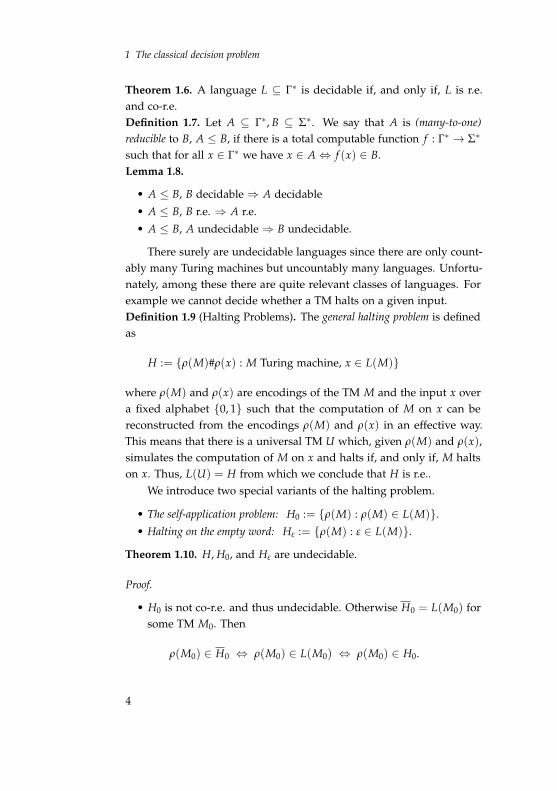
Theorem 1.6. A language L ⊆ Γ∗ is decidable if, and only if, L is r.e.and co-r.e.Definition 1.7. Let A ⊆ Γ∗, B ⊆ Σ∗. We say that A is (many-to-one)reducible to B, A ≤ B, if there is a total computable function f : Γ∗ → Σ∗

such that for all x ∈ Γ∗ we have x ∈ A ⇔ f (x) ∈ B.Lemma 1.8.

• A ≤ B, B decidable ⇒ A decidable

• A ≤ B, B r.e. ⇒ A r.e.

• A ≤ B, A undecidable ⇒ B undecidable.

There surely are undecidable languages since there are only count-ably many Turing machines but uncountably many languages. Unfortu-nately, among these there are quite relevant classes of languages. Forexample we cannot decide whether a TM halts on a given input.Definition 1.9 (Halting Problems). The general halting problem is definedas

H := {ρ(M)#ρ(x) : M Turing machine, x ∈ L(M)}

where ρ(M) and ρ(x) are encodings of the TM M and the input x overa fixed alphabet {0, 1} such that the computation of M on x can bereconstructed from the encodings ρ(M) and ρ(x) in an effective way.This means that there is a universal TM U which, given ρ(M) and ρ(x),simulates the computation of M on x and halts if, and only if, M haltson x. Thus, L(U) = H from which we conclude that H is r.e..

We introduce two special variants of the halting problem.

• The self-application problem: H0 := {ρ(M) : ρ(M) ∈ L(M)}.

• Halting on the empty word: Hε := {ρ(M) : ε ∈ L(M)}.

Theorem 1.10. H, H0, and Hε are undecidable.

Proof.

• H0 is not co-r.e. and thus undecidable. Otherwise H0 = L(M0) forsome TM M0. Then

ρ(M0) ∈ H0 ⇔ ρ(M0) ∈ L(M0) ⇔ ρ(M0) ∈ H0.

4


• H0 is a special case of H, hence H0 ≤ H, and H is undecidable.• We can reduce H to Hε, thus Hε is undecidable. q.e.d.

We next establish the much more general result that in fact, nonon-trivial semantic property of Turing machines can be decided algo-rithmically. In particular, for any fixed function, there is no algorithmthat decides whether a given program computes precisely that func-tion, i.e. we cannot algorithmically prove the correctness of a program.Note that this does not mean that we cannot prove the correctness ofa single given program. Instead the statement is that we cannot do soalgorithmically for all programs.Theorem 1.11 (Rice). Let R be the set of all computable functions andlet S ⊆ R be a set of computable functions such that S = ∅ and S = R.Then code(S) := {ρ(M) : fM ∈ S} is undecidable.

Proof. Let ⇑ be the everywhere undefined function, with domain Def(⇑) = ∅. Obviously, ⇑ is computable. Assume that ⇑∈ S (otherwiseconsider R \ S instead of S. Clearly if code(R \ S) is undecidable thenso is code(S).)

As S = ∅, there exists a function f ∈ S . Let M f be a TM thatcomputes f , i.e. fM f = f . We define a reduction Hε ≤ code(S) bydescribing a total computable function ρ(M) 7→ ρ(M′) such that

M halts on ε ⇔ fM′ ∈ S.

Specifically, given ρ(M), we construct the encoding of a TM M′ which,given an input x, proceeds as follows:

• first simulate M on ε (i.e. apply the universal TM U to ρ(M)#ε);• then simulate M f on x (i.e. apply the universal TM U to

ρ(M f )#ρ(x)).

It is clear that the reduction function is computable. Furthermore, ifM halts on ε then fM′(x) = f (x) for all inputs x, i.e. fM′ = f , so fM′ ∈ S.If M does not halt on ε then M′ does not halt on x for any x, i.e. fM′ =⇑,so fM′ ∈ S. q.e.d.

Definition 1.12 (Recursive inseparability). Let A, B ⊆ Γ∗ be two disjoint

5


sets. We say that A and B are recursively inseparable if there exists nodecidable set C ⊆ Γ∗ such that A ⊆ C and B ∩ C = ∅.Example. (A, A) are recursively inseparable if, and only if, A is undecid-able.Lemma 1.13. Let A, B ⊆ Γ∗, A ∩ B = ∅ be recursively inseparable. LetX, Y ⊆ Σ∗, X ∩Y = ∅, and let f be a total computable function such thatf (A) ⊆ X and f (B) ⊆ Y. Then X and Y are recursively inseparable.

Proof. Assume there exists a decidable set Z ⊆ Σ∗ such that X ⊆ Zand Y ∩ Z = ∅. Consider C = {x ∈ Γ∗ : f (x) ∈ Z}. C is decidable,A ⊆ C, B ∩ C = ∅, thus C separates A, B. q.e.d.

Notation: We write (A, B) ≤ (X, Y) if such a function f exists.Example. (A, A) ≤ (B, B) ⇔ A ≤ B.

As a preparation for Trakhtenbrot’s Theorem, we consider the fol-lowing refinements of Hε:

H+ε := {ρ(M) : M accepts ε}

H−ε := {ρ(M) : M rejects ε}

H∞ε := {ρ(M) : the computation of M on ε is infinite

and does not cycle.}

H+0 , H−

0 , H∞0 are defined analogously, with respect to self-

application.Theorem 1.14. H+

ε , H−ε and H∞

ε are pairwise recursively inseparable.

Proof. (H+ε , H∞

ε ): We show that every set C with H+ε ⊆ C and H∞

ε ∩ C =

∅ is undecidable by reducing the halting problem Hε to C. Define areduction ρ(M) 7→ ρ(M′) as follows. From a given code ρ(M) constructthe code of a TM M′ that simulates M and simultaneously counts thenumber of computation steps since the start. If M halts (accepting orrejecting), M′ accepts.

It is clear that the reduction function is computable. If M haltson ε then M′ halts on ε as well and accepts, so ρ(M′) ∈ H+

ε ⊆ C. IfM does not halt on ε then M′ does not halt either, and never cycles, soρ(M′) ∈ H∞

ε and as H∞ε ∩ C = ∅, we have ρ(M′) ∈ C.

6

1.2 Trakhtenbrot’s Theorem

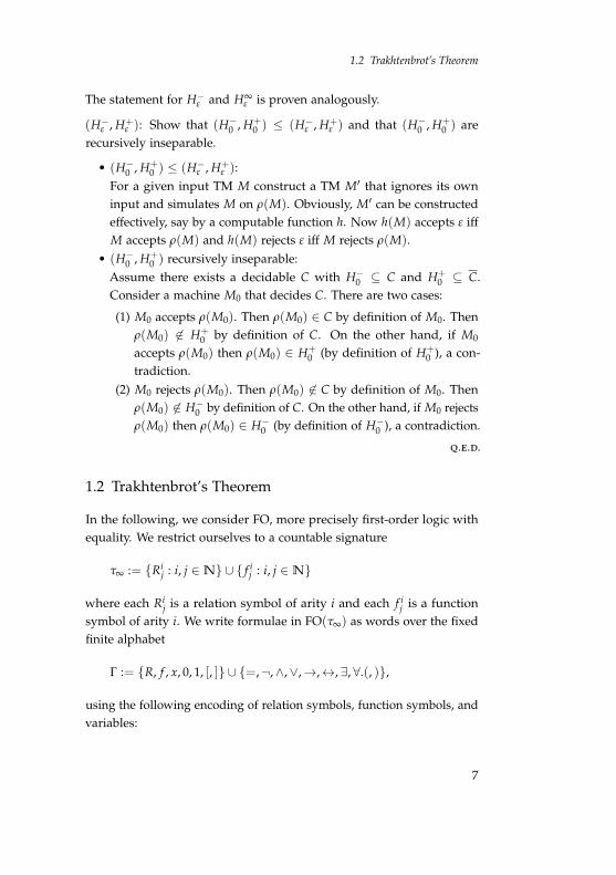
The statement for H−ε and H∞

ε is proven analogously.

(H−ε , H+

ε ): Show that (H−0 , H+

0 ) ≤ (H−ε , H+

ε ) and that (H−0 , H+

0 ) arerecursively inseparable.

• (H−0 , H+

0 ) ≤ (H−ε , H+

ε ):For a given input TM M construct a TM M′ that ignores its owninput and simulates M on ρ(M). Obviously, M′ can be constructedeffectively, say by a computable function h. Now h(M) accepts ε iffM accepts ρ(M) and h(M) rejects ε iff M rejects ρ(M).

• (H−0 , H+

0 ) recursively inseparable:Assume there exists a decidable C with H−

0 ⊆ C and H+0 ⊆ C.

Consider a machine M0 that decides C. There are two cases:

(1) M0 accepts ρ(M0). Then ρ(M0) ∈ C by definition of M0. Thenρ(M0) ∈ H+

0 by definition of C. On the other hand, if M0

accepts ρ(M0) then ρ(M0) ∈ H+0 (by definition of H+

0 ), a con-tradiction.

(2) M0 rejects ρ(M0). Then ρ(M0) ∈ C by definition of M0. Thenρ(M0) ∈ H−

0 by definition of C. On the other hand, if M0 rejectsρ(M0) then ρ(M0) ∈ H−

0 (by definition of H−0 ), a contradiction.

q.e.d.


In the following, we consider FO, more precisely first-order logic withequality. We restrict ourselves to a countable signature

τ∞ := {Rij : i, j ∈ N} ∪ { f i

j : i, j ∈ N}

where each Rij is a relation symbol of arity i and each f i

j is a functionsymbol of arity i. We write formulae in FO(τ∞) as words over the fixedfinite alphabet

Γ := {R, f , x, 0, 1, [, ]} ∪ {=,¬,∧,∨,→,↔, ∃, ∀.(, )},

using the following encoding of relation symbols, function symbols, andvariables:

7


relation symbols: Rij 7−→ R[bin i][bin j]

function symbols: f ij 7−→ f [bin i][bin j]

variables: xj 7−→ x[bin j].

In this way, every formula φ ∈ FO can be viewed as a word in Γ∗.Let X ⊆ FO be a class of formulae. We analyse the following

decision problems:

Sat(X) := {ψ ∈ X : ψ has a model}Fin-Sat(X) := {ψ ∈ X : ψ has a finite model}

Val(X) := {ψ ∈ X : ψ is valid}Non-Sat(X) := X \ Sat(X)

Inf-Axioms(X) := Sat(X) \ Fin-Sat(X)

= {ψ ∈ X : ψ is an infinity axiom, i.e. ψ has a

model but no finite model}.

Theorem 1.15. Let X ⊆ FO be decidable. Then

(1) Val(X) is r.e.(2) Non-Sat(X) is r.e.(3) Sat(X) is co-r.e.(4) Fin-Sat(X) is r.e.(5) Inf-Axioms(X) is co-r.e.

Proof. (1) φ is valid ⇔ ⊢ φ (Completeness Theorem). Thus we cansystematically enumerate all proofs and halt if a proof for φ is listed.

(2) φ valid ⇔ ¬φ is not satisfiable.(3) Follows from Item (2).(4) Systematically generate all finite models and halt if a model of φ is

found.(5) FO \ Inf-Axioms(X) = Non-Sat(X) ∪ Fin-Sat(X) is r.e. q.e.d.

Definition 1.16. A class X ⊆ FO has the finite model property (FMP) ifevery satisfiable φ ∈ X has a finite model, i.e. if Sat(X) = Fin-Sat(X).Theorem 1.17. Suppose that X ⊆ FO is decidable and that X has theFMP. Then Sat(X) is decidable.

8


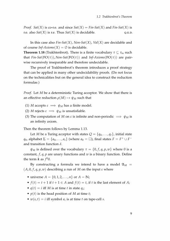
Proof. Sat(X) is co-r.e. and since Sat(X) = Fin-Sat(X) and Fin-Sat(X) isr.e. also Sat(X) is r.e. Thus Sat(X) is decidable. q.e.d.

In this case also Fin-Sat(X), Non-Sat(X), Val(X) are decidable andof course Inf-Axioms(X) = ∅ is decidable.Theorem 1.18 (Trakhtenbrot). There is a finite vocabulary τ ⊆ τ∞ suchthat Fin-Sat(FO(τ)), Non-Sat(FO(τ)) and Inf-Axioms(FO(τ)) are pair-wise recursively inseparable and therefore undecidable.

The proof of Trakhtenbrot’s theorem introduces a proof strategythat can be applied in many other undecidability proofs. (Do not focuson the technicalities but on the general idea to construct the reductionformulae.)

Proof. Let M be a deterministic Turing acceptor. We show that there isan effective reduction ρ(M) 7→ ψM such that

(1) M accepts ε =⇒ ψM has a finite model.

(2) M rejects ε =⇒ ψM is unsatisfiable.

(3) The computation of M on ε is infinite and non-periodic =⇒ ψM isan infinity axiom.

Then the theorem follows by Lemma 1.13.

Let M be a Turing acceptor with states Q = {q0, . . . , qr}, initial stateq0, alphabet Σ = {a0, . . . , as} (where a0 = □), final states F = F+ ∪ F−

and transition function δ.

ψM is defined over the vocabulary τ = {0, f , q, p, w} where 0 is aconstant, f , q, p are unary functions and w is a binary function. Definethe term k as f k0.

By constructing a formula we intend to have a model AM =

(A, 0, f , q, p, w) describing a run of M on the input ε where

• universe A = {0, 1, 2, . . . , n} or A = N;

• f (t) = t + 1 if t + 1 ∈ A and f (t) = t, if t is the last element of A;

• q(t) = i iff M is at time t in state qi;

• p(t) is the head position of M at time t;

• w(s, t) = i iff symbol ai is at time t on tape-cell s.

9


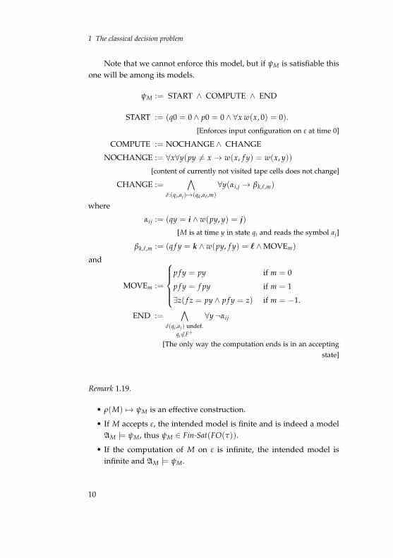
Note that we cannot enforce this model, but if ψM is satisfiable thisone will be among its models.

ψM := START ∧ COMPUTE ∧ END

START := (q0 = 0 ∧ p0 = 0 ∧ ∀x w(x, 0) = 0).

[Enforces input configuration on ε at time 0]

COMPUTE := NOCHANGE ∧ CHANGE

NOCHANGE := ∀x∀y(py = x → w(x, f y) = w(x, y))

[content of currently not visited tape cells does not change]

CHANGE :=∧

δ:(qi,aj) 7→(qk,aℓ,m)

∀y(αi,j → βk,ℓ,m)

where

αij := (qy = i ∧ w(py, y) = j)

[M is at time y in state qi and reads the symbol aj]

βk,ℓ,m := (q f y = k ∧ w(py, f y) = ℓ ∧ MOVEm)

and

MOVEm :=

p f y = py if m = 0

p f y = f py if m = 1

∃z( f z = py ∧ p f y = z) if m = −1.

END :=∧

δ(qi,aj) undef.qi ∈F+

∀y¬αij

[The only way the computation ends is in an acceptingstate]

Remark 1.19.

• ρ(M) 7→ ψM is an effective construction.

• If M accepts ε, the intended model is finite and is indeed a modelAM |= ψM, thus ψM ∈ Fin-Sat(FO(τ)).

• If the computation of M on ε is infinite, the intended model isinfinite and AM |= ψM.

10


It remains to show that if M rejects ε, then ψM is unsatisfiable, andif the computation of M on ε is infinite and aperiodic, then ψM is aninfinity axiom.

Suppose B = (B, 0, f , q, p, w) |= ψM.

Definition 1.20. B enforces at time t the configuration (qi, j, w) withw = ai0 . . . aim ∈ Σ∗ if

(1) B |= qt = i,(2) B |= pt = j,(3) for all k ≤ m, B |= w(k, t) = ik and for all k > m, B |= w(k, t) = 0.

Since B |= ψM, the following holds:

• B enforces C0 = (q0, 0, ε) at time 0 (since B |= START.)• If B enforces at time t a non-final configuration Ct, then B enforces

the configuration Ct+1 = Next(Ct) at time t + 1.• Especially, the computation of M cannot reach a rejecting configura-

tion. It follows that if M rejects ε, then ψM is unsatisfiable.Consider an infinite and aperiodic computation of M, and assumeB |= ψM is finite. Since B is finite, it enforces a periodic computa-tion in contradiction to the assumption that the computation of Mis aperiodic.

C0 ⊢ . . . ⊢Cr ⊢ . . . ⊢Ct−1

We have shown:

• If M accepts ε, then ψM has a finite model.• If M rejects ε, then ψM is unsatisfiable.• If the computation of M is infinite and aperiodic, then ψM is an

infinity axiom. q.e.d.

We now know that the sets of all finitely satisfiable, all unsatisfiableand all only infinitely satisfiable formulae are undecidable for FO(τ)

where τ consists of only three unary functions and one binary function.This raises a number of questions.

(1) For which other vocabularies σ do we have similar undecidabilityresults for FO(σ)?

11


(2) For which σ is satisfiability of FO(σ) decidable?

(3) Is there a complete classification? In this case, we want to find mini-mal vocabularies σ such that the above problems are undecidable,i.e. vocabularies such that any further restriction yields a class offormulae for which satisfiability is decidable.

We first define what it means that a fragment of FO is as hard forsatisfiability as the whole FO.Definition 1.21. X ⊆ FO is a reduction class if there exists a computablefunction f : FO → X such that ψ ∈ Sat(FO) ⇔ f (ψ) ∈ Sat(X).

Let X, Y ⊆ FO. A conservative reduction of X to Y is a computablefunction f : X → Y with

• ψ ∈ Sat(X) ⇔ f (ψ) ∈ Sat(Y), and

• ψ ∈ Fin-Sat(X) ⇔ f (ψ) ∈ Fin-Sat(Y).

X is a conservative reduction class if there exists a conservative reduc-tion of FO to X.Corollary 1.22. Let X be a conservative reduction class. Then Fin-Sat(X),Inf-Axioms(X) and Non-Sat(X) are pairwise recursively inseparable, andthus Fin-Sat(X), Sat(X), Val(X), Non-Sat(X), Inf-Axioms(X) are undecid-able.

Proof. A conservative reduction from FO to X yields a uniform reduc-tion from Fin-Sat(FO), Inf-Axioms(FO) and Non-Sat(FO) to Fin-Sat(X),Inf-Axioms(X) and Non-Sat(X), respectively. q.e.d.

It is indeed possible to give a complete classification of those vocab-ularies σ such that FO(σ) is decidable.Theorem 1.23. If σ ⊆ {P0, P1, . . .} ∪ { f } consists of at most oneunary function f and an arbitrary number of monadic predicatesP0, P1, . . ., then Sat(FO(σ)) is decidable. In all other cases, Sat(FO(σ)),Inf-Axioms(FO(σ)) and Non-Sat(FO(σ)) are pairwise recursively insepa-rable, and FO(σ) is a conservative reduction class.

A full proof of this classification theorem is rather difficult. Inparticular, the decidability of the monadic theory of one unary function,which implies the decidability part, is a difficult theorem due to Rabin.

12

1.3 Domino problems

On the other side, one has to show that Trakhtenbrot’s theorem appliesto the vocabularies

τ1 = {E} where E is a binary relation,τ2 = { f , g} where f , g are unary functions,τ3 = {F} where F is a binary function,

and hence also to all extensions of τ1, τ2, τ3.Of course, one may also look at other syntactic restrictions besides

restricting the vocabulary. One possibility is to restrict the number ofvariables. This is only interesting for relational formulae. If we havefunctions, satisfiability is undecidable even for formulae with only onevariable, as we shall see later.

Define FOk as first-order logic with relational symbols only and afixed collection of k variables, say x1, . . . , xk.Theorem 1.24.

• FO2 has the finite model property and is decidable (see Sect. 1.6).• FO3 is a conservative reduction class.

A further important possibility is to restrict the structure of quan-tifier prefixes of formulae in prenex normal form, and to combine thiswith restrictions on the vocabulary, and the presence or absence ofequality. This leads to the notion of a prefix-vocabulary class in first-orderlogic, and indeed, also for these fragments of FO there is a completeclassification of those with a solvable satisfiability problem, and thosethat are conservative reduction classes.

A full description of this classification exceeds the scope of thiscourse by far (see E. Börger, E. Grädel, and Y. Gurevich, The ClassicalDecision Problem, 1997). Instead we shall present some of the funda-mental methods for establishing such results, and illustrate these withapplications to specific fragments of first-order logic.

1.3 Domino problems

Domino problems are a simple and yet general tool for proving unde-cidability results (and lower bounds in complexity theory) without theneed of explicit encodings of Turing machine computations.

13


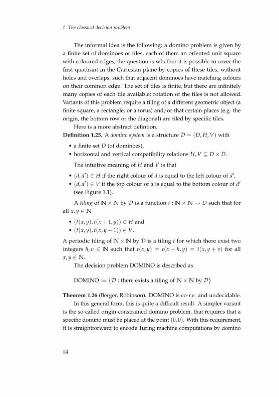
The informal idea is the following: a domino problem is given bya finite set of dominoes or tiles, each of them an oriented unit squarewith coloured edges; the question is whether it is possible to cover thefirst quadrant in the Cartesian plane by copies of these tiles, withoutholes and overlaps, such that adjacent dominoes have matching colourson their common edge. The set of tiles is finite, but there are infinitelymany copies of each tile available; rotation of the tiles is not allowed.Variants of this problem require a tiling of a different geometric object (afinite square, a rectangle, or a torus) and/or that certain places (e.g. theorigin, the bottom row or the diagonal) are tiled by specific tiles.

Here is a more abstract defintion.Definition 1.25. A domino system is a structure D = (D, H, V) with

• a finite set D (of dominoes),• horizontal and vertical compatibility relations H, V ⊆ D × D.

The intuitive meaning of H and V is that

• (d, d′) ∈ H if the right colour of d is equal to the left colour of d′,• (d, d′) ∈ V if the top colour of d is equal to the bottom colour of d′

(see Figure 1.1).

A tiling of N × N by D is a function t : N × N → D such that forall x, y ∈ N

• (t(x, y), t(x + 1, y)) ∈ H and• (t(x, y), t(x, y + 1)) ∈ V.

A periodic tiling of N × N by D is a tiling t for which there exist twointegers h, v ∈ N such that t(x, y) = t(x + h, y) = t(x, y + v) for allx, y ∈ N.

The decision problem DOMINO is described as

DOMINO := {D : there exists a tiling of N × N by D}

Theorem 1.26 (Berger, Robinson). DOMINO is co-r.e. and undecidable.In this general form, this is quite a difficult result. A simpler variant

is the so-called origin-constrained domino problem, that requires that aspecific domino must be placed at the point (0, 0). With this requirement,it is straightforward to encode Turing machine computations by domino

14

1.3 Domino problems

ab

c

d

c

••

•

••

•b

Figure 1.1. Domino adjacency condition

tilings (successive rows of the tiling correspond to successive configura-tions in the computation), and thus to reduce halting problems to tilingproblems for domino systems. The origin constraint is used to encodethe beginning of the computation (and to avoid that the entire space canbe tiled by a domino corresponding to the blank symbol) Without anorigin constraint, the problem is more difficult to handle; an essentialpart of the proof is the construction of a set of dominoes that admitsonly non-periodic tilings.

There are several extensions and variations of this result.Theorem 1.27. A domino system D admits a tiling of Z×Z if, and onlyif, it admits a tiling of N × N.

Proof. It is clear that a tiling of Z × Z also gives a tiling of N × N. Theconverse is a nice application of König’s Lemma. Suppose that t is a tilingof N × N by D. There exists at least one domino d such that for all nthere exist i, j > n with t(i, j) = d. Fix such a d. Further, for every k ∈ N,let Sk be the square {−k, . . . ,−1, 0, 1, . . . , k} × {−k, . . . ,−1, 0, 1, . . . , k}.

We define a finitely branching tree whose nodes are the correcttilings tk of Sk by D such that tk(0, 0) = d. The root is the unique suchtiling of S0 and the children of a tiling tk are the possible extensionsto tilings tk+1 of Sk+1. This tree contains paths of any finite length. ByKönig’s Lemma it also contains an infinite path from the root, whichmeans that D admits a tiling of Z × Z. q.e.d.

The undecidability result from Theorem 1.26 can be strengthened toa recursive inseparability result.

15


Theorem 1.28. The set of domino systems admitting a periodic tilingof N × N, those that admit no tiling of N × N and those that admit atiling but not a periodic one are pairwise recursively inseparable.

The proof of Theorem 1.28 reduces the halting problems H+ε , H−

ε , H∞ε ,

to the domino problems. There exists a recursive function that associateswith every TM M a domino system D satisfying

• If M ∈ H+ε then D admits a periodic tiling of N × N.

• If M ∈ H−ε then D admits no tiling of N × N.

• If M ∈ H∞ε then D admits a tiling of N × N but no periodic one.

Definition 1.29. A computable function f is a conservative reduction fromdomino systems to X if, for all domino systems D, f (D) = φD is in X andthe following holds:

• D admits a periodic tiling of N × N ⇒ ψD has a finite model• D admits no tiling of N × N ⇒ ψD is unsatisfiable• D admits a tiling of N × N but no periodic one ⇒ ψD is an infinity

axiom.

Proposition 1.30. Let X ∈ FO. If there exists a conservative reductionfrom domino systems to X then X is a conservative reduction class.

Proof. Since Fin-Sat(FO) and Non-Sat(FO) are recursively enumerableand Inf-Axioms(FO) is co-recursively enumerable, we can associate withevery first-order formula ψ a Turing machine M such that

• ψ ∈ Fin-Sat(FO) ⇒ ρ(M) ∈ H+ε ,

• ψ ∈ Non-Sat(FO) ⇒ ρ(M) ∈ H−ε ,

• ψ ∈ Inf-Axioms(FO) ⇒ ρ(M) ∈ H∞ε .

According to the assumption, there is a reduction D 7→ φD fromdomino systems to X. Thus, the domino method yields a conservativereduction from FO to X.

q.e.d.

1.4 Applications of the domino method

We now apply the domino method to obtain several reduction classes.

16


The Kahr-Moore-Wang class KMW is the class of all first-ordersentences of form ∀x∃y∀zφ, where φ is a quantifier-free formula withoutequality, whose vocabulary contains only binary relation symbols.Theorem 1.31. The Kahr-Moore-Wang class is a conservative reductionclass.

Proof. It suffices to construct a conservative reduction from dominosystems to KMW, i.e., a mapping D 7→ ψD over a vocabulary consistingof binary relation symbols (Pd)d∈D such that

(1) D admits a periodic tiling of N × N ⇒ ψD has a finite model

(2) D admits no tiling of N × N ⇒ ψD is unsatisfiable

(3) D admits a tiling of N × N but no periodic one ⇒ ψD is an infinityaxiom

For a tiling t : N × N → D, an intended model of ψD is N withthe interpretation Pd = {(i, j) ∈ N × N : t(i, j) = d} for all d ∈ D. Wedefine ψD by

ψD := ∀x∃y∀z( ∧

d =d′Pdxz → ¬Pd′xz

∧∨

(d,d′)∈H

(Pdxz ∧ Pd′yz) ∧∨

(d,d′)∈V

(Pdzx ∧ Pd′zy))

.

Obviously ψD is of the desired format, i.e. ψD ∈ KMW.(1) Suppose that D admits a periodic tiling t of N × N, such that

t(x, y) = t(x + h, y) = t(x, y + v) for all x, y. We construct a finite modelof ψD as follows. Let m := lcm(h, v) be the least common multiple of hand v. Then t induces a tiling

t′ : Z/mZ × Z/mZ → D

with t′(x, y) = t(x( mod m), y( mod m)).It follows that A = (Z/mZ, (Pd)d∈D) with Pd = {(i, j) : t′(i, j) = d}

is a finite model for ψD (for x in Z/mZ choose y := x + 1 (mod m)).(2) By analogous arguments, it follows, that whenever D admits a

tiling of N × N, then ψD has a model over N.

17


(3) Finally we prove that if ψD has a model, then D admits a tilingof N × N, and if that model is finite, we even obtain a periodic tiling.

Consider the Skolem normal form φD of ψD:

φD := ∀x∀z(∧

d =d′Pdxz → ¬Pd′xz

∧∨

(d,d′)∈H

(Pdxz ∧ Pd′ f xz) ∧∨

(d,d′)∈V

(Pdzx ∧ Pd′z f x).

If ψD is satisfiable, then also φD has a model B = (B, f , (Pd)d∈D).Define a tiling t : N × N → D as follows: choose any b ∈ B, and for alli, j ∈ N, set t(i, j) := d for the unique d ∈ D such that B |= Pd( f ib, f jb).Since B |= φD, it follows that t is a correct tiling.

Now suppose that B |= φD is finite.

• •f bf

· · · · · · •f

Choose b ∈ B such that, for some n ≥ 1, f nb = b. Then the definedtiling t is periodic. q.e.d.

Corollary 1.32. FO3 is a conservative reduction class.Later we shall prove that FO2 has the FMP.

Consider now formula classes X ⊆ FO over functional vocabularies.One can prove that FO(τ) is a conservative reduction class if τ contains

• two unary functions or• one binary function.

This is even true for sentences of the form ∀xφ where φ is quantifier-free.We stablish, again via a conservative reduction from domino prob-

lems, a weaker result from which the above mentioned ones can beobtained by interpretation arguments (see exercises).Theorem 1.33. The class F , consisting of all sentences ∀xφ where φ

is a quantifier-free formula whose vocabulary consists only of unaryfunction symbols, is a conservative reduction classes.

Proof. We define a conservative reduction D = (D, H, V) 7→ ψD whereψD ∈ F has the vocabulary { f , g, (hd)d∈D} where all function symbols

18


are unary. The intended model is N × N with successor functions fand g. The subformula ∀x( f gx = g f x) ensures that the models of ψDcontain a two-dimensional grid. The fact that a position x is tiled byd ∈ D is expressed by requiring that hdx = x, i.e. that x is a fixed pointof hd.

ψD := ∀x(

f gx = g f x ∧∧

d =d′(hdx = x → hd′x = x)

∧∨

(d,d′)∈H

(hdx = x ∧ hd′ f x = f x)

∧∨

(d,d′)∈V

(hdx = x ∧ hd′gx = gx))

.

We claim that there exists a tiling t : N × N → D if and only if ψDis satisfiable.

” ⇒ ” Assume that t is a correct tiling. Construct the (intended) modelA = (N × N, f , g, (hd)d∈D) with

– f (i, j) = (i + 1, j),– g(i, j) = (i, j + 1),

– hd(i, j)

= (i, j) if t(i, j) = d

= (i, j) otherwise.

Clearly A |= ψD.” ⇐ ” Consider B = (B, f , g, (hd)d∈D) |= ψD.

Choose an arbitrary b ∈ B and define t : N × N → D by

t(i, j) := d iff B |= hd f igjb = f igjb.

Note that every point in B is a fixed-point of exactly one of thefunctions hd, and t is well-defined and a a correct tiling. Further, ifB is finite, then σ is periodic, and thus the reduction is conservative.

q.e.d.

Exercise 1.1. Prove that the more restricted class F2 ⊆ F consisting ofsentences in F that contain just two unary function symbols, is also aconservative reduction class.

19


Hint: Transform sentences ∀xφ with unary function symbolsf1, . . . , fm into sentences ∀xφ := ∀xφ[x/hx, fi/hgi] where h, g are freshunary function symbols.

1.5 The finite model property

We study the finite model property (FMP) for fragments of FO as amean to show that these fragments are decidable, and also to betterunderstand their expressive power and algorithmic complexity.

Recall that a class X ⊆ FO has the finite model property if Sat(X) =

Fin-Sat(X). Since for any decidable class X, Fin-Sat(X) is r.e. and Sat(X)

is co-r.e., it follows that Sat(X) is decidable if X has the FMP. In manycases, the proof that a class has the finite model property provides abound on the model’s cardinality, and thus a complexity bound for thesatisfiability problem. To prove completeness for complexity classes wemake use of a bounded variant of the domino problem.

We shall illustrate the power of this method by a few examples.Definition 1.34. The atomic k-type of a1, . . . , ak in A is defined as

atpA(a1, . . . , ak) := {γ(x1 . . . , xk) : γ atomic formula or negated

atomic formula such that A |= γ(a1, . . . , ak)}.

In the examples that we consider here, the structures contain unaryor binary relations only. Hence, to describe a structure it suffices todefine its universe and to specify the atomic 1-types and 2-types for allof its elements.Example 1.35. Let A be the structure (A, E1, . . . , Em) where the Ei arebinary relations. Then for a ∈ A:

atpA(a) = {Eixx : A |= Eiaa} ∪ {¬Eixx : A |= ¬Eiaa}.

The monadic class (also called the Löwenheim class) is the class offirst-order sentences over a vocabulary the contains only unary predi-cates.Theorem 1.36. The monadic class has the FMP.

20

1.6 The two-variable fragment of FO

Proof. Let A = (A, PA1 , . . . , PA

n ) |= φ where qr(φ) = m. For each se-quence of bits α = α1 . . . αn ∈ {0, 1}n we define PA

α = Q1 ∩ Q2 ∩ . . . ∩ Qn,where Qi = PA

i if αi = 1 and Qi = A \ PAi if αi = 0. Notice that the sets

PAα define a partition of A, and that α completely describes the atomic

1-type of any a ∈ PAα .

We construct B by taking min(|PAα |, m) elements into each PB

α . Ob-serve that B is completly specified in this way, with PB

i =⋃

α|αi=1 PBα ).

We show that A ≡m B using the Ehrenfeucht-Fraïssé Theorem.The following is a winning strategy for Duplicator in the

Ehrenfeucht-Fraïssé game with m moves on (A,B): Answer any el-ement chosen by Spoiler by an element with the same atomic type in theother structure, respecting equalities and inequalities with previouslychosen elements. Due to the construction it is certainly possible to dothat for m moves, so Duplicator wins the game. Hence A ≡m B, andtherefore B |= φ. q.e.d.

From the proof we see that the constructed finite model B is in facta submodel of the arbitrary model A that we started with. Thus wehave in fact established a stronger result than the finite model property,namely the finite submodel property of the monadic class: every infinitemodel of a sentence in the monadic class has a finite substructure whichis also a model of that sentence.

In general it need not be the case that classes with the FMP alsohave the finite submodel property.


We denote relational first-order logic over k variables by FOk, i.e.

FOk := {φ ∈ FO : φ relational, φ only contains k variables}.

We have shown that the Kahr-Moore-Wang class KMW, and hence alsoFO3, are conservative reduction classes. We now prove that FO2 has thefinite model property and is thus decidable. Note that FOk formulaeare not necessarily in prenex normal form. A further motivation for thestudy of FO2 is that propositional modal logic can be viewed as a frag-

21


ment of FO2 (in fact ML can be proven to be precisely the bisimulationinvariant fragment of FO2).

Before we proceed to prove the finite model property for FO2, as afirst step we establish a normal form for formulae in FO2.Lemma 1.37 (Scott). For each sentence ψ ∈ FO2 one can construct inpolynomial time a sentence φ ∈ FO2 of the form

φ := ∀x∀yα ∧n∧

i=1

∀x∃yβi

such that α, β1, . . . , βn are quantifier free and such that ψ and φ aresatisfiable over the same universe. Moreover, we have |φ| = O(|ψ| ·log |ψ|).

Proof. First of all, we can assume that formulae φ ∈ FO2 only containunary and binary relation symbols. This is no restriction since relationsof higher arity can be substituted by introducing new binary and unaryrelation symbols. For example, if R is a relation of arity three, onecould add a unary relation Rx and three binary relations Rx,x,y, Rx,y,x

and Rx,y,y and replace each atom R(x, x, x) (or R(y, y, y)) by Rx(x) (orRx(y)) and atoms as R(x, x, y) or R(x, y, x) by Rx,x,y(x, y) and Rx,y,x(x, y)respectively. By adding appropriate new subformulae one can ensurethat the semantics are preserved, i.e. that the newly introduced relationspartition a ternary relation in the intended sense. For example we wouldintroduce as a new subformula ∀x(Rx(x) ↔ Rx,x,y(x, x)).

With ψ containing at most binary relations, we iterate the followingsteps until ψ has the desired form. We choose a subformula Qyη of ψ

(Q ∈ {∀, ∃}, η quantifier free) and add a new unary relation R:

ψ′ := ψ[Qyη/Rx]

ψ 7→ ψ′ ∧ ∀x(Rx ↔ Qyη).

R captures those x that satisfy Qyη. The resulting formula φ is not yetof the desired form, but it is equivalent to the following:

(a) if Q = ∃, then

22


φ ≡ ψ′ ∧ ∀x∀y(η → Rx) ∧ ∀x∃y(Rx → η)

(b) else if Q = ∀, then

φ ≡ ψ′ ∧ ∀x∀y(Rx → η) ∧ ∀x∃y(η → Rx)

Now use that conjunctions of ∀∀-formulae are equivalent to a ∀∀-formula

and obtain ψ ≡ ∀x∀yα ∧n∧

i=1∀x∃yβi. q.e.d.

Theorem 1.38. FO2 has the finite model property. In fact, every satisfi-able formula ψ ∈ FO2 has a model with at most 2|ψ| elements.

Proof. The proof strategy is as follows: we start with a model A of ψ andproceed by constructing a new model B of ψ such that |B| ≤ 2O(|ψ|).For the construction the following definitions will be essential.

An element a ∈ A is said to be a king of A if its atomic 1-type isunique in A, i.e. if atpA(b) = atpA(a) for all b = a. We let

• K := {a ∈ A : a is a king of A} be the set of kings of A, and

• P := {atpA(a) : a ∈ A, a /∈ K} be the set of atomic 1-types whichare realized at least twice in A.

Since A |= ∀x∃yβi for i = 1, . . . , n, there exist (Skolem) functionsf1, . . . , fn : A → A such that A |= βi(a, fia) for all a ∈ A. The courtof A is defined as

C := K ∪ { fik : k ∈ K, i = 1, . . . , n}.

Let C be the substructure of A induced by C. We construct a modelB |= ψ with universe B = C ∪ (P × {1, . . . , n} × {0, 1, 2}).

23


A

CK

B

CK

P

P

P

To specify B we set B|C = C and for all other elements we specifythe 1- and 2-types (in this way fixing B on the remaining part). However,

(1) This must be done consistently:

• atpA(b, b′) and atpA(b, b′′) must agree on atpA(b), and• γ(x, y) ∈ atpB(b, b′) ⇔ γ(y, x) ∈ atpB(b

′, b).

(2) Of course we have to ensure that B |= ψ.

We illustrate the construction with the following example.

Example 1.39. Consider the formula ψ over the signature τ = {R, B} (rededges and blue edges).

ψ = ∃x(Rxx ∧ Bxx)

∧ ∀x∀y((Rxx ∧ Bxx ∧ Ryy ∧ Byy → x = y)

∧(Rxx ∨ Bxx)

∧(Rxy ∧ Ryx → x = y)

∧(Bxy ∧ Byx → x = y)

∧(Bxy ∧ x = y → Ryy))

∧ ∀x∃y(x = y ∧ (Rxx → Rxy)

∧ (Bxx → Bxy)).

Let A |= ψ, then A looks like follows:

• • • • · · ·K C

24


In this case P = {{Rxx,¬Bxx}, {¬Rxx, Bxx}} and the universe ofB is B = C ∪ (P × {1} × {0, 1, 2}).

We proceed to construct B by specifying the 1-types and 2-types ofits elements as follows.

(1) The atomic 1-types of elements (p, i, j) are set to atpB((p, i, j)) = p.

(2) The atomic 2-types atpB(b, b′) will be set so that B |= ∀x∃yβi fori = 1, . . . , m.Choose for each p ∈ P an element h(p) ∈ A with atpA(h(p)) = p.Find for each b ∈ B and each i a suitable element b′ such thatB |= βi(b, b′) (by defining atpB(b, b′) appropriately).

(a) If b is a king, set b′ := fi(b) ∈ C ⊆ B. Then B |= βi(b, b′).

(b) If b ∈ C \ K (non-royal member of the court), distinguish:• If fi(b) ∈ K, then set b′ := fi(b) ∈ K ⊆ B.

• Otherwise it holds that atpA( fi(b)) = p ∈ P.In this case, set b′ := (p, i, 0). Now set atpB(b, b′) :=atpA(b, fi(b)). Thus B |= βi(b, b′) since A |= βi(b, fi(b)).

(c) If b = (p, j, ℓ) for some p ∈ P, j ∈ {1, . . . , n}, ℓ ∈ {0, 1, 2}, leta := h(p) and consider fi(a).If fi(a) ∈ K, set b′ = fi(a) and atpB(b, b′) := atpA(a, b′).If fi(a) /∈ K, then atpA( fi(a)) = p′ ∈ P.Set b′ := (p′, i, (ℓ+ 1) (mod 3)).Then set atpB(b, b′) := atpA(a, fi(a)), and thus B |= βi(b, b′).

To complete the construction of B, let b1, b2 ∈ B be such thatatpB(b1, b2) is not yet specified. Choose a1, a2 ∈ A so that

atpA(a1) = atpB(b1) and

atpA(a2) = atpB(b2)

and set

atpB(b1, b2) := atpA(a1, a2).

Since A |= α(a1, a2), also B |= α(b1, b2).For the previously considered example, B looks as follows:

25


CK

P × {0} P × {1}

P × {2}

••

••

••

••

Overall, we obtain B |= ∀x∀yα ∧n∧

i=1∀x∃yβi = ψ, and the size of B

is restricted by

|B| = |C|︸︷︷︸≤|K|(n+1)

+ 3n|P| = O(n · # (atomic 1-types)) .

For k relation symbols, there are 2k atomic 1-types, hence |B| = 2O(|ψ|).

q.e.d.

This result implies that Sat(FO2) is in NEXPTIME (indeed it isNEXPTIME-complete), since we can simply guess a finite structureA of exponential size (in the length of ψ) and verify that A |= ψ.Corollary 1.40. Sat(FO2) ∈ NEXPTIME = (

⋃k

NTIME(2nk)).

This is a typical complexity level for decidable fragments of FO.In fact, Sat(FO2) is even complete for NEXPTIME. For showing this, wereduce a bounded version of the domino problem to Sat(FO2).Definition 1.41. Let D = (D, H, V) be a domino system and let Z(t)denote Z/tZ × Z/tZ. For a word w = w0, . . . , wn−1 ∈ Dn we say thatD tiles Z(t) with initial condition w if there is τ : Z(t) → D such that

• if τ(x, y) = d and τ(x + 1, y) = d′ then (d, d′) ∈ Hfor all (x, y) ∈ Z(t) ,

• if τ(x, y) = d, τ(x, y + 1) = d′ then (d, d′) ∈ Vfor all (x, y) ∈ Z(t) and

• τ(i, 0) = wi for all i = 0, . . . , n − 1.

26


Let D be a domino system and T : N → N a mapping. Define

DOMINO(D, T) := {w ∈ D∗ : D tiles Z(T(|w|)) with initial

condition w} .

One can describe computations of a (in this case non-deterministic)Turing machine by domino tilings in such a way that the input conditionof the domino problem relates to the initial configuration of the Turingmachine. The restrictions on the size of the tiled rectangle correspondto the time and space restrictions of the Turing machine. To provethat a problem A is NEXPTIME-hard, it then suffices to show thatDOMINO(D, 2n) ≤p A.

Our goal is to show that DOMINO(D, 2n) reduces to Sat(X) forrelatively simple classes X ⊆ FO. Set

X = {φ ∈ FO2 : φ = ∀x∀y α ∧ ∀x∃y β, s.t. α, β quantifier-free,

without =, and with only monadic predicates} .

We show that Sat(X) is NEXPTIME-complete and hence alsoSat(FO2) is NEXPTIME-complete.Lemma 1.42. For each domino system D = (D, H, V) there exists apolynomial time reduction w ∈ Dn 7→ ψw ∈ X such that D tiles Z(2n)

with initial condition w if and only if ψw is satisfiable.

Proof. The intended model of ψw is a description of a tiling τ : Z(2n) →D in the universe Z(2n).

Let z = (a, b) ∈ Z(2n) with a =n−1∑

i=0ai2i and b =

n−1∑

i=0bi2i. Encode the

tuple as (ao, . . . , an−1, b0, . . . , bn−1) ∈ {0, 1}2n.To encode the tiling, we define ψw with the monadic predicates Xi,

X∗i , Yi, Y∗

i , Ni for 0 ≤ i < n and Pd(d ∈ D) with the following intendedmeaning:

Xiz iff ai = 1.

X∗i z iff aj = 1 for all j < i.

Yiz iff bj = 1.

27


Y∗i z iff bj = 1 for all j < i.

Niz iff z = (i, 0).

Pdz iff τ(z) = d.

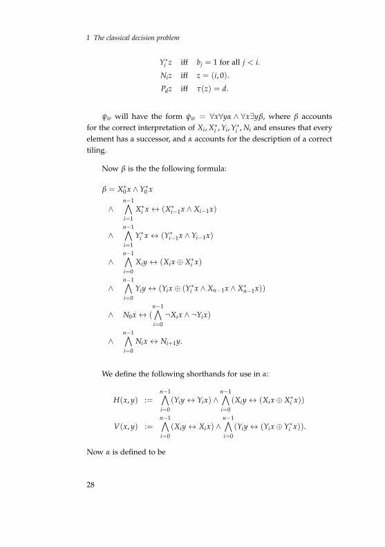
ψw will have the form ψw = ∀x∀yα ∧ ∀x∃yβ, where β accountsfor the correct interpretation of Xi, X∗

i , Yi, Y∗i , Ni and ensures that every

element has a successor, and α accounts for the description of a correcttiling.

Now β is the the following formula:

β = X∗0 x ∧ Y∗

0 x

∧n−1∧

i=1

X∗i x ↔ (X∗

i−1x ∧ Xi−1x)

∧n−1∧

i=1

Y∗i x ↔ (Y∗

i−1x ∧ Yi−1x)

∧n−1∧

i=0

Xiy ↔ (Xix ⊕ X∗i x)

∧n−1∧

i=0

Yiy ↔ (Yix ⊕ (Y∗i x ∧ Xn−1x ∧ X∗

n−1x))

∧ N0x ↔ (n−1∧

i=0

¬Xix ∧ ¬Yix)

∧n−1∧

i=0

Nix ↔ Ni+1y.

We define the following shorthands for use in α:

H(x, y) :=n−1∧

i=0

(Yiy ↔ Yix) ∧n−1∧

i=0

(Xiy ↔ (Xix ⊕ X∗i x))

V(x, y) :=n−1∧

i=0

(Xiy ↔ Xix) ∧n−1∧

i=0

(Yiy ↔ (Yix ⊕ Y∗i x)).

Now α is defined to be

28


α =∧

d =d′¬(Pdx ∧ Pd′x)

∧ (H(x, y) →∨

(d,d′)∈H

(Pdx ∧ Pd′y))

∧ (V(x, y) →∨

(d,d′)∈V

(Pdx ∧ Pd′y))

∧ (n−1∧

i=i

(Nix → Pwi x)).

Claim 1.43. ψw is satisfiable if and only if D tiles Z(2n) with initialcondition w.

Proof. We show both directions.

(⇐) Consider the intended model, ψw holds in it.(⇒) Consider C = (C, X1, . . .) |= ψw and define a mapping

f : C → Z(2n)

c 7→ (a, b) ≡ (a0, . . . , an−1, b0, . . . , bn−1)

with ai = 1 iff C |= Xic and

bi = 1 iff C |= Yic.

As C |= ∀x∃yβ, f is surjective. Choose for each z ∈ Z(2n) an elementc ∈ f−1(z) and set τ(z) = d for the unique d that satisfies C |= Pdc.Then τ is a correct tiling with initial condition w. q.e.d.

Since the length of ψw is |ψw| = O(n log n), the above claim com-pletes the proof of the lemma. q.e.d.

29

Algorithmic Model Theory SS 2016 - RWTH Aachen University

Documents

Transcript of Algorithmic Model Theory SS 2016 - RWTH Aachen University