Dorothea Schäfer* Boriss Siliverstovs** Eva Terberger***

Banking competition, good or bad? The case of promoting micro and small enterprise finance in Kazakhstan *

Discussion Papers

Berlin, April 2005

* German Institute for Economic Research, DIW Berlin, dschaefer@diw.de

** German Institute for Economic Research, DIW Berlin, bsiliverstovs@diw.de *** Ruprecht-Karls-Universität Heidelberg, Alfred-Weber-Institut, eva.terberger@awi.uni-heidelberg.de

IMPRESSUM

c© DIW Berlin, 2005

DIW BerlinDeutsches Institut für WirtschaftsforschungKönigin-Luise-Str. 514195 BerlinTel. +49 (30) 897 89-0Fax +49 (30) 897 89-200www.diw.de

ISSN 1433-0210 (Druck) 1619-4535 (elektronisch)

Alle Rechte vorbehalten.Abdruck oder vergleichbareVerwendung von Arbeitendes DIW Berlin ist auch inAuszügen nur mit vorherigerschriftlicher Genehmigunggestattet.

Banking competition, good or bad?

The case of promoting micro and small enterprise finance in Kazakhstan χ

Dorothea Schäfer♣, Boriss Siliverstovs♣ and Eva Terberger♦

Competition is claimed to be beneficial in development projects promoting micro and small enterprise finance although there are still some doubts whether these loans can be developed into a profitable business. Actually nothing is known about how many MSE banking units optimally should be created and supported in a certain region. Our research aims at shedding new light on this important issue in development finance. We employ a unique dataset from the Small Business Department of the European Bank for Reconstruction and Development for Kazakhstan, and investigate which strategy contributes more to the overall program’s success: a strategy of building up several competing banking units targeted at MSE lending or a strategy of establishing regional monopolies.

Keywords: development finance, micro loans, competition, financial institution building

JEL: O16, O18, G21, G28

χ We are grateful to the the EBRD Small Business Department, namely Elizabeth Wallace and Elvira Lefting, which kindly supported the supply of the data. We thank Berthold Hertzfeld and Dennis Völzke from the KSBP for their valuable support during the period of building the dataset. We also acknowledge the excellent research assistance of Benjamin Klaus. Of course, we are responsible for all errors. ♣ German Institute for Economic Research, DIW Berlin, Königin-Luise-Straße 5, 14195 Berlin, Phone: 49 30 89789162, email: dschaefer@diw.de. ♣ German Institute for Economic Research, DIW Berlin, Königin-Luise-Straße 5, 14195 Berlin, Phone: 49 30 89789133, email: bsiliverstovs@diw.de. ♦ Ruprecht-Karls-Universität Heidelberg, Alfred-Weber-Institut, Grabengasse 14, 69117 Heidelberg, Phone: 49 6221 543174, email: eva.terberger@awi.uni-heidelberg.de.

1

“Competition is the most important principle on which our strategy is

based. As in any other market, effective competition provides

incentives for banks to offer market based and demand-oriented

financial services. Competition encourages the development of better

products and services at lower cost.” (Matthäus-Maier/von Pischke

2004, p. 1)

1 Introduction Development politics considers creating financial institutions targeted at the supply of

financial services to lower income households, particularly at the supply of loans to micro and

small entrepreneurs (MSE) as one of the most powerful tools for fighting poverty and for

speeding up growth in developing and transition countries (Morduch 1999, Robinson 2001).

For more than a decade, public and private donor agencies have been spending millions of

dollars every year to support the microfinance approach. Hundreds of new microfinance

institutions (MFIs) were founded all over the world. In some areas with a high density of

micro and small entrepreneurs where not long ago the lack of access to finance had been

considered a main impediment to development and accordingly donors became active, the

microfinance markets are crowded by now. Not only informal money lenders compete with

semiformal or formal MFIs, but different MFIs compete for serving the same client group

(Rhyne/Christen 1999, Chaudhury/Matin 2002).

Whether increased competition should always be welcomed, however, is far from being clear.

Politicians, bank practicians as well as members of the economic scientific community claim

that competition in banking may have negative impacts on both, the financial stability of a

single bank and the stability of the banking system as a whole

(Franklin/Gersbach/Krahnen/Santomero 2001). If potential virtues and vices of rising

competition in financial markets, last not least caused by internationalization and

globalization, are a subject of controversial discussion in developed countries, there should be

even more caution with respect to competition in the microfinance markets of developing or

transition countries. After all, the market segment of microfinance has not been shaped purely

by commercial forces. It rather have been subsidies which supported the creation of this

market and influenced the degree of competition.

2

Our paper wants to shed new light on the yet unsolved question of whether competition is

good or bad in microfinance markets. The microfinance approach follows a dual mission:

outreach to the target group of MSE and financial sustainability of the supplying institution.

The latter provides the guarantee that the new business will survive in the market once the

donors’ support is faded out. To investigate how these two dimensions of project success are

affected by competition, we analyse a unique set of microdata on MSE lenders in Kazakhstan.

The data was collected by the Kazakhstan Small Business Programme (KSBP), a

microfinance program supported by the European Bank for Reconstruction and Development

(EBRD) (Terberger/Lepp 2004). The set up of the KSBP and, accordingly, the nature of the

data, seem ideal to follow our research question because the creation of competition was not

only an implicit, but an explicit part of the program’s strategy.

The creation of competition as an integral strategy component is not a unique feature of

KSBP. It is typical for any microfinance program following the so called downscaling

approach. In distinction to donors’ support for a non-profit organisation serving microclients

to become a professional MFI (upscaling), development aid is used in downscaling to give

incentives for commercial banks to move down the market and start a loan business for micro

and small enterprise. Typically, a downscaling project is designed as follows: In a first step,

several partner banks are selected who show a serious interest in receiving support for the

foundation of microloan departments. In a second step, partner banks receive subsidies to

cover the start up cost of their new business line. Usually the subsidies are provided in the

form of technical assistance for selecting, training and paying special micro loan officers and

establishing the administrative structures and procedures of the new loan departments. When

the new business starts, its revenues go towards the coverage of its costs with the ultimate aim

that revenues exceed costs, the partner banks make profits and will stick to their new business

on their own behalf when the donor withdraws.

Being a partner bank in such a program means competing with other partner banks for the

same clients right from the beginning if more than one partner bank is located in the same

regional market. For this feature of the program design, downscaling projects are a ‘living

proof’ of donors’ belief in the virtues of competition. Downscaling serves as a kind of

‘controlled field experiment’ ideally suitable to study the effects of competition on the dual

mission of the microfinance approach empirically.

Therefore, our results offer new insights into the problem of optimal policy design. By and

large we find that competition is an impediment to the SME-branches’ profitability but does

not necessarely endanger their financial sustainability. The results concerning outreach are

3

ambiguous. While the volumes disbursed by each banking unit grow with competition,

competition shows no effect on the number of new loans. Average loan size as the proxy for

target group orientation goes up with competition, indicating that competition may force

banking units towards serving wealthier clients.

The rest of the paper is organised as follows. Section 2 gives a brief review of the related

literature. In section 3 we develop the hypotheses to be tested. Details about KSBP’s history,

the data set and the applied testing methods are provided in section 4. Section 5 contains the

presentation and discussion of results. Section 6 concludes and points to open questions for

further research.

2 Review of Related Literature Since the beginning of the 1990ies numerous papers pointed out that competition in banking

might show different effects than those predicted by the neoclassical equilibrium analysis

(Cetorelli 2001). Due to the special characteristics of the banking business, which can only be

explained in a setting of incomplete and imperfect markets, competition might not be a purely

positive phenomenon driving prices down and enhancing efficiency. Competition may cause

unwanted effects like suboptimal levels of screening, winner’s curse problems, excessive risk

taking or even the break down of the market which need to be counteracted by institutions

like supervisory regulations to secure the financial stability of the banking sector. Closely

related to our research question are those papers which analyse competition in the context of

relationship lending. This lending technique is considered the most appropriate for lending to

young firms and micro and small entrepreneurs, even more so in less developed financial

markets with little public information on potential clients and low legal enforcement of

creditor rights (Rajan/Zingales 1998). As relationship lending can only be applied if the

lender has some monopolistic power (Rajan 1992), relationship lending might be undermined

by competition (Petersen/Rajan 1995). Accordingly, micro and small firms might find it more

difficult to get access to loan finance if the banking market is characterized by high

competition - a hypothesis which was first confirmed in empirical analyses based on data of

the U.S. banking market (Berger/Udell 1994; Petersen/Rajan 1995) and later on for other

countries.

Although in development projects trying to promote MSE finance the relationship lending

technique is regularly applied and although there exists a vast literature on microfinance, there

are very few papers addressing the question of competition. The phenomenon of competition

simply was not considered relevant for microfinance projects. After all, these projects were

4

trying to promote a service which formal players of the financial market would not supply out

of their own business interest. Accordingly, the main focus was on the problem of making the

supply of MSE loans a viable business. The first paper to point out that competition has

reached the microfinance market and will be important for the future of the microfinance

approach is Rhyne and Christen (1999).1 The paper is based on a case study of microfinance

in Bolivia, which is one of the furthest developed microfinance markets in the world.2 Rhyne

and Christen point to the dangers, which the entrance of commercial players into the

microfinance market carries for the financial sustainability of incumbent non-profit players.

This view is theoretically backed by Hoff/Stiglitz (1998). Inspired by development projects

trying to extend the supply of microloans in informal markets by offering cheap formal

refinancing sources to moneylenders (interlinkage approach), Hoff and Stiglitz provide

arguments against the beneficial effects of competition. They show that economists’ intuition

which “suggests that a fall in the costs of funds to any group in a money market should lower

the cost of credit to all through general equilibrium effects” (Hoff/Stiglitz 1998, p. 488) might

be misleading if government subsidies lowering the cost of (informal) for-profit

moneylenders are concerned. The argument rests on the new entry, which is attracted by

subsidies because it may undermine the endogenous disciplining and monitoring

technologies, which a provider of microfinance as a typical relationship lender has to rely on.

New entry has an adverse effect on contract enforcement cost if the repayment discipline of

microclients declines due to their lower cost of switching to an alternative lender. Under such

circumstances the threat of cutting off a defaulting client from future credit supply, which is

an important disciplining device for relationship lenders under monopolistic competition,

cannot be applied effectively anymore. Similar effects arise if new entry prevents the

exploitation of economies of scale or induces microclients to borrow from multiple sources.

These effects of rising competition can be so strong that the intended effect of government

subsidies to provide better access to finance for MSE may even be reversed.

The Hoff/Stiglitz paper directs its arguments against the interlinkage approach and even

concludes that supporting MFIs in the formal sector is the superior microfinance approach

(Hoff/Stiglitz 1998, p. 513). Nevertheless, their arguments against competition still hold for

1 The paper was presented 1998 at a conference on Microfinance for practicians and academics by Elizabeth Rhyne, one of the most prominent figures in the microfinance industry holding the position of a vice president in ACCION International, a big private consultancy firm specialised on development finance. 2 Donors started to support microfinance in Bolivia already in the end of the 1980ies building up several MFIs, underneath them BancoSol and Caja los Andes who belong to the flagship institutions of the microfinance movement by now (Rhyne 2001).

5

MFIs as long as they apply the relationship lending approach and subsidies attract new

entries. Other theoretical papers have followed which highlight possible negative effects of

competition in the microfinance market. Ghosh and Ray (2001) analyze competition between

for-profit relationship lenders, showing that competition might destroy repayment incentives

and lead to market break down unless lenders react by credit rationing to threat bad borrowers

off. Uhlig and Gersbach (2004) show, for the banking market in general, that rationing will

not be a stable equilibrium as lenders can compete in being more and more strict in their

rationing policy. The paper by McIntosh and Wydick (2003) is taking up again – much in line

with Hoff/Stiglitz - the subject of competition in the subsidized microfinance market leading

to new entry. They show that multiple source lending might lead to greater defaults due to

overindebtedness, that competition might prevent MFIs to fulfill their mission of lending to

the poor as cross subsidizing between more wealthy and poorer customers becomes

impossible. Subsidization might even deter commercial lenders to enter the MSE market.

There do exist theoretical papers, however, which argue that an adequate institutional

framework might overcome adverse effects of competition in the MSE loan market. Several

papers, underneath them Padilla and Pagano (2000) analyze, again for the banking market in

general, how information sharing between competing lenders can help to restore payment

discipline. Actually, information sharing was already mentioned in the Bolivian case study

based paper by Rhyne/Christen (1999) as a device against strategic borrower default in

microfinance markets. Navajas, Conning and Gonzalez-Vega (2003) show, inspired by the

Bolivian microfinance market as well, that competing MFIs can survive if they can

concentrate on different customer groups and apply different lending technologies.3

No doubt, the message of the theoretical literature on competition and microfinance is

ambiguous. Thus the question whether competition in microfinance is generally good or bad

has to be answered empirically. However, papers systematically analyzing data on

competition and microfinance are rare. The study of Vogelgesang (2003) analyzes the effects

of competition on repayment behaviour by using a data set on the loan portfolio of Caja los

Andes, one of the Bolivian MFIs. She finds that borrowing from multiple sources and loan

default have increased with competition. At the same time, however, repayment discipline of

those customers with unaffected borrowing behaviour increased.

McIntosh/Janvry/Sadoulet 2003 study the effects of competition on borrower behaviour for

Uganda. Similar to the Bolivian situation, they find that multi source borrowing is going 3 Navajas, Conning and Gonzales-Vega (2003) find some empirical evidence for their model results in the data of two big competing MFIs in Bolivia, BancoSol and Caja los Andes.

6

along with a decline of repayment discipline. However, overall they conclude a positive effect

of competition. The negative impact on repayment behaviour did not undermine the financial

stability of the institutions while competition contributed positively to outreach and financial

deepening. Chaudhury/Matin 2002 find similar results for the “crowded” microfinance market

in Bangladesh. Multiple source lending and borrower overindebtedness are “being managed

from turning into a major default problem” (Chaudhury/Matin 2002: 46).

The empirical studies have got in common that they rely on a data set which is provided by

one institution. Moreover, competitive effects are analyzed indirectly by information about

multi source borrowing of the institutions’ clients and – in the case of Uganda – information

about the number of local competitors. Navajas et al (2003) study a data set supplied by two

competing MFIs but concentrate on the question of how competition affects the lending

technologies applied and the behaviour of borrowers leading to market segmentation. To our

knowledge, no empirical study has tackled the question of how competition influences the

outreach and the financial situation of MFIs directly yet. Due to our unique set of microdata

on the credit portfolio as well as on cost and revenues of competing microloan departments in

Kazakhstan, we are able to provide answers to this question.

3 Impact of Competition: Hypotheses Our study aims at offering empirical insights, which could enhance the efficiency of

development strategies promoting MSE loan finance by the financial institution building

approach. Specifically we are interested in the question whether competition is conducive to

the program’s success.

Consequently we develop our hypotheses according to the dual mission followed by these

projects in general and the KSBP in particular: financial sustainability in the form of cost

coverage or even profitability of the loan supplier and – assuming that the budget or the level

of financial sustainability is given - maximal outreach to the target group.

For the financial sustainability dimension the majority of the theoretical literature predicts a

negative effect of competition on profits although this does not always imply a rise in welfare.

Profitability is not equivalent to financial sustainability, however. It is a necessary

precondition for the sustainability of the MSE loan business. Without reaching the brink of

profitability, loan suppliers can or will not stick to the business unless they are provided with

further subsidies. Therefore, profitability is an important indicator not only for financial

sustainability but also for subsidy requirements. Accordingly, the first hypothesis to be tested

is:

7

Hypothesis 1: The number of competing banks offering micro and small business loans

in a location negatively affects profitability.

We test Hypothesis 1 by employing different indicators for profitability.

Outreach to the target group has several dimensions in itself. Outreach could be measured as

the volume of the MSE-loan portfolio, it could be measured in client numbers, and it could

also be interpreted in the sense of reaching the target group of low-income clientele. Although

the literature even argues that competition might lead to a fall in the overall supply of MSE

loans this hypothesis would not make sense in our context where first entries into a formerly

unserved market are promoted. The number of banking units offering MSE loans should have

a positive impact on total outreach purely by size effects. It seems appropriate, however, to

predict that the number of competitors has a negative effect on the outreach of every single

branch in that region because competition makes it more difficult for every single bank to

extend the new business. This leads us to predict:

Hypothesis 2: The outreach of a single MSE banking unit decreases with the number of

competing MSE-banks operating in a location.

We test Hypothesis 2 by employing different indicators trying to capture the different

dimensions of outreach mentioned above.

4 Empirical Evidence

4.1 The EBRD Downscaling Program in Kazakhstan4

Kazakhstan belongs to the group of the most advanced CIS states concerning transformation

and economic development because the government firmly committed to follow a policy of

liberalization, privatization and structural reform as early as 1993/94. Positive growth-rates,

except in the aftermath of the Russian financial crisis, an almost balanced state budget and a

successful fight against inflation have characterized the Kazakh macroeconomic situation for

the past few years.

Kazakhstan is rich in natural resources, especially in oil and gas, which on the one hand is an

important source of income and attracts foreign investment; on the other hand it causes a

dependence of the Kazakh economy on the world’s oil and gas market. The need for more

diversification in the economy was one of the reasons for the government’s early commitment 4 This paragraph draws on Lepp/Terberger 2004.

8

to promote small and medium enterprise development, which was reflected in several legal

acts and in the request for the KSBP microfinance program.

Reforms in the financial sector had far advanced when the microfinance program took up its

activity in 1998. Interest rate ceilings and directed policy lending had been abandoned, a two

tier banking system had been established as early as 1993, and the government pushed the

process of privatization with the last commercial bank being privatized in 2001. Moreover a

well functioning banking supervisory authority had been established in the National Bank of

Kazakhstan. A formal loan market for micro and small enterprise, however, was almost non-

existent.

KSBP was implemented in April 1998. KSBP’s “principal objectives are (i) to provide

finance to MSEs, which currently have insufficient access to formal sector finance; (ii) to

build up the credit capabilities of Kazakhstan's financial sector so that local banks are able to

provide MSEs with access to finance on a permanent basis” (EBRD 1997). These objectives

clearly point out the dual mission of the microfinance approach. According to its objectives,

KSBP was not designed as a project to directly fight poverty, but as a project of financial

market development. An impact on poverty reduction is expected in an indirect way by

creating sustainable access to formal loan finance for small and micro entrepreneurs.

KSBP was provided with a sovereign guaranteed EBRD credit line of 77.6 Mio. USD as a

refinancing facility for the MSE business of the partner banks. The conditions, however, made

these funds not much more attractive than funds partner banks could borrow on the market.

Some partner banks even had access to cheaper refinancing facilities. The main financial

incentive for partner banks to participate was the donors’ support of the organizational

implementation of the new business for which the Kazakh government, EBRD and several

other donor organizations provided a considerable sum5.

Five partner banks had been selected beforehand which could meet the qualification criteria6,

underneath them some of the largest Kazakh commercial banks. Four of these banks were in

private ownership. The fifth bank was fully privatized in 2001. Two more private banks

joined the program in November 1998 and in September 1999 respectively.

5 Among them EBRD, USAID and TACIS. 6 The qualification criteria consisted of a full banking license, approval by the NBK, IAS-Audit, program compatible strategy and commitment of bank-management to gain experience in MSE business, location of geographical interest as well as financial stability according to banking regulation standards.

9

Competition was implemented by KSBP right from the beginning. All competitors had

standardized starting conditions and offered the same standardized products. Furthermore,

KSBP standardized the implementation of the organizational structure of the new loan

departments within each bank.7 By early 2004 all urban centers in Kazakhstan were covered

by the program. The outstanding MSE-portfolio grew to over 162 Mio. USD in volume and

over 35.000 in number, and growth rates were still high. “So far, the program has greatly

outperformed expectations and serves as a model for expanding the outreach of commercial

banks to poorer enterprises.” (Worldbank 2004)

In 2003 KSBP started to establish a profit center calculation for the MSE business in each

partner bank. The first reliable profit center data came out in late 2003. Therefore, the chance

to analyze panel data right from the start of the program is foregone. Nevertheless, the data

which were made available are unique and will allow a cross sectional analysis of the field

experiment on competition and microfinance in Kazakhstan.

4.2 Dataset and Variables

The data for our analysis come from several sources. Most importantly we have cost and

revenue information of the MSE loan departments of five out of seven banks participating in

KSBP. The information comprises a cross-sectional survey of the loan departments for the

first quarter of 2004. In addition to cost-revenue figures the survey contains information on

the opening and, if applicable, the closing date for every reporting department, the name of

the bank that established it and the city/town8 where the banks’ branch opening up the MSE

department is located. By the end of 2003 the seven participating banks had established MSE-

departments in 126 branches. As the MSE departments operate as separate profit centres

within each branch, we will refer to the MSE departments just as MSE branches or branches

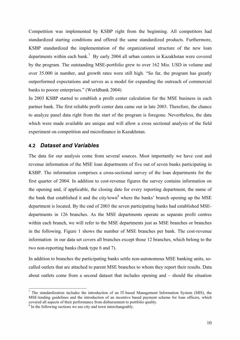
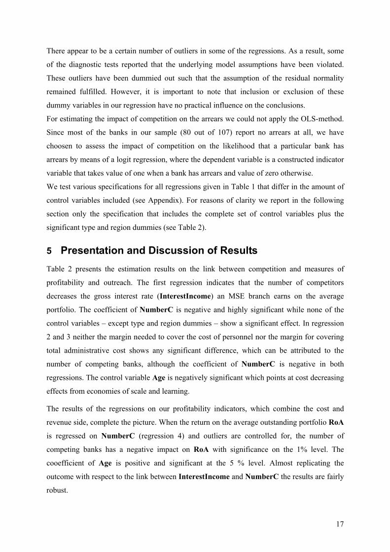
in the following. Figure 1 shows the number of MSE branches per bank. The cost-revenue

information in our data set covers all branches except those 12 branches, which belong to the

two non-reporting banks (bank type 6 and 7).

In addition to branches the participating banks settle non-autonomous MSE banking units, so-

called outlets that are attached to parent MSE branches to whom they report their results. Data

about outlets come from a second dataset that includes opening and – should the situation

7 The standardization includes the introduction of an IT-based Management Information System (MIS), the MSE-lending guidelines and the introduction of an incentive based payment scheme for loan officers, which covered all aspects of their performance from disbursement to portfolio quality. 8 In the following sections we use city and town interchangeably.

10

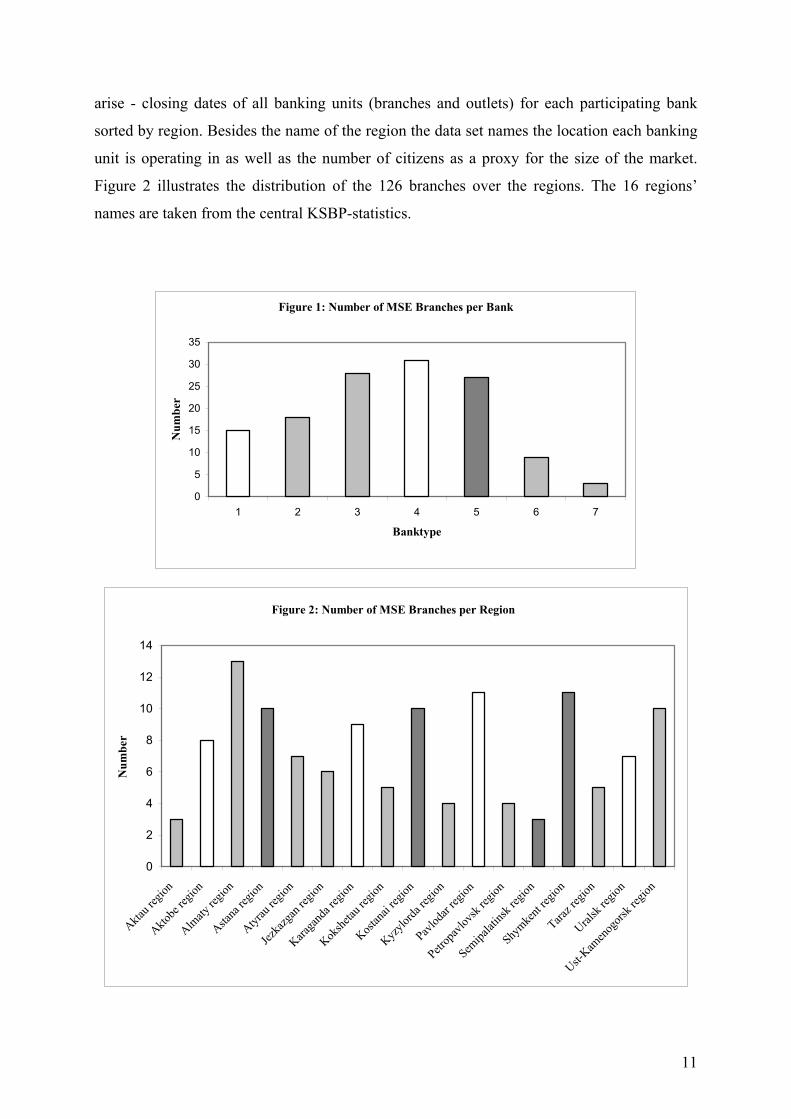
arise - closing dates of all banking units (branches and outlets) for each participating bank

sorted by region. Besides the name of the region the data set names the location each banking

unit is operating in as well as the number of citizens as a proxy for the size of the market.

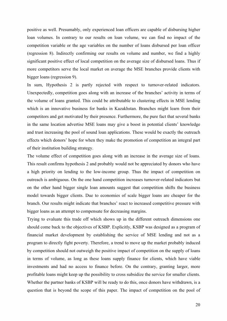
Figure 2 illustrates the distribution of the 126 branches over the regions. The 16 regions’

names are taken from the central KSBP-statistics.

Figure 1: Number of MSE Branches per Bank

0

5

10

15

20

25

30

35

1 2 3 4 5 6 7

Banktype

Num

ber

Figure 2: Number of MSE Branches per Region

0

2

4

6

8

10

12

14

Aktau r

egion

Aktobe

regio

n

Almaty

regio

n

Astana

regio

n

Atyrau

regio

n

Jezka

zgan

regio

n

Karaga

nda r

egion

Kokshe

tau re

gion

Kostan

ai reg

ion

Kyzylo

rda re

gion

Pavlod

ar reg

ion

Petrop

avlov

sk reg

ion

Semipa

latins

k reg

ion

Shymke

nt reg

ion

Taraz r

egion

Uralsk

region

Ust-Kam

enog

orsk r

egion

Num

ber

11

4.3 Independent Variables

The number of banks present in every single town/city at the beginning of 2004 reveals the

state of competition. Each distinct bank present in a certain location is taken as one

competitor. Thus the number of competitors (NumberC) ranges from one to seven (number

of participating banks). If one bank owns more than one branch or outlet in a city all branches

and outlets belonging to the same bank are counted as one competitor. In very few cities some

banks are running only outlets. Nevertheless, the bank is present as a competitor in this

location and therefore is counted as such.

Parent MSE branch and reporting outlets may be located in different towns. This could cause

distortions of cost-revenue figures of parent branches with respect to the impact of

competition. For example, if the parent branch’s figures contain the results of an outlet that is

a monopolist in its location, the effect of competition in the parent branch’s own city is hardly

reflected by these figures. To account for such distortions we would have had to remove

parent branches from our data set, if parent branch and corresponding outlet face different

competitive pressure. Luckily, however, the sample contains only outlets that face the same

competitive environment as their parent branch even if both are located in different towns.

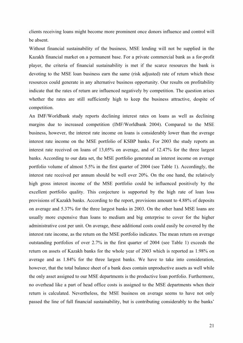
Thus we keep the information on all parent branches in the sample. The competitive

environment in which the KSBP-MSE-branches operate is shown in Figure 3. Most

frequently two or three distinct banks operate in the same city.

Figure 3: Competitive Environment

0

1

2

3

4

5

6

7

8

9

1 2 3 4 5 6 7

Number of Competitors

Num

ber

of C

ities

/Tow

ns

12

The degree of competition may not only depend on the number of competitors but also on the

proximity of clients to the next banking unit (Degryse/Ongena 2005) and market size. As we

are lacking information on the local distribution of banking units we try to control for these

issues by employing a density measure. The density of MSE-banking units (LDensity) is

defined as the number of inhabitants of the town divided by the sum of branches and outlets

in that location.

To control for other effects than the one of multiple entrance into the local microlending

market we employ several control variables. Most importantly, we expect that the age of each

banking unit or rather the time it has been in operation (Age) influences its performance due

to economies of scale. Since as a bank branch gets older the marginal effect of time it has

been in operation is likely to change, we have inlcuded the age squared (AgeSqr) variable

that induces differentiated marginal effects of the Age variable on the dependent variables in

question.

The portfolio volume of most branches is growing over time while certain fixed costs remain

constant. Furthermore, experience leads to greater professionalism of the loan officers and

thus could have a positive impact on results – to name just a few reasons for the likely impact

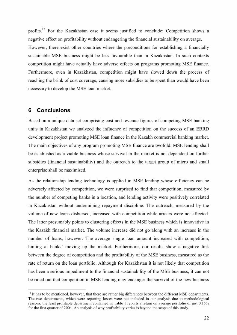
of ‘age’. The age distribution in the complete sample is shown in Figure 4. To control for the

different structure of administrative cost, the size of each branch defined by the number of

loan officers (Size) is included into the econometric model. Figure 5 reflects the complete

sample’s size distribution. Class 1 contains all branches with one or zero loan officers. Class 9

includes all branches, which employ more than 8 loan officers. The remaining classes

correspond to the respective number of loan officers given on the horizontal axis.

A bank-type dummy variable (Type) ranging from one to seven is included to capture the

specific influences coming from the mother bank, such as business style, popularity of the

brand name, corporate governance or refinancing situation. We do not have access to region-

specific socio-economic information for the year 2003 and 2004. In order to capture economic

differences between the 16 regions we employ a region dummy (Region).

13

Figure 4: Age Distribution Within and Across Branches

0

1

2

3

4

5

6

7

8

9

10

1 2 3 4 5 6 7

Banktype

Num

ber

per

Age

Gro

up

below one year1 - 2 years

2 - 3 years3 - 4 years4 - 6 years

Figure 5: Size Distribution

7

16

26

15

19

16

6 6

3

0

5

10

15

20

25

30

1 2 3 4 5 6 7 8 9

Size class

Num

ber

of B

ranc

hes

14

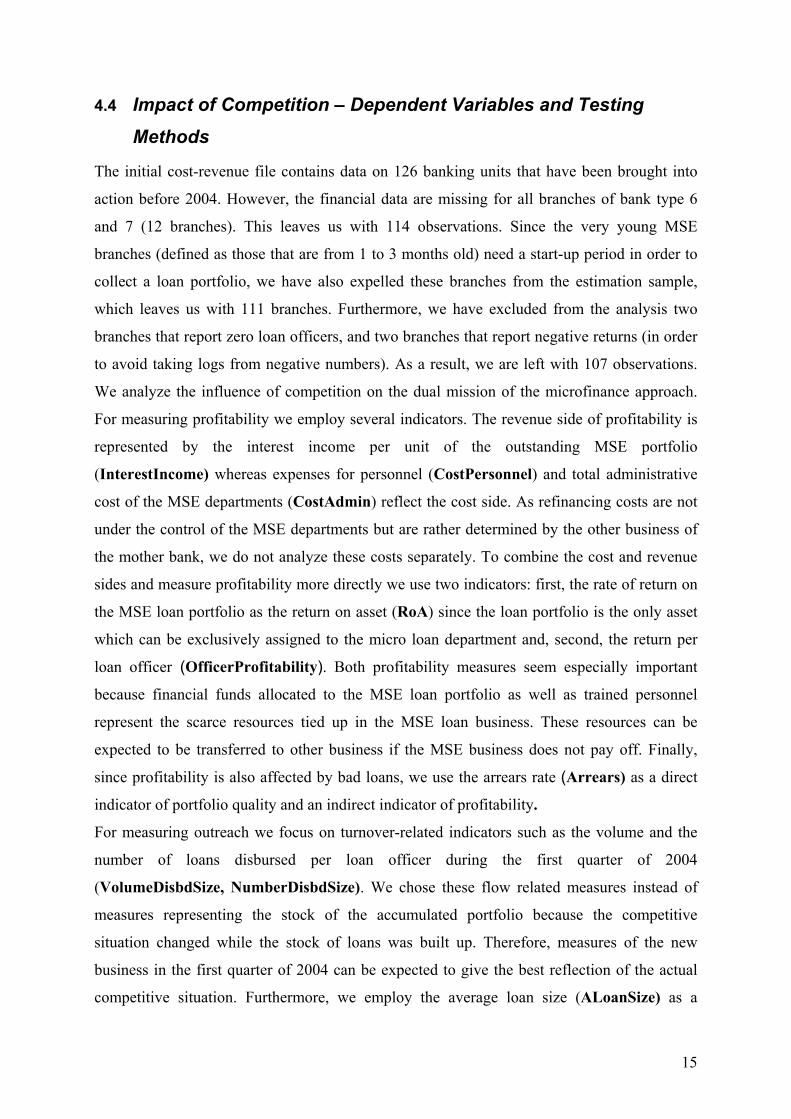
4.4 Impact of Competition – Dependent Variables and Testing Methods

The initial cost-revenue file contains data on 126 banking units that have been brought into

action before 2004. However, the financial data are missing for all branches of bank type 6

and 7 (12 branches). This leaves us with 114 observations. Since the very young MSE

branches (defined as those that are from 1 to 3 months old) need a start-up period in order to

collect a loan portfolio, we have also expelled these branches from the estimation sample,

which leaves us with 111 branches. Furthermore, we have excluded from the analysis two

branches that report zero loan officers, and two branches that report negative returns (in order

to avoid taking logs from negative numbers). As a result, we are left with 107 observations.

We analyze the influence of competition on the dual mission of the microfinance approach.

For measuring profitability we employ several indicators. The revenue side of profitability is

represented by the interest income per unit of the outstanding MSE portfolio

(InterestIncome) whereas expenses for personnel (CostPersonnel) and total administrative

cost of the MSE departments (CostAdmin) reflect the cost side. As refinancing costs are not

under the control of the MSE departments but are rather determined by the other business of

the mother bank, we do not analyze these costs separately. To combine the cost and revenue

sides and measure profitability more directly we use two indicators: first, the rate of return on

the MSE loan portfolio as the return on asset (RoA) since the loan portfolio is the only asset

which can be exclusively assigned to the micro loan department and, second, the return per

loan officer (OfficerProfitability). Both profitability measures seem especially important

because financial funds allocated to the MSE loan portfolio as well as trained personnel

represent the scarce resources tied up in the MSE loan business. These resources can be

expected to be transferred to other business if the MSE business does not pay off. Finally,

since profitability is also affected by bad loans, we use the arrears rate (Arrears) as a direct

indicator of portfolio quality and an indirect indicator of profitability.

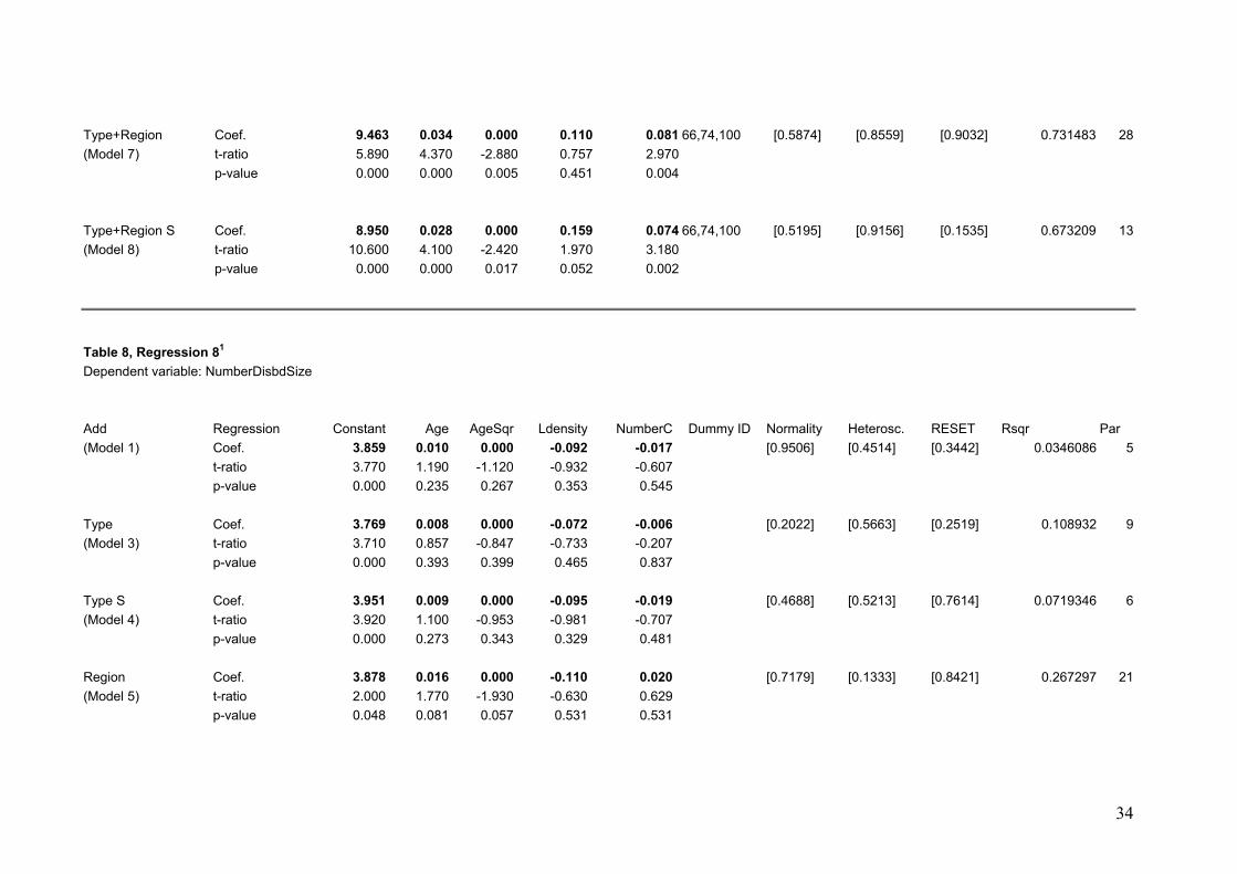
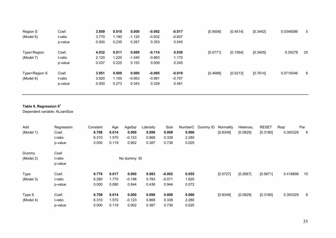
For measuring outreach we focus on turnover-related indicators such as the volume and the

number of loans disbursed per loan officer during the first quarter of 2004

(VolumeDisbdSize, NumberDisbdSize). We chose these flow related measures instead of

measures representing the stock of the accumulated portfolio because the competitive

situation changed while the stock of loans was built up. Therefore, measures of the new

business in the first quarter of 2004 can be expected to give the best reflection of the actual

competitive situation. Furthermore, we employ the average loan size (ALoanSize) as a

15

measure of outreach. The latter is likely to reflect the degree to which a branch is dedicated to

the target group of low-income clientele. Table 1 presents the summary statistics for the

selected indicators. Table 1: Summary Statistics

Dependent Variables

Explanation Number of Observations in

est-imation sample

Mean Standard Deviation

Min Max

Profitability Measures InterestIncome

(in %) Regression 1

Interest income divided by average outstanding

portfolio*

107 5.4793 0.79170 3.7142 9.4031

CostPersonnel (in %)

Regression 2

Wages and salaries divided by average outstanding

portfolio*

106 0.56319 0.30473 0.094762 1.7662

CostAdmin+

(in %) Regression 3

Total administrative costs divided by average

outstanding portfolio*

106 0.83692 0.46603 0.21895 2.6390

RoA (in %)

Regression 4

Department profit before tax divided by average

outstanding portfolio*

107 2.7753 0.98572 0.15000 6.6900

OfficerProfitability (in US-Dollar) Regression 5

Department profit before tax per loan officer

107 7757.1 5549.3 105.40 35196

Arrears° (in %)

Regression 6

Arrears divided by average outstanding

portfolio*

27 0.35609 0.57571 0.0059998 2.8406

Outreach Measures VolumeDisbdSize

(in US-Dollar) Regression 7

Loan volume disbursed in quarter 1 of 2004 per loan

officer

107 103690 57455 14493 346850

NumberDisbdSize

Regression 8

Number of loans disbursed in quarter 1 of 2004 per loan

officer

107 21.414 9.7398 6.0000 54.833

ALoanSize (in US-Dollar)

Regression 9

Total volume of loans disbursed in quarter 1 of

2004 divided by number of loans disbursed during the

period

107 5386.3 3147.4 1407.5 16427

* All figures were multiplied by a hundred.

+ One branch reports zero administrative costs. This branch is excluded from the sample when regressing the administrative costs on the number of competitors and the controls. ° The summary statistics refer to the 27 branches which report arrears.

The dependent variables InterestIncome, CostPersonnel, CostAdmin, OfficerProfitability,

VolumeDisbdSize, NumberDisbdSize, AloanSize have been log transformed in the

regressions. All of the regressions except the regression for arrears (regression 6) have been

estimated by the Ordinary Least Squares (OLS) method. The OLS-regression adequacy has

been checked by the following tests available as the standard regression diagnostic tests in

PcGive 10.4 (see Doornik and Hendry 2001): Doornik-Hansen (1994) test for residual

normality, White (1980) test of no residual heteroscedasticity, and Ramsey (1969) RESET

regression misspecification test.

16

There appear to be a certain number of outliers in some of the regressions. As a result, some

of the diagnostic tests reported that the underlying model assumptions have been violated.

These outliers have been dummied out such that the assumption of the residual normality

remained fulfilled. However, it is important to note that inclusion or exclusion of these

dummy variables in our regression have no practical influence on the conclusions.

For estimating the impact of competition on the arrears we could not apply the OLS-method.

Since most of the banks in our sample (80 out of 107) report no arrears at all, we have

choosen to assess the impact of competition on the likelihood that a particular bank has

arrears by means of a logit regression, where the dependent variable is a constructed indicator

variable that takes value of one when a bank has arrears and value of zero otherwise.

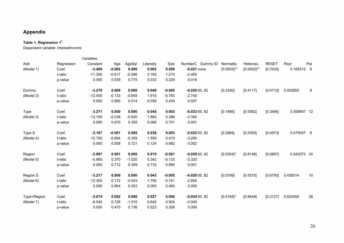
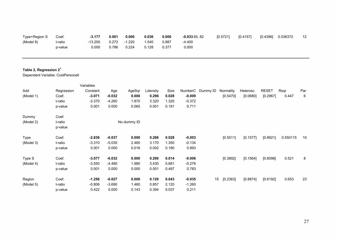
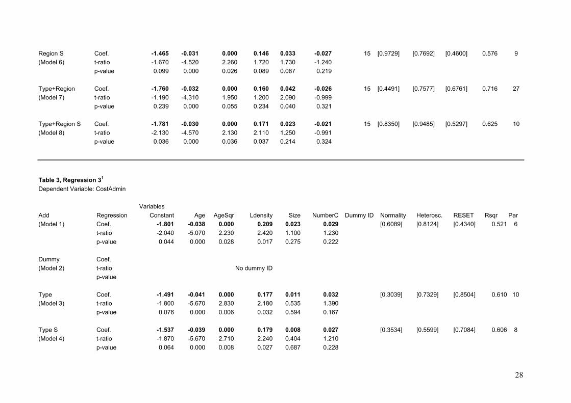
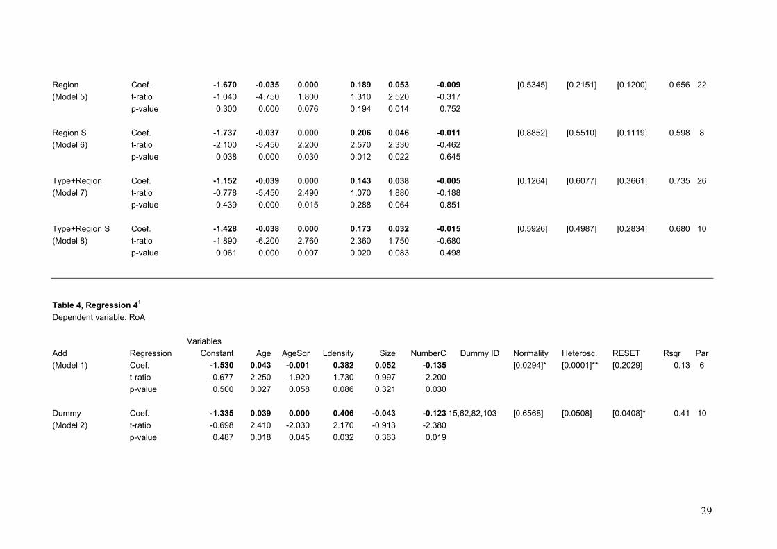
We test various specifications for all regressions given in Table 1 that differ in the amount of

control variables included (see Appendix). For reasons of clarity we report in the following

section only the specification that includes the complete set of control variables plus the

significant type and region dummies (see Table 2).

5 Presentation and Discussion of Results Table 2 presents the estimation results on the link between competition and measures of

profitability and outreach. The first regression indicates that the number of competitors

decreases the gross interest rate (InterestIncome) an MSE branch earns on the average

portfolio. The coefficient of NumberC is negative and highly significant while none of the

control variables – except type and region dummies – show a significant effect. In regression

2 and 3 neither the margin needed to cover the cost of personnel nor the margin for covering

total administrative cost shows any significant difference, which can be attributed to the

number of competing banks, although the coefficient of NumberC is negative in both

regressions. The control variable Age is negatively significant which points at cost decreasing

effects from economies of scale and learning.

The results of the regressions on our profitability indicators, which combine the cost and

revenue side, complete the picture. When the return on the average outstanding portfolio RoA

is regressed on NumberC (regression 4) and outliers are controlled for, the number of

competing banks has a negative impact on RoA with significance on the 1% level. The

cooefficient of Age is positive and significant at the 5 % level. Almost replicating the

outcome with respect to the link between InterestIncome and NumberC the results are fairly

robust.

17

Table 2:9 Results Profitability Measures10

Constant Age AgeSqr Ldensity Size NumberC Dummy ID Normality Heterosc. RESET Rsqr ParInterestIncome Coef. -3.177*** 0.001 0.000 0.036 0.006 -0.033*** 65, 82 [0,5721] [0,4157] [0,4396] 0.536 12 (Regression 1) t-ratio -13.200 0.272 -1.220 1.540 0.887 -4.400

p-value 0.000 0.786 0.224 0.128 0.377 0.000 CostPersonell Coef. -1.781** -0.030*** 0.000** 0.171** 0.023 -0.021 15 [0,8350] [0,9485] [0,5297] 0.625 10(Regression 2) t-ratio -2.130 -4.570 2.130 2.110 1.250 -0.991

p-value 0.036 0.000 0.036 0.037 0.214 0.324 CostAdmin Coef. -1.428* -0.038*** 0.000*** 0.173** 0.032* -0.015 [0,5926] [0,4987] [0,2834] 0.680 10

(Regression 3) t-ratio -1.890 -6.200 2.760 2.360 1.750 -0.680 p-value 0.061 0.000 0.007 0.020 0.083 0.498

RoA Coef. -1.483 0.031** 0.000** 0.403** 0.036 -0.138*** 15,62, [0,8874] [0,4963] [0,0611] 0.568 13(Regression 4) t-ratio -0.848 2.150 -2.050 2.370 0.816 -3.000 82,103

p-value 0.399 0.034 0.043 0.020 0.416 0.003 OfficerProfitability Coef. 6.132*** 0.060*** 0.000*** 0.142 0.043 -0.082** 15,70,103 [0,0879] [0,2162] [0,1625] 0.729 11

(Regression 5) t-ratio 4.540 5.670 -3.160 1.080 1.470 -2.410 p-value 0.000 0.000 0.002 0.281 0.146 0.018

Arrears Coef. -8.864 0.143** -0.002** 0.350 0.453** 0.036 (Regression 6) t-ratio -1.190 2.120 -2.100 0.499 2.590 0.199

p-value 0.235 0.037 0.038 0.619 0.011 0.843 Outreach Measures

VolumeDisbdSize Coef. 8.950*** 0.028*** 0.000** 0.159* 0.074*** 66,74,100 [0.5195] [0.9156] [0.1535] 0.673 13(Regression 7) t-ratio 10.600 4.100 -2.420 1.970 3.180

p-value 0.000 0.000 0.017 0.052 0.002 NumberDisbdSize Coef. 3.951*** 0.009 0.000 -0.095 -0.019 [0.4688] [0.5213] [0.7614] 0.072 6

(Regression 8) t-ratio 3.920 1.100 -0.953 -0.981 -0.707 p-value 0.000 0.273 0.343 0.329 0.481

ALoanSize11 Coef. 7.128*** 0.018** 0.000 0.057 -0.008 0.088*** [0.4018] [0.0041]*** [0.6720] 0.570 11(Regression 9) t-ratio 9.166 2.440 -0.548 0.744 -0.403 2.960

p-value 0.000 0.015 0.5824 0.4592 0.688 0.003

9 The regressions include all control variables and both the type and region dummies. 10 * significant at 10%; ** significant at 5%; *** significant at 1% 11 The t-ratios and the associated p-values have been calculated using the heteroscedasticity consistent covariance matrix estimator.

18

The impact of local competition on OfficerProfitability (regression 5) is also negative and

significant on the 5%. OfficerProfitability is an increasing function of age. The coefficient

is highly significant and robust, hinting just like the regression results on cost measures at

learning effects.

In sum Hypothesis 1 is confirmed by the data. As most of the theoretical literature suggests

profitability, measured in rates of return on scarce financial and human resources, is linked

negatively to local competition for microlending branches in Kasakhstan. The finding is

consistent with an empirical result developed in Chang et. al. (1997) for the banking market

of New York City. They concluded that profits decrease if banks follow other banks’

branches. As mentioned before, declining rates of return do not per se endanger financial

sustainability, however. The donor community might even welcome such a development if

profits are still high enough to keep the business attractive – a discussion which is picked up

again later on.

What we already can conclude, however, is that the negative effect of competition on return

measures cannot be attributed to a decline in repayment discipline. Although most theoretical

literature predicts that competition will undermine disciplining devices of relationship

lending, we do not find any evidence that the quality of the portfolio is affected. The logit

regression fails to reveal a significant impact of NumberC on the likelihood of arrears

(regression 6). This result is in contrast to Matin/Chaudhury (2001), McIntosh et. al (2003),

and Vogelgesang (2003) but is consistent with Park et. al. (2002). The latter argue that in

presence of credit rationing, competition induces financial institutions to exert greater

screening and enforcement effort.

Interpreting our result, it needs to be kept in mind that all of the MSE departments are still

under the influence of the central consulting service provided by KSBP. The standardized

screening and monitoring technique implemented by KSBP is a very restrictive one, which

implies rather risking to reject a loan application of a client which might perform well than

risking a default. Therefore, the rates of arrears and the loan write offs have always stayed

extremely low in almost all of the MSE departments, no matter, how fast their loan portfolios

were growing (Lepp/Terberger 2004).

Turning to our results on outreach, the regression results are quite clear again. The variable

VolumeDisbdSiz measures the gross increase in the size of the portfolio per loan officer in

quarter one of 2004. The competition coefficient is positive and highly significant (regression

7). This result implies that individual employee’s disbursement of loans increases in volume if

local competition intensifies. Age is highly significant, the sign of the coefficient being

19

positive as well. Presumably, only experienced loan officers are capable of disbursing higher

loan volumes. In contrary to our results on loan volume, we can find no impact of the

competition variable or the age variables on the number of loans disbursed per loan officer

(regression 8). Indirectly confirming our results on volume and number, we find a highly

significant positive effect of local competition on the average size of disbursed loans. Thus if

more competitors serve the local market on average the MSE branches provide clients with

bigger loans (regression 9).

In sum, Hypothesis 2 is partly rejected with respect to turnover-related indicators.

Unexpectedly, competition goes along with an increase of the branches’ activity in terms of

the volume of loans granted. This could be attributable to clustering effects in MSE lending

which is an innovative business for banks in Kazakhstan. Branches might learn from their

competitors and get motivated by their presence. Furthermore, the pure fact that several banks

in the same location advertise MSE loans may give a boost in potential clients’ knowledge

and trust increasing the pool of sound loan applications. These would be exactly the outreach

effects which donors’ hope for when they make the promotion of competition an integral part

of their institution building strategy.

The volume effect of competition goes along with an increase in the average size of loans.

This result confirms hypothesis 2 and probably would not be appreciated by donors who have

a high priority on lending to the low-income group. Thus the impact of competition on

outreach is ambiguous. On the one hand competition increases turnover-related indicators but

on the other hand bigger single loan amounts suggest that competition shifts the business

model towards bigger clients. Due to economies of scale bigger loans are cheaper for the

branch. Our results might indicate that branches’ react to increased competitive pressure with

bigger loans as an attempt to compensate for decreasing margins.

Trying to evaluate this trade off which shows up in the different outreach dimensions one

should come back to the objectives of KSBP. Explicitly, KSBP was designed as a program of

financial market development by establishing the service of MSE lending and not as a

program to directly fight poverty. Therefore, a trend to move up the market probably induced

by competition should not outweigh the positive impact of competition on the supply of loans

in terms of volume, as long as these loans supply finance for clients, which have viable

investments and had no access to finance before. On the contrary, granting larger, more

profitable loans might keep up the possibility to cross subsidize the service for smaller clients.

Whether the partner banks of KSBP will be ready to do this, once donors have withdrawn, is a

question that is beyond the scope of this paper. The impact of competition on the pool of

20

clients receiving loans might become more prominent once donors influence and control will

be absent.

Without financial sustainability of the business, MSE lending will not be supplied in the

Kazakh financial market on a permanent base. For a private commercial bank as a for-profit

player, the criteria of financial sustainability is met if the scarce resources the bank is

devoting to the MSE loan business earn the same (risk adjusted) rate of return which these

resources could generate in any alternative business opportunity. Our results on profitability

indicate that the rates of return are influenced negatively by competition. The question arises

whether the rates are still sufficiently high to keep the business attractive, despite of

competition.

An IMF/Worldbank study reports declining interest rates on loans as well as declining

margins due to increased competition (IMF/Worldbank 2004). Compared to the MSE

business, however, the interest rate income on loans is considerably lower than the average

interest rate income on the MSE portfolio of KSBP banks. For 2003 the study reports an

interest rate received on loans of 13,05% on average, and of 12.47% for the three largest

banks. According to our data set, the MSE portfolio generated an interest income on average

portfolio volume of almost 5.5% in the first quarter of 2004 (see Table 1). Accordingly, the

interest rate received per annum should be well over 20%. On the one hand, the relatively

high gross interest income of the MSE portfolio could be influenced positively by the

excellent portfolio quality. This conjecture is supported by the high rate of loan loss

provisions of Kazakh banks. According to the report, provisions amount to 4.88% of deposits

on average and 5.37% for the three largest banks in 2003. On the other hand MSE loans are

usually more expensive than loans to medium and big enterprise to cover for the higher

administrative cost per unit. On average, these additional costs could easily be covered by the

interest rate income, as the return on the MSE portfolio indicates. The mean return on average

outstanding portfolios of over 2.7% in the first quarter of 2004 (see Table 1) exceeds the

return on assets of Kazakh banks for the whole year of 2003 which is reported as 1.98% on

average and as 1.84% for the three largest banks. We have to take into consideration,

however, that the total balance sheet of a bank does contain unproductive assets as well while

the only asset assigned to our MSE departments is the productive loan portfolio. Furthermore,

no overhead like a part of head office costs is assigned to the MSE departments when their

return is calculated. Nevertheless, the MSE business on average seems to have not only

passed the line of full financial sustainability, but is contributing considerably to the banks’

21

profits.12 For the Kazakhstan case it seems justified to conclude: Competition shows a

negative effect on profitability without endangering the financial sustainability on average.

However, there exist other countries where the preconditions for establishing a financially

sustainable MSE business might be less favourable than in Kazakhstan. In such contexts

competition might have actually have adverse effects on programs promoting MSE finance.

Furthermore, even in Kazakhstan, competition might have slowed down the process of

reaching the brink of cost coverage, causing more subsidies to be spent than would have been

necessary to develop the MSE loan market.

6 Conclusions

Based on a unique data set comprising cost and revenue figures of competing MSE banking

units in Kazakhstan we analyzed the influence of competition on the success of an EBRD

development project promoting MSE loan finance in the Kazakh commercial banking market.

The main objectives of any program promoting MSE finance are twofold: MSE lending shall

be established as a viable business whose survival in the market is not dependent on further

subsidies (financial sustainability) and the outreach to the target group of micro and small

enterprise shall be maximised.

As the relationship lending technology is applied in MSE lending whose efficiency can be

adversely affected by competition, we were surprised to find that competition, measured by

the number of competing banks in a location, and lending activity were positively correlated

in Kazakhstan without undermining repayment discipline. The outreach, measured by the

volume of new loans disbursed, increased with competition while arrears were not affected.

The latter presumably points to clustering effects in the MSE business which is innovative in

the Kazakh financial market. The volume increase did not go along with an increase in the

number of loans, however. The average single loan amount increased with competition,

hinting at banks’ moving up the market. Furthermore, our results show a negative link

between the degree of competition and the profitability of the MSE business, measured as the

rate of return on the loan portfolio. Although for Kazakhstan it is not likely that competition

has been a serious impediment to the financial sustainability of the MSE business, it can not

be ruled out that competition in MSE lending may endanger the survival of the new business

12 It has to be mentioned, however, that there are rather big differences between the different MSE departments. The two departments, which were reporting losses were not included in our analysis due to methodological reasons, the least profitable department contained in Table 1 reports a return on average portfolio of just 0.15% for the first quarter of 2004. An analysis of why profitability varies is beyond the scope of this study.

22

in a market altogether under less favourable conditions. Thus, future research on the effect of

competition in developing banking markets should be dedicated to cross-country studies.

References

Allen, Franklin, Hans Gersbach, Jan Krahnen and Anthony Santomero , eds. (2001), Competition among Banks – Good or Bad, European Financial Review, Special Issue. Berger, Allen N. and Gregory F. Udell (1995), Relationship Lending and Lines of Credit in Small Firm Finance, Journal of Business, 68, 351-381. Cetorelli, Nicola (2001), Competition among banks: Good or Bad, Federal Reserve Bank of Chicago, Economic Perspectives 20, 38-48. Chang, Angela, Shubham Chaudhuri and Jith. Jayaratne (1997), Rational herding and the spatial clustering of bank branches: an empirical analysis, Research Paper 9724. Federal Reserve Bank of New York. New York. Chaudhury, Iftekhar A. and Imran Matin (2002), Dimensions and dynamics of microfinance membership overlap – a micro study from Bangladesh, Small Enterprise Development, 13 No. 2, 46-55. Degryse Hans and Steven Ongena (2005), Distance, Lending Relationships, and Competition, Journal of Finance 60 (1), 231-266. Doornik, J. A. and H. Hansen (1994), An omnibus test for univariate and multivariate normality, Working paper, Nuffield College, Oxford. EBRD (1997), Kazakhstan Small Business Programme, Project summary document, www.ebrd.com/projects/psd/psd1997/5009.htm Gersbach, Hans and Harald Uhlig (2004), Debt Contracts and Collapse as Competition Phenomena, Journal of Financial Intermediation, Forthcoming. Ghosh, Parikshit and Debraj Ray (2001), Information and Enforcement in Informal Credit Markets, unpublished manuscript, University of New York, New York. Hendry, D. F. and Doornik, J. A. (2001), Empirical Econometric Modelling Using PcGive Volume I (3rd edition), London: Timberlake Consultants Press. Hoff, Karla and Joseph E. Stiglitz (1998), Moneylenders and bankers: price-increasing subsidies in amonopolistically competitive market, Journal of Development Economics, 55, 485-518. IMF and World Bank (2004): Republic of Kazakhstan – Bank Profitability and Competition, Technical Note. Matthäus-Maier Ingrid and J.D. von Pischke, Introduction, in: Matthäus-Maier Ingrid and J.D. von Pischke (ed.), The Development of the Financial Sector in Southeast Europe, Springer-Verlag Berlin – Heidelberg – New York, 1-6.

23

McIntosh, Craig and Bruce Wydick (2002), Competition and Microfinance, Working paper, University of California at Berkeley and University of San Francisco. McIntosh, Craig, Alain de Janvry and Elisabeth Sadoulet (2003), How Rising Competition Among Microfinance Lenders Affects Incumbent Village Banks, CUDARE Working Papers, University of California, Berkeley. Morduch, Jonathan (1999), The Microfinance Promise, Journal of Economic Literature, 37, 1569-1614. Navajas, Sergio, Jonathan Conning and Claudio Gonzales-Vega (2003), Lending Technologies, Competition, and Consolidation in the Market for Microfinance in Bolivia, Journal of International Development, 15, 747-770. Padilla, A. Jorge and Marco Pagano (2000), Sharing default information as a disciplining device, European Economic Review, 44, 1951-1980. Peterson, Mitchell A. and Raghuram G. Rajan (1995), The effect of credit market competition on lending relationships, Quarterly Journal of Economics 110, 406-443. Park, Albert, Loren Brandt and John Giles (2002), Competition Under Credit Rationing: Theory and Evidence from Rural China, mimeo, University of Michigan. Rajan, Raghuram G. (1992), Insiders and Outsiders: The Choice between Informed and Arm’s Length Debt, Journal of Finance, 47, 1367-1400. Rajan, Raghuram G. and Zingales (1998), Which Capitalism? Lessons from the East Asian Crisis, Journal of Applied Corporate Finance 11, 40-48. Ramsey J. B. (1969), Tests of specification errors in classical linear regression analysis, Journal of the Royal Statistical Society, vol. B31, 350-371. Robinson, Marguerite (2001), The Microfinance Revolution: Sustainable Finance for the Poor, World Bank, Washington, D.C. Rhyne, Elizabeth (2001), Mainstreaming Microfinance: How Lending to the Poor Began, Grew, and Came of Age of Age in Bolivia, West Hartford, CT. Rhyne, Elizabeth and Robert Peck Christen (1999), Microfinance Enters the Marketplace, USAID Washington, D.C. Terberger, Eva and Anja Lepp (2004), Kazakhstan: Commercial Banks Entering Micro and Small Business Finance – The Kazakhstan Small Business Program, in: Scaling up Poverty Reduction: Case Studies in Microfinance, CGAP/ The Worldbank Group, Washington D.C, 125-138. Vogelgesang, Ulrike (2003), Microfinance in Times of Crisis: The Effects of Competition, Rising Indebtedness, and Economic Crisis on Repayment Behavior, World Development, 31, 2085-2114.

24

25

White, H. (1980), A heteroscedastic-consistent covariance matrix estimator and a direct test for heteroscedasticity, Econometrica 48, 817-838. Worldbank (2004), Kazakhstan: Commercial Banks Entering Micro and Small Business Finance – The Kazakhstan Small Business Program, www.worldbank.org/wbi/reducingpoverty/case-Kazakhstan-SmallBusinessProgram.htm

26

Appendix Table 1, Regression 11

bl s

Dependent variable: InterestIncome

Varia eAdd Regression Constant Age AgeSqr Ldensity Size NumberC Dummy ID

Normality Heterosc. RESET Rsqr Par

(Model 1)

Coef. -3.469 -0.002 0.000 0.065 0.009 -0.021 none [0.0003]** [0.0002]** [0.7635] 0.165512 6t-ratio -11.300 -0.617 -0.286 2.160 1.210 -2.460 p-value

0.000 0.539

0.775

0.033

0.228

0.016

Dummy Coef. -3.279 0.000 0.000 0.049 -0.005 -0.020 65, 82 [0.2240] [0.4117] [0.6710] 0.402855 8(Model 2)

t-ratio -12.400 -0.133 -0.655 1.910 -0.793 -2.740 p-value

0.000 0.895

0.514

0.059

0.430

0.007

Type Coef. -3.271 0.000 0.000 0.045 0.003 -0.023 65, 82 [0.1985] [0.5582] [0.3494] 0.508697 12(Model 3)

t-ratio -13.100 -0.038 -0.930 1.860 0.386 -3.350 p-value

0.000 0.970

0.355

0.066

0.701

0.001

Type S Coef. -3.187 -0.001 0.000 0.038 0.003 -0.022 65, 82 [0.3984] [0.5300] [0.4973] 0.475057 9(Model 4)

t-ratio -12.700 -0.664 -0.359 1.550 0.410 -3.260 p-value

0.000 0.508

0.721

0.124

0.682

0.002

Region Coef. -2.897 0.001 0.000 0.015 -0.001 -0.029 65, 82 [0.0354]* [0.8146] [0.0897] 0.542073 24(Model 5)

t-ratio -5.860 0.370 -1.020 0.342 -0.133 -3.320 p-value

0.000 0.712

0.309

0.733

0.895

0.001

Region S Coef. -3.217 0.000 0.000 0.043 -0.005 -0.020 65, 82 [0.0789] [0.5575] [0.6750] 0.438314 10(Model 6)

t-ratio -12.300 0.172 -0.933 1.700 -0.741 -2.850 p-value

0.000 0.864

0.353

0.093

0.460

0.005

Type+Region Coef. -3.074 0.002 0.000 0.027 0.006 -0.034 65, 82 [0.0184]* [0.8648] [0.2127] 0.624556 28(Model 7)

t-ratio -6.540 0.726 -1.510 0.642 0.924 -4.040 p-value 0.000 0.470 0.136 0.523 0.358 0.000

Type+Region S Coef. -3.177 0.001 0.000 0.036 0.006 -0.033 65, 82 [0.5721] [0.4157] [0.4396] 0.536372 12(Model 8)

t-ratio -13.200 0.272 -1.220 1.540 0.887 -4.400 p-value 0.000 0.786 0.224 0.128 0.377 0.000

Table 2, Regression 21

Dependent Variable: CostPersonell

Variables Add Regression Constant Age AgeSqr Ldensity Size NumberC Dummy ID

Normality Heterosc. RESET Rsqr

Par

(Model 1)

Coef. -3.071 -0.032 0.000 0.296 0.028 -0.009 [0.5470] [0.0680] [0.2967] 0.447 6t-ratio -3.370 -4.260 1.870 3.320 1.320 -0.372 p-value

0.001 0.000

0.065 0.001

0.191

0.711

Dummy Coef.(Model 2)

t-ratio No dummy ID

p-value

Type Coef. -2.836 -0.037 0.000 0.266 0.028 -0.003 [0.5511] [0.1577] [0.8921] 0.550115 10(Model 3)

t-ratio -3.310 -5.030 2.460 3.170 1.350 -0.134 p-value 0.001

0.000

0.016

0.002

0.180 0.893

Type S Coef. -3.077 -0.032 0.000 0.290 0.014 -0.006 [0.3892] [0.1564] [0.6098] 0.521 8(Model 4)

t-ratio -3.550 -4.480 1.980 3.430 0.681 -0.276 p-value 0.001

0.000

0.050

0.001

0.497 0.783

Region Coef. -1.256 -0.027 0.000 0.120 0.043 -0.035 15 [0.2363] [0.8874] [0.6192] 0.653 23(Model 5)

t-ratio -0.806 -3.690 1.480 0.857 2.120 -1.260 p-value 0.422

0.000

0.143

0.394

0.037 0.211

27

Region S Coef. -1.465 -0.031 0.000 0.146 0.033 -0.027 15 [0.9729]

[0.7692] [0.4600] 0.576(Model 6)

t-ratio -1.670 -4.520 2.260 1.720 1.730 -1.240 p-value 0.099

0.000

0.026

0.089

0.087 0.219

Type+Region Coef. -1.760 -0.032 0.000 0.160 0.042 -0.026 15 [0.7577] [0.6761] 0.716 27(Model 7)

t-ratio -1.190 -4.310 1.950 1.200 2.090 -0.999 p-value 0.239

0.000

0.055

0.234

0.040

Type+Region S Coef. -1.781 -0.030 0.000 0.023 -0.021 15 [0.8350] [0.9485] [0.5297] 0.625 10(Model 8)

t-ratio -2.130 -4.570 2.110 1.250 -0.991 p-value 0.036 0.036 0.037 0.214 0.324

9

[0.4491]

0.321

0.1712.130

0.000

Table 3, Regression 3 1

Dependent Variable: CostAdmin

Variables Add Regression Constant Age AgeSqr Ldensity Size NumberC Dummy ID

Normality Heterosc. RESET Par

(Model 1) Coef. -1.801 -0.038 0.000 0.209 0.023 0.029 [0.6089]

[0.8124]

0.521

6t-ratio -2.040 -5.070 2.230 2.420 1.100 1.230p-value

Rsqr [0.4340]

0.044 0.000

0.028

0.017 0.275

0.222

Dummy Coef.(Model 2)

t-ratio No dummy ID

p-value

Type Coef. -1.491 -0.041 0.000 0.177 0.011 0.032 [0.3039]

[0.7329]

[0.8504]

0.610

10(Model 3) t-ratio -1.800 -5.670 2.830 2.180 0.535 1.390

p-value

0.076 0.000

0.006

0.032 0.594

0.167

Type S Coef. -1.537 -0.039 0.000 0.179 0.008 0.027 [0.3534]

[0.5599]

[0.7084]

0.606

8(Model 4) t-ratio -1.870 -5.670 2.710 2.240 0.404 1.210

p-value 0.064 0.000 0.008 0.027 0.687 0.228

28

Region Coef. -1.670 -0.035 0.000 0.189 0.053 -0.009 [0.5345]

[0.2151]

[0.1200]

0.656

22(Model 5) t-ratio -1.040 -4.750 1.800 1.310 2.520 -0.317

p-value

0.300 0.000

0.076

0.194 0.014

0.752

Region S Coef. -1.737 -0.037 0.000 0.206 0.046 -0.011 [0.8852]

[0.5510]

[0.1119]

0.598

8(Model 6) t-ratio -2.100 -5.450 2.200 2.570 2.330 -0.462

p-value

0.038 0.000

0.030

0.012 0.022

0.645

Type+Region Coef. -1.152 -0.039 0.000 0.143 0.038 -0.005 [0.1264]

[0.6077]

[0.3661]

0.735

26(Model 7) t-ratio -0.778 -5.450 2.490 1.070 1.880 -0.188

p-value

0.439 0.000

0.015

0.288 0.064

0.851

Type+Region S Coef. -1.428 -0.038 0.000 0.173 0.032 -0.015 [0.5926]

[0.4987]

[0.2834]

0.680

10(Model 8) t-ratio -1.890 -6.200 2.760 2.360 1.750 -0.680

p-value 0.061 0.000 0.007 0.020 0.083 0.498 Table 4, Regression 41

iab es

Dependent variable: RoA

Var lAdd Regression Constant Age AgeSqr Ldensity Size NumberC Dummy ID

Normality Heterosc. RESET Rsqr Par

(Model 1) Coef. -1.530 0.043 -0.001 0.382 0.052 -0.135 [0.0294]*

[0.0001]**

[0.2029]

0.13

6t-ratio -0.677 2.250 -1.920 1.730 0.997 -2.200p-value

0.500 0.027

0.058

0.086

0.321

0.030

Dummy Coef. -1.335 0.039 0.000 0.406 -0.043 -0.123 15,62,82,103

[0.6568]

[0.0508]

[0.0408]*

0.41

10(Model 2) t-ratio -0.698 2.410 -2.030 2.170 -0.913 -2.380

p-value

0.487 0.018

0.045

0.032

0.363

0.019

29

Type

Coef. -0.712 0.035 0.000 0.333 0.027 -0.158 15,62,82,103

[0.5873]

[0.1118]

[0.0075]**

0.55

14(Model 3) t-ratio -0.407 2.240 -1.980 1.940 0.593 -3.270

p-value

0.685 0.028

0.051

0.056

0.555

0.002

Type S Coef. -0.924 0.035 0.000 0.381 -0.012 -0.140 15,62,82,103

[0.6342]

[0.0672]

[0.0232]*

0.49

11(Model 4) t-ratio -0.514 2.280 -1.860 2.170 -0.270 -2.880

p-value

0.608 0.025

0.066

0.033

0.788

0.005

Region Coef. 1.149 0.047 -0.001 0.180 -0.033 -0.136 15,62,82,103

[0.8311]

[0.1614]

[0.0304]*

0.49

26 (Model 5) t-ratio 0.301 2.640 -2.290 0.524 -0.618 -2.010

p-value

0.764 0.010

0.025

0.602

0.538

0.048

Region S Coef. -2.164 0.041 0.000 0.479 -0.042 -0.113 15,62,82,103

[0.7783]

[0.0690]

[0.1056]

0.43

11(Model 6) t-ratio -1.090 2.520 -2.230 2.490 -0.884 -2.180

p-value

0.277 0.014

0.028

0.014

0.379

0.032

Type+Region Coef. 1.178 0.041 -0.001 0.147 0.037 -0.164 15,62,82,103

[0.9500]

[0.2359]

[0.1000]

0.62

30(Model 7) t-ratio 0.342 2.390 -2.170 0.475 0.729 -2.660

p-value

0.733 0.019

0.033

0.636

0.468

0.009

Type+Region S Coef. -1.483 0.031 0.000 0.403 0.036 -0.138 15,62,82,103

[0.8874]

[0.4963]

[0.0611]

0.57

13(Model 8) t-ratio -0.848 2.150 -2.050 2.370 0.816 -3.000

p-value 0.399 0.034 0.043 0.020 0.416 0.003 Table 5, Regression 51

Dependent variable: OfficerProfitability

VariablesAdd Regression Constant Age AgeSqr Ldensity Size NumberC Dummy ID

Normality Heterosc. RESET Rsqr Par

(Model 1) Coef. 5.909 0.079 -0.001 0.128 0.009 -0.072 [0.0006]** [0.0599] [0.0072]** 0.502147 6t-ratio 3.650 5.830 -3.510 0.808 0.229 -1.630 p-value 0.000 0.000 0.001 0.421 0.819 0.106

30

Dummy Coef. 6.582 0.062 0.000 0.092 0.024 -0.081 15,70,103 [0.5953] [0.0600] [0.0612] 0.657122 9(Model 2) t-ratio 4.580 5.240 -2.900 0.658 0.758 -2.160

p-value

0.000 0.000

0.005

0.512 0.450

0.033

Type Coef. 6.806 0.060 0.000 0.081 0.047 -0.093 15,70,103 [0.1453] [0.2407] [0.1227] 0.718523 13(Model 3) t-ratio 5.020 5.180 -2.830 0.608 1.500 -2.560

p-value

0.000 0.000

0.006

0.545 0.138

0.012

Type S Coef. 6.959 0.058 0.000 0.069 0.043 -0.093 15,70,103 [0.1384] [0.1855] [0.1404] 0.716094 10(Model 4) t-ratio 5.290 5.420 -2.820 0.535 1.450 -2.690

p-value

0.000 0.000

0.006

0.594 0.151

0.008

Region Coef. 6.062 0.071 -0.001 0.147 -0.014 -0.018 15,70,103 [0.0571] [0.2218] [0.1333] 0.716681 25(Model 5) t-ratio 2.260 5.540 -3.380 0.605 -0.383 -0.370

p-value

0.026 0.000

0.001

0.547 0.703

0.712

Region S Coef. 5.682 0.063 -0.001 0.172 0.025 -0.070 15,70,103 [0.5589] [0.0670] [0.1411] 0.672268 10(Model 6) t-ratio 3.860 5.490 -3.240 1.210 0.779 -1.880

p-value

0.000 0.000

0.002

0.231 0.438

0.063

Type+Region Coef. 7.154 0.066 -0.001 0.052 0.007 -0.019 15,70,103 [0.0015]** [0.5566] [0.0117]* 0.775358 29(Model 7) t-ratio 2.860 5.220 -3.080 0.231 0.197 -0.427

p-value

0.005 0.000

0.003

0.818 0.845

0.671

Type+Region S Coef. 6.132 0.060 0.000 0.142 0.043 -0.082 15,70,103 [0.0879] [0.2162] [0.1625] 0.728606 11(Model 8) t-ratio 4.540 5.670 -3.160 1.080 1.470 -2.410

p-value 0.000 0.000 0.002 0.281 0.146 0.018

31

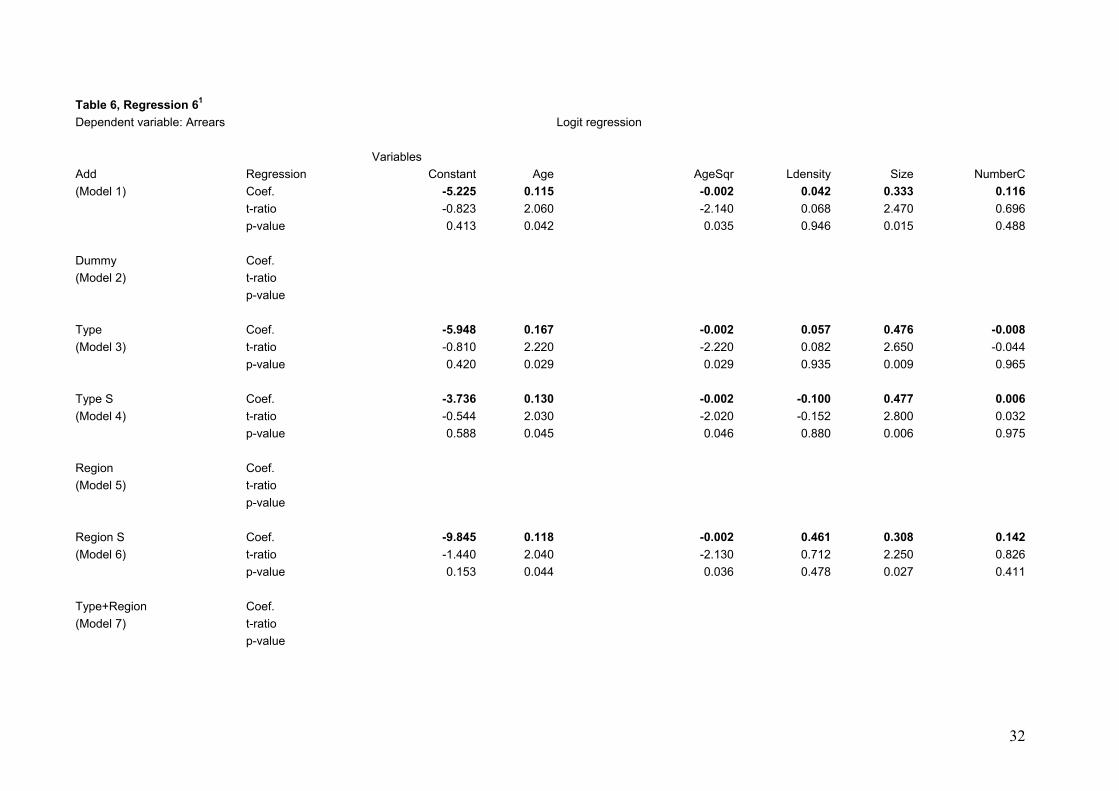
Table 6, Regression 61

Dependent variable: Arrears

Logit regression

Variables

Add Regression Constant Age AgeSqr Ldensity Size NumberC(Model 1) Coef. -5.225 0.115 -0.002 0.042 0.333 0.116

t-ratio -0.823 2.060 -2.140 0.068 2.470 0.696 p-value 0.413

0.042 0.035 0.946

0.015 0.488

Dummy Coef.(Model 2) t-ratio

p-value

Type Coef. -5.948 0.167 -0.002 0.057 0.476 -0.008 (Model 3) t-ratio -0.810 2.220 -2.220 0.082 2.650 -0.044

p-value 0.420

0.029 0.029 0.935

0.009 0.965

Type S Coef. -3.736 0.130 -0.002 -0.100 0.477 0.006 (Model 4) t-ratio -0.544 2.030 -2.020 -0.152 2.800 0.032

p-value 0.588

0.045 0.046 0.880

0.006 0.975

Region Coef.(Model 5) t-ratio

p-value

Region S Coef. -9.845 0.118 -0.002 0.461 0.308 0.142 (Model 6) t-ratio -1.440 2.040 -2.130 0.712 2.250 0.826

p-value 0.153

0.044 0.036 0.478

0.027 0.411

Type+Region Coef.(Model 7) t-ratio

p-value

32

Type+Region S Coef. -8.864 0.143 -0.002 0.350 0.453 0.036 (Model 8) t-ratio -1.190 2.120 -2.100 0.499 2.590 0.199 p-value 0.235 0.037 0.038 0.619 0.011 0.843 Table 7, Regression 71

Dependent variable: VolumeDisbdSize

Add Regression Constant Age AgeSqr Ldensity NumberC Dummy ID

Normality Heterosc. RESET Rsqr

Par (Model 1) Coef. 10.499 0.024 0.000 0.006 0.051 [0.0551] [0.7519] [0.4634] 0.350035 5

t-ratio 9.860 2.690 -1.150 0.061 1.790 p-value 0.000

0.008 0.253 0.952

0.076

Dummy Coef. 10.215 0.025 0.000 0.042 0.043 66,74,100 [0.5580] [0.9967] [0.4444] 0.511914 8(Model 2) t-ratio 10.900 3.140 -1.560 0.466 1.660

p-value 0.000

0.002 0.122 0.642

0.101

Type Coef. 10.237 0.024 0.000 0.052 0.044 66,74,100 [0.5567] [0.9965] [0.4011] 0.571597 12(Model 3) t-ratio 11.300 2.920 -1.320 0.585 1.680

p-value 0.000

0.004 0.191 0.560

0.095

Type S Coef. 10.345 0.024 0.000 0.039 0.039 66,74,100 [0.4551] [0.9936] [0.4205] 0.567417 9(Model 4) t-ratio 11.600 3.120 -1.350 0.451 1.570

p-value 0.000

0.002 0.182 0.653

0.119

Region Coef. 9.155 0.037 0.000 0.130 0.074 66,74,100 [0.8782] [0.8383] [0.5413] 0.673941 24(Model 5) t-ratio 5.420 4.640 -3.160 0.850 2.610

p-value 0.000

0.000 0.002 0.398

0.011

Region S Coef. 8.724 0.030 0.000 0.172 0.078 66,74,100 [0.7226] [0.9221] [0.0947] 0.627074 12(Model 6) t-ratio 9.760 4.100 -2.650 2.010 3.120

p-value 0.000 0.000 0.009 0.047 0.002

33

Type+Region Coef. 9.463 0.034 0.000 0.110 0.081 66,74,100 [0.5874] [0.8559] [0.9032] 0.731483 28(Model 7) t-ratio 5.890 4.370 -2.880 0.757 2.970

p-value 0.000

0.000 0.005 0.451

0.004

Type+Region S Coef. 8.950 0.028 0.000 0.159 0.074 66,74,100 [0.5195] [0.9156] [0.1535] 0.673209 13(Model 8) t-ratio 10.600 4.100 -2.420 1.970 3.180

p-value 0.000 0.000 0.017 0.052 0.002 Table 8, Regression 81

[0.2022]

Dependent variable: NumberDisbdSize

Add Regression Constant Age AgeSqr Ldensity NumberC Dummy ID

Normality Heterosc. RESET Rsqr

Par (Model 1) Coef. 3.859 0.010 0.000 -0.092 -0.017 [0.9506]

[0.4514]

[0.3442]

0.0346086

5

t-ratio 3.770 1.190 -1.120 -0.932 -0.607p-value 0.000

0.235 0.267 0.353

0.545

Type Coef. 3.769 0.008 0.000 -0.072 -0.006 [0.5663]

[0.2519]

0.108932

9

(Model 3) t-ratio 3.710 0.857 -0.847 -0.733 -0.207p-value 0.000

0.393 0.399 0.465

0.837

Type S Coef. 3.951 0.009 0.000 -0.095 -0.019 [0.4688]

[0.5213]

[0.7614]

0.0719346

6

(Model 4) t-ratio 3.920 1.100 -0.953 -0.981 -0.707p-value 0.000

0.273 0.343 0.329

0.481

Region Coef. 3.878 0.016 0.000 -0.110 0.020 [0.7179]

[0.1333]

[0.8421]

0.267297

21

(Model 5) t-ratio 2.000 1.770 -1.930 -0.630 0.629p-value 0.048

0.081 0.057 0.531

0.531

34

Region S Coef. 3.859 0.010 0.000 -0.092 -0.017

[0.9506]

[0.4514]

[0.3442]

0.0346086

5(Model 6) t-ratio 3.770 1.190 -1.120 -0.932 -0.607

p-value 0.000

0.235 0.267 0.353

0.545

Type+Region Coef. 4.032 0.011 0.000 -0.114 0.038 [0.0771]

[0.1564]

[0.3405]

0.35278 25(Model 7) t-ratio 2.120 1.220 -1.440 -0.663 1.170

p-value 0.037

0.225 0.153 0.509

0.245

Type+Region S Coef. 3.951 0.009 0.000 -0.095 -0.019 [0.4688]

[0.5213]

[0.7614]

0.0719346

6(Model 8) t-ratio 3.920 1.100 -0.953 -0.981 -0.707

p-value 0.000 0.273 0.343 0.329 0.481 Table 9, Regression 91

Dependent variable: ALoanSize

Add Regression Constant Age AgeSqr Ldensity Size NumberC Dummy ID

Normality Heterosc. RESET Rsqr

Par (Model 1)

Coef. 6.708 0.014 0.000 0.090 0.008 0.066 [0.8349] [0.0829] [0.3180] 0.393329 6t-ratio 6.310 1.570 -0.123 0.868 0.339 2.280 p-value

0.000

0.119

0.902

0.387

0.736

0.025

Dummy Coef.(Model 2)

t-ratio No dummy

ID p-value

Type Coef. 6.776 0.017 0.000 0.083 -0.002 0.055 [0.5727] [0.2687] [0.5671] 0.418898 10(Model 3)

t-ratio 6.280 1.770 -0.198 0.783 -0.071 1.820 p-value

0.000

0.080

0.844

0.436

0.944

0.072

Type S Coef. 6.708 0.014 0.000 0.090 0.008 0.066 [0.8349] [0.0829] [0.3180] 0.393329 6(Model 4)

t-ratio 6.310 1.570 -0.123 0.868 0.339 2.280 p-value 0.000 0.119 0.902 0.387 0.736 0.025

35

36

Region Coef. 6.412 0.021 0.000 0.130 -0.018 0.084 [0.5144] [0.0316]* [0.8975] 0.647346 22(Model 5)

t-ratio 3.700 2.590 -0.679 0.829 -0.793 2.760 p-value

0.000

0.011

0.499

0.410

0.430

0.007

Region S Coef. 7.128 0.018 0.000 0.057 -0.008 0.088 [0.4018] [0.0041]** [0.6720] 0.570041 11(Model 6)

t-ratio (HCSE) 9.166 2.440 -0.548 0.744 -0.403 2.960 p-value

0.000

0.015

0.5824

0.4592

0.688

0.003

Type+Region Coef. 6.920 0.025 0.000 0.086 -0.031 0.075 [0.4599] [0.2299] [0.9171] 0.666025 26(Model 7)

t-ratio 3.910 2.890 -0.897 0.541 -1.290 2.400 p-value

0.000

0.005

0.373

0.590

0.202

0.019

Type+Region S Coef. 7.128 0.018 0.000 0.057 -0.008 0.088 [0.4018] [0.0041]** [0.6720] 0.570041 11(Model 8)

t-ratio (HCSE) 9.166 2.440 -0.548 0.744 -0.403 2.960 p-value 0.000 0.015 0.5824 0.4592 0.688 0.003

Annotation: 1 Model 1 explores the correlation between profitability measures and outreach indicators respectively and the number of competitors, controlling just for age, age squared,

density, size. In model 2, we control for outliers by including a dummy for each of them. In model 3 the bank type is controlled for as well. Model 4 contains only significant type dummies. Region dummies are included in model 5 and 6 (6: only significant ones). Finally, we control for both type and region in model 7 and 8 (8: only significant ones).